quasiperiodic motions in superquadratic time-periodic potentials
TRANSCRIPT

Commun. Math. Phys. 143, 43-83 (1991) Communications in Mathematical
Physics �9 Springer-Verlag 1991
Quasiperiodic Motions in Superquadratic Time-Periodic Potentials
Mark Levi
Department of Mathematical Sciences, Reusselaer Polytechnic Institute, Troy, NY 12180, USA
Abstract. It is shown that for a large class of potentials on the line with su- perquadratic growth at infinity and with the additional time-periodic dependence all possible motions under the influence of such potentials are bounded for all time and that most (in a precise sense) motions are in fact quasiperiodic. The class of potentials includes, as very particular examples, the exponential, polynomial and much more. This extends earlier results and gives an answer to a problem posed by Littlewood in the mid 1960's. Along the way machinery is developed for estimating the action-angle transformation directly in terms of the potential and also some apparently new identities involving singular integrals are derived.
1. Introduction and the Results
In the early 1960's Littlewood [LI] asked whether or not the solutions of the Duffing-type equations
2 + g(x) = p(t), where p(t q- 1) = p(t) (1.0)
are bounded for all time, i.e. whether there are resonances that might cause the amplitude of the oscillations to increase without bound. In this paper we study the more general problem of describing the behavior of solutions of the system of the form
+ Vx(x, t) = 0 , (1.1)
which is a Hamiltonian system governing the motion of a particle on the line subject to a time-periodic force. We show that under appropriate growth assump- tions on V for large x, the system is near-integrable for large amplitudes in the sense that "most" large amplitude solutions are quasiperiodic and all solutions are bounded for all time with no smallness assumptions on the time-dependence of V (x, t). Intuitively, one might expect that if V (x, t) is superquadratic in x, then the larger amplitude solutions oscillate faster giving rise to a twist in the Poincar~ map of the (x, ~) plane and thus a hope of applying Moser's twist theorem to

44 M. Levi
prove boundedness. This intuition turns out to be too crude: Littlewood [LI] (see also [L2], [LO]) produced an oscillator 2 + U'(x) = p(t) with U satisfying U'(x)
- - - , oo as x ~ oo, U E C ~, and with a periodic piecewise constant p(t) pos- x
sessing an unbounded solution. This was accomplished by modifying the quartic potential U(x) = �88 x 4 in such a way as to create a resonance for a particular solution while still preserving the superlinear growth of U'(x) at infinity. Further details can be found in [L!, L2, LO].
The problem of boundedness of solutions for (1.1) can be separated into two parts: first, to gain the information on the period map (also called the Poincar~ map or the stroboscopic map) (x, s ~ (x, 2)t=l, and second, to use this information to decide whether or not the solutions are bounded. Neither of these two problems is fully tractable. This is due to the implicit character of the relationship between the potential V (x, t) and the Hamiltonian H(O, I, t) expressed in the action-angle variables. In other word, Eq. (1.1) cannot be solved explicitly and a qualitative estimate has to be made. Such estimates are provided in this paper.
The second problem, of a more general nature, lies in determining whether or not a given map has escaping orbits. This fundamental classical problem was solved only relatively recently by KAM theory [Nil, HE, R1, R2, M2, SZ]: the only known way to assure that all iterates of a map are bounded is to show that there are invariant circles arbitarily close to oo in the (x, ~) plane of the map. In fact, the invariant curves are necessary for the boundedness, as was shown by Birkhoff ([B1, B2]); in that sense there is no hope of proving boundedness without demonstrating at the same time the existence of an invariant curve. In fact, earlier attempts to prove boundedness [D1], [D2] without using the invariant tori contain a mistake.
The first boundedness result is due to Morris [MO], who showed that all solutions of 2 + X 3 ~--- p(t) are bounded, with p(t) c C ~ Subsequently, this result was extended to a wider class of systems with polynomial potentials (of even degree) by Dieckerhoff and Zehnder [DZl, DZ2]. The restriction on the constancy of the leading coefficient that was required in that latter work was removed by Laederich and the author in [LL], by using a different transformation to a normal form. It might seem surprising at a first glance that all solutions of, say 2 + a(t)x 3 = 0, with a smooth a(t) = a(t + 1) > 0 are bounded for all time-after all, the potential V (x, t) = �88 a(t)x 4 undergoes a large change in the course of one t-period and thus could (it seems) "pump up" the oscillations of x(t) as in fact happens in the linear case 2 + a(t)x -- 0 when there is parametric resonance, for instance, in the Mathieu equation [S]. In the nonlinear case just mentioned, the nonlinearity does not allow the resonance to persist. In contrast to this, Littlewood's counterexample is based on constructing a resonance for a nonlinear case, but this construction violates the monotone twist condition [AD, BE, HA, KA, M], see [L2]. We mention finally an elegant result by Norris [N] for Eq. (1.0) when the x- and t-dependence separate: if g ( x ) / x < g'(x) (a superquadraticity condition), and if g(x) is analytic in a strip around the x-axis in the complex plane, then the system is near-integrable for large energies; the same result holds for the subquadratic growth g ( x ) / x > g'(x) as well. (For a geometrical discussion of this condition see the end of this section.)
It should be pointed out that the result of Morris and its generalization by Norris hold with no smoothness assumptions on p(t). This is due to the fact that

Quasiperiodic Motions in Superquadratic Time-Periodic Potentials 45
the Poincar~ map (x, 2)t=0 --+ (x, 2 )x= 1 is a small perturbation of the completely integrable Poincar+ map of the autonomous equation 2+g(x) = 0. By contrast to this, in the case of a more general potential V (x, t), with a stronger t-dependence the Poincar6 map mentioned above is not close to an integrable one, and higher smoothness in t is necessary to construct the change of variables in which the system is (say) C(4)-close to an integrable one. We point out that although the smoothness of p(t) does not affect the smoothness of the Poincar~ map, it does affect its proximity to an integrable map. This remark is illustrated by the counterexample of Littlewood, in which the construction of a non-near-integrable Poincar+ map is crucially dependent on the discontinuity of p(t). As soon as we make p(t) smooth, Littlewood's construction (of a "bad" map) fails, as can be shown by more careful estimates; this suggests that smoother p (for a fixed g) give rise to "nicer" (i.e., closer to integrable) Poinear6 maps.
We conclude this brief historical discussion by mentioning a related problem when V(x, t) in (1.1) is periodic in x as well as in t; the nonlinear pendulum with periodic (zero-average) forcing is a primary example. In this case it has been shown that, as long as V (x, t) is sufficiently smooth, there exist invariant tori y = f (x, t), where x mod 1, t mod 1, which are preserved by the flow ~ = y, i = 1, # = - V ( x , t) in the phase space {(x, t, y)} - T 2 • IR, [M3, CZ, L1]. In particular, for any solution there exists a constant C > 0 such that for all time I21 < c.
The main result of this paper is the following
Theorem 1. Assume that the potential function V (x, t) = V (x, t+ 1) tends to oo as Ixl ~ ~ and that it satisfies conditions (1.2), (1.3), and (1.4) below.
Then Eq. (1.1) is near-integrable for large energies, more precisely for any 0 < co < 1 satisfying the Diophantine conditions
co - qP 1 >~[q [ -~ foral l O --/= q, p E Z ,
the Poincar~'s map P : (x, 2)t=0 ~ (x, 2)z=l of Eq. (1.1) possesses countably many invariant circles with rotation number co and these circles cluster at infinity in the (x, 2) plane. These circles are the intersections of the invariant tori in the (x, 2, t mod 1)-space with the {t = O}-plane, Fig. 1.1; each such torus carries a quasiperiodic solution with basic frequencies 1 and k + co. All integers k >_ ko(co) are represented by an invariant torus. In particular, 1) All solutions are bounded for all time: sup (x[ + 121) < oo.
2) Most solutions with large amplitude are quasiperiodic, i.e. most initial condi- tions (in the sense of Lebesque measure) with large [x(0)[ + I~(0)l give rise to quasiperiodic solutions: x(t) = f (t, (co + k)t), where f is a function on a 2-torus. 3) Any sufficiently large number is a rotation number for some solution, i.e. there exists 0o such that for any 0 > 0o there exists a solution xo(t ) with that rotation number 1. Furthermore, for any rational p/q > 0o there exists a periodic solution with that rotation number; the corresponding periodic point of the Poincard map is a Birkhoff periodic point.
1 The standard definition of the (forward) rotation number is 0 = 1/2~z lim arg(x, •). Another t---~cO
interpretation of O is one half the average number of zeros of the solution during the forcing period: = lim 1/2T (# of zeros of x(t) on the interval 0 < t < T)
r ~ o o

46 M. Levi
/
x ,J ')
Fig. 1.1. Invariant tori in the extended phase space of Eq. (1.1)
The last statement 3) is a direct consequence of the Aubry-Mather theory; one can say much more by just applying the results of that theory [AD, BE, BH, HA, KA, MA1, MA2] to the Poincar6 map of the system, using the information gained here.
Conditions on the potential V (x, t).
For some constants c, Cl, a > O, 0 </~ < 1--0-6 - a and all x and t we have
~k+~ V <- clxl-kVa+", k + r _< 6, (1.2)
1 1 - ~ + C l < W x _ < a < ~ , where W = V / V x , (1.3)
and
k z k "c IOxOt UI, I~?xc3t W I <_ clxr l-k, k + r _< 5, where U = Vt/Vx. (1.4)
Remark I. Condition (1.4) can be weakened to read 13k,~ UI, I3 k'~ W[ < clxll-kg~; furthermore, the above assumptions on V can be weakened to require that these hold for Ixl _> A, for any fixed A. These stronger statements do not pose principal new difficulties.
Remark 2. Even a very special case of/ , -- 0 includes, together with the polynomial, some new examples, e.g. the exponential potential V(x, t) = ( 2 + c o s 0 coshx. (Condition (1.3) holds after subtracting 2+cos t from V - this does not affect Eq. (1.1).) For/_t > 0 the class widens drastically to allow some oscillation in x. A very particular example is V(x, t) = p(t) (x + cos ]/~)2,, where n is (specifiably) large and p(t) e 6 ~6) is periodic and positive.
An Outline of the Proof of Theorem 1. There are two parts: first, the formal reduc- tion to normal form and second, the estimates. The formal reduction (Fig. 1.2) consists of the following sequence of transformations; the quadruples list the position, the momentum, the time in that order with the Hamiltonian in the last place:
x , 2 , t ; H o = - ~ + V (O,I , t ;H=Ho+St) B,(t,H,O;I) c,(r ,h,O;J),
where A is the standard action-angle transformation of (x, 2) into (0, I) with t as the parameter (hence the extra term St in the Hamiltonian), B is the change

Quasiperiodic Motions in Superquadratic Time-Periodic Potentials
Fig. 1.2. The transformation to normal form and invariant tori
47
into time and energy as the new position and momentum, with the angle 0 now playing the role of new time, and C is another action-angle transformation to make the leading term of the Hamiltonian independent of the position variable.
The estimate of the composition C o B of the maps in the above diagram and a subsequent application of Moser's twist theorem will result in Theorem 5.1, which we restate here for convenience:
Theorem 2. I f the Hamiltonian function H(O, I, t) = Ho(I, t) + Hi(O, I, t) is peri- odic in 0 and t and satisfies for some fl > 0 the growth estimates
IQIg~H1 (0, t, t)l < cI-k-ZHo(I, t), l + k N 5, (5.1)
and i f the inverse function Io(H) = Io(t, H) o f rio(I, t) in H satisfies
13{O~Io(t, H)[ < cH-klo(t, H), j + k < 5, (5.2) k<2
cH-klo(t, H) <_ I~Io(t, H)l, (5.3)
then the Hamiltonian system
0 = H I , i = Ho
possesses invariant tori I = f (O, t) carrying a quasiperiodic flow, in any region I > M, for an arbitrarily large M, Fig. 1.2.
This theorem is actually a combination of Theorem5.1 and the results of Sect. 4.
The following three theorems estimate the action-angle change A in the diagram; they are restatements of Theorems6.1-6.3:
Theorem3. I f the potential V(x, t) satisfies the superquadraticity condition (1.3) together with the bounds (1.2) and (1.4), then there exists fl = fl(lt, a) such that the action-angle Hamiltonian Ho + H1 satisfies the bound (5.1).
Theorem4. I f the potential V satisfies the bounds (1.4), then Ho(I, t) satisfies (5.2), where Io is the inverse function o f Ho in I.
Theorem 5. I f V satisfies (I.2), then Ho(1, t) satisfies the twist conditions (5.3).
Potentials with Blow-Up and Pulsating Billiards. One can apply the same methods to the cases when the potential blows up at one or two (end)points. For instance, one can show that the potentials
1 1 VI(X, t) -- x2 - aZ(t ) or V2(x, t) -- x - b(t~) + a(t)x4'

48 M. Levi v Fig. 1.3. Potentials with finite
V ~
I P x
I
t * < t
R (t*) < R (t) < R (t**)
or semifinite domains and pulsating "billiards"
where a > 0, and a, b E C (5), give rise to near-integrable motion for large energies. The potential Vt can be viewed as a "softened" potential of the Fermi-Ulam's "ping-pong." The latter problem deals with a particle bouncing between two rigid periodically moving walls. If the motion of the walls is sufficiently smooth then the velocity of any motion is bounded for all time. This was shown by Moser (unpublished lecture notes) and independently by Douady [DO] and Laederich and the author [LL].
This kind of a potential with a blowup at one end arises in the motion of a particle z ~ IR 2 governed by ~ + grad z V = 0, where V has an SO(I) symmetry: g(z, t) = W(Izl , t), with V ( z , t) = V ( z , t + 1) as usual. The angular momentum M = z A ~ = I m ~ is a conserved quan t i t y : A;/ = ~ A ~ + z A ~ = - -z A Vz = 0 , the latter because Vz [tz by symmetry. The polar coordinates r, 0 : z = re i~ satisfy r20 = M and f - r202 + Wr(r, t) = 0; substituting the expression for 0 = M r -2 we obtain the equation for r valid for all motions with the fixed value of M :
+ Ur(r, t, M ) = O,
M 2 where U = ~ r 2 + W (r, t).
One can show that if the effective, or the reduced, potential U(r, t) satisfies the conditions similar to (1.2)-(1.4) then all motions are bounded.
A particular case of this statement gives a stability statement about the "pulsating soft billiards": let V ( z , t) = ( z / R ( t ) ) 2u, where R(t) is periodic and positive. For N large, the potential is near zero inside the circle away from its boundary and it rises very steeply outside the circle, making this problem the elastic analog of the usual billiard whose potential is zero inside the circle and infinity outside. One can show using similar methods that if R(t) c C (5), then the energy of any motion will stay bounded for all time, and hence each solution r(t) has an upper and a posit ive lower bound for all time. The same then
is true for the angular velocity 0 = ~-~. An explicit formulation o f conditions
for near-integrability for the potentials which blow up at finite x will be given elsewhere.
R e m a r k 3 . It was stated in [D1] and [D2] that every solution of 2 + g(x) = p(t)
is bounded for all time, provided that g(x) ~ oo and that p is periodic and X
continuous. The statement seems to be false without further assumptions. The argument does not use the continuity ofp(t) and thus should apply to Littlewood's counterexample, which, however, exhibits unbounded solutions. (The original paper of Littlewood contained some minor errors which were found and corrected

Quasiperiodic Motions in Superquadratic Time-Periodic Potentials 49
by Long [LO]. A much simplified version of Littlewood's counterexample with an optimal estimate on the growth of g(x) can be found in [L2].)
Other Results: Identities and the Growth Rate for the Period T(H). We give a brief sample of some of the simplest results from the appendix. These auxiliary facts could be of some independent interest. The main results from the appendix are contained in A2 and A4; we do not discuss these here and touch only on a part of Appendix A3. The period of the solution of an autonomous system 2 + V'(x) = 0 with the energy H is given by f dt = f(ds/v), or by the singular integral [A1]
x+(H)
f ax T(H) = v/2 v/(H - V (x)) ' x_(H)
where the limits x• of integration are the points where the denominator vanishes: V (x• = H, and V (x) < H for x_ < x < x+. To be specific, let us also assume that V(O) = W(O) = 0 and that V'(x) ~ 0 for all x :~ O. Then one has the following formula for T'(H):
x +
T'(H) = v ~ ~ J ,,1 - 2 (V,) 2 j x/(H - V (x)) " (1.5)
x _
Proof of this is given in Appendix A3.
The relationship between the potential and the period as a function of the energy has been studied starting with Abel lAB] ; of the more recent papers we mention [K, M4, SW]. The latter paper contains differentiation formulas for the period as a function of the energy (different from our formulas).
A Remark on the Twist Condition. This is essentially a repetition of an observation made in [L2], where it was pointed out that the period of solutions of 2 + V/(x) = 0 as a function of the energy is a monotone decreasing function if Vn(x) > V ' (x ) /x (the same condition appears in the result of Norris). We note first that this condition follows from the above condition Wx =- (V/Vx)x < 1/2 - a, a > 0, in the case when V (0) = V'(0) = 0 (there is no loss of generality in this assumption). The latter condition on W in turn guarantees the monotonicity T'(H) < 0, as follows from Eq. (1.5). We give here a geometrical proof of the fact that the condition V" > V ' / x implies that the period is a decreasing function of the energy. Let z(t) = (x(t), 2(0 ) be a solution of 2 + V~(x) = 0 in the phase plane, and let ~ = (~(t), t/(t)) be a solution of the system linearized around z(t). Assume that each solution vector z(t) rotates clockwise in the phase plane. The criterion is based on the following geometrical observation, Fig. 1.4.
Take any solution z(t) and let ~ (0) be parallel to z(O). I f ~ (t) turns clockwise faster than z(t) at t = O, then the period T(H) of the oscillations is a decreasing function of the energy (or the amplitude, or the area enclosed by the curve). In other words, then the Poincar~ map possesses a monotone twist (with radial lines as the reference foliation). Expressing the above idea analytically, we rewrite the condition on the angular velocities of z and ~ in the form
> ~ , whenever y _ t/ x 3 '

50 M. Levi
I Y
Fig. 1.4. A sufficient condition for monotone twist: any solution vector turns slower than the collinear to it linearized solution vector
Using the governing equations 2 = y, 3) = - V ' ( x ) , ~ = tl, it = - V " ( x ) ~ , the above criterion reduces to
V' - - < V". x
Norris [N] gave an alternative proof of this condition using the Sturm com- parison argument.
The plan o f the paper is as follows. Section 2. Reduction to the action-angle variables (step A, Fig. 1.2). Section 3. Reduction to the normal form at infinity (steps B and C). Section 4. Application of KAM assuming the estimates on normal form. Section 5. A transformation lemma: Estimating the normal form in terms of
the action-angle Hamiltonian. Section 6. Estimating the action-angle Hamiltonian in terms of V (x, t). Appendix: A1. An inverse function lemma. A2. Estimates on the operators s jC{, L, M. A3. Algebra of the action-angle maps: Differentiation formulas and identities. A4. Estimates on the action-angle map. By far the main difficulty lies in the estimates on H via V carried out in
Sect. 6.
2. Reduction to the Action-Angle Variables
In this section we carry out the standard reduction to the action-angle variables. We refer to [A1] for further details.
2.1. A geometric description. Let us denote the Hamiltonian for Eq. (1.1) by y2
Jr(x , y, t) = ~ + V(x, t). Fixing t as a parameter, we let I = I(x, y, t) denote
the area enclosed by that level curve of ~ which passes through (x, y), Fig. 2.1. We assume that the level curve in question is (topologically) a circle, at least for I large enough (this is guaranteed if V is a monotone function for large Ixl, increasing for x > 0 and decreasing for x < 0). The geometrical meaning of the definition of the action-angle variables is summarized in Fig. 2.1.
dax To define the symplectic angle 0 = O(x, y, t), we look at the system ~ +
V (x, t) = 0 (with s playing the role of time and t = const), consider that periodic solution which passes through (x, y), Fig. 2.1, and let 0 = O(x, y, t) be the ratio of

Quasiperiodic Motions in Superquadratic Time-Periodic Potentials 51
. _ _ ~ A AI x AA
/ / ~ ~x
~ \ x , \ \ ' - I
(o,I)
I
0 1
Fig. 2.1. The definition of the action-angle variables. To each point (x, y) we assign the action I given by the area enclosed by the level curve through (x, y) and the angle 0 which is given by the proportion of the area of an infinitesimal ring enclosed between the y-axis and (x, y)
the time it takes the solution x, ds to travel between the y-axis and the given
point (x, y) to the period T = T(x, y, t) of this solution. The transformation (x, y) ~ (0, I) is area-preserving, as follows from the definition of I and 0 and from the zero-divergence property of the Hamiltonian flow x" -4- Vx(x, t) = 0. We note that 0 is defined rood 1.
2.2. The formal definition. To construct the map (x, y) ~ (0, I) more formally, we y2
let Ho(I, t) be the value of ~ = ~- + V(x, t) on that level curve which encloses
area I in the (x, y) plane, i.e. we define 11o(1, t) (implicitly) by
ydx = I , (2.1)
~(x, y, 0 =/~o (I, t)
with time t as a parameter. We define now the generating function S(x, I, t) as the area (shaded in Fig. 2.1):
S(x, I, t) = f ydx, (2.2) , /
C
where C is the part of the level curve ~ ( x , y, t) = Ho(I, t) connecting the y-axis with the point (x, y), oriented clockwise. This defines S up to an integer multiple of I = f ydx since C is defined up to an integer number of full trips around the level curve. We define the map (0, I, t) ~ (x, y, t) via
Sx(x, I, t) = y, Sl(X, I, t) = 0 ; (2.3)
it is well-known to be symplectic:
dx A dy = dx A (Sxxdx + SxidI) = Sxidx A dI ; dO A dI = (Sixdx + SudI) A dI = Si~dx A dl .
The last definition (2.3) is equivalent to the geometric definition above. Equation (1.1) in the new variables (0, I, t) retains its Hamiltonian character with the new Hamiltonian
H(O, I, t) = Ho(I, t) + Hi(O, I, t), where H1 = St(x, I, t), (2.4)
with x = x(O, I, t) defined implicitly by (2.3). We complete this section with the formulas that will be used later in the
estimates.

52 M. Levi
2.3. Expressions for Ho(I, t) and Hi(O, I, t). Rewriting Eq. (2.1) we obtain the implicit definition of rio(l, t) :
X+
I = 2 v ~ j v/Ho(I, t) - V(~, t)d~, (2.5)
X _
where x_(1, t) < x+(I, t) are given by V (x+_, t) = Ho(I, t), Fig. 2.1. Restating this slightly, Ho(I, t) is defined as the inverse function (in I) of
X+
I(H, t) = 2v~ f v /H - V(~, t)d~, (2.6)
X _
where x_(H, t) < x+(H, t) are given by V (x+, t) = H. To write down H1 more explicitly, we write the area S as
X
S(x, x, t) = v /no(x , t) - v ( r 0d ,
0
so that ~(o, I, 0
Hi(O, I, t) ~-- V~ "/ ~tHo(I, t) - ~tV(r t) de (2.7) 2 ~ X/Ho(I, t) - V(~, t) '
o where x(O, 1, t) is defined implicitly by Si(x, I, t) = 0, (cf. 2.3) i.e. by
3 r
OIHo(I, t) f d~ = O. (2.8) 2 ~ x/So(1, t ) - V(~, t)
o
This formula has a simple dynamical interpretation: O,H o ig the inverse of the period of the solution emclosing area I (t is fixed as a parameter so that the system is autonomous)" ~iH0 = T- 1(1, t). The rest of the product in the left-hand side of
is the time [ _ds it takes to go from x = 0 to x; Eq. (2.8) therefore coincides (2.8) J /)
with our first definition of 0.
3. Reduction to the Normal Form at Infinity by Averaging
The Hamiltonian (2.4) is still far from time-independent, even in its leading term, and at this stage it is not clear that it is a small perturbation of an integrable system. In this section we choose new variables that "soak up" the unpleasant time-dependence in the leading term. (The meaning of the word "leading" is formal so far as no estimates have been made as yet.) Following Poincar~, Arnold [A] or Moser [M3], we change the variables by choosing H, t as the new momentum and position, while giving 0 the role of the new time. The precise definition of this transformation (0, I, t) --> (q, p, T) is as follows: q -- t, p = H(O, I, t) and T = 0. Rather than burdening the reader's memory with new symbols q, p, T, we reserve the old notation (t, H, 0) for the new variables with position, momentum and time occupying the first, second and third place in the triple. The flow in this (t, H, 0)-space is Hamiltonian where the Hamiltonian I = I(t, H, 0) in the inverse function 2 of 1-1(0, 1, t): indeed, the canonical 1-forms
2 with t, 0 playing the role of parameters

Quasiperiodic Motions in Superquadratic Time-Periodic Potentials 53
i
~ t 1
Fig. 3.1 The Hamiltonian averaging
hi, , '~ zh , (/~, h)
1
coincide up to a sign [A]:
I d O - H(O, I, t)dt = - ( H d t - I(t, H, O)dO).
Along with I(t, H, O) we define Io(t, H) as the inverse in H of Ho(I, t) (t is still a parameter); we write
I(t, H, O) = Io(t, H ) + Ii(t, H, 0), (3.1)
thus defining 11. Now that t has become a new position variable, it can be eliminated from the leading term in (3.1) by choosing action-angle variables in the t, H-plane as was done by Arnold [A].
We are looking for a function Z(t, h) generating a map (t, H) ~ (z, h) via
Z,t(t, h) = H, Zh(t, h) = z (3.2)
such that the Hamiltonian of the transformed system would be z-independent in its leading part, that is,
Io(t, Xt(t, h)) =- Jo(h) (3.3)
should depend on h alone. As an additional condition, we want the map (3.2) to preserve periodicity: if (t, H) ~ (I, h), then (t + 1, H) ~ (~ + 1, h). These two conditions define Jo(h) (up to a constant); specifically, (3.3) gives ~t = Ho(Ho(h), t) and thus Z can be taken as
t
X(t, h) = / Ho(Jo(h), ~)d~ (3.4) d
0
The periodicity condition translates into
1 1
27h(1, h) -- 22h(0, h) = Ho(ao(h), ~)d~ = ~ Ho(a, ~)d~la=so(h) " a~ o o
i [ _ i ' o ( j ) i j = j o ( h ) " J;(h) = 1 ,
which holds if we choose J0 (h) as the inverse function of the averaged Hamiltonian 1
[-Io(a) = I Ho(a, ~)d~. , ]
o Having thus specified the transformation (3.2), we apply it to the flow defined
by I(t, H, 0); the new flow will be Hamiltonian, and the new Hamiltonian
54 M. Levi
J(z, h, 0) is obtained simply by substituting (3.2) in (3.1), since the change (3.2) is 0-independent:
J(~, h, O) = Jo(h) + J l ( I , h, 0) , (3.5)
where J1 (t, h, 0) = 11(t, H, 0). This completes the reduction; so far all this is purely formal with no estimates.
In the next Sect. 4 we assume some estimates an J and apply KAM theory to prove boundedness of solutions of (1.1). These estimates are proved in Sects. 5 and 6.
4. Application of KAM Theory Assuming the Estimates on Normal Form
We state the key assumptions on the transformed Hamiltonian Jo + J1 in Sect. 4.1 and we prove the existence of invariant tori using Moser's twist theorem in Sect. 4.2. The main job of proving these assumptions is done in Sects. 5 and 6 below.
4.1. Assume that Jo(h) and Jl(~, h, 0) satisfy the following
Hypothesis on Jo, J1 - There exist constants a > 0, b > b r > 0, fi > 0, C > c > 0 such that for all h large enough we have for J0 and J1 (actually, (4.1) and (4.2) follow from (4.3), but we list them for future use)"
Jo(h) >_ ch a, (4.1)
J;(h) >_ ch -b , (4.2)
k=1,2 ch-kJo(h) < 4kl(h) k<-5 <_ Ch-kJo(h ) , (4.3)
and the main estimate for J1, J0"
l k [Oz0hJl('C, h, 0)l __ ch-kJo(h) 1-~ l + k < 5. (4.4)
These estimates are proven in Sects. 5 and 6 under the assumptions on V (x, t) stated in Theorem 1. Here we use the above estimates (4.1)-(4.4) to apply Moser's twist theorem.
4.2. Appl icat ion o f K A M . The equations corresponding to the Hamiltonian J = J0 +J1 are
dr = J~(h) + ~hJl('~, h, O) gO dh _ O~Jt(z, h, 0) , dO
where Oh denote s ~ . To bring h down from the neighborhood of oo we rescale it by
J~(h) = er, 1 _< r _< 2. (4.5)
Small e correspond to large h since J~(h) ~ 0 as h ~ oo by (4.2). We now have the advantage of the fixed range for the new variable 3 r.
3 The resulting map (I, h) ~ (~, r) reverses the orientation. We could have chosen .J~(h) = er 1 to obtain an orientation-preserving map
Quasiperiodic Motions in Superquadratic Time-Periodic Potentials 55
The transformed equations are
{ d z = gr q- RI (% gr, 0)
dr = R2 (% gr, O) (4.6)
Js Q~Jt(z, h(er), 0). with R1 = t?hJl(% h(er), O) and R2 = -~j~(h(er))-~ 2
We claim that for some v > 0 and eo > 0 the estimates
~k+l Ri < e l+v (4.7)
hold for all 0 < k + l < 4, i = 1, 2, 1 < r _< 2, 0 < e < e0. Before proving this claim we use it to apply KAM. Integrating Eq. (4.6) from 0 = 0 to 0 = 1 we obtain the Poincar~ map
121 = "C O "~ ~r 0 ~- QI("C, P, ,S),
r l = r0 --I- Q2( 'c , r , e) (4.8)
with Qa,2 still satisfying the same estimates (4.7) as R1,2. The map (4.8) of the covering strip {(-c, r) : -c c IR, 1 _< r _< 2} of the annulus
S 1 x [1, 2] into the covering plane N x IR of the cylinder S 1 x ~ satisfies the conditions of Moser's small twist theorem [M1], as extended later by Riissman to the C(4)-case [R1, 2]. We conclude that for small enough e the map (4.8) has an invariant curve in the annulus. Retracting the sequence of transformations back to the original system, we conlude that there exist invariant curves of the PoincarO map P : (x, 2)t=0 -~ (x, 2)t=1 of the original system (1.1) arbitrarily far from the origin.
Equations (4.8) show, moreover, that the map satisfies the monotone twist condition, so that we can invoke the Aubry-Mather theory; retracing the trans- formations we obtain for the map (x, 2)t=0 ~ (x, 2)t=1 the existence of minimal Mather sets for any rotation number 0 beyond some 00, and of Birkhoff periodic orbit for any p/q > Qo.
In the rest of this section we prove the estimates (4.7) on the remainders, assuming (4.1)-(4.4).
To estimate R1 = Oh J1 we use (4.4), (4.3), and (4.5) in that order; the abbrevi- ation h(er) = h is used throughout:
IN1 I= I OhJl ('c, h(er), 0)[ (~ ) Ich- l j 1-~ (h)[
-= c h-l J~ J~Jo ~ (~) [clJDJJI (4.s)lelerJJI j~
! _ ! We estimate J J by using J~(h) (4"2) > ch -b to obtain h > c(Ho) b ; together with
! a _ a
j(4.1) > ch a this gives Jo >- c(J~) ~ = c(er)-~, and thus the desired estimate
Jo B <_ Ce~ B. Using this we obtain
]Ral <- C81+~'6 ;

56 M. Levi
a If we take v > ~/~ and choose 0 < e _< e0 with e0 small enough, we obtain (4.7)
for R1 and for k = l = 0. For R2 we have
(4.4) j~t (4.3) h-2J~ (J1)/ < ceJo 1Jl-fl IR21= ( j ~ ( J 1 ) ~ -< c e ~ _
= c e J J < cd+~ ~ < d +~ ,
as claimed. The remaining estimates (4.7) on the derivatives of R1,2 follow by differentiating these remainders and using the Hypothesis. To be more precise, each differentiation by I does not change the bound e 1+' by (4.4). We show that the application of the r-derivatives to R1 does not violate the bounds either. The case of R2 is treated similarly and is omitted. For the sake of brevity we let F(h) = F(I , h, 0) = 02Jl(I, h, 0), so that R1 = F(h(er)) (we suppress the remaining variables).
Differentiating F(h(er)) with respect to r we obtain
arE (h(er)) = f 'hr hr = -~r h(er)
02rF(h(er)) = F"h2r + F'hrr (4.9)
03F(h(er)) = F ' h ~ + 3F"hrhrr + F'hrrr
~?4F(h(er)) F(4)h4 + ,,, 2 3F"h2rr 4 F " h " = 6F hrhrr + + ,,rl'lrrr q- Fthrrrr .
Our main estimate (4.4) gives
F(h) <_ c h - k - l j 1-~ , k = 1 . . . . . 4, (4.10)
and we estimate h(er). Differentiating the composition J[~(h(er)) in (4.5) we obtain
J;' (h)hr = e,
J~hrr -t- J~'h 2 = O,
J~hrrr + 3J~'hrhrr + J(4)h~ = O, ttl . l l t t t l~2 L:r (4) L2/, 1 (5)h4 J~hrrrr + 4J~ hrhrr + Jo o '~rr + UaO "r'~rr + ~0 -~ = O.
Expressing the highest r-derivative from each of these four equations, we obtain
~r h(er) _< ch(er), k = 1, 2, 3, 4; (4.11)
indeed,
using this in
I hrl ~ e ~ (4.3)g~ e h = = <_ c = c - - < _ c h ;
g r
together with (4.3): j~,
hrr = - -777" h2 , s ;
<_ ch, we obtain hrr ~ ch, etc.

Quasiperiodic Motions in Superquadratic Time-Periodic Potentials 57
Using now (4.10) and (4.11) in (4.9), we obtain the desired estimate on ~!k)F:
IgkF[ < ch-k-lJ~ -~ �9 h k = ch- l j~ -~ < e l+v '
the last inequality has been proven above. This completes the estimate on the remainder in (4.6).
5. Estimates on the Reduced Hamiltonian
It remains to prove the estimates (4.1)-(4.4) on J = J0 + J1. Actually, (4.1) and (4.2) follow from (4.3) at once by integrating the latter differential inequality, and only (4.3) and (4.4) remain to be proven. In this section we reduce these estimates to the ones on H(I, t, 0). More precisely, we will prove
Theorem 5.1. I f rio(I, t) and Hi(0, I, t) obey, for some fl > O, I k I Ot~t HI (0, I, t) l < cI-k-~Ho (I, t), I + k < 5, (5.1)
and i f the inverse function Io(H) = Io(t, H) o f rio(I, t) in H satisfies
IOJtOklo(t, H)I _< cH-klo(t, H), j + k _< 5, (5.2)
cH-klo(t , H) k<2 ~ [~I0(t , H)I, (5.3)
then the reduced Hamiltonian J = Jo(h) + Jl(Z, h, O) satisfies (4.1)-(4.4).
Proof We assume that (5.1)-(5.3) hold.
5.1 Proof o f (4.4) is the longest and we address it first; we start by proving a similar estimate for I:
l alc~ ~11 (t, H, O) l <_ cH-klo(t, H) I-~, 1 + k _< 5, (5.4)
and then we show that the action-angle map (t, H) ~ (z, h) satisfies
i j [OrC3hH(Z, h)l < ch 1-j (5.5)
Ic~c~ t(z, h)[ _< ch - j (5.6)
(these last two estimates depend only on the properties (5.2)-(5.3) of H0 since the map is defined in terms of H0 alone). The estimates (5.4)-(5.6) imply (4.4). Indeed, recall that Jl(z, h, 0) = I1(z, H, 0), where t = t(z, h), H = H(z , h), and Jo(h) = Hol(h), the latter denoting the inverse function. Using now (5.4) and
�9 I k l k (5.5) m O~hJ1(z, h, O) =- OtOhll(t, H, 0), where t = t(z, h), H = H(z , h) together with the induction in l + k, we arrive at (4.4). We prove (5.4) and (5.5)-(5.6) in the following two subsections.
An Inverse Function Estimate (5.4). Using the definition of I(t, H, O) as the inverse function of H(O, I, t) : Ho(I, t) + Hi(O, I, t):
Ho(I(H)) + HI(I(H)) = H , (5.7)
where we treat H as the independent variable and 0, t as parameters, we obtain
I (H) = Io(H -- HI(I(H))) , (5.8)
and finally, expanding
II(H) ~ I(H) - Io(H) = Io(H - Hi) - Io(H)
58 M. Levi
in Taylor's series"
HI
II(H) = -I~(H)HI(I(H)) + / sI~'(H - H1 + s)ds, H1 HI(I(H)). (5.9) 0
We will now estimate HI(I(H)) via (5.7), then use it in (5.8) to estimate I(H) and finally use this in (5.9) to estimate II(H). To estimate HI(I(H)), note that I(H) --+ oo as H -+ oo [as follows from (5.1) with 1 = k = 0 and (5.3)], and that IHI(I)I _< 1Ho(I) for all I large enough and for all t, 0; consequently,
IHI(I(H))I < ~ Ho(I(H)) (5.10)
for all H large enough and for all t, 0. To estimate new I(H) we use (5.10), (5.8) and the monotonicity of I0 in H [cf. (5.3)], obtaining
I o ( ~ H ) < I ( H ) < I 0 ( ~ H ) , (5.11)
1 which again holds for all sufficiently large H. Wishing to get rid of the factors and 3 above, we use (5.3) to conclude that
3 H) < cIo(H), (5.12) Io (~H)>c- l lo (H) and I 0 ( ~
which leads [using (5.11)] to
c-llo(H) < I(H) < clo(H). (5.13)
This in turn is used to bound HI(I(H)) as follows:
HI(I(H) (~)cI(H)-~Ho(I(H)) (5~3) (5.13) _ cllo(H)-I~Ho(I(H)) <_ clio(H) -~ Ho(clo(H) ) .
From (5.3) we obtain Ho(clo) < elHo(Io) =- clH, and thus
H1 (I (H)) <_ cHIo (H)-13, (5.14)
which we now finally use to estimate 11(H) from (5.9). Estimating the first term, we get
]I~(H)H1 (I(H))[ (5~4) cI~(H)HIJ (H) (~) c1I~ -~ (H),
as desired. The second term in (5.9) is bounded by
(5.1) H 2 sup Ig(/~) _< HI sup /q-210(/)) _<
H--H1 <<_~I <H H--H~ <.I7I <H
(5.10, ~2) cH~H -2 sup I0 (/t) <
H--H1 <_~I <_H
c l H 2 H - 2 I o ( H ) < c 2 H 2 I o 2 ~ H - 2 I o = c2Io(H) I-2~ ,
< cI~ -is, and it remains to estimate the This completes the proof of [11[ derivatives of I1.

Quasiperiodic Motions in Superquadratic Time-Periodic Potentials 59
Estimating 0}t~ (H), 1 _< k < 5. This is done by differentiating (5.9), as follows. Considering H-derivatives at first, we note that each differentiation of II(H)
in (5.9) lowers its growth or rather the growth of its upper bound by one power of H, since for 1 _< m _< 5 we have (1) O~I~(H) <_ cH-m-Ilo(H) by (5.2); (2) 0)'Hi(I) < cI2'~Ho(I) [by (5.1)]; and (3) O~I(H) <_ cH-mI(H). We prove now this last inequality and thus (5-4) for l = 0. Differentiating (5.8):
I'(H) = I;(H -- H1 (I(H)) . (1 -- H' 1 (I(H))I'(H)),
we express 1
I ' ( H ) = I ; ( H - - HI) 1 + I;(H - H1) .H~ ' (5.15)
where H1 = HI(I(H)). The denominator above is dose to one for large H-indeed,
g(U - Hi). U~ = I ; ( U - HI)" U ; q o ( U - H1)) U~ q(U)) H~ (Io (H - H1))
= 1" H~(I(H)) (5.13) 0 as H ~ ~ . H6(I(H))
For H large enough we get
I'(H) < 2I~(H - Hi) (~) c(H - Hl ) - l lo (S -- Hi)
<_ clH-1Io(H - H1) = ClH-1I(H),
proving the case m = 1. The estimates for higher m follow by differentiating (5.15) and using the estimates obtained in previous differentiations inductively: we note that the differentiation of (5.15) m times gives I(ml(H) in terms of the lower derivatives. We omit the tedious but obvious details. We conclude by pointing out that the differentiation of I (m)(H) with respect to t I times, 1 < l _< 5 - m does not increase the order of growth of the upper bound, as follows by application (5.1) and (5.2) after each t-differentiation of (5.15).
5.1.2. Proof of the Transformation Estimate (5.5-6). We first express (~, h) in terms of (t, H) and then show that the inverse function satisfies the desired estimates. 1. Expressing (I, h) via (t, H): From Eq. (3.2) and (3.4) we have the expressions for ~'
t
/ OHo (Jo(h), ~)d~. (5.16) "C ~ - ~ - J ; ( h )
0
and it remains to express h via (t, H); recall that Io(t, H) = Jo(h) [Eq. (3.3)], and Jo(h) =/ to l (h ) , so that
h = [-Io(Io(t, H)) ~f G(t, H). (5.17)
Substituting the last expression into (5.16) we obtain
t
f -0 = ~ qo(t, H), ~)d~. 4(~o(~o(t, H))) = F(t , H) ; (5.18)
0

60 M. Levi
Eqs. (5.18) and (5.17) give an explicit expression for the inverse of the map (~, h) ~ (t, H) which we now proceed to estimate. 2. Note that F, G obey the estimate
i j ]OtaHF[ <-- eH-J F ' (5.19)
i j ]OtOHG [ ~_ cH 1-j G, i + j <_ 5,
as follows from the estimate (5.2) on the unperturbed Hamiltonian. (We recall that the map is determined by H0 alone.)
3. Denoting ( ; ) = X , ( ; ) = Y, ( F ) =qo, we rewrite (5.18) and (5.17) as
0Y X = q~(Y) and differentiate by X �9 0X - ~~ Since the action-angle map cp
is area-preserving, i.e. det opt(y) = 1, we obtain a simplification for the inverse
OY OX - Dp'(Y) , (5.20)
where L is the linear operator acting on 2 x 2 matrices according to L ( a b ) =
(de : ) 4. The last relationship (5.20) used inductively with the estimates (5.19) on ~o' and its derivatives gives (5.5) and (5.6).
5.2. Proof o f (4.3). We recall that J0(h) was defined by
1
/~0(Y0(h)) = / Ho(do(h), t)dt = h, , Y
0
i.e. Yo(h) =/~o~(h) is the inverse of the t-verage of the inverse of I0, and proving (4.3) amounts to the following general statement on implicit functions"
Lemma 5.1. I f the function F(x, t) satisfies
k<_2 k<_5 cF <_ xklO~F(x, t)] _< C F ,
with no 1. ]for k = 1, for x large enough (5.21)
and i f lEd ~ eF (5.22)
then the inverse ['unction f of the t-average o f the x-inverse o f F, defined by
1
j F- l ( f ( x ) , t)dt = (5.23) X ,
0
where F -1 is the inverse function o fF(x , t) in x, satisfies
k<2 k<_5 cf(x) <_ xklf(k)(x)[ <_ Cf(x); no J. l for k = 1, (5.24)
the same estimate as F.

Quasiperiodic Motions in Superquadratic Time-Periodic Potentials 61
To apply this lemma we choose x = h and F(x, t) = Io(h, t); recalling the definition of Jo(h) we have g(x) - Jo(h) and (5.24) translates into the desired estimate (4.3).
Proof of Lemma 5.1 goes by differentiating (5.23).
1. Casek 1. First, we obtain (with ' 0-~)
dt f ' (x) = F'(F-I( f (x) , t), t) '
Using the estimate (5.21) on F ' we obtain
or
( i dt ) . m i n F _ t ( f ( x ) , t ) < f , ( x ) F(F- l ( f (x) , t), t) t ( / ) 1
dt _ - max F -I (f (x), t) < C F ( F - I ( f ( x ) , t), t) t
0
cf (x) min F-lOr (x), t) <_ f ' (x) <_ C f (x) max F - l ( f (x), t) . t t
It remains to prove that
cx < rain f - l ( f ( x ) , t) < max f - l ( f ( x ) , t) < Cx. t t
To that end we first show that (5.22) holds for F - t as well:
[OtF-t(y, t)l < cF-l(y, t).
Differentiation of F-I(F(x, t), t) = x by t gives
Ft(x, t)
(5.25)
(5.26)
F 2 1 ( F ( x , t), t) - ~ - - F l l ( F ( x , t), t) " F t ( x , t) - Yx(x, t) '
where 2 and 1 indicate partial derivatives with respect to the second and the first arguments. Using (5.22) for the numerator and (5.21) for the denominator we obtain
]F2X(F(x, t), t)] _< cx.
For an arbitrary y > 0 large enough there exists (correspondingly large) x such that y = F(x, t), and the last estimate gives (5.26), which we use to prove (5.24). Dividing (5.26) by F -1 and integrating from t = to to t, we obtain
F - I (y, to)e -c(t-t~ <_ F-l (y, t) <_ F- l (y, to)e c(t-t~ .
Pick now a specific to, namely the one which gives the integrand in (5.23) its average value: F - t ( f (x , ) , to) = x; setting y = f(x), we get
x e -c(t-t~ ~ F - l ( f ( x ) , t) <_ x e c(t-t~ .
Taking max and min over 0 _< t _< 1 yields (5.25) thereby proving (5.24) for k = 1.

62 M. Levi
2. Case k > 2. Differentiating the definition (5.23) of the inverse we obtain the expressions for f(k) with the notation G(f(x), t) =-F-l(f(x), t):
1
i G'dt.f' = 1, 0
1
I Gt'dt . (f')2 + l G'dt . f" = O , o
1 1 1
i G"dt.(f')3 + 3 i G"dt.ftf" + l G'dt . f '=O, (5.27)
o 0 0 1 1 1
f G (4)dr" 0e')4 + 6 of G'ttdt" (f ' )2f" + 3 j " G"d" (f,,)2
0 0 0 1 1
+4 i G"dt. f'f"t + f G'dt. f(4) =O , o o
and finally
1 1 1
j G(5)dt. (f')5 + lO i G(4)dt. (f')3f" § f G'dt. f'(f")2 o o o
1 1
+ ~o j ~,,,d,. o<,~s,,, +,o j ~,,,,,. :,,:,,, 0 o
+ ~ j ~,,d,.:,:,4~ + j o,d,.:<~, =o;
(D) here G (m) = G(y, t)ly=f(x) and f - f (x).
The above identities (5.27) give us f(k)(x) in terms of its lower derivatives
(7 f(k)(x) = G'dt
1
X Z amnl...n m f G(m)dt. f(nl+l)...f(n,,+l), (5.28) m+nl +...+nrn=k 0
m>~2, ni >_0
with integer coefficients amn~...,~, and we estimate f(k)(x) by induction. Assume that (5.24) holds up to k - 1 derivatives and prove it for k. We have just shown
that the first factor G'& = f' lies between cx-lf and Cx -if for large x, 0

Quasiperiodic Motions in Superquadratic Time-Periodic Potentials 63
and only the sum in (5.28) needs be estimated. To that end we need an estimate on the inverse function G(y, t) of F(x, t).
Lemma 5.2. I f a real function cp(x) satisfies I~0(m)(x)l _< cx-m~o, 1 <_ m <_ k and ~0'(x) > x-Xcp(x)for all x large enough, then the inverse function lp = qo -1 satisfies I@m)(y)I _< cy--m~p(y) for 1 <_ m <_ k. I f moreover, I~0"(x)[ _> cx-2~o(x), then I~"(y)l -> cy-2~(y).
Proof of this lemma goes by differentiating the identity ~00p(y)) = y and using the estimates given in the statement of the lemma. We omit the details. [5.
Applying Lemma 5.2 to G(y, t) = F - l (y , t) we obtain cy-mG(y, t) <_ IG(m)(y, t)l _< Cy-mG(y, t), where the first inequality holds for m = 1, 2 and the second for 1 _< m _< 5, as follows from (5.21). We note that the constants can be chosen independent of t. Substituting y = f (x) in the above inequality we obtain
cf-m(x)G(f (x), t) <_ IG('~)(f (x), t)l < Cf-m(x)G( f (x), t),
which implies, by (5.25), that
cxf-m(x) < G m < Cxf-m(x) ,
and it remains to estimate the products of the derivatives of f in (5.28). We note that in (5.28) nj + 1 < k - m + 1 < k - 1 , so that the inductive
assumption on the derivatives of f (x) is applicable to (5.28); we obtain (for the upper bound) :
f(k)(x) <- Cx - l f ( x ) Z amnl...nm(Cmxf-m(x)) m+nt +...+nm=k
m>_2,ni>_O
• (Cnl" x - n x - l f ) ' . . . " (Cnmxn"-lf)
cx-l+l-(nl+l)-...-(nm+l)f 1-m+l...+l (x) = cx-k f (X),
the lower bound on f"(x) is established in the same way using (5.28) for k = 2 [i.e. (5.27b)].
This completes the proof of Lemma 5.1 and thus of the estimate (4.3). []
6. Estimating the Action-Angle Hamiltonian H(O, I, t) in Terms of the Potential V(x, t)
In the preceding sections we have reduced the problem to the estimates (5.1)-(5.3) on the action-angle Hamiltonian H = Ho(I, t) + HI(O, I, t); (5.1) says that Ha should not be too large, (5.2) says that H0 should not behave too wildly and (5.3) is a twist condition, i.e. a convexity condition on the Hamiltonian.
In this section we finally address the main difficulty of the problem: find a set of conditions on V (x, t) which would imply the above estimates (5.1)-(5.3).
Theorem 6.1. I f the potential V (x, t) satisfies the superquadraticity condition
1 Wx < a < ~ , (6.1)
together with la~0~V[, P q IOxO t W[ <_ cx t-p p + q _< 5, (6.B)
64 M. Levi
where W = V/Vx and U = V~/Vx, and
[xPQPO~V(x, t)l _< eV 1+~ , # = const > 0, p + q _< 5 (6.C)
for all x, t, then there exists/~ = fl(#, a) > 0 such that the bound (5.1) holds.
IOlt~Hl(O, I, t)l <- cI-k-ZHo(I, t), 1 4- k _< 5. (5.1)
Theorem 6.2. I f the potential V satisfies the above estimates (6.B), then H0(I, t) satisfies (5.2):
10{~kHI0(t, H)I -< cH-klo(t, H), j 4- k _< 5. (5.2)
Theorem 6.3. I f V satisfies (6.A) then Ho(I, t) satisfies the twist conditions (5.3),
k<2 cH-kIo(t, H)I -< dkHIo(t, H). (5.3)
6.1. Proof of Theorem6.1. 1. We begin by showing that the superquadracity condition (6.A) implies the superlinearity of H0 in I:
Ho(I) _> cI 1+ I+2~, ," (6.1.1)
we suppress the t-dependence in the notation. To relate I and Ho(I), we note that the level curve y2/2 4- V(x) = Ho(1) lies
inside the rectangle with the sides 2 ~ and 2V -I (Ho(I)), so that
I ~_ 4 ~ V - I ( H o ( I ) ) .
Using now the bound V >_ cx 1/a which follows by integrating the superquadratic- ity condition (6.A), we obtain cV-1Ho(I)) <_ H0(I) a, and thus
I <_ Clio(I)�89 +a,
whic is equivalent to (6.1.1).
2. We show now that if for some ~ > 0 the inequality
IOttOk~Hl(O, I, t)[ < cl-k+lHo(I, t) ~ , 1 4- k < 5 (6.1.2)
holds, then it together with (6.1.1) implies (5.1) with/~ given by
( -2a) /~ = 1 + ~ ] (1 - f i ) - 1. (6.1.3)
This reduces the proof of (5.1) to showing that (6.1.2) holds with some 0 < 6 < �89 - a; the last inequality is necessary to have/? > 0.
Indeed, the implication (6.1.2) ~ (5.1) amounts to showing that (for all I large enough and for all t)
I-k+lH~o <_ CI-k-BHo, (6.1.4)
H0 = H0(I, t), or equivalently, l+fl
I W <_clio,
1 +f l 1 --2a which holds because of (6.1.1) if 1 - 6 - 1 4- 1 + 2----a' which is the same as (6.1.3).
This reduces the estimates (5.1) to (6.1.2) wherein the main difficulty sits. We will prove that (6.1.2) holds with 6 = 100#.

Quasiperiodic Motions in Superquadratic Time-Periodic Potentials 65
In order to assure fl > 0 we need fi < �89 - a, or # _< 1~0 (1 _ a), as in fact is required in the main theorem.
3. The expression for H1. With all the reductions now finally out of the way, we come to the substance, i.e. to the proof that (6.1.2) holds with fi -- 100#.
Recall that Hi = St(x, I, t)[x=x(O,i,t), and
x
I, t) = x/2 [ v/H(I, t) - V(4, t)d4. S(x, J o
From now on we write H instead of Ho without risk of ambiguity. Differentiation of S with respect to the last argument yields
x
x/2 [ Ht(I, t) -- Vt(~, t) Hi(O, I, t) -5- j i) d4. (6.1.5)
0
It should be emphasized that x = x(O, I, t) in the last expression. Let K = K(I, t, 4) = Ht(I, t) - Vt(4, t); differentiating (6.1.5) with respect to
I yields, according to (A3.12) (see Appendix):
K(I, t, 4) dr = -K(I , t, x) L(4, I, t) v / _ ~ c~IH1 = ~I x/H - V (4, t) 0 o
2 r
+ / ~ ( K ) d ~ . (6.1.6) H4g-z--V_ v ' , J
0
L is given in terms of H and V by (see Appendix)
HIe HI ( r r x x ) HIe HI ( 1 ) - - L ( x , I , t ) = ~ - t - ~ 1 - - 2 ~ - 2 = - ~ - / + - f f - - ~ + W x ,
and 5f is the linear differential operator acting on functions of x, I, t, according to
HI{( V ) ~ } ~ ( f ) = H - f ~ x - f + f I .
4. Proof of (6.1.2) with l = 0: it suffices to show that (6 = 100# and d4 = d4/v/I-I - V (4) throughout):
[O~K(x, I, t)[ __ cl-kH 1+~/2 , k _ 4, (6.1.7)
ok ( / L(~, l, t)d~) < cI-kH -1+6/2, k <_ 4, (6.1.8)
t ? ~ ( / ~ ( K ) d ~ <_cI-kH 6 k < 4 (6.1.9) \ J / 0
where x = x(O, I, t) and ~i refers to the total derivative: Olf(x, I) = fxXi + fi .
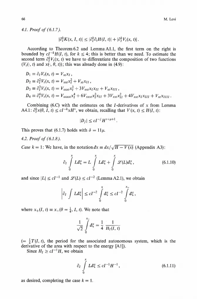
66 M. Levi
4.1. Proof of (6.1.7).
Icing(x, I, t)l ~ IOkIO,H(I, t)l + Icings(x, t)l.
According to Theorem6.2 and LemmaAl.1, the first term on the right is bounded by cI-kI-I(I, t), for k _< 4; this is better than we need. To estimate the second term OklV,(x, t) we have to differentiate the composition of two functions (Vt(', t) and x(., 0, t)); this was already done in (4.9):
D1 =- 6i Vt(x, t) = Vxtxi ,
D2 - 02V,(x, t) = V..tx 2 + V x t x I I ,
03 - a~V,(x, t) = V=x,x~ + 3Vxx~XiXu + V x , x i i i ,
D4 =-- ~?4iVt(x, t) = Vx~xxtX I 4 + 6VxxxtX~Xu + 3V~xtx211 + 4Vxvx~xHz + Vxtxuu.
Combining (6.C) with the estimates on the /-derivatives of x from Lemma A4.1: Okix(O, I, t) <_ eI -kxH v, we obtain, recalling that V (x, t) < H(I, t):
]Dj] <_ cI-J H v+#+l .
This proves that (6.1.7) holds with ~ = 11#.
4.2. Proof of (6.1.8).
Case k = 1:We have, in the notat iondx = d x / v / H - V(x) (Appendix A3):
0 0 0
and since ILl < c1-1 and 5~(L) < c1-2 (LemmaA2.1), we obtain
x x+
0 0
where x+ (I, t) - x+ (0 = �88 I, t). We note that
x+ lj _ r
0
1 �84 1
4 HI(I, t)
(= �88 t), the period for the associated autonomous system, which is the derivative of the area with respect to the energy [A1]).
Since HI > cI-1H, we obtain
81 f Ld~ <__ cI-1H -1 , (6.1.11)
0
as desired, completing the case k = 1.

Quasiperiodic Motions in Superquadratic Time-Periodic Potentials 67
Case k = 2: Applying 0i to (6.1.10), we obtain:
where { f t , . . . , f ,} denotes a linear combination of functions fa . . . . . f , with integer coefficients.
First, ]0ILl < c1-2 by LemmaA2.1. Furthermore, since
/ Ld;~ < cI-1H~ 1 < cH -1 , (6.1.13)
we obtain the desired bound on the first term in (6.1.12). The same bound is valid for the second term in (6.1.12) using (6.1.11) and the fact that ILl < c1-1. For the remaining two terms we use ]~(L)I < cl-2H v and ~2(L) < cl-3H ~ (Lemma A2.1). This completes the case k = 2.
Case k = 3: Applying 01 to (6.1.12) we obtain
~ ( L ) O I f L , ~2(L) J L , fLr (6.1.14)
where f L = fLd~, etc.; we prove that all these terms are bounded by c I - 3 H .
Considering the first one we have by Lemma A2.1:
102LI = 02(HII 2 ~ ) ( _ ~ ) H, l02Wxl (6.1.15) ~k HI "[- -Jl" 02 Wx <__ c1-3 -t- ~ ,
where 102wxl = lo~(W~xxi)l = IWxxxX2 + w j H I <_ c I - 2 ~ 2~ ,
using the assumptions on W and the estimates on xi, Xli from Lemma A4.1. This gives I02L I < cI-3H 2v. Using I f L] < cH -1 we obtain the desired bound on 02L f L. That the same bound cI-3H -1+2~ holds for the second, third and fifth terms in braces in (6.1.14) follows from the estimates already mentioned in previous steps. The remaining terms in (6.1.14) satisfy the same bound according to Lemma A2.1.
Case k = 4: From (6.1.14) we get
0/k+l J L = {O~Q~'m(L)~3kl-m-n f L, f ~k+l(L)O<_m+n<_k},
or more explicitly,
5('3(L) f L, j ~4(L)). (6.1.16)

68 M. Levi
We have I(0]L) (O~ 3-" f Z)l ~ cI-4H -1+3v - for n = 0, 1, 2 this follows from our previous steps, and for n = 3 we have, using (6.1.15) and Theorem 6.2:
HI 02Wx I03LI ~ ci-4 -'}- ~ I ,
and I03Wxl 3 = [WxxxxX I -I-3WxxxXlXll + WxxXlII <- cI-3H 3v by the asumptions on W and Lemma A4.1, so that
103El _< c I - 4 n 3v "
The remaining terms in (6.1.16) are estimated in the same way as above using Lemma A2.1.
This completes the proof of (6.1.8)
4.3. Proof o f (6.1.9). Abbreviating ~ ( K ) = s ~,(,2(K ) = s ) = ~ 2 , etc., we use the differentiation formula to obtain
Of / ~(g)d~ = {(0}~9~ / Z~)i+j+m=p, f ,,~pq-l(~},
where m > 1, i, j > 0 and i + j < p = 1, 2, 3, 4. Applying Lemma A2.2 to this formula, we obtain
(o,~m) @ f L) <_ cI-i-mHI+VI-JH-a+v = c I - P H 2v .
Using Lemma A2.2 again we estimate (p < 4):
f L , e p + l d ~ < c l - P - l H 1 + ~ f d ; ~ < c l - p - l H l + v l - - < cl-PH ~ . - - HI
This completes the proof of (6.1.9) and thus of (6.1.2).
4. Proof of (6.1.2) with k = 0. Differentiating H1 we obtain
O t H l = ~ t J ' K d ~ - K / M c ? ~ + / d / / ( K ) d ~ , (6.1.17)
where M and ~r are given by (A3.5) and (A3.6). The desired first estimate 10trill -< cln~o follows from Intl -< cn (Theorem 6.2), IVtl < cVn~ (assumption), IMI < cRY, Jg(K) < cH l+v (Lemma A2.2) - these estimates give
IOtnll < cH 1+2~ / d e =- cH 1+2v 1 OH < clH2V < clH~'
OI the inequality before last holding by Theorem 6.2.
Differentiating now (6.1.17) in order to estimate higher derivatives, it suffices to prove that (here x = x(O, 1, t), as usual):
IOIK(x, I, t)l < cH 1+~/2 , (6.1.18) X
M(r I, t)d~ <_ cH -1+~/2, (6.1.19) OI , J
o
[ Jg(K)c~ <_ cH 6 , (6.1.20) 0~ J
with 6 ~ 100#.

Quasiperiodic Motions in Superquadratic Time-Periodic Potentials 69
5.1. Proof of(6.1.18), c~IK = al+tHtlt , , t)-c~Vt(x, t); the first term is bounded by cH according to Theorem 5.2 and Lemma AI.1. The second term is given by
t ) = rt+...+rq+s=l r j _ > l , q _ > 0 , s > _ 0
6 ~ q + s + l V
"'"'~t X, Cqrs OxqOts+l ~TIx rq (6.1.21)
where Cqrs are integers and dt denotes the total derivative. The value q = 0 ~1+1V .
corresponds to the term ~ m (6.1.21) (with no factors involving x).
By Lemma A4, IO~x . . . . - O~qxl < xqH qv. Using this inequality together with (6.C) in (6.1.21) we obtain (6.1.18) with 6 = # + 4v = 81#.
5.2. Proof of (6.1.19). The proof is almost identical to that of (6.1.8).
5.3. Proof of (6.1.20). The proof is analogous to that of (6.1.9).
6. Proof of (6.1.2)for all k, I. We represent O[0/kHt by the points in the integer lattice
k = 0 1 2 3 4 5
1=0
1=1
1=2
1=3
1=4
1=5
e -.-). o -.-.~ �9 -..~ �9 . .~ �9 .-~o $ $ $ $ $
i �9
It remains to estimate the terms not lying on the lines 1 = 0 and k = 0; we proceed in the direction indicated by the arrows, considering the four columns in the diagram.
For the column k = 1 we need to estimate
t ? l a x H l = O l t ? i / K = a l ( K / L + / Z f ( K ) ) , 1 _ < l < 4 ,
and it suffices to prove [cf. (6.1.7)-(6.1.9) that for l = 1, 2, 3, 4,
[01KI < cH t+a/2, (6.1.22)
air f L <_ cH -1+a/2, (6.1.23)
a[ f SY(K) <_cH ~. (6.1.24)
(6.1.22) has already been proven.

70 M. Levi
For (6.1.23) we use O~ f L = O~-I(L f M + f J/(L)), and estimate the t-derivatives of each term in the last expression. By Lemma A2.1 we have
[OI-1LI < cI-1H v . (6.1.25)
The t-derivatives of f M are given by (6.1.19), and we estimate the remaining term
01-1 j dg(L) < cn -l+v, I = 1 , 2 , 3 , 4 ,
using Lemma A2.1. This completes the proof of (6.1.23).
Proof of (6.1.24). We use the identity
01 f 5~(K)= {[0~,/~m-l,,acsO(K)] [0~ f M] i+m+n=l' f dgt~(K)} ;
applying LemmaA2.2 we obtain (6.1.24). The remaining columns k = 2, 3, 4 are estimated in the same way, using
the results of Lemmas A2.1, A2.2, and A4.1. The cases k = 2, 3, 4 are done analogously. This completes the proof of Theorem 6.1. []
x+ (H, t) 6.2. Proof of Theorem 6.2. We recall that Io(t, H) = 4 f x / 2 ( H - V ({, t))d{.
0 Let us denote the operators involved in the differentiation formulas (A3.2) and (A3.3) by W and ~-:
1 1 v (6.2.1) ~ ( K ) = -uff K + K . + (KW)~, W V~'
V~ Y-(K) = Kt - (KU)x, U = ~--~, (6.2.2)
so that
and
0 Io(t, H) = 4v~ OH
x(H, t) f ;e(1)v/-ff- v d~
Io = 4v~ 3--(1)v~ - V d~,
1 ~/fk(1) = ~ Pk(W, 0xW, . . . , 0xkW), (6.2.4)
and the proof reduces to showing that any composition of ~f and 3- of length _< 5 applied to K = 1 gives a function of (t, H, x), 0 <_ x <_ x+(H, t) bounded by cH -k, k being the number of occurrences of J f in the composition. Note first
0 0 that since ~ and ~ commute, so do J and x/g, and it suffices to show that
~-- o . . . o ~ o ('of o . . . ~ ( 1 ) < e H -k , i + j _ < 5 . (6.2.3) Y U - - J
Lemma 6.2.1. The k th composition of J/g" applied to K = 1 is given by

Quasiperiodic Motions in Superquadratic Time-Periodic Potentials 71
where Pk is a polynomial of degree k in its k + l variables, and where each monomiaI w(iL).... �9 W (i') (n <_ k) is such that the number of differentiations equals the number
n
o f fac tors : iv = n. p=l
Proof of the lemma. For k = 1 the statement is obvious. Equation (6.2.1) gives the recurrence relation
( ~ ) d 1 (6.2.5) Pk = + Wx Pk-1 q- W d x Pk-1 -- k ~ '
which shows that if the statement of the lemma holds for k - 1 then it does for k. []
Lemma 6.2.2. The compositions of ~-- and J f applied to K = 1 is given by 4
1 { p + q < j , r + s < j + k J-J o ~f~k(1) ---- ~-~ Pjk(U (p'q), W (r's)) �9 - - (6.2.6)
p<_j 1, r<_j,
where Pjk is a polynomial of degree j + k and each monomial
U (pt'ql) ' . . . " U(Pm'qm) w (rL'sl) " . . . " w(r"s")(m + n <_ j + k)
has the property: the number of factors equals the number of x-differentiations: m n
Z q + Z s = m + n (6.2.7) 1 1
Proof The statement holds for j = 0 by the previous lemma (there is no U- dependence at all). We show now that if it holds for some j then it does for j + 1(_< 5). We have by (6.2.2):
H k J j+l~t~ = -UxPjk + OtPjk -- UOxPjk .
1 p We see that as the result of one application of ~ to ~-~ jk, each monomial
of Pjk gets acted upon by the operators -Uxld, Ot and -UOx. Each of these operations preserves the property (6.2.7) and the resulting expression Pj+l,k is a polynomial in uP'q, W r's and p, q, r, 2 are in the range
p + q < _ j + l , p<_j, r + s < _ j + l + k , r < _ j + l . []
Lemma 6.2.2 and the estimates on U, W from the statement of Theorem 6.2 complete the proof of the latter. []
x+ (H, t) 6.3. Proof of Theorem 6.3. Differentiating I0 = 4x/~ f ~/H - V (4, t)d~ we obtain, using (A3.2): o
x+ (H, t)
01---9-~ = 4v~ (6.3.1) OH
f w(1)v/I-I- t)d . 0
4 U(p,q) denotes OPtoqu
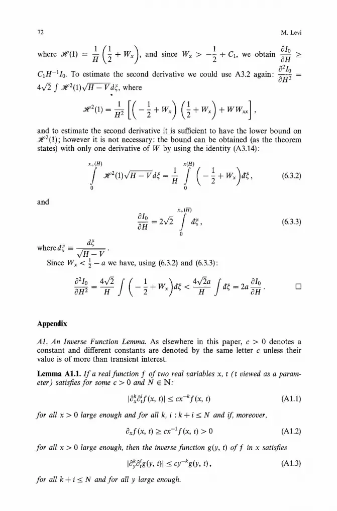
72 M. Levi
1 01o + W~ , and since W~ > - ~ + C1, we obtain ~ > where Yf(1) =
021o CIH-11o. To estimate the second derivative we could use A3.2 again: 0H 2
4v/2 f )ff2(1)v/-H- Vd~, where
1 [ ( 1 ) ( ~ ) _ ~ + W x ] Jta2(1)=~--~ + Wx + WWxx ,
and to estimate the second derivative it is sufficient to have the lower bound on W2(1); however it is not necessary: the bound can be obtained (as the theorem states) with only one derivative of W by using the identity (A3.14)"
x+(H) x(H)
1 1 Wx)d~, if' 3 ~ 2 ( 1 ) v / H - - V d ~ = ~ / ( - - 2 + 0 o
(6.3.2)
and
where d~ - - - d~
v
x+ (n)
0I__~o = 2v/~ J d~ 0H
0
Since Wx < �89 - a we have, using (6.3.2) and (6.3.3):
(6.3.3)
021o 4 f(1 )4v/2a/ ~Io OH 2 - H - - ~ + Wx d~ < ~ d~ = 2a--.OH
[]
Appendix
A1. An Inverse Function Lemma. As elsewhere in this paper, c > 0 denotes a constant and different constants are denoted by the same letter c unless their value is of more than transient interest.
Lemma AI.1. I ra real function f o f two real variables x, t ( t viewed as a param- eter) satisfies for some c > 0 and N E N:
k i lOxOtf(x, t)l < cx-kf(x, t) (AI.1)
for all x > 0 large enough and for all k, i : k + i <_ N and if, moreover,
Oxf (x, t) > cx-l f (x, t) > 0 (A1.2)
for all x > 0 large enough, then the inverse function g(y, t) o f f in x satisfies
10yk0~g(y, t)[ < cy-kg(y, t), (A1.3)
for all k + i < N and for all y large enough.

Quasiperiodic Motions in Superquadratic Time-Periodic Potentials 73
P r o o f We proceed by induction in N. For i + k = 1 (A1.3) is easy to check: first, 1
for i = 0, k = 1 we have gy(y, t) = f x ( X , ~ t - - - - - - -~ and (A1.2) gives
c x ]gy(y, t)] <_ f ( x , t~) -- c y - l g ( y ' t ) , (A1.4)
as desired. Second, for i = 1, k = 0 the definition g ( f ( x , t), t) = x gives gt(Y, t) = -gy(y, Of t (x , t), where x = g(y , t), and the desired estimate follows from (A1.4) and (AI.1) :
[gt(Y, t)l -< c y - l g(y , t) " c f (x, t) = cg(y, t) .
To carry out the induction step we show that if the implication (A1.1) & (A1.2) ~(A1.3) holds for i + k _< N - I(N _> 2) then it holds for i + k = N as well. To that end we derive a formula for 0yk8~g(y, t).
Differentiating k > 0 times the definition f (f (x, t), t) = x by x and expressing the highest derivative, we obtain with y - f (x, t) :
a ,g(y, t) = 1
(Oxf (x, t)) k
ar, m(Oyg(y, t))~n~ f (x, t) " . . . " om~f (x, t ) , l<r<k mj >_1
m 1 +...+mr =k
(A1.5)
k [cf. (4.9)] where a~,m - ar, m I ..... mr are integers. Differentiation of (A1.5) by t is ambiguous unless we specify which variable is independent; let it be y; then x =- x (y , t) = g(y, t) and the application of 0~ to (A1.5) gives
oi ok "
t y g t Y , t) = Z kar, m ~ ( q ) @ p p S (Oxf(g(y,1 t),t)) k ) p+q+s=i
q r ( ) x (Ot0yg) 0~ 1-I x JtgtY, t), t) ,
l_<j<_r
(A1.6)
Here we used the Leibnitz differentiation formula for the ith derivative of the product of three functions. For the case k = 0 we have a separate formula, by differentiating gt(Y, t) = - g y ( y , t ) f t ( x , t):
i--1 ( r ) ( ( d ) i-l-r ) 0~g(y, t) = - - Z i-- 1 (~;0yg(y, t)) ~ f2(g(Y, t), t) ,
r=0
(A1.7)
d where ~ denotes the total derivative and the subscript 2 indicates the differenti-
ation with respect to the second argument. We activate now the inductive assumption: (A1.1) & (A1.2)~(A1.3) for i + k _<
N - 1. Assume that (AI.1) holds for i + k = N and prove (A1.3) for i + k = N. First let k > 0, so that (A1.6) is applicable.

74 M. Levi
First, we h a v e p = i - q - s = N - k q s < N , and
Ot p 1 I fx(g(Y, t), t) k < cy-kg(y ' t)k (A1.8)
by induction on p. Next, q + r = i - p - s + r < i - p - s + k < N, and thus
q r l0 t 0yg(y, t)l < cy-rg(y, t) (A1.9)
by the inductive assumption on g. Finally, s + mj ~ i q- k = N , and
~ ~mj ~, , t) t) (-~mj) I-[ x J tgty, t), <_ cg(y, I ' I f(g(Y' t), t) l<j<r l<j<_r
= cg(y, t)--ky ~ , (AI.10)
using (AI.1) and the inductive assumption on g. Using now (A1.8)-(AI.10) in (A1.6) we obtain (A1.3) with i + k = N, as
desired. It remains only to consider the case k = 0; this is done in a similar way using (A1.7). []
A2. Estimates on ~ , Jg, L, M . The following expressions L, M, ~ and ~/ar ise in the process of differentiation of the action-angle transformation and are estimated in this section. These expressions are given by the formulas (13.6-9) below.
Lemma A2.1. I f the potential function V (x, t) satisfies IxqOqo[ V I <_ cV 1+~,
j lot ~xWI < clxl a-j, ~ + j < 5, (A2.1)
and j 10,0xuI _< clxl 1-j , ~ + j < 5, (12.2)
where W = V /Vx, U = V~/Vx, then there exists a constant v < 20# such that for all z + i + l < 3 we have
10[0}S(L)I < e I - i - t -XH ~ , (A2.3)
10t 0~J//m(M)I -< c I - i H ~ , (12.4)
]~[ J{m~q~l(L)l < c I - t - l H v , (A2.5)
and
o~Q.Qp4(L) ~ c1-5 , (A2.6)
J~4(M) N c, (A2.7)
where L, M , ~LP, and A / a r e given by the formulas (A3 .6 -9 ) below.
Lemma 12.2. Under the asumptions o f Lemma A2.1, the kernel K(x , I, t) = Ht(I, t) -- Vt(x, t) satisfies f o r some v < 20~:
I~[0~r < c I - i - I H l+v , �9 + i - t - m + l <_ 4
and IJC/mS#(K)l < c I - t H l+v , m -q- 1 = 5.
Proo f o f Lemma A2.1. We start with the proof of 12.6; the proof of 12.7 is virtually identical and is omitted.
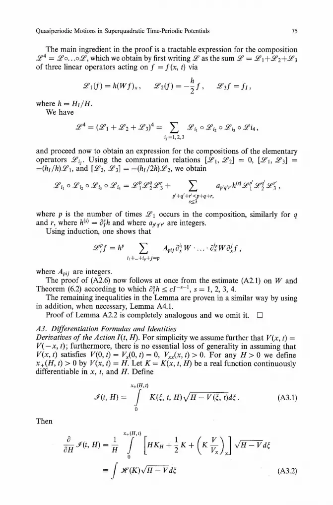
Quasiperiodic Motions in Superquadratic Time-Periodic Potentials 75
The main ingredient in the proof is a tractable expression for the composition 504 = 50o. . .o50, which we obtain by first writing 50 as the sum 50 = Y1+502+503 of three linear operators acting on f = f (x, t) via
501(f) = h(W f )x ,
where h = HI/H. We have
504 = (501 -[- 502 -'}- 503) 4 =
h 502(f) = --~ f , 503f = f I ,
Z ij =1, 2, 3
50il O 50i20 50i30 50i4,
x+ (H, t)
J(t , H) = f K(~, t, H ) v / H - - V(~, t)d~. (A3.1)
0
x+ (u, t)
0
= f -
Then
(A3.2)
and proceed now to obtain an expression for the compositions of the elementary operators 500" Using the commutation relations [501, 502] = 0, [5~ 5e3] = -(ht /h)50b and [5e2, 503] = -(hi/2h)502, we obtain
Z r~ , , ,la(S) c4oP (Pq (.pr 50il o 50i2 o 50i3 o 50i4 ~ (pP c4oq ror ' ' ' ~ l ~ 2 ~ z " 3 -'}- ~ p q r ' * ~ 1 ~ 2 ~ 3 ,
f+qr+r~<p+q+r, s<_3
where p is the number of times 501 occurs in the composition, similarly for q and r, where h (s) = O~h and where ap, q,r, are integers.
Using induction, one shows that
50P f hP Z il . ~3ixp w oj f , = ApijC3 x W " . . .
il+...+ip+j=p
where Apij are integers. The proof of (A2.6) now follows at once from the estimate (A2.1) on W and
Theorem (6.2) according to which ~Sih < cl -s-l, s = 1, 2, 3, 4. The remaining inequalities in the Lemma are proven in a similar way by using
in addition, when necessary, Lemma A4.1. Proof of Lemma A2.2 is completely analogous and we omit it. []
A3. Differentiation Formulas and Identities Derivatives o f the Action I(t, H). For simplicity we assume further that V(x, t) = V ( - x , t); furthermore, there is no essential loss of generality in assuming that V(x, t) satisfies V(0, t) = Vx(0, t) = 0, Vx~(x, t) > 0. For any H > 0 we define x+(H, t) > 0 by V(x, t) = H. Let K = K(x, t, H) be a real function continuously differentiable in x, t, and H. Define

76 M. Levi
and x+ (H, t)
Vt ~7 j ( t ' H) = / [Kt - (KVxx)x] v / -~-Vd{
0
=- / J(K)v/-H - Vd~. (13.3)
When K = 1, we obtain the action integral: (1/4v~)J(t, H) = Io(t, H). 4 x+(H,t) d~
Derivatives of the Period T(H, t) = - ~ fo ~/H - V (4, t) are given by
x+ (H, t)
v/'2 ~ T(H,t) 1 / ( V~@) dg (13.4) 4 0H = ~ - ~ 1 - 2 x / H - V ( 4 , t)
o
and x+ (H, t)
v~ 0 T(H, t) = f (VVr Vt Vct) d~ (A3.5) 4 OT J \ V~ V VCJ C H - V ( ~ , t ) "
o Derivatives of the Action-Angle Map (x, y) ~ (0, I): (13.10) and (13.11). Let (x(O, I, t), y(O, I, t)) be the point in the xy-lane corresponding to the action-angle variables I, 0 as described in Sect. 2.
The following expressions L, M and the operators 5 ~ ~ will play a key role:
L = L(x, t, I) = H'I H~ + --~ W~ - I )
- ( - 2 Vvxx HH //I 1 (A3.6) HI 2H Vx 2 J '
M = M(x, t, I) - HItHI 2HHt (1 - 2 ~VVxx'~j + --~'Vxt (A3.7)
The linear differential operators 5r and JC{ act on functions f (x, t, I) according to
HI ( V V~'~ H1 V ~(f)=Tff . l -2 v~ / f + -ff Vx fx + fI
=--5 (fW)~-- f + f l ,
and
(A3.8)
Ht ( V Vxx "~ Vxt Ht V d//(f)----f~ , ,1--2 V~ ] f - -vT T + -H -~ fx + ft
= (fW)x-- f + f t - - ~--~f. (13.9)
We point out the close similarity between 2~o and Jg - in fact, one obtains s by replacing the t-differentiations in ~ by the/-differentiations.

Quasiperiodic Motions in Superquadratic Time-Periodic Potentials 77
V Derivatives of the action-angle map are given by as usual, W = ~ and
f d~ it// a__ai x(O, i, t) = ~ L ~ _ + ~- W, (A3.10)
and -~ / d ~ + -HH t x(O, I, t) = ~ M s W - U. (A3.11)
One could easily obtain similar expressions for r Oiy.
Derivatives of Singular Integrals. Let again K = K(x, t, I) be a smooth function of three variables.
We have the key identities:
x(O,I,t)
'i / / O--I K(~, t, I) x/H(I, t) - V (~, t) = L K + ~(K) , (13.12) 0
x
where L = L(x, I, t), is given by (A3.6), f K = f K(r I, t)d-~, with at = dr x 0
H ~ - V, ~ given by (A3.8), and f ~(K) = f ~(K) (4, I, t)at~. Similarly for the t-derivative: 0 ' j j / K = K M + J/t(K), (A3.13)
with the abbreviations as above.
Some Interesting Identities. Under the above assumptions on V, we have (sup- pressing the t-dependence which plays no role here):
x+(H)
V = - - where W Vx'
o
x+(H)
V-H- Vd~
and
x+(H) x+(H)
i-i f VH - v (~) v~ } o o
(A3.14)
(A3.15)
H V(2:, t]]3/2 = - - + W~ . ~ / - f f - - - _ t z
o o
1 + 2 W
v'U - V (x) (A3.16)

78 M. Levi
It should be noted that x c (0, x+(H)) in the last identity is arbitrary, while in the previous two identities the upper limit of integration is x = x+.
An infinite hierarchy of further identities of this kind can be obtained using the method of proof outlined below.
The last identity can be used to study the blowing up of the integral on the left-hand side of (A3.16) as x "f x+(H).
Proofs v (~, t)
Proof of (A3.2). Let us choose - - = a E [0, 1] as the new variable of inte- gration; (A3.1) becomes H
i
I(t, H) = Hv/-H / K(~(6, t, H), t, H) v/1 ado-; (A3.17) Vx(~(a, t, H), t)
o
0 differentiating by H, observing that ~-~ ~ (a, t, H) - ~ and simplifying we ob- tain (A3.2). []
a a Vt Proof of (A3.3). Applying ~ to (A3.17), we use ~ ~(a, t, H) = -~-x"
Proof of (A3.10)-(A3.12).
d~ X
We obtain
[]
Ot K(I, t, 4) ~ - ~ t?,x + Ot x/H(l, t ) - V(r t) 0 o
To find the expression for ~tx(O, I, t) we differentiate the identity H1 0
1 - 0, where T - is the period of the frozen system.
c~/H (I, t)
J J de + I-/i de HI, V'H-V ~ x , + U l O' r t)-V(r
o o
and
= 0 ,
. j xt _ Hit / d~ - r162 (A3.19) 4 - ~ - v s-I1
o o
Using the differentiation formula (A3.20) below for singular integrals, we obtain for the last term in (A3.18),
x
f ~?t(Kdt~) o
.,j x
o o
X
0

Quasiperiodic Motions in Superquadratic Time-Periodic Potentials 79
we used the assumption V (0, t) = V~(0, t) = 0. Setting K - 1 we obtain the expression for the last term in (A3.19) as well:
/ H t / H t / ( l )
X o 0
/ ( ) ( V ) 1 1 ~=x + ~ t t
0
Substitution of the last two expressions into (A3.18) leads, mercifully, to the cancellation of the boundary terms, resulting in (A3.12). The remaining identities are proven similarly. []
An Auxiliary Formula. Let A(2, x), B(2), W(2, x) be real functions of independent real variables x and 2 such that the expressions below are well defined. Then
/ ( ) ) ( ) ] A(2, ~)d~ [ B~ A A W - - _ ~-~ A + 2 W +
0 0
• B,/ga-W- W + B B x Wx B,/UCY--V
Proof goes by first choosing the new variable a - W(~) in the integral and then differentiating the integral. [] B
A4. Estimates on the Derivatives of the Action-Angle Map: ~?~}x(O, I, t). In this section, we use the above differentiation formulas together with the assumptions on the potential function V to obtain the desired estimates on the derivatives in terms of the action-angle variables.
V Vt satisfy the bounds Lemma A4.1. Assume that the functions W = -~, U = ~xx
p v p z 18~8 t < + ~ < 5, IO~t WI, UI CX 1-p , p --
]xqOqo~g[ < c V #+1 , p + z < 5 ;
then 18~ 8~x(0, I, t)[ <_ cI-ix(O, I, t)H ~ ,
where v = v(#) < 20~t is a constant s.
Proof. la. The formula for xi :We recall (A3.10):
XI = ~ g V / ~ o
i + z <_4,
_ _ + h(I, t)W(x, t), (A4.1)
where h = Hx/H, W = V /Vx.
5 Whose value can be estimated much more precisely. For z + i _< 2, for instance, the estimate holds with v = 0. We sacrifice this precision to avoid further complications in the exposition

80 M. Levi
lb. The estimate of xi: For 0 < ( _< x we have V(4, t) <_ V(x, t), and thus , / H - V (x)
< 1. Now, ILl < c1-1 using the assumption on W which for p = 1 x/H - V (4) -
V Vxx gives ~ _< C. Using this in (A4.1) we obtain
x1 < c I - l x .
2a. The formula for xi1" We first differentiate H ~ - V in (A4.1) and obtain using (A4.1) :
c~?i ~ - V = hv/ -H- V - 5 Vx Ld~, (A4.2)
0
d~ where d~ - v//_ / _ V(~) ' Using this and the differentiation formula (A3.12) we obtain
( l j ) / j x~ = h v ~ - - V - ~ vx La'~ r ~ + v ~ - VL L ~
0 ~) 0
+ ~ / 5f(L)d~ + h iW + hWxxi . (A4.3)
0
2b. Estimating X~l" It suffices to prove that
[ V x j L d ~ < c I - l v / H - V (14.4)
0
[for 0 _< x < x+(I, t)] - indeed, all the remaining terms in (A4.3) are estimated by cI-2x in the same way as in lb - one only needs to use the bound I~(L)[ < c1-2 (Lemma A2.1) for the fourth term in (A4.3) and W~ < c in the last term in (A4.3), together with the last estimate on xi. Now, (A4.4) is equivalent to
1 --B(x) =--- --c1-1 ~xx v /~ -- V <_ A(x)
j - Ld~ <_ c1-1 ~ v/-H - V = B(x), (14.5)
o which holds for x = x+ : A(x+) = B(x+) = 0, and it remains to prove that --Br(x) > A'(x) > B'(x) for 0 _< x < x+.
After multiplying by ~ - V both sides in --B' _> W > B' these inequalities reduce to
c1-1 ] ~ f (H - V) + > L(I, x, t) > c1-1 - (H - V) -
V~ here V = V(x, t). Since ~ (H - V) > 0, this holds, if we have
1 ~ c1-1 >_ L >_ --~ c1-1 '
which we do if c is fixed at a large enough value.

Quasiperiodic Motions in Superquadratic Time-Periodic Potentials 81
3a. The formula: differentiating (A4.3) we obtain
] A46a 0 0
+ O I [ v / - H - V L J i L d ~ ] + O I ( ~ J S ~ ( L ) d ~ ) (a4.6b)
0 0
-'1- 0I (hi W) -}- Oi(hWxxi) . (A4.6c)
3b. The estimate: We show that (A4.6a) is bounded by cI-3xHV;indeed, 10shl <_ c1-2, 101~I(A42&4) <-- c I - l ~ , OS ( fo gd~) <- cI-2 i c~ (checking
the latter, 0s fo Ld~ = L fo Ld~ + fo ~(L)d~ < cI-2 i d~) , and it remains
to show that Vxxxs fo Ld~ < cI-2v/H - VHL To that end, we write
VxxXl Ld~ < cV~xx1-1 Lct~ = c ~ Ld~ o o 0
<_ cfl-lH~Vx j Ld~ <_ cfl-ZH~v/H - V. o
Proving the desired bound on (A4.6b) and (A4.6c) is straightforward; in
addition to the estimates mentioned above we use IOILI <_ c1-2, Os f 5~(L)ct~ <_
[ ~ ( L ) d ' ~ Y ( L ) f i ~2(L)d-~ x c1-3 f d~ Indeed , Os ~( = Ld;~ + <_ c1-3 f d~ by 0 0 o
the differentiation formula and the estimates on 5r and ~2(L) from Lemma
A2.1], Ihss] < cl-2H (Theorem 6.2), and Wxx <_ cx -t. Further estimates proceed
in the same way and pose no new difficulties. []
Acknowledgements. Most of this paper was written at the Forschungsinstitut ffir Mathematik at ETH Ziirich. I would like to express my thanks to Jiirgen Moser for the opportunity to visit ETH and for his helpful comments on this paper. I would also like to thank Joseph Keller for his hospitality at Stanford University, where a considerable part of this paper was written.
References
lAB] [A]
[A1]
lAD]
Abel, N.H.: Resolution d'un probleme mechnique. J. Reine Angew. Math. 1, 13-18 (1826) Arnol'd, V.I.: On the behavior of an adiabatic invariant under a slow periodic change of the Hamiltonian. DAN 142, (4) 758-761 (1962), (Transl. Soy. Math. Dokl. 3, 136-139) Arnol'd, V.I.: Mathematical methods of classical mechanics. Berlin, Heidelberg, New York: Springer 1978 Aubry, S., LeDaeron, P.Y.: The discrete Frenkel-Kontorova model and its extensions. I. Exact results for the ground states. Physica 8D, 381M22 (1983)

82 M. Levi
[BE]
[B1]
[B21
[BH]
[CZ]
[DZ1]
[DZ2]
{DO] [D1] [D2]
[HA]
[HE]
[KA]
[K] [LL]
[LI]
[L21
[LI]
[LB]
[LO]
[MA1]
[MA2]
[MO]
[M1]
[M2]
[M3]
[M41
IN]
[R1]
Bernstein, D.: Birkhoff periodic orbits for twist maps with the graph intersection property. Erg. Th. Dyn. Sys. 5, 531-537 (1985) Birkhoff, G.D.: Surface transformations and their dynamical properties. Acta Math. 43, 1-119 (1920) Birkhoff, G.D.: Sur quelques courbes fermees remarquables. Bull. Soc. Math. France 60, 1-26 (1932) Boyland, RL., Hall, G.R.: Invariant circles and the order structure of periodic orbits in monotone twist maps. Topology 26, 21-35 (1987) Chiercia, L., Zehnder, E.: On asymptotic expansion of quasiperiodic solutions. Annali della Sc. Norm. Sup. di Pisa Serie IV Vol. XVI, 245-258 (1989) Dieckerhoff, R., Zehnder, E.: An "a priori" estimate for oscillatory equation. Dyn. systems and bifurcations. Groningen, 1984. Lecture Notes in Mathematics, Vol. 1125, pp.9-14. Berlin, Heidelberg, New York: Springer 1985 Dieckerhoff, R., Zehnder, E.: Boundedness of solutions via the Twist theorem. Ann. Scuola Norm. Sup. Pisa 14(1), 79-85 (1987) Douady, R.: Docteur D'etat Thesis, Ecole Polytechnique Tongren Ding: Boundedness of solutions of Duffing's equation. JDE 61, 178-207 (1986) Tongren Ding: An answer to Littlewood's problem on boundedness for super-linear Duff- ing's equations. JDE 73, 269-287 (1988) Hall, G.R.: A topological version of a theorem of Mather on twist maps. Erg. Th. Dyn. Sys. 4, 585-603 (1984) Herman, M.R.: Sur les Courbes invariantes par les diffeomorphismes de l'anneau, Vol. 1 Asterisque, 103-104, 1983, and Vol. 2, Asterisque 144, 1986 Katok, A.: Some remarks on Birkhoff and Mather twist map theorems. Erg. Th. Dyn. Sys. 2, 185-194 (1982) Keller, J.B.: Inverse problems. The American Mathematical Monthly 83, 107-118 (1976) Laederich, S., Levi, M.: Invariant curves and time-dependent potentials. Erg. Th. Dyn. Sys. (to appear) Levi, M.: KAM Theory for particles in Periodic Potentials. To appear in Erg. Th. Dyn. Sys. (1989) Levi, M.: On the Littlewood's counterexample of unbounded motions in superquadratic potentials. ETH preprint, October 1988; to appear in Dynamics Reported Littlewood, J.E.: Unbounded solutions of an equation ~ + g(y) = p(t), with p(t) periodic and bounded and g(y ) / y ~ oo as y ~ +m. J. Loud. Math. Soc. 41, 497 507 (1966) Liu Bin: On Moser's boundedness problem for solutions of Duffing's equation. Preprint, Math. Dept., Peking University, 1987 Yiming Long: Unbounded solutions of a superlinear Duffing's equation, Preprint, Nankai Institute of Mathematics, Tianjun, China, 1989 Mather, J.N.: Existence of quasi-periodic orbits for twist homeomorphisms of the annulus. Topology 21, 457-476 (1982) Mather, J.: More Denjoy minimal sets for area-preserving diffeomorphisms. Comment. Math. Helv. 60, 508-557 (1985) Morris, G.R.: A case of boundedness in Littlewood's problem on oscillatory differential equations. Bull. Austr. Math. Soc. 14, 71-93 (1976) Moser, J.K.: On invariant curves of area preserving mappings of an annulus. Nachr. Akad. Wiss. G~Sttingen Math. Phys. K1. II, 1-20 (1962) Moser, J.K.: A stability theorem for minimal foliations of the toms. Erg. Th. Dyn. Sys. 8, 151-188 (1988) Moser, J.K.: Quasi-periodic solutions of nonlinear elliptic partial differential equations. Bol. Soc. Bras. Mat., 20(1), 29-45 Moser, J.K.: The scattering problem for some particle systems on the line. Lecture Notes Math., vol. 597, pp.441-463. Berlin, Heidelberg, New York: Springer 1977 Norris, J.: Boundedness in periodically forced second order conservative system. Preprint, Aberystwyth, 1990 Rfissman, H.: Ober invariante Kurven differenzierbarer Abbildungen eines Kreisringes. Nachr. Akad. Wiss. G~Sttingen, Math. Phys. K1. II, 67-105 (1970)

Quasiperiodic Motions in Superquadratic Time-Periodic Potentials 83
[R21
[s]
[sl]
[swl
Riissman, H.: On the existence of invariant curves of twist mapping of an annulus. In Geometric dynamics. Palis, J. (ed.). Lecture Notes in Mathematics, vol. 1007, pp. 677-718. Berlin, Heidelberg, New York: Springer 1981 Salamon, D., Zehnder, E.: KAM theory in configuration space. Commun. Math. Helv. 64, 84 132 (1989) Stoker, J.J.: Nonlinear vibrations in mechanical and electrical systems. New York: Inter- science 1950 Smoller, J., Wasserman, A.: Global bifurcations of steady state solutions. J. Diff. Eq. 39, 269-290 (1981), or in the book Smoller, J.: Shock waves and reaction-diffusion equations. New York, Heidelberg, Berlin: Springer 1983
Communicated by M. Herman