quasi-normal modes of electromagnetic perturbations of four-dimensional topological black holes with...
TRANSCRIPT
arX
iv:h
ep-t
h/06
0609
6v2
14
Sep
2006
hep-th/0606096May 2006
Quasi-normal Modes of Electromagnetic Perturbations ofFour-Dimensional Topological Black Holes with Scalar Hair
George Koutsoumbas,a,∗ Suphot Musiri,b,† Eleftherios Papantonopoulosa,♭
and George Siopsisc,♮
aDepartment of Physics, National Technical University of Athens,Zografou Campus GR 157 73, Athens, Greece
bDepartment of Physics, Srinakharinwirot University, Bangkok 10110, ThailandcDepartment of Physics and Astronomy, The University of Tennessee, Knoxville, TN
37996 - 1200, USA
Abstract
We study the perturbative behaviour of topological black holes with scalar hair.We calculate both analytically and numerically the quasi-normal modes of the elec-tromagnetic perturbations. In the case of small black holes we find evidence of asecond-order phase transition of a topological black hole to a hairy configuration.
∗ [email protected]† [email protected]♭ [email protected]♮ [email protected]
–2–
1 Introduction
Quasi-normal modes (QNMs) are well known to play an important role in black holephysics. They determine the late-time evolution of fields in the black hole exterior. Afteran initial perturbation the black hole starts vibrating into quasi-normal oscillation modeswhose frequencies and decay times depend only on the intrinsic features of the black holeitself being insensitive to the details of the initial perturbation. For these reasons, QNMsof black holes in asymptotically flat spacetimes have been extensively studied (for reviews,see [1, 2]).
The Anti-de Sitter - conformal field theory (AdS/CFT) correspondence has led to anintensive investigation of black hole QNMs in asymptotically AdS spacetimes. Quasi-normal modes in AdS spacetime were first computed for a conformally invariant scalarfield, whose asymptotic behaviour is similar to flat spacetime [3]. Subsequently, motivatedby the AdS/CFT correspondence, Horowitz and Hubeny made a systematic computationof QNMs for scalar perturbations of Schwarzschild-AdS (S-AdS) spacetimes [4]. Theirwork was extended to gravitational and electromagnetic perturbations of S-AdS black holesin [5]. The study of scalar perturbations was further extended to the case of Reissner-Nordstrom-AdS (RN-AdS) black holes in [6]. Finally, the QNMs of scalar, electromagneticand gravitational perturbations of RN-AdS black holes were presented in [7] using theresults of [8].
In a parallel development, exact black hole solutions in asymptotically non-flat space-times were studied recently and solutions with scalar hair and negative cosmological con-stant were found. Exact black hole solutions are known in three [9, 10] and four dimen-sions [11]. For asymptotically flat spacetime, a four-dimensional black hole is also known,but the scalar field diverges at the horizon [12]. Also spherically symmetric black hole so-lutions have been found numerically in four [13, 14] and five dimensions [15]. Spaces witha negative cosmological constant also allow for the existence of black holes whose horizonhas nontrivial topology in four [16, 17, 18, 19] and higher dimensions [20, 21, 22, 23] as wellas for gravity theories containing higher powers of the curvature [24, 25, 26, 27].
Recently, an exact black hole solution in four dimensions with a minimally coupled self-interacting scalar field, in an asymptotically locally anti-de Sitter spacetime, was found [28](MTZ black hole). The event horizon is a surface of negative constant curvature enclosingthe curvature singularity at the origin. It was shown that there is a second-order phasetransition at a critical temperature below which a black hole in vacuum undergoes a spon-taneous dressing up with a nontrivial scalar field. An extension of the above solutionincluding a charge was presented in [29]. Aspects of the thermodynamics of the MTZ blackhole are discussed in [30]. In [31] it was shown that the four-dimensional MTZ black holecan be uplifted to eleven dimensions in supergravity theory.
In this work, we make a perturbative study of the MTZ black hole. We compute thesimplest possible QNMs of the MTZ black hole, those of electromagnetic (EM) perturba-tions. The computation is carried out both analytically and numerically with fairly goodagreement. The QNMs provide, near a critical temperature and for small black holes,support for the claim that a vacuum topological black hole (TBH) goes over to a hairyconfiguration, the MTZ black hole, through a second-order phase transition.
–3–
The paper is organized as follows. In section 2, we review the MTZ black hole andits charged extension. In section 3, we discuss the thermodynamics of the MTZ and TBHblack holes. In section 4, we calculate the QNMs of the EM perturbations analyticallywhereas in Section 5 we present the numerical computation of the QNMs and comparethem with the analytical results of section 4. Finally, section 6 contains our conclusions.
2 Four-Dimensional Topological Black Hole with Scalar Hair
Consider four-dimensional gravity with negative cosmological constant (Λ = −3l−2)and a scalar field described by the action
I =
∫
d4x√−g
[
R + 6l−2
16πG− 1
2gµν∂µφ∂νφ− V (φ)
]
, (2.1)
where l is the AdS radius, and G is the Newton’s constant. The self-interaction potentialis given by
V (φ) = − 3
4πGl2sinh2
√
4πG
3φ , (2.2)
which has a global maximum at φ = 0, and has a mass term given by m2 = V ′′|φ=0 =
−2l−2. This mass satisfies the Breitenlohner-Friedman bound that ensures the perturbativestability of AdS spacetime [32, 33]. The field equations are
Gµν −3
l2gµν = 8πGTµν ,
�φ− dV
dφ= 0 , (2.3)
where � ≡ gµν∇µ∇ν , and the stress-energy tensor is given by
Tµν = ∂µφ∂νφ− 1
2gµνg
αβ∂αφ∂βφ− gµνV (φ) . (2.4)
A static black hole solution with topology R2 × Σ, where Σ is a two-dimensional manifold
of negative constant curvature, is given by [28]
ds2 =r(r + 2Gµ)
(r +Gµ)2
−(
r2
l2−(
1 +Gµ
r
)2)
dt2 +
(
r2
l2−(
1 +Gµ
r
)2)−1
dr2 + r2dσ2
,
(2.5)and the scalar field is
φ =
√
3
4πGArctanh
Gµ
r +Gµ. (2.6)
The position of the horizon is at r+, which is the solution of
Gµ =r2+
l− r+ . (2.7)
–4–
For φ = 0 we get the vacuum solution (Topological Black Hole (TBH)) [16, 17, 18, 19]
ds20 = −
[
r2
l2− 1 − 2Gµ
r
]
dt2 +
[
r2
l2− 1 − 2Gµ
r
]−1
dr2 + r2dσ2 . (2.8)
A charged black hole with scalar hair was presented in [29]. The action is given by
I =
∫
d4x√−g
[
R + 6l−2
16πG− 1
2gµν∂µφ∂νφ − 1
12Rφ2 − αφ4
]
− 1
16π
∫
d4x√−gF µνFµν , (2.9)
where α is an arbitrary coupling constant.The corresponding field equations are
Gµν −3
l2gµν = 8πG(T φ
µν + T emµν ) ,
�φ =1
6Rφ+ αφ3 ,
∂ν(√−gF µν) = 0 , (2.10)
and the energy-momentum tensor is given by the sum of
T φµν = ∂µφ∂νφ− 1
2gµνg
αβ∂αφ∂βφ+1
6[gµν� −∇µ∇ν +Gµν ]φ
2 − gµναφ4, (2.11)
and
T emµν =
1
4π
(
FµαFνβ − 1
4gµνFγαFδβg
γδ
)
gαβ. (2.12)
The charged static black hole solution with topology R2 × Σ is given by
ds2 = −[r2
l2−(
1 +Gµ
r
)2]
dt2 +[r2
l2−(
1 +Gµ
r
)2]−1
dr2 + r2dσ2, (2.13)
where −∞ < t <∞ and r > 0. The scalar field is
φ =
√
1
2αl2Gµ
(r +Gµ), (2.14)
with α > 0 and the only non-zero component of the electromagnetic field is
At = −qr. (2.15)
The integration constants q and µ are not independent. They are related by
q2 = −Gµ2
(
1 − 2πG
3αl2
)
. (2.16)

–5–
They correspond to conserved charges,
M =σ
4πµ and Q =
σ
4πq , (2.17)
respectively, where σ denotes the area of Σ.Eq. (2.16) fixes a charge-to-mass ratio for this black hole, which is a function of the
constants appearing in the action, G and α. Moreover, eq. (2.16) determines an upperbound for α
0 < α ≤ 2πG
3l2. (2.18)
If the upper bound is saturated, the charge vanishes. Then we recover the MTZ blackhole. Indeed the form of the self-interacting potential considered in (2.2) can be naturallyobtained through the relation between the conformal and Einstein frames [28].
Note that if µ = 0 then both the MTZ black hole (2.5) and the TBH black hole (2.8)go to
ds2AdS = −
[
r2
l2− 1
]
dt2 +
[
r2
l2− 1
]−1
dr2 + r2dσ2 , (2.19)
which is a manifold of negative constant curvature possessing an event horizon at r = l.We can say that as φ→ 0 the MTZ and TBH black holes match continuously at µ = 0 orr = l with (2.19) being a transient configuration as it becomes apparent in the following.In the sequel we set l = 1.
3 Thermodynamics
For the MTZ black hole, the temperature, entropy and mass are given respectivelyby [28]
T =2r+ − 1
2π,
S =σr+(r+ + 2Gµ)
4G(r+ +Gµ)2r2+ =
σ
4G(2r+ − 1) ,
M =σµ
4π=σ(r2
+ − r+)
4πG. (3.1)
Notice that the entropy in this case does not satisfy an area law. It is easy to show thatthe law of thermodynamics dM = TdS holds. Defining the free energy as F = M − TSand using relations (3.1), we obtain
FMTZ = − σ
8πG(2r2
+ − 2r+ + 1) . (3.2)
The free energy (3.2) can be written as
FMTZ = − σ
8πG
(
1 + 2(T − T0)π + 2(T − T0)2π2)
, (3.3)

–6–
where T0 = 1/2π ≈ 0.160 is the critical temperature. For the vacuum TBH black hole(denoting by ρ+ the horizon for this case) , the temperature, entropy and mass are, respec-tively,
T =3ρ2
+ − 1
4πρ+,
S =σρ2
+
4G,
M =σ(ρ3
+ − ρ+)
8πG. (3.4)
Then, the free energy of the TBH black hole, using relations (3.4), is
FTBH = − σ
16πG(ρ3
+ + ρ+) , (3.5)
which can be expanded around the critical temperature T0 as
FTBH = − σ
8πG
(
1 + 2(T − T0)π + 2(T − T0)2π2 + (T − T0)
3π3 + . . .)
. (3.6)
Using (3.3) and (3.6), we can calculate the difference between the TBH and MTZ freeenergies. We obtain
∆F = FTBH − FMTZ = − σ
8πG(T − T0)
3π3 + . . . , (3.7)
indicating a phase transition between MTZ and TBH at the critical temperature T0. Match-ing the temperatures of the MTZ black hole and the TBH we get:
T =2r+ − 1
2π=
1
4π
(
3ρ+ − 1
ρ+
)
⇒ r+ =3ρ+
4− 1
4ρ+
+1
2. (3.8)
It is easily seen that r+ ≤ ρ+, and the inequality is saturated for r+ = ρ+ = 1. We remarkthat the temperature T should be non-negative, so r+ ≥ 1
2for the MTZ black hole and
ρ+ ≥ 1√3
for the TBH black hole.Thermodynamically we can understand this phase transition as follows. Using relations
(3.1), (3.4) and (3.8), we find that STBH > SMTZ and MTBH > MMTZ for the relevantranges of the horizons r+ or ρ+. If r+ > 1 (T > T0), both black holes have positive mass.As T > T0 implies FTBH ≤ FMTZ , the MTZ black hole dressed with the scalar field willdecay into the bare black hole. In the decay process, the scalar black hole absorbs energyfrom the thermal bath, increasing its horizon radius (from r+ to ρ+ > r+) and consequentlyits entropy. Therefore, in a sense the scalar field is absorbed by the black hole.
If r+ < 1 (T < T0), both black holes have negative mass, but now FTBH > FMTZ , whichmeans that the MTZ configuration with nonzero scalar field is favorable. As a consequence,below the critical temperature, the bare black hole undergoes a spontaneous “dressing up”with the scalar field. In the process, the mass and entropy of the black hole decrease andthe differences in energy and entropy are transferred to the heat bath.

–7–
At the critical temperature, the thermodynamic functions of the two phases matchcontinuously, hence, the phase transition is of second order. The order parameter thatcharacterizes the transition can be defined in terms of the value of the scalar field at thehorizon; using the solution for the scalar field (2.6) we obtain for T < T0,
λφ =
∣
∣
∣
∣
∣
tanh
√
4πG
3φ(r+)
∣
∣
∣
∣
∣
=
∣
∣
∣
∣
r+ − 1
r+
∣
∣
∣
∣
=T0 − T
T0 + T. (3.9)
For T > T0, λφ vanishes. Then the relation (3.7) can be written in terms of the orderparameter λφ as
∆F = FTBH − FMTZ = +σr3
+
8πGλ3
φ + . . . (T < T0). (3.10)
The pure AdS space of (2.19) has free energy FAdS = −σ/8πG as easily can be seenusing relations (3.2) or (3.5) with r+ = 1. Then observe that FAdS is the constant termof both FMTZ in (3.3) and FTBH in (3.6). Hence the difference of free energies of MTZ orTBH black holes with the free energy of pure AdS space indicates that the configuration(2.19) is transient between the MTZ and TBH phase transition.
In the next two sections we will find the QNMs of the electromagnetic perturbations ofthe MTZ black hole and its charged generalization and compare them with the correspond-ing QNMs of the TBH. This study will provide additional information on the stability ofthe MTZ black hole and its generalization under electromagnetic perturbations. Note thatfor the MTZ black hole and its charged generalization, the wave equations, after factor-ing out the angular parts, are the same. For the TBH, only the function f(r) (eq. (4.2))changes. There is no change due to the axial or polar character of the perturbation.
4 Analytical Calculation
In this section, we calculate analytically the QNMs of electromagnetic perturbations forboth MTZ and topological black holes. Numerical results will be discussed in section 5. Ourapproach is based on the method discussed in [34, 35, 36]. In order to calculate QNMs,in general, one solves the wave equation subject to appropriate boundary conditions atinfinity and the horizon. In asymptotically flat spacetime, this can be implemented by amonodromy method [37]. It is then advantageous to follow Stokes lines which go throughthe black hole singularity. In asymptotically (A)dS spacetimes, the calculation simplifiesbecause the wavefunction vanishes at infinity. Although the monodromy does not enter thecalculation, in several cases it is still advantageous to follow Stokes lines and analyticallycontinue the wavefunction through the black hole singularity [34, 35, 36]. However, this isnot always necessary, if a general solution (or approximation thereof) of the wave equationas in, e.g., [38] is readily available. In our case, we shall solve the wave equation near theblack hole singularity perturbatively and then analytically continue the wavefunction inorder to match with the expected behaviour at infinity and the horizon, respectively. Thiswill produce an explicit form of the QNMs for r+ > 1 (Gµ > 0). For r+ < 1 (Gµ < 0), we
–8–
do not have explicit analytical expressions. Instead, we obtain a lower bound which is inaccord with numerical results.
Electromagnetic perturbations obey the wave equation
f(r)d
dr
(
f(r)dΨω
dr
)
+
[
ω2 −(
ξ2 +1
4
)
f(r)
r2
]
Ψω = 0 , (4.1)
where
fMTZ(r) = r2 −(
1 +Gµ
r
)2
, fTBH(r) = r2 − 1 − 2Gµ
r. (4.2)
It may be cast into a Schrodinger-like form if written in terms of the tortoise coordinatedefined by
dx
dr=
1
f(r). (4.3)
We obtain
− d2Ψω
dx2+ V (x)Ψω = ω2Ψω , (4.4)
where the potential is
V [x(r)] =
(
ξ2 +1
4
)
f(r)
r2. (4.5)
For QNMs, we impose the boundary condition Ψω → 0 as r → ∞, since the potential doesnot vanish for large r. At the horizon (x→ −∞), we demand Ψω ∼ eiωx (ingoing wave).
Near the black hole singularity (r ∼ 0), the tortoise coordinate (4.3) may be approxi-mated by
x ≈ −Gµaλ
(
r
Gµ
)λ
, (4.6)
where a = 1, λ = 3 for MTZ and a = 2, λ = 2 for TBH. In arriving at (4.6), we choose theintegration constant so that x = 0 at r = 0. The potential near the singularity is
V (x) ≈ − Ax1+1/λ
, A =
(
ξ2 +1
4
)
1
(aGµ)1−1/λ(−λ)1+1/λ. (4.7)
We will solve the wave eq. (4.4) by treating the potential (4.7) as a perturbation. Thezeroth-order solutions are
Ψ±0 = e±iωx (4.8)
and the first-order corrections are
Ψ±1 (x) =
1
2iω
∫ x
0
dx′ei(ω−iǫ)(x−x′)V (x′)Ψ±0 (x′)− 1
2iω
∫ x
0
dx′e−i(ω+iǫ)(x−x′)V (x′)Ψ±0 (x′) (4.9)
where we included a small ǫ > 0 to render integrals finite. We shall work with generalvalues of λ in the potential (4.7) and take the limit of interest (λ→ 2, 3) at the end of thecalculation. The desired solution will be a linear combination of the above wave functions,
Ψω(x) = A+(Ψ+0 + Ψ+
1 ) + A−(Ψ−0 + Ψ−
1 ) . (4.10)
–9–
Asymptotically, it behaves as
Ψω(x) ≈(
A+ + ieiπ
2λ
AΓ(−1/λ)
(2ω)1−1/λA−
)
eiωx +
(
A− − ie−iπ
2λ
AΓ(−1/λ)
(2ω)1−1/λA+
)
e−iωx . (4.11)
At large r (x→ +∞), the tortoise coordinate (4.3) may be approximated by
x ≈ x0 −1
r, x0 =
∫ ∞
0
dr
f(r)(4.12)
and the potential (4.7) is
V (x) ≈ ξ2 +1
4. (4.13)
Since we are interested in the asymptotic form of quasi-normal frequencies, we may ignorethe potential (V (x) . ω2). We obtain the eigenfunction for large r (x ∼ x0)
Ψω(x) ∼ sinω(x− x0) , (4.14)
where we applied the boundary condition Ψω → 0 as r → ∞ (x→ x0).This is matched by the linear combination (4.11) provided
A+ + ieiπ
2λ
AΓ(−1/λ)
(2ω)1−1/λA− = −e−2iωx0
(
A− − ie−iπ
2λ
AΓ(−1/λ)
(2ω)1−1/λA+
)
(4.15)
of eigenfunction (eqs. (4.8) and (4.9)) in the vicinity of the singularity.Next, we approach the horizon (x→ −∞) by analytically continuing (4.10) to negative
x. This amounts to a rotation by −π in the complex x-plane. For x < 0, we obtainfrom (4.9), using eqs. (4.7) and (4.8),
Ψ±1 (x) =
A2iω
eiπ/λ
∫ −x
0
dx′
x′ 1+1/λ
(
ei(ω+iǫ)(x+x′) − e−i(ω−iǫ)(x+x′))
e∓iωx′
. (4.16)
Taking the limit x→ −∞, we obtain the behavior near the horizon
Ψω(x) ≈(
A+ − ie3iπ
2λ
AΓ(−1/λ)
(2ω)1−1/λA−
)
eiωx +
(
A− + ieiπ
2λ
AΓ(−1/λ)
(2ω)1−1/λA+
)
e−iωx . (4.17)
Since we want an ingoing wave (Ψω ∼ eiωx) at the horizon, we obtain the constraint on thecoefficients
A− + ieiπ
2λ
AΓ(−1/λ)
(2ω)1−1/λA+ = 0 . (4.18)
For compatibility with the other constraint (4.15), we ought to have∣
∣
∣
∣
∣
e−2iωx0 + eiπ
2λC 1
1 − Ce− iπ
2λ e−2iωx0 Ce− iπ
2λ
∣
∣
∣
∣
∣
= 0 , (4.19)
where C = iAΓ(−1/λ)(2ω)−1+1/λ. We deduce
e2iωx0 = 2e−iπ
2λC , (4.20)
–10–
where we discarded terms which were of order higher than linear in C. Solving for ω, weobtain the quasi-normal frequencies
ωn =nπ
x0
+ o(lnn) . (4.21)
Thus the asymptotic behaviour is completely determined by the parameter x0 (eq.(4.12)).In the case of MTZ black holes, f(r) has four roots,
r± =1
2
(
1 ±√
1 + 4Gµ)
, r± =1
2
(
−1 ±√
1 − 4Gµ)
. (4.22)
For Gµ > 0, the horizon is at r+ and r+ > 1. We obtain
x0 =1
2(r+ − r−)lnr−r+
+1
2(r+ − r−)lnr−r+
. (4.23)
For large Gµ, the quasi-normal frequencies are
ωn ≈ 2(1 − i)r+n (4.24)
matching the behaviour in five-dimensional AdS space.For small (positive) Gµ, we find
ωn ≈ −2ni
(
1 +2Gµ
πilnGµ
)
. (4.25)
Continuing to negative values of Gµ is not straightforward. The above discussion is notapplicable, because going beyond the horizon (as we approach the singularity) we encountera potential well at r− < r < r+ for Gµ > −1/4 (horizon 1/2 < r+ < 1) which admits boundstates and alters the behaviour of quasi-normal frequencies. The minimum of the potentialprovides a lower bound to the frequencies. By setting V ′(r) = 0, we find the minimum at
rmin = −2Gµ . (4.26)
At the minimum,
V (rmin) = −(
ξ2 +1
4
){
1
16(Gµ)2− 1
}
. (4.27)
It is also easily seen that V ′′(rmin) > 0, showing that r = rmin is indeed a minimum. Theeigenfrequencies have imaginary part
ωI ≥ −√
|V (rmin)| , (4.28)
which is verified by numerical results. The lowest frequency is close to the lower bound (4.28).In the TBH case, the horizon is given by
r+ = 2ℜ(eiπ/6s) , s =
(
√
1
27− (Gµ)2 − iGµ
)1/3
, (4.29)
–11–
where |Gµ| < 3−3/2. The other two roots of f(r) are also real,
r− = −2ℜ(e−iπ/6s) , r′− = 2ℑs . (4.30)
We obtain
x0 = − r−3r2
− − 1lnr−r+
− r′−3r′2− − 1
lnr′−r+
. (4.31)
For small Gµ, we have
ωn ≈ −2ni
(
1 +4Gµ
πilnGµ
)
(4.32)
to be compared with the behaviour of MTZ QNMs (4.25) near the transition point. Thediscrepancy is of second order.
For large Gµ, the above formulae for the roots read
r+ =
(
Gµ+
√
(Gµ)2 − 1
27
)1/3
+
(
Gµ−√
(Gµ)2 − 1
27
)1/3
≈ (2Gµ)1/3 ,
r− = −e− iπ
3
(
Gµ+
√
(Gµ)2 − 1
27
)1/3
− e+iπ
3
(
Gµ−√
(Gµ)2 − 1
27
)1/3
≈ −e− iπ
3 r+ ,
r′− = (r−)∗ ≈ −e+ iπ
3 r+ . (4.33)
Then
ωn ≈ nr+
(
3√
3
4− i
9
4
)
. (4.34)
For Gµ < 0, we encounter a potential well behind the horizon. Arguing as in the MTZcase, we obtain a lower bound
ωI ≥ −√
|V (rmin)| (4.35)
In the TBH case, rmin = −3Gµ and
V (rmin) = −(
ξ2 +1
4
){
1
27(Gµ)2− 1
}
(4.36)
5 Numerical Results
5.1 The Method
Another method of studying the same problem is the procedure of Horowitz and Hubeny[4]. We briefly review the method as we applied it to our problem. After performing thetransformation Ψω(r) = ψω(r)e−iωr∗ , the wave equation (4.1) becomes
f(r)d2ψω(r)
dr2+
(
df(r)
dr− 2iω
)
dψω(r)
dr=
(
ξ2 + 14
)
r2ψω(r) . (5.1)
–12–
The change of variables r = 1/x (not to be confused with the tortoise coordinate (4.3))yields an equation of the form
s(x)
[
(x− x+)2d2ψω(x)
dx2
]
+ t(x)
[
(x− x+)dψω(x)
dx
]
+ u(x)ψω(x) = 0 ,
where x+ = 1/r+. It turns out that s(x), t(x) and u(x) are polynomials of third degree forMTZ black holes and of second degree for TBHs. Thus,
s(x) = s0 + s1(x− x+) + s2(x− x+)2 + s3(x− x+)3,
t(x) = t0 + t1(x− x+) + t2(x− x+)2 + t3(x− x+)3,
u(x) = u0 + u1(x− x+) + u2(x− x+)2 + u3(x− x+)3 .
Expanding the wavefunction around the (inverse) horizon x+,
ψω(x) =∞∑
0
an(ω)(x− x+)n , (5.2)
we arrive at a recurrence formula for the coefficients,
an(ω) = − 1
n(n− 1)s0 + nt0 + u0
n−1∑
m=n−3
[m(m− 1)sn−m +mtn−m + un−m]am(ω) . (5.3)
We note that the few coefficients am(ω) with negative index m which will appear for n < 2should be set to zero, while a0(ω) is set to one. Since the wave function should vanish atinfinity (r → ∞, x = 0), we deduce
ψω(0) ≡∞∑
0
an(ω)(−x+)n = 0 . (5.4)
The solutions of this equation are precisely the quasi-normal frequencies.
5.2 MTZ Black Holes
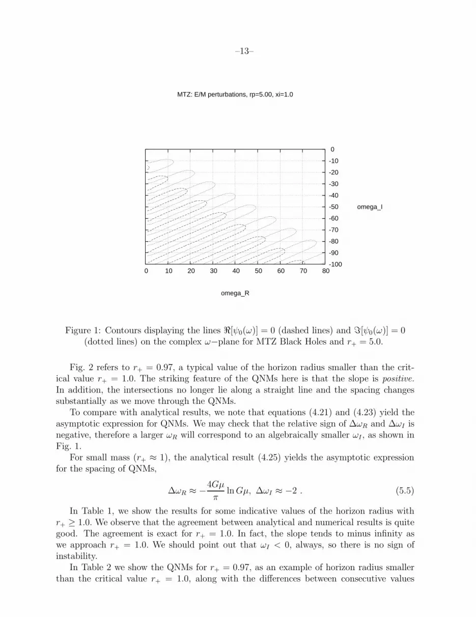
We compute the QNMs for the MTZ black holes by solving eq. (5.4) numerically. As afirst step we draw the contours ℜ[ψω(0)] = 0 and ℑ[ψω(0)] = 0 on the complex ω−planeand check the points of intersection. This provides good initial values for the subsequentMuller root-finding technique [39]; in addition it provides an overview of the (approximate)values of the quasi-normal frequencies. In Fig. 1 we show sample contours for the caser+ = 5.0, ξ = 1.0. We note that the parameter ξ does not seem to play a significant rolein the behaviour of quasi-normal frequencies, so we set it to a typical value (ξ = 1.0) fromnow on.
From Fig. 1, it is evident that the QNMs lie on a straight line with negative slope andtheir spacing is more or less constant. In fact the spacing changes a little as we move tothe right and eventually attains an asymptotic value, which should be compared with theanalytical results of section 4.
–13–
0 10 20 30 40 50 60 70 80-100
-90
-80
-70
-60
-50
-40
-30
-20
-10
0
MTZ: E/M perturbations, rp=5.00, xi=1.0
omega_R
omega_I
Figure 1: Contours displaying the lines ℜ[ψ0(ω)] = 0 (dashed lines) and ℑ[ψ0(ω)] = 0(dotted lines) on the complex ω−plane for MTZ Black Holes and r+ = 5.0.
Fig. 2 refers to r+ = 0.97, a typical value of the horizon radius smaller than the crit-ical value r+ = 1.0. The striking feature of the QNMs here is that the slope is positive.
In addition, the intersections no longer lie along a straight line and the spacing changessubstantially as we move through the QNMs.
To compare with analytical results, we note that equations (4.21) and (4.23) yield theasymptotic expression for QNMs. We may check that the relative sign of ∆ωR and ∆ωI isnegative, therefore a larger ωR will correspond to an algebraically smaller ωI , as shown inFig. 1.
For small mass (r+ ≈ 1), the analytical result (4.25) yields the asymptotic expressionfor the spacing of QNMs,
∆ωR ≈ −4Gµ
πlnGµ, ∆ωI ≈ −2 . (5.5)
In Table 1, we show the results for some indicative values of the horizon radius withr+ ≥ 1.0. We observe that the agreement between analytical and numerical results is quitegood. The agreement is exact for r+ = 1.0. In fact, the slope tends to minus infinity aswe approach r+ = 1.0. We should point out that ωI < 0, always, so there is no sign ofinstability.
In Table 2 we show the QNMs for r+ = 0.97, as an example of horizon radius smallerthan the critical value r+ = 1.0, along with the differences between consecutive values

–14–
0 0.1 0.2 0.3 0.4 0.5 0.6 0.7 0.8 0.9 1-10
-9
-8
-7
-6
-5
-4
-3
-2
-1
0
MTZ: E/M perturbations, rp=0.97, xi=1.0
omega_R
omega_I
Figure 2: Contours displaying the lines ℜ[ψ0(ω)] = 0 (dashed lines) and ℑ[ψ0(ω)] = 0(dotted lines) on the complex ω−plane for MTZ Black Holes and r+ = 0.97.
of QNMs. Note that in this case Gµ = −0.029, T = 0.150. These are the exact QNMspresented in Fig. 2. It appears that, apart from the change of the sign of the slope, thereis a novel phenomenon: the quasi-normal frequencies converge toward the imaginary axis,i.e., their real part decreases. There is only a finite number of QNMs for r+ < 1.0. Thisbehaviour has already been predicted analytically in section 4; eq. (4.28) yields a predictionfor the lowest possible imaginary part of the frequencies. The result is ωI ≥ −9.54i, which isindeed respected by the imaginary parts appearing in Table 2. Although not fully justified,using the analytical result (5.5), we deduce the estimates |∆ωAna
R | ≈ 0.131, |∆ωAnaI | ≈
2.000. Checking against the numerical values in Table 2, we see that the values in the thirdcolumn (real part) are of the same order of magnitude as the analytical prediction, whereasthe values in the fourth column (imaginary part) are quite close to the analytical estimate2. However, the variations are significant. If one further decreases the value of the horizon,the number of QNMs decreases until they finally disappear. The behavior of QNMs for suchhorizons may be viewed as modifications of the critical point r+ = 1.0. In the latter case,the first quasi-normal frequency is ω = 1.0 − 1.5i, followed by frequencies with imaginaryparts ωI = −3.5,−5.5,−7.5, . . .. Unlike the points below criticality, for r+ = 1.0, the realparts do not change and there is no lower bound.
To summarize our findings, for r+ > 1, Fig. 1 shows that the QNMs have a negativeslope and hence large values of ωR correspond to large values of ωI . Then as r+ → 1 the
–15–
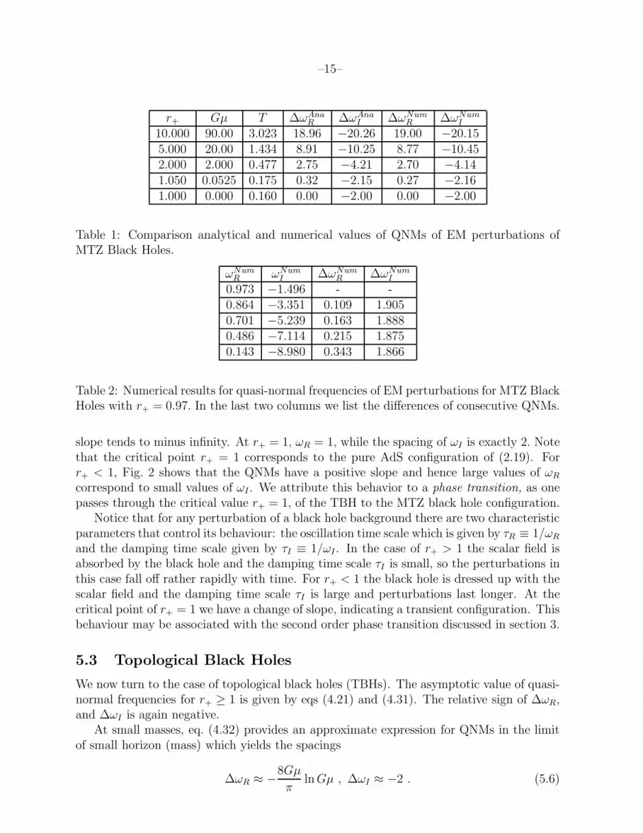
r+ Gµ T ∆ωAnaR ∆ωAna
I ∆ωNumR ∆ωNum
I
10.000 90.00 3.023 18.96 −20.26 19.00 −20.155.000 20.00 1.434 8.91 −10.25 8.77 −10.452.000 2.000 0.477 2.75 −4.21 2.70 −4.141.050 0.0525 0.175 0.32 −2.15 0.27 −2.161.000 0.000 0.160 0.00 −2.00 0.00 −2.00
Table 1: Comparison analytical and numerical values of QNMs of EM perturbations ofMTZ Black Holes.
ωNumR ωNum
I ∆ωNumR ∆ωNum
I
0.973 −1.496 - -0.864 −3.351 0.109 1.9050.701 −5.239 0.163 1.8880.486 −7.114 0.215 1.8750.143 −8.980 0.343 1.866
Table 2: Numerical results for quasi-normal frequencies of EM perturbations for MTZ BlackHoles with r+ = 0.97. In the last two columns we list the differences of consecutive QNMs.
slope tends to minus infinity. At r+ = 1, ωR = 1, while the spacing of ωI is exactly 2. Notethat the critical point r+ = 1 corresponds to the pure AdS configuration of (2.19). Forr+ < 1, Fig. 2 shows that the QNMs have a positive slope and hence large values of ωR
correspond to small values of ωI . We attribute this behavior to a phase transition, as onepasses through the critical value r+ = 1, of the TBH to the MTZ black hole configuration.
Notice that for any perturbation of a black hole background there are two characteristicparameters that control its behaviour: the oscillation time scale which is given by τR ≡ 1/ωR
and the damping time scale given by τI ≡ 1/ωI . In the case of r+ > 1 the scalar field isabsorbed by the black hole and the damping time scale τI is small, so the perturbations inthis case fall off rather rapidly with time. For r+ < 1 the black hole is dressed up with thescalar field and the damping time scale τI is large and perturbations last longer. At thecritical point of r+ = 1 we have a change of slope, indicating a transient configuration. Thisbehaviour may be associated with the second order phase transition discussed in section 3.
5.3 Topological Black Holes
We now turn to the case of topological black holes (TBHs). The asymptotic value of quasi-normal frequencies for r+ ≥ 1 is given by eqs (4.21) and (4.31). The relative sign of ∆ωR,and ∆ωI is again negative.
At small masses, eq. (4.32) provides an approximate expression for QNMs in the limitof small horizon (mass) which yields the spacings
∆ωR ≈ −8Gµ
πlnGµ , ∆ωI ≈ −2 . (5.6)
–16–
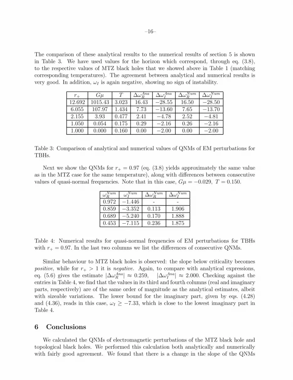
The comparison of these analytical results to the numerical results of section 5 is shownin Table 3. We have used values for the horizon which correspond, through eq. (3.8),to the respective values of MTZ black holes that we showed above in Table 1 (matchingcorresponding temperatures). The agreement between analytical and numerical results isvery good. In addition, ωI is again negative, showing no sign of instability.
r+ Gµ T ∆ωAnaR ∆ωAna
I ∆ωNumR ∆ωNum
I
12.692 1015.43 3.023 16.43 −28.55 16.50 −28.506.055 107.97 1.434 7.73 −13.60 7.65 −13.702.155 3.93 0.477 2.41 −4.78 2.52 −4.811.050 0.054 0.175 0.29 −2.16 0.26 −2.161.000 0.000 0.160 0.00 −2.00 0.00 −2.00
Table 3: Comparison of analytical and numerical values of QNMs of EM perturbations forTBHs.
Next we show the QNMs for r+ = 0.97 (eq. (3.8) yields approximately the same valueas in the MTZ case for the same temperature), along with differences between consecutivevalues of quasi-normal frequencies. Note that in this case, Gµ = −0.029, T = 0.150.
ωNumR ωNum
I ∆ωNumR ∆ωNum
I
0.972 −1.446 - -0.859 −3.352 0.113 1.9060.689 −5.240 0.170 1.8880.453 −7.115 0.236 1.875
Table 4: Numerical results for quasi-normal frequencies of EM perturbations for TBHswith r+ = 0.97. In the last two columns we list the differences of consecutive QNMs.
Similar behaviour to MTZ black holes is observed: the slope below criticality becomespositive, while for r+ > 1 it is negative. Again, to compare with analytical expressions,eq. (5.6) gives the estimate |∆ωAna
R | ≈ 0.259, |∆ωAnaI | ≈ 2.000. Checking against the
entries in Table 4, we find that the values in its third and fourth columns (real and imaginaryparts, respectively) are of the same order of magnitude as the analytical estimates, albeitwith sizeable variations. The lower bound for the imaginary part, given by eqs. (4.28)and (4.36), reads in this case, ωI ≥ −7.33, which is close to the lowest imaginary part inTable 4.
6 Conclusions
We calculated the QNMs of electromagnetic perturbations of the MTZ black hole andtopological black holes. We performed this calculation both analytically and numericallywith fairly good agreement. We found that there is a change in the slope of the QNMs

–17–
as we decrease the value of the horizon radius below a critical value, and we argued thatthis change signals a phase transition of a vacuum topological black hole toward the MTZblack hole with scalar hair.
One may attribute this change in behaviour to the dynamics of the scalar field andassociate it with a second-order phase transition [28]. For small black holes (r+ < 1) thescalar field is dressing up the bare topological black hole introducing an order parameter λφ
(see (3.10)) which controls the dynamics of the scalar field. A second-order phase transitionfor small black holes occurs in more general configurations (including charge, etc) as studiesof general scalar, electromagnetic and gravitational perturbations show [40]. We have alsofound that the vacuum AdS solution at the critical temperature is a transient configurationof the change of phase of the topological black hole to a configuration with scalar hair.
One interesting aspect of small MTZ black holes is that the quasi-normal frequenciesconverge toward the imaginary axis, i.e., their real part decreases and after the first fewquasi-normal frequencies, it vanishes, indicating that for r+ < 1 there are only a finitenumber of QNMs. We showed that the finite number of such modes for small horizons(r+ < 1) is due to the existence of bound states behind the horizon, which is an unobservableregion. This curious phenomenon is worthy of further investigation.
Acknowledgements
We thank Kostas Kokkotas for his valuable assistance in the numerical applications ofthis work. The work of S. M. was partially supported by the Thailand Research Fund.G. K. and E. P. were supported by (EPEAEK II)-Pythagoras (co-funded by the EuropeanSocial Fund and National Resources). G. S. was supported in part by the US Departmentof Energy under grant DE-FG05-91ER40627.
References
[1] K. D. Kokkotas and B. G. Schmidt, Living Rev. Rel. 2, 2 (1999) [arXiv:gr-qc/9909058].
[2] H.-P. Nollert, CQG 16, R159-R216 (1999).
[3] J. S. F. Chan and R. B. Mann, Phys. Rev. D 55, 7546 (1997) [arXiv:gr-qc/9612026]; Phys. Rev. D59, 064025 (1999).
[4] G. T. Horowitz and V. E. Hubeny, Phys. Rev. D 62, 024027 (2000) [arXiv:hep-th/9909056].
[5] V. Cardoso and J. P. S. Lemos, Phys. Rev. D 64, 084017 (2001) [arXiv:gr-qc/0105103].
[6] B. Wang, C. Y. Lin and E. Abdalla, Phys. Lett. B 481, 79 (2000) [arXiv:hep-th/0003295].
[7] E. Berti and K. D. Kokkotas, Phys. Rev. D 67, 064020 (2003) [arXiv:gr-qc/0301052].
[8] F. Mellor and I. Moss, Phys. Rev. D 41, 403 (1990).
[9] C. Martinez and J. Zanelli, Phys. Rev. D 54, 3830 (1996) [arXiv:gr-qc/9604021].
[10] M. Henneaux, C. Martinez, R. Troncoso and J. Zanelli, Phys. Rev. D 65, 104007 (2002)[arXiv:hep-th/0201170].
–18–
[11] C. Martinez, R. Troncoso and J. Zanelli, Phys. Rev. D 67, 024008 (2003) [arXiv:hep-th/0205319].
[12] N. Bocharova, K. Bronnikov and V. Melnikov, Vestn. Mosk. Univ. Fiz. Astron. 6, 706 (1970);J. D. Bekenstein, Annals Phys. 82, 535 (1974); Annals Phys. 91, 75 (1975).
[13] T. Torii, K. Maeda and M. Narita, Phys. Rev. D 64, 044007 (2001).
[14] E. Winstanley, Found. Phys. 33, 111 (2003) [arXiv:gr-qc/0205092].
[15] T. Hertog and K. Maeda, JHEP 0407, 051 (2004) [arXiv:hep-th/0404261].
[16] J. P. S. Lemos, Phys. Lett. B 353, 46 (1995) [arXiv:gr-qc/9404041].
[17] R. B. Mann, Class. Quant. Grav. 14, L109 (1997) [arXiv:gr-qc/9607071]; R. B. Mann, Nucl. Phys. B516, 357 (1998) [arXiv:hep-th/9705223].
[18] L. Vanzo, Phys. Rev. D 56, 6475 (1997) [arXiv:gr-qc/9705004].
[19] D. R. Brill, J. Louko and P. Peldan, Phys. Rev. D 56, 3600 (1997) [arXiv:gr-qc/9705012].
[20] D. Birmingham, Class. Quant. Grav. 16, 1197 (1999) [arXiv:hep-th/9808032].
[21] R. G. Cai and K. S. Soh, Phys. Rev. D 59, 044013 (1999) [arXiv:gr-qc/9808067].
[22] B. Wang, E. Abdalla and R. B. Mann, [arXiv:hep-th/0107243].
[23] R. B. Mann, [arXiv:gr-qc/9709039].
[24] J. Crisostomo, R. Troncoso and J. Zanelli, Phys. Rev. D 62, 084013 (2000) [arXiv:hep-th/0003271].
[25] R. Aros, R. Troncoso and J. Zanelli, Phys. Rev. D 63, 084015 (2001) [arXiv:hep-th/0011097].
[26] R. G. Cai, Y. S. Myung and Y. Z. Zhang, Phys. Rev. D 65, 084019 (2002) [arXiv:hep-th/0110234].
[27] M. H. Dehghani, Phys. Rev. D 70, 064019 (2004) [arXiv:hep-th/0405206].
[28] C. Martinez, R. Troncoso and J. Zanelli, Phys. Rev. D 70, 084035 (2004) [arXiv:hep-th/0406111].
[29] C. Martinez, J. P. Staforelli and R. Troncoso, [arXiv:hep-th/0512022]; C. Martinez and R. Troncoso,[arXiv:hep-th/0606130].
[30] E. Winstanley, Class. Quant. Grav. 22, 2233 (2005) [arXiv:gr-qc/0501096]; E. Radu and E. Win-stanley, Phys. Rev. D 72, 024017 (2005) [arXiv:gr-qc/0503095]; A. M. Barlow, D. Doherty andE. Winstanley, Phys. Rev. D 72, 024008 (2005) [arXiv:gr-qc/0504087].
[31] I. Papadimitriou, [arXiv:hep-th/0606038].
[32] P. Breitenlohner and D. Z. Freedman, Phys. Lett. B115, 197 (1982); Annals Phys. 144, 249 (1982).
[33] L. Mezincescu and P. K. Townsend, Annals Phys. 160, 406 (1985).
[34] V. Cardoso, J. Natario and R. Schiappa, J. Math. Phys. 45, 4698 (2004) [arXiv:hep-th/0403132].
[35] J. Natario and R. Schiappa, Adv. Theor. Math. Phys. 8, 1001 (2004) [arXiv:hep-th/0411267].
[36] S. Musiri, S. Ness and G. Siopsis, Phys. Rev. D 73, 064001 (2006) [arXiv:hep-th/0511113].
[37] L. Motl and A. Neitzke, Adv. Theor. Math. Phys. 7, 307 (2003) [arXiv:hep-th/0301173].

–19–
[38] A. J. M. Medved, D. Martin and M. Visser, Class. Quant. Grav. 21, 2393 (2004)[arXiv:gr-qc/0310097].
[39] W.-H. Press, S. A. Teukolsky, W. T. Vetterling and B. P. Flannery in Numerical Recipies (CambridgeUniversity Press, Cambridge, England, 1992).
[40] G. Koutsoumbas, S. Musiri, E. Papantonopoulos and G. Siopsis, in preparation.