arX

iv:g

r-qc

/001

0006

v1 3

Oct

200

0

Gravitational Perturbations of a Radiating

Spacetime.

Manasse R. MbonyePhysics Department, University of Michigan, Ann Arbor, Michigan 48109

Ronald L. MallettDepartment of Physics, University of Connecticut, Storrs, Connecticut, 06269

February 4, 2008

Abstract

This paper discusses the problem of gravitational perturbations of ra-

diating spacetimes. We lay out the theoretical framework for describing

the interaction of external gravitational fields with a radiating spacetime.

This is done by deriving the field perturbation equations for a radiating

metric. The equations are then specialized to a Vaidya spacetime. For

the Hiscock ansatz of a linear mass model of a radiating blackhole the

equations are found separable. Further, the resulting ordinary differential

equations are found to admit analytic solutions. We obtain the solutions

and discuss their characteristics.

1 INTRODUCTION.

The study of gravitational perturbations can be traced back to the famousEinstein-Infeld-Hoffman paper of 1938 [1] which pioneered the treatment of thetwo body problem in general relativity. In 1957 Regge and Wheeler [2] addressedthe problem of the stability of a Schwarzschild black hole. Later, in his studyof perturbations of a rotating black hole ( [3] and later papers), Teukolsky wasable to put the discipline on a stronger footing. However, little progress hasbeen made at extending this success to cover the radiating cases. The problemof perturbing a radiating spacetime with integral spin fields has not receivedthe attention it deserves. This, despite the fact that most astrophysical objectsradiate. From regular stars to supernovae, from quasars to primordial blackholes one finds that the inhabitants of our universe are generally non-static.

In the present paper, we develop a framework for discussing the problem ofhow external gravitational fields may interact with radiating spacetimes. Thisis done by deriving the field perturbation equations. It is found that two suchequations are sufficient to describe all the non-trivial features of the perturbinggravitational field. We find that one of these equations decouples completely

1

and is homogeneous in one of the field components. The equation for the otherfield component contains, in its source terms, several perturbed and thereforeundetermined quantities. Using a systematic approach we are able to determineall these quantities completely, in terms of the former field component. The re-sult is that all the perturbations are described by only two field componentswhich satisfy two partial differential equations. The equations are then special-ized to a Vaidya spacetime. For a particular model of a radiating black hole theequations are found separable. Interestingly, the resulting ordinary differentialequations are found to admit analytic solutions. We obtain these solutions anddiscuss their characteristics.

The mathematical framework used in this paper is the null tetrad formalismof Newman and Penrose (hereafter NP formalism) [6]. In section II we give abrief description of the background geometry, the radiating spacetime of Vaidya.In section III we derive the perturbation field equations for a general non-vacuumtype D spacetime and adapt these equations to the Vaidya spacetime. In sectionIV we calculate the perturbed quantities in the source terms to arrive at the finalworking field equations. It is demonstrated in section V that these equations areseparable for the Hiscock linear model [12] of a radiating black hole. In sectionVI we obtain and discuss some of the solutions and we conclude the discussionin section VII..

2 THE VAIDYA SPACETIME.

2.1 The Metric

In this analysis we perturb the Vaidya spacetime [9] with incoming externalgravitational fields. The Vaidya geometry, the simplest of the radiating space-times, is non-rotating and spherically symmetric. The energy-momentum tensor

Tµν = ρkµkν ,

describes a null fluid, (kµkµ = 0), of density ρ with radial flow, k2 = k3 = 0.

Using this energy-momentum tensor to solve the Einstein field equations oneobtains [10] a line element, in retarded coordinates, given by

ds2 =

[

1 − 2m (u)

r

]

du2 + 2dudr − r2dΩ2. (1)

Here, u is the retarded time coordinate and m(u), the mass, is a monotoni-cally decreasing function of u.

It is convenient to introduce a null tetrad basis zmµ = (lµ, nµ,mµ, mµ) atevery point in this spacetime. The metric tensor gµν then becomes

gµν = zmµznνηmn = lµnν + nµlν −mµmν − mµmν , (2)

2

where ηmn is the flat spacetime metric. Following Carmeli and Kaye [8] wechoose the covariant form of the null tetrad basis as

lµ = δ 0µ ,

nµ =1

2

[

1 − 2m (u)

r

]

δ 0µ + δ 1

µ ,

mµ = − r√2

[

δ 2µ + i sin θδ 3

µ

]

, (3)

mµ = − r√2

[

δ 2µ − i sin θδ 3

µ

]

The contravariant vectors, zm, considered as tangent vectors, define the direc-tional derivatives as

~zm = z µm∇µ (4)

In the Vaidya spacetime these directional derivatives are given (from equa-tion 3) by

D = lµ∇µ =∂

∂ r,

∆ = nµ∇µ =∂

∂ u− 1

2

[

1 − 2m (u)

r

]

∂

∂ r,

δ = mµ∇µ =√

2 r

[

∂

∂ θ+ i csc θ

∂

∂ ϕ

]

,

δ = mµ∇µ =√

2 r

[

∂

∂ θ− i csc θ

∂

∂ ϕ

]

. (5)

One finds that the only surviving spin (Ricci rotation) coefficients [8] of theVaidya spacetime are

ρ = −(

1

r

)

, α = − 1

2√

2 rcot θ, β = −α,

µ = − 1

2r

[

1 − 2m (u)

r

]

, and γ =m (u)

2 r2(6)

The only surviving tetrad component of Ricci tensor [8] is

3

Φ22 =−m (u)

r2, (7)

where m = dmdu

. With this component, it is easily shown that

Tµν = 2Φ22lµlν = −[

2m (u)

r2

]

lµlν . (8)

Further, the only non-vanishing tetrad component of the of the Weyl tensoris

Ψ2 =−m (u)

r3. (9)

The Vaidya spacetime is then [6] said to be Petrov type D with repeatedprincipal null vectors lµ and nµ. The three optical scalars are found, to beσ = ω = 0, θ = − 1

r. The metric contains two shear-free, twistless and

diverging geodetic null congruencies.

3 The Perturbed Field Equations

3.1 The Type D Spacetime.

In this section we develop the gravitational field perturbation equations for ageneral Petrov type D spacetime. We start with the Newman-Penrose (NP)equations. The full set of the NP equations can be found in several publica-tions, for example [8]. We only mention here that the set is made up of firstorder differential equations which, in the NP formalism, replace the Einsteinfield equations. The equations link together the null tetrad basis, the spin(Ricci rotation) coefficients, the Weyl tensor, the Ricci tensor and the scalarcurvature. In using this formalism to do perturbation analysis one first spec-ifies the perturbations of the geometry. Here we shall write the tetrad of theperturbed spacetime as

l = lb + lp, n = nb + np, m = mb+mp, m = mb+mp. (10)

where the superscripts b and p refer to the background and the perturbingquantities, respectively. Since all the other field quantities are expressible interms of the tetrad [7] their perturbed forms can be written down. For example:Ψa =(0,1,2,3,4) = Ψ b

a + Ψ pa .

We shall, in general, assume that the perturbations in the basis vectors aresufficiently small so that only their first order contributions are significant. The

4

field equations are, then, first order in the perturbing fields, linearized aboutthe background quantities.

In type D spacetimes one can choose the tetrad vectors (see section II) l andn so that certain spin coefficients and certain Weyl scar components

κb = σb = νb = λb = 0,

Ψ b0 = Ψ b

1 = Ψ b3 = Ψ b

4 = 0. (11)

We start our analysis from three of the NP [8] field equations. From the Bianchiidentities we consider the two equations,

δΨ3 −DΨ4 + δΦ21 − ∆Φ20 = 3λΨ2 − 2 (α+ 2π)Ψ3 + (4ǫ− ρ)Ψ4

−2νΦ10 + 2λΦ11 + (2γ − 2γ + µ)Φ20 + 2 (τ − α)Φ21 − σΦ22, (12)

and

∆Ψ3 − δΨ4 + δΦ22 − ∆Φ21 = 3νΨ2 − 2 (γ + 2µ) Ψ3 + (4β − τ )Ψ

−2νΦ11 − νΦ20 + 2λΦ12 + 2 (γ + µ) Φ21 +(

τ − 2β − 2α)

Φ22, (13)

from the spin coefficient system of equations we take

∆λ− δν = − (µ+ µ)λ− (3γ − γ)λ+(

3α+ β + π − τ)

ν − Ψ4. (14)

We have complete knowledge of the geometry of the background spacetime, sowe write down the equations only in those terms that make first order con-tributions to the perturbed field quantities. Making use of equations 11 onequations 12, 13 and 14, respectively, it is seen that for a perturbed Petrov typeD spacetime

−3λpΨ2 +(

δ + 2α+ 4π)

Ψ p3 − (D + 4ǫ− ρ)Ψ p

4

= (∆ + 2γ − 2γ + µ) Φ p20 −

(

2α− 2τ + δ)

Φ p21 − σpΦ22, (15)

−3νpΨ2 + (∆ + 2γ + 4µ)Ψ p3 − (4β − τ + δ)Ψ p

4 = (2γ + 2µ+ ∆)Φ p21

5

+(

−δ + τ − 2β − 2α)p

Φ22 +(

−δ + τ − 2β − 2α)

Φ p22, (16)

and

(∆ + 3γ − γ + µ+ µ)λp −(

δ + 3α+ β + π − τ)

νp + Ψ p4 = 0. (17)

We note that the perturbed equations are coupled both in the Weyl tensorcomponents and the Ricci tensor components. They also contain unknown spincoefficients and directional derivatives. In attempting to decouple the equationsabove we use an approach akin to Teukolsky’s [3]. After some algebra we find,on eliminating Ψ3 between the equations 15 and 16, we are left with

[(∆ + 3γ − γ + 4µ+ µ) (D + 4ǫ− ρ)] Ψ p4

−[(

δ + 3α+ β + 4π − τ)

(4β − τ + δ) − 3Ψ2

]

Ψ p4 = Q4, (18)

Now, under the interchange l n, m m, the full set of the NP equationsis invariant [11]. This symmetry is not destroyed by the choice of l and n whichgave equations 11. One finds under this interchange that [7]

Ψ0 Ψ∗4, Ψ3 Ψ∗

1, Ψ2 Ψ∗2,

κ −ν, ρ −µ, σ −λ, α −β, ǫ −γ and π −τ , (19)

Applying this to equation 18 we obtain the following equation for Ψ p0

(D − 3ǫ− ǫ− 4ρ− ρ) (δ − 3β − α− 4τ + π)(

δ − 4α+ π)

Ψ p0

− (D − 3ǫ− ǫ− 4ρ− ρ) [(∆ − 4γ + µ) − 3Ψ2] Ψp0 = Q0. (20)

Here, the source term Q0 is given by

Q0 = (δ − 3β − α− 4τ + π) (D − 2ρ− 2ǫ) Φ p02

− (δ − 3β − α− 4τ + π) (δ + π − 2α− 2β)Φ p00

6

+ (δ − 3β − α− 4τ + π) (δ + π − 2α− 2β)pΦ00

+ (D − 3ǫ+ ǫ− 4ρ− ρ) (δ − 2β + 2π)Φ p02

− (D − 2ǫ+ 2ǫ− ρ)Φ p22 + (D − 3ǫ+ ǫ− 4ρ− ρ)σp (∆ − µ)Φ00. (21)

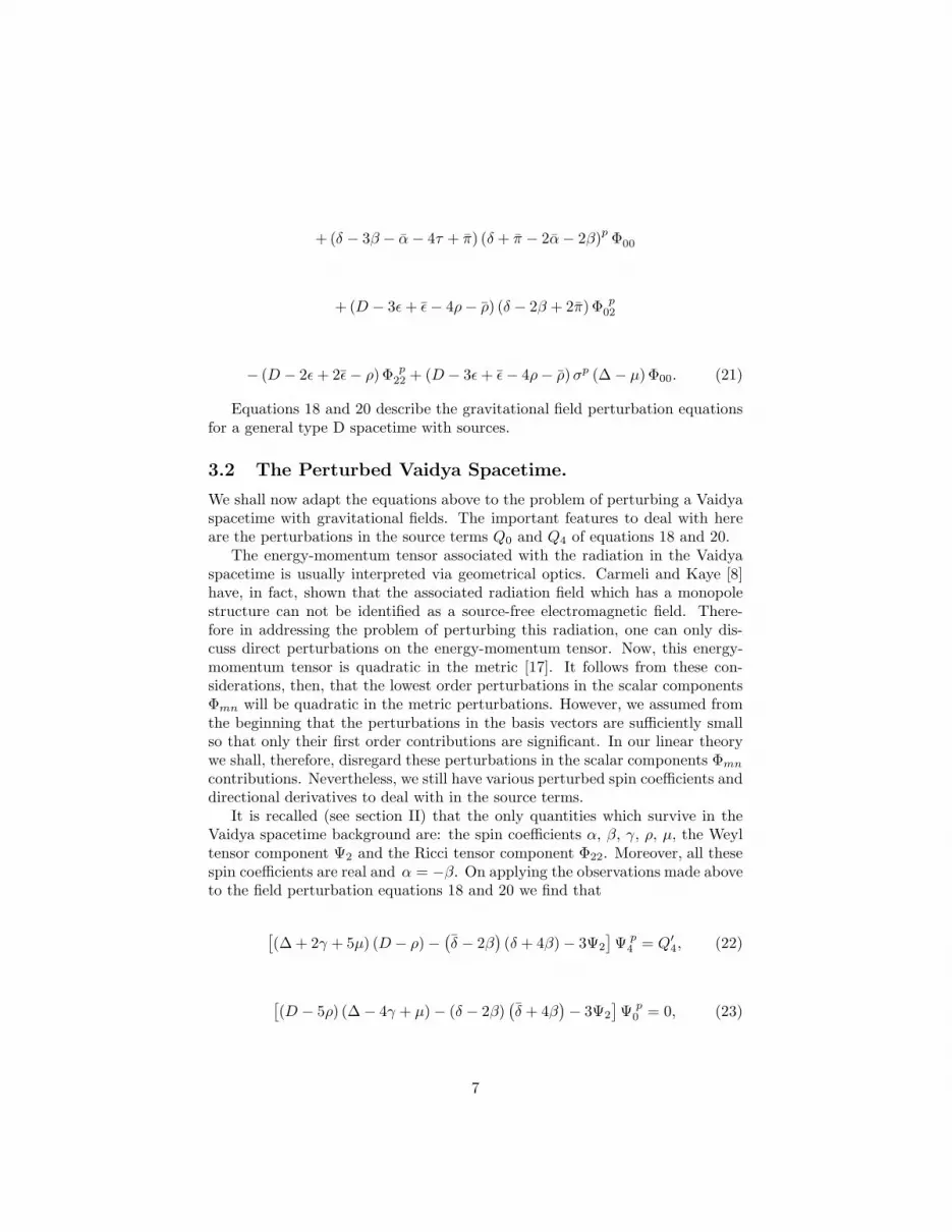
Equations 18 and 20 describe the gravitational field perturbation equationsfor a general type D spacetime with sources.

3.2 The Perturbed Vaidya Spacetime.

We shall now adapt the equations above to the problem of perturbing a Vaidyaspacetime with gravitational fields. The important features to deal with hereare the perturbations in the source terms Q0 and Q4 of equations 18 and 20.

The energy-momentum tensor associated with the radiation in the Vaidyaspacetime is usually interpreted via geometrical optics. Carmeli and Kaye [8]have, in fact, shown that the associated radiation field which has a monopolestructure can not be identified as a source-free electromagnetic field. There-fore in addressing the problem of perturbing this radiation, one can only dis-cuss direct perturbations on the energy-momentum tensor. Now, this energy-momentum tensor is quadratic in the metric [17]. It follows from these con-siderations, then, that the lowest order perturbations in the scalar componentsΦmn will be quadratic in the metric perturbations. However, we assumed fromthe beginning that the perturbations in the basis vectors are sufficiently smallso that only their first order contributions are significant. In our linear theorywe shall, therefore, disregard these perturbations in the scalar components Φmn

contributions. Nevertheless, we still have various perturbed spin coefficients anddirectional derivatives to deal with in the source terms.

It is recalled (see section II) that the only quantities which survive in theVaidya spacetime background are: the spin coefficients α, β, γ, ρ, µ, the Weyltensor component Ψ2 and the Ricci tensor component Φ22. Moreover, all thesespin coefficients are real and α = −β. On applying the observations made aboveto the field perturbation equations 18 and 20 we find that

[

(∆ + 2γ + 5µ) (D − ρ) −(

δ − 2β)

(δ + 4β) − 3Ψ2

]

Ψ p4 = Q′

4, (22)

[

(D − 5ρ) (∆ − 4γ + µ) − (δ − 2β)(

δ + 4β)

− 3Ψ2

]

Ψ p0 = 0, (23)

7

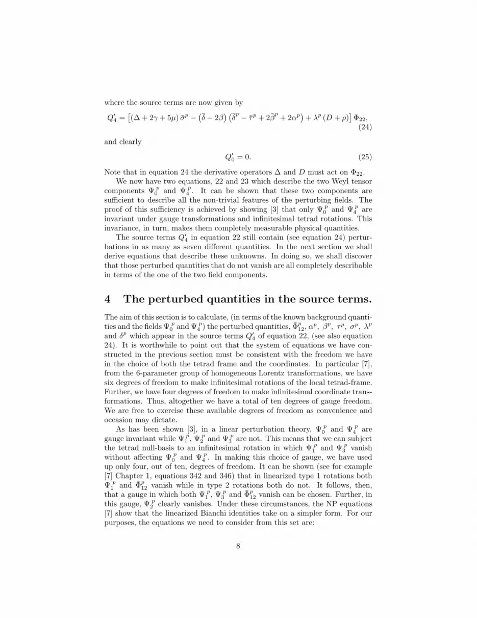
where the source terms are now given by

Q′4 =

[

(∆ + 2γ + 5µ) σp −(

δ − 2β) (

δp − τp + 2β

p+ 2αp

)

+ λp (D + ρ)]

Φ22,

(24)

and clearly

Q′0 = 0. (25)

Note that in equation 24 the derivative operators ∆ and D must act on Φ22.We now have two equations, 22 and 23 which describe the two Weyl tensor

components Ψ p0 and Ψ p

4 . It can be shown that these two components aresufficient to describe all the non-trivial features of the perturbing fields. Theproof of this sufficiency is achieved by showing [3] that only Ψ p

0 and Ψ p4 are

invariant under gauge transformations and infinitesimal tetrad rotations. Thisinvariance, in turn, makes them completely measurable physical quantities.

The source terms Q′4 in equation 22 still contain (see equation 24) pertur-

bations in as many as seven different quantities. In the next section we shallderive equations that describe these unknowns. In doing so, we shall discoverthat those perturbed quantities that do not vanish are all completely describablein terms of the one of the two field components.

4 The perturbed quantities in the source terms.

The aim of this section is to calculate, (in terms of the known background quanti-ties and the fields Ψ p

0 and Ψ p4 ) the perturbed quantities, Φp

12, αp, βp, τp, σp, λp

and δp which appear in the source terms Q′4 of equation 22, (see also equation

24). It is worthwhile to point out that the system of equations we have con-structed in the previous section must be consistent with the freedom we havein the choice of both the tetrad frame and the coordinates. In particular [7],from the 6-parameter group of homogeneous Lorentz transformations, we havesix degrees of freedom to make infinitesimal rotations of the local tetrad-frame.Further, we have four degrees of freedom to make infinitesimal coordinate trans-formations. Thus, altogether we have a total of ten degrees of gauge freedom.We are free to exercise these available degrees of freedom as convenience andoccasion may dictate.

As has been shown [3], in a linear perturbation theory, Ψ p0 and Ψ p

4 aregauge invariant while Ψ p

1 , Ψ p2 and Ψ p

3 are not. This means that we can subjectthe tetrad null-basis to an infinitesimal rotation in which Ψ p

1 and Ψ p3 vanish

without affecting Ψ p0 and Ψ p

4 . In making this choice of gauge, we have usedup only four, out of ten, degrees of freedom. It can be shown (see for example[7] Chapter 1, equations 342 and 346) that in linearized type 1 rotations bothΨ p

1 and Φp12 vanish while in type 2 rotations both do not. It follows, then,

that a gauge in which both Ψ p1 , Ψ p

3 and Φp12 vanish can be chosen. Further, in

this gauge, Ψ p2 clearly vanishes. Under these circumstances, the NP equations

[7] show that the linearized Bianchi identities take on a simpler form. For ourpurposes, the equations we need to consider from this set are:

8

∆Ψ p0 = (4γ − µ)Ψ p

0 + 3σpΨ2, (26)

−3δpΨ2 = −9τpΨ2 − 2κpΦ22, (27)

−DΨ p4 = 3λpΨ2 − ρΨ p

4 − σpΦ22, (28)

0 = −κpΦ22, (29)

4.1 Calculation of σp and λp.

From equation 26 and the fact that all the background quantities here are realwe find that

σp =

(

∆ − 4γ + µ

3Ψ2

)

Ψp

0 . (30)

Further, using equation 30 on equation 28 gives

λp =

(

ρ−D

3Ψ2

)

Ψ p4 − Φ22

(

∆ − 4γ + µ

9 (Ψ2)2

)

Ψp

0 . (31)

We note that the perturbed spin coefficients λp and σp display a definitedependence on Ψ p

4 and/or Ψp

0 . In the rest of this section we shall derive ex-pressions for the remaining perturbed quantities.

4.2 The perturbation matrix for the basis vectors.

In order to determine the perturbed quantities τp, αp, βp and δp and theirrelations , it is necessary to study the effects of the perturbations on the basisvectors, (lµ, nµ, mµ, mµ). For compactness, it is convenient to introduce thefollowing index notation:

l1 = lµ, l2 = nµ, l3 = mµ, l4 = mµ. (32)

We can write [7] the perturbations l(p)i, (i = 1, 2, 3, 4) in the vectors, aslinear combinations of the unperturbed basis vectors li. Thus

l(p)i = P ij l

j, (33)

9

where the P ij are elements of a matrix P that describes, completely, the pertur-

bations in the basis vectors. Explicitly,

P =

P 11 P 1

2 P 13 P 1

4

P 21 P 2

2 P 23 P 2

4

P 31 P 3

2 P 33 P 3

4

P 41 P 4

2 P 43 P 4

4

. (34)

The l1 and l2 are real while the l3 and l4 are complex conjugates. It follows,then, that the matrix elements P 1

1, P12, P

21 and P 2

2 are real while the remainingelements of P are complex. Moreover, the elements in which the indices 3 and4 replace one another, are complex conjugates. For example, P 2

3 = (P 24)

4.3 Perturbations in the Angular functions, δp, τp, αp, and

βp.

The perturbations in the directional derivative δp, are given from equations 5

and 33, by

δp

=(

l4∇4

)p. (35)

But from equations 33 and 34 we see that

lp(4) = P 4j l

j = P 41l

1 + P 42l

2 + P 43l

3 + P 44l

4. (36)

Using equation 36 on Equation 4.3 shows that

δp

=(

l4∇4

)p= P 4

1D + P 42∆ + P 4

3δ + P 44δ. (37)

Thus, if we operate with δp

on the background Ψ2 we get

δpΨ2 = P 4

1DΨ2 + P 42∆Ψ2 + P 4

3δΨ2 + P 44δΨ2. (38)

Now, in the background

Ψ2 =−m(u)

r3.

Substituting for Ψ2 in equation 38 and using definitions of the operators inequations 5 we find that

δpΨ2 = P 4

1

[3m (u)]

r4+ P 4

2

(−mr3

)

− P 42

(

1 − 2m (u)

r

)

3m (u)

r4. (39)

10

Recall that in the Vaidya spacetime background, the component Φ22 =

− m(u)r2 is non-vanishing. Using this on equation 29 shows that κp must van-

ish. It follows, then that equation 27 becomes,

δpΨ2 = 3τpΨ2, (40)

We see immediately, that the results expressed in equation 39 will be incon-sistent with the eigenvalue equation 40 unless the P 4

2 vanish, so that

δpΨ2 = P 4

1

[3m (u)]

r4= −3P 4

1

(

1

r

)

Ψ2. (41)

Equations 40 and 41, then, show that

τp = −P 41

(

1

r

)

. (42)

Moreover, equation 37 along with the condition that the P 42 vanish means that

whenever δp

acts on a function with no angular dependence its only contributionis

δp

= P 41

∂

∂r= −τpr

∂

∂r. (43)

We now have, in equation 43, a general relationship between δp

and τp.Next, we need to deal with αp and β

p. It is known [6] that if the null vectors

lµ are tangent to the geodesics and equal to a gradient field, then

ρ = ρ and τ = α+ β. (44)

These conditions are fulfilled in all Type D space-times. In particular, theunperturbed Vaidya space-time satisfies

α+ β = τ = 0.

Consequently, in our linear perturbation analysis we should have

(

α+ β)p

= τp. (45)

Consider, now, the second of the source terms in equation 24 which reads as

(

δ − 2β) (

δp − τp + 2β

p+ 2αp

)

Φ22.

11

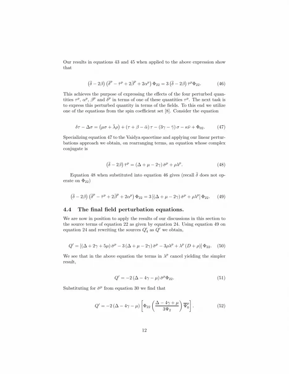
Our results in equations 43 and 45 when applied to the above expression showthat

(

δ − 2β) (

δp − τp + 2β

p+ 2αp

)

Φ22 = 3(

δ − 2β)

τpΦ22. (46)

This achieves the purpose of expressing the effects of the four perturbed quan-tities τp, αp, βp and δp in terms of one of these quantities τp. The next task isto express this perturbed quantity in terms of the fields. To this end we utilizeone of the equations from the spin coefficient set [8]. Consider the equation

δτ − ∆σ =(

µσ + λρ)

+ (τ + β − α) τ − (3γ − γ) σ − κν + Φ02. (47)

Specializing equation 47 to the Vaidya spacetime and applying our linear pertur-bations approach we obtain, on rearranging terms, an equation whose complexconjugate is

(

δ − 2β)

τp = (∆ + µ− 2γ) σp + ρλp. (48)

Equation 48 when substituted into equation 46 gives (recall δ does not op-erate on Φ22)

(

δ − 2β) (

δp − τp + 2β

p+ 2αp

)

Φ22 = 3 [(∆ + µ− 2γ) σp + ρλp] Φ22. (49)

4.4 The final field perturbation equations.

We are now in position to apply the results of our discussions in this section tothe source terms of equation 22 as given by equation 24. Using equation 49 onequation 24 and rewriting the sources Q′

4 as Q′ we obtain,

Q′ = [(∆ + 2γ + 5µ) σp − 3 (∆ + µ− 2γ) σp − 3ρλp + λp (D + ρ)] Φ22. (50)

We see that in the above equation the terms in λp cancel yielding the simplerresult,

Q′ = −2 (∆ − 4γ − µ) σpΦ22. (51)

Substituting for σp from equation 30 we find that

Q′ = −2 (∆ − 4γ − µ)

[

Φ22

(

∆ − 4γ + µ

3Ψ2

)

Ψp

0

]

. (52)

12

Equation 52 forms the result of our analysis in this section. All the perturbationsin the sources have now been expressed in terms of the perturbed field Ψ

p

0 only.The working field equations (see 22 and 23) have become

[

(∆ + 2γ + 5µ) (D − ρ) −(

δ − 2β)

(δ + 4β) − 3Ψ2

]

Ψ p4 = Q′, (53)

and

[

(D − 5ρ) (∆ − 4γ + µ) − (δ − 2β)(

δ + 4β)

− 3Ψ2

]

Ψ p0 = 0, (54)

where, now, Q′ is given by equation 52.Equations 53, 54 along with 52 form the main result of our perturbation anal-

ysis. These equations give the essential features of a gravitationally perturbedVaidya space time. All the non-trivial perturbations are sufficiently describedby two tetrad scalar components of the Weyl tensor, Ψ p

0 and Ψ p4 , which com-

ponents represent the extreme helicity states of the gravitational field.We now can rewrite the equations in a form that reveals the dependence of

the fields on the physical variables of spacetime. Thus, using equations 5, 6, 7and 9 on 54, 53, and 52 respectively, we find that

[

∂2

∂ r ∂ u+

5

r

∂

∂ u− 1

2

(

1 − 2m (u)

r

)

∂2

∂ r2− 3

r

(

1 − m (u)

r

)

∂

∂ r− 2

r2

]

Ψ p0 +

1

2 r2

[

∂2

∂ θ2+ cot θ

∂

∂ θ− 2

(

csc2 θ + cot2 θ)

+ csc2 θ∂

∂ ϕ2+ 4i csc θ cot θ

∂

∂ ϕ

]

Ψ p0 = 0

(55)

and

[

∂2

∂ u ∂r+

1

r

∂

∂ u− 1

2

(

1 − 2m (u)

r

)

∂2

∂ r2− 1

r

(

3 − 7m (u)

r

)

∂

∂ r− 2

r2

(

1 − 4m (u)

r

)]

Ψ p4

− 1

2 r2

[

∂2

∂ θ2− cot θ

∂

∂ θ− 2

(

csc2 θ + cot2 θ)

+ csc2 θ∂2

∂ ϕ2− 4i csc θ cot θ

∂

∂ ϕ

]

Ψ p4 = Q′

(56)

where now

Q′ = −2

[

∂

∂ u− 1

2

(

1 − 2m (u)

r

)

∂

∂ r− 3m (u)

r2+

1

2r

]

⋆

(

m (u)

3m (u)r

)[

∂

∂ u− 1

2

(

1 − m (u)

r

)

∂

∂ r− m (u)

r− 1

2r

]

Ψp

0

, (57)

13

5 Separation of Variables

In this section we seek to separate the equations that were derived in the previoussection. This separation of variable is effected in two phases. In Phase I we dealwith the angular variables while in Phase II we deal with the retarded time andradial variables. We shall, for now, concentrate on the homogeneous parts of theequations. The contribution due to the source terms can always be constructedlater once a solution for Ψ p

0 has been obtained. Incidentally, one notices (seeequation 57) that the luminosity-mass ratio L

3m(u) , (L = −m) which scales the

source term will almost always be vanishingly small since for most radiatingobjects the mass being radiated at any given time is much smaller than the restof the body mass.

5.1 Phase I: The Spin-weighted Angular functions.

We suppose that the gravitational fields entering the spherically symmetric back-ground spacetime are plane waves so that the problem has azimuthal symmetry.With this, we then assume that the field equations are separable in the angularvariables admitting solutions of the form

Ψi=(0,4) (u, r, θ, ϕ) = φi=(0,4) (u, r, θ) eimϕ = Rp=(±2) (u, r) Sp=(±2) (θ) e. (58)

Here the subscript p is used to identify a particular spin-s field component by thespin weight. For our purposes, the spin weight p only takes on the extreme valuesof ± s corresponding to the extreme helicity states of the field. Explicitly, Ψ0

has a spin weight of 2 while Ψ4 has a spin weight of −2. Note, to avoid confusionin notation, here and henceforth we discard the superscript p previously usedto identify the perturbed quantities.

Substituting 58 in the field equations 55 and 56 yields the following generalequation in the angular variables:

1

sin θ

d

d θ

(

sin θd

d θ

)

+

(

p− p2 cot θ − 2mp cos θ

sin2 θ− m2

sin2 θ−K

)

Sp (θ) eimϕ = 0.

(59)

This equation along with boundary conditions of regularity at θ = 0 and θ =π constitute a Sturm-Liouville eigenvalue problem for the separation constantK = pK

ml . For fixed p and m values, the eigenvalues can be labelled by l. The

smallest eigenvalue has l = max (p, |m|). For each p and m the eigenfunctions

pSml (θ) are complete and orthogonal on the interval 0 ≤ θ ≤ π, as required by

the Sturm Liouville theory. In our case, where the background is non-rotatingthe eigenfunctions are, the well known [13], spin-weighted spherical harmonics:

pYml (θ, ϕ) = pS

ml (θ) eimϕ (60)

14

and the separation constant K is found to be given by

K = pKl = (l − p) (l + p+ 1) (61)

5.2 Phase II: The radial-null equations

The separation of variables effected in the last section leaves us with two equa-tions for the functionsR+2 andR−2. These functions are coefficients of 2Y

ml (θ, ϕ)

and −2Yml (θ, ϕ), respectively, in the spin-2 fields Ψ0 and Ψ2 and are each de-

pendent on u and r only. On substituting equation 60 into equations 55 to 57one finds that R+2 satisfies

[

∂2R2 (u, r)

∂r ∂u+

5

r

∂R2 (u, r)

∂u− 1

2

(

1 − 2m (u)

r

)

∂2R2

∂r

]

−[

3

r

(

1 − m (u)

r

)

∂R2 (u, r)

∂ r− (2Kl − 4)

2r2R2 (u, r)

]

= 0. (62)

and R−2 satisfies

[

∂2R−2

∂u∂r+

1

r

∂R−2

∂u− 1

2

(

1 − 2m (u)

r

)

∂2R−2

∂r2−(

3

r− 7m (u)

r2

)

∂R−2

∂ r2

]

+

(

1

2r2(−2K − 4) +

8m (u)

r3

)

R−2 (u, r) = 0 (63)

We deal with equations 62 and 63 separately. First, we shall seek to separateequation 62 in R2 (u, r). By adopting a change of variables we show that theequation is separable for a specific choice of mass function. Thereafter, we shallapply this approach to equation 63.

5.2.1 Change of variables.

Equation 62, as it stands, is not separable. We shall, therefore, find it convenientto introduce the following change of variables: let us set

τ =1

uand ξ =

2m (u)

r. (64)

Then it is seen that

∂

∂u= −τ2 ∂

∂τ+

m

m (τ)ξ∂

∂ξ,

15

∂

∂r= − ξ2

2m (τ )

∂

∂ξ, (65)

and

∂2

∂r2=

ξ3

2 [m (τ )]2∂

∂ξ+

ξ4

4 [m (τ )]2∂2

∂ξ2,

where, now, m is a function of τ but m still means dmd u

.

5.3 Equation for R+2.

On substituting equations 64 and 65 into 62 and rearranging we find that

(

−5ξ∂R2

∂τ+ ξ2

∂2R2

∂ξ ∂τ

)

4 τ2m (τ) − 4m

(

ξ3∂2R2

∂ξ2− 4ξ2

∂R2

∂ξ

)

+(

ξ5 − ξ4) ∂2R2

∂ξ2

−(

ξ4 − 4ξ3) ∂R2

∂ξ+ εl ξ

2R2 (τ , ξ) = 0 (66)

where we have set

εl = (l − p) (l + p+ 1) − 4 = (l − 2) (l + 3) − 4 (67)

We would like, as an example, to apply our analysis on an evaporatingblackhole. In general, the equation 66 is not separable for an arbitrary massfunction m (u). However it can be shown to separate for one particular modelof such a radiating blackhole.

Vaidya model for a linearly radiating blackhole.

In the Vaidya model of a radiating blackhole [12], the spacetime is, initially,Minkowski flat for u < 0. Then at u = 0 an imploding δ−function-like nullfluid with a total positive mass M forms a blackhole. Hereafter, 0 < u < u0

negative energy null fluid then falls into the blackhole evaporating the latterin the process. One known consequence [12] is that the spacetime violates theweak energy condition. Eventually the blackhole vanishes so that for u ≥ u0

the spacetime becomes Minkowski flat again.One of the popular models of radiating black holes is the so-called self-similar

model originally developed by Hiscock, [12]. Popular, because from it one canconstruct the quantum energy stress tensor for the entire spacetime. The modelhas been extensively used lately, (see for example [14] and [15]). In this modelthe mass is a linear function of the retarded time coordinate u.

16

We shall show, presently, that for the Hiscock linear mass function ansatzthe above equation is separable.

Suppose

m (u) =

0, u < 0M0 (1 − λ u) , 1

λ> u > 0

0, u > 1λ

(68)

so that

m = −λM0 (69)

wherem0 is the initial mass at u = 0 and λ is some positive parameter 0 < λ < 1u

that scales the radiation rate.We shall find it convenient to institute a change of variable u = v0 +v where

v0 is some fixed value of u.

m (v) =

m0 (1 + λv) , −v0 < v < 0m0, v = 0m0 [1 − λ v] , 1

λ> v > 0

0, v > 1λ

(70)

This seemingly trivial change is important for the following reasons. In ourproblem we would like to discuss the behavior of the gravitational fields in aradiating blackhole background. However as we noted above just before u = 0there is no black hole and yet we need the ingoing fields to have been moving in anon-minkowski background. This change, therefore, makes it physically possiblefor us to introduce the external gravitational fields into a spacetime that alreadycontains the black hole. Mathematically the change makes it possible, as we findout soon, to construct complete solutions that include a description of ingoingfields.

Substituting equation 68 into 66 and making use of equation 64 we find that

(

−5ξ∂R2

∂τ+ ξ2

∂2R2

∂ξ ∂τ

)

4 τ2m (τ)+,(

ξ5 − ξ4 + 4λm0 ξ3) ∂2R2

∂ξ2

(

−5ξ∂R2

∂τ+ ξ2

∂2R2

∂ξ ∂τ

)

4 τ2m (τ) +(

ξ5 − ξ4 + 4λm0 ξ3) ∂2R2

∂ξ2

−(

ξ4 − 4ξ3 + 16λm0ξ2) ∂R2

∂ξ+ εl ξ

2R2 (τ , ξ) = 0 (71)

17

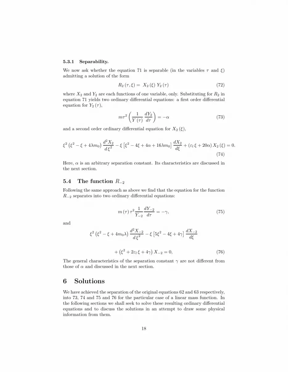
5.3.1 Separability.

We now ask whether the equation 71 is separable (in the variables τ and ξ)admitting a solution of the form

R2 (τ , ξ) = X2 (ξ) Y2 (τ ) (72)

where X2 and Y2 are each functions of one variable, only. Substituting for R2 inequation 71 yields two ordinary differential equations: a first order differentialequation for Y2 (τ ),

mτ2

(

1

Y (τ )

dY2

dτ

)

= −α (73)

and a second order ordinary differential equation for X2 (ξ),

ξ2(

ξ2 − ξ + 4λm0

) d2X2

d ξ2− ξ

[

ξ2 − 4ξ + 4α+ 16λm0

] dX2

dξ+ (εl ξ + 20α)X2 (ξ) = 0.

(74)

Here, α is an arbitrary separation constant. Its characteristics are discussed inthe next section.

5.4 The function R−2

Following the same approach as above we find that the equation for the functionR−2 separates into two ordinary differential equations:

m (τ ) τ2 1

Y−2

dY−2

dτ= −γ, (75)

and

ξ2(

ξ2 − ξ + 4m0λ) d2X−2

d ξ2− ξ

[

5ξ2 − 4ξ + 4γ] dX−2

dξ

+(

ξ2 + 2εl ξ + 4γ)

X−2 = 0, (76)

The general characteristics of the separation constant γ are not different fromthose of α and discussed in the next section.

6 Solutions

We have achieved the separation of the original equations 62 and 63 respectively,into 73, 74 and 75 and 76 for the particular case of a linear mass function. Inthe following sections we shall seek to solve these resulting ordinary differentialequations and to discuss the solutions in an attempt to draw some physicalinformation from them.

18

6.1 The functions Yp (τ)

The first order differential equations for Y2 (τ ) and Y−2 (τ ) above can be inte-grated immediately. Thus from equation 73 we find that

Y2 (v) = exp

(

−α∫ u

0

dv

m0 (1 − λv)

)

= eα

λm0ln(1−λv)

. (77)

Now 0 ≤ λ < 1 and in fact for most radiating bodies λ ≪ 1. This allows us toexpand the logarithmic expression ln (1 − λu) in the solution so that

Y2 (v) = e−Ωve−Ω

∞∑

n=1

1n+1λnvn+1

, (78)

where the separation constant now takes the form Ω in which we absorb theSchwarzschild mass m0

α = m0Ω. (79)

Consider, now, the case in which the background is not radiating. It is cleareither from the solution above or from the original differential equation that forsuch a case the solution reduces to

Y2 (vs) = e−Ωsvs , (80)

where the subscript s indicates quantities associated with the Schwarzschildgeometry. One notices that in such a static background the quantity Y2 (vs)above constitutes the only time dependent part of the Ψ0 field. It follows thenthat to be consistent with the known [3] solutions we should require

Ωs = iω, (81)

where ω is the frequency of the gravitational waves. This suggests that in thecase of the radiating background we should expect the parameter Ω to be acomplex function of λ and ω such that

limλ→0

Ω (λ, ω) = iω. (82)

The integration of the differential equation for Y−2 (v) follows the same trendand we find that

Y−2 (v) = e−Γve−Γ

∞∑

n=1

1n+1λnvn+1

, (83)

where

19

γ = m0Γ, (84)

Γ being a complex function of λ and ω such that

limλ→0

Γ = iω (85)

As would be expected from the theory of deferential equations the separationconstants Ω and Γ can not have unique values. The individual solutions weobtain will therefore be representatives of classes of solutions. The range of thesesolutions is described in terms of the frequency spectrum of the gravitationalfield which, in our classical treatment, takes on continuous values. It will, later,be shown that by using certain conditions on the solutions the functional formof these separation constants can be more rigidly fixed.

6.2 The functions Xp (ξ)

Following the integrations of the first order differential equations for Yp we arenow left with the two equations for X2 and X−2 to solve. These are respectively,

ξ2(

ξ2 − ξ + 4λm0

) d2X2

d ξ2− ξ

[

ξ2 − 4ξ − 4m0 (4λ− Ω)] dX2

dξ+ (εl ξ − 20m0Ω)X2 (ξ) = 0

(86)

and

ξ2(

ξ2 − ξ + 4m0λ) d2X−2

d ξ2− ξ

[

5ξ2 − 4ξ + 4m0Γ] dX−2

dξ

+(

ξ2 + 2εl ξ + 4m0Γ)

X−2 = 0. (87)

It is clear that at ξ = 0 (or r = ∞) both the equations above have regular sin-gularities [16]. This encourages us to seek for analytic solutions. Such solutionsat ξ = 0 (r = ∞) should be useful in discussing the asymptotic fall-offs of thefields and the question of energy flux.

6.2.1 The peeling behavior

Our initial goal is to develop asymptotic solutions for the functions X2 (ξ) andX−2 (ξ). Consider a zero rest mass spin-s field ψp in a helicity state p. According

to the peeling theorem by Roger Penrose [6], the quantities r(s+p+1)ψp and

r(s−p+1)ψp have a limit at null-infinity. In the case of gravitational fields weexpect the outgoing components of the solutions to fall off as

ψ(p=±2) ∼1

r(s+p+1)=

1

r(2±2+1), (88)

20

while the ingoing solutions should fall off as

ψ(p=±2) ∼1

r(s−p+1)=

1

r(2∓2+1). (89)

It is necessary, therefore, that the solutions to our differential equations displaythe above asymptotic behavior. This, indeed, will be one of the tests for theirvalidity.

6.2.2 The Indicial Equations.

It has been pointed out that at ξ = 0 we have a regular singularity in bothequations 86 and 87 . Therefore it seems natural to attempt developing solutionsabout this point. Such solutions will be valid at far distances from the blackhole. This class of solutions at such distances is useful if one is to engage, as weshall later, in a meaningful discussion of the gravitational energy flux.

Let us assume that equation 86 admits, as a solution, a series expansionabout ξ = 0 of the form

X2 (ξ) =

∞∑

n=0

anξn+k, (90)

where k is some value to be determined. Using equation 90 in equation 86 gives

∞∑

n=0

an (n+ k) (n+ k − 2) ξn+k+2

−∞∑

n=0

an [(n+ k) (n+ k − 5) − εl] ξn+k+1

∞

+∑

n=0

4an (n+ k) [(n+ k − 5)λm0 −m0Ω] + 5m0Ω ξn+k = 0 (91)

For n = 0, a0 6= 0 we get the indicial equation

k [(k − 5)λ− Ω] + 5Ω = 0. (92)

which has two distinct roots,

k =

(

5,Ω

λ

)

. (93)

21

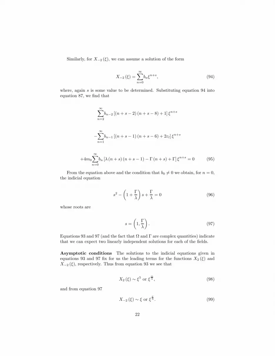
Similarly, for X−2 (ξ), we can assume a solution of the form

X−2 (ξ) =

∞∑

n=0

bnξn+s, (94)

where, again s is some value to be determined. Substituting equation 94 intoequation 87, we find that

∞∑

n=2

bn−2 [(n+ s− 2) (n+ s− 8) + 1] ξn+s

−∞∑

n=1

bn−1 [(n+ s− 1) (n+ s− 6) + 2εl] ξn+s

+4m0

∞∑

n=0

bn [λ (n+ s) (n+ s− 1) − Γ (n+ s) + Γ] ξn+s = 0 (95)

From the equation above and the condition that b0 6= 0 we obtain, for n = 0,the indicial equation

s2 −(

1 +Γ

λ

)

s+Γ

λ= 0 (96)

whose roots are

s =

(

1,Γ

λ

)

. (97)

Equations 93 and 97 (and the fact that Ω and Γ are complex quantities) indicatethat we can expect two linearly independent solutions for each of the fields.

Asymptotic conditions The solutions to the indicial equations given inequations 93 and 97 fix for us the leading terms for the functions X2 (ξ) andX−2 (ξ), respectively. Thus from equation 93 we see that

X2 (ξ) ∼ ξ5 or ξΩλ , (98)

and from equation 97

X−2 (ξ) ∼ ξ or ξΓλ . (99)

22

Both equations 98 and 99 show that the first solutions are consistent with thepeeling theorem and can, in fact be recognized as outgoing fields (recall ξ =2m(v)

r= 2m0(1−λv)

r).

On the other hand the second solutions are scaled by the quantities Ω andΓ, respectively. These are the same arbitrary separation constants which, inthe last section, we showed to be complex. Since, physically, our solutionsrepresent gravitational fields these constants must now be chosen to conformwith the known boundary values for such ingoing waves. Consequently, in orderto satisfy the peeling theorem, it is clear that we must have ReΩ ∼ λ, so thatX2 ∼ 1

rand ReΓ ∼ 5λ, so that X−2 ∼ 1

r5 . Moreover, the imaginary parts ofthese quantities must reduce to the limiting cases, lim

λ→0Ω = iω and lim

λ→0Γ = iω

as was shown to be the case. These two conditions dictate that we set

Ω = λ+ iω, (100)

and

Γ = 5λ+ iω, (101)

The roots to the indicial equations 93 and 97, respectively, now become

k =

[

5,

(

1 +i

λω

)]

, (102)

and

s =

[

1,

(

5 +i

λω

)]

. (103)

So that as ξ → 0,

X2 (ξ) → ξ5 or X2 (ξ) → ξξi

λω, (104)

and

X−2 (ξ) → ξ or X−2 (ξ) → ξ5ξi

λω. (105)

The full functions X2 (ξ) are readily obtained by writing down recurrence rela-tions using equations 91 and 95. The general solutions are, in each case, found

to be linear combinations of the outgoing component X(out)p and the ingoing

component X(in)p .

Thus

Xp (ξ) = ApX(out)p +BpX

(in)p . (106)

Here the Ap and Bp are arbitrary constants of integration. These solutions arealso found to converge.

23

7 The asymptotic solutions and physical infor-

mation.

7.1 Significance

The principal aim of our study is to understand how gravitational waves arescattered by a background radiating spacetime. In particular, we are interestedin the measurable physical results of this process, such as the energy flux and themanner in which the waves are reflected and absorbed by a radiating black hole.To this end we have, in the preceding discussions, developed field equations thatdescribe the effects of these waves on the background spacetime. The physicalquantities that we seek should, in principle, be calculated from the solutions ofthese equations. As can easily be shown, however, the series solutions obtainableare a result, in each case, of a three term recursion relation and so containvarious coefficients that are not easy to relate. This feature of our solutionswould seem to make inconvenient, their use in calculating a number of otherphysical quantities. It turns out, though, that for the features of our interest itis sufficient to consider the form of the solutions at certain special points. Forexample Chandrasekhar [7] shows that a knowledge of the incident and reflectedwave amplitudes can be deduced from the form of the solution at null-infinity.Moreover, one can also engage in a meaningful discussion pertaining to energyflux at these points. This means that we need only consider the leading termsin the solutions.

7.2 The Source Terms

In creating the function Ψ4 we have, so far, only considered solutions for thehomogeneous part of the original differential equation (see equations 56 and57). However, the full equation for Ψ4 is inhomogeneous so that the completesolution should contain a contribution due to the sources. We recall that thesource term is scaled by the luminosity L = − dm

dv= λm0 which obviously

vanishes as the background radiation is switched off, λ −→ 0. Since, in the first

place, λ ≪ 1 =⇒ m(v)3m(v) ≪ 1, we shall presently assume that at large r values

the source terms do not contribute significantly to the solution. Consequentlywe shall consider the asymptotic solutions from the homogeneous equation tobe a sufficient representation of the general asymptotic solutions. With this wenow write down the asymptotic form of the entire solutions.

7.3 The Solutions

It was shown, in equation 78, that for Ψ0,

Y2 (u) = e−Ωλ

ln(1−λv) = e−Ωue

∞

−∑

n=1

1n+1λnvn+1

. (107)

24

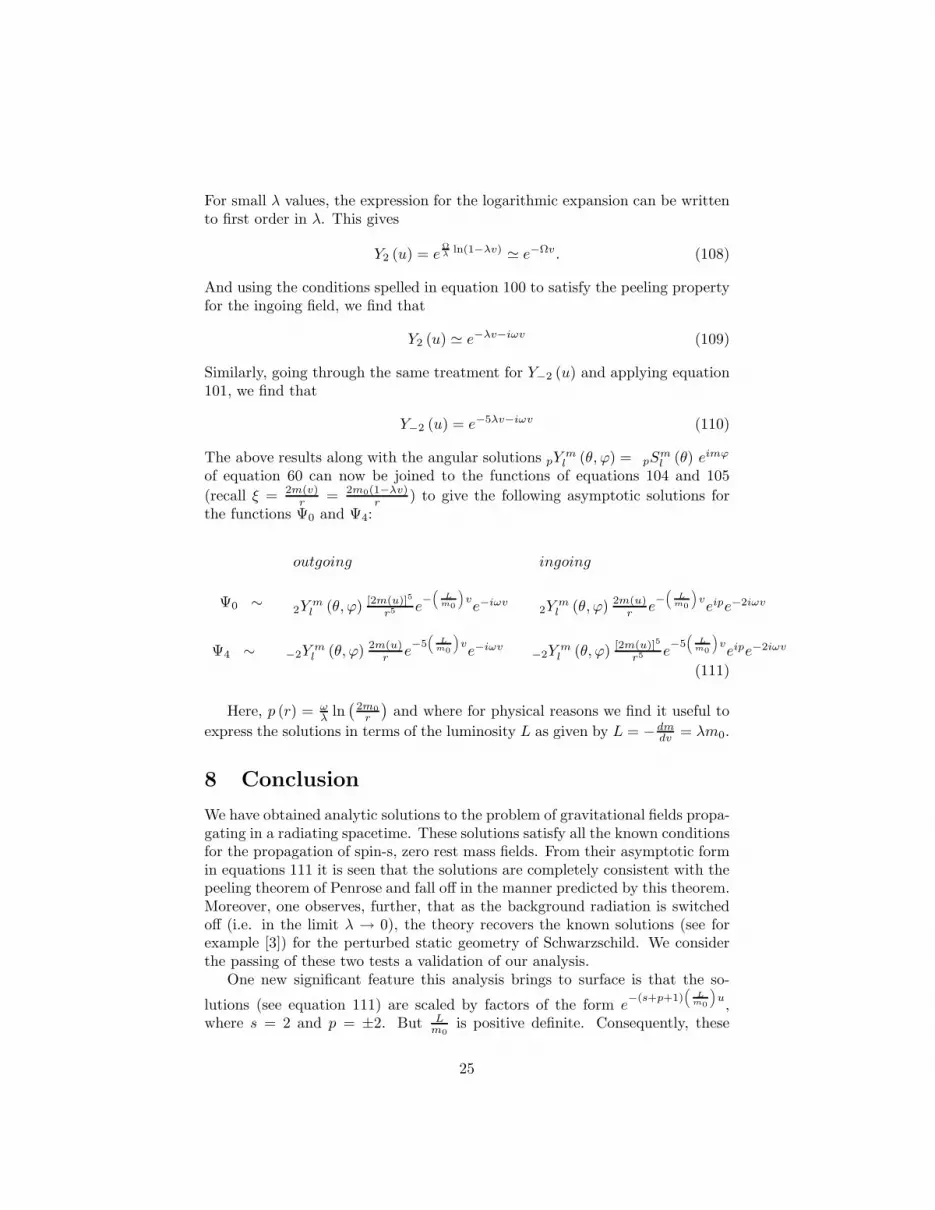
For small λ values, the expression for the logarithmic expansion can be writtento first order in λ. This gives

Y2 (u) = eΩλ

ln(1−λv) ≃ e−Ωv. (108)

And using the conditions spelled in equation 100 to satisfy the peeling propertyfor the ingoing field, we find that

Y2 (u) ≃ e−λv−iωv (109)

Similarly, going through the same treatment for Y−2 (u) and applying equation101, we find that

Y−2 (u) = e−5λv−iωv (110)

The above results along with the angular solutions pYml (θ, ϕ) = pS

ml (θ) eimϕ

of equation 60 can now be joined to the functions of equations 104 and 105

(recall ξ = 2m(v)r

= 2m0(1−λv)r

) to give the following asymptotic solutions forthe functions Ψ0 and Ψ4:

outgoing ingoing

Ψ0 ∼2Y

ml (θ, ϕ) [2m(u)]5

r5 e−(

L

m0

)

ve−iωv

2Yml (θ, ϕ) 2m(u)

re−(

L

m0

)

veipe−2iωv

Ψ4 ∼ −2Yml (θ, ϕ) 2m(u)

re−5(

L

m0

)

ve−iωv

−2Yml (θ, ϕ) [2m(u)]5

r5 e−5(

L

m0

)

veipe−2iωv

(111)

Here, p (r) = ωλ

ln(

2m0

r

)

and where for physical reasons we find it useful to

express the solutions in terms of the luminosity L as given by L = − dmdv

= λm0.

8 Conclusion

We have obtained analytic solutions to the problem of gravitational fields propa-gating in a radiating spacetime. These solutions satisfy all the known conditionsfor the propagation of spin-s, zero rest mass fields. From their asymptotic formin equations 111 it is seen that the solutions are completely consistent with thepeeling theorem of Penrose and fall off in the manner predicted by this theorem.Moreover, one observes, further, that as the background radiation is switchedoff (i.e. in the limit λ → 0), the theory recovers the known solutions (see forexample [3]) for the perturbed static geometry of Schwarzschild. We considerthe passing of these two tests a validation of our analysis.

One new significant feature this analysis brings to surface is that the so-

lutions (see equation 111) are scaled by factors of the form e−(s+p+1)

(

L

m0

)

u,

where s = 2 and p = ±2. But Lm0

is positive definite. Consequently, these

25

factors indicate that when gravitational fields propagate in a radiating space-time they suffer an attenuation, and this attenuation can be quantitativelydescribed. The attenuation weight seems in turn to be directly related to thespin weight of the perturbed fields. It is also scaled by the luminosity L of thebackground. Further, as one notices from the solutions, the attenuation per-sists independent of whether the fields are ingoing or outgoing. It is of coursefair to ask whether this character of our solutions is not, in the first place, areflection of the mass function that we chose. Recalling that general radiativemass function m (v) is a monotonic decreasing function in v an expansion of them (v) = m0−Lm0− dL

2!dvm0− .... about v = 0 indicates that the first order term

in the luminosity would seem to make the significant contribution. This seemsto suggest that the attenuations manifested in our solutions are independent ofthe manner in which the blackhole radiates and may persist for any mass func-tion chosen. As far as we know this seems to be a new feature in the literatureof this branch of general relativity; one that may, indeed, have some interestingastrophysical implications.

A persistent attenuation of this sort would seem to suggest the possibilitythat energy is being dumped into the host spacetime. Over large time scales,this could have significant implications on the evolution of such a radiatingsystem. This question can, however, only be resolved by a rigorous calculationof the energy flux. For such a calculation and an extension of this discussionsee [18] We intend to follow up this issue in future discussions.

References

[1] A. Einstein, L. Infeld and B. Hoffmann, Ann. Phys., 39, 65 (1938).

[2] T. Regge and J. Wheeler, Phys. Rev. 10, 1063 (1957).

[3] S. Teukolsky, Astrophy. J. 185, 635, (1973).

[4] C. W. Allen, Astrophysical Quantities, (Pergamon, London, 1959).

[5] N. Roos et al, Astrophys. J. 409, 130 (1993).

[6] E. Newman and R. Penrose, J. Math. Phys. 3, 566 (1962).

[7] S. Chandrasekhar, The Mathematical Theory of Black Holes, (Oxford Press,1983).

[8] M. Carmeli and M. Kaye, Ann. Phys. 103, 97 (1977).

[9] P. C. Vaidya, Proc. Indian Acad. Sci. A 33, 264 (1951).

[10] P. C. Vaidya, Nature, 171, 260 (1952).

[11] R. Geroch, A. Held and R. Penrose, J. Math. Phys. 14, 874 (1973).

[12] W. A. Hiscock, Phys. Rev. D 23 2813 (1981).

26

[13] J. Goldberg et al, J. Math. Phys. 8 2155 (1967).

[14] Y. Kaminaga, Class. Quantum Grav. 7, 1135(1990)

[15] T. Christodoulakis, et al, J. Math. Phys. 35, 5 (1994)

[16] W. Kaplan, Ordinary Differential Equations, (Addison-Wesley, Reading,Massachusetts, 1958)

[17] C. Misner, K. Thorne and J. Wheeler, Gravitation, (W.H. Freeman andCo, San Francisco, 1973).

[18] M. R. Mbonye, Ph. D. dissertation, 1996 (Unpublished).

27