P H YS i CAL R EV I EW VOLUM E 160, NUM B ER~S 25 AUGUST 196 7

Quantum Theory of Parametric Amplification. IPB. R. MQLLow AND R. J. GLAUBER

Lymars Laboratory of Physics, Harvard Ursiversity, Cambridge, 3fassachmsetts

(Received 18 January 1967)

The analysis of the quantum-mechanical parametric amplifier begun in the preceding paper is extended todescribe the joint quantum state of the two interacting modes of oscillation of the system. Equations arederived for the time evolution of the Schrodinger density operator. Comparison with classical theory ismade by describing the state of the quantum-mechanical system by means of the I' representation. Thetime evolution of the weight function P(n,P,t) for this representation, and of the corresponding Wignerdistribution function W (o,p, f), is found. A decoupled form for the equations of motion for the Geld variablesis exhibited which simplifies the solutions for these functions. It is shown that the amplification processgives rise to a correlation between the two mode amplitudes which becomes exceedingly strong with in-creasing time. The relation of this correlation to the time development of the functions P (n,p, f) and W(n, p, f)ls discussed.

I. DTTRODUCTIOH' 'N the preceding paper' we have begun an analysis of& - the statistical behavior of the quantum-mechanicalparametric amplifier. The model of the amplifier wehave discussed is one in which two modes of oscillation,represented by harmonic oscillators, are coupled bymeans of a time-dependent parameter. ' The analysispresented in I took the coupling between the modesfully into account, but was concerned with describingthe output of only one of the two modes of the system.A complete description of the parametric amplifier,however, must specify the state of both of the interact-ing modes, since the coupling mechanism leads to corre-lations between them which are readily detected, experi-mentally. If the two modes of oscillation correspond, ,for example, to optical-frequency electromagneticfields, then the correlations of the mode amplitudes canbe measured by observing coincidences of photonsrecorded by two counters, one sensitive to the field ofeach mode. To be able to predict the results of this typeof experiment and others which respond to the state ofboth modes, we must develop the full statisticaldescription of the two-mode system.

We shall base our discussion of the statistical behaviorof the amplifier system on the time-dependent densityoperator p(t) for the field amplitudes of its two modes.As in the case of single-mode systems, one of the moreuseful ways of expressing the density operator is bymeans of the I' representation. ' When this representa-tion exists it tends to permit particularly direct compar-isons with classical theory, and to allow the computationof certain expectation values by methods similar tothose of classical probability theory. The weightfunction E(cr,P, f) which appears in the P representation.of p(t) is in this sense a quantum analog of the classical

*Supported in part by the U. S. Air I'orce OfI5ce of ScientificResearch.' B. R. Mollow and R. J. Glauber, preceding paper, Phys. Rev.160, 1076 (1967). We shall refer to this paper hereafter as I;equation numbers cited from it will be prefixed by I.

'%. H. Louisell, A. Yariv, and A. E. Siegman, Phys. Rev. 124,1646 (1961).' R. J. Glauber, Phys. Rev. 131, 2766 (1963).

160

joint-probability distribution for Gnding the 3 and 8modes of the system with complex amplitudes n and p,respectively. By finding the time evolution of thisfunction we are able to express the solution for thedensity operator in a form which exhibits quite directlythe correlation between the mode amplitudes.

We shall also discuss the dynamics of the amplifiersystem in terms of the Wigner function, 4 ' a species ofquantum-mechanical phase-space distribution which isdefinable for arbitrary density operators. The Wignerfunction W(cc,P, f) for the parametric amp1ifier evolvesin time a particularly simple way: It obeys Liouville'sequation, and is therefore constant along a classicaltrajectory.

The time evolution of the function P(n, p, t), on theother hand, exhibits more explicitly quantum-mechan-ical features. We are able to show, for example, that anon-negative function E(cr,P, f) can exist for the systemonly during a finite time interval. For times outsidethat interval the function must either take on negativevalues or fail to be definable. The simple initial statesof the amplifier which we treat indeed, lead to functionsP(n, P,f) which become strongly singular at the end ofthe interval and then fail to be definable at later times.A general integral representation which we find forI'(cr, p, t) shows that for nearly all initial states of thesystem the function sooner or later becomes undefinable.Such behavior means simply that the description of thesystem as being in a "diagonal" mixture of coherentstates has become inappropriate.

The physical reason for the breakdown of the I'representation lies in the extremely close correlation inthe amplitudes of the two modes of the system which isbrought about by the amplification process. In a purecoherent state of the amplifier system the field ampli-tudes of the two modes Quctuate independently of oneanother, with variances which are the same as those ofvacuum fluctuations. It is easily seen, however, fromthe equations of motion for the system, that as theamplification continues the fields in the two modes

e E. Wigner, Phys. Rev. 40, 749 (1932).~ J. K. Moyal, Proc. Cambridge Phil. Soc. 45, 99 (1948).

1097

B. R. MOLLOW AND R. J. GLAUBER

II. THE TWO-MODE CHARACTERISTICFUNCTION

The modep of the parametric amplifier on which ouranalysis is based consists of two quantum-mechanicalharmonic oscillator Inodes, the A and 8 modes, des-cribed by annihilation operators u(t) and b(t), respec-tively. The Hamiltonian for the system is assumed tohave the- form

H (t) =h~.ut(t)u(t)+b»bt(t)b(t)—A~La' (t)bt (t)e

—'"+u(t) b(t)e'"j (2.1)

where or, and cob are the natural frequencies of oscillationof the uncoupled A and 8 modes, and the frequency co

of the time-varying coupling is assumed. to satisfy theresonance condition

9)=Mg+K g ~ (2.2)

The solutions to the Heisenberg equations of motionwhich follow from the Hamiltonian (2.1) may bewritten as in Eqs. (I, 3.14) in the form

become so tightly correlated that they may no longerfluctuate independently to even the small degree allowedby pure coherent states. It is at that point in the timedevelopment of the system that it becomes impossibleto have a non-negative function E(a,P,t), and thesingularities occur for the examples we discuss. Thedensity operator itself, on the other hand, is at notime singular. It may always be constructed explicitlyin terms of creation and annihilation operators, orcharacterized by means of its maxtrix elements or theWigner function which remain well-behaved at alltimes.

An arbitrary density operator may be expressed in aparticularly simple form in terms of its characteristicfunction. In Sec. II we find this function at an arbitrarytime t in terms of its form at t=0, and thereby obtaina formal solution for the density operator. The solutionfor the characteristic function is then used in Sec. IIIto find the signer function in terms of the form ittakes -initially.

In Sec. IV we derive a decoupled form for theequations of Inotion of the system which exhibits the-time-dependent correlation -. of the mode amplitudes.The characteristic functions and the functions W(n, P, t)and E(n,P, t) are then expressed in terms of suitablydefined decoupled variables in Secs. V and VI. Anintegral solution is obtained for P(n, P, t) and is shownto diverge after some finite time for a broad class ofinitial states. An example which illustrates this behavioris discussed in Sec. VII, and in Sec. VIII we present ageneral analysis of the relationship between the break-down of the two-mode I' representation and the corre-lation between the mode amplitudes.

where u—=u(0), b=b(0), and the c-number functionsc.(t), s.(t), cg(t), and sg(t) are defined by

c (t)—= e ' o' coshld,

s~(t)=M ' ~ slllhKt,

c~(t)=e' "—coshzt,

sq(t)=ie '""sinh~t.

(2.4)

Our problem is to solve for the density operator whichdescribes the two-mode system at an arbitrary time t,when we are given the density operator at 1=0. Thedensity operator may be specified at any time by meansof its characteristic function. This function is definedfor arbitrary complex p and i by

X(n,u)=«{p(t)e"""""* "*'} (23)in which p(t) is the time-dependent Schrodinger densityoperator for the system, and u and 6 are the Schrodingerannihilation operators for the 3 and 8 modes, respec-tively. We may express X(p,f, t) equally well in termsof the Heisenberg density operator p and the Heisenbergannihilation operators u(t) and, b(t) by means of thecanonical transformation of Eqs. (I, 4.3) and (I, 4.4).The trace when written in this form is

X(g,i., t) = tr(pe«t«&+r~f~o "~N('& F~«) }. (2.6)

Since the characteristic function X determines thedensity operator uniquely, ' ' we can exhibit a solutionto our initial value problem by expressing the functionX at time t in terms of its intial value X(g,i,0). Toconstruct the solution in this way we begin by substitut-ing Eqs. (2.3) for u(t) and b(t) into Eq. (2.6)

X(q,i,t) = tr(p expLg(utc, *(t)+bs *(t))+t'(btct ~(t)+usq*(t)) —H.c.f}, (2.7)

where H.c.means Hermitian conjugate. If we now definec-number functions go(g, t,t) and f'o(g, f, t) by theequations

«(~,l, t)=nc.*(t) —i *»(t), —&o(n,P)=Pc~*(t)—n*s.(t),

(2 8)

then we find by collecting coefFicients of at, b~, a, and bin Eq. (2.7) that the function X(p,i,t) obeys the func-tional identity

X(YJ,t,t) = tr(p expt utero(g, i,t)+ bt| o(g,i', t) —H.c.)}=X(Z, (~,f,t), t, (&,f,t), 0). (2.9)

The characteristic function X(q,f,t) is thus specified interms of the form it takes at 1=0, and the c-numberfunctions defined by the Eqs. (2.8).

A formal solution for the Schrodinger densityoperator p(t) may now be constructed from our knowl-edge of the characteristic function. To accomplish this,

u(t) =uc, (t)+bts, (t),

b(t) =bcp(t)+utsy(t),

(2.3a)

(2.3b)

6H. Weyl, The Theory of Groups and Quantum Mechanicst',Dover Publications, Inc. , New York, 1950), pp. 272—276.

7A. E. Glassgold and D. Holliday, Phys. Rev. 139, A1717(1965), Sec. III.

160 QUANTUM THEORY OF PARAMETRIC AMPLIFICATION. I I 1099

let us first note that an arbitrary density operator pfor a single-mode system may be expressed in terms ofits characteristic function

X(rI) = tr(pe& t-p"} (2.10)

by means of the expansion'~

(2.11)

where d'q—=d(Reg)d(Imp). This relation is an operatoranalog of the two-dimensional Fourier transform; itmay be verified by multiplying the right side byexp(gut —g*a) and evaluating the trace of the resultingexpression.

The generalization of the expansion (2.11) approp-riate to the two-mode density operator p(t) is

p(&) =— X(~,f,~)e-.t-r't+ "+r"bd'~d f (2.12)

If we substitute Eq. (2.9) for X(g,t', t) into this relation,we obtain

1p(I)= X(no(98—'~) fo(n f', I) 0)

%2

Xe pat rbt+—p e+—r*bd

prado(

(2 13)

III. THE WIGNER FUNCTION'

The Wigner function was originally introduced as aquantum analog of the classical phase-space distributionfunction. ' It is useful for evaluating the mean valuesof certain quantum-mechanical operators as integralsof c-number functions carried out over the phase spacedefined by the eigenvalues of the coordinates andmomenta of the system under consideration. Althoughthe Wigner function approaches a classical distributionfunction in the classical limit, it cannot be unambig-uously interpreted as a probability density in quantum-mechanical contexts. The Wigner function is like theweight function of the P representation in that it maytake on negative values for suitably restricted values ofits arguments. It is unlike the P function, however, inthat it exists in a well-defined sense for arbitrary densityoperators, and is never singular.

In this section we shall solve for the Wigner functionfor the parametric amplifier in terms of its initial form.We shall show that for arbitrary initial quantum statesof the system, the Wigner function satisfies Liouville'sequation.

To define the Wigner function, we first note that for aclassical oscillator of frequency co;, the coordinate q,and momentum p, are related to the complex amplitudeo.; by means of the expressions

The integration in this equation may be carried outmost conveniently by changing the variables of integra-tion from g and f to gp qp(g, f,t) an——d fp fp(q, t', t——), andmaking use of the readily proved identity

th -q'~'

p'= &i i (n *—n;)

(3 1)

dodd f'=dogodofo (2.14)

The Eqs. (2.8) are easily inverted; by taking intoaccount the definitions (2.4) of the coeKcients c,(t),s (&), cb(&), and sb(I), we 6nd that the solutions for pand f take the form

n(noZo, I)=ape (~)+io*s (I)

f (gp t 0 I) focb(I)+'Vp sb(I)(2.15)

When this change of variables is carried out on Eq.(2.13), we 6nd that the density operator takes the form

1p(&) =— X(g,f'o, 0) expi —p(rIp, f'p, t)at

These relations Inay be used to write the Wignerfunction in terms of the complex arguments 0., ratherthan the real arguments q; and p, . Let us now considera single-mode system, i.e., a single harmonic oscillator,described by the density operator p. The Wignerfunction in this case may be defined'' as the two-dimensional Fourier transform of the characteristicfunction X(g)

(3 2)

We may gain some insight into the meaning of theWigner function by supposing that the density operatorp has a P representation

f (q p, f o,t)bt H.c—.fd'g pd'f p. —(2.16) p= P(n) in)(nid'n, (3.3)

The time-dependent density operator is thus expressedin terms of the initial form of the characteristic functionand the time-independent Schrodinger operators at, bt,

a, and b; the time dependence of p(t) is containedcompletely within the functions g(pp, f p, t),and f(pp, f p, t),which depend only linearly on the variables gp and fp

and then expressing W(n) in terms of P(n) By combin-.

Reference 5, Sec. 3.' R. J. Glauber, in Qguetum OPtics and electronics, edited by C.de Witt et al. (Gordon and Breach Science Publishers, Inc. , NewPork, 1965), lecture No. 13.

1100 B. R. MOLLOW AND R. J. GLAUBER

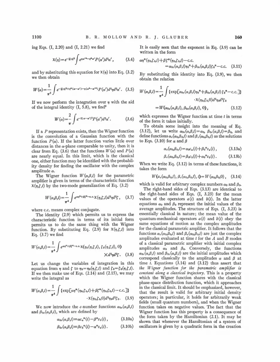
ing Eqs. (I, 2.20) and (I, 2.21) we find

x()))= e—&~&~' eo" "* 'P—(n')d'n' (3 4)

and by substituting this equation for X(g) into Eq. (3.2)we then ob tain

It is easily seen that the exponent in Eq. (3.9) can bewritten in the form

~*(~o,f „t)+Pt *(~.,f „t)—"=n,.(n,P,t)~,'+P,.(n,P, t)g,*—c.c. (3.11)

By substituting this identity into Eq. (3.9), we thenobtain the relation

1W(n) =-

7r2

klol2+o+(~a') o(a+—~'4)P(nl)do~donl (3 5)

If we now perform the integration over g with the aidof the integral identity (I, 5.8), we find'

2W(n) =— e o~ '~'P(n')don' (3.6)

where c.c. means complex conjugate.The identity (2.9) which permits us to express the

characteristic function in terms of its initial formpermits us to do the same thing with the Wignerfunction. By substituting Eq. (2.9) for X(i),f,t) into

Eq. (3.7) we find

1W(n, p, t) =— e *+@* "&(rt,(g,t,t), fo-(rt, f,t), 0)

X4

)&d'i)d'f'. (3.8)

Let us change the variables of integration in thisequation from i) and f' to rto rto(rt, f,t) and f——o=go(7/ t,t).If we then make use of Eqs. (2.14) and (2.15), we maywrite the integral as

W(,p, t) =— (e pL ))*()) Zo, t)+N*(rt, f'o, t) —c c-3}m4

&())o l o,o)d'))od'Po. (3.9)

We now introduce the c-number functions no (n,P t)and Po, (n,P,t), which are defined by

no. (n,p, t) —=nc,*(t)—p*s,(t), (3.10a)

Po (n,P,t) =—Pc *(t)—n*s, (t) . (3.10b)

If a P representation exists, then the Wigner functionis the convolution of a Gaussian function with thefunction P(n). If the latter function varies little overdistances in the n-plane comparable to unity, then it isclear from Eq. (3.6) that the functions W(n) and P(n)are nearly equal. In this limit, which is the classicalone, either function may be identified with the probabil-

ity density for 6nding the oscillator with the complexamplitude n.

The Wigner function W(n, P,t) for the parametric

amplifier is given in terms of the characteristic function

X(i)g, t) by the two-mode generalization of Eq. (3.2)

1W( p )=— '"' '-'

( f, ) ' 'C, (.7)

1(exp Lno. (n,p, t)~o*+po.(np, t) f o*-c.c.)}

m4~ X(~,g „O)do&pe,

= W(no, (n,p, t), po, (n,p, t), 0), (3.12)

n (no Po, t)=noc (t)+Po*s (t), (3.13a)

P.(noPo, t)=Poco(t)+no*so(t). (3.13b)

When we write Eq. (3.12) in terms of these functions, ittakes the form

W(,.(no p„t), p. (no,p, t), t)= W(,p„0), (3.14)

which is valid for arbitrary complex numbers no and p, .The right-hand sides of Eqs. (3.13) are identical to

the right-hand sides of Eqs. (I, 3.23) for the meanvalues of the operators a(t) and b(t). In the latterequations no and po represent the initial values of theaverage amplitudes. The structure of Eqs. (I, 3.23) isessentially classical in nature; the mean value of thequantum-mechanical operators a(t) and b(t) obey thesame equations of motion as the complex amplitudesfor the classical parametric amplifier. It follows that thefunctions n. (no,po, t) and p, (no,po, t) are just the complexamplitudes evaluated at time t for the 2 and 8 modesof a classical parametric amplifier with initial complexamplitudes no and Po. Conversely, the functionsn„(n,P,t) and Po, (n, P, t) are the initial amplitudes whichcorrespond classically to the amplitudes n and P attime t. Equations (3.14) and (3.12) thus assert thatthe Wiggler fuection for the parametric amplifie isconstant along a classical trajectory. This is a propertywhich the Wigner function shares with the classicalphase-space distribution function, which it approachesin the classical limit. It should be emphasized, however,that the result is valid for arbitrary initial densityoperators; in particular, it holds for arbitrarily weakfields (small quantum numbers), and when the Wignerfunction takes on negative values. The fact that theWigner function has this property is a consequence ofthe form taken by the Hamiltonian (2.1). It may beshown that whenever the Hamiltonian of a system ofoscillators is given by a quadratic form in the creation

which expresses the Wigner function at time t in termsof the form it takes initially.

To obtain some insight into the meaning of Eq.(3.12), let us write no, (n,P,t) =no, Po, (n,P,t)=Po, anddefine functions n. (no, po, t) and p. (no, po, t) as the solutionsto Eqs. (3.10) for n and P

160 QUANTUM THEORY OF PARAMETRIC AMPLIFICATION. II iioi

and annihilation operators, the Wigner function isconstant along classical trajectories. '0 "This propertydoes not extend to systems with arbitrary Hamiltonians,as it does in the case of the classical phase-spacedistribution.

To express Eq. (3.12) or (3.14) in differential form,we first introduce the total time derivative d/dt, which

is de6ned as the ordinary time derivative taken alonga classical trajectory. For a system of particles withcoordinates q; and momenta p;, d/dt is given by

d 8 (BH8 BH 8)—=—+2(dt Bt i (Bp; Bq; Bq; Bp;)

(3.15)

where H is the Hamiltonian for the system. If we useEqs. (3.1) to define derivatives with respect to thecomplex quantities 0.; and n;* by means of the relations

8—z(-,'ho& )'('8pi

(b 1/28+i (-'Ito&;)"'

8(i~ (2G0 Bq ' BP '

(3.16)

d 8 i (BH 8 BH 8 )dt Bt tz 1 (B(rj 8(r' 8(r' 8(r'~

(3.17)

For the parametric amplifier, the index j takes on

the values u and b, corresponding to the complexamplitudes (r =n, (rb P The ——Ham. iltonian for theclassical parametric amplifier is obtained by replacingthe operators a(t) and b(t) in Eq. (2.1) by (r and P,respectively. If we substitute the resulting expressionfor the classical Hamiltonian into Eq. (3.17), we find

then by solving these equations for 8/Bq; and 8/BP; and

substituting the results into Eq. (3.15) we find

c(+) (t) —c(+)eKi

c(—) (t) —c(—)e—a&

(4.2a)

(4.2b)

in which the operators c~+) are the initial values ofc(+&(t), and are given in terms of the Schrodingeroperators a and b by

c(+&=2—'"(aazbt) . (4.3)

It is clear from Eqs. (4.2) that the operators c(+&(t)and c( ) (t) are decoupled from one another. The trans-forrnation (4.1) evidently defines a species of normalcoordinates for the system, but one with exponentialrather than oscillatory time dependence. The operatorsc(+&(t) and c( )(t) are not canonical; they satisfy thecommutation relations

[' '(') '+"(')]=5 ' '(t) ' "(t)]=["+'(t),c' '(t)]=o, (4.4)

[c + (t), c — (t)]= [c' ' (t), c (+& (t)]= 1 .The operators c(+'(t) are defined by Eqs. (4.1) as

linear combinations of the operators

a'(t) —=e'"'a(t),

b'(t) —=e'"z'b (t),

(4.5a)

(4.5b)

simplified by carrying out a transformation of variableswhich decouples the basic equations of motion for thesystem. We introduce two operators c(+&(t) and c( &(t),which we define in terms of the Heisenberg operatorsa(t) and b(t) by the relations

c(+&(t)—= 2 '"[a(t)e'"-'+ibt(t)e '"z'] (4.1a)

c' '(t)=—2 '"[a(t)e'"'—ibt(t)e '~z'] (4.1b)

By substituting the solutions (2.3) to the Heisenbergequations of motion for a(t) and b(t) into Eqs. (4.1),we observe that the operators c(+&(t) have the simpletime dependence

and their adjoints. The time dependence of theseoperators is entirely due to the coupling of the modes;they reduce to the Schrodinger operators a and bwhen the coupling vanishes. It is possible, indeed, toconstruct a formal solution for a'(t) and b'(t) as acanonical transformation on a and 5, in which thetransformation depends only on the interaction termof the Hamiltonian (2.1). To accomplish this, let usfirst consider the operator a(t), which according toEq. (I, 4.3a) is given by

8 8—=—+ z (o&~(r Kpe )dt Bt Bn*

8+i ((dbP* K(re'"') —+c.c. . (3.18)

BPQ

Since the Wigner function is constant along a classical

trajectory, it satisfies Liouville s equation

—w(u, p, t) =0.dt

(3.19)a(t) = U '(t)aU(t), (4.6)

where U(t) is the unitary time translation operatordefined by Eqs. (I, 4.1) and (I, 4.2). If we substitutethis form for a(t) into Eq. (4.5a), and then use theidentity

IV. DECOUPLED EQUATIONS OF MOTION

The time dependence of the various functions whichcharacterize the density operator p(t) may be greatly

& ~~~@—&—~HO(O) ~II2+&iH P(0) tlag

» W. H. Wells Ann. Phys. (N.Y.) 12 1 (1961). (4 7)"R.P. Feynrnan and F. L. Vernon, Jr. , Ann. Phys. (N.Y.) 24,

118 (1963). where Hop0p is the initial value of the uncoupled part oiB.R.Mollow, thesis, Harvard University, 1966 (unpublished). the Hamiltonian, we see that we may write Eq. (4.5a)

1102 B. R. MOLLOW AND R. J. GLAUBER 160

in the forma'(t) = V- (t)aV(t), (4.8)

may define the function X,(o&+&, o& &, t) in terms ofX(t&,Q) by means of the relation

in which the unitary operator V (t) is defined by

V'(t) =cirro(o)tli&P(t)

In the same way, we see that b'(t) is given by

(4.9)

X.(o &+&,o & &,t)—= X(&)(o &+&,o & ', t), {(o &+&,o & &,t), t) . (5.2)

To evaluate X.(o&+&,o& &,t) we have only to expressthe exponent in Eq. (2.6) in terms of o &+& and o & ). Ifwe make use of the identity

ih—V(t) =H, ;.t(t) V(t) .dt

(4.12)

In this equation, Hi;„t(t) refers to the interactionterm in the Hamiltonian, evaluated in the interactionrepresentation, i.e., with a(t) and b(t) replaced by thecorresponding operators in the interaction representa-tion, which are ae '" ' and be '"f', respectively. Becauseof the special form of the interaction we have used,i.e., since the frequency co is chosen to be equal toto,+too, the operator Hi; t(t) is actually independentof time, and we have

II&, ;„t(t)=H ;„i(0)t= , A/&(atbt+a—b) . (4.13)

The solution to Eq. (4.12) is therefore

V(t) eia(attt+ab)t (4.14)

which obviously reduces to unity when the couplingvanishes.

b'(t)= V '(t)bV(t). (4.10)

The operators c&+)(t), which are defined as linearcombinations of a'(t) and b't(t), may be expressed bymeans of the same canonical transformation as

c(+)(t)= V-&(t)c&+)V(t). (4.11)

An explicit expression for V(t) may be derivedwithout difhculty. If we differentiate Eq. (4.9) withrespect to time and make use of Eq. (I, 4.1) for thetime derivative of U(t), we find

If we now substitute Eqs. (4.2) for c(+&(t) into Eq.(5.4), we obtain

X (g(+) g(—)t)= tr{p expI tr(+)eatc(+)t+o( —)e—atc( )t—H.c.])—X (o(+)eat o( )e Ki —0)— (5.5)

The function X at time t is thus obtained from its format 3=0 simply by multiplying one of its arguments bya positive exponential and the other by a negative one.

I et us now turn to the evaluation of the normallyordered characteristic function X)&/(», {,t). This functionis defined in terms of the Schrodinger density operatorp(t) and the Schrodinger annihilation operators a and6 as

X„(gZ,t) = tr{p(t)e '+r'"e- " r*') -(5.6)

and may be expressed in terms of the Heisenbergdensity operator p and the Heisenberg operators a(t)and b(t) by means of the relation

X/&/ (t) Q) = tr{peO t(t)+or Ot(t)e O*a(t) r*b (t—))—(5 7)

It is related to the ordinary characteristic function by

qa'(t)+{ b" (t) —H.c.—o(+)c(+)t(t)+o(—)c(—)t(t) H c (5 3)

which follows directly from Eqs. (5.1) and (4.1), we Gnd

X, (o (+),o.( ),t) = tr{p expLo. &+)c &+)t(t)+o & 'c )t(t) —H.c.)) . (5.4)

X)&/(&& { t) = ealol +a'irlX(&// i. t) (5.8)

g (+)—2—ilo(&&ei(oat j{oe irubt)—g ( )=2 /2(geitaat+@'oe —i(sot)

(5.1a)

(5.1b)

The functional form of the characteristic functionwill change when it is expressed in terms of 0-&+~ ando & & rather than &) and f. We shall indicate this newfunctional form by attaching the subscript 0 to X. Ifwe write the solutions to Eqs. (5.1) for t& and f' as

&&(o &+), o ( )& t) and f (o (+), o'& ), t), respectively, then we

V. CHARACTERISTIC FUNCTIONS EXPRESSEDIN TERMS OF DECOUPLED VARIABLES

We have shown in Sec. II that the characteristicfunction X(&),{,t) is expressible at any time t in terms ofthe form it takes at time t=0. The explicit expressionfor it may be reduced to a particularly simple form bymaking use of the decoupled operators c&+)(t). To thisend we introduce the transformation of variables

which is the two-mode generalization of Eq. (I, 2.20).We shall now express X~ in terms of the variables

a&+) defined by Eqs. (5.1);as in the case of the ordinarycharacteristic function, we add the subscript 0 to XN toindicate the explicit functional form which results.If we use the identity

I~I'+ I{I'=Io'+'I'+ Io( 'I' (5.9)

which follows simply from Eqs. (5.1), then by expressingEq. (5.8) in terms of o.&+& and o.& & we find

XN, (o +,o),t) = l' +e'oI'+ .l oloaX, (o&+) o&—

& t) (5 10)

By making use of Eq. (5.5) we may then write

XN (o.&+& o. & & t)=e-'. la&+&I'+ala& —&l'X (o(+)e"to( &e "t0) (511)

If we evaluate Eq. (5.10) at t= 0 and with g &+& and or&—

&

QUANTUM THEORY OF PARAMETRIC AMPLIFICATION. II 1103

replaced by 0-&+)e"' and a( ~e "', respectively, we find

X (a(+)ett a( )e—tt —P)

exp' ~~I a +

I

'e'"' —i~

g ( )~

'e 2"](g (+)ett g ( )e Kt 0) (5.12)

and if we then substitute this relation into Eq. (5.11)we obtain

Xi«, (a&+& o'—& t)=expPi2~ g &+&

[ (1—e "')+/~~

g ( &

~

~ (1—e 2"')]

Xi)(.(a&+)e"' o & &e "' 0—) (5.13)

When the Wigner function is expressed in terms of thedecoupled variables in other words, it may be evaluatedat any given time in terms of its initial form simply byperforming a pair of exponential scale transformationson the arguments y(+~.

The classical trajectories which we defined in Sec. IIItake a particularly simple form when expressed interms of the variables p&+). If we let y.&+)(t) be thevariables which correspond through Eqs. (6.1) to theclassical amplitudes n, (t) and P.(t) given by Eqs.(3.13), then we find

which expresses the normally ordered characteristicfunction at time t in terms of its value at t=0.

(+) (t) ~ (+) (p) ett

7 (t)=v (0)e "~

(6.7a)

(6.7b)

y (+)—2—1/2 (otei tt »t+ t'p«'e (tt tt)— (6.1a)

t2((«et"»t —jP+e tt»tt) (6 1b)

In order to express the Fourier transform relationship(3.7) in terms of the variables p(+) for W and a&+) forX, we first note the identities

VI. $V AND P EXPRESSED IN TERMS OFDECOUPLED VARIABLES

The time dependence of the Wigner function andthe function P(ot,p, t) takes an especially simple formwhen these functions are expressed in terms of variableswhose delnition parallels that of the operators c&+) (t)given by Eqs. (4.1).Let us define the variables y&+) interms of n and p by means of the relations

t (t) = P(~,p, t)I ~,p)(~,pl d'«'p. (6.9)

We find from these relations and Eq. (6.6) that theWigner function, along a classical trajectory defined byparticular values of y, &+) (0), obeys the identity

W, (y, '+ (t), y, ' '(t), t)=W (y '+'(0), y. ( &(0), 0), (68)

which exhibits explicitly the constancy of the functionalong such a trajectory.

I.et us now consider the I' representation. We shallsay that a I' representation for the joint system of 2and 8 modes exists at time t if the Schrodinger densityoperator p(t) can be expressed in the form

~t)++PP c c —y(+)a(+)@+.y(—)g (—)* c c (6 2)

d't)d'{ =d'a &+&d'a &-&, (6.3)

A I' representation exists if the normally orderedcharacteristic function X&«(t),f,t) possesses a Fouriertransform. The function P(ot,p, t) is then given by

and

which follow from the definitions (5.1) and (6.1) of0.(+) and &(+), respectively. If we substitute the lasttwo relations into Eq. (3.7), and attach the subscript

to lV to indicate its functional form when it isexpressed in terms of y~+), we obtain

1(P P(«, t) =— e «*+et' *" e*rx~(tt,f t)d'«&d'f (6.10)

m4

which is the two-mode generalization of Eq. (I, 4.10).If we express I' in terms of the variables y(+), and

Xt«t ln terms of the variables o. +) defined by Eqs. (5.1),then we may show by steps similar to those leading toEq. (6.4) that Eq. (6.10) falls into the formX, (g (+),a, t)d2o (+)d o & ) . (6.4)

1W (y&+),y& &,t) =— {exp(y&+)a&+)*+y& )a( )* c c ])—. .

X4

By substituting Eq. (5.5) for X.(o&+&,o.& ', t) into thisequation, and then changing the variables of integrationfrom 0-{:+),0-(—) to

1P (y(+) y(—) t)=— {expLy(+)g (+)»+.y(—)g (—)» c c ])

X4

((+)=a (+)e» t7

(6.5)g(

—)— (—) »t-=0 8X&«.(o.&+&,o &

—&,t)d'o &+&d'o &

—& . (6.11)

we find

W (~(+) p(—) t)

{exp/7&+)e «t$&+)»+p( )ett(( )» c c ])—— —

.x (g(+) ~(—) 0)d2g(+)d2P( —)

—W (p(+)e »t ~( )e«t 0)——(6.6)

Here we have again introduced the subscripts y and o-

to indicate the explicit form which the functions I' andXN take in terms of their new arguments.

The integration in Eq. (6.11) may be carried outmost conveniently by changing the variables of integra-tion from o &+& to P&+) as defined by Eqs. (6.5). If wedefine the function X~~ as

X~5(k'+', 5' ',t)=X~.(5'+'e "' 5' 'e"' t) (612)

ii04 B. R. MOLLOW AND R. J. GLAUBER

then Eq. (6.11) takes the form

p (p(+) p(—) t)

1(expLy(+)e —«((+)"+.y(—)e«((—)' c c j)

X4

'X~)($ +,$ t)d $ + d $ . (6.13)

The function X&vt($&+&, $( &,t) may be expressed in

terms of the form it takes at t= 0 by using Eq. (5.12) toevaluate the right-hand side of Eq. (6.12). We find

XN&(~(+) p(—) t)

=expLpi~

(&+) ('(e—'« —1)y—',~

$& & ('(e'« —1)gx„.(~&+),~&-),0). (6.14)

Equation (6.13) states that P~(y(+),p& ),t) is theFourier transform, evaluated at the complex argumentsp&+)e "' and y& &e"', of the function X~t($&+),$& ),t). Weindicated earlier in this section in connection with thefunction W~, that a function remains constant along aclassical trajectory if it depends upon the variables7(+~, p( ), and t only through the combinations p(+)e "'

and y& &e"'. The function P„(y&+),y& &,t), on the otherhand, has in addition to an implicit time dependence ofthis kind, an explicit time dependence due to the timedependence of the function X~(:(&&+),&& ', t), as given byEq. (6.14). It is evident that the function P, unlike thesigner function, does not in general remain constantalong a classical trajectory.

It is clear from the form of Xzp($&+), $( ),t) as given byEq. (6.14), that the integral representation (6.13) ofthe function P need not always converge. Indeed, theexponential which contains the argument)& (e'"'—1) increases so rapidly as t increases that theintegral will always begin to diverge at some finite timeunless X»(, ($(+),$& &,0) decreases with remarkablerapidity as

~f& )

~

—+ pp. A similar requirement must beplaced on the dependence of X~, on f&+) if the integralis not to diverge for times prior to some negative time.When, as is typically the case, X&, fails to satisfy eitherof these conditions of rapid decrease, the integral inEq. (6.13) diverges for large values of &t The integral.then converges only within a 6nite interval of time atmost, and no P representation as defined by Eq. (6.10)exists outside it. This result is in marked contrast to theresult established in I for the P representation for asingle mode of the parametric amplifier. It was shownthere that for a broad class of initial states the Prepresentation for a single mode must exist after acertain characteristic time, and in many cases exists atall times.

To state our result for the function P more explicitly,let us return to our original sets of variables, n and pfor P, and» and f for X&i. We find then that Eq. (6.13)

d ( BP—+i&&~ e'"

dt 4 Bn*&)p*

—e '"'~

P(n,P, t) =0, (6.16)anapJ

in which the total time derivative d/dt is defined byEq. (3.18).Equation (6.16) is the analog for the functionP of the Liouville equation which is satisfied by theWigner function.

VII. RESULTS FOR CHAOTIC INITIAL STATES

To illustrate the results of the previous section let usconsider a particularly simple example. We assume thetwo modes of the amplifier to be in independent chaoticstates initially, so that the state of each mode isspecified by its mean initial occupation number. Tobegin with the simplest case, let us assume that the twomean occupation numbers are equal. Then the initialdensity operator for the two-mode system has a Prepresentation

p= P(,P,o) I,P)(,P ld' d'P, (7.1)

with the function P given by

P(n,P,O) = exp-o'((I))'

(7.2)(~) (~)-

where (e) is the mean initial occupation number ofboth modes.

The normally ordered characteristic function at 1=0is the I'ourier transform of P(u, P,O)

x&(&)&f &0)= e"~*+re* "P(n&P&0)d'nd'P (7 3)

By substituting Eq. (7.2) for P (u, P,O) into this equationand performing the integrations with the aid of theintegral identity Eq. (I, 5.8) we find

X~(n|,0)=expL —(ii&([nl'+)f I')1 (74)

We may express this result in terms of the variables

may be written as

1P(,p, t) =— {expL o.(,p, t)»*+po.(,p, t)t*—c.c.

vr4

+(I I'+ lt I')"(t)+ (t) (t)( *f'*—nf')7)

X (~,f-,O)dP&dPf-, (6.15)

in which np, (n,P, t) and Pp (n, P t) are defined by Eq.(3.10), and

c(t)=cosh&&t, s(t) —= sinh&&t.

We may verify from Eq. (6.15) that P(n, P,t) satisfiesthe differential equation

160 QUANTUM THEORY OF PARAMETRIC AMPLIFICATION. II

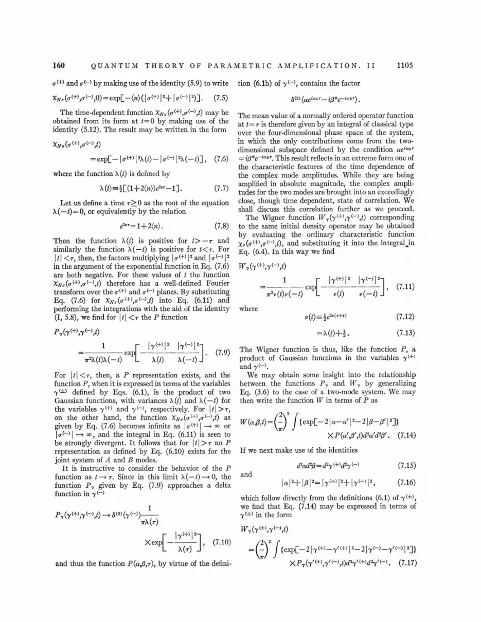
0 &+& and o & & by making use of the identity (5.9) to write tion (6.1b) of p & &, contains the factor

x~.(~'+',~' ' 0) =emL —(~)(l~'+'I'+ I~' 'I')1 (7 5) $(2) (nglGlp1' jP8g &h15T)

The time-dependent function X&r. (0 (+&,0 & &,t) may beobtained from its form at t=0 by making use of theidentity (5.12). The result may be written in the form

The mean value of a normally ordered operator functionat t= r is therefore given by an integral of classical typeover the four-dimensional phase space of the system,in which the only contributions come from the two-dimensional subspace defined by the condition ne'"~'=iP*&, '"" Th. is result reflects in an extreme form one ofthe characteristic features of the time dependence ofthe complex mode amplitudes. While they are beingamplified in absolute magnitude, the complex ampli-tudes for the two modes are brought into an exceedinglyclose, though time dependent, state of correlation. Keshall discuss this correlation further as we proceed.

The Wigner function W, (7(+),y( &,t) correspondingto the same initial density operator may be obtained

by evaluating the ordinary characteristic function

X (0&+&,0& &,t), and substituting it into the integral inEq. (6.4). In this way we find

X~ (~(+) 0 (—) t)

=eel —l~'+'I'~(t) —l~' 'I'~( —t)3, (7.6)

where the function I((t) is defined by

I (t) =——,'I (1+2(~))e2 —1j. (7.7)

Let us delne a time r&0 as the root of the equationI((—t) =0, or equivalently by the relation

&,'«= 1+2(e) . (7.8)

gI (7(+) 7(—) t)

(7.11)) (t) P(—t)

expm'p(t)) (—t)

where(7.12)),(t)—1~2m(r+t)

Then the function )~(t) is positive for t& rand—similarly the function X(—t) is positive for t(r. ForIt I

(r, then, the factors multiplying I0 &+& I' and

I0 & & I'

in the argument of the exponential function in Eq. (7.6)are both negative. For these values of 3 the functionX&r, (o(+),o.( &,t) therefore has a well-defined Fouriertransform over the 0 (+' and o. ~ ~ planes. By substitutingEq. (7.6) for Xir, (0 (+),o.( &,t) into Eq. (6.11) andperforming the integrations with the aid of the identity(I, 5.8), we find for Itl (r the P function

p (&(+) &(—) t) =I (t)y-,'. (7.13)

exp~9.(t)I&(—t)

Iv(+) I'

) (t) x(—t)(7 9)

p (~(+) ~(—) t) ~ t&(2)(&(—))vrI((r)

Xexplv'+'I'

(7.10)I((r)

and thus the function P(n,P,r), by virtue of the defini-

For Itl (r, then, a P representation exists, and thefunction I', when it is expressed in terms of the variables

defined by Eqs. (6.1), is the product of twoGaussian functions, with variances 'A(t) and I((—t) forthe variables p(+) and p( &, respectively. For Itl &r,on the other hand, the function X~ (0&+),0& &,t) asgiven by Eq. (7.6) becomes infinite as Io.&+&

I~ ~ or

I0&—

&

I-+ oo, and the integral in Eq. (6.11) is seen to

be strongly divergent. It follows that forI tl &r no P

representation as defined by Eq. (6.10) exists for thejoint system of A and 8 modes.

It is instructive to consider the behavior of the I'function as t —& r. Since in this limit I((—t) ~ 0, thefunction Pr given by Eq. (7.9) approaches a deltafunction in y( ~

The Wigner function is thus, like the function I', aproduct of Gaussian functions in the variables y(+)

and y& ).We may obtain some insight into the relationship

between -the functions I'~ and 8'~ by generalizingEq. (3.6) to the case of a two-mode system. We maythen write the function 8' in terms of I' as

If we next make use of the identities

d'nd'P =d'y (+)d'y( '

and

II'+IPI'= l~") I'+l~( 'I',

(7.15)

(7.16)

which follow directly from the definitions (6.1) of y(+),we find that Eq. (7.14) may be expressed in terms ofy&+) in the form

(+(+) +(—) t)

(2'l'

~)(expL —2

Iy(+) —y'(+)

I

2—2 Iy(—& —7'(—)I q)

Xp (&~(+) +~(—) t)d&&'(+)d27'( —) (7 17)

2

~(n,P, t) = — {expL—2 ln —n'I '—2I 4—O' I'j)

XP (n' P' t)d'n'd'P' (7.14)

B. R. MOLLOW AND R. J. GLAUBER 160

P (n,P,O) = exp—'()( )

(7.18)(e) (m)

where (m) and (m) are the initial mean quantum numbersfor the A and 8 modes, respectively. By following theobvious generalizations of the steps used earlier in thissection we may derive the corresponding time-depend-ent P function. Let us now de6ne the function X(t)by the equation

For the state with initial P function (7.2) we foundthat a P representation exists for

~

t~

& r, with Pr given

by Eq. (7.9). If we substitute Eq. (7.9) for Pr intoEq. (7.17), then by performing the integrations we onceagain 6nd the result in Eq. (7.11) for W„, with v(t)given by Eq. (7.13). This derivation of Eq. (7.11)depends on the existence of the P representation, andhence is valid only for ~t~ &r. The derivation of theWigner function given by Eq. (7.11), on the other hand,is valid at all times.

If we examine the time dependence of the Wignerfunction (7.11), we see that its form does not changein any dramatic waynear the times t= &r. Ast —& ~, infact, the variance of y( ' which it contains goes uni-

formly to zero. As far as the description implicit in theWigner function is concerned, the complex amplitudesof the A and 3 modes tend steadily to become morecorrelated as t —&~. In the function P~, on the otherhand, the expression P, (—t), which is the variance ofy~ ), goes to zero for t —+ r, and P7 fails to be well-

defined thereafter. The convolution transform (7.17)fails to have a meaningful inverse for t&r, since

v( —t)&2. Evidently the P representation ceases toexist because it is incapable of describing closer heldcorrelations than exist at time t=~. We shall discussthis point further in the next section.

When the initial mean occupation numbers of thetwo modes are allowed to take on different values, we

may write the initial P function as

The Fourier transform which leads to this resultexists only when M(t)&0; this is equivalent to therequirement

2(N)(m)cosh 2)d & 1+

1+(I)+(m)(7.24)

which may be shown to imply the weaker conditionsX (t) &0 and X (—t) &0, or

~

t~& r. For times too large

to satisfy the inequality (7.24) no P representationexists.

We may note that if either (n) or (m) vanishes, a Prepresentation exists only at t=0. In particular, if theinitial state is the vacuum ((m)=(m)=0), then theamplification process immediately destroys the Prepresentation.

It is not dificult to extend our analysis to treatmore general forms for the initial P function. Let ussuppose, for example, that the system is initiallydescribed by the displaced Gaussian function

P(n,P,O) = expm'(ri)(m) (e) (m)

(7.25)

where np and po are the mean values of a and b, respec-tively. Let us de6ne the functions p&+'(t) and p& & (t) asthe mean values of the operators c&+&(t) and c& &(t)

defined by Eqs. (4.1). Then we may show that thefunction Pv(y(+), y( ', t) which corresponds to the statedescribed initially by the P function (7.25) is just thefunction given by Eq. (7.23), with y(+) replaced byy(+) —p(+)(t), and y( & by y( ' —y( &(t). The timeinterval during which a P representation exists is onceagain the interval de6ned by the inequality (7.24).If (m) =0, the initial state of the A mode is the coherentstate ~no); likewise if (m)=0, the initial state of the 8mode is the coherent state ~PO). In either of these casesthe inequality (7.24) is satisfied only for t=0 and a Prepresentation fails to exist for all times other than1=0.

"(t)=-'L(1+( )+( )) '"'—1j (7.19)

and the time r&0 as the root of the equation X(—t) =0,so that

e'"'= 1+(n)+(m).

If we then introduce the quantities

(7.20)

anda =-', ((~)—(m))

M (t) =) (t)& (—t) —A',

(7.21)

(7.22)

P (&(+) &(—) t)

(t)exp( ~ (t)LI'r'+) I'y( —t)+ IV' 'I'&((t)

t& (p(+) p(—)+p(+)p(—)'))) (7 23)

we hnd that the function P~ at time t may be writtenin the form

VIII. CORRELATIONS OF THEMODE AMPLITUDES

We have remarked that the amplihcation processleads as it continues to an increasingly close correlationbetween the complex amplitudes of the two modes of theampliher. That the moduli of the complex amplitudesbecome electively equal in the limit of large times isclear from the conservation law Eq. (I, 3.9), whichstates that the difference at(t)a(t) —bt(t)b(t) is a con-stant of the motion. Since the magnitudes of bothat(t)a(t) and bt(t)b(t) increase exponentially as t ~ m,the relative magnitude of the diGerence between thembecomes exceedingly small.

The complex mode amplitudes become stronglycorrelated not only in modulus, but in phase as well.The asymptotic form as t —& ~ of the solutions (2.3)

QUANTUM THEORY OF PARAMETRIC AMPLIFICATION. II 1107

to the Heisenberg equations of motion is

a (t) I (a+gt) e ice&—t+s i

b (t)~ 1 (b+iat) e ice bt—+at (8.1)

By recalling that ~=(d,+or), we see that in the limit oflarge times the amplitude operators obey the relation

a(t) ib) (t)e—'"'. (8.2)

Similarly, if we consider the motion of the system asextending over an infinite period of time prior to t=0,then the equations of motion lead to the correlation

a(t)- —ibt(t)e '" (8.3)

in the limit t~ —~.To investigate the time-dependent correlation be-

tween the modes in greater detail, let us assume thatthe system is described by a given Heisenberg densityoperator p. Let us next define the c-number functions(&((t) and P(t) through Eqs. (I, 3.22) as the mean valuesof a(t) and b(t), respectively. We then introduce theoperators

a (t) =a (t) (i(t)

b(t) —=b(t) —p(t),(84)

t((—& (t) = tr{p[a'(t) e—'""+ib(t)e'" '$

X [a(t)e'"'—tb (t)e '""j} (8.6)

=2 tr{pc& )t(t)c(—&(t)}. (8 7)

To discuss the correlation of the fluctuations as t ~ —~we likewise form the correlation function

p(+) (t) —2 tr{pc(+)t(t)c(+) (t) } (8.8)

Since p is Hermitian and positive-definite, both of thesefunctions are real and non-negative

ti' '(t) &0, ti(+'(t) &0. (8.9)

The solutions (4.2) for the operators c(+)(t) implythat the correlation functions vary exponentially with

which describe the quantum fluctuations of the modeamplitudes about their mean values. It is clear that theoperators a(t) and b(t) obey the same linear equationsof motion as do a(t) and b(t). If we similarly define theoperators c(+'(t) as the deviations of the operatorsc&+& (t) defined by Eqs. (4.1) from their mean values,

c(+) (t) =—c(+) (t) —tr{pc&+) (t)}, (8.5)

then it is clear that the defining Eqs. (4.1) and thesolutions to the equations of motion (4.2) remain validwhen c(+)(t), a(t), and b(t) are replaced by c&+&(t),

a(t), and b(t), respectively.The fluctuations of the mode amplitudes about their

mean values become correlated as t~ ~ much as themode amplitudes themselves do. To discuss thesecorrelations we introduce the correlation function

It is clear that the fluctuations of the mode amplitudestend to become extremely closely correlated as tincreases or decreases from zero, no matter how uncor-related they may be initially.

Let us consider the form which the correlationfunctions ti(+) (t) take in the Schrodinger picture. If wemake use in Eq. (8.6) [and in the correspondingequation for t((+) (t)] of the transformation rules (I, 4.3)and (I, 4.4), we find

t "'(t)= {p(t)L(a'—~*(t))e '""+ ( —p(t))e'""3X[(.—-(t))e'-"~i(» —P*(t))e-'- )}, (8.11)

which expresses the correlation functions in terms of theSchrodinger density operator p (t).

The time dependence of the correlation functionsexpressed by Eqs. (8.10) enables us to draw some quitegeneral inferences concerning the time-dependent stateof the amplifier system. For large values of ~t~, forexample, the relations (8.10) tend to specify correla-tions of the field amplitudes which are even closer thancan be realized by any pure coherent state ~n, p) forthe system. Such states specify minimal uncertaintiesin the fields of the A mode and the 8 mode individually,but leave small margins equal to those zero-pointuncertainties, within which the two fields may fluctuateindependently. Even so minute a degree of independenceis too great to be consistent with Eqs. (8.10). Indeed,if at any time t the density operator takes the formp(t) = ~n,p)(n, p ~, we find by using Eq. (8.11) and thecommutation relations for b and b~ that

p(+) (t) =1 (8.12)

It is clear from Eqs. (8.10) that for all times other thanthis time either ti( )(t) or p, &+) (t) is smaller than unity,and that the Geld correlations are therefore too closeto be described by a coherent state. They are in facttoo close to be described within the much more generalframework of the P representation, since, as we notedat the end of Sec. VII, if the system is initially in anycoherent state, no P representation exists at timesother than the initial time.

It is appropriate at this point to ask in more generalterms what conditions the values of the correlationfunctions impose on the P representation. We shall showthat. if either of the functions ti(+) (t) is smaller thanunity, no non-negative P function for the two-modedensity operator can exist. A corresponding theorem wasproved in Sec. X of I for the single mode P function.That function, it was shown, must take on negativevalues or fail to exist if the variance of either of thevariables defined by Eqs. (I, 10.3) is less than one half.For the two-mode case let us assume that p(t) has a I'representation as expressed by Eq. (6.9). Then bymaking use of Eq. (8.11) and the commutation relations

time, i.e., we have

p '-'(t) =t ' '(o)e '"', t '"'(t) =p"'(0)e'"' (8 10)

ii08 B. R. MOLLOW AND R. J. GLAUBER 160

for b and bt we find

(eset( (—)(())ts(+) (0)

(8.14)

We have not of course proved in general that no I'representation exists outside the interval defined by thecondition (8.14), though that is indeed the case for the

~" (/) = 1+I II-—=(/)) '-"~'TP*-P*(/)3e-'-"& I'

XI'(~,P, /)d'~dsP. (8.13)

It is clear that if E(n,P,t) is to be non-negative then wemust have ts(+) (/) )1.Ily virtue of the values (8.10) forthe time-dependent correlation functions we see thenthat I'(n, P,t) can remain non-negative only within thetime interval specified by

examples considered in the last section. For example inthe case of the initially chaotic mixture with equalmean quantum numbers (rt) for each mode, we havets(+)(0)=1+2(n), and the time interval defined byEq. (8.14) is thus —r(/(r, with r defined by Eq.(7.8);we have seen that for this example a I' representa-tion ceases to exist outside the stated interval.

It is worth emphasizing that the condition (8.14) ismerely a necessary one for the existence of a non-negative I' function. We should not be surprised,therefore, if a E representation fails to exist inside theindicated interval of time. This is indeed the case for aninitially chaotic mixture when the two mean occupationnumbers are unequal. In that case the bounds in Eq.(8.14) are specified by ts(+)(0)=1+(rt)+(m), but theinterval within which the I' representation exists is theone given by Eq. (7.24). It is in general a smallerinterval.

PHYSICAL REVIEW VOLUM E 160, NUMBER 5 28 AUGUST 1967

Radiation of Gravitational Waves in Brans-DickeGeneral-Relativity Theory

R. F. O' CONNELL*

Instststte for Space StstdSes, Goddard Space F/sgkt Center,Eationa/ Aeronailtics and Space Administration, Rem York, Eem York

AND

A. SALMONAt'

City Co//ege, City Un/vers/ty of New York, New York, New York

(Received 28 March 1967; revised manuscript received 17 May 1967)

The rate of radiation of gravitational waves, I'» =—I'&+I'z, from a system of binary stars is calculatedusing the general-relativity theory of Brans and Dicke. It is shown that, for a circular orbit, the radiationarises purely from the tensor-Geld contribution I'z, and E» is smaller than the corresponding Einsteinresult FE, by a factor (2au+3)/(2or+4), where co is the usual Brans-Dicke dimensionless constant (w 6).In the case of an elliptic orbit, there is also a contribution I'8 from the scalar Geld. However, we show thatthe contribution of Pz to E» is always negligible compared to the contribution I'z. Thus we are able toconclude that, for all values of the eccentricity e, the Brans-Dicke theory predicts that the rate of gravita-tional radiation from a system of binary stars is always smaller, by a factor of the order of —,'6, than the ratepredicted by Einstein's theory.

~

~

SCALAR as well as a tensor Geld has beenincluded in Brans and Dicke's' modification of

Einstein's general theory of relativity. The effect of thescalar field is to make the gravitational constant Gdependent on the mass distribution in the universe.Subsequently, Dicke' showed that the BD theory couldbe put into a form in which the rest masses of allparticles vary with position, being functions of P, the

* On leave of absence from Department of Physics and Astron-omy, Louisiana State University, Baton Rouge, Louisiana.

t On leave of absence from L'Observatoire de Meudon, Meudon,France.' C. Brans and R. H. Dicke, Phys. Rev. 124, 925. (1961) (here-after referred to as BD).' R. H. Dicke, Phys. Rev. 125, 2163 (1962).

scalar field. For our purposes the latter representationof the theory will be the more useful; the reasons forthis choice are discussed in the paper of Morgansternand Chiu' on scalar gravitational Gelds in pulsatingstars. The BD theory has gained some support recentlyas a result of the work of Dicke and Goldenberg on thecontribution of solar oblateness to the precession of theperihelion of Mercury. However, it is still not possibleto decide between the Einstein and BD theories on thebasis of present experimental data. It is the purpose of

' R. E. Morganstern and Hong-Vee Chiu, Phys. Rev. 157, 1228(1967).

4 R. H. Dicke and H. M. Goldenberg, Phys. Rev. Letters 18,313 (1967).