arX

iv:1

303.

1687

v1 [

gr-q

c] 7

Mar

201

3

Quantum states of the bouncing universe

Jean Pierre Gazeau†, Jakub Mielczarek‡,♯ and W lodzimierz Piechocki‡† Laboratoire APC, Univ Paris Diderot, Sorbonne Paris Cite, 75205 Paris, France‡ Department of Fundamental Research, National Centre for Nuclear Research,

Hoza 69, 00-681 Warsaw, Poland♯ Institute of Physics, Jagiellonian University, Reymonta 4, 30-059 Cracow, Poland

(Dated: March 8, 2013)

In this paper we study quantum dynamics of the bouncing cosmological model. We focus on themodel of the flat Friedman-Robertson-Walker universe with a free scalar field. The bouncing behav-ior, which replaces classical singularity, appears due to the modification of general relativity alongthe methods of loop quantum cosmology. We show that there exist a unitary transformation thatenables to describe the system as a free particle with Hamiltonian equal to canonical momentum.We examine properties of the various quantum states of the Universe: boxcar state, standard co-herent state, and soliton-like state, as well as Schrodinger’s cat states constructed from these states.Characteristics of the states such as quantum moments and Wigner functions are investigated. Weshow that each of these states have, for some range of parameters, a proper semiclassical limit fulfill-ing the correspondence principle. Decoherence of the superposition of two universes is described andpossible interpretations in terms of triad orientation and Belinsky-Khalatnikov-Lifshitz conjectureare given. Some interesting features regarding the area of the negative part of the Wigner functionhave emerged.

I. INTRODUCTION

It is known that the cosmological singularity problemof the Friedman-Robertson-Walker (FRW) universe canbe resolved, in the sense that big bang may be replaced bybig bounce, by applying loop quantum cosmology (LQC)methods. However, quantum states specifying quantumevolution of the universe have not been examined in asatisfactory way yet.

There exist two alternative forms of LQC: Dirac’s LQC(see e.g. [1, 2] and references therein) and reduced phasespace (RPS) LQC (see e.g. [3–6]) and references therein).Both approaches rely on the same form of modification ofgeneral relativity. It consists in approximating the cur-vature of connection by holonomies around small loopswith non-zero size. Going with the size to zero removesthe modification. One of the main differences betweenthese two approaches is an interpretation of the way ofresolving the singularity. In the Dirac LQC, one arguesthat the resolution is due to strong quantum effects atthe Planck scale. In the RPS LQC, one says that it isthe modification of GR by loop deformation of the phasespace that is responsible for the resolution of the singu-larity.

In what follows we apply the RPS LQC method. Itconsists in first solving dynamical constraints at the clas-sical level and then quantizing the resulting classical sys-tem. This approach allows to implement quantizationeasily. It gives a clear picture of quantum dynamics forany value of an evolution parameter (time), and enablesobtaining analytical results (at least for the FRW case).

The quantum evolution across the big bounce can givean insight into the structure of the quantum phase. Theinput in describing an evolution is a self-adjoint Hamil-tonian (generator of dynamics) together with an initial

state of the universe. Taking different initial states maylead to different quantum evolutions. Since it is unknownwhich initial state is the most natural one, we examinegeneric states known in quantum physics with differentproperties. Comparison of obtained results with observa-tional cosmological data may give suggestions concerningthe choice of some realistic initial state.

The paper is organized as follows. In Sec. II the classi-cal dynamics of the model is examined and the canonicaltransformation simplifying the dynamics is introduced.In Sec. III we make canonical quantization of the model.We also introduce unitary map which corresponds to thecanonical transformation introduced in Sec. II. In Sec.IV different choices of the initial quantum state are in-troduced as well as all the necessary tools which willbe used to investigate their properties. Thereafter, inSections V, VI and VII, detailed analysis of the boxcarstate, standard coherent state, soliton-like state as wellas Schrodinger cat states constructed from these states isperformed. In Sec. VIII, decoherence of the Schrodingercat state is discussed, and possible interpretations of sucha process in the cosmological realm are given. The issueof quantum entropy is discussed Sec. IX. It is shown that,in contrast to the results of Ref. [6], entropy of squeez-ing is constant for the canonically transformed system.Then, in Sec. X, ranges of the parameters of consideredstates are constrained by using the correspondence prin-ciple between quantum and classical mechanics. In Sec.XI, we summarize our results and draw conclusions.

2

II. CLASSICAL DYNAMICS

The flat FRW model of the universe with a free scalarfield is described by the Hamiltonian constraint [5]

H = − 3

8πGγ2sin2(λβ)

λ2v +

p2ϕ2v

≈ 0, (1)

where, as in the rest of this paper, we use the units withthe speed of light in vacuum equal to one. Here, γ isthe Barbero-Immirzi parameter, a free parameter of thetheory. However, value of this parameter is usually fixedfrom considerations of the black hole entropy. In partic-ular, as derived in Ref. [7], γ ≈ 0.2375. The parameter λis a ‘discretization scale’, which is expected to be of theorder of the Planck length lPl =

√ℏG ≈ 1.62 · 10−35 m,

but in fact should be fixed by observational data.The variables β and v, fulfilling the Poisson bracket

{β, v} = 4πGγ, parametrize the gravitational sector.In turn, the scalar field ϕ and its conjugated momentapϕ satisfy standard relation {ϕ, pϕ} = 1, and specifysources.

Hamiltonian (1) has the symmetry

β → β +π

λ, (2)

so the gravitational part of phase space has topology ofa cylinder, S1 × R. Already classically we have bouncetype solutions in the regions: λβ ∈ [0 +mπ, π+mπ], form ∈ Z.

The Hamiltonian constraint (1) can be rewritten in theform

v2 sin2(λβ) = const, (3)

where we used the fact that pϕ = const for the free fieldcase. It turns, that the square root of (3) plays a role ofthe physical Hamiltonian. Based on this, dynamics of aflat FRW cosmological model, with a freescalar field, canbe described by

H = p sin q, (4)

where q ∈ [0, π] and p ∈ R are canonical variables satis-fying the algebra {q, p} = 1. The Hamiltonian (4) occursboth in the reduced phase space approach [5] and stan-dard formulation of LQC [8]. It need not be boundedfrom below as it describes the entire universe, which isan isolated system. The p variable is proportional to thevolume v, but we increase its range to negative values formathematical convenience. Physical meaning of this vol-ume is not clear for the flat FRW model. It correspondsto the total volume of space if topology is compact. Thepossibility of positive and negative values of p may berelated to two orientations of triad. Namely, the phasespace (β, v) is only half of the original phase space of

the model since v :=∣∣∣pV 2/3

0

∣∣∣3/2

, where p ∈ R is a vari-

able parametrizing densitized triad Eai = pδai . The V0 is

a fiducial cell over which the spatial integration is per-formed. By allowing positive and negative values of thevariable p we recover the volume of the original phasespace. The variable q := λβ is proportional to the Hub-ble factor in the classical limit (q ≪ 1).

The Hamiltonian (4) generates evolution of any phasespace function f according to the equation

df

dT= {f,H}. (5)

The T variable is an intrinsic time parameter related withthe value of the scalar field. The direction of time T ,which also occurs in [5], is opposite to the direction ofthe coordinate time t. In order to fix the directions ofT and t one has to redefine T by multiplying it and theHamiltonian (4) by minus one. But these are only tech-nical details devoid of deep meaning.

Applying (5) for the canonical variables we get

dq

dT=∂H

∂p= sin q, (6)

dp

dT= −∂H

∂q= −p cos q. (7)

0 Π

2Π

-1

-12

0

12

1

q

p

FIG. 1. Trajectories in the phase space with original variables(q, p).

Solutions to these equations are given by

q(T ) = 2 arctan exp(T − T0), (8)

p(T ) = p0 cosh(T − T0), (9)

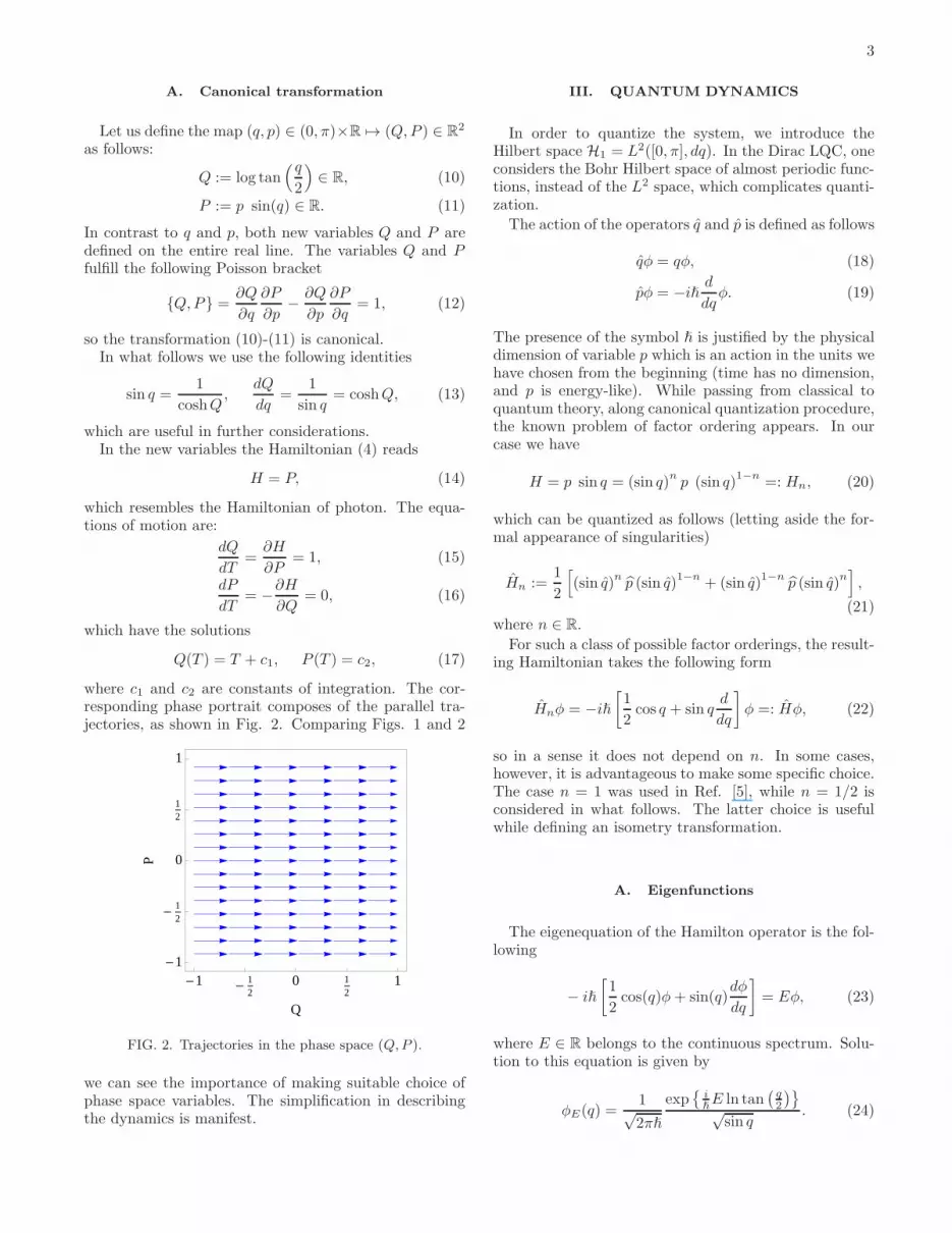
where p0 and T0 are constants of integration. The solu-tion for p presents a nonsingular symmetric bounce typeevolution. Fig. 1 presents the phase portrait of the phasespace, illustrating Eqs. (8) and (9).

3

A. Canonical transformation

Let us define the map (q, p) ∈ (0, π)×R 7→ (Q,P ) ∈ R2

as follows:

Q := log tan(q

2

)∈ R, (10)

P := p sin(q) ∈ R. (11)

In contrast to q and p, both new variables Q and P aredefined on the entire real line. The variables Q and Pfulfill the following Poisson bracket

{Q,P} =∂Q

∂q

∂P

∂p− ∂Q

∂p

∂P

∂q= 1, (12)

so the transformation (10)-(11) is canonical.In what follows we use the following identities

sin q =1

coshQ,

dQ

dq=

1

sin q= coshQ, (13)

which are useful in further considerations.In the new variables the Hamiltonian (4) reads

H = P, (14)

which resembles the Hamiltonian of photon. The equa-tions of motion are:

dQ

dT=∂H

∂P= 1, (15)

dP

dT= −∂H

∂Q= 0, (16)

which have the solutions

Q(T ) = T + c1, P (T ) = c2, (17)

where c1 and c2 are constants of integration. The cor-responding phase portrait composes of the parallel tra-jectories, as shown in Fig. 2. Comparing Figs. 1 and 2

-1 -12

0 12

1-1

-12

0

12

1

Q

P

FIG. 2. Trajectories in the phase space (Q,P ).

we can see the importance of making suitable choice ofphase space variables. The simplification in describingthe dynamics is manifest.

III. QUANTUM DYNAMICS

In order to quantize the system, we introduce theHilbert space H1 = L2([0, π], dq). In the Dirac LQC, oneconsiders the Bohr Hilbert space of almost periodic func-tions, instead of the L2 space, which complicates quanti-zation.

The action of the operators q and p is defined as follows

qφ = qφ, (18)

pφ = −iℏ ddqφ. (19)

The presence of the symbol ℏ is justified by the physicaldimension of variable p which is an action in the units wehave chosen from the beginning (time has no dimension,and p is energy-like). While passing from classical toquantum theory, along canonical quantization procedure,the known problem of factor ordering appears. In ourcase we have

H = p sin q = (sin q)np (sin q)

1−n=: Hn, (20)

which can be quantized as follows (letting aside the for-mal appearance of singularities)

Hn :=1

2

[(sin q)

np (sin q)

1−n+ (sin q)

1−np (sin q)

n],

(21)where n ∈ R.

For such a class of possible factor orderings, the result-ing Hamiltonian takes the following form

Hnφ = −iℏ[

1

2cos q + sin q

d

dq

]φ =: Hφ, (22)

so in a sense it does not depend on n. In some cases,however, it is advantageous to make some specific choice.The case n = 1 was used in Ref. [5], while n = 1/2 isconsidered in what follows. The latter choice is usefulwhile defining an isometry transformation.

A. Eigenfunctions

The eigenequation of the Hamilton operator is the fol-lowing

− iℏ

[1

2cos(q)φ+ sin(q)

dφ

dq

]= Eφ, (23)

where E ∈ R belongs to the continuous spectrum. Solu-tion to this equation is given by

φE(q) =1√2πℏ

exp{

iℏE ln tan

(q2

)}√

sin q. (24)

4

One can verify that

〈φE1 |φE2〉 =

∫ π

0

φE1(q)φE2(q)dq

=1

2πℏ

∫ π

0

dqexp

{iℏ

(E2 − E1) ln tan(q2

)}

sin q

=1

2πℏ

∫ +∞

−∞dQe

iℏ(E2−E1)Q

= δ(E2 − E1), (25)

where we have used the mapping (10)

(0, π) ∋ q → Q(q) ∈ R. (26)

B. Unitary map

For n = 1/2, the quantum Hamiltonian reads

H :=√

sin q p√

sin q. (27)

Now, we introduce a new Hilbert space H2 = L2(R, dQ)connected with H1 as follows

U : φ(q) ∈ H1 → ψ(Q) =√

sin(q(Q))φ(q(Q)) ∈ H2.(28)

In particular, the eigenfunctions φE(q) are mapped intothe plane waves

U : φE(q) → ψE(Q) =e

iℏEQ

√2πℏ

. (29)

The map U is an invertible isometry (unitary trans-form), since we have

〈φ1|φ2〉H1 =

∫ π

0

φ1(q)φ2(q)dq

=

∫ +∞

−∞φ1(q(Q))φ2(q(Q)) sin(q(Q))dQ

=

∫ +∞

−∞ψ1(Q)ψ2(Q)dQ = 〈ψ1|ψ2〉H2 . (30)

Under this isometry, an operator OH1 acting in H1 is

transformed into an operator OH2 acting on H2 and viceversa

OH2 = UOH1U−1, (31)

OH1 = U−1OH2U . (32)

As an example, let us consider the operator P whichacts in H2 as follows

Pψ(Q) = −iℏ d

dQψ(Q). (33)

Using the transformation (32) as well as relation (13), weobtain

Pψ(Q) = U−1PUφ(q) =1√sin q

(−iℏ d

dQ

)√sin qφ(q)

=1√sin q

(−iℏ sin q

d

dq

)√sin qφ(q)

=√

sin q

(−iℏ d

dq

)√sin qφ(q)

=√

sin q p√

sin qφ(q)

= Hφ(q). (34)

Thus, the isometry U transforms the Hamiltonian H act-ing in H1 into a well known momentum operator P actingin H2.

Using the above results, we define a unitary evolutionoperator U as follows:

Uφ(q) := e−iℏHTφ(q) = e−

iℏPTψ(Q)

= exp

{−T d

dQ

}ψ(Q) = ψ(Q− T ). (35)

Therefore, a time evolution in H1 corresponds to trans-lation operator in H2. So the shape of the probabilitydistribution is preserved in time.

The classical dynamics of the Q variable is Q = T + c1(See Eq. 17). Thus, if the probability distribution ispeaked on the classical trajectory at some given momentin time, it will trace the classical trajectory during thewhole evolution [9].

We should notice at this point that combining transla-

tion (35) with phase modulation, Ψ(Q) 7→ eiℏP0QΨ(Q) :=

ΨP0(Q), leads to the unitary irreducible representation ofthe Weyl-Heisenberg group

Ψ(Q) 7→ eiℏP0QΨ(Q− T ) := ΨP0,T (Q) , (36)

used for constructing coherent states in quantum me-chanics (up to a constant phase factor) [10, 11] and theGabor states for time-frequency analysis used in signalprocessing [12]. The Weyl-Heisenberg action (36) will beat the heart of the construction of the examples presentedin the next section.

IV. CHOICE OF INITIAL STATE

In the next three sections we investigate three repre-sentative initial quantum states:

• Boxcar state

• Standard coherent state

• Soliton-like state

Moreover, for each of these states we investigateSchrodinger cat type superposition in the form

Ψ =N√

2(ΨP0 + Ψ−P0) (37)

5

where P0 is the mean value of the P operator in the con-stituent state ΨP0 and N is the normalization factor. Itis known that such states are experimentally attainable(for instance in quantum optics [13]). The state (see Sec.VI D) can be viewed also as a superposition of the twoorientations of triads. Decoherence of two triads orienta-tions in LQC was recently studied in Ref. [14]. In whatfollows we study such a process in our framework.

As was already mentioned, quantum dynamics of theconsidered model reduces to shifting the initial state inthe Q variable: U(T )Ψ(Q) = Ψ(Q − T ). Thereforewhile we have the initial quantum state Ψ(Q), the cor-responding state at the time T is obtained by replacingQ → Q − T . For the later convenience we define vari-able X := Q − T , which absorbs all time dependence ofa given quantum state.

To characterize the states under consideration westudy quantum moments of the operators Q and P in thegiven state. In particular, determination of the mean val-ues 〈Q〉 and 〈P 〉 is crucial to compare quantum dynamicswith the classical phase-space trajectories. Furthermore,quantum dispersions

σQ :=

√〈Q2〉 − 〈Q〉2, σP :=

√〈P 2〉 − 〈P 〉2, (38)

as well as covariance

CQP := 〈(Q − 〈Q〉)(P − 〈P 〉)〉

=1

2〈QP + P Q〉 − 〈Q〉〈P 〉, (39)

will be a source of information about spreading andsqueezing of the quantum states. Furthermore, by em-ploying dispersions and covariance, one can define thecovariance matrix

Σ :=

[σ2Q CQP

CQP σ2P

]. (40)

Making use of it, one can define the Schrodinger-Robertson uncertainty relation as follows

detΣ ≥ ℏ2

4. (41)

The value of detΣ is an important characteristic of thequantum state, telling us about spread of the state on thephase space. One could expect that for small values ofdetΣ, the quantum systems behaves more like a classicalone. However, it is not a general rule. Therefore, otherindicators of semi-classicality should be used.

In the literature, the relative fluctuations σO/〈O〉are usually considered as a measure of semi-classicality.Namely, one could expect that, in the semiclassical limit,quantum fluctuations of some observable O should bemuch smaller that its mean value: σO/〈O〉 ≪ 1. Such adefinition has to be however applied with care. Namely,while denominator 〈O〉 approaches zero, the relative fluc-tuations diverge even, if the quantum dispersion is very

small. But this does not correspond to any strong quan-tum effects, and is only a result of the definition of theobservable O. Another important aspect is the meaningof choosing σO/〈O〉 being much smaller that one. Shouldit be one hundred or one million times smaller? Whilethe choice is quite arbitrary, we already have a referencevalue coming from the measurements of a given observ-able. If our experimental abilities does not allow us tosee the quantum aspects of a given phenomenon, thenwe can state that the underlying dynamics is classical.Therefore, the state can be called semiclassical if rela-tive fluctuations of some observable are smaller than therelative uncertainty of experimental (observational) de-termination of that observable.

In what follows we study one quantity, which canbe used to characterize semi-classicality of a quantumstate. Namely, the Wigner function, which is a quasi-probability distribution defined on the phase space. Hav-ing the wave function Ψ(Q) = 〈Q|Ψ〉 of a pure state |Ψ〉,the Wigner function is defined to be

W (Q,P ) :=1

πℏ

∫ +∞

−∞Ψ(Q+y)Ψ(Q−y)e2iPy/ℏdy. (42)

The basic properties of the Wigner function are

∫ +∞

−∞

∫ +∞

−∞W (Q,P )dQdP = 1, (43)

∫ +∞

−∞W (Q,P )dP = |Ψ(Q)|2, (44)

∫ +∞

−∞W (Q,P )dQ = |Ψ(P )|2, (45)

and

− 1

πℏ≤W (Q,P ) ≤ 1

πℏ. (46)

The last property tells us that also negative values ofthe the Wigner function are allowed. It was suggestedthat such negative part of the Wigner function can beconsidered as an indicator of quantumness [15]. Briefly,less negative the Wigner function is, more classically thesystem behaves. In this context the parameter δ(Ψ) wasintroduced in Ref. [15]:

δ(Ψ) :=

∫ +∞

−∞

∫ +∞

−∞|W (X,P )|dXdP − 1 ∈ [0,∞]. (47)

One half of this parameter is equal to the modulus of theintegral over those domains of the phase space where theWigner function is negative.

One says that a state is semiclassical if δ(Ψ) ≪ 1.In this paper, we study also areas of the negative parts

of the Wigner functions for the considered states. Thisissue, as far as we know, was not systematically investi-gated yet. We show that the structure of these negativesectors may uncover some deep aspects of the formulationof quantum mechanics on phase space.

6

The Wigner function for the Schordinger cat state (seeSec. VI D) can be written as the following sum

W (X,P ) =N2

2(W+ +W−) +Wint, (48)

where W± are Wigner functions for Ψ±P0 states whilethe interference term

Wint =N2

2πℏ

∫ +∞

−∞

[ΨP0(x+ y)Ψ−P0(x− y)

+ Ψ−P0(x+ y)ΨP0(x − y)]e2iPy/ℏdy. (49)

Surprisingly for the considered states, including theSchrodinger cat states, it is possible to find analyticalformulas for the corresponding Wigner functions. Plotsof the Wigner functions will allow to better visualize somequantum aspects of the states.

V. BOXCAR STATE

A. Construction

We begin with considering the most basic example ofa state with compact support, namely the rectangularor ‘boxcar’ window, widely used in Gabor signal analysis[12]. The definition of the state is the following

ΨP0(Q) =

{0 for |Q| > L

21√Le

iℏQP0 for |Q| ≤ L

2

, (50)

where L > 0 (the dependence of ΨP0 on parameter L isnot made explicit for the sake of simplicity). This statecan be also written as

ΨP0(Q) =1√Le

iℏQP0Θ

(L

2+Q

)Θ

(L

2−Q

), (51)

where Θ(x) is the Heaviside step function.

B. Quantum moments

The mean value and the dispersions of Q at the timeT are found to be

〈Q〉 = T, (52)

σQ =L√12. (53)

As expected from the previous analysis, evolution of themean value 〈Q〉 traces the classical dynamics. Here, thequantum dynamics correspond to the classical trajectorywith the constant of integration c1 = 0 (see Eq. (17).

Difficulties due to the discontinuous character of theconsidered state prevent the evaluation of a similar quan-tity for the momentum, since the computation of 〈P 〉 and

〈P 2〉 involves divergent integrals. In principle, one canproceed with a regularization of these divergences, how-ever the obtained expressions for 〈P 〉 and σP would nothave standard interpretation. Such results, are howeverof little use, and therefore not discussed here.

C. Wigner function

Based on definition (42), Wigner function for the box-car state is

W (X,P ) =

0 for |X | > L2

sin

2(P − P0)

ℏ(L

2 −|X|)

πL(P−P0)for |X | ≤ L

2

(54)We plot this function in Fig. 3. Furthermore, in Fig.

FIG. 3. Wigner function for the boxcar state.

4, we show regions of the negative values of the Wignerfunction.

-1 -12

0 12

1

-20

-10

0

10

20

X�L

HP-

P0L

L

Ñ

FIG. 4. Regions where the Wigner function for the boxcarstate assumes its negative values.

It is worth noticing that for X = 0 and P = P0 theWigner function takes the maximal possible value:

W (0, P0) =1

πℏ. (55)

As we will see later, analysis of the Wigner functions

7

suggests that

W (〈X〉, 〈P 〉) =1

πℏ. (56)

As far as we know such a relation was not proved sofar. However, at least for the known Wigner functions itis always fulfilled. For the boxcar state, indeed 〈X〉 =

〈Q〉 − T = T − T = 0, however the value of 〈P 〉 is notproperly defined in the present case. However, since theobtained Wigner function is symmetric with respect toP0, one can formally write 〈P 〉 = P0, supporting therelation (56).

D. Schrodinger cat state

The normalization factor for the Schrodinger cat statecomposed of two boxcar states is

N =1√

1 + sin(LP0/ℏ)(LP0/ℏ)

. (57)

The interference part of the Wigner function is

Wint =

0 for |X | > L2

N2 cos[2P0X

ℏ

]sin[2Pℏ

(L2 − |X |

)]

πLPfor |X | ≤ L

2

(58)Plot of the Wigner function for the Schrodinger cat

state composed of two boxcar states is shown in Fig. 5.

FIG. 5. Wigner function of the Schrodinger cat state LP0 =7ℏ.

In Fig. 6 we show regions of the negative values ofthe Wigner function. For LP0 & 6.04 there are two re-gions with negative values of the Wigner function, lo-cated at the X = 0 axis. We observe that for the par-ticularly case LP0 = 7ℏ the area of each of these regionsis about 0.198~. However, while approaching the value

-1 -12

0 12

1

-20

-10

0

10

20

X�L

PL Ñ

FIG. 6. Regions where the Wigner function for theSchrodinger cat state assumes its negative values, with LP0 =7ℏ. The black dots represent peaks of the two constituentstates.

LP0 ≈ 6.04, the area of these regions falls to zero. Ataround LP0 & 7.64 these two regions merge with the twonegative domains located at P = 0 axis.

VI. STANDARD COHERENT STATE

A. Construction

Standard or Glauber coherent states (see [11] and refer-ences therein) are known to play a central role in studiesof connection between classical and quantum world.

In quantum cosmology one expects that in the low en-ergy density limit, the state is described by the coherentstate mimicking the classical behavior. Here we studythe state in which such a semi-classical behavior is pre-served during the whole evolution. Namely, we considera squeezed initial wave packet state like

Ψ0(Q) =

∫ +∞

−∞f(P )ψP (Q)dP, (59)

where ψP (Q) is the eigenstate of the P operator and

f(P ) = exp(−z1P 2 + z2P + z3

), (60)

where z1, z2, z3 ∈ C, such that ℜz1 > 0. The integral (59)is of the Gaussian type and can be calculated analytically.Due to (35) we get Ψ(Q, T ) = UΨ0(Q) which finallyreads

Ψ(Q, T ) =

(2ℜa1π

)1/4

e−a1(Q−T )2+a2(Q−T )− (ℜa2)2

4ℜa1 .

(61)The factors a1 and a2 can be expressed in terms of coef-ficients z1 and z2 as follows

a1 :=1

4ℏ2z1, a2 :=

iz22ℏz1

. (62)

8

It is worth stressing that the condition ℜz1 > 0 enablesnormalization of the state.

B. Quantum moments

The mean values of the canonical variables in the state(61) are found to be

〈Q〉 = T +1

2

ℜa2ℜa1︸ ︷︷ ︸

= c1∈R

, 〈P 〉 = ℏ

(ℑa2ℑa1

− ℜa2ℜa1

)ℑa1

︸ ︷︷ ︸= c2∈R

, (63)

and are in agreement with the classical solutions (17).Furthermore, the dispersions are

σQ =1

2√ℜa1

(64)

and

σP = ℏ√ℜa1

√

1 +

(ℑa1ℜa1

)2

. (65)

Finally, the covariance reads

CQP = −ℏ

2

ℑa1ℜa1

. (66)

Based on the above, the determinant of the covariancematrix reads

detΣ = σ2Qσ

2P − C2

QP

=1

4ℜa1ℏ2ℜa1

[1 +

(ℑa1ℜa1

)2]−(ℏ

2

ℑa1ℜa1

)2

=ℏ2

4. (67)

As expected for such a case, the squeezed state saturatesthe Schrodinger-Robertson uncertainty relation.

C. Wigner function

For the standard coherent state, the Wigner functiontakes the form of the two dimensional Gauss distribution

W (X,P ) =1

πℏexp

(−1

2xTΣ

−1x

), (68)

where x = (X − 〈X〉, P − 〈P 〉). It is worth stressing,that the Wigner function (68) is positive definite. AsHudson-Piquet [16] theorem says, this is a characteristicproperty of the standard coherent states, distinguishingthem among other pure states. Therefore, positivenessof the Wigner function can be treated as a definition ofthe standard coherent state. Taking negativeness of theWigner function as a measure of the quantumness, one

can conclude that the standard coherent states are themost classical pure states. Furthermore, the positivitive-ness of the Wigner function is observed also for the mixedstates [17].

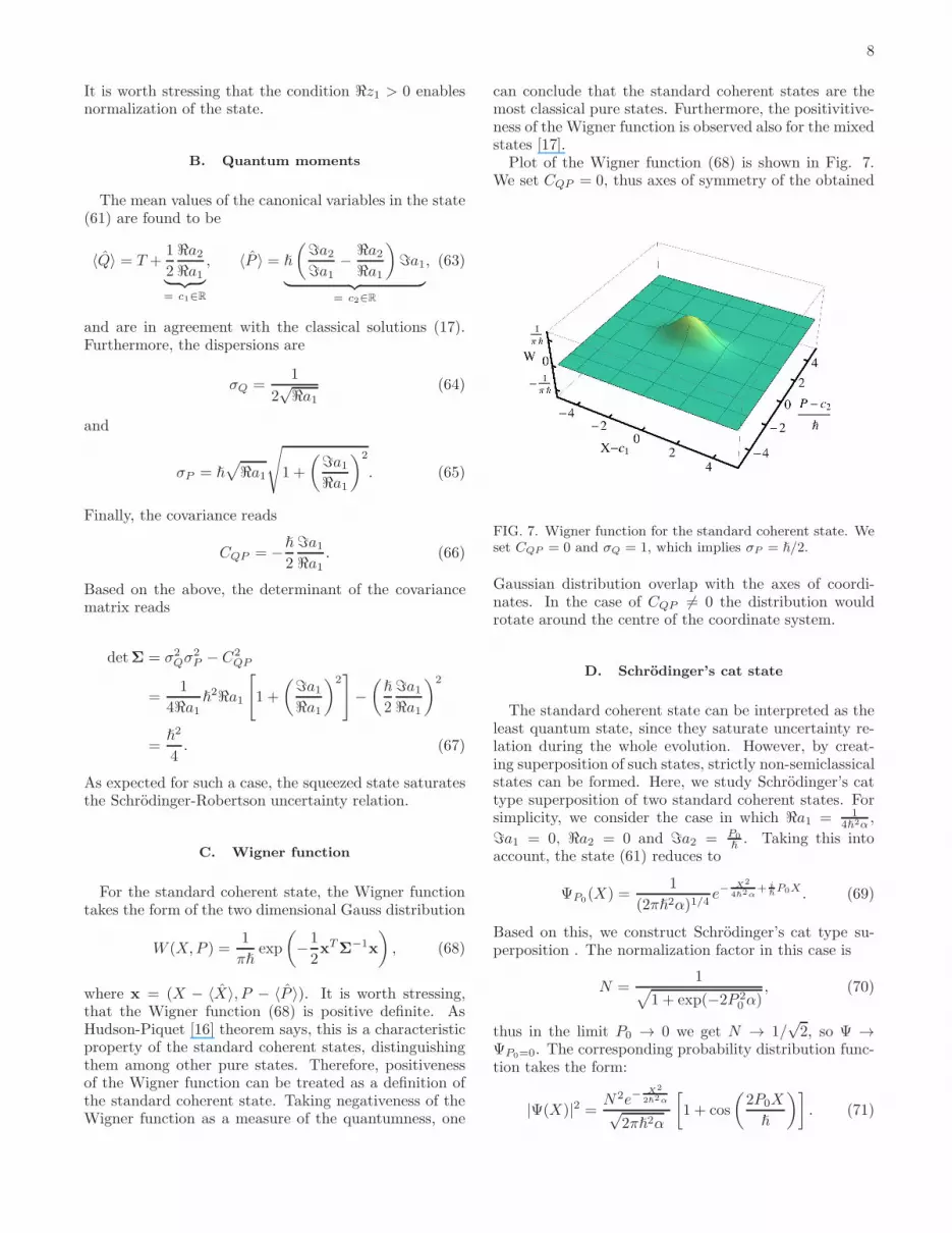
Plot of the Wigner function (68) is shown in Fig. 7.We set CQP = 0, thus axes of symmetry of the obtained

FIG. 7. Wigner function for the standard coherent state. Weset CQP = 0 and σQ = 1, which implies σP = ℏ/2.

Gaussian distribution overlap with the axes of coordi-nates. In the case of CQP 6= 0 the distribution wouldrotate around the centre of the coordinate system.

D. Schrodinger’s cat state

The standard coherent state can be interpreted as theleast quantum state, since they saturate uncertainty re-lation during the whole evolution. However, by creat-ing superposition of such states, strictly non-semiclassicalstates can be formed. Here, we study Schrodinger’s cattype superposition of two standard coherent states. Forsimplicity, we consider the case in which ℜa1 = 1

4ℏ2α ,

ℑa1 = 0, ℜa2 = 0 and ℑa2 = P0

ℏ. Taking this into

account, the state (61) reduces to

ΨP0(X) =1

(2πℏ2α)1/4e−

X2

4ℏ2α+ i

ℏP0X . (69)

Based on this, we construct Schrodinger’s cat type su-perposition . The normalization factor in this case is

N =1√

1 + exp(−2P 20α)

, (70)

thus in the limit P0 → 0 we get N → 1/√

2, so Ψ →ΨP0=0. The corresponding probability distribution func-tion takes the form:

|Ψ(X)|2 =N2e−

X2

2ℏ2α

√2πℏ2α

[1 + cos

(2P0X

ℏ

)]. (71)

9

The mean values of the canonical variables in the state(see Sec. VI D) are

〈Q〉 = T, 〈P 〉 = 0. (72)

Therefore, they correspond to the particular classical tra-jectory with c1 = 0 = c2. The dispersions are:

σ2Q = (ℏ2α)

1 + e−2k2

(1 − 4k2)

1 + e−2k2 , (73)

where for the later convenience we have introduced thedimensionless parameter k := P0

√α, and

σ2P =

ℏ2

4

1

(ℏ2α)

(e−2k2

+ (1 + 4k2))

1 + e−2k2 , (74)

while the covariance is vanishing

CQP = 0. (75)

Using the above we have:

σ2Qσ

2P − C2

QP =ℏ2

4(1 + ξ(k)) ≥ ℏ2

4, (76)

where the inequality comes from the fact that ξ(k) ≥ 0.Plot of the function ξ(k) is shown in Fig. 8.

0 1 2 3 4 5

0

4

8

12

16

20

k

Ξ

FIG. 8. Function ξ(k).

In the expression for the Wigner function

W (X,P ) =N2

2(W+ +W−) +Wint, (77)

we have

W± =1

πℏe−

X2

2ℏ2α−2(P∓P0)

2α, (78)

and the interference term reads

Wint =N2

πℏe−

X2

2ℏ2α−2P 2α cos

(2P0X

ℏ

). (79)

Collecting the contributions, the Wigner function can bewritten as

W (X,P ) =N2

πℏe−

X2

2ℏ2α−2P 2α ×

×[cosh(4PP0α)e−2P 2

0 α + cos

(2P0X

ℏ

)]. (80)

FIG. 9. Wigner function for the Schrodinger cat state. Hereα = 1/ℏ2 and P0 = 4ℏ, such that k = 4.

The plot of this function is shown in Fig. 9.Using the expression (80) we get:

δ(Ψ) = N2 − 1 +N2

√2π

∫ +∞

−∞e−

z2

2 |cos(2kz)| dz. (81)

We plot this function in Fig. 10. One can show that

0 1 2 3 4

0

0.5

2Π

1

k

∆

FIG. 10. Indicator δ(Ψ) for the Schrodinger cat state. In thelimit k → ∞ the value 2

π≈ 0.637 is approached, while for

k → 0 the state becomes coherent δ(Ψ) = 0.

there exists the following limit:

limk→∞

δ(Ψ) =2

π≈ 0.637. (82)

The regions of the negative values of the Wigner func-tion are specified by the inequality:

cosh(4PP0α)e−2P 20 α + cos

(2P0X

ℏ

)< 0. (83)

Due to the periodicity of the cosine function we obtainan infinite set of ellipse-like regions of negative values ofthe Wigner function, as shown in Fig. 11. The area of

10

-4 -2 0 2 4-6

-4

-2

0

2

4

6

X

P Ñ

FIG. 11. Regions where the Wigner function for the CS catstate assumes its negative values. The black dots representpeaks of the two constituent states.

each such region can be expressed as follows

A =ℏ

2

e−2k2

k2

∫ e2k2

1

arccosh(z)√1 − e−4k2z2

dz ≈ πℏ

2=h

4. (84)

The value of above integral was found numerically for abroad range of the parameter k, exhibiting independenceon the value of k. While we were not able to determinethe above integral analytically, in the k → 0 limit, afterchange of variables, it reduces to

limk→0

A = ℏ

∫ 1

0

dz√1 − z2

= ℏπ

2=h

4, (85)

in agreement with the numerical result. Thus, while pass-ing to the case of the standard coherent states the areaof the negative parts of the Wigner function is preserved.This may seem to be inconsistent since there are no re-gions of negative values for the coherent states at all.However, this discrepancy is only apparent. In fact, inthe limit k → 0 the domains of W < 0 elongate in theP direction and disperse in the X direction. In the limitk → 0, separation between these domains tends to infin-ity. In short, the domains of W < 0 escape to infinity inthe limit k → 0, maintaining its areas.

It is interesting to notice that the area (84) is the sameas in the case of the |1〉 Fock state of the harmonic oscilla-tor. This coincidence may exhibit some deeper propertiesof the formulation of quantum mechanics on phase space[18, 19].

VII. SOLITON-LIKE STATE

A. Construction

In this section we study a state given by superpositionof the eigenstates of the Hamiltonian with the profile

f(P ) ∝ 1

cosh (a(P − P0)). (86)

We will see that while this profile looks qualitativelysimilar to the Gaussian distribution, its properties aresignificantly different. In particular, the correspondingWigner function takes negative values. We have

ΨP0(Q) =

√π

4aℏ

eiℏP0Q

cosh(

π2aℏQ

) . (87)

This state is also of the hyperbolic secant form, sincethe hyperbolic secant function is a fixed point of theFourier transform, as the Gaussian distribution.

It is worth mentioning that the obtained state has theform of the so-called bright soliton, which is a solutionof the Gross-Pitaevskii equation describing Bose-Einsteincondensate. For experimental evidences of such solitonstates see for instance [20–22].

The mean values of the canonical variables are

〈Q〉 = T, 〈P 〉 = P0. (88)

Therefore the classical constant of integration c1 is fixedto be zero, while integration constant c2 = P0.

The covariance is equal to

CQP = 0. (89)

The dispersions are

σQ =aℏ√

3, (90)

and

σP =1

aℏ· π√

3· ℏ

2(91)

Based on the above, the uncertainty relation is satisfied

σQσP =π

3· ℏ

2≃ 1.0472 · ℏ

2>

ℏ

2. (92)

The uncertainty differs only by the factor π3 ≈ 1.0472

from the case of minimal uncertainty realized by the stan-dard coherent states.

B. Wigner function

Inserting the wave function (87) into the definition ofthe Wigner function we obtain the integral

W (X,P ) =1

aℏ2

∫ ∞

0

cos(2yℏ

(P − P0))dy

cosh(

πaℏX

)+ cosh

(πaℏy) . (93)

This integral can be calculated analytically by using theformula (see Integral 3.983 in Ref. [23])

∫ ∞

0

cos(ay)

b cosh(βy) + cdy =

π sin(

aβarccosh

(cb

))

β√c2 − b2 sinh

(aπβ

) , (94)

11

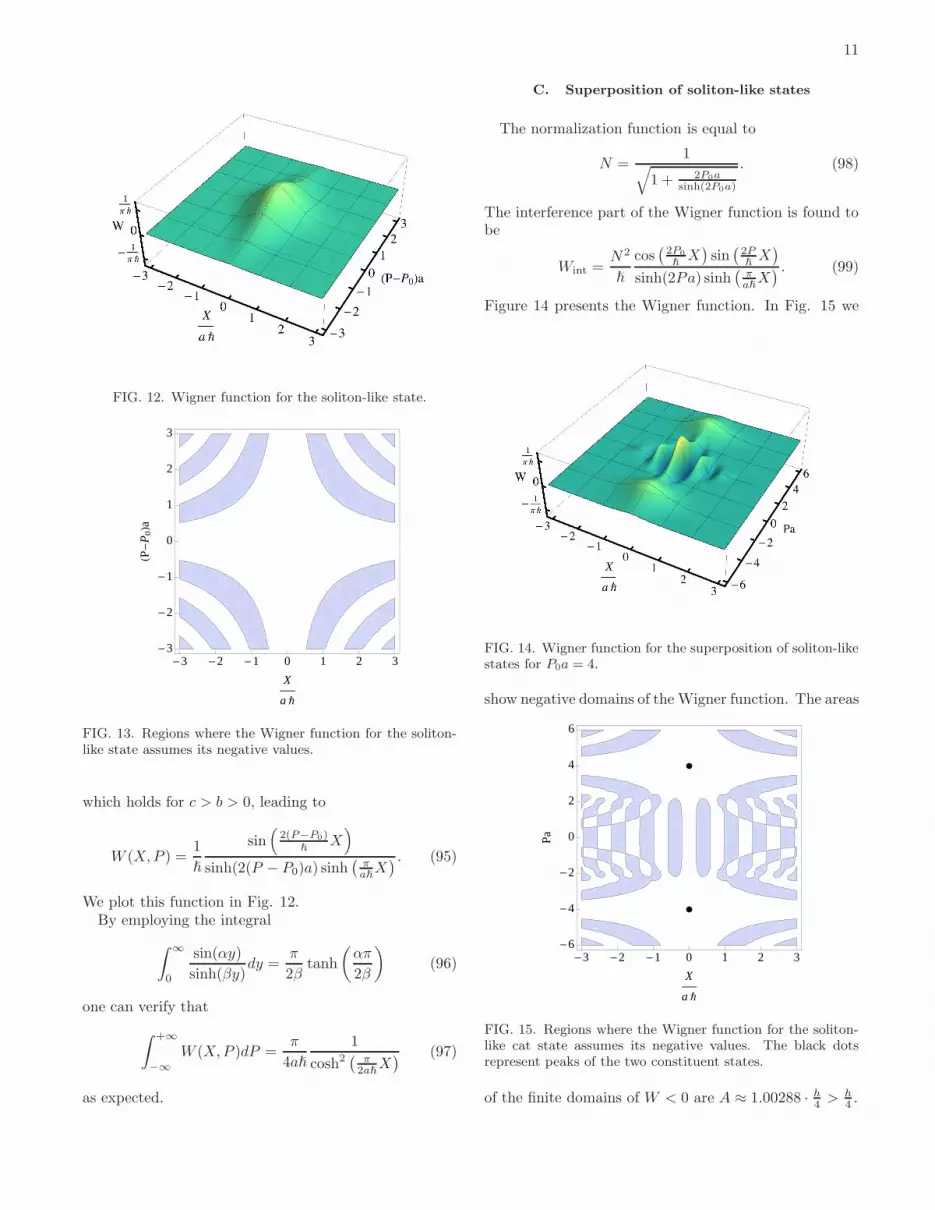
FIG. 12. Wigner function for the soliton-like state.

-3 -2 -1 0 1 2 3-3

-2

-1

0

1

2

3

X

a Ñ

HP-

P0L

a

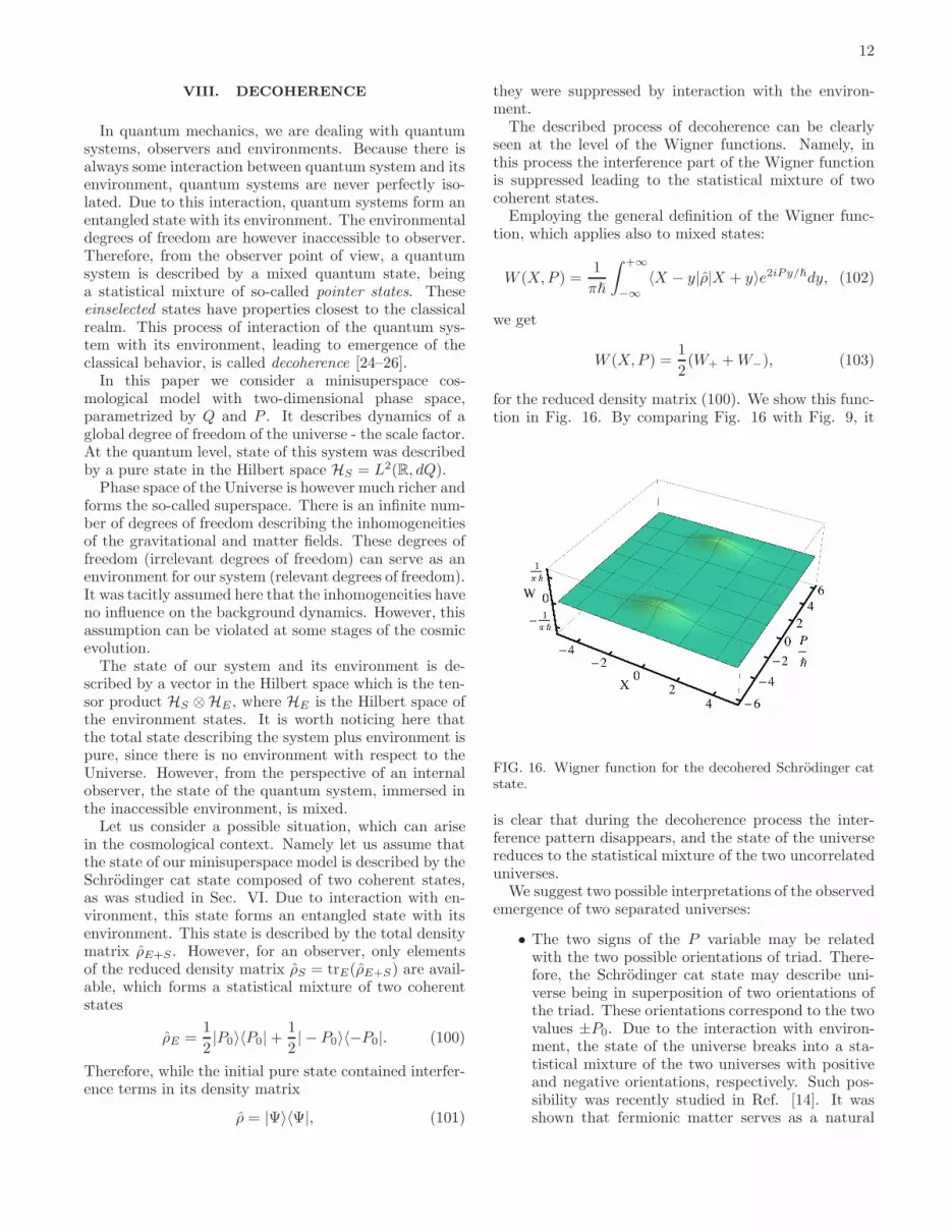
FIG. 13. Regions where the Wigner function for the soliton-like state assumes its negative values.

which holds for c > b > 0, leading to

W (X,P ) =1

ℏ

sin(

2(P−P0)ℏ

X)

sinh(2(P − P0)a) sinh(

πaℏX

) . (95)

We plot this function in Fig. 12.By employing the integral

∫ ∞

0

sin(αy)

sinh(βy)dy =

π

2βtanh

(απ

2β

)(96)

one can verify that

∫ +∞

−∞W (X,P )dP =

π

4aℏ

1

cosh2(

π2aℏX

) (97)

as expected.

C. Superposition of soliton-like states

The normalization function is equal to

N =1√

1 + 2P0asinh(2P0a)

. (98)

The interference part of the Wigner function is found tobe

Wint =N2

ℏ

cos(2P0

ℏX)

sin(2PℏX)

sinh(2Pa) sinh(

πaℏX

) . (99)

Figure 14 presents the Wigner function. In Fig. 15 we

FIG. 14. Wigner function for the superposition of soliton-likestates for P0a = 4.

show negative domains of the Wigner function. The areas

-3 -2 -1 0 1 2 3-6

-4

-2

0

2

4

6

X

a Ñ

Pa

FIG. 15. Regions where the Wigner function for the soliton-like cat state assumes its negative values. The black dotsrepresent peaks of the two constituent states.

of the finite domains of W < 0 are A ≈ 1.00288 · h4 >

h4 .

12

VIII. DECOHERENCE

In quantum mechanics, we are dealing with quantumsystems, observers and environments. Because there isalways some interaction between quantum system and itsenvironment, quantum systems are never perfectly iso-lated. Due to this interaction, quantum systems form anentangled state with its environment. The environmentaldegrees of freedom are however inaccessible to observer.Therefore, from the observer point of view, a quantumsystem is described by a mixed quantum state, beinga statistical mixture of so-called pointer states. Theseeinselected states have properties closest to the classicalrealm. This process of interaction of the quantum sys-tem with its environment, leading to emergence of theclassical behavior, is called decoherence [24–26].

In this paper we consider a minisuperspace cos-mological model with two-dimensional phase space,parametrized by Q and P . It describes dynamics of aglobal degree of freedom of the universe - the scale factor.At the quantum level, state of this system was describedby a pure state in the Hilbert space HS = L2(R, dQ).

Phase space of the Universe is however much richer andforms the so-called superspace. There is an infinite num-ber of degrees of freedom describing the inhomogeneitiesof the gravitational and matter fields. These degrees offreedom (irrelevant degrees of freedom) can serve as anenvironment for our system (relevant degrees of freedom).It was tacitly assumed here that the inhomogeneities haveno influence on the background dynamics. However, thisassumption can be violated at some stages of the cosmicevolution.

The state of our system and its environment is de-scribed by a vector in the Hilbert space which is the ten-sor product HS ⊗HE , where HE is the Hilbert space ofthe environment states. It is worth noticing here thatthe total state describing the system plus environment ispure, since there is no environment with respect to theUniverse. However, from the perspective of an internalobserver, the state of the quantum system, immersed inthe inaccessible environment, is mixed.

Let us consider a possible situation, which can arisein the cosmological context. Namely let us assume thatthe state of our minisuperspace model is described by theSchrodinger cat state composed of two coherent states,as was studied in Sec. VI. Due to interaction with en-vironment, this state forms an entangled state with itsenvironment. This state is described by the total densitymatrix ρE+S . However, for an observer, only elementsof the reduced density matrix ρS = trE(ρE+S) are avail-able, which forms a statistical mixture of two coherentstates

ρE =1

2|P0〉〈P0| +

1

2| − P0〉〈−P0|. (100)

Therefore, while the initial pure state contained interfer-ence terms in its density matrix

ρ = |Ψ〉〈Ψ|, (101)

they were suppressed by interaction with the environ-ment.

The described process of decoherence can be clearlyseen at the level of the Wigner functions. Namely, inthis process the interference part of the Wigner functionis suppressed leading to the statistical mixture of twocoherent states.

Employing the general definition of the Wigner func-tion, which applies also to mixed states:

W (X,P ) =1

πℏ

∫ +∞

−∞〈X − y|ρ|X + y〉e2iPy/ℏdy, (102)

we get

W (X,P ) =1

2(W+ +W−), (103)

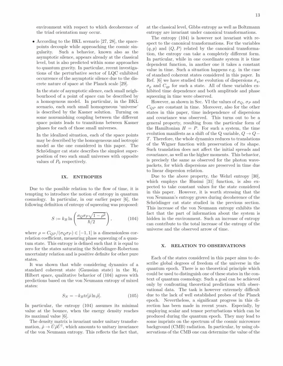
for the reduced density matrix (100). We show this func-tion in Fig. 16. By comparing Fig. 16 with Fig. 9, it

FIG. 16. Wigner function for the decohered Schrodinger catstate.

is clear that during the decoherence process the inter-ference pattern disappears, and the state of the universereduces to the statistical mixture of the two uncorrelateduniverses.

We suggest two possible interpretations of the observedemergence of two separated universes:

• The two signs of the P variable may be relatedwith the two possible orientations of triad. There-fore, the Schrodinger cat state may describe uni-verse being in superposition of two orientations ofthe triad. These orientations correspond to the twovalues ±P0. Due to the interaction with environ-ment, the state of the universe breaks into a sta-tistical mixture of the two universes with positiveand negative orientations, respectively. Such pos-sibility was recently studied in Ref. [14]. It wasshown that fermionic matter serves as a natural

13

environment with respect to which decoherence ofthe triad orientation may occur.

• According to the BKL scenario [27, 28], the space-points decouple while approaching the cosmic sin-gularity. Such a behavior, known also as theasymptotic silence, appears already at the classicallevel, but is also predicted within some approachesto quantum gravity. In particular, recent investiga-tions of the perturbative sector of LQC exhibitedoccurrence of the asymptotic silence due to the dis-crete nature of space at the Planck scale [29].

In the state of asymptotic silence, each small neigh-bourhood of a point of space can be described bya homogenous model. In particular, in the BKLscenario, each such small homogeneous ‘universe’is described by the Kasner solution. Turning onsome nonvanishing coupling between the differentspace points leads to transitions between Kasnerphases for each of those small universes.

In the idealized situation, each of the space pointsmay be described by the homogeneous and isotropicmodel as the one considered in this paper. TheSchrodinger cat state describes the simplest super-position of two such small universes with oppositevalues of P0 respectively.

IX. ENTROPIES

Due to the possible relation to the flow of time, it istempting to introduce the notion of entropy in quantumcosmology. In particular, in our earlier paper [6], thefollowing definition of entropy of squeezing was proposed:

S := kB ln

(σQσP

√1 − ρ2

ℏ/2

), (104)

where ρ = CQP /(σQσP ) ∈ [−1, 1] is a dimensionless cor-relation coefficient, measuring phase squeezing of a quan-tum state. This entropy is defined such that it is equal tozero for the states saturating the Schrodinger-Robertosnuncertainty relation and is positive definite for other purestates.

It was shown that while considering dynamics of astandard coherent state (Gaussian state) in the H1

Hilbert space, qualitative behavior of (104) agrees withpredictions based on the von Neumann entropy of mixedstates:

SN = −kBtr[ρ ln ρ]. (105)

In particular, the entropy (104) assumes its minimalvalue at the bounce, when the energy density reachesits maximal value [6].

The density matrix is invariant under unitary transfor-mation, ρ→ U ρU †, which amounts to unitary invarianceof the von Neumann entropy. This reflects the fact that,

at the classical level, Gibbs entropy as well as Boltzmannentropy are invariant under canonical transformations.

The entropy (104) is however not invariant with re-spect to the canonical transformations. For the variables(q, p) and (Q,P ) related by the canonical transforma-tion, the entropy can take a completely different form.In particular, while in one coordinate system it is timedependent function, in another one it takes a constantvalue in time. Such a situation happens e.g. in the caseof standard coherent states considered in this paper. InRef. [6] we have studied the evolution of dispersions σq,σp and Cqp for such a state. All of these variables ex-hibited time dependence and both amplitude and phasesqueezing in time were observed.

However, as shown in Sec. VI the values of σQ, σP andCQP are constant in time. Moreover, also for the otherstates in this paper, time independence of dispersionsand covariance was observed. This turns out to be ageneral property, resulting from the particular form ofthe Hamiltonian H = P . For such a system, the timeevolution manifests as a shift of the Q variable, Q→ Q−T . Therefore, the whole dynamics reduces to translationsof the Wigner function with preservation of its shape.Such translation does not affect the initial spreads andcovariance, as well as the higher moments. This behavior,is precisely the same as observed for the photon wave-packets, for which dispersions are preserved in time dueto linear dispersion relation.

Due to the above property, the Wehrl entropy [30],which employs the Husimi [31] function, is also ex-pected to take constant values for the state consideredin this paper. However, it is worth stressing that thevon Neumann’s entropy grows during decoherence of theSchrodinger cat state studied in the previous section.This increase of the von Neumann entropy exhibits thefact that the part of information about the system ishidden in the environment. Such an increase of entropycan contribute to the total increase of the entropy of theuniverse and the observed arrow of time.

X. RELATION TO OBSERVATIONS

Each of the states considered in this paper aims to de-scribe global degrees of freedom of the universe in thequantum epoch. There is no theoretical principle whichcould be used to distinguish one of these states in the con-text of quantum cosmology. Such a goal can be achievedonly by confronting theoretical predictions with obser-vational data. The task is however extremely difficultdue to the lack of well established probes of the Planckepoch. Nevertheless, a significant progress in this di-rection has been made in recent years. Especially, byemploying scalar and tensor perturbations which can beproduced during the quantum epoch. They may lead tosome imprints on the spectrum of the cosmic microwavebackground (CMB) radiation. In particular, by using ob-servations of the CMB one can determine the value of the

14

Hubble factor

H :=1

a

da

dt, (106)

during the phase of inflation, which follows the quantumepoch. This measurement can be used to put constraintson the quantum fluctuations of the Hubble factor in agiven state describing the Universe. Namely, we expectthat relative quantum fluctuations of the Hubble parame-

ter are smaller than the relative uncertainty of the mea-

surement. It means that:

σH

〈H〉<

∆HH , (107)

where H is the measured value of the Hubble parame-ter and ∆H is the uncertainty of the measurement. Asshown in Ref. [6], based on the seven years observa-tions of the WMAP satellite, uncertainty of the mea-surement of the Hubble at some fixed point of inflationis ∆H

H ≈ 0.19. Whereas, measurements of the present

value of the Hubble factor give us ∆HH ≈ 0.02. Both re-

sults are in agreement with our expectation that relativequantum fluctuations should satisfy

σH

〈H〉≪ 1. (108)

Such a restriction is usually considered as a condition ofsemi-classicality [32].

One can also interpret the above as a requirement ofthe correspondence principle. Namely, in the limit oflarge quantum numbers the quantum mechanics shouldreproduce classical dynamics. Here, the limit of the largequantum numbers corresponds to the limit of large vol-ume.

Based on the above we can guess, as confirmed by theastronomical observations, that the relative fluctuationsof the Hubble parameter may be used to indicate semi-classicality of the expanding universe. In what follows weuse this restriction to put constraints on the parametersof considered states of the universe.

The important observation is that in the limit of largevolumes (|p| → ∞, q → 0), the value of the parameter qis proportional to the Hubble factor: q = γλH. But thisis precisely where our observational constraints can beapplied. Therefore, in the considered limit, the constraint(107) leads to

σq〈q〉 <

∆HH . (109)

The task is now to determine the left hand side of theabove equation for the examined states in the limit q →0. Since we investigated properties of the states in theHilbert space H2, we have to express the parameter q interms of Q. Employing the definition (10), we can write

q = 2arctan(eX+T

)= ǫeX + O(ǫ3), (110)

where we have performed expansion in the parameterǫ = eT , which tends to zero in the limit T → −∞. Inthis limit q → 0.

Now we express the first and the second moment of thevariable q as follows:

〈q〉 = 2ǫ

∫ +∞

−∞eX |Ψ(X)|2dX + O(ǫ3), (111)

〈q2〉 = 4ǫ2∫ +∞

−∞e2X |Ψ(X)|2dX + O(ǫ4). (112)

Using the above expressions, the relative uncertainty ofq in the limit ǫ→ 0 can be written as

limǫ→0

σq〈q〉 = lim

ǫ→0

√〈q2〉〈q〉2 − 1

=

√√√√√

∫ +∞−∞ e2X |Ψ(X)|2dX

(∫ +∞−∞ eX |Ψ(X)|2dX

)2 − 1. (113)

The condition of semi-classicality (108) now states that:

limǫ→0

σq〈q〉 ≪ 1. (114)

In what follows, we will use this restriction to put con-straints on the parameters of our models.

A. Boxcar state

For the boxcar state, the following integrals can beeasily found:

∫ +∞

−∞eX |Ψ(X)|2dX =

2

Lsinh

(L

2

), (115)

∫ +∞

−∞e2X |Ψ(X)|2dX =

1

Lsinh(L). (116)

By applying those integrals to expression (113), we ob-tain

limǫ→0

σq〈q〉 =

√L/2

tanh(L/2)− 1. (117)

Employing the condition of semi-classicality (114) we ob-tain the following transcendental ineqality

2 tanh(L/2) ≫ L/2. (118)

This equation can be solved numerically leading to therestriction

L≪ 3.83. (119)

Only for such values the state reveals the correct semi-classical limit. As we see, by imposing the requirementof an agreement with the semi-classical behavior of theuniverse in the expanding branch, a dominant part of therange of the parameter L is excluded.

15

B. Schrodinger cat composed of boxcar states

For the Schrodinger cat composed of boxcar states, theformula (113) can be expressed as follows

limǫ→0

σq〈q〉 =

√eL(1 + 4P 2

0 )2(LP0 + sin(LP0))(P0 cosh(L) sin(LP0) + (1 + P 20 + cos(LP0)) sinh(L))

((P0 + P 30 )((−1 + eL)(1 + 4P 2

0 ) + (−1 + eL) cos(LP0) + 2(1 + eL)P0 sin(LP0))2)− 1, (120)

where P0 = P0/ℏ. This equation simplifies to (117),

in the limit P0 → 0. Based on equation (120), in Fig.17 we show the region of the parameter space for whichlimǫ→0

σq

〈q〉 < 1. In this region, relative quantum fluctua-

tions of the Hubble factor in the large volume limit aresmaller than unity. Therefore, only for the values of the

0 2 3.83 6 8 100

2

4

6

8

10

L

P0

Ñ

FIG. 17. Shadowed region of the parameter space representslimǫ→0

σq

〈q〉< 1, a necessary condition for semi-classicality,

which holds in a neighborhood of the origin.

parameters belonging to this region, the Schrodinger catcomposed of boxcar states has a semiclassical limit. Itis worth noticing that for P0/ℏ = 0, the obtained con-straints overlap with (119), as expected.

C. Standard coherent state

For the standard coherent state

∫ +∞

−∞eX |Ψ(X)|2dX = exp

[(2ℜa2 + 1)2

8ℜa1

], (121)

∫ +∞

−∞e2X |Ψ(X)|2dX = exp

[(2ℜa2 + 2)2

8ℜa1

]. (122)

Using these integrals we get

limǫ→0

σq〈q〉 =

√exp

[1 − 2(ℜa2)2

4ℜa1

]− 1. (123)

The condition of reality of the above expression togetherwith the requirement of semi-classicality can be writtenas

0 ≤ 1 − 2(ℜa2)2

4ℜa1≪ ln 2. (124)

Because ℜa1 > 0, the two conditions must hold:

(ℜa2)2≤ 1

2, (125)

ℜa1≫1 − 2(ℜa2)2

4 ln 2. (126)

For the special case ℜa2 = 0 (α = 0) we obtain

ℜa1 ≫ 1

4 ln 2, (127)

which yields the following constraint on dispersion

σQ ≪√

ln 2 ≈ 0.83. (128)

D. Schrodinger cat composed of standard coherent

states

For the Schrodinger’s cat state we have

∫ +∞

−∞eX |Ψ(X)|2dX =

= N2eℏ2α2

[1 + e−2P 2

0 α cos(P0αℏ)], (129)

∫ +∞

−∞e2X |Ψ(X)|2dX =

= N2e2ℏ2α[1 + e−2P 2

0 α cos(4P0αℏ)].

Based on the above we find

limǫ→0

σq〈q〉 =

√√√√eℏ2α

N2

[1 + e−2P 2

0 α cos(4P0αℏ)]

[1 + e−2P 2

0 α cos(P0αℏ)]2 − 1. (130)

16

In the limit P0 → 0, this equation simplifies to

limǫ→0

σq〈q〉 =

√eαℏ2 − 1. (131)

The semi-classicality condition (114) applied to (130)leads to the following constraint

eℏ2α

N2

[1 + e−2P 2

0 α cos(4P0αℏ)]

[1 + e−2P 2

0 α cos(P0αℏ)]2 ≪ 2. (132)

In Fig. 18 we show the region of the parameter space forwhich limǫ→0

σq

〈q〉 < 1, indicating the part of the param-

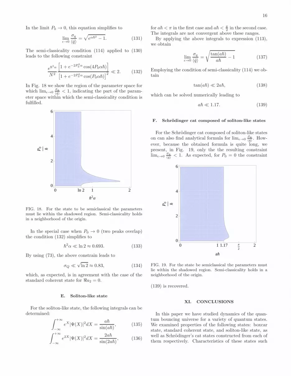
eter space within which the semi-classicality condition isfulfilled.

0 ln 2 1 20

2

4

6

Ñ2Α

P0

Ñ

FIG. 18. For the state to be semiclassical the parametersmust lie within the shadowed region. Semi-classicality holdsin a neighborhood of the origin.

In the special case when P0 → 0 (two peaks overlap)the condition (132) simplifies to

ℏ2α ≪ ln 2 ≈ 0.693. (133)

By using (73), the above constrain leads to

σQ ≪√

ln 2 ≈ 0.83, (134)

which, as expected, is in agreement with the case of thestandard coherent state for ℜa2 = 0.

E. Soliton-like state

For the soliton-like state, the following integrals can bedetermined:

∫ +∞

−∞eX |Ψ(X)|2dX =

a~

sin(a~), (135)

∫ +∞

−∞e2X |Ψ(X)|2dX =

2a~

sin(2a~), (136)

for a~ < π in the first case and a~ < π2 in the second case.

The integrals are not convergent above these ranges.By applying the above integrals to expression (113),

we obtain

limǫ→0

σq〈q〉 =

√tan(aℏ)

aℏ− 1 (137)

Employing the condition of semi-classicality (114) we ob-tain

tan(aℏ) ≪ 2aℏ, (138)

which can be solved numerically leading to

aℏ ≪ 1.17. (139)

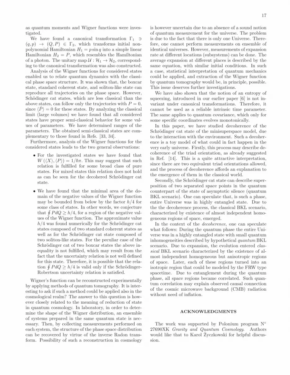
F. Schrodinger cat composed of soliton-like states

For the Schrodinger cat composed of soliton-like stateson can also find analytical formula for limǫ→0

σq

〈q〉 . How-

ever, because the obtained formula is quite long, wepresent, in Fig. 19, only the the resulting constraintlimǫ→0

σq

〈q〉 < 1. As expected, for P0 = 0 the constraint

0 1 1.17 Π

22

0

2

4

6

aÑ

P0

Ñ

FIG. 19. For the state be semiclassical the parameters mustlie within the shadowed region. Semi-classicality holds in aneighborhood of the origin.

(139) is recovered.

XI. CONCLUSIONS

In this paper we have studied dynamics of the quan-tum bouncing universe for a variety of quantum states.We examined properties of the following states: boxcarstate, standard coherent state, and soliton-like state, aswell as Schrodinger’s cat states constructed from each ofthem respectively. Characteristics of these states such

17

as quantum moments and Wigner functions were inves-tigated.

We have found a canonical transformation Γ1 ∋(q, p) → (Q,P ) ∈ Γ2, which transforms initial non-polynomial Hamiltonian H1 = p sin q into a simple linearHamiltonian H2 = P , which resembles the Hamiltonianof a photon. The unitary map U : H1 → H2, correspond-ing to the canonical transformation was also constructed.

Analysis of the Wigner functions for considered statesenabled us to relate quantum dynamics with the classi-cal phase space structure. It was shown that, the boxcarstate, standard coherent state, and soliton-like state canreproduce all trajectories on the phase space. However,Schodinger cat states, which are less classical than theabove states, can follow only the trajectories with P = 0,since 〈P 〉 = 0 for these states. By analyzing the classicallimit (large volumes) we have found that all consideredstates have proper semi-classical behavior for some val-ues of parameters. We have determined ranges of theparameters. The obtained semi-classical states are com-plementary to those found in Refs. [33, 34].

Furthermore, analysis of the Wigner functions for theconsidered states leads to the two general observations:

• For the investigated states we have found thatW (〈X〉, 〈P 〉) = 1/ℏπ. This may suggest that suchrelation is fulfilled for some broad class of purestates. For mixed states this relation does not holdas can be seen for the decohered Schrodinger catstate.

• We have found that the minimal area of the do-main of the negative values of the Wigner functionmay be bounded from below by the factor h/4 forsome class of states. In other words, we conjecturethat

∮PdQ ≥ h/4, for a region of the negative val-

ues of the Wigner function. The approximate valueh/4 was found numerically for the Schrodinger catstates composed of two standard coherent states aswell as for the Schrodinger cat state composed oftwo soliton-like states. For the peculiar case of theSchrodinger cat of two boxcar states the above in-equality is not fulfilled, which may result from thefact that the uncertainty relation is not well definedfor this state. Therefore, it is possible that the rela-tion

∮PdQ ≥ h/4 is valid only if the Schrodinger-

Robertson uncertainty relation is satisfied.

Wigner’s function can be reconstructed experimentallyby applying methods of quantum tomography. It is inter-esting to ask if such a method could be applied also in thecosmological realm? The answer to this question is how-ever closely related to the meaning of reduction of statein quantum cosmology. In laboratory, in order to deter-mine the shape of the Wigner distribution, an ensembleof systems prepared in the same quantum state is nec-essary. Then, by collecting measurements performed oneach system, the structure of the phase space distributioncan be recovered by virtue of the inverse Radon trans-form. Possibility of such a reconstruction in cosmology

is however uncertain due to an absence of a sound notionof quantum measurement for the universe. The problemis due to the fact that there is only one Universe. There-fore, one cannot perform measurements on ensemble ofidentical universes. However, measurements of expansionrate at different locations (subsystems) can be done. Theaverage expansion at different places is described by thesame equation, with similar initial conditions. In sucha case, statistical interpretation of quantum mechanicscould be applied, and extraction of the Wigner functionby quantum tomography would be, in principle, possible.This issue deserves further investigations.

We have also shown that the notion of an entropy ofsqueezing, introduced in our earlier paper [6] is not in-variant under canonical transformations. Therefore, itcannot be used as a reliable intrinsic time parameter.The same applies to quantum covariance, which only forsome specific coordinates evolves monotonically.

In this paper, we have studied decoherence of theSchrodinger cat state of the minisuperspace model, dueto the interaction with the environment. Such a decoher-ence is a toy model of what could in fact happen in thevery early universe. Firstly, this process may describe de-coherence of the triad orientation, as already suggestedin Ref. [14]. This is a quite attractive interpretation,since there are two equivalent triad orientations allowed,and the process of decoherence affords an explanation tothe emergence of them in the classical world.

Secondly, the Schrodinger cat state can describe super-position of two separated space points in the quantumcounterpart of the state of asymptotic silence (quantumBKL scenario). One can speculate that, is such a phase,entire Universe was in highly entangled state. Due tothe the decoherence process, the classical BKL scenario,characterized by existence of almost independent homo-geneous regions of space, emerged.

In the context of the decoherence, one can speculatewhat follows: During the quantum phase the entire Uni-verse was in a highly entangled state with small quantuminhomogeneities described by hypothetical quantum BKLscenario. Due to expansion, the evolution entered clas-

sical BKL scenario characterized by the existence of al-most independent homogeneous but anisotropic regionsof space. Later, each of these regions turned into anisotropic region that could be modeled by the FRW typespacetime. Due to entanglement during the quantumphase, all space regions became correlated. Such quan-tum correlation may explain observed causal connectionof the cosmic microwave background (CMB) radiationwithout need of inflation.

ACKNOWLEDGMENTS

The work was supported by Polonium program N◦

27690XK Gravity and Quantum Cosmology. Authorswould like that to Karol Zyczkowski for helpful discus-sion.

18

[1] A. Ashtekar and P. Singh, “Loop Quantum Cosmology:A Status Report,” Class. Quant. Grav. 28 (2011) 213001[arXiv:1108.0893 [gr-qc]].

[2] M. Bojowald, “Loop quantum cosmology”, Living Rev.Rel. 8 (2005) 11.

[3] P. Dzierzak, P. Malkiewicz and W. Piechocki, “Turningbig bang into big bounce. 1. Classical dynamics”, Phys.Rev. D 80 (2009) 104001 [arXiv:0907.3436 [gr-qc]].

[4] P. Malkiewicz and W. Piechocki, “Turning big bang intobig bounce: II. Quantum dynamics”, Class. Quant. Grav.27 (2010) 225018 [arXiv:0908.4029 [gr-qc].

[5] J. Mielczarek and W. Piechocki, “Evolution in bounc-ing quantum cosmology”, Class. Quant. Grav. 29 (2012)065022 [arXiv:1107.4686 [gr-qc]].

[6] J. Mielczarek and W. Piechocki, “Gaussian state for thebouncing quantum cosmology”, Phys. Rev. D 86 (2012)083508 [arXiv:1108.0005 [gr-qc]].

[7] K. A. Meissner, “Black hole entropy in loop quan-tum gravity,” Class. Quant. Grav. 21 (2004) 5245[gr-qc/0407052].

[8] M. Bojowald, “What happened before the Big Bang?”,Nature Phys. 3N8 (2007) 523.

[9] Authors are grateful to Antonia Zipfel for pointing outthe possibility of such a behavior.

[10] A. Perelomov, Generalized coherent states and their ap-

plications, (Berlin: Springer, 1986).[11] J.-P. Gazeau, Coherent States in Quantum Physics

(Berlin: Wiley-VCH, 2009).[12] J. S. Walker, A Primer on Wavelets and Their Scientific

Applications, Sd Edition (Studies in Advanced Mathe-matics), (Chapman and Hall/CRC, 2008).

[13] A. Ourjoumtsev, H. Jeong, Rosa Tualle-Brouri and P.Grangier, “Generation of optical ‘Schrodinger cats’ fromphoton number states”, Nature 448 (2007) 784.

[14] C. Kiefer and C. Schell, “Interpretation of the triad ori-entations in loop quantum cosmology”, arXiv:1210.0418[gr-qc].

[15] A. Kenfeck and K. Zyczkowski, “Negativity of theWigner function as an indicator of nonclassicality”, J.Opt. B: Quantum Semiclass. Opt. 6 (2004) 396.

[16] R. L. Hudson, “When is the Wigner quasi-probabilitydensity non-negative?,” Rep. Math. Phys. 6 (1974) 249.

[17] T. Brocker and R. F. Werner, “Mixed states with positiveWigner functions,” J. Math. Phys. 36 (1995) 62.

[18] W. P. Schleich, Quantum Optics in Phase Space (Berlin:Wiley-VCH, 2001).

[19] C. K. Zachos, D. B. Fairlie, and T. L. Curtright (eds)Quantum Mechanics In Phase Space, World Scientific Se-ries in 20th Century Physics 34 (World Scientific 2006).

[20] C. Becker et al “Oscillations and interactions of dark anddark-bright solitons in Bose-Einstein condensates”, Na-ture Physics 4 (2008) 496501.

[21] L. Khaykovich et al. “Formation of a Matter-Wave BrightSoliton”, Science 296 (2002) 1290.

[22] S. L. Cornish, S. T. Thompson, and C. E. Wieman, “For-mation of Bright Matter-Wave Solitons during the Col-lapse of Attractive Bose-Einstein Condensates”, Phys.Rev. Lett. 96 (2006) 170401.

[23] I. S. Gradshteyn and I. M. Ryzhik, Table of Integrals,

Series, and Products (Alan Jeffrey, 1994), Fifth edition.[24] W. H. Zurek, “Decoherence and the transition from

quantum to classical”, Phys. Today 44N10 (1991) 36.[25] W. H. Zurek, “Decoherence, einselection, and the quan-

tum origins of the classical”, Rev. Mod. Phys. 75 (2003)715.

[26] W. H. Zurek, S. Habib and J. P. Paz, “Coherent statesvia decoherence”, Phys. Rev. Lett. 70 (1993) 1187.

[27] V. A. Belinskii, I. M. Khalatnikov and E. M. Lifshitz,“Oscillatory approach to a singular point in the relativis-tic cosmology”, Adv. Phys. 19 (1970) 525.

[28] V. A. Belinskii, I. M. Khalatnikov and E. M. Lifshitz, “Ageneral solution of the Einstein equations with a timesingularity”, Adv. Phys. 31 (1982) 639.

[29] J. Mielczarek, “Asymptotic silence in loop quan-tum cosmology,” AIP Conf. Proc. 1514 (2012) 81[arXiv:1212.3527 [gr-qc]].

[30] A. Wehrl, “General properties of entropy”, Rev. Mod.Phys. 50 (1978) 221.

[31] K. Husimi, “Some Formal Properties of the Density Ma-trix”, Proc. Phys. Math. Soc. Jpn. 22 (1940) 264314.

[32] A. Corichi and P. Singh, “Quantum bounce and cos-mic recall,” Phys. Rev. Lett. 100 (2008) 161302[arXiv:0710.4543 [gr-qc]].

[33] A. Corichi and E. Montoya, “Coherent semiclassicalstates for loop quantum cosmology,” Phys. Rev. D 84

(2011) 044021 [arXiv:1105.5081 [gr-qc]].[34] A. Corichi and E. Montoya, “On the Semiclassical Limit

of Loop Quantum Cosmology,” Int. J. Mod. Phys. D 21

(2012) 1250076 [arXiv:1105.2804 [gr-qc]].