quantitative interpretation of toc in complicated lithology
TRANSCRIPT
applied sciences
Article
Quantitative Interpretation of TOC in Complicated LithologyBased on Well Log Data: A Case of Majiagou Formation in theEastern Ordos Basin, China
Shuiqing Hu 1, Haowei Zhang 2, Rongji Zhang 3, Lingxuan Jin 2 and Yuming Liu 2,4,*
�����������������
Citation: Hu, S.; Zhang, H.; Zhang,
R.; Jin, L.; Liu, Y. Quantitative
Interpretation of TOC in Complicated
Lithology Based on Well Log Data: A
Case of Majiagou Formation in the
Eastern Ordos Basin, China. Appl. Sci.
2021, 11, 8724. https://doi.org/
10.3390/app11188724
Academic Editor: Kun Sang Lee
Received: 19 August 2021
Accepted: 14 September 2021
Published: 18 September 2021
Publisher’s Note: MDPI stays neutral
with regard to jurisdictional claims in
published maps and institutional affil-
iations.
Copyright: © 2021 by the authors.
Licensee MDPI, Basel, Switzerland.
This article is an open access article
distributed under the terms and
conditions of the Creative Commons
Attribution (CC BY) license (https://
creativecommons.org/licenses/by/
4.0/).
1 Research Institute of Petroleum Exploration & Development, Beijing 100083, China;[email protected]
2 College of Geosciences, China University of Petroleum-Beijing, Beijing 102249, China;[email protected] (H.Z.); [email protected] (L.J.)
3 Dagang Oil Field, China National Petroleum Corporation, Tianjin 300280, China; [email protected] State Key Laboratory of Petroleum Resources and Prospecting, China University of Petroleum-Beijing,
Beijing 102249, China* Correspondence: [email protected]
Abstract: Source rock evaluation plays a key role in studies of hydrocarbon accumulation andresource potential. Total organic carbon (TOC) is the basis of source rock evaluation and it is a keyparameter that influences petroleum resource assessment. The Majiagou formation in the easternOrdos Basin has complicated lithology and low abundance of organic matters. There are differentopinions over the existence of scale source rocks. Due to inadequate laboratory data of TOC in theOrdos Basin, it is difficult to accurately describe source rocks in the region; thus, log interpretation ofTOC is needed. In this study, the neural network model in the artificial intelligence (AI) field wasintroduced into the TOC logging interpretation. Compared with traditional ∆logR methods, sampleoptimization, logging correlation analysis and comparative optimization of computational methodswere carried out successively by using measured TOC data and logging data. Results show that theneural network model has good prediction effect in complicated lithologic regions and it can identifyvariations of TOC in continuous strata accurately regardless of the quick lithologic changes.
Keywords: complicated lithology; neural network; TOC logging calculation
1. Introduction
Total organic carbon (TOC) content is an important index to evaluate source rock in oil–gas exploration. On the one hand, there are limited measured data of TOC. Measured dataof TOC are from laboratory coring analysis and the limited core samples and experimentalcost leads to the inadequate TOC data. On the other hand, source rock shows strongheterogeneity. There’s a substantial error between TOC data gained by traditional methodsand the real TOC data. Such errors cannot meet requirements of source rock evaluation.
Schmoker et al. [1] pointed out that TOC content has linear relations with densitylogging (Schmoker, 1979) and gamma-ray logging (Schmoker, 1981), and TOC content canbe calculated by density and gamma logging. Chen et al. [2] calculated TOC of sourcerock in carbonate formation by establishing an interpretation formula between naturalgamma-ray logging and TOC of source rock, which achieved a good interpretation effect.When studying the Pearl River Mouth Basin, Xu et al. [3] found that the interpretation effectof TOC based on multiple logging parameters was significantly better than that based on asingle logging parameter. Du et al. [4] calculated TOC contents by using the single loggingparameter interpretation method and multi-logging parameter interpretation method. Theyalso concluded that the interpretation effect based on multiple logging parameters wasbetter than that based on single logging parameter and the multi-parameter regressivecalculation accuracy increased with the increase of logging parameter types. Exxon and
Appl. Sci. 2021, 11, 8724. https://doi.org/10.3390/app11188724 https://www.mdpi.com/journal/applsci
Appl. Sci. 2021, 11, 8724 2 of 18
Esso proposed the overlapping method of interval transit time and resistivity curve in1979, that is, ∆logR analytical method. The porosity curve and resistivity curve wereoverlapped to identify source rocks through the amplitude differences between two curves.Passey et al. [5] proposed the calculation formula of TOC based on data statistics:
TOC = (∆logR) × 10α (1)
α = 2.297 − 0.1688 LOM (2)
∆logR = lg(R/Rbase) + K·(∆t − ∆tbase) (3)
where Rbase and ∆tbase are baseline values of resistivity and interval transit time, respectively.K is the proportionality coefficient and LOM is the maturity of organic matters. This is therelatively common ∆log R method present being used. Although the ∆log R method hasstrong applicability, it needs artificial determination of logging baselines. Baselines varysignificantly in different wells as well as different strata and sedimentary environments [6].
More and more scholars believe that the linear relationship between TOC of sourcecarbon and logging parameters is not simple and it is difficult to be reflected by an explicitfunction [7–9]. The neural network model possesses remarkable advantages in addressingnonlinear problems, which cannot be expressed in explicit functions. Hence, neural networkmodelling becomes a new way for TOC logging interpretation of source rock [10,11].Neural networks have obvious advantages in TOC logging interpretation of source rock.Its interpretation result not only conforms well to laboratory analysis data, but also canretain detailed changes of TOC. However, TOC logging interpretation of source rockbased on neural networks has complicated principles and requires professional softwareprogramming, which determines the high threshold of applications. The operation iscompleted automatically by software, without any disclosure of details. As a result, TOClogging interpretation of source rock based on neural networks is difficult to be promoted.
Recently, many new TOC log interpretation methods have been proposed. Li [12],Rui [13], Amosu [14] and Liu [15] carried out TOC log interpretation using SVM. Zhao [16]and Yin Mei et al. [17] introduced the optimal estimation and Bayesian discriminant intoTOC log interpretation. Yu [6] and Rui [18] interpreted TOC of source rock throughGaussian regression. Although there are many TOC log interpretation methods of sourcerock, no method is universally applicable. The optimal TOC log interpretation methodshall be chosen according to practical conditions of the study area.
2. Geological Background
The Ordos Basin is the second largest sedimentary basin in China, with a basin areaof about 25 × 104 km2. This basin is a multicycle sedimentary Craton petroliferous basinwith stable sedimentation, migrating depression and obvious torsion. It is a polybasiccompound sedimentary basin of Meso–Cenozoic and Proterozoic and Paleozoic rocks [19].
The Ordos Basin has two sets of source rocks, including the Upper Paleozoic marine-continental transitional coal series and Lower Paleozoic marine carbonate rocks. There aresufficient gas sources [20].
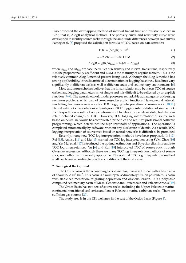
The study area is in the LT1 well area in the east of the Ordos Basin (Figure 1).
Appl. Sci. 2021, 11, 8724 3 of 18Appl. Sci. 2021, 11, x FOR PEER REVIEW 3 of 19
Figure 1. Location map of the study area.
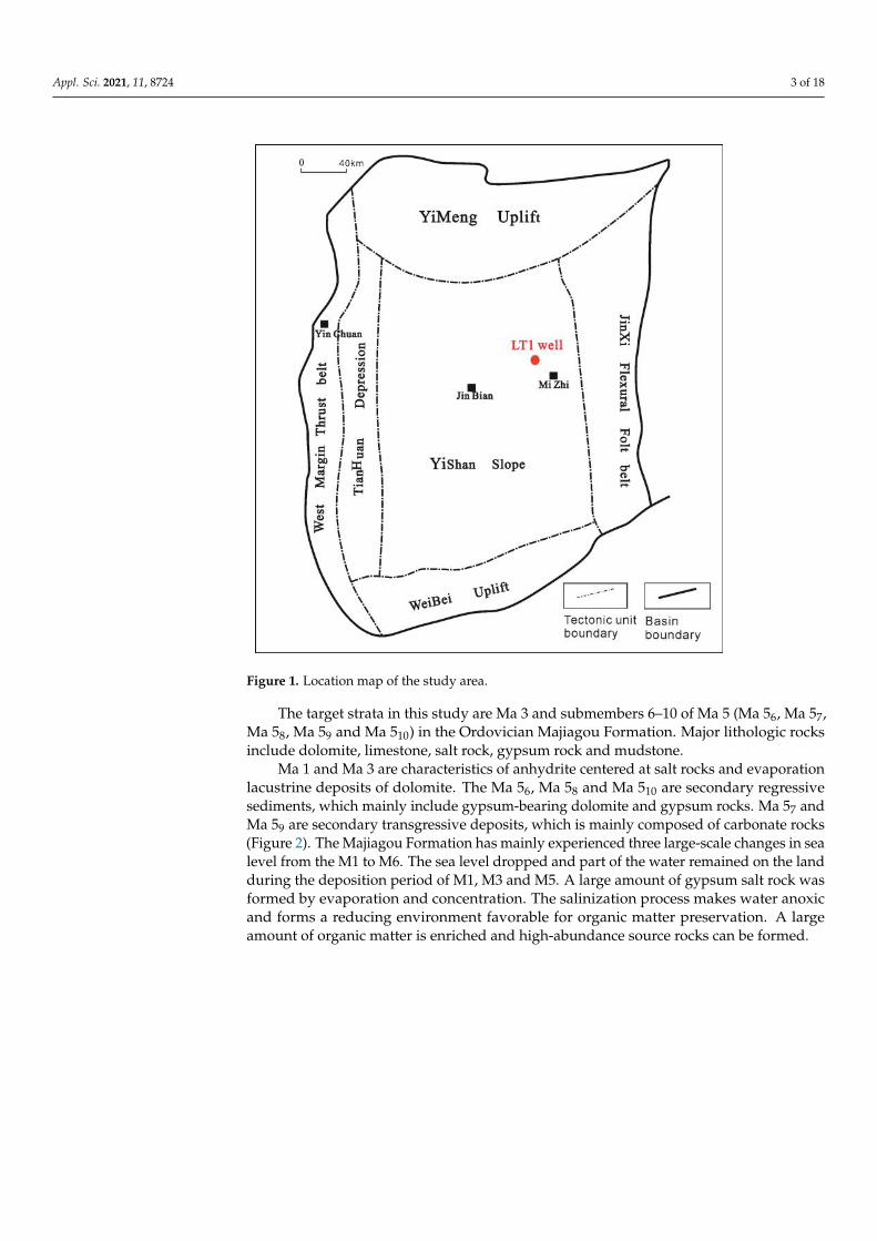
The target strata in this study are Ma 3 and submembers 6–10 of Ma 5 (Ma 56, Ma 57,
Ma 58, Ma 59 and Ma 510) in the Ordovician Majiagou Formation. Major lithologic rocks
include dolomite, limestone, salt rock, gypsum rock and mudstone.
Ma 1 and Ma 3 are characteristics of anhydrite centered at salt rocks and evaporation
lacustrine deposits of dolomite. The Ma 56, Ma 58 and Ma 510 are secondary regressive
sediments, which mainly include gypsum-bearing dolomite and gypsum rocks. Ma 57 and
Ma 59 are secondary transgressive deposits, which is mainly composed of carbonate rocks
(Figure 2). The Majiagou Formation has mainly experienced three large-scale changes in
sea level from the M1 to M6. The sea level dropped and part of the water remained on the
land during the deposition period of M1, M3 and M5. A large amount of gypsum salt rock
was formed by evaporation and concentration. The salinization process makes water an-
oxic and forms a reducing environment favorable for organic matter preservation. A large
amount of organic matter is enriched and high-abundance source rocks can be formed.
Figure 1. Location map of the study area.
The target strata in this study are Ma 3 and submembers 6–10 of Ma 5 (Ma 56, Ma 57,Ma 58, Ma 59 and Ma 510) in the Ordovician Majiagou Formation. Major lithologic rocksinclude dolomite, limestone, salt rock, gypsum rock and mudstone.
Ma 1 and Ma 3 are characteristics of anhydrite centered at salt rocks and evaporationlacustrine deposits of dolomite. The Ma 56, Ma 58 and Ma 510 are secondary regressivesediments, which mainly include gypsum-bearing dolomite and gypsum rocks. Ma 57 andMa 59 are secondary transgressive deposits, which is mainly composed of carbonate rocks(Figure 2). The Majiagou Formation has mainly experienced three large-scale changes in sealevel from the M1 to M6. The sea level dropped and part of the water remained on the landduring the deposition period of M1, M3 and M5. A large amount of gypsum salt rock wasformed by evaporation and concentration. The salinization process makes water anoxicand forms a reducing environment favorable for organic matter preservation. A largeamount of organic matter is enriched and high-abundance source rocks can be formed.
Appl. Sci. 2021, 11, 8724 4 of 18Appl. Sci. 2021, 11, x FOR PEER REVIEW 4 of 19
Figure 2. Formation histogram of Majiagou Formation in the eastern Ordos Basin.
3. Data Preparation
3.1. Optimal Sampling
Source rocks in the Majiagou Formation in the Ordos Basin mainly include the thin-
layered dark dolomite mudstones and argillaceous dolomite. The LT1 well has full-section
coring and plenty of TOC measured data. There are relatively complete conventional log-
ging data, including natural gamma, interval transit time, neutron porosity, density and
resistivity. Therefore, the core of LT1 well in the eastern Ordos Basin was chosen and log-
ging data were used as the basic data. After core location and logging normalization, 309
TOC measured data and corresponding logging data were gained.
During the sedimentary period of the Majiagou Formation in the eastern Ordos Ba-
sin, sea level changed frequently, thus resulting in the very complicated lithology and
common thin interbedded formations. It can be seen from Figure 3 that gypsum rock and
dolomite are in thin alternating deposit and thickness of some lithologic strata is smaller
than 1 cm, lower than the logging resolution. Although core lithology changes, the logging
curve shows no obvious responses, thus causing mismatching rock–electricity relations.
Although there’s relatively high TOC in some thin strata, they are too thin to generate
obvious logging responses (Figure 3).
Figure 2. Formation histogram of Majiagou Formation in the eastern Ordos Basin.
3. Data Preparation3.1. Optimal Sampling
Source rocks in the Majiagou Formation in the Ordos Basin mainly include the thin-layered dark dolomite mudstones and argillaceous dolomite. The LT1 well has full-sectioncoring and plenty of TOC measured data. There are relatively complete conventionallogging data, including natural gamma, interval transit time, neutron porosity, densityand resistivity. Therefore, the core of LT1 well in the eastern Ordos Basin was chosen andlogging data were used as the basic data. After core location and logging normalization,309 TOC measured data and corresponding logging data were gained.
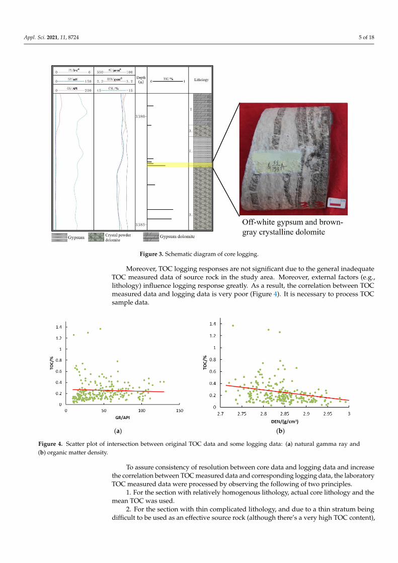
During the sedimentary period of the Majiagou Formation in the eastern Ordos Basin,sea level changed frequently, thus resulting in the very complicated lithology and commonthin interbedded formations. It can be seen from Figure 3 that gypsum rock and dolomiteare in thin alternating deposit and thickness of some lithologic strata is smaller than1 cm, lower than the logging resolution. Although core lithology changes, the loggingcurve shows no obvious responses, thus causing mismatching rock–electricity relations.Although there’s relatively high TOC in some thin strata, they are too thin to generateobvious logging responses (Figure 3).
Appl. Sci. 2021, 11, 8724 5 of 18
Appl. Sci. 2021, 11, x FOR PEER REVIEW 5 of 19
Moreover, TOC logging responses are not significant due to the general inadequate
TOC measured data of source rock in the study area. Moreover, external factors (e.g., li-
thology) influence logging response greatly. As a result, the correlation between TOC
measured data and logging data is very poor (Figure 4). It is necessary to process TOC
sample data.
Figure 3. Schematic diagram of core logging.
(a) (b)
Figure 4. Scatter plot of intersection between original TOC data and some logging data: (a) natural gamma ray and (b)
organic matter density.
To assure consistency of resolution between core data and logging data and increase
the correlation between TOC measured data and corresponding logging data, the labora-
tory TOC measured data were processed by observing the following of two principles.
1. For the section with relatively homogenous lithology, actual core lithology and the
mean TOC was used.
2. For the section with thin complicated lithology, and due to a thin stratum being
difficult to be used as an effective source rock (although there’s a very high TOC content),
Figure 3. Schematic diagram of core logging.
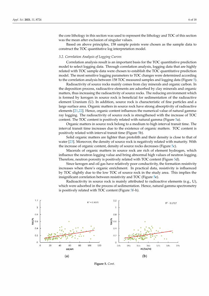
Moreover, TOC logging responses are not significant due to the general inadequateTOC measured data of source rock in the study area. Moreover, external factors (e.g.,lithology) influence logging response greatly. As a result, the correlation between TOCmeasured data and logging data is very poor (Figure 4). It is necessary to process TOCsample data.
Appl. Sci. 2021, 11, x FOR PEER REVIEW 5 of 19
Moreover, TOC logging responses are not significant due to the general inadequate
TOC measured data of source rock in the study area. Moreover, external factors (e.g., li-
thology) influence logging response greatly. As a result, the correlation between TOC
measured data and logging data is very poor (Figure 4). It is necessary to process TOC
sample data.
Figure 3. Schematic diagram of core logging.
(a) (b)
Figure 4. Scatter plot of intersection between original TOC data and some logging data: (a) natural gamma ray and (b)
organic matter density.
To assure consistency of resolution between core data and logging data and increase
the correlation between TOC measured data and corresponding logging data, the labora-
tory TOC measured data were processed by observing the following of two principles.
1. For the section with relatively homogenous lithology, actual core lithology and the
mean TOC was used.
2. For the section with thin complicated lithology, and due to a thin stratum being
difficult to be used as an effective source rock (although there’s a very high TOC content),
Figure 4. Scatter plot of intersection between original TOC data and some logging data: (a) natural gamma ray and(b) organic matter density.
To assure consistency of resolution between core data and logging data and increasethe correlation between TOC measured data and corresponding logging data, the laboratoryTOC measured data were processed by observing the following of two principles.
1. For the section with relatively homogenous lithology, actual core lithology and themean TOC was used.
2. For the section with thin complicated lithology, and due to a thin stratum beingdifficult to be used as an effective source rock (although there’s a very high TOC content),
Appl. Sci. 2021, 11, 8724 6 of 18
the core lithology in this section was used to represent the lithology and TOC of this sectionwas the mean after exclusion of singular values.
Based on above principles, 158 sample points were chosen as the sample data toconstruct the TOC quantitative log interpretation model.
3.2. Correlation Analysis of Logging Curves
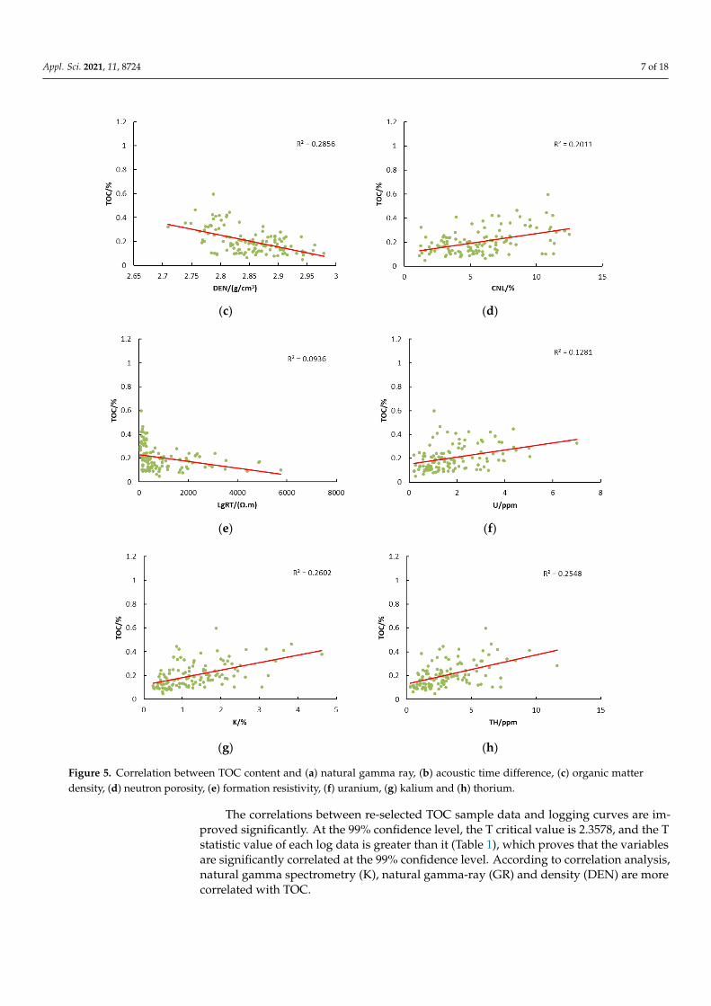
Correlation analysis result is an important basis for the TOC quantitative predictionmodel to select logging data. Through correlation analysis, logging data that are highlyrelated with TOC sample data were chosen to establish the TOC quantitative predictionmodel. The most sensitive logging parameters to TOC changes were determined accordingto the correlation analysis between 158 TOC measured samples and logging data (Figure 5).
Radioactivity of source rocks mainly comes from clay minerals and organic carbon. Inthe deposition process, radioactive elements are adsorbed by clay minerals and organicmatters, thus increasing the radioactivity of source rocks. The reducing environment whichis formed by kerogen in source rock is beneficial for sedimentation of the radioactiveelement Uranium (U). In addition, source rock is characteristic of fine particles and alarge surface area. Organic matters in source rock have strong absorptivity of radioactiveelements [21,22]. Hence, organic content influences the numerical value of natural gamma-ray logging. The radioactivity of source rock is strengthened with the increase of TOCcontent. The TOC content is positively related with natural gamma (Figure 5a).
Organic matters in source rock belong to a medium to high interval transit time. Theinterval transit time increases due to the existence of organic matters. TOC content ispositively related with interval transit time (Figure 5b).
Solid organic matters are lighter than protolith and their density is close to that ofwater [23]. Moreover, the density of source rock is negatively related with maturity. Withthe increase of organic content, density of source rocks decreases (Figure 5c).
Macerals of organic matters in source rock are rich of element hydrogen, whichinfluence the neutron logging value and bring abnormal high values of neutron logging.Therefore, neutron porosity is positively related with TOC content (Figure 5d).
Since kerogen and oil gas have relatively poor conductivity, the formation resistivityincreases when there’s organic enrichment. In practical data, resistivity is influencedby TOC slightly due to the low TOC of source rock in the study area. This implies theinsignificant correlation between resistivity and TOC (Figure 5e).
Radioactivity in source rock is mainly attributed to radioactive elements (e.g., U),which were adsorbed in the process of sedimentation. Hence, natural gamma spectrometryis positively related with TOC content (Figure 5f–h).
Appl. Sci. 2021, 11, x FOR PEER REVIEW 6 of 19
the core lithology in this section was used to represent the lithology and TOC of this sec-
tion was the mean after exclusion of singular values.
Based on above principles, 158 sample points were chosen as the sample data to con-
struct the TOC quantitative log interpretation model.
3.2. Correlation Analysis of Logging Curves
Correlation analysis result is an important basis for the TOC quantitative prediction
model to select logging data. Through correlation analysis, logging data that are highly
related with TOC sample data were chosen to establish the TOC quantitative prediction
model. The most sensitive logging parameters to TOC changes were determined accord-
ing to the correlation analysis between 158 TOC measured samples and logging data (Fig-
ure 5).
Radioactivity of source rocks mainly comes from clay minerals and organic carbon.
In the deposition process, radioactive elements are adsorbed by clay minerals and organic
matters, thus increasing the radioactivity of source rocks. The reducing environment
which is formed by kerogen in source rock is beneficial for sedimentation of the radioac-
tive element Uranium (U). In addition, source rock is characteristic of fine particles and a
large surface area. Organic matters in source rock have strong absorptivity of radioactive
elements [21,22]. Hence, organic content influences the numerical value of natural
gamma-ray logging. The radioactivity of source rock is strengthened with the increase of
TOC content. The TOC content is positively related with natural gamma (Figure 5a).
Organic matters in source rock belong to a medium to high interval transit time. The
interval transit time increases due to the existence of organic matters. TOC content is pos-
itively related with interval transit time (Figure 5b).
Solid organic matters are lighter than protolith and their density is close to that of
water [23]. Moreover, the density of source rock is negatively related with maturity. With
the increase of organic content, density of source rocks decreases (Figure 5c).
Macerals of organic matters in source rock are rich of element hydrogen, which in-
fluence the neutron logging value and bring abnormal high values of neutron logging.
Therefore, neutron porosity is positively related with TOC content (Figure 5d).
Since kerogen and oil gas have relatively poor conductivity, the formation resistivity
increases when there’s organic enrichment. In practical data, resistivity is influenced by
TOC slightly due to the low TOC of source rock in the study area. This implies the insig-
nificant correlation between resistivity and TOC (Figure 5e).
Radioactivity in source rock is mainly attributed to radioactive elements (e.g., U),
which were adsorbed in the process of sedimentation. Hence, natural gamma spectrome-
try is positively related with TOC content (Figure 5f–h).
(a) (b)
Figure 5. Cont.
Appl. Sci. 2021, 11, 8724 7 of 18Appl. Sci. 2021, 11, x FOR PEER REVIEW 7 of 19
(c) (d)
(e) (f)
(g) (h)
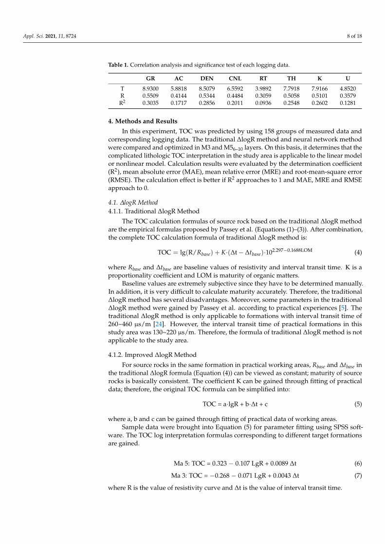
Figure 5. Correlation between TOC content and (a) natural gamma ray, (b) acoustic time difference, (c) organic matter
density, (d) neutron porosity, (e) formation resistivity, (f) uranium, (g) kalium and (h) thorium.
The correlations between re-selected TOC sample data and logging curves are im-
proved significantly. At the 99% confidence level, the T critical value is 2.3578, and the T
statistic value of each log data is greater than it (Table 1), which proves that the variables
are significantly correlated at the 99% confidence level. According to correlation analysis,
natural gamma spectrometry (K), natural gamma-ray (GR) and density (DEN) are more
correlated with TOC.
Figure 5. Correlation between TOC content and (a) natural gamma ray, (b) acoustic time difference, (c) organic matterdensity, (d) neutron porosity, (e) formation resistivity, (f) uranium, (g) kalium and (h) thorium.
The correlations between re-selected TOC sample data and logging curves are im-proved significantly. At the 99% confidence level, the T critical value is 2.3578, and the Tstatistic value of each log data is greater than it (Table 1), which proves that the variablesare significantly correlated at the 99% confidence level. According to correlation analysis,natural gamma spectrometry (K), natural gamma-ray (GR) and density (DEN) are morecorrelated with TOC.
Appl. Sci. 2021, 11, 8724 8 of 18
Table 1. Correlation analysis and significance test of each logging data.
GR AC DEN CNL RT TH K U
T 8.9300 5.8818 8.5079 6.5592 3.9892 7.7918 7.9166 4.8520R 0.5509 0.4144 0.5344 0.4484 0.3059 0.5058 0.5101 0.3579R2 0.3035 0.1717 0.2856 0.2011 0.0936 0.2548 0.2602 0.1281
4. Methods and Results
In this experiment, TOC was predicted by using 158 groups of measured data andcorresponding logging data. The traditional ∆logR method and neural network methodwere compared and optimized in M3 and M56–10 layers. On this basis, it determines that thecomplicated lithologic TOC interpretation in the study area is applicable to the linear modelor nonlinear model. Calculation results were evaluated by the determination coefficient(R2), mean absolute error (MAE), mean relative error (MRE) and root-mean-square error(RMSE). The calculation effect is better if R2 approaches to 1 and MAE, MRE and RMSEapproach to 0.
4.1. ∆logR Method4.1.1. Traditional ∆logR Method
The TOC calculation formulas of source rock based on the traditional ∆logR methodare the empirical formulas proposed by Passey et al. (Equations (1)–(3)). After combination,the complete TOC calculation formula of traditional ∆logR method is:
TOC = lg(R/Rbase) + K·(∆t − ∆tbase)·102.297−0.1688LOM (4)
where Rbase and ∆tbase are baseline values of resistivity and interval transit time. K is aproportionality coefficient and LOM is maturity of organic matters.
Baseline values are extremely subjective since they have to be determined manually.In addition, it is very difficult to calculate maturity accurately. Therefore, the traditional∆logR method has several disadvantages. Moreover, some parameters in the traditional∆logR method were gained by Passey et al. according to practical experiences [5]. Thetraditional ∆logR method is only applicable to formations with interval transit time of260~460 µs/m [24]. However, the interval transit time of practical formations in thisstudy area was 130~220 µs/m. Therefore, the formula of traditional ∆logR method is notapplicable to the study area.
4.1.2. Improved ∆logR Method
For source rocks in the same formation in practical working areas, Rbase and ∆tbase inthe traditional ∆logR formula (Equation (4)) can be viewed as constant; maturity of sourcerocks is basically consistent. The coefficient K can be gained through fitting of practicaldata; therefore, the original TOC formula can be simplified into:
TOC = a·lgR + b·∆t + c (5)
where a, b and c can be gained through fitting of practical data of working areas.Sample data were brought into Equation (5) for parameter fitting using SPSS soft-
ware. The TOC log interpretation formulas corresponding to different target formationsare gained.
Ma 5: TOC = 0.323 − 0.107 LgR + 0.0089 ∆t (6)
Ma 3: TOC = −0.268 − 0.071 LgR + 0.0043 ∆t (7)
where R is the value of resistivity curve and ∆t is the value of interval transit time.
Appl. Sci. 2021, 11, 8724 9 of 18
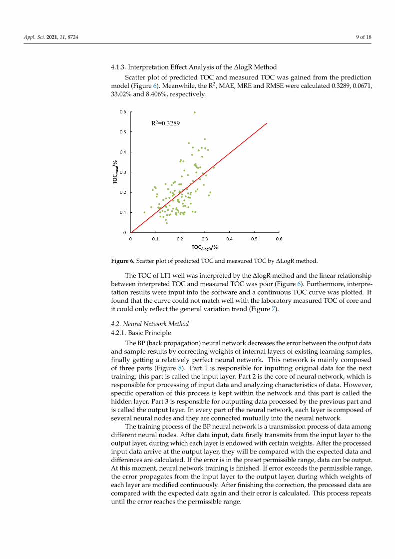
4.1.3. Interpretation Effect Analysis of the ∆logR Method
Scatter plot of predicted TOC and measured TOC was gained from the predictionmodel (Figure 6). Meanwhile, the R2, MAE, MRE and RMSE were calculated 0.3289, 0.0671,33.02% and 8.406%, respectively.
Appl. Sci. 2021, 11, x FOR PEER REVIEW 9 of 19
4.1.3. Interpretation Effect Analysis of the ΔlogR Method
Scatter plot of predicted TOC and measured TOC was gained from the prediction
model (Figure 6). Meanwhile, the R2, MAE, MRE and RMSE were calculated 0.3289,
0.0671, 33.02% and 8.406%, respectively.
Figure 6. Scatter plot of predicted TOC and measured TOC by ΔLogR method.
The TOC of LT1 well was interpreted by the ΔlogR method and the linear relation-
ship between interpreted TOC and measured TOC was poor (Figure 6). Furthermore, in-
terpretation results were input into the software and a continuous TOC curve was plotted.
It found that the curve could not match well with the laboratory measured TOC of core
and it could only reflect the general variation trend (Figure 7).
4.2. Neural Network Method
4.2.1. Basic Principle
The BP (back propagation) neural network decreases the error between the output
data and sample results by correcting weights of internal layers of existing learning sam-
ples, finally getting a relatively perfect neural network. This network is mainly composed
of three parts (Figure 8). Part 1 is responsible for inputting original data for the next train-
ing; this part is called the input layer. Part 2 is the core of neural network, which is re-
sponsible for processing of input data and analyzing characteristics of data. However,
specific operation of this process is kept within the network and this part is called the
hidden layer. Part 3 is responsible for outputting data processed by the previous part and
is called the output layer. In every part of the neural network, each layer is composed of
several neural nodes and they are connected mutually into the neural network.
The training process of the BP neural network is a transmission process of data
among different neural nodes. After data input, data firstly transmits from the input layer
to the output layer, during which each layer is endowed with certain weights. After the
processed input data arrive at the output layer, they will be compared with the expected
data and differences are calculated. If the error is in the preset permissible range, data can
be output. At this moment, neural network training is finished. If error exceeds the per-
missible range, the error propagates from the input layer to the output layer, during which
weights of each layer are modified continuously. After finishing the correction, the pro-
cessed data are compared with the expected data again and their error is calculated. This
process repeats until the error reaches the permissible range.
Figure 6. Scatter plot of predicted TOC and measured TOC by ∆LogR method.
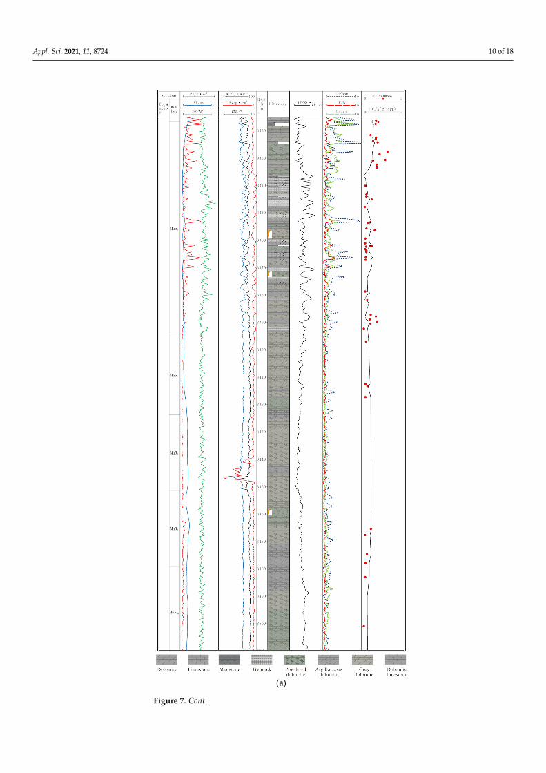
The TOC of LT1 well was interpreted by the ∆logR method and the linear relationshipbetween interpreted TOC and measured TOC was poor (Figure 6). Furthermore, interpre-tation results were input into the software and a continuous TOC curve was plotted. Itfound that the curve could not match well with the laboratory measured TOC of core andit could only reflect the general variation trend (Figure 7).
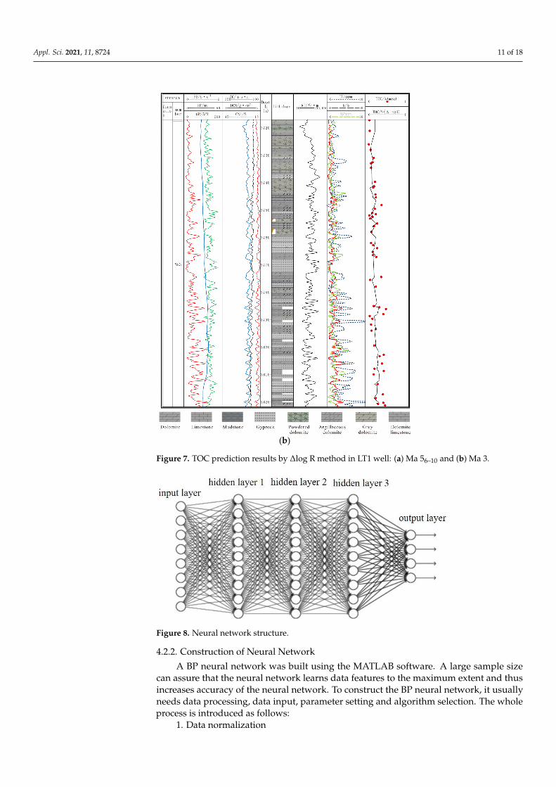
4.2. Neural Network Method4.2.1. Basic Principle
The BP (back propagation) neural network decreases the error between the output dataand sample results by correcting weights of internal layers of existing learning samples,finally getting a relatively perfect neural network. This network is mainly composedof three parts (Figure 8). Part 1 is responsible for inputting original data for the nexttraining; this part is called the input layer. Part 2 is the core of neural network, which isresponsible for processing of input data and analyzing characteristics of data. However,specific operation of this process is kept within the network and this part is called thehidden layer. Part 3 is responsible for outputting data processed by the previous part andis called the output layer. In every part of the neural network, each layer is composed ofseveral neural nodes and they are connected mutually into the neural network.
The training process of the BP neural network is a transmission process of data amongdifferent neural nodes. After data input, data firstly transmits from the input layer to theoutput layer, during which each layer is endowed with certain weights. After the processedinput data arrive at the output layer, they will be compared with the expected data anddifferences are calculated. If the error is in the preset permissible range, data can be output.At this moment, neural network training is finished. If error exceeds the permissible range,the error propagates from the input layer to the output layer, during which weights ofeach layer are modified continuously. After finishing the correction, the processed data arecompared with the expected data again and their error is calculated. This process repeatsuntil the error reaches the permissible range.
Appl. Sci. 2021, 11, 8724 10 of 18Appl. Sci. 2021, 11, x FOR PEER REVIEW 10 of 19
(a)
Figure 7. Cont.
Appl. Sci. 2021, 11, 8724 11 of 18Appl. Sci. 2021, 11, x FOR PEER REVIEW 11 of 19
(b)
Figure 7. TOC prediction results by Δlog R method in LT1 well: (a) Ma 56–10 and (b) Ma 3.
Figure 8. Neural network structure.
Figure 7. TOC prediction results by ∆log R method in LT1 well: (a) Ma 56–10 and (b) Ma 3.
Appl. Sci. 2021, 11, x FOR PEER REVIEW 11 of 19
(b)
Figure 7. TOC prediction results by Δlog R method in LT1 well: (a) Ma 56–10 and (b) Ma 3.
Figure 8. Neural network structure.
Figure 8. Neural network structure.
4.2.2. Construction of Neural Network
A BP neural network was built using the MATLAB software. A large sample sizecan assure that the neural network learns data features to the maximum extent and thusincreases accuracy of the neural network. To construct the BP neural network, it usuallyneeds data processing, data input, parameter setting and algorithm selection. The wholeprocess is introduced as follows:
1. Data normalization
Appl. Sci. 2021, 11, 8724 12 of 18
Since different logging data have different units that may influence training of themodel, it is necessary to implement normalization of TOC data and logging data beforethe logging data are input into the model in order to improve accuracy of the model andshorten operation time. The normalization uses the range method and its formula is:
Xn =X − Xmin
Xmax − Xmin(8)
where Xn is the sample normalization result of logging curve, X is the original loggingvalue, Xmin is the minimum and Xmax is the maximum.
2. Data inputAccording to correlation analysis results, the normalized K, GR and DEN logging data
were input into the neural network.To avoid overfitting and assure training quality, a cross-training verification mode was
used in the training process of the neural network. Training set, verification set and test setwere allocated randomly according to proportions of 70%, 15% and 15%, respectively. Datain the training set (110 groups) were used for the neural network to learn and identify datacharacteristics. Data in the verification set (24 groups) were used to test whether overfittingoccurs (if the error between data used for learning that are output by the neural networkand real results decreases, but the error between the current data group after neural networkoutput and the real result is unchanged, overfitting occurs). Data in the test set (24 groups)were used to test unknown sample prediction capacity of the neural network.
3. Parameter setting of the hidden layerIncreasing hidden layers can decrease the error of the neural network and increase the
interpretation accuracy. Nevertheless, excessive hidden layers may cause more operationsduring data transmission in the neural network, so it takes more time for assignment ofeach layer. Moreover, increasing hidden layers is conducive to explore data characteristicsmore carefully. With limitations of sample size, some characteristics might exist in learningsamples only and they are not applicable to whole data. Hence, overfitting occurs. TheBP neural network still can approach any function by adjusting training times or numberof nodes in the hidden layer even though it contains only one hidden layer. To decreasecalculation while assuring accuracy of the neural network, the number of hidden layerswas set 1 during construction of the BP neural network.
Setting the number of nodes in the hidden layer is crucial to construction of the neuralnetwork. If the number of nodes is too high, it increases computational loads during datatransmission in the neural network. If the number of nodes is too low, it is impossibleto learn data features accurately so that the trained neural network cannot recognize theunlearned samples. To determine number of nodes in the hidden layer, several studieshave been carried out and many empirical formulas have been proposed.
According to the Kolmogorov theorem, when there’s only one hidden layer, thenumber of nodes meets:
Nhid = 2Nin + 1 (9)
where Nhid is the number of nodes in the hidden layer and Nin is the number of nodes inthe input layer.
The number of nodes in the hidden layer, proposed by Jadid et al. [25], meets:
Nhid ≤ Ntrain/R × (Nin + Nout) (10)
where Ntrain is number of training samples and Nout is number of nodes in the output layer,5 ≤ R ≤ 10.
Different scholars use different methods to calculate number of nodes in the hiddenlayer. There’s no uniform formula to calculate the number of nodes in the hidden layer.The distribution range of the number of nodes in the hidden layer is usually calculatedaccording to the empirical formula and then verifies and determines a specific number
Appl. Sci. 2021, 11, 8724 13 of 18
according to practical data. To optimize the neural network structure and save the learningtime of characteristics, it is suggested to use the least nodes while assuring precision. Basedon the above formula, the number of nodes in the hidden layer of the neural network shallbe 3~13. The neural network was trained with data of practical working areas. When therewere 9 nodes in the hidden layer, the training error was the lowest and the correlationamong samples was the maximum (Table 2). Therefore, the number of nodes in the hiddenlayer of the constructed neural network was determined to be 9 in this study area.
Table 2. The MSE and correlation of different node quantities in the hide layer.
Number of Nodes 3 4 5 6 7 8 9 10 11 12 13
Error/10−3 9.13 8.62 8.44 6.52 6.89 5.75 5.26 5.82 6.14 5.97 6.25Correlation/10−1 7.27 7.26 7.34 8.51 7.45 9.01 9.39 8.82 9.16 8.78 8.24
4. Algorithm selectionThe Levenberg–Marquardt algorithm, Bayesian regularization algorithm and quanti-
tative conjugate gradient algorithm are three common algorithms during data training [26].The Levenberg–Marquardt algorithm is characteristic of quick calculation, but it
incurs a operation machine requirement. The Bayesian regularization algorithm avoidsoverfitting of a characteristic variable by retaining all characteristic variable, which takes alonger operation time. The quantitative conjugate gradient algorithm doesn’t need linearsearching, has quick operation and requires a small computational memory, but is notapplicable to all datasets. According to practical verification, the Levenberg–Marquardtalgorithm can complete neural network training the most quickly and accurately; thisalgorithm was chosen for data training for the neural network in this study.
4.2.3. Interpretation Effect Analysis of Neural Network Method
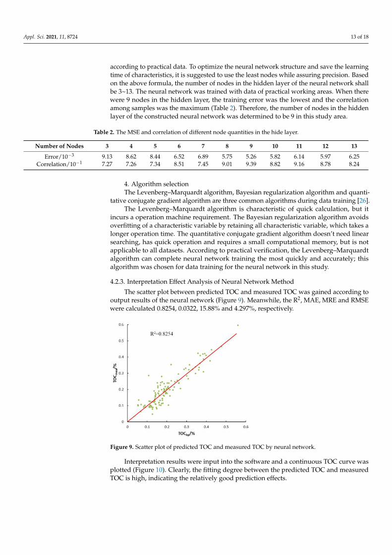
The scatter plot between predicted TOC and measured TOC was gained according tooutput results of the neural network (Figure 9). Meanwhile, the R2, MAE, MRE and RMSEwere calculated 0.8254, 0.0322, 15.88% and 4.297%, respectively.
Appl. Sci. 2021, 11, x FOR PEER REVIEW 14 of 19
Figure 9. Scatter plot of predicted TOC and measured TOC by neural network.
Interpretation results were input into the software and a continuous TOC curve was
plotted (Figure 10). Clearly, the fitting degree between the predicted TOC and measured
TOC is high, indicating the relatively good prediction effects.
Figure 9. Scatter plot of predicted TOC and measured TOC by neural network.
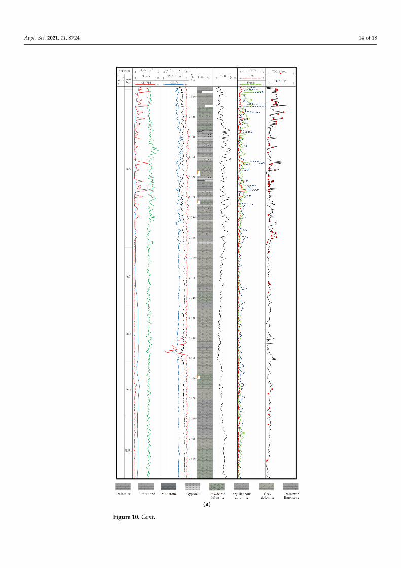
Interpretation results were input into the software and a continuous TOC curve wasplotted (Figure 10). Clearly, the fitting degree between the predicted TOC and measuredTOC is high, indicating the relatively good prediction effects.
Appl. Sci. 2021, 11, 8724 14 of 18Appl. Sci. 2021, 11, x FOR PEER REVIEW 15 of 19
(a)
Figure 10. Cont.
Appl. Sci. 2021, 11, 8724 15 of 18Appl. Sci. 2021, 11, x FOR PEER REVIEW 16 of 19
(b)
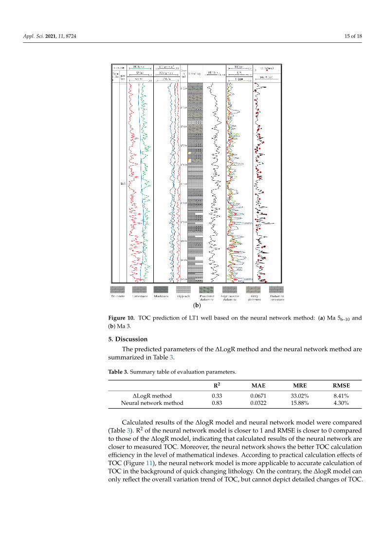
Figure 10. TOC prediction of LT1 well based on the neural network method: (a) Ma 56–10 and(b) Ma 3.
5. Discussion The predicted parameters of the ΔLogR method and the neural network method are
summarized in Table 3.
Table 3. Summary table of evaluation parameters.
R2 MAE MRE RMSE ΔLogR method 0.33 0.0671 33.02% 8.41% Neural network
method 0.83 0.0322 15.88% 4.30%
Calculated results of the ΔlogR model and neural network model were compared (Table 3). R2 of the neural network model is closer to 1 and RMSE is closer to 0 compared to those of the ΔlogR model, indicating that calculated results of the neural network are closer to measured TOC. Moreover, the neural network shows the better TOC calculation efficiency in the level of mathematical indexes. According to practical calculation effects of TOC (Figure 11), the neural network model is more applicable to accurate calculation of TOC in the background of quick changing lithology. On the contrary, the ΔlogR model can only reflect the overall variation trend of TOC, but cannot depict detailed changes of TOC.
Figure 10. TOC prediction of LT1 well based on the neural network method: (a) Ma 56–10 and(b) Ma 3.
5. Discussion
The predicted parameters of the ∆LogR method and the neural network method aresummarized in Table 3.
Table 3. Summary table of evaluation parameters.
R2 MAE MRE RMSE
∆LogR method 0.33 0.0671 33.02% 8.41%Neural network method 0.83 0.0322 15.88% 4.30%
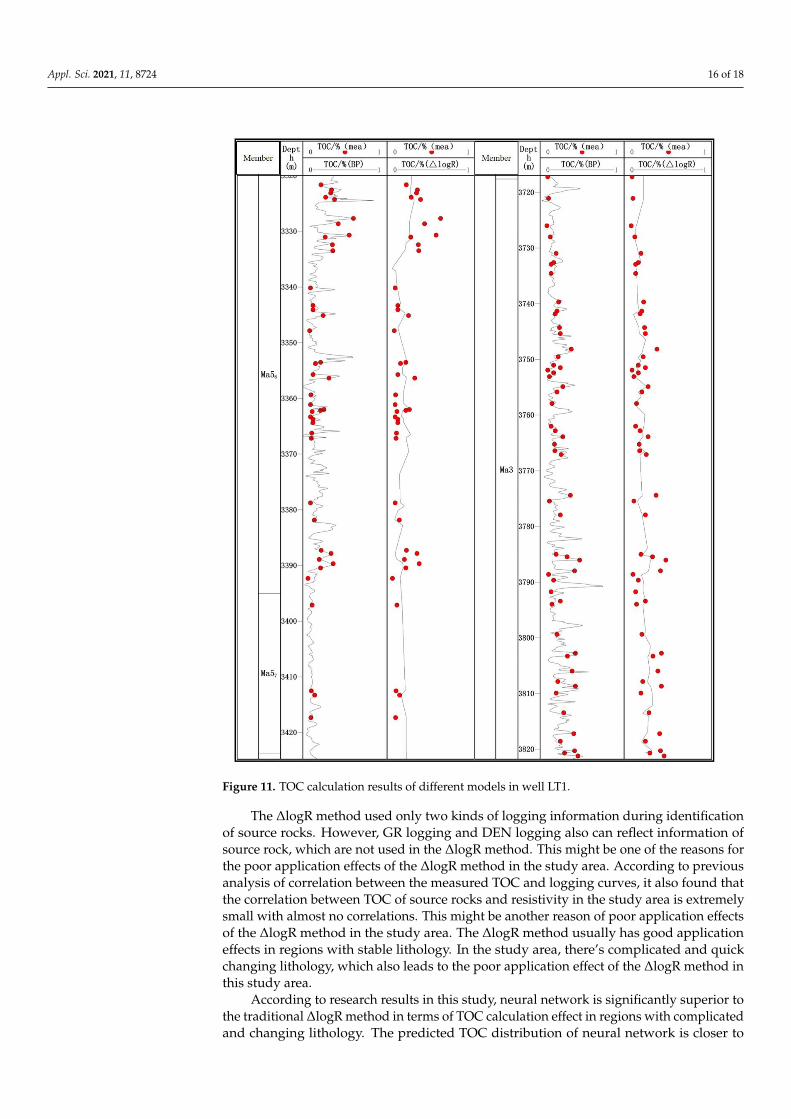
Calculated results of the ∆logR model and neural network model were compared(Table 3). R2 of the neural network model is closer to 1 and RMSE is closer to 0 comparedto those of the ∆logR model, indicating that calculated results of the neural network arecloser to measured TOC. Moreover, the neural network shows the better TOC calculationefficiency in the level of mathematical indexes. According to practical calculation effects ofTOC (Figure 11), the neural network model is more applicable to accurate calculation ofTOC in the background of quick changing lithology. On the contrary, the ∆logR model canonly reflect the overall variation trend of TOC, but cannot depict detailed changes of TOC.
Appl. Sci. 2021, 11, 8724 16 of 18
Appl. Sci. 2021, 11, x FOR PEER REVIEW 17 of 19
can only reflect the overall variation trend of TOC, but cannot depict detailed changes of
TOC.
Figure 11. TOC calculation results of different models in well LT1.
The ΔlogR method used only two kinds of logging information during identification
of source rocks. However, GR logging and DEN logging also can reflect information of
source rock, which are not used in the ΔlogR method. This might be one of the reasons for
the poor application effects of the ΔlogR method in the study area. According to previous
analysis of correlation between the measured TOC and logging curves, it also found that
the correlation between TOC of source rocks and resistivity in the study area is extremely
small with almost no correlations. This might be another reason of poor application effects
of the ΔlogR method in the study area. The ΔlogR method usually has good application
effects in regions with stable lithology. In the study area, there’s complicated and quick
changing lithology, which also leads to the poor application effect of the ΔlogR method in
this study area.
Figure 11. TOC calculation results of different models in well LT1.
The ∆logR method used only two kinds of logging information during identificationof source rocks. However, GR logging and DEN logging also can reflect information ofsource rock, which are not used in the ∆logR method. This might be one of the reasons forthe poor application effects of the ∆logR method in the study area. According to previousanalysis of correlation between the measured TOC and logging curves, it also found thatthe correlation between TOC of source rocks and resistivity in the study area is extremelysmall with almost no correlations. This might be another reason of poor application effectsof the ∆logR method in the study area. The ∆logR method usually has good applicationeffects in regions with stable lithology. In the study area, there’s complicated and quickchanging lithology, which also leads to the poor application effect of the ∆logR method inthis study area.
According to research results in this study, neural network is significantly superior tothe traditional ∆logR method in terms of TOC calculation effect in regions with complicatedand changing lithology. The predicted TOC distribution of neural network is closer to
Appl. Sci. 2021, 11, 8724 17 of 18
practical geological conditions. The neural network method has important significance tofurther petroleum exploration and development in the future.
6. Conclusions
In this study, the neural network in the AI field was introduced into the TOC loggingcalculation. The traditional ∆logR method and neural network method were used for TOClog interpretations of source rock, which has low abundance and complicated lithology inthe Majiagou Formation in the LT1 well of the eastern Ordos Basin. Some major conclusionscould be drawn:
1. There’s low abundance of source rock in the study area and logging response toTOC is not significant. The complicated and changing lithology also weakens influencesof TOC variations on logging, thus resulting in the generally poor correlations betweenlogging data and measured TOC. Therefore, the ∆logR method, which calculates TOCbased on linear relationship is difficult to get the ideal outcomes. The calculated results of∆logR method can only reflect the general longitudinal variation trend of TOC but cannotprovide a thorough depiction of TOC changes.
2. When calculating TOC in lithologic alternating regions, the neural network modelcan retain details of TOC changes and thereby reflect TOC changes truly. Furthermore,the neural network model has higher prediction accuracy and stronger adaptation due tothe remarkable nonlinear mapping capacity and flexible network structure. It can providemore real references for petroleum exploration and development in the future.
Author Contributions: Project administration, S.H.; writing—original draft preparation and editing,H.Z.; Supervision, R.Z., L.J. and Y.L. All authors have read and agreed to the published version ofthe manuscript.
Funding: Supported by the National Natural Science Foundation of China (Grant No. 42172154).
Institutional Review Board Statement: Not Applicable.
Informed Consent Statement: Not Applicable.
Data Availability Statement: The data presented in this study are available on request from thecorresponding author. The data are not publicly available due to privacy.
Conflicts of Interest: The authors declare no conflict of interest.
References1. Schmokerj, W. Determination of Organic-Matter Content of Appalachian Devonian Shales from Gamma-Ray Logs. AAPG Bull.
1981, 65, 1285–1298.2. Chen, Z.; Hao, S.; Xi, S. Logging Evaluation Method for Organic Matter Abundance of Carbonate Source Rock. J. Univ. Pet. (Ed.
Nat. Sci.) 1994, 18, 16–19.3. Xu, S.; Zhu, Y. Well logs response and prediction model of organic carbon content in source rocks—a case study from the source
rock of Wenchang formation in the pearl mouth basin. Pet. Geol. Exp. 2010, 32, 290.4. Du, W.; Wang, P.; Liang, M. Well logs response characteristics and quantitative prediction model of organic carbon content of
hydrocarbon source rocks in coal-bearing strata measures. J. China Coal Soc. 2016, 41, 954–963.5. Passey, Q.R.; Creaney, S.; Kulla, J.B.; Stroud, J.D. A Practical Model for Organic Richness from Porosity and Resistivity Logs.
AAPG Bull. 1990, 74, 1777–1794.6. Yu, H.; Rezaee, R.; Wang, Z.; Han, T.; Zhang, Y.; Arif, M.; Johnson, L. A new method for TOC estimation in tight shale gas
reservoirs. Int. J. Coal Geol. 2017, 179, 269–277. [CrossRef]7. Yan, J.; Cai, J.; Zhao, M.H.; Zheng, D.S. Advances in the study of source rock evaluation by geophysical logging and its significance
in resource assessment. Prog. Geophys. 2009, 24, 270–279.8. Meng, Z.; Guo, Y.; Liu, W. Relationship between organic carbon content of shale gas reservoir and logging parameters and its
prediction model. J. China Coal Soc. 2015, 40, 247–253.9. Tan, M.J.; Bai, Y.; Wang, Q.; Wu, J.; Shi, Y.J.; Li, G.R.; Wei, X.P. Proceedings of the 2019 Oil and Gas Geophysics Annual Conference;
Oil and Gas Geophysics Professional Committee of the Chinese Geophysical Society: Nanjing, China, 2019.10. Alizadeh, B.; Najjari, S.; Kadkhodaie-Ilkhchi, A. Artificial neural network modeling and cluster analysis for organic facies and
burial history estimation using well log data: A case study of the South Pars Gas Field, Persian Gulf, Iran. Comput. Geosci. 2012,45, 261–269. [CrossRef]

Appl. Sci. 2021, 11, 8724 18 of 18
11. Bakhtiar, H.A.; Telmadarreie, A.; Shayesteh, M.; Fard, M.H.H.; Talebi, H.; Shirband, Z. Estimating Total Organic Carbon Contentand Source Rock Evaluation, Applying ∆logR and Neural Network Methods: Ahwaz and Marun Oilfields, SW of Iran. Liq. FuelsTechnol. 2011, 29, 1691–1704. [CrossRef]
12. Li, Z.; Du, W.; Hu, J.; Li, D. Prediction of shale organic carbon content support vector machine based on logging parameters. CoalSci. Technol. 2019, 47, 199–204.
13. Rui, J.; Zhang, H.; Zhang, D.; Han, F.; Guo, Q. Total organic carbon content prediction based on support-vector-regressionmachine with particle swarm optimization. J. Pet. Sci. Eng. 2019, 180, 699–706. [CrossRef]
14. Amosu, A.; Imsalem, M.; Sun, Y. Effective machine learning identification of TOC-rich zones in the Eagle Ford Shale. J. Appl.Geophys. 2021, 188, 104–113. [CrossRef]
15. Liu, X.; Lei, Y.; Luo, X.; Wang, X.; Chen, K.; Cheng, M.; Yin, J. TOC determination of Zhangjiatan shale of Yanchang formation,Ordos Basin, China, using support vector regression and well logs. Earth Sci. Inform. 2021, 14, 22–34. [CrossRef]
16. Zhao, W.; Gao, H.; Yan, G.; Guo, T. TOC prediction technology based on optimal estimation and Bayesian statistics. Lithol. Reserv.2020, 32, 86–93.
17. Yin, M.; Cen, C.; Ruan, J.; He, W.W. Classification and prediction method of total organic carbon content in shale gas reservoirbased on Bayesian discrimination. J. Geol. 2020, 44, 362–369.
18. Rui, J.; Zhang, H.; Ren, Q.; Yan, L.; Guo, Q.; Zhang, D. TOC content prediction based on a combined Gaussian process regressionmodel. Mar. Pet. Geol. 2020, 118, 104–118. [CrossRef]
19. Li, G.; Zhao, T.; Shi, Y.; Hu, C.; Chen, Z.; Fan, X.; Li, D.; Lai, J. Diagenetic facies logging recognition and evaluation of carbonatereservoirs in Majiagou Formation, Ordos Basin. Acta Pet. Sin. 2018, 39, 1141–1154.
20. Guo, Y.; Zhao, Z.; Zhang, Y.; Xu, W.; Bao, H.; Zhang, Y.; Gao, J.; Song, W. Development characteristics and new exploration areasof marine source rock in Ordos Basin. Acta Pet. Sin. 2016, 37, 939–951.
21. Qin, J.Q.; Fu, D.L.; Qian, Y.F.; Yang, F.; Tian, T. Progress of geophysical methods for the evaluation of TOC of source rock. Geophys.Prospect. Pet. 2018, 57, 803–812.
22. Dong, H.C. Application of natural gamma spectroscopy logging. Petrochem. Ind. Technol. 2017, 24, 260.23. Zhong, W.J.; Li, H.; Ge, Z.W.; Dong, X.X. Optimum method for calculating organic carbon content from logging data—Taking
Longmaxi Formation Shale in X area of southern Sichuan as an example. China Pet. Chem. Stand. Qual. 2020, 40, 12–14.24. Bian, L.; Liu, G.; Sun, M.; Yang, D.; Wan, W.; Zhang, Y. Improved ∆logR technique and its application to predicting total organic
carbon of source rocks with middle and deep burial depth. Pet. Geol. Recovery Effic. 2018, 25, 40–45.25. Jadid, M.N.; Fairbairn, D.R. The application of neural network techniques to structural analysis by implementing an adaptive
finite-element mesh generation. AI EDAM 1994, 8, 177–191. [CrossRef]26. Chen, M. Analysis and Compare of BP Neural Network’s Training Arithmetic. Sci. Technol. Plaza 2010, 23, 24–27.