Quantifying Episodic SnowmeltEvents in Arctic Ecosystems

Stine Højlund Pedersen,1* Glen E. Liston,2 Mikkel P. Tamstorf,1

Andreas Westergaard-Nielsen,3 and Niels Martin Schmidt1

1Arctic Research Centre, Department of Bioscience, Aarhus University, Frederiksborgvej 399, 4000 Roskilde, Denmark; 2CooperativeInstitute for Research in the Atmosphere (CIRA), Colorado State University, Fort Collins, Colorado 80523, USA; 3Center for Permafrost

(CENPERM), Department of Geosciences and Natural Resource Management, University of Copenhagen, Oester Voldgade 10,1350 Copenhagen K, Denmark

ABSTRACT

Rapid and extensive snowmelt occurred during

2 days in March 2013 at a low-Arctic study site in

the ice-free part of southwest Greenland. Me-

teorology, snowmelt, and snow-property observa-

tions were used to identify the meteorological

conditions associated with this episodic snowmelt

event (ESE) occurring prior to the spring snowmelt

season. In addition, outputs from the SnowModel

snowpack-evolution tool were used to quantify the

snow-related consequences of ESEs on ecosystem-

relevant snow properties. We estimated a 50–80%

meltwater loss of the pre-melt snowpack water

content, a 40–100% loss of snow thermal resis-

tance, and a 4-day earlier spring snowmelt snow-

free date due to this March 2013 ESE. Further-

more, the accumulated meltwater loss from all

ESEs in a hydrological year represented 25–52% of

the annual precipitation and may potentially have

advanced spring snowmelt by 6–12 days. Guided

by the knowledge gained from the March 2013

ESE, we investigated the origin, past occurrences,

frequency, and abundance of ESEs at spatial scales

ranging from local (using 2008–2013 meteoro-

logical station data) to all of Greenland (using

1979–2013 atmospheric reanalysis data). The fre-

quency of ESEs showed large interannual varia-

tion, and a maximum number of ESEs was found in

southwest Greenland. The investigations suggested

that ESEs are driven by foehn winds that are typical

of coastal regions near the Greenland Ice Sheet

margin. Therefore, ESEs are a common part of

snow-cover dynamics in Greenland and, because of

their substantial impact on ecosystem processes,

they should be accounted for in snow-related

ecosystem and climate-change studies.

Key words: snow; meltwater; modeling; growing

season; snow thermal properties; foehn; upscaling;

Greenland.

INTRODUCTION

Terrestrial snow cover is a key variable controlling

Arctic ecosystem processes (Jones 1999; Post and

others 2009; Brooks and others 2011; Callaghan

and others 2011). Snow properties, such as depth,

density, snow-water-equivalent (SWE), thermal

conductivity, and timing of snowmelt, affect biotic

and abiotic components of the Arctic ecosystem.

The presence and the absence of snow cover in-

fluence the surface energy balance both locally

Received 4 July 2014; accepted 15 February 2015

Author contributions Stine Højlund Pedersen: Designed the study,

performed research, analyzed data, contributed with new methods, and

wrote the paper. Glen E. Liston: contributed with new methods and

models and wrote the paper. Mikkel P. Tamstorf: contributed with new

methods and wrote the paper. Andreas Westergaard-Nielsen: wrote the

paper. Niels Martin Schmidt: wrote the paper.

*Corresponding author; e-mail: shp@bios.au.dk

EcosystemsDOI: 10.1007/s10021-015-9867-8

� 2015 Springer Science+Business Media New York

(Marks and Dozier 1992) and globally (Groisman

and others 1994), which in turn affects below-

ground surface thermal regime that controls a

range of ecosystem processes (Schimel and others

2004; Johansson and others 2013). The snow cov-

er, with its low thermal conductivity (Goodrich

1982; Sturm and others 1997) and high thermal

resistance (Liston and others 2002), acts as an ef-

fective insulator. This keeps soil thermal conditions

relatively stable during snow-covered periods

(Zhang 2005) and protects vegetation from frost

damages (Bokhorst and others 2011). Throughout

the Arctic, solid precipitation accumulates during

autumn, winter, and spring in a snowpack, which

acts as a water reservoir (Jones 1999). In spring, the

water is released during snowmelt and provides

moisture for plant growth not only at the growing

season initiation, but also into the summer period

(Blankinship and others 2014). Since the presence

and the absence of snow cover play a major role in

ecosystem functions and dynamics, snow-cover

timing and duration must be accounted for in

Arctic process and climate-change ecosystem stud-

ies (Høye and others 2007; Callaghan and others

2011; Bokhorst and others 2012).

Snow properties, and the spatial and temporal

development in these, are directly influenced by

the weather and climate processes that occur dur-

ing the snow season. Often these snow properties

can change dramatically and abruptly in response

to extreme weather events. These abrupt changes

in snow properties can, in turn, have important

impacts on ecosystem components and processes.

Extreme weather events are occurring throughout

the Arctic and are predicted to become more fre-

quent in a warming climate (AMAP 2012). Cur-

rently, these events are infrequent and record-

breaking, but with increased frequency, they may

become a common part of the future Arctic climate

system.

Ecologically relevant extreme events include

rain-on-snow (ROS) events (Rennert and others

2009), early snowmelt events (Semmens and oth-

ers 2013), extreme winter warming events (Bo-

khorst and others 2010; Semenchuk and others

2013), icing events (Hansen and others 2013), re-

freeze events (Bartsch and others 2010), and win-

ter thaw–freeze events (Wilson and others 2013).

These events are caused by different factors such as

winter warming or warm spells, high wind speeds

from storms or katabatic winds (for example, Fuller

and others 2009), or heavy winter rainfall (for

example, Rennert and others 2009; Hansen and

others 2014). They may be caused by different

weather phenomena, but they all have the fol-

lowing in common: (1) an abrupt and sporadic

nature, (2) they are unusual for the season and

winter climate in the geographic locations where

they occur, and (3) they cause changes in snow-

pack properties that affect ecosystems. Their tem-

poral extent varies from a few hours to many days,

and their spatial extent is controlled by the weather

phenomenon that drives them. The area of influ-

ence can range from large regions of the Siberian

tundra exposed to ROSs (Bartsch and others 2010),

to leeside areas of the Canadian Rockies experi-

encing warm and dry chinook winds (Nkemdirim

1997; Fuller and others 2009).

In recent decades, the ability of extreme weather

events to change snowpack properties and impact

local Arctic ecosystems has gained increased at-

tention. This interest is largely due to the recogni-

tion that these snow-related impacts can be

significant, influencing not only single ecosystem

components, but also entire communities (Hansen

and others 2013). An example of this is the creation

of ice layers on the snow surface, within the

snowpack, and at the ground surface, as result of

refreezing meltwater or rainwater. These ice layers

can severely limit the foraging area for Arctic un-

gulates (Forchhammer and Boertmann 1993;

Bartsch and others 2010; Hansen and others 2011,

2013, 2014). Another consequence of extreme

weather events can be snow-cover depletion and

thereby loss of insulating effect for the below-snow

vegetation. This increases the risk of frost damage

to the vegetation when it is exposed to subsequent

freezing temperatures (Inouye 2000; Bokhorst and

others 2010; Semenchuk and others 2013).

An extreme warming event and the associated

abrupt changes in terrestrial snow-cover properties

were observed in Kobbefjord in southwest Green-

land on March 15 and 16, 2013. Air temperature

increased from -7.9�C to above freezing within

24 h and caused extensive snowmelt across the

landscape (Figure 1). Observations of this relatively

short-term melt event (occurring prior to the onset

of spring snowmelt) formed the basis for this study

and it is, herein, referred to as an episodic snow-

melt event (ESE). The focus of our study is to in-

vestigate such ESEs and their potential importance

in Arctic ecosystem processes and components. The

study consists of three interconnected parts (I, II,

and III). In Part I, on local-scale in the Kobbefjord

study area (71 km2), meteorological station data

and field observations of snow properties were used

to characterize the March 2013 ESE. From those

results, we developed an automated algorithm that

processed meteorological data to identify past ESEs

and their temporal distributions on a local scale for

S. H. Pedersen and others

the period 2008–2013. This led to Part II, where we

quantified how biologically relevant snow proper-

ties, such as snowpack water content, the insulat-

ing effect of the snowpack (snow thermal

resistance), and the timing of spring snowmelt

(snow-free date), had changed during the local

ESEs identified in Part I. This was accomplished by

running and validating the SnowModel (Liston and

Elder 2006a, b) spatially distributed snow-evolu-

tion modeling system over the Kobbefjord study

area. Finally, the local-scale results from Part I and

II were used, elaborated on, and scaled-up to all of

Greenland in Part III. Herein, we applied the local-

scale results from Kobbefjord (Part I and II) to

identify the ESE spatial distributions and trends on

a regional-scale, using a 34-year time series of

historical climate data covering all ice-free parts of

Greenland (410,500 km2). Lastly, we discussed the

driving mechanisms for the ESEs.

PART I: CHARACTERIZING EPISODIC

SNOWMELT EVENTS (ESES)

The first-hand observations of an ESE in March

2013 initiated the investigation of the meteoro-

logical characteristics and snowpack changes asso-

ciated with this ESE, aiming to develop an

algorithm to identify ESEs in Kobbefjord.

Study Area

The low-Arctic, 7.6 km by 9.3 km, Kobbefjord

study area is located at the head of the fjord,

Kangerluarsunnguaq, in the Godthabsfjord system

in southwest Greenland (64�7¢59¢¢N, 51�20¢35¢¢W)

(Figure 2). The Kobbefjord study area includes a

3-km-wide main valley with two adjacent elevated

valleys at 200–250 meters above sea level (m a.s.l.)

surrounded by steep mountains up to 1375 m a.s.l.

The valley floor topography varies on the order of

100 m with hill tops and depressions with fresh-

water lakes. The mountain slopes above 200 m

a.s.l. are characterized by alluvial cones, recent

rock slides, small hanging glaciers, and snow

patches. The hill slopes below 200 m a.s.l. are

vegetated with heath and dwarf shrubs and

dominated by patterns of inactive solifluction

sheets and 3–4-m-deep depressions eroded by

streams, which favor growth of 0.7–1.0 m tall Salix

glauca shrubs.

The observed mean annual air temperature

during the study period of 2008–2013 was 0.19�C,

with the lowest temperatures measured in Febru-

ary and the highest in July. The dominant wind

direction during May–August was west–northwest

(from the fjord) and during September–April east–

northeast (from inland). Easterly winds originated

from the inner parts of the fjord system and were

channeled by the main valley (Jensen and Rasch

2008, 2009, 2010, 2011, 2013; Jensen 2012).

Method and Data

Local Meteorological Data

To support the analyses, meteorological variables

including air temperature, wind speed, and snow

depth were provided by the main meteorological

station, KOB, located in the study area (Table 1;

Figure 2). The time series covered the period

September 2008–August 2013. All meteorological

data were provided by Nuuk Ecological Research

Operations (NERO); technical information, for ex-

ample, sensor types and measurement frequency

are available in Jensen and Rasch (2008, 2009,

2010, 2011, 2013), and Jensen (2012).

Figure 1. Digital photos from March 14, 2013 (left) and March 16, 2013 (right) showing the center part of the Kobbefjord

study area. The photos were taken by an automated camera installed at 550 meters above sea level (m a.s.l.). Photo:

GeoBasis, Nuuk Ecological Research Operations.

Episodic Snowmelt Events in Arctic Ecosystems

Identification of Past ESEs in Kobbefjord

To identify past ESEs, we used local meteorological

data and snow observations collected before, dur-

ing, and after the March 15–16, 2013 ESE. The

three-point characterization of ESEs (Table 2),

based on the March 2013 ESE, included conditions

required for snowmelt, such as snow presence and

above-freezing air temperatures. We also included

a relatively high daily wind speed (corresponding

to the 90th percentile of daily mean wind speed

data for 2012–2013) for an ESE to occur. The wind

speed threshold was introduced because high wind

speeds were present during the March 2013 ESE,

and turbulent fluxes at high wind speeds are often

associated with high melt rates (Dadic and others

2013). The duration of the local past ESEs (2008–

2013) was determined by the number of con-

secutive days, where these three criteria were met.

Part I Findings

Over the 5-year period, September 2008–August

2013, we identified 31 ESEs in Kobbefjord using

available meteorological data (Table 1) and the

automated algorithm (Table 2). The ESEs occurred

from mid-October until mid-May, and ranged be-

tween 3 and 13 ESEs per year. The identified ESEs

varied in duration from 1 to 3 days; however, 81%

of all identified ESEs were 1-day events. Further-

more, decreases in snow depth during the ESEs

were observed. In Part II, we investigated how

these changes in the snowpack and snow cover

were affecting ecologically relevant snow proper-

ties in Arctic ecosystems during and after the ESEs.

Figure 2. Kobbefjord

study area in west

Greenland. Brown color

scale indicates elevation

(m a.s.l.). Red triangles

mark the location of four

climate stations (SoilFen,

KOB, M1000, and M500).

The blue triangle is a soil

temperature station. Black

boxes are annually

repeated snow-

observation sites with

cross transects of snow-

depth measurements and

snow pits; the west-most

site was only repeated on

and March 14 and 19,

2013.

Table 1. Kobbefjord Meteorological Stations and Available Variables (Red Triangles in Figure 2)

Station Established Latitude Longitude Elevation (m. a.s.l.) Climate variables

KOB 2007 64�7¢59¢¢ 51�20¢35¢¢ 30 tair, rh, wspd, wdir, Qsi, Qli, snod

SoilFen 2007 64�7¢50¢¢ 51�23¢60¢¢ 30 tair, rh

M500 2007 64�7¢20¢¢ 51�22¢19¢¢ 550 tair, rh, Qsi

M1000 2008 64�9¢13¢¢ 51�21¢10¢¢ 1000 tair, rh, wspd

tair = 2-m air temperature (�C), rh = relative humidity (%), wspd = wind speed (m s-1), wdir = wind direction (�), Qsi = incoming shortwave radiation (W m-2),Qli = incoming longwave radiation (W m-2), and snod = snow depth (m).

Table 2. Episodic Snowmelt Event (ESE) Char-acteristics

Snow depth > 0.0 m

Daily mean air temperature > 0.0�C

Daily mean wind speed > 5.5 m s-1

S. H. Pedersen and others

PART II: ECOLOGICAL RELEVANCE OF ESES

IN KOBBEFJORD

Quantifying the impact of ESEs on snow properties

in low-Arctic ecosystems required application of a

spatially distributed snow-evolution modeling sys-

tem to convert the simple environmental variables,

given in the ESE identification algorithm (Table 2),

into more complex, ecologically relevant variables.

Because the snowpack changes potentially affect a

wide range of ecosystem components and processes

(see ‘‘Introduction’’ section), we chose to focus our

analyses on quantifying the ESE-induced changes in

(1) snowpack water content, (2) snow thermal re-

sistance (that is, the snow insulating effect), and (3)

snow-free date. Each of these three snow properties

can affect a range of low-Arctic ecosystem compo-

nents, even after the snow season is over. Most

notably, these snow-related features can impact the

early and middle portion of the growing season. For

example, the meltwater lost during an ESE will be

unavailable during the onset of plant growth in the

spring (Blankinship and others 2014). In addition,

changes in snow thermal resistance may change the

soil thermal conditions, limiting the decomposition

processes and nutrient availability in the soil during

the growing season (Pattison and Welker 2014). As

further examples, changes in spring snowmelt tim-

ing may potentially alter the timing of net CO2 up-

take (Lund and others 2012), insect emergence

(Høye and others 2007), plant flowering (Cooper

and others 2011), and vegetation green-up (Elleb-

jerg and others 2008).

To quantify these potential affects, first a spatially

distributed snow-evolution model was run over the

Kobbefjord area and model outputs of SWE, snow

depth, and timing of the snow-covered period were

validated against observations from Kobbefjord.

Second, the model outputs were used to estimate

the snowpack changes during the 31 identified

ESEs in Part I. Finally, we quantified the spatial

distribution of the snow meltwater loss and re-

duction in the snow thermal resistance, and esti-

mated the number of days that the spring snow-

free date would occur earlier in a point in the valley

center (KOB, Figure 2) due to the meltwater loss

associated with the March 2013 ESE.

Methods and Data

Model Description

To obtain spatial and temporal snow distributions

through the 5-year period, 2008–2013, for the

Kobbefjord study area, we implemented Snow-

Model (Liston and Elder 2006b). SnowModel con-

sists of three interconnected submodels (Figure 3):

EnBal, SnowPack, and SnowTran-3D. EnBal cal-

culated the surface energy exchanges and snow-

melt (Liston 1995, 1999); SnowPack modeled the

evolution of the snowpack in time and space by

accounting for snowfall, snow density evolution,

and snowmelt (Liston and Hall 1995; Liston and

Mernild 2012); and the blowing-snow transport

was generated by SnowTran-3D (Liston and Sturm

1998; Liston and others 2007). The three sub-

models were coupled with a high-resolution simple

meteorological model, MicroMet (Liston and Elder

2006a), which spatially distributed the meteoro-

logical input variables over the simulation domain

and provided input to SnowModel.

MicroMet and SnowModel require meteorological

station and/or gridded atmospheric forcing inputs of

air temperature, relative humidity, precipitation,

Figure 3. Input variables, SnowModel submodels, and output variables. SWE = Snow-water-equivalent, AWS = Auto-

matic weather station, and RCM = Regional climate model.

Episodic Snowmelt Events in Arctic Ecosystems

wind speed, and wind direction. All meteorological

variables, except precipitation, were provided by the

four meteorological stations installed in the study

area (Table 1; Figure 2) for the period September

2008–August 2013, which defined the temporal

boundaries of the Kobbefjord SnowModel simula-

tions. Because of uncertainties associated with in si-

tu winter precipitation measurements (Goodison

and others 1998), SnowModel precipitation inputs

were provided by NASA’s Modern-Era Retrospective

Analysis for Research and Applications (MERRA) 2/

3� longitude by 1/2� latitude gridded atmospheric

reanalysis precipitation data (Rienecker and others

2011); daily precipitation rates from the six nearest

MERRA data grid points were spatially extrapolated

by MicroMet to cover the Kobbefjord simulation

domain. Furthermore, measured incoming short-

wave and longwave radiation were included in the

SnowModel energy balance calculations as an im-

proved alternative to the MicroMet calculation of

the radiation components. In addition to the three

submodels, a data assimilation scheme, SnowAssim

(Liston and Hiemstra 2008), was included in the

model runs. SnowAssim was used to correct the

input of precipitation rates by constraining the

modeled field of SWE by the observed pre-melt

SWE. This technique, pioneered by Liston and

Sturm (2002), has proven to be an effective way to

produce realistic precipitation fluxes when available

precipitation datasets may be inadequate.

SnowModel was run over the spatial domain

shown in Figure 2 using a 10 m by 10 m grid in-

crement and daily time steps. Required digital

elevation model (DEM) data were based on a di-

gitized version of a 25-m topographic contour in-

terval map and provided on the same grid as

SnowModel. Also required by SnowModel are

snow-holding depths (SHDs), that is, the depth

below which the vegetation captures the snow and

prevents snow-transport by wind. The assigned

SHDs (Table 3) for the two vegetation types, ‘Low

shrub heath’ and ‘Tall shrub copse,’ were based on

48 manual vegetation height measurements dis-

tributed in the main valley in July 2012 (Wester-

gaard-Nielsen and others 2013).

Assimilation Data

Observed SWEs were used as part of the SnowModel

integrations to overcome uncertainties in the MER-

RA reanalysis precipitation rates (Reichle and others

2011). NERO conducted annual snow surveys every

spring (March–May) during 2008–2013, where

snow pits were dug in the same locations (Figure 2)

each year to provide detailed measurements of the

snowpack grain size, grain type, hardness, stratigra-

phy, density, and temperature. Observed SWE val-

ues were calculated from the bulk density

observations and the total depth of these snow pits

(Figure 2) and used to adjust MERRA precipitation

fluxes using SnowAssim (Liston and Hiemstra 2008)

running within SnowModel. This was done under

the constraint that modeled SWE matched the ob-

served SWE both in time and location.

Validation Data

Model outputs were validated against observations

of SWE, snow depth, and albedo. Observed SWE

was obtained from 3 to 6 snow pit locations per year

in the main valley; SWE was calculated using mean

snow depths measured along 100 m by 100 m cross

transects and from snow bulk density from snow pits

(Figure 2). We used the observed density values

obtained from the snow pits in the assimilation

(letting SnowModel simulate the snow depth) and

validation because snow density is conservative and

its spatial variation typically falls within well-de-

fined limits (Sturm and others 2010); the available

bulk density observations made within 1–2 days in

the valley varied less than 8%.

Automated snow depth (sonic ranging sensor)

measurements available during 2008–2013 from the

Table 3. Estimated Snow-Holding Depths (SHDs) for Land-Cover Types Present in Kobbefjord

Land-cover type1 SHD

(m)

Land-cover

fraction (%)2

Permanent snow/glaciers 0.01 8.3

Fjord and lakes (possible frozen) 0.01 3.0

Exposed bedrock and fell field/wind-blown area 0.01 69.0

Fen (Carex rariflora, Scirpus caespitosus, Eriophorum angustifolium) 0.15 <0.1

Low shrub heath (Empetrum nigrum, Vaccinium uliginosum, Betula nana) 0.15 8.2

Tall shrub copse (Salix glauca) 0.60 2.3

1From Bay and others (2008).2Based on the area of the simulation domain of approximately 71 km2.

S. H. Pedersen and others

KOB climate station (Figure 2) were used to validate

modeled snow depth. The timings of the start and

end of the modeled snow-covered periods were

compared with the observed snow-covered periods.

To define the start and end of the observed snow-

covered periods, we used observed albedo during

2008–2013 from KOB. The observed start of the

snow-covered period was defined as the day the

observed albedo exceeded 0.8, and the end of the

period as the day the albedo went below 0.2. For the

modeled snow cover, at the SnowModel grid cell

coincident with the KOB station location, the start of

the snow-covered period was defined to be the first

day with snow depth greater than 0.0 m, and the end

was the day before the snow depth equaled 0.0 m.

Estimating ESE-Related Snow-Property Changes

We estimated the spatial distribution of meltwater

loss during the March 2013 ESE by calculating the

difference in modeled SWE before and after these

two dates for all grid cells in the simulation domain.

The meltwater loss associated with the 31 identified

ESEs was estimated by calculating the difference in

SWE depth between the start and end day of each

ESE and accumulated for each hydrological year.

Similarly, the change in snowpack thermal resis-

tance, R (K W-1), resulting from the March 2013

ESE, was calculated as the difference between the

spatially distributed R prior to and after the March

2013 ESE. R was based on the sum of R for two

different snow type layers, new/recent snow and

depth hoar, that we observed in the snowpack dur-

ing field work in March 2013. R was estimated from

R ¼SD� snow type 1 fraction

keff snow type1 � A

þSD� snow type 2 fraction

keff snow type2 � A;

ð1Þ

where SD is the snow depth (m), A is a unit area

(1 m2), and keff_snow_type (W m-1 K-1) is the snow

thermal conductivity specific for the two observed

snow types in the snowpack (Liston and others

2002). Snowmelt during ESEs can produce snow-

pack SWE reductions that lead to an earlier snow-

free date during spring snowmelt. This means that

the amount of meltwater lost during the ESE rep-

resents an amount of snow, which is lacking in the

end-of-winter snowpack, regardless of additional

precipitation between the time of the ESE occur-

rence and the end of the snow-covered period.

How much earlier the snow-free date is depends on

the amount of snowpack SWE lost during the ESE

and the spring snowmelt rate. The spring snowmelt

rate is given for each hydrological year, because it

depends on year-specific cloud cover and snow

albedo evolution. The change in snow-free date (in

days) was assumed to equal to the ratio between

the total ESE SWE loss in a given year (Table 4)

and the year-specific spring snowmelt rate (0.004–

0.030 m water equivalent per day), both derived

from the SnowModel outputs for one point in the

valley.

Part II Findings

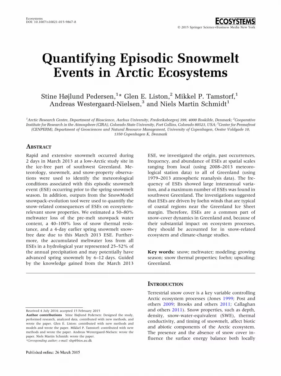
The modeled snow depth showed pronounced in-

terannual variation from 2008 to 2013 (Figure 4).

Snow depth was expected to decrease during ESEs,

and during the March 2013 ESE, we saw a 55%

decrease in the modeled snow depth (Figure 4, black

line). The hydrological year 2009–2010 was snow-

poor with a mean snow depth of 0.15 m and several

snow-free periods during the winter season (Fig-

ure 4). The earliest end of the snow-covered period

was in late April 2010. In all other years, the snow-

free date occurred between mid-May and mid-June.

The longest continuous snow-covered period of

236 days (7.7 months), the maximum annual mean

Table 4. ESEs Identified for the Hydrological Years (September 1–August 31) from 2008 to 2013 and TheirModeled Accumulated Effect on the Snowpack in the Grid Cell Corresponding to the Location of the KOBClimate Station (Figure 2)

Hydrological year Number of

ESEs (#)

ESE

duration

(days)

Total water

loss from ESEs

(m water equivalent)

Earlier

snow-free

date (days)

Total water

loss as fraction

of annual

precipitation (%)

2008–2009 13 15 0.31 10 35

2009–2010 2 4 0.31 10 52

2010–2011 4 4 0.19 6 25

2011–2012 3 4 0.22 12 23

2012–2013 (March 2013 ESE) 9

(1)

12

(2)

0.19

(0.12)

11

(4)

23

(14)

Episodic Snowmelt Events in Arctic Ecosystems

snow depth (0.71 m), and the maximum snow depth

(1.24 m) were all found during 2011–2012.

Model Validation

The modeled snow depth was validated against

observed snow depth measured by an automated

snow-depth sensor at KOB (Figure 5A). The linear

regression between all available snow depth mea-

surements (September 2008–August 2013, n =

1560) and modeled snow depths showed that the

relationship between the modeled and the ob-

served snow depths was statistically significant

(P < 0.001), and the SnowModel output explained

85.3% of the variation in the observed snow depth.

The largest difference between modeled and ob-

served snow depth of 0.41 m was found during

2011–2012. The validation of the modeled SWE

against the observed snowpack water content

showed that the modeled SWE explained 74.3% of

the interannual variation in observed SWE, and the

linear fit between the modeled and observed SWEs

was statistically significant (P < 0.001) (Fig-

ure 5B).This interannual SWE variation is strongly

related to the interannual water equivalent snow

precipitation used in the simulations (not shown).

Modeled snow-covered period timing and dura-

tion were compared with observed start and end of

the snow-covered period(s) defined by the albedo

evolution (Figure 5C). On average, the timing of

modeled start and end matched the observed with

1–2 days difference. However, during 2011–2012,

the start and end were offset by 7 and 5 days, re-

spectively (Figure 5C). Modeled snow cover also

captured the timing of shorter snow-covered and

snow-free periods during October–February. All

dates of start and end from both shorter and longer

observed snow-covered periods showed a high

correlation with the timing of modeled snow cover

(Linear regression statistics: intercept = 0.081,

slope = 1.000, n = 15, P < 0.001, R2 = 0.999).

ESE-Related Snow-Property Changes

Snow depth and snow density observations col-

lected before and after the March 2013 ESE en-

abled evaluation of the SnowModel performance

during an ESE. Modeled and observed SWE dif-

fered by 0.03 m on March 14, 2013 and 0.04 m on

March 19, 2013 in the point of the west-most snow

pit (Figure 2). The simulated snowpack water loss

between the two dates was partitioned into 98.9%

meltwater runoff and a minor moisture loss (1.1%)

from the snowpack surface by sublimation.

On March 14, we observed a 0.90 m deep snow-

pack in the west-most snow pit (Figure 2) with a top

0.40 m thick fine-grained recent/new snow layer

with a density of 185 kg m-3 (44% of the snow

depth), and a bottom 0.50 m thick layer of coarse-

grained depth hoar with a density of 300 kg m-3

(56% of the snow depth). The thermal conductivity

(keff) for the new snow layer is 0.062 W m-1 K-1

and keff for depth hoar is 0.126 W m-1 K-1 based on

the quadratic equation in Sturm and others (1997).

The vertically integrated R for that snow pit was

estimated using equation 1

RMarch14; 2013 ¼0:90m� 0:44

0:062Wm�1 K�1 � 1m2

þ0:90m� 0:56

0:126Wm�1 K�1 � 1m2

¼ 10:4KW�1:

Figure 4. Modeled snow

depth (m) from one grid

point with low shrub

vegetation in flat terrain,

located in the center of

the study area (Figure 2,

near KOB) for the

hydrological years

(September 1–August 31)

from 2008 to 2013.

S. H. Pedersen and others

Due to small spatial variability in snow depth and

vegetation height in the area, on March 19, 2013

we dug a new snow pit 2 m away from the March

14, 2013 snow pit. The top 0.40 m of new snow

had melted away and only the lowest 0.38 m of the

depth hoar layer remained; the bulk density of the

bottom layer had increased 2%, which corre-

sponded to an increase in keff of 0.006 W m-1 K-1.

The resulting R on March 19, 2013 was calculated

for the remaining bottom depth hoar layer as,

RMarch19;2013 ¼0:38m�1:00

0:131Wm�1K�1�1m2¼ 2:9KW�1

:

These estimates resulted in 72% snow thermal re-

sistance reduction from the observed snowpack

from March 14 to March 19, in the west-most snow

pit. We applied this partitioning of 44% new snow

and 56% depth hoar to the spatially distributed

modeled snow depth on the days March 14, 15,

and 16, 2013 (end-of-day modeled outputs) be-

cause the observed snow depth (0.38 m) in the

snow pit on March 19 was representative for the

range of modeled snow depth for the valley on that

date (0–50 cm). We assumed that the snowpack did

not change much from March 16, until the obser-

vations were made on March 19, 2013, because

both automated snow-depth sensor measurements

at KOB and modeled snow depth showed that the

majority of the snowmelt took place during the

2 days (March 15 and 16).

During the March 2013 ESE, the mean water loss

over the 2 days per grid cell (10 m by 10 m) ranged

between 0.06 and 0.12 m water equivalent in the

valley below 200 m a.s.l. (Figure 6A), which rep-

resents 50–80% of the pre-melt snowpack water

content. These differences are primarily related to

slope, aspect, and elevation variations associated

with the simulation domain. The resulting modeled

snow thermal resistance loss during the March

Figure 5. A Regression between modeled and observed snow depths in the location of the climate station, KOB, at time

increments (daily), where observed snow depth were available, that is, September 2008–August 2013. Linear fit statistics

(solid line): Intercept = -0.016, slope = 0.826; R2 = 0.853, F1,1560 = 9070, P < 0.001. Dotted line is 1:1 line. B Regression

between the observed and the modeled snow-water-equivalents (SWEs). Linear fit statistics (solid line): Intercept = 0.089,

slope = 0.530; R2 = 0.743, F1,46 = 133.5, P < 0.001. Dotted line is 1:1 line. C Snow-covered periods, where modeled snow

depth (black lines) is above 0.0 m in comparison with the observed timing (red crosses) of snow-cover onset (albedo is above

0.8) and snow-cover end (albedo is less than 0.2) from 2008 to 2013. No observed albedo data were available prior to

August 2008.

Episodic Snowmelt Events in Arctic Ecosystems

2013 ESE varied spatially as well, varying from 40

to 100% in the valley area below 200 m a.s.l.

(Figure 6B). Furthermore, observations of snow-

free areas in the digital photo from March 16, 2013

(Figure 1) was consistent with the modeled 100%

snow depletion being confined primarily to small,

local hill tops in the valley area.

By applying SnowModel to the Kobbefjord study

area, we were able to quantify the recent local ESE-

associated changes in ecologically relevant snow

properties in the studied low-Arctic ecosystem.

Among the 31 identified ESEs (Table 4) we found

maximum meltwater losses of 0.12 m water

equivalent during October 27–28, 2008 and 0.12 m

during March 15–16, 2013. The meltwater lost

during these two ESEs alone represented more

than a tenth of the annual precipitation sum and

were estimated to cause up to 3.8 and 3.8 days

earlier snow-free date, respectively. The majority of

the identified 1-day ESEs led to thinning of the

snowpack, and thereby a loss of snow thermal re-

sistance. The meltwater loss associated with single

ESEs (1- to 3-day ESEs) ranged between 0.0 and

0.05 m water equivalent. However, the accumu-

lated meltwater loss through the winter for all

events occurring within the same hydrological year

equaled 23–52% of the annual precipitation, which

potentially represented an advancement of 6–

12 days in spring snowmelt per year (Table 4). For

seven of the ESEs identified in the meteorological

data (Part I), the SnowModel outputs showed no

snowmelt. The meltwater loss along with a 40–

100% decrease in the snow insulation effect can

potentially influence the dynamics and functioning

of the ecosystem on this local scale.

In light of the ecological importance of ESEs on

snow properties in the low-Arctic terrestrial

ecosystem, and that the meteorological variables

controlling the occurrence of ESEs are assumed to

be strongly tied to middle- and high-latitude low

pressure systems (Steffen and Box 2001; Mernild

and others 2014), we expected the scope of influ-

ence associated with ESEs to cover a larger area

than our local Kobbefjord study domain. Hence, we

then looked beyond the Kobbefjord valley and fo-

cused in Part III on the greater coastal ice-free area

of Greenland using a meteorological dataset

(MERRA; Rienecker and others 2011) that mat-

ched the synoptic scale (�1000 km) over which the

low-pressure weather patterns occur. Therefore, in

Part III we investigated whether past ESEs could be

identified further north, south, and east of Kobbe-

fjord and estimated their temporal frequency and

spatial extent.

PART III: PAST ESES IN GREENLAND

Methods and Data

To identify trends in the occurrence of past ESEs

over the ice-free part of Greenland, we used the

automated ESE identification algorithm (Table 2)

on this regional scale. As input, we used a Green-

land subset of MERRA reanalysis data (see Part II;

Rienecker and others 2011) that covered the 34-

year period from September 1, 1979 to August 31,

2013 and included the variables: air temperature,

SWE, and wind speed.

Part III Findings

We found that the ESE identification algorithm

applied on the MERRA data reproduced all the

Kobbefjord ESEs. This allowed us to conclude that

it was appropriate to run the ESE identification

algorithm over Greenland using the MERRA en-

vironmental data. The results also showed that

ESEs have indeed been occurring outside the

Kobbefjord area during the past 34 years. However,

the majority of the identified ESEs were mainly

confined to west–southwest Greenland (Figure 7).

Furthermore, the spatial representation of the

identified ESEs in west Greenland (Figure 7)

showed a relatively larger number of ESEs along

the Greenland Ice Sheet margin and near the coast.

The timings of the identified ESEs differed between

west–southwest Greenland (59�–75�N) and north-

Figure 6. A Summed

water loss (m water

equivalent) from

snowpack during ESE on

March 15 and 16, 2013.

B Loss of snow thermal

resistance (%) during

March 2013 ESE. Lower

left corner coordinates are

64�7¢25.4¢¢N,

51�25¢24.8¢¢W.

S. H. Pedersen and others

west Greenland (75�–84�N). In southwest Green-

land, the ESEs occurred mostly from October to

November, while the lower number of ESEs iden-

tified in north Greenland occurred from June to

September. Conducting a linear temporal trend

analysis for each individual grid cell on the basis of

the 34-year time series of the annual number of

identified ESEs showed a statistically significant

positive trend (P < 0.05) in a few areas of west–

southwest Greenland and southeast Greenland. In

addition, a statistically significant negative trend

was found in the outer coastal areas of northwest

Greenland (>81.0�N), where relatively few ESEs

were identified (Figure 7).

DISCUSSION

The validation of model outputs demonstrated that

SnowModel reproduced the snow distribution in

Kobbefjord well, both in terms of timing and du-

ration of the snow-covered periods and in match-

ing the observed snow depth and SWE during the

years 2008–2013. Only during 2011–2012 did the

modeled snow-covered period and deep snowpack

show less-than-ideal correspondence with the ob-

servations. This was partly caused by uncertainties

in the measured snow depth at the snow-cover

onset in October 2011. Although daily automated

camera photos (as in Figure 1) and observed albedo

from KOB (Figure 2) showed the first snowfall on

October 9, the snow-depth sensor at KOB showed

0.0-m snow depth until October 23. The difference

between modeled and observed snow depth is

likely to be explained by these snow-depth mea-

surement errors. In addition, the difference during

2011–2012 could be explained by a precipitation

event resulting in either snowfall or rainfall in

SnowModel, depending on the simulated air tem-

perature. Because we were operating in a valley

surrounded by mountains (up to 1375 m a.s.l.),

temperature lapse rates heavily affect the snowfall

variation with elevation. To account for this, we

incorporated daily temperature lapse rate estima-

tions in MicroMet, based on air temperature ob-

servations from climate stations in the valley (KOB,

Table 1) and on the mountain tops (M1000 and

M500, Table 1), when data were available. During

time steps where data were unavailable from

M1000 and M500, we used monthly mean lapse

rates based on data from the whole time series

(2008–2013). This was the case for the period

January 1–August 31, 2012, where M1000 data

were lacking. Hence, the applied monthly mean

lapse rate during this end-of-winter/spring season

may have led to a later snowmelt onset than the

observed and, therefore, created a mismatch be-

tween the modeled and the observed snow-free

date (Figure 5C). In addition, on days when the

monthly mean lapse rates were applied, it could

occur that the model output showed snowfall in

both the valley and on mountain tops, but in re-

ality the snowfall was confined to the mountain top

because of a relatively higher temperature lapse

rate present that day. During snow-cover onset in

October 2011, air temperature observations were

available for all three meteorological stations: KOB,

M500, and M1000 (Table 1). This enabled inclu-

sion of observed lapse rates in the model run and

on October 2, 2011, the daily mean air tem-

peratures were 1.93; -2.62; and -5.14�C at the

three stations, respectively. However, it resulted in

modeled snowfall both at the mountain tops and in

the valley, because the snow-rain phase threshold

in MicroMet was set to 2.0�C according to Auer

(1974). Furthermore, automated camera photos

showed snowfall only on the mountain tops that

same day. Valley snowfall events similar to this

occurred until October 23, and resulted in a mod-

eled snow depth of 0.39 m on that date (October

23, 2011) when the observed snow depth went

above 0.0 m in the valley for the first time that

winter. This caused a modeled snow depth that was

0.39 m greater than the observed valley snow

depth. This depth increment persisted throughout

the winter and produced the differences found

between the modeled and the observed snow and

SWE depths during the 2011–2012 winter.

Based on the model validation, we used Snow-

Model outputs for Kobbefjord to estimate snow-

property changes for ESEs identified with the

Figure 7. Mean annual number of ESEs identified dur-

ing the period 1979–2013.

Episodic Snowmelt Events in Arctic Ecosystems

automated identification algorithm during 2008–

2013. The snow thermal resistance (R) calculations

were not validated because no such measurements

have been conducted in Kobbefjord. However, the

RMarch 14, 2013 and RMarch 19, 2013 have been found

to correspond to R of snow covers found on Arctic

dry and scrub tundra (Liston and others 2002).

Nevertheless, some observations of snow stratigra-

phy were available in the valley prior of the March

2013 ESE to support the extrapolation of 44% new

snow and 56% depth hoar from one observation

point to the rest of the valley. This means that the

decrease in snow thermal resistance (Figure 6B)

may be underestimated in areas with less depth

hoar fraction than 56%, while it could be overes-

timated in areas with higher depth hoar fraction,

depending on the depth hoar development in the

snowpack on different surfaces (Sturm and John-

son 1992; Benson and Sturm 1993). Still, depth

hoar crystals were observed in all (6) snow pits

after March 2013 and are common in a tundra

snowpack (Benson and Sturm 1993; Sturm and

others 1995). Hence, the depth hoar fraction in-

troduces uncertainty in these results.

Ecological Effects of ESEs

To assess the potential effects on ecosystem com-

ponents and processes caused by ESEs, knowledge

of ESE-related changes in snow properties, such as

those presented in Part II, are required (see Bo-

khorst and others 2010). For instance, the March

2013 ESE caused changes in the soil thermal re-

gime due to loss of the snow-cover insulating ef-

fect. Observations showed a 3.0�C increase in 3-day

average soil temperature between before and after

the March 2013 ESE in a valley area (Soil station,

Figure 2), which experienced a 60–70% reduction

in thermal resistance (Figure 6B). Also, an ESE

may cause frost damage to vegetation, if the pre-

melt snow depth is shallow enough for the snow

cover to deplete completely during an ESE (Bo-

khorst and others 2011). The ESE observed in

Kobbefjord in March 2013 (Table 4) may have re-

sulted in such vegetation frost damage, because the

snow cover depleted completely on the hill tops

and in other thin-snow areas. This resulted in a

patchy insulating snow cover (see Figure 1) and

exposed vegetation to freezing temperatures (daily

mean air temperature of -3.3�C).

The majority of the identified ESEs in Kobbefjord

resulted in a thinning of the snowpack and a reduced

insulating effect, which may not prevent frost dam-

age and reduced flowering the following growing

season(s) (Semenchuk and others 2013). However,

frost sensitivity varies between plant species. Two

dwarf shrub types, Empetrum hermaphroditum and

Vaccinium vitis-idaea found in south and west Green-

land, including Kobbefjord (Bocher and others 1978;

Bay and others 2008), respond differently to expo-

sure to freezing temperatures. Extreme winter

warming experiments in a sub-Arctic ecosystem have

shown that E. hermaphroditum is prone to frost

damage, whereas V. vitis-idaea shows no or only

limited sign of frost damage (Bokhorst and others

2011). Hence, because ESEs appear to be a common

part of the snow-cover dynamics in west Greenland,

the species living there are likely to be resilient or

resistant to frequent frost exposure (see Bokhorst and

others 2010; Semenchuk and others 2013). However,

the adaptive capacity of some species in the Arctic

ecosystem may be challenged due to a future in-

creasing frequency of ESEs in west Greenland.

In Arctic ecosystems dependent on winter pre-

cipitation and snow accumulation as a moisture

source for plant growth during the growing season

(Elberling and others 2008; Brooks and others

2011), the consequences of ESE-related meltwater

loss of up to 52% of the annual precipitation from

the snowpack may reach into the plant growing

season and impact growing conditions. The melt-

water loss may have caused a moisture shortage at

the beginning of and during the growing season

(Ellebjerg and others 2008; Schmidt and others

2012) and potentially limited the vegetation growth

for some species (Ellebjerg and others 2008; Schmidt

and others 2012; Rumpf and others 2014). Fur-

thermore, the lack of soil moisture through the

growing season may have increased decomposition

rates of organic matter in the soil and limited the

gross primary production (Lund and others 2012),

thereby affecting the ecosystem CO2 balance

(Brooks and others 2011). Meltwater lost from the

snowpack during winter and spring during an ESE is

likely to be lost through surface runoff, because the

ground is frozen, and the water is routed under the

snowpack into streams and rivers (Bayard and oth-

ers 2005; this study). The meltwater loss during the

March 2013 ESE represented up to 80% of pre-melt

snowpack water content and up to 14.2% of the

annual precipitation. The model outputs showed

that this substantial amount of water was lost pri-

marily through runoff. This is supported by auto-

mated soil temperature measurements in and below

10-cm depth in heath- and fen-covered soils in

Kobbefjord. The data showed freezing temperatures

from November to March, which thereby limited

the meltwater percolation into the soil and fa-

cilitated lateral runoff into streams and lakes (Ba-

yard and others 2005).

S. H. Pedersen and others

The March 2013 ESE was the single ESE having

the largest impact on the snowpack in terms of

thinning of the snow cover (0.20 m), meltwater

loss (0.12 m water equivalent = 14% of the 2012/

2013 annual precipitation), and potential ad-

vancement of the spring snowmelt (4 days). This

emphasizes that the March 2013 ESE was stronger

than the regularly occurring ESEs. However, be-

cause the cumulated meltwater loss from all annual

ESEs potentially equal 23–52% of the annual pre-

cipitation, the additive effect from all ESEs plays a

major role for the hydrological cycle of the

ecosystem. Furthermore, the potential 6–12 days

advancement of the start of the snow-free season

can potentially cause a shift in a range of biotic and

abiotic terrestrial processes, such as plant-flowering

phenology (Høye and others 2007; Cooper and

others 2011; Iler and others 2013), gas–flux ex-

change (Brooks and others 2011; Lund and others

2012), arthropod emergence (Høye and others

2007), and avian-breeding phenology (Meltofte

and others 2007), which are dependent on the

timing of the spring snowmelt and thereby ground

exposure.

All these examples and observations illustrate the

potential impact that ESEs have on the Arctic

ecosystem through changes in snow properties.

Our analysis documented that ESEs have been a

common and natural part of the snow-cover dy-

namics in west Greenland at least since 1979, and

most species found in Greenland are thus likely

adapted to this phenomenon. However, an in-

creasing frequency of ESEs may put the ecosystems

under severe pressure, ultimately resulting in al-

terations in local species composition (see for ex-

ample, Elmendorf and others 2012a, b) to cope

with reoccurring abrupt meltwater losses and de-

creases in snow-cover insulating effect. We focused

on three snow properties in this study; snow ther-

mal resistance (controlling the thermal conditions

in the soil and thereby the soil heterotrophic ac-

tivity during the snow-covered period (Nobrega

and Grogan 2007; Gouttevin and others 2012)),

meltwater content available for plant growth, and

the snow-free date defining the growing-season

onset. As discussed above, these three snow prop-

erties are, individually and combined, driving and

controlling ecosystem processes occurring outside

the snow-covered period, that is, within the

growing season. Hence, changes occurring during

winter, such as an ESE, may cause ecosystem

changes during the following growing season(s)

(Bokhorst and others 2011; Semenchuk and others

2013). This highlights and emphasizes the need for

ecosystem-monitoring programs that run year-

round, because changes and interannual variations

observed during the heavily studied summer field

season may be explained by events or changes oc-

curring during winter and/or the shoulder seasons.

ESE Scale-Issues, Driving Factors, andTiming

The comparison between the number of identified

ESEs locally in Kobbefjord through station obser-

vations (Part I) and a MERRA grid cell matching

the same location is challenged by the lack of

subgrid variability in topography and physical

processes within a MERRA grid cell. The 2/3� by 1/

2� MERRA grid cell covering the Kobbefjord valley

and surroundings spans an elevation range from

sea level to 1400 m a.s.l. For comparison, the

photos in Figure 1 and the study area map in Fig-

ure 2 correspond to approximately 1/4 of the

MERRA grid cell. The topographic variation is the

main driver for the spatial variations in air tem-

perature, wind speed, and snow cover with eleva-

tion and across the landscape (Liston and Elder

2006a). Such variation is inevitably not captured

with one single data value per MERRA grid cell for

any of the three climate variables used in the

identification algorithm (Part 1). A direct compar-

ison between the MERRA grid cell, covering the

location of the KOB station, and the KOB station

data for the years 2008–2013 resulted in 12%

higher mean annual air temperature and 22%

higher mean annual wind speed in MERRA than in

KOB station observations. Hence, due to this scal-

ing-issue, more ESEs were identified with MERRA

data as input to the identification algorithm than

when using Kobbefjord station data (Part I). We are

therefore aware that the mean annual number of

identified ESEs in Kobbefjord, and likely in other

areas in Greenland, may be overestimated when

using the MERRA data. We are, however, confi-

dent that the MERRA dataset captures the general

patterns of the Greenland atmospheric environ-

ment and most importantly, the weather features

causing the ESEs, for example, latitudinal and

coast–inland gradients in air temperature. The

MERRA data thus represent the relative spatial and

temporal distributions and differences in ESEs be-

tween regions in north, south, east, and west

Greenland.

The driver for the ESEs is likely related to large-

scale weather patterns occurring on the west coast

of Greenland and particularly in southwest

Greenland, where we found the highest ESE fre-

quency (Figure 7). The ESE-associated high wind

speeds, rapid increase in air temperatures, and the

Episodic Snowmelt Events in Arctic Ecosystems

location of the highest ESE frequency suggested a

possible relation to foehn winds. The assumption

that foehn winds are driving the ESEs is further-

more supported by the finding that the highest

frequency values of ESEs are in southwest Green-

land (Figure 7), where foehn winds are the stron-

gest and most frequent (Fristrup 1953; Gorter and

others 2014). The first scientific description of

foehn winds in west Greenland was by Hoffmeyer

(1877). This early publication year suggests that

foehn winds have been a feature of west Greenland

climate for a long time. During foehn events, warm

dry wind is able to create high snowmelt rates. In

Greenland, foehn winds are driven by the Green-

land katabatic wind system (Figure 5 in Cappelen

and others 2001; Gorter and others 2014), which is

driven by the density difference between the heavy

cold air close to the ice surface of the Greenland Ice

Sheet interior and the lower density and warmer

air above. When the winds approach the ice mar-

gin, the wind speed is accelerated due to topo-

graphic channeling and the steeper slopes of the

coastal mountains and outlet glaciers. The out-

flowing air mass is compressed as it descends from

the ice sheet because of the altitude change, and

the air pressure increase results in heating of the air

mass. Figure 7 includes not only the ice-free areas,

but also the Greenland Ice Sheet margin to identify

whether the frequency of the identified ESEs

would potentially be higher on the ice and there-

fore support the argument that foehn winds are a

driver for ESEs, because foehn winds originate

from the Greenland Ice Sheet and reach high wind

speeds in the ice marginal area. Indeed, Figure 7

shows a pattern of more ESEs being closest to the

ice sheet margin and at the outer coast in west

Greenland (65�–72�N). The climatic conditions for

ESEs to occur are likely to be favorable in both

places. During a foehn event, the area near the ice

sheet margin is relatively warm and relatively more

windy than further out by the coast (Cappelen and

others 2001), whereas near the outer coast, the air

temperature is generally higher than inland in

winter because of the relatively warm ice-free Da-

vid Strait. However, the outer coast is also windier

because the high wind speeds associated with

foehn winds may be sustained through channeling

in fjord systems and valleys on their way to the

outer coast and fjord heads. This pattern is consis-

tent with our March 2013 ESE observations, be-

cause Kobbefjord is located approximately 100 km

from the ice sheet margin.

The timing of ESE occurrences differed between

northwest and southwest Greenland and the few

northern-identified ESEs occurred from June to

September, when air temperatures reached above

0�C (DMI 2014). The combination of small solar

angle, that is, relatively limited energy amounts

reaching these northern latitudes, and air tem-

peratures ranging between -30 and -15�C (Cap-

pelen 2011), limits the chance for air temperatures

in northwest Greenland rising above freezing for

most of the year. Therefore, ESEs are less likely to

occur in the north, and may have less ecosystem

impact than at lower latitudes because they mainly

occur during spring or summer, when the snow

cover is depleting. Furthermore, the low ESE fre-

quency north of 81.0�N has significantly decreased

over the last 34 years. In middle-west Greenland,

the ESEs predominantly occurred during the onset

of the snow-covered season during October and

November. The region below the Arctic Circle

(approximately 66�34¢N) is less affected by reduced

solar radiation during winter. This region has gen-

erally higher air temperatures than further north,

so that a temperature rise during winter would

more likely result in above-freezing temperatures,

and therefore ESEs were also identified through the

winter months in this area. The early-winter timing

of ESEs may cause frost penetrating into the soil if

the ground is exposed to subfreezing temperatures

after an ESE. These frozen soils can be preserved

during the winter, when the snow cover is

reestablished (Zhang 2005). Also, meltwater from

early-winter ESEs may create ice layers within or

below the remaining snow cover, which will po-

tentially block food access for herbivores through

the winter and have fatal consequences for a

population (for example, Hansen and others 2011).

In south Greenland, the identified ESEs occurred

through the autumn, winter, and spring, that is,

from October to mid-May. In this region, local

sheep herding is dependent on soil moisture

originating from spring snowmelt for vegetation

growth, especially in meadows and snow-beds that

provide the majority of the plant forage for sheep

grazing in the mountains (Austrheim and others

2008). If meltwater amounts are reduced due to

ESEs during winter, it may result in reduced

vegetation growth, and thereby limit food avail-

ability for the sheep during summer grazing in ar-

eas already at risk of overgrazing (Aastrup and

others 2014). The north–south difference in ESE

frequency is most likely to be tied to the locations,

where foehn winds are most frequent and

physically possible to occur in terms of air tem-

perature and wind regime, which in turn are con-

trolled by synoptic-scale weather circulation

patterns and topography and slope gradients, re-

spectively (Gorter and others 2014).

S. H. Pedersen and others

ESEs in a Changing Climate

For future perspectives, the predicted reduction in

the temperature deficit over the center of the

Greenland Ice Sheet will result in wind-speed re-

ductions in the center of the ice sheet, where

katabatic forcing is predominant. However, as a

subsequent consequence, the wind speeds are

predicted to increase in the coastal areas with steep

topography (Gorter and others 2014), thereby in-

creasing the foehn wind frequency. This may cause

a continued increase in the number of extreme

events in, for example, air temperature (Mernild

and others 2014) and snowmelt (ESEs). Further-

more, because the annual mean surface air tem-

perature in coastal Greenland continues to increase

(Hartmann and others 2013; Cappelen and Vinther

2014), especially during winter (Hanna and others

2012), future increased magnitude and frequency

of air temperatures above freezing may result in

higher snowmelt rates than we have seen in the

recent, identified ESEs.

During the March 2013 ESE, the foehn event

appeared to be tied to and driven by the location,

strength, and the associated wind patterns of syn-

optic-scale pressure systems. A high-pressure ridge

was located over the Greenland Ice Sheet and a

low-pressure trough over Baffin Island, which are

typical locations for anticyclones and cyclones

during winter (Serreze and others 1993). The

pressure gradient generated south-easterly winds,

passing in a westward direction over the ice sheet,

presumably resulting in foehn winds and ESEs in

west Greenland. If the foehn events are tied to the

locations and strength of these high- and low-

pressure systems, it might explain the pronounced

difference in the timings of ESEs between north-

west and southwest Greenland, as the location and

strength of the high- and low-pressure systems

over and surrounding the Greenland Ice Sheet are

tied to the seasons and dark/light periods (Serreze

and others 1993).

In this analysis, we found a positive temporal

trend in the annual frequency of ESEs in few areas

of west and east Greenland (59.9�–81.0�N) and

identified large interannual variations in the

number of ESEs through the 34 years. If we assume

that ESEs are driven by foehn winds and that the

timing of the foehn winds to some extent is con-

trolled by locations and strengths of low- and high-

pressure systems in and around Greenland, an

amplification of a future continued increase in ESE

frequency could originate from changes in synop-

tic-scale weather systems. Such changes are de-

scribed by Francis and Vavrus (2012), who suggest

a weakening of the Jetstream due to a reduced

temperature gradient between the Northern

Hemisphere middle-latitudes and high-latitudes

caused by increased warming in the Arctic. A

weakened Jetstream potentially generates slower

movement of pressure systems across the North

Atlantic, creating more persistent weather and al-

tered large-scale circulation patterns in the North-

ern Hemisphere. This change in circulation pattern

is likely to influence the location and strength of

low-pressure systems in relation to the high-pres-

sure over the Greenland Ice Sheet, which may

potentially affect future ESE frequency, distribu-

tion, and strength, which in turn may challenge

the Arctic ecosystems in Greenland.

SUMMARY AND CONCLUSIONS

First-hand observations of snow-property changes

and weather conditions during an ESE in March

2013 in the Kobbefjord coastal low-Arctic study site

in southwest Greenland enabled us to define ESEs

that occur during times when snow depth is greater

than 0.0 m, daily air temperature is above 0.0�C,

and wind speed is greater than 5.5 m s-1. These

ESE characteristics were the basis for developing an

automated algorithm that was used to identify 31

recent ESEs (2008–2013) occurring on a local scale

in Kobbefjord. Next, we applied SnowModel as a

tool to model snow distributions in Kobbefjord. The

model outputs were used to quantify ecologically

relevant snow-property changes resulting from the

March 2013 ESE. We estimated a water loss

equaling 50–80% of the pre-melt snowpack water

content, and a 40–100% decrease in snow thermal

resistance caused by changes in snow depths, snow

type composition of the snowpack, and thereby

changes in snow thermal resistance during the ESE.

Potential impacts from these changes in snow

properties on ecosystem processes and components

include frost damage to vegetation and changes in

soil moisture and soil thermal conditions. In addi-

tion, ESEs occur frequently during the winter and

are a part of the snow-cover dynamics in Kobbe-

fjord and constitute a significant part of the annual

precipitation (23–52%) lost primarily through

surface runoff, which potentially could result in 6–

12 days earlier spring snowmelt.

On a regional scale of the ice-free parts of

Greenland, we found that ESEs are common in

west and southwest Greenland. The annual num-

ber of ESEs in a few areas in west and east

Greenland from 1979 to 2013 showed a statistically

significant positive trend, but also large interannual

variation in the occurrence of ESEs. Based on the

Episodic Snowmelt Events in Arctic Ecosystems

geographic location of the highest ESE frequencies

and the characteristics identified for ESEs, we

suggest that foehn winds are likely to be a key

driver of ESEs in Greenland. The ESEs seem to be a

natural and common part of the snow-cover dy-

namics in low-Arctic west and east Greenland, and

the local species assemblages have likely adapted to

these. However, in a warmer Greenland climate,

the frequency of ESEs may continue to increase

and the associated snowmelt rates might also in-

crease due to increasing air temperatures. This will,

in turn, gradually increase the pressure on the

ecosystem, including its species, and the processes

associated with moisture availability and timing,

thermal protection, and growing season (snow-

free) duration.

ACKNOWLEDGMENTS

We wish to thank Nuuk Ecological Research Op-

erations and Asiaq, Greenland Survey for providing

data and helping us with data collection in March

2013 in Kobbefjord; and NASA for permission to use

Modern-Era Retrospective Analysis for Research

and Applications (MERRA) reanalysis datasets. We

offer our special thanks to K. Elder for thorough

guidance and recommendations on snow-sampling

methods and strategies used during the field cam-

paign. We also thank two anonymous reviewers

whose comments greatly improved this manuscript.

We gratefully acknowledge the logistic support of

Arctic Research Centre (ARC), Aarhus University.

Support was also provided by the Canada Excellence

Research Chair (CERC). This study was funded by

the Environmental Protection Agency and the

Danish Energy Agency, and it is a contribution to

the Arctic Science Partnership (ASP) asp-net.org.

REFERENCES

Aastrup P, Raundrup K, Feilberg J, Krogh PK, Schmidt NM,

Nabe-Nielsen J. 2014. Effects of large herbivores on biodi-

versity of vegetation and soil microarthropods in low Arctic

Greenland—Akia, West Greenland and Southern Greenland.

Scientific report from DCE—Danish Centre for Environment

and Energy. Roskilde: Aarhus University, DCE—Danish

Centre for Environment and Energy, p. 40.

AMAP. 2012. Arctic Climate Issues 2011: Changes in Arctic

Snow, Water, Ice and Permafrost. SWIPA 2011 Overview re-

port. Oslo: Arctic Monitoring and Assessment Programme

(AMAP), p. xi + 97.

Auer AH. 1974. The rain versus snow threshold temperature.

Weatherwise 27:67.

Austrheim G, Asheim L-J, Bjarnason G, Feilberg J, Fosaa AM,

Holand Ø, Høegh K, Jonsdottir IS, Magnusson B, Mortensen

LE, Mysterud A, Olsen E, Skonhoft A, Steinheim G,

Thorhallsdottir AG. 2008. Sheep grazing in the North-Atlantic

region—A long term perspective on management, resource

economy and ecology. Rapport zoologisk serie 2008-3.

Trondheim: Norges teknisk-naturvitenskapelige universitet

Vitenskapsmuseet. p 86.

Bartsch A, Kumpula T, Forbes BC, Stammler F. 2010. Detection

of snow surface thawing and refreezing in the Eurasian Arctic

with QuikSCAT: implications for reindeer herding. Ecol Appl

20:2346–58.

Bay C, Aastrup P, Nymand J. 2008. The NERO line. A vegetation

transect in Kobbefjord. West Greenland: National Environ-

mental Research Institute, Aarhus University. p 40.

Bayard D, Stahli M, Parriaux A, Fluhler H. 2005. The influence

of seasonally frozen soil on the snowmelt runoff at two Alpine

sites in southern Switzerland. J Hydrol 309:66–84.

Benson CS, Sturm M. 1993. Structure and wind transport of

seasonal snow on the Arctic slope of Alaska. Ann Glaciol

18:261–7.

Blankinship JC, Meadows MW, Lucas RG, Hart SC. 2014.

Snowmelt timing alters shallow but not deep soil moisture in

the Sierra Nevada. Water Resour Res 50:1448–56.

Bocher TW, Fredskild B, Holmen K, Jakobsen K. 1978. Grøn-

lands flora. Copenhagen: P. Haase & Søn.

Bokhorst S, Bjerke JW, Davey MP, Taulavuori K, Taulavuori E,

Laine K, Callaghan TV, Phoenix GK. 2010. Impacts of extreme

winter warming events on plant physiology in a sub-Arctic

heath community. Physiol Plant 140:128–40.

Bokhorst S, Bjerke JW, Street LE, Callaghan TV, Phoenix GK.

2011. Impacts of multiple extreme winter warming events on

sub-Arctic heathland: phenology, reproduction, growth, and

CO2 flux responses. Glob Change Biol 17:2817–30.

Bokhorst S, Bjerke JW, Tommervik H, Preece C, Phoenix GK.

2012. Ecosystem response to climatic change: the importance

of the cold season. Ambio 41:246–55.

Brooks PD, Grogan P, Templer PH, Groffman P, Oquist MG.

2011. Carbon and nitrogen cycling in snow-covered envi-

ronments. Geogr Compass 5:682–99.

Callaghan TV, Johansson M, Brown RD, Groisman PY, Labba N,

Radionov V, Bradley RS, Blangy S, Bulygina ON, Christensen

TR, Colman JE, Essery RLH, Forbes BC, Forchhammer MC,

Golubev VN, Honrath RE, Juday GP, Meshcherskaya AV,

Phoenix GK, Pomeroy J, Rautio A, Robinson DA, Schmidt

NM, Serreze MC, Shevchenko VP, Shiklomanov AI, Shmakin

AB, Skold P, Sturm M, Woo MK, Wood EF. 2011. Multiple

effects of changes in arctic snow cover. Ambio 40:32–45.

Cappelen J. 2011. DMI monthly climate data collection 1768-

2010, Denmark, The Faroe Islands and Greenland technical

report. Copenhagen: Danish Meteorological Institute. p 54.

Cappelen J, Vinther BM. 2014. SW Greenland temperature data

1784-2013. Technical report. Copenhagen: Danish Meteoro-

logical Institute.

Cappelen J, Vraae Jørgensen B, Vaarby Laursen E, Sligting

Stannius L, Sjølin Thomsen R. 2001. The observed climate of

Greenland, 1958-99—with climatological standard normals,

1961-90. Technical report. Copenhagen: Danish Meteoro-

logical Institute. p 151.

Cooper EJ, Dullinger S, Semenchuk P. 2011. Late snowmelt

delays plant development and results in lower reproductive

success in the High Arctic. Plant Sci 180:157–67.

Dadic R, Mott R, Lehning M, Carenzo M, Anderson B, Mack-

intosh A. 2013. Sensitivity of turbulent fluxes to wind speed

over snow surfaces in different climatic settings. Adv Water

Resour 55:178–89.

S. H. Pedersen and others

DMI. 2014. Danish Meteorological Institute Weather archive:

climate archive of climate normal period 1961–1990. Copen-

hagen: DMI.

Elberling B, Tamstorf MP, Michelsen A, Arndal MF, Sigsgaard C,

Illeris L,BayC,HansenBU,ChristensenTR,HansenES, Jakobsen

BH, Beyens L. 2008. Soil and plant community-characteristics

and dynamics at Zackenberg. In: Meltofte H, Christensen TR,

Elberling B, Forchhammer MC, Rasch M, Eds. Advances in

ecological research. London: Academic Press. p 223–48.

Ellebjerg SM, Tamstorf MP, Illeris L, Michelsen A, Hansen BU.

2008. Inter-annual variability and controls of plant phenology

and productivity at Zackenberg. In: Meltofte H, Christensen

TR, Elberling B, Forchhammer MC, Rasch M, Eds. Advances

in ecological research. London: Academic Press. p 249–73.

Elmendorf SC, Henry GHR, Hollister RD, Bjork RG, Bjorkman

AD, Callaghan TV, Collier LS, Cooper EJ, Cornelissen JHC,

Day TA, Fosaa AM, Gould WA, Gretarsdottir J, Harte J, Her-

manutz L, Hik DS, Hofgaard A, Jarrad F, Jonsdottir IS, Keuper

F, Klanderud K, Klein JA, Koh S, Kudo G, Lang SI, Loewen V,

May JL, Mercado J, Michelsen A, Molau U, Myers-Smith IH,

Oberbauer SF, Pieper S, Post E, Rixen C, Robinson CH, Sch-

midt NM, Shaver GR, Stenstrom A, Tolvanen A, Totland O,

Troxler T, Wahren CH, Webber PJ, Welker JM, Wookey PA.

2012a. Global assessment of experimental climate warming on

tundra vegetation: heterogeneity over space and time. Ecol

Lett 15:164–75.

Elmendorf SC, Henry GHR, Hollister RD, Bjork RG, Boulanger-

Lapointe N, Cooper EJ, Cornelissen JHC, Day TA, Dorrepaal E,

Elumeeva TG, Gill M, Gould WA, Harte J, Hik DS, Hofgaard A,

Johnson DR, Johnstone JF, Jonsdottir IS, Jorgenson JC,

Klanderud K, Klein JA, Koh S, Kudo G, Lara M, Levesque E,

Magnusson B, May JL, Mercado-Diaz JA, Michelsen A, Molau

U, Myers-Smith IH, Oberbauer SF, Onipchenko VG, Rixen C,

Schmidt NM, Shaver GR, Spasojevic MJ, Porhallsdottir PE,

Tolvanen A, Troxler T, Tweedie CE, Villareal S, Wahren CH,

Walker X, Webber PJ, Welker JM, Wipf S. 2012b. Plot-scale

evidence of tundra vegetation change and links to recent

summer warming. Nat Clim Change 2:453–7.

Forchhammer M, Boertmann D. 1993. The Muskoxen Ovibos

moschatus in north and northeast Greenland: population

trends and the influence of abiotic parameters on population

dynamics. Ecography 16:299–308.

Francis JA, Vavrus SJ. 2012. Evidence linking Arctic amplifica-

tion to extreme weather in mid-latitudes. Geophys Res Lett

39:L06801.

Fristrup B. 1953. De grønlandske foehnvinde. Tidsskriftet

Grønland 3:4.

Fuller MC, Geldsetzer T, Yackel JJ. 2009. Surface-based polari-

metric C-band microwave scatterometer measurements of

snow during a chinook event. IEEE Trans Geosci Remote Sens

47:1766–76.

Goodison BE, Louie PYT, Yang D. 1998. WMO solid precipitation

intercomparison. Final report WMO/TD-872 Instruments and

observing methods report. Geneva: World Meteorological

Organization. p 212.

Goodrich LE. 1982. The influence of snow cover on the ground

thermal regime. Can Geotech J 19:421–32.

Gorter W, van Angelen JH, Lenaerts JTM, van den Broeke MR.

2014. Present and future near-surface wind climate of

Greenland from high resolution regional climate modelling.

Clim Dyn 42:1595–611.

Gouttevin I, Menegoz M, Domine F, Krinner G, Koven C, Ciais

P, Tarnocai C, Boike J. 2012. How the insulating properties of

snow affect soil carbon distribution in the continental pan-

Arctic area. J Geophys Res 117:G02020.

Groisman PY, Karl TR, Knight RW, Stenchikov GL. 1994.

Changes of snow cover, temperature, and radiative heat-bal-

ance over the Northern-Hemisphere. J Clim 7:1633–56.

Hanna E, Mernild SH, Cappelen J, Steffen K. 2012. Recent

warming in Greenland in a long-term instrumental (1881–

2012) climatic context: I. Evaluation of surface air tem-

perature records. Environ Res Lett 7:045404.

Hansen BB, Aanes R, Herfindal I, Kohler J, Saether BE. 2011.

Climate, icing, and wild arctic reindeer: past relationships and

future prospects. Ecology 92:1917–23.

Hansen BB, Grotan V, Aanes R, Saether BE, Stien A, Fuglei E,

Ims RA, Yoccoz NG, Pedersen AO. 2013. Climate events

synchronize the dynamics of a resident vertebrate community

in the high Arctic. Science 339:313–15.

Hansen BB, Isaksen K, Benestad RE, Kohler J, Pedersen AO, Loe

LE, Coulson SJ, Larsen JO, Varpe O. 2014. Warmer and wetter

winters: characteristics and implications of an extreme

weather event in the High Arctic. Environ Res Lett 9:114021.

Hartmann DL, Klein Tank AMG, Rusticucci M, Alexander LV,

Bronnimann S, Charabi Y, Dentener FJ, Dlugokencky EJ,

Easterling DR, Kaplan A, Soden BJ, Thorne PW, Wild M, Zhai

PM. 2013. Observations: atmosphere and surface. In: Stocker

TF, Qin D, Plattner G-K, Tignor M, Allen SK, Boschung J,

Nauels A, Xia Y, Bex V, Midgley PM, Eds. Climate change

2013: The Physical Science Basis. Contribution of Working

Group I to the Fifth Assessment Report of the Intergovern-

mental Panel on Climate Change. Cambridge: Cambridge

University Press.

Hoffmeyer N. 1877. The Greenland Foehn. Nature 16:296–7.

Høye TT, Post E, Meltofte H, Schmidt NM, Forchhammer MC.

2007. Rapid advancement of spring in the high Arctic. Curr

Biol 17:R449–51.

Iler AM, Høye TT, Inouye DW, Schmidt NM. 2013. Nonlinear

flowering responses to climate: are species approaching their

limits of phenological change? Philos Trans R Soc B

368:20120489.

Inouye DW. 2000. The ecological and evolutionary significance

of frost in the context of climate change. Ecol Lett 3:457–63.

Jensen LM. 2012. Nuuk Ecological Research Operations, 5th

annual report 2011. Roskilde: Aarhus University,

DCE—Danish Centre for Environment and Energy. p 84.

Jensen LM, Rasch M. 2008. Nuuk Ecological Research Op-

erations, 1st annual report 2007. Roskilde: Danish Polar

Centre, Danish Agency for Science, Technology and Inno-

vation, Ministry of Science, Technology and Innovation. p

112.

Jensen LM, Rasch M. 2009. Nuuk Ecological Research Opera-

tions, 2nd annual report 2008. Roskilde: National Environ-

mental Research Institute, Aarhus University. p 80.

Jensen LM, Rasch M. 2010. Nuuk Ecological Research Opera-

tions, 3rd annual report 2009. Roskilde: National Environ-

mental Research Institute, Aarhus University. p 80.

Jensen LM, Rasch M. 2011. Nuuk Ecological Research Opera-

tions, 4th annual report 2010. Roskilde: Aarhus University,

DCE—Danish Centre for Environment and Energy. p 84.

Jensen LM, Rasch M. 2013. Nuuk Ecological Research Opera-

tions, 6th annual report 2012. Roskilde: Aarhus University,

DCE—Danish Centre for Environment and Energy. p 92.

Johansson M, Callaghan TV, Bosio J, Akerman HJ, Jackowicz-

Korczynski M, Christensen TR. 2013. Rapid responses of

Episodic Snowmelt Events in Arctic Ecosystems

permafrost and vegetation to experimentally increased snow

cover in sub-arctic Sweden. Environ Res Lett 8:035025.

Jones HG. 1999. The ecology of snow-covered systems: a brief

overview of nutrient cycling and life in the cold. Hydrol

Process 13:2135–47.

Liston GE. 1995. Local advection of momentum, heat, and

moisture during the melt of patchy snow covers. J Appl Me-

teorol 34:1705–15.

Liston GE. 1999. Interrelationships among snow distribution,

snowmelt, and snow cover depletion: implications for atmo-

spheric, hydrologic, and ecologic modeling. J Appl Meteorol

38:1474–87.

Liston GE, Elder K. 2006a. A meteorological distribution system

for high-resolution terrestrial modeling (MicroMet). J Hy-

drometeorol 7:217–34.

Liston GE, Elder K. 2006b. A distributed snow-evolution mod-

eling system (SnowModel). J Hydrometeorol 7:1259–76.

Liston GE, Hall DK. 1995. An energy-balance model of lake-ice

evolution. J Glaciol 41:373–82.

Liston GE, Hiemstra CA. 2008. A simple data assimilation system

for complex snow distributions (SnowAssim). J Hy-

drometeorol 9:989–1004.

Liston GE, Mernild SH. 2012. Greenland freshwater runoff. Part

I: A runoff routing model for glaciated and Nonglaciated

landscapes (HydroFlow). J Clim 25:5997–6014.

Liston GE, Sturm M. 1998. A snow-transport model for complex

terrain. J Glaciol 44:498–516.

Liston GE, SturmM. 2002. Winter precipitation patterns in arctic

Alaska determined from a blowing-snow model and snow-

depth observations. J Hydrometeorol 3:646–59.

Liston GE, McFadden JP, Sturm M, Pielke RA. 2002. Modelled

changes in arctic tundra snow, energy and moisture fluxes

due to increased shrubs. Glob Change Biol 8:17–32.

Liston GE, Haehnel RB, Sturm M, Hiemstra CA, Berezovskaya S,

Tabler RD. 2007. Instruments and methods simulating com-

plex snow distributions in windy environments using Snow-

Tran-3D. J Glaciol 53:241–56.

Lund M, Falk JM, Friborg T, Mbufong HN, Sigsgaard C, Soegaard

H, Tamstorf MP. 2012. Trends in CO2 exchange in a high

Arctic tundra heath, 2000-2010. J Geophys Res 117:G02001.

Marks D, Dozier J. 1992. Climate and energy exchange at the

snow surface in the alpine region of the Sierra-Nevada. 2.

Snow cover energy-balance. Water Resour Res 28:3043–54.

Meltofte H, Høye TT, Schmidt NM, Forchhammer MC. 2007. Dif-

ferences in food abundance cause inter-annual variation in the

breeding phenology of high Arctic waders. Polar Biol 30:601–6.

Mernild SH, Hanna E, Yde JC, Cappelen J, Malmros JK. 2014.

Coastal Greenland air temperature extremes and trends 1890–

2010: annual andmonthly analysis. Int J Climatol 34:1472–87.

Nkemdirim LC. 1997. On the frequency and sequencing of

chinook events. Phys Geogr 18:101–13.

Nobrega S, Grogan P. 2007. Deeper snow enhances winter res-

piration from both plant-associated and bulk soil carbon pools

in birch hummock tundra. Ecosystems 10:419–31.

Pattison RR, Welker JM. 2014. Differential ecophysiological re-

sponse of deciduous shrubs and a graminoid to long-term

experimental snow reductions and additions in moist acidic

tundra, Northern Alaska. Oecologia 174:339–50.

Post E, Forchhammer MC, Bret-Harte MS, Callaghan TV,

Christensen TR, Elberling B, Fox AD, Gilg O, Hik DS, Høye TT,

Ims RA, Jeppesen E, Klein DR, Madsen J, McGuire AD, Rys-

gaard S, Schindler DE, Stirling I, Tamstorf MP, Tyler NJC, van

der Wal R, Welker J, Wookey PA, Schmidt NM, Aastrup P.

2009. Ecological dynamics across the Arctic associated with

recent climate change. Science 325:1355–8.

Reichle RH, Koster RD, De Lannoy GJM, Forman BA, Liu Q,

Mahanama SPP, Toure A. 2011. Assessment and enhance-

ment of MERRA land surface hydrology estimates. J Clim

24:6322–38.

Rennert KJ, Roe G, Putkonen J, Bitz CM. 2009. Soil thermal and

ecological impacts of rain on snow events in the circumpolar

Arctic. J Clim 22:2302–15.

RieneckerMM, SuarezMJ, Gelaro R, Todling R, Bacmeister J, Liu

E, Bosilovich MG, Schubert SD, Takacs L, Kim GK, Bloom S,

Chen JY,CollinsD,ConatyA,DaSilvaA,GuW, Joiner J,Koster

RD, Lucchesi R,MolodA, Owens T, Pawson S, Pegion P, Redder

CR, Reichle R, Robertson FR, Ruddick AG, Sienkiewicz M,

Woollen J. 2011. MERRA: NASA’s modern-era retrospective

analysis for research and applications. J Clim 24:3624–48.

Rumpf SB, Semenchuk PR, Dullinger S, Cooper EJ. 2014.

Idiosyncratic responses of high arctic plants to changing snow

regimes. PLoS ONE 9:E86281.

Schimel JP, Bilbrough C, Welker JA. 2004. Increased snow

depth affects microbial activity and nitrogen mineralization in

two Arctic tundra communities. Soil Biol Biochem 36:217–27.

Schmidt NM, Kristensen DK, Michelsen A, Bay C. 2012. High

Arctic plant community responses to a decade of ambient

warming. Biodiversity 13:191–9.

Semenchuk PR, Elberling B, Cooper EJ. 2013. Snow cover and

extreme winter warming events control flower abundance of

some, but not all species in high arctic Svalbard. Ecol Evol

3:2586–99.

Semmens KA, Ramage J, Bartsch A, Liston GE. 2013. Early

snowmelt events: detection, distribution, and significance in a

major sub-arctic watershed. Environ Res Lett 8:014020.

Serreze MC, Box JE, Barry RG, Walsh JE. 1993. Characteristics

of Arctic synoptic activity, 1952–1989. Meteorol Atmos Phys

51:147–64.

Steffen K, Box J. 2001. Surface climatology of the Greenland Ice

Sheet: Greenland climate network 1995–1999. J Geophys Res

106:33951–64.

Sturm M, Johnson JB. 1992. Thermal-conductivity measure-

ments of depth hoar. J Geophys Res Solid Earth 97:2129–39.

Sturm M, Holmgren J, Liston GE. 1995. A seasonal snow cover

classification-system for local to global applications. J Clim

8:1261–83.

Sturm M, Holmgren J, Konig M, Morris K. 1997. The thermal

conductivity of seasonal snow. J Glaciol 43:26–41.

Sturm M, Taras B, Liston GE, Derksen C, Jonas T, Lea J. 2010.

Estimating snow water equivalent using snow depth data and

climate classes. J Hydrometeorol 11:1380–94.

Westergaard-Nielsen A, Lund M, Hansen BU, Tamstorf MP.

2013. Camera derived vegetation greenness index as proxy for

gross primary production in a low Arctic wetland area. ISPRS J

Photogram Remote Sens 86:89–99.

Wilson RR, BartschA, Joly K, Reynolds JH, OrlandoA, LoyaWM.

2013. Frequency, timing, extent, and size of winter thaw-re-

freeze events in Alaska 2001-2008 detected by remotely sensed

microwave backscatter data. Polar Biol 36:419–26.

Zhang T. 2005. Influence of the seasonal snow cover on the

ground thermal regime: an overview. Rev Geophys

43:RG4002.

S. H. Pedersen and others