•___quality assurance - dtic

I

AMC PAMPHLET AMCP 7013

_ Q/•___QUALITY

ASSURANCE

S~RELIABILITY HANDBOOKiii

•'I -

Repodiced by tho

CLEAR INGHOUSE

I., Fudoral Sc Pntl c & Tuchn~cal

In, ormaron Springfield Va 22151

UEAI•IIATERS, U. S. ARMY MATEPUL COMMAND OCTOBER 1956

HEADQUARTERSUNITED STATES ARMY MATERIEL CCM>hAND

WASHINGTON, D.C. 20315

AM AMHE 28 October 1968

No. 702-3

QUALITY ASSURANCE

°- RELIABILITY HANDBOOK

This Pamphlet is published for the information and guidance of all concerned.

S(AMC QAoE)

FOR THE COKI-WDER:

OFFICIAL: CLARENCE J. LANGMajor General, USA

Colonel Chief of Staff

Ciief, Administrative Office

DISTRIBUTION:Special

V

AMCP 702-3

F FOREWORD

This handbook was prepared by the U. S. Army ManagementEngineering Training Agency. under the technical direction ofthe Quality Assurance Directorate, Headquarters, AMC. It isintended to serve as a guide for project and commodity managersand professional personnel in the planning, direction, and mon-itoring of reliability programs. While not regulatory in nature,the material in the handbook is applicable to both in-house andcontracted-for effort.

-1 The format of the handbook is such that there are seven basicchapters with appendixes topically aligned to each. The materialin the chapters is in narrative form and provides a simple,straightforward approach to the life cycle aspects of reliabilitywithout reworting -to language of a mathematical or highly technicalnature. Included in each chapter are topics which should be con-sidered fur that phase of the reliability program in the productlife cycle. The discussion which follows each of these topicscontains a brief explanation to provide guidance for the develop-ment, monitoring, or evaluation of reliability as it pertains tothat element of total system performance.

The appendixes contain technical discussions and mathematicaltreatments of techniques as they apply to the narrative in thechapters. Examples, applications, and solutions are included.It is felt that this twofold approach to the subject lends itselfto use by the manager and/or generalist, as well as the practitioner.

S

(

AMCP 702-3

CONTENTS

Paragraph Page

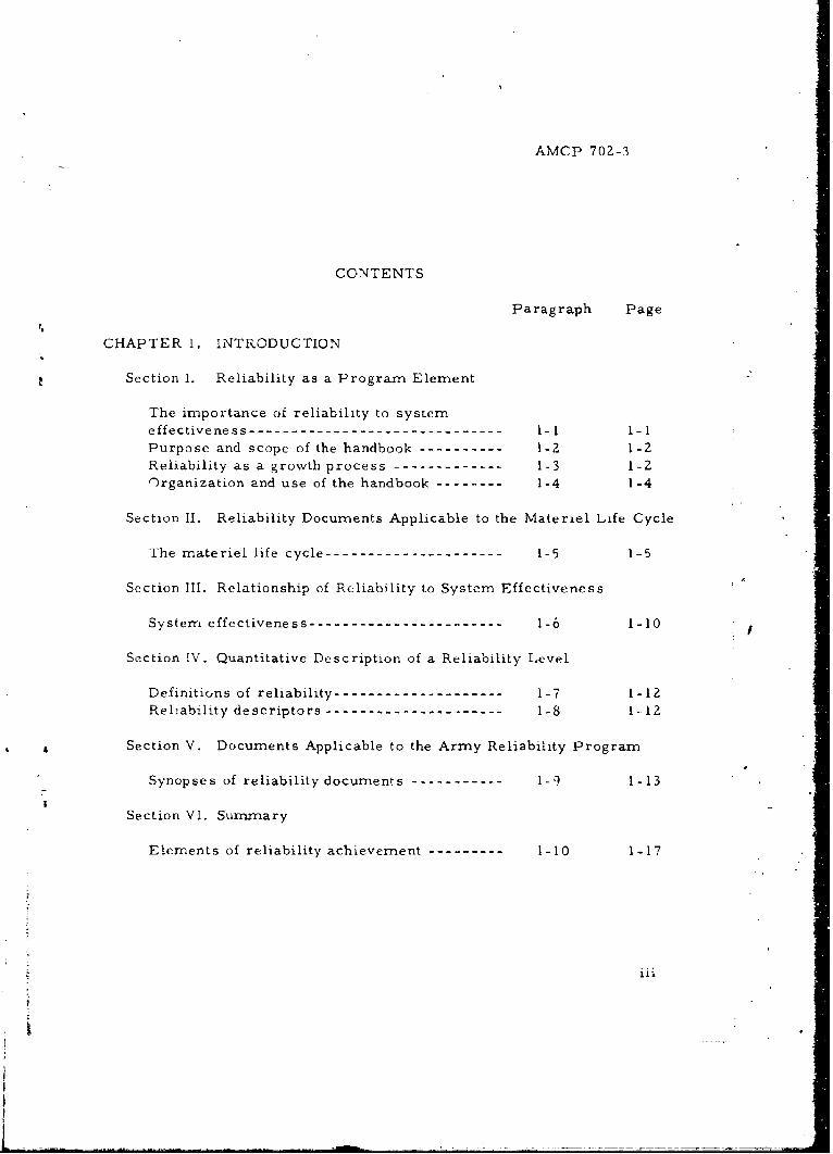
CHAPTER 1. INTRODUCTION

Section 1. Reliability as a Program Element

The importance of reliability to systemeffectiveness- ------------------------------ 1-1 1-1Purpose and scope of the handbook ---------- 1-2 1-2Reliability as a growth process ------------- 1-3 1-2")rganization and use of the handbook --------- 1-4 1-4

Section II. Reliability Documents Applicable to the Materiel Life Cycle

The materiel life cycle-- -------------------- 1-5 1-5

Section III. Relationship of Reliability to System Effectiveness

System effectiveness ------------------------ -6 1-10

Section IV. Quantitative Description of a Reliability Level

Definitions of reliability -------------------- 1-7 1-12Reliability descriptors ---------------------- -8 1-12

4 Section V. Documents Applicable to the Army Reliability Program

Synopses of reliability documents ----------- 1-9 1-13

Section VI. Summary

Elements of reliability achievement ---------- 1-10 1-17

li

iii

L_ _ _

AMCP 702-3

Paragraph Page

CHAPTER 2. RELIABILITY PROGRAM REQUIREMENTS, PLANNING,AND MANAGEMENT GUIDE

Section I. Introduction

General ----------------------------------- 2-1 2-1

Section II. Recommended Contractor Program

General ---------------------------------- 2-2 2-3Reliability organization -------------------- 2-3 2-3Reliability management, control, and

monitoring activities ---------------------- 2-4 2-3Program review -------------------------- 2-5 2-4Development testing ----------------------- 2-6 2-4Integrating equipment ---------------------- 2-7 2-4Parts reliability improvement -------------- 2-8 2-5Critical items ----------------------------- 2-9 2-5Apportionment, prediction, and mathematicalmodels ----------------------------------- 2-10 2-5Contractor design reviews ------------------ 2-11 2-6Subcontractor and supplier reliabilityprograms -------------------------------- 2-12 2-7Reliability indoctrination and training ------- 2-13 2-7Statistical methods ------------------------- 2-14 2-8Trade-off considerations ------------------- 2-15 2-8

Effects of storage, shelf-life, packaging,transportation, handling, and maintenance--- 2-16 2-8

Manufacturing controls and monitoring ------ 2-17 2-8Failure reporting, analysis, and correctiveaction ------------------------------------ 2-18 2-9Reliability demonstration ------------------- 2-19 2-9

Section III. Program Management and Monitoring

Program implementation -------------------- 2-20 2-11

iv

AMCP 702-3

Paragraph Page

Section IV. Reliability Training

General ---------------------------------- 2-21 .- 8Guidelines -------------------------------- 2-22 2-18

Course outliie- ---------------------------- 2-23 2-19

CHAPTER 3. TECHNICAL REQUIREMENTS ANALYSIS ANDDOCUMT'ENTATrTON OF RELIABILITY REQUIREMENTS


General ----------------------------------- 3l 3-1

Section II. Contents of QMR's and SDR's

General ----------------------------------- -2 3-1Reliability information in QMR's and SDR's -- 3-3 3-3

Section III. Documentation of Reliability Requirements in TechnicalDevelopment Plans (TDP's)

Role of the TDP and the research andtechnology resume in system development --- 3-4 3-4TDP format ------------------------------ 3-5 3-4

Documentation of reliability in TDP's -------- 3-6 3-5

Section IV. Documentation of Reliability Requirements inProcurement Documents and Specifications

General ---------------------------------- 3-7 3-5Types of documents and specificationsrequired --------------------------------- 3-8 3-7Essential reliability features of

specifications ----------------------------- 3-9 3-7

Iv

j

t

____ _

AMCP 702-3

Paragraph Page

CHAPTER 4. RELIABILITY MODELING, PREDICTION, ANDAPPORTIONMENTr TECHtNIQUES


General ----------------------------------- 4-1 4-1

Section II. Reliability Models

General --------.--- -------------------- 4-2 4-1Procedural steps -------------------------- 4-3 4-2

Section III. Reliability Prediction

General ---------------------------------- 4-4 4-3Feasibility prediction procedure ------------ 4-5 4-4Design prediction procedure---------------- 4-7 4-6Specific techniques of reliability prediction - 4-7 4-6

Section IV. Reliability Apportionment

General ---------------------------------- 4-8 4-8

Considerations for reliability apportionment - 4-9 4-9Specific techniques of reliabilityapportionment ---------------------------- 4-10 4-10

CHAPTER 5. RELIABILITY DESIGN AND REVIEW

Section 1. Introduction

General ---------------------------------- 5-1 5-1

Section II. Some Basic Principles of Reliability Design

General ---------------------------------- 5-2 5-ZSimplicity -------------------------------- 5-3 5-2Use of proven components-preferred circuitsand preferred design concepts -------------- 5-4 5-2

vi

I,

IF ___ __

AMCP 702-3

SParagraph Page

S!=ress/strength design --------------------- 5-5 5-2Redundancy ------------------------------- 5-6 5- 4

Local environment control ----------------- 5-7 5-4Identification and elimination of criticalfailure modes ----------------------------- 5-8 5-5Self-healing ------------------------------ 5-9 5-5Detection of impending failure -------------- 5-10 5-5"Preventive maintenance -------------------- 5-11 5-6

STolerance evaluation ---------------------- 5-12 5-6Prediction and apportionment--------------- 5-13 5-7

Human engineering ------------------------ 5-14 5-7Mean life ira-i -------------------- -- 15 5-8

Section IIl. Reliability Reviews

General ---------------------------------- 5-16 5-8Basic review philosophy ------------------- 5-17 5-8Required review points -------------------- 5-18 5-9

CHAPTER 6. DEMONSTRATION AND TESTING


General ---------------------------------- 6-1 6-1

Section II. Reliability Demonstration and Test Procedures

General ---------------------------------- 6-2 6-1Parameter estimation --------------------- 6-3 6-2Tests of hypotheses ----------------------- 6-4 6-4

Acceptance life testing --------------------- 6-5 6-4Regression analysis ----------------------- 6-6 &-4Accelerated life testing -------------------- 6-7 6-4

Stress-strength testing -------------------- 6-8 6-5Reliability testing and the total test program-- 6-9 6-,

iI

!vii *

LI

-I I1

AMCP 702- 3

Paragraph Page

Section 111. Test Design

General ----------------------------------- 6-10 6-6Test procedures -------------------------- 6-11 6-6Importance of technical characteristics ------- 6-_1Z 6-7Design of test programs ------------------- 6-13 6-8

CHAPTER 7. RELIABIIATY EVALUATION, FAILI.URE ANALYSIS ANDCORRECTION -- TI-IE FEEDBACK LOOP


General ------------------------------------ 7-1 7-1

Section HL. Oilectives of a Po)b:iivc Matr,.l" Failu; e A~al-yi;s arndC,)nt rn)l Svstem

Objecti,,cs 2...... ............. 7-2 7-2

Section III ,cttodt: cf Da,.a (.OflccOiU.L. ' Do-w-l el;a :,:

SGeneral-- -- -... .... ... ... . . ............ 7-3- ".--- 3

Reliability data sorces .--------.. -- 7-4R ep o rts .. . . ..... . ...... ......... .. .. . .. . . .... ... - 7- 7 -Selection of data fo',eni £or dtacollection forms ... ............... 7--.. 7.7

Section IV -ee'Iback Cycle

GCen ra- ..----------------------------------- 7-7 7-8

P D a:nd cdevelopment phase requirements - 7-8 7-I0! anf.r:.fturing or production phase

requ. rnments ----------------------------- 7-9 7-010

C'pe-rational or field evaluation phaser qcuirements ----------------------------- 7-10 7-11

viii

ANIC13 70?- 5

Paragraph Page

Section V. Stcps for Utilization of Failure Data

Procedural steps ---------------------------- 7--11 7-11

APPENDIX A. CONCEPTS 01' RELIABILITY QUANTIFICATION

Section I. Introduction -------------------------------- A-1Section I. Probability --------------------------------- A-ISection III. Statistics and IProbability Distributions A-13Section IV. Stress-Strength Analysis -------------------- A-55Section V. Conc, pt of System Effectiveness --.-.--------- A-SectionVi. Rc-lia i1ity Descriptors ------- 7-------------- -

APPENDIX B. RELIABILITY tPROGRAN¶ REQUIREMENTS PLANNINGAND MANAGEMENT GUIDE

Section 1. Introduction .------------------------------------ B-Section I1. frundamentais of Network Diagramm.-ning ------- B-I.vc,'ion III. Reliability Network Diag.ram and M.1stone

Char- ...---------------------------------------

APFPENDIX C. 'I F(7I-INICAL P EQUIREMENTS ANALYSIS ANDD;OCU M •ENTArION OF RELIABILITY RYeQUIREMENTS

Section 1. ht roduct on-... -------------------------------- 1C -Section I'. Comments on Typical Favht6s in StLti!ng

R.liabilit, Requircnments in QMR1s/SDI 's- -.. C-Section '11. Stating the Reliability Clause in Contract. C-5SeC(tion IV, incentive Contractling ------------------------- C-8

APPENDIX D. RELIABILITY PREDICTION AND APPORTIONMENT

PROCEDURES

Section 1. introduction -------.--------------------------- I)-iSection 1I. lt',thematicai Models ------------------------. )-ISection III Reliabilitv Prediction - ------------------------ D-16Section IV . Reliabilit1 Apportionment -------------------- D-21

ix

AMCP 702-3

Page

APPENDIX E. RELIABILITY DESIGN

Section 1. Introduction------------------------------------ E-1iSection 1I. Example of Reliability Prediction and

Apportionment During the Development Phase - E -I

APPENDIX F., DEMONSTRATION AND TESTING

Section I. Introduction------------------------------------ F- ISection 11. Parameter Estimation --------------------------- F-ISection III. Tests of Hypotheses--------------------------.. F-30Section JV. Acceptance Life Testing ------------------------- F-56Section V. Regression Analysis---------------------------- F-62

APPENDIX G. RELIABILITY EVALUATION, FAILURE ANALYSIS ANDCORRECTION - - THE FEEDBACK LOOP

(Not included in this issue)

APPEND)IX H. TABLESH-

APPENDIX L. DEFINITION OF ACRONYMS AND SYMBOLS -

INi-EX

x

AMCP 702-3

CHAPTER 1

INTRODUCTION

Section I. RELIABILITY AS A PROGRAM ELEMENT

1-1. The importance of reliability to system effectiveness, a. Reli- .-bility is defined as the probability that an itemI will perform its intended

function for a specified interval under stated conditions. As it relates toArmy systerns, equipments, components, and parts, reliability is one ofthe important characteristics by which the usefulness of an item is judged.

b. Usefulness is measv in terms of an item's effectivenessfor its intended role; therefore, eliability is one of the important param-eters contributing to effectiveness. As roles and mission requirementsbecome more sophisticated, items becorne more complex in the functionalconfiguration necessary to satisfy increased performance requirements.

As item complexity increases, reliability invariably becomes more prob-lemnatical and elusive as a design parameter, and thus more difficult toassure as an operational characteristic under the projected conditions ofuse. These difficulties can never be completely eliminated, but may bereduced by means of the establishment and implementation of sound re-

liability program activities.

c. it is also now recognized that with the exercise of very de-liberate and positive reliability engineering methods throughout the life

cycle of the item-from the early planning sta ,es through design, devel-opment, production, and field use--the teasi--c reliability level canusually be attained. Like other system characteristics, reliability is a

quantitative characteristic: predictable in design, measurable in test,controllable in production, and sustainable in the field. It follows thatreliability may be achieved by introducing sound monitoring practiceswith corrective action criteria at key points throughout the life cycle.

1 In this document, the words item, equiriment, and system are used

inter changeably.

, 1-1

---- ___-t~-- - ___ ------- - -

AMCP 702-3

1-2. Purpose and scope of the handbook. a. This handbook providesprocedures for the definition, pursuit, and acquisition of required re-liability in Army systems, equipments, and components. The methodspresented are generally applicable to all categories of items, including

electronic, electromechanical, mechanical, hydraulic, and chemical.However, examples chosen to illustrate the application of specific pro-cedures are drawn largely from experience with electronic and electro-mechanical systems because of the availability of documented experiencewith these systems.

b. The document is not intended to provide detailed instructionsrelative to arny specific program or eauipment, but is intended to fillthree basic needs within the Army and its contractor facilities.

(1) Project management. General guidance for the imple-mentation of selected reliability program functions at appropriate pointsin the item life cycle.

(2) Project engineering. Discussion of some proceduresuseful to the engineer in the actual performance of these reliability pro-gram functions.

(3) Design engineering. Identification of some importantprinciples affecting reliability and some analytic techniques for predict-

ing and measuring the reliability of a given design configuration.

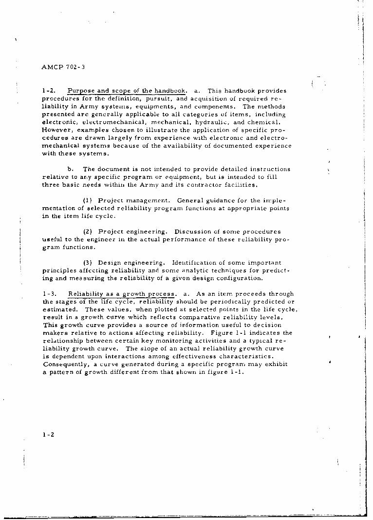
1-3. Reliability as a growth process. a. As an item proceeds throughthe stages of the life cycle, reliability should be periodically predicted orestimated. These values, when plotted at selected points in the life cycle,

result in a growth curve which reflects comparative reliability levels.This growth curve provides a source of information useful to decisionmakers relative to actions affecting reliability. Figure 1-1 indicates therelationship between certain key monitoring activities and a typical re-liability growth curve. The slope of an actual reliability growth curveis dependent upon interactions among effectiveness characteristics.

Consequently, a curve generated during a specific program may exhibita pattern of growth different from that shown in figure 1-1.

1-2

-AMCP 702- 3

o to

Q- 04

ul)

Cd )0

1-3

AMCP 702- 3

b. Desirable reliability growth results from planning, design-ing, testing, producing, and ultimately using the product according to a

set of effectiveness-oriented procedures. Lack of reliability growthmay result from overlooking or disregarding these same procedures atany single point in the growth process.

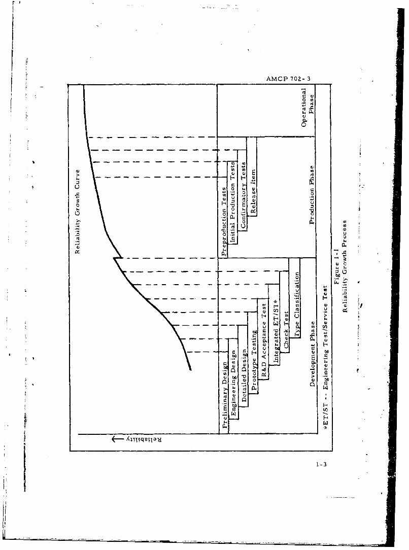
1-4. Organization and use of the handbook. Figure 1-2 identificsapplicable chapters within the handbook corresponding to major relia-

bility functions to be performed throughout the life cycle of a system.The figure may also serve as a basic checklist of things to be done in

planning a new program. Not all of these functions are applicable forall materiel items, e. g. , those items for which a Research and Tech-

nology R~sum6 (DD Form 1498) is used instead of a Technical Develop-ment Plan (TDP). 2

CHAPTER/APPENDIXRELIABILITY FUNCTIONS / 2/ 3/C 4/D

Determination of feasibility_ XDocumentation of requirements X X XPreparation of RFP X X XEvaluation of proposal X XPrediction of reliability level XApportionment of reliability goals X

Formulation of design X

Conduct of design review X

Conduct of test and evaluation X X Xactivities

Conduct of failure analysis XUtilization of a data feedback system X

Conduct of appropriate training XPlanning a reliability program X XMonitoring a reliability program X

Managing a reliability program X X

Figure 1-2Reference Index for the Performance of

Some Specific Reliability Functions

2 Where Technical Development Plan is used in this Pamphlet, System

Development Plan (SDP) is also included.

1-4

AMCP 702-3

Section II. RELIABILITY DOCUMENTS APPLICABLE TO THEMATERIEL LIFE CYCLE

1-5. The materiel life cycle, a. For purposes of discussion, themateriel life cycle is broken into the following six phases;

(1) Conceptual phase. The life cycle is initiated by a state-ment of general need for a particular capability. The general objectiveof this phase is to establish a feasible technical approach for satisfyingthe general requirements, to evaluate whether a specific approach is fworth pursuing, or whether the military requirement should be satisfiedin another manner. If the approach is found to be worth pursuing, theconceptual phase should:

(a) Provide explicit definition of effectiveness for theparticular item under consideration; and

(b) Provide guidelines for item refinement in the defi-nrtion phase.

(Z) Definition phase. (a) During the definition phase, thedetailed cost, schedule and technical design requirements of a programare defined and validated prior to development and production. Tech-nological advances resulting from the conceptual phase are translatedinto design requirements to be met during development and production.

(b) The definition phase serves to refine the systemdefinition to subsystem level based on the guidelines established duringthe conceptual phade. Thus, it Uenhances the probability of successfulaccomplishment of these requirements and allows development to pro-ceed with minirnum change. This phase provides the inputs to a requestfor proposal and the resulting contractor competition for development.

(3) Development phase. The development phase is theperiod during which design engineering and testing is performed to comeup with an end item which satisfies the military requirement. The mainproduct of the development phase is documentation of information for usein production of the end item for field use. Items produced during thisphase generally serve to test the effectiveness of the research and thevalidity of the data. The design and configuration is determined duringthis phase, and the inherent reliability is established. Inherent relia-

bility refers to the achievable reliability of the equipment under idealenvironmental conditions.

1-5

AMCP 702-3

(4) Production phase. The production phase utilizes thetechnical data package formulated during the development phase toproduce, manufacture, and make engineering changes to the itemunder consideration. This phase includes production testing andarranging for facilities and logistic support.

(5) Operationalphase. This phase is characterized by re-

build, supply, training, maintenance, and materiel readiness operations

while the system is being utilized by an operational unit. It is herethat the results of all prior effort is put to the test in the field. How-ever, this phase is not independent of preceding phases; e. g. , inherentreliability established in design can be realized only if support activitiesare perforined as specified. Feedback data from this phase can be uti-lized for improving reliability, either by engineering changes in thepresent system or in the development of new systems.

(6) Dispobai phase. This phase is induceua in this doc-unient to complete the life cycle. It has to do with the removal of obsolete

* items from the inventory and consequently has little influence on reliability.

b. The major reliability system life cycle considerations are* shown in figure 1-3.

c. A great many documents support the overal- Army reliabilityprogram. These are intended to give assurance that each item ultimatelysatisfies the need initially anticipated. Figure 1-4 shows many of the doc-uments related to the appropriate considerations in figure 1-3.

d. Somne of these documents identify certain engineering or man-agement procedures, test plans, and data requirements which are neededto fulfill contractual requirements. Similar requirements are implicitlycielined in others. In general, they impose a responsibility upon the proj-ect office, contractor, or contracting agency to do certain things to assureultimate realization of required reliability in the field. References whichsupplement the contents of the documents are identified in the documentsthemselves. Figure 1-5 is an abbreviated document directory. Oppositeeach document identification number are indicated those sections of thishandbook that relate to these requirements.

1-6

a --~-~----~----- * - -- - ----- ____ ---- ----- ____- --_____-- -- -

I

AMCP 702- 3

L1

0NNEED for reliability must be anticipated.

SQualitative Materiel Requirements (QMR) or Small

Development Requirements (SDR) must reflect this need.S~Q Plans must be formulated to fulfill the reliability need, suchS~as: (a) Reliability requirements defined and specified; (b) Reliability

program plan formalized; (c) Requests for proposal (RFP) and contracts

documented.GD Reliability program is implemented: Reliability is monitoredS~continuously.S@® Conceptual item is designed: Reliability is assessed in de-

r sign review; design is revised to correct deficiencies; reliability isdesigned in by requirement.

S@® Prototype is developed according to the design: ReliabilityS~is evaluated by test; design is refined to correct deficiencies; reliability

S~is validated by demonstration when practical.S~Item is produced: Parts, materials, and processes areS• controlled; equipment acceptability is determined by test.

F Item is deployed to the field: Operators and maintenance

S~technicians are trained; operating and maintenance instructions are

S~distributed; reliability is sustained by procedure.SQ Item is evaluated to determine that the original need is met.

!• Feedback loop completes the cycle: (a) to guide product im-

S~provements; (b) to guide future development planning; (c) to correct fielddeficiencies.

j Figure I-3

Reliability Considerations in the Materiel Life Cycle 1-7

Deveopmnt Rquiemens (DR) ustreflct hisieed

AMCP 702-3

CIRCLED NUMBERS CORRESPOND TO THOSE IN FIGURE 1-3

AR 705-5

MIL - STD -756 A4120.3-M (AR 715-10)

MiL-HDBK-217A

MIL-STD-781AMIL-STD- 105DMIL-STD-414MIL-STD- 1235

H108

TR-3TR-4TR-6TR-7

MLL-STD-690AMIL-STD-790A

MIL-STD-785AR 705-50AMCR 700-15MIL-STD-721BMIL-Q- 9858AAMCR 702-8

Figure 1-4

Documents Apphicable to Materiel Life CycleReliability Considerations

Note. See section V for document titles.

1-8

AMCP 702- 3

ForInformationRelative to See

DOCUMENT CHAPTER -

34 5 6 7

MiL-Q-9858A X

MIL-STD- 105D xMIL-STD-414 X- -|

MIL-STD-690A xMIL-STD-790A X XMIL-STD-721B XMIL-STD-756A x xMIL-STD-781A XMIL-STD-785 X X X X X X XMIL-STD- 1235 XAR 705-5 X XAR 705-50 X X X XAMCR 700-15 X X X X X X XAMCR 702-8 X4120. 3-M (AR 715-10) XMIL-HDBK-217A X XH108 XTR-3 X

TR-4 __X

TR-6 j XTR-7 __X__

Figure 1-5Ready-Reference Index for Compliance with Specified Documents

1-9

I4[ i'i

AMCP 702-3

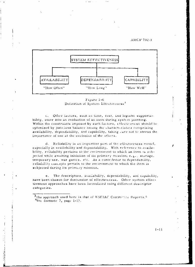
Section III. RELATIONSHIP OF RELIABILITY

TO SYSTEM EFFECTIVENESS

1-6. System effectiveness, a. The worth of a particular item isdetermined primarily by the effectiveness with which it does its job.

Many characteristics, including reliability, contribute to system (item)

effectiveness. For purposes of discussion, effectiveness- related charac-teristics may be grouped into three general categories:

(1) Those affecting resporse to a mission call.

(2) Those affecting endurance of item operation.

(3) Those comprising terminal results of the mission.

b. The contributions of these categories may be referred to as

availability, dependability, and capability, respectively, (sec figure 1-6).

Then system effectiveness may be expressed as a function of availability,

dependability, and capability.

(1) Availability is a measure of the degree to which an itemis in the operable and committable state at the start of the mission when

the mission is called for at an unknown (random) point in time.

(2) Dependability is a measure of the item operating condi-tion at one or more points during the mission, including the effects of

reliability, maintainability, and survivability, given the item condition(s)at the start of the mission. It may be stated as the probability that an

item will enter or occupy one of its required operational modes during

a specified mission and perform the functions associated with thoseoperational modes.

(3) Capability is a measure of the ability of an item to achievemission objectives, given the cond;.tions during the mission.

1-10

AINICP 702-3

"How Often. ''F.How Lo ng" How Well"

Figure 1-6

Definition of Systern LfIcctivencvss3

c. Other lactors, sucal as time, cost, and logistic supporta-

bility, enter into an evaluation of an item during systkin pplanning.Within the constraints imposed by such fat tors, eJfecti,'en.ots5 should beoptimized by judicious balance among the charactcristics comprising

availability, dependability, and capability, taking care n-ot to stress theimportance of one at the exclusion of the others.

d. Reliability is an important part of th¶_ effectiveness mocel,especially in availability and dependability. With reference to availa-bility, reliability pertains to the environment to which an item is sib-

jected while awaiting initiation of its primary mission; e. ., storage,temporary use, war games, etc. As a contributor to dependaoility,

reliability concepts pertain to the enmironmentt to which the item issubjected during its primary mission.

e. The descriptors, availability, dependability, and capability,have been chosen for discussion of effectiveness. Other system effec-tiveness approaches have been formulated using different descriptorcategories.

3fhe approach used here is that of VSEIAC Commrtto,. Reports. 4

4See footnote 7, page 1-17.

1-11

AMCP 702- 3

Section IV. QUANTITATIVE DESCRIPTION

OF A RELIABILITY LEVEL

1-7. Definitions of reliability, a. The reliability of an item is de-

fined as the probability that the item will perform its intended functionfor a specified interval under stated conditions. When applied to a spe-

cific equipment or system, reliability is frequently defined as:

(1) The probability of satisfactory performance for specifiedtime and use conditions; or

(2) The probability of a successful mission of specified dura-tion under specified use conditions; or

(3) The probability of a successful event under specifiedconditions. This definition is particularly applicable to nontime depend-ent items.

b. Whenever the definition is worded to fit a particular item ordevice, it is always necessary to:

(1) Relate probability to a precise definition oi success orsatisfactory performance;

(Z) Specify the time base or operating cycles over whichsuch performance is to be sustained (except for nontime dependent items

such as one shot devices); and

(3) Specify the environmental or usz conditions which will

prevail.

1-8. Reliability descriptors. A reliability level, and ultimately a ru-liability requirement, may be stated by using various descriptors. Anyof the following may be used to specify a reliability requirement for a

given mission time.

a. Both mission time and the reliability associated with thatmission time; (i. e. , the probability that the equipment will not fail dur-ing tne required mission time). Such a requirement statement reflectsthe reliability definition.

1-12

AMCP 70Z- 3

b. Mean time between failures (MTBF), This deqcriptorreflects a specific reliability level only if the relationship 6 betweenMTBF and reliability level is known. If different relationships applyto two items, it is highly likely that the same MTBF for both itemswill reflect different reliability levels. Thus, MTBF should be usedwith caution to express reliability requirements.

c. Failure rate. Failure rate may be used to express relia-bility requirements with the same type of precautions described forMTBF.

d. Probability of properly performing a specific function.This descriptor is useful ,or expressing reliability requirementsi tornontime dependent items.

Section V. DOCUMENTS APPLICABLE TO THEARMY RELIABILITY PROGRAM

. -9. tynopses of reliability documents. A brief synopsiE- for each ofthe documents shown in figure 1-4 follows.

a. AR 705-50, Army Materiel Reliability and Maintainability,Sets forth concepts, objectives, responsibilities, and general policiesfor the Army reliability and maintainability program. This regulationidentifies reliability and maintainability characteristics which must bespecified for the design of materiel and must be considered and absessedthroughout the life cycle.

b. MIL.STD-785, Requirements for Reliability Program (forSystems and Equipments). Provides general requirements for relia-bility programs, as well as guidelines for the preparation of reliabilityprogram plans. Particular attention is directed toward the topics ofnumerical reliability objectives and minimum acceptable requirements.Approval of or deviation from the proposed reliability plan, preplanned

5 For nonrepairable items, mean time to failure (MTF) may be used inlieu of MTBF. These terms are frequently ustd interchangeably.

6This relationship depends upon the probability distribution functionof failure times. Some important probability distribution functions aresurnnarized in appendix A.

1-13

AMCP 7 02-3

program review check points, itemization of government-furnished orcontractor-supplied equipment, which is to be integrated to provide acomplete operational system, are also emphasized. In addition, humanengineering design criteria reference documents, a list of items to be

included in failure report form, milestones at which demonstration isto be performed, and the reliability test plan are included.

c. AMCR 700-15, Reliability Program for AMC Materiel.Establishes policies, procedures, and responsibilities concerning a re-liability program for Army materiel. Included is a listing of essentialfactors to be considered in a reliability program, as well as essentialphases during which reliability actions must be taken.

d. MIL-Q-9858A, Quality Program Requirements. Specifiesrequirements for an effective and economical quality program, plannedand developed in consonance with the contractor's other administrativeand technical programs. Design of the program shall be based uponconsideration of the technical and manufacturing aspects of production

and related engineering design and materials.!

e. MIL-STD-105D, Sampling Procedures and Tables forInspection by Attributes. Provides tabled acceptance sampling plansand general procedures for deciding whether a lot of components, sub-systems, systems, etc., have an acceptable percentage defective whencompared to specification limits or goals. Specification of a missionprofile allows for usage for reliability acceptance plans.

f. MIL-STD-414, Sampling Procedures and Tables for Inspec-tion by Variables for Percent D'fective. Provides general procedures

and sampling plans for determining acceptance of lots when quality isbased on a characteristic which is measured on a continuous scale, andthe measurements and the underlying distribution are normal. Theseplans may be applied to reliability tests if a mission time is specified.

g. MIL-STD-721B, Definition of Effectiveness Terms forReliability, Maintainability, Human Factors, and Safety. Defines termscommonly used in reliability, maintainability, human factors, andsafety.

1-14

AMCP 702- 3

h. MIL-STD-756A, Reliability Prediction. Establishes uni-form procedures for predicting the quantitative reliability of aircraft,missiles, electronic equipment, and their subdivisions early in thedevelopment phases, to reveal design reliability weaknesses and toform a basis for apportionment of reliability requirements to thevarious subdivisions of the item. Graphically portrays the effectsof system complexity on reliability to permit the early prediction of jtolerance and interaction problems not accounted for in the simple

multiplicative case, and provides appropriate factors by which toadjust MIL-HDBK-217A predictions for airborne and missile environ-ments.

i. MIL-STD-781A, Reliability Tests, Exponential Distribution.Outlines a series of test levels and test plans for certain reliabilityacceptance tests and longevity tests. The test plans are based upon the A

exponential (or Poisson) distribution.

I. MIL-STD-690A, Failure Rate Sampling Plans and Proce-dures. Provides procedures for failure rate qualification samplingplans for establishing and maintaining failure rate levels at selectedconfidence levels and lot conformance inspection procedures associatedwith failure rate testing.

k. MIL-STD-790A, Reliability Assurance Program for Elec-

tronic Parts Specifications. Provides the controls and procedures armanufacturer iriust establish and continue to maintain in order to qualifyparts to an established reliability level.

1. MIL-STD-1235, Sampling Procedures and Tables for Con-

tinuous Inspection by Attributes. Provides tabled acceptance samplingplans and general procedures for use where disposition of product is

made on a unit-by-unit basis and production/rebuild is on a moving line.

m. AR 705-5, Army Research and Development. Specifiesresponsibilities and establishes policy and procedures for conducting

research and development in the Department of Army. These proce-dures are classified into the three major categories of research, de-velopment, and special instructions pertaining to nuclear energy.Appendixes are included regarding the format for submitting QMR's

and SDR's.

1-15

AN4C P 702-3

n. AMCR 702-8, Reliability Record and Status Report. Pre-scribes policies, procedures, and responsibilities for the preparationof quarterly reports on item reliability throughout the entire life cycle.

o. 4120. 3-M (AR 715-10), Defense Standardization Manual.

Establishes format and general instructions for the preparation ofspecifications, standards, handbooks, and maintenance manuals.

p. MIL-HDBK-217A, Reliability Stress and Failure Rate Datafor Electronic Equipment. Provides the procedures and failure ratedata for the prediction of part-dependent equipment reliability fromstress analysis of the parts used in the design of the equipment. Mustbe used according to procedures outlined in MIL.-STD-756A for esti-mates of MTBF and reliability at the system level, and to account fortolerance and interaction failures, and to adjust for the particular useenvironment.

q. 1-108, Sampling Procedures and Tables for Life and Relia-bility Testing (Based on Exponential Distribution). This documentdescribes the general principles and outlines specific procedures andapplications of life test sampling pians for determining conformanceto established reliability requirements, assuming failure times to be

exponentially distributed.

r. TR-3, Sampling Procedures and Tables for Life and Relia-

bility Testing Based on the Weibull Distribution (Mean Life Criterion'.

Provides procedures and tables of life test sampling plans for deter-

mining conformance to established reliability requirements (in terms

ot mean life) where the Weibull distribution describes failure times.

s. FR-4, Sampling Procedures and Tables for L.ife and Relia-

bility Testing Based on the Weibull Distribution (Hazard Race Criterion). 8

Provides procedures and tables of life test sampling plans for deter-

mining conformance to established reliability requirements (in terms

of hazard rate) where the Weibull distribution describes failure times.

t. TR-6, Sampling Procedures and Tables for Life and Relia-

bility Testing Based on the Weibull Distribution (Reliable Life Criteriont. 8

Provide- procedures and provides tables of life test sampling plans for

determining conformance to established reliability requirements (interms of reliable life) where the Weibull distribution describes failure

time s.

1-16

AMCP 702.3

u. TR-7, Factors and Procedures for Applying MIL-STD-105DSampling Plans to Life and Reliability Testing.6 Provides a procedureand contains related tables of factors for adapting MIL-STD-105Dsampling plans to reliability acceptance tests. The underlying distri-bution of failure times is assumed to be Weibull.

Section VI. SUMMARY

1-10. Elements of reliability achievement, a. The pursuit and ac-quisition of reliability objectives requires that management:

I

(1) Acknowledge and strive to attain established itemeffectiveness.

(2) Know and define the level of reliability desired.

(3) Recognize the disparity between the desired reliabilitylevel and that level which will probably be achieved unless proper con-trols are exercised to influence the reliability growth process.

(4) Understand the application of available approaches bywhich controlled reliability trowth may be assured.

b. The remaining chapters of this document outlne some ofthe planning considerations and describe some of the procedures thatcan be fruitful, both in the achievement of required reliability in spcci-fic programs and in the eval ualion and monitoring of reliability on a ]program-wide basis throughout the system life cycle.

7 Final Report of the Weapon System Effectiveness Industry AdvisoryCon•ittee (WSEIAC). The documents listed below are available from the

* ' Defense Documentation Center, Cameron Station, Alexandria, Virginia22314.AFSC-TR-65-1, Requirements Methodology (AD-458453).AFSC-TR-65-2, Prediction Measurement (3 volumes)(AD-458454, AD-458455, AD-458456).AFSC-TR-65-3, Data Collection and Management Reports (AD-458585).AFSC-TR-65-4, Cost Effectiveness and Optimization (3 volumes)(AD-458595, AD-462398, AD-458586).AFSC-TR-65-5, Management Systems (2 volumes)(AD-461171, AD-461172).

AFSC-TR-65-6, Chairman's Final Report (AD-467816).8 See footnote 1, page F-57.

1-17

AMCP 702-3

CHAPTER 2

RELIABILITY PROGRAM REQUIREMENTS,

PLANNING, AND MANAGEMENT GUIDE

Section I. INTRODUCTION

2-I. General. a. Project and commodity managers are chargedwith the responsibility for delivering reliable systems to the field.

This iesponsibility can be fulfilled only by giving due considerationto all characteristics, including reliability, in the early planning andfeasibility study stages and continuing with a comprehensive programthroughout the entire materiel life cycle. However, some programsdo not provide adequate reliability control or monitoring prior to the

operational phase. By then, it is usually too late to make modifica-tions for improvement, since:

(1) The equipment is needed now for operational use (de-

velomnient time has been exhausted); and

(2) The money invested is too great to be written off becauseof poor reliability. Often it is considered more expedient to add fundsin a desperate attempt to make product improvement.

b. This chapter sets forth reliability program activities deemedvital to development and production programs in general. Emphasis isplaced upon reliability program planning, monitoring, and managementreview procedures. Appendix B contains a network diagram comprised

of a suggested list of milestones for monitoring a reliability program.Among the primary purposes of a reliability program are-

(1) Focusing engineering and management attention on thereliability requirements;

(2) Insuring that reliability is treated as a design param-eter of equal importance with other effectiveness parameters; and

2-1

[I

K. _ ,

AMCP 702-34k

(3) Alerting management, throughout the program, toreliability discrepancies which may require management decisions.

c. An adequate program must contribute to, and guide, anorderly and scientific approach to designing for reliability. It musthelp contractors and individuals overcome a lack of recognition thatreliability must be a designed-for parameter with practical limita-tions. It must foster the realization that good conventional design maynot result in the inherent reliability required to satisfy the Army.

d. A reliability program will not necessarily increase theeffectiveness of an equipment, but an effectively monitored programwill not permit an inadequate design to proceed into development,test, production, and field use without specific management approval.It is this effective monitoring that assists project and commoditymanagers to assess and pinpoint potential reliability probleinzs intime to make adjustments.

e. The concept of a total reliability program, as generally

endorsed by the DoD, has four major points:

(1) Quantitative requirements are stated in the cortractor design specifications.

(2) A reliability progArm is established by the contractor.

(3) Reliability progress is monitored or audited by theresponsible Armny agency.

(4) Realistic requirements are stated in the QualitativeMateriel Requirements (QMR) and that they are included as one ofthe necessary requirements to be fulfilled for successful passing ofacceptance tests. This applies to prototype or demonstration modelsprior to production approval and to production samples.

2-2

AMCP 702-3

Section 11, RECOMMENDED CONTRACI'OR PROGRAM

Z-2. General. Of specific interest is the reliability program re-quired of the contractor. Those activities which experience has showncontribute to an orderly and scientific approach to designing for relia-bility are discussed below.

2-3. Reliability organization. The reliability function should bean integral part of the overall contractor organizational structure.Considerations for this function should include;

a. Proper placement within the overall organizational struc-ture so as to have proper authority and effectivity.

b. Clear identification of the personnel responsible for manag-ing the reliability program.

c. Clear definition of responsibilities and functions of thosedirectly associated with reliability policits and implementation.

d. Integration of such functions as engineering, manufacturing,quality, and reliability.

2-4. Reliability management, control, and monitoring activities.

a. Management and control. The management of the reliabilitygroup should establish policies and maintain control of reliability func-tions, To assure these functions, the reliability program plan shouldinclude:

(1) Description of all tasks to be performed with a de-tailed list of ,pecific tasks, including implermentation and controlprocedures.

(2) Clearly defined authority and responsibility for carry-ing out each task.

(3) Schedule of activities indicating major milestones(network diagram) and estimates of manpower, equipment, facilities,

F time, and cost.

2-3,I

Ii

AMCP 702- 3

(4) A method for identification, effect analysis, and

currective actions for potential problems.

b. Contractor-e stablished reliability monitoring activity.

This activity provides analysis of reliability status relative to re-

quirements, weaknesses, and follow-up on corrective action. Docu-mentation of reliability assurance and monitoring procedures, such

as checklists and instructional material normally used by the con-tractor, should be maintained so as to clearly delineate approach

used and results obtained, and should be available for review by theprocuring agency.

2-5. Program review. Contractor and procuring agency provisions

for review of the reliability program status should include:

a. Establishment of major review points by procuring agency

at time of program planning.

b. Criteria and information to be used for assessment of re-liability progress.

c. Identification of the responsible group for carry-ng out thereviews.

2-6. Development testing. A main purpose of development testing

is to determine how well design reliability requirements have beenmet and with what degree of confidence. Among the considerations

necessary to accomplish this is a planned program, including:

a. Environmental tests based on extreme stress conditions.

b. Test-related procedures, including provisions for non-

specified environmental criteria, nonavailable testing data, record

keeping and a listing of items having critically limited useful life.

2-7. Integrating equipment. The reliability program plan should

include provisions for use of equipment supplied by the governmentor other contractors. For such equipment, consideration must be

given to:

2-4

b]

AMCP 702-3

a. Use of known or estimated reliability values.

b. Procedures for getting such data, if not available.

c. Procedures for liand..ing of pot_1irial reliability problemi

introduced by such eqnipmei,t.

2-8. Parts reliability inprovement. The reliability plan shouldinclude procedures for identifying those parts, if awvy, needing im-provement and for accomplishing the necessary irmprovement. De-ficiencies in MIL-Specificatiorns ,r inadequate parts requlting fromsuch specifications should be reported.

Z-9. Critical items. Procedures should be cstablished for identify-ing and providing for critical items. Critical iems are those:

a. The failure of which would prevent satisfactory operation

of the system (of which it is a part) or cieate unwarranted safetyhazards;

b. Which are of sufficient complexity to warra-it special pro-

duction techniques cr cont os;

C. Which require special treatment or handling during trans-port or storage;

d. Which impose a heavy maintenance and supply support

burden; or1

e. Which have a long production lead tione.

2-10. Apportionment, prej,.:tion, and mathematical models. a. Meth-

ods shroild be established for developing mathematical models basedon functional analysis for apportionment and prediction of reliability.

b. These models often provide the basis for periodic analy-sLs of reliahility achievcrner-t. These analyses should be scheduled

to coincide with iochnical progress reporting requirements establishedby the contrcctor a,'d should consider:

2-5

'I

AMCP 702-3

(1) Reliability estimates based on predictions and testdata.

(2) The relationship between present reliability statusand schedule progress.

(3) The changes in concepts and approaches that arenecessary to accomplish the contract objective.

(4) The effects of changes made in design and manufactur-ing methods since the previous analysis.

(5) Criteria for success and failure, including partialsuccesses (degraded operation) and alternative modes of operation.

(6) Production tolerances and techniques, includingassembly test and inspection criteria and test equipnment a'scuracies.

(7) Specific pi -blern areas and recommended alternativeapproaches.

2-11. Contractor design reviews. Engineering design review andevaluation procedures should include reliability as a tangible op. ra-tional characteristic of the equipment, assembly or part under review.Among reliability considerations during design reviews are.

a. Review of current reliability estimates and achievementsfor each mode of operation.

b. Reviev.' of potential design or production problem areas.

c. Analysis of mode(s) and effectts) of failure.

d. Identification of the principal items inhibiting reliabilityachievement and proposed solutions.

e. The effects of engineering decisions and trade-offs uponreliability achievement.

2-6

AMCP 702-3

f. Procedures to assure that -ppropriate personnel fromthe reliability organizations participate in the design reviews.

g. Documentations of design review results.

2- 12. Subcontractor and supplier reliability.rograms. Provisionsshould be established to insure that subcontractors and supplierselection and performance are consistent wit! the Aiability require-ments of the contract. The prime contracter must extend the scopeof his reliability program t, )i, monitoring and control of subcon-tractors and suppliers. C( kderations bere are j

a. Incorporation oi reliability requliements in subcontractorand supplier procurement documents.

b. Provision for assessment of reliability progress, includ-ing qualification and acceptance testing of incoming products.

c. Adequate liaison to insure compatibility among supplierproducts to be integrated into the end item.

d. Initial selection procedures for subcontractors andsuppliers, which consider--in relation to the requirements- -pastperformance, willingness to test and share test data, interest andresponse on feedback of deficiency information, test philosophy,and realism of cost and delivery schedules.

2-1 I Reliability inioctrination and training. Provisions should bemade to include reliability in the basic training and indoctrination ofpersonnel with consideration given to:

a. Purpose, i.e. , improvement of skills.

b. Skill level of personnel to be trained, e. g., manager,engineer, technician or vorker.

c. Methods of instruction.

j 2-7

AMCP 702-3

2-14. Statistical methods. Statistical analysis is a part of relia-bility assessment activities. The reliability plan should fully describeappropriate statistical techniques and where in the life cycle they areto be used.

2-15. Trade-off considerations. The prime purpose of any hardwaredevelopment program is to get an effective item to the field. Fulfill-ment of this objective requires that the reliability plan provide forpotential trade-offs between reliability and other disciplines, such as:

a. Maintainability.

b. Safety and human engineering

c. Design configuration.

d. Production.

e. Cost and schedule

2-16. Effects of storage, shelf life, packaging, transportation,handling, and maintenance. Provisions to prevent degrading relia-""oility by improper storage, packaging, shipping, handling, andmaintenance of parts, units, subsystems, and systems should beestablished. The plan should include procedures for;

a. Periodic inspection and tests to determine effects ofstorage, shelf life, packaging. transportation, handling, and main-tenance on the reliability of the product.

b. Identification of major or critical characteristics ofitems which deteriorate with age, environmental conditions, etc.

c. Maintenance or restoration of equipment.

2-17. Manufacturing controls and monitoring. Manufacturing con-trols and monitoring are required to assure that the reliability achievedin design is sustained during production. Detailed consideration shouldbe given to:

Z-8

AMCP 702-3

a. Integration of reliability requirements into production

process and production control specifications.

b. Production environments induced by handling, transport-

ing, storage, processing, and human factors.

c. Quality standards from incoming piece-part inspections.

d. Calibration and tolerance controls for production, instru-mentation, and toolin

e. Integration of reliability requirements and acceptancetests into procurement activities.

f. Identification and correction of production control dis-c repancie s.

g, Production change orders for compliance with reliabilityrequirements.

h, Life tests of production samples to verify quality standards.

2-18. Failure reporting, analysis, and corrective action. A for-malized system for the reporting, analysis, correction, and datafeedback for all failures should be a part of the contractor reliabilityprogram. A mechanism for failure data feedback to engineering,management, and production activities in accordance with contractualrequirements is an integral part of such a program. Complete re-porting provides data on such things as accumulated operating time,on-off cycling, adjustments, replacements, and repairs related toeach system, subsystem, component, and critical part. The analysisof all failure reports by an analysis team formally designated by

management determines the basic or underlying causes of failuresin parts, assemblies, and end items. These results provide forassignment of corrective action and follow-up responsibilities.

2-19. Reliability demonstration, a. A pAan should be included fordemonstrating achieved reliability at specified milestones. A demon-stration plan normally includes:

2-9

_i_ _ __ _ _ __ _ _ _ _ _ _ _

4

AMCP 702-3

(1) Number of test articles.

(2) Accept/reject criteria (or other quantitative decision

criteria).

(3) Confidence levels.

(4) Subsystem vs. system level testing.

(5) Plans for handling of invalid data.

(6) Duration of test.

(7) Condition of test.

b. Provisions for periodic and final reports of demonstra-tion results as specified by the procuring agency are a necessary

part of such a plan.

c. Reliability demonstration tests are, in general, statis-

tically designed experiments with consideration given to confidence

levels and experimental error. Unless proof of adequacy can besubstantiated by other available data acceptable to the procuring ac-tivity, all items of equipment of higher order designations should be

tested in order to verify that reliability is achievable with the pro-posed design. If it is not, problem areas which prevent its attainmentshould be isolated and defined. The test program should include testsof questionable areas where reliability experience is not available,

particularly new or unique concepts, materials, and environments.

d. The extent of the test progratm is determined by weighingthe cost of testing against the degree of assurance required that theproduct will have a given level of reliability.

e. In addition to those tests performed specifically for re-

liability demonstration, all formally planned and documented testswhich are performed throughout the contract period should be evaluatedfrom a reliability viewpoint to maximize the data return per test dollar.

Data which are obtained should facilitate prediction of reliability on thebasis of individual and accumulated test results and the determination

of performance variabilities and instabilities that are induced by time

and stress.

2-10

AMCP 702-3

Section III. PROGRAM MANAGEMENf AND MONIlfORIlNG

2-20. Program implementation. Effective implementation requiresthat both the procuring agency and the contractor fulfill obligations

and responsibilities in a cooperative framework toward the commonobjective of reliable equipment in the field. The following steps arepresented as a guide in this implementation.

a. Step 1: Specify reliability requirements. The procuringagency should state the reliability requirements in design specifica-tions or procurement documents (including Requests for Proposals).Format and details for including the requirements as part of the speci-

fication are provided in Defense Standardization Manual 4120. 3-M(AR 715-10) and appendix C of this document.

b. Step 2: Establish schedules. The procuring agency shouldestablish schedules for reliability reporting and monitoring, to include:

(1) Reliability report(s). Delivery dates for such reports

imay be specified on either a calendar or a program-phase basis.

(2) Test plans. The detailed test plan should be submittedwell in advance ot test initiation in order to allow sufficient time forArmy review and approval.

(3) Progress evaluation schedule. Progress evaluationsfor effective monitoring are scheduled to correspond with major mile-stones rather than at fixed time intervals.

c. Step 3: Prepare Request for Proposal (RFP). The pro-curing agency should include desired proposal coverage of reliabilityin the Request for Proposal. A clause similar to the following, in-serted in the RFP, aids in obtaining desired reliability: Proposalsresponsive to this RFP shall, in addition to the requirements listedin MIL-STD-785, contain the following:

(I) A narrative of the contractor's interpretation of therequirements to demonstratL that the requirements are understood.

2

f 2-11I

AMCP 702- 3

(2) Proposed technical and management approachtoward achievement within the stated or implied limitations (if thebidder deems the requirement unrealistic, that which he considlersrealistic and achievable should be stated).

(3) Supporting evidence for the above, including re-liability predictions of the proposed concept -nd approach; source

and applicability of data; experience of bidder with similar programs;specific ways and means of attainment; assumptions and noncontrollable

dependencies upon which the approach is based.

(4) Description of the proposed reliability program,including specific technical activities; responsibilities and authoritieswithin the proposed organizational structure (including list of keypersonnel, together with background and experience); proposedschedule of reliability activities; recommended monitoring pointsand major milestones (including cost milestones); and proposed re-liability development test program.'

d. Step 4: Prepare proposal. The prospective contractorshould prepare a proposal in response to the RFP. Specifically, theproposing contractor should:

(1) Analyze the reliability requirements and make apreliminary prediction to determine feasibility for a given time andcost.

(2) Establish and cost the reliability activities andintegrate them into the total program.

(3) Schedule in-house reliability activities and monitor-ing which become part of the master schedule.

(4) Plan development reliability tests. The contractor

should evaluate the design approach and planned developments todetermine which assemblies and components will require testdemonstration.

(5) Prepare his total reliability plan.

2-12

AMCP 702-3

e. Step 5: Evaluate proposals. (1) The procuring agencyshould evaluate proposals for their response to the specific task re-quirement in source selection evaluation procedures.

(2) The proposal review should give particular attentionto specific proposed reliability activities rather than stress the con-tractor's organizational structure.

(3) Figures 2-1.a, 2-1. b and 2-1. c provide guidancefor evaluating proposals with respect to reliability.

f. Step 6: Review contractual documents. The procuring Iagency should review contractual documents prior to contract negotia-tion. Changes in the reliability requirements, program, or acceptancetests that are recommended in the proposal submitted by the success-ful bidder must be reflected in the design specifications, references,or contractual documents. When the recommendations are not ac-

cepted, the prospective contractor should be notified early in thenegotiation period in order that his cost and time estimates may beadjusted prior to final negotiation.

g. Step 7: Implement reliability program in developmentcontract. Both contractor and procuring agency should implementand monitor the reliability program during design and development.The contractor is committed to perform in accordance with the speci-fications in the contractual documents. The milestones of appendix Bprovide a guide for monitoring a reliability program.

h. Step 8: Implement reliability program in production. Im-plementation and monitoring of the reliability program during produc-tion is a key step. A suggested list of review points is provided by

the milestones in appendix B. Reliability records should include:

(1) Design changes in order to insure that each produc-tion engineering and design change is given the same reliabilityconsiderations and approvals as the original design.

I SZ2-13

i

AMCP 702-3

(2) Procurement of parts and assemblies in accorda.ncewith appropriate reliability requirements.

(3) Evidence that each step in the production processhas been evaluated for its possible detrimental effect upon reliability.

(4) Effectiveness of production inspections and collection,analysis, and feedback of test data in maintaining design quality.

(5) Summaries of qualification, environmental, andother test data.

(6) Compliance with the production acceptance testsrequirements.

2 1

2-14

AMCP 702-3

REQUIREMENTS ANALYSIS

Is the reliability requirement treated as a designparameter?

Has the requirement been analyzed in relation to theproposed design approach?

Is there a specific statement that the requirement is, or isnot, feasible within the time and costs quoted? If notfeasible, is an alternative recommended?

Is there evidence in the proposal that the reliability re-quirement influenced the cost and time estimates?

Are initial predictions and apportionments included insufficient detail (data sources, complexity, block diagram,etc. ) to permit Army evaluation of its realism?

Are potential problem areas and unknown areas discussed?Or, if none arte anticipated, is this so stated?

If the requirement is beyond that which presently can beachieved through conventional design, does the proposaldescribe how and where improvements will be accomplished';

Is consideration given to conducting trade-offs betweenreliability and other technical parameters?

RELIABILITY PROGRAM AND MONITORING

Does the proposed program satisfy the requirements of

the RFP?

If the contractor has indicated that certain of the reliability

activities requested are not acceptable to him, has hesuggested satisfactory alternatives?

Figure 2-l.aProposal Evaluation Guide

2-15

AMCP 702- 3

RELIABILITY nROGRAM AND MONITORING(continued)

Is the program specifically oriented to the anticipated needsof the proposed equipment? Is it in sufficient detail?

Are program activities defined in terms of functions andaccomplishments relating to the proposed equipment?

Does the proposal include planned assignment of responsi-bilities for reliability program accomplishments?

Is it clear by what means the program may influence de-velopment of the proposed equipment?'

Have internal 'independent" reliability assessments been

scheduled?

Does the proposal provide justification (data derived fromtesting or other experience) for the exclusion of specifieditems from demonstration testing?'

is the proposed documentation of activities, events, andanalyse.q designed for ease in monitoring, ease of dataretrieval, and use on future programs?

Are planned activities and events scheduled and docu-mented?

Does the proposal include a controlled corrective actionprogram for reliability data?

rigure 2-l.bProposal Evaluation Guide

2-16

AMCP 702-3

BACKGROUND ORGANIZATION AND EXPERIENCE

Does the bidder have an established program whereby pastexperience is made available to engineers and designers?

Does the bidder have a designated group (or individual) towhom designers can turn for technical reliability assistance?

Does the assignment of responsibilities include reliability

activities?

Do (or will) company standards manuals or other documentsset forth standard reliability operating procedures?

Does the bidder provide for appropriate reliability trainingfor management, engineering, and technical personnel?

Does the bidder implement and conduct planned researchprograms in support of line activities, seeking newr materi-

els, new techniques, or improved analytical methods?

ACCEPTANCE TESTING

Has the biddcr agreed to perforin acceptance tests andincluded the costs and time within I-Lis proposal?

If acceptance test plans were not included in the request for

proposai, has the bidder recommended any?

Does the proposal contain a positive statement concerningthe bidder's liability in the event of rejection by the accept-ance tests?

Figure 2-..c

Proposal Evaluation Guide

2-17

L

AMCP 702- 3

Section IV. RELIABILITY TRAINING

2-21. C;r-eral. a. The concept of reliability in system develop-

merit is not new. Only a few of the fundamental principles need be

understood by project management and engineering in order to putquantitative measurements on this system parameter. It is truethat the complexities of redundancy, statistical test design, sampling,

and many other aspects of reli bility assessment are difficult con-

cepts, and an effective training program must include considerationof all levels of personnel involved with the reliability program. The

technical content of a training course must be tailored to the person-

nel to be trained; e. g., a survey course for management and detailed

technique courses for engineers ant technical personnel.

b. The training problem is to prepare and present highlypractical c, ,rses in the fundamentals of reliability, tailored to fit

the needs o, individual groups within the Army. Thus, the coursemust be dynamic in its flexibility and adaptability. It must be well

documented with examples and "tools of the trade.

c. Training courses available at DoD schools and private

schools and conferences sponsord by various technical societiesprovide valuabie means of meeting training needs at minimum cost.

2-22. Guidelines. 1deal training activities include classi n instruc-

tion, supplemented by on-the-job application of the subject iuaterials.The tollowing questions are helpful in planning or selecting trainingcourses. Do they-

a. Reflect the needs of attendees in ternms of the scope ofthe course to be presented'?

b. Include separate training programs and materials to

specifically meet the needs of management and technical personnel"

c. Include management practices and engineering methodsutilized throughout the entire !ife- cycle'-

2-18

AMCP 702- 3

2-23. Course content. The following suggested course outline canbe adapted to specific needs drawing on appropriate sections of thisdocument.

a. What should be known about basic concepts of reliabilityas a measurable product characteristic? How, for example, do you:

(I) Define characteristics for specific equipments?

(2) Graphically and mathematically visualize thesecharacteristics?

(3) Express reliability in terms of confidence statements?

b. What should be known about specifications pertaining toreliability? 1low do you:

(1) Determine reliability requirements for parts, equip-ments, and systemsO

(2) Specify the requirements?

(3) Specify tests for compliance with given confidencelevels?

c. What should be known about reliability as an engineering

function? How do you:

(1) Predict reliability feasibility of new design concepts?

(2) Predict reliability achievement during the develop-merit phase?

(3) Evaluite the described reliability problem areas forcorrection in early de.iign?

d. What should be known about reliability assu.irance? Howdo you:

2-19

K,

AMCP 702-3

(t) Control reliability?

(2) Demonstrate reliability achievement?

e. How do you review and develop specific equipment andsystem program plans and specifications? Include:

(1) Program requirements.

(2) Quality assurance provisions for reliability.

f. How do you review development status of specific systems'.,Include

(l) Reliability apportionnrient.

(2) Problem areas.

i%. What should be known about contractor reliability pro-grams? How do you

(1) Evaluate a program)

(Z) Specify program requirements?

(3) Monitor contractor programs for compliance'?

h. What should be known about reliability monitorini, andfailure diagnosis.

(1) In design, development, production, and f..eld use?

(2) To assure earliest practicable correction!

i. What specific steps can you take to assure higher relia-bility in systems? These include review of:

(!) Rcquiremernts analysis and specifications.

(2) Demonstration and acceptance.

2-20

AMCP 702- 3

(3) Procurement documentation.

(4) Monitoring and follow-up (including feedback).

2-21

I

AMCP 702-3

CHAPTER 3

TECHNICAL REQUIREMENTS ANALYSIS AND DOCUMENTATIONOF RELIABILI L' REQUIREMENTS


3-!. General. a. Early system development plans are not completeif they do not quantitatively define the required characteristics of the

product or system proposed for development. While in the past thecharacteristics of a new equipment or system have been adequate toguide development effort toward full realization of performance require-

ments, they often have not been sufficiently descriptive of the reliabilitycharacteristics required for system success under field use conditions.These important success cha.-acteristics must be planned for and design-

ed into the system. They cannot be added as an afterthought. Thischapter outlines procedures for the definition and documentation ofreliability requirements in essential planning documents, specificationsand contractual task statements.

b. The problem is one of first stating system requirements forreliability in the Qualitative Materiel Requirements (QMR). These con-stitute the basis for the preparation of the Technical Development Plan(TDP) to accomplish CDC objectives. Required is the definition and

documentation of requirements in the TDP and the definition baselinein order to give the system concept a clean entry into its developmentcycle. This is intended to insure that an operationally suitable systemevolves as a result of good planning followed by effective pursuit ofplanned objectives.

Section II. CONTENTS OF QMR'S and SDR'S

3-2. General. a. Among the most important phases of the system life

cycle are the concept and definition phases, where system requirementsare analyzed and translated into well-defined technical objecti ,es and

detailed plans are laid to assure successful achievement of theseobjectives.

3-1

II

I,

AMCP 702-3

b. In general, there are three closely related analyses required

in order to generate the essential descriptive information needed fore preparation of technical development plans, design specifications, re-

Srquest for proposals, and contractual task statements. These are:

(1) Analysis and definition of the operational requirements --performance, reliability, and maintainability -- necessary for the de-sired level of system effectiveness.

(2) Prediction of the feasibility of achieving these require-ments by conventional design in order to assess the practical difficultyof the development job.

(3) An equitable method of initial apportionment (allocation)of requirements and supporting R&D effort among subsystems,

c. The last two of these analyses are discussed in chapter 4. Thefirst is discussed in this section. It pertains to the formulation of aQMR/SDR based upon national defense objectives, intelligence estimates,and concept or feasibility studies which determine the requirements fora new capability and the need for a new item. The QMR/SDR expressesDepartment of Army requirements for new equipment or for majorinnovations or improvements related to research and development asdeveloped from new concepts.

d. The QMR is a Department of Army approved statement of amilitary need for a new item, system or assemblage, the developmentol which is believed feasible, and is directed toward attainment of newor substantially improved materiel. It is stated at the earliest timeafter the need is recognized and feasibility of development has beendetermined.

e. The SDR is used to state a DA need for development of equipmentof proven feasibility which can be developed with less effort. Becauseof low cost and simplicity of development, such equipment does notwarrant the establishment of a QMR.

f. The QMR/SDR goes through four stages before final approvalis given. These are:

3-Z

AMCP 702- 3

(I) Initial Oraft proposed QMR/SDR

(2) Draft proposed QMR/SDR.

(3) Proposed QMR/SDR

(41 Department of Army approved QMR/SDR .

3-3. Reliability information in QMR's and SDR's. a. Reliabilityrequirements should be stated in terms appropriate to the item con-sidering its intended purpose, its complexity, and the quantity ex-pected to be produced. In addition, these requirements must be clear,quantitative, and capable of being measured, tested for, or otherwiseverified. QMR's/SDR's must include detailed essential reliability re-quirements. Statistical confidence levels and risks associated withdemonstrating achievement of these requirements are to be stated indocuments describing test requirements, but not in the QMR or SDR.Specifically, the information to be included in requirements is asfollows:

(1) Reliability. The overall reliability requirementmust be quantitatively expressed as a probability of success for one(or more) specified operational and environrmental cycleis) or func-tional sequence(s). Reliability may be apportioned for major phasesof the mission. When an operational profile is not well defined (e. g.,continuous operation), the closely related attribute, MTBF, may bespecified instead of probability of success. Normally, one or theother attribute, but not both, is specified. Reliability requirementsshould be stated for two or more operational profiles, if appropriate.

(2) Reliability after storage. This must be specified soas to indicate the arnount of deterioration which can be tolerated dur-ing storage. Length of storage, storage environment, and surveil-lance constraints should bc identified for planning purposes.

b. Of the above requirements, only those that are appropriate

for the item or equipment in question should be used. A mote detaileddiscussion with examples of how the above requirements are to bestated in QMR's/SDR's is given J.n appendix C.

3-iI

3-3

I,

AMCP 702-3

c. The discussions in this section represent an approach todetermination of feasible requirements of the proposed system. Quan-tification of the above elements provides input fur the development ofrealistic and meaningful contractual documents and specifications.

Sec'ion III. DOCUMENTATION OF RELIABILITY REQUIREMENTSIN TECHNICAL DEVELOPMENT PLANS (TDP's)

3-4. Role of the TDP and the research and technology resume in sys-tern development. The technical development plan (TDP) is expectedto outline plans for development and provide guidance, goals, and speci-fic direction necessary to assure that effectiveness will be achieved.The inclusion of statements delineating performance, reliability, andmaintainability in TDP's is airrmed at this goal. The TDP is applicableto those major development projects and tasks selected by the Chief

of Research and Development and announced by separate correspond-ence. In order that the Army Research, Development, Test, andEvaluation (RDTE) Program be extended to all major equipment, theResearch and Technology R4sum6 (DD Form 14981, applies to projectsnot covered by TDP's.

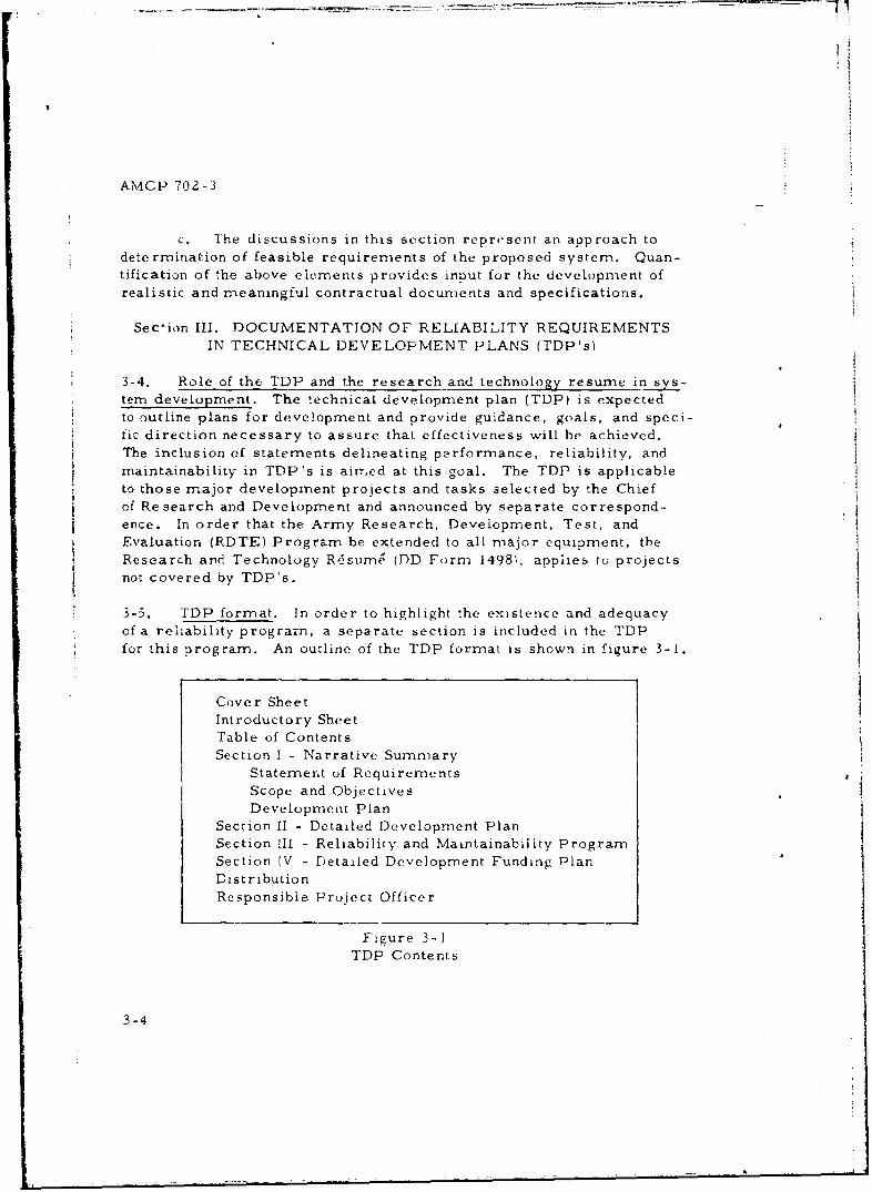
3-5. TDP format. In order to highlight the existence and adequacyof a reliability program, a separate section is included in the TDPfor this program. An outline of the TDP format is shown in figure 3-1.

Cover SheetIntroductory Sheet"Table of Contents

Section I - Narrative SummaryStatement of RequirementsScope and Objectives

Development PlanSection II - Detailed Development PlanSection III - Reliability and Maintainability ProgramSection IV - Detailed Development Funding PlanDistribution

Responsibie Project Officer

Figure 3-1TDP Contents

3-4

AMCP 702-3

3-6. Documentation of reliability in TDP's. a. Each TDP mustinclude information on the reliability program for that project Indon the interface of these characteristics with other characteric ics,as follows:

(I) Information listed in OMR's/SDR's.

(2) The plan for achieving reliability goals.

(3) The plan for conducting the reliability program.

(4) Reliability inputs to the costs and scheduling portionsof the development plan.

(5) The plan for life cycle assessment of reliabilitycharacteristics.

(6) The plan for development of compatibility with multi-

purpose maintenance equipment and of system peculiar maintenanceequipment.

b. Information contained in development plans is expectedto be more detailed than that normally found ia objectives/require-rnents docume.its (e.g. , C!MR); therefore, direct extracts fromQMR's are no, adequate. In those instances where the developmentplan is preliminary, listing of significant elements without detail willsuffice; e.g. , the fact that apportionment and prediction will be partof the program. Subsequent revisions must become increasingly moreexplicit and detailed, and must include updated reliability status in-formation for comparison with requirements.

Section IV. DOCUMENTATION OF RELIABILITY REQUIREMENTS

IN PROCUREMENT DOCUMENTS AND SPECIFICATIONS

3-7. General. a. The specification is, ... a document intendedprimarily for use in procurement, which clearly and accurately de-scribes the essential and technical requirements for items, materials,or servi _-s including the procedures by which it will be determinedthat the requirements have been met.' (Defense Standardization

Manual 4120.3-M (AR 715-10)]

3-5

Si

AMCP 702- 3

b. Reliability specification requirements consist of three

distinct but related areas of coverage:

(G) Detailed quantitative requirements.

(2) General program requirements.

(3) Quality assurance provisions (Test and EvaluationRequirements).

c. These three areas may be included in the overall designspecification for a product (Method A) or covered under a separatereliabiliiy specification (Method B).

(1) Method A. Integrated specifications: Reliability

as a design paramneter is logically specified in section III of the de-sign specification (both detailed and general coverage) and thequality assurance orovisions inteerated into the overall provisionsof section IV.

(2) Method B. Separate specifications: This alterna-tive is reconmmended only when ciarity and simplicity can be greatlyenhanced. A reliability specification must follow approved specifica-tion format, consisting of the foliowing.

ia) Scope.

(b) Applicable documents.

(c) Requirements.

(d) Quality assurance provisions (Test and Evalua-tion Requirements).

(e) Prepazation for delivery.

(f) Note s.

3-6

AMCP 702- 3

3-8. Types of documents and specifications required. In order tomaintain control throughout the materiel life cycle, it is necessary tohave a given plan which requires documentation of item requirements.Throughout AMC, control is accomplished by means of the conceptknown as configuration management in conjunction with project man-agement or commodity management (see AMCR 11-26).

3-9. Essential reliability features of specifications, a. The con-tent of military specifications is prescribed in Defense Standardization Manual4120. 3-M. Important features of the specifications are the numericalrequirements for equipment characteristics and the compliance require-ments. These are given, respectively, in the sections labeled Re-quirements and Quality Assurance Provisions (Test and EvaluationRequirements).

b. Basically, the section of the specification outlining re-quirements for system and/or development descriptions containsperformance and design requirements. Requirements for the testand evaluation methods to be used to check on conformance with theserequirements are stated separately.

(1) The introductory paragraph consists of descriptiveand introductory material, while quantitative requirements are statedand explained in detail as separate parts of the section. Th( paragraphspecifying reliability requirements must be in agreement with thosestated in the QMR,'SDR and TDP and must be in quantitative terms.In order to assure that these reliability requirements are properlyspecified, system operational requiremeits, use condiLions, the time nmeasure or mission profile, reliability design objectives, quantita-Live reliability requirements, and reliability program requirementsshould be considered as sources of information for preparing thespecifications.

(a) System operational requirenients. Reliabilityis a system characteristic in the same sense that speed, range, andmaneuverahility are system characteristics. To hay, full understand-ing of the reliability requirement, operational requirernen!s expressedin QMR's and TDP's must be described as well. The description pr,)-vides a dividing line between what corstitutes satisfactory and unsatis-factory equipment. To clearly make this distinction, it is necessaryto include both design objectives and minimum acceptable values as alower tolerance limit on the performance parameter.

3-7

A'\I(-t' 7f)£-' 3

Exani!) : A radar designi soecificati,)II rriav desire !he S\'Sterfl todetect I sq. meter targets at 300, 000 meters. Th- quantitativerequireiment might be stated as follows: The d,.i.. iibje ctive shallbe to detect I sq. nneter targetb at 300, 000 met ý_s. The systemshall be considered unacceptable if 1 sq. Meter targets are not de-tected at 225,000 meters.

(b) Use conditions. The conditions under whichthe item nmust perform should be stated in standard terminology.Use conditions refer to those conditions under ,hic' specified re-liability is to be obtained, including temperature, humidity, shock,vibration, pressure, penetration/abrasion, ambient light, nmount-ing position, weather (wind, rain, snowv), operator skills and otherconditions covered in AR 705-15, Operation o, Equipment tinderExtreme Conditions of Environment. in order to prevent undueequipment costs, stated use conditions should not be overly strin-gent, nor should unnecessary conditions be specifi, 3 for equipmentwhich will be used under controlled or limited climatic conditions.Use conditions are stated in both narrative and specific formats,with mission profiles included where environmental changes are

expected through the operating period.

Example: Narrative. The XXX Tractor must be capable of operat-ing as specified in climatic and weather conditions ranging fromtemperate to arctic and must be resistant to fungus, humidity,water, condensation, and icing.

Example: Specific. The XXX Tractor must opera c as specified

under any or all of the following environmental con-.itions: tem-perature, -65o F. to 1600 F. ; humidity, up to 100':,; and waterdepth, traverse up to 3 feet.

Example: Mission Profile. The ABC system shall meet its per-formance requirements when subjected to a mission temperatureprofile similar to that shown In figure 3-2.

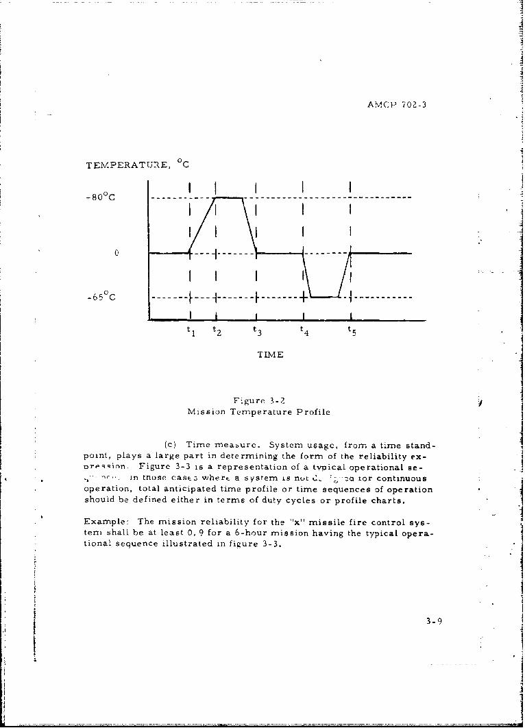
AMC1P 702-3

TEMPERATURE, °C

0I I I I I

0 iI

+0°

S I I I I It t t t t

TIME

Figure 3-2Mission Temperature Profile

(c) Time measurc. System usage, from a time stand-point, plays a large part in determining the form of the reliability ex-

orp-Q~in. Figure 3-3 is a representation of a tvpical operational se-•n.* in those case.z whert a system is nut ki :- ca tor continuous

operation, total anticipated time profile or time sequences of operationshould be defined either in terms of duty cycles or profile charts.

Example: The mission reliability for the 'x" missile fire control sys-tern shall be at least 0. 9 for a 6-hour mission having the typical opera-tional sequence illustrated in figure 3-3.

3-9

i-

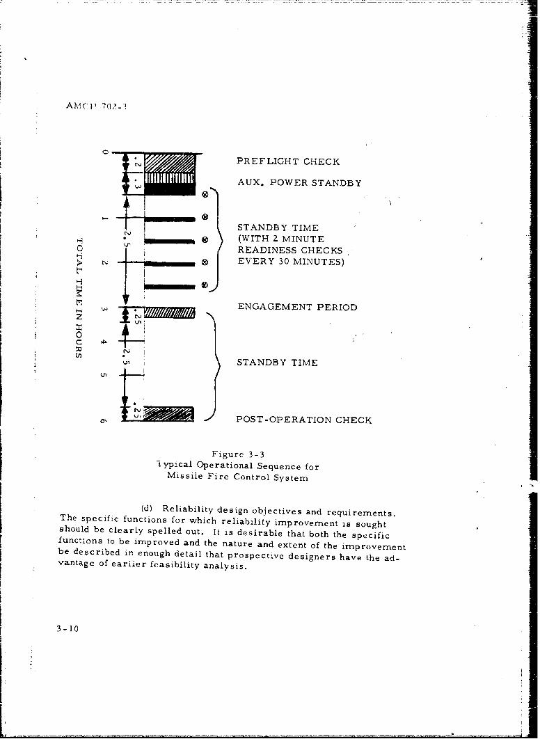
AMCA 702-3

PREFLIGHT CHECK

E f AUX. POWER STANDBY

STANDBY TIME-(WITH 2 MINUTE

i •READINESS CHECKS> - -I ® EVERY 30 MINUTES)

ENGAGEMENT PERIODz

ON

STANDBY TIME

POST-OPERATION CHECK

Figure 3-3

iypical Operational Sequence for

Missile Fire Control System

(d) Reliability design objectives and requirements.The specific functions for which reliability improvement is soughtshould be clearly spelled out. It is desirable that both the specificfunctions to be improved and the nature and extent of the improvementbe described in enough detail that prospective designers have the ad-vantage of earlier feasibility analysis.

3-10

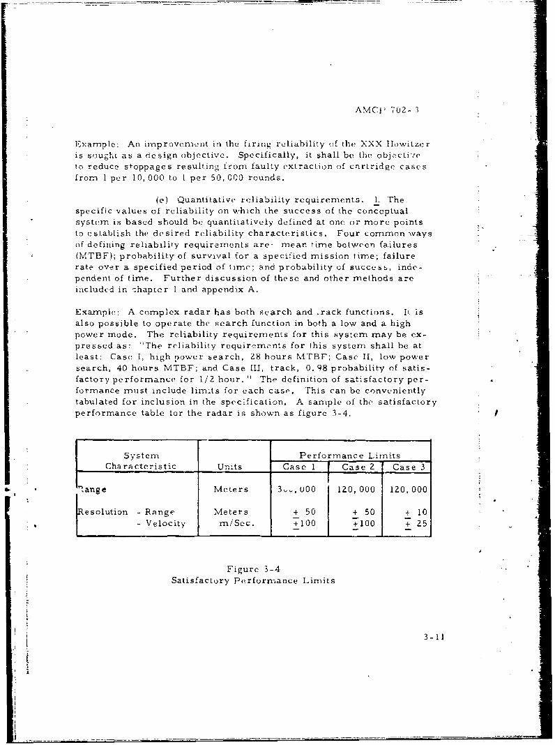
AMCIj 702- 3

Example: An improvenment in the firing reliability of the XXX Howitzeris sought as a design objective. Specifically, it shall be the object~iveto reduce stoppages resulting from faulty extraction of cartridge casesfrom 1 per 10,000 to I per 50,000 rounds.

(e) Quantitative reliability requirements. 1. thespecific values of reliability on which the success of the conceptualsystem is based should bc quantitatively defined at one or more pointsto establish the desired reliability characteristics. Four common waysof defining reliability requirements are: mean time between failures(MTBF); probability of survival for a specified mission time; failurerate over a specified period of time; and probability of succes!s, inde-pendent of time. Further discussion of these and other methods areincluded in zhapter 1 and appendix A.

Example: A complex radar has both search and .rack functions. It isalso possible to operate the search function in both a low and a highpower mode. The reliability requirements for this system may be ex-pressed as: "The reliability requirements for this system shall be atleast: Case i, high power search, 28 hours NMTBF; Case II, low powersearch, 40 hours MTBF; and Case III, track, 0. 98 probability of satis-factory performance for 1/2 hour." The definition of satisfactory per-formance must include limits for each case. This can be convenientlytabulated for inclusion in the specification. A sample of the satisfactoryperformance table for the radar is shown as figure 3-4.

System Performance LimitsCharacteristic Units Case I Case 2 Case 3

,ange Meters 3,., u00 120, 000 120,000

esolution - Range Meters + 50 + 50 + 10

- Velocity m/Sec. +100 +100 + 25

Figure 3-4Satisfactory Performance Limits

3-11

S-L : ! --- 4

AMCP '7Z-3

2. The specified reliability requirement shouldalso be defined in termns of nominal or minimum values. This can bedone by either identifying a NOMINAL value with which the user wouldbe satisfied, along with a minimuum that must be exceeded, or simplya MINIMUM value below which the user would find the system unac-ceptable.

(f) Reliability program requirements. 1. Thecharacteristics of the proposed program should be desE.ribed in sucha way that the fulfilling of these requirements wili provide for con-trols and decision points necessary to assure the development of anitem which will meet desired reliability requirements. For discussionof reliability programs, see chapter 2.

2. in the requiring of a reliability program, thefollowing points should be kept in mind:

a Do not expect a reliability program toprovide unlimited reliability. On the contrary, expect the programto provide realistic appraisals of progress, status, and potential ofthe overall program.

b. Avoid specifying, as part of the relia-bility program, organizational or internal (contractor) responsibilitieswhich would limit or constrain the contractor's individual approach.

c. Reliability analyses or assessments areprimarily design guides and rnonitnring techniques and should not beused as acceptance criteria ii, lieu of acceptance testing.

(2) Test and evaluation requirements. The reliabilityrequirement is uf little value if a method for measurement is notincluded in the specification. Conformance to the requirement isdemonstrated by tests such as research and development acceptancetests, engineer design tests, engineering service tests, and environ-mental tests. The requirements for conducting the tests for eachitem performance and design characteristic must be included in sec-tion 4 of the specification test and evaluation requirements. It shouldbe remembered that test data and test results may provide multi-purpose information. Therefore, formal tests and analysis oriented

3-12

L _ _ _ _ _ _

AMCP 702-3

primarily to demonstrate reliability should be limited to those testswhich provide relianility intormation not otherwise available.

c. Production description requirements and quality assur-ance provisions are summarized below.

(1) Requirements. The requirements section of the pro-duction description provides the same information for production con-tracts as the requirements section of a development document providesfor development contracts. This s.ction uses the drawings and speci-ficatins for the item to be produced as well as description of theprocesses needed for production. The relationship of reliability to

the production description is primarily one of insuring that the levelof reliability designed into the item is maintained during productionand can be realized only if a successful transition from design toproduction of hardware is achieved.

(2) Quality assurance provisions (test and evaluation re-quirrments. The specification must, in addition, set forth methodsby which product acceptability can be determined. This involvestypes of tests to be conducted, inspectiorn provisir•-n 2nd test r..thodsand procedures. Quality assurance provisions should contain descrip-tions of preproduction, initial production, confirmatory acceptanceand product improvement tests. 'hese test provisions provide forlot formation, classification of characteristics, and acceptable qualitylevels as well as number of failures per sample, treatment of failures,preparation of specimens, apparatus and/or reagents, and decisionmaking criteria. Further discussion of these provisions is includedin chapter 6 and appendix F.

3 1

II•• 3-13

iI

AMCP 702-3

CHAPTER 4

RELIABILITY MODELING, PREDICTION, ANDAPPORTIONMENT TECHNIQUES


4-1. General. a. Certain reliability analyses involve relating systemreliability to subsystem or component reliability. This chapter con-tains a general method for constructing models relevant to such ananalysis. Such models are useful for predicting system reliabilityfrom subsystem reliability data and for apportioning system reliability

requirements among the subsystems.

b. In addition to the discussion of models, this chapter discussesthe last two of the three analysis techniques mentioned in Chapter 3,Section II, which are used to generate the essential descriptive informa-tion needed for the preparation of TDP's, design specifications, requestsfor proposals, and contractual tasks statements. These techniques areprediction and apportionment.

Secticn II. RELIABILITY MODELS

4-2. General, a. The reliability model relates equipment or system

reiiability to subsystem and/or component reliability. These models

are used for reliability prediction and apportionment. The particularform taken by the model is dependent upon the functional configurationof the system considered and thereby depicts the effect of failure on the

system.

b. The typj.s uf models are ai numerous as there are types ofsystems. However, all systems can be reduced to combinations and/or

modifications of basic configurations. These configurations and com-binations thereof, which are discussed in detail in Appendix D, are:

(I) Series configurations;

(2) Parallel (redundant) configurations;

4-1

I

ANIICP 702 -3

(3) Mixed (se ries, and pa rallcl) configurations:

(4) Partiailly re dundanat configu rat i aps; and

(5) Standby re dundz ncy cnnfi goratioas.

4-3. Procedural steps. The basic. procedural Steps for' constructinga reliability model may be stated as follows:

a. Ste-p 1. Coilplet el y define the components and sub~systemsand their relationship to system success.

b. Ste p Z. Con strnuct a block Iia eram wVhi ch iad i cAt( 01Cth funic -

tion of each compone nt or ,-ub systcmn, including redvindancy con side ra -tion s. The block diagram s constr ucted not as a physical appe~arancce7

of the -;ystemn, but to indicat- the function of each sub system relativeto system- function. In pencrial, a reliability block diagriam repre seatsa systematic arrangement o. functions that miust be pe rlormed and.

when appropriate, the suquetnce in which they must be performed forsystem success. For example, the. diagran- contained in figure 4-1

Figure 4-1

Sc rics Block lDiagram

indicates that all subsystems (1, Z and 3) must function properly ifthe system is to be successful, and the diagram contained in figure 4-Z

Figure 4-2

Parallel Block Diagram4-z

AN 1 CtP 702.- 3

indicate:; that the' !systt,'ii Will lbt' a SticU-tSS 01 at Va'ýst 1 ')I' 11f ý lb su-

syst'iis (,2Or 3) hitlumI !))prpuY -INj~ i.

c . Stcp 3. Yiroil I the,1 l Hic tliJA Q'Frdii, vlioe It li miatl hitIwII irat

ni~odcl as, Sli~kiit i A aptiendix ]).

Sect ion 11l. RM AAlAILI'1 Y PRY DICTiON

4-4, Cweneral. a. Reliatolity puetli, tiol E s Jii" pi'oCkss lk \vhiAhy a

niumeri'ical v a Ic is assit goid Initicatin rg the ab iii v of a dosg o-r

posed de sign to pe rio ci inl aceoit' u ce With bi O clfit' rci le i ali v

1). Thle pri ma r obelectiv of. 0 reliability pre (dictio Oiis to pr'ovide .

gulidan)Ce rclativt' to ('Npcctf'( d01 i't,'int (iIfli o h i '

Infoirmnation ohtaincd irtirri irecliction techojolo s is most use'ful en clv

inl the life cyclI' pciialy during the c once~pt ua I deli ni Lionl, andl

do vt' opiit'nt phases. Basically, the. poe past' of rei' iability p to dict'tion

include s fea s nibiity covalua tion, cornpariiso0n of alite.'rnativYe configuirations,

identification of potcotial problemis, loclastics -,VlcppC rt

tniinatlim: of dlata (I'iil iLnki(,lo, I raldcoff deziie,;pport.uzni'. it ol

re~quire'no Lnti s, L't C. SOzIi- c iiipolcia nit usesC of yout'1ill itt y predi ctuon

i nc k-Iui: de

Et st athillshmnion olf firm rell iabil ht y r'equii rem'o.icit~s i n QMI( Rand SDR's, T1DP' s, preliminary dusigne specifiealions andi requests

for Proposals, as xxell as; detecoiinahlulo oil tlIn' feasibity oft a i ip):cr cli a lilit\ re~qo:il't,11'iiei

(2o(mojlfflnc semitf the t'stablhtjstd r'ii~it tto ''i'i

withi state of the a! tfea sibi lity for gui d;arec in budge~t a rid s chetdule'

decisitons.

(3) IProv iding a baiisi s fuor uoniform pro posal preparation anrd

o va liitiomi and linih a e coit ra ctor 1'SOIc i on.

(4) Yvalbati an oif re i ab ility proedictions5 sibmiiitied in toelhi i

cat propsl)si anld reports ini 1 recantract transactions.A

441.

AMCP 702-3

(5) Identification and ranking ot potential problem areas

and the suggestion of possible solutions.

(() Apportionment of reliability requirements am-orng the

subsystems.

(7) Evaluation of the choice of proposed parts, materials,

components and processes.

(8) Conditional evaluation of the design for prototype

fabrication during the development phase.

(9) Provides a basis for trade-off anatysis.

4-5. Feasibility prediction ,rocedure. The feasibiiity prediction pro-cedure is useful during the conceptual phase from initial design con-cept to its preliminary paper design. Details of the product are, atthis time, usually restricted lo those which may be derived from

existing products having similar functional and operational require-ments. The procedure may he defined by the foli',.ving steps:

a. .1 Define the product.

(1) Determine its purpose, intended function, or mission.

(2) Determine, in terms of performance requirements,the conditions which constitute product failure,

(3) Determine functional and physical boundaries of the

system for v'hich the prediction will Le nLade.

b. Step. Establish the reliability model.

(1) Conrtruct a reliability block diagram to the lowest identi-fiable function, showing the relat"onships necessary for successful sys-tem operation. Clearly indicate alternate modes of operation.

(2) Establish a mathematical model relating 5ysterr: relia-

bility to the functional blocks in the block diagram.

4-4

Li

AMCP 702- 3

c. Step 3. (1) Establish the functional complexity.

(a) Estimate the complexity of each block in terms ofthe number and use of functional parts.

(b) Determine failure rates associated with these parts.

(c) Combine part failure rates to establish a predictedfailure rate for the block.

(Z) Many electronic part failure rates may be found in MIL-lIDBK- 217A. For electronic oarts not covered in this handbook,as well as nonrZlectronic parts,use available existing data and identifythe source or estimate the failure rate from experience with existingequipment of :-'milar design and function.

cd. Step 4. Conipute predicted system reliability by utilizing themathematical model and the functional block predictions.

4-6. Desijn =.ediction procedure. This procedure is useful during thedesign phase which may continue through ronstruction of prototype,preproduction, and production models. During this time, detailedschematics, breadboards, mockups, firm part selections and descrip--tion, and complete functional block diagrams are developed. Inaddition, information pertaining to environmental, storage, final pack-aging, and handling conditions becoine available. Thus, prediction atthis tine is more dependable than that of the feasibility study. Predic-tions during this portion of the product cycle shall be made at intervalsspecified by the procuring agency for information regarding reliabilitySgrowth. The steps for the procedure are:

a. Step 1. Define the system in the same manner as indicated by thefeasibility prediction procedure.

b. Step 2. Establish the reliability model in the same manner asindicated by the feasibility prediction procedure.

4-5

f

AMOP 702- 3

c. Step 3. Determine the part population for each functionalblock. In addition to compiling a list of individual parts, includedetailed information on factors that are pertinent to reliability.

d. Step 4. Determine appropriate stress factors for each partin its particular application.

e. Steu 5. Assign applicable failure rate to each part.

f. Step 6. Compute reliability for each functional block utilizingthe mathematical model and the predicted reliability of the parts.

g. Step 7. Compute predicted reliability for the system usingthe mathematical model and the predicted block reliability.

4-7. Specific techniques of reliability prediction. There are severalaources of guidance for prediction procedures. Three techniques arediscussed herein.

a. AGREE technique for dezipn phase prediction. Thistechnique recommends a procedure for design star~e predictionof reliability of new equipment (electronic). The reliabilityfunction for this procedure uses the exponential distribution.The technique is summarized by the fcllow~inrz_ steps:

(1) Step 1. Define the equipment explicitly and uniquely interms of its functions, boundar points, operating conditions and per-formance characteristics.

(2) Step 2. Specify the components within the system. Com-ponents must be uniquely identifiable without duplication and must beselected in such a wa~y as to take into account any redundancy and

* independence of operation.

(3) Step 3. Select the parts which have a dor.,inant effect onsystemn reliability, either because of their large number or because

* of their large failure rate, etc.

4-6

AMCP 702-3

(4) Step 4. Determine a failure rate for each part or classof parts used in each component of the system. If parts are groupedand not analyzed singly, then classification of parts could be made interms of homogeneity of failure rate, such as: tubes with high temper-ature of operation; tubes with low temperature; tubes that can deteri-orate to the life test end point; tubes that can deteriorate well belowlife test end point; condensers with high voltage applied; resistors withhigh power rating; etc. From data obtained from MIL-HDBK-217A, orother available sources, the failure rate as related to the variousstresses applied to the parts will be estimated. In the case of new partsor applications, it may be necessary to obtain new data through specialinvestigations.

(5) Step 5. Determine a failure rate for each component withinthe equipment. Add the failure rates for all parts in each componentof the equipment as determined in Step 4 to obtain the figures forcomponent failure rates. ]

(6) Step 6. Determine the failure rate for each component.

(7) Step 7. Determine a failure rate for the equipment. Addthe failure rates for all independent comnponents within the equipmentto obtain the figure for the equipment failure rate.

(e) Step 8. Determine the predicted reliability function forthe equipment. The reliability for the equipment is based on theexponential failure distribution and is dependent upon failure rate andmission time.

(9) Step 9. Determine the predicted mean time betweenequipment failures (NITBF). The predicted mean number of hoursbetween malfunctions is the reciprocal of failure rate.

b. ARINC technique of predesign reliability prediction. A pre-design reliability prediction for ground electronic systems has beendeveloped by ARINC Research Corporation. " was intended to provideprediction of reliability during the early planning stages and, as a con-sequence, is based on general information which can only be estimated.

4-7

•i~i

jt *1

41

AMCP 702-3

The procedure provides a method for estimating confidenceintervals associated with the predictions.

c. NAVSHIIPS offers four methods for obtaining reli-ability predictions for electronic items. Each method per-tains to a different category confipuration.

(1) The first method deals with system reliability predictionfrom "typical" equipment failure rates. It pertains to systems whichwill be comprised of subsystems similar, in parts count, to equipmentwhich has been used in the past.

(2) The second method applies to nontypical equipment 4in terms of the number of parts employed. It utilizes a factor to bemultiplied by the number of parts to obtain a prediction of failurerate.

(3) The third method utilizes parts failure rate by part cate-gory in prediction of reliability. Employment of this method requiresa count of the various type parts included in the design.

(4) The fourth method is the most detailed of the group anddeals with reliability prediction of equipment or circuits from partsrates with severity function. It requires not only a parts count butthe design must be carefully analyzed to determine the severity ofstress to which each part will be subjected.

Section IV. RELIABILITY APPORTIONMENT

4-8. General. a. Reliability apportionment (allocation) representsthe assignment of reliability goals or requirements to subsystems insuch a manner that the system reliability goals or requirements willbe satisfied. Whereas prediction utilized the reliability model to ob-tain system reliability from subsystem reliability values, apportion-ment makes use of the same models by proceeding from system reli-ability goals to compatible subsystem goals.

4-8

zI

AMCP 70Z-3

b. Apportioned reliability requirements will prove useful fordirecting reliability effort along profitable channels and keeping thedevelopment effort compatible. A few important uses & r liabilityapportionment are listed.

(1) During the conceptual phase, apportionment of proposedreliability requirements will provide an aid in determination of feasi-bility.

(2) When various subsystems are being developed by differentcontractors, apportionment will provide compatible contractual relia-bility requirements.

(3) Apportionment will provide the prime contractor, as wellas government monitors, with a means of evaluating subcontractorreliability achievements.

(4) Apportioned reliability requirements may be used asdevelopmnental goals for parts and subsystems. Consequently, relia-bility growth progress can be monitored for subsystems with theresult that problem areas may be discovered and such problemsalleviated by reallocation of resources and efforts or initiatingappropriate reliability trade-offs.

4-9. Considerations for reliability apportionment. The ideal appor-tionment would be the allocation of requirements resulting in the mosteconomical use of resources, including time and cost. Apportionmentof reliability is a trade-off between the reliabilities of units to achievea specified system reliability. By imposing high requirements onthose units in which high reliability is easier to attain, and lowerrequirements on those in which high reliability is more difficult andmore costly, the overall cost of system development may be reduced.A few important factors for consideration follow.

a. The complexity of the system will nave an effect on the -

achievable reliability. The more complex the system, the greater thenumber of subassemblies and modules, the more difficult and costlyit is to achieve a high reliability. Imposing an unrealistically high re-liability on the more complex systems increases the cost dispropor-tionately when compared with the effect of increasing the reliabilityrequirement for simpler systems.

4-9

I.I

AMCP 702- 3

b. The amount of development and research required to producethe system will greatly influence the time and cost of development.Imposition of a high reliability requirement on a system underdevelopment will increase the development time, number of testsrequired to obtain the reliability, and the cost.

c. The intended operational environment will have an effect onthe achievable reliability. A system to be used in a rugged environ-ment will tend to cost more to develop to an equal reliability than asimilar one to be used under less severe conditions.

d. The length of time the equipment is required to perform willinfluence the achievable reliability. It will require more developmenteffort and cost to produce a system capable of operating for a longperiod of time without failure than to develop one for a shorter periodof use.

e. The need for high reliability in a component is based on the im-portance of its operation. A component whose failure would not jeopardizethe accomplishment of the mission need not be highly reliable. To theextent that failures can be tolerated, lower reliability requirementsshould be imposed.

4-10. Specific techniques of reliability apportionment. Several techni-ques of reliability apporti .'-nent have been discussed in the literature.Those to be presented herein are the equal apportionment method, theAGREE method, a method by ARINC Research Corporation, and twomethods for minimizing total effort expended. More detail is foundin appendix D.

a. Equal apportionment technique. In the absence of definitiveinformation on the system, other than the fact that n subsystems areto be used in series, equal apportionment to each subsystem would seemreasonable. In this case, the nth root of the system reliability require-ment would be apportioned to each of the n subsystems.

b. AGREE apportionment technique. A method of apportionmentfor electronics systems is outlined in the AGREE. This technique

4-10

i:____-

A

*1i

AMCP 702-3

takes into consideration both the complexity and importance of eachsubsystem. It assumes a series of k subsystems, each with exponen-tial fAilure distributions. The apportioned reliability goal is expressed |

in terms of MTBF.

c. ARINC apportionment technique. This method assumesseries subsystems with constant failure rates such that any subsystemfailure causes system failure and that subsystem mission time is equal 711to system mission time. This apportionment technique requires ex-pression of reliability requirements in terms of failure rate.

d. Minimization of effort algorithm. This algorithm con-siders minimization of total effort expended to meet system reliabilityrequirements. It assumes a system comprised of n subsystems inseries. Certain assumptions are made concerning the effort function.It assumes that the reliability of each subsystem is measured at thepresent stage of development or is estimated, and apportions relia-bility such that greater reliability improvement is demanded of thelower reliability subsystems.

e. Dynamic programming approach. If all subsystems arenot equally difficult to develop, dynamic programming provides anapproach to reliability apportionment with minimum effort expenditurewhen the subsystems are subject to different but identifiable effortfunctions.

4-117 U

*1

'6 14-IIl

*11

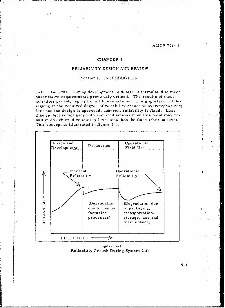
AMCP 702- 3

CHAPTER 5

RELIABILITY DESIGN AND REVIEW


5-1. General. During development, a design is formulated to meetquantitative requirements previously defined. The results of these

activities provide inputs for all future actions. The importance of de-signing in the required degree of reliability cannot be overemphasized;for once the design is approved, inherent reliability is fixed. Lessthan perfect compliance with required actions from this point may re-sult in an achieved reliability level less than the fixed inherent level.This concept is illustrated in figure 5-1.

Design and Production OperationalDevelopine nt Field Use

Inherent Ope rationalReibility Reliability

(Degradation (Degradation due

due to manu- to packaging,facturing transportation,processes) storage, use and

maintenance)

LIFE CYCLE >

Figure 5-1

Reliability Growth During System Life

5-1

AMCP 702-3

Section 11. SOME BASIC PRINCIPLES OF

RELIABILITY DESIGN

5-2. General. This chapter deals with identification of sole basicprinciples of reliability design of which the designer should be vware

and with th, concept of design reviews. Each is discussed briefly interms of its role in the design of rt liable equipment.

5-3. Simplicity. Simplification of item configuration can contribute

to reliability improvement mainly by reducing the. number of possiblefailure modes. A common approach t.oward design simplification,especially structura]l is that of component integration, i.e. , the use ofa single part to perform multiple functions.

5-4. Use of prov.-n components, preferred circuits, and preferred desixn

S concepts, a. If reliability is to be designed into in item, the reliabilityof the individual components must be predicted oi ,.:stimated. Whenworking within time and cost constraints, it is wise to use proven com-ponents where possible, thus minimizing analysis and testing.

b. iforumation is available concerning reliability of certaincomponent configurations and circuits. There are electronic de.signhandbooks available, for exanmple, illustrating standard circuitry whichshould be used in preference to unique designs. Just as with electronicdesigns, proven mechanical and fluid system design concepts can becategorized and proven configurations given first preference.

C, Existing standards must be constantly reviewed and updated.The establishment of new hardware standards must be preceded bythorough reliability vwrification. Some areas in standardization whichare impcrtant to reliability design are standard values, parts, compo-nents, systems and subsystems. Another area of importance is thatof analysis techniques. Accepted methods, such as reliability prediction,can be established for use by design and reliability engineers. These

analysis methods are useful provided their limitations are recognized.

5-5. Stress/strength design. a. The classical approach to designis to give every part enough strength to handle the worst stress it willencounter. Several references, such as MIL-HDBK-5 ace availableproviding data on the strength of materials, and some of these provide

5-2

AMCP 70Z.-j

limited data on strength degradation wvith time, re sulting from fatigue.

Howeve r, when designing for at specified reliability, the traditionaLIaind corinunn use of safcty factors often is inadequate. Fft,:. ti.ve designIprocedures should provide for evaluaitinig alternative configurations withru'spec~t to i eliability. Since failure is not aiw; ys relatted to uime, the

designer needs techniqu~es for comparing stress vs. strength. These

III CI Udk(1) De_-ratiing. Use- pa rts rated higher than expected stres s .

(2) Reliability margin. Measure the separation between

stress aind strength.

(3) Stress /strength testing. Determine the stress ands trecngth di stributionis.

b. The concept of stress-strength in) design recognizes the realitythat loads or stre sses and strengths of particular items siibjt'ctkci to these-stresses cannot be identified as at specific: value but have ranges of valueswith a probability of cccurrence as sociated with each value in the range.

tht C. The reliabil itv of an item mi iy be cdcfinod as the probabilitythtthe strength of that item wvill never be luss than the stress to whichiI

*it v4.11 be subjected (set, ippendiN A for analytic 'methods of determiningreliability using stress and str-cngth distri-bittins). There are fourbasic proc edurcs the designeLr may use to increase reliability.

(1) Increase average !sLrength. This ipproachi is tolerableI* if size and weight increases car, he a ceepted oir if a Stronger mnaterial

is available.I

(2) Decrease average stress. 0Occasionally the average

stress on a component can be roduced wvithout greatly affecting its ca-

pability.

(3) Decrease stress variation. The variation it, stress-is usually hard to control. Howevecr, the stress distribution Can, beeffectively truncated by putting limitations on use Conditions.

F 5-3

AMCP 702-3

(4) Decrease strength variation. The inherent part topart variation in strength can be reduced by improving the basic process,

holding tighter control over the process, or by utilizing tests to eliminatethe less desirable parts.

5-6. Redundancy. Redundancy provides more than one way to accom-plish a function. In some design situations, reliability improvementmay be achieved by introducing reduidant subsystems or components.

For details of various evaluation models, see appendix D.

5-7. Local environment control. Often it becomes apparent duringdesign that a severe local environment would prevent achievement of the

required component reliability. The design engineer is faced with thechoice of improving the component to withstand the environment or, iipossible, changing the environment to satisfy the component. Such

local environment control may acid weight, space and cost; so tradeoffsmust be evaluated on the basis of overall effectiveness. Some'imesoverlooked is the harmful effcct of transportation and installation asopposed to operation. Improved packaging and special handling in-structions may be necessary to preserve rc:liability. Some typical

environmental problems are:

a. Shock and vibration. There are two approaches that may

be tatcn when shock or vibratiun are present. Either isolate the equip-ment ur build it to vithstand the shock or vibration. The problem with

is. lation is that effeitive, simultaneous control of both shock and vi-bration is difficult. When only one or the other is present, specialmountings are often used.

b. Heat. In virtually any kind of syste-m, heaL buildup increases

the possibility of failure. Conmmonly used methods of heat transferinclude free convection, forced air cooling, liquid cooling, conduction,radiation and vaporization cooling.

c. Corrosion. The following design considerations are used

to provide protection against corrosion:

(1) Use corrosion resistant materials.

(2) Use plating and protective finishes,

5-4

La - __ ~- __ __ -

AMCP 702- 3

(3) Avoid dissimilar metal contact.

(4) Control the environment (prevent water entrapment,remove atmospheric moisture, etc.

5-8. Identification and elimination of critical failure modes, a. Fail-

ure mode and effect analysis (FMEA) is an effective technique for

revealing design deficiencies and potential hazards, The FMLA team,to be most effective relative to reliability, should include a reliabilityand a design engineer.

b. FMEA is nothing more than a thorough analysis of the questions:

"How could ... fail? " a-4 "What would happen if ... fails?" FMEA ismore than a check on a, -sign. The design concept can be developed

using this technique as follows:

(1) Start with a functional block diagram to determine import-ance of each function.

(2) Based on this importance, certain configurations may be

developed.

(3) Analysis of the resulting design for compatibility betweenfailure effects and predicted failure probatbility.

5-9. Self-healing, A design approach which has possibilities for futuredevelopment is the use of self-healing devices. Perhaps the simplest

example of a self-healing device is - ire with a layer of sealing corn-pound which will seal any small punctures. A similar technique is used

in some aircraft fuel cells. In this case, a puncture exposes a layer

of uncured rubber which swells to seal the leak. Automatic sensing andswitching devices represent a form of self-healing.

5-10. Detection of impending failure. Achieved reliability in the field

may be facilitated by the introduction of methods and/or devices for

detecting impending failures. Such devices may be used for:

a, Screening of parts and components.

b. Periodic maintenance schedules.

c. Monitoring of operating equipment.

5-5

-I

AMCP 702-3

5-11. Preventive maintenance, a. For continuously operatingrepairable items, preventive maintenance procedures may greatlyenhance reliability when recommended practices are followed. Be-cause such practices may be difficult to comply with, the designermay add to achieved reliability by avoiding the need for preventivemaintenance to the highest degree possible.

b. When the need for preventive maintenance cannot beavoided, the design should provide for the longest possible periodbetween such maintenance, and above all must be consistent withthe overall maintenance policy, the availability of skills, and accessi-bility.

c. Finally, the technical manuals must emphatically call outthe schedule and importance of such maintenance to reliability; andit may be desirable to place prominent labels containing maintenanceinstructions directly on the equipment.

5-12. Tolerance evaluation. A design is not considered completeuntil it has been determined that the different types of tolerancescannot combine in such a way as to interfere with the intended func- . -

tion. In a complex item, it is necessary to consider the expectedrange of manufacturing process variance, operational environment,and all stresses, as well as the effect of time. Tolerances resultingfrom environment (temperature, etc.) and time must be added tomanufacturing tolerances in order to determine the real operationaldistribution. Some niethods of tolerance evaluation consist of:

a. Worst case tolerance analysis. Determining whether theequipment can perform properly with all parts simultaneously at theirtolerance limits and in such a direction as to produce the greatestdeviation of nominal performance.

b. Statistical tolerance analysis. A statistical proceduredetermining the manner in which individual parts tolerances affectthe overall tolerance. This avoids the inherent pessimism of theworst case approach.

c. Marginal checking. A quantitative method for statingwhat sensitivity a given circuit has to variations in its components.

5-6

I

! •-

AMCP 702- 3

5-i3. Prediction and apportionment, a. The role of reliability pre-

diction during design is that of providing an evaluation of a proposed

design and to provide a comparison of alternative designs. Similarly,apportionment provides an approach for identifying reliability goalsfor subsystems in such a combination so as to afford design feasibility.

Generally, these procedures may be useful in the following applications:

(l) As a planning tool for the initial establishment of re-* liability requirements.

(2) As a design tool to guide the designer in the choice of

* parts to meet the specified reliability requirement.

(3) As a design review tool by management for the evalua-

tion of design adequacy to meet the reliability requirement and to pointup potential reliability problem areas for design correction.

iI(4) As a monitoring tool for the assessment of development

program progress toward established goals to predict and circumventoncoming problems before the hardware stage.

b. Design reliability assessnmenLs can be divided into twophases:

(I) The conceptual or design proposal phase. A predic-

tion is based on the design concept as reflected in development speci- I

fications and early design documentation.

(2) The design or development phase. Pred;ctions arebased on the actual design.

c. For prediction and apportionment methodology, see chap-

ter 4.

5-14. Human engineering. Mistakes by people often result in failureof an item to perform its function. Therefore, human activities and

limitations may be very important to item reliability. The reliabilityof people can be influenced by the design engineer by considering the .factors which directly refer to human aspects, such as:

5-7 :_

:I

AMCP 702- 3

a. Human factors.

b. Man-machine interface.

c. Evaluation of man in the system.

d. Human reliability.

5-15. Mean life ratio. Frequently a design engineer wishes to evalu-ate the life of a new product or process in relation to the old. In makinga decision, he should perform a statistical evaluation on the variationbetween the two sample results; or, in other words, he would state thatthe new product or process is better only when he could make the state-rment with a statistically high confidence of being correct. A commonmethod for determining the confidence is the mean life ratio approach.

Section III. RELIABILITY REVIEWS

5-16. General. a. A reliability review is defined as planned monitor-ing of a product to assure that it will meet the expressed and impliedperformance requirements of the equipment during operational use.Such a review provides periodic appraisal of the design effort to deter-mine the progress being made in achieving the design objectives andsystematically brings to bear specialized talent on specific problemareas. In this manner, an overall evaluation is made to identify speci-fic reliability problems that may be encountered later in the develop-ment and production cycles.

b. Realization of the full worth of reliability design reviewsrequires that system program personnel actively participate in the de-sign review process on all development programs which result in items

entering the military inventory.

5-17. Basic review philosophy. Reviews may be profitably appliedat any point during design activities ranging from concept to produc-tion. Design chang .s during the early design reviews generally re-quire very little engineering effort since they usually involve onlypaper changes of a part, dimension, or value; although redesign ofcomponents might at times be mandatory. Design changes occurring

5-8

9i -

AMCP 702-3

during subsequent design reviews involving changes to drawings, modi-fications, replacement of existing hardware, replacement of field per-sonnel, etc., will be considerably more costly. The periodic reviewof reliability at key points in the development program facilitates de-tection and correction of actual or potential problems prior to the finaldesign.

5-18. Required review points. A review schedule should include thetime-phased events representing the appropriate milestones at whichformal reviews are made at major decision points. The number ofcritical decision points will vary according to the type of development

' program underway. The reliability management milestone guide in

appendix B covers the basic reliability review points in the materiel:- life cycle. As reliability reviews are normally repetitious, it is- recommended the review points be expanded and reoriented to con-

form to each unique program. - -

-5I

r i *

*1

I

-_ AMCP 702-3

CHAPTER 6

DEMONSTRATION AND TESTING


6-1. General. a. The design and proper use of adequate test anddemonstration methods and procedures is of prime importance if theuser is to be assured a reliable equipment for field use. This chap-ter is devoted to a general description of such methods and procedureswhich are applicable to a wide variety of equipments and components.

b. The purpose of reliability demonstrations and tests is todetermine current item reliability level. The demonstration of hi1 hreliability with a high level of confidence usually requires testing of"a greater number of items than are available, especially when con-cerned with complex or expensive items. Thus, it is important todesign tests in such a manner that maximum information can be ob-tained from a minim,:m amount of testing. The efficient use ofstatistical techniques is often essential. f

C. A major problem in the formulation of adequate tests isthat of simulating a realistic use environment. During its lifetime,an equipment may be subjected to many environmental factors orstresses such as temperature, vibration, moisture, acceleration,rough handling, etc. , and these stresses may be encountered singly,simultaneously, or sequentially.

d. The ideal test program should provide continuity of relia-bility assessment activities from prediction through end item dem-onstration and testing activities.

Section II. RELIABILITY DEMONSTRATION ANDTEST PROCEDURES

6-2. General. a. Reliability demonstration and test proceduresare applied in order to gain information concerning failures and theirfrequency of occurrence.

6-1

AMCP 702-3

b. Demonstration of reliability may be accomplished by thetesting of sample items and nmay be defined as the process of placing

an item or product under a specified set of conditions and observingthe results. Such tests may be applied to systems, subsystems, orcomponents.

C. Developmental tests are quite useful for estimating thevalues of certain reliability parameters, or deciding whether the re-liability parameters have reached an acceptable level at the particularstage of development. Statistical estimation techniques and statistical

tests of hypotheses, respectively, are utilized-for these purposes. _ _

d. Acceptance tests are used for deciding whether the relia-bility of an item is at an acceptable level. This is merely an adapta-tion of the above -mentioned tests of hypotheses. Statistical analysiswill provide measures of the risk involved in these inferences.

e. Life tests may assume any of several different test dis-ciplines. The test may be terminated after a preassigned time haselapsed, or it may be terminated when a preassigned number of failureshave occurred. F,.r either termination criteria, the test may be con-ducted either by replacing or by not replacing items as they fail. A

major difference between the test disciplines is that time terminatedand nonreplacement tests usually are simpler to conduct than arefailure terminated and replacement tests.

f. Several types of analysis may be applicable to a particulartesting situation. The determination of the appropriate type must betaken into account during pretest planning. Among the common tech-niques to be discussed include: parameter estimation, testing ofhypotheses, acceptance testing, regression analysis, acceleratedlife testing, and stress-strength testing.

6-3. Parameter estimation, a. For each population of components,subsystems, or systems, there exists one or more numerics whichdescribe the entire population. These numerics are called populationparameters. If the important reliability parameters of a populationwere known, reliability testing would not be required. However, inpractice, they are not known, and we must resort to submitting sample

items to tests in order to estimate these parameters.

6-2

li

AMCP 702-3

b. A population may be a group of existing items, or it maypertain to items potentially generated by a process. The differenceis reflected by the interpretation of the estimated parameters. Inthe first case, the estimated parameter describes existing items orequipments; and in the second case, the estimated parameter de-scribes the capability of the process for generating reliable items.

c. An estimate of a reliability parameter may take the form* of either a point or an interval to which a degree of confidence may be

attached. A point estimate is merely a single number which is de-fined as the estimated value of the parameter of interest, e.g., thepopulation MTBF r:tay be estimated as 100 hours. The confidenceinterval consists o. the statement that the parameter falls between

* two numerical values with the associated degree of confidence. The, confidence interval is, in effect, a measure of precision.

d. The estimation of reliability parameters is facilitated ifthe underlying distribution of failure times is known. Analysis tech-niques which do not depend on a known failure time distribution areknown as nonparametric techniques. In general, nonparametric re-liability analysis has the advantage of providing information withoutprior knowledge of the failure distribution, but it also has the dis-advantage of less precise information than that obtained when the

- underlying distribution is known.

e. Knowledge of the failure distribution usually depends uponhistorical information about similar items or upon a relatively large

Ssample by which the hypothesized distribution can be tested. Since, most development tests are based upon a small sample of prototype

models, and in many cases no historical information exists for simi-lar items, nonparametric analysis may be necessary.

f. Appendix F contains several analysis procedures per-taining to the estimation of reliability parameters. These apply to

((1 Unknown distribution of failure times.

(Z) Determination of the underlying distribution offailure times.

6-3

I

AMCP 702- 3- -i

(3) Normal failure times.

(4' Exponential failure times.

5 Weibull failure times.

6-4. Tests of hypotheses. The preceding comments on test analysiswere concerned with estimating the value of certain parameters. tI

is sometimes more meaningful to decide whether or not the parametersare at acceptable levels. Such decisions may be accomplished by hy-pothesizing a value for the parameter of interest and using the test re-sults to decide whether the hypothesis should be accepted or rejected.These procedures are referred to as tests of hypotheses and are dis-cussed in detail in appendix F.

6-5- Acceptance testing. The test of hypothesis, when used as abasis for accepting material, is sometimes referred to as an accept-ance test. There are a number of government documents which con-tain reliability test plan tables. These, too, are discussed in appen-dix F.

6-6. Regression analysis. Regression analysis sometimes may be jused to determine a reliability param-eter for various stress levels|

or design characteristics, such as determination of the mean time tofailure at different levels of stress, e.g. , determination of the rocketbursting pressure for different wali thicknesses. The determinationsare useful for evaluating equipment design, identifying trouble areas,and potential corrective activities, etc. Regression analysis tech-niques are sometimes used to generate this type information fromtest results. For these methods, see appendix F.

6-7. Accelerated life testing. a. Life tests, conducted at or near

normal operating stresses, have proven useful for evaluating anequipment with regard to reliability and for providing data to be usedin reliability improvement activities. The extreme test duration timeposes a serious problem when conventional life testing procedures areused to demonstrate very high reliability. This life test duration timecan sometimes be shortened, however, by utilizing the functional re-lationship between life characteristics and variable stress conditions.The technique of inducing failures by subjecting test items to exces-sive stresses is known as accelerated life testing.

AMCP 702-3

b. The primary purpose of accelerated life testing is to re-duce the time required to obtain failure data. This data, however, isnot representative of reality and must be transformed to failure datapertaining to normal stress conditions by means of a functional rela-tionship between stress level and failure occurrence.

c. Accelerated life testing can be successful only if the func-tional relationship is available from existing sources or if it can bedetermined experimentally, and if additional modes of failure are notintroduced.

d. MIL-HDBK-217A, Rliability Stress and Failure RateData for Electronic Equipment, provides data concerning stress levelsversus failure rate for certain electrical components. The data inthis handbook were intended for reliability prediction purposes, butthe included adjustment factors would allow failure rate transforma-

tion from one stress level to another.

6-8. S ress-strength testing. a. Stress-strength testing techniquesmay be used for evaluating reliability in instances when time or dura-tion of mission does not contribute significuantly to failure, e.g.

mechanical devices and one-shot devices. Analysis techniques forevaluating reliability for stress and strength are discussed in appen-dix A.

b. Stress testing generally involves simulated usage of theitem of interest to determine the stress distribution. The stressesincurred are determined by using such things as strain gages, plastic

models, polarized light, etc. The results are as dependable as theaccuracy of simulation oZ manufacturing variations, operational E n-

vironment, external stresses, time effects, and other importantvariables.

c. Strength testing usually involves some variation of test-ing under increased stresses until failure occurs. The strengthdistribution can be determined by a number of tests to failure causedby continually increasing the stress load. For such tests, it is ex-trernely important that failure be precisely defined before testing.

6-5

. - . - . . . . • - : . . = -1

i t

AMCP 702- 3

d. Thc method of increasing strcss of an item until it failsis applicable only if there is no degradation of strength due to thepreceding stress level. In this case, one-shot testing may he per-formed where an item will be subjected to a given stress level; butif it does not fail, it will not again be tested at an increased stresslevel. By properly selecting the test stress levels and recordingwhether the item failed, it is possible to determine the stress dis-tribution.

6-9. Reliability testing and the total test program. In general,tests should not be conducted solely for determination of reliabilitycharacteristics, but should include consideration of other technicalcharacteristicsa. Thus, reliability personnel should be acquaintedwith the overall Army test program. To fulfill the AMC testing con-cepts, an~ item of Army materiel must be tested at appropriate points.-throughout its life cycle. The reliability considerations associatedwith life cycle testing are shown in appendix B.

Section III. TEST DESIGN

6-10. General. This section furnishes guidance in the application ofthe Army testing concepts to test planning and design. In addition, atest matrix is discussed as an approach for development of an effec-tive test program,

6-11. Test procedures. Test conditions and methods of data analysisare preplanned on the basis of engineering requirements, test method-ulogy, and statistical considerations. The following cycle must becompleted if effective and unbiased test results are to be achieved-.

a. Define the problem.

b. State test objective.

C. Establish tebt requirements.

d. Design test.

e. Implement test.

f. Analyze results.

6-6

AMCP 702-3

6-12. Importance of technical characteristics, a. The approvedstatement of the military need for a new end item or system is con-tained in the QMR/SDR. A statement of essential characteristics maybe derived from this document to provide the basic elements of a de-sign matrix. Such a matrix serves as guidance for development ofthe item or system in response to a stated military need.

b. In order to develop an efficient test design, it is essentialthat key performance parameters be identified to assure that the testprogram is comprehensive and complete. Some important determina-tions relevant to an efficient test design follow.

(1g Definition of the overall mission of the system under- -going test and evaluation.

-4(2) Breakout of the overall mission into major system

characteristics.

3) Further breakout of each major system characteris-tic into a related set of subsystem characteristics.

4) identification and definition of required subsystemcharacteristics necessary for each element of the system requiringevaluation. *1

(5) Determination of critical high risk characteristicswhich are essential to successful system performance.

c . These determinations provide an orderly breakout of per-

fornmance characteristics such that the test results may be evaluatedagainst some given standards or performance criteria. The perform-ance criteria must have been based upon an associated rationale trace-

able to intended tactical performance.

d. End item performance criteria are incorporated into theSove ra~l test plan through application of appropriate prior data, use ofmathematical modeling ano simulation techniques, use of statisticaltechniques, and engineering analysis.

6-7

I - ___ ____ __ ____ ___ ___ ____ __ ____ ___ ____ ___ __ W

AMCP 702- 3

6-13. Design of test programs. a. The following discussions applyto test programs planned during any portion of the materiel life cycle.It should be kept in mind that program emphasis changes as the itemmoves from conception to obsolescence.

b. The relationship between stated performance characteris-tics, performance criteria, criteria rationale and sample require-ments are outlined in figure 6-1. This figure represents the require-nient for a generalized test matrix upon which a comprehensive setof development and test objectives can be based.

c, Figure 6-2 provides an example of a partial engineeringand service test matrix. The matrix for other tests may be developed .. --.

in a similar manner.

d. A test matrix provides a ready outline for the development -oi a comprehensive set of test objectives. Detailed test objectivesprovide the basis for a test plan. Each objective should discuss theprimary purpose of the test, the relationship of the specific test to thepurpose of the overall test prcgram, and the test standards which re-quire satisfaction. In all cases, the performance criteria associated

with each performance characteristic should be included. This in-formation, coupled with the test method to be employed in the execu-tion of the test and the data to be obtained from the test, constitutesthe major portion of any test plan.

e. Verification of technical performance with a reasonablyhigh level of confidence requires a well-designed test program. In

conjunction with engineering analysis and test methodology determina-tion, modeling and statistical analysis techniques are useful for de-

velopment of a test program.

(1) Modeling. The application of modeling is a valuable

engineering tool which provides a means of analyzing dependent sys-tem characteristics to identify maximum stress conditions. Modelingtechniques provide preliminary performance estimates which can be

subsequently verified through test; thus reducing the empirical elementin test planning. Some reliability modeling approaches are treated in

appendix D.

(2) Statistical techniques. Some techniques for analysisof test results are shown in appendix F.

6-s

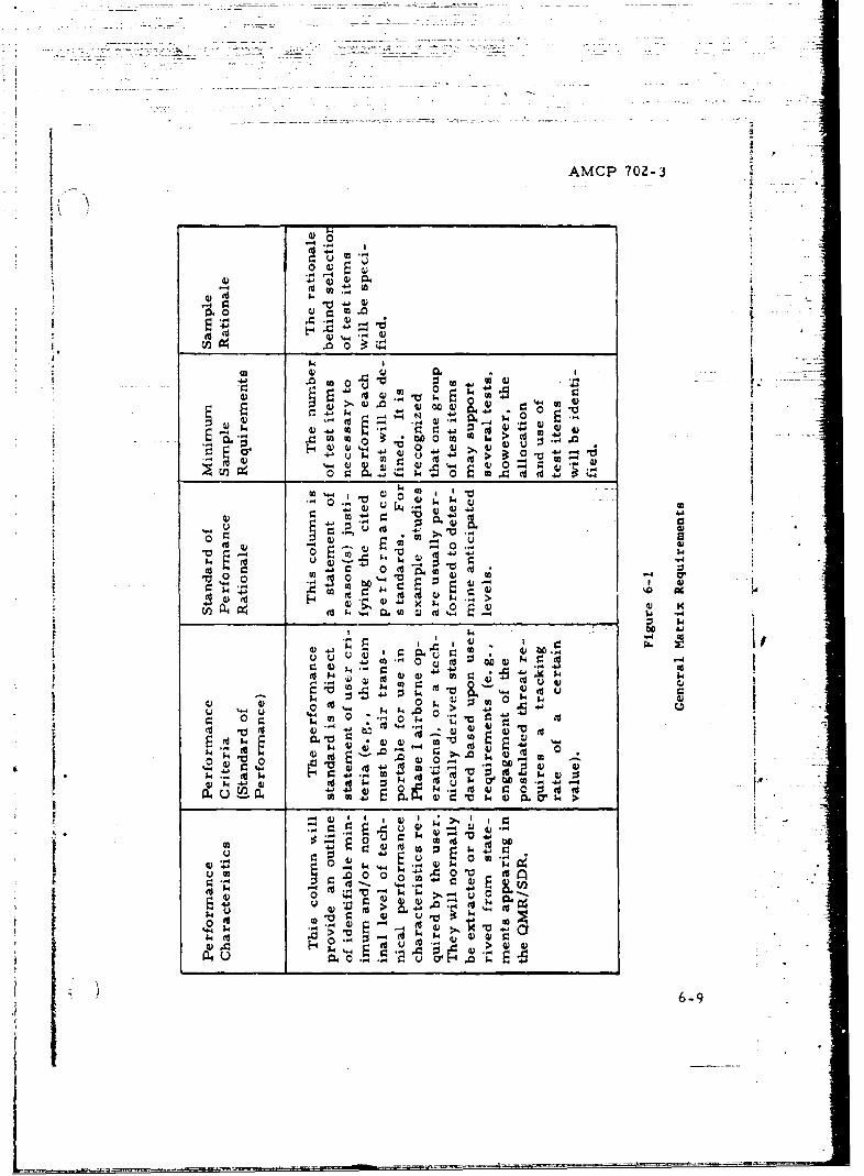
77 :ýi

AMCP 702-3

-4

4?02

4214 14 4j

Old4 4-r. 4

-A 0 tx

1.4)

00

0 u. ~~-0~~ '-0 '( 0)

3. co 14

0 -4 l4j r' 1:0

4)4 4?4 84 0o

un 0' ~ CLV$4$ .

~~~ , 4? * ? 4 r )~

ca 04 C) r )o~ji 4j~ 4J4O~ D 4

41 61 .tO k o o~ al~

02 0 0 CI

*d .- IO r- 4) 4)E O 0

0 ' 0 PC 0

0.3 4.' 4J ( 4C4

11 6-9

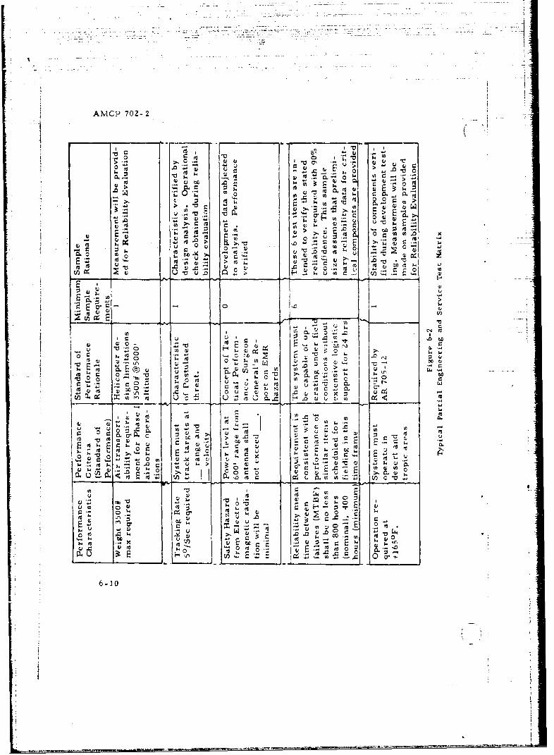
AMvCP 702-2

0 CO~O V-

- d 4.) ME k

> 2ý & , M2

') -c (d 04 04 E

ww u , E..

4 4) u

1>1

I:

-: b 1

U o' -x

LI 4) -0 ce

t)4 0 '004 r-

cI

w ~ 00 (

(0 0 'oI

P4 U E 0 E 0E o

6 -10.-

AMCP 702- 3

CHAPTER 7

RELIABILITY EVALUATION, FAILURE ANALYSIS AND CORRECTION-- THE FEEDBACK LOOP

Section L INTRODUCTIONI --

7-1. General. a. Reliability improvement may be characterized byfive policy type objectives in order to concentrate the project resources - .effectively. These are represented by a reduction of: safety hazards;catastrophic equipment hazards; failure rate of highly replicated systemcomponents; relatively high subsystem failure rates; and failures whichproduce very high support costs. Implementation of these objectivesis brought about through increased technical understanding and improve-ment of the design. Data analysis is used by the engineer as a tool to -

identify those areas where greater technical understanding must bedeveloped. The nature and true value of the reliability improvementprogram thus lies in the conscientiousness and rigcr with which relia-bility personnel investigate problems or weak areas and follow up withcorrective action. The determination of which problems to pursue, to j- .what lengths and by what means, should be based upon thorough under-standing of the system, Army policies, contractual limitations, andexperience with previous problems. In areas not covered by establishedArmy policy, procedures or experience, it is necessary to pursue what- I Iever areas seem to promise the most benefit to overall item reliability.

b. Field operation, in addition to development testing, can beviewed as an extremely important -- albeit costly -- source of relia-bility data. A failure reporting program should never be implemented

before making a careful analysis of what data is to be measured, howthe data is to be analyzed and interpreted, and what can be done tocorrect the system faults as a result of such interpretation. The pur- : ,pose of this chapter is to provide guidance for planning such a testingand feedback information program.I.I

c. In planning for data collection, it is just as important to collectdata on successful or satisfactory operations as it is to collect data onfailures. The use of statistical analysis techniques should be explored

7-1II

AMCP 702- 3

since programs may sink from their own weight where requirementsfor data collection are excessive. In addition to collecting data, caremust be taken to assure that the lessons learned from experience arerecorded and that failure modes are identified. Data collection shouldinclude plans for incorporating proper statistical procedures forevaluating the data. Decisions resulting in corrective action shouldbe made with careful regard for the system mission requirements and

the effective use of available resources.

Section I!. OBJECTIVES OF A POSITIVE MATERIAL FAILUREANALYSIS AND CONTROL SYSTEM

7-2. Objectives. In order to develop a positive material failure analy-sis and control system (FACS), the following objectives should beadhered to.

a. Provide only the pertinent facts needed to evaluate the criticalityof a failure by:

(1) Collecting both success and failure data.

(2) Using accepted statistical analysis techniques to providea confidence level and assure the precision of the data.

(3) Taking care to gather data pertaining to all failure modes.

b. Timely distribution of failure data and information to allorganizational elements needing such data through the use of a simpleand quick response data collection and reporting system.

c. Provide for the cause and effect of failures to be establishedand evaluated by the proper organizational element in a methodicalmanner which uses appropriate statistical techniques and quantitativeapplication of engineering principles.

d. Assure that cost-effective and timely corrective action istaken by:

7-2

- . - -.-

AMCP 702-3

(1) Preplanned and scheduled steps for handling an identifiedreliability problem.

(2) Requiring that changes be made with due regard for the"stated mission-responsive requirements of the system.

(3) Requiring that cost-effectiveness principles and the officialguidelines on this subject be adhered to.

e. Closing the loop on each action using the methods of data collection ......and evaluation provided by the system to verify and evaluate the effective-ness of the action.

Section III. METHODS OF DATA COLLECTIONAND DOCUMENTATION

7-3. General. a. Data collection involves some meaod of placing dataon individual events into source documents or records. Documentationfor reporting purposes involves assembling data on individual eventsinto composite reports which present the information in a meaningfuland usable form. Masses of data improperly collected and assembledwill not provide needed information. Thus, the requirements for whatdata is to be collected, how it is to be collected, and how it is to bereported are fundamental and tasks which must be approached withgreat care in planning. If this is not done, a tremendous amount of

effort and resources may be expended on an effort which has relativelylittle value.

b. Basically, data requirements consist of two factors: dataelements and data reports. The data elements form the basis for de-vising individual event source document forms. Choice of data elementsmust be based on the requirements of the reliability reports program.Data reports reduce the many individual data source documents tomanageable and meaningful form which communicates pertinent informa-tion to decision makers. The requirements for these reports must bebased on a detailed, planned concept of how reliability analysis andevaluations are to be performed. From such a plan, the minimuminformation needed in each report and the report format can be con-structed.

~ I7-3

AMCP 702- 3

c, After establishing the requirements for the data elementsand data reports, the method of implementation is selected. imple-mentation may consist of using an existing Army data collection andreporting system if it meets the requirements, or the procuring agencymay elect to develop its own data collection and reporting system ifresources are available.

7-4. Reliability data sources. The design engineer is dependent- - upon data feedback of part performance and failure data from a wide

range of applications and use environments if he is to optimize designreliability. Some specific sources of such data follow:

a. MIL-HDBK-217A, Reliability Stress Analysis for Elec- itronic Equipment. This handbook provides a source of parts failurerate data for standard electronic and electromechanical parts. Catas-trophic part failure rates observed over wide ranges of electrical andthermal stresses have been analyzed and presented in a form whichpermits determination of the most likely failure rate for a given setof stresses.

b. The Army Equipment Record System (TAEiýS). TheTAERS system is designed to provide field commanders, commoditycommand managers, project managers, and top-level headquarterswith problem-solving data for improved materiel readiness. It isan official Army method for reporting information necessary for con-trol of operation and maintenance support of Army equipment.

c. Tri-Service and NASA Failure Rate Data (FARADA)Program. The purpose of the FARADA Program is to provide part/component failure rate and failure mode data to reliability engineersand design engineers engaged in the design, developme-ni and produc-tion of hardware for the entire spectrum of military and ,pace appli-cations. The information presented in the FARADA lHandbooks hasbeen obtained from operational experience on milit3ýrv and spaceequipments from many tri-service and NASA contractors and govern-ment agencies. As a result of applying engineering and statisticaltechniques to failure rate data, the program provides design and re-liability engineers with ready access to analyzed, summarized, and

7-4

_.. ._- -_... . -_ _--_-._ _. . -... . . -- •

AMCP 702-3

descriptive statistics of failure rates at the component/part level.If properly applied, the information will provide a means of numeri-cally assessing the probability of survival (reliability) of an itemprior to or simultaneously with the construction of hardware. Asexperience in the use of this method is gained, refinements can bemade, and improved design should result. In detail, the program ,

covers:* I

(1) Stress analysis: to assist designers in performingquantitative reliability stress analyses by providing operational stressdata on parts/components.

(2) Environmental factors: to provide data on variousoperating modes influencing failure rates and highlighting the criticalfunctional environmental stresses of each mode.

(31 Application factors: to provide data which modifythe basic failure rate in order to allow for different applications ofthe parts/components.

(4) Performance degradation: to provide data on stabilityor degradation of parts/components under a specific set of applicationconditions.!

The FARADA Program is directed by the Navy and is administeredand implemented by the U. S. Naval Fleet Missile Systems Analysisand Evaluation Group (FMSAFG) at Corona, California. I

d. Inter-Service Data Exchange Program. (11 IDEP is aStrin-service program for the exchange of part test reports to assist

system designers in the selection and application of reliable part

I' ~types. The test data exchanged includes, but is not limited to, thatobtained from: qualification or certification tests; production accept-ance tests; diagnostic or design and development tests; general orcomparative evaluation tests; reliability, exaggerated stress, andlife tests; controlled data collection and sampling programs.I

(2) The IDEP exchange program does not sumfnarize oredit test reports; instead, the three distribution centers (one for eachservice) act as clearing houses. Contractor test reports are for-

warded to their appropriate service distribution center where theyare reproduced and forwarded to other participants in the program.

7-5

Si

- ---- -- -~----_ -i ---

AMCP 702- 3

(3) The Army IDEP contact is IDEP Office, RedstoneScientific Center, U. S. Army Missile Command, Redstone Arsenal,Alabama.

7-5. Reports. a. Reports are the products resulting from the dataelements. They summarize for management the status on varioussystem parameters such as: reliability, availability, maintainability,parts usage rates, capability, system effectiveness, etc.

* b. Within the scope of official guidelines, the procuring agencyhas freedom of action for developing its own methods to meet the statedrequirements, as weil as the restraints imposed on it by resources,etc.

c. For the reliability portion of the program, reliability datafiles should be established for Army materiel and that the followingtechnical type data should be recorded where appropriate:

(1) Critical design or manufacturing features.

"(2) Applicable specifications or standards.

(3) Modes of failure.

(4) Causes of failure.

(5) Stresses at failure.

(6) Methods of detection or test.

(7) Type of failure distributions.

(8) Recommended necessary preventive or correctiveaction.

(9) Estimate of reliability for various applications.

(10) Prime manufacturer and alternate sources.

7-6

!i

N=

AMCP 702- 3

d. The above technical type data is to be collected during

the development and testing phases. Such items provide the quanti-

tative and engineering data upon which a decision for actions may be

based.

e. In addition to technical type data, tactical and operational

data accumulation is required and should be organized so as to pro-

vide background information for combat development purposes. Speci-fic items of data must be patterned according to the nature of the iterm.

Where appropriate, the data should include information concerning:

(1) Mission reliability with respect to the overall missionassigned to the field unit.

(2) Reliability data for tactically or operationally sig-

nificant phases of the overall mission.

(3) Data for environmental and operational conditionsvarying from the normal.

"7-6. Selection of data elements for data collection forms, a. In

selecting or developing data collection forms for use in a reliabilityprogram, the following data elements are suggested:

(I) Using unit.

(2) Ecuipment identification (aircraft tail number, gun

tube number, etc.).

(3) Data of failure.

(4) Identification of failure (part number, subsystem, etc.).

(5) Result of failure (red-X, mission abort, launch hold,item not available, etc.).

f

7-7

* AMCP 702- 3

(6) Total system time (flight hours, equipment hours, miles,rounds fired, etc.).

(7) Number of previous failures of this type on the equipment.

(8) Time to each previous failure of this type.

(9) Characteristic of the failure (cable jammed, receiverintermittent, heavy vibration, out of specification limits, etc.).

(10) Environment in which the failure occurred (use conditions).

b. It should be kept in min'd that the above list of elements is by nomeans complete. However, these are basic to reliability analysis andstatus reporting. In order for a reliability program to effectivelyutilize data source documents, a system must be established to handlethe paper flow and -educe it to a compact and comprehensible form.The basic requirement is to determine the minimum needed dataelements and then synthesize these into a composite xozm from which therequired reliability analysis ard reports may be generated. Obviously,an alternative to using established forms and systems is to develop adata collection system tailored strictly to the project. The lattermethod is probably the most efficient, relative to a specific project.

Section IV. FEEDBACK CYCLE

7-7. General. a. A basic failure analysis and corrective action feed-back loop should determine: what failed; how it failed; why it failed;and when it failed.

b. Failure data provides information to determine the first twofactors. The third, essential to corrective action, usually requiresinformation which can be obtained only by laboratory study and/orengineering analysis of the problem areas uncovered by failure analysis.

c. A well planned failure reporting program provides importantinputs for reliability improvement. Such a closed loop feedback cycleis illustrated in figure 7-1. Data collection is only one task of several

7-8

, -!

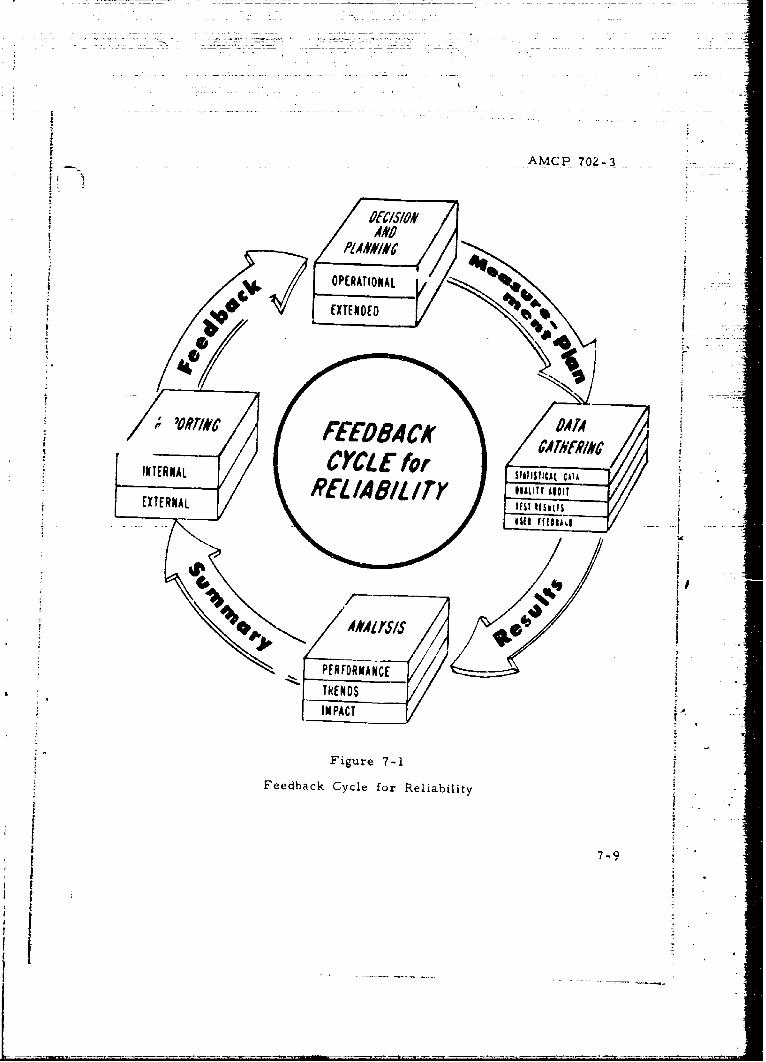
AMCP 70Z- 3

* EXTENDED

10R

~ FEEDB4ACKINTERNL CCEfrSIITCLDI

EXTERNAL PEL IA fiL IT)

Figur 7-1j~

FedakCtefooeiblt

0.417$.9

PEFOMAC

TRNDIMPACT

AMCP 702-3

in a well conceived reliability program plan. Contained herein aresome basic requirements of a data collection system, data sources,and data uses. This discussion is concerned with three major phasesof an overall program; namely, the design and development phase,the manufacturing or production phase, and the operational or fieldevaluation phase.

7-8. Design and develop-nent phase requirements, a. It is during

this phase that system inherent reliability is planned and established.Various test programs are conducted at this time. Examples ofthese tests are those conducted at the part level, breadboard andprototype assembly and subassembly levels, and many times, at theprototype system level.

b. Some very meaningful reliability data results from initialtests performed in the engineering laboratory under either roomambient or controlled environmental conditions. The collectionsystem should provide for the routine collection of these data, eitherby completion of failure report forms by test personnel, or by lifting

the desired data from the test logs by the reliability personnel, or acombination of both. It is very important that due consideration begiven to the total planned test program -- not only those tests thatare to be performed during the design and development phase, butfor all phases of the overall program as sources for reliability data.It is at the beginning of a proposed program that the reliabilityengineers should plan and coordinate with other activities for theirtotal data needs and the manner in which these data will be timephased as inputs for use during the performance of the other relia-bility tasks.

7-9. Manufacturing or production phase requirements. a. Assources of data, the procuring agency reliability personnel should lookto the areas and agencies responsible for the preservation of reliability;namely, manufacturing (production), handling, storage, maintenance,and test.

b. Thus, data gathered can be separated into broad categoriesas quality data and reliability data. Quality data includes records of

7-10

AMCP 702- 3

inspection and testing; e. g., go no-go tests, measurements of vari-ables such as resistarce and capacitance to determine conformance

to established technical requirements contained in specifications,drawings, and purchase orders. Reliability data on equipment isdeveloped during preproduction stages in order to detect equipment _

weaknesses before release to production and to obtain a quantitativeestimate of equipment reliability. Reliability data on parts and/orcomponents is developed during the production stages to assure thatthe equipment inherent reliability is not unduly degraded by manu- I ..facturing processes. When the data indicates excessive failure rates,corrective action should follow. f

7-10. Operational or field evaluation phase requirements, a. Ob-taining timely, accurate and complete reliability data from the field ais probably the most difficult. People who are more concerned withgetting the equipmnent to function (their prime mission) may be lax inreporting data (failure and success). An initially well conceived data Icollection plan which is properly coordinated should reduce datacollection to a routine activity.

b. Data sources include operational logs, contractor's reportforms, and reports associated with the Army equipment failure report-ing system.

c. The types and evaluation of field failure and repair data aremuch the same as those for other phases of the equipment life cycle.However, greater emphasis is given to operational mnalpractices andincompatibility between inplant performance specifications and opera-tional specifications. During the operational phase of a given program,the reliability engineer should be exerting a great deal of effort touncover the causes for equipment and system unreliability by searchingout both quantitative and qualitative information pertaining to failures.

Section V. STEPS FOR UTILIZATION OF FAILURE DATA

7-11. Procedural steps. Of the many questions which may be asked ofa failure reporting system, and among the most useful when answered, is:

7-11

t

'II

... . .: .... .....

AMCP 702-3- I

What, within an equipment, contributes most to its unreliability? The

Sfollowing represents a step by step approach for analyzing presentfailure reports, whether originating in the field, at a test facility, orin a contractor's plant, designed to answer this question.

a. Step 1, Organize the data. Reliability data should be evalu-ated at planned periods throughout the program and should be tailored

to each specific phase. A reliability data center is useful in therealistic assessment of current reliability levels. It is a tool which

enables failure data to be used in indicating where design improvement--and support is needed and is a necessary storehouse of vital informa-tion to be used in engineering, manufacturing, quality, and serviceactivities. Here, the data is generally arranged first by identifiable

- -. • subassemblies within the subject equipment; then by subsystem or part

reference designation. (This step is easily accomplished by machinesorting of data when information is transcribed on punched cards ortape.)

b. Step 2, Frequency analysis. The data center can be inter-rogated to provide failure data; failure times; accumulated operatingtime on the system or equipment; and total accumulated number offailures for a selected subsystem, assembly, or component. Con-

tinuous updating of reports will provide continuous managementvisibility of the reliability program. Information may be arranged as

to frequency of failure occurrence vs. subsystem for the purpose ofidentifying those subsystems causing the most trouble. This proce-dure can then be repeated through descending levels to identify most

troublesome assemblies, components, or parts.

c. Step 3, Selection of vital failures. Failure types considered

vital should be sought and can be recognized as those failure modes,

failure parts, and problem areas to which reliability improvement

effort can be profitably applied. Specific components and subsystems

which fit into this category are:

(I) Those whose failure markedly affects the safety of the

system both in terms of human safety and equipment destruction.

7-12

-- I

AMCP 702- 3

(2) Those which appear in large numbers in the system.

(3) Those whose failure results in high support costs.

(4) Those whose reliability level is relatively low withrespect to the rest of the system.

d. Step 4, Problem evaluation. Identification of vital failures |within troublesome subsystems, assemblies, etc., is not enough tosatisfy the requirement for a sound reliability intelligence system.Corrective action can only be accomplished if the cause can be deter-mined. This is an engineering job consisting of such things as qualityaudits, laboratory tests, engineering evaluation, etc. It is throughthese methods, coupled with the routine observation, irterview, anddata evaluation, that failure causes can be isolated and necessary cor-rective action initiated.

T e. Step 5, Determine corrective action. Corrective actionmust be carried out with the objective of providing a design change ormodification which mitigates the causes of failure. In generating atechnique for handling corrective action, prime consideration shouldbe given to a system which would prevent discrepancies from escapingdetection, tap the many available sources of data, and be rapid andcomprehensive in its closure action. Figure 7-2 is a schematic of atypical corrective action system. All changes, including correctiveactions, shall undergo engineering-reliability analysis. This approachis applicable to all phases of the life cycle.

f. Step 6, Implement. Implementation of corrective action!involves the developing of a new design or modification of an existing

design within a system. Once the problem area has been recognizedand defined, the cause identified, and corrective action initiated,there must be a means for implementing this change in the program.

This implementation can be accon plished in many ways, such as:procedures, engineering change proposals (ECP), or modification AV

r work orders (MWO). A point to remember is that implementationmust take place in a 'imely manner in order for it to be effective.This action complete the cycle for a closed loop feedback system. [ "

7-13Ii

AMCP 702-3

g. Step 7, Follow-up. The approach illustrated in the pre-ceding steps will be useful and effective only if changes conceived,tested, and introduced into existing systems or used to develop newsystems are evaluated and monitored to assure compliance with theintent. Follow-up should also provide checks to determine whetherthe problem has been eliminated, and review to see whether new prob-lems have been introduced as a result of the corrective action.

7-14 7-14

I I .

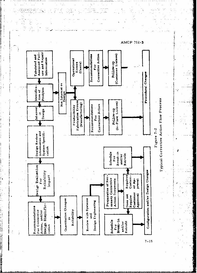
AMCP 702Z-3

44

00

60 0

4. V)V

U0

.d 0'u0 0l

7-1

AMCP 702-3

APPENDIX A

CONCEPTS OF RELIABILITY QUANTIFICATION


A-i. General. Quantitative expression and measurement of relia-bility requires an understanding of the concepts of probability and - -

-statistics. Probability serves as a measurement scale by which relia-bility is expressed and, as such, is a measure of the likelihood or chancethat an item will survive a required nussion time for a specified intendedfunction and use environment. This appendix reviews a few basic rules,symbols, and concepts necessary for quantification of reliability. The

review does not constitute an exhaustive coverage of the necessary mate-rials. Further coverage may be found in various textbooks, professionaljournals, etc.

Section II. PROBABILITY

A-2. Definition. a. In general, the probability that an event A willhappen is the portion of time the event will occur over a large numberof trials. When only a Eingle trial is to be encountered, the probabilitythat event A will happen is merely the relative chance of its happening.

p

b. The statement which follows provides a more formal defi-nition of probability. Given an experiment, if an event may happenin 'a" ways and fail to happen in "b" ways, and all of these ways are"mutually exclusive and equally likely to occur, the probability of the

r event happening is

a+b

L. e. the ratio of the number of favorable ways to total number of waysthe event can happen. Symbolically, the probability that the event Awill happen is expressed: P(A).

c. The numerical expression of probability operates along adimensionless, continuous scale extending from 0 to 1. If P(A) = 0,

* A

A-I

I

AMCP 702- 3

the event A will not happen. If P(A) = 1, the event A will always happen.If P(A) = .5, the event A would be expected to occur in 50% of a largenumber of trials. In general, high frequency events will be assigned aprobability value near one, and low frequency events will be assigned aprobability value near zero.

d. To illustrate the definition of probability, consider an ex-periment consisting of a single toss of an "honest" die. Find the prob-ability that the upturned face will show an odd number.

Total number possible outcomesP(odd number) -resulting in odd number

Total number possible outcomes

-3 1

6 2

This means that in a large number of tosses, about half of the tosses* would result in an odd number. The interpretation for a single toss

is that there is a 50-50 chance that the outcome would be odd.

A-3. Concept of a set. a. General. A brief investigation of setnotation and operation will facilitate the discussion of probability.A set is defined as a collection of objects having certain specifiedproperties. Each object belonging to the set is called an element.The set that contains the totality of all elements that may appear inour investigation is called a space. A space has neither dimensionnor volume, but is comprised of a complete set of elements.

b. Definitions of specific sets.

(I) Infinite set. Set having an infinite number of elements.

(2) Finite set. Set having a finite number of elements.

(3) Empty set. Set having no elements,

(4) Subset. Set consisting of several elements of anotherset. A subset is, of course, a set and the operations on sets will beapplicable to subsets.

A-2

'1

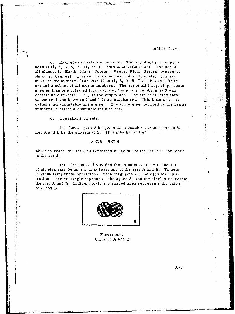
AMCP 702-3

c. Examples of sets and subsets. The set of all prime nurn-bers is (1, 2, 3, 5, 7, 11, ). This is an infinite set. The set ofall planets is (Earth, Mars, Jupiter, Venus, Pluto, Saturn, Mercury.Neptune, Uranus). This is a finite set with nine elements. The setof all prime numbers less than II is (1, 2, 3, 5, 7). This is a finiteset and a subset of all prime numbers. The set of all integral quotientsgreater than one obtained from dividing the prime numbers by 3 willcontain no elernents, i. e. , is the empty set. The set of all elementson the real line between 0 and 1 is an infinite set. This infinite set is A.called a non-countable infinite set. The infinite set typified by the primenumbers is called a countable infinite set.

d. Operations on sets.

(1) Let a space S be given and consider various sets in S.Let A and B be the subsets of S. This may be written

ACS, BCS

which is read: the set A is contained in the set S; the set D3 is contained- in the set S.

(2) The set A U B called the union of A and B is the setof all elements belonging to at least one of the sets A and B. To helpin visualizing these opec-ations, Venn diagrams will be used for illus-tration. The rectangle represents the space S, and the circles representthe sets A and B. In figure A-i, the shaded area represents the unionof A and B.

Figure A-IUnion of A and B

A-3

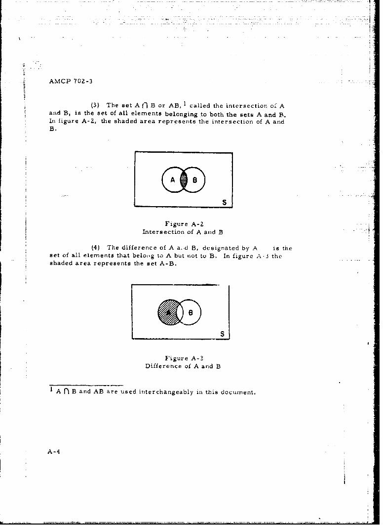
-A-

AMCP 702-3

(3) The set A (1 B or AB, 1 called the intersection of Aand B, is the set of all elements belonging to both the sets A and B.In figure A-Z, the shaded area represents the intersection of A andB.

S

Figure A-2Intersection of A and B

(4) The difference of A a .d B, designated by A is theset of all elements that belong to A but not to B. In figure A-3 theshaded area represents the set A-B.

s

Figure A-3Difference of A and B

1 A f B and AB are ubed interchangeably in this document.

A-4

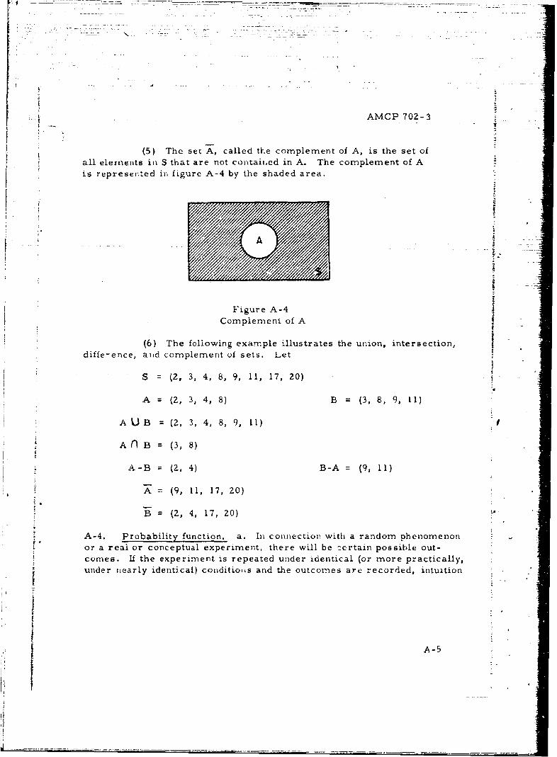
AMCP 702-3

(5) The set A, called the complement of A, is the set ofall elenments in S that are not coritaiiEed in A. The complement of Ais represented in figure A-4 by the shaded area.

-jFigure A-4 -

Complement of A

(6) The following example illustrates the union, intersection,diffe-ence, and complement of sets. Let

S = (2, 3, 4, 8, 9, 11, 17, 20)

A = (2, 3, 4, 8) B = (3, 8, 9 11)

A U B (2, 3, 4, 8, 9,11)

An B= (3, 8)

A-B = (Z, 4) B-A = (9, 11)

= (9, 11, 17, 20)

B - (2, 4, 17, 20)

A-4. Probability function, a. In connection with a random phenomenon

or a real or conceptual experiment, there will be •certain possible out-

comes. If the experiment is repeated under identical (or more practically,

under nearly identical) conditiojis and the outcomes are recorded, intuition

I7

A-5

I_

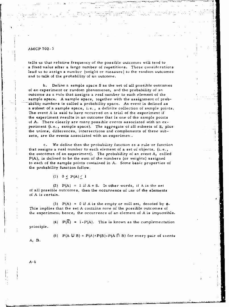
AMCP 702- 3

tells us that relative frequency of the possible outcomes will tend toa fixed value after a large number of repetitions. These considerationslead us to assign a number (weight or measure) to the random outcomesand to talk of the probability of an outcome.

b. Define a sample space S as the set of all possible outcomesof an experiment or random phenomenon, and the probability of anoutcome as a rule that assigns a real number to each element of thesample space. A sample space, together with the assignment of prob-ability numbers is called a probability space. An event is defined asa subset of a sample space, i. e. , a definite collection of sample points.The event A is said to have occurred on a trial of the experiment ifthe experiment results in an outcome that is one of the sample pointsof A. There clearly are many possible events associated with an ex-periment (i.e. , sample space). The aggregate of all subsets of S. plusthe unions, differences, intersections and complements of these sub-sets, are the events associated with an experimen..

c. We define then the probability function as a rule or functionthat assigns a real number to each element of a set of objects, (i. e.,the outcomes of an experiment). The probability of an event A, calledP(A), is defined to be the sum of the numbers (or weights) assignedto each of the sample points contained in A. Some basic properties ofthe probability function follow.

(1) 0 < P(A)< I

(2) P(A) = 1 if A = S. In other words, if A is the setof all possible outcomes, then the occurrence of one of the elementsof A is certain.

(3) P(A) = 0 if A is the empty or null set, denoted by *ý.This implies that the set A contains none of the possible outcomes ofthe experiment; hence, the occurrence of an element of A is impossible.

(4) P(A) = I-P(A). This is known as the complementationprinciple.

(5) P(A U B) = P(A)+P(B)-P(A f B) for every pair of £ventsA, B.

A-6

V.i

:- -, - - -- •.-_ _ _ _----

AMCP 702- 3

d. In many probability situations when the outcomes of a ran-dom phenomenon are finite in number and the outcomes are equallylikely, we assign equal probabilities to the possible outcomes. Forexample, in the experiment of tossing a coin, S = (H, T), the possibleoutcomes are heads and tails and each is equally likely and has prob-ability 1/2. In general, if

S'A" LA UJA U- -) A where A. A. =J

2 3 r r j

and the probability

P(A 1 ) = P(Az) = .. P(Ar), then P(A.) ..r....

For any event E=AUAI U'" U Ak wherek < r and A .A-- 1

"the probability of E is

P(E) P(A 1 1 + P(A) + + I(A

1 1 1k+ i -i+ +1_k,

r r r r ISometimes probability is defined ur.ng this concept where k is the num-ber of equally likely ways favorable to the event E and r is the totalnumber of possible outcomes of the experiment or random phenomenon.The probability of the event E is defined as the ratio k/r.

e. To exemplify the assignment of probabilities, consideran experiment consisting of tossing a coin twice. The sample spaceS is defined as S = (,HT, HH, TH, TT), consisting of four outcomeswhcre HT denotes heads on the first toss and tails on the second, and

so forth. Since each is equally likely, we might assign the numbers1/4, 1/4, 1/4, 1/4 to each of these sample points.

(1) Let E event of a head on the first toss 1P(E) = P(HT) + P(HH)

= 1/4 + 1/4 =Z/4

A-7

i

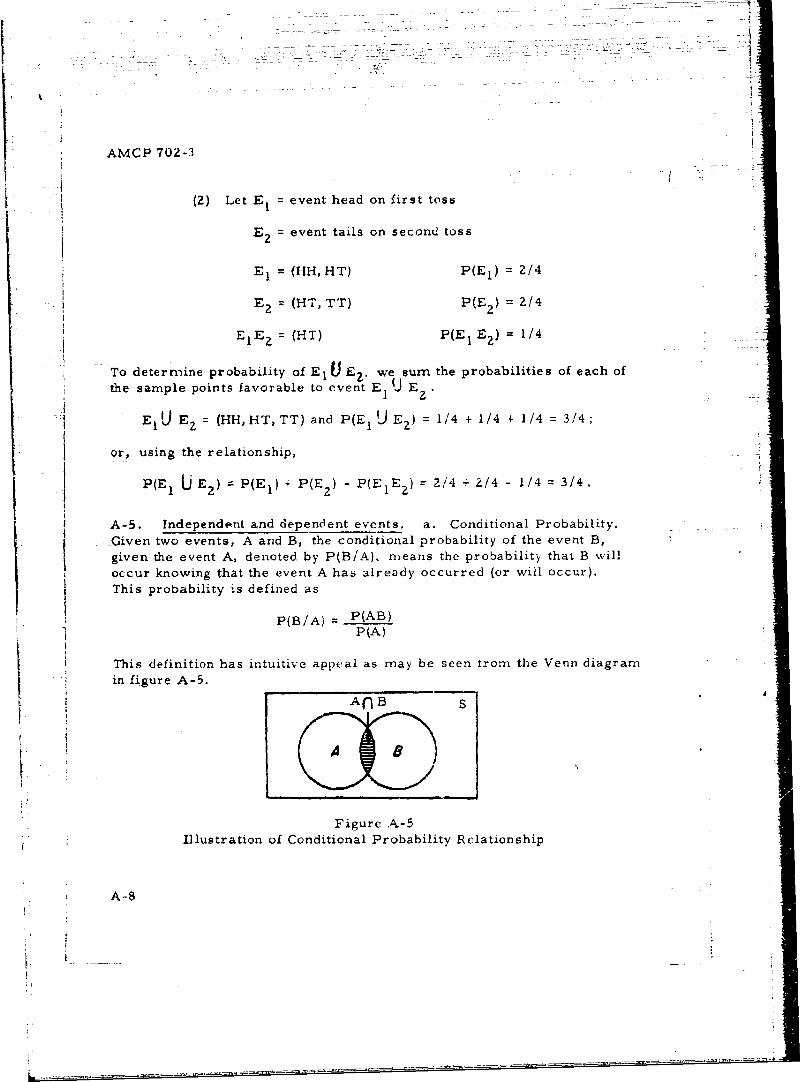
AMCP 702-3

(2) Let E event head on first toss

S2 = event tails on second toss

E1 = (HH, HT) P(EI) = 2/4

E (HT, TT) P(E 2 ) = 2/4-i

E EIZ= (H T) P(EI Ed) = 1/4

- To determine probability of E1 (I E 2 . we sum the probabilities of each ofthe sample points favorable to event E U E

"* E1 9 Ez = (HH, HT, TT) and P(E 1UE.) 2 14 + 1/4 + 1/4 = 3/4;

or, using the relationship,

P(EI U E2 ) P(EI) + P(E 2 ) - P(E E 2 ) 2/4 + 2/4 - 1/4 = 3/4.

A-5. Independent and dependent events, a. Conditional Probability.-Given two events, A and B, the conditional probability of the event B,given the event A, denoted by P(B/A), means the probability that B will"occur knowing that the event A has already occurred (or will occur).This probability is defined as

P(B/A) = P(AB)

P(A)

This definition has intuitive appeal as may be seen trom the Venn diagram

in figure A-5.AnlB s

Figure A-5Illustration of Conditional Probability Relationship

A-8

---

L• _ .. - . . . . . .

AMCP 702-3 .

(1) Knowing that the event A has occurred, our attentionis turned to the set A. The -leements in A favorable to the event Bis the set AB, represented by the shaded area. The set A may nowbe considered in a sense our sample space, and the set AB, the set in i

A favorable to the event B. Therefore, the probability of the eventB/A is given by the ratio of the two probabilities, P(AB) and P(A).

(2) N )te that this form also defines the joint probabilityof the event AB. Ij -

P(AB) = P(A)P(B/A) P(B)P(A/B)

(3) For example, consider the problem of drawing withoutreplacement samples of size 2 from an urn containing 3 white and 2red balls. Let A be the event the first ball drawn is white and B the

event the second ball drawn is white. Determine P(B/A) the probability Ithe second ball drawn is white given the first ball drawn is white. Bydefinition,

P(B/A,.) =P(AB)P(A)BA....

Three outcomes are favorable to the event AB, namely (w, W2 ), (w , w2 3

(w 1 ,w 3 ), where wi is white ball i. Since there are 5 _2! 3!

possible outcomes, we assign the value 1/10 to each outcome and,

hence P(AB) 3/10. Relating the event A = (wl, w 2 , w 3 ) to the 5 possible

outcomes of the first draw gives P(A) 3/5. Thus, P(B/A, = (3/10)/(3/5)=i/Z.

b. Independence. Let A and B be events defined on the same

probability space. The events A and B are defined to be independent if

P(AB) P(A)P(B)

Events that do not satisfy the above relation, oip are said to be dependent.The concepts of independence and conditio 4i probability may be definedfor n events." ~All Az,"' Al

h nilA-9

AMCP 702- 3

The conditional probability of A given that the events Al, A2 , , Ann-have occurred is given by

P(An/AI, A?, , An-) - P(Al, A 2 , A 3 , An)P(Al, A 2 , . Anj )

and the n events are mutually independent if

P(AA) A P(A.)P(A)

--- p(AiAjAk) = P(Ai)P(A )P(Ak)

P(AIA2 '" An) = P(AI)P(AZ)" P(An)

for all combinations 1 i ,j k '<. < n.

A-6. Basic rules of probability. Certain basic rules of probability-will be useful for reliability analysis activities. Some of these follow.

a. Multiplication. (1) Consider two events A and B with re-spective probabilities of occurrence of P(A) and P(B). Then the prob-ability of occurrence of both A and B is

P(A fn B) = P(AB) = P(A)P(B/A)

= P(B)P(A/B)

(a) To illustrate the above relationship, considerdrawing two cards (without replacement) from a well-shuffled, 52-carddeck. What is the probability that both cards will be aces ?

(b) Let A be the event of af, ace on the first draw and

B the event of an ace on the second draw. Then

P(A) =-4 anJ P(B/A) -52 51

ri4 3 _ 1P(AE) z P(A)P(B/A) = 3 1

A-10

AMCP 70Z-3

(2, If the events A and B are independent, the above re-lationship reduces to

P(AB) P(A f B) = P(A)P(B)

because

P(B/A) P(B) and P(A/B) = P(A).

Then A and B are defined as statistically independent events.

(a) To illustrate this special case, consider an elec-tronic assembly consisting of two independent subsystems: A and B,functionally connected in series. Both subsystems must function properlyin order for the system to function properly. Suppose that the probabil-ity of A working properly = 0. 9 and that the probability of B working 4

properly = 0. 8. Compute the probability that the system will functionproperly.

P(A) 0.9 and P(B)= 0.8

(b) The event that the system will work properly is the

intersection of A and B.

P(AB) = P(A)P(B) (0. 9)(0.8) - 0.72

b. Addition. (I) The probability that at Least one of two events,A and B, occurs, (i. e. , either A or B or both) is

7 P(A U B) = P(A) + P(B) - P(AB)

where A U B is defined as A union B.

(a) For example, a certain operation can be performedby either one of two systems, A and B. Aisume that the systems A and

B operate completely independently and that the probability of A function-ing properly is 0. 8 and that the probability of B functioining properly isU. 7. Compute the probability that the operation is performed success-fully by at least one of the two systcms, A, B. Then P(A) = 0.8 andP(B) = 0.7.

A-Il

L _ _ +_ _ _ _ _ _ _ _ _ -- _ _ _ _ _ _ -_ _ _ _ _ _ _ _ _

AMCP 702- 3

(b) The event that the system will work properly isthe union of A and B and

P(A UB) = P(A) P(B) - P(AB) 0.8 + 0.7 - (0. 8)(0. 7) 0.94.

(2) If A and B are mutually exclusive, i. e., P(AB) 0,

the above relationship becomes

t P(AU B) P(A) + P(B)

(a) To illustrate, consider drawing one card froma well-shuffled deck. Find the probability of that card being either a

club or a diamond. Let A = the event of a club and B = the event of a-diamond.

(b) Then P(A)_-1, P(B) =3and P(AB) 052 52

i.e., A and B are mutually exclusive.

S13 +13 _26SP(A UJ B)= P(A) + P(B) L3 + -3S52 52 52

c. Complementation. (1) The last of the probability relation-ships to be discussed at thi, time is that of complementation. if P(A)is the probability that the event A will occur, then P(W) is the probabil-ity that the event A will not occur, and

P(A) + P(A) = I

be the (2) To illustrate, consider the toss of a single die. Let

A be the event of a six appearing and W the event of a six not appearing.Then

1 - 5 1 5P(A) =and P(A)= -and P(A) + P(A) - + -1.

d. Summary of probability rules.

(1) Multiplication of probabilities when events are notindependent; conditional probabilities. If E and F are not independent,

A-lZ

Ii9!

AMCP 70Z- 3

(i. e., occurrence of event E affects the probability of the occurrenceof event F), then the probability of the joint occurrence of E and F isgiven by

P(E ri F) P(•)P(F/E) = P(F)P(E/F)

(2) Multiplication of probabilities for independent events.If E and F are independent, (i.e. , the occurrence of E does not affectthe occurrence of F), then

P(E (1 F) = P(E)P(F)

(3) Addition of probabilities when events are not mutuallyexclusive. If E and F are events which are not mutually exclusive,(i. e. , events E and F can happen together), then the probability ofthe occurrence of E or F is given by

P(E U F) = P(E) + P(F) - P(E F)

(4) Addition of probabilities for mutually exclusive events.

If two events Eand F are mutually exclusive, (i. e., they cannot happentogether); then

P(E U F) = P(E) + P(F) 11

(5) Complementation. Suppose E is an event, then

t P(E) = I - P(E).

Section III. STATISTICS AND PROBABILITY DISTRIBUTIONS

A-7. General. Statistics has sometimes been defined as the collection,analysis and p- esentation of numerical data. Numerical expression ofreliability requires a basic understanding of certain statistical methods.

A-8. Basic descriptive statistics. a. There exist certain character-tics which may be used to describe a group or population of numerical

data. Basic descriptive characteristics to be considered herein arecentral tendency, variability and shape of the data distribution. Central

A! A-i13

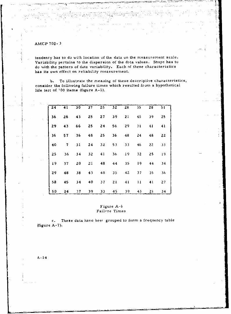
Ia

AMCP 702- 3

tendency has to do with location of the data on the measurement scale.Variability pertains to the dispersion of the d&-ta values. Shape has todo with the pattern of data variability. Each of these characteristicshas its own effect on reliability measurement.

b. To illustrate the meaning of these descriptive characteristics,consider the following failure times which resulted from a hypotheticallife teat of 100 items (figure A-5).

24 41 30 37 25 32 28 35 28 51

36 26 43 25 27 39 21 45 39 25

29 43 66 25 24 56 29 31 41 41

36 57 36 48 25 36 48 24 48 22

40 7 31 24 32 53 33 46 22 33

25 36 34 32 41 36 19 32 25 19

19 37 20 21 48 44 35 19 44 34

29 48 38 43 48 35 42 37 35 36

58 45 34 40 37 Z1 41 11 41 27

25 24 37 39 33 45 39 43 21 34

Figure A-6Failvre Times

c. These data have beei grouped to form a frequency table(figure A-7).

A-14V

tI

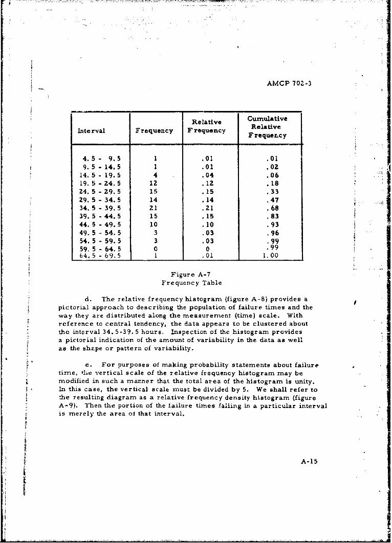
AMCP 70Z-3

S Relative CumulativeRelativeInterval Frequency Frequency Relte

F requer~cy

4.5- 9.5 1 .01 .019.5 - 14.5 1 .01 .02

14.5- 19.5 4 .04 .06

19. 5 -24.5 12 .12 .1824. 5 - 29.5 15 .15 ,3329. 5 - 34.5 14 .14 .4734. 5 - 39.5 21 .21 .6839. 5 -44.5 15 .15 .8344. 5 -49.5 10 .10 .9349. 5 - S4.5 3 .03 .96

54. 5 - 59.5 3 .03 .9959. 5 - 64.5 0 0 .99 I64.5 - 69.5 1 .01 1.00

Figure A-7Frequency Table

d. The relative frequency histogram (figure A-8) provides apictorial approach to describing the population of failure times and theway they are distributed along the measurement (time) scale. Withreference to central tendency, the data appears to be clustered aboutthe interval 34.5-39.5 hours, Inspection of the histogram providesa pictorial indication of the amount of variability in the data as wellas the shape or pattern of variability.

T e. For purposes of making probability statements about failuretime, the vertical scale of the relative frequency histogram may bemodified in such a manner that the total area of the histogram is unity.In this case, the vertical scale must be divided by 5. We shall refer tothe resulting diagram as a relative frequency density histogram (figureA-9). Then the portion of the failure times falling in a particular intervalis merely the area of that interval.

A

S~A-iS

&I

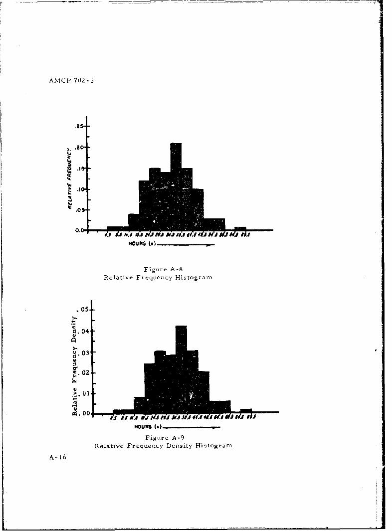
AMCF 702- 3

.2

.0

0. J: NJUJ "lJ E .4O 9.1 SO Ji A

HOW*i (xi

Figure A-8Relative Frequency Histogram

.05

0. 04

03-

0, ., w~ A.M 40J n JlJiJJDIEEs . .1 IIJ'u #.S

HOURS 430

Figure A-9

Relative Frequency Density Histogram

A-16

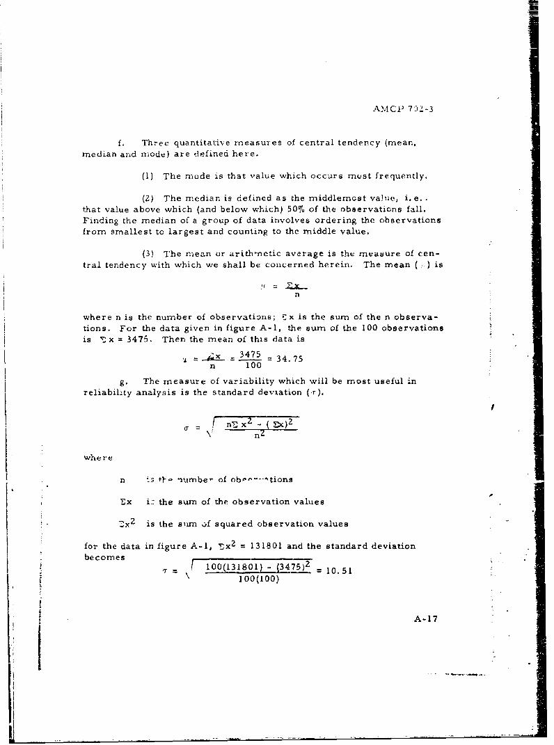
U

AMCP 70--3

f. Three quantitative measures of central tendency (mean,median arnd mode) are defined here.

(1) The mode is that value which occurs must frequently.

(2) The median is defined as the middlemost value, i. e.,that value above which (and below which) 50% of the observations fall.

Finding the median of a group of data involves ordering the observations

from smallest to largest and counting to the middle value.

(3) The mean or arith-netic average is the measure of cen-tral tendency with which we shall be concerned herein. The mean ( -) is

n

where n is the number of observations; ;x is the sum of the n observa-

tions. For the data given in figure A-I, the sum of the 100 observationsis Zx = 3475. Then the mean of this data is

3475= 5= 34.75n 100

g. The measure of variability which will be most useful in

reliability analysis is the standard devxation (r).

Sn 2 x2

\' nZ

where

n is tl-' numbe- of ob,'--'tions

-x i_: the sum of the observation values

Zx 2 is the sum of squared observation values

for the data in figure A-1, 'Sx 2 = 131801 and the standard deviation

becomes2becomes [ 100(131801) - (3475)2 i.

= ~37)= 10.51100(100)

A-17

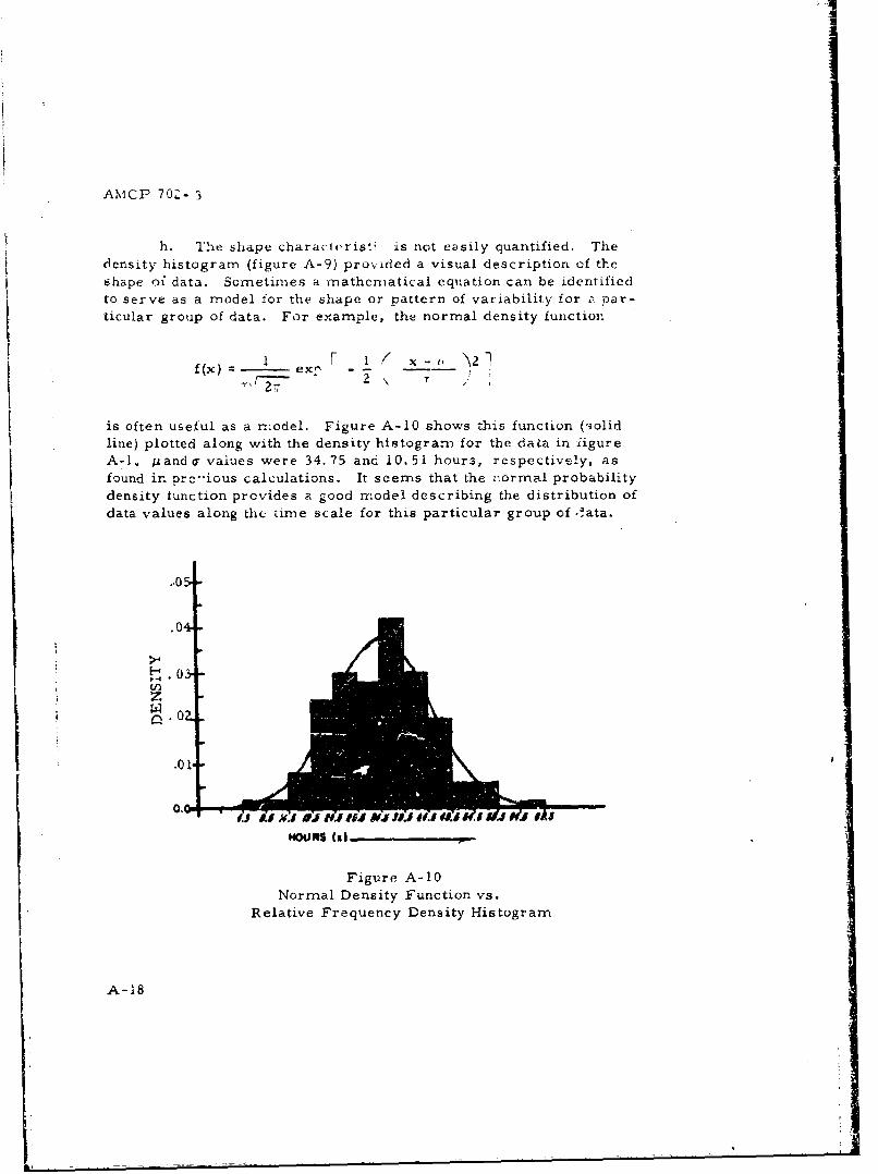
AMCP 70Z- 3

h. The shape characterist4 is not easily quantified. Thedensity histogram (figure A-9) provided a visual description of theshape of data. Sometimes a mathematical equation can be identifiedto serve as a model for the shape or pattern of variability for a par-ticular group of data. For example, the normal density function

1 r I! X-f, Vzf(x) - ex --

22-.

is often useful as a n-odel. Figure A-10 shows this function (3olidline) plotted along with the density histogram for the data in figureA-I. panda values were 34.75 and 10.51 hours, respectively, asfound in prc-'ious calculations. It seems that the normal probabilitydensity function provides a good model describing the distribution ofdata values along the time scale for this particular group of .ata.

.05

.04

0 .0U)z

S.0Z

NOWMS (•)

Figure A-10Normal Density Function vs.

Relative Frequency Density Histogram

A-18

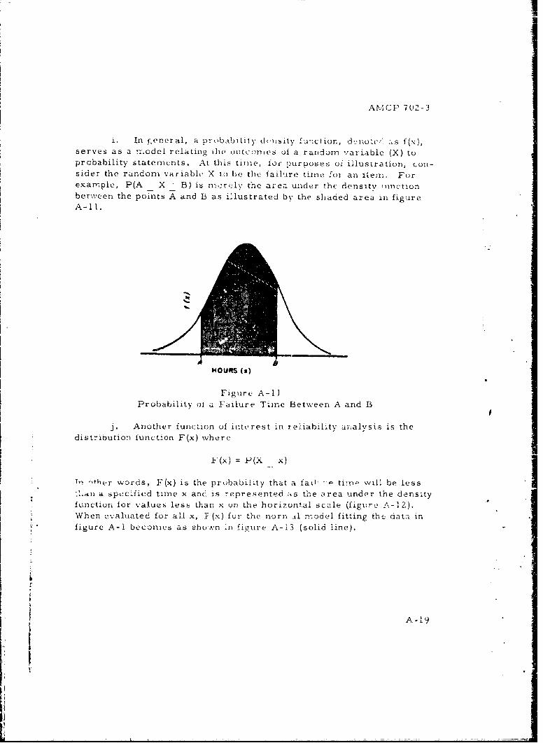
AMCP 702-3

i. In r eneral, a probability dclisity fun ction, d-,t s f(x),serves as a nmodel relating Whe outconies of a raxidom variable (X) toprobability statements. At this time, for purposes ot illustration, con-sider the random variable X to be the failure time for an item. Forexample, P(A X B) is nwrclv the area under the density unnction

between the points A and B as illustrated by the shaded area in figureA-11.

HO UR•S (2)

Figure A-IlProbability ol a Failure Time Between A and B

j. Another function of interest in reliability analysis is thedistribution function F(x) where

F(x) = P(X x)

T, rther words, F(x) is the probability that a fa -f- timne will be less

"-an a s pecified time x and is represented ;is the area under the densityfunction for values less than x on the horizontal scale (figure A-12).When evaluated for all x, 7'(x) for the norn al model fitting the data infigure A-i becomes as shown in figure A-13 (solid line).

A

~A -19

I|

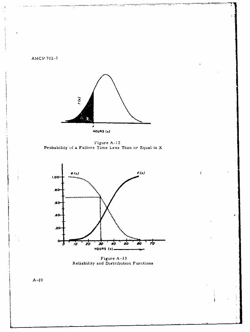
AMCP 70Z-3

I

HOURS (a)

Figure A-12Probability of a Failure Time Less Than or Equal to X

.O " •..... .... ,....

*.0- so-

.8 * ,....

HOURS (9)-

Figure A-13Reliability and Distribution Functions

A-20

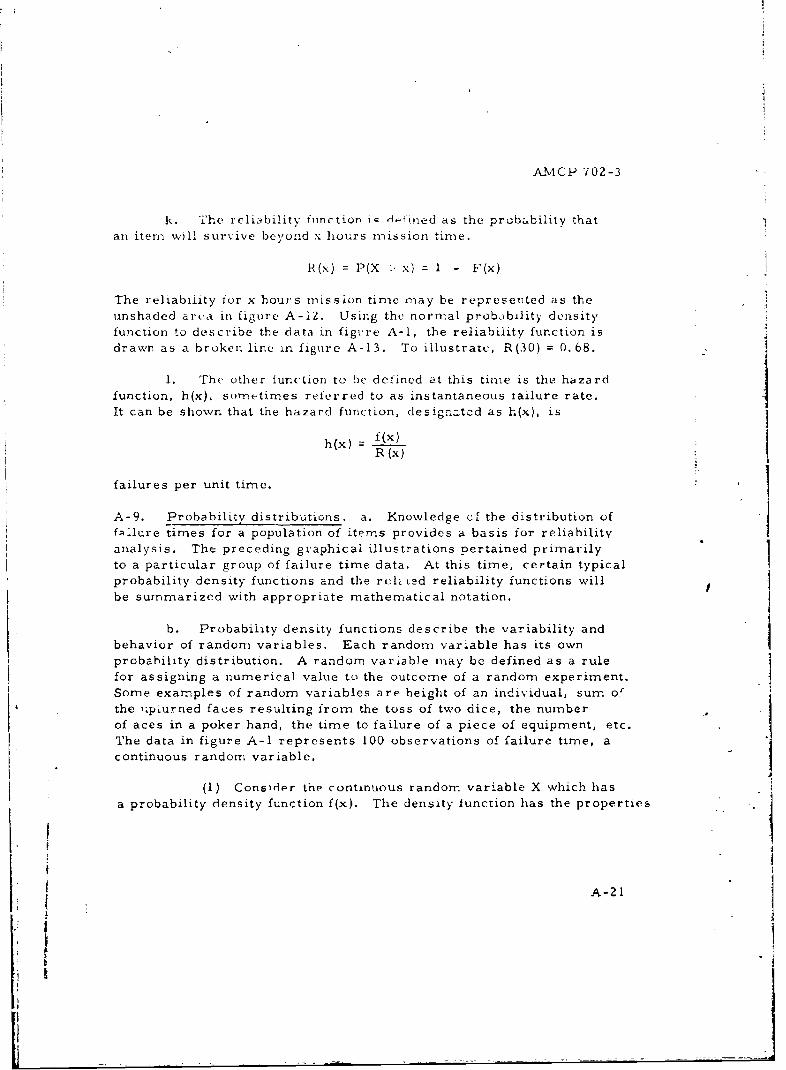
A-MCP 702-3

k. The reliability function ic .l.fined as the probabilitv that

an itern will survive beyond x hours inission time.

R(x) 2 P(X - x) = 1 - F(x)

The reliability for x hours mission time may be represented as theunshaded area in figure A-IZ. Using the normal prob•ibility densityfunction to describe the data in figt're A-I, the reliability function is

drawn as a broken line in figure A-13. To illustrate, R(30) = 0.68. -

1. The other Junction to be defined at this time is the hazardfunction, h(x). sometimes referred to as instantaneous tailure rate. IIt can be shown that the hazard function, designatcd as h(x), is

h(x) = f(x)R (x)

failures per unit time.

A-9. Probability distributions, a. Knowledge cf the distribution of

fnilure times for a population of items provides a basis for reliabilityanalysis. The preceding graphical illustrations pertained primarilyto a particular group of failure time data. At this time, certain typicalprobability density functions and the relz ted reliability functions will

be summarized with appropriate mathematical notation.

b. Probability density functions describe the variability andbehavior of random variables. Each random variable has its ownprobability distribution. A random variable may be defined as a rule

for assigning a numerical value to the outcome of a random experiment.

Some examples of random variables are height of an individual, sum of

the uipturned faces resulting from the toss of two dice, the numberof aces in a poker hand, the time to failure of a piece of equipment, etc.The data in figure A-1 represents 100 observations of failure time, acontinuous random variable.

(1) Consider the continuous random variable X which has

a probability density function f(x). The density function has the properties

A-21

AMCP 702-3

thatf(x) > 0

and

f(x)dx = 1

(2) The density function serves as a model for probi:&,.iitystatements about the random variable; e. g.

P(A<. X - B) f(x)dxA

and

P(x < X < x + dx) f(x)dx

where

dx-- 0

(3) The central tendency of X may be measured by themean or expected value, E(X), of the random variable.

E(X) C xf(x)dx

(4) The variance, V(X), of the random variable measures

its variability and is defined as

V(X) =(Xa) -( E(X) 1-J

c. The distribution function, F(x), which in reliability analysisis often referred to as unreliability for x hours mission time is

CxF(x) P(X x) = f(t)dt

A-2Z

7

AMCP 70Z-3

and has these properties:

(I- F(x) > 0

(2) F(x) is a non-decreasing function

(3) F(-c)=0

(4) F(-)

d. For a random variable, X, which represents failure times,the reliability function becomes

R(x) 1 - F(x) = f(t)dt.

e. The hazard function, h(x), sometimes referred to as in-stantaneous failure rate, of a probability distribution of times to failureis often used in reliability considerations. It is def-.ned as the conditionalprobability density function of time to failure, given the item has notfailed prior to time x. In other words,

h(x)dx = P (x X x + dx) I (X> x)1

which reduces to_ f(x)

h(x) R(x)

f. Figure A-1 provides a sumn,,ary of the above relationshipsior continuous random variables.

A- 23

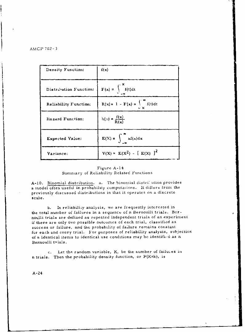
AMCP 702- 3

Density Function: f(x)

Distrioution Function: F(x) . X(tdt

Reliability Function: R(x)= I -F(x)= f(t)dt

Hazard Function: - f(x)R( x)

Expected Value: E(X) = \ xf(x)dx

Variance: V(X) - E(XZ) - [ E(X)

Figure A-14Summary of Reliability Related Functions

A-10. Binomial distribution, a. The binomial distri' ution provides

a model often useful in probability computations. It differs from the

previously discussed distributions in that it operates on a discrete

scale.

b. In reliabili1y analysis, we are frequently interested in

the total number of failures in a sequence of n Bernoulli trials. Ber-

noulli trials are defined as repeated independent trials of an experiment

if there are only two possible outcomes of each trial, classified as

success or failure, and the probability of failure remains constant

for each and every trial. For purposes of reliability analysis, subjection

of n identical items to identical use conditions may be identifi, d as n

Bernoulli t'ials.

c. Let the random variable, K, be the number of failuaes in

n trials. Then the probability density function, or P(K=k), is

A--24

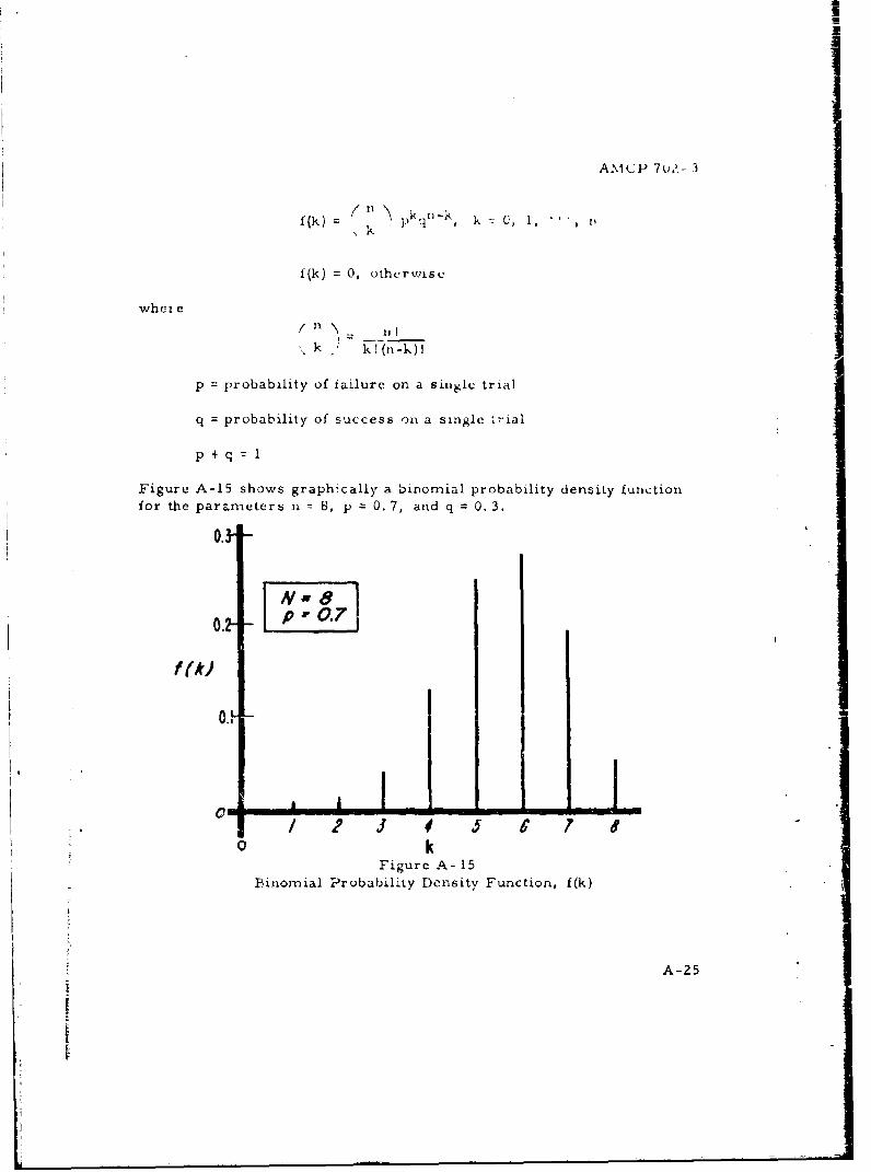
AMCP 7u,ý- 3

f(k) = /n ( I'll, k"

f1(k) = (, othcrwise

whei e/ n 1, ] !

k! k z k (n -k) I

p = probability of failure on a sinelc trial

q = probability of success on a single trial

p+q q

Figure A-15 shows graphically a binomial probability density functionfor the parameters n = 8, p 0. 7, and q = 0. 3.

0.

Nir 8f (k)

0.,

! 2 6' 5 Go k

Figure A- 15B~inomial Probability Density Function, f(k)

A-25

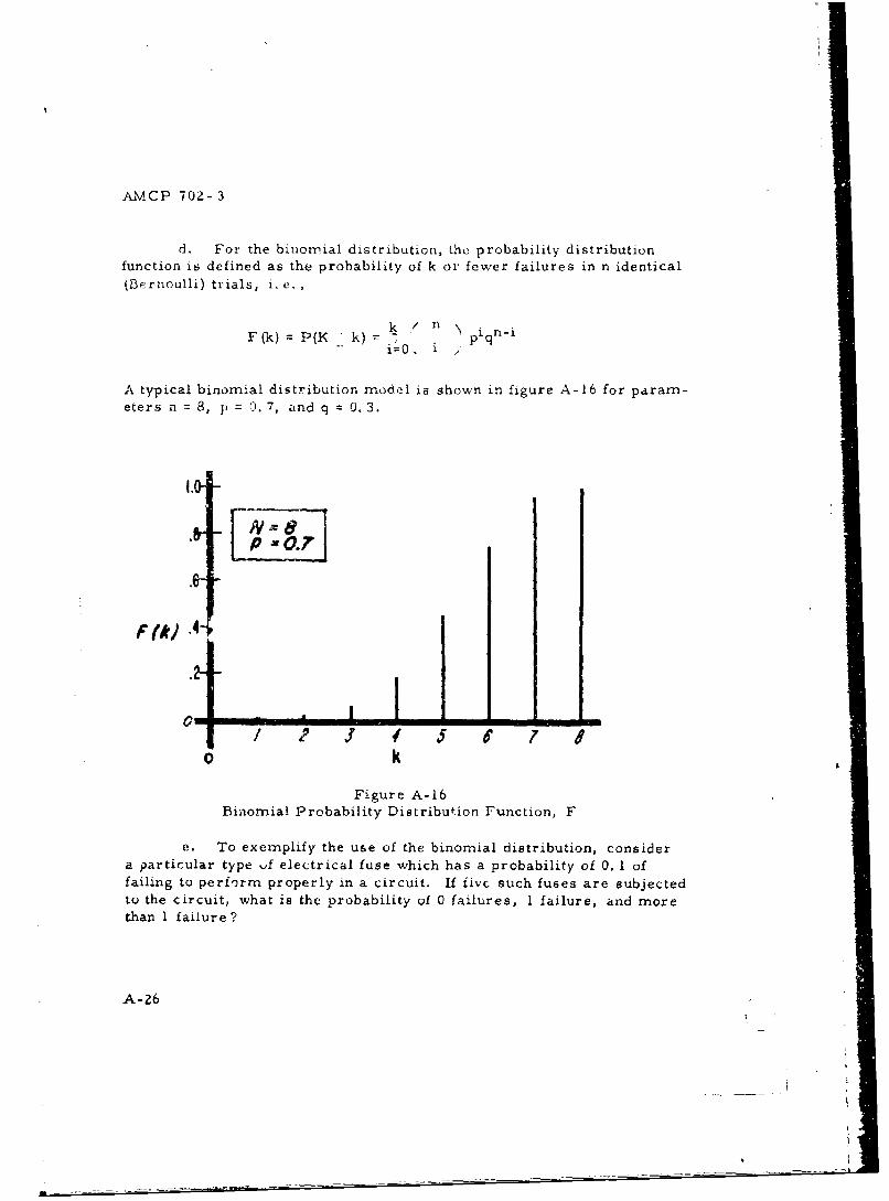
AMCP 70Z- 3

d. For the binonrrial distribution, the probability distributionfunction is defined as the probability of k or fewer failures in n identical

(Beroulli) trials, i, e.,

n / i n-iF(k) = P(K k) k piq

S i=0, I ;

A typical binomial distribution model is shown in figure A-16 for param-eters n = 8, p = 0. 7, and q = 0. 3.

.0- - I

.8 Xr 0•.7-8

F * .4-

0 WM • | I. ,

/ 2 ,' 4 5 7 1 /0 k

Figure A-16Binomial Probability Distribution Function, F

e. To exemplify the use of the binomial distribution, considera particular type %if electrical fuse which has a probability of 0. 1 offailing to perform properly in a circuit. If fivc such fuses are subjectedto the circuit, what is the probability of 0 failures, 1 failure, and morethan 1 failure?

A-26

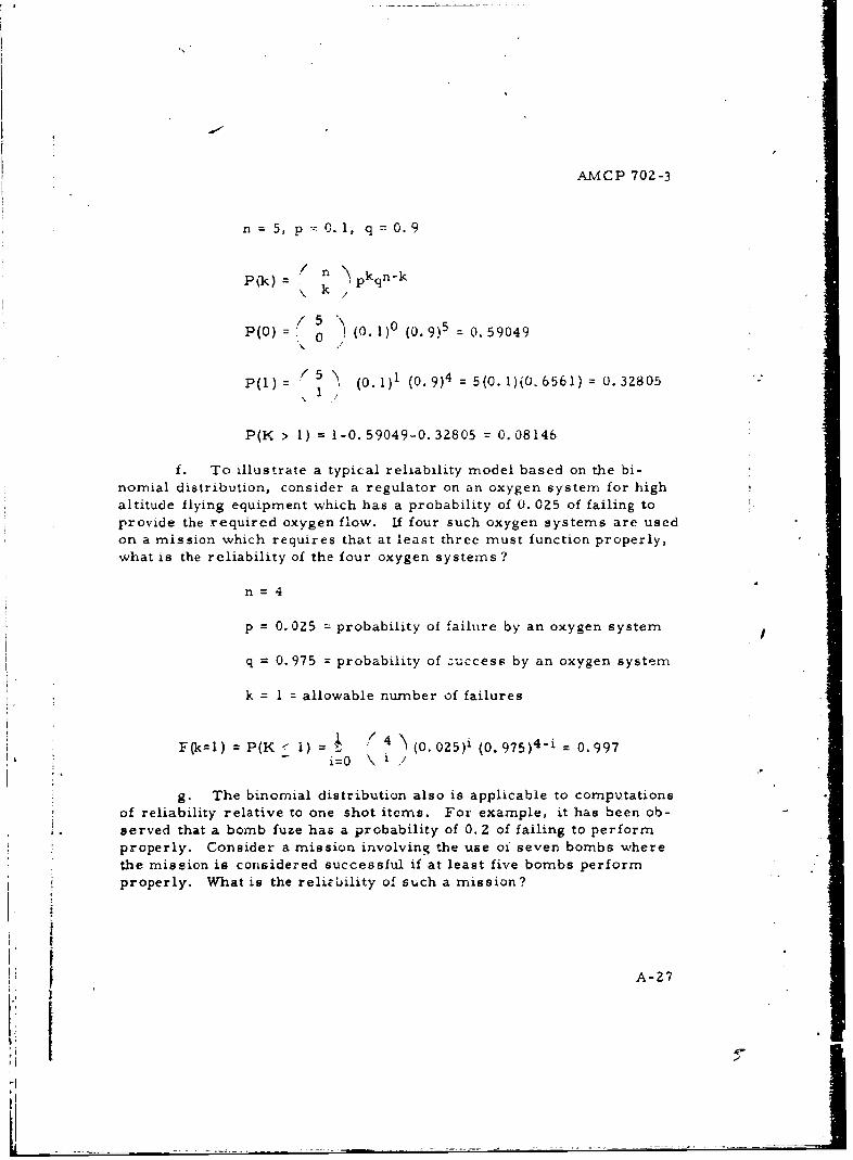
AMCP 702-3

n 5, p = 0.1, q 0.9

Pik) "n pkqn-k\ k /

P(0) = 0 (0. 1)0 (0. 9)5 0, 59049

P(l) = 5 (0. I)1 (0.9)4 = 5(0. 1)(0. 6561) 0. 328051

P(K > 1) = 1-0. 59049-0.32805 = 0.08146

f. To illustrate a typical reliability model based on the bi-

nornial distribution, consider a regulator on an oxygen system for highaltitude flying equipment which has a probability of 0. 025 of failing toprovide the required oxygen flow. Li four such oxygen systems are usedon a mission which requires that at least three must function properly,what is the reliability of the four oxygen systems?

n=4

p 0. 025 probability of failure by an oxygen system

q 0.975 probability of Luccess by an oxygen system

k = I = allowable number of failures

F(k=l) = P(K " 1) = 4 * 4 > (0.025)i (0. 975)4.i = 0.997=i0 \ i /

g. The binomial distribution also is applicable to computationsof reliability relative to one shot items. For example, it has been ob-served that a bomb fuze has a probability of 0. 2 of failing to performproperly. Consider a mission involving the use oi seven bombs wherethe mission is considered successful if at least five bombs performproperly. What is the relizb~ility of such a mission?

A-27

IJ

AMCP 702- 3

n=7

p 0. 2 probability of failure by any one bomb

q = 0.8= probability of success by any one bomb

k = 2 = number of allowable failures

2 /7 )7-iF(k=2) =P(K 2) =(1 2) (0.8 = 0.852

- i=0 \ii

A-11. Normal distribution, a. Ihe normal distribution is sometimesuseful as a model for failure times, particularly when failures areoccurring because of wearout. A normal distribution of failure timesis continuous and has an increasing failure rate. This model is oftenuseful when mission times are such that failures are due to wearout.Defined below are the normal probability density function and relatedreliability functions.

b. The probability density function for the normally distributedrandom variable X is

f _ 1 exp " ; X -. hz2J -

where -m < x < co, and the pararae- rs , and r are the mean and

standard deviation, respectively. Io- ' is referred to as the variance.)Figure A-17 shows graphically the normal probability density functionwith parameters =1 and -2 = 0.25.

c. Probability tables (table H-Z, appendix H) are availablefor the standard normal distribution. Since any normal random variableX can be transformed to the standard normal random variable Z, thetables may be applied to any normal distribution.

A-28

-i- -__ _____ -i - -

AMCP 702-3

IITime (x)

Figure A-17Normal Probability Density Function, f(x)

(1) The transformation is

(2) The expected value and variance of the normalrandom variable X is:

IiE(X) =

V(X) =

(3) The expected value and variance of the standardnormal variable Z is:

E(Z) 0

V(Z) = 1

d. The density function for the standard normal variable is

f(z) = _ exp -22

A-29

AMCP 702-3

where - o e z oo.

e. The distribution function of X may be expressed as afunction of Z.

F(x) 1(X < x1 exp F _ t -. N. dt

T 7'

= z I exp dt

where

x - f

F(z) values can be obtained from table H-2, appendix H.

f. The reliability function of the normal :andom variable X is

I /xR (x)= I-F (x) P P(X >x) = PI Z > Ix- =" zi

1-F(z)

The normal reliability function is illustrated in figure A-18 for parani-

eters , = 1 and -2 =0.25

g. The hazard function for the normal distribution of failure

times may be found by

h (x)

A-30

r I

I

AMCP 70Z-3

1.0•

.5 1.01, 0

Time Wx)Figure A-18

Normal Distribution Reliability Function, R(x)

where

f(x) = f(z)

and f(z) may be found frorn table H-9, appendix H. Figure A-19 con-tains a plot of the normal hazard function for parameters 1,

= 0. Z5.

h. To illustrate the use of the normal probability densityfunction as a reliability model, consider a model 555 rifle which hasdemonstrated a normal distribution of failure times with 100 hours Ip

ano = 10 hours. Find the reliability of such a rifle for a missiontime of 104 hours and the hazard rate of one of these rifles at age 105hours.

// R (x) P Z > x

R(104) = P Z > 1,'41,, P(Z - 0.40) 0.34 as found in table H-Z.

A-31

I"

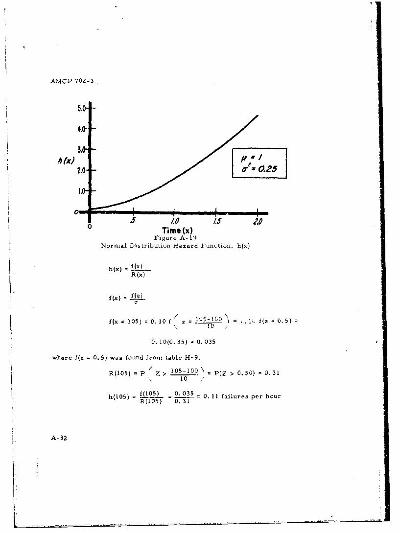
AMCP 702-3

5.

4.0-

3,."

2. - 0.25

10 -I2.

Time (x)Figure A-19

Normal Distribution Hazard Function, h(x)

h(x) f(x)

R (x)

i(x) f f(z)

f(x = 105) = 0. 10 f z = = I 1(, f(z 0.5)t0

0. 10(0.35) 0. 035

where f(z 0.5) was found from table H-9.(105 -100 P(Z > 0.50) 0.31

R(105) =P Z > •- -10

h(105) = (105) _ 0.035 0. 11 failures per hourR(105) 0.31

A-32

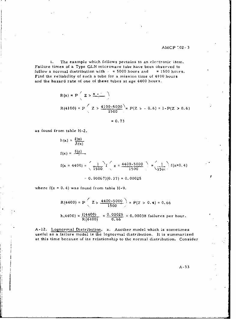
AMCP -02- 3

i. The example which follows pertains to an electronic item.Failure times of a Type GLN microwave tube have been observed tofollow a normal distribution with . = 5000 hours and = 1500 hours.Find the reliability of such a tube for a mission time of 4100 hoursand the hazard rate of one of these tubes at age 4400 hours.

R(x) = P Z>--'

/ 4100-5000'_N (R(4100) P Z > -= P(Z 0.6) = I-P(Z > 0.6), 1500

= 0.73

as found from table H-2.

h (x) . f(x)R (x)I

f (X) f(z)

f(x = 4400) = f z 4400-5000 f f(z-- 4)S1500oo, 1500 \,I50C

= 0. 00067)(0. 37) = 0. 00025

where f(z = 0. 4) was found from tabie H-9.

R(4400) P Z 4400-5000> =_ P(Z > 0. 4) = 0.661500

h 4400) = f(4400) 0.00025 = 0. 00038 failures per hour.R(4400) 0.66

A-12. Lognormal Distribution. a. Another model which is sometimesuseful as a failure model is the lognormal distribution. It is summarizedat this time because of its relationship to the normal distribution. Consider

A-33

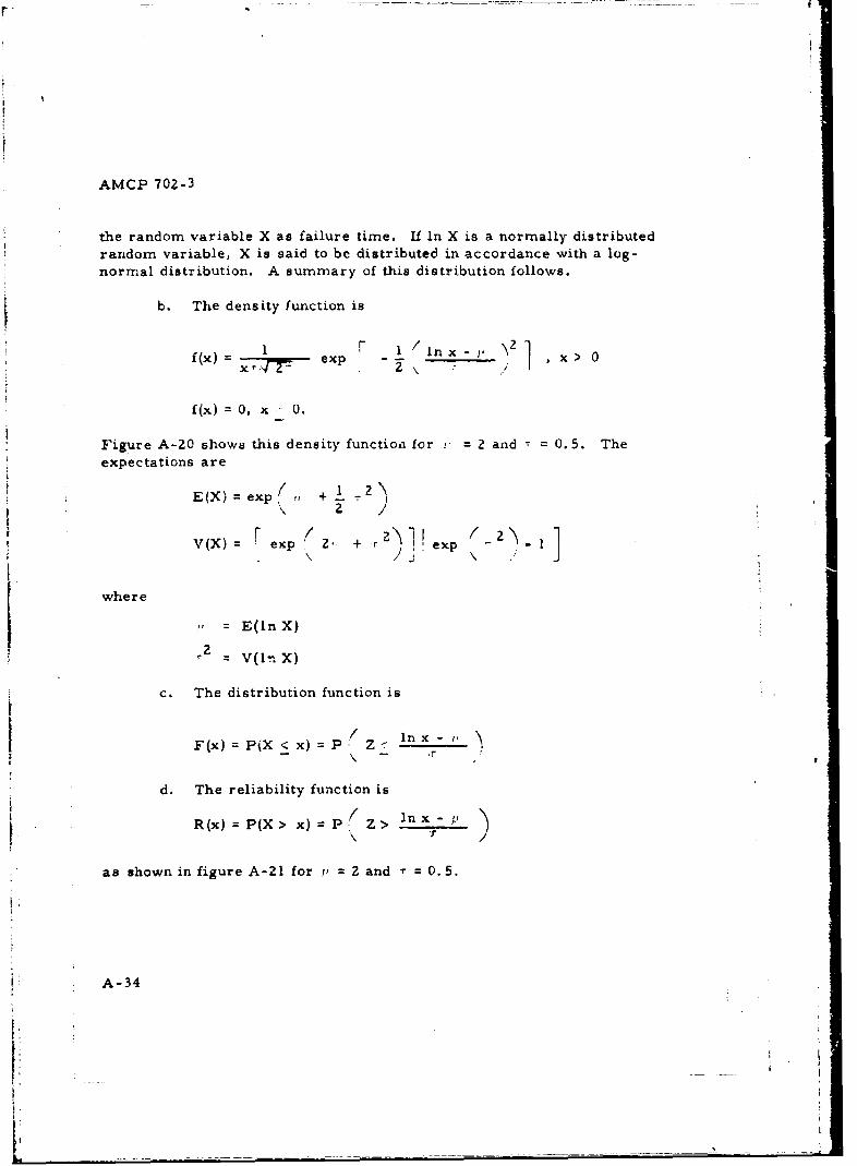
AMCP 702-3

the random variable X as failure time. If in X is a normally distributedrandom variable, X is said to be distributed in accordance with a log-normal distribution. A summary of this distribution follows.

b. The density function is

f(x) X exp -> 0

f(x) 0, x 0.

Figure A-20 shows this density functioni for 2= and = 0.5. Theexpectations are

E(X)-exp +2y

V(X) M exp 2', + " 1 exp ( -1

where

= E(In X)

= V(ln X)

c. The distribution function is

/ In - , .F(x) =P{X < x)= P Z < x

d. The reliability function is

R (x) = P (X > x) = P\ I/ Z > in x r- ;

as shown in figure A-21 for v' = 2 and i = 0.5.

A-34

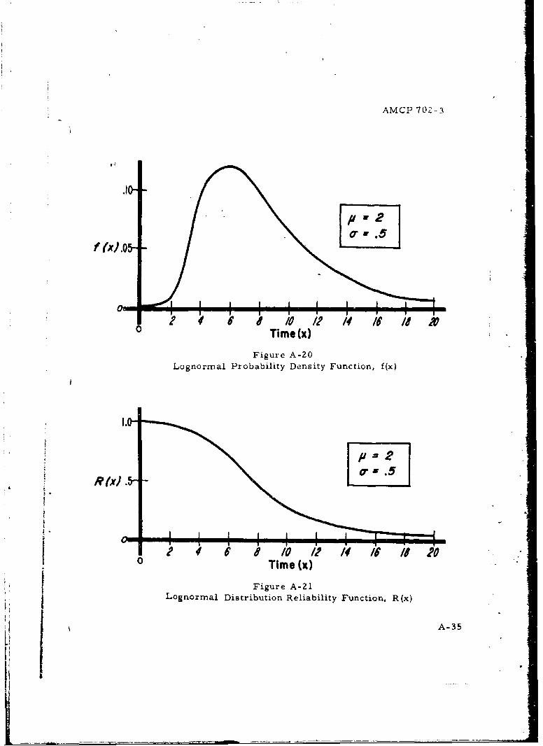
AMCP 702-3

20 2

Time W.Figure A-20

Lognormal Probability Density Function, f(x)

I. .5

2 V 6' 1 /0 /2 /€ /1 /1 200 Time W

Figure A-21Lognormal Distribution Reliability Function, R(x)

A-35

L!

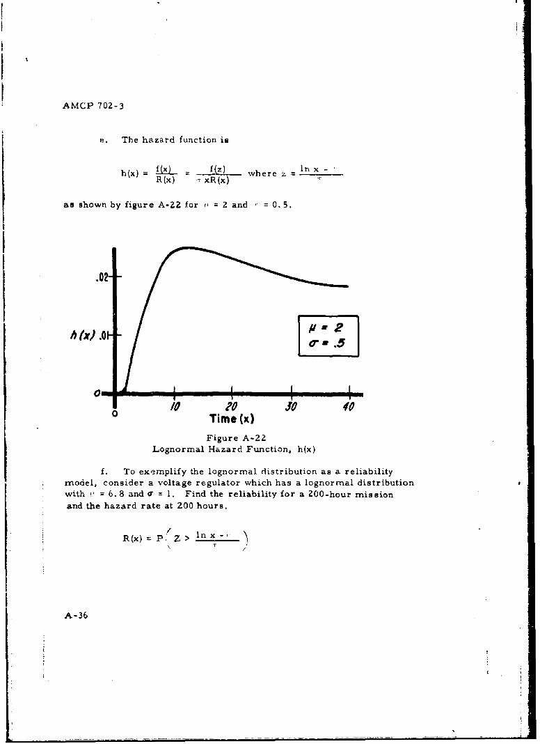
AMCP 702-3

e. The hazard function is

h(x) (x) - fz) where z I in x -R(x) TxR(x)

as shown by figure A-22 for 2 and = 0.5.0t.0

Time Wx)Figure A-22

Lognorrnal Hazard Function, h(x)

f. To exemplify the lognormal distribution as a reliabilitymodel, consider a voltage regulator which has a lognormal distributionwith !. = 6.8 and " = 1. Find the reliability for a 200-hour missionand the hazard rate at ZOO hours.

R(x) =P. Z > IA-36

A -36

AMCP 702- 3

R(200) = P." Z In > 00-6.8

= P(Z > - 1.50) = 0.93

h (x) (x__) -R(x) xR(x)

h(200) = f(200) = 0.0006475 - 0.00070 failures per hour.R(200) 0.93

g. The following example relates the lognormal reliabilitymodel to a mission length expressed in units other than time. Supposeit has been observed that gun tube tailures occur according to lognormaldistribution due to metal fatigue with parameters ; = 7.0 ando" = 2.0.Find the reliability for a 1000-round mission and the hazard rate at800 rounds.

R(x) W P Z> Ix-

/kr

R(1000) = Z > n 1000-7.0 02.0

= P(Z > -0. 045)= 0.52

h(x) f (x)R (x f 6. 68-._ _7_h(800) - -80) - 7

R 00) 2(80) z>6.68-7

= 0.3939 : 0.0004 failures per round.2(800)(o. 5636)

A-37

AMCP 702- 3

A-13. Poisson distribution, a. A brief investigation of the Poissonprocess will provide an intuitive basis for evaluating the usefulness oftne Poisson distribution as a reliability model.

b. Considei a probabilistic (stochastic) process which is subjectto the occurrence of events, all of which are of the same kind, and weare interested in the number of events that occur. Each event occurrencemray be represented as a point on a time scale. For purposes of reli-

ability analysis, an even' will be defined as a failure. Such a processhaving the following characteristics is called a Poisson process.

(I) The probability that a given number of failures is con-tained in a time interval dependc only on the length oi the interval,(and not on where the interval is located or on the past history of the sys-

tem).

(2) Ii P(h) is the probability of 2 or more failures in an

interval of length h, then

lim P(h) O.h--a0 h

Essentially, thie imolies that failures do not occur simultaneously.

(3) Ii P 1 (h) is the probability of 1 failure in an intervalof length h, then

lira Pl(h)h--o0 h

Essentially, this implies that failure rate does not depend on item age;i. e. failure rate is constant.

c. If these properties are satisfied, the Poisson probabilitydensity function may be used as a model for the number of failures in

a time interval of length, x. If the random variable K is the rumberof failures in a time interval of length x, the Poisson density function

A-38S-

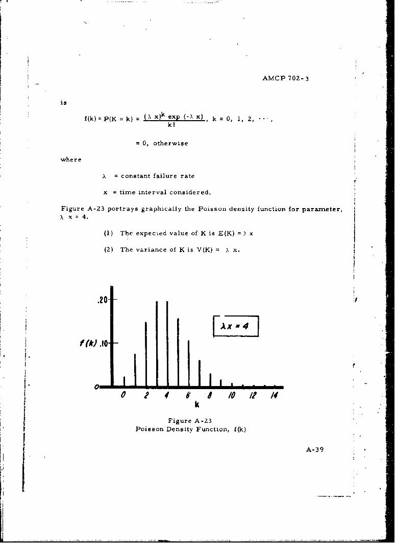
AMCP 702- 3

is

f(k):P(K k) (Xx)k exp ( x), k 0, 1, 2,",kI

= 0, otherwise

where

= constant failure rate

x = time interval considered.

Figure A-23 portrays graphically the Poisson density function for parameter,,k x 4.

(1) The expected value of K is E(K) = >. x

(2) The variance of K is V(K) = x.

.20

f(k .10

0 2 6 1 l/0 /1 /Mk

Figure A-23

Poisson Density Function, f(k)

A-39

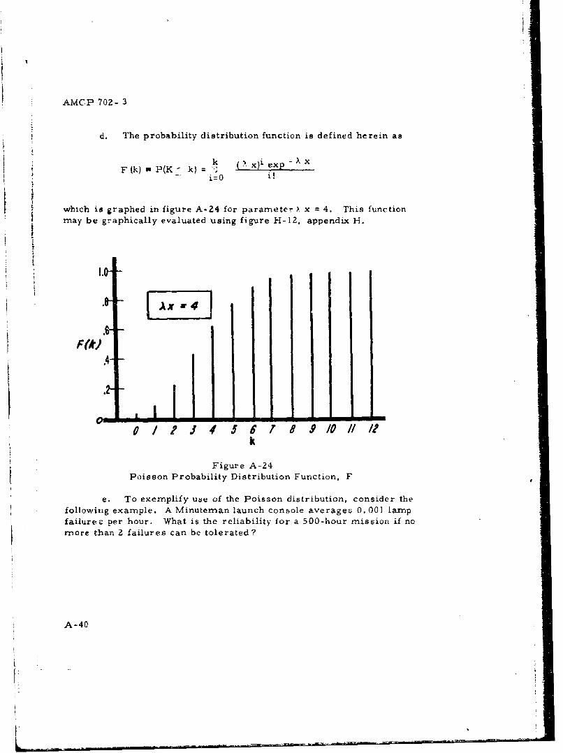
AMCP 702- 3

d. The probability distribution function is defined herein as

k e), jex- xF(k) P(K k) =-- i=0 i

which is graphed in figure A-24 for parameter X x = 4. This functionmay be graphically evaluated uIsing figure H-12, appendix H.

i 1.4

• E- Ax =r4

.60F(k)

Poisson PoaiiyDsrbto ucin

0 /

e. To exemplify use of the Poisson distribution, consider thefollowing example. A Minuteman launch console averages 0.001 lampfailurezs per hour. What is the reliability for a 500-hour mission if nomore than 2 failures can be tolerated?

A-40

AMCP 702-3

k Z failures

x = 500 hours

= 0. 001 failures per hour

Sx ;0.50

Z (0.50O'i exp "0.5 0F(k = 2) = P(K 2) = ( 0 0.986

i=O i!

f. A second Poisson example considers failure of a mechanicalitem. During the first year of operation, a 1/4-ton truck experiencesfailures in the drive train due to defects and workmanship. Failuresoccur in accordance with a Poisson process with a mean time betweenfailures of 400 hours. What is the reliability of such a truck if no failuresare allowed for a mission of 40 hours?

x =40

k= 0

X = 1/400 = 0. 0025 failures per hour

P(K=k) = (X x)k exp(- x)k!

F(k--0) = P(K=0) = [ (0. 0025)(40)1] exp (-0. 0025)(40)10!

- exp (-0. 10) 0.90

g. The following example illustrates a use for the Poissondistribution when x is not a time interval. The number of rocdet-bombhits within a specified small portion of a comparatively large areaunder prolonged bombardment has been observed to follow a Poissondistribution. The rocket-bombs average 0. 02 target misses per bomb.What is the reliability of a 50-shot bombardment if no more than 2misses are allowed?

A-41

- --

AMCP 702-3

k = 2 failures

x = 50 rounds

= 0. 02 failures per round

x = 1.00

F(k=2) = P(K-- 2) = (100)' exp -1.00 = 0.920- i!

A-14. Exponential distribution. a. The exponential distribution is apopular model for failure times. Some particular applications of thismodel include:

(1) Items whose faiiure rate does not change with age.

(2) Complex items which do not include excessive redundancyof components and/or subsystems.

(3) Items for which early failures have been eliminated,e. g., vacuum tubes which have survived a burn-in period.

b. The exponential density function may be obtained directlyfrom the Poisson density function. Consider the continuous randomvariable X as the time to failure (or time between failures). Then

f(x) = exp (- xx), x > 0

f(x) 0, x< 0

c. The resulting distribution is called an exponential distribution.It describes the random variable denoting the time to first occurrencein a Poisson process. Since the Poisson process is temporally hoino-geneous, the time between successive occurrences (failures) has the -

same distribution. Figure A-25 portrays graphically the exponentialdistribution where the x -cale is expressed in multiples of the mean timeto failure (9). The expected value and variance of X are:

E (X) ýx exp(-. .xx= 1 x

A-42

____ _____ _ __

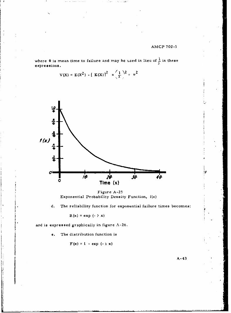
AMCP 702-3

where 6 is mean time to failure and may he used in lieu of - in these

expressions.

v(X) X2 ) . [ E(X)1 =,,7-

.e

.6 ;-

f (X)A

4t.

0 Time (x)

Figure A-Z5

Exponential Probability Density Function, f(x)

d. The reliability function for exponential failure times becomes:

R(x) = exp (-x)

and is expressed graphically in figure A-26.

e. The distribution function is

F (x) =l-exp (-,x)

A-43

Ii

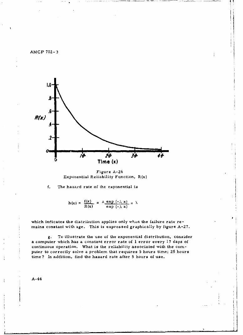
AMCP 702- 3

1.0

R(x)

Time (W

Figure A-26Exponential Reiiability Function, R(x)

f. The hazard rate of the exponential is

h (x)~ = ~ f (x exp (-x) -R (x) exp (xx)

which indicates the distribution applies only whzen the failure rate re-mains constant with age. This is expressed graphically by figure A-27.

g. To illustrate the use of the exponential distribution, considera computer which has a constant error rate of 1 error every 17 days ofcontinuous operation. What is the reliability associated with the corn-puter to correctly solve a problem that requires 5 hours time; 25 hourstime? In addition. find the hazard rate after 5 hours of use.

A-44

____________________ _____

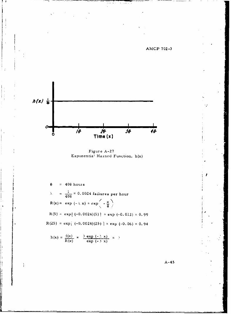
AMCP 702-3

o I I , I

Time WK)

Figure A-27Exponential Hazard Function, h(x)

0 = 408 hours

-= . = 0. 0024 failures per hour408

R(x)= exp (-x) =exp -

R(5) = exp[ (-0. 0024)(5) 1 exp (-0. 01Z) = 0.99

R(25) = exp1 (-0. 00Z4)(25) ] = exp (-0. 06) = 0.94

h(x)= f(x) = exp -7, x)R(x) exp (-x)

A-45

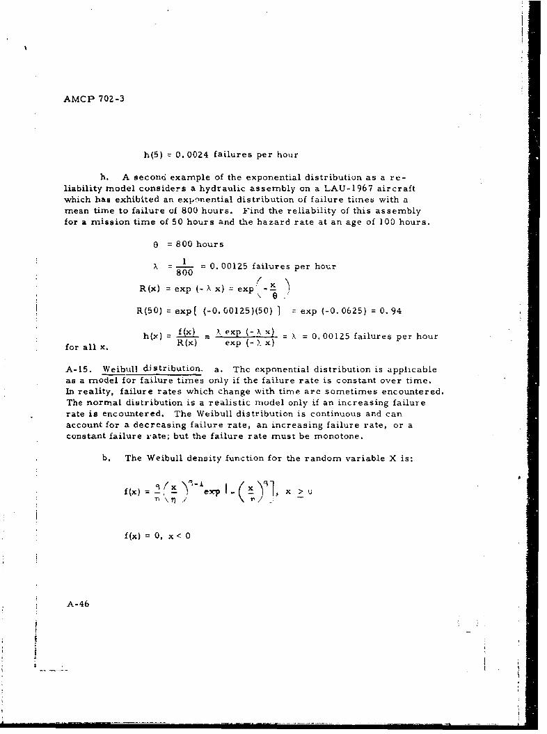
AMCP 702-3

h(5) 0.0024 failures per hour

h. A second example of the exponential distribution as a re-liability model considers a hydraulic assembly on a LAU-1967 aircraftwhich has exhibited an exponential distribution of failure times with amean time to failure of 800 hours. Find the reliability of this assemblyfor a mission time of 50 hours and the hazard rate at an age of 100 hours.

0 = 800 hours

1 - - 0. 00125 failures per hour800

(xR(x) = exp (-X x) = exp

R(50) = exp[ (-0. 00125)(50) ] exp (-0. 06Z5) = 0.94

h(x) = f(x) = X exp (- X x) - X = 0.00125 failures per hourfor all x. R x exp x)

A-15. Weibull distribution, a. The exponential distribution is applicableas a model for failure times only if the failure rate is constant over time.In reality, failure rates which change with time are sometimes encountered.The normal distribution is a realistic model only if an increasing failurerate is encountered. The Weibull distribution is continuous and canaccount for a decreasing failure rate, an increasing failure rate, or aconstant failure rate; but the failure rate must be monotone.

b. The Weibull density function for the random variable X is:

x _ ) x >-

f(x) 0, x < 0

A-46

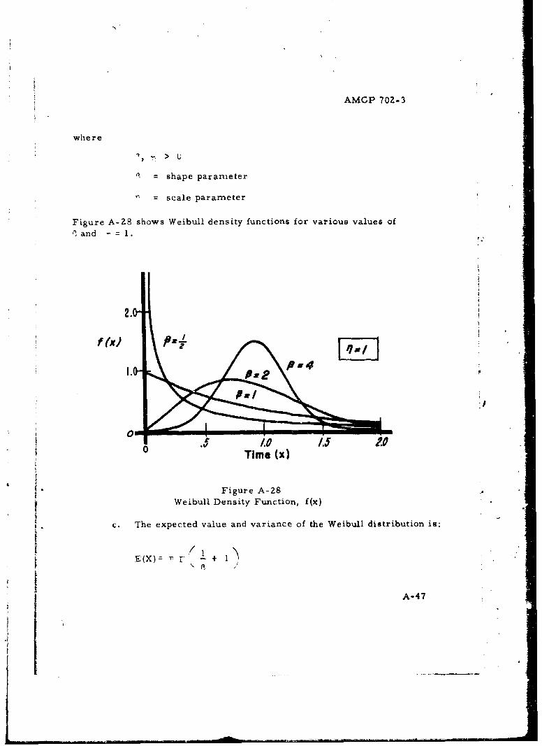
AMOP 70Z-3

where

r* >

= shape pararmeter

scale parameter

Figure A-28 shows Weibull density functions for various values of,1 and -=1.

2.P"

i 0 Time Wx

Figure A-28Weibull Density Function, f(x)

c. The expected value and variance of the Weibull distribution is:I1E (X) r -+ 1r

A-47

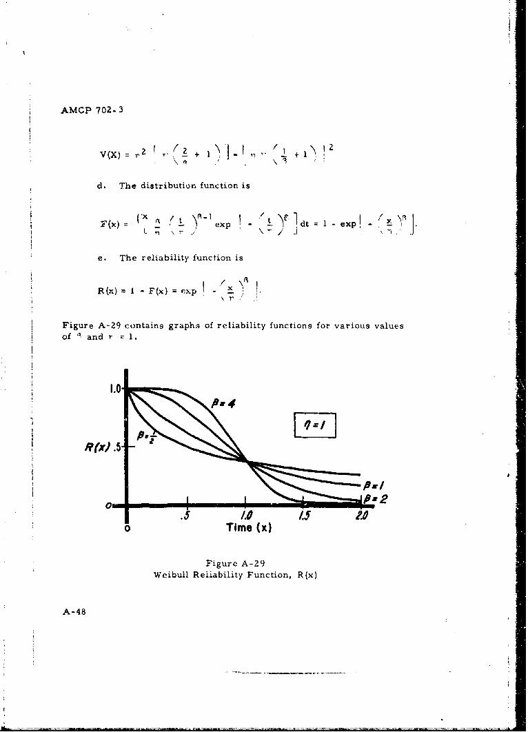
AMOP 702- 3

v(x) ,. + I,. / 1

d. The distribution function is

(X _ . -- . exp t dt- I exp. I _r j.

e. The reliability function is

(x)= I - F(x) = .xp x . .

Figure A-29 contains graphs of reliability functions for various valuesof ' and r =1.

Time Wx

Figure A-29Weibull Reliability Function, R(x)

A-48

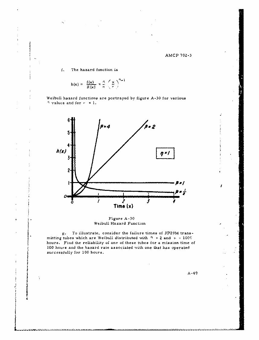
AMCP 702-3

f. The hazard function is

h() f (x) -

R (x) -r1

Weibull hazard functions are portrayed by figure A-30 for variousSvalues and for - 1.

"P*4 &2

4j

2-

/ Time Wx) "

* Figure A-30Weibull Hazard Function

iig. To illustrate, consider the failure times of JP29M trans-mitting tubes which are Weibull distributed with 1 = 2 and 7, 7 100(hours. Find the reliability of one of these tubes for a mission time of100 hours and the hazard rate associated wvith one that has operatedsuccessfully for 100 hours.

A-49

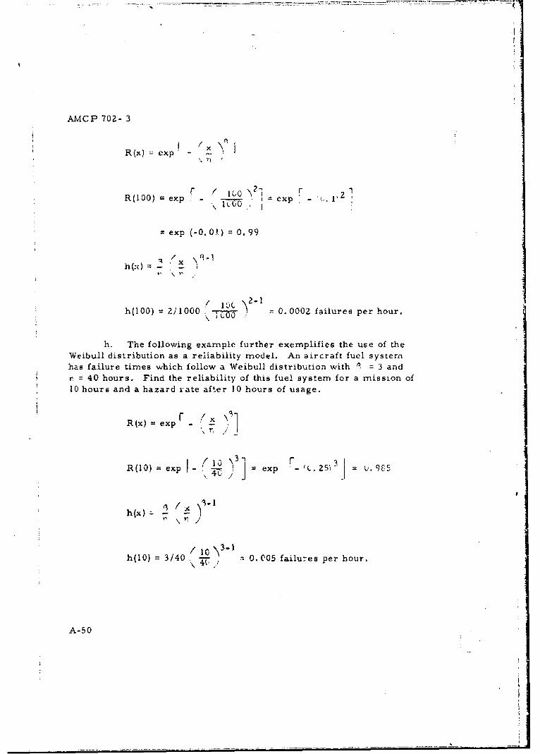
AMCP 702- 3

R(x)-exp-2,

R(100) exp ; , = exp -

= exp (-0.0.1) = 0.99

h(100) = 2/1000 .7 ic-TO2 = 0.0002 failures per hour.

h. The following example further exemplifies the use of theWeibull distribution as a reliability model. An aircraft fuel systernhas failure times which follow a Weibull distribution with R 3 andr = 40 hours. Find the reliability of this fuel system for a mission of10 hours and a hazard iate after 10 hours of usage.

R(x) exp r {_•

R(10) = exp 4/ exp = u.925

C. U.IJ.

h (x) 2 2'3 "

h(10) = 3/40 0. 05 failures per hour.\ 4(A 05

A-50

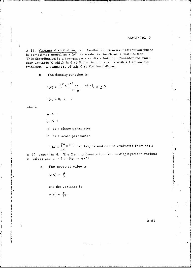
AMCP 702- 3

A-16. Gamma distribution, a. Another continuous distribution which

is sometimes useful as a failure model is the Gamma distribution.

This distribution is a two-parameter distribution. Consider the ran-

doin variable X which is distributed in accordance with a Gamma dis-

tribution. A summary of this distribution follows.

b. The density function is

.a cf-IAx exp -X)f (X) - X e p ' - x, _> 0

f(x) 0, x 0

where

a >

3. > t

a is • shape parameter

) is a scale parameter

(. x a-I exp (-x) dx and can be evaluated from table

H-10, appendix H. The Gamma density function is displayed for various

a values and A = 1 in figure A-31.

c. The expected value is

and the variance is

A-51

AMCP 702- 3

1.0

cx) jj 2

0 Time (x)Figure A-31

The Gamma Density Function, f(x)

d. The distribution function is

F(x) = P(X ': x) X t exp(-Xt) 0 dt

Special tables, Table of Incomplete Gamma Function,are required to evaluate F(x). However, if a is an integer,

C xp, (-xx)F (x) = " '- _ ex

k=a k

which may be evaluated from a Poisson table.

e. The reliability function is

Rtx) W - F(x).

A-52

_ _ _ _ _ _

AMCP 702- 3

If a is an integer

a- 1 x)k

k=O k!

The Garnmna reliability function is displayed for various values of aand ,; = 1 in figure A-32.

R (X) N

' 4 5 f 7 ,0 Time (x)

Figure A-32

The Gamma Reliability Function

f. The hazard function is

h f(x )R(x)

is displayed for various a values and k = I in figure A-33. IP

g. In addition to its potential use as a failure distribution, the

Gamma distribution serves as a model for the time to the a th failure

if the underlying failure distribution is exponential. For this purpose,the random variable X is the time to the ath failure and a can assumeonly positive integer values.

A-53

[*

AMCP 702-3

2.

h(x) 1.0 -/,,

/ 2) 166 I 7Time (W)

Figure A-33The Gamma Hazard Function

h. The following example illustrates the use of the Gammadistribution as a reliability model. A Nark missile system has demon-strated a failure distribution which fits a gamma distribution with a = 3and X = 0. 05. Determine the reliability for a 24 hour mission timeand the hazard rate at time 24 hours.

CO ( x k ex2 (- . x)R(x) I - F(x) = 1 'S (XX).

R(Z4) = I - (l.Z)k exp (-1.2)

k=3 ki

T- (.301) (1. 2 )k = 0.88k-3 kI

from Poisson curves, figure H-12, appendix H.

A-54

_ _ I-, - - ------- =1

x'J

AMCP 702-3

f(x)t ~~h(x) -fxi~ R(x)

f(x) - x eExp (-xx)

r (

f(d) = '0."Q5)1 124MZ exp (-1.20) _ (0.000125) (576) (0.301) -0.011r-(3) 2 jh(24) R () _ 0.8 0. 01Z failures per hour.h4)=R(-'24) 0.88

Section IV. STRESS-STRENGTH ANALYSIS

A-17. Introduction. a. In previous reliability discussions, reli-ability has been defined as a function of mission length. Failureof certain materiel items such as one-shot items, mechanical items,

etc. is not necessarily dependent upon time of usage. In some cases,failures may be more directly traceable to some other stress variable.Then reliability of an item may be determined by comparing its strengthto the stress to which it will be subjected. Reliability may be definedas the probability that strength exceeds stress.

b. Neither item strength nor the stress to which it is sub-

jected are constant values, but both are random variables each withits own probability density function. If these distributions are known,reliability may be determined analytically. Since data is generallylimited to sample information, the goodness-of fit methods of appendixF may be used in an attempt to identify the appropriate underlyingdistributions.

A-18. Normal stress and strength distribigtions, a. Assuming boththe stress and strength distributions to be normal, reliability can bedetermined as follows:

I

Iii

II

_____ _ ___

AMCP 702-3

(I) Item strength (S) is a random variable with normalprobability density function

1 I 1 S-L' ,r S . - 2 TS I J

where

U S = mean strength

SS = strength standard deviation

(2). Stress (s) is a random variable with normal probabilitydensity function

-(s) 1 expl s -T 27 2 T -SS S

where

= mean stress level

stress standard deviation

(3) Then the difference D = S-s is a random variablewith normal probability density function

e Dj (D I/ LD \r D 2- .- DrD

A-56

AMCP 702-3

where

" D "S ;- = mean difference

•r + standard deviation of differenceD = S s

(4) Then reliability may be defined as

f 0-: D D -:R P(D > 0) PD Z > P Z >

" -D rD

which may be determined from table H-Z, appendix H.

b. To exemplify, the material strength (ultimate shear stress)of a lug shear is a normally distributed random variable with a mean

of 104, 300 psi and a standard deviation of 3, 600 psi. The stress towhich the lug is subjected is a normally distributed random variable

with a mean of 95, 160 psi and a standard deviation of 2, 070 psi. What

is the reliability of the lug in such an environment?

' 95, 160 psi S= 104, 300 psi

r s = 2,070 psi 3,600 psi

S'D =S "s =9,40 psi

AS ÷ = 4,153 psi

9140 2.207 D T4153

iR teP(Z > - 2.ZO) 1 - P(Z > 2. 20) = 0.986 as foundSin table H- 2.

A

Im

A-57

[I

I

AMCP 702- 3

A-19. General stress-strength distributions, a. Determinationof reliability based on stress-strei-,th analysis requires that boththe stress and strength probability density functions (f(s) and f(S)respectively] be known. As shown above, analytic determination isquite straightforward if both distributions are normal. Althoughanalytic determination is difficult for other distributions, reliabilitycan be determined from

R f(S)dS 1 ds0

which lends itself to numerical methods easily adapted for use bydigital computers.

h. Graphical determination. The following technique, usingtransformations, provides a graphical reliability determination whichmay be applied to any distribution. It may also be applied to sampledata when the underlying distribution cannot be identified. The follow..ing elements are involved.

(1) Let 0 f (S)dS

s

(2) Let H = C. i( f(s)ds which implies

0

dH = f(s)ds

(3) Then R = ' G d H which may be evaluated by plotting

C as a function of H and finding the area between the function and G = 0and between H = 0 and H = I. Figure A-34 indicates this graphicallyfor a hypothetical function.

c. Example - Known mathematical distribution. (1) Theabove procedure may be applied to density functions either in mathe-rnatical or empirical form. The example which immediately follows

A-58

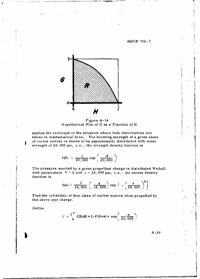
AMCP 702- 3

A

Figure A-34 }Hypothetical Plot of G as a Function of H

applies the technique to the situation where both distributions areknown in mathematical form. The bursting strength of a given class

of rocket motors is known to be exponentially distributed with meanstrength of 20, 000 psi, i. e. , the strength density function is

e -S

2fS 0,000 \ 0,000

)I

The pressure exerted by a given propellant charge is distributed Weibullwith parameters 11 = 2 and n=18, 000 psi, i. e. , the stress densityfunction is

S' ~ ~fl s 2 1/00 ' x(S) 18, 000 \'1'00 x 18,000 I

SFind the reliability of this class of rocket motors when propelled by._the above type charge.

Define

C Coo f(S)dS = -FlS=s)= exp,/ -s 20Z, 0oo00"

A-59I

'1777

0- -m

Hi

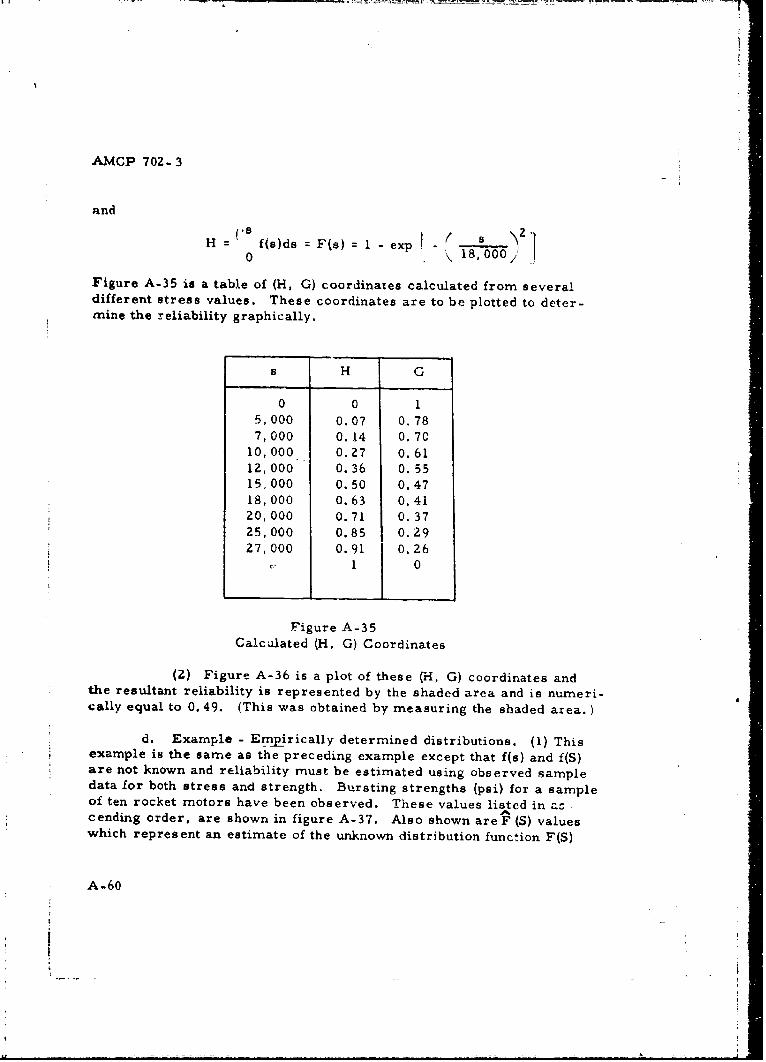
AMCP 702- 3

and

H . f(s)ds F(s)=l - exp0 .C

Figure A-35 is a table of (H, G) coordinates calculated from severaldifferent stress values. These coordinates are to be plotted to deter-mine the reliability graphically.

s H G

0 0 15,000 0.07 0.787,000 0. 14 0. 7C

10,000 0.27 0.6112, 000 0.36 0. 5515,000 0.50 0.47

18,000 0.63 0.4120,000 0. 71 0. 3725,000 0.85 0.2927,000 0.91 0.26

S1 0

Figure A-35Calculated (H, G) Coordinates

(Z) Figure A-36 is a plot of these (H, G) coordinates andthe resultant reliability is represented by the shaded area and is numeri-cally equal to 0. 49. (This was obtained by measuring the shaded area.)

d. Example - ETrnirically determined distributions. (1) Thisexample is the same as the preceding example except that f(s) and f(S)are not known and reliability must be estimated using observed sampledata for both stress and strength. Bursting strengths (psi) for a sampleof ten rocket motors have been observed. These values listed in accending order, are shown in figure A-37. Also shown are F (S) valueswhich represent an estimate of the unknown distribution function F(S)

A-60

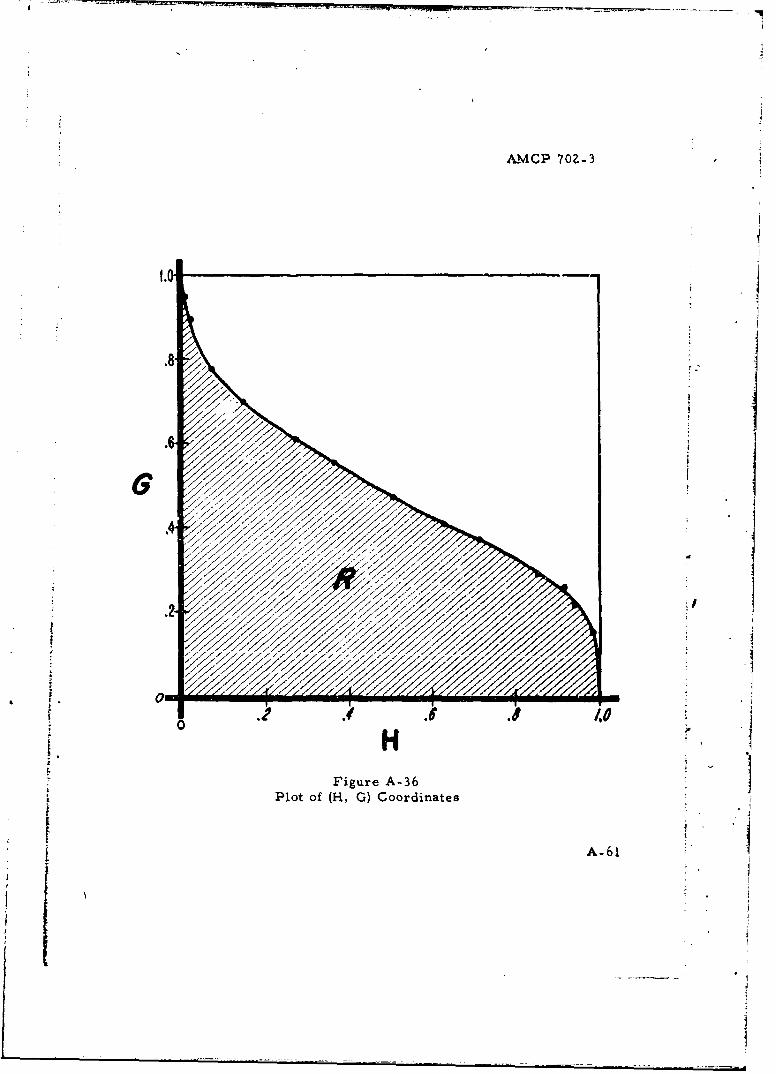
AMCP 70Z-3

XWI

Figure A-36*Plot of (H, C) Coordinates

A- 61I

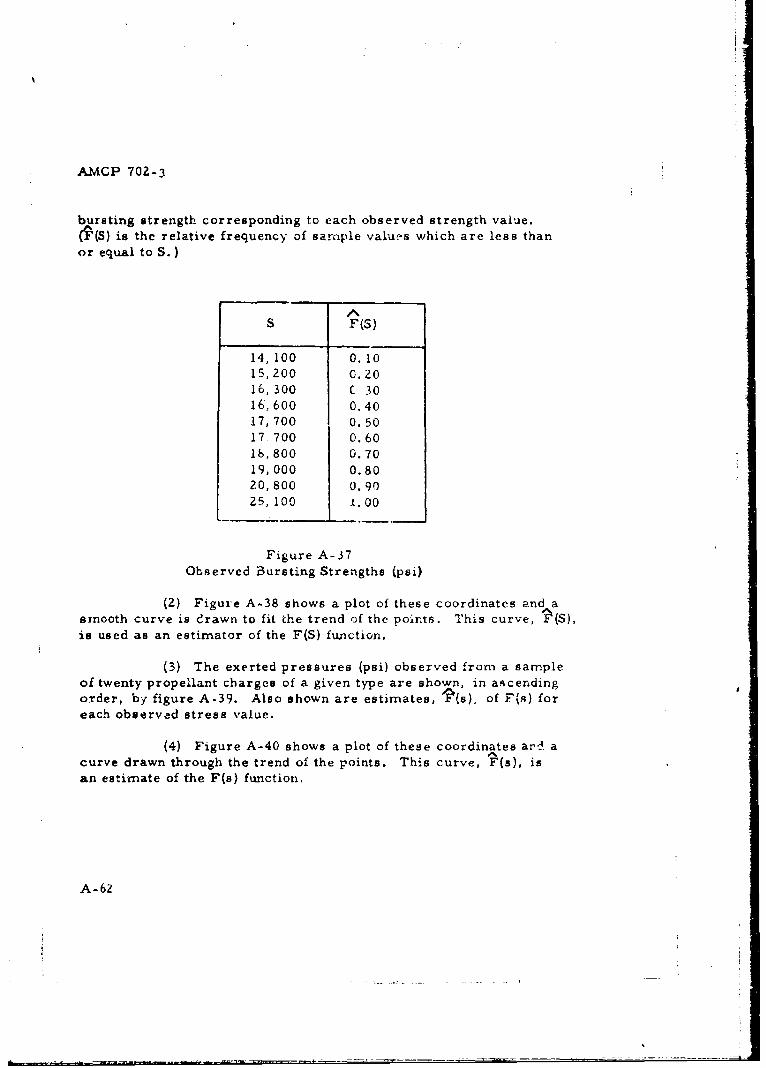
AMCP 702-3

bursting strength corresponding to each observed strength value.(T-(S) is the relative frequency of sample values which are less thanor equal to S.)

S F(S)

14, 100 0. 1015,200 0.2016, 300 C 3016,600 0.4017,700 0.5017. 700 0.6016,800 0.7019,000 0.80

20,800 0.9025, 100 1.00

Figure A-37Observed Bursting Strengths (psi)

(2) Figure A-38 shows a plot of these coordinates and asmooth curve is erawn to fit the trend of the points. This curve,is used as an estimator of the F(S) function.

(3) The exerted pressures (psi) observed from a sampleof twenty propellant charges of a given type are shown, in ascendingorder, by figure A-39. Also shown are estimates, I(s), of F(s) foreach observed stress value.

(4) Figure A-40 shows a plot of these coordinates are. acurve drawn through the trend of the points. This curve, F(s), isan estimate of the F(s) function.

A-62

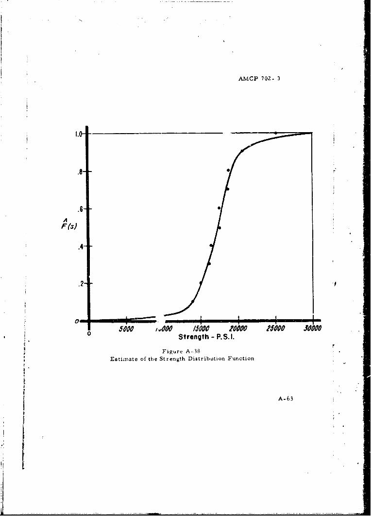
AMCP 702- 3

.8

.6AF s)

.4-

.2-

o5000 000 5000 20000 25000 30000Strength - P.S.I.

Figure A-38

Estimate of the Strength Distribution Function

A-63

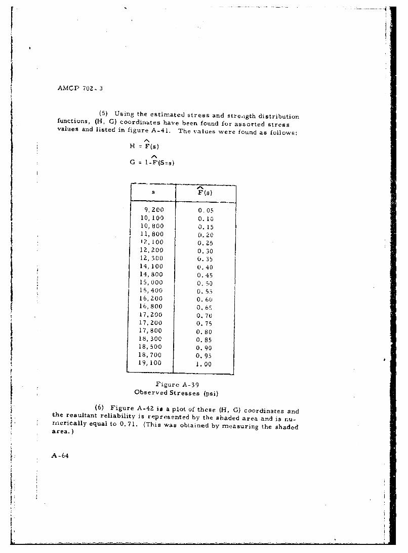
AMCP 702- 3

(5) Using the estimated stress and streagth distributionfunctions, (H, G) coordinates have been found for assorted stressvalues and listed in figure A-41. The values were found as follows:

H z F(s)

G = I-F(S=s)

77 F(s)9,200 0,05

10, 100 0. 1010,800 0. 1511,800 0.20j ?, 100 0. 2512, 200 0. 301g, 300 0. 3514, 100 0.4014,800 0.4515,000 0. 5015,400 0. 5516,200 0. 6016,800 0. 6517,200 0. 7017,200 0. 7517,800 0.80

18, 300 0. 8518, 500 0. 9018,700 0. 9519, 100 1.00

Figure A-39

Observed Stresses (psi)

(6) Figure A-4Z is a plot of these (H, G) coordinates andthe resultant reliability is represented by the shaded area and is nu-rnerically equal to 0.71. (This was obtained by measuring the shadedarea.)

A -64

F

V _ _ _ _ _ _

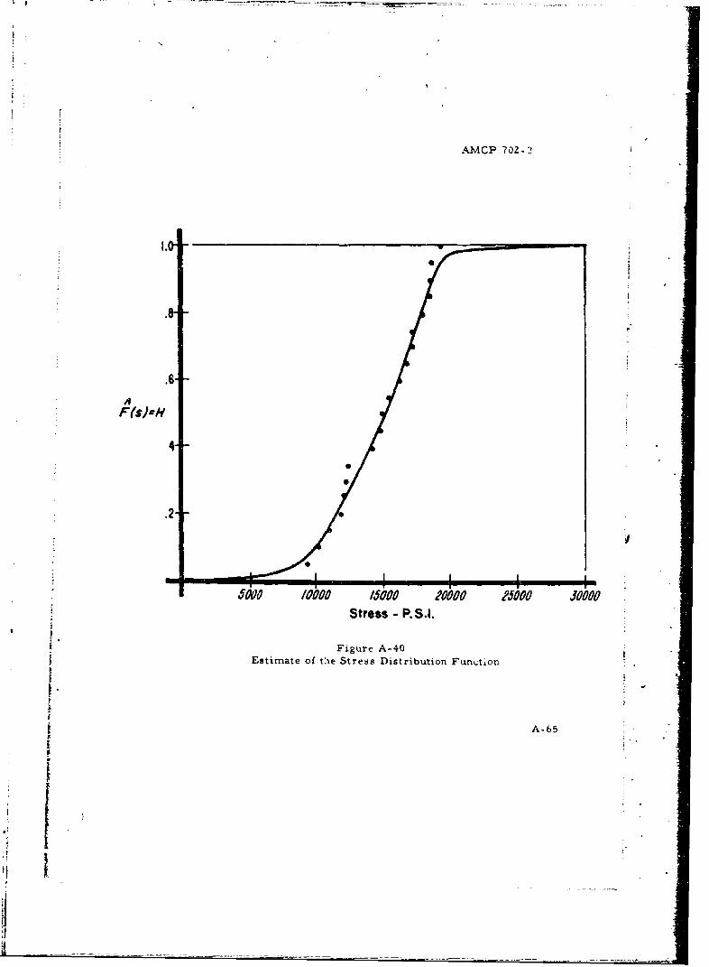
AMCP 702-3

1.00

Stress P.SI.

--6F'{sJ'HY

S5000 /0000 /5000 20000 25000 30000!,• Stress - P.S.I.

S. Figure A-40

Estimate of the Stress Distribution Function

. 0

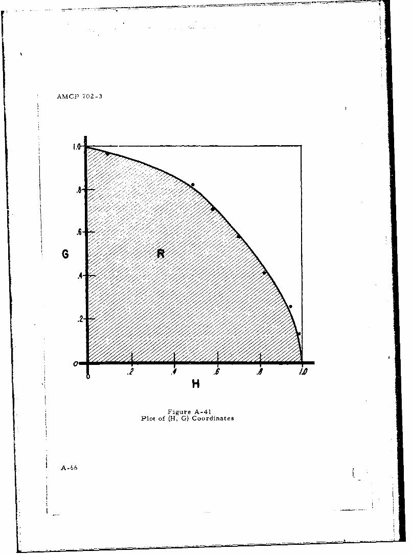
AMCPD 702-3

!X

:

H

Figure A-41

Plot of (H, G) Coordinates

A-66

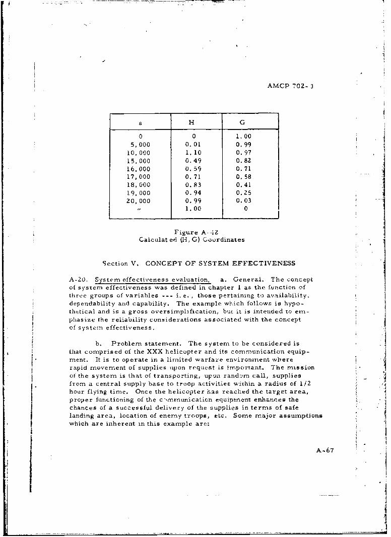
AMCP 702- 3

s H G

0 0 1.005,000 0.01 0.99

10, 000 1.10 0.97

15, 000 0.49 0.8216,000 0. 59 0. 7117,000 0.71 0. 5818,000 0.83 0.4119, 000 0.94 0. 2520, 000 0. 99 0. 03

1.00 0

Figure A-4ZCalculated (H, G) Coordinates

Section V. CONCEPT OF SYSTEM EFFECTIVENESS

A-20. System effectiveness evaluation, a. General. The conceptof system effectiveness was defined in chapter I as the function ofthree groups of variables --- i. e. , those pertaining to availability,dependability and capability. The example which follows is hypo-thetical and is a gross oversimplification, but it is intended to em--phasize the reliability considerations associated with the conceptof system effectiveness.

b. Problem statement. The system to be considered isthat comprised of the XXX helicopter and its communication equip-ment. It is to operate in a limited warfare environmYent whererapid movement of supplies upon request is important. The missionof the system is that of transporting, upOn random call, suppliesfrom a central supply base to troop activities within a radius of 1/2hour flying time. Once the helicopter has reached the target area,proper functioning of the c-,mmunication equipmnent enhances thechances of a successful delivery of the supplies in terms of safelanding area, location of enemy troops, etc. Some rnajor assumptionswhich are inherent in this example are:

A-67

AMCP 702-3

(1) A call for supplies is directed to a single helicopterwhich is located at the base. If this craft is not in flyable condition

(i. e, , it is in process of maintenance) the mission will not be started.A flyable craft is defined as one which is in condition to take off andfly with a standard supply load.

(2) The flight time required to reach the target area isl/IZ hour.

(3) The communication equipment cannot be maintainedor repaired in flight.

(4) A loaded helicopter which goes down while on routeto or does not reach the target area has no delivery value, i. e., assumethat supplies lost in route cannot be effectively recovered by groundtroops.

c. Model determination. (1) For purposes of model formula-tion, the system condition is divided into 3 states, namely:

(a) State I - Helicopter flyable, communication

equipment operable.

(b) State 2 Heiicopter flyable, communication

equipment non-operable.

(c) State 3 - Helicopter non-flyable.

(2) The effectiveness model is defined as

E 7 ADC

where A, D and C are defined as follows:

(a) The availability vector is a three element row* vector, i.e.

A (a,, a 2 , a 3 )

A-68

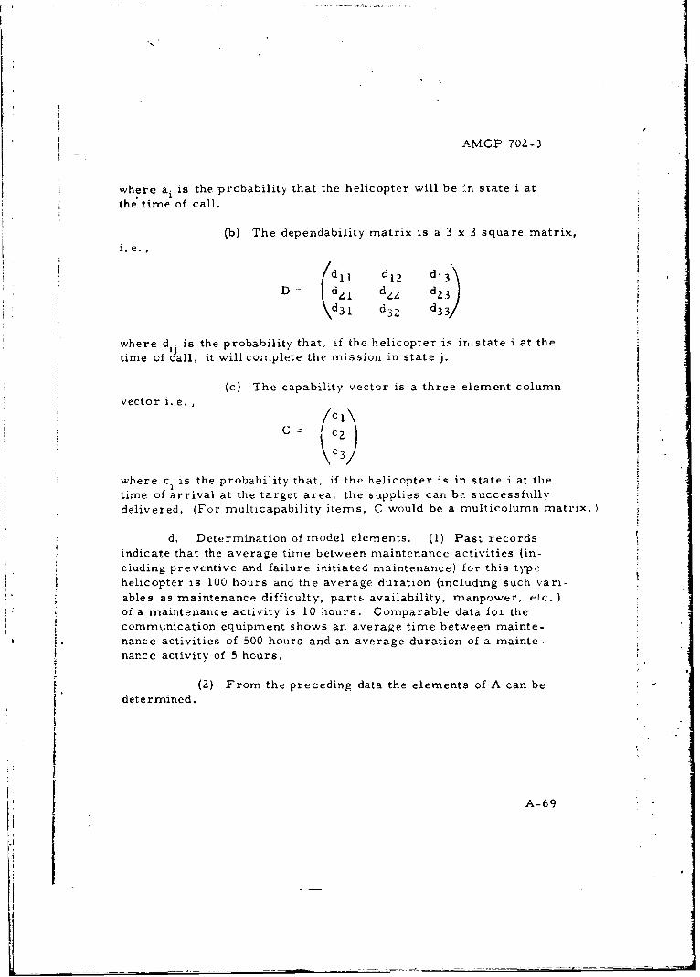
I

AMCP 702-3

where ai is the probability that the helicopter will be :*n state i at

the tirne of call.

(b) The dependability matrix is a 3 x 3 square matrix,

i.e.,

/d 1 _ d1 2 d,,D d d d2 3K 1 2

d 3 1 d 3 z d 3 3

where d.. is the probability that, if the helicopter is in state i at thetime of call, it willcomplete the mission in state j.

(c) The capability vector is a three element columnvector i. e.,

Sc 1

• / c3

where ci is the probability that, if the helicopter is in state i at the1

time of arrival at the target area, the supplies can b. successfullydelivered. (For multicapability items, C would be a multicolumn matrix.

d, Determination of model elements. (1) Past recordsindicate that the average time between maintenance activities (in-cluding preventive and failure initiated maintenance) for this typehelicopter is 100 hours and the average duration (including such vari-

ables as maintenance difficulty, part& availability, manpower, etc.)of a maintenance activity is 10 hours. Comparable data for thecommunication equipment shows an average time between mainte-nance activities of 500 hours and an average duration of a mainte-nance activity of 5 hours.

(2) From the preceding data the elements of A can bedetermined.

A-69

L _ _ _ _ _ _ _ _ _ _ _ _ _ _ - - _ _ _ _ _ _ _ _ - _ _ -

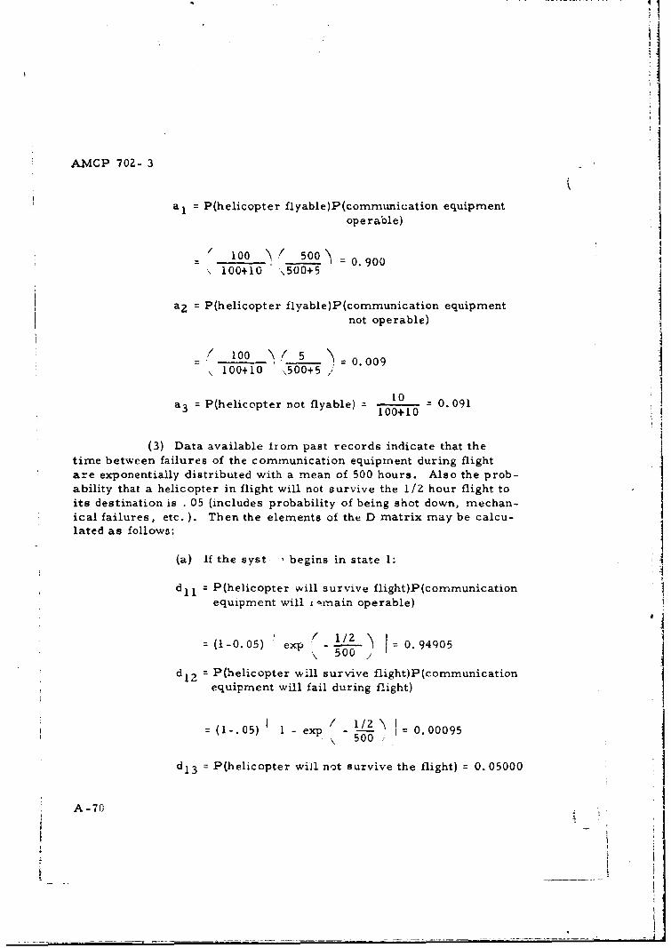
AMCP 702- 3

a= P(helicopter flyable)P(commnmication equipment

operable)

/ 100 " soo\ 0. 9001 l00+10 \500+5

a2 P(helicopter flyable) P (communication equipmenti not operable)

/ 100 / 5 0091 100+10 \500+5 .i

10

a 3 P(helicopter not flyable) = 0.0913 100+10

(3) Data available from past records indicate that the

time between failures of the communication equipment during flightare exponentially distributed with a mean of 500 hours. Also the prob-ability that a helicopter in flight will not survive the 1/2 hour flight toits destination is . 05 (includes probability of being shot down, mechan-ical failures, etc.). Then the elements of the D matrix may be calcu-lated as follows:

(a) If the syst , begins in state 1:

dIl P(helicopter will survive flight)P(communication

equipment will i -main operable)

= (I-0.05) e xp 0_ -. 94905\500

d 1 2 P(helicopter wIll survive flight)P(communicationequipment will fail during flight)

1' 1/2 N=(1-.05) 1 - exp 0- I = 0.00095

d13 P(helicopter will not survive the flight) 0. 05000

A-70 _, '

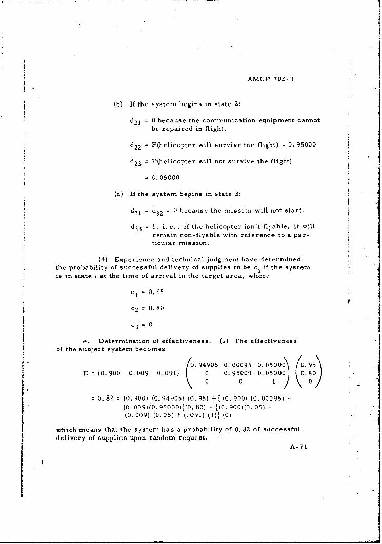
|I{I

AMCP 702-3

(b) If the system begins in state 2:

d 2 1 = 0 because the commrinication equipment cannotbe repaired in flight.

d 2 2 = P(helicopter will survive the flight) 0. 95000

d 2 3 = P(helicopter will not survive the flight)

0= . 05000

(c) If the system begins in state 3:

3 d3 2 d 0 because the mission will not start.

d33 1, i. e. , if the helicopter isn't flyable, it will

remain non-flyable with reference to a par-ticular mission.

(4) Experience and technical judgment have determinedthe probability of successful delivery of supplies to be ci if the systemis in state i at the time of arrival in the target area, where

c = 0. 95

? = 0. 80

C3 =0

e. Determination of effectiveness. (1) The effectiveness

of the subject system becomes

0.94050.00095 0. 05000 0. 95E = (0. 900 0.009 0.091) 0 0. 95000 0. 0500 0 0.80

0 1 )= 0. 82 = (0. 900) (0. 94905) (0. 95) + [(0. 900) (0. 00095) +

(0. 009)(0. 95000)](0. 80) + [(0. 900)(0. 05) +

(0.009) (0.05) + (.091) (1)1 (0)

which means that the system has a probability of 0. 82 of successfuldelivery of supplies upon random request.

A-71

AMCP 702-3

(2) The effectiveness value attained provides a basis

for deciding whether improvement is needed. The model provides

the basis for evaluating the effectiveness of alternative systems con-sidered.

f. The preceding example was not intended to emphasizethe technical approach to system effectiveness evaluation, but topoint out that reliability is a factor of effectiveness and may be con-

sidered at more than one point in system life. For example, relia-bility of the system (and subsystems) must be considered for the en-virontnent encountered while awaiting mission call (such as storage,

temporary use, etc. ) i.e. , for determining the availability elements.Reliability also comes into the picture during the mission, i. e. in

determining the dependability elements. In addition, reliability mustbe considered relative to each of the system states.

Section VI. RELIABILITY DESCRIPTORS

A-21. Some meaningful parameters. Any of several different descrip-

tors nmay be used for measuring or specifying the reliability of a pro-duct. A useful descriptor must be meaningful in terms of the defini-tion of reliability. Commonly used reliability descriptors include :he

probability of success in x hours mission time, mean time betweenfailures (MTBF), hazard function, and probability of success where

time isn't of primary importance. Each of these is dependent upona specified intended function and use environment.

a. Probability of success for x hours mnission time. (I) This

descriptor is actually the basic definition of reliability and is meaning-

ful whether or not the underlying failure distribution is known. It is

composed of a probability statement as well as the mission durationtime to which the probability applies. It represents a .ingle point on

the reliability function curve as defined earlier in this appendix.

(2) This descriptor nmay be related to other reliability

indices if the underlying failure distribution is known.

o. Mean time between failures. (1) MTBF is a very popu-

lar measure of reliability. However, care must be exercised in its

A-72

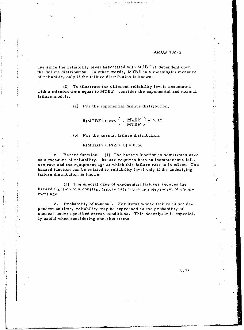
AMCP 702-3

use since the reliability level associated with MTBF is dependent uponthe failure distribution. In other words, MTBF is a meaningful measureof reliability only if the failure distribution is known.

(2) To illustrate the different reliability levels associatedwith a mission time equal to MTBF, consider the exponential and normalfailure models.

(a) For the exponential failure distribution,

R(MTBF) exp / MTBF=______ €' 0. 37

\ MTBF -

(b) For the normal failure distribution,

R(MTrBF) = P(Z > 0) = 0. 50

c. Hazard function. (1) The hazard function is sometimes usedas a measure of reliability. Its use requires both an instantaneous fail-ure rate and the equipment age at which this failure rate is in eff2ct, Thehazard function can be related to reliability level only if the underlyingfailure distribution is known.

(2) The special case of exponential failures reduces thehazard function to a constant failure rate which is independent of equip-ment age.

d. Probability of success. For items whose failure is not de-pendent on time, reliability may be expressed as the probability ofsuccess under specified stress conditions. This descriptor is especial-

2 • ly useful when considering one.shot items.

tA -I

i A-73

t,

__ _ ____ _ __]

AMGP 702-3

APPENDIX B

RELIABILITY PROGRAM REQUIREMENTS

PLANNING AND IMANAGEMENT GUIDE

Section 1. INTRODUCTIONt

B-1. General. Thiis appendix is designed to supplement chapter 2.It provides guidance information for planning and management of areliability program. This guidance takes two forms: first, adiscussion of some fundamentals of network diagramming and second,a general network to use as an example when developing a plan forreliabil.ty nmnagernent of a specific project.

Section IL. FUNDAMENTALS OF INETWORK DIAGRAMMING

11-2. General. Several forms of this technique exist, the details vrsomewhat, although tile underlying principles are- the same. Thetechnique is assigned to assist program managers in planning and con-trolling a variety of interrelated projects. None of the ta-chniques arediscus sed a detail herein. It is the purpose of this apperidix to showthe sequence of events and identify the interfaces, relationships, andconstraints of a reliability program by incans of an activity diagram.The reader mnust remnember that netN~orks such as th~is are nut devices

for measuring the reliability of a product.

B3-3. Definitions of terms used in network dliagrimming.

a. Network.

(1) A network is a flo~v' diagram cwiýsioýtiiig of the activities

and events which must be accomplished to reach the project objec~tives(total life cycle) showmni, the planned si-quezices of accom~plislument,.nterdependencies ana .aterrelationshipi. It is used as a tool in the

project management ýecisioni making process, for platnning, activ'ities tobe performed, as wall as progress repurting cand corrective action.The network includes all action involved dand is not liivnite~d to workactivities. Time consuminig actions, buch. as lead time for procurQ-rnent of purchased parts, shipmentnt of materiel fromi oile loc;'rion toanother, and management alction, are shown on the network.

B-

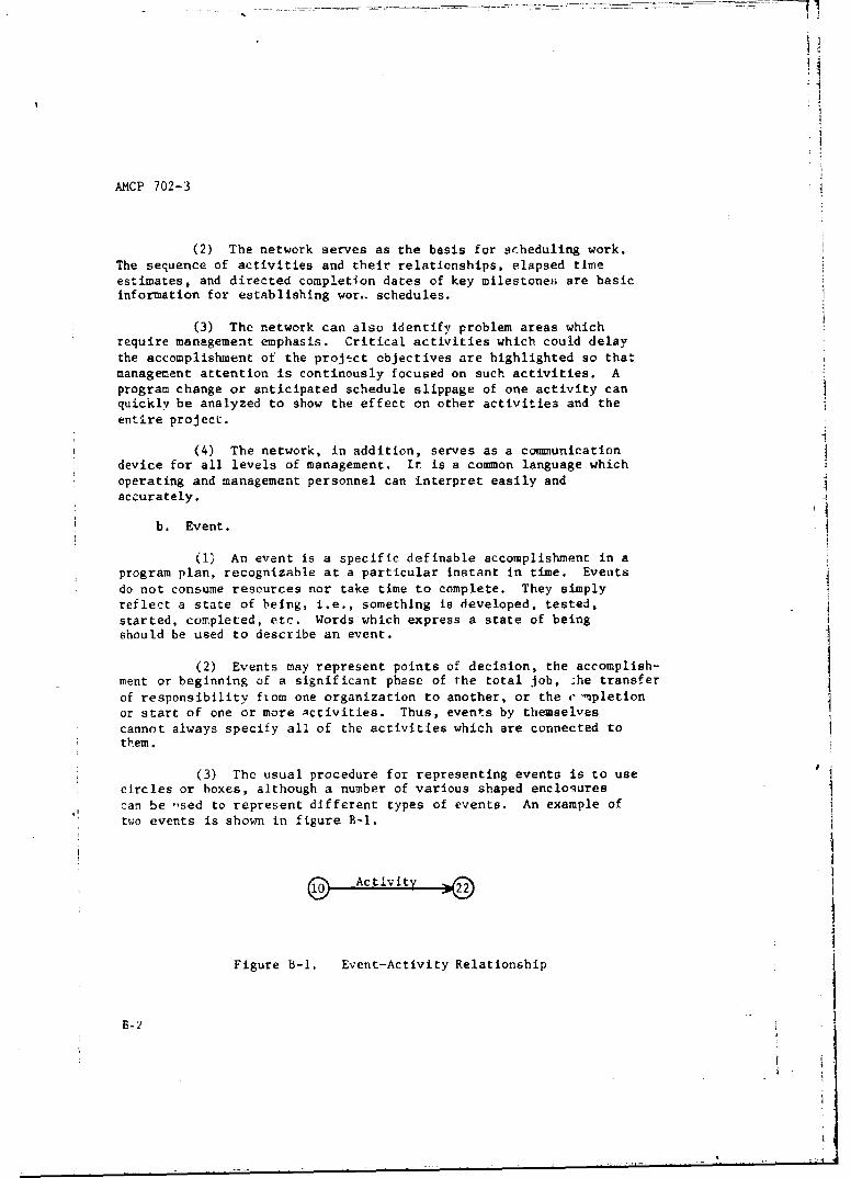
AMCP 702-3

(2) The network serves as the basis for scheduling work.The sequence of activities and their relationships, elapsed timeestimates, and directed completion dates of key milestones are basicinformation for establishing wor.. schedules.

(3) The network can also identify problem areas whichrequire management emphasis. Critical activities which could delaythe accomplishment of the project objectives are highlighted so thatmanagement attention is continously focused on such activities. Aprogram change or anticipated schedule slippage of one activity canquickly be analyzed to show the effect on other activities and theentire project.

(4) The network, in addition, serves as a communicationdevice for all levels of management. It is a common language whichoperating and management personnel can interpret easily andaccurately. 4

b. Event.

(1) An event is a specific definable accomplishment in aprogram plan, recognizable at a particular instant in time. Eventsdo not consume resources nor take time to complete. They simplyreflect a state of being, i.e., something is developed, tested,started, completed, etc. Words which express a state of beingshould be used to describe an event.

(2) Events may represent points of decision, the accomplish-ment or beginning of a significant phase of the total job, -he transferof responsibility fiom one organization to another, or the r mpletionor start of one or more Activities. Thus, events by themselvescannot always specify all of the activities which are connected tothem.

(3) The usual procedure for representing events is to usecircles or boxes, although a number of various shaped enclosurescan be .sed to represent different types of events. An example of

,IItwo events is shown in figure B-A.

Figure B-1. Event-Activity Relationship

B-2

AMCP 702- 3

i4) Events numbered 10 and 22 are related and unless event 10is completed, the activity between them cannot be started. Furthermore,it will be impossible to reach the point in time represented by event 22until the activity represented by the arrow is completed.

c. Activity.

(1) An activity is the work effort of a program. It is that which

must be done, characterized by people using facilities, materials, andequipment over some period of time to accomplish a stated objective.Activities imply doing such things as researching, building, negotiating,testing, etc. Activities are the flow of a network, and it is this flow ofhuman effort, materials, use of facilities, investment, and expensethat can be controlled by the manager.

(2) In order to avoid confusion in the milestone list, and gen-erally to improve the clarity of presentation, considerable attentionshould be given to the names of events and activities. Since an activityimplies doing or acting, it should be expressed as a verb form (develop,test) which will not be confused with the beginning or completion pointof the activity. Each description of an event or an activity should beconcise so that personnel with different backgrounds and points of viewwill interpret it in the same manner.

(3) An activity is represented on a network by an a.-row withthe head of the arrow pointing in the direction of the time ilow asshown in figure B-1. The activity connecting the two events cannotbegin until event number 10 is completed nor can event number 22 takeplace unless the activity is completed. When several activities leadto an event, all activities must be completed before the event comesinto existencc- For instance, the network activities numbered 7-10,q-10, and 6-10 in figure B-2 must all be completed before event

number 10 can occur.

B-3

Ix

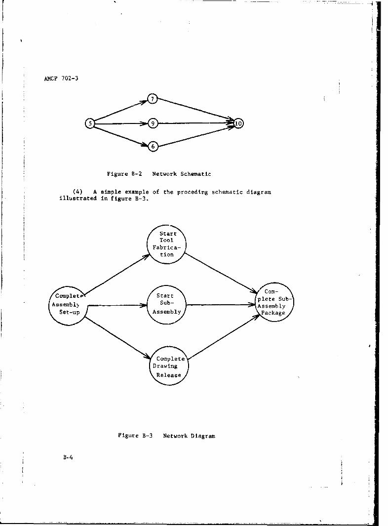
AMCP 702-3

i7

!9

Figure B-2 Network Schematic

(4) A simple example of the proceding schematic diagramillustrated in figure B-3.

SToolbFabrica-l

Figure B-3 Network Diagram

B-io

Copt Sta-4om

Sub-plet Sub

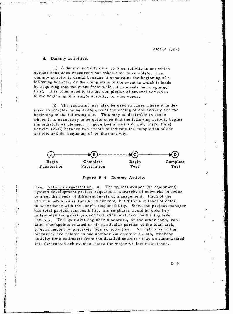
AMCP 702-3

d. Dummy activities.

(1) A dummy activity or z ro time activity is one whichneither consurnes resources nor takes time to complete. The

dummy activity is useful because it c-nstrains the beginning of afollowing activity, or the completion of the event to which it leadsby requiring that the event from which it proceeds be completedfirst. It is often used to tie the completion of several activitiesto the beginning of a single activity, or vice versa.

(2) The restraint may also be used in cases where it is de-sired to indicate by separate events the ending of one activity and thebeginning of the following one. This may be desirable in caseswhere it is necessary to be quite sure that the following activity beginsimmediately as planned. Figure B-4 shows a dummy (zero time)activity (B-C) between two events to indicate the completion of oneactivity and the beginning of another activity.

--- --- ---00-Begin Complete Begin Complete

Fabrication Fabrication Test Test

Figure B-4 Dummy Activity

B-4. Network organization. a. The typical weapon (or equipment)system development project requires a hierarchy of networks in orderto meet the needs of different leels of management. Each of thevarious networks is similar in concept, but differs in level of detailin accordance with the user's responsibility. Since the project managerhas total project responsibility, his emphasis would be upon key

milestones and gross project activities portrayed on the top levelnetwork. The operating engineer's network, on the other hand, con-tains checkpoints related to his particular portion of the total task,interconnected by precisely defined activities. AM|. networks in thehierarchy are related to one another via comme- e. ants, wherebyactivity time estimates from the de-tailed networt - wvay ue summarized

into forecasted achievement dates for major project milestones.

i; B-5

U -

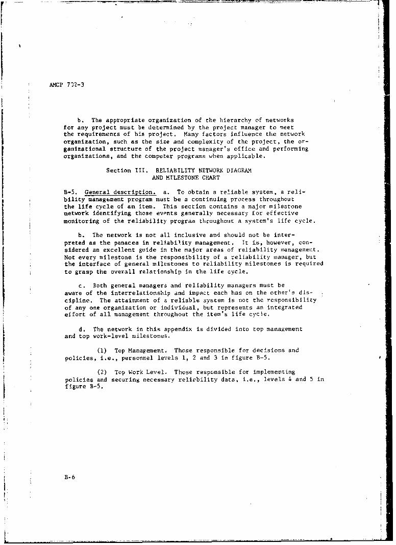
AMCP 702-3

b. The appropriate organization of the hierarchy of networksfor any project must be determined by the project manager to meetthe requirements of his project. Many factors influence the networkorganization, such as the size and complexity of the project, the or-ganizational structure of the project manager's office and performingorganizations, and the computer programs when applicable.

Section III. RELIABILITY NETWORK DIAGRAMAND MILESTONE CH1ART

B-5. General description, a. To obtain a reliable system, a reli-bility management program must be a continuing process throughoutthe life cycle of an item. This section contains a major milestonenetwork identifying those events generally necessary for effectivemonitoring of the reliability progran throughout a system's life cycle.

b. The network is not all inclusive and should not be inter-preted as the panacea in reliability management. It is, however, con-sidered an excellent guide in the major areas of reliability management.Not every milestone is the responsibility of a reliability manager, butthe interface of general milestones to reliability milestones is required

to grasp the overall relationship in the life cycle.

c. Both general managers and reliability managers must beaware of the interrelationship and impact each has on the other's dis-cipline. The attainment of a reliable system is not the responsibilityof any one organization or individual, but represents an integratedeffort of all management throughout the item's life cycle.

d. The network in this appendix is divided into top managementand top work-level milestones.

(1) Top Management. Those responsible for decisions andpolicies, i.e., personnel levels 1, 2 and 3 in figure B-5.

(2) Top Work Level. Those responsible for implementingpolicies and securing necessary reliebility data. i.e., levels 4 and 5 infigure B-5.

B-6

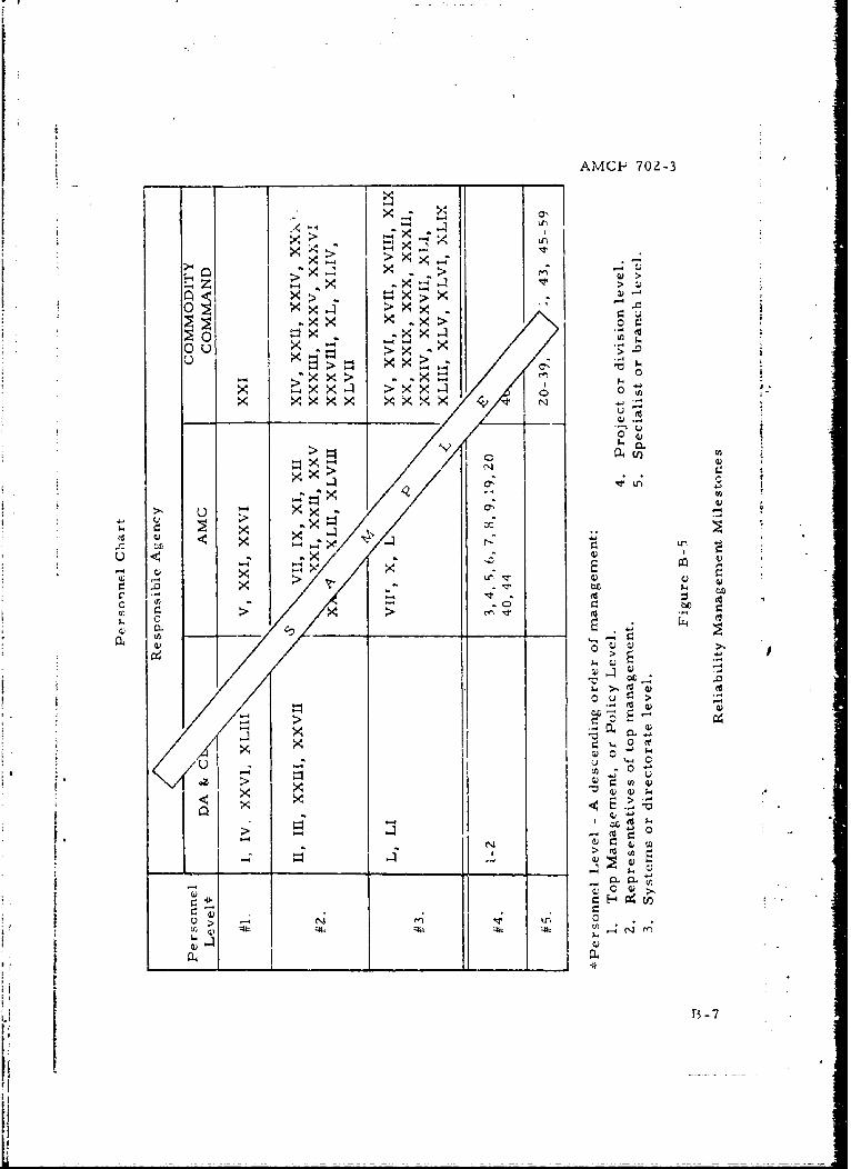
AMCP 702-3

.4~ý-4

>)

x xxx > ~~ >__ _ __ _ 4) .

x LO N

>' 0 'u xX

X x x2 > cc

->4

>1

C) to

x > 9t

o~ u z :

> N (

Ctv

0> ~ 4' Lf

0.. C_ _

B-7

J

AMCP 702-3

e. A sample personnel chart (figure B-5) is included togenerally relate the milestones to a particular command and actionlevel. The acceptance and assignment of responsibilities shouldfilter from the top level downward.

f. The milestone definitions included are event oriented.The explanation is a brief description of activities leading into or

from the event. This, it is possible for each manager to expand theevents within his functional area of responsibilicy to cover alL aspectsof reliability. Top management milestones are identified by Romannumerals; top work-level milestones by Arabic numerals, with AMC

interface milestones from AMCR 11-27 qhown parenthetically follow-ing the milestone title.

g. The milestone chart is divided into the concept and defini-tion phases (figure B-6), the development phase (figure B-7), and theproduction, operation and disposal phases (figure B-8).

B-6. Definitions of management milestones for reliability.

a. Concept Phase (see figure B-6).

I. Guidance Documents Initiated. The Army planning documentsBASE, ASP, AFDP, et al, which s. guidelines, objectives, and pri-ority operational requirements, are initiated. These documents fore-cast the needs and techiaological advances, thereby formii.g the frame-work for the Army's total mission responsibility. They also ititiatethe materiel life cycle and provide guidance during the concept, dffini-tion, and development phases. The above documents are r.vitedand updated annually.

II. User Requirements Established. Studies, which culminate in newor improved doctrine, organizational concepts, operational capabilityobjectives, logistical concepts, QMDO's, and QMR's, are coupleted.These studies establish user requirements for new items and materielto satisfy future tactical concepts. A desirable, but realistic, reli-

ability goal is established as a result of these studies. Activitiesare planned and conducted within the framework provided by the guidancedocuments.

B-S

- ----

AMC1P 702-3

I11. Technological ForecastingCmpleted. AU basic research

projects, such as parametric analysis, applied research, techno-logical forecast, systemn synthesis, technical es'rimates, etc. , arecompleted. These analytical studies provide data and a theoreticalbasis for predicting the expected sci.-ntific and t(echnical gains to beachieved by the anticipated production date. By determining whatand where furdamental knowledge is lacking, development effortsare precludeci from less productive areas until additional researchwork is accomplished. The predictions, capabilities, objectives,concepts. and estimates resulting from these projects provide in- .'

formation for QMDO requirements, such as the proposed reliabilitygoal.

IV. QMDO Approved and Assigned W100). A Qualitative MaterielDe-velopment Objective (QMDO) is an Army-approved statement ofrmilitary need for thu developmxent of new materiel, the feasibility or

specific definition of which cannot be determined sufficiently to per-mnit Ihe establishment of a Qualitative Materiel Requirement (QMR).Appr,.),.al of the QMDO provides the first formal requirements docu-ment that the Army uses in the research and development cycle.'rhis document should contain a proposed reliability goal for the itemunder consideration. The QMDO is assigned by AMC to one of thesubordinate commands or laboratories on a sole, prime, or attendantbasis. The designated development atency will prepare and coordinate,with other developing agencies that have competence and responsibili-ties in the area concerned, a brief but specific plan that outlines all

the research and developniTrt work that is required to prove out thefeasibility of the QMDO. The plan summarizes existing researchprojects and tasks, states arn estinate of the additional projects andtasks required to achieve the technological capability, and gives anestimate of the research risks involved in each approach. Cost

estimates are also ircluded.

1. Total Feasibility Study Completed (0600. The total feasibilityrstudy, which includes consideration of technical feasibility, cost

* effectiveness, system effectiveness, availability of all funds through-out th. life cycle, qualitative and quantitative pe.rsonn,,l inipl icat ions.

operational and organizational concepts, logistical support implica-tions, and impact upon inven!tory, is cornplet(d. This study states

determinations that the Depar!tnnre of Army is capable of supportingthe desired new item of materiel ihrougliout i's life cycle. Completed

when AMC technical data to support the item or system is submitted toDepartment of Army.

>1!

AMCP 702-3

2. QMA Established. The Qualitative Materiel Approach (QMA),based on review of research feasibility and standard equipment capa-bility for the expected state of the art, is established. The QMAdescribes recommended technical approach(es) or solution(s) to amateriel requirement. it will include trade-offs in approaches, timeto develop, size and weight. crst ef operation (manpower and funds),technological risks, cstimarea development and procurement costs,and comparison with existing Items, if applicable.

V. TDP Initiated. The prel.iminary Technical Development Plan (TDP)is used for pcogramming purposes In order to obtain program approvalon a timely basis. Information included in the preliminary plan should

include initial concepts, schedules, and funding estimates. In addition,the plan Is pynected to o-itline those plans for development and provideguidance, goals, and specific direction necessary to assure that opera-tional effectiveness will be achieved. The inclusion of statementsdelineating performance, reliability, and maintainability are aimed atthis goal. This document is to be prepared by the responsible Armydeveloping agency.

VI. QMR Initiated. The initial draft proposed Qualitative MaterielRequirement (QMR) document is initiated. Contents of the QMR arebased upon national defense objective, intelligence estimates, andconcept or feasibility studies which determine the requirements for anew capability and the need for a new item. The Q[a expresses De-partment of Army requirements for new equipment or for major in-novations or improvements related to research anj deielopment as

developed from new concepts. During preparation of the QM, theCDC will coordinate with AMC to assure that proposed requirementsreflect current state of the art and best integration of competitivecharacteristics. This milestone taks place when iNC begins prepara-tion of the technical data to complete the QbM or SDR.

VII. Reliability Documentation Initiated. Documentation of the reli-ability requirements to be placed in the QMR and TDP is initiated.

3._ QMR ReliabilityRequirements Established. Documentation ofthe basic reliability requirements to be placed on the item is completed.This is a clear and concise set of statements which includes the objector mission, the quantitative reliabiltiy require:>ents--essential anddesired--and the definition of what constitutes a failure.

B-10

AMCP 702-3

VIII. Draft Proposed QMIR Subh.itted (0400). The draft proposedQMR, consisting of inforrna!ion rejuired in milestones V[[, V\l[I and 3,is reviewed and subilLtt-d to CDC.

4. I-DtB Reliablity Requirements Established. A summation ofreliability requirements covering systein and subsystem characteris-tics, pe rformance requirements, and the reliability review pointschedule arc established for the prelinminary TDP document.

IX. FDI' Rcliability Documnentation (ompleted. !ntegration of relia-bility requirements (i-'ilestone 4) and -,ther information pertinent tothe preliminary IDP iniilestone \V[) is completed.

X. Prelitninary TDP Approved. The preliminary D*DP cuntainingreliability documentation is reviewed and approved.

b. Definition Phase tsee figure 13-6).

NI. RFP _Initiatted. 'ihe Request for Propnsal (RFP. F |) docu-entationis initiated by the consumer complete with the systerm mission andrequests for contractor schedules and methods for devwlopnment. Theinformation to be included nmust consist of both technical and managerialaspects of the proposed engineering developnment, it sh,)uld be informa-tion that wil be mneaninjful to 'he poitential contractors in preparingtheir respective proposals.

D. Prediction Requirement Established. The requirerment forcontrzctor prediction of itein reliabilitv is establishe-d and diocurm entedin the R.I"P. This requirenient should include conside'ration of quanti-tativc ptir'dlict ins and a schedule fV r updating predictions.

f,. Appo lionrvnt ,equirenent Es'ablished. The rcquiremrient

for contractor apporiionment of item reliability is established and docu--cnttcd inlto he h i-P. The ri'quironiownt shall be clcarly state-d so as toassure achhievernoen of item reliability. Any previous e xperinces withthese syst ms shall be re-fere 'JiOed in tIie 1VI( ').

I-I

ii

A.R(V 1 i2-3

7. Record Keeping Requirement Established. The requirementfor contractor record keeping of item reliability data is establishedand documented in the RFP. This requirement should call for aneffective record keeping system which specifies the type of informa-tion to be recorded, such as reliability tesL -•ilts, technical prob-lems, and progress reports on item reliabilit",. t should also requirea schedule for status reporting.

8. Testing Requirement Established. The requirement for thecontractor to adequately demonstrate achievcmcnt of item reliabilityis established and documented in the RFP. This will include anydefinite tests required, methods of testing, conditions for testing,test schedule, use of test results, and other test requirements when-ever applicable.

9. Trade-off Policy Requirement Established. The requirementfor conLractor Pstablishment of a trade-off policy, covering the inter-relationships of cost, support,performance, and safety as related toreliability, is documented into the RFP.

XII. RDP Approved. The RDP is reviewed for compliance withoriginal reliability requirements. After compliance has be-n verificdand approved, the RDP is used as a communication link between theArmy and prospective contractors.

XIII. Contract Definition Contracts Awarded. The findings and recom-mendations resulting from evaluation of the initial proposals have beenprovided by the appropriate agency to Department of Army for contractaward to potential development contractors.

XIV. Proposals Received and Review Initiated. As the contractor'sproposals are received, they are thoroughly reviewed for compliancewith reliability requirements as requested in the RDP.

XV. Organization Review Completed. Reviews of the prospectivecontractors' managerial acticities, including organization structures,training programs, and personnel technical capabilities. Results ofthis review should indicate whether or not the prospective contractorgives proper emphasis to reliability.

B-12

AMC!'! 702-3

XVI. Tpstin2 Progrm TRevlew Competed. The testCng programs

proposed by the interested contractors to demonstrate reliability arereviewed. These reviews encompass test environments, equipment,data feedback programs, analysis techniques, and use of test resultsto answer that the RFP requirements are included and understood.

XVII. Detailed Reliabilitv Review Initiated. After all the proposalshave been submitted, a comprehensive review of reliability provisionsis initiated. The results of this review should plan an important rolein deciding upon the prospective development contractor. The purpose

of this review is to evaluate proposals for apportionment, prediciton,and trade-off policy with respect to feasibility, completeness, andclarity.

10. Block Diagram Review Completed. The reliability blockdiagram for the overall system is reviewed to assure all aspects of

the system have been given proper consideration. This includes suchthings as determining if the diagram is sufficiently descriptive of theproposed system from both an cperational and technical viewpoint.

This diagram is the basis for a reliability apportionment model.

11. Standard Subsystems Review Completed. Proposed sub-systems utilizing standardized parts and assemblies are evaluated

for acceptability of reliability apportionment. Also, it should beassured by this review that standard subsystems have been employedwhen applicable in order to minimize cost.

12. Developmental Subsystem Review Completed. Proposedsubsystems requiring development of new items are reviewed with

regard to reliability apportionment. This rcvicw covers the non-standard subsystems that are to be employed in the various proposals.The proposals should provide adequate empirical data to determine

that the required reliability of these new subsystems can be achieved.Also, math models should be provided in the proposals to illustratehow the reliabilities apportioned to the subsystems are to be achieved.

13. Reliability__esign Techniques Evaluation Completed. Thedevelopmental subsystems are reviewed for reliability design tech-niques. This includes the proper use of partial redudancy, mixedmodels, standby redundancy, etc. The review should concentrate on

B-13

AMCP' 702-3

both the possible use ,f such techniques s w en they are appllcalhe

but not considered in the proposals. anm the use of such lteliti(tat,

in situatio0ns where their use is not warranted because ot altreadyacceptable reliability, nonfeasibiltu , txcessi.'e costs, ctc.

XVIII. Reliability Apportionnment Evaluation Coinpie ted. Lvaloat iol

of the reliability apportionnient section of the proposal is ýonipleted.This apportionment represents a possible mnans of achievin-i th'"

required system reliability. It should be ascertained whether or notthe apportionment has been done optimally; i.e., to imiininiize costwhile maintaining overall systemn rcliability.

14. History Check Evaluation Cofrpleted. The cont racý,tr's useof failure data concerning stadard subsystems utilzetd -n thli pro-posals is checked for accuracy, applicability, and coxnpl. tteness.This evaluation should verify that the data used to supp'rt 'he us"

of any such subsystem was obtained from conditions similar to thosewhich the subsystem will be subjected to in the ne-w systcn;. Thisevaluation establishes the validity of the data for reliability prediction

purposes.

15. State of the Art Review Completed. Projections for the stateof the art throughout development and production are reviewed and

compared to the projection from the total feasibility study conductedearlier in the CDP. The purpose of such a review is tI assure that

the progress for development of such equipment is consistent with theanticipated schedule established earlier in the CDP. Any differencesshould be notcd in order that potential probiems can be identified. !tis important that such problems be pointed out in this review becausethey may cause delay in project completion or even prove the projectinfeasible for completion.

16. Minimum Reliability Evaluation Cornpletd be In,-tinui,

reliability predictions are evaluated to assure that the system require-ment is met. If the system requirement is not met, the results should

point out possible courses of action to correct such deficiencies.

17. Optimum Reliability Evaluation Completed. Predictions ofdesirable reliability are evaluated to assure that the predictions are

realistic. Careful attention should be given to the coturactor's under-lying assumpti".ns for meeting the reliability values quoted. Any

B-14

'II

A.. %. I, ?C}-P 3

inalid ass5qumptlijns ur uurealistic rclaht1it, values should bek talledto his alt• ntion.

XIX. iReliability ProedictioN A(:ceptd. Evaluation of !he reliabilityprediction section of the proposals, as a suitable outcome for sysitemreliability, is completed. The results of this evaluation are to bcused in dec.iding which of th( prospective contractors will receivc thecont ract.

18. Trade-Off Policy Reliability Evaluation Completed. Anyco'ntractor proposed change in estimated development cost, timie,performancc, support, safety, human engineering, etc. , nmade atthe expense of reliability will be carefully evaluated as trade-offconside rations.

XX. "'Trade-Off Policy Accepted. After the trade-off considerationsare analyzed, the selected proposed trade-off policy is accepted.

XXI. Proroosal Scleclion Completed. 'The most probablc proposai(s)to succ,.ed in development and to meet the technical requirementsis(are) selected. Major reliability considerations, which the contrac-tor expresses in his proposal, should be given proper emphasis inproposal selec'ion,

XXII. Coordinated Test Program Approved (14001. The eoordinatedTest Program (CTP) is an all-inclusive materiel test plan whichspecifies test objectives, number of prototypes to be available, en-vironmentl testing required, testing schedule, funding requiirements,test support requirements, and whether an integrated, concurrent, orsequential testing program will be conducted. This milestone is com-pleted on acceptance of the test program by major commands, projectmanagers, or agencies involved. After acceptance, the program isincluded in the TDP. It is reviewed and updated at the technicalcharacteristics, engineering concept, and design ch'iaracteristicsin-process review.

19. QMR Updated. Based on review and evaluation of the pro-posals, the QMR may need to be revised and updated. Changesaffecting reliability will be wo ,ded so as not to lose the intent of thereliability requirement.

j B- 15i/

jkjj' 7?U2-3~

XXII. j-OR Approved (0700). The updated QýR is reviewed withproper emphasis placed on reliability. After receiving a satisfactoryreview, the OMR ;•s approved by Department of Army.

XXIV. Tec'h-nical Characteristic IPR Completed (1500). This reviewis held upon receipt of the approved QMR and prior to finalizing thetechnical characteristics. The primary purpose of the technicalcharacteri:3tics in-process review (IPR) is to insure that the developerunderstandi the requirement and has properly statcd it in terms oftechnical characteristics. The technical characteristics, once ap-proved by the proper authority, are used for full-scale development,either in-house or by contract.

20. TDP Revised. A re-evaluation and revision of the TDPincorporating inputs from the CTP, selected prot.osal(s), and thetechnical characteristic IPR, is completed. This TDP presents indetail an illustrative format and a comprehensive plan for develop-ment of a syntem. Factors considered on a continuing basis are themanagement plan, configuration management plan, test and evaluationplan, personnel and personnel training plan, logistics support plan,facilities, foreign technology, planned production, and technicaldocumentation.

XXV. Updated TDP Apnroved (0900). The updated TDP is reviewed,with proper emphasis being placed on the reliability section, andapproved. It is the prime basis for approval, disapproval, or modi-fieation of the projecc. IL tebcribes aud is the approved plan forexecution by the Army. The TDP is to be updated and changed asrequired throughout the program.

XXVI. Development Decision Made. A decision is made on whetheror not to enter the development phase. The decision sh-uld be basedon the results of effectiveness studies, as well as whether or not theproposals show that the reliability requirements can be met.

c. Development Phase (see figure B-7)

XXVII. Development Contract Awarded (2000). The primary contractis executed by the contractor and contracting officer for developmentof the item.

B- 16

- -~ ,

A (;I' 702-3

XXVIII. Reh]abhlity Specialist As__signcd to Deve!opricnt Progran.When an agency relceives developmental rcsr.onsibility tor an item,an individual(s) knowledgeable in the tcchnical aspects ,•f reliabilityis(arc assigned the rcsponsibility for monitoring for reliabilitythroughout the development program. This is to provide assuranceto the Army that reliability is being given proper emphasis in thedevelopn-ient activities.

XXIX. Predeveloprnent Conference Completed. A predevelopmentconference to clarify the contractor's responsibilities for meetingcontractual requirements, including those relating to reliability, iscomiplcted.

XXX. Start Preliminary Design Review. Review during preliminarydesign, as performed by the contractor, is to include reliability con-siderations. Such reviews will faciliiate early evaluation and identi-fication of potential design trouble areas.

21. Math Model Evaluation Completed. The math model, includ-ing th2 block diagram, is evaluated for total consideration and adequacy.This provides assurance that all functional and failure modes have beenproperly considered and that the model provides an adequate repre-sentation of the relationship between item reliability and the rcliabilitof subsystems, parts, and components.

22. Reliability Prediction Revitw Completed. Basic contractorreliability predictions, which support preliminary design, are re-viewed to assure that predictions, including any revised predictions,are suitable and are based on sound rationale. important considera-tions include standard parts, derating, functional complexity, re-dundancy, and failure definition.

23. Reliability Apportionment Review Completed. The reliabilityapportionment of the preliminary design is reviewed against the pro-posed values of the definition phase. Major deviations should be in-vestigated. Of major importance is the compatibility of apportionedgoals with the cost and schedule for fulfilling these goals.

B-17

II|

I

24. Patnt Ia. I FroblcoAIct iiiEvaton Com, ½ted. t' ii onAt tonof the corrective action program detail ýs e proposed I!, the contrna tor

to handle potential reliability problems is cormpl] eted. The progr;7,should provide for aLi on whIl is both ti m!v a;Id tecrhrn ically -dArit,.

25. I eview and Recommend-tion Complet ed. The preimInar>development design is reviewed for reliability aspects and r cevant

trade-off recommendations arc presented to decision make.

XXXI. Engineering Concept il-Process REview Completed (1700O

The contractor's preliminary design is reviewed and decisions -'ereached on all recommendations. These activities may become a

part of the engineering concept review (ECR). Rigid attention to reli-ability in this IPR assures that the design concept is not beyond the

state of the art and that all feasible engineering approaches have beenconsidered.

XXXII. Initate Engineering Desij-, Review. Reliabilitv analysis of

the svstem as development proceeds from preliminary design intodetailed engineering development is initiated. Analyses should be

continuously updated to reflect the most recent information available.

26. First Hardware Assessment Completed. The reliability

assessment of experimental and standard component test results andof the contractor's failure mode and effects analysis (UMEA) is com-

pleted. Data is obtained from tests conducted by the contractor.. . !•f L1 dat- '.111 p.rcvidc a, U . f reliability growtl,

and may provide an identification of additional potential problem areas.

27. Corrective Action Verification Completed. Verification that

the corrective actions which have been taken by the contractor willimprove reliability and are in accordance with established trade-offpolicy.

28. GFE Document Completed. A document stating the predicted

reliability and potertial reliability problems of proposed government-furnished equipment (CFE) is completed. This report will be based

upon prior field use data and, when necessary, duei to lack of sufficient

data on the capabilities of GFE, tests of these items shall be per-formed. When the apportioned reliability requirement is not met, atrade-off recommendation is established and placed in the document.

B-18

ANCP 702 -3

29. Matl' Model Review ('ompoILLed . The math eo.Apl is reviewedfor adequacy ba:;cd on the latest reliability Information. Requests forupdati1n are mado as appropriate. An updated model, will provide anassessment of item reliability, reflecting latest test information and]laest rlock diagram changes which have resulted from correctiveact ion.

30. Reliability_ Prediction Review Completed. Any revised pre-dictions made by the contractor are rev'ewed for adequacy and rationale.The predicLions should reflect the updated block diagram and math model.

31. ReliabillityAp~portioument Review Complotcd. The updated

reliability apportionment is reviewed to insure that all changes areacceptable to the government and that they do not conflict with otherperformance parameters. The revised apportionment goals shouldhe compatible with economic and schtdule constraints.

32. Maintenance Support Plan I'puts Completed (2200). As theinitial maintenance support plan is prepared, reliability personnelhave the responsibility of supplying data. This data should containas a minimum: failure mode; failure rate; 50% failure life; and thefailure impact. The purpose of this plan is to assure timely avail-ability of all elements required for support of the item in the field.

33. Recommendations for Trade-Offs Submitted. The contractor'ssuggested trade-offs are assessed and recommendations are submittedtor decision at the design characteristics in-process review.

XXXIII. bebign Characteristics In-Process Review Completed (2700).Results of the engineering dcsign are reviewed and decisions reached

on all recommendations to avoid development of !e-.d;are that doesnot satisfy the requirement.

MXXIV. Detailcd Design Review Tinitiated. Review ot all detaileddesign efforts in terms of reliability is initiated. This review willnormally be carried down to part level. Major effort should concen-trate in areas such as unique design and new or unproven parts.

B-19

L

ANI( 1) 7o--3

Se .S 1. 1 miii' Sa, . sti-i ii " : itn I•.-ll :'iit'V ,(ilh lt Ili'le ,1(5t~! i. 'i~i,'l,.'l1

(It , l •l Q it ' It C o a lI ' .i I il \* , Fci ti lot 1'-d Ii l ai 1 1-'I l Ii lt]l; 11".

~~('s~iI1~! Ir Ii I~cOi 12/S IiieS

h r1)• i•)lo t 11" 1i , ,'-- . ll 1 o . ,I' i' t I 1, it', I ,cn 11 11 1 11 1i! ' 1 - -

areaS 0 " I , re l l ity .I 1-- 1 Strt-1 1,, rs ;I t Niimtr (I ,Sr u l' 1 1

t lal,'nhc ie p llpi! c l u, "r1 111 ,1 1 d, a ,- Iti aa I - •I . \. I - l

1,rm nilar'v c',,lcc'pis and! talk ula!_,)ll.-. ,'11'd decl rll•;ilt. O w,, , ,lIIl)Ali I1 !

,>4 1:• • p , l s 111,' a t I IV II [,' t''týll li)ts 1 ' .' :il . it :~ p , l,( •I t •

of Ihi' it".,kitiIl I Sn. l K I t Ir l 0r1,!, n .-, Ih,, b ot pap.. ove r 1 ' l -•

:',tmlj or It)l (r,-urc( E, I'/S] 1 odes ktIi.(,

Taiur oioe l the, 1SS Slr r ididb teclrtb e

arieas .b Ihe,,, rt fl Jhihi1y. 'It) h irital I, . .,-ill k n, frequ nchiya l. i t.huI.r it.al , a nd I-h c n IcalI p ropt, rI , iics, a ý; %% , I I as t 11t, I uln1(:t I ):,a[ I it k rf ,.1k

of I h,- sub)s v s tt':iib. C 1 '1: t' lt, s , ),r , :•+ I)• bc 1)a.; st, d , ',',,r I!u r in IT, lti .

lailurc iiiodcs o)! thc, ,ys-;i'i1, ark' Updated by the ,rlla •, ancl l'-c

v ic wed by t h,. g.,,,vc 'r ni it',.It to r k,. r itI ca I l tik ,'s a nId f requo ncv ,) fa- Li l re.

37. P'roposed Cor rective Actions Review (:oYiplet'd. I'he' en-tractor's ,sled Gorr.ccx." actions art- r viewed tt dt, ktr ineile ih

effects (in re liability and trade-off policy.

38. Finar! Data Ch-ck Co(:onpltted. The final data check cIF comn-pieted. This * cx,,,,Iv. W, i i . i dud ,v d.iuation ot the final updated

math model, system apportiiunmenL, and reliability prediction basedon test results.

31). Initial: T'rade-off Stuidy. niliate trade-off study based onresulits of d(tailed design efforts.

40. Fotrmnulaaion of Trade-Off Recommnendations Coniulet ed. 'To

preclude pottlntial problems, trade-off reconir(e ndations are fornmu-

lated in consonance with trade-off policy established during the defini-

tion phase and submitted to decision lI-vel.

B-20

A --M. C 7) - 3

11l. di' 11G.C

A! I. tit i~ I -i'lih I I

( I, a i I ) I i I' ~ I C* I ( I 1i 1 :

tv cs)c~i iI-wilUkIlit , Ili ,'III cs~ab~ Ioit~i1 :itti, and

Skippo r I III p-1i'! 1 jr"(111k 1 11 1. p ,\I- ta'al)ili!\ i,) p:oiu~c; fabri-

fti' 1r i 11! 1"(,i 1 ni 'Ii I r - I- I I a~ jl t r i -A iI i ' rI( di Ucs

priv d I i-k - ildIll'iii( P t'r I I-: I !I I~ ;d i~ I !C( il , I') rodli( t- 1)t-,dU,--

tion C'i)sts, redu, i I it,'' Ilii ht procci-s. rc iability. t)r

assurt- ia ti-.ýi ; p1 flt

ii' :!i II It A ~ I ~ pl- ip¶., tniath1- 1 r,duLt I~i b .i i' 111 r '11 11) rh- c:: ionw ,I ; :I :l'as-, i,; as Such

art, consi5-l.rcdi i 1w. pl 11- r 1~ - ', ;!nnit

4 1. I tc hn ica II )-;it '11 1.1 1-ru11i t i 1 (-l 1 Iip a r atu; ,on -f a p;ic ka g v.

conlsi stlit I ot11 ra .ving s, 1F)t-I I i I k alio s, and sonic! WI Ilt' S SPPC I" -:t IL)fl n 6

the' proccssýs piwt-dted iir iiianut a(tuirc, is s15 ned, The technical datapackage has as its aiim ih(- piilu tpion "I thle SVSICem 11IIL i,. i~venlt (ta!

practiccs t.vitthmp the capahubikv ).S ihiti.tisU-Sod as tlii hasli, [o)rinvitation ior bid (,I]- IP! (it ft~i toPrntracts.

XXXV1IT. FPro)iotypjý .]-s.h!ieli 51(1!leiorin&ý rat ml Im~ I ed. Prot otypetestsi tio ivalualt. pet tprnl~a:i(t and u~~pr. ra'e, rkcluabIlit are, nit patd.

fl-st results W it1 he Iilst'I It) (It ,,l'--I rit- albilitV .. i i pid np)iitI(Ilt 5' i-

temi prol)icili arca!; prio)r teI,, pasltain

q ~

AMCP 102-3

42. R&D Acceptance Test Completed (3600). The R&D accept-

ance test is conducted by or under the control of the responsiblegovernment agency of an item or system designed and developed bythe cor.tractor to insure that the specifica.ion of the development con-tract has been fulfilled. The test is completed when the responsiblegovernment agency has approved test results and determines the sys-tem acceptable for further testing. The reliability analysis of theresults should be used for guidance in the next test series.

43. Integrated EI/ST Completed (5100). The integrated en-gineering and service tests conducted by the government are com-pleted. The objective of the engineering test is to determine thesafety and technical performance characteristics of the prototypes.The service test has as its objective the determination of whetherthe system satisfies the QMR and is suitable for use by the Army.A reliability analysis is conducted and recommendation formulatedfor the IPR.

XXXVIil. Integrated ET/ST In-Process Review Completed (5200).This review will be held upon completion of the integrated ET/ST toarrive at a recommendation concerning adoption of the item or sys-Ler, as standard or planned action to remedy inadequacies and de-ficiencies found in the test.

44. Check Test Completed '5900). The che . test to prove outcorrective actions taken by the contractor on deficiencies from ET/STis completed. Test results should be assessed to assure that correc-tive actions meet reliability requirements and that the system is nowsuitable for type classification. This milestone is completed whenthe final check test report, is such a test is required, is forwarded toAMC, These reports indicate that the item and ali elements of main-tenance support have been found suitable or unsuitable for Army use.

XYXIX. T- e Classification Completed (6000). Standard classifica-tion designates the items that 'ave been adopted as suitable for Armyuse, are acceptable as assets to meet opetational requirements, areauthorized for inclusion in equipment authorization documents, andare described in published adopted items lists Completed upon ap-proval of AMC Technical Committee action by Hez iquarters, Depart-menit of Army.

B-22

II

AMNCP -02-3

45. Technical Data Package Preparation Comipleted. A technical

data package, including inspection tables and AQL's to assure that the

reliability demonstrated in development is kept during production, isprepared for the 1F1B.

XL. Invitatlon for Production Bid Released. The Invitation for Bid(FB) or Request for Proposal (RFP) for production of the system is

released.

d. Production Phase (sce figure B-8).

XL1. Contractor's Capability Review C__wop leted. After receipt ofbids, a production preawaAd 7urvey' hoard complet•'- assessment of

contractor's capability to perform production fur.Ct.ions essential toupholding the reliability designed Into the item. Primary emphasisshould be given to the completeness of each prospective contractor'sproduction testing program. These tests are required to assure that

the product from production meets the user reliability requirementsand is at least as good as the reliability requirements expressed in

the QMR or the type classified item. Such tests primarily serve to

prevent production of unsatisfactory products.

XLII. Production Contract Awarded (6500). This event is the date ofaward of a production contract by the contracting officer after secur-

ing required award approvals or clearances.

XLIII. Reliability Specialist Assigned to Production Program. Afteraward of the production contract, a reliability specialist(s) from theprocuring agency, knowledgeable in the technical aspects of relia-bility, is(are) assigned the responsibility for reliability through the

producLion phase. This assignment includes assuring that production

does in no way reduce the reliability degigned into the item.

XLIV. Preproduction Conference Completed. The preproduction con-ference to clarify the contractor's responsibility for meeting contractual

requirements, including those relating to reliability, is completed.Primary emphasis should be given to the contractor's manner for car-rying out production tests. It should be pointed out by the procuring

agency that a production testing sequence is required for each pro-

ducer and will usually be repeated whenever there is a lengthy delay

B-23

L L. --- ___- - -

AMCP 70>'3

or interrupt .ion o', production, or whcere major changes (engineeringchange o rdc rsl diiring- U roNeILC1 ;iooa t' flect ed. The frequency and

extent of production tesling will vary from contract to contract.

46. Component Test Re-sult, Review Conmpleted. Components

fabricated by product ion te('boiques are tested and the results re-viewed to as su 1 rc Iiabi it y is no! ab ridgod. 1 est jog is normally

conducted bv the cont ractor.

47. Verification of AQI. s andLispcctjon Tables Completed.

A r e- inspect ion o.- ac cep %cd lot s to v.r i fy !hat AQL. s and samuplingtables are providing lot.- capable f.f inc et itg the required reliability

is coniplete~d.

48. Fngineo.n (an~ ist P,\ie (-oinpleted. Engineeringchanges are tested as approýpriate and the results reviewed to de-

te rmrine the effect on svst(eni re1 ai y 'eing is conducted bythe governme~nt.

49. Records Review Initiated. After the contractor makesavailable all reliabilit', records rt.goired by the contract, an in-depthreview is initiated.

50. Contractor's Records Revie-w Completed. The reliabilityrecords of (he contractor are- reviev.ed against gove rnment recordsto assure potential problemis have been idenrtified and steps taken to

preclude theni,

5 1. Anal vsi s ofI P reD rodti eion 'lust Results Criletd Resultsof the prep roductioij test are analyzed. Reliability problems areidentified and rarlt -ott rcc(,~onanonlations established if necessary.

XLV. Trrade-Off 1> ( 1sion ( oin 1 .ted. Trade-off decisions affecting

reliability and based upon component and prep roduct ion test results

are completed. This decision should include what reliability will betraded with so that the prodluced itoem still will be effective.

52. PI vaiotto C~ople~d.Initial production test (IPTIresults arc evaluaicd to dew errnine sys'erm reliability and degree ofconformance toIyp, elassi td zsvs cmi.

B-24

AMCP 702-3

53. Confirmatory Test (Type I) Completed (7500). A confirma-tory type I test of a system is conducted to insure that modificationrequired by corrective actions and trade-offs are acceptable. Theresults are to be assessed for their impact on system reliability,

54. Confirmatory Test (Type II) Completed (7700). A confirma-tory type II test cf a system is used to preclude time-consumingretrofit ptograms by early and intensive use in the field by usingtable of organization and equipment (TOE) type units to conduct thetest. The results are to be assessed for their impact on systemreliability.

55. In-House Statistical Analysis Completed. A thorough pre-release data analysi6 of the produced system, covering all aspects ofthe production contractual documents, is completed. This analysisis based on all data from production records and testing, the resultsof which are to be used for determining item suitability for releaseto user. Carrying out of this task is the responsibility of the pro-curing agency.

XLVI. Statistical Analysis Review Completed. The in-house statis-tical analysis is reviewed to determine if the system meets the mini-mum requirements and is suitable for release to the user.

XLVII. Release Request Initiated. Release of the production item tothe user if requested. This is the date when the first item has beenaccepted by the procuring agency and is available for delivery to anoperational or training activity with the assurance that proper supportrequirements are available.

e. Operation and Disposal Phases (see figure B-8).

XLVIII. Release Completed (7900). All necessary action to releasethe item to the user is completed. This event is completed upon firstshipment of end item to the overseas command or CONUS installationscheduled to receive the end item in accordance with the approveddistribution plan.

56. ICT Evaluation Completed. Inspection comparison test (ICT)

results are evaluated to assure production reliability does not decreasebelow limits of the QMR. This evaluation is the responsibility of theproduction reliability specialist.

B-25

II I_ _ _ _

AMCP 702- 3

XLIX. Reliability Specialist Assigned to Operation Phase. Afterrelease of the system to the user, a reliabiiity specialist, knowledge-able in the technical aspects of reliability, is assigned the responsi-bility for reliability through the operation phase.

57. Field Reliability Determined. Based on data feedback fromthe field use of the item, field reliability level is determined. Thisinformation may be useful for future procurement of this item or forestablishment of requirements associated with developmcnt ot future

generation items.

58. Storage Reliability Determined. The data from depot storageinspection and depot maintenance reports are used to determine stor-

age reliability level of the item. The information may also be used asinput to future procurement and development of next generation iteics.

59. Rebuiit Equipment Reliability Determined. Field daca andreconditioning test results are used to establish the reliability of re-

built equipment.

60. Parts Reliability Determined. Data from field, storage,and rebuild are cumulated and analyzed to determine Darts reliabilityfor history banks.

L. Statistical History Review Completed. Prior to a second buy ordisposal action, the statistical history of the system is reviewed. Theoperational reliability demonstrated in the field is checked for para-metric deviation from production test results.

LI. E•.uipment Disposal Completed (8700). The point in time %hendisposal and/or demilitarization of the system is completed.

B-26

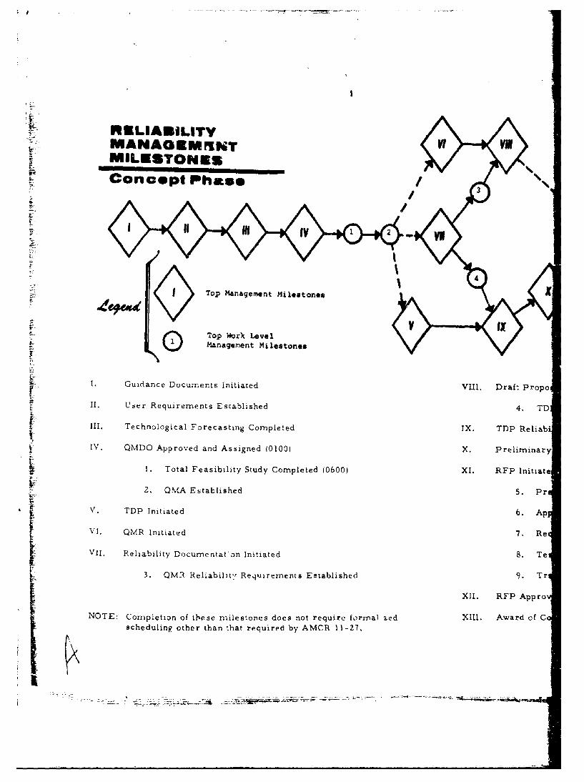
RELIABILITYMANAGEMrMNTMILESTONES

5-Conept Phase// 3

Top M~anagement Milestones

Top Work~ LevelOManagement MilestonesI. Guiciance Documents Initiated VIII. Draft Propo

if. User Requirements Established 4. TD

YIII. Technological Forecasting Completed IX. TDP Reliabi

IV. QMIJO Approved and Assigned (0100) X. Preliminary

1. Total Feasibility Study Completed (0600) XI. RFP Initiat

2. OVA Established 5. Pr

V. TDP Initiated 6. Ap

V1. QMR Initiated 7. Re

VII. Reliability Docum-entat art Initiated 8. Te

3. QMR Reliabilitr Requirements Established 9. Tr

XII. RFP Appro

NOTE: Completion of these milestones does not require formra) -zed Xi111. Award of Cschdulngothr hantha rquiedby AMCR 11-27.

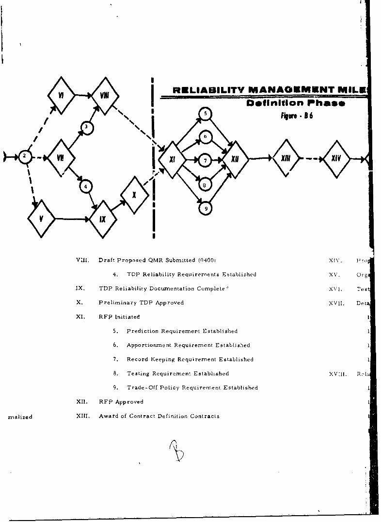
j RELIABILITV MANAGEMEINT MILE•I Definition Phase

5 Fkwe 86

VE I Dr1f 7rpoe QMR Submtte -- XIV. 'o

II

VI1I, Draft Proposed QMR Submitted (0400i XIV. P-o

4. TDP Reliability Requirements Established XV. Org

IX. TDP Reliability Documentation Complete' XVI. Tes

X. Preliminary TDP Approved XVII. Det

XI. RFP Initiated

5. Prediction Requirement Established

6. Apportionment Requirement Establdshed

7. Record Keeping Requirement Established

8. Testing Requirement Established XVIII. R,'li

9. Trade-Off Policy Requirement Established

XII. RFP Approved

rnalized XIII. Award of Contract Definition Contracts

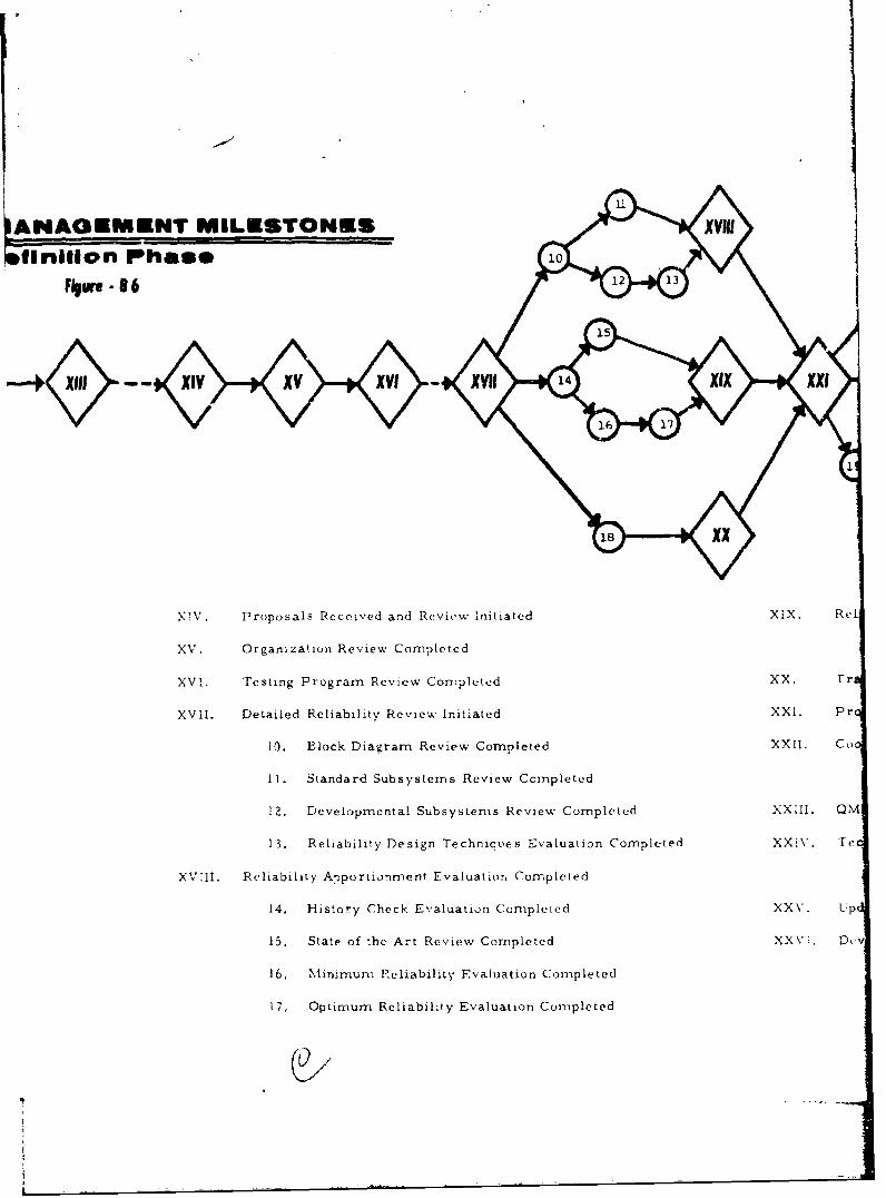
2ANAOEMNT MILESTONES 9

X!V. Proposals Received and Review initiated XiX. Rel

XV. Organization Review Completed

XVI, Testing Program Review Completed XX, Frr

151

XVII. Petale Reliability andReview nitiated Xox. Prd

10. Block Diagram Review Completed XXVI. Co

11. Standard Subsstesrt Review CompletediD.

12. Developmental Subsystems Review Completed XXIII. Q M

13. Reliability Design Techniques Evaluation Comnpleted XX iV. Te

XV[11. Reliability Apportionment Evaluatior n Completed

14. History Check Evaluation Completed XXV. LIP

15. State of the Art Review Completed XX V:..

16. Minimum Reliability Evaluation Completed

17 , Optimum Reliability Evaluation Completed, /0

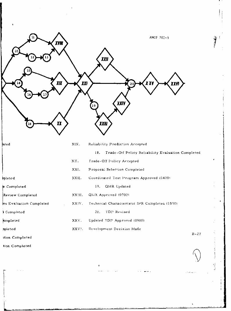
U AMCP 702-3 -6

xvm10

12 13 XI

14 xxXI2 vXV

16 17

18 XX

ated XIX. Reliability Prediction Accepted

18. Trade-Off Policy Reliability Evaluation Completed

XX. rrade-Off Policy Accepted

XXI. Proposal Selection Completed

;pleted XXII. Coordinated Test Program Approved (14001

SCormpleted 19. QAR Updated

Review Completed XXIII. QXiR Approved (0700,

jes Evaluation Completed XXIV, Technical Characteristic 1PR Coirpletet (1500)

t Completed 20. TDP Revised

rnpleted XXV. Updated TDP Approved (0900)

ppleted XXVI. Development Decision Made

13-27ition Completed

tion Completed

Fi

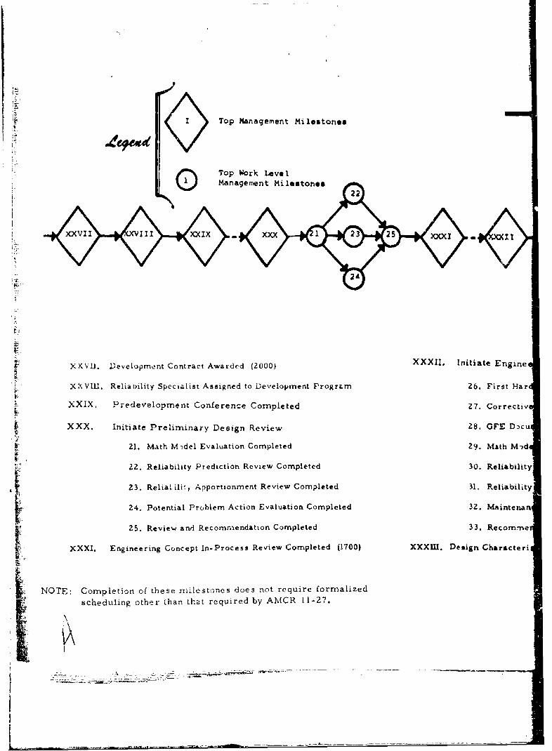
I• Top Management Milestones

Top Work LevelO Management Milestones

X nit Engine

SXXVII. Development Contract Awarded (2000) XXXII. Initiate Engine

XXVIII. Reliability Specialist Assigned to Development Frogr.m 26. First Har

XXIX. Predevelopment Conference Completed Z7. Correctly

XXX. Initiate Preliminary Design Review 28. GFE D:cu

21. Math M-.del Evaluation Completed 29. Math M-,d

22. Reliability Prediction Review Completed 30. Reliability

23. Relialili'y Apportionment Review Completed 31. ReliabilLty

24. Potential Problem Action Evaluation Completed 32. Maintenran

25. Review and Recomrm-endation Completed 33. Recomme

XXXI. Engineering Concept In-Process Review Completed (1700) XXXIi. Design Characteri

~ NOTE: Completion of these rnilestones does not require formalized

scheduling other than that required by AMCR 11-27.

L _ -- _ \

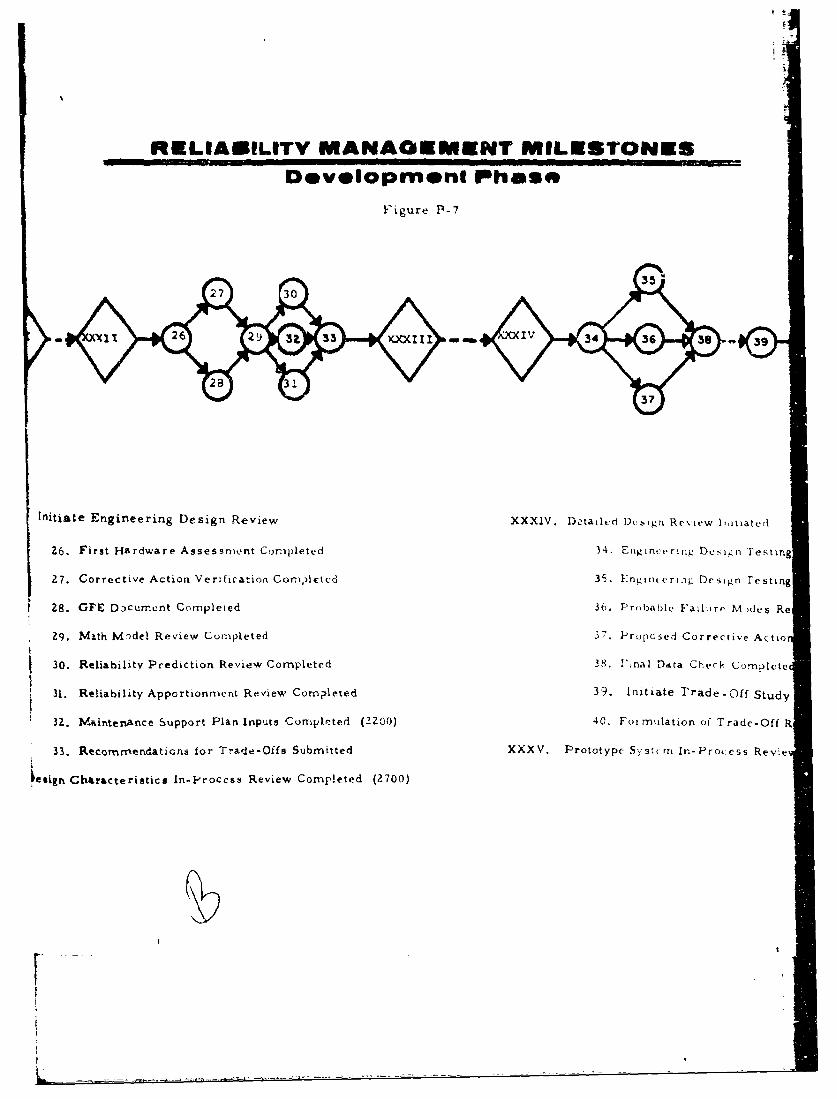
RELIAMILITY MANAOEMKENT MILESTONESDevelopment Phase

Figure P-7

7 30IV

Initiate Engineering Design Review XXXIV. D.2tailced Dbign Review litiated

Z6. First Hardware Assessment Conmtpleted 34. Enginering Dc.ign Test'.ng

27. Corrective Action Ver'fication Corn,)lctcd 35. Enginteri.ig Design Testing

28. GFE Document Completed 36. Pro bable lailltr•, M"&(' ds Re

29. Mith Mo•del Review Cournpleted 37. Propcsed Corrective Actio

30. Reliability Prediction Review Completed 38. I',nal Deta Check C'omplete

31. Reliability Apportionment Review Cormpleted 39. Initiate Trade-Off Study

32. M-aintenance Support Plan Inputs Completed (2200) 40. Fom tilation of Trade-Off R

33. Recorrmrmendations for Trade-Offs Submitted XXXV. Prototype Systcrri In-Process Rev:e

eeigri • Characteristics In-Process Review Completed (2700)

r

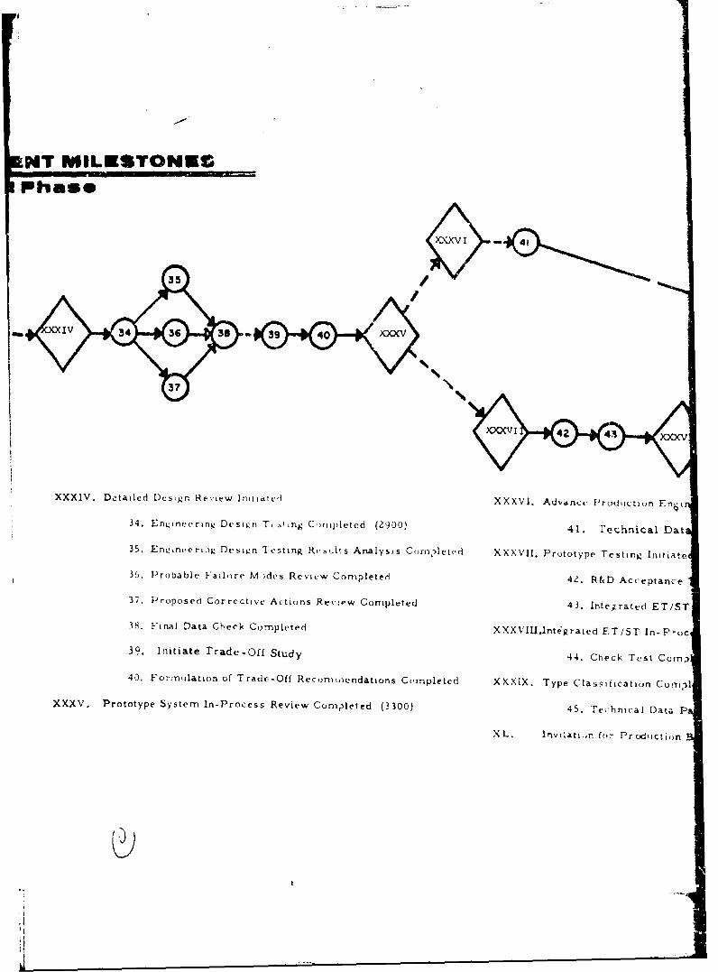
HT MILESTONECPhase

I V 34 36 36a 39 40X3C

37

)OO'V1 42 43 xxxv

XXXIV. Detailed Dcs~gr Rev.iew Inhititc-i XXXV1. Advance Production En~i

34. Engineering Dvsi~n T', nri Cejipleted (2900ý4.Fchia a

35. EnL~neerL.)g Design 'Iesting Results Analysis Com,,leted XXXVII. Prototype Testing Initiate

36. Probable F-ailnirf M.des Revicw Completed 42. R&D Acceptance

37. Proposed Corrective Attions RevPw Completed 43. Inte~ rated ET/5T

38. Final Data Check Completed XXX VIU.Iit~g rated F.T/ST In-Proc

39. Initiate Trade-(Off Study 44. Chieck Test Corn?)

40. Formulation of Trade.-Off Recomrsiendations Ctomrpleted XXXIX. Type Classification Comrnil

XXXV. Prototype Systomn In-Process Review Compdleted (3300) 45. Technical Data P

XL. Irtvt',atu.,n for Pr cdiiction

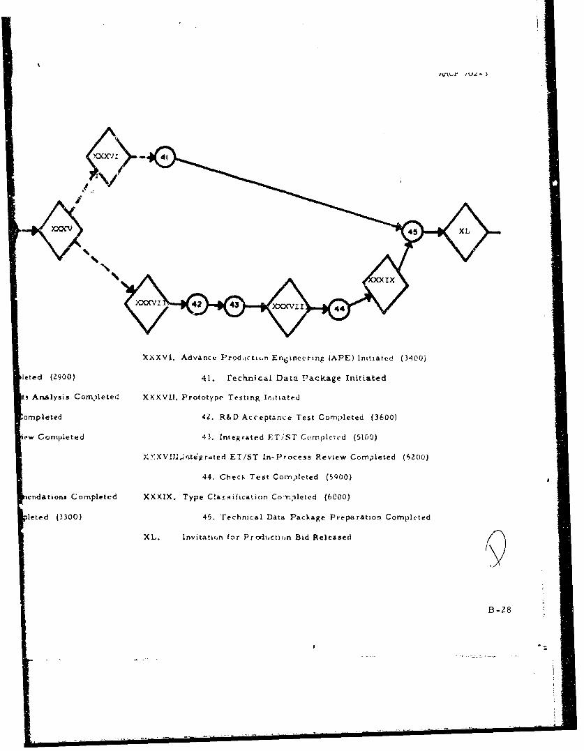
XXXV1. Advance Prodiiction Engincering (APE) Initiated (3400)

leted (2900) 41. technical Data Package Initiated

ts Analysis Com2leted XKKVII. Prototype Testing lntiated

onipleted 4,. R&D Acceptance Test Completed (3600)

ew Corripieted 43. Integrated ET.ST COrnplcetd (5100)

X':*XV/;I.Thttgrated ET/ST In-Process Review Completed (5200)

44. Check Test Completed (5900)

iendations Completed XXXIX. Type C!a• qification Cori1ctcd (6000)

leted (3300) 45. 'rechnical Data Package Preparation Completed

XL. Invitation for Prodricti(n Bid Released

B-28

71

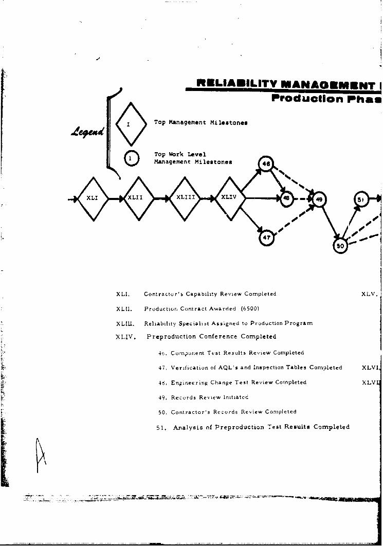
RELIABILITV MANAORMENT IProduction Pham

Top Mnagement Milestones

Q Management Milestones

XLI. Contractor's Capabiity Revie" Completed XLV.

XLII. Production Contract Awarded (6500)

XLIUI. Reliability Specialist Assigned to Production Program

XLIV. Preproduction Conference Completed

46. Component Test Results Review Completed

47. Verification of AQL's and Inspection Tables Completed XLVI

46. Engineering Change Test Review Completed XLV

49. Records Review Initiated

50, Contractor's Records Rcview Completed

51. Analysis of Preproduction Test Results Completed

EMENT MILESTONESIon Phase

Figure B-8

51 XV LI XLI IXLVIII

56

XLV. Trade-Off Decisic-n Com*,l1eted XLVII. Release Cor

52. IPT Evaluation Comnjleted 5r; ICT

53. Confirrmatory Test (Type 1) Completed (7500) XLLX. Rei'a!,lhty' S1

54. ConfJi'matory Test (Type II) Completed (7700) 57. Fie

55. In-House Statistical Anaiysis Completed 5-. Stur

rpleted XLVI. Statistical Analysis Review Completed 59. Re!

XLVII. Release Requrst Initiated ý0. Par

ýrnple ted

I

x!

RELIABILITY MANAGEMENT MILESTONESOperatlon & Disposal Phases

56 6

XLVIII, Release Completed (7',00) L. Statistical History Review C

5,). ICT E\-auat ion Ccinp4tcd LI. Equipmrnt Disp,,sal Coniplet

XLIX. Reliability Specialist Assigncd to Operation Phase

57. Field Reliability Determined

5S. Sturagv' Relia'ci:ty Deternmined

59. Rebuilt Equipment Reliability Determined

,;0. Part Reliabui•hy Deterimined

NOTE: Completion of these milestones does no

scheduling other than that required by

__ __ _ _

AMCP 702-3

lAEILITY MANAOEMENT MILESTONES-Operation & ospo o ,sal Phases

57596

XL LI

(7900) L. StcttistLcal Histury Review Completed

.ion Comvpleted L!. Equiprntnt Disposal Coniplcted .(t4700)

t Assigncd to Operation Phase

ability Determined

iabllity Determnined

uipment Reliability Determined

ihty Determined

NOTE: Completion of these milestones does not require formalizedscheduling other than that required by AMCR 11-27.

B-29

L-4'

AMCP 702.3

APPENDIX C

TECHNICAL REQUIREMENTS ANALYSIS ANDDOCUMENTATION OF RELIABILITY REQUIREMENTS


C-i. General. The contents of this appendix are intended to providethe reader with guidance for implementation of the discussicns inchapter 3. In addition to examples, it provides information explain-ing how reliability requirements should be stated in QMR's/SDR's.

A discussion of the relationship between reliability and incentive con-

tracting i• also included.

Section II. COMMENTS ON TYPICAL FAULTSIN STATING RELIABILITY REQUIREMENTS

IN QMR's/SDR's

C-?.. Examples. The following examples represent typical cases asto how reliability requirements have been stated in QMR's and SDR's.

Following each example are comments which critique the example andstate ways of improving the requirement. When writing reliability re-quirements in QMR's/SDR's, the following may be used ar, guidance:

a. Draft Proposed QMR for Automatic Test Equipment forCommunications Electronic Material:

(1) Requirement: The mission duration for ATE/C-E atall maintenance levels will be eight hours of operation. Assuming anexponential failure distribution, a mission reliability for a mean timebetv.een failures (MTBF) of 100 hours would be 92. 3%.

(2) Comment: Weakness is exhibited in three elements

of this requirements paragraph.

(a) The requirement, as stated, is not a requirementbut merely a statement of mathematical fact under the assumption ofan 8-hour mission duration and an exponential distribution of failuretime s.

Cl1

AMCP 70Z- 3

(b) There are two possible interpretations of the

word failure. First, a failure could be defined as the inability of thetester to detect the fault when a fault exists. On the other hand, i.could be defined as a false detection of a nonexistent fault. It couldalso be both. This should be explicitly defined in order for the re-liability requirement to be meaningful.

(c) At this point of the life cycle, mission reliabilityshould be expressed as a probability and not in terms of MTBF; i.e.it is premature to assume the distribution of failure times to be ex-ponential or any other distribution.

b. Draft Proposted SDR for a Short Range Mission Radio Set:

(1) Requirement: Mission reliability: 100% capable ofperforming a mission over a twelve-hour period without changingbatteries when transmitting one minute out of every ten.

(2) Comment: Reliability may be considered to be proba-bility of successful operation for the time period indicated. In thiscontext, the requirement as stated is impossible to comply with. Allitems have some distinct possibility of faling during any given periodof operating time, and this possibility has been ruled ouL by the state-ment above.

c. Draft Proposed SDR for Cold Water Detergents:

(I) Requirement:

(a) Mission reliability: 99%.

(b) Availability (Combat Ready Rate): 99T%.

(c) Reliability after storage: 97% after two years'

storage.

(?) Comment: The quantitative requirements pertaining

to mission reliability, availability, and reliability after storage shouldbe deleted in each case, These parameters arc not applicable in theframe of reference intended by AR 705-50.

C-2 j

AMCP 702-3

* d. Draft Proposed SDR for Forward Area Air Defense AlertRadar (FAAR):

(1) Requirement: The inherent equipment reliability shallprovide as a minimum a reliability of % for a critical time ofhours and mean time between failures (MTBF) of hours.

(2) Comment: Only one of the parameters required to beincluded in QMR/SDR by AR 705-50 wao specifically identified in thisSDR, and this requirement (reliability) is stated in such a mannerthat it would be impossible to comply with; i.e. , the mission duration,reliability rcquirenment, and MTBF were mutually incompatible.

C-3. Review of reliability requirements in QMR's and SDR's. Thefollowing should be considered when reviewing reliability requirements

in QMR's and SDR's to determine their technical adequacy and feasi-

bility of attainment. Maximum coordination with counterparts atUSACDC is encouraged in connection with making this determination.

a. The document should include a statement relative to whatconstitutes a failure. Since the word reliability normally impliesprobability of successful operation (nonfailures) for a specified periodof time, it can only take on true meaning if failure is defined.

b. The mission duration should be defined. Often QMR's andSSDR's include a vague statement, such as the mission duration will

vary depending upon a number of influencing factors. Yet, many ofthese same documents include a quantitative, minimum reliability re-

F quirement identified as being essential. Again, since reliability nor-mally means probability of successful operation for a specified periodof time, it is relatively meaningless to inc]ude a quantitative reliabilityrequirement unless it is associated with a definite period of time(mission duration), with the obvious exception of nortime dependent

* devices such as one-shot devices, (e.g., munitions).

SC. There should not be a statement associating a quantitativelevel of statistical confidence with the reliability requirement, suchas: "the minimum acceptable reliability shall be 95% to be demon-strated at a 90% confidence level." Degree of confidence is deter-mined when designing the test plan and, as such, is influenced byfactors such as cost, time, and required precision of test results.

C-3

AMCP 70Z-3

To specify it in a QMAR or SDR as a requirement that must be met inassociation with a reliability requirement is prernaturc. It shouldsuffice that a quantitative reliability requirement be specified in theQMR/SDR.

d. Reliability requirements should neither be too lax nortoo stringent. They are seldom too lax, but often too stringent andin some cases, literally impossible to attain and verify. A criticalanalysis should therefore be made on a case-by-case basis to deter-mine the feasibility of attaining and verifying the achievement of thereliability requirements within the current or projected state of theart and within time and cost constraints.

e. Analysis of the reliability requirements in QMR's andSDR's bhould include a deter,.Aination whether all of the appropriaterequirements of AR 705-50 have been considered. Two of the mostrepetitive faults of QMR's and SDR's are the exclusion of these re-quirements when they are applicable and the inclusion of these require-ments if they are not applicable. Consequently, an analysis should bemade to determine whether the requirements set forth by AR 705-.50are applicable for the particular item described by the documentsand, if so, whether or not they have been included.

f. If a quantitative requirement is included, that is, identifiedas being the durability requirement for the item, the definition of dura-bility as it applies to the item should be included. The reason for thisis that a great deal of confusion exists relative to what durability means.AR 705-50 does not require that a durability requirement he includedin QMR's and SDR's, and the DoD standard for definitions of reliabilityterms (MIL-STD-721B) does not include a definition of durability, yeta durability requirement sometimes appears in QMR's and SDR's, par-ticularly in the "priority of characteristics" section contained therein.It should either be omitted or be precisely defined in the document.

g. The requirements should be quantitatively expressed interms that are mutually understandable to both the user and developer.Reliability requirements are generally expressed in terms of proba-bility of successfui operation for the duration of the mission by meansof percentages or equivalent decimal fractions. However, there may

G-4

{I

AMCP 702-3

be a few situations where it is considered more feasible to expr,.essthe requirement in other terms, such as mcan time between failures

(MTBF), or probability of correct functioning for one-shot dexices,etc. It should be noted, however, that it is nut considered appropriateto express a given requirement as both a probability and an MTBF,such as: "The mission reliability will be no less than 85% for a 10-hour mission with an MTBF of 62 hours. " For this example, if thefailure rate were determined to be approximnately constant (and this

cannot be verified until items are built and operated a sufficient lengthof time to determine the distribution of failure tirnesi, the MTBF andpercentage value are redundant. If the failure rate is not constant,the percentage value and the MTBIF are incompatible.

Section III. STATING THE RELIABILITY CLAUSE IN CONTRACTS

C-4. General. Presently thore is much concern over the generalinadequacy of contractual provicions for the assurance of equipmner.treliability. The DoD has emphasized the use of incentive-type con-tracts wheonLver possible in lieu of the traditional cost-plus -fixed -fee

* (GPFF) contracts for procurenment of equipt-ent. The purpose of thisdiscussion, then, is two, fold: (1) Ito provide the procuring agency withguidance on the inclusion of certain contractual provisions which em-

phasize contractor obligations absociated with attainment of specifiedequipment reliability; and (2) to provide general guidelines for staru-lating reliability incentive requirements and identify certain technicalprobleihs thaL arise in the process of doing so.

C-5. Reliability clause for dt-vclopment contracts, a. AR 705-50requires that all equiwnuLt coiO racts will contain minimum numericalreliability requirements (mir.inium acceptable reliahil:Lv levels).

Additionally, it is required that contractual provisions include the

requirement for demonstration of stated quantitative requirements atselected prograrni mil.stnne:,.

b. In addition, Military Standard 785 and AR 705-50 statethat reliability tcsts, evaluations, or measurements will be conductedunder conditions specified by the proposal or any subsequent test pian

approved by competent authority. if contractual reliability require-ments are not met during demnorns ration tests; the deficient portionsof the system must be redesigned and demonstration tests continued

or repeated to verify that acceptance reliability has been achieved.

C-5

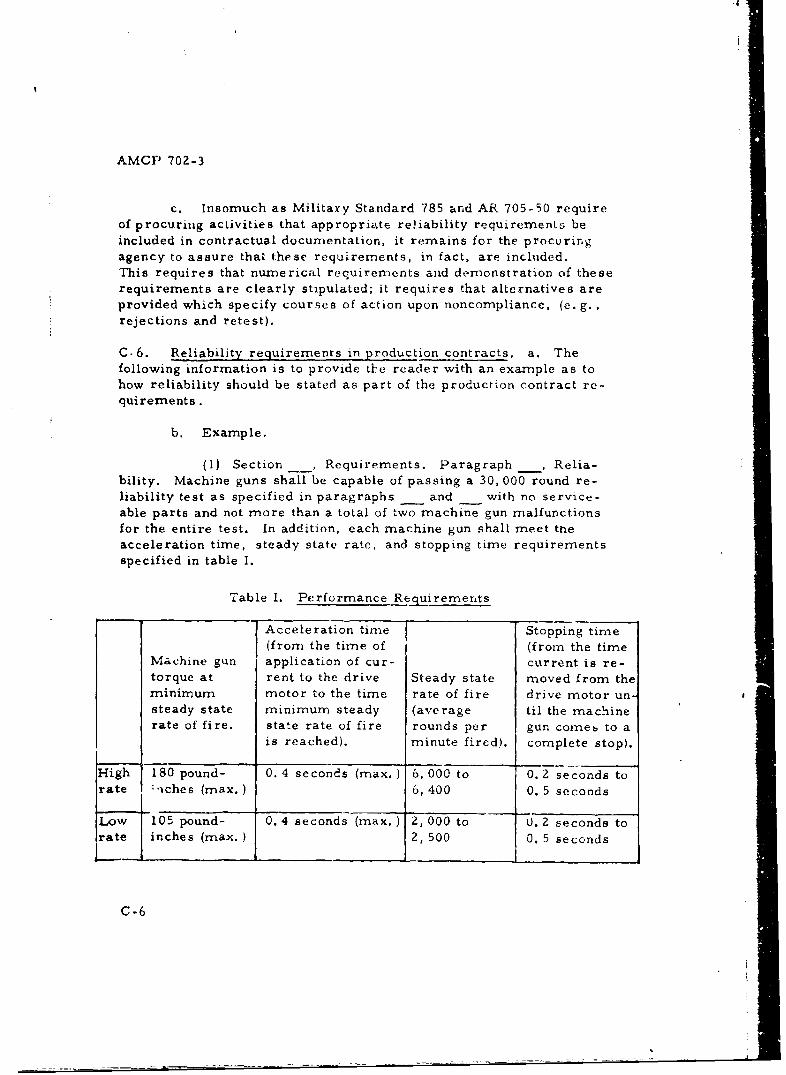
AMCP 702-3

c. Insomuch as Military Standard 785 and AR 705-50 requireof procuring activities that appropriate reliability requirements beincluded in contractual documentation, it remains for the procurirngagency to assure that these requirements, in fact, are included.This requires that numerical requirements and demonstration of theserequirements are clearly stipulated; it requires that alternatives are

provided which specify courses of action upon noncompliance, (e.g.,rejections and retest).

C. 6. Reliability requirements in production contracts, a. Thefollowing information is to provide the reader with an example as tohow reliability should be stated as part of the production contract re-quirements.

b, Example.

(I) Section , Requirements. Paragraph , Relia-bility. Machine guns shall be capable of passing a 30, 000 round re-liability test as specified in paragraphs _ and with no service-able parts and not more than a total of two machine gun malfunctionsfor the entire test. In addition, each machine gun shall meet theacceleration time, steady state rate, and stopping time requirementsspecified in table I.

Table I. Performance Requirements

Acceleration time Stopping tinme

(from the time of (from the timeMachine gun application of cur- current is re-torque at rent to the drive Steady state moved from theminimum motor to the time rate of fire drive motor un- *

steady state minimum steady (average til the machinerate of fire. state rate of fire rounds per gun comes to a

is reached). minute fired), complete stop).

High 180 pound- 0.4 seconds (max.) 6, 000 to 0. 2 seconds torate 4qches (max.) 6,400 0. 5 seconds

Low _105 pound- 0.4 seconds (max.) 2,000 to 0. 2 seconds torate inches (max. ) 2, 500 0. 5 seconds

C-6

AMCP 702-3

(2) Section , Quality Assurance Provisions. Para-graph , Reliability Testing.

Paragraph Lot Si7,. The initial reliability test lot size shallconsist of the initial month's production; subsequent reliability testlot sizes shall consist of 100 machine guns. When five successivelots meet the requirements, the reliability test lot size shall be in-creased to 200 machine guns.

Paragraph Procedure. Machine guns selected by the governmentrepresentative from each reliability lot shall bo testeOI by the contrac-tor for reliability using th. test method specified in paragraph _. Ifthe reliability requirements are not met, the represented lot shall bcrtejected subject to relest or reconditioning and further test as a re-conditioned lot. A reliability it'ttst of .__ machine guns from thesame lot shall be mnade withoul reconditioning the represented lot,unless in the opinion of the governnent representative the failure indi-cates serious defects in the item, in which case retest shall be madeonly if authorized by the proc uring agency. Failure of the machineguns in the retest to meet the requirermnts shall cause rejection ofthe represented lot subject to reconditioning and further testing as areconditioned lot. Prior te submission of a lot of machine guns asa reconditioned lot, the cause of fajlurte shall be determined and con-tractor correction shall be effec|cd on all machine guns in the lot.Sample size and test inethods for reconditioned lots shall be the sameas for retest.

Paragraph Reliability Test.

Paragraph . Testing of machine guns for reliability requirements(see section ) shall be accomplished with the machine gun held in

• a mount using the ammunition feed system, calibrated drive (for highrate), power supply, and in instrumentation in accordance with descrip-tion.

Paragraph Testing shall 1:e accomplished using ball cartridgesin belts of 1500 rounds each. The machine gun shall be fired using tenbursts of 150 round each at a steady state rate of 6000 to 6400 rounds

C-7

AMCP 702- 3

per minute. Acceleration and stopping time, torque, and steadystate rate of fire shall be meaaured and recorded on the last burstof each 1500-round belt. These recorded values shall be forwardedin accordance with paiagraph _-

Paragraph . After each 150-round burst, the machine gun shallbe allowed to cool (without cooling aids) for 5 to 15 seconds. Aftereach 1500-round belt, the machine gun shall be cooled to within 250 F.of ambient room temperature (using cooling aids other than water).After each 3000 rounds, the machine gun shall be examined and lubri-cated as necessary. Parts removed from the machine gun duringexarmination shall be replaced in original firing position from which.they were removed. Headepace and breech lock gap shall be ex-amined at the start of the test and at the end of the test on the cleanedand unlubrica'ed machine gun. At the end of each day's firing, themachine gun shall be protected against corrosion.

Paragraph -. No alteration or replacement of parts shall be made

unless the parts are either broken or worn to the extent that they areunserviceable. An unserviceable part is one that causes malfunctionsor imrrpairs the safety of the machine gun. A complete record shall bekept for each reliability test, showing each malfunction and all partsreplaced including the number of the -machine gun round at which theyoccurred.

Paragraph_. 7he contractor shall investigate causes of malfunc-tions and unserviceable parts and indicate corrective action taken.

Paragraph . Reliability tested machine guns and parts shall bedisposed of as specified in the procurement documents.

Section IV. INCENTIVE CONTRACTING

C-7. General. a. Increased emphasis is being placed on the use

of incentive contracts, especially in lieu of cost-plus-fixed-fee con-tracts. DoD Incentive Contracting Guide (FM 38-34) provides guidancefor the use of incentive contracting. While most of what follows appliesto incentive contracting in general, much of it is applicable to reliability

incentives in particular.

C-8

I%

AMCP 702- 3

b. A rapidly changing technology and expanding requirementsfor more complex systems has radically altered the character andfunction of military materiel, N-, longer is military research and de-velopment typically the low cost predecessor of large, multi-yearproduction runs of items with relatively stable designs. In manycases, the hardware evolved during an R&D effcirt becomes the sys-

tern specified for operational deployment. No longer, for many mili-tary systems, is the injunction, "Make it like the drawing shows, "

adequate guidance for obtaining satisfactory system performance andlife during the production phase. No longer can military systems bemaintained satisfactorily by the using troops; highly trained and skilledmaintenance personnel are required. These changes have made thecontractors' trade-off decisions important to the overall cost to theArmy of military systems.

c. One effective means of motivating a contractor to makethese trade-off decisions amongst cost, schedules, and the variousperformance characteristics (including reliability) which the Armydesires, is the use of properly structured incentive contracts. Thatis, a properly structured incentive contract, through the use of re-wards and penalties, will motivate the contractor to make the sametrade-off decisions that the Army would if it were doing the work itself.

C-8. Incentive contracting principles. If an incentive contract is tobe effective and to yield an acceptable product, (e. g., technical data"package, hardware, services), several principles should be observed.First, the contract terms must be clear, complete and unambiguous;these conditions are especially important in stating the incentive pro-visions. Second, nothing in the incentive provisions should permitthe contractor to meet his contractual obligations unless the perform-ance meets all of the minimum requirements of the contract. Third,incentive payments for changes in levels of performance should be

t offered only if the Army can be expected to benefit from such changes

and the contractor has the ability and authority to cause such changes;similarly, incentive deductions for changes in levels of performanceshould be required only if the Army can be expected to be adverselyaffected by such changes and the contractor has the ability and authorityto prevent such changes. Fourth, the magnitudes of the maximuan pos.sible incentive payment and of the maximum possible incentive deduction I "

I|C-9

I!e

AMCP 702-3

should reflect both the risk taken by the contra.tor and the magnitudesof the benefit to the Army of optimum contract performance and of theloss to the Army of rrminimum acceptable performance as compared totarget level performance. Fifth, the number of performance charac-teristics covered by the incentive provisions should be kept small;each additional characteristic considered dilutes the impact of the

* incentive and let;sens the probability of the contractor making thetrade-off decisions most beneficial to the Army. Finally, the struc-tures of the incentive provisions should be kept as simple as practical;the object is to motiva'te the contractor, not to impress him with theerudition of Army personnel.

C-9. Structuring incentive provisions, a. The first step in struc-turing incentive provisions is to determine which performance charac-teristics to consider for inclusion. Only those characteristics shouldbe considered whose levels are dependent mainly on the contractor'sactions and whose levels determine or help determine the value of thecontract product to the Army. If the contractor is unable to changethe performance level of a characteristic because of conditions beyondhis control, inclusion of the characteristic in the incentive Provisionsfrustrates the contractor and reduces his motivation. If the perform-ance level of a characteristic does not affect the value of the contractproduct to the Army, inclusion of the characteristic in the incentiveprovisions wastes the contractor's efforts and the Army's money.

b. The second step in structuring incentive provisions is todetermine, for each performance characteristic considered, whatlevel of performance is to be sought (i.e., the target level), what levelof performance is the worst acceptable, and what level of performanceis the best which can be reached under the current state of the art (i.e.,the optimum level). The optimum level must be feasible. In thoseinstances where the value of the contract product does not decreaseafter a certain performance level below the target level is reached,that certain level, for purposes of what follows, is the worst accept-able level. Similarly, in those instances where the value of the con-tract product does not increase after a certain performance levelabove the target level is reached, that certain level is the optimumlevel.

C-10

AMCP 702- 3

c. The third step is to determine the differences in value tothe Army, for each performance characteristic considered, between"optimum level and target level and between target level and worstacceptable level. For mzost performance characteristics, other thancost, these differences will be estimates rather than exact. For ex-

Sample, if reliability is one of the performance characteristics con-sidered, one approach to estimating the differences is to consider howmany more items would be needed if the reliability were at the worst

* acceptable level instead of at target level and how many fewer items* would be needed if the reliability were at the optimum level instead of

at the target level and to multiply these changes each by the target* - per-item-cost. Assuming that the impact of reliability upon procure-

rment costs is several times that upon other costs, then the computed

changes in value are accurate enough for use in structuring the incen-tive provisions.

d. The fourth step is to find the total difference in valuebetween having all the characteristics at their optimum level and hay-ing all the characteristics at their target level and the total differencein value between having all the characteristics at their target leveland having all the characteristics at tneir worst acceptable level.Each difference in value found in c between optimum level performanceand target level performance is divided by the first difference to findthe proportion of the maximum allowable incentive payment to be al-located to the corresponding characteristic. Similarly, each differencein value fc-nd in c between target level performance aid worst accept-

* able level performance is divided by the second difference to find theproportion of the maximum incentive deduction to be allocated to thecorresponding characteristic.

e. The fifth step is to relate achieved performance level foreach characteristic to incentive payment or deduction. The relation-ship between performance level and incentive payment or deductionshould be the same type as the relationship between performance leveland value. Usually, the performance level-incentive relationshipchanges at the target level since the two sets of proportions found in dt usually are not the same. Types of possible relationships includelinear, exponential and step; a linear relationship may be applied tofraction defective when this is small; an exponential relationship maybe applied to reliability when level is measured in .nean time between

failures; a step relationship may be used for such characteristics aaschedules.

J C-ll

AMCP 702-3

f. The sixth step is to detterniin, what vvidence is to be usedto measure the level of perform~ance for each characteristic. For re.-liability, this includes the sampling plans, estimates and test methods,

and conditions to be used. The sampling plans selected should reflecta good balance between test cost and cost of a wrong estimate of per-formance levcl.

g. The final step is to convert the results of the precedingI steps into the incentive provisions for the contract. These provisi-Ilsmust state in clear and unambiguous terms exactly how the incentivepayment(s) and deduction(s) are to be determined.

h. As the structure of the incentive provisions evolves, judg-mnent and experiencc may dictate that one or more of the characteris-tics be dropped or changed to achieve more effective incentive pro-

visions; this should be clone and the appropriate steps repeated usingthe new set of characteristics.

C-10. Example. a. Consider a program to develop a nonre'pairableitem having the following expected characteristics:

(1) Item failure rate rema'ns constant with time.

(2) Mission duration will be 21 hours.

(3) Cost per production unit will be $36, 000.

(4) At the target reliability level of 90%, an initial pro-duction run of 500 units is required.

(5) Each week's delay in completing the development ofthe item costs the Army $5000.

Because a cost-plus-incentive-fee contract was to be used to coverthe development of the item, the performance characteristics selectedfor consideration were: contract cost, item reliability, and contractduration.

b. The three characteristics were studied to find their threekey levels.

C- 12

AMCP 702- 3

(1) The cost analysts arrived at a target contract cost of$12, 000, 000; a minimum feasible (or optimum) concract cost of$10, 000, 000: and a maximum allowable (or worst acceptable) contractcost of $15, 000, 000.

(2) Engineering analysis indicated a maximum feasible(or optimum) mean time to failure of 2100 hours (or an optimum re-liability of 99%) and a minimum allowable (worst acceptable) meantime to failure of 164 hours (or a worst acceptable reliability of 80%).The target reliability of 90% is equivalent to a mean time to failure of(Z1 hours)/(-In 0.9) or 199. 32 hours.

(3) Application of PERT to the work to be accomplishedindicated that the contract would take at least 36 weeks from start tofinish, was expected to have a duration of 52 weeks, and would be corn-pleted in no more than 68 weeks after its start. Therefore, the targetcontract duration was set at 52 weeks; the optimum contract durationwas set at 36 weeks; and the worst acceptable contract duration wasset at 68 weeks.

c. Further study was made of the impact of the three keylevels of each characteristic.

(1) Little additional study was needed to show that the valueto the Army of the optimum contract cost rather than the target contractcost would be $12, 000, 000 - $10, 000, 000, or $2, 000, 000, and that the a

: value to the Army of the target contract cost rather than the worst ac-ceptable contract cost would be $15,000,000 - $12, 000, 000, or$3,000,000.

f (2) Further study of the reliability levels revealed that ifthe item reliability were equal to 90%, the target level, the initial pro-duction run of 500 units could be expected to complete (0. 90)(500), or I'450 successful missions. Also, it was found that if the item reliabilitywere equal to 807o, the worst acceptable level, 450 successful missionswould require on the average (450)/(0, 80), or (rounding upward) 563units and, if the item reliability were equal to 99%0, the optimum ievel,

S~~C- 13 -

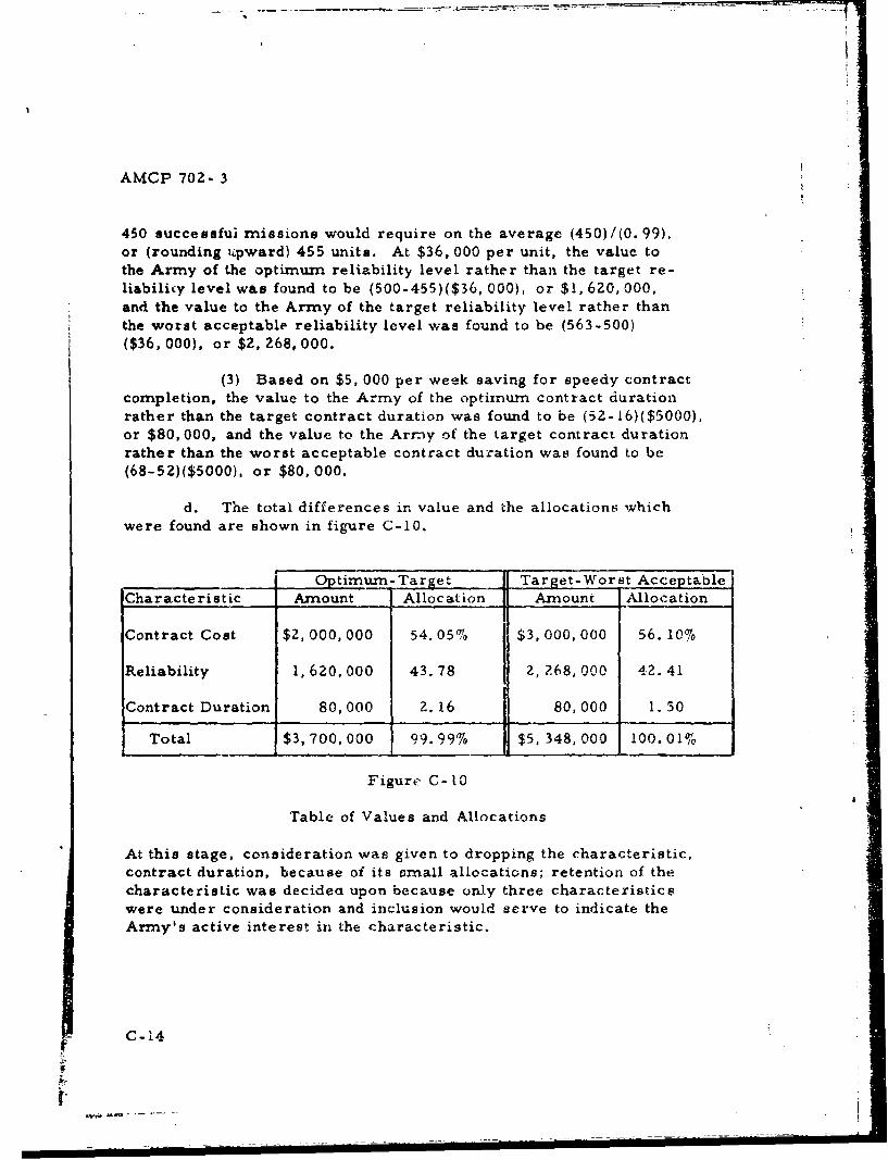
AMCP 702- 3

450 successfui missions would require on the average (450)/(0. 99),or (rounding 4pward) 455 units. At $36, 000 per unit, the value tothe Army of the optimum reliability level rather than the target re-liabilicy level was found to be (500-455)($36, 000), or $1, 620, 000,and the value to the Army of the target reliability level rather thanthe worst acceptable reliability level was found to be (563-500)($36, 000), or $2, 268, 000.

(3) Based on $5, 000 per week saving for speedy contractcompletion, the value to the Army of the optimum contract durationrather than the target contract duration was found to be (52-16)($5000),or $80, 000, and the value to the Army of the target contract durationrather than the worst acceptable contract duration was found to be(68-52)($5000), or $80, 000.

d. The total differences in value and the allocations whichwere found are shown in figure C-10.

Optimum-Target_ Target-Worst Acceptable

Characte ristic Amount Allocationli Amount Allocation

Contract Cost $2,000,000 54.05% $3,000,000 56. 10%

Reliability 1,620,000 43.78 j , 2?68,000 42.41

Contract Duration 80,000 2. 16 80,000 1. 50

Total $3,700,000 99.99% $5, 348,000 100.01%

Figure C-O0

Table of Values and Allocations

At this stage, consideration was given to dropping the characteristic,contract duration, because of its small allocations; retention of thecharacteristic was decidea upon because only three characteristicswere under consideration and inclusion would serve to indicate theArmy's active interest inj the characteristic.

C-14

i.d

r

AMCP 702- 3

e. Based upon the judgment of the negotiator who was to ne-gotiate the contract for the item, a maximum allowable incentive pay-ment of $1, 200,000 and a maximum incentive deduction of $600,000were selected for use in setting up the incentive structure. When thefinal contract was written, the structure was adjusted easily by multi-plying the incentive rates by the appropriate constant.

(1) The contract cost incentive structure was set at(0. 5405)($1, 200, 000)/(2000), or $324. 30, incentive paid for every$1000 that the contract cost fell below $12. 000, 000, and (0. 5610)($600, 000)1(3000), or $11Z. 20, incentive deducted for every $1000that the contract cost exceeded $12, 000, 000. Any incentive paymentearned for contract cost was to be added to the target fee and any otherincentive payments; any incentive deduction for contract cost was to be

deducted from the target fee and any incentive payments. (Essentially,this structure is that of two straight lines, since there are 2000 possible

* payment steps and 3000 deduction steps,

S(2) The reliability incentive structure required the most

study. Since mean time to failure could be estimated, a table re-

lating incentive to that variable was prepared. Also, a table relat-ing incentive to estimated reliability was prepared. The second tableshowed the incentive-to-reliability relationship to be nearly linear.To achieve a simple structure, it was decided to pay (0. 4378)($1, 200, 000)/9, or (rounding off) $58, 400, for each percent that the

demonstrated reliability exceeded 90%; and to deduct (0. 4241)* ($600, 000)/i0, or (rounding off) $25, 450, for each percent that the

demonstrated reliability fell below 90%. (In effect, the incentive struc-ture for reliability consisted of 19 steps: 9 payment steps and 10 de-duction steps.) i

(3) The contract duration incentive structure was set at(0. 0216)($1, 200,000)/16, or $1620, incentive paid for each week lessthan 52 weeks that the contract takes to complete; and (0. 015)($600, 00)/16, or $562. 50, incentive deducted for each week more than 52 weeksthat the contract takes to complete. (The incentive structure for con-tract duration also was a step one: 16 each for payments and deductions.

t

- C-15

AMCP 702-3

f. Having developed the skeleton of the incentive structure,the team for developing the incentive provisions turned to the ques-tion of how the level of performance was to be measured for eachcharacteristic.

(1) The team member from the comptroller's office hadno problem, since the Armed Services Procurement Regulation andprecedence provided ample guidance.

(2) The team member from the reliability office realizedthat his efforts to achieve maximum efficiency would have a large pay-off. Past experience with similar units indicated that the mean timesto failure of the units in the field and the mean times to failure ofunits tested, using Reliability Laboratory Test H, were the same,and that the total test cost (including the cost of performing the test,the cost of the components degraded by the test, and the cost of dis-assembly) averaged $21'0 per unit tested for Reliability LaboratoryTest H. Since this test permitted the test units to be returned toas-good-as-new condition, a replacement test was chosen. A time-terminated plan had to be used, since only one week (168 hours) couldbe allowed for running the test. Unable to arrive at the best samplesize by theory, the team member selected a sample size of 20 on thebasis of his best judgment and recommended that the estimate,exp[-(nurnber of failures occurring)/ 160]. be used to determineachieved reliability.

(3) The contract was to be considered completed whenthe contractor had met all contractual requirements and had deliveredthe required technical data package in its final form.

g. The incentive provisions submitted for legal review stated:

"The cost of the work covered by this contract, the reliability ofthe item developed under this contract, and the contract duration, i. e. ,

award of this contract to delivery of the final draft of the required tech-nical data package) shall be used to adjust the fee for this contract.For each $1000 that the cost of the work covered by this contract ex-ceeds $12, 000, 000, $112. 20 will be deducted from the target fee. Foreach week that the contract duration is less than 52 weeks, $1620 will

C-16

2I

AMCP 702-3

be added to the target fee; and for each week that the contract durationexceeds 52 weeks, $562. 50 will be deducted from the target fee. Foreach percent that the estimated item reliability, as determined by theprocedure given in paragraph _. 2, below, exceeds 90%, $58, 400 willbe added to the target fee; and for each percent that the estimated itemreliability, as determined by the procedure given in paragraph .2,below, is less than 90n, $25, 450 will be deducted fromn the target fee.The total fee paid shali be equal to the target fee plus any additionsand minus any deductions required by the above provisions.

"_.2. Procedure for Determining Estimated [ten) Reliability.Twenty units, prior to sealing, plus forty additional widget assemblies, f

will be furnished to the Army for conducting Reliability LaboratoryTest I-1 of KLG Test Manual 702-8 at a total cost of $724, 000. Thiscost will not be used in determining the total fee. The Army will test

the twenty units for 168 hours, replacing each failure by disassern-bling the failing unit, inserting a new widget assembly, reassemblingthe unit, and continuing to test the unit until its total time under testis 168 hours. The number of failures observed, r, will be inserted

in the expression e-r/1 6 0); the value of this expression will be rounded

off to the nearest percent and this percentage used as the estimated

reliability.

C -17 -

-- -.!- - - - . -_ _ _ _ _ _ _

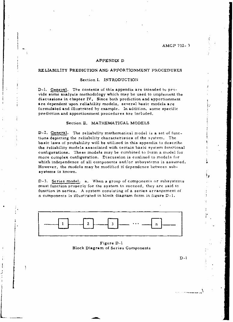
AMCP 702- 3

APPENDIX D

RELIABILITY PREDICTION AND APPORTIONMENT PROCEDURES

Section 1. INTRODUCTION

D-1. General. The contents of this appendix are intended to pro-vide some analysis methodology which may be used to implement thediscussions in chapter IV. Since both prediction and apportionmentare dependent upon reliability models, several basic models areformulated and illustrated by example. In addition, some specific

prediction and apportionment procedures are included.

Section U. MATHEMATICAL MODELS

D-2. General. The reliability mathematical nmodel is a set of func-tions depicting the reliability characteristics of the sy-stemn. Thebasic laws of probability will be utilized in this appendix to describethe reliability models associated with certain basic system functionalconfigurations. These models may be combined to form a model formore complex configuration. Discussion is confined to models forwhich independence of all components and/or subsystems is assumed.However, the models may be modified if dependence between sub-systems is known.

D-3. Series model. a. When a group of components or subsystemsmust function properly for the system to succeed, they are said tofunction in series. A system consisting of a series arrangement ofn components is illustrated in block diagram form in figure D-1.

Figure D-1

Block Diagram of Series Components

D-1

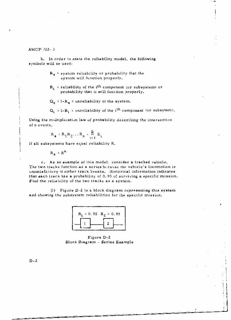
AMCP 702- 3

b. In order to state the reliability model, the followingsymbols will be used:

R3 = system reliability or probability that the

system will function properly.

Ri = reliability of the ith component (or subsystem) orprobability that it will function properly.

Q5 = I'Rs = unreliability ot the system.

Qi = -lRi = unreliability of the ith component (or subsytern).

Using the mkltiplication law of probability describing the intersectionof n events,

nKs I 2" '" n i=l zRS=RR R a.I t

If all subeystems have equal reiiability R,

RS = Rn

c. As an example of this model, consider a tracked vehicle.The two tracks function as a series bcausc the vehicle's locomotion isunsatisfactory if either track breaks. Historical information indicatesthat each track has a probability of 0. 95 of surviving a specific mission.Find the reliability of the two tracks as a system.

(1) Figure D-2 is a block diagram representing this systemand showing the subsystem reliabilitics for the specific mission.

R O = 0.95 RZ = 0.95-fEJ--El --Figure D-2

Block Diagram Series Example

D-2

SI

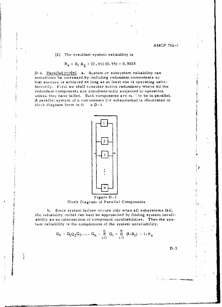
AMCP 702-3

(2) The resultant cystern reliability is

R RI RZ = (0.95) (0.95) z 0.90z5

D-4. Parallel model. a. System or subsystem reliability cansornetimes be increased by including redundant components so

* that success is achieved as long as at least one is operating satis-factorily. First we shall consider active redundancy where all theredundant components are simultaneously subjected to operationunless they have failed. Such components are s. ' to be in parallel.A parallel system of n corroonents (c-r subsystems) is illustrated inblock diagram form in fi e D-3.

1

}2

3 w:

Figure D-3

Block Diagram of Parallel Components

b. Since system failure occurs only when all subsystems fail,

the reliability model can best be approached by finding system unreli-ability as an intersection of component unreliabilities. Then the sys-tern reliability is the complement of the system unreliability.

n n1Qs QlQQ3 Qn = l Qi RI (l-Ri) I-Rs

i=l

D-3

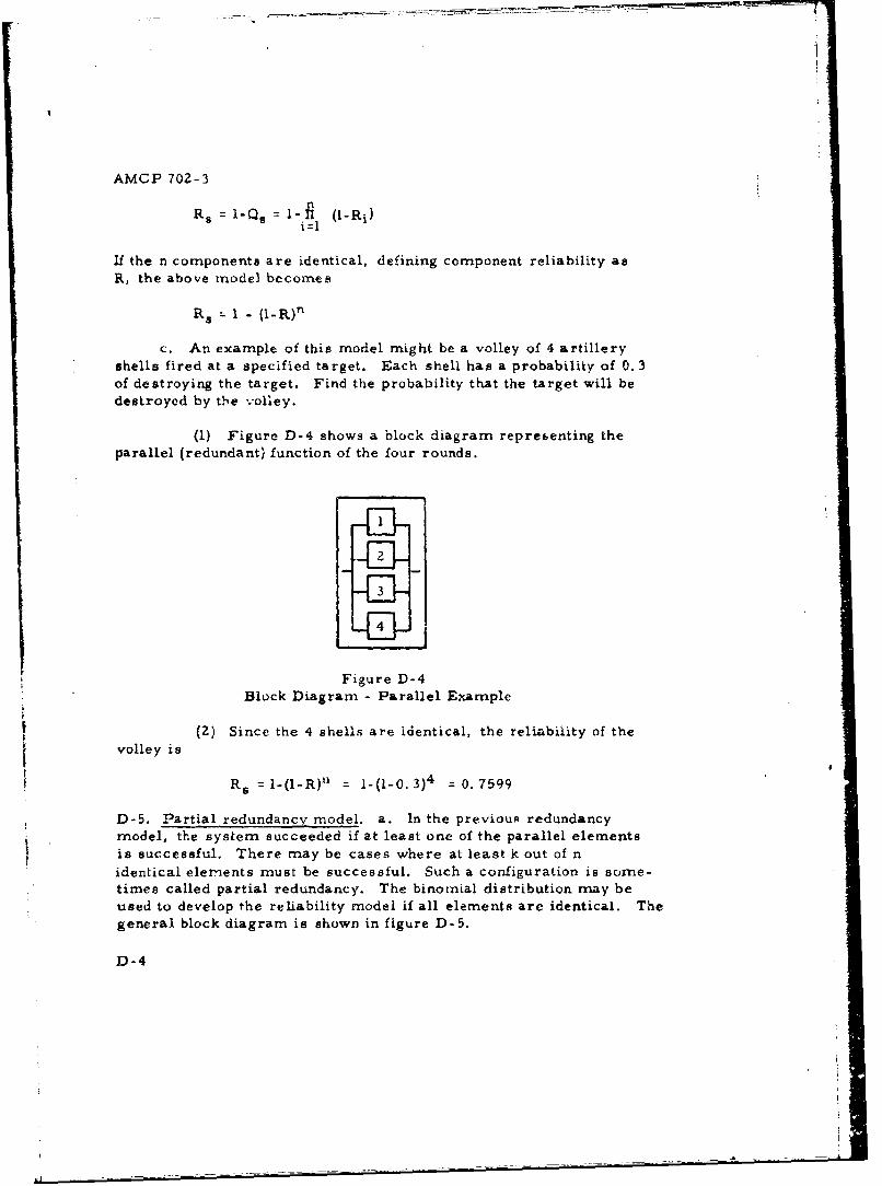
AMCP 702-3

-Q 9 :i-HI (l-Ri)i=l

If the n components are identical, defining component reliability asR, the above model becomes

Rs z I - (I-R)n

c. An example of this model might be a volley of 4 artillery

shells fired at a specified target. Each shell has a probability of 0. 3of destroying the target. Find the probability that the target will bedestroyed by the volley.

(1) Figure D-4 shows a block diagram representing the

parallel (redundant) function of the four rounds.

2

3

4 4

Figure D-4

Block Diagram - Parallel Example

(2) Since the 4 shells are identical, the reliability of thevolley is

Rs = 1-(-R)" = _-(_-0.3)4 = 0. 7599

D-5. Partial redundancy model, a. In the previouR redundancymodel, the system succeeded if at least one of the parallel elements

is successful. There may be cases where at least k out of n

identical elements must be successful. Such a configuration is some-times called partial redundancy. The binomial distribution may beused to develop the reliability model if all elements are identical. The

general block diagram is shown in figure D-5.

D-4

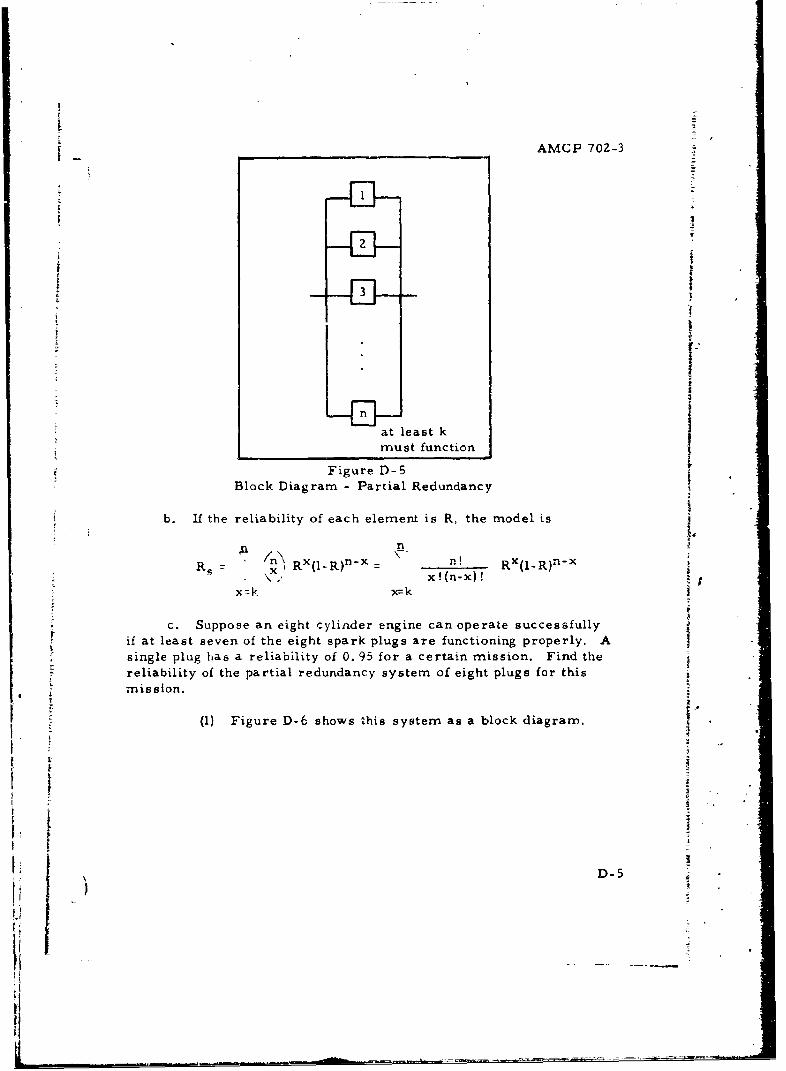
AMCP 702-3

I

3 133

at least k Imust function

Figure D-5Block Diagram - Partial Redundancy

b. If the reliability of each element is R, the model is' n '

n- \/n) RX(l-R)n-x: \-- n! Rx(l-R)n-xKs = \x, x ! (n-x) !

xzk x-k

c. Suppose an eight cylinder engine can operate successfullyif at least seven of the eight spark plugs are functioning properly. A Isingle plug has a reliability of 0. 95 for a certain mission. Find thereliability of the partial redundancy system of eight plugs for thism1ission.

(1) Figure D-6 shows this system as a block diagram.Tt

D -5 -

H .)

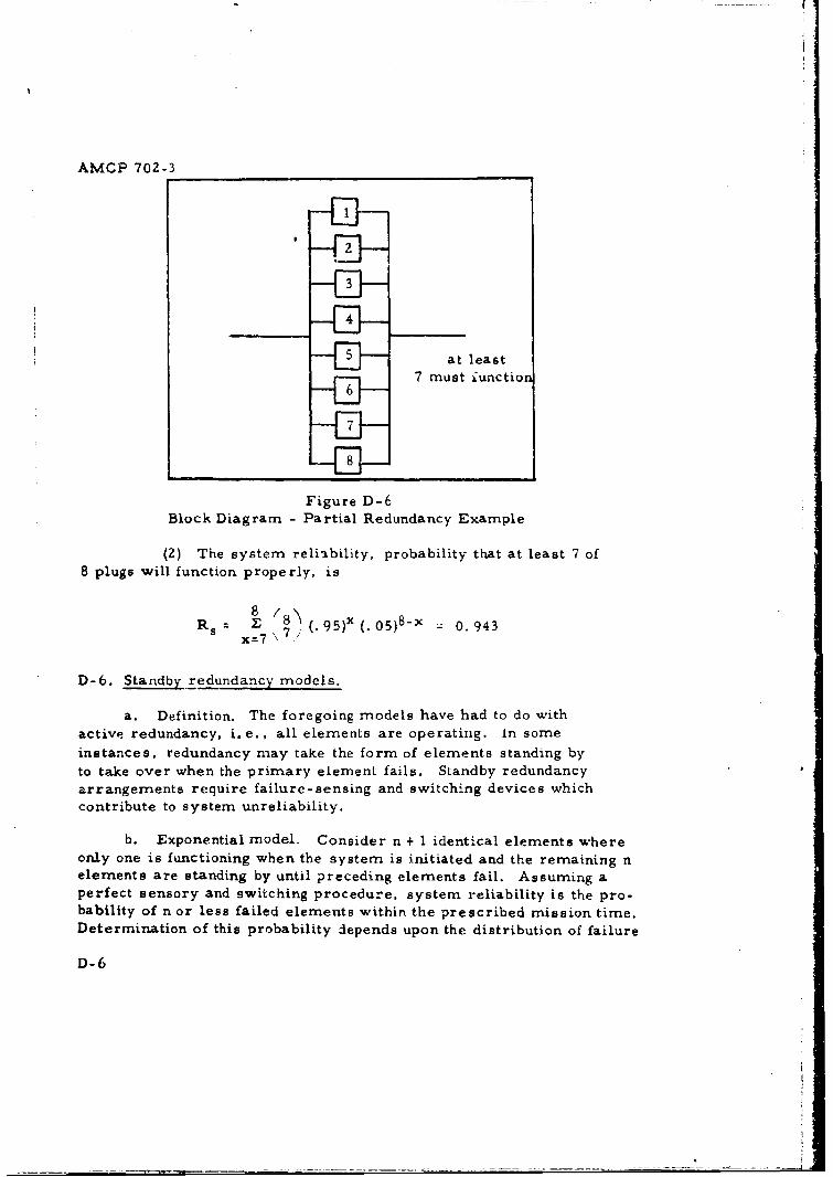
AMCP 702-3

34-

i at least

7 must iunction6

Figure D-6Block Diagram - Partial Redundancy Example

(2) The system reliability, probability that at least 7 of8 plugs will function properly, is

Rs= 2; 95)x 05)8-x 0. 943x=7 (7. )

D-6. Standby redundancy models.

a. Definition. The foregoing models have had to do withactive redundancy, i. e., all elements are operating. In someinstances, redundancy may take the form of elements standing byto take over when the primary element fails. Standby redundancyarrangements require failure-sensing and switching devices whichcontribute to system unreliability.

b. Exponential model. Consider n + 1 identical elements whereonly one is functioning when the system is initiated and the remaining nelements are standing by until preceding elements fail. Assuming aperfect sensory and switching procedure, system reliability is the pro-bability of n or less failed elements within the prescribed mission time.Determination of this probability depends upon the distribution of failure

D-6

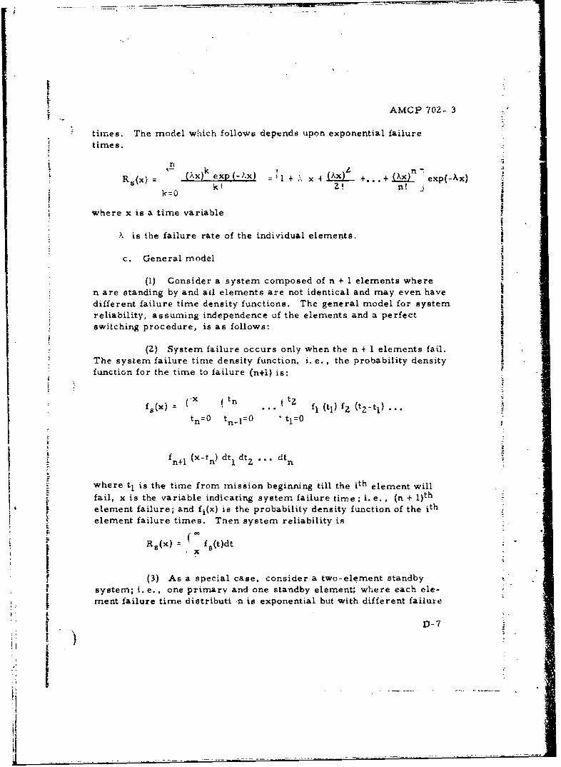
AMCP 702- 3

times. The model which follows depends upon exponential failuretimes.

n €xkR-(x) (Xx) exp(-4x) + , + (Ax) + exp(-Ax)ksxI•=0 kV 2! n! j

k I j

where x is a time variable

X is the failure rate of the individual elements.&

c. General model

(1) Consider a system composed of n + 1 elements wheren are standing by and ail elements are not identical and may even havedifferent failure time density functions. The general model for systemreliability, assuming independence of the elements and a perfectswitching procedure, is as follows:

jI

(2) System failure occurs only when the n + I elements fail.The system failure time density function, i. e., the probability density .function for the time to failure (n+l) is:

(.x tn ttz A•fs(x) ... fl (tl) fz (tz-tl) -..

tn=O tn1 l=0 tl=0

Sfnf+1 (x-tn) dtl dtz " dtnInwhere tI is the time from mission beginning till the ith element willfail, x is the variable indicating system failure time ; i. e. , (n + 1)th

ii I element failure; and fi(x) is the probability density function of the ith

element failure times. Then system reliability is

R 5 (x) fr(t)dt

(3) As a special case, consider a two-element standbysystem; i. e. , one primary and one standby element; where each ele-

ment failure time distributi n is exponential but with different failure

D-7

.i

ii

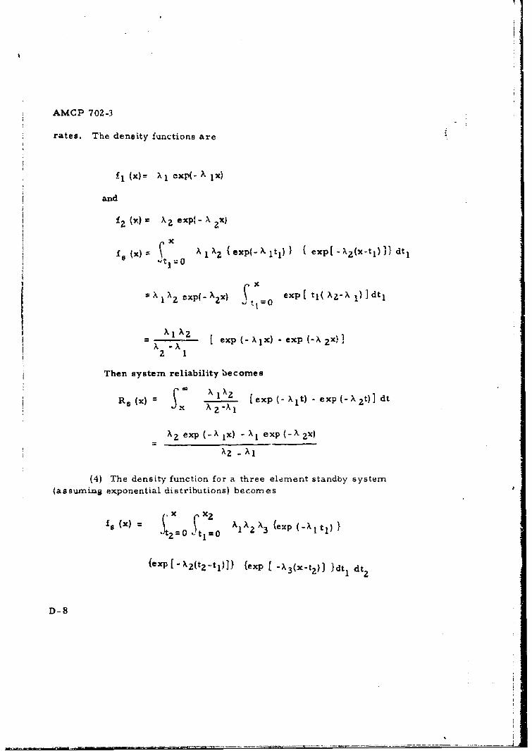
AMCP 702-3

rates. The density functions are

fl (x)- X IeXP(-A Ix)

and

f 2 (x) - Xexpl- ax)

Sxf 5x) AiA'z {exp(-Xlt1 )} { exp[-X 2 (x-tx)i} dt,

X X exp(-x) exp[ t1 ( AZ- X IdtI

X [ exp (- 1 x) -exp (- X 2x)]

Then system reliability becomes

"R5 ( 1 [ (-. X t) - exp (X- t)] dt

Rs()= _ _ 2 "__

Az exp (X x) - A I exp (-X 2 x)

XZ2 - X•1

(4) The density function for a three element standby system(assuming exponential distributions) becomes

fs Wx) = AI X2 X3 {exp (-A tI) }

{exp[- X2 (t 2 -tl)]} {exp [ -X 3 (x-t2 )] dt dt2

D-8

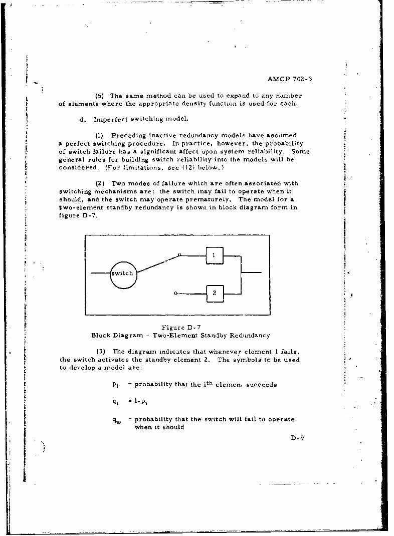
I

- AMCP 702-3

(5) The same method can be used to expand to any numberof elements where the appropriate density function is used for each.

d. !mperfect switching model.

(1) Preceding inactive redundancy models have assumed

a perfect switching procedure. In practice, however, the probabilityF of switch failure has a significant affect upon system reliability. Some

genera] rules for building switch reliability into the models will beconsidered. (For limitations, see (12) below.)

(2) Two modes of failure which are often associated withswitching mechanisms are: the switch inay fail to operate when itshould, and the switch may operate prematurely. The model for a

two-element standby redundancy is shown in block diagram form infigure D-7.

-switch£

Figure D-7Block Diagram - Two-Element Standby Redundancy

(3) The diagram indicates that whenever element I !ails,i- the switch activates the standby element 2. The symbols tc be used

to develop a model are:

P Pi = probability that the ith elemen, succeeds

qi = 1-p.

qw probability that the switch will fail to operate

when it should

D-9

I

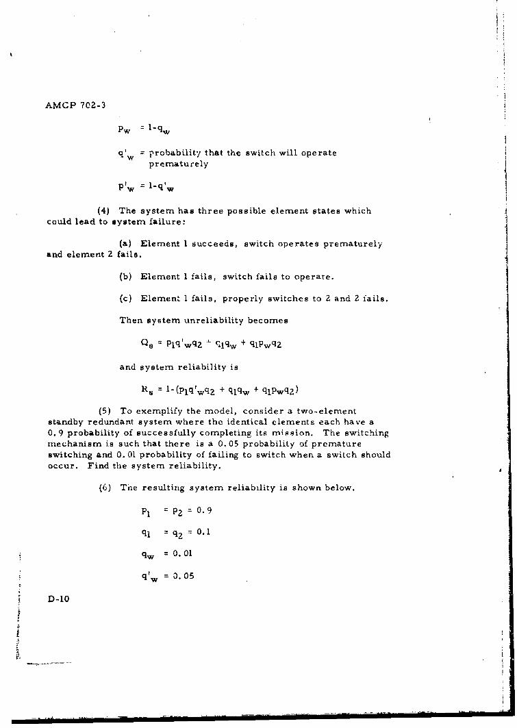
AMCP 702-3

Pw = -qw

o' = probability that the switch will operate"-Wprematurely

ptw = l'qIw

(4) The system has three possible element states whichcould lead to system failure:

(a) Element I succeeds, switch operates prematurelyand element 2 fails.

(b) Element 1 fails, switch fails to operate.

(c) Element 1 fails, properly switches to 2 and 2 fails.

Then system unreliability becomes

Qs = PlqlwqZ - clqw + qlpwqz

and system reliability is

Rs = l'(plq'wqZ + qlqw + qlpwq2)

(5) To exemplify the model, consider a two-elementstandby redundant system where the identical elements each have a0. 9 probability of successfully completing its mission. The switchingmechanism is such that there is a 0. 05 probability of prematureswitching and 0. 01 probability of failing to switch when a switch shouldoccur. Find the system reliability.

(6) The resulting system reliability is shown below.

P1 = P= 0.9

q, = q2 0.1

qw, = 0.01

qtW = 0. 05

D-10

1

rf

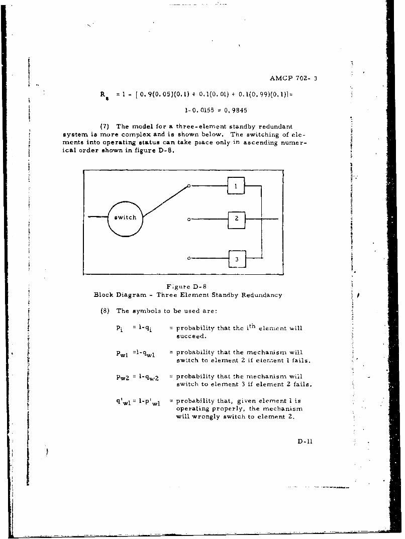
AMCP 702- 3

R = 1 - [0.9(0. 05)(0.1) + 0.1(0. 01) + 0.1(0. 99)(0. 1)=

1- 0. 0155 = 0.9845

(7) The model for a three-element standby redundantsystem is more complex and is shown below. The switching of ele-ments into operating status can take place only in ascending numer-ical order shown in figure D-8.

0 3

Figure D-8

Block Diagram - Three Element Standby Redundancy 1

II

S~(8) The symbols to be used are:

•Pi =l-qi =probability that thc ith elenient will•- succeed.

ii

Pwl =l-qwl probability that the mechanism willS~~switch to element 2 if elemnent I fails. "-

t ~pw? = I'qw : probability that the m~echanism willw2 switch to element 3 if element 2 fails.

qII

", 'Pwl =-~w probability that, given element I isoperating properly, the mechanismwill wrongly switch to element Z.

D-11gr---

Blciga he leetSadyRdnac

(8-h ymost e sdae

AMCP 70Z-3

q'wz= l-P'w = probability that, given element 2 isoperating properly, the mechanismwill wrongly switch to element 3.

(9) System failure ci. - happen only in the following sevenelement states.

(a) Element 1 succeed, wrongly switch to 2, 2 succeed,

wrongly switch to 3 and 3 fail

(b) Element 1 succeed, wrongly switch to 2, 2 fail,properly switch to 3 and 3 fail.

(c) Element 1 succeed, wrongly switch to 2, 2 failand no switch to 3.

(d) Element 1 fail and no switch to 2.

(e) Element 1 fail, a proper switch to 2, 2 fail andno switch to 3.

(f) Element I fail, a proper switch to 2, 2 succeed,

wrongly switch to 3 and 3 fail.

(g) Element 1 fail, a proper switch to 2, 2 fail, aproper switch to 3 and 3 fail.

(10) Then system unreliability is

= Plq'wlPzqlwZq 3 + Plq'wlq2Pwzq3 + Plq'wlqpqwvZ

qlqw + qlp wq 2 q~w + qlPwlP 2 q' wq 3 + qlPwlqZpwq

and

R =I-Q

(11) The method may be extended to standby redundantsystems of more than three elements. Other failure modes may alsobe added, e.g., switch contact failure is sometimes encountered.

D-12

AMCP 702-3

(12) The standby redundancy models, with imperfect

swicching mechanisms, shown above, have considered success orfailure of an element as being independent of time, i. e., the re-maining mission time when an element is activated does not affect

the probability of its success. The models may be further refinedby considering failure distrib itions of the elements as well as theincorrect switch time distribution. Development of such modelswould be similar to the method used for redundant models with perfectswitching mechanisms. Such models, however, are not included here-in.

D-7. Conditional probability and the reliability model.

a. General.

(1) There exist configurations of subsystems which arenot series, parallel, or standby as previously defined. Conditionalprobability may be used to facilitate the modeling of .uch configura-tions. A useful theorem is stated:

P(A) = P(A/Bi)P(Bi)i~rl

where the Bi are mutually exclusive events such that

mX.P(B i)

A special case of this theorem where m = 2 is sometimes useful forreliability modeling

P(A) = P(A/BI) P(BI) + P(A/B.) P(B2 )

where B1 and B 2 are mutually exclusive and exhaustive events.

(2) For example, consider a configuration as shown by

figure D-9.

D-13

II

I

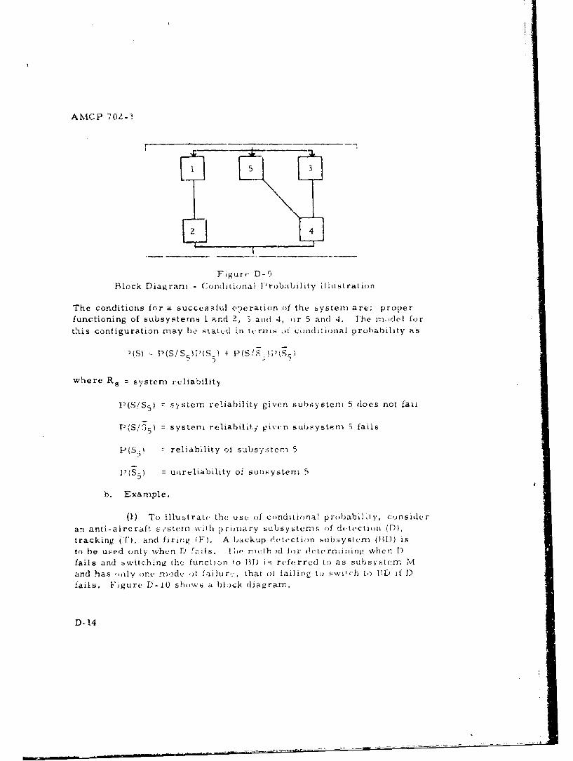
AMCP 702-3

15 3

2 4

Figure D-9

Block Diagram - Conditinmal lProbability illustration

The conditions for a successful o2eration of the bystem are: proper

functioning of subsystems I and 2, 3 and 4, or 5 and 4. The mlel for

t'ais configuration may be stat,:d in ter ms of conditional probability as

"(S) I P(SIS IP(S ) 4 P(S!S.1 ,5:- *5 '"

where Rs = system reliability

P(S/S 5 ) = sfstem reliability given subsystem 5 does not faii

IS/S-5) = system rcliabilit1 given subsystem 5 fails

P{( :S7 reliability ol subsystem 5

* (S5,) unreliability of su(i;yste" 5

b. Example.

(1) To illustrate the(. use of conditional probabili ,y, cunsider

an anti-aircraft s cstern with priroary subsysterns of detection, (D),tracking (lV), and firirn (F'. A backup Oetectinn subsyst em (11D) is

to be used only when D fails. 'I;o mobth )d ior deternim:inig when D

fails and .witching thi function to B1) is referred to as subsystem XIand has (,Ily ome mode of -ajlur,:, that of failing, tu switch to BE) if 1)

fails. Figure D-I0 shomw-s a block diagrarm.

D-14

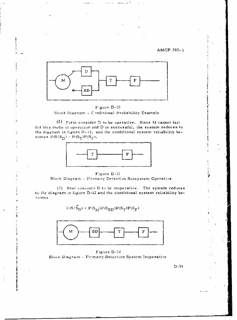
AMCP 702- 3

DtMF

Figure D-10.

BMock Diagram - C-nditional Probability Example

(Z) First consider D to be ooerative. Since M cannot faii

for this mode of operation and D is successful, the svstem reduces tothe diagram in figure D- 1 1, and the conditional system reliability be-comes P(SiSD/ S P(ST)P(SF).

Figure D-l1

Block Diagram - Primary Detectioa-n Suosystem Operative

(3) Next consider D to be inoperative. The system reducesto the diagram in figure D-12 and the conditional system reliability be-comes

P(S/SD) N P(S)P(SBD)P(ST)P(SY)

C-O

Figure D-1ZSBlock Diagram - Primary Detection System !noperative

D-15I

AMCP 702- 3

(4) The unconditional system reliability then is

P(S) = P(ST)P(SF)P(SD% + P(SM)P(SBD)P(ST)P(SF)P(SD)

c. Conditional probability may be applied to a variety of comn-

ponent configurations. Complex combinations of series and parallelmodels are often more easily analyzed by applying the conditi-)nal

probability theorem one or more times, considering a key item first

as operative and then as inoperative.

Section II. RELIABILITY PREDICTION

D-8. General. Reliability prediction is the use of the reliabilitymodel to combine reliability inrformation concerning components andsubsystems to determine a predlictiablf system reliability. The keyactivities associated with reliability prediction are discussed in

chapter 4.

D-9. Mixed model example, a. Most practical systems willnot fit any single model of section 11, but rather are representedby combinations and/or variations of these models. To show this,the following paragraphs contain an example of reliability prediction

for a mixed system.

b. An automobile is to be used for a 500 mile trip and thereliability is to be predicted for this trip. Reliability informationis available concerning automobile subsystems: tires, lighting group,spark plugs, brake system and all other subsystems collectively.

c. The tire subsystem (subsystem T) ir comprised of 5 tires,four originals and a spare, where the spare is a standby to r lace thefirst, if any blowout. The trip length is such that wearout does notoccur, but blowouts may occur because of chance random stresses en-countered. Past information indicates miles between blowouts to be

exponentially distributed with failure rate of 0. 0001 blowouts per mile.

Figure D-13 shows block diagrams for the four potential configurationswhich may occur. TI, T2, T3 and T4 are the original tires and T5 isthe spare.

D-16

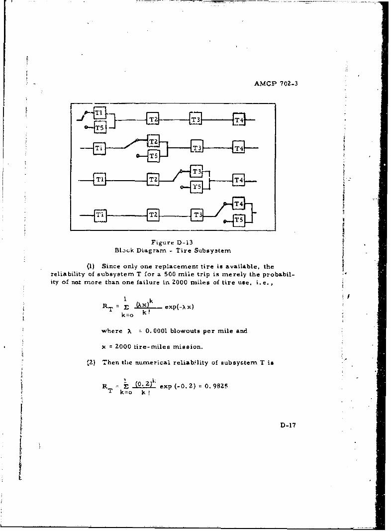
AMCP 702-3

ýT3TZ T4

Figure D-13Bla)ck Diasgram - Tire Subsystem

(1) Since only one replacement tire is available, thereliability of subsystem T for a 500 mile trip is merely the probabil-ity olf not more than one failure in 2000 miles of tire use, i. e.,

I kRT exp(-x x)

where X. 0. 0001 blowouts per mile and

x 2000 tire-miles mission.

12) Then the numerical reliab~lity of subsyrtem T is

R E (0- ?-) exp (-0.2Z) 0. 9825T k=o k!I

D-17

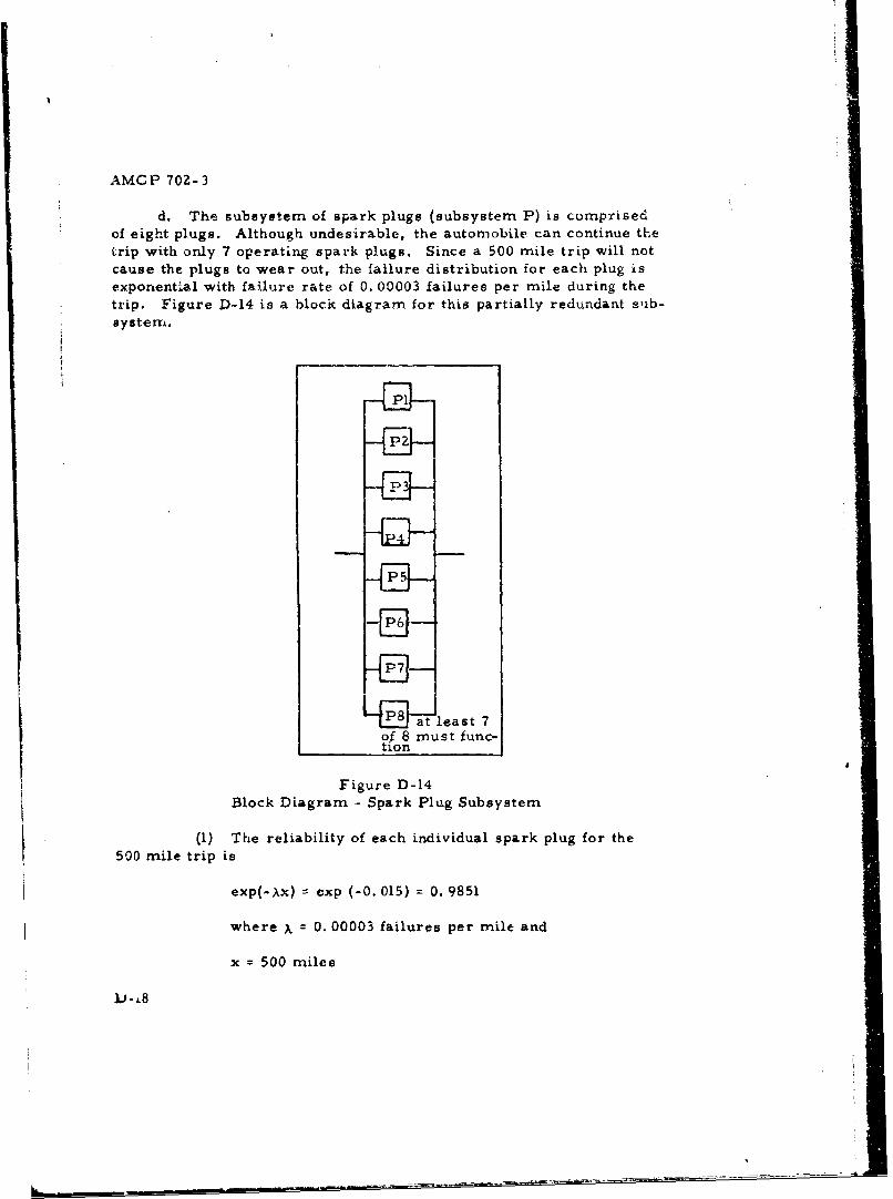
AMCP 702-3

d. The subsystem of spark plugs (subsystem P) is comprisedof eight plugs. Although undesirable, the automobile can continue theirip with only 7 operating spark plugs. Since a 500 mile trip will notcause the plugs to wear out, the failure distribution for each plug isexponential with failure rate of 0. 00003 failures per mile during thetrip. Figure D-14 is a block diagram for this partially redundant sub-system.

E-•a't [east 7

oftio8 must func-!

tion

Figure D-14Block Diagram - Spark Plug Subsystem

(1) The reliability of each individual spark plug for the

500 mile trip is

exp(- Xx) =exp (- 0. 015) = 0. 9 851

where X% 0. 00003 failures per mile and -

x =500 miles

IJ- 8

L!

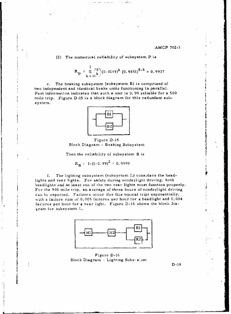
AMCP 702-3

(Z) The numerical reliability of subsystem P is

R 7 _,,k8(0, 01 4 9 )k (0. 9 8 5 1)8-k = 0.9937k~o

e. The braking subsystem (subsystem B) is comprised oftwo independent and identical brake unita functioning in parallel.Past information indicates that such a unit is 0. 99 reliable for a 500mile trip. Figure D-15 is a block diagram for this redundant sub-system.

51•S

B2

Figure D-15Block Diagram - Braking Subsystem

Then the reliability of subsystem B isr2

R = l-(4-0.99)2 0.9999

f. The lighting subsystem (subsystem L) considers the head-lights and rear lights. For bafety during nondaylight driving, bothheadlights and at least one of the two rear lights must function properly.For the 500 mile trip, an average of three hours of nondaylight drivingcan be expected. Failures occur (for this typical trip) exponentially,with a failure rate of 0. 005 failures per hour for a headlight and 0, 004failures per hour for a rear light. Figure D-16 shows the block dia-grain for subsystem L.

RIHi H2

R2

Figure D-16Block Diagram - Lighting Subs, s>.m

D-19

I,

I

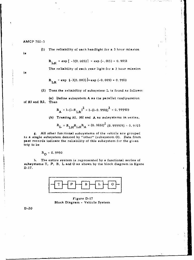
AMCP 702-3

(1) The reliability of each headlight for a 3 hour missionis

RLH = exp [ -3(0. 005)] = exp (-. 015) = 0.9851

The reliability of each rear light for a 3 hour missionis

RLR-- exp 1-3(0. 003)I=exp (-0. 009) = 0.9910

(2) Then the reliability of subsystem L is found as follows:

(a) Define subsystem A as the parallel configurationof RI and R2. Then

RA = 1-(I-RLR )z = 1-(1-0. 9910)2 = 0. 999919

(b) Treating iil, HZ and A as subsystems in series,

RL = RLH RLHRA = (0. 9 8 5 1) z (0. 999919) - 0. 9/03

g. All other fun,.tionral subsystems of the vehicle are groupedas a single subsystem denoted by "other" (subsystem 0). Data frompast records indicate the reliability of this subsystem for the giventrip to be

R = 0.9q90

0

h. The entire system is represented by a functional series ofsubsystems T, P, B, L and 0 as shown by the block diagram in figureD-17.

Figure D-17Block Diagram - Vehicle System

D-20

L -i

AMCP 70Z- 3

Then the system reliability may be predicted a3

R =R RRRS TPBLO

= (0. 9825)(0. 9937)(0. 9999)(0. 9703)(0. 9990) = 0. 9463

Section IV. RELIABILITY APPORTIONMENT

D-10. General. Reliability apportionment utilizes the reliability modelto assign combinations of compatible goals among subsystems such thatsubjection of the model to these subsystem goals will yield the systemgoal. Discussion of apportionment in this appendix will be confined tosome specific techniques of apportionment, two of which approachapportionment with minimum expenditure of effort.

D-11. Equal apportionment technique, a. The equal apportionmenttechnique assumes a series of n subsystems each of which is to be as-signed the same reliability goal. A prime weakness of the method isthat the subsystem goals are not assigned in accordance with the degreeof difficulty associated with achievement of these goals. For this tech-nique, the model is

*• n * -'

R 1I R•i=l

or

*1/n(R i ( ) for i 1, 2 ..... n

Where R is the required system reliability and

Ri is reliability requirement apportioned to subsystem i.

Sb. To exemplify this technique, consider a proposed commun-ication system which consists of 3 subsystems (transmitter, receiverand coder) each of which must function if the system is to function.Each of these subsystems is to be developed independently. Assumingeach to be equally expensive to develop, what reliability requirementshould be assigned to each subsystem in order to meet a system re-quirement of 0. 7Z9.

D-21

AMCP 702- 3

c. The apportioned subsystem requirements are found es

R*T = R*R = R (R n = (0.7Z9) 1/3 = 0.90

Then a reliability requirement of 0. 90 should be assignedto each subsystera.

D-12. AGREE apportionment technique. a. This technique takes intoconsideration both the complexity and importance of each subsystemfor electronic systems. It assumes a series of k subsystemns each withexponential failure distributions. Then the minimum acceptable meanlife of the ith subsystem is defined as

Nwiti0*ni [-In R*(t)]

and the corresponding ith subsystem reliability requirement becomes

Ri (ti) = exp ( -ti

where

i 1, Z, 3 ..... k

t required mission time of t' .! system

ti required mission time of the ith subsystem

wi = importance factor expressed as the probability that failureof the i h subsysLem will result in system failure.

ni =number of modules in the ith subsystemk

N Z ni = total number of modules in the systemi=l

R*(t) = the required system reliability for system mission timeR t) = the reliability apportioned to the ith subsystem for

Ri (t sbyte)o itsmission time

.= apportioned mean time to failure for the ith subsystem

1

D-Z2

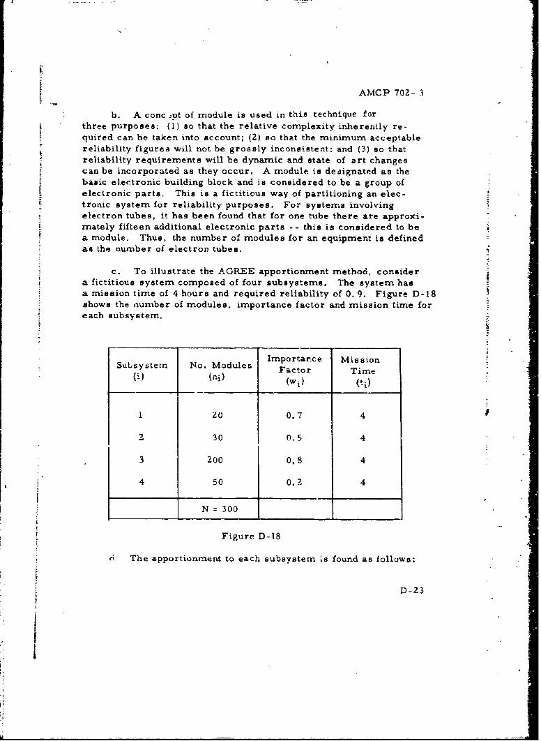
AMCP 70Z- 3

b. A conc-;nt of module is used in this technique forthree purposes: (1) so that the relative complexity inherently re-quired can be taken into account; (2) so that the minimum acceptablereliability figures will not be grossly inconsistent: and (3) so thatreliability requirements will be dynamic and state of art changes"can be incorporated as they occur. A module is designated as thebasic electronic building block and is considered to be a group ofelectronic parts. This is a fictitious way of partitioning an elec-tronic system for reliability purposes. For systems involvingelectron tubes, it has been found that for one tube there are approxi-rmately fifteen additional electronic parts -- this is considered to bea module. Thus, the number of modules for an equipment is definedas the number of electron tubes.

c. To illustrate the AGREE apportionment method, considera fictitious system composed of four subsystems. The system hasa mission time of 4 hours and required reliability of 0. 9. Figure D-18shows the number of modules, importance factor and mission time foreach subsystem.

Importan~ce Mission

SuLsystem No. Modules Factor Time(i)i)

1 Z0 0.7 4

2 30 0.5 4

3 200 0,8 4

4 50 0.2 4

N 300

Figure D-18

SThe apportionment to each subsystem Ls found as follows:

D-23

''

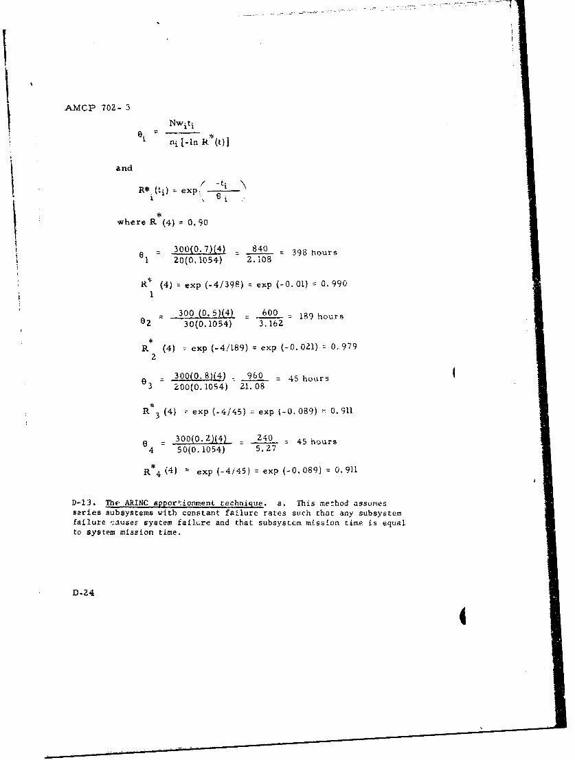
AMCP 702- 3

Nwiti

I ni [-In R,*(t)

and

exp..

where R (4) = 0.90

= 300 0 v IJ 840_ 398 hours1 2.(0.1054) 2. i08

R (4) = exp (-4/398) exp (-0. 01) = 0.9901

_ 300 (Q. 5)(4) 32600 = 189 hours02 30(0.1054) 3.162

R (4) = exp (-4/189) = exp (-0. 021) = 0. 9792

300(0. 8)(4) - 960 - 45 hours3 =200(0. 1054) 21. 08

R 3 (4) = exp (-4/45) - exp (-0. 089) - 0.911

300(0. Z)(4) Z40 - 45 hours4 50(0. 1054) 5. 27

R * 4 (4) = exp (-4/45) = exp (-0. 089) = 0.911

D-13. The ARINC apportionment technique. a. This method assumesseries subsystems with constant failure rates such that any subsystemfailure 'auses system failure and that subsystem mission time is equalto system mission time.

D-24

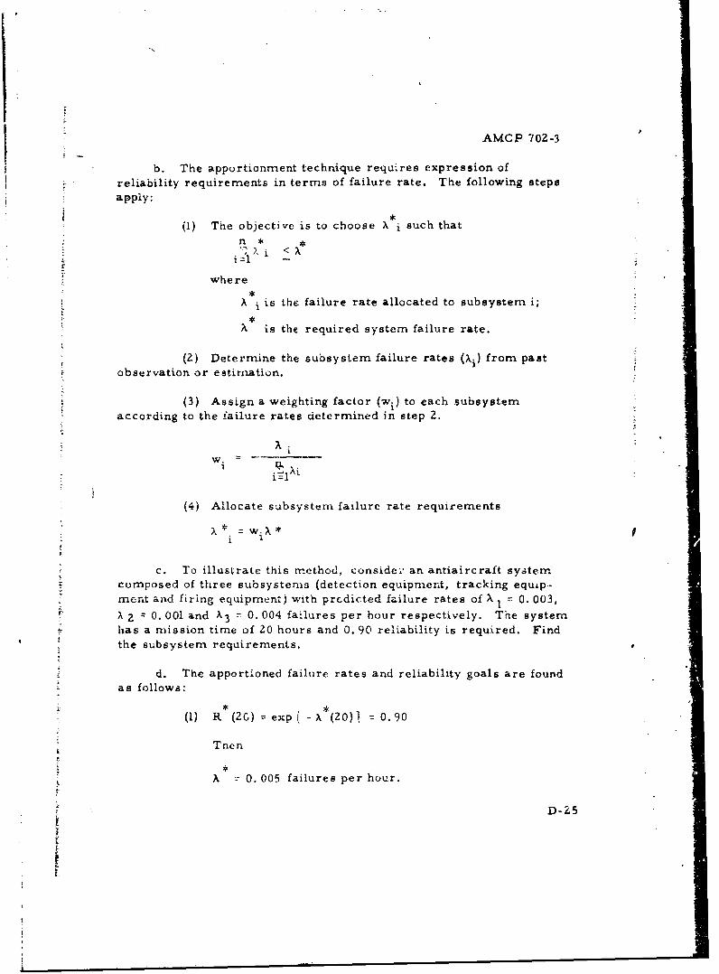
p

AMCP 702-3

b. The apportionment technique requires expression ofreliability requirements in terms of failure rate. The following stepsapply:

(1) The objective is to choose X i such thatn * *: "•, ?,i <kx

f<

where

Si is the failure rate allocated to subsystem i;

X is the required system failure rate.

(2) Determine the subsystem failure rates (Xi) from pastobservation or estimation.

(3) Assign a weighting factor (wi) to each subsystemaccording to the failure rates determined in step 2.

w . 14 iX i

(4) Allocate subsystem failure rate requirements

w * ,i i

c. To illustrate this method, conside' an antiaircraft systemcomposed of three subsystemns (detection equipment, tracking equip-ment and firing equipment) with prcdicted failure rates of X 1 = 0. 003,X z 0. 001 and X3 = 0. 004 failures per hour respectively. The systemhas a mission time of 20 hours and 0. 90 reliability is required. Findthe subsystem requirements.

d. The apportioned failure rates and reliability goals are foundas follows:

(1) R (20) expf -\*(20)1 0.90

Tnen

SA 0. 005 failures per hour.

D-Z5

I

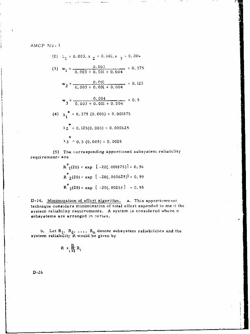
AMCP 7c-?- 3

(2) -= 0.003, X 0, oo0, 3,k 0.004

(3) W = 0.003 = 0.3750.003 + 0.001 + 0.004

W 0. 001 = 0. 12502 . 003 + 0.001 + 0.004

0. 004 0.53 0.003 + 0.001 + 0.004

(4) xl* = 0. 375 (0. 005) = 0. 001875

XZ 0.125(0. 005) = 0.000625

X3 -0. 5 (0. 005) = 0.0025

(5) The corresponding apportioned subsystem reliability

requiremento are

R 1(20) = exp [ -ZO(. 001875)] = 0. 96

R 2(20)= exp [ -Z0(. 000625)] = 0. 99

R 3 (20) exp [ -20(. 0025) = 0. 95

D-14. Minimization of effort algorithm, a. This apportionment

technique considers minimization of total effort expended to me t thesystem reliability requirements. A system is considered where nsubsystems are arranged in series.

b. Let R 1 , RZ, ... Rn denote subsystem reliabilities and thesystem reliability R would be given by

R N-l R.

D-26

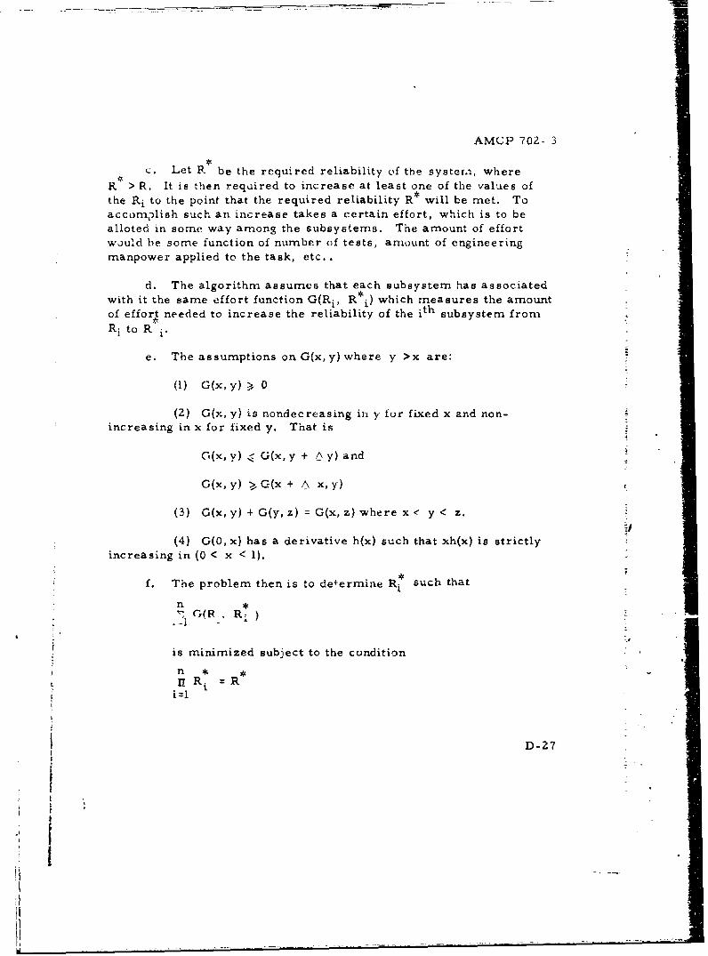
AMC;P 702- 3

C. Let RP. be the required reliability of the systerm, where

R > R. It is then required to increase at least one of the values ofthe Ri to the point that the required reliability R* will be met. Toaccomplish such an increase takes a certain effort, which is to bealloted in some way among the subsystems. The amount of effortwould be some function of number of tests, anmount of engineeringmanpower applied to the task, etc..

d. The algorithm assumes that each subsystem has associatedwith it the same effort function G(Ri, R*i) which measures the amountof effort needed to increase the reliability of the ith subsystem fromRi to R i.

e. The assumptions on G(x, y) where y >x are:

(1 G(x, y) >' 0

(2) G(x, y) is nondecreasing in y for fixed x and non-increasing in x for fixed y. That is

G(x, y) < G(x, y + A y) and

C(x, y) >,.G(x + A x, y)

(3) G(x,y) + G(y,z) = G(x,z) where x y < z.

(4) G(O, x) has a derivative h(x) such that xh(x) is strictlyincreasing in (0 < x < 1).

f. The problem then is to determine Rt such that

n*SGCR. R*

is minimized subject to the conditionInR. =Rn

i R

D-27

a

-ItI

I

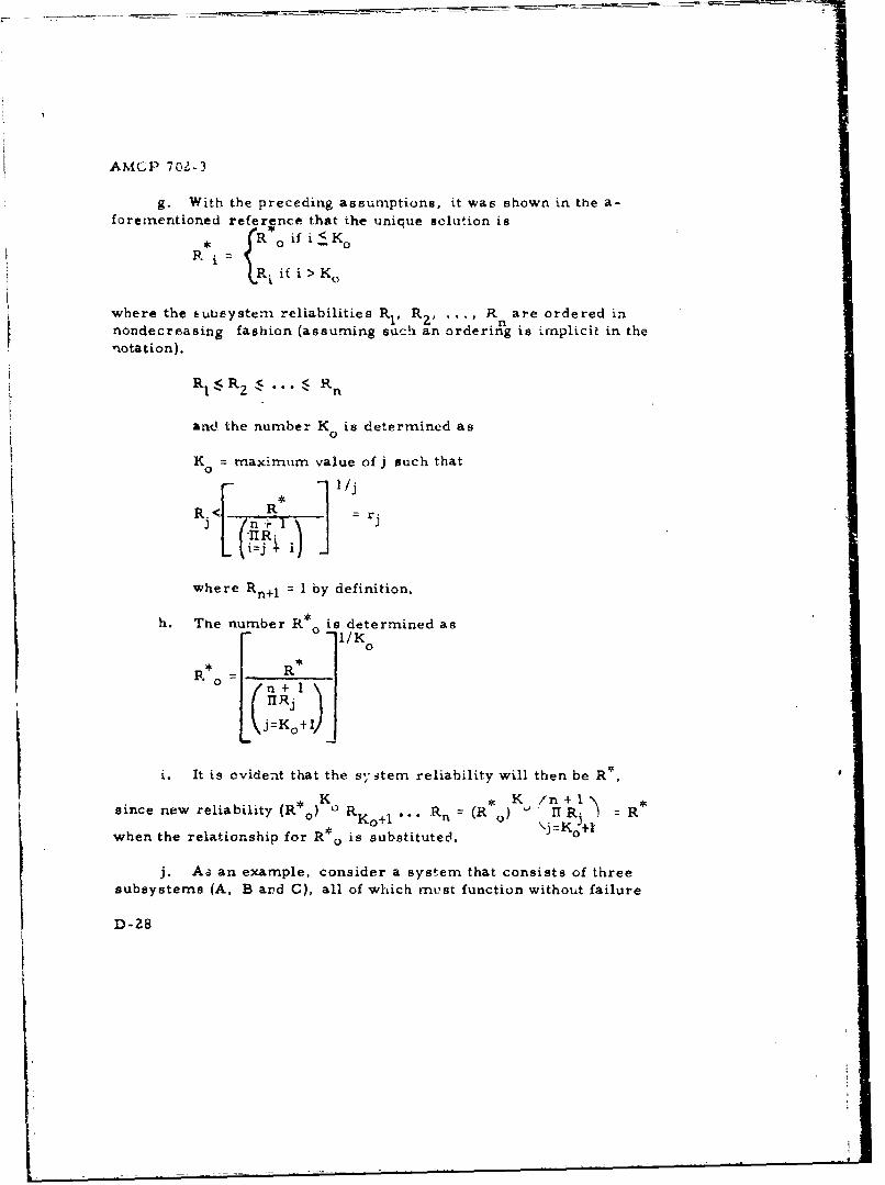
AMCP 70Z-3

g. With the preceding assumptions, it was shown in the a-forementioned reference that the unique solution is

S oif i Ko

R if i > K

where the EubSystem reliabilities R1 , Rz? ... R are ordered inn

nondecreasing fashion (assuming such an ordering is :mplicit in thenotation).

R, -< RL2 ... <Rn

and the number K is determined as0

K0 maximum value of j such that

R.< =r.J

where Rn+ I by definition.

.The number R is determined as-- /K 0

R*° 0 R*

n +l

(J=Ko+A/

i. It is evident that the sy item reliability will then be R•'

* ( R o K o *n ( K ,• / n + I *since new reliability (R..0RKol R = (R0) ,lR j =R

when the relat.ionship for R * 0 ssbtiue.j=K°+l,

j. Aa an example, consider a system that consists of threesubsystems (A, B and C), all of which mu~st function without failure

D-28

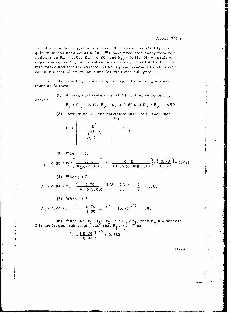
AMCP 702-3

in o: der to actuee system success. The system reliability re-

quirement has been set at 0. 70. We have predicted subsystem reli -

abilities as RA = 0. 90. RB - 0.80, and Pc = 0.85. How should weapportion reliability to the subsystems in order that total effort beminimized and that the system reliability requirement be satisfied?Assume identical effort functions for the three sahsystetiL.

k. The resulting minimum effort apportionment goals arefound as follows:

(1) Arrange subsystem reliability value3 in ascendingorder:

RI = RB = 0. 80; R = RC . 85 and R 3 RA = 0.90

(2) Determine Ko, the maximum value of j, such that" I/j

R. R ]r.

n+!~izj+11

(3) When= 1, 0.j0

rf

R 0. 80 <rl= 0.70 -0.70 =0.7 0.K9 1 5SR2R-ý(I. 00) (0. 85)(0. 90)(1. 00)_ 0. 765.

(4) When j = 2,

5 r 0.70 li/2 /7•I/2 088

(0.90)(1.00) \9. 3

(5) When i = 3,R o-g0 r 0. 70 _i/-k 0.70)./3

R 3 >r 3 1.00 =.888

(6) Since RI< rl, R2< r2, but R 3 > r 3 , then Ko = 2 because2 is the largest subscript j such that R < r.. Thus,J .J

0. 701/2R = 0.70 =0.882

0.90 '

D-29

AMCP 702-3

which means tnat the effort is to be allotted so that subsystem B

increases in reliLbility from 0. 80 to 0. 882, and subsystem C in-creases in reliability from 0. 85 to 0. 882; whereas subsystem A isleft alone with a reliability of 0. VI. T-ic resulting reliability of the

entire system is, as required, 0. 70 = (. 882)2 (. 90). This meansthat effort should be expended on subsystem C and B to raise theirrespective reliabilities to . 882 with no developmental effort spent onsubsystem A. This policy would minimize the total expended effortrequired to meet system reliability requirements. The minimization,however, is dependent upon the effort function meeting the initialassumptions.

D-15. Dyn.amic programrming approach to rcl.ability apportionment.

a. General. The preceding minimization of effort algorithmrequires that all subsystems be stibiect to the same effort function.

if all subsystems are not equally difficult to develop, dynamic pro-gramrming provides an approach to reliability apportionment withminimum effort expenditure when the subsystems are subject todifferent but identifiable effort functions.

b, Introduction to dynamic programming. To serve as abasis for formulation of such problems, a brief summary of theessential elements of the dynamic programming procedure follows.

(1) The dynamic programming technique is applicableto multi-stage (or sequential) decision problems. The technique con-verts such a problem to a series of single-stage optimiization problems.

(2) In additicn to defining the stages of such a process,four attributes of the problem must be identified if the technique is

to be applied.

(a) Sk ""l te set uf alh possible states of stage k.Its elemnents are designated as Sk, " e. I E Sk.

(b) Dk is the set of all possible decision alternativesavailable at stage k. Its elements are designated as ('k t Dk-

(c) T k(sk, dk) is a function transforming sk to Sk_1

D-30

1 j

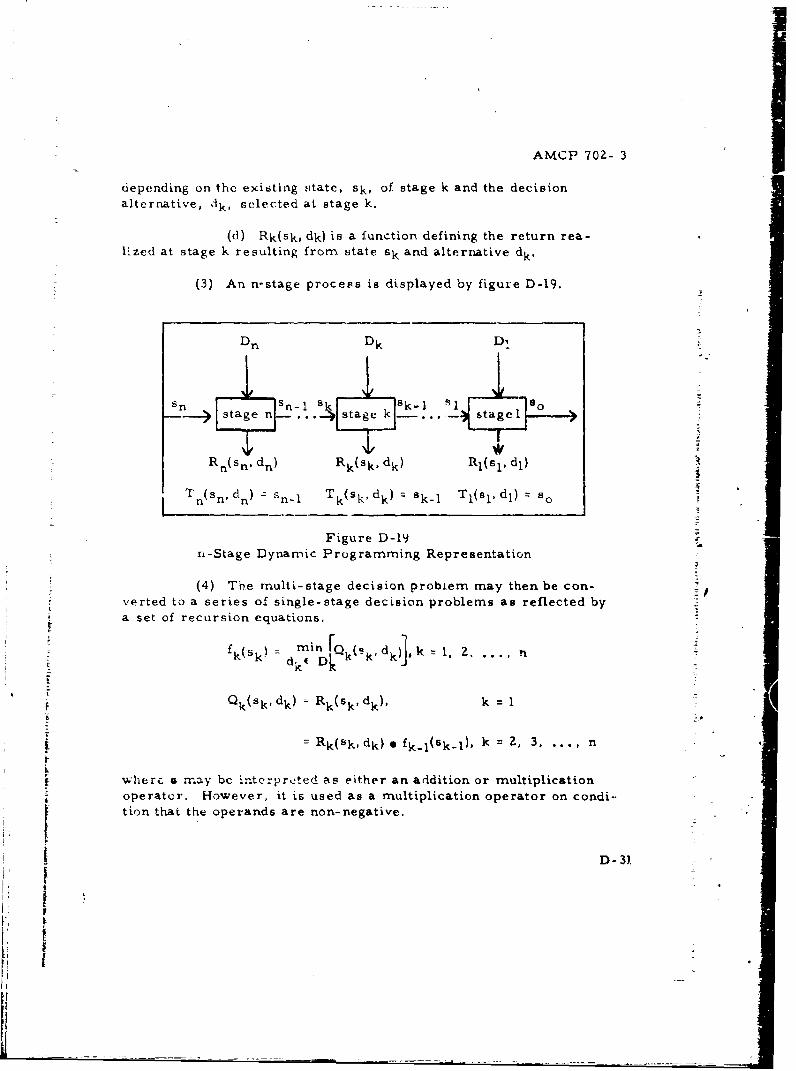
AMCP 702- 3

depending on thc existing state, Sk, of stage k and the decisionalternative, dk, selected at stage k.

(d) Rk(sk, dk) is a function defining the return rea-lized at stage k resulting from state sk and alternative dk.

(3) An n-stage process is displayed by figure D-19.

Dn Dk D,,n Sn- 8 I Isstage kstage 1

Rn(sn' dn) Rk(Sk. dk) RI(Sl* dl)

T(sn, d) Sn_1 Tk(sk, dk) = 5 k-l TI(sl,dl) d so

Figure D-19ni-Stage Dynamic Programming Representation

(4) The multi-stage decision probiem may then be con-verted to a series of single-stage decision problems as reflected bya set of recursion equations.

fkSk) dk D k -k' d k 1, Z.

Qk(sk, dk) Rk(Skdk), k

- Rk(sk, dk) 0 fk.l(Sk-l), k = 2, 3, ... n

Fwher a may be interpreted as either an addition or multiplicationoperator. However, it is used as a multiplication operator on condi-tion that the operands are non-negative.

D-31

I

~1

AMCP 702-

(5) ToenS-i

fnnim R (S dn)ffn(sn) Rd D -- n, n

is the total return which results from the optinill setof decision alternatives.

d* (d d 2.

(6) The a'ove forn-ittlation may be applied to a maximniza-tion objective by the )substitution of max fur min.

c. Subsystems oter-iting in series.

(1) The (ynamic programming formulation containedherein pertains to apportioameont of system reliability requirementamong series subsystems in such a manner to minimize the total ex-penditure of development effort. Some basic assumptions which are

fundamental to the formulation are:

(a) At any particular stage of the development program(at time of apportionment), the systemn can be partitioned into n sub-systems and that the present reliability level can be estimated for each

subsystem. Failure of any subsystem will cause system failure. Inaddition, it is assumed that the subsystem goal cannot be less than itsestimated present level.

(b) The n subsystems function independently so thatexpected system reliability resulting from the subsystem goals canbe expressed as the product of these subsystem goals:

ny = ITyi

i=l

where y is the system reliability goal and yi is the goal for the ithsubsystema.

(c) An effort function can be identified for each sub-

system, defining the number of units of development effort required

D-32

I

AMCP 702- 3

to raise its reliability level from the present value to any potentialreliability goal. The effort may represent a single important re-source or a combination of resources if these can be expressed bya common unit. The effort function may be either continuous or

discrete. A continuous mathematical function allows the reliabilitygoal to assume any value beitvi'e,, ihe estimated present level and

one. A discrete functi.r. lmhits potential suboystern goals to par-

ticular values.

(2) Consider a proposed system comprised of n sub-systems, each of which are to be developed independently. These

subsystems are to function independently and in series. What reli-ability goal should be assigned to each subsystem in order that thesysterr, goal be satisfied at a minimum expenditure of development

effort? Symbols to be used in problem formulation are defined as:

= system reliability goal, 0. Y-' 1

xi =reliability level of subsystem i at the present

state of development, 0<' xi< 1

Yi = reliability goal apportioned to subsystem i,xi< yi<

Gi(xi, yi) = units of development effort required to raisethe reliability level of subsystem i from xi to yi

n number of subbystems

S= reliability goal apportioned to subsystem i such

that total development effort is minimized.

(3) The problem may be formulated ý.s:

minimize iXl Gi(xi, yi)

nsubject to TI yi =y

i =1

xi <Yii = 1 2, n

D-33

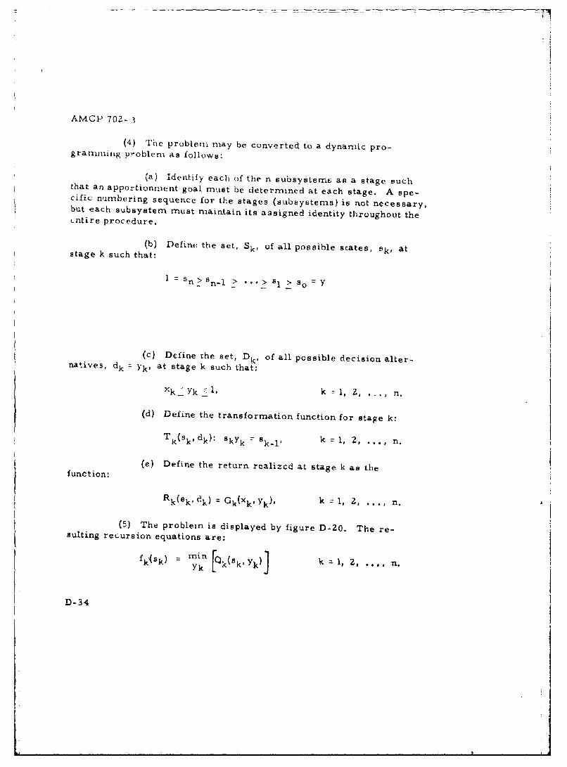
:1

AMCP 702- 3

(4) Tiie problemi may be converted to a dynamic pro-gran-ming p-'oblem as follows:

(a) identify each of the n subsysternt as a stage suchthat an apportionment goal must be determined at each stage. A spe-cific numbering sequence for the stages (subsystems) is not necessary,but each subsystem must maintain its assigned identity throughout the-ntire procedure.

(b) Define the set, Sk, of all possible states, sk, atstage k such that:

1 =Sn _> sn- ... > 61 > So y ,

(c) Define the set, Dk, of all possible decision alter-natives, dk Yk, at stage k such that:

Xk ' Y k l' 1,k = , Z. . . n

(d) Define the transformation function for stage k:

T (sk dk: ky = kI k = 1, 2, ..... n.

(e) Define the return realizcd at stage k as thefunction:

R k(sk, Ok) = Gk(xk'yk), k = 1, 2,... n.

(5) The problem is displayed by figure D-20. The re-sulting recursion equations are:

fkm krin yk)Jfk ) Y k IQk(sk' Y)k = , 2,.. n.

D-34

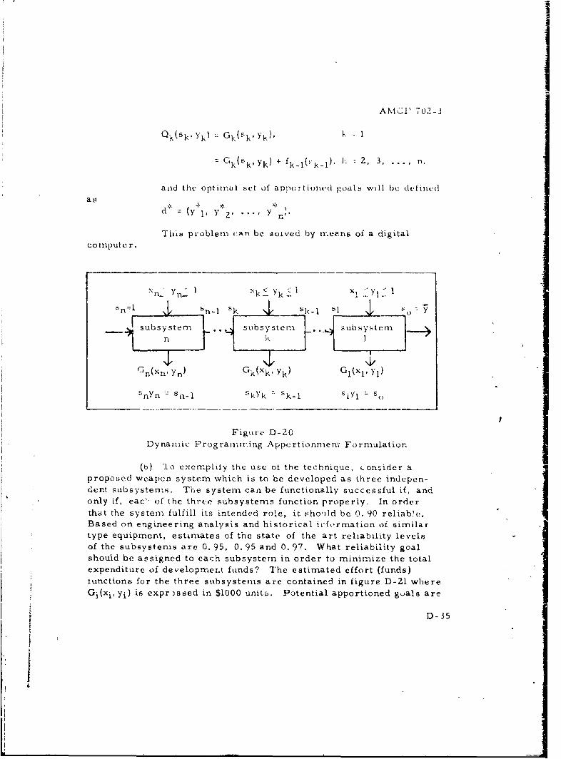
I

AMJVP 702-3

Qk(Sk, Y1,1 Gk(Sk Yk) -

CGk(bk, Yk) + fk-l(;k-l' k 2, 3, n.

and the optirnal set of apportioned goals will be definldas

= (Y l' Y . ' Y r "

This problem can be SoLved by n-eans of a digitalconmpute r.

ST_ 1 k1X .Y5n=n i-I • sk ,sk.1 y,-o

subsystem subsystcrnl subsystemn 4

Gn1("nYn) Gk(xkk'Yk) Gl(Xl, Yl)

-yn -' SIl 5kyk sk_1 sIy1 s

Figure D-20Dynairric Programmning Apportionmenm Forrmulation

(b) lo exemplify the use ot the technique, consider aproposed weapon system which is to be developed as three indepen-dent subsystems. The system can be functionally successful if, andonly if, eac' of the thrce subsystems function properly. In orderthat the system fulfill its intended role, it should be 0. 90 reliable.Based on engineering analysis and historical irformation of similartype equipment, estimates of the state of the art reliability levelsof the subsystems are 0. 95, 0. 95 and 0. 97. What reliability goalshould be assigned to each subsystem in order to minimize the totalexpenditure of developmer.t funds? The estimated effort (funds)functions for the three subsystems are contained in figure D-ZI whereGi(xi,Yi) is expr•-ssed in $1000 unitE. Potential apportioned goals are

D-35

*

i

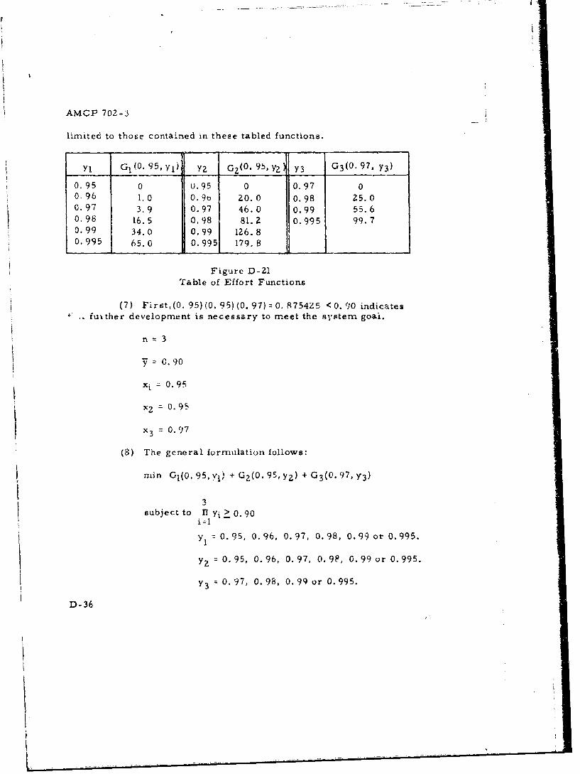
AMCP 702-3

limited to those contained in these tabled functions.

Yi G1 (0. 95, YI) YZ GZ(O. 95, ¶j Y3 G 3 (0. 97, Y3)

0. 95 0 u. 95 0 0.97 00. 96 1.0 O. 91 20. 0 0.98 25.00. 97 3.9 0.97 46.0 0.99 55, 60. 98 16.5 0.98 81.2 0.995 99.70.99 34.0 0.99 126.8

0.995 65.0 0.995 179. 8

Figure D-21

Table of Effort Functions

(7) First,(0. 95)(0. 95)(0. 97) = 0. 87542.5 <0. 90 indicatesfuither development is necessary to meet the system goai.

n~ 3

S:0.90

xi 0.95

x2 = 0.9 5

x 3 = O. 97

(8) The general formulation follows:

min GI(0. 95, vi) + G 2 (0. 95, YZ) + G 3 (0" 97, Y3)

3

subject to II Yi> o0.90i=1

Y = 0.95, 0.96, 0.97, 0.98, 0.99 or 0.995.

YZ =0. 95, 0. 96, 0. 97, 0. 9F, 0.99 or 0.995.

Y3 0. 97, 0. 98, 0. 99 or 0.995.

D-36

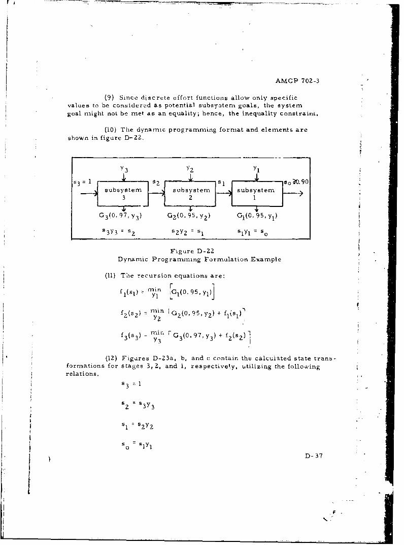
AMCP 702-3

(9) Since discrete effort functions allow only specificvalues to be considered as potential subsystem goals, the systemgoal might not be met as an equality; hence, the inequality constraint.

(10) The dynamic programming format and elements are

shown in figure D-ZZ.

Y3 Y? Yl

53= 1 sl 80 0.90subsystem subsystem subsystem

3 2 1

G 3 (0.97, y 3 ) G 2 (0.95, y2 ) GO(0.95, yl)

s 3 y 3 = szsy 2 Sly = so

Figure D-ZZDynamic Programming Formulation Example

(11) The recursion equations are:

f l (sl) .rain G(0. 9

min GZ(O. 95, Yz) + klsff

f 3 (s 3 ) = mur. G 3 (0' 97, y 3 ) + f2 (s 2 ) 1

(12) Figures D-23a, b, and c contain the calculated state trans-

formations for stages 3, Z, and 1, respectively, utilizing the followingrelations.

s13

62 = I3Y3

t

5, SS~D-37

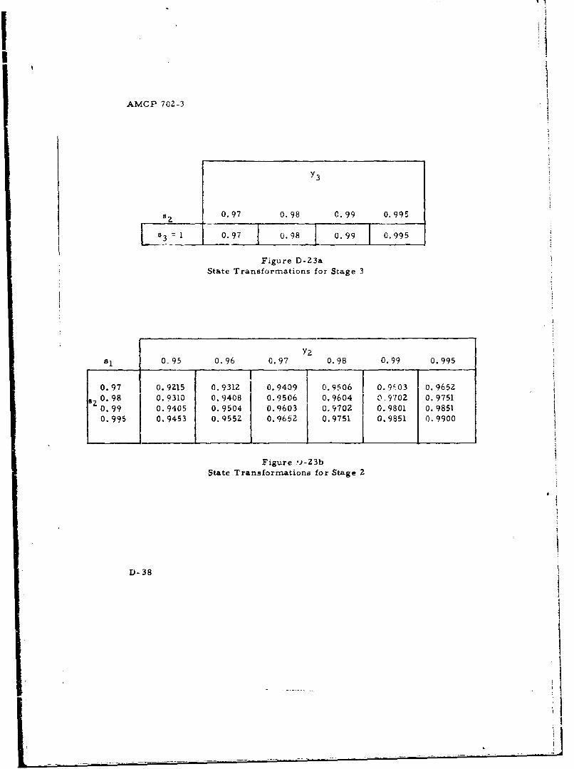
AMCP 702-3

Y3

5 0.97 0. 98 0.99 0.995

1 3= 1 .7 0.98 0.99 10.995

Figure D-23aState Transformations for Stage 3

Y20. 95 0.96 0.97 0.98 0.99 0.995

0.97 0. 9215 0.9312 0.9409 0.9506 0F . 9 03 0.9652a? 0. 98 0.9310 0.9408 0.9506 0.9604 0-9,702 0. 9751

0. 99 0. 9405 0. 9504 0.9603 0. 970Z 0. 9801 0. 9851

0.995 0.9453 0.955Z 0.9652 0,9751 0.9851 0.9900

Figure '.,.-23bState Transformations for Stage 2

D-38

_ _ _ _ _ _ ___ _ ____ ___ __1

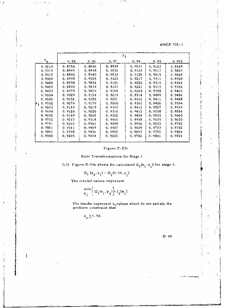
AMCP 702- 3

Yl0 0. 95 0.96 0. 97 0.98 0. 99 0. 995

0.9215 0. 8754 0.8846 0.8939 0.9031 0.9123 0.91690.9310 0. 8845 0.8938 0.9031 0. 9124 0. 9217 0.92630.9312 0.8846 0.8940 0.9033 0.9126 0.9219 0.92650.9405 0.8935 0.9029 0.9123 0.9217 0.9311 0.93580.9408 0.8938 0. 9032 0. 9126 0. 9220 0.9314 0.93610.9409 0.8939 0. 9033 0.9127 0. 9221 0. 9315 0.93620.9453 0. 8979 0. 9074 0. 9169 0.9263 0. 9358 0, 94050,9504 0.9029 0.9124 0.9219 0.9314 0.9409 0.94560,9506 0. 9031 0.9126 0.9221 0.9316 0.9411 0.9458

Ss 0.9552 0.9074 0. 9170 0. 9265 0. 9361 0. 9456 0. 95040.9603 0.9123 0.9219 0. 9315 0.9411 0.9507 0. 95550.9604 0. 9124 0.9220 0. 9316 0. Q412 0. 9508 0. 9556

0,.9652 0.,9169 0. 9265 0. 9362 0. 9458 0. 9555 0. 96030. 9702 0. 9217 0. 9314 0. 9411 0.9.508 0. 9605 0.96530. 9751 0. 9263 I0.9361 0. 9458 0. 9556 0. 9653 0.97020.9801 0. 9311 0.9409 0. 9507 0. 9605 0.9703 0. 97520. 9851 0. 9358 0. 945b 0. 9555 0. 9653 0. 975 0.98010.9900 0.9405 0.9504 0.9603 0.9702 0.9801 0.9851

Figure V-23c

State Transformations for Stage 1

(13) Figure D-24a shows the calculated 01lsly for stage 1.

QI (slyl) y G (0".95,y 1]The circled values represent

i I

The blanks represent sovalues which do not satisfy theV problem constraint that

B >0.90.lv 0-

D-39

rr

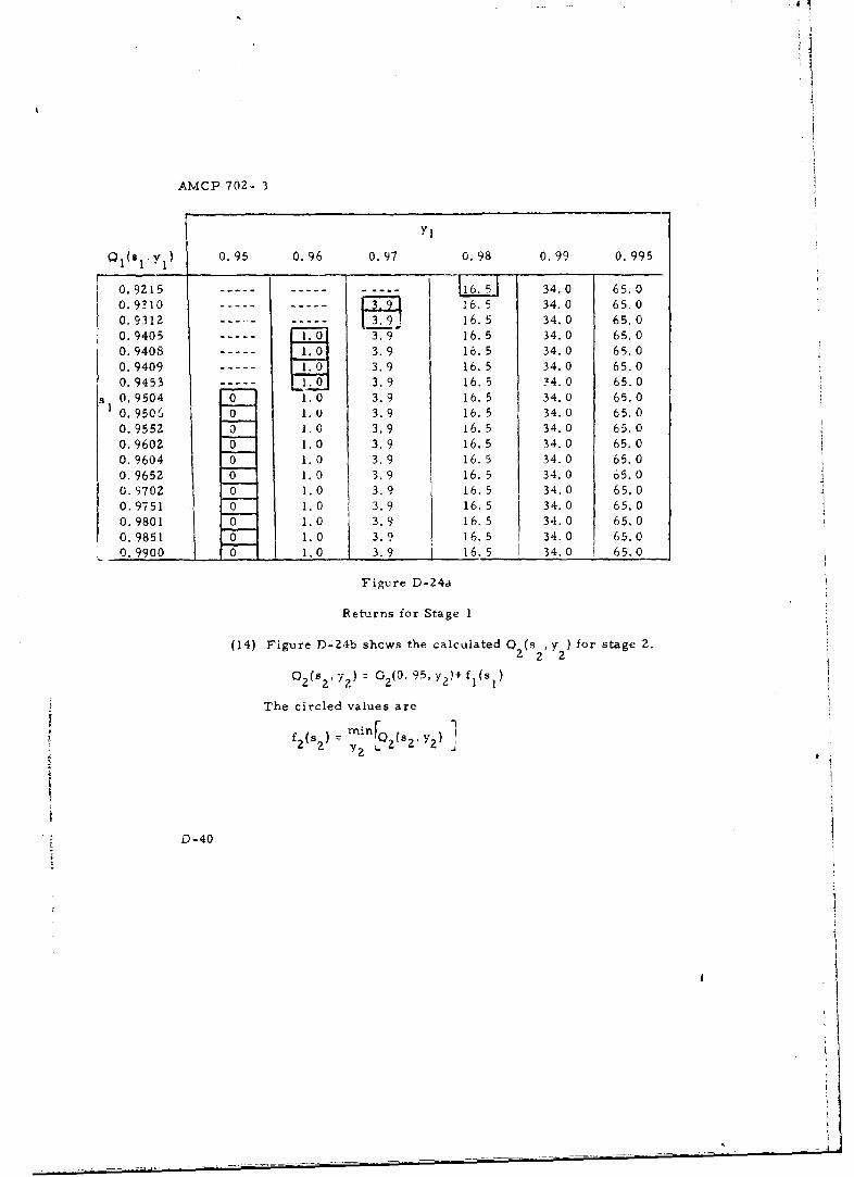
AMCP 702- 3

Yl

Q1 (s1 . y) 0.95 0.96 0.97 0. 98 0. 99 0. 995

0.9215 ----- 34.0 65.0

0.9-110 16. 5 34.0 65.00.9312 ----- 16. 5 34.0 65.00.9405 1.. 3.9 16.5 34.0 65. 00. 9408 1.0 3.9 16. 5 34.0 65. 00.9409 5.... 3.9 16. 5 34.0 65.00.94530 - 3. 9 16. 5 ?4. 0 65. 00. 9504 0 1.0 3.9 16.5 34.0 65.00. 9506 0 I.o 3. 9 16. 5 34.0 65. 00. 9552 0 1. 0 3.9 16. 5 34. 0 65. 00.9602 0 1. 0 3.9 16. 5 34.0 65.00. 9604 0 1. 0 3.9 16. 5 34.0 65. 00. 9652 0 1. 0 3.9 16. 5 34.0 65. 00. 9702 0 1.0 3.9 16. 5 34.0 65. 00.9751 .0 1.0 3.9 16. 5 34.0 65.00.9801 0 1.0 3.9 16. 5 34. 0 65. 00. 9851 0 1. 0 3.9 16. 5 34.0 65.00.9900 0 1.0 3.9 16.5 34.0 65.0

Figure D-24a

Ret-urns for Stage 1

(14) Figure D-Z4b shows the calculated 0 2(s, y 2) for stage 2.

Q 2 (s 2 , 72 ) z G2 (0, 95, y2 )+f I(s )

The circled values are

f2 (s2 ) (s Y. 2 Y2) ]

D-40

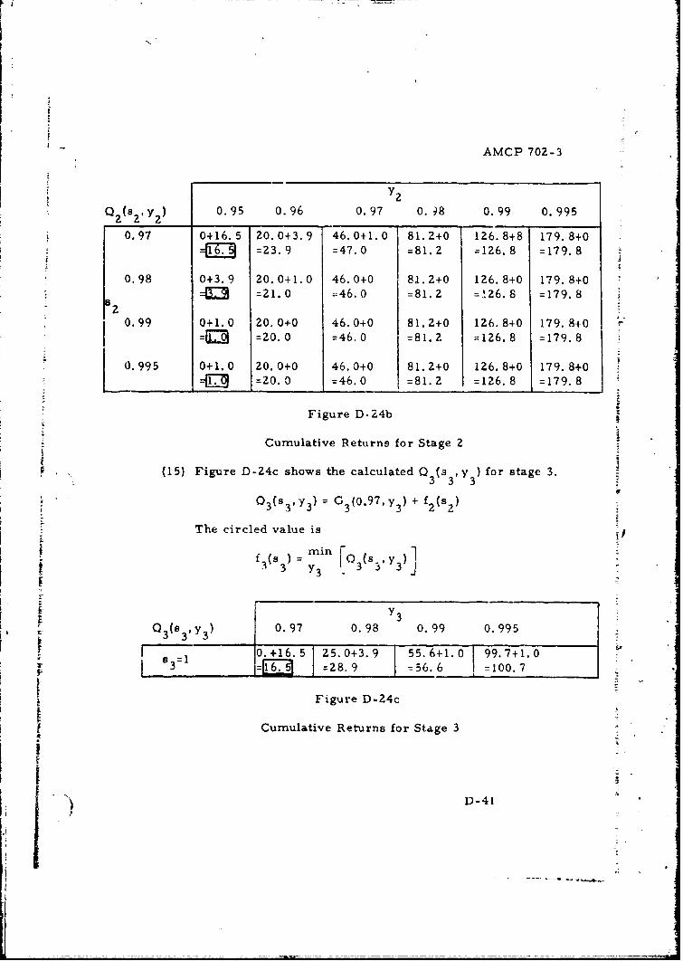
AMCP 702-3

y 2

Q (s, y2 ) 0.95 0.96 0.97 0. 98 0.99 0. 995

0.97 0+16.5 20.0+3.9 46.0+1.0 81.2+0 126.8+8 179.8+0=23.9 =47.0 =81.2 =126.8 =179.8

0.98 0+3.9 20.0+1.0 46.0+0 81.2+0 126.8+0 179.8+00903 =21.0 =46.0 =81.2 =!26.8 =179.8

0.99 0+1.0 20.0+0 46.0+0 81.2+0 126.8+0 179.8+0=Ml =20.0 =46.0 =81.2 =126.8 =179.8

0.995 0+1.0 20.0+0 46.0+0 81.2+0 126.8+0 179.8+0j_ =20.0 =46.0 = =81.2 =126.8 =179.8

Figure D-24b

Cumulative Returns for Stage 2

(15) Figure D-Z4c shows the calculated Q (a y for stage 3.

03 (s 3 ' Y3) = G 3 (o.97, y 3) + f2 (s2 ) 2

The circled value is

f 3 (S 3 ) = ra (s y iSY3 -

y Y3Q3(ay 3 ) 0.97 0.98 0.99 0.995

0.+16.5 25.0+3.9 55.6+1. 0 99.7+1.03 =16.5 =28.9 =56.6 =100.7

Figure D-24c

Cumulative Returns for Stage 3

"D-41

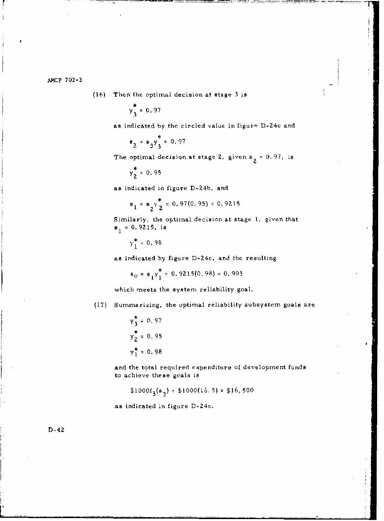
AMCP 702-3

(16) Then the optimal decision at stage 3 is

y 3 = 0. 97

as indicated by the circled value in figure. D-24c and

52 = s y = 0.97

The optimal decision at stage 2, given s= 0. 97, is

Y 0.95

as indicated in figure D-24b, and

6 2s V 2 = 0.97(0. 95) = 0.9215

Similarly, the optimal decision at stage 1, given thatS=0.9215, is1

S0. 98

as indicated by figure D-24c, and the resulting

so = slyl = 0. 9215(0. 98) = 0. 903

which meets the system reliability goal.

(17) Summarizing, the optimal reliability subsystem goals are

Y3 = 0.97

Y2 = 0.95

ya = 0. 98

and the total required expenditure of development fundsto achieve these goals is

$1000f 3 (s 3 ) = $i000(16. 5) : $16, 500

as indicated in figure D-24c.

D-4Z

AMCP 702- 3

d. Other uses of dynamic programming relative to reliabil-i ity. The dynamic programming optimization technique has applica-

!tion potential in other areas of reliability analysis. For example, use-

ful models have been developed for determining an optimal number ofredundant components (subsystems) subject to restraints such as weight,cost, volume, opposing failure modes, etc. Also, a dynamic program-ming model has been developed for providing a systems approach to

test planning, i. e., planning for an optimal number of tests.

D4

!I

}A

€IrI

I !'

SI-

I. -' I _ "•D-43

AMCP 702-3

APPENDIX L

RELIABILITY DESIGN

Sectioi, I, INTRODUCTION

E-1. General. This appendix is intended to supplement the reliabilitydesign discussion of chapter 5. It consists of an example illustratingthe role of prediction and apportionment activities during the develop-nient phase. The elements of awoortionment and prediction techniques

are described in chapter 4 and illustrated in appendix D.

Section IL EXAMPLE OF RELIABILITY PREDICTION AND APPOR-TIONMENT DURING THE DEVELOPMENT PHASE

E-2. Statement of Example. a. A weapon system to be used by the

U. S. Army field units was selected. Since this exercise is for ex-emplary purposes only, duplicate actLvities will be eliminated wherepossible. In other words, each and every subsystem will not be sub-jected to the entire analysis but only exemplary subsystems. Allclassified areas of the problem were evaded and data is hypothetical.

b. The system to be used is the 115 MM XM70E4 towed RocketLauncher. The objectives are to:

(1) Predict from the design and available data the reliabilityof the proposed 115 MM XM70E4 automatic rapid fire field artilleryweapon system.

(2) Determine whether the reliability predicted will satisfythe requirement.

(3) Propose an alternate set of requirements if the predictedreliability does not satisfy the requirement.

c. The product is defined as follows.

(1) Description of mission environment and use factors.

E

IE-I

AMCP 702-3

(a) The launcher rocket 115 MM XM7OE4 is a lightweight, towed, close support field artillery wc-apon system capableof automatically firing a six round burst of 115 MM anintinition,highly mobile, helicopter transportable, quickly emplaced in positionto fire.

(b) Transportable by any helicopter capable of a 3400 lb.load, can be towed by any present in service vehicle at 40 mph highwaytravel and 10 mph cross country, also capable of being air dropped.

(c) Programmed mode of fire from single shot to burstsof 2 to 6 rounds of 115 MM ammunition.

(d) Environment.

1. Thirty percer-t of the operation will he underprevailing environmental conditions with a temperature range between0 to 80 degrees Farenheit.

Sixty percent of the operation will be underprevailing environmental conditions with a temperature range between80 and 105 degrees Farenheit.

3. Ten percent of the operation will be ui der p'e-vailing environmental conditions with a temperature range between -25to 0 degrees Farenheit.

(e) Use conditions. Twenty-five miles of crosscountry towing per 1000 rounds fired under standard field conditions;"25 miles of helicopter sling transport per 1000 rounds of fire.

(2) Performance parameters and allowable limits, operatingmodes and functions, mission profiles and duty cycles.

(a) The 115 MM KM70E4 can be elevated from -5° to

700. Hand-wheeled powered track traverse Z00 each side of center lineor 400 total. Rapid traverse of 3600 by lifting trail.

(b) Fire 115MM ammunition in single shot fashion 12rounds per minute or automatically in bursts of 2 to 6 rounds or semi-automatically in single shot fashion where the number of rounds and modeof fire is preselected. The gun has a six round magazine.

E-2

AMCP 702-3

(c) Emplaced and trained on target. in less than 3 minutes.

(d) Range: Minimum range at maximum elevation 1000 m;maximum range 15, 000 m. The weapon must be c,;pable of changirgrange at the rate of 100m/sec. whilc simultaaeously changing the de-flection lay of the gun at the rate of 5 degrees of arc/sec.

(e) Accuracy: Horizontal range error at 80% maximumrango is to be 90 '1 of the rounds within 15m of the center of the set

range; deflection error at 80% maximum range is 90T6 of the roundsvithin 5m o)f center of set aitoing point.

(3) Reliability mission profiles.

(a) Mission A. Fire six, six round bursts; fire in theautornatic mode. Miniumn acceptable reliability is 0. 90.

(b) MiEsion 13. Fire 20 bursts - each burst less than sixrounds; fire in the automatic mode two to five round bursts. Minimumacceptable reliability is 0. 95.

(c) Mission C. Same as mission B. Firing rate is singleshot in the semiautomatic ri de. Mission is 120 rounds or 20 full loadsueni;,utomatic single round bursts. Minimum acceptable reliability is0.95.

(4) Function and physical boundaries, physical constraints,operating environment, physical parameters and configuration.

(a) Wcights:

Complete weapon with cover 3400 lbsRecoiling parts 1528 lbsTipping parts 1827 lbsCarriage assembly 1553 lbs

(b) Tires:Carriage wheel 7. 00 x 16, 6 plyPressure 45 PSI

(c) Recoiling Parts:

Breech Block Swing PivotFiring Mechanism Percussion Pin

Recoil System Hydro Pneumatic

E-3

i

AMCF 702-3

(d) Performance:Towing Speed 40 mph on highway

10 mph cross country

Angle of departure (long tow position)-27°

Ground clearance - 10 in.

Traverse - 3600

(e) Ammunition:115 MM Booster Rocket orConventional Projectile

(f) Firing CapabilitySingle roundSemiautomaticFull automatic - 6 rounds in 2 seconds

(g) Crew: 5

(h) Basic Lists RequiredParts ListListing of Parts Lists

List of DrawingsL>At of SpecificationsEquipment List

(i) MobilityTowedAir DropHelicopter Transportable

(5) Product failure is defined as a stoppage of function with notime for repair allowed. The system will have failed its mission if:

(a) Mission A fails to successfully complete an automa-tic six round burst (stoppage).

(b) Mission B fails to comple'e a burst of at least tworounds and no more than five rounds in auton atic firing mode (stoppage).

E-4

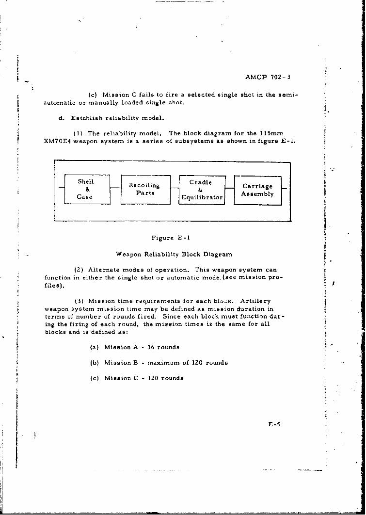
AMCP 702-3

(c) Mission C fails to fire a selected single shot in the semi-automatic or manually loaded single shot.

d. Establish reliability model.

(1) The reliability model. The block diagram for the 115mm.

XM70E4 weapon system is a series of subsystems as shown in figure E-1.

F Sheil _ Recoiling Crale CarriageS& Parts Equilibrator Assembly

Case e

Figure E-I

Weapon Reliability Block Diagram

(2) Alternate modes of operation. This weapon system can

function in either the single shot or automatic mode. (see mission pro-

files).

(3) Mission time req-uirements for each blo.;K. Artilleryweapon system mission time may be defined as mission duration in

S terms of number of rounds fired. Since each block must function dur-"ing the firing of each round, the mission times is the same for allblocks and is defined as:

(a) Mission A - 36 rounds

(b) Mission B - maximum of 120 rounds

(c) Mission C - 120 rounds

E-5

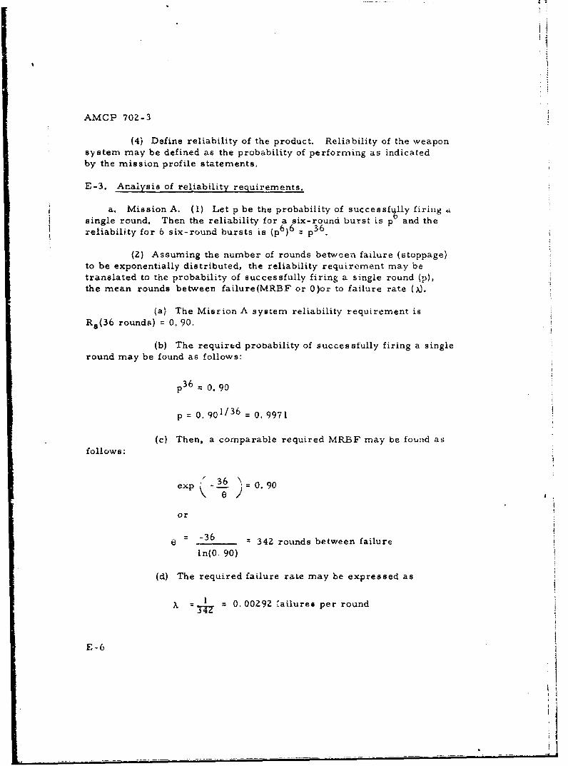
AMCP 702-3

(4) Define reliability of the product. Reliability of the weaponsystem may be defined as the probability of performing as indicatedby the mission profile statements,

E-3. Analysis of reliability requirements.

a. Mission A. (1) Let p be the probability of successfully firing asingle round. Then the reliability for a six-round burst is p and thereliability for 6 six-round bursts is (p 6 )6 - p 3 6

(2) Assuming the number of rounds between failure (stoppage)to be exponentially distributed, the reliability requirement may betranslated to the probability of successfully firing a single round (p),the mean rounds between failure(MRBF or 0)or to failure rate (?J.

(a) The Mission A system reliability requirement isR,(36 rounds) 0,90.

(b) The required probability of successfully firing a singleround may be found as follows:

p 3 6 = 0. 90

p = 0. 901/36 - 0. 9971

(c) Then, a comparable required MRBF may be found asfollows:

.' 36 hexp - 0.90

IJ

or

= -36 =342 rounds between failure

In(0. 90)

(d) The required failure rate may be expressed as

1 = 0. 00Z92 failures per round

E-6

l

AMCP 702-3

b. Mission B. (1) Since this mission allows for the automaticfiring of 2 to 5 rounds in a burst for 20 bursts or any combination of"2 to 5 round. (e. g., Z0 bursts of 2 rounds, 3 rounds, 4 rounds, 5rounds or a sequence of varied bursts, e. g. , 2, 3, 5, 4, 2, 2, 2, 4,3, 2, 2, 3, 3, 3, 5, 5, 4, 4, 2 and Z)or a total of 20 4 = 160,000possible mission combinations. It is an impractical task to determineeach possible combination. For the purpose of demonstration, tenbursts of 2 rounds each and ten bursts of 4 rounds each will be con-sidered as mission duration requirement. (Note total rounds are evenmultipies of six) In practice we miay consider those combinations re-presenting the most severe requirement.

(2) The system reliability requiremnent may be stated in any ofthe following ways.

(a) The mission B system reliability requirement isRs(60) 0. 90.

I

(b) The conparable p requirement may be found as follcws:

Rs(60) = p60 = 0. 95

p (0. 95)1/60 = 0. 999147

(c) The required MRBF is

- -60 = 1170 rounds between failure

(d) The required failure rate is

X - 1 - 0.000855 failures per round1170

c. Mission C. (1) Tnis mission requires the firing of 20 one shotfull loads semi-automatically (a total of 120 rounds).

(2) The system reliability requirement may be stated in any ofthe following ways.I .I

(a) The mission C system reliability requirement is

Rs(I 0) =0,95.

E-7

I

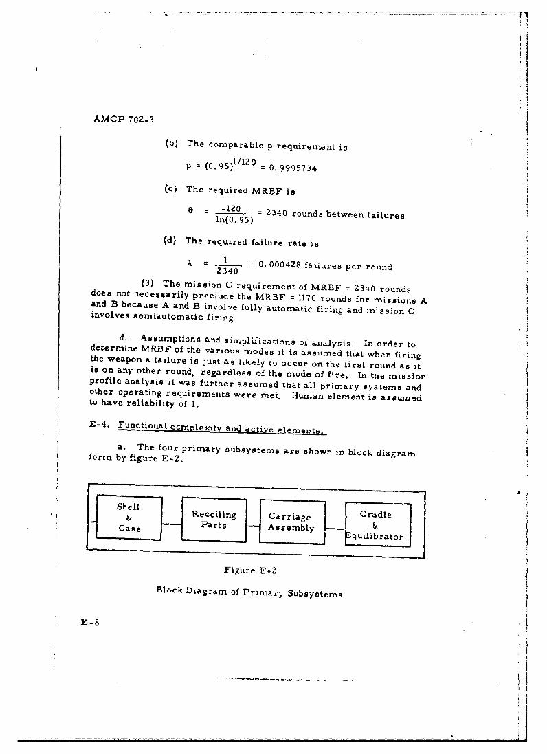
AMCP 702-3

(b) The comparable p requirement is

p = (0. 95)1/120 0 9995734

(c The required MRBF is

= -z-1-20 2340 rounds between failuresln(0. 95)

(d) The reouired failure rate is

=0. 000428 faii.ares per round2340

(3) The mission C requirement of MRBF 2340 roundsdoes not necessarily preclude the MRBF = 1170 rounds for missions Aand B because A and B involve fully automatic firing and mission Cinvolves semiautomatic firing.

d. Assumptions and simplifications of analysis. In order todetermine MRBe of the various modes it is assumed that when firingthe weapon a failure is just as likely to occur on the first round as itis on any other round, regardless of the mode of fire. In the missionprofile analysis it was further assumed that all primary systems andother operating requirements were met. Human element is assumedto have reliability of I.

E-4. Functional ccDilexity and active elements,

a. The four primary subsystems are shown in block diagramform by figure E-2.

Shell Cr-d 1-&Recoiling Carriage

Case Eat seml quilibrator

Figure E-2

Block Diagram of Prirna,5 Subsystems

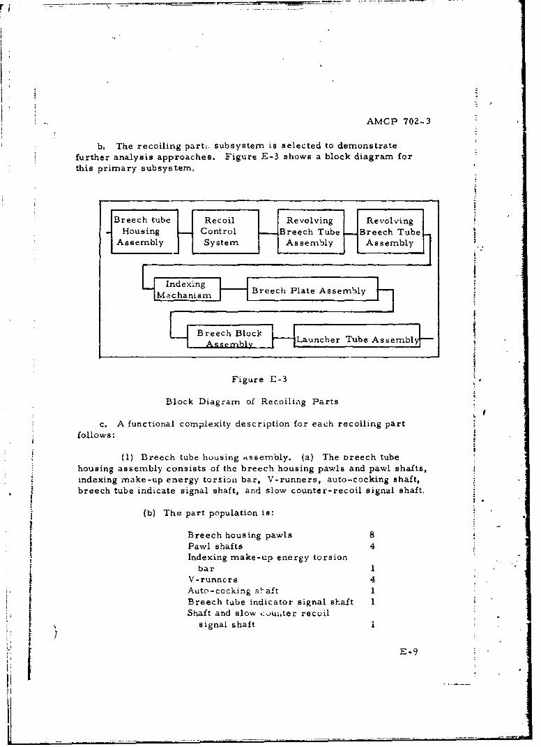
AMCP 702-3

b. The recoiling part. subsystem is selected to demonstratefurther analysis approaches. Figure E-3 shows a block diagram forthis primary subsystem.

Breech tube Recoil Revolving RevolvingHousing Control -Breech Tube -Breech Tube

Assembly System Assembly Assembly

IndexinghPltAs

[MechanismBrehlteAsmy

L BIre e ch Blo c k]I

Launcher Tube Assembl

Figure E-3

Block Diagram of Recoiling Parts

c. A functional complexity description for each recoiling partfollow s:

(1) Breech tube housing assembly. (a) The Breech tube

housing assembly consists of the breech housing pawls and pawl shafts,indexing make-up energy torsion bar, V-runners, auto-cocking shaft,breech tube indicate signal shaft, and slow counter-recoil signal shaft.

(b) The part population is:

Breech housing pawls 8Pawl shafts 4

Indexing make-up energy torsionbar 1

V-runners 4

Auto-cocking s~aft 1Breech tube indicator signal shaft 1Shaft and slow coui.ter recoil

signal shaft I

E-9

I

AMCP 702- 3

(2) Recoil control system. (a) The recoil system is a hydro-pneumatic arrangement. Two single acting recoil cylinders are connectedto a hydraulic accumulator. Interposed between the recoil cylinders andthe accumulator is a control system which will be referred to as thehydraulic recoil control.

(b) The part population is:Single acting recoil cylinders 2Hydraulic accumulator 1Manifold 1Recuperator 1Recuperator piston 1Recoil pistons 1Buffer pistons 1Buffer cylinders 1Cocker pistons 1Hydraulic recoil control block 1Recoil throttle valve 1Recoil flow control release 1Recoil signal orifice 1Check valve 4Counter recoil flow control valve 1Counter recoil orifice spool 1Orifice 1Anti-cavitation valve 1Spring actuated relief valve 1Indexing cock and release actuator 1Recoil timing valve 1Pressure actuated relief valve 1Recoil pressure regulator 1

(3) Breech tube assemblies. (a) Two assemn,!ic, consistingof three breech tubes each, are located in the breech tube housingbetween the front and rear bulkheads. Each assembly is composed ofthree smoothbore tubes fastened to a spider weldment.

E-lO

i •.

AMCP 702-3

(b) The part population is:Breech tubes 3Spider 1

(4) Indexing mechanism. (a) The indexing mechanism is anenergy-conserving type operated by torsion bar springs. With thismechanism, indexing motion is divorced from recoil motion.

(b) The part population is:Cam s 2Cam rollers 2Torsion bars 2Gears 6Worm gear I

(5) Breech plate assembly. (a) The breech plate assemblycovers the rear of the breech tube housing and contains the manualindexing linkage, firing mechanism and extractor linkage.

(b) The part population is:Firing mechanism 1

Extractor linkage ITorsion bar wind-up linkage 1Pawl release linkage 1

(6) Breech block assembly. The breech block is a swingingtype featuring center position loading. This allows firing single shotsfrom the same chamber without indexing.

(7) Launcher ttube. The single 115mrn launcher tube is P

mounted in the indexing mechanism housing. The tube which weighs147 pounds is progressively rifled. Gunner's quadrant pads are pro-vided on the top of the tube for checking tube elevation.

E-5. Prediction of failure rates for primary subsystems. a. Recoil-parts subsystem. In order to establish failure rates, available test

1i

E-I

E-1 1

AMCP 702- 3

data, supplemented by data from FARADA, were used.

(1) Breech tube housing assemhly. Past firing data onearly experimental rapid fire weapons of this type have shown thatapproximately four failLres per 6, 000 rounds occurred to the breechtube housing assembly. Therefore, we will assign a failure rate of4 failures ver 6, 000 rounds or 1500 MRBF.

(2) Recoil control system. The recoil control systemis basically a hydraulic system consisting of hydraulic pistons and ahydraulic valve network in a single manifold. Figure E-4 shows atabulation of the number of different types of valves in the system,and the estimated failure rates.

Quantity Estimated TotalValve Type in Failure Failure

_ _System Rate Rate :,

CheckValves 4 50/106 hrs. 200/106 hrs.

Control Valves 3 100/106 hrs. 300/106 hrs.

Relief Valves 2 100/106 hrs. 200/106 hrs.

Estimated Total System Failure Rate 700/106 hrs.

Figure E-4

Valve Failure Rate Data

*To convert failures per 106 hours to failures per round, we assume

an average of approximately 10 rounds per hour. Estimated failurerate for this system then is 7 failures/ 00, 000 rounds.

E-IZ

AMCP 702-3

(3) Indexing mechanism, The indexing mechanism. isessentially a gear train, therefore gear failure rates may be used toestimate the MRBF. Figure E-5 shows failure rates obtained fromFARADA on similar parts.

TotalPart Quantity Failure Fail

Rat Rate

Cams 2 l/104 hrs. ./104 hrs.

Rollers 2 0. 5/104 hrs. 1/104 hrs.

Gears (spur) 6 Z/10 4 hrs. 12/104 hrs.

Worm GearAssembly 1 10/104 hrs. 10/10 4 hrs.

Subsystem Total Failure Rate 25/104 hrs.

Figure E-5

Indexing Mechanism Parts Failure Rate DatatV

*Using 10 rounds per hour as an average firing rate, the failure ratein terms of rounds fired is 25 failures/100, 000 rounds.

b. Other subsystems. (1) No historical failure data are availablefor the following items:

(a) Breech tube assemblies

F (b) Breech plate assemblies

(c) Breech block assemblies

(d) Launcher tube

E-13

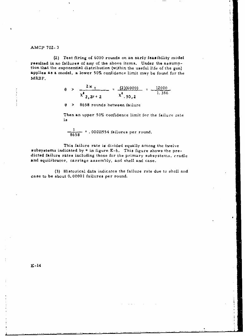
AMCP 702- 3

(2) Test firing of 6000 rounds on an early feasibility modelresulted in no failures of any of the above items. Under the assump-tion that the exponential distribution (within the useful 14fe of the gun)applies as a model, a lower 50% confidence limit may be found for theMRBF.

SZX t (2)(6000) 120001.386S2, + 2 .50,2

0 > 8658 rounds between failure

Then an upper 500/% confidence limit for the failure rateis

1 00011554 failures per round.8658 "

This failure rate is divided equally among the twelvesubsystems indicated by * in figure E-6. This figure shows the pre-dicted failure rates including those for the primary subsystems, cradleand equilibrator, carriage assembly, and shell and case.

(3) Historical data indicates the failure rate due to shell andcase to be about 0. 00001 failures per round.

E-14

I ---~--~--- ~- ------- -- --- -

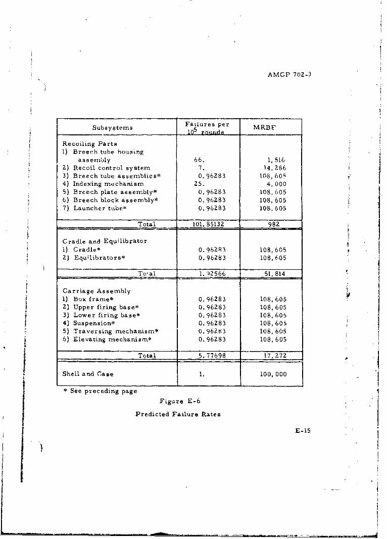
AMGP 702-3

Failures per MRBFSubsystems 0 rou ndBs 1

Recoiling Parts1) Breech tube housing

assembly 66. 1, 5162) Recoil control system 7. 14, 2863) Breech tube assemnblies* 0. 96283 108, 605 I4) Indexing mechanism 25. 4,0005) Breech plate assembly* 0. 96283 108, 6056) Breech block assembly* 0. 96283 108, 6057) Launcher tube* 0.96283 108,605

Total 101. 85132 982

Cradle and Equilibrator1) Cradle* 0. 96283 108, 6052) Equilibrators* 0. 96283 108,605

Total 1. 'ý2566 51,814

Carriage Assembly1) Box frame* 0. 96283 108,6052) Upper firing base* 0.96283 108,6053) Lower firing base* 0. 96283 108, 6054) Suspension* 0. 96283 108,6055) Traversing mechanism* 0. 96283 108,6056) Elevating mechanism* 0. 96283 108, 605

Total 5.77698 17, 272

Shell and Case 1. 100,000

* See preceding page

Figure E-6|

Predicted Failure Rates

E-15

)

-i

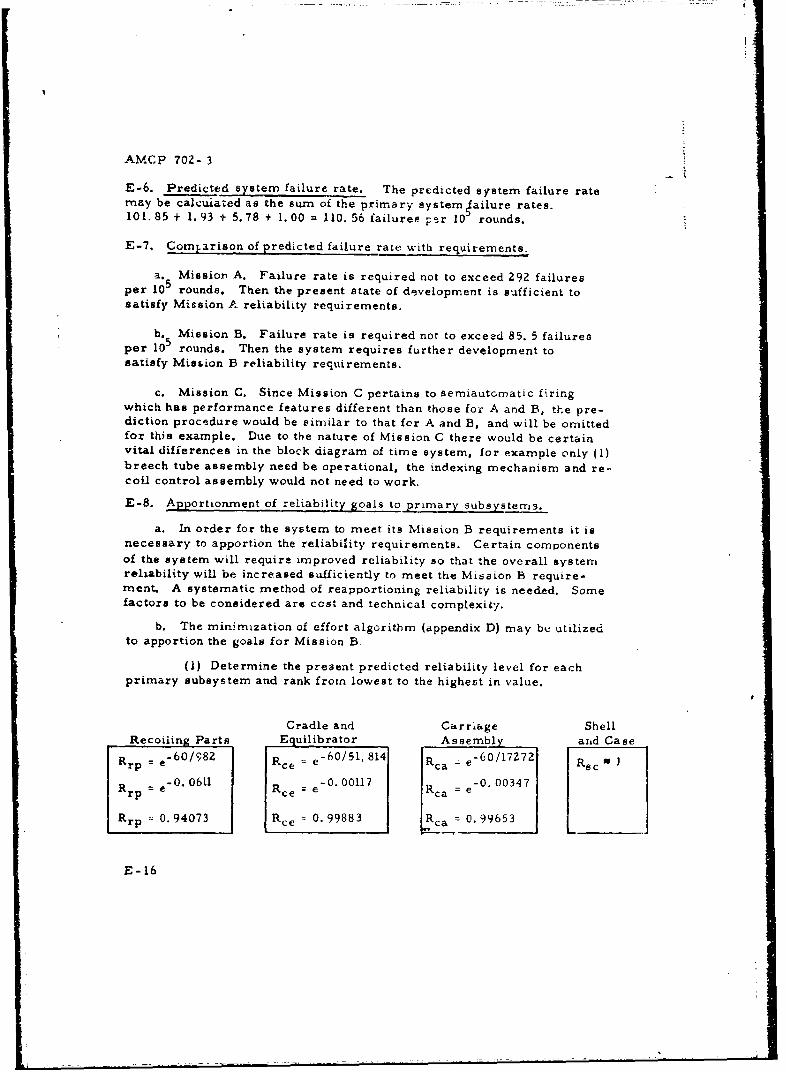
AMCP 702- 3

E-6. Predicted system failure rate. The predicted system failure ratemay be calcuiated as the sum of the primary system ailure rates.101.85 + 1.93 + 5.78 + 1.00 = 110. 56 failures per 10 rounds.

E-7. Comparison of predicted failure rate with requirements.

a. Mission A. Failure rate is required not to exceed 292 failuresper 105 rounds. Then the present state of development is sufficient tosatisfy Mission A reliability requirements,

b. Mission B. Failure rate is required not to exceed 85. 5 failuresper 10 rounds. Then the system requires further development tosatisfy Mis&ion B reliability requirements.

c. Mission C. Since Mission C pertains to semiautomatic fi'ringwhich has performance features different than those for A and B, the pre-diction procedure would be similar to that for A and B, and will be omittedfor this example. Due to the nature of Mission C there would be certainvital differences in the block diagram of time system, for example only ({)breech tube assembly need be operational, the indexing mechanism and re-coil control assembly would not need to work.

E-8. Apportionment of reliability goals to primary subsystem3.

a. In order for the system to meet its Mission B requirements it isnecessary to apportion the reliability requirements. Certain componentsof the system will require improved reliability so that the overall systemreliability will be increased sufficiently to meet the Mission B require-ment. A systematic method of reapportioning reliability is needed. Somefactors to be considered are cost and technical complexity.

b. The minimization of effort algorithm (appendix D) may bu utilizedto apportion the goals for Mission B.

(1) Determine the present predicted reliability level for eachprimary subsystem and rank from lowest to the highest in value.

I

Cradle and Carriage ShellRecoiling Parts Equilibrator Assembly. ad Case

Rrp =e-6 o/1 8 2 Rce e-6 0/51, 814 Rca e-6 0/17 2 7 2 Rec

Rr e_0.0611 Rc =e- .01 e-0. 00347

Rrp = 0. 94073 Rce 0. 99883 Rca _ 0. 99653

E-16

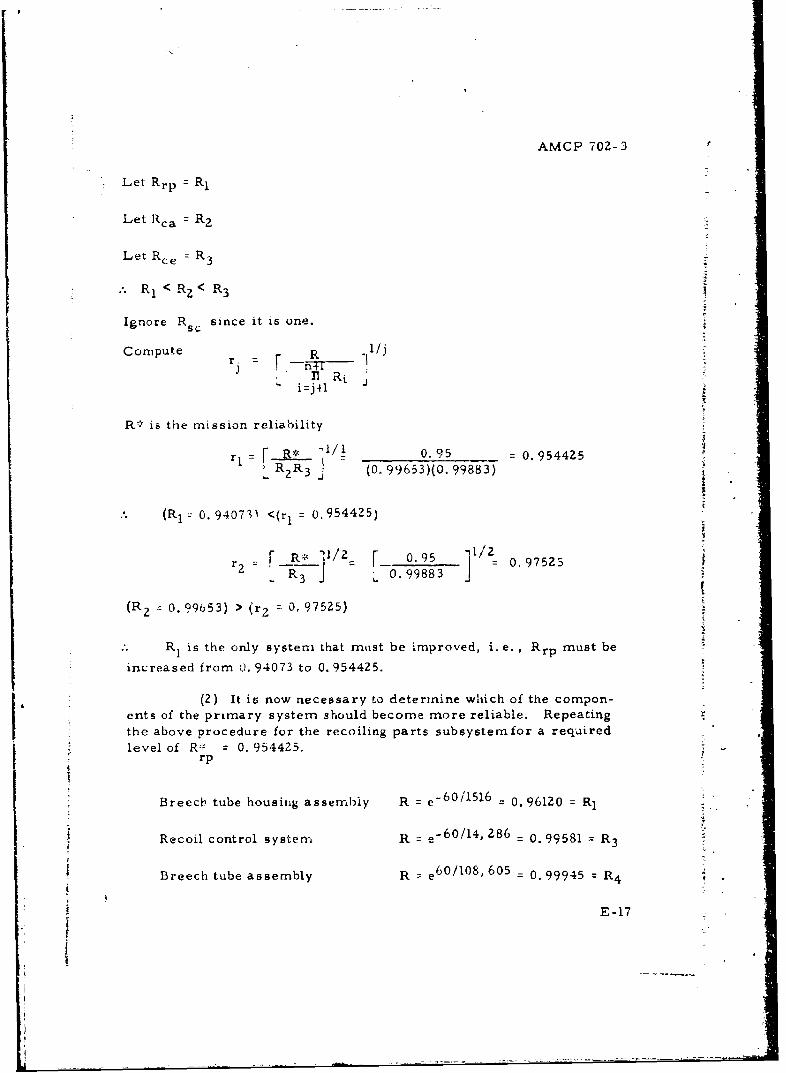
AMCP 702-3

Let Rrp = Rl

Let Rca = R7

Let Rce R3

R, < R2 < R 3

Ignore Rsc since it is one.

Compute R 1/jS--nRi

"izj+l

R:ý' is the mission reliability

rl= [ R* ]I/_ 0.95 - 0.954425R 2 R 3 (0. 99653)(0. 99883)

(Ri 0. 94073 <(r = 0.954425)

r? = F R*4]/2 [ 0.95 ] / 0.97525tR 3 J 0. 99883

(R 2 0. 99b53) > (r 2 0, 97525)

R 1 is the only system, that rmist be improved, i. e., Rrp must be

increased from 0. 94073 to 0. 954425.

(2) It is now necessary to determine which of the compon-ents of the primary system should become more reliable. Repeatingthe above procedure for the recoiling parts subsystemfor a requiredlevel of R* 0. 954425.

rp

Breech tube housing assembly R e-6 0/15 6 0. 96120 =R

Recoil control system R e-60/14, 286 = 0. 99581 R

Breech tube assembly R e 6 0 /1 0 8 ' 605 = 0. 99945 R4

E-17

Li

I!

AMCP 702-3

Indexing mechanism R e- 6 0/4000 0. 98511 R,

Breech plate assembly R e- 6 0 /1 0 8 , 605 = 0. 99945 ý R

Breech block asa..i,!y R e-60/108, U05 z 0. 99941 - R6

Launcher tube assembly R e- 6 0/108,605 0.99945 R7

RI< RZ<R 3 <R 4 <R 5 <R 6 <R 7

~i=j+l i

r 0.954425 0.954425 ] . 97507L R . 3 P v4"R 5R6 -J -(0. 9851l)(0. 99581)(0. 99945)4 .

(R 1 = 0o 96120) < (r, = 0. 97507)

r2 0.9544255 0.96055L (0. 99581)(0. 99945)

(RZ 0. 98511) >r 2 = 0.96055)

The breech tube housing assembly is the only subsystem that must beimproved. Therefore in order for the recoiling parts to acquire areliability 0. 954425, the breech tube housing assembly reliabilitymust be increased from 0. 96129 to 0. 97507.

(3) Then for Mission B

Rs = RrpRceRcaRsc

Re = (0. 9544Z5)(0. 99883)(0. 99653XI)

Re =0.95

E-18

• ,l = " • i , i, :• , .. . . . . .

AMCP 702-3

The breech tube housing assembly must have a reliability of 0. 97507or a maximum failure rate of

1 in (0. 97507) = 41 failures per 105 rounds60

E-9. An alternatc mc}•hoc ot apportionment. a. The procedure 3fMinimum Effort illustrated above assumes that the effort (time, money,resources, etc.) to be expended in improving any of the subsystems isequivalent. Obviously this is not always a good assumption. A moregeneral approach to the problem is the technique of dynamic programmingdescribed in appendix D.

b. This technique, though general in nature, requires that a costand improvement relationship be specified. As a result it is mnoredefinitive and requires knowledge about the economy of improving specificsubsystems such as cost of improvemrnent per incremental jump.

c. Since thev'e are no such data available for the preceding system,- a hypothetical cost function will be used as an example. The problemSmay be formulated as follows.

Minimize 3

SL Ci (xi yi)

i=l

Subject to y > y

K xi < Yi <1

xi is the existing reliability level of subsystem i

Yi is the level to which subsystem i should be improved.£

Gi (xi , = amount of effort required to raise the reliabilityL level of subsystem from xi to Yi.

E

I E-19

I;

AMCP 702-3

y is the system reliability goal or requirement for

Mission B.

R(Mission B) = 0. 95

Rrp = 0.94073 = x

Rce = 0.99883 = xz

Rca = 0.99653 = x,

Rsc 1, i. e. , it will be ignored since it is not likelythat reliability can be improved. For this example let the cost be as

described in figure E-7 with cost expressed in thousand dollar unitsrequired for additional development. (Note: Due to lack of cost

data, the following figures are purely hypothetical).

Yl G(0. 94, yl) YZ GZ(O. 99883, y 2 ) Y3 G 3 (0. 9965, Y3)

0.94 0 0. 99883 0.0 0.9965 0

0. 945 40.0 0. 9990 200. 0 0. 9970 100

0.95 120.0 0.9992 600.0 0. 9975 200

0. 955 480.0 0. 9994 2400. 0 0. 9980 600

0.96 2400.0 0. 9996 12000.0 0. 9985 2400

0. 965 14,400.0 0. 9998 72000.0 0. 9990 12, 0000.97 100, 800.0 0. 9999 504000.0 0. 9995 72,000

0. 975 907, 200.0 0. 99999 4032000.0 0.9999 504,000

Figure E-7

Cost Function for Increasaing Reliability

The computer yields the following solution

Subsystem 1 Goal = 0. 95500



E-Z0

AMCP 702-3

Requiring 480.00 units of effort (cost)

Rs Z RIR 2 R 3 = 0.95054

This indicates that the recoiling parts subsystem relia-

bility should be increased to 0. 955.f

E-10. Stress-strength design. In the design of mechanical hardware, jtithe interrelationship of stress-strength distributions is often inves-

tigated to insure that the probability of over-stress failures is atan acceptable level. This method of statistical design evaluationutilizes the estimated or known stress levels to be encountered in

conjunction with material properties, in order to obtain a designwhich normally minimizes weight and cost due to overdesign. De-

sign engineers who use strength of materials, techniques will find

this method easy to master and useful when reliability is of prime

concern.

E-1 1. Summary. a. The entirety of this appendix has been to ex-empiify early prediction and apportionment. The numerical accuracy

used has been unrealistic in the face of grossly estimated data and

simplifying assumptions.

b. It should also be noted that there are several procedures

available for prediction and apportionment, all of which must bemodified to satisfy a given project. The methodology described here-in was to demonstrate the procedur= and was chosen primarily for

ease of discussion.

-2

I.

I

E-2l

-I!

N

AMCP 702- 3

APPENDIX F

DEMONSTRATION AND TESTING


F-1. General. a. The materials contained in this appendix areintended to supplement the discussions in chapter 6. The contentincludes sume typical statistical analysis techniques associated withreliability demonstration and testing along with some brief examples.This is not an exhaustive coverage of available techniques, but asummary of some typical and basic techniques. A more thoroughcoverage may be found in the various published reliability literature.

b. These techniques pertain to inferences about certain reliabilityrelated parameters from sample test results. Coverage includesboth estimation of and hypothesis testb about such parameters. Thedistributions and parameters covered are those discussed in appen-dix A.

Section II. PARAMETER ESTIMATION

F-Z. General. a. The principles of statistical estimation maybe applied to the results of sample tests to estimate reliabilityparameters. The principle of parameter estimation may be illus-trated by considering a random variable X with a density functionf(x) which is described by a parameter 8. Suppose we make nindependent observations on X, i.e., x 1 , x, .... x. Analysisof these values will allow us to estimate 6 by:

(1) A point estimate designated as 0 and/or

(2) A confidence statement that

A< <B B

where A and B are dependent upon the specified degree of confidencerequired and may be found by performing an appropriate analysis on

the sample observations.

F-1

i"

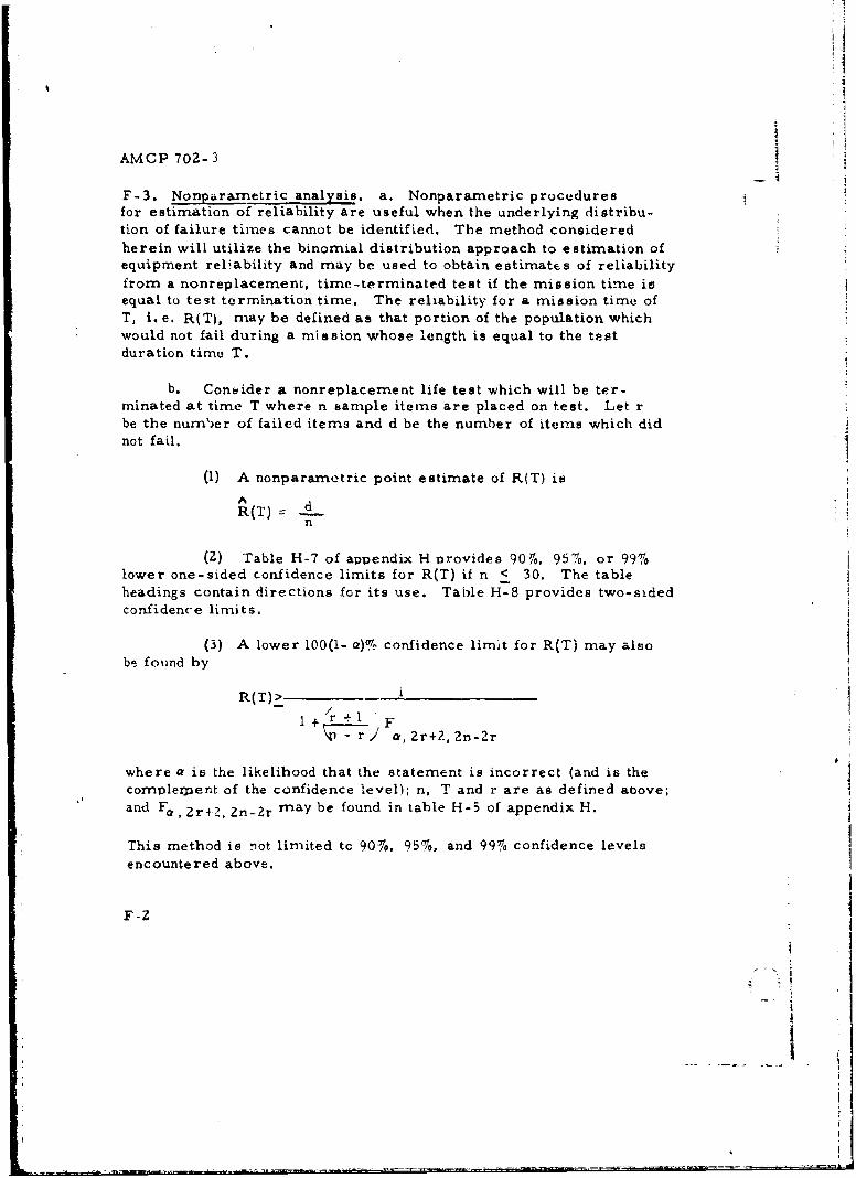
AMCP 702- 3

F-3. Nonparametric analysis, a. Nonparametric proceduresfor estimation of reliability are useful when the underlying distribu-tion of failure times cannot be identified. The method consideredherein will utilize the binomial distribution approach to estimation ofequipment reliability and may be used to obtain estimates of reliabilityfrom a nonreplacement, time-terminated test if the mission time isequal to test termination time. The reliability for a mission time ofT, i. e. R(T), may be defined as that portion of the population whichwould not fail during a mission whose length is equal to the testduration time T.

b. Consider a nonreplacement life test which will be ter-minated at time T where n sample items are placed on test. Let rbe the number of failed items and d be the number of items which didnot fail.

(1) A nonparametric point estimate of R(T) is

R(T) = dn

(2) Table H-7 of appendix H provides 90Y716 95TF!, or 99%lower one-sided confidence limits for R(T) if n < 30. The tableheadings contain directions for its use. Table H-8 provides two-sLdedconfidence limits.

(3) A lower 100(1- a)% confidence limit for R(T) may alsobe found by

R(T)_>- .

I + Ai r+- rj a,2r+2,2n-2r

where a is the likelihood that the statement is incorrect (and is thecompleropent of the confidence level); n, T and r are as defined above;and Fa, 2r42, 2n-2r may be found in table H-5 of appendix H.

This method is -not limited tc 9076, 95%76, and 99% confidence levels

encountered above.

F-2

!:I

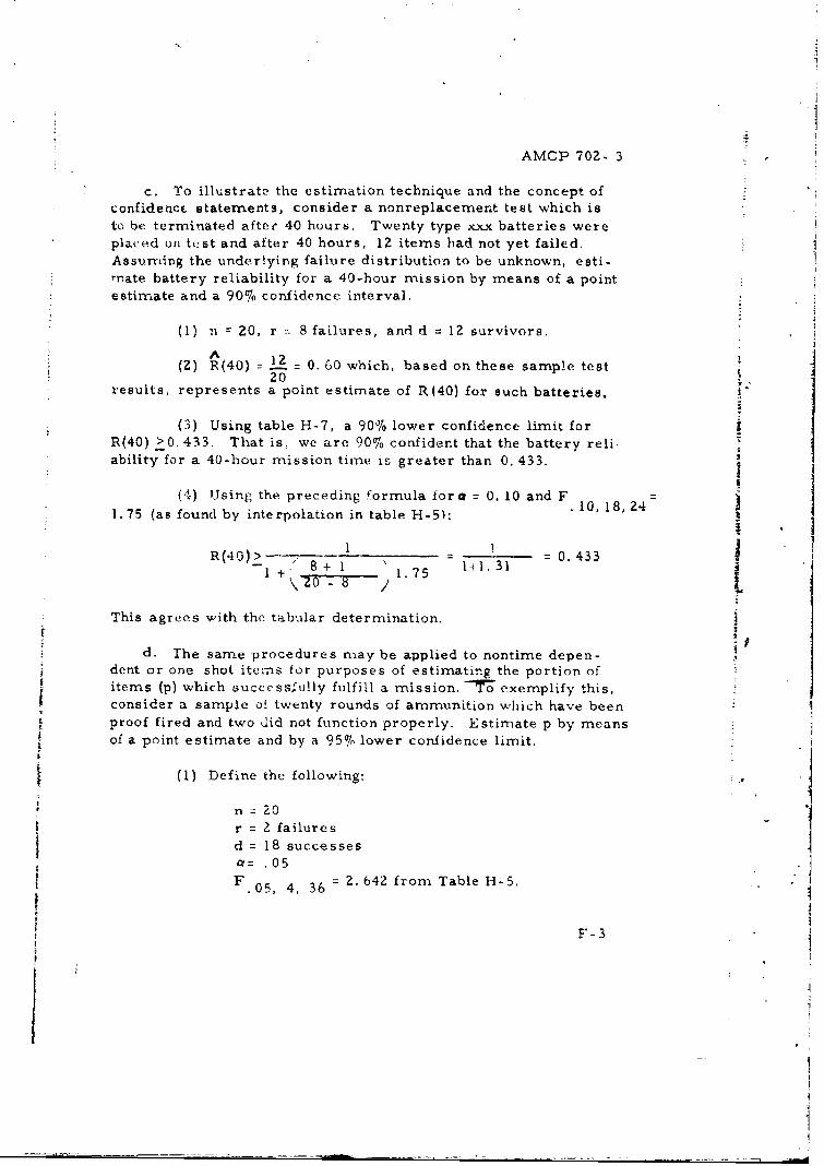
AMCP 702- 3

c. To illustrate the estimation technique and the concept ofconfidence statements, consider a nonreplacemnent test which isto be terminated after 40 hours. Twenty type xxx batteries wereplaced on test and after 40 hours, 12 items had not yet failed.Assuming the underlying failure distribution to be unknown, esti-Ymate battery reliability for a 40-hour mission by means of a point

estimate and a 90% confidence interval.

(1) n 20, r 8 failures, and d 12 survivors.; A

(Z) R(40) = 12 = 0. 60 which, based on these sample test20

results, represents a point estimate of R(40) for such batteries.

(3) Using table H-7, a 90% lower confidence limit forR(40) >0. 433. That is, we are 90% confident that the battery reli-ability for a 40-hour mission time is greater than 0. 433.

(4) Using the preceding formula fora = 0. 10 and F1.75 (as found by interpolation in table H-5): .10,18,24

R(40). 0.433R +' 8 + 1 1+1.31I- + 1.75

This agrees with the tabular determination.

d. The same procedures nmay be applied to nontime depen-dent or one shot items for purposes of estimating the portion ofitems (p) which success,"ully fulfill a mission. -'- exemplify this,consider a sample of twenty rounds of ammunition which have been

proof fired and two did not function properly. Estimate p by meansof a point estimate and by a 95% lower confidence limit.

(1) Define the following:

n =0

r = 2 failuresd = 18 successes f

a= .05F.5 4,3 2 . 642 from Table H-5.

F-3

Ii

I

AMCP 702-3

(2) A point estimate of p is 1-=8= 0.90.

n 20

(3) Using table H-7, a 95% lower confidence limit forp is

p • 0. 717

In other words, there is 95% confidence that at least 0. 717 of allrounds will perform successfully.

(4) By formula, a 95% lower confidence limit for p maybe found as

I -0. 694i + 3 4 1.44

S F-4. Determination of underlying distribution, a. More preciseestimates of reliability parameters can be obtained if the underlyingdistribution of failure times can be determined. Certain goodness offit tests can be applied to test failure times for determining whethera hypothesized distribution is a reasonable model. Both graphicalprocedures and statistical methods are included herein for this pur-pose.

b. Exponential graphical procedure.

(1) Semi-log graph paper may be used to determine thevalidity of the assumption that the underlying distribution is exponen-tial. The vertical scale of this graph paper is logarithmic and thehorizontal is arithmetic. Given a sample of size n resulting infailure times xl, x2 . . . . . Xn, the graphical procedure follows:

(a) For each failure time, compute n + 1 wheren+1 -1

i = 1, 2, 3 ..... n and stands for the failure number.

(b) Plot the points x., + . where x. is found\ n+l -In+l

on the horizontal arithmetic scale and n + I- i on the verticallogarithmic scale.

F-4

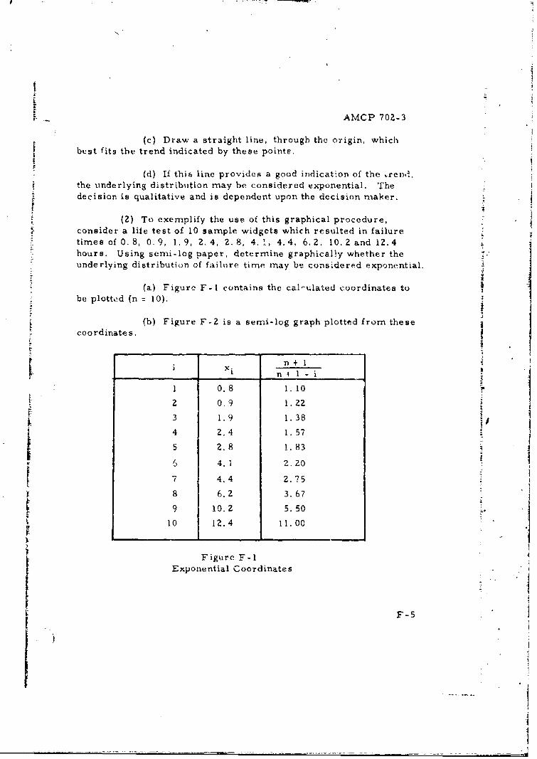
I

AMCP 702-3

(c) Draw a straight line, through the origin, whichbest fits the trend indicated by these points.

(d) If this line provides a good indication of the rrend,the underlying distribution may be considered exponential. Thedecision is qualitative and is dependent upon the decision maker.

c i (2) To exemplify the use of this graphical procedure,consider a life test of 10 sample widgets which resulted in failuretimes of 0. 8, 0.9, 1. 9, 2. 4, 2.8, 4. 1, 4.4, 6.2, 10.2 and 12.4hours. Using semi-log paper, determine graphically whether theunderlying distribution of failure time may be considered exponential,

(a) Figure F-I contains the calculated coordinates tobe plotted (n = 10).

(b) Figure F-2 is a semi-log graph plotted from these

coordinates,

~ n + lxi

1 0.8 1.10

2 0.9 1.22

3 1.9 1.38i4 2.4 1. 57

5 2.8 i.83

4.1 2. 20

7 4.4 2.75

8 6.2 3.679 10.2 5. 50

10 12.4 11. 00

Figure F- I

Exponential Coordinates

F-5

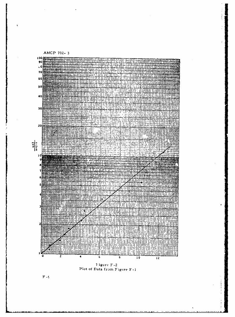
AMCP 702- 3too ql-;l

Ttl90t ill: if4.0 lilt!

70p4i60 L11,

lipI I L4j t

m -TT r1l i T,40 10 M

110,30ft or Pi 1,ji I;,

t 4. 141

I fri, 1; , I : ! I; ;- I; I: , I 'IT . ....... I . i,

fff 1ý I- 11'1ý, I i 1 ;11411

- J., I 41ý

M, !ý If

ir itit!14 Itifl-t-' 144: 0 t20 r- j.1 Hif I., ý11 4'. p

q ti ýi Mý 4ýif

j,14 1,:,qt i4

t

Wi19,t1i .1 f 4j,

10

9

a

7

6 : it,

N5 i: ql!..1 Hit

ýJTI fft4lit I

11:! VoA ll JA i I 'H il 11 Ill 1i ! I I, I I .. ;IýH ; I .

Ill: ;T ;1;;, I 1 1, 1 ! 11!

I I ý 1!T I M

ifIdti I

if

Ný :iij lit fit !V ? f11 d

if

;l4ill"

0 2 4 6 8 10 12

1: iguric. F-2Plot of Data from Figure F- I

F-6

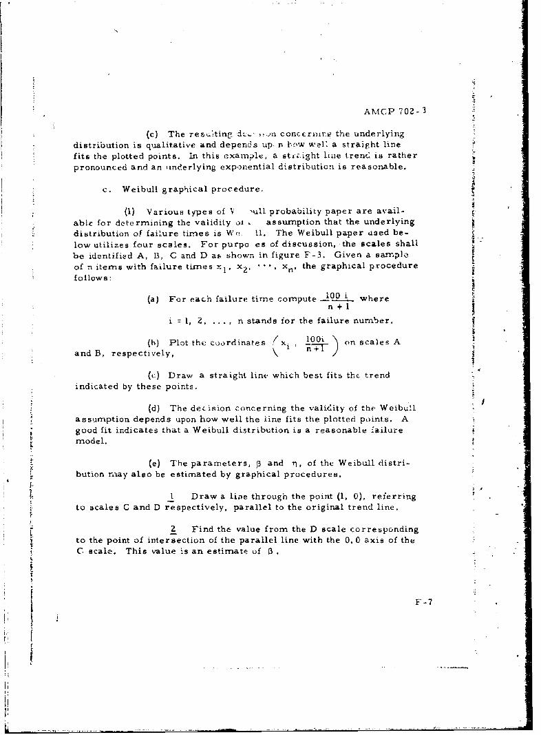
AMCP 702-3

(c) The resulting d.., ,,ojn concernutre the underlying

distribution is qualitative and depends up, n bow well a straight line

fits the plotted points. In this example, a stiz.ight liae trendl is rather

pronounced and an underlying exponential distribution is reasonable.

c. Weibull graphical procedure.

(1) Various types of 'V -ull probability paper are avail-

able for determining the validity oi assumption that the underlying

distribution of failure times is We. 11. The Weibull paper used be-

low utilizes four scales. For purpo es of discussion, the scales shall

be identified A, B, C and D as shown in figure F-3. Given a sample

of n items with failure times x,, x 2 , " n the graphical procedure

follows:

(a) For each failure time compute -I00 i where

n+l

i , 2, .... n stands ior the failure number.

(b) Plot the coordinates /xi ;100i on scales Aand B, respectively, nT-

(c) Draw a straight linte which best fits the trendindicated by these points.

(d) The decision concerning the validity of the Weibullassumption depends upon how well the line fits the plotted points. A

good fit indicates that a Weibull distribution is a reasonable failuremodel.

(e) The parameters, 5 and 71, of the Weibull distri-bution rn1ay also be estimated by graphical procedures.

I Draw a line through the point (1, 0), referringto scales C and D respectively, parallel to the original trend line.

2 Find the value from the D scale corresponding

to the point of intersection of the parallel line with the 0. 0 axis of the

C scale. This value is an estimate of B.

F-7

Ir

AWMOP 702-3

3 Find the value from 'he A scale corres-

ponding to the point of intersection of the trend line with the 0. 0axis of the D scale. This value is an estimate of the parameter nl.

(f) If the trend of plotted points is something otherthan a straight line, the assumption of a two-parameter Weibull

distribution is rejected.

C

B D

A

Figure F-3IWeibull Paper Scales

(2) To exernolify the use of this graphical procedure,consider a life test of 9 vacuuni tubes resulting in failure times of2. 0, 3. 7, 5. 3, 6. 2, 8. 5, 9.4, 11.1, 16.0, and 18.8 hours. UsingWeibull probability paper, determine graphically the validity of theassumption of an underlying Weibull distribution. If the assumpticn

is valid, estimate the parameters ,P and rT

(a) Figure F-4 shows the coordinates to be plotted and

the plot of: Xi, 100) is shown by figure F-5.

+ I(b) Since the trend line fits the plotted points quite

well, the Weiboll model of failure tinmes is reasonable. As indicatedby the graph, estimates of0.3 and r, are 1. 35 and .0. 5 respectively.

F-8

11

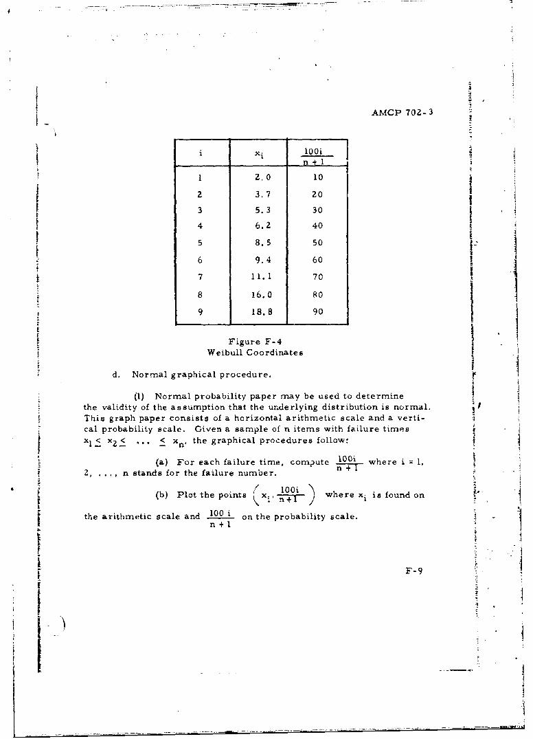
41

I AMCP 702- 3

xi 100i__ _n+1 n +

1 2.0 10

2 3.7 20 1, I

3 5.3 304 6.2 40

5 8.5 50

6 9.4 60

17 I1.1 70

8 16.0 90 I

9 18.8 90 1

Figure F-4Weibull Coordinates

d. Normal graphical procedure.

(1) Normal probability paper may be used to determinethe validity of the assumption that the underlying distribution is normal.

This graph paper consists of a horizontal arithmetic scale and a verti-cal probability scale. Given a sample of n items with failure times

xf< X2_< ... < xn, the graphical procedures follow:

(a) For each failure time, compute L00i where i = 1,n +-7IZ, ... , n stands for the failure number. fl-+"1

S/ ~~100i "(b) Plot the points lx:' -- where xi is found on

the arithmetic scale and 100 i on the probability scale.n +

F-9

Ii

I1

IJ_____ ____

____ ___ - -- - - -- ,-

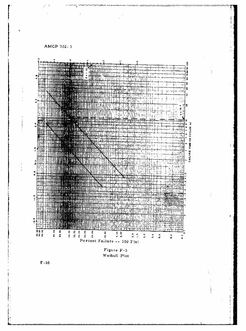
AMGP 702- 3

'Ii '''ii I4

.. - I- ' 1 -

F -1

I'

F-.

iA

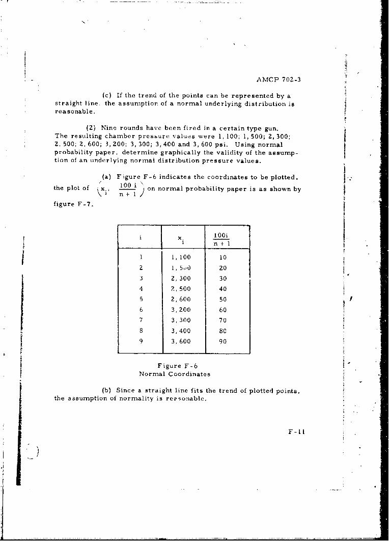
AMCP 702-3

(c) If the trend of the points can be represented by astraight line, the assumption of a normal underlying distribution isreasonable.

(Z) Nine rounds have been fired in a certain type gun.The resulting chamber pressure values were 1, 100; 1,500; 2,300;2, 500; 2, 600; 3, 200; 3, 300; 3,400 and 3, 600 psi. Using normalprobability paper, determine graphically the validity of the assump-tion of an underlying normal distribution pressure values.

(a) Figure F-6 indicates the coordinates to be plotted.the plot of i'x. 100 ) on normal probability paper is as shown by

1 n+lfigure F-7.

!X. 1 0

SI1 n+l

1, 100 10S 1, 5A0 20

3 2, 300 30

4 2, 500 40

5 2,600 506 3,200 607 3, 300 70

8 3,400 80r 9 3, 600 90

Figure F-6Normal Coordinates

(b) Since a straight line fits the trend of plotted points,the assumption of normality is reasonable.

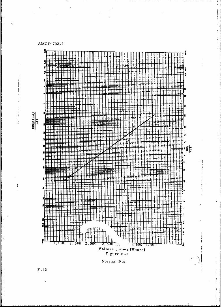
AMCP 702-3

I IHII

Failur4e4 T4i,~ous

Figure F-7 I

No ml Pot

F- k2 4 11 41

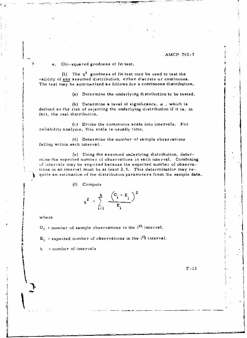
AMCP 702-3

e. Chi-squared goodness of fit test..4

(1) The X2 goodness of fit test may be used to test thevalidity of any assumed distribution, either discrete or continuous.The test may be summarized as follows for a continuous distribution.

|I(a) Determine the underlying distribution to be tested.

* (b) Determine a level of significance, a , which isSdefined as the risk of rejecting the underlying distribution if it is, in

fact, the real distribution.

(c) Divide the continuous scale into intervals. For

reliability analysis, this scale is usually time.

I (d) Determine the number of sample obeervations

falling within each interval.

(e) Using the assurr,ed underlying distribution, deter-

.mine the expected number of observations in each interval. Combiningof intervals may be required because the expected number of observa-tions in an interval must be at least 2. 5. This determinatior may re-

Squire an estimation of the distribution parameters from the sample data.

(f) Compute

k -E -

2

- "= / - -

where

Ii number of sample observations in the ith interval.

Ei expected number of observations in the iti interval.

k = number of intervals

F-13

V1

-, I i'I

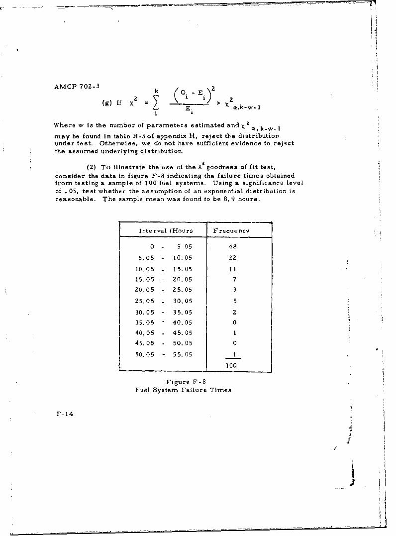
AMCP 702-3 k ( .1

(g) If X E X > x -i A

Where w is the number of parameters estimated andxa y ,k-w-1

may be found in table H-3 of appendix H, reject the distributionunder test. Otherwise, we do not have sufficient evidence to rejectthe assumed underlying distribution.

(2) To illustrate the use of the X goodness of fit test,

consider the data in figure F-8 indicating the failure times obtainedfrom testing a sample of 100 fuel systems. Using a significance levelof . 05, test whether the assumption of an exponential distribution isreasonable. The sample mean was found to be 8. 9 hours.

Interval (Hours Freauencv

0- 5 05 48

5.05 - 10.05 22

10.05 - 15.05 11

15.05 - 20.05 7

20.05 - 25.05 3

25.05 - 30.05 5

30.05 - 35.05 2

35.05 - 40.05 0

40.05 - 45.05 1

45.05 - 50.05 0

50.05 - 55.05 1

100

Figure F-8Fuel System Failure Times

F-14

/

S H

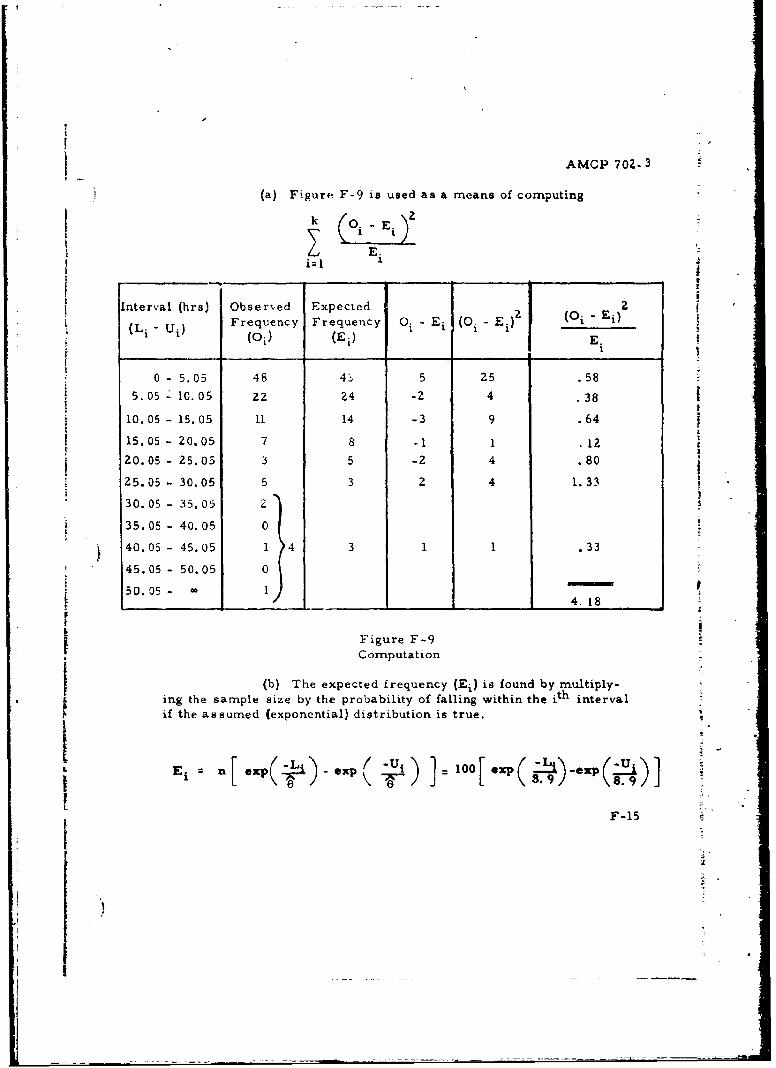
AMCP 702- 3

(a) Figure F-9 is used as a means of computing

k - E.

E.

Interval (hrs) Observed Expected 2Frequency Frequency O - Ei (0. - Ei) (O"Ei)

(L" Ui) (O) (El) E.(

0 - 5. 05 48 4 5 25 .58

5.05- 10.05 22 24 -2 4 .38

10.05- 15.05 11 14 -3 9 .64

15.05 -20.05 7 8 - 1 1 .12

20.05 -25.05 3 5 -2 4 .80

25.05- 30.05 5 3 2 4 1.33

30.05- 35.05 2

35.05 - 40.05 0

40.05- 45.05 1 4 3 1 1 .33

* 45.05 - 50.05 0

50.05- M 4S/ ~4.18 -p-

Figure F-9Computation

(b) The expected frequency (Ei) is found by multiply-ing the sample size by the probability of falling within the ith intervalif the assumed (exponential) distribution is true.

I

L -U

F-15

. I

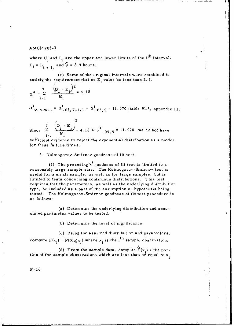
AMCP 702-3

where Ui and L. are the upper and lower limits of the ith interval,

Ui = L and E = 8.9 hours.i+l1

(c) Some of the original intervals were combined tosatisfy the requirement that no E. value be less than 2. 5.

½I

"7 i- 1 -4.18i-I E.

a,k-w-l X 0 5 , 7 -- 1 o0 5 , 5 = 11.070 (table H-3, appendix 1).

./2

7 *.0-E.Since Z i = 4. 18 < X 05.5= 11.070, we do not have

i-I E.

sufficient evidence to reject the exponential distribution as a modelfor these failure times.

f. Kolmogorov-Smirnov goodness of fit test.

(1) The preceding X goodness of fit test is limited to areasonably large sample size. The Kolnogorov-Smirnov test isuseful for a small sample, as well as for large samples, but islimited to tests concerning continuous distributions. This testrequires that the parameters, as well as the underlying distributiontype, be included as a part of the assumption or hypothesis beingtested. The Kolmogorov-Smirnov goodness of fit test procedure isas follows:

(a) Determine the underlying distribution and asso-ciated parameter values to be tested.

(b) Determine the level of significance.

(c) Using the assumed distribution and parameters,

compute F(xi) = P(X < xi) where x. is the ith sample observation.

A(d) From the sample data, compute F(x.) = the por-1

tion of the sample observations which are less than or equal to x..1

F-16.

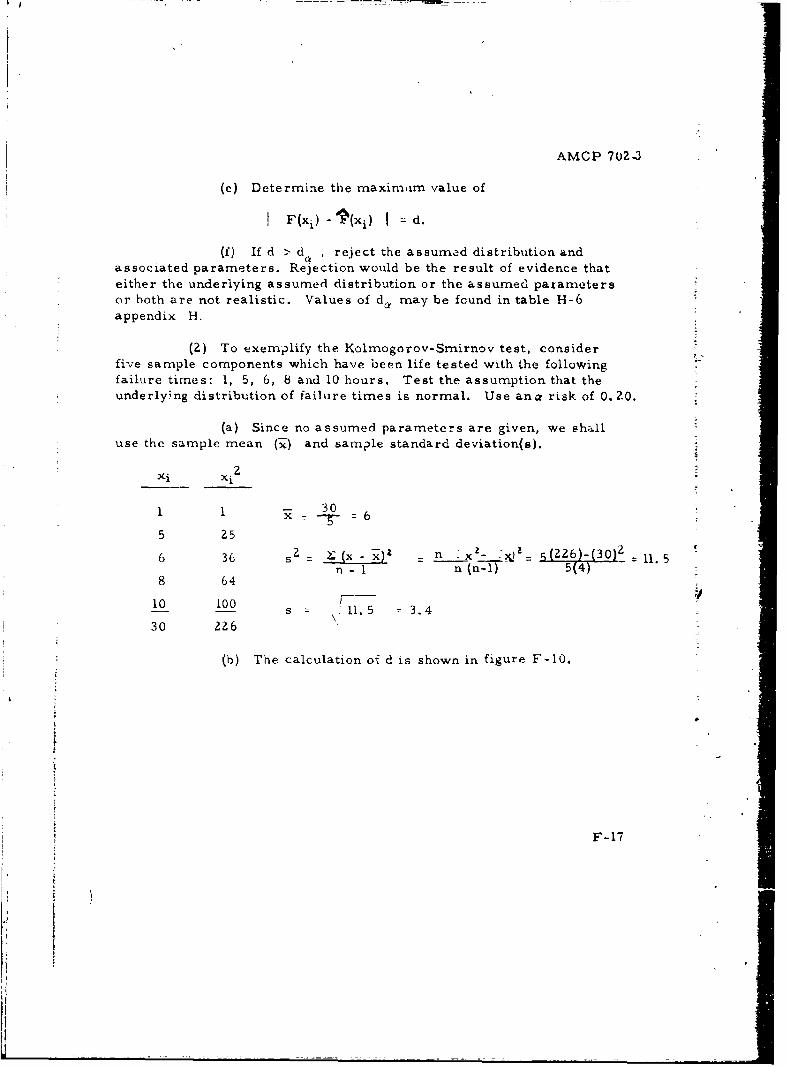
AMCP 702-3

(e) Determine the maxim im value of

I F(x I d.

(f) If d > d , reject the assumed distribution andassociated parameters. Rejection would be the result of evidence thateither the underlying assumed distribution or the assumed parametersor both are not realistic. Values of d. may be found in table H-6appendix H.

(2) To exemplify the Kolmogorov-Smirnov test, considerfive sample components which have been life tested with the followingfailure times: 1, 5, 6, 8 and 10 hours. Test the assumption that theunderlying distribution of failure times is normal. Use ana risk of 0.20.

(a) Since no assumed parameters are given, we ehalluse the sample mean (x-) and sample standard deviation(s).

xi xiz-

301 1 x 6

.2 25

6 36 s= -(x x) = nX(6)-(30)

n- 1 n(n-1) 548 64

10 100 s 11. 5 3.430 226

(b) The calculation of d is shown in figure F-10.

F1

F-17

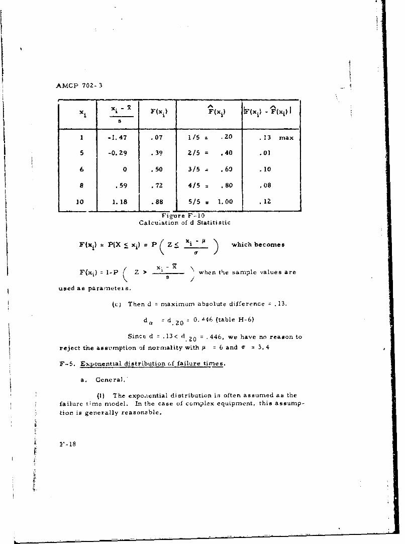
AMCP 702- 3

x x F(x.) F(xi.) j(xi) - F(xi)

1 -1.47 .07 1/5 = .20 .13 max

5 -0.29 .39 2/5 = .40 .01

6 0 .50 3/5 = .60 .10

8 .59 .72 4/5 = .80 .08

10 1.18 .88 5/5 = 1.00 .12

Figure F-IOCalculation of d Statitistic

F(X1 ) = P(X < xi) = P (z• xi ) which becomes

F(xi) 1-P Z >xi - x when the sample values ares .

used as paraineteis.

S(c) Then d = maximum absolute difference = .13.

d a = d. 20 = 0. a46 (table H-6)

Since d = .13< d. 20 = . 446, we have no reason to

reject the assumption of normality with A = 6 and 0' = 3.4

F-5. Ex,~onentxal distribution of failure times.

a. General.

(1) The expoaential distribution i.i often assumed as thefailure timc model. In the case of complex equipment, this assump-

tion is generally reasonable.

SF-18

AMCP 702- 3

The exponential probability density function has been defined as

f(x) = X. exp(- A x) ='exp - if x > 0

f(x) 0 if x < 0

where , = failure rate

and 6 = mean failure time.A

(2) Then the parameter to be estimated from sample lifetest data is either 6 or X . A point estimate of the exponential para-meter leads to a point estimate of the reliability function. Each canalso be estimated by means of confidence statements. The symbols

I J Iand if(x) are used herein as point estimates of the para-meters 8, A and R(x) respectively. The vaiue for will not beshown but may be determined as 1

(3) F-mple data may be generated from different types oflife tests. Life tests may be conducted either with or without replace-ment of ;ailed components and may be terminated either upon the oc-currence of a preassigned number of failures or at a preassigned time.

b. Life tests terminated upon the occurrence of a preassigned

number of failures.

(1) Assuming an exponential distribution of failure times,ccnsider a life test which is to be terrninated upon the occurrence ofthe rth failure -- i. e. , n items are placed on test until the rth failureoccurs. The failure times are expressed as xl<_ x2 < . xr. Themethod for estimating 8 or X depends upon whether the test procedure"involves replacement or nonreplacement of field items.

(2) Point es-ýimates of 0 and R(x) arer

x + x (n- r)

i-I 1 tfor the nonreplacemrcntr test, failure termirated

F-19

K II

AMCP 702- 3A n x r for the replacement test,

r failure terminated

'(x) = e (- for either case ofX \ failure terminated test

(a) Ten engines are initially to be placed on test withoutreplacement, until the third failure occurs. At the conclusion of thetest, the resulting failure times were found to be 6, 8, 20 hours.

Assuming an exponential distribution of failure times, find a pointestimate of the mean failure time 0 and of R(5).

r = 3

n = 10

x =20

rSx. =341

i=l

= 34 + (7)ZO 174 = 58 hours3 3

R(5)= exp (- exp (-0. 09) = 0. 91

(b) Twenty vehicles were originally placed on test until

the fifth failure. Failed vehicles were replaced at the time of test

Conduct of the teat resulted in the fifth vehicle failure occurring 40hours after the beginning of the test. Assuming an exponential dis-

tribution of failure times, estimate the population mean failure time6 and R(100).

n = 20

x = 40r

r- 5

E0= -- = ]60 hours5 5

F-20

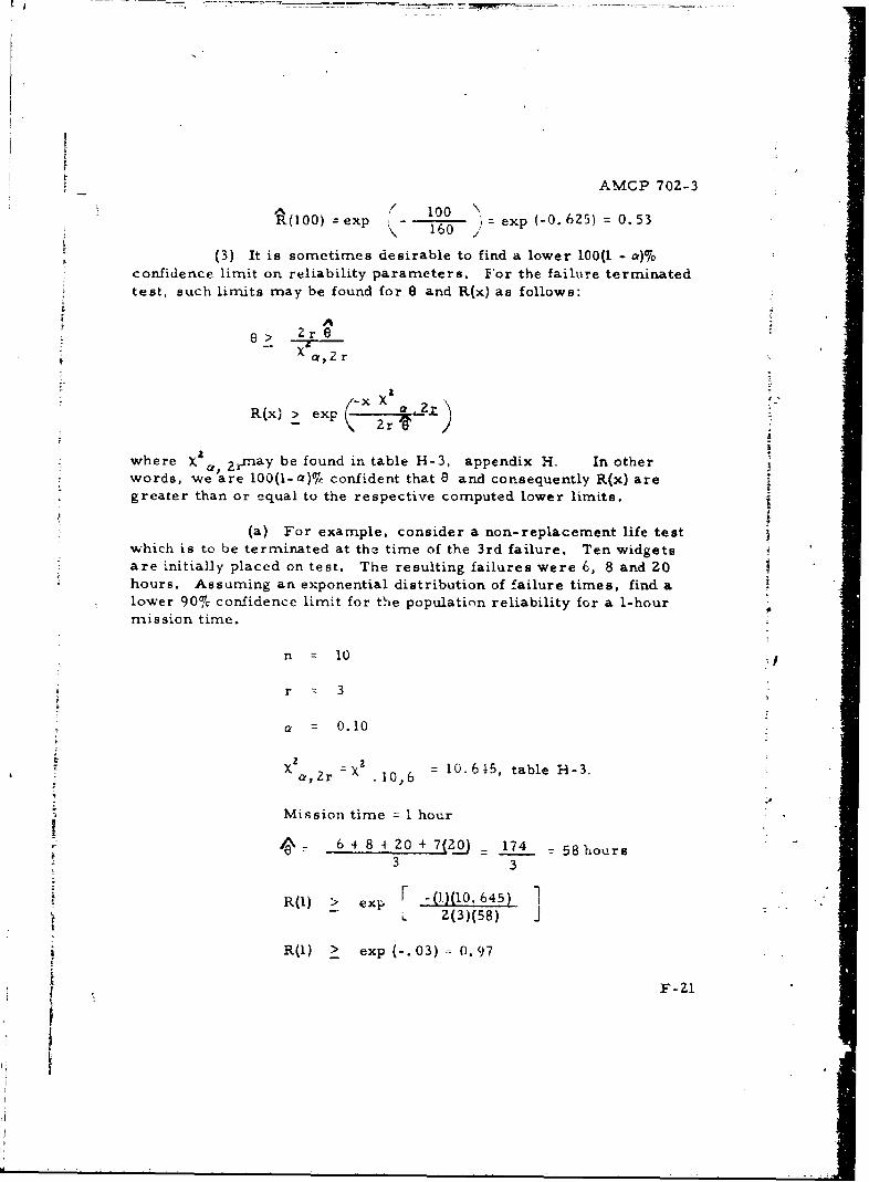
AMCP 702-3A /' 100 "

%(100) =exp 10• exp (-0.625) = 0.53xp\ 1-60 exp

(3) It is sometimes desirable to find a lower 100(1 - a)oconfidence limit on reliability parameters. For the failure terminatedtest, such limits may be found for B and R(x) as follows:

A8> 2r0

X a,2 r

R(x) > exp

where XY, arnmay be found in table H-3, appendix 14. In otherwords, we are 100(1- a)%lr confident that 0 and consequently R(x) aregreater than or equal to the respective computed lower limits.

(a) For example, consider a non-replacement life testwhich is to be terminated at thc time of the 3rd failure. Ten widgetsare initially placed on test. The resulting failures were 6, 8 and 20hours. Assuming an exponential distribution of failure times, find alower 90% confidence limit for the population reliability for a 1-hourmission time.

n 10

r 3

0.10

XZ : -0 = 10.645, table H-3.ce, Zr .10,6

Mission time = 1 hour

S6 + 8 + 20 + 7(2 174 - 5 ours

3 3

R(l) > exp F -(1)(l0. 645) 1L 2(3)(58) i

R(1) > exp (-.03) : 0.97

t

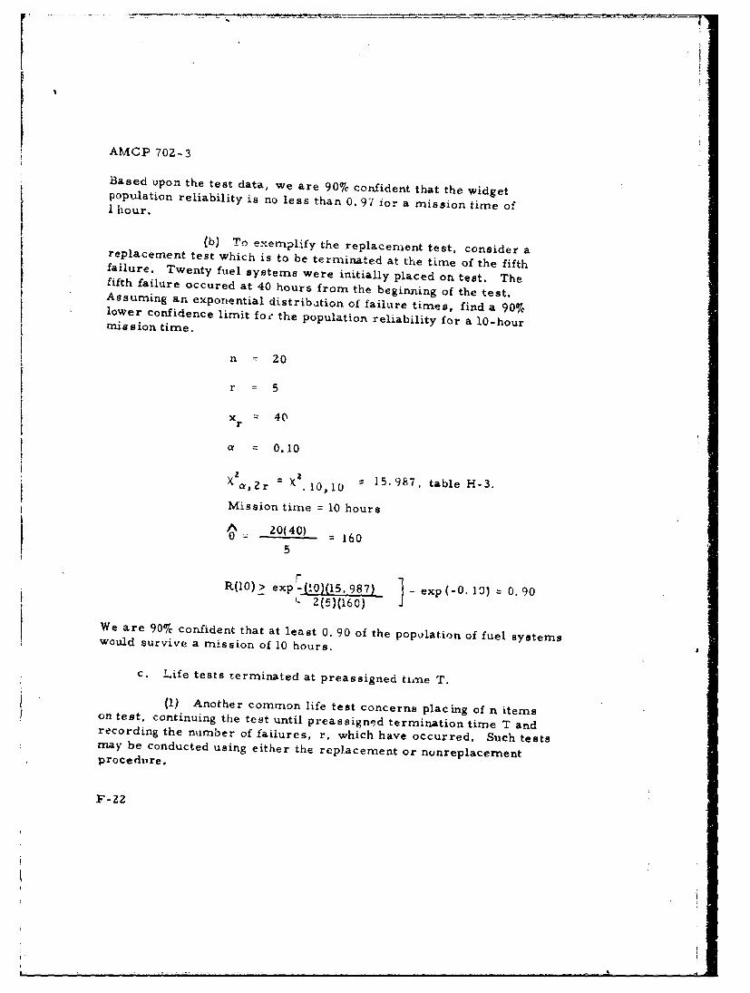
AMCP 70Z- 3

Based upon the test data, we are 900/c confident that the widgetpopulation reliability is no less than 0. 97 ior a mission time ofI hour.

(b) To exemplify the replacement test, consider areplacement test which is to be terminated at the time of the fifthfailure. Twenty fuel systems were initially placed on test. Thefifth failure occured at 40 hours from the beginning of the test.Assuming an exponential distribution of failure times, find a 90%lower confidence limit for the population reliability for a 10-hourmission time.

n 20

r - 5

x 40r

a 0.10

x- a, .10, 15-987, table 1--3.

Mission time = 10 hours

0 20(40) 1605

R(10)> exp-L.0)(5.987) = exp(-0. 10) 0.90L 2(5)(160)

We are 900%c confident that at least 0. 90 of the population of fuel systemswould survive a mission of 10 hours.

c. Life tests terminated at preassigned tinne T.

(1) Another common life test concerns placing of n itemson test, continuing the test until preassigned termination time T andrecording the number of failures, r, which have occurred. Such testsmay be conducted using either the replacement or nunreplacemnentprocedtire.

F-22

-- - ---- - - - - --i-

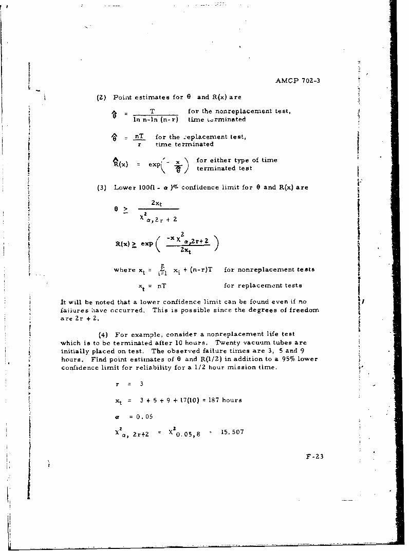
AMCP 702-3

(Z) Point estimates for 0 and R(x) are

T for the nonreplacement test,In n-in (n-r) time Lrminated

= nT for the :eplacement test,r time terminated

for either type of timeý(x) exp; T) terminated test

(3) Lower 100(1- a )0- confidence limit for 0 and R(x) are

2 xt> X'a,Zr + 2

R(,) > exp X O(Zr+ o

where xt = xi + (n-r)T for nonreplacement tests

xt = nT for replacement tests

It will be noted that a lower confidence limit can be found even if nofaiiures have occurred. This is possible since the degrees of freedomare 2r + 2.

(4) For example, consider a nonreplacement life testwhich is to be terminated after 10 hours. Twenty vacuutm tubes are

initially placed on test. The observed failure times are 3, 5 and 9Shours. Find point estimates of 0 and R(I/Z) in addition to a 95% lower

confidence limit for reliability for a 1/2 hour mission time. "

r = 3

xt 3 + 5 + 9 + 17(0)= 187 hours

a =0.05

a, 2r+.05,8 =- 15.507

F-23

L=

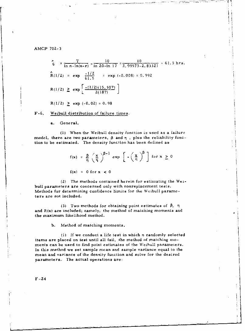
VJ

AMCP 702-3

T 10 10In n-ln(n-r) In 20-in 17 =Z.99573-2.83321

R(1/2) = exp exp (-0.008) = 0.992

R(1/2) exp -(/2)(15. 507)1

pL 2(187)

R(I/2) > exp (-0.02) 0.98

F-6. Weibull distribution of failure times.

a. General.

(1) When the Weibull density function is used as a failure

model, there are two parameters, P and -n , plus the reliability func-tion to be estimated. The density function has been defined as

f (x) e xp43 .~ ' for x > 0

f(x) = 0for x < 0

(2) The methods contained herein for estimating the Wei-bull parameters are concerned only with nonreplacement tests.

Methods for determining confidence limits for the Weibull parame-

ters are not included.

(3) Two methods for obtaining point estimates of •, 1

and R(x) are included; namely, the method of matching moments andthe maximum likelihood method.

b. Method of matching moments.

(1) If we conduct a life test in which n randomly selecteditems are placed on test until all fail, the method of matching mo-

ments can be used to find point estimates of the Weihull parameters.In this method we set sample mean and sample variance equal to themean and variance of the density function and solve for the desired

parameters. The actual operations are:

F-24

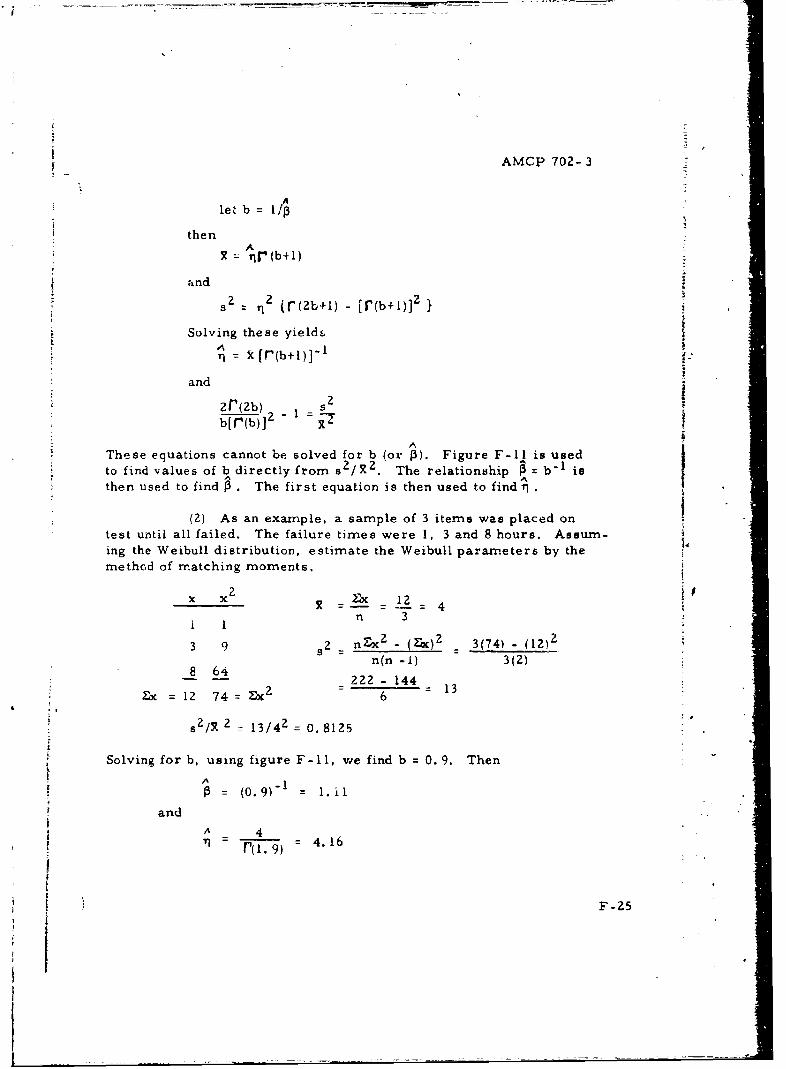
AMCP 702- 3

let b =/p

then

X. rUi(b+l)

and

Z 2 i(zbl) r(b+l)]Z )

Solving these yield&T = f r(h+l)]-r

and

zr(zb) s 2

btrl(b)]2

These equations cannot be solved for b (or 3). Figure F-Il is usedto find values of b directly from s2/R2. The relationship b 1 isthen used to find P. The first equation is then used to find .

(2) As an example, a sample of 3 items was placed on

test until all failed, The failure times were 1, 3 and 8 hours. Assum-ing the Weibull distribution, estimate the Weibull parameters by themethod of matching moments,

x 2 Ex 12n 3

92 n2.x 2 - (E)x=2 3(74) - (12)2

n(n -1) 3(2)8 64 222- 144

Sx =12 74 Z 6 13

2 •2/ - 13/42 = 0.8125

Solving for b, using figure F-11, we find b 0.9. Then

A -P = (0.9) 1. il

andA 4

*] - rTl.9) - 4.16

F-25

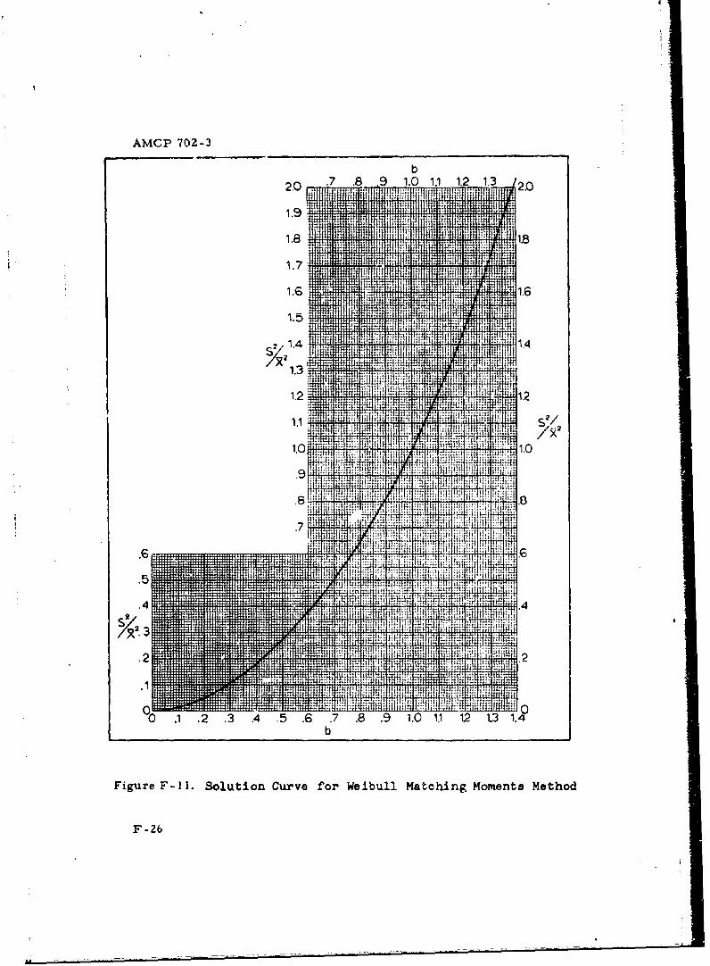
AMCP 702-3

b

2.0 -7 .8 .9 1.0 1.1 1. 2.0p fl HHOMM

1.9 i MIMS I 1I

1.8 1.8III w 4t4;1,t U4

4t4;1,t

IC UH i I p

P1.G li"O., HUM i lil i 1 1.6

1, ý A Q H P, i ý 1. 1U :11 -- Wh,Wm t4 4 pwliwi, F . r, il jjL1

- i R, ii: M i 1MH. 15

S2/1.4 414 HITT -H. 14

2 4W- iq;+-. " A+1.3W., It + "i.

+ 11 ! + H1.2, _t 1.2

1%, N., NR wrIff n iNIT'. 2/

14 75<2R-0i 1921 i N! -10:11::...

1.01.0

I :iT:1 4'"

i1V

.7

L Pl. ':i

-'ýJt 4-:1 1

1: z:.5

FixtPt- .4

F. T, iFill- IN -it

3

MURfif-UM-1,311:1 !,.i: 1 .41M W. _151 1:4.:,ý: .2

r4: t n:

itFri I. .4q

U4 jii nv

00 .1 .2 .3 .4 5 .6 .7 .8 .9 1.0 1.1 12 13 14"

b

Figure F-11. Solution Curve for Weibull Matching Moments Method

F-26

AMGP 702-3

c. Maximum likelihood method. Maximum likelihood esti-mates of the Weibull parameters may be found by solving iteratively

AAthe following equations foi 3 and Y.

n A

SX.Y = exp X Inn

nn= n

T.In xi . In xiiTl i=l

F-7. Normal distribution of failure times,

a. General.

(I) The normal probability density function is sometimesuseful as a failure model in reliabijity analysis, especially when fail-ures are a result of wearout. The normal density function is

1i F 1 /jj >217f(x) W exp 2<XT \! 27 Lx ! -~

Estimation of the parameters .u and a- will be considered only fora life test where n items are placed on test until all fail with resultingfailure times xl, x2 , .. . xn.

b. Then point estimates of 0*, 2" and R(x) are respectively

t - ExS~X=

n

n-I n(n-1)

F-27

AMCP 702- 3

A'\ s

c. The 100(l-ct)%i confidence intervals for the two parameters are

and

(n-I)s2 2 (n-l)s 2X < T < 2

&X/2,n-1I I -a/2.n-I

where

n = sample size

n-I = degrees of freedom

tal?, n-i may be found in tabl H-4, appendix H.

XzI2,n-I may be found in table H-3, appendix H-

d. To illustrate the estimation of w and T , consider 4randomly selected vehicles which have been tested till failure.The failure times were 110, 114, 116 and 120 hours. Assuming failuretimes to be normally distributed, estimate both p and T by a pointestimate and by a 957c confidence interval. Also find a point estimatefor the reliability for a mission time of 120 hours.

(1) X X-F (X_7)__

110 -5 25

114 -1 1

116 1 1

120 5 25

460 52

F-28

I,

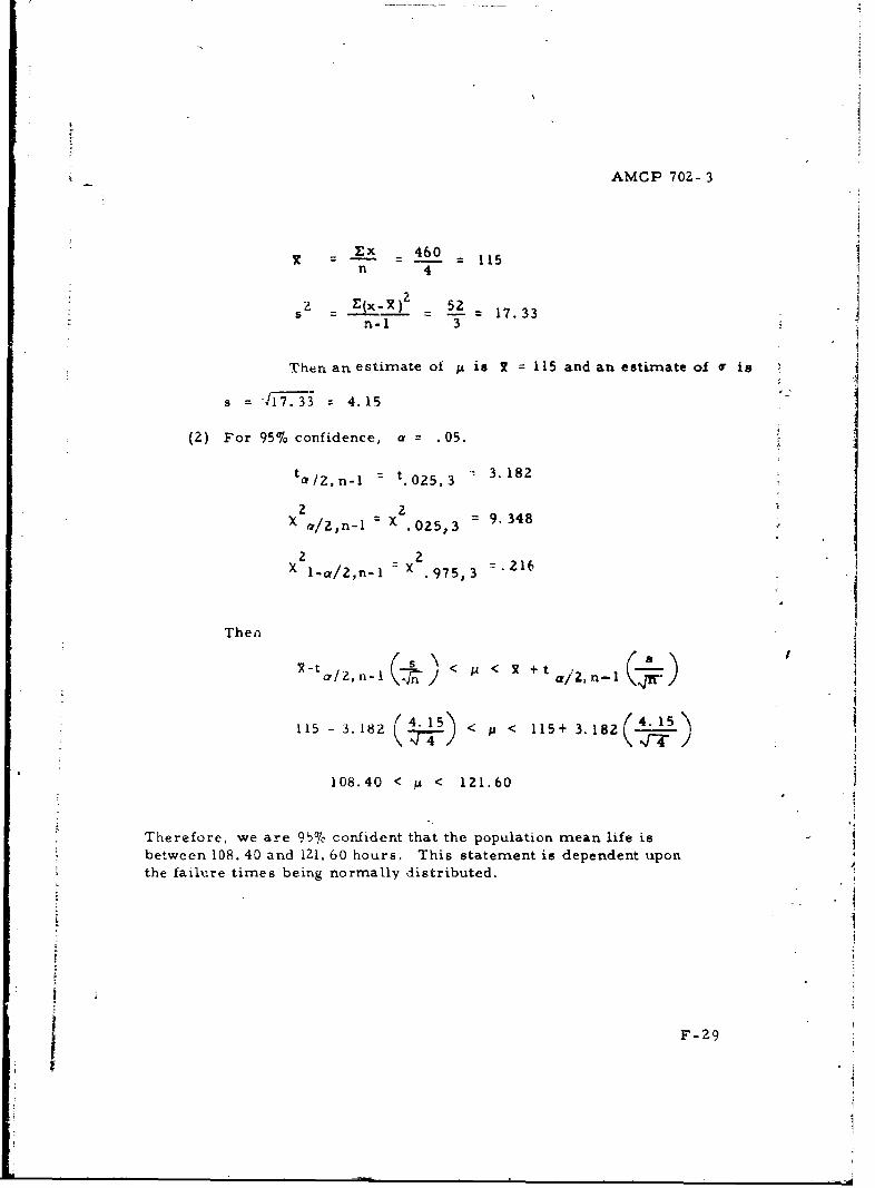
AMCP 70Z- 3

=_x 460 115n 4

s = (x-X)2 _ 52 - 17.33n-i 3

Then an estimate of pi is 7 : 115 and an estimate of or is

s = Ii.33 : 4.15

(2) For 95% confidence, a = .05.

ta/Z,n-1 = t. 0 2 5 , 3 " 3. 182

2 2X a/2,n-1 X .025,3 = 9.348

2 2X 1-a/2, n- 1 Y .975,3 =.216

Then

•-ta,/, n~l< Pl < R + t a _

4 15) < < I+4. 1 2115 -3.182 11 +3.1 7

108.40 < M < 121.60

Therefore, we are 95% confident that the population mean life isbetween 108. 40 and 121. 60 hours. This statement is dependent uponthe failure times being normally distributed.

F-29

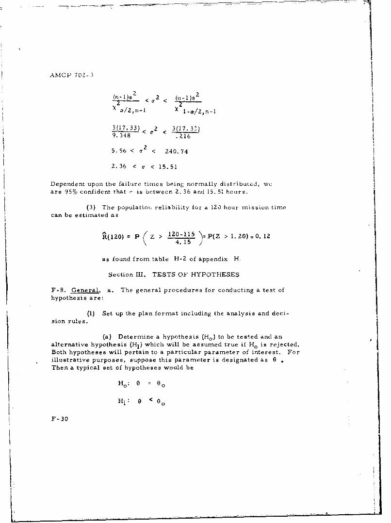
AMCP 702- 3

(n- )s(n)s2 < "TX a/2,-I X -a,/2,n-i

3(17.33) 2 3(17.3^)9. 348 < .216

5. 56 < < 240.74

2.36 < a < 15.51

Dependent upon the failure times being normally distributed, weare 95% confident that *r is between 2. 36 and 15. 51 hours.

(3) The population reliability for a 120 hour mission timecan be estimated as

%(l2O): P (z > O-12015 P(z > . o0)=0. 124.15 }

as found from table H-2 of appendix H.

Section 1H1. TESTS OF HYPOTHESES

F-8. General. a. The general procedures for conducting a test ofhypothesis are:

(1) Set up the plan format including the analysis and deci-sion rules.

(a) Determine a hypothesis (Ho) to be tested and analternative hypothesis (H1 ) which will be assumed true if Ho is rejected.Both hypotheses will pertain to a particular parameter of interest. For

illustrative purposes, suppose this parameter is designated as 0 ,Then a typical set of hypotheses would be

Ho: 0 = ao

F-: 3 <8O

F-30

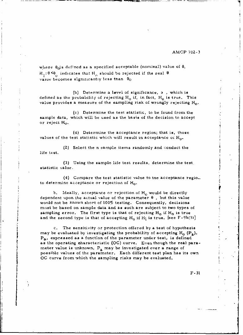
AMCP 702-3

where Oois deflned as a specified acceptable (nominal) value of 8.

H <6<0 indicates that H. should be rejected if the real evajue becomes signiticantly less thian O0

(b) Determine a level of significance, 2 , which isdefined as the probability of rejecting Ho if, in fact, H. is true. Thisvalue provides a measure of the sampling risk of wrongly rejecting Ho.

(c) Determine the test statistic, to be found from thesample data, which will be used as the basis of the decision to accept

or reject Ho.

(d) Determine the acceptance region; that is, thosevalues of the test statistic which will result in acceptance oi Ho.

(2) Select the n sample items randomly and conduct thelife test.

(3) Using the sample life test results, determine the test.statistic value.

(4) Compare the test statistic value to tne acceptance regio..to determine acceptance or rejection of H,.

b. Ideally, acceptance or rejection of H. would be directly

dependent upon the actual value of the parameter 0 , but this valuewould not be known short of 100% testing. Consequently, decisionsmalst be based on sample data and as such are subject to two types ofSsampling error. The first type is that of rejecting Ho if Ho is true

S~and the second type is that of accepting H~ if Hl is true. [See F-9b(3)]o 0

c. The sensitivity or protection offered by a test of hypothesismay be evaluated by investigating the probability of accepting Ho (Pa)"

Pa, expressed as a function of the parameter under test, is defined Ias the operating characteristic (OC) curve. Even though the real para-meter value is unknown, Pa may be investigated over a range ofpossible values of the parameter. Each different test plan has its ownOC curve from which the sampling risks may be evaluated.

F-31

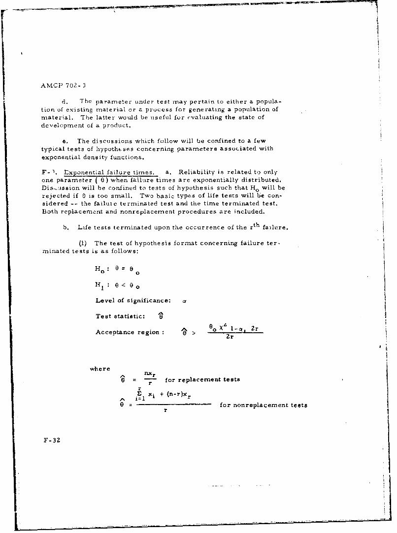
I]

AMCP 702- 3

d. The parameter under test may pertain to either a popula-tion of existing material or a process for generating a population ofmaterial. The latter would be useful for evaluating the state ofdevelopment of a product.

e. The discussions which follow will be confined to a fewtypical tests of hypotheses concerning parameters assocriated withexponential density functions.

F- 1. Exponential failure times. a. Reliability is related to onlyone parameter ( 0 ) when failure times are exponentially distributed.Dis-ussion will be confined to tests of hypothesis such that Ho will berejected if 0 is too small. Two basic types of life tests will be con-sidered -- the failuic terminated test and the time terminated test.Both replacement and nonreplacement procedures are included.

b. Life tests terminated upon the occurrence of the rth failure.

(1) The test of hypothesis format concerning failure ter,rninated tests is as follows:

8<oHI:O< 0o

Level of significance: a

Test statistic:80X" 1- a Zr

Acceptance region >Zr

where

- rr for replacement tests

Sxi + (n-r)xro = for nonreplacernent tests

r

F-32

AMCP 7C2Z- 3

00 acceptable mean life

r termination number

n sample size

n > r for nonreplacement tests

The OC curve is expressed by

P Kz (09 21a P[ >r- '0 X I-a,?r

(Z) To exemplify this test of hypothesis, a new vehicle isunder development dnd five prototype models are available for testingto evaluate the process by which these models were generated. If theprocess is such that it has the capability of generating items whic'hhave a mean time to failure of E = 100 hours or more, no furtherdevelopment effort is required. A nonreplacement test is prcposedsuch that the five models will be placed on test until the third failureoccurs. The test of hypothesis can tolerate an a . 05 risk of reject-ing the present process if it is actually capable of generating productwith 0 = 100 hours. Set up the test format; draw the OG curve for theplan, and answer the question, if failure times are 20. 40 and 50, should

the item be subjected to further development?

(a) Define n, r, 0° and a as:

n= 5, r= 3, 0= 100, a=.05

F (b) H 0 : 0 = 100 hours

HI: E < 100 hours

Level of significance: • = . 05

r 3•=xi + (n-r)xr 1xi+Test statistic: A = x-nrx.

= r 3

F-33

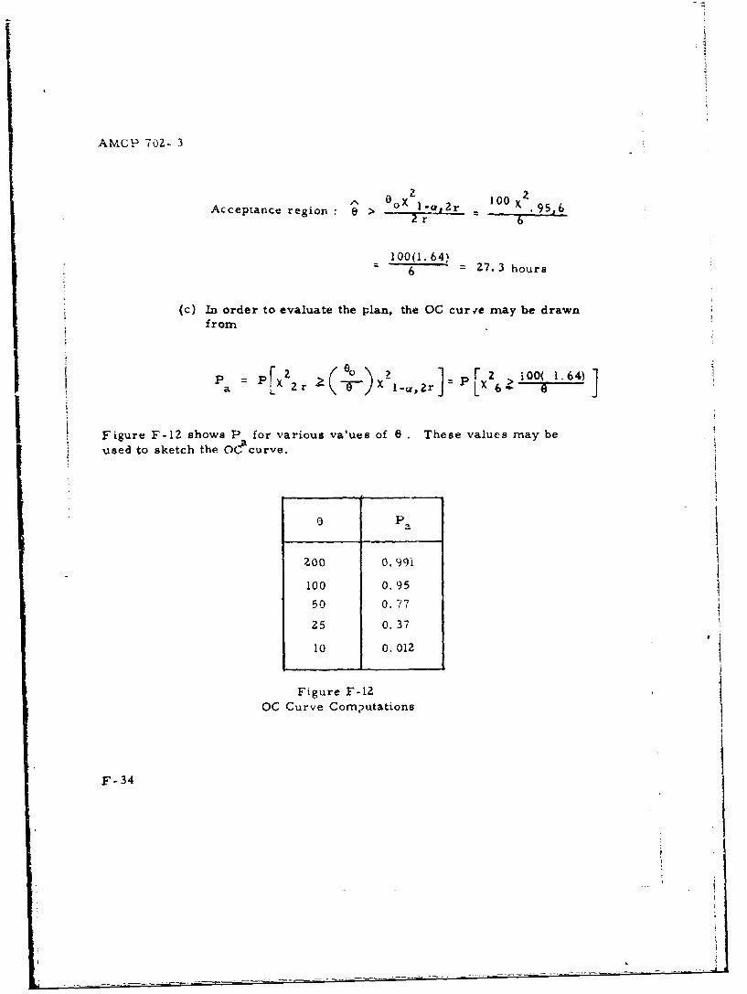
AMCP 702- 3

Acceptance region - 1 > " - X 95 6

100(l.64)6 = 27.3 hours

(c) In order to evaluate the plan, the OC curre may be drawnfrom

-P =-1 2 2p >i0( 1.64)a L r -IXJ6 .'0

Figure F-12 shows P for various va'ues of 8 . These values may beused to sketch the Ocacurve.

O P,

ZOO 0. 99i

100 0.95

50 0.77

25 0.37

10 0.012

Figure F-12

OC Curve Com3utations

F-34

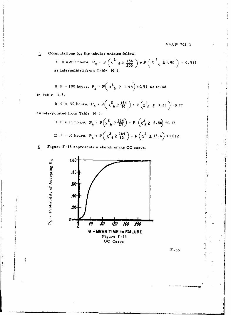
AMCP 702-3

I Computations for the tabular entries follow.

I 0 = 200 hours, Pa = P(X 6X 164 )P x 6 '0.8Z 0.991

as intervolated from Tahle.- H-3

If = 100 hours, P = P > 1.64 =L 95 as found

in Table 1-3.If 0 = 50 hours, Pa =- ) = p > 3. Z8) 20.77

as interpolated from Table H-3.

If 0 25 hours, Pa P >(216 ,) p (X2> 6.5 =0. 37

11O 0 10 hours, P = 2 >64> 16. 4 0.012a (X 6 -IF

2 Figure F-13 represents a sketch of the OC curve.

o 1.0

K .6 0I

S.4

0

- MEANTIME to FAILURE

Figure F-13OC Curve

F-35

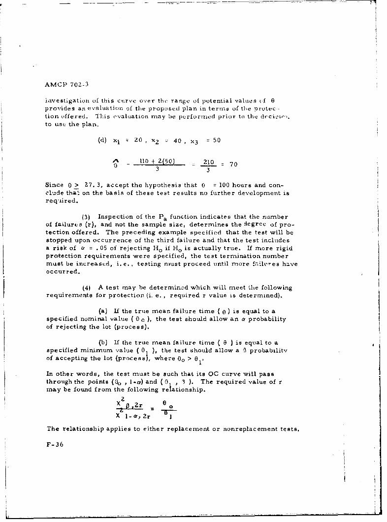
AMCP 702-3

investigation of this curve over the range of potential values (4 eprovides an evaluation of the proposed plan in terms of the protec -tion offered. This evaluation may be performed prior to the dccio-'(.to use the plan.

(d) x1 2 0, x 2 - 40, x3 = 50

A no + 2(50) 210 - 700 33 3

Since 0 > 27. 3, accept the hypothesis that 0 = 100 hours and con-clude that on the basis of these test results no further development isreqiired.

(3) Inspection of the Pa function indicates that the numberof failures (r), and not the sample size, determines the degree of pro-tection offered. The preceding example specified that the test will bestopped upon occurrence of the third failure and that the test includesa risk of cr = .05 of rejecting I-10 if Ho is actually true. If more rigidprotection requirements were specified, the test termination numbermust be increased, i.e. , testing must proceed until more fnileres haveoccurred.

(4) A test may be determinzd which will meet the followingrequirements for protection (i. e. , required r value is determined).

(a) If the true mean failure time (0) is equal to aspecified nominal value ( 0 o ), the test should allow an a probabilityof rejecting the lot (process).

(b) If the true mean failure time ( 0) is equal to aspecified minimum value (,0 ), the test should allow a I probabilitvof accepting the lot (processi, where 0o > e1

In other words, the test must be such that its OC curve will passthrough the points (0o , I-&) and (0 , 3 ). The required value of rmnay be found from the following relationship.

aX r

X 1-a, 2r

The relationship applies to either replacement or nonreplacement tests.

F-36

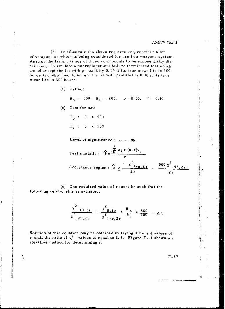
AMCP 702-3

(5) To illustrate the above requirement, con-ider a lotof con,.oflents which is being considered for use in a weapons system.Assume the failure times of these components to be exponentially dis-tributed. Formulate a nonreplacement failure terminated test whichwould accept the lot with probability 0. 95 if its true mean life is 500hours and which would accept the lot with probability 0. 10 if its truemean life is Z00 hours.

(a) Define:

00 = 500, 01 200, : 0.05, 1 0.10

(b) Test format:

Ho : = 500

H, : < 500

Level of significance : = . 05

r

Test statistic : A - xi + (n-r)Xrr

e 2 5002XAcceptance region : 0 > l->2r 5 95- r

Zr Zr

(c) The required value of r mnust 'e such that thefollowing relationship is satisfied.

2 210 2r X 0 500 2IF-2. 5 .

X .9 5 ,Zr X I-a,zr

Solution of this equation may be obtained by trying different values ofr until the ratio of x2 values is equal to 2. 5. Figure F-14 shows aniterative method for determining r.

F-37

~-

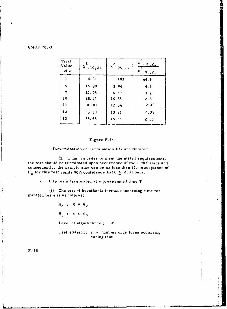
AMCP 702-3

Trial 2Z X 10, r

Value X .10,Zr X .9 5 ,2r 2.,of r X . 95,2r

1 4.61 . 103 44.8

5 15. 99 3.94 4.1

7 21.06 6.57 3.2

10 28.41 10.85 2.6

11 30. 81 12.34 2.49

1- 33.20 13.85 2. 39

13 35. 56 15.38 2.31

Figure F-14

Determination of Termination Failure Number

(d) Thus, in order to meet the stated requirements,the test should be terminated upon occurrence of the llthfiilure andconsequently, the sample size can be no lees than II. Acceptance ofHo ior this test yields 90% confidence that 0 > ZOO hours.

c. Life tests terminated at a preassigned time T.

(1) The test of hypothesis format concerning time ter-minated tests is as follows:

HO : e = 60

H1 : 0< eo

Level of significance a

Test statistic: r - number of failures occurringduring test

F-38

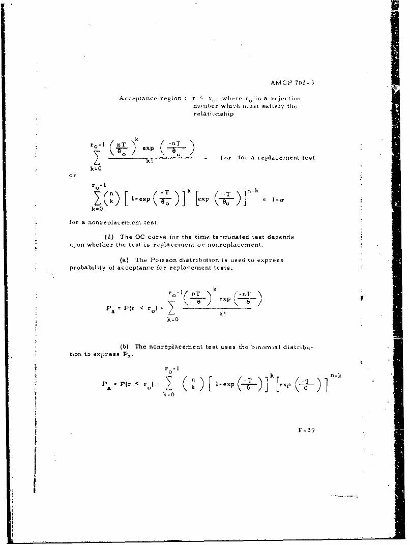
AMCP 702- 3

Acceptance region r < r, where ro is a rejectionnumber which itast satisfy therelationship

ro-I 2 nT xp "nT-k] 0 oI-a for a replacement test

orr-1

n-T kT -k -x x-P

k=O-

for a nonreplacement test.

(2) The OC curve for the time te-minated test dependsupon whether the test is replacement or nonreplacement.

(a) The Poisson distribution is used to expressprobability of acceptance for replacement tests.

r exp

Pa =P(r < r°) = \ O' ,

k=O

(b) The nonreplacement test uses the binomial distribu-

tion to express Pa"

r -1

k0

•. ok n -k

P =P~r < r )n k -exp Texp -•-a. 0 L_ k

S~~F-39 _-

I k=O

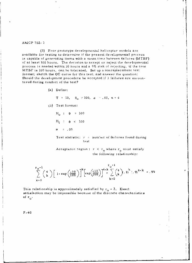
AMCP 702- 3

(3) Four prototype developmental helicopter models arc

available for testing to determine if the present developmental processis capable of generating itern6 with a mean tinie betwveen failures (MTBF)

of at least 100 hours. The decision to accept or reject the developmentalprocess is needed within 10 hours and a 5% risk of rejecting, if the trueMTBF is 100 hours, can be tolerated. Set up a nonrepiacement testformat; sketch the OC curve for this test; and answer the question:Should the development procedure be accepted if 3 failures are eincoun-tered during conduct of the test?

(a) Define:

T = 10, 0- 100, a - .05, n 4

tb) Test format:

HO :0 = 100

H : E) < 100

a .05

Test statistic: r num'er of failures found duringtest

Acceptance region r < r° where r must satisfy

the following relationship:

r -1

r°' kl _0ý- 4 1-9k 4-k 9k 1-(e]p Ie ) 0 Y) L 9 ,95

k-0 k=0

This relationship is approximately satisfied by ro = 2. Exactsatisfaction may be impossible because of the discrete characteristicsof r

F-0"

II-

-,-- - -! - -

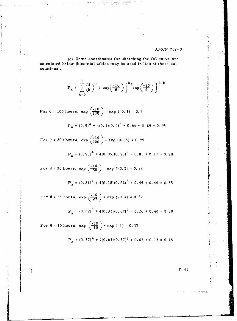
AMCP 702- 3

(c) Some coordinates for sketching the OC curve arecalculated below (binomial tables may be used in lieu of these cal-culations).

I k, 47 -ka , F k l -exp/ 1 .rexp/'1a jýkL'KJ'O/

k=0

(-10.For 0 = 100 hours, exp exp (-0. 1) -0.9

3IPa (0. 9)4 t 4(0. 1)(0. 9)3 = 0.66 + 0.29 = 0. 95

For 8 200 hours, exp , exp (0.05) 0.95

P = (0.95)4 + 4(0. 05)(0. 95)3 0.81 + 0. 17 0.98

Fcir e = 50 hours, exp L--• exp (-0.2) 0. 82

P= (0.82)4 + 4(0. 18)(0. 82)3 = 0.45 + 0.40 = 0.85

_-10 \Fc: E ) 25 hours, exp exp (-0.4) 0.67

674 673p = (0.67) + 4(0. 33)(0. 67)= 0. 20 + 0.40 = 0.60a (€

For 86 lhours, exp ' exp (-1) = 0.37

P (0.37)4 + 4(0.63)(0. 37)3 = 0.32 + 0.13 = 0.15a

ti4

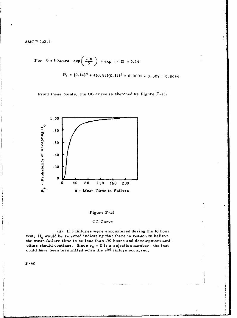
AMCP 702-3

For e 5 hours, exp(. ) 4exp -2) =0.14

Pa = (0. 14)4 + 4(0. 86)(0. 14)3 0 0. 0004 + 0. 009 0. 0094

From these points, the OC curve is sketched as Figure F-15.

1.00

0

S.80

. .60U

"q• .40

.20

0 A

0 40 80 120 160 200

e - Mean Time to Fail-ire

Figure F-15

OC Curve

(d) If 3 failures were encountered during the 18 hourtest, Ho would be rejected indicating that there is reason to believethe mean failure time to be less than 100 hours and development acti-vities should continue. Since ro = 2 is a rejection number, the testcould have been terminated when the Znd failure occurred.

F-42

AMCP 702- 3

(4) Inspection of the Pa functions for a time terminatedtest shows that sample size contributes to the degree of protectionoffered for a specified termination time T. The required sample sizeand rejection number may be found if the following test requirementsare specified.

(a) Test termination time (T).

(b) A lot (process) with 9 = 8 would have a(l-a)

probability of being accepted.

(c) A lot (process) with 0 0 0 would have a S proba-bility of being accepted.

The required sample size and rejection number mist satisfy the fol-lowing relationships. For a replacement test:

r4r°- ( TL>"'" J exD (.-nT -•l

and kr0 l(nT exp (nTZ)

k=O

SFor a nonreplacement test b

0r -0

k=OO

and -o-I

k l-exp exp=

0 -4k _"p -43

AMCP 702- 3

These determinations may be made by trying different values of roand n until the equations are satisfied. Figure H- 12 in appendix Hmay be used for the replacement test determinations. Binomial tableswould facilitate the nonreplacement test determinations.

d. Sequential tests.

(1) Often times a decision concerning acceptance or

rejection of Ho can be reached more quickly by applying a sequentialdecision procedure. A sequential test involves a set of rules to beapplied each time a failure occurs (theoretically applied continuouslyover time.) The decision will be one of these: Accept Ho and stop thetest, reject Ho and stop the test, or continue testing. The test wouldcontinue until a decision to accept Ho or reject Ho is reached.

(2) The tests discussed herein are determined by applyingWald's probability ratio test to an exponential distribution of failuretimes. The test procedure will be designed to test the following set ofhypotheses:

H :8<Eo

H1 :08<8

(3) In order to design a test, the following requirementsmust be specified.

(a) Determine an acceptable mean life Eo.

(b) Determine the magnitude of an a risk which maybe tolerated, where a is the probability of rejecting Ho if the popula-tion mean life 0 = 00.

(c) Determine an unacceptab)e or limiting mean life01 where 61 < 6o.

(d) Determine the magnitude of a 3 risk which may betolerated, where B is the probability of accepting Ho if 0 8 01.

F-44

F -°

AMCP 702-3

(4) Ihe protection offered by the test may be evaluated byexamining it'j operating characteristic (OC) curve. Another factorwhich is of importance in selecting a plan is the expected duration ofthe test, i. e. how long must we wait for the decision?

(5) The sequential decision criteria are:

If h- + k s < V(t)< ho + k s, continue the test.

If V(t) h + k s, stop the test and accept Ho.

If V(t) < hI + k a, stop the test and reject H0

where

InK .)ho n In! o = IIh I = - II

I h -- T

00 00,-0'SIn

!7

i s= I

1 o

Vlt) = nt for a replacement test

kV(t) E X i + (n-k)t for a non-replacement test

i=l

t is the test duration time

n is the original numnber placed on test

x, is the time of the ith failure measured from test beginning

IF-45

AMCP 702- 3

(6) This sequential procedure may be applied at any pointin time but must be applied at least upon the occurrence of each failure.Graphically, these decision rules appear as shown by figure F-16.

Accept H 0

Continue the test

k

Figure F-16Graphical Decision Rules of the Sequential Test

(7) The OC curve coordinates may be found by letting theparameter h run through all real values in the following parametricequations.

eo h

e >h

F-46

AMCP 702-3

Figure F-17 shows five points which are easily found and enable us tosketch the OC curve.

0 p

|

-a

0 0

IDI

* Figure F-17Coordinates for Sketching Sequential Test OC Curve

decision, E 0 (r), is dependent upon the lot mean life and may beI found as follows:

- (h0 -hl) PaE(r)=a#

E e

s

-hh

,, 8

E l-e =

where the random variable r is the number of failures requiredS dis to reach a decision. The approximatn values of E y(r) if

) F-47

found asfol-ows

AMCP 702-3

a =0O13119,6 or -reduce to0i

-hi

Eo(r) =

SIn (T.) + (1-1)ln (In )

_in (±-2),°(t*In

a 0

-In in i

E (r)

in (6 0

02

E 0o(r)

eoe

E,.(r) = 0

(9) The expected waiting time to reach a decision, E e (t),is a function of 0 and is found by

E 6 (t) =i E 0 (r) ior a replacement testn

and approximately

Eo(t) M - In [ nn-E0 3 for a nonreplacement test

For either case. 0 : m -duces to E D (t) - 0n

F-48

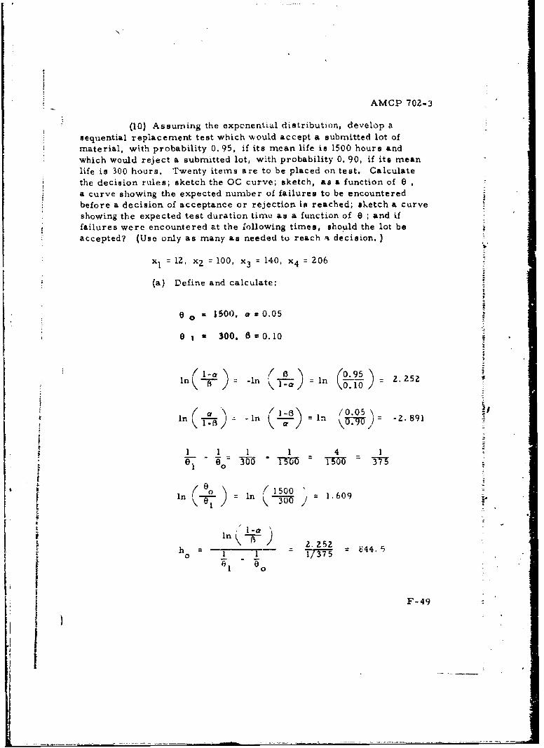
)N

AMCP 702-3

(10) Assuming the exponential distribution, develop a

sequential replacement test which would accept a submitted lot of

material, with probability 0. 95, if its mean life is 1500 hours and

which would reject a submitted lot, with probability 0. 90, if its mean

life is 300 hours. Twenty items are to be placed on test. Calculate

the decision rules; sketch the OC curve; sketch, as a function of 8a curve showing the expected number of failures to be encounteredbefore a decision of acceptance or rejection is reached; sketch a curve

showing the expected test duration time as a function of 0 ; and if

failures were encountered at the following times, should the lot be

accepted? (Use only as many as needed to reach a decision.)

x 12, x) = 100, x 3 = 140, x 4 N 206

(a) Define and calculate:

8 o = 1500. a 0.05

0 1 * 300, 8=0.10

In -n I In (2-1-/)= .252

Inln L(2) In /0.0 ~ 2.891

1 1 1 1 4 1

S1500

In (- In 3- 0 1.609

Iniln-j ) 2. 252 Sh 6 - 44. 5

0

F-

F-49

II

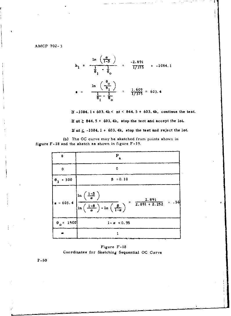
AMCP 702- 3

in(T7 _Z. 891h uI ! i7 -1084.1

IWl " o

a 1.609 = 603.4

If -1084. 1 + 603. 4k< nt < 844. 5 + 603. 4k, continue the test.

If nt > 844. 5 + 603. 4k, stop the tect and accept the loL

If nt <. -1084. 1 + 603. 4k, stop the test and reject the lot.

(b) The OC curve may be sketched from points shown infigure F-18 and the sketch as shown in figure F-19.

B p0 Pa

0 0

a 300 0 =0. 10

__Iell 2.891a = 603.4 -- L.891+2.25 .56

In -I 2.81+Z 5

00= 1500 i-0 Z0.95

Figure F-18Coordinates for Sketching Sequential OC Curve

F-P0

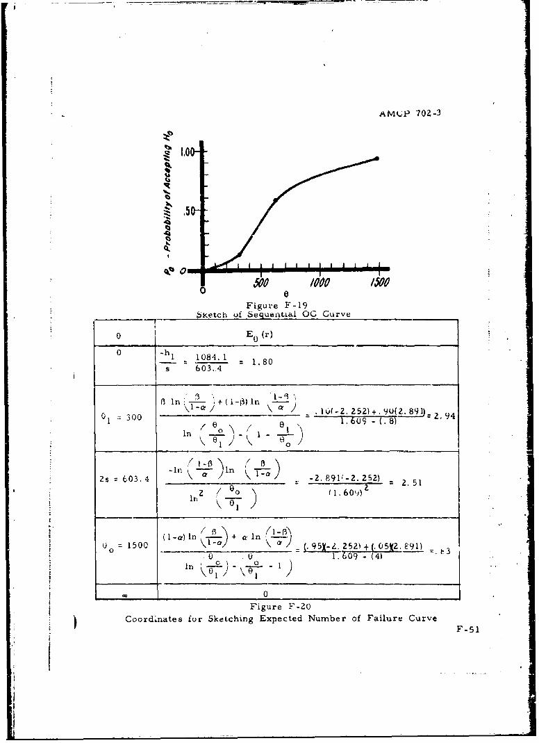
Am(-;? 70Z-3

4ý 0

0e

Figure F-196 ketch of Sequential OG Curve

o~Eo (r)

0__hl 10 4.1 = 1.80s 603,A

8 60 /0 /000

____300__ SkeI ch- 2. 2q5e) ial_089C2.v9

o 1084. 1.619 -8)

-In )L2s =603.4 -2, 891-2. 252) = 2, 51

/ Oo ( 1.60,))Z

13 3

a) I no-- +aI3003 in- +150C ,in \--,) 95X-Z. 2 521+(.0•(Z. E91) _ 3

in°:.:-- 16u5008

o 1o- .609 - (4)

os=634 , on ) -I-.9-. ) 25

In

o0 0Figure F-20

S~Coordinates for Sketching Expected Number of Failure CurveS~F-51

-_ _ _ _ _ _ _ _ _ _ _ _

( (3 1-r3'

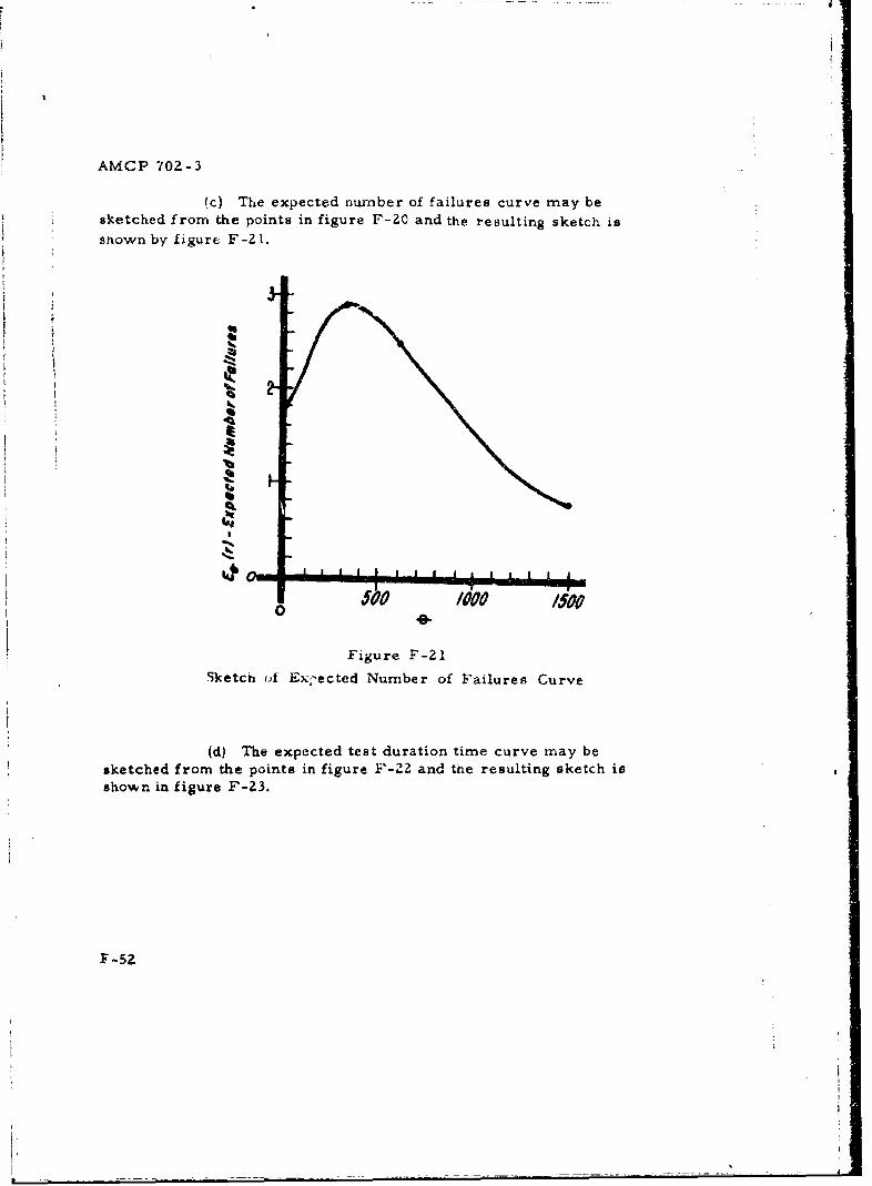
Iif

AMCP 702-3

(c) The expected number of failures curve may besketched from the points in figure F-Z0 and the resulting sketch is

shown by figure F-21.

500,"•s,' /000 /500IT

Figure F-21

Sketch (A Ex-ected Number of Failures Curve

(d) The expected test duration time curve may besketched from the points in figure F-22 and the resulting sketch isshown in figure F-23.

F-52

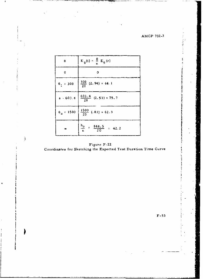
AMCP 702-3

TI-

8 E 0 (t)= _0 Ee(r) 4

0 0

8, =300 MOO (2.94) = 44 1620

8 603A4 6 134(2.51) :75.76. 20

1500 00 (.83) = 62. 3

ho 844.5n 42.2

Figure F-22Coordinates for Sketching the Expected Test Duration Time Curve

F-53

IF.53

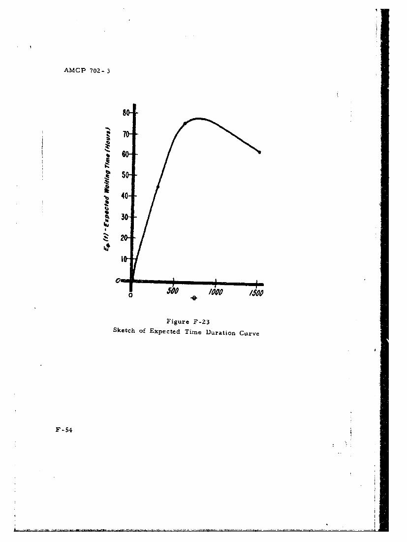
AMCP 702- 3

8

40e

Figure F-23Sketch of Expected Time Duration Curve

F-54

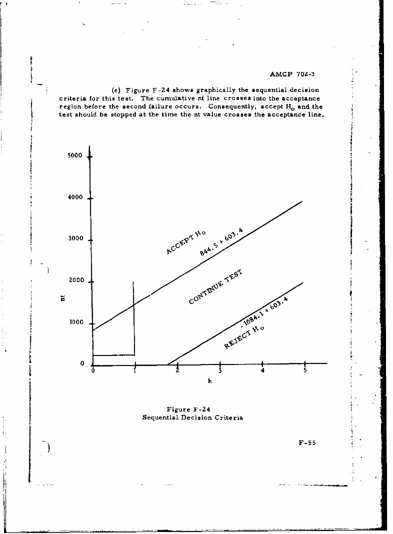
AMCP 70Z-3

(e) Figure F-24 shows graphically the sequential decisioncriteria for this test. The cumulative nt line crosses into the acceptanceregion before the second failure occurs. Consequently, accept H. and thetest should be stopped at the time the nt value crosses the acceptance line.

f

5000

10

3000tI

2-- 32000 ,• o

4- o.. °÷I

1 0

4 5

k

Figure F-24Sequential Decision Criteria

) F-55

AMCP 702-3

(11) The primary advantage of sequeiaLial testing is that,on the average, less testing is required. Some important disadvan-tages of sequential testing are as follows:

(a) The exact amount of testing is not specified inadvance with the result that planning and budgeting problems maydevelop.

(b) The greatest amount of testing is required if thevalue of 0 lies in the zone of indifference between 8 1 and "0.

(c) The required record keeping becomtes more complex.

F-10. Weibull failure times. The Weibull distribution depends upontwo parameters ,3 and i . Tests of hypotheses concerning these para-meters are ratheir complex and will not be discussed herein. However,there are government sampling tables pertaining to the Weibull distri-bution.

F-11. Normal failure times. Tests of hypotheses may be applied tothe parameters M and a' , of the normal distribution. However, thesetests are found in numerous elementary statistics textbooks and willnot be discussed herein.

Section IV. ACCEPTANCE LIFE TESTING

F-12. General. a. The precedinp. tests were concerned wiih testingof hypothesis about reliability and reliability related parameters. Thistype of test, when used as a basis for accepting material, is scnLetimresreferred to as an acceptance life test. There are a number of govern-nment documents which contain tables of test plans which were calcula edusing tests of hypothesis similar to those already discussed. These wlibe discussed under the title of acceptance life tests.

b. Tables are available for different failure time models. Thoseto be discussed herein will include the exponential distribution, Weibulldistribution and normal distribution, as well as nonparametric tablesSince these documents are self-explanatory and include examples, thecontents will only be summarized.

F-56

- _ _ _ _-

I -- - - ~ ------ =-~-----~--=-=----------

AMCP 702-3

F -13. Exponential failure times.

a. DoD Quality Control and Reliability Handbook H108,Sampling Procedures and Tables for Life and Reliability Testing(Based on the Exponential Distribution) contains tables of life testingsampling plans pertaining to exponential failure times. The plansare divided into three general categories- failure terminated tests,time terminated tests and sequential tests. The mean failure time 8is used as the reliability parameter under test. Minimal and nominalacceptable values of e, along with allowable risks, are used as thebasis for specifying a satisfactory sampling plan.

b. The sequential test procedures are outlined and the para-meters of the test are tabled. The formulas of paragraph F-9d ofthis appendix may be used for expanding these tables. I

c. Operating characteristic curves are drawn for most tabledplans. The methods in paragraph F-9 of this appendix may be used for

* constructing OC curves which are not included.

* F-14. Weibullfailure times. A series of technical reports containtabled sampling plans when failure times are distributed in accordancewith a Weibull distribution. Each is dependent upon a known Pparameter

a. DOD Quality Control and Reliability Technical Report TR-3, 1

Sampling Procedures and Tables for Life and Reliability Testing Basedon the Weibull Distribution, (Mean Life Criterion) provides tabled • Iplans when mean failure time is the reliability parameter to be tested.

b. DOD Quality Control and Reliability Technical Report TR-4, 1

Sampling Procedures and Tables for Life and Reliability Testing Based -

on the Weibull Distribution (Hazard Rate Criterion) provides tabledplans when hazard rate or instantaneous failure rate is the parameter iunder test. 5

c. DOD Quality Contrul and Reliability Technical Report TR-6, 1

Sampling Procedures and Tables for Life and Reliability Testing Basedon the Weibull Distribution (Reliable Life Criterion) provides plans whenreliable life is the parameter under test. Reliable life is defined as thattime beyond which a specified portion of a lot can be expected to survive.

d. DOD Quality and Reliability Assurance Technical ReportTR-7, Factors and Procedures for Applying MIL-STD-105D SamplingPlans to Life and Reliability Testin , provides instructions for selectinglife test sampling plans from MIL-STD-105D.IThese reports may be secured from the Superintendent of DocumentsU.S. Government Printing Office, Washington, D.C. 20402. -57

AMCP 702-3

F-15. Normal failure timas.

a. if failure times are known to be normally distributed, alife test sampling plan may be found from MIL-STD-414, SamplingProcedures and Tables for Inspection by Variables for Percent De-fective. Am indicated by the title, MIL-STD-414 expresses confor-mance as percent defective, i.e., the percent of the iterr i fallingoutside specification limits. In the case of life testing, c ,nformancemay be expressed as the percent of items failing prior to a specifiedtime.

b. A life test sampling plan from MIL-STD-414 would requirethat all sample items be tested until failure. The resulting failuretimes may then be symbolized as xl, x 2 , . . # xn. A sampling planconsists of two parameters -- sample size (n) and maximum allow-able percent defective (M) - - and may be obtained if an AQL inspectionlevel, degree of inspection, and lot size are specified. The first stepis to find a code letter in table A-2 by using the lot size and inspec-tion level. If normal or tightened inspection are to be used, entertable B-3 with AQL and code letter to find n and M. For reduced in-spection, table B-4 is to be used.

C. The procedures of analyzing the sample data and decidingupon lot acceptance is summarized in the following steps,

(1) Compute the sample mean X Exn

(2) Compute the sample standard deviation

a-/nZ; x -'(Z; x)Z

n(n- 1)S--

(3) Calculate the quality index

QL= -L

a

where L is a lower specification limit (specified time) andwhere QL is the quality index associated with L.

F-58

AMCP 702- 3

(4) Enter table B-5 with QL and n to find the estimatedlot percent defective (PL) associated with the lower specification limit.

(5) The decision rules are as follows:

(a) If PL - M, accept the lot

(b) If p > M, reject the lot

cd. To illustrate the selection of a life test sampling plan fromMIL-STD-414, consider a lot of 60 components which has been submittedfor acceptance relative to life characteristics. The failure times are "known from past experience to be normally distributed. A life test 9

sampling plan is to be selected from MIL-STD-414 using inspectionlevel III, normal inspection, variability unknown - ctandard deviation

method, single specification limit and form Z.

(1) Find the sampling plan, n and M, such that if the lothas a reliability of 0. 975for a 35 hour mission time, R(33) = 0. 975,

the probability of acceptance would be high.

(2) If the submitted lot has R(35) = 0. 90 what is its prob-ability of being accepted?

(3) Using the plan found in part(1), the failure times wereas follows: 34, 38, 47, 51, 55, 59 -nd 62 hours (use only as many as

required in the sampling plan). D( 'rmine whether the lot should beaccepted. j

i e. The solution is as follows:

(1) An AQL of 2. 501 defective for a lower specificationSlimit L = 35 hours would correspond with R(35) = 0. 975.

(a) Using a lot size of 60 and inspection level III,table A-Z yields code letter C.

(b) Using code letter C and AQL = .05%, table B-3yields n =4 and M 10.92.

F-59

.1

*1_I

AMCP 702-3

(2) Find the OG curve which is shown for code letter Cand AQL = 2. 5% on page 7. For a lot with R(35) -: 0. 90 (i. e. , 10%

failing before 35 hours) tE.s OC curve shows a probability of accep-tance of 62%.

(3) Since n = 4, the resulting failure times were 34, 38,47, 51.

'C

34 1156

38 1444

47 2209

51 2601

170 7410

(a) ( ILZ x 170 425n 4

(b) * j= nZ x 2 - (2 x)L / 4(7410) - (170)" 7.85(b n(n-1) 4(3) 7

(c) OL IZ -L 42.5- 35 0.96a 7.85

(d) Using QL =0. 96 and n = 4, Table B-5 yields an estimatedpercent defective PLI 18. 00,

(e) Since PL =18. 00 > M = 10. 92, the lot is rejected, andconclude that the reliability of the lot is too low.

F-16. _Nonparametric sampling plans.

a. MIL-STD-105D, Sampling Procedures and Tables forInspection By Attributes, provides sampling plans relative to attributes

F-60

1

AMCP 702-3

inspection. Attributes inspection is inspection whereby either theunit of product is classified simply as defective or nondefective, or

tk the number of defects in the unit is counted, with respect to a givenrequirement or set of requirements. Thus, conformance can be

I expressed in terms of percent defective or defects per hundred units.For reliability testing purposes, we rhall be concerned with percentdefective.

tsb. These procedures apply directly to one shot items, i.e.,those for which failures do not depend on time. However, thesesampling plans may also be applied to life tests even if the distribu-tion of failure times is unknowr. In this case a defective item wouldbe defined as an item which failed prior to a specified time t. Sucha life test must be nonreplacement and must be terminated at t.

c. A sampling plan may be found from MIL-STD-105D if thelot size, inspection level, AQL, degree of inspection, and type ofsampling are specified. The initial step is to find a code letter in

table I using lot size and inspection leval. If either normal or tightenedinspection is specified, enter table X with the code letter and AQL tofind the sampling plan. If reduced inspection is in effect, find the plantt • in table 11-C for single sampling-

d. The single sampling plan consists of a sample size (n), and

acceptance number (Ac) and rejection number (Re). The lot is to bet accepted if the number of defectives found in the sample does not exceed

the acceptance number. The lot is to be rejected if the number of sam-* ple defectives is equal to or greater than the rejection number.

e. For example, a lot of 125 components has been submittedfor acceptance with respect to life characteristics. The distributionof failure times is unknown. A nonreplacement life tes, sampling planis to be selected from MIL-STD-105D using inspection level llU, normalins,,ection and single sampling.

(1) Find a sampling plan such that the probability of accep-tance will be high if reliability for a 10 hour mission time is 0. 96.

(2) If the submitted lot has R(10) = 0. 92, what is itsprobability of its being accepted if this plan is used?

F-61

AMCP 702-t

(3) A sample of the size found in part 1 was subjected totest and 2 items failed prior to the 10 hour termination time. Shouldthe lot be accepted?

f. The solution follow.-;:

(1) The life test is to be terminated at 10 hours. Then anAQL o" 4% would correspond to R(10) = 0.96. The sampling plan isfound a s follow s:

(a) For a lot size of 125 and inspection level III,

table I yields code letter G.

(b) For code letter G, AQL ý 4. 0, normal inspection

and single sampling, table X-G-2 indicates a sampling plan of n - 32,

Ac = 3 and Re - 4.

(2) Find the OC curve for code letter G and AQL = 4. 0

in chart G. For a lot with R(10) ý 0. 92 (i. e. , 8%/c failing before 10 hours)

this OC curve indicates a 74% probability of acceptance.

(3) Of the 32 sample items, 2 failed before test terminationtir.e of 10 hours. Since the number of failures did not exceed the accep-tance number, the lot should 1e accepted because its reliabiliry is high

enough.Section V. REGRESSION ANALYSIS

F-17. General. a. A major problem during the research and develop-

ment of an equipment is the assurance of high functioning reliability ofthe final prototype model. Reliability analysis sometincs involves the

determination of some reliability parameter for various known stresslevels a-r design characteristics; for example, determination of the mean

time to failure at different levels of stress, determination of the burstingpressure for different wall thicknesses of rocket motors, determinationof vehicle fuel usage at different velocity levels, etc. Such determina-

tions are sometimes useful for evaluating equipment design, identifyingtrouble areas and potential corrective activities, etc.

b. Regression analysis, applied to experimental data, may beused to provide information concerning the relationship between a

F-62

AMCP 702-3

response (dependent) variable and various levels of an independentvariable(s).

F-18. Simple Linear Regression.

a. The simplest form of regression involves determinationof the expected value of the response or dependent variable from in-formation concerning the independent variable value. Herein, weshall discuss simple linear regression where the expected response isa linear function of the independent variable. The regression model is

.A+Bxy. x

whereJA y. x expected response associated with x

k A and B are parameters of the model

b. The parameter B indicates the amount oi change in y whichcan be attributed to a unit change in x, i. e., the slope of the line. Ais the value of ;A Y. x evaluated at x = 0.

c. Since A and B are parameters, they may be estimated byanalyzing n observations of paired values of (xi, Yi) where i = 1, 2,n. The regression equation for estimating the expected response is

Ay =a + bx

where

a 2 is an estimate of AX)2

nZx 2 -(I

b• -. is an estimate of B"n Ex2 - (x)Z-

and

Sis an estimate of fy x

F-63

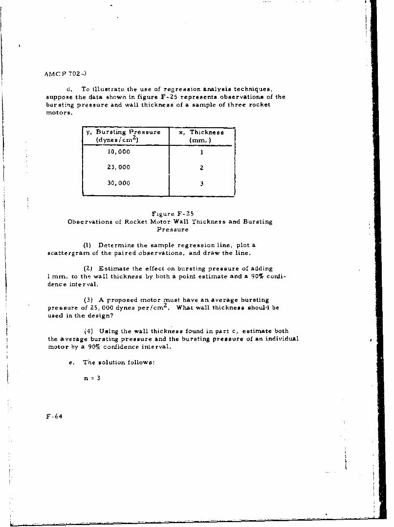
AMCP 702-3

d. To illustrate the use of regression analysis techniques,suppose the data shown in figure F-25 represents observations of thebursting pressure and wall thickness of a sample of three rocketmotors.

y, Bursting Pressure x, Thickness(dy'nes)/cmz (ram.)

10,0001

23,0002

30,000 3

Figure F-Z5Observations of Rocket Motor Wall Thickness and Bursting

Pressure

(1) Determine the sample regression line, plot ascattergram of the paired observations, and draw the line.

(Z) Estimate the effect on bursting pressure of adding1 mm. to the wall thickness by both a point estimate and a 90% confi-

dence interval.

(3) A proposed motor must have an average bursting

pressure of 25, 000 dynes per/cmZ. What wall thickness should beused in the design?

(4) Using the wall thickness found in part c, estimate boththe average bursting pressure and the bursting pressure of an individualmotor by a 900 confidence interval.

e. The solution follows:

n=3

F.64

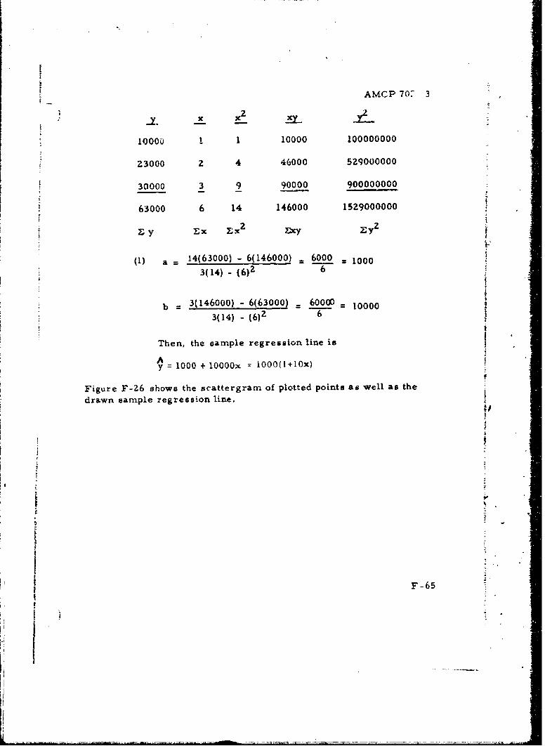
AMCP 707 3

y . xx 2 y 2 .•

10000 1 10000 100000000

Z..3000 2 4 46000 529000000

30000 3 9 90000 900000000

63000 6 14 146000 1529000000

E y Ex Ex 2 cY

(1) a = 14(63000) - 60146000) 6000 1 I0003(14) - (6)2 6

i b = 3(146000) - 6(63000) _ 6 I00003(14) - (6)7 6

Then, the sample regression line is

y = 1000 + l000x = 1000(1+lOx)

Figure F-26 shows the scattergram of plotted points as well as the

drawn sample regression line.

F -65

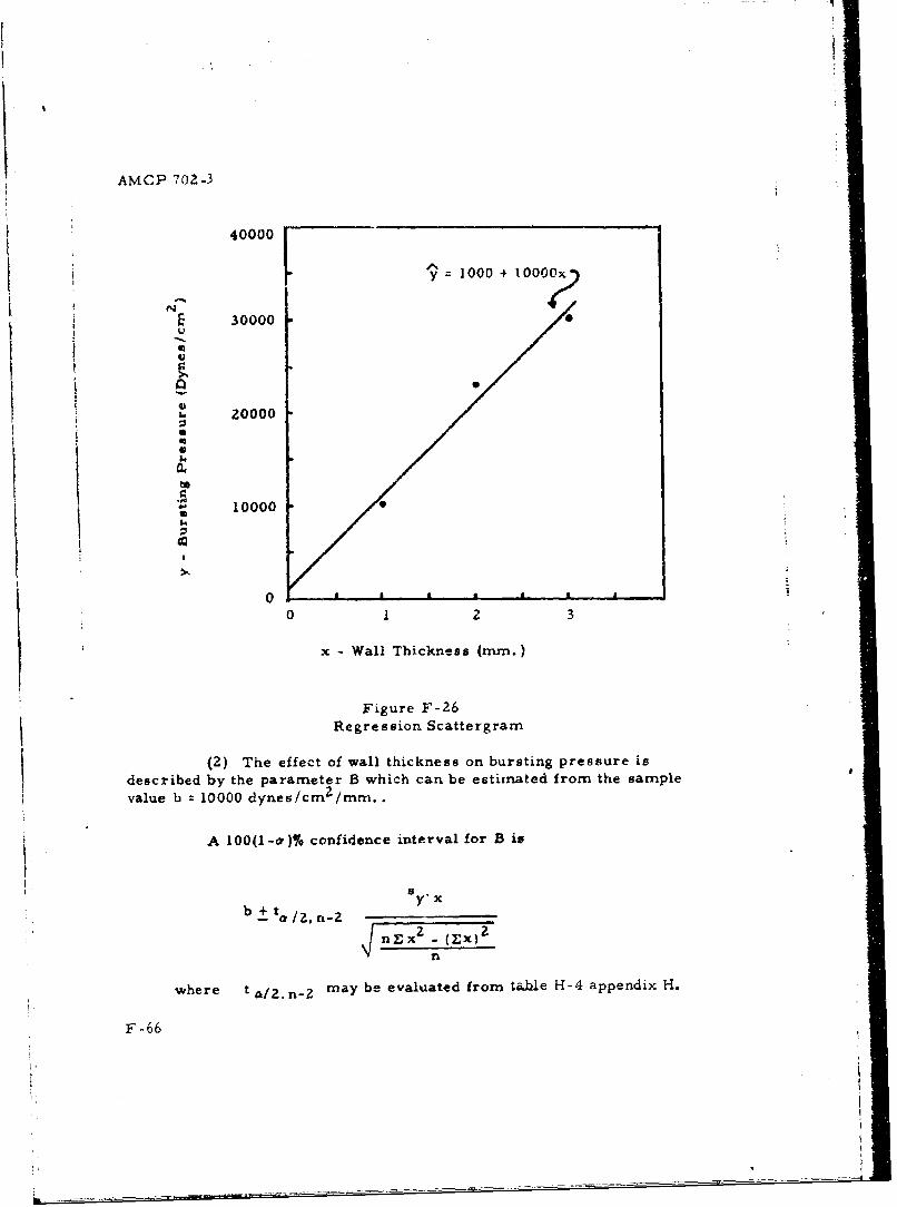
AMCP 702-3

40000

y 1 000 + 100(0;• ý

N 3000011

I1. 20000a

F 10000

00 2 3

x - Wall Thickness (mm.)

Figure F-26Regression Scattergram

(2) The effect of wall thickness on bursting pressure is

described by the parameter B which can be estimated from the sample

value b 10000 dynes/cm 2 /mm..

A 100(1-&, )% confidence interval for B is

Y--6b + t

nZ~x Z-(EZX)n

where t 4/2, Z may be evaluated from t~.ble H--4 appendix H.

F-66

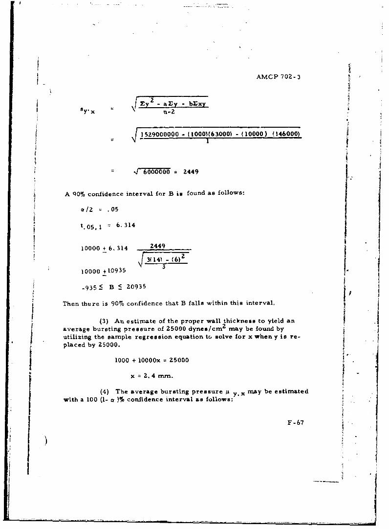
AMCP 702- 3I -.

-/y aZ~y - blxy

8Yx

I529000000 - (1000)(630001 - (10000) (146000)

/6000000 2449- I":

A qOj% confidence interval for B is found as follows:

0/Z .05

t. 05.1 = 6.314

10000 + 6. 314 2449

St 3( 141 6

0oooo +10935 3 (6)2

.-9355 B 5 20935

Then there is 90%6 confidence that B falls within this interval,

(3) An estirmate of the proper wall thickness to yield an .

average bursting pressure of 25000 dynes/cm may be found byutilizing the sample regression equation to solve for x when y is re-

placed by 25000.

1000 + 10000x = 25000

x = 2.4 nm.

(4) The average bursting pressure g y.x ray be estimated

with a 100 (1- a )% confidence interval as follows:

F-67 -

j o

*1

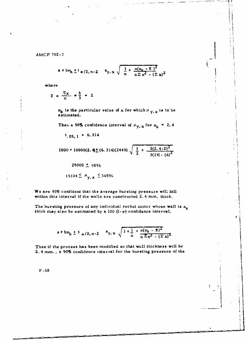
AMCP 702-3

a+bxk~t/*12,n-Z sy.x + nx.x Z (IY

where

Ex 6

n 3

xk is the particular value of x for which 11 . x is to bee stimated.

Thez. a 90% confidence interval of A y. for xk = 2. 4

t. 05,1= 6. 314

1000 + 10000(2. q± (6. 314)(Z4491 1 + 3(2.4-2)3(14) - (6)Z

25000 ±. 9896

15104 _ My. x -< 34896

We are 90% confident that the average bursting pressure will fallwithin this interval if the walls are constructed 2. 4 mm. thick.

The bursting pressure of any individual rocket motor whose wall is xkthick may also be estimated by a 100 (1- a) confidence interval.

a+bxk + t z,n2 n yZ +I + nlxk--n n Exz _ (E X)

Then if the process has been modified so that wc.ll thickness will be2. 4 mm., a 90% confidence interval for the bursting pressure of the

F-68

I I ,

S. . . _ _ _ _ _ - . . ..

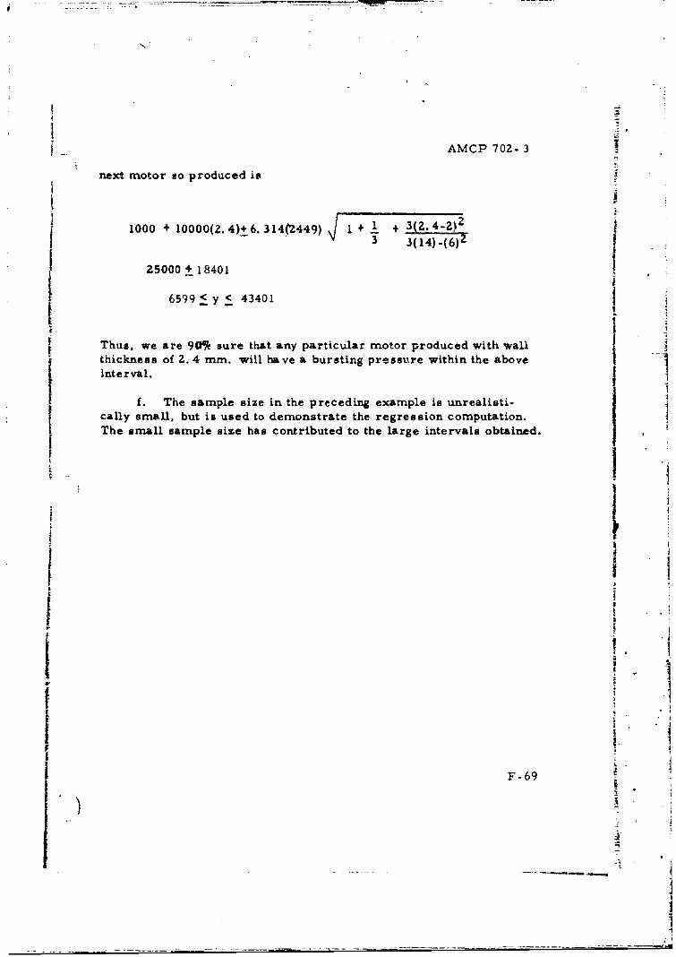
AMCP 702- 3

next motor so produced is

1000 + 10000(2.4)+ 6. 314(2449) 1 + 1 + 3.2.4-2)t -3 3(14)-(6)2

25000 + 18401

I 6599 ! y < 43401

Thus, we are 90% sure that any particular motor produced with wallthickness of 2. 4 mm. will have a bursting pressure within the aboveinterval.

f. The sample size in the preceding example is unrealisti- Acally smaull, but is used to demonstrate the regression computation.The small sample size has contributed to the large intervals obtained.

1F I

I

IiI I.

I!• -1I 1;

1.

:1

AMCP 702- 3

I APPENDIX G

RELIABILITY EVALUATION, FAILURE ANALYSISAND CORRECTION -- THE FEEDBACK LOOP

(Not included in this issue.)

G-1

10

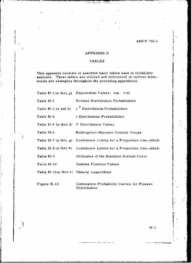
!N

AMCP 702-3

APPENDIX H

TABLES

Ths

This appendix consists of assorted basic tables used in reliabilityanalysis. These tables are utilized and referenced in various state-

nments and examples throughout the preceding appendices.

Table H-I (a thru g) Exponential Values: exp (-x)

Table H-2 Normal Distribution Probabilities

Table H-3 (a and b) xy Distribution Probabilities

Table H-4 t Distribution Probabilities

Table H-5 (a thru d) F Distribution Values

Table H-6 Kolmogorov-Smirnov Critical Values

Table H-7 (a thru g) Confidence Limits for a Proportion (one-sided)I

Table H-8 (a thru h) Confidence Limits for a Proportion (two-sided) I

Table H-9 Ordinates of the Standard Normal Curve i

Talle H-10 Gamma Function Values

Table H-11(a thru c) Natural Logarithms

Figure H-12 Cumulative Probability Curves for PoissonDistribution

H-1.- H -I

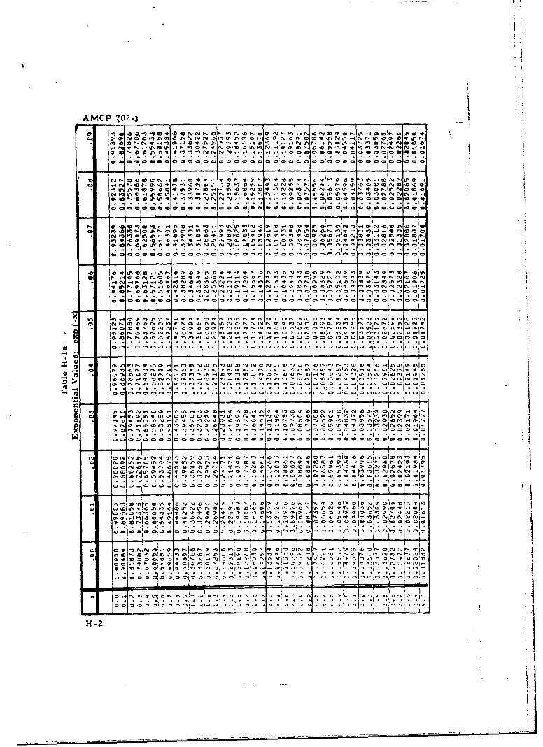
AMCP 702-3 ____

0. ~ ~ ~ W W ~ ~'. 04) 10 ev I0 N l'N CIO N )l ' I n K m0" 0 ' AN "'1 14 LmJ 17,N '.4,' In'. cIz In W.'

M .4Un M 0 ' )04N N ý'4 CD. rI V M1 4 U I 4 'IC 'O'n0 0100 MI0000itv1-1

10 .vi 'L)0 a n I- 00' -4 W' M' l'0 ' a, l' P ZP vOP "' c W 1 0, 3.o- 0, n~ 'A. WIN NIU'0.', P. CI 0, '0 N ' 0DII Lf Q) 0. (V 0 A 0 C' I ". uN U' .0.-N U' .0 0.) C-O . ~ 0 -4 0 012

.4 0 .4U 0N vA 1-I K) 0D M! 0A ! I 7 II' 1N.- '0N. 0 NU '4 04)AN NNIfK n '0 0ý Q' v' v' U4 'A 43v N N 04 N''- .'111- N- '-0 .- 0 0 V 0 NI 0. w OO a j o0

00o )).- %- '44 O.4': ' .- flU .4 0 ... .A .0. .' 05 .I 'N 0c) c0 0 ý Nb l C2N 03 a' CD 0D 0(0 Co M. C0 N~c 0ý oi-4 4'. 40 'U 'N QN 0

' In0 0 0

0) P " HA ~-r% 10 ~ -1 00 UM 3' ; N1 !4 0' .04 04 'D 0 L .\JI. .4.004- 04- .- vlL 00ýom) 4 ' lC '00 N '0 O I.4 n-V Ol0 JU c NA K0 Nv un ': 0 N e0 '.0 '0. 'n v04 4' 0 n 00 C

C4 V 0. "1 '4 0 00 4!- .1- 4. -. i0 0,0 W) m m no0 0:C'0.

N l CD CN NO .0 -i 0 3 m' 4z C.. . 4C'. 4r~04 'N C) 0 ')N4 4 -N D

10 000 0 00 IV 000 D0 0 00 0 00 It IV 00 N W1 0 v0 00t 01 0: C,

- 4CI l4 O )1 I lný1 r tI -0 -) - -ý 1 4mnK -

go N 0ý oN N N) v404 40U -o- N L' 4D W'. n' 1,.n -N ell 1\1 IT "4' W ' 10 0, N ' v N v' 14D It -N 0 4 0A J.I 4 ) 4 , - 0 .t >11 1' V.. 1 ..4 .I I .' 0 1 n: . I. I 0v 0 ) 00 :ý 0 D0 MIn0000, -

1c:; I."C.

.0W 0In3 0 v 'I. M' NS t) 00 CI0 0 11) 0 N0 " '4 M vI 0,0 J\1 0a C. ci 00

-0 IN 0 P, IN 0 U' 'r co : .0 c ) I 'a NI x IN ) -' 1) In It M. W N . g -4I N .- -W i

I I I I)) -.4 I4 10 I.? 1 0 -14) 1. '1 0 -V 1 0 0 -i ' JD ,V.N -) 3. N 2'ý0 Fl p

10~~~~ ~ ~ ~ 0D V0 1 l11 0 0 0n It v v " 010 m IN0

___1_ . .C vc ýc

) LAX t') DI DN-4 aNN c '0'7.0 >4.44-

0oD .V IO 40 0 I- 0 ' O4 I ' Y 0 310 n r% 13N 010ý ýA(IN J'0.000'AINN 01 0.-I1

NN0.-I'110 A' r - U' Nv '00 N, 3 04 4 47 N N 0U '' ' '( 00 0

C* 0 ý C >*i 0 C2, A I='000 - 0 -. ,. 00 11, 1c; 0; 0 0 0 00

-V 00 00i 00 0' 00 0 00 0 200C 0 0 '000

m0 N N I U: PI lOP v' z' m ' , 0' <' .4'4 0- 0 O V0 I- 1 L .0 -T v .' 011 N C 4 ' IN

n40 AI' -,0U'0 N 0' NJ N A). vN N0 0-~ 0 10 IN)0 '7 a. 4'1 \0. .- t . n Nm ')00.0 a '0N ;AN 4, 0 0-In 1A N x - 01'.c 110! CsJ IN JOO N\ A!T . 0040') -0 In,) 0.'0 - 3I4

Y\ - ' - If. ID14

0.~ 0 4 10 J!- 0.N 4 .0 n' \1 r.004 . ,7 1N.~C 04 ''0000 N G N.mCD .:OJ':'4 4' 0 1 ONI N N 0 ) p-i z.: 0 01 10-0 N. '00 ': 0 0 0

t -HW--i-4 I -

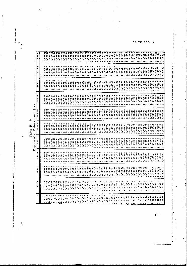
ANICII 7U~- 3

C,0Iý aV

0 000'00C0 90 0 0 ,00. 000 0 0 0000

0:6 0 :00 0 :0 : 0 C00000 0: C. 0 :0 0 0 :0 C fl 000 0O:ao o c O

*i a 2 - 0 . .0 ?NeC* J w w~qI..owm r..o tIN.cnr 0

4#).04N4 WN n)bCI0, 0.0I l &V ; ýC ,0aa0

0. "'o 0 0 0 0 & ' * 0 0 0,0, 0, C Cý I

C: 0: 0:C . I

0k nU 000W00N 00 0 0 q, In 00 0 000 0 0 0 0 0 0 0 0 00~1 O O C

0 0 0 0 0 0

0 0 0 0 0 0 0 0 9 0 00oo o ~ o c oa,*.. . . . . .. . . . . . . . . . . ..ma 9. . . . . ..ý 0

0ý1 0C C WW 4 ,. C W CV'. ra a -0: Cr C0\ MN - c

000~ ~~~~~~~~ a00 0 22 0 4 t NNN N-. a. NN 000 C CC Cýu 00rm inn u

a0 a

. 0 0 0 0 0 0 0 0 0 1 4 C 0 00 0 a . 4 0 0 0 0 0 0 0 0 0 0 00 0 0

NV- ~ ~ ~ ~ ~ Q N 0NNN -ý-~ a C ý a 0. a

Oc. 0: nvN..cO ar1ý rý o. co 1 cr ro ,.oc:cr.oe4

.c a. .r ,. .,

aC 00 00 0 00 a a0aC ý0

- ~ ~ N -O-O- - - - - - - - - -- - - - - -

a00C 00 0 0 l0 0 a 0 0 o o o o. .C,

. . . . . . . . . . . . . . .. . . . . . . . . . . . . . . . . .

C 000000 N 00000000~~~C c0

C 0 t 0 0 0 n n o 0 , o o a~~

N ; 4C 02 . 00 C7a.r r 4.rzrz7o o 7O oO ~ y C,4

,O~ O 0

1. 0 N~ wr a-~(r r. 4.I W C.N-- 4 N .4 a N N -. C 4 9 ' ~ * N C C t ~g . H -3 ~

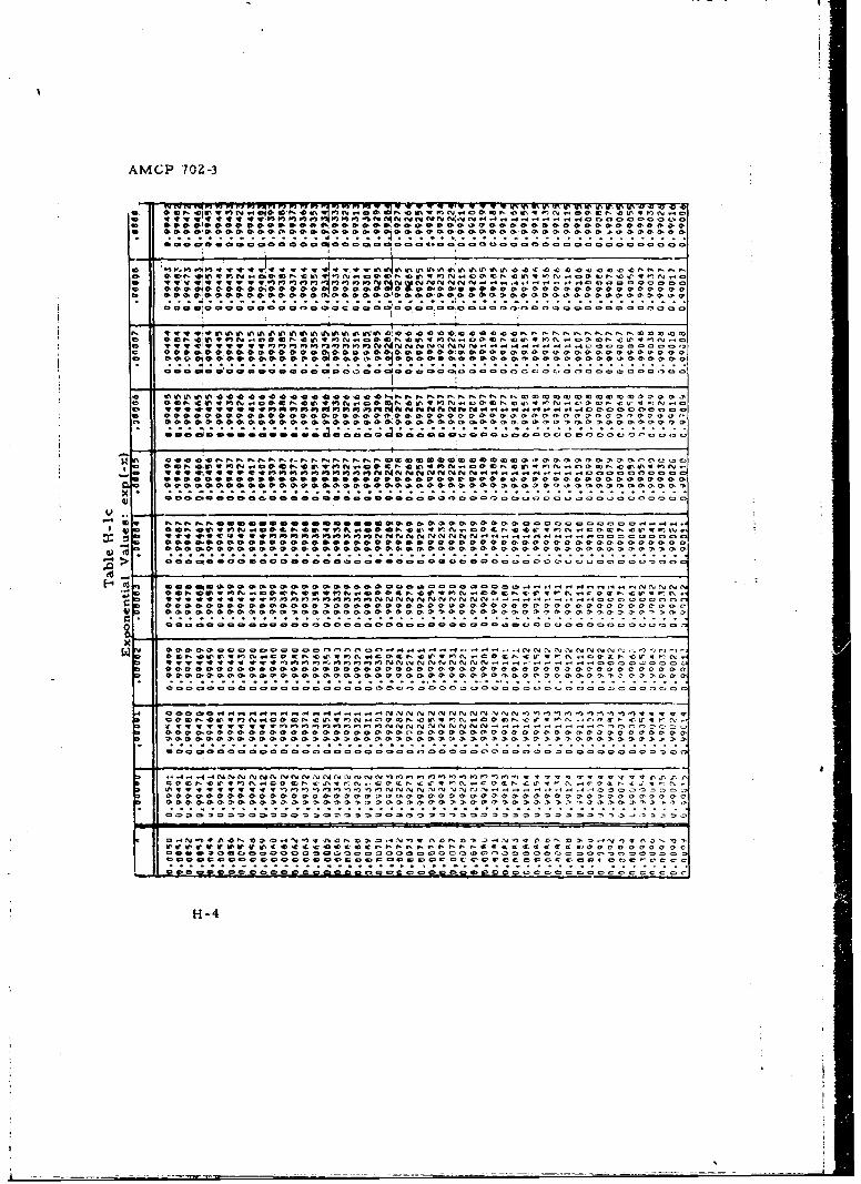
AMCP 70Z-3

*~ ~ . . . . . . .9 .-0 .0 0 0- 4NNN(9N00 V. 4. .4 .4 . . .4 . 0 0 00

*ýl w oo 090'99 W99 999 a~ 99 999 99 9 90 999 a 00 0 c- 0 00 C,0,0990ý

* ~ ~ a 0 *1 a. 000000 00 0 0 0a.C 0 0 0 0 00 0 0 0 0 0 0

t* :0 tttt . I . .*~ .~ .9 9 99 9 .I .I .. 0: 0:004 11.4- 4 0 0. . OCNN

41 V0 * 9% N ,N4N 9 %ft kn 0N 0 t.ss O . 0 0. . 0 . N . 4 0 N ' 0 0

001bb4000101010 00000= *000 .0 .0.000:0t: 0. . . 00. 00. 00..0..0..0..

00 9 1 491 0 4W lo, 419, 9l 01 4ý m 0. NP 4009N0V .0 0 099 -

O ~ ~ W N99 9 99 9 9 9 99 9 9 9 9 9 9 9 0 O 00990909" 00 0 0

0900 00 00 0000C.1 V ý 0 000- l0,0 000001000000 a 0ý CI0 0 00 0 0 0

9, 51199914 44 44 4 44 4 Q. (1, m cp. a m0OOOO9),00399 .9 to 9904It90N.t999N49190N009 6~ 4 9 N 0 9 0VI9. . . .90 0 0

* N' p-E 9O 09 041 0. Owl ON, 0I 9 OwlNC 000 9 N 09 W* vI W-0 N0 119 99 q999 9900O000004dNIdNINNN0-- -- -b---------

: 9 9 90 9 9 9 990909 9 9 9 90:90 0 0 9 9 9 9 0 0

9 9 9 9 9 9 9 99:9 9 9 9 9 9 9 9 9 0 . 9 9 9 9 9 9

C .00.0.0.0.0 .0. 00.0.0.0.0.9 .0 1 . . I . . .00 1,.0 0

99999p,99 9 0 0000a0NN 00 04 00 a0-l0 0. 0,0000a 0C 0

IU 090 0999999-99-9-9-9-00-0-0N0N0N .4 40 0 .4.N 1 N

9999999 090~l0 0~ N I N N N N 0. 4-..-.I- 00, 0 -l C a000

00 00 0 0. 0000000000 : & 00 ýC 000 00 0 00 0 000 0 0 0 0

9900900 01000 00 000:0: t t .. t .04.-. - .-4 .NINN.NI O .S. n..

0000 0000 0 a00000 00 0 a00 00 000009. 0 000, 0 000* 4 0

0000 0....4..4f.40.4.4 - - N. NN NNN . C, I10 -09 .)>999099 491 0N 090 00 00. 0904t00 .90. .. t .P N.-C.flI . . C W0O.

C; 9 9 9 9 9 0 I O OO N N S N N 0-.40 .4- 0 0 0 0 0

09 .4! 9 00 0 0 90 0 9 CC 0999999999 9 0 0 9 99 !9

9 H-4 9 9 9 9 9 9 9 9 9 9 9 9999 099. 9 999 9

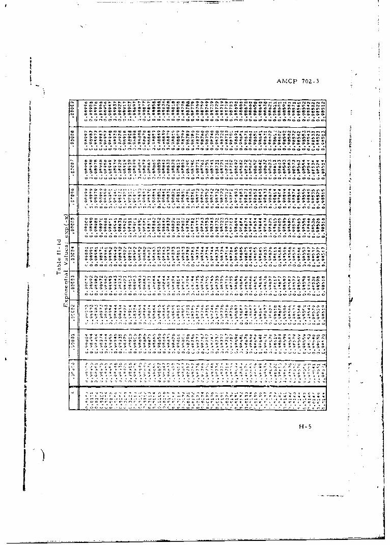
SAMCP 702-3

0 ~ ~ ~ ~ ~ ~ ~ . -amt Wr ,coJmmorr Ctac'~.rNlltaýmCOC,.M I O,.CO tC a~p

O " ..... .. .. "c ..- .-. N F.r.... r........ .....Ct C.. .. .b..... .

u0 vaavaN s4 NaaM%

• . o .o • .. ..... ...... ° ... . . . . . . . . . •. . • °.. .

a.-O"•, " wr• r'."-" t." U "o . (...... ..... ~ f..........o ...... c.. .... ...

0 . • .o ,o ,• o o , o.aa'Da o, aa r..rat -,•• ,, No NN..o,~ o, , -o . ,o

- l aa a a~ G a Gr v , -.'

I C,a • C o CIa.. . . . . . . . . .. o • G.I . . b. .... . ... . ... o.... I. . .a . . -

f 0 Oa-. tr- -.. ... o .. - -

' ... ..

~~~~~~~~. ... . .. . . . . I . . . . . . . . . . .. .. . . . . . ...

. . . .o: o, ,ý 1 ý . . . . . . . . . ..° o . . . . . ... . .. .

- - - - - - - - - - - 5

o~ ~~~ -~r -ra nba C C e S I-.N- - - - N - ~ e -t t - -- -- - - -- -- --

)I

I aa

-a -~Oa ~ . - .

C~~~~~~~~~~ 'oO~ ,Ctm "'~ C tO .O fCO 0 0 tO O ~ O otJ t tf o c

XI r ~ o ~ . a - . . . . n ~ r . N ~ o , . n ~ r . w a ~ a ~ ~ o ccCGUJN~b*VN~a .O ...t ... .tWfN-4 0.-r r,. . ,. r~~w N 4 ~ ,c..

. a W t ~ C~~ o W C . . . . . . . . . . . . . . . . . . . .

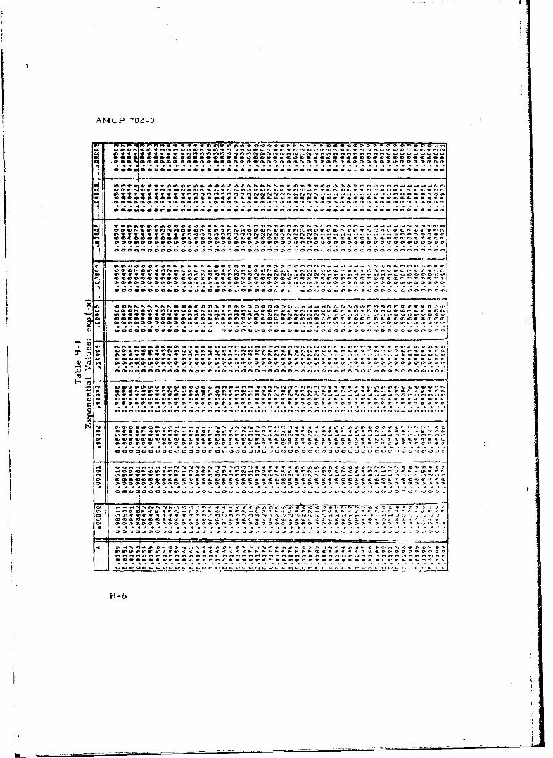
AMCP 7OZ-3

-a" IN V~~ft 2X w C r o ~ ~ N - - C ~ e ~ v ' 0 0 C ..A~ A

- ~~~~~~~~~~ .O. .~w~ vc c . .C~ NN o~ .C~VC'.. .a .W~ . ( C C . v...' .. . . .O S% t~tqtrtfl 0Ofl fl' Of----------------*000 000

a. a, 0, 0, Ca- 0, a-*. a,,- Cb m > m~ .400 a P'- 0-t 0, a "I.. 0or

0~ ~~~~~~~~~ -g. C -eee-e -C -e -00 cc -cC CC-cCC -

ýVl OCCC0, No 00 0. 01 N IN N I N A, A, A,00

0: 0: 0: .f . . . . . I . . . . I . . . . . . . . . . .

C OO 0S0 NP-N .CN e0C CC0G .Co n~o .~,~ ,o. '-, NN.4 0.) l0xo ~ ~ ~ ~ ~ ~ ~ M 0 C tq 4 .. co rw N c v( crr.NZ .c C.4Cy(4.C0 N~t

at 0' ;0%Cch a. 0'e0' 4p, a- oC 0' vp, co, Aw:, 0 0' 0- vi 0- a co

> __________________________________________________________ ______________

F0 0 0 0 0 0 0 0 0 0 0 0 toC t 0 00 ~ ' 0 0 0 0 0 4 C

COP-NF~~fCNNNOCOCOCOG~~~eCC-A, , .,...tO N 4 1 0 4 0 ~ S '.4

o ~ ~ ~ ~ ~ ~ ~ C inC V~~~llllf,0! N N C N W N.n.0: O OO1 c'000010~ -::-:-:- - - -oo-:-p- - -::- -:-N-o: -, - - -N- - - r -U-v-

CL O O C C* * Ce 00 CCe ee C.CWC . IC-OcCaC v

4J 0 000 000 0000 000 000 0000 00 000 00C3 300 0000or

C~ ~~~~~~~~ N0 S C G O f 0 0 0 4 4 4. . 4 N N r f P C -0 .y . VO...W

~ , C Ce~C0W0 .- eoOC#.Ctrr~o00ar.CC.(4 rvorc C~ CCwt

Za .W. .Y W . . . . .P4 v NN N N N~ - - - - .. s 00 00 CQ OCOO CCC CCO~iCU0:CC CCC~eC~i-CCCCC CC :'CCl C

RA0 A0 0 0 C C 0 0 0 0 0 0 0 C,0 0 0 . 4 0 0 0 0 0

1110 C0 0 C0: Q 0 b0.1 .d 4 ( .Nýl 4 0 0:r Oi I O C 0 .O r

w CO DU vC AIDt t 0r. V.0 Av tr tN4. N C WO .C C 4W, ttrW, W *t4O4ý) w0P) NC NN d - - - - -0WC0

0~ ~~~ ~~~ C C 0 C 0C 0: C.C C L ? C C C C C,. U C - C C C C . n...

H-6 0 C O C '0 0 00 C @ C . C ~ ~ 0~ @ 0 ~ G C 'C~

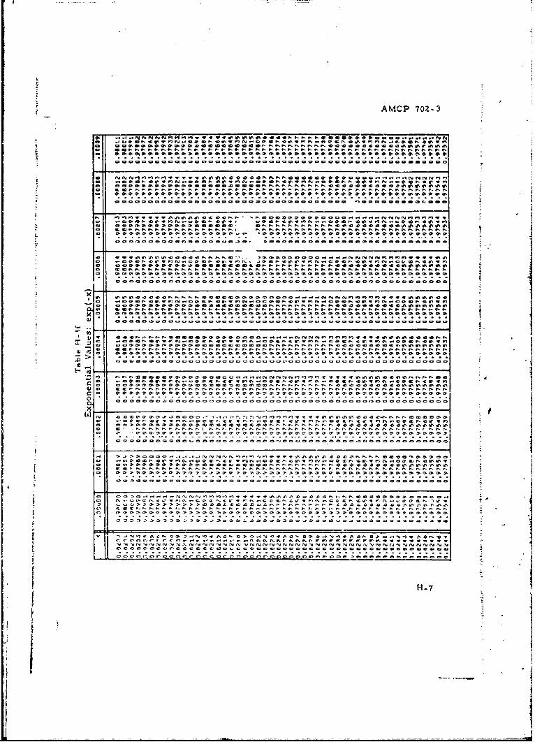
AMCP 70Z-3

000 000 000 000 00000 00aa" 00 0 a, 000000000000.9000 0

0 ~ ~ ,0.0 "N~ ,w~ 'P04 044.NPQ0 "#"00 .oN

17.~~~ 0 4 0 4C. I & 0 0 0'e 444444404! 44 11a,0 0 000

0A A NP0. .0101 1,a A ow""O~ a ~ a ~~a 0 0 0 000.00 f 0 a 0 'o a 000 "101" 000t

1ý 0:4 4 =ý1 ýtI ýI :0 ýI tI ýC :C t1 ta ý11: tý tt0 ýtý ýttC t I

0~ ~~~~~~~ 1000 C W IN O N W C 0 A wrwft CCO O WC oo& 040

0 ~ ~ ~ ~ ~ ~ ~ ~ ~ 0 00 40 4 .NOP .00 0 0 0 0 - ~ P 0 .000

- -0 4 - 0 ~ l. 0 0 -U W I .4 0 0 -O -0 0 0 00 4 0 p - * I -----

a ~ ~ ~ ~ ~ ~ ~ ~ ~ 0W oo1lS C OW C O O O 00 0 0 4 4 4 4 40 0 00a ,w.....N.... 0-S -. D..'...N .D-P.N..P4PN0'a00 .0 d, AdP.d

0l ý 00000eO0O00GOO00Ge00OC00a..000 0' 0 ý0:0: 00 ý0: 00000I.) .0 0 0 0 0 0 0 00 0 0 0 0 0 0 0 000000000000000000- --- -- -- --- --

Vol . , WA",

..D -1 I-- , C J WV W W 0 04 0 . 00

N N N 4 VN.,t N N rqVO.(M0NC0m 2~C~ N40 mlftC4 2N C. m 7

00O0 0.O C~OO~ 0Z 0C0O 440 NON NNNN 444 04C4 40 H-70

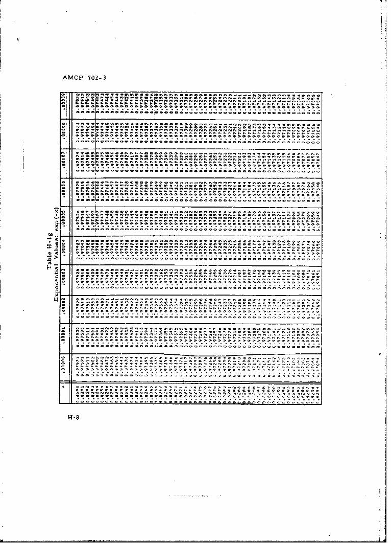
AMCP 702-3

NN 1, N M NP.. N. I. Nve .N NN N NN -N @I o NNNNl N f-li NNIN N.NI-t-.NN Nf N. N

- % *inlflt W,0 ~ N N0 0 0 oo." Cy o.V .y ma,~~M M " uNmvo ONNo0 N N ~ . N ( ~ ~ 0 0 0

0 ~ ~ ~ r N NN C. 0 ~ NPNN.NNNNNNNNNNNNN WNNW 41w, O fNOoe 0 0c0 00w 00 0 0v 42 c0 N0 .000 000000

CI~~V NNI) NN N N N.N N N N > N N N N N NN NN NN ""01.0vm0

100d 6~tl S O0 *q nr rýplm mm- - -s - -n- -. "fooo o if

........................-...............

o ý 0000 C O 00ccý 0 0000000000000000000000000000 a . 00000 . 0. . t.

-~~~ - - - - - - - - - - - - - - - - - - - - - - - - - -0000~0o

~ 0 ~ t~* %0fl00* W000lflflfflp~lfl-------f-J-------00 0

U' V

or%00 w 4C v * aaa 0a&0 0 P S ~ l N f l N N J - - - 00a0aNNN14NN NfNIVNNN O N. , O NN N N ON N N N N N N NNN NO

o ~ ~ ~ ~ ~ c ý ...~.0000 00PvfIPfO-O N N N N - - - ------

H -8 NNNNNNNNNNNNNNNNN -NF -1 N N A

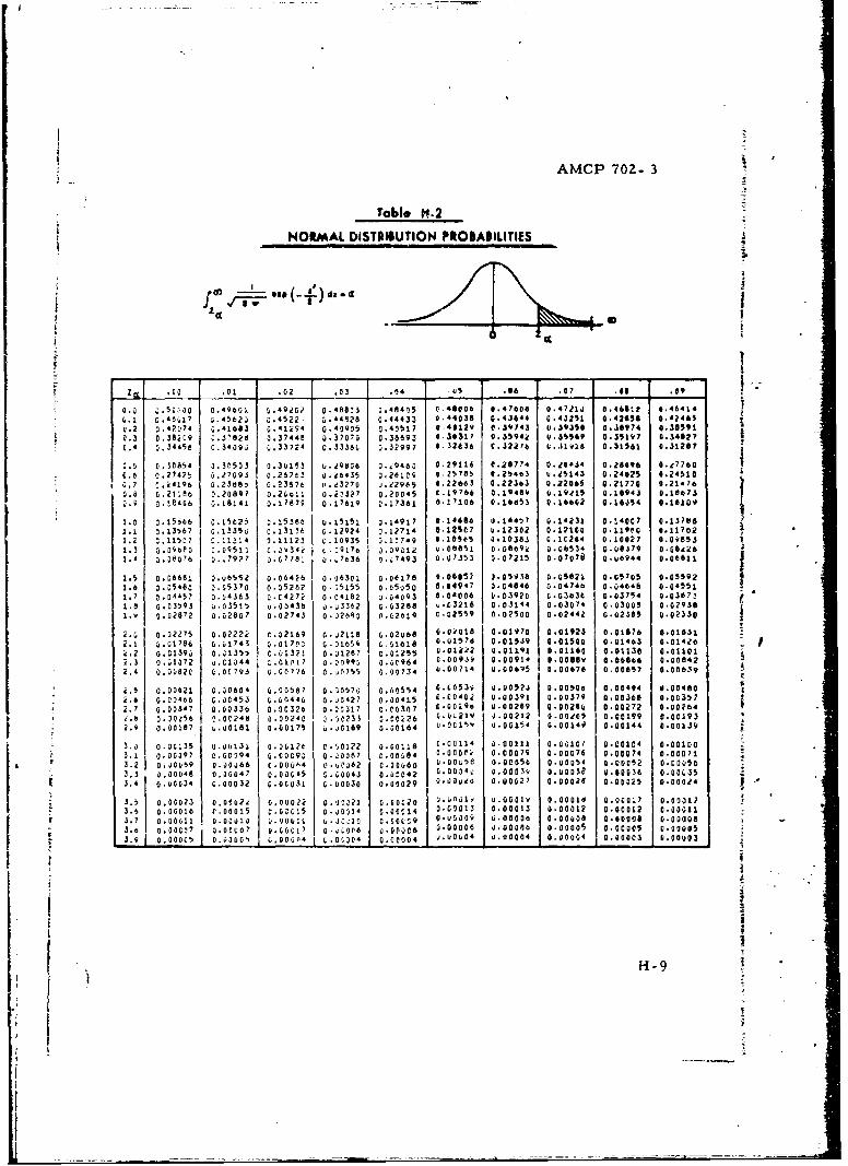
AMCP 702- 3

table 01-2

NORMAL DISYROUTION PRODADILITIES

4,-

.0 0. 0 C(.4 6 .06 .07 .00 .09

0. o500 .'600.4907 0.063 .4 C0 o46V06 0.47606 0.47213 0 .46602 t .464140.1 U .'6017 .4:5623 a .4522 3.44 928 0.44433 0 .44038 0.43644 0.43251 0.42868 6.42465

.2 ?U?42 0.41683 0.41i94 4 a 905 0.40517 0.40129 0.3V143 0.39350 a.36974 o.3859100.3 0 .39Z19 C.3,02S 0.37440 o .37073 0.36693 0 .30317 0 .35.94W .3SS69 0.35197 0.34627

0. 0.34456 C.3409) 0.33724 C.33360 0.32997 0. 32636 c . 22 76 1.3 1 Y18 0.31561 0.31207

1. .05 .30503 0.30153 1.9006 0.j9460 0 .29114 0.267,'4 0 .da#4 0.28096 0.i77o0.6 0.27425 0.27091 0.26763 Q .oeOe3 0.26icg 2.7075 0 .25463 v0.45143 0.24025 0.24510

0.7 ~ ~ ~ ~ ~ ~ t .216 .30, .376 .o2o ul9 .22663 0 . 2363 0.22066 9.21770 0.214760 .6 c k2 96 0.23069 c.235e ( 0. d3270 0.d2005 C .1It766 0.1946V9 6.19405 0.16943 0.18673 I

0 0.e4G6 0. 18041 0.0.7797 D. 17619 0.17361 0.17106 0.1685) 0.16602 0,16454 0.161091.0 0.5~6 .102 21531 .115 ~1'1' 0.14666 0.144t.7 G.14231 0.140C7 0.13)86

11 0.13567 0.1335G c .13136 o0.1292' 0 .127 1 It 12SC7 u.12302 0.12106 0.11900 0 117021.2 c 115 17 c.11314 3 .11123 c .10935 G.11749 0.126505 -0.1630 0 .11c204 0.100027 0. 0165 31.0 o. "eo 0 c. ~0 ; aw3di3 L D1. 76 3.39C12 v .60851 0.08692 Q.Q6534 Q.08379 0.082260. a 3.30806 G-7927 3.077: 2. 7o36 9..3493 o6.0u735,3 0.07215 0-0707k Q.U6944 0.06811

1.5 0.0 6661 3.06552 0.06426 0 .06301 0 .06L1708 0.060,37 0.05%,38 D-0.56281 0.05705 0.0591.6 3.05480 a 0.05370a 0. 35202 0~ -5155 0.05050 8.e4947 0.04846 0.04746 0.046.8 0.04551

3. ~l~5 .133 .422 0.462 3~4Q 0000 .03920 0.0363C 0.03754 9.0387

1.0 0 .03593 .,,035115 .05438 ~.0,362 C.03268 u .1)3216 0.01144 0.03074 0.03005 0.029633.v 0 .0287? 0.0280? 0 .02743 0 . 261* 7I.C2619 0.02559 0.02500 0.02442 0.02305 U0.0330

2. I0 .32275 0.o2222 o.2169 . U2118 G0.02068 0 .01018l 0.01970 0.01923 0.01676 0.0103512.1 -.01786 0.61743 0.017n 1.26'. '1.6162 a 6.92576 9.01139 0.01500 0.01463 0.014?6

.2 .192 0035 .0'1321 0.31207 0.0-:255 0 .0122 6zu.0a1191 0.01160 0.01130 0.01101i . o 0027 .C1044 o1.07? 0 . 'Ow, 0.06C964 0.00 ..01 I000698 0.006666 0.008427.4 0 .302C c ,00793y 0 .Gt076 0 .6C755 6,.00734 6 .06714 Q. 60v 0.00676 0.00657 0.00639

.5 0021 0.3604 0.0050, ;05o76 o. rlas' 0.1053i 0. 00573 0.00500 0.00494 6,0048003.6 ~ ~ ~ ~ 1 0.06 ,343 10440 0 u042; 0.45 0.00 00391 0.07 0006 0035

2.7 0.003'7 0,00336 0.00326 0 .3001 o0o367 0.00290 .00269 0.00280 .02? 0002643.6 0.026 000'0 0.020 .2Ž3 00026 1.DL21V 3.00212 0.00205 0.00199 0.00193

2.9 0 .0D107 G1.00161 0 .00175 2.0169 0.00164 u0 O15V 0 .00154 0. 00144 0 .00144 0.C0039

3 . 0-01C13 5 0.oG131 0 .01120e c 0.1022 0.00oli8 0.00114 o.00011 0.00101 0.00104 0.001003.0 0.00097 0 .02-j9 4 0.10009G 0 . .00867 0.006 0 0 a U') 0. 00 076 0. 00070 a.07 0D 52 1.000713.2j 0 . JD0 "9 0.3o0066 0.0006ý4 0 -UOJ62 C0. 3060 0. 0034v 0. 0 00 39 0. 0004 u 0.00052 0.00L35m3.3 3300'6 0. 00047 0, 00045 5 . 00043 0 .oC42 .0

4 .00 .03 .03 .03

3.4 a0.00074 1.03 .. 3 0.03 0.02 j d d a. 00027 0.00026 0.00925 0 .000 143.4 0 .001234 0.00032 G030002Ž 0.0020 0. 000209 .01 .01 .01 .01 .01

3.5 0 .00006 o.00015 0.01 coo30 .004 0013 0.003 0001? 0.00012 0.00113.? 0 .00011 .000015 .06 .330 0,1 00091 0.-6u305 0 6.00000 0.00008 0.00998 0.000083. o0:0V7' I 0.00107 Q . 00 c1

7 0~~0 -. 0906 0.6 0000 L1.00006 0. 00004 0.00O06 0.OO0300

3.9, 0.0 0015 o 0.000 0.0000' L,.01,3004 0 .00004 .00 0004 0.00 0000 0000

H-9

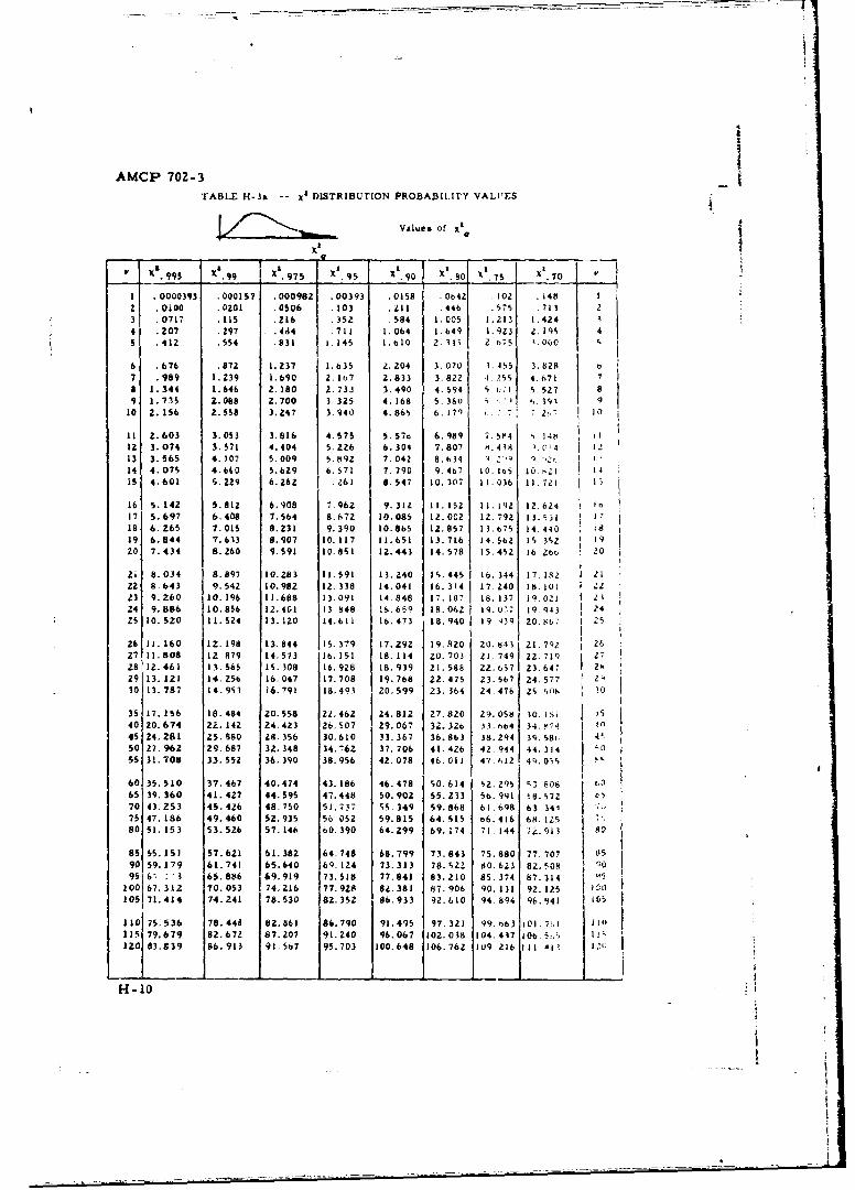
AMCP 702-3

TABLE H-3a -- x3 DISTRIBUTION PROBA331t.ITY VALUES

Value's of)(x"t

.995 X4. 99 Xa. 975 X'. 95 .90 x 8 0 .75 1.0

1 .0000393 .000157 .000982 .00393 .0158 -0e42 .102 .148 1

2 .0100 .0201 .0506 .103 .t11 .446 .575 .723 23 .0717 .115 .216 .352 584 1.005 1.213 1.4244 .207 .297 - .4d4 711 1.064 1.649 1.923 2.195 4S .412 .554 .831 1.245 1.t10 2, 111 2.b-"5 o.0(c .

6 .676 .872 1.237 1.635 2.204 3,070 3. 455 3.828 27 .989 1.239 1.690 2.167 2.833 3.822 1 .'.5, 4.671 78 1.344 1.646 2.180 2.733 3.490 4.594 1 71 5.527 89 1.735 2.088 2.700 3.325 4.168 5.3&u "' . 3f 13

10 2.186 2.558 3.247 3.940 4.865 6.7 ý 1: 2,7

11 2.603 3.053 3.816 4.S75 S.57b 6.989 7.5K4 14b12 3.074 3.571 4.404 5.226 6.304 7.807 3.43 1 .C-4 0 213 3.565 4.107 5.009 5.892 7.042 8..634 : 2 Q, . ,14 4.075 4.660 5.629 6.571 7.790 9.40? 10. lbs IC. 21 1415 4.601 S.229 6.262 .261 8.547 10.307 11.036 11. 7-Z1 I

16 5.142 5.812 6.908 7 962 9.312 11.152 11.192 12.62417 5.697 6.408 7.564 8.672 10.085 12.002 12.792 13. 5 3118 6.265 7.015 0.231 9.390 10.865 12.857 13.675 14.440 i819 6.844 7.613 8.907 10.117 11.651 13.716 14.562 15. 3s2 1920 7.434 8.260 9.591 10.051 12.443 14.578 15.452 16. 2b 20

I i 8.034 8.897 10.283 11.591 13.240 1S.445 16. 344 17. 182 2l22 8 643 9.542 10.982 12. 338 14.041 16. 314 17.240 18. 101 223 9.260 10.196 11.688 13.091 14.848 17.187 18.137 19.02 1 224 9.886 10.856 12.4G1 13 848 15.659 18.062 19.07 19. 943 2425 10.520 11.524 13.120 14.611 16.473 18.940 29 439 20.8,7 1

A6 I. 260 12. 198 13.844 15.379 17.292 19.820 20,'k43 21. 7Q? 2627 11.808 12 079 14.573 16. 151 18. 114 20.703 21.749 ZZ. 719 2728 12.461 13. 565 15.308 16.9Z8 18.939 21.588 22. 657 23.647 2z29 13. 121 14. Z56 16.047 17.708 19.768 22.475 23.567 24.577 2 ý,30 13. 787 14. 953 16.791 18.493 20. 99 23. 364 24. 476 2 .Otl 30

35 17. 156 18.484 20.558 22.462 24,812 27.820 29.058 30- I. 7540 20.674 22.142 24.423 26,507 29.067 32.32o 33.3,64 34.3' -145 24.281 25.880 28.356 30,610 33.367 36.863 38,294 3c,. 58t. 4a50 27.962 29.687 32.348 34,76Z 37.706 41.426 42. 944 44.314 055 31.708 33.552 36.390 38.956 42.078 46.011 47,612 49.0501,9

60 35.510 37,467 40,474 43.186 46.478 50.614 52. 245 ',7 80865 39. 360 41.427 44.595 47.448 50.902 55. Z33 56. 991 zO. 572 570 43.253 45, 4Z6 48.750 51.737 55.349 59.868 61.698 63, 34475 47. 186 49.460 52.935 56 052 59.815 64. 515 66. 416 68. 12580 S1. 153 53.526 57.146 60. 390 64.299 69.174 7L.144 7,.913 8

85 55.151 57.621 61.382 64.748 68.799 73.843 75.880 77.707 05"90 59.179 61.741 65.640 69. 124 73.313 78. 522 80. 623 82,50.4 909S 6- 2-3 65.886 69.919 73,510 77.841 83.210 85.374 87.314 &.

100 67. 312 70.053 74.216 77.928 82.381 87.906 90.131 92.125 fý,)105 71.414 74.241 78.530 82.352Z 86,933 92.610 94.894 96.941 f,5

110 75.536 78.448 82. 861 86.790 91.495 97.321 99.b63 |01. 7oi 13o115 79.679 82. 67Z 87.207 91.240 96.067 102.038 104.447 106 5t..220 83.839 86. 913 91.567 95.703 100.648 j106.762 109 216 l11. 1

H-10

.A

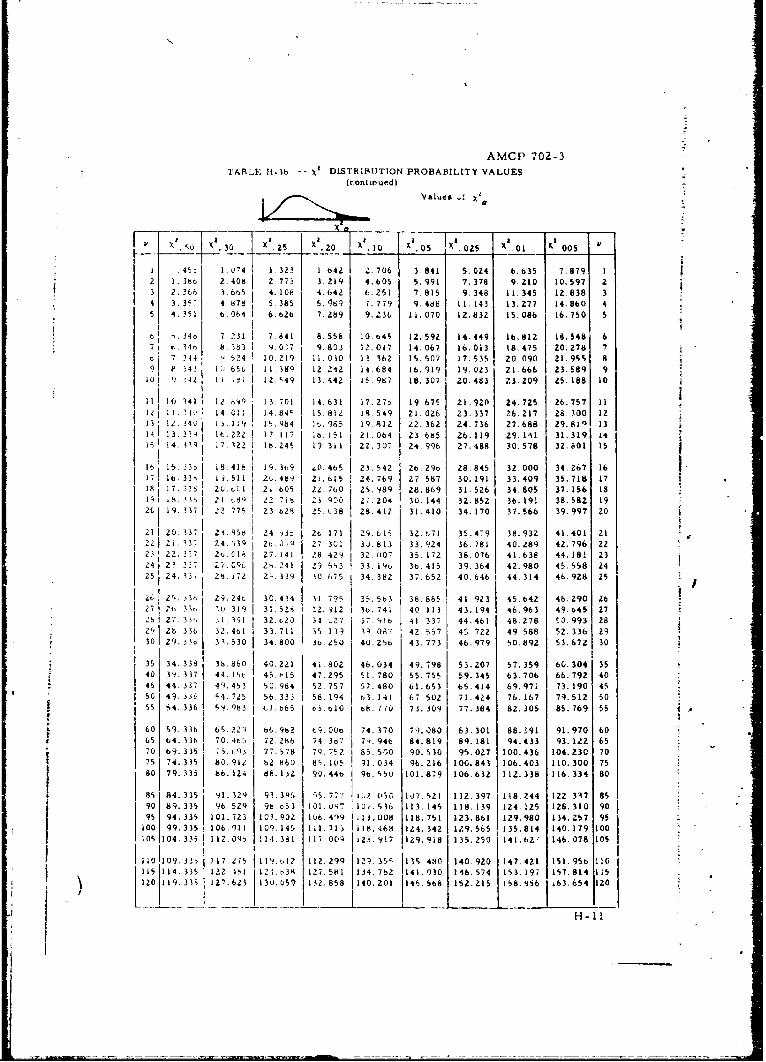
AMCP 702-3

TARLA, H.1b -- XO DISTRIBUTION PROBABILITY VALUES(contirued)

Values. X- ,

X ,X.3 0 x .25 z .i0 x .0 X2

025 X Ocs O, 00

.45ý 1.074 1.323 1 642 -. 706 3.841 5,024 6.635 7.879 11.386 2.408 2 773 3.219 4.605 5.991 7.378 9.210 10.597 2

2.366 3.6b5 4.108 4.642 6.251 7.815 9.348 11.345 12.838 33.31' 4,b78 5.385 5.183 7.779 9.488 11.143 13.277 14.860 4

5 4.351 t.064 6.b26 7.289 9.236 11.070 12.832 15.086 16.750 5

S. 34, 7 231 i 7.841 8.558 10.o45 12.592 14.449 16,812 12 .548 671 ¢..3,, 8,513 [ 9.057 9.803 12.017 14.067 16.013 18.475 20.278 70 7 344 " 5?4 10.219 11.010 12 362 15.501 17.535 20.090 21.55 89 F 43 1 J 11 3189 12 242 14.684 16,919 M7.53 21.666 23.589 9i0o 1 .'42 11.,ii 12. 49 13.442 15.9b7 18.307 20.483 23.209 25.188 10i I III 10 '44 12 89 13 701 14.631 17.273 19 675 21.92n 24.725 26.757 11I I I. -1.t 14. 011 14.84 I 159812 14.549 21.026 23.337 26.217 28. 300 12

1 0.1 34U 1 . 1.9 1'.,14 8 .43985 19.A12 22.362 24.736 27.688 29.8l• 13141 ', 33- i 1 22, 17 117 1 . 151 21.064 23. 685 26. 119 29. 141 31.319 14

1 14, 119 ;7. 2 122 b.Z45 19 3il 2Z. -0 24.996 27•.•488 30.578 32.801 15

16 15. j3o i8 418 19. 3t, 1 0.4t5 23.542 26.29t 28.845 32-000 34.267 16b 16.33, 13511 2t, 48 2i.615 24. 769 27.587 30.191 33.409 35.718 17

18 17.3• 2(.t:1 2i605 22.700 29.989 28.869 31.526 34.805 37.156 18

:9 1 b 33b 21 t.Q S 2 7i 2 t QD. 27. 204 30 144 32.852 36.191 38.58Z 192C 19. 337 -22 77; 23 b29 25. 38 28.412 31.410 34.170 37.566 39.99? 20

21 20 337 23.R56 24. ý 26 171 29.(1 32.671 35.479 38.932 41.401 2122 Zi 13' 24. '431 2 ,0,: 27 301 3i.813 33. 924 36.781 40.289 42.796 2223 22.177 2, C, 1 27. 14i .8.429 I 32.o07 35. 172 38.076 41.638 44.18! 23244 2I --7 7. .09- r • 241 29 5.3 35. 1 3b. 415 39. 364 42.980 45. 558 2425 24.33; Z'J.i72 2. 339 30.675 34.382 37.652 40.6461 44.314 46.928 25

it 2.3,. 23. 24u 3C, 434 31.795 33. 563 36. 865 41-923 45.64Z 48.290 262 1 2 33t 0. 319 31 521 I 2. 912 1 36. 741 40 113 1 43.194 46.963 49.b45 27lb 27. 33,, ..i 31 32..23 94.,27 37. 9 41.337 44.461 48.278 50.993 28

20 26.336 3Z.4ol 33.711 3.5 139 3.087 4 42.-57 45.722 49 588 52.336 2930 29.31 31.530 34.800 3tZ50 40.256 43.773 46.979 50.892 53.672 30

35 34.338 36.860 40.221 4i.80Z 46.034 49.798 53.207 57.359 60.304 3540 31.337 44.1ýt 45.b15 47.295 51.780 55.751, 59.345 63.706 66.792 4045 44.337 49.453 50.984 52 757 ;7.480 61-653 bS5.414 69.971 73.190 4550 49. 3.t 94. 725 5b 333 1 58. 194 63. 141 67. 502 71.424 76.167 79.512 50

S55 54. 336 5.?. P83 jtI1 . t65 o3, 10 68. 770 73.309 77.384 82.305 85.769 55

60 59.336 6S.229 66.962 t9.000 74.370 79.080 63.301 88.191 91.970 60"65 t4. 336 70. 46, 72.286 74.367 74. 946 84.819 89.181 94.433 93.122 6570 49.335 5.t.3 77.578 79.752 85. S0 90.510 95.027 100.436 104.230 70

75 74.335 8Q. 91 b2 860 85. 105 91.034 9b.216 100.843 106.403 110.300 7580 79.335 86.124 88.13z 90.446 9b.150 101.879 106.632 112.338 116.334 80

81 84.335' 91. 129 91.3*4 -5. 77 (6 . 1 0 7. 21 112.397 118.244 122.317 85

90 89.335 96.529 98.o53 101.U97 .10, . 3b 113. 14S 118. 139 124.125 128.310 9095 94.335 101.723 103.902 IQ6 .4 19 ;13.008 118.751 123.861 129.980 134.257 95

100 99.335 106.011 109.140 111.713 i18.468 124.342 I29.565 135.814 140.179 10010S 104. 335 112.099 111.381 117 00Q 123.917 329.918 135.250 141.62-' 146.078 105

f110 109 315 1317.275 1 19. t,17 112. 299 32n. 399 13 480 140.920 147.421 151.95b 1101 15 335 122_451 12 1.,38 123. 581 134. 752 141.030 146. 574 153.197, 157.814 115

120

119.33t5 127.623 315.059 142.858 140.201 346.568 352.235 158.956 .654 320

H-1I

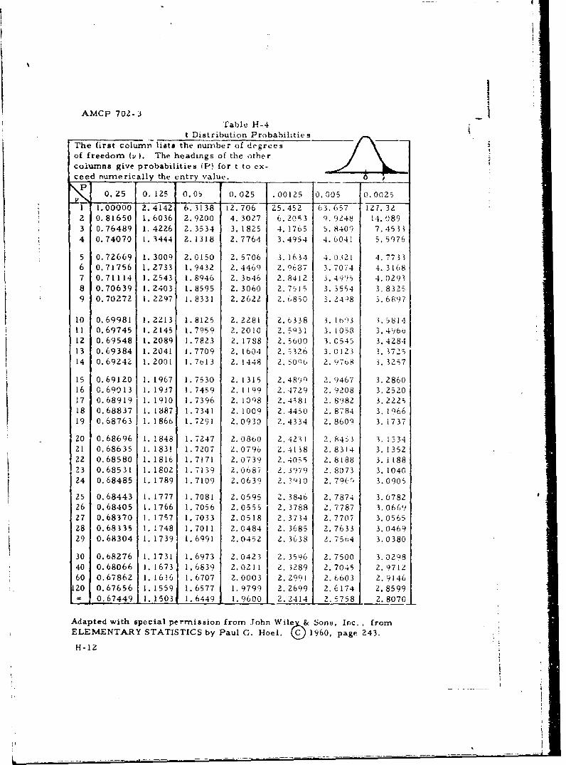
AMCP 702- 3Table H-4

t Distribution Probabilities

The first column lists the number of degreesof freedom (P). The headings of the other

columns give probabilities (P) for t to ex-ceed numerically the entry value. 6

0.25 0. 125 0.05 0.025 .00125 0.005 0.0025

1 1.00000 2.4142 6.3138 12.706 25.4•52 63.657 127. 322 0.81650 1.6036 2.9200 4. 3027 6. 2053 9. 9248 14. 0893 0.76489 1.4226 2.3534 3. 1825 4. 1765 5.8409 7.45334 0.74070 1.3444 2.1318 2.7764 3.4954 4.604i 5.i976

5 0.72669 1.3009 2.0150 2,5706 3.1634 4.0321 4.77336 0.71756 1.2733 1.9432 2.4469 2. 0637 3. 7074 4. 3 1687 0.71114 1.2543 1.8946 2.3t46 2.8412 3.4995 4.02938 0.70639 1.2403 1.8595 2.3060 2.7515 3.3554 3,83259 0.70272 1.2297 1.8331 2. 2622 2. 6850 3.2408 3. 6897

10 0.69981 1.2213 1.8125 2.2281 2.6338 3. lb')3 3. 581411 0.69745 1.2145 1.7959 2.2010 2.5931 3. 1058 3.496612 0.69548 1.2089 1.7823 2. 1788 2.5000 3.0545 3.428413 0.69384 1.2041 1.7709 2. 1604 2.:5326 3.0123 3. 372514 0.69242 1.2001 1.7o13 2. 1448 2. 50Q6 2. 9768 3.3257

15 0.69120 1. 1967 1.7530 2. 1315 2.4899 2.9467 3. 286016 0.69013 1. 1937 1.7459 2. 1199 2.4729 2.9208 3. 252017 0.68919 1. 1910 1.7396 2. 10O8 2.4;81 2.8982 3.222318 0.68837 1.1887 1.7341 2. 1009 2.4430 2.8784 3.1066

19 0.68763 1. 1866 1.7291 2.0930 2.4334 2. 8609 3. 1737

20 0.68696 1. 1848 1.7247 2.0860 2.4231 2. 8453 3. 153421 0.68635 1. 1831 1.7207 2.0796 2.4118 2.8314 3. 135222 0.68580 1.1816 1.7171 2.0739 2.4035 2.8188 3.118823 0.68531 1.1802 1.7139 2.0687 2.3979 2.8073 3.104024 0.68485 1. 1789 1.7109 2.0639 2. 3-10 2. 796 r 3.0905

25 0.68443 1.1777 1.7081 2.0595 2.3846 2.7874 3.078226 0.68405 1.1766 1.7056 2.0555 2.3788 2.7787 3.066927 0.68370 1.1757 1.7033 2.0518 2.3734 2.7707 3.056528 0.68335 1. 1748 1. 7011 2.0484 2. 3685 2. 7633 3.046929 0.68304 1. 1739 1.6991 2.0452 2. 3638 2.7564 3.0380

30 0.68276 1.1731 1.6973 2.0423 2.3596 2.7500 3.029840 0.68066 1.1673 1.6839 2.0211 2.3289 2.7045 2.971260 0.67862 1.1616 1.6707 2.0003 2.2991 2.6603 2.9146

120 0.67656 1. 1559 1.6577 1.9799 2.2699 2.6174 2.85990.67449 1.15031 1.6449 1.9600 2.2414 2.5758 2.8070

Adapted with special permission from John WileA& Sons, Inc. fromELEMENTARY STATISTICS by Paul G. Hoel, C• 1960, page 243.

H-12

I.. ~ -

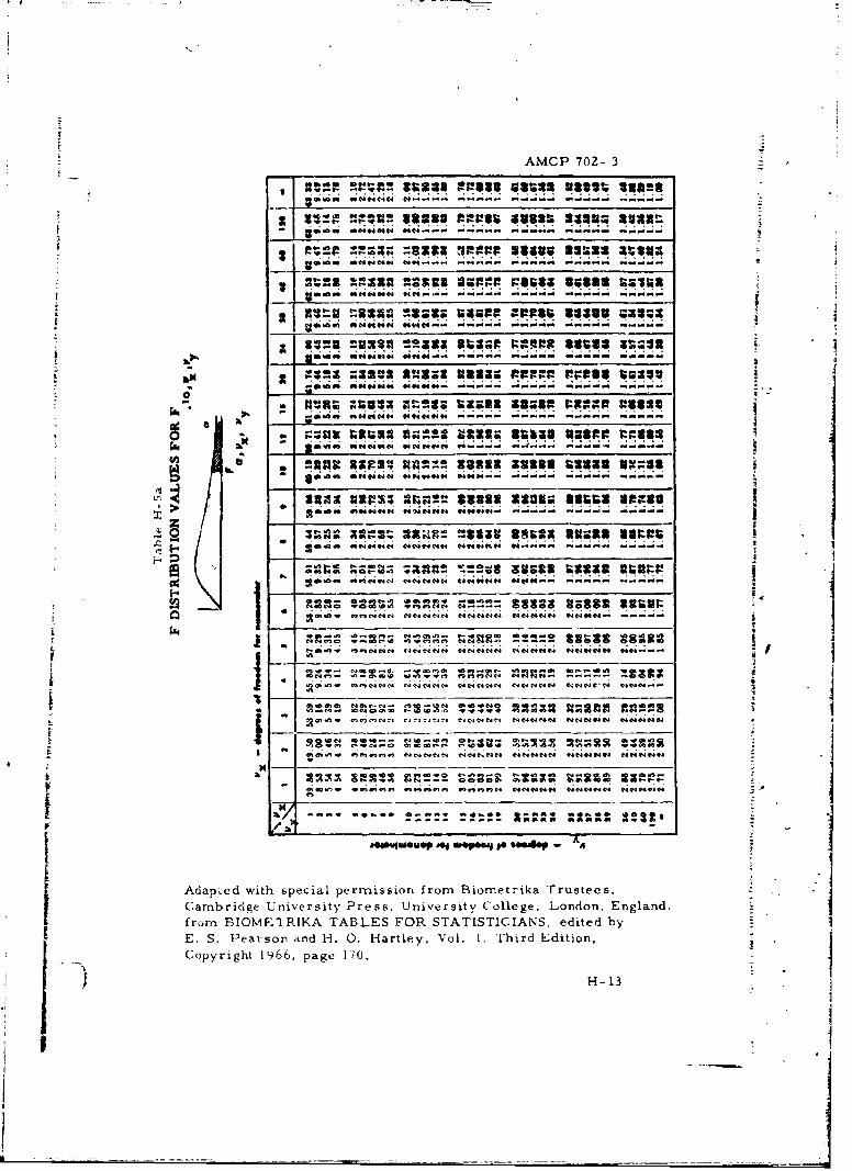
AMCP 702- 3

0 . - . 1 ..... .. . ...... !s u .....omf N"NN N ------------------------

SIZ.,- ngu loan 99s SV2 2320 MISS

--- --------- ----- -----

nut !Zz3% n~a usg ra 33019 93~3;

----. ---- ---we-- ---- ---

fv ;3Uni 0:?122; tags$ 322 9 usso N4 W

;:;t .24232 0s tx gt rl21 04.ý6 " M~a 9. ~ u aa4u: Cý;;

U2 4 t ng N 29 4 UMM nl*ase M nIN$

229 22M at~v asses Stagg gluts leglNtN IAtI

"*cwc tIN C'sN C. 4iceatIN

-0la ~- ---- ----------u ---- ----- -- rrPSe2" Tzit~v NCXatat U92994 Ant

-ol-o -6 23U3q P;3 600AS

Coy igt16, page_ __1- __0.

-HI1

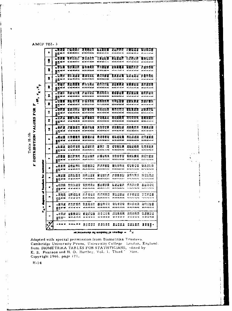
AMCP 702- 3

:~ ~ A.3d 04fI3 t~~t4.2mg t4Nts4---------

IX12 0Z ~ ~ ~ :s

- ..*Qtni *wi .C@4NNý Ct4 44Ne4 r4 W. t4N~' t.4'.

tnR--a it233! --0

car . a23 l Iz; oa ; ý

Wi. 0 .i . . N NN " t.J41 C N N NN ""tl C4---

64 amftn -ow""~n fta-fb 4"' N' 44 N4 et#-.' 4 N ' 4

1l + .Ž; I ... W.- VV~. t ." .... ce Ce,,eC.N 4C 1 -NIj4 4 ".

"- s A2n '"1

Adate wt special permnission frmmt Boe~triaý Trusles

E. S. Pear In and H. 0.7rly o. 1ý. Thr1 tion

Coyrgh 196 paW11

F-1-14

V ng! A 3;--z-G

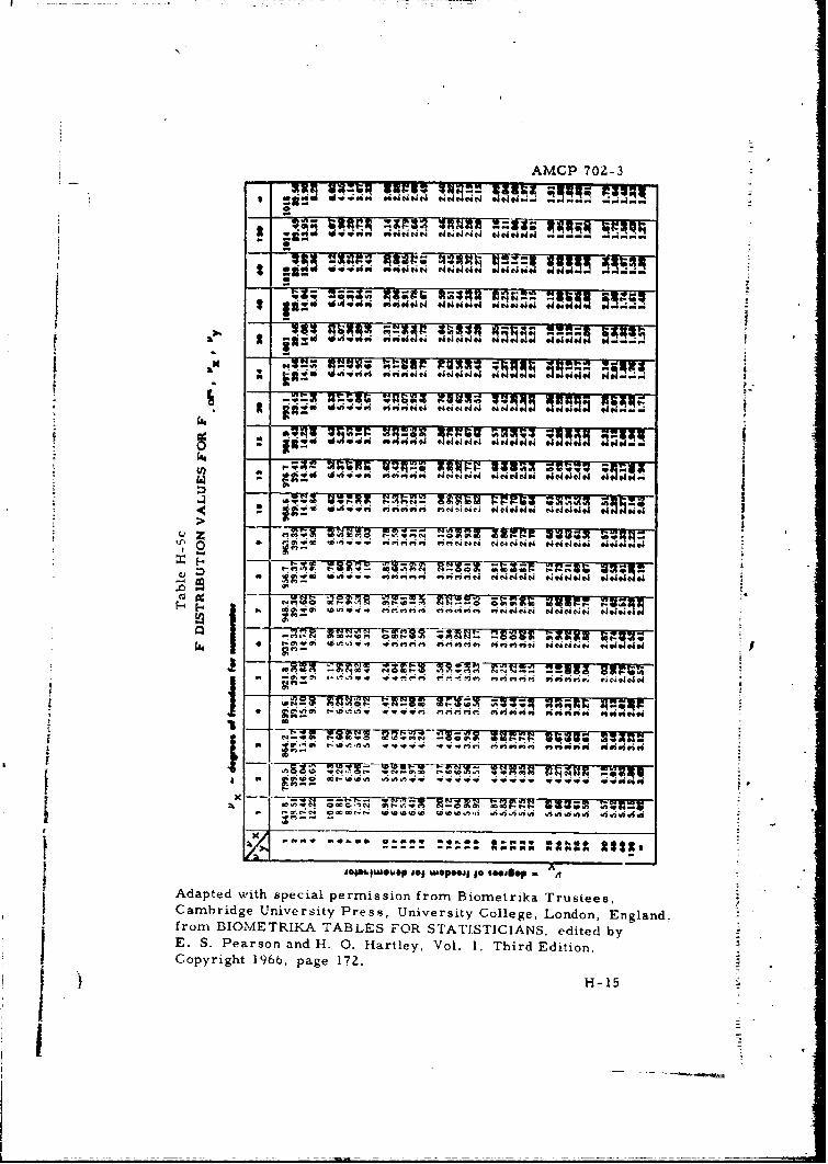
_ _ -- , " - . . . . =2 -- T C £

AMCP 702-3

SRI 8 Wn3p HE" 1 M .!

1 I• #4 # 4 4~N#4 .1g.i• I 3 0i Id- --

aAM

kMi3 u;; -

ga x ,! If' -.W[ - .��.l ~ C4 1 4o4 WW

- •- • - ]I -T •. ..2. 5.

, t • . ........... el444 .4#t# #,I4#

I p I HIM 51WH

"9--W1

I ~Adapted with special permission from Biometrika Trustees, ;• ~Cambridge University Press, University College, London, England,i ~from BIOMETRIKA TABLES FOR STATISTICIANS, edited by -

E. S. Pearson and H. 0. Hartley, Vol. 1, Third Edition,

Copyright 196b, page 17Z..0 v -"5

4I_

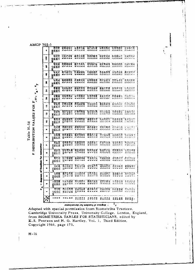
AMOP 702-3

'i t'i .'N N -

T-ý t .. I

"mmm a

0 0

Z -! igviC-i - . 0to~~ ~ P-I2. o .n, ,. .c'e ~~ . ~ O . ~ i'z ~'S (I4ý ý\ e, C

vo n -m m m-m It4*. 1 7 Cl

:I: ' .W C .II.'.N 4...

75 ,,. n * * 'VcC l* ll? ~l' 1 -

F-J

2m-o ýý~ v.0 6 :;

6'6r*96 o00W4 4444' 4. 00

K ~ ~~~ 7no V" ;F11' C! *Mi

Q 17 11 t-

Copyrights 1966 pageDi 173.jep

H-16

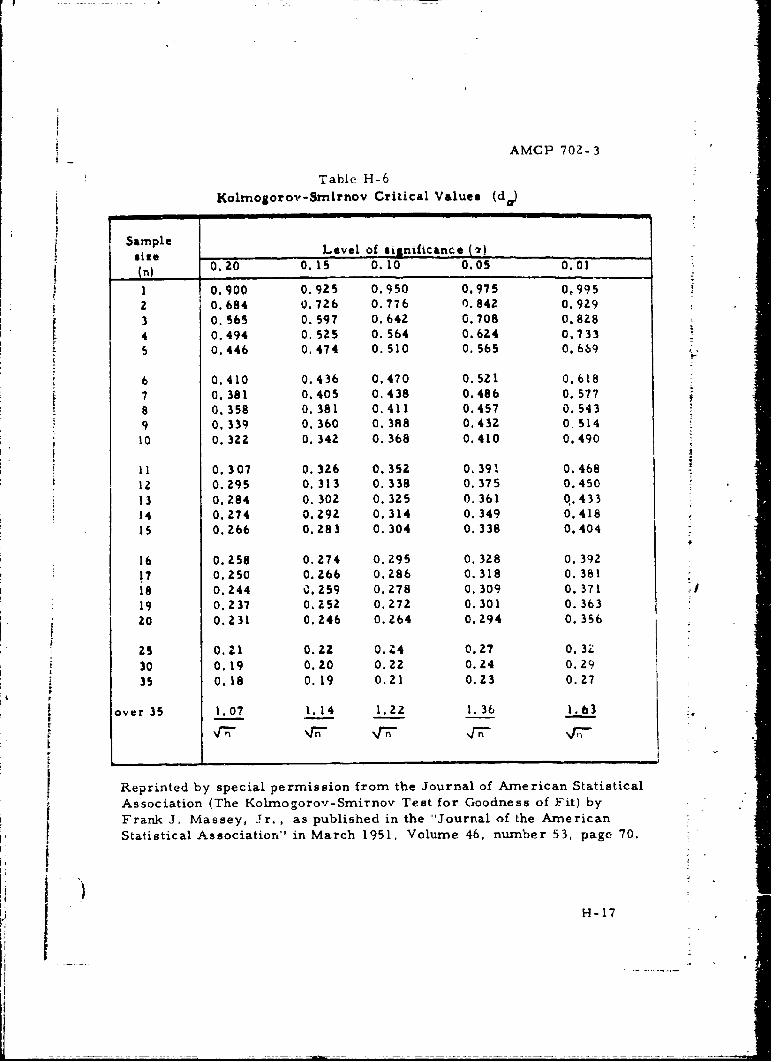
AMCP 70Z-3

Table H-6

Kolmogorov-Smirnov Critical Values (da)

Sample Level of significance (,)size

(n) 0.20 0.15 0.10 0.05 0.01

1 0.900 0.925 0.950 0.975 0995

2 0.684 0.726 0.776 0.842 0. 9Z93 0. 565 0. 597 0.642 0.708 0.8284 0.494 0. 525 O. 564 0.624 0,7335 0.446 0.474 0.510 0. 565 O.659

6 0.410 0.436 0.470 0. 521 0.618

7 0. 381 0.405 0.438 0.486 0. 5778 0.358 0.381 0.411 0.457 0.5439 0. 339 0. 360 0. 388 0.432 0- 51410 0. 322 0. 342 0.368 0.410 0.490

11 0. 307 D. 326 0.352 0. 391 0.4681Z 0.295 0.313 0.338 0.3375 0.450

13 0. 284 0. 302 0. 325 0. 361 0.43314 0.Z74 0. 29Z 0.314 0.349 0.418is 0.266 0.283 0.304 0.338 0.404

16 0.258 0.274 0.295 0. 328 0. 39217 0.250 0.266 0. Z86 0.318 0. 38118 0.244 C. 259 0.Z78 0.309 0.371

19 0. 237 0. Z52 0.272 0.301 0. 363

20 0.231 0.246 0. Z64 0.294 0.356

25 0.21 0.22 0. 26 4 0.27 0. 3Z30 0. 19 0.20 0.22 0.24 0.2935 0.18 0.19 0.21 0.23 0. 7

over 35 1.07 1.14 1.22 1.36 1.,34 7 l r n - q 7 v r n % T I

Reprinted by special permission from the Journal of American Statistical

Association (The Kolmogorov-Smirnov Test for Goodness of Fit) byFrank J. Massey, Jr. , as published in the "Journal of the American

Statistical Association" in March 1951, Volume 46, number 53, page 70.

HH-17

77 _ _ __ _______ _ __ .-

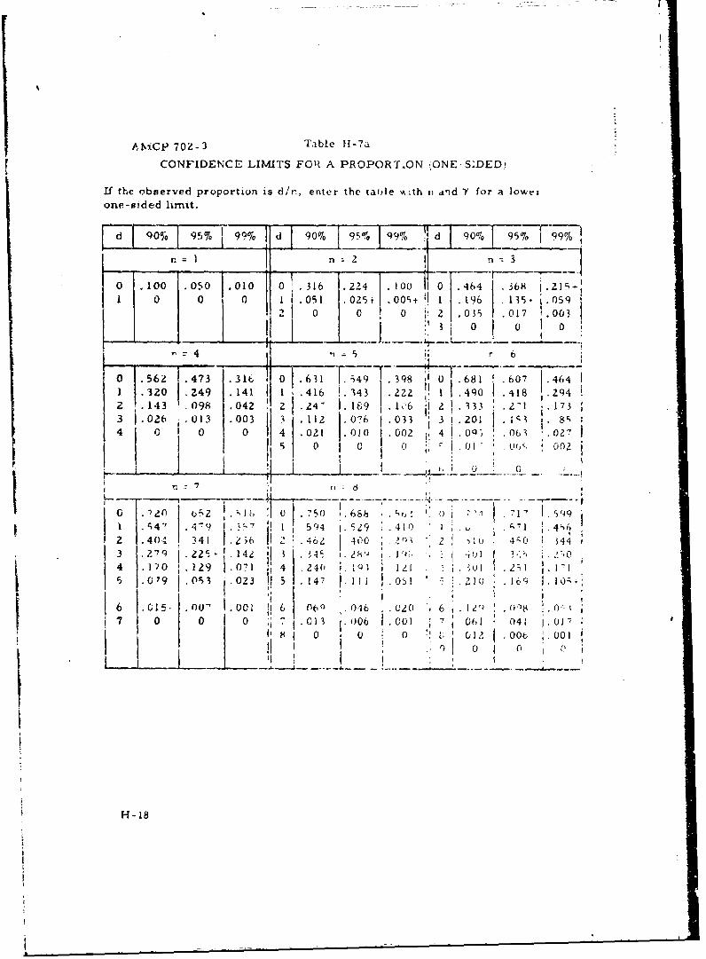
A.xCP 70Z-3 Table H-7a

CONFIDENCE LIMITS FOl A PROPORT.ON :.ONE S:DED,,

If the observed proportion is d/r., enter the tattle Aith n and V for a lowerone-sided limit.

d 90% 95% 99% 0 99% d i7% 99%

n= n2 3

0 .100 .050 1.010 0 .316 .224 .10I0 .464 .368 1.I--1 0 0 .0sl .0 5i 100± 1 .196 13'i- -' 59

0 o 0 o 2 .035 .017 003IJ3

4 ;6

0 1.56Z .473 31 b 01.631 :49 .398I0 .. ..607 .464

I .3Z0 Z49 .141 I .416 1.343 .2zZ 1 .490 .419 2942. .143 .098 .042 2 .24 .189 1 k.6 .2 3,33 .21 1.73

3 .026 .013 .003 j3 .112 V.06 .033 3.201 1~3~.84 4 .021 010 .002 "4 -00; 06 02 .

S0 2 . L, .750 . " 1 - Q

4" '4-9 7 1 , 5Q4 . 529 .410r,'I .4h,Z 404 341 1 26 ,. .46Zo 400 V) 1 0 47]'0 544

4-0. 9 .- 14 ," 1 "4 170 12 071 4 .240 1. i IZI : '1 l 2:1 ].1"1

121~ J.0 102 !;1 -r, 079 .053 023 5 147 I1 1 0 ! .- 218 . 169 1. I),

6 1 .5- 00" .001 I 6 C'20 6,7 0 0 0 70.013 0.o06 .001 7 06], 041 .017

8 8 0 0 0 - 012 .006 o.00,

f1H-1

S~H-18

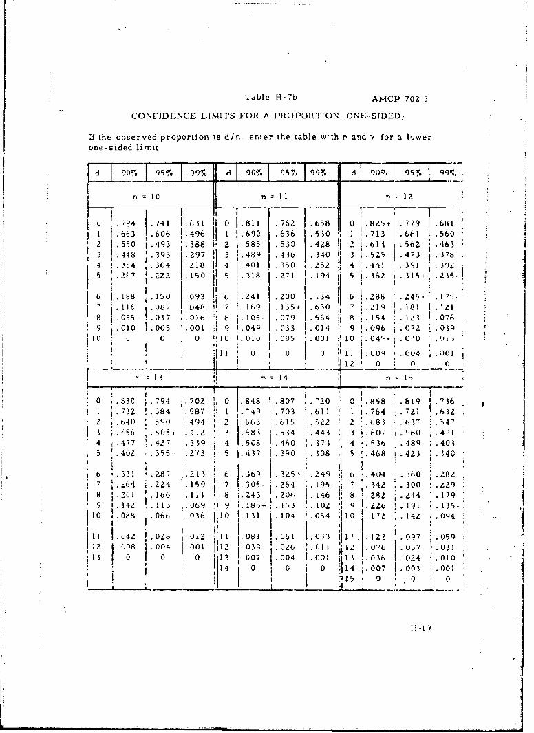
Table H-7b AMCP 702-3

CONFIDENCE LIMITS FOR A PROPORT:ON ONE-SIDED.,

if the observed proportion is d/n enter the table w-th r and y for a lower

one-sided limit

dd 90%' 9 999 d 90o7, 1'5% 99

n 1 0 n = 1 1 ", : 1 2

0 i94 .741 631 0 .811 .762 .658 0 .825 .779 .6811 .663 .606 1.496 1 .690 .636 .530 1 .713 .661 .560

.3 448 .33 .297 3 .48 6 340 3 .525 473 378 8

4 .5 .403 2 1.5 .50 .48-141 .6I ' I I O

354 , 304 .218 4 •301 .,50 .262. 4 .541 391S .267 2ZZ 150 5 .318 271 194 S 362 11 235.I '' •

6 1.188 >150 093 6 1.241 .200 134 6 2.Z88 24, 7'r,

11 6 .,b7 048 I: 7 !.169 135+ 650 7 Z.,,1 . .181 I L.8 Ls05- . 03 7 016 ' 8 .105. 079 .564 81 8 1,4 1 r I 076

9 .010 ,.005 I 001 9 •04c' 033 .014 9 .096 •02' .03910 0 0 0 h"10 1.010 005 001 :!10 .04- .0 0 .013

1 0 0 0 1 1 oo.0o .004 ,ol.12 0 0 0

13 1I

.,0 .. 848 807 ,20 0 0 .858 .6819 736'1 2 .684 0 8 7 1 -4 703 .611 1 7721 .6I..3 .84 8. ,,~' ' 1 .764 • "i 6IZ

, ,.;.640 590o 494 2 .663 615 .5•2 2 :.683 .63-.54'3 `56 5 0:; 412 . k .583 .534 .443 3 i .607 560 4'•1

4 4 7 7 .427 ;.339 4 .508 .460 .37 4 .. 36 .489 .4035 .402 .355..2v3 •' 5 3 .437 390 308 J 5 '.468 .423 K?40

'15 26 6 364 q.331 '.28' 213 3256 .6 '6 .404 .360 i.282S, 7 I~.,.64 i.224 1. 199 21 0 - . 64 .195-. 4 o . z

3224 7 15 342 .300 Z8 .201 ' 166 11 8 .243 1.- 146 282 .244 179

9 i.14Z 113 .069 9 1.1851- .153 .. 102 q .2 . 191 .135..11 1.088 06f .036 112 0 !.131 .j104 .064 10 17Z .142 .Oq4

I I •0-42 .02.8 I1 .08 1 o061 .0 3 111. •12• 097 .0912 1008 00O4 1.001 112 103q .026 0 ;;112 .076 057 0310 ~ 0 007 .004 0 D 1 13

o13 0 1031o1, 3 .036 0 .. ,4 .01014 0 0 0 }14 .007 .003 1.001

I "115 0 0 0

[1-19

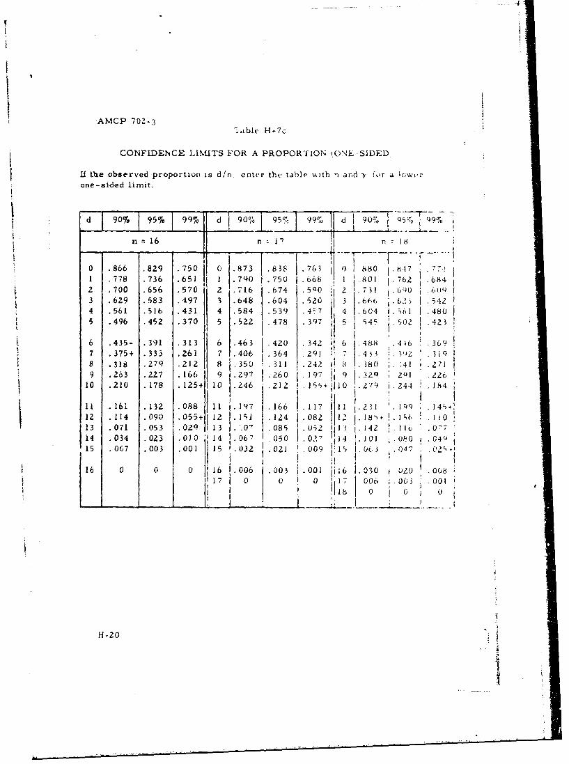
.AMCP 702-3ilable H- 7 c

CONFIDENCE LIMITS FOR A PROPORTION (ONE-SIDED

If the observed proportion is d/n. enter the table .%th n and >- for a inwtr

one-sided limit.

d 90% 95% 99% d 90% 9!5%5 L99 Iý,9

n 16 n i7 n 18

0 .866 .829 .750 0 .873 .838 .763 0 880 .47 77!1 .778 .736 .651 1 .790 .750 .668 1 801 762 .6842 .700 .656 .570 2 .716 .674 .590 2 7 33! .6qo .0,1(43 .629 .583 .497 3 .648 .604 .520 3 .66r, 63 .6424 .561 .516 .431 4 .584 .539 .4:: 4 604 i- 1 .480

6 .435- .391 .313 6 A63 .420 .34,? 6,,8 Ai 67 .375+ .333 .261 7 .406 364 2'9! :,7 4 3 . IQ• Z 1 W?

8 .318 .279 .212 8 1.350 .311 ..24280 0. 841 .2,19 .263 .227 .166 I Z .297 .260 -197 9 32Q 201 .226

10 .210 .178 .125+j 10 .246 .212 I 15q3i10 27Q .244 .1.4

1 A .161 .132 .088 11 1.197 .166 11 1 231 1 co 14q ;12 .114 .090 .055+ 12 .1 1 .14 082 12 l .5+ I .1i013 .071 .053 .02? [ 13 .0" 085 052 13 .142 .11614 .034 .023 .013 '14 1067 .050 0.0?? 114 .J0] ~OO GQ4Q15 .067 003 001 15 032 .021 .009 1 06 3 .OaT e-

16 o0 16 006 .03 1.001 ji 6 1.030 020 00817 0 0 10 ~1 .006 .061 .00

18 0 j 0

H-2

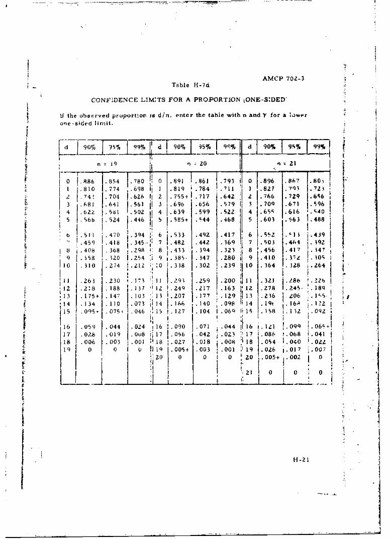
AMCP 702-3Table H-7d

CONF-DENCE LINCTS FOR A PROPORTION IONE-SDED'.

If the observed proportior is d/n, enter the table with n and V for a tower-one-sided limit.

9 95% % d 94% d 90% 9% 99 %

n1 ) 720 = :21

.79 0696 67 8091 1.986 854 .780 0 861 .793 " 0 .896 .867 .80

1 .810 .774 .698 .191784 .1 .2 7 .2

3 .681 .641 .561 i 3 .696 .656 .579 3 . 70q .671 . 5 9 6 .

4 .622 .58 .502 4 1.639 .599 .522 4 .65S .616 'i40

.5 .566 .524 .446 , 1.5 85+ .r44 .468 5 .603 .563 .48

b .511 .470 .394 5 6 .533 .492 .417 6 .552 .•13 .439.459 .418 345 7 .482 .442 .369 7 .503 .464 392

8 .408 368 .298 1: 8 .433 3q4 .323 8 .456 .417 .4A9 ]58 .20 .254 9 .385- 347 .280 9 .410 37 L 1r0 I

1 0 310 274 Z. 1 0 .338 .302 .239 10 .364 328 264 j

S 3 .13 11 .5 0 .321 286 .226

1 11 -2643 .25917 0S12 .2.8 188 .13? 7 12 1.24 163 7l .78 . A,- i8q

13 .175+1 147 103 '13 .207 177 .129 113 .236 10 6 11,5,'14 .134 110 073 j14 .166 .140 .098 1i .4 19t .16A .I Z I

15 .095 075. .046 15 127 .104 1 .069 1'15 158 .132 .0z 0

S16 .059 .044 .024 16 .090 .071 .044 ! 16 I.Il .09g .06-+I

17 02.8 .019 .0U8 ii17 .056 .04Z .0Z3 I17 .086 .068 1.04118 .006 003 .001 ! 18 ;.027 .018 .008 .I .054 1.040 .OZZ0

S19 0 0 1 11 9 .005+ .003 '.001 :1 19 .026 1.017 ,007:20 0 0 1o0 , -0 0 o0 0

2 0 0 0

__ ____ _H -,1 I

I{

.9 H-21

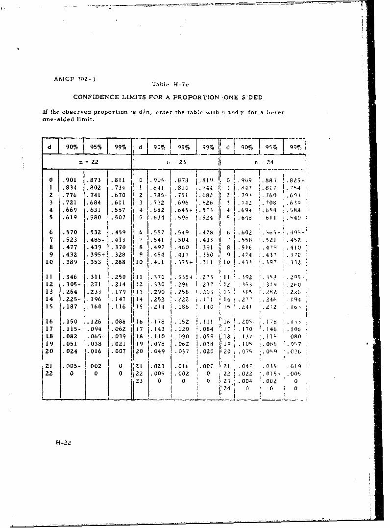
AMCP 702-3 Table H-Te

CONFIDENCE LIMTIS F@R A PROPORTION -ONE S'DED

If the observed proporti.on 's d/n, enter the table with u andY for a lowerone-sided limit.

n = 22 I--23 n 24

0 .901 .873 .811 0 .905- .878 I. 8 1') G 90Q .881 '.825.1 834 .802 .734 1 .841 .810 7.44 I:1 .8.7 .7 e 7r42 .776 .741 .670 2 .785- .751 .682 2 71) 760 .6e)I3 .721 .684 .611 3 .752 .696 ,.626 3 74- .1 70 .6 IQ4 .669 .631 .557 4 .68Z o45+ 1.57" 4 694 .6"8 .5885 .619 .580 .507 5 1.634 .596 !.5Z4 r, 648 t)l I . 140 ;

6 .570 .532 .459 6 .587 . 54q 1 .478 6! .602 .".0 - 4, ,;

7 .523 .485- .413 .541 .504 .433 .558 .521 .4528 .477 .439 370 8 497 460 391 8 .516 .47q .419 .432 .395+ .328 0 .454 .417 1. 350 ..44 .43 4 7 .e

10 .389 .353 288 10 +[ 311 375 .43• . 3 qv . J32+;1 1. 1 107 .4311 .346 .311 .250 11 .370 .3354 -.73 11 .. ,12 .305- .271 Z214 12 330 .296 1.237 '12 .3; 3 .31Q .ýOC13 .264 .233 179 13 .290 .258 '.203 13 •19 ;..2 .2Z6

14 .225- 196 147 114 .252 .122 I- 1 14 .27' :.246 19415 .187 160 116 115 .214 186 .140 1 .241 .zV2 i b

S116 .150 1.126 .088 1.b .178 ,152 117 115- .094 062 1I17 1.143 120 -.084 17 I 170 146 10618 .082 1.065- 1.039 j18 110 ' .090 1.059 ~18 .137 I1 1 ORO19 .051 1.038 1 .021 119 !.078 j.062 1.038 '19. lOq :066 .01720 .024 .016 .007 j120 .049 , 037 .020 120 .079, O',Q C .f

1.02 3 ~. 16 .007 2IZI 105- .002 0 1.002 .0160 .0022 0 0 0 I22 00o5 002 0 .22 0oz2 01. .006

23 . 05 .00 1 .;~ 004 .002

I I 24 0 0 0

H-22

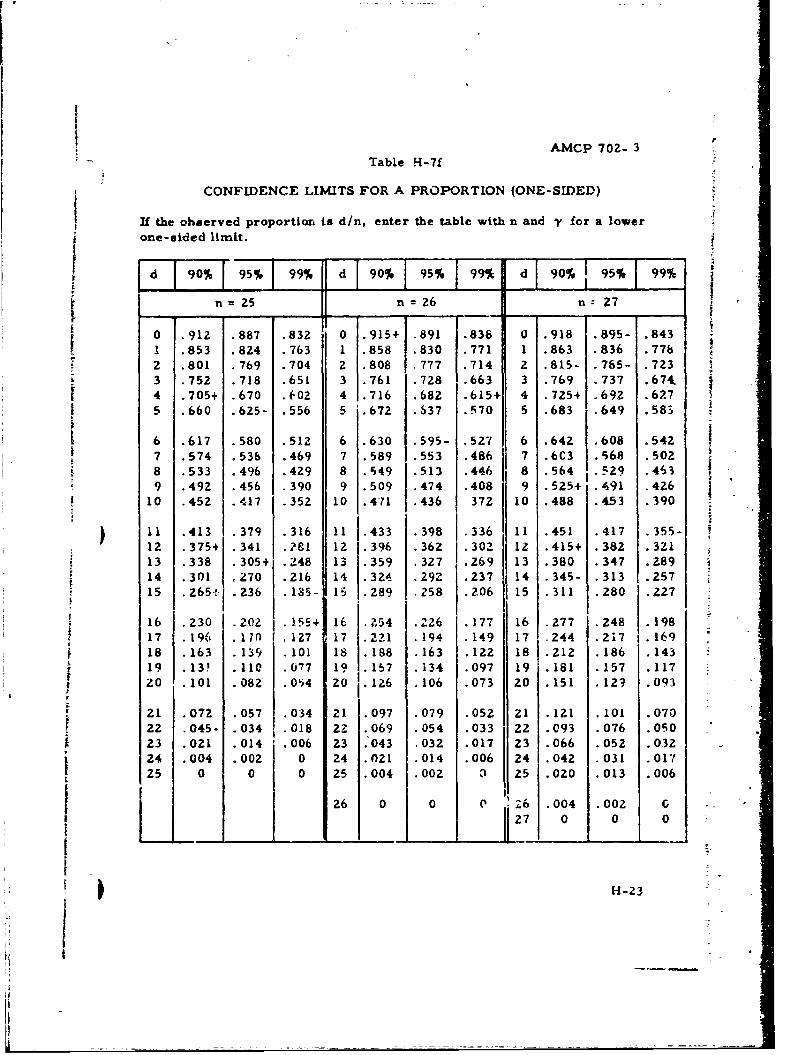
|p

AMCP 702- 3Table H-7f

CONFIDENCE LIMITS FOR A PROPORTION (ONE-SIDED)

If the ohberved proportion is d/n, enter the table with n and - for a lowerone-sided limit.

jd 90% 95% F9;% d 90% 95% 99% d 90% 95% 99%

' = 2s n = 26 n: 27 _

0 .912 .887 .832 0 .915+ .891 .838 0 .918 .895- .8431 .853 .824 .763 1 .858 .830 .771 1 .863 .836 .7762 .801 .769 .704 2 .808 .777 .7141 2 .815- .785- .7233 .752 .718 .65I 3 .761 .728 .663 3 .769 .737 .674• -

t 4 .705+ .670 .602 4 .716 .682 .615+1 4 .725+ .692 .6275 .660 .625- .556 5 '.672 .637 .570 5 .683 .649 .583

6 .617 .580 .512 6 .630 .595- .527 6 .642 .608 .5427 .574 .536 .469 7 .589 .553 .486 j 7 .6C3 .568 5028 .533 .496 .429 8 .549 .513 .446 8 .564 -.529 .463 ,9 .492 .456 .390 9 .509 .474 .408 9 .525+ .491 .426

II110 .452 .417 .352 10 .471 .436 37Z 10 .488 .453 .390

11 .413 379 .316 11 1.433 .398 .336 11 .451 .417 .355-12 .375+ .341 .281 12 1.396 .362 .302 12 .415+ .382 .32113 .338 .305+ .248 13 .359 .327 .269 13 .380 .347 .28914 .301 Z70 .216 14 .324 292 .237 14 .345- .313 .25715 .265+ .236 .185- 1 .289 .258 .206 15 .311 .280 .227

S16 .230 .20Z .155+ 16 .254 .226 .177 16 .277 .248 .198

17 .196 .l7ln .127 17 2.2.1 .194 .149 17 .244 .217 .16918 .163 139 .101 18 .188 .163 .122 18 .212 186 .14319 13 .110 .077 19 .157 .134 .097 19 .181 .157 .117Z 0 .101 .082 .054 20 1.126 .106 .073 20 .151 .129 .093

S~I.

21 .072 .057 .034 21 .097 .079 .052 21 .121 .101 .07022 .045- .034 .018 2Z .069 .054 .033 22 .093 .076 .05023 .021 .014 .006 23 .'043 ,032 .017 23 .066 .052 .03224 .004 .002 0 24 .021 .014 .006 24 .042 .031 .01725 0 0 0 25 .004 .OOZ 3 25 .020 .013 .006

26 0 .004 .002 C27 0 0 0

H-23

I

hF

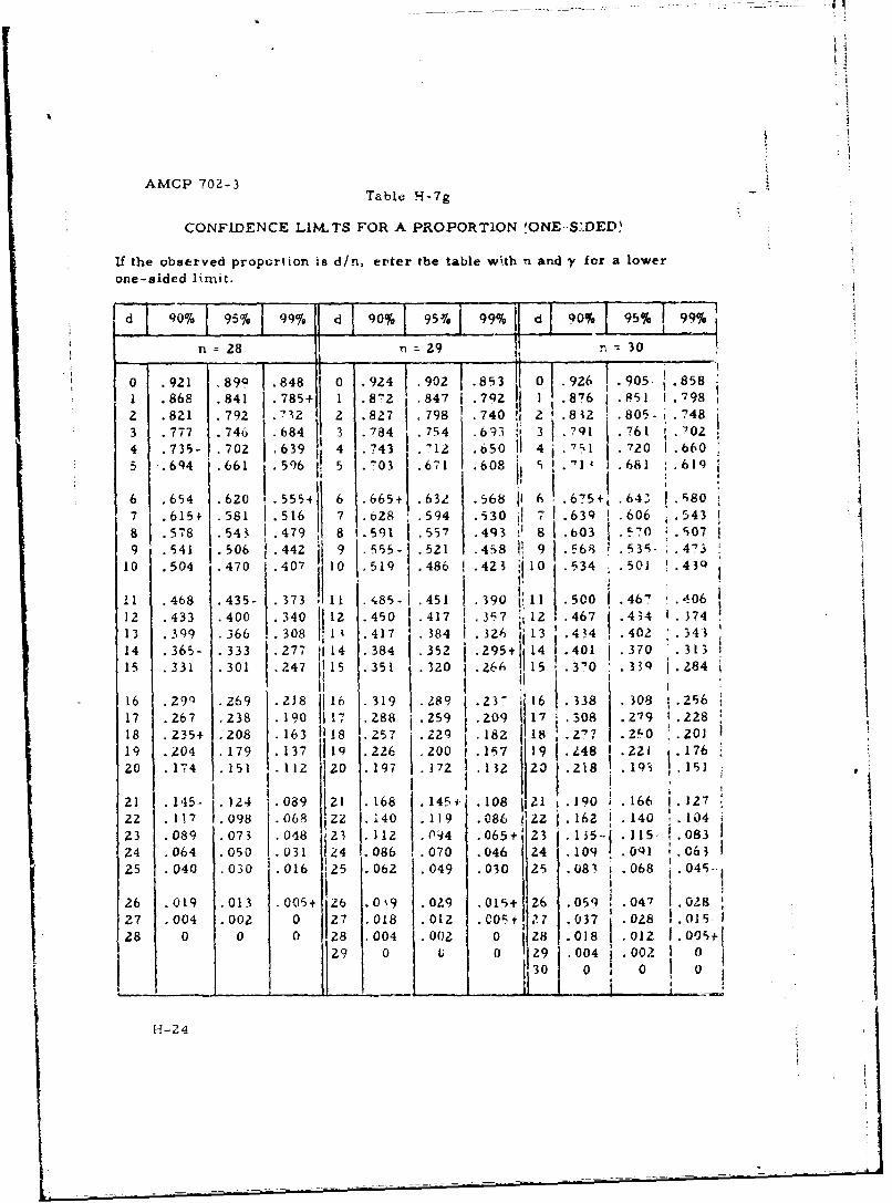
AMCP 702-3

Table H--7g

CONFIDENCE LI&LTS FOR A PROPORTION eONE-SLDED)

If the observed proportion is d/n, enter the table with n and y for a lowerone-sided li.mit.

Id 90% 95%4 99%7 d 90% 195-7. 99% 1 d 90% 95% 99%,

n 28n 0

.921 .899 .848 0 .924 1.902 3 0 9z6 .905..858.868 .841 785+ 1 8Z .847 .792 .8'6 .851 .798

5~~~87 S51 •6o 61 .o ! - •1 .7,9,82 .81 7Z 552 2 .827 .798 .740 2. .812 .805-.748.777 .746 .684 3 .784 .754 .6530 3 .791 .761 .502

4 .735- .702 .639 4 .743 .12 .650 44 .3 .570 .6605 .69 4 .661 .596 5 .5-03 .671 .608 9 .1 .681 .619

6 .66 47 0 519 .463 .568 11l 6 64 ; S800 .,I I

6 .65455+ 63 .368 I!1 .500 .467 .806.615+ .581 .516 7 .625 .594 .530 I7 .67 .460 .3

8 .576 .543 .479 8 .591 .557 .493 S .603 ý57C) S07

13 .3 9 366 .308 1• 4 417 .384 .326 113 .434 .402 .4 1

96 4 Z69 .218 16 319 .289 232 1 338 • 308 .256

1 .27 Z38 Igo 17 Z88 .259 .209 17 308 .279 t.2.2818 Z3+.08 163 18 Z5,1" 229 182 18 .Z..? 2.L0 .20110 ?.04 179 137 1 q.6 248 12 9 .. 48 .51 *.176

20 174 l 1Z20 197 .172 l z ZO . 18 ,.19, is)

2,1 .1,15- ]. Z4 .089 21 168 .145i .108 121 .190 .166 1 . 2

lI.Z

22 .117 .098 .068 ZZ 140 119 .086 Z11 .500 i .140 ,.104 i

23 .089 073 .048 23 .12 .094 .065 -t23 .135-I 1 15- .08324 .064 .050 031 24 .086 .070 .046 24 .109 0Q] ,.063

525 .04 .00 .0 12 .0 .049 .030 7 5 .084 .068 i 045-0 I I

16 .o99 0263 .218+ 16 .319 .289 o23 1j6 1.03_8 .o08 ~.028,17 .267 .028 .10 7 .088 .259 C~.20 I27 .037 . 2_9 l .08

20 .10 .5 .112 .107 p'102 .3 20 .2 18] .193 .05

.. 0 . 0 1 19 .004 I .022 176I2030 0 0 0

H-24

.168 .145' .18 121 ~i90 166 .12

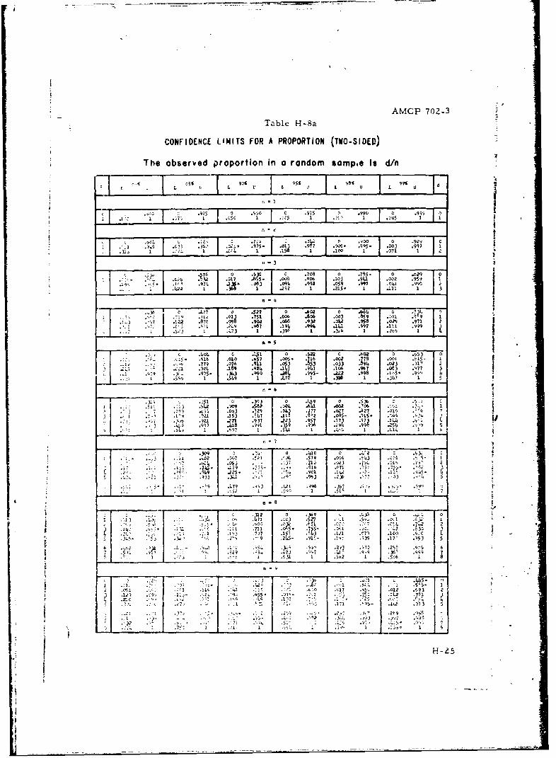
AMCP 702-3

Table H-8a

CONFIDENCE LIMITS FOR A PROPORTION (TWO-SIDED)

The observed proportion in a random sompe Is d/n

9% 9% 75 St 9?%LL 1- L 1: U L U L U

0 .55 0 9 -.C '2 "?- .9"5 o .95o .-75"' .•qo .9•5 5s 1. 1 ... ; 1 .7512 1 .2 1 ...•:.-0 1.1

9I .2;l 1 ~ .lO :995- .003 . 1 I1 071° 1 z3• 17 07 .52? .600 ,00 .691, .O1 .95"4

. .~a 1 .24 .987• .191k .99,7 ~ 9 .191,, 95_

3{

Q .00 .657 1.105 .u .002 ,- f .O 95 . 1.9 _ .3 .99 .•fr .,9, . 2 .#8 3 .. ,5 17

772 I I • W .oI21 1 .1,, 1.,1 .6016 0 .0 66

.- .:_. * - __ .51.9 1 j .67- 1 j .. ,T 1 ._______7 __I 5

.7 51 006 003~ .85 2ý

7 . 12_2 8 .0.2 .958 .02 9 -

.0 .587 1 . 9.4 .1j .997-

. I .5a .6-1 * .653

. -5 , ,, � 01.67 .1• I .002 197 a 5. 2. 3 i . . .9'5- 343 . 0. .9, .2a ... . 1 b

7 317 004..2 .96

____3__ . 2 9 .04J ________ ____-____19

. 7 .. . ..15 .3; .' ,-00• • .

% .2. "- .7 i .71,4 .2t1 .937 . 1. Z1

0--, M3.

a9~75 55ý6 C.1 :

.3, .1 . -963 .2) 33 9-

2?9 . 3 L.21 .996 -3

'0 .369 5 L. .7 0.19 123:1

r .. r -:c

.77712..,'7 I.1

.2 35

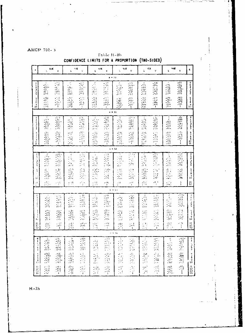
AMCP 702- 3Fable 1-81


U , L U " U 1 L L u

*10

5 129~ .572 o

1 3 ~.IL .3 j~4 4:

2 l •.• , " *L"-- ., 0-'" • , ";. *,'•• .:: 7: .,?)? .7l.?

S , : L', . 7 .. q; 77 5 009S 2) 7% ,-- 7 .73 -'' '? )' ,.073S . 0 ,1' .'072

... .'5 .031 . 6

*,¢ - . 1 : ] , ) • ) .•:L . • ,510 ,,U'_ ,6.. ,l3." *2VI

0 ..• . * .,,, .a:, .3'. ,. .•,:.9'3

102

S.:• . .. • .o" ., ... -,.• .. • - - .,-. 2; .s)e, 0

•I .: : 7 c 7 " b "I .:i .•. 5 03 131 53

172

4s -

,-I.2' .. .,I I ". ."L - L7

1: - " , i .

,1

3 1 313

125

12 23 '. •'

7 3% "95'; . •,• ! .. ,' . ''• .,,; '• ) ,

S.. .-'' ",, ... .

II"1" • "' :• I :•• .7: • , . . •: .

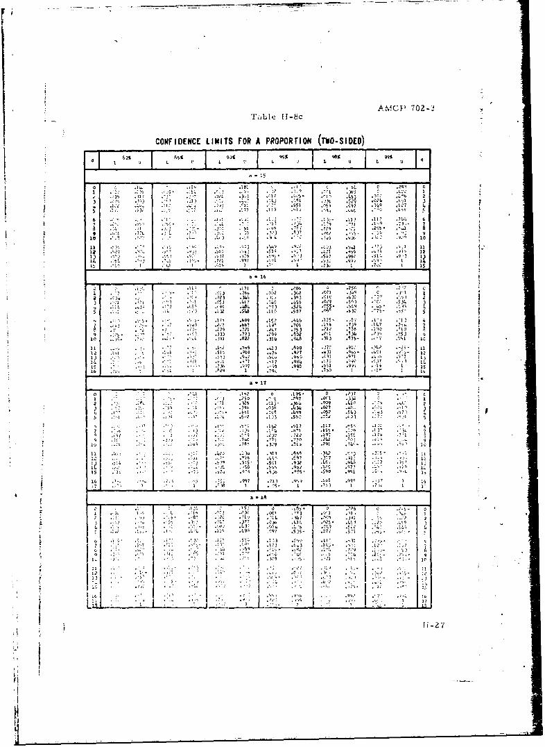
S~AMCP 702-3

Table H-8c

CONFIDENCE LIMITS FOR A PROPORrION (TWO.SIDED)

0*15

S.. i• .5• .~l •? .2• .c:;1 .. C

.. .'17 . i5Z . '67

7 .551 05 "'" 6.."7 ,9 , 4

1 , 7, .L' L .

'6 . . .% T . 10

7 .• ,. . • . 7 ,• 7gil ." * .96 " .57. .ss •:• 9-

72 .. , s. *ss

.76

.2.7 37

- . .54... . .06 .)7 3,--5

-" .; • " i ."•, .60 .15 .1. .1•7' .. S " 1• : 6

.21 2 ..9 7 . 156 .212 ,7 C 19' '17".73 .?31 isy .s

10 .. )-. 1 .T22 *357. ,7 .31E ,.37 '131 IC

"11 2 .;... .: . l . .1-.13 .930 .7.7 ..3? .2, ,1

.. " . : • . ;. . , .31.1 .57a,, .36'7 .1.57 .73' .'-: ., : 1.

.I•.- "'- °? :7 .'79 .'17 .351 . 0 27 .'21 . ':, 3* 17

376 *)57 .*,.93 *395 o ,7 3 -5 17• 15

16." 1 77 1 .7)l1

S171

.*•.:. . •• .l .112 079: -135- ,I 0 .77 2• •'

7 .257 .:.1 .328 N.17 .33

.-:23..',3 ...3 .', .5 3 . .... . ,

Si. .2 .... .11 .4

5 .:1 ' :.23 .172 .137 75- 5 5-1 7i...1 .676 .125 6'

-.. .-. :' -70 -'-3 . ... ..... *31,- .•;"

._ ,.3-i. x .1,3. *45 "7~ 4

.'316. 71

7 . 3

T. . .701 Isb .7 1,-

7 . 72 .20o .753* ?10 3

1619 :82 353 .71 *3io U3 .175 .-

16 3 ). 1 .o

1L -7

:7,3 j7 ;; 96 99 1 6713 1*711.5

5315 27 ocl 33Z-

2. .12 '1 7 II ? .1

II ;

.3 72? 19.

.7j .- 0 2W -

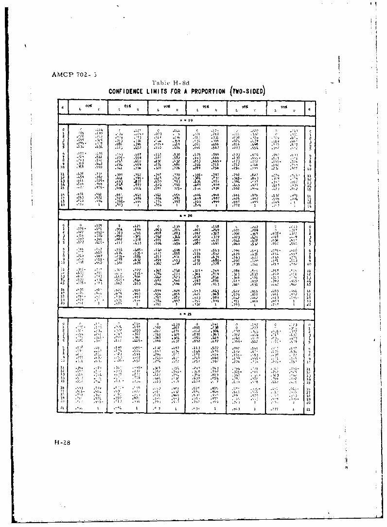
AMCP 702- 3Table H-8d


d~~~~ u ; L U • I L U !L I

"196 -.7 ,19. ..11 .g .56,.7 0 .6.6 . .241

•1 5. 25 .559" .0 9 .5 .- 1'3 .66 .-131 .6.92 * .111

2 ' .2 .'1 .617 .0 ,". ."'1 ." 3 .173 .7a . L-99 310 ,61.2 .294 .59 . 351. . 9 ,34. .716 ozt. L139 .1'. ,5.'

0 , 3$ 8 .99o . ]1 j . i o• .327 5 7 26 .219 .7 5 6 CL I, .7 49 .2 3 " 1

1 1 . 1. 7 .74 3 . 3, .7 5 2 7 0 4 i . 0 ,7 - . 9 3 7 ..5 5 L,

6 ' .. 7175 3 507 . .566' ,1.59 ,927 .1o " 13 6" 5 .559 :.970 .953 6 .137 .571 . .-0s71 .53.2 .. 08 . .56 .5 .97 .31 .v 1111.-'5-".90 .7 91 .5737 . .5 l .50 1 .12 :i; 1l

15 _2. .9c5- .64 . .1. 9 L0. .925 .56u .07.5 .7J .1 1 161 71.3 .9.2 . .7 .9476 s7 .1s .609 ."97 .562 .970 . 5 441. 1•

.11, . 795 . "t .Mn b .9Q .69i .91 .11 1 q ,73 I .51 J .I?9c 1 .7' 7 1

a *20

c2U 1067 . k2l 0 .119 0 .168 , .277 Z3,3 71 .a59 .l1l oc4 .19 :?15 . . - .. Dw .?69 .• 5 • .1 .81 .09 . 0 .013 .31 .* .*5

9 .o3n5 7 2

5b : N .3 . . 0d . 9 *3 .••.79 02 ,:,• .;. . I14 .07 .578 c35 So

15 .5) -9 .1-17 . 316 .104 ,956 :997, :g491 .95 J 05,9 .q 6

6 .,? .154 .75- .140 Soo6 .119 SL93 .'o .*5'3 .- 1.5 .ol- 6

.15 637 2. 3g .5 2 .17 *6590( .191 .6j9 .163 t7 .,11 4 'I9 . 1, 5 5 27, 6 V 359 . .271 :6 .7 * .201270 13 9

10 34 . ; . 3R2 . 2 62302 .39 .:77 .11 11 . , , .702 .347 .71 .35- .769 .7@0 .9-o .- 57 11- . • 0 * .' .7' .L 7,5 .333 .937 .2-97 • 12

b.,: .9 .0LS9 .230 .0.1 . .3. .39 .'12 .•L "1 .l .3j .• .. l5 .954b .1.92 .97 .6.5? .691 .1g2 ."91Y .)go 915.1 9 . <73 .5. 7 .5•, .5 .954 .:9 5,) .913 .1 .9)1 ,L.97 ,-,17 1

16 b.1i .918 .5q9 .939 .ý 9.i : ,1 11 1. "' 6 . 99 .3..-,' 1 :5.' ."95 .. 1.9 ... 1. 76.. ..62 977 -751 I17 .7 3 .1O .972 ..3 9 .81 .9 1 , 119 .15 , .78. .997 _.'9 .'19 .771 .937 .63 ."9 192o 1 i,61 I .3Y 1 .793 1 .7,7 1 0

.31 C .133 3 .1.1 o0 17 0S " -o 901 .20 .01 .p 3" 0 .?7 *'1.1 7

2 j.250 .31. .??l X012 .)04l .'717 3. .-3'2. 2

7063 .34 .05L ' f1.L , ý -"

09i. .. oqg 37 .052 .4,72 .055- . .179

L 1.133 .,57 . 3 .52t .7 .5,.494 .V4 .51 1 .% :IL .570 1244 7

54 2 501 .20ý .5' , 1.341 .1 1.9 .27' 2,. 6. .231 .660 91~ ~ 9 7

?' ~ 2 .?57 .70 6.722475 1

l1 VS9. 32 11 .291 .743 t. ' .54. *7,.. 11I1- .7i .37i .7 , .31.0 .792 .37-6 1.13 .. ' . 7 11 .7.. .391. 99 .9 2 1

4.91 :"' .342 .41 7. 9- 7ý> ~2e I

16 .3 z.3 . .9C1 .529ý .9151 .4 ',-- '1Y f .992 . i .91., .5k.1 137

11 L91. .7.3 .9'9.7 19

31 1 '-7 1 .'.' I .. 13 1 '7 2 21

H-28

z•I

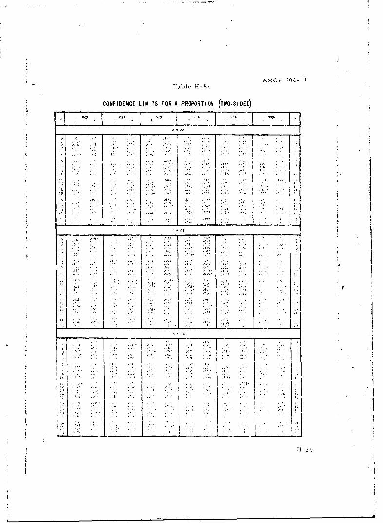
TableH-8eAMCP 702- 3


a I

71,I1 3

IC2

:ICI45 1

j -- - 4

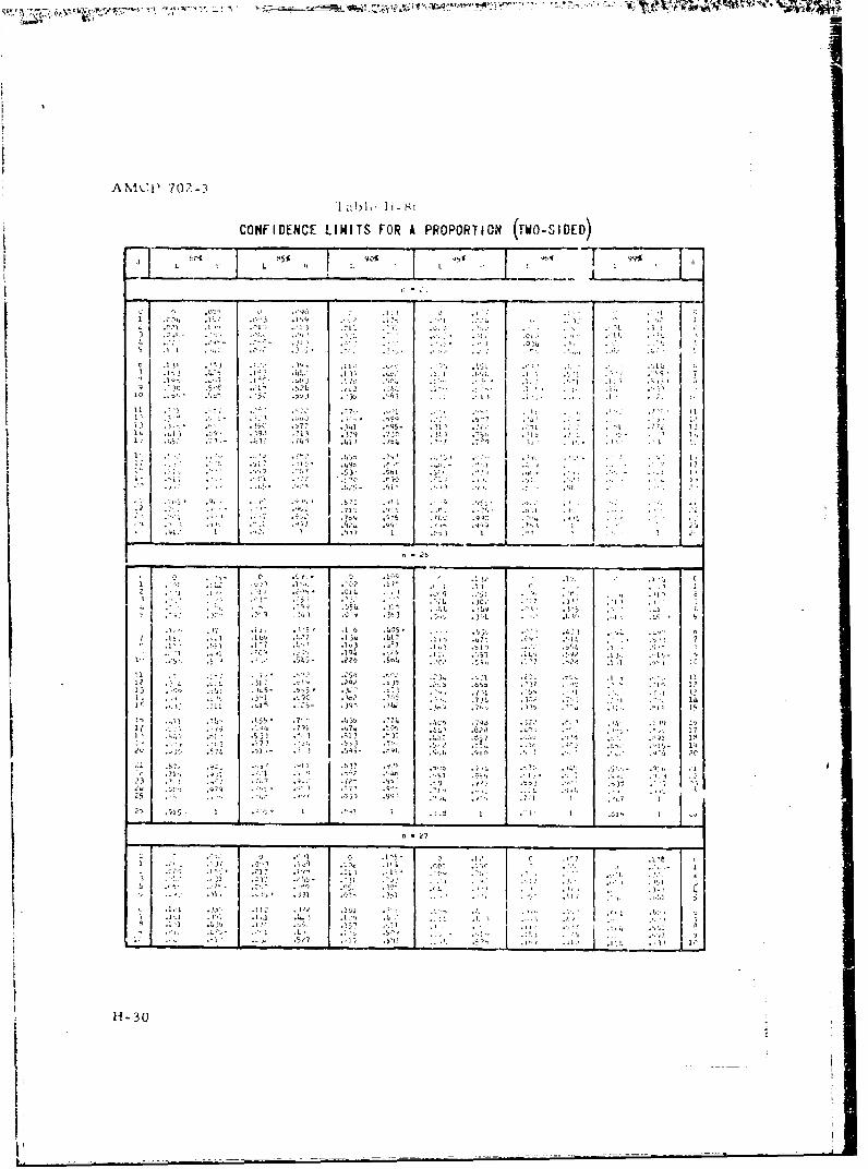
II


7 .7

I'72

.41 1 .?b;

''7 3

1 3u.W313

'~3c 1 3,4r 3.73- .''.74i

.7 s' I:.3 11

.*

I.I

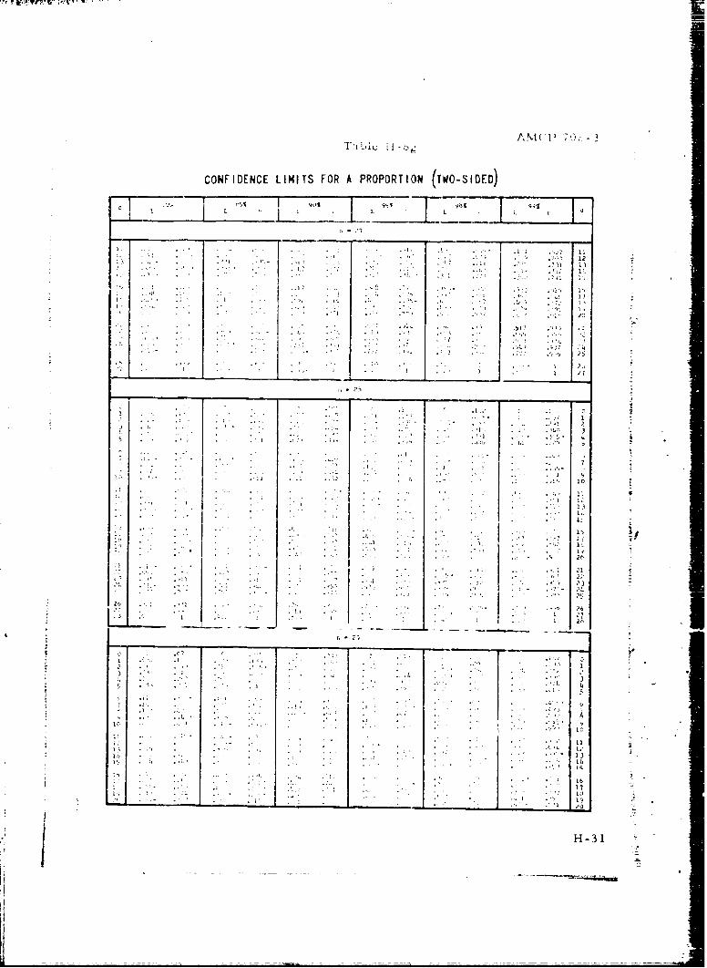
T-i~ !ý):. I3


*~ . 3 1

3 12

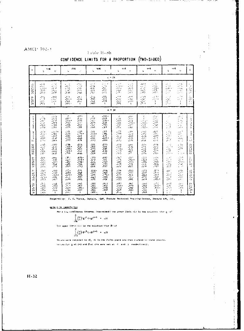
AAC 7C,'- 51 oUlv P-Msh

CONFIDENCE LIMITS FOR A PROPORTION (rWO-SIDED)

21

.97 7. :

.I- 1 :?7ýi7 .793 ýý :2: 41

4 : :Iz. OC M,1 .0 I~1 _ _ _ _ _

1 . .O0 0; ~ **5 .1L95. ý 3

07b2 33 9 .1 3 197

716 .5 15- .3,14 .- qq

:,1, .;i7 5? " 1 .1L0 99 .1. .SS 9C L 32 .15679 .4.36 .i 6 SL!7

12 :5 .5,3 S25 .512 .250 .566 S1'4II1 3 .56 .2 95- .937 .219 .5911 .5 :l 13

Ii. 13: .%44 .3-15 t .91 .3W8 .63037. t19 .6. .339 .991 .71,

1... 69, .391 .65 *777 .692 .3. 1 71 .73 LL.-!9 .o 71.75 * .32 .721 :)L. .73.9 L. )3 .7'.

19 ... 7 7.' 52 ,5 . .6 .790 6.O72 33. *9

2C .5, 7'2 .519 .7) .5o1 .c,7 .0.2 8z7 *, 9 *L

Sn .310 .;53. .821 .5)5- .634 .'06 .1153 _373 .611 .0:42'3 .569 .53.8 .57D 90 .~ .,i .537 .5 e

.9 '3 .5. * ,5- .74. .c .9 97 .9 .543 2"1.1. .o73* 79 .-. .89 .63 .99 nl3. .9c. . .917

.7: 372 .9~3 ,9 97 * .,,- ..7 I

6 .3 .41' Z,9' .2. . 1 .932 .'5 3 .9 b!.99 .955.3.ý3 9A 720 9.97 .39- *91.0 .96. C1

.71 9 b~ .465- .905- .958 .779 q492 .73.9 .91,5- 1 2

25 9; 6n .997 .851 .905 .62 ( .99, .- 193 1 .12.0.37 1 .909r- I I$3 .75s6 1

V.1-.....1-.-t.1 t. -0, -1 In the (iftt, piece .11j Zr.n ,0I-1o8 lo th.9.e rI.:...

Vol-ex fcr 91 at d-O and ý at d-n set. a.t 6 and 1 resapct 1.01'

H-32

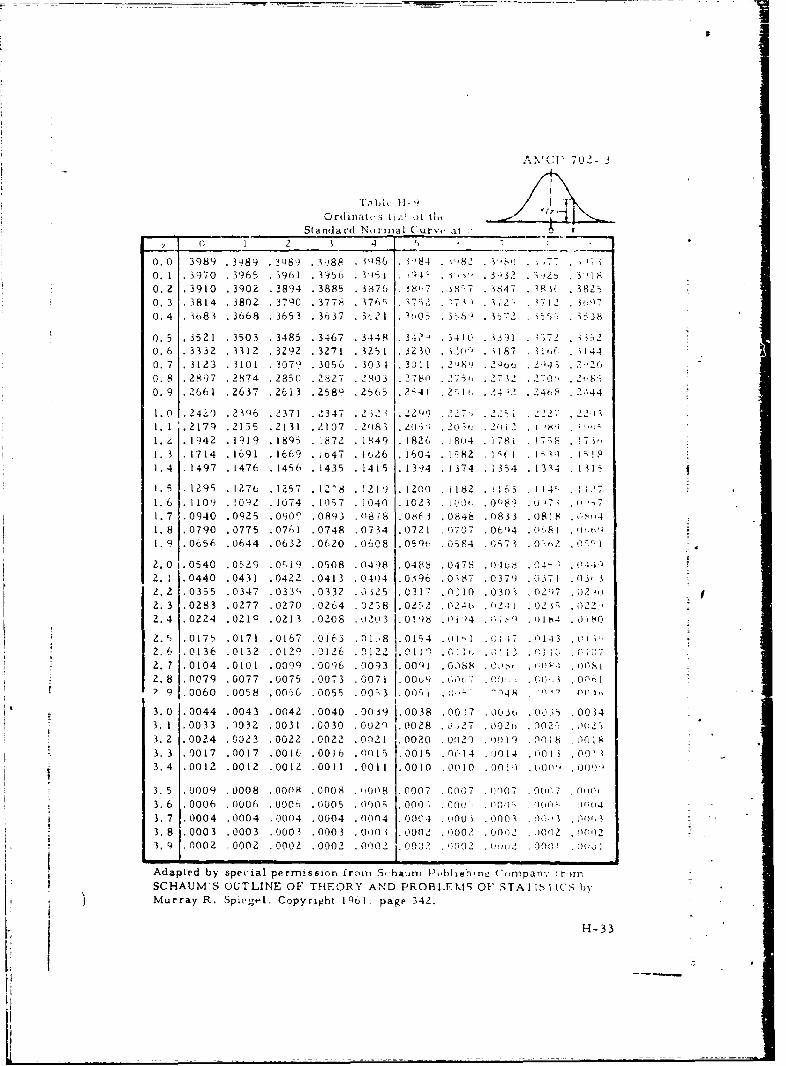
I

AMC" 702-3

T1Ltc lI -I

OrdinatQ s . , th,:Standard Nornial Curve at

/ C 1 2 4 5

0.0 3989 .3989 , 3P8) .3988 . •)8%6 3"84 . ,82 . 7-,', .;,-7 . 730. . 3970 .3965 .3961 .3956 .13' 1 4 .3,v' .3'i3, ., . 3180.2 3910 .3902 .3894 .3885 . 3ý876 5802 .5x, ,7 . 3847 .1 . 38250. 3 38 14 .3802 .3790 . 3778 . 7 ,• 373 , . 7 .7,2 \ . 2 .10.4 .3683 .3668 .3653 .3637 .312 1.ou05 . .335 .I555:% .S53

0. 5 3521 .3503 .3485 .3467 .3448 3.;," .419 i 3f 72 . -0.6 3332 .3312 .3292 .3271 .3251 3230 . 2.0n .2 .187 . i t,(. 1.440.7 3123 .3101 .3 0 7) .3056 .3034 3011 .2J8¼.20uu .-243 .2260.8 2897 .2874 ,28;0 .2527 . 2803 . 2780 .2"3' .2732 . -70., . K8j

0.9 2661 .2637 .2613 .2589 .2565 254! .2 1H .24) .2.4 ,t) .1444

1.0 249 .Z..2396 .2371 2347 .23 229 227 ,2 . -7... .•.• 227-..-1. 1 2179 .2135 .2131 .!107 .2083 Z05 2 . 0 - .t" iij . ,1 1 ,i i,1.2 .19,2 .1919 .1895 .872 .1849 1826 .1804 .178i . S 77 .1. 3 1714 .1691 .1669 . ,047 . 1 26 1604 .582 1 .I I1.4 1497 .1476 .1456 .1435 .1415 13 .14 .1374 .1354 1 3"4 . 515

1.5 1295 .1276 .1257 .12' . 1210 1200 . 182 .163 14< .I 11c 7

1.6 1109 .!0"2 .1074 .1057 .1040 1023 . L 'O', .00'89 .0'7, .- '; 7

1.7 .0940 .0925 .090" .0893 .0878 0863 .084b .0833 .0818 .,,41.8 0790 .0775 .0761 .0748 .0734 .072t .1707 .06)4 .08, . O

1.9 06556 .0644 .0632 .0620 .0608 .05Q1 .0584 .6373 .0m . '-I

2.0 .0540 .05 29 .05.1 i9 .0508 .0498 .0488 .0478 . 1 :..• 0¢ 4 - .0449

2.1 .0440 .0431 .0422 .0413 .0404 .0396 .0-;87 .0379 .037o1 03 32. 2 .0355 .0347 .033' .0332 .0315 .03 17 .,10 .0 30 .027 .022. 3 .0283 .0277 .0270 0264 .0258 .02;2 C 024, .,2 -1 .02 , .5 2 Z2.4 .0224 .021 9 .0213 .0208 .o203 1.0!1)8 .0i 14 f! .0-11 2 .0i80

2.5 .0175 .0171 .0167 .0163 . 11.,8 0 4 .01 .1 1 -7 .- 143 .72.6 10136 .0132 .0129 .0126 012- . 0"1 1 13 ",1V.2. 7 0104 .0101 .0099 0096 0093 00,4l 0.)88 . . it -- 002. 8 .0079 .0077 .0075 .0073 .0071 00ou .L ' 0 7 .1 : . (;0ý .0")6!' 9 0060 .0058 .0036 .0055 .0033 00- 1 .4 48 00 1",l,

3.0 .0044 .0043 0042 .0040 .0039 0038 .00,7 .00 0t .00 0 '0343. 1 .0033 1 4032 .0031 0030 0029 .0028 . 7 .02,7,00 . 002 .00003. 2 0024 0023 0022 0022 0'0021 0020 On> 21)fm1 .)0!f8 .008•3. 3 .0017 0017 0016 .0016 .0015 I0015 . 14 .t0 14 .00 1 . r) ' I3.4 .0012 .0012 0012 .0011 .0011 0010 .0010 .001) .1,00, .0ow,''

3. 5 0009 0008 00(1 .0008 . 1)008 0007 0007 .4r)07 . 0(10 . 0! i1,3. 6 0006 0006 0006i .0005 .,r)00, 0 00 0 0.o 0 11 G .; ) 041 .- 111043. 7 0004 .0004 0004 .0004 .00n4 0004 .000, .0003 . F)> . OF;

3,81.0003 .0003 000 1 .0003 .0110 .0002 002 .00-,2 . 0C)2 .4F) 03 .co 0002 .0002 .0002 .0002 . 0o02 I.00J12 . 00r2 0!1412 0 0:o I

Adapted by special permission from Sc haum Publishino ('Fmpanv !r 1r.1

SCHAUM'S OUTLINE OF THFORY AND PROBI.EMS O1. STATISlICS by)-

Murray R. Spegel. Copyright 1)61 page 342.

H-33

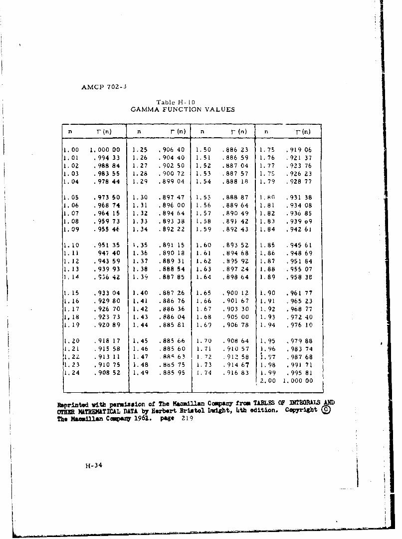
IU

AMCP 702-3

Table H- 10GAMMA FUNCTION VALUES

n r(n) jn T(n) n r-(n) n r(n)

I.oo 1.000 00 1.25 .906 40 1.50 ,886 23 1.75 .919 06I. 01 .994 33 1. 26 .904 40 1, 51 .886 59 1. 76 .92I 37I. 02 .988 84 1. 27 .90250 S 1.52 .887 04 1. 77 .923 761. 03 .983 55 1.28 .900 72 1.53 .887 57 1. 7S .926 231.04 .978 44 1.29 .899 04 1.54 .888 18 1. 79 .928 77

I . 05 .973 50 1. 30 .897 47 1. 55 .888 87 1, 80 .931 381.06 .968 74 1. 31 .896 00 1. 56 .889 64 1.81 .934 081 .07 .964 15 1. 32 .894 64 1.57 .890 49 1.82 .936 851.08 .959 73 1.33 .893 38 1.58 .89) 42 1.83 .939 691.09 .955 46 1.34 .892 22 1.59 .892 43 1.84 .942 61

I. 10 .951 35 1.35 .891 15 1.60 .893 52 1.85 .945 611.11 94740 1.36 .890 18 1.61 .89468 1.86 .948 691.12 .943 59 1.37 .889 31 1.62 .895 92 1.87 .951 841.13 .939 93 1.38 .888 54 1.63 .897 24 1.88 .955 071,14 .96 42 1. 39 .887 85 1.64 .898 64 1.89 .958 3e

1.15 .933 04 1.40 .887 26 1.65 .900 12 1.90 .961 771. 16 .929 80 1.41 .886 76 1.66 .901 67 1.91 .965 231.17 .926 70 1.42 .886 36 1.67 .903 30 1.92 .968 771 18 .923 73 1.43 .886 04 1.68 .905 00 1.93 .972 401.19 .920 89 1.44 .885 81 1.69 .906 78 1.94 .976 10

1.20 .918 17 1.45 .885 66 1.70 .908 64 1.95 .979 881.21 .915 58 1.46 .885 60 1.71 .910 57 1.96 .983 741.2Z .913 11 1.47 g88r 63 1.72 .912 58 1.97 .987 681.23 .910 75 1.48 .885 75 1.73 .914 67 1.98 .991 711.24 .908 52 1.49 .885 95 1,74 .916 83 1.99 .995 81

2.00 1.000 00

oprinted vith permission of The IaWaillan COMpazY from TABLES OF INT•EGRU ANDMM PMThEMTIAL DATA by Herbert Bristol bWibt, hIth edition. CopyrightThe MyAmillan Cmpazi 1961. page 2 19

H-3 4

I.

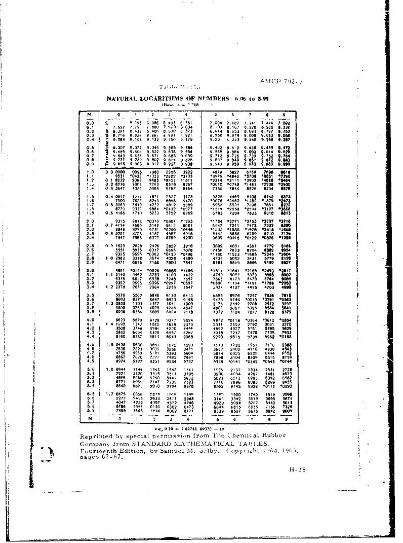
I

AMCP 702. 3

NA'TURAL ILOARITHIMS OF NJMWBERS- tO. to 5.9"

N! 0 1 2 3 4 5 6 7 a 9

0.0 1E 5.395 6.08S 6-493 f. 761 7.004 7.187 7.341 7.474 7. W0.1 7.697 7.791 7.880 7.960 8.034 8.103 8.167 8.228 8.285 8.3300.2 • 8.391 8.439 8.4e6 8.510 8.573 6.614 8.653 8.691 8.727 1.7820.3 j L.7ý6 8.829 8.86i 8 991 4.921 8L950 R.973 9.006 9.032 9.05O0.4 I 9.084 9.108 9.'32 9.15M. 9.179 9.201 ZL.3 9.245 9.284 0.20?

0.5 - 9.307 9.327 9.346 9.365 9.384 9.402 9.4 0 9.438 9.455 0.4n20.6 9.489 9.506 9.522 9.538 9.554 9.569 9.584 9.600 9.614 9.6290.7 v.643 9.656 9.671 9.685 9.699 9.712 9.7U6 9.739 9.752 9,740.:8 q7?T 9.789 9.802 9.814 9.828 9.837 9.849 9.861 9.872 9. 830. 9.895 9.906 9.917 9.927 9.938 9.949 9.959 9.970 9.980 9.990

1.0 0.0 0000 0995 1980 2958 3922 4879 5827 6786 7896 8181.1 9531 '0436 11333 .2222 .303 *3976 '4842 570D *65l1 07,"BI.2 0.1 8232 9062 9885 '0701 *1511 "2314 -3111 *3902 '4680 05441.. 0.2 6236 7003 7763 8518 9267 '0010 10748 *1481 *2208 *2901.4 0.3 3647 4359 5066 5767 6464 7156 7844 8526 9204 04761.5 0.4 05(2 1e1 1871 2527 3178 3525 4469 5106 6742 63731.6 7000 7623 8243 8858 9470 "0078 *0682 '1282 01879 024731.7 0.5 3063 3649 4232 4812 5389 5962 6531 7J98 7661 8222I.q 8779 9331 9884 0432 '0977 *15?n -205a '2594 *3127 038451.9 0.6 4185 4710 5233 5752 6269 0783 7294 7803 8310 3113

2.0 9315 9813 10310 '0804 '1295 .1784 *2271 '2755 '3237 *3?102.1 0.7 4194 466) 5142 5612 6081 6547 7011 7473 7932 IM902.2 8846 9299 9751 *0200 "0648 -I 5 ."1536 1978 '2418 `-1b82.3 0.8 3291 3725 4157 4587 5015 5442 5866 6289 6710 71292.4 7547 7963 8377 8789 9200 9609 X0016 -0422 '0826 -1221

2.5 0.4 1629 2028 2426 2822 3216 3609 4001 4391 4779 51002.6 5551 5935 6317 6698 7078 7456 7833 8206 882 8984e.7 9325 9695 *0063 10430 '0796 1160 *1523 '1885 '2245 *2w042.8 1.0 29H2 3318 3674 4028 4380 4732 50112 5431 5779 £1262.9 8471 6815 7158 7500 7841 8181 8519 8850 9192 9527

3.0 9861 '0194 *0526 *0856 '1186 '1514 1841 '2168 02493 2t?3.1 1.1 3140 3462 3783 4103 4422 4740 h0k? 5373 5868 G0023.2 6315 6627 6938 7248 7557 7865 8173 8479 8784 NO093.3 9392 9695 9996 *0297 .0597 '0896 '1194 '1491 '1768 '20633.4 1.2 2378 2671 2964 3255 3547 .A37 4127 4415 4703 4990

3.5 5276 5562 5146 6130 6413 6a95 6976 7257 75306 7813.6 8093 8371 8647 8923 9198 9473 9746 *0019 *0291 *05633.7 1.3 0833 1103 1377 1641 1909 2176 2442 2708 2972 39373.8 3500 3763 4025 4286 4547 4807 5067 5325 5584 58413.9 6098 6354 6609 6164 7118 7372 7624 7877 8128 8379

4.0 8629 6879 9128 9377 9624 9872 -0118 *0364 '0610 '08544.1 1,4 !i99 134- 15 5 1828 2070 2311 2552 2792 3031 32704.2 3508 3746 398; 4220 444$ 1 4692 4927 5161 5395 56294.3 5862 6094 6326 6557 6787 7018 7247 7476 7705 79334.4 8160 8387 8614 8640 9065 9290 9515 9739 9962 *0188

4.5 1.5 0408 0630 0851 1072 1293 1513 1732 1951 2170 23044 6 2606 2923 3103 3256 3471 3687 3902 4116 4330 4543'.7 4756 4959 5181 5393 5604 5814 6025 6235 6444 V53I4.8 6862 7070 7277 7485 7691 7898 8104 8309 8515 87194.9 8924 9127 9331 9534 9737 9939 *0141 *0342 *0543 '0744

5.0 1.6 0944 1144 1343 1542 1741 1935 2137 2334 2531 2728561 2921 3120 3315 3511 3705 3900 4094 4287 4461 46735.2 4866 5058 5250 5441 5632 5823 6013 6203 6393 6S825.3 6771 b959 7147 7335 7523 7710 7896 8083 8269 84555.4 8640 BU25 90a0 9194 9378 9562 9745 9928 *0111 '0293

6.5 1.7 0475 0556 C581 101Q If09 !3Pl 1560 1740 1919 2094*.t 2277 2455 2633 2811 2988 3166 3342 3519 3695 38715.7 4047 4?2? 4197 4572 4746 4920 5094 5267 5440 56138.8 5786 5958 6130 6302 6473 6644 6815 69015 7156 7325.9 7495 7665 7-34 8002 8171 8339 8507 8625 8842 9009-W -0

N- 0 1 2 4 6 7 8

, -i10O - 1769741 49070 -10

Reprinted by special pt'rmis;i,)n from "I'hc Chemical RubberCompany from STANDAR!D MALJF'tIIEMATICAL TAR1JES.Fourteenth Edition, bv Samuel M. 3elby. CooyriLiht I (-I, 1965.-Dages 62-67.

Hj-35

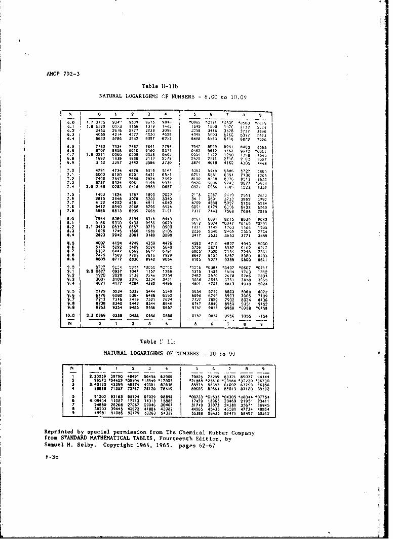
AMCP 702-3

Table H-llb

NATURAL LOGARIGHIIS CF NUMBERS - 6.00 to 10.09

S0 1 2 3 4 5 6 7 d S

6.0 1.7 9176 934- 9509 9675 9840 1 006 -0171 *t33§a *OsOo o0.) 56.1 1.8 0829 0093 1156 1319 1482 1 i45 1808 1t,70 2132 7.146.2 2452 2616 2777 2938 309t 3258 3418 3578 3737 38q66.3 4055 4214 4372 •530 A688 4.94,1 5003 -b C 5317 54736.4 5630 5786 5942 6097 6253 6408 6563 6716 6872 7026

6.5 7180 7334 7487 7641 7794 7947 8099 8251 8403 85556.6 8707 8858 9010 9160 9311 9462 9612 9762 9912 *00C19.7 1.0 0211 0360 0509 0658 0103 00 54 1102 1250 1398 154ý68 1692 1839 1986 2132 2'79 2425 2571 2716 262 33076:9 3152 3297 3442 3586 3730 3874 4018 4162 4305 4448

7.0 4591 4734 4876 5019 516' 5303 5445 5581 6727 5l6•7.1 6009 6150 6291 643. 65tI 6711 6651 6991 7130 72697.2 7408 7547 7685 7824 7962 8100 8238 8376 8513 86507.3 8787 8924 9061 9198 6334 9470 9606 9742 9877 *G01 37.4 2.0 0148 0283 0418 0553 0687 0321 0956 1019 1223 1357

7.5 1490 1624 1757 1890 2022 21-5 2287 2419 2551 2GF37.6 2815 2946 3078 3209 3340 34 1 3621 2732 3862 39927.7 4122 4252 4381 4511 4640 4769 4898 5027 5156 52847.8 5412 5540 5668 5796 5924 6051 6179 6306 6433 6V607.9 6813 6939 7065 7191 7317 7443 7568 7694 7819

0 7944 8069 8194 8318 8443 8!67 8691 SOIS 8939 9063.1 9186 930 9433 9 55 9679 96802 9924 .0,17 *016,9 .0ý918.2 2.1 0413 0535 0657 0779 0900 1021 1142 1263 1384 15058.3 1626 1746 1866 1986 2106 2226 2346 2495 2585 27C48.4 2823 2942 3061 3180 3293 3417 3535 3653 3771 3d898.5 4007 4124 4242 4359 4476 4593 4710 4827 4943 50608.6 5176 5292 5409 5524 5640 5756 5871 5987 6102 62:78.7 6332 6447 6562 6677 6791 6905" 7220 7134 7248 73618.6 7475 7589 7702 7816 7929 8042 8155 8267 8380 84938.9 8605 8717 8830 8942 9054 9185 9277 9289 9500 9611

..0 Vý722 Z;:4 .011 . ...76 *0387 '0497 -0607 -07179.1 2.2 0827 0937 1047 1157 1266 1375 1485 1594 1703 18129.2 1920 2029 2138 224t 2354 2462 2570 2678 2786 28949.3 3001 3109 3216 3324 3431 1 3538 3645 3751 3858 39059.4 4071 4177 4284 4390 4496 46b1 4707 4813 4918 5024

9.5 5)29 5234 5339 5444 5549 5654 5759 56G3 5968 60729.6 6176 6280 6364 6488 6592 6696 6799 6903 7006 71099.7 7213 7316 7419 7521 7624 7727 7829 7932 8034 81369.8 8238 8340 8442 8544 8646 6747 8849 8950 0051 91529.9 9253 9354 9455 9556 9657 9757 9858 9958 *0058 *0158

10.0 2.3 0259 0358 0458 0558 0658 0757 0857 0956 1055 1154

N 0 1 2 3 4 5 6 7 8 9

Table !1 1"L

NATURAL LOGARIGMS OF NUMBERS - 10 to 99

S0 1 2 3 4 5 6 7 8 9

1 2.30259 39790 48491 56495 63906 70805 77259 83321 89037 944442 99573 *04452 -09104 *13549 *17005 121888 *25810 *72584 '33220 367303 3.40120 43399 46574 49651 52636 55535 58352 61092 63759 663564 68888 71357 73767 76120 78419 80666 82864 85015 87120 89182

5 91202 93183 95124 97029 98898 *00733 102535 *04305 -06044 -077546 4.09434 1108? 12713 14313 15888 17439 18965 20469 21951 234117 24850 26268 27667 29046 30407 31749 33073 34381 35671 369458 38203 39445 43872 41884 43082 44265 45435 45591 47734 488G49 40981 51086 52179 53263 54329 55388 56435 57471 58497 59512

Reprinted by special permission from The Chemical Rubber Companyfrom STANDAMD MATHEMATICAL TABLES, Fourteenth Edition, bySamuel M. Selby. Copyright 1964, 1965. pages 62-67

H-36

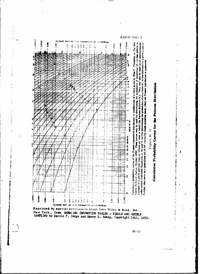
AMOI' 702- 3

$61jO ~ 1 JO * 3JNIOU'i3ýO 10 klIS919VS d

0, 0 0 0 0 1

4. r- i-T '-

4" ~i

t 4-

j-iZ

CS 4

r 1L

I I a

" 4"0 03 *0 O000~ vi ;0 A0 0 0 0fo

Reprinted by special ovrrn1isson f rom ohn Wiley &Sons, Inc. ,Naw York , f ran SA'ISING flSPECTION TABLEs - sflNOLE AND DOUBLESAJG'LDIN by Harold F. Dodge and Harry G. R=4 Copyriht 19Jjh, 1959.

"H-37

AMCi1 702-3

APPENDIX 1

DEFINITION OF ACRONYMS AND SYMBOLS

I-1. General. The more frequently used syxnbols ;-nd acr-----in ascontained in'this handbook are defined below. Some are standarddefinitions and others may be uniquely used herein. Iii either case, Ithe definitions apply to usaee 0, this handbook.

1-2. Acronyms.

Ac Acceptance number

AFDP Air Force Development Plan

AFSCM Air Force Systems Command Manual

AFSC-TR Air Force Systems Comrnmand-Techni.zalReport

AGREE Advisory Group on Reliability for ZlectronicEquipment

AIAA American Institute of AeronauticG and Astro-nautics j

AlchE American Institute of Oheroicai Engineers

AMC Army MaterikA Coriimand

AMCP Army Materiel Command Pamphlet

AMCP. Army Materiel Command Regulation

APE Advance Procuction Engineering

AQL Accepiable Quality Level

!I

I-1

¢'

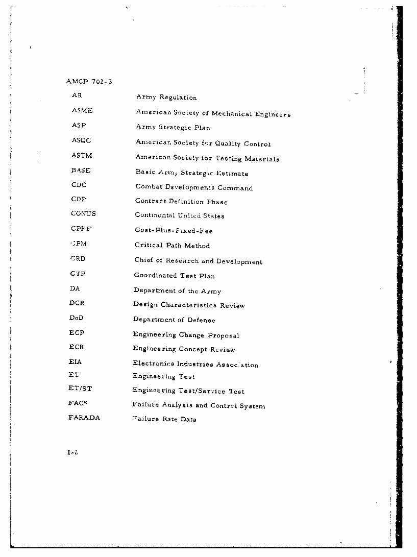
AMCP 702- 3

AR Army Regulation

ASME American Society of Mechanical Engineers

ASP Army Strategic Plan

ASQC Aniericar. Society for Quality Control

ASTM American Society for Testing MaterialsBASE Basic Army. Strategic Estimate

CDC Combat Developments Command

CDP Contract Definition Phase

CONUS Continental United States

CPFF Cost-Plue-Fixed-Fee

-PM Critical Path Method

CRD Chief of Research and Development

CTP Coordinated Test Plan

DA Department of the Army

DCR Design Characteristics Review

DoD Department of Defense

ECP Engineering Change Proposal

ECR Engineering Concept Review

EIA Electronics Industries Assoc'ation

ET Engineering Test

ET/ST Engineering Test/Service Test

FAC, Failure Analysis and Control SystemFARADA T ailure Rate Data

I-Z

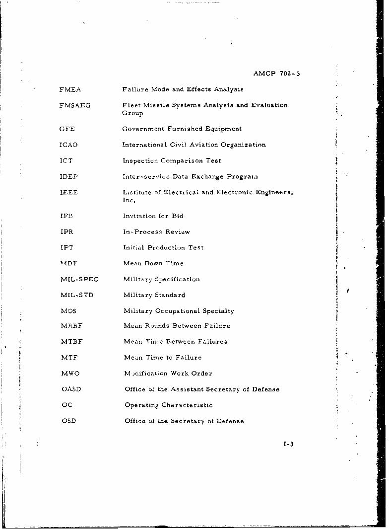
AMCP 702- 3

FMEA Failure Mode and Effects Analysis

FMSAEG Fleet Missile Systems Analysis and EvaluationGroup

GFE Government Furnished Equipment

ICAO International Civil Aviation Organization

ICT Inspection Comparison Test

IDEP Inter-service Data Exchange Prograxm

IEEE L-Istitute of Electrical and Electronic Engineers,Inc.

IIIFB Invitation for Bid

IPR In-Process Review

IPT Initial Production Test

114DT Mean Down Time

MIL-SPEC Military Specification

MIL-STD Military Standard

MOS Military Occupational Specialty

MRBF Mean Rounds Between Failure

MTBF Mean Time Between Failures

MTF Mean Time to Failure

MWO M.jdificatlon Work Order

OASD Office oi the Assistant Secretary of Defense

OC Operating Characteristic

OSD Office of the Secretary of Defense

1-3

H!

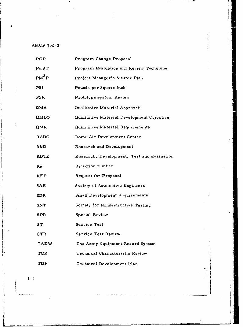
AMCP 702-3

PCP Program Change Proposal

PERT Program Evaluation and Review Technique

PM P Project Manager's Master Plan

PSI Pounds per Square Inch

PSR Prototype System Review

QMA Qualitative Materiel Appronrh

QMDO Qualitative Materiel Development Objective

QMR Qualitative Materiel Requirements

RADC Rome Air Development Center

R&D Research and Development

RDTE Research, Development, Test and Evaluation

Re Rejection number

RFP Request for Proposal

SAE Society of Automotive Engineers

SDR Small Development FR-'quirements

SNT Society for Nondestructive Testing

SPR Special Review

ST Service Test

STR Service Test Review

TAERS The Army £:quipment Record System

TCR Technical Characteristic Review

TDP Technical Development Plan

&-4

V i

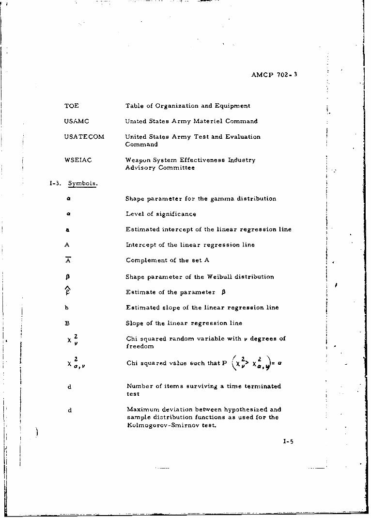
F' I

AMCP 702- 3

TOE Table of Organization and Equipment

USAMC United States Army Materiel Command

USATECOM United States Army Test and EvaluationCommand

WSEIAC Weapon System Effectiveness IndustryAdvisory Committee

1-3. Symbols.

a Shape parameter for the gamma distribution

a Level of significance

a Estimated intercept of the linear regression line

A Intercept of the linear regression line

A Complement of the set A

Shape parameter of the Weibull distribution

AEstimate of the parameter

b Estimated slope of the linear regression line

B Slope of the linear regression line

X 2 Chi squared random variable with P degrees ofI, freedom,

2 "2 2I Chi squared value such that P ' > X

d Number of items surviving a time terminatedtest

d Maximum deviation between hypothesized andsample distribution functions as used for theKolmogorov-Smirnov test,

k-5

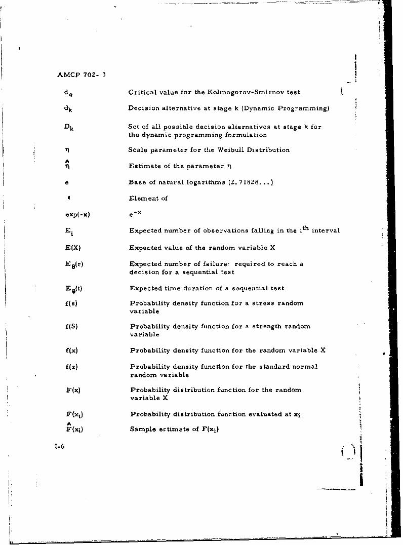
ri

iI

AMCP 702- 3

do Critical value for the Kolmogorov-Srnirnov test

dk Decision alternative at stage k (Dynamic Progr-amming)

Dk Set of all possible decision alternatives at stage k for

the dynamic programming formulation

TI Scale parameter for the Weibull Distribution

Estimate of the parameter TI

e Base of natural logarithms (Z. 71828...)

4 Element of

exp(-x) e-x

E. Expected number of observations falling in the ith interval

E(X) Expected value of the random variable X

EO(r) Expected number of failure, required to reach adecision for a sequential test

Ee(t) Expected time duration of a sequential test

f(s) Probability density function for a stress random

variable

f(S) Probability density function for a strength randomvariable

f(x) Probability density function for the random variable X

f~z) Probability density function for the standard normal

random variable

F(x) Probability distribution function for the randomvariable X

F(xi) Probability distribution function evaluated at xi

AF(xi) Sample ectimate of F(xi)

1-6

Ii:i

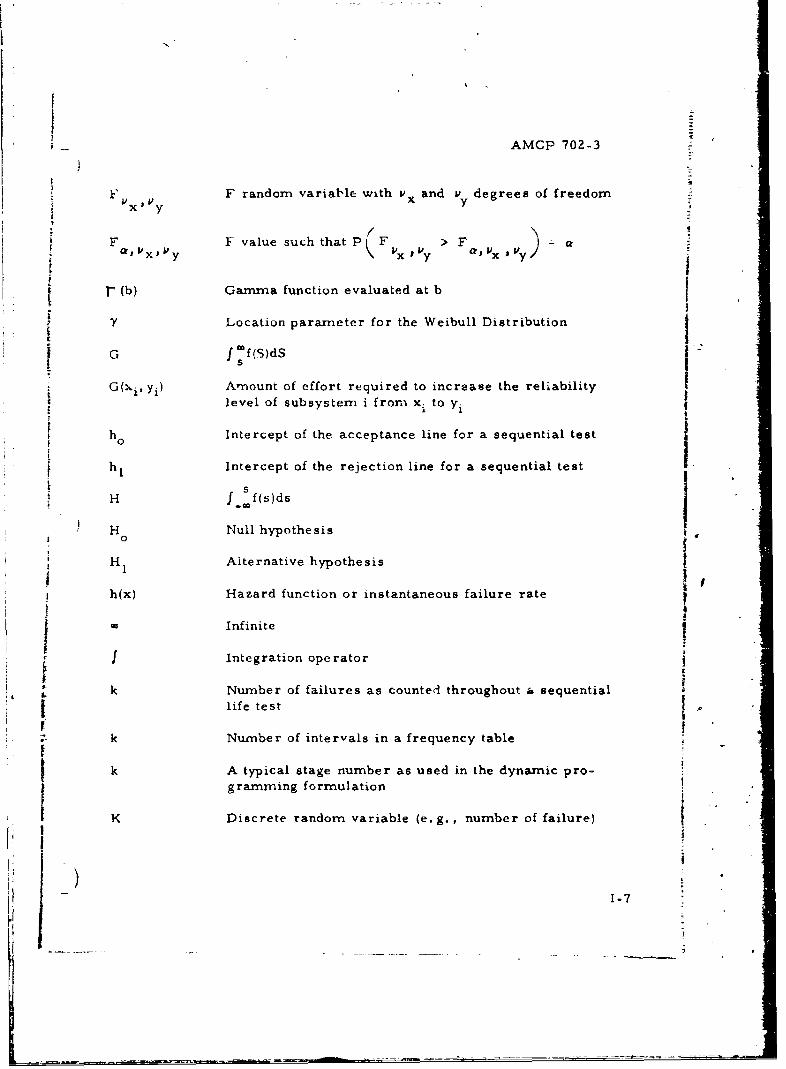
AMCP 702-3

F F random variable with Vx and v degrees of freedom

x yF value such that P(F > F )

SrVx,Vy Vx I y a, Yx V

r• (b) Gamma function evaluated at b

SV Location parameter for the Weibull Distribution jC f: f (s)dS I

G(xi, yi) Amount of effort required to increase the reliability Ilevel of subsystem i from xi to yi

h Intercept of the acceptance line for a sequential test -[0

h Intercept of the rejection line for a sequential test IH f• f(s)ds

H Null hypothesisH0

S H Alternative hypothesis

h(x) Hazard function or instantaneous failure rateLI

InfiniteI

f Intcgration operator

k Number of failures as counted throughout a sequential

life test

k Number of intervals in a frequency table

k A typical stage number as used in the dynamic pro-grammning formulation

K Discrete random variable (e.g., number of failure)

-1 1-7

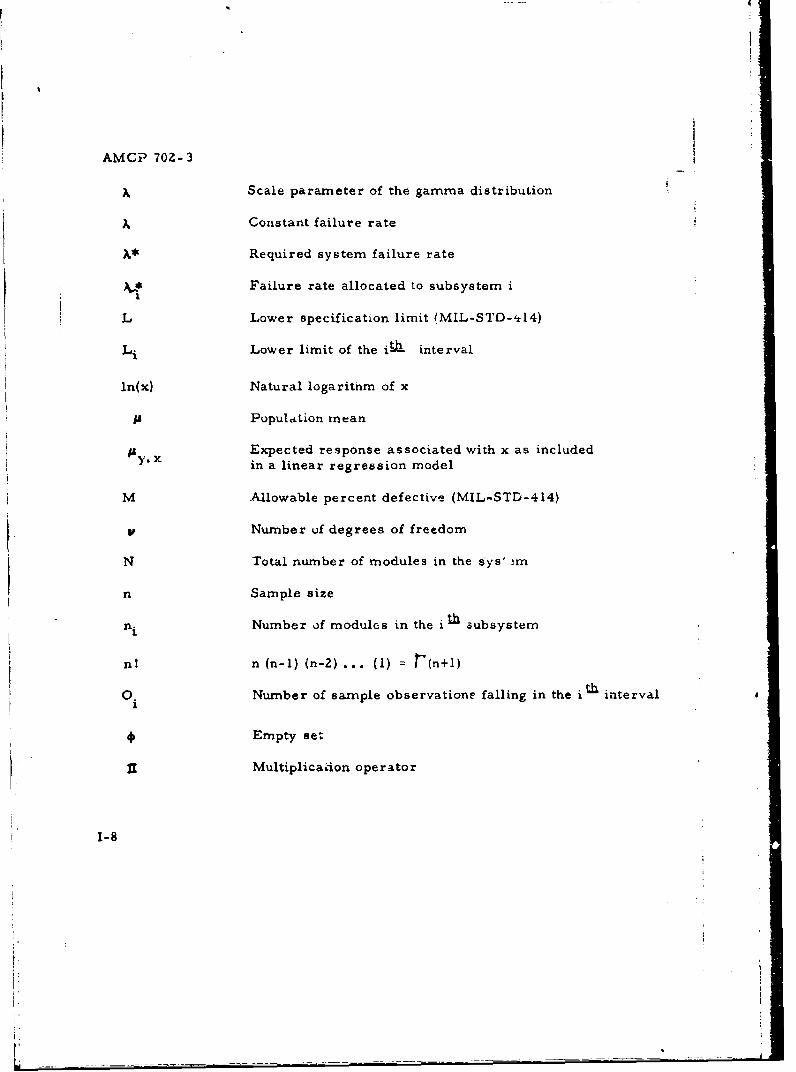
AMCP 702-3

Scale parameter of the gamma distribution

1.Constant failure rate

Required system failure rate

ý Failure rate allocated to subsystem i

L Lower specification limit (MIL-STD-,tl4)

ln Lower limit of the it-- interval

In(x) Natural logarithm of x

p Population mean

p ~ Expected response associated with x as includedin a linear regression model

M Allowable percent defective (MIL-STD-414)

V Number uf degrees of freedom

N Total number of modules in the sys' !m

n Sample size

ni Number )f modules in the ith subsystem

n! n (n-i) ýn-2) ... (1) = r'(n+l)

o. Number of sample observatione falling in the ith intervali

* Empty see.

uI Multiplicadon operator

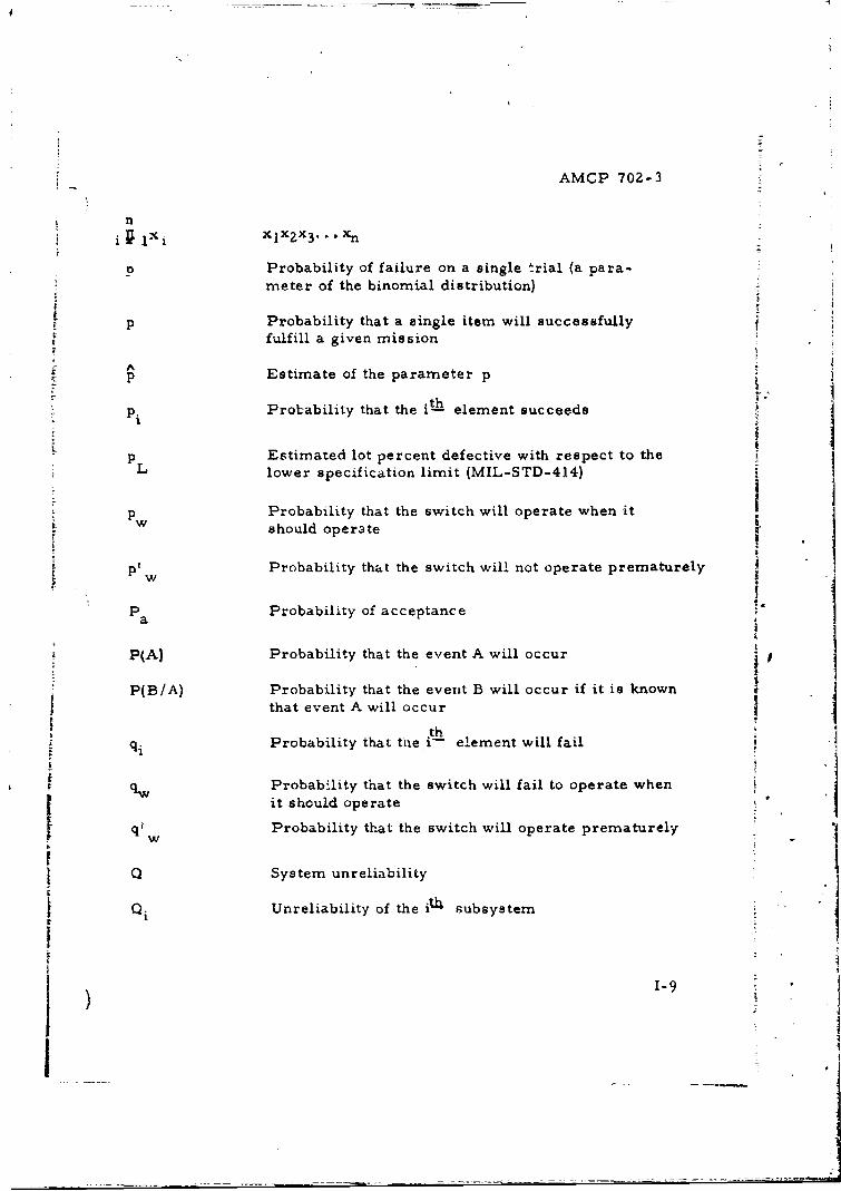
AMCP 702-3

n

XlXZX 3 ... Xn

Probability of failure on a single trial (a para-

meter of the binomial distribution)

I

p Probability that a single item will successfullyfulfill a given mission

Ap Estimate of the parameter p

thp Probability that the it- element succeeds

p Estimated lot percent defective with respect to theSL lower specification limit (MIL-STD-414)

Pw Probability that the switch will operate when itshould operate

tp Probability that the switch will not operate prematurely[ w

pPa Probability of acceptance "

P(A) Probability that the event A will occur

P(B/A) Probability that the event B will occur if it is knownthat event A will occur

thqi Probability that the i- element will fail

qw Probability that the switch will fail to operate whenit should operate

qI Probability that the switch will operate prematurely• w

1 Q System unreliability

Unreliability of the ih subsystem

1-9

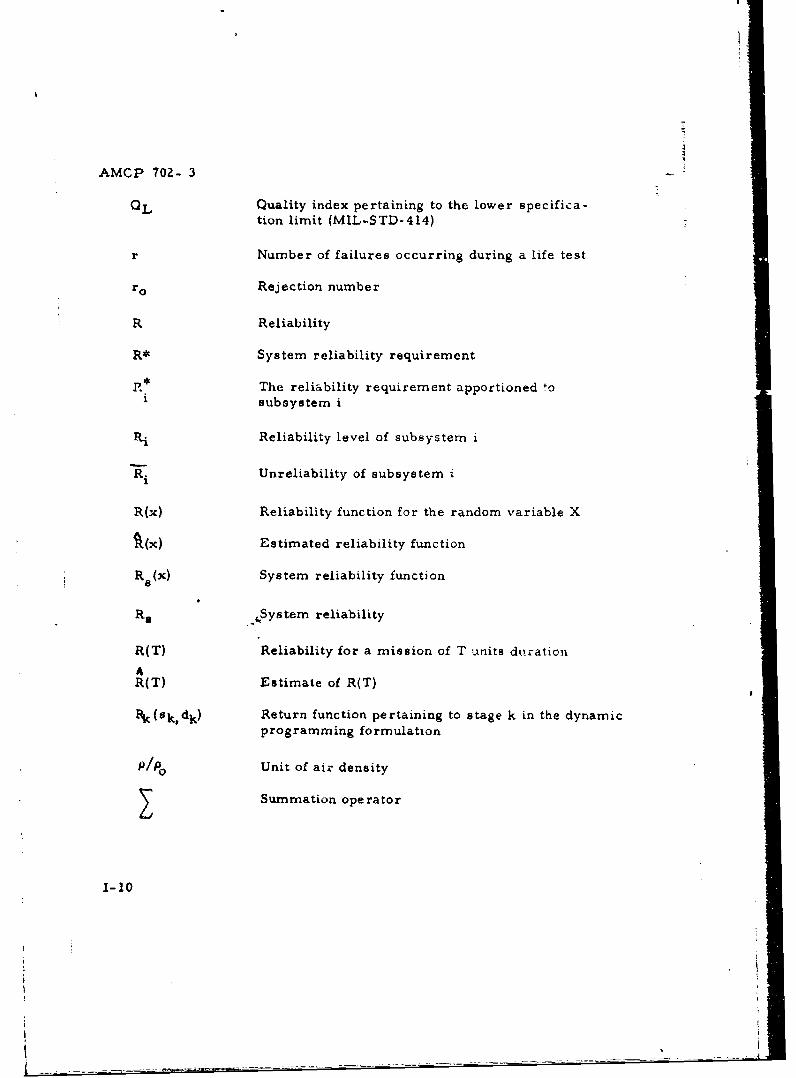
AMCP 70Z- 3

OL Quality index pertaining to the lower specifica-

tion limit (MIL-STD-414)

r Number of failures occurring during a life test

ro Rejection number

R Reliability

R* System reliability requirement

The reliability requirement apportioned toi subsystem i

Ri Reliability level of subsystem i

"Ri Unreliability of subsystem i

R(x) Reliability function for the random variable X

• (x) Estimated reliability function

R (x) System reliability function

Rs ,•System reliability

R(T) Reliability for a mission of T units durationAR(T) Estimate of R(T)

k(dk, dk) Return function pertaining to stage k in the dynamicprogramming formulation

P/P 0 Unit of air density

Summation operator

I-10

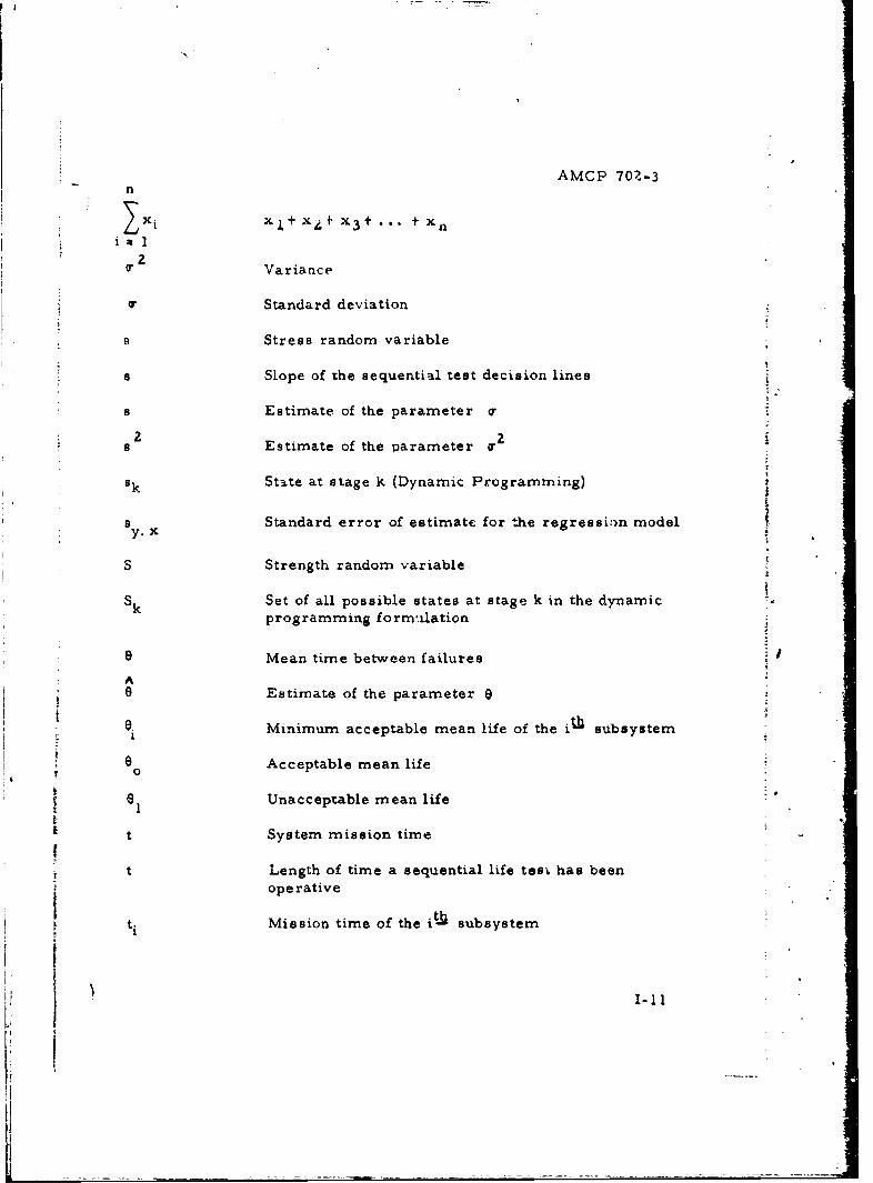
AMCP 70Z-3n

Sxi xl+ x1 + x 3 +... + xn

Variance

0a Standard deviation

Stress random variable

Slope of the sequential test decision lines

s Estimate of the parameter o*

2 Estimate of the parameter a*

State at stage k (Dynamic Programming)

s Standard error of estimate for the regressi:n modely.

S Strength random variable

Sk Set of all possible states at stage k in the dynamicprogramming forrm',lation

9 Mean time between failures

9 Estimate of the parameter 0

e. Minimum acceptable mean life of the i-h subsystem

0 Acceptable mean life

06 eUnacceptable mean life

t System mission time

Length of time a sequential life test has been

operative

|ti Mission time of the i t- subsystem

I-i

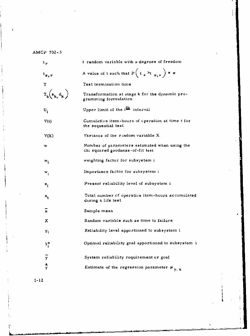
AMCP 702-3

t vt random variable with t, degrees of freedom

ta, V A value of t such that P t >t a, V

T Test termination time

Tkk dk). d Transformation at stage k for the dynamic pro-gramming formulation

Ui Upper limit of the il6 interval

V(t) Cumulative item-hours of cperation at time t forthe sequential test

V(X) Variance of the rLndom variable X

w Number of parameters estimated when using thechi squared goodness-of-fit test

wi weighting factor for subsystem i

wi Importance factor for subsystem i

x i Present reliability level of subsystem i

xt Total number of operative item-hours accumulatedduring a life test

X Sample mean

X Random variable such as time to failure

Yi Reliability level apportioned to subsystem i

yý Optimal reliability goal apportioned to subsystem i

y System reliability requirement or goal

Ay Estimate of the regression parameter IA y. x

I-lZ

1' ________________________

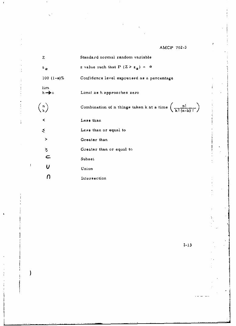
AMCP 702-3

Z Standard normal random variable

z a z value ouch that P (Z > z,) -

100 (1-cZ)% Confidence level expressed as a percentage

-lirh--o Limit as h approaches zero

(n) Combination of n things taken k at a time n!)

< Less than

Less than or equal to

Greater than

Greater than or equal to

Subset

I)Union

Intersection

1-13

-_AMCP 702-3

INDEX

A B

Accelerated life testing, 6-5 Bayes theorem, D-13 to D-16I Acceptable mean life, F-33, F-44 Bernoulli trials, A-24

Acceptable quality level, B-25, B-26, Binomial distributionF-58 to F-6Z approach to nonparametric

Acceptance number, F-61 testing, F-2Acceptance region, F-31, F-32, general, D-4

F-34, F-37, F-39, F-40 probability density function, A-24, •'-

Acceptance test, 1-3, 2-2, 2-17, A-Z5, F-41, F-446-2, 6-4, F-50 to F-62 random variable, A-24

Achieved reliability, 2-9, 5-1 reliability function, A-26, A-27,= Active rf-dundancy, F-39

4 (see Parallel) Block diagram, 4-2, 4-3, B-15, a

Advanced production engineering, B-Z0, B-21, D-1 to D-5, D-9,I B-Z3, B-Z4 D-11, D-14, D-15, D-17 toAGREE D-Z0, E-5, E-8, E-9

apportionment technique, 4-10,4-11, D-ZZ to D-24 C

prediction technique, 4-6, 4-7Allocation, Capability, 1-10, 1-11, 7-6, A-66,

(see Apportionment) A-69, A-71Apportionment Category I tests

general, 1-4, Z-5, 4-9, B-i4 to check tests, 1-3, 6-8, B-25B-16, B-20, B-21, B-Z3, C-17, coafirmatory tests (type 1), 1-3,C-18, D-1, D-21 to D-43, E-16 6-7. 6-8, B-27

purpose, 4-10, 5-6, 5-7 eLf,-neering tests, 1-3, 5-10,some specific techniques, 4-10, 6-8, B-22, B-24, B-254-11, D-Z1 to D-42, E-16 to E-Z1 environmental tests, 6-8

ARINC service tests, 1-3, 5-10, 6-8,apportionment technique, 4-11, B-2Z, B-Z4, B-Z5D-Z4 to D-26 Category II tests

prediction technique, 4-8, 4-9 comparison tests, 6-10Attributes inspection, 1-13, F-61 component development tests, 6-9Availability, 1-10, 1-11, 3-3, 7-6, engineer design tests, 5-10, 6-9

A-66, A-68, A-70, C-Z, C-9, C-28 engineering change tests, 6-9,B-Z6

Index- I

j....

AMCP 702-3

Category 11 tests (Cont'd) Contract (Cont'd)feasibility tests, 6-9 multiple incentives, C-31 toinitial production tests, 1-3, 3-15, C-39

6-10, B-27 production, B-26, C-24 topreproduction tests, 1-3, 3-15, c-z6

6-10, B-27 reliability clauses for, C-23 toresearch tests, 6-9 C-39R&D acceptance testa, 1-3, 6-9 Contract definition phase, 3-R,

Central tendency, A-13 to A-15, A-17, B-17A-22 Contractor capability, B-25

Check test, 1-3, 6-8 Contractor proposal, B-15 to B-19Chi Square goodness-of-fit test, F-13 Contractor reliability program,

to F-16 2-3 to 2-10, 2-13, 3-10Combat ready rate, 3-3, C-2, C-9 Coordinated test program, 5-10,

(see also Availability) 6-19, B-18Complement of a set, A-5 Corrective action, Z-9, 7-11,Complementary events, A-12, A-13, 7-13 to 7-15, B-i, B-20, B-21,

D-3 B-23, B-25, B-27, C-22, C-26Conceptual phase, 1-5, 3-1, 4-9, Cost-effectiveness, 3-7, 7-2, 1-3,

6-7, 6-9, B-9, B-Il, B-IZ, B-30 B-12Conditional probability, A-8, A-23, Critical items, 2-5

D-15Confidence interval, 6-3, C-39, E-14, D

F-I to F-4, F-19, F-21 to F-24,F-27 to F-30, F-64, F-66 to F-69 Data

Confidence level, 2-10, C-3, C-31, analysis of, 7-1, 7-11 to 7-14,G-33, F-2, F-21 to F-Z3, F-38 C-21(see also Significance level and collection of, 7-1, 7-3 to 7-8,

risk) 7-10, C-21, C-33Configuration management, 3-7, 3-8, documentation of, 7-3 to 7-10

B-1S elements, 7-3, 7-7, 7-8Confirmatory test, 1-3, 3-15, 6-7, failure, 7-1 to 7-15, C-21

6-8, 6-10, B-27 quality, 7-10, 7-11Contract sources of, 7-4 to 7-6, 7-10,

cost-plus-fixed-fee, C-23, C-26 7-11development, 2-13, B-19, C-Z3, use of, 7-1, 7-11 to 7-14, C-21

C-24 Decreasing failure rate, A-46fixed price, C-31, C-32 Definition phase, 1-5. 3-1, 3-8,incentive, C-26 to C-29 6-7, 6-9, B-9, B-12 to B-20,

B-30

Indox- 2

AMCP 702-3

Degrees of freedom, F-Z3 Dynamic programming, D-30 toDemonstration and teut, 2-9, 2-10, D-43, E-19 to E-Z1

2-17, 6-1 to 6-22, B-14, B-ZZ,B-ý4, B-26, C-19 to C-Z0, C-23. EC-25, C-26. C-31, F-i to F-69

Dependability, 1-10, 1-11, A-66, EffectivenessA-69 to A-71 cost, 3-7. 7-2, 7-3

Dependent events, A-8 to A-10 determination of, A-71, A-7Z

Deployrrient, planned, C-5 general, 1-1Derating. 5-3. B-Z0 range of, C-32 to C-39Descriptive statistics, A-13 to A-20 system, 1-1, 1-10, 1-11, 7-6,Descriptors, 1-12, 1-13, A-72, A-73 A-66 to A-72Design Effcrt function, 4-11, D-27, D-32,

detailed, 1-3, B-2Z, B-23, C-Zl D-33, D.-35, D-37. E-17. E-19,engineering, 1-Z, 1-3, C-21 E-Z0formulation, 1-4, 5-1 Element of a set. A-a, A-3for reliability, Z-2, 5-1 to 5-10, Engineering change proposal, 7-13,

B-16, E-1 to E-Z1 C-27preliminary, C-17 Engineering concept review, 5-10principles, 5-Z to 5-7 B-18, B-Z0, C-20

* requirements, 1-5 Engineering design. 1-2, 1-3,reviev,, 1-4, 2-6, 3-6, 5-Z, 5-7 B-20, B-ZZ, B-Z3, C-21

to 5-- 0, B-22, C-z0, C-Z1 Environmental control, 5-4simplifi,:ation, B-23, C-28 Environmental factors, 7-5spec ificat.on. 4-1 Equal appartionmnent technique, 4-10,streas-strength, 5-2 to 5-4 D-2i, D-ZZ

Design characteristics review, 5-10, Equally likely events, A-i, A-7B-18, B-ZZ. C-20 Estimated. lot percent defective,

Determination of underlying distribution, F-59, F-60F-4 to F-18 Evaluation of proposal, 1-4. 2-13.

Development description, 3-8, 3-.9 2-15 to 2-17Development phase, 1-3, !-5, 6-7, Expected number of failures, F-47

7-10, B-9, B-19 to E-Z5, 8-31, to F-52Expected test duration, F-45, F-48

Development tests, Z-4, 6-9 to F-54Disposal phase, 1-6. B-O9 B-Zg, B-Z9, Expected value

B-32 definition, A-22Documentaticen o- requiren~eras, I -i, exponential, A-4Z

3-1 to 3-15, B-13, B-14, C-i to gamma, A-51C-39 logao.rmal, A-34

Durability, C-4 normal, A-29

Index- 3

- -*---*-

AMCP 702-3

Expected value (Cont'd) Failure rate, 1-13, 3-13. 4-5 topoisson, A-39 4-8, A-38 to A-40, A-42,Weibull, A-47 A-44, A-46, A-73, B-ZZ, C-5,

Exponential distribution C-19, C-37, D-7. D-16 to D-19,deter'nination of, F-4 to F-7, D-24, D-25, L-6 to E-8, F-19

F-13 to F-iB (see also Hazard function)estimation of parameters, F-4. Failure reporting, Z-9, 7-1 to

F-18 to F-Z4 7-15, C-21 to C-23expected value, A-42 Failure sensing devices, D-6hazard function, A-44 to A-46 Failure terminated tests, 6-2,probability density function, A-42, F-19 to F-24, F-3Z to F-38,

C-2. F-19 F-5$7probability distribution function, FARADA. program, 7-4, 7-5, E-13

A-43 Feasibility study, B-12, B-13, B-15random variable, A-4Z Feedback, 1-4, 2-9, 2-21, 7-8 toreliability function, A-43 to A-46, 7-11, B-15, B-28, C-17

C-I1, F- 19 to F-2 1, F-23, F-24 Forecasting technological, B-livariance, A-43 Formulation of design, 1-4, 5-1

Exponential failure times F~requency table, A-14, A-15acceptance tests, F-57parallel model, D-19, D-20 Gpartial redundancy model, D-18,

D- 19 Gamma distributionseries model, D-19. D-20 expected value, A-5Istandby redundancy modei, D-6 hazard function, A-53 to A-55

to D-8, D-16, D-17 probability density function, A-5iptests of hypothesis, F-32 to F-56 probability dist~'bution function,

A -52F random variable, A-.51

reliability function, A-52 to A-55Failure analysis, 1-4, 2-9, 7-11 to variance, A-51

7-1,., C-Z1 to C-Z3 Goodness-of-fit testFailure analysis and control system, analytical, F-13 to F-18

7-2, 7-3 graphical, F-4 to F-12Failure, definition of, B-20, C-i to Government furnished equipment,

C-3, C-9. C-22, C-31, C-33 B-Zl, B-22Failure modes, 5-5, 7-2, B-20, B-Z2, Guidance documents, B-11

B-23, D-9, D-12, D-43, E-4Failure mode and effect analycis,

5-5, B-21

Index- 4

t

AMCP 702-3

Hi K

Hazard function Kolmogorov-Smirnov test, F-16as a reliability descriptor, A-73 to F-18definition, A-21, A-23exponential, A-44 to A-46 Lgamma, A-53 to A-55lognormal, A-36, A-37 Life cyclenormal, A-30 to A-33 applicable documents, 1-8 to 1-9Weibull, A-49, A-50, F-57 conceptual phase, 1-5, 3-1, 4-9,

Histogram, A-15, A-16 6-7, 6-9, B-9, B-Il, B-lZ,Human engineering, 5-7 B-30Hypotheses, F-30 to F-3Z, F-56 considerations in, 1-7Hypothesis tests, 6-Z, 6-4, F-30 to definition phase, 1-5, 3-1, 3-8,

F-56 6-7, 6-9, B-9, B-lZ to B-19,B-30

development phase, 1-3, 1-5,6-7, 7-10, B-9, B-19 to B-25,

IDEP, 7-5, 7-6 B-31, E-1Importance factor, D-22, D-23 disposal phase, 1-6, B-9, B-28,Increasing failure rate, A-26, A-46 B-29, B-32Independent events, A-9 to A-li, feedback, 1-4, 2-9, 2-21, 7-8 to

A-13, D-l, D-7, D-19, D-33, 7-11, C-17D-3r general, 1-5, 1-6, 2-1

Inher availability, C-9 operational phase, 1-3, 1-6, 2-1,Inherent reliability, 1-5, 5-1, 7-10, 6-7, 7-10, 7-11, B-9, B-28,

7-11, C-2 B-29, B-32In-house statistical analysis, B-Z7, production phase, 1-3, 1-6, 2-8,

B-28 2-9, 6-7, 7-10, 7-11, B-9,Initial production test, 1-3, 3-15, L-25 to B-28, B-32

6-7, 6-10, system, 1-4, 1-17, B-1In-process review, 5-9, B-18, B-20, teat programming, 5-12 to 6-16

B-22 to .9-25, C-20 Life testingInspection comparison tests, B-28 (see demonstration and test)Instantaneous failure rate (see test and demonstration)

(see Hazard function) (see testing)Integrated tests, 1-3, 6-14 to 6-16, B-24 Linear regression, F-63 to F-69Intersection of events, D-3 Linear regression equation. F-63,Intersection of sets, A-4, A-10, A-11 F-65Invitation for bids, B-24, B-25

Index-5

") I

Fl

~!AMCP 702-3

Lognormal distribution Model, reliabilityexpected value, A-34 general, 2-5, 4-1 to 4-3,hazard function, A-30 to A-33 6-19, B-15, 13-Z0, B-21,probability density function, A-34 B-23, D-1probability distribution function, parallel, D-3, D-4, D-16,A-34 D-19, D.-20

random variable, A-34 partial redundancy, D-4 to D-6,reliability function, A-34 to A-36 D-18, D-19variance, A-34 series, D-1 to D-3, D-16,

Lower specification limit, F-58 D-19, D-20, D-24, D-26,D-27, D-32, D-33

M standby redundancy, D-6 toD-13, D-16, D-17

Maintainability, 7-6 use of Bayes theorem, D-13 toMaintenance, 5-6. C-I, C-5, C-6, D-16

C-10, C-13 to C-15, C-19 Model, system effectiveness,Maintenance personnel, C-15, C-16 A-68 to A-71Maintenance support plan, B-22 Modification work order, 7-13Matching moments, F-24 to F-26 Module, D-22, D-23Materiel life cycle Monitoring a reliability program,

(see Life cycle) 1-4, 2-1, 2-3, 2-4, 2-8. 2-9,Maximum allowable percent defec- 2-15, 5-8

tive, F-58 to F-60 Monotone failure rate, A-46Maximum likelihood, F-24, F-27 Mutually exclusive events, A-I,Mean downtime, 3-3, C-I1 to C-13, A-12, D-13

C-Z8Mean time between failures, 1-13, N

3-13, 4-11, A-7Z, C-1 to C-3,

C-5, C-16, C-20, C-28, C-37 Nonparametric analysis, F-2 toto C-39, D-22, F-19 to F-24, F-4F-32 to F-57 Nonparametric sampling plans,

Mean time to failure F-60 to F-62(see Mean time between failures) Nonreplacement tests, 6-2, F-2

Minimization of effort algorithm, to F-4, F-19 to F-24, F-324-11, D-26 to D-30, E-16 to E-21 to F-56, F-61

Mission duration, 3-3, C-,0, C-Il, Nontime depsiaieni items, C-3,C-37 F-3, F-61

Mission profile, 3-11, C-8, C-9, Normal distributionE-3 determination of, F-9 to F-18

Mission reliability, 3-3, C-1, C-2, estimation of parameters,C-7 to C-9 F-17, F-18, F-Z7 to F-30

Index- 6

ii

i_

AMCP 70Z-3

Normal distribution (Cont'd) Parameters (Cont'd)expected value, A-29 general, C-Zhazard function, A-30 to A-33 test of hypothesis, 6-4, F-30probability density function, to F-56

A-18, A-19, A-Z8, A-29, A-55 Partially redundant functionalto A-57, F-27 configuration, 4-2, D-4 to

probability distribution function, D-6, D-18A-30 Parts reliability,B-29

random variable, A-28 to A-30 Parts reliability improvement, Z-5reliability function, A-30 to A-33, Point estimation, 6-3, F-I to F-4,

SF-Z8 F-19 to F-30, F-63 to F-67variance, A-28, A-Z9 Poisson distribution

Normal failure times expected value, A-39acceptance tests, F-58 to F-60 probability density function, A-38tests of hypothesis, F-56 random variable, A-38

Normal probability paper, F-9 to F-12 reliability function, A-40 to A-4Z,F-39

0 variance, A-39Pcisson process, A-38

One shot item, 1-12, 6-5, 6-6, A-55, PredictionA-73, C-3, C-5, F-3, F-61 design procedure, 4-5, 4-6,

Operating characteristics curve, F-31, E-Z to E-16F-33 to F-35, F-39 to F-42, F-45 feasibility procedure, 4-4, 4-5to F-47, F-49 to F-51, F-57, F-60, general, 1-4, 2-5, 4-3, 4-4,F-62 B-14 to B-17, B-20, B-21,

Operational environment, 3-3, C-10 B-Z3, C-19, D-l, D-16 to D-21Operational readiness, C-I1 purpose and uses, 4-3, 4-4, 5-2,Operational phase, 1-3, 1-6, 2-1, 5-6, 5-7, E-1

6-7, 7-10, 7-11, B-9, B-28, some specific techniques, 4-6

B-29, B-32 to 4-8

Organization, 2-3, 2-17, B-15 Preliminary design, 1-3, B-19,B-20, C-17, C-21

P Preproduction conference, B-26Probability

Parallel (redundant) functional con- complementary events, D-3figuration, 4-1, C-28, D-3, D-4, conditional, A-8, A-23, D-15

D-19, D-20, D-4V definition, A-iParameters function, A-6

definition, 6-2 independent events, D-1, D-33,estimation of, 6-2 to 6-4, F-I to D-35

F-30, F-63 to F-69

Index-7

AMCP 702-3

Probability (Cont'd) Proposal, B-15 to B-19intersection of events. A-10, A-Il, Prototype systems review, 5-10,

D-2. D-3 B-Z3, C-20joint, A-9, A-10 Prototype testing, 1-3, B-24measurement scale, A-1union of events, A-Il, A-I2 Q

Probability density functionbinomial, A-24, A-25 Qualitative materiel approach,

definition, A-21, A-Z2 B-12

exponential, A-42, C-2, F- i9 Qualitative materiel developmentgamma, A-51 objective, 3-8. B-11, B-IZgeneral, D-7 Qualitative materiel requirements,histogram, A-15, A-16 1-7, 2-2, 3-1 to 3-5, 4-3, 5-9,

lognormal, A-34 5-10, 6-8, 6-12, 6-17, B-li tonormal, A-18, A-19, A-28, A-29, B-13, B-18, B-23, B-24, B-26,A-55 to A-57, F-27 B-28, C-I to C-5

poisson, A-38 Quality assurance, 3-7, 3-9, 3-15,

stress-strength, A-55 to A-65 7-10, 7-11, B-24, C-21, C-Z5Weibull, A-46, F-24 Quality index, F-58, F-60

Probability distribution function Quantitative reliability requirements,definition, A-19, A-22, A-23 3-13, 3-14, C-4exponential, A-43gamma, A-52 Rlognormal, A-34normal, A-30 Random variableWeibull, A-48 binomial, A-24

Probability of acceptance, F-31, definition, A-19, A-21, F-i

F-33 to F-36, F-39, F-42, F-43, exponential, A-42F-60, F-61 gamma, A-51

Probability of rejection lognormal, A-34(see Probability of acceptance) normal, A-28 4

Productiondescription, 3-8, 3-15 poisson, A-38Production phase standard normal, A-28 to A-30

feedback data, 7-10, 7-11 stress-strength, A-55general, 1-3, 1-6, 6-7, B-9, Weibull, A-46

B-Z4, B-25 to B-28, B-32 Reaction time, 3-3, C-6, C-7manufacturing controls, 2-8, 2-9 R.3cord keeping system, B-14

Project engineering, 1-2 Recursion equations, D-31, D-34,Project management, 1-2 D-35, D-37

Index-8

|i I '

AMCP 702-3

R&D acceptance test, 1-3, 6-7, 6-9, Reliability (Cont'd)•

B-Z4 function, 1-4, A-21, A-23, A-Z6,S Redundancy, 5-4, B-20, C-28, D-3 A-27, A-30 to A-36, A-40 to

to D-13 A-46, A-48 to A-50, A-52 toRedundant functional configuration A-55, A-58, C-i, F-20, F-23,

(see Parallel functional con- F-24, F-28, F-39 Ifiguration) goal, B-20, B-Z1, C-17 to C-19, !

Regression analysis, 6-4. F-62, C-Z2, C-27, D--I, D-29, D-32F-69 to D-36, D-42

Reliability improvement, 3-13 1achieved, 2-9, 5-1 incentive contracting, C-26 toafter storage, 3-3, C-2, C-13 C-39apportionment, 1-4, 2-5, 4-9 to inherent, 1-5, 5-1, 7-10, 7-11,

4-11, 5-6, 5-7, B-14 to B-16, C-23B-Z0, B-21, B-23, C-17, C-18, leveis, 1-2, C-8, C-23, C-28,

D-21 to D-42, E-16 to E-21 C-30, C-31, C-33as a function of stress-strength, milestones, B-8 to B-3ZA-58 mission, 3-3, C-1, C-2, C-7 to

as a growth process, 1-2 to 1-4, C-9B-Z1 model, 2-5, 4-1 to 4-3, 6-19,

contractor program, 2-3 to 2-10, B-15, B-20, B-21, B-23, D-12-13, 3-10 to D-43, E-5

data, 7-1 to 7-15, 0-33 multiple incentive contr;ý.cting,definition of, )-1, 1-12, C-2, C-3, C-31 to C-33E-6 network diagram, B-8 to B-32

descriptors, 1-12, 1-13, A-72, uf rebuilt equipment, B-Z9A-73 organization, 2-3, 2-17, B-15

design for, 2-2, 5-1 to 5-10, B-16, prediction, 1-4, 2-5, 4-3 to 4-8,E-1 to E-21 5-2, 5-6, 5-7, B-14 to B-17,

desired, C-8. C-33 B-20, B-21, B-23, C-19, D-1,documentation of, B1-13, B -14 D-16 to D-21, E-1 to E-16documents applicable to, 1-8, 1-9, program managing, 1-4, 2-11

1-13 to 1-16 to 2-17, B-I to B-32engineering, 1-1 program monitoring, 1-4, 2-2estimation, 6-2 to 6-4, F-2 to F-4, to 2-4, 2-11 to 2-17, B-1 toF-19 to F-22, F-27 to F-30 B-32

feasibility, 1-1, 1-4, 4-4, 5-10, program planning, 1-4, B3-1 toB-l2, B-13, B-15, C-3 to C-5 B-32, C-16 to C-23

Index-9

V I

I .

4

AMCP 702- 3

Reliability (Cont'd) Rejection number, F-39, F-40,program review, 2-4 F-42, F-43, F-61 0

records, B-27 Risks, 6-13, 6-14, C-33, C-37,relationship to system effective- F-31, F-33, F-40, F-44,ness, 1-1, 1-10 F-57

required, C-8, C-28 (see also Significance level)requirements, Z-11, Z-15, 3-1 (see also Confidence level)

to 3-15, B-1l, B-17, C-i toC-39, D-21, D-ZZ, D-26, D-27, SD-30, D-39, E-6 to E-8

storage, B-28, B-29 Samplesubcontractor program, 2-7 mean, F-58, F-60test and demonstration, 2-9, 2-10, standard deviation, F-58, F-602-17, 6-1 to 6-22, B-14, B-Z2, Sample size, C-19, F--, F-4,B-24, B-26, C-19, F-i to F-69 F-7, F-9, F-16, F-19, F-2Z,

trade-offs, 2-8, 2-15, 4-4, B-IZ, F-24, F-27, F-33, F-43, F-45,B-15, B-17, B-20 to B-23, B-Z7 F-58, F-63, F-64, F-69

training, 1-4, 2-7, 2-17 to 2-21, SamplingB-15. B-19 error, C-34, F-31

Reliability margin, 5-3, C-16, C-17, plans, F-57, F-58, F-61, F-62C-Z8 random, F-31

Replacement tests, 6-2, F-19 to F-23, Self healing devices, 5-5F-32 to F-56 Semi-log graph paper, F-4, F-5

Request for proposal, 1-4, 1-7, 2-11 Sequential decision criteria, F-45,to 2-13, 4-1, B-14, B-15, B-25 F-46, F-49, F-50, F-55

Required review points Sequential tests, C-31, F-44 todesign characteristics review, F-57

5-10 Series functional configuration, 4-1,engineerirg concept review, 5-10 D-1 to D-3, D-19 to D-22, D-24,prototype systems review, 5-10 D-26, D-32, D-33service test review, 5-10 Service test review, 5-10, C-20special revicw, 5-19technical characteristics review, complement, A-5, A-12

5-9, 5-10 definition, A-ZRequirements, reliability, 2-11, 2-15, element of, A-2, A-3

3-1 to 3-15, B-I1, C-I to C-39, empty, A-Z, A-3D-21, D-22, D-Z6, D-27, D-29, finitce. A-2, A-3D-30, D-39, E-6 to E-8 infinite, A-2

Research & technology resume, 1-4, intersections, A-4, A-S'O, A-li3-4 space, A-2 to A-5

Index- 10

L _ _'_ _

AMCP 702-3

Sets (Cont'd) Statisticssubset, A-2, A-3 definition, A-13union, A-3, A-Il, A-12 descriptive, A-13 to A-Z0

Shape of data distribution, A-13, Stress-strengthA-18 analysis, 7-5

Significance level, F-13, F-16, design approach, 5-2 to 5-4

F-31, F-3Z, F-37, F-38, F-40 normal probability density(see also Confidence level) function, A-55(see also Risks) probability density functions,

Small development requirements, A-55 to A-651-7, 3-1 to 3-5, 4-3, 5-9, 5-10, random variable, A-55

t 6-8, 6-I, 6-17, B-12, C-i to reliability function, A. 580 C-5 testing, 6-5, 6-6

Space, A-Z to A-5 Subcontractor reliability program,Special review, 5-10, C-21 2-7

SSpecial tests Switching devices, D-6, D-7, D-9i aircraft & allied equipment tests, to D-13

6-11 System description, 3-8* confirmatory type II teats, 1-3, System effectiveness

6-7, 6-10, B-27 availability, 1-10, 1-11, 7-6,military potential tests, 6-10 A-66, A-68, A-70nuclear weapons tests, 6-11 capability, 1-10, 1-11, A-66,surveillance, 6-10 A-69, A-71troop tests, 6-11 dependability, 1-10, 1-11, A-66,

Specifications, 3-6 to 3-15, C-20 A-69 to A-71Standard deviation, A-17, A-Z8, F-58 example, A-66 to A-72Standard normal distribution, A-28 general, 1-1, 7-6, B-IZ

to A-30 model, A-68 to A-71

i Standardization, 5-2, B-16, B-20 relationship to reliability, 1-1,Standby redundancy functional con- 1-10

figuration (see also Effectiveness)exponential model, D-6, D-7 System functional configuration

general, 4-2, D-6 to D-13, D-16, parallel (redundant), 4-1, C-Z8,D-17 D-3, D-4, D-19, D-Z0, D-43

general model, D-7 to D-9 partially redundant, 4-2, D-4imperfect switching model, D-9 to D-6, D-18 f

to D-13 series, 4-1, D-1 to D-3, D-19Statistical inference to D-2Z, D-24, D-26, D-32,

"estimation, F-i to F-30, F-63 tc D-33

SF-69 standby redundancy, 4-2, D-6test of hypothesis, F-30 to F-56 to D-13, D-16, D-17

* jI ~Index-l1

---

AMCP 702-3

System life cycle, 1-4, 1-17, B-1 Testing (Cont'd)development, 2-4, B-19 to

T B-Z5life, 6-2, 7-5, 7-10, F-30 to

Table of org-.nization and equipment, F-62B-27 prototype, 1-3

TAERS, 7-4 stress-strength, 6-5, 6-6Technical characteristics review, Testing program, B-15, B-25

5-9, D-18, C-Z0 TestsTechnical data package, B-Z4, B-25 determinattcn of underlyingTechnical development plan, 1-4, distribution, 5-4 to F-18

3-1, 3-4 to 3-6, 4-1, 4-3, B-13, failure terminated, 6-2, F-19B--14, B-18, B-19, C-1, C-5 to to F-22, F-32 to F-38C-23 goodness-of-fit, F-4 to F-I18

Termination number, F-33, F-36, nonreplacement, 6-2, F-Z toF-38 F-4, F-19 to F-24, F-32 to

Termination time, F-2, F-38 to F-56, F-61F-44, F-61, F-62 replacement, 6-2, F-19 to

Test and checkout methodology, C-14, F-23, F-32 to F-56

T - 15 sequential, C-31, F-44 to F-57Test and demonstration, 2-9, 2-10, time terminated, 6-Z, F-2 to

2-17, 6-1 to 6-22, B-14, B-2Z, F-4, F-22 to F-24, F-38 to

B-24, B-26, C-19 to C-20, C-23, F-44, F-57, F-_1C-25, C-26, C-31, F-I to F-69 Time terminated test, 6-2, F-2 to

Test and evaluation activities, 1-4, F-4, F-38 to F-44, F-57, F-613-6, 3-9, 6-1 to 6-22, 13-18. B-19 Tolerance evaluation, 5-6

Test categories Trade-off, 2-8, 2-15, 4-4, B-12,category 1, 6-6 to 6-8 B3-15, B-20 to B-23, B-27,category II, 6-8 to 6-10 C-27, C-28, C-32special, 6-10, 6-11 Training, 1-4. 2-7, d-17 to 2-21,

Test design, 6-17 to 6-22 B-15, B-19Test environmekntai conditirns, C-16, Turnaround time, 3-3, C-6

C-i7 Type classification, 1-3, 6-7,Test matrix, 6-17 to 6-22 B-24 to B-27Test programming 6-12 to 6-16Test statistic, F-31 to F-33, F-37, U

F-38, F-40Testing Unacceptable mean life, F-44

accelerated, 6-5 Union of sets, A-3, A-!i, A-12acceptance, I-3, 2-17, 6-2, 6-4, Use conditions, 3-10, E-2F-56 to F-62 Utiihzation rate, 3-3, C-11

I -Index- 12

• !

AMCP 702-3

V

Variability, A-13 to A-15, A-Zl,A-22

Van iance

definition, A-22exponential, A-43gamma, A-51

lognormal, A-34normal, A-28, A-29poisson, A-39Weibull, A-48

Venn diagram, A-3

W

Weibull distribution

determination of, F-7, F-8,F-13 to F-18

estimation of parameters,F-7, F-8, F-Z4 to F-26

expected value, A-47hazard function, A-49, A-50probability density function,A-46, F-Z4

probability distribution function,A-48

random variable, A-46reliability function, A-48 to A-50,S~F-24

variance,, A-48Wcibull failure times

acceptance tests, F-57tests of hypothesis, F-56

Weibull probability paper, F-7, F-8Weighting factor, D-25

.. "

Index-13IJ S, .OVIaNSEI *•.'tIG , '$.1C 04e0 -j," lt