HAL Id: tel-03116650https://tel.archives-ouvertes.fr/tel-03116650

Submitted on 20 Jan 2021

HAL is a multi-disciplinary open accessarchive for the deposit and dissemination of sci-entific research documents, whether they are pub-lished or not. The documents may come fromteaching and research institutions in France orabroad, or from public or private research centers.

L’archive ouverte pluridisciplinaire HAL, estdestinée au dépôt et à la diffusion de documentsscientifiques de niveau recherche, publiés ou non,émanant des établissements d’enseignement et derecherche français ou étrangers, des laboratoirespublics ou privés.

Qualité des eaux souterraines et de surface dans lamétropole de Cotonou au sud du Bénin : Implications

pour la leptospiroseHonore Houemenou

To cite this version:Honore Houemenou. Qualité des eaux souterraines et de surface dans la métropole de Cotonou au suddu Bénin : Implications pour la leptospirose. Sciences agricoles. Université d’Avignon, 2020. Français.�NNT : 2020AVIG0058�. �tel-03116650�

ACADEMIE D’AIX-MARSEILLE

AVIGNON UNIVERSITE

École Doctorale ED536 - Agrosciences & Sciences UMR INRA-UAPV 1114 - EMMAH

Environnement Méditerranéen et Modélisation des Agro-Hydrosystèmes Laboratoire d'Hydrogéologie

Thèse présentée pour l’obtention du grade de

DOCTEUR EN HYDROGEOLOGIE

Soutenance publique à Avignon, le 27 avril 2020

Honoré René HOUEMENOU

Qualité des eaux souterraines et de surface dans la métropole de

Cotonou au Sud du Bénin. Implications pour la leptospirose

Membres du jury

Richard TAYLOR RapporteurJean-Michel VOUILLAMOZ Rapporteur

Fabienne TROLARD Examinatrice

Daouda MAMA Examinateur

Abdoukarim ALASSANE ExaminateurGauthier DOBIGNY Encadrant

Sarah TWEED Co-directrice de thèseMarc LEBLANC Co-directeur de thèse

Chargée de recherche, UMR G-eau, IRD, Montpellier, FranceProfesseur des Universités, UMR EMMAH, Avignon Université, France

Directrice de Recherche, UMR EMMAH, University of Avignon, INRAe, Avignon, France

Directeur de Recherche, IRD, CNRS, Grenoble INP, IGE, Grenoble, France

Professeur, University College London

Professeur des Universités, INE, Université d'Abomey-Calavi, BéninMaître de Conférence, INE, Université d'Abomey-Calavi, BéninChargé de recherche, UMR CBGP, IRD, INRA, Cirad, Montpelllier SupAgro, MUSE, Montpellier France

1

2

Remerciements

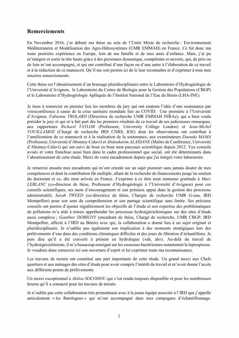
En Novembre 2016, j’ai débuté ma thèse au sein de l’Unité Mixte de recherche : Environnement Méditerranéen et Modélisation des Agro-Hdrosystèmes (UMR EMMAH) en France. Ce fut donc ma toute première expérience en Europe, loin de ma famille et de mes amis d’enfance. Mais, j’ai pu m’intégrer et sortir la tête haute grâce à des personnes dynamique, compétente et ouverte, qui, de près ou de loin m’ont accompagné, et qui ont contribué d’une façon ou d’une autre à l’élaboration de ce travail et à la rédaction de ce manuscrit. Qu’il me soit permis ici de le leur reconnaître et d’exprimer à tous mes sincères remerciements.

Cette thèse est l’aboutissement d’un brassage pluridisciplinaire entre le Laboratoire d’Hydrogéologie de l’Université d’Avignon, le Laboratoire du Centre de Biologie pour la Gestion des Populations (CBGP) et le Laboratoire d’Hydrogéologie Aplliquée de l’Institut National de l’Eau du Bénin (LHA-INE).

Je tiens à remercier en premier lieu les membres du jury qui ont soutenu l’idée d’une soutenance par visioconférence à cause de la crise sanitaire mondiale liée au COVID. Une première à l’Université d’Avignon. Fabienne TROLARD (Directrice de recherche UMR EMMAH INRAe), qui a bien voulu présider le jury et qui m’a fait part dès les premiers résultats de ce travail de ses judicieuses remarques, aux rapporteurs Richard TAYLOR (Professeur, University College London) et Jean-Michel

VOUILLAMOZ (Chargé de recherche IRD CNRS, IGE) dont les observations ont contribué à l’amélioration de ce manuscrit et à la réalisation de la soutenance, aux examinateurs Daouda MAMA

(Professeur, Université d’Abomey-Calavi) et Abdoukarim ALASSANE (Maître de Conférence, Université d’Abomey-Calavi) qui ont suivi de bout en bout mon parcours scientifique depuis 2012. Vos conseils avisés et votre franchise aussi bien dans le cadre professionnel que social, ont été déterminants dans l’aboutissement de cette étude. Merci de votre encadrement depuis que j'ai intégré votre laboratoire.

Je remercie ensuite mes encadrants qui m’ont orienté sur un sujet pionnier sans jamais douter de mes compétences et dont la contribution fût multiple, allant de la recherche de financements jusqu’au soutien du doctorant et ce, dès mon ariivée en France. J’exprime à ce titre mon immense gratitude à Marc

LEBLANC (co-directeur de thèse, Professeur d’Hydrogéologie à l’Université d’Avignon) pour ces conseils scientifiques, ses mots d’encouragement et son présieux appui dans la gestion des processus administratifs; Sarah TWEED (co-directrice de thèse, Chargée de recherche UMR G-eau, IRD Montpellier) pour son sens de compréhension et son partage scientifique sans limite. Ses précieux conseils ont permis d’ajuster régulièrement les objectifs de l’étude et son expertise des problématiques de pollutions m’a aidé à mieux appréhender les processus hydro(géo)chimiques sur des sites d’étude aussi complexe ; Gauthier DOBIGNY (encadrant de thèse, Chargé de recherche, UMR CBGP, IRD Montpellier, affecté à l’IRD au Bénin) avec qui, la collaboration a donné lieu à un sujet original et pluridisciplinaire. Je n’oublie pas également son implication à des moments stratégiques lors des prélèvements d’eau dans des conditions climatiques difficiles et des jours de filtration d’échantillons. Je puis dire qu’il a été converti à présent en hydrologue («ah, ah»). Au-delà du travail de l’hydro(géo)chimiste, il m’a beaucoup enseigné sur les zoonoses bactériennes notamment la leptospirose. Je voudrais donc remercier ici son ouverture d’esprit et lui exprimer toute ma reconnaissance.

Les travaux de terrain ont constitué une part importante de cette étude. Un grand merci aux Chefs quartiers et aux ménages des sites d’étude pour avoir compris l’intérêt du travail et m’avoir donné l’accès aux différents points de prélèvements.

Un merci exceptionnel à Akilou SOCOHOU qui s’est rendu toujours disponible et pour les nombreuses heures qu’il a consacré pour les travaux de terrain.

Je n’oublie pas cette collaboration très prometteuse avec à la jeune équipe associée à l’IRD que j’appelle amicalement « les Ratologues » qui m’ont accompagné dans mes campagnes d’échantillonnage.

3

Sylvestre BADOU, Henri-Joël DOSSOU, Jonas ETOUGBETCHE et les étudiants de l’EPAC. Qu’ils reçoivent ici toute ma reconnaissance.

C’est avec une grande sincérité que je témoigne ma reconnaissance à tout ce qui m’ont aidé à réaliser les nombreuses analyses nécessaires à ce travail : Je pense à Roland SILMER pour les analyses chimiques, Milanka BABIC pour les analyses isotopiques dans le laboatoire d’Hydrogéologie à Avignon Université, Jean-Luc SEIDEL pour les éléments traces dans le laboratoire HydroSciences de Montpellier et Phillipe

GAUTHIER pour la détection des bactéries leptospires dans le laboratoire du CBGP.

Je remercie les chercheurs et le personnel administratif de l’UMR EMMAH particulièrement, l’actuel direcetur de l’unité, Stéphane RUY, qui a accepté sans réserve faire partie des membres de comité et de suivi de thèse. Recevez l’expression sincère de ma profonde gratiude.

Je voudrais évidemment remercier toute l’équipe d’hydrogéologue avec qui j’ai passé plus de trois années géniales. Vous aviez participer activement à mon intégration. Je tiens à remercier paticulièrement les doctorants et post-doctorants avec qui j’ai passé de très bons moments et qui ont rendu mon séjour encore plus agréable. Merci à Chloé OLLIVIER, Florian MALLET, Hamed BOUARE, Irène KINOTI, Angélique

POULAIN, Sébastien SANTONI, Simon CARRIERE.

Un grand merci également à tous ceux qui m’auront vu et soutenu chaque jour. A tous les compatriotes béninois rencontrés à Avignon. Belmys, Père Christian, Dave, Sayidathou, Emilienne, Marc, Habil, Omar, Rodérick, Naomi, Mohamed avec qui j’ai tissé de très bonnes relations. Merci à Guy BOYER, Patrick OLLIVIER et Catherine DEVIGNON, j’ai été très sensible l’immense soutien que vous m’avez apporté.

A ma famille qui m’a apporté soutien moral et encouragement. Une pensée spéciale à ma mère Célestine

HOUNNOUVI et à mon père Gualbert HOUEMENOU, qui m’ont toujours soutenu par des prières. Nos frères et sœur Modeste, Florent, Alexendre, Constant, Jean-Luc et Bernadette HOUEMENOU, qui m’ont soutenu même à distance.

Enfin, à mon épouse Clotilde Mahudé GBESSE pour les lourds sacrifices dont elle a fait montre lors de nos nombreuses absences liées aux travaux de thèse. A notre cher garçon Kiliann Fênou. Cette thèse leur est dédiéee.

4

Résumé

Les eaux souterraines captées par les puits à grand diamètre dans la métropole de Cotonou (Sud

du Bénin) sont tirées de l’aquifère du Quaternaire qui appartient au Bassin Sédimentaire Côtier. Cet

aquifère côtier est particulièrement vulnérable non seulement de par son caractère superficiel et par

l’influence des activités anthropiques mais aussi de par sa proximité avec les eaux salées du lac Nokoué

et les mares contaminées. Les habitants des milieux défavorisés représentant environ 60% de la

population de Cotonou sont les plus exposés face à l’utilisation quotidienne de cette ressource à des fins

domestiques. Les campagnes de prélèvement spatio-temporel et les analyses physico-chimiques,

isotopiques et bactériologiques, nous ont permis de décrire l’état actuel des eaux de l’aquifère peu

profond, d’identifier les principaux facteurs et les périodes à risque de contamination des maladies

hydriques notamment la leptospirose, une zoonose émergente méconnue à Cotonou. La nappe paraît

principalement alimentée par les pluies locales. Mais l’utilisation conjointe des traceurs

environnementaux (ions majeurs, ratio Cl/Br et isotopes stables), ont montré que cet aquifère peu profond

est contaminé par les apports d'eau salée du lac Nokoué pendant la saison sèche, le lexiviat de déchets

solides, d’eaux usées des fosses septiques et des fuites de latrines pendant la recharge par les pluies et

aussi via les mares temporaires et permanantes. Même si l’interaction eau souterraine et les minéraux

rocheux contribuent à la minéralisation, certains polluants anthropiques notamment les nitrates et les

éléments traces (Mo, V, Zn et Al) peuvent parvenir à la nappe par lessivage ou être retenus par adsorption

des sédiments sablo-argileux dans la Zone Non Saturée. D’autres comme le Fe et le Mn dépendent des

conditions réductrices du milieu qui interviennent principalement au cours des processus de

dénitrification et de dégradation de la matière organique. Les eaux contaminées de Cotonou se présentent

donc comme un environnement favorable à la survie des leptospires en occurrence les mares obtenues

après les précipitations du début de la saison des pluies. Le contact fréquent avec l'eau pendant la saison

des pluies expose les habitants de Cotonou aux risques d'infections à la leptospirose. Les mesures de

prévention des risques de contamination des maladies hydriques méritent sans doute une plus grande

attention de la part des autorités sanitaires de la région côtière de l'Afrique de l'Ouest, en pleine

expansion.

Mots clés : Urbanisation, contamination des eaux souterraines, maladie hydrique, risque sanitaire,

leptospires pathogènes

5

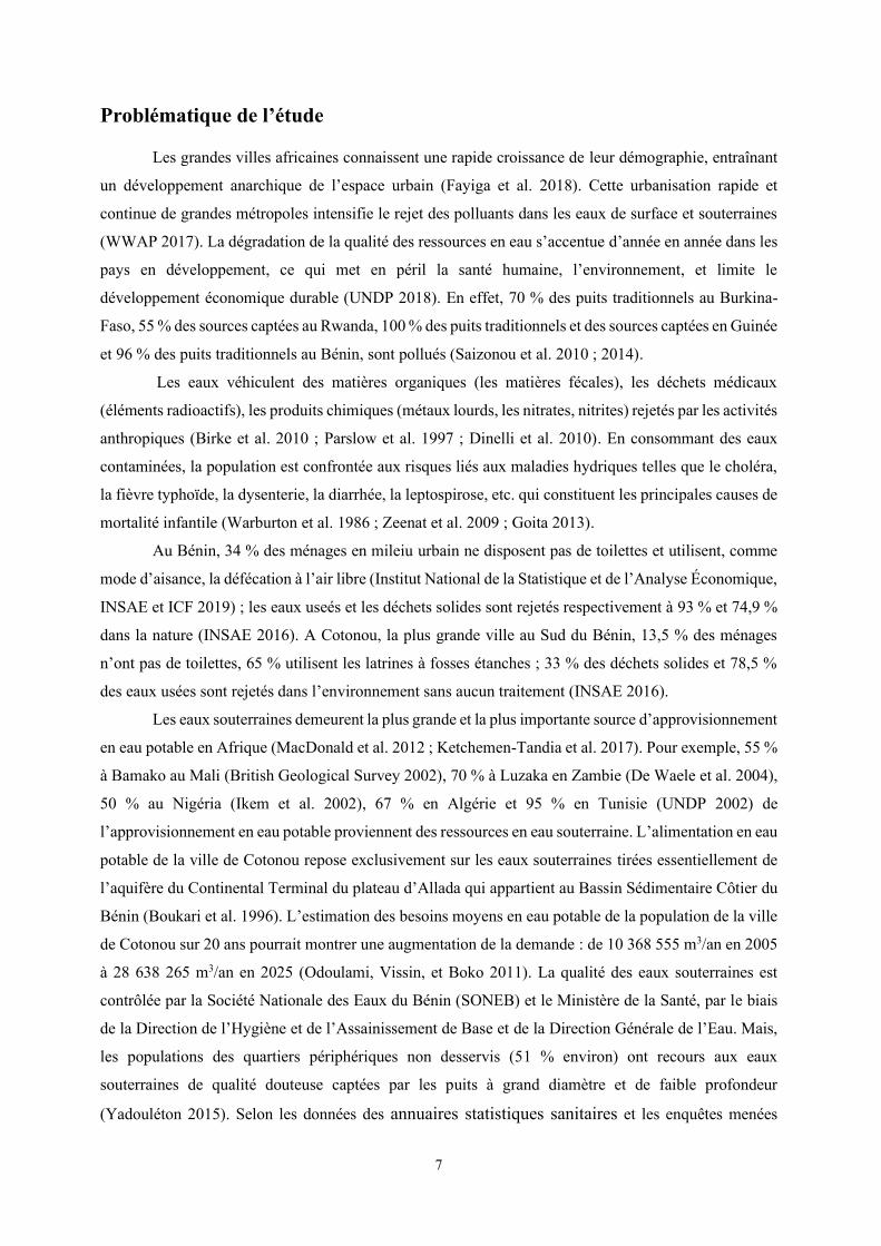
Abstract

Groundwater from large diameter wells in the Cotonou metropolis (southern Benin) is drawn

from the Quaternary aquifer, which belongs to the Coastal Sedimentary Basin. This coastal aquifer is

particularly vulnerable not only by its shallow nature and therefore risks from anthropogenic activities,

but also by its proximity connectivity with a saline lake and contaminated pond waters. Inhabitants

of underprivileged areas accounting for approximately 60% of the city's inhabitants are the most exposed

to the daily use of this water resource for domestic purposes. Spatio-temporal sampling surveys and

physico-chemical, isotopic and bacteriological analyses helped to describe the current state of the shallow

aquifer waters, to identify the main factors and periods at risk of contamination by waterborne diseases,

in particular leptospirosis, an emerging zoonosis that is unknown in Cotonou. The aquifer appears to be

mainly recharged by local rainfall. But the combined use of environmental tracers (major ions, Cl/Br

ratio and stable isotopes), showed that this shallow aquifer is contaminated by salt water from Nokoué

Lake during the dry season, by the leaching of solid waste, by wastewater from septic tanks and latrine

leaks during rainfall recharge and via the recharge of temporary and permanent ponds. Although the

interaction between groundwater and rock minerals contributes to mineralization, some anthropogenic

pollutants such as nitrogen and trace elements (Mo, V, Zn and Al) can leach to groundwater or be retained

by adsorption to sandy clay sediments in the unsaturated zone. Others, such as Fe and Mn, depend heavily

on the redox conditions and the degradation of organic matter. The contaminated waters of Cotonou are

a compatible environment for the survival of leptospirosis, especially in the pond waters that are

formed at the start of the rainy season. Frequent contact with pond waters during the rainy season exposes

the population of Cotonou to the risk of leptospirosis infections. Preventive measures against the risk of

contamination of water-borne diseases undoubtedly deserve greater attention from the health authorities

in the rapidly expanding populations in the coastal region of West Africa.

Keywords: Urbanization, groundwater contamination, waterborne diseases, human health risk,

pathogenic leptospires

6

CHAPITRE I. INTRODUCTION GENERALE

7

Problématique de l’étude

Les grandes villes africaines connaissent une rapide croissance de leur démographie, entraînant

un développement anarchique de l’espace urbain (Fayiga et al. 2018). Cette urbanisation rapide et

continue de grandes métropoles intensifie le rejet des polluants dans les eaux de surface et souterraines

(WWAP 2017). La dégradation de la qualité des ressources en eau s’accentue d’année en année dans les

pays en développement, ce qui met en péril la santé humaine, l’environnement, et limite le

développement économique durable (UNDP 2018). En effet, 70 % des puits traditionnels au Burkina-

Faso, 55 % des sources captées au Rwanda, 100 % des puits traditionnels et des sources captées en Guinée

et 96 % des puits traditionnels au Bénin, sont pollués (Saizonou et al. 2010 ; 2014).

Les eaux véhiculent des matières organiques (les matières fécales), les déchets médicaux

(éléments radioactifs), les produits chimiques (métaux lourds, les nitrates, nitrites) rejetés par les activités

anthropiques (Birke et al. 2010 ; Parslow et al. 1997 ; Dinelli et al. 2010). En consommant des eaux

contaminées, la population est confrontée aux risques liés aux maladies hydriques telles que le choléra,

la fièvre typhoïde, la dysenterie, la diarrhée, la leptospirose, etc. qui constituent les principales causes de

mortalité infantile (Warburton et al. 1986 ; Zeenat et al. 2009 ; Goita 2013).

Au Bénin, 34 % des ménages en mileiu urbain ne disposent pas de toilettes et utilisent, comme

mode d’aisance, la défécation à l’air libre (Institut National de la Statistique et de l’Analyse Économique,

INSAE et ICF 2019) ; les eaux useés et les déchets solides sont rejetés respectivement à 93 % et 74,9 %

dans la nature (INSAE 2016). A Cotonou, la plus grande ville au Sud du Bénin, 13,5 % des ménages

n’ont pas de toilettes, 65 % utilisent les latrines à fosses étanches ; 33 % des déchets solides et 78,5 %

des eaux usées sont rejetés dans l’environnement sans aucun traitement (INSAE 2016).

Les eaux souterraines demeurent la plus grande et la plus importante source d’approvisionnement

en eau potable en Afrique (MacDonald et al. 2012 ; Ketchemen-Tandia et al. 2017). Pour exemple, 55 %

à Bamako au Mali (British Geological Survey 2002), 70 % à Luzaka en Zambie (De Waele et al. 2004),

50 % au Nigéria (Ikem et al. 2002), 67 % en Algérie et 95 % en Tunisie (UNDP 2002) de

l’approvisionnement en eau potable proviennent des ressources en eau souterraine. L’alimentation en eau

potable de la ville de Cotonou repose exclusivement sur les eaux souterraines tirées essentiellement de

l’aquifère du Continental Terminal du plateau d’Allada qui appartient au Bassin Sédimentaire Côtier du

Bénin (Boukari et al. 1996). L’estimation des besoins moyens en eau potable de la population de la ville

de Cotonou sur 20 ans pourrait montrer une augmentation de la demande : de 10 368 555 m3/an en 2005

à 28 638 265 m3/an en 2025 (Odoulami, Vissin, et Boko 2011). La qualité des eaux souterraines est

contrôlée par la Société Nationale des Eaux du Bénin (SONEB) et le Ministère de la Santé, par le biais

de la Direction de l’Hygiène et de l’Assainissement de Base et de la Direction Générale de l’Eau. Mais,

les populations des quartiers périphériques non desservis (51 % environ) ont recours aux eaux

souterraines de qualité douteuse captées par les puits à grand diamètre et de faible profondeur

(Yadouléton 2015). Selon les données des annuaires statistiques sanitaires et les enquêtes menées

8

auprès des ménages (Hounsinou et al. 2015; Odoulami 2009), les maladies hydriques font partie des

principales affections recensées à Cotonou. L’aquifère peu profond est donc soumis à une forte pression

anthropique et également aux risques de contamination par les eaux salées. En effet, la proximité de

l’aquifère côtier de la région de Cotonou avec le lac Nokoué et l’océan atlantique, le soumet à des risques

d’intrusions salines (Stephen et al. 2010).

Des études hydrogéochimiques ont montré que les eaux souterraines des centres urbains situés

dans des régions côtières sont influencées par l’intrusion d’eau salée (Adepelumi et al. 2009; Steyl et

Dennis 2010). C’est le cas de l’aquifère côtier situé dans la région de Cap-Bon en Tunisie, qui connaît

une intrusion d'eau de mer avec des teneurs en sel pouvant atteindre de 5 à 8 g/L (Paniconi et al. 2001).

Dans la région de Tripoli (Libye) où l’urbanisation et le développement des activités agricoles ont

contribué à la salinisation des eaux souterraines dans la plaine de Gefara (Sadeg et Karahanoðlu 2001).

Au Kenya et au Mozambique, des interfaces d’échanges d’eau douce et d’eau salée ont été observés au

niveau des aquifères côtiers (Zektser, G, et Internacional 2004). Au Sénégal, des teneurs de 3g/L de sel

ont été enregistrées dans l’aquifère superficiel de la région de Saloum (Faye et al. 2003). Au Ghana, dans

la région de Keta située entre la lagune et l’océan atlantique, la salinisation de l’aquifère côtier présente

des fluctuations saisonnières avec une augmentation des teneurs en chlorures (3,5 à 5,3 g/l) pendant la

saison sèche (Banoeng-Yakubo et al. 2006).

La présente étude porte sur la « Qualité des eaux souterraines et de surface dans la métropole

de Cotonou. Implication pour la leptospirose », les campagnes d’investigation hydrochimiques et

isotopiques ont permis d’améliorer notre compréhension des processus de contaminations d’un aquifère

côtier peu profond sous forte pression anthropique. De même, cette étude permet d’idenfier les types

d’eau positifs aux bactréries pathogènes leptospires et de décrire les spètres physicochimiques des eaux

de surface et soutarraines dans lesquels les leptospires sont identifés.

La problématique de cette étude est de connaître la qualité des eaux utilisées par les populations

défavorisées de la zone côtière au Sud du Bénin, et ses risques sur la santé humaine.

9

I.1. Synthèse bibliographique : Qualité des eaux souterraines à Cotonou

sous l’impact de l’urbanisation

Cette section fait la synthèse des types de polluants anthropiques identifiés dans les villes

urbaines de l’Afrique de l’Ouest et à Cotonou (Bénin). Sur la base de la bibliographie, l’évolution de la

qualité des eaux, les différentes sources de pollutions des eaux souterraines et de surface, et les maladies

hydriques, dans les villes de l’Afrique de l’Ouest et plus précisement à Cotonou ont été présentées.

I.1.1. Aperçu de l’urbanisation en Afrique de l’Ouest

Les grandes villes africaines connaissent une rapide croissance de leur démographie, entraînant

un développement anarchique de l’espace urbain (Fayiga et al. 2018). La majeure partie de la population

urbaine est concentrée dans la plus grande ville (« primauté urbaine ») dans les pays d’Afrique (WWAP

2017). 40 % de la population africaine est urbaine contre 8%, il y a un siècle (ONU Habitat 2014).

L’Afrique de l’Ouest n’échappe guère à cette « révolution urbaine » qui est en cours sur le

continent. En 1960, il n'y avait encore aucune agglomération urbaine de plus d'un million d'habitants en

Afrique de l'Ouest. L’urbanisation n’a progressé que lentement jusqu’en 1990. C’est à cette époque que

le taux d’urbanisation de l’Afrique de l’Ouest a dépassé la moyenne du continent et s’est mis à augmenter.

La population urbaine est passée à 92 millions en l’an 2000 et a été estimée à 137 millions en

2010 (près de 50% d’augmentation ; ONU Habitat 2010). Selon les projections pour l’Afrique de l’Ouest,

la population urbaine pourrait atteindre 196 millions en 2020 (ONU Habitat 2014). Entre 2020 et 2030,

on pourait atteindre une augmentation annuelle moyenne de plus de 6 %. Les pays de la sous-région

Ouest-Africaine sont donc confrontés à l’accélération des taux d’expansion des villes urbaines.

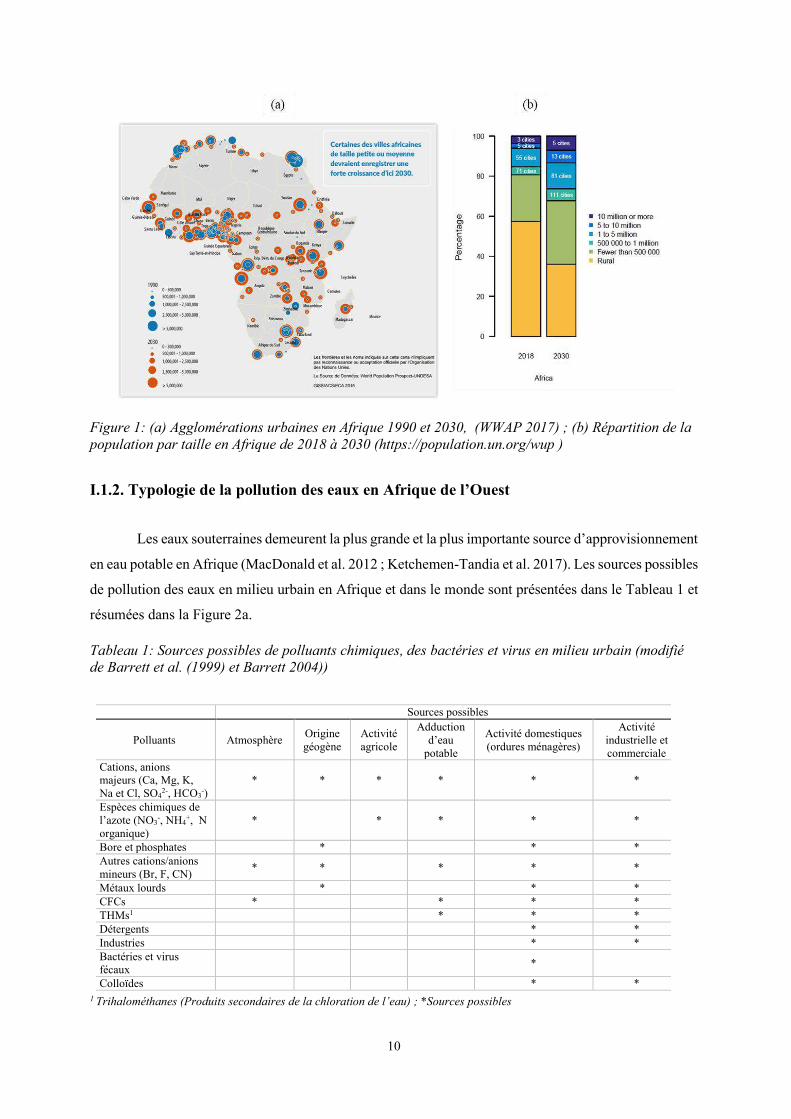
La Figure 1, présente l’évolution estimée des agglomérations urbaines entre 1990 et 2030 en

Afrique. Les populations africaines résidant dans les villes de petites et moyennes tailles ont enregistré

une nette augmentation de 1990 à 2030 (WWAP 2017 ; Fig. 1a). De même, d’après les projections des

Nations Unis (https://population.un.org/wup) en Afrique, entre 2018 et 2030, la croissance de la

population sera forte pour les villes de petites et moyennes taille (pop.< 5 millions, Fig.1b).

10

Figure 1: (a) Agglomérations urbaines en Afrique 1990 et 2030, (WWAP 2017) ; (b) Répartition de la

population par taille en Afrique de 2018 à 2030 (https://population.un.org/wup )

I.1.2. Typologie de la pollution des eaux en Afrique de l’Ouest

Les eaux souterraines demeurent la plus grande et la plus importante source d’approvisionnement

en eau potable en Afrique (MacDonald et al. 2012 ; Ketchemen-Tandia et al. 2017). Les sources possibles

de pollution des eaux en milieu urbain en Afrique et dans le monde sont présentées dans le Tableau 1 et

résumées dans la Figure 2a.

Tableau 1: Sources possibles de polluants chimiques, des bactéries et virus en milieu urbain (modifié

de Barrett et al. (1999) et Barrett 2004))

1 Trihalométhanes (Produits secondaires de la chloration de l’eau) ; *Sources possibles

Sources possibles

Polluants Atmosphère Origine géogène

Activité agricole

Adduction d’eau

potable

Activité domestiques (ordures ménagères)

Activité industrielle et commerciale

Cations, anions majeurs (Ca, Mg, K, Na et Cl, SO4

2-, HCO3-)

* * * * * *

Espèces chimiques de l’azote (NO3

-, NH4+, N

organique) * * * * *

Bore et phosphates * * * Autres cations/anions mineurs (Br, F, CN)

* * * * *

Métaux lourds * * * CFCs * * * * THMs1 * * * Détergents * * Industries * * Bactéries et virus fécaux

*

Colloïdes * *

11

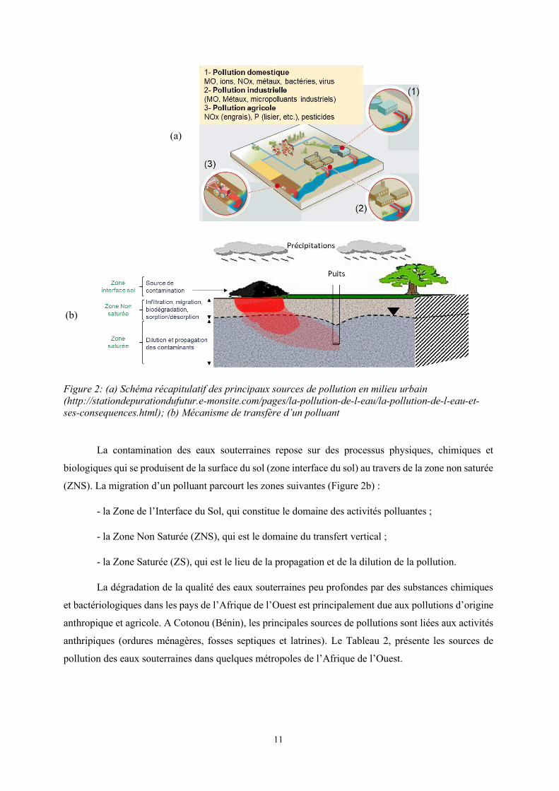
Figure 2: (a) Schéma récapitulatif des principaux sources de pollution en milieu urbain

(http://stationdepurationdufutur.e-monsite.com/pages/la-pollution-de-l-eau/la-pollution-de-l-eau-et-

ses-consequences.html); (b) Mécanisme de transfère d’un polluant

La contamination des eaux souterraines repose sur des processus physiques, chimiques et

biologiques qui se produisent de la surface du sol (zone interface du sol) au travers de la zone non saturée

(ZNS). La migration d’un polluant parcourt les zones suivantes (Figure 2b) :

- la Zone de l’Interface du Sol, qui constitue le domaine des activités polluantes ;

- la Zone Non Saturée (ZNS), qui est le domaine du transfert vertical ;

- la Zone Saturée (ZS), qui est le lieu de la propagation et de la dilution de la pollution.

La dégradation de la qualité des eaux souterraines peu profondes par des substances chimiques

et bactériologiques dans les pays de l’Afrique de l’Ouest est principalement due aux pollutions d’origine

anthropique et agricole. A Cotonou (Bénin), les principales sources de pollutions sont liées aux activités

anthripiques (ordures ménagères, fosses septiques et latrines). Le Tableau 2, présente les sources de

pollution des eaux souterraines dans quelques métropoles de l’Afrique de l’Ouest.

(a)

(b)

12

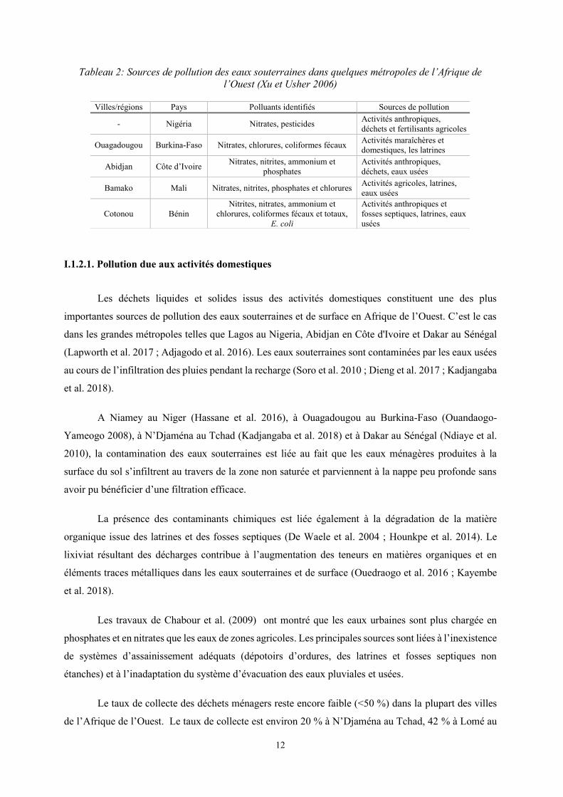
Tableau 2: Sources de pollution des eaux souterraines dans quelques métropoles de l’Afrique de l’Ouest (Xu et Usher 2006)

I.1.2.1. Pollution due aux activités domestiques

Les déchets liquides et solides issus des activités domestiques constituent une des plus

importantes sources de pollution des eaux souterraines et de surface en Afrique de l’Ouest. C’est le cas

dans les grandes métropoles telles que Lagos au Nigeria, Abidjan en Côte d'Ivoire et Dakar au Sénégal

(Lapworth et al. 2017 ; Adjagodo et al. 2016). Les eaux souterraines sont contaminées par les eaux usées

au cours de l’infiltration des pluies pendant la recharge (Soro et al. 2010 ; Dieng et al. 2017 ; Kadjangaba

et al. 2018).

A Niamey au Niger (Hassane et al. 2016), à Ouagadougou au Burkina-Faso (Ouandaogo-

Yameogo 2008), à N’Djaména au Tchad (Kadjangaba et al. 2018) et à Dakar au Sénégal (Ndiaye et al.

2010), la contamination des eaux souterraines est liée au fait que les eaux ménagères produites à la

surface du sol s’infiltrent au travers de la zone non saturée et parviennent à la nappe peu profonde sans

avoir pu bénéficier d’une filtration efficace.

La présence des contaminants chimiques est liée également à la dégradation de la matière

organique issue des latrines et des fosses septiques (De Waele et al. 2004 ; Hounkpe et al. 2014). Le

lixiviat résultant des décharges contribue à l’augmentation des teneurs en matières organiques et en

éléments traces métalliques dans les eaux souterraines et de surface (Ouedraogo et al. 2016 ; Kayembe

et al. 2018).

Les travaux de Chabour et al. (2009) ont montré que les eaux urbaines sont plus chargée en

phosphates et en nitrates que les eaux de zones agricoles. Les principales sources sont liées à l’inexistence

de systèmes d’assainissement adéquats (dépotoirs d’ordures, des latrines et fosses septiques non

étanches) et à l’inadaptation du système d’évacuation des eaux pluviales et usées.

Le taux de collecte des déchets ménagers reste encore faible (<50 %) dans la plupart des villes

de l’Afrique de l’Ouest. Le taux de collecte est environ 20 % à N’Djaména au Tchad, 42 % à Lomé au

Villes/régions Pays Polluants identifiés Sources de pollution

- Nigéria Nitrates, pesticides Activités anthropiques, déchets et fertilisants agricoles

Ouagadougou Burkina-Faso Nitrates, chlorures, coliformes fécaux Activités maraîchères et domestiques, les latrines

Abidjan Côte d’Ivoire Nitrates, nitrites, ammonium et

phosphates Activités anthropiques, déchets, eaux usées

Bamako Mali Nitrates, nitrites, phosphates et chlorures Activités agricoles, latrines, eaux usées

Cotonou Bénin Nitrites, nitrates, ammonium et

chlorures, coliformes fécaux et totaux, E. coli

Activités anthropiques et fosses septiques, latrines, eaux usées

13

Togo, et à 24 % à Dakar au Sénégal (Ngambi 2015). La caractérisation des eaux usées en milieu urbain

à Cotonou (Bénin) par Saizonou et al. (2014 ; 2010) et à Abidjan par Soro et al. (2010) a montré que ces

effluents bruts véhiculent d’importantes charges de matières azotées, de métaux lourds et de bactéries.

Ces eaux usées sont constituées d’eaux-vannes (excréments, urine, boues fécales) et d’eaux usées

ménagères (eau de douche, de cuisine, de vaisselle, de lessive, de lavage de cours, de lavage de

motos)(Yadouléton 2015).

I.1.2.2. Pollution due aux activités agricoles

La croissance démographique et les changements dans le régime alimentaire ont contribué à

l’augmentation de la demande alimentaire (WWAP, 2017). L’agriculture a connu une forte expansion et

intensification afin de pouvoir satisfaire à cette demande. Dans la plupart des pays de l’Afrique de l’Ouest

(ex. Mali, Niger, Bénin, Côte d’Ivoire, Nigéria, etc.) les produits chimiques sont utilisés sous forme

d'engrais et de pesticides afin d’accroitre la productivité (Dicho et al. 2013). Des études indiquent que

les pratiques agricoles ont conduit à la contamination des eaux souterraines peu profondes et des eaux de

surface par les nitrates, les phosphates, les hydrocarbures, les métaux lourds et les fluorines (Soro et al.

2010 ; Paré et Bonzi-Coulibaly 2013 ; Atidegla et Agbossou 2010). Par la dissolution et le transport de

quantités excessives d’engrais, de pesticides, d’herbicides et des antibiotiques (Ahouangninou, 2013).

Savadogo et al. (2006) et Paré et al (2013) ont montré que les sols sont contaminés par endosulfan (1–22

µg/kg) et imethoate (1.7–5 µg/kg) utilisés comme pesticides dans la production du coton au Burkina-

Faso.

Plus de 60 % des maraîchers du site de Houéyiho à Cotonou appliquent la fumure au moins

quatre fois au cours du cycle végétatif des cultures avec des doses (1000-3000 kg/ha de NPK et 2500-

5000 kg/ha d’urée) supérieures à celles recommandées par les services techniques (Atidégla et al. 2010).

Ces doses d’engrais non utilisées se retrouvent dans les eaux souterraines et de surface après lessivage

des sols par les pluies (Paré et al. 2013 ; Adjagodo et al. 2016).

Ba et al. (2016) ont montré que les pratiques d’utilisation des fertilisants organiques et

inorganiques par les agriculteurs en mileu urbain à Dakar (Sénégal) ont des impacts sur les ressources en

eau et sur la santé des populations. En dehors de l’utilisation des engrais chimiques en agriculture,

certains agriculteurs utilisent des engrais organiques (déjections animales et humaines, engrais vert,

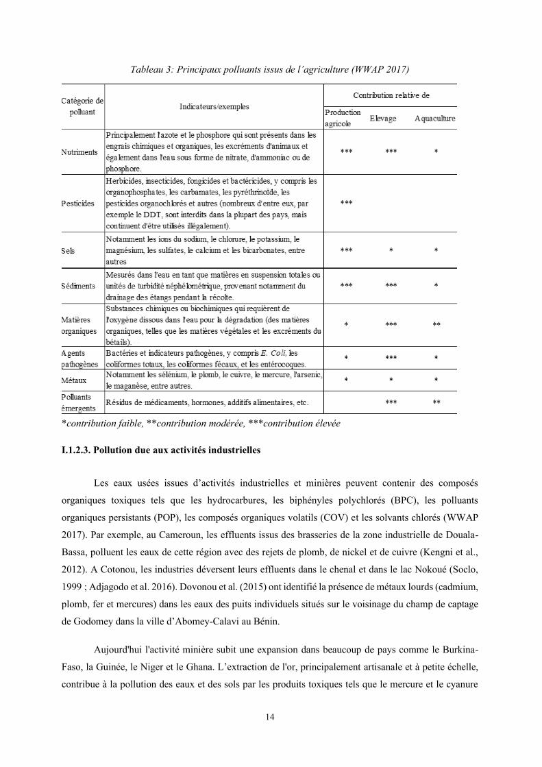
lisières et résidus de récolte) comme fertilisant. Le Tableau 3 présente les principaux polluants de l’eau

issus de l’agriculture.

14

Tableau 3: Principaux polluants issus de l’agriculture (WWAP 2017)

*contribution faible, **contribution modérée, ***contribution élevée

I.1.2.3. Pollution due aux activités industrielles

Les eaux usées issues d’activités industrielles et minières peuvent contenir des composés

organiques toxiques tels que les hydrocarbures, les biphényles polychlorés (BPC), les polluants

organiques persistants (POP), les composés organiques volatils (COV) et les solvants chlorés (WWAP

2017). Par exemple, au Cameroun, les effluents issus des brasseries de la zone industrielle de Douala-

Bassa, polluent les eaux de cette région avec des rejets de plomb, de nickel et de cuivre (Kengni et al.,

2012). A Cotonou, les industries déversent leurs effluents dans le chenal et dans le lac Nokoué (Soclo,

1999 ; Adjagodo et al. 2016). Dovonou et al. (2015) ont identifié la présence de métaux lourds (cadmium,

plomb, fer et mercures) dans les eaux des puits individuels situés sur le voisinage du champ de captage

de Godomey dans la ville d’Abomey-Calavi au Bénin.

Aujourd'hui l'activité minière subit une expansion dans beaucoup de pays comme le Burkina-

Faso, la Guinée, le Niger et le Ghana. L’extraction de l'or, principalement artisanale et à petite échelle,

contribue à la pollution des eaux et des sols par les produits toxiques tels que le mercure et le cyanure

15

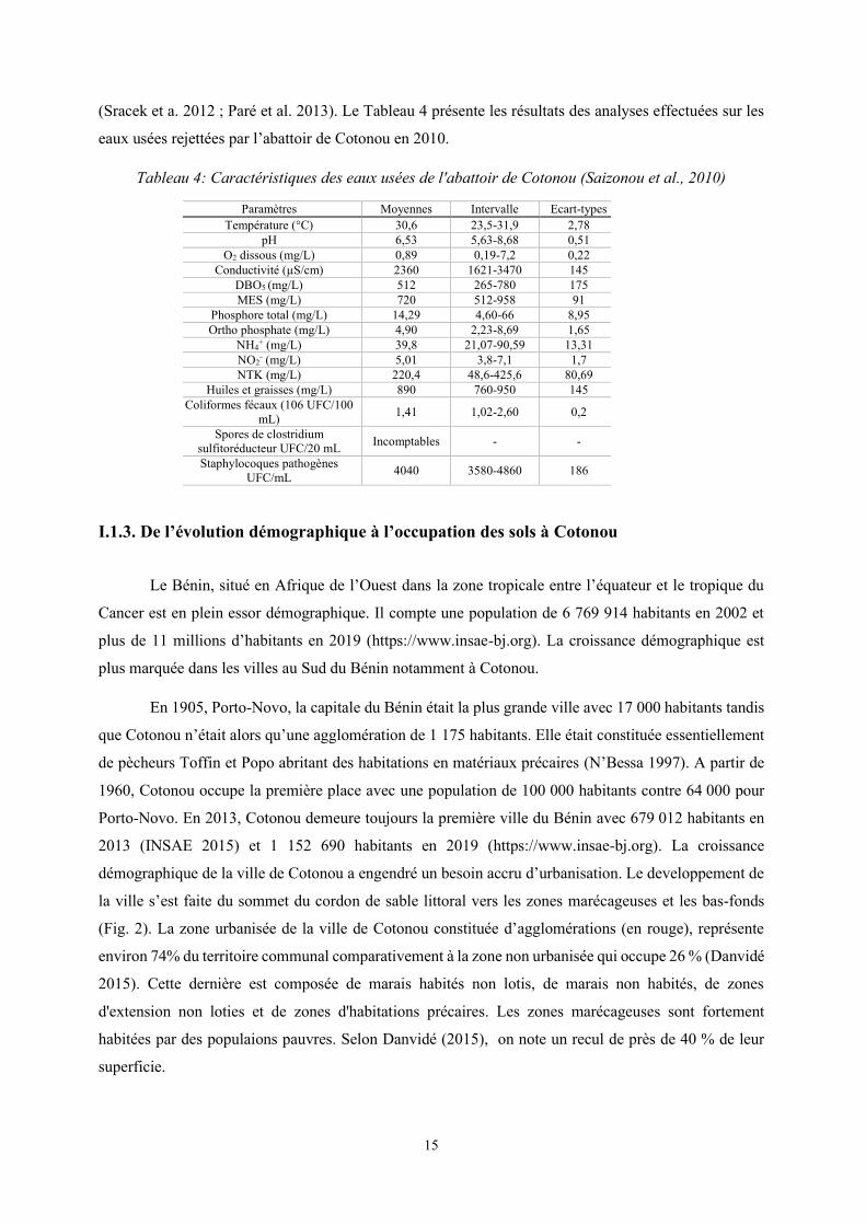
(Sracek et a. 2012 ; Paré et al. 2013). Le Tableau 4 présente les résultats des analyses effectuées sur les

eaux usées rejettées par l’abattoir de Cotonou en 2010.

Tableau 4: Caractéristiques des eaux usées de l'abattoir de Cotonou (Saizonou et al., 2010)

I.1.3. De l’évolution démographique à l’occupation des sols à Cotonou

Le Bénin, situé en Afrique de l’Ouest dans la zone tropicale entre l’équateur et le tropique du

Cancer est en plein essor démographique. Il compte une population de 6 769 914 habitants en 2002 et

plus de 11 millions d’habitants en 2019 (https://www.insae-bj.org). La croissance démographique est

plus marquée dans les villes au Sud du Bénin notamment à Cotonou.

En 1905, Porto-Novo, la capitale du Bénin était la plus grande ville avec 17 000 habitants tandis

que Cotonou n’était alors qu’une agglomération de 1 175 habitants. Elle était constituée essentiellement

de pècheurs Toffin et Popo abritant des habitations en matériaux précaires (N’Bessa 1997). A partir de

1960, Cotonou occupe la première place avec une population de 100 000 habitants contre 64 000 pour

Porto-Novo. En 2013, Cotonou demeure toujours la première ville du Bénin avec 679 012 habitants en

2013 (INSAE 2015) et 1 152 690 habitants en 2019 (https://www.insae-bj.org). La croissance

démographique de la ville de Cotonou a engendré un besoin accru d’urbanisation. Le developpement de

la ville s’est faite du sommet du cordon de sable littoral vers les zones marécageuses et les bas-fonds

(Fig. 2). La zone urbanisée de la ville de Cotonou constituée d’agglomérations (en rouge), représente

environ 74% du territoire communal comparativement à la zone non urbanisée qui occupe 26 % (Danvidé

2015). Cette dernière est composée de marais habités non lotis, de marais non habités, de zones

d'extension non loties et de zones d'habitations précaires. Les zones marécageuses sont fortement

habitées par des populaions pauvres. Selon Danvidé (2015), on note un recul de près de 40 % de leur

superficie.

Paramètres Moyennes Intervalle Ecart-types Température (°C) 30,6 23,5-31,9 2,78

pH 6,53 5,63-8,68 0,51 O2 dissous (mg/L) 0,89 0,19-7,2 0,22

Conductivité (µS/cm) 2360 1621-3470 145 DBO5 (mg/L) 512 265-780 175 MES (mg/L) 720 512-958 91

Phosphore total (mg/L) 14,29 4,60-66 8,95 Ortho phosphate (mg/L) 4,90 2,23-8,69 1,65

NH4+ (mg/L) 39,8 21,07-90,59 13,31

NO2- (mg/L) 5,01 3,8-7,1 1,7

NTK (mg/L) 220,4 48,6-425,6 80,69 Huiles et graisses (mg/L) 890 760-950 145

Coliformes fécaux (106 UFC/100 mL)

1,41 1,02-2,60 0,2

Spores de clostridium sulfitoréducteur UFC/20 mL

Incomptables - -

Staphylocoques pathogènes UFC/mL

4040 3580-4860 186

16

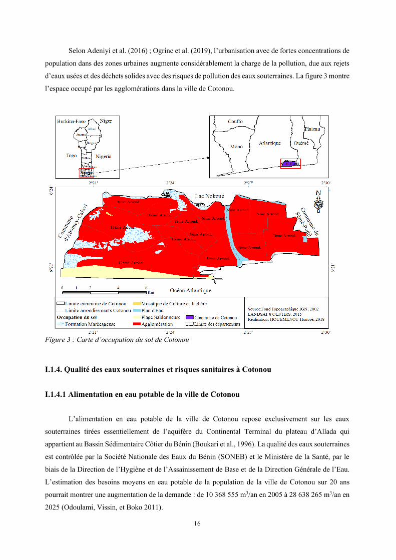
Selon Adeniyi et al. (2016) ; Ogrinc et al. (2019), l’urbanisation avec de fortes concentrations de

population dans des zones urbaines augmente considérablement la charge de la pollution, due aux rejets

d’eaux usées et des déchets solides avec des risques de pollution des eaux souterraines. La figure 3 montre

l’espace occupé par les agglomérations dans la ville de Cotonou.

Figure 3 : Carte d’occupation du sol de Cotonou

I.1.4. Qualité des eaux souterraines et risques sanitaires à Cotonou

I.1.4.1 Alimentation en eau potable de la ville de Cotonou

L’alimentation en eau potable de la ville de Cotonou repose exclusivement sur les eaux

souterraines tirées essentiellement de l’aquifère du Continental Terminal du plateau d’Allada qui

appartient au Bassin Sédimentaire Côtier du Bénin (Boukari et al., 1996). La qualité des eaux souterraines

est contrôlée par la Société Nationale des Eaux du Bénin (SONEB) et le Ministère de la Santé, par le

biais de la Direction de l’Hygiène et de l’Assainissement de Base et de la Direction Générale de l’Eau.

L’estimation des besoins moyens en eau potable de la population de la ville de Cotonou sur 20 ans

pourrait montrer une augmentation de la demande : de 10 368 555 m3/an en 2005 à 28 638 265 m3/an en

2025 (Odoulami, Vissin, et Boko 2011).

17

Les quartiers des zones périurbaines non viabilisés ne sont pas raccordés au réseau public de

distribution. Selon (INSAE 2016), à Cotonou, 49 % des ménages ne disposent pas d’eau potable desservie

par la SONEB à domicile. Cette frange de la population s’approvisionne en eaux via les puits privés ou

publics, rivières, mares ou marigots. Les eaux souterraines captées par les puits peu profonds et à grand

diamètre, sont tirées de l’aquifère du Quaternaire (Maliki 1993; Boukari 1998).

La figure 4 présente les sources d’eau pour les divers usages domestiques à Cotonou en 2005 et

en 2015. Il montre qu’en dehors de l’eau de la SONEB, l’eau captée par les puits à grand diamètre est

surtout utilisée pour la vaisselle (49.4-54.5%), la douche (38-53.07%), la lessive (56-50.8%) et parfois

pour la boisson (0,26-2,3 %) et la cuisine (4,52-16,1 %). L’eau de pluie est faiblement sollicitée à cause

du caractère temporaire et saisonnier de sa disponibilité. L’utilisation des eaux de puits pour la boisson

et la cuisine a augmenté en 2015 (2,3 et 16,1 % respectivement) par rapport à 2005 (0,66 et 4,52 %).

*Lavage moto-auto, arrosage cultures maraichères, nettoyage véranda.

Figure 4 : Source d’eau pour divers usages domestiques à Cotonou en 2005 (Odoulami et al. 2011) et en 2015 (Yadouléton 2015)

I.1.4.2 Qualité chimique et bactériologique

I.1.4.2.1 Ions majeurs

Entre 1991 et 1992, les eaux souterraines à Cotonou étaient en général de bonne qualité à

l'exception des zones à forte concentration humaine (ex. Akpakpa) où des teneurs élevées en nitrates

(>50 mg/L) ont été enregistrées (Maliki 1993). Cette même étude a notifié que la contamination des eaux

souterraines par les nitrates est liée à un apport en matières azotées surtout d’origine anthropique. Boukari

et al., (1996) ont également mis en évidence une pollution d’origine anthropique par nitrate, phosphate

et potassium dans les secteurs de Togbin-Dèkoungbé, le pourtour Sud du lac, tout Cotonou-centre à

l'Ouest du Chenal dans les eaux souterraines. Effet, la toxicité des nitrates résulte de leur réduction en

nitrites, de la formation de méthémoglobine d’une part et de leur contribution possible à la synthèse

18

endogène de composés N-nitrosés d’autre part, qui ont un effet cancérigène (Kahoul et Touhami 2013).La

qualité de l’eau potable de la SONEB stockée dans des réservoirs (bassines, seaux, jarres, etc) au niveau

des ménages à Cotonou se dégrade et peut constituer des sources potentielles de maladies

hydriques(Odoulami 2009; Yadouléton 2015; Rapport EAA 2018a). Les teneurs en bicarbonates (<200

mg/L), ont montré des variations saisonnières. Les plus fortes valeurs (>120 mg/L) se rencontrent dans

les secteurs habituels (Maliki 1993 ; Boukari et al. 1996).

De 2002 à 2004, les puits situés sur la plaine côtière ont révélé des valeurs élevées en Cl-, NO3-,

NH4+ et PO4

3- (Boukari et al. 2006 ; Xu et Usher 2006). Saizonou et al. (2010) ont mesuré des teneurs en

nitrites trois (3) fois supérieures à 3,2 mg/L (limite admise par le décret N°2001-094 du 20 février fixant

les normes de la qualité de l’eau potable en République du Bénin) dans les puits à proximité de l’abattoir

de Cotonou. Boukari et al. (1996), Stephen et al. (2010) et McInnis et al. (2013) ont souligné des

intrusions d’eaux salées du lac Nokoué et de l’Océan Atlantique contribuant à l’augmentation des teneurs

en Chlorures dans l’aquifère côtier au Sud du Bénin.

Ainsi, sur la base des rares études ménées de 1993 à 2013, l’aquifère côtier de Cotonou a connu

une dégradation progressive due principalement à la contamination anthropique de leur qualité.

L’utilisation des eaux souterraines captées par les puits à grand diamètre comme source

d’approvisionnement en eau potable constituent donc une ménace pour la santé de la population de

Cotonou.

I.1.4.2.2 Eléments traces métalliques

Dans l’aquifère du Quaternaire de Cotonou, très peu d’études ont véritablement porté sur les

éléments traces métalliques. Ceci s’explique par le manque de données qui exsiste sur les eaux

souterraines de la zone côtière au Sud du Bénin. Boukari et al. (1996) ont montré que les teneurs en Fe

total (entre 0,1 et 0,2 mg/L) et en Zn (0,5 et 1 mg/L) n’étaient pas compromettantes pour la qualité des

eaux souterraines et la santé des populations. Néanmoins, des secteurs de fortes teneurs en zinc (2 à 3,5

mg/l) correspondant à la zone de Cotonou centre ont été obtenues pendant la même période. L’étude

effectuée sur les eaux de puits et de forages utilisées sur le site maraîcher de Houéyiho à Cotonou a

montré que ces eaux d’arrosage sont contaminées par le cadmium (Cd), le plomb (Pb) et le manganèse

(Mn) qui sont issus des ordures ménagères utilisées pour la fertilisation (Yehouenou Azehoun Pazou et

al. 2009). L’évaluation qualitative dans les principales spéculations maraîchères consommées (laitue,

carotte, chou et grande morelle) produits sur ledit site, a montré une contamination des légumes analysés

due à une toxicité résiduelle en métaux lourds (Cd, Pb, Cu, Zn et Cr). Dans l’aquifère peu profond du

champ de captage intensif de Godomey au Sud du Benin, des teneurs élevées en fer total (0,5 mg/L dans

les puits de Togba) et en plomb (0,18 mg/L dans un puits à Hèvié) comparé à la à la norme béninoise

(0,3 pour le Fe et 0,05 mg/L pour Pb ont été enregistrées (Dovonou et al. 2015). Ces valeurs sont proches

19

de celles mesurées par (Azokpota 2005) dans les eaux des puits des quartiers de Cotonou où se pratiquent

les activités de teinturerie.

La mauvaise gestion des eaux usées contribue à la pollution des eaux souterraines par les

éléments traces métalliques en zone urbaine avec des risques d’intoxication pour la santé humaine (Rai

et al. 2019 ; Dong et al. 2019). La toxicité des métaux en occurrence le plomb sur la santé humaine a été

soulignée par (OMS 2016). En effet, ils peuvent affecter le développement du cerveau et du système

nerveux et augmenter le risque d’hypertension artérielle et de lésions rénales.

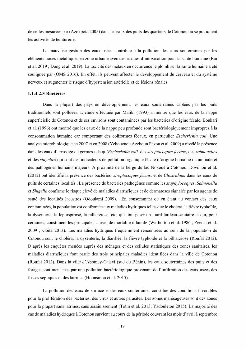
I.1.4.2.3 Bactéries

Dans la plupart des pays en développement, les eaux souterraines captées par les puits

traditionnels sont polluées. L’étude effectuée par Maliki (1993) a montré que les eaux de la nappe

superficielle de Cotonou et de ses environs sont contaminées par les bactéries d’origine fécale. Boukari

et al. (1996) ont montré que les eaux de la nappe peu profonde sont bactériologiquement impropres à la

consommation humaine car comportant des coliformes fécaux, en particulier Escherichia coli. Une

analyse microbiologique en 2007 et en 2008 (Yehouenou Azehoun Pazou et al. 2009) a révélé la présence

dans les eaux d’arrosage de germes tels qu’Escherichia coli, des streptocoques fécaux, des salmonelles

et des shigelles qui sont des indicateurs de pollution organique fécale d’origine humaine ou animale et

des pathogènes humains majeurs. A proxmité de la berge du lac Nokoué à Cotonou, Dovonou et al.

(2012) ont identifié la présence des bactéries streptocoques fécaux et de Clostridium dans les eaux de

puits de certaines localités . La présence de bactéries pathogènes comme les staphylocoques, Salmonella

et Shigella confirme le risque élevé de maladies diarrhéiques et de dermatoses signalée par les agents de

santé des localités lacustres (Odoulami 2009). En consommant ou en étant au contact des eaux

contaminées, la population est confrontée aux maladies hydriques telles que le choléra, la fièvre typhoïde,

la dysenterie, la leptospirose, la bilharziose, etc. qui font peser un lourd fardeau sanitaire et qui, pour

certaines, constituent les principales causes de mortalité infantile (Warburton et al. 1986 ; Zeenat et al.

2009 ; Goita 2013). Les maladies hydriques fréquemment rencontrées au sein de la population de

Cotonou sont le choléra, la dysenterie, la diarrhée, la fièvre typhoïde et la bilharziose (Roufai 2012).

D’après les enquêtes menées auprès des ménages et des cellules statistiques des zones sanitaires, les

maladies diarrhéiques font partie des trois principales maladies identifiées dans la ville de Cotonou

(Roufai 2012). Dans la ville d’Abomey-Calavi (sud du Bénin), les eaux souterraines des puits et des

forages sont menacées par une pollution bactériologique provenant de l’infiltration des eaux usées des

fosses septiques et des latrines (Hounsinou et al. 2015).

La pollution des eaux de surface et des eaux souterraines constitue des conditions favorables

pour la prolifération des bactéries, des virus et autres parasites. Les zones marécageuses sont des zones

pour la plupart sans latrines, sans assainissement (Totin et al. 2013; Yadouléton 2015). La majorité des

cas de maladies hydriques à Cotonou survient au cours de la période couvrant les mois d’avril à septembre

20

(saison des pluies) : leur prévalence est plus élévée pendant la saison des pluies comparé à la saison sèche

(Hounsinou et al. 2015). En effet, la saison des pluies est marquée par l’omniprésence des eaux

stagnantes, notamment dans les quartiers plus défavorisés (Rapport EAA 2018a).

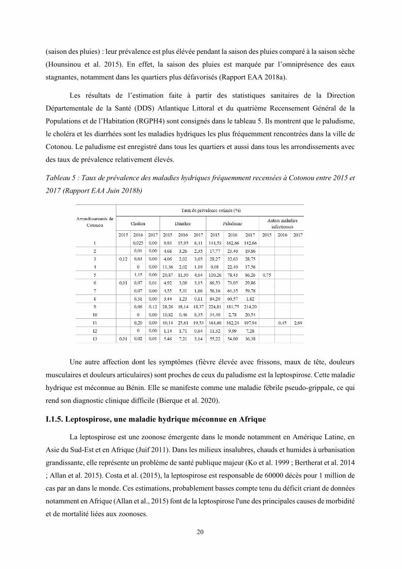
Les résultats de l’estimation faite à partir des statistiques sanitaires de la Direction

Départementale de la Santé (DDS) Atlantique Littoral et du quatrième Recensement Général de la

Populations et de l’Habitation (RGPH4) sont consignés dans le tableau 5. Ils montrent que le paludisme,

le choléra et les diarrhées sont les maladies hydriques les plus fréquemment rencontrées dans la ville de

Cotonou. Le paludisme est enregistré dans tous les quartiers et aussi dans tous les arrondissements avec

des taux de prévalence relativement élevés.

Tableau 5 : Taux de prévalence des maladies hydriques fréquemment recensées à Cotonou entre 2015 et

2017 (Rapport EAA Juin 2018b)

Une autre affection dont les symptômes (fièvre élevée avec frissons, maux de tête, douleurs

musculaires et douleurs articulaires) sont proches de ceux du paludisme est la leptospirose. Cette maladie

hydrique est méconnue au Bénin. Elle se manifeste comme une maladie fébrile pseudo-grippale, ce qui

rend son diagnostic clinique difficile (Bierque et al. 2020).

I.1.5. Leptospirose, une maladie hydrique méconnue en Afrique

La leptospirose est une zoonose émergente dans le monde notamment en Amérique Latine, en

Asie du Sud-Est et en Afrique (Juif 2011). Dans les milieux insalubres, chauds et humides à urbanisation

grandissante, elle représente un problème de santé publique majeur (Ko et al. 1999 ; Bertherat et al. 2014

; Allan et al. 2015). Costa et al. (2015), la leptospirose est responsable de 60000 décès pour 1 million de

cas par an dans le monde. Ces estimations, probablement basses compte tenu du déficit criant de données

notamment en Afrique (Allan et al., 2015) font de la leptospirose l'une des principales causes de morbidité

et de mortalité liées aux zoonoses.

21

Le réservoir des leptospires est constitué de petits mammifères à affinité anthropophile

(principalement les rongeurs dont les rats), de mammifères domestiques (chiens, porcs, bovins, ovins,

etc.) et d’animaux sauvages (chauve souris, ect.). Ces hôtes réservoirs abritent l’agent pathogène dans

leurs tissus rénaux et les leptospires sont excrétées par voie urinaire dans l’environnement. L’homme se

contamine soit par contact direct avec des animaux infectés ou leurs urines (Fig. 5a), soit indirectement

par contact avec des eaux ou des sols humides contaminés par les urines d’animaux infectés (Fig. 5b. et

e).

Figure 5: Voie de transmission de la leptospirose

Les données statistiques dans les hôpitaux et les enquêtes sur la séroprévalence aux États-Unis

indiquent que plus de 70% des infections à la leptospirose sont attribuées au contact physique avec les

eaux contaminées (Wynwood et al. 2014). En 1984 en Italie, trente-trois (33) cas confirmés de

leptospirose ont été attribués à l'eau contaminée (Wynwood et al. 2014). Au Japon, (Aoki, Koizumi, et

Watanabe 2001) ont confirmé qu’un homme de 48 ans a été contaminé (serovar Leptospira autumnalis)

après avoir été en contact avec une eau de puits de qualité douteuse. Des épidémies de leptospirose sont

également survenues au contact des eaux de baignade, pendant la pratique d’activités de loisirs ou

sportives, comme l’Éco Challenge en Malaisie (Sejvar et al. 2003), le triathlon en Illinois (Ristow 2007).

Les milieux précaires et insalubresurbains sont également à l’origine de contamination endémique et

parfois très nombreuses (ex. dans les bidonvilles de la ville de Salvador au Brésil ; Kô et al., 1999 ;

Maciel et al. 2008). En Nouvelle Calédonie, des leptospires pathogènes ont été identifiés dans les

échantillons de sols et de rivières contaminés (Thibeaux et al. 2017 ; Bierque et al. 2020) et dans les eaux

de surface en milieu urbain au Sud du Chili (Mason et al. 2016 ; Muñoz-Zanzi et al. 2014).

La leptospirose est particulièrement fréquente dans les zones tropicales où les hommes et les

animaux vivent en contact étroit avec les animaux; les conditions climatiques chaudes et humides

favorisent la survie du pathogène dans l’environnement et la coexistence d’espèces animales

potentiellemnt réservoirs et des habitants favorise la transmission humaine (Mwachui et al. 2015). Au

22

Thaïland, en Asie du Sud-Est, la leptospirose est reconnue comme une cause importante d'insuffisance

rénale et de maladie fébrile (Wuthiekanun et al. 2007).

Dans les eaux de surface et dans les sols humides de régions tempérées et tropicales, la survie

des leptospires pathogènes est dépendante de plusieurs facteurs dont la température et le pH (revue dans

Bierque et al. 2020). Les leptospires supportent une alcalinisation jusqu’à 7,8 et leur croissance est

inhibée pour un pH inférieur à 6,8. Elles sont également détruites par les détergents ou les désinfectants

(Juif 2011). Les conditions climatiques saisonnières impliquant des inondations ont longtemps été

reconnues comme une source potentielle d’émergence de la leptospirose (Ko, Goarant, et Picardeau 2009

; Lau et al. 2010 ; Mwachui et al. 2015). La majorité des cas surviennent entre juillet et novembre en

France métropolitaine, et durant la saison des pluies sous les tropiques (Goita 2013). En plus de

l’inondation, la croissance démographique, l'urbanisation associée à des conditions de vie précaires, le

manque d’hygiène et d’assainissement, l'intensification agricole et les changements climatiques sont des

facteurs aggravants de la transmission de la leptospirose (Lau et al. 2010 ; 2016). Par exemple, la

leptospirose est fortement répandue dans les bidonvilles où les personnes vivent dans des habitations

entourées d’égouts à ciel ouvert, proches du principal réservoir de la maladie, le rat (Rattus Norvegicus)

(Ristow 2007 ; Maciel et al. 2008 ; Felzemburgh et al. 2014). Au Pérou, dans la région d’Iquito, la

prévalence des leptospires dans les caniveaux à ciel ouvert, les eaux souterraines et de surface est plus

élevée dans les environnements urbains que ruraux (Ganoza et al. 2006).

En Afrique subsaharienne, beaucoup de pays ont des caractéristiques bioclimatiques propices à

la transmission des leptospires, mais l’incidence et la prévalence restent rarement évaluer (revues dans

Allan et al 2015 ; De Vries et al 2014). Cependant, au Gabon, des cas de contamination aux leptospires

ont été rapportés régulièrement depuis 1994 (Aubry et Gauzère 2019). Ntakirutimana (2013), après avoir

montré que la leptospirose canine existe à Dakar au Sénégal, a mis en exergue les facteurs de risque de

contamination que sont la présence des rongeurs et des chiens à la maison ou dans les environs, les eaux

usées des canaux d’évacuation et la présence des ordures. Au Nigéria, une séroprévalence élevée (20,4

%) a été observée chez les mineurs de charbon, les travailleurs au niveau des abattoirs et les agriculteurs.

Au Ghana, parmi les personnes notées séropositives, 33% étaient des agriculteurs et des travailleurs de

plantation de cacao. Sur 190 patients souffrants de l’ictère et/ou des fièvres dans la région d’Ashanti

(Ghana), 3,2 % ont été confirmés malades de la leptospirose (de Vries et al. 2014). Dans le sud du Bénin,

environ 12% des rats sont porteurs des pathogènes Leptospira et la séroprévalence à la leptospirose dans

les populations humaines a été estimé à 15,8 % (Houéménou et al. 2014; 2019). Cette étude a montré que

la séroprévalence de l’infection à la leptospirose au sein des populations installées dans les bas-fonds, le

long de la lagune et du lac Nokoué est d’environ 40 %. Les risques de contamination à la leptospirose

sont donc élevés dans les villes de l’Afrique de l’Ouest, notamment celles qui s’étalent le long du Golfe

de Guinée pour former le « corridor urbain Abidjan-Lagos » (Dobigny et al. 2018), mais les conditions

environnementales, les caractérisques physico-chimiques et les périodes favorables à la survie des

leptospires dans les eaux souterraines et de surface restent encore mal documentées.

23

I.3. Questions scientifiques

Les études effectuées à Cotonou ont montré que l’urbanisation et la mauvaise gestion des déchets

issus des activités anthropiques constituent les principales sources de contamination des eaux

souterraines de l’aquifère côtier au Sud du Bénin (Maliki 1993 ; Boukari et al. 1996 ; 2006 ; Totin et al.

2013). Les quartiers précaires des grandes métropoles de l’Afrique de l’Ouest vivent dans des

environnements humides et pollués favorables au développement des maladies hydriques (Ikem et al.

2002 ; Ouandaogo-Yameogo 2008 ; De Waele et al. 2004 ; Hassane et al. 2016 ; Lapworth et al. 2017).

A Cotonou, la qualité des eaux souterraines de l’aquifère du Quaternaire n’est pas contrôlée ni

suivie par la SONEB (Société Nationale des Eaux du Bénin) car elles ne représentent pas une ressource

recommandée pour l’approvisionnement en eau potable de la population. Mais la proximité de cette

ressource (faible profondeur) et le taux relativement faible (49 %) d’accès à l’eau de la SONEB, amènent

les populations des quartiers précaires à s’approvisionner en eau via les puits à grand diamètre. Ces eaux

souterraines non suivies sont utilisées pour la lessive, la vaiselle, la douche, la cuisine et parfois la

boisson, et ce, avec les risques de contamination des maladies hydriques (Yadouléton 2015; Hounsinou

et al. 2015; Roufai 2012).

La plupart des études sur les eaux souterraines à Cotonou se sont limitées à sa qualité

microbiologiques et ont porté sur l’analyse des bactéries hydriques indicatrices de pollutions fécales

telles que E. Coli, Streptocoques fécaux, des Salmonelles, Klebsiella pneumoniae, Enterobacter cloacae,

etc. et d’autres bactéries provenant de sources environnementales telles que Enterobacter intermedium

et amnigenus, Klebsiella terrigena, Buttiauxella agresti (Odoulami 2009 ; Saizonou et al. 2010 ;

Dovonou et al. 2012 ; Saizonou et al. 2014). D’autres études ont mis l’accent sur les pollutions par les

composés azotés notamment les nitrates et les métaux lourds tels que Fe, Pb, et Zn, etc. (Boukari 1998;

Yehouenou Azehoun Pazou et al. 2009; Azokpota 2005). Les travaux de Yalo et al. (2012) et McInnis et

al. (2013) ont abordé la problématique d’intrusion d’eaux salées du lac Nokoué et de l’Océan Atlantique

dans l’aquifère côtier au Sud du Bénin en utilisant les approches géophysiques.

Ces études n’ont donc pas abordé la variation temporelle et spatiale des mécanismes de

salinisation (minéralisation, processus d’évaporation, intrusion d’eau salée) et de pollution anthropique

à partir des approches hydrochimiques et isotopiques dans des systèmes hydrogéologiques différents

dans la zone côtière au Sud du Bénin. De même, les données spatio-temporelles sur la distribution des

teneurs en éléments traces métalliques sont vraiment rares ou n’existe pas sur les eaux souterraines et de

surface à Cotonou. Par ailleurs, les possibilités de transfert de contaminants dans les eaux souterraines

au travers de la Zone Non Saturée (ZNS) n’ont jamais été mis en évidence sur ce site.

En dehors de son hôte mammifère, aucune étude n’a été menée sur la présence ou non des

bactéries leptospires pathogènes dans les eaux souterraines et de surface dans la zone côtière au Sud du

Bénin. Très peu de connaissance existent sur les conditions environnementales et hydrochimiques qui

24

sont compatibles avec le Leptospira pathogène surtout dans les habitats urbains où la pollution peut être

très importante.

Cette étude pluridisciplinaire qui utilise une approche combinant les traceurs environnmentaux

(chimiques et isotopiques) et les analyses bactériologiques (les leptospires) permet la mise en place d’une

base de données spatio-temporelles importantes. Elle apporte des informations sur les facteurs qui

contrôlent le fonctionnement de l’aquifère côtier au Sud du Bénin et sur les conditions

environnementales, chimiques et hydroclimatique propices à l’émergence des leptospires pathogène dans

les bidonvilles de Cotonou.

Ainsi, des pistes de recherches pertinentes ont porté sur les questions scientifiques ci-après :

1- Quels sont les processus dominants de contamination par les chlorures et nitrates dans les eaux

souterraines ?

2- Quels sont les facteurs contribuant à l’accumulation du fer et du manganèse ?

3- Quels sont les types d’eaux contaminés et les périodes à risque de contamination à la

leptospirose? Quelles sont les conditions qui favorisent la présence des leptospires pathogènes ?

Pour répondre à chacune des questions de recherches, trois (3) articles scientifiques ont été

rédigés.

1- Houéménou, Honoré, Sarah Tweed, Gauthier Dobigny, Daouda Mama, Abdoukarim Alassane, Roland

Silmer, Milanka Babic, et al. 2019. « Degradation of Groundwater Quality in Expanding Cities in West

Africa. A Case Study of the Unregulated Shallow Aquifer in Cotonou ». Journal of Hydrology, décembre,

124438. https://doi.org/10.1016/j.jhydrol.2019.124438. Publié dans un journal scientifique

2- Houéménou, Honoré, Seidel Jean Luc, Sarah Tweed, Abdoukarim Alassane, Daouda Mama, Fabienne

Trolard, Gauthier Dobigny, Salifou Orou-Pete, Akilou Socohou, et Marc Leblanc. (in preparation) «

Seasonal variations in processes driving manganese and iron concentrations above drinking water

guidelines in the unregulated shallow aquifer of Cotonou (Southern Benin) ». Non soumis dans un journal

scientifique

3- Houéménou, Honoré, Philippe Gauthier, Sarah Tweed, Henri-Joel Dossou, Marc Leblanc, Jean-Luc

Seidel, Akilou Socohou, et Gauthier Dobigny. (in preparation) « Pathogenic Leptospira and water quality

in African cities: a case study of Cotonou, Benin». Soumis dans le journal Water and Health

Ces résultats ont permis de proposer un schéma conceptuel de contamination des eaux souterraines

pour chacun des sites étudiés

25

I.5. Structuration du manuscrit

Ce manuscrit est organisé en quatre chapitres dont trois sont rédigés sous le format

d’articles scientifiques.

Le chapitre I (ci-dessus) présente une synthèse bibliographique de l’état actuel des

connaissances au niveau régional et national de l’urbanisation et son influence sur la qualité des

eaux souterraines peu profondes de grandes métropoles africaines. A l’issu de cet état de l’art,

trois questions scientifiques ont été énoncées afin d’apporter une plus large information sur le

fonctionnement de l’aquifère côtier de Cotonou (Sud du Bénin).

Le chapitre II illustre le contexte hydrogéologique de la zone d’étude et décrit également

les traits majeurs de la zone d’étude qui n’ont pas été précisés dans les articles scientifiques. Il

présente également les caractérisques environnementales qui justifient le choix des sites d’étude.

Le chapitre III présente les résultats du premier article publié sur la dégradation de la

qualité des eaux souterraines peu profondes à Cotonou. Après avoir caractérisé les eaux

souterraines peu profondes de Cotonou dans trois contextes hydrogéologiques, l’utilisation des

traceurs environnements a permis de proposer un schéma conceptuel des facteurs et périodes à

risques de contamination.

Le chapitre IV présente les résultats des investigations menées sur les éléments traces

métalliques dans les eaux souterraines. Ce chapitre illustre les résultats du deuxième article

scienifique sur les éléments traces métalliques dans les eaux souterraines peu profondes à

Cotonou.

Le Chapitre V présente les résultats obtenus sur l’identification des leptospires

pathogènes dans les eaux souterraines et de surface dans les bidonvilles de Cotonou. Ce chapitre

rédigé sous forme d’article scientifique a permis de décrire les conditions environnementales,

les caratériques géochimiques et isotopiques des échantillons d’eau positifs aux leptospires

pathogènes. De même, les périodes à risques de propagation de la leptospirose ont été

soulignées.

Cette étude est cloturée par une conclusion générale qui souligne les principaux résultats

obtenus afin de proposer des pistes de recherche. Chaque chapitre est suivi de la liste de

références bibliographiques. Les informations complétaires pouvant faciliter la lecture de ce

document sont mentionnées dans les Annexes.

26

CHAPITRE II. CADRE D’ETUDE ET APPROCHES METHODOLOGIQUES

27

II.1 Synthèse hydrogéologique de la zone d’étude

Cette partie aborde certains traits caractéristiques du milieu d’étude qui n’ont pas été

suffisamment développés ou pris en compte dans les articles scientifiques. Il s’agit notamment du

contexte climatique, de la stratigraphie du Quaternaire margino-littoral, des contextes hydrogéologiques

et hydrographiques.

II.1.1 Climat

La ville de Cotonou se trouve dans la zone climatique subéquatoriale chaude et humide,

caractérisée par deux saisons pluvieuses annuelles (de mars à juillet et de septembre à octobre) et deux

saisons sèches (de novembre à mars et juillet à août).

A partir des données climatiques de la station ASECNA de Cotonou, la moyenne pluviométrique

annuelle calculée pour la période de (1971- 2016) est d’environ 1280 mm. De Novembre à Mars, les

pluies sont faibles et les moyennes mensuelles sont inférieures à 100 mm : c'est la grande saison sèche.

Courant le mois d'Avril et ce jusqu’en Juillet, la hauteur moyenne mensuelle est supérieure à 100 mm.

Les maximas moyens sont centrés sur le mois de Juin (338,75 mm) : c'est la grande saison pluvieuse. Au

mois d'Août, la pluviométrie fléchit brutalement et tombe à environ 47 mm : c'est la petite saison sèche.

En Septembre, les pluies reprennent et atteignent un second maximum en Octobre (144,22 mm, moins

important qu'en Juin), puis décroissent de nouveau en Novembre (40 mm) : c'est la petite saison des

pluies. La température moyenne quant à elle varie de 23,52 à 31,12 °C pour la même période (1971-

2016). La répartition des températures moyennes permet de considérer Juillet (26,72) Août (26,43 °C) et

septembre (26,93) comme les mois les plus frais, Février (29,48°C), Mars (29,93°C) et Avril (29,60°C)

comme les mois les plus chauds (Fig. 2, chapitre II).

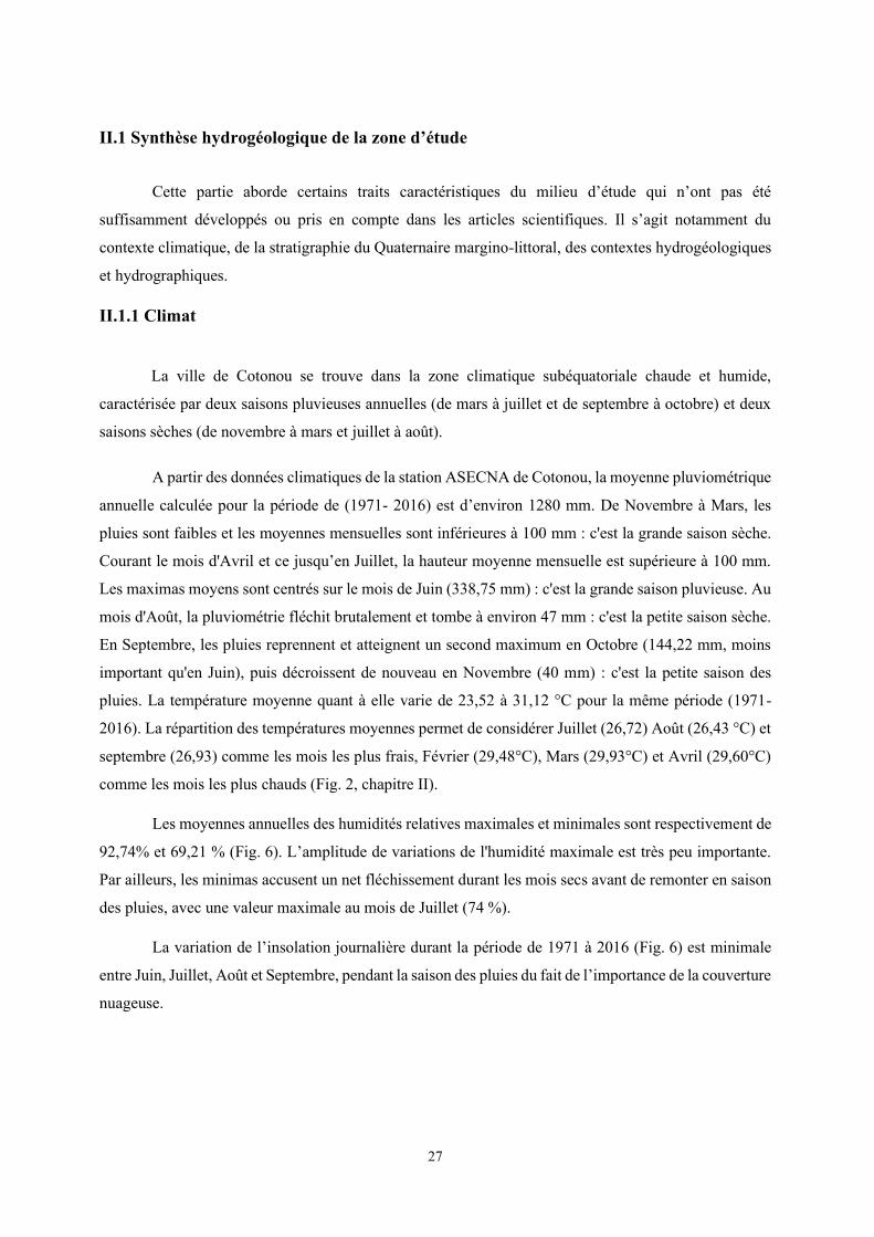
Les moyennes annuelles des humidités relatives maximales et minimales sont respectivement de

92,74% et 69,21 % (Fig. 6). L’amplitude de variations de l'humidité maximale est très peu importante.

Par ailleurs, les minimas accusent un net fléchissement durant les mois secs avant de remonter en saison

des pluies, avec une valeur maximale au mois de Juillet (74 %).

La variation de l’insolation journalière durant la période de 1971 à 2016 (Fig. 6) est minimale

entre Juin, Juillet, Août et Septembre, pendant la saison des pluies du fait de l’importance de la couverture

nuageuse.

28

Figure 6: Humidité relative moyennes mensuelles interannuelles et l’insolation journalière à la station de Cotonou de 1971 à 2016 (ASECNA)

II.1.2 Hydrographie

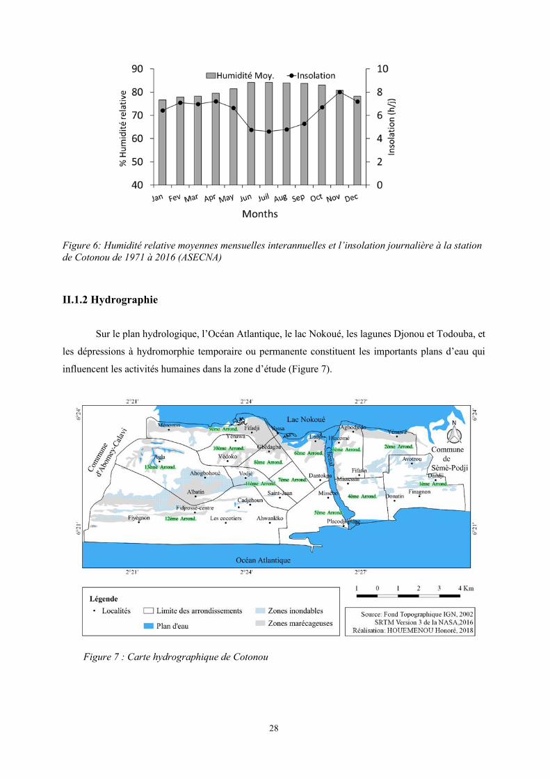
Sur le plan hydrologique, l’Océan Atlantique, le lac Nokoué, les lagunes Djonou et Todouba, et

les dépressions à hydromorphie temporaire ou permanente constituent les importants plans d’eau qui

influencent les activités humaines dans la zone d’étude (Figure 7).

Figure 7 : Carte hydrographique de Cotonou

29

Les principaux tributaires du lac Nokoué sont les fleuves Ouémé, Sô et la lagune Djonou. Les

rivières Todouba, Dati et Ahouhangan sont à leurs tours tributaires de la lagune Djonou. Le lac Nokoué

communique à la mer par le chenal de Cotonou (lagune de Cotonou) qui sépare les étendues Est et Ouest

de la ville. Par ailleurs, il existe dans ses environs, un système de lagons et de bas-fonds avec lesquels il

était à l’origine en communication, mais qui sont actuellement isolés par l’urbanisation de la ville. Les

fluctuations de niveaux des lagunes sont en rapport non seulement avec la pluie, mais aussi avec

l’hydrodynamique de la nappe superficielle, celles- ci étant en continuité hydraulique avec elles.

Le relief et l’hydrogéologie de la ville de Cotonou facilitent donc la recharge de la nappe et

favorisent les inondations. Celles-ci sont accentuées par le régime hydrologique du lac Nokoué qui reste

sous l’influence des eaux de pluie du nord. En fait, le lac connaît deux périodes de crue de mai à juin

(petite crue) et de septembre à novembre (grande crue). Ces apports d’eau de pluie au lac Nokoué se font

par l’intermédiaire des fleuves Ouémé et Sô (Odoulami, 2009).

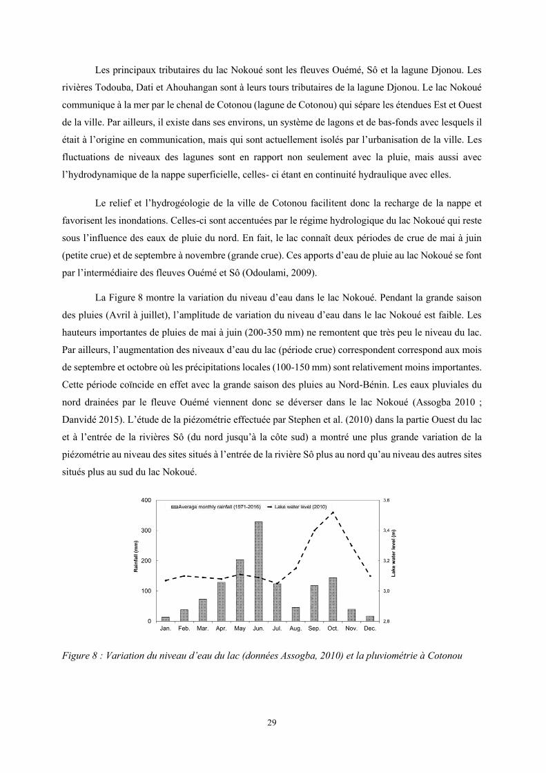
La Figure 8 montre la variation du niveau d’eau dans le lac Nokoué. Pendant la grande saison

des pluies (Avril à juillet), l’amplitude de variation du niveau d’eau dans le lac Nokoué est faible. Les

hauteurs importantes de pluies de mai à juin (200-350 mm) ne remontent que très peu le niveau du lac.

Par ailleurs, l’augmentation des niveaux d’eau du lac (période crue) correspondent correspond aux mois

de septembre et octobre où les précipitations locales (100-150 mm) sont relativement moins importantes.

Cette période coïncide en effet avec la grande saison des pluies au Nord-Bénin. Les eaux pluviales du

nord drainées par le fleuve Ouémé viennent donc se déverser dans le lac Nokoué (Assogba 2010 ;

Danvidé 2015). L’étude de la piézométrie effectuée par Stephen et al. (2010) dans la partie Ouest du lac

et à l’entrée de la rivières Sô (du nord jusqu’à la côte sud) a montré une plus grande variation de la

piézométrie au niveau des sites situés à l’entrée de la rivière Sô plus au nord qu’au niveau des autres sites

situés plus au sud du lac Nokoué.

Figure 8 : Variation du niveau d’eau du lac (données Assogba, 2010) et la pluviométrie à Cotonou

30

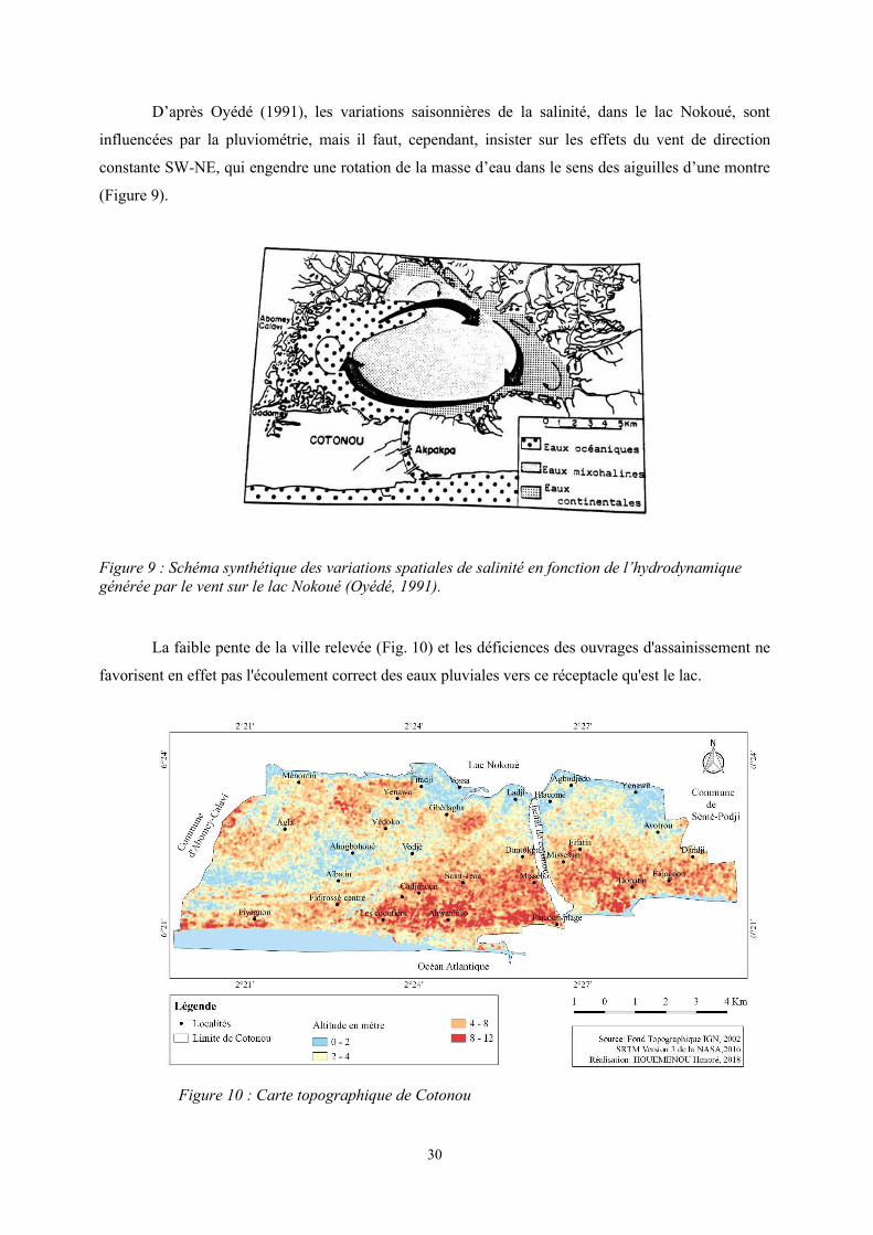
D’après Oyédé (1991), les variations saisonnières de la salinité, dans le lac Nokoué, sont

influencées par la pluviométrie, mais il faut, cependant, insister sur les effets du vent de direction

constante SW-NE, qui engendre une rotation de la masse d’eau dans le sens des aiguilles d’une montre

(Figure 9).

Figure 9 : Schéma synthétique des variations spatiales de salinité en fonction de l’hydrodynamique générée par le vent sur le lac Nokoué (Oyédé, 1991).

La faible pente de la ville relevée (Fig. 10) et les déficiences des ouvrages d'assainissement ne

favorisent en effet pas l'écoulement correct des eaux pluviales vers ce réceptacle qu'est le lac.

Figure 10 : Carte topographique de Cotonou

31

II.1.3 Bassin Sédimentaire Côtier

II.1.3.1 Stratigraphie du Quaternaire margino-littoral

La ville de Cotonou est localisée dans le bassin sédimentaire côtier plus précisément dans les

sédiments du Quaternaire. Le bassin sédimentaire côtier est transgressif sur les formations cristallines et

cristallophyliennes d'âge panafricain qui s'enfoncent progressivement en direction de la mer (Boukari,

1998). Il présente une structure monoclinale à très faible pendage en direction du Sud-Est (moins de 3

%). Le Tableau 6 présente deux interprétations stratigraphiques du Quaternaire margino-littoral dans le

Golfe de Guinée.

Tableau 6 : Deux interprétations stratigraphiques du Quaternaire margino-littoral dans le Golfe de

Guinée avec précisions sur la mise en place des formations et sur leur aspect morphologique (d’après

Oyédé (1991))

Echelle chronologique

Chronologie selon Lang et Paradis (1986) d’après Guilcher (1959-1978)

Slansky (1962) ; Paradis (1977)

Chronologie selon (Assemien et al., 1970)

Tastet (1975, 1977, 1979) Germain (1975)

Holocène

(10 000 ans BP actuel avec

épisode transgressif

nouakchottin de 5000 ans BP)

Marin et fluvio-

lagunaire

4ème ensemble

Sable gris et blancs Cordons externes de Guilcher (1978) Sables et vases Dépressions – lagunes 3ème ensemble

Sables jaunes Bas plateaux Cordons internes et médians de Guilcher (1978)

Marin et fluvio-lagunaire

Sables – vases et Sables lessivés Cordons parallèles et flèches littorales Dépressions - lagunes

Ogolien

(entre 20000-40000 ans ?

suivant les auteurs à 10000 ans BP)

Margino-littoral

2ème ensemble

Argiles noires et sables blancs à gris (Slansky, 1962) Niveau tourbeux d’âges variés Dépressions

Continental

Sables argileux Les plateaux Cordons internes et médians de Germain, 1975

Anté-Ogolien Marin Sables ocres Cordons les plus internes de Guilcher 1978

Lagunaire Argiles noires et sables Dépressions

Quaternaire

ancien Continental

1er ensemble

Sables argileux fins, plus ou moins rubefiés- « terres de barre » Hauts plateaux

32

II.1.3.2 Différents systèmes aquifères

Les études réalisées par Oyédé (1991), Maliki (1993) et Boukari (1998) dans le Bassin

Sédimentaire Côtier ont permis d’identifier, de bas en haut, les aquifères du Crétacé Supérieur, de l'Eo-

Paléocène, du Mio-Pliocène (Continental Tenninal) et du Quaternaire (Fig. 11).

Aquifère des sables du Maestrichtien

Les sables du Maestrichtien renferment l'aquifère le plus profond du bassin sédimentaire côtier.

L'aquifère est libre au Nord et mis en charge par les argiles du Crétacé supérieur ou du Paléocène et

Eocène au Sud. Son épaisseur croit graduellement de 50-60 mètres au Nord à plus de 800 mètres à

proximité de la côte. En allant vers le Sud, l'aquifère est plus profond en particulier au Sud de la

dépression de la LAMA où il atteint 600 m sous les collines du Continental terminal.

Aquifère du crétacé à faciès continental

Le Crétacé à faciès continental est quasiment stérile (argilo-sableux) sauf à l'approche des

niveaux de base au Nord du bassin. La recherche de l'eau doit se limiter près de ces niveaux, à la

périphérie des collines où près des axes de drainage les plus importants. Vers le Sud, les sables marins

du Crétacé se présentent sous forme de biseaux dans le crétacé à faciès continental où la recharge n'est

pratiquement pas possible. Ces biseaux seront donc secs. Dans cette zone, les débits peuvent atteindre 7

m3/h et le niveau statique se rencontre à plus de 50 m de profondeur.

Aquifère de l'Eocène-Paléocène

Les sédiments de l'Eocène-Paléocène sont à prédominance argileuse avec des intercalations

calcaires zoogènes à macrofaunes. L'épaisseur des couches argileuses varie de 5 à 10 m. Celle des

bancs calcaires est très variable : 15 m à Issaba, 10 m à Hêtin-Sota. Les formations de l'Eocène-

Paléocène occupent essentiellement la partie Nord de la dépression de la LAMA, mais

s'approfondissent très vite vers le Sud sous les plateaux du Continental Terminal entre 150 m et 450

m de profondeur. Le niveau de l'eau est artésien ou peu profond. Les débits peuvent atteindre 90

m3/h.

Aquifère du Continental terminal

Le Continental Terminal est constitué de sédiments détritiques continentaux à faciès sablo-

argileux fins qui reposent en discordance angulaire sur le Lutétien (Eocène moyen). Les sables et les

graviers du Continental Terminal renferment l'aquifère le plus intéressant du Bassin Sédimentaire

Côtier particulièrement au niveau des plateaux d'Allada et de Sakété. Son épaisseur varie de 60 m à

plus de 140 m. Les forages réalisés dans cet aquifère offrent des débits variant de 20 à plus de 1000

m3/h en général. Les forages de Godomey (SBEE) donnent un débit variant entre 44 et 300 m3/h.

33

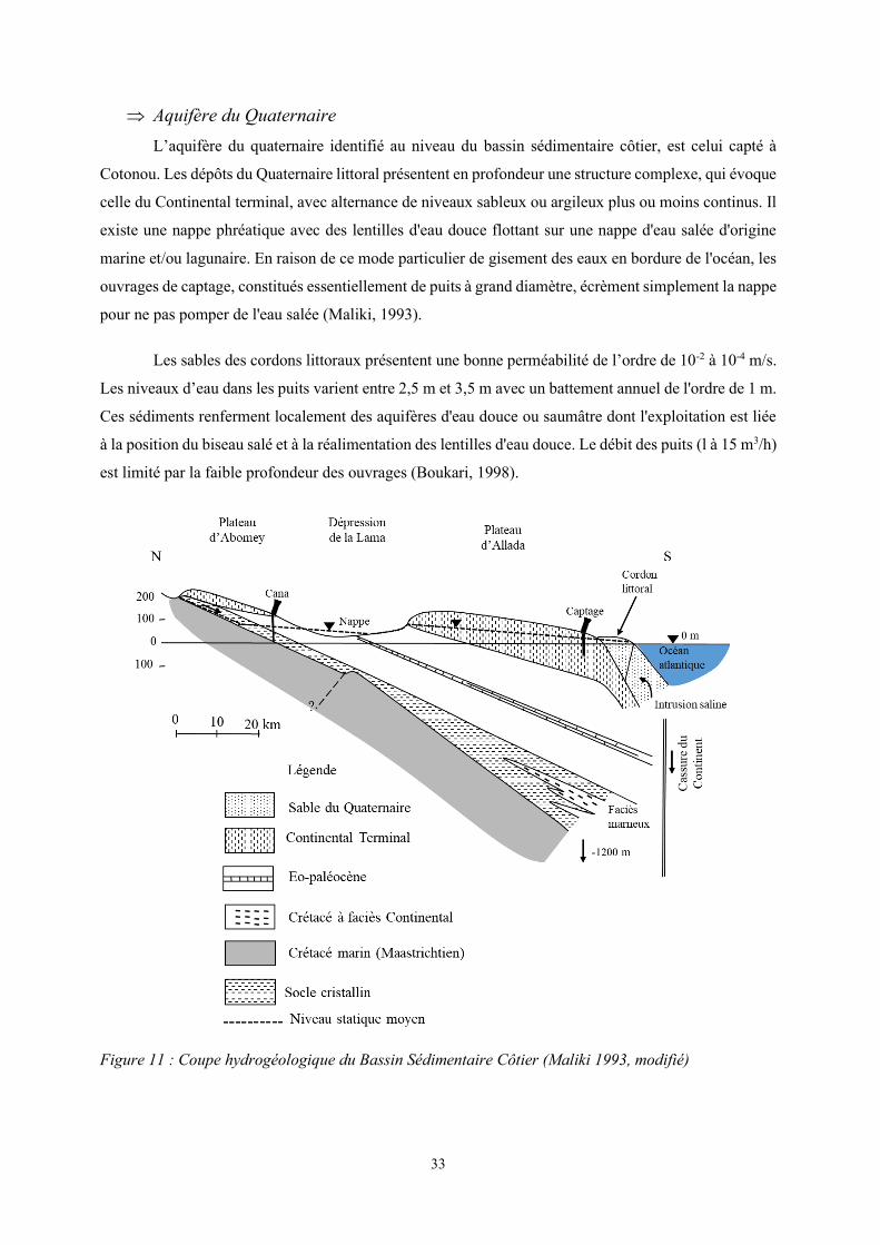
Aquifère du Quaternaire

L’aquifère du quaternaire identifié au niveau du bassin sédimentaire côtier, est celui capté à

Cotonou. Les dépôts du Quaternaire littoral présentent en profondeur une structure complexe, qui évoque

celle du Continental terminal, avec alternance de niveaux sableux ou argileux plus ou moins continus. Il

existe une nappe phréatique avec des lentilles d'eau douce flottant sur une nappe d'eau salée d'origine

marine et/ou lagunaire. En raison de ce mode particulier de gisement des eaux en bordure de l'océan, les

ouvrages de captage, constitués essentiellement de puits à grand diamètre, écrèment simplement la nappe

pour ne pas pomper de l'eau salée (Maliki, 1993).

Les sables des cordons littoraux présentent une bonne perméabilité de l’ordre de 10-2 à 10-4 m/s.

Les niveaux d’eau dans les puits varient entre 2,5 m et 3,5 m avec un battement annuel de l'ordre de 1 m.

Ces sédiments renferment localement des aquifères d'eau douce ou saumâtre dont l'exploitation est liée

à la position du biseau salé et à la réalimentation des lentilles d'eau douce. Le débit des puits (l à 15 m3/h)

est limité par la faible profondeur des ouvrages (Boukari, 1998).

Figure 11 : Coupe hydrogéologique du Bassin Sédimentaire Côtier (Maliki 1993, modifié)

34

II.1.3.3 Piézométrie de l’aquifère du Quaternaire

La Figure 12 présente la surface piézométrique de l’aquifère peu profond de Cotonou observée

pendant la période de septembre 2016. Dans la zone située à l’Ouest du chenal, les courbes isopièzes se

referment au centre de la ville (Cadjèhoun, Gbégamey) et au Nord-ouest (kouhounou) représentant des

dômes piézométriques. Ce sont en effet des zones de recharge préférentielle de la nappe compte tenu de

leur altitude par rapport à la nappe phréatique (Malaki, 1993). A partir des dômes, les écoulements sont

centrifuges. Ainsi, on note un écoulement à partir du centre de Cotonou vers l’océan, le lac Nokoué et

les marécages. Les dômes de dépressions ou les zones marécageuses sont observées (Agla, Fidjrossè,

Aïbatin et Ahogbohouè).

Figure 12 : Carte de la surface piézométrique de l’aquifère peu profond de Cotonou pendant la saison des pluies en septembre 2016

35

II.2 Approche méthodologique

II.2.1 Sites d’investigation

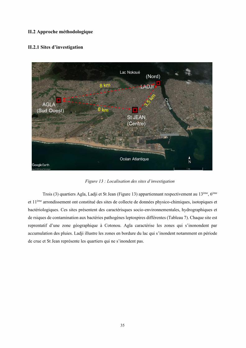
Figure 13 : Localisation des sites d’investigation

Trois (3) quartiers Agla, Ladji et St Jean (Figure 13) appartiennant respectivement au 13ème, 6ème

et 11ème arrondissement ont constitué des sites de collecte de données physico-chimiques, isotopiques et

bactériologiques. Ces sites présentent des caractérisques socio-environnementales, hydrographiques et

de rsiques de contamination aux bactéries pathogènes leptospires différentes (Tableau 7). Chaque site est

reprentatif d’une zone géographique à Cotonou. Agla caractérise les zones qui s’inonondent par

accumulation des pluies. Ladji illustre les zones en bordure du lac qui s’inondent notamment en période

de crue et St Jean représente les quartiers qui ne s’inondent pas.

36

Tableau 7: Critères de choix des quartiers

Quartiers Situation environnementale (Yadouléton 2015)

Illustration de l’état d’insalubrité (Photos Houéménou H. Juin 2017)

Prévalence leptospirose

(Dossou et al.

Données non

publiées)

Agla (13ème arrondissement)

- Population de 44000 hbts dans les quartiers en zone marécageuse -Eaux usées, ordures ménagères rejetées dans la nature ; défécation à l’air libre, présence de latrines, très bas standing -Inondable par accumulation des précipitations saisonnières ; faible capacité de retention en eau

11.8%

Ladji (6ème arrondissement)

-Population de 7000 hbts, quartier en bordure du lac -Pas d’eau courante à domicile, eaux usées et ordures ménagères rejetées dans la nature, présence de latrines, très bas standing -Inondable par les crues au niveau du Lac Nokoué pendant la petite saison des pluies où les crues sont prononcées

14%

Saint Jean (11ème arrondissement)

-Population de 3500 hbts, ancien quartier au centre ville - Ordures ménagères précollectées et/ou rejetées dans les caniveaux ; présence de latrines et fosses septiques -Non inondable en saison de pluies car les eaux de pluie peuvent s’infiltrer ou ruisseler vers les bas-fonds ou drainer vers les collecteurs d’eau pluviale

0.4%

Très insalubre

Très insalubre

Moyennement salubre

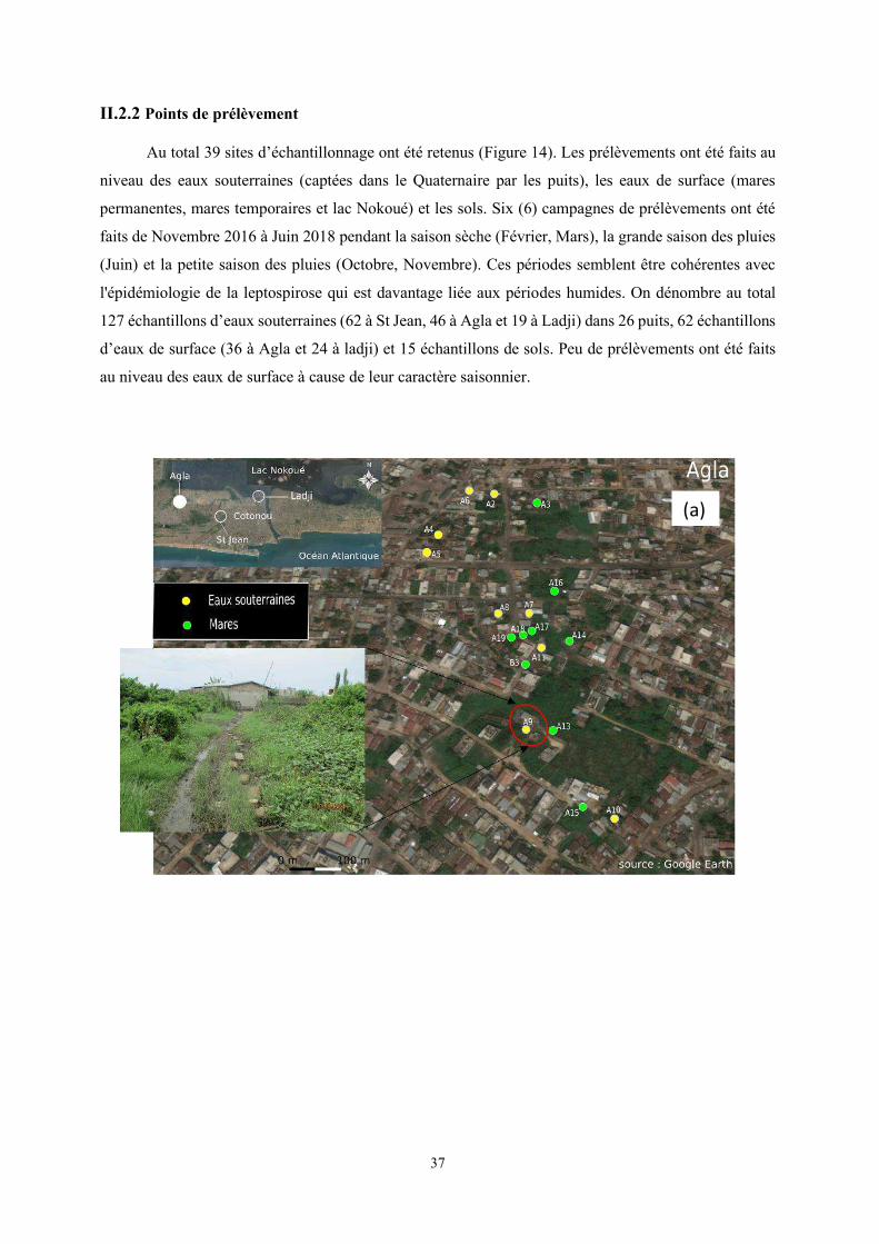
37

II.2.2 Points de prélèvement

Au total 39 sites d’échantillonnage ont été retenus (Figure 14). Les prélèvements ont été faits au

niveau des eaux souterraines (captées dans le Quaternaire par les puits), les eaux de surface (mares

permanentes, mares temporaires et lac Nokoué) et les sols. Six (6) campagnes de prélèvements ont été

faits de Novembre 2016 à Juin 2018 pendant la saison sèche (Février, Mars), la grande saison des pluies

(Juin) et la petite saison des pluies (Octobre, Novembre). Ces périodes semblent être cohérentes avec

l'épidémiologie de la leptospirose qui est davantage liée aux périodes humides. On dénombre au total

127 échantillons d’eaux souterraines (62 à St Jean, 46 à Agla et 19 à Ladji) dans 26 puits, 62 échantillons

d’eaux de surface (36 à Agla et 24 à ladji) et 15 échantillons de sols. Peu de prélèvements ont été faits

au niveau des eaux de surface à cause de leur caractère saisonnier.

(a)

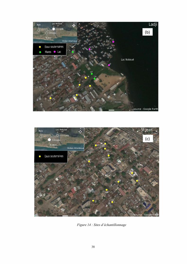
38

Figure 14 : Sites d’échantillonnage

(b)

(c)

39

II.2.2.1 Prélèvement des échantillons d’eaux souterraines et de surface

Les eaux de puits ont été prélevées à l’aide des puisettes souvent disposées sur les margelles des

puits. Pour les eaux de surface, le flacon est plongé chaque fois dans l’eau jusqu’à son remplissage. Les

mesures in situ sont effectuées au niveau de chaque point de prélèvement après rinçage des électrodes

avec l’eau à analyser.

Les prélèvements destinés à l’analyse des ions majeurs (Na+, K+, Mg2+, NH4+, Ca2+, Cl-, NO3

-,

NO2-, SO4

2-, PO43-, HCO3

-) sont filtrés sur des membranes en acétate de cellulose à 0,45 µm et prélevées

dans des flacons en polyéthylène de 50 ml. Les flacons pour le dosage des cations sont acidifiés avec de

l’acide nitrique ultra pur (HNO3).

Le prélèvement pour l’analyse des éléments traces (Li, B, Al, V, Cr, Mn, Fe, Co, Ni, Cu, Zn, As,

Mo, Ba, Pb, U) est réalisé dans des flacons de 15 mL en HDPE décontaminés à l’acide nitrique ultra pur.

Des échantillons blancs (avec de l’eau MilliQ) ont été préparés dans les mêmes conditions pour assurer

le contrôle qualité des résultats de laboratoire.

Le prélèvement pour les isotopes stables de la molécule d’eau l’oxygène-18 et le deutérium (18O

et ²H) est réalisé dans des piluliers de verre ambré de 20 mL.

Le prélèvement pour le Carbone Organique Dissout (COD) est effectué dans des pilulier de verre ambré

de 30 mL. De l’acide mercurique a été ajouté aux échantillons destinés à l’analyse du Carbone Organique

Dissous pour empêcher la dégradation du carbone organique par des bactéries.

Ensuite, les flacons sont hermétiquement fermés et bien conservés à 4°C avant leur acheminement dans

les différents laboratoires sollicités pour leur analyse.

Parallèlement à ces activités de prélèvement, une fiche de questionnaire a été renseignée. Elle a

pris en compte les aspects tels que : la gestion des ordures ménagères, les usages par rapport aux différents

types d’eau, les informations générales sur chaque site (surface inondée, présence d’animaux, activités

agricoles, etc.) (Voir annexe 1)

II.2.2.2 Prélèvement des échantillons de sols dans la Zone Non Saturée

Le prélèvement des sols a été fait sur les sites A11, L18 et J11 respectivement à Agla, Ladji et

St Jean en février 2018 pendant la saison sèche (Fig. 15). Les sites identifiés sont des dépotoirs sauvages

anciens datant de plus de 5 ans (A11 et L18) et d’un site sans dépôtoire (J11). Ils ont été choisis afin de

mieux comprendre le processus de transfert de pollaunts au travers de la Zone Non Saturée. Les

échantillons ont été prélevés à l’aide d’une tarière de dimension 5cm*20 cm. Les échantillons de sol ont

été prélevés depuis la surface sur sol (au dessus du terrain naturel) et à chaque 20 cm de la profondeur

de la Zone Non Saturée. La profondeur d’investigation qui correspond à l’épaisseur de la Zone Non

Saturée, est de 40 cm pour A11, 80 cm pour L18 et 120 cm J11. Les échantillons ont eté enrôlés dans des

fils plastiques alimentaires afin de les garder frais et ensuite mis dans des sacs étanches en polyéthylène.

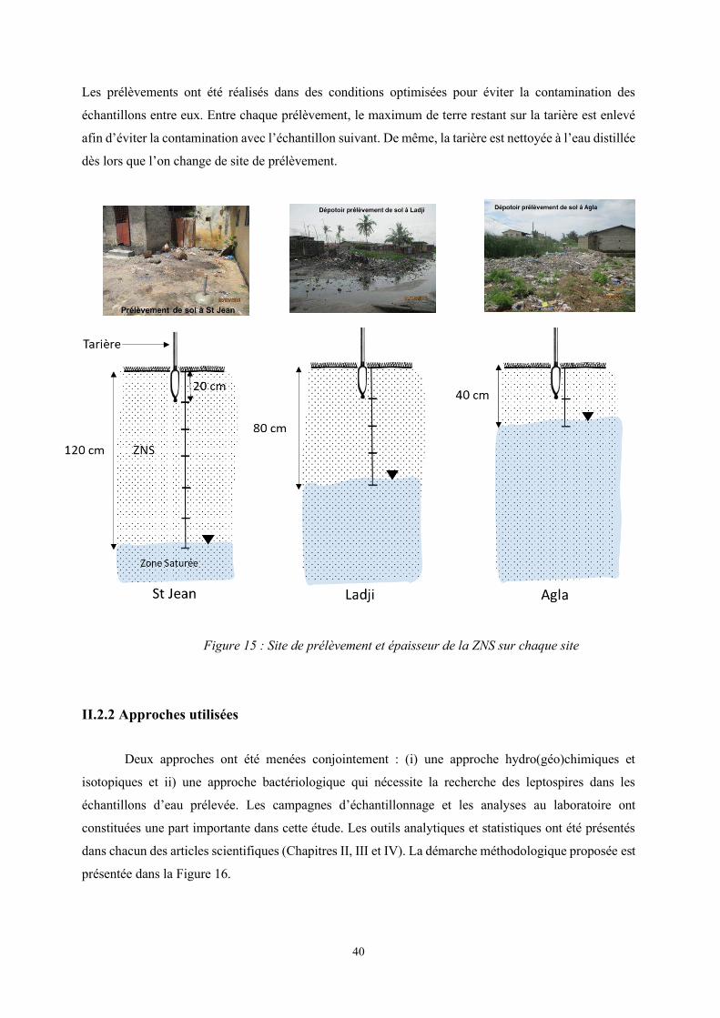
40

Les prélèvements ont été réalisés dans des conditions optimisées pour éviter la contamination des

échantillons entre eux. Entre chaque prélèvement, le maximum de terre restant sur la tarière est enlevé

afin d’éviter la contamination avec l’échantillon suivant. De même, la tarière est nettoyée à l’eau distillée

dès lors que l’on change de site de prélèvement.

Figure 15 : Site de prélèvement et épaisseur de la ZNS sur chaque site

II.2.2 Approches utilisées

Deux approches ont été menées conjointement : (i) une approche hydro(géo)chimiques et

isotopiques et ii) une approche bactériologique qui nécessite la recherche des leptospires dans les

échantillons d’eau prélevée. Les campagnes d’échantillonnage et les analyses au laboratoire ont

constituées une part importante dans cette étude. Les outils analytiques et statistiques ont été présentés

dans chacun des articles scientifiques (Chapitres II, III et IV). La démarche méthodologique proposée est

présentée dans la Figure 16.

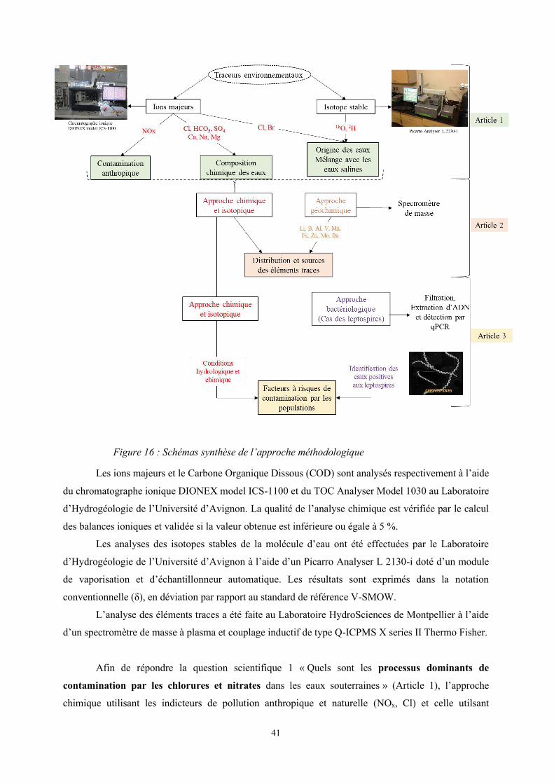
41

Figure 16 : Schémas synthèse de l’approche méthodologique

Les ions majeurs et le Carbone Organique Dissous (COD) sont analysés respectivement à l’aide

du chromatographe ionique DIONEX model ICS-1100 et du TOC Analyser Model 1030 au Laboratoire

d’Hydrogéologie de l’Université d’Avignon. La qualité de l’analyse chimique est vérifiée par le calcul

des balances ioniques et validée si la valeur obtenue est inférieure ou égale à 5 %.

Les analyses des isotopes stables de la molécule d’eau ont été effectuées par le Laboratoire

d’Hydrogéologie de l’Université d’Avignon à l’aide d’un Picarro Analyser L 2130-i doté d’un module

de vaporisation et d’échantillonneur automatique. Les résultats sont exprimés dans la notation

conventionnelle (δ), en déviation par rapport au standard de référence V-SMOW.

L’analyse des éléments traces a été faite au Laboratoire HydroSciences de Montpellier à l’aide

d’un spectromètre de masse à plasma et couplage inductif de type Q-ICPMS X series II Thermo Fisher.

Afin de répondre la question scientifique 1 « Quels sont les processus dominants de

contamination par les chlorures et nitrates dans les eaux souterraines » (Article 1), l’approche

chimique utilisant les indicteurs de pollution anthropique et naturelle (NOx, Cl) et celle utilsant

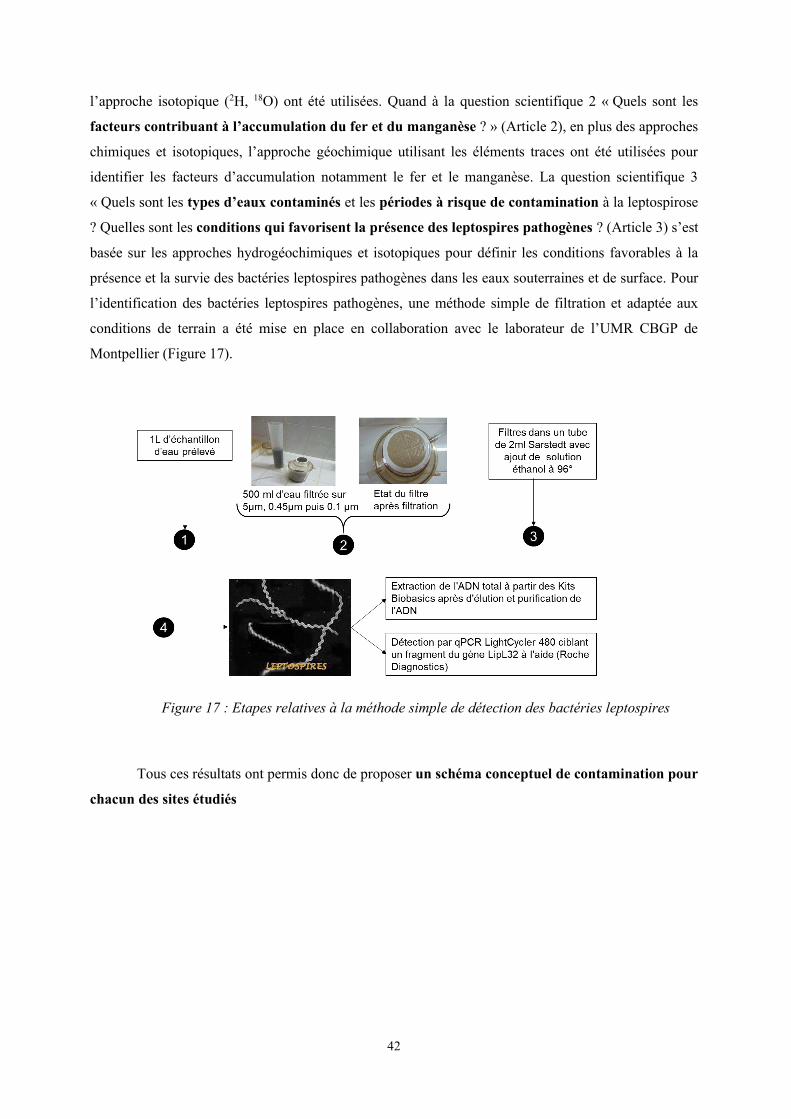
42

l’approche isotopique (2H, 18O) ont été utilisées. Quand à la question scientifique 2 « Quels sont les

facteurs contribuant à l’accumulation du fer et du manganèse ? » (Article 2), en plus des approches

chimiques et isotopiques, l’approche géochimique utilisant les éléments traces ont été utilisées pour

identifier les facteurs d’accumulation notamment le fer et le manganèse. La question scientifique 3

« Quels sont les types d’eaux contaminés et les périodes à risque de contamination à la leptospirose

? Quelles sont les conditions qui favorisent la présence des leptospires pathogènes ? (Article 3) s’est

basée sur les approches hydrogéochimiques et isotopiques pour définir les conditions favorables à la

présence et la survie des bactéries leptospires pathogènes dans les eaux souterraines et de surface. Pour

l’identification des bactéries leptospires pathogènes, une méthode simple de filtration et adaptée aux

conditions de terrain a été mise en place en collaboration avec le laborateur de l’UMR CBGP de

Montpellier (Figure 17).

Figure 17 : Etapes relatives à la méthode simple de détection des bactéries leptospires

Tous ces résultats ont permis donc de proposer un schéma conceptuel de contamination pour

chacun des sites étudiés

43

II.3 Références

Adeniyi, Adeleke, Kafeelah Yusuf, Olumuyiwa Okedeyi, et Mutiu Sowemimo. 2016. « Classification and Health Risk Assessment for Borehole Water Contaminated by Metals in Selected Households in Southwest Nigeria ». Journal of Water Resource and Protection 08 (04): 459‑71. https://doi.org/10.4236/jwarp.2016.84039.

Adjagodo, Antoinette, Micheline Agassounon Djikpo Tchibozo, Nelly C. Kelome, et Rébécca Lawani. 2016. « Flux des polluants liés aux activités anthropiques, risques sur les ressources en eau de surface et la chaine trophique à travers le monde : synthèse bibliographique ». International

Journal of Biological and Chemical Sciences 10 (3): 1459‑72. Allan, Kathryn J., Holly M. Biggs, Jo E. B. Halliday, Rudovick R. Kazwala, Venance P. Maro, Sarah

Cleaveland, et John A. Crump. 2015. « Epidemiology of Leptospirosis in Africa: A Systematic Review of a Neglected Zoonosis and a Paradigm for ‘One Health’ in Africa ». Édité par Jakob Zinsstag. PLOS Neglected Tropical Diseases 9 (9): e0003899. https://doi.org/10.1371/journal.pntd.0003899.

Aoki, Tomohiro, Nobuo Koizumi, et Haruo Watanabe. 2001. « A Case of Leptospirosis Probably Caused by Drinking Contaminated Well-Water after an Earthquake ». Laboratory and

Epidemiology Communication, no Jpn. J. Infect. Dis., 54: 243‑44. Assogba, Liliane Philippine. 2010. « Memoire Online - Etude de l’influence du lac Nokoué et du

chenal sur les inondations dans la ville de Cotonou au Bénin ». Memoire Online. 2010. https://www.memoireonline.com/10/12/6381/m_Etude-de-l-influence-du-lac-Nokoue-et-du-chenal-sur-les-inondations-dans-la-ville-de-Cotonou-au-Be.html.

Atidegla, C, et K Agbossou. 2010. « Pollutions chimique et bactériologique des eaux souterraines des exploitations maraîchères irriguées de la commune de Grand-Popo : cas des nitrates et bactéries fécales ». International Journal of Biological and Chemical Sciences 4 (2). https://doi.org/10.4314/ijbcs.v4i2.58119.

Aubry, Pierre, et Bernard-Alex Gauzère. 2019. « Leptospirose: Actualité 2018 ». Médécine tropicale. 13 janvier 2019. http://medecinetropicale.free.fr/cours/leptospirose.pdf.

Azokpota, V. 2005. « Impact de l’utilisation des colorants sur la qualité du milieu aquatique à Cotonou : cas de la teinture artisanale des textiles ».

Barrett, M. H., Kevin M. Hiscock, Stephen Pedley, David N. Lerner, John H. Tellam, et Mike J. French. 1999. « Marker Species for Identifying Urban Groundwater Recharge Sources: A Review and Case Study in Nottingham, UK ». Water Research 33 (14): 3083‑97. https://doi.org/10.1016/S0043-1354(99)00021-4.

Barrett, M.H. 2004. Characteristics of Urban Groundwater. In: Urban Groundwater Pollution. D. N. Lerner Ed. Taylor & Francis. Leiden, Netherlands. International Contributions to Hydrogeology n°24: International Association of Hydrogeologists (IAH). https://www.crcpress.com/Urban-Groundwater-Pollution-IAH-International-Contributions-to-Hydrogeology/Lerner/p/book/9789058096296.

Bertherat, Eric, Melissa J. Mueller, Jean-Christophe Shako, et Mathieu Picardeau. 2014. « Discovery of a Leptospirosis Cluster Amidst a Pneumonic Plague Outbreak in a Miners’ Camp in the Democratic Republic of the Congo ». International Journal of Environmental Research and

Public Health 11 (2): 1824‑33. https://doi.org/10.3390/ijerph110201824. Bierque, Emilie, Roman Thibeaux, Dominique Girault, Marie-Estelle Soupé-Gilbert, et Cyrille

Goarant. 2020. « A systematic review of Leptospira in water and soil environments ». PLOS

ONE 15 (1): e0227055. https://doi.org/10.1371/journal.pone.0227055. Birke, Manfred, Uwe Rauch, Bodo Harazim, Hans Lorenz, et Wolfgang Glatte. 2010. « Major and

trace elements in German bottled water, their regional distribution, and accordance with national and international standards ». Journal of Geochemical Exploration, Mineral Waters of Europe, 107 (3): 245‑71. https://doi.org/10.1016/j.gexplo.2010.06.002.

Boukari. 1998. « Fonctionnement du système aquifère exploité pour l’approvisionnement en eau de la ville de Cotonou sur le littoral béninois : impact du développement urbain sur la qualité des ressources ». Université cheikh Anta Diop de Dakar, Faculté des Sciences et Technique, Département de Géologies.

44

Boukari, M., A. Alassane, F. Azonsi, F. Dovonou, A. Tossa, et D. Zogo. 2006. « Groundwater Pollution from Urban Development in Cotonou City, Benin. » In Yongxin Xu, Brent Usher 2006, Groundwater Pollution in Africa, 125-138.

Boukari, M., C. B. Gaye, A. Faye, et S. Faye. 1996. « The impact of urban development on coastal aquifers near Cotonou, Benin ». Journal of African Earth Sciences, Hydrogeochemical Studies in Sub-Saharan Africa, 22 (4): 403‑8. https://doi.org/10.1016/0899-5362(96)00027-9.

Chabour, Nabil, Benabbas Chaouki, Bourefis Ahcene, et Kermandji Adnane. 2009. « L’impact de l’etalement urbain sur les hydrosystemes littoraux. Cas de la plaine de collo (N-E Algerien) », 10.

Costa, Federico, José E. Hagan, Juan Calcagno, Michael Kane, Paul Torgerson, Martha S. Martinez-Silveira, Claudia Stein, Bernadette Abela-Ridder, et Albert I. Ko. 2015. « Global Morbidity and Mortality of Leptospirosis: A Systematic Review ». Édité par Pamela L. C. Small. PLOS

Neglected Tropical Diseases 9 (9): e0003898. https://doi.org/10.1371/journal.pntd.0003898. Danvidé, Taméon, Benoît. 2015. « Gouvernance des politiques de planification urbaine et gestion des

inondations à Cotonou (Bénin) ». Thèse unique de Doctorat, Université d’Abomey-Calavi et Université Paris 8.

De Waele, J., I. A. Nyambe, A. Di Gregorio, F. Di Gregorio, S. Simasiku, R. Follesa, et S. Nkemba. 2004. « Urban waste landfill planning and karstic groundwater resources in developing countries: the example of Lusaka (Zambia) ». Journal of African Earth Sciences, Key Points on African Geology, 39 (3): 501‑8. https://doi.org/10.1016/j.jafrearsci.2004.07.014.

Dieng, Ndeye Maguette, Philippe Orban, Joel Otten, Christine Stumpp, Serigne Faye, et Alain Dassargues. 2017. « Temporal Changes in Groundwater Quality of the Saloum Coastal Aquifer ». Journal of Hydrology: Regional Studies 9 (février): 163‑82. https://doi.org/10.1016/j.ejrh.2016.12.082.

Dinelli, E., A. Lima, B. De Vivo, S. Albanese, D. Cicchella, et P. Valera. 2010. « Hydrogeochemical Analysis on Italian Bottled Mineral Waters: Effects of Geology ». Journal of Geochemical

Exploration 107 (3): 317‑35. https://doi.org/10.1016/j.gexplo.2010.06.004. Dobigny, Gauthier, Philippe Gauthier, Gualbert Houéménou, Armelle Choplin, Henri-Joël Dossou,

Sylvestre Badou, Jonas Etougbétché, et al. 2018. « Leptospirosis and Extensive Urbanization in West Africa: A Neglected and Underestimated Threat? » Urban Science 2 (2): 29. https://doi.org/10.3390/urbansci2020029.

Dong, Bo, Renzhi Zhang, Yandong Gan, Liqun Cai, Ariel Freidenreich, Kepeng Wang, Tianwen Guo, et Hongbin Wang. 2019. « Multiple methods for the identification of heavy metal sources in cropland soils from a resource-based region ». Science of The Total Environment 651 (février): 3127‑38. https://doi.org/10.1016/j.scitotenv.2018.10.130.

Dovonou, Flavien, Naéssé Adjahossou, Eric Alamou, Abdoukarim Alassane, Daouda Mama, et Moussa Boukari. 2015. « Pollution des eaux souterraines par les métaux lourds et leur impact sur l’environnement : cas de l’aquifère superficiel du champ de captage intensif de Godomey au Sud-Bénin ». LHA / FAST / UAC) 01 BP 4521 Cotonou (Bénin), 22.

Dovonou, Flavien, M Aina, M Boukari, et A Alassane. 2012. « Pollution physico-chimique et bactériologique d’un écosystème aquatique et ses risques écotoxicologiques: Cas du lac Nokoue au Sud Benin ». International Journal of Biological and Chemical Sciences 5 (4). https://doi.org/10.4314/ijbcs.v5i4.23.

Fayiga, Abioye O., Mabel O. Ipinmoroti, et Tait Chirenje. 2018. « Environmental Pollution in Africa ». Environment, Development and Sustainability 20 (1): 41‑73. https://doi.org/10.1007/s10668-016-9894-4.

Felzemburgh, Ridalva D. M., Guilherme S. Ribeiro, Federico Costa, Renato B. Reis, José E. Hagan, Astrid X. T. O. Melendez, Deborah Fraga, et al. 2014. « Prospective Study of Leptospirosis Transmission in an Urban Slum Community: Role of Poor Environment in Repeated Exposures to the Leptospira Agent ». PLOS Neglected Tropical Diseases 8 (5): e2927. https://doi.org/10.1371/journal.pntd.0002927.

Ganoza, Christian A, Michael A Matthias, Devon Collins-Richards, Kimberly C Brouwer, Calaveras B Cunningham, Eddy R Segura, Robert H Gilman, Eduardo Gotuzzo, et Joseph M Vinetz. 2006. « Determining Risk for Severe Leptospirosis by Molecular Analysis of Environmental Surface

45

Waters for Pathogenic Leptospira ». Édité par Nicholas White. PLoS Medicine 3 (8): e308. https://doi.org/10.1371/journal.pmed.0030308.

Goita, Adam. 2013. « Les bactéries pathogènes d’origine hydrique de lépidémiologie à la prévention ». Université Mohamed v-Souissi.

Hassane, Aïssata B., Christian Leduc, Guillaume Favreau, Barbara A. Bekins, et Thomas Margueron. 2016. « Impacts of a Large Sahelian City on Groundwater Hydrodynamics and Quality: Example of Niamey (Niger) ». Hydrogeology Journal 24 (2): 407‑23. https://doi.org/10.1007/s10040-015-1345-z.

Houéménou, G., A Ahmed, R. Libois, et R.A. Hartskeerl. 2014. « Leptospira spp. Prevalence in Small Mammal Populations in Cotonou, Benin ». International Scholarly Research Notices Volume 2013, Article ID 502638 (ISRN Epidemiology): 8. http://dx.doi.org/10.5402/2013/502638.

Houéménou, G., Philippe Gauthier, Jonas Etougbétché, Sylvestre Badou, Henri-Joël Dossou, David Agossou, Mathieu Picardeau, et Gauthier Dobigny. 2019. « Pathogenic Leptospira in Commensal Small Mammals from the Extensively Urbanized Coastal Benin ». Urban Science 3 (3): 99. https://doi.org/10.3390/urbansci3030099.

Hounkpe, Sena Peace, Edmond Codjo Adjovi, Martin Crapper, et Esi Awuah. 2014. « Wastewater Management in Third World Cities: Case Study of Cotonou, Benin ». Journal of

Environmental Protection 05 (avril): 387. https://doi.org/10.4236/jep.2014.55042. Hounsinou, Parfait Sagnon, Daouda Mama, Micheline Agassounon Djikpo Tchibozo, Moussa Boukari,

et Dominique Sohounhloue. 2015. « Microbiological Pollution Indication as Tracer for the Pollution of Well Water: The Example of the District of Abomey-Calavi (Benin) ». Journal of

Environmental Protection 06 (04): 290‑98. https://doi.org/10.4236/jep.2015.64029. Ikem, Abua, Seyi Odueyungbo, Nosa O. Egiebor, et Kafui Nyavor. 2002. « Chemical quality of bottled

waters from three cities in eastern Alabama ». Science of The Total Environment 285 (1): 165‑75. https://doi.org/10.1016/S0048-9697(01)00915-9.

INSAE. 2016. « Principaux indicateurs socio-démographiques et économiques du département du Littoral ».

Institut National de la Statistique et de l’Analyse Économique (INSAE), et ICF. 2019. « Enquête Démographique et de Santé au Bénin, 2017-2018 ». Cotonou, Bénin et Rockville, Maryland, USA : INSAE et ICF.

Juif, Marylène. 2011. « Les zoonoses transmissibles du rat à l’homme: Conseils en officine ». Université Henri Poincare-Nancy.

Kadjangaba, Edith, Daїra Djoret, Jean-Caude Doumnang Mbaigane, Anacle Ndoutamia Guelmbaye, et Yaya Mahmout. 2018. « Impact des Processus Hydrochimique sur la Qualité des Eaux souterraines de la Ville de N’Djaména-Tchad ». European Scientific Journal 14 (18). https://doi.org/10.19044/esj.2018.v14n18p162.

Kayembe, John M., Periyasamy Sivalingam, Carmen Diz Salgado, Jeff Maliani, Patience Ngelinkoto, Jean-Paul Otamonga, Crispin K. Mulaji, Josué I. Mubedi, et John Poté. 2018. « Assessment of Water Quality and Time Accumulation of Heavy Metals in the Sediments of Tropical Urban Rivers: Case of Bumbu River and Kokolo Canal, Kinshasa City, Democratic Republic of the Congo ». Journal of African Earth Sciences 147 (novembre): 536‑43. https://doi.org/10.1016/j.jafrearsci.2018.07.016.

Ko, Albert I., Cyrille Goarant, et Mathieu Picardeau. 2009. « Leptospira : the dawn of the molecular genetics era for an emerging zoonotic pathogen | Nature Reviews Microbiology ». Natural

reviews microbiology, 7(10): 736–747. https://doi.org/10.1038/nrmicro2208. Ko, Albert I, Mitermayer Galvào Reis, Cibele M Ribeiro Dourado, Warren D Johnson, et Lee W Riley.

1999. « Urban Epidemic of Severe Leptospirosis in Brazil ». The Lancet 354 (9181): 820‑25. https://doi.org/10.1016/S0140-6736(99)80012-9.

Lapworth, D. J., D. C. W. Nkhuwa, J. Okotto-Okotto, S. Pedley, M. E. Stuart, M. N. Tijani, et J. Wright. 2017. « Urban Groundwater Quality in Sub-Saharan Africa: Current Status and Implications for Water Security and Public Health ». Hydrogeology Journal 25 (4): 1093‑1116. https://doi.org/10.1007/s10040-016-1516-6.

Lau, Colleen L., Lee D. Smythe, Scott B. Craig, et Philip Weinstein. 2010. « Climate Change, Flooding, Urbanisation and Leptospirosis: Fuelling the Fire? » Transactions of the Royal

46

Society of Tropical Medicine and Hygiene 104 (10): 631‑38. https://doi.org/10.1016/j.trstmh.2010.07.002.

Lau, Colleen L., Conall H. Watson, John H. Lowry, Michael C. David, Scott B. Craig, Sarah J. Wynwood, Mike Kama, et Eric J. Nilles. 2016. « Human Leptospirosis Infection in Fiji: An Eco-Epidemiological Approach to Identifying Risk Factors and Environmental Drivers for Transmission ». Édité par Mathieu Picardeau. PLOS Neglected Tropical Diseases 10 (1): e0004405. https://doi.org/10.1371/journal.pntd.0004405.

Levett, Paul N. 2001. « Leptospirosis ». Clinical Microbiology Reviews 14 (2): 296‑326. https://doi.org/10.1128/CMR.14.2.296-326.2001.

Maciel, Elves A. P., Ana Luiza F. de Carvalho, Simone F. Nascimento, Rosan B. de Matos, Edilane L. Gouveia, Mitermayer G. Reis, et Albert I. Ko. 2008. « Household Transmission of Leptospira Infection in Urban Slum Communities ». PLOS Neglected Tropical Diseases 2 (1): e154. https://doi.org/10.1371/journal.pntd.0000154.

Maliki, Raoufou Aboudou. 1993. « Etude hydrogéologique du littoral béninois dans la région de Cotonou et ses environs ». Université C. A. Diop de Dakar. Sénégal, Faculté des Sciences et Techniques, Département de Géologie.

Mason, Meghan R., Carolina Encina, Srinand Sreevatsan, et Claudia Muñoz-Zanzi. 2016. « Distribution and Diversity of Pathogenic Leptospira Species in Peri-Domestic Surface Waters from South Central Chile ». Édité par Mathieu Picardeau. PLOS Neglected Tropical

Diseases 10 (8): e0004895. https://doi.org/10.1371/journal.pntd.0004895. McInnis, D., S. Silliman, M. Boukari, N. Yalo, S. Orou-Pete, C. Fertenbaugh, K. Sarre, et H. Fayomi.

2013. « Combined Application of Electrical Resistivity and Shallow Groundwater Sampling to Assess Salinity in a Shallow Coastal Aquifer in Benin, West Africa ». Journal of Hydrology 505 (novembre): 335‑45. https://doi.org/10.1016/j.jhydrol.2013.10.014.

Muñoz-Zanzi, Claudia, Meghan Mason, Carolina Encina, Angel Astroza, et Alex Romero. 2014. « Leptospira Contamination in Household and Environmental Water in Rural Communities in Southern Chile ». International Journal of Environmental Research and Public Health 11 (7): 6666‑80. https://doi.org/10.3390/ijerph110706666.

Mwachui, Mwanajaa Abdalla, Lisa Crump, Rudy Hartskeerl, Jakob Zinsstag, et Jan Hattendorf. 2015. « Environmental and Behavioural Determinants of Leptospirosis Transmission: A Systematic Review ». Édité par Pamela L. C. Small. PLOS Neglected Tropical Diseases 9 (9): e0003843. https://doi.org/10.1371/journal.pntd.0003843.

N’Bessa, Benoît. 1997. « Porto-Novo et Cotonou (Bénin): origine et évolution d’un doublet urbain ». Thèse d’État, France: Université Bordeaux Montaigne.

Ndiaye, M. L., H.-R. Pfeifer, S. Niang, Y. Dieng, M. Tonolla, et R. Peduzzi. 2010. « Impacts de l’utilisation des eaux polluées en agriculture urbaine sur la qualité de la nappe de Dakar (Sénégal) ». VertigO - la revue électronique en sciences de l’environnement, no Volume 10 numéro 2 (septembre). https://doi.org/10.4000/vertigo.9965.

Ngambi, Jules Raymond. 2015. « Déchets solides ménagers de la ville de Yaoundé (Cameroun) : de la gestion linéaire vers une économie circulaire ». Thèse de doctorat, Université du Maine.

Ntakirutimana, Désiré. 2013. « Etude sérologique de la leptospirose canine au Sénégal ». Université cheikh Anta Diop de Dakar, Ecole Inter-Etat des ciences et médécine vétérinaires.

Odoulami, Léocadie. 2009. « La problématique de l’eau potable et la santé humaine dans la ville de Cotonou (République du Bénin) ». Université d’Abomey-Calavi.

Odoulami, Léocadie, Expédit W Vissin, et Michel Boko. 2011. « Projection des besoins d’approvisionnement en eau de la ville de Cotonou d’ici l’an 2025 », 76.

Ogrinc, Nives, Samo Tamše, Saša Zavadlav, Janja Vrzel, et Lixin Jin. 2019. « Evaluation of geochemical processes and nitrate pollution sources at the Ljubljansko polje aquifer (Slovenia): A stable isotope perspective ». Science of The Total Environment 646 (janvier): 1588‑1600. https://doi.org/10.1016/j.scitotenv.2018.07.245.

OMS. 2016. « Intoxication au plomb et santé ». 2016. ONU Habitat. 2010. « Etat des villes africaines: Gouvernance, inégalité et marchés fonciers urbains ». ———. 2014. « L’urbanisation: Un impératif pour la transformation structurelle de l’Afrique. Une

nouvelle conception de l’urbanisation en appui à l’Agenda 2063 ».

47

Ouandaogo-Yameogo, Suzanne. 2008. « Ressources en eau souterraine du centre urbain de Ouagadougou au Burkina Faso, qualité et vulnérabilité ». Thèse de Doctorat de l’Université d’Avignon et des Pays de Vaucluse, spécialité Hydrogéologie,. http://www.theses.fr/2008AVIG0040.

Ouedraogo, Issoufou, Pierre Defourny, et Marnik Vanclooster. 2016. « Mapping the groundwater vulnerability for pollution at the pan African scale ». Science of The Total Environment 544 (février): 939‑53. https://doi.org/10.1016/j.scitotenv.2015.11.135.

Paré, Samuel, et L Yvonne Bonzi-Coulibaly. 2013. « Water Quality Issues in West and Central Africa: Present Status and Future Challenges ». AHS Publ. 361, Understanding Freshwater Quality Problems in a Changing World, , 87‑95.

Parslow, R. C., P. A. McKinney, G. R. Law, A. Staines, R. Williams, et H. J. Bodansky. 1997. « Incidence of Childhood Diabetes Mellitus in Yorkshire, Northern England, Is Associated with Nitrate in Drinking Water: An Ecological Analysis ». Diabetologia 40 (5): 550‑56. https://doi.org/10.1007/s001250050714.

Rai, Prabhat Kumar, Sang Soo Lee, Ming Zhang, Yiu Fai Tsang, et Ki-Hyun Kim. 2019. « Heavy metals in food crops: Health risks, fate, mechanisms, and management ». Environment

International 125 (avril): 365‑85. https://doi.org/10.1016/j.envint.2019.01.067. Rapport EAA. Juin 2018b. « Etude de référence sur les comportements, attitudes et pratiques des

populations de Cotonou sur la chaine de l’eau dans la ville de Cotonou ». ———. 2018a. « Organisation de la campagne de prélèvement et d’analyse de contrôle sanitaire de la

qualité de l’eau stockée et consommée dans la ville de Cotonou ». Rapport final. Ristow, Paula. 2007. « La leptospirose : Les défis actuels d’une ancienne maladie ». Bulletin de

l’Académie vétérinaire de France, no 2: 267. https://doi.org/10.4267/2042/47896. Roufai, Mohamed Chakirou. 2012. « Environnement, santé publique et risques sanitaires liés à l’eau à

Cotonou au Bénin : approches par modélisation et analyse spatiales ». Thesis, Paris 4. École doctorale de Géographie de Paris. Espace, sociétés, aménagement (Paris). http://www.theses.fr/2012PA040095.

Saizonou, Mickael, Boniface Yehouenou, Honoré S Bankolé, Roger Gérard Jossé, et Henri Soclo. 2010. « Impacts des déchets de l’Abattoir de Cotonou dans la dégradation de la qualité des eaux de la nappe phréatique », 13.

Saizonou, Mickael, Alassane Youssao, Magloire Gbaguidi, Léonce Dovonon, Henri H Soclo, et Dominique Sohounhoulé. 2014. « [ Contribution of household wastewater and stormwater in pollution of waters of the channel of Cotonou in Benin ] » 9 (1): 14.

Sejvar, James, Elizabeth Bancroft, Kevin Winthrop, Julie Bettinger, Mary Bajani, Sandra Bragg, Kathleen Shutt, et al. 2003. « Leptospirosis in “Eco-Challenge” Athletes, Malaysian Borneo, 2000 ». Emerging Infectious Diseases 9 (6): 702‑7. https://doi.org/10.3201/eid0906.020751.

Soro, N., L. Ouattara, K. Dongo, E. K. Kouadio, E. K. Ahoussi, G. Soro, M. S. Oga, I. Savane, et J. Biemi. 2010. « Déchets Municipaux Dans Le District d’Abidjan En Côte d’Ivoire: Sources Potentielles de Pollution Des Eaux Souterraines ». International Journal of Biological and

Chemical Sciences 4 (6). https://doi.org/10.4314/ijbcs.v4i6.64952. Thibeaux, Roman, Sophie Geroult, Claire Benezech, Stéphane Chabaud, Marie-Estelle Soupé-Gilbert,

Dominique Girault, Emilie Bierque, et Cyrille Goarant. 2017. « Seeking the Environmental Source of Leptospirosis Reveals Durable Bacterial Viability in River Soils ». Édité par Claudia Munoz-Zanzi. PLOS Neglected Tropical Diseases 11 (2): e0005414. https://doi.org/10.1371/journal.pntd.0005414.

Totin, Henri S V, Ernest Amoussou, Léocadie Odoulami, Patrick A Edorh, Moussa Boukari, et Michel Boko. 2013. « Groundwater Pollution and the Safe Water Supply Challenge in Cotonou Town, Benin (West Africa) ». IAHS Publ. 361, Understanding Freshwater Quality Problems in a Changing World, , 7.

UNDP, United Nations Development Programme. 2018. « Nature for Water, Nature for Life: Nature-Based Solutions for Achieving the Global Goals. » New York, USA: UNDP. http://www.undp.org/content/undp/en/home/librarypage/poverty-reduction/nature-for-water---nature-for-life.html.

Vries, Sophia G. de, Benjamin J. Visser, Ingeborg M. Nagel, Marga G.A. Goris, Rudy A. Hartskeerl, et Martin P. Grobusch. 2014. « Leptospirosis in Sub-Saharan Africa: A Systematic Review ».

48

International Journal of Infectious Diseases 28 (novembre): 47‑64. https://doi.org/10.1016/j.ijid.2014.06.013.

Warburton, D. W., P. I. Peterkin, K. F. Weiss, et M. A. Johnston. 1986. « Microbiological Quality of Bottled Water Sold in Canada ». Canadian Journal of Microbiology 32 (11): 891‑93.

Wuthiekanun, Vanaporn, Nisa Sirisukkarn, Prayad Daengsupa, Prangyong Sakaraserane, Amornwadee Sangkakam, Wirongrong Chierakul, Lee D. Smythe, et al. 2007. « Clinical Diagnosis and Geographic Distribution of Leptospirosis, Thailand ». Emerging Infectious Diseases 13 (1): 124‑26. https://doi.org/10.3201/eid1301.060718.

WWAP, Programme mondial pour l’évaluations des ressources en eau). 2017. Rapport mondial des

Nations Unies sur la mise en valeur des ressources en eau 2017. Les eaux usées – Une

ressource inexploitée. Paris, UNESCO. http://creativecommons.org/licenses/by-sa/3.0/igo/. Wynwood, Sarah Jane, Glenn Charles Graham, Steven Lance Weier, Trudi Anne Collet, David Brian

McKay, et Scott Benjamin Craig. 2014. « Leptospirosis from Water Sources ». Pathogens and

Global Health 108 (7): 334‑38. https://doi.org/10.1179/2047773214Y.0000000156. Xu, Yongxin, et Brent Usher. 2006. Groundwater Pollution in Africa. UNEP/Earthprint. Yadouléton, M.J. 2015. « Assainissement environnemental à Cotonou et lutte contre le choléra ».

Thèse de Doctorat Unique, Université d’Abomey-Calavi. Yalo, Nicaise, Descloitres Marc, Alassane Abdoukarim, Mama Daouda, et Boukari Moussa. 2012.

« Environmental Geophysical Study of the Groundwater Mineralization in a Plot of the Cotonou Littoral Zone (South Benin) ». International Journal of Geophysics 2012: 1‑10. https://doi.org/10.1155/2012/329827.

Yehouenou Azehoun Pazou, E., B. Fayomi, D. Azocli, H. Acakpo, A. Soton, M. Boko, L. Fourn, D. Houinsa, et J.-C. Kèkè. 2009. « Qualité des eaux d’arrosage utilisées sur le site maraîcher de Houéyiho de Cotonou au Sud-Bénin ». Bulletin de la Recherche Agronomique du Bénin Numéro 65: 6.

Zeenat, A., A. a. M. Hatha, L. Viola, et K. Vipra. 2009. « Bacteriological Quality and Risk Assessment of the Imported and Domestic Bottled Mineral Water Sold in Fiji ». Journal of Water and

Health 7 (4): 642‑49. https://doi.org/10.2166/wh.2009.137.

49

CHAPITRE III : DEGRADATION DE LA QUALITE DES EAUX SOUTERRAINES (Article 1)

Contents lists available at ScienceDirect

Journal of Hydrology

journal homepage: www.elsevier.com/locate/jhydrol

Research papers

Degradation of groundwater quality in expanding cities in West Africa. Acase study of the unregulated shallow aquifer in Cotonou

Honoré Houéménoua,e,⁎, Sarah Tweedb, Gauthier Dobignyc,d, Daouda Mamae,Abdoukarim Alassanee, Roland Silmera, Milanka Babica, Stéphane Ruya, Alexis Chaigneauf,g,h,Philippe Gauthierc,d, Akilou Socohoue, Henri-Joël Dossoud, Sylvestre Badoud, Marc Leblanca

aUniversity of Avignon, Hydrogeology Laboratory, UMR EMMAH, Avignon, FrancebUMR G-eau, IRD, Montpellier, FrancecUMR CBGP, IRD, INRA, Cirad, Montpelllier SupAgro, MUSE, Montpellier Franced Laboratory of Research in Applied Biology, University of Abomey-Calavi, EPAC, Cotonou, Benine Laboratory of Applied Hydrology, University of Abomey-Calavi, 01 B.P. 4521 Cotonou, Beninf Laboratoire d’Études en Géophysique et Océanographie Spatiale (LEGOS), Université de Toulouse, CNES, CNRD, IRD, UPS, Toulouse, Franceg Institut de Recherches Halieutiques et Océanologiques du Bénin (IRHOB), Cotonou, Beninh International Chair in Mathematical Physics and Applications (ICMPA–UNESCO Chair), University of Abomey-Calavi, Cotonou, Benin

A R T I C L E I N F O

Keywords:GroundwaterSewerage and septic tank contaminationSalinizationUrbanizationRecharge and discharge

A B S T R A C T

In Cotonou, as in many expanding West African cities, major population growth and infrastructural developmenthas not kept up with informal settlement development onto floodable plains and marshes. The population of theslum, which makes up about 60% of the city’s inhabitants, is highly disadvantaged and vulnerable to rising sealevels, flooding, sanitation and waste management issues. However, the risks associated with the use of con-taminated shallow groundwater for domestic purposes are less recognised. Our study demonstrates that, in manyinstances, the cheaper option of the use of shallow groundwater from the coastal Quaternary aquifer for do-mestic purposes represents a significant risk for the poorer residents of Cotonou through the voluntary (drinking)or non-volontary (dish washing, cooking) consumption of this unmonitored and untreated water resource. In the3 neighbourhoods surveyed, environmental tracers (major ions, Cl/Br molar ratios and stables isotopes) showedthat this shallow aquifer is degraded by seawater intrusion as well as septic and sewerage contamination. Inparticular, the higher NOx concentrations correspond to ranges associated with sewerage and septic tank effluentpollution and the major ion concentrations and δ2H–δ18O signatures showed that high salinity values are wheregroundwater mixes with saline Lake Nokoue water. The population using this resource from local wells shouldbe made aware of seasonal changes in groundwater contamination and potential health risks associated withsewerage and septic tank contamination.

1. Introduction

With cities in developing countries expanding at unprecedentedrates, ensuring clean water supplies for all inhabitants is becoming in-creasingly more challenging. This is particularly the case in more im-poverished urban areas, where infrastructure development often lagsbehind population growth (Lapworth et al., 2017). In addition, thereoften exist two types of water supplies: firstly, there is the official watersupply that is monitored, treated and comes at a cost for consumers;and then there is the second unregulated water supply that is oftensourced from wells accessing shallow groundwater that is unmonitored,untreated but free.

The health risks in using the unregulated groundwater resource fordomestic purposes, including drinking water supplies, is high due towater quality issues in many urban areas (e.g. Ouedraogo et al., 2016;Hassane, 2010). The same factors driving the demand for water sup-plies, accelerated urban growth and the expansion of informal settle-ments, are also significant drivers of groundwater pollution (UNESCO,2017). One of the many threats to shallow groundwater quality in citiesis from sanitary wastewater and solid waste disposal (Lu et al., 2015).Uncontrolled seepage of wastewater from septic tanks and human ac-tivities as well as infiltration of urban stormwater lead to groundwatercontamination (Dhanasekarapandian et al., 2016). Many parts of theworld are now reporting groundwater and surface water nitrate

https://doi.org/10.1016/j.jhydrol.2019.124438Received 30 May 2019; Received in revised form 3 December 2019; Accepted 4 December 2019

⁎ Corresponding author at: 301 rue Baruch de Spinoza, BP 21239, 84911 Avignon Cedex 9, France.E-mail address: houemenou.honore@univ-avignon.fr (H. Houéménou).

Journal of Hydrology 582 (2020) 124438

Available online 14 December 20190022-1694/ © 2019 Published by Elsevier B.V.

T

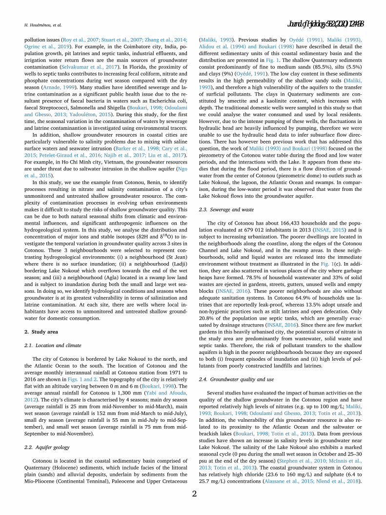
pollution issues (Roy et al., 2007; Stuart et al., 2007; Zhang et al., 2014;Ogrinc et al., 2019). For example, in the Coimbatore city, India, po-pulation growth, pit latrines and septic tanks, industrial effluents, andirrigation water return flows are the main sources of groundwatercontamination (Selvakumar et al., 2017). In Florida, the proximity ofwells to septic tanks contributes to increasing fecal coliform, nitrate andphosphate concentrations during wet season compared with the dryseason (Arnade, 1999). Many studies have identified sewerage and la-trine contamination as a significant public health issue due to the re-sultant presence of faecal bacteria in waters such as Escherichia coli,faecal Streptococci, Salmonella and Shigella (Boukari, 1998; Odoulamiand Gbesso, 2013; Yadouléton, 2015). During this study, for the firsttime, the seasonal variation in the contamination of waters by sewerageand latrine contaminantion is investigated using environmental tracers.

In addition, shallow groundwater resources in coastal cities areparticularly vulnerable to salinity problems due to mixing with salinesurface waters and seawater intrusion (Barker et al., 1998; Cary et al.,2015; Petelet-Giraud et al., 2016; Najib et al., 2017; Liu et al., 2017).For example, in Ho Chi Minh city, Vietnam, the groundwater resourcesare under threat due to saltwater intrusion in the shallow aquifer (Ngoet al., 2015).

In this study, we use the example from Cotonou, Benin, to identifyprocesses resulting in nitrate and salinity contamination of a city’sunmonitored and untreated shallow groundwater resource. The com-plexity of contamination processes in evolving urban environmentsmakes it difficult to study the risks of shallow groundwater quality. Thiscan be due to both natural seasonal shifts from climatic and environ-mental influences, and significant anthropogenic influences on thehydrogeological system. In this study, we analyse the distribution andconcentration of major ions and stable isotopes (δ2H and δ18O) to in-vestigate the temporal variation in groundwater quality across 3 sites inCotonou. These 3 neighbourhoods were selected to represent con-trasting hydrogeological environments: (i) a neighbourhood (St Jean)where there is no surface inundation; (ii) a neighbourhood (Ladji)bordering Lake Nokoué which overflows towards the end of the wetseason; and (iii) a neighbourhood (Agla) located in a swamp low landand is subject to inundation during both the small and large wet sea-sons. In doing so, we identify hydrological conditions and seasons whengroundwater is at its greatest vulnerability in terms of salinization andlatrine contamination. At each site, there are wells where local in-habitants have access to unmonitored and untreated shallow ground-water for domestic consumption.

2. Study area

2.1. Location and climate

The city of Cotonou is bordered by Lake Nokoué to the north, andthe Atlantic Ocean to the south. The location of Cotonou and theaverage monthly interannual rainfall at Cotonou station from 1971 to2016 are shown in Figs. 1 and 2. The topography of the city is relativelyflat with an altitude varying between 0 m and 6 m (Boukari, 1998). Theaverage annual rainfall for Cotonou is 1,300 mm (Yabi and Afouda,2012). The city’s climate is characterised by 4 seasons; main dry season(average rainfall is 25 mm from mid-November to mid-March), mainwet season (average rainfall is 152 mm from mid-March to mid-July),small dry season (average rainfall is 55 mm in mid-July to mid-Sep-tember), and small wet season (average rainfall is 75 mm from mid-September to mid-Novembre).

2.2. Aquifer geology

Cotonou is located in the coastal sedimentary basin comprised ofQuaternary (Holocene) sediments, which include facies of the littoralplain (sands) and alluvial deposits, underlain by sediments from theMio-Pliocene (Continental Tenninal), Paleocene and Upper Cretaceous

(Maliki, 1993). Previous studies by Oyédé (1991), Maliki (1993),Alidou et al. (1994) and Boukari (1998) have described in detail thedifferent sedimentary units of this coastal sedimentary basin and thedistribution are presented in Fig. 1. The shallow Quaternary sedimentsconsist predominantly of fine to medium sands (85.5%), silts (5.5%)and clays (9%) (Oyédé, 1991). The low clay content in these sedimentsresults in the high permeability of the shallow sandy soils (Maliki,1993), and therefore a high vulnerability of the aquifers to the transferof surficial pollutants. The clays in Quaternary sediments are con-stituted by smectite and a kaolinite content, which increases withdepth. The traditional domestic wells were sampled in this study so thatwe could analyse the water consumed and used by local residents.However, due to the intense pumping of these wells, the fluctuations inhydraulic head are heavily influenced by pumping, therefore we wereunable to use the hydraulic head data to infer subsurface flow direc-tions. There has however been previous work that has addressed thisquestion, the work of Maliki (1993) and Boukari (1998) focused on thepiezometry of the Cotonou water table during the flood and low waterperiods, and the interactions with the Lake. It appears from these stu-dies that during the flood period, there is a flow direction of ground-water from the center of Cotonou (piezometric dome) to outlets such asLake Nokoué, the lagoon, the Atlantic Ocean and swamps. In compar-ison, during the low-water period it was observed that water from theLake Nokoué flows into the groundwater aquifer.

2.3. Sewerage and waste

The city of Cotonou has about 166,433 households and the popu-lation evaluated at 679 012 inhabitants in 2013 (INSAE, 2015) and issubject to increasing urbanization. The poorer dwellings are located inthe neighborhoods along the coastline, along the edges of the CotonouChannel and Lake Nokoué, and in the swamp areas. In these neigh-bourhoods, solid and liquid wastes are released into the immediateenvironment without treatment as illustrated in the Fig. 1(c). In addi-tion, they are also scattered in various places of the city where garbageheaps have formed. 78.5% of household wastewater and 33% of solidwastes are ejected in gardens, streets, gutters, unused wells and emptyblocks (INSAE, 2016). These poorer neighborhoods are also withoutadequate sanitation systems. In Cotonou 64.9% of households use la-trines that are reportedly leak-proof, whereas 13.5% adopt unsafe andnon-hygienic practices such as stilt latrines and open defecation. Only20.8% of the population use septic tanks, which are generally evac-uated by drainage structures (INSAE, 2016). Since there are few marketgardens in this heavily urbanised city, the potential sources of nitrate inthe study area are predominantly from wastewater, solid waste andseptic tanks. Therefore, the risk of pollutant transfers to the shallowaquifers is high in the poorer neighbourhoods because they are exposedto both (i) frequent episodes of inundation and (ii) high levels of pol-lutants from poorly constructed landfills and latrines.

2.4. Groundwater quality and use

Several studies have evaluated the impact of human activities on thequality of the shallow groundwater in the Cotonou region and havereported relatively high levels of nitrates (e.g. up to 100 mg/L; Maliki,1993; Boukari, 1998; Odoulami and Gbesso, 2013; Totin et al., 2013).In addition, the vulnerability of this groundwater resource is also re-lated to its proximity to the Atlantic Ocean and the saltwater orbrackish lakes (Boukari, 1998; Totin et al., 2013). Data from previousstudies have shown an increase in salinity levels in groundwater nearLake Nokoué. The salinity of the Lake Nokoué also exhibits a markedseasonal cycle (0 psu during the small wet season in October and 25–30psu at the end of the dry season) (Stephen et al., 2010; McInnis et al.,2013; Totin et al., 2013). The coastal groundwater system in Cotonouhas relatively high chloride (23.6 to 160 mg/L) and sulphate (6.4 to25.7 mg/L) concentrations (Alassane et al., 2015; Nlend et al., 2018).

H. Houéménou, et al. Journal of Hydrology 582 (2020) 124438

2

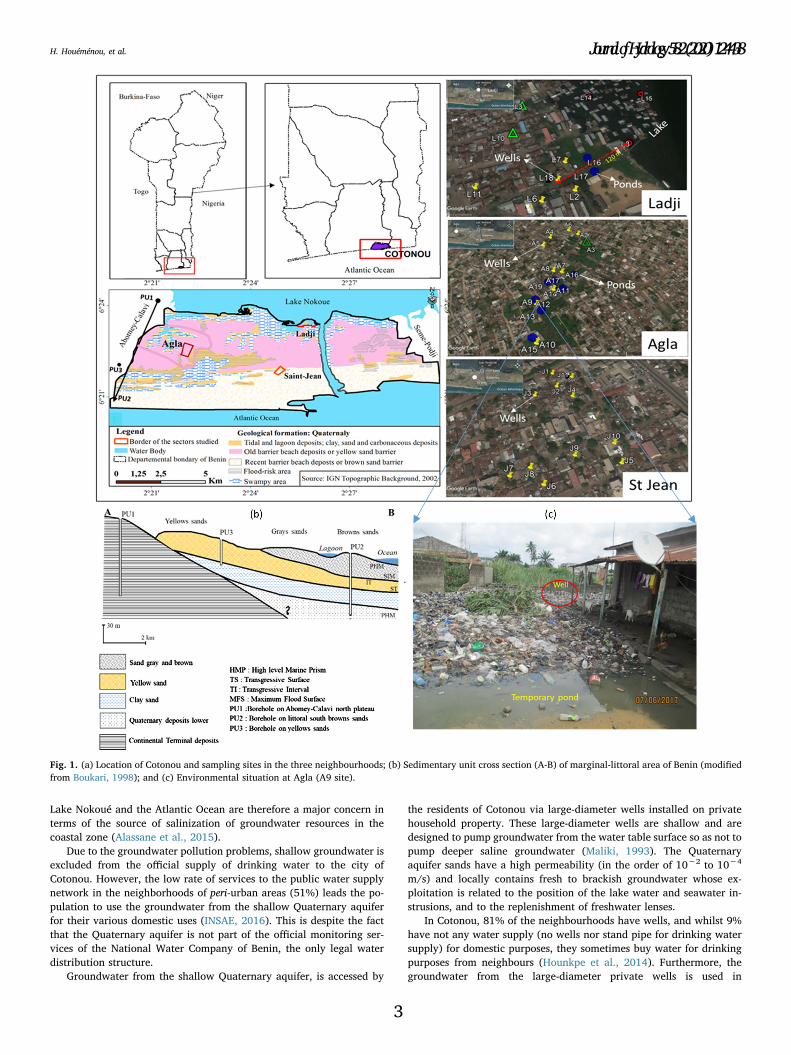
Lake Nokoué and the Atlantic Ocean are therefore a major concern interms of the source of salinization of groundwater resources in thecoastal zone (Alassane et al., 2015).

Due to the groundwater pollution problems, shallow groundwater isexcluded from the official supply of drinking water to the city ofCotonou. However, the low rate of services to the public water supplynetwork in the neighborhoods of peri-urban areas (51%) leads the po-pulation to use the groundwater from the shallow Quaternary aquiferfor their various domestic uses (INSAE, 2016). This is despite the factthat the Quaternary aquifer is not part of the official monitoring ser-vices of the National Water Company of Benin, the only legal waterdistribution structure.

Groundwater from the shallow Quaternary aquifer, is accessed by

the residents of Cotonou via large-diameter wells installed on privatehousehold property. These large-diameter wells are shallow and aredesigned to pump groundwater from the water table surface so as not topump deeper saline groundwater (Maliki, 1993). The Quaternaryaquifer sands have a high permeability (in the order of 10−2 to 10−4

m/s) and locally contains fresh to brackish groundwater whose ex-ploitation is related to the position of the lake water and seawater in-strusions, and to the replenishment of freshwater lenses.

In Cotonou, 81% of the neighbourhoods have wells, and whilst 9%have not any water supply (no wells nor stand pipe for drinking watersupply) for domestic purposes, they sometimes buy water for drinkingpurposes from neighbours (Hounkpe et al., 2014). Furthermore, thegroundwater from the large-diameter private wells is used in

Fig. 1. (a) Location of Cotonou and sampling sites in the three neighbourhoods; (b) Sedimentary unit cross section (A-B) of marginal-littoral area of Benin (modifiedfrom Boukari, 1998); and (c) Environmental situation at Agla (A9 site).

H. Houéménou, et al. Journal of Hydrology 582 (2020) 124438

3

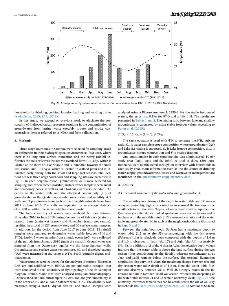
households for drinking, cooking, laundry, bathing and washing dishes(Yadouléton, 2015; EAA, 2018).

In this study, we expand on previous work to elucidate the sea-sonality of hydrogeological processes resulting in the contamination ofgroundwater from latrine waste (notably nitrate and nitrite con-centrations, herein referred to as NOx) and from salinization.

3. Methods

Three neighbourhoods in Cotonou were selected for sampling basedon differences in their hydrogeological environments: (i) St Jean, wherethere is no long-term surface inundation and the heavy rainfall in-filtrates the soils or leaves the site via overland flow; (ii) Ladji, which islocated at the shore of Lake Nokoué and is inundated towards the smallwet season; and (iii) Agla, which is located in a flood plain and is in-undated early during both the small and large wet seasons. The loca-tions of these three neighbourhoods and sampling sites are presented inFig. 1. In each neighbourhood, groundwater wells were selected forsampling and, where/when possible, surface water samples (permanentand temporary pools, as well as Lake Nokoué) were also included. Thedepths to the water table and the electrical conductivity (EC) ofgroundwater in the Quaternary aquifer were monitored monthly at 9wells and 3 piezometers from each of the 3 neighbourhoods from June2017 to June 2018. The wells are separated by an average distanceof ~ 200 m within the same neighbourhood probe.

The hydrochemistry of waters were analysed 6 times betweenNovember 2016 to June 2018 during the months of February (main dryseason), June (main wet season) and November (small wet season),resulting in a total of 127 groundwater, and 60 surface water samples.In addition, for the period from June 2017 to June 2018, 13 rainfallsamples were analysed to determine water stable isotopes (δ2H andδ18O). Lastly, 2 water samples from atlantic ocean (AO) were collectedof the periods from January 2019 (main dry season). Groundwater wassampled from the Quaternary aquifer via the large-diameter wells.Groundwater and surface water temperature, EC, and dissolved oxygen(DO) were measured in-situ using a WTW 3430i portable digital mul-tiparameter.

Water samples were collected for the analyses of cations (filtered at0.45 µm and acidified with HNO3), anions and stable isotopes, thatwere conducted at the Laboratory of Hydrogeology of the University ofAvignon, France. Major ions were analysed using ion chromatography(Dionex; ICS1100 and autosampler AS-AP). Ion analysis uncertainty isin the order of 3%, and all ionic balances were≤5%. The alkalinity wasmeasured using a HACH digital titrator, and stable isotopes were

analysed using a Picarro Analyser L 2130-I. For the stable isotopes ofwaters, the error is± 0.1‰ for δ18O and±1‰ δ2H. The results arepresented in Tables 1 and 2. The mixing ratio between lake and shallowgroundwater is calculated by using stable isotopes values according toParan et al. (2015):

= + −δ O f δ O f δ O. (1 ).m L GW18 18 18

The same equation is used with δ2H to compute the δ2Hm mixingratio. Om is water sample isotope composition where groundwater (GW)and Lake (L) mixing is supposed. OL is Lake isotope composition. OGW isgroundwater isotope composition and F is mixing fraction.

One questionnaire in each sampling site was administered, 10 perstudy area (Ladji, Agla and St. John). A total of thirty (30) ques-tionnaires were administered through an interview with households ineach study area. Main information such as the the source of drinkingwater supply, groundwater use, waste and wastewater management arementioned in the questionnaire (supplementary data).

4. Results

4.1. Seasonal variations of the water table and groundwater EC

The monthly monitoring of the depth to water table and EC over aone-year period highlights the variations in seasonal fluctuations of theaquifers between the sites. Typical of unconfined shallow aquifers, theQuaternary aquifer shows marked spatial and seasonal variations and isin phase with the monthly rainfall. The seasonal variations of the watertable and groundwater EC in each of the neighbourhoods are illustratedin Figs. 3 and 5.

Between the neighbourhoods, St Jean has a maximum depth towater table (1.5 m at site J5) corresponding with the dry season(February) that is relatively deep compared with the depths of 1.4 mand 1.0 m observed in Ladji (site L7) and Agla (site A4), respectively(Fig. 5). In addition, at 2 of the 4 sites in Agla, the negative depth valuesindicate that the water table is above the land surface during the wetseason (thus contributing to the floods), whereas groundwater at StJean and Ladji remains below the surface. The seasonal fluctuationamplitudes also vary. In St Jean, the maximum change between wet anddry season water table depth is of 1.2 m. Here the water table fluc-tuations also vary between wells. Well J5 strongly reacts to the in-creased rainfall in October (small wet season) whereas the deepening ofthe water table in wells J1 and J2 remain relatively weak (Fig. 5). Theserelatively low water table values can be attributed to the use of wells byhouseholds (Boukari, 1998; Kadjangaba et al., 2018). Similar to St Jean,

Fig. 2. Average monthly interannual rainfall at Cotonou station from 1971 to 2016 (ASECNA station).

H. Houéménou, et al. Journal of Hydrology 582 (2020) 124438

4

Table 1

Chemical parameters and isotopic values in shallow groundwater.

ID Sampling month Origin Depth T°C pH DO EC NOx HCO3− Cl− NO2

− Br− NO3− PO4

−− SO4−− Na+ NH4

+ K+ Mg++ Ca++ DOC d18O d2H

Units m mg/L µS/cm meq/L mg/L ‰

J1 Nov-16 well 29.50 6.97 590 0.67 221.49 27.59 DBL DBL 37.68 8.69 3.90 47.20 DBL 19.57 5.42 58.13 −3.07 −14.04Mar-17 well 29.70 7.24 2.59 998 1.84 244.00 74.90 0.80 0.97 66.12 8.26 85.49 86.41 0.25 29.43 9.19 93.52 −2.85 −12.48Jun-17 well 0.80 28.20 7.45 3.60 1002 318.12 77.18 DBL DBL DBL 6.99 115.78 94.37 DBL 3.86 9.99 89.42 10.85 −2.94 −12.61Oct-17 well 0.90 27.90 7.57 3.93 799 0.44 314.76 28.52 7.13 DBL 17.67 5.68 4.87 44.68 DBL 22.27 9.69 92.45 5.89 −3.89 −21.22Feb-18 well 1.23 29.10 7.16 2.35 1285 1.18 384.30 85.78 DBL DBL 73.45 8.34 8.62 14.51 13.65 35.65 8.76 79.28 6.80 −3.36 −16.10Jun-18 well 0.88 29.20 7.40 3.24 731 1.16 152.50 57.74 1.19 DBL 7.37 4.97 54.63 68.32 0.58 19.86 5.16 53.95 −3.22 −13.37

J2 Nov-16 well 29.00 6.92 502 0.76 99.56 34.52 0.12 0.28 46.95 6.93 36.23 45.47 0.28 12.67 2.80 44.77 −2.81 −11.64Mar-17 well 29.90 6.93 2.42 552 0.70 113.46 42.75 0.17 0.65 37.70 7.13 31.75 41.98 0.30 18.60 3.24 49.58 −3.35 −15.40Jun-17 well 0.59 28.60 7.04 3.13 347 128.10 25.67 DBL DBL DBL 5.27 17.90 31.66 DBL 7.32 1.94 33.24 8.30 −3.65 −16.31Oct-17 well 0.77 28.60 7.36 5.13 297 121.60 15.94 DBL DBL DBL 6.52 13.00 22.97 DBL 7.66 1.56 28.22 6.31 −4.17 −21.87Feb-18 well 1.04 29.70 6.88 2.56 586 0.50 119.56 52.64 0.43 DBL 3.49 6.40 49.37 37.97 0.62 13.28 3.14 46.95 5.55 −3.39 −15.90Jun-18 well 0.75 29.03 7.06 3.39 341 0.24 86.93 2.19 DBL DBL 12.43 3.77 26.87 22.87 0.22 8.45 1.79 31.72 −3.54 −15.48

J3 Nov-16 well 29.70 7.02 658 0.74 125.58 46.97 0.53 0.61 45.39 9.82 54.88 62.97 1.64 17.99 3.46 53.96 −3.01 −13.16Mar-17 well 29.20 7.15 4.61 891 1.59 191.54 81.73 0.31 0.13 98.13 6.28 53.17 86.30 2.25 21.71 4.96 68.47 −3.02 −12.99Jun-17 well 27.60 7.35 7.85 822 0.63 254.68 75.52 DBL 0.18 0.39 5.25 52.61 84.25 DBL 22.82 4.27 63.45 1.17 −3.19 −13.76Oct-17 well 29.00 5.91 3.55 630 29.84 56.65 DBL DBL DBL 5.19 4.84 51.28 DBL 13.35 4.54 6.62 4.53 −3.56 −16.94Feb-18 well 29.20 7.00 3.61 791 1.18 156.16 74.76 0.29 DBL 73.98 4.26 61.19 62.85 0.33 15.11 6.18 79.89 5.37 −3.19 −13.90Jun-18 well 29.40 6.90 3.90 792 1.12 158.60 7.88 DBL DBL 69.65 3.83 41.29 66.47 0.38 14.90 5.79 63.11 −3.38 −15.19

J4 Nov-16 well 29.80 7.11 500 0.22 18.45 27.63 0.77 0.45 13.48 2.47 36.46 37.84 0.31 17.42 3.77 51.35 −2.37 −8.98Mar-17 well 29.90 7.15 4.95 572 0.31 195.20 33.68 0.11 0.79 18.69 2.36 37.86 41.44 0.12 13.45 6.22 57.91 −2.58 −9.93Jun-17 well 27.90 7.63 3.98 368 0.33 132.37 2.34 0.15 DBL DBL 1.99 23.22 29.65 DBL 15.53 2.62 31.66 14.96 −3.23 −14.08Oct-17 well 28.70 8.06 5.35 342 81.74 29.18 DBL DBL DBL 2.45 24.79 25.31 DBL 7.95 2.97 29.79 4.24Feb-18 well 29.20 7.15 3.33 434 0.22 96.38 47.54 DBL DBL 13.85 2.27 27.26 28.87 0.81 3.52 3.64 36.94 3.79 −3.07 −13.61Jun-18 well 28.80 7.41 4.08 379 0.33 122.00 25.24 DBL DBL 18.82 2.37 28.23 24.75 0.48 16.77 3.00 36.36 −3.52 −15.23

J5 Nov-16 well 29.70 6.83 642 0.45 28.68 38.17 DBL 0.82 0.28 0.82 3.38 46.38 DBL 43.42 6.31 56.38 −3.22 −14.19Mar-17 well 29.70 6.89 3.25 715 0.69 17.80 57.97 0.43 0.96 42.66 0.21 59.64 72.32 0.34 37.83 3.69 49.65 −3.06 −13.09Jun-17 well 1.05 28.50 7.03 1.96 798 0.48 193.22 79.80 0.22 DBL DBL DBL 89.97 72.19 0.58 35.18 6.18 65.25 11.57 −3.17 −13.43Oct-17 well 0.43 27.10 7.03 1.31 630 272.60 37.12 DBL 0.19 DBL DBL 26.37 43.66 DBL 19.78 5.82 65.35 4.93 −3.61 −17.56Feb-18 well 1.53 28.60 6.96 2.34 558 0.46 164.70 38.37 DBL DBL 2.89 DBL 44.12 34.22 0.50 16.46 3.98 46.12 8.59 −2.89 −12.01Jun-18 well 0.66 27.80 6.97 2.03 639 0.25 265.35 35.12 DBL DBL 1.53 DBL 31.40 44.85 0.62 19.72 5.49 62.37 −3.46 −15.23

J6 Nov-16 well 29.10 6.76 548 1.15 66.49 41.99 DBL 0.49 71.59 5.27 51.16 47.46 0.65 21.98 3.87 4.27 −3.24 −15.12Mar-17 well 29.40 6.99 3.60 1326 5.67 85.40 111.13 1.95 0.18 311.33 2.68 91.61 115.00 0.73 37.66 13.46 17.85 −2.85 −11.68Jun-17 well 29.20 7.06 5.12 1129 3.80 154.79 99.84 54.79 DBL 157.26 2.57 87.74 99.79 0.39 4.98 1.37 87.46 16.65 −2.60 −10.19Oct-17 well 28.50 6.99 4.40 637 1.94 54.90 44.28 2.28 DBL 117.19 2.33 53.18 46.00 DBL 21.69 4.32 48.44 8.31 −3.28 −15.11Feb-18 well 29.00 6.97 4.35 961 3.37 439.20 51.14 0.17 DBL 28.87 2.62 47.94 93.79 0.16 29.53 15.13 114.74 8.63 −3.32 −15.88Jun-18 well 29.00 7.17 5.96 346 0.43 54.90 29.35 DBL DBL 24.95 4.54 2.49 26.22 0.27 11.87 2.27 24.73 −3.23 −13.82

J7 Nov-16 well 30.10 6.87 431 0.74 93.25 26.42 0.19 0.40 45.76 3.19 27.42 34.79 0.39 13.95 2.89 36.26 −2.85 −12.03Mar-17 well 29.90 7.05 5.12 695 0.87 184.22 44.50 0.22 0.11 53.78 0.79 44.46 53.47 0.18 2.82 4.77 55.50 −3.08 −12.98Jun-17 well 30.20 7.00 3.78 742 0.56 22.36 61.44 0.26 DBL DBL 1.14 68.21 63.46 DBL 22.43 5.45 63.31 6.80 −2.61 −9.98Oct-17 well 28.90 7.14 4.20 652 1.29 16.14 38.98 13.15 DBL 57.27 0.73 59.96 4.94 DBL 15.58 5.28 62.60 4.59 −3.13 −14.66Feb-18 well 29.00 6.90 4.19 647 1.55 113.46 3.99 0.49 DBL 95.59 1.18 59.66 38.17 0.23 24.95 4.69 48.66 7.08 −3.04 −13.22Jun-18 well 29.40 7.08 4.19 616 0.66 14.30 37.00 DBL DBL 4.89 1.87 56.59 47.58 0.24 31.95 4.20 43.35 −3.38 −14.29

J8 Nov-16 well 29.40 6.99 701 2.21 126.41 4.12 0.58 0.66 136.47 4.61 32.89 38.52 0.32 18.17 5.39 78.67 −3.35 −15.92Mar-17 well 29.70 6.78 3.62 885 2.58 115.90 72.18 0.48 0.16 159.26 5.87 36.16 74.78 2.78 29.87 4.94 61.28 −2.77 −11.16Jun-17 well 29.20 7.27 4.67 894 2.56 128.86 79.23 93.70 DBL 32.54 4.43 54.90 8.34 0.71 25.57 5.65 72.48 5.82 −2.92 −11.84Oct-17 well 27.80 7.49 4.75 564 0.99 128.10 22.92 45.57 DBL DBL 5.67 3.47 36.54 DBL 19.17 3.18 53.58 5.54 −3.64 −17.99Feb-18 well 28.50 6.91 3.30 840 2.60 118.34 56.71 0.46 DBL 16.63 6.20 6.15 59.92 0.32 25.37 4.63 59.75 4.09 −3.12 −13.91Jun-18 well 28.40 7.65 4.56 377 0.62 128.10 14.14 DBL DBL 38.59 4.18 18.97 19.89 0.46 1.39 2.17 38.72 −3.55 −13.45

J9 Nov-16 well 29.50 7.19 448 0.34 213.58 25.43 0.23 0.47 0.18 DBL 16.48 18.58 4.60 2.88 3.11 49.79 −2.96 −12.98Mar-17 well 30.10 6.98 4.82 461 0.88 82.96 42.48 0.69 0.19 54.42 DBL 21.57 36.85 0.33 11.14 2.94 41.27 −2.64 −9.55Jun-17 well 29.10 7.20 4.06 437 0.49 126.58 24.64 8.35 DBL 19.20 DBL 26.35 29.73 0.26 1.53 3.20 46.72 8.89 −3.06 −12.08Oct-17 well 28.10 7.21 4.04 323 0.46 97.60 27.93 1.56 DBL 0.42 DBL 11.57 17.19 0.58 5.12 2.22 36.84 0.41 −3.44 −15.80Feb-18 well 28.60 7.00 4.63 242 0.13 56.12 28.38 DBL DBL 8.23 DBL 11.53 14.34 0.60 7.64 1.82 26.23 4.58 −3.74 −18.62

(continued on next page)

H.Houém

énou,et

al.Journal of Hydrology 582 (2020) 124438

5

Table 1 (continued)

ID Sampling month Origin Depth T°C pH DO EC NOx HCO3− Cl− NO2

− Br− NO3− PO4

−− SO4−− Na+ NH4

+ K+ Mg++ Ca++ DOC d18O d2H

Jun-18 well 28.60 7.04 3.67 251 0.15 122.00 14.44 DBL DBL 9.45 DBL 15.59 11.91 0.43 5.34 1.62 38.59 −3.43 −13.35J10 Nov-16 well 29.20 6.95 572 0.75 13.63 41.52 0.32 0.49 43.32 2.64 38.84 56.63 0.45 26.72 2.86 42.15 −3.44 −16.28

Mar-17 well 28.50 6.89 2.37 615 0.39 173.24 42.31 0.86 0.96 23.27 DBL 48.34 42.65 1.74 37.39 4.64 52.68 −3.17 −14.39Jun-17 well 29.50 7.13 3.43 770 1.12 163.18 65.67 DBL DBL 69.32 DBL 61.25 72.53 1.46 33.84 4.70 57.83 11.67 −3.17 −13.29Oct-17 well 29.30 8.03 4.94 481 98.82 39.22 DBL DBL DBL 2.51 47.65 28.13 DBL 13.14 3.82 47.88 3.81 −3.17 −14.61Feb-18 well 29.60 6.90 2.77 943 0.99 229.36 8.94 0.56 DBL 6.44 0.52 47.17 6.59 14.36 28.62 5.34 56.68 7.19 −3.14 −13.91Jun-18 well 30.50 6.75 0.73 878 0.90 25.10 65.43 DBL DBL 55.54 1.52 47.69 66.77 5.41 27.62 6.57 65.57 −3.28 −14.91

J11 Feb-18 Piezometer 1.40 31.30 7.21 497 0.89 92.72 57.13 DBL 0.60 55.30 4.48 27.92 42.63 2.29 11.97 4.67 46.88 13.50 −3.09 −15.03Jun-18 Piezometer 0.88 29.40 7.33 6.79 444 0.65 141.52 13.61 DBL DBL 4.26 6.47 22.82 13.44 0.15 12.46 4.81 49.92 −3.73 −17.66

A2 Nov-16 well 28.60 6.60 1164 0.72 432.95 118.77 DBL 0.38 0.44 DBL 33.32 15.85 0.25 35.77 1.85 8.73 −1.81 −5.39Mar-17 well 29.90 6.28 3.32 990 0.87 13.70 123.64 0.39 0.22 53.39 DBL 136.56 125.35 0.23 28.66 7.45 49.37 −2.72 −10.94Jun-17 well −0.01 27.30 7.21 2.42 1273 435.85 16.53 DBL 0.35 DBL DBL 74.85 147.93 DBL 35.17 17.46 78.28 22.27 −2.32 −9.17Oct-17 well 0.04 26.50 7.02 2.33 1150 441.64 14.00 DBL 0.53 DBL DBL 1.45 111.34 DBL 29.87 15.27 81.80 25.62 −2.02 −7.51Feb-18 well 0.69 28.30 6.96 2.83 733 0.83 22.52 97.21 DBL 0.40 0.51 DBL 32.23 86.88 0.32 15.55 14.75 41.54 14.65 −2.90 −12.08Jun-18 well 0.04 28.90 7.02 1.61 959 292.80 111.26 DBL DBL DBL DBL 3.56 93.69 DBL 24.14 1.24 68.46 −2.75 −11.56

A4 Nov-16 well 29.60 6.02 326 0.27 31.95 17.78 0.35 0.12 1.63 DBL 78.71 29.22 0.16 6.91 3.73 16.65 −3.22 −14.01Mar-17 well 30.90 5.85 2.95 269 0.39 27.00 27.70 0.57 0.17 2.32 DBL 44.29 29.25 0.38 6.53 3.67 13.12 −3.12 −14.05Jun-17 well 0.47 30.70 6.01 5.34 353 0.43 37.82 56.98 DBL 0.23 2.52 DBL 38.15 32.98 0.54 8.24 5.30 2.99 9.86 −2.96 −12.84Oct-17 well 0.29 28.00 5.95 4.53 497 0.18 54.90 69.62 DBL 0.35 1.95 DBL 61.86 46.93 DBL 1.46 6.77 27.46 8.79 −2.68 −10.44Feb-18 well 0.99 29.50 5.84 3.97 548 0.42 36.60 86.61 DBL 0.46 25.86 DBL 5.46 51.32 0.76 1.49 7.16 2.14 10.38 −2.89 −12.28Jun-18 well 0.25 29.00 5.76 3.32 666 0.66 36.60 97.38 DBL DBL 37.26 DBL 59.26 6.43 0.10 12.96 1.98 32.71 −2.81 −11.54

A5 Nov-16 well 30.70 6.00 1037 0.27 13.62 158.50 DBL 0.25 16.97 DBL 135.17 131.15 0.90 17.93 6.68 37.45 −2.77 −11.89Oct-17 well 27.20 7.01 2.75 500 15.60 5.92 DBL 0.13 DBL DBL 19.18 51.31 DBL 9.32 6.26 33.27 10.06 −3.52 −17.61Feb-18 well 29.00 6.55 2.39 652 0.39 154.94 6.87 0.20 0.12 23.85 DBL 58.67 67.19 2.58 13.73 9.77 47.38 8.85 −3.18 −14.14Jun-18 well 29.20 6.74 4.33 652 0.17 155.55 48.84 DBL DBL 1.53 DBL 52.19 52.72 0.12 11.19 8.15 4.83 −3.46 −16.07

A6 Nov-16 well 30.30 6.16 983 0.86 155.55 1.56 1.67 0.17 51.84 1.38 125.27 113.75 DBL 22.17 5.98 45.76 −2.99 −12.98Jun-17 well 29.00 7.12 8.45 1338 0.90 245.53 175.75 8.61 0.17 38.63 DBL 216.32 158.45 DBL 38.76 1.17 96.61 14.60 −2.02 −8.14Oct-17 well 27.60 6.50 5.40 1095 0.37 162.26 128.13 16.70 0.26 0.14 DBL 172.62 13.59 DBL 28.97 6.95 62.43 7.43 −2.49 −10.75Feb-18 well 30.30 6.22 4.25 967 0.77 87.84 137.65 DBL 0.33 47.68 DBL 165.24 128.49 2.42 26.57 7.92 47.19 7.08 −2.62 −10.75Jun-18 well 29.60 6.72 8.31 935 0.59 144.88 91.65 DBL DBL 31.57 DBL 19.87 13.93 0.24 25.35 6.24 51.88 −2.66 −11.51

A7 Nov-16 well 34.00 7.51 1302 0.36 125.58 44.84 DBL 0.12 0.23 DBL 43.42 58.32 1.63 13.37 3.69 21.27 −3.57 −18.22Mar-17 well 30.20 6.21 2.01 631 0.75 97.60 84.84 DBL 0.26 0.46 DBL 72.31 76.93 0.91 21.42 8.34 25.66 −2.96 −13.00Jun-17 well 30.70 6.31 2.52 763 0.42 95.75 11.86 0.52 0.28 0.19 DBL 131.16 93.31 0.68 19.39 1.26 34.31 6.80 −2.92 −12.16Oct-17 well 29.10 6.28 2.12 687 0.35 112.24 13.59 DBL 0.29 0.19 DBL 74.26 84.18 0.36 16.73 6.42 28.45 6.19 −2.89 −13.15Feb-18 well 29.30 6.20 2.12 689 0.56 79.30 12.42 DBL 0.38 0.35 DBL 74.59 8.83 1.77 21.11 8.15 29.82 7.79 −2.99 −13.11Jun-18 well 28.30 6.38 2.83 816 0.63 155.55 18.42 DBL DBL 0.39 DBL 67.64 89.20 0.89 27.33 9.20 32.96 −3.02 −13.62

A8 Nov-16 well 29.50 6.20 551 0.25 75.41 7.68 DBL 0.13 0.16 DBL 59.96 66.77 0.12 6.86 1.90 26.92 −2.58 −10.57Mar-17 well 29.10 6.03 2.13 560 0.28 78.80 73.69 0.19 0.24 1.26 DBL 69.90 84.16 1.28 7.44 2.28 22.49 −2.90 −12.29Jun-17 well 0.02 29.70 6.37 3.98 842 0.27 98.67 11.17 0.19 0.24 1.39 DBL 171.18 16.87 2.49 13.32 6.34 44.49 9.95 −2.87 −12.41Oct-17 well −0.12 27.80 6.03 4.51 645 64.23 70.00 DBL 0.26 DBL DBL 149.72 92.14 0.22 3.37 4.96 2.22 7.31 −2.67 −10.51Feb-18 well 0.48 28.90 6.29 2.93 642 0.18 73.20 77.37 DBL 0.30 1.14 DBL 116.63 82.51 0.88 5.91 4.88 2.54 8.89 −2.69 −10.74Jun-18 well −0.20 29.10 6.15 7.49 778 143.35 78.94 DBL DBL DBL DBL 139.61 95.79 0.91 7.69 9.16 33.59 −2.64 −10.29

A9 Nov-16 well 29.00 7.04 666 246.67 67.77 DBL 0.23 DBL 1.46 8.92 67.94 DBL 18.82 9.32 34.30 −0.33 0.51Mar-17 well 29.70 6.85 2.34 765 0.84 174.46 82.83 0.53 0.26 0.45 0.39 93.83 91.12 0.34 1.21 9.13 52.77 −2.52 −11.02Oct-17 well 28.90 7.78 8.22 931 374.83 77.28 DBL 0.29 DBL 4.26 2.17 7.46 2.98 71.94 15.24 49.57 20.79 −2.29 −10.29Feb-18 well 28.40 7.84 4.22 1475 0.37 475.80 155.00 DBL 0.66 0.23 5.15 93.18 127.81 5.78 55.96 19.57 87.88 26.91 −0.03 2.78Jun-18 well 27.40 7.29 0.56 1200 488.00 94.55 DBL DBL DBL 3.19 66.50 86.96 1.48 53.93 2.64 92.00 −2.27 −9.04

A10 Nov-16 well 28.50 6.56 700 0.96 35.84 34.77 0.62 0.74 5.14 3.69 25.72 39.59 9.44 16.33 5.00 64.39 −3.29 −14.98Mar-17 well 31.10 7.55 2.48 1023 0.96 381.86 96.39 0.14 0.24 0.50 DBL 5.69 92.29 2.52 31.14 1.53 8.56 −1.11 −1.57Jun-17 well 30.20 7.60 6.36 837 193.68 84.73 DBL DBL DBL DBL 136.69 85.33 DBL 22.51 7.26 75.40 14.76 −1.85 −6.87Oct-17 well 29.20 7.84 6.43 835 0.17 245.22 119.79 DBL 0.20 0.66 DBL 4.98 11.90 DBL 26.97 8.75 44.20 22.53 −0.29 −1.64Feb-18 well 28.70 7.77 0.12 1870 0.12 751.52 112.19 DBL 0.76 0.77 DBL 37.48 121.80 88.40 44.42 9.35 45.65 26.47 −0.26 1.72Jun-18 well 28.80 7.33 3.71 654 262.30 6.83 DBL DBL DBL DBL 4.68 67.89 DBL 14.47 6.75 47.42 −2.03 −6.96

A11 Feb-18 Piezometer 0.40 32.20 6.61 1.19 1212 0.14 346.48 12.41 0.56 0.69 0.94 DBL 84.86 85.96 7.45 43.27 9.63 8.93 23.4 −2.86 −13.02Jun-18 Piezometer −0.26 28.20 7.23 0.06 1468 0.42 491.66 148.36 DBL DBL 24.94 DBL 54.75 114.51 5.11 64.13 13.96 91.52 −2.46 −10.21

(continued on next page)

H.Houém

énou,et

al.Journal of Hydrology 582 (2020) 124438

6

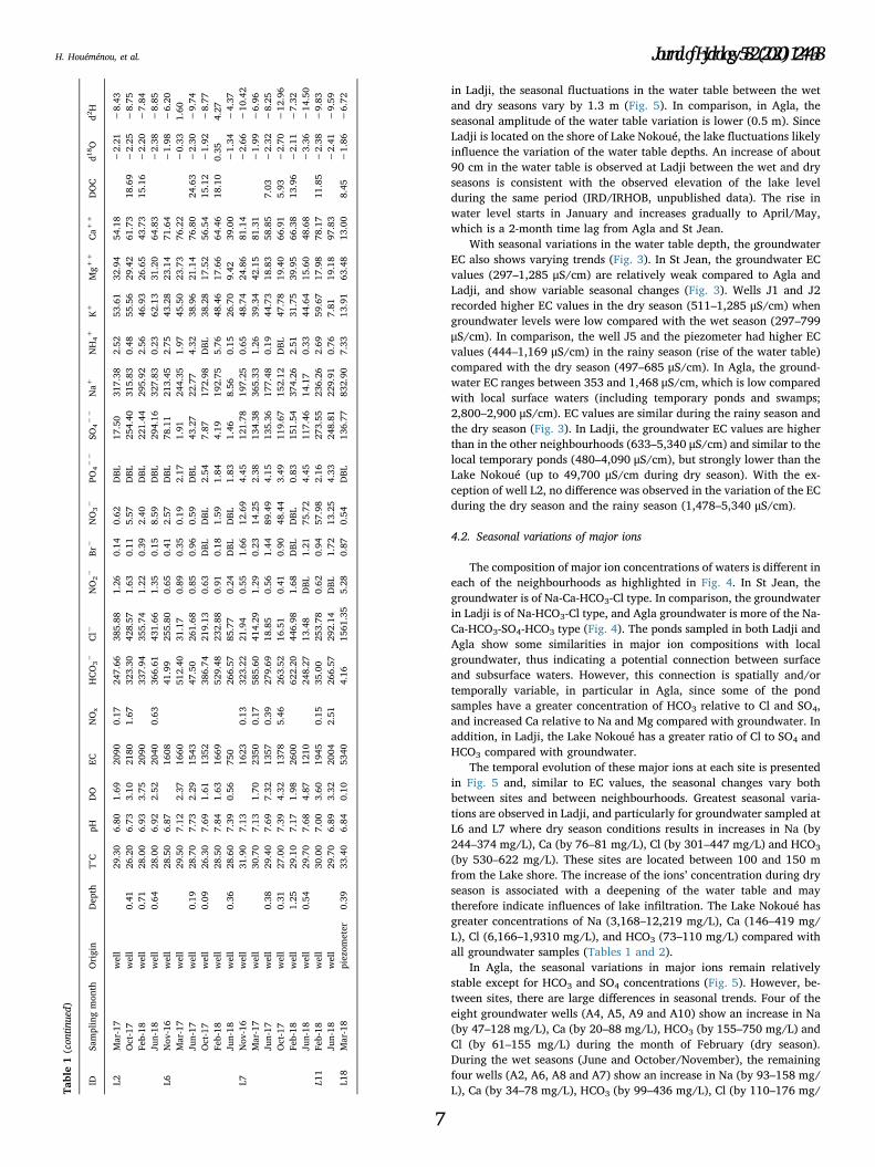
in Ladji, the seasonal fluctuations in the water table between the wetand dry seasons vary by 1.3 m (Fig. 5). In comparison, in Agla, theseasonal amplitude of the water table variation is lower (0.5 m). SinceLadji is located on the shore of Lake Nokoué, the lake fluctuations likelyinfluence the variation of the water table depths. An increase of about90 cm in the water table is observed at Ladji between the wet and dryseasons is consistent with the observed elevation of the lake levelduring the same period (IRD/IRHOB, unpublished data). The rise inwater level starts in January and increases gradually to April/May,which is a 2-month time lag from Agla and St Jean.

With seasonal variations in the water table depth, the groundwaterEC also shows varying trends (Fig. 3). In St Jean, the groundwater ECvalues (297–1,285 μS/cm) are relatively weak compared to Agla andLadji, and show variable seasonal changes (Fig. 3). Wells J1 and J2recorded higher EC values in the dry season (511–1,285 μS/cm) whengroundwater levels were low compared with the wet season (297–799μS/cm). In comparison, the well J5 and the piezometer had higher ECvalues (444–1,169 μS/cm) in the rainy season (rise of the water table)compared with the dry season (497–685 μS/cm). In Agla, the ground-water EC ranges between 353 and 1,468 μS/cm, which is low comparedwith local surface waters (including temporary ponds and swamps;2,800–2,900 μS/cm). EC values are similar during the rainy season andthe dry season (Fig. 3). In Ladji, the groundwater EC values are higherthan in the other neighbourhoods (633–5,340 μS/cm) and similar to thelocal temporary ponds (480–4,090 μS/cm), but strongly lower than theLake Nokoué (up to 49,700 μS/cm during dry season). With the ex-ception of well L2, no difference was observed in the variation of the ECduring the dry season and the rainy season (1,478–5,340 μS/cm).

4.2. Seasonal variations of major ions

The composition of major ion concentrations of waters is different ineach of the neighbourhoods as highlighted in Fig. 4. In St Jean, thegroundwater is of Na-Ca-HCO3-Cl type. In comparison, the groundwaterin Ladji is of Na-HCO3-Cl type, and Agla groundwater is more of the Na-Ca-HCO3-SO4-HCO3 type (Fig. 4). The ponds sampled in both Ladji andAgla show some similarities in major ion compositions with localgroundwater, thus indicating a potential connection between surfaceand subsurface waters. However, this connection is spatially and/ortemporally variable, in particular in Agla, since some of the pondsamples have a greater concentration of HCO3 relative to Cl and SO4,and increased Ca relative to Na and Mg compared with groundwater. Inaddition, in Ladji, the Lake Nokoué has a greater ratio of Cl to SO4 andHCO3 compared with groundwater.

The temporal evolution of these major ions at each site is presentedin Fig. 5 and, similar to EC values, the seasonal changes vary bothbetween sites and between neighbourhoods. Greatest seasonal varia-tions are observed in Ladji, and particularly for groundwater sampled atL6 and L7 where dry season conditions results in increases in Na (by244–374 mg/L), Ca (by 76–81 mg/L), Cl (by 301–447 mg/L) and HCO3

(by 530–622 mg/L). These sites are located between 100 and 150 mfrom the Lake shore. The increase of the ions’ concentration during dryseason is associated with a deepening of the water table and maytherefore indicate influences of lake infiltration. The Lake Nokoué hasgreater concentrations of Na (3,168–12,219 mg/L), Ca (146–419 mg/L), Cl (6,166–1,9310 mg/L), and HCO3 (73–110 mg/L) compared withall groundwater samples (Tables 1 and 2).

In Agla, the seasonal variations in major ions remain relativelystable except for HCO3 and SO4 concentrations (Fig. 5). However, be-tween sites, there are large differences in seasonal trends. Four of theeight groundwater wells (A4, A5, A9 and A10) show an increase in Na(by 47–128 mg/L), Ca (by 20–88 mg/L), HCO3 (by 155–750 mg/L) andCl (by 61–155 mg/L) during the month of February (dry season).During the wet seasons (June and October/November), the remainingfour wells (A2, A6, A8 and A7) show an increase in Na (by 93–158 mg/L), Ca (by 34–78 mg/L), HCO3 (by 99–436 mg/L), Cl (by 110–176 mg/T

able

1(con

tinued)

IDSa

mplingmon

thOrigin

Dep

thT°C

pHDO

EC

NOx

HCO3−

Cl−

NO2−

Br−

NO3−

PO4−−

SO4−−

Na+

NH4+

K+

Mg+

+Ca+

+DOC

d18O

d2H

L2Mar-17

well

29.30

6.80

1.69

2090

0.17

247.66

385.88

1.26

0.14

0.62

DBL

17.50

317.38

2.52

53.61

32.94

54.18

−2.21

−8.43

Oct-17

well

0.41

26.20

6.73

3.10

2180

1.67

323.30

428.57

1.63

0.11

5.57

DBL

254.40

315.83

0.48

55.56

29.42

61.73

18.69

−2.25

−8.75

Feb-18

well

0.71

28.00

6.93

3.75

2090

337.94

355.74

1.22

0.39

2.40

DBL

221.44

295.92

2.56

46.93

26.65

43.73

15.16

−2.20

−7.84

Jun-18

well

0.64

28.00

6.92

2.52

2040

0.63

366.61

431.66

1.35

0.15

8.59

DBL

294.16

327.83

0.23

62.13

31.20

64.83

−2.38

−8.85

L6Nov

-16

well

28.50

6.87

1608

41.99

255.80

0.65

0.41

2.57

DBL

78.11

213.45

2.75

43.28

23.14

71.64

−1.98

−6.20

Mar-17

well

29.50

7.12

2.37

1660

512.40

31.17

0.89

0.35

0.19

2.17

1.91

244.35

1.97

45.50

23.73

76.22

−0.33

1.60

Jun-17

well

0.19

28.70

7.73

2.29

1543

47.50

261.68

0.85

0.96

0.59

DBL

43.27

22.77

4.32

38.96

21.14

76.80

24.63

−2.30

−9.74

Oct-17

well

0.09

26.30

7.69

1.61

1352

386.74

219.13

0.63

DBL

DBL

2.54

7.87

172.98

DBL

38.28

17.52

56.54

15.12

−1.92

−8.77

Feb-18

well

28.50

7.84

1.63

1669

529.48

232.88

0.91

0.18

1.59

1.84

4.19

192.75

5.76

48.46

17.66

64.46

18.10

0.35

4.27

Jun-18

well

0.36

28.60

7.39

0.56

750

266.57

85.77

0.24

DBL

DBL

1.83

1.46

8.56

0.15

26.70

9.42

39.00

−1.34

−4.37

L7Nov

-16

well

31.90

7.13

1623

0.13

323.22

21.94

0.55

1.66

12.69

4.45

121.78

197.25

0.65

48.74

24.86

81.14

−2.66

−10

.42

Mar-17

well

30.70

7.13

1.70

2350

0.17

585.60

414.29

1.29

0.23

14.25

2.38

134.38

365.33

1.26

39.34

42.15

81.31

−1.99

−6.96

Jun-17

well

0.38

29.40

7.69

7.32

1357

0.39

279.69

18.85

0.56

1.44

89.49

4.15

135.36

177.48

0.19

44.73

18.83

58.85

7.03

−2.32

−8.25

Oct-17

well

0.31

27.00

7.39

4.32

1378

5.46

263.52

16.51

0.41

0.90

48.44

3.49

119.67

152.12

DBL

47.78

19.40

66.91

5.93

−2.70

−12

.96

Feb-18

well

1.25

29.10

7.17

1.98

2600

622.20

446.98

1.68

DBL

DBL

0.83

151.54

374.26

2.51

31.75

39.95

66.38

13.96

−2.11

−7.32

Jun-18

well

0.54

29.70

7.68

4.87

1210

248.27

13.48

DBL

1.21

75.72

4.45

117.46

14.17

0.33

44.64

15.60

48.68

−3.36

−14

.50

L11

Feb-18

well

30.00

7.00

3.60

1945

0.15

35.00

253.78

0.62

0.94

57.98

2.16

273.55

236.26

2.69

59.67

17.98

78.17

11.85

−2.38

−9.83

Jun-18

well

29.70

6.89

3.32

2004

2.51

266.57

292.14

DBL

1.72

13.25

4.33

248.81

229.91

0.76

7.81

19.18

97.83

−2.41

−9.59

L18

Mar-18

piezom

eter

0.39

33.40

6.84

0.10

5340

4.16

1561

.35

5.28

0.87

0.54

DBL

136.77

832.90

7.33

13.91

63.48

13.00

8.45

−1.86

−6.72

H. Houéménou, et al. Journal of Hydrology 582 (2020) 124438

7

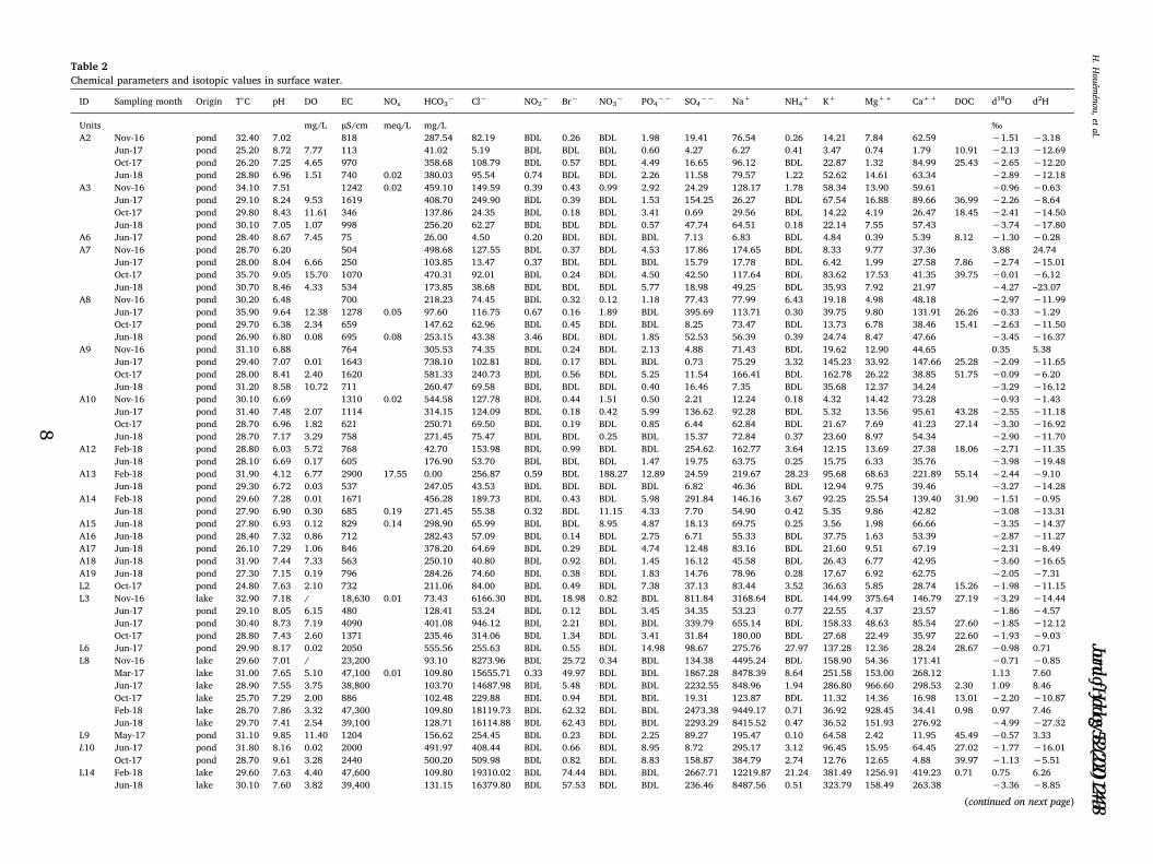
Table 2

Chemical parameters and isotopic values in surface water.

ID Sampling month Origin T°C pH DO EC NOx HCO3− Cl− NO2

− Br− NO3− PO4

−− SO4−− Na+ NH4

+ K+ Mg++ Ca++ DOC d18O d2H

Units mg/L µS/cm meq/L mg/L ‰

A2 Nov-16 pond 32.40 7.02 818 287.54 82.19 BDL 0.26 BDL 1.98 19.41 76.54 0.26 14.21 7.84 62.59 −1.51 −3.18Jun-17 pond 25.20 8.72 7.77 113 41.02 5.19 BDL BDL BDL 0.60 4.27 6.27 0.41 3.47 0.74 1.79 10.91 −2.13 −12.69Oct-17 pond 26.20 7.25 4.65 970 358.68 108.79 BDL 0.57 BDL 4.49 16.65 96.12 BDL 22.87 1.32 84.99 25.43 −2.65 −12.20Jun-18 pond 28.80 6.96 1.51 740 0.02 380.03 95.54 0.74 BDL BDL 2.26 11.58 79.57 1.22 52.62 14.61 63.34 −2.89 −12.18

A3 Nov-16 pond 34.10 7.51 1242 0.02 459.10 149.59 0.39 0.43 0.99 2.92 24.29 128.17 1.78 58.34 13.90 59.61 −0.96 −0.63Jun-17 pond 29.10 8.24 9.53 1619 408.70 249.90 BDL 0.39 BDL 1.53 154.25 26.27 BDL 67.54 16.88 89.66 36.99 −2.26 −8.64Oct-17 pond 29.80 8.43 11.61 346 137.86 24.35 BDL 0.18 BDL 3.41 0.69 29.56 BDL 14.22 4.19 26.47 18.45 −2.41 −14.50Jun-18 pond 30.10 7.05 1.07 998 256.20 62.27 BDL BDL BDL 0.57 47.74 64.51 0.18 22.14 7.55 57.43 −3.74 −17.80

A6 Jun-17 pond 28.40 8.67 7.45 75 26.00 4.50 0.20 BDL BDL BDL 7.13 6.83 BDL 4.84 0.39 5.39 8.12 −1.30 −0.28A7 Nov-16 pond 28.70 6.20 504 498.68 127.55 BDL 0.37 BDL 4.53 17.86 174.65 BDL 8.33 9.77 37.36 3.88 24.74

Jun-17 pond 28.00 8.04 6.66 250 103.85 13.47 0.37 BDL BDL BDL 15.79 17.78 BDL 6.42 1.99 27.58 7.86 −2.74 −15.01Oct-17 pond 35.70 9.05 15.70 1070 470.31 92.01 BDL 0.24 BDL 4.50 42.50 117.64 BDL 83.62 17.53 41.35 39.75 −0.01 −6.12Jun-18 pond 30.70 8.46 4.33 534 173.85 38.68 BDL BDL BDL 5.77 18.98 49.25 BDL 35.93 7.92 21.97 −4.27 –23.07

A8 Nov-16 pond 30.20 6.48 700 218.23 74.45 BDL 0.32 0.12 1.18 77.43 77.99 6.43 19.18 4.98 48.18 −2.97 −11.99Jun-17 pond 35.90 9.64 12.38 1278 0.05 97.60 116.75 0.67 0.16 1.89 BDL 395.69 113.71 0.30 39.75 9.80 131.91 26.26 −0.33 −1.29Oct-17 pond 29.70 6.38 2.34 659 147.62 62.96 BDL 0.45 BDL BDL 8.25 73.47 BDL 13.73 6.78 38.46 15.41 −2.63 −11.50Jun-18 pond 26.90 6.80 0.08 695 0.08 253.15 43.38 3.46 BDL BDL 1.85 52.53 56.39 0.39 24.74 8.47 47.66 −3.45 −16.37

A9 Nov-16 pond 31.10 6.88 764 305.53 74.35 BDL 0.24 BDL 2.13 4.88 71.43 BDL 19.62 12.90 44.65 0.35 5.38Jun-17 pond 29.40 7.07 0.01 1643 738.10 102.81 BDL 0.17 BDL BDL 0.73 75.29 3.32 145.23 33.92 147.66 25.28 −2.09 −11.65Oct-17 pond 28.00 8.41 2.40 1620 581.33 240.73 BDL 0.56 BDL 5.25 11.54 166.41 BDL 162.78 26.22 38.85 51.75 −0.09 −6.20Jun-18 pond 31.20 8.58 10.72 711 260.47 69.58 BDL BDL BDL 0.40 16.46 7.35 BDL 35.68 12.37 34.24 −3.29 −16.12

A10 Nov-16 pond 30.10 6.69 1310 0.02 544.58 127.78 BDL 0.44 1.51 0.50 2.21 12.24 0.18 4.32 14.42 73.28 −0.93 −1.43Jun-17 pond 31.40 7.48 2.07 1114 314.15 124.09 BDL 0.18 0.42 5.99 136.62 92.28 BDL 5.32 13.56 95.61 43.28 −2.55 −11.18Oct-17 pond 28.70 6.96 1.82 621 250.71 69.50 BDL 0.19 BDL 0.85 6.44 62.84 BDL 21.67 7.69 41.23 27.14 −3.30 −16.92Jun-18 pond 28.70 7.17 3.29 758 271.45 75.47 BDL BDL 0.25 BDL 15.37 72.84 0.37 23.60 8.97 54.34 −2.90 −11.70

A12 Feb-18 pond 28.80 6.03 5.72 768 42.70 153.98 BDL 0.99 BDL BDL 254.62 162.77 3.64 12.15 13.69 27.38 18.06 −2.71 −11.35Jun-18 pond 28.10 6.69 0.17 605 176.90 53.70 BDL BDL BDL 1.47 19.75 63.75 0.25 15.75 6.33 35.76 −3.98 −19.48

A13 Feb-18 pond 31.90 4.12 6.77 2900 17.55 0.00 256.87 0.59 BDL 188.27 12.89 24.59 219.67 28.23 95.68 68.63 221.89 55.14 −2.44 −9.10Jun-18 pond 29.30 6.72 0.03 537 247.05 43.53 BDL BDL BDL BDL 6.82 46.36 BDL 12.94 9.75 39.46 −3.27 −14.28

A14 Feb-18 pond 29.60 7.28 0.01 1671 456.28 189.73 BDL 0.43 BDL 5.98 291.84 146.16 3.67 92.25 25.54 139.40 31.90 −1.51 −0.95Jun-18 pond 27.90 6.90 0.30 685 0.19 271.45 55.38 0.32 BDL 11.15 4.33 7.70 54.90 0.42 5.35 9.86 42.82 −3.08 −13.31

A15 Jun-18 pond 27.80 6.93 0.12 829 0.14 298.90 65.99 BDL BDL 8.95 4.87 18.13 69.75 0.25 3.56 1.98 66.66 −3.35 −14.37A16 Jun-18 pond 28.40 7.32 0.86 712 282.43 57.09 BDL 0.14 BDL 2.75 6.71 55.33 BDL 37.75 1.63 53.39 −2.87 −11.27A17 Jun-18 pond 26.10 7.29 1.06 846 378.20 64.69 BDL 0.29 BDL 4.74 12.48 83.16 BDL 21.60 9.51 67.19 −2.31 −8.49A18 Jun-18 pond 31.90 7.44 7.33 563 250.10 40.80 BDL 0.92 BDL 1.45 16.12 45.58 BDL 26.43 6.77 42.95 −3.60 −16.65A19 Jun-18 pond 27.30 7.15 0.19 796 284.26 74.60 BDL 0.38 BDL 1.83 14.76 78.96 0.28 17.67 6.92 62.75 −2.05 −7.31L2 Oct-17 pond 24.80 7.63 2.10 732 211.06 84.00 BDL 0.49 BDL 7.38 37.13 83.44 3.52 36.63 5.85 28.74 15.26 −1.98 −11.15L3 Nov-16 lake 32.90 7.18 / 18,630 0.01 73.43 6166.30 BDL 18.98 0.82 BDL 811.84 3168.64 BDL 144.99 375.64 146.79 27.19 −3.29 −14.44

Jun-17 pond 29.10 8.05 6.15 480 128.41 53.24 BDL 0.12 BDL 3.45 34.35 53.23 0.77 22.55 4.37 23.57 −1.86 −4.57Jun-17 pond 30.40 8.73 7.19 4090 401.08 946.12 BDL 2.21 BDL BDL 339.79 655.14 BDL 158.33 48.63 85.54 27.60 −1.85 −12.12Oct-17 pond 28.80 7.43 2.60 1371 235.46 314.06 BDL 1.34 BDL 3.41 31.84 180.00 BDL 27.68 22.49 35.97 22.60 −1.93 −9.03

L6 Jun-17 pond 29.90 8.17 0.02 2050 555.56 255.63 BDL 0.55 BDL 14.98 98.67 275.76 27.97 137.28 12.36 28.24 28.67 −0.98 0.71L8 Nov-16 lake 29.60 7.01 / 23,200 93.10 8273.96 BDL 25.72 0.34 BDL 134.38 4495.24 BDL 158.90 54.36 171.41 −0.71 −0.85

Mar-17 lake 31.00 7.65 5.10 47,100 0.01 109.80 15655.71 0.33 49.97 BDL BDL 1867.28 8478.39 8.64 251.58 153.00 268.12 1.13 7.60Jun-17 lake 28.90 7.55 3.75 38,800 103.70 14687.98 BDL 5.48 BDL BDL 2232.55 848.96 1.94 286.80 966.60 298.53 2.30 1.09 8.46Oct-17 lake 25.70 7.29 2.00 886 102.48 229.88 BDL 0.94 BDL BDL 19.31 123.87 BDL 11.32 14.36 16.98 13.01 −2.20 −10.87Feb-18 lake 28.70 7.86 3.32 47,300 109.80 18119.73 BDL 62.32 BDL BDL 2473.38 9449.17 0.71 36.92 928.45 34.41 0.98 0.97 7.46Jun-18 lake 29.70 7.41 2.54 39,100 128.71 16114.88 BDL 62.43 BDL BDL 2293.29 8415.52 0.47 36.52 151.93 276.92 −4.99 −27.32

L9 May-17 pond 31.10 9.85 11.40 1204 156.62 254.45 BDL 0.23 BDL 2.25 89.27 195.47 0.10 64.58 2.42 11.95 45.49 −0.57 3.33L10 Jun-17 pond 31.80 8.16 0.02 2000 491.97 408.44 BDL 0.66 BDL 8.95 8.72 295.17 3.12 96.45 15.95 64.45 27.02 −1.77 −16.01

Oct-17 pond 28.70 9.61 3.28 2440 500.20 509.98 BDL 0.82 BDL 8.83 158.87 384.79 2.74 12.76 12.65 4.88 39.97 −1.13 −5.51L14 Feb-18 lake 29.60 7.63 4.40 47,600 109.80 19310.02 BDL 74.44 BDL BDL 2667.71 12219.87 21.24 381.49 1256.91 419.23 0.71 0.75 6.26

Jun-18 lake 30.10 7.60 3.82 39,400 131.15 16379.80 BDL 57.53 BDL BDL 236.46 8487.56 0.51 323.79 158.49 263.38 −3.36 −8.85

(continued on next page)

H.Houém

énou,et

al.Journal of Hydrology 582 (2020) 124438

8

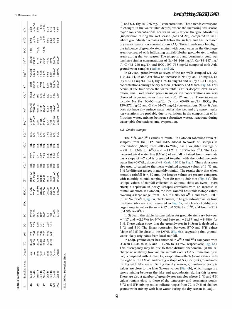
L), and SO4 (by 75–276 mg/L) concentrations. These trends correspondto changes in the water table depths, where the increasing wet seasonmajor ion concentrations occurs in wells where the groundwater is(sub)artesian during the wet season (A2 and A8), compared to wellswhere groundwater remains well below the surface and has increaseddry season major ion concentrations (A4). These trends may highlightthe influence of groundwater mixing with pond water in the dischargeareas, compared with infiltrating rainfall diluting groundwater in otherareas during the wet season. The temporary and permanent pond wa-ters have similar concentrations of Na (56–166 mg/L), Ca (34–147 mg/L), Cl (43–240 mg/L), and HCO3 (97–738 mg/L) compared with Aglagroundwater samples (Tables 1 and 2).

In St Jean, groundwater at seven of the ten wells sampled (J1, J2,J10, J3, J4, J6 and J9) show an increase in Na (by 36–115 mg/L), Ca(by 49–114 mg/L), HCO3 (by 119–439 mg/L) and Cl (by 42–111 mg/L)concentrations during the dry season (February and March, Fig. 5). Thisoccurs at the time when the water table is at its deepest level. In ad-dition, small wet season peaks in major ion concentrations are alsoobserved in groundwater from wells J5, J7 and J8. These increasesinclude Na (by 63–65 mg/L), Ca (by 63–80 mg/L), HCO3 (by128–272 mg/L) and Cl (by 61–79 mg/L) concentrations. Since St Jeandoes not have any surface water bodies, the wet and dry season majorion variations are probably due to variations in the composition of in-filtrating water, mixing between subsurface waters, reactions duringwater table fluctuations, and evaporation.

4.3. Stables isotopes

The δ18O and δ2H values of rainfall in Cotonou (obtained from 95samples from the IITA and IAEA Global Network of Isotopes inPrecipitation (GNIP) from 2005 to 2016) has a weighted average of−2.8 ± 1.6‰ for δ18O and −11.2 ± 11.7‰ for δ2H. The localmeteorological water line (LMWL) of rainfall obtained from these datahas a slope of ~7 and is presented together with the global meteoricwater line (GMWL; slope of ~8, Craig, 1961) in Fig. 6. These data werealso used to calculate the mean weighted average values of δ18O andδ2H for different ranges in monthly rainfall. The results show that whenmonthly rainfall is< 50 mm, the isotope values are greater comparedwith monthly rainfall ranging from 50 mm to 500 mm (Fig. 6a). Theisotope values of rainfall collected in Cotonou show an overall masseffect; a depletion in heavy isotopes correlates with an increase inrainfall amounts. In Cotonou, the local rainfall has stable isotope valuescovering a large range; from −5.4 to 0.8‰ for δ18O, and from −30.9to 14.5‰ for δ2H (Fig. 6a, black crosses). The groundwater values fromthe three sites are also presented in Fig. 6a, which also highlights alarge range in values (from −4.17 to 0.35‰ for δ18O, and from −21.9to 4.3‰ for δ2H).

In St Jean, the stable isotope values for groundwater vary between−4.17 and −2.37‰ for δ18O and between −21.87 and −8.98‰ forδ2H. These values show that the groundwater in St Jean is depleted atδ18O and δ2H. The linear regression between δ18O and δ2H values(slope of 7.5) lie close to the LMWL (Fig. 6a), suggesting that ground-water likely originates from local rainfall.

In Ladji, groundwater has enriched in δ18O and δ2H compared withSt Jean (-3.36 to 0.35 and −12.96 to 4.17‰, respectively; Fig. 6b).This discrepancy may be due to three distinct phenomena: (i) the re-charge of relatively low volume rainfall events (< 50 mm/month) inLadji compared with St Jean; (ii) evaporation effects (some values lie tothe right of the LMWL indicating a slope of 5.2), or (iii) groundwatermixing with lake water. During the dry season, groundwater isotopicvalues are close to the lake Nakoue values (Fig. 6b), which suggests astrong mixing between the lake and groundwater during this season.There are also a number of groundwater samples whose δ18O and δ2Hvalues remain close to those of the temporary and permanent ponds.δ18O and δ2H mixing ratios indicate ranges from 72 to 74% of shallowgroundwater mixing with lake water during the dry season in Ladji.T

able

2(con

tinued)

IDSa

mplingmon

thOrigin

T°C

pHDO

EC

NOx

HCO3−

Cl−

NO2−

Br−

NO3−

PO4−−

SO4−−

Na+

NH4+

K+

Mg+

+Ca+

+DOC

d18O

d2H

L15

Feb-18

lake

30.20

7.90

7.29

49,700

113.46

1803

1.65

BDL

69.73

BDL

BDL

249.49

9579

.63

25.33

32.24

955.30

323.52

1.02

0.93

7.34

Jun-18

lake

37.00

7.67

5.85

38,100

57.95

1517

3.94

BDL

52.19

BDL

BDL

2165

.47

7884

.58

0.34

296.81

994.89

254.81

−1.34

−14

.50

L16

Mar-18

pond

29.20

8.65

1.16

3830

1115

.08

824.56

BDL

3.41

BDL

7.25

2.78

698.15

BDL

34.17

73.68

11.74

40.37

0.56

5.05

Jun-18

pond

29.10

7.37

0.01

1024

289.75

120.41

BDL

0.17

BDL

6.98

41.34

121.28

0.83

39.94

12.58

39.45

−1.34

−4.37

L17

Mar-18

pond

28.90

7.20

0.01

2000

274.50

356.31

BDL

5.95

BDL

BDL

224.64

314.95

1.96

12.20

19.63

43.30

33.59

−2.02

−6.86

Jun-18

pond

30.90

6.86

0.35

831

259.25

46.16

BDL

BDL

BDL

1.66

1.43

47.63

2.57

1.98

8.63

44.32

0.50

5.33

L19

Jun-18

pond

30.30

6.88

0.04

633

251.32

53.73

BDL

BDL

BDL

3.55

8.52

62.68

0.24

26.85

5.28

32.71

0.63

6.15

AO1

Jan-19

Ocean

51,000

132.00

1909

1.00

BDL

7.00

BDL

BDL

2317

.00

126.00

0.70

384.00

1219

.00

391.00

0.52

4.68

AO2

Jan-19

Ocean

51,300

135.00

1917

2.00

BDL

64.00

BDL

BDL

2329

.00

1178

.00

0.40

382.00

1216

.00

386.00

0.54

4.69

*BDL:

Below

Detection

Limit.

H. Houéménou, et al. Journal of Hydrology 582 (2020) 124438

9

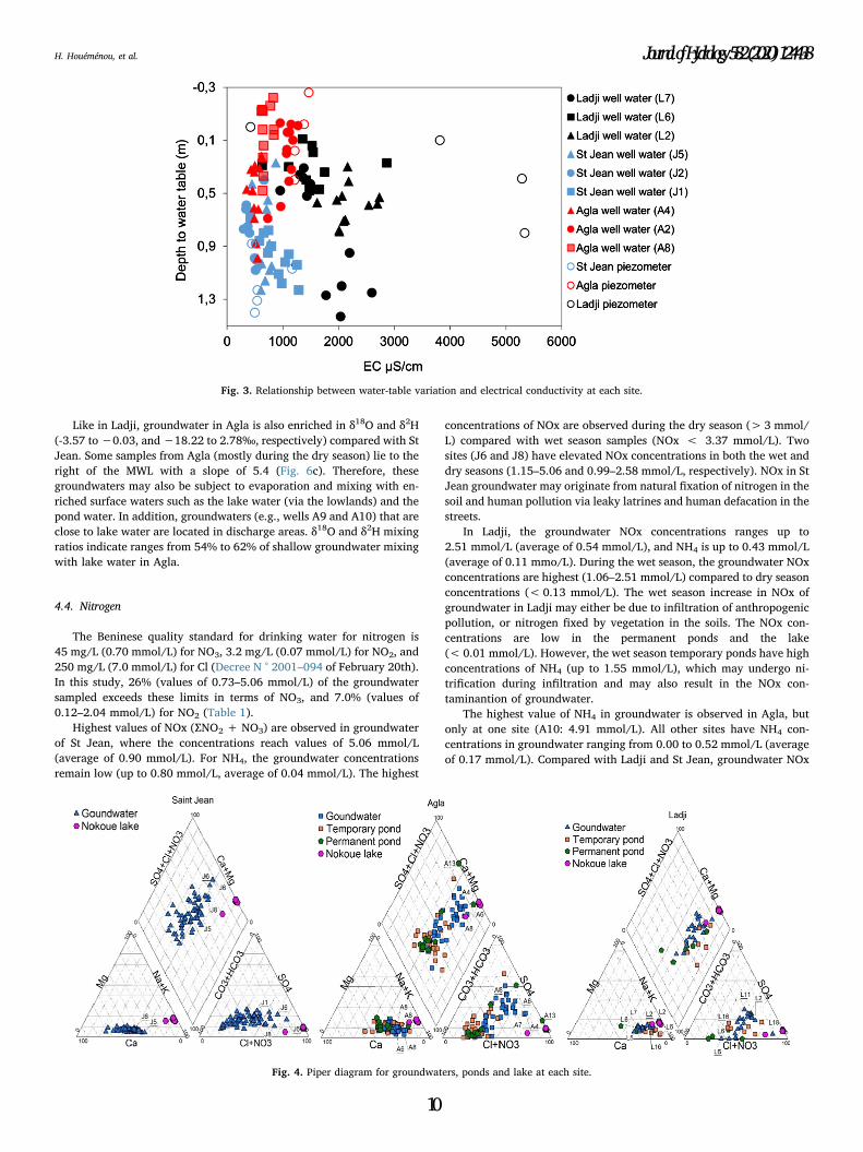
Like in Ladji, groundwater in Agla is also enriched in δ18O and δ2H(-3.57 to−0.03, and−18.22 to 2.78‰, respectively) compared with StJean. Some samples from Agla (mostly during the dry season) lie to theright of the MWL with a slope of 5.4 (Fig. 6c). Therefore, thesegroundwaters may also be subject to evaporation and mixing with en-riched surface waters such as the lake water (via the lowlands) and thepond water. In addition, groundwaters (e.g., wells A9 and A10) that areclose to lake water are located in discharge areas. δ18O and δ2H mixingratios indicate ranges from 54% to 62% of shallow groundwater mixingwith lake water in Agla.

4.4. Nitrogen

The Beninese quality standard for drinking water for nitrogen is45 mg/L (0.70 mmol/L) for NO3, 3.2 mg/L (0.07 mmol/L) for NO2, and250 mg/L (7.0 mmol/L) for Cl (Decree N ° 2001–094 of February 20th).In this study, 26% (values of 0.73–5.06 mmol/L) of the groundwatersampled exceeds these limits in terms of NO3, and 7.0% (values of0.12–2.04 mmol/L) for NO2 (Table 1).

Highest values of NOx (∑NO2 + NO3) are observed in groundwaterof St Jean, where the concentrations reach values of 5.06 mmol/L(average of 0.90 mmol/L). For NH4, the groundwater concentrationsremain low (up to 0.80 mmol/L, average of 0.04 mmol/L). The highest

concentrations of NOx are observed during the dry season (> 3 mmol/L) compared with wet season samples (NOx < 3.37 mmol/L). Twosites (J6 and J8) have elevated NOx concentrations in both the wet anddry seasons (1.15–5.06 and 0.99–2.58 mmol/L, respectively). NOx in StJean groundwater may originate from natural fixation of nitrogen in thesoil and human pollution via leaky latrines and human defacation in thestreets.

In Ladji, the groundwater NOx concentrations ranges up to2.51 mmol/L (average of 0.54 mmol/L), and NH4 is up to 0.43 mmol/L(average of 0.11 mmo/L). During the wet season, the groundwater NOxconcentrations are highest (1.06–2.51 mmol/L) compared to dry seasonconcentrations (< 0.13 mmol/L). The wet season increase in NOx ofgroundwater in Ladji may either be due to infiltration of anthropogenicpollution, or nitrogen fixed by vegetation in the soils. The NOx con-centrations are low in the permanent ponds and the lake(< 0.01 mmol/L). However, the wet season temporary ponds have highconcentrations of NH4 (up to 1.55 mmol/L), which may undergo ni-trification during infiltration and may also result in the NOx con-taminantion of groundwater.

The highest value of NH4 in groundwater is observed in Agla, butonly at one site (A10: 4.91 mmol/L). All other sites have NH4 con-centrations in groundwater ranging from 0.00 to 0.52 mmol/L (averageof 0.17 mmol/L). Compared with Ladji and St Jean, groundwater NOx

Fig. 3. Relationship between water-table variation and electrical conductivity at each site.

Fig. 4. Piper diagram for groundwaters, ponds and lake at each site.

H. Houéménou, et al. Journal of Hydrology 582 (2020) 124438

10

concentrations in Agla are low, with a maximum of 0.86 mmol/L(average of 0.15 mmol/L). In contrast, permanent ponds in the Aglalowlands have high NOx levels only at one site (A13: 17.50 mmol/L),particularly in the dry season.

As described by Katz et al. (2011), the Cl/Br ratio can be a valuablefirst assessment of septic tank contamination of shallow groundwater.This is based on the assumption that sewerage waters and septic tankeffluent exhibit distinct ranges and higher values of Cl/Br molar ratios

Fig. 5. Temporal variation between, depth water table, electrical conductivity, major ion and isotopic stable at each site.

H. Houéménou, et al. Journal of Hydrology 582 (2020) 124438

11

and Cl concentrations compared with rainwater (Davis et al., 1998), asobserved in many samples form this study (Fig. 7a). Elevated Cl/Brratios may also result from the dissolution of halite. However, haliteshave not been reported in the local Quaternary aquifer. In addition,many of the groundwater values correspond to ranges reported forsewerage and septic tank effluent (Davis et al., 1998; Vengosh andPankratov, 1998; Katz et al., 2011) compared with waters with halitedissolution (Davis et al., 1998; Pastén-Zapata et al., 2014; Panno et al.,2006), rainwater from coastal areas, and seawater (Alcalá and Custodio

2008; Davis et al., 1998). According to Fig. 7b, groundwater valueswith similar Cl/Br ratios and Cl concentrations than sewerage waste-water also show higher concentrations of NOx. Three samples (wells J2,L9 and A6) plot above the Cl/Br ratios for sewage or septic tank effluent(Cl/Br molar ratios 676–1350; Cl < 1000 ml/L), likely indicatinganimal manure. As evidenced in Fig. 7b, values that fall into the animalmanure/animal urine (Cl/Br molar ratios, 2810–3730; Cl < 1000 mg/L) also have high NOx concentrations (0.76–0.81 mmol/L). Other evi-dence for a septic tank and animal manure influence are the corre-sponding elevated dissolved organic carbon (DOC) concentrations(Table 1). However, not all the groundwater samples have high DOCconcentrations. According to Kortelainen and Karhu (2006), rapidoxidation of DOC into carbon dioxyde may account for the low DOCconcentration in groundwater.

Alternatively, samples with low NOx concentrations and relativelylow Cl/Br ratios, such as groundwater from Agla (Fig. 7b), can indicateareas of organic biodegradation (e.g. McArthur et al., 2012). The re-lationship between HCO3, NOx and DO for all groundwater sampled atAgla is shown in Fig. 8. The samples where dissolved oxygen (DO) andNOx are low compared with HCO3 correspond to discharge areas. Thisis especially the case for groundwater sampled during the dry season atwells A10, A9 and piezometers A11, J11 where HCO3 values increases(4.80–12.31 mmol/L) and NOx decreases (0.0–0.40 mmol/L) with lowDO values (0.06–4.22 mg/L). However, this may also indicate areas ofrecent rainfall infiltration resulting in a dilution of NOx concentrations(e.g. for well A4).Fig. 9.

Fig. 6. Relationship between 18O and 2H with Global Meteoric Water Line(GMWL) and Local Meteoric Water Line (GMWL).

Fig. 7. (a) Groundwater, pond and lake water Cl/Br molar ratios with changesin Cl concentrations highlights different sources of Cl in the waters. (b)Relationship between Cl/Br ratios and Cl concentrations showing higher con-centrations in NOx (circle sizes are relative to NOx concentrations).

H. Houéménou, et al. Journal of Hydrology 582 (2020) 124438

12

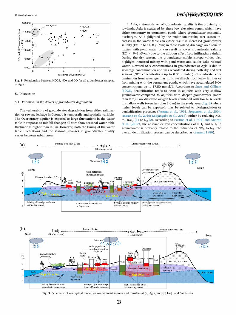
5. Discussion

5.1. Variations in the drivers of groundwater degradation

The vulnerability of groundwater degradation from either saliniza-tion or sewage leakage in Cotonou is temporally and spatially variable.The Quarternary aquifer is exposed to large fluctuations in the watertable in response to rainfall changes; all sites show seasonal water tablefluctuations higher than 0.5 m. However, both the timing of the watertable fluctuations and the seasonal changes in groundwater qualityvaries between urban areas.

In Agla, a strong driver of groundwater quality is the proximity tolowlands. Agla is scattered by these low elevation zones, which haveeither temporary or permanent ponds where groundwater seasonallydischarges. As highlighted by the major ion results, wet season in-creases in the water table can either result in increased groundwatersalinity (EC up to 1468 µS/cm) in these lowland discharge areas due tomixing with pond water, or can result in lower groundwater salinity(EC < 842 µS/cm) due to the dilution effect from infiltrating rainfall.During the dry season, the groundwater stable isotope values alsohighlight increased mixing with pond water and saltier Lake Nokouéwater. Elevated NOx concentrations in groundwater at Agla is due tosewerage contamination and was recordered during both dry and wetseasons (NOx concentrations up to 0.86 mmol/L). Groundwater con-tamination from sewerage may infiltrate direcly from leaky latrines orfrom mixing with the permanent ponds, which have accumulated NOxconcentrations up to 17.50 mmol/L. According to Starr and Gillham(1993), denitrification tends to occur in aquifers with very shallowgroundwater compared to aquifers with deeper groundwater (morethan 2 m). Low dissolved oxygen levels combined with low NOx levelsin shallow wells (even less than 1.0 m) in the study area (Fig. 8) wherehigher levels can be expected, may be related to biodegradation ordenitrification processes (Postma et al., 1991, Jorgensen et al., 2004,Hassane et al., 2016; Kadjangaba et al., 2018). Either by reducing NO3

to HCO3 (1) or N2 (2). According to Postma et al. (1991) and Anornuet al. (2017), the absence or low concentrations of NO2 and NH4 ingroundwater is probably related to the reduction of NO3 to N2. Theoverall denitrification process can be described as (Berner, 1980):

Fig. 8. Relationship between HCO3, NOx and DO for all groundwater sampledat Agla.

Fig. 9. Schematic of conceptual model for contaminant sources and transfers at (a) Agla, and (b) Ladji and Saint-Jean.

H. Houéménou, et al. Journal of Hydrology 582 (2020) 124438

13

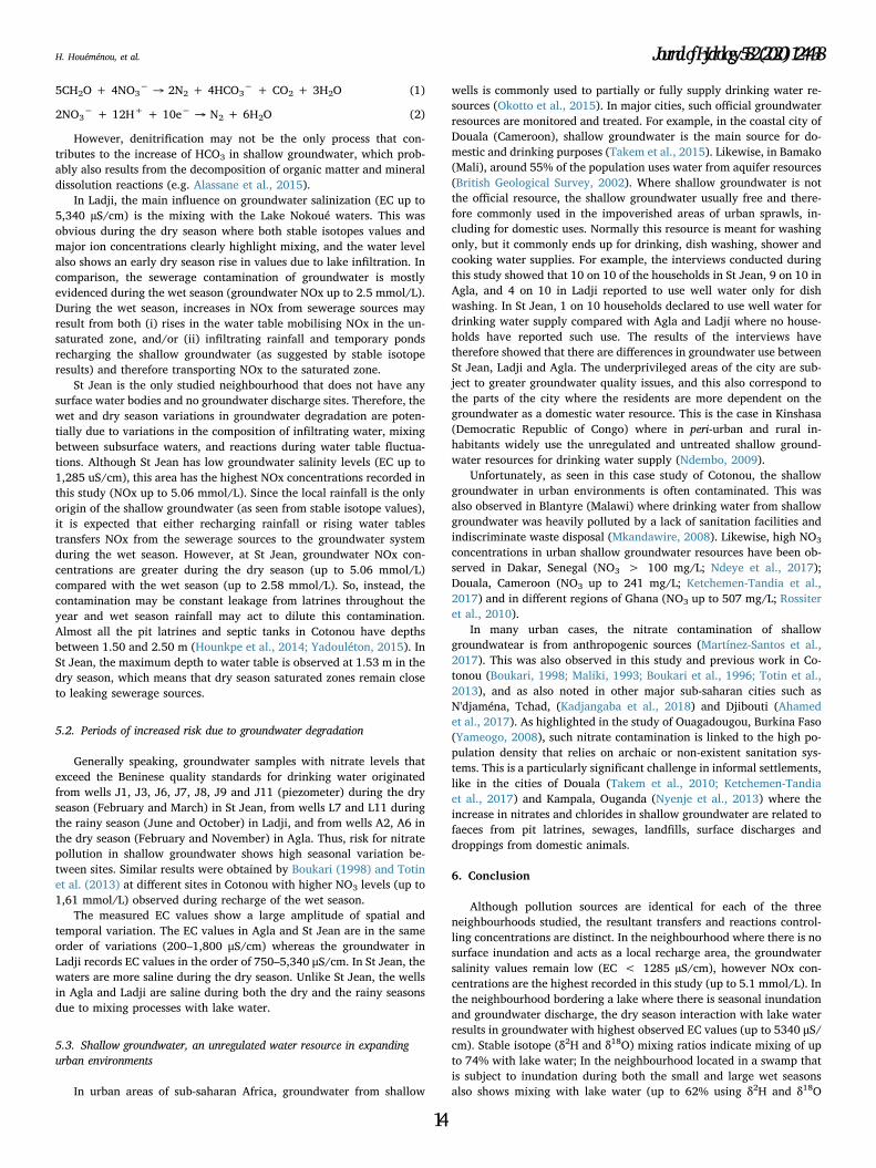
5CH2O + 4NO3−→ 2N2 + 4HCO3

− + CO2 + 3H2O (1)

2NO3− + 12H+ + 10e− → N2 + 6H2O (2)

However, denitrification may not be the only process that con-tributes to the increase of HCO3 in shallow groundwater, which prob-ably also results from the decomposition of organic matter and mineraldissolution reactions (e.g. Alassane et al., 2015).

In Ladji, the main influence on groundwater salinization (EC up to5,340 µS/cm) is the mixing with the Lake Nokoué waters. This wasobvious during the dry season where both stable isotopes values andmajor ion concentrations clearly highlight mixing, and the water levelalso shows an early dry season rise in values due to lake infiltration. Incomparison, the sewerage contamination of groundwater is mostlyevidenced during the wet season (groundwater NOx up to 2.5 mmol/L).During the wet season, increases in NOx from sewerage sources mayresult from both (i) rises in the water table mobilising NOx in the un-saturated zone, and/or (ii) infiltrating rainfall and temporary pondsrecharging the shallow groundwater (as suggested by stable isotoperesults) and therefore transporting NOx to the saturated zone.

St Jean is the only studied neighbourhood that does not have anysurface water bodies and no groundwater discharge sites. Therefore, thewet and dry season variations in groundwater degradation are poten-tially due to variations in the composition of infiltrating water, mixingbetween subsurface waters, and reactions during water table fluctua-tions. Although St Jean has low groundwater salinity levels (EC up to1,285 uS/cm), this area has the highest NOx concentrations recorded inthis study (NOx up to 5.06 mmol/L). Since the local rainfall is the onlyorigin of the shallow groundwater (as seen from stable isotope values),it is expected that either recharging rainfall or rising water tablestransfers NOx from the sewerage sources to the groundwater systemduring the wet season. However, at St Jean, groundwater NOx con-centrations are greater during the dry season (up to 5.06 mmol/L)compared with the wet season (up to 2.58 mmol/L). So, instead, thecontamination may be constant leakage from latrines throughout theyear and wet season rainfall may act to dilute this contamination.Almost all the pit latrines and septic tanks in Cotonou have depthsbetween 1.50 and 2.50 m (Hounkpe et al., 2014; Yadouléton, 2015). InSt Jean, the maximum depth to water table is observed at 1.53 m in thedry season, which means that dry season saturated zones remain closeto leaking sewerage sources.

5.2. Periods of increased risk due to groundwater degradation

Generally speaking, groundwater samples with nitrate levels thatexceed the Beninese quality standards for drinking water originatedfrom wells J1, J3, J6, J7, J8, J9 and J11 (piezometer) during the dryseason (February and March) in St Jean, from wells L7 and L11 duringthe rainy season (June and October) in Ladji, and from wells A2, A6 inthe dry season (February and November) in Agla. Thus, risk for nitratepollution in shallow groundwater shows high seasonal variation be-tween sites. Similar results were obtained by Boukari (1998) and Totinet al. (2013) at different sites in Cotonou with higher NO3 levels (up to1,61 mmol/L) observed during recharge of the wet season.

The measured EC values show a large amplitude of spatial andtemporal variation. The EC values in Agla and St Jean are in the sameorder of variations (200–1,800 μS/cm) whereas the groundwater inLadji records EC values in the order of 750–5,340 μS/cm. In St Jean, thewaters are more saline during the dry season. Unlike St Jean, the wellsin Agla and Ladji are saline during both the dry and the rainy seasonsdue to mixing processes with lake water.

5.3. Shallow groundwater, an unregulated water resource in expandingurban environments

In urban areas of sub-saharan Africa, groundwater from shallow

wells is commonly used to partially or fully supply drinking water re-sources (Okotto et al., 2015). In major cities, such official groundwaterresources are monitored and treated. For example, in the coastal city ofDouala (Cameroon), shallow groundwater is the main source for do-mestic and drinking purposes (Takem et al., 2015). Likewise, in Bamako(Mali), around 55% of the population uses water from aquifer resources(British Geological Survey, 2002). Where shallow groundwater is notthe official resource, the shallow groundwater usually free and there-fore commonly used in the impoverished areas of urban sprawls, in-cluding for domestic uses. Normally this resource is meant for washingonly, but it commonly ends up for drinking, dish washing, shower andcooking water supplies. For example, the interviews conducted duringthis study showed that 10 on 10 of the households in St Jean, 9 on 10 inAgla, and 4 on 10 in Ladji reported to use well water only for dishwashing. In St Jean, 1 on 10 households declared to use well water fordrinking water supply compared with Agla and Ladji where no house-holds have reported such use. The results of the interviews havetherefore showed that there are differences in groundwater use betweenSt Jean, Ladji and Agla. The underprivileged areas of the city are sub-ject to greater groundwater quality issues, and this also correspond tothe parts of the city where the residents are more dependent on thegroundwater as a domestic water resource. This is the case in Kinshasa(Democratic Republic of Congo) where in peri-urban and rural in-habitants widely use the unregulated and untreated shallow ground-water resources for drinking water supply (Ndembo, 2009).

Unfortunately, as seen in this case study of Cotonou, the shallowgroundwater in urban environments is often contaminated. This wasalso observed in Blantyre (Malawi) where drinking water from shallowgroundwater was heavily polluted by a lack of sanitation facilities andindiscriminate waste disposal (Mkandawire, 2008). Likewise, high NO3

concentrations in urban shallow groundwater resources have been ob-served in Dakar, Senegal (NO3 > 100 mg/L; Ndeye et al., 2017);Douala, Cameroon (NO3 up to 241 mg/L; Ketchemen-Tandia et al.,2017) and in different regions of Ghana (NO3 up to 507 mg/L; Rossiteret al., 2010).

In many urban cases, the nitrate contamination of shallowgroundwatear is from anthropogenic sources (Martínez-Santos et al.,2017). This was also observed in this study and previous work in Co-tonou (Boukari, 1998; Maliki, 1993; Boukari et al., 1996; Totin et al.,2013), and as also noted in other major sub-saharan cities such asN'djaména, Tchad, (Kadjangaba et al., 2018) and Djibouti (Ahamedet al., 2017). As highlighted in the study of Ouagadougou, Burkina Faso(Yameogo, 2008), such nitrate contamination is linked to the high po-pulation density that relies on archaic or non-existent sanitation sys-tems. This is a particularly significant challenge in informal settlements,like in the cities of Douala (Takem et al., 2010; Ketchemen-Tandiaet al., 2017) and Kampala, Ouganda (Nyenje et al., 2013) where theincrease in nitrates and chlorides in shallow groundwater are related tofaeces from pit latrines, sewages, landfills, surface discharges anddroppings from domestic animals.

6. Conclusion

Although pollution sources are identical for each of the threeneighbourhoods studied, the resultant transfers and reactions control-ling concentrations are distinct. In the neighbourhood where there is nosurface inundation and acts as a local recharge area, the groundwatersalinity values remain low (EC < 1285 µS/cm), however NOx con-centrations are the highest recorded in this study (up to 5.1 mmol/L). Inthe neighbourhood bordering a lake where there is seasonal inundationand groundwater discharge, the dry season interaction with lake waterresults in groundwater with highest observed EC values (up to 5340 μS/cm). Stable isotope (δ2H and δ18O) mixing ratios indicate mixing of upto 74% with lake water; In the neighbourhood located in a swamp thatis subject to inundation during both the small and large wet seasonsalso shows mixing with lake water (up to 62% using δ2H and δ18O

H. Houéménou, et al. Journal of Hydrology 582 (2020) 124438

14

values) resulting in groundwater EC values up to 1468 µS/cm. Thisdischarge site notably has lower NOx concentrations (up to 0.86 mmol/L), however this is not indicative of less sewerage contamination onlygreater degradation processes. Understanding the seasonal changes inprocesses controlling groundwater quality between each site is key toidentifying risks to the residents who use this unregulated shallowgroundwater resource for domestic purposes, including drinking watersupplies. Seasonal variations highlight heightened risks from sewerageand septic tank leakage during the wet season in neighbourhoods lo-cated in discharge areas compared with increased risk during the dryseason in the recharge area. In addition, there are increased risks ofshallow groundwater salinization during both the small wet and dryseasons in discharge areas.

Stable water isotopes showed a direct relationship between localrainfall water and groundwater at St Jean compared with Ladji andAgla where groundwaters are also be subjected to mixing with enrichedsurface waters such as the lake water (via the lowlands) and the pondwater, particularly during the dry and small wet seasons.

Groundwaters chemistry in each of the neighbourhoods are dif-ferent. In St Jean, the composition of major ion concentrations of wa-ters is dominated by Na-Ca-HCO3-Cl groundwater type, while Ladji is ofthe Na-HCO3-Cl type and Agla of the Na-Ca-HCO3-SO4-HCO3 one. Theponds sampled in both Ladji and Agla showed some similarities inmajor ion compositions with local groundwater, thus indicating a po-tential connection. The Lake Nokoué has greater concentrations of Naand Cl compared with all groundwater samples.

Groundwater samples indicated that 26% for NO3 and 7.0% for NO2

do not comply with the Beninese quality standard for drinking water.Based on Cl/Br molar ratios, sources of NOx in groundwater appear tobe dominated by infiltration of sewerage and septic tanks in dry seasonin St Jean, while in Agla and Ladji, contamination was obvious in wetseason following infiltrating rainfall and ponds recharging. Low NOxfor some of the groundwater samples may indicate effects from biode-gradation in discharge area or dilution from rainfall.

CRediT authorship contribution statement

Honoré Houéménou: Conceptualization, Writing - original draft,Writing - review & editing, Methodology, Investigation, Formal ana-lysis, Visualization. Sarah Tweed: Conceptualization, Methodology,Writing - original draft, Visualization, Supervision. Gauthier Dobigny:Conceptualization, Supervision, Writing - original draft. Daouda

Mama: Supervision. Abdoukarim Alassane: Supervision. Roland

Silmer: Resources. Milanka Babic: Resources. Stéphane Ruy: Writing- original draft. Alexis Chaigneau: Writing - original draft. PhilippeGauthier: Investigation. Akilou Socohou: Investigation. Henri-Joël

Dossou: Investigation. Sylvestre Badou: Investigation. Marc Leblanc:

Supervision, Resources, Project administration.

Declaration of Competing Interest

The authors declare that they have no known competing financialinterests or personal relationships that could have appeared to influ-ence the work reported in this paper.

Acknowledgements

The authors owe much gratitude to hydrogeology laboratory ofAvignon University, EPAC/LARBA and IRD/CBGP for the full financialand logistical support of this work. We are grateful to neighbourhoodchiefs and people who kindly authorized us to sample in their districtsand households. We thank the reviewers whose comments improvedthis paper.

Appendix A. Supplementary data

Supplementary data to this article can be found online at https://doi.org/10.1016/j.jhydrol.2019.124438.

References

Ahamed, H.A., Rayaleh, W.E., Zghibi, A., Ouddane, B., 2017. Assessment of chemicalquality of groundwater in coastal volcano-sedimentary aquifer of Djibouti, Horn ofAfrica. J. Afr. Earth Sci. 131, 284–300. https://doi.org/10.1016/j.jafrearsci.2017.04.010.

Alassane, A., Trabelsi, R., Dovonon, L.F., Odeloui, D.J., Boukari, M., Zouari, K., Mama, D.,2015. Chemical evolution of the continental terminal shallow aquifer in the south ofthe coastal sedimentary basin of Benin (West Africa) using multivariate factor ana-lysis. J. Water Resour. Protect. 7, 496–515.

Alcalá, F.J., Custodio, E., 2008. Using the Cl/Br ratio as a tracer to identify the origin ofsalinity in aquifers in Spain and Portugal. J. Hydrol. 359, 189–207.

Alidou, S., Boukari, M., Oyedé, L.M., Gaye, C.B., Faye, A., Gelinas, P., Isabel, D., Locat, J.(1994). Rapport technique final du projet “hydrogéologie du quaternaire du sud-bénin”, phase 2. CRDI 3-p-89-1017. Tomes 1, ii, iii et iv. Univ. nat. Bénin, univ. CAdiop, dakar, univ. Laval québec.

Anornu, G., Abass, G., Dickson, A., 2017. Tracking nitrate sources in groundwater andassociated health risk for rural communities in the White Volta River basin of Ghanausing isotopic approach (δ15N, δ18ONO3 and 3H). Sci. Total Environ. 603–604,687–698. https://doi.org/10.1016/j.scitotenv.2017.01.219.

Arnade, L.J., 1999. Seasonal correlation of well contamination and septic tank distance.Groundwater 37, 920–923. https://doi.org/10.1111/j.1745-6584.1999.tb01191.x.

Barker, A.P., Newton, R.J., Bottrell, S.H., Tellam, J.H., 1998. Processes affectinggroundwater chemistry in a zone of saline intrusion into an urban sandstone aquifer.Appl. Geochem. 13, 735–749. https://doi.org/10.1016/S0883-2927(98)00006-7.

Berner, R.A., 1980. Early Diagenesis: A Theoretical Approach. Princeton University Press.Boukari, M., 1998. Fonctionnement du système aquifère exploité pour l’approvisionne-

ment en eau de la ville de Cotonou sur le littoral béninois. Impact du développementurbain sur la qualité des ressources. Thèse Doctorat ès- Science. Université C. A.Diop de Dakar, Sénégal.

Boukari, M., Gaye, C.B., Faye, A., Faye, S., 1996. The Impact of Urban Development onCoastal Aquifers near Cotonou, Benin. J. Afr. Earth Sci. 22 (4), 403–408. https://doi.org/10.1016/0899-5362(96)00027-9.

British Geological Survey, 2002. Groundwater Quality: Mali. http://www.bgs.ac.uk/downloads/start.cfm?id=1284.

Cary, L., Petelet-Giraud, E., Bertrand, G., Kloppmann, W., Aquilina, L., Martins, V.,Hirata, R., 2015. Origins and processes of groundwater salinization in the urbancoastal aquifers of Recife (Pernambuco, Brazil): A multi-isotope approach. Sci. TotalEnviron. 530–531, 411–429. https://doi.org/10.1016/j.scitotenv.2015.05.015.

Craig, H., 1961. Standards for reporting concentrations of deuterium and oxygen-18 innatural waters. Science 133, 1833–1834.

Davis, S.N., Whittemorw, D.O., Martin, J.F., 1998. Uses of Chloride/Bromide Ratios inStudies of Potable Water. Groundwater 36 (2), 338–350. https://doi.org/10.1111/j.1745-6584.1998.tb01099.x.

Decret, 2001 No-094 du 200/02/2001 fixant les normes de qualité de l’eau potable enRépublique du Bénin.

Dhanasekarapandian, M., Chandran, S., Saranya Devi, D., Kumar, V., 2016. Spatial andtemporal variation of groundwater quality and its suitability for irrigation anddrinking purpose using GIS and WQI in an urban fringe. J. Afr. Earth Sc. 124,270–288. https://doi.org/10.1016/j.jafrearsci.2016.08.015.

EAA, 2018. Etude de reference sur les comportments, attitudes et pratiques des popula-tions de Cotonou sur la chaîne de l’eau dans la ville de cotonou. Rapport technique duprojet SAC-TIC. 72.

Hassane, A.B., 2010. Aquifères superficiels et profonds et pollution urbaine en Afrique:Cas de la communauté urbaine de Niamey (NIGER), 250.

Hassane, A.B., Leduc, C., Favreau, G., Bekins, B.A., Margueron, T., 2016. Impacts of aLarge Sahelian City on Groundwater Hydrodynamics and Quality: Example ofNiamey (Niger). Hydrogeol. J. 24 (2), 407–423. https://doi.org/10.1007/s10040-015-1345-z.

Hounkpe, S.P., Adjovi, E.C., Crapper, M., Awuah, E., 2014. Wastewater Management inThird World Cities: Case Study of Cotonou, Benin. J. Environ. Protect. 05, 387.https://doi.org/10.4236/jep.2014.55042.

INSAE, 2016. Principaux indicateurs socio-demographiques et economiques, mai 2013,synthèse des résultats d’analyse. Rapport, Direction des études démographiques,Cotonou, Bénin.

INSAE, 2015. Quatrième Recensement Général de la Population et de l’Habitat, mai 2013,synthèse des résultats d’analyse. Rapport, Direction des études démographiques,Cotonou, Bénin.

Jorgensen, P.R., Urup, J., Helstrup, T., Jensen, M.B., Eiland, F., Vinther, F.P., 2004.Transport and Reduction of Nitrate in Clayey till underneath Forest and Arable Land.J. Contam. Hydrol. 73 (1), 207–226. https://doi.org/10.1016/j.jconhyd.2004.01.005.

Kadjangaba, E., Djoret, D., Doumnang, J.C., Ndoutamia, G.A., Mahmout, Y., 2018. Impactdes Processus Hydrochimique sur la Qualité des Eaux souterraines de la Ville deN’Djaména-Tchad. Vol. 14. Doi: 10.19044/esj.2018.v14n18p162.

Katz, B.G., Eberts, S.M., Kauffman, J.L., 2011. Using Cl/Br ratios and other indicators toassess potential impacts on groundwater quality from septic systems: A review andexamples from principal aquifers in the United States. J. Hydrol. 397 (3), 151–166.https://doi.org/10.1016/j.jhydrol.2010.11.017.

H. Houéménou, et al. Journal of Hydrology 582 (2020) 124438

15

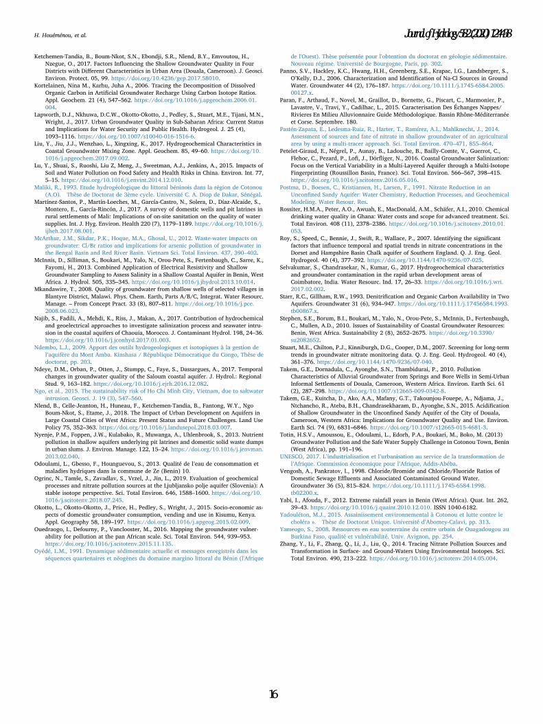
Ketchemen-Tandia, B., Boum-Nkot, S.N., Ebondji, S.R., Nlend, B.Y., Emvoutou, H.,Nzegue, O., 2017. Factors Influencing the Shallow Groundwater Quality in FourDistricts with Different Characteristics in Urban Area (Douala, Cameroon). J. Geosci.Environ. Protect. 05, 99. https://doi.org/10.4236/gep.2017.58010.

Kortelainen, Nina M., Karhu, Juha A., 2006. Tracing the Decomposition of DissolvedOrganic Carbon in Artificial Groundwater Recharge Using Carbon Isotope Ratios.Appl. Geochem. 21 (4), 547–562. https://doi.org/10.1016/j.apgeochem.2006.01.004.

Lapworth, D.J., Nkhuwa, D.C.W., Okotto-Okotto, J., Pedley, S., Stuart, M.E., Tijani, M.N.,Wright, J., 2017. Urban Groundwater Quality in Sub-Saharan Africa: Current Statusand Implications for Water Security and Public Health. Hydrogeol. J. 25 (4),1093–1116. https://doi.org/10.1007/s10040-016-1516-6.

Liu, Y., Jiu, J.J., Wenzhao, L., Xingxing, K., 2017. Hydrogeochemical Characteristics inCoastal Groundwater Mixing Zone. Appl. Geochem. 85, 49–60. https://doi.org/10.1016/j.apgeochem.2017.09.002.

Lu, Y., Shuai, S., Ruoshi, Liu Z, Meng, J., Sweetman, A.J., Jenkins, A., 2015. Impacts ofSoil and Water Pollution on Food Safety and Health Risks in China. Environ. Int. 77,5–15. https://doi.org/10.1016/j.envint.2014.12.010.

Maliki, R., 1993. Etude hydrogéologique du littoral béninois dans la région de Cotonou(A.O). Thèse de Doctorat de 3ème cycle. Université C. A. Diop de Dakar, Sénégal.

Martínez-Santos, P., Martín-Loeches, M., García-Castro, N., Solera, D., Díaz-Alcaide, S.,Montero, E., García-Rincón, J., 2017. A survey of domestic wells and pit latrines inrural settlements of Mali: Implications of on-site sanitation on the quality of watersupplies. Int. J. Hyg. Environ. Health 220 (7), 1179–1189. https://doi.org/10.1016/j.ijheh.2017.08.001.

McArthur, J.M., Sikdar, P.K., Hoque, M.A., Ghosal, U., 2012. Waste-water impacts ongroundwater: Cl/Br ratios and implications for arsenic pollution of groundwater inthe Bengal Basin and Red River Basin. Vietnam Sci. Total Environ. 437, 390–402.

McInnis, D., Silliman, S., Boukari, M., Yalo, N., Orou-Pete, S., Fertenbaugh, C., Sarre, K.,Fayomi, H., 2013. Combined Application of Electrical Resistivity and ShallowGroundwater Sampling to Assess Salinity in a Shallow Coastal Aquifer in Benin, WestAfrica. J. Hydrol. 505, 335–345. https://doi.org/10.1016/j.jhydrol.2013.10.014.

Mkandawire, T., 2008. Quality of groundwater from shallow wells of selected villages inBlantyre District, Malawi. Phys. Chem. Earth, Parts A/B/C, Integrat. Water Resourc.Manage. – From Concept Pract. 33 (8), 807–811. https://doi.org/10.1016/j.pce.2008.06.023.

Najib, S., Fadili, A., Mehdi, K., Riss, J., Makan, A., 2017. Contribution of hydrochemicaland geoelectrical approaches to investigate salinization process and seawater intru-sion in the coastal aquifers of Chaouia, Morocco. J. Contaminant Hydrol. 198, 24–36.https://doi.org/10.1016/j.jconhyd.2017.01.003.

Ndembo, L.J., 2009. Apport des outils hydrogeologiques et isotopiques à la gestion del’aquifère du Mont Amba. Kinshasa / République Démocratique du Congo, Thèse dedoctorat, pp. 203.

Ndeye, D.M., Orban, P., Otten, J., Stumpp, C., Faye, S., Dassargues, A., 2017. Temporalchanges in groundwater quality of the Saloum coastal aquifer. J. Hydrol.: RegionalStud. 9, 163–182. https://doi.org/10.1016/j.ejrh.2016.12.082.

Ngo, et al., 2015. The sustainability risk of Ho Chi Minh City, Vietnam, due to saltwaterintrusion. Geosci. J. 19 (3), 547–560.

Nlend, B., Celle-Jeanton, H., Huneau, F., Ketchemen-Tandia, B., Fantong, W.Y., NgoBoum-Nkot, S., Etame, J., 2018. The Impact of Urban Development on Aquifers inLarge Coastal Cities of West Africa: Present Status and Future Challenges. Land UsePolicy 75, 352–363. https://doi.org/10.1016/j.landusepol.2018.03.007.

Nyenje, P.M., Foppen, J.W., Kulabako, R., Muwanga, A., Uhlenbrook, S., 2013. Nutrientpollution in shallow aquifers underlying pit latrines and domestic solid waste dumpsin urban slums. J. Environ. Manage. 122, 15–24. https://doi.org/10.1016/j.jenvman.2013.02.040.

Odoulami, L., Gbesso, F., Hounguevou, S., 2013. Qualité de l’eau de consommation etmaladies hydriques dans la commune de Ze (Benin) 10.

Ogrinc, N., Tamše, S., Zavadlav, S., Vrzel, J., Jin, L., 2019. Evaluation of geochemicalprocesses and nitrate pollution sources at the Ljubljansko polje aquifer (Slovenia): Astable isotope perspective. Sci. Total Environ. 646, 1588–1600. https://doi.org/10.1016/j.scitotenv.2018.07.245.

Okotto, L., Okotto-Okotto, J., Price, H., Pedley, S., Wright, J., 2015. Socio-economic as-pects of domestic groundwater consumption, vending and use in Kisumu, Kenya.Appl. Geography 58, 189–197. https://doi.org/10.1016/j.apgeog.2015.02.009.

Ouedraogo, I., Defourny, P., Vanclooster, M., 2016. Mapping the groundwater vulner-ability for pollution at the pan African scale. Sci. Total Environ. 544, 939–953.https://doi.org/10.1016/j.scitotenv.2015.11.135.

Oyédé, L.M., 1991. Dynamique sédimentaire actuelle et messages enregistrés dans lesséquences quartenaires et néogènes du domaine margino littoral du Bénin (l'Afrique

de l'Ouest). Thèse présentée pour l'obtention du doctorat en géologie sédimentaire.Nouveau régime. Université de Bourgogne, Paris, pp. 302.

Panno, S.V., Hackley, K.C., Hwang, H.H., Greenberg, S.E., Krapac, I.G., Landsberger, S.,O’Kelly, D.J., 2006. Characterization and Identification of Na-Cl Sources in GroundWater. Groundwater 44 (2), 176–187. https://doi.org/10.1111/j.1745-6584.2005.00127.x.

Paran, F., Arthaud, F., Novel, M., Graillot, D., Bornette, G., Piscart, C., Marmonier, P.,Lavastre, V., Travi, Y., Cadilhac, L., 2015. Caracterisation Des Échanges Nappes/Rivieres En Milieu Alluvionnaire Guide Méthodologique. Bassin Rhône-Méditerranéeet Corse. Septembre. 180.

Pastén-Zapata, E., Ledesma-Ruiz, R., Harter, T., Ramírez, A.I., Mahlknecht, J., 2014.Assessment of sources and fate of nitrate in shallow groundwater of an agriculturalarea by using a multi-tracer approach. Sci. Total Environ. 470–471, 855–864.

Petelet-Giraud, E., Négrel, P., Aunay, B., Ladouche, B., Bailly-Comte, V., Guerrot, C.,Flehoc, C., Pezard, P., Lofi, J., Dörfliger, N., 2016. Coastal Groundwater Salinization:Focus on the Vertical Variability in a Multi-Layered Aquifer through a Multi-IsotopeFingerprinting (Roussillon Basin, France). Sci. Total Environ. 566–567, 398–415.https://doi.org/10.1016/j.scitotenv.2016.05.016.

Postma, D., Boesen, C., Kristiansen, H., Larsen, F., 1991. Nitrate Reduction in anUnconfined Sandy Aquifer: Water Chemistry, Reduction Processes, and GeochemicalModeling. Water Resour. Res.

Rossiter, H.M.A., Peter, A.O., Awuah, E., MacDonald, A.M., Schäfer, A.I., 2010. Chemicaldrinking water quality in Ghana: Water costs and scope for advanced treatment. Sci.Total Environ. 408 (11), 2378–2386. https://doi.org/10.1016/j.scitotenv.2010.01.053.

Roy, S., Speed, C., Bennie, J., Swift, R., Wallace, P., 2007. Identifying the significantfactors that influence temporal and spatial trends in nitrate concentrations in theDorset and Hampshire Basin Chalk aquifer of Southern England. Q. J. Eng. Geol.Hydrogeol. 40 (4), 377–392. https://doi.org/10.1144/1470-9236/07-025.

Selvakumar, S., Chandrasekar, N., Kumar, G., 2017. Hydrogeochemical characteristicsand groundwater contamination in the rapid urban development areas ofCoimbatore, India. Water Resourc. Ind. 17, 26–33. https://doi.org/10.1016/j.wri.2017.02.002.

Starr, R.C., Gillham, R.W., 1993. Denitrification and Organic Carbon Availability in TwoAquifers. Groundwater 31 (6), 934–947. https://doi.org/10.1111/j.17456584.1993.tb00867.x.

Stephen, S.E., Borum, B.I., Boukari, M., Yalo, N., Orou-Pete, S., McInnis, D., Fertenbaugh,C., Mullen, A.D., 2010. Issues of Sustainability of Coastal Groundwater Resources:Benin, West Africa. Sustainability 2 (8), 2652–2675. https://doi.org/10.3390/su2082652.

Stuart, M.E., Chilton, P.J., Kinniburgh, D.G., Cooper, D.M., 2007. Screening for long-termtrends in groundwater nitrate monitoring data. Q. J. Eng. Geol. Hydrogeol. 40 (4),361–376. https://doi.org/10.1144/1470-9236/07-040.

Takem, G.E., Dornadula, C., Ayonghe, S.N., Thambidurai, P., 2010. PollutionCharacteristics of Alluvial Groundwater from Springs and Bore Wells in Semi-UrbanInformal Settlements of Douala, Cameroon, Western Africa. Environ. Earth Sci. 61(2), 287–298. https://doi.org/10.1007/s12665-009-0342-8.

Takem, G.E., Kuitcha, D., Ako, A.A., Mafany, G.T., Takounjou-Fouepe, A., Ndjama, J.,Ntchancho, R., Ateba, B.H., Chandrasekharam, D., Ayonghe, S.N., 2015. Acidificationof Shallow Groundwater in the Unconfined Sandy Aquifer of the City of Douala,Cameroon, Western Africa: Implications for Groundwater Quality and Use. Environ.Earth Sci. 74 (9), 6831–6846. https://doi.org/10.1007/s12665-015-4681-3.

Totin, H.S.V., Amoussou, E., Odoulami, L., Edorh, P.A., Boukari, M., Boko, M. (2013)Groundwater Pollution and the Safe Water Supply Challenge in Cotonou Town, Benin(West Africa), pp. 191–196.

UNESCO, 2017. L’industrialisation et l’urbanisation au service de la transformation del’Afrique. Commission économique pour l’Afrique, Addis-Abéba.

Vengosh, A., Pankratov, I., 1998. Chloride/Bromide and Chloride/Fluoride Ratios ofDomestic Sewage Effluents and Associated Contaminated Ground Water.Groundwater 36 (5), 815–824. https://doi.org/10.1111/j.1745-6584.1998.tb02200.x.

Yabi, I., Afouda, F., 2012. Extreme rainfall years in Benin (West Africa). Quat. Int. 262,39–43. https://doi.org/10.1016/j.quaint.2010.12.010. ISSN 1040-6182.

Yadouléton, M.J., 2015. Assainissement environnemental à Cotonou et lutte contre lecholéra ». Thèse de Doctorat Unique. Université d’Abomey-Calavi, pp. 313.

Yameogo, S., 2008. Ressources en eau souterraine du centre urbain de Ouagadougou auBurkina Faso, qualité et vulnérabilité. Univ. Avignon, pp. 254.

Zhang, Y., Li, F., Zhang, Q., Li, J., Liu, Q., 2014. Tracing Nitrate Pollution Sources andTransformation in Surface- and Ground-Waters Using Environmental Isotopes. Sci.Total Environ. 490, 213–222. https://doi.org/10.1016/j.scitotenv.2014.05.004.

H. Houéménou, et al. Journal of Hydrology 582 (2020) 124438

16

67

CHAPITRE IV : DISTRIBUTION ET SOURCES DES ELEMENTS TRACES (Article 2)

68

Seasonal variations in processes driving manganese and iron concentrations above

drinking water guidelines in the unregulated shallow aquifer of Cotonou

(Southern Benin)

Authors: Honoré Houéménou 1,6*, Seidel Jean Luc2, Sarah Tweed3, Abdoukarim Alassane6, Daouda Mama6,

Fabienne Trolard1, Salifou Orou-Pete6, Akilou Socohou6, Gauthier Dobigny4,5, Marc Leblanc1

Affiliations

1UMR EMMAH, Hydrogeology Laboratory, University of Avignon, INRA, Avignon, France

2UMR HSM, Univ. Montpellier, CNRS, IRD, Montpellier, France

3UMR G-eau, IRD, Montpellier, France

4 UMR CBGP, IRD, INRA, Cirad, Montpelllier SupAgro, MUSE, Montpellier France

5Laboratory of Research in Applied Biology, University of Abomey-Calavi, EPAC, Cotonou, Benin

6Laboratory of Applied Hydrology, University of Abomey-Calavi, 01 B.P. 4521 Cotonou, Benin

Abstract

Urbanization combined with the production of domestic and industrial waste in expanding West African cities

are a significant contributor of elevated level of metallic trace elements of groundwater, which are a greatest

risk to human health. The Fe and Mn concentrations in the unregulated shallow aquifer of Cotonou (Benin)

intermittently exceed concentrations of Beninese drinking water guidelines (100 µg/L and 300 µg/L for Mn

and Fe respectively). The processes controlling the elevated Fe and Mn concentrations (up to 999 and 643

g/L) were analysed in three urban neighborhoods of Cotonou with distinct hydrogeological contexts: Ladji is

seasonally inundated by water from the Lake Nokoué, Agla is subject to inundations and is located in a swampy

low-lying area, and St Jean is located at higher elevations where there is no inundation or ponds. The

concentrations of trace elements and Rare Earth Elements (REE) in groundwater, surface-water and soil were

determined from a total of 142 samples acquired between June 2017 to June 2018 by Spectrometry (Q-ICP

MS). Results of this study highlight that infiltration of waters from shallow ponds are a key element in driving

elevated Mn and Fe concentrations and their role is multi-faceted. Firstly, the ponds transmit high loads of

dissolved inorganic carbon (DOC) to the aquifer that is used in the reductive dissolution of the Mn-bearing

minerals (Mn (IV) (oxyhydr)oxides). In-aquifer Fe-mineral dissolution is unlikely due to the super-saturation

of common Fe-oxyhydroxide minerals for these groundwaters. Relatively low Ce/Ce* anomalies at Agla (1.06)

compared with Ladji (1.08) may indicate higher organic matter transfers to the groundwater from the ponds in

Agla, compared with the ponds in Ladji. Secondly, the ponds are a significant source of both Fe and Mn, with

concentrations up to 1742 and 561 in Agla, and 1232 and 235 in Ladji. The lake (with Mn concentrations up to

970) is also likely to contribute to high concentrations of Mn in groundwater at Ladji. The analysis of sediments

at each site also highlighted the accumulation of Fe in the unsaturated zone where the sediments are clay-rich.

69

The increases in Mn and Fe concentrations in the shallow aquifer predominantly occurs during the dry season;

when this unregulated water resource is most solicited by local residents living in underprivileged areas.

Key words: Surface water and groundwater, reductive condition, organic matter, iron and manganese concentrations, human health risks

1. Introduction

In 2014, according to statistical data, 1.8 billion people are using water sources of dubious quality; and

in 2030, the global demand for water resources is expected to increase by 50 per cent (UNDP 2018). In Africa,

World Bank predictions in 2005 show that 75 to 250 million people will have difficulty reaching their water

needs in 2020 (WWAP 2017). Urbanization in many expanding West African cities, combined with the

significant production of domestic and industrial waste, incineration waste, the use of fertilizers and

agrochemicals contribute to the contamination of urban soils and water resources by metallic trace elements

(Weissmannová and Pavlovský 2017). The high contamination of groundwater and surface water by metallic

trace elements represents the greatest health risk to human health (Ritter et al. 2002; Merkel, and Offiong 2003;

Ogunlaja et al. 2019). In addition, due to their non-biodegradable nature and persistence in the environment,

trace elements can accumulate in the soil and/or pass through the unsaturated zone, which may increase the

potential risk to groundwater and to the immediate population (Ogunlaja et al. 2019). The trace elements can

be found in groundwater either during water-rock interactions or from different sources of anthropogenic

activities (Schneider 2016). The determination of trace elements in the soil solution makes it possible to

quantify the contents of dissolved trace elements that can be directly transferred between soil compartments to

shallow groundwater. The mobility of trace element such as As, Fe and Mn is highly dependent upon the

concentration of dissolved organic carbon (DOC) due to its ability to change the redox conditions and microbial

abundances. DOC concentrations in groundwater are higher in urban areas compared to natural or agricultural

areas (McDonough et al. 2020).

The processes of precipitation, mineral dissolution, adsorption/desorption, complexation/dissociation

and oxidation/reduction control the mobility and availability of trace elements in the soil and groundwater

(Leung and Jiao 2006; Sun et al. 2010 ; Ye et al. 2019). Many studies have focused on the presence and

monitoring of trace elements in groundwater and drinking water. For example, in South West Palestine

(Malassa et al. 2013) have shown that groundwater is contaminated with trace elements such as Pb, Al, Cr, Co,

Ni, Cu, Zn, Tl, Bi, Mn, Ag, Cd and Mo. It is clear that studies on the presence and determination of these

elements in groundwater, surface water and soil are an important issue for human health and the environment.

The study area is located in Cotonou (south of Benin) and is the most urbanization city of the country

with intense human activities that produce a huge amount of solids wastes and sewages (Yadouléton 2015).

Groundwater is becoming increasingly vulnerable to contamination from sewage, septic tanks and seawater,

such as Nokoué Lake (Houéménou et al. 2019). Unmonitored and untreated shallow groundwater is used by

populations through large diameter wells for domestic uses. Cotonou groundwater in the Quaternary aquifer is

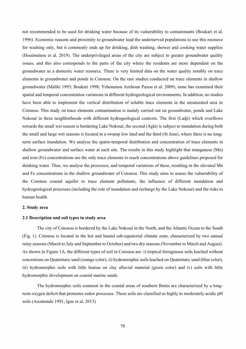
70

not recommended to be used for drinking water because of its vulnerability to contaminants (Boukari et al.

1996). Economic reasons and proximity to groundwater lead the underserved populations to use this resource

for washing only, but it commonly ends up for drinking, dish washing, shower and cooking water supplies

(Houéménou et al. 2019). The underprivileged areas of the city are subject to greater groundwater quality

issues, and this also corresponds to the parts of the city where the residents are more dependent on the

groundwater as a domestic water resource. There is very limited data on the water quality notably on trace

elements in groundwater and ponds in Cotonou. On the rare studies conducted on trace elements in shallow

groundwater (Maliki 1993; Boukari 1998; Yehouenou Azehoun Pazou et al. 2009), none has examined their

spatial and temporal concentration variations in different hydrogeological environments. In addition, no studies

have been able to implement the vertical distribution of soluble trace elements in the unsaturated area in

Cotonou. This study on trace elements contamination is mainly carried out on groundwater, ponds and Lake

Nokoué in three neighborhoods with different hydrogeological contexts. The first (Ladji) which overflows

towards the small wet season is bordering Lake Nokoué, the second (Agla) is subject to inundation during both

the small and large wet seasons is located in a swamp low land and the third (St Jean), where there is no long-

term surface inundation. We analyse the spatio-temporal distribution and concentration of trace elements in

shallow groundwater and surface water at each site. The results in this study highlight that manganese (Mn)

and iron (Fe) concentrations are the only trace elements to reach concentrations above guidelines proposed for

drinking water. Thus, we analyse the processes, and temporal variations of these, resulting in the elevated Mn

and Fe concentrations in the shallow groundwater of Cotonou. This study aims to assess the vulnerability of

the Cotonou coastal aquifer to trace element pollutants, the influence of different inundation and

hydrogeological processes (including the role of inundation and recharge by the Lake Nokoué) and the risks to

human health.

2. Study area

2.1 Description and soil types in study area

The city of Cotonou is bordered by the Lake Nokoué in the North, and the Atlantic Ocean to the South

(Fig. 1). Cotonou is located in the hot and humid sub-equatorial climate zone, characterized by two annual

rainy seasons (March to July and September to October) and two dry seasons (November to March and August).

As shown in Figure 1A, the different types of soil in Cotonou are: i) tropical ferruginous soils leached without

concretions on Quaternary sand (orange color), ii) hydromorphic soils leached on Quaternary sand (blue color),

iii) hydromorphic soils with little humus on clay alluvial material (green color) and iv) soils with little

hydromorphic development on coastal marine sands.

The hydromorphic soils common in the coastal areas of southern Benin are characterized by a long-

term oxygen deficit that promotes redox processes. These soils are classified as highly to moderately acidic pH

soils (Azontonde 1991; Igue et al. 2013)

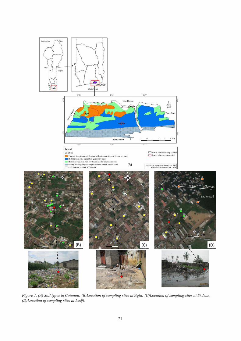
71

Figure 1. (A) Soil types in Cotonou; (B)Location of sampling sites at Agla; (C)Location of sampling sites at St Jean,

(D)Location of sampling sites at Ladji.

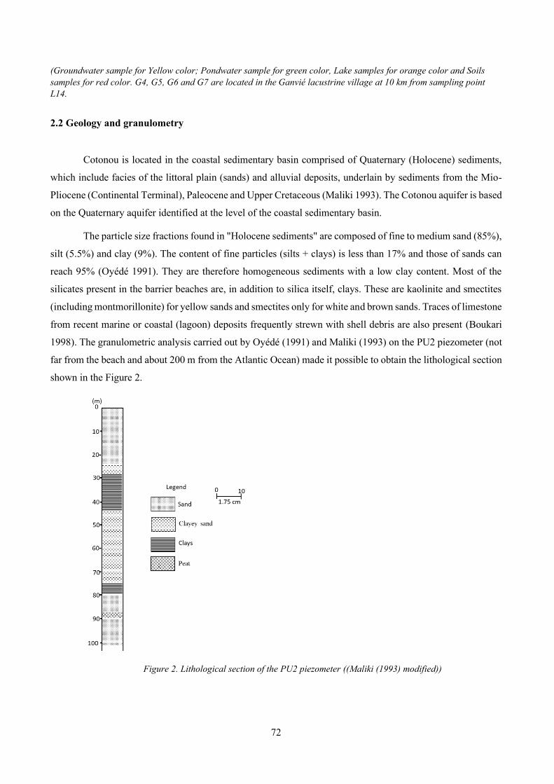
72

(Groundwater sample for Yellow color; Pondwater sample for green color, Lake samples for orange color and Soils

samples for red color. G4, G5, G6 and G7 are located in the Ganvié lacustrine village at 10 km from sampling point

L14.

2.2 Geology and granulometry

Cotonou is located in the coastal sedimentary basin comprised of Quaternary (Holocene) sediments,

which include facies of the littoral plain (sands) and alluvial deposits, underlain by sediments from the Mio-

Pliocene (Continental Terminal), Paleocene and Upper Cretaceous (Maliki 1993). The Cotonou aquifer is based

on the Quaternary aquifer identified at the level of the coastal sedimentary basin.

The particle size fractions found in "Holocene sediments" are composed of fine to medium sand (85%),

silt (5.5%) and clay (9%). The content of fine particles (silts + clays) is less than 17% and those of sands can

reach 95% (Oyédé 1991). They are therefore homogeneous sediments with a low clay content. Most of the

silicates present in the barrier beaches are, in addition to silica itself, clays. These are kaolinite and smectites

(including montmorillonite) for yellow sands and smectites only for white and brown sands. Traces of limestone

from recent marine or coastal (lagoon) deposits frequently strewn with shell debris are also present (Boukari

1998). The granulometric analysis carried out by Oyédé (1991) and Maliki (1993) on the PU2 piezometer (not

far from the beach and about 200 m from the Atlantic Ocean) made it possible to obtain the lithological section

shown in the Figure 2.

Figure 2. Lithological section of the PU2 piezometer ((Maliki (1993) modified))

73

2.3 Groundwater contamination by iron and manganese

The iron may have an oxidation state of +2 or +3. The stability of the ions Fe2+, Fe3+, Fe(OH)2+, and

Fe(OH)+ with respect to Fe(OH)3 and Fe(OH)2 precipitate or colloidal depends on pH, Eh, and the composition

of the solution. Manganese presents three possible oxidation states in such environments rather than two (+2,

+3, and +4) and can form a wide variety of mixed-valence oxides (Hem 1985). The chemistry of manganese is

somewhat like that of iron. In general, manganese occurs as Mn2+, which easily oxidizes to MnO2 and may

form stable organic complexes, as iron does. The main sources of Fe2+ include the dissolution of iron (II)

bearing minerals and the reduction of iron oxyhydroxides (Fe-OOH) present in the sediments and clay minerals

such as smectites (Appelo et al. 1994).

Very few studies have actually focused on metallic trace elements in groundwater and surface water.

This is due to the absence or the limited data base on water resources in the coastal zone of southern Benin

compared to other African countries. Moussa Boukari (1998) had shown that total iron contents are generally

between 0.1 and 0.2 mg/L, which is below the WHO (World Health Organization) guideline of 0.3 mg/L. As

far as zinc is concerned, the levels are between 0.5 and 1 mg/L and are also not harmful to water quality.

Nevertheless, sectors with high zinc contents (2 to 3.5 mg/L) corresponding to the Central Cotonou area were

obtained during the same period. The study carried out on well and borehole water used at the Houéyiho market

garden site in Cotonou showed that these irrigation waters are contaminated with cadmium, lead and

manganese; metallic trace elements produced from household waste used for fertilization (Yehouenou Azehoun

Pazou et al. 2009). Low quality physico-chemical water can effectively promote the contamination of vegetable

cultures and compromise human health.

In the shallow aquifer of the Godomey wellfield in southern Benin, high contents of total iron (0.5

mg/L in the Togba wells) and lead (0.18 mg/L in a well in Hèvié) were recorded. These values are above the

Beninese standard of 0.3 and 0.05 mg/L respectively (Dovonou et al. 2015).These values are similar to those

of (Azokpota 2005) who found iron and lead contents of 0.8 mg/L and 0.16 mg/L respectively in the waters of

wells in the Cotonou districts where dyeing activities are carried out.

Inadequate wastewater management contributes to groundwater contamination by metallic trace

elements in urban areas; and the consumption of wastewater poses risks of poisoning to human health (Roufai

2012). The toxicity of trace elements such as lead to human health can affect brain and nervous system

development and increase the risk of high blood pressure and kidney damage (WHO 2018).

3. Material and methods

3.1 Water sampling

In the three neighborhoods in Cotonou, thirty-eight (35) sampling sites were selected as representative

groundwater, ponds and Lake of the study area (Fig. 1A). In each neighborhood, groundwater wells were

selected for sampling and, where/when possible, surface water samples (permanent and temporary pools, as

74

well as Lake Nokoué) were also included. Groundwater was sampled from the Quaternary aquifer via the large-

diameter wells. The wells are separated by an average distance of ~200 m within the same neighborhood.

The trace elements and major ions of waters were analyzed 6 times between November 2016 to June

2018 in February (main dry season), June (main wet season) and October (small wet season), resulting in a

total of 77 groundwater and 50 surface water samples. Other samples were collected in the centre of the Lake

(G1, G2, G3) and near the Ganvié lacustrine village (G4, G5, G6 and G7) during dry season.

3.2 Soil sampling

In February 2018 (dry season), three soil profiles were carried out in Ladji, Agla and St Jean sites at

L18, A11 and J11 respectively. Sites A11 and L18 are old garbage landfills (respectively, from 5 to 10 years),

while J11 is a soil without landfills (Fig. 1). The samples were taken with a 5*20 cm auger. Soil samples were

collected from the soil surface (horizon above the natural terrain) and every 20 cm depth of the unsaturated

zone. The depth of investigation, which corresponds to the thickness of the unsaturated zone, is 40 cm for A11,

80 cm for L18 and 120 cm for J11. A total of fifteen (15) soil samples were collected and stored in polyethylene

bags before being transported to the laboratory.

3.3 Water extraction method

For the analysis of metallic trace elements and major ions in soils, 200 g of soil is leached in 200 mL

of milliQ water. The leachate is obtained after mixing by a stirrer for 1 hour and centrifugation for 10 minutes

at 4000 laps per minutes. This extraction method used by (Blondel 2008) and (Cras 2005), promotes the

leaching of elements weakly bound to the solid fraction of the soil and makes it possible to determine the

distribution of the total content of trace elements and ions..

Water samplings from extraction, from groundwater and surface water were filtered in situ with

disposable PP syringe and Durapore membrane (0.22 µm) and stored in acid washed HDPE bottles. Aliquots

for cations and trace elements were acidified with ultrapure HNO3 (1‰ v/v) to pH 2.

3.4 Analytical methods

Groundwater and surface water temperature (T°C), pH, redox potential (Eh), Electrical

conductivity (EC), and dissolved oxygen (DO) were measured in situ using a WTW 3430i portable

digital multiparameter.

Major ions are analyzed using the DIONEX model ICS-1100 ion chromatograph at the

Hydrogeology Laboratory of the University of Avignon. The quality of the chemical analysis is

verified by the calculation of ionic balances and validated if the value obtained is less than or equal to

5%.

75

Trace elements (Li, B, Al, V, Cr, Mn, Fe, Co, Ni, Cu, Zn, As, Mo, Ba, Pb, and U) and the Rare

Earths Elements (REE) were analyzed with Q-ICP MS (iCAP Q, Thermo Scientific® equipped with

an Argon Gas Dilution in-line system) at 1% v/v HNO3- at the AETE-ISO (Analyse des Elements en

Trace dans l’Environnement et Isotopes) technical platform of the OSU OREME, University of

Montpellier. The Argon Gas Dilution in-line system allows us to introduce the highly mineralized

samples without previous dilution. Precision error was typically < 5%. SLRS-6, fresh water reference

material, and CASS-6 and NASS-6 seawater reference materials for trace metals (National Research

Council, Canada) were analyzed every 20 samples to check the analysis accuracy. Mean results are

within the range of certified uncertainties. Precision error was typically < ± 5%. The results are

presented in Tables 2, 3 and 4. The Ce/Ce* ratios were calculated using formula

Ce/Ce*= CeNASC/(LaNASC * PrNASC)0.5.

3.5 Granulometric method

The granulometric analysis was performed on the fifteen (15) soil samples collected. After

removing the fraction less than 0.063 mm, each soil sample was subjected to a dry granulometric

analysis on a sieve column (AFNOR series, Association Française de Normalisation). The sieves are

shaken using mechanical systems such as Ro-TAP. The grains are classified according to their

diameter and the fractions retained on the successive sieves (2 mm, 1 mm, 0.5 mm, 0.25 mm, 0.125

mm, 0.063 mm) are weighed. The classification adopted for the nature of sediments is that defined by

Blott and Pye (2001). The particle size composition is expressed as a percentage (%) of the total

sample weight.

3.6 Statistical analysis

The distribution of trace elements in water was done using descriptive analysis based on arithmetic

average, minimum, maximum and standard deviation. The chemical analysis data were processed by PCA and

AC using XLSTAT (Microsoft Excel add on). The PCA was used to classify sample locations on an observation

chart, the trace elements and ions concentrations were analyzed to generate a correlation circle and associated

Pearson's correlation matrix (significance level of 5%). The main objective of Cluster Analysis (CA) is to reveal

an underlying relationships that is presumed to exist within a set of PCA observations. The degree of correlation

between traces elements is represented by the distance between the clusters. Minerals that influence the

solubility of the elements were identified by calculating the saturation index using PHREECQ 3.5.0 with

wateq4f.

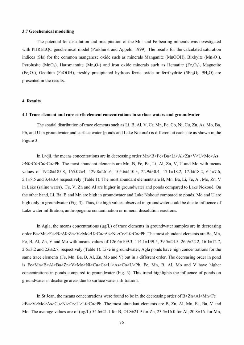
76

3.7 Geochemical modelling

The potential for dissolution and precipitation of the Mn- and Fe-bearing minerals was investigated

with PHREEQC geochemical model (Parkhurst and Appelo, 1999). The results for the calculated saturation

indices (SIs) for the common manganese oxide such as minerals Manganite (MnOOH), Bixbyite (Mn2O3),

Pyrolusite (MnO2), Hausmannite (Mn3O4) and iron oxide minerals such as Hematite (Fe2O3), Magnetite

(Fe3O4), Geothite (FeOOH), freshly precipitated hydrous ferric oxide or ferrihydrite (5Fe2O3. 9H2O) are

presented in the results.

4. Results

4.1 Trace element and rare earth element concentrations in surface waters and groundwater

The spatial distribution of trace elements such as Li, B, Al, V, Cr, Mn, Fe, Co, Ni, Cu, Zn, As, Mo, Ba,

Pb, and U in groundwater and surface water (ponds and Lake Nokoué) is different at each site as shown in the

Figure 3.

In Ladji, the means concentrations are in decreasing order Mn>B>Fe>Ba>Li>Al>Zn>V>U>Mo>As

>Ni>Cr>Cu>Co>Pb. The most abundant elements are Mn, B, Fe, Ba, Li, Al, Zn, V, U and Mo with means

values of 192.8±185.8, 165.07±4, 129.8±261.6, 105.6±110.3, 22.9±30.4, 17.1±18.2, 17.1±18.2, 6.4±7.6,

5.1±8.5 and 3.4±3.4 respectively (Table 1). The most abundant elements are B, Mn, Ba, Li, Fe, Al, Mo, Zn, V

in Lake (saline water). Fe, V, Zn and Al are higher in groundwater and ponds compared to Lake Nokoué. On

the other hand, Li, Ba, B and Mn are high in groundwater and Lake Nokoué compared to ponds. Mo and U are

high only in groundwater (Fig. 3). Thus, the high values observed in groundwater could be due to influence of

Lake water infiltration, anthropogenic contamination or mineral dissolution reactions.

In Agla, the means concentrations (µg/L) of trace elements in groundwater samples are in decreasing

order Ba>Mn>Fe>B>Al>Zn>V>Mo>U>Cu>As>Ni>Cr>Li>Co>Pb. The most abundant elements are Ba, Mn,

Fe, B, Al, Zn, V and Mo with means values of 126.6±109.3, 114.1±139.5, 39.5±24.5, 26.9±22.2, 16.1±12.7,

2.6±3.2 and 2.6±2.7, respectively (Table 1). Like in groundwater, Agla ponds have high concentrations for the

same trace elements (Fe, Mn, Ba, B, Al, Zn, Mo and V) but in a different order. The decreasing order in pond

is Fe>Mn>B>Al>Ba>Zn>V>Mo>Ni>Cu>Cr>Li>As>Co>U>Pb. Fe, Mn, B, Al, Mo and V have higher

concentrations in ponds compared to groundwater (Fig. 3). This trend highlights the influence of ponds on

groundwater in discharge areas due to surface water infiltrations.

In St Jean, the means concentrations were found to be in the decreasing order of B>Zn>Al>Mn>Fe

>Ba>V>Mo>As>Cu>Ni>Cr>U>Li>Co>Pb. The most abundant elements are B, Zn, Al, Mn, Fe, Ba, V and

Mo. The average values are of (µg/L) 54.6±21.1 for B, 24.8±21.9 for Zn, 23.5±16.0 for Al, 20.8±16. for Mn,

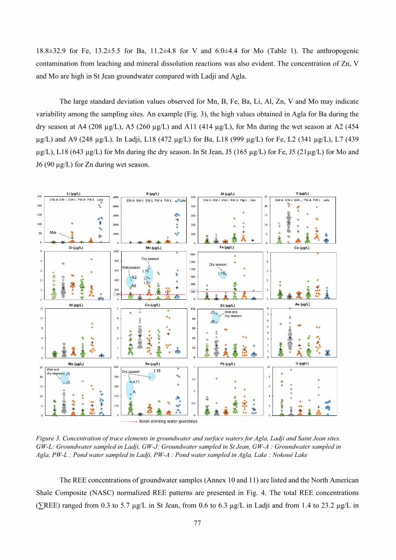
77

18.8±32.9 for Fe, 13.2±5.5 for Ba, 11.2±4.8 for V and 6.0±4.4 for Mo (Table 1). The anthropogenic

contamination from leaching and mineral dissolution reactions was also evident. The concentration of Zn, V

and Mo are high in St Jean groundwater compared with Ladji and Agla.

The large standard deviation values observed for Mn, B, Fe, Ba, Li, Al, Zn, V and Mo may indicate

variability among the sampling sites. An example (Fig. 3), the high values obtained in Agla for Ba during the

dry season at A4 (208 µg/L), A5 (260 µg/L) and A11 (414 µg/L), for Mn during the wet season at A2 (454

µg/L) and A9 (248 µg/L). In Ladji, L18 (472 µg/L) for Ba, L18 (999 µg/L) for Fe, L2 (341 µg/L), L7 (439

µg/L), L18 (643 µg/L) for Mn during the dry season. In St Jean, J5 (165 µg/L) for Fe, J5 (21µg/L) for Mo and

J6 (90 µg/L) for Zn during wet season.

Figure 3. Concentration of trace elements in groundwater and surface waters for Agla, Ladji and Saint Jean sites.

GW-L: Groundwater sampled in Ladji, GW-J: Groundwater sampled in St Jean, GW-A : Groundwater sampled in

Agla, PW-L : Pond water sampled in Ladji, PW-A : Pond water sampled in Agla, Lake : Nokoué Lake

The REE concentrations of groundwater samples (Annex 10 and 11) are listed and the North American

Shale Composite (NASC) normalized REE patterns are presented in Fig. 4. The total REE concentrations

(∑REE) ranged from 0.3 to 5.7 µg/L in St Jean, from 0.6 to 6.3 µg/L in Ladji and from 1.4 to 23.2 µg/L in

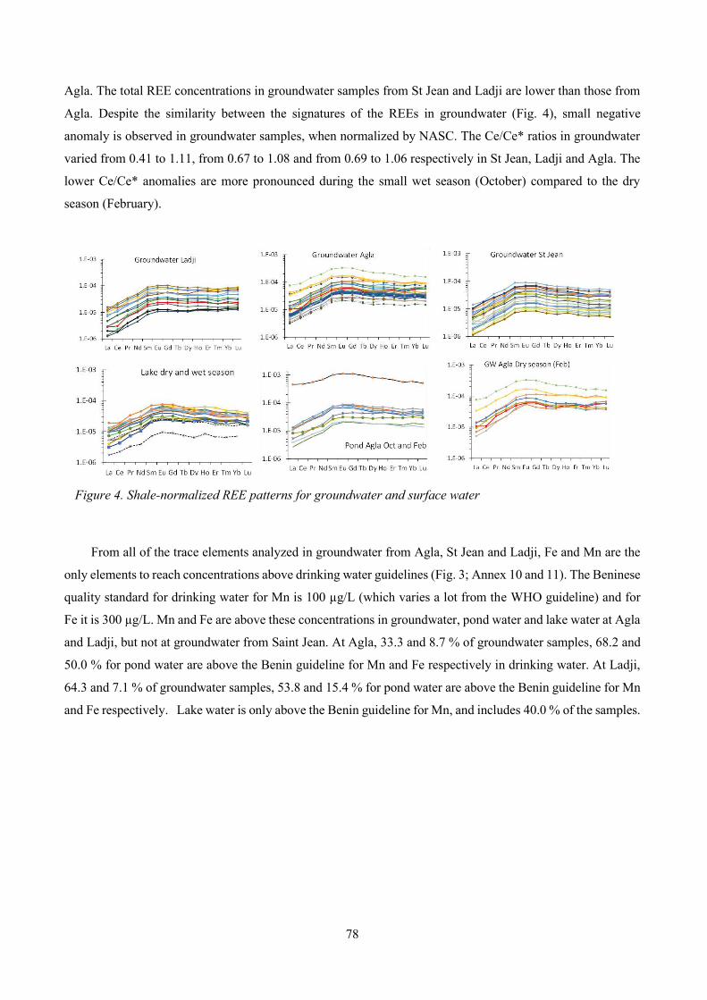
78

Agla. The total REE concentrations in groundwater samples from St Jean and Ladji are lower than those from

Agla. Despite the similarity between the signatures of the REEs in groundwater (Fig. 4), small negative

anomaly is observed in groundwater samples, when normalized by NASC. The Ce/Ce* ratios in groundwater

varied from 0.41 to 1.11, from 0.67 to 1.08 and from 0.69 to 1.06 respectively in St Jean, Ladji and Agla. The

lower Ce/Ce* anomalies are more pronounced during the small wet season (October) compared to the dry

season (February).

Figure 4. Shale-normalized REE patterns for groundwater and surface water

From all of the trace elements analyzed in groundwater from Agla, St Jean and Ladji, Fe and Mn are the

only elements to reach concentrations above drinking water guidelines (Fig. 3; Annex 10 and 11). The Beninese

quality standard for drinking water for Mn is 100 µg/L (which varies a lot from the WHO guideline) and for

Fe it is 300 µg/L. Mn and Fe are above these concentrations in groundwater, pond water and lake water at Agla

and Ladji, but not at groundwater from Saint Jean. At Agla, 33.3 and 8.7 % of groundwater samples, 68.2 and

50.0 % for pond water are above the Benin guideline for Mn and Fe respectively in drinking water. At Ladji,

64.3 and 7.1 % of groundwater samples, 53.8 and 15.4 % for pond water are above the Benin guideline for Mn

and Fe respectively. Lake water is only above the Benin guideline for Mn, and includes 40.0 % of the samples.

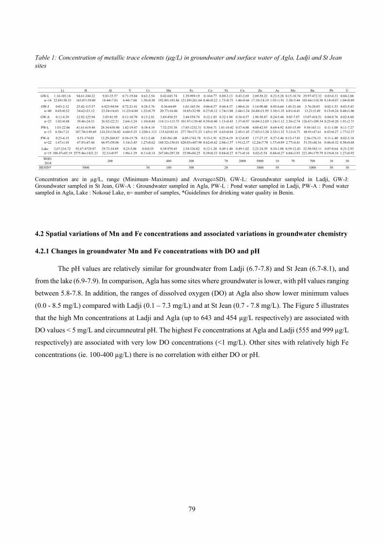
79

Table 1: Concentration of metallic trace elements (g/L) in groundwater and surface water of Agla, Ladji and St Jean

sites

Concentration are in µg/L, range (Minimum–Maximum) and Average±SD). GW-L: Groundwater sampled in Ladji, GW-J: Groundwater sampled in St Jean, GW-A : Groundwater sampled in Agla, PW-L : Pond water sampled in Ladji, PW-A : Pond water sampled in Agla, Lake : Nokoué Lake, n= number of samples, *Guidelines for drinking water quality in Benin.

4.2 Spatial variations of Mn and Fe concentrations and associated variations in groundwater chemistry

4.2.1 Changes in groundwater Mn and Fe concentrations with DO and pH

The pH values are relatively similar for groundwater from Ladji (6.7-7.8) and St Jean (6.7-8.1), and

from the lake (6.9-7.9). In comparison, Agla has some sites where groundwater is lower, with pH values ranging

between 5.8-7.8. In addition, the ranges of dissolved oxygen (DO) at Agla also show lower minimum values

(0.0 - 8.5 mg/L) compared with Ladji (0.1 – 7.3 mg/L) and at St Jean (0.7 - 7.8 mg/L). The Figure 5 illustrates

that the high Mn concentrations at Ladji and Agla (up to 643 and 454 µg/L respectively) are associated with

DO values < 5 mg/L and circumneutral pH. The highest Fe concentrations at Agla and Ladji (555 and 999 µg/L

respectively) are associated with very low DO concentrations (<1 mg/L). Other sites with relatively high Fe

concentrations (ie. 100-400 µg/L) there is no correlation with either DO or pH.

Li B Al V Cr Mn Fe Co Ni Cu Zn As Mo Ba Pb U

GW-L 1.16-103.16 94.61-244.22 9.83-35.57 0.71-19.84 0.62-2.54 0.42-643.74 1.29-999.19 0.14-0.77 0.89-3.13 0.43-2.69 2.09-58.22 0.23-5.28 0.15-10.74 29.97-472.32 0.03-0.33 0.04-2.88n=14 22.89±30.35 165.07±39.00 18.44±7.01 6.44±7.60 1.58±0.50 192.89±185.86 121.89±261.64 0.46±0.22 1.73±0.75 1.46±0.66 17.10±18.19 1.93±1.91 3.38±3.44 105.66±110.30 0.14±0.07 1.04±0.89

GW-J 0.03-2.12 25.42-115.57 6.823-94.94 0.72-21.41 0.24-3.76 0.36-64.09 1.01-165.54 0.06-0.57 0.44-4.37 1.00-6.18 3.14-90.40 0.85-6.64 1.45-21.44 3.76-28.03 0.02-1.53 0.03-5.43n=40 0.65±0.52 54.62±21.12 23.54±16.01 11.23±4.80 1.22±0.79 20.77±16.86 18.85±32.98 0.27±0.12 1.74±1.08 2.44±1.24 24.88±21.95 3.10±1.35 6.01±4.41 13.21±5.49 0.15±0.24 0.48±1.06

GW-A 0.11-4.39 12.92-125.94 3.85-81.95 0.11-10.70 0.13-2.81 3.69-454.55 3.44-554.74 0.12-1.85 0.32-1.94 0.36-4.57 1.96-50.87 0.24-5.44 0.03-7.87 15.07-418.51 0.04-0.76 0.02-8.60n=23 1.02±0.88 39.46±24.51 26.92±22.21 2.64±3.24 1.10±0.84 114.11±115.75 101.97±139.48 0.59±0.40 1.13±0.43 1.37±0.97 16.04±12.69 1.24±1.12 2.56±2.74 126.67±109.34 0.25±0.20 1.91±2.71

PW-L 1.03-22.06 41.61-619.44 28.34-458.90 1.82-19.47 0.38-4.19 7.32-235.38 17.85-1232.31 0.30-6.71 1.81-10.42 0.57-4.80 4.08-42.93 0.69-4.92 0.85-15.49 9.50-163.11 0.11-1.08 0.11-7.27n=13 6.56±7.21 187.70±149.69 124.25±136.02 6.68±5.35 1.220±1.113 115.62±82.41 277.70±371.23 1.65±1.93 4.63±0.84 2.45±1.45 17.02±13.20 2.52±1.32 5.12±4.73 48.91±47.61 0.43±0.27 1.77±2.37

PW-A 0.23-4.15 8.51-174.03 13.29-268.87 0.56-15.78 0.11-2.48 3.03-561.08 4.05-1741.78 0.13-1.91 0.25-6.19 0.12-8.85 1.17-27.15 0.37-3.46 0.13-17.81 2.36-176.13 0.11-1.40 0.02-3.14n=22 1.67±1.01 67.83±47.44 66.97±58.06 3.14±3.45 1.27±0.62 168.52±156.01 420.03±447.96 0.62±0.42 2.04±1.57 1.91±2.37 12.24±7.70 1.37±0.89 2.77±4.41 51.53±44.16 0.46±0.32 0.50±0.68

Lake 2.67-216.72 92.67-4729.87 29.72-34.89 0.23-5.06 0.0-0.55 8.38-970.45 2.34-336.02 0.12-1.20 0.49-1.40 0.49-1.02 2.23-24.39 0.34-1.08 0.59-12.43 32.50-583.11 0.07-0.64 0.21-2.93n=15 106.47±65.19 2575.46±1421.21 32.31±0.97 1.96±1.39 0.11±0.14 247.68±287.38 35.98±84.25 0.39±0.33 0.84±0.27 0.71±0.16 6.02±5.54 0.68±0.27 6.04±3.93 221.49±179.79 0.19±0.16 1.27±0.92

WHO 2018

200 400 300 70 2000 5000 10 70 700 10 30

BENIN* 5000 50 100 300 20 3000 50 1000 50 30

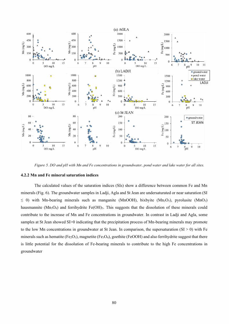
80

Figure 5. DO and pH with Mn and Fe concentrations in groundwater, pond water and lake water for all sites.

4.2.2 Mn and Fe mineral saturation indices

The calculated values of the saturation indices (SIs) show a difference between common Fe and Mn

minerals (Fig. 6). The groundwater samples in Ladji, Agla and St Jean are undersaturated or near saturation (SI

≤ 0) with Mn-bearing minerals such as manganite (MnOOH), bixbyite (Mn2O3), pyrolusite (MnO2)

hausmannite (Mn3O4) and ferrihydrite Fe(OH)3. This suggests that the dissolution of these minerals could

contribute to the increase of Mn and Fe concentrations in groundwater. In contrast in Ladji and Agla, some

samples at St Jean showed SI>0 indicating that the precipitation process of Mn-bearing minerals may promote

to the low Mn concentrations in groundwater at St Jean. In comparison, the supersaturation (SI > 0) with Fe

minerals such as hematite (Fe2O3), magnetite (Fe3O4), goethite (FeOOH) and also ferrihydrite suggest that there

is little potential for the dissolution of Fe-bearing minerals to contribute to the high Fe concentrations in

groundwater

81

Figure 6. Saturation indices of Mn- and Fe- bearing minerals for groundwater sampled at Agla, Ladji and St Jean.

4.2.3 Principal Component Analysis for Mn and Fe

The variations of Fe and Mn with key chemical parameters (DO, pH, DOC, NH4) in the shallow

groundwater of the Cotonou coastal aquifer as well as major ions (data from Houéménou et al. 2019) and other

trace elements (Li, B, Al, V, Zn, Mo and Ba) in Nokoué Lake are analysed using a PCA (Principal Component

Analysis). Table 2 and Figure 7 summarize the PCA results in groundwater and Lake, respectively.

In Ladji, F1 and F2 axis explain 73.9% of the total variance (Table 3). The main F1 axis (46.3% of the

variance) is shows that Mn and Fe are positively correlated with DOC and NH4. These two elements (Fe and

Mn) are negatively correlated with pH and DO. This indicates that the increase in Mn and Fe concentrations in

groundwater may be due to an increase in DOC and NH4. The PCA analysis on Lake Nokoué samples (Fig. 7.)

shows that Ba, Fe, Zn, Mn and V sites have a different origin than Cl, Na, Ca, SO4, Li and B. The high

concentrations of Fe and Mn in Lake Nokoué (e.g. sites G5, G6 and G7) are not due to contact with the Atlantic

Ocean, unlike the ions Cl, Na, Ca, SO4, Li and B.

In Agla, three axis are extracted, together explaining 86.7 % of the total variance. F1 axis (42.7 % of

the variance) shows a strong positive correlation between Mn with NH4, DOC and pH and weakly correlated

with DO. Fe shows a positive but weak correlation with NH4, DOC, pH and DO. On the F2 axis, NH4 is

negatively correlated to DO. Fe is correlated with F3 axis.

In St Jean, the three axis F1, F2 and F3 are considered, describe 72.1 % of the total variance. On F1

axis, Mn and to a lesser extent Fe are negatively correlated with pH and DO. F2 axis is positively correlated

with NH4, COD and negatively correlated with DO, Fe and Mn. On F3 axis, Fe and COD are moderately

correlated.

The anaerobic decomposition of organic material which contribute an increase of NH4 concentrations

could play significant role in the increase of Fe and Mn concentrations in Agla and Ladji compared in St Jean.

The input of high DOC concentrations in groundwater in Agla and Ladji via ponds can promote the reductive

dissolution of iron and manganese oxide minerals.

Table 2: Matrix of principal components

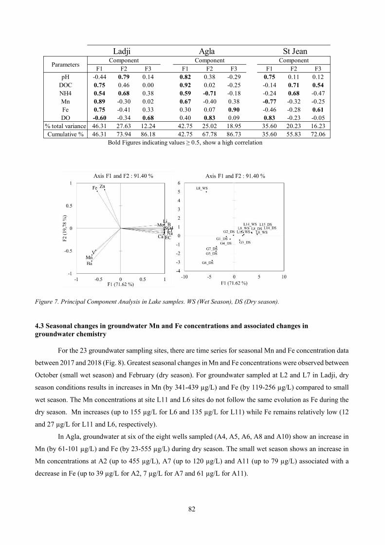
82

Figure 7. Principal Component Analysis in Lake samples. WS (Wet Season), DS (Dry season).

4.3 Seasonal changes in groundwater Mn and Fe concentrations and associated changes in

groundwater chemistry

For the 23 groundwater sampling sites, there are time series for seasonal Mn and Fe concentration data

between 2017 and 2018 (Fig. 8). Greatest seasonal changes in Mn and Fe concentrations were observed between

October (small wet season) and February (dry season). For groundwater sampled at L2 and L7 in Ladji, dry

season conditions results in increases in Mn (by 341-439 µg/L) and Fe (by 119-256 µg/L) compared to small

wet season. The Mn concentrations at site L11 and L6 sites do not follow the same evolution as Fe during the

dry season. Mn increases (up to 155 µg/L for L6 and 135 µg/L for L11) while Fe remains relatively low (12

and 27 µg/L for L11 and L6, respectively).

In Agla, groundwater at six of the eight wells sampled (A4, A5, A6, A8 and A10) show an increase in

Mn (by 61-101 µg/L) and Fe (by 23-555 µg/L) during dry season. The small wet season shows an increase in

Mn concentrations at A2 (up to 455 µg/L), A7 (up to 120 µg/L) and A11 (up to 79 µg/L) associated with a

decrease in Fe (up to 39 µg/L for A2, 7 µg/L for A7 and 61 µg/L for A11).

Ladji Agla St Jean

F1 F2 F3 F1 F2 F3 F1 F2 F3pH -0.44 0.79 0.14 0.82 0.38 -0.29 0.75 0.11 0.12

DOC 0.75 0.46 0.00 0.92 0.02 -0.25 -0.14 0.71 0.54

NH4 0.54 0.68 0.38 0.59 -0.71 -0.18 -0.24 0.68 -0.47Mn 0.89 -0.30 0.02 0.67 -0.40 0.38 -0.77 -0.32 -0.25Fe 0.75 -0.41 0.33 0.30 0.07 0.90 -0.46 -0.28 0.61

DO -0.60 -0.34 0.68 0.40 0.83 0.09 0.83 -0.23 -0.05% total variance 46.31 27.63 12.24 42.75 25.02 18.95 35.60 20.23 16.23Cumulative % 46.31 73.94 86.18 42.75 67.78 86.73 35.60 55.83 72.06

Bold Figures indicating values ≥ 0.5, show a high correlation

ComponentParameters

Component Component

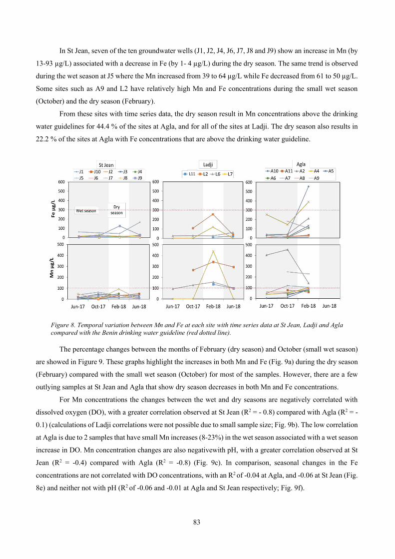
83

In St Jean, seven of the ten groundwater wells (J1, J2, J4, J6, J7, J8 and J9) show an increase in Mn (by

13-93 µg/L) associated with a decrease in Fe (by 1- 4 µg/L) during the dry season. The same trend is observed

during the wet season at J5 where the Mn increased from 39 to 64 µg/L while Fe decreased from 61 to 50 µg/L.

Some sites such as A9 and L2 have relatively high Mn and Fe concentrations during the small wet season

(October) and the dry season (February).

From these sites with time series data, the dry season result in Mn concentrations above the drinking

water guidelines for 44.4 % of the sites at Agla, and for all of the sites at Ladji. The dry season also results in

22.2 % of the sites at Agla with Fe concentrations that are above the drinking water guideline.

Figure 8. Temporal variation between Mn and Fe at each site with time series data at St Jean, Ladji and Agla

compared with the Benin drinking water guideline (red dotted line).

The percentage changes between the months of February (dry season) and October (small wet season)

are showed in Figure 9. These graphs highlight the increases in both Mn and Fe (Fig. 9a) during the dry season

(February) compared with the small wet season (October) for most of the samples. However, there are a few

outlying samples at St Jean and Agla that show dry season decreases in both Mn and Fe concentrations.

For Mn concentrations the changes between the wet and dry seasons are negatively correlated with

dissolved oxygen (DO), with a greater correlation observed at St Jean (R2 = - 0.8) compared with Agla (R2 = -

0.1) (calculations of Ladji correlations were not possible due to small sample size; Fig. 9b). The low correlation

at Agla is due to 2 samples that have small Mn increases (8-23%) in the wet season associated with a wet season

increase in DO. Mn concentration changes are also negativewith pH, with a greater correlation observed at St

Jean (R2 = -0.4) compared with Agla (R2 = -0.8) (Fig. 9c). In comparison, seasonal changes in the Fe

concentrations are not correlated with DO concentrations, with an R2 of -0.04 at Agla, and -0.06 at St Jean (Fig.

8e) and neither not with pH (R2 of -0.06 and -0.01 at Agla and St Jean respectively; Fig. 9f).

84

The seasonal changes in Fe and Mn concentrations are weakly positive with the Ce/Ce* anomaly at St

Jean (R2 = 0.2 for Mn and 0.04 for Fe) where dry season increases are associated with Ce/Ce* increases (Figs.

8d and g). In contrast, at Agla the Ce/Ce* anomaly mostly decreases with increases in Mn and Fe. This could

indicate the effects of high organic matter on Ce/Ce* anomalies at Agla, since this area has many low elevation

areas that are frequently inundated, and is discussed further below.

Figure 9. Percentage change in both dry and wet seasons at each site with time series data at St Jean, Agla and Ladji.

4.4 Soil profiles and trace elements

The soils studied in L18 (Ladji), A11 (Agla) and J11 (St Jean) sites show textural variability between

sites (Fig. 10). Overall, the unsaturated zone of the coastal aquifer in Cotonou is of sandy and silt-clayey-sandy

type except in certain areas where there is a low gravel content. During soil analysis, the depth of the unsaturated

zone ranged from 40 cm at Agla, 80 cm at Ladji and 120 cm at St Jean. In Ladji, the soil sampling site (L18) is

85

characterized by a silt-clay-sand texture with an average of 52.8% silts and clay, 45.7% sand and 1.4% gravel

(Fig. 10o). The surface horizons (0-20 cm) and at depths closer to the saturated zone (60-80 cm) contain

sediments composed respectively of fine to medium low clay sand and clayey sands compared to the

intermediary horizon (20-60 cm) where clay and silt have accumulated. In Agla, the sampling soil site (A11)

is dominated by a sandy-clayey texture with an average of 76% sand, 19.8% clay and 4.1% gravel (Fig. 10n).

There is a horizon consisting of medium to coarse clayey fine sands (0-20cm) and an accumulation horizon of

very little clayey medium fine sand (20-40cm). In St Jean, J11 site is characterized by a sandy texture with an

average of 98.3% sand, 1.6% clay and silt, and 0.1% gravel (Fig. 10m). The soil site at St Jean shows a

homogeneous profile of medium sand along the unsaturated zone (0-120 cm).

The vertical evolution of the electrical conductivity (EC), major ions (NO3, Ca, Cl, Na, HCO3) and

trace elements (Fe, Mn, Zn, Al, B, V, Ba, Mo) in the soil leaching are presented in Figure 9. Water from soil

leaching in Agla and Ladji was extracted from sediments collected from garbage landfills compared to St Jean

that was collected from soil without a landfill. The EC is higher in Agla and Ladji (landfill sites) compared to

St Jean (no landfill). The EC at the surface horizon (0-20 cm) ranges from low values at St Jean (92-156 µS/cm),

medium values at Ladji (448-796 µS/cm), and higher values at Agla (1525-1617 µS/cm). At greater depths

(>20 cm), values decrease at St Jean (35-67 µS/cm) and Agla (up to 288 µS/cm), whereas at Ladji the EC

values increase (1080-1217 µS/cm)

In Ladji (Fig. 10i), the increase in EC is greater between 40-60 cm and is accompanied by an increase

in major ions including Na (167.9-212.7 mg/L) and Cl (58.9-77.9 mg/L) compared to Ca and HCO3 which

remain relatively stable throughout the profile. NO3 only accumulates on the soil surface, indicating the

contribution of relatively recent contamination due to human activities (Zhou, Peng, and Pan 2004; Bouih et

al. 2005; Kadjangaba et al. 2018). The figures 10i, j and k show that most trace elements (with the exception

of B and Mo) accumulate in the surface horizon (at 20 cm depth) and gradually decrease in concentrations with

depth (up to 60 cm). The silty-clayey texture present on the horizon at 20-60 cm probably facilitated the

retention of these trace elements during surface water leaching (landfill waste water, ponds and lake water).

The concentration of Fe (up to 9632.2 µg/L) in this clay-rich zone is particularly elevated compared with other

trace elements, including Al (5704.2 µg/L), V (17.9 µg/L), Mn (138.7 µg/L), Zn (632.4 µg/L) and Ba (62.4

µg/L).

In Agla (Fig. 10h), the increase in EC in the sallow zone (0-20 cm depth) is associated with an

accumulation of HCO3 (382-500 mg/L), Cl (73.3 to 100.6 mg/L), Na (56.4 to 81.0 mg/L), Ca (104.3 to 112

mg/L) and trace elements such as Fe (665.1 to 1192.9 µg/L), Zn (8.9 to 15.5 µg/L) and Ba (18.5 to 25.9 µg/L).

Mo (from 29.5 to 8.3 µg/L), Mn (from 69.5 to 3.7 µg/L), B (from 217.6 to 28.8 µg/L) decrease with depth

compared to NO3 (from 0 to 14.7 mg/L), V (from 9.3 to 51.4 µg/L) and Al (from 72.5 to 309.7 µg/L) that

increase with depth. Thus, high concentrations of HCO3, Cl, Na, Ca, Fe, Zn and Ba in horizons close to the soil

surface may be due to enrichment from the surface water or related to the evaporation effect (Houéménou et

al. 2019). In ponds, the concentrations of Fe and Ba are high, up to 1741.7 µg/L and 176.1 µg/L, respectively.

86

In St Jean (Fig. 10d), the high EC observed in the surface horizon (0-20 cm) is accompanied by an

relatively high concentrations of Cl (20.5 mg/L), Mn (139.5 µg/L), Zn (487.1 µg/L) compared to HCO3, Na,

Ca and Mo which remains relatively stable throughout the profile. NO3, Ba, B, V, Al and Fe are accumulated

both in the soil surface and in the deep horizon. The quasi-sandy texture of the sediments (Fig. 10m) seems to

promote the transfer of pollutants from the unsaturated zone to accumulate in groundwater. The respective

concentrations in the surface horizon and in the deep horizon for each element are 2.3 and 3.7 mg/L for NO3,

23.1 and 7.4 µg/L for Ba, 7.8 and 5.8 µg/L for V, 9.5 and 13.7 µg/L for B, 4255.1 and 4569.3 µg/L for Al,

2267.4 and 1132.5 µg/L for Fe respectively.

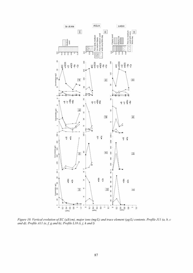
87

Figure 10. Vertical evolution of EC (µS/cm), major ions (mg/L) and trace element (µg/L) contents. Profile J11 (a, b, c

and d); Profile A11 (e, f, g and h); Profile L18 (i, j, k and l)

88

5. Discussion

5.1 Processes controlling Fe and Mn concentrations

A schematic of the main processes controlling Fe and Mn concentrations at each site are presented in

Figure 11. The dissolution of Fe/Mn oxide-hydroxide minerals in reduced aquifers is a common source of Fe

and Mn in groundwater (Hem 1972; Thomas et al. 1994). The oxides of Fe (III) and Mn (IV) previously formed

under oxidizing conditions are reduced to Fe (II) and Mn (II) which are readily mobilized in the aquifer (Gounot

1994; Borch et al. 2010). According to Thomas et al. (1994), the reductive dissolution of manganese oxides

occurs for the Eh values ranging from 100 to 600 mV where the pH ranges from 5-8 (pH values observed in

this study range from 5.8 to 8.1). In comparison, the microbial decomposition of organic matter and the

reductive dissolution of Fe(III) oxyhydroxides occurs under more anaerobic conditions; within the Eh range

from 0 to -500 mV. Eh values of groundwater from this study ranges from 42 – 598 mV. This suggests that

redox-controlled mineral dissolution reactions at all sites are likely a main factor controlling the high

concentrations of Mn in solution but not Fe. In addition, in Agla, the increases in Mn concentrations in the dry

season are weakly correlated with decreases in groundwater DO concentrations (Fig. 9b), whereas the increases

in dry season Fe concentrations are not correlated with changes in DO concentrations (Fig. 9e). The results of

the geochemical modelling also confirm that groundwater has the potential to dissolve several common Mn-

bearing minerals (Fig. 6). On the contrary, groundwater samples were super-saturated with respect to common

Fe oxide-hydroxide minerals, thus indicating that mineral dissolution was not a major driver of high Fe

concentrations in groundwater at all sites sampled in this study.

The reductive dissolution of the Mn-bearing minerals (Mn (IV) (oxyhydr)oxides) that mobilises Mn in

groundwater may be driven by the transfer of young organic matter from pond waters into the aquifers.

Dissolved organic carbon (DOC) concentrations in groundwater are elevated at Agla and Ladji (average DOC

= 13.8 and 13.9 mg/L respectively) compared with St Jean (average DOC = 7.1 mg/L), which is likely due to

recharging waters from ponds (DOC data from Houéménou et al., 2019). The ponds at both Agla and Ladji

have high DOC concentrations (average DOC = 24.3 and 27.83 mg/L respectively) compared with the lake

water (average DOC = 3.1 mg/L). From the PCA, increases in Mn are correlated with increases in DOC at

Ladji and Agla. McDonough et al. (2020) showed that reduced dissolved species of Fe(II) and Mn(II) are

positively correlated with DOC concentrations in groundwater. Thus, the redox conditions favoring the increase

in Fe and Mn are largely controlled by the increase in COD. Mn-oxides and Fe-oxides are used as alternative

electron acceptors to DO in the presence of DOC under anoxic conditions by bacteria (Appelo et al. 2005).

Organics matter can stabilize Fe and Mn in waters by forming organic complexes with them, leading to elevated

Fe and Mn concentrations in groundwater (Weng et al. 2007; McDonough et al. 2020).Where there are high

organic matter compositions in reducing groundwater conditions this can result in a decrease in the Ce/Ce*

anomalies (Davranche et al., 2015). The effects of increased mixing with organic matter on the Ce/Ce*

89

anomalies are predominantly observed at Agla, where the change in Ce/Ce* anomaly during the dry season is

low compared with Ladji and St Jean (Fig. 9.d). This may indicate higher organic matter transfers to the

groundwater from the ponds in Agla, compared with the ponds in Ladji. The anaerobic decomposition of

organic material can also result in elevated concentrations of NH4 and decreases in NO3 in reducing waters

(Lovley 1991; Ferro 2003). According to the PCA, Mn are well correlated with NH4 at Ladji and Agla relating

its release to organic matter decomposition and the source of Mn appears to be the Mn-oxides being reduced.

The infiltration of Mn and Fe from surface waters into the aquifer during the dry season may also

contribute to increases in groundwater Mn and Fe concentrations at Ladji and Agla. Surface waters include the

infiltration of pond water or lake water into the aquifers. From a previous study in Ladji (Houéménou et al.

2019), the 18O and 2H data indicate that there is dry season mixing between the lake and groundwater, and there

are evaporation processes that effect groundwater major ion chemistry. Therefore, these processes also

potentially control trace element concentrations. According to the PCA analysis, the high concentrations of Fe

and Mn in Lake Nokoué are not due to contact with the Atlantic Ocean. In addition, the reference values

certified by the National Research Council Canada (Canada 2016), Fe and Mn (µg/L) have low levels in

seawater (CASS-6: 2.22 ± 0.12 for Mn, 1.56 ± 0.12 for Fe). Instead, the high Fe and Mn concentrations in the

lake water may be due to desorption mechanisms from sediments (Russak, Sivan, and Yechieli 2016). At Ladji,

where there is both infiltration from lake and pond water, it is the recharge from pond water that potentially

contributes to the high Fe concentrations because lake water Fe concentrations are below maximum

groundwater values (Fig. 5b). In contrast, it is the recharge from lake water that potentially contributes to the

elevated concentrations of Mn in groundwater (Fig. 5b). According to Weng et al. (2007) and Pezzetta et al

(2011), the release of iron and manganese in groundwater can be enhanced by contact with a saline solution. In

Agla, in many areas the decrease in rainfall between the small wet to the dry season results in a change from

(sub)artesian groundwater to hydraulic heads that are below the ground surface. Therefore, the numerous

ephemeral ponds at Agla in the small wet season have the potential to recharge the aquifer during the dry season

and stable isotope values have confirmed this pond water recharge (Houemenou et al., 2019). Ponds analysed

in this study have both Fe and Mn concentrations higher than groundwater (Fig. 5a). Therefore, direct

infiltration from pond waters at Agla has the potential to result in both the high Fe and Mn concentrations in

groundwater. In West Bengal and Bangladesh, the studies showed that the addition supply of organic matter

caused by infiltration from surface water may promote a release of supplemental amounts of Fe and Mn into

groundwater (Neidhardt et al. 2013; Farooq et al. 2010; Sutton et al. 2009)

Desorption and sorption processes of Fe and Mn, in either the unsaturated or saturated zone may also

contribute to changing Fe and Mn concentrations. The soil samples highlight that Fe concentrations are

relatively high in the unsaturated zone in areas where the sediments are rich in clay, such as at Ladji (Fe up to

9632.19 µg/L) compared with the relatively clay-poor soil profiles of St Jean (Fe up to 2267.4 g/L) and Agla

(Fe up to 1192.9 g/L). In comparison, Mn concentrations between soil profiles are less variable, with

concentrations up to 138.6, 139.5 and 69.5 g/L at Ladji, St Jean and Agla. Therefore, spatial variations in the

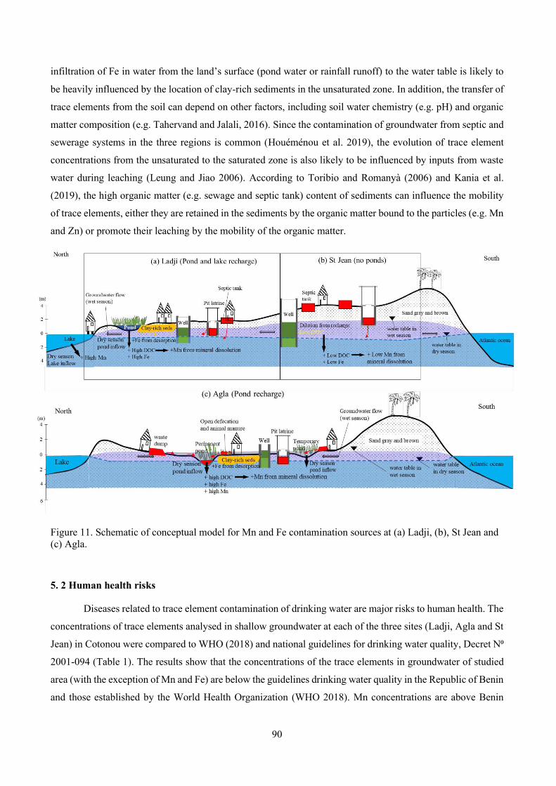
90

infiltration of Fe in water from the land’s surface (pond water or rainfall runoff) to the water table is likely to

be heavily influenced by the location of clay-rich sediments in the unsaturated zone. In addition, the transfer of

trace elements from the soil can depend on other factors, including soil water chemistry (e.g. pH) and organic

matter composition (e.g. Tahervand and Jalali, 2016). Since the contamination of groundwater from septic and

sewerage systems in the three regions is common (Houéménou et al. 2019), the evolution of trace element

concentrations from the unsaturated to the saturated zone is also likely to be influenced by inputs from waste

water during leaching (Leung and Jiao 2006). According to Toribio and Romanyà (2006) and Kania et al.

(2019), the high organic matter (e.g. sewage and septic tank) content of sediments can influence the mobility

of trace elements, either they are retained in the sediments by the organic matter bound to the particles (e.g. Mn

and Zn) or promote their leaching by the mobility of the organic matter.

Figure 11. Schematic of conceptual model for Mn and Fe contamination sources at (a) Ladji, (b), St Jean and (c) Agla.

5. 2 Human health risks

Diseases related to trace element contamination of drinking water are major risks to human health. The

concentrations of trace elements analysed in shallow groundwater at each of the three sites (Ladji, Agla and St

Jean) in Cotonou were compared to WHO (2018) and national guidelines for drinking water quality, Decret N⁰

2001-094 (Table 1). The results show that the concentrations of the trace elements in groundwater of studied

area (with the exception of Mn and Fe) are below the guidelines drinking water quality in the Republic of Benin

and those established by the World Health Organization (WHO 2018). Mn concentrations are above Benin

91

drinking water guidelines (300 µg/L) at L2, L7, L6, L18 sites in Ladji and at A4, A2, A7 and A9 sites in Agla.

Fe concentrations are above Benin drinking water guidelines (100 µg/L) at A4 and A10 in Agla and at L18

sites in Ladji (Fig. 3). In Brong-Ahafo, Ashanti and Western regions (Ghana), drinking water in Ghana

produced from groundwater is contaminated by iron and manganese with concentrations above respectively

300 µg/L and 400 µg/L, the drinking-water guideline value commonly accepted for Fe and Mn (Buamah et al.

2008). Drinking water contaminated with manganese can pose a significant risk to human health. The United

States Environmental Protection Agency report (USEPA 2004) mentioned that the health effects included

lethargy, increased muscle tonus, tremor and mental disturbances. In both Bangladesh and the United States,

children who consumed well water with an average Mn concentration of 793 μg/L, were exposed at the risk for

Mn-induced neurotoxicity (Wasserman et al. 2006).

6. Conclusion

This study developed a quality dataset on trace element concentrations in Cotonou groundwater, which

can serve as a resource for future research on the geochemistry of Mn and Fe in particular. Geochemical data

showed that groundwater is contaminated by Fe and Mn, the only trace elements with concentrations are below

the Beninese health guideline (100 µg/L and 300 µg/L for Mn and Fe respectively). Mn concentrations are

above Benin drinking water guidelines (300 µg/L) at L2, L7, L6, L18 sites in Ladji and at A4, A2, A7 and A9

sites in Agla. Fe concentrations are above Benin drinking water guidelines (100 µg/L) at A4 and A10 in Agla

and at L18 sites in Ladji. The high Mn concentration is explained by dissolution process from water-rock

interaction. Also, given the increase of DOC and redox condition (low Eh), the high Mn and Fe in groundwater

is controlled by denitrification process in reduced environments and by Fe-reducing microorganism

decomposition. Drinking water contaminated with manganese can pose a significant risk to human health. The

main factors controlling Mn and Fe concentrations in groundwater are redox conditions which are explained

by increase of Fe and Mn in dry season when Eh values are ranged from 42 to 500 mV. In reduced environments

(low Eh), denitrification process is followed by the reductive dissolution of Mn oxides. The presence of organic

matter and microbial activities contribute to the increase in the Fe concentration in groundwater. The scale of

the problem of increase Mn and Fe concentrations in the analyzed groundwater highlights the need for wider

sampling in the coastal aquifer in southern Benin.

7. References

Agbossou, KE, MS Sanny, B Zokpodo, B Ahamidé, and HJ Guédégbé. 2003. “Evaluation Qualitative de Quelques Légumes Sur Le Périmètre Maraîcher de Houéyiho, à Cotonou Au Sud-Bénin.” Bulletin de

La Recherche Agronomique Du Bénin N° 42-Décembre: 12. Azokpota, V. 2005. “Impact de l’utilisation Des Colorants Sur La Qualité Du Milieu Aquatique à Cotonou :

Cas de La Teinture Artisanale Des Textiles.” Azontonde, H A. 1991. “Propriétés physiques et hydrauliques des sols au Bénin.” Soil Water Balance in the

SudanoSahelian Zone (Proceedings of the Niamey Workshop, February). IAHS Publ., no. 199: 10.

92

Blondel, Thibaut. 2008. “Traçage Spatial et Temporel Des Eaux Souterraines Dans Les Hydrosystèmes Karstiques Par Les Matières Organiques Dissoutes : Expérimentation et Application Sur Les Sites Du Laboratoire Souterrain à Bas Bruit (LSBB) de Rustrel - Pays d’Apt et de Fontaine de Vaucluse,” December.

Blott, Simon J., and Kenneth Pye. 2001. “GRADISTAT: A Grain Size Distribution and Statistics Package for the Analysis of Unconsolidated Sediments.” Earth Surface Processes and Landforms 26 (11): 1237–48. https://doi.org/10.1002/esp.261.

Bouih, H. Ben, H. Nassali, M. Leblans, and A. Srhiri. 2005. “Contamination En Métaux Traces Des Sédiments Du Lac Fouarat (Maroc).” Afrique Science: Revue Internationale Des Sciences et

Technologie 1 (1). https://www.ajol.info/index.php/afsci/article/view/35403. Boukari. 1998. “Fonctionnement du système aquifère exploité pour l’approvisionnement en eau de la ville de

Cotonou sur le littoral béninois : impact du développement urbain sur la qualité des ressources.” Université cheikh Anta Diop de Dakar, Faculté des Sciences et Technique, Département de Géologies.

Boukari, M., C. B. Gaye, A. Faye, and S. Faye. 1996. “The Impact of Urban Development on Coastal Aquifers near Cotonou, Benin.” Journal of African Earth Sciences, Hydrogeochemical Studies in Sub-Saharan Africa, 22 (4): 403–8. https://doi.org/10.1016/0899-5362(96)00027-9.

Canada, Government of Canada National Research Council. 2016. “CASS-6: Nearshore Seawater Certified Reference Material for Trace Metals and Other Constituents - National Research Council Canada.” November 16, 2016. https://www.nrc-cnrc.gc.ca/eng/solutions/advisory/crm/certificates/cass_6.html.

CRAS, Alexandre. 2005. “Etude et modélisation de la dynamique de fonctionnement hydrologique des bassins versants torrentiels marneux. Apport du traçage naturel Application aux Bassins Versants de Recherche et d’Expérimentation (BVRE) de Draix, Alpes-de-Haute-Provence, France.” Doctorat, Université d’Avignon et des Pays de Vaucluse.

Davranche M., Gruau G., Dia A., Marsac R., Pédrot M., Pourret O. 2015. Biogeochemical Factors Affecting Rare

Earth Element Distribution in Shallow Wetland Groundwater. Aquatic Geochemistry, 21(2-4), 197–215.

Dovonou, Flavien, Naéssé Adjahossou, Eric Alamou, Abdoukarim Alassane, Daouda Mama, and Moussa Boukari. 2015. “Pollution des eaux souterraines par les métaux lourds et leur impact sur l’environnement : cas de l’aquifère superficiel du champ de captage intensif de Godomey au Sud-Bénin.” LHA / FAST / UAC) 01 BP 4521 Cotonou (Bénin), 22.

Edet, A. E., B. J. Merkel, and O. E. Offiong. 2003. “Trace Element Hydrochemical Assessment of the Calabar Coastal Plain Aquifer, Southeastern Nigeria Using Statistical Methods.” Environmental

Geology 44 (2): 137–49. https://doi.org/10.1007/s00254-002-0738-1. Ferro, Imola. 2003. “Cycling of Iron and Manganese in Freshwater, Estuarine and Deep Sea Sediments.” In . Hem, John D. 1972. “Chemical Factors That Influence the Availability of Iron and Manganese in Aqueous

Systems.” GSA Bulletin 83 (2): 443–50. https://doi.org/10.1130/0016-7606(1972)83[443:CFTITA]2.0.CO;2.

Houéménou, Honoré, Sarah Tweed, Gauthier Dobigny, Daouda Mama, Abdoukarim Alassane, Roland Silmer, Milanka Babic, et al. 2019. “Degradation of Groundwater Quality in Expanding Cities in West Africa. A Case Study of the Unregulated Shallow Aquifer in Cotonou.” Journal of Hydrology, December, 25.

Huang, S. S., Q. L. Liao, M. Hua, X. M. Wu, K. S. Bi, C. Y. Yan, B. Chen, and X. Y. Zhang. 2007. “Survey of Heavy Metal Pollution and Assessment of Agricultural Soil in Yangzhong District, Jiangsu Province, China.” Chemosphere 67 (11): 2148–55. https://doi.org/10.1016/j.chemosphere.2006.12.043.

Igue, A.M., A. Saidou, A. Adjanohoun, G. Ezui, P. Attiogbe, G. Kpagbin, H. Gotoechan-Hodonou, et al. 2013. “Evaluation de La Fertilité Des Sols Au Sud et Centre Du Bénin.” Bulletin de la Recherche Agronomique du Bénin (BRAB).

Jayasinghe, JMPK, Michael Phillips, and M. U. Mohamed Anas. 2010. “Behaviour of Environmental Iron, Manganese and Aluminium in Relation to Brown/Black Gill Syndrome in Penaeus Monodon Cultured in Ponds on Acid Sulphate Soils.” Sri Lanka Journal of Aquatic Sciences 13 (August). https://doi.org/10.4038/sljas.v13i0.2208.

Kadjangaba, Edith, Daїra Djoret, Jean-Caude Doumnang Mbaigane, Anacle Ndoutamia Guelmbaye, and Yaya Mahmout. 2018. “Impact des Processus Hydrochimique sur la Qualité des Eaux souterraines de

93

la Ville de N’Djaména-Tchad.” European Scientific Journal 14 (18). https://doi.org/10.19044/esj.2018.v14n18p162.

Kania, Manon, Mathieu Gautier, Denise Blanc, Maria Lupsea-Toader, Laurent Merlot, Maria-Chiara Quaresima, and Rémy Gourdon. 2019. “Leaching Behavior of Major and Trace Elements from Sludge Deposits of a French Vertical Flow Constructed Wetland.” The Science of the Total

Environment 649 (February): 544–53. https://doi.org/10.1016/j.scitotenv.2018.08.364. Keefe, S. H., L. B. Barber, L. E. Hubbard, P. M. Bradley, D. A. Roth, and D. W. Kolpin. 2019. “Behavior of

Major and Trace Elements in a Transient Surface Water/Groundwater System Following Removal of a Long-Term Wastewater Treatment Facility Source.” Science of The Total Environment 668 (June): 867–80. https://doi.org/10.1016/j.scitotenv.2019.02.358.

Kumpiene, Jurate, Anders Lagerkvist, and Christian Maurice. 2008. “Stabilization of As, Cr, Cu, Pb and Zn in Soil Using Amendments – A Review.” Waste Management 28 (1): 215–25. https://doi.org/10.1016/j.wasman.2006.12.012.

Leung, Chi-Man, and Jiu Jimmy Jiao. 2006. “Heavy Metal and Trace Element Distributions in Groundwater in Natural Slopes and Highly Urbanized Spaces in Mid-Levels Area, Hong Kong.” Water Research 40 (4): 753–67. https://doi.org/10.1016/j.watres.2005.12.016.

Li, Jing, Fadong Li, Qiang Liu, and Yan Zhang. 2014. “Trace Metal in Surface Water and Groundwater and Its Transfer in a Yellow River Alluvial Fan: Evidence from Isotopes and Hydrochemistry.” Science

of The Total Environment 472 (February): 979–88. https://doi.org/10.1016/j.scitotenv.2013.11.120. Lovley, D R. 1991. “Dissimilatory Fe(III) and Mn(IV) Reduction.” Microbiological Reviews 55 (2): 259–87. Luther, George, Bjorn Sundby, Brent Lewis, Paul Brendel, and Norman Silverberg. 1997. “Interactions of

Manganese with the Nitrogen Cycle: Alternative Pathways to Dinitrogen.” Geochimica et

Cosmochimica Acta 61 (October): 4043–52. https://doi.org/10.1016/S0016-7037(97)00239-1. Malassa, Husam, Mutaz Al-Qutob, Mahmoud Al-Khatib, and Fuad Al-Rimawi. 2013. “Determination of

Different Trace Heavy Metals in Ground Water of South West Bank/Palestine by ICP/MS” 2013 (July). https://doi.org/10.4236/jep.2013.48096.

Maliki, Raoufou Aboudou. 1993. “Etude hydrogéologique du littoral béninois dans la région de Cotonou et ses environs.” Université C. A. Diop de Dakar. Sénégal, Faculté des Sciences et Techniques, Département de Géologie.

Mora, Abrahan, Laura Rosales-Lagarde, Arturo Hernández-Antonio, and Jürgen Mahlknecht. 2017. “Hydrogeochemistry of Groundwater Supplied to the City of Monterrey, Mexico.” Procedia Earth

and Planetary Science 17: 356–59. https://doi.org/10.1016/j.proeps.2016.12.090. Ogunlaja, Aemere, Olumuyiwa O. Ogunlaja, Dorcas M. Okewole, and Olajumoke A. Morenikeji. 2019.

“Risk Assessment and Source Identification of Heavy Metal Contamination by Multivariate and Hazard Index Analyses of a Pipeline Vandalised Area in Lagos State, Nigeria.” Science of The Total

Environment 651 (February): 2943–52. https://doi.org/10.1016/j.scitotenv.2018.09.386. Oyédé, LM. 1991. “Dynamique Sédimentaire Actuelle et Messages Enregistrés Dans Les Séquences

Quartenaires et Néogènes Du Domaine Margino Littoral Du Bénin (l’Afrique de l’Ouest).” Université de Bourgogne, Paris.

Parkhurst D.L., Appelo C.A.J. 1999. User's Guide to PHREEQC (Version 2): a Computer Program for Speciation, Batch-reaction, One-dimensional Transport, and Inverse Geochemical Calculations, Water-resources Investigations Report.

Ritter, Len, Keith Solomon, Paul Sibley, Ken Hall, Patricia Keen, Gevan Mattu, and Beth Linton. 2002. “Sources, Pathways, and Relative Risks of Contaminants in Surface Water and Groundwater: A Perspective Prepared for the Walkerton Inquiry.” Journal of Toxicology and Environmental Health.

Part A 65 (February): 1–142. https://doi.org/10.1080/152873902753338572. Roufai, Mohamed Chakirou. 2012. “Environnement, Santé Publique et Risques Sanitaires Liés à l’eau à

Cotonou Au Bénin : Approches Par Modélisation et Analyse Spatiales.” Thesis, Paris 4. École doctorale de Géographie de Paris. Espace, sociétés, aménagement (Paris). http://www.theses.fr/2012PA040095.

Russak, A., O. Sivan, and Y. Yechieli. 2016. “Trace Elements (Li, B, Mn and Ba) as Sensitive Indicators for Salinization and Freshening Events in Coastal Aquifers.” Chemical Geology 441 (November): 35–46. https://doi.org/10.1016/j.chemgeo.2016.08.003.

94

Schneider, Arnaud. 2016. “Comportement et Mobilité Des Éléments Traces Métalliques Dans Des Sols Environnant Une Usine de Seconde Fusion Du Plomb. Approches Expérimentales et Modélisation.” Thesis, Reims. http://www.theses.fr/2016REIMS043.

Sun, Yuebing, Qixing Zhou, Xiaokui Xie, and Rui Liu. 2010. “Spatial, Sources and Risk Assessment of Heavy Metal Contamination of Urban Soils in Typical Regions of Shenyang, China.” Journal of

Hazardous Materials 174 (1): 455–62. https://doi.org/10.1016/j.jhazmat.2009.09.074. Tahervand S. and Jalali M., 2016. Sorption, desorption, and speciation of Cd, Ni, and Fe by four calcareous

soils as affected by pH. Environmental Monoitoring and Assessment 188(6):322. Thomas, N. E., K. T. Kan, D. I. Bray, and K. T. B. MacQuarrie. 1994. “Temporal Changes in Manganèse

Concentrations in Water from the Fredericton Aquifer, New Brunswick.” Groundwater 32 (4): 650–56. https://doi.org/10.1111/j.1745-6584.1994.tb00901.x.

Toribio, Montse, and Joan Romanyà. 2006. “Leaching of Heavy Metals (Cu, Ni and Zn) and Organic Matter after Sewage Sludge Application to Mediterranean Forest Soils.” The Science of the Total

Environment 363 (1–3): 11–21. https://doi.org/10.1016/j.scitotenv.2005.10.004. UNDP, United Nations Development Programme. 2018. “Nature for Water, Nature for Life: Nature-Based

Solutions for Achieving the Global Goals.” New York, USA: UNDP. http://www.undp.org/content/undp/en/home/librarypage/poverty-reduction/nature-for-water---nature-for-life.html.

USEPA. 2004. “Drinking Water Health Advisory for Manganese.” Wasserman, Gail A., Xinhua Liu, Faruque Parvez, Habibul Ahsan, Diane Levy, Pam Factor-Litvak, Jennie

Kline, et al. 2006. “Water Manganese Exposure and Children’s Intellectual Function in Araihazar, Bangladesh.” Environmental Health Perspectives 114 (1): 124–29. https://doi.org/10.1289/ehp.8030.

Weissmannová, Helena Doležalová, and Jiří Pavlovský. 2017. “Indices of Soil Contamination by Heavy Metals – Methodology of Calculation for Pollution Assessment (Minireview).” Environmental

Monitoring and Assessment 189 (12): 616. https://doi.org/10.1007/s10661-017-6340-5. WHO. 2018. “A Global Overview of National Regulations and Standards for Drinking-Water Quality.”

Licence: CC BY-NC-SA 3.0 IGO. https://creativecommons.org/licenses/by-nc-sa/3.0/igo. Wright, Michael T., and Kenneth Belitz. 2010. “Factors Controlling the Regional Distribution of Vanadium

in Groundwater.” Groundwater 48 (4): 515–25. https://doi.org/10.1111/j.1745-6584.2009.00666.x. WWAP, Programme mondial pour l’évaluations des ressources en eau). 2017. Rapport mondial des Nations

Unies sur la mise en valeur des ressources en eau 2017. Les eaux usées – Une ressource inexploitée. Paris, UNESCO. http://creativecommons.org/licenses/by-sa/3.0/igo/.

Yadouléton, M.J. 2015. “Assainissement Environnemental à Cotonou et Lutte Contre Le Choléra.” Thèse de Doctorat Unique, Université d’Abomey-Calavi.

Ye, Chen, Orpheus M. Butler, Ming Du, Wenzhi Liu, and Quanfa Zhang. 2019. “Spatio-Temporal Dynamics, Drivers and Potential Sources of Heavy Metal Pollution in Riparian Soils along a 600 kilometre Stream Gradient in Central China.” Science of The Total Environment 651 (February): 1935–45. https://doi.org/10.1016/j.scitotenv.2018.10.107.

Yehouenou Azehoun Pazou, E., B. Fayomi, D. Azocli, H. Acakpo, A. Soton, M. Boko, L. Fourn, D. Houinsa, and J.-C. Kèkè. 2009. “Qualité Des Eaux d’arrosage Utilisées Sur Le Site Maraîcher de Houéyiho de Cotonou Au Sud-Bénin.” Bulletin de La Recherche Agronomique Du Bénin Numéro 65: 6.

Zhou, Huai-yang, Xiao-tong Peng, and Jian-ming Pan. 2004. “Distribution, Source and Enrichment of Some Chemical Elements in Sediments of the Pearl River Estuary, China.” Continental Shelf Research, Pearl River Estuary Study, 24 (16): 1857–75. https://doi.org/10.1016/j.csr.2004.06.012.

Appelo, C. & Postma, D. Geochemistry, Groundwater and Pollution, 2nd edn. (Balkema, 2005)

95

CHAPITRE V : LEPTOSPIRES PATHOGENES DANS LES EAUX DE SURFACE ET LES EAUX

SOUTERRAINES (Article 3)

96

Pathogenic Leptospira and water quality in African cities: a case study of

Cotonou, Benin

HOUEMENOU Honoréa,b*, GAUTHIER Philippec, HOUEMENOU Gualbertd, MAMA Daoudab,

ALASSANE Abdoukarimb, SOCOHOU Akiloub, DOSSOU Henri-Joëld,e, BADOU Sylvestred,

PICARDEAU Mathieuf, LEBLANC Marca, TWEED Sarahg & DOBIGNY Gauthierc,d

a EMMAH (UMR INRAE-UAPV), Avignon, France b INE, Université d’Abomey-Calavi, Cotonou, Benin c IRD, CBGP (UMR IRD-INRAE-Cirad-Montpellier SupAgro), MUSE, Montferrier-sur-Lez, France d LARBA, EPAC, Université d’Abomey-Calavi, Cotonou, Benin e IGATE, Université d’Abomey-Calavi, Cotonou, Benin f Institut Pasteur de Paris, Laboratoire des Spirochètes, Paris, France

g G-EAU (UMR IRD-IRSTEA-Cirad-Agro Paris Tech-Montpellier SupAgro), Montpellier, France

* corresponding author: honore.houemenou@alumni.univ-avignon.fr

Abstract

Leptospirosis is a waterborne zoonosis (60,000 infections and 1 million deaths annually). Knowledge

about the disease in the urban context is surprisingly rare, especially in Africa. Here, we provide the first

study of leptospires in waters within an African city. A simple centrifugation-based method was

developed to screen waterborne leptospires from remote or poorly areas. Major ions, trace elements,

stable isotopes and pathogenic Leptospira were then seasonally investigated in 193 water samples from

three neighborhoods of Cotonou (Benin) with different socio-environmental and hydrographic

characteristics. Firstly, no leptospire was detected in tap waters. Secondly, although surface

contamination cannot be excluded, one groundwater well was found leptospire positive. Thirdly,

pathogenic Leptospira mainly contaminated surface waters of temporary and permanent ponds (9.5%

and 27.3% of total prevalence, respectively). Isotopic signatures suggest that leptospires occurred in

pond waters formed at the beginning of the rainy season following low to moderate rainfall events.

Nevertheless, Leptospira-containing waters possess physico-chemical characteristics that are similar to

the spectrum of waters sampled throughout the three sites, thus suggesting that Cotonou waters are

widely compatible with Leptospira survival. The frequent contact with water exposes Cotonou

inhabitants to the risk of leptospirosis which deserves more attention from public health authorities.

97

Highlights:

- Waterborne leptospires were investigated in surface water (Lake Nokoué, temporary and permanent

ponds), groundwater and tap water in Cotonou, Benin, using a newly designed filtration-based

approach.

- Relationships between waterborne Leptospira and water chemistry (stable isotopes, major ions and

trace elements) were investigated.

- An average of 9.5 and 27.3 % of total prevalence of temporary and permanent ponds, respectively,

were contaminated with Leptospira at the beginning of the rainy seasons.

- Leptospira-positive ponds were formed following moderate rainfall events and showed little mixing

with groundwater.

- Chemical characteristics of Leptospira-positive waters widely overlap with Leptospira-negative pond

waters, thus suggesting that most Cotonou waters are compatible with Leptospira survival, making

many people at risk.

Keywords: environmental health, leptospirosis, urbanization, water-borne pathogens, West Africa

Running title: Water-borne leptospires in Cotonou

98

INTRODUCTION

Leptospirosis is a bacterial disease caused by spirochetes of the genus Leptospira. Leptospires

infect and develop inside renal tubules of a variety of Vertebrates, essentially mammals, notably rodents,

which excrete the pathogen into the external environment. Humans are infected following contact with

contaminated water or humid soils. Symptoms range from null to very severe and death (reviewed in

Haake & Levett 2015). It is considered that one million cases occur annually in the world, among which

60,000 have fatal issues (Costa et al. 2015). Leptospirosis has been mainly associated with rice

agriculture and breeding as well as water recreational activities (Mwachui et al. 2015). Flooding

episodes may also trigger local leptospiral epidemics (e.g., Thaipadungpanit et al. 2013), with one out

of eight flood event-associated epidemics being due to leptospirosis (Cann et al. 2013). In addition, more

and more evidence suggest that the disease may occur in urban settings, especially socio-economically

disadvantaged, informal and poorly sanitated ones, such as slums (e.g., Ko et al. 1999; Cornwall et al.

2016), sometimes with higher waterborne leptospires concentrations compared to surrounding rural

areas (e.g. in Peru, Ganoza et al. 2006). As a consequence, ongoing urbanization together with

multiplying extreme climatic events are expected to increase the risk of human leptospirosis (Lau et al.

2010). This may be particularly true in Africa where the disease is present but yet remains poorly

documented (reviews in de Vries et al. 2014; Allan et al. 2015). In particular, we are aware of no study

focusing on soil- or waterborne leptospires in Africa (see Tab. 2 in the review by Bierque et al. 2020).

The so-called « Abidjan-Lagos corridor » (ALC) is a 700km-long conurbation that sprawls

along the West African Atlantic coast. It currently houses >25 million people who live within and in the

surroundings of large adjacent cities such as Lagos (11.8 million inhabitants), Porto-Novo (570,000

inhabitants), Cotonou (1.5 million inhabitants), Lomé (1.7 million inhabitants), Accra (4.4 million

inhabitants) and Abidjan (4.7 million inhabitant) (2015 data; OECD/Africapolis project,

www.africapolis.org, 2020). It is expected to reach ca. 34 million city dwellers by 2025 (UN Habitat,

2014). This very rapid and mostly uncontrolled urbanization translates into the creation and expansion

of vast socially disadvantaged areas where pollution, access to basic services (e.g., health care,

education, transport, sanitation, waste management) and acceptable housing conditions are rare, thus

raising important environmental and health issues. In addition, the ALC comprises many lakes,

mangroves and swamps which form a dense hydrographic network. Together with a subequatorial

climate, low altitude and flatness, this makes this West African coastal region extremely susceptible to

flooding events. For instance, 43% of Cotonou, Benin, is flooded one to two months a year either

following Lake Nokoué overflows or rain accumulation in shallows. Such episodes directly affect

200,000 inhabitants and indirectly impact many others through service interruption, resource

unavailability or degraded water quality (PCUG3C, 2010; Houéménou et al. 2019b). In addition, they

are often enhanced by poor drainage due to defective or crowded sanitation network as well as anarchic

land use (PCUG3C, 2010).

99

These conditions as well as the omnipresence of anthropophilous rodents (Houéménou et al.

2019a) elevate the risk of leptospiral contamination in the ALC (Dobigny et al. 2018). Accordingly, up

to 18.9% of commensal rodents were found pathogenic Leptospira-positive in cities from south Benin

(Houéménou et al. 2014, 2019a), suggesting that leptospires may massively circulate in the ALC urban

environment. Mean annual temperatures (ca. 27°C) and rainfalls (ca. 800-1,600mm) are highly

favorable to Leptospira survival. However, although waters and humid soils appear as the corner stone

of human contamination (Barragan et al. 2017; Bierque et al. 2020), little is known about the precise

environmental conditions that are compatible with pathogenic Leptospira outside of its mammalian host

(see for instance Chang et al. 1948; Gordon-Smith & Turner 1961; Khairani-Bejo et al. 2004; Wojcik-

Fatla et al. 2014; André-Fontaine et al. 2015; reviewed in Barragan et al. 2017 and Bierque et al. 2020),

especially in urban habitats where pollution may be very important (Lapworth et al. 2017). The present

study aims are: (i) to confirm the presence of pathogenic leptospires out of their hosts in Cotonou waters,

(ii) to determine the physico-characteristics of waters where it was found, and (iii) to compare these

physico-characteristics with the chemical spectrum of all waters within the city. Altogether, our

preliminary data allow us to explore for the first time the ability of leptospires to evolve in water within

an urban polluted habitat in Africa.

MATERIAL AND METHODS

Study area and sampling

Cotonou town is located in the coastal sandy plain of Benin between the Atlantic Ocean at the

south and Lake Nokoué at the north (Fig. 1). The littoral zone in the south of Benin is characterized by

a subequatorial climate. The average annual rainfall for Cotonou is 1,300 mm (Yabi and Afouda, 2012).

Seasonal variations during the year are marked by a large rainy season from mid-March to mid-July

followed by a small rainy season from mid-September to mid-November alternated, respectively, by a

small dry season from mid-July to mid-September and a large dry season from mid-November to mid-

March.

The study area involves 3 districts located in the core city of Cotonou: Ladji, Agla and Saint

Jean (Fig. 1a) that are distinct in the sources and duration of inundation and pond waters. Ladji is located

at the edge as well as upon the Lake Nokoué, thus displaying houses built both on hard ground and on

stilt pegs (Fig. 1b). Lacustrine waters are permanent, but flooding of zones adjacent to the lake only

occurs at the end of the rainy season (i.e., September and October) following the rise in lake levels.

Therefore, the area has both long-standing lake water and temporary pond waters. Permanent ponds are

also present due to dry season groundwater discharge (Houéménou et al. 2019b). Ladji is densely

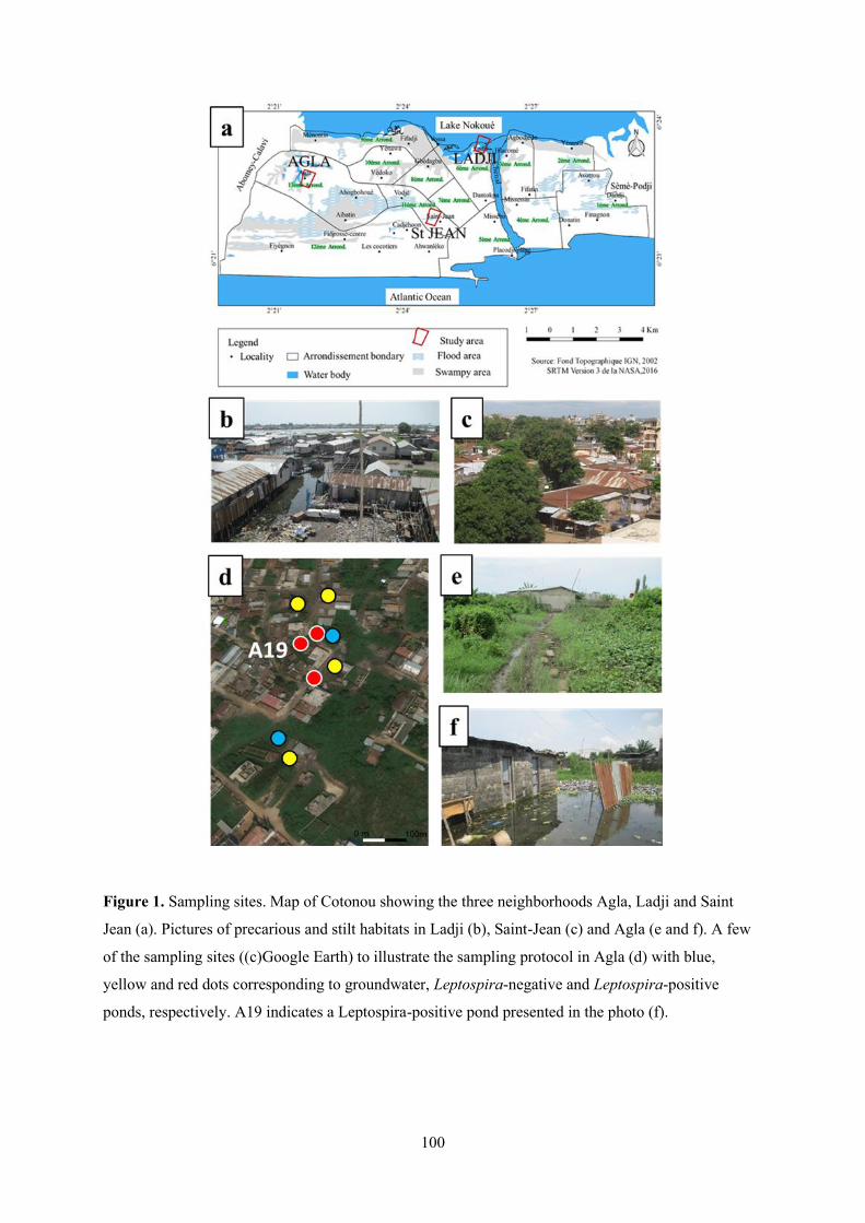
100

Figure 1. Sampling sites. Map of Cotonou showing the three neighborhoods Agla, Ladji and Saint

Jean (a). Pictures of precarious and stilt habitats in Ladji (b), Saint-Jean (c) and Agla (e and f). A few

of the sampling sites ((c)Google Earth) to illustrate the sampling protocol in Agla (d) with blue,

yellow and red dots corresponding to groundwater, Leptospira-negative and Leptospira-positive

ponds, respectively. A19 indicates a Leptospira-positive pond presented in the photo (f).

101

populated, has essentially informal housing development and is a very poor area where even the most

basic public services are usually missing. In particular, waste management is almost inexistent, garbage

are omnipresent and are even often used as embankment material. Such an environment favors

proliferation of rodents, which are abundant and infest 60-100% of households depending on the season

(Dobigny et al. 2019).

Agla is a recent but rapidly expanding district within a vast lowland that is extensively flooded

early in the rainy season (i.e., starting from June) following rainfall accumulation. Similar to Ladji,

permanent ponds are also present in Agla due to the extensive low-lying areas. The permanent ponds

are formed by groundwater discharge in the dry months, whereas during the winter months the rainfall

inputs to the ponds reverse the hydraulic gradients, resulting in groundwater recharge ponds

(Houéménou et al. 2019b). The habitat in Agla includes hard-built houses as well as very precarious

cabins, with the poorest inhabitants usually gathering around or within these floodable low-lying areas

(Fig. 1b). These low-lying areas are also widely used as dumping sites for household waste (Fig. 1b).

Rodents are abundant in households, with infestation rates always ≥ 90% (Dobigny et al. 2019).

Saint-Jean is an old and formal district that has large open sewers and many houses that are

solidly constructed. This district is not floodable per se, but large ponds may stand for several days after

heavy rains. Rodents are also abundant in ca. 90% of households (Dobigny et al. 2019).

In 2017 and 2018, the three districts of Cotonou (Agla, Ladji and Saint Jean; Fig.1b) were

monitored for both water quality parameters (physical parameters, major ions and trace elements) and

leptospire presence. Water sampling was organized concomitantly (i.e. within the same week) in the

three districts during the dry season (March 2017 and February 2018) as well as at the beginning (June

2017 and June 2018) and at the end (October 2017) of the rainy season. In total, 193 water samples were

collected: 85 in Agla, 53 in Ladji and 55 in Saint Jean. Eighty-three samples were tap waters and 61, 29,

17 and 3 samples were from groundwater wells, temporary ponds, permanent ponds and Lake Nokoué,

respectively. This corresponds to 51, 64, 55, 5 and 18 samples collected in March 2017, June 2017,

October 2017, February 2018 and June 2018, respectively. The detailed distribution of samples among

districts, periods and water types are provided in Table 1. The temporary ponds were differentiated from

the permanent ponds by noting locations where the waters were present in the wet season but not in the

dry season. Both temporary and permanent ponds were sampled in Ladji (8 and 6, respectively) and

Agla (21 and 11, respectively), but not in St Jean where ponds only last a few days.

Cartography of each studied area was performed within the same month immediately after each

of the five seasonal sampling campaigns. The land use categories and the extent of surface waters

(diameter > 3m) were systematically delineated using Open Street Map Tracker v.0.6.11 (Tools Open

Street Map) on an Android smartphone. A Geographic Information System was produced under QGIS

102

v.2.14 (QGIS Development team 2016). Surface water superficies were computed using the

LandscapeMetric package (option level class) in RStudio v.3.6.1 (RStudio Team 2016).

Table 1. Leptospira screening results by sampling sites and dates. “ok”: physico-chemical data are

available; “NA”: not assessed; “t.ponds”: temporary ponds; “p.ponds”: permanent ponds.

AGLA

Mar-

17 Jun-17 Oct-17 Feb-18 Jun-18

N=85 Groundwater 7 7 8 1 Temporary ponds 10 6 5 Permanent ponds 3 8 Tap water 10 10 10

Total 17 27 24 3 14 Positive leptospires 2+(t.ponds.) 3+(p.ponds.) Total prevalence 0.00 0.07 0.00 0.00 0.20 Ponds prevalence NA 0.20 0.00 0.00 0,21 Measures ok ok ok 1/2

LADJI

Mar-

17 Jun-17 Oct-17 Feb-18 Jun-18

N=53 Groundwater 3 2 3

Temporary ponds 5 3

Permanent ponds 1 2 3 Tap water 10 10 8

Lake

Total 14 18 15 2 4 Positive leptospires 1+(well)

Total prevalence 0.00 0.06 0.00 0.00 0.00 Groundwater prevalence 0.00 0.50 0.00

Measures NA ok ok ok ok St

JEAN Mar-

17 Jun-17 Oct-17 Feb-18 Jun-18

N=55 Groundwater 10 10 10

Tap water 10 9 6

Total 20 19 16

Positive leptospires 0 0 0

Total prevalence 0.00 0 0.00

Measures NA ok ok

103

Screening of waterborne pathogenic Leptospira

Test of a filtration-based method of water-borne Leptospira screening

Published studies on water-borne leptospires usually rely on high-speed centrifugation methods

and freezing preservation of field samples (e.g., Ganoza et al. 2006; Munoz-Zanzi et al. 2014; Lall et al.

2016; Riedeger et al. 2016; Thibeaux et al. 2017; Sato et al. 2019). These approaches are poorly adapted

to field surveys, especially in developing countries where lab facilities are usually hardly available

and/or distantly located. In order to adapt protocols of Leptospira screening of waters to the latter

conditions, we developed a simple filtration-based method that can be used in the field in absence of

costly and high-tech materials. To do so, we first experimentally compared the percentage of bacteria

recovery from mineral water (EC=180µS/cm) using centrifugation on the one hand, and filtration on the

other hand. For centrifugation tests, lab water samples were inoculated with various amounts (from

36,800 to 3,680,000 cells per sample, each sample in sextuplets) of living culture-originating Leptospira

interrogans. Centrifugation consisted in spinning 15mL of inoculated lab water samples at 4,000 rpm

during 30 minutes. Water-borne DNA was extracted immediately after centrifugation. Filtration was

performed on 500mL of inoculated lab water samples (representing 2,000 to 2,000,000 cells per sample,

each sample in triplicates) that were sequentially filtered on 0.45µm and 0.1µm membranes. Filters were

then stored in ethanol 96° for subsequent DNA extraction.

Total DNA was extracted from both centrifuged and filtered samples using the Biobasics EZ-

10 Spin column Genomic DNA Minipreps kit, and eluted in 50µL of elution buffer. The same amounts

of expected bacteria were extracted directly from 20µL of culture medium as a positive control.

Leptospires detection and quantification were performed following a probe-based qPCR method

that targets a fragment of the LipL32 gene using a LightCycler® 480 (Roche Diagnostics) in 96-well

micro-titre plates with a 10µL final volume for each reaction (see Dobigny et al. 2015). All qPCR

investigations were conducted in duplicates.

Leptospires screening in field water samples

For each of the 193 samples, one liter was collected during the morning. The 1 L bottles were

rinsed at least twice with the sample water before collection. Up to 500ml of water aliquots were filtered

for Leptospira screening within the same day, once in the lab. All field water samples were first filtered

using 5µm filter papers to retain the large suspended particles. Waters were then filtered using 0.45µm

filter papers. DNA extraction and leptospirosis quantification proceeded as described above, except that

for each water sample both 5µm and 0.45µm filter papers were pooled for DNA extraction.

104

Physico-chemical analysis of waters

A wide spectrum of physico-chemical parameters were measured for each water sample

investigated for Leptospira. These included the field parameters temperature, electrical conductivity

(EC), dissolved oxygen (DO) and pH, and laboratory analysed parameters stable isotopes, major ions

and trace elements. The methods and results of these hydrochemical data are detailed in Houéménou et

al. (2019b, 2020).

The comparison of physico-parameters of leptospire-positive and leptospire-negative waters was

performed using univariate plots. Principal Component Analysis (PCA) was used under XLSTAT

(Addinsoft 2019) to explore in a multivariate manner the chemical characteristics of water samples

where pathogenic leptospires were found compared to those with no leptospires. In addition, using the

same parameters as for the PCA, a hierarchical cluster analysis (CA) was performed to identify

homogeneous groups of leptospire-negative pools that have similar chemical characteristics to

leptospire-positive pool samples. The degree of association between pond sampling sites is represented

by the euclidian distance between groups.

RESULTS

Centrifugation vs. filtration-based approaches

Our experimental comparison of centrifugation- vs. filtration-based approaches showed that spinning

allowed us to recover only 24.45% 10.14 of the initial inoculated number of bacteria, while 98.30%

23.78% was recovered by filtration, thus demonstrating that the latter method provides an excellent

opportunity to survey environmental leptospires. Importantly, the recovered bacteria were unevenly

distributed among the 0.45µm and 0.1µm filter membranes, with 87.50% 22.26% and 10.80%

5.36%, respectively. Importantly, there was a high retention of leptospires on the 0.45µm filter papers,

which was also observed by Kaboosi et al. (2010). We did not detect any difference in recovery rates

between the different amounts of inoculated bacteria (data not shown).

Leptospira-positive waters

In total, six water samples were found pathogenic Leptospira-positive. Five positive samples originated

from pond water in Agla, whilst a sixth positive sample was from groundwater collected inside a well

at Ladji (Table 1). In Agla, Leptospira-positive waters were from both temporary and permanent ponds.

For temporary ponds the total prevalence was 9.5% (2/21). In comparison, for the permanent ponds the

prevalence was 27.3 % (3/11) (Table 1). All positive samples were obtained in June (2 temporary ponds

in Agla and one groundwater well in Ladji in June 2017; 3 permanent ponds in Agla in June 2018;

Fig.1a, 1d and 1e). No positive samples were found in Saint Jean, and no leptospires were detected in

the 83 tap waters analyzed.

105

Chemical characteristics of Leptospira-positive and -negative waters

The results of the physicochemical analysis of the early wet season (June) Leptospira-positive pond

waters in Agla, Ladji and Saint-Jean indicated there was little distinction with early wet season pond

waters that were Leptospira-negative (data presented in Suppl. Figure 1). Leptospira-positive ponds in

Agla had water temperatures ranging between 28.2 and 31.9 °C, which is within the range for all pond

waters analysed (24.9-35.9°C). The pH of the Leptospira-positive pond waters (6.72-8.67) were also

within the range of pH for all other ponds sampled (6.69-9.85). This only partly overlaps the pH range

for waters usually recognized for pathogenic Leptospira survival (i.e. pH 5.5 - 7.6; reviewed in Barragan

et al., 2017). The DO and EC values of the Agla Leptospira-positive pond waters ranged from 0-7.5

mg/L and 62-796 µS/cm, respectively, which are within the same range for all of the pond waters

sampled (0-12.4 mg/L and 28-4090 µS/cm respectively). Major ion and trace element concentrations of

positive ponds are also within the same ranges as ponds that were Leptospira-negative. For example,

the concentrations of the cations Na and Ca in Leptospira-positive ponds ranged between 6.8-78.9 and

0.4-62.7 mg/L, respectively, and between 1.1-8415.5 and 0.2-276.9 mg/L, respectively, for negative

ponds. The concentrations of the anions in the positive ponds include HCO3 and Cl that range between

26.0-284.3 and 4.5-74.6 mg/L, respectively, and in the negative ponds these range from 11.7-1115.1 and

0.7-16114.9 mg/L. The results of selected trace elements for Leptospira-positive ponds includes 37.6-

65.9 µg/L for Al, 3.1-194.2 µg/L for Mn, 7.9-3099 µg/L for Fe, 13.8-51.1 µg/L for B and 3.0-24.6 µg/L

for Zn.

The univariate plots also highlight that the Leptospira-containing waters have T°C, pH, EC, DO,

major ions and trace elements that overlap with the range of values observed for all urban pond water

samples. Similarly, the multivariate analyses shows overlaps of the four first principal components (that

together represent 62% of the total variance) between Leptospira-positive waters and other urban pond

waters (Fig. 2). The results of the hierarchical cluster analysis (AC; illustrated in the dendrogram on Fig.

3) also show that the positive pond samples (N38, N21, N18 and N25) are grouped within the same class

as several other negative pond samples (e.g. A2, A1, A7, A3, A17, A16, A10, A12, A14).

The only groundwater sample to be Leptospira-positive also had values of chemical parameters

that were similar to ranges observed in groundwater sampled from the shallow aquifer that were

Leptospira-negative. In Ladji, the Leptospira-positive groundwater sample had a temperature of 29.4°C

and a pH of 7.69, which is within the range of values for other groundwater samples (26.2-31.1°C and

5.85-7.84 respectively). In addition, the DO and EC of the Leptospira-positive groundwater (4.4 mg/L

and 1357 µS/cm respectively) was also within the range for all other Leptospira-negative groundwater

values (0.1-8.5 mg/L and 286-2480 µS/cm respectively).

106

Figure 2. Principal Component Analysis showing the physico-chemical characteristics of the

Leptospira-positive samples (red dots) among all urban water samples collected in Agla and Ladji.

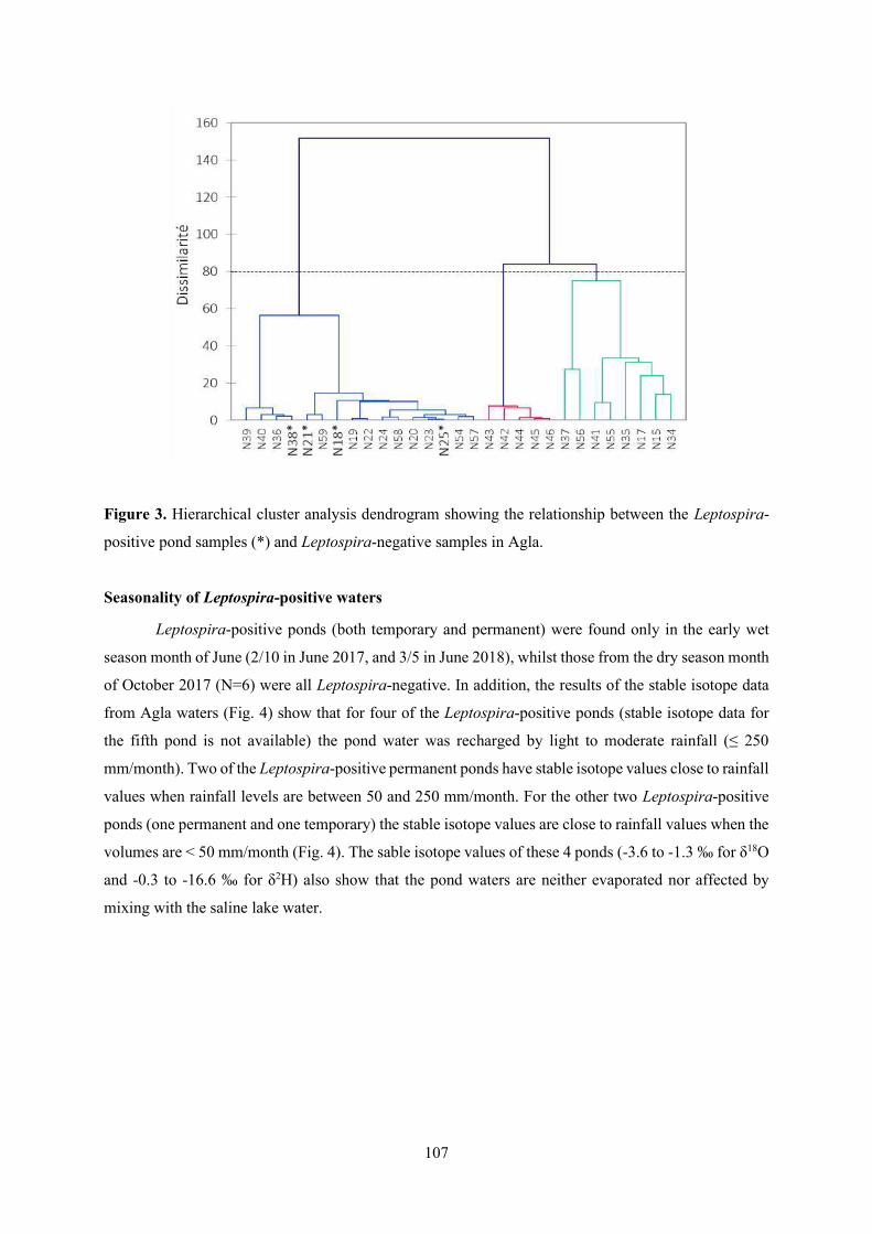
107

Figure 3. Hierarchical cluster analysis dendrogram showing the relationship between the Leptospira-

positive pond samples (*) and Leptospira-negative samples in Agla.

Seasonality of Leptospira-positive waters

Leptospira-positive ponds (both temporary and permanent) were found only in the early wet

season month of June (2/10 in June 2017, and 3/5 in June 2018), whilst those from the dry season month

of October 2017 (N=6) were all Leptospira-negative. In addition, the results of the stable isotope data

from Agla waters (Fig. 4) show that for four of the Leptospira-positive ponds (stable isotope data for

the fifth pond is not available) the pond water was recharged by light to moderate rainfall (≤ 250

mm/month). Two of the Leptospira-positive permanent ponds have stable isotope values close to rainfall

values when rainfall levels are between 50 and 250 mm/month. For the other two Leptospira-positive

ponds (one permanent and one temporary) the stable isotope values are close to rainfall values when the

volumes are < 50 mm/month (Fig. 4). The sable isotope values of these 4 ponds (-3.6 to -1.3 ‰ for δ18O

and -0.3 to -16.6 ‰ for δ2H) also show that the pond waters are neither evaporated nor affected by

mixing with the saline lake water.

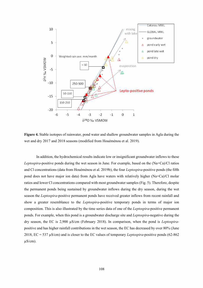
108

Figure 4. Stable isotopes of rainwater, pond water and shallow groundwater samples in Agla during the

wet and dry 2017 and 2018 seasons (modified from Houéménou et al. 2019).

In addition, the hydrochemical results indicate low or insignificant groundwater inflows to these

Leptospira-positive ponds during the wet season in June. For example, based on the (Na+Ca)/Cl ratios

and Cl concentrations (data from Houéménou et al. 2019b), the four Leptospira-positive ponds (the fifth

pond does not have major ion data) from Agla have waters with relatively higher (Na+Ca)/Cl molar

ratios and lower Cl concentrations compared with most groundwater samples (Fig. 5). Therefore, despite

the permanent ponds being sustained by groundwater inflows during the dry season, during the wet

season the Leptospira-positive permanent ponds have received greater inflows from recent rainfall and

show a greater resemblance to the Leptospira-positive temporary ponds in terms of major ion

composition. This is also illustrated by the time series data of one of the Leptospira-positive permanent

ponds. For example, when this pond is a groundwater discharge site and Leptospira-negative during the

dry season, the EC is 2,900 µS/cm (February 2018). In comparison, when the pond is Leptospira-

positive and has higher rainfall contributions in the wet season, the EC has decreased by over 80% (June

2018, EC = 537 µS/cm) and is closer to the EC values of temporary Leptospira-positive ponds (62-862

µS/cm).

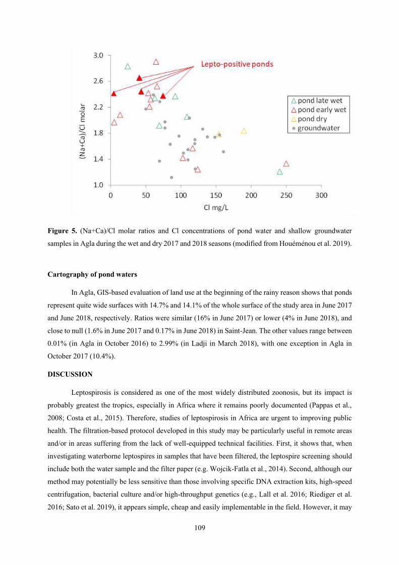
109

Figure 5. (Na+Ca)/Cl molar ratios and Cl concentrations of pond water and shallow groundwater

samples in Agla during the wet and dry 2017 and 2018 seasons (modified from Houéménou et al. 2019).

Cartography of pond waters

In Agla, GIS-based evaluation of land use at the beginning of the rainy reason shows that ponds

represent quite wide surfaces with 14.7% and 14.1% of the whole surface of the study area in June 2017

and June 2018, respectively. Ratios were similar (16% in June 2017) or lower (4% in June 2018), and

close to null (1.6% in June 2017 and 0.17% in June 2018) in Saint-Jean. The other values range between

0.01% (in Agla in October 2016) to 2.99% (in Ladji in March 2018), with one exception in Agla in

October 2017 (10.4%).

DISCUSSION

Leptospirosis is considered as one of the most widely distributed zoonosis, but its impact is

probably greatest the tropics, especially in Africa where it remains poorly documented (Pappas et al.,

2008; Costa et al., 2015). Therefore, studies of leptospirosis in Africa are urgent to improving public

health. The filtration-based protocol developed in this study may be particularly useful in remote areas

and/or in areas suffering from the lack of well-equipped technical facilities. First, it shows that, when

investigating waterborne leptospires in samples that have been filtered, the leptospire screening should

include both the water sample and the filter paper (e.g. Wojcik-Fatla et al., 2014). Second, although our

method may potentially be less sensitive than those involving specific DNA extraction kits, high-speed

centrifugation, bacterial culture and/or high-throughput genetics (e.g., Lall et al. 2016; Riediger et al.

2016; Sato et al. 2019), it appears simple, cheap and easily implementable in the field. However, it may

110

further be improved by being coupled with higher efficiency DNA extraction kits (Riediger et al. 2016),

something that we did not test here. In addition, we did not investigate possible negative impacts of

suspended matter in field water samples on our filtration approach as well as on our qPCR-based

detection method (Riedeger et al. 2016). In some instances, we noted that after filtration, filter papers

appeared quite coloured, thus suggesting the presence of undetermined suspended particles. The latter

may have inhibited to some extent subsequent DNA extractions and qPCRs. To highlight the possible

presence of inhibitory compounds in these coloured filter paper samples, a known amount of leptospire

DNA obtained from a bacterial culture was added after extraction. These Leptospira-enriched samples

remained qPCR-negative, suggesting the presence of qPCR inhibitors co-extracted with the DNA (data

not shown). Consequently, we cannot exclude the possibility of false negatives where the waters were

very turbid, and our results from the field should be cautiously interpreted as potentially underestimated.

The results retrieved from Cotonou waters demonstrate for the first time that water-borne

leptospires circulate in the heart of this large African city (3.1% of total prevalence; 5.5% when tap

waters are excluded; see Table 1).

It is noteworthy that leptospire-infected waters were found in the two most insalubrious areas,

namely Agla and Ladji, whilst none were observed in the popular but non-floodable Saint Jean district.

A survey of 780 rodents was conducted in the exact same areas of these three districts, and during the

exact same periods (Dossou et al. unpublished data). Interestingly, data in rodents fit well to patterns

retrieved in waters since 11.8% and 14% of rodent-borne leptospire prevalence were observed in Agla

and Ladji, respectively, while only 0.4% were positive in Saint Jean. This expectedly points towards a

higher environmental Leptospira contamination in poor, lowland and lake-edge districts where both

commensal rodents and surface water are omnipresent (Houéménou et al. 2014; Dobigny et al. 2018).

However, different patterns are observed between the high-risk districts of Agla and Ladji. The

positive water sample found in Ladji was collected in a groundwater well, thus suggesting that either

groundwater in the aquifer was contaminated from infiltration of Leptospira-positive water from the

surface, or by accident (e.g., use of an infected bucket or rope, or an infected rodent falling down the

well). At this stage, we cannot decipher between the two hypotheses, and since the sample size is low

we cannot draw robust conclusions on the potential of groundwater contamination by leptospires.

Further investigation of leptospires in groundwater in Cotonou deserves special attention, whatever its

origin, since one well out of two (50%) was affected in Ladji in June 2017. It is also worth noting that

although the groundwater in Agla is shallow, and in contact with permanent ponds water via recharge

in the wet season and discharge in the dry season, no leptospires were detected in the Agla groundwater.

In comparison, other studies have found groundwater well to be contaminated by leptospires (i.e. in

rural Chile; Munoz-Zanzi et al. 2014). In Cotonou, human activities in the immediate proximity of

groundwater wells are plentiful, with many children and women searching water daily with their bare

111

feet in close contact with humid soils and the water surrounding the well. Therefore, on-going

investigations of leptospires in groundwater is of critical importance.

In Agla, all Leptospira-positive waters originated from ponds, both temporary and permanent,

and all were collected in June. Although more intensive sampling is required during different rainfall

events, such a pattern strongly suggests that the water-mediated risk of leptospirosis infection may be

higher at the beginning of the rainy season through ponds. Our results agree with the conclusions drawn

from other studies where leptospiral risk is variable in both time and space, and is strongly dependent

on local environmental conditions (reviewed in Barragan et al. 2017). Similar to the results in Cotonou,

seasonality patterns were also observed in several regions, such as the Pao da Lima slum (Brazil), where

sewage and puddle samples were detected positive more often during the rainy season (Casanovas-

Massana et al. 2018). Pathogenic leptospires were also detected in several other urban surface waters

(see Tab. 1 in Barragan et al. 2017) where spatial heterogeneity is observed. For example, on the south

Andaman Island, the water-borne leptospires were only found in household drainage (18.7%) and

sewage (9.8%) waters and, unlike in Cotonou, there were no leptospire found in the pond waters (Lall

et al. 2016). The variable results from each study once again highlights the importance of understanding

the local socio-environmental context in determining leptospire transmission pathways to humans (e.g.,

Maciel et al. 2008; Himsworth et al. 2013; Mwachui et al. 2015; Houéménou et al. 2019a; reviewed in

Barragan et al. 2017).

The hydrochemical analysis of contaminated waters strongly suggest there are key hydrological

processes that may favor the presence of leptospires in the surface waters of Cotonou. Indeed, stable

isotopes and major ion data (from Houéménou et al., 2019b) indicate that leptospires are found in

temporary and permanent ponds at the beginning of the rainy season that have recently formed as a

result of low to moderate precipitation, and have relatively high runoff inputs compared to groundwater

or lake water inputs. This agrees with the expectation that there will be larger concentrations of the

pathogen in small water bodies (Barragan et al. 2017). It also corresponds well with the proposed model

of soil-to-water dispersion of leptospires recently recapitulated by Bierque and colleagues (2020).

Finally, and although the causal relationship remains untested, these results are strikingly consistent

with previous data on south Benin urban rodents in which Leptospira prevalence was found higher

during (or soon after) periods of moderate rains (100-200 mm; Houéménou et al. 2019b).

Though data are quite scarce, some physico-chemical parameters are known to have an influence

on Leptospira presence, survival and virulence (e.g., Chang et al. 1948; Khairani-Bejo et al. 2014;

André-Fontaine et al. 2015; Lall et al. 2018). Our observations strongly suggest that most negative pond

samples have similar physico-chemical characteristics to those positive for pathogenic Leptospira. In

particular, it was recently suggested that iron, manganese and copper could influence the survival of

leptospires in Andamanese soils (Lall et al. 2018). However, our data do not confirm such a trend since

112

leptospire-positive and negative water samples did not show any noticeable differences in these ions

concentrations (see Suppl. 1). Overlaps observed with both univariate and multivariate approaches mean

that the possible ecological spectrum of water-borne leptospires extensively covers the physico-

chemical spectrum of Cotonou waters as a whole. For instance, pH and temperature of Cotonou waters,

which are suspected to be of primary importance for leptospires biology (Chang et al. 1948; Gordon-

Smith & Turner, 1961; Khairani-Bejo et al. 2004; André-Fontaine et al. 2015), are perfectly compatible

with pH and temperature ranges that allow for the long-term survival of pathogenic leptospires (André-

Fontaine et al. 2015). In other words, the potential distribution of waters compatible with Leptospira

survival, hence human contamination risk, is quite wide in the city, meaning that, though quite polluted

(Lapworth et al. 2017; Houéménou et al. 2019b), urban waters in Cotonou are widely compatible with

the leptospire life cycle. In the city and, beyond, along the West African Abidjan-Lagos urban corridor,

surface waters inundate many zones of the public space, including areas that are used daily by the

inhabitants: walking pathways and streets, courtyards and even homes may be flooded for several days

if not weeks. Consequently, the population has extensive and on-going contact with potentially

contaminated water. Altogether, this indicates that millions of people living along the extensively

urbanizing Guinea Gulf are at risk for falling sick of leptospirosis.

CONCLUSION

Future studies should include two major aspects of leptospires ecology, hence leptospiral

contamination risk, that were not taken into consideration here: water microbiota and biofilms (e.g.,

Trueba et al. 2004; Kumar et al. 2015) on the one hand, and soil-associated leptospires on the other hand

(e.g., Thibeaux et al. 2017; Bierque et al. 2020). Nevertheless, our filtration-based results, though

potentially underestimated, clearly show that the Cotonou inhabitants live in an urban environment that

exposes them to leptospirosis infection risk, potentially at a wide spatial scale. Everyday uses and habits

as well as a lack of street and sanitation infrastructures results in many people in close contact with

standing waters on a regular basis, especially during the rainy season and associated flooding events.

Spatio-temporal investigations of water-borne leptospires point towards a higher risk at the beginning

of the rainy season, especially via ponds that are recharged by rainfall. We believe that awareness

increase about leptospirosis should be a public health priority since the disease is very poorly

documented and obviously overlooked in Benin and, further, along the rapidly extending Abidjan-Lagos

urban corridor.

ACKNOWLEDGEMENTS

We are in debt to all Cotonou inhabitants who allowed us to enter and collect samples within

their households. This research was funded by the UMRs CBGP, EMMAH and G-EAU. Field works in

Benin were conducted under the research agreement between Republic of Benin and the French Institute

of Research for sustainable Development that was signed on 30th September 2010.

113

REFERENCES

Addinsoft 2019. XLSTAT statistical and data analysis solution. Paris, France. https://www.xlstat.com.

Africapolis 2020. Visualise urbanisation in Africa. OECD Sahel and West Africa Club, https://www.africapolis.org/ (last accessed on 21/04/2020).

Allan K.J., Biggs H.M., Halliday J.E.B., Kazwala, R.R., Maro V.P., Cleaveland S. & Crump, J.A. 2015. Epidemiology of leptospirosis in Africa: A systematic review of a neglected zoonosis and a paradigm for ‘One Health’ in Africa. PLOS Neglected Tropical Diseases, 9, e0003899. https://doi.org/10.1371/journal.pntd.0003899.

André-Fontaine G., Aviat F. & Thorin C. 2015. Waterborne leptospirosis: Survival and preservation of the virulence of pathogenic Leptospira spp. in fresh water. Current Microbiology, 71, https://doi.org/10.1007/s00284-015-0836-4.

Barragan V., Olivas S., Keim P. & Pearson T. 2017. Critical knowledge gaps in our understanding of Environmental cycling and transmission of Leptospira spp. Applied Environmental

Microbiolobiology, 83, https://doi.org/10.1128/AEM.01190-17. Bierque E., Thibeaux R., Girault D., Soupé-Gilbert M.-E. & Goarant C. 2020. A systematic review of

leptospira in water and soil environments. PLoS ONE, 15, e0227055. Cann K.F., Thomas D.R., Salmon R.L., Wyn-Jones A.P. & Kay D. 2013. Extreme water-related weather

events and waterborne disease. Epidemiology and Infections, 141, 671–686. Casanovas-Massana A., Pedra G.G., Wunder E.A., Diggle P.J., Begon M. & Ko A.I. 2018.

Quantification of leptospira interrogans survival in soil and water microcosms. Applied

Environmental Microbiology 84, https://doi.org/10.1128/AEM.00507-18. Chang S.L., Buckingham M. & Taylor M.P. 1948. Studies on Leptospira icterohaemorrhagiae: IV.

Survival in water and sewage: destruction in water by halogen compounds, synthetic detergents and heat. Journal of Infectious Diseases, 82, 256-266.

Cornwall W. 2016. A plague of rats. Science, 352, 912–915. Costa F., Hagan J.E., Calcagno J., Kane M., Torgerson, P., Martinez-Silveira M.S., Stein C., Abela-

Ridder B. & Ko A.I. 2015. Global morbidity and mortality of leptospirosis: A systematic review. PLoS Neglected Tropical Diseases, 9, e0003898.

de Vries S.G., Visser B.J., Nagel I.M., Goris M.G.A., Hartskeerl R.A. & Grobusch M.P. 2014. Leptospirosis in Sub-Saharan Africa: a systematic review. International Journal of Infectious

Diseases, 28, 47–64. Denis E., Moriconi-Ebrard F., Harre D., Thiam O., Séjourné M. & Chatel C. 2009. Africapolis -

dynamiques de l’urbanisation, 1950-2020, une approche géostatistique : Afrique de l’Ouest (Urbanization dynamics, 1950-2020, a geostatistic approach: West Africa). https://hal.archives-ouvertes.fr/hal-00357271/file/Africapolis_1_Rapport.pdf (last accessed on 21/04/2020).

Dobigny G., Garba M., Tatard C., Loiseau A., Galan M., Kadaouré I., Rossi J.-P., Picardeau M. & Bertherat E. 2015. Urban market gardening and rodent-borne pathogenic Leptospira in Arid Zones: A Case Study in Niamey, Niger. PLoS Neglected Tropical Diseases, 9, e0004097.

Dobigny G., Gauthier P., Houéménou G., Choplin A., Dossou H.-J., Badou S., Etougbétché J., Bourhy P., Koffi S., Durski K., Bertherat E. & Picardeau M. 2018. Leptospirosis and extensive urbanization in West Africa: A neglected and underestimated threat? Urban Science, 2, e029.

Dobigny G., Gauthier P., Houéménou G., Dossou H.-J., Badou S.A., Etougbétché J., Tatard C. & Truc P.H.V. 2019. Spatio-temporal survey of small mammal-borne Trypanosoma lewisi in Cotonou, Benin, and the potential risk of human infection. Infection, Genetics and Evolution, e103967.

Ganoza C.A., Matthias M.A., Collins-Richards D., Brouwer K.C., Cunningham C.B., Segura E.R., Gilman R.H., Gotuzzo E. & Vinetz J.M. 2006. Determining risk for severe leptospirosis by molecular analysis of environmental surface waters for pathogenic Leptospira. PLoS Medicine, 3, e030308.

Haake D.A. & Levett P.N. 2015. Leptospirosis in humans. Current Topics in Microbiology and

Immunology, 387, 65–97.

114

Himsworth C.G., Bidulka J., Parsons K.L., Feng A.Y.T., Tang P., Jardine C.M., Kerr T., Mak S., Robinson J. & Patrick D.M. 2013. Ecology of Leptospira interrogans in Norway rats (Rattus

norvegicus) in an inner-city neighborhood of Vancouver, Canada. PLoS Neglected Tropical

Diseases, 7, e2270. Houéménou H. 2020. Qualité des eaux souterraines et de surface dans la métropole de Cotonou (Bénin) :

Implications pour la leptospirose (Ground and surface waters quality in Cotonou, Benin:

implications for leptospirosis). PhD thesis, Avignon University, France. Houéménou G., Ahmed A., Libois R. & Hartskeerl R.A. 2014. Leptospira spp. prevalence in small

mammal populations in Cotonou, Benin. International Scholarly Research Notices, 8, ID 2013, 502638, http://dx.doi.org/10.5402/2013/502638.

Houéménou G., Gauthier P., Etougbétché J., Badou S., Dossou H.-J., Agossou D., Picardeau M. & Dobigny G. 2019a. Pathogenic Leptospira in commensal small mammals from the extensively urbanized coastal Benin. Urban Science, 3, e3030099.

Houéménou H., Tweed S., Dobigny G., Mama D., Alassane A., Silmer R., Babic M., Ruy S., Chaigneau A., Gauthier P., Socohou A., Dossou H.-J., Badou S. & Leblanc, M. 2019b. Degradation of groundwater quality in expanding cities in West Africa: a case study of the unregulated shallow aquifer in Cotonou. Journal of Hydrology, 582, e124438.

Kaboosi H. & Razavi M.R. 2010. Efficiency of filtration technique for isolation of leptospires from surface waters: role of different membranes with different pore size and materials. African Journal

of Microbiology Research 4(9), 671-676. Khairani-Bejo S., Bahaman A.R.B., Zamri-Saad M. & Mutalib A.R. 2004. The Survival of Leptospira

interrogans Serovar Hardjo in the Malaysian environment. Journal of Animal and Veterinary

Advances, 3(3), 123-129. Ko A.I., Reis M.G., Dourado C.M.R., Johnson W.D. & Riley L.W. 1999. Urban epidemic of severe

leptospirosis in Brazil. The Lancet, 354, 820–825. Kumar V.K., Lall C., Vimal Raj R., Vedhagiri K. & Vijayachari P. 2015. Co-existence and survival of

pathogenic leptospires by formation of biofilm with Azospirillum. FEMS Microbiology and

Ecology, 91, pii:fiv051. Lall C., Vinod Kumar K., Raj R.V., Vedhagiri K., Sunish I.P. & Vijayachari P. 2018. Correlation

between physicochemical properties of soil and presence of Leptospira. EcoHealth, 15, 670–675. Lapworth D.J., Nkhuwa D.C.W., Okotto-Okotto J., Pedley S., Stuart M.E., Tijani M.N. & Wright, J.

2017. Urban groundwater quality in sub-Saharan Africa: current status and implications for water security and public health. Hydrogeology Journal, 25, 1093–1116.

Lau C.L., Smythe L.D., Craig S.B. & Weinstein P. 2010. Climate change, flooding, urbanisation and leptospirosis: fuelling the fire? Transactions of the Royal Society of Tropical Medecine and

Hygiene, 104, 631-638. Maciel E.A.P., Carvalho A.L.F., de Nascimento S.F., Matos R.B., de Gouveia E.L., Reis M.G. & Ko

A.I. 2008. Household transmission of Leptospira infection in urban slum communities. PLoS

Neglected Tropical Diseases, 2, e154. Muñoz-Zanzi C., Mason M.R., Encina C., Astroza A. & Romero A. 2014. Leptospira contamination in

household and environmental water in rural communities in Southern Chile. International Journal

of Environmental Research and Public Health, 11, 6666–6680. Mwachui M.A., Crump L., Hartskeerl R., Zinsstag J. & Hattendorf J. 2015. Environmental and

behavioural determinants of leptospirosis transmission: A systematic review. PLoS Neglected

Tropical Diseases, 9, e0003843. Pappas G., Papadimitriou P., Siozopoulou V., Christou L. & Akriditis N. 2008. The globalization of

leptospiroris: worldwide incidence trends. International Journal of Infectious Diseases, 12, 351-357.

Programme de Protection de la Communauté Urbaine de Cotonou Face aux Changements Climatiques. (PCUG3C) 2012. Inondations dans le grand Cotonou : facteurs humains, vulnérabilité des populations et stratégies de lutte et de gestion. (Program for the protection of the urban community

of Cotonou against climatic changes: human factors, population vulnerability and management

stratagies). Final Report, Abomey-Calavi, Benin. Available online: https://idl-bnc-idrc. dspacedirect.org/handle/10625/50607 (last accessed on 21/04/2020).

115

QGIS Development Team 2016. QGIS: Geographic Information System. Open Source Geospatial Foundation Project. http://qgis.osgeo.org.

Riediger I.N., Hoffmaster A.R., Casanovas-Massana A., Biondo A.W., Ko A.I. & Stoddard, R.A. 2016. An optimized method for quantification of pathogenic Leptospira in environmental water samples. PLoS ONE, 11, e160523.

RStudio Team 2016. RStudio: Integrated development for R. RStudio Inc., Boston, USA. http://www.rstudio.com/.

Sato Y., Mizuyama M., Sato M., Minamoto T., Kimura R. & Toma, C. 2019. Environmental DNA metabarcoding to detect pathogenic Leptospira and associated organisms in leptospirosis-endemic areas of Japan. Scientific Reports, 9, 1–11.

Smith C.E.G. & Turner L.H. 1961. The effect of pH on the survival of leptospires in water. Bulletin of

the World Health Organization, 24, 35–43. Thaipadungpanit J., Wuthiekanun V., Chantratita N., Yimsamran S., Amornchai P., Boonsilp S.,

Maneeboonyang W., Tharnpoophasiam P., Saiprom N., Mahakunkijcharoen Y., Day N.P.J., Singhasivanon P., Peacock S.J. & Limmathurotsakul D. 2013. Leptospira species in floodwater during the 2011 floods in the Bangkok Metropolitan Region, Thailand. American Journal of

Tropical Medicine and Hygiene, 89, 794-796. Thibeaux R., Geroult S., Benezech C., Chabaud S., Soupé-Gilbert M.S., Girault D., Bierque E. &

Goarant, C. 2017. Seeking the environmental source of leptospirosis reveals durable bacterial viability in river soils. PLoS Neglected Tropical Diseases, 11, e5414.

Trueba G., Zapata S., Madrid K., Cullen P. & Haake D. 2004. Cell aggregation: a mechanism of pathogenic Leptospira to survive in fresh water. International Microbiology, 7, e35–40.

UN Habitat 2014. L’urbanisation - un impératif pour la transformation structurelle de l’Afrique : une nouvelle conception de l’urbanisation en appui à l’Agenda 2063. United Nations, Nairobi, Kenya.

Wójcik-Fatla A., Zając V., Wasiński B., Sroka J., Cisak E., Sawczyn-Domańska A. & Dutkiewicz J. 2014. Occurrence of Leptospira DNA in water and soil samples collected in eastern Poland. Annals of Agricultural and Environmental Medicine of the American Academy of Emergency

Medicine, 21, e730-732. Yabi I. & Afouda F. 2012. Extreme rainfall years in Benin (West Africa). In: West African paleoecology

and human responses. West African Quaternary Research Association, 262, 39–43.

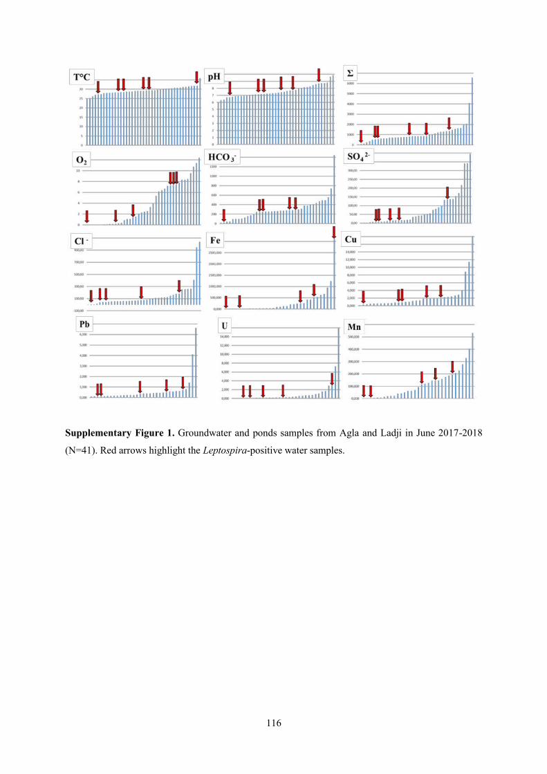
116

Supplementary Figure 1. Groundwater and ponds samples from Agla and Ladji in June 2017-2018

(N=41). Red arrows highlight the Leptospira-positive water samples.

117

CONCLUSION GENERALE ET PERSPECTIVES

118

Conclusion générale

L’étude faisant objet du présent manuscrit a porté sur la qualité des eaux souterraines et de surface

dans la métropole de Cotonou au Sud du Bénin et les risques de maladies hydriques associées, cas de la

leptospirose. Les travaux effectués ont permis de fournir des données de base pour aboutir à une meilleure

compréhension du fonctionnement spatio-temporel de l’aquifère côtier de Cotonou. Cette étude à caractère

multidisciplinaire a utilisé une approche combinant les outils chimiques (ions majeurs, éléments traces

métalliques) et isotopiques (2H et 18O) d’une part, et d’autre part une approche bactériologique (screening

des leptospires). Cette dernière est une première investigation qui après détection et la quantification des

bactéries leptospires, s’est basée sur la caractérisation physico-chimique et isotopique des eaux dans les

bidonvilles de Cotonou pour expliquer les risques d’émergence de la leptospirose.

Le suivi saisonnier de Novembre 2016 à Juin 2018 des eaux souterraines du Quaternaire captées

par les puits à grand diamètre, les mares et les eaux du lac Nokoué a été effectué dans trois quartiers aux

contextes hydrogéologiques différents. Le premier, Ladji qui s’inonde pendant la petite saison des pluies,

est situé en bordure du lac Nokoué. Le deuxième, Agla situé dans une zone de décharge, est sujet à des

inondations pendant la grande saison des pluies et le troisième, St Jean où il n'y a pas d'inondation, est situé

au centre-ville.

La synthèse bibliographique abordée dans le chapitre I de ce manuscrit, a montré que l’aquifère du

Quaternaire dans la ville de Cotonou est confronté à de réel problème de contaminations qui, dans les

conditions actuelles ne fait que s’accentuer avec la croissance démographique, le manque de systèmes de

gestion des eaux usées et des déchets solides.

Selon les études antérieurs (Boukari 1998 ; Yehouenou Azehoun Pazou et al. 2009 ; Odoulami 2009

; Totin et al. 2013 ; Adjahouinou et al. 2014 ; Yadouléton 2015) et les enquêtes de terrain lors de cette étude,

les eaux souterraines peu profondes de Cotonou, même contaminées, demeurent une source non négligeable

d’approvisionnement en eau des populations des milieux défavorisés qui n’ont pas accès à l’eau potable

desservie par la SONEB.

Cette conclusion permet de ressortir les principaux résultats illustrés dans les trois articles

scientifiques du manuscrit. Des perspectives de recherche seront ensuite proposées.

Fluctuation des niveaux d’eau dans les puits

Le suivi mensuel des niveaux d’eau et de la conductivité électrique (CE) dans les puits de Juin 2017-

Juin 2018 a permis de mieux caractériser le contexte hydrogéologique sur chacun des sites d’étude.

L’amplitude saisonnière des niveaux d’eau à St Jean a montré qu’il s’agit d’une zone de recharge locale de

119

la nappe comparé à Ladji et Agla qui eux, sont des zones de décharge de la nappe. La réalisation d’une carte

piézométrique par saison pourrait permettre de confirmer ces zones de recharge et les exutoires. Le facteur

important qui conditionne la qualité des eaux souterraines à Agla est sa proximité avec les mares

permanentes (bas-fonds) et temporaires. Ladji étant situé à proximité du lac Nokoué, les fluctuations du

niveau d’eau du lac influencent la variation du niveau de la nappe notamment pendant la petite saison des

pluies. Même si les fluctuations saisonnières des niveaux d’eau sont en phase avec les précipitations

mensuelles, on note une remontée du niveau de la nappe qui démarre pendant la saison sèche en Février à

Agla et en Janvier à Ladji puis avance progressivement jusqu'en avril/mai (saison des pluies), soit un

décalage respectif de 1 à 2 mois par rapport à St Jean. La menace liée à l’apport d’eaux de surface provenant

des mares et du lac Nokoué est devenue plus évidente avec les mesures de la CE qui ont montré des

tendances similaires suivant la variation du niveau de la nappe. La remontée inattendue du niveau de la

nappe qui survient plutôt pendant la saison sèche à Agla et à Ladji correspond aussi à une augmentation de

la CE qui est plus marquée à Ladji. L’utilisation des outils géochimiques et isotopiques a été nécessaire pour

apporter des précisions et quantifier les mélanges entre les eaux souterraines et les eaux de surface, en

occurrence le lac Nokoué.

Composition isotopique et chimique des pluies locales, des mares et du lac Nokoué

Les données isotopiques obtenues sur le site du GNIP/IITA et de l’AIEA ont permis d’établir la

droite météorique caractérisant la signature isotopique des eaux de pluies de 2005-2016 à Cotonou. Les

quantités de pluies (>50 mm/mois) sont appauvries en isotopes stables. Les données de pluies collectées

dans le cadre de cette étude de juin 2017 à Juin 2018 (n=13) montrent des valeurs d’isotopes stables qui

varient de -5,4 à 0,8 pour δ18O et de -30,9 à 14,5 ‰ pour δ²H. Les pluies sont faiblement minéralisées

(21<CE<122 µS/cm) et ne constituent pas une source majeure de contamination des eaux souterraines.

Néanmoins, ces pluies locales sont influencées par l’apport sous forme d’aérosols des embruns marins et

dans une moindre mesure d’origine terrigène.

Les analyses isotopiques ont montré que les valeurs en δ18O sont comprises entre -5 à 1,6 pour le

lac Nokoué et entre de -4,3 et 3,9 ‰ pour les mares. Les eaux du lac Nokoué sont largement dominées par

le faciès chloruré sodique correspondant à l’influence de l’Océan Atlantique. Les mares à Ladji et à Agla

ont des compositions chimiques similaires à celles des eaux souterraines locales, ce qui indique un lien

potentiel entre les eaux de surface et les eaux souterraines.

120

Minéralisation des eaux souterraines

Le suivi saisonnier (grande saison sèche, grande saison des pluies et petite saison des pluies) des

concentrations en ions majeurs dans les eaux souterraines et les eaux de surface (mares et Lac Nokoué) a

montré les mécanismes ayant un impact sur la chimie des eaux étudiées. Les eaux souterraines ont des faciès

très variables selon les sites. Cette variabilité est fortement influencée par la proximité avec les mares et le

lac Nokoué. Les eaux souterraines sont faiblement ou encore moyennement minéralisées pour le faciès

bicarbonaté calcique et fortement minéralisées vers le faciès chloruré sodique avec présence de nitrates.

Outre les processus de minéralisation induits par l’interaction eau-roche dont la couche réservoir est formée

de dépôts récents marins constitués de débris coquillers à test calcaire et éventuellement de silicates (Boukari

et al. 1996), le mélange avec les eaux salines du lac Nokoué, les mares, les apports anthropiques,

l’évaporation et la dégradation de la matière organique sont les facteurs qui contribuent à la minéralisation

des eaux souterraines peu profondes.

La compréhension de la variation spatio-temporelle des processus contrôlant la qualité des eaux

souterraines a été très utile pour identifier les risques pour les résidents qui utilisent cette ressource en eaux

souterraines peu profondes non réglementées à des fins domestiques, y compris d'approvisionnement en eau

potable.

Périodes à risque d’intrusion d’eau saline

Les approches utilisant les outils chimiques et isotopiques ont permis de définir les facteurs et les

périodes à risque de contamination des eaux souterraines. Bien que la source de pollution soit identique pour

chacun des trois quartiers étudiés, les périodes à risque qui contrôlent l’augmentation des concentrations en

ions majeurs sont variables. Les isotopes stables de la molécule d’eau ont permis d’exclure la présence d’une

intrusion d’eau saline par l’eau de mer et/ou le lac Nokoué dans les eaux souterraines à St Jean. Les eaux

souterraines à St Jean sont rechargées par les pluies locales comparé à celles de Ladji et Agla qui sont non

seulement évaporées mais également soumises aux mélanges avec les eaux du lac Nokoué et des mares, en

particulier pendant la saison sèche et la petite saison pluvieuse. La quantification des fractions de mélange

avec les eaux salines du lac Nokoué à partir des ratios isotopiques indiquent 72 à 74 % à Ladji et 54 à 62 %

à Agla.

Périodes à risque de contamination anthropique

Sur la base des ratios Cl/Br, les sources anthropiques de contamination des eaux souterraines ont

été identifiées. Elles sont principalement dues à l'infiltration des eaux usées des fosses septiques, les

suintements des latrines creusées à proximité de la nappe et le lessivage des déchets solides.

L’échantillonnage saisonnier a mis en évidence les risques accrus de fuites des latrines et de fosses septiques

121

pendant la saison des pluies dans les quartiers situés dans les zones de décharge (Ladji et Agla , Figures 18

et 19 ) par rapport au zone de recharge (St Jean, Figure 18) où la contamination est plus importante pendant

saison sèche. Par ailleurs, les conditions réductrices dans les zones de décharge pendant la saison sèche ont

favorisé les processus de dénitrification conduisant à l’augmentation des teneurs en HCO3.

Distribution des éléments traces métalliques (ETM) dans les eaux souterraines

En dehors des composés azotés, les eaux usées et les déchets solides qui sont acheminés par les

lixiviats vers la nappe, renferment également des éléments traces métalliques. L’étude des éléments traces

métalliques dans l’investigation des eaux souterraines du système aquifère côtier de Cotonou a permis de

combler le déficit d’information sur la distribution et la géochimie des éléments traces métalliques (ETM).

L’ordre de croissance des ETM varient d’un site à l’autre. A Ladji, les ETM, ayant des concentrations

relativement élevées dans les eaux souterraines sont Mn, B, Fe, Ba, Li, Al, Zn, V, U et Mo. A Agla, il s’agit

du Ba, Mn, Fe, B, Al, Zn, V and Mo et à St Jean du B, Zn, Al, Mn, Fe, Ba, V and Mo. Conformément aux

normes Béninoises relatives à la qualité des eaux potables, seuls le Fe et le Mn ont des concentrations

supérieures aux valeurs standards respectives de 300µg/L et 100 µg/L notamment pendant la saison sèche.

Grâce à l’approche géochimique utilisée, les facteurs qui contribuent à l’augmentation du Fe et Mn dans les

eaux souterraines ont été décrits. Outre les interactions eau-roche qui facilitent la dissolution des oxydes de

manganèse, la dénitrification, l’oxydation réductive et la dégradation bactériologique de la matière

organique, sont les principaux facteurs qui contrôlent la distribution du Fe et Mn dans les eaux souterraines.

A travers la Zone Non Saturée, il a été distingué différents schémas de transfert de polluants dans

les profils réalisés sur les dépotoirs sauvages de déchets. Dans le profil constitué uniquement de sable (St

Jean), les éléments traces traversent la Zone Non Saturée et atteignent la Zone Saturée (B, V, Mo, Al et Fe)

et d’autres migrent sans atteindre la nappe (Mn et Zn). Dans les profils sableux argileux (Agla et ladji), la

plupart des éléments traces se sont accumulés dans la Zone Non Saturée. L’argile constituent jusqu’à présent

une barrière naturelle à la migration des éléments traces dans les eaux souterraines notamment à Ladji et à

Agla.

Risques de contamination hydrique : cas de la leptospirose

L’apport des approches géochimiques et isotopiques à la compréhension de l’écologie des

leptospires dans le compartiment hydrique a permis d'explorer pour la première fois la capacité des

leptospires à évoluer dans un habitat urbain pollué. Malgré un nombre d’échantillons positifs relativement

faibles, l’étude de ces bactéries pathogènes dans les eaux souterraines et de surface de Cotonou a permis

d’aboutir à des conclusions robustes qui appelleront, à n’en pas douter, d’autres investigations sur cette

maladie hydrique méconnue mais incontestablement morbide au Bénin. En premier lieu, nous avons pu

confirmer la présence de leptospires pathogènes dans les eaux de Cotonou, identifier les périodes et les

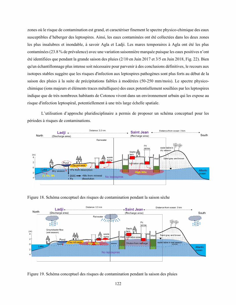
122

zones où le risque de contamination est grand, et caractériser finement le spectre physico-chimique des eaux

susceptibles d’héberger des leptospires. Ainsi, les eaux contaminées ont été collectées dans les deux zones

les plus insalubres et inondable, à savoir Agla et Ladji. Les mares temporaires à Agla ont été les plus

contaminées (23.8 % de prévalence) avec une variation saisonnière marquée puisque les eaux positives n’ont

été identifiées que pendant la grande saison des pluies (2/10 en Juin 2017 et 3/5 en Juin 2018, Fig. 22). Bien

qu'un échantillonnage plus intense soit nécessaire pour parvenir à des conclusions définitives, le recours aux

isotopes stables suggère que les risques d'infection aux leptospires pathogènes sont plus forts au début de la

saison des pluies à la suite de précipitations faibles à modérées (50-250 mm/mois). Le spectre physico-

chimique (ions majeurs et éléments traces métalliques) des eaux potentiellement souillées par les leptospires

indique que de très nombreux habitants de Cotonou vivent dans un environnement urbain qui les expose au

risque d'infection leptospiral, potentiellement à une très large échelle spatiale.

L’utilisation d’approche pluridisciplinaire a permis de proposer un schéma conceptuel pour les

périodes à risques de contaminations.

Figure 18. Schéma conceptuel des risques de contamination pendant la saison sèche

Figure 19. Schéma conceptuel des risques de contamination pendant la saison des pluies

123

Figure 20. Schéma conceptuel des risques de contamination pendant la saison sèche

Figure 21. Schéma conceptuel des risques de contamination dès le début de la saison des pluies

Figure 22. Schéma conceptuel des risques de contamination pendant la saison des pluies

124

Recommandations

Les mesures simples et qui ne nécessitent pas la mobilisation des moyens onéreux sont proposées

aux autorités pour protéger les populations contre les risques de contaminations aux maladies hydriques.

Sensibiliser et éduquer les populations sur les risques liés aux maladies hydriques notamment

pendant les périodes de contamination

Saison sèche à Ladji et à St Jean

Interdiction d’utiliser les eaux souterraines pour les usages domestiques

Faciliter l’accès à l’eau potable aux populations défavorisées en diminuant le coût d’achat et

d’abonnement au service de l’eau

Saison des pluies à Ladji et à Agla

Eviter le contact avec les eaux de surface (mares) dès le début de la saison des pluies

Aménagement ponctuel (mini pont, diguette, passage hors de l’eau,

Mettre à disposition des ménages les équipements de protection individuelle

Perspectives de recherches

Les résultats obtenus dans le cadre de cette étude fournissent certes de bonnes bases de données et des

informations sur les facteurs de contamination de l’aquifère côtier de Cotonou. Compte tenu de la

complexité du contexte hydrogéologique locale, des études supplémentaires à plus grande échelle sont

nécessaires pour la caractérisation globale de la zone côtière.

Vulnérabilité de l’aquifère inférieur (Continental Terminal)

L’alimentation en eau potable de la ville de Cotonou repose exclusivement sur les eaux souterraines

tirées essentiellement de l’aquifère du Continental Terminal du plateau d’Allada. Les logs de forages dans

la région côtière sud et la zone délimitant le champ de captage indiquent une hétérogénéité horizontale et

verticale des sédiments (McInnis et al. 2013). La contamination des eaux souterraines peu profondes, que

ce soit par l'intrusion saline des eaux de surface ou par la contamination anthropique des activités urbaines

comme mentionné dans cette étude, représenterait une menace potentielle pour les ressources en eau de

l’aquifère inférieur, même si les études antérieures n’ont pas notifié une contamination évidente de

l’aquifère inférieur par le transport des polluants de la région côtière. Les études sur le traçage isotopique

125

(isotope stable et radioactif) et sur le transport des contaminants chimiques notamment les éléments traces

dans les eaux de l’aquifère inférieur doivent être menées.

La surveillance de l’aquifère inférieur pourrait aussi passer par l’étude des processus de transfert de

contaminants (ions majeurs et éléments traces) au travers de la Zone Non Saturée. Cet aspect qui a été peu

développé au cours de nos travaux doit être poursuivi notamment dans les sédiments où la profondeur de la

zone non saturée est plus importante.

Rôle des sols dans la survie des leptospires

Même si les résultats sur l’identification des leptospires pathogènes dans les eaux de Cotonou ont

montré une prévalence plus élevée pendant la saison des pluies qui semble cohérente avec les résultats

obtenus sur les rongeurs, les données restent à densifier pour construire des bases de données précises et

robustes pour la région de Cotonou. Les études sur l’identification et le temps de survie des leptospires

d’une part, et le taux de contaminations humaines d’autre part doivent être urgemment entamées, notamment

dans les zones de bas-fonds inondables de Cotonou où les risques de contamination semblent être très élevés.

Un nombre croissant de travaux (Kingscote 1970; Wilson et Fujioka 1995; Fuh et al. 2011 ;

Thibeaux et al. 2018 ; Schneider et al. 2018 ; Casanovas-Massana et al. 2018 ; Bierque et al. 2020) semble

montrer que les sols humides constituent également un environnement très favorable où les pathogènes

Leptospira peuvent survivre pendant plusieurs jours voire plusieurs mois. Lall et al. (2018) ont mis en

évidence une corrélation positive entre les éléments chimiques dans les sols (les nitrates, le fer, le manganèse

et le cuivre) et la présence de leptospires pathogènes. Ces auteurs ont émis l’hypothèse selon laquelle les

précipitations saisonnières peuvent remettre en suspension les leptospires dans les eaux de surface à partir

des particules du sol. Un tel scénario pourrait être testé à Cotonou où la plupart des sols sont sableux et

souvent saturés en eau.

Diffusion scientifique et sensibilisation face aux risques liées aux maladies hydriques

Cette étude sur la qualité des eaux souterraines et les risques de contamination par des pathogènes

environnementaux en général, et la leptospirose notamment, doit être élargie à un volet « perception et

sensibilisation ». Même si les différents usages des eaux souterraines par les populations ont été notifiés

dans ce manuscrit, les risques de contamination des maladies hydriques que ça soit par la voie orale ou le

contact physique restent parfois méconnus des populations, en l’occurrence de celles qui vivent dans les

milieux les plus défavorisés en même temps que les plus à risque (les bas-fonds, le long des berges du Lac

Nokoué et du Chenal de Cotonou). La mise en place d’un projet d’extension à la dimension « Vulgarisation

et sensibilisation » associant des collègues socio-anthropologues, des biologistes, des hydrogéologues et des

126

acteurs publics de la santé et du secteur de l’eau permettrait de mettre les résultats scientifiques au service

des populations de façon opérationnelle.

Toutes ces investigations pourraient déboucher à long terme sur la mise en place d’une politique

de gestion des eaux souterraines peu profondes, jusque-là non suivie par les autorités. Cette dernière devra

tenir compte du schéma directeur de l’urbanisation de la ville de Cotonou et celui de l’assainissement et de

la gestion des déchets, indispensables pour la protection des ressources en eaux souterraines.

127

Annexes

128

Annexe 1. Normes sur la qualité des eaux potables en République du Bénin

Le Décret N°2001-094 du 20 février fixant les normes de la qualité de l’eau potable en République du Bénin

Normes microbiologiques

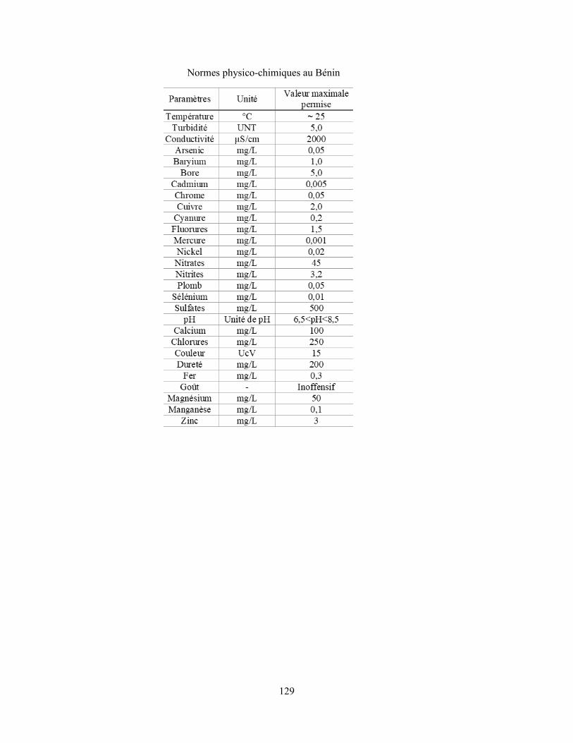
129

Normes physico-chimiques au Bénin

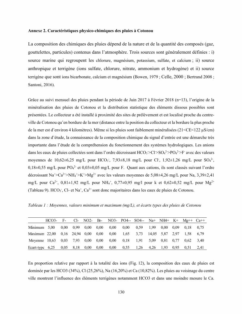
130

Annexe 2. Caractéristiques physico-chimiques des pluies à Cotonou

La composition des chimiques des pluies dépend de la nature et de la quantité des composés (gaz,

gouttelettes, particules) contenus dans l’atmosphère. Trois sources sont généralement définies : i)

source marine qui regroupent les chlorure, magnésium, potassium, sulfate, et calcium ; ii) source

anthropique et terrigène (ions sulfate, chlorure, nitrate, ammonium et hydrogène) et ii) source

terrigène que sont ions bicarbonate, calcium et magnésium (Bowen, 1979 ; Celle, 2000 ; Bertrand 2008 ;

Santoni, 2016).

Grâce au suivi mensuel des pluies pendant la période de Juin 2017 à Février 2018 (n=13), l’origine de la

minéralisation des pluies de Cotonou et la distribution statistique des éléments dissous possibles sont

présentées. Le collecteur a été installé à proximité des sites de prélèvement et est localisé proche du centre-

ville de Cotonou qu’en bordure de la mer (distance entre la position du collecteur et la bordure la plus proche

de la mer est d’environ 4 kilomètres). Même si les pluies sont faiblement minéralisées (21<CE<122 µS/cm)

dans la zone d’étude, la connaissance de la composition chimique du signal d’entrée est une démarche très

importante dans l’étude de la compréhension du fonctionnement des systèmes hydrologiques. Les anions

dans les eaux de pluies collectées sont dans l’ordre décroissant HCO3->Cl->SO4

2->PO42->F- avec des valeurs

moyennes de 10,62±6,25 mg/L pour HCO3-, 7,93±8,18 mg/L pour Cl-, 1,92±1,26 mg/L pour SO4

2-,

0,18±0,55 mg/L pour PO42- et 0,03±0,05 mg/L pour F. Quant aux cations, ils sont classés suivant l’ordre

décroissant Na+>Ca2+>NH4+>K+>Mg2+ avec les valeurs moyennes de 5,08±4,26 mg/L pour Na, 3,39±2,41

mg/L pour Ca2+, 0,81±1,92 mg/L pour NH4+, 0,77±0,95 mg/l pour k et 0,62±0,52 mg/L pour Mg2+

(Tableau 9). HCO3-, Cl- et Na+, Ca2+ sont donc majoritaires dans les eaux de pluies de Cotonou.

Tableau 1 : Moyennes, valeurs minimum et maximum (mg/L), et écarts types des pluies de Cotonou

En proportion relative par rapport à la totalité des ions (Fig. 12), la composition des eaux de pluies est

dominée par les HCO3 (34%), Cl (25,26%), Na (16,20%) et Ca (10,82%). Les pluies au voisinage du centre

ville montrent l’influence des éléments terrigènes notamment HCO3 et dans une moindre mesure le Ca.

HCO3- F- Cl- NO2- Br- NO3- PO4-- SO4-- Na+ NH4+ K+ Mg++ Ca++

Minimum 5,00 0,00 0,99 0,00 0,00 0,00 0,00 0,59 1,99 0,00 0,09 0,18 0,75

Maximum 22,00 0,16 24,94 0,00 0,00 0,00 1,65 3,73 14,05 5,87 2,97 1,58 6,79

Moyenne 10,63 0,03 7,93 0,00 0,00 0,00 0,18 1,91 5,09 0,81 0,77 0,62 3,40

Ecart-type 6,25 0,05 8,18 0,00 0,00 0,00 0,55 1,26 4,26 1,93 0,95 0,51 2,41

131

Toutefois, la signature marine demeure prépondérante dans la minéralisation globale car le cumul des

éléments qui y sont associés (Cl, Na, Mg, SO4 et K) réprésentent 52 % de la totalité des ions même si les

aérosols marins sont surtout pourvoyeurs de Cl et Na (Bertrand, 2008 ; Santoni 2016). Le NH4 (2,56%) qui

correspond à l’influence des activités anthropiques, est par contre présents en faible proportion dans les

pluies. La chimie des pluies semble donc être principalement influencée par des éléments provenant de

sources terrigènes dominant, marine et anthropique en faible proportion.

Figure 1: Distribution statistiques des ions majeurs dans les pluies de Juin 2017-Février 2018

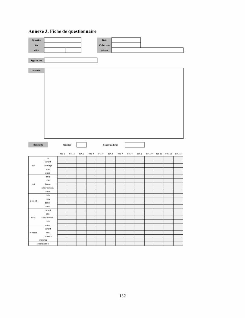
132

Annexe 3. Fiche de questionnaire

Quartier Date

Site Collecteur

GPS Adresse

Type de site

Plan site

Bât. 1 Bât. 2 Bât. 3 Bât. 4 Bât. 5 Bât. 6 Bât. 7 Bât. 8 Bât. 9 Bât. 10 Bât. 11 Bât. 12 Bât. 13

rafia/bambou

tissu

toit

autre

bois

ciment

murs

Bâtiments Nombre Superficie bâtie

sol carrelage

ciment

nu

autre

tapis

dalle

tôle

banco

surélévation

bois

rafia/bambou

autre

plafond

autre

tôle

marches

terrasse

banco

couverte

nue

ciment

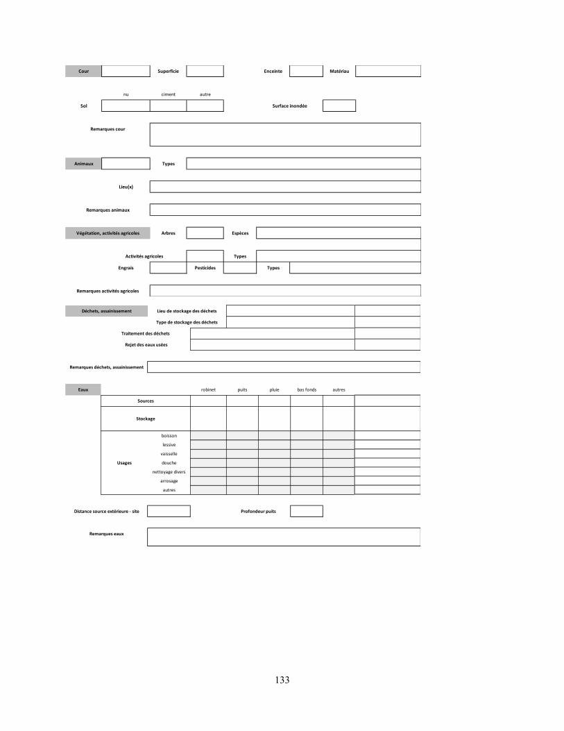
133

Cour Superficie Enceinte Matériau

nu ciment autre

Sol

Animaux Types

Lieu(x)

Arbres Espèces

Types

Engrais Pesticides Types

Remarques activités agricoles

Activités agricoles

Remarques animaux

Végétation, activités agricoles

Surface inondée

Remarques cour

Eaux robinet puits pluie bas fonds autres

boisson

lessive

vaisselle

douche

nettoyage divers

arrosage

autres

Remarques eaux

Distance source extérieure - site Profondeur puits

Sources

Stockage

Usages

Déchets, assainissement Lieu de stockage des déchets

Type de stockage des déchets

Traitement des déchets

Rejet des eaux usées

Remarques déchets, assainissement

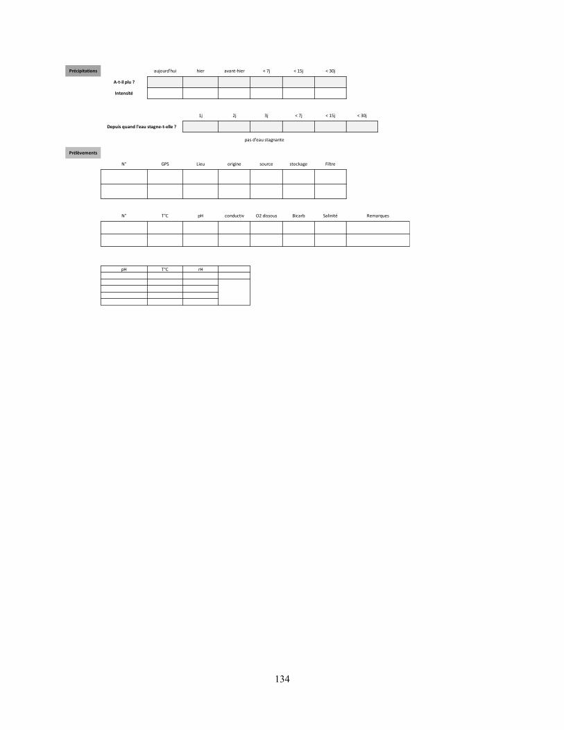
134

Précipitations aujourd'hui hier avant-hier < 7j < 15j < 30j

A-t-il plu ?

Intensité

1j 2j 3j < 7j < 15j < 30j

Prélèvements

N° GPS Lieu origine source stockage Filtre

N° T°C pH conductiv O2 dissous Bicarb Salinité

pH T°C rH

Depuis quand l'eau stagne-t-elle ?

Remarques

pas d'eau stagnante

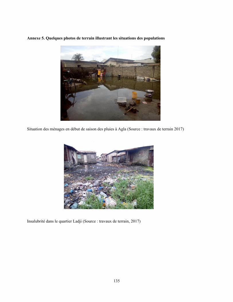
135

Annexe 5. Quelques photos de terrain illustrant les situations des populations

Situation des ménages en début de saison des pluies à Agla (Source : travaux de terrain 2017)

Insalubrité dans le quartier Ladji (Source : travaux de terrain, 2017)

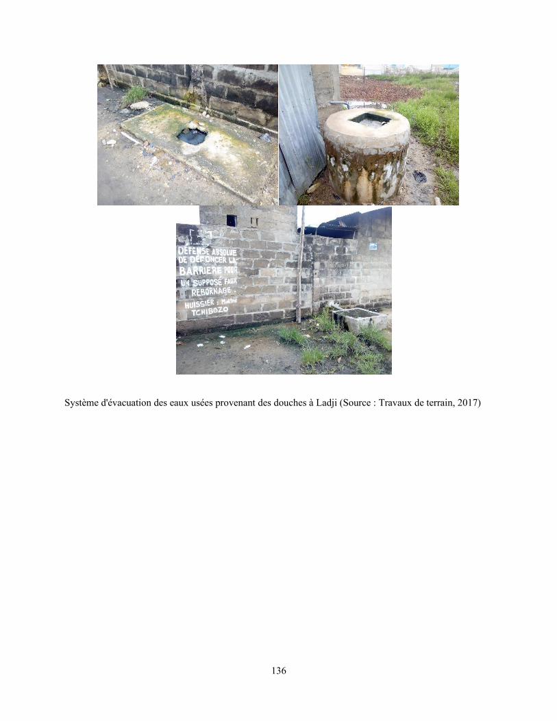
136

Système d'évacuation des eaux usées provenant des douches à Ladji (Source : Travaux de terrain, 2017)

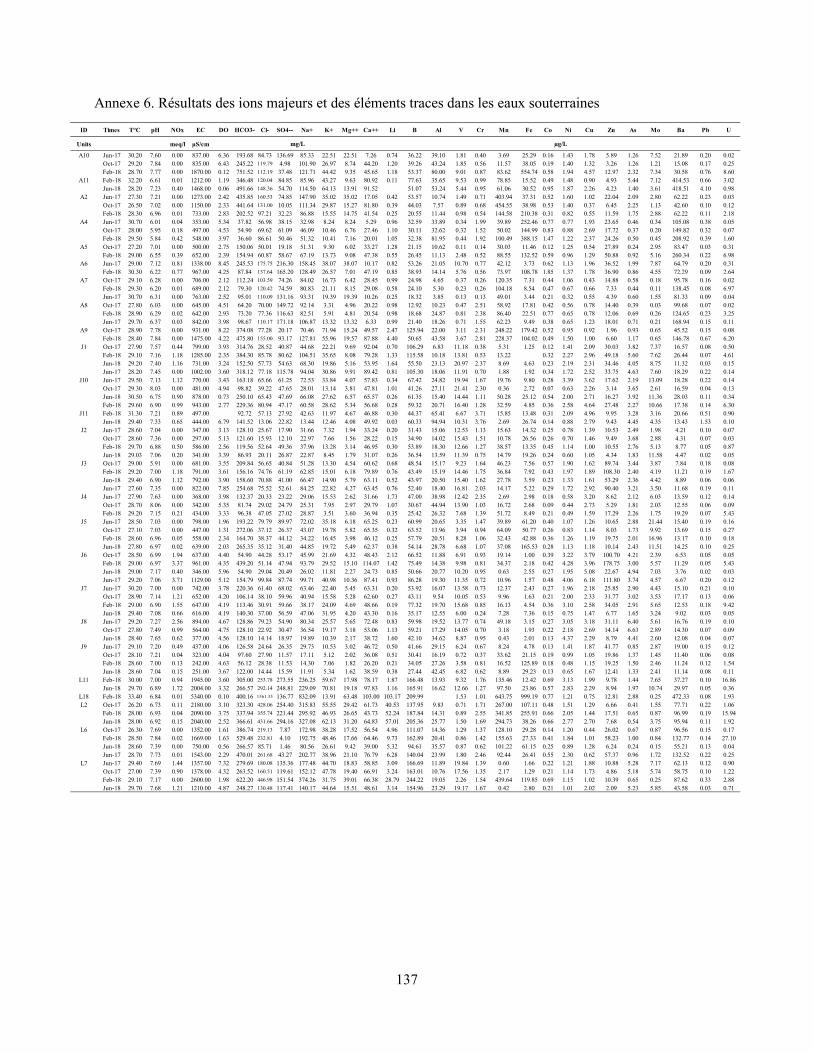
137

Annexe 6. Résultats des ions majeurs et des éléments traces dans les eaux souterraines

ID Times T°C pH NOx EC DO HCO3- Cl- SO4-- Na+ K+ Mg++ Ca++ Li B Al V Cr Mn Fe Co Ni Cu Zn As Mo Ba Pb U

Units meq/l µS/cm

A10 Jun-17 30.20 7.60 0.00 837.00 6.36 193.68 84.73 136.69 85.33 22.51 22.51 7.26 0.74 36.22 39.10 1.81 0.40 3.69 25.29 0.16 1.43 1.78 5.89 1.26 7.52 21.89 0.20 0.02Oct-17 29.20 7.84 0.00 835.00 6.43 245.22 119.79 4.98 101.90 26.97 8.74 44.20 1.20 39.26 43.24 1.85 0.56 11.57 38.05 0.19 1.40 1.32 3.26 1.26 1.21 15.08 0.17 0.25Feb-18 28.70 7.77 0.00 1870.00 0.12 751.52 112.19 37.48 121.71 44.42 9.35 45.65 1.18 53.37 80.00 9.01 0.87 83.62 554.74 0.58 1.94 4.57 12.97 2.32 7.34 30.58 0.76 8.60

A11 Feb-18 32.20 6.61 0.01 1212.00 1.19 346.48 120.04 84.85 85.96 43.27 9.63 80.92 0.11 77.63 35.65 9.53 0.99 78.85 15.52 0.49 1.48 0.90 4.93 5.44 7.12 414.53 0.66 3.02Jun-18 28.20 7.23 0.40 1468.00 0.06 491.66 148.36 54.70 114.50 64.13 13.91 91.52 51.07 53.24 5.44 0.95 61.06 30.52 0.95 1.87 2.26 4.23 1.40 3.61 418.51 4.10 0.98

A2 Jun-17 27.30 7.21 0.00 1273.00 2.42 435.85 160.53 74.85 147.90 35.02 35.02 17.05 0.42 53.57 10.74 1.49 0.71 403.94 37.31 0.52 1.60 1.02 22.04 2.09 2.80 62.22 0.23 0.03Oct-17 26.50 7.02 0.00 1150.00 2.33 441.64 131.00 10.05 111.34 29.87 15.27 81.80 0.39 44.03 7.57 0.89 0.68 454.55 38.98 0.53 1.40 0.37 6.45 2.25 1.13 42.60 0.10 0.12Feb-18 28.30 6.96 0.01 733.00 2.83 202.52 97.21 32.23 86.88 15.55 14.75 41.54 0.25 20.55 11.44 0.98 0.54 144.58 210.38 0.31 0.82 0.55 11.59 1.75 2.88 62.22 0.11 2.18

A4 Jun-17 30.70 6.01 0.04 353.00 5.34 37.82 56.98 38.15 32.98 8.24 8.24 5.29 0.96 32.59 33.89 0.34 1.99 39.89 252.46 0.77 0.77 1.93 23.65 0.46 0.34 105.08 0.38 0.05Oct-17 28.00 5.95 0.18 497.00 4.53 54.90 69.62 61.09 46.09 10.46 6.76 27.46 1.10 30.11 32.62 0.32 1.52 50.02 144.99 0.83 0.88 2.69 17.72 0.37 0.20 149.82 0.32 0.07Feb-18 29.50 5.84 0.42 548.00 3.97 36.60 86.61 50.46 51.32 10.41 7.16 20.01 1.05 32.38 81.95 0.44 1.92 100.49 388.15 1.47 1.22 2.37 24.26 0.50 0.45 208.92 0.39 1.60

A5 Oct-17 27.20 7.01 0.00 500.00 2.75 150.06 50.01 19.18 51.31 9.30 6.02 33.27 1.28 21.15 10.62 0.11 0.14 30.03 11.46 0.12 1.25 0.54 27.89 0.24 2.95 83.47 0.03 0.31Feb-18 29.00 6.55 0.39 652.00 2.39 154.94 60.87 58.67 67.19 13.73 9.08 47.38 0.55 26.45 11.13 2.48 0.52 88.55 132.52 0.59 0.96 1.29 50.88 0.92 5.16 260.34 0.22 6.98

A6 Jun-17 29.00 7.12 0.81 1338.00 8.45 245.53 175.75 216.30 158.45 38.07 38.07 10.17 0.82 53.26 21.05 10.70 0.77 42.12 3.73 0.62 1.13 1.96 36.52 1.99 7.87 64.79 0.20 0.31Feb-18 30.30 6.22 0.77 967.00 4.25 87.84 137.64 165.20 128.49 26.57 7.01 47.19 0.85 38.93 14.14 5.76 0.56 73.97 108.78 1.85 1.37 1.78 36.90 0.86 4.55 72.29 0.09 2.64

A7 Oct-17 29.10 6.28 0.00 706.00 2.12 112.24 103.59 74.26 84.02 16.73 6.42 28.45 0.99 24.98 4.65 0.37 0.26 120.35 7.31 0.44 1.06 0.43 14.88 0.58 0.18 95.78 0.16 0.02Feb-18 29.30 6.20 0.01 689.00 2.12 79.30 120.42 74.59 80.83 21.11 8.15 29.08 0.58 24.10 5.30 0.23 0.26 104.18 8.54 0.47 0.67 0.66 7.33 0.44 0.11 138.45 0.08 6.97Jun-17 30.70 6.31 0.00 763.00 2.52 95.01 110.09 131.16 93.31 19.39 19.39 10.26 0.25 18.32 3.85 0.13 0.13 49.01 3.44 0.21 0.32 0.55 4.39 0.60 1.55 81.33 0.09 0.04

A8 Oct-17 27.80 6.03 0.00 645.00 4.51 64.20 70.00 149.72 92.14 3.31 4.96 20.22 0.98 12.92 10.23 0.47 2.51 58.92 17.81 0.42 0.56 0.78 14.40 0.39 0.03 99.68 0.07 0.02Feb-18 28.90 6.29 0.02 642.00 2.93 73.20 77.36 116.63 82.51 5.91 4.81 20.54 0.98 18.68 24.87 0.81 2.38 86.40 22.51 0.77 0.65 0.78 12.06 0.69 0.26 124.65 0.23 3.25Jun-17 29.70 6.37 0.03 842.00 3.98 98.67 110.17 171.18 106.87 13.32 13.32 6.33 0.99 21.40 18.26 0.71 1.55 62.23 9.49 0.38 0.65 1.23 18.01 0.71 0.21 168.94 0.15 0.11

A9 Oct-17 28.90 7.78 0.00 931.00 8.22 374.08 77.28 20.17 70.46 71.94 15.24 49.57 2.47 125.94 22.00 3.11 2.31 248.22 179.42 0.52 0.95 0.92 1.96 0.93 0.65 45.52 0.15 0.08Feb-18 28.40 7.84 0.00 1475.00 4.22 475.80 155.00 93.17 127.81 55.96 19.57 87.88 4.40 50.65 43.58 3.67 2.81 228.37 104.02 0.49 1.50 1.00 6.60 1.17 0.65 146.78 0.67 6.20

J1 Oct-17 27.90 7.57 0.44 799.00 3.93 314.76 28.52 40.87 44.68 22.21 9.69 92.04 0.70 106.29 6.83 11.18 0.38 5.31 1.25 0.12 1.41 2.09 30.03 3.82 7.37 16.57 0.08 0.50Feb-18 29.10 7.16 1.18 1285.00 2.35 384.30 85.78 80.62 104.51 35.65 8.08 79.28 1.33 115.58 10.18 13.81 0.53 13.22 0.32 2.27 2.96 49.18 5.60 7.62 26.44 0.07 4.61Jun-18 29.20 7.40 1.16 731.00 3.24 152.50 57.73 54.63 68.30 19.86 5.16 53.95 1.64 55.50 23.13 20.97 2.37 8.69 4.63 0.23 2.19 2.31 34.46 4.05 8.75 11.32 0.03 0.15Jun-17 28.20 7.45 0.00 1002.00 3.60 318.12 77.18 115.78 94.04 30.86 9.91 89.42 0.81 105.30 18.06 11.91 0.70 1.88 1.92 0.34 1.72 2.52 33.75 4.63 7.60 18.29 0.22 0.14

J10 Jun-17 29.50 7.13 1.12 770.00 3.43 163.18 65.66 61.25 72.53 33.84 4.07 57.83 0.34 67.42 24.82 19.94 1.67 19.76 9.80 0.28 3.39 3.62 17.62 2.19 13.09 18.28 0.22 0.14Oct-17 29.30 8.03 0.00 481.00 4.94 98.82 39.22 47.65 28.01 13.14 3.81 47.81 1.01 41.26 27.11 21.41 2.30 0.36 2.72 0.07 0.63 2.26 3.14 3.65 2.61 16.59 0.04 0.13Jun-18 30.50 6.75 0.90 878.00 0.73 250.10 65.43 47.69 66.08 27.62 6.57 65.57 0.26 61.35 15.40 14.44 1.11 50.28 25.12 0.54 2.00 2.71 16.27 3.92 11.36 28.03 0.11 0.34Feb-18 29.60 6.90 0.99 943.00 2.77 229.36 80.94 47.17 60.58 28.62 5.34 56.68 0.28 59.32 20.71 16.40 1.28 32.59 4.85 0.36 2.58 4.64 27.48 2.27 10.66 17.38 0.14 6.30

J11 Feb-18 31.30 7.21 0.89 497.00 92.72 57.13 27.92 42.63 11.97 4.67 46.88 0.30 44.37 65.41 6.67 3.71 15.85 13.48 0.31 2.09 4.96 9.95 3.28 3.16 20.66 0.51 0.90Jun-18 29.40 7.33 0.65 444.00 6.79 141.52 13.06 22.82 13.44 12.46 4.08 49.92 0.03 60.33 94.94 10.31 3.76 2.69 26.74 0.14 0.88 2.79 9.43 4.45 4.35 13.43 1.53 0.10

J2 Jun-17 28.60 7.04 0.00 347.00 3.13 128.10 25.67 17.90 31.66 7.32 1.94 33.24 0.20 31.43 15.06 12.53 1.13 15.63 14.32 0.25 0.78 1.39 10.53 2.49 1.98 4.21 0.10 0.07Oct-17 28.60 7.36 0.00 297.00 5.13 121.60 15.93 12.10 22.97 7.66 1.56 28.22 0.15 34.90 14.02 15.43 1.51 10.78 26.56 0.26 0.70 1.46 9.49 3.68 2.88 4.31 0.07 0.03Feb-18 29.70 6.88 0.50 586.00 2.56 119.56 52.64 49.36 37.96 13.28 3.14 46.95 0.30 53.89 18.30 12.66 1.27 38.57 13.35 0.45 1.14 1.00 10.55 2.76 5.13 8.77 0.05 0.87Jun-18 29.03 7.06 0.20 341.00 3.39 86.93 20.11 26.87 22.87 8.45 1.79 31.07 0.26 36.54 13.59 11.39 0.75 14.79 19.26 0.24 0.60 1.05 4.34 1.83 11.58 4.47 0.02 0.05

J3 Oct-17 29.00 5.91 0.00 681.00 3.55 209.84 56.65 40.84 51.28 13.30 4.54 60.62 0.68 48.54 15.17 9.23 1.64 46.23 7.56 0.57 1.90 1.62 89.74 3.44 3.87 7.84 0.18 0.08Feb-18 29.20 7.00 1.18 791.00 3.61 156.16 74.76 61.19 62.85 15.01 6.18 79.89 0.76 43.49 15.19 14.46 1.75 36.84 7.92 0.43 1.97 1.89 108.30 2.40 4.19 11.21 0.19 1.67Jun-18 29.40 6.90 1.12 792.00 3.90 158.60 70.88 41.00 66.47 14.90 5.79 63.11 0.52 43.97 20.50 15.40 1.62 27.78 3.59 0.23 1.33 1.61 53.29 2.36 4.42 8.89 0.06 0.06Jun-17 27.60 7.35 0.00 822.00 7.85 254.68 75.52 52.61 84.25 22.82 4.27 63.45 0.76 52.40 18.40 16.81 2.03 14.17 5.22 0.29 1.72 2.92 90.40 3.21 3.50 11.68 0.19 0.11

J4 Jun-17 27.90 7.63 0.00 368.00 3.98 132.37 20.33 23.22 29.06 15.53 2.62 31.66 1.73 47.00 38.98 12.42 2.35 2.69 2.98 0.18 0.58 3.20 8.62 2.12 6.03 13.59 0.12 0.14Oct-17 28.70 8.06 0.00 342.00 5.35 81.74 29.02 24.79 25.31 7.95 2.97 29.79 1.07 30.67 44.94 13.90 1.03 16.72 2.68 0.09 0.44 2.73 5.29 1.81 2.03 12.55 0.06 0.09Feb-18 29.20 7.15 0.21 434.00 3.33 96.38 47.05 27.02 28.87 3.51 3.60 36.94 0.35 25.42 26.32 7.68 1.39 51.72 8.49 0.21 0.49 1.59 17.29 2.26 1.75 19.29 0.07 5.43

J5 Jun-17 28.50 7.03 0.00 798.00 1.96 193.22 79.79 89.97 72.02 35.18 6.18 65.25 0.23 60.99 20.65 3.35 1.47 39.89 61.20 0.40 1.07 1.26 10.65 2.88 21.44 15.40 0.19 0.16Oct-17 27.10 7.03 0.00 447.00 1.31 272.06 37.12 26.37 43.07 19.78 5.82 65.35 0.32 63.52 13.96 3.94 0.94 64.09 50.77 0.26 0.83 1.14 8.03 1.73 9.92 13.69 0.15 0.27Feb-18 28.60 6.96 0.05 558.00 2.34 164.70 38.37 44.12 34.22 16.45 3.98 46.12 0.25 57.79 20.51 8.28 1.06 32.43 42.88 0.36 1.26 1.19 19.75 2.01 16.96 13.17 0.10 0.18Jun-18 27.80 6.97 0.02 639.00 2.03 265.35 35.12 31.40 44.85 19.72 5.49 62.37 0.38 54.14 28.78 6.68 1.07 37.08 165.53 0.28 1.13 1.18 10.14 2.43 11.51 14.25 0.10 0.25

J6 Oct-17 28.50 6.99 1.94 637.00 4.40 54.90 44.28 53.17 45.99 21.69 4.32 48.43 2.12 66.52 11.88 6.91 0.93 19.14 1.00 0.39 3.22 3.79 100.70 4.21 2.39 6.53 0.05 0.05Feb-18 29.00 6.97 3.37 961.00 4.35 439.20 51.14 47.94 93.79 29.52 15.10 114.07 1.42 75.49 14.38 9.98 0.81 34.37 2.18 0.42 4.28 3.96 178.75 3.00 5.57 11.29 0.05 5.43Jun-18 29.00 7.17 0.40 346.00 5.96 54.90 29.04 20.49 26.02 11.81 2.27 24.73 0.85 50.66 20.77 10.20 0.95 0.63 2.55 0.27 1.95 5.08 22.67 4.94 7.03 3.76 0.02 0.03Jun-17 29.20 7.06 3.71 1129.00 5.12 154.79 99.84 87.74 99.71 40.98 10.36 87.41 0.93 86.28 19.30 11.35 0.72 10.96 1.57 0.48 4.06 6.18 111.80 3.74 4.57 6.67 0.20 0.12

J7 Jun-17 30.20 7.00 0.00 742.00 3.78 220.36 61.40 68.02 63.46 22.40 5.45 63.31 0.20 53.92 16.07 13.58 0.73 12.37 2.43 0.27 1.96 2.18 25.85 2.90 4.43 15.10 0.21 0.10Oct-17 28.90 7.14 1.21 652.00 4.20 106.14 38.10 59.96 40.94 15.58 5.28 62.60 0.27 43.11 9.54 10.05 0.53 9.96 1.63 0.21 2.00 2.33 31.77 3.02 3.53 17.17 0.13 0.06Feb-18 29.00 6.90 1.55 647.00 4.19 113.46 30.91 59.66 38.17 24.09 4.69 48.66 0.19 77.32 19.70 15.68 0.85 16.13 4.54 0.36 3.10 2.58 34.05 2.91 5.65 12.53 0.18 9.42Jun-18 29.40 7.08 0.66 616.00 4.19 140.30 37.00 56.59 47.06 31.95 4.20 43.30 0.16 35.17 12.55 6.00 0.24 7.28 7.36 0.15 0.75 1.47 6.77 1.65 3.24 9.02 0.03 0.05

J8 Jun-17 29.20 7.27 2.56 894.00 4.67 128.86 79.23 54.90 80.34 25.57 5.65 72.48 0.83 59.98 19.52 13.77 0.74 49.18 3.15 0.27 3.05 3.18 31.11 6.40 5.61 16.76 0.19 0.10Oct-17 27.80 7.49 0.99 564.00 4.75 128.10 22.92 30.47 36.54 19.17 3.18 53.06 1.13 59.21 17.29 14.05 0.70 3.18 1.93 0.22 2.18 2.69 14.14 6.63 2.89 14.30 0.07 0.09Jun-18 28.40 7.65 0.62 377.00 4.56 128.10 14.14 18.97 19.89 10.39 2.17 38.72 1.60 42.10 34.62 8.87 0.95 0.43 2.01 0.13 4.37 2.29 8.79 4.41 2.60 12.08 0.04 0.07

J9 Jun-17 29.10 7.20 0.49 437.00 4.06 126.58 24.64 26.35 29.73 10.53 3.02 46.72 0.50 41.66 29.15 6.24 0.67 8.24 4.78 0.13 1.41 1.87 41.77 0.85 2.87 19.00 0.15 0.12Oct-17 28.10 7.21 0.04 323.00 4.04 97.60 27.90 11.57 17.11 5.12 2.02 36.08 0.51 30.41 16.19 0.72 0.37 33.62 21.15 0.19 0.99 1.05 19.86 1.37 1.45 11.40 0.06 0.08Feb-18 28.60 7.00 0.13 242.00 4.63 56.12 28.38 11.53 14.30 7.06 1.82 26.20 0.21 34.05 27.26 3.58 0.81 16.52 125.89 0.18 0.48 1.15 19.25 1.50 2.46 11.24 0.12 1.54Jun-18 28.60 7.04 0.15 251.00 3.67 122.00 14.44 15.59 11.91 5.34 1.62 38.59 0.38 27.44 42.45 6.82 0.62 8.89 29.23 0.13 0.65 1.67 12.41 1.33 2.41 11.14 0.08 0.11

L11 Feb-18 30.00 7.00 0.94 1945.00 3.60 305.00 253.78 273.55 236.25 59.67 17.98 78.17 1.87 166.48 13.93 9.32 1.76 135.46 12.42 0.69 3.13 1.99 9.78 1.44 7.65 37.27 0.10 16.86Jun-18 29.70 6.89 1.72 2004.00 3.32 266.57 292.14 248.81 229.09 70.81 19.18 97.83 1.16 165.91 16.62 12.66 1.27 97.50 23.86 0.57 2.83 2.29 8.94 1.97 10.74 29.97 0.05 0.36

L18 Feb-18 33.40 6.84 0.01 5340.00 0.10 400.16 1561.35 136.77 832.09 13.91 63.48 103.00 103.17 209.99 1.53 1.01 643.75 999.19 0.77 1.21 0.75 12.81 2.88 0.25 472.33 0.08 1.93L2 Oct-17 26.20 6.73 0.11 2180.00 3.10 323.30 428.06 254.40 315.83 55.55 29.42 61.73 40.53 137.95 9.83 0.71 1.71 267.00 107.11 0.48 1.51 1.29 6.66 0.41 1.55 77.71 0.22 1.06

Feb-18 28.00 6.93 0.04 2090.00 3.75 337.94 355.74 221.44 295.92 46.93 26.65 43.73 52.24 187.84 14.31 0.89 2.55 341.85 255.91 0.66 2.05 1.44 17.51 0.65 0.87 96.99 0.19 15.94Jun-18 28.00 6.92 0.15 2040.00 2.52 366.61 431.66 294.16 327.08 62.13 31.20 64.83 57.01 205.36 25.77 1.50 1.69 294.73 38.26 0.66 2.77 2.70 7.68 0.54 3.75 95.94 0.11 1.92

L6 Oct-17 26.30 7.69 0.00 1352.00 1.61 386.74 219.13 7.87 172.98 38.28 17.52 56.54 4.96 111.07 14.36 1.29 1.37 128.10 29.28 0.14 1.20 0.44 26.02 0.67 0.87 96.56 0.15 0.17Feb-18 28.50 7.84 0.02 1669.00 1.63 529.48 232.81 4.10 192.75 48.46 17.66 64.46 9.73 162.89 20.41 0.86 1.42 155.63 27.33 0.41 1.84 1.01 58.23 1.00 0.84 132.77 0.14 27.10Jun-18 28.60 7.39 0.00 750.00 0.56 266.57 85.71 1.46 80.56 26.61 9.42 39.00 5.32 94.61 35.57 0.87 0.62 101.22 61.15 0.25 0.89 1.28 6.24 0.24 0.15 55.21 0.13 0.04Jun-17 28.70 7.73 0.01 1543.00 2.29 470.01 261.68 43.27 202.77 38.96 21.10 76.79 6.28 140.04 23.99 1.80 2.46 92.44 26.41 0.55 2.30 0.62 57.37 0.96 1.72 132.52 0.22 0.25

L7 Jun-17 29.40 7.69 1.44 1357.00 7.32 279.69 180.08 135.36 177.48 44.70 18.83 58.85 3.09 166.69 11.89 19.84 1.39 0.60 1.66 0.22 1.21 1.88 10.88 5.28 7.17 62.13 0.12 0.90Oct-17 27.00 7.39 0.90 1378.00 4.32 263.52 160.51 119.61 152.12 47.78 19.40 66.91 3.24 163.01 10.76 17.56 1.35 2.17 1.29 0.21 1.14 1.73 4.86 5.18 5.74 58.75 0.10 1.22Feb-18 29.10 7.17 0.00 2600.00 1.98 622.20 446.98 151.54 374.26 31.75 39.01 66.38 28.79 244.22 19.05 2.26 1.54 439.64 119.85 0.69 1.15 1.02 10.39 0.65 0.25 87.62 0.33 2.88Jun-18 29.70 7.68 1.21 1210.00 4.87 248.27 130.48 117.41 140.17 44.64 15.51 48.61 3.14 154.96 23.29 19.17 1.67 0.42 2.80 0.21 1.01 2.02 2.09 5.23 5.85 43.58 0.03 0.71

mg/L µg/L

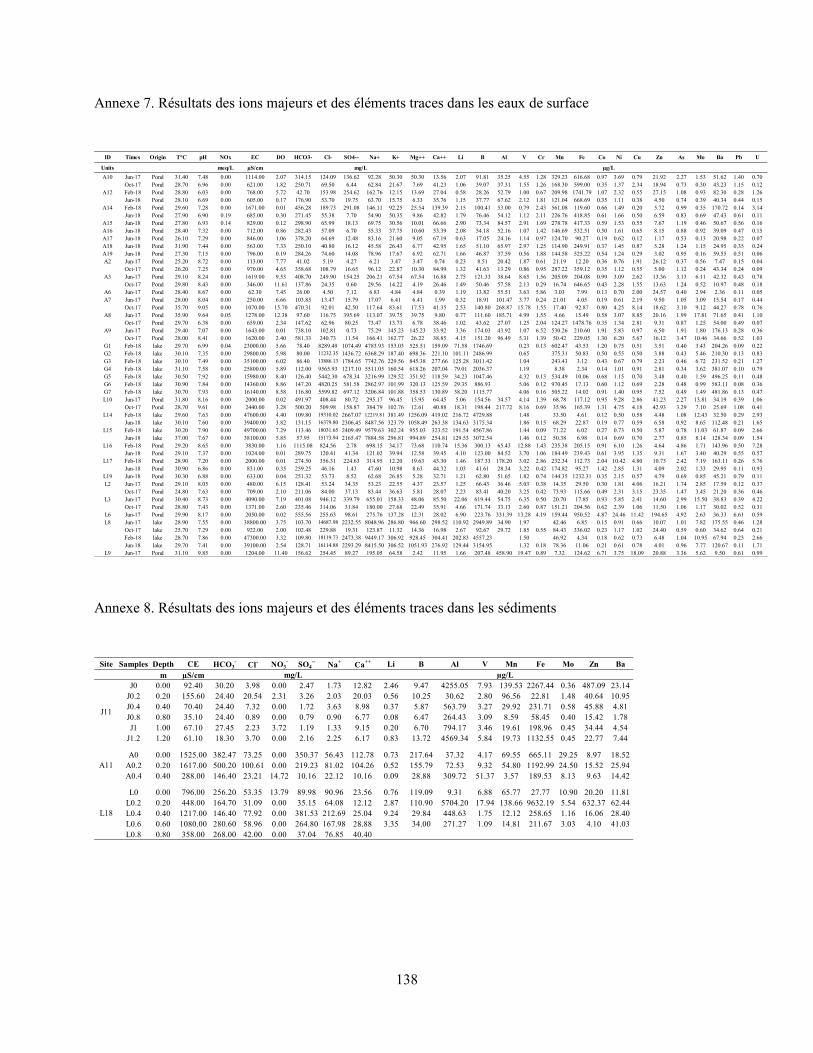
138

Annexe 7. Résultats des ions majeurs et des éléments traces dans les eaux de surface

Annexe 8. Résultats des ions majeurs et des éléments traces dans les sédiments

ID Times Origin T°C pH NOx EC DO HCO3- Cl- SO4-- Na+ K+ Mg++ Ca++ Li B Al V Cr Mn Fe Co Ni Cu Zn As Mo Ba Pb U

Units meq/L µS/cm

A10 Jun-17 Pond 31.40 7.48 0.00 1114.00 2.07 314.15 124.09 136.62 92.28 50.30 50.30 13.56 2.07 91.81 35.25 4.55 1.28 329.23 616.68 0.97 3.69 0.79 21.92 2.27 1.53 51.62 1.40 0.70Oct-17 Pond 28.70 6.96 0.00 621.00 1.82 250.71 69.50 6.44 62.84 21.67 7.69 41.23 1.06 39.07 37.31 1.55 1.26 168.30 599.00 0.35 1.37 2.34 18.94 0.73 0.30 43.23 1.15 0.12

A12 Feb-18 Pond 28.80 6.03 0.00 768.00 5.72 42.70 153.98 254.62 162.76 12.15 13.69 27.04 0.58 28.26 52.79 1.00 0.67 209.98 1741.79 1.07 2.32 0.55 27.15 1.08 0.93 82.30 0.28 1.26Jun-18 Pond 28.10 6.69 0.00 605.00 0.17 176.90 53.70 19.75 63.70 15.75 6.33 35.76 1.15 37.77 67.62 2.12 1.81 121.04 668.69 0.35 1.11 0.38 4.50 0.74 0.39 40.34 0.44 0.15

A14 Feb-18 Pond 29.60 7.28 0.00 1671.00 0.01 456.28 189.73 291.08 146.11 92.25 25.54 139.39 2.15 100.41 53.00 0.79 2.43 561.08 119.60 0.66 1.49 0.20 5.72 0.99 0.35 170.72 0.14 3.14Jun-18 Pond 27.90 6.90 0.19 685.00 0.30 271.45 55.38 7.70 54.90 50.35 9.86 42.82 1.79 76.46 54.12 1.12 2.11 226.76 418.85 0.61 1.66 0.50 6.59 0.83 0.69 47.43 0.61 0.11

A15 Jun-18 Pond 27.80 6.93 0.14 829.00 0.12 298.90 65.99 18.13 69.75 30.56 10.01 66.66 2.90 73.34 84.57 2.91 1.69 278.78 417.33 0.59 1.53 0.55 7.67 1.19 0.46 50.67 0.56 0.16A16 Jun-18 Pond 28.40 7.32 0.00 712.00 0.86 282.43 57.09 6.70 55.33 37.75 10.60 53.39 2.08 54.18 52.16 1.07 1.42 146.69 532.51 0.50 1.61 0.65 8.15 0.88 0.92 39.09 0.47 0.15A17 Jun-18 Pond 26.10 7.29 0.00 846.00 1.06 378.20 64.69 12.48 83.16 21.60 9.05 67.19 0.63 17.05 24.16 1.14 0.97 124.70 90.27 0.19 0.62 0.12 1.17 0.53 0.13 20.98 0.22 0.07A18 Jun-18 Pond 31.90 7.44 0.00 563.00 7.33 250.10 40.80 16.12 45.58 26.43 6.77 42.95 1.65 51.10 65.97 2.97 1.25 114.90 249.91 0.37 1.45 0.87 5.28 1.24 1.15 24.95 0.35 0.24A19 Jun-18 Pond 27.30 7.15 0.00 796.00 0.19 284.26 74.60 14.08 78.96 17.67 6.92 62.71 1.66 46.87 37.59 0.56 1.88 144.58 525.22 0.54 1.24 0.29 3.02 0.95 0.16 59.55 0.51 0.06A2 Jun-17 Pond 25.20 8.72 0.00 113.00 7.77 41.02 5.19 4.27 6.21 3.47 3.47 0.74 0.23 8.51 20.42 1.87 0.61 21.19 12.20 0.36 0.76 1.91 26.12 0.37 0.56 7.47 0.15 0.04

Oct-17 Pond 26.20 7.25 0.00 970.00 4.65 358.68 108.79 16.65 96.12 22.87 10.30 84.99 1.32 41.63 13.29 0.86 0.95 287.22 359.12 0.35 1.12 0.55 5.00 1.12 0.24 43.34 0.24 0.09A3 Jun-17 Pond 29.10 8.24 0.00 1619.00 9.53 408.70 249.90 154.25 206.21 67.54 67.54 16.88 2.75 121.33 38.64 8.65 1.56 205.09 204.08 0.99 3.09 2.62 13.36 3.13 6.11 42.32 0.43 0.78

Oct-17 Pond 29.80 8.43 0.00 346.00 11.61 137.86 24.35 0.60 29.56 14.22 4.19 26.46 1.49 50.46 57.58 2.13 0.29 16.74 646.65 0.43 2.28 1.55 13.63 1.24 0.52 10.97 0.48 0.18A6 Jun-17 Pond 28.40 8.67 0.00 62.30 7.45 26.00 4.50 7.12 6.83 4.84 4.84 0.39 1.19 13.82 55.51 3.63 5.86 3.03 7.99 0.13 0.70 2.00 24.57 0.40 2.94 2.36 0.11 0.05A7 Jun-17 Pond 28.00 8.04 0.00 250.00 6.66 103.85 13.47 15.79 17.07 6.41 6.41 1.99 0.32 18.91 101.47 3.77 0.24 21.01 4.05 0.19 0.61 2.19 9.50 1.05 3.09 15.54 0.17 0.44

Oct-17 Pond 35.70 9.05 0.00 1070.00 15.70 470.31 92.01 42.50 117.64 83.61 17.53 41.35 2.53 140.80 268.87 15.78 1.55 17.40 92.87 0.80 4.25 8.14 18.62 3.10 9.12 44.27 0.78 0.76A8 Jun-17 Pond 35.90 9.64 0.05 1278.00 12.38 97.60 116.75 395.69 113.07 39.75 39.75 9.80 0.77 111.60 185.71 4.99 1.55 4.66 15.49 0.58 3.07 8.85 20.16 1.99 17.81 71.65 0.41 1.10

Oct-17 Pond 29.70 6.38 0.00 659.00 2.34 147.62 62.96 80.25 73.47 13.73 6.78 38.46 1.02 43.62 27.07 1.25 2.04 124.27 1478.76 0.35 1.34 2.81 9.31 0.87 1.25 54.00 0.49 0.07A9 Jun-17 Pond 29.40 7.07 0.00 1643.00 0.01 738.10 102.81 0.73 75.29 145.23 145.23 33.92 3.36 174.03 43.92 1.07 6.52 530.26 210.60 1.91 5.83 0.97 6.50 1.91 1.80 176.13 0.28 0.36

Oct-17 Pond 28.00 8.41 0.00 1620.00 2.40 581.33 240.73 11.54 166.41 162.77 26.22 38.85 4.15 151.20 96.49 5.31 1.39 50.42 229.05 1.30 6.20 5.67 16.12 3.47 10.46 34.66 0.52 1.03G1 Feb-18 lake 29.70 6.99 0.04 23000.00 5.66 78.40 8289.49 1074.49 4783.93 153.03 525.51 159.09 71.58 1746.69 0.23 0.13 602.47 43.53 1.20 0.75 0.51 3.51 0.40 3.43 204.26 0.09 0.22G2 Feb-18 lake 30.10 7.35 0.00 29800.00 5.98 80.00 11232.35 1436.72 6368.29 187.40 698.36 221.10 101.11 2486.99 0.65 375.31 50.83 0.50 0.55 0.50 3.88 0.43 5.46 210.30 0.13 0.83G3 Feb-18 lake 30.10 7.49 0.00 35100.00 6.02 86.40 13886.13 1784.65 7742.76 229.56 845.38 277.66 125.28 3011.42 1.04 243.43 3.12 0.43 0.67 0.79 2.23 0.46 6.72 231.52 0.21 1.27G4 Feb-18 lake 31.10 7.58 0.00 25800.00 5.89 112.00 9565.93 1217.10 5511.05 160.54 618.26 207.04 79.01 2036.37 1.19 8.38 2.34 0.14 1.01 0.91 2.81 0.34 3.62 381.07 0.10 0.79G5 Feb-18 lake 30.50 7.92 0.00 15980.00 8.40 126.40 5442.30 678.34 3216.99 129.52 351.92 118.59 34.23 1047.46 4.32 0.13 534.49 10.06 0.68 1.15 0.70 3.48 0.40 1.59 496.25 0.11 0.48G6 Feb-18 lake 30.90 7.84 0.00 14360.00 8.86 147.20 4820.25 581.58 2862.97 101.99 320.13 125.59 29.35 886.93 5.06 0.12 970.45 17.13 0.60 1.12 0.69 2.28 0.48 0.99 583.11 0.08 0.36G7 Feb-18 lake 30.70 7.93 0.00 16140.00 8.58 116.80 5599.82 697.12 3206.84 101.88 358.53 130.89 38.20 1115.77 4.06 0.16 505.22 14.02 0.91 1.40 0.95 7.52 0.49 1.49 481.86 0.13 0.47L10 Jun-17 Pond 31.80 8.16 0.00 2000.00 0.02 491.97 408.44 80.72 295.17 96.45 15.95 64.45 5.06 154.56 34.57 4.14 1.39 68.78 117.12 0.95 9.28 2.86 41.23 2.27 13.81 34.19 0.39 1.06

Oct-17 Pond 28.70 9.61 0.00 2440.00 3.28 500.20 509.98 158.87 384.79 102.76 12.61 40.88 18.31 198.44 217.72 8.16 0.69 35.96 165.39 1.31 4.75 4.18 42.93 3.29 7.10 25.69 1.08 0.41L14 Feb-18 lake 29.60 7.63 0.00 47600.00 4.40 109.80 19310.02 2667.07 12219.81 381.49 1256.09 419.02 216.72 4729.88 1.48 33.50 4.61 0.12 0.50 0.58 4.48 1.08 12.43 32.50 0.29 2.93

Jun-18 lake 30.10 7.60 0.00 39400.00 3.82 131.15 16379.80 2306.45 8487.56 323.79 1058.49 263.38 134.63 3175.34 1.86 0.15 68.29 22.87 0.19 0.77 0.59 6.58 0.92 8.65 112.48 0.21 1.65L15 Feb-18 lake 30.20 7.90 0.00 49700.00 7.29 113.46 18031.65 2409.49 9579.63 302.24 955.03 323.52 191.54 4567.86 1.44 0.09 71.22 6.02 0.27 0.73 0.50 5.87 0.78 11.03 61.87 0.09 2.66

Jun-18 lake 37.00 7.67 0.00 38100.00 5.85 57.95 15173.94 2165.47 7884.58 296.81 994.89 254.81 129.53 3072.54 1.46 0.12 50.38 6.98 0.14 0.69 0.70 2.77 0.85 8.14 128.34 0.09 1.54L16 Feb-18 Pond 29.20 8.65 0.00 3830.00 1.16 1115.08 824.56 2.78 698.15 34.17 73.68 110.74 15.36 300.13 65.43 12.88 1.43 235.38 205.15 0.91 6.10 1.26 4.64 4.86 1.71 143.96 0.50 7.28

Jun-18 Pond 29.10 7.37 0.00 1024.00 0.01 289.75 120.41 41.34 121.02 39.94 12.58 39.45 4.10 123.00 84.52 3.70 1.06 184.49 239.43 0.61 3.95 1.35 9.31 1.67 3.40 40.29 0.55 0.57L17 Feb-18 Pond 28.90 7.20 0.00 2000.00 0.01 274.50 356.31 224.63 314.95 12.20 19.63 43.30 1.46 187.33 178.20 3.02 2.86 232.34 112.73 2.04 10.42 4.80 10.73 2.42 7.19 163.11 0.26 5.76

Jun-18 Pond 30.90 6.86 0.00 831.00 0.35 259.25 46.16 1.43 47.60 10.98 8.63 44.32 1.03 41.61 28.34 3.22 0.42 174.82 95.27 1.42 2.85 1.31 4.09 2.02 1.33 29.95 0.11 0.93L19 Jun-18 Pond 30.30 6.88 0.00 633.00 0.04 251.32 53.73 8.52 62.68 26.85 5.28 32.71 1.21 62.80 51.65 1.82 0.74 144.35 1232.31 0.35 2.15 0.57 4.79 0.69 0.85 45.21 0.79 0.11L2 Jun-17 Pond 29.10 8.05 0.00 480.00 6.15 128.41 53.24 34.35 53.23 22.55 4.37 23.57 1.25 66.43 36.46 5.03 0.38 14.35 29.50 0.30 1.81 4.06 16.21 1.74 2.85 17.59 0.12 0.37

Oct-17 Pond 24.80 7.63 0.00 709.00 2.10 211.06 84.00 37.13 83.44 36.63 5.81 28.07 2.23 83.41 40.20 3.25 0.42 73.93 115.66 0.49 2.31 3.15 23.35 1.47 3.45 21.20 0.36 0.46L3 Jun-17 Pond 30.40 8.73 0.00 4090.00 7.19 401.08 946.12 339.79 655.01 158.33 48.06 85.50 22.06 619.44 54.75 6.35 0.50 20.70 17.85 0.93 5.85 2.41 14.60 2.99 15.50 38.83 0.39 4.22

Oct-17 Pond 28.80 7.43 0.00 1371.00 2.60 235.46 314.06 31.84 180.00 27.68 22.49 35.91 4.66 171.74 33.13 2.60 0.87 151.21 204.56 0.62 2.39 1.06 11.50 1.06 1.17 30.02 0.52 0.31L6 Jun-17 Pond 29.90 8.17 0.00 2050.00 0.02 555.56 255.63 98.61 275.76 137.28 12.31 28.02 6.90 223.76 331.39 13.28 4.19 159.44 950.52 4.87 24.46 11.42 194.65 4.92 2.63 36.33 6.61 0.59L8 Jun-17 lake 28.90 7.55 0.00 38800.00 3.75 103.70 14687.98 2232.55 8048.96 286.80 966.60 298.52 110.92 2949.89 34.90 1.97 42.46 6.85 0.15 0.91 0.66 10.07 1.01 7.82 175.55 0.46 1.28

Oct-17 lake 25.70 7.29 0.00 922.00 2.00 102.48 229.88 19.31 123.87 11.32 14.36 16.98 2.67 92.67 29.72 1.85 0.55 84.43 336.02 0.23 1.17 1.02 24.40 0.59 0.60 34.62 0.64 0.21Feb-18 lake 28.70 7.86 0.00 47300.00 3.32 109.80 18119.73 2473.38 9449.17 306.92 928.45 304.41 202.83 4557.23 1.50 46.92 4.34 0.18 0.62 0.73 6.48 1.04 10.95 67.94 0.23 2.66Jun-18 lake 29.70 7.41 0.00 39100.00 2.54 128.71 16114.88 2293.29 8415.50 306.52 1051.93 276.92 129.44 3154.95 1.32 0.18 78.36 11.06 0.21 0.61 0.78 4.01 0.96 7.77 120.67 0.11 1.71

L9 Jun-17 Pond 31.10 9.85 0.00 1204.00 11.40 156.62 254.45 89.27 195.05 64.58 2.42 11.95 1.66 207.48 458.90 19.47 0.89 7.32 124.62 6.71 3.75 18.09 20.88 3.36 5.62 9.50 0.61 0.99

mg/L µg/L

Site Samples Depth CE HCO3-

Cl- NO3

-SO4

--Na

+Ca

++ Li B Al V Mn Fe Mo Zn Ba

m µS/cm

J0 0.00 92.40 30.20 3.98 0.00 2.47 1.73 12.82 2.46 9.47 4255.05 7.93 139.53 2267.44 0.36 487.09 23.14J0.2 0.20 155.60 24.40 20.54 2.31 3.26 2.03 20.03 0.56 10.25 30.62 2.80 96.56 22.81 1.48 40.64 10.95J0.4 0.40 70.40 24.40 7.32 0.00 1.72 3.63 8.98 0.37 5.87 563.79 3.27 29.92 231.71 0.58 45.88 4.81J0.8 0.80 35.10 24.40 0.89 0.00 0.79 0.90 6.77 0.08 6.47 264.43 3.09 8.59 58.45 0.40 15.42 1.78J1 1.00 67.10 27.45 2.23 3.72 1.19 1.33 9.15 0.20 6.70 794.17 3.46 19.61 198.96 0.45 34.44 4.54

J1.2 1.20 61.10 18.30 3.70 0.00 2.16 2.25 6.17 0.83 13.72 4569.34 5.84 19.73 1132.55 0.45 22.77 7.44

A0 0.00 1525.00 382.47 73.25 0.00 350.37 56.43 112.78 0.73 217.64 37.32 4.17 69.55 665.11 29.25 8.97 18.52A0.2 0.20 1617.00 500.20 100.61 0.00 219.23 81.02 104.26 0.52 155.79 72.53 9.32 54.80 1192.99 24.50 15.52 25.94A0.4 0.40 288.00 146.40 23.21 14.72 10.16 22.12 10.16 0.09 28.88 309.72 51.37 3.57 189.53 8.13 9.63 14.42

L0 0.00 796.00 256.20 53.35 13.79 89.98 90.96 23.56 0.76 119.09 9.31 6.88 65.77 27.77 10.90 20.20 11.81L0.2 0.20 448.00 164.70 31.09 0.00 35.15 64.08 12.12 2.87 110.90 5704.20 17.94 138.66 9632.19 5.54 632.37 62.44L0.4 0.40 1217.00 146.40 77.92 0.00 381.53 212.69 25.04 9.24 29.84 448.63 1.75 12.12 258.65 1.16 16.06 28.40L0.6 0.60 1080.00 280.60 58.96 0.00 264.80 167.98 28.88 3.35 34.00 271.27 1.09 14.81 211.67 3.03 4.10 41.03L0.8 0.80 358.00 268.00 42.00 0.00 37.04 76.85 40.40

mg/L µg/L

J11

A11

L18

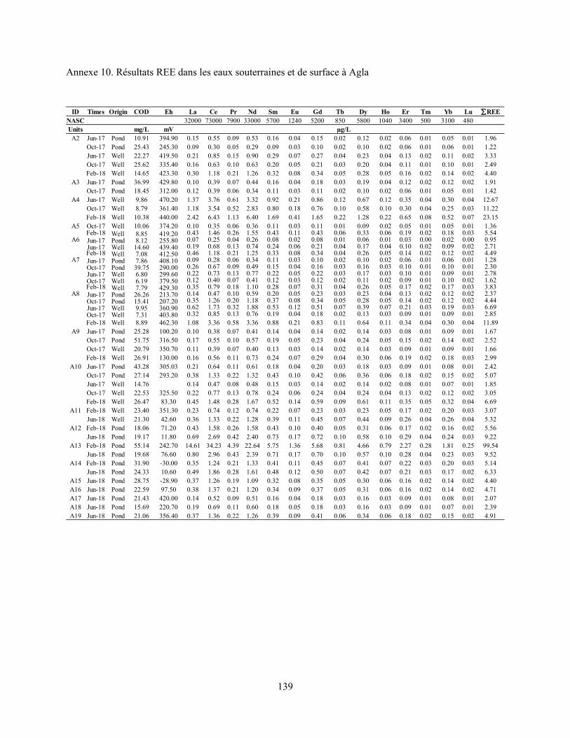
139

Annexe 10. Résultats REE dans les eaux souterraines et de surface à Agla

ID Times Origin COD Eh La Ce Pr Nd Sm Eu Gd Tb Dy Ho Er Tm Yb Lu REE

NASC 32000 73000 7900 33000 5700 1240 5200 850 5800 1040 3400 500 3100 480Units mg/L mV

A2 Jun-17 Pond 10.91 394.90 0.15 0.55 0.09 0.53 0.16 0.04 0.15 0.02 0.12 0.02 0.06 0.01 0.05 0.01 1.96Oct-17 Pond 25.43 245.30 0.09 0.30 0.05 0.29 0.09 0.03 0.10 0.02 0.10 0.02 0.06 0.01 0.06 0.01 1.22Jun-17 Well 22.27 419.50 0.21 0.85 0.15 0.90 0.29 0.07 0.27 0.04 0.23 0.04 0.13 0.02 0.11 0.02 3.33Oct-17 Well 25.62 335.40 0.16 0.63 0.10 0.63 0.20 0.05 0.21 0.03 0.20 0.04 0.11 0.01 0.10 0.01 2.49Feb-18 Well 14.65 423.30 0.30 1.18 0.21 1.26 0.32 0.08 0.34 0.05 0.28 0.05 0.16 0.02 0.14 0.02 4.40

A3 Jun-17 Pond 36.99 429.80 0.10 0.39 0.07 0.44 0.16 0.04 0.18 0.03 0.19 0.04 0.12 0.02 0.12 0.02 1.91Oct-17 Pond 18.45 312.00 0.12 0.39 0.06 0.34 0.11 0.03 0.11 0.02 0.10 0.02 0.06 0.01 0.05 0.01 1.42

A4 Jun-17 Well 9.86 470.20 1.37 3.76 0.61 3.32 0.92 0.21 0.86 0.12 0.67 0.12 0.35 0.04 0.30 0.04 12.67Oct-17 Well 8.79 361.40 1.18 3.54 0.52 2.83 0.80 0.18 0.76 0.10 0.58 0.10 0.30 0.04 0.25 0.03 11.22Feb-18 Well 10.38 440.00 2.42 6.43 1.13 6.40 1.69 0.41 1.65 0.22 1.28 0.22 0.65 0.08 0.52 0.07 23.15

A5 Oct-17 Well 10.06 374.20 0.10 0.35 0.06 0.36 0.11 0.03 0.11 0.01 0.09 0.02 0.05 0.01 0.05 0.01 1.36Feb-18 Well 8.85 419.20 0.43 1.46 0.26 1.55 0.43 0.11 0.43 0.06 0.33 0.06 0.19 0.02 0.18 0.03 5.54

A6 Jun-17 Pond 8.12 255.80 0.07 0.25 0.04 0.26 0.08 0.02 0.08 0.01 0.06 0.01 0.03 0.00 0.02 0.00 0.95Jun-17 Well 14.60 439.40 0.19 0.68 0.13 0.74 0.24 0.06 0.21 0.04 0.17 0.04 0.10 0.02 0.09 0.02 2.71Feb-18 Well 7.08 412.50 0.46 1.18 0.21 1.25 0.33 0.08 0.34 0.04 0.26 0.05 0.14 0.02 0.12 0.02 4.49

A7 Jun-17 Pond 7.86 408.10 0.09 0.28 0.06 0.34 0.11 0.03 0.10 0.02 0.10 0.02 0.06 0.01 0.06 0.01 1.28Oct-17 Pond 39.75 290.00 0.26 0.67 0.09 0.49 0.15 0.04 0.16 0.03 0.16 0.03 0.10 0.01 0.10 0.01 2.30Jun-17 Well 6.80 299.60 0.22 0.73 0.13 0.77 0.22 0.05 0.22 0.03 0.17 0.03 0.10 0.01 0.09 0.01 2.78Oct-17 Well 6.19 379.50 0.12 0.40 0.07 0.41 0.12 0.03 0.12 0.02 0.11 0.02 0.09 0.01 0.10 0.02 1.62Feb-18 Well 7.79 429.30 0.35 0.79 0.18 1.10 0.28 0.07 0.31 0.04 0.26 0.05 0.17 0.02 0.17 0.03 3.83

A8 Jun-17 Pond 26.26 213.70 0.14 0.47 0.10 0.59 0.20 0.05 0.23 0.03 0.23 0.04 0.13 0.02 0.12 0.02 2.37Oct-17 Pond 15.41 207.20 0.35 1.26 0.20 1.18 0.37 0.08 0.34 0.05 0.28 0.05 0.14 0.02 0.12 0.02 4.44Jun-17 Well 9.95 360.90 0.62 1.73 0.32 1.88 0.53 0.12 0.51 0.07 0.39 0.07 0.21 0.03 0.19 0.03 6.69Oct-17 Well 7.31 403.80 0.32 0.85 0.13 0.76 0.19 0.04 0.18 0.02 0.13 0.03 0.09 0.01 0.09 0.01 2.85Feb-18 Well 8.89 462.30 1.08 3.36 0.58 3.36 0.88 0.21 0.83 0.11 0.64 0.11 0.34 0.04 0.30 0.04 11.89

A9 Jun-17 Pond 25.28 100.20 0.10 0.38 0.07 0.41 0.14 0.04 0.14 0.02 0.14 0.03 0.08 0.01 0.09 0.01 1.67Oct-17 Pond 51.75 316.50 0.17 0.55 0.10 0.57 0.19 0.05 0.23 0.04 0.24 0.05 0.15 0.02 0.14 0.02 2.52Oct-17 Well 20.79 350.70 0.11 0.39 0.07 0.40 0.13 0.03 0.14 0.02 0.14 0.03 0.09 0.01 0.09 0.01 1.66Feb-18 Well 26.91 130.00 0.16 0.56 0.11 0.73 0.24 0.07 0.29 0.04 0.30 0.06 0.19 0.02 0.18 0.03 2.99

A10 Jun-17 Pond 43.28 305.03 0.21 0.64 0.11 0.61 0.18 0.04 0.20 0.03 0.18 0.03 0.09 0.01 0.08 0.01 2.42Oct-17 Pond 27.14 293.20 0.38 1.33 0.22 1.32 0.43 0.10 0.42 0.06 0.36 0.06 0.18 0.02 0.15 0.02 5.07Jun-17 Well 14.76 0.14 0.47 0.08 0.48 0.15 0.03 0.14 0.02 0.14 0.02 0.08 0.01 0.07 0.01 1.85Oct-17 Well 22.53 325.50 0.22 0.77 0.13 0.78 0.24 0.06 0.24 0.04 0.24 0.04 0.13 0.02 0.12 0.02 3.05Feb-18 Well 26.47 83.30 0.45 1.48 0.28 1.67 0.52 0.14 0.59 0.09 0.61 0.11 0.35 0.05 0.32 0.04 6.69

A11 Feb-18 Well 23.40 351.30 0.23 0.74 0.12 0.74 0.22 0.07 0.23 0.03 0.23 0.05 0.17 0.02 0.20 0.03 3.07Jun-18 Well 21.30 42.60 0.36 1.33 0.22 1.28 0.39 0.11 0.45 0.07 0.44 0.09 0.26 0.04 0.26 0.04 5.32

A12 Feb-18 Pond 18.06 71.20 0.43 1.58 0.26 1.58 0.43 0.10 0.40 0.05 0.31 0.06 0.17 0.02 0.16 0.02 5.56Jun-18 Pond 19.17 11.80 0.69 2.69 0.42 2.40 0.73 0.17 0.72 0.10 0.58 0.10 0.29 0.04 0.24 0.03 9.22

A13 Feb-18 Pond 55.14 242.70 14.61 34.23 4.39 22.64 5.75 1.36 5.68 0.81 4.66 0.79 2.27 0.28 1.81 0.25 99.54Jun-18 Pond 19.68 76.60 0.80 2.96 0.43 2.39 0.71 0.17 0.70 0.10 0.57 0.10 0.28 0.04 0.23 0.03 9.52

A14 Feb-18 Pond 31.90 -30.00 0.35 1.24 0.21 1.33 0.41 0.11 0.45 0.07 0.41 0.07 0.22 0.03 0.20 0.03 5.14Jun-18 Pond 24.33 10.60 0.49 1.86 0.28 1.61 0.48 0.12 0.50 0.07 0.42 0.07 0.21 0.03 0.17 0.02 6.33

A15 Jun-18 Pond 28.75 -28.90 0.37 1.26 0.19 1.09 0.32 0.08 0.35 0.05 0.30 0.06 0.16 0.02 0.14 0.02 4.40A16 Jun-18 Pond 22.59 97.50 0.38 1.37 0.21 1.20 0.34 0.09 0.37 0.05 0.31 0.06 0.16 0.02 0.14 0.02 4.71A17 Jun-18 Pond 21.43 420.00 0.14 0.52 0.09 0.51 0.16 0.04 0.18 0.03 0.16 0.03 0.09 0.01 0.08 0.01 2.07A18 Jun-18 Pond 15.69 220.70 0.19 0.69 0.11 0.60 0.18 0.05 0.18 0.03 0.16 0.03 0.09 0.01 0.07 0.01 2.39A19 Jun-18 Pond 21.06 356.40 0.37 1.36 0.22 1.26 0.39 0.09 0.41 0.06 0.34 0.06 0.18 0.02 0.15 0.02 4.91

µg/L

140

Annexe 11. Résultats REE dans les eaux souterraines et de surface à Ladji

ID Times Origin COD Eh La Ce Pr Nd Sm Eu Gd Tb Dy Ho Er Tm Yb Lu REE

NASC 32000 73000 7900 33000 5700 1240 5200 850 5800 1040 3400 500 3100 480Units mg/L mV

G1 Feb-18 Lake 2.61 288.40 0.23 0.67 0.10 0.57 0.16 0.04 0.16 0.02 0.12 0.03 0.06 0.01 0.06 0.01 2.25G2 Feb-18 Lake 1.83 447.70 0.30 0.80 0.13 0.68 0.20 0.05 0.20 0.03 0.16 0.03 0.08 0.01 0.07 0.01 2.74G3 Feb-18 Lake 1.44 475.30 0.31 0.93 0.15 0.83 0.21 0.06 0.24 0.04 0.20 0.04 0.11 0.01 0.10 0.01 3.24G4 Feb-18 Lake 1.75 489.50 0.16 0.42 0.08 0.42 0.12 0.03 0.13 0.02 0.12 0.02 0.07 0.01 0.06 0.01 1.66G5 Feb-18 Lake 3.27 471.90 0.13 0.46 0.08 0.43 0.13 0.03 0.13 0.02 0.14 0.03 0.08 0.01 0.07 0.01 1.75G6 Feb-18 Lake 4.96 505.80 0.10 0.31 0.06 0.35 0.12 0.03 0.12 0.02 0.13 0.03 0.08 0.01 0.07 0.01 1.41G7 Feb-18 Lake 2.89 481.60 0.33 1.14 0.18 1.01 0.29 0.08 0.29 0.04 0.28 0.05 0.15 0.02 0.12 0.02 4.01L10 Jun-17 Pond 27.02 85.40 0.02 0.08 0.02 0.12 0.05 0.01 0.05 0.01 0.06 0.01 0.04 0.01 0.04 0.01 0.51

Oct-17 Pond 39.97 319.10 0.23 0.49 0.08 0.43 0.13 0.03 0.12 0.02 0.14 0.03 0.08 0.01 0.07 0.01 1.87L11 Feb-18 Well 11.85 430.00 0.15 0.57 0.10 0.61 0.17 0.04 0.19 0.03 0.18 0.03 0.11 0.01 0.10 0.01 2.31

Jun-18 Well 8.84 268.20 0.09 0.34 0.05 0.33 0.10 0.02 0.11 0.02 0.09 0.02 0.06 0.01 0.05 0.01 1.30L14 Feb-18 Lake 0.71 424.30 0.39 1.03 0.18 0.97 0.29 0.08 0.34 0.05 0.34 0.07 0.20 0.02 0.14 0.02 4.12

Jun-18 Lake 1.93 261.90 0.37 1.29 0.20 0.98 0.29 0.07 0.28 0.05 0.24 0.05 0.12 0.02 0.09 0.01 4.06L15 Feb-18 Lake 1.02 412.50 0.05 0.16 0.03 0.13 0.04 0.01 0.05 0.01 0.04 0.01 0.02 0.00 0.02 <LD 0.57

Jun-18 Lake 1.46 256.20 0.17 0.52 0.07 0.45 0.13 0.03 0.13 0.02 0.11 0.02 0.05 0.01 0.05 0.01 1.77L16 Feb-18 Pond 40.37 363.20 0.14 0.29 0.04 0.21 0.05 0.02 0.06 0.01 0.08 0.01 0.05 0.01 0.07 0.01 1.05

Jun-18 Pond 20.73 152.80 0.33 0.87 0.13 0.66 0.18 0.05 0.19 0.03 0.17 0.03 0.09 0.01 0.08 0.01 2.83L17 Feb-18 Pond 33.59 98.30 0.54 1.51 0.25 1.46 0.42 0.11 0.46 0.07 0.45 0.09 0.28 0.04 0.28 0.04 5.99

Jun-18 Pond 14.96 159.40 0.13 0.47 0.08 0.47 0.15 0.04 0.15 0.02 0.14 0.03 0.08 0.01 0.07 0.01 1.84L18 Feb-18 Well 8.45 254.00 0.50 1.09 0.16 0.92 0.24 0.06 0.29 0.04 0.29 0.07 0.21 0.03 0.20 0.03 4.15L19 Jun-18 Pond 17.68 32.00 0.44 1.65 0.25 1.39 0.42 0.10 0.43 0.06 0.34 0.06 0.17 0.02 0.14 0.02 5.48L2 Jun-17 Pond 15.26 380.20 0.07 0.22 0.04 0.24 0.08 0.02 0.07 0.01 0.06 0.01 0.03 0.00 0.03 0.00 0.89

Oct-17 Pond 27.19 314.80 0.11 0.31 0.05 0.30 0.09 0.02 0.10 0.01 0.09 0.02 0.05 0.01 0.04 0.01 1.22Oct-17 Well 18.69 361.20 0.26 0.77 0.15 0.89 0.28 0.07 0.28 0.04 0.25 0.05 0.14 0.02 0.15 0.02 3.36Feb-18 Well 15.16 428.40 0.37 1.35 0.24 1.43 0.42 0.11 0.44 0.06 0.39 0.07 0.23 0.03 0.22 0.03 5.39Jun-18 Well 16.05 303.90 0.41 1.59 0.27 1.63 0.50 0.13 0.53 0.08 0.48 0.09 0.27 0.04 0.25 0.04 6.31

L3 Jun-17 Pond 27.60 335.90 0.06 0.27 0.06 0.35 0.14 0.04 0.16 0.03 0.18 0.04 0.12 0.02 0.12 0.02 1.59Oct-17 Pond 22.60 306.40 0.19 0.54 0.09 0.51 0.16 0.04 0.16 0.03 0.15 0.03 0.08 0.01 0.08 0.01 2.09

L6 Jun-17 Pond 28.67 368.10 0.37 1.60 0.29 1.79 0.71 0.18 0.70 0.12 0.70 0.12 0.36 0.05 0.34 0.05 7.37Oct-17 Well 15.12 316.80 0.09 0.22 0.06 0.35 0.11 0.03 0.12 0.02 0.13 0.02 0.08 0.01 0.08 0.01 1.33Feb-18 Well 18.10 361.30 0.10 0.32 0.06 0.40 0.13 0.04 0.16 0.03 0.20 0.04 0.12 0.02 0.11 0.02 1.74Jun-18 Well 9.23 124.40 0.15 0.57 0.09 0.51 0.15 0.04 0.16 0.02 0.15 0.03 0.08 0.01 0.07 0.01 2.04Jun-17 Well 24.63 358.10 0.22 0.90 0.16 0.97 0.32 0.07 0.28 0.04 0.27 0.05 0.15 0.02 0.18 0.03 3.66

L7 Jun-17 Well 7.03 414.10 0.04 0.17 0.03 0.20 0.07 0.02 0.06 0.01 0.07 0.01 0.05 0.01 0.05 0.01 0.79Oct-17 Well 5.93 342.50 0.06 0.14 0.03 0.21 0.06 0.02 0.07 0.01 0.07 0.01 0.04 0.01 0.04 0.01 0.77Feb-18 Well 13.96 308.00 0.32 1.09 0.20 1.22 0.35 0.09 0.39 0.06 0.38 0.07 0.24 0.03 0.26 0.04 4.76Jun-18 Well 4.52 301.11 0.04 0.13 0.02 0.15 0.05 0.01 0.06 0.01 0.06 0.01 0.04 0.01 0.04 0.01 0.63

L8 Jun-17 Lake 2.30 321.10 0.30 1.00 0.18 1.00 0.31 0.07 0.26 0.04 0.22 0.04 0.12 0.02 0.11 0.02 3.68Oct-17 Lake 13.01 363.10 0.60 1.39 0.26 1.48 0.40 0.09 0.39 0.05 0.29 0.05 0.14 0.02 0.11 0.02 5.29Feb-18 Lake 0.98 308.00 0.34 0.77 0.14 0.72 0.17 0.06 0.25 0.04 0.22 0.04 0.12 0.02 0.11 0.01 3.02Jun-18 Lake 2.31 150.80 0.42 1.26 0.17 1.03 0.25 0.06 0.28 0.04 0.23 0.05 0.13 0.02 0.11 0.02 4.08

L9 Jun-17 Pond 45.49 321.50 0.29 0.87 0.14 0.80 0.26 0.07 0.26 0.04 0.26 0.05 0.15 0.02 0.14 0.02 3.36

µg/L

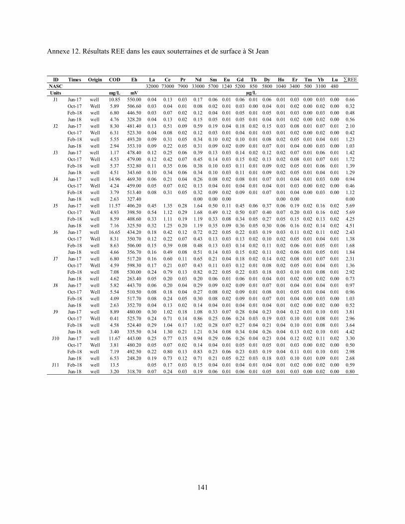
141

Annexe 12. Résultats REE dans les eaux souterraines et de surface à St Jean

ID Times Origin COD Eh La Ce Pr Nd Sm Eu Gd Tb Dy Ho Er Tm Yb Lu REENASC 32000 73000 7900 33000 5700 1240 5200 850 5800 1040 3400 500 3100 480Units mg/L mV

J1 Jun-17 well 10.85 550.00 0.04 0.13 0.03 0.17 0.06 0.01 0.06 0.01 0.06 0.01 0.03 0.00 0.03 0.00 0.66Oct-17 Well 5.89 506.60 0.03 0.04 0.01 0.08 0.02 0.01 0.03 0.00 0.04 0.01 0.02 0.00 0.02 0.00 0.32Feb-18 well 6.80 446.50 0.03 0.07 0.02 0.12 0.04 0.01 0.05 0.01 0.05 0.01 0.03 0.00 0.03 0.00 0.48Jun-18 well 4.76 328.20 0.04 0.13 0.02 0.15 0.05 0.01 0.05 0.01 0.04 0.01 0.02 0.00 0.02 0.00 0.56

J2 Jun-17 well 8.30 481.40 0.13 0.51 0.09 0.59 0.19 0.04 0.18 0.02 0.15 0.03 0.08 0.01 0.07 0.01 2.10Oct-17 Well 6.31 523.30 0.04 0.08 0.02 0.12 0.03 0.01 0.04 0.01 0.03 0.01 0.02 0.00 0.02 0.00 0.42Feb-18 well 5.55 493.20 0.09 0.31 0.05 0.34 0.10 0.02 0.10 0.01 0.08 0.02 0.05 0.01 0.04 0.01 1.23Jun-18 well 2.94 353.10 0.09 0.22 0.05 0.31 0.09 0.02 0.09 0.01 0.07 0.01 0.04 0.00 0.03 0.00 1.03

J3 Jun-17 well 1.17 478.40 0.12 0.25 0.06 0.39 0.13 0.03 0.14 0.02 0.12 0.02 0.07 0.01 0.06 0.01 1.42Oct-17 Well 4.53 479.00 0.12 0.42 0.07 0.45 0.14 0.03 0.15 0.02 0.13 0.02 0.08 0.01 0.07 0.01 1.72Feb-18 well 5.37 532.80 0.11 0.35 0.06 0.38 0.10 0.03 0.11 0.01 0.09 0.02 0.05 0.01 0.06 0.01 1.39Jun-18 well 4.51 343.60 0.10 0.34 0.06 0.34 0.10 0.03 0.11 0.01 0.09 0.02 0.05 0.01 0.04 0.01 1.29

J4 Jun-17 well 14.96 469.30 0.06 0.21 0.04 0.26 0.08 0.02 0.08 0.01 0.07 0.01 0.04 0.01 0.03 0.00 0.94Oct-17 Well 4.24 459.00 0.05 0.07 0.02 0.13 0.04 0.01 0.04 0.01 0.04 0.01 0.03 0.00 0.02 0.00 0.46Feb-18 well 3.79 513.40 0.08 0.31 0.05 0.32 0.09 0.02 0.09 0.01 0.07 0.01 0.04 0.00 0.03 0.00 1.12Jun-18 well 2.63 327.40 0.00 0.00 0.00 0.00 0.00 0.00

J5 Jun-17 well 11.57 406.20 0.45 1.35 0.28 1.64 0.50 0.11 0.45 0.06 0.37 0.06 0.19 0.02 0.16 0.02 5.69Oct-17 Well 4.93 398.50 0.54 1.12 0.29 1.68 0.49 0.12 0.50 0.07 0.40 0.07 0.20 0.03 0.16 0.02 5.69Feb-18 well 8.59 408.60 0.33 1.11 0.19 1.19 0.33 0.08 0.34 0.05 0.27 0.05 0.15 0.02 0.13 0.02 4.25Jun-18 well 7.16 325.50 0.32 1.25 0.20 1.19 0.35 0.09 0.36 0.05 0.30 0.06 0.16 0.02 0.14 0.02 4.51

J6 Jun-17 well 16.65 434.20 0.18 0.42 0.12 0.72 0.22 0.05 0.22 0.03 0.19 0.03 0.11 0.02 0.11 0.02 2.43Oct-17 Well 8.31 350.70 0.12 0.22 0.07 0.43 0.13 0.03 0.13 0.02 0.10 0.02 0.05 0.01 0.04 0.01 1.38Feb-18 well 8.63 506.00 0.15 0.39 0.08 0.48 0.13 0.03 0.14 0.02 0.11 0.02 0.06 0.01 0.05 0.01 1.68Jun-18 well 4.66 356.70 0.16 0.49 0.08 0.51 0.14 0.03 0.15 0.02 0.11 0.02 0.06 0.01 0.05 0.01 1.84

J7 Jun-17 well 6.80 517.20 0.16 0.60 0.11 0.65 0.21 0.04 0.18 0.02 0.14 0.02 0.08 0.01 0.07 0.01 2.31Oct-17 Well 4.59 598.30 0.17 0.21 0.07 0.43 0.11 0.03 0.12 0.01 0.08 0.02 0.05 0.01 0.04 0.01 1.36Feb-18 well 7.08 530.00 0.24 0.79 0.13 0.82 0.22 0.05 0.22 0.03 0.18 0.03 0.10 0.01 0.08 0.01 2.92Jun-18 well 4.62 263.40 0.05 0.20 0.03 0.20 0.06 0.01 0.06 0.01 0.04 0.01 0.02 0.00 0.02 0.00 0.73

J8 Jun-17 well 5.82 443.70 0.06 0.20 0.04 0.29 0.09 0.02 0.09 0.01 0.07 0.01 0.04 0.01 0.04 0.01 0.97Oct-17 Well 5.54 510.50 0.08 0.18 0.04 0.27 0.08 0.02 0.09 0.01 0.08 0.01 0.05 0.01 0.04 0.01 0.96Feb-18 well 4.09 517.70 0.08 0.24 0.05 0.30 0.08 0.02 0.09 0.01 0.07 0.01 0.04 0.00 0.03 0.00 1.03Jun-18 well 2.63 352.70 0.04 0.13 0.02 0.14 0.04 0.01 0.04 0.01 0.04 0.01 0.02 0.00 0.02 0.00 0.52

J9 Jun-17 well 8.89 480.00 0.30 1.02 0.18 1.08 0.33 0.07 0.28 0.04 0.23 0.04 0.12 0.01 0.10 0.01 3.81Oct-17 Well 0.41 525.70 0.24 0.71 0.14 0.86 0.25 0.06 0.24 0.03 0.19 0.03 0.10 0.01 0.08 0.01 2.96Feb-18 well 4.58 524.40 0.29 1.04 0.17 1.02 0.28 0.07 0.27 0.04 0.21 0.04 0.10 0.01 0.08 0.01 3.64Jun-18 well 3.40 335.50 0.34 1.30 0.21 1.21 0.34 0.08 0.34 0.04 0.26 0.04 0.13 0.02 0.10 0.01 4.42

J10 Jun-17 well 11.67 443.00 0.25 0.77 0.15 0.94 0.29 0.06 0.26 0.04 0.23 0.04 0.12 0.02 0.11 0.02 3.30Oct-17 Well 3.81 480.20 0.05 0.07 0.02 0.14 0.04 0.01 0.05 0.01 0.05 0.01 0.03 0.00 0.02 0.00 0.50Feb-18 well 7.19 492.50 0.22 0.80 0.13 0.83 0.23 0.06 0.23 0.03 0.19 0.04 0.11 0.01 0.10 0.01 2.98Jun-18 well 6.53 248.20 0.19 0.73 0.12 0.71 0.21 0.05 0.22 0.03 0.18 0.03 0.10 0.01 0.09 0.01 2.68

J11 Feb-18 well 13.5 0.05 0.17 0.03 0.15 0.04 0.01 0.04 0.01 0.04 0.01 0.02 0.00 0.02 0.00 0.59Jun-18 well 3.20 318.70 0.07 0.24 0.03 0.19 0.06 0.01 0.06 0.01 0.05 0.01 0.03 0.00 0.02 0.00 0.80

µg/L

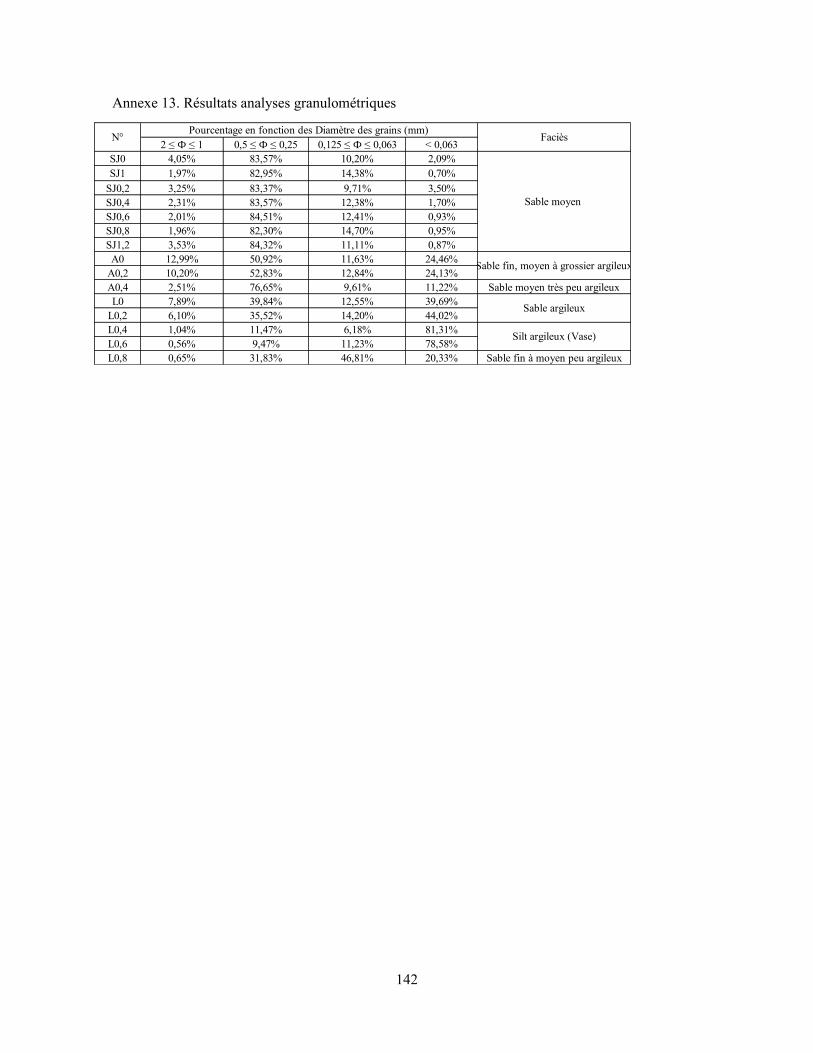
142

Annexe 13. Résultats analyses granulométriques

2 ≤ Ф ≤ 1 0,5 ≤ Ф ≤ 0,25 0,125 ≤ Ф ≤ 0,063 < 0,063SJ0 4,05% 83,57% 10,20% 2,09%SJ1 1,97% 82,95% 14,38% 0,70%

SJ0,2 3,25% 83,37% 9,71% 3,50%SJ0,4 2,31% 83,57% 12,38% 1,70%SJ0,6 2,01% 84,51% 12,41% 0,93%SJ0,8 1,96% 82,30% 14,70% 0,95%SJ1,2 3,53% 84,32% 11,11% 0,87%A0 12,99% 50,92% 11,63% 24,46%

A0,2 10,20% 52,83% 12,84% 24,13%A0,4 2,51% 76,65% 9,61% 11,22% Sable moyen très peu argileuxL0 7,89% 39,84% 12,55% 39,69%

L0,2 6,10% 35,52% 14,20% 44,02%L0,4 1,04% 11,47% 6,18% 81,31%L0,6 0,56% 9,47% 11,23% 78,58%L0,8 0,65% 31,83% 46,81% 20,33% Sable fin à moyen peu argileux

Sable argileux

Silt argileux (Vase)

N°Pourcentage en fonction des Diamètre des grains (mm)

Faciès

Sable moyen

Sable fin, moyen à grossier argileux

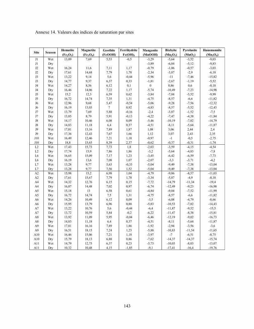
143

Annexe 14. Valeurs des indices de saturation par sites

Site SeasonHematite

(Fe2O3)

Magnetite

(Fe3O4)

Geothite

(FeOOH)

Ferrihydrite

Fe(OH)3

Manganite

(MnOOH)

Bixbyite

(Mn2O3)

Pyrolusite

(MnO2)

Hausmannite

(Mn3O4)

J1 Wet 13,09 7,69 5,53 -0,5 -3,29 -5,64 -3,52 -9,03J1 Dry -3,89 -6,84 -5,12 -9,83J2 Wet 16,24 11,6 7,11 1,17 -0,79 -1,06 -0,57 -3,03J2 Dry 17,61 14,68 7,79 1,78 -2,34 -3,87 -2,9 -6,18J3 Wet 13,22 9,14 5,6 -0,44 -5,96 -11 -7,46 -15,82J3 Dry 14,77 9,37 6,37 0,33 -1,81 -2,67 -1,19 -5,52J4 Wet 14,27 8,56 6,12 0,1 0 0,86 0,6 -0,18J4 Dry 16,46 14,06 7,22 1,17 -5,74 -10,49 -7,23 -14,98J5 Wet 15,2 12,3 6,59 0,62 -3,84 -7,04 -5,52 -9,99J5 Dry 16,72 14,74 7,35 1,31 -4,75 -8,57 -6,6 -11,82J6 Wet 12,96 9,68 5,47 -0,54 -5,06 -9,28 -7,56 -12,32J6 Dry 16,19 13,03 7 0,92 -4,83 -8,57 -5,52 -12,43J7 Wet 13,79 7,69 5,88 -0,16 -2,4 -3,87 -1,52 -7,5J7 Dry 13,85 8,79 5,91 -0,13 -4,22 -7,47 -4,38 -11,84J8 Wet 14,17 10,46 6,08 0,09 -5,46 -10,19 -7,02 -14,79J8 Dry 14,83 11,18 6,4 0,37 -4,51 -8,11 -5,64 -11,87J9 Wet 17,81 13,16 7,89 1,87 1,08 3,06 2,44 2,4J9 Dry 17,36 12,43 7,67 1,66 1,12 3,07 2,43 2,35

J10 Wet 16,49 12,46 7,21 1,18 -0,97 -1 -0,5 -2,75J10 Dry 18,8 15,65 8,39 2,37 -0,62 -0,37 -0,31 -1,74L2 Wet 17,43 15,73 7,73 1,8 -2,03 -3,59 -4,15 -4,54L2 Dry 17,74 15,9 7,86 1,86 -3,2 -5,64 -4,83 -7,8L6 Wet 16,65 15,09 7,17 1,23 -3,45 -6,42 -6,59 -7,73L6 Dry 16,19 13,6 7,08 1,07 -2,07 -3,3 -3,71 -4,2L7 Wet 13,28 9,77 5,63 -0,33 -5,04 -9,49 -7,38 -13,04L7 Dry 13,28 9,77 7,56 1,52 -5,04 -9,49 -7,38 -13,04A2 Wet 15,98 15,2 6,98 1,04 -4,79 -9,06 -8,57 -11,03A2 Dry 17,61 15,67 7,79 1,78 -3,34 -5,87 -4,9 -8,18A4 Wet 14,32 12,76 6,15 0,15 -7,72 -14,79 -11,34 -19,4A4 Dry 16,07 14,48 7,02 0,97 -6,74 -12,49 -9,23 -16,98A5 Wet 15,18 13 6,58 0,61 -4,84 -9,04 -7,52 -11,99A5 Dry 16,72 14,74 7,5 1,31 -4,75 -8,57 -6,6 -11,82A6 Wet 14,26 10,49 6,12 0,09 -3,5 -6,08 -4,79 -8,66A6 Dry 15,95 13,79 6,96 0,88 -5,83 -10,53 -7,82 -14,43A7 Wet 13,22 10,76 5,6 -0,44 -6,4 -11,87 -9,52 -15,5A7 Dry 13,72 10,59 5,84 -0,2 -6,22 -11,47 -8,38 -15,81A8 Wet 13,92 11,09 5,95 -0,04 -6,46 -12,19 -9,02 -16,73A8 Dry 14,83 11,18 6,4 0,37 -4,51 -8,11 -5,64 -11,87A9 Wet 17,81 16,16 7,89 1,86 -1,92 -2,94 -3,56 -3,6A9 Dry 16,51 18,15 7,24 1,23 -5,88 -10,83 -11,54 -11,65

A10 Wet 16,46 15,06 7,21 1,18 -3,97 -7 -6,51 -8,75A10 Dry 15,79 18,13 6,88 0,86 -7,62 -14,37 -14,37 -15,74A11 Wet 14,79 12,75 6,37 0,23 -5,73 -10,03 -8,03 -13,07A11 Dry 10,32 10,48 4,15 -1,85 -9,1 -17,41 -16,4 -19,76

144

Annexe 15. Résultats questionnaire à St Jean

n° Nom LieuNombre de

bâtis

Présence

de courSol cour

Superficie

cour (m2)

Surface

inondée/cou

r (%)

Présence

d'animaux

Type

d'animaux

Lieu

stockage

déchets

Type de

stockageTraitement

Rejet Eaux

UséesSAE

Profondeur

PuitsStockage ER

Stockage

EP

Stockage

Pluie

Usage Eau du

robinetUsage Eau du Puits

Usage Eau de la

pluie

Aujourd'hui hieravant-

hier<7j <15j <30j 1j 2j 3j <7j <15j <30j

1 w-JEA-1-Do 06°21,912 N 002°24,869 E Cour 8 oui nu 140 0 non Néant cour panierRamassés et

sortispuisard et extéreur

Robinet, puits 3 Néant Néant Néant Boisson, douche lessive,vaiselle,douche Néant non non un peuun peu

fortun peu

fortun peu fort non non non non non non

2 w-JEA-1-So 06°21,912 N 002°24,869 E Maison 8 oui nu 140 0 non Néant cour panierRamassés et

sortispuisard et extérieur

Robinet, puits 3 Néant Néant Néant Boisson, douche lessive,vaiselle,douche Néant non non un peuun peu

fortun peu

fortun peu fort non non non non non non

3 w-JEA-2-So 06°21,883 N 002°24,835 E Maison 1 non Néant Néant Néant non Néant cour sachetramassés par

tricyclepuisard et extérieur

Robinet, puits, pluie

4 Néant Néant Néant Boisson lessive,vaiselle,douche lessive non non non fort fort fort non non non non non non

4 w-JEA-2-Do 06°21,883 N 002°24,835 E Maison 1 non Néant Néant Néant non Néant cour sachetramassés par

tricyclepuisard et extérieur

Robinet, puits, pluie

4 Néant Néant Néant Boisson lessive,vaiselle,douche lessive non non non fort fort fort non non non non non non

5 w-JEA-3-So 06°21,896 N 002°24,883 E Cour 3 oui nu 150 0 oui poules courrécipient plastique

Ramassés et sortis

extérieurRobinet, puits,

pluie2 Néant Néant Néant

boisson, lessive, douche

lessive, vaiselle, doucheBoisson,

lessive,vaisselle, douche

non non non nsp fort fort non non non non non non

6 w-JEA-3-Do 06°21,896 N 002°24,883 E Cour 3 oui nu 150 0 oui poules courrécipient plastique

Ramassés et sortis

extérieurRobinet, puits,

pluie2 Néant Néant Néant

boisson, lessive, douche

lessive, vaiselle, doucheBoisson,

lessive,vaisselle, douche

non non non nsp fort fort non non non non non non

7 w-JEA-4-So 06°21,233 N 002°24,948 E Cour 5 oui nu 100 0 oui poules courrécipient plastique

Ramassés et sortis

puisard et cour

robinet, puits 3 Néant Néant Néantboisson, lessive,

douchelessive, vaiselle, douche Néant non non non moyen moyen fort non non non non non non

8 w-JEA-4-Do 06°21,233 N 002°24,948 E Cour 5 oui nu 100 0 oui poules courrécipient plastique

Ramassés et sortis

puisard et cour

robinet, puits 3 Néant Néant Néantboisson, lessive,

douchelessive, vaiselle, douche Néant non non non moyen moyen fort non non non non non non

9 w-JEA-5-So 06°21,792 N 002°24,888 E Cour 4 ouinu et

cimenté350 0 non Néant cour sachets, bidons

Ramassés et sortis

puisard et extérieur

Robinet, puits, pluie

Néant Néant Néant bassineBoisson, vaiselle,

douchelessive, vaiselle, douche lessive, douche non non non non nsp fort non non non non non non

10 w-JEA-5-Do 06°21,792 N 002°24,888 E Cour 4 ouinu et

cimenté350 0 non Néant cour sachets, bidons

Ramassés et sortis

puisard et extérieur

Robinet, puits, pluie

Néant Néant Néant NéantBoisson, vaiselle,

douchelessive, vaiselle, douche lessive, douche non non non non nsp fort non non non non non non

11 w-JEA-6-Do 06°21,787 N 002°24,856 E Cour 8 ouinu et

cimenté150 0 oui chats cour

récipient plastique

Ramassés et sortis

cour robinet, puits 2 Néant Néant Néantboisson, lessive, vaiselle, douche

lessive, vaiselle, douche Néant non non non nonun peu

fortfort non non non non non non

12 w-JEA-6-So 06°21,787 N 002°24,856 E Cour 8 ouinu et

cimenté150 0 oui chats cour

récipient plastique

Ramassés et sortis

cour robinet, puits 2 Néant Néant Néantboisson, lessive, vaiselle, douche

lessive, vaiselle, douche Néant non non non nonun peu

fortfort non non non non non non

13 w-JEA-7-So 06°21,828 N 002°24,901 E Cour 6 oui nu 300 0 oui poules courrécipient plastique

Ramassés et sortis

cour, puits perdu (eaux de douche)

Robinet, puits, pluie

3 Néant Néant Néant boissonboisson, lessive, vaiselle, douche,

terrasse

lessive, vaiselle, douche

non non non fort NSP NSP non non non non non non

14 w-JEA-7-Do 06°21,828 N 002°24,901 E Cour 6 oui nu 300 0 oui poules courrécipient plastique

Ramassés et sortis

cour, puits perdu (eaux de douche)

Robinet, puits, pluie

3 Néant Néant Néant boissonboisson, lessive, vaiselle, douche,

terrasse

lessive, vaiselle, douche

non non non fort NSP NSP non non non non non non

15 w-JEA-8-So 06°21,848 N 002°24,945 E Cour 8 oui nu 300 0 non Néant cour sachetsramassés et

sortiscour

Robinet ext, puits

NéantRécipient en

plastiqueNéant Néant boisson lessive, vaiselle, douche Néant non non un peu non non très fort non non non non non non

16 w-JEA-8-Do 06°21,848 N 002°24,945 E maison 8 oui nu 300 0 non Néant cour sachetsramassés et

sortiscour

Robinet ext, puits

NéantRécipient en

plastiqueNéant Néant boisson lessive, vaiselle, douche Néant non non un peu non non très fort non non non non non non

17 w-JEA-9-So 06°21,795 N 002°24,864 E Cour 7 ouinu et

cimenté150 0 oui poules cour

plastiques, panier, sachet

Ramassés et sortis

carniveaux robinet, puits 3 Néant Néant Néant boisson, douche lessive, vaiselle, douche non non non nonun peu

fortfort non non non non non non

18 w-JEA-9-Do 06°21,795 N 002°24,864 E Cour 7 ouinu et

cimenté150 0 oui poules cour

plastoques, panier, sachet

Ramassés et sortis

carniveaux robinet, puits 3 Néant Néant Néant boisson, douche lessive, vaiselle, douche non non non nonun peu

fortfort non non non non non non

19 w-JEA-10-So 06°21,928 N 002°24,841 E cour 6 oui nu 150 0 oui poules cour bidonRamassés et

sortispuisard

Robinet, puits, pluie

Néant Néant Néant NéantBoisson,lessive,va

iselle, doucheLessive,vaiselle,douche,

motolessive non non non oui oui oui non non non non non non

20 w-JEA-10-Do 06°21,928 N 002°24,841 E cour 6 oui nu 150 0 oui poules cour bidonRamassés et

sortispuisard

Robinet, puits, pluie

Néant Néant Néant NéantBoisson,lessive,va

iselle, doucheLessive,vaiselle,douche,

motolessive non non non oui oui oui non non non non non non

Coordonnées GPS Précipitations Stagnation des eaux de pluie

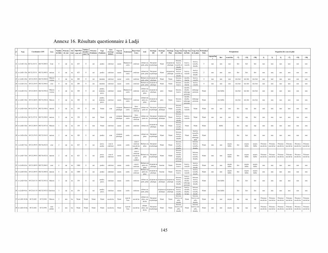
145

Annexe 16. Résultats questionnaire à Ladji

n° Nom LieuNombre

de bâtis

Présence

de cour

Sol

cour

Superficie

cour (m2)

Surface

inondée/

cour (%)

Présence

d'animaux

Type

d'animaux

Lieu

stockage

déchets

Type de

stockageTraitement

Rejet Eaux

UséesSAE

Stockage

ER

Stockage

EP

Stockage

Pluie

Usage Eau

du robinet

Usage Eau

du Puits

Usage Eau

de la pluie

Profondeur

Puits

Aujourd'hu

ihier avant-hier <7j <15j <30j 1j 2j 3j <7j <15j <30j

21 w-LAD-1-So 06°23,333 N 002°25,989 E Cour 4 oui nu 625 0 oui poules extérieur aucunRamassés et

sortisextérieur

robinet ext, puits, pluie

Récipient en plastique

Néantrécipient en

plastique

boisson, lessive,

vaiselle et douche

lessive, vaiselle

lessive, vaiselle, douche

5 non non non fort fort fort non non non non non non

22 w-LAD-1-Do 06°23,333 N 002°25,989 E maison 4 oui nu 625 0 oui poules extérieur aucunRamassés et

sortisextérieur

robinet ext, puits, pluie

Récipient en plastique

Néantrécipient en

plastique

boisson, lessive,

vaiselle et douche

lessive, vaiselle

lessive, vaiselle, douche

5 non non non fort fort fort non non non non non non

23 w-LAD-2-Do 06°23,358 N 002°25,994 EMaison voisine

4 oui nu 200 0 oui moutons extérieur aucun sortis extérieurRobinet ext, puits, pluie

récipient en plastique

Néant Néantboisson, lessive

vaiselle, douche

lessive, vaiselle

4 non non non très fort très fort très fort non non non non non non

24 w-LAD-2-So 06°23,358 N 002°25,994 E cour 4 oui nu 200 0 oui moutons extérieur aucun sortis extérieurRobinet ext, puits, pluie

récipient en plastique

Néant Néantboisson, lessive

vaiselle, douche

lessive, vaiselle

4 non non non très fort très fort très fort non non non non non non

25 w-LAD-3-So 06°23,360 N 002°25,956 EMaison voisine

5 oui nu 100 0 ouipoules,

moutons, porcs

extérieur aucunRamassés et

sortisextérieur

robinet ext, puits ext,

pluie

récipient en plastique

jarre Néantboisson, lessive

vaiselle, douche,

nettoyage poissons

nettoyage poissons

Néant très faible très fort très fort très fort non non non non non non

26 w-LAD-3-Do 06°23,360 N 002°25,956 E Maison 5 oui nu 100 0 ouipoules,

moutons, porcs

extérieur aucunRamassés et

sortisextérieur

robinet ext, puits ext,

pluie

récipient en plastique

jarre Néantboisson, lessive

vaiselle, douche,

nettoyage poissons

nettoyage poissons

Néant très faible très fort très fort très fort non non non non non non

27 w-LAD-4-Do 06°23,373 N 002°25,930 E maison 5 oui nu 150 0 non Néant courrécipient plastique

Ramassés et sortis

fosse septique et extérieur

robinet ext, puits ext

Récipient en plastique

récipient en plastique

Néant

boisson, lessive, vaiselle, douche

lessive, vaiselle

Néant Néant non non non fort nsp fort non non non non non non

28 w-LAD-4-So 06°23,373 N 002°25,930 E maison 5 oui nu 150 0 non Néant courrécipient plastique

Ramassés et sortis

fosse septique et extérieur

robinet ext, puits ext

Récipient en plastique

récipient en plastique

Néant

boisson, lessive, vaiselle, douche

lessive, vaiselle

Néant Néant non non non fort nsp fort non non non non non non

29 w-LAD-5-Do 06°23,384 N 002°25,957 E Maison 1 oui nu 150 0 non Néant extérieur aucun sortis extérieur robinet extrécipient en

plastiqueNéant Néant

boisson, lessive, vaiselle, douche,

Néant Néant Néant faible fort nsp nsp non non non non non non

30 w-LAD-6-Do 06°23,376 N 002°25,916 E maison 3 oui nu 100 0 oui poules courrécipient plastique

sortis extérieurrobinet ext,

pluieRécipient

en plastiqueNéant Néant

boisson, lessive, vaiselle, douche

Néant

lessive, vaisselle, douche,

nettoyage moto

Néant fort fort fort non non non non non non

31 w-LAD-7-Su 06°23,398 N 002°26,032 E cour 2 oui nu 625 0 ouiporcs, poules

cour et extérieur

aucun sortis

cour et extérieur

(eau du lac pour

Robinet ext, pluie

Récipient en plastique

Néant Néant

boisson, lessive, vaiselle, douche,

boisson, lessive, vaiselle, douche,

Néant non nonun peu faible

fortun peu faible

un peu faible

Présence eau du lac

Présence eau du lac

Présence eau du lac

Présence eau du lac

Présence eau du lac

Présence eau du lac

32 w-LAD-7-Do 06°23,398 N 002°26,032 E maison 2 oui nu 625 0 ouiporcs, poules

cour et extérieur

aucun sortis

cour et extérieur

(eau du lac pour

remblai)

Robinet ext, pluie

Récipient en plastique

Néant Néant

boisson, lessive, vaiselle, douche,

nettoyage poissons

boisson, lessive, vaiselle, douche,

Néant non nonun peu faible

fortun peu faible

un peu faible

Présence eau du lac

Présence eau du lac

Présence eau du lac

Présence eau du lac

Présence eau du lac

Présence eau du lac

33 w-LAD-8-So 06°23,309 N 002°25,960 E cour 6 oui nu 1400 0 oui poules extérieur aucun sortiscour et

extérieur

Robinet ext, puits ext,

pluie

récipient en plastique

bassine Néantboisson, lessive

lessive, vaiselle

lessive, vaiselle, douche

Néant non nonun peu faible

fortun peu faible

un peu faible

non non non non non non

34 w-LAD-8-Do 06°23,309 N 002°25,960 E maison 6 oui nu 1400 0 oui poules extérieur aucun sortiscour et

extérieur

Robinet ext, puits ext,

pluie

récipient en plastique

bassine Néantboisson, lessive

lessive, vaiselle

lessive, vaiselle, douche

Néant non nonun peu faible

fortun peu faible

un peu faible

non non non non non non

35 w-LAD-9-Do 06°23,411 N 002°25,955 E Maison 3 oui nu 150 0 ouipoules, porcs

extérieur aucun sortis extérieurrobinet ext, puits, pluie

récipient en plastique

récipient en plastique

récipient en plastique

boisson, lessive, vaiselle, douche

lessive, vaiselle, douche,

nettoyage poissons

boisson, lessive, vaiselle, douche

Néant très faible fort fort fort non non non non non non

36 w-LAD-9-So 06°23,411 N 002°25,955 E Extérieur 3 oui nu 150 0 ouipoules, porcs

extérieur aucun sortis extérieurrobinet ext, puits, pluie

récipient en plastique

récipient en plastique

boisson, lessive, vaiselle, douche

lessive, vaiselle, douche, lavage

boisson, lessive, vaiselle, douche

Néant très faible fort fort fort non non non non non non

37 w-LAD-10-Do 06°23,482 02°25,994 Maison 2 non lac Néant Néant Néant Néant eau du lac Néantrejet ds

l'eaueau du lac

robinet ext, pluie, eau

du lac

Récipient en plastique

Néant Néant

boisson, lessive,vai

selle, douche

Néant

boisson, lessive,vais

selle, douche,

Néant non non un peu nsp nsp nspPrésence eau du lac

Présence eau du lac

Présence eau du lac

Présence eau du lac

Présence eau du lac

Présence eau du lac

38 w-LAD-10-Su 06°23,482 02°25,994sous

pilotis2 non lac Néant Néant Néant Néant eau du lac Néant

rejet ds l'eau

eau du lacrobinet,

pluie, eau du lac

Récipient en plastique

Néant Néant

boisson, lessive,vai

selle, douche

Néant

boisson, lessive,vais

selle, douche,

Néant non non un peu nsp nsp nspPrésence eau du lac

Présence eau du lac

Présence eau du lac

Présence eau du lac

Présence eau du lac

Présence eau du lac

Coordonnées GPS Précipitations Stagnation des eaux de pluie

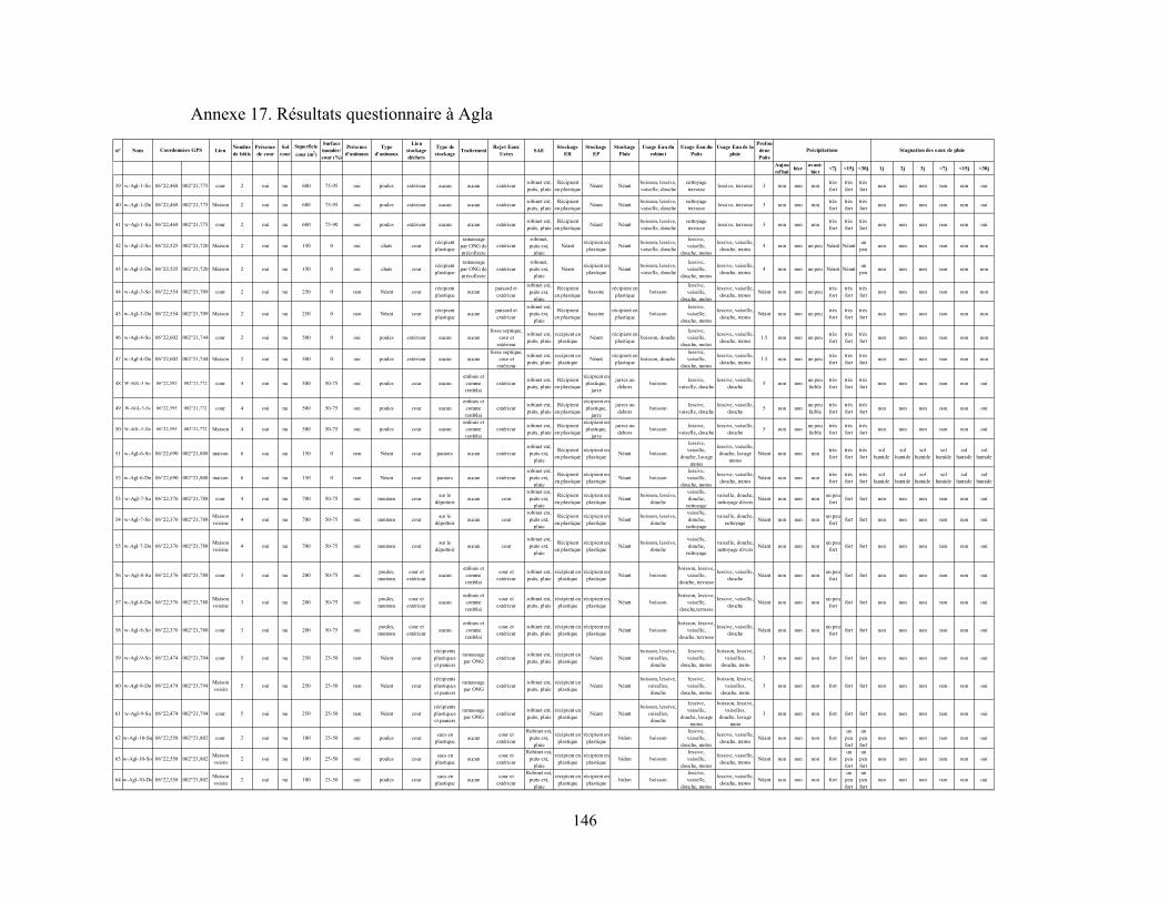
146

Annexe 17. Résultats questionnaire à Agla

n° Nom LieuNombre

de bâtis

Présence

de cour

Sol

cour

Superficie

cour (m2)

Surface

inondée/

cour (%)

Présence

d'animaux

Type

d'animaux

Lieu

stockage

déchets

Type de

stockageTraitement

Rejet Eaux

UséesSAE

Stockage

ER

Stockage

EP

Stockage

Pluie

Usage Eau du

robinet

Usage Eau du

Puits

Usage Eau de la

pluie

Profon

deur

Puits

Aujou

rd'huihier

avant-

hier<7j <15j <30j 1j 2j 3j <7j <15j <30j

39 w-Agl-1-So 06°22,468 002°21,775 cour 2 oui nu 600 75-95 oui poules extérieur aucun aucun extérieurrobinet ext, puits, pluie

Récipient en plastique

Néant Néantboisson, lessive, vaiselle, douche

nettoyage terrasse

lessive, terrasse 3 non non nontrès fort

très fort

très fort

non non non non non oui

40 w-Agl-1-Do 06°22,468 002°21,775 Maison 2 oui nu 600 75-95 oui poules extérieur aucun aucun extérieurrobinet ext, puits, pluie

Récipient en plastique

Néant Néantboisson, lessive, vaiselle, douche

nettoyage terrasse

lessive, terrasse 3 non non nontrès fort

très fort

très fort

non non non non non oui

41 w-Agl-1-Su 06°22,468 002°21,775 cour 2 oui nu 600 75-90 oui poules extérieur aucun aucun extérieurrobinet ext, puits, pluie

Récipient en plastique

Néant Néantboisson, lessive, vaiselle, douche

nettoyage terrasse

lessive, terrasse 3 non non nontrès fort

très fort

très fort

non non non non non oui

42 w-Agl-2-So 06°22,525 002°21,720 Maison 2 oui nu 150 0 oui chats courrécipient plastique

ramassage par ONG de précollecte

extérieurrobonet, puits ext,

pluieNéant

récipient en plastique

Néantboisson, lessive, vaiselle, douche

lessive, vaiselle,

douche, motos

lessive, vaiselle, douche, motos

4 non non un peu Néant Néantun

peunon non non non non non

43 w-Agl-2-Do 06°22,525 002°21,720 Maison 2 oui nu 150 0 oui chats courrécipient plastique

ramassage par ONG de précollecte

extérieurrobonet, puits ext,

pluieNéant

récipient en plastique

Néantboisson, lessive, vaiselle, douche

lessive, vaiselle,

douche, motos

lessive, vaiselle, douche, motos

4 non non un peu Néant Néantun

peunon non non non non non

44 w-Agl-3-So 06°22,554 002°21,709 cour 2 oui nu 250 0 non Néant courrécipient plastique

aucunpuisard et extérieur

robinet ext, puits ext,

pluie

Récipient en plastique

bassinerécipient en

plastiqueboisson

lessive, vaiselle,

douche, motos

lessive, vaiselle, douche, motos

Néant non non un peutrès fort

très fort

très fort

non non non non non non

45 w-Agl-3-Do 06°22,554 002°21,709 Maison 2 oui nu 250 0 non Néant courrécipient plastique

aucunpuisard et extérieur

robinet ext, puits ext,

pluie

Récipient en plastique

bassinerécipient en

plastiqueboisson

lessive, vaiselle,

douche, motos

lessive, vaiselle, douche, motos

Néant non non un peutrès fort

très fort

très fort

non non non non non non

46 w-Agl-4-So 06°22,602 002°21,744 cour 2 oui nu 500 0 oui poules extérieur aucun aucunfosse septique,

cour et extérieur

robinet ext, puits, pluie

recipient en plastique

Néantrécipient en

plastiqueboisson, douche

lessive, vaiselle,

douche, motos

lessive, vaiselle, douche, motos

1.5 non non un peutrès fort

très fort

très fort

non non non non non non

47 w-Agl-4-Do 06°22,602 002°21,744 Maison 2 oui nu 500 0 oui poules extérieur aucun aucunfosse septique,

cour et extérieur

robinet ext, puits, pluie

recipient en plastique

Néantrécipient en

plastiqueboisson, douche

lessive, vaiselle,

douche, motos

lessive, vaiselle, douche, motos

1.5 non non un peutrès fort

très fort

très fort

non non non non non non

48 W-AGL-5-So 06°22,595 002°21,772 cour 4 oui nu 500 50-75 oui poules cour aucunenfouis et

comme remblai

extérieurrobinet ext, puits, pluie

Récipient en plastique

récipient en plastique,

jarre

jarres au dehors

boissonlessive,

vaiselle, douchelessive, vaiselle,

douche5 non non

un peu faible

très fort

très fort

très fort

non non non non non oui

49 W-AGL-5-Su 06°22,595 002°21,772 cour 4 oui nu 500 50-75 oui poules cour aucunenfouis et

comme remblai

extérieurrobinet ext, puits, pluie

Récipient en plastique

récipient en plastique,

jarre

jarres au dehors

boissonlessive,

vaiselle, douchelessive, vaiselle,

douche5 non non

un peu faible

très fort

très fort

très fort

non non non non non oui

50 W-AGL-5-Do 06°22,595 002°21,772 Maison 4 oui nu 500 50-75 oui poules cour aucunenfouis et

comme remblai

extérieurrobinet ext, puits, pluie

Récipient en plastique

récipient en plastique,

jarre

jarres au dehors

boissonlessive,

vaiselle, douchelessive, vaiselle,

douche5 non non

un peu faible

très fort

très fort

très fort

non non non non non oui

51 w-Agl-6-So 06°22,690 002°21,808 maison 6 oui nu 150 0 non Néant cour paniers aucun extérieurrobinet ext, puits ext,

pluie

Récipient en plastique

récipient en plastique

Néant boisson

lessive, vaiselle,

douche, lavage motos

lessive, vaiselle, douche, lavage

motosNéant non non non

très fort

très fort

très fort

sol humide

sol humide

sol humide

sol humide

sol humide

sol humide

52 w-Agl-6-Do 06°22,690 002°21,808 maison 6 oui nu 150 0 non Néant cour paniers aucun extérieurrobinet ext, puits ext,

pluie

Récipient en plastique

récipient en plastique

Néant boissonlessive, vaiselle,

douche, motos

lessive, vaiselle, douche, motos

Néant non non nontrès fort

très fort

très fort

sol humide

sol humide

sol humide

sol humide

sol humide

sol humide

53 w-Agl-7-Su 06°22,376 002°21,788 cour 4 oui nu 700 50-75 oui moutons coursur le

dépottoiraucun cour

robinet ext, puits ext,

pluie

Récipient en plastique

récipient en plastique

Néantboisson, lessive,

douche

vaiselle, douche,

nettoyage

vaiselle, douche, nettoyage divers

Néant non non nonun peu

fortfort fort non non non non non oui

54 w-Agl-7-So 06°22,376 002°21,788Maison voisine

4 oui nu 700 50-75 oui moutons coursur le

dépottoiraucun cour

robinet ext, puits ext,

pluie

Récipient en plastique

récipient en plastique

Néantboisson, lessive,

douche

vaiselle, douche,

nettoyage

vaiselle, douche, nettoyage

Néant non non nonun peu

fortfort fort non non non non non oui

55 w-Agl-7-Do 06°22,376 002°21,788Maison voisine

4 oui nu 700 50-75 oui moutons coursur le

dépottoiraucun cour

robinet ext, puits ext,

pluie

Récipient en plastique

récipient en plastique

Néantboisson, lessive,

douche

vaiselle, douche,

nettoyage

vaiselle, douche, nettoyage divers

Néant non non nonun peu

fortfort fort non non non non non oui

56 w-Agl-8-Su 06°22,376 002°21,788 cour 3 oui nu 200 50-75 ouipoules, montons

cour et extérieur

aucunenfouis et

comme remblai

cour et extérieur

robinet ext, puits, pluie

récipient en plastique

récipient en plastique

Néant boissonboisson, lessive,

vaiselle, douche, terrasse

lessive, vaiselle, douche

Néant non non nonun peu

fortfort fort non non non non non oui

57 w-Agl-8-Do 06°22,376 002°21,788Maison voisine

3 oui nu 200 50-75 ouipoules, montons

cour et extérieur

aucunenfouis et

comme remblai

cour et extérieur

robinet ext, puits, pluie

récipient en plastique

récipient en plastique

Néant boissonboisson, lessive,

vaiselle, douche,terrasse

lessive, vaiselle, douche

Néant non non nonun peu

fortfort fort non non non non non oui

58 w-Agl-8-So 06°22,376 002°21,788 cour 3 oui nu 200 50-75 ouipoules, montons

cour et extérieur

aucunenfouis et

comme remblai

cour et extérieur

robinet ext, puits, pluie

récipient en plastique

récipient en plastique

Néant boissonboisson, lessive,

vaiselle, douche, terrasse

lessive, vaiselle, douche

Néant non non nonun peu

fortfort fort non non non non non oui

59 w-Agl-9-So 06°22,474 002°21,794 cour 5 oui nu 250 25-50 non Néant courrécipients plastiques et paniers

ramassage par ONG

extérieurrobinet ext, puits, pluie

récipient en plastique

Néant Néantboisson, lessive,

vaiselles, douche

lessive, vaiselle,

douche, motos

boisson, lessive, vaiselles,

douche, moto3 non non non fort fort fort non non non non non oui

60 w-Agl-9-Do 06°22,474 002°21,794Maison voisin

5 oui nu 250 25-50 non Néant courrécipients plastiques et paniers

ramassage par ONG

extérieurrobinet ext, puits, pluie

récipient en plastique

Néant Néantboisson, lessive,

vaiselles, douche

lessive, vaiselle,

douche, motos

boisson, lessive, vaiselles,

douche, moto3 non non non fort fort fort non non non non non oui

61 w-Agl-9-Su 06°22,474 002°21,794 cour 5 oui nu 250 25-50 non Néant courrécipients plastiques et paniers

ramassage par ONG

extérieurrobinet ext, puits, pluie

récipient en plastique

Néant Néantboisson, lessive,

vaiselles, douche

lessive, vaiselle,

douche, lavage motos

boisson, lessive, vaiselles,

douche, lavage moto

3 non non non fort fort fort non non non non non oui

62 w-Agl-10-Su 06°22,558 002°21,802 cour 2 oui nu 100 25-50 oui poules coursacs en

plastiqueaucun

cour et extérieur

Robinet ext, puits ext,

pluie

récipient en plastique

récipient en plastique

bidon boissonlessive, vaiselle,

douche, motos

lessive, vaiselle, douche, motos

Néant non non non fortun

peu fort

un peu fort

non non non non non oui

63 w-Agl-10-So 06°22,558 002°21,802Maison voisin

2 oui nu 100 25-50 oui poules coursacs en

plastiqueaucun

cour et extérieur

Robinet ext, puits ext,

pluie

récipient en plastique

récipient en plastique

bidon boissonlessive, vaiselle,

douche, motos

lessive, vaiselle, douche, motos

Néant non non non fortun

peu fort

un peu fort

non non non non non oui

64 w-Agl-10-Do 06°22,558 002°21,802Maison voisin

2 oui nu 100 25-50 oui poules coursacs en

plastiqueaucun

cour et extérieur

Robinet ext, puits ext,

pluie

récipient en plastique

récipient en plastique

bidon boissonlessive, vaiselle,

douche, motos

lessive, vaiselle, douche, motos

Néant non non non fortun

peu fort

un peu fort

non non non non non oui

Coordonnées GPS Précipitations Stagnation des eaux de pluie