proceedings of the sixth eurostat/unece work session ... - istat.it
TRANSCRIPT

Proceedings of the Sixth Eurostat/Unece Work Session
on Demographic Projections
�
Italian National Institute of Statistics
Pro
ceed
ings
of t
he S
ixth
Eur
osta
t/U
nece
Wor
k Se
ssio
n
o
n D
emog
raph
ic P
roje
ctio
ns
On Autumn 2013 Eurostat and UNECE were co-organisers, in cooperation with Istat, of a Work Session on Demographic Projections. The meeting was hosted by Istat and held in Rome on 29-31 October 2013.
The objective of the Work Session was to bring together policy makers, demographic researchers, academics, producers and users of demographic projections in order to: a) review and discuss the different uses of demographic projections and the current practices at national and international level; b) illustrate research approaches and innovative methodologies; c) improve the communication between policy makers and demographers and producers of demographic projections.
The Work Session was attended by 127 participants coming from national statistical offices, demographic research institutes, universities and other institutions. The discussion in the substantive sessions was based on 49 papers, 36 of which are published by the authors in this book on a voluntary basis.
€ 40,00


© 2014Istituto nazionale di statisticaVia Cesare Balbo, 16 - Roma
Salvo diversa indicazione la riproduzione è libera, a condizione che venga citata la fonte
Immagini, loghi, marchi registrati e altri contenuti di proprietà di terzi appartengono ai rispettivi proprietari e non possono essere riprodotti senza il loro consenso
Proceedings of the Sixth Eurostat/UNECE Work Sessionon Demographic Projections
ISBN: 978-88-458-1810-3 (elettronico)ISBN: 978-88-458-1811-0 (stampa)
A cura di: Marco Marsili e Giorgia Capacci

3
Proceedings of the Sixth Eurostat/Unece Work Session on Demographic Projections
FOREWORD
On Autumn 2013 Eurostat (Statistical Office of the European Union) and UNECE (United Nations Economic Commission for Europe) were co-organisers, in cooperation with Istat (Italian National Institute of Statistics), of a Work Session on Demographic Projections. The meeting was hosted by Istat and held in Rome on 29-31 October 2013. The meeting was part of a series of meetings jointly organized in this domain by Eurostat and UNECE. Previous meetings were organized in Mondorf-les-Bains (1994), Perugia (1999), Vienna (2005), Bucharest (2007) and Lisbon (2010).
The objective of the Work Session was to bring together policy makers, demo-graphic researchers from the National Statistical Institutes as well as from other na-tional and international organisations, academics, producers and users of demo-graphic projections in order to: a) review and discuss the different uses of demo-graphic projections and the current practices at national and international level; b) illustrate research approaches and innovative methodologies; c) improve the com-munication between policy makers and producers of demographic projections.
The contributions to the Work Session were grouped in sessions including the following items: Assumptions on future migration Assumptions on future fertility Assumptions on future mortality Actual and potential use of demographic projections at national and interna-
tional level National and international population projections out of the EU region Multiregional projections Household projections Stochastic methods in population projections Bayesian approaches Demographic sustainability and consistency with macroeconomic assumptions Beyond population projections by age and sex: inclusion of additional popula-
tion characteristics Population projections by age, sex and level of education.
The Work Session in Rome was attended by 127 participants coming from na-tional statistical offices, demographic research institutes, universities and other in-stitutions, and representing the following countries: Austria, Belgium, Canada, Croatia, Czech Republic, Denmark, Estonia, France, Georgia, Germany, Greece, Hungary, Iceland, Ireland, Israel, Italy, Japan, Republic of Korea, Latvia, Luxem-bourg, Netherlands, Norway, Poland, Portugal, Romania, Russian Federation, Slo-venia, Spain, Sweden, Switzerland, Turkey, United Kingdom and United States of America.
The discussion in the substantive sessions was based on 49 papers, 36 of which are published by the authors in this book on a voluntary basis. The Work Session included two key-note lectures given in the opening session by Nico Keil-man (University of Oslo) and by Tommy Bengtsson (University of Lund).

4
Proceedings of the Sixth Eurostat/Unece Work Session on Demographic Projections
The agenda of the Work Session was finalised by a Scientific Committee while an Organising Committee was responsible for overseeing the logistics plan-ning of the Work Session. The supervision and coordination of activities between the Scientific Committee and the Organising Committee were assured by a Coordi-nation Committee.
AKNOWLEDGMENTS
We would like to thank the members of the Organising Committee and the members of the Scientific Committee for their appreciated contribution to the suc-cess of the Work Session, as well as the participants for their scientific contribu-tions in the demographic projection domain. We would also like to thank the fol-lowing chairpersons for their valuable efforts that made the completion of this meeting possible: Mr. Saverio Gazzelloni (Istat), Mr. Eduardo Barredo Capelot (Eurostat), and Mr. Paolo Valente (UNECE) who opened the meeting and wel-comed the participants; Ms. Marianne Tonnessen (Norway) who was elected chair-person of the meeting; Mr. Valerio Terra Abrami (Italy) for items 4 and 14 of the agenda; Ms. Graziella Caselli (Italy) for items 5 and 12; Ms. Maria Graça Magalhaes (Portugal) for items 6 and 8; Mr. Giampaolo Lanzieri (Eurostat) for item 7; Ms. Rebecca Graziani (Italy) for items 9 and 13, Ms. Elisabetta Barbi (Ita-ly) for items 11 and 15, Ms. Anne Clemenceau (Eurostat) for items 16 and 17.
The views expressed in the current publication are purely those of the authors and may not in any circumstances be regarded as stating an official position of the three Organisations involved in the Work Session, namely Eurostat, UNECE and Istat.
Members of the Coordination Committee Mr. Lanzieri Giampaolo – Eurostat Mr. Marsili Marco – Istat Mr. Valente Paolo – UNECE Members of the Scientific Committee Ms. Barbi Elisabetta, University of Rome “Sapienza” Ms. Caselli Graziella, University of Rome “Sapienza” Ms. Graziani Rebecca, Bocconi University of Milano Ms. Magalhães Maria Graça, Statistics Portugal Mr. Terra Abrami Valerio, Istat Members of the Organising Committee Ms. Capacci Giorgia, Istat Mr. Corsetti Gianni, Istat Ms. Olsson Rosemarie, Eurostat Ms. Oyunjargal Mijidgombo, UNECE Ms. Paciello Micaela, Istat Ms. Pellicanò Cinzia, Istat Ms. Tabanella Bruna, Istat Ms. Willis-Nunez Fiona, UNECE

AGENDA AND TIMETABLE 5
Proceedings of the Sixth Eurostat/Unece Work Session on Demographic Projections
JOINT EUROSTAT-UNECE-ISTAT WORK SESSION ON DEMOGRAPHIC PROJECTIONS
Rome (Italy) 29-31 October 2013
AGENDA AND TIMETABLE
The meeting was held at Roma Eventi Fontana di Trevi Piazza della Pilotta, 4
Rome - Italy
SUMMARY OF AGENDA ITEMS FOR THE MEETING:
1. Opening of the meeting and welcoming remarks 2. Adoption of the agenda and election of officers 3. Key note lectures 4. Assumptions on future migration 5. Assumptions on future mortality 6. Actual and potential use of demographic projections at national and international
level 7. National and international population projections out of the EU region 8. Assumptions on future fertility 9. Stochastic methods in population projections 10. Household projections 11. Demographic sustainability and consistency with macroeconomic assumptions 12. Bayesian approaches (1) 13. Bayesian approaches (2) 14. Multiregional projections 15. Beyond population projections by age and sex: inclusion of additional popula-
tion characteristics 16. Population projections by age, sex and level of education (1) 17. Population projections by age, sex and level of education (2) 18. Adoption of the report and closing of the meeting

6 AGENDA AND TIMETABLE
Proceedings of the Sixth Eurostat/Unece Work Session on Demographic Projections
TIMETABLE
TIME ITEM SESSION/ACTIVITY
TUE, 29 OCTOBER, MORNING – AULA CARDUCCI – PLENARY SESSION
9:30–10:30 Registration of participants
10:30–11:20 1. OPENING OF THE MEETING
Welcoming remarks by:
Saverio Gazzelloni | Istat
Eduardo Barredo Capelot | Eurostat
Paolo Valente | UNECE
11:20–11:30 2. Adoption of the agenda and election of officers
11:30–13:00
11:30–12:15
12:15–13:00
3. KEYNOTE LECTURES
Probabilistic demographic projections Nico Keilman | University of Oslo
Population ageing - a threat to the Welfare State?
Tommy Bengtsson | University of Lund
TUE, 29 OCTOBER, AFTERNOON – AULA CARDUCCI – PARALLEL SESSION
14:30–16:00
14:30–14:45
14:45–15:00
15:00–15:15
15:15–15:30
15:30–16:00
4. ASSUMPTIONS ON FUTURE MIGRATION
Chair: Valerio Terra Abrami | Istat
Projections of ageing migrant populations in France: 2008-2028 Jean Louis Rallu | INED
Introducing duration dependant emigration in DREAMs population projection model Marianne Frank Hansen | DREAM
Model to forecast the re-immigration of Swedish-born by background Andreas Raneke | Statistics Sweden
Dynamical models for migration projections Violeta Calian | Statistics Iceland
Questions & Discussion

AGENDA AND TIMETABLE 7
Proceedings of the Sixth Eurostat/Unece Work Session on Demographic Projections
Time Item Session/Activity
16:30–18:00
16:30–16:45
16:45–17:00
17:00–17:15
17:15–17:30
17:30–18:00
5. ASSUMPTIONS ON FUTURE MORTALITY
Chair: Graziella Caselli | University of Rome “La Sapienza”
Cohort effects and structural changes in the mortality trend Edviges Coelho | Statistics Portugal, Luis Catela Nunes | Nova University of Lisbon
Evaluation of Korean Mortality Forecasting Models Jee Seon Baek, Mi Ock Jeong, Yun Kyoung Oh, Ji-Youn Lee, Sooyoung Kim | Statistics Korea
Coherent forecasting of multiple-decrement life tables: compositional models for French Cause of Death data, 1925-2008 Jim Oeppen | MPIDR, Carlo Giovanni Camarda | INED
Changing mortality trends by age and sex are challenges for assumptions on future mortality Örjan Hemström | Statistics Sweden
Questions & Discussion
TUE, 29 OCTOBER, AFTERNOON – AULA FOSCOLO – PARALLEL SESSION
14:30–16:00
14:30–14:50
14:50–15:10
15:10–15:30
15:30–16:00
6. ACTUAL AND POTENTIAL USE OF DEMOGRAPHIC PROJECTIONS AT NATIONAL AND INTERNATIONAL LEVEL
Chair: Maria Graça Magalhães | Statistics Portugal
Indexation of the pension age to projected remaining life expectancy in The Netherlands. Coen van Duin | Statistics Netherlands
The role of population projections for a redefinition of the Portuguese higher educational institutional network Le Rui Dias, Maria Filomena Mendes, M. Graça Magalhães, Paulo Infante | University of Évora
On the use of seasonal forecasting methods to model birth and deaths data as an input for monthly population estimates Jorge Bravo | University of Évora, Edviges Coelho, M. Graça Magalhães | Statistics Portugal
Questions & Discussion

8 AGENDA AND TIMETABLE
Proceedings of the Sixth Eurostat/Unece Work Session on Demographic Projections
Time Item Session/Activity
16:30–18:00
16:30–16:45
16:45–17:00
17:00–17:15
17:15–17:30
17:30–18:00
7. NATIONAL AND INTERNATIONAL POPULATION PROJECTIONS OUT OF THE EU REGION
Chair: Giampaolo Lanzieri | Eurostat
Qualitative and methodological aspects of population projections in Georgia; Georgian Population Prospects: 1950-2050 Avtandil Sulaberidze, Shorena Tsiklauri | Ilia State University
Population Prospects of Georgia Nika Maglaperidze | Ilia State University
Estimation of the size and vital rates of the Haredi (ultra-orthodox) population in Israel for the purpose of long-range population projections Ari Paltiel | Israel Central Bureau of Statistics
Population and development scenarios for EU neighbor countries in the South and East Mediterranean region George Groenewold, Joop de Beer | NIDI
Questions & Discussion
End of first day
WED, 30 OCTOBER, MORNING – AULA CARDUCCI – PARALLEL SESSION
09:30–11:00
09:30–09:45
09:45–10:00
10:00–10:15
10:15–10:30
10:30–11:00
8. ASSUMPTIONS ON FUTURE FERTILITY
Chair: Maria Graça Magalhães | Statistics Portugal
Contribution of fertility model and parameterization to population projection errors Dalkhat M. Ediev | VID
New family values and increased childbearing in Sweden? Lotta Persson, Johan Tollebrant | Statistics Sweden
Projecting fertility by regions considering tempo-adjusted TFR, the Austrian approach Alexander Hanika | Statistics Austria
Effects of childbearing postponement on cohort fertility in Germany Olga Pötzsch, Bettina Sommer | Destatis
Questions & Discussion

AGENDA AND TIMETABLE 9
Proceedings of the Sixth Eurostat/Unece Work Session on Demographic Projections
Time Item Session/Activity
11:30–13:00
11:30–11:45
11:45–12:00
12:00–12:15
12:15–12:30
12:30–13:00
9. STOCHASTIC METHODS IN POPULATION PROJECTIONS
Chair: Rebecca Graziani | Bocconi University
Measuring uncertainty in population forecasts: a new approach David A. Swanson | University of California Riverside, Jeff Tayman | University of California San Diego
Stochastic population forecast: an application to the Rome Metropolitan Area Salvatore Bertino, Oliviero Casacchia | University of Rome “La Sapienza”, Massimiliano Crisci | IRPPS-CNR
Long-term contribution of immigration to population renewal in Canada: a sensitivity analysis using Demosim Patrice Dion, Éric Caron Malenfant, Chantal Grondin | Statistics Canada
From agent-based models to statistical emulators Jakub Bijak�, Jason Hilton, Eric Silverman, Viet Dung Cao | University of Southampton
Questions & Discussion
WED, 30 OCTOBER, MORNING – AULA FOSCOLO – PARALLEL SESSION
9:30–11:00
9:30–9:50
9:50–10:10
10:10–10:30
10:30–11:00
10. HOUSEHOLD PROJECTIONS
Chair: Marco Marsili | Istat
Estimating the number of households: an un-avoidable challenge for the statistical system Antonio Argüeso Jiménez, Sixto Muriel de la Riva | INE
A household projection model for Belgium based on individual household membership rates, using the LIPRO typology Marie Vandresse | Federal Planning Bureau
Household Projections and Welfare Elisa Barbiano di Belgiojoso, Gian Carlo Blangiardo | University of Milan Bicocca, Alessio Menonna | ISMU, Natale Forlani | Ministero del Lavoro e delle Politiche Sociali
Questions & Discussion

10 AGENDA AND TIMETABLE
Proceedings of the Sixth Eurostat/Unece Work Session on Demographic Projections
Time Item Session/Activity
11:30–13:00
11:30–11:50
11:50–12:10
12:10–12:30
12:30–13:00
11. DEMOGRAPHIC SUSTAINABILITY AND CONSISTENCY WITH MACROECONOMIC ASSUMPTIONS
Chair: Elisabetta Barbi | University of Rome “La Sapienza”
Ageing alone? The future of the Portuguese population in discussion Filipe Ribeiro, Lídia Patrícia Tomé, Maria Filomena Mendes | University of Évora
Integrating labor market in population projections Juan Antonio Fernández Cordón | CSIC - Spanish Council for Scientific Research, Joaquín Planelles Romero | Institute of Statistics and Cartography of Andalusia
Economic factors and net migration assumptions for EU countries – how to incorporate lessons from the recent economic crisis? Pawel Strzelecki | Warsaw School of Economics
Questions & Discussion
WED, 30 OCTOBER, AFTERNOON – AULA CARDUCCI – PARALLEL SESSION
14:30–16:00
14:30–14:50
14:50–15:10
15:10–15:30
15:30–16:00
12. BAYESIAN APPROACHES (1)
Chair: Graziella Caselli | University of Rome “La Sapienza”
Bayesian functional models for population forecasting Han Lin Shang, Arkadiusz Wiśniowski, Jakub Bijak�, Peter W.F. Smith, James Raymer | University of Southampton
Towards stochastic forecasts of the Italian population: an experiment with conditional expert elicitations Francesco Billari | University of Oxford, Gianni Corsetti, Marco Marsili | Istat, Rebecca Graziani, Eugenio Melilli | Bocconi University
Expert-Based stochastic population forecasting: a bayesian approach to the combination of the elicitations Francesco Billari | University of Oxford, Rebecca Graziani, Eugenio Melilli | Bocconi University
Questions & Discussion

AGENDA AND TIMETABLE 11
Proceedings of the Sixth Eurostat/Unece Work Session on Demographic Projections
Time Item Session/Activity
16:30–18:00
16:30–16:50
16:50–17:10
17:10–17:30
17:30–18:00
13. BAYESIAN APPROACHES (2)
Chair: Rebecca Graziani | Bocconi University
Bayesian probabilistic projection of international migration rates Jonathan Azose, Adrian E. Raftery | University of Washington
Bayesian probabilistic population projections: do it yourself Hana Ševčiková | University of Washington, Adrian E. Raftery | University of Washington, Patrick Gerland | UNPD
Bayesian mortality forecasts with a flexible age pattern of change for several European countries Christina Bohk, Roland Rau | University of Rostock
Questions & Discussion
WED, 30 OCTOBER, AFTERNOON – AULA FOSCOLO – PARALLEL SESSION
14:30–16:00
14:30–14:45
14:45–15:00
15:00–15:15
15:15–15:30
15:30–16:00
14. MULTIREGIONAL PROJECTIONS
Chair: Valerio Terra Abrami | Istat
Examining the Role of International Migration in Global Population Projections Guy Abel, Nikola Sander | VID, Samir K.C | IAASA
Subnational population projections for Turkey, 2013-2023 Sebnem Bese Canpolat, Baris Ucar, M. Dogu Karakaya | Turkish Statistical Institute
An alternative projection model for interprovincial migration in Canada Patrice Dion | Statistics Canada
A Space-Time extension of the Lee-Carter model in a hierarchical bayesian framework: modelling and forecasting provincial mortality in Italy Fedele Greco, Francesco Scalone | University of Bologna
Questions & Discussion

12 AGENDA AND TIMETABLE
Proceedings of the Sixth Eurostat/Unece Work Session on Demographic Projections
Time Item Session/Activity
16:30–18:00
16:30–16:45
16:45–17:00
17:00–17:15
17:15–17:30
17:30–18:00
15. BEYOND POPULATION PROJECTIONS BY AGE AND SEX: INCLUSION OF ADDITIONAL POPULATION CHARACTERISTICS
Chair: Elisabetta Barbi | University of Rome “La Sapienza”
Projecting inequality: the role of population change Ingrid Schockaert, Patrick Deboosere | Vrije University of Bruxelles, Rembert De Blander, André Decoster | KU Leuven University
The impact of Canadian immigrant selection policy on future imbalances in labour force supply by broad skill levels Alain Bélanger | INRS Urbanisation Culture Société Research Centre
Microsimulation of language characteristics and language choice in multilingual regions with high immigration Alain Bélanger, Patrick Sabourin | INRS Urbanisation Culture Société Research Centre
A method for projecting economically active population. The case of Andalusia Silvia Bermúdez, Juan Antonio Hernández, Joaquín Planelles | Institute of Statistics and Cartography of Andalusia
Questions & Discussion
End of second day
THU, 31 OCTOBER, MORNING – AULA CARDUCCI – PLENARY SESSION
09:30–10:45
09:30–09:45
09:45–10:00
10:00–10:15
10:15–10:45
16. POPULATION PROJECTIONS BY AGE, SEX AND LEVEL OF EDUCATION (1)
Chair: Anne Clemenceau | Eurostat
The scientific base of the new Wittgenstein Centre Global Human Capital Projections: defining assumptions through an evaluation of expert views on future fertility, mortality and migration Wolfgang Lutz | Wittgenstein Centre
Developing Expert-Based assumptions on future fertility, mortality and migration Guy Abel, Stuart Basten, Regina Fuchs, Alessandra Garbero, Anne Goujon, Samir K.C., Elsie Pamuk, Fernando Riosmena, Nikola Sander, Tomáš Sobotka, Erich Striessnig, Kryštof Zeman | Wittgenstein Centre
The impact of alternative assumptions about migration differentials by education on projections of human capital Nikola Sander, Guy J. Abel, Samir K.C | Wittgenstein Centre
Questions & Discussion

AGENDA AND TIMETABLE 13
Proceedings of the Sixth Eurostat/Unece Work Session on Demographic Projections
Time Item Session/Activity
11:15–12:30
11:15–11:30
11:30–11:45
11:45–12:00
12:00–12:30
17. POPULATION PROJECTIONS BY AGE, SEX AND LEVEL OF EDUCATION (2)
Chair: Anne Clemenceau | Eurostat
Estimating transition age schedules for long-term projections of global educational attainment Bilal Barakat | Wittgenstein Centre
Results of the New Wittgenstein Centre Population Projections by age, sex and level of education for 171 countries Samir K.C., Sergei Scherbov, Erich Striessnig, Wolfgang Lutz | Wittgenstein Centre
Labor force projections for Europe by age, sex, and highest level of educational attainment, 2008 to 2053 Elke Loichinger | Wittgenstein Centre
Questions & Discussion
12:30–13:30
18. ADOPTION OF THE REPORT AND CLOSING OF THE MEETING
Chair: Paolo Valente | UNECE
Adoption of the report
Closing of the meeting
End of third day


TABLE OF CONTENTS 15
Proceedings of the Sixth Eurostat/Unece Work Session on Demographic Projections
TABLE OF CONTENTS
SESSION 4: ASSUMPTIONS ON FUTURE MIGRATION
Projections of ageing migrant populations in France: 2008-2028 21 Jean Louis Rallu | INED
Introducing emigration by duration of residence in the DREAM population projection model
33
Marianne Frank Hansen | DREAM
Model to forecast the re-immigration of Swedish-born by background 46 Andreas Raneke | Statistics Sweden
Dynamical models for migration projections 55 Violeta Calian | Statistics Iceland
SESSION 5: ASSUMPTIONS ON FUTURE MORTALITY
Changing mortality trends by age and sex are challenges for assumptions on future mortality
67
Örjan Hemström | Statistics Sweden
SESSION 6: ACTUAL AND POTENTIAL USE OF DEMOGRAPHIC PROJECTIONS AT NATIONAL AND INTERNATIONAL LEVEL
Indexation of the pension age to projected remaining life expectancy in The Netherlands
81
Coen van Duin | Statistics Netherlands
Population projections: a tool for a (re)definition of the Portuguese higher education system
93
Rui Dias, Maria Filomena Mendes, M. Graça Magalhães, Paulo Infante | University of Évora
SESSION 7: NATIONAL AND INTERNATIONAL POPULATION PROJECTIONS OUT OF THE EU REGION
Qualitative and methodological aspects of population projections in Georgia; Georgian Population Prospects: 1950-2050
109
Avtandil Sulaberidze, Shorena Tsiklauri | Ilia State University
Population Prospects of Georgia 118 Nika Maglaperidze | Ilia State University
Population estimates and vital rates of the Haredi (ultra-orthodox) population in Israel: a new component of long-range population projections
125
Ari Paltiel | Israel Central Bureau of Statistics

16 TABLE OF CONTENTS
Proceedings of the Sixth Eurostat/Unece Work Session on Demographic Projections
Population and development scenarios for EU neighbor countries in the South and East Mediterranean region
139
George Groenewold, Joop de Beer | NIDI
SESSION 8: ASSUMPTIONS ON FUTURE FERTILITY
Contribution of fertility model and parameterization to population projection errors
153
Dalkhat M. Ediev | VID
New family values and increased childbearing in Sweden? 165 Lotta Persson, Johan Tollebrant | Statistics Sweden
Projecting fertility by regions considering tempo-adjusted TFR, the Austrian approach
176
Alexander Hanika | Statistics Austria
Effects of childbearing postponement on cohort fertility in Germany 188 Olga Pötzsch, Bettina Sommer | Destatis
SESSION 9: STOCHASTIC METHODS IN POPULATION PROJECTIONS
Measuring uncertainty in population forecasts: a new approach 203 David A. Swanson | University of California Riverside, Jeff Tayman | University of California San Diego
Stochastic population forecast: an application to the Rome Metropolitan Area
216
Salvatore Bertino, Oliviero Casacchia | University of Rome “La Sapienza”, Massimiliano Crisci | IRPPS-CNR
Long-term contribution of immigration to population renewal in Canada: a sensitivity analysis using Demosim
230
Patrice Dion, Éric Caron Malenfant, Chantal Grondin, Dominic Grenier | Statistics Canada
From agent-based models to statistical emulators 241 Jakub Bijak, Jason Hilton, Eric Silverman, Viet Dung Cao | University of Southampton
SESSION 10: HOUSEHOLD PROJECTIONS
A household projection model for Belgium based on individual household membership rates
257
Marie Vandresse | Federal Planning Bureau
Household Projections and Welfare 272 Elisa Barbiano di Belgiojoso, Gian Carlo Blangiardo | University of Milan Bicocca, Alessio Menonna | ISMU, Natale Forlani | Ministero del Lavoro e delle Politiche Sociali
TABLE OF CONTENTS 17
Proceedings of the Sixth Eurostat/Unece Work Session on Demographic Projections
SESSION 11: DEMOGRAPHIC SUSTAINABILITY AND CONSISTENCY WITH MACROECONOMIC ASSUMPTIONS
Ageing alone? The future of the Portuguese population in discussion 287 Filipe Ribeiro, Lídia Patrícia Tomé, Maria Filomena Mendes | University of Évora
Integrating labor market in population projections 299 Juan Antonio Fernández Cordón | CSIC - Spanish Council for Scientific Research, Joaquín Planelles Romero | Institute of Statistics and Cartography of Andalusia
SESSION 12: BAYESIAN APPROACHES (1)
Bayesian functional models for population forecasting 313 Han Lin Shang, Arkadiusz Wiśniowski, Jakub Bijak, Peter W.F. Smith, James Raymer | University of Southampton
Towards stochastic forecasts of the Italian population: an experiment with conditional expert elicitations
326
Francesco Billari | University of Oxford, Gianni Corsetti, Marco Marsili | Istat, Rebecca Graziani, Eugenio Melilli | Bocconi University
SESSION 13: BAYESIAN APPROACHES (2)
Bayesian probabilistic projection of international migration rates 341 Jonathan Azose, Adrian E. Raftery | University of Washington
Bayesian probabilistic population projections using R 347 Hana Ševčiková | University of Washington, Adrian E. Raftery | University of Washington, Patrick Gerland | UNPD
Mortality forecasts with a flexible age pattern of change for several European countries
360
Christina Bohk, Roland Rau | University of Rostock
SESSION 14: MULTIREGIONAL PROJECTIONS
Examining the Role of International Migration in Global Population Projections
375
Guy Abel, Nikola Sander | VID, Samir K.C | IAASA
Subnational population projections for Turkey, 2013-2023 388 Sebnem Bese Canpolat, M. Dogu Karakaya | Turkish Statistical
Institute
An alternative projection model for interprovincial migration in Canada 400 Patrice Dion | Statistics Canada

18 TABLE OF CONTENTS
Proceedings of the Sixth Eurostat/Unece Work Session on Demographic Projections
A Space-Time extension of the Lee-Carter model in a hierarchical bayesian framework: modelling provincial mortality in Italy
412
Fedele Greco, Francesco Scalone | University of Bologna
SESSION 15: BEYOND POPULATION PROJECTIONS BY AGE AND SEX: INCLUSION OF ADDITIONAL POPULATION CHARACTERISTICS
Projecting inequality: the role of population change 427 Ingrid Schockaert, Patrick Deboosere | Vrije University of Bruxelles, Rembert De Blander, André Decoster | KU Leuven University
Microsimulation of language characteristics and language choice in multilingual regions with high immigration
443
Alain Bélanger, Patrick Sabourin | INRS Urbanisation Culture Société Research Centre
A method for projecting economically active population. The case of Andalusia
457
Silvia Bermúdez, Juan Antonio Hernández, Joaquín Planelles | Institute of Statistics and Cartography of Andalusia
SESSION 16: POPULATION PROJECTIONS BY AGE, SEX AND LEVEL OF EDUCATION
Developing Expert-Based assumptions on future fertility, mortality and migration
473
Guy Abel, Stuart Basten, Regina Fuchs, Alessandra Garbero, Anne Goujon, Samir K.C., Elsie Pamuk, Fernando Riosmena, Nikola Sander, Tomáš Sobotka, Erich Striessnig, Kryštof Zeman | Wittgenstein Centre
REPORT OF THE WORK SESSION ON DEMOGRAPHIC PROJECTIONS
487
SUMMARY OF THE DISCUSSION ON SUBSTANTIVE TOPICS
489

Session 4
ASSUMPTIONSON FUTURE MIGRATION
Chair: Valerio Terra Abrami (Istat)


Session 4: ASSUMPTIONS ON FUTURE MIGRATION 21
Proceedings of the Sixth Eurostat/Unece Work Session on Demographic Projections
PROJECTIONS OF AGEING MIGRANT POPULATIONS IN FRANCE: 2008-2028
Jean Louis Rallu, INED Summary As migrant populations are ageing, migration is becoming less a factor of demograph-ic rejuvenation than in the past. Ageing migrant projections provide data for social and health services that will have to serve linguistically and culturally diverse popula-tions. Although migrants return less than they planned, return migration is the main component of old age migration, but migrants will engage more and more in back and forth moves in the future. Old age immigration is also significant, mostly for females. These flows will tend to rebalance the sex ratios of migrants from labour sending coun-tries. However, the main determinant of migrant ageing is the shape of their age pyra-mids that vary according to origin, following migration history: pre- and post-colonial migration, economic booms and crisis. Migration policies, like the closed border poli-cy after 1974 and subsequent family reunification will also impact on trends in migrant ageing. Keywords: migrant ageing, projections, France
1. Introduction
While the ageing of European countries is abundantly documented, migrant ageing has not been much addressed, except for England and Wales (Lievesley 2010). The large waves of migrants who arrived from 1960 to 1975 have started to reach retirement ages and migrant ageing will significantly contribute to population ageing in older immigration countries of Western and Northern Europe1. It is no longer expected that most migrants will return after retirement. Surveys show that migrants return much less than they intended to.
The issue is important, because health and social services will have to serve large numbers of linguistically and culturally diverse elderly. Migrants often have low pensions and resources due to life histories of unstable employment. They visit less frequently health services than natives. As labourers, sometimes in unhealthy environment, they are affected by specific diseases. Migrant ageing also has impli-cations on intergenerational transfers and support. Older migrants with little re-sources will rely on their children, but they will be able to assist them for child
1 Immigration to Southern European countries is more recent and, except for migrants from former colonies, most-ly in Portugal and Spain, migrant ageing will occur more lately.

22 Session 4: ASSUMPTIONS ON FUTURE MIGRATION
Proceedings of the Sixth Eurostat/Unece Work Session on Demographic Projections
care. Migrant ageing has also implications for household composition, lifestyles, informal activities, culture transmission, etc.
This paper will present projections of older migrants in France from 2008 to 2028, using the component method. We shall estimate in- and out-migration rates at ages above 45 years from 2006 and 2008 census data. Special attention will be devoted to the different situations according to origin and sex.
2. Methodology
We project only migrant populations at ages 65 years and over for two rea-sons. The first reason is the difficulty to project migration rates at working ages, because they are strongly affected by economic booms and crisis and changes in migration policies. The second reason is that most of migrants’ children were born in host country and they do not appear on foreign-born migrants’ age-pyramid. This causes particular age-structures: specifically a narrow basis of the age-pyramid. Therefore, the proportions of large age groups and dependency ratios of foreign-born populations are not comparable with national averages or with those of natives and are therefore of little use.
Projections of older migrants are much less affected by uncertainties than pro-jections of total migrant populations, because migration at older ages is rather small and will not much be affected by economic changes over time. They can provide reliable growth rates of elderly migrants and sex ratios. Growth rates by age and sex are the most useful indicators to adjust services delivery to population trends.
We use the component method. Census data by sex, age and country of birth2 are the baseline data. We project the population 65 years old and over to 2028 from the population aged 45 and over in 2008, using survival rates and migration rates.
Migrants’ mortality is difficult to assess due to various bias. It is naively as-sumed that migrants have higher death rates than national average, but the contrary is often observed. Migrants are selected at different times in the migration process. They are positively selected for qualification, health status, etc. Once in host coun-try, migrants experience often hard work conditions that are usually associated with high mortality. They also have poorer diet than national average. But this has some advantages, like less fats and alcohol consumption (Courbage, Khlat 1995). These authors also show that migrants benefit from their cultural differences, with less smoking/drinking and other risky behaviours. Return migration is also selective. Many handicapped migrants return to home country. Older migrants may also re-turn when their condition becomes critical, because they want to be buried in homeland. Late emigration decreases mortality rates in host countries, because deaths are not registered while these people have been enumerated. Thus, there are various factors affecting both positively and negatively migrants’ survival rates, and global effects may well vary according to origins.
2 French by birth born outside of France have not been included because most of them are former European colo-nists.

Session 4: ASSUMPTIONS ON FUTURE MIGRATION 23
Proceedings of the Sixth Eurostat/Unece Work Session on Demographic Projections
Survival rates by origin are not available for France. Therefore, we use nation-al averages. Note that national survival rates increase migrant ageing if survival rates of ethnic minority populations are lower than national average, and decrease migrant ageing if they are higher.
2.1 Migration rates French immigration data provide only immigrant figures. As France has no
population file to record departures, and as surveys of return migrants have to be carried out in origin countries, we use censuses to estimate the migration of for-eign-born in France.
We estimated net migration at ages 45 years and over as the difference be-tween the 2006 population projected to survive3 to 2008 and the enumerated popu-lation in 20084. Then, we calculated net migration rates by 5-year age groups, sex and origin in 2006-2008.
Net migration, immigration and emigration rates
All calculations are done by birth cohorts.
Net migration rates (M) are estimated by the expected population method: M2006-2008,x,x+n = P2008,x+n / P2006,x * Sx,x+n With : P = enumerated population; x = age ; n = 2008 - 2006 = 2;
In-migration rates (IM) in 2006-2008 are calculated as a fractiona of the number of arrivals in the 5-years-period before 2008, as reported in the question on resi-dence five year before census date:
Arrivals2006-2008,x = 0.44 * arrivals in the five years prior to 2008 IM2006-2008,x,x+n = arrivals2006-2008,x,x+n / P2006,x
Then, out-migration rates (OM) are estimated as: OM2006-2008,x,x+n = (P2008,x+n – arrivals2006-2008,x,x+n) / P2006,x * Sx,x+n
Single-age rates calculated for 2006-2008 have been averaged for 5-year age-groups.
a) We used INSEE recommendations. For the two-year period before census, INSEE uses 0.44 instead of 0.40 to account for survival and departures of those who entered at the be-ginning of the 5 year period.
Although they are more difficult to estimate than net migration, we calculated
in- and out-migration rates. Information on the components of net migration is nec-essary to understand its levels and trends and it is also useful to design scenarios. In- and out-migration rates can be estimated from the information on residence 5 3 As regards migration estimates from census data, using national survival rates reduce immigration rates and in-creases emigration rates, if rates of ethnic minority populations are smaller than national average, and vice versa if they are higher. 4 We assume the completeness of 2006 and 2008 censuses is similar. If this is not the case, migration estimates are affected by the differences in censuses’ completeness. France carries annual censuses of 20% of the population. Results are published for the central year when all the population has been enumerated. Thus, 2006 figures relates to enumerations in 2004-2008 (and 2006-2010 for 2008). Annual censuses have improved coverage, particularly of migrants.

24 Session 4: ASSUMPTIONS ON FUTURE MIGRATION
Proceedings of the Sixth Eurostat/Unece Work Session on Demographic Projections
years prior to census date that provides the number of migrants who entered in the last 5 years and are still present at census date. The estimated numbers of net mi-grants minus enumerated numbers of in-migrants gives an estimate of out-migrants (see box).
The major concern with estimates of in- and out-migration is inaccurate report-ing of previous residence. Errors are obvious when out-migration rates are positive, but lesser errors are not easily visible. Positive out-migration rates have been set to 0. Hectic age patterns have been smoothed or replaced by averages of neighbouring countries. After smoothing, in-migration rates have been adjusted so that net mi-gration rates remain unchanged.
2.2 Migration hypotheses We have no long time series to estimate trends. But, we have clues that return
migration rates will decline. Most probably, lone males experience higher return migration after retirement than migrants who came or reunited with their family. Given that the share of lone males is declining in cohorts that will reach retirement age from 2018, return migration is expected to decline then. However, in the frame of increasing circulation, return could become more frequently temporary, resulting in a kind of bi-residence of couples as well as of lone migrants. In this case, more migrants would spend only part of the year in host country resulting in smaller numbers of older migrants being present and enumerated by censuses – which would appear like increased return migration. It is difficult to estimate the balance between less permanent return – due to less lone males - and more frequent moves back and forth of migrants alone or in couples. Longer times series of inter-censal migration estimates will be needed to better project trends in the future.
We did three scenarios5. Scenario A assumes migration rates will be stable at their 2006-2008 level. Scenario B is similar to scenario A until 2018. Then, emi-gration rates decline by 15% for non-EU European, Algerian and Turk males (10% for Moroccans, Tunisians, ‘other Africans’ and ‘other countries’) and 10% for all females (except for ‘other countries’ - stable) in 2018-2023 and, respectively for each sex, by 40% (20% for Moroccans, Tunisians, ‘other Africans’ and ‘other countries’) and 20% (stable for ‘other countries’) in 2023-2028, comparatively to 2008-2018. These trends are based on changes in the proportions of lone males and females in migrant cohorts. Scenario C does not include migration. It is aimed at showing the relative impacts of population structures and migration.
3. Age-structures in 2008
Age-pyramids vary considerably according to migrants’ country of origin. They mostly reflect the history of migration from the various countries of origin to France. The earliest migratory flows are from Italy and Spain, starting before
5 We did not do scenarios for EU migrants, because free movement will result in more frequent bi-residence the effect of which is difficult to assess.

Session 4: ASSUMPTIONS ON FUTURE MIGRATION 25
Proceedings of the Sixth Eurostat/Unece Work Session on Demographic Projections
WW2, and Portugal6. Italian, Spanish and secondarily Portuguese migrants are old populations due to little recent flows of young adults from these countries, unlike for non-EU Europeans. Among non-EU migrants, Europeans and Northern Afri-cans, mostly Algerians who started to migrate before independence, show already significant numbers of migrants in their 60s and 70s (fig. 1). The most recent mi-gration flows: ‘other African’ and ‘other countries’ show much smaller numbers of migrants at ages above 65 years.
The various migration histories result in different proportions of population 65 years and above, with more than half of Italians and 45% of Spanish in this age group (table 1). The oldest non-EU migrants: Algerians, Tunisians and Europeans, show 15% or more population 65 years and older, against around 5% for recent migrants: ‘other Africans’, Turks and migrants from ‘other countries’.
Table 1 - Proportion (percent) of migrants 65 years-old and over by country of origin, France 2008 census
Italy Portugal Spain ‘other EU'
Non-EU Europa Algeria Morocco Tunisia
‘other Africa’’ Turkey
‘other countries’
53,2 14,3 44,9 22,4 14,7 17,8 10,3 15,9 3,8 5,1 7,2
A closer look at the age-pyramids from age 45 shows the potential for ageing
in the next 20 years. Except for Italians and Spanish, cohorts are much larger at ages 55-64 than at older ages. However, except for Italians, Spanish, ‘other Africa’ and ‘other countries’, age-pyramids show a surprising indentation for males at ages 45-54, and up to 55-59 for Algerians. This is the result of the closed border policy following the 1974 oil-shock. Labour migration nearly came to a halt for a decade or more. Young adults from North Africa and non-EU European countries arriving at working ages - which are also the main migration ages - had more difficulty to migrate to France. Therefore, these male cohorts are smaller. Later, some males en-tered at older ages and in smaller numbers than their elders who could migrate younger and with less restriction; some used other channels. It is the case for Mo-roccans who entered in large numbers, often illegally, between the 1975 and 1982 censuses. There is no similar indentation in female age-pyramids. The closed bor-der policy also saw the development of family reunification schemes. Thus, larger numbers of females entered from the mid 1970s than before.
Thus, current population ageing varies greatly according to migrants’ origins due to migration histories. Future ageing will also vary for the same reasons, but migration policies enacted from the mid-1970s will also have an impact.
6 The public census data file provides only four national categories for EU member states: Italy, Portugal, Spain and ‘others’. There was also significant migration from Poland in the early 20th century, but data are not available separately from ‘other EU countries’.

26 Session 4: ASSUMPTIONS ON FUTURE MIGRATION
Proceedings of the Sixth Eurostat/Unece Work Session on Demographic Projections
Figure 1 - Age-pyramids of migrants by origin, France, 2008 census
3.1 Migration at older ages Among EU migrants, Italians and Spanish show nearly nil both in- and out-
migration. Errors in reporting previous residence for Portuguese and ‘other EU’ migrants result in unreliable estimates of in- and out-migration. Therefore, net mi-gration rates have been projected for EU migrants. Portuguese show net migration of 1% yearly until age 54, followed by rates of -2.0% to -2.5% until age 70. ‘Other EU’ migrants show net migration of 4% to 5% yearly from age 40 to 70. Such high
Italia, 2008
-25000 -20000 -15000 -10000 -5000 0 5000 10000 15000 20000 25000
0
15
30
45
60
75
90
F
H
F
H
Spain, 2008
-20000 -15000 -10000 -5000 0 5000 10000 15000 20000
0
15
30
45
60
75
90
F
H
F
H
Portugal, 2008
-60000 -40000 -20000 0 20000 40000 60000
0
15
30
45
60
75
90
F
H
F
H
'other EU', 2008
-30000 -20000 -10000 0 10000 20000 30000 40000
0
10
20
30
40
50
60
70
80
90
100
F
H
F
H
non-EU Europa, 2008
-10000 -5000 0 5000 10000 15000
0
10
20
30
40
50
60
70
80
90
100
F
H
F
H
Algeria, 2008
-60000 -40000 -20000 0 20000 40000 60000
0
10
20
30
40
50
60
70
80
90
100
F
H
F
H
'other Africa', 2008
-60000 -40000 -20000 0 20000 40000 60000
0
10
20
30
40
50
60
70
80
90
100
F
H
F
H
'other countries', 2008
-40000 -20000 0 20000 40000 60000
0
10
20
30
40
50
60
70
80
90
100
F
H
F
H

Session 4: ASSUMPTIONS ON FUTURE MIGRATION 27
Proceedings of the Sixth Eurostat/Unece Work Session on Demographic Projections
levels will probably decline in the future. However, given free-movement of EU citizens in the Schengen area, migration of EU natives will be more and more tem-porary and difficult to assess.
Figure 2 - Five-year out-migration rates (unsmootheda) for 50-69 years-old birth co-horts by sex and origin, France, 2006-2008
a) and not corrected for errors, therefore rates can be < 0 Emigration consists mainly in return migration, more rarely of migration for-
ward to other destinations. Emigration rates of non-EU migrants tend to increase from age 50-54 to 65-697, mostly for males (fig. 2). At ages 60-64 and 65-69, i.e. around statutory retirement ages, males’ emigration rates are mainly in the range of 1.1% to 2% per year8, and somewhat higher for Turks and non-EU Europeans. Rates are usually lower for females, except for migrants from ‘other countries’. They are most often below 1% yearly, and they do not show as steep increases with age as for males. Older female migrants are less frequently workers than males. But the main reason for these gender differences is probably9 that males are more likely to return to their country of origin if they are alone, while couples are less likely to return. Thus, male emigration rates are higher than female ones, because males are more often alone than females, mostly among older Africans and Turks. However, the proportion of lone male workers will decline in the future due to in-creases in family reunification and more frequent family migration from the mid 1970s. Among the 60-64 years-old males in employment, 30% of the Algeria-born and Sub-Saharan Africa-born, and 17% of the Turkey-born were living alone, against 15%, 25% and 10% respectively among the 50-54 years-old. Lone workers were less frequent among 60-64 years old Moroccans (17%) and migrants from ‘other countries’ (18%), and these figures will only decline by 3 to 5 percentage points in younger cohorts.
7 Out-migration rates at ages 45-49 are very small and rates decline and become hectic from age 70, therefore, they are not shown. 8 or in the range of 5.6% to 10.4% for five years rates, as presented on figures. 9 Survey data would be necessary to assess the patterns of return migration after retirement by sex, work histories and family situation.
Males
-10,000
-5,000
0,000
5,000
10,000
15,000
20,000
50-54 55-59 60-64 65-69
non-EU Europa
Algeria
Morocco
Tunisia
other Africa
Turkey
other countries
Females
-10,000
-5,000
0,000
5,000
10,000
15,000
20,000
50-54 55-59 60-64 65-69
non-EU Europa
Algeria
Morocco
Tunisia
other Africa
Turkey
other countries

28 Session 4: ASSUMPTIONS ON FUTURE MIGRATION
Proceedings of the Sixth Eurostat/Unece Work Session on Demographic Projections
Thus, the gap between male and female return migration rates is in part struc-turally related to household situation. Therefore, we made assumptions that emigra-tion rates, mostly for males, will decline from 2018 (see above). Actually, it is like-ly that retired migrants will more and more move back and forth between France and their countries of origin.
Figure 3 - Five-year in-migration rates (unsmoothed) for 50-69 years-old birth cohorts by sex and origin, France, 2006-2008
Immigration consists mostly in late family reunification, including migration
of migrants’ parents: the so-called ‘Zero Generation’, coming to help their children in home duties and child care, often for short periods. There are also small numbers of non-EU nationals migrating after retirement to enjoy better way of life. In-migration rates of older migrants are most often much smaller than out-migration rates. They also vary much more than out-migration rates according to origin of migrants. In-migration rates of older migrants are above 1% yearly10 for non-EU Europeans only, and just below 1% for ‘other countries’. They are much lower: be-low 0.5% yearly, for ‘other Africans’ and often below 0.2% for North Africans and Turks. Female in-migration of non-EU Europeans and from ‘other countries’ is ra-ther high, about at the same level or slightly higher than for males, while ‘other Af-rican’ females show much higher migration than males. Rates are much lower for North African and Turk females, but they are significantly higher than for males at almost all ages. This is probably due to late family reunification and very secondar-ily to migration of the zero generation.
Altogether, net migration is positive at ages 45-59 for Algerian and ‘other Af-rican’ males and up to age 64 for ‘other countries’. But it is negative for other males from age 50, and even from age 45 for non-EU Europeans, Tunisians and Turks. Net migration is most often positive for females. Thus, female migrant pop-ulations are still building up at ages between 50 and 65, mostly for non-EU Euro-peans and ‘other Africans’, and secondarily up to age 60 for ‘other countries’. At ages where it is positive for both sexes, female net migration is always higher than male net migration.
10 Or 5.1% over 5 years.
Males
0,000
1,000
2,000
3,000
4,000
5,000
6,000
7,000
50-54 55-59 60-64 65-69
non-EU Europa
Algeria
Morocco
Tunisia
other Africa
Turkey
other countries
Females
0,000
1,000
2,000
3,000
4,000
5,000
6,000
7,000
50-54 55-59 60-64 65-69
non-EU Europa
Algeria
Morocco
Tunisia
other Africa
Turkey
other countries

Session 4: ASSUMPTIONS ON FUTURE MIGRATION 29
Proceedings of the Sixth Eurostat/Unece Work Session on Demographic Projections
4. Future trends in migrant ageing
The numbers of elderly migrants in France will increase by 38% by 2018 and 79% by 2028 in scenario B, the most realistic scenario. However, trends vary con-siderably according to origin.
Figure 4 - Projected trends in older migrant populations by origin, scenario B, France, ages 65 years and over, 2008 = 100
Table 2 - Projected trends in older migrant populations by origin, scenario B, France, ages 65 years and over, 2008 = 100
year Italy Portugal Spain ‘other EU’
non-EU Europa Algeria Morocco
‘other Africa’ Turks
‘other countries’
All mi-grants
2018 86 180 89 145 135 132 195 249 231 185 138
2028 63 227 79 206 162 147 273 583 353 352 179
Except for Italians and Spanish, elderly migrant populations will increase in
the future. However, in the next 10 to 20 years, increases in the numbers of 65 years-old migrants will be tempered by the indentations seen in the male age-pyramids. Older non-EU Europeans and Algerians, the most affected by the ‘closed border’ policy, will increase by a little more than 30% by 2018 and by around 50% by 2028 (table 2 and fig 4). Migrant ageing will be higher for EU migrants who en-tered freely after they joined the EU. A similar phenomenon appears for Moroc-cans who migrated, often undocumented, in the second half of the 1970s and the 1980s. The numbers of older Moroccans, ‘other Africans’, Turks and ‘others’ will about double by 2018 and increase by 3-fold or more - even 6-fold for ‘other Afri-cans - by 2028 (table 2).
The numbers of migrants 75 years-old and over will increase by 29% by 2018 and by 82% by 2028. Thus, increases by 2018 will be slower than at ages 65 years and over, but they will be faster between 2018 and 2028. These varied trends are due to the different sizes of the cohorts arriving at ages 65 and over and 75 and over. At ages 85 and over, trends are affected by small numbers.
0
100
200
300
400
500
600
700
2008 2013 2018 2023 2028
Italia
Portugal
Spain
Europa non EU
Algeria
Morocco
Other' Africa
Turkey
other countries'

30 Session 4: ASSUMPTIONS ON FUTURE MIGRATION
Proceedings of the Sixth Eurostat/Unece Work Session on Demographic Projections
4.1 Trends by sex
Except ‘other EU’ and ‘other countries’11, the increase is faster for females than for males (table 3 and fig. 5). This is due to declining male cohorts during the closed border policy after 1975, whereas female cohorts increased steadily due to family reunification. Moreover, female migrants have recently experienced lower return migration and higher immigration than males.
Figure 5 - Projected trends in older migrant populations by sex for selected origins, scenario B, France, ages 65 years and over, 2008 = 100
Table 3 - Projected trends in older migrant populations by sex and origin, scenario B, France, ages 65 years and over, 2008 = 100
2018 2028 2018 2028 2018 2028 2018 2028 2018 2028
Italy Portugal Spain other EU non EU Europa
Total 86 63 180 227 89 79 145 206 135 162
M 87 65 174 210 87 79 163 251 124 123
F 84 61 186 243 91 79 133 176 144 192
Algeria Morocco Africa other Turks other countries
Total 132 147 195 273 249 583 231 353 185 352
M 112 102 177 184 250 488 216 291 197 379
F 169 227 228 433 248 715 248 424 175 332
Thus, while the increase by 2018 is very small (12%) for Algerian males, fol-
lowed by a decline between 2018 and 2028 resulting in stable numbers over the 2008-2028 period, the number of Algerian females will double by 2028. A rather similar pattern is seen for non-EU Europeans, and for Moroccans. After an increase by 80% by 2018, numbers of Moroccan males are nearly stable from 2018 to 2028,
11 For ‘other countries’, this is due to higher emigration of females than males ; for ‘other EU’ this is due to much smaller numbers of male than female older migrants in France in 2008; therefore, the increase is relatively much higher for males than for females.
100
200
300
400
500
600
700
800
2008 2013 2018 2023 2028
Europe non EU
Algeria
Morocco
other' Africa
other countries
Europe non EU
Algeria
Morocco
other' Africa
other countries

Session 4: ASSUMPTIONS ON FUTURE MIGRATION 31
Proceedings of the Sixth Eurostat/Unece Work Session on Demographic Projections
but, between 2008 and 2028, the number of Moroccan older females will increase more than twice as fast as for males, with an index of 433 against 184. Increases will also be much faster for Turkish and ‘other African’ females than for males, with the latter seeing the fastest increase. Sex differentials are moderate for mi-grants from ‘other countries’, with males increasing slightly faster than females, due to different age structures and higher emigration of females than males.
Due to more balanced sex ratios of younger migrant cohorts, lower death rates and higher immigration of females than males – in the frame of late family reunifi-cation12-, sex ratios will decline for most migrant origins, mostly from labour send-ing countries.
5. Comparing scenarios
Comparatively to stable rates (scenario A), declining out-migration of scenario B increases the numbers by 3% or less in 202813 (Table 4). Changes are more im-portant for males who emigrate more than females, reaching 6% for non-EU Euro-peans and Turks, while they are below 1.5% for females.
Table 4 - Changes in 2028 due to declining out-migration (Scenario B/scenario A)
non EU Europa Algeria Morocco Other Africa Turkey other' countries
total 1,027 1,025 1,011 1,025 1,029 1,007
M 1,058 1,038 1,017 1,041 1,060 1,007
F 1,011 1,014 1,006 1,011 1,006 1,007
Comparing scenario C (no-migration) with scenario A, shows important dif-
ferences in 2028: sometimes above 20% and up to 40% for males. Thus, return mi-gration significantly reduces the numbers of elderly males in the long-term. On the opposite, higher immigration of females often results in smaller numbers in scenar-io C. Differences for both sexes are most often under 10% or 15%, showing that cohort sizes are the main component of ageing trends.
6. Conclusion
Age-pyramids of migrants by country of origin show very different shapes that mirrors the history of migration: pre- and post-independence migration, economic booms and crises, as well as migration policies of host countries, and will deter-mine future ageing of migrant populations. Migration has been rapidly increasing from 1950 to 1975 and migrant ageing will be very fast in the next decades. How-ever, the closed border policy from 1975 will slow migrant ageing in the next 10 to 15 years for non-EU migrant males, whereas post 1975 family reunification
12 The sex ratio of older arrivals is affected by specific factors in the frame of family reunification. A man has to be alive to bring his wife under family reunification. This partly erases the effect of male excess mortality and tends to raise sex ratios of older migrants. 13 Rates changing only from 2018, there is no difference at that date.

32 Session 4: ASSUMPTIONS ON FUTURE MIGRATION
Proceedings of the Sixth Eurostat/Unece Work Session on Demographic Projections
schemes will result in rapid increase of elderly migrant females. Then, the arrival of larger cohorts at age 65 will result in a boom in numbers of older migrants, with increases by two- to three- fold for most origins, except non-EU Europeans and Algerians. ‘Other Africans’ will show the fastest ageing, with their numbers in-creasing 6-fold by 2028.
Return migration is the main component of old age migration, but migrants will more and more move back and forth in a kind of bi-residence. Immigration is not negligible, mostly for females due to late family reunification. These flows tend to rebalance the sex ratios of elderly migrants from labour sending countries.
Projections show varied patterns of migrant ageing by origin. This implies to use data by origin for international comparisons so that the different situations of migrant ageing are well understood. Social and health services will also need data by origin to serve linguitiscally and culturally diverse populations.
REFERENCES
Gibson, D., P. Braun, C. Benham and F. Mason. 2001. Projections of older immi-grants: people from culturally and linguistically diverse backgrounds, 1996–2026, Australia. Canberra: Australia Institute of Health and Welfare (Aged Care Series no. 6).
Blake, S. 2009. Subnational patterns of population ageing. Population Trends. 136, 3: 43-63
Courbage, Y. M. Khlat. 1995. La mortalité et les causes de décès des Marocains en France 1979-1991. Population, 1995, 1: 7-32 et 1995, 2: 447-472
Green, M., M. Evandrou and J. Falkingham. 2009. Older International Migrants: who migrate to England and Wales in later life? Population Trends N°137. Of-fice for National Statistics. London.
Blanpain, N., O. Chardon. 2012. Projections de population à l’horizon 2060. Divi-sion Enquêtes et études démographiques. Insee. Paris. http://www.insee.fr/fr/themes/document.asp?reg_id=0&ref_id=ip1320
Lievesley, N. 2010. The future ageing of the Ethnic Minority Population of Eng-land and Wales. Runnymede. Centre for Policy on Ageing. London.
Office for National Statistics. 2009. Population estimates by ethnic group: 2001 to 2007 commentary.
http://www.statistics.gov.uk/downloads/theme_population/PEEGCommentary.pdf
Platt, L., L. Simpson and B. Akinwale. 2005. Stability and change in ethnic groups in England and Wales, Population Trends. 121, 4: 35-46

Session 4: ASSUMPTIONS ON FUTURE MIGRATION 33
Proceedings of the Sixth Eurostat/Unece Work Session on Demographic Projections
INTRODUCING EMIGRATION BY DURATION OF
RESIDENCE IN THE DREAM14 15
POPULATION PROJECTION MODEL16
Marianne Frank Hansen
Summary
During the recent decade, changes in immigration flows and immigration behav-iour are important sources to explain changes in the composition of the resident immi-grant population with respect to duration of residence. Considering that demographic behaviour varies considerably with the length of duration, this challenges the baseline assumption of not considering duration of residence when determining future demo-graphic flows. This working paper explains the consequences of allowing forecasted emigration of immigrants, i.e. re-emigration, to depend on duration of residence and investigates whether including this characteristic enhances projection accuracy when facing shifts in immigration structure. The results suggest that duration dependant em-igration should be applied with caution.. Keywords: emigration, duration of residence, feature selection.
1. Introduction
For foreign nationals the possibilities of taking residence in Denmark are pri-marily affected by law and by the situation in the country of origin. The difficulties in projecting changes in these factors contribute significantly to the challenge of determining future immigration and future immigrant behaviour. During the past decade an increase is observed in immigration from especially Western countries. This is mainly due to legislation easing the access to the Danish labour market for citizens from Eastern European countries. Since annual immigration from non-Western countries is fairly constant during the same period, a change is induced in the composition of origin of resident immigrants. This is reflected in a shift in the pattern of residence permits, which are recently being granted primarily on the grounds of work or study rather than on the grounds of asylum and family reunifi-
14 In cooperation with Statistics Denmark, DREAM is responsible of performing the official national projection of the Danish population. 15 DREAM, Danish Rational Economic Agents Model. Amaliegade 44, 1256 København K, e-mail: [email protected], web: www.dreammodel.dk. 16 This is an abridged version of the working paper submitted to the Joint Eurostat/UNECE Work Session on De-mographic Projections held in October 2013. A reference to the original version can be found at the end of this paper.

34 Session 4: ASSUMPTIONS ON FUTURE MIGRATION
Proceedings of the Sixth Eurostat/Unece Work Session on Demographic Projections
cation. Work- and study-warranted residence permits are generally associated with a shorter duration of residence than other permits, leading to a change in the com-position of the immigrant population with respect to duration of residence.
Considering that demographic behaviour varies considerably with the length of duration, this challenges the DREAM baseline assumption of not considering dura-tion of residence when determining future demographic flows. The following sec-tions explain the consequences of allowing forecasted emigration of immigrants, i.e. re-emigration, to depend on duration of residence and investigates whether in-cluding this characteristic enhances projection accuracy when facing the aforemen-tioned shifts in immigration structure.
In general the propensity to re-emigrate decreases with duration of residence. Typically emigration probabilities for individuals having immigrated within the last two years lie above the average re-emigration probability, whereas the propen-sity to re-emigrate lies below average when duration of residence exceeds two years. Using constant emigration probabilities depending on gender, age, origin, and number of years of duration in a cell based population projection model is shown to lead to an increase in the immigrant population. This is due to the fact that the effect of lower than average emigration propensities for those with long residencies dominates because of composition effects.
By performing sequential within-data population projections respectively in-volving and omitting duration dependant re-emigration, the challenges of including this demographic characteristic are assessed. Finding that a shift in immigration behaviour severely challenges projection accuracy when taking duration into ac-count, it is suggested that duration dependant re-emigration should be used with caution.
The paper is organized as follows. Section 2 is dedicated to a brief overview of the historical development in the immigration pattern and the hereby induced change in the composition of the immigrant population across origin and duration of residence. Following a description of the baseline projection model in section 3, emigration by duration of residence is introduced, and the nature of data is de-scribed. The consequences of including duration dependant emigration behaviour in the demographic projection are outlined in section 4. Projection accuracy is as-sessed in section 5 prior to the conclusion being presented in section 6.
2. An overview of immigration to Denmark in recent decades
Business cycle effects, legislation, and the political environment in the country of origin are among the most important factors determining not only the quantity of immigration but also the composition of residence permits. During the last two decades a significant change in the pattern of residence permits can be observed and alterations are typically easily identified with known changes in the aforemen-tioned factors. From initially being granted on the grounds of asylum and family reunification, residence permits are now primarily associated with work or study related stays17. This shift is particularly evident for immigrants from non-Western
17 Hansen (2013): cf. Figure 2.1.

Session 4: ASSUMPTIONS ON FUTURE MIGRATION 35
Proceedings of the Sixth Eurostat/Unece Work Session on Demographic Projections
countries since resident permits given on the grounds of asylum or family reunifi-cation are rare, when regarding Western immigration.
The number of residence permits warranted within a certain year is unlikely to represent the number of immigrants arriving throughout that year. This is partly explained by the fact that a residence permit is not necessarily warranted in the year of immigration and by the possibility of an individual experiencing a change in residence permit status. Typically, the number of immigration events are inferior to the number of residence permits warranted.
Changes in the pattern of residence permits and changes in the immigration quantity are significant sources to explain alterations in the distribution of duration of residence within the immigrant population. Work- and study-warranted resi-dence permits are generally associated with a shorter duration of residence than other permits. A change in the grounds on which residence permits are being war-ranted is therefore likely to lead to changes in average immigrant behaviour and thus to changes in the distribution of the immigrant population on duration of resi-dence. Immigrants having not previously been residing in Denmark are assigned a duration of residence of zero years on arrival. An increase in the annual flow of this type of immigration is therefore also likely to change the composition of the immi-grant population with respect to duration of residence.
A change in the duration of residence distribution is evident within both the Western and the non-Western immigrant population during the recent decades18. Especially for Western immigrants, the recent persistent increase in annual immi-gration has contributed to an increasing share of short residencies.
As mentioned above, changes in demographic behaviour are also likely to be at least partly explained by the change in the pattern of residence permits. The em-igration propensities for non-Western immigrants have been increasing over time, while emigration propensities for Western immigrants have been decreasing19. Consequently this has reduced the difference between non-Western and Western emigration propensities, the latter typically being by far the largest.
Due to registration issues, data describing each individual in the resident im-migrant population by gender, age, and duration of residence cannot be combined with data describing types of residence permits. This disables immediate verifica-tion of the hypothesized relationship between types of residence permits and dura-tion of residence. However, strong support for the alleged correlation is found in Statistics Denmark (2008, 2011). Based on a set of special assumptions these pa-pers link duration of residence to residence permits granted on the grounds of fugi-tive status and non-fugitive status respectively20. This suggests that immigrants holding resident permits granted on the grounds of asylum have a long duration of residence21.
As depicted in Figure 1, the emigration propensities for short residencies typi-cally lie above the average propensity, whereas the propensity to emigrate lies be- 18 Hansen (2013): cf. Figure 2.2. 19 Hansen (2013): cf. Figure 2.3. 20 Information regarding the type of resident permits granted to immigrants arriving prior to 1997 is typically not
referred to a social security number. However, if the country of origin is classified as a refugee country in the year of immigration, the immigrant is classified as having obtained a residence permit on the grounds of fugi-tive status, cf. Statistics Denmark (2008).
21 Statistics Denmark (2011): Section 1.11 pp. 41.

36 Session 4: ASSUMPTIONS ON FUTURE MIGRATION
Proceedings of the Sixth Eurostat/Unece Work Session on Demographic Projections
low the average for long residencies. This pattern is valid for any given point in time, though the dispersion from the average might decrease or increase. The annu-al immigration flow from non-Western and Western countries has overall been in-creasing since 2005, contributing to an increase in the share of the immigrant popu-lation holding a short duration of stay. Assuming that the propensities to emigrate by duration of residence were constant during the same period and ranked accord-ing to the pattern in Figure 1, composition effects would lead to a long run increase in the average emigration propensity22. However, this is only apparent for non-Western immigrants, thus suggesting that the change in the average emigration propensity is not only explained by increasing immigration and composition ef-fects, but should also be attributed to a change in emigration behaviour by duration of residence. Expanding Figure 1 to comprise the development during the recent decade will in fact confirm that the trend of the average emigration propensity is reproduced when regarding the development in emigration behaviour by duration of residence. I.e. the direction of movement of the average emigration propensities can be identified in emigration propensities representing both short and long resi-dencies. Since the change in the pattern of residence permits not only contributes to a change in the average emigration propensity, but also induces changes in emi-gration by duration of residence, variation not explained by duration of stay exists throughout the historical period.
Figure 1 - Male emigration propensities by duration of residence and average propen-sities across duration of residence
a) Non-Western immigrants b) Western immigrants
Note: For demographic events the duration of residence refers to the status at the end of the year. Emigration by
duration of residence of d years in year t is applied to the population holding a duration of residence of d-1 years at the beginning of year t. Propensities indexed by a duration of residence of "5" are applied to the immi-grant population with a duration of stay of 4 years and above at the beginning of the year. The depicted propen-sities are calculated as a three-year average of the actual propensities from 2009 to 2011. Individuals past the age of 70 are assumed to emigrate according the average propensity across duration of residence.
Source: Statistics Denmark.
22 Note that this is also contingent on the maximum residency category being the dominant in the duration distribu-
tion of the immigrant population.
0
0.05
0.1
0.15
0.2
0.25
0.3
0.35
0.4
0.45
0.5
0 5 1015202530354045505560657075808590
Pct.
Age
1
2
3
4
5
Avg.
0
0.05
0.1
0.15
0.2
0.25
0.3
0.35
0.4
0.45
0.5
0 5 1015202530354045505560657075808590
Pct.
Age
1
2
3
4
5
Avg.

Session 4: ASSUMPTIONS ON FUTURE MIGRATION 37
Proceedings of the Sixth Eurostat/Unece Work Session on Demographic Projections
That the propensities to emigrate from the population group comprising non-Western immigrants have been increasing over time for all categories of duration of residence might be explained by the shift in the pattern of residence permits and the supposed relationship linking residence permits granted on the grounds of work or education to a higher emigration propensity than residence permits associated with asylum and family reunification. If work related residence permits are associ-ated with a longer duration of stay than study related permits, this could offer an explanation as to why the propensity to emigrate has been decreasing for Western immigrants both within and across duration of residence.
Based on the above, it is suggested that residence permit status is likely to be an important source to explain changes in demographic behaviour within a popula-tion group, and hence changes in the distribution of the immigrant population across duration of residence. Further, the historical development suggests that in-cluding duration of residence when describing emigration might still leave part of the behaviour unexplained, since the emigration propensity by gender, age, origin, and duration of residence is not constant over time. Behavioural changes therefore might still be attributed to differences in the grounds on which residence permits are warranted, leaving duration of residence an imperfect instrument for residence permit status. Data simultaneously characterizing an individual by duration of resi-dence and by residence permit status are required in order to eliminate variation in demographic behaviour caused by the latter. The existence of unexplained varia-tion might suggest that improving forecast accuracy perhaps requires more than simply expanding the present framework by an additional covariate.
3. The projection model
The DREAM population model is a cell based model determining the annual changes in the resident population stock from separately forecasted propensities of demographic events. Unlike an individual based framework primarily known from microsimulation models, a cell based model simultaneously projects the behaviour of a group of individuals with identical demographic characteristics. The cell based model holds the advantage of executing faster than the individual based model, but suffers from memory drainage when adding further demographic characteristics to the model.
The latter feature constitute a significant restriction on applying numerous ad-ditional population characteristics to the model framework. However, regardless of the model framework applied, introducing additional characteristics will reduce the number of observations with identical properties, hereby challenging the estimation of future demographic flows. In the projection model variation in demographic be-haviour induced by lacking observations is predominantly reduced by using a sim-ple three-year average of demographic flow propensities or by assuming identical demographic behaviour across origin groups.
The baseline model The baseline model projects the development in the Danish population by gen-
der, one-year age groups and origin given assumptions on future mortality, fertility,

38 Session 4: ASSUMPTIONS ON FUTURE MIGRATION
Proceedings of the Sixth Eurostat/Unece Work Session on Demographic Projections
and propensities to emigrate, immigrate, and change citizenship. The origin dimen-sion consists of ten population groups: the residual population with and without Danish citizenship, Western immigrants with and without Danish citizenship, non-Western immigrants with and without Danish citizenship, descendants of Western immigrants with and without Danish citizenship, and descendants of non-Western immigrants with and without Danish citizenship23.
The projected population by age x + 1, gender g, origin o, at the beginning of year t + 1 ( 1, ,
1x g otN ) is determined from the population stock at the beginning of
the previous year t ( , ,x g otN ) adjusted for immigration ( 1, ,x g o
tI and 1, ,x g otI ), emi-
gration ( 1, ,x g otU ), change in citizenship ( 1, ,x g o
tS and 1, ,x g otS ), and number of
deaths ( 1, ,x g otD ) during year t:
1, , , , 1, , 1, , 1, , 1, , 1, , 1, ,
1x g o x g o x g o x g o x g o x g o x g o x g ot t t t t t t tN N I I U S S D
(1.1) The number of persons aged 0, i.e. 0, ,
1g o
tN , is determined from the number of
births ( ,g otF ) and the previously mentioned demographic flows:
0, , , 0, , 0, , 0, , 0, , 0, , 0, ,
1g o g o g o g o g o g o g o g o
t t t t t t t tN F I I U S S D (1.2)
Note that the age dimension of the same cohort is dated differently depending
on whether the population stock or the demographic flows are considered. The age of the population is dated according to the age at the beginning of the year whereas the age of demographic flows refers to the age at the end of the year in which the demographic event occurred.
An overlined variable in equations (1.1) and (1.2) indicates, that the flow is de-termined exogenously in the projection model. Immigration to the two population groups consisting of immigrants from Western and non-Western countries without Danish citizenship, , ,x g o
tI , is determined exogenously, leaving , ,x g otI empty for
eight out of ten origin categories. The event of changing citizenship occurs within each of the following five groups: Western and non-Western immigrants, descend-ants of Western and non-Western immigrants, and the residual population. The number of individuals leaving a foreign citizenship, , ,x g o
tS , is determined endoge-
nously. This simultaneously defines an equivalent exogenous increase in the num-
ber of individuals holding a Danish citizenship, hence , , , ,x g DANISH x g FOREIGNt tS S .
The model ignores the rare event of individuals acquiring a foreign citizenship. Most demographic flows are determined endogenously from a combination of
an exogenous probability of an event occurring and the population exposed to risk,
23 The group of Western countries consists of: all members of the EU, Andorra, Iceland, Liechtenstein, Monaco,
Norway, San Marino, Switzerland, The Vatican, Canada, USA, Australia, and New Zealand. The non-Western countries are the remaining countries.

Session 4: ASSUMPTIONS ON FUTURE MIGRATION 39
Proceedings of the Sixth Eurostat/Unece Work Session on Demographic Projections
where the latter is unknown until the beginning of each projection year. Hence, the demographic flows in (1.1)24 are determined according to
1, , 1, , , ,
1, , 1, , , ,
1, , 1, , ,
1, , 1, , , ,
x g o x g o x g ot t t
x g o x g o x g ot t t
x g o x g x g ot t t
x g o x g o x g ot t t
I i E
U u E
D d E
S s E
(1.3)
where , ,x g otE defines exposure to risk and 1, ,x g o
ti , 1, ,x g o
tu , 1,x gtd , and 1, ,x g o
ts
are the propensities to respectively immigrate, emigrate, die, and change citizen-ship during year t for all combinations of gender, age, and origin. Exposure to risk is defined as
, , , , 1, ,1
2x g o x g o x g ot t tE N S (1.4)
where the latter part of the expression is only defined for individuals of Danish
origin. Mortality and the propensities to immigrate, emigrate, and nationalize are all exogenous. By rearranging the terms of (1.3) the propensities can be calculated from historical data. The propensities to immigrate, emigrate, and nationalize are assumed constant in the projection and are calculated as a three-year-average of the most recent propensities. The Lee-Carter method is used to forecast mortality from data ranging from 1990 until the latest year available. Due to sparse observations on descendant mortality, the Lee-Carter estimation is only performed by gender and not by origin. The number of births in (1.2) are determined from origin specific fertility rates depending on the age of the mother and a term of exposure to risk consisting of the female population in the middle of the year aged between 15 and 49. Fertility rates are exogenously determined from origin specific forecasts re-stricting total fertility by a predefined target of cohort fertility.
By definition, immigrants are not exposed to the risk of emigrating, dying or changing citizenship within the year of arrival. However, if an immigrant on arrival is aged between 15 and 49, current fertility rates will apply.
Though the baseline model does not incorporate behaviour depending on dura-tion of residence, the model is keeping track of the expected future composition of the immigrant population across duration of residence. By using the distribution of the immigrant population on duration of residence prior to the first projection year and by assigning a duration of residence of zero years to immigrants on arrival25, an updated duration distribution can be retrieved at any time in the projection. This is a necessary condition when implementing duration dependant behaviour.
24 The definition of exposure to risk for persons aged 0 is here ignored for convenience. DREAM (2013) can be
consulted for clarification.

40 Session 4: ASSUMPTIONS ON FUTURE MIGRATION
Proceedings of the Sixth Eurostat/Unece Work Session on Demographic Projections
Introducing emigration by duration of residence The projection model does not allow immigrant behaviour to depend on type
of residence permits, though this is likely a significant source to explain variation in demographic behaviour within origin groups. Due to the registration issues men-tioned in section 2, duration of residence and not residence permit status is used to account for variations in demographic behaviour not explained by gender, age, and origin. However, as previously mentioned, variation within each duration group is still left unexplained. The model does therefore not project the future composition of residence permits. Due to data sparseness, the analysis is restricted to cover on-ly re-emigration from the immigrant population from Western and non-Western countries holding a foreign citizenship.
The propensity to emigrate depending on duration of residence, d, is defined as
1, 1, ,1, 1, ,
, , ,
x d g ox d g o tt x d g o
t
Uu
E
(1.5)
where 1, 1, ,x d g otU is the number of persons emigrating during year t from
origin group o. As mentioned previously, x + 1, and d + 1 respectively refers to the age and duration of residence at the end of year t. Exposure to risk is defined simi-larly to (1.4). As in the baseline model, the emigration propensities in (1.5) are cal-culated as a three-year-average of the most recent propensities. Benefitting from already tracking the duration distribution of the immigrant population in the base-line model, the expansion induced by introducing emigration by duration of resi-dence, practically reduces to inferring and applying emigration propensities by an increased level of detail.
Data Data on the resident population and the demographic events outlined above are
available from Statistics Denmark´s Population Register. Requiring information on citizenship restricts the time period covered to comprise the years from 1992 to 2012. Within this time period data categorizing the resident population by gender, single year of age and duration of residence, and origin are available. Data on de-mographic events can be obtained from 1992-2011.
Though available information on duration of residence ranges from 0 to 16+ years of stay, no significant variation in emigration behaviour can be identified above the fourth year of residency. This suggests that no information will be lost by collapsing these categories, hence forming a new category of maximum dura-tion of residence comprising data ranging from four years of stay and above.
According to (1.5) the propensity to emigrate for age a + 1 and duration d + 1 during year t is applied to the population exposed to risk characterized by age a and duration of residence d at the beginning of year t. E.g. the population exposed to risk with duration of residence = 0 at the beginning of year t is multiplied by the propensity to emigrate for duration of residence = 1 to establish emigration during year t from the group characterized by the shortest duration of stay. The immigrant population holding a duration of residence = 0 at the beginning of year t, has im-migrated during year t - 1 and therefore has a duration of stay less than one year.
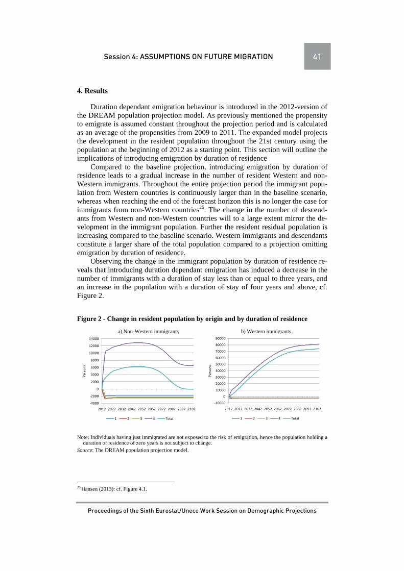
Session 4: ASSUMPTIONS ON FUTURE MIGRATION 41
Proceedings of the Sixth Eurostat/Unece Work Session on Demographic Projections
4. Results
Duration dependant emigration behaviour is introduced in the 2012-version of the DREAM population projection model. As previously mentioned the propensity to emigrate is assumed constant throughout the projection period and is calculated as an average of the propensities from 2009 to 2011. The expanded model projects the development in the resident population throughout the 21st century using the population at the beginning of 2012 as a starting point. This section will outline the implications of introducing emigration by duration of residence
Compared to the baseline projection, introducing emigration by duration of residence leads to a gradual increase in the number of resident Western and non-Western immigrants. Throughout the entire projection period the immigrant popu-lation from Western countries is continuously larger than in the baseline scenario, whereas when reaching the end of the forecast horizon this is no longer the case for immigrants from non-Western countries26. The change in the number of descend-ants from Western and non-Western countries will to a large extent mirror the de-velopment in the immigrant population. Further the resident residual population is increasing compared to the baseline scenario. Western immigrants and descendants constitute a larger share of the total population compared to a projection omitting emigration by duration of residence.
Observing the change in the immigrant population by duration of residence re-veals that introducing duration dependant emigration has induced a decrease in the number of immigrants with a duration of stay less than or equal to three years, and an increase in the population with a duration of stay of four years and above, cf. Figure 2.
Figure 2 - Change in resident population by origin and by duration of residence
a) Non-Western immigrants b) Western immigrants
Note: Individuals having just immigrated are not exposed to the risk of emigration, hence the population holding a
duration of residence of zero years is not subject to change. Source: The DREAM population projection model.
26 Hansen (2013): cf. Figure 4.1.
‐4000
‐2000
0
2000
4000
6000
8000
10000
12000
14000
2012 2022 2032 2042 2052 2062 2072 2082 2092 2102
Persons
1 2 3 4 Total
‐10000
0
10000
20000
30000
40000
50000
60000
70000
80000
90000
2012 2022 2032 2042 2052 2062 2072 2082 2092 2102
Persons
1 2 3 4 Total

42 Session 4: ASSUMPTIONS ON FUTURE MIGRATION
Proceedings of the Sixth Eurostat/Unece Work Session on Demographic Projections
This development is explained by the relationship between two effects: the di-rect effect and the dynamic effect. The direct effect is a composition effect which is defined as the effect obtained by combining the emigration propensities by dura-tion of residence with exposure to risk by duration of residence. Since the share of immigrants in the initial population holding a long duration of residence is by far the largest, introducing emigration by duration of residence will lead to an overall decrease in emigration, hence an increase in the resident immigrant population. This is subject to the assumption of a constant annual level of future gross immi-gration. The effect of a higher propensity to emigrate from the immigrant groups with short residencies is therefore dominated by the fact that the largest share of the immigrant population is facing a decrease in the propensity to emigrate.
Whether composition effects will lead to an increase or decrease in total emi-gration might vary between age groups depending on the distribution on duration of residence within the age group. If re-emigration from population groups with short residencies increases more in absolute terms than emigration from long resi-dencies, the total population is immediately reduced. Implicitly the number of resi-dent immigrants subject to future emigration in old age groups are reduced, hence reducing the direct effect of lower than average emigration propensities for long residencies in the future. If the decrease in emigration from long residencies domi-nates within an age group, the total population increase will potentially enhance the composition effect within old age groups in the future. I.e. dynamic effects can ei-ther increase or decrease the impact of future composition effects.
The change in both the Western and non-Western immigrant population results from the interaction between the direct and the dynamic effect. The interaction changes over time hereby explaining the differences in the nature of change in long residencies between Western and non-Western immigrants. In order to aid compre-hension of the latter, age profiles of the changes in Figure 2. a and Figure 2.b can be extracted for selected forecast years. From these profiles it becomes evident that the nature of the change in the immigrant population compared to the baseline sce-nario can be explained by a shift in the distribution of the change on age and dura-tion of residence over time. For brevity, a detailed description of these dynamics has been omitted in this paper, but are available in section 4 of Hansen (2013).
5. Assessing forecast accuracy
By performing a sequence of within-data population projections with a 5-year forecast horizon, it is established whether introducing emigration by duration of residence enhances forecast accuracy. Following the approach from above, emigra-tion propensities respectively including and omitting duration of residence are cal-culated from a three-year average of the propensities prior to the starting point of each projection. Other demographic events are estimated by using the actual rates or propensities. Note especially that gross immigration to the population groups consisting of non-Western and Western immigrants with a foreign citizenship is exogenous and hence reflects the increase in annual inflows during the recent dec-ade. Data on emigration ranges from 1992-2011, hence the starting point of the first projection is the resident population by gender, age, origin, and duration of

Session 4: ASSUMPTIONS ON FUTURE MIGRATION 43
Proceedings of the Sixth Eurostat/Unece Work Session on Demographic Projections
residence in the year of 1995. By estimating emigration propensities as an average of 1992-1994, the number of emigrants are projected for the years of 1995-1999 and the absolute difference between actual and forecasted emigration is used to as-sess forecast accuracy. Based on the population in 1996 and an average of the emi-gration propensities from 1993-1995, emigration is subsequently forecasted until the year 2000. By repeating this procedure annually through the starting year 2007, a total of 13 within-data projections are obtained for each assumption on emigra-tion behaviour.
The result of the multiple forecasts is ambiguous since not uniquely identify-ing whether or not duration of residence should be considered when modelling em-igration behaviour. For non-Western immigrants the dominant approach varies by projection starting year. For Western immigrants including emigration by duration of residence will almost consistently lead to the largest deviance from actual emi-gration
Forecasted emigration from the population of non-Western immigrants typi-cally undershoot the actual emigration, whereas forecasted re-emigration from Western immigrants is typically overshooting the actual levels. This pattern of de-viance is qualitatively identical within the projections respectively including and omitting emigration by duration of residence. In general this indicates that using a three-year average of the emigration propensities prior to the projection starting year induces poor forecast performance when changes in emigration behaviour oc-cur within the forecast horizon. Since the emigration propensities have been in-creasing for non-Western immigrants, undershooting the actual immigration is a comprehensible consequence of estimating emigration behaviour by a three-year average of the propensities prior to the projection starting year. The decrease in Western emigration propensities during the recent decade explains that overshoot-ing is prevalent for this origin group.
The direct effect, i.e. the composition effect, aids explaining why using emi-gration propensities by duration of residence, will lead to a larger forecast inaccu-racy than when using identical emigration behaviour across residencies. The in-crease in annual immigration contribute to an increasing share of immigrants hold-ing short residencies. Using constant emigration propensities by duration of resi-dence is then likely to result in an increase in emigration because of composition effects regarding duration of residence. Such effects are absent when using the baseline assumptions, thus reducing the effect of over- or undershooting.
6. Conclusion
During the recent decade changes in the composition of the resident immigrant population across duration of residence is largely attributable to changes in annual immigration quantities and changes in immigrant behaviour. Previous studies link-ing resident permit status with duration of residence, suggest that the former is an important source when explaining changes in immigrant behaviour, and hence changes in the distribution of the immigrant population on short and long term res-idencies.

44 Session 4: ASSUMPTIONS ON FUTURE MIGRATION
Proceedings of the Sixth Eurostat/Unece Work Session on Demographic Projections
Recognizing that emigration behaviour varies across duration of residence, motivates that introducing this characteristic when forecasting emigration will eliminate some of the variation in emigration patterns not already accredited to gender, age, and origin.
Initially the consequences of introducing emigration by duration of residence in the baseline model was investigated. Under the assumption of constant exogenous annual immigration and constant re-emigration propensities, composition effects inducing a decrease in the average emigration propensity lead to an increase in the immigrant population. Using duration dependant emigration propensities further causes a change in the age distribution of immigrants, subsequently resulting in a change in the size of the descendant population.
A series of within-data projections respectively omitting and including duration dependant emigration were conducted in order to establish whether emigration by duration of residence, will improve forecast accuracy. However, partly due to the presence of changing emigration behaviour within each category of duration of residence, the historical development in emigration patterns cannot entirely be dedicated to composition effects obtained by combining the resident population by duration of residence with constant emigration behaviour by duration of residence. Applying emigration by duration of residence is then more likely to over- or undershoot actual emigration than baseline emigration behaviour. This suggests that emigration by duration of residence should be applied with caution if expecting behavioural changes within population groups characterized by gender, age, origin and duration of residence.
Alternatively the subject of assessing forecast accuracy could have been approached by statistically validating the performance of the projection models respectively including and omitting emigration by duration of residence. Further it can be verified if the use of additional covariates describing the decision to emigrate enhances model performance. Subjecting the baseline assumptions to various competing approaches is reserved to further studies27. Data mining techniques can aid extending the use of duration dependency to other demographic flows besides emigration. This is also an appropriate subject for future studies.
REFERENCES
Hansen, M. F. (2013): Introducing duration dependant emigration in the DREAM population projection model, DREAM working paper 2013:3 (unabridged version), September 2013.
27 Competing approaches used to estimate emigrate propensities could potentially comprise classification models,
logit and probit models.

Session 4: ASSUMPTIONS ON FUTURE MIGRATION 45
Proceedings of the Sixth Eurostat/Unece Work Session on Demographic Projections
Hansen, M. F. & Stephensen, P. (2012): Danmarks fremtidige befolkning - Befolkningsfremskrivning 2011. Report, March 2012.
Statistics Denmark (Denmarks Statistik) (2008,2011): Indvandrere i Danmark 2008/2011, December 2008/2011.

46 Session 4: ASSUMPTIONS ON FUTURE MIGRATION
Proceedings of the Sixth Eurostat/Unece Work Session on Demographic Projections
MODEL TO FORECAST THE RE-IMMIGRATION OF SWEDISH-BORN BY BACKGROUND
Andreas Raneke Summary
The immigration and emigration in Statistics Sweden’s national population projection are projected for seven birth-groups, of which Swedish-born constitutes one. To estimate the future re-immigration of Swedish-born, a population living abroad are created by adding emigrated persons and subtracting re-immigrants. This population are then used in a linear regression model applied to re-immigration rates and information about emigration three years earlier to project the re-immigration. The model does not consider the background of the Swedish-born living abroad, i.e. their parents country of birth. In the present model for the future re-immigration, irrespective of their background, all Swedish-born have the same propensity to re-immigrate. Since the estimations of re-immigrants have been biased in the latest projection is it useful to see if there are any diversities in re-immigration depending on the parents background. The aim of this study is to further develop the model that predicts the re-immigration of Swedish-born. Parents country of birth are added to the population living abroad and re-immigration rates are estimated for Swedish born with; two Swedish-born parents, two foreign born parents and one Swedish-born and one foreign born parent. The results shows that Swedish-born with two Swedish-born parents have the lowest rate to emigrate and the highest rate for return immigration. This leads to a slowly increasing number of emigrants and also an increasing re-immigration. Swedish-born with two foreign born parents have the highest propensity to emigrate but doesn’t return to Sweden in the same extend as those with two Swedish-born parents. This leads to an increasing number of persons with two foreign born parents living abroad. However, compared to the latest population projection, including parents background doesn't give any considerable differences in re-immigration during the projected period. Therefore it might not be necessary to include this information in the population projection.
Keywords: Return migration, regression.
1. Background
Fluctuations in immigration and emigration to and from Sweden have been significant in recent decades. Labour migrants, especially from Finland and Yugoslavia, dominated both the immigration and emigration throughout the 1970s. In the 1980s and the 1990s, an increasing number of refugees and asylum seekers

Session 4: ASSUMPTIONS ON FUTURE MIGRATION 47
Proceedings of the Sixth Eurostat/Unece Work Session on Demographic Projections
migrated to Sweden due to conflicts or political troubles in their home countries and it peaked in 1994 with people seeking protection from the wars of the former Yugoslavia. Emigration increased during the financial crisis in the 1990s and since the turn of the millennium, the migration to and from Sweden has continued to be high. Migration due to labour, refugees, family reunifications and from EU’s new member states are some reasons for the latest years high numbers. Another reason is the increasing migration of Swedish-born. The emigration of Swedish-born improved throughout the 1990s during the financial crisis and even if it decreased some during the first half of the 21st century, it is still on a relative high level with about 20 000 Swedish-born emigrants each year. The number of emigrants in 2012 were the highest ever with about 51 700 persons and of which Swedish-born constituted about 40 percent.
Figure 1 – Immigration and emigration, total and Swedish-born, 1970-2012
Statistics Sweden do annual national population projections based on analysis
on births, deaths and immigration and emigration by seven different birth country groups were Swedish-born are one. For Swedish-born, first the future emigration is projected which makes it possible to estimate the return immigration. The number of people who emigrates are estimated by age- and sex-specific emigrations rates. Since emigration differs between Swedish-born persons with different background, i.e. parents country of birth, emigration rates are divided into three groups; both parents are Swedish-born, foreign born or if one parent is foreign born and the other is Swedish-born. As could be seen in figure 2 below, persons with two parents born in another country have the highest emigration rate followed by those with one Swedish-born parent and one foreign born parent.
0
20 000
40 000
60 000
80 000
100 000
120 000
1970 1973 1976 1979 1982 1985 1988 1991 1994 1997 2000 2003 2006 2009 2012Total immigrationImmigation Swedish-bornTotal emigrationEmigration Swedish-born

48 Session 4: ASSUMPTIONS ON FUTURE MIGRATION
Proceedings of the Sixth Eurostat/Unece Work Session on Demographic Projections
Figure 2 – Emigration rates for Swedish-born aged 0-70 by background, average for 2003-2012
Assumption are made about the proportions of Swedish-born by parents country of birth and the emigration rates are weighted to emigration rates for the whole group of Swedish-born. The rates are then used in the population projection.
When it comes to re-immigration of Swedish-born in the population projection, we use a model that first estimates a re-immigrant rate, applies this to a population of Swedish-born living abroad and then adjust the number of re-immigrants with a regression model based on the emigration three years earlier. This study is based on earlier work at Statistics Sweden were no assumptions have been made on the re-immigrants background (Statistics Sweden, 2009). But we have recently been able to see that the rates for re-immigration differs depending on the parents background and this particularly applies to children. For example, the re-immigration of children was a large bias in the latest national population projection. Therefore, the aim of this study is to investigate whether parents background should be taken into consideration when estimating the future re-immigration of Swedish-born.
1.1 Data and method Two administrative registers from Statistics Sweden has been used in this
study. Flows of emigration and immigration has been collected from the Register of the Total Population. Data on parents country of birth has been derived from the Multi-Generation Register, a register were information about parents is available since 1969 and for persons born 1932 or after. When information about parents are missing, we assume that they have two Swedish-born parents. This mostly applies to persons born earlier than 1932. To be an emigrant, you need to have the intension to stay at least one year abroad and have reported it to the National Tax Board.
There is no comprehensive register of Swedish-born living abroad. The Swedish Pension Agency has information on persons who live abroad and who had an income in Sweden. But this information does not include those who have not
0
5
10
15
20
25
30
35
40
0 2 4 6 8 10 12 14 16 18 20 22 24 26 28 30 32 34 36 38 40 42 44 46 48 50 52 54 56 58 60 62 64 66 68 702 foreign born parents
1 Swedish-born parent
2 Swedish-born parents
Per 1 000

Session 4: ASSUMPTIONS ON FUTURE MIGRATION 49
Proceedings of the Sixth Eurostat/Unece Work Session on Demographic Projections
had an income in Sweden, such as those who emigrate at a young age. The Nation-National Tax Board has information on Swedish citizens living in another country. This information is nevertheless saved for ten years. To estimate the number of Swedish-born that are living in another country we use information about immigration and emigration from our registers. The proportion of emigrants of Swedish-born with either two Swedish-born parents, two foreign born parents or one Swedish-born parent has then been applied on each year’s number of emigrants. The estimated number of Swedish-born abroad is then calculated as:
SB E I SB 1 q
where,
E is the number of emigrants at year t
I is the number of immigrants at year t
q is the death-risks at year t
For those aged 0, SB E
Death risks are the same as for all persons living in Sweden, even if there could be a selection effect for those who migrates. The age- and sex-specific death risks are also assumed to be the same whether the parents country of birth. Since there are very few migrants aged 70 and older, this study only include persons younger than that. Information about the number of persons living abroad is then used to estimate a 5 year average age- and sex-specific re-immigration rate for each of the three groups:
R∑ I∑ M
where,
I is the number of Swedish-born immigrants at year t
M is the mean population of Swedish-born living abroad at year t
For those aged 0 and 1, R 0
1.2 Model for return immigration of Swedish-born As seen in figure 3 below, the estimation of immigration does not follow the
observed development when using only re-immigrant rates. However, the figure also shows a pattern that re-immigration follows the emigration with a delay of three years. For example the increased emigration in the mid-1980s were followed by an increase of re-immigrants a few years later and the downturn in emigration in 1989 were followed by a decrease in 1991. Instead a linear regression model where immigration estimated by re-immigration rates combined with information on

50 Session 4: ASSUMPTIONS ON FUTURE MIGRATION
Proceedings of the Sixth Eurostat/Unece Work Session on Demographic Projections
emigration three years earlier is used to adjust the re-immigration28. The regression estimates are given by:
I 3882 0,69 ∙ I 0,42 ∙ E
where, I R ∙ SB
Figure 3 – Observed emigration and re-immigration and rate based re-immigration and regression based immigration, 1990-2012
1.3 Results The emigration of Swedish-born with two Swedish-born parents increased
rapidly during the financial crisis in the mid-1990s and continued to be at a high level during the 2000s. Swedish-born with two foreign born parents and one Swedish-born parent has also somewhat experienced an increase during the same period. Results from the model gives a firm increase for all groups and an emigration of more than 16 000 persons with two Swedish-born parents at year 2060. Similar could be seen for the two other groups with an emigration of nearly 7 000 Swedish-born with two foreign born parents and around 4 800 Swedish-born with one Swedish-born parent at the end of the period.
28 R2=0,79 when based on the period 1999 – 2012
0
5 000
10 000
15 000
20 000
25 000
1990 1992 1994 1996 1998 2000 2002 2004 2006 2008 2010 2012Rate-based re-immigrationObserved re-immigrationRegression based re-immigration (1999-2012)Observed emigration

Session 4: ASSUMPTIONS ON FUTURE MIGRATION 51
Proceedings of the Sixth Eurostat/Unece Work Session on Demographic Projections
Figure 4 – Emigration of Swedish-born aged 0-70 by background 1970-2012 and projection 2013-2060
As shown in figure 5 below, about 220 000 Swedish-born persons were estimated to live in another country at year 2012. The largest group, persons with two Swedish-born parents, constitutes about half of the population. The second largest group is of persons with two foreign born parents. All three groups increases until the first years of 2030s when the number of Swedish-born with two Swedish-born parents decreases and finally stabilizes around 120 000 persons until the end of the projection. The number of persons with two foreign born parents continues to increase during the whole period, leading them to exceed the numbers of persons with two Swedish-born parents in the late 2020s. The estimated number of persons with two foreign born parents living in another country in 2060 is nearly 165 000. The number of persons with one Swedish-born parent living abroad is about 80 000 at the end of the forecast period.
Figure 5 – Estimated Swedish-born aged 0-70 living abroad by background 2000-2012 and projection 2013-2060
0
2 000
4 000
6 000
8 000
10 000
12 000
14 000
16 000
18 000
1970 1975 1980 1985 1990 1995 2000 2005 2010 2015 2020 2025 2030 2035 2040 2045 2050 2055 20602 foreign born parents
1 Swedish-born parent
2 Swedish-born parents
0
20 000
40 000
60 000
80 000
100 000
120 000
140 000
160 000
180 000
2000 2010 2020 2030 2040 2050 20602 foreign born parents
1 Swedish-born parent
2 Swedish-born parents

52 Session 4: ASSUMPTIONS ON FUTURE MIGRATION
Proceedings of the Sixth Eurostat/Unece Work Session on Demographic Projections
The rates for re-immigration are different depending on parents country of birth. Persons with two foreign born parents are least likely to return to Sweden after emigration. The highest tendency to return to Sweden have persons with two Swedish-born parents with a peak for persons in their early twenties where about half of the population re-immigrates. The structure of the age-specific rates for persons with one foreign born parent are similar but not as high as the rates for person with two Swedish-born parents.
Figure 6 – Re-immigration rates for Swedish-born aged 0-70 by background, 2008-2012
The rapid rise of emigrants with two Swedish-born persons in the mid-1990s
led to a subsequent increase of re-immigrants, shown in figure 5. The high numbers of returning persons with two Swedish-born parents will continue to increase during the forecast period with about 15 000 persons returning at year 2060. The long-term increase in the estimated number of persons re-immigrating is due to the number of Swedish-born persons abroad grows according to the calculations. Even though there is a large number of estimated persons with two foreign born parents living abroad, the relative low rates for return immigration means that a low number decides to return to Sweden.
0
10
20
30
40
50
60
0 10 20 30 40 50 60 702 foreign born parents
1 Swedish-born parent
2 Swedish-born parents
Per 100
Age

Session 4: ASSUMPTIONS ON FUTURE MIGRATION 53
Proceedings of the Sixth Eurostat/Unece Work Session on Demographic Projections
Figure 7 – Re-immigration of Swedish-born aged 0-70 by background 1970-2012 and projection 2013-2060
When comparing the projection of return immigrants based on a model which includes parents background and the latest official projection (Statistics Sweden, 2013), the re-immigration is about the same for the first 20 years. After 2030, the estimated number of re-immigrants given by this study’s results are not increasing at the same pace as the official projection leading to about 1 000 less re-immigrants per year at the end of the period.
Figure 8 – Re-immigration of Swedish-born aged 0-70 by background 1970-2012 and projection 2013-2060
0
2 000
4 000
6 000
8 000
10 000
12 000
14 000
16 000
1970 1980 1990 2000 2010 2020 2030 2040 2050 20602 foreign born parents
1 Swedish-born parent
2 Swedish-born parents
0
5 000
10 000
15 000
20 000
25 000
2000 2010 2020 2030 2040 2050 2060
Re-immigration, consideration is not taken to background
Re-immigration, consideration is taken to background

54 Session 4: ASSUMPTIONS ON FUTURE MIGRATION
Proceedings of the Sixth Eurostat/Unece Work Session on Demographic Projections
1.4 Concluding comments By looking at parents country of birth there’s different behaviour in re-
immigration for Swedish-born persons. Those with two foreign born parents are the most eager to leave the country and returns to Sweden in the least extend. This leads to an increasing number of Swedish-born with two foreign born parents living abroad. Emigrating persons with two Swedish-born parents are by far the largest group which leads them to consist a major proportion of all Swedish-born living abroad. Although since this group have high rates of return immigration, a large number is also returning to Sweden. A development that leads to that the number of persons living in another country with two foreign born parents exceeds those with two Swedish-born parents during the projected period. Compared to Statistics Sweden’s population projection, the results from this study are about the same until the 2030s and after that, there’s only a smaller difference between the two projections. This shows that including the variable parents country of birth is not necessary when projecting the future re-immigration of Swedish-born.
REFERENCES
Statistics Sweden (2009), Model to forecast the re-immigration of Swedish-born, Background material about demography, children and family 2009:1
Statistics Sweden (2013), The future population of Sweden 2013 – 2060.

Session 4: ASSUMPTIONS ON FUTURE MIGRATION 55
Proceedings of the Sixth Eurostat/Unece Work Session on Demographic Projections
DYNAMICAL MODELS FOR MIGRATION PROJECTIONS
Violeta Calian Summary
The goal of this paper is to model and forecast migration during unstable economical conditions, based on auto-correlated and non-stationary time series data and to provide reliable uncertainty control. We use dynamical, or auto-regressive distributed lag (ARDL) models as a solution to this problem. The dependent variable at time “t” is modelled as a function of its own values at different time lags and of the values of several simultaneous or lagged predictor variables. We have obtained short time predictions for the number of immigrants/emigrants of Icelandic and foreign citizenships as functions of several time series predictors: unemployment, change in GDP values, number of graduating students and dummy variables mirroring the EEA resizing in time and the Icelandic economic boom which ended in 2008. The time series we used for fitting the models are about 45 year time steps long and we produced a forecast for the next 5 years in 2011, 2012 and 2013. The results are a good fit to the true values, even as point estimates, although our confidence intervals are rather large. Keywords: forecasting, migration, time series, dynamical models.
1. Introduction
Migration forecasting is an important part of population projections and may also have a significant impact on economical decision making. Statistics Iceland, as most statistical offices, has traditionally reported predictions for medium and low / high variants of migration flows, based on deterministic models. These models had always involved economic and social variables, but did not take into account the time series properties of the data and did not provide prediction intervals for the forecasted variants. Nor could they give reliable answers during high economic instability.
Starting with the year 2011, we have improved our methods. Based on a careful data analysis we found that, in order to be able to give valid forecasts, the main statistical problem to be solved was to deal correctly with the auto-correlated and non-stationary character of the time series data, for both the independent and dependent variables. We proved instead that these time series are first-difference stationary, making auto-regressive distributed lag (ARDL) models legitimate candidates for inference, see Pesaran (1995, 1999). This is a necessary but not sufficient condition, see Johansen (2010), for un-biased and consistent point

56 Session 4: ASSUMPTIONS ON FUTURE MIGRATION
Proceedings of the Sixth Eurostat/Unece Work Session on Demographic Projections
estimates and independent and identically distributed residuals. Choosing the structure and the order of the ARDL model by a consistent model selection criterion is a crucial step, too.
Dynamical economical models for population projections are gradually attracting some well deserved attention, as discussed for example in Brunborg (2010) and already suggested by Keilman (2002). We prove here that they can also capture the very diverse evolution of the migration components (emigrating/immigrating women/men/Icelandic/foreign citizens) under strong oscillations of the economic background and thus can be used for short term predictions.
In this paper: (i) we explain why we need to use dynamical models, (ii) what are the mathematical conditions for a reliable statistical inferrence and whether they are fulfilled by our data and models, (iii) we show how our models for all migration components are built and how they perform.
2. Data and notations
The source of migration demographic data is the Icelandic National Register, which contains information on migration events since 1961 and is updated on a continuous basis, as opposed to once a year, since 1986. As showed by Statistics Iceland in WP1 (2010) and WP2 (2010), the estimated values of migration flows are reasonably accurate, although the short term migration has an influence on the accuracy of the emigration figures. This effect is mainly due to de-registration lag effects but is well measured and stable in time. The net migration numbers are not affected by this phenomenon in a significant way.
The data concerning unemployment rates, gross domestic product and their short term forecast is provided by the department of national accounts and public finances of Statistics Iceland.
The number of graduating students and its predicted values for the next few years is provided by the department of education of Statistics Iceland.
In the next sections, we will use the following notation: , - the number of Icelandic immigrants/emigrants, men; , - the number of Icelandic immigrants/emigrants, women; , - the number of immigrants/emigrants, women of foreign citizenship; , - the number of foreign immigrants/emigrants, men, - the unemployment rate; - a measure of GDP,
, - the number of graduating students, men and women respectively; boom - a dummy variable coupled to the Icelandic economic boom, reflecting also temporary changes in the registration process; eea – a dummy variable which mirrors the re-sizing of the EEA.
All these (ten) time series of 42 years length were tested for: (i) stationarity , by using augumented Dickey-Fuller and Kwiatkowski-Philips_Schmidt_Shin (KPSS) and (ii) auto-correlation of first and higher order, by using Durbin-Watson and Breusch-Gofrey tests. We found (see figure 1 for illustration) that they are first difference stationary or I(1).

Session 4: ASSUMPTIONS ON FUTURE MIGRATION 57
Proceedings of the Sixth Eurostat/Unece Work Session on Demographic Projections
3. Statistical models and short term forecast
Statistics Iceland must provide short and long term predictions for all the 8 components of migration to , and for the net migration values, once a year.
Predicting the net migration numbers can be done in two ways: (i) by building an ARDL model for the time series which is the algebraic sum of the emigration and immigration series or (ii) by combining the results of eight ARDL models of all migration time series which enter the definition of the net migration.
The last method has the advantages that the estimates of the net migration are manifestly equal to the sum of the components‘ estimates and that it displays the widely different influence of economic evolution on the behaviour of various migration groups. But it also has the dissadvantage that the confidence intervals are rather broad and one has to expertly take into account the multiple (auto-) correlations (intra/) betweeen components. The former method has to deal only with autocorrelations and usual model parameter errors and gives narrower confidence intervals, but the values of the net migration estimates would not (in general) match the sums of components perfectly. It is most adequated when one needs only the net migration to be reported or used for further calculations.
We have built, in a consistent and parcimonious way, the following ARDL models:
~ 1 1 1 ~ 1 2 2 ~ 1 1 1 ~ 1 2 2 ~ 1
1 1 ~ 1 1 1
1
A note of caution is in order here: the interpretation and model diagnostics when using ARDL is very different
from the classical so-called static models. Collinearity, short and long term effects are key ingredients which have to be treated appropriately. One way to apply the classical notions is to transform the dynamical model into the equivalent error correction model (ECM). We actually did build both ARDL and ECM in most cases.
Our calculation of prediction intervals is correct and optimal in some sense, see Pessaran (1997), for each dynamical model to , and it required significant additional work for the net migration when not analysed as a time series on its own but as a sum of correlated time series. We have to note also that and were not modeled separately but we used instead the empirically verified correlation between men and women migration numbers and the results of models , .

58 Session 4: ASSUMPTIONS ON FUTURE MIGRATION
Proceedings of the Sixth Eurostat/Unece Work Session on Demographic Projections
Figure 1 - Regressor time series and their first order differences, displaying first difference stationarity, confirmed by Augumented Dickey-Fuller tests
We applied several tests in order to establish the goodness of fit and the
behaviour of residuals for all our models:
(i) Augumented Dickey – Fuller and KPSS tests for stationarity of residuals.
(ii) Box – Ljung and Durbin – Watson tests for autocorrelation, the latter not reliable for ARDL residuals but aplicable to individual predictor seies.
(iii) Auto-correlation function and partial auto-correlation functions calculations.
unemployment rate
Time
x4
1970 1980 1990 2000 2010
04
8
change in unemployment rate
Time
diff(
x4)
1980 1990 2000 2010
04
GDP
Time
x8
1970 1980 1990 2000 2010
4010
0
change in GDP
Time
diff(
x8)
1980 1990 2000 2010
-55
number of graduate students, women
Time
x6
1970 1980 1990 2000 2010
500
2000
change in number of graduate students, women
Time
diff(
x6)
1980 1990 2000 2010
-100
100
number of graduate students, men
Time
x5
1970 1980 1990 2000 2010
400
1200
change in number of graduate students, men
Time
diff(
x5)
1980 1990 2000 2010
-100
50

Session 4: ASSUMPTIONS ON FUTURE MIGRATION 59
Proceedings of the Sixth Eurostat/Unece Work Session on Demographic Projections
(iv) Breusch-Godfrey test for higher order serial correlation which also per-forms correctly for ARDL models.
(v) rainbow tests for the quality of fit.
(vi) standard residuals’ normality checks (q-q plots, histograms) and Jacque – Bera tests.
Figure 2 - Independent time series displaying first difference stationarity, confirmed by augumented Dickey-Fuller tests
As shown in Appendix 1, the results of the tests confirm the assumption that the models can be used for valid inference. All these tests have to be interpreted
change in number of Icelandic immigrant men
Time
diff(
y1)
1980 1990 2000 2010
-400
020
0
change in number of Icelandic emmigrant men
Time
diff(
y2)
1980 1990 2000 2010
-400
040
080
0
change in number of Icelandic immigrant women
Time
diff(
y3)
1980 1990 2000 2010
-300
-100
100
300
change in number of Icelandic emmigrant women
Time
diff(
y4)
1980 1990 2000 2010
-200
200
600
change in number of foreign immigrant women
Time
diff(
y7)
1980 1990 2000 2010
-100
00
500
change in number of foreign emmigrant women
Time
diff(
y8)
1980 1990 2000 2010
-400
020
0

60 Session 4: ASSUMPTIONS ON FUTURE MIGRATION
Proceedings of the Sixth Eurostat/Unece Work Session on Demographic Projections
with great care and flexibility, too, since most are themselves based on some mod-els and null hypotheses rejections can be caused by more than one reason.
4. Results and conclusions
The net migration is projected to be positive for the next 5 years (see Figure 4), slowly increasing if the economic factors evolve according to our forecast. The confidence intervals do not exclude zero net migration. They reflect both the model uncertainty and more ad-hoc measures of the regressor prediction errors. Our past predictions gave a good fit to the subsequently recorded values, both as point esti-mates and as degree of confidence of the prediction intervals which included the true values.
Figure 3 - Short term projections (red lines) and prediction intervals (blue lines) for the migration components
2013 2014 2015 2016 2017
1000
1500
2000
2500
time
y1
2013 2014 2015 2016 2017
1000
2000
3000
time
y2
2013 2014 2015 2016 2017
1200
1600
2000
time
y3
2013 2014 2015 2016 2017
1500
2000
2500
3000
time
y4
2013 2014 2015 2016 2017
500
1000
2000
time
y7
2013 2014 2015 2016 2017
200
600
1000
1400
time
y8

Session 4: ASSUMPTIONS ON FUTURE MIGRATION 61
Proceedings of the Sixth Eurostat/Unece Work Session on Demographic Projections
Figure 4 - Net migration numbers: predicted values (continuous lines) and prediction intervals (dash lines), for various economic scenarios (current economic forecast in red, higher GDP growth in green, lower GDP growth in blue)
The economic factors have a strong effect on the migration rates, as illustrated
by the predicted values of migration under different scenarios which are created by modifying the GDP growth values, see Figure 4.
Modelling separately the eight migration components implies that we assumed independence. This is however not the case and an ideal solution to this issue would be to use vector autoregressive distributed lag models. This in turn can be done only after a careful examination of the dimension of the problem in terms of time series lengths and number of parameters estimated on their joint distribution. Otherwise, uniquely modelling the net migration is a safer although not as com-prehensive alternative.
2013 2014 2015 2016 2017
-1000
01000
2000
time
net m
igra
tion n
um
bers

62 Session 4: ASSUMPTIONS ON FUTURE MIGRATION
Proceedings of the Sixth Eurostat/Unece Work Session on Demographic Projections
REFERENCES
Alho, J.M. (1997): Scenarios, uncertainty and conditional forecasts of the world population, Journal of Royal Statistical Society A 160, Part 1, 71-85. Brunborg, H. And Cappelen, A. (2010): Forecasting migration flows to and from Norway using an economic model, Joint Eurostat/UNECE work session on demographic projections, Lisbon, Portugal, 28-20 April 2010. Johansen, S. (1996): Likelihood-based inference in cointegrated vector autoregressive models, Oxford University Press, Oxford. Johansen, S. (2010): The analysis of nonstationary time series using regression, correlation ans cointegration with an application to annual mean temperature and sea level, Discussion Papers, no.10-27, Department of economics, University of Copenhagen. Keilman, N., Pham, D. Q., Hetland, A. (2002): Why population forecasts should be probabilistic - illustrated by the case of Norway, Demographic Research, Vol. 6, Article 15. Pesaran, M. H. (1999): An autoregressive distributed lag modelling approach to cointegration analysis, Symposyum of the Norwegian Academy of Science and Letters, Oslo, 3-5 March 1995, and DAE Working Paper Series No. 9514. Department of Econometrics, University of Cambridge, 1999. Pesaran, M.H., Shin, Y. and Smith, R.J. (1996): Testing the existence of long-run relationships, DAE Working Paper Series No. 9622, Department of Econometrics, University ofCambridge. Pesaran, M.H., Shin, Y. and Smith, R.J. (2001): Bounds testing approaches to the analysis of level relationships, J. Applied Econometrics, 16: 289-326. WP1 Statistics Iceland (2010): Hardarson, O., Long-term and short term migration in Iceland - Analysis of estimation methods of Statistics Iceland, Working paper 13 at the Joint UNECE/Eurostat Expert Group Meeting on Register-Based Censuses, The Hague, The Netherlands, 10-11 May 2010. WP2 Statistics Iceland (2010): Hardarson, O., The population statistics in Iceland - Analysis of population estimation methods of Statistics Iceland, Working paper 6 at the Joint UNECE/Eurostat Expert Group Meeting on Register-Based Censuses, The Hague, The Netherlands, 10-11 May 2010. Figures and appendix:

Session 4: ASSUMPTIONS ON FUTURE MIGRATION 63
Proceedings of the Sixth Eurostat/Unece Work Session on Demographic Projections
Appendix 1: Models‘ goodness of fit and behaviour of residuals
A) Stationarity of residuals: the KPSS tests do not reject the hypothesis of stationarity of residuals‘ distributions for any of our models (all p-values greater than 0.1). Supporting this conclusion, augumented Dickey-Fuller tests reject non-stationarity (all p-values smaller than 0.01)
B) Normality of residuals: Jacques-Bera tests do not reject normality for any of the model residuals‘ distributions. The p – values of the tests are greater than 0.08 and reflect extremely well the general aspect of the empirircal distributions (histograms not shown).
C) Autocorrelation of residuals: Box-Ljung tests do not reject the hypothesis of random residuals. Same conclusion is supported by the direct calculation of autocorrelation for residuals shown in Figure A-1:
Figure A-1 - Values of residuals‘ autocorrelation of the economic models
0 5 10 15
-0.2
0.2
0.6
1.0
Lag
AC
F
residuals of model 1
0 5 10 15
-0.2
0.2
0.6
1.0
Lag
AC
F
residuals of model 2
0 5 10 15
-0.2
0.2
0.6
1.0
Lag
AC
F
residuals of model 3
0 5 10 15
-0.2
0.2
0.6
1.0
Lag
AC
F
residuals of model 4
0 5 10 15
-0.2
0.2
0.6
1.0
Lag
AC
F
residuals of model 7
0 5 10 15
-0.2
0.2
0.6
1.0
Lag
AC
F
residuals of model 8

64 Session 4: ASSUMPTIONS ON FUTURE MIGRATION
Proceedings of the Sixth Eurostat/Unece Work Session on Demographic Projections
D) Goodness of fit: rainbow tests imply that we can not reject any of our models.
Figure A-2 - Migration components: true (dots) and model estimated (continuous red lines) values, confidence intervals (continuous lines)
1980 1990 2000 2010
500
1000
1500
time
y1
1980 1990 2000 201050
015
0025
00
time
y2
1980 1990 2000 2010
500
1000
1500
time
y3
1980 1990 2000 2010
500
1000
2000
time
y4
1980 1990 2000 2010
050
015
0025
00
time
y7
1980 1990 2000 2010
050
010
0015
0020
00
time
y8

Session 5
ASSUMPTIONSON FUTURE MORTALITY
Chair: Graziella Caselli (University of Rome “Sapienza”)


Session 5: ASSUMPTIONS ON FUTURE MORTALITY 67
Proceedings of the Sixth Eurostat/Unece Work Session on Demographic Projections
CHANGING MORTALITY TRENDS BY AGE AND SEX
ARE CHALLENGES FOR ASSUMPTIONS ON FUTURE
MORTALITY
Örjan Hemström
Summary
Trend shifts in recent mortality in relation to age and sex are challenges to the Lee–Carter (LC)-model as well as to other extrapolative models with an aim to forecast mortality. An important question is how to interpret and evaluate such shifts for the fu-ture. It has previously been shown that mortality in the latter half of the 20th century declined somewhat faster at older relative to younger ages than in the first half of the 20th century. Has this development continued further? The development of Swedish mortality in the period 1975–2011 was analyzed by means of various sex-specific LC-models using base-periods of varying length. For comparison, simple sex and age-specific trend calculations were performed. Results suggest that the LC-model is suita-ble in forecasting Swedish women’s mortality but not as suitable for men’s mortality. The predicted mortality change in men differed by length of the base-period, in par-ticular at ages 65 years and over. Close inspection of older men’s mortality shows that mortality has declined at an increasing rate in older age groups. Such shifts makes it difficult to forecast men’s mortality only on the basis of past trends. Findings also sug-gest that LC-models incorporating all ages 0–100 years tend to underestimate the mor-tality decline in age groups 50 and older as compared with simple age-specific trend calculations. Keywords: mortality trends, forecast, Sweden, sex differences
1. Introduction
This paper summarizes some of the analyses that was performed regarding mortality prior to the population projection for Sweden in 2012 (Statistics Sweden, 2012).
Life expectancy in Sweden has increased by about 35 years during the period 1861–2011, from 49 to nearly 84 years for women and from 45 to nearly 80 years for men, as shown in Figure 1. Life expectancy has increased on average by about 2.5 years per decade since 1900. However, the increase was larger up until the mid-

68 Session 5: ASSUMPTIONS ON FUTURE MORTALITY
Proceedings of the Sixth Eurostat/Unece Work Session on Demographic Projections
20th century than it was afterwards. The changes are not unique for Sweden and has been observed in a number of other countries (Ahlbom, Drefahl, & Lundström, 2010).
Women have had a more unbroken increase of life expectancy than men. Life expectancy at age 65 increased for instance about as much for women and men during the entire period 1861–1950. From the 1950s onwards, life expectancy of women from age 65 began to increase at a faster rate than earlier. The same clear increase from age 65 for men was not observed until the 1980s, that is, three dec-ades later than for women.
Figure 1 – Sex-specific life expectancy at birth, 50, 65, 75 and 85 years 1861–2011
Source: Statistics Sweden
Since the end of the 1970s life expectancy has increased more for men than for women. However, this does not mean that the life expectancy for women has stag-nated in the same way as it did for men during the period 1950–1980. Since the 1950s life expectancy for women has increased by between 0.6 and 1.2 years per five-year period. Between the most recent two five-year periods, 2001–2005 to 2006–2010, the increase for women was 0.8 years. This was near the average in-crease of 0.9 years per five-year period for the entire period 1951–2010 (Statistics Sweden, 2011). The corresponding increase on average for men was 0.8 years per five-year period.
As seen in Figure 2, mortality have declined for women and men for all ages during recent decades. Minor changes have occurred in the age pattern of mortality for certain ages. The mortality rates in men are in principle the same for an age in-terval of about 20–40 years of age. In the 1980s mortality was clearly higher among men in their 40s than men in their 20s.
0
10
20
30
40
50
60
70
80
90
1860 1880 1900 1920 1940 1960 1980 2000
Women
Men
At birth
50 years
65 years
75 years
85 years
Years

Session 5: ASSUMPTIONS ON FUTURE MORTALITY 69
Proceedings of the Sixth Eurostat/Unece Work Session on Demographic Projections
When projecting future mortality it is important to consider the changing ages at death. Assumptions of future mortality is most important for those ages where the largest number of deaths occur. In the period 2006–2010 only 1.5 percent of the deaths among women, and 2.6 percent of the deaths among men, occurred in the age interval 0–44 years.
Figure 2 – Mortality rate by sex and age for the periods 1984–1986 and 2009–2011
Logarithmic scale. The information refers to annual average values in both periods for one-year age groups. Age at the end of the year
2. Analysis of the mortality trends by age and sex
There are a number of different ways to forecast mortality. Extrapolative methods, such as the one suggested by Lee and Carter (LC), has been widely used in recent years (Lee & Carter, 1992). Evaluations of the mortality development during the 20th century suggest that the LC-model satisfactorily predicts future gains in life expectancy. Key assumptions of the LC-model are constant age de-pendency to the predicted general mortality change. The LC-model is therefore conditioned upon rather smooth mortality changes and relatively homogenous time trends across age groups.
From 2003 onwards Statistics Sweden has partly used outcomes from the LC-model in the population projections. In the forecasts of 2003 (Statistics Sweden, 2003), 2006 (Statistics Sweden, 2006) and 2009 (Statistics Sweden, 2009) howev-er, the results of the estimations of the model have not been allowed to be used dur-ing the entire forecast period. This paper summarizes some of the analyses that was performed regarding mortality prior to the population projection for Sweden in 2012 (Statistics Sweden, 2012).
A critical viewpoint of the LC-model, as well as other extrapolative methods, is that if a break in the trend occurs over time, the result of the model could be mis-leading for the ages that have had such a break in the trend. It is particularly im-
0.01
0.1
1
10
100
1000
0 20 40 60 80 100
1984–1986
2009–2011
MenDeaths per 1 000
0.01
0.1
1
10
100
1000
0 20 40 60 80 100
1984–1986
2009–2011
WomenDeaths per 1 000

70 Session 5: ASSUMPTIONS ON FUTURE MORTALITY
Proceedings of the Sixth Eurostat/Unece Work Session on Demographic Projections
portant to consider any changes in the speed of the mortality changes in different ages. Such changes have occurred since the beginning of the 20th century and mor-tality reduction has been about the same, about 2 percent per year, for an extended age interval, about 15–80 years, in several countries (Lee & Miller, 2000). If for instance mortality declines more among older people than among younger people at the end of a base period, the mortality decline of the future can be underestimated. This may be a reason that mortality forecasts based on the Lee-Carter model with long base periods tend to somewhat underestimate the mortality decline in the long term. A smaller underestimation of the mortality decline has been evaluated (Lee & Miller, 2000).
When men and women have had different trends in mortality in recent years, it has been observed that the model has led to increased sex differences in mortality and not decreases (Lee, 2000). Such a result would also be the effect of using a long historical base period for Sweden. The last 25 years has been proposed as a suitably long base period to capture the different trends of a mortality decline for women and men (Lundström & Qvist, 2004).
In the analyses in relation to the population forecast for Sweden in 2012, the development of Swedish mortality in the period 1975–2011 was analyzed by means of various sex-specific LC-models using base-periods of varying length, but also compared with simple trend calculations separate by age and sex (Statistics Sweden 2012).
The parameters of the LC-model are estimated with an original matrix of mor-tality rates per age, sex and time. The model uses a logarithm of mortality rates per sex, age and time. The following expression describes the model according to Lee and Carter:
txtxxtx kbam ,, )ln( ,
xa = age-specific average level of mortality
xb = age-specific weight for trends over time
tk = trends over time in the mortality rate
tx , = random terms
The effects of age and time, xb and tk , are estimated using ”singular value de-
composition” (SVD) for men and women. To compare the different results of the Lee-Carter models, a simplified method
was also used to estimate mortality trends at different ages. This if often called trend estimation with the empirical intensity of mortality (Olsén, 2005). The mor-tality rate for an age category is then compared with a starting year i and a finishing
year j. The average annual change xc , was calculated as follows:
1)/(1 ij
ix
jx
xc
The annual average values are used in the calculation for a period of three years to avoid the random error that can easy be the result of only using one start-

Session 5: ASSUMPTIONS ON FUTURE MORTALITY 71
Proceedings of the Sixth Eurostat/Unece Work Session on Demographic Projections
ing and one finishing year. The notation i and j in the above expression thus stand for an annual average for a short period. The difference between j and i is the num-ber of years between the starting period and the finishing period. The rate of
change xc gives the relative change in mortality per year for each age category for
1–99 years. The age categories that are used are 1–4 years and five-year age groups starting with 5–9 years up until 95–99 years.
3. Results
The assumptions about future changes in mortality are mainly based on mor-tality trends from the 1970s up until 2011. The period that comprises the main ob-servation period (base period) is 1985–2011, that is, about that which was previ-ously proposed as a suitably long period to estimate the partially different mortality trends for men and women since the beginning of the 1980s.
Different estimations of annual mortality rates based on trend analyses for the period 1985–2011 consistently show negative values (Figure 3). The rates of change can therefore be seen as reduction rates.
Figure 3 – Percentage annual change in mortality rates by sex and age with three different estimations 1985–2011
For trend estimation with five-year age groups, the annual average values for mortality rates 1984–1986 and
2009–2011 have been used as start and end points.
Figure 3 shows the smoothing reduction rates over the ages that are the result of the Lee-Carter calculation, but significant swings in ages less than 50 years. For men up to age 50, the simple trend estimation gives nearly identical reduction rates as a LC-model for ages 0–100 years. At older ages the simple trend estimation is instead completely in line with the result of a LC-model for ages 50–100 years. For women the age specific trend estimation gives greater fluctuations than the Lee-Carter model for younger women. For older women the reduction rates from the
-4.0
-3.0
-2.0
-1.0
0.0
0 10 20 30 40 50 60 70 80 90 100
Lee–Carter0–100 years
Lee– Carter50–100 years
Trend estimationfive-year age groups
Percent Women
-4.0
-3.0
-2.0
-1.0
0.0
0 10 20 30 40 50 60 70 80 90 100
Lee-Carter0–100 years
Lee–Carter50–100 years Trend estimation
five-year age groups
Percent Men

72 Session 5: ASSUMPTIONS ON FUTURE MORTALITY
Proceedings of the Sixth Eurostat/Unece Work Session on Demographic Projections
simple trend estimations follow the outcome of the LC-model for ages 50–100 years.
The LC-model for all ages (0–100 years) seems to underestimate the mortality reduction among older persons compared to the simple trend estimation. The results therefore speak for choosing the results of the LC-model for ages 50–100 years as the main alternative. It is most common to use all ages. But the results may be because the evaluations of the results of the LC-model showed a certain underestimation of mortality reduction in the long term (Lee & Miller, 2000). Up until about age 50 the trends in mortality are not stable. The results from the Lee-Carter method have therefore been concentrated to ages 50 and older, which is about the same as in the previous forecasts for Sweden of most recent years.
The number of deaths below age 50 comprise a small part of mortality and have little significance in the context of forecasts. Further, the weights for age have not been especially stable at younger ages (Lundström & Qvist, 2004). For younger ages, 0–44 years, the annual average change in mortality is used between the life tables 1996–2000 and 2006–2010. The change (mortality decline) is calculated as a total for women and men at 2 percent annually.
For women the choice of a base period 1975–2001, 1985–2011 or 1995–2011 has little significance on the mortality reduction that will be assumed in the future. For men the mortality decline at certain ages has been quicker at the end of the pe-riod 1975–2011 than at the beginning. This means that there is greater uncertainty in the mortality assumption for men than for women, especially for those aged 65 and older. The results from the base period 1985–2011 are mainly used for both sexes.
4. Changing mortality trends in older men
Mortality changes in the period 1970 (mean from 1969 to 1971) to 2010 (2009 to 2011) were analyzed by means of moving averages, and mortality changes be-tween all 10-year periods were measured. This indicate that men’s mortality reduc-tion has changed almost constantly, from small reductions to larger reductions (Figure 4). This is probably one reason why LC-models are not so suitable for ex-trapolating men’s mortality for the future. In certain age groups, such as 80 to 84 years, there has been a constant increase in the mortality decline over time, where-as in the age group 60 to 64 years this development has been halted from an annual reduction of 3 percent to 2 percent. In ages 90 to 94 and 95 to 99 trend changes fol-lowed younger age groups early in the period but a plateau phase followed until the decline increased again in the early 2000s.
There are no such trend changes in mortality reductions for women, not shown in a figure. Therefore, the LC-model is probably more accurate in projecting wom-en’s mortality. This is also indicated by the trend in life expectancy for women in Figure 1. It is men that deviate from a smooth trend. The deviation, as compared with women, has been observed for at least six decades in Sweden. If we use a longer observation period, starting in the early 1800s, the conclusion should be no different. In Sweden the gap in life expectancy between the sexes was about 4.5 years in the 1820s, down to about 2 years in the 1920s, up to 6 years at the end of

Session 5: ASSUMPTIONS ON FUTURE MORTALITY 73
Proceedings of the Sixth Eurostat/Unece Work Session on Demographic Projections
the 1970s and down (again) to 3.6 years in 2013. The historical data indicate that what is probably not a realistic assumption for the future is a linear long-term trend of increasing or decreasing mortality differences between women and men.
Figure 4 – Percentage annual mortality change between 10 years by age group 1970−2010. Changes are estimated from 3-year moving averages. Swedish men in the age interval 60−99 years
Changes are estimated from 3-year moving averages. The first observation is based on the mortality change be-tween 1969−1971 and 1979−1981 (“1980/1970” in the figure), and the last observation is based on changes be-tween 1999−2001 and 2009−2011 (“2010/2000”).The figure displays all the moving values between 10 years. This is one way to detect the moving mortality trend in older Swedish men.
5. Epidemiologic analysis
It is necessary to understand the reasons behind the trends for mortality in or-der to predict the trends for the future. One way to come closer to this understand-ing is to describe the trends for different causes of death, an epidemiologic analy-sis. There are interesting attempts to include historical trends in well-known epi-demics that produces shifts and changes in population mortality trends. This has been done for instance with the smoking epidemic (Wang & Preston, 2009; Janssen, van Wissen, & Kunst, 2013).
During the last three decades mortality among younger and middle-aged per-sons has declined significantly for both sexes in the four larger groups of causes of death that are presented here, i.e. cancer, circulatory diseases, external causes of death and other causes, see Figure 5.
A more varied picture is seen for age 65 and older. There is a decline in cancer mortality for most ages, with the exception of women in their 70s and men 90 and older. For other causes of death, among them respiratory diseases, diseases of the digestive system and mental disorders, mortality has increased among the old.
‐3
‐2
‐1
0
1
1980/1970 1990/1980 2000/1990 2010/2000
Percent
95−99 yrs
90−94 yrs
85−89 yrs
80−84 yrs
60−64 yrs
60−64 yrs75−79 yrs
70−74 yrs
65−69 yrs

74 Session 5: ASSUMPTIONS ON FUTURE MORTALITY
Proceedings of the Sixth Eurostat/Unece Work Session on Demographic Projections
The somewhat different development for causes of death indicates several pro-cesses that have varying degrees of significance for different causes of death. Dif-ferent changes in risk factors have probably caused the difference in the trends of causes of death. Mortality from circulatory diseases have decreased the most dur-ing the last three decades, 3–4 percent per year for women and men alike at the en-tire age interval of 30–79 years. In ages 35–64, the decline was larger for men than for women, 4 and 3 percent respectively.
Deaths of women from external causes of death have declined by 1.5–3 per-cent per year for all age groups. This also applies to men aged 20–74. However, mortality from external causes for men of older ages has had a smaller decline than that for women.
Other causes of death have decreased more for men than for women who are middle-aged, while they have increased for women aged 60–79 and decreased for men. At age 80 and older, women have had a larger increase in mortality than men.
Figure 5 – Average annual change in mortality rates for four main causes of death by sex and age group 1978–1980 to 2008–2010
Source: Processed statistics from the National Board of Health and Welfare and Statistics Sweden. The change is
calculated on the annual average values 2008–2010 compared to 1978–1980 per cause of death, sex and five-year age group (starting with age group 20–24 years until age group 85–89 years) and an age group 90 years and older.
-5
-4
-3
-2
-1
0
1
2
20–24 40–44 60–64 80–84
Women
Men
Percent Cancer
-5
-4
-3
-2
-1
0
1
2
20–24 40–44 60–64 80–84
Women
Men
Percent Circulatory diseases
-5
-4
-3
-2
-1
0
1
2
20–24 40–44 60–64 80–84
Women
Men
Percent External causes
-5
-4
-3
-2
-1
0
1
2
20–24 40–44 60–64 80–84
Women
Men
Percent Other causes
Session 5: ASSUMPTIONS ON FUTURE MORTALITY 75
Proceedings of the Sixth Eurostat/Unece Work Session on Demographic Projections
The somewhat varying trends of causes of death over time, especially among older persons, make the assumption on the future mortality trends more difficult since the distribution of the causes of death gradually change. During the last three decades the proportion of deaths from circulatory diseases has decreased. Instead the proportion of deaths caused by cancers and other causes of death has increased (Statistics Sweden, 2011). It is possible that mortality from certain chronic diseases, such as deaths from cancers, change according to a cohort pattern1. Then a mortality decline from cancers in recent decades for middle-aged persons could indicate an expected decline among older persons in the future.
Are there trends for known risk factors that have contributed to the different trends in causes of death? Causes of death that have a well-documented connection with smoking, such as lung cancer and chronic diseases in the lower respiratory passages (such as chronic obstructive pulmonary disease COPD), have in recent years had a development that to a certain extent is similar to other causes of death presented in Figure 5. Mortality from lung cancer has increased in recent years, es-pecially among older women. In contrast, mortality from lung cancer has decreased among men in the 35–74 year age interval. Despite more than three decades of re-duced smoking among men, mortality from lung cancer has still not begun to de-cline among the oldest men. Even though lung cancer mortality is low for persons under age 60, it is important to note a decline from lung cancer mortality among women and men in these ages.
Mortality from chronic diseases in the lower respiratory passages such as COPD has developed in about the same way as lung cancer since the end of the 1990s. However, mortality from this cause of death group has also decreased somewhat even for men in the oldest age groups since the end of the 1990s. For women age 70 and older, mortality from chronic diseases in the lower respiratory passages has increased during the same period. Figure 5 includes this specific cause of death group in other causes of death.
The difference in lung cancer mortality between the sexes has changed in a short time, as seen in Figure 6. At the end of the 1990s men had higher lung cancer mortality than women. Those differences changed one decade later. In the younger ages (35–54 years), women’s lung cancer mortality was as high or higher than men’s as early as the end of the 1990s. In the older ages the difference between the sexes has decreased, but men still have twice as high lung cancer mortality as women in ages 80 and older. The change between 1997–99 and 2008–10 shows the trend that is probable in the near future. The percentage of daily smokers has been somewhat higher among women than men since the middle of the 1990s. (The National Board of Health and Welfare & Swedish National Institute of Public Health, 2012)2. At the same time, since the end of the 1980s a higher percentage of men than women report occasional smoking (The Swedish National Institute of Public Health, 2011). In a few decades the trends of smoking habits should also 1If a certain birth cohort has been exposed to particular health risks more than others, which have remaining health effects during the rest of their lives, mortality will increase for younger ages first. The increase will then gradually spread to older ages. When the birth cohorts with special risk factors are replaced by birth cohorts without risk factors, the mortality decline will begin for younger ages and gradually spread with time to older ages. Such pro-posals for mortality changes per cohort are among other things found for smoking (Wang & Preston, 2009). 2National information about smoking in a longer historical perspective come from Statistics Sweden’s Survey of Living Conditions and are limited to ages 16–84.

76 Session 5: ASSUMPTIONS ON FUTURE MORTALITY
Proceedings of the Sixth Eurostat/Unece Work Session on Demographic Projections
show a little or no difference between the sexes in lung cancer mortality even in the oldest age groups.
Figure 6 – Difference in lung cancer mortality between women and men in various age groups 1997–1999 and 2008–2010. The difference is calculated as a rate ratio between the mortality rate for men divided by the mortality rate for women
A logarithmic scale has been used so the bars in the figure will be comparable in terms of size, regardless if the
rate ratio is smaller or larger than 1. A value greater than 1 means that men have a higher mortality than women and a value of less than 1 that women have a higher mortality than men.
Source: Calculations from the information that was collected from the statistical database of the National Board of Health and Welfare in January 2012. The information is based on annual average values for each period.
Just like lung cancer, alcohol-related causes of death have contributed to re-
duced mortality in certain ages but increased mortality in others. During the last decade mortality from these causes of death have increased somewhat for ages 60–84, but decreased or remained unchanged for other ages. Mortality from alcohol-related deaths is several times higher among men than among women. In contrast to lung cancer, the difference between the sexes has not changed particularly for alcohol-related deaths. During the years 1997−1999 as well as 2008−2010, men had at least three times higher mortality than women in various age groups.
6. Discussion
A number of factors may have caused the different mortality trends for men and women that started from the middle of the 20th century. But an important con-tributing factor has been the historical trends of smoking among men and women (Hemström, 1999). The shrinking difference in mortality between women and men that has been seen in several countries in recent years is largely centred on causes of death that have a clear connection to smoking, among other things heart and cir-culatory diseases, cancer and respiratory diseases (Pampel, 2002).
0.40.6
1.0
1.0 1.21.5
2.2 2.3 2.4 2.7 2.9
0.6 0.60.7
0.9 0.9 1.0
1.11.4
1.7 1.92.2
0.1
1
10
35–39 40–44 45–49 50–54 55–59 60–64 65–69 70–74 75–79 80–84 85+
1997–99 2008–10
0.1
Rate ratio
Session 5: ASSUMPTIONS ON FUTURE MORTALITY 77
Proceedings of the Sixth Eurostat/Unece Work Session on Demographic Projections
Sweden has had a small difference in smoking behaviour between the sexes for several years. From birth cohorts born from the 1940s and later, sex differences has been small for several decades, and the proportion of daily smokers have de-creased among both sexes in all cohorts born after 1920 from the end of the 1980s until 2004–05 (Danielsson, Gilljam, & Hemström, 2012). The effects of this smoothing out have already been seen in ages up to 69 years where women and men have largely the same mortality from lung cancer, see Figure 1.6. In the theory about the global spreading of the smoking epidemic, the percentage of smoking-related deaths in the population will decrease for men before they decrease among women (Lopez, Collishaw, & Piha, 1994).
Other causes of death with considerable differences between women and men, which are largely directly related to lifestyle, have not shown any clearly narrow-ing sex differences in mortality. Among other things, this applies to external causes of death, such as suicides, as well as alcohol and drug-related mortality. However, these causes of death have developed about the same for women and men in recent decades, although for some age groups sex differences has increased and for some age groups differences has decreased. This means that in the long term, starting from the 2040s, we assess that women and men will have about the same mortality trend. It also means that the gap in life expectancy between women and men will continue to narrow as in the last three decades until the 2040s. From this decade it is assumed that the increase in life expectancy will be approximately the same for women and men.
REFERENCES
Ahlbom, A., S. Drefahl, H. Lundström. 2010. Den åldrande befolkningen – Fortsatt ökning av medellivslängden kontroversiell och spännande fråga. Läkartidningen, 107: 3048−3051.
Danielsson, M., H. Gilljam, Ö. Hemström. 2012. Tobacco habits and tobacco-related diseases. Health in Sweden. The National Public Health Report 2012. Chapter 10. Scandinavian Journal of Public Health, 40(Suppl. 9): 197−210.
Hemström, Ö. 1999. Explaining differential rates of mortality decline for Swedish men and women: a time series analysis, 1945−1992. Social Science & Medicine, 48: 1759−1777.
Janssen, F., L.J.G. van Wissen, A. E. Kunst A. E. 2013. Including the smoking epi-demic in internationally coherent mortality projections. Demography, 50: 1341−1362.
Lee, R. 2000. The Lee-Carter method for forecasting mortality, with various exten-sions and applications. North American Actuarial Journal, 4: 80−93.

78 Session 5: ASSUMPTIONS ON FUTURE MORTALITY
Proceedings of the Sixth Eurostat/Unece Work Session on Demographic Projections
Lee, R., L.R. Carter. 1992. Modeling and forecasting U. S. mortality. Journal of the American Statistical Association, 87: 659−671.
Lee, R., T. Miller. 2000. Evaluating the performance of Lee−Carter mortality forecasts. Berkeley, CA, USA: University of California.
Lopez, A., N. Collishaw, T. Piha. 1994. A descriptive model of the smoking epi-demic in developed countries. Tobacco Control, 3: 242−247.
Lundström, H., J. Qvist. 2004. Mortality forecasting and trend shifts: an application of the Lee−Carter model to Swedish mortality data. International Statistical Review, 72: 37−50.
Olsén, J. 2005. Modeller och projektioner för dödlighetsintensitet [Models and projections for mortality intensity]. Stockholm: Försäkringstekniska Forskningsnämnden/Hannover Re.
Pampel, F.C. 2002. Cigarette use and the narrowing sex differential in mortality. Population and Development Review, 28: 77−104.
Statistics Sweden. 2003. The future population of Sweden − Population pro-jection for the years 2003−2050. Demografiska rapporter [Demographic Report] 2003: 2.
Statistics Sweden. 2006. The future population of Sweden 2006−2050. Demo-grafiska rapporter [Demographic Report] 2006: 2.
Statistics Sweden. 2009. The future population of Sweden 2009−2060. Demografiska rapporter [Demographic Report] 2009: 1.
Statistics Sweden. 2011. Livslängden i Sverige 2001−2010. Livslängdstabeller för riket och länen [Life expectancy in Sweden 2001−2010. Life tables for the coun-try and by county]. Demografiska rapporter [Demographic Report] 2011: 2.
Statistics Sweden. 2012. The future population of Sweden 2012−2060. Demo-grafiska rapporter [Demographic Report] 2012: 2.
The National Board of Health and Welfare. 2011. Dödsorsaker 2011 [Causes of death 2011].
The National Board of Health and Welfare, The Swedish National Institute of Pub-lic Health. 2012. Folkhälsan i Sverige – Årsrapport 2012 [Public health in Swe-den – Annual report 2012].
The Swedish National Institute of Public Health. 2011. Målområde 11. Tobak. Kunskapsunderlag för Folkhälsopolitisk rapport 2010.
Wang, H., S.H. Preston. 2009. Forecasting United States mortality using cohort smoking histories. Proceedings of the National Academy of Sciences of the Unit-ed States of America, 106: 393−398.

Session 6
ACTUAL AND POTENTIAL USE OF DEMOGRAPHIC PROJECTIONS
AT NATIONAL ANDINTERNATIONAL LEVEL
Chair: Maria Graça Magalhães (Statistics Portugal)


Session 6: ACTUAL AND POTENTIAL USE OF DEMOGRAPHIC PROJECTIONS AT NATIONAL AND INTERNATIONAL LEVEL 81
Proceedings of the Sixth Eurostat/Unece Work Session on Demographic Projections
INDEXATION OF THE PENSION AGE TO PROJECTED REMAINING LIFE EXPECTANCY IN THE NETHER-
LANDS
Coen van Duin
Summary
In 2012, a law has been passed to increase the state pension age in The Netherlands gradually from 65 in 2012 to 67 years in 2021. To set the pension age after 2021, an indexation procedure is used in which the pension age tracks the increases in remain-ing period life expectancy at age 65. The state pension age is fixed 5 years in advance, based on the then most current life expectancy projection of Statistics Netherlands. The age of entitlement for the supplementary collective pensions is fixed 12 years in ad-vance, and hence is based on an earlier edition of the mortality projections. This paper discusses the indexation procedure and its consequences. This new applica-tion of the mortality projections has changed the requirements for the projection mod-el. Transparency and robustness are now more important. Statistics Netherlands has introduced a new mortality projection model in 2012, in part to better meet these new requirements. Communicating to the general public about the uncertainty in life expec-tancy projections has also become more important. Under the new pension system, life expectancy projections also imply projections for the future pension age. People will be planning their financial future based on these projections and therefore should be informed about their considerable uncertainty. Under the new system, the definitions of potential labour force and grey pressure, which are a function of the pension age, become dynamic. Using Statistics Nether-lands’ 2012 stochastic population projections, we show how this affects the level and uncertainty of the future pension age, the number of pensioners, the potential labour force and the grey pressure. One attractive feature of the new system is that it makes projections of grey pressure and number of pensioners much more certain. The indexa-tion procedure cancels out much of the uncertainty in this projection that is related to the future development of life expectancy. Projections for the potential labour force, however, acquire additional uncertainty. Keywords: pension reform, stochastic projections, potential labour force
1. Introduction
When the General Old age Act was passed in The Netherlands in 1957, it cre-ated a state pension system that entitled all residents aged 65 and older to monthly benefits. At that time, the expected remaining lifetime for those receiving the bene-fits was 15 years. In the explanatory memorandum that accompanied the bill it was

82 Session 6: ACTUAL AND POTENTIAL USE OF DEMOGRAPHIC PROJECTIONS AT NATIONAL AND INTERNATIONAL LEVEL
Proceedings of the Sixth Eurostat/Unece Work Session on Demographic Projections
suggested that, should life expectancy increase further, it might be necessary to raise the entitlement age. In 2012, more than half a century later, this suggestion was implemented. By this time, the remaining period life expectancy at age 65 had increased to almost 20 years.
The new legislation introduced a 2 year increase of the state pension age to compensate, partly, for the increases in life expectancy since 1957. For the longer term, it included an indexation of the pension age to life expectancy. Future in-creases in life expectancy would automatically result in additional upward adjust-ments of the pension age. The indexation mechanism in the bill uses the life expec-tancy projections of Statistics Netherlands as input.
This new application for its mortality projections meant that Statistics Nether-lands had to rethink its extrapolation model and publication strategy. This paper describes the adjustments that were made. In the last section, results are presented from the stochastic population projections to show how the indexation of the pen-sion age affects demographic ageing indicators such as grey pressure and their un-certainty.
2. The Dutch pension system
The pension system in The Netherlands consists of two “pillars”. The first pil-lar, the state pension, is meant to cover the basic needs. On average, it comes to 10 thousand euros per year. There is no dependence on income level, but those living with a partner receive less than those living alone. The state pension is financed through a pay-as-you-go system, which means that those working are paying the benefits for those already retired. Demographic grey pressure is therefore an im-portant indicator for the financial sustainability of this system.
The second pillar consists of collective supplementary pensions. These are fi-nanced through a savings based system, where, in principle, each generation pays for its own retirement benefits. This pension system is organized by economic sec-tor and run by non-government agencies with representatives of employers and la-bour unions on the board. The supplementary pensions depend on the average in-come earned during the working life. Because the system is savings-based, fluctua-tions in the size of successive generations, like the babybust at the end of the 1960s, do not affect its financial sustainability. However, if life expectancy in-creases more strongly than expected, the premiums paid into the system by the old-er generations may in retrospect have been too low. This has been happening in The Netherlands, where the rate of increase of life expectancy at older ages has ris-en dramatically since 2002. The downturn on the stock markets in 2008 and the current low interest rates have further worsened the outlook for the supplementary pensions. As a result, cuts have been made both in the benefits for the current retir-ees and in the entitlements for younger generations.

Session 6: ACTUAL AND POTENTIAL USE OF DEMOGRAPHIC PROJECTIONS AT NATIONAL AND INTERNATIONAL LEVEL 83
Proceedings of the Sixth Eurostat/Unece Work Session on Demographic Projections
3. The indexation procedure
The law of 2012 implemented the following adjustments in the state pension age. (1) The entitlement age is raised gradually from 65 years in 2012 to 67 years in 2021. (2) From 2022 onwards, each year a further increase with 3 months is im-plemented if this is warranted based on the developments in life expectancy.
To check whether a further increase is warranted, the following formula is used
V= (L – 18.26) – (P – 65) (1)
where P is the pension age at that time, L is the period life expectancy at age
65 and 18.26 is the average period life expectancy at 65 for the years 2000-2009. The life expectancy used in this formula is gender-neutral (calculated on data for men and women combined).
If V is larger than 0.25 years, the pension age is increased by 3 months. If it is smaller, the pension age remains unchanged.
Figure 1 illustrates how the pension age would develop under an imagined time path for future life expectancy. If life expectancy decreases, the pension age remains unchanged. If life expectancy increases strongly, the pension age increases no faster than 3 months per year. In this way, the indexation procedure dampens the effects of year to year fluctuations in life expectancy.
Figure 1 – Development of the state pension age, according to the indexation proce-dure, for a fictional time path for remaining life expectancy at 65
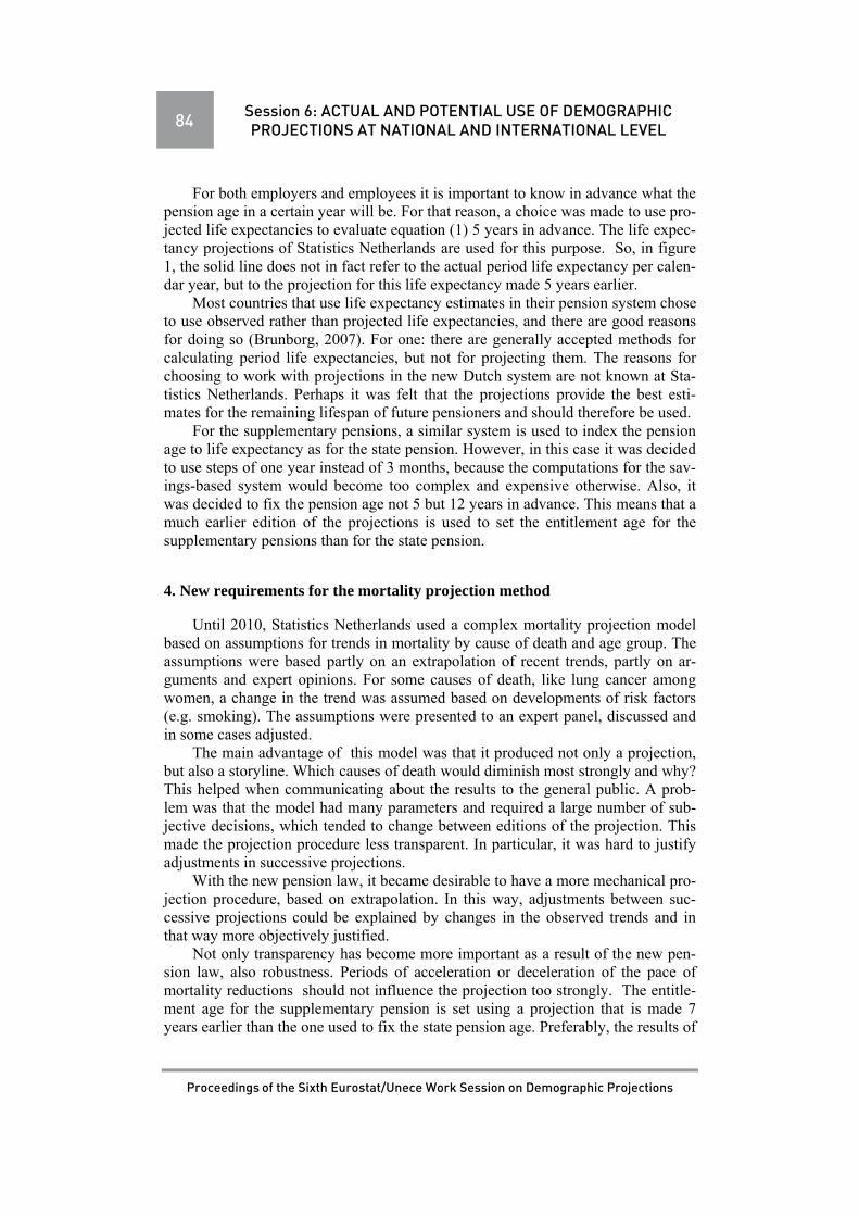
84 Session 6: ACTUAL AND POTENTIAL USE OF DEMOGRAPHIC PROJECTIONS AT NATIONAL AND INTERNATIONAL LEVEL
Proceedings of the Sixth Eurostat/Unece Work Session on Demographic Projections
For both employers and employees it is important to know in advance what the pension age in a certain year will be. For that reason, a choice was made to use pro-jected life expectancies to evaluate equation (1) 5 years in advance. The life expec-tancy projections of Statistics Netherlands are used for this purpose. So, in figure 1, the solid line does not in fact refer to the actual period life expectancy per calen-dar year, but to the projection for this life expectancy made 5 years earlier.
Most countries that use life expectancy estimates in their pension system chose to use observed rather than projected life expectancies, and there are good reasons for doing so (Brunborg, 2007). For one: there are generally accepted methods for calculating period life expectancies, but not for projecting them. The reasons for choosing to work with projections in the new Dutch system are not known at Sta-tistics Netherlands. Perhaps it was felt that the projections provide the best esti-mates for the remaining lifespan of future pensioners and should therefore be used.
For the supplementary pensions, a similar system is used to index the pension age to life expectancy as for the state pension. However, in this case it was decided to use steps of one year instead of 3 months, because the computations for the sav-ings-based system would become too complex and expensive otherwise. Also, it was decided to fix the pension age not 5 but 12 years in advance. This means that a much earlier edition of the projections is used to set the entitlement age for the supplementary pensions than for the state pension.
4. New requirements for the mortality projection method
Until 2010, Statistics Netherlands used a complex mortality projection model based on assumptions for trends in mortality by cause of death and age group. The assumptions were based partly on an extrapolation of recent trends, partly on ar-guments and expert opinions. For some causes of death, like lung cancer among women, a change in the trend was assumed based on developments of risk factors (e.g. smoking). The assumptions were presented to an expert panel, discussed and in some cases adjusted.
The main advantage of this model was that it produced not only a projection, but also a storyline. Which causes of death would diminish most strongly and why? This helped when communicating about the results to the general public. A prob-lem was that the model had many parameters and required a large number of sub-jective decisions, which tended to change between editions of the projection. This made the projection procedure less transparent. In particular, it was hard to justify adjustments in successive projections.
With the new pension law, it became desirable to have a more mechanical pro-jection procedure, based on extrapolation. In this way, adjustments between suc-cessive projections could be explained by changes in the observed trends and in that way more objectively justified.
Not only transparency has become more important as a result of the new pen-sion law, also robustness. Periods of acceleration or deceleration of the pace of mortality reductions should not influence the projection too strongly. The entitle-ment age for the supplementary pension is set using a projection that is made 7 years earlier than the one used to fix the state pension age. Preferably, the results of

Session 6: ACTUAL AND POTENTIAL USE OF DEMOGRAPHIC PROJECTIONS AT NATIONAL AND INTERNATIONAL LEVEL 85
Proceedings of the Sixth Eurostat/Unece Work Session on Demographic Projections
these two projections should be close. Otherwise, people will be receiving one type of pension much earlier than the other type.
Partly because of these considerations, Statistics Netherlands switched to a new model for the 2012 mortality projections (Stoeldraijer et al, 2013). The method was developed in collaboration with the University of Groningen. It is a variant of a model used in 2010 by the National institute for health and the environment (RIVM) (Janssen and Kunst, 2010; Janssen et al., 2013). The method aims to im-prove the robustness and accuracy of the projections by using stable long term trends for the extrapolations. This is done by basing the long term trend not only on the observed developments in The Netherlands, but also in other Western European countries. Furthermore, the effects of changes in smoking behaviour are modelled separately, because these give rise to nonlinearities in the mortality trends.
5. Communicating about uncertainty
As a result of the new pension law, Statistics Netherlands’ life expectancy pro-jections now also imply projections for the future pension age. If they are published without an explanation about their uncertainty, people may interpret them as a guarantee that their pension will start at the projected age and not plan for other possibilities. The fact that the pension age is adjusted with incremental steps of 3 months could be taken to imply that life expectancy can be forecasted to within a 3 months accuracy. Adjustments between successive projections by a larger amount than that, which will inevitably happen, could be met with anger or disbelief.
For this reason, it was decided to publish projections of the pension age only in terms of probability distributions or with uncertainty intervals. Projections of life expectancy are also accompanied by intervals wherever possible.
Figure 2 shows a probability distribution for the pension age by year. The sizes of the coloured segments in each column represents the probability that the pension age will be in that one-year age range. The age range with the highest likelihood for every year is labelled. In 2025, the state pension age is very likely between 67 and 68 years, by 2060, it is probably in the range of 70 to 73 years. This figure is complex and readers will often not immediately understand what is being shown. However, it does provide a good image of the uncertainty. Because no single pro-jection is shown, a discussion of this kind of figure will automatically focus on age-intervals and likelihoods. This kind of figure was used in a publication aimed at people working in the pension industry.
Figure 3 shows a more traditional time plot for the pension age with confi-dence intervals. This is easier to understand at first sight. Although the interpreta-tion of the confidence intervals is quite technical. It can also be used to compare different projections, as is shown here. This figure was used in the publication that accompanied the 2012 projections (Van Duin and Stoeldraijer, 2012), which was aimed at policymakers and the general public.. A problem with this kind of figure is that the sharp upper and lower boundaries suggest that the estimates of the level of uncertainty are themselves very certain.

86 Session 6: ACTUAL AND POTENTIAL USE OF DEMOGRAPHIC PROJECTIONS AT NATIONAL AND INTERNATIONAL LEVEL
Proceedings of the Sixth Eurostat/Unece Work Session on Demographic Projections
Figure 2 – Probability distribution of the state pension age by calendar year
Source: Statistics Netherlands
Figure 3 – State pension age, calculated from the 2012- and 2010-based life expectancy projections, with 67 and 95 per cent projection intervals
Source: Statistics Netherlands

Session 6: ACTUAL AND POTENTIAL USE OF DEMOGRAPHIC PROJECTIONS AT NATIONAL AND INTERNATIONAL LEVEL 87
Proceedings of the Sixth Eurostat/Unece Work Session on Demographic Projections
6. New demographic indicators
Under the new pension system, the definitions of potential labour force and grey pressure, which are a function of the pension age, become dynamic. The po-tential labour force is defined as “that part of the population that, given its age, is eligible for participation in the labour process”. Clearly, if the pension age increas-es, the “age of eligibility for labour participation” increases as well. As a result, the potential labour force gets a twofold time-dependence.
For the 2012 projections, Statistics Netherlands has published both about the static and dynamic potential labour force, defined as
PLFstatic(y) = N(20-64, y), (2)
PLFdynamic(y)= N(20 – Xpension(y-1), y), (3)
where N(x0-x1, y) denotes the population between ages x0 and x1 on January first of year y and Xpension(y) denotes the state pension age in year y. Because we are look-ing at the population at the start of the year, the pension age in the previous year should be used.
Similarly, the number of elderly can be defined in a static and dynamic way as
Estatic(y) = N(65 or older, y), (4)
Edynamic (y) = N(Xpension(y-1) or older, y) (5) And grey pressure is defined as
GPstatic (y) = Estatic(y)/ PLFstatic(y) (6)
GPdynamic(y) = Edynamic(y)/ PLFdynamic (y) (7)
Figures 4-6 shows the results for the three demographic indicator using the
static and dynamic definition. The results for the 2012-based projections are shown, with uncertainty intervals calculated using stochastic populations projec-tions. The method for the stochastic projections had to be extended in order to ob-tain intervals for the dynamic quantities. Because the pension age is determined us-ing projected instead of observed life expectancy, the forecast errors introduce an additional element of uncertainty, which had to be incorporated into the simula-tions.
Figure 4 shows the projected number of elderly, according to both definitions. Clearly, increasing the state pension age is an effective cost-saving measure. The number of people that qualify for a state pension in 2040 is reduced from 4.7 to 3.9 million. After 2040, the number of elderly in the 2012-based projections remains almost constant according to the static definition, but it decreases according to the dynamic definition.
If we compare the forecast-intervals for the two quantities, we find that the dynamic number of elderly can be forecasted with much greater accuracy than the

88 Session 6: ACTUAL AND POTENTIAL USE OF DEMOGRAPHIC PROJECTIONS AT NATIONAL AND INTERNATIONAL LEVEL
Proceedings of the Sixth Eurostat/Unece Work Session on Demographic Projections
static number. The uncertainty in the future number of elderly for the intermediate term is mostly due to uncertainties in the development of life expectancy. The in-dexation procedure cancels out most of this uncertainty. A secondary result of the new pension policy is therefore that it makes the future number of pensioners much more predictable. The 95 per cent interval for the static number of elderly in 2040 has a width of 1.2 million people. For the dynamic number, the width is only 0.3 million.
Figure 5 shows the results for the static and dynamic potential labour force. The static potential labour force is expected to decrease from 10.1 to 9.3 million people between 2013 en 2040. The dynamic potential labour force is expected to be at the same level in 2040 as currently. By that time, 800 thousand people aged 65 or older are in the potential labour force, 8 per cent of the total size. How many of these will also be in the actual labour force depends on to what extend the labour force participation of the elderly will increase along with the rising pension age.
The projections for the dynamic potential labour force are more uncertain than those for the potential labour force. The width of the 95 per cent interval in 2040 for the static quantity is 1.5 million people, for the dynamic quantity 1.9 million people. The unpredictability of fertility rates and international migration mostly de-termine the uncertainty for the static potential labour force. For the dynamic ver-sion, there is an additional uncertainty from life expectancy through the pension age.
Figure 6 shows the results for grey pressure. Dynamic grey pressure is ex-pected to rise from 0.28 now to 0.39 in 2040, instead of to 0,51 for static grey pressure. Like for the number of elderly, the uncertainty intervals are much nar-rower for the dynamic quantity, because indexation of the pension age with life ex-pectancy cancels out the main source of uncertainty.

Session 6: ACTUAL AND POTENTIAL USE OF DEMOGRAPHIC PROJECTIONS AT NATIONAL AND INTERNATIONAL LEVEL 89
Proceedings of the Sixth Eurostat/Unece Work Session on Demographic Projections
Figure 4 – Number of elderly for the Netherlands (static and dynamic definition)
Source: Statistics Netherlands
Static definition
Dynamic definition
0
10
20
30
40
50
60
1995 2000 2005 2010 2015 2020 2025 2030 2035 2040 2045 2050 2055 2060
x 100 thousand
0
10
20
30
40
50
60
1995 2000 2005 2010 2015 2020 2025 2030 2035 2040 2045 2050 2055 2060
x 100 thousand
Forecast interval (95%) Forecast interval (67%)
Observed values 2012-based projections

90 Session 6: ACTUAL AND POTENTIAL USE OF DEMOGRAPHIC PROJECTIONS AT NATIONAL AND INTERNATIONAL LEVEL
Proceedings of the Sixth Eurostat/Unece Work Session on Demographic Projections
Figure 5 – Potential labour force for the Netherlands (static and dynamic definition)
Source: Statistics Netherlands
Static definition
Dynamic definition
75
85
95
105
115
125
1995 2000 2005 2010 2015 2020 2025 2030 2035 2040 2045 2050 2055 2060
x 100 thousand
75
85
95
105
115
125
1995 2000 2005 2010 2015 2020 2025 2030 2035 2040 2045 2050 2055 2060
x 100 thousand
Forecast interval (95%) Forecast interval (67%)
Observed values 2012-based projections

Session 6: ACTUAL AND POTENTIAL USE OF DEMOGRAPHIC PROJECTIONS AT NATIONAL AND INTERNATIONAL LEVEL 91
Proceedings of the Sixth Eurostat/Unece Work Session on Demographic Projections
Figure 6 – Grey pressure for the Netherlands (static and dynamic definition)
Source: Statistics Netherlands
Static definition
Dynamic definition
0
0.1
0.2
0.3
0.4
0.5
0.6
0.7
1995 2000 2005 2010 2015 2020 2025 2030 2035 2040 2045 2050 2055 2060
0
0.1
0.2
0.3
0.4
0.5
0.6
0.7
1995 2000 2005 2010 2015 2020 2025 2030 2035 2040 2045 2050 2055 2060
Forecast interval (95%) Forecast interval (67%)
Observed values 2012-based projections

92 Session 6: ACTUAL AND POTENTIAL USE OF DEMOGRAPHIC PROJECTIONS AT NATIONAL AND INTERNATIONAL LEVEL
Proceedings of the Sixth Eurostat/Unece Work Session on Demographic Projections
REFERENCES
Brunborg, H. 2007. Life expectancy adjustments in the Norwegian pension reform, Joint Eurostat/UNECE Work Session on Demographic Projections, Bucharest.
Duin C. van en L. Stoeldraijer 2012, Bevolkingsprognose 2012-2060: Langer leven, langer werken [Population forecast 2012-2060: Living longer, working longer], www.cbs.nl (published 13-12-2012)
Janssen, F. & A. Kunst 2010, The future of Dutch life expectancy. In: A.H.P. Luijben & G.J. Kommer (eds.), Towards Better Health, the Dutch 2010 Public Health Status and Forecasts Report.
Janssen, F., L.J.G. van Wissen and A.E. Kunst 2013 Including the smoking epidem-ic in internationally coherent mortality projections. Demography 50(4): 1341-1362..
Stoeldraijer, L., C. van Duin, F. Janssen 2013, Bevolkingsprognose 2012-2060: Model en veronderstellingen betreffende de sterfte. [Population forecast 2012-2060: Model and assumptions on mortality] Bevolkingstrends June 2013, pp. 1-27.

Session 6: ACTUAL AND POTENTIAL USE OF DEMOGRAPHIC PROJECTIONS AT NATIONAL AND INTERNATIONAL LEVEL 93
Proceedings of the Sixth Eurostat/Unece Work Session on Demographic Projections
POPULATION PROJECTIONS: A TOOL FOR THE
(RE)DEFINITION OF THE PORTUGUESE HIGHER
EDUCATION SYSTEM
Rui Dias, Maria Filomena Mendes, M. Graça Magalhães, Paulo Infante Summary
Population projections can be used as a tool to provide information on possible sce-narios of future population and, namely, to support decision-making processes in di-verse socio-economic areas, such as, higher education institutional network planning, both in public and private sectors. In a country like Portugal, nowadays affected by a severe economical and financial crisis, with a young population characterized by low levels of education and qualification is fundamental to use population projections as a basis for higher education planning. The main goal of this paper is to evaluate the possible changes in the younger popula-tion size in the coming years as a tool to (re)think and (re)design geographically the higher education institutional network in Portugal. Our findings will provide a range of reliable forecasts to support a more rational political decision contributing to an efficient and effective planning in what concerns higher education requirements ad-justed to the evolution of future population.
Keywords: Population Projections, Higher Education Institutional Network, time series analysis.
1. Introduction
Population projections can be used as a tool to provide information on possible scenarios of future dimension, age and sex composition of population, and there-fore to support decision-making processes in diverse socio-economic areas, such as higher education institutional network planning, namely, in a context of a young population still characterized by very low levels of education. The main goal of this paper is to evaluate the possible changes in younger popula-tion size in the coming years, based on the results of population projections, by age and sex, using the cohort-component method. This main goal is part of an extended research project, with the aim of a (re)definition of the Network for Higher Educa-tion in Portugal. The projection of the population in the near future that will be "at risk" of entering that grade level is crucial. We will focus our scope on young peo-ple aged between 18 and 30, considering sex and age distribution, in the time hori-zon of the next 25 years.

94 Session 6: ACTUAL AND POTENTIAL USE OF DEMOGRAPHIC PROJECTIONS AT NATIONAL AND INTERNATIONAL LEVEL
Proceedings of the Sixth Eurostat/Unece Work Session on Demographic Projections
In this paper, we will test the application of different methodologies to predict fertility and mortality, the main components responsible for the evolution trend of young people, as potential candidates to higher education at the considered time interval.
Despite the importance of the migration component, once both levels of emi-gration and immigration are more significant at young adult ages, at which may af-fect the prediction of the number of young people under the usual age of accessing higher education, and simultaneously influence the number of births (however, in this case, the biggest effect will be noted only18 years later), we do not include the migration component in this study, namely due to its high volatility and the high level of difficulty to predict it in the long term.
2. Brief overview of Higher Education in Portugal
Over the past 40 years, the development of the Higher Education Network in Portugal has proved to be a major factor for the country development. One of the key questions regarding the future of higher education network is related to the fact that the number of young people in Portugal have declined dramatically in recent years. Does the entry of young adult population in this level of education will con-tinue to increase, as seen in the first 30 years of democracy, i.e., since the begin-ning of the 80’s in the past century? Or will simply follow the same downward trend observed in recent years?
The Higher Education System is divided into two subsystems: public and pri-vate; and organized according an “university subsystem” (that grants a more solid scientific preparation) or a “polytechnic subsystem” (that provides a more technical training and more profession-oriented).
A preliminary analysis of students enrolled in higher education in Portugal al-lows to highlight some issues. In the last 12 years, students enrolled in higher edu-cation are mostly women, despite the decrease of the differences between sexes in the recent past. The public system is the predominant one, whether at the level of university or polytechnic. This can be explained by two reasons: 1) the high cost of private education; and, 2) the high quality of public education. It is also noteworthy the increase in the number of students in the public sector compared with the de-crease in the private one, namely since 2008/2009. Such disparity can be explained by the greater difficulties faced by families to support educational costs, mostly due to the current economic crises.
In watt concerns to university or polytechnic subsystems, the university sub-system absorbs most of the students in Higher Education in Portugal, and the dif-ference between the two subsystems remains approximately the same throughout the past 12 years. About the selected scientific areas, Agriculture remains the less attractive area to higher education students. Social Sciences, Business and Law are the areas that attract more students. The major decrease on the number of enrolled students by scientific area was in the case of Education, while a marked increase was observed in the case of Health and Social Protection. Of all the areas analyzed,

Session 6: ACTUAL AND POTENTIAL USE OF DEMOGRAPHIC PROJECTIONS AT NATIONAL AND INTERNATIONAL LEVEL 95
Proceedings of the Sixth Eurostat/Unece Work Session on Demographic Projections
these two show an obvious change in the number of enrolled students between 2000 and 2012, whereas in the remaining six areas1 the number remains constant.
After April 25th 1974 there has been a radical change in the attitude towards education in Portugal and changes in the level of education were overwhelming. In 1986/1987, the compulsory education was raised to nine years of schooling and in 2005/2006 to 12. In 2010/2011, took effect, the requirement of one year of pre-primary schooling covering all children 5 years of age. Prior to April 25th 1974 the number of students in higher education were less than 30 thousand, while in the ac-ademic year 2011/2012 this number was around 400,000 (DGEEC2). However, and despite the numerous efforts made since the democratic revolution in April 1974, Portugal still has poor educational indicators, particularly when compared with other European countries.
Although the Bologna Process, implemented in 2006/2007, has allowed anoth-er increase in the number of students enrolled in higher education, mainly due to restructuring the different courses with the consequent decrease in the number of years required to obtain a degree, therefore causing smaller financial stress of fami-lies, the rate of enrolment in Portugal remained very low, compared to the majority of the European Union.
In recent years the rate of enrolment in Portugal has risen steadily, reaching values around 20% for young people aged between 18 and 29, already quite close to the 22% (2013) of the EU average (27 countries). However, this proportion is still distant from countries such as Finland, which has an enrolment rate at the same age group of 26% (Eurostat).
So, a projection of the number of individuals enrolled in higher education in the coming years is critical for a redefinition of the higher education network.
Will the increase in enrolment in higher education in Portugal offset the sharp decline expected for the younger resident population? Or, conversely, the popula-tion decrease will cause a decrease in the number of young people able to apply to higher education? The number of places offered by the Portuguese higher educa-tion network in recent years is the most appropriate considering the evolution of the demand?
3. Data and methods
3.1 Population Projection Methodology Deterministic projections are frequently performed using different scenarios to
deal with uncertainty. More recently, probabilistic projections of population have been developed with increasingly interest namely considering that they allow the estimation of a confidence interval associated with each outcome (Bongaarts & Bu-latao, 2000). The uncertainty in the results come not from the formal model but from the uncertainty of the future evolution of components, being frequently the use of different scenarios or variants as a way of dealing with uncertainty.
1 The six scientific areas are: “Agriculture”, “Arts and Humanities, Education”, “Engineering, Manufacturing In-dustries and Construction”, “Health and Social Protection”, “Science, Mathematics and Computing”, “Social Sci-ences, Business and Law, Services”. 2 Direcção-Geral de Estatísticas da Educação e Ciência, Portugal

96 Session 6: ACTUAL AND POTENTIAL USE OF DEMOGRAPHIC PROJECTIONS AT NATIONAL AND INTERNATIONAL LEVEL
Proceedings of the Sixth Eurostat/Unece Work Session on Demographic Projections
An alternative is to explicitly take into account the uncertainty of the fertility, mortality and migration trends, and derive the probability distributions for the re-sulting size and age structure of the population projected (O'Neill, Balk, Brickman, & Ezra, 2001).
Thus, the complementary application of the most useful aspects of different methodologies, combining the scenario approach with probabilistic forecasts seems to be the most productive attitude (Goldstein, 2007; Sanderson et al, 2004).
The population projections have been calculated using the cohort-component method, were the populations are successively update according to the assumptions about future levels of the components and the natural ageing, in each scenario, from 2011 to 2035 (2010 is the base year). The formulation of hypotheses for fu-ture developments of components (fertility, mortality and migration) is based on the observation, analysis and modelling of past trends of each of the components and expert opinion and do not incorporated any exogenous variables. The alterna-tive hypotheses are intended to illustrate a range of possible future results. The complexity of migration flows, especially regarding its volatility and the difficul-ties in addressing new forms of population mobility, supported the decision of in-clude only a null migration assumption on this exercise.
The combination of alternative assumptions about the future evolution of mor-tality and fertility allows designing scenarios and we have chose the following three combinations of hypotheses: (a) Optimistic (high fertility and low mortality); (b) Central (medium fertility and medium mortality); (c) Pessimistic (low fertility and high mortality).
3.2 Fertility We have analyzed the evolution of fertility, based on historical fertility data
from 1981 to 2009, available at the Human Fertility Database. In the fertility component we first establish the assumptions of possible evolu-
tion, in terms of expected developments in total fertility rate (TFR) and mean age at childbearing (MAC), based on the analysis of the recent trends in Portugal. Three assumptions are defined for the TFR: (f1) the maintenance of a very low fer-tility rate throughout the projection period, assuming a value of 1.3 children per woman, in 2035 – hypothesis designated by low fertility; (f2) the recovery of fer-tility levels in order to equal, in the end of the period, the value currently recorded nowadays in the European Union, reaching 1.6, by 2035 – hypothesis called high fertility; and, (f3) an intermediate scenario that envisages a less significant increase in fertility, reaching a value of 1.45 children per woman by 2035 – the central fer-tility hypothesis. The mean age at childbearing will remain around 30 years on av-erage, decreasing slightly in the most optimistic scenario and prolonging the delay in the worst case.
For the estimation of the fertility rates by age, we have applied the model pro-posed by Schmertmann (2003 and 2005). Following this author, we model specific fertility rates by age proceeding thereafter to a linear interpolation between the pro-jected values and the estimates for the base year (2010). The model characterize the profile of the specific fertility rates by age fx, in terms of three axes (ages) that syn-thesize certain features observed in fertility behaviour. These three areas corre-spond in particular to the younger age at which record births ( ), the age at which

Session 6: ACTUAL AND POTENTIAL USE OF DEMOGRAPHIC PROJECTIONS AT NATIONAL AND INTERNATIONAL LEVEL 97
Proceedings of the Sixth Eurostat/Unece Work Session on Demographic Projections
the specific fertility rates reaches the maximum value (P), and the younger age after which fertility decreases 50 % of its maximum value (H). An additional parameter (R) is also used to obtain the level of fertility.
In formal terms, the exchange between the ages and an upper age limit are modelled by splines.
( ) ( )f x R x (1)
42
0
,( )
0, ,
k kk
x t xx
x
(2)
The distribution of fertility rates by age, over the next 25 years, according to
the results for the scenario 2, may be represented as shown in Figure 1.
Figure 1 – Age specific fertility rates, Portugal, 2010-2035
Age specific fertility rates tend to increase slightly between 24 and 35 years of
age, particularly between 28 and 32 years-old, but we do not anticipate a significant recovery of births postponed to ages above 37 years.
However, the gradual decline in fertility observed in Portugal in recent decades conditioned inexorably the size of the generations that, either currently or in the coming decades, will reach the age to start a family and have children. Thus, even under a scenario of recovery of fertility without constraints (eventually caused by foreseeable emigration flows), the number of births in the future is likely to be lower for the simple fact that we have, year after year, fewer women at childbearing ages.
The estimation of the births in this projection exercise clearly shows that the consequences of fertility decline registered in our recent past will be reflected inevitably in the future; it is not possible to reverse its effects in the timeline of the coming decades.
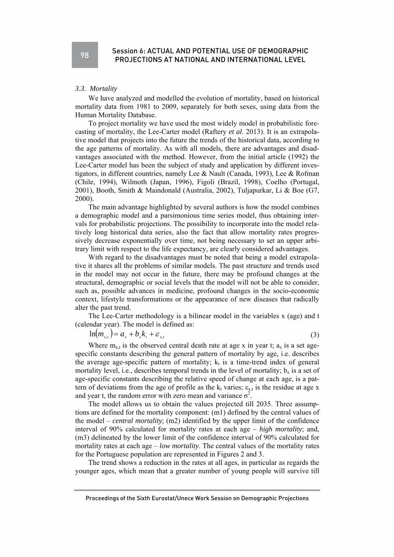
98 Session 6: ACTUAL AND POTENTIAL USE OF DEMOGRAPHIC PROJECTIONS AT NATIONAL AND INTERNATIONAL LEVEL
Proceedings of the Sixth Eurostat/Unece Work Session on Demographic Projections
3.3. Mortality We have analyzed and modelled the evolution of mortality, based on historical
mortality data from 1981 to 2009, separately for both sexes, using data from the Human Mortality Database.
To project mortality we have used the most widely model in probabilistic fore-casting of mortality, the Lee-Carter model (Raftery et al. 2013). It is an extrapola-tive model that projects into the future the trends of the historical data, according to the age patterns of mortality. As with all models, there are advantages and disad-vantages associated with the method. However, from the initial article (1992) the Lee-Carter model has been the subject of study and application by different inves-tigators, in different countries, namely Lee & Nault (Canada, 1993), Lee & Rofman (Chile, 1994), Wilmoth (Japan, 1996), Figoli (Brazil, 1998), Coelho (Portugal, 2001), Booth, Smith & Maindonald (Australia, 2002), Tuljapurkar, Li & Boe (G7, 2000).
The main advantage highlighted by several authors is how the model combines a demographic model and a parsimonious time series model, thus obtaining inter-vals for probabilistic projections. The possibility to incorporate into the model rela-tively long historical data series, also the fact that allow mortality rates progres-sively decrease exponentially over time, not being necessary to set an upper arbi-trary limit with respect to the life expectancy, are clearly considered advantages.
With regard to the disadvantages must be noted that being a model extrapola-tive it shares all the problems of similar models. The past structure and trends used in the model may not occur in the future, there may be profound changes at the structural, demographic or social levels that the model will not be able to consider, such as, possible advances in medicine, profound changes in the socio-economic context, lifestyle transformations or the appearance of new diseases that radically alter the past trend.
The Lee-Carter methodology is a bilinear model in the variables x (age) and t (calendar year). The model is defined as:
txtxxtx kbam ,,ln (3)
Where mx,t is the observed central death rate at age x in year t; ax is a set age-specific constants describing the general pattern of mortality by age, i.e. describes the average age-specific pattern of mortality; kt is a time-trend index of general mortality level, i.e., describes temporal trends in the level of mortality; bx is a set of age-specific constants describing the relative speed of change at each age, is a pat-tern of deviations from the age of profile as the kt varies; εx,t is the residue at age x and year t, the random error with zero mean and variance σ2.
The model allows us to obtain the values projected till 2035. Three assump-tions are defined for the mortality component: (m1) defined by the central values of the model – central mortality; (m2) identified by the upper limit of the confidence interval of 90% calculated for mortality rates at each age – high mortality; and, (m3) delineated by the lower limit of the confidence interval of 90% calculated for mortality rates at each age – low mortality. The central values of the mortality rates for the Portuguese population are represented in Figures 2 and 3.
The trend shows a reduction in the rates at all ages, in particular as regards the younger ages, which mean that a greater number of young people will survive till

Session 6: ACTUAL AND POTENTIAL USE OF DEMOGRAPHIC PROJECTIONS AT NATIONAL AND INTERNATIONAL LEVEL 99
Proceedings of the Sixth Eurostat/Unece Work Session on Demographic Projections
the older ages. Note that the expected gains in terms of reduced mortality in males will be substantial, maintaining however some comparatively higher values, for ex-ample, in the ages between 15 and 24 years old, associated with a history of high mortality mainly due to road traffic accidents. In the case of females, the decline in mortality rates will also increase, although it is noteworthy that the starting levels are much lower compared to those recorded by males, at all ages.
Figure 2 – Mortality rates, male population, aged from 0 to 35, Portugal, 2010-2035
Figure 3 – Mortality rates, female population, aged from 0 to 35, Portugal, 2010-2035
3.4 Enrolment Rates Scenarios One of the goals of this study is to estimate the behaviour of students enrol-
ment in higher education over the coming years. In order to do this forecast we used the values of the population initially projected building up several scenarios for forecasting enrolment rates, based on: (i) a linear evolution of the enrolment rates registered in the past 12 years; (ii) a logarithmic evolution; (iii) an average growth rate recorded in the same period of time, the last 12 years; and (iv) the as-sumption of an identical evolution to the enrolment rates observed in EU27.

100 Session 6: ACTUAL AND POTENTIAL USE OF DEMOGRAPHIC PROJECTIONS AT NATIONAL AND INTERNATIONAL LEVEL
Proceedings of the Sixth Eurostat/Unece Work Session on Demographic Projections
4. Results
4.1 Population projections In Portugal, the higher education institutions have as prime candidates young
individuals aged between 18 and 24, being the age of 18 the one with the largest number of applicants. Therefore, we considered this target population on our study. However, given that we still consider a margin of recruitment between ages 18 and 23, as well as in ages above 23 (due to the potential number of students attracted by after working courses), we analyzed not only individuals with the modal age 18, but also the people in the age groups between 18 and 24 and between 18 and 30.
With time the number of young people tends to decrease at all ages. However, depending on the initial population for each age or on the evolution of the corre-sponding probability of death, the variation has a greater or lesser extent; the varia-tion in the number of births over past time may also be the cause of changes (see Table 1).
Table 1 – Total population – central scenario, 18 to 30 years old, Portugal, 2010-2035
Age/Year 2010 2015 2020 2025 2030 2035
18 117131 107655 111397 105017 99470 89480
19 118450 108517 109278 108858 101131 91503
20 118573 106958 112470 108416 98847 93560
21 120226 110466 106628 111446 103989 95597
22 121072 113096 105960 113018 101852 97552
23 125624 116872 107462 111234 104892 99373
24 129238 118176 108312 109108 108720 101025
25 138346 118288 106746 112287 108270 98737
26 143429 119929 110240 106447 111289 103868
27 150230 120762 112855 105772 112851 101727
28 153051 125285 116608 107258 111057 104751
29 157705 128866 117888 108088 108917 108559
30 157967 137918 117975 106505 112069 108091
Considering the results of the three scenarios, the difference between the pro-
jected population values is almost nonexistent until 2028, due to the reduced effect of differences in mortality on population structure in young ages, in particular be-tween 18 and 30 years old. After 2028 and until the end of the projection period, the differences increase among the different scenarios, mostly due to the impact of changes in fertility. Projected values of the population aged 18 years reflect, main-ly, the past fertility trend in Portugal. Notice the values slightly higher than ex-pected for the calendar years 2018 to 2021 as a result of the increased fertility oc-curred in 2000, as well as relatively high fertility rates until 2003.
The general declining trend of individuals aged 18 becomes more evident from 2028 onwards, when the evolution of future fertility is crucial in calculating the size of the projected population. In fact, the population aged 18 in the years preced-

Session 6: ACTUAL AND POTENTIAL USE OF DEMOGRAPHIC PROJECTIONS AT NATIONAL AND INTERNATIONAL LEVEL 101
Proceedings of the Sixth Eurostat/Unece Work Session on Demographic Projections
ing 2028 results simply from the expected survival of births already occurred by the year 2010.
Between 2010 and 2035, it is likely that the size of the population aged 18 will decline around 23.6%, considering the so called central scenario, 21.9% in the op-timistic scenario and 25.8% in the pessimist scenario (Figure 4).
Figure 4 – Population 18 year old, central, optimistic and pessimistic scenarios
In what concerns the 18-24 age group, the downward trend remains (Figure 5).
However, we can expect a slight increase in the population of this age group be-tween 2020 and 2026, as an effect of a slight increase in fertility in Portugal be-tween 1996 and 2002. In any of the scenarios the population of this age group de-clines from about 20.4% to 22.8%, for the optimistic or pessimistic scenario and 21.4% on the central scenario.
Figure 5 – Population 18-24 age groups, central, optimistic and pessimistic scenarios

102 Session 6: ACTUAL AND POTENTIAL USE OF DEMOGRAPHIC PROJECTIONS AT NATIONAL AND INTERNATIONAL LEVEL
Proceedings of the Sixth Eurostat/Unece Work Session on Demographic Projections
For the wider group, composed of young people aged 18 to 30 years, the de-cline is also quite visible (Figure 6), with a reduction of more than 25% whatever the scenario (-26.1%, central scenario; -25.5%, optimistic scenario; -26.9%, pessi-mistic scenario).
Figure 6 – Population 18-30 age groups, central, optimistic and pessimistic scenarios
4.2 Enrolment students In overall, following a linear trend of the enrolment rates, those enrolled in
higher education in Portugal may increase to about 460 thousands by 2035; project-ing an increase of more than 13 thousands students at the age of 18 years old until 2035 (i.e., an increase of about 40%).
According to a logarithmic evolution of enrolment there’s a complete reverse of what was projected in the previous approach for the number of enrolled students in the higher education network. In this case, the increase of enrolment rates will be not large enough to counterbalance the decline in the projected population. Global-ly it would be noted a decrease around 10% of enrolled students till 2035, which represents approximately 34.000 students.
Enrolment rates will increase dramatically under the average growth rate sce-nario. The individuals in the 18 year old group will reach an enrolment rate of around 60% at the end of the period. According to this scenario, the total of en-rolled students increased about 25%, attaining above 510.000 students.
In the scenario using the average growth rate in Europe, we selected several European countries. Despite the profound differences among them, we assume the European Union (27) growth rates. In this case, the group of 18 years old, will in-crease of about 1500 students in the period in analysis, offsetting the estimated de-cline in the young resident population. However, it is the age group of 18 to 29 years old which may register the largest increase in the number of students, in-creasing about 20%.

Session 6: ACTUAL AND POTENTIAL USE OF DEMOGRAPHIC PROJECTIONS AT NATIONAL AND INTERNATIONAL LEVEL 103
Proceedings of the Sixth Eurostat/Unece Work Session on Demographic Projections
5. Conclusions
The first conclusion to be drawn of the different results is that the number of young people in Portugal will decrease significantly in the next 25 years. Thus, the young population, base of student’s recruitment will be reduced proportionately and the demand of higher education in Portugal will be strongly influenced by this trend.
On the one hand, the demand for higher education in Portugal tends to de-crease significantly in the years between 2010 and 2035, based on an expected de-cline of young population between 20-25% of the residents at the beginning of the current decade. But, on the other, considering the recent European trends, the en-rolment rates in Portugal have the possibility to grew more over the next years.
Even considering impact factors with an opposite effect, such as: (1) possible changes in social policies and incentives to attract students for higher education specific courses; (2) a broadening of the recruitment base, despite the reduction in the size of the youth population, due to the extension of compulsory education to 12 years and a possible rise on the secondary graduation rates that may cause an increase in the proportion of applicants to higher education, (3) a greater propensity of young people for chose universities and polytechnics in order to acquire a higher education; we can conclude that the demand for higher education in Portugal tend to decrease significantly in the years between 2010 and 2035, based on an expected loss of young population, between 1/5 and more than a quarter of the population existing at the beginning of the current decade.
Further, we also believe that with a future change to (again) positive net mi-gration would not be possible to reverse this trend of decreasing young population.
Moreover, there will be other factors that may act to decrease the absolute number of potential candidates, such as: (1) during periods of economic crisis the families decisions may be constrained and forced to restrict the access, in the case of the most economically disadvantaged candidates; (2) highly concentrated supply of courses (and institutions) may discourage applications from young people be-longing to the lower income classes who need to move from one region to another; (3) the emigration currently registered in Portugal may become responsible for an even greater young ages depopulation.
In general, considering all factors, it appears that young people who most like-ly would have to apply to higher education in Portugal tend to decrease considera-bly in the coming years. In fact, 3 out of 4 scenarios, forecast an increase on the number of enrolled stu-dents, even with a dramatic aging in the base of the age structure.
Based on our results the supply of Higher Education should be re-evaluated and re-organized to better suit the demand in Portugal.
We believe that the conclusions which may be drawn on the basis of this exer-cise show that demographic projections are a fundamental tool for the process of resetting the network of higher education in Portugal, particularly when major changes are foreseen either in the size of the base of recruitment, either in entry strategies, and also the reorganization of the training supply.

104 Session 6: ACTUAL AND POTENTIAL USE OF DEMOGRAPHIC PROJECTIONS AT NATIONAL AND INTERNATIONAL LEVEL
Proceedings of the Sixth Eurostat/Unece Work Session on Demographic Projections
REFERENCES
Bongaarts, J., & Bulatao, R. A. (Eds.). 2000. Beyond Six Billion: Forecasting the World’s Population. The National Academies Press.
Booth, H., Maindonald, J. and Smith, L. (2002). “Applying Lee-Carter under con-ditions of variable mortality decline”. Population Studies, 56 (3): 325–336.
Coelho, E. (2001). “Método de Lee-Carter para previsão da mortalidade”. Revista de Estudos Demográficos, nº 37 - Instituto Nacional de Estatística, Departamento de Estatísticas Sociais.
Cleland, J. (2002). “Education and future fertility trends, with special reference to mid- transitional countries”. Completing the Fertility Transition. Part 2. Back-ground Papers. New York: United Nations, Population Division, Department of Economic and Social Affairs: 187-202.
Fígoli, M. (1998). “Modelando e projectando a mortalidade no Brasil”. Revista Brasileira de Estudos de População, Vol. 1, nº 1.
Goldstein, J. R. (2007). Simpler Probabilistic Population Forecasts: Making Sce-narios Work. International Statistical Review, 72(1), 93–106. doi:10.1111/j.1751-5823.2004.tb00226.x
Lee, R. and Carter, L. (1992). “Modeling and Forecasting U.S. Mortality”. Journal of the American Statistical Association, Vol.87, n.º 419, 659-675.
Lee, R. and Nault, F. (1993). “Modeling and forecasting provincial mortality in Canada”. Paper presented at the World Congress of the International Union for the Scientific Study of Population, Montreal.
Lee, R. and Miller, T. (2000). Evaluating the Performance of Lee-Carter Mortality Forcasts, University of California, Berkeley [Online], Disponível: http//www.demog.berkeley.edu.
Lutz, W., Saariluoma, P., Sanderson, W.C., and Scherbov, S. (2000). New devel-opments in the methodology of expert- and argument-based probabilistic popula-tion projections. IIASA Interim Report IR-00-020. Available at http://www.iiasa.ac.at/cgi-bin/pubsrch?
Lee, R. and Rofman, R. (1994). “Modelacion y Proyeccion de la Mortalidad en Chile”, NOTAS 22, nº 59, 182-213. Also available in English from the authors, titled “Modeling and Forecasting Mortality in Chile”.
O’Neill, B., Balk, D., Brickman, M. and Ezra, M. (2001). “A Guide to Global Pop-ulation Projections”. Demographic Research, 4: 203-288.
Raftery, A., Chunn, J., Gerland, P. and Sevcíková, H. (2013). “Bayesian Probabil-istic Projections of Life Expectancy for All Countries”. Demography, 50: 777-801.

Session 6: ACTUAL AND POTENTIAL USE OF DEMOGRAPHIC PROJECTIONS AT NATIONAL AND INTERNATIONAL LEVEL 105
Proceedings of the Sixth Eurostat/Unece Work Session on Demographic Projections
Schmertmann C. (2003): "A system of model fertility schedules with graphically intuitive parameters". Demographic Research, 9:81-110.
Schmertmann C. (2005): "Quadratic spline fits by nonlinear least squares". Demo-graphic Research, 12:105-106.
Tuljapurkar, S., Li, N. and Boe, C. (2000). “A universal pattern of mortality de-cline in the G7 countries”. Nature, 405: 789-792.
Wilmoth, J.R. (1996). “Mortality projections for Japan: A comparison of four methods”. Caselli, G. and Lopez, A.D. (eds), Health and Mortality among Elder-ly Populations, Oxford, Clarendon Press, 266-287.


Session 7
NATIONAL AND INTERNATIONALPOPULATION PROJECTIONS
OUT OF THE EU REGION
Chair: Giampaolo Lanzieri (Eurostat)


Session 7: NATIONAL AND INTERNATIONAL POPULATION PROJECTIONS OUT OF THE EU REGION 109
Proceedings of the Sixth Eurostat/Unece Work Session on Demographic Projections
QUALITATIVE AND METHODOLOGICAL ASPECTS OF POPULATION PROJECTIONS IN GEORGIA;
GEORGIAN POPULATION PROSPECTS: 1950-2050
Shorena Tsiklauri, Avtandil Sulaberidze
Summary
Population of Georgia has decreased since its independence. Some of the population decline was due to the decrease of fertility and increased mortality levels, but the main impact is related to the emigration. In the period between two population censuses, 1989 and 2002 Georgia lost more than one million persons due to the emigration. In the years followed independence, an economic crisis, civil war and other armed con-flicts led to the displacement of many people. According to all of the exits projection population of Georgia continues to decrease. In order to discuss the Georgian population prospects, it is very important to have better estimates of the population and vital statistics, as well as migration statistics. Keywords: population projections in Georgia, methodology
1. Introduction
According to the National Statistic Office of Georgia, number of Population has decreased from 5.5 million in 1991 to 4.5 million in 2013 since its independ-ence from the USSR. Some of the population’s decline was due to decrease of the fertility and increased the mortality levels, but the main impact is related to the em-igration. In the period between two population censuses, 1989 and 2002 Georgia lost more than one million persons due to the migration. In the years followed in-dependence, an economic crisis, unemployment, civil war and other armed con-flicts led to the displacement of many people. The growing poverty, unemploy-ment, limited access to the basic social services, low income and its unequal distri-bution have had a clear direct impact on the population dynamics of Georgia. Ac-cording to all the exits projection, population of Georgia continues to decrease. In order to discuss the population prospects, it is very important to have better esti-mates of vital statistics and annual number of population.
In Georgia, data quality has always been at issue, but since collapse of Soviet Union in 1991, the population statistics has deteriorated rapidly. It concerns both, reliability of vital statistics and population estimates. In the 1990s, demographic statistics published by national statistics office of Georgia were far from the real levels. Not only due to the increasing migration flows, along with a conflicts in the country that disrupted many statistical data-series, but the current data collection

110 Session 7: NATIONAL AND INTERNATIONAL POPULATION PROJECTIONS OUT OF THE EU REGION
Proceedings of the Sixth Eurostat/Unece Work Session on Demographic Projections
system for birth and death have been deteriorating. In the 1990s, political instabil-ity in the country and socio-economic crisis caused the collapse of population reg-istration system. Especially registration of international migrants hence number of population which statistics office published was unreal. Several surveys conducted in Georgia shows that the level of fertility and mortality and especially level of in-fant mortality has been considerably underestimated, by approximately 20- 25 per-cent (Badurashvili and Kapanadze, 2003). Therefore after census of 2002 in Geor-gia it becomes necessary to correct estimation population number since 1996.
Figure 1 - The population trends of Georgia
Source: National Statistics office of Georgia
The next very important issue in data quality problems is the discontinuity of
statistical data-series due to territories being in fact out of control of Georgian gov-ernments. Since 1993-1994 Abkhazia and a large part of South Ossetia and since 2008 the whole South Ossetia have been out of control of Georgian government.
In Georgia, besides official statistics, alternative statistics made by local ex-perts are available. In most cases these two sources of population statistics provide with very different data.
All the above mentioned, first of all it is important to explore the data-quality problem in Georgia and in case of necessity to re-estimate annual numbers of population. Next step for our research will be discussing the methodological and specific qualitative aspects of Georgian population prospects. For our research we are going to use several data sources: (1) Official data which provided by National Statistical Office of Georgia; (2) estimated data made by local experts1 and (3) UN estimates2.
1 Tsuladze, G., Maglaperidze, N., and Vadachkoria, A., 2011 - Demographic Yearbook of Georgia-2010, UNFPA, Ilia
State University Institute of Demography and Sociology 2 United Nations Population Division, World Population Prospects: The 2012 Revision

Session 7: NATIONAL AND INTERNATIONAL POPULATION PROJECTIONS OUT OF THE EU REGION 111
Proceedings of the Sixth Eurostat/Unece Work Session on Demographic Projections
2. Statistical Data quality in Georgia
Official statistical data in Georgia can be grouped into two categories accord-ing to the methodology used in the collection and processing of the statistics: be-fore 1990s and later.
During the Soviet time, data collection and processing system is characterized by a unified methodology of population statistics established and developed by sta-tistical agency in Moscow and delivered to branch offices in the Soviet republics for strict implementation. Some scholars argue that data quality problem only was related to the data availability in the Soviet time (Anderson and Silver 1985, 1989). Detailed demographic data for Georgia can be found since the late1950s. Before 1959, only limited demographic information periodically published in statistical abstracts is available for Georgia, namely data on annual population counts and crude data on vital statistics. Even population structure by age and sex according to the censuses of 1926 and 1939 has never been published and was available only for restricted list of people having access to original statistical tables.
After the population census conducted in 1959, the systematic collection, pro-cessing and tabulation of routine vital statistics were set up. But, during the whole Soviet time statistical offices used to publish only aggregated demographic data on the whole “Soviet territory”, as more detailed information on population was con-sidered as being a “secret”. However, detailed demographic data for Georgia in the form of original statistical tables processed on the annual basis by the national sta-tistical offices since the late 1950s can be found in the national statistical archives. At the same time there are many gaps in the time-series on population and vital sta-tistics in Georgia (Badurashvili and Kapanadze, 2003).
The significant problem in this regard is the statistical data on migration, the matter is that the data on migration used for annual population estimates were pro-duced by central statistical authorities in Moscow and figures on migrants’ flows presented in original statistical tables on migration produced by the “republican” statistical offices did not correspond to those used in these official population esti-mations (Badurashvili, 2009).
The main demographic indicator such as number of population, which is used as denominator in most demographic and many other population-based indicators represents the best example of inconsistency of Georgian population statistics. The problem of discontinuity in the data on population by age and sex is caused by the change of the basic concept of population in the Soviet population censuses. Until the 1979 census, post-censual population estimates were based on the present (de facto) population. Later on, they were based on the permanent population, which is close to the “de jure” concept. This change causes two consequences: inconsistency of long-term data series on population by age and sex and problem of denominator for demographic rates. From a methodological point of view, updating census counts of present population with vital events of the permanent population is in-consistent. On the level of crude rates such an inconsistency creates only minor dif-ferences but for more sophisticated indicators the differences could be statistically significant. The discussions concerning incomparability of the Soviet demographic statistics with international methodology often refer to the deficiency of infant mortality statistics The definition of live birth and infant death used in Soviet Un-

112 Session 7: NATIONAL AND INTERNATIONAL POPULATION PROJECTIONS OUT OF THE EU REGION
Proceedings of the Sixth Eurostat/Unece Work Session on Demographic Projections
ion as well as the reporting procedure did not follow the World Health Organiza-tion’s recommendations until 1996.
Indeed statistical data quality has always been at issue in Georgia, but after the collapse of the Soviet Union population statistics has deteriorated rapidly. The po-litical instability in the country and socio-economic crisis caused the collapse of population registration system. Especially registration of migrants hence number of population which statistics office published was unreal (Badurashvili, 2001; Duthé et al., 2010).
As it was mentioned before, local and international experts in population sta-tistics conclude that since 1990s, the quality of demographic data has even been suffered. The reasons behind such experience are different: the Georgian statistical office that during long time was supervising by Moscow-based central authorities had not developed the necessary methodological capacity and it requires time to take over the former centrally performed functions. The next very important issue in data quality problems is the discontinuity of the statistical data-series due to ter-ritories being out of control of Georgian government. Since 1993-1994 Abkhazia and a large part of South Ossetia and since 2008 the whole South Ossetia have been out of control of Georgian government.
As a whole, instability of the political and economical situation, at the begin-ning of the 1990s, caused a worsening of the quality of official population statis-tics: noticeable and indisputable overestimates of population numbers for the 1990s, and unreliability of statistical data on births and deaths caused by the disori-entation of migration and vital registration systems in the last decade.
All abovementioned caused the situation when experts’ estimations of demo-graphic processes for 1990s sharply distinguished from those published by official statistics in the relevant period.
3. Demographic picture of Georgia
Demographic situation in Georgia seems a negative since 1990’s. The popula-tion of Georgia was steadily growing until the beginning of 1990s, when the social-economical instability caused to emigrate many people, resulting in a decline of population growth.
The population of Georgia faces challenges of depopulation and ageing. The birth rate has dropped dramatically.

Session 7: NATIONAL AND INTERNATIONAL POPULATION PROJECTIONS OUT OF THE EU REGION 113
Proceedings of the Sixth Eurostat/Unece Work Session on Demographic Projections
Figure 2 - Population trends of Georgia according to the different estimates
Source: (1) National Statistics office of Georgia;
(2) Population Division of the Department of Economic and Social Affairs of the United Nations Secretar-iat (2013). World Population Prospects: The 2012 Revision. New York: United Nations;
(3) Tsuladze, G., Maglaperidze, N., and Vadachkoria, A., 2011 - Demographic Yearbook of Georgia-2010, UNFPA, Ilia State University Institute of Demography and Sociology
Figure 3 - Age-sex Population pyramids for Georgia
Source: National Statistics Office of Georgia; Note: data for 1959, 1979, 1989 and 2002 comes from population censuses conducted in Georgia; and annual
number at 1st January, 2013

114 Session 7: NATIONAL AND INTERNATIONAL POPULATION PROJECTIONS OUT OF THE EU REGION
Proceedings of the Sixth Eurostat/Unece Work Session on Demographic Projections
It should be mentioned that since 1993-1994 Official data and local experts es-timation is given excluding Abkhazia and South Ossetia, while UN estimate num-ber of population with population of Abkhazia and South Ossetia. As already has been mentioned temporary these territory is out of control of Georgian Government and National Statistics Office could not collect the statistical data.
The proportion of persons 60 years and older increased from 11.0 to 19.1 per cent between the period from 1959 to 2013. In 1989 Georgia was the initial stage of population ageing, the proportion of persons 60 years and older was 14.4, but in 2013 the proportion of persons classified as older are 15.8 for males and 22.1 for females.
The ageing process that in many European countries is caused by the two con-ditions: decline of fertility and increasing of life expectancy at birth. In Georgia population aging is mainly addressed to the fertility decrease since 1990s. The total fertility rate (TFR) has decreased during period of 1989-2012 from 2.1 to 1.7. Alt-hough the main impact of population decline in Georgia is related to the emigra-tion.
Figure 4 - Net migration (thousands) for 1960-2012
Source: National Statistics Office of Georgia
In Georgia net-migration was slightly negative and was relatively stable until
the early 1980s, the pick in 1987 seems unrealistic, without any specific event to explain it. In the 1990’s the net migration is negative which is related to the col-lapse of the Soviet Union. After independency, Georgia has experienced a sharp increase in out-migration flows: all citizens of the former Soviet Union had the chance to travel abroad without any of the artificial impediments of the past and suddenly internal migration interchange with international migration.
The trend of net-migration in the mid of 2000’s seems unrealistic, which could only be explain by the changing of the methodology in 2003. In that period, the of-

Session 7: NATIONAL AND INTERNATIONAL POPULATION PROJECTIONS OUT OF THE EU REGION 115
Proceedings of the Sixth Eurostat/Unece Work Session on Demographic Projections
ficial statistical estimations are based on the data on passenger-flows provided to the National Statistics Office of Georgia by the Georgian Border Department. This data informs only about the gross numbers of entries and exits and there was no way to track individual comings and goings in order to distinguish migrants from other passengers. Consequently, the annual population estimates in Georgia were produced on the basis of data on cross-border flows.
Since 2012, the National Statistics office of Georgia has changed the method-ology of estimating of the annual migration flows for Georgia. Now a Georgian Border Department tracking the individual record on each person crossing Geor-gian border provides statisticians with data on number of persons who entered to Georgia and spent here period at least 6 months. These categories of passengers are considered to be international migrants according to UN methodology.
4. Population Prospects
According to all of the exits projection population of Georgia is decreasing.
Figure 5 - Number of Population for 2010-2050 (million) according to different projection; medium fertility
Source: (1) Population Division of the Department of Economic and Social Affairs of the United Nations Secretar-
iat (2013). World Population Prospects: The 2012 Revision. New York: United Nations; (2) Tsuladze, G. ( 2013) – Demographic prospects of Georgia: 2015-2030 - Ilia State University Institute
of Demography and Sociology
It should be mentioned that according to the both sources population of Geor-
gia includes Abkhazia and the South Ossetia. It is obvious that for development of the country the one of the important issue
is to have a good demographic projection, but first of all is important to have sig-nificant estimated number of population. But Georgia is the situation when the es-timation of the population of Abkhazia and South Ossetia is temporary difficult be-cause of the abovementioned situation. The next problem is related to the data quality problems caused the unrealistic trends of migration.

116 Session 7: NATIONAL AND INTERNATIONAL POPULATION PROJECTIONS OUT OF THE EU REGION
Proceedings of the Sixth Eurostat/Unece Work Session on Demographic Projections
Discussion
Before being able to draw conclusions about population prospects in Georgia, present results have to be discussed as different points are still questionable. First, we noticed registration of the vital statistics getting better but for estimate number of population is important to have better estimates of migration. Second, the esti-mates number of population of Abkhazia and South Ossetia may be discussed: as the year 1993-1994 National Statistics Office doesn’t publish the annual numbers. Indeed, this study is still in progress and further analysis must be done before providing demographic projections.
REFERENCES
Anderson B.A., Katus, K., and Silver, B.D. 1994. Developments and Prospects for Population Statistics in Countries of the Former Soviet Union. Population Index 60(1): 4-20. doi:10.2307/3645322.
Anderson, B.A. and Silver, B.D. 1986. Infant mortality in the Soviet Union: Re-gional differences and measurement issues. Population and Development Review 12(4): 705-738. doi:10.2307/1973432.
Anderson, B.A. and Silver, B.D. 1989. The Changing Shape of Soviet Mortality, 1958-1985: An Evaluation of Old and New Evidence. Population Studies 43(2): 243-265. doi:10.1080/0032472031000144106.
Badurashvili I., 2001. – Problems of comparability of population data in South-Caucasian region. in: Demography of Armenia in the threshold of millennium, p. 5-9. UNFPA, Yerevan, 100 p. In Russian
Badurashvili Irina, 2001. - Problemi neupravliaemoi trudovoi migracii v Gruzii (Problems of irregular labour migration of Georgian population). in: Demogra-phy of Armenia in the threshold of millennium, p. 5-9, UNFPA, Yerevan, In Rus-sian
Badurashvili I. and Kapanadze E., 2003 – South-Caucasian Region: Armenia, Azerbaijan and Georgia, in: Kalev KATUS and Allan PUUR (eds.), Unity and Diversity of Population Development: Baltic and South-Caucasian Regions, p. 1-48. – Estonian Interuniversity Population Research Centre, Tallinn, 353 p. In English
Badurashvili I., 2009. – Out migration from Georgia after 1990, in: Tessa Sav-vidis (Hg.) International Migration, Local Conditions and Effects, p. 80-108. Free University Berlin, 135 p.
Duthé G., Badurashvili I., Kuyumjyan K., Meslé F. and Vallin J., 2010 – Mortali-ty in the Caucasus: An attempt to re-estimate recent mortality trends in Arme-

Session 7: NATIONAL AND INTERNATIONAL POPULATION PROJECTIONS OUT OF THE EU REGION 117
Proceedings of the Sixth Eurostat/Unece Work Session on Demographic Projections
nia and Georgia in Demographic research, vol. 22, p. 691-732
Population Division of the Department of Economic and Social Affairs of the United Nations Secretariat, 2013. - World Population Prospects: The 2012 Revi-sion. New York: United Nations;
Tsuladze, G. and Badurashvili, I., 1999 - Demographic Yearbook of Georgia, 1998. Tbilissi: Centre for Social Studies
Tsuladze, G., Maglaperidze, N., AND Vadachkoria, A., 2001 - Demographic Yearbook of Georgia, 2000. Tbilissi: Georgian Academy of Sciences, Institute of Demographic and Sociological Research, and Centre for Social Studies.
Tsuladze, G., Maglaperidze, N., and Vadachkoria, A., 2011 - Demographic Year-book of Georgia, 2010. Tbilissi: UNFPA, Ilia State UniversityInstitute of De-mography and Sociology
Tsuladze, G., 2013 – Demographic prospects of Georgia: 2015-2030 - Ilia State University Institute of Demography and Sociology

118 Session 7: NATIONAL AND INTERNATIONAL POPULATION PROJECTIONS OUT OF THE EU REGION
Proceedings of the Sixth Eurostat/Unece Work Session on Demographic Projections
POPULATION PROSPECTS OF GEORGIA
Nika Maglaperidze
Summary
Population projections, in the field of demography, is an estimate of future population. In contrast with intercensal estimates and censuses , which usually involve some sort of field data gathering, projections usually involve mathematical models based only on pre-existing data may be made by a governmental organization, or by those unaffiliat-ed with a government. Population projections are calculations which show the future development of a popu-lation when certain assumptions are made about the future course of fertility, mortality and migration. Population projections based on the most recent international standards play a key role in the elaboration of strategies for Development of Georgia. The present work is the revision of demographic projections for Georgia published in 2003 (Tsuladze at al. 2003). Unfortunately, this publication, does not describe current situation in Georgia and therefore, prediction based on it will not be reliable. The purpose of our paper is to make projection of population quantity, structure by sex and age and other demographic indicators of Georgia until 2050 on the basis of new data , by application of the cohort-component method (Preston et al. 2001. Population of Georgia including population of Abkhazia and Tskhinvali region is used in perspective computations. All the projections will be based on data estimated by G. Tsuladze and N.Maglaperidze (Tsuladze at al. 2011). Keywords: population projection, cohort-component method.
1. Introduction
The cohort-component method (Preston at al. 2001) is the most widely used method for producing national-level population projections.
The cohort-component method divides the launch-year population into age-sex groups (I.e. birth cohorts) and accounts separately for the fertility, mortality and migration behavior of each cohort as it passes through the projection horizon. It is relatively simple to apply and provide useful information on the evolution of the population distribution by age and sex, as well as on future component trends.
The method requires that its users make assumptions about future trends in vi-tal rates and migration .
The declining tendency of the total fertility rate is taken into consideration in the case of low variant projections throughout the whole period under review. In

Session 7: NATIONAL AND INTERNATIONAL POPULATION PROJECTIONS OUT OF THE EU REGION 119
Proceedings of the Sixth Eurostat/Unece Work Session on Demographic Projections
the case of medium variant projections the value of total fertility rate is invariable and in the case of high variant projections the total fertility rate rises.
The intensity of mortality declines and accordingly life expectancy rises in all variant projections. In the case of low variant projections the intensity of mortality declines more slowly in the case of medium variant projections and especially in comparison with the high variant projections.
The similar value of net external migration is taken in the case of all variants of projections(low,medium,high). In addition, net external migration is negative until 2030. It will reach zero after 2030.
2. Comprehensive tables
Table 1 – Low variant projections: demographic indicators
2010 2015 2020 2025 2030 2035 2040 2045 2050
Population (thousands) 4000 3945 3877 3811 3788 3779 3753 3708 3644 Births per year (thousands) 63 62 56 51 51 52 50 46 42 Deaths per year (thousands) 53 57 56 55 55 55 56 57 57 Natural increase per year (thousands) 10 5 0 -4 -4 -3 -6 -11 -15 Crude birth rate (per 1000 population) 16.8 15.7 14.4 13.4 13.5 13.8 13.3 12.4 11.5 Crude death rate (per 1000 population) 14.0 14.4 14.4 14.4 14.5 14.6 14.9 15.4 15.6 Natural increase rate (per 1000 population) 2.8 1.3 0.0 -1 -1 -0.8 -1.6 -3 -4.1 Total fertility rate ( per woman) 2.32 2.25 2.17 2.08 2.01 1.92 1.84 1.75 1.67 Net migration per year (thousands) -23 -20 -15 -10 0 0 0 0 0 Net migration rate (per 1000 population) -5.7 -5.0 -3.8 -2.6 0 0 0 0 0 Life expectancy at birth (years): Males 65.7 65.9 66.1 66.3 66.4 66.6 66.7 66.9 67 Females 75.2 75.3 75.4 75.5 75.6 75.7 75.8 75.9 76.0 Mean age of male 35.9 34.9 34.4 36.0 34.7 35.0 35.3 35.7 36.3 Mean age of female 40.3 39.0 38.5 38.3 38.7 39.0 39.1 39.3 39.6
Table 2 – Medium variant projections: demographic indicators
2010 2015 2020 2025 2030 2035 2040 2045 2050
Population (thousands) 4000 3949 3910 3878 3903 3951 4021 4089 4151 Births per year (thousands ) 63 64 60 57 59 64 66 66 66 Deaths per year (thousands ) 53 56 55 53 52.0 52.0 52 53 53 Natural increase per year (thousands ) 10 8 5 4 7 12 14 13 13 Crude birth rate (per 1000 population ) 16.8 16.2 15.3 14.7 15.1 16.2 16.4 16.1 15.9 Crude death rate (per 1000 population ) 14.0 14.2 14.1 13.7 13.3 13.2 12.9 13 12.8 Natural increase rate (per 1000 population) 2.8 2 1.2 1 1.8 3 3.5 3.1 3.1 Total fertility rate ( per woman ) 2.32 2.32 2.32 2.32 2.32 2.32 2.32 2.32 2.32 Net migration per year (thousands ) -23 -20 -15 -10 0 0 0 0 0 Net migration rate (per 1000 population) -5.7 -5.0 -3.8 -2.6 0 0 0 0 0 Life expectancy at birth (years): Males 65.7 66.1 66.5 66.9 67.3 67.7 68.2 68.6 69.0 Females 75.2 75.8 76.5 77.3 78.0 78.7 79.5 80.3 81.0 Mean age of male 35.9 34.9 34.3 35.7 34.2 34.3 34.2 34.2 34.2 Mean age of female 40.3 39.0 38.5 38.1 38.4 38.5 38.5 38.4 38.4
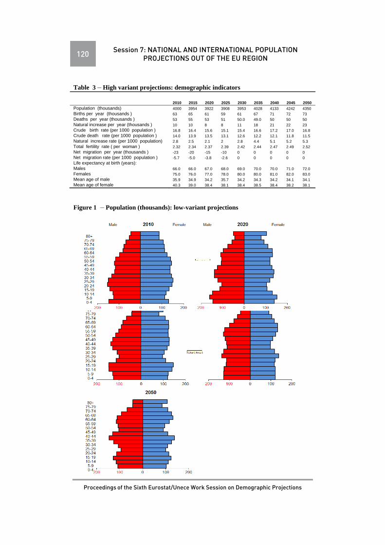
120 Session 7: NATIONAL AND INTERNATIONAL POPULATION PROJECTIONS OUT OF THE EU REGION
Proceedings of the Sixth Eurostat/Unece Work Session on Demographic Projections
Table 3 – High variant projections: demographic indicators
2010 2015 2020 2025 2030 2035 2040 2045 2050
Population (thousands) 4000 3954 3922 3908 3953 4028 4133 4242 4350 Births per year (thousands ) 63 65 61 59 61 67 71 72 73 Deaths per year (thousands ) 53 55 53 51 50.0 49.0 50 50 50 Natural increase per year (thousands ) 10 10 8 8 11 18 21 22 23 Crude birth rate (per 1000 population ) 16.8 16.4 15.6 15.1 15.4 16.6 17.2 17.0 16.8 Crude death rate (per 1000 population ) 14.0 13.9 13.5 13.1 12.6 12.2 12.1 11.8 11.5 Natural increase rate (per 1000 population) 2.8 2.5 2.1 2 2.8 4.4 5.1 5.2 5.3 Total fertility rate ( per woman ) 2.32 2.34 2.37 2.39 2.42 2.44 2.47 2.49 2.52 Net migration per year (thousands ) -23 -20 -15 -10 0 0 0 0 0 Net migration rate (per 1000 population ) -5.7 -5.0 -3.8 -2.6 0 0 0 0 0 Life expectancy at birth (years): Males 66.0 66.0 67.0 68.0 69.0 70.0 70.0 71.0 72.0 Females 75.0 76.0 77.0 78.0 80.0 80.0 81.0 82.0 83.0 Mean age of male 35.9 34.9 34.2 35.7 34.2 34.3 34.2 34.1 34.1 Mean age of female 40.3 39.0 38.4 38.1 38.4 38.5 38.4 38.2 38.1
Figure 1 – Population (thousands): low-variant projections

Session 7: NATIONAL AND INTERNATIONAL POPULATION PROJECTIONS OUT OF THE EU REGION 121
Proceedings of the Sixth Eurostat/Unece Work Session on Demographic Projections
Figure 2 - Population (thousands): medium-variant projections

122 Session 7: NATIONAL AND INTERNATIONAL POPULATION PROJECTIONS OUT OF THE EU REGION
Proceedings of the Sixth Eurostat/Unece Work Session on Demographic Projections
Figure 3 - Population (thousands):high-variant projections

Session 7: NATIONAL AND INTERNATIONAL POPULATION PROJECTIONS OUT OF THE EU REGION 123
Proceedings of the Sixth Eurostat/Unece Work Session on Demographic Projections
Figure 4-Population (thousands)

124 Session 7: NATIONAL AND INTERNATIONAL POPULATION PROJECTIONS OUT OF THE EU REGION
Proceedings of the Sixth Eurostat/Unece Work Session on Demographic Projections
4. Discussion
Pursuant the low-variant projection population of Georgia is gradually declin-ing. As concerns medium and high projections, population of Georgia will in-crease. Table 2 and table 3 show that in the medium and high projection the popu-lation of Georgia will increase and rich 4.1 and 4.3 million in 2050.
The future growth expected in the medium and high projections is partly due the continuing declines in mortality and due fertility which stays above the re-placement level.
Population projections also provide information on prospective changes in age distribution:
The proportion of the population under age 15 will decline in low-variant pro-jection and will increase in medium and high level projections.
The number and share of the females of reproductive age will noticeably de-cline compared with 2010.
The proportion of the population above age 60 will increase in all projections. The mean age of population will decline slightly in medium and high level
projections.
REFERENCES
Preston, S.,H., Heuvaline P., Guillot M. 2001. Demography: Measuring and Mod-eling Population Processes. Blackwell publishers.
Tsuladze, G., Maglaperidze N., Vadachkoria A. 2003. Population prospects of Georgia.The 2003 Revision.UNFPA.
Tsuladze, G., Maglaperidze N., Vadachkoria A. 2012. Demographic Yearbook of Georgia 2011 , UNFPA.

Session 7: NATIONAL AND INTERNATIONAL POPULATION PROJECTIONS OUT OF THE EU REGION 125
Proceedings of the Sixth Eurostat/Unece Work Session on Demographic Projections
POPULATION ESTIMATES AND VITAL RATES OF THE HAREDI (ULTRA-ORTHODOX) POPULATION IN
ISRAEL: A NEW COMPONENT OF LONG-RANGE POPULATION PROJECTIONS
Ari M. Paltiel
Summary
The first long-range population projections for Israel (2009-2059) which were de-signed for fiscal planning purposes included component projections for the Haredi (ul-tra-orthodox) population of Israel. This was justified by its potential influence on fu-ture population parameters due to its current size, its low labour force participation rates and high fertility rates. Demographic estimates were based on self-reports in pooled data from the annual CBS Social Survey, together with information obtained by linking survey records to the Na-tional Population Registry. Projections were based on a Lee-Carter model of mortality and a stochastic model of fertility based on past error in CBS projections and expert assessment, and future scenarios were based on the 95 percent confidence intervals for each of the components of change. Results showed that the Haredi population would grow from 0.75 million at the end of 2009, to 1.10 (1.05-1.15) million in 2019, 1.89 (1.63-2.16) million in 2034, and by 2059 4.15 (2.73-5.84) million, an increase of 264-686 percent. Over a quarter of Israel’s population growth in the short term, 34-42 per-cent in the medium term, and 44-92 percent in the long term will be contributed by the rapid growth of the Haredi population. Keywords: Israel, Haredi, Population Projections, high fertility, rapid growth.
1. Background
In conjunction with a re-evaluation of the financial stability of the social secu-rity system, the Israel Central Bureau of Statistics (ICBS) was asked by the Minis-try of Finance in 2009 to prepare long-range population projections for Israel for the first time (Ari Paltiel et al., 2012). Hitherto the ICBS had never attempted pro-jections for periods longer than 25 years, approximately the length of a single gen-eration. The principal justification for the tradition of preserving a modest forecast horizon was the volatility of Israel’s population: its population history has been dominated by large and irregular migration waves from diverse sources, and pre-dicting them has been one of the principal challenges for population projections(Sofia Phren and Nitzan Peri, 2010). Not only was it difficult to predict the volume and period of these waves themselves: long-range projections would

126 Session 7: NATIONAL AND INTERNATIONAL POPULATION PROJECTIONS OUT OF THE EU REGION
Proceedings of the Sixth Eurostat/Unece Work Session on Demographic Projections
have required making long-range forecasts of the fertility and mortality patterns of both the immigrants and of their native-born offspring, a task which appeared completely speculative.
The Ministry of Finance and the Bank of Israel considered it desirable that the first long-range population projections for Israel (2009-2059) include component projections for the Haredi (ultra-orthodox) population in order to assess the long-range impact of rapid growth in this population and among Arab women as well, and how their share of the population overall and in different age-groups is likely to change. Both groups are relatively poor, have high population growth rates and low labour force participation rates, and thus present a challenge to long-range fis-cal planning. Projections of the Arab population of Israel have been a traditional feature of population projections in Israel, however, focusing on the Haredi popula-tion was a departure from previous ICBS projections, which had always comprised groups which could be identified unambiguously and directly by characteristics recorded in the National Population Register (NPR).
The long-range projections for the entire population were planned as the sum of projections for each of three population groups: Jews and Others (without the Haredi population), the "Haredi" population and the Arab population.3 For these projections the ICBS utilized data-driven probabilistic projections of fertility and mortality for the first time. Since in recent years net migration has been very low, it was assumed to remain at zero for these projections. The present report will outline the methodology used to estimate and project the Haredi population.
2. Who are the Haredim (pl. of Haredi.)?
Haredi is the self-designation of a Jewish religious sub-culture, which is often called “Ultra-Orthodox”, but not by the members themselves(Samuel C Heilman and Menachem Friedman, 1991). The word Haredi can be loosely translated as “God-fearing”. It is far from monolithic, consisting of several groups and streams which are united in their rejection of modern culture and Western life-styles, up-holding instead a stringent version of Jewish religious strictures, as interpreted by particular revered and authoritative Rabbis. The latter are consulted as guides in all aspects of daily life. The Haredi code of conduct, their beliefs and social institu-tions, all serve to protect them from social and cultural assimilation into the wider society. In Israel and elsewhere these groups tend to live in geographically distinct, voluntarily segregated communities, and attend separate networks of educational institutions which play an unusually central social function. They maintain a strict delimitation of gender-defined social roles. Adolescent males before marriage at-tend a Yeshiva –institutions which focus on intensive study of Torah in its broadest sense – encompassing not only the Bible itself but the Mishnah and Talmud (com-pendia of Jewish religious law and philosophy) and their commentators over the centuries. After marriage, rather than entering the labour force, young men are en-
3 The Arab population includes Moslems, Christian Arabs and Druze. The "Others" population includes non-Arab Christians and residents who are not classified by religion in the National Population Registry. This group is com-posed mainly of family members of persons who immigrated to Israel under the Law of Return, but are not them-selves registered as Jews.

Session 7: NATIONAL AND INTERNATIONAL POPULATION PROJECTIONS OUT OF THE EU REGION 127
Proceedings of the Sixth Eurostat/Unece Work Session on Demographic Projections
couraged to attend a Kolel -- a full-time institution for continuing Torah education -- where they receive maintenance stipends. In Israel, men of eligible age are ex-empt from military conscription as long as they continue to attend these education-al frameworks. Girls and women study in separate institutions, and unlike males they often receive wider, vocationally-centered education preparing them to enter the labour force, often as teachers or in clerical occupations. Thus Haredi society has been called “a society of scholars”(Menachem Friedman, 1991), centered on Yeshivas and led by Rabbinical authorities who teach in these institutions.
Marriage is usually arranged, typically between ages 18 and 21, and large families are encouraged and celebrated. A wide network of voluntary private wel-fare institutions, underpinned by income maintenance, child allowances and other universal benefits of the welfare state, help to maintain large families in “dignified” poverty, while financially binding the members to their community. In Israel the Haredim back a small number of political parties whose principal function is to protect this way of life in the public sphere by employing political bargaining to maintain policies and sources of social welfare which protect their way of life. De-spite their high fertility levels women are typically the sole breadwinners in the family. The low labour force participation of male Haredim, its relationship to child allowances and to fertility incentives and their wider social implications, has received considerable attention in the economic and social policy literature (Eli Berman, 2000, Alma Cohen et al., 2013, Charles F Manski and Joram Mayshar, 2003, Esther Toledano et al., 2011).
The paper will present the methods used to estimate the current size of the Haredi population, its age structure, its components of change in recent decades, and it’s projected components of change. The results of the projection will be pre-sented as well.
3. Methods
3.1. Base Population A variety of methods have been used at the CBS to identify the size and char-
acteristics of the Haredi population, each based on a particular defining characteris-tic. However, there is no single overarching characteristic that identifies the Haredi population categorically. The Haredi way of life is a collection of attributes and behaviours, each of which, although typical, is not necessarily exclusive to this population or shared by all those who identify themselves as members of the group. There is no official definition of the population, or a formal act which would indi-cate membership. Because adoption of the Haredi way of life is voluntary, at least formally, membership can change over a person’s lifetime.
In the face of these difficulties, four alternative methods have been used at the CBS to estimate the Haredi population’s size and characteristics (Yisraela Friedman et al., 2011).
1. Ecological identification of the population in the electoral districts where a majori-ty of the population voted for one or more of the Haredi political parties;
2. Identification in the Labour Force Survey of respondents and their households who reported that the last educational institution they attended was a "Higher Yeshiva".

128 Session 7: NATIONAL AND INTERNATIONAL POPULATION PROJECTIONS OUT OF THE EU REGION
Proceedings of the Sixth Eurostat/Unece Work Session on Demographic Projections
3. Identification of records of individuals in multi-year national administrative files of educational institutions, targeting persons who are either studying or teaching in the Haredi educational networks and of their first-degree relatives (parents or chil-dren), the latter through record linkage by Personal Identity Number (PIN) of these records with data in the NPR.
4. Identification of respondents who identified themselves as “Haredi” in response to a direct question in the Social Survey4.
Each of these methods has disadvantages. The first method excludes those
members of the Haredi population who live outside or on the fringes of the elec-toral districts where a majority voted for Haredi parties, and includes individuals who might live in these districts without being Haredi. The second method relies on primary identification of males only, excludes Haredim who may have attended non-Haredi educational institutions, and includes individuals who were raised in the Haredi community but may have left it after they attended their last educational institution. In addition, it is restricted to a subset of monthly national samples com-prising (in 2009) approximately 12,000 households annually, and is subject to sampling error. The third method has the advantage of being population-based, but omits individuals in age groups who are not likely to be attending or teaching in schools, and risks including individuals who may have attended or taught in a Haredi institution without belonging to the group (this is especially true of pre-primary education, where non-Haredi families take advantage of Haredi facilities). The fourth method has the advantage of being based directly on unequivocal self-identification, but it is limited to a relatively small annual sample of individuals aged 20 and over and is subject to sampling error. In addition it excludes the insti-tutional population (a group that includes students at residential Yeshivas and Kolels).
For the Long-Range Projections project a modification of the Social Survey method was used. This method was adopted because, unlike the other methods, self-identification is unequivocal, and does not require additional assumptions re-garding the link between a particular characteristic and membership in the Haredi population. It provided the basis for a coherent reconstruction of population struc-ture at all ages by age and sex together with matched medium-range trends of fer-tility rates. Moreover it is possible to overcome the limitations of the small annual sample size by pooling annual surveys, and to extend the age restriction (age 20 and over) by linking the records in the pooled file to the NPR.
Respondents from the 8 annual surveys from 2002 to 2009 were pooled into a single dataset. The pool is analogous to a sample of the Haredi population taken over an eight-year period. This provided 54,500 respondents, of whom 3,320 had identified as Haredi, 1,650 males and 1,670 females, who were matched by PIN with their records in the NPR. Since the Social Survey is sampled from the NPR the match was complete. The NPR provided information on lifetime births of
4The Social Survey is an annual national sample-survey of the non-institutionalised population aged 20 and over, with an overall sample of approximately 7000 individuals. For a brief description see: http://www.cbs.gov.il/www/skarim/social_surv/what_survey_e.pdf

Session 7: NATIONAL AND INTERNATIONAL POPULATION PROJECTIONS OUT OF THE EU REGION 129
Proceedings of the Sixth Eurostat/Unece Work Session on Demographic Projections
women in the sample (sex and date of birth), and of subsequent deaths of respond-ents (and children). The reconstructed population for each calendar year was calcu-lated on the basis of the dates of birth in the NPR records. In order to estimate an-nual population sizes, the individual weighting factors from the annual surveys were corrected to reflect probabilities of selection. At the oldest ages, where proba-bilities of death (and institutionalization) are significant, adjustment of weights alone could not overcome the incomplete nature of the data.
As mentioned, one of the advantages of this method was that it could provide the data for an analysis of fertility in Israel’s population by degree of “religiosity”, which specifically included fertility rates for the Haredi population for 1980-2008 (Ahmad Hleihel, 2011). These estimates were consistent with national population-based estimates to a very high degree, and the derived annual estimates of popula-tion size by age proved to be equally consistent with national population estimates. In the age groups 20-74 the estimates were approximately 2% lower (consistent with the absent institutional population and the population residing outside locali-ties) and lower at age 75 and over (ranging from 80% of the national estimates in 2002 to 91% in 2009) reflecting the bias created by mortality at these ages. Since for long-range population projections accuracy at younger ages in the base popula-tion was the primary consideration, the bias at older ages was not regarded as a ma-jor obstacle. Reconstruction of the population aged 0-19 based on birth records ap-peared to be complete, increasing our confidence in the estimates for the Haredi population at these ages (Ari Paltiel et al., 2012).
The age structure of the estimated Haredi population was consistent with that of a rapidly growing population whose rate of growth had risen over the last 20 years. However examination of the sex ratios showed a peculiar pattern: a "surplus" of males at ages 35–49 and 65–79, and a deficit at the ages of 20–24 and 85 and over. The explanation for the deficit in the younger age groups appeared to be dif-ferential residence of males in institutional settings, excluding them from the social survey’s population. At older ages the explanation may lie in greater unwillingness of sampled Haredi women to agree to be interviewed by (male) surveyors. This conjecture has not yet been confirmed. Interestingly, estimates based on voting pat-terns also found unusual sex-ratios in a similar direction, although the effect was smaller (Norma Gurevich and Eilat Cohen-Castro, 2004). To correct this bias sex-ratios of the total population were used for adjustment, and the size of the popula-tion aged 20-29 was adjusted from linked birth records (see table 1 below for initial and corrected estimates).
3.2. Fertility and Mortality Assumptions The fertility and mortality assumptions of the Long-range Population Projec-
tions project were based on probabilistic projection models. However, a complete stochastic projection was not attempted. Traditional cohort-component methods were used for “high”, “medium” and “low” projections, with parameters drawn from the probability distributions of the models. Net migration was assumed to be zero (including movement between the three sub-populations), in order to facilitate assessment of the long-term impact of changes in fertility and because in recent years net-migration has been very low. Life expectancy and survival functions were projected using the Booth Maindonald Smith modification of the Lee-Carter

130 Session 7: NATIONAL AND INTERNATIONAL POPULATION PROJECTIONS OUT OF THE EU REGION
Proceedings of the Sixth Eurostat/Unece Work Session on Demographic Projections
model(H. Booth et al., 2002) with a single model used for the entire Jewish popula-tion, and a modification of this model was used for the Arab population. The mean trend was used for the “medium” projection, and the values of the upper and lower 95% confidence intervals were used for the “High” and “Low” projections. Results anticipate life expectancy at birth increasing for males from 79.5 in 2008, to 88.7 in 2057 (86.9 - 92.6 years with a 95% confidence interval). For females, the projec-tion anticipates life expectancy increasing from 83.3 years in 2008 to 94.9 years in 2057 (91.9 - 99.3).
The fertility assumptions were arrived at in three stages: 1. Errors in past fertility forecasts at the ICBS were analyzed in order to establish a
likely range for possible errors in the future. Root mean-square errors (RMSE) of projections of TFR over various periods were calculated.
2. Age-specific fertility trends in recent decades for each of the sub-populations and for the population as a whole were examined and a committee of experts assessed a plausible trend for the future in each sub-population.
3. A random walk with drift (rwd) model was applied to generate 2500 model paths from which the mean and 95% confidence intervals were derived. The drift term was derived from the expert-based trend, whereas the random component was de-rived from a random distribution with standard deviation equivalent to the RMSE derived in stage 1. (Ari Paltiel, Michel Sepulcre, Irene Kornilenko and Martin Maldonado, 2012, Steve Rowan and Emma Wright, 2010)
Although a discussion of Israel’s unique fertility patterns goes beyond the sub-ject of this paper a brief discussion is required to provide the context for Haredi fertility.
TFR in the Jewish population of Israel fell at a moderate rate, from 3.6 chil-dren per woman in 1955–1959 to 2.8 in 1980. Over the following twenty years TFR stabilized at a level of 2.5 to 2.8, with small annual fluctuations. Since the be-ginning of the present century fertility has been rising at a moderate rate, reaching 2.9 in 2008, a level not previously seen since the end of the 1970s. This level of fertility is unique among OECD countries.
Already in the early 1990s it became apparent that the relative stability of TFR since the early 1980s among Jewish women in Israel in general, and of native Is-raeli women in particular, was based on two opposing trends: falling fertility rates among the secular population to levels at or near replacement together with rising rates among the religious population, and especially among Haredi women (Dov Friedlander and Carole Feldmann, 1993). Thus this rise in recent years is mainly explained compositionally, by the increasing share of religious and Haredi women in the population of Jewish women of reproductive age, along with convergence to higher Israeli fertility norms by the wave of immigrants form the former USSR and their offspring, who had been characterized by Eastern European fertility patterns of approximately 1.6 children per woman.
Although levels of religiosity have been the leading dimension of heterogenei-ty in the fertility levels of the Jewish population, no consistent time series of suffi-cient quality was available on which trend-analysis could be based until the pooled data from the Social Survey was linked to NPR records (Hleihel, 2011). This da-taset showed that among women who defined themselves as Haredi, TFR rose from

Session 7: NATIONAL AND INTERNATIONAL POPULATION PROJECTIONS OUT OF THE EU REGION 131
Proceedings of the Sixth Eurostat/Unece Work Session on Demographic Projections
approximately 5.6 children per woman at the beginning of the 1980s, to a peak of approximately 7.5-7.6 in 2002–2005. It subsequently declined to approximately 6.5 in 2007–2009, returning to levels that characterized the late 1980s. Both the rise as well as the subsequent fall were found in studies of fertility rates in the Haredi population based on alternative data sources. This trend has been attributed to ris-ing levels of child-allowances for large families during the 1990s and their sharp curtailment in 2002-3, which eventually reduced the allowances for large families by over 50% (see the studies cited in section 1.2 above). Moreover, no sign of ris-ing average ages at first birth was observed in the Haredi population and the recent fall in fertility rates was shared by all age groups.
On reviewing these trends the expert advisory committee concluded that the most plausible course for Haredi fertility over the coming decades would be a con-tinuation of present trends: moderately declining TFR so that by the end of the pe-riod (2059) rates would reach the level of the religious non-Haredi population to-day – approximately 4.5 children. The rationale for this was that the present high rates were unsustainable without generous child benefits and social welfare provi-sions, that political support for such provisions had eroded and that constraints on large Haredi families were likely to rise. However this central forecast was modi-fied by the rwd model, which provided bounds of uncertainty around this central trend.
The model is:
TFRt=TFRt-1+et+dt
Where:
d – is the 'drift' value, obtained from the difference between the values of the TFR in the expert-derived central trend between consecutive years.
e – is a random value that was sampled from a normal distribution with an aver-age of zero and a standard deviation derived from an estimate of a forecast error for fertility one year forward. In order to obtain a random value a random num-ber is produced from a normal distribution by the Box-Muller method, and the random number is multiplied by the standard deviation for the following year.
2500 simulations were conducted in an EXCEL program, producing alterna-tive trajectories for changing TFR over the 50 year projection period for each of the sub-populations.
The RMSE–derived one-year ahead error for the non-Haredi population was determined as 0.11 children per woman. However, since Haredi TFR is currently more than double that of the rest of the population, this value was adjusted by a factor representing the ratio of Haredi to non-Haredi TFR. This resulted in values of e which declined from approximately 0.28 in 2010 to 0.14 in 2059. Thus in ab-solute terms the uncertainty interval for the TFR of the Haredi population is wider than that of the rest of the population, expressing the greater uncertainty ascribed to future fertility levels of this population.
Following a technique proposed by Goldstein the mean trend was recalculated as the cumulative mean of TFR from the beginning of the forecast to the date of

132 Session 7: NATIONAL AND INTERNATIONAL POPULATION PROJECTIONS OUT OF THE EU REGION
Proceedings of the Sixth Eurostat/Unece Work Session on Demographic Projections
interest, and the 95% confidence intervals were calculated on this basis as well (Joshua R. Goldstein, 2004).
Figure 1. shows the mean values and limits of a 95% confidence interval for TFR in the Haredi population. As expected, uncertainty increases throughout the forecast horizon. In the Haredi population the confidence interval increases from ±0.6 children in the initial 5-year period to approximately ±1.9 children in the final period. While the principle trend forecasts a decline in fertility, the upper limit of the 95% confidence interval (corresponding to the “High” projection) expresses TFRs which remain approximately at the current level. The lower limit of the con-fidence interval (corresponding to the “low” projection) projects a more rapid de-cline in TFR, with the fertility in the Haredi population reaching approximately 2.5 children per woman by 2055-2059, a rate identical to the rest of the Jews and Oth-ers population today. Thus the uncertainty interval covers a range of TFR values spanning a continuation of the very high fertility rates of the Haredi population at present to their convergence with the rest of the Jewish population, over a 50 year period.
Figure 1. Observed and projected values of TFR in the Haredi population 1980 – 2057
4. Results
Table 1 shows the initial and corrected estimates of the Haredi population. The base population for 2009 (year end) for the projections estimated the Haredi popu-lation at 750 thousand (9.9% of the population of Israel as a whole), of which 441.6 thousand were under 20 years of age (16.3% of the total population under 20 years of age). These results clearly show that the Haredi population is a significant pro-portion of the Israeli population today, and that its high growth rates are rapidly in-creasing its share in the youngest age groups.

Session 7: NATIONAL AND INTERNATIONAL POPULATION PROJECTIONS OUT OF THE EU REGION 133
Proceedings of the Sixth Eurostat/Unece Work Session on Demographic Projections
Table 1. Original and Corrected Estimates of the Haredi Population for the End of 2009
Age Males Females Total Percentage of Total Israeli
Population
Original Corrected Original Corrected Original Corrected
Total 378,500 378,200 362,200 371,800 740,600 750,000 9.9%
0-9 134,400 135,600 130,200 129,000 264,600 264,600 18.0%
10-19 92,600 90,700 84,400 86,300 177,000 177,000 14.3%
20-29 53,400 59,700 55,700 58,400 109,100 118,100 10.3%
30-39 39,800 37,900 36,500 38,500 76,400 76,400 7.2%
40-49 26,200 24,100 23,000 25,100 49,200 49,200 5.9%
50-59 18,300 17,800 18,900 19,400 37,200 37,200 4.9%
60-69 8,700 7,600 7,600 8,700 16,300 16,300 3.2%
70-84 4,800 4,200 4,800 5,400 9,400 9,600 2.8%
85+ 300 600 1,100 1,000 1,400 1,600 1.7%
The Long-Range Projection project calculated that the population of Israel,
which numbered 7.6 million at the end of 2009, is projected by the end of 2019 (10 years), to reach 8.8 million according to the medium projection (with a gap of 8.6 to 9.1 million between the Low and High projection); 11.0 million (9.9 – 12.1) by the end of 2034 (25 years); and 15.6 million (11.6 – 20.4) by the end of 2059 – an increase of 54 to 170 percent within 50 years.
The projections show that the Haredi population will increase remarkably both in size and in its share of the population, even if the course of the lowest alternative projection is followed. Results showed that the Haredi population would grow from 0.75 million at the end of 2009, to 1.10 (1.05-1.15) million in 2019, 1.89 (1.63-2.16) million in 2034, and by 2059 4.15 (2.73-5.84) million, an increase of 264-686 percent. As can be seen in figure 2 below, by 2019 the Haredi populations share is forecast to increase to 12.4(11.6 - 13.3) percent of the population of Israel as a whole, by 2034 to 17.2 (14.2 - 20.6) percent and by 2059 it may reach 26.6 (15.9 - 39.9) percent. Alternative scenarios were constructed in order to calculate the maximum and minimum share of the Haredi population. The relevant alterna-tive scenarios are those in which the Haredi population grows at a minimum or maximum rate relative to the other two groups.
The Haredi population’s young age structure makes a significant contribution to its growth rates. A projection designed to measure this contribution, holding mortality constant at 2009 levels and reducing TFR to replacement level, showed that the Haredi population would grow by 86 percent until 2009, entirely due to population momentum.

134 Session 7: NATIONAL AND INTERNATIONAL POPULATION PROJECTIONS OUT OF THE EU REGION
Proceedings of the Sixth Eurostat/Unece Work Session on Demographic Projections
Table 2. Projection of Sources of Population Growth in the Short, Medium and Long Range
Low Projection Medium Projection High Projection 2010-
2019 2020-2034
2035-2059
2010-2019
2020-2034
2035-2059
2010-2019
2020-2034
2035-2059
Birth rate per 1000
Total Population 18 16 13 21 19 19 24 23 25 Haredim 35 31 23 40 37 33 41 43 44 Death rate per 1000
Total Population 6 6 7 5 5 5 5 4 4 Haredim
2 2 2 1 1 1 1 1 1 Average Growth rate %
Total Population 1.3 1.0 0.6 1.6 1.4 1.4 1.9 1.9 2.1 Haredim 3.4 2.9 2.1 3.8 3.6 3.1 4.3 4.2 4.0 Share of Haredim in total population growth rate - % 30 42 92 27 37 48 25 34 44
Table 2 shows the considerable contribution of prospective growth in the
Haredi population to overall population growth in Israel. Over a quarter of Israel’s population growth in the short term, between 34 and 42 percent in the medium term, and 44 to 92 percent in the long term will be contributed by the rapid growth of the Haredi population.
As we stated earlier, one of the purposes of these projections was to estimate the future composition of age-groups by sub-population. Figure 2. shows projec-tions for the share of the three population groups in broad age groups over the short, medium, and long term, with vertical bars show uncertainty intervals from the maximum and minimum scenarios. As expected these show that overall shares of the population will change principally through changes in the youngest age groups, and that the range of uncertainty in the long term is very great – thus the share of the Haredi population at ages under 20 in the long run (2059) may fall an-ywhere from as little as 16 percent to as much as 68 percent – clearly a very wide range! Fortunately at older ages the uncertainty is much smaller, except in the long range, where fertility differences are able to influence the relative size of the 20 to 64 age group.

Session 7: NATIONAL AND INTERNATIONAL POPULATION PROJECTIONS OUT OF THE EU REGION 135
Proceedings of the Sixth Eurostat/Unece Work Session on Demographic Projections
Figure 2. Share of subgroups in the population of Israel by age, in the short, medium, and long term, with uncertainty intervals
0-19 Total
65+ 20-64
Male Haredim of working age (20-64) were a particular concern of the plan-
ners, due to their current low labour force participation rates. In 2009 they consti-tuted 4 percent of the working age population of both sexes. In the short term their share was forecast to rise to 5 percent, in the medium term to 7 percent, and over 50 years to 12 (10 - 14) percent of the working age population, triple their current share.
5. Discussion and conclusions
If the projection assumptions are realized the population of Israel will undergo significant growth in the short term, but even more so in the long term. With an overall growth rate of 1.4-1.5 percent in the medium projection the population will be doubling every 50 years or so within a small and already densely populated ter-ritory. Concurrently, its composition by subgroup would change, principally be-cause the contribution of the Haredi population to overall growth will be very great. The projections revealed additional challenges: increasing dependency ratios due to both increased population aging (mainly due to significant cohort flow of large cohorts born in the late 1940 and early 1950s) and high fertility levels – is-sues described in the full projection report (Ari Paltiel, Michel Sepulcre, Irene Kornilenko and Martin Maldonado, 2012).
0%
10%
20%
30%
40%
50%
60%
70%
80%
90%
100%
2009 2019 2034 2059
0%
10%
20%
30%
40%
50%
60%
70%
80%
90%
100%
2009 2019 2034 20590%
10%
20%
30%
40%
50%
60%
70%
80%
90%
100%
2009 2019 2034 2059

136 Session 7: NATIONAL AND INTERNATIONAL POPULATION PROJECTIONS OUT OF THE EU REGION
Proceedings of the Sixth Eurostat/Unece Work Session on Demographic Projections
The Long-range Projections project was the first attempt at the ICBS to use da-ta-based stochastic methods to project the components of growth, and to begin to introduce quantitative assessments of uncertainty in our projection results. There is still great scope to continue improving the methods we used. The model for fore-casting fertility could be improved, and the reliability of the model we used to forecast mortality should be examined in depth. Moreover, a full stochastic projec-tion has not yet been conducted. Notably, such a projection would also require a calculation of the correlations between the growth components of the population groups in Israel.
This last point requires amplification. The methodology we adopted makes the unrealistic assumption that each of the subpopulations lives on its own closed de-mographic island, with the population of Israel an archipelago of all three. Alt-hough there is currently little or no movement between the Arab population and the other population groups, one cannot predict with certainty that this state of affairs will persist fifty years into the future. Moreover since it shares the same economy, health and social services as the rest of the population there is no reason to suppose that trends in the components of demographic change between it and the other two groups should not be correlated. What is true of the Arab population is even more true of the Haredi population. Our methodology assumes that their adherence to relative self-segregation will remain intact over the coming fifty years. But it is reasonable to assume that movements in and out of this population will occur in future, as they have in the past, even though it may not be possible to predict at present their dimensions, directions or timing. Moreover, the zero net migration as-sumption we have adopted for methodological purposes does not seem reasonable when we consider the rapid growth that we project. It seems likely, given these high growth rates, that migratory “push” factors will generate some measure of out migration. But once again it is not possible at present to predict their volume or timing.
6. Postscript
The pooled Social Survey file on which estimates of Haredi population size and fertility was based can now be updated for the years 2002-2012, and results compared with our forecast for the population aged 20 and above. The comparison shows that the medium projection underestimates the size of the Haredi population by 3 – 4 percent, but more importantly, it appears that our forecast the trajectory of population growth lower than that which the Haredi population is following: ap-proximately 6 percent annualy rather than the 4.7 percent previously estimated. In addition, preliminary analysis of linked birth data show that fertility rates in the Haredi population after 2009 stabilized rather than continuing their decline. If con-firmed this would imply that over the short term this population is following a tra-jectory of growth closer to that of the High projection.

Session 7: NATIONAL AND INTERNATIONAL POPULATION PROJECTIONS OUT OF THE EU REGION 137
Proceedings of the Sixth Eurostat/Unece Work Session on Demographic Projections
Figure 3. Estimates of the Haredi population aged 20 and over from the Social Survey and from the Long-Range Population Projections project, 2002-2012
REFERENCES
Berman, Eli. 2000. "Sect, Subsidy, and Sacrifice: An Economist's View of Ultra-Orthodox Jews. The Quarterly Journal of Economics, 115(3), 905-53.
Booth, H.; J. Maindonald and L. Smith. 2002. Applying Lee-Carter under Conditions of Variable Mortality Decline. Population Studies 56(3), 325-36.
Cohen, Alma; Rajeev Dehejia and Dmitri Romanov. 2013. Financial Incentives and Fertility. Review of Economics and Statistics, 95(1), 1-20.
Friedlander, Dov and Carole Feldmann. 1993. The Modern Shift to Below-Replacement Fertility: Has Israel's Population Joined the Process? Population Studies, 47(2), 295-306.
Friedman, Menachem. 1991. The Haredi (Ultra-Orthodox) Society: Sources Trends and Processes. Jerusalem: The Jerusalem Institute for Israel Studies.
Friedman, Yisraela; Nava Shaul-Mena; Nir Fogel; Dimitri Romanov; Dan Amedi; Mark Feldman; Ruth Sechayek; Gustavo Shifris and Haim Portnoy. 2011. Measurement and Estimates of the Population of Ultra-Orthodox Jews (Hebrew). Central Bureau of Statistics Technical Paper Series, 25 Jerusalem.
Goldstein, Joshua R. 2004. Simpler Probabilistic Population Forecasts: Making Scenarios Work. International Statistical Review, 72(1), 93-106.
Gurevich, Norma and Eilat Cohen-Castro. 2004. Geographical Distribution of Demographic, Social and Economic Characteristics of the Haredi Population in

138 Session 7: NATIONAL AND INTERNATIONAL POPULATION PROJECTIONS OUT OF THE EU REGION
Proceedings of the Sixth Eurostat/Unece Work Session on Demographic Projections
1996–2001 (Hebrew). Central Bureau of Statstics Working Paper Series, 5 Jerusalem.
Heilman, Samuel C and Menachem Friedman. 1991. The Haredim in Israel: Who Are They and What Do They Want? Institute of American Jewish-Israeli Relations, the American Jewish Committee.
Hleihel, Ahmad 2011. Fertility of Jewish and Moslem Women in Israel by Their Level of Religiosity, During 1979 – 2009 (Hebrew). Central Bureau of Statistics Working Paper Series, 60 Jerusalem.
Manski, Charles F and Joram Mayshar. 2003. Private Incentives and Social Interactions: Fertility Puzzles in Israel. Journal of the European Economic Association, 1(1), 181-211.
Paltiel, Ari; Michel Sepulcre; Irene Kornilenko and Martin Maldonado. 2012. Long-Range Population Projections for Israel: 2009-2059. Central Bureau of Statistics Technical Paper Series, 27 Jerusalem.
Phren, Sofia and Nitzan Peri. 2010. Prospective Immigration to Israel through 2030: Methodological Issues and Challenges, ECE-Eurostat Work Session on Demographic Projections. Lisbon, Portugal.
Rowan, Steve and Emma Wright. 2010. Developing Stochastic Population Forecasts for the United Kingdom: Progress Report and Plans for Future Work, Joint Eurostat/UNECE Work Session on Demographic Projections. Lisbon, Portugal.
Toledano, Esther; Roni Frish; Noam Zussman and Daniel Gottlieb. 2011. The Effect of Child Allowances on Fertility. Israel Economic Review, 9(1).

Session 7: NATIONAL AND INTERNATIONAL POPULATION PROJECTIONS OUT OF THE EU REGION 139
Proceedings of the Sixth Eurostat/Unece Work Session on Demographic Projections
POPULATION AND DEVELOPMENT SCENARIOS FOR
EU NEIGHBOR COUNTRIES IN THE SOUTH AND EAST
MEDITERRANEAN REGION
George Groenewold, Joop de Beer Summary
This paper presents four population and development scenarios for 11 South and East Mediterranean countries (SEMC) for the period 2010-2050. Focus of analysis of sce-nario results is on working age population prospects, economic consequences, migra-tion pressure in four migrant-sending SEMCs (Algeria, Morocco, Tunisia, Turkey). These are main countries of SEMC labour emigration to the EU. Keywords: Scenarios, South and East Mediterranean Region
1. Introduction
In 2004, the European Neighbourhood Policy (ENP) was developed by the European Commission (EC) to overcome income and welfare gaps between Euro-pean Union (EU) countries and neighbouring countries, notably countries in the South and East Mediterranean region (SEMCs). In 2008, the ENP was revamped with the launch of the Union for the Mediterranean (UfM). ENP and UfM policy goals are implementation of good governance practices in SEMCs, development of effective social and economic ties with the EU, and furthering economic growth. A total of sixteen countries are covered by ENP of which ten are SEMCs: Algeria, Egypt, Israel, Jordan, Lebanon, Libya, Morocco, Palestine, Syria, Tunisia. Within this policy context Turkey – not an ENP country but one with an EU access per-spective- is a key player in the political arena of the region, its culture and econo-my is intertwined with most of these ENP, and country of origin of the largest non-EU born immigrant population.
Realization of ENP en UfM goals is affected by demographic change and fu-ture prospects in SEMCs as well as EU countries. The link between SEMC and EU populations through international migration is important. More than 8 million peo-ple born in SEMCs live abroad of which 6 million live EU countries. Most (90%) of these migrants originate from four SEMCS only (Algeria, Morocco, Tunisia, Turkey), and most (90%) of these live in five EU countries (Germany, France, Ita-ly, The Netherlands and Spain). These countries constitute a distinct migration sys-tem, which we shall refer to as the MT4-EU5 migration system.

140 Session 7: NATIONAL AND INTERNATIONAL POPULATION PROJECTIONS OUT OF THE EU REGION
Proceedings of the Sixth Eurostat/Unece Work Session on Demographic Projections
Various scenario studies explore the demographic future of EU populations and economic implications but studies are absent for SEMCs. This paper aims to contribute filling that gap by exploring (1) the demographic future of SEMC popu-lations according to different economic-political scenarios, and (2) the economic consequences of demographic change, with particular attention to the effect of working age population change on economic production and migration pressure within the context of the MT4-EU5 migration system.
2. Population and development scenarios
Table 1 illustrates how we derived scenarios from a conceptual framework with total wealth and political cooperation as main dimensions. Eight potential sce-narios are implied and these can be reduced to four actual scenarios (S1-S4) by im-posing certain restrictions. First, a reference scenario is chosen to indicate continu-ation of prevailing conditions before the start of the Arab Spring in 2010. Second, future increase in total wealth cannot be achieved without international coopera-tion. Third, international cooperation of SEMCs is limited to cooperation with the EU or with other countries in the region. The four scenarios were labelled Busi-ness-as-Usual or BAU scenario (S1), Integration scenario (S2), Alliance scenario (S3), Stress scenario (S4). BAU and Stress scenarios represent unfavourable out-looks while the Integration and Alliance scenarios represent favourable ones.
Table 1 - Framework for population and development scenarios
The BAU scenario (S1) is the reference scenario. In terms of total wealth and political cooperation, this scenario assumes that, between 2010 and 2015, all Arab Spring and EU financial crises related issues will have settled to levels of trend lines that would have emerged in the absence of these events. This means a contin-uation of decrease in total wealth, partly attributable to the ongoing ad hoc style of SEMC-EU cooperation failing to improve political, security, economic, socio-cultural and environmental conditions. Overall, the scenario assumes that, between 2010 and 2050, the economic influence of the EU in the Middle East continues to decline. On the political front, the Israel-Palestine conflict continues constraining economic growth and political stability in SEMCs, and tensions with the EU. The scenario assumes no further breakthrough political, social, technological, and cul-tural changes. In terms of demographic behaviour, the scenario assumes that annual net number of migrants remains more or less constant during the whole of the peri-
Increase Decrease
Success S2
Failure S1
Success S3
Failure S4
Total wealth
EU-SEMC cooperation
Meditteranean Alliance cooperation

Session 7: NATIONAL AND INTERNATIONAL POPULATION PROJECTIONS OUT OF THE EU REGION 141
Proceedings of the Sixth Eurostat/Unece Work Session on Demographic Projections
od 2010-2050. All SEMCs, except Israel, experience negative net migration with more people emigrating than immigrating. For the period 2010-2015 figures will be somewhat higher to account for higher emigration in the wake of Arab Spring events. Regarding fertility prospects, this scenario assumes a continuation of past trends in fertility rates in SEMCs. This means that fertility rates for some countries will continue to decline even further, while rates of some other countries may in-crease. Overall, the speed of fertility decline will slow down because it will takes time before institutions (men, kinship group, community) have lowered family size preferences and individual women gained more power to decide about numbers of children to have. By 2050, the average of country-specific TFRs will have settled at replacement level fertility. Regarding mortality, improvements in life expectan-cies continue but progress is less than in the more favourable scenarios. The Integration scenario (S2) assumes that SEMCs become EU Member States by 2030. The expanded EU becomes highly integrated at political, econom-ic, social and military levels, whereby total wealth increases to the average of EU27 countries in 2010. As adaptation of institutions, production systems and gov-ernance practices to EU standards take time to develop, economic production levels and growth only start matching those of EU27 countries after 2035. The precondi-tion for EU membership, solution of the Israel-Palestine conflict, is met during the 2015-2020 period, bringing political stability to the region, boosting the invest-ment climate, cultural and religious tolerance and cooperation. By 2050, the new EU38 has become one of three key powers in the world, alongside the USA and China. During the first phase of EU38 formation (2010-2030) and economic growth, emigration from SEMCs is expected to increase because of labour demand increases in the ageing and shrinking EU27 labour markets. Emigration outnum-bers immigration and return migrants. During the second economic growth phase (2030-2050) SEMCs are starting to flourish. Emigration is declining as finding jobs locally becomes easier. Return migration increases including some immigration of children of emigrants born and raised in EU27 countries exploring a future in par-ent’s country of origin. The scenario foresees increased intercultural contact and adoption of western-style ‘individualism’ in SEMCs leading to a reversal of the low status, low labour force participation and low decision-making power of wom-en, among others. The latter leads to more rapid fertility decline than in the BAU scenario, and by 2050 to fertility rates converging to the current average EU27 lev-el. The same economic, social, cultural and psychosocial factors explaining Euro-pean fertility rates are now also determining rates in SEMC populations. As health infrastructure and services improve significantly, currently high unmet need of family planning in several SEMCs will decline, contributing to lower fertility rates. Such improvements also lead to lower infant and childhood mortality rates, and to higher life expectancies than in the unfavourable scenarios. The downside of this scenario is that SEMC populations will increasingly adopt unhealthy western-style food habits and lifestyles leading to increases in obesity and related welfare diseas-es and, in the long term, to higher mortality at intermediate and older ages.
The Alliance scenario (S3) foresees that SEMCs step-up collaboration with other countries in the Middle East to form a single Pan-Arab Union, akin to EU27. Strategic economic and political alliances are formed with the EU27 though, con-tributing to economic prosperity and political stability in both regions. According

142 Session 7: NATIONAL AND INTERNATIONAL POPULATION PROJECTIONS OUT OF THE EU REGION
Proceedings of the Sixth Eurostat/Unece Work Session on Demographic Projections
to this scenario, the Israeli-Palestinian conflict is also assumed to be resolved. This peace solution removes barriers to internal (south-south) market cooperation and intercultural contact turning the South Mediterranean region into a peaceful and in-spiring meeting place, favoured by investors. Contrary to the Integration scenario, establishment and maturation of the Pan-Arab Union takes more time to develop so that investments only start amortizing after 2040. In this scenario, labour emigra-tion from SEMCs initially increases between 2010-1015, mainly in the direction of Gulf States rather than EU countries. During the 2015-2030 period, emigration will level off as economies increasingly provide more and better paid jobs to its citi-zens. This also triggers return migration and immigration from other countries in the region, such as from Sub-Saharan African countries. By 2050, it is expected that numbers emigrating and immigrating will be in balance. Two main forces will affect fertility rates. One is that economic growth leads to improvements in quality of and access to health services so that high unmet need for family planning reduc-es to zero. The other is that traditional family norms and values, and social group pressure remain intact resulting in family size preferences that are higher than in the integration scenario. However, traditions are under pressure as economic growth leads to labour force shortages so that women are increasingly stimulated to participate. Therefore, governments increasingly encourage parents to invest in ed-ucation of their daughters leading to higher educational attainment levels and oc-cupational skills among women. The currently very low labour force participation rates of women in Arab countries are expected to increase rapidly. The net outcome of both forces is that fertility levels decline, but at a lower speed than in the inte-gration scenario (S2). Health status and life expectancy improvements will develop more favourably than in the Integration scenario because adverse western lifestyles and health behaviour are not adopted widely.
The Stress scenario (S4) foresees that the Mediterranean Sea becomes a divid-ing line between two competing cultures. Within the Arab region, the Israeli-Palestinian conflict lingers on periodically escalating and deepening the divides be-tween Arab and Jews, and between Muslim communities and Christians in EU countries. Enterprises find it increasingly difficult to sustain business in the region and governments see their tax-base shrink forcing them to lay off a large share of their employees. Result is rising unemployment, poverty, social and political un-rest, and emigration pressure. Emigration to the EU increases to all times highs, re-turn migration and immigration comes to a halt. Access and quality of health and family planning infrastructure deteriorates leading couples to get more children than they want, and infant-, childhood- and maternal mortality rates to rise leading to stagnation in life expectancy increase. However, in the long term, the economic crises stimulate the revival of traditional social support systems leading to a rise of life expectancies in the long term.
On the basis of these qualitative scenarios, quantitative assumptions about fu-ture international migration, fertility and mortality rates were formulated. Regard-ing international migration, we adopted the UN Medium Variant net migration as-sumptions to represent the BAU-scenario migration assumptions. Figures for the 2010-2015 period were adapted to account for increased outmigration due to Arab Spring-related upheavals in Tunisia, Libya, Egypt, and Syria. Furthermore, we as-sumed that all those who fled have returned by 2015. Net migration assumptions

Session 7: NATIONAL AND INTERNATIONAL POPULATION PROJECTIONS OUT OF THE EU REGION 143
Proceedings of the Sixth Eurostat/Unece Work Session on Demographic Projections
for the other scenarios were derived from changes in emigration and immigration as described in the qualitative scenarios. Regarding fertility, the Integration scenar-io featured as reference for the other scenarios. It assumes the most rapid decline whereby fertility levels in 2050 are assumed to resemble the current EU average TFR. Regarding mortality, the Alliance scenario was considered as the most fa-vourable scenario so that we adopted the highest observed improvement in life ex-pectancy in the world (2.5 life expectancy years per decade), to represent life ex-pectancy increase in SEMCs. The assumptions of the other scenarios were derived from this scenario. Scenario results were calculated by applying the cohort-component projection method.
3. Working age population and economic production
The working age population (WAP) comprises persons in the age range 15-64 years old. The relationship between working-age population and economic produc-tion can be summarized as follows:
The equation conveys that, given fixed output per worker (GDP/W), fixed proportion of the labour force having a job (W/LF), and fixed labour force partici-pation (LF/WAP), an increase of the working-age population share (WAP/P) nec-essarily leads to GDP per capita growth (GDP/P). To explore potentials for eco-nomic growth and policies it is therefore important to (also) explore the future pro-spects of WAP shares. During a first stage demographic transition, from high to low fertility and mortality rates, the share of youth (<15 years old) in a population decreases while WAP shares increases. Potentially, the net effect is that the average costs of caring and raising children and youth decrease because costs are borne by a larger number of workers. Rising WAP shares are therefore an indication of po-tential demographic dividend. Whether this potential becomes real depends on whether working age population growth can be absorbed by the economy. If not it leads to rising unemployment or lower labour participation rates contributing to so-cial unrest and migration pressure. In a second stage of demographic transition, when mortality and fertility rates and youth shares hover at low levels, the oldest age groups become more populated with people who are no longer working. De-pending on accumulated assets during the life course such elderly persons become more or less dependent for their survival and care on those who work. During this second stage WAP shares are falling reflecting the rising economic dependency of elderly in an ageing population.
GDP GDP W LF WAPP W LF WAP P
═ x x x)(

144 Session 7: NATIONAL AND INTERNATIONAL POPULATION PROJECTIONS OUT OF THE EU REGION
Proceedings of the Sixth Eurostat/Unece Work Session on Demographic Projections
4. Scenario results
Table 2 summarizes scenario results for SEMCs, EU27 and EU5 countries. The figures show that SEMCs are growing rapidly, from 280 million in 2010 to 396 and 425 million in 2050 whereas EU27 countries only grow from 501 to 524 million. In both regions, most of the growth will be realized before 2030. Regard-ing the MT4-EU5 migration system, Morocco, Algeria, Tunisia, and Turkey, com-prised 151 million people in 2010 and will grow with 45 to 58 million people. Their working age populations, comprising 102 million persons in 2010, are ex-pected to grow with 19 to 23 million during the 2010-2030 period, and with anoth-er 3 to 7 million during the 2030-2050 period. EU5 countries, home to 55% of the EU population, will see their combined population increase with 11 million until 2030 after which a decline sets in. The EU5 working age population, 178 million in 2010, is expected to decline with 7 million persons between 2010 and 2030, and with 14 million during the 2030-2050 period. During the 2010-2030 period, the de-cline of the working age population is largest in Germany and The Netherlands (-15 million and -1 million persons, respectively). Italy and Spain will experience significant declines during the 2030-2050 period, totalling -3 and -2 million per-sons, respectively. The French working age population remains stable at about 42 million, mainly due to stable and relatively high fertility resulting from family pol-icy measures permitting couples to combine work and child rearing, and from poli-cies advocating a two- or three child family norm.
These opposite demographic trends in SEMCs and EU have consequences for future economic production and migration pressure in both regions. We therefore examined Working Age Population share (WAP/P) prospects of SEMCs and se-lected EU countries. A majority of SEMCs (data not shown) will experience a rise in WAP shares. They are expected to peak to about 70 per cent, or 2.3 workers (.7/.3) sustaining 1 dependent person below age 15 or above age 65. SEMCs appear to differ widely regarding when WAP shares reach peak levels and for how many years shares remain high. During this ‘window of opportunity’ economies must try to benefit from this once-in-a-lifetime-chance of ideal demographic conditions with large number of people in the working ages and small numbers in the dependent age groups. In case of Egypt, Palestine, Jordan, and Syria, most scenarios predict WAP shares to rise during the whole or most of the 2010-2050 period. For Algeria, Morocco, Turkey and Libya, WAP shares are expected to continue rising until about 2035 after which a decline sets in. Tunisia and Lebanon are the odd ones out. Due to demographic transition starting earlier than in other SEMCS, WAP shares already reached (Tunisia) or are about to reach (Lebanon) their peak level of al-most 70% . For some SEMCs the ‘demographic window-of-opportunity’ will last for several decades (Turkey, Morocco, Lebanon), while for others (Libya, Algeria) the window-of-opportunity is much shorter.

Session 7: NATIONAL AND INTERNATIONAL POPULATION PROJECTIONS OUT OF THE EU REGION 145
Proceedings of the Sixth Eurostat/Unece Work Session on Demographic Projections
Table 2 - Total and working-age population prospects, SEMCs and EU (millions)
2010S1 S2 S3 S4 S1 S2 S3 S4
Algeria Total 35.5 45.3 44.3 45.4 43.8 51.6 50.3 52.3 48.115-64 24.2 31.0 30.8 31.1 29.8 33.1 32.9 33.1 30.2
Egypt Total 81.1 109.3 106.6 109.3 107.3 133.5 125.7 132.2 130.715-64 51.5 70.8 70.6 71.3 68.8 87.6 85.9 87.2 83.9
Israel Total 7.4 9.6 10.3 9.9 7.9 11.7 13.4 11.8 7.215-64 4.6 6.0 6.6 6.2 4.8 7.2 9.1 7.6 4.1
Jordan Total 6.2 9.2 8.8 9.1 8.0 12.0 11.9 11.7 9.015-64 3.6 5.9 5.8 5.9 5.1 7.8 8.3 7.8 5.7
Lebanon Total 4.2 4.9 5.6 5.4 4.0 5.0 7.1 6.1 2.815-64 2.9 3.3 3.9 3.7 2.7 3.2 4.8 3.9 1.7
Libya Total 6.4 8.0 7.3 7.8 7.0 9.7 8.6 8.9 6.915-64 4.2 5.5 5.1 5.3 4.8 6.1 5.5 5.5 4.1
Morocco Total 31.9 38.7 37.1 39.0 37.9 42.7 41.5 44.3 40.515-64 21.2 25.9 25.1 26.1 25.1 28.0 27.5 28.5 26.2
Palestine Total 4.0 7.2 6.8 7.0 6.2 10.8 9.9 9.8 8.515-64 2.2 4.1 4.1 4.2 3.5 6.8 6.9 6.6 5.2
Syria Total 20.4 29.7 28.4 29.2 28.2 38.4 35.1 36.4 35.115-64 12.1 18.8 18.5 18.8 17.7 25.2 24.4 24.5 22.5
Tunisia Total 10.5 12.3 12.0 12.4 11.7 13.2 13.0 13.4 11.615-64 7.3 8.4 8.3 8.4 7.9 8.3 8.3 8.3 7.2
Turkey Total 72.8 87.7 86.6 88.3 87.0 96.1 92.5 98.4 95.315-64 49.2 59.6 59.6 59.9 58.7 62.0 60.6 62.2 60.9
All SEMCs Total 280.4 362.0 353.9 362.8 348.9 424.5 409.0 425.2 395.815-64 183.0 239.4 238.5 240.9 229.0 275.5 274.2 275.4 251.7
MT4 Total 150.6 184.1 180.0 185.1 180.4 203.5 197.3 208.5 195.515-64 102.0 124.9 123.8 125.5 121.5 131.4 129.3 132.2 124.5
EU-27 Total 501.0EU-5 Total 269.4EU-5 15-64 178.0Note: MT4= The Maghreb countries Morocco, Algeria, Tunisia plus Turkey
EU5= Germany, France, Italy, Spain, The Netherlands
170.7 157.3280.2 279.0522.3 524.1
2030 2050
Figure 1 illustrates WAP share prospects for MT4 and EU5 countries. They show that the Integration scenario (S2) leads to highest future WAP shares in MT4 countries. This is consistent with the expectation that favourable economic, social and political conditions defining the scenarios result in favourable demographic conditions for WAP shares to increase more than in the more pessimistic scenarios, such as the Stress scenario (S4). EU5 countries are in a more advanced stage of demographic transition and are ageing, and this is reflected in the downward trend of WAP rates in Figure 1. Overall WAP shares are expected to decline with 10 per-centage points from about 66% in 2010 to 56% in 2050, indicating a demographic penalty to future economic production levels. Whether potential demographic divi-dends (MT4 countries) or penalties (EU5 countries) result in stagnation or decrease of economic production depends on how successful countries are in maintaining or increasing labour productivity (GDP/W), employment conditions (W/LF), and la-bour participation rates (LF/WAP), and, in the case of EU5 countries, whether they manage to expand their working age population by recruiting suitable foreign la-bour migrants.

146 Session 7: NATIONAL AND INTERNATIONAL POPULATION PROJECTIONS OUT OF THE EU REGION
Proceedings of the Sixth Eurostat/Unece Work Session on Demographic Projections
Figure 1 – Prospects working age population shares for selected countries
Table 3 illustrates how SEMCs and EU5 countries actually between 2000 and 2010 regarding impact of demographic change on economic production. The last column (WAP/P) shows that in all SEMCs WAP shares increased between 2000 and 2010. The second column shows that all countries, except Syria, experienced per capita GDP growth in the range of 38 (Turkey) and 48 (Algeria) percentage points. In the case of Morocco, the potential economic benefit from an increase in WAP share with 8 percentage points (100 to 108) was attenuated by a decline in the employment ratio of 2 percentage points. In the case of Turkey, the potential demographic dividend of an increase in WAP share of 6 percentage points was re-

Session 7: NATIONAL AND INTERNATIONAL POPULATION PROJECTIONS OUT OF THE EU REGION 147
Proceedings of the Sixth Eurostat/Unece Work Session on Demographic Projections
duced to zero because of a decline in the employment ratio with 6 percentage points.
Table 3. WAP shares and economic growth (GDP in constant 1990 US$, PPP)
In Tunisia economic production grew mainly as a result of growth of labour productivity but also because of taking full advantage of demographic dividend po-tential and by a rise in employment ratio. Contrary to other MT4 countries, per cap-ita GDP growth in Algeria mainly resulted from higher employment in a growing working age population, while productivity increase was slight. EU5 countries ex-perienced an opposite development between 2000 and 2010 as WAP shares stalled or declined while economic production indicators increased, except in Italy. A de-mographic penalty of declining WAP shares was prevented because countries man-
SEMCs GDP/P Index GDP/W Index W/WAP Index WAP/P Index
Algeria 2000 1,585 100 7,831 100 0.33 100 0.62 100
2010 2,349 148 8,334 106 0.41 126 0.68 111
Egypt 2000 2,734 100 10,119 100 0.45 100 0.60 1002010 3,906 143 12,897 127 0.48 105 0.63 107
Israel 2000 14,610 100 41,122 100 0.57 100 0.62 1002010 17,195 118 44,167 107 0.62 109 0.62 101
Jordan 2000 2,939 100 13,630 100 0.38 100 0.57 1002010 3,975 135 17,679 130 0.38 101 0.59 103
Morocco 2000 2,427 100 7,925 100 0.50 100 0.62 100
2010 3,493 144 10,794 136 0.49 98 0.66 108
Syria 2000 6,263 100 22,946 100 0.49 100 0.56 1002010 5,852 93 23,911 104 0.41 85 0.59 105
Tunisia 2000 3,790 100 13,494 100 0.44 100 0.64 1002010 5,374 142 17,246 128 0.45 101 0.70 109
Turkey 2000 6,398 100 19,826 100 0.50 100 0.64 1002010 8,847 138 27,530 139 0.47 94 0.68 106
EU-5
France 2000 20,656 100 51,311 100 0.62 100 0.65 1002010 22,986 111 55,033 107 0.64 104 0.65 100
Germany 2000 18,507 100 40,847 100 0.67 100 0.68 1002010 20,645 112 43,050 105 0.73 109 0.66 97
Italy 2000 17,232 100 47,247 100 0.54 100 0.67 1002010 17,062 99 44,855 95 0.58 107 0.66 97
The Netherlands 2000 21,658 100 43,434 100 0.73 100 0.68 1002010 23,925 110 46,949 108 0.76 104 0.67 99
Spain 2000 15,094 100 38,910 100 0.57 100 0.68 1002010 16,785 111 41,641 107 0.59 104 0.68 100
Index results are affected by rounding
Economic production
Output per worker Employment ratio
Working age population share

148 Session 7: NATIONAL AND INTERNATIONAL POPULATION PROJECTIONS OUT OF THE EU REGION
Proceedings of the Sixth Eurostat/Unece Work Session on Demographic Projections
aged to increase productivity and participation rates, and importing labour (e.g. from new EU Member States such as Poland).
5. Discussion
All scenarios predict SEMC populations to grow rapidly during the 2010-2050 period while growth of EU populations is stagnating. The Integration scenario con-sistently predicts the highest working age population shares during the 2010-2050 period, and the Stress scenario the lowest shares. This is consistent with the hy-pothesis that favourable economic and social conditions contribute to favourable demographic conditions and vice versa. All scenarios indicate that working age population shares in SEMCs are expected to increase and remain at high levels for several decades. Regarding the MT4 countries. Analysis of past trends in economic and demographic indicators suggests though that some SEMCs may not be able to fully capitalize of rising WAP shares, such as Turkey and Morocco, contributing to emigration pressure, possibly in the direction of EU5 countries where countrymen reside who migrated before. On a positive note, the development gap between MT4 and EU5 countries, indicated by differences in per capita GDP, have become smaller and this trend continues it may attenuated future migration pressure. All scenarios were designed to accommodate increases and decreases in migration pressure. For instance, the optimistic Integration scenario assumes emigration first increase and then decrease during the 2010-2030 period so that by 2030 net migra-tion is zero. The pessimistic Stress scenario foresees emigration pressure to in-crease rapidly to all time high numbers by 2020, which will prevail up to 2050. To date, EU5 countries have been successful to cope with declining WAP shares by increasing productivity, participation, pension ages, and labour immigra-tion. However, WAP shares will further decline from 66 per cent in 2010 to 56 per cent in 2050. It is yet difficult to predict how long such measures can be used to prevent that a decline in per capita GPD commences. A complicating factor is that changes in population composition also affect the demand side of the economy. An increase in the proportion of elderly and decrease of the proportion of youth leads to changes in demand for products and services. Furthermore, the elderly of the fu-ture are likely to be different from the ones of today, requiring a different product and service mix. Such changes require that education and vocational training sys-tems must adapt their curricula to prepare future generations for a different job market. If such adaptations are not implemented in countries with excess labour it will become hard to find and recruit suitable labour migrants abroad. MT4 countries comprise potential future labour. However, their educational and vocational training systems needs upgrading. The EU could consider providing support but also examine current and potential levels of complementarity in work-ing age populations of both regions, and what it takes to increase complementary. Working towards complementarity of labour pools also involves social compatibil-ity of people as this fosters migrant integration and social cohesion. This requires that children and young adults in both regions have to be raised as flexible and tol-erant individuals who can work and live with people of different cultures, religion

Session 7: NATIONAL AND INTERNATIONAL POPULATION PROJECTIONS OUT OF THE EU REGION 149
Proceedings of the Sixth Eurostat/Unece Work Session on Demographic Projections
and religiosity. This sounds like Utopia, but the Integration and Alliance scenarios do assume that such complementarities and compatibilities materialize. A few words on the plausibility of the scenarios. The overall finding was that differences between scenarios are not very large between 2010 and 2030. This is not surprising because within a time-frame of 20 years population growth is almost entirely determined by the shape of the (2010) base-year age distribution. This phenomenon is known as ‘population momentum’. Effects of differences in scenar-io assumptions on future fertility, mortality, and migration rates only become visi-ble in the long-term. Another issue is that the scenarios were developed while vari-ous SEMCs are going through a period of political transition of which the outcome is yet uncertain. We made the optimistic assumption that by 2015 this transition will have been completed resulting in a new status quo which does not lead to ma-jor shifts in demographic behaviour. But is this reasonable to assume? What would happen in terms of demographic behaviour if Arab Spring related protests would lead to establishment of anti-western, conservative Islamic governments in all SEMCs? Can the presented population scenarios encompass population growth tra-jectories emerging out of such kind of context? We think the answer is affirmative for the following reasons. Firstly, the ‘population momentum’ embedded in the current age-sex pyra-mids leaves little room for effects of sudden changes in between 2010 and 2030. With respect to the international migration component, even if all persons who even slightly oppose lifestyles according to conservative Islamic law would emi-grate or flee from SEMCs, actual numbers departing would be limited by immigra-tion and asylum restrictions in receiving countries. Furthermore, after 2030, effects of changes in fertility and mortality rates would gain momentum but effects are at-tenuated because they cancel out to some extent, even if a new political order would result in higher fertility and lower life expectancies. Secondly, there is little evidence that the establishment of anti-western, conservative Muslim governments automatically leads to higher fertility and population growth. In fact, after estab-lishment of the Iranian Shiite government in 1979 fertility rates dropped to below replacement level fertility by 2010. In Saudi Arabia, heartland of Sunni Muslim tradition, fertility declined from 7 children in 1978 to 3 children in 2010. We conclude by noting that the European Neighbourhood Policy (ENP) may become victim of its success because realization of its goals may conflict with EU economic interests. The consequence of ENP success is that SEMCs cannot, for a second time in history, serve as labour pool to EU economies because economic growth in SEMCs and closure of welfare gaps is likely to result in lower emigra-tion from SEMCs and to significant return migration of former citizens, including children born, raised and educated in EU countries. Implication is that future EU labour force shortages have to be complemented by people living in other parts of the world. However, ageing and shrinking labour forces are not issues limited to EU countries as they also play in other parts of the world. It is difficult to foresee to what this may lead in terms of national and regional economic growth and power, globalization of international migration, social cohesion and migrant integration.

150 Session 7: NATIONAL AND INTERNATIONAL POPULATION PROJECTIONS OUT OF THE EU REGION
Proceedings of the Sixth Eurostat/Unece Work Session on Demographic Projections
REFERENCES
Ayadi, R. & Sessa, C. 2011. What scenarios for the Euro-Mediterranean in 2030 in the wake of the post-Arab spring? MEDPRO Policy Paper 2. Brussels: CEPS.
European Commission (EC). 2012. The European Neighbourhood Policy. http://ec.europa.eu/world/enp/policy_en.htm (17 March 2013)
Eurostat (2012). Eurostat online database. http://epp.eurostat.ec.europa.eu/ por-tal/page/portal/ help/first_visit/database (12 October 2013)
Groenewold, W.G.F., Beer de, J.A.A. and Huisman, C.C. 2012. Population scenar-ios 2010-2050 for MED11 countries: a MEDPRO WP3 research report. NIDI, The Hague. http://depot.knaw.nl/12605/ (17 March 2013)
International Labor Organization (ILO) (2012). Key Indicators of the Labor Mar-ket database (KILM). http://kilm.ilo.org/KILMnet/
Massey, D.S., Arango, J., Hugo, G., Kouaouci, A., Pellegrino, A., & Taylor, J.E. (1993). Theories of International Migration: A Review and Appraisal. Population and Development Review 19, 3: 431-466.
UN (2011b). UN Global Migration Database. http://esa.un.org/unmigration/index.aspx (15 May 2013)
Zlotnik, H. (1992). Empirical identification of international migration systems. In M. Kritz, Lin Lean Lim, & Zlotnik, H. (Eds.), International Migration Systems: A Global Approach. Oxford, England: Clarendon Press.

Session 8
ASSUMPTIONS ON FUTURE FERTILITY
Chair: Maria Graça Magalhães (Statistics Portugal)


Session 8: ASSUMPTIONS ON FUTURE FERTILITY 153
Proceedings of the Sixth Eurostat/Unece Work Session on Demographic Projections
CONTRIBUTION OF FERTILITY MODEL AND PARAMETERIZATION TO POPULATION PROJECTION
ERRORS
Dalkhat M. Ediev Summary
This work provides the needed comparative study of contributions to the population prediction accuracy of fertility model form and of the accuracy of the three main fer-tility indicators (the total fertility, mean and standard deviation of age at birth, respec-tively: the TF, MAB, SDAB). We apply to the empirical female populations set of (about thirty) fertility models and study the deviations of the imputed numbers of births from the empirical ones. Our set of fertility models includes variants of the direct transformation of the empirical schedule; Schmertmann’s Quadratic Spline model; the Gamma model; the Beta model; the Rectangular model; the Ryderian pentapartite model; and combinations of those models with abridging into 5- and 10-year age groups and regression models. Our data come from the Human Fertility Database, Re-cent Demographic Developments’ reports by the Council of Europe, Human Fertility Collection, Eurostat’s and UN Population Division’s estimates and cover (after merg-ing and cleaning) 5887 country-years of observation. We find high importance of accu-racy of the TF and MAB in population projections. The role is limited, yet considera-ble, of estimates of the SDAB and of the choice of the fertility model form. We suggest to avoid abridging fertility rates and projecting occurrence-exposure rates by parity. Our recommended approach would be, first, to model TF, MAB and SDAB and, sec-ond, to transform, however estimated beforehand, age-specific fertility rates to fit ex-actly the projected TF, MAB and SDAB. Making use of our findings already reduces the mean squared prediction errors by half as compared to existing practices. Keywords: fertility, projections, modelling.
1. Introduction
Fertility models and assumptions are the main drivers of population forecast errors in short- and long-time horizon. In the US context, Alho (1992) has suggest-ed that contribution to population mean squared forecast errors of accuracy of ini-tial population estimates is 0.3 percent, that of mortality assumptions is up to 0.02 percent, of migration is up to 0.1 percent, but considerably more, 5-10 percent, is the contribution of fertility estimates. The latter estimate is roughly comparable to the mean squared annual change of TF of about 4 percent in the Human Fertility Database (2013). The leading role of fertility estimates in determining population forecast accuracy justifies detailed analysis of various ingredients of fertility as-

154 Session 8: ASSUMPTIONS ON FUTURE FERTILITY
Proceedings of the Sixth Eurostat/Unece Work Session on Demographic Projections
sumptions, such as models used to describe its time and age variation. Meanwhile, the period total fertility rate (TF) is the prime, if not the only, fertility indicator commonly used in producing the population projection scenarios (e.g., Eurostat 2011; U.S. Census Bureau. 2012; United Nations 2013). The age distribution of fertility, usually, remains behind the scene and is rarely reported in the projection literature. The most recent UN World Population Prospects 2012 (United Nations 2013), the most advanced, well-done, and authoritative international projections as of today, offer great methodological advances and many details in modelling the Total Fertility but barely anything about modelling the age variation of fertility. Such a situation is quite typical for the population projection literature at large. In-deed, a common practical method is simply to scale up or down the baseline age pattern of fertility according the projected TF levels.
Such simplifications may work well for low-mortality, no-migration stationary populations where population sizes of fertile age groups are equal and any age pro-file of fertility rates produces the same number of births as long as the TF is fixed. In a population with n persons in each of the single-year fertile age groups, there will be TF*n births each year. More realistically, population sizes of fertile age groups vary substantially because of time-varying sizes of birth cohorts and effects of migration and mortality. Such irregular age profiles may produce differing num-bers of births and projected populations when combined with fertility curves of the same total fertility but differing age patterns.
Another set of practical questions refers to how to describe (and, hence, to model) the age pattern of fertility rates. A typical concise description of it involves, apart from TF, the mean and the standard deviation of age at childbearing (MAB and SDAB, respectively) – indicators found important in fertility and dynamic population models. More complicated fertility models involving more than three parameters have also been proposed in the literature and shown to better fit the em-pirical fertility schedules. A common sense and some advanced approaches in the projection literature assume superiority of more detailed fertility descriptions over less nuanced ones. This assumption, however, has never been tested systematically and, it appears in our study, seems not to be valid.
Our work aims to improve understanding of the role of different ingredients of fertility projections through a comparative analysis of importance of model choice and of the three main fertility parameters (TF, MAB, and SDAB) in projecting the number of births. Model-wise, we consider about thirty different fertility models of different sophistication levels. Using empirical population compositions and fertili-ty rates, we study deviations of the predicted number of births from the empirical number under alternative models of the age pattern of fertility rates and for differ-ent approximations of the fertility parameters.
2. Data and methods
Appreciating the sensitivity of the projected number of births to accuracy of the TF is straightforward. A one percent error in the TF, the age pattern of fertility being intact, would result in a similar one percent error in the projected number of births. Sensitivity to the projection errors in the age pattern of fertility is, however,

Session 8: ASSUMPTIONS ON FUTURE FERTILITY 155
Proceedings of the Sixth Eurostat/Unece Work Session on Demographic Projections
harder to study because of interaction of these errors with the age composition of the population to which the fertility pattern is applied. In a population with a ‘flat’ age pattern at fertile ages the accuracy of the fertility pattern (given the TF is fixed) hardly matters. On the contrary, in projecting a population with strongly skewed age composition applying the same TF to younger or older cohorts at childbearing ages may produce different numbers of births.
Some insights, even if under unrealistic assumptions, may be gained through analytical derivations. Ediev (2013) shows, in particular, that the relative prediction error of the number of births in a stable population may be approximated as
2rr , where r is the population growth rate, is the bias in the MAB, is the bias in the SDAB and is the SDAB. Given typical SDAB around 5 years and population growth of fractions or, at most, of few percent per year, it is clear that the effect of the bias in MAB is dominating over the effect of bias in SDAB. More so, if we take into account that biases in MAB are, usually, higher in absolute value than biases in SDAB. Despite important insights from the above relation, its practical value is rather limited. That is because populations are seldom stable and, in particular, the estimate above of the contribution of the bias in SDAB into births prediction error is far too small for a real population. Under stylized, yet realistic, assumptions (r=0.5%, SDAB=6 years, =1.6 years, and =0.5 years) the formal relation suggests 0.8% errors originating from the biases in MAB and only 0.008% errors due to biases in SDAB – both too low, as compared to our simulations-based estimates (see further down in the paper).
A more practical and realistic estimates of contributors to births prediction er-rors may be done through numerical simulation using data on actual populations. To this end, we use five detailed international population and fertility databases (Human Fertility Database 2013; Recent Demographic Developments 2005; human Fertility Collection 2013; Eurostat database 2013; and UN (2013) World Popula-tion Prospects 2012: HFD, RDD, HFC, WPP, and IDB, respectively, in the follow-ing text). Based on empirical data, we simulate percentage errors of the predicted numbers of births assuming variety of typical model simplifications about the age pattern of fertility rates. The five databases contain estimates, respectively, for 27, 43, 73, 59, and 236 populations with different calendar coverage and total 1634, 1757, 3774, 3127, and 2832 country-years covered (5887 country-years after merg-ing the datasets and cleaning the repetitive entries). The pooling was done with fol-lowing priority of the databases: HFD>RDD>HFC>EUSt>WPP. (If the same data-base, in that case HFC, had different estimates for the same population in the same year, we averaged those different estimates.) These datasets cover practically the entire range of typical fertility and population structures, both modern and histori-cal.
To each empirical female population we apply a model age profile of fertility rates, with TF set at the empirical level, and see how far the imputed number of births deviates from the empirical number. We tried number of models of age-specific fertility (about 30 individual models and combinations) and number of scenarios for the MAB and SDAB (seven scenarios for each). As noted above, we do not vary the TF, because contribution of bias in TF to births prediction error is

156 Session 8: ASSUMPTIONS ON FUTURE FERTILITY
Proceedings of the Sixth Eurostat/Unece Work Session on Demographic Projections
straightforward and needs no simulations to assess: one percent error in TF produc-es one percent error in the number of births.
More specifically, we tried the following models for the age-specific fertility: direct transformation of the empirical schedule; Schmertmann’s Quadratic-Spline model; the Gamma model; the Beta model; abridging the fertility rates into 5- and 10-year age groups; regressions of fertility rates over TF and MAB based on a se-lected dataset; the Rectangular model; and the Ryderian pentapartite model. Some of the models are described next.
In our simplest model, we transform the empirical pattern of age-specific fer-tility rates directly, according to the assumed model values of the MAB and SDAB:
k
MABxMABf
kxf ee1
, (1)
here xf is the fertility rate at age x, superscript ‘e’ denotes the empirical sched-
ule, and eSDAB
SDABk . Multiplier ‘
k
1’ before the empirical schedule assures iden-
tical TF’s in the empirical and transformed schedules; in calculations, we use dis-crete approximation to (1) and adjust the multiplier to match exactly the assumed TF. Occasionally, the transformed rates may turn non-plausible when positive at ages beyond the fertile age limits. We overcome this problem by applying (1) only in the age range 12-54 and setting fertility rates zero outside that range.
In the next model, we approximate the baseline age pattern in (1) through a linear regression of age-specific fertility rates on the TF and MAB:
MABcTFRbaF xxxx , (2)
where the regression coefficients are estimated either over the entire database or based on data for a given country only. Once the baseline (2) is set, we apply trans-formation (1) to fit exactly to the assumed values for the TF, MAB, and SDAB1.
Description of Schmertmann’s Quadratic Spline model, of Gamma and Beta models may be found in Ediev (2013) and in the original literature (Schmertmann 2003; Hoem et al. 1981). We reduce the Gamma and Beta models into two-parametric variants, by setting Alfa4 to zero in the Gamma model and alfa to 12 and beta to 55 in the Beta model2. Also note that, unlike in some other works, we fit these models to assumed values for the MAB and SDAB, and not to the whole age pattern of fertility rates. For Gamma and Beta models, that is possible using analytical relations. QS model requires optimization.
Ryder’s (1989) ‘tetrapartite’ model assumes fertility rates are all set zero ex-cept at four equally-distanced ages. Our calculations show that better results are produced by the pentapartite model (used in this work) where fertility rates are all zero except at five equally spaced ages 17.5 to 37.5. Hence, in our pentapartite model, fertility rates at ages 17.5, 22.5, 27.5, 32.5, and 37.5 are selected in order to fit to the assumed values for TF, MAB, SDAB, and, to improve the robustness of the procedure, to minimize the sum of squares of the rates.
1 In our more recent study, not presented here, we find that better results are produced by a nonlinear regression of relative fertility coefficients Fx/TF on MAB and SDAB. 2 Our more recent study suggests that better results may be obtained with alfa=17 and beta=60 for this model.

Session 8: ASSUMPTIONS ON FUTURE FERTILITY 157
Proceedings of the Sixth Eurostat/Unece Work Session on Demographic Projections
The Rectangular, as well as the Ryder’s, model serves as an extreme example of model simplification. It is based on assuming age-independent fertility in an age
range bax , and zero fertility outside the range:
,,,0
,,,
bax
baxab
TFRxf (3)
SDABMABa 3 and SDABMABb 3 assure match to assumed MAB and SDAB.
Our summary indicator of prediction accuracy is the mean squared relative er-ror (MSRE) of the predicted number of births:
N
i i
ii
B
BB
NMSRE
1
2ˆ1, (4)
where iB and iB are the observed and predicted numbers of births obtained by ap-
plying the exact and the approximate fertility schedules, respectively, to population ‘i’; N is the total number of populations in the database. This indicator in conven-ient in possibility to compare it, one-to-one, to the errors induced by the biases in the TF (a one per cent bias in TF produces a similar error in the projected number births). In addition to the summary MSRE’s, we also consider full distributions of the prediction errors because the distributions show considerable excess kurtoses and prolonged tiles at both ends of the distribution.
Models’ parameterization is based on a combination of assumptions about MAB and SDAB (the TF is always set at its empirical level): the exact empirical value; the average over all populations of the DataBase; country-specific average; regression-based approximation with the TF and TF^2 (and, for the SDAB, the MAB) used as the predictors (regressions are fit over the whole DB); country-specific linear regressions with the TF used as the predictor; country-specific linear regressions with the TF and t (time) used as the predictors.
3 Results and implications
Selected MSRE’s by database are presented in Table 1. The most simplistic–and atypical for projection practices–approximations aside, inability to project ex-actly the MAB is the most important contributor to prediction errors. Among the MAB approximations tested in the paper, the most efficient happened to be the one based on a country-specific regression on TF and time. That approximation con-tributes more than one percentage point to the prediction errors, a value compara-ble to TF’s contribution (about 4 per cent as mentioned in the introduction) and ex-ceeding contributions of other components, such as model-choice- or SDAB-related errors. In fact, quite against intuition, the cost of poor approximation of MAB is comparable (for the best approximation) or even exceeds (for the less effi-cient approximations) errors due to abridging into 10-year age groups or even as-suming a rectangular shape of the fertility age pattern. The Table also illustrates

158 Session 8: ASSUMPTIONS ON FUTURE FERTILITY
Proceedings of the Sixth Eurostat/Unece Work Session on Demographic Projections
that the common practices of abridging the fertility rates into five-year age groups and using analytical fertility models also have considerable contributions to the prediction errors and better be avoided.
Another important message from Table 1 is that the simulation results are ra-ther similar for all five databases. We, therefore, present more details of the simula-tions based on the pooled dataset of 5887 population-years of observation we kept after merging the five databases and cleaning the data for repetitions (somewhat different set of estimates based on HFD data only may also be found in Ediev 2013).
Table 2 summarizes MSRE’s in simulations based on the merged database. When both the MAB and SDAB are set at their actual values (the first row with simulation results), the MSRE’s correspond to errors due to model structure. Not surprisingly, the Rectangular and Pentapartite models show rather poor perfor-mance. More of a surprise is a similar poor prediction efficiency of four other models: abridging into 10-year age groups; Beta model with parameters obtained from the common formal relations; and obtaining age-specific rates from regres-sions on TF+MAB with either the whole merged database or only its subset for a given country used to estimate the regression equations. Another unexpected, and very much instructive, finding is that the simplest model – transformation (1) of fertility rates obtained from regression on TF and MAB – show the best prediction results with only 0.33% MAPE. Good performance of the QS model, relative to other parametric models, is also noticeable and may be taken as clear indication of prominence of quadratic splines in interpolating and smoothing the age-specific fertility.
Turning to the results for different combinations of approximated MAB and SDAB in Table 2, it is worthwhile noting that the quality of MAB approximations appears to have the highest impact on prediction errors. The best approximation happened to be the one based on a country-wise regression on TF and time. This suggests that more careful examination of trends in MAB country-by-country might have resulted in even better results.
Detailed distributions of relative births’ prediction errors, as well as summary MRSE’s, in simulations based on the pooled database suggest further conclusions and practical recommendations, as described below.
First, we studied the prediction errors caused by selected alternative approxi-mations to MAB (Figure 1, the column to the left hand side) and found that the common approach (fixing MAB at a constant level; at country-specific average in our case) produces high errors: MSRE of 2.2% and individual errors stretch as far as to 8%. The Rectangular model that would not be used in any serious projection exercise and is presented here (the first box in the second column in Figure 1.1) on-ly as a (poor-performing) benchmark, would actually be more accurate than the above assumption of constant MAB, if the Rectangular shape were fitting the ob-served MAB’s exactly. Even the Ryder’s Pentapartite model that assumes fertility concentrated in five selected ages, performs not all that worse as compared to the fixed MAB assumption. Other practical possibilities for estimating MAB (based on (country-wise) regression on TF and regression on TF and time) perform better: already the simple regression on TF reduces MSRE’s down to 1.4% (lower but still comparable to Rectangular model’s errors) and limits individual errors to about

Session 8: ASSUMPTIONS ON FUTURE FERTILITY 159
Proceedings of the Sixth Eurostat/Unece Work Session on Demographic Projections
4%. Adding time as predicting variable improves the prediction even more: MSRE down to 1.1% (half the value for the common time-fixed MAB scenario). That re-sult may seemingly be explained by regular time patterns of change in MAB and, perhaps, may be further improved if a more nuanced approach of closer examina-tion of MAB trends in a given country is adopted.
Figure 1 - Histograms and corresponding normal distributions for relative prediction errors, selected fertility models, in percent
Note: First column: the original fertility rates transformed to set the MAB at its average value for a given country (keeping SDAB at its empirical value); same, MAB set to its value approximated via (country-wise) regression on TF; same, with regression on TFR and time. Second column: the Rectangular fertility model; Ryder’s pentapartite model. Third column: the original fertility rates transformed to set the SDAB at its average value for a given coun-try (keeping MAB at its empirical value); same, SDAB set to its value approximated via (country-wise) regression on TF; same, with regression on TFR and time. “msre“ stands for the Mean Squared Relative Error. Source: Author’s calculations
Turning to alternative approximations to the SDAB (Figure 1, the column to
the right hand side), we found that approximate knowledge about SD is markedly less important (three times less important in terms of MSRE) as compared to MAB: the worst approximation (the country-specific average) yields 0.6% MSRE’s and the best one (country-wise regression on TF+MAB+time, the last box in the first column) leads to MSRE of 0.3% only.
-6 -4 -2 0 2 4 6
050
015
0025
00
Tr.Fx.c.averMA
msre 2.16
-6 -4 -2 0 2 4 6
050
015
0025
00
Tr.Fx.c.MAregTF
msre 1.38
-6 -4 -2 0 2 4 6
050
015
0025
00
Tr.Fx.c.MASDregTF.t
msre 1.12
-6 -4 -2 0 2 4 6
050
015
0025
00
Rect
msre 1.57
-6 -4 -2 0 2 4 6
050
015
0025
00
Ryder
msre 2.29
-6 -4 -2 0 2 4 60
500
1500
2500
Tr.Fx.c.averSD
msre 0.62
-6 -4 -2 0 2 4 6
050
015
0025
00
Tr.Fx.c.SDregTF
msre 0.37
-6 -4 -2 0 2 4 6
050
015
0025
00
Tr.Fx.c.SDregTF.t
msre 0.3

160 Session 8: ASSUMPTIONS ON FUTURE FERTILITY
Proceedings of the Sixth Eurostat/Unece Work Session on Demographic Projections
Next, we examined the contribution of model form chosen for age specific fer-tility rates Fx. We found that any of the models examined, except for the Rectangu-lar and Pentapartite, perform better than any of the MAB’s approximations if the models are supplied with exact MAB and SDAB. The model choice seems, in fact, to be less important than the choice for a single fertility parameter, the MAB (the model choice may also be noticed to be as important in its contribution to MSRE’s as SDAB’s approximations). Apart from that, the simple transformation of regres-sion-based Fx’s performs better than more elaborate analytical models.
Our next set of results highlights consequences for the prediction errors of var-ious levels of abridging the fertility rates: into five-year age groups, into ten-year age groups or, the ‘ultimate’ abridging, into the Rectangular shape. Abridging into ten-year age groups is already almost as bad as assuming complete Rectangularity of the Fertility. Even the more common abridging into five-year age groups has quite an impact on errors (MSRE’s of 0.5%, errors spread up to 2%), an impact stronger than that of approximated SDAB or of the model choice for Fx. It may well be suggested to avoid abridging fertility or to work with interpolated age spe-cific fertility rates in projections.
The above results suggesting unique importance of MAB in shaping the accu-racy of the predicted number of births bring us to the next research question we ad-dress: might it be better to predict the MAB explicitly and not indirectly through modeling the whole age pattern of Fx? To answer this question, we have examined errors of the Gamma, Beta, and Quadratic Spline models for two variants of model fitting: to the MAB and SDAB and to the whole age schedule of fertility rates (by minimizing the sum of squared residuals). The first option (fit to MAB and SDAB only, neglecting the fit to the whole age pattern of fertility rates) is substantially better in terms of prediction errors. Fitting the Gamma or Beta models to Fx is, against intuition, almost as bad as assuming rectangular fertility. Fitting to MAB and SDAB, on the other hand, even if producing poorer fit to Fx as a whole, yields better forecasts highlighting once more importance of accuracy of MAB estimates.
Finally, we have also examined if breaking down the fertility model by birth order may improve the prediction efficacy. Such rates are potentially interesting both due to their policy-relevance but also because one may well expect that a more specified model may perform better (we considered rates of the first kind, oc-currence/exposure, rates). On the other hand, parity-specific population exposures may have very irregular age patterns that may very much affect the prediction er-rors. That is well illustrated in our next finding that working with parity-specific o-e rates may actually increase the prediction errors beyond acceptable levels: the er-rors are measured in dozens of percent, and even the MSRE’s reach levels of 10%. Modeling directly the parity-specific o-e rates is better be avoided and, perhaps, replaced by models for the rates of the second kind and/or by decompositions of total births into births by parity.
The above results were highlighting one aspect of fertility modeling at a time. Yet, in practice, projections include multiple approximations and simplifications. Figure 2 shows what would be the combined effect of most typical simplifications of the fertility model (the left hand panel: a parametric model, Gamma in this case, abridged into five-year age groups, with MAB and SDAB fixed at their country-specific averages), how does in compare to our best-performing alternative model

Session 8: ASSUMPTIONS ON FUTURE FERTILITY 161
Proceedings of the Sixth Eurostat/Unece Work Session on Demographic Projections
(the central panel: age specific fertility rates, single years of age, obtained from country-wise regressions on TF and adjusted to fit MAB and SDAB that are, in turn, obtained from country-wise regressions on TF and time), and what could have been the ideal efficiency of the same model with perfect predictions of MAB and SDAB (the right-hand panel). Remarkably, already the simple alternative proposed above might have yielded half the errors of the common approach to fertility pro-jection; and even better models for MAB may potentially lead to eight-times lower errors as compared to current practices.
Figure 2 - Distributions of the births prediction errors, in per cent: current practices (the left-hand panel: Gamma model abridged into five-year age groups, with MAB and SDAB fixed at their country-specific averages) vs suggested alter-native (the central panel: age specific fertility rates, single years of age, ob-tained from country-wise regressions on TF and adjusted to fit MAB and SDAB that are, in turn, obtained from country-wise regressions on TF and time) vs the suggested model under perfect predictions of MAB and SDAB (the right-hand panel)
Source: Author’s calculations
-10 -5 0 5 10
050
010
0015
0020
0025
00
Gamma.averMA.SD.abridg5msre 2.37
-10 -5 0 5 10
050
010
0015
0020
0025
00
Tr.Fx.regr.MA.SDmsre 1.27
-10 -5 0 5 10
050
010
0015
0020
0025
00Tr.Fx.actual.MA.SDmsre 0.33

162 Session 8: ASSUMPTIONS ON FUTURE FERTILITY
Proceedings of the Sixth Eurostat/Unece Work Session on Demographic Projections
Table 1 - Mean squared relative errors of the predicted number of births for selected models and approximations, by database, in per cent
Contributes %% error, by Database:
Source of bias: HFD RDD HFC EUSt WPP Merged DBa
MAB (country-wise regression on TF + Calendar Year) 1.1 0.6 1.2 0.6 1.0 1.2
SDAB (country-wise regression on TF+MAB+Calendar Year)
0.3 0.2 0.3 0.2 0.3 0.3
Fx model (country-wise regression on TF, transformed to
fit MAB, SDAB) 0.2 0.2 0.3 0.1 0.3 0.3
All of the above approximations combined together 1.3 0.6 1.3 0.7 1.0 1.3
MAB (country-wise regression on TF) 1.4 1.0 1.4 1.3 1.3 1.4
SDAB (country-wise regression on TF+MAB) 0.3 0.3 0.3 0.2 0.4 0.4
Time-constant MAB (fixed at country-wise average ob-served value)
1.6 1.3 2.0 1.5 2.2 2.2
Abridging in 5-year age groups 0.5 0.5 0.6 0.5 0.4 0.5
Abridging in 10-year age groups 1.5 1.5 1.3 1.4 1.3 1.3
Gamma model 0.7 0.9 0.8 0.6 0.7 0.7
Beta model (adjusted to fit MAB and SDAB) 0.7 1.0 0.8 0.5 0.8 0.8
Country-wise regression of Fx on TF and MAB 0.3 0.5 0.6 0.2 1.1 1.0
same, adjusted to fit MAB and SDAB exactly 0.2 0.2 0.3 0.1 0.3 0.3
Database-wise regression of Fx on TF and MAB 0.8 0.8 1.0 0.8 1.5 1.4
same, adjusted to fit MAB and SDAB exactly 0.4 0.4 0.4 0.3 0.6 0.6
Rectangular model 1.5 2.0 1.7 1.3 1.5 1.6
Ryder’s 5-partite model 1.9 2.0 1.8 1.8 2.8 2.3
(a) Includes, with duplications cleaned, (in the priority order): HFD, RDD, HFC, EUSt, WPP. HFD=Human Fertility Database, RDD=Recent Demographic Developments Report (2005), HFC=Human Fertility Collection, EUSt=Eurostat’s estimates, WPP= UN’s World Population Prospects 2012 report.

Session 8: ASSUMPTIONS ON FUTURE FERTILITY 163
Proceedings of the Sixth Eurostat/Unece Work Session on Demographic Projections
Table 2 - Mean squared relative errors of the predicted number of births, selected models and parameterizations, merged database, in per cent
MAB approximation
SDAB approximation
Direct trans-formation of the fertility schedule
Same, abridged in 5-year
age groups
Same, abridged
in 10-year age groups
Country-wise re-
gres-sions-
based Fx
Same, adjusted to fit MAB and SDAB
Rec-tan-gular model
exact value exact value 0.0 0.5 1.3 1.0 0.3 1.6
exact value country average 0.6 0.7 1.4 1.0 0.7 1.6
exact value country regression
(~TF+MAB) 0.4 0.6 1.4 1.0 0.5 1.6
exact value country regression(~TF+MAB+time)
0.3 0.6 1.3 1.0 0.5 1.6
exact value DB-regression
(~TF+TF^2+MAB) 0.7 0.8 1.5 1.0 0.8 1.7
country average exact value 2.2 2.2 2.6 3.1 2.3 2.7
country regression (~TF)
exact value 1.4 1.5 1.9 1.6 1.5 2.1
country regression(~TF+time)
exact value 1.2 1.2 1.7 1.4 1.3 2.0
DB-regression (~TF+TF^2)
exact value 3.2 3.2 3.4 5.4 3.7 3.6
country average country average 2.1 2.1 2.5 3.1 2.3 2.6
country regression (~TF)
country regression (~TF+MAB)
1.3 1.4 1.9 1.6 1.5 2.1
country regression(~TF+time)
country regression(~TF+MAB+time)
1.1 1.2 1.7 1.4 1.3 2.0
DB-regression (~TF+TF^2)
DB-regression (~TF+TF^2+MAB)
3.1 3.2 3.3 5.4 3.7 3.6
TF’s mean squared annual change (%) 4.23
Table 2 - (continued)
MAB approximation
SDAB approximation
DB-wise regres-sions-
based Fx
Same, adjusted to
fit MAB and SDAB
Quadr. Spline model
Gam-ma
model
Same, abridged in 5-year age
groups
Beta model
exact value exact value 1.4 0.5 0.6 0.7 0.9 0.8
exact value country average 1.4 0.8 0.8 1.0 1.0 1.0
exact value country regression
(~TF+MAB) 1.4 0.6 0.7 0.8 0.9 0.9
exact value country regression(~TF+MAB+time)
1.4 0.6 0.6 0.8 0.9 0.8
exact value DB-regression
(~TF+TF^2+MAB) 1.4 0.9 0.9 1.0 1.1 1.1
country average exact value 2.5 2.3 2.4 2.4 2.4 2.4
country regression (~TF)
exact value 1.9 1.5 1.6 1.7 1.6
country regression(~TF+time)
exact value 1.8 1.3 1.6 1.4 1.5 1.4
DB-regression (~TF+TF^2)
exact value 3.3 3.3 3.3 3.4 3.4 3.4
country average country average 2.5 2.2 2.3 2.3 2.4 2.3
country regression (~TF)
country regression (~TF+MAB)
1.9 1.5 1.6 1.7 1.6
country regression(~TF+time)
country regression(~TF+MAB+time)
1.8 1.3 1.5 1.4 1.5 1.4
DB-regression (~TF+TF^2)
DB-regression (~TF+TF^2+MAB)
3.3 3.3 3.3 3.4 3.4 3.4

164 Session 8: ASSUMPTIONS ON FUTURE FERTILITY
Proceedings of the Sixth Eurostat/Unece Work Session on Demographic Projections
REFERENCES
Alho, J.M. 1992. The magnitude of error due to different vital processes in popula-tion forecasts. International journal of forecasting. 8(3): 301–14.
Ediev, D. M. 2013. Comparative importance of the fertility model, the total fertili-ty, the mean age and the standard deviation of age at childbearing in population projections. Presented at IUSSP International Population Conference, August 26-31, 2013. Busan, South Korea. http://www.iussp.org/en/event/17/programme/paper/3054
Eurostat. 2011. EUROPOP2010 - Convergence scenario. Accessed on 14-12-2012: http://epp.eurostat.ec.europa.eu/statistics_explained/index.php/Population_projections
Hoem, J.M., D. Madsen, J.L. Nielsen, E.-M. Ohlsen, H.O. Hansen, and B. Ren-nermalm. 1981. Experiments in modelling recent danish fertility curves. Demog-raphy. 18(2): 231-44.
Human Fertility Collection. 2013. Max Planck Institute for Demographic Research (Germany) and Vienna Institute of Demography (Austria). Available at www.fertilitydata.org (data downloaded on 16.09.2013).
Human Fertility Database. 2013. Max Planck Institute for Demographic Research (Germany) and Vienna Institute of Demography (Austria). Available at www.humanfertility.org (data downloaded on 11.06.2013).
Schmertmann, C.P. 2003. A system of model fertility schedules with graphically intuitive parameters. Demographic research. 9(5): 82-110.
U.S. Census Bureau. 2012. Methodology and assumptions for the 2012 national projections.
United Nations. 2013. World population prospects. The 2012 revision. New York: United Nations.

Session 8: ASSUMPTIONS ON FUTURE FERTILITY 165
Proceedings of the Sixth Eurostat/Unece Work Session on Demographic Projections
NEW FAMILY VALUES AND INCREASED
CHILDBEARING IN SWEDEN?
Lotta Persson, Johan Tollebrant Summary
In many countries the patterns of partnership formation and dissolution has changed substantially with a general trend towards less stable unions. In Sweden, this develop-ment seems to have come to an end. One of our studies, using register data of all chil-dren in Sweden living with their biological parents 1999–2011, shows that the percent-age of children who experience a separation of their parents have decreased during the 2000s. To better understand the reasons for this development an analysis using logistic regression has been carried out. Results show that parents higher level of education and postponement of family formation are important factors explaining the downturn. Another of our studies also suggest an end of the trend with less stable unions. Register data of all children born in Sweden from 1970 shows that half-siblings have become less common during the 2000s. An increasing proportion of children born today have only full siblings. Thus, the impact of stepfamily fertility has declined. With a logistic regression we show that higher levels of education and postponement of family for-mation are once again two explanatory factors of this development. But these and oth-er socioeconomic and demographic factors do not seem to fully explain the develop-ment. In Sweden, in the 21st century, there has been a rise in fertility. Couples who have stayed together account for the entire rise. Increased gender equality at home can have led to stronger family ties, which in turn could make women and men more inclined to have more children (with the same partner). Another explanation could be a trend to-wards more family-oriented values in society. In the 2000s, marriages have increased and childlessness has decreased. To have a second child has become more common and third births have increased, at least among women in their late 30s. That is clear when parity dependent cohort fertility is studied. How will continuing increased gender equality and attitudes towards childbearing and family formation affect childbearing in the future? Keywords: parental separations, stepfamily fertility, gender equality.
1. Introduction
In recent decades there has been a trend towards less stable relationships, and divorces and separations have increased both in Sweden and in many other coun-tries. Researchers seem to agree that women's entrance onto the labour market is one of the most important reasons for this (see for example Oláh & Gähler 2012).

166 Session 8: ASSUMPTIONS ON FUTURE FERTILITY
Proceedings of the Sixth Eurostat/Unece Work Session on Demographic Projections
When women began earning money, they became more economically independent, and it became possible to get by economically even after a separation. Women's participation in the Labour force may also have created an imbalance in the family since the traditional division of labour was changed. The fact that it became easier and more acceptable to divorce is of course also one of the reasons that separations have become more common (see for example Simonsson & Sandström, 2011).
However, in Sweden, the development towards less stable unions seems to have come to an end or there may even be a trend reversal in the 2000s. This is shown in two recent studies made at Statistics Sweden. One of them (Statistics Sweden 2013a), using register data of all children in Sweden living with their bio-logical parents 1999–2011, shows that the percentage of children who experience a separation of their parents has decreased during the 2000s. In the year 2011, 41 300 children in Sweden living with their biological parents experienced a separation, that is 2.9 percent of the total child population living with both biological parents. The number of children that experienced a separation decreased between the year 2000 and 2006, followed by a slight increase and then once again a decrease during the last years, see figure 1.
Figure 1 - Percentage of children that experienced a separation in Sweden 1999–2011
The other study (Statistics Sweden 2013b) also suggest an end of the trend
with less stable unions. Register data of all children born in Sweden from 1970 shows that half-siblings have become less common during the 2000s. An increas-ing proportion of children born today have only full siblings. Thus, the impact of stepfamily fertility has declined. This means that children who have at least one half-sibling upon birth comprise an increasingly smaller share of all children born. It means that it has become more common that children only have full siblings when they are born. This also means that women and men to a greater extent have children with the same partner. Of all children who were born in 2011, 15 percent had half-siblings at birth. If the share is only calculated based on those who at birth had siblings, 27 percent had at least one half-sibling, while the remaining 73 per-
0
1
2
3
4
1999 2000 2001 2002 2003 2004 2005 2006 2007 2008 2009 2010 2011
Percent

Session 8: ASSUMPTIONS ON FUTURE FERTILITY 167
Proceedings of the Sixth Eurostat/Unece Work Session on Demographic Projections
cent only had full siblings. At the beginning of the 2000s it was more common to have half-siblings. At that time 33 percent of all children born, and who had sib-lings, had at least one half-sibling, see figure 2.
Figure 2 - Births where the child has at least one half-sibling 1970–2011
The next two sections analyses the reasons why parental separation has de-
creased during the 2000s and why it has become less common that newborn chil-dren have half-siblings. In the first of the two sections parental separations are studied and in the second section the development of half-siblings is analysed.
2. Parental separations during 2000s
Few studies analyse separations from the children’s perspective, earlier studies have often instead looked at separations from the adults’ perspective. In this regis-ter study parental separation is analysed for all children in Sweden, 0–17 years old, living with both their parents (biological or adoptive) during the year 1999–2011. The register includes around 1.4 million children every year and is a revision from the Swedish Total Population Register. Parental separation includes both separation (parents moving apart) and divorce. The aim of the study is to find explanations for the development of separations in Sweden during the first decade of the current century.
A significant increase in the level of education of the population has occurred in Sweden. In 2000, 37 percent of the women and 32 percent of the men aged 25–44 had a post-secondary education. In 2011 those shares had risen to 52 percent of the women and 41 percent of the men (according to Statistics Sweden's survey on the education of the population). As in many other countries there has also been a continuous postponement in childbearing. In 1970, the average age for women to have the first child was 24. Today the average age is 29. The upward shift acceler-ated during the 1990s because of the economic recession at that time. So in the
0
5
10
15
20
25
30
35
1970 1975 1980 1985 1990 1995 2000 2005 2010
Percent
Percentage of all births
Percentage of births where the child has at least one sibling

168 Session 8: ASSUMPTIONS ON FUTURE FERTILITY
Proceedings of the Sixth Eurostat/Unece Work Session on Demographic Projections
1990s an increasing number of young women and men instead went on to higher education and postponed having children. This pattern has remained in the 2000s.
The risk that parents will separate depends on different socioeconomic and demographic conditions for the child, the family and the parents. In the study the development of separations is studied for children with different background. The different background variables are: type of family, child's age, number of children living at home, country of birth of the child and the parents, educational level, mother's age at birth of the child and the employment status of the parents. There are big differences between the groups. The study shows that children with cohab-iting parents have roughly twice as high a risk to experience a separation compared to married parents. However, the downturn of separations during the 2000s was greater for those with cohabiting parents than for children with married parents.
The results also show that the country of birth of the child and the parents also affects the risk of experiencing a separation. Children who themselves were born abroad, or who have parents that were, run a greater risk of experiencing a separa-tion than children with Swedish born parents. The age of the parents at birth also has significance. The younger the mother is during childbirth, the greater the sepa-ration risk. We can clearly see that mothers younger than 30 years of age at child-birth have a significantly higher risk than those over 30 years old. The results show that children with cohabiting parents have around twice the risk for experiencing a separation between their parents compared to those with married parents.
Level of education is another factor that affects separations. We see that the higher the level of education of parents, the lower the risk that the child will expe-rience a separation. If both parents only have primary education the risk for separa-tion is more than double than if one parent has post-secondary education, see fig-ure 3.
Figure 3 - Proportion of children aged 0–17 whose parents have separated by parents’ highest level of education. 1999–2011
To further analyse the reasons for the upswings and downturns of separations during the 2000s a logistic regression model is used including the background vari-
0
1
2
3
4
5
6
7
1999 2000 2001 2002 2003 2004 2005 2006 2007 2008 2009 2010 2011
Percent
Primary educationSecondary educationPost-secondary education

Session 8: ASSUMPTIONS ON FUTURE FERTILITY 169
Proceedings of the Sixth Eurostat/Unece Work Session on Demographic Projections
ables. In the logic regression, the risk that a child experiences a separation is com-pared between the period 1999–2010 and the year 2011. First of all, the above vari-ables are checked one at a time, and then all are checked at the same time. The dif-ferences over time decrease when all factors are entered.
The basic model analyses the difference in parental separation without any control variables. The results of the basic model are presented as a broken line in figure 4. When all the above factors are included in the model the differences over the years nearly disappears. This means that the downturn between 1999 and 2006 is largely due to demographic and socioeconomic changes. This model is shown with a continuous line in the same figure. The most important explanation for the downturn is that parents have a higher level of education and have become older at the same time. However, most of the years, the regression is still significantly sepa-rated from 1. That means that the control variables do not explain the whole change during the 2000s, there are other explanations in addition to these.
Figure 4 - Comparison over time for children aged 0–17 who experience that parents separate during the year. The years 2000–2010 are compared with 2011. The results are presented in the form of odds ratios
3. Half siblings less common
The demographic changes that Sweden and other countries have experienced in recent decades, such as having a family and children later in life and less stable relationships, have resulted in more single person households or single parents. When these groups become larger, the possibilities to create new relationships also increase. If these new relationships occur during childbearing ages, it can contrib-ute to further childbearing. In the study the development of childbearing that is de-pendent on new relationships is studied for the period 1970–2001. The analysis is based on data from registers with information on all births for women and men 1970–2011. The partner that the persons have children with can also be identified in the registers.
0.0
0.2
0.4
0.6
0.8
1.0
1.2
2000 2001 2002 2003 2004 2005 2006 2007 2008 2009 2010 2011
Odds ratios
No control
Control for:- parents' highest educational level- country of birth of the child and the parents- employment status of the parents- mother's age at birth of the child- type of family- number of siblings living at home- child's age

170 Session 8: ASSUMPTIONS ON FUTURE FERTILITY
Proceedings of the Sixth Eurostat/Unece Work Session on Demographic Projections
The analysis has been done from the perspective of children as well as the per-spective of parents. In the perspective of children the number of newborns who have half-siblings at birth is calculated. If a child has a half-sibling, then one of the parents had children earlier with another partner. From the parents’ perspective we study how many women and men have children with more than one partner. The results from the perspective of children is illustrated in figure 2. During the period 1970 – 1990 it became more and more common that newborn children had half-siblings but in the 2000s there has instead been a downward trend.
In figure 5 the results from the parents perspective is illustrated. Most women and men have their second child with the same partner as the first child they had together. In 2011 7 percent of women and 8 percent of men had their second child with a new partner. Of those who had their third child in 2011, 21 percent of the women and 27 percent of the men had one of the three children with another part-ner. A relatively large percentage of women and men who have a fourth child have had their children with several partners. In 2011 this applied to 31 percent of the women and 46 percent of the men who had a fourth child. Development during the 2000s shows that it has become less common to have children with different part-ners. This applies to the second as well as the third and fourth child.
Figure 5 - Proportion of all second-, third and fourth-born children that are had with a new partner 2000–2011
0
10
20
30
40
50
60
2000 2002 2004 2006 2008 2010
Proportion of all second-born children that are had with a new partner
0
10
20
30
40
50
60
2000 2002 2004 2006 2008 2010
Proportion of all third-born children where the woman/man has at least one child with another partner
0
10
20
30
40
50
60
2000 2002 2004 2006 2008 2010
Women Men
Proportion of all fourth-born children where the woman/man has at least one child with another partner

Session 8: ASSUMPTIONS ON FUTURE FERTILITY 171
Proceedings of the Sixth Eurostat/Unece Work Session on Demographic Projections
There are several possible reasons for this kind of development. One reason is that people are starting families and having children later. The risk of separation is greater for those who have children at an earlier age than those who do so at a later age (as was shown in the previous section). The age for starting a family also influ-ences the time one has to find a new partner to have more children with, in case of a separation. Starting a family at a younger age (and thereby also separating at a younger age) means that there is more time to find a new partner to have additional children with. When families are started later in life (and separations occur like-wise), many will not have time to have children with several partners.
Previous studies have shown that people with a higher level of education are less likely to have children with more than one partner (for example, see Thomson el al. 2012). The fact that women and men have a higher level of education to a greater extent can also be a contributing reason why more and more have their children with the same partner.
Another factor that may have contributed to the decrease in the 2000s is that there are more foreign born persons in the population. Studies show that foreign born persons have children with several partners to a lesser extent (for example, see Thomson el al. 2012). During the period that has been studied, the share of foreign born persons in the population has increased. In 2000, 15 percent of the population was born abroad. The corresponding share in 2011 was 21 percent.
In a logistic regression model the reasons for this decline is explored. The basic model analyses the differences in how common it is to have half-siblings at birth without any other factors. The year 2011 acts as a comparison year and it is the relative level compared with this year that is shown for other years. The results of the basic model are presented as a broken line in figure 6. The years 2000–2010 are significantly higher than for 2011. In the next model the following control vari-ables are included: the mother's age at the birth of the first child, the level of educa-tion of the parents, the country of birth of the parents, the municipality group upon the birth of the child and the number of siblings at birth. This model is shown as a continuous line in the same figure. When these variables are inserted into the mod-el, the differences over time decrease during the 2000s compared with 2011. The period 2000–2010 is still significantly higher than for 2011. This means that the downward trend of the 2000s can only partly be explained by changes in the factors described above, such as older first-time mothers, parents with higher educational levels and more children with foreign born parents. There are probably more ex-planations in addition to these.

172 Session 8: ASSUMPTIONS ON FUTURE FERTILITY
Proceedings of the Sixth Eurostat/Unece Work Session on Demographic Projections
Figure 6 - Comparison over time that children at birth have half-siblings. The years 2000–2010 are compared with 2011. The results are presented in the form of odds ratios
There is a clear connection when it comes to the level of education of the par-
ents. The higher the level of education of the parents, the less likely that the child is born with half-siblings. To see the development over time on the level of education of the parents, an interaction has been done between this variable and the year. The results are illustrated in figure 7. The tendency to have half-siblings at birth has de-creased during the period regardless of the parents' level of education. The results may indicate that the decrease began first among those with parents who had post-secondary education. For children with parents who had upper secondary educa-tion, the tendency decreases first at the end of the period.
Figure 7 - Comparison over time that children at birth have half-siblings, by parents' level of education. 1990–2010 compared with 2011. The results are pre-sented in the form of odds ratios
0.0
0.2
0.4
0.6
0.8
1.0
1.2
1.4
2000 2001 2002 2003 2004 2005 2006 2007 2008 2009 2010 2011
Odds ratios
Control for:- parents' highest educational level- parents country of birth - mother's age at first birth- number of siblings - municipality at birth of child
No control
0.0
0.2
0.4
0.6
0.8
1.0
1.2
1.4
2000 2001 2002 2003 2004 2005 2006 2007 2008 2009 2010 2011
Odds ratios
both parents primary education as highest levelone/both secondary educationone parent tertiary educationboth parents tertiary education

Session 8: ASSUMPTIONS ON FUTURE FERTILITY 173
Proceedings of the Sixth Eurostat/Unece Work Session on Demographic Projections
4. Discussion
Both studies indicate that socioeconomic and demographic factors have been significant for the downturn both in children that experienced a separation between the parents and a downturn in the tendency that newborn have half-siblings in the 2000s.
However, it appears that it is only partly explained by the factors included in these analyses. It is possible that the differences over time would decrease if more explaining variables were included in the model. But it is also probable that there are explanations in addition to the socioeconomic and demographic ones.
One such explanation could be increased gender equality between women and men. Increased gender equality can have led to stronger family ties, which in turn could make women and men more inclined to have all their children with one and the same partner. Researchers often conclude that the development of gender equality occurs in two steps (see Goldscheider 2010 for example). In the first step, gender equality increases in the public sphere. This mainly occurs by women's in-creased participation in the labour force. The second step occurs in the private sphere, that is, the family. In the first step, women enter the labour force while the men do not enter the home sphere to the same extent. This is believed to lead to in-creased conflicts in the family. In the second step of gender equality development, disagreement decreases and the family is strengthened. This is assumed to occur when men begin to contribute more to household work. Some researchers believe that gender equality development in step two has a positive effect on childbearing (see Goldscheider 2010 for example).
The statistics give support to the fact that Sweden has come closer to step two. For instance, the Labour Force Surveys show that women with small children have increased their working time during the 2000s while working time among men with small children has decreased (Statistics Sweden 2012a). So even if women with young children still work less than men with young children, they are becoming closer to one another in working time. The same applies to time use of women and men for household work. Women spend more time on housework than men, but the time use studies that were done 1990/91, 2000/01 and 2010/11 show that the dif-ferences over time between the sexes have decreased (Statistics Sweden 2012b).
Perhaps gender equality has increased the most among highly educated per-sons. Research shows that those couples who build a career are those who are the least likely to separate and most likely to have a second, third and fourth child (Dribe & Stanfors 2010). One reason is thought to be that these couples have a more even distribution of housework which in turn could be positive for the rela-tionship and for having children. Those with a higher level of education are also those who share parental leave the most. Men with a high level of education use more parental allowance days than men with a lower level of education, and the re-verse is true for women (Swedish Social Insurance Agency 2011).
Thus it could be that Sweden has reached step two to a greater extent, and that families have become stronger. In this studies, the trend towards stronger families could be shown as an increased tendency to no increased separations and to have children with the same partner during the 2000s. More and more children who are born do not have half-siblings at birth, but only full siblings.

174 Session 8: ASSUMPTIONS ON FUTURE FERTILITY
Proceedings of the Sixth Eurostat/Unece Work Session on Demographic Projections
Another explanation to the reduced tendency in the 2000s to parental separa-tions and the increased tendency to have children with the same partner could be a trend towards more family-oriented values. During the 2000s marriages have in-creased, childlessness has decreased (Statistics Sweden 2011) and that it is more common to have a third child (Statistics Sweden 2012c). These changes could be signs that attitudes have changed towards a more traditional view of the family-forming process. Perhaps is the "outdated" nuclear family on the march again?
REFERENCES
Dribe, M. & Stanfors, M. (2010) Family life in power couples: Continued childbearing and union stability among the educational elite in Sweden, 1991–2005. Demographic Research 23(30): 847–878.
Goldscheider, F.K. (2000). Men, children and the future of the family in the third millennium. Futures 32: 527–538.
Olàh, L. & Gähler M. (2012) Gender Equality Perceptions, Division of Paid and Unpaid Work, and Partnership Dissolution in Sweden. EQUAL WP 03.
Simonsson, P. & Sandström, G. (2011). Ready, Willing, and Able to Divorce: An Economic and Cultural History of Divorce in Twentieth-Century Sweden. Jour-nal of Family History 36 (2): 210–229.
Statistics Sweden (2011) Nu minskar barnlösheten [Childlessness decreases now]. Statistics Sweden's periodical Välfärd [Welfare] No 2 2011.
Statistics Sweden (2012a) Gapet minskar mellan pappor och mammor [The gap decreases between fathers and mothers]. Statistics Sweden 's periodical Välfärd [Welfare] No 4 2012.
Statistics Sweden (2012b) Swedish Time Use Survey 2010/11. Living Conditions Report 123.
Statistics Sweden (2012c) Kärnfamiljen fortfarande vanligast [The nuclear family still most common]. Statistics from Statistics Sweden. Article published 2012-12-28 No 2012: 126.
Statistics Sweden (2013a) Children, parents and separations – Trends of the 21st century. Demographic reports 2013: 1.
Statistics Sweden (2013b) Having children in new relationships. Demographic re-ports 2013: 2.

Session 8: ASSUMPTIONS ON FUTURE FERTILITY 175
Proceedings of the Sixth Eurostat/Unece Work Session on Demographic Projections
Swedish Social Insurance Agency (2011). Föräldrapenning – Båda föräldrarnas försäkring? [Parental benefit –both parents’ insurance?] Social Insurance Re-port 2011: 13.
Thomson, E., Winkler-Dworak M., Spielauer M. & Prskawets A. (2012) Union In-stability as an Engine of Fertility? A Microsimulation Model for France. Demog-raphy 49: 175–195.

176 Session 8: ASSUMPTIONS ON FUTURE FERTILITY
Proceedings of the Sixth Eurostat/Unece Work Session on Demographic Projections
PROJECTING FERTILITY BY REGIONS CONSIDERING TEMPO-ADJUSTED TFR – THE AUSTRIAN
APPROACH
Alexander Hanika Summary
Considering tempo adjusted fertility models the assumptions on fertility regarding total fertility rate (TFR) and mean age of childbearing (MAC) have to be reworked in Aus-trian population projections The intention is to reach final projected levels for TFR and MAC rather by an asymptotic curve than in a linear path. As shown in the litera-ture the model of tempo adjusted TFR* does not get along with linear increases for TFR and MAC stopping at the same time horizon. Keywords: population projection, fertility assumptions, tempo-adjusted TFR.
1. Introduction
Stimulated by the paper “Fertility Forecasting in the German–speaking World: Recent Experience and Opportunities for Improvement” (Goldstein et al. 2001), Statistics Austria developed an approach considering tempo-effects in fertility pro-jections to be implemented in the latest population projection for Austria on NUTS 2-level (Hanika, 2012). The above mentioned paper describes the inconsistencies of total fertility rate (TFR), tempo-adjusted fertility (TFR*) and mean age of childbearing (MAC) for the time horizon of fertility projection arising from discon-tiguous projections for TFR and MAC based on the national population projections for Austria, Germany and Switzerland.
The model of tempo-adjusted fertility TFR* by Bongaarts-Feeny (Bongaarts et al. 1998) estimates the level of fertility in the absence of tempo-effects:
∗ , <1>
It expresses that the true quantum of fertility is disturbed by the change of mean age of childbearing (MAC). In times of rising MAC the quantum of fertility is underestimated by the conventional measure of period TFR and vice versa (see formula <1> above). Previous fertility projections for Austria considered a rising TFR hand in hand with rising MAC due to recent trends and assumptions. A more or less linear increase of both parameters was expected until a time horizon (e.q. 2030) and held constant for the rest of the projection period. Those sudden stops

Session 8: ASSUMPTIONS ON FUTURE FERTILITY 177
Proceedings of the Sixth Eurostat/Unece Work Session on Demographic Projections
may cause inconsistencies due to the model of tempo-adjusted fertility as shown in the explanatory figure 1.
The lowermost line indicates the path of a projected TFR which rises linear from 1.43 (2010) to 1.55 (2030). At the same time MAC increases from 30 to 32 years (line in the middle). Using Bongaarts-Feeny’s model to calculate the quan-tum of TFR* we receive an increase from 1.59 (2010) to 1.72 (2030; highest line). In the case that the increase of TFR and MAC stops in the same year (2030) the quantum of TFR* would immediately fall down to the level of the TFR, because then the correction term (1-rt) of TFR equals to 1 (dotted line).
Figure 1 – The context of TFR, tempo-adjusted TFR* and MAC
Source: STATISTICS AUSTRIA, Population Projection 2012
To overcome the explained inconsistencies, Statistics Austria reformulated in
the year 2012 its fertility assumptions for the new population projection in a more consistent framework of TFR, TFR* and MAC.
2. The Austrian landscape of fertility
At the time being the Total Fertility Rate (TFR) of Austria lies in average a bit over 1.4 children per women. (2010:1.44; 2011: 1.43; 2012: 1.44). Thereby period fertility has risen slightly since the beginning of the 21st century. After the baby boom with its maximum in the year 1963 (TFR: 2.82) period fertility fell at the be-ginning of the 1970s under replacement level and reached its preliminary minimum of 1.33 in the year 2001.
29,0
29,5
30,0
30,5
31,0
31,5
32,0
32,5
1,40
1,45
1,50
1,55
1,60
1,65
1,70
1,75
TFRTFR*TFR*projMAC
TFR, TFR*
MAC

178 Session 8: ASSUMPTIONS ON FUTURE FERTILITY
Proceedings of the Sixth Eurostat/Unece Work Session on Demographic Projections
Differentiation by the nine Austrian Bundesländer (NUTS 2-level) shows the exceptional position of Vienna, the capital city of Austria: During the 1960s and 1970s Vienna’s TFR lay clearly under the Austrian average and also lower than in the other eight Bundesländer (figure 2). Even in the time of the baby boom Vien-na’s TFR did not reach replacement level. Until 1977 Vienna’s TFR fell to 1.24. Afterwards fertility in Vienna started to recover due to increasing immigration of nationalities with higher fertility levels. Since 1987 the City of Vienna is not any longer the rear light of fertility among the Austrian NUTS 2-regions. Currently the TFR of Vienna is just slightly lower than the Austrian average.
Figure 2 – TFR by Austrian NUTS 2-Regions 1961-2011
Source: STATISTICS AUSTRIA, Population Projection 2012
Vorarlberg, the westernmost region of Austria showed in the past the highest
fertility rates. In the last five years Vorarlberg shared the top position with Upper Austria on a level of more than 1.5 children per woman. Whereas fertility stagnated in Vorarlberg there was an increase in Upper Austria. The lowest fertility rates at the level of 1.3 are now observed in Burgenland, the NUTS 2-region at the eastern border of Austria.
The height of Austrian fertility lies about 30% under replacement level (Net Reproduction Rate NRR 0.69). The regional deviation ranges from 0.62 (Burgen-land) to 0.74 (Vorarlberg and Upper Austria).
1,0
1,5
2,0
2,5
3,0
3,5
Burgenland
Carinthia
LowerAustriaUpperAustriaSalzburg
Styria
Tirol
Vorarlberg
Vienna
Austria

Session 8: ASSUMPTIONS ON FUTURE FERTILITY 179
Proceedings of the Sixth Eurostat/Unece Work Session on Demographic Projections
The Mean Age of Childbearing (MAC)3 rose since the second half of the 1970s from approximately 26 years to 30 years (figure 3). Also here regional dif-ferences are observed which similarly diminished in the past. Whereas in the 1970s the span amounted more than 2.5 years it reduced to less than one year at the time being.
Figure 3 – Mean age of Childbearing by Austrian NUTS 2-Regions 1961-2011
Source: STATISTICS AUSTRIA, Population Projection 2012
3. Cohort fertility
The current relatively low level of period fertility has to be seen in the context of postponement of births as reflected in the rising MAC. Higher education and economic activities of younger women, their planning of carriers as well as prob-lems of combining family and job are suspected to cause the observed postpone-ment of births. On the other hand, as known from different surveys 4 we know that the desired number of (additionally) births is higher than the realized number. On
3 Calculated as the mean age of the age-specific fertility rates 4 E.g. Labour Force Survey (Micro Census) 4/2012, supplementary questions on (additionally) desired births.
24
25
26
27
28
29
30
31
Burgenland
Carinthia
LowerAustriaUpperAustriaSalzburg
Styria
Tirol
Vorarlberg
Vienna
Austria

180 Session 8: ASSUMPTIONS ON FUTURE FERTILITY
Proceedings of the Sixth Eurostat/Unece Work Session on Demographic Projections
the other hand, historical comparisons show that at the end final cohort fertility is lower than the reported declarations by surveys.
As indicated in table 1 Austrian women aged 20 to 44 years want do have in average 1.83 children. More than a half of them (1.03 children) is already born. The highest wish of babies we can find among women aged 30 to 34 years with nearly 2 children. Women at the age of 40 to 44 years have given birth to 1.68 children in average. This survey result fits very well to the below mentioned com-peted cohort fertility rates.
Table 1 – Mean age of Childbearing by Austrian NUTS 2-Regions 1961-2011
Age
Women 20-44 years
(in 1.000)
Additional wish of … Total number of children (realised +
desired
Realised number of children
no child maximum
1 child maximum2 children
maximum3 children
more than 3 children
in percent
Total 1.418,4 12,5 16,0 51,6 16,0 3,9 1,83 1,03
20-24 y. 257,3 13,2 9,8 61,1 13,8 (x) 1,81 0,10
25-29 y. 274,5 12,8 11,5 56,7 15,4 (3,5) 1,85 0,59
30-34 y. 276,2 8,4 14,8 54,9 18,2 (3,6) 1,96 1,09
35-39 y. 279,1 11,6 22,6 44,5 16,7 (4,6) 1,80 1,48
40-45 y. 331,3 15,9 19,9 43,1 15,9 (5,2) 1,76 1,68
Source: Labour Force Survey (Micro Census) 4/2012
Figure 4 – Cohort fertility for women born 1945/46 to 1970/71 by Austrian NUTS 2-Regions
Source: STATISTICS AUSTRIA, Population Projection 2012
1,3
1,4
1,5
1,6
1,7
1,8
1,9
2,0
2,1
2,2
2,3
Burgenland
Carinthia
Lower Austria
Upper Austria
Salzburg
Styria
Tirol
Vorarlberg
Vienna
Austria

Session 8: ASSUMPTIONS ON FUTURE FERTILITY 181
Proceedings of the Sixth Eurostat/Unece Work Session on Demographic Projections
Comparison of period TFR with cohort TFR for women born 1970 and before shows completed cohort fertility not lower than 1.6 children per woman. Only women born 1946/47 have reached cohort fertility higher than replacement level (figure 4). Women born around 1960 have a cohort fertility of 1.68. For younger women still some more births are to be expected. Women born around 1970, the youngest cohorts with completed fertility have given in average birth to 1.6 chil-dren.
Reflecting the cohort 1946/47 a regional spread in TFR of 1.59 (Vienna) to 2.25 (Burgenland) is observed in average number of births. At the time being re-gional disparities became clearly smaller. For women born in 1970 the spread in cohort fertility reaches from 1.50 (Vienna) to 1.76 (Vorarlberg).
4. Projection of fertility
To project future fertility patterns Statistics Austria uses a modified Hadwiger function (Rodgers 1994 and Condgon 1990). This model estimates age-specific fer-tility rates by four parameters, i.e. TFR, MAC, the mode and the variance of the fertility distribution. Therefore, assumptions on all this parameters have to be for-
Table 2 – Projected TFR 2060 by NUTS 2-Regions and variants5
Year Burgen-
landCarinthia
Lower Austria
UpperAustria
Salzburg Styria TirolVorarl-
bergVienna Austria
1999 1,20 1,32 1,35 1,41 1,40 1,29 1,36 1,51 1,29 1,34
2000 1,20 1,34 1,37 1,46 1,40 1,30 1,38 1,46 1,34 1,36
2001 1,23 1,32 1,35 1,41 1,35 1,23 1,33 1,51 1,31 1,33
2002 1,22 1,30 1,42 1,48 1,45 1,30 1,39 1,54 1,41 1,39
2003 1,24 1,32 1,40 1,45 1,39 1,30 1,37 1,46 1,39 1,38
2004 1,28 1,36 1,46 1,52 1,44 1,32 1,43 1,57 1,41 1,42
2005 1,27 1,37 1,46 1,49 1,45 1,32 1,41 1,55 1,38 1,41
2006 1,25 1,42 1,46 1,49 1,40 1,31 1,41 1,52 1,39 1,41
2007 1,29 1,38 1,41 1,48 1,41 1,30 1,37 1,47 1,36 1,38
2008 1,31 1,40 1,46 1,51 1,43 1,32 1,39 1,51 1,39 1,41
2009 1,27 1,37 1,42 1,51 1,39 1,32 1,38 1,51 1,36 1,39
2010 1,28 1,42 1,47 1,55 1,46 1,35 1,42 1,55 1,42 1,44
2011 1,28 1,40 1,48 1,52 1,45 1,33 1,40 1,52 1,41 1,43
2060
Med. V. 1,49 1,53 1,62 1,67 1,53 1,49 1,53 1,62 1,49 1,57
High V. 1,99 2,03 2,12 2,17 2,03 1,99 2,03 2,12 1,99 2,07
Low V. 0,99 1,03 1,12 1,17 1,03 0,99 1,03 1,12 0,99 1,07
Source: STATISTICS AUSTRIA, Population Projection 2012
5 The model for the Austrian population projection is formulated in a bottom-up approach. Therefore the result for the total of the country is the sum of a regional forecast by the 9 NUTS 2-regions. In this case demographic rates for the total of Austria have to be recalculated from the projection results for vital statistics and population. With respect to the increasing weights of regions with lower fertility, the TFR for Austria will rise to 1.55 instead of 1.57 as indicated in this table where the results of an independent extrapolation for the total of Austria are present-ed.

182 Session 8: ASSUMPTIONS ON FUTURE FERTILITY
Proceedings of the Sixth Eurostat/Unece Work Session on Demographic Projections
mulated for the 9 Austrian NUTS 2-regions as well as for 3 fertility variants (high – medium - low). We assume a change of fertility parameters until the year 2060. The time after all parameters should remain constant on the projected 2060 level.
Figure 5 – Projected fertility parameters for Austria
Source: STATISTICS AUSTRIA, Population Projection 2012
4.1 Total fertility rate and mean age of childbearing The first step is to project the TFR for the year 2060 according to the mean
variant under the precondition that completed cohort fertility will not fall substan-tially under the observed cohort fertility of generation 1970/71. The Austrian level of this value is 1.60 as shown above, the nine NUTS 2-regions vary between 1.76 (Vorarlberg) and 1.50 (Vienna).The forecast is done by a logistic regression model of TFR by time (1999-2011). In the year 1999 period fertility started to recover in Austria. Regressions use for NUTS 2-region completed cohort fertility of genera-tion 1970/71 as an upper asymptote.
∗ ln
ln ∗ ln , : <2>
29,0
31,0
33,0
35,0
0,0
0,2
0,4
0,6
0,8
1,0
1,2
1,4
1,6
1,8
2011
2013
2015
2017
2019
2021
2023
2025
2027
2029
2031
2033
2035
2037
2039
2041
2043
2045
2047
2049
2051
2053
2055
2057
2059
2061
2063
2065
2067
2069
2071
2073
2075
TFR
, TFR
*, r
TFR TFR*
r MAC
D
F
A
MAC

Session 8: ASSUMPTIONS ON FUTURE FERTILITY 183
Proceedings of the Sixth Eurostat/Unece Work Session on Demographic Projections
Those regressions produce fertility levels between 1.49 (Burgenland, Styria, Vienna) and 1.67 (Upper Austria) with a total value of 1.57 for Austria in 2060 (table 2). The high and low variant are assumed to vary at this time by ±0.5 chil-dren per woman. As spatial differences of MAC diminished over the last decades, MAC is assumed to rise up to 33.0 years in 2060 for all Austrian regions and all three fertility variants.
The next stage is to translate projected period TFR into a path of future tempo-adjusted TFR*. Due to Bongaarts-Feeny’s model, the Austrian tempo-adjusted TFR* for the year 2011 currently mounts up to 1.70 children per woman (TFR: 1.43; rt: 0.16). Because of the assumption that in the long run of population projec-tions TFR, TFR* and completed cohort fertility will converge to the same value (e.g. 1.57 for Austria), consistent paths of TFR* and rt have to be found. The first step is to calculate a path for the tempo-adjusted TFR*, starting with the actual value for the base year (1.70) and converging asymptotically to the projected value for 2060 (1.57).
We chose an asymptotic term, like
TFR∗ TFR∗ TFR∗ TFR∗ ∗ f ,f∑
∗
<3>,
Where: Index t is number of the projection year,
∗ is the tempo adjusted TFR of the last projection year, TFR∗ is the tempo adjusted TFR of the base year, and
is the number of projection years. The second step is to estimate a path for rt with
rt → 0 and ∑rt = MAC (last year of projection) minus MAC (base year of projection).
For this calculation we used
∗ , ∑
. <4>, where
Index t is number of the projection year, is the mean age of childbearing in the last projection year, is the mean age of childbearing in the base year, and
is the number of projection years. The parameter y is chosen by graphical inspection to receive a smooth curve
including the observation of rt in the base year of the projection. Based on the above mentioned relations (formula <1>) TFRt could be easily
recalculated by:
∗ ∗ 1 <5>
The results of this exercise for the total of the country and the mean variant of the latest Austrian population projection are shown in figure 5. Table 3 presents al-so values of period TFR and tempo-adjusted TFR* for the high and the low fertility variant. The green line illustrates the path of the projected TFR*, which declines gradually to the expected long-term quantum of fertility at a level of 1.57 children per women after the year 2060. The yellow line indicates the diminishing tempo rt in changing postponement of childbearing, which is reflected by the red line of MAC. MAC is assumed to reach the level of 33 years in 2060. Finally the blue line

184 Session 8: ASSUMPTIONS ON FUTURE FERTILITY
Proceedings of the Sixth Eurostat/Unece Work Session on Demographic Projections
shows the future path of period fertility, derived from the projected developments of TFR* and rt (formula <5>).
Table 3 – Projected fertility parameters for Austria by variants
Year MAC rt Medium variant High variant Low variant
TFR TFR* TFR TFR* TFR TFR*
2011 30,02 0,160 1,43 1,70 1,43 1,70 1,43 1,70
2012 30,17 0,154 1,44 1,70 1,45 1,71 1,43 1,69
2015 30,61 0,139 1,45 1,68 1,49 1,73 1,42 1,65
2020 31,23 0,116 1,47 1,66 1,56 1,77 1,40 1,59
2025 31,74 0,094 1,48 1,64 1,64 1,81 1,38 1,52
2030 32,15 0,074 1,50 1,62 1,71 1,84 1,35 1,46
2035 32,47 0,056 1,51 1,60 1,78 1,88 1,31 1,39
2040 32,70 0,040 1,53 1,59 1,84 1,92 1,27 1,33
2045 32,85 0,026 1,54 1,58 1,91 1,96 1,23 1,26
2050 32,95 0,014 1,55 1,57 1,96 1,99 1,18 1,20
2055 32,99 0,005 1,56 1,57 2,02 2,03 1,13 1,13
2060 33,00 0,000 1,57 1,57 2,07 2,07 1,07 1,07
Source: STATISTICS AUSTRIA, Population Projection 2012
Beside TFR and MAC we need also assumptions on the development of future
modes and variances of the age-specific fertility patterns. These four parameters are necessary for the estimation of future fertility patterns by Hadwiger function for all Austrian NUTS 2-regions, variants and projection years.
4.2 Variance and mode of age specific fertility rates The variances of the Austrian and regional age specific fertility rates declined
rapidly during the 1970s. At the time being they are rising again. Once more, the development of Vienna differs from the other eight NUTS 2-regions. On the one side Vienna’s variance of age specific fertility rates started to rise earlier than in the other Bundesländer, on the other hand Vienna’s variance increases much stronger (figure 6). This is a consequence of Vienna’s higher percentage of population born abroad. To a certain percentage those women give birth to their children in a younger age than women born in Austria.
Similar to TFR the variance was extrapolated to the future by a decreasing trend. According to total fertility the trend is built on the years 1999-2011. Based on the linear trend the increases of variances are reduced by 2% for each projection year. For Vienna the trend is additional reduced by 1/3 to prevent an increase be-yond observed levels of variances by NUTS 2-regions in the past (Salzburg, Tyrol and Vorarlberg). Moreover, from today’s point of view, an extraordinary strong in-crease of variance would lead to unplausible high fertility rates of women at the age of 40 to 50 years.

Session 8: ASSUMPTIONS ON FUTURE FERTILITY 185
Proceedings of the Sixth Eurostat/Unece Work Session on Demographic Projections
Figure 6 – Variance of age specific fertility rates by Austrian NUTS 2-Regions
Source: STATISTICS AUSTRIA, Population Projection 2012
The 4th parameter to estimate our fertility functions is the mode of the distribu-
tion. The mode represents the age where the highest fertility rates are observed. In the past this parameter converged from a lower level to the mean age of childbear-ing and corresponds to it at the time being (figure 7). We assume for the future, that the mode of the fertility function will be on a par with MAC. This should be true for all three variants of fertility and all nine Austrian NUTS 2-regions.
Figure 8 compares Austrian age specific fertility rates for 1972, 1988 and 2011 with the projected rates for 2030 and 2060 by all three fertility variants. In the medium variant the mode of the distribution will reach a level as observed at the end of the 1980s. Between 1988 and 2030 there is a shift of six years from 25 to 31 years and until 2060 by additional two years to 33 years. In the case that the high variant might become true, the peak of fertility could reach the level of the year 1972 with a value of about 14 percent.
20
25
30
35
40
45
Burgenland
Carinthia
Lower Austria
Upper Austria
Salzburg
Styria
Tirol
Vorarlberg
Vienna
Austria
Projection

186 Session 8: ASSUMPTIONS ON FUTURE FERTILITY
Proceedings of the Sixth Eurostat/Unece Work Session on Demographic Projections
Figure 7 – Fertility parameters for Austria 1970-2011
Source: STATISTICS AUSTRIA, Population Projection 2012
Figure 8 – Age specific fertility rates for Austria
Source: STATISTICS AUSTRIA, Population Projection 2012
0,50
1,00
1,50
2,00
2,50
3,00
15
20
25
30
35
40
45
Jahr
Mode
MAC
Variance
TFR
TFR
0,00
0,02
0,04
0,06
0,08
0,10
0,12
0,14
0,16
14 16 18 20 22 24 26 28 30 32 34 36 38 40 42 44 46 48 50
1972 (Var: 38.8; SD: 6.2 J.)
1988 (Var: 26.9; SD: 5.2 J.)
2011 (Var: 29.9; SD: 5.5 J.)
2030med (Var:32.8; SD:5.7 y.)
2030high (Var:32.8; SD:5.7 y.)
2030low (Var:32.8; SD:5.7 y.)
2060med (VAR 34.5; SD 5.9 y)
2060high (VAR 34.5; SD 5.9 y)
2060low (VAR 34.5; SD 5.9 y)
Age in yearsAge in years

Session 8: ASSUMPTIONS ON FUTURE FERTILITY 187
Proceedings of the Sixth Eurostat/Unece Work Session on Demographic Projections
REFERENCES
Bongaarts, J., Feeney, G. 1998. On the quantum and tempo of fertility. Population and Development Review 24,2: 271-291
Condgon, P. 1990. Graduation of Fertility Schedules: An Analysis of Fertility Pat-terns in London in the 1980s and an Application to Fertility Forecasts. Regional Studies 4, 1990, P. 311-326
Goldstein, J. R., Rößger, F., Jaschinski, I., Prskawetz, A. 2004. Fertility Forecast-ing in the German-speaking World: Recent Experience and Opportunities for Improvement. Comparative Population Studies – Zeitschrift für Bevölkerungs-wissenschaft, Vol. 36, 2-3 (2011): 661-692.
Hanika, A. 2012. Zukünftige Bevölkerungsentwicklung Österreichs und der Bun-desländer 2012 bis 2060 (2075), Statistische Nachrichten 10/2012, 785-809. Sta-tistics Austria
Rodgers, A., Little, J.: Parameterizing age patterns of demographic rates with the multiexponential model schedule. In: Mathematical Population Studies 3, 1994, P. 175-195.

188 Session 8: ASSUMPTIONS ON FUTURE FERTILITY
Proceedings of the Sixth Eurostat/Unece Work Session on Demographic Projections
EFFECTS OF CHILDBEARING POSTPONEMENT ON COHORT FERTILITY IN GERMANY
Olga Poetzsch and Bettina Sommer Summary
Germany has a low fertility since decades. In the last years some slight positive effects could be seen for women in their middle thirties. However, it seems that this will not lead to a sustained recovery of cohort fertility (cohort total fertility rate, CFTR). After a small recuperation, cohort fertility tends towards stagnation on a low level. We ana-lyse the effects of the increasing age at childbearing on cohort fertility. The amount of childbearing postponement and recuperation is quantified and used for an estimation of the final number of births. In addition, we also show possibilities and limitations of using analyses of cohort fertility to estimate the future development of births. Keywords: low fertility, fertility assumptions, cohort fertility, age at childbearing, postponement, recuperation index.
Preliminary remarks
Against the background of relatively low fertility in many industrialised countries, the development of births in Germany represents an exception. In west-ern Germany the total fertility rate (TFR) has remained steady at a level of 1.4 children per woman since the fall in the early 1970s; this is 30% below the re-placement level of 2.1 children per woman. Fertility halved in the new Laender in the first five years following German reunification in 1990. In the second half of the 1990s the birth rate in the new Laender rose relatively quickly and reached the same level as in western Germany in 2007. A partial recovery of the birth rate in the eastern Laender and low-level annual fluctuations in the total fertility rate for western Germany did not, however, change the continuing low fertility level.
In the last years some slight positive effects could be seen for women in their middle thirties. This caused some discussion on further development of completed fertility – will we see an increase or a stagnation? In this paper we present empiri-cal findings of the official statistics and we elucidate what these findings tell us about possible future fertility developments. We use a new approach for measur-ing the postponement and recuperation of births in the examination of cohort fer-tility. The aim is to obtain further information regarding assumptions on the de-velopment of births in the future.
The change in cohort fertility was incorporated both implicitly and explicitly in the assumptions for the most recent population projection for Germany, the so

Session 8: ASSUMPTIONS ON FUTURE FERTILITY 189
Proceedings of the Sixth Eurostat/Unece Work Session on Demographic Projections
called 12th coordinated population projection. Recuperation of the postponed births at an older age plays a major role in the modelling of the age-specific trends (Poetzsch 2010). In the future, this approach is to be refined further, including new research methods and results. It would, however, be erroneous to assume that this could significantly reduce, let alone eliminate, uncertainties surrounding long-term projection. As shown below, it helps above all to obtain a better understand-ing of the current birth situation and to state assumptions regarding the medium-term development of fertility more precisely.
In the following analysis, the changes in fertility behaviour of women in (western) Germany are examined on the basis of the completed and cumulated av-erage numbers of children in successive female cohorts. Using a technique devel-oped by Tomas Frejka for analysing the postponement and recuperation of births (Frejka et al. 2011), we then attempted to identify relevant tendencies for future development and to estimate an upper cohort fertility limit for today's 34 year olds in western and eastern Germany. Subsequently, further possibilities for improving the search for hypotheses on future fertility changes based on cohort analyses are then discussed.
1. Methodical notes
The term "cohort fertility" refers to the average number of children born to women of a particular birth cohort during the course of their life. In female co-horts which have already reached the age of 50, this figure is also known as com-pleted fertility. This paper examines both completed fertility and cumulated fertili-ty up to a given age.
The recuperation index (RI) is used for the analysis of cohort fertility6. To this end, the deviations are measured for each single year of age between the cu-mulated age-specific fertility rate of the cohort observed and that of the cohort se-lected as benchmark or reference cohort. The greatest deviation marks the "trough" at which the cumulated fertility of the cohort under examination differs most widely from the benchmark cohort. Recuperation of the postponed births be-gins after the trough. If the postponed births are not fully recuperated, there is a "residual deviation" between the completed fertility rates at the end of the repro-ductive phase. The difference between the "residual deviation" and the maximum deviation at the "trough" describes the extent to which the postponed births were recuperated. If this difference is put into relation to the deviation at the "trough", this yields the recuperation index (RI). This can be expressed as a percentage and ranges between 0% (no recuperation) to 100% (full recuperation of births) or even above 100% (overcompensation).
Formal description of the index calculation:
b the reference or benchmark cohort marks (ideally) the transition to the in-crease in age for the first birth.
6 The recuperation index was first used by Tomáš Sobotka and colleagues for the analysis and projection of cohort fertility (Sobotka et al. 2011).

190 Session 8: ASSUMPTIONS ON FUTURE FERTILITY
Proceedings of the Sixth Eurostat/Unece Work Session on Demographic Projections
m the age at which the gap between the cumulated fertility rate of the bench-mark cohort and of the observed cohort reaches a maximum. m is the "trough" age.
Fc(m) the cumulated fertility rate of women of cohort c reached by age m – mean-ing by the age of the maximum deviation from the benchmark cohort:
)(mFc
m
xc xf
15
)( ,
where )(xfc is the age-specific fertility rate of women of cohort c at age x.
Pc maximum deviation of the cumulated fertility rate of cohort c from the cu-mulated fertility rate of the benchmark cohort b at age m. Pc measures the decline in fertility in the "trough" and can therefore be described as a post-ponement measure of births in cohort c in comparison to the benchmark co-hort:
m
xbcbcc mFmFxfxfP
15
)()()]()([
Rc recuperation measure or the absolute increase in cohort fertility which took place between age m at the "trough" and the end of the reproductive period (normally at the age of 49). Depending on the issue at hand, Rc can also be calculated up to a certain age between m and 49 years.
cbcmx
bcc PCTFRCTFRxfxfR
])()([49
FDc final difference of fertility in observed cohort c in comparison to benchmark cohort b:
bcccc CTFRCTFRRPFD .
RIc recuperation index, measuring the degree of recuperation relative to the fertil-ity decline at younger ages (in “trough”):
)./( ccc PRRI
The index of recuperated births should ideally be calculated and investigated for the single birth orders, that is the first, second and further births. Unfortunate-ly, the necessary cohort data by order of births is still not available in Germany. Consequently, the results in this paper are for total births. Therefore, a certain loss of information must be taken into consideration. This is, however, limited as first and second children currently account for 84% of births in Germany.
In order to gain an insight into the more recent trends in still relatively young women, the indicators described above are not calculated for the end of the repro-ductive period, rather for several single years of ages between 34 and 44. After the

Session 8: ASSUMPTIONS ON FUTURE FERTILITY 191
Proceedings of the Sixth Eurostat/Unece Work Session on Demographic Projections
age of 40 the cohort fertility only changes marginally (currently by roughly 1.2%), meaning that the development of the number of children born to women by the age of 40 can be regarded as representative of the total cohort fertility. The (com-pleted) fertility at the ages of 44 and 49 is more or less identical.
Despite convergence during the 20 years since German reunification, there are still major differences in certain aspects of fertility behaviour between western (former territory of the Federal Republic) and eastern (new Laender) Germany. Therefore, both regions have to be analysed separately. Here, the developments are shown in detail for the former territory of the Federal Republic. Comprehen-sive results for the new Laender are published, too (Poetzsch 2013).
2. Estimation of fertility until 1977 cohort
The completed fertility rates for the 1933 to 1962 cohorts are currently avail-able. Women in the 1962 cohort were the youngest in 2011 to have reached the age of fifty and whose cumulated average fertility rate is regarded as statistically completed. In Germany the figure was 1.61 children per woman, 27% lower than for women of the 1930s cohorts, who gave birth to an average of more than two children. In the old Laender, where roughly 80% of women live today, the com-pleted fertility of the 1962 cohort was just 1.56 children per woman. Their peers in the new Laender gave birth to roughly 1.72 children on average (figure 1).
Figure 1 – Completed fertility or cumulative fertility up to given age, per woman in 2011
The 1967 cohort has not yet reached the age of fifty. However, it is already fore-seeable that the completed fertility of this cohort will fall to the lowest level yet. Afterwards, a slight increase in cohort fertility can be assumed. This is expected to continue approximately until the 1973 cohort. The 1977 cohort reached the age of 34 in 2011. Below an attempt is made to estimate the completed fertility of this cohort.
How many children women's cohort ultimately has as a result of recuperating the births postponed from a younger age is investigated using the so-called recu-
2.5 2.5
2.0
New Länder Germany
2.0
1.5 1.5
1.0
Former territory of the Federal Republic
1.0
0.5 0.5
1
0 0 1933 35 40 45 50 55 60 65 70 75 1980
Cohorts
1 Up to 1962 cohort: completed fertility per woman. From 1963 cohort: cumulative fertility up to given age.
2013 - 01 – 0080

192 Session 8: ASSUMPTIONS ON FUTURE FERTILITY
Proceedings of the Sixth Eurostat/Unece Work Session on Demographic Projections
peration index (RI). As explained in section 1, this index can be calculated for the individual cohorts and takes one cohort as a basis for comparison.
For the former territory of the Federal Republic, the 1946 women’s co-hort is taken here as the benchmark cohort. It marks a turning point in the fertility behaviour of women in the west immediately after World War 2. In the post-1946 female cohorts, the average age of women giving birth to their first child began to rise in a trend which has continued to this day; the proportion of childless women has risen as well. However, the fall in family size, which was apparent in the 1930s and early 1940s cohorts, did not continue. The average number of children per mother and the distribution of mothers by number of children stabilised in the women's cohorts born from the mid-1940s.7 Hence, the differences observed for the cohorts born up to 1968 in the recuperation index can be largely attributed to the development in the mother’s age at first birth and to the development of child-lessness.
The absolute deviations in the cumulated fertility rate for the selected cohorts are depicted in figure 2 in comparison to the 1946 cohort. It emerges that the re-cuperation of the births postponed from a younger age within the reproductive pe-riod is basically taking place at an increasing age in women and is not compensat-ing fully for the gap. The maximum deviation in the "trough" and the gap in the cumulated cohort fertility at the end of the reproductive age have increased from cohort to cohort.
Figure 2 – Absolue deviation of cumulative fertility rate from 1946 reference cohort in 2011
Note: selected west German female cohort. Births per 1,000 woman.
This development was, however, interrupted in the early 1970s cohorts. Con-
trary to the previous trend, the absolute maximum deviation in the 1970 to 1975 cohorts from the benchmark cohort was lower than that of the older women born at the end of the 1960s. Cumulated fertility between the ages of 34 and 37 (in the 2007 to 2010 calendar years) rises particularly quickly in the 1973 cohort. After the 1975 cohort the maximum deviation increases significantly again. In the 1980
7 The empirical basis for this is the 2008 microcensus and the special 2006 "Births in Germany" survey.
100 100
0
-100
1949
0
-100
-200
-300
-400
-500
-600
-700
1952
1958
1961
1964
1980
1977
1973 1975
1970
1967
-200 -300 -400 -500 -600 -700
-800
15 20 25 30 35 40 45 49
Age in years
-800
2013 - 01 – 0083

Session 8: ASSUMPTIONS ON FUTURE FERTILITY 193
Proceedings of the Sixth Eurostat/Unece Work Session on Demographic Projections
cohort it is nearly double that of the cohorts from the end of the 1950s which gave birth to an average of 1.6 children per woman.
In order to gain a clearer understanding of the current developments, figure 3 provides a comparison of the younger women's cohorts on the basis of the 1973 cohort. It demonstrates that only the 1974 cohort and possibly the 1975 cohort will reach the level of the 1973 cohort. In contrast, a visible gap is already apparent in the women of the younger cohorts. Still, it cannot be entirely excluded that this can be recuperated. However, the recuperation would have to be much more in-tensive than was the case in the last 20 years among the west German female co-horts.
Figure 3 – Absolue deviation of cumulative fertility rate from 1973 reference cohort in 2011
Note: selected west German female cohort. Births per 1,000 woman.
The extent to which the "postponed" births of the west German women's co-
horts were "recuperated" at a later age within the reproductive period is illustrated in figure 4 on the basis of the recuperated births for the 1947 to 1977 cohorts in relation to the 1946 benchmark cohort. Individual lines show the percentage of maximum deviation of cumulated fertility in the "trough" that was recuperated by the age of 34, 35, 37 and finally 40.
In figure 5 the percentage deviations for the 1947 to 1980 cohorts from the 1946 benchmark cohort are plotted. The lower curve represents the percentage by which the cumulated fertility in the relevant "trough" deviates from the benchmark cohort (%): Pc/Fb(m)*100. The other curves illustrate the respective deviations at the ages of 35, 37 and 40.
The recuperation index up to the age of 40 ranged between roughly 40% and 60% and was particularly high in the cohorts around 1960 (figure 4). After that it declined up to the 1967 cohort. The lowest completed fertility to date is expected for this cohort. The index then rose again in the 1969 to 1971 cohorts.
It emerges that the cumulated fertility achieved by the mid-thirties remains decisive for the completed cohort fertility, despite the fact that increasing numbers of births are being recuperated after the age of 35. Up to 36 percentage points could be "recuperated" between the maximum deviation from the benchmark co-
20
0
-20
-40
-60
-80
-100
-120
-140
-160
-180
1986
1974 1975
1976 1977
1978
1979
1980
1981
1982
19851984 1983
20
0
-20
-40
-60
-80
-100
-120
-140
-160
-180 15 20 25 30 35 40 45 49
Age in years
2013 - 01 – 0084

194 Session 8: ASSUMPTIONS ON FUTURE FERTILITY
Proceedings of the Sixth Eurostat/Unece Work Session on Demographic Projections
hort in the "trough" and the deviation at the age of 35. In contrast, the maximum difference between the deviation at the ages of 35 and 40 was merely 8 percentage points. Significant pointers to the future development of the younger cohorts, which have not yet reached the age of 40, can therefore be obtained from the fer-tility status at the age of 34 or 35.
Figure 4 – Recuperation index (RI) in relation to the 1946 reference cohort in 2011
Note: West German female cohort (%).
Figure 5 – Deviation of cumulative fertility rate from 1946 reference cohort in select-ed single years of age in 2011
Note: West German female cohort (%).
For the cohorts after 1973 it is apparent that the recuperation index at the ag-
es of 34 and 35 stagnates, whereas the maximum deviation from the benchmark cohort at the "trough" (lower curve) increases again. This finding calls into ques-tion the thesis of a sustained recovery in the cohort fertility represented by Gold-stein et al. (2012). Consequently, it would be necessary for the younger cohorts not to postpone their births any later and for an increasing proportion of the births to be recuperated during the later reproductive period to both increase and stabi-lise the completed fertility. This constellation has only been observed in the 1969 to 1974 cohorts to date.
Table 1 brings together the main indicators for the selected cohorts of the former territory of the Federal Republic. The expected completed fertility was es-
60 RI at age 40
50 RI at age 37
40
RI at age 35
30 RI at age 34
20
10
0
1947 50 55 60 65 70 75 1980 Cohorts
2013 - 01 – 0086
0
-10
-20
-30
Deviation at age 40
Deviation at age 35
Deviation at age 37
-40
Deviation at low point1
-50
-60
1947 50 55 60 65 70 75 1980 Cohorts
1 Corresponds to the age at which the deviation from the reference cohort is largest. 2013 - 01 - 0086

Session 8: ASSUMPTIONS ON FUTURE FERTILITY 195
Proceedings of the Sixth Eurostat/Unece Work Session on Demographic Projections
timated for the 1967, 1973 and 1977 cohorts. The 1967 cohort had reached 1,470 children per 1,000 women by the age of 44. This figure is expected to correspond more or less to completed fertility. The recuperation index at age 40 was contin-ued for the still relatively young cohorts of 1973 and 1977. An optimistic assump-tion was made here: although recuperation of the births stagnates by the age of 34 or 35, it is assumed that increasing numbers of births will be recuperated after the age of 35. Accordingly, the recuperation index at age 40 would be 57% for the 1973 cohort and 61% for the 1977 cohort. However, 3 further percentage points have been estimated by the age of 44. Overall, it emerges that the respective devi-ation at the "trough" would be reduced by 60% for the 1973 cohort and by 64% for the 1977 cohort.
Table 1. Cumulated fertility rates and indicators of recuperated births in selected female cohorts. Former territory of the Federal Republic 2011
Benchmark cohort 1946 1962 1967 1973 1977
Deviation at "trough" (Pc) Children per 1000 women X -500 -635 -605 -658
Age at maximum deviation (m) Years X 25 27 27 28
RI* at age 37 Percent X 49 42 49 -
RI* at age 40 Percent X 55 49 57 61
RI* at age 44 Percent X 57 51 60 64
Age in 2011 Years 65 49 44 38 34
Cumulated fertility at age 34 Children per 1000 women
1655 1347 1209 1233 1199
Cumulated fertility in 2011 1780 1564 1470 1466 1199
Completed fertility (CTFR) 1780 1564 1470 1540 1540
Therefore, the estimated completed fertility of just over 1.5 children per
woman assumes that the development continues unchanged. In particular for the 1977 cohort, it cannot be excluded that recuperation of the births between the ages of 35 and 40 will be either slightly higher or lower.
The last population projection (based on 2008 population) assumed for the 1977 cohort a CTFR of 1.57.
In the new Laender, completed fertility fell between the 1937 and 1947 co-horts from 2.1 children per woman to 1.8 children per woman and remained more or less constant over the next 14 years (see figure 1). The cohort fertility of wom-en in the east falls again from the 1961 cohort. For this reason, the 1960 cohort is selected as a benchmark; it marks the provisional end of the stable birth situation and the birth rate, which is comparable to that of the 1946 west German bench-mark cohort. The focus is on fertility changes in the 1960s and 1970s cohorts. At the time of German reunification in 1990, the 1960s cohorts were aged between 20 and 30. They were more strongly influenced by social and economic changes in their reproductive behaviour than women in the older cohorts, most of whom had already completed their family planning before 1990. This turning point at around 1990 emerges clearly in figure 6 from the examples of the 1964 and 1967 cohorts, which were 26 and 23 years old respectively at the time.

196 Session 8: ASSUMPTIONS ON FUTURE FERTILITY
Proceedings of the Sixth Eurostat/Unece Work Session on Demographic Projections
Figure 6 – Absolue deviation of cumulative fertility rate from 1960 reference cohort in 2011
Note: selected east German female cohort. Number of children per 1,000 woman.
Figure 6 further illustrates the two different patterns, which is a result of the
development of cohort fertility in the new Laender. The deviations from the 1960 benchmark cohort increase during the sharp decline in births in the first half of the 1990s in the 1964 and 1967 cohorts. The time at which the "postponement" of births was replaced by "recuperation" was determined in this case primarily by ex-ternal factors (rapid social and political upheavals).
The situation is different in the post-1970 cohorts. Their cohort fertility dif-fers from the benchmark cohort - similar to the situation in the west - on account of the continuously changing timing of births. There are no visible discontinua-tions in the deviations here. Worthy of note is the fact that the recuperation of the births in the 1973 to 1975 cohorts evidently accelerated in the east between 2007 and 2010 as well.
The relative indicators in figures 7 and 8 show that cohort fertility is gradual-ly stabilising in the new Laender at present. The maximum relative deviation of the cumulated fertility rates from the benchmark cohort at the "trough" (lower curve in figure 8) increased rapidly in the 1960s cohorts, whereas the rate slowed considerably from the 1971 cohort. The faster recuperation of the births - as iden-tified by the rising recuperation index (RI) in figure 7 - could compensate for the comparatively small increase in the deviation at the "trough" in the 1971 to 1975 cohorts. As a result the cumulated fertility rate for 35 year olds remained relative-ly stable in these cohorts and, at roughly 1.3 children per woman, was approxi-mately 75% of the level of the 1960 benchmark cohort (1.7 children per woman). The maximum deviation changed even less in the 1976 to 1980 cohorts. In the last few years it has become apparent that the extent to which the postponed births are recuperated by the age of 35 is increasing at an ever slower rate. The relatively low fertility of women in the east over the age of 35 is, by contrast, likely to in-crease further.
100
0
-100
-200
-300
-400
-500
-600
-700
-800
-900
-1000
Year 1990
1977 1980 – 1984
1973
1970
1967
1964
15 20 25 30 35 40 45 49 Age in years
2013 - 01 - 0087

Session 8: ASSUMPTIONS ON FUTURE FERTILITY 197
Proceedings of the Sixth Eurostat/Unece Work Session on Demographic Projections
Figure 7 – Recuperation index (RI) in relation to the 1960 reference cohort in 2011
Note: East German female cohort (%).
Figure 8 – Deviation of cumulative fertility rate from 1960 reference cohort in select-ed single years of age in 2011
Note: East German female cohort (%).
The completed fertility of the east German 1973 and 1977 cohorts was estimated based on two assumptions of recuperation increase. The results of the these op-tions are a CTFR of 1.56 for the 1973 cohort and of 1.56 resp. 1.58 children per woman for the 1977 cohort.
3. Discussion
The main conclusion to be drawn from the cohort analysis presented here is that cohort fertility in the west appears set to remain at an historically low level of between 1.5 and 1.6 children per woman in the medium term. This means that fe-male cohorts from the mid-1960s to the end of the 1970s were replaced by their offspring at a rate of roughly 75%. The central determinant of this development is the postponement of births to an older age. Only some of the postponed births are actually being recuperated later.
60
RI at age 40 RI at age 37
50
RI at age 35
40
RI at age 34 30
20
10
0
1961 62 63 64 65 66 67 68 69 70 71 72 73 74 75 76 77 78 1979 Cohorts
2013 - 01 - 0089
0
-10
-20
Deviation at age 40
Deviation at age 37
-30
-40
-50
-60
Deviation at age 35
Deviation at low point1
-70
1961 62 63 64 65 66 67 68 69 70 71 72 73 74 75 76 77 78 1979 Cohorts
1 Corresponds to the age at which the deviation from the reference cohort is largest. 2013 - 01 - 0088
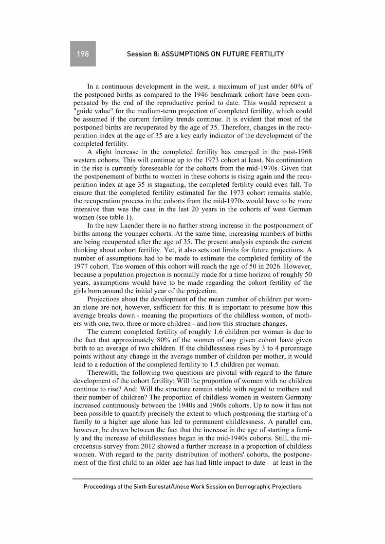
198 Session 8: ASSUMPTIONS ON FUTURE FERTILITY
Proceedings of the Sixth Eurostat/Unece Work Session on Demographic Projections
In a continuous development in the west, a maximum of just under 60% of the postponed births as compared to the 1946 benchmark cohort have been com-pensated by the end of the reproductive period to date. This would represent a "guide value" for the medium-term projection of completed fertility, which could be assumed if the current fertility trends continue. It is evident that most of the postponed births are recuperated by the age of 35. Therefore, changes in the recu-peration index at the age of 35 are a key early indicator of the development of the completed fertility.
A slight increase in the completed fertility has emerged in the post-1968 western cohorts. This will continue up to the 1973 cohort at least. No continuation in the rise is currently foreseeable for the cohorts from the mid-1970s. Given that the postponement of births to women in these cohorts is rising again and the recu-peration index at age 35 is stagnating, the completed fertility could even fall. To ensure that the completed fertility estimated for the 1973 cohort remains stable, the recuperation process in the cohorts from the mid-1970s would have to be more intensive than was the case in the last 20 years in the cohorts of west German women (see table 1).
In the new Laender there is no further strong increase in the postponement of births among the younger cohorts. At the same time, increasing numbers of births are being recuperated after the age of 35. The present analysis expands the current thinking about cohort fertility. Yet, it also sets out limits for future projections. A number of assumptions had to be made to estimate the completed fertility of the 1977 cohort. The women of this cohort will reach the age of 50 in 2026. However, because a population projection is normally made for a time horizon of roughly 50 years, assumptions would have to be made regarding the cohort fertility of the girls born around the initial year of the projection.
Projections about the development of the mean number of children per wom-an alone are not, however, sufficient for this. It is important to presume how this average breaks down - meaning the proportions of the childless women, of moth-ers with one, two, three or more children - and how this structure changes.
The current completed fertility of roughly 1.6 children per woman is due to the fact that approximately 80% of the women of any given cohort have given birth to an average of two children. If the childlessness rises by 3 to 4 percentage points without any change in the average number of children per mother, it would lead to a reduction of the completed fertility to 1.5 children per woman.
Therewith, the following two questions are pivotal with regard to the future development of the cohort fertility: Will the proportion of women with no children continue to rise? And: Will the structure remain stable with regard to mothers and their number of children? The proportion of childless women in western Germany increased continuously between the 1940s and 1960s cohorts. Up to now it has not been possible to quantify precisely the extent to which postponing the starting of a family to a higher age alone has led to permanent childlessness. A parallel can, however, be drawn between the fact that the increase in the age of starting a fami-ly and the increase of childlessness began in the mid-1940s cohorts. Still, the mi-crocensus survey from 2012 showed a further increase in a proportion of childless women. With regard to the parity distribution of mothers' cohorts, the postpone-ment of the first child to an older age has had little impact to date – at least in the

Session 8: ASSUMPTIONS ON FUTURE FERTILITY 199
Proceedings of the Sixth Eurostat/Unece Work Session on Demographic Projections
1944 to 1968 cohorts. Yet since then, the average age for having the first child has risen. Therefore, women are increasingly not entering motherhood until they are 30 or older. This development can have an effect on the frequency of the births of higher parity, that is of the third child or later children. From the data of the mi-crocensus it is evident that there is a connection between the age of starting a fam-ily and the number of children given birth to. The mothers with more than two children were on average three years younger than mothers of one or two children at the time of the birth of the first-born (Poetzsch 2013). Hence, it would not be pessimistic to expect an average number of children per woman at 1.5 to 1.6 for the next decades using the information birth statistics and additional survey results on birth behaviour.
REFERENCES
Frejka, T., G. W. Jones and J.-P.: Sardon. 2010. East Asian Childbearing Patterns and Policy Developments in Population and Development Review, year 36, issue 3/2010, page 579 ff.
Frejka, T. 2011: The Role of Contemporary Childbearing Postponement and Recu-peration in Shaping Period Fertility Trends in Comparative Population Studies – Zeitschrift für Bevölkerungswissenschaft, volume 36, issue 4/2011, pp. 959 ff.
Goldstein, J. R., Kreyenfeld, M. and F. Rößger. 2012. Gibt es eine Trendumkehr in der Kinderzahl nach Geburtsjahrgängen in Deutschland?, Berli-ner Demografie Forum 2012: Familie-Kinder-Gesellschaft, Working Paper 4
Neyer, G. R., G. Andersson, J. M. Hoem, M. Rønsen and A. Vikat. 2006. Fertilität, Familiengründung, Familienerweiterung in den nordischen Laendern, MPIDR Working Paper WP 2006-022.
Poetzsch, O. 2010. Annahmen zur Geburtenentwicklung in der 12. koordinierten Bevölkerungsvorausberechnung in Wirtschaft und Statistik 1/2010, pp. 29 ff.
Poetzsch, O. 2013: What effects do postponed births have on cohort fertility in western and eastern Germany? in Wirtschaft und Statistik 2/2103, pp. 87 (Ger-man version). English version: https://www.destatis.de/EN/Publications/WirtschaftStatistik/ChildbearingPostponement_Poetzsch_22013.pdf?__blob=publicationFile
Sobotka, T., Zeman, K., Lesthaeghe, R. and T. Frejka 2013: Postponement and Re-cuperation in Cohort Fertility: New Analytical and Projection Methods and their

200 Session 8: ASSUMPTIONS ON FUTURE FERTILITY
Proceedings of the Sixth Eurostat/Unece Work Session on Demographic Projections
Application in European Demographic Research Papers 2/2011 (www.oeaw.ac.at/vid/download/edrp_2_11.pdf; accessed on 11 January 2013).
Statistisches Bundesamt (editor). 2013. Geburtentrends und Familiensituation in Deutschland. https://www.destatis.de/DE/PresseService/Presse/Pressekonferenzen/2013/Geburten_2012/Begleitheft_Geburten.pdf?__blob=publicationFile

Session 9
STOCHASTIC METHODS IN POPULATION PROJECTIONS
Chair: Rebecca Graziani (Bocconi University)


Session 9: STOCHASTIC METHODS IN POPULATION PROJECTIONS 203
PROCEEDINGS OF THE SIXTH EUROSTAT/UNECE WORK SESSION ON DEMOGRAPHIC PROJECTIONS
MEASURING UNCERTAINTY IN POPULATION FORECASTS: A NEW APPROACH
David A. Swanson, Jeff Tayman
Summary
Two basic approaches have been used to assess population forecast uncertainty: (1) a range of projections based on alternative scenarios; and (2) statistical forecast inter-vals. In terms of the latter, there are two complementary approaches: (1) model-based intervals; and (2) empirically-based intervals. We evaluate a model-based approach in this paper, but enhance it by using it the information in historical data, a feature found in the empirically-based approach. We describe and test in this paper a regression-based approach for developing 66% forecast intervals for age-group forecasts made using the Hamilton-Perry Method. We use a sample of four states (one from each cen-sus region in the United States) with nine ex post facto tests, one for each census from 1930 to 2010, which yields 576 observations. The four states and the nine test points provide a wide range of characteristics in regard to population size, growth, and age-composition, factors that affect forecast accuracy. The tests reveal that the 66% inter-vals contain the census age-groups in 397 of the 576 observations (69 percent). We discuss the results, to include a summary by age group, and make some observations regarding the limitations of our study. We conclude that the results are encouraging, however, and offer suggestions for further work. Keywords: Hamilton-Perry Method, regression, forecast intervals
1. Introduction
Although they are widely used, population forecasts entail a tremendous amount of uncertainty, especially for long time horizons and for places with small or rapidly changing populations (Alho 1984; Alho and Spencer, 1985, 1990, 1997, 2005; Lutz, Sanderson and Scherbov 1999; Smith, Tayman and Swanson 2001: 340; Tayman, Smith, and Lin 2007; Tayman, Smith and Rayer 2011; Wilson 2012). As such, virtually every forecast is wrong, making the task of an accurate forecast impossible, but the task is unavoidable (Keyfitz 1987: 236). It is impossi-ble in that the forecasted numbers turn out to be different from what actually oc-curs, but unavoidable in that forecasts must be done in the modern world. Swanson and Tayman (1995) describe this irony as the "rock" and the "hard place." As they observed, demographers have developed several strategies for dealing with the "irony" of forecasting. They include the use of the term "projection" rather than "forecast," (Keyfitz 1972; Pittenger 1978; Smith and Bayya 1992; Smith, Tayman, and Swanson 2001: 301), "normative" forecasting (Moen 1984), and providing

204 Session 9: STOCHASTIC METHODS IN POPULATION PROJECTIONS
PROCEEDINGS OF THE SIXTH EUROSTAT/UNECE WORK SESSION ON DEMOGRAPHIC PROJECTIONS
measures of forecast uncertainty. One way to assess uncertainty is to produce sev-eral alternative projections or scenarios based on different sets of assumptions (Campbell 1996; Cheeseman-Day 1992; Spencer 1989; Tayman 2011; Thompson and Whelpton 1933; U. S. Census Bureau 1966). Another approach is to develop statistical forecast intervals based on historical data and stochastic models (Alho and Spencer 2005; Stoto 1983; Swanson and Beck 1994). It is the latter that we ex-plore in this paper.
Forecast intervals based on statistical theory and data on error distributions provide an explicit estimate of the probability that a given range will contain the future population. These intervals are sometimes called prediction intervals, proba-bility intervals, confidence intervals, or confidence limits. We call them forecast intervals to distinguish them from traditional confidence intervals, which—strictly speaking—apply only to sample data.
Two types of forecast intervals have been used most frequently for population forecasts. One is based on the development of statistical models of population growth and the other is based on empirical analyses of errors from past population projections. Both rely on the assumption that historical or simulated error distribu-tions can be used to predict future error distributions. To a large extent, the two ap-proaches complement one another, but neither is fully satisfactory. On the one hand, model-based intervals exploit the theories and underlying inferential statis-tics, but fall short in utilizing the information available in historical data. On the other hand, empirically-based intervals utilize the information from historical data, but fall short in exploiting the theories underlying inferential statistics. We evaluate a model-based approach in this paper, but enhance it by using it the information in historical data.
We begin with a description of our model-based approach, which employs simple regression models applied to a forecasting method known as the Hamilton-Perry Method (Hamilton and Perry 1962).1 We next evaluate the efficacy of the forecast intervals by examining population forecasts by age for four states covering target years for each decade from 1930 to 2010. We conclude with a discussion and suggestions for future research.
2. The Hamilton-Perry Method
The Hamilton-Perry method moves a population by age (and sex) from time t to time t+k using cohort-change ratios (CCR) computed from data in the two most recent censuses. It consists of two steps. The first uses existing data to develop CCRs and the second applies the CCRs to the cohorts of the launch year population to move them into the future. As shown by Swanson, Schlottmann, and Schmidt (2010), the formula for developing a CCR is:
nCCRx,i,t = nPx,i,t / nPx-k,i,t-k. where, nPx,i,t is the population aged x to x+n in area i at the most recent census
(t), nPx-k,i,t-k is the population aged x-k to x-k+n in area i at the 2nd most recent census (t-k), and

Session 9: STOCHASTIC METHODS IN POPULATION PROJECTIONS 205
PROCEEDINGS OF THE SIXTH EUROSTAT/UNECE WORK SESSION ON DEMOGRAPHIC PROJECTIONS
k is the number of years between the most recent census at time t and the one preceding it at time t-k. The basic formula for the second step, moving the cohorts of a population into
the future is: nPx+k,i,t+k = nCCRx,i,t × nPx,i,t where, nPx+k,i,t+k is the population aged x+k to x+k+n in area i at time t+k, and nCCRx,i,t and nPx,i,t are as defined in equation [2]. Given the nature of the CCRs, 10-14 is the youngest five-year age group for
which projections can be made if there are 10 years between censuses. To project the population aged 0-4 and 5-9 one can use the Child Woman Ratio (CWR) or more generally a “Child Adult Ratio” (CAR). These ratios do not require any data beyond what is available in the decennial census. For projecting the population aged 0-4, the CAR is defined as the population aged 0-4 divided by the population aged 20-34. For projecting the population aged 5-9, the CAR is defined as the pop-ulation aged 5-9 divided by the population aged 25-39The CAR equations for pro-jecting the population aged 0-4 and 5-9 are:
Population 0-4: 5P0,t+k = (5P0,t /15P20,t) × 15P20,t+k Population 5-9: 5P5,t+k = (5P5,t / 15P25,t ) × 15P25,t+k where P is the population, t is the year of the most recent census, and t+k is the projection year. There are other “adult” age groups that could be used to define CAR (Smith,
Tayman, and Swanson 2001: 156-157). The definitions shown in the two preceding equations are designed for a population in which fertility is at or below replace-ment, (i.e., the TFR is less than 2.1 or so), which correlates with the fact that first births tend to be postponed. Another way to project the youngest age groups is to take their ratios at two points in time and apply that ratio to the launch year age group (t). In the first step, the ratios are as follows:
Population 0-4: 5R0,t = 5P0,t / 5P0,t-k Population 5-9: 5R5,t = 5P5,t / 5P5,t-k. In the second step, the projected population at t+k is found as follows: Population 0-4: 5P0,t+k = 5P0,t × 5R0,t Population 5-9: 5P5,t+k = 5P5,t × 5R5,t. We use the ratio method in this paper since it is better suited for the regres-
sion-based method for creating intervals around forecasts for the two youngest age groups discussed later in the paper. One reason that it is better suited with the re-gression-based method is that the CAR values are substantially different than the CCRs, whereas the ratios are not. This means that the CAR values are potential outliers that could serve as influential observations that deleteriously affect model construction (Fox 1991). Another reason for not using CAR values is that the mean age at childbearing changed over the time period represented by the sample data we employ (see, e.g., Heuser, 1976; NCHS, 2013) and we desired a consistent def-inition of a given CCR or its equivalent over both the entire set of states and the study period.

206 Session 9: STOCHASTIC METHODS IN POPULATION PROJECTIONS
PROCEEDINGS OF THE SIXTH EUROSTAT/UNECE WORK SESSION ON DEMOGRAPHIC PROJECTIONS
Projections of the oldest open-ended age group also differ slightly from the projections for the age groups beyond age 10 up to the oldest open-ended age group. If for example the final closed age group is 70-74, with 75+ as the terminal open-ended age group, then calculations for the CCRi,x+,t require the summation of the three oldest age groups to get the population age 65+ at time t-k:
∞CCR75,i,t = ∞P75,i,t / ∞P65,i,t-k. The formula for projecting the population 75+ of area i for the year t+k is: ∞P75+,i,t+k = ∞CCR75,i,t × ∞P65,i,t.
3. Developing Forecast Intervals
As should be clear from the preceding discussion, the Hamilton-Perry Method is deterministic. However, we also know that population forecasting is subject to uncertainty since we do not precisely know the future components making up the fundamental equation. So, the question is how to introduce an element of statistical uncertainty into a method that is inherently deterministic. One answer to this ques-tion is found by employing a simple regression method to estimate CCRs and then applying the regression-estimated CCRs to the launch-year age groups to obtain forecasts of these age groups.
Recall from equation that nCCRx,i,t = nPx,i,t / nPx-k,i,t-k. From this, we can define the CCR for the preceding census period as nCCRx,i,t-k = nPx,i,t-k / nPx-k,i,t-2k. We can then construct a regression model with nCCRx,i,t as the dependent variable and nCCRx,i,t-k as the independent variable. We note that for age groups 0-4, 5-9, and the terminal open-ended age group that the dependent and independent observa-tions follow the equations provided earlier. Given this adjustment, we can general-ly describe the estimated CCRs at time t as follows:
nECCRx,i,t = a + b × nCCRx,i,t-k. We can then multiply the regression-estimated CCR and the corresponding
population by age at time t to forecast the CCR at time t+k: nCCRx,i,t+k = nECCRx,i,t × nPx,i,t. Utilizing the regression measure of statistical uncertainty (the standard error of
estimate) for the model along with the sample size and other characteristics of the data, we can generate forecast intervals around nCCRx,i,t+k. The forecast intervals are based on equation 4.2 found in Hyndman and Athanasopoulos, Chapter 4 (2012). These intervals can then be translated directly to the actual population numbers forecasted for each age group (Espenshade and Tayman 1982; Swanson and Beck 1994)2.
4. Empirical Evaluation
To empirically examine the regression-based method for developing intervals around population forecasts by age generated from the Hamilton-Perry Method, we selected a sample made up of one state from each of the four census regions in the United States. The states selected are Georgia (the South Region), Minnesota (the Midwest Region), New Jersey (The Northeast Region) and Washington (The West Region). We then assembled census data for these four states for each census year

Session 9: STOCHASTIC METHODS IN POPULATION PROJECTIONS 207
PROCEEDINGS OF THE SIXTH EUROSTAT/UNECE WORK SESSION ON DEMOGRAPHIC PROJECTIONS
from 1900 to 2010 (U.S. Census Bureau, 1973, 1982, 1992, 2000, 2010). The data provide nine points in time at which the forecast intervals can be evaluated, 1930, 1940, 1950, 1960, 1970, 1980, 1990, 2000, and 2010. This sample provides a wide range of demographic characteristics in terms of variation in population size, age-composition, and rates of change. Table 1 provides an overview of this range by displaying the population of each of the four states in 1900 and in 2010 and decen-nial rates of population change from 1900 to 2010. Although we do not show a summary of the changes in age composition by state and census year, they are ex-tensive.
Because of the way data for the terminal open-ended age group are reported differently over the period for which we assemble census data, we used “75 years and over” for the entire period since it was the common denominator. This means there are 16 age groups (0-4, 5-9,…,70-74, and 75+) used in the empirical evalua-tion.
We proceed by constructing CCRs over two successive decennial periods (e.g., 1910-1920/1900-1910) over the entire period, using regression to estimate the CCR in the numerator from the CCR in the denominator. We then use the regression-based estimate of the CCR of the “current period” (e.g., 1910-1920) to forecast the CCRs to the next period, the “launch year” (e.g., 1920-1930) and develop forecast intervals around the forecasted CCRs, which are then translated into the forecasted age groups for the “target year” (e.g., 1930). The forecast intervals are then exam-ined to see if they contain the census age groups for the target year.
Table 1 - The total population of each state in 1900 and 2010 and annual rates of change from 1900 to 2010 by decade
Census Year GEORGIA MINNESOTA NEW JERSEY WASHINGTON
1900 2.209.974 1.747.292 1.879.890 511.844 Population
1910 0,0164 0,0170 0,0299 0,0797 Average annual Rate of Change over the Decade
1920 0,0105 0,0141 0,0219 0,0175 Average annual Rate of Change over the Decade
1930 0,0005 0,0072 0,0247 0,0144 Average annual Rate of Change over the Decade
1940 0,0072 0,0086 0,0030 0,0106 Average annual Rate of Change over the Decade
1950 0,0098 0,0066 0,0150 0,0314 Average annual Rate of Change over the Decade
1960 0,0135 0,0135 0,0227 0,0183 Average annual Rate of Change over the Decade
1970 0,0152 0,0108 0,0167 0,0178 Average annual Rate of Change over the Decade
1980 0,0174 0,0069 0,0027 0,0192 Average annual Rate of Change over the Decade
1990 0,0170 0,0071 0,0048 0,0164 Average annual Rate of Change over the Decade
2000 0,0234 0,0117 0,0085 0,0192 Average annual Rate of Change over the Decade
2010 0,0168 0,0075 0,0044 0,0132 Average annual Rate of Change over the Decade
2010 9.687.653 5.303.925 8.791.894 6.724.540 Population
STATE
Sources: US Census Bureau, 2010, 2000, 1992, 1982, & 1973. Note: The 1900, 1910, 1920, & 1930 population totals exclude those for whom age was not reported.

208 Session 9: STOCHASTIC METHODS IN POPULATION PROJECTIONS
PROCEEDINGS OF THE SIXTH EUROSTAT/UNECE WORK SESSION ON DEMOGRAPHIC PROJECTIONS
How well does the regression approach based on the Hamilton Perry method perform in its ability to predict the uncertainty of population forecasts? One way to address this question is to determine the number of population counts that fall in-side the forecast intervals (Tayman, Smith, and Lin 2007). In terms of the forecast interval probability, we selected 0.66 or 66 percent because of prior research indi-cating that “low” and “high” scenarios constructed for the cohort-component meth-od corresponded empirically to 66% confidence intervals (Stoto 1983) as well as findings by Swanson and Beck (1994). Table 2 provides a summary of the results for all four states at each of the nine census test points. The table shows the number of times (out of 16) that the 66% forecast interval contained the corresponding cen-sus number for a given age group. If the forecast intervals provide a valid measure of uncertainty, they will contain approximately 11 of the 16 observed population counts. The table also shows percent of the counts falling within the forecast inter-vals for all target years for each state (144 intervals), the percent falling within all states for each target year (64 intervals), and the single percent falling within all states for all target years (576 intervals).
Table 2 - Summary results of the regression-based 66% forecast intervals by state and year of test
TEST YEAR GEORGIA MINNESOTA NEW JERSEY WASHINGTON TOTAL
1930 9 12 8 13 42 65,63%
1940 3 5 11 12 31 48,44%
1950 10 14 4 3 31 48,44%
1960 13 14 14 8 49 76,56%
1970 6 12 14 13 45 70,31%
1980 7 12 12 10 41 64,06%
1990 13 14 14 14 55 85,94%
2000 8 15 14 15 52 81,25%
2010 7 15 15 14 51 79,69%
TOTAL 76 113 106 102 397
PERCENT (N/144) 52,78% 78,47% 73,61% 70,83% 68,92%
STATEPERCENT
(N/64)
N=(144*4)=576 = (64*9)
Note: The number in each cell shows how many times the census value fell within the forecast interval.
5. Discussion
Overall, the 66 percent intervals contain their corresponding census age groups in 397 cases, which represents 69 percent of the 576 total observations.3 In terms of the nine census target years, the overall results show that in five of them (1960, 1970, 1990, 2000, and 2010) the forecast intervals contain the census age groups substantially more than 66 percent of the time. In two target years (1930 and 1980), the intervals contain the census age groups 67 percent of the time. In the remaining two target years, 1940 and 1950, the intervals contain the census age groups 48

Session 9: STOCHASTIC METHODS IN POPULATION PROJECTIONS 209
PROCEEDINGS OF THE SIXTH EUROSTAT/UNECE WORK SESSION ON DEMOGRAPHIC PROJECTIONS
percent and 47 percent of the time, respectively. We note that the 1940 test point encompasses the economic boom experienced in the 1920s and the economic de-pression during the 1930s and the large scale “baby bust” associated with it. The 1950 point encompasses the depression and baby bust period of the 1930s and the economic recovery stimulated by World War II and the initial part of the large scale “baby boom” from 1946 to 1950. Table 3 contains a summary of the results by age group across all of the nine census target years and the four states. The table shows the number of times (out of 36) that the 66% forecast interval contained the corresponding census number for a given age group. If the forecast intervals pro-vide a valid measure of uncertainty, they will contain approximately 24 of the 36 observed population counts. In general, Table 3 shows that forecast intervals cap-ture the population count at least 66 percent of the time for age groups 10-14, 15-19, 20-24 and 40-44 through 75+. For age groups 0-4 and 5-9, the forecast intervals only encompass the population counts 25 percent of time. For age group 30-34, the count is encompassed 53 percent of the time while for age group 25-29, it is 58 percent of the time. The population counts are captured by the forecast intervals 61 percent of the time for age group 35-39.
Table 3 - Summary results of the regression-based 66% forecast intervals by age group
AGE GROUP TOTALPERCENT
(N/36)
0-4 9 25,00%
5-9 9 25,00%
10-14 26 72,22%
15-19 27 75,00%
20-24 24 66,67%
25-29 21 58,33%
30-34 19 52,78%
35-39 22 61,11%
40-44 26 72,22%
45-49 28 77,78%
50-54 30 83,33%
55-59 31 86,11%
60-64 30 83,33%
65-69 31 86,11%
70-74 33 91,67%
75+ 31 86,11%
SUM 397 68,92% Note: the number in each cell shows how many times the census value fell within the forecast interval
Perhaps it should not be surprising that the cohort change method is better able
to capture older age groups than the very youngest since births are not part of a co-hort change ratio. In addition, migration likely comes into play in that the popula-tion in the two youngest age groups (0-4 and 5-9) would be moving with their par-ents, who are likely to be in age groups 25-29, 30-34, and 35-39, the other age

210 Session 9: STOCHASTIC METHODS IN POPULATION PROJECTIONS
PROCEEDINGS OF THE SIXTH EUROSTAT/UNECE WORK SESSION ON DEMOGRAPHIC PROJECTIONS
groups for which the forecast intervals encompassed the population counts less than 66 percent of the time. Overall, we find that these effects are consistent with theory regarding migration in that those who tend to move are less socially inte-grated into communities than those who tend not to move and that as adults age, community social integration tends to increase (Goldscheider 1978). Finally, as shown at the bottom of Table 3, the intervals capture the population count 69 per-cent of the time (397 out of 576), which matches the summary for Table 2.
Although they are not shown here, the average width of the forecast intervals appears to us to be reasonable at the 66 percent level in that they are neither so wide as to be meaningless nor too narrow to be overly-restrictive. This is largely consistent with prior work by Swanson and Beck (1994) on confidence intervals derived from regression-based forecasts. Also consistent with the work by Swan-son and Beck (1994), is the fact that the regression-based forecast intervals contain the actual numbers by age in 71 percent of the 576 observations provide further support that 66 percent forecast intervals based on the regression-estimated CCR approach are both useful and feasible. We find these results encouraging.
At this point, we suggest caution using this method beyond a ten-year forecast horizon. This is consistent with observations about the use of the Hamilton-Perry method in general (Smith, Tayman, and Swanson 2001; Swanson, Schlottmann, and Schmidt 2010) and as such is not a major limitation.4 We also suggest that this approach to developing uncertainty measures be used with care when applied to small populations, such as those found at the county and sub-county levels. While our sample provides a wide range of demographic behavior in terms of size, age composition, and population changes, it is a sample of states, which means that greater variability in demographic characteristics found at sub-state levels is not present (Swanson, Schlottmann, and Schmidt 2010). We suggest that further re-search using this approach would be useful by examining both longer forecast hori-zons and smaller populations (i.e., the sub-state populations) and different proba-bility intervals. Another area for further research would be to utilize Keyfitz’s (1981) approach using root mean square errors in conjunction with the Hamilton-Perry Method.
The fact that the forecast intervals do not contain the population counts at least 66 percent of the time for neither the two youngest age groups (0-4 and 5-9) nor the age groups associated with those most likely to be the parents of these children (25-29, 30-34 and 35-39) should not be surprising: The dynamics of birth and migra-tion are difficult to capture in a full-blown cohort-component method forecast and the Hamilton-Perry Method is a variant of the full- blown method (Smith, Tayman and Swanson 2001; Smith and Tayman 2003). Thus, work on these issues in regard to one of these two methods should be of use to the other.
6. Endnotes
1. Although the name “Hamilton-Perry Method” is virtually universal today, the first published instance of cohort change ratios being used for purposes of pro-jecting a population is found in Hardy and Wyatt (1911), who built cohort change ratios from the 1901 and 1906 census counts of England and applied them to the

Session 9: STOCHASTIC METHODS IN POPULATION PROJECTIONS 211
PROCEEDINGS OF THE SIXTH EUROSTAT/UNECE WORK SESSION ON DEMOGRAPHIC PROJECTIONS
1906 census to generate a forecast for 1911. Hamilton and Perry acknowledge that they learned about this method from a general description found in Wolfenden (1954) who cited the Hardy and Wyatt article. However, they were unable to se-cure a copy of the 1911 article and were, therefore, not exactly certain what was done by Hardy and Wyatt. In any event, Hamilton and Perry deserve credit for providing a clear and detailed description of this approach to population projection in a journal (Social Forces) that was read by many demographers in the United States and elsewhere prior to the founding of demographic journals such as Cana-dian Studies in Population (first published in 1973) Demography (first published in 1966) and Population Research and Policy Review (first published in 1982).
2. Space considerations prevent us all of the regression, forecast intervals, and evaluation results here. The authors will be pleased to provide them upon request.
3. It should be clear that we are primarily interested in measuring uncertainty in forecasts of age groups. This is an important topic due to the role that the abso-lute and relative sizes of age groups have in regard both to commerce (Gauthier, Chu and Tuljapurkar 2006; Martins Yusuf and Swanson 2012, Murdock et al. 1997) and public policy (Bongaarts and Bulatao 2000, Murdock et al. 1997, Smith Tayman and Swanson 2001, Tuljapurkar, Pool, and Prachuabmoh 2005, Gauthier, Chu and Tuljapurkar 2006). We are aware that levels of uncertainty in regard to forecasts of the total population are important as well. In this regard, we note that technically the forecast intervals we generated here apply only to the age groups. There are two ways in which they can be used to place intervals around the total population forecast, one is informal while the other is formal. In the informal ap-proach, we obtain 66 percent forecast intervals for the total population by adding the lower and upper boundaries of the intervals for each age group. We found that in 28 of the 36 forecasts (four states at each of nine time points) the summed lower and upper boundaries contained the actual total population, or 78 percent. By state, we find: Georgia’s total population is contained in 5 of the 9 time points (56%); Minnesota’s is in 9 of the 9 time points; New Jersey’s is in 6 of the 9 time points (67%); and Washington’s is in 8 of the 9 time points (89%). By target year, we find: 4 of 4 were contained in the 1960, 1970, and 1990 years; 3 of 4 were con-tained in the 1930, 1980, 2000, and 2010 years; and 2 of 4 in the 1940 and 1950 years. The formal approach is called the “error propagation method” by Deming (1950: 127- 134). In different forms it has been used by Alho and Spencer (2005), Espenshade and Tayman (1982), and Hansen, Hurwitz, and Madow (1953), among others. In this application, the error propagation method involves summing the squared values of the forecast intervals by age, finding the square root of the summed forecast interval values and dividing this square root of the sample size (n=16) to obtain an estimate of the standard error for the total population forecast. This standard error is then multiplied by the total population forecast (found by summing the point forecast for each age group) to obtain the margin of error. The margin of error is added to and subtracted from the total population forecast to ob-tain its 66% forecast interval. This approach assumes that the 16 age groups are in-dependent, which is not an unreasonable assumption in that the age group forecasts are not forced to sum to any specified total (i.e., they are not “controlled” to an ex-ternally produced population total). In following this approach, we found that in 29 of the 36 forecasts (four states at each of nine time points) the error propagation in-
212 Session 9: STOCHASTIC METHODS IN POPULATION PROJECTIONS
PROCEEDINGS OF THE SIXTH EUROSTAT/UNECE WORK SESSION ON DEMOGRAPHIC PROJECTIONS
tervals contained the actual total population, or 81 percent. By state, we find: Georgia’s total population is contained in 6 of the 9 time points (67%); Minneso-ta’s is in 9 of the 9 time points; New Jersey’s is in 6 of the 9 (67%), and Washing-ton’s is in 8 of the 9 time points (89%). By time point, we find: 4 of 4 were con-tained in the 1960, 1970, 1990, and 2010 target years; 3 of 4 were contained in the 1930, 1980, and 2000 target years; and 2 of 4 in the 1940 and 1950 target years. Both the informal and formal approaches can be used to construct forecast intervals for any desired aggregations of the five-year age groups such age group 25-34, the working age population (e.g., ages 25-64), and so forth.
4. The ten-year horizon is also consistent with accuracy evaluations of the Hamilton-Perry Method, which show that the method performs well for ten year forecasts (Smith and Tayman 2003, Swanson and Tayman, 2013) and even 20 year forecasts (Smith and Tayman 2003).
REFERENCES
Alho, J. 1984. Probabilistic forecasts: The case of population projections. Scandi-navian Housing and Planning Research 1: 99-105.
Alho, J. and Spencer, B. 1985. Uncertain population forecasting. Journal of the American Statistical Association 80 390: 306-314.
Alho, J. and Spencer, B. 1990. Error models for official mortality forecasts. Jour-nal of the American Statistical Association 85 411: 609-616.
Alho, J. and Spencer, B. 1997. The practical specification of the expected error of population forecasts. Journal of Official Statistics 13: 203-225.
Alho, J. and Spencer, B. 2005. Statistical demography and forecasting. Dordrecht, The Netherlands: Springer.
Bongaarts, J. and Bulatao, R Eds.. 2000. Beyond six billion: forecasting the world’s population. Washington, D.C.: National Academy Press
Campbell, P.R. 1996. Population projections for states by age, sex, race, and His-panic Origin: 1995 to 2050. PPL-47. Washington, DC: U.S. Bureau of the Cen-sus.
Cheeseman-Day, J. 1992. Population Projections of the United States, By Age, Sex, Race, and Hispanic Origin: 1992-2050. Current Population Reports
Deming, W.E. 1950. Some theory of sampling. New York, NY: Dover Publica-tions.

Session 9: STOCHASTIC METHODS IN POPULATION PROJECTIONS 213
PROCEEDINGS OF THE SIXTH EUROSTAT/UNECE WORK SESSION ON DEMOGRAPHIC PROJECTIONS
Espenshade, T. and Tayman, J. 1982. Confidence intervals for postcensal popula-tion estimates. Demography 19 2: 191-210.
Fox, J. 1991. Regression Diagnostics. Sage Quantitative Applications in the Social Sciences, no. 79. London, England: Sage Publications.
Gauthier, A., Chu, C.Y.C. and Tuljapurkar, S. Eds. 2006. Allocating public and private resources across generations: Riding the age waves, Vol. 2. Dordrecht, The Netherlands: Springer.
Goldscheider, C. 1978. Modernization, migration, and urbanization. Paris, France: International Union for the Scientific Study of Population.
Hamilton, C.H. and Perry, J. 1962. A short method for projecting population by age from one decennial census to another. Social Forces, 41: 163-170.
Hansen, N., Hurwitz, W., and Madow, W. 1953. Sample survey methods and theo-ry, Volume I, methods and applications. New York, NY: John Wiley and Sons re-published in 1993.
Hardy, G.F. and Wyatt, F.B. 1911. Report of the actuaries in relation to the scheme of insurance against sickness, disablement, etc. Journal of the Institute of Actuar-ies XLV: 406-443.
Heuser, R. L. (1976). Fertility tables for birth cohorts by color. U.S. Department of Health, Education, and Welfare. DHEW Publication No. (HRA)76-1152.
Hyndman, R.J., and Athanasopoulos, G. 2012 Forecasting: Principles and Prac-tice (online at http://otexts.com/fpp/ ).
Keyfitz, N. 1972. On future population. Journal of the American Statistical Associ-ation 67: 347-363.
Keyfitz, N. 1981. The limits of population forecasting. Population and Develop-ment Review 7: 579-593.
Keyfitz, N. 1987. The social and political context of population forecasting. pp. 235-258 in W. Alonso and P. Starr Eds. The Politics of Numbers. New York, NY: Russell Sage Foundation.
Lutz, W., Sanderson, W., and Scherbov, S. 1999. Expert-based probabilistic popu-lation projections. pp. 139-155 in W. Lutz, J. Vaupel, and D. Ahlburg Eds. Fron-tiers of Population Forecasting. New York, NY: The Population Council. A sup-plement to Population and Development Review, 24.
Martins, J., Yusuf, F., and Swanson, D.A. 2012. Consumer demographics and be-haviour: markets are people. Dordrecht, The Netherlands: Springer.
Moen, E. 1984. Voodoo Forecasting: Technical, political, and ethical issues re-garding the projection of local population growth. Population Research and Pol-icy Review 3: 1-25.
Murdock, S., Hoque, M.N., Michael, M., White, S., and Pecotte, B. 1997. The Tex-as challenge: population change and the future of Texas. College Station, TX: Texas A&M University Press.

214 Session 9: STOCHASTIC METHODS IN POPULATION PROJECTIONS
PROCEEDINGS OF THE SIXTH EUROSTAT/UNECE WORK SESSION ON DEMOGRAPHIC PROJECTIONS
NCHS (2013). ‘Births: Final data for 2011.” National Vital Statistics Reports, Vol. 62. no. 1, National Center for Vital Statistics, National Vital Statistics System, U.S. Department of Health & Human Services.
Pittenger, D. 1978. The role of judgment, assumptions, techniques, and confidence limits in forecasting population. Socio-Economic Planning Sciences 12: 271-276.
Smith, S.K. and Bayya, R. 1992. An evaluation of population forecast errors for Florida and its counties. Applied Demography 7: 1-5.
Smith, S.K., and Tayman, J. 2003. An evaluation of population projections by age. Demography 40 4: 741-757.
Smith, S.K., Tayman, J., and Swanson D.A. 2001. Population projections for state and local areas: Methodology and analysis. New York, NY: Kluwer Academ-ic/Plenum Press.
Spencer, G. 1989. Projection of the population of the United States by age, sex, and race: 1988 to 2008. Current Population Reports, P-25, No. 1018. Washington, DC: U.S. Bureau of the Census.
Stoto, M. 1983. The accuracy of population projections. Journal of the American Statistical Association 78: 13-20.
Swanson, D.A. and Beck, D. 1994. A new short-term county population projection method. Journal of Economic and Social Measurement 20: 1-26.
Swanson, D.A. and Tayman, J. 2013.The accuracy of the Hamilton-Perry method for forecasting state populations by age. Working paper 13-01, Center for Sus-tainable Suburban Development, University of California Riverside (on-line at http://cssd.ucr.edu/Papers/PDFs/THE%20ACCURACY%20OF%20THE%20HAMILTON-PERRY%20METHOD%20FOR%20 FORECAST-ING%20STATE%20POPULATIONS%20BY%20 AGE%20V6.pdf)
Swanson, D.A. and Tayman, J. 1995. Between a rock and a hard place: The evalu-ation of demographic forecasts. Population Research and Policy Review 14: 233-249.
Swanson, D.A., Schlottmann, A., and Schmidt, R. 2010. Forecasting the population of census tracts by age and sex: An example of the Hamilton–Perry method in ac-tion. Population Research and Policy Review 29: 47-63.
Tayman, J. 2011. Assessing uncertainty in small area forecasts: State of the prac-tice and implementation strategy. Population Research and Policy Review 30:781-800.
Tayman, J., Smith, S.K., and Lin, J. 2007. Precision, bias, and uncertainty for state population forecasts: An exploratory analysis of time series models. Population Research and Policy Review 26 3: 347-369.
Tayman, J., Smith, S.K., and Rayer, S. 2011. Evaluating population forecast accu-racy: A regression approach using county data. Population Research and Policy Review 30: 235-262.

Session 9: STOCHASTIC METHODS IN POPULATION PROJECTIONS 215
PROCEEDINGS OF THE SIXTH EUROSTAT/UNECE WORK SESSION ON DEMOGRAPHIC PROJECTIONS
Thompson, W. and Whelpton, P. 1933. Population Trends in the United States. New York, NY: McGraw-Hill Book Company.
Tuljapurkar, S., Pool, I. and Prachuabmoh, V. Eds. 2005. Population, resources and development: Riding the age waves, Vol. 1. Dordrecht, The Netherlands: Springer.
U.S. Census Bureau. 2010. Table QT-P1 (By State), American Factfinder (Guided Search via Specific Data Sets, Decennial Census, 2010) http://factfinder2.census.gov/faces/nav/jsf/pages/guided_search.xhtml.
U.S. Census Bureau. 2000. Table QT-P1 (By State), American Factfinder (Guided Search via Specific Data Sets, Decennial Census, 2000)
U. S. Census Bureau. 1992. 1990 Census of Population, General Population Char-acteristics by State. Washington, DC: Government Printing Office.
U.S. Census Bureau. 1982. 1980 Census of Population, General Population Char-acteristics, by State. Washington, DC: Government Printing Office.
U.S. Census Bureau 1973. 1970 Census of Population, General Population Charac-teristics by State. Washington, D.C., Government Printing Office.
U.S. Census Bureau. 1966. Illustrative projections of the population of states: 1970 to 1985. Current Population Reports, P-25, No. 326. Washington, DC.
Wilson, T. 2012. Forecast accuracy and uncertainty of Australian Bureau of Statis-tics state and territory population projections. International Journal of Popula-tion Research. Article ID 419824, 16 pages, 2012. doi:10.1155/2012/419824
Wolfenden, H.H. 1954. Population statistics and their compilation, Revised Edi-tion. Chicago, IL: University of Chicago Press.

216 Session 9: STOCHASTIC METHODS IN POPULATION PROJECTIONS
PROCEEDINGS OF THE SIXTH EUROSTAT/UNECE WORK SESSION ON DEMOGRAPHIC PROJECTIONS
STOCHASTIC POPULATION PROJECTIONS: AN APPLICATION TO THE ROME METROPOLITAN AREA
Salvatore Bertino, Oliviero Casacchia, Massimiliano Crisci Summary
The stochastic method has recently received much attention from researchers and seems to be a useful and efficient tool for implementing multiregional forecasting at a local level. In the paper the results are presented of a project financed by the Province of Rome to make a multiple stochastic population forecast of the Rome Metropolitan Area using the so-called Bertino-Sonnino method, based on micro-simulations of birth-death-emigration-immigration point event processes. This forecast is based on a range of assumptions referring to the future demographic dynamics over the period 2009-24 and forming three variants. The outcome of the stochastic method is compared with de-terministic multiregional forecasting to verify the efficiency of both methodologies. This two-step strategy allows control to be maintained over the assumed future demo-graphic variants, at the same time linking in a probability level. Keywords: Population forecast, Stochastic method, Rome, Metropolitan Area, De-terministic and stochastic comparison
1. Background and objectives
Stochastic population forecasting has recently received much attention from researchers. Various authors stress the importance of stochastic forecasts in deline-ating the future structure and size of human populations and many contributions are now available on this topic (Alho et al., 2006; Scherbov, Mamolo and Lutz, 2008; Billari, Graziani and Melilli, 2012). Also Eurostat in various studies in the past has asserted the utility of using this approach (Eurostat 2007).
The stochastic approach produces forecasts of future levels of population, fer-tility, mortality and migration by providing an estimation interval to manage uncer-tainty1. At the same time, the stochastic method represents a useful and efficient tool for implementing multiregional forecasts at a local level. In this paper a micro-simulation of birth-death-emigration-immigration point event processes is present-ed (Bertino and Sonnino, 2007; Bertino, Sonnino and Lanzieri, 2012). This so-called Bertino-Sonnino method (B-S method) represents a new approach not con-
1 With reference to the convergence scenario adopted by Eurostat in building UN forecasting, the authors of the report wrote «... in order to estimate in a quantitative way the uncertainty (...) it is needed to move to stochastic techniques» (2007).

Session 9: STOCHASTIC METHODS IN POPULATION PROJECTIONS 217
PROCEEDINGS OF THE SIXTH EUROSTAT/UNECE WORK SESSION ON DEMOGRAPHIC PROJECTIONS
sidered in the usual definition of the current probabilistic approaches (Billari, Gra-ziani and Melilli, 2012).
The stochastic approach presented here is referred to a research project of forecasting the population of Rome Metropolitan Area (RMA), a territory of around 2000 km2, with 4 million inhabitants2. The RMA territory is fractionated into five concentric sub-areas - dividing into two the huge municipality of Rome (core and urban periphery) and aggregating the districts around Rome into three rings (the metropolitan peripheries). The application of forecasting methodology was preceded by an accurate data preparation including the correction of the popu-lation structure sourced from the population register of Rome (anagrafe)3, and an analysis of demographic trends in the RMA during the first decade of the 21st cen-tury (§ 2). The stochastic approach adopted, based on the B-S method, is presented in § 3.1. Underlying the forecasts are a range of assumptions, referring to the future demographic dynamics in the period 2009-24 and consisting of three variants: high, medium and low, as illustrated in § 3.2. Some results including numerous data and demographic indicators for each year between 2009 and 2024, determined by gen-der, age and sub-area, are presented in § 4.1. The outcome of the stochastic method is compared with deterministic forecasts based upon the Rogers' multiregional method, to verify the consistency of both methodologies (§ 4.2). Last section of the paper (§ 5) includes some conclusions.
2. Demographics of Rome Metropolitan Area
The city of Rome, the capital of the province of the same name, today counts approximately two million 750 thousand residents. Since 70’s natural dynamics have been no longer a driving force behind Rome demographic growth, that during the last two decades has been only due to international migration. Foreign immi-gration has taken on aspects comparable to other western metropolises (Castles, Miller 2009) which may be summed up as the heterogeneous nature of the coun-tries of origin, the growing predominance of females in the flows, insertion in the less appealing segments of the labour market, in the first instance family assistance and care and the construction industry (Bonifazi 2013). Foreign citizens have more than tripled in just a few years. The city now accommodates about 300 thousand foreign residents belonging to nearly two hundred different ethnic communities and their impact on the local demographic situation has become increasingly marked (Sonnino 2006).
The consolidation of international migrations was actually superimposed on and interacted with another phenomenon which had been in progress for several
2 The paper presents the principal results of a research project titled “La popolazione dell’area metropolitana di
Roma. Evoluzione demografica e previsioni al 2024” funded in 2012 by the Province of Rome and carried out by IRPPS-CNR and the Department of Statistics, Sapienza University of Roma (project director Massimiliano Crisci). We thank Provinciattiva S.p.a. for permission to publish, in particular Enzo Proietti, the director of the Territory Area, Paolo Iannini and Franco Leccese.
3 The description of the procedure followed in constructing the so-called "virtual population", that is, the popula-tion obtained on the basis of the registry office and census documentation (2001), proved to be quite complex and is impossible to describe concisely in this paper: see, for further details, Sonnino et al., 2011 and Carbonetti, Crisci and Gesano, 2013. Needless to say, virtual population is different from registered population (about 2.8 million people) and 2011 Census population (nearly 2,620 thousands residents).

218 Session 9: STOCHASTIC METHODS IN POPULATION PROJECTIONS
PROCEEDINGS OF THE SIXTH EUROSTAT/UNECE WORK SESSION ON DEMOGRAPHIC PROJECTIONS
decades – the redistribution of the population between the centre and the metropoli-tan periphery (Martinotti 1999). Residents are no longer concentrated in the central and semi-central quarters but are scattered over the former farmland around Rome (‘Agro romano’) and the outlying municipalities and spread over the entire metro-politan province (Crisci 2010). In early 2011 the province of Rome had a popula-tion in the vicinity of 4 million 200 thousand and over the period 2002-11 dis-played the most rapid growth of all the large Italian urban areas with an increase of 336 thousand units. Some 91.6% of population growth was due to migratory dy-namics (+308 thousand residents) and only the remaining 8.4% to the natural bal-ance (+28 thousand residents).
The persistent monocentric structure of the area meant that this new peri-urban population, although moving its residence some distance from the city centre, con-tinued to be linked to the capital for its various activities, ranging from work to study, from shopping to personal care (Gesano 1987; Crisci 2002, 2010). There-fore, an understanding and interpretation of the socio-demographic dynamics de-mands a larger-scale territorial observation horizon than that of the municipality of Rome.
Figure 1 – The five sub-areas of the province of Rome
In actual fact, the territory of the capital is too large to be able to identify the
urban core but at the same time too small to be considered a metropolis owing to the obvious functional links between the capital and the surrounding municipali-ties. An analysis aimed at detecting the evolutionary nature of the redistribution of the Rome population must therefore endeavour to progress beyond the convention-al dichotomic concept of capital-hinterland and involve several urban strata inside Rome and its province.
For this reason, it was decided to carry out the demographic forecasts by sub-dividing the territory of the Rome Metropolitan Area into five areas using mixed regionalization criteria: institutional, functional and geographic. The five areas are the part of Rome municipality inside the Grande Raccordo Anulare (GRA), the ur-ban highway surrounding the city, and the four contiguous sub-areas: the Rome

Session 9: STOCHASTIC METHODS IN POPULATION PROJECTIONS 219
PROCEEDINGS OF THE SIXTH EUROSTAT/UNECE WORK SESSION ON DEMOGRAPHIC PROJECTIONS
municipality territory outside the GRA, the first and second ring of municipalities belonging to the Local Labour System (SLL) of Rome and the more outlying mu-nicipalities of the province that belong to other SLLs and are less closely linked to the capital from the socio-economic point of view (Map 1).
3. Methods and materials
3.1 The stochastic method The stochastic method of demographic prediction proposed by Bertino-
Sonnino (2007) and used in the present paper consists of the (reiterated) simulation of all the events occurring in each year of the period investigated. The simulation procedure is based on the hypothesis that each individual in the population gener-ates events such as death, emigration and birth, in the case of women of fertile age, according to the rules governing independent Poisson Processes4.
The postulated independence of the processes and the properties of Poisson processes allows us to state that any time during the study period a process of birth, death and emigration is ongoing and will itself follow the rules governing Poisson processes and is combined independently with a Poisson process of immigration. A Poisson process is known to be characterized by an instantaneous rate of occur-rence of events. In our hypothesis this rate can easily be computed from the func-tions of mortality, fertility and emigration (which represent input data for the pro-cedure). For instance, due to the effect of the independent Poisson processes, the instantaneous rate of mortality for the death process in a given population is ob-tained by summing the instantaneous mortality rates of all the individuals that go to make up the population. Likewise, the instantaneous birth rate is obtained by sum-ming the instantaneous birth rate of all women of fertile age present in the popula-tion. The instantaneous rate of emigration is obtained in a similar fashion. The in-stantaneous rate of the emigration process is taken as equal to the average number of immigrants for one year.
A second property of Poisson processes allows us to compute the probability distribution of individual kinds of event (birth, death, emigration, immigration. De-noting as λ1, λ2, λ3, λ4 the instantaneous rates of the processes of birth, death, emi-gration and immigration, respectively, the probability of an event occurring at a
given time t, a birth, for instance, is given by the ratio
4
11 i i. Likewise for
the other events. With this distribution, by generating a random number in (0,1), it is possible to simulate the kind of event that occurred at time t. The same procedure can be used to simulate age at birth, sex and age at death, sex and age at emigra-tion, sex and age of the immigrant. The simulation is repeated for all the events oc-curring in a given year T.
4 The stochastic projection method used in the present paper was developed several years ago by Salvatore Bertino and Eugenio Sonnino, who on several occasions proposed and developed it in a number of scientific contributions (Bertino, Sonnino, 2007). In particular, the projections described herein were constructed using the MULTI-PRODEST software developed by Salvatore Bertino.

220 Session 9: STOCHASTIC METHODS IN POPULATION PROJECTIONS
PROCEEDINGS OF THE SIXTH EUROSTAT/UNECE WORK SESSION ON DEMOGRAPHIC PROJECTIONS
In conclusion, the procedure involves the simulation of all the events occurring over the whole study area during each year of the study period, in the following steps:
1) starting from time 0, the first moment of the projection period (period of one year), determination of the time the first event occurs;
2) assignment of the region in which the event occurs; 3) determination of the kind of event; 4) change in the population’s structure as a result of the type of event. In general, starting from the time ti in which the i-th event occurs, determina-
tion of the time in which the next event occurs (ti+1). Steps 2, 3 and 4 are repeated for each event. The procedure is stopped as soon as the time in which the last event should occur exceeds one (that is, one year). At the end of the year a conventional series of parameters are defined for each region in the study year and for each year of the study period. The simulation procedure is then repeated a prescribed number of times (twenty-one in our study). In this way the mean values of all the parame-ters characterizing the population can be computed, together with the relative standard variations and, using these data, the projection intervals.
3.2. Assumptions and variants The implementation of the projection procedure was preceded by an intense
phase of input data preparation. In the first instance it was necessary to acquire population data for the first year of the projection procedure. In other words a de-tailed picture was created of the total population resident in the province and its composition by gender, annual age group, nationality and municipality, as well as urban sub-area of Rome to which it belongs, with reference to the base year from which the projection ran (1.1.2009). The next step was to aggregate the 155 urban sub-areas of Rome and the 120 municipalities of the province in order to obtain the population structure of the five territorial sub-areas by sex, age and nationality.
Once the stage of basic input preparation had been completed, the variants re-garding the future demographic dynamics of the population were obtained by ana-lyzing the trends over the past decade. In the light of recent demographic trends in the area, it was decided to adopt only one hypothesis regarding mortality, emigra-tion and changes of residence inside the province and to differentiate the three var-iants, identified as high, medium and low, in accordance with alternative hypothe-ses regarding fertility and immigration (Table 1). As far as future evolution is con-cerned, three assumptions were made: slight increase in specific fertility rates re-flecting the slight upward trend observed over the past few years; a greater increase with respect to recent evolution; rates constant at average levels observed in recent years (Casacchia, Crisci and Strozza 2006). The high variability affecting immigra-tion from abroad due to a number of factors, also of a global nature, obviously make the attempt to forecast the size of the flows more difficult. For this reason three distinct hypotheses were developed: constant in-migration versus the (already high) levels observed in recent years; increase with respect to the levels observed in recent years (+20% in 2023); marked decrease with respect to the levels ob-served over the past few years (-50% in 2023).

Session 9: STOCHASTIC METHODS IN POPULATION PROJECTIONS 221
PROCEEDINGS OF THE SIXTH EUROSTAT/UNECE WORK SESSION ON DEMOGRAPHIC PROJECTIONS
Table 1 – Variants and assumptions adopted for each demographic event
Variants Fertility Mortality
Out-Migration (leaving the prov-
ince)
In-Migration (entering the
province)
Movements inside the province
(between sub-areas)
High Strong
increase Decrease
Rates unchanged
Number increasing
Rates unchanged
Medium Slight
increase Decrease
Rates unchanged
Number unchanged
Rates unchanged
Low Unchanged DecreaseRates
unchangedNumber
decreasingRates
unchanged
The medium variant assumes the continuation over the period 2009-23 of the
trends observed during the preceding decade: slight increase in fertility, increased life expectancy, relatively high immigration volume versus emigration which pro-duces a positive migratory balance, spreading into the metropolitan sub-areas of the population resident in the urban core with decreasing intensity the further away one moves from the city centre. The high variant differs from the medium one as a re-sult of the expansion assumptions adopted for fertility and immigration, that could be facilitated by a more favourable socio-economic situation. On the contrary, the low variant envisages an increase in the effects of the economic crisis in Italy. Such circumstances could cause a strong decrease in the international migration flows and a break of the slight recovery in fertility witnessed over the past few years.
The three variants are therefore based on several “strong” assumptions: - population growth in the Rome area will continue to be due above all to immigra-tion, in particular from abroad; - fertility will not decrease, even in the case of a drop in foreign immigration; - the process of peri-urbanization will continue to cause population transfer to-wards the metropolitan zones at the same rate as in the last few years; - there will be no increase in the propensity to out-migrate from the province of Rome.
4. Main results
4.1 The results of stochastic prediction All three variants constructed using the stochastic method, albeit to different
degrees, unanimously indicate that over the next 15 years the population of the province of Rome will increase and its age structure will continue to grow older, also because the natural balance will change from positive to negative. In 2024 the number of residents will increase from the 4.1 million of 2009 to between 4.8 mil-lion for the high variant and 4.3 million for the low variant. Between 2009 and 2024, an increase in absolute terms of between 207 thousand and 688 thousand res-idents will occur, in relative terms between +5% and +16.6% (Figure 2).
The percentage of residents under the age of 15 will drop from 14% in 2009 to 12.3-13% in 2024, while the incidence of over 65s will rise from 19.4% of 2009 to 21.2-22.9% in 2024. As a result, the old-age index will increase, rising from 139 over 65s per 100 under 15s in 2009, to 163-187 over 65s per 100 under 15s. In ab-

222 Session 9: STOCHASTIC METHODS IN POPULATION PROJECTIONS
PROCEEDINGS OF THE SIXTH EUROSTAT/UNECE WORK SESSION ON DEMOGRAPHIC PROJECTIONS
solute terms, between 2009 and 2024, the elderly population will undergo a strong increase (over 65s: about +200 thousand units), while the number of under 15s will increase for the high and medium scenarios (+24-51 thousand units) and will de-crease by 46 thousand units for the low scenario. The relative ageing of the popula-tion in the province will not necessarily be paralleled by a reduction in younger age residents.
Figure 2 - Resident population according to the variants. 2009-24. Rome Province
The natural negative balance will be produced by an increase in the number of
deaths (predicted in all three scenarios, despite the increased life expectancy) due to the increase in the elderly population which is not offset by a corresponding in-crease in the number of births, the latter actually decreasing if the medium, and above all the low, scenario is considered. The decrease in the number of births could occur despite a slight increase in the mean number of children per woman as the number of women of fertile age (15-49 years) is destined to decrease over the next few years as the less numerous generations born in years of low birth rate gradually reach reproductive age. The persistent process of population flow from the central areas of the province to the metropolitan zones will result in population growth occurring at different rates and with a different sign in the five provincial sub-areas, in particular along the centre-periphery axis (Figure 3).
In 2024, inside the Rome GRA, the number of residents could decrease by 181 thousand units (-8.8%), which would bring the population below the level of 2 mil-lion should the assumptions on which the low scenario is based prove true, in par-ticular the sharp decrease in immigration from the rest of Italy and from abroad. In the medium scenario there would be a substantial freezing of the 2009 figures while in the high scenario, thanks to a further increase in immigration, it is predict-ed that the number of residents would increase by 64 thousand units over the next 15 years. The metropolitan sub-areas around the GRA will be subjected to a strong population increase. In particular, the extra-GRA zone of Rome will rise from the 690 thousand residents of 2009 to 818-896 thousand in 2024, with an increase of between 18.6% and 29.8%, while the population of the municipalities in the first

Session 9: STOCHASTIC METHODS IN POPULATION PROJECTIONS 223
PROCEEDINGS OF THE SIXTH EUROSTAT/UNECE WORK SESSION ON DEMOGRAPHIC PROJECTIONS
ring will rise from 748 thousand units in 2009 to 902-987 thousand in 2024, that is, a growth of between +20.6% and +32%.
Figure 3 – Resident population in the Rome province sub-areas according to the three variants, 2009-24
Rome intra-GRA Rome extra-GRA
First ring Second ring
Outer municipalities Rome Capital

224 Session 9: STOCHASTIC METHODS IN POPULATION PROJECTIONS
PROCEEDINGS OF THE SIXTH EUROSTAT/UNECE WORK SESSION ON DEMOGRAPHIC PROJECTIONS
In the second ring municipalities compared with 2009 the growth will be be-tween +20.9% and +34.4% residents in relative terms, and the population will rise from the 264 thousand units of 2009 to 320-355 thousand in 2024. In the outlying municipalities the increase is predicted to be lower (between +10.9% and +23.5%), with an increase in the number of residents from 374 thousand to 414-462 thousand units over the period in consideration.
There will consequently be a further decrease in the relative demographic weight of Rome inside the GRA (from 49.9% in 2009, to 43-44.1% in 2024) and an increase in the metropolitan sub-areas – a particularly large one in the extra-GRA sub-area of Rome and in the first ring municipalities, and a smaller one in the sec-ond ring municipalities and the outlying municipalities of the province.
4.2 Some comparisons with results using the deterministic method During the study some predictive scenarios involving the use of the determin-
istic model of the multiregional type (Rogers' model) were developed. It is interest-ing to check whether the point event estimates obtained using the multiregional model are consistent or not with those of the stochastic model, and above all to ver-ify whether the latter, for which also prediction intervals5 are available, incorporate also the deterministic estimates or whether the latter lie outside the prediction in-terval6. Already in several previous tests it was deemed useful to compare the re-sults obtained from the two proposed methods so as to strengthen the conclusions deriving from the implementation of the prediction model which, it will be re-called, is to be considered a new model even though it has now been tested on sev-eral occasions.
The proposed comparisons refer to the 2009-2024 evolution of the resident population obtained using the two methods separately for each kind of variant (Figure 4). Other comparisons will be proposed with reference to the medium vari-ant alone (the results for the other two variants are exactly the same). It should be noted that the multiregional model implemented has produced five-year results (the population is predicted by aggregating the individual ages into five-year groups so that also the prediction interval will follow the same step). Conversely, the stochas-tic method affords more analytical results (individual ages and prediction intervals equal to one year) as the determination of the uncertainty of the estimates is ob-tained by constructing prediction intervals. It should also be noted that the stochas-tic kind of projections produces prediction intervals that can provide the user with precious information. Moreover, in the short term, the forecast uncertainty is not high: the interval after five years from 2009 lies within a narrow range of values. This in itself is an important result which may be taken as a valid orientation to-wards the governance of the provincial territory. However, in the medium and long run the forecast uncertainty is by no means negligible. In the case of less substan-
5 The prediction interval is obtained by taking a range 2.135 times the value of the standard deviation of the sto-
chastic estimates (cfr. Sonnino et al., 2011, p. 91), which corresponds to the 95% t-student value weighted with a factor corresponding to the square root of 1+1/m, in which m expresses the number of simulations (in this case 21): cf. Bertino, Sonnino and Lanzieri, 2012.
6 In the present paper the same logic is applied as that which has already produced interesting results in the case of predictions performed at the level of the nineteen Rome municipalities (cf. Sonnino et al., cit.). Equally encour-aging results were obtained by comparing deterministic estimates with stochastic predictions for the populations of the 27 European Union countries: cf. Bertino, Sonnino and Lanzieri, cit.

Session 9: STOCHASTIC METHODS IN POPULATION PROJECTIONS 225
PROCEEDINGS OF THE SIXTH EUROSTAT/UNECE WORK SESSION ON DEMOGRAPHIC PROJECTIONS
tial demographic sub-areas, where it becomes substantial, the help provided by sto-chastic predictions is rather that of encouraging the user of the projections to adopt a probabilistic stance at decision-making time, as argued in recent contributions on the subject of the effective usefulness of stochastic predictions (see Christiansen and Keilman, 2013).
Observing the two predictions – stochastic and deterministic – for the resident population of the province of Rome, a substantial consistency is found between the estimates obtained using the multiregional method and the stochastic predictions. The estimates obtained using the first method all lie within the prediction interval provided by the stochastic method, often actually almost coinciding with the cen-tral estimate value (Figure 4). No significant differences are observed in the com-parison of the levels corresponding to the two sexes. If the comparison is set up at a more greatly disaggregated territorial level (that of the five sub-areas), a lower de-gree of consistency is obviously to be expected, as the estimated consistency of the two prediction scenarios is lower versus the population of the province as a whole (the population in the metropolitan zones varies from a minimum of 300 thousand to a maximum of about one million). Also in this case, however, the results of the comparison seem to be encouraging: the consistency between the results obtained using the two methods again seems to be very high. The deterministic estimates all lie within the prediction interval for both the male and the female population. Moreover, except for the comparison set up for the first sub-area, the deterministic estimates seem practically to coincide with the central value of the stochastic esti-mates. The comparison can also be performed by further distinguishing the results of the predictions obtained using the two methods (for instance, considering specif-ic age groups): In this case the results obtained using the deterministic method are sometimes found to lie partly outside the stochastic prediction interval, although the differences are always fairly small.

226 Session 9: STOCHASTIC METHODS IN POPULATION PROJECTIONS
PROCEEDINGS OF THE SIXTH EUROSTAT/UNECE WORK SESSION ON DEMOGRAPHIC PROJECTIONS
Figure 4 – Stochastic (average and interval values) and deterministic forecasts of the population in 2024 according to sex and different variants. Rome Province
High variant
Medium variant
Low variant

Session 9: STOCHASTIC METHODS IN POPULATION PROJECTIONS 227
PROCEEDINGS OF THE SIXTH EUROSTAT/UNECE WORK SESSION ON DEMOGRAPHIC PROJECTIONS
5. Discussion
At this stage some reflections need to be made concerning the specific stochas-tic method used in this paper, the comparison with a more classical method used to construct population predictions, the specific results obtained for the 5 Rome sub-areas highlighting the basic, structural and consistency trends, focusing on the ef-fect that will be exerted on future population levels by the various demographic components (mortality, fertility, migration). As far as the methodology implement-ed to develop the population predictions proposed herein is concerned, a methodol-ogy among other things already tested in previous works, cited several times in the text, it should be emphasized that the B-S method makes available a method for checking the uncertainty of the predicted values, an uncertainty that is assessed in its two fundamental components, the one associated with deterministic predictions and that inherent in the stochastic method. The latter represents a source of varia-bility that is far greater than the variability of deterministic predictions: both forms of variability are however combined in the B-S method to yield the stochastic vari-ability of the proposed projection (Bertino, Sonnino and Lanzieri, 2012: 95). As far as the comparison between the two prediction procedures is concerned, both the deterministic and the B-S stochastic forecasting display the same trend. Moreover, the average values of random projections are not very different from the determin-istic ones, both as regards the prediction of the provincial population as a whole and observing the predictions constructed for the five metropolitan zones. Examin-ing the results obtained in detail it must be emphasized that all three variants, albeit in different degrees, unanimously predict that in 2024 the population of the prov-ince of Rome will increase and its age structure will continue to grow older. Over the next few years, to a much greater extent than as a result of natural dynamics (that is, birth rate and mortality), it will be the changes in the short, medium and long term migration dynamics that will modify the present demographic situation prevailing in the area. The three prediction variants presuppose national policies that could have different knock-on effects on the volume and characteristics of for-eign immigration in the Rome area, while migrations to/from other Italian provinc-es are obviously deemed to be less flexible and not liable to be influenced by polit-ical choices. Compared with the short-range flows it has instead been postulated that mobility within the province will take place within the framework of “un-changed territorial policies”. That is, over the next 15 years the local administra-tions will maintain the same attitude as has favored the urban sprawl of the last decade. This will facilitate the continuation of the process of urban spread from the compact city to the metropolitan periphery and will lead to a further decrease in the demographic weight of the urban core.

228 Session 9: STOCHASTIC METHODS IN POPULATION PROJECTIONS
PROCEEDINGS OF THE SIXTH EUROSTAT/UNECE WORK SESSION ON DEMOGRAPHIC PROJECTIONS
REFERENCES
Alho J., Alders M., Cruijsen H., Keilman N., Nikander T., and Pham D.Q. (2006), "New forecast: Population decline postponed in Europe", Statistical Journal of the United Nations ECE 23, 1-10.
Bertino S., Sonnino E. (2007), «A new technique for stochastic population projec-tions», in Work session on demographic projections, Joint EUROSTAT-UNECE Work Session on Demographic Projections, (Bucharest – Romania, 10-12 Octo-ber), pp. 161-175, Luxembourg: Europ. Comm. Office for Official Publications.
Bertino S., Sonnino E., Lanzieri G. (2010), Combining Deterministic and Stochas-tic Population Projections, Lisbon, 28-30 April 2010. Eurostat Methodologies and Working papers.
Bertino S., Sonnino E., Lanzieri G. (2012), Projecting the population of the 27 EU Member States by stochastic methods combined with the deterministic projec-tions Europop 2008, «Genus», LXVIII, 1, pp. 91-106.
Billari F.C., Graziani R., Melilli E. (2011), Stochastic population forecasts based on conditional expert opinions, «Journal of Royal Statistical Society», 175, part 2, pp. 491-511.
Bonifazi C. (2013), L’Italia delle migrazioni, il Mulino, Bologna.
Carbonetti R., Crisci M., Gesano G. (2013), "Studi di popolazione per la governan-ce locale", in F. Racioppi and G. Rivellini (eds.), Applied Demography, Nuova Cultura, Roma, pp.175-198.
Casacchia O. (2013), “Stime e previsioni di popolazione in ambito sub-regionale e per piccole aree”, in F. Racioppi and G. Rivellini (eds.), Applied Demography, Nuova Cultura, Roma, pp.83-98.
Casacchia O., Crisci M. (2013), La popolazione dell’area metropolitana di Roma. Evoluzione demografica e previsioni al 2024, Consiglio Nazionale delle Ricer-che, IRPPS Working papers n. 56, Roma.
Casacchia O., Crisci M., Strozza S. (2006), “Nati stranieri a Roma. Possibilità di stima e previsioni”, in I numeri di Roma, n. 2, available on the Internet at http//www.comune.roma.it/PCR/resources/cms/documents/numero2_06.pdf.
Castles S., Miller M. J. (2009), The Age of Migration. International Population Movements in the Modern World, MacMillan, London.
Christiansen S., Keilman N. (2013), Probabilistic household forecasts based on register data - the case of Denmark and Finland, «Demographic Research», vol. 28, article n. 43, 1261-1302.
Crisci M. (2002) “Sistemi giornalieri urbani di Roma: un’ipotesi di definizione”, in Morelli R., Sonnino E., Travaglini C. M., I territori di Roma, Università degli studi di Roma “La Sapienza”, Tor Vergata, Roma Tre, 531-549.

Session 9: STOCHASTIC METHODS IN POPULATION PROJECTIONS 229
PROCEEDINGS OF THE SIXTH EUROSTAT/UNECE WORK SESSION ON DEMOGRAPHIC PROJECTIONS
Crisci M. (2010), Italiani e stranieri nello spazio urbano. Dinamiche della popola-zione di Roma, FrancoAngeli, Milano.
Eurostat (2007), EUROPOP2007 Convergence Scenario: Summary Note, Working Group on Population Projections and Working Group on Ageing population and sustainability, doc.estat/f1/pro(2007)02/GL, Luxembourg 26 November.
Gesano G. (1987) La mobilità per lavoro nella provincia di Roma, Editori Riuniti, Roma.
Martinotti G. (1999), La dimensione metropolitana, il Mulino, Bologna.
Sergei Scherbov, Marija Mamolo, Wolfgang Lutz (2008), «Probabilistic Popula-tion Projections for the 27 EU Member States Based on Eurostat Assumptions», European Demographic Research Papers, IIASA, pp. 75.
Sonnino E. (2006), Roma e gli immigrati. La formazione di una popolazione multi-culturale, Franco Angeli, Milano.
Sonnino E., Bertino S., Casacchia O., Crisci M., D’Orio G., Rosati R. (2011), Po-polazione e previsioni demografiche nei municipi di Roma Capitale. Dinamiche attuali e prospettive fino al 2024, Gangemi, Roma.

230 Session 9: STOCHASTIC METHODS IN POPULATION PROJECTIONS
PROCEEDINGS OF THE SIXTH EUROSTAT/UNECE WORK SESSION ON DEMOGRAPHIC PROJECTIONS
LONG-TERM CONTRIBUTION OF IMMIGRATION TO POPULATION RENEWAL IN CANADA: A SENSITIVI-
TY ANALYSIS USING DEMOSIM
Patrice Dion, Éric Caron Malenfant, Chantal Grondin and Dominic Grenier Summary
In a context of a decline in natural increase, immigration constitutes not only an in-creasingly important component of growth in Canada, but also a major vector of change for its population composition. The goal of this paper is to analyse the direct and indirect demographic contribution of immigration in Canada according to various projections scenarios over a century, from 2006 to 2106. More specifically, we use Sta-tistics Canada’s Demosim microsimulation model to propose a long-term sensitivity analysis of the share of immigrants in Canada and that of the population that would be descendants of immigrants who landed after 2006, to both immigration levels and mixed unions. The emerging picture improves our understanding of how, and at what pace, population renewal takes place in a high immigration and low fertility country. Keywords: population projections, immigration, microsimulation, Canada, diversi-ty.
1. Introduction
David Coleman (2006) talked of a third demographic transition, referring to the fact that many low fertility countries are experiencing a societal transformation, becoming increasingly diverse with respect to the ancestry, ethnic origins, and reli-gions of their inhabitants. This is primarily a result of high levels of immigration, particularly migration from the less developed countries. To a lesser extent, higher birth rates of some of the immigrant populations further increase ethnocultural di-versity. In fact, as per Coleman, the continued migration from one population into another with sub-replacement fertility, must eventually replace one with the other. Of course, these transformations have important implications for these countries in terms of historical identities, social cohesion and policy planning, for instance.
Canada is without a doubt experiencing the abovementioned changes. The to-tal fertility rate fell below replacement level at the beginning of the 1970s and has fluctuated between 1.51 and 1.72 children per woman over the last twenty years (Milan, 2013). At the same time, sustained immigration levels from non-European countries in recent decades contributed to fast changes in the Canadian population
The views and opinions expressed in this paper do not necessarily reflect those of Statistics Canada.

Session 9: STOCHASTIC METHODS IN POPULATION PROJECTIONS 231
PROCEEDINGS OF THE SIXTH EUROSTAT/UNECE WORK SESSION ON DEMOGRAPHIC PROJECTIONS
with regards to its ethnocultural composition (see for instance Statistics Canada 2013). This diversification process is likely to continue in the future. Indeed, recent population projections have shown that close to half of the total Canadian popula-tion aged 15 and over would be either foreign-born or would have at least one for-eign-born parent in 2031, compared to 39% in 2006 (Statistics Canada 2010).
However, in the absence in most countries of data sources containing infor-mation on the ties to immigration—or “foreign-origin”— for more than two gener-ations (usually the immigrants themselves and their non immigrant children), exist-ing data do not allow for an examination of the long term demographic effects of the third demographic transition. Cohort-component projections models contain the same limitations, plus the supplementary limitations resulting from the fact that mixed unions between the projected populations are simply not taken into account (Coleman 2006). With Statistics Canada’s Demosim microsimulation model, which projects the immigrant and non immigrant populations along with other sociocul-tural characteristics, it is possible not only to project the relative share of the immi-grant population, but also to flag their children, the children of their children, and so on, and thus to assess how the descendants of immigrants also constitute a factor of change.
The goal of this paper is to analyze the direct and indirect demographic contri-bution of immigration in Canada according to various projection scenarios over a century, from 2006 to 2106. More specifically, using the Demosim model, we pro-pose, in a theoretical manner, to assess the long-term sensitivity of the share of immigrants in Canada and that of the population that would be descendants of im-migrants who landed after 2006, to both immigration levels and mixed unions. By doing so, the paper aims to obtain a better understanding of the process of popula-tion renewal in Canada and the speed at which it may take place.
This paper is structured as follows. We first describe the model, methods and main concepts used, as well as the projection assumptions and scenarios developed for this study. We then analyze the results of the projection in the following sec-tion, before concluding.
2. Methods, concepts and scenarios
The analysis was performed using Statistics Canada’s Demosim population projections model by microsimulation. Demosim, in the version used for this paper, starts from the 2006 Canadian census long-form microdatabase (20% sample) and projects, one individual at a time, various characteristics of the population : age, sex, generation status, period of immigration, country / region of birth, visible mi-nority group, Aboriginal identity, education, marital status, mixed unions and some other characteristics. To dynamically update these variables during the projections, it models different events (migrations, change in education level, for example) and, when doing so, takes into account differentials related to the projected characteris-tics (e.g., age, place of birth, time elapsed since immigration, generation status, visible minority group, marital status, education and Aboriginal identity are taken into account to model fertility). The model also includes complex modules to cre-ate the individuals added to the population over time through immigration and

232 Session 9: STOCHASTIC METHODS IN POPULATION PROJECTIONS
PROCEEDINGS OF THE SIXTH EUROSTAT/UNECE WORK SESSION ON DEMOGRAPHIC PROJECTIONS
births, both of high importance for the current study. Its numerous variables and features make it very powerful to perform sensitivity analyses which require an ex-tended set of variables7.
Using this model, we project the Canadian population from 2006 to 2106. This long projection horizon allows us to analyze the long-term process of population renewal, as very few members present in the base population should still be alive at the end of the period. However, the projection of the population by “foreign-origin” as required for this study conveys some difficulties, and therefore asks for the adoption of a few simulation strategies.
The first difficulty, not unique to Canada, is related to the information availa-ble about the ancestry of individuals in the population. If the growing diversity of most industrialized countries is now well documented in terms of ethnicity, race, mother tongue, religion, etc., this is not so much the case for the presence of for-eign ancestry in the genealogy of individuals. This is because unlike ethnic criteria, foreign-origin is not an enduring feature. Indeed, most data sources will provide, at best, a distinction between the foreign-born, the children of one or two foreign-born parents, and all others. In Canada for instance, in the Census or in the Nation-al Household Survey (as well as in the current version of Demosim), the concept of generation status refers to whether or not the person or the person's parents were born in Canada. It identifies persons as being first generation (immigrant), second generation (Canadian-born children of immigrant(s)) or third generation or more (children of parents born in Canada whatever the former ancestry). As a result, we lose track of the foreign ancestry of individuals over time. To make things worse, many studies have shown that ethnicity appears to be a poor proxy for foreign-origin (Duncan and Trejo 2012) due to attrition over time.
To circumvent this first issue, we simply reset the foreign-origin status of the population and consider every individual in Demosim’s base population as “na-tive”.8 This approach allows us to project the population without losing track of the ancestry of the population, or, in other words, to build a family-tree as we go through the projection for individuals added by immigration or by birth. This stance may look somewhat radical, and obviously brings important limitations, the most important being that it will not allow for a realistic projection of the composi-tion of the Canadian population. Rather, the projection should be seen as a theoret-ical exercise that will allow us to analyze the sensitivity of the results given differ-ent projection assumptions of immigration levels and propensities of mixed unions (which we will describe further). The results will provide us with a view “from now on” of the process of population renewal in Canada.
Following this approach, we defined a concept named, for the purpose of this study and to avoid confusion with existing concepts, New Immigrant Generation Status (NIGS). This concept assigns to each individual one of the following status-es: 7 For a more complete description of Demosim, please refer to the publications entitled Projections of the Diversi-ty of the Canadian Population, 2006-2031 (Statistics Canada 2010) and Population projections by Aboriginal Identity in Canada, 2006-2031 (Statistics Canada 2011). For examples of sensitivity analysis performed with De-mosim, see Caron-Malenfant et al. (2011) and Spielauer (forthcoming). 8 Ediev et al. (2013) use the same strategy for the calculation of period indicators of the direct and indirect effects of migration on population dynamics. As they explain, the approach leads to highly conservative assumptions giv-en the relatively high percentage of immigrants and their descendants (in European countries).

Session 9: STOCHASTIC METHODS IN POPULATION PROJECTIONS 233
PROCEEDINGS OF THE SIXTH EUROSTAT/UNECE WORK SESSION ON DEMOGRAPHIC PROJECTIONS
New immigrant: Post 2006 immigrant in Canada New immigrant descendant: Descendant of at least one New Immigrant.
Descendants of New Immigrants may be categorized furthermore by gen-erations, which relate to the distance from the newest immigrants in their genealogy tree:
o First generation: descendant having at least one parent who is a New Immigrant
o Second generation: descendant having at least one grand-parent who is a New Immigrant (so that at least one parent is a First gen-eration descendant) and whose parents are not New Immigrants
o Third generation and more: Following the same logic, there are no limitations in the number of generations we can project.
Rest of the population: Individual present in the base population, or de-scendant having no New Immigrant ancestor.
The second difficulty relates to the attribution of a New Immigrant Generation
Status to the children born during the simulation (after 2006) given the current structure of Demosim. In Demosim, when a woman gives birth to a child, a new individual (the child) is created, with all the characteristics required to simulate him. In assigning the characteristics, it is possible to use the link between the mother and the newborn and thus to take into account the mother’s characteristics in this process.9 While no link between the children and the father exist in De-mosim, which is a challenge for the attribution of characteristics which requires this information, some father’s characteristics can be taken into account indirectly through the simulation of mixed union statuses for the mother. Such statuses indi-cate for instance, in the case of immigrant status, if the female is in a mixed union or not, thus indicating if her partner is an immigrant or not. It is therefore possible to take account of a father’s characteristics when assigning a given characteristic to a newborn through the mother’s characteristics. The method used in this paper to assign New Immigrants Generation Status to newborns during the simulation fol-lows this principle, and the concept of mixed unions refers in this context to the un-ions between two individuals of different New Immigrant Generation Status.
9 For instance, the place of residence of the mother at the moment of the birth of a child is used to deterministically assign the place of birth of the children. As another example, the mother’s mother tongue, her place of residence and her immigrant status are used to assign probabilistically the mother tongue of the children.

234 Session 9: STOCHASTIC METHODS IN POPULATION PROJECTIONS
PROCEEDINGS OF THE SIXTH EUROSTAT/UNECE WORK SESSION ON DEMOGRAPHIC PROJECTIONS
Table 1 – New Immigrant Generation Status (NIGS) of children born in Demosim by NIGS of the Mother and NIGS of the Father
Table 1 shows in a more systematic fashion the logic of attribution of the sta-
tus to the newborn. When the mother is a new immigrant, the newborn is simply a first generation descendant of a new immigrant, whatever the status of the father. In all other cases however, the status of the father is needed. For instance, a first-generation descendant female will give birth to a first-generation descendant if the father is a new immigrant, but will give birth to a second-generation descendant in all other cases. Similarly, a female from the “rest of the population” will give birth to a “rest of the population” child if the father pertains also to the same group, to a first-generation descendant if the father is a new immigrant, to a second-generation descendant if the father is a first-generation descendant, etc.
In the absence of information on the distribution of the NIGS in the Canadian population, it is not possible to compute real probabilities of NIGS mixed unions. For this reason, we propose two assumptions. The first one simply hypothesizes that there are no NIGS mixed unions. Hence a mother of a given status is assumed to be in union with a partner of the same status, so the status of the father is not needed for the transmission of the NIGS status to the newborn. The second as-sumption presumes that mothers select their spouse totally at random, ignoring the NIGS status. To put this assumption into operation, we stipulate that the probability that the mother will be associated with a father of a given NIGS at the birth of a child is equal to the proportion of men aged between 15 and 49 belonging to this NIGS. These proportions are estimated for each projected year by running several iterations of the projections. It should be noted that none of these extreme assump-tions intend to reflect a plausible projection of the future diversity. The first one will yield lower diversity than what would be expected with the true probabilities while the second will yield higher diversity. Together, however, these two assump-tions cover a wide range of possibilities.
These two assumptions related to mixed unions are then combined with two different levels of immigration: a constant annual rate of 7.5 per thousand immi-grants per inhabitant, which corresponds to the average immigration rate in Canada over the last 20 years, and a constant annual number of immigrants of 252,500, corresponding to the mid-range of the planned number of immigrants to be admit-

Session 9: STOCHASTIC METHODS IN POPULATION PROJECTIONS 235
PROCEEDINGS OF THE SIXTH EUROSTAT/UNECE WORK SESSION ON DEMOGRAPHIC PROJECTIONS
ted over the next three years by Canadian immigration authorities (Citizenship and Immigration Canada 2012). In Canada, the ageing of the population, the projected depletion of the workforce and the fact that western democracies have restricted capacities to lower immigration because of family reunification programs and in-ternational conventions (Coleman 2009), plead for an increase, or at least, some stability in the number of immigrants admitted (in the short- to mid-term). In this context, both an immigration assumption framed in terms of rates, yielding increas-ing numbers of immigrants over the course of the projection given the projected growth of the population, and one that suggest a stagnation of the levels in terms of numbers, are fully conceivable options. The two immigration assumptions cover the two eventualities of stable immigration influxes in terms of proportions or in terms of numbers.
The four scenarios resulting from the two assumptions on mixed unions and two assumptions on immigration levels are summarized in Table 2. The first sce-nario includes the no mixed union assumption while the second scenario includes the random mixed union one. They both rely on the assumption of a constant annu-al immigration rate. Scenarios 3 and 4 are similar to scenarios 1 and 2 respectively, the difference being that they assume a constant number of immigrants instead of a rate. For all the other components (fertility, mortality, education, emigration, etc.), in the four scenarios, the assumptions are similar to those of the reference scenario published in Projections of the Diversity of the Canadian Population, 2006-2031 (Statistics Canada 2010).10
Table 2 – Main assumptions* of the projections scenarios
*The assumptions related to the other components of the projections are similar to those of the reference scenario published in Projections of the Diversity of the Canadian Population, 2006-2031 (Statistics Canada 2010).
3. Results
Figure 1 shows the projected share of the total population by New Immigrant Generation Status. New immigrants and their descendants start at zero by defini-tion, but increase gradually over the course of the projection. The projection shows that the proportion of new immigrants among the total population would reach be-tween 24% and 28% in 2056 and between 29% and 36% in 2106. These propor-tions remain stable at the end of the projection; an expected result since this popu-
10 Overall, the assumptions assume a continuation of the recent situation and recent trends related to the various components projected, including a total fertility rate of about 1.7 children per woman, fixed fertility differentials, a moderate increase in life expectancy, fixed mortality differentials, etc.
Scenario Mixed unions Immigration 1. Constant immigration rate /
No mixed unions None
Immigration rate = 0.75% 2. Constant immigration rate /
Random mixed unions Random
3. Constant number of immigrants / No mixed unions
None
252,500 immigrants / year 4. Constant number of immigrants /
Random mixed unions Random

236 Session 9: STOCHASTIC METHODS IN POPULATION PROJECTIONS
PROCEEDINGS OF THE SIXTH EUROSTAT/UNECE WORK SESSION ON DEMOGRAPHIC PROJECTIONS
lation is fed only through immigration, which remains stable in proportion, at least in the constant immigration rate scenarios.
In comparison, the shares of the descendants of new immigrants and of the rest of the population are not as stable. The former increases exponentially to reach be-tween 12% and 14% by 2056 and between 33% and 42% by 2106. Clearly, de-scendants of new immigrants are destined to occupy a growing share over the longer term. The share of the rest of the population decreases from 100% in 2006 to between 58% and 64% in 2056, and between 23% and 38% in 2106. The dimin-ishing trend gradually slows over the course of the projection. In comparison to new immigrants and their descendants, the range is larger, which is explained by the fact that in the most extreme scenarios, the shares of the new immigrants and their descendants both move in the opposite direction of the share of the rest of the population.
Overall, Figure 1 shows that the structure of the Canadian population in terms of origin should become more varied. Although none of these groups would com-prise the majority of the population, new immigrants and their descendants would together surpass the rest of the population by 2067 (61 years after the start of the projection) at the earliest and by 2079 (73 years after the start of the projection) at the latest across all scenarios.
Figure 1 – New immigrants, descendants of new immigrants and rest of the popula-tion as a share of the total population, intervals provided by four projec-tions scenarios, Canada 2006 to 2106
Source: Demosim custom projections
Figure 2 shows the projected share of the total population of new immigrants
and their descendants combined for all scenarios. A hundred years after the begin-ning of the projection, between 63% and 78% of the population would have either immigrated to Canada after 2006, or would be a descendant of someone who im-
0%
10%
20%
30%
40%
50%
60%
70%
80%
90%
100%
New immigrants
Descendants of new immigrants
Rest of the population

Session 9: STOCHASTIC METHODS IN POPULATION PROJECTIONS 237
PROCEEDINGS OF THE SIXTH EUROSTAT/UNECE WORK SESSION ON DEMOGRAPHIC PROJECTIONS
migrated to Canada after 2006. This is considerable when we think that this is not counting the people of foreign-origin already in the Canadian population.11
Figure 2 – New immigrants and their descendants as a share of the total population according to four projection scenarios, Canada 2006 to 2106
Source: Demosim custom projections
Scenarios 1 (constant immigration rate and no mixed unions) and 4 (constant number of immigrants and random mixed unions) converge towards the end of the projection. The share of new immigrants and their descendants is lower for scenar-io 4 than for scenario 1 during almost all of the projection period but ends up sur-passing it just before the end. This means that in the long run, mixed-union as-sumptions have a greater cumulative effect than the chosen immigration assump-tions in terms of the share of new immigrants and their descendants taken together. This is a sensible result since the share of new immigrants is somehow capped by the immigration rates selected in the constant immigration rate assumption specific to scenario 1, while the share of descendants of new immigrants is not limited in the same fashion.
Figure 3 shows the new immigrants as well as their descendants, disaggregated by generation and as a share of the total population in 2106, for scenarios 1 and 4. The proportion of descendants of new immigrants is higher in scenario 4 than in scenario 1 (42% versus 35%), reflecting the effect of a random selection of mixed unions versus no mixed unions. This illustrates to what extent the results may vary when neglecting to project mixed unions in the population, especially in the long term.
11 Of course, one should refrain from adding the proportion measured in 2006 to the growth showed in these pro-jections. Taking into account the foreign-origin of the 2006 population, if possible, would have resulted in very different trends in the projections; additionally the results must be taken for what they are, a sensitivity analysis.
0%
10%
20%
30%
40%
50%
60%
70%
80%
90%
1. Immigration rate / no mixed unions
2. Immigration rate / random mixed unions
3. Number of immigrants / no mixed unions
4. Number of immigrants / random mixed unions

238 Session 9: STOCHASTIC METHODS IN POPULATION PROJECTIONS
PROCEEDINGS OF THE SIXTH EUROSTAT/UNECE WORK SESSION ON DEMOGRAPHIC PROJECTIONS
Figure 3 – New immigrants and their descendants by generation as a share of the to-tal population according to projection scenarios 1 (no mixed union and immigration rate) and 4 (random mixed unions and immigration number), Canada 2106
Source: Demosim custom projections
4. Discussion and Conclusion
In this paper, we aimed to examine the direct and indirect contribution of im-migration to the process of population renewal in Canada through the use of vari-ous microsimulation projection scenarios which differed from one another accord-ing to their assumed levels of immigration and mixed unions. The results of the simulations show that the diversity of the population with regards to foreign origin is destined to increase significantly: in 2106, between 63% and 78% of the popula-tion would be either immigrants who landed after 2006 or their descendants ac-cording to the proposed scenarios. Sensitive to both immigration levels and mixed unions, the process of population renewal seems likely to take place at a fast pace, with a population that could be composed of a majority of immigrants who landed after 2006 and their descendants in a time frame ranging from 61 to 73 years. While the lack of data prevents us from comparing the projected pace of diversifi-cation between Canada and other countries, we can appreciate the speed of the pro-cess through comparisons with Canada’s own recent past. In 2006, 37% of the Ca-nadian population was composed of immigrants or the Canadian-born children of at least one immigrant parent (Statistics Canada 2010). In our projection, starting from zero percent in 2006, it would take between 48 and 55 years to reach the same composition (corresponding to the proportion of new immigrants and first genera-tion of descendants of new immigrants). In 2106, the proportion of immigrants and first generation descendants would reach between 48% and 57%.
Obviously, theoretical exercises typically contain many limitations, and this exercise is no exception. One clear limitation is the inability to model mixed unions based on real data. However, as far as mixed unions are concerned, the range of re-sults projected may be considered large because of the extreme character of the two
0%
10%
20%
30%
40%
50%
60%
70%
80%SCENARIO 1
New immigrants
1st gen.descendants
2nd gen. descendants
3rd + gen. descendants
SCENARIO 4

Session 9: STOCHASTIC METHODS IN POPULATION PROJECTIONS 239
PROCEEDINGS OF THE SIXTH EUROSTAT/UNECE WORK SESSION ON DEMOGRAPHIC PROJECTIONS
assumptions, and is likely to be inclusive of plausible future values, in the context, of course, of the proposed immigration assumptions.
Another limitation is that we offer no distinction between adult and children immigrants, or between children with one foreign-born parent and those with two foreign-born parents, although the literature shows that these distinctions are rele-vant to identify groups with very different outcomes in regards to integration.
Lastly, alternative views about the foreign-origin concept are also possible. In this paper, we examine the presence of foreign origin in the ancestry of individuals, and generations are measured in terms of distance from the closest new-immigrant ancestor in the family-tree. However, the opposite could be done where the genera-tion status would be framed in terms of the closest distance to an ancestor born in Canada.
In conclusion, the results obtained highlight the relevance of Coleman’s third demographic transition as a conceptual framework to describe the changes current-ly underway in many countries, including Canada. Still, the long-term sociological consequences of these transformations are difficult to envision, especially since di-versity will occur gradually across generations. Immigrants will likely integrate in-to a very different Canada a century from now, perhaps so different that some cur-rent concepts used to describe population diversity will lose their pertinence.
REFERENCES
Caron-Malenfant, É, P. Dion, A. Lebel and D. Grenier. 2011. « Immigration et structure par âge de la population du Canada : quelles relations ? », Cahiers qué-bécois de démographie, vol. 40, no.2.
Citizenship and Immigration Canada 2012, “2012 Annual Report to Parliament on Immigration”, Cat. no. Ci1-2012E-PDF.
Coleman, D. A. 2006. "Immigration and ethnic change in low-fertility countries: A third demographic transition," Population and Development Review 32(3): 401-446.
Coleman, D. A. 2009. “Divergent Patterns in the Ethnic Transformations of Socie-ties”, Population and Development Review 35(3): 401-446.
Duncan B., S. J. Trejo, 2012. “The Complexity of Immigrant Generations: Impli-cations for Assessing the Socioeconomic Integration of Hispanics and Asians”, Research paper.
Ediev, D., D. Coleman and S. Scherbov, 2013. “New measures of Population Re-production for an Era of High Migration”, Population, Space and Place. doi: 10.1002/psp.1799.

240 Session 9: STOCHASTIC METHODS IN POPULATION PROJECTIONS
PROCEEDINGS OF THE SIXTH EUROSTAT/UNECE WORK SESSION ON DEMOGRAPHIC PROJECTIONS
Milan, A. 2013. Fertility: Overview, 2009-2011, in “Report on the Demographic Situation in Canada”. Statistics Canada catalogue no. 91-209.
OECD (2013), “International Migration Outlook 2013”, OECD publishing. http://dx.doi/10.1787/migr_outlook-2013-en
Spielauer, M. (forthcoming). The relation between education and labour force par-ticipation of Aboriginal peoples: a simulation analysis using the Demosim popu-lation projection model. Canadian Studies in Population (paper accepted with minor changes)
Statistics Canada. 2010. “Projections of the Diversity of the Canadian Population, 2006-2031”. Statistics Canada catalogue no. 91-551.
Statistics Canada. 2010-2. “Population Projections for Canada, Provinces and Ter-ritories 2009 to 2036”, Statistics Canada catalogue no. 91-520.
Statistics Canada. 2011. “Population Projections by Aboriginal Identity in Canada, 2006-2031”. Statistics Canada catalogue no. 91-552.
Statistics Canada. 2013. “Immigration and Ethnocultural Diversity in Canada: Na-tional Household Survey, 2011”. Statistics Canada catalogue no. 99-010.

Session 9: STOCHASTIC METHODS IN POPULATION PROJECTIONS 241
PROCEEDINGS OF THE SIXTH EUROSTAT/UNECE WORK SESSION ON DEMOGRAPHIC PROJECTIONS
FROM AGENT-BASED MODELS TO STATISTICAL EMULATORS
Jakub Bijak , Jason Hilton, Eric Silverman and Viet Dung Cao
Summary
In statistical demography information about population processes is inferred from em-pirical data. In contrast, agent-based approaches focus on aggregate outcomes of indi-vidual-level behavioural rules. Given the non-linearities and feedbacks present in agent-based settings, their direct statistical analysis is not always feasible. Hence, in order to bridge the gap between these two perspectives, we propose to utilise Gaussian process emulators, which enable studying the outcomes of rule-based models statisti-cally. The discussion is illustrated by presenting a Semi-Artificial Model of Population, which augments an agent-based model of partnership formation with statistical data on natural population change in the United Kingdom. The resulting multi-state model of population dynamics is better aligned with selected aspects of the demographic reality than its underpinning agent-based component alone. Keywords: Agent-based models – Gaussian process emulator – Multi-state mod-els – Population dynamics – Sensitivity Analysis – Wedding Ring
1. Introduction
Contemporary demographic micro-simulations are largely concerned with populations of statistical individuals, whose life courses can be inferred from em-pirical information (Courgeau 2012). In contrast, agent-based models study simu-lated individuals, for whom certain behavioural rules are assumed. We wish to bring these two approaches closer together by coupling the rule-based explanations driving an agent-based model with observed data. Our overarching research goal is to explain the emergence of macro-level demographic patterns as a result of rea-sonable micro level assumptions which are explored in the model. To that effect, we propose a method to analyse selected statistical properties of agent-based mod-els, which utilises statistical emulators (Kennedy & O’Hagan 2001; Oakley & O’Hagan 2002).
In this paper, we present a Semi-Artificial Model of Population, which aims to bridge demographic micro-simulation and agent-based traditions. We extend the ‘Wedding Ring’ agent-based model of marriage formation (Billari et al. 2007) to include empirical information on the natural population change for the United Kingdom, alongside the behavioural explanations that drive the observed trends in nuptiality. We must note that our model is illustrative rather than attempting to be

242 Session 9: STOCHASTIC METHODS IN POPULATION PROJECTIONS
PROCEEDINGS OF THE SIXTH EUROSTAT/UNECE WORK SESSION ON DEMOGRAPHIC PROJECTIONS
fully realistic with respect to all aspects of the underlying demographics. Subse-quently, we utilise Gaussian process emulators – statistical models of the base model – to analyse the impact of selected parameters on two key simulation out-puts: population size and share of agents with partners. We also attempt a sensitivi-ty analysis, aiming to assess the relative importance of different inputs.
In general, agent-based models (ABMs) are a class of computational models designed to simulate the interactions of autonomous agents which may represent individuals or groups. The goal of such models is to assess the effects of these ac-tions on the overall system, and to replicate incidences of complex macro-level phenomena by simulating the actions of simple, micro-level agents (Epstein and Axtell 1996, Gilbert and Tierna 2000, and Silverman and Bryden 2007). As a con-sequence, these simulations will generally include simple behavioural rules for au-tonomous agents, with the goal of observing how these low-level behaviours inter-act to produce higher-level complexity. The existing examples of applying agent-based models in population-related applications are scarce, yet varied (see Billari and Prskawetz 2003 and Billari et al. 2006 for contemporaneous overviews). From the classical example of the residential segregation model of Schelling (1978), oth-er applications include marriage formation (Todd, Billari, and Simão 2005; Billari et al. 2007), family-related decisions with respect to parenthood transitions (Apari-cio Diaz et al. 2011), migration (Kniveton, Smith, and Wood, 2011; Willekens 2012), as well as overall household dynamics (Geard et al. 2013). In more general terms, Entwisle (2007) discussed the potential for harnessing the power of ABMs to understand the importance of locality and space in population models. With that in mind, the current paper attempts to narrow the gap between the behavioural as-sumptions of agent-based models, aimed mainly at explanations and guiding intui-tion about phenomena, and the higher predictive power of demographic micro-simulations.
2. Semi-Artificial Model of Population
2.1 Model Architecture Here we present a Semi-Artificial Model of Population (hereafter: SAMP), a
simple multi-level and multi-state model of population dynamics, combining statis-tical and agent-based modelling approaches. The model follows the life courses of simulated individuals (agents), who are subject to empirical patterns of fertility and mortality. For illustration, we use time-varying data on age-specific birth and death rates for the United Kingdom (UK) for the period 1951–2010, and their fur-ther predictions yielded by Lee-Carter type models. The agent-based component is focused on the process of marriage, and thus also household formation. For this purpose, we use an adapted version of the ‘Wedding Ring’ model of Billari et al. (2007). Since SAMP is intended to be illustrative and exploratory, we have omit-ted other demographic processes such as migration for the sake of transparency. In terms of multi-level structure, SAMP operates at three levels: individuals (agents); households; and the whole population, with a direct bottom-up aggregation be-tween these levels. Various technical aspects of the model are discussed in more

Session 9: STOCHASTIC METHODS IN POPULATION PROJECTIONS 243
PROCEEDINGS OF THE SIXTH EUROSTAT/UNECE WORK SESSION ON DEMOGRAPHIC PROJECTIONS
detail in Sections 2.2 and 2.3; Section 2.4 describes a framework for analysing un-certainty in such a model, based on the concept of Gaussian process emulators.
2.2. Agent-Based Component: Marriage Formation on the Wedding Ring In order to illustrate the potential benefits and pitfalls of combining the demo-
graphic micro-simulation and agent-based approaches, we replicate and expand upon the ‘Wedding Ring’ agent-based model of marriage formation designed by Billari et al. (2007). The model attempts to explain age-at-marriage patterns seen in contemporary developed countries. In brief, the Wedding Ring represents the process of marriage formation as a consequence of social pressure. Pressure arises from contact between married- and non-married individuals within a given social network. This conceptual framework serves as a means of formalising some recent research in social influence and social learning, which has shown that these pro-cesses are highly relevant in individuals’ decisions to get married (e.g., Bernardi 2003, idem).
The Wedding Ring is so named due to the fact that in the original model agents live in a one-dimensional ring-shaped world (Billari et al. 2007). Each agent’s location is thus specified purely by a single coordinate (angle). The authors appear to have chosen the ring shape to avoid edge effects for agents located near a boundary. As the simulation progresses, each time-step in the simulated world is equivalent to one year. The agents are thus effectively situated in a cylindrical space, with one dimension of space and another of time (alternatively, age). Each agent’s network of ‘relevant others’ is then defined as a two-dimensional neigh-bourhood on that cylinder (idem). The size of the spatial interval for the agent’s network of relevant others is symmetric around their location, and varies according to the size of the initial population; in our reimplementation we have included a pa-rameter for ‘spatial distance’, denoted as d, which determines the search space. Within that neighbourhood, the proportion of married agents determines the ‘social pressure’ felt by an individual agent, which influences their decision to seek out a partner (prospective spouse). The overall level of social pressure and the agent’s age influence parameter determine the range in which agents search for suitable partners. The age influence value is defined using a piecewise-linear function that varies with the age of the agent. As social pressure increases, agents widen their search range, and thus have a greater chance of successfully finding a partner (idem). However, the search is mutual: if one unmarried agent finds another within its acceptable range, marriage may only occur if the suitable partner has the search-ing agent within its acceptable range as well. Once married, agents may bear chil-dren; these children are then placed into the ring-world at a random spot in their parents’ neighbourhood and begin life at age zero.

244 Session 9: STOCHASTIC METHODS IN POPULATION PROJECTIONS
PROCEEDINGS OF THE SIXTH EUROSTAT/UNECE WORK SESSION ON DEMOGRAPHIC PROJECTIONS
2.3. Demographic Components: Mortality and Fertility To ensure that the starting structures within the simulation are reasonable, ini-
tial populations have been generated randomly, but with agent distributions by age, sex, and marital status corresponding to the breakdown observed in England and Wales in the 1951 census12. To the same end, fertility and mortality rates experi-enced by agents over the course of the simulation are based on empirical and pro-jected data for the United Kingdom. For mortality, the first 59 years of the simula-tion are based on age-specific mortality rates for the UK for 1951–2009. The data are split by individual year and single years of age from birth to the open interval 110+, and are based on population exposure estimates and death counts from the Human Mortality Database (2011). To obtain logarithms of mortality rates ln(mx,t)for the next half a century (2010–2061), predictions were produced using the well-known Lee and Carter (1992) model.
The fertility rates were obtained in a similar way to those for mortality. Age-specific rates from 1973–2009 for UK woman of childbearing age were obtained from the Eurostat database (Eurostat 2011), while earlier data for the period 1951–1972 were taken from the Office of National Statistics data for England and Wales13. A Lee-Carter model for logarithms of age-specific fertility rates, ln(fx,t),was again fitted to the data, but, in contrast to the mortality predictions, two bi-linear terms bxkt were required to best capture the trends in fertility. Formally, the forecasting equations for mortality and fertility have the form:
(1) ln , , ,
(2) ln , , .
where εx,t and x,t are normally distributed age-and-time-specific errors. For mortality, kt was projected forwards to 2061 using a random walk with drift, while for fertility the ARIMA(1,1,1) model has been then selected for each time-variant parameter k*t in the above equation using standard selection procedures, as imple-mented in the R package forecast (Hyndman 2011).
In order to ensure that fertility rates remain close to empirical values, we also
utilise empirical and projected values for the proportion of births to married moth-ers by year and age of mother, denoted here asrx,t . The rate of childbearing for a simulated married woman is then calculated by taking the product rx,t fx,t and mul-tiplying it by the ratio of total to married women in that age group:
(3) , , ,,
,,
where superscripts M denote the population of married agents, and Px,t refers to the total simulated female population at age x and time t. Similar calculations are made for unmarried women’s fertility using the value (1 – rx,t) and the ratio of total
12 Source: Table 26 of the census output: [Population by] ages (quinary) by marital condition, by courtesy of the Office for National Statistics (ONS), Titchfield (personal communication on 29/11/2011). 13Source:http://www.ons.gov.uk/ons/rel/vsob1/birth-statistics--england-and-wales--series-fm1-/no--27--1998/birth-statistics-series-fm1.pdf (retrieved on 15/11/2011).

Session 9: STOCHASTIC METHODS IN POPULATION PROJECTIONS 245
PROCEEDINGS OF THE SIXTH EUROSTAT/UNECE WORK SESSION ON DEMOGRAPHIC PROJECTIONS
to unmarried women. The data for rx,t come from the Eurostat database (2011) for 1982–2010, and the remaining years are obtain by back- and forward-prediction for the periods 1951–1981 and 2011–2061 from another Lee-Carter model (4):
(4)logit , , .
The time varying element of this model βt is considered to be approximately proportional to the values of rt , the proportion of the births to married women irre-spective of age. Eurostat data for rt prior to 1982 could therefore be transformed in order to continue the times series for κt by subtracting the mean value of rt between 1982–2010 and multiplying by the ratio of the standard deviations σκ /σr. The au-to.arima method of the forecast package (Hyndman 2011) was used to select a ARIMA(3,2,0) model for the backward, and ARIMA(1,1,2) model for the forward prediction.
2.4. Analysing Uncertainty: From Monte Carlo to Gaussian Process Emulators Due to the inherent non-linearities of relationships within agent-based models
such as SAMP, and the presence of various feedback loops, the uncertainty of model outputs may not be easily (if at all) assessable analytically. Instead, a Monte Carlo simulation can be performed, where the model based on a pre-defined set of parameters is run many times, and the empirical realisations analysed in the form of statistical distributions. This solution is appropriate for assessing the code un-certainty, related to variation in the realisations of the model itself (cf. O’Hagan 2006). An example of applying the Monte Carlo approach to SAMP is presented in Section 3.3.
However, the code uncertainty is not everything. Considerable uncertainty is also associated with the unknown parameters driving the model assumptions. In principle, this issue could be also addressed using a Monte Carlo approach, alt-hough given the potentially high dimensionality of the problem, the number of re-quired iterations, coupled with the computational complexity of the models and the time required to run them, this quickly becomes prohibitive (Kennedy and O’Hagan 2001). An alternative approach is to construct an emulator – effectively, a statistical model of the underlying complex computational model, reduced to the inputs and outputs of immediate interest – and to examine its properties (Oakley and O’Hagan 2002). In order for the uncertainty of the emulator to be described coherently and correctly, the preferred underlying statistical framework is the one of Bayesian inference (idem). Amongst methods that have been proposed for build-ing emulators, the one that is argued to be relatively simple, yet very flexible for applications to complex computational models, is based on Gaussian processes. A succinct introduction to Gaussian process emulators is provided below. In general, the theoretical foundations have been laid out in the work of Kennedy and O’Hagan (2001), Oakley and O’Hagan (2002), Kennedy (2004), O’Hagan (2006), and on the website of the research community Managing Uncertainty in Complex Models (http://www.mucm.ac.uk).
Let f(·) denote the base computational model of interest – in our case, SAMP. For the purpose of building an emulator, the focus is on a pre-defined vector of n inputs, xXn, and a single output, yY, such that y = f(x). X does not

246 Session 9: STOCHASTIC METHODS IN POPULATION PROJECTIONS
PROCEEDINGS OF THE SIXTH EUROSTAT/UNECE WORK SESSION ON DEMOGRAPHIC PROJECTIONS
have to exhaust the whole parameter space of the underlying model, but rather should relate to those inputs which are considered important from the point of view of the output studied. Following Oakley and O’Hagan (2002: 771) and Kennedy (2004: 2), we define a Gaussian process emulator, conditionally on its parameters, as a multivariate Normal distribution for p realisations of f, y1 = f(x1), … , yp = f(xp), denoted jointly as f (idem):
(5) ∙ | , , ~ ∙ , ∙,∙ .
The mean of the process, m, is modelled through a vector linear regression function of x, h(x), with coefficients θ, such that for every output f (x), m(·) = h(·)T θ. Further, is the joint variance parameter, and c(·,·) denotes a correlation ma-trix, the elements of which are here assumed as cij(xi, xj) = exp{–(xi – xj)
T R (xi – xj)}. The diagonal matrix R = diag(r1, …, rn) is composed of roughness parameters {r1, …, rn}, which indicate how strongly the emulator responds to particular inputs (Kennedy and O’Hagan 2001: 432–433; O’Hagan 2006).
In order to estimate the parameters of the emulator, a set of simulation data D = [f(δ1), … , f(δN)] is required for a set of N experimental points Δ = { δ1, …, δN}, where Δ X (Kennedy 2004: 2). Making additional assumptions on the prior dis-tributions of the parameters of the emulator (5), allows for applying full Bayesian inferential mechanism to obtain the posterior distribution of f given D. In order to incorporate the code uncertainty into the emulator, an additional variance term (re-ferred to as a nugget) can be subsequently included in the estimation of the mean and the covariance matrix of the posterior distribution (idem). The emulator, once built, can be used for a basic uncertainty analysis, which looks at how much uncer-tainty in the output is being induced by the set of inputs X under study, treated here as random variables with some assumed probability distributions (e.g. Kennedy 2006). A sensitivity analysis, in turn, assesses the impact of particular inputs on the output based on the reductions of the output variance due to actually observing particular inputs (Oakley and O’Hagan 2004). Output variance reductions obtained by conditioning on true observed values of single inputs are referred to as main ef-fects, and the additional reductions obtained for combinations of inputs – as joint (interaction) effects. An illustration is provided in Section 3.
3. Selected Results
3.1. Model Implementation SAMP was implemented in Repast Simphony v. 2.0, a Java-based environ-
ment especially designed for agent-based modelling and simulations. Each run of the model included 110 time steps, which in our case correspond to calendar years, starting with 1600 agents in the simulated year 1951. The starting period was cho-sen in order to match the initial population structure with the 1951 UK census. The results presented in this section focus on the simulated year 2011, for which empir-ical verification of some aspects of the simulation was possible, and on the 2061 horizon. The summary statistics are produced every simulated year, and refer to population structures and marriage hazards. The outputs also form a basis for building statistical emulators based on Δ consisting of 73 = 343 model runs, corre-

Session 9: STOCHASTIC METHODS IN POPULATION PROJECTIONS 247
PROCEEDINGS OF THE SIXTH EUROSTAT/UNECE WORK SESSION ON DEMOGRAPHIC PROJECTIONS
sponding to seven design values for each of the three parameters. For the purpose of the Monte Carlo analysis the model was run 500 times for a selected parameter set, to assess the uncertainty resulting from the inherent randomness of SAMP.
When re-implementing the Wedding Ring model and switching to empirical
and projected vital rates, the original parameter settings of Billari et al. (2007) were no longer producing results that could be considered fully plausible in the light of the empirical evidence, as discussed further in Sections 4.2 and 4.3. Most im-portantly, this concerned the two parameters, α and β, related to the social pressure function s(r), defined in the original paper as (Billari et al. 2007: 66):
(6) exp / 1 exp ,
where r denotes the proportion of agents with partners within one’s network of relevant others. The parameters were originally benchmarked as α = 0.5 and β = 7 (idem).
3.2. Uncertainty and Sensitivity Analysis: Population Size and Marriage Rates In this section we present two Gaussian process emulators for SAMP, with the
aim of identifying areas of the parameter space that result in empirically plausible population dynamics and marriage processes. The focus here is on two features of the marriage formation mechanism: social pressure and spatial distance, both of which feed into the intensity of the partner search. In the first emulator we analyse the impact of the three underlying parameters: α and β in equation (6), as well as the distance parameter d, on the uncertainty in the resultant overall share of popula-tion over 16 years who have entered into marriages at the simulation year 2011, denoted as p. Since p is bounded between 0 and 1, we have logit-transformed the output variable into u = ln[p/(1–p)]. In order to obtain the simulation data D for building the emulator, we have run the model on a Cartesian product of pre-selected input values, Δ = α’ × β’ × d’, where α’= [0, 0.333, 0.666, 1.0, 1.333, 1.666, 2.0]T, β’ = [exp(–1), exp(0), exp(1), exp(2), exp(3), exp(4), exp(5)]T, and d’ = [5, 10, 15, 20, 25, 30, 35]T. Subsequently, a basic sensitivity analysis of the out-put u to the variation in the inputs has been attempted, with the aim to assess the importance of the three parameters.
The emulator was constructed, and the uncertainty and sensitivity analysis was performed in version 1.1 of the dedicated software GEM-SA (Gaussian Emulation Machine for Sensitivity Analysis), written by Marc Kennedy and Anthony O’Hagan (Kennedy 2004; O’Hagan 2006)14. The quality of the emulator construction was assessed by using a leave-one-out cross-validation method. The root mean-squared standardised error (RMSSE) reported by GEM-SA in this case was equal to 3.112, which indicates a fair emulator fit, in comparison with the ideal outcome of 1. In GEM-SA, the distributions for the parameters of the Gaussian process (5) are a pri-ori assumed to be vague, with p(θ, σ2)σ –2 denoting limited information about the features of the process prior to observing the simulation data (inputs and outputs). The independent prior distributions for particular elements of the roughness matrix, ri, are in turn exponential, with parameter λ = 0.01 (Kennedy 2004: 2). For the
14 The software is available from http://ctcd.group.shef.ac.uk/gem.html (retrieved on 15/07/2012).

248 Session 9: STOCHASTIC METHODS IN POPULATION PROJECTIONS
PROCEEDINGS OF THE SIXTH EUROSTAT/UNECE WORK SESSION ON DEMOGRAPHIC PROJECTIONS
purpose of the uncertainty and sensitivity analysis, the three input parameters are here assumed to be unknown and described by the following Normal distributions: α ~ N(1.0, 0.25), β ~ N(2, 2.25) and d ~ N(20, 56.25). The code uncertainty was handled by adding an additional error term (nugget) in calculating the posterior es-timate of the covariance matrix. The outcomes of the uncertainty analysis indicate a mean percentage of ever-married agents of p = 62.4%, corresponding to the logit-transformed variable u = 0.507. The variance σ2 is estimated as 4.006, and the nugget variance as 0.092, indicating that, for u, the uncertainty in the three inputs is much more important than the code uncertainty resulting from the randomness in the model. The total output variance in u induced by input uncertainties is estimat-ed as 2.215, of which the emulator contributed 0.0017. In terms of sensitivity, the most important variables proved to be the two parameters of the social pressure function, α and β, accounting for 38.1% and 48.8% of the variability of the output respectively, and their interaction contributing further 9.7%. The spatial distance parameter d was responsible only for 1.7% of the variability of u.
Figure 1 - Mean share of ever-married agents and mean population size by parameters α and β, 2011
Notes: The share of ever-married people 16+ for England and Wales in the 2011 census was 0.652. (Source: http://www.ons.gov.uk/ons/rel/census/2011-census/key-statistics-for-local-authorities-in-england-and-wales /stb-2011-census-key-statistics-for-england-and-wales.html#tab---Marital-status; as of 15/08/2013) - parameter settings of Billari et al. (2007), - default parameters used in this paper. Isolines for d = 25.
A second emulator was constructed for population size in simulation year 2011
(N) as an output, log-transformed as M = ln(N), with the same input values as be-fore. The uncertainty analysis based on this emulator estimates the mean M as 7.57, corresponding to N = 1939 agents. Proportionally, the observed mid-2011 population of 63.3 million people15 corresponds therefore to 2013 agents. Know-ing that cumulated net migration for the UK, since it began to be reported in 1964 until 2010, has amounted to ca. 2.1 million people16 , a ball-park estimate of a cor- 15http://www.ons.gov.uk/ons/rel/pop-estimate/population-estimates-for-uk--england-and-wales--scotland-and-northern-ireland/mid-2011-and-mid-2012/stb---mid-2011---mid-2012-uk-population-estimates.html 16 http://www.ons.gov.uk/ons/interactive/theme-pages-1-1/index.html (retrieved on 15/08/2013).
Simulated share of ever‐married agents, 2011 2 1
0 ‐1 0 1 2 3 4 5
0.8
0.6
0.4
0.2
Simulated mean population size, 2011
‐1 0 1 2 3 4 5 ln()
2 1
0
1950
1900
1850

Session 9: STOCHASTIC METHODS IN POPULATION PROJECTIONS 249
PROCEEDINGS OF THE SIXTH EUROSTAT/UNECE WORK SESSION ON DEMOGRAPHIC PROJECTIONS
responding closed population in mid-2011 can be put at about 61.2 million people, that is, 1945 agents. This time σ2 is estimated as 0.968, and the nugget variance as 0.797, suggesting that the code itself is almost as important as the uncertainty in the underlying marriage formation process. The variance on M is estimated as 0.00074, with 0.00002 being accounted for by the emulator. Cross-validation indi-cate that the fit of this emulator is worse than before, with an RMSSE of 5.00, which is not surprising given the role of code uncertainty. The sensitivity analysis reveals the proportions of the variance accounted for by α as 12.0% and β as 32.3%, with a further 12.5% accounted for by their interaction. The spatial dis-tance parameter d is more important than for the previous emulator, accounting for 31.5% of total variance. Figure 1 illustrates contour maps of the predicted emula-tor means for the outputs p and N, plotted against the parameters α and β , for d = 25.
3.3. Illustration: A Scenario with Plausible Marriage Rates and Population Dy-namics
As indicated before, a comparison with the respective empirical data of the UK Office for National Statistics was conducted e.g. for the simulation year 2011. Af-ter all the changes were applied in our implementation of the original Wedding Ring model, the default parameter setting of Billari et al. (2007), with α = 0.5, ln(β) = ln(7), would produce overall shares of ever-married agents over 80%; visibly higher than the empirical values (dots in Figure 1). In turn, parameters α = 0.4, ln(β) = 4 and d = 25, depicted in Figure 1 by crosses, generate plausible outputs. For these settings we present a scenario of Monte Carlo population dynamics for the overall population size.
Figure 2 indicates the dynamics of the simulated population over the whole pe-riod 1951–2061. Here, the mean values are shown alongside the 2.5-th and 97.5-th percentiles from the simulated set of 500 model runs. Additionally, observed population totals for 1951–2010 are presented, as well as those projected by the ONS for 2011–2061 in the 2010 round of National Population Projections, in the zero-migration variant. The ONS projections are benchmarked to higher values, as the simulation does not take into account the positive balance of past migration into the UK. Still, the trends in the projected and simulated trajectories for the future years are very similar. The results of this illustrative simulation indicate that the generated population trajectories and structures are plausible from the point of view of selected empirical data and official projections. Differences between the simulated and observed trajectories are in large part due to the simplifications of SAMP, in particular the exclusion of international migration, which remains a very important component of the contemporary and projected population dynamics of the UK. Further discrepancies might result from the very basic description of the modelled marriage processes, with no explicit modelling of cohabitation, no di-vorce or partnership dissolution, and no re-marriage. Still, the proportions of ever-married agents averaged across the whole simulation horizon are similar to patterns observed in 2011, but with slightly higher percentages married at younger ages, and slightly lower for age 50 or above.

250 Session 9: STOCHASTIC METHODS IN POPULATION PROJECTIONS
PROCEEDINGS OF THE SIXTH EUROSTAT/UNECE WORK SESSION ON DEMOGRAPHIC PROJECTIONS
Figure 2 - Simulated population size (black), and empirical/projected UK comparisons (red)
Notes: Scaling applied. Dotted lines: 95-percent confidence bounds of the simulated population size. Source: ONS National Population Projections, no migration http://www.ons.gov.uk/ons/rel/npp/national-population-
projections/2010-based-projections/rft-table-j1-1-natural-change-variant---uk-summary.xls (as of 15/08/2013).
4. Conclusion
The main contribution of this paper to agent-based computational demography has been to demonstrate that using Gaussian process emulators is a convenient way of identifying plausible areas within the model parameter space, and of conducting a comprehensive analysis of uncertainty in complex computational models. In our example, the sensitivity analysis shows the key role for social pressure in the mar-riage formation process as implemented in the model, which proved more im-portant than the spatial distance parameter driving the partner search. We have al-so shown that agent-based models enhanced with selected series of real demo-graphic data offer improved predictive capabilities when compared to agent-based scenario generation alone. By using SAMP we have obtained the simulated popu-lation characteristics that match patterns observed in the UK demography with re-spect to population size and share of ever-married agents. The resulting multi-state model of population dynamics is argued to have enhanced predictive capacity as compared to the original specification of the Wedding Ring, but there are some trade-offs between the outputs considered. The sensitivity analysis indicates a key role of social pressure in the modelled partnership formation process. We posit that the presented method allows for generating coherent, multi-level agent-based sce-narios aligned with selected aspects of empirical demographic reality. Emulators permit a statistical analysis of the model properties and help select plausible pa-rameter values. Given non-linearities in agent-based models such as the Wedding Ring, and the presence of feedback loops, the uncertainty of the model may be im-possible to assess directly with traditional statistical methods. The use of statistical emulators offers a way forward.

Session 9: STOCHASTIC METHODS IN POPULATION PROJECTIONS 251
PROCEEDINGS OF THE SIXTH EUROSTAT/UNECE WORK SESSION ON DEMOGRAPHIC PROJECTIONS
Further important methodological extensions of the model would include learning about the input values from the benchmarking of outputs to the observed population characteristics, for example with respect to various summary measures of population structures, in a comprehensive manner. Such statistical calibration techniques could be explored by using full Bayesian inference in conjunction with emulators. This would allow for describing and propagating uncertainty stemming from different sources, not only the model code, in a coherent way. In particular, this approach could be applied to calibrating the emulator results against the series of historical data, in a process known as history matching17. Finally, more work should be done on the design of the experimental space, Δ, for example by using Latin Hypercube samples or randomisation (O’Hagan 2006).
Overall, the proposed methods allow for generating coherent, multi-level agent-based scenarios, whose increased predictive capacity is due to a combination of incorporating the empirical basis for selected aspects of the demographic reality, and exploring the parameter space by using emulators. Emulators are also conven-ient for analysing statistical properties of such models. In this way, the agent-based models can be viewed through a statistical lens, reducing the gap between ‘statistical’ and ‘simulated individuals’ (cf. Courgeau 2012). We argue that these two approaches are complementary, rather than competitive. Acknowledgements: This work was supported by the Engineering and Physical Sciences Research Council (EPSRC) grant EP/H021698/1 “Care Life Cycle”, funded within the ‘Complexity Science in the Real World’ theme. The model reported here a demographic extension of the prototype from Silverman et al. (2013). The au-thors are very grateful to Demographic Research for very useful comments that helped us improve the earlier ver-sion of the model. All the remaining errors are exclusively ours.
REFERENCES
Aparicio Diaz, B., Fent, T., Prskawetz, A., and Bernardi, L. (2011). Transition to
Parenthood: The Role of Social Interaction and Endogenous Networks. Demog-raphy, 48(2): 559–579.
Bernardi, L. (2003). Channels of social influence on reproduction, Popul Res and Policy Rev, 22(5/6): 527–555.
Bijak, J., Hilton, J., Silverman, E., and Dung Cao, V. (2013). Reforging the Wed-ding Ring: Exploring a Semi-Artificial Model of Population for the United Kingdom with Gaussian Process Emulators, Demographic Research, 29 (27), pp. 729–766. http://www.demographic-research.org for the full version of the paper.
17 See: http://mucm.aston.ac.uk/MUCM/MUCMToolkit/index.php?page=Thread GenericHistoryMatching.html (ac-cessed on 20 May 2013).

252 Session 9: STOCHASTIC METHODS IN POPULATION PROJECTIONS
PROCEEDINGS OF THE SIXTH EUROSTAT/UNECE WORK SESSION ON DEMOGRAPHIC PROJECTIONS
Billari, F., Aparicio Diaz, B., Fent, T., and Prskawetz, A. (2007). The “Wedding–Ring”. An agent–based marriage model based on social interaction. Demogr Res, 17(3): 59–82.
Billari, F., Fent, T., Prskawetz, A., and Scheffran, J. (eds.) (2006). Agent–Based Computational Modelling: Applications in Demography, Social, Economic and Environmental Sciences. Heidelberg: Physica Verlag.
Billari, F., and Prskawetz, A. (eds.) (2003). Agent–Based Computational Demog-raphy: Using Simulation to Improve Our Understanding of Demographic Behav-iour. Heidelberg: Physica Verlag.
Courgeau, D. (2012). Probability and Social Science. Methodological Relation-ships between the two Approaches. Methodos Series, vol. 10. Dordrecht: Spring-er
Entwisle, B. (2007). Putting people into place. Demography, 44(4): 687–703.
Epstein, J.M., and Axtell, R.L. (1996). Growing Artificial Societies: Social Science From the Bottom Up. Cambridge, MA: MIT.
Eurostat (2011). Eurostat Statistics Database; Domain Population and Social Con-ditions [electronic resource]. Luxembourg: Eurostat. http://epp.eurostat.ec.europa.eu (retrieved on 27/10/2011).
Geard, N., McCaw, J.M., Dorin, A., Korb, K.B. and McVernon, J. (2013) Synthetic Population Dynamics: A Model of Household Demography. J Artificial Societies and Social Simulation, 16(1): 8.
Gilbert, N., and Tierna, P. (2000). How to build and use agent-based models in so-cial science. Mind and Soc, 1(1): 57–72.
Human Mortality Database (2011). Human Mortality Database. Berkeley: Univer-sity of California; Rostock: Max Planck Institute for Demographic Research. http://www.mortality.org (retrieved on 26/07/2011).
Hyndman, R. (2011). forecast: Forecasting functions for time series. Melbourne: Monash University. http://robjhyndman.com/software/forecast (retrieved on 06/09/2011).
Kennedy, M. (2004). Description of the Gaussian process model used in GEM-SA. Sheffield: Centre for Terrestrial Carbon Dynamics. http://ctcd.group.shef.ac.uk/gem.html (retrieved on 23/05/2012).
Kennedy, M.C., and O’Hagan, A. (2001). Bayesian Calibration of Computer Mod-els. J Royal Stat Soc B, 63(3): 425–464.
Kniveton, D., Smith, Ch. and Wood, S. (2011). Agent-based model simulations of future changes in migration flows for Burkina Faso. Global Env Change, 21(S1): S34–S40.
Lee, R.D., and Carter, L.R. (1992). Modeling and Forecasting U.S. Mortality. J Amer Stat Assoc, 87(419): 659–671.
Oakley, J., and O’Hagan, A. (2002). Bayesian inference for the uncertainty distri-bution of computer model outputs. Biometrika, 89(4): 769–784.

Session 9: STOCHASTIC METHODS IN POPULATION PROJECTIONS 253
PROCEEDINGS OF THE SIXTH EUROSTAT/UNECE WORK SESSION ON DEMOGRAPHIC PROJECTIONS
Oakley, J., and O’Hagan, A. (2004). Probabilistic sensitivity analysis of complex models: A Bayesian approach. J Royal Stat Soc B, 66(3): 751–769.
O’Hagan, A. (2006). Bayesian analysis of computer code outputs: A tutorial. Reli-ability Engineering and System Safety, 91(10–11): 1290–1300.
Schelling, T.C. (1978). Micromotives and Macrobehavior. Norton, New York, USA.
Silverman, E., Bijak, J., Hilton, J., Cao, V.D., and Noble, J. (2013) When Demog-raphy Met Social Simulation: A Tale of Two Modelling Approaches. J Artificial Societies and Social Simulation, 16(4): 9 http://jasss.soc.surrey.ac.uk/16/4/9.html (retrieved on 17/02/2014).
Silverman, E., and Bryden, J. (2007) From artificial societies to new social science theory. In: Almeida e Costa, F., Rocha, L.M., Costa, E., Harvey, I. and Coutinho, A. (eds.) Advances in Artificial Life, 9th European Conference, ECAL 2007. Ber-lin-Heidelberg: Springer: pp. 565–574.
Todd, P.M., Billari, F.C. and Simão, J. (2005). Aggregate age-at-marriage patterns from individual mate-search heuristics. Demography, 42(3): 559–574.
Willekens, F. (2012). Migration: A perspective from complexity science. Paper presented at the Migration workshop of the Complexity Science for the Real World network, Chilworth, UK, 16 February 2012.


Session 10
HOUSEHOLDPROJECTIONS
Chair: Marco Marsili (Istat)


Session 10: HOUSEHOLD PROJECTIONS 257
PROCEEDINGS OF THE SIXTH EUROSTAT/UNECE WORK SESSION ON DEMOGRAPHIC PROJECTIONS
A HOUSEHOLD PROJECTION MODEL FOR BELGIUM BASED ON INDIVIDUAL HOUSEHOLD MEMBERSHIP
RATES1
Marie Vandresse
Summary
Since many years, Statistics Belgium (Directorate General Statistics and Econom-ic Information - DGSEI) and the Belgian Federal Planning Bureau (FPB) have annu-ally produced official population projections for Belgium at the NUTS3 level used by official Belgian institutions and in several short-, medium-, and long-term projection models (such as economic projections, income poverty, long-term healthcare expendi-tures, energy, transport) and for specific projects or demands. Aside from these official population projections, interest for household projections is growing. Indeed, under-standing the population in this dimension is very useful for numerous aspects of social life (expansion of single-parent households - often mothers - or of isolated households with old persons who are at higher risk of poverty problems or short of support) and of economic life (impact on consumption, taxation, housing, mobility, etc). To do so, a household projection model for Belgium, calibrated on the Belgian population projec-tion at the NUTS 3 level, is under development. The objective of this paper is to de-scribe the model and to present the provisional results.
Keywords: Household projection, static model, living arrangements.
1. Methodology
The methodology proposed in this paper is part of the so-called static house-hold models, as opposed to dynamic household models. While the latter study the transition probabilities from one state (ie. one position in a household) to another by analysing flows, the former focus on the stocks and rates of each state in the studied population. The states which are considered in the present model are indi-vidual households positions based on the living arrangement. This typology estab-lishes a univocal relationship between each position within a household and the type of households to witch an individual belongs.
1 The methodology and results presented in this paper are part of a work in progress.

258 Session 10: HOUSEHOLD PROJECTIONS
PROCEEDINGS OF THE SIXTH EUROSTAT/UNECE WORK SESSION ON DEMOGRAPHIC PROJECTIONS
1.1. General overview
The household projection starts from the population projection by age and gender at the NUTS3 level. With each group of individuals (by age, gender and NUTS3 level), an individual household membership rate is associated. Individual household membership rates are defined according to their living arrangements. Individual household positions and the corresponding household types are de-scribed in Table 1.
Table 1 - Description of household positions and household types
Household positions Household types
1 SING Single (one-person household) SING One-person household
2 MAR0 Married without child(ren) MAR0 Married couple without chil-
dren, but possibly with
NFRA
3 MAR+ Married with children MAR+ Married couple with
child(ren), and possibly with
NFRA
4 CMAR+ Child in family with married parents MAR+ Married couple with
child(ren), and possibly with
NFRA
5 UNM0 Cohabiting, no children present UNM0 Couple living in a consensu-
al union without children, but
possibly with NFRA
6 UNM+ Cohabiting, with at least one child UNM+ Couple living in a consensu-
al union with child(ren), but
possibly with NFRA
7 CUNM+ Child in family with cohabiting parents UNM+ Couple living in a consensu-
al union with child(ren), but
possibly with NFRA
8 H1PA Head of one-parent family 1PA One-parent family, possibly
with NFRA (but not a part-
ner)
9 C1PA Child in one-parent family 1PA One-parent family, possibly
with NFRA
10 NFRA Non family-related adult Belongs to MAR0, MAR+,
UNM0, UNM+ or 1PA
11 OTHR Other (multi-family households, adults living
together...)
OTHR Multi-family households,
adults living together...
12 COLL Member of a collective household COLL Collective households
The number of individuals with a household position p, at time t, gender s, age
y and living in region i ( _ , , , is obtained by multiplying the population

Session 10: HOUSEHOLD PROJECTIONS 259
PROCEEDINGS OF THE SIXTH EUROSTAT/UNECE WORK SESSION ON DEMOGRAPHIC PROJECTIONS
at time t, gender s, age y and living in region i ( , , , ) by the corresponding
individual household membership rate for position p ( _ , , , , namely:
_ , , , , , , _ , , , The number of households per type of households is deduced from the number
of individuals per position into the households. By definition, the number of one-person households corresponds to the number of singles. The number of married couples or of couples living in a consensual union with or without children are ob-tained by dividing the number of married or of cohabiting individuals by two. The number of one-parent families equals the number of heads of one-parent families. Finally, the number of households of type “other” is obtained by dividing the num-ber of individuals of type “other” by an average number of individuals in such households (see section 1.3.2).
For the household projection, the population by age, gender, and region a time t is coming from the Belgian population projection from 2012 up to 2060 (DGSEI and Belgian FPB 2013). Individual household membership rates are not presumed to be constant in the projection. The projection method for the household member-ship rates is described in next section.
The household projection focuses on private households (based on individuals in position 1 to 11). Consequently, the household projection must be based on the total population out of individuals in a collective household. To do so, a projection of individuals in collective households still must be realised. It is the topic of sec-tion 0. The selected hypothesis for the projection of individuals living in collective households has an impact on the total number of projected individuals in private households and thus on the total number of private households. Sensitivity analyses have been realized. The main results are presented in Section 3.
1.2. Method for projecting household membership rates The projection of household membership rates by age, gender and region as-
sumes that the current trend will continue in the future. The estimation of the trend is based on historical data for Belgium at the NUTS3 level. The historical data, in-cluding the position within the household, are taken from the Belgian National Register for the period 1991-2011. In order to take into account only recent trends, the estimation period is restricted to 2000-2011. Furthermore, we implicitly assume that in the long term, historical upward or downward trends (if observed) will not continue at the same pace and reach a saturation level. This is technically realised by using a logarithmic or a logistic trend. The choice between these two types of trends is based on the coefficient of determination (R2) of the regression: the re-gression with the highest R2 is selected. The assumption of a deterministic long-term trend (logarithmic or logistic) seems reasonable because evolutions in living arrangements depend on long-term processes such as cultural changes.
In some specific situations, mainly for groups of individuals with few observa-tions, the value of the R2 is very low. In such a case, the membership rate is defined by the average over the period 2000-2011. This average is maintained constant dur-ing the whole projection period. Note that in some cases, being able to choose be-tween the logistic and the logarithmic function also allows assuring a better fit be-tween the last observation and the first projected year. Remember that the projec-

260 Session 10: HOUSEHOLD PROJECTIONS
PROCEEDINGS OF THE SIXTH EUROSTAT/UNECE WORK SESSION ON DEMOGRAPHIC PROJECTIONS
tion of the rates is made by age and gender at the NUTS 3 level. Consequently, the number of regressions to be estimated is quite numerous. An automatic process, making the best choice between the logistic trends, the logarithmic trend or the av-erage mean has been implemented in Python and IODE by the IT unit of the Feder-al Planning Bureau. A correction mechanism is also implemented such that the sum of the rates per position equals 1.
To illustrate the projected membership rates, the projection of household membership rates for Belgian women (without distinction at the NUTS 3 level) aged 25 to 29 is presented in Figure 1. Data up to 2011 are observations and data from 2012 onward are projections. The impact of the logistic or logarithmic trends is reflected by the lower slopes in the long term.
Figure 1 - Household membership rates for Belgian women aged 25 to 29
(2000-2011: observations; 2012-2060: projection)
Source: 2000-2011: NR-DGSEI and FPB calculations; 2012-2060: FPB
The necessity of a gender approach in the determination of the future house-hold membership rates is illustrated in Figure 2. These graphs show, by age and gender for Belgium, the past and future evolution of the rates of heads of a one-parent family. These rates are appreciably higher for women than for men and the growth rates between 2010 and 2060 are also higher for women. This figure shows also the importance of making a distinction between age groups in the estimation.
0
0,05
0,1
0,15
0,2
0,25
0,3
0,35
2000 2010 2020 2030 2040 2050 2060
SING SING (PROJ) MAR0MAR0 (PROJ) MAR+ MAR+ (PROJ)CMAR+ CMAR+ (PROJ) UNM0UNM0 (PROJ) UNM+ UNM+ (PROJ)CUNM+ CUNM+ (PROJ) H1PA

Session 10: HOUSEHOLD PROJECTIONS 261
PROCEEDINGS OF THE SIXTH EUROSTAT/UNECE WORK SESSION ON DEMOGRAPHIC PROJECTIONS
Figure 2 - Rates of heads of a one-parent family for Belgian men and Belgian women (2000-2011: observations; 2012-2060: projection)
Source: 2000-2011: NR-DGSEI and FPB calculations; 2012-2060: FPB
Finally, the importance of taking into account local specificities by estimating the rate at the NUTS3 level is illustrated in Figure 3. This figure represents the evo-lution of the membership rates for women aged 25 to 29 and for two selected dis-tricts. On the left-hand side, the data concern the district of Furnes, characterized by a relatively small population (around 60 000 inhabitants in 2012) located along the North Sea, with a relative high share of older people. On the right-hand side, the evolution of those rates concerns the district of Brussels-Capital, with little over 1 million inhabitants and characterized by an important share of immigrants and young people. The district of Furnes could be characterized by a dominance of a “native” population while the district of Brussels-Capital is a cosmopolitan district. These specificities are part of the explanations for the differences in the levels and evolutions of membership rates. We will illustrate this with an example. From 2000 up to 2011, the rate of married women with children aged 25 to 29 living in the dis-trict of Furnes drastically decreased from 0.35 to 0.20. This might be explained by a change in socioeconomic behaviour. The traditional way of living (married with children) is progressively being replaced by other forms of households (cohabita-tion, one-person families due to the increased number of divorces...). This rate is lower for women aged 25 to 29 living in Brussels-Capital than in the district of Furnes, and decreases more slowly. This can be explained, among others, by the relative higher share (since the year 2000 and in projection) in the total population of immigrant women with more traditional behaviour (married with children) with regard union formation. Note that the rate of individuals living alone (SING) in the district of Brussels-Capital is high compared to the rate in the district of Furnes. This is also explained by specificities of the district of Brussels-Capital and, in par-ticular, the attractiveness of the city for specific groups of individuals (young peo-ple at university, job opportunities) and the later age of entering any types of un-ions for such groups.
0
0,1
0,2
0,3
0 5 1015202530354045505560657075808590
Men
2000 2010 20302040 2060
0
0,1
0,2
0,3
0 5 10 15 20 25 30 35 40 45 50 55 60 65 70 75 80 85 90
Women
2000 2010 20302040 2060
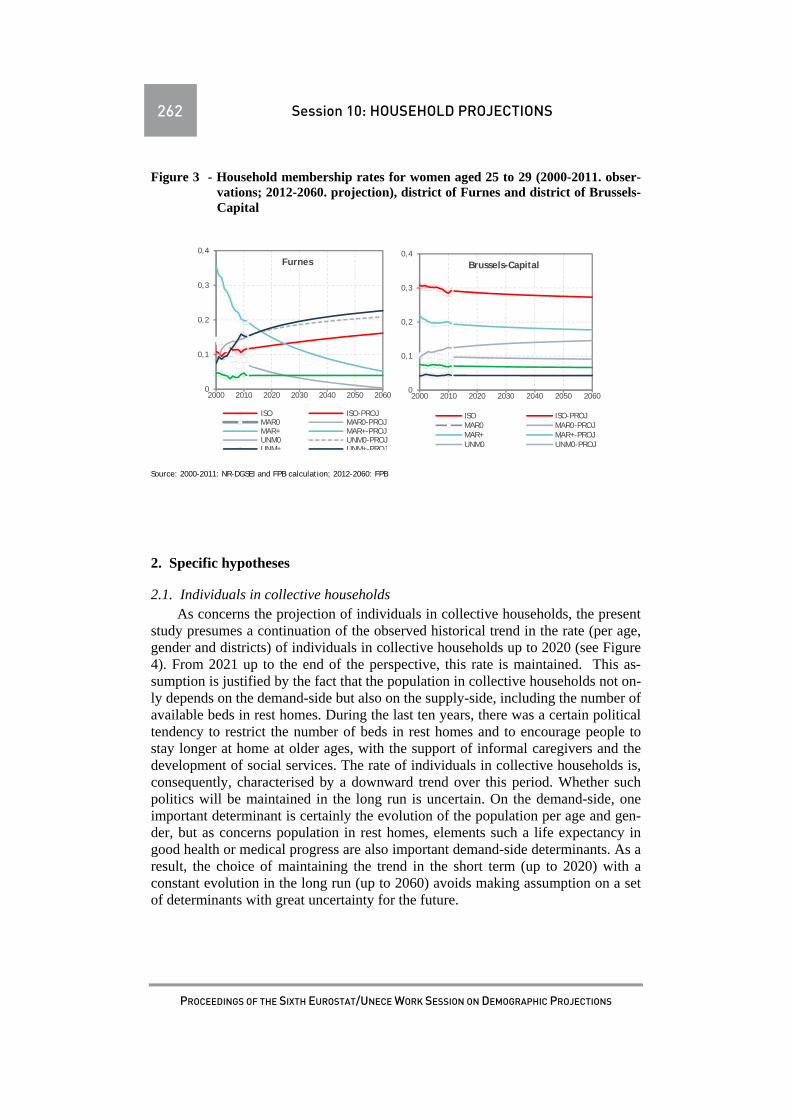
262 Session 10: HOUSEHOLD PROJECTIONS
PROCEEDINGS OF THE SIXTH EUROSTAT/UNECE WORK SESSION ON DEMOGRAPHIC PROJECTIONS
Figure 3 - Household membership rates for women aged 25 to 29 (2000-2011. obser-vations; 2012-2060. projection), district of Furnes and district of Brussels-Capital
Source: 2000-2011: NR-DGSEI and FPB calculation; 2012-2060: FPB
2. Specific hypotheses
2.1. Individuals in collective households As concerns the projection of individuals in collective households, the present
study presumes a continuation of the observed historical trend in the rate (per age, gender and districts) of individuals in collective households up to 2020 (see Figure 4). From 2021 up to the end of the perspective, this rate is maintained. This as-sumption is justified by the fact that the population in collective households not on-ly depends on the demand-side but also on the supply-side, including the number of available beds in rest homes. During the last ten years, there was a certain political tendency to restrict the number of beds in rest homes and to encourage people to stay longer at home at older ages, with the support of informal caregivers and the development of social services. The rate of individuals in collective households is, consequently, characterised by a downward trend over this period. Whether such politics will be maintained in the long run is uncertain. On the demand-side, one important determinant is certainly the evolution of the population per age and gen-der, but as concerns population in rest homes, elements such a life expectancy in good health or medical progress are also important demand-side determinants. As a result, the choice of maintaining the trend in the short term (up to 2020) with a constant evolution in the long run (up to 2060) avoids making assumption on a set of determinants with great uncertainty for the future.
0
0,1
0,2
0,3
0,4
2000 2010 2020 2030 2040 2050 2060
Furnes
ISO ISO-PROJMAR0 MAR0-PROJMAR+ MAR+-PROJUNM0 UNM0-PROJUNM+ UNM+-PROJ
0
0,1
0,2
0,3
0,4
2000 2010 2020 2030 2040 2050 2060
Brussels-Capital
ISO ISO-PROJMAR0 MAR0-PROJMAR+ MAR+-PROJUNM0 UNM0-PROJ

Session 10: HOUSEHOLD PROJECTIONS 263
PROCEEDINGS OF THE SIXTH EUROSTAT/UNECE WORK SESSION ON DEMOGRAPHIC PROJECTIONS
0,00
50000,00
100000,00
150000,00
200000,00
250000,00
300000,00
2000 2010 2020 2030 2040 2050 2060
COLL COLL (PROJ)
0
0,05
0,1
0,15
0,2
0,25
2000 2010 2020 2030 2040 2050 2060
Men
65 65 (PROJ)70 70 (PROJ)75 75 (PROJ)80 80 (PROJ)85 85 (PROJ)90 90 (PROJ)
0
0,1
0,2
0,3
0,4
0,5
2000 2010 2020 2030 2040 2050 2060
Women
65 65 (PROJ)70 70 (PROJ)75 75 (PROJ)80 80 (PROJ)85 85 (PROJ)90 90 (PROJ)
Figure 4 - Evolution of the rates of individuals older than 65 living in a collective households by age and gender (2000-2011: observations; 2012-2060: projection), Belgium
Source: 2000-2011: NR-DGSEI and FPB calculation; 2012-2060: FPB
Figure 5 - Projection of the number of individuals in collective households – reference scenario
Source: 2000-2011: NR-DGSEI and FPB calculation; 2012-2060: FPB
Population ageing (mainly due to increasing life expectancy, stagnating births and decreasing immigration), combined with a constant rate in the long run of indi-viduals in collective households, leads to a substantial increase of individuals in collective households (see Figure 5). This could be considered as unsustainable from a social, political or economic point of view. This approach has, however, the

264 Session 10: HOUSEHOLD PROJECTIONS
PROCEEDINGS OF THE SIXTH EUROSTAT/UNECE WORK SESSION ON DEMOGRAPHIC PROJECTIONS
advantage of highlighting the scale of the challenge for the future. Whether politi-cians decide to supply a sufficient number of places in collective households or to implement other politics (such as more informal care or home care) is beyond the scope of this paper. In the latter case (more informal care or home care), the num-ber of individuals in collective households would, consequently, be lower in the future.
2.2. Individuals in a position “Non Family Related Adults” or “other” The projection of the number of “Non Family Related Adults” (NFRA) indi-
viduals is realized by using projected membership rates. This approach does how-ever not allow determining which household types those individuals belong to. In order to determine the average size of the households, those individuals have to be redistributed in the household types. They can be attributed to married couples with or without children, to couples in a consensual union with or without children and to one-parent families.
Based on historical data (from 1991 to 2011), the share of NFRA individuals living in households with a married couple (with or without children) is decreasing while the share of the NFRA individuals living in households with a couple in a consensual union (with or without children) or in one-parent families is increasing. The distribution of the NFRA over the different household types is based on those shares, assuming a continuation of the historical trend with a saturation level in the long run.
For the individuals in a position “other”, the projection is also realized by us-ing the projected membership rates. To calculate the number of households of type “Other”, an assumption has to be made on the average number of individuals in such a household. Historical data (from 1991) show that the average size of the households of type “Other” remains constant at the level of 2.1. This average is as-sumed to be constant in the projection.
3. Results
This section presents the main results from the household projection 2012-2060, namely the projection of the number of individuals per position in the house-hold, the projection of the number of households per type of household and the av-erage size of the households. These results, though available, are not presented at the NUTS3 level. In the present paper, they are aggregated for the whole country.
3.1. Household positions The projection of the number of individuals in Belgium by household position
is presented in Table 2. While most of the positions face an increasing trend up to 2060, the numbers of married individuals with children and of children within a married couple decrease by 30% and 24% respectively over the period 2011-2060. This evolution is mainly explained by the downward projection of the rate of mar-ried couples with children and of children in a married couple.
While the rate of married couples without children is also projected to follow a downward trend, for all ages and both genders, the number of married individuals

Session 10: HOUSEHOLD PROJECTIONS 265
PROCEEDINGS OF THE SIXTH EUROSTAT/UNECE WORK SESSION ON DEMOGRAPHIC PROJECTIONS
without children increases by 14% in 2060 compared to 2011. This increase is ex-plained by the high proportion in the near future years of individuals aged 65 to 75 (the baby boom cohorts) and the high (but still decreasing) rate (around 0.4) of married couples without children for those ages. This effect related to the post-war baby boom disappears progressively in the long run (beyond 2030), which is re-flected by a stable evolution of the number of married individuals without children between 2030 and 2060.
Table 2 - Individuals by household position in Belgium
2011 2030 2060
Number Share
(%)
Number Share
(%)
Growth
rate
com-
pared
to 2011
(%)
Number Share
(%)
Growth
rate
com-
pared
to 2011
(%)
SINGLE 1600594 14.6 2087487 17.3 30.4 2518994 19.8 57.4
MAR0 1919416 17.5 2209196 18.3 15.1 2194571 17.2 14.3
MAR+ 2201164 20.1 1880313 15.6 -14.6 1534489 12 -30.3
CHMAR+ 2086914 19.1 1944318 16.1 -6.8 1584294 12.4 -24.1
UNM 489966 4.5 610046 5 24.5 730262 5.7 49
UNM+ 548706 5 680511 5.6 24 880315 6.9 60.4
CUNM+ 461562 4.2 619098 5.1 34.1 815423 6.4 76.7
H1PA 456905 4.2 548782 4.5 20.1 637035 5 39.4
C1PA 710839 6.5 917458 7.6 29.1 1101691 8.6 55
NFR 189069 1.7 222471 1.8 17.7 259756 2 37.4
OTHR 161503 1.5 194015 1.6 20.1 228524 1.8 41.5
COLL 124628 1.1 166615 1.4 33.7 263332 2.1 111.3
Total 10951266 100 12080310 100 10.3 12748686 100 16.4
Source: 2011: NR-DGSEI and FPB calculation; 2012-2060: FPB
Due to the extrapolation of the observed trends (with a saturation effect in the
long run) of non-consensual unions and one-person families, the number of indi-viduals (including children) within such households increases substantially be-tween 2011 and 2060, up to 77% for the number of children in families with cohab-iting parents.
The contrasting evolutions of the number of individuals according to house-hold positions lead to a change in the share of each household position in the popu-lation. Those shares are included in Table 2.
Finally, under the assumptions described in section 0, population ageing leads to an increase of individuals in collective households by 111% in 2060. The growth acceleration of the number of individuals living in collective households from 2030 onward is due to the baby boom generation attaining the age of 85 and over in 2030, with the highest probability of being in a collective household (see Figure 4).

266 Session 10: HOUSEHOLD PROJECTIONS
PROCEEDINGS OF THE SIXTH EUROSTAT/UNECE WORK SESSION ON DEMOGRAPHIC PROJECTIONS
3.2 Household types The number of households by type can be deduced (see section 1.1) from the
number of individuals in each household position. The projection of the number of households by type is presented in Table 3. The number of households follows the same evolution as the number of individuals by household positions. All types of households, except married couples with children, increase over the period 2011-2060: between 14% and 60% according to the type.
Table 3 - Private-households by household types in Belgium
2011 2030 2060
Number Share
(%)
Number Share
(%)
Growth rate com-
pared to 2011 (%)
Number Share
(%)
Growth rate com-
pared to 2011 (%)
SING 1600594 34 2087487 38.5 30.4 2518994 42.4 57.4
MAR0 959708 20.4 1104598 20.4 15.1 1097286 18.5 14.3
MAR+ 1100582 23.3 940157 17.4 -14.6 767245 12.9 -30.3
UNM 244983 5.2 305023 5.6 24.5 365131 6.2 49.0
UNM+ 274353 5.8 340256 6.3 24.0 440157 7.4 60.4
1PA 456905 9.7 548782 10.1 20.1 637035 10.7 39.4
OTHR 76906 1.6 92388 1.7 20.1 108821 1.8 41.5
Total 4714031 100 5418690 100 14.9 5934669 100 25.9
Source: 2011: NR-DGSEI and FPB calculation; 2012-2060: FPB
3.3. Total number of households and average size The evolution of the total number of households for Belgium is presented in
Figure 6, together with the evolution of the Belgian population. The number of households grows more quickly than the number of individuals. This is explained by the evolution of the distribution of households types, namely proportionally more households by 2060 with less individuals (one-person households in particu-lar).

Session 10: HOUSEHOLD PROJECTIONS 267
PROCEEDINGS OF THE SIXTH EUROSTAT/UNECE WORK SESSION ON DEMOGRAPHIC PROJECTIONS
Figure 6 - Evolution of the population and of the households by 2060 for Belgium
Source: 2011: NR-DGSEI and FPB calculation; 2012-2060: FPB
4. Sensitivity analysis for collective households
The projection of households presented in Section 2 concerns only private households. To obtain the population of private households, a hypothesis has been made concerning the individuals in collective households.
Collective households include individuals living in rest homes, prisons, con-vents etc. Around 80% of individuals living in collective households are 65 years or older. This population is, therefore, highly correlated with individuals living in rest homes (this is even more true for people older than 85 years). Given the social and economic importance of this specific population, even more in a context of population ageing, the projection of individuals in collective households is a topic on itself (see Van den Bosch et al., 2011 for a specific study on residential care for older persons in Belgium). In the present exercise, it seems of interest to analyse whether the hypothesis on the projection of the number of individuals living in col-lective households has a significant impact on the projection of private households. In this perspective, an ‘extreme’ alternative has been tested, namely maintaining the level of individuals in collective households up to 2060 at the average of the period 2007-2011 (see left-hand side of Figure 7 – alternative projection). On the one hand, this alternative seems legitimate in view of the fact that from 2000 to 2011, the level of individuals in collective households remained relative constant. On the other hand, considering population ageing in the forthcoming years, the op-posite would be expected.
2000=100
90
100
110
120
130
140
150
2000 2010 2020 2030 2040 2050 2060
Belgium
Population Households Population (PROJ) Households (PROJ)

268 Session 10: HOUSEHOLD PROJECTIONS
PROCEEDINGS OF THE SIXTH EUROSTAT/UNECE WORK SESSION ON DEMOGRAPHIC PROJECTIONS
Figure 7 - Projection of the number of individuals in collective households (left-side) and of the number of households in Belgium (right-side) according to alternative hy-potheses
Source: 2000-2011: NR-DGSEI and FPB calculation; 2012-2060: FPB
While the number of individuals in collective households decreases by 43%
(around 95 000 individuals) in 2060 in the alternative scenario compared to the ref-erence scenario, the impact on the number of private households is far less im-portant. In the alternative scenario, the number of private households increases by 1.4% (around 85 000 households) in 2060 compared to the reference scenario.
0
50000
100000
150000
200000
250000
300000
2000 2010 2020 2030 2040 2050 2060
Reference Reference (Proj)
4000000
4500000
5000000
5500000
6000000
6500000
2000 2010 2020 2030 2040 2050 2060
Reference Reference (PROJ)

Session 10: HOUSEHOLD PROJECTIONS 269
PROCEEDINGS OF THE SIXTH EUROSTAT/UNECE WORK SESSION ON DEMOGRAPHIC PROJECTIONS
%
22,1 20,4 21,6 18,5 20,0
30,5
17,4 18,412,9 14,3
3,5
5,6 5,3
6,25,8
2,6
6,3 5,0
7,4 5,6
31,338,5 38,6
42,4 42,6
8,7 10,1 9,7 10,7 10,2
0,0
10,0
20,0
30,0
40,0
50,0
60,0
70,0
80,0
90,0
100,0
REF ALT REF ALT2010 2030 2060
MAR0 MARCH UNM0 UNMCH SING 1P OTHR
Figure 8 - Impact of the alternative scenario related to households in collective house-holds on the repartition of the households
Source: 2000, NR-DGSEI and FPB calculation; 2030-2060, FPB
The impact on the distribution of household’s types is presented in Figure 8.
The difference between the two scenarios is even smaller. The alternative scenario leads to a difference between -1.8 and +1.5 percentage point in 2060 compared to the reference scenario. Consequently, the alternative ‘extreme’ scenario has a neg-ligible impact on the projection of private households.
5. Discussion
This paper presents a static method for household projections based on indi-vidual living arrangements. As already discussed in numerous articles2, a static method does not allow analysing the transition from one position to another. This is a weakness of the methodology. However, we are convinced that, by using project-ed position rates, this weakness is, to a certain extent, outweighed. More precisely, assuming that a stock (the population by position) is the result of a flow (transition from one position to another), the evolution of the stock follows the evolution of the transitions. The evolution of the stock may consequently be interpreted as the summary of the evolution of sociodemographic behaviours. By hypothesis, the continuation of the recent trends of the rate of individuals in a certain household position assumes a continuum of (recent) past sociodemographic evolutions in liv-ing arrangements.
Of course, the problem of consistency is still present. Is the projected life ex-pectancy assumed in the population projection consistent with the evolution of the rate of married couples at older age? Is the projected fertility rate, which is a hy-pothesis in the population projection, consistent with the number of children born
2 See, among others, Duin and Harmsen (2009) for an overview of the weaknesses and strengths of static and dy-namic approaches.

270 Session 10: HOUSEHOLD PROJECTIONS
PROCEEDINGS OF THE SIXTH EUROSTAT/UNECE WORK SESSION ON DEMOGRAPHIC PROJECTIONS
from married or cohabiting couples? For such consistencies, a multi-state dynamic approach is certainly recommended. Due to constraints in human resources, it was not possible to develop such methodology. Notice that some consistency rules, in particular an equal number of married women and of married men, have been im-plemented. The household projection with the present static model shows, howev-er, that the results seem coherent with the components of the population projection (more particularly migration, fertility and mortality). Furthermore, since the projec-tion of the rates of being in a position are made by age and gender at the NUTS3 level, local specificities are also, to a certain extent, integrated.
A main disadvantage of the static approach is that a situation at time t is not linked to the situation at time t-1. This lack of relationship limits the projected in-formation. For example, for single households it is not possible to determine whether singles are coming from married couples divorced, from children leaving the parental home or from other situations. To summarize, the scope of potential analyses is more limited in a static approach but the approach seems sufficient to project the number of households per household type. Note that the present projec-tion has been compared with regional projections for Belgium (Willems and E. Lodewijckx, 2011 for the Flemish Region and Dal et al., 2012 for the Walloon Re-gion), and the results are convergent. The differences are explained more by the hypotheses (e.g. on the evolution of the population, the population in collective households or the length of the historical data for estimating parameters of the models) than by the methodology in itself (even with a multi-state methodology as in Dal et al., 2012).
To conclude, a projection is always based on a set of hypotheses. The choice of the hypotheses can certainly have a greater impact on the projection results than the method itself. In the analytic approach as implemented in this paper, a continu-ation of the trends is assumed (with a saturation effect). If a continuation of the (re-cent) trends is considered as the most likely projection, this projection can be de-fined as a forecast (see De Beer 2011). For a long-term horizon as considered in this study (2060), it seems difficult to define a scenario which could be considered as the most likely projection, even for long-term processes such as living arrange-ments. The considered hypothesis in this study has the advantage of making it un-necessary to make arbitrary hypotheses for the future. Maintaining the rates of household positions at a constant level from the beginning of the projection or from a later year would have led to another projection. The results of a projection should, consequently, always be interpreted while keeping in mind the hypotheses behind the model.

Session 10: HOUSEHOLD PROJECTIONS 271
PROCEEDINGS OF THE SIXTH EUROSTAT/UNECE WORK SESSION ON DEMOGRAPHIC PROJECTIONS
REFERENCES
Directorate General Statistics and Economic Information and Belgian Federal Planning Bureau, 2012, Perspectives de population 2012-2060, May 2013.
Dal. L., Eggerickx Th., Poulain M., Sanderson J.P., Centre de Recherche en Dé-mographie et Sociétés de l'UCL, Perspectives de population et des ménages au niveau communal, 2012 (Convention IWEPS 2008/008).
De Beer, J.A.A., 2011, Transparency in population forecasting: methods for fitting and projection fertility, mortality and migration, Amsterdam: Amsterdam Uni-versity Press, 266 p.
Van den Bosch, K., P. Willemé, J. Geerts, J. Breda, S. Peeters, S. Van de Sande, F. Vrijens, C. Van de Voorde, S. Stordeur, Soins résidentiels pour les personnes âgées en Belgique: projections 2011-2025, Health Services Research (HSR), Bruxelles, Centre fédéral d’expertise des soins de santé (KCE), KCE Reports, 167 B.
Van Duin, C., and Harmsen, C., 2009, Een nieuw model voor de CBS huishoudensprognose, Bevolkingstrends, 3e kwartaal 2009, Centraal Bureau voor de Statistiek, the Netherlands.
Willems, P. and E. Lodewijckx, 2011, SVR-projecties van de bevolking en de huishoudens voor Vlaamse steden en gemeenter, 2009-2030, SVR-Studie, 2011/2.

272 Session 10: HOUSEHOLD PROJECTIONS
PROCEEDINGS OF THE SIXTH EUROSTAT/UNECE WORK SESSION ON DEMOGRAPHIC PROJECTIONS
HOUSEHOLD PROJECTIONS AND WELFARE
Gian Carlo Blangiardo, Alessio Menonna, Elisa Barbiano di Belgiojoso, Natale Forlani
Summary
In Italy, as in many other countries, the ageing process will cause the increase in the number of elderly people living alone and will probably affect the demand for elderly care. This paper aims at presenting an original method for estimating, on the one hand, the extra demand for caregivers of the elderly and similar professions on the part of Italian households due to demographic changes, and on the other, the possible additional supply of migrants. Keywords: labour demand and supply, domestic workers, foreigners, Italy
1. Introduction
The socio-demographic changes experienced by Italy in recent decades (AA.VV., 2011) – e.g. ageing, changes in the family structure - have had a pro-found effect on both the labour market and the welfare system.
More specifically, like many other countries, Italy is experiencing an ageing process, so that in the next twenty years, there will be a dramatic increase in the number of persons aged 65 and over (+34%). According to available estimates (Istat, 2011) there will be nearly 16 million of them by 2030, a significant number of whom will be oldest-old (3 million aged 85 and over).
Official statistics (Indagini Multiscopo) indicate that multi-dwellings are more and more rare (only 1.2% of households), since elderly people are more likely to live alone than in the past. Suffice it to say that according to the Census of 1971, 9% of men and 22% of women aged 65 and over were living alone, while at the Census of 2001, these percentages were 13.7% and 37% respectively. Furthermore, according to recent Italian household projections (Blangiardo et al., 2012), by 2030 there will be more than 4.5 million people aged 65 and over who will be living alone, which is equivalent to 7.7% of the total population. From a family perspec-tive, this means that nearly one household in five will consist of an elderly person living alone.
Leaving aside other implications of these changes in the family set-up, the cause of this trend is also to be found in the continuing difference in male and fe-male survival levels (by 2030, men will have a life expectancy of 82.2 years, com-pared to 87.5 for women) which will obviously add to the increasing number of el-derly people living alone. There is likely to be an accompanying increase in the need for nursing home and care assistance.

Session 10: HOUSEHOLD PROJECTIONS 273
PROCEEDINGS OF THE SIXTH EUROSTAT/UNECE WORK SESSION ON DEMOGRAPHIC PROJECTIONS
Another important change which has had a significant impact on the welfare system is the increase in female activity rates, causing a reduction in the number of housewives, and a consequent need for domestic work and care services to be car-ried out by paid workers (Parreñas, 2001) since state-funded services for elderly people and children are scarce and expensive. As a direct consequence, therefore, the demand for child carers and in particular, for caregivers for the elderly, seems bound to increase significantly in the future.
Moreover, as is well-known, home caregivers are more and more often recruit-ed from among immigrants, due to the lack of supply among the younger Italian generations (e.g. Zanfrini, 2011). According to recent estimates (Censis and Ismu, 2013), only 22.7% of domestic workers are Italian, the majority being foreigners. However, some indications of change have been noticed, especially in the South: due to the negative effects of the economic crisis on the Italian labour market, the percentage of Italian women among home caregivers is gradually increasing.
Given this social-demographic background, this paper aims at presenting an original method for estimating, on the one hand, the extra demand for caregivers of the elderly and similar professions (care provided to disabled or non-autonomous people) on the part of Italian households due to demographic changes, and on the other , the possible additional supply of migrants3. The estimates integrate official statistics and data from ad hoc surveys. Furthermore, by comparing the additional supply and demand of home caregivers, some interesting considerations and help-ful recommendations arise which may be useful to policy-makers for planning pur-poses.
The rest of the paper is as follows: section 2 describes the method used to es-timate the additional supply, while the estimate of additional demand is presented in section 3. Section 4 contains the conclusions.
2. The supply of foreign caregivers
Estimates of the additional supply have been obtained on the basis of the hy-pothesis that the latter will coincide with the availability of manpower for the care sector that will be generated by annual inflows towards Italy. The procedure con-sists of three stages: the estimation of inflows of foreign population towards Italy, by sex and citizenship, on a five-year basis (2010-2014, 2015-2019… 2030-2034); the estimation of specific regional inflows, on the basis of the national level and according to the regional trends of the latest official projections (Istat, 2011); the transformation of such flows into additional supply of home caregivers by region.
3The model was set up as part of a study carried out by Censis and Ismu Foundation on behalf of the Ministry of Labour and Social Policy, which aimed to estimate supply and demand for home care in the next thirty years in the following Italian regions: Campania, Calabria, Puglia and Sicily. More details are available on the website of the Ministry of Labour and Social Policy.

274 Session 10: HOUSEHOLD PROJECTIONS
PROCEEDINGS OF THE SIXTH EUROSTAT/UNECE WORK SESSION ON DEMOGRAPHIC PROJECTIONS
Figure 1 – Scheme of the supply module
2.1 Stage 1: estimation of inflow of foreign population towards Italy Given the great variety of foreign citizenships living in Italy, only thirty coun-
tries were selected, corresponding to nearly 90% of the overall foreign population in the Population Register as of January 1st, 2011. More specifically, twenty coun-tries were selected according to their ranking in inflows towards Italy4, plus ten from among the main countries with the highest percentage of workers in the fami-ly-care sector5.
This stage, as shown in figure 1, was composed of three steps which are de-scribed below.
Step 1: Surplus/deficit in labour force
For any country, a surplus or deficit in the labour force indicates the need ei-ther to reduce the number of jobs or create a fresh supply of workers. Otherwise, if there are no changes in the national economy, migration outflows/inflows will be required to offset the demographic imbalance. Therefore, according to the hypothe-sis of invariance of the potential employment of local labour markets, the surplus in active population in the sending countries towards Italy can be considered as a push factor for estimating future labour force flows from abroad.
4 According to the citizenship distribution of foreigners resident in Italy as of January 1st, 2011 (Istat). 5 This information has been derived from PerLa Survey (Ismu, Censis and Iprs, 2010).
STAGE 2: from national to
regional level
Step 1: Surplus/deficit in
labour force for each country
Step 2: transition from surplus to inflows towards Italy
Step 3: combination of inflows with family reunion
output
Net inflow by sex and citizenship
Step 2: distribution of home care-givers according to citizenship
Step 1: incidence rate of home caregivers among for-
eigners
output
Extra supply of home caregivers by sex and citizenship
Net inflow by sex and citizenship at regional
level
output
STAGE 1: Inflow of foreigners
toward Italy
STAGE 3: Extra supply of possible
home caregivers

Session 10: HOUSEHOLD PROJECTIONS 275
PROCEEDINGS OF THE SIXTH EUROSTAT/UNECE WORK SESSION ON DEMOGRAPHIC PROJECTIONS
Thus, firstly, the surplus or deficit in the labour force,SD t, t 4 , was es-timated for each of the thirty selected countries. Entries into and exits from the la-bour force were calculated on the basis of the population, P , t , - by sex, age class and country6 - and the increase (positive or negative) in the activity rates (AR) between two consecutive age group7 with x 10,20, … , 60, t2010,2015,… ,2030 separately for each country, as follows: SD t, t 4 ∑ P , t ∙ AR , t, t 4 AR , t, t 4 [1]
where AR(t,t+4) is the average annual activity rate from t to t+4. According to our outcomes one group of countries (i.e. China, Rumania, Slo-
vakia and Ukraine), which have usually had a surplus in the labour force, will move into deficit within a short period of time (5-10 years), while Nigeria, Somalia and Senegal will continue to increase their high surplus in the labour force. Thus, within twenty years, India, Nigeria, Philippines, Pakistan, Bangladesh, Egypt, Sen-egal, Brazil, Peru and Somalia will show the highest surplus of labour force. This surplus might also constitute a push factor towards Italy.
Step 2: transition from the surplus to the possible inflow towards Italy
The surplus estimated above may be considered as the possible outflow for work reasons from sending areas. By definition, countries with a deficit in their la-bour force have no outflow of migrant workers. Among those with a positive sur-plus during the interval t, t+4, we proceeded to estimate the amount of inflows to-wards Italy by citizenship and sex. In order to do so, we first estimated a coefficient of attraction towards Italy, as a ratio of the growth in the resident foreign population with citizenship c, registered in Italy during the period 2006-2010 (source: Istat), and the surplus in the corresponding country of origin in the same period; a surplus determined using the same procedure described above. Hence, by applying these coefficients of attraction to the expected future surplus8, we estimated the entire working inflows towards Italy by citizenship and sex, IW t, t 4 .
As a result of this procedure, we obtained the first rough estimates of future in-flows, grouped by sex and citizenship on a five-year basis, due to the possible sur-plus in labour force in the main sending countries or in those countries which have the highest percentage of workers in Italy in the care sector.
Step 3: revision of previous estimates taking into account the labour force and fam-ily reunions
Taking into account that inflows are generally made up of both workers and partners or offspring of the first family member emigrating, we revised the estima-tions produced at step 2. As regards working flows, we applied a set of coeffi-cients, k t, t 4 , - by sex and citizenship - to the previous estimations, IW t, t 4 . These coefficients represent the quota of work permits out of the number of work and family permits issued in the period 2006-2010 (Istat). We hy-pothesised a turnover between the quota of inflows for family and work reasons: a high immigration ratio of workers will then be followed by a lower inflow for work
6Medium variant of world projection (UN, 2010). http://esa.un,org/unpd/wpp/index.htm. 7Activity rates are available in the database of the ILO: http://laborsta.ilo.org/ or http://www.ilo.org/ilostat . 8Properly adjusted in each period to take into account the variability and different trends between countries.

276 Session 10: HOUSEHOLD PROJECTIONS
PROCEEDINGS OF THE SIXTH EUROSTAT/UNECE WORK SESSION ON DEMOGRAPHIC PROJECTIONS
reasons and conversely by a higher inflow for family reunions. Hence, coefficients are estimated on the basis of a recursive procedure and therefore the percentage of the next period is a function of the previous one:
k t 5, t 9k t, t 4 0.5
2 , wheret 2010, 2015,… , 2025 2
In order to estimate the additional family reunion flows, the complementary values of such coefficients , 1 k t, t 4 ,are applied to the increase in the resident population registered in the previous quinquennial.
Hence, the net inflows,I t, t 4 ,are calculated as follows: I t, t 4 IW t, t 4 ∗ k t, t 4 IF t, t 4 [3]
Where: t 2015, 2020,… , 2030 andIF t, t 4
P 1.1. t P 1.1. t 5 ∗ 1 k t, t 4 In order to calculate the population stock at the end of any period, the flows
were eventually adjusted taking into account natural increase (births and deaths) and acquisitions of citizenship.
Output of stage 1
At the end of the first stage of the estimation process, we obtained the number of foreigners residing in Italy as of January 1st, 2011, 2015, 2020, 2025, 2030 and 2035 by sex and citizenship. These outcomes can be calculated using two different population targets: the first regards persons with foreign citizenship at time t (target A population), while the second considers the target A population plus all the indi-viduals who will have become Italians since 2011 (target B population). The latter group may represent the maximum estimate, and the difference is basically due to the number of foreigners who might acquire Italian citizenship over the next two decades.
According to population target A, as of January 1st, 2035, there will be 9.6 million foreigners resident in Italy, of whom 8.5 million from the 30 selected coun-tries. If the foreigners who might acquire Italian citizenship are also considered, there should be nearly three more million residents. The acquisition of Italian citi-zenship should affect more men than women, and the effects of this should be evi-dent within 15-20 years and should influence the number of the residents with Ru-manian, Ukrainian, Polish or Bulgarian citizenship.
Overall, net inflows (workers and family reunions) will decrease markedly due to reductions in the surplus in the labour force that will come about in the main sending countries. The decreasing trend should be extremely rapid, with annual net inflows halving within twenty years. More specifically, inflows from Eastern Eu-rope should run out quickly, while those from the Philippines, India, Ecuador, Pa-kistan and Egypt should remain constant and the number of emigrants from Sene-gal, Nigeria and Somalia should actually increase. The main effect of these changes will be a completely different distribution of the citizenship of the new emigrates.

Session 10: HOUSEHOLD PROJECTIONS 277
PROCEEDINGS OF THE SIXTH EUROSTAT/UNECE WORK SESSION ON DEMOGRAPHIC PROJECTIONS
Table 1 – Net inflows (workers and family reunions) according to country of origin. Mean annual figure 2011-2034 (thousands)
Five-year period
Country 2011-14 2015-19 2020-24 2025-29 2030-34
Male and Female
Rumania 79.4 34.3 18.7 11.0 7.1
Albania 32.8 26.3 20.2 15.3 12.3
Morocco 33.1 30.8 27.9 24.7 22.2
China 16.5 13.5 8.4 5.3 3.8
Ukraine 12.8 8.0 4.2 2.3 1.4
Philippines 11.3 11.8 11.8 11.7 11.6
Moldova 13.0 9.6 5.1 2.7 1.9
India 13.9 15.2 14.9 14.3 13.4
Poland 7.6 4.0 2.5 1.7 1.4
Tunisia 6.2 5.8 4.6 3.8 3.2
Peru 8.3 7.9 7.0 6.3 5.5
Sri Lanka 6.6 5.6 5.0 4.5 3.9
Senegal 6.5 7.6 8.5 9.2 9.7
Total 30 countries 308.8 232.4 182.7 152.2 133.5
Other countries 48.2 36.3 28.5 23.7 20.8
All countries 357.0 268.7 211.2 175.9 154.2 Source: own elaboration
2.2 Stage 2: transition from the national level to sub-national level For planning purposes, the sub-national level is essential. We therefore need a
procedure which enables us to distribute the overall estimate at the sub-national level. Regional inflows are computed by taking national inflows and applying to them the probability of reaching region r conditional on being of citizenship c on a five-year basis, Pr r| c . This probability is computed as follows:
Pr r| c ∙ |
[4]
Since Pr r ∩ c Pr c ∙ Pr r|c Pr r ∙ Pr c|r Where Pr r can be approximated by the ratio between the increase of
foreigners resident in region r and the overall increase estimated according to Istat data; Pr c|r by the distribution according to citizenship of foreigners resident in region r and Pr c by the incidence of inflows from country c on the overall amount of inflows. As input, we therefore need both the estimates of inflows of foreign population at the national level by sex and citizenship, I t, t 4 - see above (step 1) - and the foreign population projected by Istat as of January 1st in the years 2011-2035 by region, sex and citizenship.
Output of stage 2
As a result of this stage, we obtained the number of foreigners residing in each Italian region as of January 1st 2011, 2015, 2020, 2025, 2030 and 2035, by sex and citizenship. These estimates are distinguished according to the two different target populations (A and B) defined previously. As usual, the target B group may be considered as the maximum regional amount.

278 Session 10: HOUSEHOLD PROJECTIONS
PROCEEDINGS OF THE SIXTH EUROSTAT/UNECE WORK SESSION ON DEMOGRAPHIC PROJECTIONS
Table 2 – Net inflows by area of residence. Mean annual figure: 2011-2034 (thousands)
Five-year period
Area 2011-14 2015-19 2020-24 2025-29 2030-34
Male and Female
North West 125.0 100.9 83.3 71.4 63.4
North East 88.9 68.4 53.1 43.9 38.9
Centre 94.5 67.4 51.9 42.8 37.2
South and Islands 48.5 32.0 23.0 17.9 14.8
Total 357.0 268.7 211.2 175.9 154.2
Source: own elaboration
2.3 Stage 3: transition from inflows to additional supply of home caregivers9 In order to estimate the additional home caregiver supply (HC) by sex and
citizenship on a five-year basis at the regional level, we applied the probability of being a home caregiver conditional on having citizenship c to the regional inflows of each specific nationality (by sex) i.e.: HC I t, t 4 ∙ Pr HC|c where the last factor can be obtained as follows:
Pr HC|cPr c|HC ∙ Pr HC
Pr c 5
Since, applying the formula of Bayes, the joint probability of having citizenship c and being a home caregiver is estimated as follows:
Pr c ∩ HC Pr c|HC ∙ Pr HC Pr c ∙ Pr HC|c . Thus for each of the three terms of [5], the most suitable and updated source
was identified as ad hoc surveys on migrants living in Italy. First, the probability of coming from country c as the ratio between
estimations of net regional inflows of foreign population (absolute values) by sex and citizenship obtained as an output of the previous stage I t, t 4 and the total
inflow (separately for each sex): Pr c ,
∑ ,
Second, the quota of each nationality among home caregivers Pr c|HC (for
any sex): Pr c|HC
This information was obtained from the outcomes of a specific survey conducted by Censis and Ismu during 2012 (“sample of workers” 2012).
Third, the incidence rate of home caregivers among the foreign populationPr HC :
Pr HC [6].
The latter was identified on the basis of the results of recent surveys carried out in Italy. More specifically, the following two surveys were considered: PerLa Survey, carried out during 2009 by Ismu, Censis and Iprs, aiming at describing the professional trajectories of migrants (Ismu, Censis and Iprs, 2010), and the Integration Indexes Survey, conducted during 2009 by Ismu, aiming at estimating the level of integration of migrants living in Italy (Cesareo and Blangiardo, 2009).
9 Henceforth the estimates concern additional labour demand and supply.

Session 10: HOUSEHOLD PROJECTIONS 279
PROCEEDINGS OF THE SIXTH EUROSTAT/UNECE WORK SESSION ON DEMOGRAPHIC PROJECTIONS
Table 3 – Additional supply of home caregivers at the national level by country of origin. Mean annual figure: 2011-2034
Five-year period
Country 2011-14 2015-19 2020-24 2025-29 2030-34
Male and Female
Rumania 19,283 10,574 7,179 5,26 4,175
Albania 3,582 2,973 2,352 1,877 1,605
Morocco 5,923 5,941 5,686 5,319 4,998
China 2,103 1,915 1,389 1,095 934
Ukraine 7,312 5,089 2,966 1,88 1,318
Philippines 6,079 6,312 6,368 6,407 6,413
Moldova 6,788 5,531 3,377 2,232 1,621
India 2,269 2,559 2,641 2,68 2,62
Poland 3,212 1,87 1,277 968 806
Peru 4,372 4,539 4,328 4,075 3,766
Sri Lanka 1,730 1,564 1,451 1,369 1,236
Senegal 957 1,121 1,270 1,418 1,530
Total 30 countries 82,996 67,227 54,873 47,675 43,163
Other countries 13,321 10,561 8,566 7,329 6,546
All countries 96,316 77,788 63,439 55,003 49,709
Source: own elaboration
Table 4 – Additional supply of home caregivers at national level by area of residence. Mean annual figure, years: 2011-2034 (thousands)
Five-year period
Macro area 2011-14 2015-19 2020-24 2025-29 2030-34
Male and Female
North West 33.5 28.3 24.0 21.3 19.5
North East 22.8 18.3 14.4 12.3 11.2
Centre 24.5 19.5 16.1 14.1 12.7
South and Islands 15.6 11.7 8.9 7.4 6.4
Italy 96.3 77.8 63.4 55.0 49.7
Source: own elaboration
Output of stage 3
As a result of this third stage of the estimation process, we obtained the additional supply of foreign home caregivers on a five-year basis by sex, region and citizenship. As for stage 1, these estimates can be distinguished according to the two different target populations (A and B), previously defined, and target B group may be considered, once again, as the maximum amount.
3. Family demand for caregivers
As regards the extra demand for home caregivers on the part of families, the estimate process is based, on the one hand, on the number and the characteristics of the population potentially in need of care and on the other, on the characteristics of home caregivers. A household perspective must be adopted, since personal care is

280 Session 10: HOUSEHOLD PROJECTIONS
PROCEEDINGS OF THE SIXTH EUROSTAT/UNECE WORK SESSION ON DEMOGRAPHIC PROJECTIONS
closely connected with the living arrangements of elderly people and of disabled or non-autonomous adults.
We hypothesize that the number of home caregiver users by age10, type of liv-ing arrangement11, sex and region,D . (x= 65, 75, 85+), may be calculated as a function of the numbers of elderly people in the population by age and type of liv-ing arrangement,E . , and the probability of need in the services of a caregiver ( ) conditional on being agedx, x 9 and in the living arrangement type h,Pr |x, x 9&h , as follows:
D , E , ∙ Pr |x, x 9&h [7] According to the formula of Bayes:
Pr x, x 9&h ∩ Pr ∙ Pr x, x 9&h| = Pr x, x 9&h ∙Pr │x, x 9&h [8]
thus
Pr │x, x 9&h ∙ , & |
, &[9]
If we indicate , & |
, & as p , & and Pr as pU, that is the rate of
caregivers among the whole elderly population: Pr |x, x 9&h ∙ p , & [10]
D , E , ∙ ∙ , & [11] Hence, the overall additional demand from elderly members in the household,
D, can be estimated as the sum of [11] D ∑ D ,, [12]
The result of equation [12] is adjusted a posteriori in order to take into account the number of users of home caregivers among people aged under 65 (disabled and non-autonomous individuals).
Hence to estimate the number of home caregivers demanded by the Italian households the following inputs are required:
first, the distribution of elderly people grouped by sex, age group (65-74; 75-84 and 85+) and living arrangements from 2011 to 2031,E . t, t 4 . These es-timates have recently been produced (Blangiardo et al., 2012), using a propensity method similar to that used by the Australian Bureau of Statistics (1999) and by Statistics New Zealand (2004). Briefly, this method assumes that each individual has one role in a family and household (living arrangement type) and that the pro-portion of population in each living arrangement type may be considered as the probability of belonging to each role, grouped by age and sex. Such proportions – available from the Indagine Multiscopo (Istat) – represent the living arrangement type rates (LATRs). Afterwards, the LATRs are applied to the future population distribution by age and sex (Istat, 2011). As a result, we obtain the distribution of the population by age, sex, region and living arrangement from which the number of families and households is derived;
10We consider three age groups: 65-74; 75-84 and 85+. 11 We consider five types of living arrangements: single person, couple with children, couple without children, one-parent family and other family.

Session 10: HOUSEHOLD PROJECTIONS 281
PROCEEDINGS OF THE SIXTH EUROSTAT/UNECE WORK SESSION ON DEMOGRAPHIC PROJECTIONS
second, the distribution by sex, age and living arrangements of elderly people aged 65 and over,E . , assisted by a home caregiver, according to the ad hoc survey conducted by Censis during 2012 on households assisted by home caregivers (Censis, 2013);
third, the number of home caregivers as of January 1st, 2011, employed by households with at least one person aged 65 and older (Censis estimates) which can be assumed as a proxy of the number of assisted elderly people.
Table 5 – Mean annual value of the additional demand for home caregivers in Italy by area of residence. (thousands): 2011-2030
Period
Area 2011-14 2015-19 2020-24 2025-29 2030
Minimum variant
North West 7.1 5.2 6.1 5.0 4.5
North East 4.2 3.4 4.1 4.0 3.8
Centre 4.1 2.9 3.7 4.0 4.3
South and Islands 2.8 2.2 2.9 3.0 3.4
Italy 18.2 13.7 16.8 15.9 16.0
Maximum variant
North West 16.4 12.4 14.3 11.8 10.6
North East 8.5 6.8 8.4 8.2 7.7
Centre 9.0 6.5 8.2 8.8 9.6
South and Islands 6.6 5.1 7.0 7.2 8.3
Italy 40.6 30.7 37.9 36.0 36.2
Source: own elaboration
Two different variants of estimates were computed: the minimum and
maximum one. In the former case, the additional demand for home caregivers is calculated considering only those workers active in the care sector, while in the latter, workers employed in the domestic and family sector are also included.
As shown in Table 6, the additional demand for caregivers due to the rise in numbers of elderly people over the next years will decrease in Italy. This trend is ascribable to the projected trend in the North West where the loss should be very sizeable, while according to our estimates the Centre and the South and Islands regions should see a slight increase in demand.

282 Session 10: HOUSEHOLD PROJECTIONS
PROCEEDINGS OF THE SIXTH EUROSTAT/UNECE WORK SESSION ON DEMOGRAPHIC PROJECTIONS
Table 6 - Mean annual value of additional demand for home caregivers in Italy by sex, age and living arrangements of the caregiving user: 2011-2030.
period Male Female
Single person
65+ other 65+ Other <65
Single person
65+ other 65+
Other <65
Total
Minimum variant
2011-2014 5,563 4,811 843 4,170 2,624 206 18,217
2015-2019 4,355 3,686 654 3,078 1,745 147 13,665
2020-2024 5,215 4,495 790 3,758 2,394 188 16,840
2025-2029 4,346 3,742 658 3,982 2,980 212 15,920
2030 3,913 3,427 598 4,187 3,595 237 15,958
Maximum variant
2011-2014 12,357 10,697 1,875 9,338 5,854 462 40,583
2015-2019 9,761 8,268 1,466 6,972 3,946 333 30,746
2020-2024 11,696 10,092 1,772 8,530 5,421 427 37,937
2025-2029 9,787 8,434 1,483 9,053 6,723 482 35,962
2030 8,868 7,783 1,357 9,556 8,087 540 36,189
Source: own elaboration
In the future, the extra demand for home caregivers will be expressed mainly
by men, persons aged 65 and over and especially those living alone. According to the maximum variant, the surplus demand will fluctuate in line with the age structure of the population. On average, therefore, in each year until 2030 between 30 and 40 thousand domestic workers will be taking care of our elderly, disabled and non-autonomous people.
4. Conclusions
The model herewith proposed is an original procedure both from the methodological perspective and in terms of results. The methodology combines official statistics with data from ad hoc surveys conducted on migrants in recent years. Taking as our starting-point the surplus in the labour force that will exist in the main sending countries - making the reasonable hypothesis that in presence of a surplus, workers will emigrate to another country in search of employment- we estimate possible inflows towards Italy taking into account not only that people emigrate for work but also to rejoin their families. The estimation at the national level is distributed according to region and we then estimate the additional home caregiver supply by sex and nationality.
Furthermore, in order to appraise the extra demand, we consider the number of potential users of home caregivers, starting from the estimated changes concerning elderly people, combined with structural modifications on the basis of their household arrangements. The outcomes constitute a helpful resource for planning purposes particularly as regards the regulation of inflows and their redistribution around the country.
According to our results, significant changes will take place in the next twenty years. Firstly, due to demographic trends in the main sending countries, there will be changes in the composition of inflows towards Italy. Inflows from the current

Session 10: HOUSEHOLD PROJECTIONS 283
PROCEEDINGS OF THE SIXTH EUROSTAT/UNECE WORK SESSION ON DEMOGRAPHIC PROJECTIONS
sending countries, both for work and family reasons, will decrease as a result of depletion in surpluses in the labour force, while inflows from central and southern Africa will increase. Secondly, the inflows of home caregivers toward Italy will gradually decrease from nearly 100 thousand to less than 50 thousand. Thirdly, the estimates suggest that the current supply of domestic workers who arrive in Italy each year from the Ukraine, Rumania, Moldova, the Philippines, Poland, Russia and Bulgaria, fully satisfies the additional demand for nearly 40 thousand domestic workers, while in twenty years’ time the supply from these countries will cover less than 30% of the additional demand. Hence, in order to satisfy the growing need for of family assistance, home caregivers will have to be recruited from other coun-tries, especially from Africa.
REFERENCES
Australian Bureau of Statistics. 1999. Household and family Projections, Australia 1996 to 2021, Australian Bureau of Statistics.
AA. VV. 2011. Il Cambiamento demografico, Rapporto proposta sul futuro dell’Italia, Bari, Laterza.
Blangiardo G.C., E. Barbiano di Belgiojoso, P. Bonomi. 2012, Le previsioni demo-grafiche delle famiglie, in Osservatorio Nazionale sulla Famiglia (eds.), Vol. I - La condizione familiare in Italia: aspetti demografici, sociali e legislativi, Carocci.
Censis and Ismu (eds.). 2013. Elaborazione di un modello previsionale del fabbiso-gno di servizi assistenziali alla persona nel mercato del lavoro italiano con parti-colare riferimento alla popolazione straniera, Sintesi della ricerca, Roma, 14 maggio, http://www.integrazionemigranti.gov.it
Cesareo V., G.C. Blangiardo (eds.). 2009. Indici di integrazione, Un’indagine em-pirica nella realtà migratoria italiana. Milano: Franco Angeli.
Ismu, Censis, Iprs (eds.). 2010. Immigrazione e lavoro, Percorsi lavorativi, Centri per l’impiego politiche attive. Quaderni Ismu 1/2010.
Istat. 2011. Previsioni regionali della popolazione residente al 2065, demo.istat.it.
Ministero del lavoro e delle politiche sociali. 2012. Modello per la stima di do-manda e offerta del lavoro domestico, Roma.
Parreñas R.S. 2001. Servants of Globalization, Women, Migration, and Domestic Work. Stanford, California: Stanford University Press.
Statistics New Zealand. 2004. New Zealand Family and Household Projections, 2001 (based)-2021, TeTariTatau, Statistics New Zealand.
Zanfrini L. 2011. Labour in The Sixteenth Italian Report on Migrations 2010. McGraw-Hill, Milan.


Session 11
DEMOGRAPHIC SUSTAINABILITYAND CONSISTENCY WITH
MACROECONOMIC ASSUMPTIONS
Chair: Elisabetta Barbi (University of Rome “Sapienza”)


Session 11: DEMOGRAPHIC SUSTAINABILITY AND CONSISTENCY WITH MACROECONOMIC ASSUMPTIONS 287
PROCEEDINGS OF THE SIXTH EUROSTAT/UNECE WORK SESSION ON DEMOGRAPHIC PROJECTIONS
AGEING ALONE? THE FUTURE OF THE PORTUGUESE POPULATION IN
DISCUSSION
Lídia Patrícia Tomé, Filipe Ribeiro, Maria Filomena Mendes
Summary
Population projections significance is recognized all around the world, being used by different governments with the intention to suppress the necessity of having more in-formation about the diverse demographic issues, and Portugal is not an exception. Ad-ditionally, the fact that Southern Europe is in economic crisis and that Portugal was the second country from the south, after Greece, in economic collapse, resulted in a strong impact not only in the family context, but also its sustainability itself. Trying to answer questions like: Will be the country economically sustainable in the future? Is Portugal going to decline total population?, or, How these changes will in-fluence the households structures in the future?, we intend to elaborate a cohort com-ponent projection, for a medium term period (next 20 years), that will allow us to iden-tify the Portuguese population structure in the future and, at the same time, evaluate the possible changes that the country will have to face. Keywords: Ageing, Household, Population Projections, Portugal.
1. Introduction
Across history profound changes in the different societies have been registered and these changes are hand in a glove with the changes occurred in demographic paradigms. Nevertheless, even that many demographic changes can be connected with individual choices, like the decision to migrate or to have a child, the truth is that there is always something behind that influences a decision. Nowadays, the economic crisis that is installed in Southern Europe has a major impact in several of these personal decisions and also in some others that cannot be really controlled, like unemployment or health demand.
The main motivation and goal for the elaboration of this study is to evaluate the impact of the crisis in the future of the Portuguese population and at the same time to analyze the structure of the ageing process itself. We will elaborate and project, based on different assumptions, diverse scenarios of evolution for the next 20 years, i.e., from 2012 to 2032. In this way, without taking into account any so-cioeconomic variable we intend to evaluate the possible changes in the Portuguese demography; if in the near future the country can still be demographically sustain-able due to ageing; if the crisis itself will accelerate and intensify the ageing pro-

288 Session 11: DEMOGRAPHIC SUSTAINABILITY AND CONSISTENCY WITH MACROECONOMIC ASSUMPTIONS
PROCEEDINGS OF THE SIXTH EUROSTAT/UNECE WORK SESSION ON DEMOGRAPHIC PROJECTIONS
cess, together with a shrinking population; and, at last, try to understand how the household dynamics are going to change. Thus, we will try to give an answer to questions like: Will the country be demographically sustainable in the future?, Is Portugal going to decline total population?, How all the demographic changes will influence the household structure in the future?, How massive out-migration will influence the overall population?, and, Can Portuguese people expect to age alone in the future?
Our guess is that Portugal is walking towards a very pronounced decline in the overall population, which consequently intensified by high emigration rates that will result in a deep change in the household composition, possibly isolating more and more individuals.
2. Data and methodological approach
Findings presented in the manuscript, were calculated based on data collected from the Human Mortality Database (HMD: www.mortality.org) and from Statis-tics Portugal (INE: www.ine.pt).
With the intention of giving an answer to the research questions and hypothe-ses advanced in the introductory section, we made use of the cohort component projection methodology. The construction of different and plausible scenarios came out from a combination of the cohort component projection model and the Lee-Carter methodology to forecast future mortality and life expectancy. The combina-tion of these two approaches results in the addiction of a probabilistic component to the projection method, and at the same time, improves the outcome. Moreover, since it is also our aim to analyze the possible changes in the household composi-tion, the headship rate method proposed by the United Nations in 1973 and the model improvements suggested by Ediev in 2007 were additionally applied.
The household headship method calculates the number of households from an existing population projection by age and sex, typically the “medium variant”, to-gether with statistics on the proportion of household heads belonging to each age-sex group. Several authors (Mason, 1987; Linke 1988; McDonald & Kippen, 1998; Ediev, 2007; Zeng et al., 2013) developed different extensions or approaches trying to improve household projections allowing the identification of more detailed in-formation about the distribution of household sizes. In our study, the choice of the methodological approach fell on the extensions to the household headship method developed by Ediev in 2007 essentially due to data availability and by the robust-ness and consistence presented by the method itself when applied to empirical data.
3. Past, present and future: defining possible scenarios
Between 1960 and 2012 the structure of the Portuguese population presented a dramatic reduction at younger ages and the number of elderly increased tremen-dously, changing significantly population dynamics. Into the light of demography, this situation can be explained being the result of fertility decline, the increase of life expectancy and, as well, an increasing of emigration in the most recent years. Portugal, as the other Southern European countries, also experienced a drastic and

Session 11: DEMOGRAPHIC SUSTAINABILITY AND CONSISTENCY WITH MACROECONOMIC ASSUMPTIONS 289
PROCEEDINGS OF THE SIXTH EUROSTAT/UNECE WORK SESSION ON DEMOGRAPHIC PROJECTIONS
fast decline in live births. The Portuguese TFR declined from the value of 3 chil-dren per women in 1960 to 1.28 in 2012. And at the same time the evolution of life expectancy at birth reveals form 1960 to 2012 the increase of 16.7 years in the fe-male case and 16.1 years for males. Besides the positive impact of this evolution of lifespan, its conjugation with low fertility rates can affect the country sustainability at the same time that the Portuguese population structure is ageing. For the first time in 17 years, and following the information given by the Statistics Portugal of-fice, Portugal presents negative net migration values in 2011 and 2012. In fact, since 2010 that the number of emigrants grew more than twofold, increasing from 23 760 in 2010, to 51 958 in 2012. The registration of in-migration flows presents an opposite evolution, as expected, decreasing from 27 575 immigrants in 2010, to 14 606 in 2012.
Nonetheless, above all and until nowadays, the decline of births and fertility rates are the major responsible for the fact that Portugal becomes currently, accord-ing to the information presented by the World Population Data Sheet 20101, the sixth country in the ranking of the most aged ones.
One of the most important steps in the elaboration of the different projection scenarios is a careful and in depth exploration of a country demographic compo-nents, i.e., fertility, mortality and migration. So, after a first phase where it was show a contextualization of the country itself, we are now in a good position to elaborate the possible and differentiated “what if” scenarios for the future of the Portuguese population.
Starting with the assumptions elaborated for the fertility component (Figure 1, panel 1), with the starting point of the last available year, i.e., the year of 2012, where the observed value for the TFR is 1.28, we believe that Portugal, following the tendency that took place in several other European countries, will keep register-ing a decrease in TFR. So, for all the scenarios it was defined that the TFR for 2016 can decrease to 1.15. Thus, is only from 2016 onwards that we can expect dif-ferent possible evolutions, and in a so-called “central” scenario we admit that the TFR will slightly increase achieving the value of 1.4 (in 2032). In a “high” scenar-io, it would be good that the value of 2.0 children per woman can be reached, and in opposition, in a “low” scenario, it can be assumed that Portugal will not recuper-ate its fertility rates and the decline can be even more pronounced, possibly attain-ing in average the value of a single (1) child per woman.
In the case of the assumptions taken for the mortality and presented in Figure 1 (panel 2 and 3), it was followed the obtained values from the Lee-Carter forecast-ing methodology. In this case, it can be expected that in a “central” scenario, the observed life expectancy at birth for females increase from around 83.5 years (2012), to 87.2 years (2032); and for males from 77.3 years to 81.4 years. This sit-uation corresponds to an increase of 3.7 and 4.1 years in the life expectancy of fe-males and males, respectively, during the 20 years of the study. Nevertheless, in our calculations, it is also assumed that life expectancy at birth could present a faster or lower increase with time. In this situation, it is expected, if the “high sce-nario” becomes real, that life expectancy at birth for females reach the value of 90.1 and for males 84.5, in 2032. Nevertheless, the values associated with the “low
1 Population Reference Bureau

290 Session 11: DEMOGRAPHIC SUSTAINABILITY AND CONSISTENCY WITH MACROECONOMIC ASSUMPTIONS
PROCEEDINGS OF THE SIXTH EUROSTAT/UNECE WORK SESSION ON DEMOGRAPHIC PROJECTIONS
scenario”, are, as predictable, a bit lower, and in 2032 is expected that females achieve 83.3 years of life expectancy at birth and 77.7 years in male case.
Figure 1 - Total fertility rate (TFR) Life expectancy at birth (e0) and between 1981
and 2012 and possible scenarios until 2032 in Portugal Panel 1: Total fertility rate (TFR) between
1981 and 2032
Panel 2: Male e0 between 1981 and 2032
Panel 3: Female e0 between 1981 and 2032
Source: own calculation, INE - Statistics Portugal, HMD.
Lastly, lets direct now our attention to the migration component that was in-
troduced in the projection model using net migration values. Based on recent trends and taking into account emigration and immigration separately, we assume that the first one will follow the same pattern of increase registered between 2009 and 2012 (11 686 emigrants per year in average) until 2022, increasing from 51 958 to 168 821. The period taken into account for this assumption is due to 2009 being the year immediately after the beginning of the crisis (2008), and when people started to realize the situation of the country. After 2022, we believe that is possible that these values decline until the ones observed in 2009 (16 899). For the second case, i.e., immigration, we assume that the inflow tendency will decelerate and, without doubt decrease, because the country is not at the time economically stable and con-sequently, non-attractive. In this way, it is really possible that in 2022 the number of immigrants equals the minimum value registered since the 1990s, more specifi-cally in 1991, with an inflow that decreases from 14 606 individuals (2012) to 4 507 individuals (2022). Once again, and like it is considered in the emigrants case, we think that these values will start to increase after the economic recuperation and possibly the values of 2009 can be registered again in 2032 (32 307). For this last component, the migration structure taken into account corresponds to the one ob-served in the year of 2012, and because there is no information available by gender, it is assumed that men and women have the same migration probability across age and time.
Our study focus three main scenarios: (Central ageing scenario) the one that we consider most probable to occur, where is combined the “central options” of both, fertility and mortality; (Fastest ageing scenario) one scenario where low rates of fertility combined with high life expectancy result in aged population structure; and lastly, (Slowest ageing scenario) a scenario where the opposite results are ob-tained, once that “higher” rates of fertility are combined with lower life expectan-

Session 11: DEMOGRAPHIC SUSTAINABILITY AND CONSISTENCY WITH MACROECONOMIC ASSUMPTIONS 291
PROCEEDINGS OF THE SIXTH EUROSTAT/UNECE WORK SESSION ON DEMOGRAPHIC PROJECTIONS
cy, resulting in a young population structure. Besides that our analyses starts only with the natural growth of population, when the migration impact is introduced, the number of scenarios taken into account becomes six though. The choice of focus-ing in only six of the constructed scenarios is directly connected with the aim of our study and formulated hypotheses.
4. The future of the Portuguese population in discussion
4.1. Portugal in 2032 As it as seen in the previous section, the economic collapse occurred in Portu-
gal is very likely to intensify the pace of ageing of the population structure itself, that was already very delicate per se. Together, the low number of registered births and the predictable fast increase of out-migration are expected to result in an even more aged population than supposed before, resulting from an economic instability that started in 2008 but that only in 2010 begun to be strongly experienced in Por-tugal.
Table 1 presents the total estimated number of individuals by the three main scenarios chosen previously for Portugal for the years of 2022 and 2032. As it can be observed, if in the estimates obtained without the impact of net migration, inde-pendently of the analyzed scenario, the total decrease in the population size for the next 20 years is expected to not be higher than 8% (-837,266 inhabitants), the im-pact of net migration can be around 3.5 times higher, resulting in a decrease be-tween 25% and 28% in the overall population (-2,625,922 to -2,927,859 inhabit-ants).
Table 1 - Total Population
2012 2022 2032
Without net migration
With net migra-tion
Without net mi-gration
With net migra-tion
Lowest ageing scenario 10 487 289 10 045 013 8 896 721 9 650 023 7 559 430
Central ageing scenario 10 487 289 10 149 553 9 006 571 9 728 165 7 712 028
Fastest ageing scenario 10 487 289 10 245 164 9 105 668 9 827 602 7 861 367
Source: own calculation, INE - Statistics Portugal. The results presented until now confirm that under the current conditions, the
Portuguese population is going to decrease, however, it is difficult to quantify. Nevertheless, if a shrinking population may not be a problem by itself, the ageing of the population structure might result in the unsustainability of the country. The population pyramids presented in Figure 2 are a very good example of this situa-tion, and if in all the three-presented scenarios ageing is common to all of them, the introduction of net migration into the equation gives a better picture about the pos-sible and concerning economic unsustainability of the country that can driven by the demographic evolution of the country.

292 Session 11: DEMOGRAPHIC SUSTAINABILITY AND CONSISTENCY WITH MACROECONOMIC ASSUMPTIONS
PROCEEDINGS OF THE SIXTH EUROSTAT/UNECE WORK SESSION ON DEMOGRAPHIC PROJECTIONS
Figure 2 - Portuguese population structure in 2012 and 2032 for the selected scenarios
Panel 1: Slowest ageing scenario witouth net migration
Panel 2: Slowest ageing scenar-io with net migration
Panel 3: Central ageing sce-nario witouth net migration
Panel 4: Central ageing scenario
with net migration Panel 5: Fastest ageing scenario
witouth net migrationPanel 6: Fastest ageing
scenario with net migration
Source: own calculation, INE - Statistics Portugal.
In a first glance the results presented in Table 2 show a concerning increase in the proportion of elderly population across time, and at the same time, a decrease in the proportion of both, young and active population. Once again, if the obtained results without the impact of net migration are already disturbing, with the impact of massive out-migration flows, the situation escalates. Another concerning situa-tion is given by the examination of the obtained results when the Ageing Index (A.I.) was calculated, mainly because if in 2012, we can define the Portuguese sit-uation as still “positive” (more younger than elderly inhabitants), when for every 100 young inhabitants where recorded around 97 elderly inhabitants, in 2032 is al-most sure that this value significantly increases. According with the chosen scenar-io, it is expected that the number of elderly inhabitants per each 100 young ones vary between 149 and 356, increasing even more the concerning about the country sustainability.

Session 11: DEMOGRAPHIC SUSTAINABILITY AND CONSISTENCY WITH MACROECONOMIC ASSUMPTIONS 293
PROCEEDINGS OF THE SIXTH EUROSTAT/UNECE WORK SESSION ON DEMOGRAPHIC PROJECTIONS
Table 2 - Proportions of young (0-19), active population (20-64), aged population (65+) and ageing index
2012 2022 2032 Slowest
ageing scenario
Central ageing
scenario
Fastest ageing
scenario
Slowest ageing
scenario
Central ageing
scenario
Fastest ageing
scenario With net migration
0-19 20.0 17.7 17.2 16.8 17.6 15.0 13.2 20-64 60.6 59.7 59.3 58.9 56.3 56.2 56.0 65+ 19.4 22.6 23.5 24.2 26.2 28.8 30.8 A.I. 96.7 128.0 136.8 144.2 149.1 192.3 233.8
Without net migration 0-19 20.0 17.0 16.5 16.2 14.5 12.2 10.7
20-64 60.6 57.5 57.0 56.6 52.6 52.0 51.4 65+ 19.4 25.5 26.5 27.3 32.8 35.7 38.0 A.I. 96.7 150.0 160.2 168.7 226.0 292.1 355.9
Source:Own calculation, INE - Statistics Portugal.
Resuming, we can see that the aged population increases at the same time that the total population decreases around one third and one fourth, depending on the different assumed scenarios.
Following the fastest ageing scenario with net migration, the aged 65+ popula-tion might achieve the number of 2,983,888 inhabitants (from which 1,708,098 are females), including 1,034,371 individuals aged 80+ (645,985 females and 388,386 males). In opposition, the labor force not only decreases in proportional terms, but also in absolute values, being only 4,340,992 inhabitants from the 6,904,482 that share the same age group, for the year of 2012. The ageing of the labor force and its reduction have a strong impact in the innovation and productivity that, per se, will negatively affect the economic development of the country, and all these changes will add more effort to the taxpayers themselves. Together, the increasing of aged population, the diminution of the labor force and young population, will change dramatically the consumption and saving habits, but always depending more on the wage itself than on the evolution of the population structure. Confirm-ing this hypothesis, the huge increase expected in the number and weight of elderly population, will have an adverse impact in the education, health and social insur-ance systems.
Projecting health care demand associated with ageing, should be always tak-ing into account variables like the marital status, the presence of adult decedents, elderly population salary and level of education and social prestige (Ziegler & Do-blhammer, 2010). In a situation like this, family could be very important, mainly in a country characterized by a welfare system highly designated according to famil-iarist principles or in elderly helping system highly centered in familiar connec-tions (familiarist welfare system).
4.2. Changes in the household structure Across our study, it can be seen the overall concerning changes that Portugal
will need to face in a near future. Nonetheless, if ageing is a major problem that can be even more pronounced due to the Portuguese economic situation, all these structural transformations will also affect families dynamics and not only the de-mographic situation per se. Population ageing will also cause an increasing demand

294 Session 11: DEMOGRAPHIC SUSTAINABILITY AND CONSISTENCY WITH MACROECONOMIC ASSUMPTIONS
PROCEEDINGS OF THE SIXTH EUROSTAT/UNECE WORK SESSION ON DEMOGRAPHIC PROJECTIONS
for different needs, becoming also urgent that this demand could be suppressed by competent and efficient solutions.
A consequence of the consolidation of a “heavier” top on the population pyramid is also the increasing proportion of the population that is living in institu-tional households, specifically after age 65. Table 3 presents the projected evolu-tion for the case of males and females separately, and it can be seen that among all the male population, it is expected that the proportion of 65 and more aged males will grow 2.4 times in the next 20 years, while that the proportion of female (65+) population institutionalized will grow around 2.3 times. However, and even that expected due to the higher female life expectancy, it is also important to refer that in any case the proportion of female population that is living in institutional house-holds after age 65 is, independently of the observed scenario, always higher than in the male case.
Table 3 - Proportions of institutionalized males and females aged 65+ in the years of 2012, 2022 and 2032
2012 2022 2032 Without net
migration With net mi-
gration Without net migration
With net mi-gration
Mal
es
Slowest ageing scenario
0.5
0.6 0.7 0.7 0.9 Central ageing scenario
0.6 0.7 0.8 1.1 Fastest ageing scenario
0.7 0.8 1.0 1.2
Fem
ales
Slowest ageing scenario
1.2
1.4 1.6 1.6 2.1 Central ageing scenario
1.6 1.8 2.0 2.5 Fastest ageing scenario
1.7 1.9 2.3 2.8
Source:own calculation, INE - Statistics Portugal. At the same time that the future of the Portuguese population is hand in a
glove with decline and ageing, it is also expected to see major changes in the household dimensions and demand. In 1960, the average size of the Portuguese households was 3.6, but after 52 years, i.e., in 2012, the observed value decreased to 2.6. This means that in the last 52 years each household lost around one people in average, however, under the current situation of the country, we expect that in the next 20 years the decrease in the average size of the households varies between a minimum of 0.2 and a maximum of 0.4, i.e., with and without the impact of net migration, respectively. This situation means that the pace of decrease observed in the last 52 years in the household average size will be hardly registered again. The results presented in Figure 3 give a very clear example about this situation, and at the same time, allow a better understanding about the possible changes in the household composition that can succeed from the predicted high negative net mi-gration.

Session 11: DEMOGRAPHIC SUSTAINABILITY AND CONSISTENCY WITH MACROECONOMIC ASSUMPTIONS 295
PROCEEDINGS OF THE SIXTH EUROSTAT/UNECE WORK SESSION ON DEMOGRAPHIC PROJECTIONS
Figure 3 - Evolution of average household size, in the selected scenarios between 2012 and 2032, for Portugal with and without the net migration impact
Source:Own calculation, INE - Statistics Portugal.
Another important information comes directly from the methodology im-
provements proposed by Ediev in 2007 to the household headship method and that allows the identification of more detailed information about the distribution of household sizes. In order to avoid the addiction of more uncertainty to our results, it was our choice to apply these methodological extensions only to the central age-ing scenario, the one that we think to be more likely to occur. Both panels from Figure 4 present the obtained results for the evolution in the proportion of private households with a certain number of persons across the next 20 years, allowing at the same time to differentiate the impact of net migration. As the legend indicates, the darker (both cases) indicates the year of 2012 and the lighter grey corresponds to 2032. The analysis of these results indicates that the proportion of households with dimension 1 and 2 are predominant, and at the same time that this predomi-nance is increasing. This situation means that one or two persons compose the most part of the households, and it is very likely that this become a standard with time. The impact of net migration in the composition of private households can be clear-ly seen in panel 2, where it seems that the proportion of private households with only one person are becoming really close to the ones that accomplish two persons.
This situation refers instantaneously to one of the major hypothesis in this study, which also shares the title designation: “Can Portuguese people expect to age alone in the future?”, and it seems that together with the ageing population structure, the Portuguese population is also walking towards a lonely future that re-sults from different choices and uncontrollable occurrences.

296 Session 11: DEMOGRAPHIC SUSTAINABILITY AND CONSISTENCY WITH MACROECONOMIC ASSUMPTIONS
PROCEEDINGS OF THE SIXTH EUROSTAT/UNECE WORK SESSION ON DEMOGRAPHIC PROJECTIONS
Figure 4 - Proportion of private households with a certain number of persons (central ageing scenario)
Panel 1: witouth net migration Panel 2: with net migration
Source:own calculation, INE - Statistics Portugal.
Still, the previous situation presented by Figure 4 can be reinforced by the re-
sults presented in Figure 5 where the proportion of persons living according with different private households size is presented. In both cases, with and without the impact of net migration (panels 1 and 2), it can be seen that at the same time that the proportion of persons living together with more than one person is decreasing, the proportion of individuals living alone or share the private household only with one person more is increasing. Once again, the impact of net migration is shown to imply major influence in the final results. The observed (possible) changes also justify and reinforce the obtained changes in the decrease of the average size of private households across time.
Figure 5 - Proportion of persons living according with different private households size (central ageing scenario)
Panel 1: witouth net migration Panel 2: with net migration
Source:own calculation, INE - Statistics Portugal.
One of the possibilities of using the household headship method is to allow
breaking the estimates into different categories, depending always from the speci-ficity of the input information specificity. In this case, and following what was de-

Session 11: DEMOGRAPHIC SUSTAINABILITY AND CONSISTENCY WITH MACROECONOMIC ASSUMPTIONS 297
PROCEEDINGS OF THE SIXTH EUROSTAT/UNECE WORK SESSION ON DEMOGRAPHIC PROJECTIONS
fined before as goals, we decided to estimate also the average size of the house-holds taking into account the civil status of the head: single, married, divorced or widowed. Once again, trying to avoid the introduction of more uncertainty into our estimates, the estimates presented in Table 4 are exclusively related to the central ageing scenario.
In a first perspective, it can be seen that the average sizes of the households when the heads are single or married is higher when compared with the divorced and widowed categories. Across time, the tendency in each category is, like it was seen before for the total population (independently of the presented scenarios), for a decrease in the average size of the households across all civil status, independent-ly of the migration impact.
Table 4 - Evolution of average household size, by civil status, 2012-2032, for Portugal with and without the net migration impact (central ageing scenario)
2012 2022 2032
Without net migration
With net migration Without net migration
With net migration
Single 2.7 2.5 2.4 2.4 2.3 Married 2.6 2.5 2.4 2.4 2.3 Divorced 1.8 1.7 1.7 1.7 1.6 Widowed 1.5 1.5 1.4 1.5 1.4
Source: own calculation, INE - Statistics Portugal. The obtained results show that only few of future Portuguese inhabitants pre-
dict to get married, breaking with the actual family paradigm and bring up to dis-cussion the necessity for an important reevaluation of their needs. At the same time that individuals become more and more compromised with their own health and living conditions keep improving, mainly due to their own individual genetic pre-disposition and as well from the health improvements that come from technology and medicine (Ziegler & Doblhammer, 2007).
5. Conclusions
According with our results, it is probable that Portugal loses between 1.5 and 3.5 millions of inhabitants until 2032. At the same time, and following the fastest ageing scenario, the number of elderly can increase from 2032606 to 2983888 be-tween 2012 and 2032. This tremendous evolution in the Portuguese population has as consequence the urgent necessity of planning equipment and resources directed to the elderly. One consequence of this remarkable ageing is the expected increase in the number of institutionalized persons in what concerns especially the female case, which present higher life expectancy than males.
The importance of family relationships and family composition with regard to support and care for the elderly, led us to forecast not only the average household size, but also the proportion of private households in function of the number of per-sons resident, and also the proportion of persons living according private house-holds with different size. The obtained results for those projections present a con-traction in the number of large families (3 or more persons) and its proportion in

298 Session 11: DEMOGRAPHIC SUSTAINABILITY AND CONSISTENCY WITH MACROECONOMIC ASSUMPTIONS
PROCEEDINGS OF THE SIXTH EUROSTAT/UNECE WORK SESSION ON DEMOGRAPHIC PROJECTIONS
the total number of families, along with a growing number of small families (1 or 2 persons) and their representation in the Portuguese society. In recent decades the proportion of large families has been declining. However, analyzing the proportion of residents according to private households size we found that, in 2012, the high-est proportion refers to households constituted by 3 individuals
The results also show the devastating effect of fertility decline in Portugal, in particular, concerning the reduction of the family size. At the same time, the ex-traordinary reduction in the proportion of individuals in private households com-posed by 4 to 5 persons, while the proportion of those living in households with 3 persons stays almost unchanged, might be connected with the option of Portuguese couples having one child only. For the elderly living especially in small families with the absence of children or spouse, this situation can create the need for greater support from the community and local health services. This need become more acute in periods of economic depression.
Under the observed circumstances, it can be concluded that planning elderly demands in what concerns to health care and health expenditure, should take into account not only the number of seniors that we projected for the near future, but also predict changes in their living conditions, particularly, their insertion in a small family, the marital status, or the (non)existence of adult children that can support them in the future.
REFERENCES
Ediev, D.M. (2007). On projecting the distribution of private households by size. Vien-na Institute of Demography Working Papers, 4/2007, Vienna, Austria.
Linke, W. (1988). The headship approach in modeling households: the case of the Federal Republic of Germany. In: Modeling Household Formation and Dissolution. N. Keilman, A. Kuijsten and A. Vossen. Oxford, Clarendon Press.
Mason, A. (1987). HOMES: A Household Model for Economic and Social Studies. East-West Center, Hawaii.
McDonald, P. & Kippen. R. (1998). Household trends and projections: Victoria 1986-2011. Victorian Department of Infrastructure, Melbourne.
Rowland, D.T. (2003). Demographic Methods and Concepts. Oxford University Press, New York.
Zeng, Y., Land, K.C., Wang, Z, Gu, D. (2013). Household and living arrangement pro-jections at the subnational level: an extended cohort-component approach. Demog-raphy, 50:827 - 852.
Ziegler, U. & Doblhammer, G. (2007). Cohort changes in the incidence of care need in West Germany, between 1986 and 2005. Rostock Center-Discussion paper, Rostock Center for the Study of Demographic Change.
Ziegler, U. & Doblhammer, G. (2010). Care need projections by marital status and childlessness for Germany 2000-2030 based on the FELICE Project. Springer.

Session 11: DEMOGRAPHIC SUSTAINABILITY AND CONSISTENCY WITH MACROECONOMIC ASSUMPTIONS 299
PROCEEDINGS OF THE SIXTH EUROSTAT/UNECE WORK SESSION ON DEMOGRAPHIC PROJECTIONS
INTEGRATING LABOR MARKET IN POPULATION PROJECTIONS
Juan Antonio Fernández Cordón, Joaquín Planelles Romero Summary
Main concerns on future population dynamics are population ageing and the decline of working-age group. The future is said to bring a growing number of elderly popula-tions, together with a diminishing number of youngsters, an equation that leads some analysts to wonder about the economic implications of population projections. Never-theless, demographic and economic features are but parts of a single system, which is more adaptive and balanced than each of its parts alone. In this paper we have devel-oped a population projection model linked to the labor market. Keywords: projection, social protection systems, pensions, dependency ratios.
1. Introduction
Population projections play an outstanding role in many aspects of social and economic governance. Although they cannot be considered as predictions, they are credited with the capacity of reducing uncertainty over the future more efficiently than forecasts in other social fields. They are crucial when planning future needs and costs in education, health services and ascertaining the future financial situa-tion of pension systems and, in general, of all welfare systems. Debates arising over these topics often rely on the projected trend of demographic based dependen-cy ratios. All existing population projections predict a continuing increase of popu-lation ageing and, in particular, an increase, both in relative and absolute terms, of the elderly and a simultaneous decrease of the working age population. These are the raw facts upon which a growing dependency ratio is supposed to lead to finan-cial imbalances in pension and other welfare systems. It is generally agreed that demographic ratios need to be completed with information from the labor market. For instance, in a given time, part of the working age population is not actually at work and, consequently, unable to support dependents and should rather be count-ed themselves as dependents. To our knowledge, these important clarifications have never been explicitly included in the making of population projections. This paper presents a model in which the demand for work, a variable from the econom-ic sector, determines the number of employed persons. Our approach takes into ac-count the impact of the labor market on population through changes in the em-ployment rate and in immigration. We apply the model to five European Union

300 Session 11: DEMOGRAPHIC SUSTAINABILITY AND CONSISTENCY WITH MACROECONOMIC ASSUMPTIONS
PROCEEDINGS OF THE SIXTH EUROSTAT/UNECE WORK SESSION ON DEMOGRAPHIC PROJECTIONS
countries (Spain, France, Germany, Italy and Sweden), comparing results to the most recent Eurostat population projections of 2010.
2. Why integrating labor market information in population projections
A dependency ratio is a fraction which measures the number of dependent population relative to the people sustaining them. The more frequently used de-pendency ratio is obtained by dividing the elderly population, usually those aged 65 and over, by the working age population, either the 15-64 or the 20-64 population, a ratio that will be called here the elderly demographic dependency ratio (EDDR) but is often alluded simply as the “dependency ratio”. Projections of this ratio show that, in the future, an increasing number of elderly will be dependent for their sur-vival on a decreasing number of younger people able to work. This widely accept-ed fact leads to foreseeing an unavoidable financial crisis of public systems based on a pay-as-you-go rule, considered as extremely sensitive to the above mentioned ratio.
Nevertheless, other dependency ratios might be more accurate to measure pro-ductive dependency. In Table 1 we compare for selected EU countries recent evo-lution of EDDR and a set of additional dependency ratios. A relevant innovation to the usual set of dependency ratios is the denominator, employed population for some of them. Thus, we take into account that the burden of dependents falls only on part of the working age population, those actually at work. This group could eventually increase in the future while the 15-64 age group shrinks, as it is foreseen in all existing projections.
Table 1 - Dependency ratios in selected European Countries
Source: EUROSTAT and own elaboration. (1) First data for Sweden corresponds to 1996.
The question is therefore whether, and to what extent, the employed popula-tion could increase in a particular country, given the expected evolution of the working age population, the margin for further increase in the employment rates and the demand for work. Projections do not usually explicitly ascertain if future population will be able to meet labor market requirements, nor if a feedback from the labor market could have an effect on population’s volume and structure. This amounts to treating population as an autonomous variable regarding the economy. Recent past trends of demographic variables are the main basis for components forecast while future economic prospects are treated, at most, as qualitative inputs. As long as the working population is growing, either by natural increase or by im-migration, current economic growth will meet no opposition. In past decades, this
1986 2012 1986 2012 1986 2012 1986 2012 1986(1)
2012
EDDR - 100[Pob65+/Pob15-64] 20 26 20 26 22 31 20 31 28 30TDDR - 100[Pob65+Pob0-14]/Pob15-64 54 48 52 55 42 50 47 53 57 55EEDR - 100[Pob65+/Employed] 46 46 32 41 34 42 36 54 39 39TEDR - 100[Pob65+Pob0-14]/Employed 122 87 85 86 67 68 87 91 80 72
TDEDR - 100[Not Employed/Employed] 247 166 147 141 126 102 173 164 122 103
Germany Italy SwedenSpain France

Session 11: DEMOGRAPHIC SUSTAINABILITY AND CONSISTENCY WITH MACROECONOMIC ASSUMPTIONS 301
PROCEEDINGS OF THE SIXTH EUROSTAT/UNECE WORK SESSION ON DEMOGRAPHIC PROJECTIONS
has been the situation and there was little harm in treating population as an auton-omous variable. This will no longer be the case for most of EU countries in the fu-ture. Will a declining working age population be sufficient to allow continuous economic growth in the future? The answer depends on the labor demand resulting from the rate of economic growth and the progress of labor productivity. It also de-pends on the existence of a corresponding labor offer. We assume, based on over-whelming past evidence, that labor shortage will not prevent economic growth in the EU countries. If the economy is able to create jobs, there will be workers, either by an increase of employment rates or by the coming of immigrants. In the long term, attracting immigrants may become more difficult, when countries of origin reach demographic maturity. However, this is not the present situation nor will it most probably be in a few decades from now (Figure 1a).
Figure 1 - Evolution and projection of the working-age population
Source: UN World Population Prospects 2012 Rev. and EUROSTAT Labor Force Survey & EUROPOP 2010
Taking recent Eurostat population projections assumptions, we find that in many EU countries the natural change of the working age population will not be sufficient to cover the present number of jobs, allowing for no job creation in the future (Figure 1b).
It may be argued that labor productivity may increase in an extent that will al-low for a growing Gross Domestic Product (GDP) with a decreasing population at work. For some EU countries, this would mean a tremendous change in productivi-ty growth performance. However, allowing for this possibility would entail im-portant economic and social changes, shifting the focus to the distribution of a growing product among a population with few workers and many dependents.
3.000
3.500
4.000
4.500
5.000
5.500
6.000
6.500
7.000
7.500
1990
1995
2000
2005
2010
2015
2020
2025
2030
2035
2040
2045
2050
2055
2060
Mil
lion
s
(a) UN World working-age population
15-64 populationProjected 15-64. UN - Low variantProjected 15-64. UN - Medium variantProjected 15-64. UN - High variant
30
35
40
45
50
55
60
1990
1995
2000
2005
2010
2015
2020
2025
2030
2035
2040
2045
2050
2055
2060
Mil
lion
s
(b) EUROSTAT German working-age population
15-64 populationProjected 15-64. EUROSTAT - No migration scenarioProjected 15-64. EUROSTAT - Convergence scenarioEmployed

302 Session 11: DEMOGRAPHIC SUSTAINABILITY AND CONSISTENCY WITH MACROECONOMIC ASSUMPTIONS
PROCEEDINGS OF THE SIXTH EUROSTAT/UNECE WORK SESSION ON DEMOGRAPHIC PROJECTIONS
Linking population projections to the future of the labor market appears as necessary in a context of decisive changes in the age structure of the population. It seems then advisable to widen the scope of dependency ratios to take into account the accompanying changes in the labor market.
3. Basic assumptions and parameters of the projection
We rely on the assumption that the labor demand, i.e. the number of workers the economic system needs to employ at a given time is solely determined by eco-nomic and technical factors. In our globalized world, the demand for goods and services does not follow demographic evolution in a particular country, at least not in the short and medium term. Competitiveness and the situation prevailing in the rest of the world are far more important variables for the production system and thus for the labor demand.
We base our projection on the assumption that the annual demand for labor as well as the activity rates by sex and age are exogenous to the model. We also as-sume that the labor market always reaches an equilibrium, while demography adapts to the production sector needs. Labor offer (persons ready to take the jobs) will equal the labor demand, though an increase (or decrease) of employment rates and, if needed, the arrival of additional immigrants.
We have projected, for each year from 2012 (initial population, taken from Eu-rostat´s Europop2010 convergence scenario) to 2061, the population by sex, age and activity status (active, employed, unemployed). In order to compare our results to Eurostat 2010 projections, we have adopted for every year, the parameters for fertility, mortality and emigration used by Eurostat in its projection. We have also kept in our projection, as a minimum number of entries, the annual number of im-migrants included in Eurostat projections, allowing for the existence of a certain amount of autonomous immigration, more related to previous trends and to past immigration than to the present economic situation. By doing this, our results will only differ from Eurostat’s if more immigrants than their projected number are needed by the labor market. Our estimates replicate exactly Eurostat results when no new immigrants are added.
For the exogenous parameters, four projection scenarios have been implement-ed, by combining values for the annual variation of the labor demand and values for the activity rates by sex and age for the period 2012-2060.
3.1 Determination of annual labor demand The annual variation of labor demand is determined by the growth rate of GDP
and the rate of labor productivity increase. Productivity is the ratio of output to in-puts in production. In its most conventional form, GDP is the output and labor in-put, to get the labor factor productivity, or simply productivity:
In terms of its growth rate:

Session 11: DEMOGRAPHIC SUSTAINABILITY AND CONSISTENCY WITH MACROECONOMIC ASSUMPTIONS 303
PROCEEDINGS OF THE SIXTH EUROSTAT/UNECE WORK SESSION ON DEMOGRAPHIC PROJECTIONS
∆ 1⁄⁄
11 ∆1 ∆
1
∆ ∆1 ∆
By rearranging terms, we can express employment growth as a direct function
of GDP and productivity growths:
∆∆ ∆1 ∆
We have developed three scenario of combined growth rate of GDP and
productivity. We are only interested, at this stage, with the result on the employ-ment growth rate, approximately equal to the difference between GDP and produc-tivity growth rates, as we have shown above. However, the impact on average in-come and, consequently on the countries capacity to support dependents, is higher when GDP and productivity are high. This is not considered when estimating the dependency ratios, where every person in the population, employed or dependent, is counted as one, irrespective of his or her productivity.
The central scenario is inspired on a recent OECD report titled “Looking to 2060: Long-term global growth prospects”. It presents the results of a new model for the economic growth of OECD countries for the next 50 years, showing that the crisis has only reduced the level of trend GDP, currently and over the next few years, and has had no permanent effects on trend growth rates (OECD, 2012, p.9). Taking into account the expected evolution of the basic determinants of economic growth, the report provides a projection of the average growth rate of GDP and productivity for the period 2011-2060 (table 2).
Table 2 - Average annual growth rate for 2011-2060
Source: OECD. Looking to 2060: long-term global growth prospects
The other two growth scenarios will illustrate contrasting futures in relation with trends in job creation. As a second economic scenario (job friendly scenario), we have picked from the OECD report mentioned above the case of the United States of America for which annual average growth rates of 2.1% for GDP and 1.2% for productivity are projected, leading to an employment growth rate of 0.9%.
We can see that the productivity growth rate is close to those for the five EU countries considered here. The difference lies in a higher growth of GDP because
Country GDP Productivity
Spain 1,7% 1,1%France 1,6% 1,1%Germany 1,1% 1,4%Italy 1,4% 1,1%Sweden 1,9% 1,3%

304 Session 11: DEMOGRAPHIC SUSTAINABILITY AND CONSISTENCY WITH MACROECONOMIC ASSUMPTIONS
PROCEEDINGS OF THE SIXTH EUROSTAT/UNECE WORK SESSION ON DEMOGRAPHIC PROJECTIONS
of a higher increase of the employed population. How would our five countries’ demography behave if such an increase of employed were targeted?
For the last economic scenario (neutral scenario) we have modified the USA scenario using a smaller GDP growth rate of 1.2%, equivalent to the productivity increase. Therefore, no new job will be created in this scenario and economic growth relies exclusively on productivity.
3.2 The offer of labor: activity rates by sex and age The volume and the sex and age structure of the population (P) together with
the activity rates (RA) determine the active population (A), representing the offer of labor of a country at a given moment. Activity rates measure in each sex and age group the proportion of people at work (the employed population) plus those looking for a job2 (the unemployed population).
We have for sex s, age x and time t, , , , , , , and , , , , , , , , ,i s x t i s x t i s x tA W U with W representing the employed population
and U the unemployed. For 2012, the initial year, activity rates by sex and ages are taken from the La-
bor Force Surveys published by Eurostat. Two scenarios are developed. In one of the scenarios, activity rates remain constant at their value of 2012. In the second one, each country will converge to a unique set of rates, equivalent to the maxi-mum observed in 2012, namely those for Sweden. Rates at 1/1 of each year are es-timated by linear interpolation between the value in 2012 and the corresponding Swedish rate assigned to the year 2060.
3.3 The four projection scenarios By combining the above demand and offer scenarios we have formed the four
projection scenarios shown in the following Table (Table 3).
Table 3. Projection scenarios
4. The projection model
The projection for each year is divided in two steps. The first one deals with the normal renewal of the labor force, with older workers leaving and young enter-ing it. We will call this process the “demographic renewal” because its causes are
2 The Labor Force Surveys give a precise definition of this category.
Growth of Growth of ActivityGDP Productivity rates
A OECD OECD constant
B OECD OECD convergent
C 2.1% 1.2% constant
D 1.2% 1.2% convergent
Scenario

Session 11: DEMOGRAPHIC SUSTAINABILITY AND CONSISTENCY WITH MACROECONOMIC ASSUMPTIONS 305
PROCEEDINGS OF THE SIXTH EUROSTAT/UNECE WORK SESSION ON DEMOGRAPHIC PROJECTIONS
mortality, emigration and retirement. The second step deals with the equilibrium of the labor market adjusting to the new labor demand. Here we estimate how the needs are met by a possible increase of employment rates in the country (or a de-crease) with the possible addition of new immigrants.
4.1 The demographic renewal of the labor force In the first step, we estimate the survivors at the end of the year of the initial
population and of autonomous immigrants arrived during the year by applying the mortality and emigration parameters for that year. We also project the survivors in each activity group: actives, employed and unemployed by applying the same mor-tality and emigration rates and by estimating exit from activity to inactivity for both occupied and non-occupied population3.
, , , ,, 1, 1 , , , , , , , ,' (1 )(1 ) (1 )(1 )
2 2s x t s x t
s x t s x t s x t s x t s x t
k eP P k e AI
AI represents the autonomous immigration equivalent here to the number of immigrants included in EUROPOP 2010.
The probabilities of entering and leaving the active population for all sex-age groups, are estimated using the activity rates:
, , ,, , , , , ,
, , ,, , , , , , ,
, , ,, , , , , ,
1 , , ,, , , , , , ,
Therefore, surviving employed population can be obtained by subtracting jobs
deserted by people either dying, emigrating or retiring4.
, 1, 1 , , , , , , , ,' (1 )(1 )(1 )s x t s x t s x t s x t s x tW W k e vlw
The difference ( 1't tW W ) represents the normal renewal of active popula-
tion. We have assumed that redistribution of these jobs among the actives is part of the renewal of the active population as young non-actives enter from the education system. We will then distribute ( 1't tW W ) in proportion to the entries of the
young in the active population up to the maximum employment rate for each sex-age, defined below. Therefore, new employment for the young will be:
, , 1 , ,, , 1 1 , , 1 , , 1 , , 1
, , 1 , ,
'( ' ) or =( ' (1 )) '
'
s x t s x ts x t t t s x t s x t s x t
s x t s x ts x
NA veXW W W P RA RUm W
NA ve
if the maximum is attained.
At the end of this first step of the projection, a new estimate of employed pop-
ulation is obtained: , , 1′′
, , 1′
, , 1
3 We assume that the probabilities of emigration and of death do not vary with the working status. We also accept the more dubious assumption that retirement (the probability of leaving the active population) is the same for the occupied and for the unemployed. 4 The number of actives (A), non-actives (NA) and unemployed (U) are estimated likewise.

306 Session 11: DEMOGRAPHIC SUSTAINABILITY AND CONSISTENCY WITH MACROECONOMIC ASSUMPTIONS
PROCEEDINGS OF THE SIXTH EUROSTAT/UNECE WORK SESSION ON DEMOGRAPHIC PROJECTIONS
1''tW will be equal to tW if all deserted jobs have been covered. If young en-
tries fail to occupy all jobs, 1''t tW W . In both cases, the sex and age structure
could vary, depending on the trend followed by activity rates. We are now able to estimate the existing unmet labor offer (NMO) during year
t by the population, which is smaller than the number unemployed due to the fixed minimum unemployment rate RUm :
, , , , 1 , 1, 1 , 1, 1
, , 1 , 1, 1 , 1, 1
( ' (1 )) ''
( ' (1 )) ''
s x t s x t s x t s x t
t s x t s x t s x ts x
NMO P RA RUm W
NMO P RA RUm W
4.2 The economic adjustment of the labor force As we have repeatedly stated, demand for labor is an exogenous variable in
our model. Needs of the labor market, the unmet demand (NCD) in year t are ex-pressed as the difference between the total demand for labor and the existing em-ployment:
1 1''t t tNCD D W
The non covered demand during year t needs to be met by a corresponding
unmet offer in the population. By comparing the previously estimated offer tNMO
, with tNCD we will determine if market equilibrium asks for a decrease of the
unemployed or inactives, an addition of new immigrants or a combination of both. The proportion of uncovered demand which is compensated by additional im-
migrations is a decreasing monotone function of the unmet offer of labor
t tpI f NMO .
More specifically, ∑ ∑ , , , ,
Being compositional data which must add to one, (uncovered demand is totally
balanced either by non employed residents, additional immigrants or both) we re-stricted possible values to the unit interval [0;1], with non employed share of unmet demand equal to 1 . In our projection, we set β 0.35. Therefore, addi-tional immigrants are required only when unmet offer is close to zero.
tXUW is the employment increase covered by unemployment and tXIW with
additional immigration t t tNCD XUW XIW .
If 1 t t tpI NCD NMO i.e. if the demand expected to be covered by un-
employed residents is less than the unmet labor offer, 1 t tpI NMO will be dis-

Session 11: DEMOGRAPHIC SUSTAINABILITY AND CONSISTENCY WITH MACROECONOMIC ASSUMPTIONS 307
PROCEEDINGS OF THE SIXTH EUROSTAT/UNECE WORK SESSION ON DEMOGRAPHIC PROJECTIONS
tributed in proportion to the unmet offer in each sex-age group with a maximum imposed by the fixed minimum employment rate RUm .
, ,, , , 1 s x t
s x t i t tt
NMOXUW pI NCD
NMO
The rest is to be covered by new immigrants: t t tXIW NCD XUW
However, one must not forget that he total immigrants arriving include also non working dependents. To estimate the total new incoming population, we adopt here the sex and age distribution of immigrants in the Eurostat projection and con-sider that new immigrants have the same activity rates than the resident popula-tion at the time of their arrival. As immigration is induced by the labor market, we consider that the unemployment rate of these new immigrants is equal to the fixed minimum.
s,x,t , ,
1
, , 15
1
, , , ,15
with 1 (sex and age composition of additional immigrants)
(the proportion of working age in new immigrants)
(the proportion of active pe
s x ts x
s x ts x
s x t s x ts x
ci ci
ci
ci RA
1
, , , , , ,15
rsons in new immigrants)
(1 ) (the proportion employed in new immigrants)s x t s x t s x ts x
RUm ci RA
t1
, , , ,15
, , t 1 , ,
, , , , , ,
, , , .
Total new immigrants: (1 )
(1 )
t
s x t s x ts x
s x t s x t
s x t s x t s x t
s x t s x t
XIWXI
RUm ci RA
XI XI c
XAI XI RA
XIW XAI RUm
Total immigration during year t is obtained by adding the new immigrants to
autonomous immigration: t t tI AI XI
We finally arrive to the projected population in t+1 and its components:
491
, 1, , , 1, , 1, 2,213
+ ( ) =0.485 and 0.515x
t x t x t x t x t t t t tx
B f P f I B N B N

308 Session 11: DEMOGRAPHIC SUSTAINABILITY AND CONSISTENCY WITH MACROECONOMIC ASSUMPTIONS
PROCEEDINGS OF THE SIXTH EUROSTAT/UNECE WORK SESSION ON DEMOGRAPHIC PROJECTIONS
5. Results
Our projection, integrating the labor market, brings out two types of results. On the one hand, total, and sex and age structure of the population, together with usual components of its dynamics (births, deaths, emigration and immigration) on an annual basis. On the other, some variables related to the labor market: absolute number and rates for activity, employment and unemployment. By assuming that the population depends to a certain extent on the outcomes of the labor market, we obtain results that differ from those of the Eurostat projection, including the de-pendency ratios.
Our scenarios lead to a higher than Eurostat’s total population projection both with constant activity rates (scenario A) and with growing activity rates (scenario B). The closer to Eurostat results is scenario D, that allows for no new job creation (employment remains at 2012 level through 2061) and for increasing activity rates. All countries, except Germany, are able to confront a scenario of steady GDP growth (at the average annual rate of 1.2%) based exclusively on increasing labor productivity, without more immigrants than the Eurostat forecast. This is achieved by increasing the population participation in production, offsetting the decline of the working age population. Germany is the exception: to achieve the modest goal Germany would need more immigrants than the number projected by Eurostat and its total population would be 33% higher than the Eurostat projection. A scenario based on OECD prospects for the USA, with high GDP growth and moderate productivity increase, and no increase in activity rates (scenario C) would entail considerable population growth, through immigration. Differences between coun-tries are important. They reflect differences in their present situation. A country like Spain with a very high unemployment rate (around 25%) and relatively low activity rates may draw longer on its own resources before turning to immigration for sustained employment growth. This is also the case, to a lesser extent, of Italy, France and Sweden, if we compare them to Germany. The latter will need massive immigration in this scenario and its expected population by 2061 will double the one projected by Eurostat.
Table 4 - Population projections (in x1000) for selected EU Countries
Source:EUROSTAT and own elaboration. See table 3 for scenario definitions.
1990 2012 Eurostat A B C D
Spain 38.826 46.353 52.196 55.916 52.362 61.688 52.196France 58.605 65.389 73.782 83.108 75.572 95.545 73.783Germany 79.113 81.427 65.950 82.401 77.757 133.029 87.851Italy 56.694 60.970 64.871 75.932 65.223 92.701 64.870Sweden 8.527 9.503 11.550 13.585 13.585 15.099 11.663
Population Population projection 1-1-2061Population projections based on labour demandCountry

Session 11: DEMOGRAPHIC SUSTAINABILITY AND CONSISTENCY WITH MACROECONOMIC ASSUMPTIONS 309
PROCEEDINGS OF THE SIXTH EUROSTAT/UNECE WORK SESSION ON DEMOGRAPHIC PROJECTIONS
Figure 2 - Total population projections (in millions) compared to population in 1990 and 2012. Selected EU Countries
Source:EUROSTAT and own elaboration. See table 3 for scenario definitions.
It appears that the future economic trend could have a non-negligible impact
on EU countries population. With a declining working age population, immigration emerges as the only way to allow for economic growth, especially in countries where employment rates are already high and have little margin for further in-crease. For a sustained economic growth without employment growth, we would need higher than recent increases in productivity. This scenario or, to a greater ex-tent, one with declining employment offset by higher productivity gains, will mean a very different society than the present one, as a declining proportion of highly productive paid workers will keep growing the GDP. The main problem will then be the redistribution of income among a growing proportion of dependents.
According to Eurostat projection, only France, out of the four most populated countries, will experience a positive natural growth of population (together with Sweden in our sample of five countries). Italy and Spain will be able to counter their negative natural growth with net immigration and Germany will receive net immigration but will end with a negative growth of its population by 2061 (Table 5). Natural change in Table 4 includes the indirect effect of immigrant’s births. Without immigration, the decline in German population would be higher than indi-cated.
The scenarios developed in this paper only confirm the importance of immi-gration for the economic future of these countries, which appears already in the Eu-rostat projection. If we accept scenario B, based on OECD prospects and increasing
0
10
20
30
40
50
60
70
1990 20120
10
20
30
40
50
60
70
Eur
osta
t D B A C
2061
Spain
0
20
40
60
80
100
1990 20120
20
40
60
80
100
Eur
osta
t D B A C
2061
France
0
20
40
60
80
100
1990 20120
20
40
60
80
100
Eur
osta
t D B A C
2061
Italy
0
20
40
60
80
100
120
140
1990 20120
20
40
60
80
100
120
140
Eur
osta
t D B A C
2061
Germany
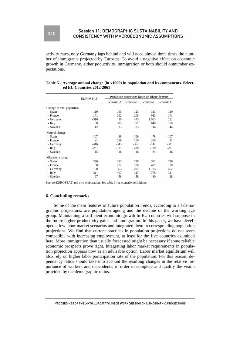
310 Session 11: DEMOGRAPHIC SUSTAINABILITY AND CONSISTENCY WITH MACROECONOMIC ASSUMPTIONS
PROCEEDINGS OF THE SIXTH EUROSTAT/UNECE WORK SESSION ON DEMOGRAPHIC PROJECTIONS
activity rates, only Germany lags behind and will need almost three times the num-ber of immigrants projected by Eurostat. To avoid a negative effect on economic growth in Germany, either poductivity, immigration or both should outnumber ex-pectations.
Table 5 - Average annual change (in x1000) in population and its components. Select-ed EU Countries 2012-2061
Source:EUROSTAT and own elaboration. See table 3 for scenario definitions.
6. Concluding remarks
Some of the main features of future population trends, according to all demo-graphic projections, are population ageing and the decline of the working age group. Maintaining a sufficient economic growth in EU countries will suppose in the future higher productivity gains and immigration. In this paper, we have devel-oped a few labor market scenarios and integrated them in corresponding population projections. We find that current practices in population projections do not seem compatible with increasing employment, at least for the five countries examined here. More immigration than usually forecasted might be necessary if some reliable economic prospects prove right. Integrating labor market requirements in popula-tion projection appears now as an advisable option. Labor market equilibrium will also rely on higher labor participation rate of the population. For this reason, de-pendency ratios should take into account the resulting changes in the relative im-portance of workers and dependents, in order to complete and qualify the vision provided by the demographic ratios.
Population projections based on labour demand
Scenario A Scenario B Scenario C Scenario D
Change in total population - Spain 119 195 123 313 119 - France 171 362 208 615 171 - Germany -316 20 -75 1.053 131 - Italy 80 305 87 648 80 - Sweden 42 83 83 114 44
Natural change - Spain -107 -98 -106 -78 -107 - France 91 139 100 209 91 - Germany -416 -343 -362 -142 -321 - Italy -231 -191 -230 -130 -231 - Sweden 15 26 26 34 16
Migration change - Spain 226 293 229 391 226 - France 80 222 108 407 80 - Germany 100 363 287 1.195 452 - Italy 311 497 317 778 311 - Sweden 27 58 58 80 28
EUROSTAT

Session 12
BAYESIANAPPROACHES (1)
Chair: Graziella Caselli (University of Rome “Sapienza”)


Session 12: BAYESIAN APPROACHES (1) 313
PROCEEDINGS OF THE SIXTH EUROSTAT/UNECE WORK SESSION ON DEMOGRAPHIC PROJECTIONS
BAYESIAN FUNCTIONAL MODELS FOR POPULATION FORECASTING
Han Lin Shang, Arkadiusz Wiśniowski, JakubBijak, Peter W. F. Smith and James Raymer
Summary
We explore the functional modelling approach to population forecasting within the wider context of Bayesian predictions and model uncertainty. The functional modelling approach can be used to analyse and forecast different age- and time-specific compo-nents for fertility, mortality and migration. For each of these demographic processes, we perform Bayesian model averaging across the outcomes of two functional models to take into account model uncertainty. We illustrate the method with a population fore-cast for the United Kingdom for 2010-2030. We conclude that regularities in age pro-files of demographic processes, where available, provide important information for the forecasts and as such should be included in the forecasting process. Keywords: Age schedules, Bayesian model selection, Functional models, Lee-Carter model, Model uncertainty, Population forecasting
1. Introduction
In this paper, we extend the population forecasting framework developed by Wiśniowski et al. (2013), which utilises the well-known model of Lee and Carter (1992), to explore the functional modelling approach to population forecasting. We additionally embed this framework in a wider context of Bayesian predictions and model uncertainty. The underlying functional modeling approach, originally sug-gested by Hyndman and Ullah (2007), allows for analysing and forecasting many different age- and time-specific components for each of the three main processes of population dynamics, namely fertility, mortality and migration. For each process we perform Bayesian model averaging across the outcomes of two functional mod-els, in order to take into account the model uncertainty and a varying level of data support for different models. Finally, we combine the results in a joint cohort-component framework to obtain population forecasts.
The population forecast method proposed in this paper is illustrated for the United Kingdom (UK) for 2010-2030 and compared with official population pro-jection published by the Office for National Statistics (2011). We discuss the im-portance of various modifications of the basic functional approach, as well as to smoothing irregular age patterns of international migration. The proposed method

314 Session 12: BAYESIAN APPROACHES (1)
PROCEEDINGS OF THE SIXTH EUROSTAT/UNECE WORK SESSION ON DEMOGRAPHIC PROJECTIONS
is argued to offer more flexibility than those based on single forecasting models, whilst allowing for a coherent treatment of various types of uncertainty.
The rest of this paper is structured as follows. In Section 1.2, we present the proposed framework for population forecasting by using functional models. The description of the applied cohort-component model of population renewal is fol-lowed by a brief introduction to the functional analysis, and a recapitulation of Bayesian model selection and averaging. In Section 1.3, we present the age-specific mortality, fertility, emigration rates and immigration counts for the UK. Selected results are shown in Section 1.4. Finally, Section 1.5 offers some conclud-ing remarks and suggestions for further work.
2. Functional models for population forecasting
2.1. Population renewal framework A cohort component model is used for describing the evolution of an age-
specific population (see also Preston et al., 2001; Wiśniowski et al., 2013). For each age or age group, we need to estimate age-specific fertility, mortality, emigra-tion rates and immigration counts. We work with single year of age and, instead of modelling net migration, we choose to model emigration rates and immigration counts separately for the reasons given e.g., in Raymer et al. (2012). The accurate estimation and forecast of mortality is important for the calculation of the survival rate for age groups 0,… ,89,90 . The survival rate measures the propor-tion of population in age , which will survive to the next period of time. Second, the fertility rate, , for 13,… ,51 measures the yearly average number of sur-
viving offspring per woman aged . Third, the emigration rate for 0,… ,89,90 measures the average yearly number of emigrants of age relative to the population exposure. Finally, the immigration count, , measures the total number of immigrants of age .
=
1 + , (1)
where , = M or F, denotes the male and female population, respectively, for all ages at the beginning of year , and = 1/(1+1.05) is the assumed default proportion of female births in the population (Preston et al., 2001). Then,0, … , , ,…,, , ) is a vector of life-table birth rates, which can be derived from
the age-specific fertility rates as follows
, = . µ ,
, , , ,
where , 0represents the fertility rate at age i in year t; µ , represents the
age-specific female or male mortality rate at age 0; and , represents female sur-
vival rate at age in year . For males and females, the age-specific survival rate can be estimated from age-specific mortality and emigration rates. It is defined by

Session 12: BAYESIAN APPROACHES (1) 315
PROCEEDINGS OF THE SIXTH EUROSTAT/UNECE WORK SESSION ON DEMOGRAPHIC PROJECTIONS
,
. , ,
. , ,, 0, … 89
. , ,
. , ,, 90
.
Here µ , represents the mortality rate at age in year ; and , represents
the emigration rate at age in year . As shown in Preston et al. (2001), the surviv-al rate matrix for all ages can then be expressed as
= , ⋯ 0⋮ ⋱ ⋮0 ⋯ ,
Note that in Equation (1), 0 = (0,…,0) is a vector of length 91, Ο is a matrix of
zeros of size (90 x 91), , , … , ,′ represents the vector of immigra-
tion counts at year , and ′ represents vector transpose.
2.2. Functional models: Preliminaries Recent advances in computer recording and storing facilities allow statisticians
to analyse high-dimensional data that include many variables, such as mortality for different ages. The objective of the functional data analysis is to analyse a set of underlying functions, usually smooth and bounded within an interval; such func-tional data may be age-specific mortality or fertility rates (see for example, Hynd-man and Ullah, 2007).
The functional data modelling process can be summarised into the following steps:
1. Box-Cox transformation. Let , represent the original data for age 0,… ,89,90 in year . The Box-Cox transformation is applied to each com-
ponent of population in order to alleviate heteroscedasticity. This can be specified as
,
1, 1 , 0 1
, , 0
where , represents the transformed data at age in year , and is the Box-Cox transformation parameter.
2. Pre-smoothing step. Since the object in functional data analysis is a smooth function, we apply a smoothing technique to transform a set of discrete data points to such a function. As a result, there is a change of notation from , to , where represents the discrete observations of a continuum. It is assumed that there is an underlying continuous and smooth function that is observed with error at discrete ages. Then, we can write

316 Session 12: BAYESIAN APPROACHES (1)
PROCEEDINGS OF THE SIXTH EUROSTAT/UNECE WORK SESSION ON DEMOGRAPHIC PROJECTIONS
, , where models the variability for each age in year , and , ~
N(0,1) is an independent and identically distributed random variable. The values of and are estimated from data (see Hyndman and Ullah, 2007, for de-
tail). For modelling age-specific mortality, we utilise penalised regression splines
with a partial monotonic constraint for age above 65 (see Hyndman and Ullah, 2007, for more details). For modelling age-specific fertility, we use a weighted median smoothing B-spline, constrained to be concave. For modelling age-specific emigration rates and immigration counts, a smoothing spline is used where the smoothing parameter is automatically determined by generalised cross validation.
The functional models can be either independent or coherent, where the latter one is done jointly for both genders.
3a. Decomposition step for the independent functional model. By using functional principal component analysis (FPCA), a set of functions is decomposed into orthogonal functional principal components and their associated scores. The functional principal component decomposition is given by
μ ∑ , , ∈ 0, 90 ,
(2)
where µ is the mean function; , … , is a set of the first functional principal components; , , … , is a set of the corresponding prin-
cipal component scores; ~ N(0, is the residual function with mean zero and finite variance; and is the number of retained components. In practice,
mean function can be estimated by µ ∑ ; , … ,
can be obtained from singular value decomposition; , and are estimated by using the Bayesian approach, and are drawn from their respective posterior distri-butions, where the prior densities of the variance parameters associated with the principal component scores and model error term are inverse gamma distributions with hyperparameters 10 and 10 . Throughout the paper, we select the num-ber of components that explain at least 99% of the total variation in data.
3b. Decomposition step for the coherent functional model. Equation (2) is designed to model a single population, such as for fertility for females. For analys-ing female and male mortality jointly, we adapt the multilevel functional data mod-el to analyse two subpopulations that may be correlated (see for example, Li and Lee,
2005). The basic idea is to decompose functions from different subpopulations into an aggregated average, a common trend, a sex-specific trend and meas-
urement error. The common and sex-specific trends are modelled by projecting them onto the eigenvectors of covariance operators of the aggregated and sex-specific centred stochastic processes, respectively. For example, the smoothed fe-male mortality rate at year can be expressed as

Session 12: BAYESIAN APPROACHES (1) 317
PROCEEDINGS OF THE SIXTH EUROSTAT/UNECE WORK SESSION ON DEMOGRAPHIC PROJECTIONS
μ , 3
where the terms in (3) can be estimated by
μ μ ,
, , , .
Following the work of Crainiceanu and Goldsmith (2010), we draw the princi-pal component scores and the variance of model error from their posterior using the Bayesian paradigm. The values of and are determined by the principal compo-nents set to explain at least 95% and 90% of the total variations in the common and sex-specific trends, respectively.
4a. Forecasting step for the independent functional model. Conditioning on the smoothed functions , … and the estimated set of functional principal components Φ , … , , the -step-ahead probabilistic
forecast of can be obtained as | | ,μ ∑ | , | . Here
1,… , , and 1000 represents the number of iterations, | , denotes the
-step-ahead forecast of | , using a univariate time series model, such as the optimal autoregressive integrated moving average (ARIMA) model selected by the automatic algorithm of Hyndman and Khandakar (2008) based on an information criterion, for example the corrected Akaike information criterion. Further, |
is simulated from a normal distribution with zero mean, represents the estimated variance from the historical observations, and is simulated from a standard normal distribution. By using the parametric bootstrap method, the predic-tion interval for the multilevel functional data model can be constructed similarly.
4b. Forecasting step for the coherent functional model. Conditioning on the smoothed functions , … , and the estimated set of functional principal components Φ , … , and , … , , the
-step-ahead probabilistic forecast of can be obtained as
| μ | , | ,,
|
2.3. Model selection and averaging
Let , , … , be a set of possible models, and let , , … , be the vector of parameters associated with each model. Denote as the quantity of inter-

318 Session 12: BAYESIAN APPROACHES (1)
PROCEEDINGS OF THE SIXTH EUROSTAT/UNECE WORK SESSION ON DEMOGRAPHIC PROJECTIONS
est, such as a combined forecast of age-specific mortality, then its posterior distri-bution given data D is
Pr | ∑ Pr | ,|
∑ |
where Pr | Pr | , Pr | is the integrated (mar-ginal) likelihood of model , Pr | is the prior density of under model
, Pr | , is the likelihood function, and Pr is the prior probability that is the true model.
Given equal prior probability for the two models, the posterior odds can be ob-tained by the ratios of two marginal likelihoods averaged over all Markov chain Monte Carlo (MCMC) iterations. For illustration purposes, we assume that the marginal likelihood can be approximated by harmonic mean estimators (Newton and Raftery, 1994).Despite known problems with the properties of harmonic mean estimators, in this paper we use it mainly as a proof of concept, to illuminate the model selection and averaging procedure.
3. Data
The historical UK population data include observations from 1975 to 2009, from which we aim to forecast population by age and sex from 2010 to 2030. The fertility data were obtained from the Human Fertility Database (2013), while the mortality data were obtained from the Human Mortality Database (2013). The emi-gration rates and immigration counts were obtained directly from the Office for National Statistics (ONS). The UK population has also been obtained from Human Mortality Database (2013). Finally, the UK mid-year population estimate for 2009, used as a baseline for prediction, has been obtained from the ONS.
Consider mortality rates for single year of age from 0 to 90+ years. For each gender in a given calendar year, the mortality rates, given by the ratio between the “number of deaths” and the population at risk of death, can be arranged in a matrix by age and year. To have an idea of their evolution, we present the log mortality rates for ages 0-90+ from 1975 to 2009 in Figure 1 Mortality rates dip in early childhood high, climb in the teen years, stabilise in the early 20s, and then steadily increase with age. Some years exhibit sharp increases in mortality between the late teens and early 20s. In general, we notice that for both females and males, mortali-ty rates are decreasing over time, especially for ages between 0 and 10. Males ex-hibit considerably higher mortality in young adulthood than females.
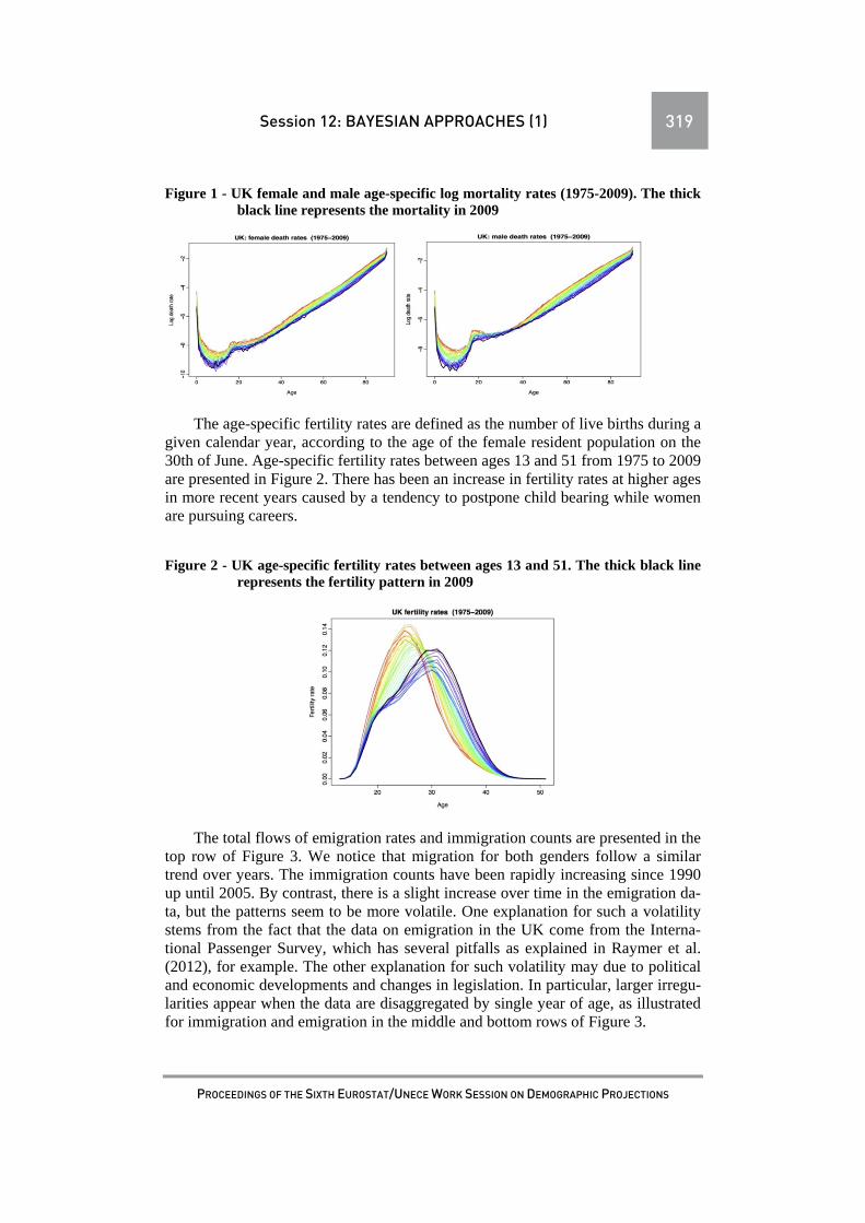
Session 12: BAYESIAN APPROACHES (1) 319
PROCEEDINGS OF THE SIXTH EUROSTAT/UNECE WORK SESSION ON DEMOGRAPHIC PROJECTIONS
Figure 1 - UK female and male age-specific log mortality rates (1975-2009). The thick black line represents the mortality in 2009
The age-specific fertility rates are defined as the number of live births during a
given calendar year, according to the age of the female resident population on the 30th of June. Age-specific fertility rates between ages 13 and 51 from 1975 to 2009 are presented in Figure 2. There has been an increase in fertility rates at higher ages in more recent years caused by a tendency to postpone child bearing while women are pursuing careers.
Figure 2 - UK age-specific fertility rates between ages 13 and 51. The thick black line represents the fertility pattern in 2009
The total flows of emigration rates and immigration counts are presented in the top row of Figure 3. We notice that migration for both genders follow a similar trend over years. The immigration counts have been rapidly increasing since 1990 up until 2005. By contrast, there is a slight increase over time in the emigration da-ta, but the patterns seem to be more volatile. One explanation for such a volatility stems from the fact that the data on emigration in the UK come from the Interna-tional Passenger Survey, which has several pitfalls as explained in Raymer et al. (2012), for example. The other explanation for such volatility may due to political and economic developments and changes in legislation. In particular, larger irregu-larities appear when the data are disaggregated by single year of age, as illustrated for immigration and emigration in the middle and bottom rows of Figure 3.

320 Session 12: BAYESIAN APPROACHES (1)
PROCEEDINGS OF THE SIXTH EUROSTAT/UNECE WORK SESSION ON DEMOGRAPHIC PROJECTIONS
Figure 3 - Total and age-specific emigration and immigration counts for the UK from 1975 to 2009. The black line represents the migration data in 2009
4. Selected Results
For both mortality and emigration rates, we found that the coherent functional model outperforms the independent functional model in terms of the estimated pos-terior model probabilities. For immigration counts, we found that the independent functional model has a larger marginal likelihood than the coherent functional model. The log marginal likelihood (LML) and weights associated with each model are given in Table 1 Fertility is not included because the rates only refer to the fe-male population at risk.

Session 12: BAYESIAN APPROACHES (1) 321
PROCEEDINGS OF THE SIXTH EUROSTAT/UNECE WORK SESSION ON DEMOGRAPHIC PROJECTIONS
Table 1 - Log marginal likelihood and corresponding weight associated with each model for forecasting age-specific mortality rates, emigration rates and immigration counts
Mortality Emigration Immigration
LML Weight LML Weight LML Weight
Coherent model 11022.38 1 19284.05 1 -9335.64 0
Independent model 10267.61 0 18951.01 0 -7602.9 1
4.1. Forecasts of fertility rates Based on the historical fertility data from 1975 to 2009, we produce the proba-
bilistic forecasts of age-specific fertility in Figure 4. The greatest forecast change is a continuing decrease in fertility rates for ages between 17 and 30, but a continuing increase in fertility for ages between 30 and 40. The resulting total fertility rates are also presented in Figure 1.4.2. It seems that the total fertility rates are expected to decrease until 2015, and then increase thereafter.
Figure 4 - Forecasted age-specific fertility rates in 2030. The black dotted line repre-sents the point forecast, where the dashed red lines represent the 80% prediction interval
4.2. Forecasts of emigration rates and immigration counts Since the raw migration data are rather noisy, we apply the smoothing spline
to obtain smooth curves, where the amount of smoothing is determined by general-ised cross validation. Based on the historical emigration rates and immigration counts from 1975 to 2009, we produce the probabilistic forecasts of age-specific emigration rates and immigration counts. From Figure 5, the greatest forecast change is a continuing increase in emigration rates and immigration counts for ages between 20 and 40.

322 Session 12: BAYESIAN APPROACHES (1)
PROCEEDINGS OF THE SIXTH EUROSTAT/UNECE WORK SESSION ON DEMOGRAPHIC PROJECTIONS
Figure 5 - Forecasted age-specific emigration rates and immigration counts in 2030 for both females and males, based on the historical data (1975 to 2009)
4.3. Forecasts of population With the population in 2009 as a baseline, the age composition of forecasted
population in 2030 is presented in the left panel of Figure 6 Forecasts of the total female and male populations are presented in the right panel of Figure 6. The age profile of the population in 2030 is mainly driven by future mortality and, to some extent, fertility and migration. The median size of 2030 population is expected to reach 71.6 million, which is 10 million larger than the population of 61.6 million in 2009. We expect that the total population could exceed 70 million between 2028 and 2029. As shown in Table 2, we also compare our forecasts of total population with the five-year official forecasts prepared by the ONS, with 2010 as a baseline population. For each year considered, the ONS forecasts fall into our 80% predic-tion interval. The differences in forecasts may be due to the fact that the ONS as-sumes a constant net migration at the level of 200 thousand annually (ONS, 2011). It is impossible to verify whether such an assumption will hold, given high volatili-ty in migration and recent policy of the UK government to reduce net migration be-low 100 thousand per year.

Session 12: BAYESIAN APPROACHES (1) 323
PROCEEDINGS OF THE SIXTH EUROSTAT/UNECE WORK SESSION ON DEMOGRAPHIC PROJECTIONS
Figure 6 - Forecasted age-specific population pyramid in 2030, along with the fore-casted population sizes of females, males and total
Table 2 - Comparison of population forecasts (in million) between the ONS, the proposed method and Wisniowski et al. (2013) method based on the appli-cations of the Lee-Carter model
Point forecast 80% prediction interval
Year ONS Functional Wiśniowski et al. (2013)
Functional Wiśniowski et al. (2013)
2010 62.262 62.165 62.238 (61.801, 62.512) (62.171, 62.302)
2015 64.776 64.061 64.802 (62.941, 65.184) (64.243, 65.386)
2020 67.173 66.214 67.905 (64.415, 68.049) (66.481, 69.429)
2025 69.404 68.736 -- (66.193, 71.293) --
2030 71.392 71.599 -- (68.238, 74.968) --
5. Conclusion and future research
We present the independent and coherent functional time-series models for es-timating and forecasting age schedules of the four demographic components of population change in the UK. By using a smoothing technique, the two functional models decompose the smoothed data into a number of functional principal com-ponents and their scores. The principal component scores and the variance parame-ter of the model errors are drawn from their posterior. For each sample, we produce time-series forecasts of the estimated principal component scores. The forecasted curves are obtained by multiplying the forecasted scores with fixed functional prin-cipal components and mean function.
We compute the marginal likelihoods of the two functional models and assign the corresponding weights to the forecasts of mortality rates, emigration rates and immigration counts. Forecast population is then obtained through a cohort compo-nent projection model. The advantage of our approach can be attributed to: (1) the use of a smoothing technique to smooth out noisy or missing observations; (2) the

324 Session 12: BAYESIAN APPROACHES (1)
PROCEEDINGS OF THE SIXTH EUROSTAT/UNECE WORK SESSION ON DEMOGRAPHIC PROJECTIONS
use of higher order functional principal components to extract patterns in the data; (3) accounting for the uncertainties embedded in fertility, mortality and migration for each age and gender. Also, the advantage of the multilevel functional data model is that it incorporates correlation between two genders and thus allows each component of population to be modelled jointly, except fertility.
Since our models are conditional on the estimated functional principal compo-nents and mean function, it is likely that uncertainty is underestimated. In future, we aim to propose a fully Bayesian functional data analysis approach, in which the modelling and forecasting steps are considered together. Furthermore, our method models period age-specific rates, and it remains a future research to include cohort effect, at least in some of the four demographic components. Similarly, in future work going beyond an illustration of the proof of concept, the Newton and Raftery (1994) method for approximating the marginal likelihood will need to be replaced with a more robust approach.
Finally, an important contribution of this paper consists in evaluating an appli-cation of the proposed methodology to a situation of relatively good, yet still not perfect data source. Given the regularities in age profiles of fertility, mortality and migration, disaggregation of the relevant data by age and sex provides important additional information for the forecasts. We argue that, data permitting, the popula-tion forecasting should follow bottom-up, from the age-specific rates, which de-scribe the underlying processes more fully, rather than top-down, from summary aggregates as total fertility rates or life expectancies. For that purpose, the func-tional approach coupled with a coherent analysis of model uncertainty offers a very natural way of maximising the use of the available information.
Acknowledgements This work was carried out as a part of the Economic and Social Research
Council (ESRC) Centre for Population Change (RES-625-28-0001) modelling strand. The findings expressed in this paper are entirely those of the authors, and should not be attributed in any manner to the institutions with which they are affili-ated.
REFERENCES
Crainiceanu, C. M. and Goldsmith, J. A. (2010). Bayesian functional data analysis using WinBUGS, Journal of Statistical Software, 32(11).
Human Fertility Database (2013). Max Planck Institute for Demographic Research (Germany) and Vienna Institute of Demography (Austria). Accessed at 8/01/2013. http://www.humanfertility.org/cgi-bin/main.php
Human Mortality Database (2013). University of California, Berkeley (USA), and Max Planck Institute for Demographic Research (Germany). Accessed at 8/01/2013, http://www.mortality.org/

Session 12: BAYESIAN APPROACHES (1) 325
PROCEEDINGS OF THE SIXTH EUROSTAT/UNECE WORK SESSION ON DEMOGRAPHIC PROJECTIONS
Hyndman, R. J. and Khandakar, Y. (2008). Automatic time series forecasting: the forecast package for R. Journal of Statistical Software, 27(3).
Hyndman, R. J. and Ullah, S. (2007). Robust forecasting of mortality and fertility rates: A functional data approach, Computational Statistics and Data Analysis, 51(10), 4942-4956.
Lee, R. D. and Carter, L. R. (1992). Modeling and forecasting U.S. mortality, Jour-nal of the American Statistical Association, 87(419), 659-675.
Li, N. and Lee, R. (1992). Coherent mortality forecasts for a group of populations: An extension of the Lee-Carter method, Demography, 42(3), 575-594.
Newton, M.A. and Raftery, A.E. (1994). Approximate Bayesian inference by the weighted likelihood bootstrap (with Discussion). Journal of the Royal Statistical Society, series B, 56(1), 3-48.
Office for National Statistics (2011). National population projections, 2010-based reference volume: Series pp2, Technical report, Office for National Statistics, Population projections unit.
Preston, S. H., Heuveline, P. and Guillot, M. (2001). Demography: Measuring and Modeling Population Processes, Blackwell, UK.
Raymer, J., Abel, G. J. and Rogers, A. (2012). Does specification matter? Experi-ments with simple multiregional probabilistic population projections, Environ-ment and Planning A, 44(11), 2664-2686.
Wiśniowski, A., Smith, P. W. F., Bijak, J. and Raymer, J. (2013). Bayesian cohort component projection forecasts, in `Paper for the Population Association of America 2013 Annual Meeting’, New Orleans.
326 Session 12: BAYESIAN APPROACHES (1)
PROCEEDINGS OF THE SIXTH EUROSTAT/UNECE WORK SESSION ON DEMOGRAPHIC PROJECTIONS
TOWARDS STOCHASTIC FORECASTS OF THE ITALIAN POPULATION: AN EXPERIMENT WITH
CONDITIONAL EXPERT ELICITATIONS
Francesco Billari, Gianni Corsetti, Rebecca Graziani Marco Marsili, Eugenio Melilli
Summary
In this work we report on the whole process developed to produce expert-based sto-chastic forecast of the Italian population for the period 2011-2065. We follow the method proposed by Billari et al. (2012), where the full probability dis-tribution of forecasts is specified on the basis of expert opinions on future develop-ments of the main components of the demographic change. In particular, we derive the joint forecast distribution of the pair Total Fertility Rate and Immigration, on one side, and of the pair Male and Female Life Expectancy at Birth on the other side. The distri-bution of Emigration and Mean Age at Birth are derived separately. The conditional elicitation procedure makes it possible to derive information on the marginal behaviour of a single indicator in terms of expected value and variability, but also on the across time correlation of each indicator and on the correlation between any two indicators at a given year or across time. Any indicator is then prorated in term of age specific values, the distribution of which is obtained resorting to well-known and widely used demographic models. We show the main results of this experimental project, covering the projected distribu-tion for indicators of the demographic behaviour, for the total population and for age related population indicators. In specifying the probabilistic distribution of each indicator, we discuss the problems that can arise in the collection of expert opinions and the solutions that can be imple-mented in order to avoid inconsistencies in the calculation of the parameters. Keywords: stochastic forecast, expert opinion, Italy.
1. Introduction
In the last years both national and international statistical offices have started to develop strategies for the implementation of probabilistic population projections. May be mentioned the works carried out by UN Population division (Heilig et al., 2010), Eurostat (Bertino et al., 2010), UK-Office for national statistics (Rowan and Wright, 2010), the Uncertainty Population of Europe project, which aimed at pro-ducing stochastic population forecasts of the population of 18 countries of the EEA

Session 12: BAYESIAN APPROACHES (1) 327
PROCEEDINGS OF THE SIXTH EUROSTAT/UNECE WORK SESSION ON DEMOGRAPHIC PROJECTIONS
and, above all, the work done at Statistics Netherlands, the first statistical office making available probabilistic projections on the website (CBS, 2011).
The main goal of the probabilistic forecasts is to obtain prediction intervals of demographic variables and thus to measure uncertainty. With the deterministic pro-jections, on the other hand, the user has no idea how likely they are. He has to trust what the experts have provided him with scenarios (low, main, high) representing the “most likely” variant and its plausible borders (Alho and Spencer, 1997).
Stochastic forecasts have the advantage of providing to the user the level of likelihood that a particular future population value will occur given a set of as-sumptions about the underlying probability distributions.
ln our study, belonging to the random scenario approach (Keilman et al., 2002), we apply the method proposed by Billari et al. (2012), where the full proba-bility distribution of forecasts is specified on the basis of expert opinions on future developments of the main components of the population change. This can be seen as a follow-up of previous studies carried out by Bocconi University and Istat (Graziani, Keilman, 2011; Corsetti, Marsili, 2012) on the effectiveness of the ex-pert-based method.
In particular, the experts evaluations are elicited in a "conditional" way, through a questionnaire submitted to seventeen Italian demographers out of a total of thirty initially invited. From the experts we derive opinions on the predicted val-ue of any indicator, its expected variability and its across time correlation; second-ly, we derive its correlation (at the same time and across time) with respect another indicator.
The paper is structured as follows. Section 2 briefly recalls the stochastic pop-ulation forecasting method suggested in Billari et al. (2012) and in particular the conditional elicitation procedure. In sections three and four we focus on the de-scription of the questionnaire submitted to the experts and on the data collection. In section five we deal with the data processing requested for preparing the input of our stochastic forecasts. Section five shows the main results of the projections for Italy from 2011 to 2065.
2. Methodology
The attention is focused on summary indicators of the three components of the population change, namely Total Fertility Rate (TFR) and Mean Age at Childbear-ing (MAC) for fertility, Female and Male Life Expectancy at Birth (LE) for mortal-ity, Number of Immigrants (IMM) and Emigrants (EMI) for migration. The age-schedules of each indicator are derived resorting to specific models, then we run population forecasts with the cohort-component method. The procedure makes it possible to work out the joint forecasting distribution of all summary indicators.
We allow for correlation between TFR and IMM, because we consider that the large number of people with a foreign background that will come to Italy may have an impact on the total level of fertility. We allow also for correlation between sexes for mortality, as we aim to explore the future evolution of the gender gap. Last, some simplifying assumptions are made in order to reduce the complexity of the problem. In particular, we assume that the pair TFR and IMM is independent on

328 Session 12: BAYESIAN APPROACHES (1)
PROCEEDINGS OF THE SIXTH EUROSTAT/UNECE WORK SESSION ON DEMOGRAPHIC PROJECTIONS
mortality and, moreover, we assume EMI and MAC being independent on the all components.
The method works by deriving the joint distribution of the indicators at 2030 and 2065, while the complete distribution of the process over the forecasting inter-val (from 2011 to 2065) is obtained by interpolation.
The forecasting distributions of the indicators at the two time points are as-sumed to be multivariate Gaussian, and the parameters are specified on the basis of the information elicited from experts.
In a first step of the questionnaire experts are asked to report on the mean of one indicator, given the value taken by the same indicator at the previous time point. In this case a single distribution for that indicator has to be derived. In a sec-ond step, given (1) the values taken by a couple of indicators at a previous time point and given (2) the value taken by one of them at the second time point, experts are asked to report on the mean of the second indicator at the second time point. In this latter case, a joint distribution of a pair of indicators has to be worked out. In the same way, conditional quantiles of given order are elicited to obtain means and variances of all conditional distributions. The joint distribution of the indicators across time is worked out using well known standard results on the Gaussian dis-tribution.
3. The expert’s questionnaire
The elicitation procedure was implemented in a questionnaire to be submitted online. Thirty Italian demographers were invited to participate in the survey through a letter of presentation of the project and a description of the underlying methodology. Data collection took place in late Spring 2012.
The questionnaire is set out in four sections: the first on TFR and IMM, the second on Male and Female LE, the third on EMM and the fourth on MAC, the evaluations on this latter being used to derive the fertility age-schedules. The first two sections aim at eliciting opinions on a pair of indicators and have the same structure. At the beginning the expert is asked to provide central scenarios of the two indicators at 2030 and 2065 and a high scenario of one of them in a not condi-tional way. Then, in a second step, the expert is requested to elicit conditional cen-tral and high scenarios. For example, typical conditional questions in section 1 are: if IMM is 100,000 at 2030, provide a central scenario for the TFR at 2030. if IMM is 100,000 at 2030 and 80,000 in 2065 and the TFR is 1.5 at 2030, pro-vide a central scenario for the TFR at 2065. if IMM is 100,000 at 2030 and 80,000 in 2065 and the TFR is 1.5 at 2030, pro-vide a high scenario (the quantile of order 0.10) for the TFR at 2065.
Section 2, dealing with the correlations between male and female LE, has similar settings and questions. Last two sections of the questionnaire, respectively about EMM (section 3) and MAC (section 4), concern one single indicator, so that central and high scenarios are elicited conditioned on the values taken by the same indicator at the previous time.

Session 12: BAYESIAN APPROACHES (1) 329
PROCEEDINGS OF THE SIXTH EUROSTAT/UNECE WORK SESSION ON DEMOGRAPHIC PROJECTIONS
4. Data collection
Seventeen experts, out of a total of thirty, answered to the survey by filling out the questionnaire completely or partially. Fourteen out of seventeen experts is the minimum number of opinions collected for any question, once we controlled for missing or misreported answers. Any indicator shows an increasing variability from 2030 to 2065. Furthermore, the simple average of the opinions is in line with the assumptions produced by Istat in latest deterministic projections (base 1.1.2011). Some results are summarized below: • male LE: the mean value increases from 82.8 years at 2030 to 86.8 at 2065, whereas the width of the confidence interval at 95% moves from 1.7 to 2.7 years; • female LE: the mean value increases from 87.1 years at 2030 to 90.3 at 2065, whereas the width of the confidence interval at 95% moves from 1.1 to 2.3 years; • TFR: the mean value increases from 1.53 child per woman at 2030 to 1.65 at 2065, whereas the width of the confidence interval at 95% moves from 0.12 to 0.15 child per woman; • MAC: the mean value increases from 31.7 years at 2030 to 32.2 at 2065, where-as the width of the confidence interval at 95% moves from 1.3 to 1.9 years; • IMM: the mean value decreases from 253 thousand at 2030 to 212 at 2065, whereas the width of the confidence interval at 95% moves from 100 to 152 thou-sand; • EMM: the mean value increases from 130 thousand at 2030 to 140 at 2065, whereas the width of the confidence interval at 95% moves from 120 to 170 thou-sand.
5. Data processing
The expert opinions, synthesized with a simple mean, produce the average values we assume for our stochastic distributions of the indicators. The variance of each indicator and the covariance among indicators are obtained from the condi-tional questions, summarized through the average values provided by the experts.
The calculation of variances and covariance is more complex. In presence of a single indicator (MAC, EMM) variances and covariance of the bivariate random variables (MAC2030, MAC2065) and (EMM2030, EMM2065) are obtained by re-sorting to the rules of the standard bivariate normal variable.
In the case of a couple of indicators, as (TFR-IMM) for instance, variance and covariance of the multivariate normal random variable (TFR2030, IMM2030, TFR2065, IMM2065) are obtained by assuming conditional independence between TFR2065 and IMM2030, given the bivariate random variable (TFR2030, IMM2065). For example the variance of variable MAC2030 is equal to:
21
11)2030(
z
CHMACVAR
where C1 and H1 are the mean values provided by the experts for central and high scenario (with a confidence level α equal to 0.1) of MAC at 2030;

330 Session 12: BAYESIAN APPROACHES (1)
PROCEEDINGS OF THE SIXTH EUROSTAT/UNECE WORK SESSION ON DEMOGRAPHIC PROJECTIONS
the covariance between MAC2030 and MAC2065 is indeed equal to
11
212 )2030(/)2065,2030(
CH
MACVARCHCMACMACCOVAR
where C2 / H1 is the central scenario for the indicator at time 2065 given H1, and C2 is a not conditional central scenario at time 2065.
Table 1 – Means, standard deviations and correlations obtained from experts
Indicator Year Mean Standard Deviation
Correlation
LEM LEF IMM TFR MAC EMM
2030 2065 2030 2065 2030 2065 2030 2065 2030 2065 2030 2065
LEM 2030 83.00 1.57 1.00 0.89 0.89 0.74
2065 87.00 1.75 1.00 0.80 0.76
LEF 2030 87.00 1.75 1.00 0.76
2065 91.00 2.63 1.00
IMM 2030 258.33 93.64 1.00 0.57 0.35 -0.38
2065 211.67 117.75 1.00 0.20 -0.40
TFR 2030 1.54 0.11 1.00 -0.19
2065 1.68 0.18 1.00
MAC 2030 31.80 0.78 1.00 0.71
2065 32.30 1.10 1.00
EMM 2030 133,00 39.01 1.00 0.69
2065 142.00 48.00 1.00
Table 1 shows means, standard deviations and correlations representing our
input data of the stochastic process that allows us to draw 2,000 samples from the corresponding multivariate distributions.
It is interesting to analyze the values of the correlations between indicators. Summary of expert opinions shows that the statistical associations between indica-tors are positive, except for the TFR2065. This rate has always negative correlation with TFR2030 (-0.19), IMM2030 (-0.38) and IMM2065 (-0.40).
Then we notice that: • an increase of TFR in the 2011-2030 will cause a weak decrease of the same in-dicator in 2030-2065; • in contrast, a decrease in the number of immigrants in both the first and the sec-ond forecast period will push the TFR to grow in the second period.
Next step is to obtain the values of demographic parameters for each forecast year by interpolation with linear (IMM, EMI) or quadratic functions (TFR, MAC, LE), the choice between the two functions depending on the best fit to observed past trends.
Figures 1-2 (representing only 250 simulations out of a total of 2,000) display future stochastic trends of some demographic parameter along time. Focusing on median values and confidence intervals, we can state that the trends of synthetic indicators follow a path similar to the assumptions set out in the latest deterministic projections released by Istat (base 1.1.2011): we observe a slight but steady in-

Session 12: BAYESIAN APPROACHES (1) 331
PROCEEDINGS OF THE SIXTH EUROSTAT/UNECE WORK SESSION ON DEMOGRAPHIC PROJECTIONS
crease for life expectancy at birth, a less pronounced one for fertility and, finally, a decreasing trend for immigrants, especially in the first forecast period.
Figure 1 – Future stochastic trends for male and female life expectancy at birth – 2011-2065
In order to run a cohort-component model for each simulation we derive the
age-schedules of each component through the implementation of well-known de-mographic models. For fertility the age-schedule has been modelled using a system of quadratic splines developed by Schmertmann (2003). For mortality the standard Lee-Carter model was performed (Lee and Carter, 1992). Finally, the distributions by age and sex for IMM and EMI are derived fitting a Rogers-Castro model (Rog-ers and Castro, 1981).

332 Session 12: BAYESIAN APPROACHES (1)
PROCEEDINGS OF THE SIXTH EUROSTAT/UNECE WORK SESSION ON DEMOGRAPHIC PROJECTIONS
Figure 2 – Future stochastic trends for total fertility rate and number of immigrants – 2011-2065
6. Main results
Figure 3 displays our expert-based stochastic forecasts (EBM) of the total population for Italy in 2011-2065 in term of median values and confidence inter-vals. The picture also shows the deterministic scenarios (low, main, high) of the latest Istat projections (DET).
The median EBM covers faithfully the trend of the main DET scenario until 2030, while in the second period it develops a faster decrease of the Italian popula-tion (56.9 million by 2065, against 61,1 million of the Istat assumption).Variability measured in term of confidence intervals rapidly increases along time: at 75% of confidence level, the interval is large 3.7 million at 2030, 9.5 at 2050 and 14.2 at 2065. We also see that the high DET scenario is external, with probability equal to 85% (darkest range), to the range provided by our stochastic forecast.

Session 12: BAYESIAN APPROACHES (1) 333
PROCEEDINGS OF THE SIXTH EUROSTAT/UNECE WORK SESSION ON DEMOGRAPHIC PROJECTIONS
Figure 3 – Future stochastic trends for the total population – 2011-2065
Table 2 – Future trends for the population by main age group – 2011-2065
Age group Model Variant 2011 2020 2030 2040 2050 2065
0-14 EBM Median 8.5 8.5 8.1 7.9 7.8 7.3
C.I. 85% 8.3-8.8 7.3-8.9 6.9-9.1 6.5-9.1 5.8-9.1
DET Main 8.5 8.5 8.0 8.0 8.0 7.8
Low-High 8.3-8.7 7.4-8.6 7.0-8.8 6.7-9.2 5.9-9.7
15-64 EBM Median 39.8 40.1 38.7 35.1 32.9 30.8
C.I. 85% 39.8-40.4 37.5-39.9 32.6-37.8 29.0-37.0 25.3-36.8
DET Main 39.8 40.0 38.9 36.1 34.5 33.5
Low-High 39.8-40.1 38.3-39.4 34.8-37.3 32.5-36.6 29.8-37.2
65+ EBM Median 12.3 14.0 16.5 19.6 20.6 19.0
C.I. 85% 13.8-14.3 15.6-17.2 18.0-21.1 18.3-22.7 16.2-22.1
DET Main 12.3 14.1 16.6 19.9 21.0 20.0
Low-High 13.8-14.3 15.9-17.2 18.7-20.9 19.4-22.5 17.7-22.3
Table 2 shows the evolution of the population by main age groups: 0-14 years,
15-64 years and 65 years and more. As well as the official projections, even the stochastic forecasts confirm further aging of the Italian population. The young population would be affected by a decrease of 1.2 million, from 8.5 in 2011 to a median value of 7.3 million by 2065. On the contrary, population aged 65 years and more would increase quickly, from 12.3 million in the base year to a peak of 20.6 million by 2050, after which it would begin to decline with a median value of 19.0 million by 2065. Stochastic forecasts would give a rapid decrease of the work-ing-age population in the medium-long run: from about 40 million of persons in 2020 to 30.8 million in 2065, according to the median forecast. About this latter

334 Session 12: BAYESIAN APPROACHES (1)
PROCEEDINGS OF THE SIXTH EUROSTAT/UNECE WORK SESSION ON DEMOGRAPHIC PROJECTIONS
age group, we also find a significant difference with respect to DET projections. The main scenario, in fact, provides a more optimistic evolution, giving a projec-tion of 33.5 million people by 2065.
The uncertainty of our stochastic estimates, expressed in absolute numbers, varies from age group to age group: it is lower for the class 0-14 years and higher for the class 15-64 years, especially in the last two decades.
Figure 4 – Future stochastic trends of old age dependency ratios – 2011-2065
Differences between EBM and DET are very low if we take into account the
old age dependency ratio (OADR), which is a key indicator of the level of popula-tion aging (Figure 4). Looking at the stochastic median value, we can see a fast in-crease of OADR in 2011-2045, from 30% to 60% , and an almost constant trend in the long term. The result is in line with the one provided by the main DET scenario but, EBM forecasts provide higher levels of uncertainty than the differences pro-duced by the deterministic scenarios.
Figures 5-6 show the forecast on the components of the demographic change. Births and Immigrations are the components affected by higher uncertainty. The comparison with DET projections is very interesting. Except for births, low and high scenarios are well within the stochastic forecast intervals; it means that the de-terministic range is very narrow and therefore there is a low probability of contain-ing the true prediction. From this point view the deterministic trend shown by deaths is very explicative. The three deterministic scenarios converge to the same value by 2065. Then we could say that the number of deaths for that year is a value determined without error. Projections-makers know that this conclusion is far from being true and that, although mortality could be considered an easier component on which to speculate, there is a degree of uncertainty to be considered, as it is pointed out by the stochastic confidence intervals.

Session 12: BAYESIAN APPROACHES (1) 335
PROCEEDINGS OF THE SIXTH EUROSTAT/UNECE WORK SESSION ON DEMOGRAPHIC PROJECTIONS
Figure 5 – Future stochastic trends for births and deaths – 2011-2065
7. Conclusions
In this paper we describe methodological assumptions and operational choices to derive expert-based population forecasts through a random-scenario approach. The opinions were collected thanks to a questionnaire submitted to seventeen Ital-ian experts in late Spring 2012.
Although this is still a preliminary study, the method has produced satisfactory results in term of data collection and data processing, allowing us the definition of a good set of hypotheses for our forecasting exercise. For further development of the methodology it is appropriate to analyze the problems raised during the opera-tions, as the search for solutions to these issues would greatly improve the overall quality of the forecasting process.
These solutions concern primarily the overall assessment of the questionnaire and the possible ways to refine it, secondly the way we manage the synthesis of the responses. For instance, we consider as appropriate to simplify the structure of the questionnaire and to plan actions to facilitate the expert’s task. This objective can be achieved by better refining the parts of the questionnaire where the expert is

336 Session 12: BAYESIAN APPROACHES (1)
PROCEEDINGS OF THE SIXTH EUROSTAT/UNECE WORK SESSION ON DEMOGRAPHIC PROJECTIONS
asked to give “independent” opinions and those parts where he is requested to think in a conditional way.
Figure 6 – Future stochastic trends for immigrants and emigrants – 2011-2065
Another simplification regards the choice of the correlations between indica-
tors. In this study we selected two time points (2030, 2065) and two correlations to be investigated: TFR against IMM and male/female LE. An alternative to this choice could be the removal of correlation between indicators, holding only the correlation of an indicator with itself across time. This solution would allow to in-crease the time-points, reducing the length of the intervals to be interpolated.
In addition, we aim to improve the treatment of the responses. In this exercise, the opinions are combined by averaging them, the same weight being then assigned to each expert. We intend to evaluate other combination methods, as weighted means, in which the weights might be defined on the basis of an evaluation of the expertise.
Another source of error we intend to examine is the procedure we adopted for interpolating between consecutive time-points. In this study we chose linear (IMM, EMI) or quadratic functions (TFR, MAC, LE), the choice between them depending

Session 12: BAYESIAN APPROACHES (1) 337
PROCEEDINGS OF THE SIXTH EUROSTAT/UNECE WORK SESSION ON DEMOGRAPHIC PROJECTIONS
on the best fit to observed past trends. In fact, we should better understand what kind of stochastic response we get, due to the fact that the optimal interpolating function can take different forms from those selected by us.
Last, except for fertility, where TFR and MAC are both subjected to expert opinion, we should better study the relationship between an indicator of overall in-tensity (LE, IMM, EMI) and its chosen age-pattern. Actually, this latter really im-pacting input is also taken for running the stochastic forecasts, but with a level of uncertainty that, although existing, we do not take in consideration in this study.
REFERENCES
Alho J.M. and B.D. Spencer. 1997. The practical specification of the expected error of population forecasts. Journal of Official Statistics. 13(3): 203-225.
Bertino S., E. Sonnino and G. Lanzieri. 2010. Combining deterministic and sto-chastic population projections. Eurostat, Work session on demographic projec-tions, Lisbon, 28-30 April 2010, Methodologies and Working papers, European Commission.
Billari, F.C., R. Graziani and E. Melilli. 2012. Stochastic population forecasts based on conditional expert opinions. Journal of the Royal Statistical Society. Se-ries A. 175(2): 491-511.
CBS. 2011. Key figures of the population forecasts 2010-2060. Statline, Centraal Bureau voor der statistiek, http://statline.cbs.nl/statweb/.
Corsetti G. and Marsili M. 2012. A stochastic population projection from the per-spective of a national statistical office. European Population Conference 2012. Stockholm, 13-16 June 2012, EAPS. http://epc2012.princeton.edu/papers/120635.
Heilig G.K., T. Buettner, N. Li, P. Gerland, F. Pelletier, L. Alkemah, J. Chunni, H. Ševcikova, A.E. Rafter. 2010. A probabilistic version of the United Nations world population prospects: methodological improvements by using bayesian fertility and mortality projections. Eurostat, Work session on demographic pro-jections, Lisbon, 28-30 April 2010, Methodologies and Working papers, Europe-an Commission.
Istat. 2011. Il futuro demografico del paese - Previsioni regionali della popolazio-ne residente al 2065. Statistiche Report, www.istat.it, 28 dec 2011. Rome.
Keilman, N., D.Q. Pham and A. Hetland. 2002. Why population forecasts should be probabilistic - illustrated by the case of Norway. Demographic Research. 6(15): 409-454.

338 Session 12: BAYESIAN APPROACHES (1)
PROCEEDINGS OF THE SIXTH EUROSTAT/UNECE WORK SESSION ON DEMOGRAPHIC PROJECTIONS
Lee R.D. and L.R. Carter. 1992. Modeling and forecasting U.S. Mortality. Journal of the American Statistical Association, September. 87/419.
Rogers A. and L. Castro. 1981. Model migration schedules. International Institute for Applied System Analysis. Laxenberg. Austria. RR-8 1-30.
Rowan S. and Wright E. 2010. Developing stochastic population forecasts for the United Kingdom: Progress report and plans for future work. Eurostat, Work ses-sion on demographic projections, Lisbon, 28-30 April 2010, Methodologies and Working papers, European Commission.
Schmertmann C.P. 2003. A system of model fertility schedules with graphically intuitive parameters. Demographic Research. 9(5): 81-110.

Session 13
BAYESIANAPPROACHES (2)
Chair: Rebecca Graziani(Bocconi University)


Session 13: BAYESIAN APPROACHES (2) 341
PROCEEDINGS OF THE SIXTH EUROSTAT/UNECE WORK SESSION ON DEMOGRAPHIC PROJECTIONS
BAYESIAN PROBABILISTIC PROJECTION OF INTERNATIONAL MIGRATION RATES
Jonathan J. Azose, Adrian E. Raftery
Summary
We propose a method for obtaining joint probabilistic projections of migration rates for all countries, broken down by age and sex. Joint trajectories for all countries are constrained to satisfy the requirement of zero global net migration. We evaluate our model using out-of-sample validation and compare point projections to migration rates produced using a persistence model. Keywords: autoregressive model, Bayesian hierarchical model, Markov chain Monte Carlo, World Population Prospects.
1. Introduction
In this paper we propose a method for probabilistic projection of net interna-tional migration rates. Our technique is a simple one which nonetheless overcomes some of the usual difficulties of migration projection. Firstly, we produce both point and interval estimates, providing a natural quantification of uncertainty. Sec-ondly, since our model uses only demographic variables as input, we can make long-term projections without explosion in the degree of uncertainty. Thirdly, sim-ulated trajectories from our model satisfy the common sense requirement that worldwide net migration sum to zero. Lastly, we sidestep the difficulty in project-ing a complete large matrix of pairwise flows by instead working directly with net migration rates. Sample projections from our model for a diverse selection of coun-tries are given in Figure 1.

342 Session 13: BAYESIAN APPROACHES (2)
PROCEEDINGS OF THE SIXTH EUROSTAT/UNECE WORK SESSION ON DEMOGRAPHIC PROJECTIONS
Figure 1 - Net International Migration Probabilistic Projections: 80% and 95% pre-dictive intervals for four countries, with example trajectories included in gray
2. Methods
2.1 Data
We use data from the 2010 revision of the United Nations Population Divi-sion’s biennial World Population Prospects (WPP) report (United Nations Popula-tion Division, 2011). WPP reports contain both estimates and projections of coun-tries’ age- and sex-specific fertility and mortality rates as well as estimates and point projections of their net migration rates.
The quantity we are interested in forecasting is rc;t, the net annual migration rate for country c in time period t, reported in units of migrants per thousand indi-viduals in the WPP data. For calculations, we sometimes convert rates to corre-sponding counts yc,t. Our method also requires knowledge of the average popula-tion of countries, nc,t, indexed by country and time, and projections of nc,t into the future for all countries.
2.2 Probabilistic Projection Method
Our technique is to fit a Bayesian hierarchical first-order autoregressive (AR(1)) model to net migration rate data for all countries. We model the migration rate rc;t, , in country c and time period t as

Session 13: BAYESIAN APPROACHES (2) 343
PROCEEDINGS OF THE SIXTH EUROSTAT/UNECE WORK SESSION ON DEMOGRAPHIC PROJECTIONS
We put normal priors on each country’s theoretical equilibrium migration rate μc,
and a uniform prior on the autoregressive parameter φc. Full specifications of pri-
ors and hyperpriors are below.
We obtain draws from the posterior distributions of all parameters using Mar-kov Chain Monte Carlo methods. In our implementation, we use the Just Another Gibbs Sampler (JAGS) software package for Markov chain simulations (Plummer, 2003).
Having obtained a sample of independent draws from the joint distribution of the parameters, we use these draws to obtain a sample from the joint posterior pre-
dictive distribution. For each sampled point from the joint posterior distribu-
tion of the parameters, we simulate a set of joint trajectories for net migration rates at time points until 2100. However, this procedure generally produces trajec-tories which are impossible in that they give nonzero global net migration counts.
We create corrected net migration rate trajectories , as follows:
1. On the basis of parameter vector , project net migration rates for all coun-tries a single time point into the future. Denoting the next time period in the future
as t', this allows us to obtain a collection of (uncorrected) projected values , for all countries c.
2. Convert net migration rate projections to net migration count projections
. This is done by multiplying by a fixed point projection of each country’s
population, . We obtain these point projections from WPP 2010 (United Na-tions Population Division, 2011). 3. Further break down migration counts by age a and sex s to obtain estimates of
net male and female migration counts for all countries and age groups, .

344 Session 13: BAYESIAN APPROACHES (2)
PROCEEDINGS OF THE SIXTH EUROSTAT/UNECE WORK SESSION ON DEMOGRAPHIC PROJECTIONS
This is accomplished by applying projected model migration schedules to all coun-tries. We use the naïve projection method which takes each country’s age- and sex-specific migration schedule to be the same as the migration schedule in the most recent time point for which detailed data were available for that country. 4. Within each age and sex category, apply a correction to ensure zero worldwide net migration. The correction we apply redistributes any overflow migrants to all countries, proportional to their projected populations. Specifically, take the cor-
rected migration count projection to be
5. Convert the corrected age- and sex-specific net migration counts back
to corrected net migration rates by disaggregating and converting counts to rates in the obvious way. 6. Continue projecting trajectories one time step at a time into the future by repeat-ing steps 1-5.
Note that although the uncorrected net migration rates come from the de-sired marginal posterior predictive distributions, the correction in step 4 changes those distributions by projecting them onto a lower dimensional space. Sensitivity analysis suggests that the correction introduces only minor changes in the marginal distributions with and without the correction, as measured by estimating the Kol-mogorov-Smirnov distance between the two distributions.
3. Results
3.1 Evaluation
We do not know of any other model that produces probabilistic projections of all countries’ net international migration rates. However, we can take our model’s median projections to be point projections and compare against models that pro-duce point projections only. As a baseline for comparison, we evaluate against the naïve persistence model which projects migration rates to continue at the most re-cently observed levels indefinitely into the future. In the short horizon, the persis-tence model is similar to the expert knowledge-based projections in the WPP (United Nations Population Division, 2011).
Our historical data consist of a series of migration rates for 197 countries at 12 time points with five-year resolution, spanning the period from 1950 to 2010. We performed an out-of-sample evaluation by holding out the data from the m most recent time points for all countries and producing posterior predictive distri-butions on the basis of the remaining 12−m time points. For point forecasts we used the median of the posterior predictive distribution.

Session 13: BAYESIAN APPROACHES (2) 345
PROCEEDINGS OF THE SIXTH EUROSTAT/UNECE WORK SESSION ON DEMOGRAPHIC PROJECTIONS
We report out-of-sample mean absolute error as a measure of the quality of point forecasts and both interval scores and coverage as measures of quality of our interval predictions. Interval scores provide a negatively oriented score for proba-bilistic forecasts which rewards sharpness subject to calibration (Gneiting and Raftery, 2007). If we predict a distribution with (1−α) predictive interval (ℓ,u) and the value x arises, the interval score is given by
The intuition is that we are rewarded for providing forecasts with tight bounds
and punished if observations fall outside those bounds. Table 1 contains these evaluation metrics for our Bayesian hierarchical model
and the mean absolute errors for the persistence model. Across the board, our point projections outperform the persistence model, and our interval projections achieve reasonably good calibration.
Table 1 - Mean absolute errors, interval scores, and predictive interval coverage for our Bayesian hierarchical model and the persistence model
# of points held out Model MAE 80% I.S. 95% I.S. 80% Cov. 95% Cov. 1 point Bayesian 3.24 24.5 48.4 91.4% 96.4% Persistence 3.57 — — — — 3 points Bayesian 4.76 27.1 48.1 84.9% 93.4% Persistence 6.74 — — — — 6 points Bayesian 5.12 30.1 60.4 77.2% 89.3% Persistence 7.17 — — — —
3.2 Projections for the least-developed countries The United Nations publishes a list of the least-developed countries, with
countries classified as least-developed based on assessments of their economic vul-nerability, human capital, and gross national income (Committee for Development Policy and United Nations Department of Economic and Social Affairs, 2008). (LDC2008). A total of 46 countries in our data fall into the least-developed catego-ry. We now consider briefly the projections that our model makes for these least-developed countries in comparison to all other countries.
In the 2005-2010 time period, only 26% of the least-developed countries were net receivers of migration, as compared to 43% of all other countries. Our model projects that this discrepancy will lessen somewhat in the future. By 2050, we pro-ject an average of 45% of the countries which currently fall into the least-developed category and 49% of other countries to be net receivers.
Additionally, in 2005-2010, the least-developed countries had an average net migration rate of -0.97 (per thousand), compared with an average of 2.64 (per thou-sand) in all other countries. Our model again projects that this gap in migration be-tween least-developed and all other countries will narrow over time. Over the next decades, we project growth in net migration rates among the least developed coun-tries and decline in net migration rate on average across all other countries, as summarized in Table 2.

346 Session 13: BAYESIAN APPROACHES (2)
PROCEEDINGS OF THE SIXTH EUROSTAT/UNECE WORK SESSION ON DEMOGRAPHIC PROJECTIONS
Table 2 - Mean projected change in migration rates among least-developed countries
(LDC) versus all other countries (Other) LDC Other By 2020 +0.02 -1.49By 2040 +0.29 -2.12By 2060 +0.34 -2.29
Acknowledgements
This work was supported by the U.S. National Institute of Child Health and Devel-opment through grants nos. R01 HD054511 and R01 HD070936, and by a Science Foundation Ireland ETS Walton visitor award, grant reference 11/W.1/I2079.
REFERENCES
Committee for Development Policy and United Nations Department of Economic and Social Affairs (2008). Handbook on the Least Developed Country Category: Inclusion, Graduation, and Special Support Measures.
Gneiting, T. and A. E. Raftery (2007). Strictly proper scoring rules, prediction, and
estimation. Journal of the American Statistical Association 102 (477): 359-378. Plummer, M. (2003). JAGS: A program for analysis of Bayesian graphical models
using Gibbs sampling. In Proceedings of the 3rd International Workshop on Dis-tributed Statistical Computing (DSC 2003), pp. 20-22.
United Nations Population Division (2011). World Population Prospects: The 2010
Revision. United Nations.

Session 13: BAYESIAN APPROACHES (2) 347
PROCEEDINGS OF THE SIXTH EUROSTAT/UNECE WORK SESSION ON DEMOGRAPHIC PROJECTIONS
BAYESIAN PROBABILISTIC POPULATION PROJECTIONS USING R
Hana Ševčíková, Adrian E. Raftery, Patrick Gerland
Summary
A Bayesian approach for probabilistic population projections has recently been used by the United Nation Population Division in the preparation of the 2012 revision of the World Population Prospects. The methods have been implemented in publicly available open-source software as a collection of R packages. In this paper, we demonstrate how to easily reproduce such population projections, including probabilistic projections of total fertility rate and life expectancy. The packages allow any analysts to generate variations of the UN projections using their own data. Probabilistic results can be summarized and visualized in graphs, maps, or population pyramids. The software can be conveniently controlled from a graphical user interface. Keywords: Bayesian hierarchical model, World Population Prospects, United Na-tions
1. Introduction
A systematic framework for producing probabilistic population projections for all countries, both developed and developing, has recently been proposed by Raft-ery et al., 2012. It consists of probabilistically projecting total fertility rate and life expectancy using Bayesian hierarchical models (Alkema, 2011; Raftery et al., 2013), converting the results to age-specific rates, and projecting the population forward using the cohort-component method applied to each trajectory simulated from their predictive distributions. The median projection from these rates has been used as the UN’s official medium projection for all countries in the 2012 revision of the World Population Prospects, or WPP (UN2013).
Here we describe a suite of software packages developed to allow users be-yond the UN to implement the methodology. These are four R packages: bayesTFR to project total fertility rate, bayesLife to project life expectancy, bayesPop to pro-ject population, and a graphical user interface, bayesDem. All are freely available. We also introduce a package for interactive visual exploration of various indicators derived from WPP data, called wppExplorer.

348 Session 13: BAYESIAN APPROACHES (2)
PROCEEDINGS OF THE SIXTH EUROSTAT/UNECE WORK SESSION ON DEMOGRAPHIC PROJECTIONS
2. Methodology
Almost all methods used for predicting population in country c at time pe-riod t are based on the demographic balancing equation
where B denotes the number of births, D the number of deaths and M net migra-tion. In most applications this equation is solved deterministically using the cohort component method (Whelpton1928; Whelpton1936) which decomposes it into age- and sex-specific components.
The traditional UN methodology of population projections (UN1989) for future time periods t>0 follows the cohort component method and for that purpose, it uses the following inputs for each country:
• Sex- and age-specific population estimates at the initial time t=0 • Projections of total fertility rate (TFR) • Projections of fertility distribution over ages • Projections of sex ratio at birth • Projections of male and female life expectancy at birth (e0)
• Historical data on sex- and age-specific death rates (for t≤0) • Projections of sex- and age-specific net migration In each future time period t, the projected TFR is converted to age-specific fer-
tility rates using the fertility distribution over ages at t. Using the historical data on death rates, the projected life expectancy is converted to age-specific mortality rates using a variant of the Lee-Carter method (Lee Carter, 1992). Then the cohort component model is applied.
Recently, approaches to probabilistic projections of two main input compo-nents were introduced, namely TFR (Alkema, 2011) and life expectancy (Raftery et al., 2013). Raftery et al. 2012 describes a methodology for combining these components into probabilistic population projections. The idea is to
1. simulate a large set of trajectories of future values of TFR, 2. simulate an equal number of trajectories of life expectancy, 3. convert each of the trajectories into a future trajectory of sex- and age-
specific population quantity, using the current UN methodology as described above.
The resulting set of values is viewed as a sample from the predictive distribution of population projections.
This process is fully supported by open-source packages implemented in R (Ihaka Gentleman, 1996). The simulation of TFR trajectories (1.) is implemented in a package called bayesTFR (Sevcikova 2011). Life expectancy trajectories (2.) can be generated using the package bayesLife (bayesLife). Finally, population pro-jections by age and sex can be obtained using the package bayesPop (bayesPop). A graphical user interface (GUI) for the three packages is provided by the R package bayesDem (bayesDem) which allows to generate probabilistic projections of TFR

Session 13: BAYESIAN APPROACHES (2) 349
PROCEEDINGS OF THE SIXTH EUROSTAT/UNECE WORK SESSION ON DEMOGRAPHIC PROJECTIONS
and life expectancy, and combine those results into probabilistic population projec-tions from a single interface.
In what follows, we assume that the reader is somewhat familiar with basic R syntax. Furthermore, in order to reproduce the code examples in the text, R and the three packages, bayesTFR, bayesLife and bayesPop should be installed. One can accomplish the package installation simply by calling > install.packages("bayesPop", dependencies=TRUE)
from the R environment. This installs all three packages at once. To load them into the environment, type the command > library(bayesPop)
When describing a function, only its main functionality will be mentioned, without going into great detail about its arguments. More information can be obtained from the functions’ help pages, using ?function_name.
3. Total Fertility Rate
The bayesTFR package (Sevcikova 2011) implements a methodology for probabilistic projection of TFR as proposed by Alkema et al. 2011 and Raftery, Alkema, Gerland 2013. The model is based on the observation that the evolution of the TFR includes three broad phases, referred to as Phase I, II and III: (I) a high-fertility pre-transition phase, (II) the fertility transition in which the TFR decreases from high fertility levels towards or below replacement level fertility, and (III) a low-fertility post-transition phase, which includes recovery from below-replacement fertility toward replacement fertility and oscillations around replace-ment-level fertility. The left panel of Figure 1 shows an example of a TFR time se-ries for Denmark divided into the three phases.
Figure 1 - Left panel: TFR time series for Denmark divided into three phases. Right panel: Hypothetical double logistic decline function plotted agains TFR

350 Session 13: BAYESIAN APPROACHES (2)
PROCEEDINGS OF THE SIXTH EUROSTAT/UNECE WORK SESSION ON DEMOGRAPHIC PROJECTIONS
Phase II, the fertility transition phase, is modeled by a random walk with a nonconstant drift. The drift, or TFR decline, is a double logistic function with a country-specific set of parameters that defines the shape of the decline curve (see right panel of Figure 1). These parameters are estimated using a Bayesian hierar-chical model (BHM) in which the country-specific decline curves arise from a “world" distribution. Alkema 2011 and Sevcikova 2011 describe this part of the model in more detail.
Phase III, the post-transition phase is modeled as a first-order autoregressive model where the model parameters are allowed to vary between countries, follow-ing a BHM (Raftery, Alkema, Gerland, 2013).
3.1 Simulating TFR Future Trajectories This section explains how to generate TFR future trajectories using the bayesTFR package. After loading the package into the environment as shown in Section 2, choose a directory on which the package will operate: > tfr.dir <- "/my/TFR/directory"
There are three main steps to obtain TFR projections, each of which translates into one function call:
Step 1 Estimate the parameters of the Phase II model using Markov Chain Monte Carlo (MCMC):
> mc1 <- run.tfr.mcmc(output.dir=tfr.dir, iter="auto", wpp.year=2012, start.year=1950, present.year=2010)
Note that such a call is set up to produce long MCMC chains, ideally passing convergence diagnostics. Thus, its processing can take a very long time, possibly multiple days. Setting an optional argument parallel=TRUE could significantly improve the run time as it processes all chains (three by default) in parallel. How-ever, for a toy simulation, one can set the argument iter to a small number, for example on the order of tens, but for somewhat realistic simulation iter should be on the order of ten thousands. The argument wpp.year determines which his-torical data are being used; in this case it is a dataset from the R package wpp2012 (Rwpp2012). For some countries, that dataset goes back to year 1750 and the argument start.year determines the first time period to be used, i.e. data prior to start.year are ignored. If an analyst wishes to (possibly partly) replace the default UN dataset with his/her own data, an argument my.tfr.file can be used that points to a user-defined historical TFR dataset. Such dataset must follow the same structure as the default UN dataset, which can be seen with the commands data(tfr, package="wpp2012"); head(tfr). The package contains a

Session 13: BAYESIAN APPROACHES (2) 351
PROCEEDINGS OF THE SIXTH EUROSTAT/UNECE WORK SESSION ON DEMOGRAPHIC PROJECTIONS
template file for this purpose, called “my_tfr_template.txt”, located in the package directory “inst/extdata”.
Step 2 Estimate the parameters of the Phase III model by MCMC: > mc2 <- run.tfr3.mcmc(sim.dir=tfr.dir, iter="auto")
The Phase III MCMCs will run substantially faster than step 1. Nevertheless again, iter should be decreased for a toy simulation. Any time-specific arguments are inherited from the Phase II simulation. In the estimation, the historical TFR values from countries that reached Phase III between start.year and present.year are used. Again, the default historical dataset can be overwritten with a user-specific one using the optional argument my.tfr.file.
Step 3 Using the estimated parameters, generate future TFR trajectories: > tfr.pred <- tfr.predict(sim.dir=tfr.dir, end.year=2100, use.diagnostics=TRUE)
The use.diagnostics argument should be set to TRUE only if iter="auto" was used in the estimation commands. In such a case, the MCMC burn-in and thin (or equivalently number of trajectories) is automatically determined from existing di-agnostics. If a toy simulation was generated, these values should be provided ex-plicitly, e.g. burnin=10, burnin3=10, nr.traj=100. This command produces a set of future TFR trajectories for each country included in the historical dataset and stores it in the simulation directory.
A simulation generated with these three steps is sufficient for use in a popula-tion projection. In addition, the package contains various functions to explore the future TFR trajectories, such as trajectories graphs and TFR world maps. To re-trieve projections from the disk, i.e. to obtain the object tfr.pred in later R session, then create a graph for one country and view tabular values of such graph, one can do: > tfr.pred <- get.tfr.prediction(tfr.dir) > tfr.trajectories.plot(tfr.pred, "Sudan", nr.traj=50) > tfr.trajectories.table(tfr.pred, "Sudan")
More details on bayesTFR functions and methodology can be found in Sevcikova 2011 and in the package help pages.
4. Life Expectancy
In WPP 2012 for the first time, the UN Population Division used a probabilis-tic model to project life expectancy at birth (e0). It follows a BHM introduced by
Raftery, Chunn, Gerland & Sevcikova (2013) which is implemented in the R pack-age bayesLife (Sevcikova & Raftery, 2013b).

352 Session 13: BAYESIAN APPROACHES (2)
PROCEEDINGS OF THE SIXTH EUROSTAT/UNECE WORK SESSION ON DEMOGRAPHIC PROJECTIONS
Similarly to TFR, life expectancy is modeled using a random walk with drift where the drift, or life expectancy increase, is modeled by a double-logistic func-tion with country-specific parameters determining the shape of the function. This model allows one to pool information about the rates of gains across countries by assuming that each set of country-specific double-logistic parameters is randomly sampled from a common (world) distribution.
The population projection methodology requires projections of female and male life expectancy simultaneously. Generating them independently from the BHM above is unsatisfactory because there is generally a strong relationship be-tween them, and ignoring this can lead to future trajectories of female and male life expectancy that diverge unrealistically. Raftery et al., 2014, proposed a method for joint projections of female and male life expectancy that models the gap between them, the gap being defined as female e0 minus male e0. In such a model, projec-
tions of female life expectancy are generated by the BHM, and are then combined with projections of the gap to produce projections of male life expectancy.
4.1 Simulating Future Trajectories of Life Expectancy The implementation of the BHM in bayesLife closely follows the structure of
the bayesTFR package. Many functions in one package have their analogues in the other, and their names differ only in the part called “tfr” versus “e0”. As for TFR, we first set a directory for the e0 simulation:
> e0.dir <- "/my/e0/directory"
Obtaining e0 projections involves two steps:
Step 1 Estimate parameters for female e
0 via MCMC:
>run.e0.mcmc(output.dir=e0.dir,sex="Female", iter="auto", wpp.year=2012)
The note from above regarding long processing time for an “auto” setting and possible improvement by setting the parallel and/or iter arguments applies here as well. The function has many of the same arguments as run.tfr.mcmc with the same meaning, for example arguments specifying time (*.year), some of which are left out here as their defaults are to be used, or my.e0.file for specifying user-defined (female) historical data.
Step 2 Using estimated parameters, generate future female and male e0 trajecto-
ries. > e0.pred <- e0.predict(sim.dir=e0.dir, end.year=2100, use.diagnostics=TRUE)

Session 13: BAYESIAN APPROACHES (2) 353
PROCEEDINGS OF THE SIXTH EUROSTAT/UNECE WORK SESSION ON DEMOGRAPHIC PROJECTIONS
Again, the use.diagnostics argument is to be used in combination with an “au-to” simulation only. This call first generates trajectories of female e0, then esti-
mates the gap model, predicts the gap, and finally produces trajectories of male e0.
Any user-defined data on male e0 would be passed here via an optional my.e0.file
argument.
The package supports various ways of viewing the results. In addition to view-ing trajectories for each sex separately, one can create graphs of the marginal dis-tribution as well as the joint distribution of life expectancy for the two sexes: > e0.pred <- get.e0.prediction(e0.dir) > e0.trajectories.plot(e0.pred, "Brazil", nr.traj=10, both.sexes=TRUE) > e0.joint.plot(e0.pred, "Brazil", nr.points=100, pi=80, years=c(2010, 2050, 2100))
Other functions for exploring results are available in bayesLife, such as creat-ing maps, or generating plots for all countries at once.
5. Population Projection
5.1 Producing Future Population Trajectories As mentioned in Section 2, probabilistic population projections implemented
in bayesPop incorporate two probabilistic components, namely TFR and sex-specific e0. For each country, the prediction function applies the cohort component
method to each trajectory, keeping the remaining input components constant. Thus in standard cases, to generate future population trajectories, all one needs
to do is to point the code to the place on disk where TFR and e0 are stored, in our
case the tfr.dir and e0.dir directories. The results are stored in a separate directory: > pop.dir <- "/my/pop/directory" > pop.pred <- pop.predict(end.year=2100,
start.year=1950, present.year=2010, wpp.year=2012, output.dir=pop.dir, nr.traj=1000, inputs=list(tfr.sim.dir=tfr.dir, e0F.sim.dir=e0.dir, e0M.sim.dir="joint_"))
The keyword “joint_” directs the function to extract the male e0 projections
from the female simulation directory, i.e. it indicates that e0 was simulated jointly
for female and male. The start.year determines the first time period for observed death rates to be used in the Lee-Carter method, and present.year is the time period

354 Session 13: BAYESIAN APPROACHES (2)
PROCEEDINGS OF THE SIXTH EUROSTAT/UNECE WORK SESSION ON DEMOGRAPHIC PROJECTIONS
of the initial population data. Obviously, end.year cannot go beyond the end year used in TFR and e0 projections, nor beyond the end year of other projection inputs,
such as migration. If the number of trajectories to be produced (nr.traj) is smaller than the number of available TFR and e0 trajectories, these are equidistantly
thinned. The deterministic input components are taken from the given wpp pack-age, here wpp2012. However, the inputs argument allows one to overwrite each of them using tab-delimited text files. An optional logical argument keep.vital.events can be used for storing additional data generated during projection, such as births and deaths. By default these are not kept, as it more than doubles the amount of da-ta stored.
To access such population prediction objects in a later session one can use: > pop.pred <- get.pop.prediction(pop.dir)
5.2 Viewing Population Trajectories Population trajectories can be viewed on a country-specific basis. A simple sum-mary function gives a quick look at various quantiles of the country’s projections, e.g.: > summary(pop.pred, country="Italy")
The following code shows how to create plots of trajectories by time as well as by age, including adding curves to existing plots. Results are shown in Figure 2. > country <- "China" > pop.trajectories.plot(pop.pred, country,
sum.over.ages=TRUE, nr.traj=50) > pop.byage.plot(pop.pred, country, year=2100,
nr.traj=50, pi=80, ylim=c(0,130000)) > pop.byage.plot(pop.pred, country, year=2010,
add=TRUE, show.legend=FALSE, col="blue") > legend("topright", legend=2010, col="blue", lty=1,
bty="n")

Session 13: BAYESIAN APPROACHES (2) 355
PROCEEDINGS OF THE SIXTH EUROSTAT/UNECE WORK SESSION ON DEMOGRAPHIC PROJECTIONS
Figure 2 - Projected trajectories for China. Left panel shows the population projec-tion by time; the right panel shows the population projection by age for 2100 (red lines) and for the present year, 2010, (blue line)
If sum.over.ages in pop.trajectories.plot is FALSE, separate plots for each age group are generated. The function also accepts arguments for specifying sex and age where age is defined as an index to the vector (0-4, 5-9, 10-14, …, 125-129, 130+), thus of length 27. A graph for male population aged 0-14 would have argu-ments sex="male", age=1:3, or women in child bearing age would be defined as sex="female", age=4:10.
Numerical analogous to the trajectory plots is implemented in the functions pop.trajectories.table and pop.byage.table, respectively.
5.3 Probabilistic Population Pyramids
The package supports plotting probabilistic population pyramids for given country and one or more given years. There are two different kinds of pyramids – a classic pyramid consisting of boxes, and a so called trajectory pyramid which is created using age trajectories such as the ones on the right in Figure 2. The classic pyramid can display projections for up to two years in one pyramid with one set of probabil-ity intervals; the trajectory pyramid can include any number of years and any num-ber of probability intervals. Here is an example of generating the two pyramid types, see Figure 3: > country <- "Russian Federation" > pop.pyramid(pop.pred, country, year=c(2080, 2010)) > pop.trajectories.pyramid(pop.pred, country,
year=c(2100, 2015, 1950), nr.traj=0, proportion=TRUE, age=1:23, pi=80)

356 Session 13: BAYESIAN APPROACHES (2)
PROCEEDINGS OF THE SIXTH EUROSTAT/UNECE WORK SESSION ON DEMOGRAPHIC PROJECTIONS
Figure 3 - Probabilistic population pyramid for Russia: a classic type comparing two time periods on the left, and trajectory type comparing three time periods on a proportion scale on the right
Here the trajectory pyramid uses the argument proportion to switch the x-
axis to a proportional scale, which is useful when comparing pyramids from differ-ent time periods. Both functions also accept various arguments for changing the appearance of the pyramids, such as colors, height and thickness of boxes etc.
In addition to creating pyramids for the results of the pop.predict func-tion, both pyramid functions can also be applied to any user-defined data that can be fitted into a pyramid data structure. See the package documentation for more de-tail.
6. Graphical User Interface
6.1. bayesDem: Bayesian Demographer A graphical user interface for bayesTFR, bayesLife, and bayesPop is imple-
mented in the R package bayesDem. One can generate probabilistic projections of TFR, life expectancy, and combine those results into probabilistic population pro-jections from a single interface. In addition, it offers functionality for exploring re-sults, such as trajectories, maps, population pyramids and others.
Bayesian Demographer can be loaded into and started from the R interface by > library(bayesDem) > bayesDem.go()
which opens the main window of the GUI. There are three upper level tabs each of which corresponds to one of the underlying packages. All functions described in this paper and many more can be accessed through the GUI.
6.2 wppExplorer: Interface for UN Estimates and Projections Many datasets from the latest WPP revision are included in the R package
wpp2012 (Sevckova et al., 2013). We have developed a package for easy visualisa-tion of these datasets and their derivatives, called wppExplorer (Sevcikova, 2013b),

Session 13: BAYESIAN APPROACHES (2) 357
PROCEEDINGS OF THE SIXTH EUROSTAT/UNECE WORK SESSION ON DEMOGRAPHIC PROJECTIONS
which is based on the package shiny (shiny). One can load and start the exploration by issuing the commands > library(wppExplorer) > wpp.explore()
It opens an interface in user’s default browser and offers interactive maps, ta-bles, time series plots, histograms and pyramids. Where available, uncertainty is also included. Figure 4 shows an example of the interface. An optional argument to wpp.explore can be used to switch to explore data from previous revisions of WPP, namely 2010 or 2008, in which case R packages wpp2010 or wpp2008 would be used.
Figure 4 - wppExplorer: Interactive exploration of the wpp packages (Population pyramid of China and India)
7. Discussion
We have shown the basic functionality of our demographic packages, namely bayesTFR, bayesLife, bayesPop, bayesDem, and wppExplorer. They can be used to reproduce some of the UN WPP 2012 demographic projections and visualize re-sults. The packages offer additional features not mentioned in this paper, such as aggregations, special handling of small areas, imputing missing values, analysing MCMCs, exporting projections, powerful expression language for dealing with various population quantities, etc. We refer the reader to the corresponding pack-age documentation for more details.
In the World Population Prospects, the UN currently publishes estimates back to 1950, and population projections are based on them. However, data are available

358 Session 13: BAYESIAN APPROACHES (2)
PROCEEDINGS OF THE SIXTH EUROSTAT/UNECE WORK SESSION ON DEMOGRAPHIC PROJECTIONS
for some countries long before 1950, in some cases back to 1750, and these can be taken into account in the projections if desired. We have shown how to do this.
Acknowledgements
This work was supported by the Eunice Kennedy Shriver National Institute of Child Health and Human Development under grants R01 HD054511 and R01 HD070936. Raftery’s research was also supported by Science Foundation Ireland E.T.S. Walton visitor award 11/W.1/I2079.
Disclaimer
The views and opinions expressed in this paper are those of the authors and do not necessarily represent those of the United Nations. The contents has not been for-mally edited and cleared by the United Nations. The designations employed in this paper do not imply the expression of any opinion whatsoever on the part of the Secretariat of the United Nations concerning the legal status of any country, territo-ry or area or of its authorities, or concerning the delimitation of its frontiers or boundaries.
REFERENCES
Alkema et al.2011Alkema, L., Raftery, A. E., Gerland, P., Clark, S. J., Pelletier, F., Buettner, T., & Heilig, G. K. (2011). Probabilistic projections of the total fertility rate for all countries. Demography, 48, 815–839.
Ihaka, R. & Gentleman, R. (1996). R: A language for data analysis and graphics. Journal of Computational and Graphical Statistics, 5, 299–314.
Lee, R. D. & Carter, L. (1992). Modeling and forecasting the time series of US mortality. Journal of the American Statistical Association, 87, 659–671.
Raftery, A. E., Alkema, L., & Gerland, P. (2013). Bayesian population projections for the United Nations. Statistical Science, in press.
Raftery, A. E., Chunn, J. L., Gerland, P., & Ševčíková, H. (2013). Bayesian probabilistic projections of life expectancy for all countries. Demography, 50, 777–801.
Raftery, A. E., Lalic, N., & Gerland, P. (2014). Joint probabilistic projection of female and male life expectancy. Demographic Research, 30, 795–822.

Session 13: BAYESIAN APPROACHES (2) 359
PROCEEDINGS OF THE SIXTH EUROSTAT/UNECE WORK SESSION ON DEMOGRAPHIC PROJECTIONS
Raftery, A. E., Li, N., Ševčíková, H., Gerland, P., & Heilig, G. K. (2012). Bayesian probabilistic population projections for all countries. Proceedings of the National Academy of Sciences, 109, 13915–13921.
RStudio & Inc. (2013). shiny: Web Application Framework for R. R package version 0.7.0.
United Nations (1989). The United Nations Population Projection Computer Program : A User’s Manual. New York, NY: Dept. of Economic and Social Affairs, Population Division.
United Nations (2013). World Population Prospects: The 2012 Revision. New York, NY: United Nations.
Ševčíková, H. (2013a). bayesDem: Graphical User Interface for bayesTFR, bayesLife and bayesPop. R package version 2.3-2.
Ševčíková, H. (2013b). wppExplorer: Explorer of World Population Prospects. R package version 1.0-3.
Ševčíková, H., Alkema, L., & Raftery, A. E. (2011). bayesTFR: An R package for probabilistic projections of the total fertility rate. Journal of Statistical Software, 43, 1–29.
Ševčíková, H., Gerland, P., Andreev, K., Li, N., Gu, D., & Spoorenberg, T. (2013). wpp2012: World Population Prospects 2012. R package version 2.0-0.
Ševčíková, H. & Raftery, A. (2013a). bayesPop: Probabilistic Population Projection. R package version 4.1-1.
Ševčíková, H. & Raftery, A. E. (2013b). bayesLife: Bayesian Projection of Life Expectancy. R package version 2.0-1. Original WinBugs code written by Jennifer Chunn.
Whelpton, P. K. (1928). Population of the United States, 1925–1975. American Journal of Sociology, 31, 253–270.
Whelpton, P. K. (1936). An empirical method for calculating future population. Journal of the American Statistical Association, 31, 457–473.

360 Session 13: BAYESIAN APPROACHES (2)
PROCEEDINGS OF THE SIXTH EUROSTAT/UNECE WORK SESSION ON DEMOGRAPHIC PROJECTIONS
MORTALITY FORECASTS WITH A FLEXIBLE AGE
PATTERN OF CHANGE FOR SEVERAL EUROPEAN
COUNTRIES
Christina Bohk, Roland Rau Summary
Forecasting mortality for multiple countries is particularly challenging, because dif-ferent factors influence mortality by age and sex and induce, therefore, diverse levels and paces of growth for life expectancy at birth. Hence, a mortality forecasting ap-proach should be able to model dynamic age-shifts in survival improvements as well as major changes in long-term mortality trends – these are two requirements we consid-ered to be particularly important developing our mortality forecasting model (Bohk and Rau, 2014). We generated retrospective mortality forecasts from 1991 to 2009 for Denmark, Italy, Spain, Great Britain, West Germany and Sweden to test the broad ap-plicability of our model. The results suggest that our model can forecast diverse mor-tality developments for multiple countries and that its conducted forecasts are more accurate than those of other renowned models such as the Lee-Carter model (1992) and its extensions of Renshaw and Haberman (2003; 2006). This effect is particularly striking in the case of Denmark – a country, whose women experienced a period of stagnating life expectancy from the 1980s to the early 1990s and a considerable in-crease thereafter. In contrast to the other applied models, our model can capture this major change in the long-term trend, because it not only extrapolates the Danish mor-tality trend, but it also complements it with mortality trends of Sweden, France, Italy and Japan. In addition, prospective mortality forecasts from 2010 to 2050 indicate fur-ther increases in life expectancy for both sexes in each of the six selected European countries. Keywords: Mortality forecasting, Life expectancy, Denmark, Italy, Spain, West Ger-many, Great Britain and Sweden.
1. Diverse mortality development
Japan is the current record life expectancy holder. In 2009, Japanese women expected to live on average 86.42 years, whereas men expected to live on average 79.61 years (Human Mortality Database, 2013). In the 28 EU-countries, life expec-tancy is somewhat lower: On average, women expected to live 83.1 years, whereas men expected to live 77.5 years in 2012 (Eurostat, 2014). In countries like Spain, Italy and Sweden, life expectancy is above this average level, whereas in countries like Poland, Hungary and Bulgaria, life expectancy is below this average level.
However, life expectancy does not only differ in its level, but also in the pace at which it increases. Since about 1840, record life expectancy increased almost

Session 13: BAYESIAN APPROACHES (2) 361
PROCEEDINGS OF THE SIXTH EUROSTAT/UNECE WORK SESSION ON DEMOGRAPHIC PROJECTIONS
linearly, even though the slope for women (with approximately 2.5 years per dec-ade) is slightly higher than for men (Oeppen and Vaupel, 2002). In many European countries, life expectancy also experienced an upward trend, but it did not increase linearly. For instance, Spanish life expectancy increased relatively strongly be-tween 1950 and 2009, but this growth was particularly sharp in the 1970s due to exceptional survival improvements at all ages (probably as a result of a major polit-ical change). In contrast, Denmark belonged to the countries with the highest life expectancy worldwide for long periods of time, but from 1980 until about the mid-dle of the 1990s, Danish life expectancy remained rather stationary, caused by women born between the two world wars who are/were heavy smokers (e.g. Chris-tensen et al., 2010; Jacobsen et al., 2002). Denmark is not the only country with pe-riods of stagnation during the latter part of the twentieth century. For example, the United States and the Netherlands experienced similar below-average improve-ments in survival chances (e.g. Meslé and Vallin, 2006).
Next to the level and pace of growth in life expectancy, countries also differ in the ages at which mortality reductions are (most) prevalent (Kannisto et al., 1994). Hence, different age-groups have contributed to the increase in life expectancy over time. During the age of receding pandemics - in accordance with Omran's ep-idemiologic transition theory (1971) - reductions in infancy and childhood mortali-ty were instrumental for the increase of life expectancy for many decades. Most years of life-years gained were caused by reductions in mortality at higher ages. Starting in the 1950s and accelerating during the 1970s, survival improvements were observed at ages 80 and higher, continuing into the presence (Kannisto, 1994; Kannisto et al., 1994; Rau et al., 2008; Vaupel, 1997). Christensen et al. (2009) es-timated that about 80% of the increase in life expectancy in Japan between 1990 and 2007 could be attributed to survival gains at ages 65 and higher, approximately half of it even by women aged 80 years and older. This age-shift is visualized best, in our opinion, by plotting rates of mortality improvement, which are the time-derivative of age-specific death rates. Figure 1 depicts them for women and Figure 2 depicts them for men in Denmark, Great Britain, Spain, West Germany, Italy and Sweden. Though Kannisto et al. (1994) introduced this concept as average annual improvements in mortality using a ten year time window, we use smoothed mortali-ty surfaces and estimate the annual change in death rates, expressed in percent. Strong improvements (>4%) in infancy and childhood are indicated by red and yel-low colors. Minor and moderate improvements are shown in blue and green colors. Stagnating mortality is given in white, worsening survival in gray and black colors. Besides recognizing that older and older ages benefit from mortality reductions, mapping such rates of mortality improvement on the Lexis surface allows the easy detection of period and cohort effects. In the case of Denmark, we can see several gray areas along the 45 degree line. Since a person ages one year with every calen-dar year, such diagonals depict cohort effects. In Spain, in contrast, we can see a period effect in the 1970s by a rather vertical pattern of green colors for women and men. Obviously such a rough map cannot differentiate whether those effects were due to the political change in Spain (end of the Franco regime) or the first signs of the cardiovascular revolution. Nevertheless, they allow us to easily identi-fy period- and/or cohort effects and to assess survival improvements by age and time.

362 Session 13: BAYESIAN APPROACHES (2)
PROCEEDINGS OF THE SIXTH EUROSTAT/UNECE WORK SESSION ON DEMOGRAPHIC PROJECTIONS
Figure 1 – Rates of mortality improvement, Women
Source: own calculation. Data are from the Human Mortality Database (2013).
Year
Age
1950 1960 1970 1980 1990 2000 2010
0
10
20
30
40
50
60
70
80
90
100
−5.0−3.0−1.0−0.5
0.00.51.01.52.02.53.03.54.04.55.06.0
Rate ofImprovement
in %
Denmark
Year
Age
1950 1960 1970 1980 1990 2000 2010
0
10
20
30
40
50
60
70
80
90
100
−5.0−3.0−1.0−0.5
0.00.51.01.52.02.53.03.54.04.55.06.0
Rate ofImprovement
in %
Great Britain
Year
Age
1950 1960 1970 1980 1990 2000 2010
0
10
20
30
40
50
60
70
80
90
100
−5.0−3.0−1.0−0.5
0.00.51.01.52.02.53.03.54.04.55.06.0
Rate ofImprovement
in %
Spain
Year
Age
1950 1960 1970 1980 1990 2000 2010
0
10
20
30
40
50
60
70
80
90
100
−5.0−3.0−1.0−0.5
0.00.51.01.52.02.53.03.54.04.55.06.0
Rate ofImprovement
in %
Germany
Year
Age
1950 1960 1970 1980 1990 2000 2010
0
10
20
30
40
50
60
70
80
90
100
−5.0−3.0−1.0−0.5
0.00.51.01.52.02.53.03.54.04.55.06.0
Rate ofImprovement
in %
Italy
Year
Age
1950 1960 1970 1980 1990 2000 2010
0
10
20
30
40
50
60
70
80
90
100
−5.0−3.0−1.0−0.5
0.00.51.01.52.02.53.03.54.04.55.06.0
Rate ofImprovement
in %
Sweden
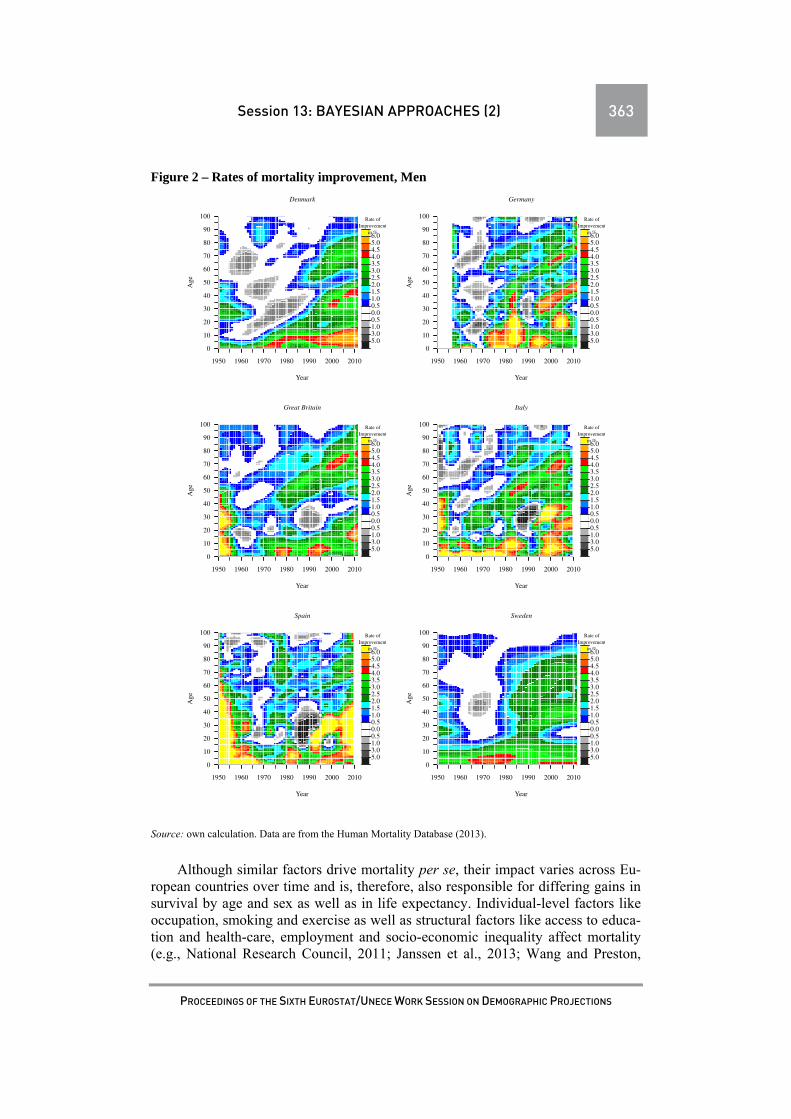
Session 13: BAYESIAN APPROACHES (2) 363
PROCEEDINGS OF THE SIXTH EUROSTAT/UNECE WORK SESSION ON DEMOGRAPHIC PROJECTIONS
Figure 2 – Rates of mortality improvement, Men
Source: own calculation. Data are from the Human Mortality Database (2013).
Although similar factors drive mortality per se, their impact varies across Eu-
ropean countries over time and is, therefore, also responsible for differing gains in survival by age and sex as well as in life expectancy. Individual-level factors like occupation, smoking and exercise as well as structural factors like access to educa-tion and health-care, employment and socio-economic inequality affect mortality (e.g., National Research Council, 2011; Janssen et al., 2013; Wang and Preston,
Year
Age
1950 1960 1970 1980 1990 2000 2010
0
10
20
30
40
50
60
70
80
90
100
−5.0−3.0−1.0−0.5
0.00.51.01.52.02.53.03.54.04.55.06.0
Rate ofImprovement
in %
Denmark
Year
Age
1950 1960 1970 1980 1990 2000 2010
0
10
20
30
40
50
60
70
80
90
100
−5.0−3.0−1.0−0.5
0.00.51.01.52.02.53.03.54.04.55.06.0
Rate ofImprovement
in %
Great Britain
Year
Age
1950 1960 1970 1980 1990 2000 2010
0
10
20
30
40
50
60
70
80
90
100
−5.0−3.0−1.0−0.5
0.00.51.01.52.02.53.03.54.04.55.06.0
Rate ofImprovement
in %
Spain
Year
Age
1950 1960 1970 1980 1990 2000 2010
0
10
20
30
40
50
60
70
80
90
100
−5.0−3.0−1.0−0.5
0.00.51.01.52.02.53.03.54.04.55.06.0
Rate ofImprovement
in %
Germany
Year
Age
1950 1960 1970 1980 1990 2000 2010
0
10
20
30
40
50
60
70
80
90
100
−5.0−3.0−1.0−0.5
0.00.51.01.52.02.53.03.54.04.55.06.0
Rate ofImprovement
in %
Italy
Year
Age
1950 1960 1970 1980 1990 2000 2010
0
10
20
30
40
50
60
70
80
90
100
−5.0−3.0−1.0−0.5
0.00.51.01.52.02.53.03.54.04.55.06.0
Rate ofImprovement
in %
Sweden

364 Session 13: BAYESIAN APPROACHES (2)
PROCEEDINGS OF THE SIXTH EUROSTAT/UNECE WORK SESSION ON DEMOGRAPHIC PROJECTIONS
2009; Cutler et al., 2006), but - despite social, cultural and/or geographical proxim-ity -, diversity in life expectancy is present across Europe.
In this article, we employ our model (Bohk and Rau, 2014) to forecast mortali-ty in several European countries, namely in Denmark, Great Britain, Spain, West Germany, Italy and Sweden to show its broad applicability. We generate retrospec-tive forecasts from 1991 to 2009 to compare the forecast errors of our model with those of other well-accepted approaches like, for instance, the Lee-Carter model (1992) and its extension of Renshaw and Haberman (2003; 2006). We also gener-ate prospective mortality forecasts from 2010 to 2050.
2. Mortality forecasting
Regarding the diverse mortality development in each country, plausible mor-tality forecasts should fulfill (at least) two requirements: First, they should be able to model dynamic shifts from younger to older ages at which relatively high mor-tality reductions are prevalent nowadays. Such dynamic age shifts already started in the mid of the last century and we expect them to continue in many European countries in the future. Second, they should be able to model continuations as well as major changes in long-term mortality trends. If a forecaster expects past mortali-ty trends to sustain in the future, a model should be able to extrapolate them; but if a forecaster expects major changes in long-term mortality trends (due to anticipated crises or even progress), a model should be able to alter extrapolated trends to meet a forecaster's expectations and to increase the plausibility of a forecast.
2.1 Mortality forecasting approaches Many mortality forecasting approaches, like the renowned Lee-Carter model
(1992) and some of its variants, for instance, proposed by Renshaw and Haberman (2003; 2006), extrapolate past mortality trends; these models often lack the ability to model dynamic age-shifts in survival improvements as well as major changes in long-term mortality trends. For instance, the Lee-Carter model assumes the relative progress in mortality between ages to be time-invariant. This assumption can lead to substantial forecast errors, in particular for longer forecasting periods.
To overcome such shortcomings, we employ our probabilistic mortality fore-casting approach (Bohk and Rau, 2014), which combines advanced techniques: To catch dynamic shifts in survival improvements across ages and periods, we use the rates of mortality improvement to forecast death rates as well as life expectancy at birth. Mitchell et al. (2013) and Haberman and Renshaw (2012) recently adopted a similar strategy, i.e. both apply the predictor structure of the Lee-Carter model, but instead of the death rates, they use the rates of mortality improvement to forecast mortality. To model major changes in long-term mortality trends, we can optional-ly complement the extrapolated mortality trend in a country of interest with mortal-ity trends of selected reference countries. In this context, Li and Lee (2005) and Cairns et al. (2011) recently suggested, among others, so-called coherent mortality forecasts; since mortality does not develop independently for women and men in a country or between neighbouring countries, they jointly forecast mortality of mul-tiple (sub)populations, arguing that they are exposed to similar conditions regard-

Session 13: BAYESIAN APPROACHES (2) 365
PROCEEDINGS OF THE SIXTH EUROSTAT/UNECE WORK SESSION ON DEMOGRAPHIC PROJECTIONS
ing health, morbidity and mortality. To capture forecast uncertainty and to provide probability statements for our mortality forecasts, we use Bayesian inference to run our hierarchical models.
2.2 Mortality forecasts for Denmark, Italy, Spain, Great Britain, Sweden and West Germany
We conduct retrospective and prospective mortality forecasts for women and men in six European countries - namely for women and men in Denmark, Italy, Spain, Great Britain, West Germany and Sweden - with our model as well as with the original Lee-Carter model (1992) and three of its variants proposed by Ren-shaw and Haberman (2003; 2006).
In the retrospective setting, we forecast mortality from 1991 to 2009, based on data from 1970 to 1990. Since we have observed mortality data for each country until 2009, we use forecast errors to evaluate their performance. Forecast errors provide information on the amount and direction of deviances between forecasted and observed mortality data. For instance, if forecast errors accumulate over time, they can indicate that a forecast systematically over- or underestimates the progress in life expectancy at birth.
In the prospective setting, we forecast mortality from 2010 to 2050, based on data from 1970 to 2009. In contrast to the retrospective forecasts, we cannot use actually observed mortality data to evaluate their performance. But we can use these prospective forecasts to compare probable future developments in life expec-tancy according to the different approaches.
To generate the mortality forecasts with the original Lee-Carter model (1992), we apply the freely available implementation of Timothy Miller (http://www.demog.berkeley.edu/~tmiller/research/forecasts/mort.forecast.module.s); for the forecasts with the three variants of Renshaw and Haberman (2003; 2006), we use the ilc R-package of Butt and Haberman (2010).
2.2.1 Retrospective mortality forecasts Figure 3 depicts the actually observed (black) and the forecasted life expectan-
cy of our model (blue), of the Lee-Carter model (red) as well as of its three exten-sions, h0 (green), h1 (yellow) and h2 (magenta), proposed by Renshaw and Ha-berman for women (top lines) and men (lower lines) from 1991 to 2009. The green vertical lines represent the base period from 1970 to 1990.
Although all models capture the observed mortality development quite well, there are considerable differences regarding bias and accuracy. To assess the fore-casting performance, we compare the annual forecast errors, i.e. the differences be-tween the forecasted and the actually observed life expectancy in each year be-tween 1991 and 2009, in Figure 4. We want to note three issues:

366 Session 13: BAYESIAN APPROACHES (2)
PROCEEDINGS OF THE SIXTH EUROSTAT/UNECE WORK SESSION ON DEMOGRAPHIC PROJECTIONS
Figure 3 – Retrospective mortality forecasts
Source: own calculation.
(1) Our model typically generates smaller forecast errors than the other ap-
proaches; this applies for women in five and for men in six out of six coun-tries. The forecast errors of our model roughly fluctuate around small val-ues between -0.5 and +0.5 for all countries. Few exceptions (with slightly larger forecast errors) are, for instance, Spanish males and German females: Our model underestimates - like the other approaches, but to a much lesser extent - the progress in Spanish male life expectancy, which is particularly stronger in the forecast years than in the last decade of the base period. In
1950 1960 1970 1980 1990 2000 2010
65
70
75
80
85
90ObservedOur modelRH−h0RH−h1RH−h2LC−TM
Denmark
Year
e 0
1950 1960 1970 1980 1990 2000 2010
65
70
75
80
85
90
Germany
Year
e 0
1950 1960 1970 1980 1990 2000 2010
65
70
75
80
85
90
Great Britain
Year
e 0
1950 1960 1970 1980 1990 2000 2010
65
70
75
80
85
90
Italy
Year
e 0
1950 1960 1970 1980 1990 2000 2010
65
70
75
80
85
90
Spain
Year
e 0
1950 1960 1970 1980 1990 2000 2010
65
70
75
80
85
90
Sweden
Year
e 0

Session 13: BAYESIAN APPROACHES (2) 367
PROCEEDINGS OF THE SIXTH EUROSTAT/UNECE WORK SESSION ON DEMOGRAPHIC PROJECTIONS
the case of German females, our model slightly overestimates the progress in life expectancy. However, the forecasts of our model mirror the actually observed mortality development for most countries more precisely than the other applied approaches.
(2) Forecast errors are usually higher for men than for women. One reason
might be that male life expectancy appears to increase sharper in the fore-cast years than in the base years. Since the other models assume that the pace of the increase in life expectancy primarily relies on the long-term trend, they cannot easily capture major (and minor) changes and generate, therefore, larger forecast errors.
Figure 4 – Forecast errors of the retrospective mortality forecasts
Source: own calculation.
(3) Progress in male life expectancy is systematically underestimated by the
other approaches, i.e. the forecast errors are below zero and accumulate with time. This effect can be detected particularly well in Denmark: The Lee-Carter model and its extensions underestimate male life expectancy by over 4 years (after only 20 forecast years), whereas the forecast of our model deviates only slightly from the actually observed values. We in-
1990 1995 2000 2005 2010
−4
−3
−2
−1
0
1
2
Our modelRH−h0RH−h1RH−h2LC−TM
Denmark, Women
1990 1995 2000 2005 2010
−4
−3
−2
−1
0
1
2Denmark, Men
1990 1995 2000 2005 2010
−4
−3
−2
−1
0
1
2Italy, Women
1990 1995 2000 2005 2010
−4
−3
−2
−1
0
1
2Italy, Men
1990 1995 2000 2005 2010
−4
−3
−2
−1
0
1
2Spain, Women
1990 1995 2000 2005 2010
−4
−3
−2
−1
0
1
2Spain, Men
1990 1995 2000 2005 2010
−4
−3
−2
−1
0
1
2Germany, Women
1990 1995 2000 2005 2010
−4
−3
−2
−1
0
1
2Germany, Men
1990 1995 2000 2005 2010
−4
−3
−2
−1
0
1
2Great Britain, Women
1990 1995 2000 2005 2010
−4
−3
−2
−1
0
1
2Great Britain, Men
1990 1995 2000 2005 2010
−4
−3
−2
−1
0
1
2Sweden, Women
1990 1995 2000 2005 2010
−4
−3
−2
−1
0
1
2Sweden, Men

368 Session 13: BAYESIAN APPROACHES (2)
PROCEEDINGS OF THE SIXTH EUROSTAT/UNECE WORK SESSION ON DEMOGRAPHIC PROJECTIONS
crease the accuracy of our forecast by complementing the purely extrapo-lated Danish mortality trend with that of the neighbouring country Sweden, assuming that Danish life expectancy probably catches up to international trends again.
2.2.2 Prospective mortality forecasts
Figure 5 depicts the observed (black) and the forecasted life expectancy of our model (blue), of the Lee-Carter model (red) as well as of its three extensions, h0
Figure 5 – Prospective mortality forecasts
Source: own calculation.
1950 1970 1990 2010 2030 2050
65
70
75
80
85
90
95
ObservedOur modelRH−h0RH−h1RH−h2LC−TM
Denmark
Year
e 0
1950 1970 1990 2010 2030 2050
65
70
75
80
85
90
95
Germany
Year
e 0
1950 1970 1990 2010 2030 2050
65
70
75
80
85
90
95
Great Britain
Year
e 0
1950 1970 1990 2010 2030 2050
65
70
75
80
85
90
95
Italy
Year
e 0
1950 1970 1990 2010 2030 2050
65
70
75
80
85
90
95
Spain
Year
e 0
1950 1970 1990 2010 2030 2050
65
70
75
80
85
90
95
Sweden
Year
e 0

Session 13: BAYESIAN APPROACHES (2) 369
PROCEEDINGS OF THE SIXTH EUROSTAT/UNECE WORK SESSION ON DEMOGRAPHIC PROJECTIONS
(green), h1 (yellow) and h2 (magenta), proposed by Renshaw and Haberman for women (top lines) and men (lower lines) from 2010 to 2050. The green vertical lines represent the base period from 1970 to 2009.
All models predict additional gains in life expectancy until 2050, but their forecasts differ in their level as well as in their pace of growth (for future life ex-pectancy). Regarding the level: Italy and Spain are likely to reach one of the high-est life expectancy values in 2050 among the selected European countries, whereas Denmark is likely to reach one of the lowest life expectancy values at the same time. For instance, according to our model, Italy will reach with 91.13 years for women and with 88.57 years for men life expectancy values in 2050 that are sub-stantially higher than those for Danish women and men with 89.82 years and 86.86 years, respectively.
Regarding the pace of growth: Despite the fact that all models forecast life ex-pectancy of Danish females to be relatively low, our model forecasts an accelerat-ing increase with the largest gain of additional years to live, whereas the other models forecast a rather linear increase (like for each other country), which contin-ues the slow increase of the base period. Hence, we allow Danish women to catch up with international trends again by not only extrapolating their mortality trend (like the other models), but by complementing it with mortality trends of Sweden, France, Italy and Japan(, assuming that these countries represent international mor-tality trends). We apply the same procedure for Sweden, complementing its mortal-ity trends with those of France, Italy and Japan.
3. Concluding Remarks
Forecasting the diverse mortality developments in Denmark, Italy, Spain, Great Britain, West Germany and Sweden demonstrates that our model (Bohk and Rau, 2014) is able to project regular as well as irregular mortality developments. We would argue that two characteristics of our model play a key role for the suc-cess: (1) Modeling dynamic shifts in survival improvements from younger to older ages via the rates of mortality improvement instead of death rates. (2) Irregular mortality developments cannot be simply extrapolated but require additional (ex-pert) information. We did this by including extrapolated mortality trends of coun-tries, which we considered to be forerunners in mortality developments for the country of interest, similar to Li and Lee (2005) who pioneered this approach.
Acknowledgements The European Research Council has provided financial support under the Eu-
ropean Community's Seventh Framework Programme (FP7/2007-2013) / ERC grant agreement no. 263744.

370 Session 13: BAYESIAN APPROACHES (2)
PROCEEDINGS OF THE SIXTH EUROSTAT/UNECE WORK SESSION ON DEMOGRAPHIC PROJECTIONS
REFERENCES
Bohk, C. and R. Rau. 2014. Probabilistic Mortality Forecasting with Varying Age-Specific Survival Improvements. arXiv:1311.5380v2[stat.AP].
Butt, Z. and S. Habermann. 2010. ilc: A Collection of R Functions for Fitting a Class of Lee-Carter Mortality Models using Iterative Fitting Algorithms. Actuar-ial Research Paper No.190, Cass Business School, Faculty of Actuarial Science and Insurance, London.
Cairns, A. J. G., D. Blake, K. Dowd, G. D. Coughlan, and M. Khalaf-Allah. 2011. Bayesian Stochastic Mortality Modelling for Two Populations. ASTIN Bulletin 41, 29–59.
Christensen, K., M. Davidsen, K. Juel, L. Mortensen, R. Rau, and J. W. Vaupel. 2010. The Divergent Life Expectancy Trends in Denmark and Sweden — and Some Potential Explanations. In: E. M. Crimmins, S. H. Preston, and B. Cohen, eds. 2010. International Differences in Mortality at Older Ages. Dimensions and Sources. Chapter 14, pp. 385–407. Washington D.C.: The National Academies Press.
Christensen, K., G. Doblhammer, R. Rau, and J. Vaupel. 2009. Ageing popula-tions: the challenges ahead. The Lancet 374(9696), 1196–1208.
Cutler, D., A. Deaton, and A. Lleras-Muney. 2006. The Determinants of Mortality. Journal of Economic Perspectives 20 (3), 97-120.
Eurostat. 2014. Statistics Database. Population and social conditions (popul). Mor-tality (demo_mor). Life expectancy by age and sex (demo_mlexpec). Available at: http://epp.eurostat.ec.europa.eu/. Access on 4 March 2014.
Haberman, S. and A. E. Renshaw. 2012. Parametric mortality improvement rate modelling and projecting. Insurance: Mathematics and Economics 50(3), 309–333.
Jacobsen, R., N. Keiding, and E. Lynge. 2002. Long term mortality trends behind low life expectancy of Danish women. Journal of Epidemiology and Community Health 56, 205–208.
Janssen, F., L. J. G. van Wissen, and A. E. Kunst. 2013. Including the Smoking Ep-idemic in Internationally Coherent Mortality Projections. Demography 50(4), 1341–1362.
Kannisto, V. 1994. Development of oldest-old mortality, 1950–1990: Evidence from 28 developed countries. Monographs on Population Aging, 1. Odense, DK: Odense University Press.
Kannisto, V., J. Lauritsen, A. R. Thatcher, and J. W. Vaupel. 1994. Reductions in Mortality at Advanced Ages: Several Decades of Evidence from 27 Countries. Population and Development Review 20(4), 793–810.

Session 13: BAYESIAN APPROACHES (2) 371
PROCEEDINGS OF THE SIXTH EUROSTAT/UNECE WORK SESSION ON DEMOGRAPHIC PROJECTIONS
Lee, R. D. and L. R. Carter. 1992. Modeling and Forecasting U.S. Mortality. Jour-nal of the American Statistical Association 87(419), 659–671.
Li, N. and R. Lee. 2005. Coherent mortality forecasts for a group of populations: An extension of the Lee-Carter method. Demography 42(3), 575–594.
Meslé, F. and J. Vallin. 2006. Diverging trends in female old-age mortality: the United States and the Netherlands versus France and Japan. Population and De-velopment Review 32(1), 123–145.
Mitchell, D., P. Brockett, R. Mendoza-Arriage, and K. Muthuraman. 2013. Model-ing and forecasting mortality rates. Insurance: Mathematics and Economics 52(2), 275–285.
National Research Council. 2011. Explaining Divergent Levels of Longevity in High-Income Countries. Panel on Understanding Divergent Trends in Longevity in High-Income Countries. Committee on Population, Division of Behavioral and Social Sciences and Education.
Oeppen, J. and J. W. Vaupel. 2002. Broken limits to life expectancy. Science 296, 1029–1031.
Omran, A. R. 1971. The Epidemiologic Transition: A Theory of the Epidemiology of Population Change. The Milbank Memorial Fund Quaterly 49(4), 509–538. Part 1.
Rau, R., D. Jasilionis, E. L. Soroko, and J.W. Vaupel. 2008. Continued Reductions in Mortality at Advanced Ages. Population and Development Review 34(4), 747–768.
Renshaw, A. E. and S. Haberman. 2003. Lee-Carter mortality forecasting with age specific enhancement. Insurance: Mathematics and Economics 33(2), 255–272.
Renshaw, A. E. and S. Haberman. 2006. A cohort-based extension to the Lee-Carter model for mortality reduction factors. Insurance: Mathematics and Eco-nomics 38(3), 556–570.
University of California, Berkeley (USA), and Max Planck Institute for Demo-graphic Research, Rostock, (Germany). 2013. Human Mortality Database. Available at www.mortality.org.
Vaupel, J. W. 1997. The remarkable improvements in survival at older ages. Philo-sophical Transactions of the Royal Society of London: Biological Sciences 352, 1799–1804.
Wang, H. and S. H. Preston. 2009. Forecasting United States mortality using cohort smoking histories. PNAS 106(2), 393–398.


Session 14
MULTIREGIONALPROJECTIONS
Chair: Valerio Terra Abrami (Istat)


Session 14: MULTIREGIONAL PROJECTIONS 375
PROCEEDINGS OF THE SIXTH EUROSTAT/UNECE WORK SESSION ON DEMOGRAPHIC PROJECTIONS
EXAMINING THE ROLE OF INTERNATIONAL MI-GRATION IN GLOBAL POPULATION PROJECTIONS
Guy J. Abel, Samir K.C. and Nikola Sander Summary
Advances in projecting international migration have been hindered by a lack of ade-quate data. Consequently, international projection-making agencies commonly use simplistic assumptions of net-migration measures derived as residuals from demo-graphic accounting. However, past net migration can be often volatile and introduce bias when projecting populations (Rogers, 1990). This paper presents sets of global population projections to 2060, focusing on two alternative assumptions of interna-tional migration. Assumptions on rates of other demographic factors, namely fertility and mortality, are held constant allowing an examination of the role of international migration in global population projections models. In the first projection, we set the future net number of migrants by age and sex in each country to mirror that of the United Nations. In the second projection, we use a set of estimated 5-year bilateral migration flows by sex developed from the flows from stocks methodology of Abel (2013) and Abel & Sander (2014). The sex-specific bilateral flow table estimates are disaggregated by age using a parametric assumption for emigra-tion schedules, and then summed over rows and columns to obtain immigration and emigration rates by age and sex. These estimates are used as base data in a bi-regional projection model, where immigration and emigration rates are assumed to remain con-stant up to 2060. Our results highlight differences in the future level of populations around the globe and numbers of migrant flows between a net migration projection model and a bi-regional projection model. Keywords: international migration flows, global population projections, bi-regional projection model
1. Introduction
International migration is an important driver of demographic growth in many countries (Lee, 2011). In recent decades, migration often has had a significant ef-fect on population change in more developed regions. In some of these nations, migration is beginning to account for over half of population growth (National Research Council, 2000). The rise in influence of migration on demographic change is likely to spread to more countries as fertility and mortality rates continue to fall in the developing world.

376 Session 14: MULTIREGIONAL PROJECTIONS
PROCEEDINGS OF THE SIXTH EUROSTAT/UNECE WORK SESSION ON DEMOGRAPHIC PROJECTIONS
Migration is widely considered as the largest source of uncertainty in demo-graphic projections (Bongaarts & Bulatao, 2000). Unlike other demographic com-ponents, there does not exist an acknowledged underlying transition theory to ena-ble effective future levels of long run international migration flows to be forecast. In addition, migration flows can be volatile since short term changes in economic, social or political factors can often play and important role. These factors are com-plex process themselves, where no single force can explain the history of observed past migration. The exploration of these relationships at a global level has been hindered by the lack of data of comparable migration. Most countries in the world do not produce estimates on the number of international migrants entering or leav-ing their borders. Those that do, tend to be in developed nations where data are col-lected under multiple definitions (Kelly, 1987; Nowok, Kupiszewska, & Poulain, 2006).
With no viable alternative, global population projection models have been based on net migration numbers derived by the United Nations based on demo-graphic accounting and, in some cases, scaled annual flows derived from migration records where they exist. The use of net migration as a measure of geographical mobility has long been known to be problematic. In what Rogers (1990) describes as the uni-regional fallacy, the use of net migration measures leads to bias and in-consistency in demographic projections. These features are introduced as a net mi-gration measure confounds changing migration propensities with a changing (fu-ture) population. Moreover, they obscure regularities in the age profiles of migra-tion and thereby further misspecify the spatial dynamics generating observed set-tlement patterns.
This paper considers an alternative, multi-regional type approach, to projecting global population where both immigration and emigration terms are specified in the projection model. Input data for these terms are based upon new estimates of global migration flows using an adaptation of the methodology of Abel (2013) and Abel & Sander (2014) to obtain bilateral migrant flow tables from existing bilateral migrant stock tables. In Section 2 we outline the basic mathematics behind a few possible models of global population projections. In Section 3 we provide details of the baseline migration data and future assumptions on global migration required as inputs into the projection models. In Section 4 comparisons for different migration specifications on the future level of populations and number of migrants are illus-trated. Finally, in Section 5 the results are discussed.
2. Migration in Global Projection Models
In a global population projection model, with complete geographic coverage, there exists various ways to specify international migration. In each case there must be a consideration for a closed system, i.e. there cannot be non-zero global net mi-gration total or total outflows from all countries must equate to the total inflows. In this section we illustrate a couple of approaches to project population for all coun-tries.
The simplest option to incorporate international migration into population pro-jection models, beyond ignoring all migration, is to use a measure on the net migra-

Session 14: MULTIREGIONAL PROJECTIONS 377
PROCEEDINGS OF THE SIXTH EUROSTAT/UNECE WORK SESSION ON DEMOGRAPHIC PROJECTIONS
tion for each country. Two distinct migration measures are available in this uni-regional setting.
For each country, future population can be projected by multiplying current population levels by birth, death and net migration rates. To ensure a closed global system, a restriction of a global zero sum of net migrants in each age group, during each projected time period must be set. As Rogers (1990) showed, using a rate of net migration leads to bias and inconsistency future projections if there is non-zero migration. This due to the incorrect population at risk, being applied to the net mi-gration rate where the net migration rate encompasses not only moves out the pop-ulation, but also moves in from all other countries. It is perhaps for this reason that the United Nations uses an alternative specification of for net migration based on counts of gross flows, where again a constraint for zero sum of net migrants is maintained in all future time periods.
Age-specific migration rates exhibit a strong age-specific regularities and tem-poral stabilities (Rogers & Castro, 1981). The use of migrant counts rather than rates is likely to lead to distorted age schedules for migration in future time peri-ods. For example, consider a country with a high fertility rate and net emigration such. As the numbers of population in peak migration ages (early 20’s) in future projection periods grows, the proportional age-specific rate of migrants leaving will fall as the total amount of age-specific amount of migrants leaving is fixed. One possible solution to avoid the pitfalls of net migration in global population projection models is to move away from the uni-regional perspective and used a model with age specific immigration and emigration rates in each country.
In a bi-regional projection model the immigration rate for a given coun-try is calculated based on the population at risk, i.e. the population of the rest of the world. The emigration rate out of country is based on the resident population at the time. A constraint is commonly set to ensure a closed global system of migrants in each age groupd. Where the balance in immigration and emigration numbers in future projected periods is not maintained, a small adjustment is typically made to scale up or down immigration or emigration counts.
3. Baseline Migration Data
Until recently, the migration estimates to run global bi-regional projection model have not been available. However, global bilateral migrant stock data pub-lished by the World Bank (Özden, Parsons, Schiff, & Walmsley, 2011) and the United Nations Population Division (2012) estimates of global bilateral migrant flows have been derived by Abel (2013) and Abel & Sander (2014) that are con-strained to match the changes in migrant stocks. What follows in this section is a brief overview of the flows-from-stock method of Abel (2013) and Abel & Sander (2014) which is then applied to produce global bilateral migrant flow tables by sex. The results of these estimates for the 2005-10 period are shown alongside further assumptions to obtain age specific immigration and emigration rates required for a bi-regional projection model.

378 Session 14: MULTIREGIONAL PROJECTIONS
PROCEEDINGS OF THE SIXTH EUROSTAT/UNECE WORK SESSION ON DEMOGRAPHIC PROJECTIONS
3.1 Origin-Destination-Sex Dimension As migration flow data is often incomplete and not comparable across nations,
Abel & Sander (2014) estimates the number of movements by linking changes in bilateral migrant stock data over time. Figure 1 illustrates the methodology to ob-tain bilateral flows from changes in the stock tables for people born in a hypothet-ical Country A.
Figure 1 - Hypothetical Example of Flows-From-Stock Methodology of Abel & Sander (2014) for People Born in Country A
In the example, the location of people born in Country A is given in 2005 and 2010. As we assume no births and deaths in this example, the stock of migrants across all (of the possible 3) locations in both years are equal (270 + 30 + 50 = 210 + 80 + 60 = 350). The number of people born in Country A and living in Country A (blue field) decreases from 270 in 2005 to 210 in 2010. The number of people born in A and living in Country B (green field) increases from 30 to 80 and the number of people living in Country C (red field) also increases from 50 to 60. The

Sessione 14: MULTIREGIONAL PROJECTIONS 379
PROCEEDINGS OF THE SIXTH EUROSTAT/UNECE WORK SESSION ON DEMOGRAPHIC PROJECTIONS
Figure 2 - Estimated migrant flows (in millions) between regions for 2005-10. Males (bottom) and Females (top)

380 Session 14: MULTIREGIONAL PROJECTIONS
PROCEEDINGS OF THE SIXTH EUROSTAT/UNECE WORK SESSION ON DEMOGRAPHIC PROJECTIONS
estimate of the minimum number of migrant flow required to match the differences in the stocks of people born in Country A is calculated. In doing so the number of stayers, those who remain in their country of residence between 2005 and 2010, are set to their maximum possible number. In this simplified example, 210 people born in A stay in A, 30 stay in B and 50 stay in C. The remaining flows required to match the stocks and number of stayers are estimated using an iterative proportion-al fitting algorithm. This results in conditional maximum likelihood estimates of 50 moves from Country A to Country B and 10 moves from Country A to Country C, whilst maintaining the observed stocks in 2005 and 2010.
We produce a comparable set of global migration flows by simultaneously rep-licating the estimation procedure in Figure 1 for 196 countries twice, once for male stock data and once for female stock data provided by United Nations Population Division (2012). Alterations are made to the migrant stock counts to control for births and deaths during the period, as given in the World Population Prospects of United Nations Population Division (2011). Estimated migrant flow tables have net migration levels in each country that are almost identical to those in the World Population Prospect for the 2005-10 period, due to the demographic accounting method presented in Abel & Sander (2014). Estimates themselves represent the minimum number of migrant transition flows required to match the stock tables at the beginning and end of the period.
In order to briefly illustrate the patterns estimated in the two bilateral migra-tion tables we plot in Figure 2 a representation of the data after aggregating the 196 country specific flows into 10 world regions using the circlize package (Gu, 2013) in R. In each side of the figure, the origins and destinations are represented by the circle’s segments. Flows have the same colour as their origin and the width at the base of the flow ribbon indicates their size. The direction of the flow is shown by the gap between ribbon and region, where ribbons are attached to their flows origin, and the gap denotes the destination. Tick marks show each region's gross migration in millions.
The two plots show patterns that broadly follow conventional thinking on cur-rent international migration flows. The size and direction of flows appear to be similar between the sexes, with the exception of larger flows moving from South Asia to West Asia (mainly oil rich Gulf States). The underlying estimates provide a set of immigration and emigration rates for each country, by sex, to be utilised in a global population projection model, such as the bi-regional model shown in the previous section. However, in order to obtain projections disaggregated by age, a further step is required.
3.2. Age Dimension As there was no information on migrant stock populations by age, we were
unable to estimate any age-specific flows using the flows-from-stock methodology outlined above. In order to derive estimates by age groups, required for bi-regional projection models, we relied upon the seven parameter age schedule of Rogers & Castro (1981) to disaggregate each estimated flow in our bilateral table. Rogers & Castro (1981) discussed a set of fundamental parameters obtained by fitting their schedule to multiple sets of internal migration data.

Session 14: MULTIREGIONAL PROJECTIONS 381
PROCEEDINGS OF THE SIXTH EUROSTAT/UNECE WORK SESSION ON DEMOGRAPHIC PROJECTIONS
The migration schedule formed by the fundamental parameter of Rogers & Castro (1981) is plotted in the solid black line of Figure 3, where the estimates from the schedule have been scaled to fix the area under the curve to be unity. In order to account for differences between internal and our international migration application we altered some parameter values, depending on the country of origin. For flows from less developed countries outside the OECD (Organisation for Eco-nomic Co-operation and Development) and GCC (Gulf Cooperation Council) countries, we applied a migration schedule with a larger labour force peak, as shown in Figure 3. Flows that originated from OECD and GCC countries were as-sumed to follow a migration age schedule with a later peak. This schedule, shown in Figure, scaled to set the sum of the age-specific rates to sum to unity. The altera-tive schedule reflects an assumption of moves after longer periods of education and/or later entry into the education market in these countries, while allowing re-turn migration of temporary workers from OECD and GCC countries at older ages.
Figure 3 - Standardised Rogers-Castro Curves for Parameter Values in Table 1
Given the origin specific age-schedules, where the sum of the age-specific mi-
gration rates summed to unity, we multiplied through age specific rates at each 5 year interval to each origin-destination-sex ( ) table;

382 Session 14: MULTIREGIONAL PROJECTIONS
PROCEEDINGS OF THE SIXTH EUROSTAT/UNECE WORK SESSION ON DEMOGRAPHIC PROJECTIONS
This resulted in an array of origin-destination migration flow table by sex and age covering the 5 year time period between 2005 and 2010.
3.3. Future Assumptions Migration is widely considered as the most difficult demographic component
to predict. Unlike other demographic components, are no acknowledged underlying transition theory to enable effective future levels of long run migration flows to be estimated. As a result, most agencies making long run population projections use some form of naive forecast for migration, where all future values are set to their least observed values.
The United Nations Population Division (2011) World Population Prospects assume a naive forecast of net migration up until 2050. Under their normal migra-tion assumption, the future path of international migration is set on the basis of past net migration counts which are disaggregated by age using a standardised Rogers-Castro schedule. Exceptions in the overall level from the naive forecast are made for some selected countries where consideration of the policy stance of future in-ternational migration flows are made. After 2050, it is assumed that net migration will gradually decline and reach zero by 2100.
For similar reasons we also assume the naive forecast for future immigration and emigration rates for the bi-regional model based on estimated values in 2005-10 with some exceptions. Adjustments in the first two forecast periods, where we considered our estimates in 2005-10 to be unsustainable in the long run were made to 21 immigration rates and 7 emigration rates. The countries where adjustments are applied are listed in Table 1. For most immigration counties this involved a re-duction in the 2010-15 migration rates by 20% from the estimated rate in 2005-10, followed by a further reduction of 20% in the 2015-20 period. For emigration counties we increased the 2010-15 and 2015-20 rate by 20%. Full details on these adjustments and all other assumptions are provided in Sander, Abel, & Riosmena (2014).
Table 1 - Countries with Adjustments to Immigration (left) and Emigration (Right) Rates in First Two Projection Periods. For the majority of countries 2005-10 rates were reduced (for immigration) or increased (for emigration) by 20% period on period. For countries in italics 2005-10 rates were reduced by 60% period on period
Immigration
Emigration
Australia Ireland Qatar
Bahrain
Austria Italy Singapore
Micronesia
Bahrain Kuwait Spain
Qatar
Burundi Liberia Sweden
Samoa
Czech Republic Luxembourg Switzerland
Tonga
Greece Macao UAE
UAE
Iceland Norway United Kingdom
Zimbabwe

Session 14: MULTIREGIONAL PROJECTIONS 383
PROCEEDINGS OF THE SIXTH EUROSTAT/UNECE WORK SESSION ON DEMOGRAPHIC PROJECTIONS
4. Results
The results of the two difference projection models on future migration in each continent are shown in Figure 4 where we plot five lines. The first two represent past data and future levels of net migration as estimated and assumed (respectively) by the United Nations Population Division for the World Population Prospects in 2010 and 2012. Data are taken from the wpp2010 Sevcikova & Gerland (2013) and wpp2012 Sevcikova et al. (2013) R packages. As illustrated in the plot, past data in the 2012 edition go back further than 2010. In addition in some continents such as Africa, the past estimates of net migration given in the 2012 edition are markedly different from that of the 2010 edition.
The two dotted blue lines represent the resulting future immigration (positive) and emigration (negative) levels that resulted from the assumed rates in the bi-regional projection model. The bi-regional model projects an increase in the num-ber of emigrants from continents with young populations such as Africa. As the model is based on migration rates it adapts to changes in the population structure. Conversely, the projection model used by the United Nations assumes, in most countries, a constant net level in future projections despite expected changing age structures and population size. In Europe, North America and Oceania the bi-regional model projects a rise in net migration (shown in the solid blue line) as the immigration rate uses the rest of the world population as the population at risk. As this population at risk increases, so does the immigration to countries where we as-sumed a comparatively high constant rates of immigration. Note, differences be-tween our implied net and the United Nations 2010 net migration in the base year of the projection are due to a small number of countries used in the projection model.
The bi-regional projection model provides substantially different future popu-lations than in the net migration model. In Figure 5 we plot four lines representing various projected populations. The solid black lines are the median forecast of the 2012 World Population Prospects in each continent, which are shown purely for reference. The red line is a hybrid of the mid scenario in our Wittgenstein Centre (WiC) global population projections, where we drop the bi-regional specification and replace it with the same net migration levels as the United Nations (that under-lie the black lines in Figure 4) As the level of net migration in this model is identi-cal to that of the United Nations the difference between the red and black line rep-resent differences solely from alternative fertility and mortality forecasts.

384 Session 14: MULTIREGIONAL PROJECTIONS
PROCEEDINGS OF THE SIXTH EUROSTAT/UNECE WORK SESSION ON DEMOGRAPHIC PROJECTIONS
Figure 4 - Projected Net Migration Levels by Continent (in Millions)
Figure 5 - Projected Population by Continent (in Millions)

Session 14: MULTIREGIONAL PROJECTIONS 385
PROCEEDINGS OF THE SIXTH EUROSTAT/UNECE WORK SESSION ON DEMOGRAPHIC PROJECTIONS
The solid blue is the original WiC bi-regional projection model. The differ-ences between the red and blue represent the difference in the migration specifica-tion within global population projection models. For Europe, North America and Oceania the effect is drastic. The high levels of immigration from the rest of the world in the bi-regional model lead to a continuation of population growth. Under the hybrid model, with the United Nations net migration assumption, the future populations are expected to either fall (Europe) or slow in their increase (North America and Oceania). In the case of these latter two continents the bi-regional specification recovers the lower population, driven by alternative fertility and mor-tality assumptions, to levels close to those of the United Nations. Unsurprisingly, the impact of migration on the projected populations is largest in continents where fertility and mortality rates are at already stable low levels. This impact is shown by the difference in the principal projections from the populations resulting from the zero migration projection model.
5. Summary
At present, the research on migration measures and assumptions in global pro-jection models are relatively unexplored in comparison to other demographic com-ponents. This study has made an initial attempt address this issue by investigating the role of an alternative specification, beyond net migration, in a global population projection model.
The bi-regional projection model produces some notable differences in the fu-ture levels of migration and resulting population in comparison to the net assump-tions used by the United Nations. These differences could be due to two factors. First, in the bi-regional model we used assumptions on future rates. This allows projected immigration and emigration to adjust to changing population structures, where the standardized age schedules in Figure 3 are maintained. Conversely, the United Nations does not have, to our knowledge, have any equivalent dynamics in their projection model to ensure sensible age schedules for future migration rates. Second, in the bi-regional projection model, immigration and emigration rates can respond to changing sizes in their corresponding population at risk. Projection models based on net migration levels do not have any functions to allow for this dynamic response.
Whilst the results in this paper clearly demonstrate the importance of migra-tion specification within global projection model there are a number of possible improvements that could be made. In employing a bi-regional model we have dis-regarded a lot of (estimated) information in the base data on the origin-destination patterns. These patterns could potentially be used in a full multi-regional projection model at the global level. Further, models fitted to the estimated data might allow for alternative model based forecasts, beyond the naive methods, currently used, as suggested by Cohen, Roig, Reuman, & Gogwilt (2008). Alternative assumptions on the age-schedules used to derive age-specific immigration and emigration rates might also play an important role in the projection model. For instance, there is some evidence to suggest that international migration of children occur at a con-stant low rate rather than declining at birth as we assumed.

386 Session 14: MULTIREGIONAL PROJECTIONS
PROCEEDINGS OF THE SIXTH EUROSTAT/UNECE WORK SESSION ON DEMOGRAPHIC PROJECTIONS
Although it is difficult to claim any one specification of migration in a global population projection model can provide superior, i.e. more accurate forecasts, without some full validation exercises, it is known from work on multi-regional projections in single countries that models which rely on some measure of net mi-gration tend to perform worse (Raymer, Abel, & Rogers, 2012; Wilson & Bell, 2004). As international migration is expected to play an increasingly important role in future demographic change, we have illustrated that an alternative migration specification within a global projection model can have a large impact on future population sizes.
REFERENCES
Abel, G. J. (2013). Estimating global migration flow tables using place of birth data. Demographic Research, 28(March), 505–546. doi:10.4054/DemRes.2013.28.18
Abel, G. J., & Sander, N. (2014). Quantifying Global International Migration Flows. Science, 343(6178).
Bongaarts, J., & Bulatao, R. A. (Eds.). (2000). Beyond Six Billion: Projecting the World’s Population (1st ed.). Washington D.C., USA: National Academies Press.
Cohen, J. E., Roig, M., Reuman, D. C., & Gogwilt, C. (2008). International migration beyond gravity: A statistical model for use in population projections. Proceedings of the National Academy of Sciences, 105(40), 15269–15274. doi:10.1073/pnas.0808185105
Gu, Z. (2013). circlize: Circular layout in R. Retrieved from http://cran.r-project.org/package=circlize
Kelly, J. J. (1987). Improving the Comparability of International Migration Statistics: Contributions by the Conference of European Statisticians from 1971 to Date. International Migration Review, 21(4), 1017–1037. doi:10.2307/2546502
Lee, R. D. (2011). The outlook for population growth. Science, 333(6042), 569–73. doi:10.1126/science.1208859
National Research Council. (2000). Beyond six billion: Forecasting the world’s population. (J. Bongaarts & R. Bulatao, Eds.)Population English Edition (p. 258). Washington D.C., USA: National Academy Press. Retrieved from http://books.google.com/books?hl=en&lr=&id=5h3_m_XtKuQC&oi=fnd&pg=PT3&dq=Beyond+six+billion:+forecasting+the+world’s+population&ots=AHODF-Y2C2&sig=SqSQvo0cYPGxtrppObBtUtXJxNY

Session 14: MULTIREGIONAL PROJECTIONS 387
PROCEEDINGS OF THE SIXTH EUROSTAT/UNECE WORK SESSION ON DEMOGRAPHIC PROJECTIONS
Nowok, B., Kupiszewska, D., & Poulain, M. (2006). Statistics on International Migration Flows. In M. Poulain, N. Perrin, & A. Singleton (Eds.), Towards the Harmonisation of European Statistics on International Migration (THESIM) (pp. 203–233). Louvain-La-Neuve, Belguim: UCL--Presses Universitaires de Louvain.
Özden, Ç., Parsons, C. R., Schiff, M., & Walmsley, T. L. (2011). Where on Earth is Everybody? The Evolution of Global Bilateral Migration 1960--2000. World Bank Economic Review, 25(1), 12–56. doi:10.1093/wber/lhr024
Raymer, J., Abel, G. J., & Rogers, A. (2012). Does Specification Matter? Experiments with Simple Multiregional Probabilistic Population Projections. Environment and Planning A, 44(11), 2664–2686. Retrieved from http://www.pubmedcentral.nih.gov/articlerender.fcgi?artid=3518036&tool=pmcentrez&rendertype=abstract
Rogers, A. (1990). Requiem for the Net Migrant. Geographical Analysis, 22(4), 283–300. Retrieved from http://onlinelibrary.wiley.com/doi/10.1111/j.1538-4632.1990.tb00212.x/abstract
Rogers, A., & Castro, L. J. (1981). Model migration schedules. IIASA Research Report, 81(RR-81-30), 1–160. Retrieved from http://webarchive.iiasa.ac.at/Admin/PUB/Documents/RR-81-030.pdf
Sander, N., Abel, G. J., & Riosmena, F. (2014). The Future of International Migration. In W. Lutz, B. Butz, & S. K.C. (Eds.), World Population and Human Capital in the 21st Century (pp. 333–397). Oxford, United Kingdom: Oxford University Press.
Sevcikova, H., & Gerland, P. (2013). wpp2010: World Population Prospects 2010. Retrieved from http://cran.r-project.org/package=wpp2010
Sevcikova, H., Gerland, P., Andreev, K., Li, N., Gu, D., & Spoorenberg, T. (2013). wpp2012: World Population Prospects 2012. Retrieved from http://cran.r-project.org/package=wpp2012
United Nations Population Division. (2011). World Population Prospects: The 2010 Revision, Highlights and Advance Tables. Working Paper ESA/P/WP (Vol. 220, pp. 1–164). New York, USA.
United Nations Population Division. (2012). Trends in International Migrant Stock: Migrants by Destination and Origin. New York, USA: United Nations Department of Economic and Social Affairs/Population Division. Retrieved from http://esa.un.org/MigOrigin/UN_MigStock_Origin_Methodology.pdf
Wilson, T., & Bell, M. (2004). Comparative empirical evaluations of internal migration models in subnational population projections. Journal of Population Research, 21(2), 127–160. doi:10.1007/BF03031895

388 Session 14: MULTIREGIONAL PROJECTIONS
PROCEEDINGS OF THE SIXTH EUROSTAT/UNECE WORK SESSION ON DEMOGRAPHIC PROJECTIONS
SUBNATIONAL POPULATION PROJECTIONS FOR
TURKEY, 2013-2023
Sebnem Bese Canpolat, Mehmet Dogu Karakaya
Summary
Turkey consists of 81 provinces among which there are considerable differences re-garding demographic indicators. The scope of this study is to view the population fig-ures of Turkey by the new provincial population projections for the centenary of the Republic of Turkey (2023), based on the updated Address Based Population Registra-tion System (ABPRS) database, besides to the 2013-2075 population projections for Turkey. This is the first official study for provincial based cohort-component popula-tion projections. The end of the year values of ABPRS 2012 results were used as base population. Births and deaths are compiled from Central Civil Registration System (“CCRS”-MERNIS). Internal migration assumptions were produced from ABPRS. An average of recent migration patterns of provinces were taken as an input. Institutional population living in barracks was separated from the rest of the population and the age structure of this population was regarded not be changed throughout the projection period. According to the results of the study, population of Turkey will be about 84 mil-lion in 2023 with decelerating growth rate. Population of 60 provinces will increase and population of 21 provinces will decrease in 2023. The order of the most populous four provinces will not change. The population of İstanbul will be 16.6 million in 2023, the population of Ankara will increase to 5.9 million, the population of İzmir will be 4.4 million, and the population of Bursa will be 3.1 million. The proportion of elderly population in the population of Turkey will increase to 10.2% in 2023. Keywords: Turkey, TurkStat, population projections.
1. Introduction
Demographic changes over time have always been an important topic for planning about the future. Population projections are methods that make estima-tions for past and future by using the data of censuses and surveys, and are applied by relevant official and non-official institutions. The most comprehensive projec-tions have been presented by The United Nations since 1950, up to now. But now-adays, regional projections are a lot more needed by governments and institutions.
After establishment of the Republic of Turkey, the first population census was conducted in 1927 and the next one was in 1935, and 5 years periodic censuses were conducted until 1990, and then the census time period expanded to 10 years. 2000 General Population Census is the last and the most recent traditional one.

Session 14: MULTIREGIONAL PROJECTIONS 389
PROCEEDINGS OF THE SIXTH EUROSTAT/UNECE WORK SESSION ON DEMOGRAPHIC PROJECTIONS
“Address Based Population Registration System” (ABPRS) was developed in 2007, by Ministry of Interior Affairs and Turkish Statistical Institute (TurkStat). A brand-new window on demography is being opened in Turkey (Karakaya, 2009).
2. Scope of the Study
The official population projection method in Turkey is cohort-component method which is currently used by Turkish Statistical Institute for national-level population projections. TurkStat has used this method for population projections since 1994.
Population projections are revised due to new demographic trends, when vari-ous radical changes are determined. New population projections were fundamental-ly needed for Turkey. Some different alternative regional projections have been made for academic studies. ABPRS was begun to be used first, but there was ab-sence of adequate administrative data sources for assumptions. In recent years, ad-ministrative data sources have been improved significantly in Turkey.
Population projections of TurkStat, which was last produced according to the results of 2008 ABPRS and 2008 Turkey Demographic and Health Survey, are re-newed due to improvements on the birth and death data obtained from registration systems, formation of a serial of migration statistics from ABPRS and to meet the national and international needs. The study for the population projections were car-ried out by a working group including the participants from related university and institutions. A working group has been constructed by representatives from Turk-Stat, Ministry of Development and Hacettepe Universitiy Institute of Population Studies.
The main aim was to produce national and sub-regional population projections by using the current administrative data sources and new software, named as PADIS-Int. Regional projections have been produced in 81 provinces (Statistical Region-3)1 detail. In this respect, the study is performed as the first of such an offi-cial studies:
Projection of Turkey total population (2013-2075), Projections for each provinces (2013-2023).
In Turkey, sub-regional population projections by cohort component method
were produced officially for the first time by this study. These projections were made for 81 provinces for the period 2013-2023. The reason for the choice of the projection period was that 2023 is the centenary of the Republic of Turkey.
1 Detailed information for classification of NUTS Regions: http://tuikapp.tuik.gov.tr/DIESS/SiniflamaSurumDetayAction.do?surumId=164&turId=7&turAdi=%205.%20Geographical%20Classifications (Last visited on: 03rd October 2013)

390 Session 14: MULTIREGIONAL PROJECTIONS
PROCEEDINGS OF THE SIXTH EUROSTAT/UNECE WORK SESSION ON DEMOGRAPHIC PROJECTIONS
3. Data Sources
The reliability of every projection depends on the reliability and quality of in-put data and assumptions. This is the perspective for projections. In these study, administrative registers were widely used as data source. In other words, the main difference from previous projections was use of administrative data as inputs. As the basic data sources, ABPRS and Central Civil Registration System (MERNIS) registers were used.
As mentioned before, the quality and coverage of demographic data from ad-ministrative sources have improved extensively in recent years. Since 2007 popula-tion of Turkey is announced to the public by Turkish Statistical Institute annually and regularly from ABPRS. The base population used in the projections was taken from 2012 figures of ABPRS. Besides, births and death data are compiled from MERNIS. Birth data is available in the system since 2001. Death data are also ob-tained from MERNIS since 2009.
Data regarding internal migration was produced from ABPRS. An average of recent migration patterns for the last 4 years (period between 2008-2009, 2009-2010, 2010-2011, 2011-2012) of provinces were taken as an input.
4. Methodology
Cohort-component method was used in the projections. All calculation pro-cesses were done according to the requirements of this method. This method pro-jects the effects of many demographic indicators on age-sex structure of the popu-lation. Cohort-component method bases on lifelong monitoring of the cohorts that are at the same age, by fertility, mortality and migration components. The cohorts are annual birth cohorts (age-cohorts). The basic components are births, deaths and migration.
4.1 Assumptions Turkey consists of 81 provinces among which there are considerable differ-
ences regarding demographic indicators. All provinces were examined by their fer-tility, mortality and migration patterns. Then, inputs were prepared for the projec-tions.
In 2012 ABPRS, which was taken as the base population, age correction was needed to be done due to late registrations of births. This correction has been done in accordance with annual “birth registration ratios” (based on year of registry) and is based on cohorts.
United Nations World Population Prospects - 2010 Revision and 2000 General Population Census were used for fertility and mortality assumption trends at na-tional and sub-national level.
During the projection designing process, it has been assumed that there are slight decreases in fertility rate and declining tendency in infant mortality rate (IMR). In this respect, detailed literature study was carried out and historical de-velopments of the world countries were investigated. Life tables were developed by using IMR values which were derived from administrative registers, via MATCH

Session 14: MULTIREGIONAL PROJECTIONS 391
PROCEEDINGS OF THE SIXTH EUROSTAT/UNECE WORK SESSION ON DEMOGRAPHIC PROJECTIONS
module of MORTPAK Demography Applications software. By this way, e0 (life expectancy) values were obtained. These values were analyzed by sex aggregation. Life expectancy trends of different countries and assumptions for Turkey were evaluated by the data source of UN- World Population Prospects. In order to calcu-late mortality rates, “Coale Demeny-West” Model Life Tables (Coale and Demeny, 1983) was used as the optimal model for Turkey’s mortality structure.
For international migration, 2010, 2011 and 2012 ABPRS results were used and annual net migration by sex, age and province was estimated by residual meth-od.
Trends of fertility rates and historical data sources were analyzed and future attitudes were assumed by demographic approaches.
Figure 1 - History of total fertility rate due to different data sources, 1976-2075
Data regarding internal migration was produced from ABPRS. An average of
recent migration patterns of provinces were taken as inputs. Annual migration sizes and percent age-sex distributions were calculated from 2008-2009, 2009-2010, 2010-2011 and 2011-2012 ABPRS Internal Migration Statistics. ABPRS is a de-jure based system and provides updated data. It gives annual information about mi-gration. Internal migration assumptions are the most important and difficult phase of this study. The values have been assumed to stay constant until 2023.
Reference periods of all demographic indicators that were used are taken into consideration; end-of-the-year values for 2012 were calculated after determining the trends. So, all factors that affect the projection were combined at the same time cross-section.
Firstly, “Scenario 1” designed as the basic projection for Turkey and outputs were obtained up to the year 2075. The assumptions and trends of basic scenario till 2023 were used for provincial projections. The assumptions for provincial pro-jections were developed by using the mathematical relationships between the indi-cator of the provinces and Turkey in total.
3,41
2,592,652,53
2,37
2,092,02
4,33
4,05
3,04
2,652,61
2,23 2,15
2,011,85
1,651,85
1,50
2,00
2,50
3,00
3,50
4,00
4,50
1976
1979
1982
1985
1988
1991
1994
1997
2000
2003
2006
2009
2012
2015
2018
2021
2024
2027
2030
2033
2036
2039
2042
2045
2048
2051
2054
2057
2060
2063
2066
2069
2072
2075
TFR (Total Fertility Rate)Turkey 1976‐2075
General Population Censuses Administrative Registers T‐DHS Assumption

392 Session 14: MULTIREGIONAL PROJECTIONS
PROCEEDINGS OF THE SIXTH EUROSTAT/UNECE WORK SESSION ON DEMOGRAPHIC PROJECTIONS
Projections of Turkey and all provinces were produced separately and final figures were obtained by calibrating the provincial values to total population of Turkey.
4.2 Software At the design and production stages of projections, “PADIS-Int” software was
used. PADIS-Int is a population projection package program that was produced by China Population Information and Research Center.It was equipped for personal computers and makes population projections based on cohort-component method. The main reasons for choosing this software are its infrastructure allowing single-age calculations and avability of graphical representation of all assumptions.
5. Findings
This study was carried out in 2013 and published by as a news release on 14th February 2013 on Web site of TurkStat2.Population projections were made on the basis of the results of 2012 ABPRS and produced for both Turkey in total and 81 provinces. Besides, projections were made by single ages until the year 2075 for Turkey. In addition, required population projections at provincial level were pro-duced officially and announced to the public with this news release for the first time in Turkey. Changes in the population of all the provinces between 2013 and 2023 were projected by analyzing the trends of the demographic events. On the other hand, alternative population projections (different scenarios) reflecting dif-ferent fertility variants were also made. The details of the study can be seen in the tables of this news release.
Population growth rate will decline until 2023 in Turkey according to the pro-jections of Turkey total. When the outputs of the study are observed in detail, it is seen that net migration sizes and their age/sex distributions assumptions affect the projection results greatly. Fertility and mortality patterns are more predictable than migration.
The results indicate that the population of Turkey will be about 84 million in 2023. Population of 60 provinces will increase and population of 21 provinces will decrease in 2023 compared to 2012 ABPRS results.The total population of Turkey will increase slowly to the year 2050, and it will reach to its highest value with al-most 93.5 millions. After 2050, the population will start to decline, and it is ex-pected to be 89 millions in 2075.
2 http://www.turkstat.gov.tr/PreHaberBultenleri.do?id=15844 (Last accession date: 30th September 2013)

Session 14: MULTIREGIONAL PROJECTIONS 393
PROCEEDINGS OF THE SIXTH EUROSTAT/UNECE WORK SESSION ON DEMOGRAPHIC PROJECTIONS
‐1,00 ‐0,50 0,00 0,50 1,00
17
131925313743495561677379859197
Males‐2013 Males‐2023 Females Females‐2023
‐1,00 ‐0,50 0,00 0,50 1,00
17
131925313743495561677379859197
Males‐2013 Males‐2050 Females‐2013 Females‐2050
‐1,00 ‐0,50 0,00 0,50 1,00
17
131925313743495561677379859197
Males‐2013 Males‐2075 Females‐2013 Females‐2075
Figure 2 - Population size of Turkey, 2013-2075
Figure 3 – Population pyramids of Turkey, 2013-2023, 2013-2050 and 2013-2075

394 Session 14: MULTIREGIONAL PROJECTIONS
PROCEEDINGS OF THE SIXTH EUROSTAT/UNECE WORK SESSION ON DEMOGRAPHIC PROJECTIONS
Table 1 - Median age by sex for Turkey, 2012-2023
YEAR Total Males Females
2012 30.1 29.5 30.6
2023 34.0 33.3 34.6
2050 42.9 41.8 44.0
2075 47.4 46.0 48.7
Figure 4 - Annual growth rate of Turkey, 2013-2075
While the median age of the population of Turkey was 30.1 in 2012, it will in-
crease to 34 in 2023.
Figure 5 – Dependency ratios for Turkey, 2013-2075
854461
707012
12263
‐294853‐400000
‐200000
0
200000
400000
600000
800000
1000000
2013 2023 2050 2075
Annual Population Growth 2013, 2023, 2050, 2075
Annual Population Growth
36,99
25,6925,31
11,12
47,9348,11
72,75
2012
2015
2018
2021
2024
2027
2030
2033
2036
2039
2042
2045
2048
2051
2054
2057
2060
2063
2066
2069
2072
2075
Dependency Ratios (Total &Child&Old)
Child D.R.(%) Elderly D.R.(%) Total D.R.(%)

Session 14: MULTIREGIONAL PROJECTIONS 395
PROCEEDINGS OF THE SIXTH EUROSTAT/UNECE WORK SESSION ON DEMOGRAPHIC PROJECTIONS
Demographic issues of any province vary from one to another. The order of the most populous four provinces will not change. The population of İstanbul will be 16.6 million in 2023, the population of Ankara will increase to 5.9 million, the pop-ulation of İzmir will be 4.4 million, and the population of Bursa will be 3.1 million.
Figure 6 – Total fertility rates, 2012-2023
Table 2 - The highest and the lowest provincial growth rates between 2012 and 2023
2012 2023
Province ‰ Province ‰
1 Şanlıurfa 25.8 77 Yozgat -35.72 Tekirdağ 21.0 78 Ardahan -15.5
3 Antalya 20.7 79 Çorum -13.14 Gaziantep 20.6 80 Zonguldak -10.65 Şırnak 20.3 81 Tunceli -8.2
Table 3 - Most populous first 10 provinces in 2012 and 2023
2012 2023
Province Total
Population Province
TotalPopulation
1 İstanbul 13 855 1 İstanbul 16 5692 Ankara 4 966 2 Ankara 5 927
3 İzmir 4 005 3 İzmir 4 4054 Bursa 2 688 4 Bursa 3 0735 Adana 2 126 5Antalya 2 626
6 Antalya 2 093 6Şanlıurfa 2 3397 Konya 2 052 7 Adana 2 2878 Gaziantep 1 800 8 Gaziantep 2 257
9 Şanlıurfa 1 762 9 Konya 2 17510 Mersin 1 683 10 Kocaeli 1 984

396 Session 14: MULTIREGIONAL PROJECTIONS
PROCEEDINGS OF THE SIXTH EUROSTAT/UNECE WORK SESSION ON DEMOGRAPHIC PROJECTIONS
Table 4 - Least populous 10 provinces in 2012 and 2023
2012 2023
Province Total
Population Province
TotalPopulation
1 Sinop 201 1 Çankırı 2062 Iğdır 190 2 Iğdır 2043 Bartın 188 3 Sinop 192
4 Çankırı 184 4 Bartın 1895 Artvin 167 5Artvin 1626 Gümüşhane 135 6Gümüşhane 140
7 Kilis 124 7 Kilis 1308 Ardahan 107 8 Ardahan 909 Tunceli 86 9 Tunceli 79
10 Bayburt 76 10 Bayburt 73
Figure 7 – Annual population growth rates by provinces, 2012-2023
Elderly population (65+) was 5.7 million in 2012 with a proportion of 7.5%.
The population of Turkey will continue ageing. This population will reach to 8.6 million people with a proportion of 10.2% in 2023. Sinop will still have the highest median age in 2023. Çorum will follow Sinop (44.4), which will have the highest median age, with a median age of 42.9 in 2023. While the median age was lowest in Şırnak (18.5) in 2012, it will be lowest in Şanlıurfa in 2023 with a median age of 20.8.

Session 14: MULTIREGIONAL PROJECTIONS 397
PROCEEDINGS OF THE SIXTH EUROSTAT/UNECE WORK SESSION ON DEMOGRAPHIC PROJECTIONS
Table 5 - First five provinces that have the highest median age, 2012-2023
2012 2023
Province Age Province Age
1 Sinop 37.5 1 Sinop 44.42 Çanakkale 37.2 2 Çorum 42.9 3 Balıkesir 37.2 3 Giresun 42.8
4 Kastamonu 37.2 4 Kastamonu 42.4 5 Edirne 37.1 5 Zonguldak 42.2
Table 6 - First five provinces that have the lowest median age, 2012-2023
2012 2023
Province Age Province Age
1 Şırnak 18.5 1 Şanlıurfa 20.8
2 Şanlıurfa 18.9 2 Şırnak 21.7 3 Ağrı 19.5 3 Ağrı 22.5 4 Siirt 19.5 4 Muş 22.9 5 Muş 19.6 5 Siirt 22.9
Şanlıurfa will have the highest proportion of child population in 2023 with
38.6%, while Şırnak had the highest proportion of child population (0-14 age group) in 2012 with 42%. In 2023, Şanlıurfa will have the highest proportion of child population, and Ağrı will follow Şanlıurfa with 35.2%.
Table 7 – First five provinces that have the highest values of percentage of elderly (65+ population), 2012-2023
2012 2023
Province % Province %
1 Sinop 16.3 1 Sinop 21.4 2 Kastamonu 15.5 2 Kastamonu 20.4 3 Çankırı 14.2 3 Giresun 19.6 4 Giresun 13.9 4 Artvin 18.9 5 Artvin 13.9 5 Yozgat 18.8
There will be population ageing issues in most of the provinces of Turkey in
the future, except the Eastern ones. Percents of age of 65 and over are increasing greatly, until 2023. Ageing will be occurring as a result of constantly declining TFR values. In addition to this, population structure is directly affected by the migration patterns. The eastern regions and rural areas will feed the western and more urban-ized ones by young and dynamic migrants as well as the higher fertility rates.
As stated previously, there are significant differences among the demographic structures of the provinces in Turkey. Western provinces are near to the end of third stage of demographic transition according to their fertility and mortality lev-els. Population sizes of this region will usually increase because of the positive in-migration flow from east part. Population will become dense in cities.

398 Session 14: MULTIREGIONAL PROJECTIONS
PROCEEDINGS OF THE SIXTH EUROSTAT/UNECE WORK SESSION ON DEMOGRAPHIC PROJECTIONS
6. Conclusion and evaluation
The current demographic structure of Turkey is in the last phase of demograph-ic transition process (Canpolat,2008; DİE,1995; Karakaya, 2009; Yavuz,2008).
The population figures of these projections differ from the previous ones, about being produced as end-of-the-year values, targeting to be comparable with the re-sults of Address Based Population Registration System.
When resulting findings were gotten together, Turkey’s total population until 2023 will reach a value between approximately 84 million with decelerating growth rate. Fertility and mortality levels will decrease and life expectancy at birth will in-crease. Population will become dense in cities and high population areas. However, regional differences continue in this regard.
Western regions are in an advanced level than the average in Turkey; by de-mographic transition. Fertility and mortality levels in these settlements decreased. The wellbeing levels and developmental indicators are regionally unlike in Turkey, and it seems it will continue to be unlike. Differences between the regions are also clearly seen when examined birth registration ratios even at the phase of assump-tions.
TFR values of many provinces are less than “2.1” replacement level. This veri-fies prospective findings of this study which were obtained and interpretations that were made on it. These results present parallelism with scientific studies that has been done before.
Now, rapid population growth in Turkey got behind; there is no probability of re-acceleration of population growth and it can be certainly said that annual popula-tion growth rate will continue to decline hereafter (TÜSİAD,1999; Karakaya, 2009). Republic of Turkey's population growth rate will reach very low levels to-ward next century; it can reach nil in the process of time and maybe it can even reach negative values. In other words, the dream of “Turkey of 100 million popula-tion size” will be probably never realized (TÜSİAD,1999; Karakaya, 2009).
The most important assumption of this study is about the internal migration, because of the absence of adequate internal migration data in Turkey. It has been assumed to be constant.
Migration is the most important, complex and the most unpredictable foot of demographic studies in Turkey. Fertility and mortality are partially more predicta-ble than migration. Demographic registration systems may straighten this issue. ABPRS is hoped to provide consistent data about internal migration. Our future in-stitutional plans are:
Improving the estimations by new demographic data, Making household projections Making probabilistic projections.

Session 14: MULTIREGIONAL PROJECTIONS 399
PROCEEDINGS OF THE SIXTH EUROSTAT/UNECE WORK SESSION ON DEMOGRAPHIC PROJECTIONS
REFERENCES
Canpolat, Ş., (2008), “Population Ageing in Turkey: Current and Prospective Co-Residence Pattern of Elderly Population”, Ph.D. Thesis, Hacettepe University, Institute of Population Studies, Ankara.
Karakaya, M. D., (2009). “Provincial and Regional Population Projections for the Centenary of the Republic of Turkey”, M.A. Thesis, Hacettepe University Insti-tute of Population Studies, Ankara.
TÜSİAD (1999) “Türkiye’nin Fırsat Penceresi Demografik Dönüşüm ve İzdüşüm-leri”(Turkey’s Window of Opportunity: Demographic Transition Process and Its Consequences), Türk Sanayicileri ve İşadamları Derneği, ISBN: 975 – 7249 – 78 – 5, İstanbul.
United Nations Population Division, (2001). “The Prospectus for World Urbaniza-tion and Rural Growth, World Urbanization Prospects: The 2001 Revision”.
Yavuz, S., (2008), “Fertility Decline in Turkey From the 1980s onwards: Patterns by Main Language Groups” Unpublished Ph.D. Thesis, Hacettepe University, In-stitute of Population Studies, Ankara.

400 Session 14: MULTIREGIONAL PROJECTIONS
PROCEEDINGS OF THE SIXTH EUROSTAT/UNECE WORK SESSION ON DEMOGRAPHIC PROJECTIONS
AN ALTERNATIVE PROJECTION MODEL FOR INTERPROVINCIAL MIGRATION IN CANADA
Patrice Dion Summary
The multiregional model has numerous advantages for the projection of internal migra-tion. However, it also exhibits important limitations that are especially acute in the Canadian context. The goal of this paper is to present a simple and elegant adjustment method to correct the imperfections of the multiregional model while maintaining its main benefits. We propose adding a simple out-migration rate correction factor to take into account changes in the population sizes of the regions of destination and to reduce the variability in net migration rates over time. The proposed solution can be easily ap-plied with the cohort projection model used by the Demography Division of Statistics Canada. Keywords: internal migration, projections, Canada.
1. Introduction
Plausible interprovincial migration projections3 are crucial to the credibility of population projections in Canada. And for good reason: it is the most significant component of population growth in certain provinces and territories (Dion and Cou-lombe 2008). To reflect the inherent uncertainty in internal migration, Statistics Canada creates numerous scenarios in which the migration assumptions vary. These assumptions are created by varying the reference period, each one reflecting differ-ent migration patterns. However, even if the possible variations in internal migra-tion are considered, this component is often the source of the largest gaps when a posteriori comparisons are made with observed data.4
The large divergences associated with the internal migration component may be the result not only of imperfect future migration assumptions, but also partly of the limits of the methodology used, the multiregional model, to project the popula-tion of the provinces and territories. Based on the calculation of inter-regional out-migration rates by age and sex, this method complicates the development of varied, plausible internal migration assumptions (Werschler and Nault 1996). Often the re-
3 By convention, and for brevity, “interprovincial migration” refers to migration between provinces and/or territo-ries. For simplicity, “internal migration” will be used in this document. 4 For example, Dion (2012) conducted an a posteriori assessment of the concordance between the 2005-2031 edi-tion of projections published by Statistics Canada and historical estimates, and noted that even if the migration pat-tern most similar to reality is selected for each province and territory, internal migration is, among all components, the one showing the highest divergences in eight of the 13 provinces and territories.

Session 14: MULTIREGIONAL PROJECTIONS 401
PROCEEDINGS OF THE SIXTH EUROSTAT/UNECE WORK SESSION ON DEMOGRAPHIC PROJECTIONS
sults of the projection are inconsistent with the intent of the analysts who created the assumptions, and the results exhibit latent effects, that is, effects of which the analysts may have been unaware (Pittenger 1978). While these issues have been known for some time, the problem is amplified by the fact that Canada is composed of regions whose size and growth vary widely (Werschler and Nault 1996).
In this document, we give a brief description of the method that Statistics Can-ada currently uses to project internal migration, and we point out its inherent limita-tions. We then recommend a specific model, and present a projection simulation to show how it contributes to alleviate the limitations of the multiregional model while maintaining its benefits.5
2. The multiregional model
Statistics Canada began projecting internal migration using rates of out-migration from the region of origin to each region of destination in its 1984 edition of the Population Projections for Canada, Provinces and Territories. The rates, age- and sex-disaggregated, were applied directly to the persons who were “at risk to migrate”, which is consistent with the way other population growth components are normally projected. This model is often called the “multiregional model,” because it can project multiple regions simultaneously.
2.1 Advantages and limitations of the multiregional model The multiregional model is used to project a large number of regions simulta-
neously and coherently, rather than projecting each one separately (Plane and Rog-erson 1994), making it possible to avoid a large number of conceptual pitfalls. Un-like the use of net migration rates or flows, the use of multiregional rates enables migration flows to change dynamically depending on population size, geographical distribution, and age-sex composition (Wilson and Bell 2004), and follows the “person at risk” principle (Isserman 1992). The multiregional model also respects accounting principle, that is the number of in-migrants always equals the number of out-migrants, a conceptual argument that is not guaranteed with the use of net mi-gration rates (for example, see Rogers 1990).
However, the multiregional model also holds significant limitations. In fact, its popularity has more to do with the fact that it allows to incorporate all the popula-tion growth components into transition matrices (Le Bras 2008), which makes for a perfect fit with the largely used cohort-component method of projection. The great-est limitation of the multiregional model is that migration flows are determined on-ly by out-migration rates and the size of the region of origin, while in reality migra-tion flows tend to vary in proportion to the regions of origin and regions of destina-tion (Courgeau 1991, Le Bras 2008; Plane 1982, 1993; Plane and Rogerson 1994; Poulain 1982). To illustrate, consider a simple system of only two regions. When the annual growth rate, say r, is the same for both regions, the out-migration also
5 It should be noted that these limitations of the multiregional model relate to projections made using the cohort-component model, which is used by Statistics Canada to produce the Population projections for Canada, Provinces and Territories, generally released every five years following the Census cycle. Hence, other models of projection, such as microsimulation models (also used by Statistics Canada for distinct projections of the characteristics of the Canadian population) are purposely ignored in this paper.

402 Session 14: MULTIREGIONAL PROJECTIONS
PROCEEDINGS OF THE SIXTH EUROSTAT/UNECE WORK SESSION ON DEMOGRAPHIC PROJECTIONS
increases by r each year in both regions. Consequently, net migration changes, but the net migration rate does not (Table 1).
Table 1 - Internal migration in a system composed of two regions with the same growth rate (10%)
Year Population A
Population B
Out-migra-tion of A
Out-migra-tion of B
Net migra-tion of A
Net migra-tion of B
Net migra-tion rate of A
Net migra-tion rate of B
1 1,000 2,000 100 200 +100 -100 +10.0% -5.0% 2 1,100 2,200 110 220 +110 -110 +10.0% -5.0% 3 1,210 2,420 121 242 +121 -121 +10.0% -5.0%
Note: Both regions have the same out-migration rate, namely 10%.
By contrast, when the two regions have different growth rates the net migration rate changes over the projection period. Since out-migration increases by r, the re-gion with more growth will have a decreasing net migration rate and, conversely, the region with less growth will have an increasing net migration rate. This is illus-trated in Table 2, in which out-migration increases by 7% annually in region A, and by 10% annually in region B.
Since the multiregional model disregards population size changes in the re-gions of destination, the changes in the net migration rates in Table 2 are the result of a purely mechanical process, namely the increase or decrease in the number of out-migrants according to growth in the regions of origin. However, unlike other demographic events such as births and deaths, migration involves more than one region (Feeney 1973, Plane and Rogerson 1994). In fact, inter-regional out-migration rates at a given time are empirically tied to the distribution of the popula-tion across the various regions of destination (Courgeau 1991, Plane 1993, Poulain 1982).6
6 Of course, there are numerous variables influencing migration other than region of destination, and the cohort-component is obviously an underspecified model of migration. Simply, what is stated here is that in terms of the regions as variables, both origin and destination regions are needed to accurately represent migration dynamics. Besides, if it is not possible to incorporate the numerous variables tied to migration in the cohort-component mod-el, the region of destination is, incidentally, one of the very few variables available in this model (usually with age, sex, and the origin region).

Session 14: MULTIREGIONAL PROJECTIONS 403
PROCEEDINGS OF THE SIXTH EUROSTAT/UNECE WORK SESSION ON DEMOGRAPHIC PROJECTIONS
Table 2 - Internal migration in a system composed of two regions with different growth rates (7% for region A and 10% for region B)
Year Popula-tion A
Popula-tion B
Out-migration of A
Out-migra-tion of B
Net migra-tion of A
Net migra-tion of B
Net migra-tion rate of A
Net migra-tion rate of B
1 1,000 2,000 100 200 +100 -100 +10.0% -5.0% 2 1,070 2,200 107 220 +113 -113 +10.6% -5.1% 3 1,145 2,420 115 242 +127 -127 +11.1% -5.2%
Note: Both regions have the same out-migration rate, namely 10%.
The problem lies not in the use of out-migration rates, which properly measure
an event that occurs regularly, but rather in the use of out-migration rates that are constant over time. In this context, to use constant out-migration rates is to deny the potential effect of changes in the distribution of the population in the regions of destination, thereby painting an incomplete picture of migration dynamics (Plane 1993, Plane and Rogerson 1994). Besides, movement in net migration rates accord-ing to changes in the relative sizes of the regions is not intuitive and is not well sub-stantiated in the literature. On the contrary, studies in spatial interaction analysis suggest that the distribution of the population in the entire system must be consid-ered (Plane 1993).
These limitations of the multiregional model carry non-negligible consequenc-es for projections. One consequence is that it introduces latent effects that are very hard to anticipate, and the results are often strikingly different from what was ex-pected.7 Pittenger (1978) defines latent effects as effects of which the analyst is un-aware or over which he has only limited control; in contrast to manifest effects, which are known, expected and controlled to a certain extent by the analyst. Ideally, the results of the projection reflect the intentions of the analyst (Pittenger 1978).
Another consequence of the “unintended” variations in the net migration rates is related to the great variability of observed internal migration patterns. The insta-bility inherent to this demographic component leads to greater uncertainty about its contribution to population growth, and thus calls for the creation of multiple distinct scenarios that attempt to encompass several plausible outcomes. However, because projected migration flows are determined not only by out-migration rates but also substantially by changes in the relative population size of regions, scenarios show-ing similar regional growth patterns will also show similar net migration patterns, converging over time. This phenomenon leads to a reduction in the variability be-tween scenarios, and causes the uncertainty associated with the internal migration component to decrease over time, when it should theoretically increase.
Finally, the limitations of the multiregional model are especially apparent in the context of projections for the Canadian provinces and territories. The large dif-ferences observed in terms of population growth and size between the provinces and territories intensifies the variations in net migration rates (Werschler and Nault 1996). Furthermore, net international immigration has had a significant effect on observed disparities in growth, because it now accounts for close to two thirds of
7 This problem is especially apparent when the out-migration rates are based on a historical period, typically select-ed on the basis of an analysis of net migration and net migration rates. In this case, assumptions are expected to reproduce what was observed in the historical period.

404 Session 14: MULTIREGIONAL PROJECTIONS
PROCEEDINGS OF THE SIXTH EUROSTAT/UNECE WORK SESSION ON DEMOGRAPHIC PROJECTIONS
Canada’s population growth and because a large majority of immigrants choose to go to a small number of provinces and territories8 (Werschler and Nault 1996). The corollary of this, in the multiregional model, is that over the projection period, a large number of immigrants would leave proportionally faster-growing provinces, which are generally the provinces that attract the largest number of international immigrants, for provinces that are generally less popular. Yet this is rarely observed (for example, see Dion 2011).
3. An alternative model
Several models have been proposed in the literature with the potential purpose-ly or not, to mitigate the limitations of the multiregional model.9 Most of these models are adaptation of the gravity model. In this section, we propose an alterna-tive model, a simple, intuitive approach that is compatible with the multiregional model. The Net migration rates preservation model (NMRP), as we call it, is simi-lar to gravity models, in that it considers the population sizes of both origin and destination regions. However, our approach differs in that it aims to tackle the very mechanism that causes the net migration rates to evolve during the projection.
3.1 Overview of the model The NMRP model uses the multiregional model framework, with the differ-
ence that the out-migration rates are adjusted according to the relative population sizes of the destination regions. The adjustment aims specifically to project net mi-gration rates that are much more stable and consistent with those observed during the reference period chosen for the projection assumption.
This objective raises a common objection: that net migration is but a “mathe-matical abstraction” (Rogers 1990).10 For example, individuals cannot be at risk of being “net” migrants in the same way as they can be at risk of dying. However, our model suggests a slight change of perspective, a shift in viewpoint from the indi-vidual to the context in which the individual exists. Indeed, if one accepts the as-sumption that the volume of internal migrants from a region depends not only on the conditions and size of the population of that region, but also on the conditions in the regions of destination, the net migration rate has the advantage of summarizing in a way a global context that has led interregional migrations to a certain state. Projecting on the basis of the net migration rates then implies that it is this context that remains constant in the future, and not the probability that an individual will migrate outside its province, regardless of what is happening in the province of des-tination.
8 For example, in 2011, close to three out of four (74.8%) newcomers to Canada went to Ontario, Quebec or British Columbia (Chagnon 2013). 9 See for instance: Courgeau (1991), Feeney (1973), Plane (1982, 1993), Werschler and Nault (1996) or Wilson and Bell (2004). 10 Net migration is even described as an artifact in a summary of the Seminar on New Conceptual Approaches to Migration in the Context of Urbanization: “(The imaginary “net migrant” is the classic illustration of how an arti-fact of measurement can take on concept weight.)” (IUSSP 1979).

Session 14: MULTIREGIONAL PROJECTIONS 405
PROCEEDINGS OF THE SIXTH EUROSTAT/UNECE WORK SESSION ON DEMOGRAPHIC PROJECTIONS
Besides, assumptions based on net migration rates are very intuitive because the net migration rates indicate, just as the crude death rate and gross fertility rate do, the direct impact on population growth. For these reasons, assumptions dealing with net migration rates are “more easily digested” by audiences less familiar with the mechanics of population projections (Wilson and Bell 2004). Being more con-crete and intuitive, they are more easily communicated, so that more people can be included in the process of their development. Finally, the NMRP model meets other requirements, such as following the basic accounting principles and being con-sistent in regards to the age structure of migrants.
3.2 Specifications It is neither possible, nor desirable to obtain time invariant net migration rates,
since that would imply that the sum of the net migration flows may not be zero, which is theoretically incorrect. Net migration rates must therefore be allowed to change over the projection period. The question is therefore whether or not the out-migration rates can be modified to minimize net migration rate variations in a non-arbitrary, consistent and clear manner.
One could imagine a simple adjustment on the basis of changes in the relative sizes of the populations in the regions, which is the very source of variations in net migration rates over time in the multiregional model. In such a model, the origin-destination-specific out-migration rate for a projection at time t is:
, / ∑
/∑
where the “nominal” out-migration rate (the initial parameter) is multiplied by the ratio of the size of the population in the region of destination over the total popula-tion size at time t, divided by the same ratio as measured in the reference period. Alternatively, the adjustment could be calculated as follows, on the basis of rates and populations in the preceding year, which would provide the same results:
, , / ∑
/∑
Table 3 shows the result of this adjustment applied to the previous example of Ta-ble 2. We see that compared to the unadjusted multiregional model, the variation in the net migration rates is contained. Specifically, because region B grows propor-tionally more than region A, the adjustment contributes to reduce out-migration from region B and increase out-migration from region A.

406 Session 14: MULTIREGIONAL PROJECTIONS
PROCEEDINGS OF THE SIXTH EUROSTAT/UNECE WORK SESSION ON DEMOGRAPHIC PROJECTIONS
Table 3 - Example of Table 2.2 using NMRP adjustment
Year Popula-tion A
Popula-tion B
Out-migration of A
Out-migration of B
Net mi-gration of A
Net migra-tion of B
Net migra-tion rate of A
Net migra-tion rate of B
1 1,000 2,000 100 200 +100 -100 +10.0% -5.0% 2 1,070 2,200 108 216 +108 -108 +10.1% -4.9% 3 1,145 2,420 117 233 +117 -117 +10.2% -4.8% Note: Initially, both regions have the same out-migration rate, namely 10%.
This form implies that a migrant considers all the possible destinations, and that
each destination is compared to all the other regions of destination and not only the region of origin. Although not totally inconsistent with theories on the decision pro-cess underlying migrations 11, the ability of a migrant to evaluate all potential re-gions of destination equally may seem questionable, especially when there is a large number of them (Fotheringham et al. 2000). In the end, these considerations must be placed in context: the NMRP model favours a regional perspective over the indi-vidual’s decision-making process; more for practical reasons than for correspond-ence to any theoretical viewpoint. The model, while very simple and transparent, makes it possible to project net migration flows whose sum is zero and net migra-tion rates that remain closer to the nominal net migration rates.
Finally, the long-term behaviour of the multiregional model is well known: even-tually the population reaches a stable state in which it maintains a constant age, sex and regional distribution (Le Bras 2008). This result is intrinsic to the projected (time invariant) rates and the linear nature of the model, and is completely inde-pendent of the characteristics of the initial population. Conversely, when the transi-tion probabilities become nonlinear functions of the population sizes, as in the NMRP model, non-linearity follows (Haag and Weidlich 1984, Blanchet 1998, Courgeau 1991). Aside from their practicality, there is no apriori reason to think that linear models are superior to nonlinear models, but the long-term behaviour of the latter is difficult to assess, especially since it depends on the initial conditions. However, in the case of the NMRP model, we argue that because it aims to control for the growth of the population induced by internal migration (best measured by the net migration rate), the outcome of the projection is very predictable, even more so than with the multiregional model. Additionally, under the assumption that popu-lation sizes (and the characteristics of the regions for which it may be seen as a proxy) matter, it only makes sense that the initial conditions of the system have an impact on the eventual state reached.
4. Simulations
We now apply the NMRP model to two distinct scenarios of the latest edition of Population Projections for Canada, Provinces and Territories (the 2009–2036 edition), namely the scenarios M1 and M2 (see Statistics Canada 2010). These two scenarios are medium-growth scenarios distinct only by their internal migration as-sumptions, M1 reflecting the migrations observed over the period 1981-1982 to
11 For example, Stouffer (1940) stated that the number of migrants between a place of origin and a place of destina-tion is directly proportional to the presence of opportunities that exist at the distance that separates the two places, which he termed “intervening opportunities”.

Session 14: MULTIREGIONAL PROJECTIONS 407
PROCEEDINGS OF THE SIXTH EUROSTAT/UNECE WORK SESSION ON DEMOGRAPHIC PROJECTIONS
2007-2008, and M2 being based on more recent trends, that is the years 2006-2007 and 2007-2008. The goal is to compare the results with adjusted rates to the original projections as published in 2010.
Figure 1 - Historical (1981-2008) and projected (2010-2036) net migration rates, Nova Scotia, M1 and M2 scenarios, with and without adjustment
Figure 2 - Historical (1981-2008) and projected (2010-2036) net migration rates, Alber-ta, M1 and M2 scenarios, with and without adjustment
For the sake of brevity, we show the results for two provinces only, namely Nova Scotia and Alberta, selected for their very distinct growth patterns. Figures 1 and 2 show the historical net migration rates and the projected net migration rates up to 2036 from the M1 and M2 scenarios, from the original projection and with the NMRP model. The figures speak by themselves: the projected net migration rates are much closer to the “nominal” rates with the NMRP model. As expected, they also remain, in both scenarios, more stable over time then in the original scenarios.
‐0.6%
‐0.4%
‐0.2%
0.0%
0.2%
0.4%
0.6%
1981/82 1991/92 2001/02 2011/12 2021/22 2031/32
M1 period average M1 projected M1 NMRP projectedM2 period average M2 projected M2 NMRP projected
‐2.0%
0.0%
2.0%
1981/82 1991/92 2001/02 2011/12 2021/22 2031/32
M1 period average M1 projected M1 NMRP projectedM2 period average M2 projected M2 NMRP projected

408 Session 14: MULTIREGIONAL PROJECTIONS
PROCEEDINGS OF THE SIXTH EUROSTAT/UNECE WORK SESSION ON DEMOGRAPHIC PROJECTIONS
Figure 3 - Historical (1981-2008) and projected (2010-2036) population, Nova Scotia, Various scenarios
Figure 4 - Historical (1981-2008) and projected (2010-2036) population, Alberta, Vari-ous scenarios
This is not without consequences for the projected sizes of population. In Nova Scotia, where the internal migration component is sometimes the most important component of population change, the differences are striking. Figure 3 shows the original projected population compared to the population projected with adjusted rates for the province of Nova Scotia. The original projections clearly show break of trends, especially in the M1 scenario. Two other projections are also shown in Figure 3: the first one was obtained with the microsimulation model Demosim used in Statistics Canada (Statistics Canada 2011) and the second one is the projections made by the Department of Finance of the province of Nova Scotia. These two pro-jections are very different from Statistics Canada’s original projections because mi-crosimulation allows for the inclusion of many more variables, in the first case, and because economic assumptions are used in the latter case. These two projections tend to more closely follow the declining trends shown by the scenarios using the NMRP adjustment, especially the M2 scenario. Figure 4 compares original, non-adjusted and microsimulation results for the province of Alberta, which show very different trends than Nova Scotia. In this case, the projection by microsimulation follows closely the adjusted M1 scenario, both in terms of trends and levels.12 12 It should be noted that the parameters need be adjusted not only during the projection, but also before the projec-tion, this in order to “correct” for differences between the average relative sizes of the regions during the reference period compared to relative sizes of the regions in the base population, that is at the beginning of the projection.
850
900
950
1,000
1,050
1,100
1981 1991 2001 2011 2021 2031
Tho
usand
s M1M1 - NMRPM2M2 - NMRPMicrosimulationDept. of Finance 2008-2034
1,800
2,800
3,800
4,800
5,800
1981 1991 2001 2011 2021 2031
Tho
usand
s M1M1 - NMRPM2M2 - NMRPMicrosimulation

Session 14: MULTIREGIONAL PROJECTIONS 409
PROCEEDINGS OF THE SIXTH EUROSTAT/UNECE WORK SESSION ON DEMOGRAPHIC PROJECTIONS
5. Conclusion
The multiregional model has numerous advantages for internal migration pro-jection. However, it causes changes in net migration on a purely mechanical basis, which do not recognize theoretical principles. Furthermore, it compromises the de-velopment of varied, clear migration assumptions, which are crucial given the high volatility of this component over time. We propose to correct the imperfections of the multiregional model “at the source.” It appears to us that the criterion for judg-ing these imperfections should rightly be the net migration rate, in particular be-cause it directly accounts for the impact migration on each region, and because it is a criterion often used in formulating assumptions. The NMRP model makes it pos-sible to project migration flows that give rise to net migration rates that are quite close to those observed during the reference period and that are relatively stable over time, and whose changes can be explained in a fairly intuitive way. The great-er control over the results thus obtained makes it possible to propose a range of pro-jections that are more varied and therefore paint a more realistic picture of the po-tential impact of internal migration.
Finally, although the NMRP shares similarities with models proposed by re-searchers such as Feeney (1973) and Plane (1982, 1993) and hold more generally on research into spatial interaction, it is rooted in a different perspective in which the goal is not to attempt to predict migration flows on the basis of incomplete in-formation, but rather to project internal migration according to clear assumptions that deal with net migration rates. Furthermore, it fits easily with the matrix model for projections by cohort and retains the key advantages of the multiregional model.
These differences explain why the projected net migration rates are often very far, in the first projected year, from the average level measured over the reference period. Additionally, the farther the reference period is from the start of the projection, the more likely the differences are to be high; thus the fact that the projected net migration rates are usually closer to the average level of the reference period in the M2 scenario than in the M1 scenario. The ad-justments make these differences smaller, but cannot remove them completely.

410 Session 14: MULTIREGIONAL PROJECTIONS
PROCEEDINGS OF THE SIXTH EUROSTAT/UNECE WORK SESSION ON DEMOGRAPHIC PROJECTIONS
REFERENCES
Blanchet, D. 1998. “Nonlinear Demographic Models and Chaotic Demo-Dynamics.” Population: An English Selection 10(1):139-50.
Chagnon, J. 2013. “Migration: International, 2010 and 2011”, Report on the Demo-graphic Situation in Canada, Component of Statistics Canada Catalogue no. 91-209-X; available at: http://www.statcan.gc.ca/pub/91-209-x/2013001/article/11787-eng.pdf (consulted September 12th, 2013).
Courgeau, D. 1991. “Perspectives avec migrations”, Population, 46:6, pp. 1513-1530.
Delisle, F. and R. Shearmur. 2010. “Where does all the talent flow? Migration of young graduates and nongraduates, Canada 1996-2001”, The Canadian Geogra-pher, 54:3, pp. 305-323.
Dion, P. 2012. “Evaluating Population Projections: Insights from a Review made at Statistics Canada, Preliminary version, paper presented at the Annual meeting of the Population Association of America, San Francisco, May 4th 2012. Available at: http://paa2012.princeton.edu/papers/122233.
Dion, P. 2011. “ Migrations secondaires des nouveaux immigrants au cours de leurs quatre premières années au Canada : motivations et trajectoires”, Cahiers québé-cois de démographie, 39:2, p. 243-273.
Dion, P. and S. Coulombe 2008. “Portrait of the Mobility of Canadians in 2006: Trajectories and Characteristics of Migrants, 2005 and 2006”, Ottawa, Statistics Canada, catalogue no. 91-209.
Feeney, G. 1973. “Two models for multiregional population dynamics”, Environ-ment and Planning, 5, pp. 31-43.
Fotheringham, A. S., C. Brundson, et M. Charlton. 2000. Quantitative Geography, Perspectives on Spatial Data Analysis, London: Sage, 270 p.
Haag G. and W. Weidlich. 1984. “A Stochastic Theory of Interregional Migration.” Geographical Analysis 16(4): 331-57.
Isserman, A. 1992. “The Right People, the Right Rates: Making Population Esti-mates and Forecasts with an Interregional Cohort-Component Model”, Research Paper 9216, West Virginia University. Available at: http://www.rri.wvu.edu/pdffiles/wp9216.pdf.
IUSSP (International Union for the Scientific Study of the Population) 1979. “The Territorial Mobility of Population: Rethinking its Forms and Functions”, IUSSP Papers N°13, Committee on Urbanization and Population Redistribution, 54 p.
Le Bras, H. 2008. The Nature of Demography, Princeton University Press, New Jersey, 362 p.

Session 14: MULTIREGIONAL PROJECTIONS 411
PROCEEDINGS OF THE SIXTH EUROSTAT/UNECE WORK SESSION ON DEMOGRAPHIC PROJECTIONS
United Nations 1992. Preparing Migration Data for Subnational Population Projec-tions, Department of International Economic and Social Affairs, New York, 48 p.
Pittenger, D. B. 1978. “On Making Flexible Projections of Age-Specific Net”, En-vironment and Planning A, 10, pp. 1253-1272.
Plane, D. A. 1982. “An information-theoretic approach to the estimation of migra-tion flows”, Journal of Regional Science, 22:4, pp. 441-56.
Plane, D. A. 1993.” Requiem for the fixed-transition probability migrant”, Geo-graphical Analysis, 25, pp. 211-23.
Plane, D. A. and P. A. Rogerson 1986. “Dynamic flow modeling with interregional dependency effects: an application to structural change in the US migration sys-tem”, Demography, 23, pp. 91-104.
Plane, D. A. and P. A. Rogerson 1994. “The geographical analysis of population with applications to planning and business”, New York: Wiley, 418 p.
Poulain, M. 1982. “L’analyse spatiale d’une matrice de migration interne : l’exemple des migrations interprovinciales de six provinces du Canada pour les périodes 1956-1961, 1966-1971 et 1971-1976”, Cahiers québécois de démogra-phie, 11:1, p. 47-68.
Rogers, A. 1990. “Requiem for the Net Migrant”, Geographical Analysis, 22;4: pp. 283-300.
Stouffer, S. A. 1940. “Intervening opportunities: a theory relating mobility and dis-tance”, American Sociological Review, 5: 845-867.
Statistics Canada. 2011. Population Projections by Aboriginal Identity in Canada, 2006 to 2031, catalogue no. 91-552-X, Ottawa.
Statistics Canada 2010. Population Projections for Canada, Provinces and Territo-ries 2009 to 2036, Statistics Canada, catalogue no. 91-520-X, Ottawa.
Werschler, T. and F. Nault. 1996. “Projecting interregional migration balances within a multiregional cohort-component framework”, Environment and Planning A, 58, pp. 769-782.
Wilson, T. and M. Bell. 2004. “Comparative Empirical Evaluations of Internal Mi-gration Models in Subnational Population Projections”, Journal of Population Re-search, 21:2, pp.127-160.

412 Session 14: MULTIREGIONAL PROJECTIONS
PROCEEDINGS OF THE SIXTH EUROSTAT/UNECE WORK SESSION ON DEMOGRAPHIC PROJECTIONS
A SPACE-TIME EXTENSION OF THE LEE-CARTER MODEL IN A HIERARCHICAL BAYESIAN FRAME-WORK: MODELLING PROVINCIAL MORTALITY IN
ITALY
Fedele Greco, Francesco Scalone Summary
The main purpose of this paper is to define a statistical method to model mortality rates by age and sex for provincial areas in Italy. In a preliminary descriptive analysis, we demonstrate the existence of specific spatio-temporal patterns. Thus, we propose a hi-erarchical Bayesian model that allows area-level estimates to borrow strength from each other by exploiting spatial association of provincial mortality rates and taking in-to account temporal correlation. As a result, it appears that model based estimates are less variable than direct estimates. Keywords: Lee-Carter model, Hierarchical Bayesian models, Provincial mortality.
1. Introduction
The main purpose of this paper is to define a statistical method to model mor-tality rates by age and sex for provincial areas in Italy. In this endeavour, we will combine mortality modelling techniques using a Bayesian approach.
Direct mortality rates poorly perform at a small area level. In fact, when work-ing on single small areas, forecasters have to deal with large variances of direct es-timates of the mortality rates, i.e. estimates obtained by exploiting data which refer to each small area separately. We propose a statistical model that allows area-level estimates to borrow strength from each other by exploiting spatial association of provincial mortality rates and taking into account temporal correlation. The need for a spatiotemporal model is motivated by an explorative analysis. This approach has become very popular in the disease mapping literature (Kim and Lim 2010, Knorr-Held 2000) but, to our knowledge, it has not been employed for modelling and forecasting age-sex mortality rates in a demographic framework. In these terms, we redefine an extension of the Lee-Carter method as a statistical model accounting for sub-populations at provincial geographical level. Adopting a Bayesian ap-proach, Markov Chain Monte Carlo methods (Girosi and King 2008) will be used to sample from the posterior predictive distribution.
The outline of this paper is as follows. We first review the most used mortality modelling techniques such as the classical Lee-Carter method, its log-linear Poisson formulation, the extensions for multiple sub-populations and the more recent

Session 14: MULTIREGIONAL PROJECTIONS 413
PROCEEDINGS OF THE SIXTH EUROSTAT/UNECE WORK SESSION ON DEMOGRAPHIC PROJECTIONS
Bayesian hierarchical models. Then we present the data providing a brief descrip-tion of the provincial mortality trends in Italy. Afterwards, adopting a Bayesian ap-proach, we define a spatial-temporal model, giving details on implementation and prediction. In the final part, some concluding remarks are provided.
2. Literature review
In this section we briefly look at the most recent modelling mortality tech-niques. We don’t consider the ones based on pure deterministic and extrapolative methods (see Pitacco et al. 2009, 137-169), focusing on methods that include sto-chastic components. For the purposes of this paper, we also need to look at methods that forecast mortality in multiple sub-group populations. From this point of view, a Bayesian hierarchical formulation can be ideal to control for all possible sources of variability (concerning both model parameters and predictions) and to forecast mor-tality rates on different geographical sub-national units, as in the case of the prov-ince.
Lee and Carter (1992) proposed a method (henceforth the LC method) for modelling long term change in mortality as a function of a unique temporal index. Based on standard time series procedures, the LC method takes into account histor-ical trends and projects distributions of age-specific death rates.
In order to represent the age-specific mortality, Lee and Carter (1992) model the central death rate by using the following formulation. Let xm t denote the
central death rate for age x at time t, the following log-linear form is assumed:
x x x t x ,tln m t k
As Lee and Carter proposed, x describes the age-pattern of mortality aver-
aged over time, whereas x describes the deviations from the averaged pattern
when tk varies. The change in the level of mortality over time is described by the
(univariate) mortality index tk . The quantity x ,t denotes the error term, with mean
0 and variance 2 , reflecting particular age-specific historical influence that are not captured by the model.
However, the LC methodology works as a mere extrapolation based on the fact that the future will be someway like the past, but without taking into account the effects of sudden improvements in survivorship, for example related to new medi-cal discoveries and treatments.
In order to predict future age-specific mortality rates, Lee and Carter assume that the temporal component tk can be modelled as a random walk with drift, fol-lowing an ARIMA(0,1,0) process. As a matter of fact, this stochastic process re-mains the only source of variability taken into account.
However, the estimation error of the parameters cannot be taken into account and the proposed model only incorporates uncertainty related to the tk index fore-cast (Lee and Carter, 1992). So the prediction intervals may result too narrow.
In order to take into account all variability sources, a bootstrap procedure for a Poisson log-bilinear formulation of the LC model was implemented in Brouhns et

414 Session 14: MULTIREGIONAL PROJECTIONS
PROCEEDINGS OF THE SIXTH EUROSTAT/UNECE WORK SESSION ON DEMOGRAPHIC PROJECTIONS
al. (2005). As suggested by Alho (2000), switching from a classical linear model to a generalized linear model is possible. So the original LC method was embedded in a Poisson regression model, which is perfectly suited for age–sex-specific mortality rates - the Poisson distribution arises naturally when data take the form of counts (Brouhns et al. 2002).
Using the LC method to forecast mortality rates for the two sexes or other sub-groups of a population can, however, be difficult. As a matter of fact, it seems im-proper to forecast mortality for provincial or other sub-national populations in isola-tion from one another. Indeed, closely related populations have similar mortality patterns that do not diverge in the long run. In order to improve the mortality fore-casts for individual provinces or other sub-national populations, the LC model can be modified by taking into account their membership in a group. While forecasting provincial mortality for Canada, Lee and Nault (1993) propose making use of the same x and tk for each province, only in the case the historical x s do not vary significantly by province. In another application, the LC model is applied to a group of populations, allowing its own age pattern and level of mortality but imposing shared rates of change by age (Lii and Lee 2005).
Turning to the Bayesian approach, Czado et al. (2005) proposed a Bayesian formulation of the log-linear Poisson to consider all possible sources of variability that affect prediction values and intervals. A further Bayesian formulation of the LC method is given in Pedroza (2006), by using simulation methods. So Markov Chain Monte Carlo (henceforth MCMC) methods are proposed to draw samples from the joint posterior distribution of the parameters and to shape the posterior predictive distribution of the log-mortality rates. In particular, the model is fitted and the rates are forecasted making use of the Gibbs sampler.
During the last two decades, further hierarchical Bayesian estimates of mortali-ty rates were proposed, based on Binomial or Poisson sampling and taking into ac-count spatial correlation. These hierarchical models are generally based on a Pois-son model for the first stage and incorporate covariates by various modelling of the Poisson parameters at the second stage (Kim and Lim 2010). Spatial effects are typ-ically included as random with some distributions where their parameters must be estimated. In particular, Knorr-Held (2000) propose spatio-temporal interaction models where the spatial effects are nested within time so that it is possible to take into account how spatial heterogeneity and patterns evolved over time.
3. Descriptive analyses
First of all, it is worth defining the geo-unit of our analysis. In Italy, a province is an administrative division of intermediate level between a municipality and a re-gion. In 2009, on average they count about half million persons, whereas the medi-an is equal to 385 thousands, the first and third quartiles are 232 thousands and 586 thousands, respectively. However, some provinces can be quite different in terms of population dimension. As a matter of fact, ten provinces have more than 1 million inhabitants, whereas 18 have less than 200,000. The two most populated provinces of Rome and Milan count respectively 4,1 and 3,9 million, whereas the least popu-lated ones of Isernia and Ogliastra count 88 and 58 thousands. From this point of

Session 14: MULTIREGIONAL PROJECTIONS 415
PROCEEDINGS OF THE SIXTH EUROSTAT/UNECE WORK SESSION ON DEMOGRAPHIC PROJECTIONS
view, we want to take into account this variation in population size when we model and predict mortality levels by province.
In order to model age-specific mortality rates at provincial level, we take into account number of deaths and population amounts by 5-year age groups and prov-inces in each year from 1992 to 2009. We used data collected by the Italian Institute of National Statistics (Istat) referring to 103 Italian provinces in the period between 1992 and 2009. The deaths and population series were preliminary reconstructed in order to have time-constant provincial borders.
In order to highlight spatio-temporal trends of mortality in Italy, we take into account age group specific mortality rates.
Let jtpD denote the frequencies of deaths for the t-th time period within the j-th
age group of the p-th province. Direct estimates of the age-sex specific central pro-vincial death rates are obtained as:
jtp jtp jtpm D P
The j-th age group is a 5–years age class comprising all single one-year ages from x to x+4. jtpP is the average population in the j-th age group at time t in prov-
ince p. For the sake of brevity, all the figures discussed in this section are referred to
the female population. In figure 1, provinces are classified by direct mortality rates level in age group between 0 and 4 for six given years (1992, 1995, 1998, 2001, 2004 and 2007). In each map, data are presented according to a seven intervals classification based on the septiles (7-quantiles). In order to have the same classifi-cation in each year, septiles are calculated by taking into account all the observed death rates in each province between 1992 and 2009. In these terms, figure 1 repre-sents the general declining trend which occurred in the 0-4 age group during the pe-riod in question. Indeed, we can easily see that the 1992 and 1995 maps in figure 1 are dominated by the darkest highest mortality categories, since almost all the prov-inces fell in the highest quantiles. On the other hand, in 2005 and 2007, we can see the lowest mortality categories prevalence.
In figure 2, mortality rates in the 0-4 age group are still considered. Neverthe-less, category intervals are not constant, since septiles are calculated on death rates of the given single year which the map refers to. In these terms, we can observe the permanence of mortality clustering during the whole period in question, right up to 2007.
As a matter of fact, higher death rates are concentrated in some visible cluster of provinces, providing evidence of spatial autocorrelation of mortality. In these terms, we demonstrate the importance of spatial structure components when model-ling mortality rates for provincial sub-populations.
It is also important to say that the two tendencies (general mortality decline and clustering persistence) we have just observed for the age group between 0 and 4 are common to the other age classes. To give a further example, in figure 3 and 4, we report direct mortality rates in the 75-79 age group, creating the interval categories in the same way we did for figure 1 and 2, respectively.

416 Session 14: MULTIREGIONAL PROJECTIONS
PROCEEDINGS OF THE SIXTH EUROSTAT/UNECE WORK SESSION ON DEMOGRAPHIC PROJECTIONS
Figure 1 - Mortality rates in age class 0-4 by province. Intervals = Seven quantiles based on the distribution of all mortality rates observed from 1992 to 2009
Figure 2 - Mortality rates in age class 0-4 by province. Intervals = Seven quantiles based on distributions of mortality rates observed in each single year
1992 1995 1998
2001 2004 2007
1992 1995 1998
2001 2004 2007

Session 14: MULTIREGIONAL PROJECTIONS 417
PROCEEDINGS OF THE SIXTH EUROSTAT/UNECE WORK SESSION ON DEMOGRAPHIC PROJECTIONS
1992 1995 1998
2001 2004 2007
To better demonstrate spatial mortality clustering, we measure spatial autocor-relation by using Approximate Profile Likelihood Estimator (APLE) Indexes. Fig-ure 5 displays male and female APLE calculated on direct provincial death rates for different years and age groups. We prefer the APLE index to the more commonly used Moran’s I because the former index has shown better behaviours when de-scribing spatial correlation (Li et al., 2007).
Stronger spatial autocorrelation is observed for both male and female popula-tions in the 0-4 age group on each year from 1992 to 2009. The persistence of mor-tality clustering for infant ages can be due to differences in health care systems and environmental conditions. As a matter of fact, neonatology and paediatric care is organized at district and regional levels and so changing from area to area.
Spatial clustering evidently reduces in younger age classes for both sexes (al-most disappearing for males). Direct mortality rates in those ages are very low and thus are more affected by random variations.
Figure 3 - Mortality rates in age class 75-79 by province. Intervals = Seven quantiles based on the distribution of all mortality rates observed from 1992 to 2009

418 Session 14: MULTIREGIONAL PROJECTIONS
PROCEEDINGS OF THE SIXTH EUROSTAT/UNECE WORK SESSION ON DEMOGRAPHIC PROJECTIONS
Figure 4 - Mortality rates in age class 75-79 by province. Intervals = Seven quantiles based on distributions of mortality rates observed in each single year
Figure 5 - APLE Index based on provincial mortality rates by years and 5-age groups for males and females, 1992-2009
In addition, stronger mortality clustering is evident for males in adult ages (with higher APLE Index levels before 2000), whereas almost no spatial autocorre-lation is observed for the oldest ages between 80 and 99. On the contrary, when looking at females, we observe weaker mortality clustering for central adult ages and stronger spatial correlation for oldest age groups.
Given the differences in survivorship between the two sexes, higher mortality levels in adult ages significantly and selectively reduce the number of male survi-vors in oldest age groups. On the one hand, oldest male survivors should be more robust, making biological components prevail on environmental factors and health systems and thus cancelling mortality clustering. In these terms, women in oldest
1992 1995 1998
2001 2004 2007
5 10 15 20
1995
2000
2005
Males
Age
Yea
r
0.0
0.2
0.4
0.6
5 10 15 20
1995
2000
2005
Females
Age
Yea
r
-0.2
0.0
0.2
0.4
0.6
j-th age class j-th age class

Session 14: MULTIREGIONAL PROJECTIONS 419
PROCEEDINGS OF THE SIXTH EUROSTAT/UNECE WORK SESSION ON DEMOGRAPHIC PROJECTIONS
age groups should be less selected and numerous than men and so more affected by spatial differences. On the other hand, direct mortality rates for men in oldest age classes are based on very small numbers both at the numerator and denominator, making them extremely sensitive to random fluctuations and thus annulling spatial autocorrelation.
4. Hierarchical Bayesian Models for Space-Time Variation
In this section, we illustrate a Bayesian hierarchical model that is intended to capture both temporal and spatial features of the mortality trends, along with spatio-temporal interactions. The model which follows was first proposed by Knorr-Held (2000) and has been adopted, with some modification, in several disease mapping applications (see for example: Kim and Lim 2010). As a starting point, we propose separate models for each age class; thus, in order to simplify notation, we drop the subscript j indexing age groups. Let tpP and tpD denote respectively the exposure
to risk and the death counts at year t and province p, 1 1t ,...,T; p ,...,P . At the first level of the hierarchy, conditionally on model parameters involved
in higher levels, we assume that mortality counts tpD follow independent Poisson
distributions with parameter tp tpP , i.e.:
tp tp tpD ~ Poisson P
where tp denotes the mortality rate which is modelled as a logarithm function
of three sets of random effect as follows:
tp t p tpln .
Random terms t p tp, , are temporal, spatial and spatio-temporal random ef-
fects respectively. Model hierarchy is completed by assuming prior distributions for
each random vector 1 t T,..., ,..., α , 1 p P,..., ,..., φ ,
11 tp TP,..., ,..., δ . For all these set of parameters, an Intrinsic Conditional Au-
toRegressive (ICAR) model is assumed, that can be expressed as multivariate Nor-mal distributions parameterized in terms of mean vectors and precision matrices as follows:
2T~ MVN , α 0 M W
2P~ MVN , φ 0 M W
2TP~ MVN , δ 0 M W M W
where matrices W and W are adjacency matrices whose generic ij entry 1ijw
if elements i and j are considered as neighbours, while 0ijw otherwise. Matrices

420 Session 14: MULTIREGIONAL PROJECTIONS
PROCEEDINGS OF THE SIXTH EUROSTAT/UNECE WORK SESSION ON DEMOGRAPHIC PROJECTIONS
M and M are diagonal matrices with diagonal entries equal to the number of
neighbours. As regards the temporal structure of the model, we consider only adjacent times as neighbours, i.e. 1tt 'w if 1t t' : this delivers a first order Random Walk for
capturing temporal dynamics. As regards spatial random effects, provinces are con-sidered as neighbours if they share a common boundary. The precision matrix of the spatio-temporal interaction term delta is specified as the Kronecker product of
M W and M W as suggested by Clayton (1996). As regards precision
parameters 2 , 2
and 2
, we assume independent small parameter Gamma as
prior distribution both to preserve non-informativeness and to take advantage of the conjugacy between the Normal and the Gamma distribution. In order to allow mod-el identifiability, constraints are imposed on spatial (φ ) and spatio-temporal ( δ )
random effects, while the unconstrained temporal random effects (α ) capture the average log-mortality rate at each year t.
Let 2 2 2, , , , , θ α φ δ denote the set of model parameters. Eventually,
the full Bayesian model can be written as follows:
2 2 2 2 2 2p p p p p p p p θ D D θ α φ δ
where p θ D denotes the joint posterior distribution of model parameters. Since
such distribution is not available in closed form, fully Bayesian inference proceeds by means of a MCMC algorithm which allows us to obtain samples from the poste-rior distribution.
The MCMC algorithm consists in Metropolis steps for sampling random ef-fects , , α φ δ . Gibbs steps can be adopted for sampling precision parameters
, , 2 2 2 , since their full conditional distributions are available in closed
form.
5. Application
Results shown in this section are based on posterior samples from the posterior distribution. High autocorrelation can be observed in the MCMC samples and con-vergence is quite slow. For this reason, after a 30,000 burn-in period, we perform heavy thinning of the chains, building a final sample of 10,000 post-convergence samples. For the sake of brevity, only results referred to the female population are shown. In Figure 6, posterior means of the temporal random effects α are reported for each year and age class.

Session 14: MULTIREGIONAL PROJECTIONS 421
PROCEEDINGS OF THE SIXTH EUROSTAT/UNECE WORK SESSION ON DEMOGRAPHIC PROJECTIONS
Figure 6 - Posterior means of the temporal random effects α vs age class. Each line corresponds to a year
The expected shape of the log-mortality rate along ages is recovered from the
model even if the proposed model does not explicitly take into account dependence between mortality rates by age. The downward shifting of the year-specific curves testifies the decreasing trend in the mortality rates. As can be seen from Figure 7, while average levels of the log-morality rates show a smooth trend over age classes, province-specific curves show quite a noisy behaviour.
Figure 7 - Posterior means of the temporal random effects α (green lines) and prov-ince-specific log-rates in years 1992 and 2009
5 10 15 20
-8-6
-4-2
j-th age class
j
1992-19971998-20032004-2009
5 10 15 20
-10
-8-6
-4-2
0
Year 1992
j-th age class
j
5 10 15 20
-10
-8-6
-4-2
0
Year 2009
j-th age class
j

422 Session 14: MULTIREGIONAL PROJECTIONS
PROCEEDINGS OF THE SIXTH EUROSTAT/UNECE WORK SESSION ON DEMOGRAPHIC PROJECTIONS
Figure 8 - Model-based estimates (black dots) and Bayesian credibility intervals (black lines). Direct estimates (red dots) and confidence intervals (red dashed lines). Year 1992 age class 0-4
In Figure 8, model-based estimates are compared with direct estimates: it can
be seen that model based estimates are less variable than direct estimates. In fact, the confidence intervals which refer to direct estimates are on average 20% wider than the model-based credibility intervals. Such reduction in the uncertainty of the estimates can be attributed to the borrowing strength process.
6. Concluding remarks
In this preliminary paper, we discuss a spatio-temporal Bayesian hierarchical model to estimate small-area mortality rates at provincial level. Since provincial sub-populations in Italy can widely vary, direct estimates of mortality rates can show huge uncertainty when considering specific age groups in some smaller prov-inces. In a preliminary descriptive analysis, we clearly demonstrated the existence of specific spatio-temporal patterns which can be easily incorporated in a compre-hensive Bayesian hierarchical model. By exploiting the observed spatial association and temporal correlation trends, we proposed a model where provincial-level mor-tality rates estimates can borrow strength from each other in order to reduce uncer-tainty related to the estimates. Model estimation is performed, under a Bayesian framework, by adopting an MCMC algorithm to obtain samples from the posterior distribution. As a result, it appears that model based estimates are less variable than direct estimates. Even if the dependence between mortality rates by age is not in-cluded in the model, the estimated log-mortality rates assume a typical J-shape curve which is totally coherent with the expected results.
The ability of the proposed model in forecasting mortality rates needs to be evaluated; technically, predictions proceed on the basis of the posterior predictive distribution: prediction will be the next step of the present work, along with exten-sions that will allow to take account of age dependence.
0 20 40 60 80 100
0.00
00.
001
0.0
02
0.0
03
0.0
04
Province
Est
imat
ed R
ate

Session 14: MULTIREGIONAL PROJECTIONS 423
PROCEEDINGS OF THE SIXTH EUROSTAT/UNECE WORK SESSION ON DEMOGRAPHIC PROJECTIONS
REFERENCES
Alho, J.M.. 2000. Discussion of Lee. North American Actuarial Journal, 4, 91–93.
Brouhns, N., Denuit, M. and Vermunt, J.K. 2002. A Poisson log-bilinear regression approach to the construction of projected lifetables. Insurance: Mathematics and Economics, 31, 373–393.
Brouhns, N., Denuit, M. and Van Keilegom, I. 2005. Bootstrapping the Poisson log-bilinear model for mortality forecasting. Scandinavian Actuarial Journal, 212–224.
Clayton, D. 1996. Generalized linear mixed models. In Markov Chain Monte Carlo in Practice, ed. by W.R. Gilks, S. Richardson, and D.J. Spiegelhalter. Chapman and Hall, 275-301.
Czado, C., Delwarde, A. and Denuit, M. 2005. Bayesian Poisson log-bilinear mor-tality projections. Insurance: Mathematics & Economics, 36, 260–284.
Girosi, F. and King, G. 2008. Demographic Forecasting. Princeton University Press.
Kim, H. and Lim, H. 2010. Comparison of Bayesian Spatio-Temporal Models for Chronic Diseases. Journal of Data Science, 8, 189-211.
Knorr-Held, L. 2000. Bayesian modelling of inseparable space-time variation in disease risk. Statistics in Medicine, 19, 2555-2567.
Lee, R.D. and Carter, L. 1992. Modeling and Forecasting the Time Series of U.S. Mortality. Journal of the American Statistical Association, 87, 659–71.
Lee, R.D. and Nault, F. 1993. Modeling and Forecasting Provincial Mortality in Canada. Paper presented at World Congress of the IUSSP, Montreal, Canada.
Li, H., Calder, C.A. and Cressie, N.A. C. 2007. Beyond Moran’s I: testing for spa-tial dependence based on the spatial autoregressive model. Geographical Analy-sis, 39, 357-375.
Li, N. and Lee, R.D. 2005. Coherent mortality forecasts for a group of populations: An extension of the Lee-Carter method. Demography, 42(3), 575–594.
Pedroza, C. 2006. A Bayesian forecasting model: predicting U.S. male mortality. Biostatistics, 7(4), 530–550.
Pitacco, E., Denuit, M., Haberman, S. and Olivieri A. 2009. Modelling Longevity Dynamics for Pensions and Annuity Business. Oxford University Press.


Session 15BEYOND POPULATION
PROJECTIONS BY AGE AND SEX:INCLUSION OF ADDITIONAL
POPULATION CHARACTERISTICS
Chair: Elisabetta Barbi (University of Rome “Sapienza”)


Session 15: BEYOND POPULATION PROJECTIONS BY AGE AND SEX: INCLUSION OF ADDITIONAL POPULATION
CHARACTERISTICS427
PROCEEDINGS OF THE SIXTH EUROSTAT/UNECE WORK SESSION ON DEMOGRAPHIC PROJECTIONS
PROJECTING INEQUALITY: THE ROLE OF POPULATION CHANGE
Ingrid Schockaert, Rembert De Blander, André Decoster, Patrick Deboosere
Summary
In this paper, we analyse inequality in relation to population change in Flanders between 2011 and 2031. We project demographic changes by means of two multi-state population projections: by age, sex and household position and by age, sex and educational attainment. The EU-SILC 2008 dataset is reweighted and calibrated on the basis of these combined projections. We find that population change will slightly decrease inequality. Using decomposition of the Theil index and the relative distribution method, we show that the population ageing and concommitant modifications in household structure and educational attainment have counteracting effects on inequaltiy responsable for the only modest change.
Keywords : income inequality, household and educational projections
1. Introduction
In this paper, we analyse the evolution of inequality in relation to demographic evolution in Flanders, the Northern region of Belgium, over the next twenty years. We build on our previous work focussing on the impact of population change on policy indicators, as compared to role of economic transformations (De Blander et al., 2013). We found that between 2011 and 2031, income inequality will slightly decrease. Population change was the driving force behind this process, counteracting the wage and benefits evolution that would otherwise have increased inequality. In order to enhance our understanding of the population-inequality relationship, in the present paper, we aim to disentangle the demographic elements most affecting inequality, and single out socio-demographic groups moving to the lower or upper end of the distribution. We focus on the ageing of the population and concomitant modifications in household structure and educational attainment.
We thus join a strand of recent research aiming at quantifying the role of demographic change for inequality (Peichl et al., 2012; Burtless, 1999; Breen and Salazar, 2010; Daly and Valletta, 2006). In this recent literature a positive relationship is found between the prevalence of single headed households, especially single motherhood, and income inequality Kollmeyer (2013). The gender pay gap and impossibility of income pooling, in addition to lower educational levels of single mothers, are advanced as explanations for this relationship. Nevertheless, the negative impact of single motherhood is found to be

428 Session 15: BEYOND POPULATION PROJECTIONS BY AGE
AND SEX: INCLUSION OF ADDITIONAL POPULATION CHARACTERISTICS
PROCEEDINGS OF THE SIXTH EUROSTAT/UNECE WORK SESSION ON DEMOGRAPHIC PROJECTIONS
mainly restricted to the United States as the strong European welfare state would mitigate the impact (Esping-Andersen, 2007). Educational advancement, leading in the first place to higher wages and labour force participation, is often found to increase inequality; combined with assortative mating, it leads to increased income disparity between highly educated working couples on the one hand, and lowly educated couples with low work intensity or single headed households on the other (Esping-Andersen, 2007). However, the larger the group of educated and the lower educational disparity, the smaller the role this factor will play in the determination of income inequality. In the long run, we well might expect the rise in educational attainment to temper inequality, as also Kollmeyer (2013) concluded.
In contrast to former studies, we investigate population change and inequality prospectively. This is important from a policy point of view: for social policy aiming at guiding societal evolution to go beyond ad hoc answers to structural changes, it needs to be informed about future tendencies. Note that we limit our attention to the coming 20 year period, since further increasing it leads to increasingly uncertain predictions and since the effects of the babyboom wil reach a peak around 2030. We build on the methodology established in De Blander et al. (2013), based on micro-simulation. Population change is implemented by static reweighting of the EU-SILC 2008 data on the basis of population projections (Schockaert and Surkyn, 2012; De Blander et al., 2013). This reweighting procedure allows measuring household income distributions for 2011 and for 2031 congruent with the population composition of projections by age, sex, household position and education. The results in this paper were obtained using the microsimulation model Euromod.
To disentangle the impact of ageing and its covariates on inequality, we combine several methods. First, a decomposition of the Theil index and poverty rate is used to estimate the contribution to inequality of changes in each demographic subgroup by age, household position and education. Secondly, we isolate the effect of each population covariate - age, gender, household position and education - constructing counter-factual income distributions. In the context of distributional analysis this method has been applied by DiNardo et al. (1996), Hyslop and Maré (2005), Handcock and Morris (1998), to name but a few. Handcock and Morris (1999) developed the relative distribution method. This method allows to move beyond the analysis of the means alone, to decompose the co-variate effects on the whole income distribution in detail. Moreover, the method detects subtle changes in the upper and lower tails of the distributions and indicates how this is related to changes in population attributes.
2. Data
Data are constructed as proposed by De Blander et al. (2013), involving: 1. a Lipro population projection (Lifestyle Projection) (Van Imhoff and
Keilman, 1991) at five-year intervals, for the next twenty years (from 2011 up to 2031), by age, sex and household position and by age, sex and educational attainment.

Session 15: BEYOND POPULATION PROJECTIONS BY AGE AND SEX: INCLUSION OF ADDITIONAL POPULATION
CHARACTERISTICS429
PROCEEDINGS OF THE SIXTH EUROSTAT/UNECE WORK SESSION ON DEMOGRAPHIC PROJECTIONS
2. a calibration of the EU-SILC 2008 data to the distribution of the different population subgroups obtained by the demographic projections. This procedure is called static ageing.
Lipro-projections estimate population structures prospectively by multiplying the density of the initial observed population state vector (baseline vector) with a transition matrix to obtain the density of the state vector in the next period. This way we recursively project the population one period further. The transition rate matrix indicates the probability to transit from one household position (educational level) to another and also includes death and emigration rates from each household position (educational level) as well as births and immigration to each household position (educational level). The population as found in the 2001 Census data served as the baseline state vector for both projections. For the projection by household position, the population is broken down by age and sex and 12 “Lipro household positions”: children of married and unmarried couples, children in lone parent households, married and unmarried couples with or without children, single households, lone parents, non-related family members, members of collective households and an “other category” 1. For the projection by educational attainment level, the state vector comprises age, sex and nine educational levels: individuals can be still in school or have finished school with a diploma of primary education, lower secondary education (general, technical and professional), higher secondary education ((general, technical and professional) and higher education.
The initial rate matrix is externally obtained from from linked 2001census and Register Data. Rate matrices for consecutive projection periods are estimated following plausible scenarios about the evolution of fertility, mortality, migration, household formation processes and educational behaviour(Studiedienst Vlaamse Regering, 2011): we assume that the recent revival of fertility in Flanders will continue up to the period 2016-2021 to go down again afterwards; life expectancy will continue to increase, a little faster for men than for women; we assume international immigration to increase up to the 2016-2021 period; emigration increases linearly with about 20 over the whole projection period (Schockaert and Surkyn, 2012). Note that we assume that the household formation processes will remain identical during the complete projection horizon. This means that the forecasted population structure (and its impact on inequality) are the result of ageing and the projection of household formation processes of the current population. In the case of the educational projection, we assume a slight rise in educational retention.
When performing static ageing, we reweigh the EU-SILC 2008 data in such a way that the sample characteristics match the forecasted population distribution. For example, the newly calculated weights ensure that the fraction of single mothers aged 20-25 equals the projected fraction for 2011 and 2031. On the basis of these new weights, we now compute the income distributions for 2011 and 2031.
Reweighting by a simple reweighting of cells (Kalton and Flores-Cervantes,
1 The application of the Lipro-household typology to the Census and register data was discussed intensively by Lesthaeghe et al. (1997). De Blander et al. (2013) applied the typology to the EU-Silc.

430 Session 15: BEYOND POPULATION PROJECTIONS BY AGE
AND SEX: INCLUSION OF ADDITIONAL POPULATION CHARACTERISTICS
PROCEEDINGS OF THE SIXTH EUROSTAT/UNECE WORK SESSION ON DEMOGRAPHIC PROJECTIONS
2003) however, is ruled out for two reasons. First, we use two sets of demographic projections - by age, sex and household position and by age, sex and educational attainment. Since these are made independently from each other, they possibly result in conflicting reweighting factors. Second, although a solution seems to be available by calibrating the conflicting individual weights, we prefer to build household weights since households are the unit of analysis for income inequalit and poverty. In order to marry the individual-based demographic projections with the household-based income data, we calibrate the base year sample using household weights, to the individual-based totals implied by the demographic projections (Deville and Sarndal, 1992). Such a calibration procedure finds new weights as close as possible to the old ones, such that the individual-based demographically projected totals are respected. The procedure is explained in detail in De Blander et al. (2013).
Finally, it is important to note that we presume that economic conditions will remain those of the base-year 2008. In the context of the present analysis, we chose to omit potential wage or benefit changes in order to single out, ceteris paribus, the impact of population change.
3. Method
The Theil index is a inequality measure. It is given by
It ranges from 0 at complete income equality (everybody earns the same
amount) to ln N, when inequality is maximal (only one individual earns total income). It is measured by
The main advantage of the Theil index is its sub-group decomposability, i.e.
where g = 1,...,G constitutes a partition of the population2, qg is the
equivalized income share of subgroup g , TFg is the Theil index of sub-group g and is the between group Theil index. It is calculated by attributing every individual
the group-mean equivalized income μFg . We use this property of the Theil-index to analyse the contribution to forecasted inequality of changes in the prevalence of population categories. This contribution can be derived from the second part of the
formula since the income share is related to the sub-group population share.
To analyse the complete income distribution, we use the relative distribution method proposed by (Handcock and Aldrich, 2002; Handcock and Morris, 1999).
2 Under a partition, every individual belongs to exactly one subgroup.

Session 15: BEYOND POPULATION PROJECTIONS BY AGE AND SEX: INCLUSION OF ADDITIONAL POPULATION
CHARACTERISTICS431
PROCEEDINGS OF THE SIXTH EUROSTAT/UNECE WORK SESSION ON DEMOGRAPHIC PROJECTIONS
Let denote the cumulative distribution function (CDF) of an outcome attribute for a reference group and F ∙ sthe CDF for the comparison group, assuming both
are absolutely continuous with common support. Letting y0 and y be random samples from . and . , respectively, the grade transformation of to is
defined as the random variable
realisations of which are called relative data. Its value is the rank that observation y would obtain in the distribution v . The CDF . of can be expressed as
where represents the proportion of values smaller than , and is the quantile function of . If ≡ , is uniform and
is a 45° line, the probability density function (PDF) of R is
The relative data can be interpreted as the percentile rank that the comparison
value y would have in the reference group. The relative PDF can be interpreted as a density ratio: the ratio of the fraction of respondents in the comparison group to the fraction in the reference group at a given level of the
outcome attribute . Letting the rth quantile of be denoted by the value on the original measurement scale, then
0 1
Handcock and Morris (1999) developed an approach to decompose the overall
relative distribution into relative distributions that represent shifts in location and in shape.
Let be a hypothetical adjusted population in that has the median income (“location”) of the population, but its own observed shape. Than with . To isolate the location shift, we take the relative distribution of versus , in the same way as described in (1). Differences with that remain after a location adjustment are differences in “shape”.
To capture the shape shift in a concise way, we will use the polarization index. The median relative polarization index is the mean absolute deviation around the median of location adjusted relative distribution
R = F0(Y ) ,
G(r ) = F ( F 0(− 1)(r )) 0≤ r≤ 1 ,
g ( r ) =f ( F0
(− 1 )( r ) )
f 0( F 0(− 1 )(r ))
0≤ r≤ 1.
MRP ( F ; F 0) = 4 E[�F0(Y − ρ)−12
�]− 1 ,

432 Session 15: BEYOND POPULATION PROJECTIONS BY AGE
AND SEX: INCLUSION OF ADDITIONAL POPULATION CHARACTERISTICS
PROCEEDINGS OF THE SIXTH EUROSTAT/UNECE WORK SESSION ON DEMOGRAPHIC PROJECTIONS
with . It varies between -1 and 1, with positive values
indicating a proportional shift from more central to less central values. The lower
polarization index is the contribution of the lower tail to the MRP
and similarly for the upper polarization index URP. A decomposition method similar to the median and shape decomposition can be
used for co-variate decomposition of the relative distribution. This is done estimating an adjusted population by modifying the population to have the marginal covariate distribution of the population and than calculating the income distribution for this adjusted (hypothetical) population, . The relative
distributions of the adjusted population to the observed t 1 population / and to the population comparison groups / then isolate the
compositional and residual effects respectively.
4. Population forecasts to 2031
During the second half of the last century, intense modifications in family formation and dissolution were observed Lesthaeghe et al. (1997): a postponement of first marriage, a reduction of marriage intensity and an increment in divorce rates. These evolutions in combination with the endurance of fertility decline and the increase of life expectancy, will induce a profound change in Flanders´ demographic structure over the next twenty years. We foresee a pronounced ageing of the population, as the baby-boom generations at working and reproductive age in 2011 reach retirement age. This ageing process gives rise to changes in the population’s household composition as shown in Figure 1. On the x-axes are represented the five-year age groups and on the y-axes the proportion of individuals from each age group in single headed households and living in couples with and without children in 2011 and 2031. The curves represent the projection years. Panel (a) and panel (b) correspond to women and men respectively. We observe a decrease of the share of individuals in couples with children and an increase of single-headed households, mosteminent between the ages of 40 and 70; single headed households, mainly found among the young in 2011, is reflected at more advanced ages in 2031 as these younger generations grow older. However, among the elderly population, above the age of 75 for women and 85 for men, the prevalence of individuals living in a couple increases in time. This is easily understood as the result of growing partner’s survival rates since we projected women’s and especially men’s life expectancy to grow.
Figure 2 depicts the proportional distribution by age of individuals with only primary education or less, lower and higher secondary education and higher education for each five year projection period between 2011 and 2031. Panel (a) and panel (b) represent the distribution for women and men respectively. The Figure shows that parallel to ageing and changes in household position, for all age groups and the two sexes, we foresee a considerable advancement in educational
LRP ( F ; F0) = 4 E [�F 0(Y− ρ)−12
��F 0(Y − ρ)≤12
]− 1,

Session 15: BEYOND POPULATION PROJECTIONS BY AGE AND SEX: INCLUSION OF ADDITIONAL POPULATION
CHARACTERISTICS433
PROCEEDINGS OF THE SIXTH EUROSTAT/UNECE WORK SESSION ON DEMOGRAPHIC PROJECTIONS
attainment. That is, for each age group the share of the population with higher secondary and higher education is higher in 2031 than in 2011. This process is almost entirely due to the ageing of the population as from each projection year to the next, the educational profile of the younger generations is progressively spread to all ages. Consequently, in the long run, an equalizing tendency between generations is observed. In 2011, the younger generations of women had already suppurated the level of the men; in 2031 this will be the case for almost all age groups

434 Session 15: BEYOND POPULATION PROJECTIONS BY AGE
AND SEX: INCLUSION OF ADDITIONAL POPULATION CHARACTERISTICS
PROCEEDINGS OF THE SIXTH EUROSTAT/UNECE WORK SESSION ON DEMOGRAPHIC PROJECTIONS
Figure 1 - Population by age, sex and Lipro position
(a) Couples with children
(b) Couples without children
(c) Single headed households
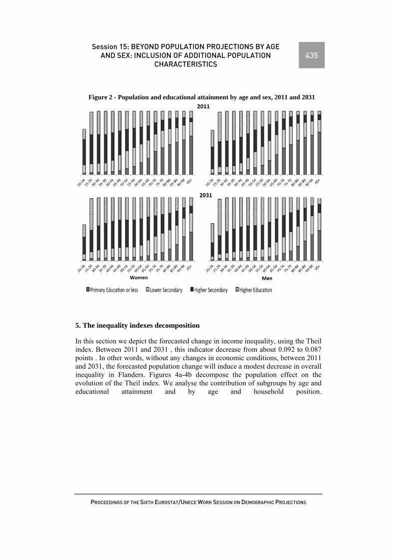
Session 15: BEYOND POPULATION PROJECTIONS BY AGE AND SEX: INCLUSION OF ADDITIONAL POPULATION
CHARACTERISTICS435
PROCEEDINGS OF THE SIXTH EUROSTAT/UNECE WORK SESSION ON DEMOGRAPHIC PROJECTIONS
Figure 2 - Population and educational attainment by age and sex, 2011 and 2031
5. The inequality indexes decomposition
In this section we depict the forecasted change in income inequality, using the Theil index. Between 2011 and 2031 , this indicator decrease from about 0.092 to 0.087 points . In other words, without any changes in economic conditions, between 2011 and 2031, the forecasted population change will induce a modest decrease in overall inequality in Flanders. Figures 4a-4b decompose the population effect on the evolution of the Theil index. We analyse the contribution of subgroups by age and educational attainment and by age and household position.

436 Session 15: BEYOND POPULATION PROJECTIONS BY AGE
AND SEX: INCLUSION OF ADDITIONAL POPULATION CHARACTERISTICS
PROCEEDINGS OF THE SIXTH EUROSTAT/UNECE WORK SESSION ON DEMOGRAPHIC PROJECTIONS
Figure 3 - Decomposition of the change in Theil index
(a) Decomposition of the change in Theil index by age and educational attainment
(b) Decomposition of the change in Theil index by age and household position
The first bar at the left depicts the change in the between-groups Theil. The
other bars indicate each population group’s contribution to the overall inequality
change. This contribution depends on the inequality evolution within each group
and the group’s share of the total population’s income, represented in light and
dark grey bars respectively (cf. Equation (2)). The size of the bar indicates the size
of contribution to inequality change; upward means a positive impact, downward a
negative one. Note that the income share of each group plays the most important

Session 15: BEYOND POPULATION PROJECTIONS BY AGE AND SEX: INCLUSION OF ADDITIONAL POPULATION
CHARACTERISTICS 437
PROCEEDINGS OF THE SIXTH EUROSTAT/UNECE WORK SESSION ON DEMOGRAPHIC PROJECTIONS
role, while within-group shifts have mostly only modest effects. Since we work
under the assumption of “no economic change”, the within-group inequality
change is only due to modifications in the unobserved variable composition (and
the sex composition) related to the forecasted population change. Under the same
assumption, it is clear that changes in the income share are largely driven by
changes in the population; a change in the prevalence of a population category
provokes an income share change in the same direction. This way we can directly
link the results of the Theil decomposition with the population change described in
Section 4.
Sub-figure 4a indicates that the overall decrease in inequality between 2011 and
2031 is related to two processes: a reduction of between-group inequality and a
decrease in income share of the population with no or only primary education. The
latter process is related to the general increase in educational attainment depicted in
Figure 2. The reduction of between-group inequality can easily be understood
through the attenuation of the generational differences in education. In contrast,
Sub-figure 4a also shows that the increase of the income share of individuals over
55 with secondary or higher education, increases inequality. In other words, ageing
and the subsequent growth of the elderly population increases inequality, despite
their higher educational attainment. This effect is however not enough to offset the
impact of the reduction in the lowest educational levels combined with the decrease
in between-group inequality.
Figure 4b decomposing the Theil by age and household position also reveals
that the growth of the elderly population’s income share positively contributes to
the Theil, weather living in a couple or in single-headed households. The decrease
of the adult population younger than 55 living in couples with children, has a
negative impact on inequality. Note however that the within-group inequality
among couples under 55 of the same age group increases. This can be understood
by the larger effect of education growth on the income of double-income
households than in households with only one income, leading to increased
dispersion. The between-group inequality decreases due to the before mentioned
diminishing generational inequality.
6. The income distribution
Section 5 showed that population change between 2011 and 2031 will decrease
inequality. It also indicated what population subgroups contribute to this process,
and which ones have a counteracting effect. The analysis however has two mayor
shortcomings. First, summary indicators such as the Theil do not tell us what part
of the income distribution is actually (most) affected. Is inequality reduced because
the lower end of the income distribution caches up, or because the upper end loses
ground? Secondly, a subgroup decomposition falls short on determining the effects
of covariates. While we saw for example that ageing increases inequality despite
the educational gains of the elderly population, this observation does not say
anything about the impact of ageing and educational change separately. In this
section, we will answer questions such as “how much would the impact of ageing
have been if no educational gains would have been recorded?”

438 Session 15: BEYOND POPULATION PROJECTIONS BY AGE
AND SEX: INCLUSION OF ADDITIONAL POPULATION CHARACTERISTICS
PROCEEDINGS OF THE SIXTH EUROSTAT/UNECE WORK SESSION ON DEMOGRAPHIC PROJECTIONS
In this section, we use the relative distribution method to complement the
analysis of Section 5. Figure 4 represents the income distribution of 2031 relative
to 2011. Panel (a) presents the overall relative distribution: the bars indicate the
gain (above the horizontal line at value 0) or loss (below the horizontal line at
value 0) by the year 2031 of each income decile in 2011 (cf. Section 3). We
observe a decrease of the extreme left tale of the distribution, while income
concentrates more in the lower middle part of the distribution. The highest income
level shares in the population is also emphasised. The graph is is congruent with
the observed decrease of the Theil and the poverty rate. They are related to the
decrease of the lowest income decile and the growth of the deciles towards the
middle of the distribution. Nevertheless, the entropy measure (entropy = 0.0258)
indicates that the income distribution is only modestly affected by population
change.
In Subsection 3, we explained that the relative distribution is the result of a shift
in the income level (median) and of a modifications in the shape of the distribution.
This is shown in panel (b) and panel (c) of Figure 4. We observe a slight increase
in median income level. The shape modification indicates a larger increase of the
highest income decile and the lower middle part of the distribution than one would
expect if income increase would have been evenly distributed.
Figure 4 - Decomposition of the overall change in income distribution in median and
shape shift.

Session 15: BEYOND POPULATION PROJECTIONS BY AGE AND SEX: INCLUSION OF ADDITIONAL POPULATION
CHARACTERISTICS 439
PROCEEDINGS OF THE SIXTH EUROSTAT/UNECE WORK SESSION ON DEMOGRAPHIC PROJECTIONS
Table 1- Polarization index, age, education and household position
Ageing Education Household comp. Index Pr [∣ I ∣> 0 ]
Index Pr [∣ I ∣> 0 ]
Index Pr [∣ I ∣> 0 ]
MPI -0,008 0,163 0,012 0,055 -0,002 0,409 LPI -0,042 0,004 0,048 0,001 -0,019 0,113 RPI 0,027 0,044 -0,023 0,061 0,015 0,167
Figure 5 decomposes the effect of the overall population change on the income
distribution into the impact of ageing, changes in household composition and
educational advancement on the income distribution separately. These pictures
show the relative distribution of 2031 versus 2011 if only the age, household or
educational composition changed, keeping all other marginals as in the baseline
year 2008. In absence of any other population change, ageing and changes in
household composition increase the lower end of the income distribution.
Educational advancement in contrast favours the higher part of the income
distribution and decreases the share of the population in at the lower end. In
addition, Table 1 indicates that educational change increases the polarization in the
left tale of the distribtuion, while decreasing polarization in the upper tale. Ageing
has the opposite effect. In other words, the change in prevalence of the different
population covariats has counteracting effects on the income distribution. They
alter the proportion of individuals with low or high income levels in opposite ways,
not only by increasing/decreasing the median income level but also by broading or
crushing the distributional shape in opposite directions. The result is the small
distributional change and the absence of overall polarization observed in Figure 4.
Figure 5 - Decomposition of demographic effect in age, household composition and
educational effect
(a) Ageing (b) Education (c ) Household compostion

440 Session 15: BEYOND POPULATION PROJECTIONS BY AGE
AND SEX: INCLUSION OF ADDITIONAL POPULATION CHARACTERISTICS
PROCEEDINGS OF THE SIXTH EUROSTAT/UNECE WORK SESSION ON DEMOGRAPHIC PROJECTIONS
7. Conclusion
In this paper, we analysed changes in income distribution and inequality in
Flanders, Belgium, between 2011 and 2031, and demonstrated how they are related
to population change. We used multi-state population projections (Lipro-
projections) and reweighting procedures to construct the necessary population and
income data in 2011 and 2031. An important feature of our approach is the we
assume absence of economic progress; we demonstrate, ex ante, the effect that
would have projected population change in absence of all other possible societal or
behavioural modifications. We decomposed the Theil inequality measure, and
applied relative distribution methods and quantile regression highlight the
relationship between population change and income inequality from different
viewpoints. These analytical frames provide pieces of the answer to our research
question : Can we disentangle the demographic elements most affecting inequality,
and single out socio-demographic groups moving to the lower or upper end of the
distribution?
Our population projection models foresee a pronounced ageing of the Flemish
population between 2011 and 2031. Parallell, the household and educational
composition of the region will also change, as with the ageing process, family
formation behaviour and educational levels of each generation in the current
population are transferred to older age groups. Consequently, the projection results
demonstrate an increase of single headed households to the detriment of couples,
especially with children. Educational attainment levels increase and
intergenerational and gender differences in education attenuate.
In the next step of our analysis, we linked these population changes to
adjustments in income inequality. Overall, between 2011 and 2031, we found a
modest inequality reduction. This reduction is related to the decrease of the adult
population with no or only primary education as well as the reduction of
intergenerational differences in education. We also found an attenuating effect of
the decrease in the prevalence of couples with children. The increase of the elderly
population inhibits the inequality reduction, independently of the household
position and despite their better educational profile.
Using the relative distribution method and counterfactual decomposition, we
analysed the changes in income distribution in more detail. This analysis revealed
influences of the population covariates seperately: educational advancement
increases the share of people with higher income levels and decreases the lower
end of the distribution; ageing and modifications in the population’s household
composition have exactly the opposite effect. In addition, education narrows the
left tale of the distribution, while increases polarization of the upper tale. Ageing
does exactly the opposite. These counteracting covariate effects clarify the only
modest modification in income inequality due to population change.

Session 15: BEYOND POPULATION PROJECTIONS BY AGE AND SEX: INCLUSION OF ADDITIONAL POPULATION
CHARACTERISTICS 441
PROCEEDINGS OF THE SIXTH EUROSTAT/UNECE WORK SESSION ON DEMOGRAPHIC PROJECTIONS
REFERENCES
Breen, R., Salazar, L., 2010. Has increased women’s educational attainment led to
greater earnings inequality in the United Kingdom? A multivariate
decomposition analysis. European Sociological Review 26, 143–157.
Burtless, G., 1999. Effects of growing wage disparities and changing family
composition on the U.S. income distribution. European Economic Review 43 (4-
6), 853–865.
Daly, M. C., Valletta, R. G., 2006. Inequlity and poverty in the United States: The
effects of rising dispersion and men’s earnings and changing family behaviour.
Economica 73 (289), 75–98.
De Blander, R., Schockaert, I., Decoster, A., Deboosere, P., 2013. The impact of
demographic change on policy indicators and reforms. FLEMOSI Discussion
Paper DP25, CES - KU Leuven.
Deville, J.-C., Sarndal, C.-E., 1992. Calibration estimators in survey sampling.
Journal of the American Statistical Association 87 (418), 376–382.
DiNardo, J., Fortin, N. M., Lemieux, T., 1996. Labor market institutions and the
distribution of wages, 1973-1992: A semiparametric approach. Econometrica 64
(5), 1001–1044.
Esping-Andersen, G., 2007. Sociological explanations of changing income
distributions. American Behavioral Scientist 50 (5), 639–658.
Handcock, M. S., Aldrich, E. M., 2002. Applying relative distribution methods in
R. Working Paper 27, Center for Statistics and the Social Sciences, University of
Washington.
Handcock, M. S., Morris, M., 1998. Relative distribution methods. Sociological
Methodology 28 (1), 53–97.
Handcock, M. S., Morris, M., 1999. Relative Distribution Methods in the Social
Sciences. Statistics for Social Science and Behavorial Sciences. Springer.
Hyslop, D. R., Maré, D. C., 2005. Understanding New Zealand’s changing income
distribution, 1983-1998: A semi-parametric analysis. Economica 72 (287), 469–
495.
Kalton, G., Flores-Cervantes, I., 2003. Weighting methods. Journal of Official
Statistics 19 (2), 81–97.
Kollmeyer, C., 2013. Family structure, female employment, and national income
inequality: A cross-national study of 16 Western countries. European
Sociological Review 29 (4), 816–827.
Lesthaeghe, R., Deboosere, P., Surkyn, J., Boulanger, P. M., Lambert, A., 1997.
Huishoudens en Gezinnen in België. No. 4 in Census Monograph. National
Institute for Statistics Belgium, Brussels.

442 Session 15: BEYOND POPULATION PROJECTIONS BY AGE
AND SEX: INCLUSION OF ADDITIONAL POPULATION CHARACTERISTICS
PROCEEDINGS OF THE SIXTH EUROSTAT/UNECE WORK SESSION ON DEMOGRAPHIC PROJECTIONS
Peichl, A., Pestel, N., Schneider, H., 2012. Does size matter? the impact of changes
in household structure on income distribution in Germany. Review of Income &
Wealth 58 (1), 118–141.
Schockaert, I., Surkyn, J., 2012. Snapshots of our future families. FLEMOSI
Discussion Paper 12, VUB.
Studiedienst Vlaamse Regering, 2011. Svr-projecties van de bevolking en de
huishoudens voor vlaamse steden en gemeenten, 2009–2030. SVR-internet page,
Brussels.
Van Imhoff, E., Keilman, N. W., 1991. LIPRO 2.0: An Application of a Dynamic
Demographic Projection Model to Household Structure in the Netherlands.
Swets and Zeitlinger B.V., Amsterdam.

Session 15: BEYOND POPULATION PROJECTIONS BY AGE AND SEX: INCLUSION OF ADDITIONAL POPULATION
CHARACTERISTICS443
PROCEEDINGS OF THE SIXTH EUROSTAT/UNECE WORK SESSION ON DEMOGRAPHIC PROJECTIONS
MICROSIMULATION OF LANGUAGE CHARACTER-ISTICS AND LANGUAGE CHOICE IN MULTILIN-
GUAL REGIONS WITH HIGH IMMIGRATION
Patrick Sabourin, Alain Bélanger Summary
In this paper, we present the results of a microsimulation model projecting lan-guage characteristics – mother tongue, language spoken at home and knowledge of French and English – of the Canadian population. Globally and locally, French is declining in Canada, for all projected variables, whereas non-official languages are generally soaring due to relatively large immigration intakes. Results of the projections show that immigration has a larger impact on the linguistic equilibrium of a multilingual region such as Québec (a French province of Canada) than in a largely monolingual region like the rest of Canada. Competition between French and English in Québec adds further complexity to the language dynamics. Keywords: language, microsimulation, Canada
1. Introduction
Language is a ubiquitous element of our everyday life. Not only is it essen-tial to human communication in general, it is also a vector of culture and identi-ty. The first language learnt at home in childhood generally constitutes a major piece of the self, a mean to define one’s identity and to construct one’s own world views. Although most of the people around the world make use of their mother tongue in their daily activities, many, such as national minorities and immigrants, have to use a second or a third language to get by in their public life. Knowledge of a society’s dominant language constitutes a fundamental prerequisite to economic and cultural integration. In time, simple integration turns into linguistic assimilation as immigrants or their children abandon their mother tongue to use the host society’s dominant language at home. Such as-similation of immigrant languages usually occurs within less than three genera-tions (Rumbaut, Massey, and Bean 2006; Bélanger, Lachapelle, and Sabourin 2011), but some exceptions do exist.

444 Session 15: BEYOND POPULATION PROJECTIONS BY AGE
AND SEX: INCLUSION OF ADDITIONAL POPULATION CHARACTERISTICS
PROCEEDINGS OF THE SIXTH EUROSTAT/UNECE WORK SESSION ON DEMOGRAPHIC PROJECTIONS
Language characteristics are seldom included in national projection models. Canada constitutes an exception to this rule, mainly because data on language uses and characteristics is abundant in census and surveys alike. This is mostly explained by the fact that Canada has put its official languages – English and French – at the core of its constitution, political symbolism and founding my-thology. The Canadian census includes seven questions related to language use and language proficiency, three of which are part of the projections presented in this paper: mother tongue, language spoken most often at home, and knowledge of official languages. Combining these variables allows for the creation of use-ful derived variables, such as the first official language spoken (used by the Federal government to plan services to minority language communities) or the official language proficiency (OLP) variable, designed for the study of over-qualification. This latter variable turns out to be well correlated to economic success as well, especially for immigrants with a university degree, as can be seen in table 1 below.
Table 1 – Total income of individuals with a university degree according to immi-grant status, region of residence and Official language proficiency (source: 2006 census). MT = mother tongue; LS = language spoken at home; KOL-X = knowledge of X official languages; NO = non official; O = official. Arrow indicates increasing level of proficiency
Official language proficiency
Canada outside Qc Québec
Natives Immigrants Natives Immigrants
1 (MT-NO; LS-NO; KOL-0) --
15 226 $ -- 15 136 $
2 (MT-NO; LS-NO; KOL-1) 43 645 $ 36 116 $ 44 983 $ 23 705 $
3 (MT-NO; LS-NO; KOL-2) 41 091 $ 44 069 $ 42 892 $ 34 210 $
4 (MT-NO; LS-O; KOL-1) 64 658 $ 53 872 $ 47 833 $ 35 824 $
5 (MT-NO; LS-O; KOL-2) 62 106 $ 66 490 $ 58 250 $ 49 842 $
6 (MT-O; LS-O; KOL-1) 67 165 $ 68 724 $ 48 546 $ 45 917 $
7 (MT-O; LS-O; KOL-2) 64 256 $ 71 777 $ 63 390 $ 55 969 $
Canada is well settled in a low-fertility, rapid-ageing and high-immigration
demographic regime. The annual influx of immigrants continuously modifies the country’s demographic and linguistic landscape. Fertility is low among both English and French Canadians, and about two thirds of the Canadian population growth is due to an increasingly diverse immigration. Between 2001 and 2006, Canada's foreign-born population increased by 14% – four times faster than the growth rate of the Canadian-born population during the same period – and most immigrants have a mother tongue that is neither English nor French. Conse-

Session 15: BEYOND POPULATION PROJECTIONS BY AGE AND SEX: INCLUSION OF ADDITIONAL POPULATION
CHARACTERISTICS445
PROCEEDINGS OF THE SIXTH EUROSTAT/UNECE WORK SESSION ON DEMOGRAPHIC PROJECTIONS
quently the share of the Allophone population – those having a non-official lan-guage as a mother tongue – is growing rapidly: from 18.0% in 2001 to 20.5% in 2011.
In this paper, we will present the results of a microsimulation model simul-taneously projecting three language variables. In the past, only one of these lan-guage dimensions had been projected in a single model. Termote’s multistate model (Termote, Thibault, and Payeur 2011; Termote and Thibault 2008) in-cluded language spoken at home whereas Statistics Canada’s Demosim only projected mother tongue (Caron Malenfant, Lebel, and Martel 2010). Including all three variables in the model allows us to get a more complete picture and to provide projections of derived variables, whose relevance has been shown above in relation to income. Furthermore, the microsimulation model allows for easy inclusion of important determinants of language shift, such as place of birth or duration of residence for immigrants having a mother tongue that is nei-ther French nor English.
2. Methods
The results were obtained from Hermès, a cased-based, open, dynamic, continuous-time projection model implemented using Modgen, a microsimula-tion programming language developed at Statistics Canada. The geographical template used in the model takes into account the location of immigrants as well as the concentration of official language minorities (i.e. English in Québec and French in the rest of Canada). Although the model includes 19 regions to ac-count for regional dynamics, only the results for the province of Québec and the rest of Canada will be discussed in this paper. The base population used in the model is taken from the 2006 census confidential microdata. Life course events were implemented in various demographic and linguistic modules, whose input parameters are briefly described below.
Differentials in age-specific fertility rates according to the place of resi-dence and language spoken at home were estimated from census data using the own-children method (Desplanques 1993; Cho, Retherford, and Choe 1986). Total fertility rates in 2011 were 1.61 for Canada (including Québec) and 1.69 in Québec.
Age-specific death rates (ASDR) were taken from provincial vital statistics. ASDR were not allowed to vary according to language characteristics as the da-ta is generally unreliable or simply unavailable.
Characteristics of cohorts of immigrants entering the model are taken from the characteristics of recent immigrants in the 2006 census (arrived between 2000 and 2006). The model allows for the geographical and linguistic (mother tongue, see table 2 below) distribution of immigrants to be modified in order to create different scenarios related to the composition of immigration.

446 Session 15: BEYOND POPULATION PROJECTIONS BY AGE
AND SEX: INCLUSION OF ADDITIONAL POPULATION CHARACTERISTICS
PROCEEDINGS OF THE SIXTH EUROSTAT/UNECE WORK SESSION ON DEMOGRAPHIC PROJECTIONS
Net international outmigration rates were estimated by Statistics Canada and sum up to a global annual rate of approximately one per thousand. In the model, relative risks are also inserted so that recent immigrants make up for about 80% of international out-migrants, to reflect the fact that net international migration rates are small for Canadian-born individuals.
Annual probability of internal outmigration (i.e. getting out of a region) was estimated using census data and a logit model controlling for age, sex, lan-guage spoken at home, region of residence, and immigrant status. Once a migra-tion event occurs in the model, the destination region is determined through an origin-destination matrix, which varies according to language spoken at home.
Mother tongue is defined as the first language learned at home in child-hood. It can take one of three values: French, English, or Others. In Québec, the “Others” category is further split in three different sub-categories: Others-Eng, Others-Fr, and Others. Suffix “Eng” and “Fr” describe the tendency of immi-grants to choose English (Eng) or French (Fr) according to their ethnic or lin-guistic origin when making a language shift. For instance, immigrants having a Latin mother tongue or coming from the Francophonie have a strong tendency to speak French at home, whereas immigrants from the Commonwealth tend to use English. Québec has an immigration policy favoring selection of immi-grants from the “Fr” category. In the Canadian demolinguistic jargon, “Others-Fr” are called “francotropes” and “Others-Eng” are called “anglotropes”. We should note that these distinctions are quite useless outside of Québec, as virtu-ally all immigrants to these regions choose English when making a language shift. Table 2.1 below shows the linguistic distribution of recent immigrants in Québec and in the rest of Canada.
Table 2 – Linguistic distribution of immigrants arrived between 2000 and 2006 (Mother tongue, Canadian 2006 census)
Canada outside Qc Québec
English 16,4% 4,8%
French 1,0% 19,8%
Others - Eng 82,6% 22,4%
Others - Fr N/A 49,2%
Others N/A 3,8%
In the model, mother tongue is determined at birth through an origin-
destination matrix linking the mother’s mother tongue to her child’s mother tongue, and no modification is allowed afterwards. The matrix is estimated us-ing census data and changes according to the mother’s language spoken at home, her region of residence, and her immigrant status.
Language spoken most often at home can take one of three values: French, English, or Others. In the model, it is set at birth to be equal to the mother tongue. Actors in the model are then submitted to the risk of making a language

Session 15: BEYOND POPULATION PROJECTIONS BY AGE AND SEX: INCLUSION OF ADDITIONAL POPULATION
CHARACTERISTICS447
PROCEEDINGS OF THE SIXTH EUROSTAT/UNECE WORK SESSION ON DEMOGRAPHIC PROJECTIONS
shift, which may only occur between the age of 0 and 49. The probability of shifting was determined using a method developed in a previous version of the model (Sabourin and Bélanger 2011).
Knowledge of official languages was determined using a technique similar to the one used above for language shift. Rates of acquisition of French and English were estimated as a function of region of residence, mother tongue, and immigrant status.
3. Scenarios
Scenarios are designed to illustrate possible policy orientations affecting language dynamics in Canada.
The base scenario is constructed on recent trends for all characteristics and demographic events, that is, for Canada as a whole: a total fertility rate of 1.61; a life expectancy of 78 years for men (84 at the end of the simulation) and 83 years for women (87 at the end of the simulation); the internal mobility rates observed from 2005 to 2006; an annual international immigration intake of 250,000 (with characteristics of immigrants arrived between 2000 and 2006); and language shifts of immigrants arrived between 1986 to 2006.
Two scenarios focus on the global impact of immigration, one by increas-ing immigration volume by 20% (300,000 immigrants, total) and the other by decreasing it by 20% (200,000 immigrants, total).
Since high or low immigration volumes are likely to be a policy response to low or high fertility regimes, two more scenarios are implemented where high immigration is matched with low fertility (recent trend minus 10%) and low immigration is matched with high fertility (recent trend plus 10%).
Since language choice of first and second generation immigrants is an im-portant issue in Québec, scenarios modifying language shift behaviour and lan-guage composition of immigration are also implemented. Two scenarios attrib-ute language preferences of anglotropes (“Others-Eng”) or francotropes (“Oth-ers-Fr”) to all individuals having a non-official mother tongue. These scenarios are far-fetched in the short term because overnight changes in language choice patterns are sociologically unlikely. Nevertheless, they still provide a useful range of possible outcomes under different language shift regimes. Before lan-guage laws were first adopted in Québec in the 70s, language choices of immi-grants were in fact close to the anglotropes scenario, regardless of their ethnic or linguistic origins.
Two more scenarios hold language preferences constant while modifying the linguistic composition of immigration. This composition is modified so that the number of anglotropes or immigrants having English as a mother tongue are doubled or halved. These scenarios help to investigate the impact of Québec’s selection policy of immigrants. Recently, the government modified the selection

448 Session 15: BEYOND POPULATION PROJECTIONS BY AGE
AND SEX: INCLUSION OF ADDITIONAL POPULATION CHARACTERISTICS
PROCEEDINGS OF THE SIXTH EUROSTAT/UNECE WORK SESSION ON DEMOGRAPHIC PROJECTIONS
grid in order to favor French and francotrope immigrants. An intermediate level of French is now required to be selected as an economic immigrant in Québec.
Finally, a scenario is used to examine the impact of an increase in French immigration in Canada outside of Québec. This scenario investigates the possi-ble long-term impact of a policy that is being implemented by Citizenship and Immigration Canada in order to linguistically revitalize French communities liv-ing in minority contexts.
Table 3 –Summary of all scenarios
Scenario Immigration
volume
Linguistic composition of
immigration Language shift Fertility
Base 250,000 Recent Recent Recent
Imm + 300,000 Recent Recent Recent
Imm - 200,000 Recent Recent Recent
Imm + Fer - 300,000 Recent Recent -10%
Imm - Fer + 200,000 Recent Recent +10%
Imm Eng Qc + 250,000 50% more Eng and Oth-ers-Eng in Qc
Recent Recent
Imm Eng Qc - 250,000 50% less Eng and Others-Eng in Qc
Recent Recent
Shift FR Qc + 250,000 Recent All shifts like Others-Fr in Qc
Recent
Shift FR Qc - 250,000 Recent All shifts like Others-Eng in Qc
Recent
Imm FR ROC + 250,000 Number of Fr immigrants doubled in the rest of
Canada
Recent Recent
4. Results
Results from the base scenario are briefly presented for all three language variables: mother tongue, language spoken at home and knowledge of official languages. A more detailed account is presented for language spoken at home. The linguistic composition of the population in 2006 is compared to the project-ed population in 2056. The 50 years horizon of the projection is relatively long, but necessary to fully reveal the effects of intergenerational language shifts.
Variations are most important for mother tongue characteristics. In Cana-da outside Québec, the proportion of Anglophones and Francophones drops by 6.1 and 1.7 points, from 73.3% and 4.1%, respectively (table 4.1). The propor-tion of individuals having a mother tongue that is not an official language in-creases from 20.3% to 28.9%. In Québec, the English group is relatively stable (+0.6), while French drops by 11.7 points and the non-official language group increases by 11.2 points.

Session 15: BEYOND POPULATION PROJECTIONS BY AGE AND SEX: INCLUSION OF ADDITIONAL POPULATION
CHARACTERISTICS449
PROCEEDINGS OF THE SIXTH EUROSTAT/UNECE WORK SESSION ON DEMOGRAPHIC PROJECTIONS
Table 4 – Projection results for three language characteristics and two regions, base scenario, Hermès
Canada outside
Québec Québec
2006 2056 2006 2056
Mother tongue
English 73,3% 67,2% 8,2% 8,8%
French 4,1% 2,4% 79,5% 67,8%
Others - E 22,6% 29,7% 5,8% 8,6%
Others - F 0,0% 0,6% 5,8% 13,4%
Others 0,0% 0,1% 0,7% 1,5%
Language spoken at home
English 84,2% 83,2% 10,6% 12,0%
French 2,5% 1,5% 81,8% 77,0%
Others 13,2% 15,3% 7,6% 11,1%
Knowledge of official languages
English 87,3% 86,5% 4,6% 5,7%
French 0,5% 0,3% 53,7% 41,1%
Both 10,2% 12,0% 40,7% 52,5%
None 1,9% 1,1% 1,0% 0,8%
Changes were smaller for language spoken at home, as linguistic mobility
constantly “redistribute” speakers from third languages to official language groups. In Canada outside of Québec, English and French both decrease by 1 point, whereas the proportion of third languages increases by 2.1 points. In Québec, French decreases by 4.8 points from 81.8%, while English increases by 1.4 point and non official languages increase by 3.4 points.
Results related to knowledge of official languages in Canada outside Qué-bec show a global increase in the knowledge of English and French, as a slight decrease in monolingual English (-0.8) and monolingual French (-0.2) individu-als is compensated by an increase in bilingual individuals (+1.8). In Québec, the proportion of monolingual French individuals decreases strongly from 53.7% to 41.1% (-12.6).
In Canada as a whole, the proportion of French speakers decreases for all language characteristics (data not shown). This is partly due to the fact that the Canadian population increases faster outside Québec where English is domi-nant.
In order to better understand the demographical dynamics at play, we plot the components of growth for French or English as a language spoken at home, for both Québec and the rest of Canada (Figure 1). Comparing the French ma-jority in Québec to the English majority in the rest of Canada (Figure 1, panels B and C), we see that both groups benefit in similar ways from international migration and from internal migration. Natural increase, however, declines more rapidly for French in Québec than for English in the rest of Canada, yet

450 Session 15: BEYOND POPULATION PROJECTIONS BY AGE
AND SEX: INCLUSION OF ADDITIONAL POPULATION CHARACTERISTICS
PROCEEDINGS OF THE SIXTH EUROSTAT/UNECE WORK SESSION ON DEMOGRAPHIC PROJECTIONS
fertility and mortality rates are similar for the two groups. This might be ex-plained by the fact that fertility rates dropped earlier in Québec than in the rest of Canada after the Baby Boom, and also by the fact that English in Canada gets more benefits from language shift, as new “English-speaking mothers” are cre-ated through language shift and can then generate English-speaking children. French in Quebec doesn’t benefit as much from language shift as English does in the rest of Canada.
Figure 1 – Components of growth for Québec and Canada, population groups by language spoken at home, base scenario, Hermès
Looking at minority languages – English in Québec and French in the rest
of Canada – we see two contrasting situations (Figure 1, panels A and D). Whereas both groups gain from international migration, English in Québec makes large gains from language shift, while French speakers in the rest of Canada are shifting to English, thus erasing any potential gains from immigra-tion.
−0.8
−0.6
−0.4
−0.2
0
0.2
0.4
0.6
0.8
2010 2020 2030 2040 2050
Gro
wth
(%
)
Year
English, Québec
A
Natural increaseInternational migration
Internal migrationLanguage shift
−0.8
−0.6
−0.4
−0.2
0
0.2
0.4
0.6
0.8
2010 2020 2030 2040 2050
Gro
wth
(%
)
Year
French, Québec
B
−0.8
−0.6
−0.4
−0.2
0
0.2
0.4
0.6
0.8
2010 2020 2030 2040 2050
Gro
wth
(%
)
Year
English, rest of Canada
C
−0.8
−0.6
−0.4
−0.2
0
0.2
0.4
0.6
0.8
2010 2020 2030 2040 2050
Gro
wth
(%
)
Year
French, rest of Canada
D

Session 15: BEYOND POPULATION PROJECTIONS BY AGE AND SEX: INCLUSION OF ADDITIONAL POPULATION
CHARACTERISTICS451
PROCEEDINGS OF THE SIXTH EUROSTAT/UNECE WORK SESSION ON DEMOGRAPHIC PROJECTIONS
For Québec’s English minority, internal migration is the only source of de-cline. This demographic trend is well-known and explains part of the communi-ty’s constant decline in Québec throughout the past decades. Internal migration for French in the rest of Canada is negative at the beginning of the simulation, but turns positive around midway. This is to be expected as the decline of the French population outside Québec reduces the number of French speaking mi-grants to Québec, whereas the number of French Quebecers moving to the rest of Canada is increasing. Finally, as was observed for majority language com-munities, natural growth for French minorities in the rest of Canada declines steadily and becomes negative at the middle of the simulation. Despite having similar net reproduction rate, natural growth for English in Québec is declining very slowly and never becomes negative.
We can now turn to the effect of the different scenarios on language spoken at home. Figure 2 below shows the proportion of French speakers among offi-cial language speakers in Québec. All but one scenarios show a decline of the relative weight of French among official languages in Québec. Only the scenar-io assuming larger shifting rates to French allows for a stabilisation of the French-speaking population of the province.
Figure 2 – In Québec, proportion of French speakers among speakers of an official language, various scenarios, Hermès
. The two scenarios showing the most important effects are indeed the ones
affecting language shift behaviours of individuals with non-official mother tongue. This is to be expected as those scenarios are rather unlikely in the short term and are mainly implemented to establish the potential long-term outcome of language policies. The second most noteworthy scenarios are the ones where the linguistic composition of immigration is modified. Increase or decrease of immigration, with no change in language behaviour or language composition of
83
84
85
86
87
88
89
90
1990 2000 2010 2020 2030 2040 2050 2060Pro
port
ion
Fre
nch
amon
g of
ficia
l lan
guag
es (
%)
Year
BaseImm +Imm −Imm +, Fer −Imm −, Fer +Shift Fr Qc −Shift Fr Qc +Imm Eng Qc +Imm Eng Qc −

452 Session 15: BEYOND POPULATION PROJECTIONS BY AGE
AND SEX: INCLUSION OF ADDITIONAL POPULATION CHARACTERISTICS
PROCEEDINGS OF THE SIXTH EUROSTAT/UNECE WORK SESSION ON DEMOGRAPHIC PROJECTIONS
immigration, have little impact on the projection outcomes. Finally, changing fertility levels doesn’t significantly shift the balance between the two official languages.
Contrary to what is observed in Québec, the share of majority language speakers in the rest of Canada is increasing steadily for all scenarios, although less (in %) than French is declining in most scenarios in Québec (data not shown). This is due to the fact that, outside Québec, French and third language speakers are rapidly assimilating to English. Increasing French speaking inter-national migration cannot compensate for this relative decline of French speak-ers. Even the scenario where French immigration is doubled has hardly any ef-fect. Contrasting with what was observed in the Québec situation, English is an absorbing state in the rest of Canada as far as language shift is concerned, and changing immigration levels, fertility, or linguistic composition of newcomers has virtually no effect on the evolution of its increasingly dominant position.
Looking at non-official language speakers in Canada outside of Québec, we find that most scenarios predict that their proportion will plateau in the next decades (Figure 3). In some scenarios, it is also possible to observe a small de-cline in their proportion at the end of the simulation. This is due to the increas-ing importance of language shifts with respect to the flux of immigrants, and to the increasing proportion of second generations among non-official language speakers, which tend to shift and adopt English even more often. This demon-strates that in a mostly monolingual region, despite the fact that an increase in immigration levels can significantly change the current linguistic composition of the population, in the longer term, the effect of high immigration is damp-ened by the language shifts operated by the second generation of immigrants (Rumbaut, Massey, and Bean 2006). It also constitutes a form of rebuttal of the alarmist point of view on language “invasion” (Hungtinton 2004).
In Québec, the non-official language population increases throughout the whole simulation for all scenarios, but reaches only the level initially observed in the rest of Canada (data not shown). This is because immigration rates in Québec are lower than in the rest of Canada, and because the increase of immi-gration influx is more recent. A slight deceleration in this increase may be ob-served at the end of the simulation for the scenario with lower immigration in-takes and higher fertility, but a longer projection period would lead to a deceler-ation for all scenarios in a manner similar to what was observed for the rest of Canada (Figure 3).

Session 15: BEYOND POPULATION PROJECTIONS BY AGE AND SEX: INCLUSION OF ADDITIONAL POPULATION
CHARACTERISTICS453
PROCEEDINGS OF THE SIXTH EUROSTAT/UNECE WORK SESSION ON DEMOGRAPHIC PROJECTIONS
Figure 3 – In Canada outside Québec, proportion of non-official language speakers in the total population, various scenarios, Hermès
We now look at the effect of different scenarios on the Official language
proficiency indicator in 2056 in comparison with 2006 (Table 5). Since scenari-os modifying language behaviour or language composition of immigration don’t have a big impact on this derived variable, they will be excluded from this part of the analysis.
Results for all scenarios are qualitatively similar to the ones obtained from the base scenario. All scenarios show a significant increase in the proportion of official language speakers having a non-official mother tongue. The increase is smallest for the Imm-Fer+ (from 10.3% to 17.5%) and largest for the Imm+Fer- scenario (from 10.3% to 21.1%), with Imm+ and Imm- falling in between. High immigration scenarios also further increase the proportion of the population speaking a non-official language at home and having a non-official mother tongue, which was shown to be the economically less favoured group.
8
10
12
14
16
18
1990 2000 2010 2020 2030 2040 2050 2060
Pro
port
ion,
non
−of
ficia
l lan
guag
es (
%)
Year
BaseImm +Imm −Imm +, Fer −Imm −, Fer +

454 Session 15: BEYOND POPULATION PROJECTIONS BY AGE
AND SEX: INCLUSION OF ADDITIONAL POPULATION CHARACTERISTICS
PROCEEDINGS OF THE SIXTH EUROSTAT/UNECE WORK SESSION ON DEMOGRAPHIC PROJECTIONS
Table 5 – Distribution of population aged 15 to 65 according to Official language proficiency index (see table 1.1 for definition), various scenarios, Hermès. Larger index means higher language proficiency
Official language
proficiency 2006 Base Imm + Imm - Imm + Fer - Imm - Fer +
Québec
1 0,4% 0,4% 0,4% 0,3% 0,4% 0,3%2 3,2% 4,2% 4,6% 3,7% 4,9% 3,5%3 3,2% 5,7% 6,3% 5,0% 6,5% 4,8%4 1,6% 4,2% 4,6% 3,8% 4,7% 3,7%5 4,0% 11,8% 12,8% 10,7% 13,2% 10,4%6 47,3% 33,8% 32,6% 35,2% 32,0% 35,7%7 40,3% 39,9% 38,8% 41,2% 38,3% 41,5%
Rest of Canada
1 1,2% 0,7% 0,8% 0,6% 0,8% 0,6%2 11,2% 11,8% 13,0% 10,5% 13,6% 10,1%3 0,5% 1,2% 1,3% 1,0% 1,3% 1,0%4 9,3% 16,6% 17,6% 15,4% 18,1% 15,0%5 1,0% 2,7% 2,9% 2,5% 3,0% 2,5%6 67,2% 58,4% 56,2% 61,0% 55,1% 61,9%7 9,7% 8,6% 8,3% 8,9% 8,1% 9,0%
5. Discussion and conclusion
Results of the projections show that immigration has a much larger impact on the linguistic equilibrium of a multilingual region like Québec than in a largely monolingual region like the rest of Canada. Competition between French and English in Québec adds further complexity to the language dynam-ics.
Globally and locally, French is declining in Canada, for all projected varia-bles. In Canada outside Québec, French will over time represent a negligible portion of the population. This may lead to difficult political situations as the demographic justification to maintain a nationwide policy of institutional bilin-gualism will get ever thinner. Even in Ontario, where the second largest popula-tion of French speakers is located, the dispersion and decrease of the minority population prompted the government to close the only French hospital in the province. The hospital was finally kept open after the Ontario Court of Appeal ruled in favour of the French communities at the end of a judiciary fight that lasted four years.
Increasing French immigration in Canada outside Québec doesn’t appear to be a suitable policy to maintain French vitality, at least country-wide. Perhaps some specific regions where the French minority is more important can benefit from it. Further analysis might shed light on this important issue.
In Québec, most scenarios show a decline in French relative to English, as well as in absolute terms. The population is also getting more and more bilin-gual, as knowledge of English increases fast. The English minority sees its share of the population increase, regardless of the language variable used to define

Session 15: BEYOND POPULATION PROJECTIONS BY AGE AND SEX: INCLUSION OF ADDITIONAL POPULATION
CHARACTERISTICS455
PROCEEDINGS OF THE SIXTH EUROSTAT/UNECE WORK SESSION ON DEMOGRAPHIC PROJECTIONS
them. Their right for services in their language doesn’t appear to be in jeopardy in Québec.
Projection results for a derived variable, the “official language proficien-cy”, show that the proportion of individuals relatively less favoured economi-cally – in part because of increased difficulties to fully integrate the labor mar-ket due to lower language skills – will be growing in the next decades, although important nuances need to be made regarding these findings. First, the weight of the least favored groups, speakers of a non-official language having a non-official mother tongue, is stabilized in the projection period and doesn’t increase much overall. Second, the proportion of bilingual speakers, which tend to have higher incomes, is increasing fast in Québec and a little bit in the rest of Cana-da. The increase in the proportion of people having a non-official mother tongue calls for increasing investment in language training in order to maximize their contribution to the country’s future prosperity.
The model has been thoroughly tested but still needs some fine-tuning: small discrepancies with respect to recent trends need to be investigated. The proportion of bilingual individuals in Canada outside Québec is increasing slowly in the model, but the 2011 census data showed an actual decline in bilin-gualism. This may be due to an overoptimistic hypothesis as to the rate of French learning by Canadian-born non-French speakers. It is also possible that the data from the 2006 and 2011 censuses are not comparable, as questionnaires and sample sizes were different (Corbeil and Houle 2013).
REFERENCES
Bélanger, A., R. Lachapelle, and P. Sabourin. 2011. Persistance et orientation linguistiques de divers groupes d’allophones. Office québécois de la langue française.
Caron Malenfant, É., A. Lebel, and L. Martel. 2010. “Projection de la diversité de la population canadienne, 2006 à 2031.” Statistique Canada.
Cho, L. -J., R. D. Retherford, and M. K. Choe. 1986. The own-children method of fertility estimation. Population Institute.
Corbeil, J. -P., and R. Houle. 2013. “Methodology Document on the 2011 Cen-sus Language Data.” Statistics Canada.
Desplanques, G. 1993. “Mesurer les disparités de fécondité à l’aide du seul re-censement.” Population (French Edition): 2011–2024.

456 Session 15: BEYOND POPULATION PROJECTIONS BY AGE
AND SEX: INCLUSION OF ADDITIONAL POPULATION CHARACTERISTICS
PROCEEDINGS OF THE SIXTH EUROSTAT/UNECE WORK SESSION ON DEMOGRAPHIC PROJECTIONS
Hungtinton, Samuel P. 2004. Who are we? The challenges to America’s nation-al identity. Simon & Schuster.
Rumbaut, R. G., D. S. Massey, and F. D. Bean. 2006. “Linguistic life expectan-cies: Immigrant language retention in Southern California.” Population and Development Review 32 (3): 447–460.
Sabourin, P., and A. Bélanger. 2011. “Microsimulation of language use at home in a multilingual region with high immigration.” International Microsimula-tion Association, Stockholm.
Termote, M., and N. Thibault. 2008. Nouvelles perspectives démolinguistiques du Québec et de la région de Montréal, 2001-2051. Office québécois de la langue française.
Termote, M., N. Thibault, and F. Payeur. 2011. Perspectives démolinguistiques du Québec et de la région de Montréal (2006-2056). Office québécois de la langue française.

Session 15: BEYOND POPULATION PROJECTIONS BY AGE AND SEX: INCLUSION OF ADDITIONAL POPULATION
CHARACTERISTICS457
PROCEEDINGS OF THE SIXTH EUROSTAT/UNECE WORK SESSION ON DEMOGRAPHIC PROJECTIONS
A METHOD FOR PROJECTING ECONOMICALLY ACTIVE POPULATION. THE CASE OF ANDALUSIA
Silvia Bermúdez, Juan Antonio Hernández, Joaquín Planelles
Summary
Population structure is changing. And so is concern on dependency and sustaina-bility. A key factor for evaluating ageing, dependency and sustainability is plausible development of the economically active population, both in absolute and relative numbers against their non-active counterpart. In this paper, we put forward a new cohort parametric model for projecting the economically active population. Keywords: projection, economically active population, parametric model.
1. Introduction
World population structure has come across dramatic changes over the last few decades. With the exception of several “demographic outliers”, mean lifespan kept growing during that period. Meanwhile, fertility rates decreased and/or remained very low. As this process is expected to continue in the coming future, there is a growing concern about population ageing, dependency and sustainability.
A key factor for evaluating all those issues is plausible development of the economically active population, both in absolute and relative numbers against their non-active counterpart. Future active population depends not only on pop-ulation structure, but also on individual willingness to work, something that ex-perienced equally dramatic changes in the past.
In this paper, we put forward a new method for projecting economically ac-tive population which we developed to project active population in Andalusia, the most populated of the Spanish regions (8.4 million inhabitants in January 2013). Therefore, hereunder we use Andalusian data -extracted from the Span-ish Labour Force Survey- to exemplify the model. Nonetheless, it could be used to project active population in other areas undergoing similar changes in their activity patterns, namely growing retirement age and gender convergence.
The model is a cohort parametric model, based on the two following empir-ical findings. First, women´s willingness to work is more affected by a “cohort-effect”, with younger generations of women showing increasingly similar la-

458 Session 15: BEYOND POPULATION PROJECTIONS BY AGE
AND SEX: INCLUSION OF ADDITIONAL POPULATION CHARACTERISTICS
PROCEEDINGS OF THE SIXTH EUROSTAT/UNECE WORK SESSION ON DEMOGRAPHIC PROJECTIONS
bour market behaviour to that of men. And second, the male age-specific active profile is more stable both across time and space than women´s. Major changes for males are found in entry and exit times from the labour market. Finally, con-sidering that labour patterns differ between genders, we allow for gender differ-ences in our projecting methodology.
Our suggested methodology to project male activity rates is similar, but not exactly the same as, other methods developed elsewhere to project economical-ly active population. Thus, the main novelty we introduce is to be found in fe-male methodology, which explicitly models the convergence process in activity rates towards men´s.
The paper is organized as follows. In section 2 we present a general ap-proach to prospective works on the labour market, distinguishing between sup-ply-side and demand-side focuses. Section 3 summarizes recent trends in Euro-pean labour force. Section 4 develops the suggested methodology to project ac-tivity rates for men. Section 5 focuses on female methodology. In section 6 we briefly present results. Finally, the paper ends with concluding remarks in sec-tion 7.
2. Forecasting models in the labour market
Prospects in the labour market are focused either on the demand or the sup-ply sides of the market. Demand focused models aim to assess how many peo-ple will be required to work in the future, according to economic needs. Thus, these models depend mainly on economic variables such as expected GDP per-formance and structure, productivity, etc.
On the other hand, the active population is the number of people willing to work (supply). Therefore, it is made up of both people who actually fulfil their wish and people who don´t. That being so, supply focused models are intimately related to demographics instead of economics, as the future number of people willing to work depends on future population size and structure (at least, sex and age). In fact, we can express active population as a weighted average of differ-ent groups within population, where weight is given by their likeliness to supply labour force (their activity rates):
, ,, ,
, ,, , _ , , , ,
Where: x: age, x = 16,17, … ,74, 75+ s: sex, s = male, female t: calendar time, t = 2009, 2010, … , 2035 _ , , : activity rate for calendar year t, age x and sex s , , : mean population for calendar year t, age x and sex s

Session 15: BEYOND POPULATION PROJECTIONS BY AGE AND SEX: INCLUSION OF ADDITIONAL POPULATION
CHARACTERISTICS459
PROCEEDINGS OF THE SIXTH EUROSTAT/UNECE WORK SESSION ON DEMOGRAPHIC PROJECTIONS
Factoring labour supply into population groups and their activity rates ena-
bles to obtain future active population from population projections (which most likely will be already available) and a set of assumptions on future changes in activity rates.
The issue of projecting age and sex-specific activity rates will be addressed in the following sections. However, a few comments on future population are in order:
1. Population projections are widely available. They are nowadays standard products in statistical offices. Nonetheless, a check on their hypothesis is advis-able. Moreover, sometimes time horizon, or age-sex groups might be different from the ones required to project active population. If adequate population pro-jections are not available, they can be developed ad-hoc.
2. Certain population ratios extracted from population projections are used with a sense of future dependency in the labour market. That is the case of ‘po-tential actives’ (16 to 64) per ‘retired’ (65 or over). Although they provide a quick overview on underlying demographic trends, it is strongly misleading to extract from them conclusions on dependency. Those ratios could only have a sense of dependency under the historically fake hypothesis of stable activity rates. Active (or employed) population projections are required instead.
3. Finally, two comments on ageing. First, ageing is a process of change in the age-structure of population. That itself has significant effects on activity rates. For instance, age-specific activity rates might be expected to keep rising in the future and at the same time, global activity rates might be expected to fall instead. That would be due to the increasing number of senior citizens with low likeliness to remain active in the labour market. Under those circumstances, if goals are fixed in terms of global rates, it must be underlined that it will be a goal increasingly difficult to fulfil in terms of age-specific activity rates (that is also the case with the 75% employment rate goal established in “Europe 2020”).
And second (last but not least) ageing is a process which will have major implications for all facets of human life. Therefore, both individual and institu-tional labour market behaviours will change along with ageing. Active popula-tion projections should incorporate findings on the interaction ageing-labour be-haviour. That is to say, our model is only valid for the time being.
3. Past trends and driving forces in the labour supply
Table 1 contains participation rates for Andalusia and selected countries in Europe. Despite some “country specifics”, recent trends and main determinants are common for all European countries. We can summarize these trends and de-terminants as follows:

460 Session 15: BEYOND POPULATION PROJECTIONS BY AGE
AND SEX: INCLUSION OF ADDITIONAL POPULATION CHARACTERISTICS
PROCEEDINGS OF THE SIXTH EUROSTAT/UNECE WORK SESSION ON DEMOGRAPHIC PROJECTIONS
1. Prime-age men (25 to 49 years) kept a steady participation rate, above 90%. That is the highest among all population groups. On the contrary, older male workers’ participation was not that stable over time. Older workers’ activi-ty rates decreased in the 1990s, and grew thereafter. Moreover, as retirement schemes are changing all over Europe (basically, the legal retirement age is in-creasing) a further increase in activity rates might be expected for the coming future.
2. Female activity rates rose steadily over the last 20 years, showing an in-creasingly similar behaviour to males.
3. Young population participation and evolution is slightly different across countries. That is due to several social factors which remain different among the countries. That is the case with the length of schooling cycles, gender roles at home or the share of part-time employment on overall employment.
Table 1 - Historical participation rates. Andalusia and selected countries. 1990-2012
Age groupsCountry/Region 1990 2000 2012 1990 2000 2012 1990 2000 2012
Between 15 and 24 yearsANDALUSIA 46,9 42,5 39,1 51,1 47,0 40,6 42,4 37,9 37,5EU - 15 i47,2 47,5 45,6 i50,4 50,9 48,1 i44,0 44,1 43,1Germany 60,7 50,4 50,7 62,5 53,7 53,2 58,8 47,1 48,1Spain 47,0 43,1 38,8 51,6 46,7 40,2 42,6 39,4 37,4France 44,6 35,5 37,8 47,7 38,6 41,1 41,6 32,4 34,5Italy 46,8 38,1 28,7 50,7 42,2 33,1 43,0 34,0 24,0Netherlands 59,6 72,2 69,9 60,0 73,4 68,5 59,2 70,9 71,4Sweden i45,5 40,7 52,6 i44,2 41,1 51,8 i46,8 40,4 53,4United Kingdom 71,8 63,4 59,3 76,7 67,0 61,7 66,7 59,8 56,8
Between 25 and 49 yearsANDALUSIA 67,7 75,6 85,8 93,8 91,9 92,0 41,3 59,1 79,4EU - 15 i82,1 83,8 86,2 i93,6 93,6 92,6 i70,4 73,9 79,8Germany 80,9 86,1 87,9 94,0 94,1 93,3 67,4 77,8 82,3Spain 72,1 80,1 88,0 95,0 93,9 93,3 49,8 66,2 82,5France 85,2 87,4 88,9 96,6 95,2 94,2 74,0 79,7 83,8Italy 75,3 76,6 78,4 95,4 91,9 89,3 55,7 61,1 67,4Netherlands 78,0 85,6 88,4 94,6 95,0 93,4 60,6 76,0 83,5Sweden i89,9 86,5 90,7 i92,3 88,4 93,8 i87,3 84,6 87,5United Kingdom 84,8 84,8 85,9 95,9 93,0 92,7 73,8 76,8 79,1
50 years or overANDALUSIA 23,7 22,5 31,4 41,7 35,4 40,0 8,9 11,7 24,0EU - 15 i28,6 29,5 35,9 i39,6 39,1 42,9 i19,7 21,5 29,9Germany 32,9 31,0 39,6 49,0 40,2 46,2 20,7 23,3 33,9Spain 26,0 25,2 33,6 42,8 38,5 41,3 12,4 14,0 27,0France 26,0 27,5 33,9 34,2 33,3 38,2 19,5 22,7 30,2Italy 25,2 22,1 28,2 40,5 33,8 37,6 12,2 12,4 20,4Netherlands 25,2 31,8 42,0 38,9 42,8 50,5 13,5 21,9 34,2Sweden i52,1 41,8 44,3 i57,0 47,8 49,4 i47,4 36,7 39,6United Kingdom 34,1 36,2 40,8 45,8 44,6 47,1 24,6 28,9 35,1
Source: EUROSTAT and INE. Labor Force Survey. (i) Data from 1995
Total Males Females

Session 15: BEYOND POPULATION PROJECTIONS BY AGE AND SEX: INCLUSION OF ADDITIONAL POPULATION
CHARACTERISTICS461
PROCEEDINGS OF THE SIXTH EUROSTAT/UNECE WORK SESSION ON DEMOGRAPHIC PROJECTIONS
4. Projection of male activity rates
Methodology to project male activity rates is based on a cohort-approach. Nonetheless, we have seen in the previous section that male activity rates are rather stable over time and space. Major changes are localized regarding the en-try and exit of the male population into the workforce. Therefore, we adapted the model to those features. In short, we use a fictitious cohort (time data) to es-timate entry and exit probabilities from the labour market. As it will be shown hereunder, that helps to make well-grounded assumptions about future changes in entry and exit probabilities.
The first step involved estimating a robust age-profile of activity rates out of the rather erratic age-specific survey results. To do so, we resorted to a stand-ard statistical method, the spline interpolating functions. Nonetheless, the ob-served jump at the age of 65 was kept, as it is not due to survey variance, but to the regulatory framework of retirement schemes. Figure 1 contains the survey data and the estimated age-profile for 2009.
Figure 1 - Survey data and age profile of activity rates. Andalusia
Source: INE. Labour Force Survey.
The second step was estimating entry and exit probabilities to and from the la-bor market, which would result in our robust age-profile:
0
10
20
30
40
50
60
70
80
90
100
0
10
20
30
40
50
60
70
80
90
100
15 20 25 30 35 40 45 50 55 60 65 70 75
Age
-spe
cifi
c ac
tivi
ty ra
tes (
%)
Age
Spline fit Survey data

462 Session 15: BEYOND POPULATION PROJECTIONS BY AGE
AND SEX: INCLUSION OF ADDITIONAL POPULATION CHARACTERISTICS
PROCEEDINGS OF THE SIXTH EUROSTAT/UNECE WORK SESSION ON DEMOGRAPHIC PROJECTIONS
_ ,_ , _ ,
1 _ ,
_ ,_ , _ ,
_ ,
Entry probabilities apply up until the age activity rates reach their maxi-
mum. That is for ages x verifying R_Act , R_Act , . On the contrary, exit probabilities apply for ages beyond that maximum, that is for ages with R_Act , R_Act , .Working with entry and exit probabilities instead of activity rates themselves, has several advantages in terms of internal consistency of results. Without being a longitudinal perspective it guaranties certain dia-chronic soundness, as entry and exit probabilities affect activity rates from their starting point, whatever that may be.
It was shown in the previous section that different regions and countries in Europe have distinct labor lifespan (although differences are rather small for men). Thus, what we do is fixing as reference two countries which are tradition-ally European Union leaders in an early access to the labor market (Netherlands) and a late exit from it (Sweden). Finally, depending on the projection variant, future entry and exit probabilities are either kept constant or alternatively, they converge towards the ones recently recorded in leading countries.
_ , _ , 1 _ ,
_ , _ , 1 _ , Where:
, , : Andalusian, Duch & Swedich data, respectively
0 , 1. In our case, we set a linear convergence process: ,
It must be underlined that convergence of probabilities within a given time
horizon does not involve convergence in activity rates at the same time. Proba-bilities will affect individual generations which carry their own history. Finally, we can express future activity rates in terms of previous activity rates and pro-jected entry and exit probabilities:
_ ,_ , 1 _ , _ , _ , _ ,
_ , 1 _ , _ , _ ,
5. Projection of female activity rates
Female activity rates experienced a big change over the last 30 years in An-dalusia, as in many other regions around the world. Two main changes were recorded during that period; a delay in entry age of women in the labor market, as new generations of women invest more time in their studies, and the continu-

Session 15: BEYOND POPULATION PROJECTIONS BY AGE AND SEX: INCLUSION OF ADDITIONAL POPULATION
CHARACTERISTICS463
PROCEEDINGS OF THE SIXTH EUROSTAT/UNECE WORK SESSION ON DEMOGRAPHIC PROJECTIONS
ous growth of activity rates beyond 25 years of age, shaping an active profile increasingly similar to men (figure 2).
Therefore, the methodology developed to project female activity rates ex-plicitly considers the gender convergence process. More specifically, for each generation we estimate and project the relative willingness to work of women compared to that of men. Finally, we will use that ratio to obtain future female activity rates. In order to obtain a robust outcome, we used the following cen-tred, third-order moving average:
,
∑ _ , ,
∑ _ , ,
The ongoing convergence process is plain as shown in Figure 3, as the
younger the generation, the closer the ratio is to equality (ratio=1). Besides, the younger the generation, the lesser the amount of data available.
Figure 2 - Changes in women’s age-profile of activity. Andalusia
Source: INE. Labour Force Survey.
0%
10%
20%
30%
40%
50%
60%
70%
80%
90%
100%
0%
10%
20%
30%
40%
50%
60%
70%
80%
90%
100%
15 20 25 30 35 40 45 50 55 60 65 70
Wom
en a
ge-s
peci
fic
activ
ity ra
tes (
%)
Age1980 1990 2000 2012

464 Session 15: BEYOND POPULATION PROJECTIONS BY AGE
AND SEX: INCLUSION OF ADDITIONAL POPULATION CHARACTERISTICS
PROCEEDINGS OF THE SIXTH EUROSTAT/UNECE WORK SESSION ON DEMOGRAPHIC PROJECTIONS
Figure 3 - Relative willingness to work. Generations from 1940 to 1980
To project the ratio we have developed a parametric model which fits to ob-
served data in each generation. Nonetheless, we make use of certain empirical regularities in pattern changes.
1. As previously mentioned, the younger the generation, the closer the ratio is to equality (ratio=1).
2. Since 1960 generation, the minimum of the age-ratio profile is reached at an older age (a movement to the right in the x-axis). Besides, the ratio´s value at that point increases (an upward movement in the y-axis).
3. For any given generation, there is relative ratio-stability for ages beyond 45.
Those regularities were introduced into the projection system with the help of logistic functions as is detailed below. First, Figure 4a represents the average activity ratio for ages 45 and older. Certainly, a logistic function provides an outstanding fit to the observed data. And more importantly, it helps to make as-sumptions on the relative willingness to work of generations for which no such information is available. We used a similar procedure we project the generation-al minimum (Figure 4b).
Finally, we have the two bases on which we support the projection of the ratio: the empirical information up until 2009 and extra information projected with the aid of logistic functions. This allows us to complete the curves for gen-erations with the following cohort-parametric model.
0%
10%
20%
30%
40%
50%
60%
70%
80%
90%
100%
22 24 26 28 30 32 34 36 38 40 42 44 46 48 50 52 54 56 58 60 62 64
Ra
tio
(wo
men
to
men
)
Age (cohort-period data)
1980 1978 1976 1974 1972 1970 19681966 1964 1962 1960 1958 1956 19541952 1950 1948 1946 1944 1942 1940

Session 15: BEYOND POPULATION PROJECTIONS BY AGE AND SEX: INCLUSION OF ADDITIONAL POPULATION
CHARACTERISTICS465
PROCEEDINGS OF THE SIXTH EUROSTAT/UNECE WORK SESSION ON DEMOGRAPHIC PROJECTIONS
Figure 4 - Logistic fit and projection to the average ratio for ages 45 and older
Let R x r x , … , r x be the ratio of activity rates (women to
men) for generationg and age x x , … , x . Given a function family de-pendent on a parameter vector λ, which is represented as ; λ , the adjust-ment of the ratio of generationg could be done by selecting the value of λ which best suits ; λ to R x , by minimizing the squared error. Therefore, the fitting function emerges from the following optimization problem:
minλ
rg x , λ
Specifically, the model that was developed fits the ratio of activity rate
r x for generation g at agex by a mixture of functions, one being a logistic function and the other a gamma function:
; λ1
Where: λ a, b, c, α, β, γ represents the parameter vector to be estimated. The use of provides an optimal solution to the suggested model. Figure 5
shows the resulting ratio curves for four representative generations (1955, 1960, 1965 and 1970 respectively).
0,0
0,2
0,4
0,6
0,8
1,0
0,0
0,2
0,4
0,6
0,8
1,0
19
35
19
40
19
45
19
50
19
55
19
60
19
65
19
70
19
75
19
80
19
85
19
90
19
95
Ra
tio
(wo
men
to m
en)
Ra
tio
(wo
men
to m
en)
Generation
Average ratio for ages 45+
Logistic fit and projection Survey data
0,0
0,2
0,4
0,6
0,8
1,0
0,0
0,2
0,4
0,6
0,8
1,0
19
35
19
40
19
45
19
50
19
55
19
60
19
65
19
70
19
75
19
80
19
85
19
90
19
95
Generational minimum
Generation

466 Session 15: BEYOND POPULATION PROJECTIONS BY AGE
AND SEX: INCLUSION OF ADDITIONAL POPULATION CHARACTERISTICS
PROCEEDINGS OF THE SIXTH EUROSTAT/UNECE WORK SESSION ON DEMOGRAPHIC PROJECTIONS
Figure 5 - Projected relative willingness to work. Selected generations
6. Results
It is not intended here to present a detailed description of results. Our aim is to focus on methodology instead. Therefore, in this section we focus in greater detail on several outcomes which are useful to address ageing, dependency and sustainability issues. Before we start, Table 2 summarizes the assumptions which determine the three projection variants which were developed. Each of these departs from the homonym future population scenario developed by the Statistical Office of Andalusia. Besides, Table 2 itemizes the other required as-sumptions on entry and exit probabilities.
Table 2 - Andalusian active population projections variants
One major result is that economically active population is expected to keep growing in the coming future, but at a slower pace. Such result is mainly due to the two following opposite effects. On the one hand, demographic trends will gradually concentrate more people at older ages, with a low willingness to work.
0,2
0,4
0,6
0,8
1,0
0,2
0,4
0,6
0,8
1,0
15 20 25 30 35 40 45 50 55 60 65
Rat
io (w
omen
to m
en)
AgeParametric fit Survey data
1955 generation
1965 generation
1975 generation
Convergence
to EU‐leader T
Convergence
to EU‐leader T
Low‐Growth No ‐‐ No ‐‐ Low‐Growth
Baseline No ‐‐ Yes 2035 Baseline
High‐Growth Yes 2020 Yes 2020 High‐Growth
Entry Probabilities Exit ProbabilitiesPopulation variant
SCENARIOS

Session 15: BEYOND POPULATION PROJECTIONS BY AGE AND SEX: INCLUSION OF ADDITIONAL POPULATION
CHARACTERISTICS467
PROCEEDINGS OF THE SIXTH EUROSTAT/UNECE WORK SESSION ON DEMOGRAPHIC PROJECTIONS
On the other hand, age-specific activity rates are expected to keep growing as younger generations replace previous cohorts in the labour force.
Figure 6 summarizes the expected changes (baseline variant) in the age and sex-structure of the economically active population. Major changes are found in an increasingly balanced sex composition of active population and an older me-dian active individual.
One final comment on dependency is in order. Changes in labor market be-havior (in particular, women´s) eased dependency ratios over the last 20 years (Table 3). Baseline variant of projection advances more improvements in the near future, but to a lower degree. According to the projection, In 2016 the ratio active versus inactive population would reach a maximum of 1,47. Beyond that point in time the indicator experiences a decrease and finishes in 2035 with 1,30 actives per inactive, which is slightly below current values. It is worth mention-ing that the pure-demographic ratios such as potentially active population versus people above 65 tell us quite a different story.
Figure 6 - Active and overall population´s pyramids. Baseline variant of projection
80 60 40 20 0 20 40 60 8005
101520253035404550556065707580859095
100
Thousands of people
1990
80 60 40 20 0 20 40 60 8005
101520253035404550556065707580859095
100
Thousands of people
2009
80 60 40 20 0 20 40 60 8005
101520253035404550556065707580859095
100
Thousands of people
2020
80 60 40 20 0 20 40 60 8005
101520253035404550556065707580859095
100
Thousands of people
2035

468 Session 15: BEYOND POPULATION PROJECTIONS BY AGE
AND SEX: INCLUSION OF ADDITIONAL POPULATION CHARACTERISTICS
PROCEEDINGS OF THE SIXTH EUROSTAT/UNECE WORK SESSION ON DEMOGRAPHIC PROJECTIONS
Table 3 - Dependency ratios
7. Concluding remarks
In this paper, we put forward a method of projecting economically active population. The model is a cohort parametric model, based on three empirical findings. One, the male age-specific active profile is rather stable across time and space, with major differences in their recorded entry and exit into and from the labor force. Two, womens’ willingness to work is more affected by a “co-hort-effect”, so it is advisable to use longitudinal data. And three, the female la-bor participation profile is increasingly similar to that of men.
The results of the projection confirm our initial argument, namely that pure-demographic ratios on dependency and sustainability might be misleading. Eco-nomically active population projections are required instead.
REFERENCES
Bermudez, S., Blanquero, R., Hernandez, J. A., Planelles, J. 2012. A new para-metric model for fitting fertility curves. Population Studies, 66(3), 297-310.
Bermúdez, S., Hernández, J., Planelles, J. 2010. El futuro de la población en España. Distintos escenarios. Estadística Española, Vol. 52, 174, pp. 237-276.
Bijak, J. et al. 2007. Population and labour force projections for 27 European countries, 2002-2052: impact of international migration on population ageing. European Journal of Population 23(1):1-31.
YEARHigh
growthBaseline
Low
growth
High
growthBaseline
Low
growth
High
growthBaseline
Low
growth
1990 5,64 5,64 5,64 3,29 3,29 3,29 0,98 0,98 0,98
1995 5,24 5,24 5,24 3,08 3,08 3,08 0,98 0,98 0,98
2000 4,78 4,78 4,78 2,99 2,99 2,99 1,07 1,07 1,07
2005 4,74 4,74 4,74 3,13 3,13 3,13 1,19 1,19 1,19
2010 4,40 4,40 4,40 3,14 3,14 3,14 1,39 1,39 1,39
2015 4,05 4,04 4,05 3,05 2,99 2,98 1,52 1,46 1,45
2020 3,74 3,72 3,72 2,94 2,81 2,77 1,64 1,47 1,42
2025 3,32 3,30 3,29 2,72 2,53 2,45 1,70 1,44 1,33
2030 2,87 2,84 2,82 2,42 2,24 2,12 1,68 1,40 1,24
2035 2,48 2,43 2,40 2,15 1,99 1,83 1,62 1,38 1,16

Session 15: BEYOND POPULATION PROJECTIONS BY AGE AND SEX: INCLUSION OF ADDITIONAL POPULATION
CHARACTERISTICS469
PROCEEDINGS OF THE SIXTH EUROSTAT/UNECE WORK SESSION ON DEMOGRAPHIC PROJECTIONS
Carone, G. 2005. Labour force projections: a set of data for assessing the long-run economic impact of ageing. Joint Eurostat/UNECE Work Session on De-mographic projections.
De Boor, C. 1978. A practical guide to splines. Springer-Verlag, New York.
European Commission. 2010. Europe 2020 - A Strategy for Smart, Sustainable and Inclusive Growth.
Eurostat, European Commission. 2010. Eurostat yearbook 2010.
Hair, J. et al. 1999. Análisis multivariante. Prentice Hall. Madrid.
ILO. 2009. Estimates and Projections of the Economically Active Population: 1980-2020 (fith edition).
Instituto de Estadística de Andalucía. 2010. Proyección de la población de Andalucía 2009-2070. Sevilla
Johnson, D. 1998. Applied Multivariate Methods for Data Analysts. Duxbury Press, Books/Cole Publishing Company
Planelles, J., Bermúdez, S., Hernández, J. 2010. Sub-national and foreign-born population projections. The case of Andalusia. Joint Eurostat/UNECE Work Session on Demographic Projections, Lisbon.
Pressat, R. 1995. Eléments de démographie mathématique. Aidelf, Paris.
Scherer. 2002. Age withdrawal from the labour force in the OECD countries. Labour Market and Social Policy Occasional Papers, 49-DELSA.
Semyonov, M. 1980. Social Context of Women's Labor Force Participation: A Comparative Analysis. The American Journal of Sociology, 86, 3: 534-550
Taha, H. 2004. Operations research. Pearson, México
United Nations. 1971. Methods of projecting the economically active popula-tion.
United Nations. 2010. World population ageing 2009.
Willekens, F., Drewe, P. 1984. A multiregional model for regional demographic projection. Demographic Research and Spatial Policy. Academis. London.


Session 16
POPULATION PROJECTIONS BY AGE, SEX AND LEVEL
OF EDUCATION
Chair: Anne Clemenceau (Eurostat)


Session 16: POPULATION PROJECTIONS BY AGE, SEX AND LEVEL OF EDUCATION 473
PROCEEDINGS OF THE SIXTH EUROSTAT/UNECE WORK SESSION ON DEMOGRAPHIC PROJECTIONS
DEVELOPING EXPERT-BASED ASSUMPTIONS ON
FUTURE FERTILITY, MORTALITY
AND MIGRATION
Guy Abel, Stuart Basten, Regina Fuchs, Alessandra Garbero, Anne Goujon, Samir K.C., Elsie Pamuk, Fernando Riosmena, Nikola Sander, Tomáš Sobotka,
Erich Striessnig, and Kryštof Zeman Summary
The article summarizes the assumption making process for fertility, mortality, and migration for the global population projections by levels of educational attainment to be released in Lutz, Butz, and K.C.(2014). Keywords: Global, population projections, assumptions, multistate, education, fertility, mortality, migration, scenarios.
1. Introduction
The new set of projections by levels of educational attainment were pro-duced by a large team of researchers at the Wittgenstein Centre for Demography and Global Human Capital (WIC1). The data and metadata can be found online2. The main novelties to other global – meaning covering most world countries – population projections like that of the United Nations Population Division are twofold:
1) We applied multistate population projections and included systemati-cally educational attainment in the projections as a further disaggregation from the usual cohort component by age and sex. The multistate methodology has been developed at IIASA in the 1970s (Rogers 1980) and since the early 1990s, IIASA has had a long tradition of running multistate models of population pro-jections by levels of educational attainment. It was firstly theorized in Lutz, Goujon and Doblhammer (1998) and more recently in Lutz and K.C. (2011).
2) The assumptions about future trends in fertility, mortality and migra-tion include the scientific input of hundreds of source experts who responded to
1 The WIC is a virtual research centre composed of research teams, all located in Austria, at the Vienna Insti-tute of Demography (VID) of the Austrian Academy of Sciences, at the International Institute for Applied Systems Analysis (IIASA) and at the Vienna University of Economics and Business (WU). 2 www.wittgensteincentre.org/dataexplorer [25/3/2014]

474 Session 16: POPULATION PROJECTIONS BY AGE, SEX AND LEVEL OF EDUCATION
PROCEEDINGS OF THE SIXTH EUROSTAT/UNECE WORK SESSION ON DEMOGRAPHIC PROJECTIONS
an online questionnaire and assessed the validity of alternative arguments that impact on these trends, and the intensive discussions at five meta-expert meet-ings in which the available knowledge was systematically assessed, which is presented in Lutz and Skirbekk (2014).
This article presents how the expert based opinions (source experts and me-ta-experts) are combined with statistical models, to arrive at assumptions on fu-ture fertility, mortality, and migration by levels of educational attainment3. This article is a summary of different chapters in Lutz et al. (2014) i.e. on the future of fertility in low fertility countries: Basten, Sobotka and Zeman (2014); on the future of fertility in high fertility countries: Fuchs and Goujon (2014); on the future mortality: Garbero and Pamuk (2014); on the future of international mi-gration: Sander, Abel, and Riosmena (2014); and on methodology and scenario description: K.C. et al (2014).
In developing the assumptions, we had to overcome several difficulties. First of all, there exists no international empirical time series on education-specific fertility, mortality and migration trends over the recent or even more distant past. Plus, the expert knowledge on education-specific trends is very limited. Hence, the process of defining assumptions initially focused on defin-ing the numerical values for overall fertility, mortality and migration levels, not distinguishing by levels of educational attainment. In a second step education-specific fertility and mortality assumptions over time were derived by assuming certain relative differentials between the vital rates of the different education groups and by assuming that the base scenario, the medium Global Education Trend (GET) scenario describes the future educational attainment trend that un-derlies the assumed aggregate level trends in vital rates.
2. Assumptions4
2.1 Fertility assumptions Because the drivers of future fertility are very different between countries
that are still in the process of fertility transition and those that are already to-ward the end of this global transition, the countries were divided in two sets: low fertility and high fertility countries based on two numerical cut-off points – period TFRs of 2.1 and 2.5 for the period 2005-10 according to the United Na-tions (2011) – together with the countries levels of socio-economic development as assessed by the Human Development Index (UNDP, 2010).
The procedures chosen to derive the fertility trajectories differed somewhat between the high- and low-fertility groups. For the high fertility group of coun-tries, the assumption-making process consists of a four-stage approach.
1. First, we estimate a model of historical analogy (for all countries) by em-ploying past levels and decreases of fertility across countries taken from the his-torical time-series estimated by the United Nations ( 2011). This methodology is
3 Six education categories are being considered: 1) No education, 2) Incomplete primary, 3) Completed prima-ry (ISCED 1), 4) Completed lower secondary (ISCED 2), 5) Completed upper secondary (ISCED 3), and 6) Post-secondary education (ISCED 4-6). For more details see Bauer et al. (2012). 4 The description of assumptions related to education transitions can be found in Barakat and Durham (2014).

Session 16: POPULATION PROJECTIONS BY AGE, SEX AND LEVEL OF EDUCATION 475
PROCEEDINGS OF THE SIXTH EUROSTAT/UNECE WORK SESSION ON DEMOGRAPHIC PROJECTIONS
quite similar to what the United Nations assumed until 2010. We compared each country’s level and decrease of fertility in the past 5-year interval to all countries that have undergone similar levels and decreases of fertility (+/- 10 percent) at any 5-year period between 1970 and 2005. Only countries that were exposed to comparable decreases in fertility (+/- 5 percentage points) relative to the previous period were considered in the calculation of the expected fertility decline. Taking the mean fertility decline for all countries fulfilling these 2 con-straints, represents the expected fertility decline for the following 5-year period.
2. Second, we estimate the expected decrease of fertility by source experts from the 140 responses (for 37 countries) to the high-fertility module in the ex-pert questionnaire by developing a model that translates responses from argu-ments to respective changes in fertility.
3. Third, during the meeting with meta-experts in Dhulikhel, Nepal, we gained further insights into the most important drivers of fertility across world regions, and formulated numerical estimates of fertility (for 14 countries) in 2030 and 2050. From there, we calculated two rates of decrease, one from 2010 to 2030 and another from 2030 to 2050.
4. In a final step, we combined all three models by weighting the estimated fertility decreases of each respective model. Model results, meta-expert assump-tions and source expert score-based values were weighted in the ratio 1:1:0.2. For countries that by this procedure reached a TFR of 1.6 or lower in any peri-od before 2100, the procedure chosen by the low fertility group was enacted, implying a slow convergence towards a TFR of 1.75. Figure 1 provides an ex-ample of the modelling results for Bangladesh and compares it to the United Nations estimates and projections.
Figure 1 - TFR in Bangladesh, according to source- and meta-experts, and com-bined models and comparison to the United nations (2010 and 2012)
For the low fertility countries, point estimates of the period TFR in 2030 and 2050 (medium scenario) were derived in several steps. Following the source experts’ judgements gathered in the online survey and the agreements reached
1.5
22.
53
3.5
Tot
al F
erti
lity
Rat
e, T
FR
2000
2010
2020
2030
2040
2050
2060
2070
2080
2090
2100
year
combined models UN 2010 UN 2012
Source Experts Meta Experts

476 Session 16: POPULATION PROJECTIONS BY AGE, SEX AND LEVEL OF EDUCATION
PROCEEDINGS OF THE SIXTH EUROSTAT/UNECE WORK SESSION ON DEMOGRAPHIC PROJECTIONS
during the discussions of the meta-expert meeting in Vienna, TFR scenarios for a number the key countries were derived. Based on these, the point estimates for all remaining low-fertility countries were derived by analogy. A special effort was made to account for the effect of the on-going economic recession in the near term by combining most recent information about annual fertility trends with the assumption that fertility rates were likely to fall somewhat in the most affected countries and that no country would see a fertility increase in the period 2010-15. As mentioned above for countries in the high fertility group, it was as-sumed that period TFR levels in low-fertility countries would slowly converge to an average value of 1.75 (with the convergence point in the year 2200).
Table A.1 in the appendix provides the result of this exercise for most Eu-ropean countries (N=45).
The TFR were then translated into age-specific fertility rates (ASFR) apply-ing the period-specific age schedules of the UN-medium variant (for a detailed description of their methodology, see United Nations, 2006).
Country-specific differentials in fertility by level of education for the base year were obtained from the literature and from census and survey data. Table A.2 in the appendix lists these differentials for European countries (see also K.C. and Potančoková, 2013). Over time the education differentials are assumed to converge to ratios of TFRs of 1.42, 1.42, 1.42, 1.35, 1.14, and 1, for the dif-ferent education levels relative to post-secondary education (see footnote 3 for the list of the education levels). These values are assumed to be reached by the time TFR reaches 1.8 children per woman. For countries where the maximum differential is below 1.42 in the base-year, the relative ratios are kept constant at those lower levels.
2.2. Mortality assumptions As with fertility, the mortality assumptions are based on a combination of a
statistical model and source- and meta-expert assessments. The model itself is based on the general assumption of convergence which was one of the main outcomes of the meta-expert meeting in San Jose, Costa Rica. The idea of a global mortality convergence is widely acknowledged (Wilson 2001), however there have been relatively few attempts to deal with convergence explicitly e.g. Heuveline (1999). We specifically used the concept of sigma-convergence (Anand and Ravallion 1993; Bidani and Ravallion 1997) in absolute terms in our model to produce female life expectancy forecasts for all countries covered by this study.
This convergence procedure was implemented in five steps: 1) Firstly, Japan was identified as the current global forerunner in female
life expectancy. Under the medium scenario the life expectancy at birth of Japa-nese females is assumed to grow by two years per decade from 86.1 years in 2005-2010 to 104.2 in 2095-2100. Regional forerunners (22 regions) were iden-tified, wherein female life expectancies were projected so that the change in life expectancies converges to the assumed change in Japan, that is, by 2 years per decade. This was implemented by applying a dynamic panel data model, auto-regressive of order 1 with fixed effects, which was estimated with 2-step gener-alized method of moments (GMM) over the period 1980-2005.

Session 16: POPULATION PROJECTIONS BY AGE, SEX AND LEVEL OF EDUCATION 477
PROCEEDINGS OF THE SIXTH EUROSTAT/UNECE WORK SESSION ON DEMOGRAPHIC PROJECTIONS
2) Once the life expectancies for regional forerunners were projected, a similar model was applied for countries within each region that were assumed to follow their regional forerunners. This convergence model has the advantage that it is based on empirical data. In addition, it takes into account the heteroge-neous country-specific historical experiences as well as differences in gains be-tween forerunners and laggards over time and across regions.
3) In the third step, for HIV-affected countries and two high mortality countries (Haiti and Afghanistan) the UN Medium-Variant life expectancies (2011) were assumed until the period 2045-2050. After 2050 life expectancies to the end of the century were projected using the model with Namibia (as the forerunner country for this group of countries.)
4) In the fourth step, the model results were blended with the country-specific expert assessments by a weighting procedure: the results of the statisti-cal model was assigned the weight of 1.0, the average of the meta-experts the weight 1.0 and the specification of each individual source expert who made a statement on a given country the weight 0.2.
5) In the final step, the model net gains for the period 2050-2100 were re-estimated and modified using the new parameters obtained from the weighted net gains during 2010-2050.
Similar steps were repeated for the high and low mortality scenarios (see below in section 3). Once life expectancies at birth for five-year periods during 2010-2100 were modelled for females in 196 countries, life expectancies for males were derived by applying the difference between the female and overall life expectancy in the UN medium variant (United Nations, 2011). For a given sex-specific , life-tables were derived by interpolating and extrapolating (when the values were higher than the highest in the UN Medium variant) using country-specific life tables used in the UN-medium variant.
We introduce gender-specific education differentials in mortality as differ-ences in life expectancy at age 15 following the literature: The difference in life expectancy at age 15 between the “no education” category and the tertiary-educated population is assumed to be of six years for men and four years for women. Between these extreme points, among males we assume two years dif-ference between “completed primary” and “completed lower secondary”, and one year for the remaining levels of attainment. Likewise, for females, we pro-portionally adjust to the lower assumption of a four years differential overall.
Finally, for children up to age 15 the differential mortality is introduced through the mother's education. We assume that the differentials in terms of rel-ative ratio of mortality rates with respect to the completed upper secondary cat-egory are 1.8, 1.7, 1.6, 1.4, 1.0 and 0.8, in ascending order of educational at-tainment. These values are based on the averages of under-five mortality rates in the DHS countries.
2.3. Migration assumptions The migration component of the projections represents a significant innova-
tion in the way migration is handled in global population projections. Instead of the conventional approach of net-migration models, we made use of bilateral migration flow estimates by Abel and Sander (2014). These estimates of coun-

478 Session 16: POPULATION PROJECTIONS BY AGE, SEX AND LEVEL OF EDUCATION
PROCEEDINGS OF THE SIXTH EUROSTAT/UNECE WORK SESSION ON DEMOGRAPHIC PROJECTIONS
try-to-country migration flows for five-year periods (see Table A.4 in the Ap-pendix) allow us to use a bi-regional cohort-component projection model where flows rather than net numbers are projected. We further assume that the age pro-file of migration flows to follow a modified Rogers-Castro standard age sched-ule.
As required by the bi-regional model, migration assumptions were formu-lated as probabilities of immigration and emigration. Since the risk populations differs for emigration rates i.e. the national populations, compared to immigra-tion rates i.e. the global populations, and both populations can develop differ-ently, the level of net migration is not constant even under constant immigration and emigration rates as is assumed in the medium scenariosfor the coming half century. The assumption of a continuation of current trends until the year 2060 marks the most important outcome of the meta-experts meeting on migration After 2060, immigration and emigration flows gradually converge to their aver-age. As a result, net migration for each country is zero in the last period of the projection, 2095-2100.
In the absence of a harmonised dataset on the education composition of global bilateral migration flows, we assume that the education composition of migration flows is equal to that in the origin country.
3. Scenarios
Beside the medium demographic scenario, incorporating the GET scenario for education, which is considered as the most likely scenario of global popula-tion development, some further scenarios combining alternative assumptions for fertility, mortality, migration, and education are developed. The “high” and “low” fertility scenarios are defined as gradual increases to a point of 20 percent higher and lower, respectively, than the “medium” by 2030, and 25 percent dif-ferent by 2050 and thereafter. These numbers are based on averages of the in-puts given by the experts in the web-survey, when they were asked to provide a number covering an 80 percent range of uncertainty in 2030 and 2050, respec-tively.
For the “high” and “low” mortality scenarios we assume that life expectan-cy would increase by one year per decade faster or slower than in the “medium” case.
For countries – most in sub-Saharan Africa – with a high prevalence of HIV/AIDS, larger uncertainty intervals are assumed for the nearer-term future. In the first decade of the projections, life expectancy is assumed to be five years lower or higher than in the medium. This takes into account serious develop-mental and food insecurity problems, high vulnerability to climate change, and possible feed-backs from very high population growth.
After 2020, the “high” mortality scenario for those countries assumes a one year lower decadal gain than in the medium scenario. The “low” mortality sce-nario, assumes an additional two years gain per decade on top of the gain from the medium scenario until 2050, and one year additional gain thereafter. We al-so developed two further special disaster scenarios that show the consequences

Session 16: POPULATION PROJECTIONS BY AGE, SEX AND LEVEL OF EDUCATION 479
PROCEEDINGS OF THE SIXTH EUROSTAT/UNECE WORK SESSION ON DEMOGRAPHIC PROJECTIONS
of some possible future mortality crises that are much more extreme than the high mortality scenarios described above.
The alternative migration scenarios are simple modifications of the medium scenario. The “high” scenario assumes a 50 percent higher, and the “low” mi-gration scenario a 50 percent lower net migration than in the medium scenario. A gradual decline in the first three of the five-year time steps is assumed. In ad-dition, two alternative migration scenarios were developed based on expert views: The “rise of the East” assumes economic stagnation in Europe and North America and restrictive migration policies, resulting in lower levels of global migration flows. South and south-east Asia become increasingly attrac-tive destinations, resulting in a shift in global migration patterns. The “steady global growth” scenario assumes dynamic economic growth and social devel-opment, resulting in growing competition of (skilled) labor and liberal immigra-tion policies in the more developed world. Economic growth in the developing world also contributes towards rising levels of global mobility.
A specific set of five scenarios was also defined that refer to the story lines of the SSPs (Shared Socio-economic Pathways) as they have been defined by a group of international research institutes in the context of climate change mod-eling (Arnell et al. 2011). These five distinct scenarios have been composed by combining different elements of the high and low scenarios described above.
4. Conclusion
In addition to the base-year distribution, the traditional cohort-component model of population projection requires particular assumptions about the future levels of fertility, mortality, and migration. Here we summarized the approach and the procedures that were applied to combine statistical models with expert judgment about the validity of alternative arguments that matter for future trends and with the synthesizing assessments of meta-expert meetings. The out-come of this process in terms of overall TFR, life expectancy at birth, and narra-tives for future migration assumptions were used in the cohort component mod-el to project the future.
As a final step, education was introduced in the model by including educa-tion differentials in fertility and mortality, along with specific education scenar-ios for the future. Using the multi-dimensional population projection model, population by age, sex, and educational attainment for 171 countries for the pe-riod 2010-2100 are generated for several scenarios
In introducing the education dimension in population projections, we con-fronted two main challenges. First, the empirical data on current education dif-ferentials in fertility, mortality, and migration are not available in many coun-tries. While we successfully estimated the differentials in fertility for most countries, in the case of mortality, data on differentials by education was not available and we could only rely on generalisations about the differentials re-ported in the literature for some countries. Migration is the most difficult among the three in this regard. Although we are developing methods for estimating dif-
480 Session 16: POPULATION PROJECTIONS BY AGE, SEX AND LEVEL OF EDUCATION
PROCEEDINGS OF THE SIXTH EUROSTAT/UNECE WORK SESSION ON DEMOGRAPHIC PROJECTIONS
ferential migration by education level, we were not able to apply such a differ-ential in this round of projections.
Secondly, the methodology developed earlier to deal with education in population projections (K.C. et al. 2010), was modified and improved in this round. Some shortcomings in the earlier versions are fixed and additional mod-ules are added, the most important being the mortality differentials among chil-dren according to their mothers’ education. Summing up, the main modelling challenge has been to generate the education-specific mortality, fertility, and migration rates. Given the data constraints, specifically in terms of age and sex, several optimization procedures were developed that can be considered the methodological core of the current projection model.
REFERENCES
Abel, G. J. and N. Sander. 2014. Quantifying global international migration flows. Science 343(6178).
Anand, S. and M. Ravallion. 1993. Human development in poor countries: On the role of private incomes and public services. Journal of Economic Perspec-tives. 7: 133–50.
Arnell, N., T. Kram, T. Carter, K. Ebi, J. Edmonds, S. Hallegatte et al. 2011. A framework for a new generation of socioeconomic scenarios for climate change impact, adaptation, vulnerability and mitigation research (scenario framework paper). Potsdam: Potsdam Institute for Climate Impact Research.
Barakat, B. and R. E. Durham. Future education trends. In: Lutz, W., W. Butz and S. K.C. (eds.) World population and human capital in the 21st century, Oxford: Oxford University Press, pp. 397-433.
Basten, S., T. Sobotka, and K. Zeman. 2014. Future fertility in low fertility countries. In: Lutz, W., W. Butz and S. K.C. (eds.) World population and hu-man capital in the 21st century, Oxford: Oxford University Press, pp. 39-146.
Bauer, R., M. Potančoková, A. Goujon and S. K.C. 2012. Populations for 171 Countries by age, sex, and level of education around 2010: Harmonized esti-mates of the baseline data for the Wittgenstein Centre projections (IIASA In-terim Report IR-12-016). Laxenburg: IIASA.
Bidani, B. and M. Ravallion. 1997. Decomposing social indicators using distri-butional data. Journal of Econometrics. 77: 125–39.
Fuchs, R. and A. Goujon. 2014. Future fertility in high fertility countries. In: Lutz, W., W. Butz and S. K.C. (eds.) World population and human capital in the 21st century, Oxford: Oxford University Press, pp. 147-226.

Session 16: POPULATION PROJECTIONS BY AGE, SEX AND LEVEL OF EDUCATION 481
PROCEEDINGS OF THE SIXTH EUROSTAT/UNECE WORK SESSION ON DEMOGRAPHIC PROJECTIONS
Garbero, A. and E. Pamuk. 2014. Future mortality in high mortality countries. In: Lutz, W., W. Butz and S. K.C. (eds.) World population and human capital in the 21st century, Oxford: Oxford University Press, pp. 273-332.
Heuveline, P. 1999. The global and regional impact of mortality and fertility transitions 1950---2000. Population and Development Review. 25: 681–702.
K.C., S., M. Potančoková, R. Bauer, A. Goujon, and E. Striessnig. 2014. Data and methods. In: Lutz, W., W. Butz and S. K.C. (eds.) World population and human capital in the 21st century, Oxford: Oxford University Press, pp.434-518.
K.C., S. and M. Potančoková. 2013. Differential fertility by level of education in DHS countries. Paper presented at the 2013 Annual Meeting of the Popula-tion Association of America, New Orleans, 11-13 April 2013.
K.C., S., B. Barakat, A. Goujon, V. Skirbekk, W.C. Sanderson and W. Lutz. 2010. Projection of populations by level of educational attainment, age, and sex for 120 countries for 2005–2050. Demographic research, 22: 383–472.
Lutz W. and V. Skirbekk. 2014. How education drives demography and knowledge informs projections. In: Lutz, W., W. Butz and S. K.C. (eds.) World population and human capital in the 21st century, Oxford: Oxford University Press, pp14-38.
Lutz, W. and S. K.C. 2011. Global human capital: integrating education and population. Science 333(6042): 587-592.
Lutz, W., A. Goujon, G. Doblhammer-Reiter. 1998. Demographic dimensions in forecasting: Adding education to age and sex. In Lutz, W., J. W. Vaupel, and D. A. Ahlburg. Eds. Frontiers of population forecasting, supplement to population and development review, Vol. 24, 42-58. NY, NY: Population Council.
Lutz, W., W. Butz, and S. K.C. 2014. World population and human capital in the 21st century. Oxford: Oxford University Press.
Rogers, A. 1980. Introduction to multistate mathematical demography. Envi-ronment and Planning, 12(5):489-498.
Sander, N., G. J. Abel, and F. Riosmena. 2014. The future of international mi-gration. In: Lutz, W., W. Butz and S. K.C. (eds.) World population and hu-man capital in the 21st century, Oxford: Oxford University Press, pp. 333-397.
UNDP 2011 Human Development Index (HDI). United Nations Development Program: New York.
United Nations, 2006. World population prospects: The 2006 revision, Volume III: Analytical report. New York, NY: Department of Economic and Social Affairs, Population Division.
United Nations, 2011. World population prospects: The 2010 revision. New York, NY: Department of Economic and Social Affairs, Population Division.

482 Session 16: POPULATION PROJECTIONS BY AGE, SEX AND LEVEL OF EDUCATION
PROCEEDINGS OF THE SIXTH EUROSTAT/UNECE WORK SESSION ON DEMOGRAPHIC PROJECTIONS
United Nations, 2013. World population prospects: The 2012 revision. New York, NY: Department of Economic and Social Affairs, Population Division.
Wilson, C. 2001. On the scale of global demographic convergence 1950–2000. Population and Development Review 27: 155–71.
APPENDIX
Table A.1 - Medium assumptions for aggregate TFR for 2010-2100, 45 European countries
Country
2005-10
2010-15
2030-35
2050-55
2070-75
2095-00
Country 2005-10
2010-15
2030-35
2050-55
2070-75
2095-00
Albania 1.4 1.4 1.5 1.5 1.5 1.6 Latvia 1.2 1.3 1.5 1.6 1.6 1.6 Armenia 1.6 1.5 1.7 1.7 1.7 1.7 Lithuania 1.6 1.6 1.7 1.7 1.7 1.7
Austria 1.4 1.4 1.5 1.6 1.6 1.6Luxem-bourg
1.6 1.5 1.8 1.8 1.8 1.8
Azerbai-jan
1.9 2.4 1.7 1.7 1.7 1.7Macedo-nia
1.6 1.5 1.6 1.6 1.6 1.6
Belarus 1.5 1.5 1.5 1.6 1.6 1.6 Malta 1.4 1.5 1.6 1.6 1.6 1.6 Belgium 1.8 1.8 1.8 1.8 1.8 1.8 Moldova 1.2 1.3 1.5 1.5 1.5 1.6 Bosnia Herz
1.8 1.3 1.5 1.5 1.5 1.6Montene-gro
1.7 1.6 1.6 1.6 1.6 1.6
Bulgaria 1.5 1.4 1.6 1.6 1.6 1.6Nether-lands
1.8 1.7 1.8 1.8 1.8 1.8
Channel Isles
1.6 1.6 1.6 1.6 1.6 1.6 Norway 2.0 1.9 2.0 2.0 2.0 1.9
Croatia 1.5 1.4 1.5 1.6 1.6 1.6 Poland 1.4 1.3 1.7 1.7 1.7 1.7 Cyprus 1.5 1.3 1.6 1.6 1.6 1.6 Portugal 1.4 1.3 1.5 1.7 1.7 1.7 Czech Rep.
1.5 1.5 1.7 1.7 1.7 1.7 Romania 1.3 1.3 1.5 1.5 1.5 1.6
Denmark 1.9 1.7 2.0 2.0 2.0 1.9 Russia 1.5 1.6 1.5 1.7 1.7 1.7 Estonia 1.6 1.5 1.7 1.7 1.7 1.7 Serbia 1.4 1.4 1.6 1.6 1.6 1.6 Finland 1.9 1.8 2.0 2.0 2.0 1.9 Slovakia 1.4 1.4 1.7 1.7 1.7 1.7 France 2.0 2.0 2.0 1.9 1.9 1.9 Slovenia 1.6 1.6 1.7 1.7 1.7 1.7 Georgia 1.9 1.6 1.7 1.7 1.7 1.7 Spain 1.4 1.3 1.5 1.7 1.7 1.7 Germany 1.4 1.4 1.6 1.6 1.6 1.6 Sweden 2.0 1.9 2.0 2.0 2.0 1.9
Greece 1.5 1.4 1.6 1.6 1.6 1.6Switzer-land
1.5 1.5 1.7 1.8 1.8 1.8
Hungary 1.3 1.2 1.5 1.6 1.6 1.6 Turkey 2.2 2.0 1.8 1.6 1.6 1.6 Iceland 2.2 2.0 2.0 2.0 2.0 1.9 U.K. 2.0 2.0 2.0 1.9 1.9 1.9 Ireland 2.1 2.0 2.0 1.9 1.9 1.9 Ukraine 1.4 1.5 1.5 1.6 1.6 1.6 Italy 1.4 1.4 1.6 1.6 1.6 1.6

Session 16: POPULATION PROJECTIONS BY AGE, SEX AND LEVEL OF EDUCATION 483
PROCEEDINGS OF THE SIXTH EUROSTAT/UNECE WORK SESSION ON DEMOGRAPHIC PROJECTIONS
Table A.2 - Relative fertility index in the base year period, 45 European countries
Coun-try
No edu.
In-comp. Prim.
Comp. Prim.
Low Sec-ond.
Upper Sec-ond.
Post Sec-ond.
Coun-try
No edu.
In-comp. Prim.
Comp. Prim.
Low Sec-ond.
Upper Sec-ond.
Post Sec-ond.
Albania 1.47 1.47 1.47 1.39 1.00 0.80 Latvia 1.22 1.22 1.22 1.22 1.00 0.85
Arme-nia
1.12 1.12 1.12 1.14 1.00 0.79
Lithuathua-nia 1.22 1.22 1.22 1.22 1.00 0.85
Austria 1.27 1.27 1.27 1.27 1.00 1.04
Lu-xem-bourg 1.15 1.15 1.15 1.15 1.00 0.96
Azer-baijan
1.12 1.12 1.12 1.14 1.00 0.79
Ma-cedo-nia 1.47 1.47 1.47 1.39 1.00 0.80
Bela-rus 1.13 1.13 1.13 1.35 1.00 0.84
Malta 1.24 1.24 1.24 1.11 1.00 0.91
Bel-gium 1.04 1.04 1.04 1.04 1.00 1.06
Mol-dova 1.47 1.47 1.47 1.39 1.00 0.80
Bosnia Herz.
1.47 1.47 1.47 1.39 1.00 0.80
Mon-tene-gro 1.47 1.47 1.47 1.39 1.00 0.80
Bulga-ria
1.47 1.47 1.47 1.39 1.00 0.80
Ne-ther-lands 1.08 1.08 1.08 1.08 1.00 0.88
Chan-nel Isles 1.15 1.15 1.15 1.15 1.00 0.96
Nor-way
1.05 1.05 1.05 1.05 1.00 0.97
Croatia 1.22 1.22 1.22 1.22 1.00 0.86
Po-land 1.39 1.39 1.39 1.39 1.00 0.79
Cyprus 1.24 1.24 1.24 1.11 1.00 0.91
Por-tugal 1.24 1.24 1.24 1.11 1.00 0.91
Czech Rep. 1.13 1.13 1.13 1.13 1.00 0.88
Ro-mania 1.81 1.81 1.81 1.42 1.00 0.77
Den-mark 1.02 1.02 1.02 1.02 1.00 0.98
Rus-sia 1.47 1.47 1.47 1.39 1.00 0.80
Estonia 1.14 1.14 1.14 1.14 1.00 0.77 Serbia 1.47 1.47 1.47 1.39 1.00 0.80
Finland 0.96 0.96 0.96 0.96 1.00 0.97
Slo-vakia 1.25 1.25 1.25 1.25 1.00 0.81
France 1.29 1.29 1.29 1.29 1.00 1.00
Slo-venia 1.14 1.14 1.14 1.14 1.00 0.87
Geor-gia 1.12 1.12 1.12 1.14 1.00 0.79
Spain 1.24 1.24 1.24 1.11 1.00 0.91
Ger-many 1.10 1.10 1.10 1.10 1.00 0.89
Swe-den 1.01 1.01 1.01 1.01 1.00 0.98
Greece 1.21 1.21 1.21 1.09 1.00 0.92
Swi-tzer-land 1.11 1.11 1.11 1.11 1.00 0.86
Hunga-ry 1.22 1.22 1.22 1.22 1.00 0.95
Tur-key 2.55 1.70 1.50 1.02 1.00 0.76
Iceland 1.01 1.01 1.01 1.01 1.00 0.98 U.K. 1.15 1.15 1.15 1.15 1.00 0.96
Ireland 1.15 1.15 1.15 1.15 1.00 0.96
Ukrai-ne 1.47 1.47 1.47 1.39 1.00 0.80
Italy 1.27 1.27 1.27 1.13 1.00 0.89 Note: Data are based on observed cohort fertility differences by level of education in 22 European countries among the women born in the late 1950s and the early 1960s. Countries with no available data were assumed to have the average of fertility differentials of all countries from a broader region to which they belong to.
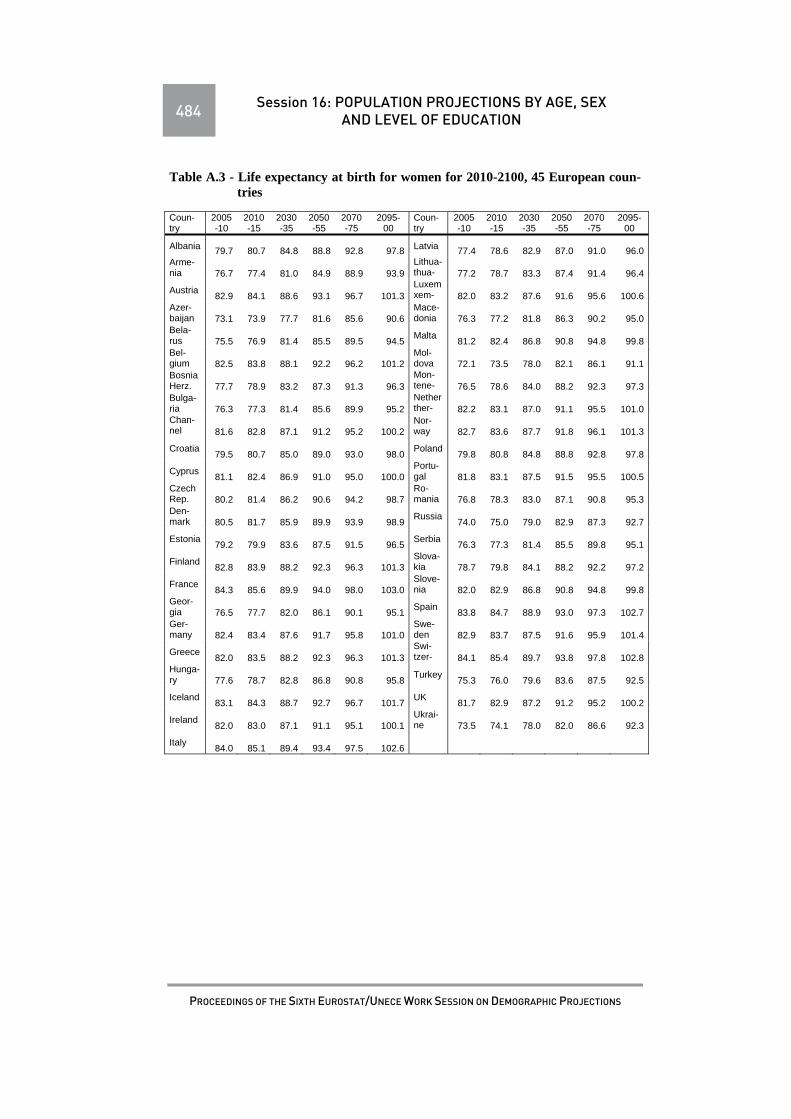
484 Session 16: POPULATION PROJECTIONS BY AGE, SEX AND LEVEL OF EDUCATION
PROCEEDINGS OF THE SIXTH EUROSTAT/UNECE WORK SESSION ON DEMOGRAPHIC PROJECTIONS
Table A.3 - Life expectancy at birth for women for 2010-2100, 45 European coun-tries
Coun-try
2005-10
2010-15
2030-35
2050-55
2070-75
2095-00
Coun-try
2005-10
2010-15
2030-35
2050-55
2070-75
2095-00
Albania 79.7 80.7 84.8 88.8 92.8 97.8 Latvia 77.4 78.6 82.9 87.0 91.0 96.0 Arme-nia 76.7 77.4 81.0 84.9 88.9 93.9
Lithua-thua- 77.2 78.7 83.3 87.4 91.4 96.4
Austria 82.9 84.1 88.6 93.1 96.7 101.3
Luxemxem- 82.0 83.2 87.6 91.6 95.6 100.6
Azer-baijan 73.1 73.9 77.7 81.6 85.6 90.6
Mace-donia 76.3 77.2 81.8 86.3 90.2 95.0
Bela-rus 75.5 76.9 81.4 85.5 89.5 94.5
Malta 81.2 82.4 86.8 90.8 94.8 99.8
Bel-gium 82.5 83.8 88.1 92.2 96.2 101.2
Mol-dova 72.1 73.5 78.0 82.1 86.1 91.1
Bosnia Herz. 77.7 78.9 83.2 87.3 91.3 96.3
Mon-tene- 76.5 78.6 84.0 88.2 92.3 97.3
Bulga-ria 76.3 77.3 81.4 85.6 89.9 95.2
Netherther- 82.2 83.1 87.0 91.1 95.5 101.0
Chan-nel 81.6 82.8 87.1 91.2 95.2 100.2
Nor-way 82.7 83.6 87.7 91.8 96.1 101.3
Croatia 79.5 80.7 85.0 89.0 93.0 98.0
Poland79.8 80.8 84.8 88.8 92.8 97.8
Cyprus 81.1 82.4 86.9 91.0 95.0 100.0
Portu-gal 81.8 83.1 87.5 91.5 95.5 100.5
Czech Rep. 80.2 81.4 86.2 90.6 94.2 98.7
Ro-mania 76.8 78.3 83.0 87.1 90.8 95.3
Den-mark 80.5 81.7 85.9 89.9 93.9 98.9
Russia 74.0 75.0 79.0 82.9 87.3 92.7
Estonia 79.2 79.9 83.6 87.5 91.5 96.5
Serbia 76.3 77.3 81.4 85.5 89.8 95.1
Finland 82.8 83.9 88.2 92.3 96.3 101.3
Slova-kia 78.7 79.8 84.1 88.2 92.2 97.2
France 84.3 85.6 89.9 94.0 98.0 103.0
Slove-nia 82.0 82.9 86.8 90.8 94.8 99.8
Geor-gia 76.5 77.7 82.0 86.1 90.1 95.1
Spain 83.8 84.7 88.9 93.0 97.3 102.7
Ger-many 82.4 83.4 87.6 91.7 95.8 101.0
Swe-den 82.9 83.7 87.5 91.6 95.9 101.4
Greece 82.0 83.5 88.2 92.3 96.3 101.3
Swi-tzer- 84.1 85.4 89.7 93.8 97.8 102.8
Hunga-ry 77.6 78.7 82.8 86.8 90.8 95.8
Turkey 75.3 76.0 79.6 83.6 87.5 92.5
Iceland 83.1 84.3 88.7 92.7 96.7 101.7
UK 81.7 82.9 87.2 91.2 95.2 100.2
Ireland 82.0 83.0 87.1 91.1 95.1 100.1
Ukrai-ne 73.5 74.1 78.0 82.0 86.6 92.3
Italy 84.0 85.1 89.4 93.4 97.5 102.6

Session 16: POPULATION PROJECTIONS BY AGE, SEX AND LEVEL OF EDUCATION 485
PROCEEDINGS OF THE SIXTH EUROSTAT/UNECE WORK SESSION ON DEMOGRAPHIC PROJECTIONS
Table A.4 - Current level of in-migration and out migration (2005-2010) number (in 000), 45 European countries
Country Emigration Immigration Net Migration
Country Emigration Immigration
Net Migra-tion
Fe-male
Ma-le
Fema-le
Male Fema-
le Male
Fema-le
Ma-le
Fema-le
Male Fema-
le Ma-le
Albania 49 30 16 15 -34 -14
Latvia 6 5 0 0 -6 -4
Armenia 49 50 23 1 -26 -49
Lithua-nia 20 17 0 0 -19 -16
Austria 21 32 103 110 81 78
Luxem-bourg 0 0 21 22 20 22
Azerbai-jan 11 3 26 42 15 38
Mace-donia 9 7 10 8 1 1
Belarus 57 52 31 28 -26 -24
Malta 0 0 2 3 2 3
Belgium 7 11 109 108 103 97
Moldo-va 88 95 1 10 -86 -86
Bosnia Herz. 16 14 11 10 -5 -5
Monte-negro 12 9 11 7 -1 -2
Bulgaria 41 43 16 18 -26 -24
Nether-lands 115 132 139 158 24 26
Channel sles 2 1 4 4 2 2
Norway 4 0 76 100 72 99
Croatia 14 14 18 20 4 6
Poland 6 31 44 48 38 18
Cyprus 1 1 18 28 16 28
Portu-gal 91 74 161 155 69 81
Czech Rep. 0 0 96 145 96 145
Roma-nia 72 70 20 23 -52 -48
Denmark 8 12 55 55 47 43
Russia 148 119 706 696 558 577
Estonia 4 1 4 1 0 0
Serbia 91 84 90 85 -1 1
Finland 0 0 33 40 33 40
Slova-kia 4 0 15 25 11 25
France 120 133 363 391 243 258
Slove-nia 1 2 11 14 9 13
Georgia 70 82 1 1 -69 -81
Spain 71 87 1143 1265 1072
1178
Germany 319 471 671 670 351 199
Sweden26 27 153 166 127 139
Greece 36 23 106 106 71 84
Switzer-land 56 67 142 163 87 96
Hungary 5 4 42 42 37 38
Turkey 82 79 52 59 -29 -20
Iceland 1 2 6 7 5 5
UK 429 289 911 827 482 539
Ireland 35 33 83 84 49 52
Ukraine 227 196 204 178 -23 -17
Italy 13 1 879 1135 865 1134


487
PROCEEDINGS OF THE SIXTH EUROSTAT/UNECE WORK SESSION ON DEMOGRAPHIC PROJECTIONS
REPORT OF THE JOINT EUROSTAT-UNECE-ISTAT
WORK SESSION ON DEMOGRAPHIC PROJECTIONS
Paolo Valente, UNECE
1. Attendance
The joint Eurostat-UNECE-Istat Work Session on Demographic Projec-tions was held in Rome (Italy) on 29-31 October 2013, at the invitation of Istat – National Statistical Institute of Italy. It was attended by participants from na-tional statistical offices, demographic research institutes, universities, and other institutions representing the following countries: Austria, Belgium, Canada, Croatia, Czech Republic, Denmark, Estonia, France, Georgia, Germany, Greece, Hungary, Iceland, Ireland, Israel, Italy, Japan, Republic of Korea, Lat-via, Luxembourg, Netherlands, Norway, Poland, Portugal, Romania, Russian Federation, Slovenia, Spain, Sweden, Switzerland, Turkey, United Kingdom and United States of America. The European Commission was represented by Eurostat. The United Nations Population Division, the Kosovo Statistical Agen-cy, the Wittgenstein Centre for Demography and Global Human Capital (IIASA, VID/ÖAW, WU) were also represented. 2. Organization of the meeting
Mr. Saverio Gazzelloni (Istat), Mr. Eduardo Barredo Capelot (Eurostat), and Mr. Paolo Valente (UNECE) opened the meeting and welcomed the partici-pants.
The meeting adopted the agenda of the work session, and elected Ms. Mari-anne Tonnessen (Statistics Norway) as Chairperson.
Keynote lectures were given by Mr. Nico Keilman (University of Oslo) on “Probabilistic demographic projections”, and Mr. Tommy Bengtsson (Universi-ty of Lund) on “Population Ageing - A Threat to the Welfare State?”.
The meeting included sessions on the following substantive topics: a) Assumptions on future migration b) Assumptions on future mortality c) Actual and potential use of demographic projections at national and interna-tional level d) National and international population projections out of the EU region e) Assumptions on future fertility f) Stochastic methods in population projections g) Household projections h) Demographic sustainability and consistency with macroeconomic assump-tions i) Bayesian approaches (1) and (2) j) Multiregional projections k) Beyond population projections by age and sex: inclusion of additional popu-lation characteristics

488
PROCEEDINGS OF THE SIXTH EUROSTAT/UNECE WORK SESSION ON DEMOGRAPHIC PROJECTIONS
l) Population projections by age, sex and level of education The following participants and members of the Scientific Committee acted
as session chairs: Mr. Valerio Terra Abrami (Italy) for topic (a) and (j), Ms. Graziella Caselli (Italy) for topics (b) and (e) (1), Ms. Maria Graça Magalhaes (Portugal) for topics (c), and (e), Mr. Giampaolo Lanzieri (Eurostat) for topic (d), Ms. Rebecca Graziani (Italy) for topics (f) and i) (2), Mr. Marco Marsili (It-aly) for topic (g), Ms. Elisabetta Barbi (Italy) for topics (h) and (k), Ms. Anne Clemenceau (Eurostat) for topic (l).
The discussion in the substantive sessions was based on 49 papers, that were available on the meeting web page maintained by the UNECE Statistical Division. Presentations have been made available on the same web page shortly after the meeting. A summary of the discussion in the substantive sessions, pre-pared after the meeting, is presented in the next chapter.
3. Conclusions
The participants recommended that the next meeting take place in about three years time. A list of possible topics for discussion is as follows: a) Assumptions on future migration b) Assumptions on future mortality c) Actual and potential use of demographic projections at national and interna-tional level d) National and international population projections out of the EU region e) Assumptions on future fertility f) Stochastic methods in population projections g) Experiences on how the results of projections are presented to and accepted by the users h) Household projections i) Demographic sustainability and consistency with macroeconomic assump-tions j) Bayesian approaches k) Multiregional projections l) Beyond population projections by age and sex: inclusion of additional popula-tion characteristics m) Projections and National Transfer Accounts (NTA).
The participants expressed their great appreciation to the members of the Scientific, Organizing and Coordination Committees for their work, and to Istat - National Statistical Institute of Italy - for hosting the meeting and providing excellent facilities.
4. Adoption of the report of the meeting
The present report of the meeting was adopted during the closing session.

489
PROCEEDINGS OF THE SIXTH EUROSTAT/UNECE WORK SESSION ON DEMOGRAPHIC PROJECTIONS
SUMMARY OF THE DISCUSSION ON SUBSTANTIVE
TOPICS
Item 4. ASSUMPTIONS ON FUTURE MIGRATION (Chair: Valerio Terra Abrami)
1. Jean Louis Rallu (INED-France) developed a model to project return mi-gration of aging foreign born immigrated population. Although the migration component is very difficult to forecast, projections of ageing immigrants are more reliable because at older ages migration is much smaller and most of fu-ture elderly migrants are already in country.
2. In the population projection model of Statistics Sweden (Adreas Ran-eke), immigration and emigration are broken down by seven different groups of country of birth (background), which Swedish-born persons are one out of. A specific group of Swedish-born Living-abroad persons is created (using histori-cal administrative data) to complete the immigration-emigration based model. The model has been further developed by adding the background (parent coun-try of birth) of Swedish-born Living-abroad group in order to verify its impact on projected return migration.
3. Projecting international migration involves intrinsically more uncertainty than projecting the natural components due to the unpredictability of many ex-ternal factors (like the influence of high economic instability). The traditional deterministic models, setting variants in the medium and long-run, are not able to face such instability and do not provide prediction intervals for the forecasted variants. On the other hand, classical regression type models are not reliable due to the auto-correlated and non-stationary character of the time series involved in migration processes. Statistics Iceland (Violeta Calian) applies from 2011 dy-namical, or auto-regressive distributed lag (ARDL), models that incorporate au-to-correlation and non-stationarity in the model, in order to obtain short time predictions for the number of immigrants/emigrants of Icelandic and foreign cit-izenships as functions of several time series predictors: unemployment, change in GDP values, number of graduating students and dummy variables mirroring the EEA resizing in time and the Icelandic economic boom which ended in 2008.
4. Before the discussion opening, it has been briefly summarized the con-tribution of DREAM (Danish Rational Economic Agents Model, Marianne Frank Hansen), that could not have been presented in the Session. During the past decade an increase is being observed in immigration, leading to a shift in the pattern of residence permits, which are recently being granted mostly for work or study reasons, rather than for asylum and family reunification. The former residence permits are associated with a duration of stay shorter than the latter, resulting in a corresponding shift in the composition of the immigrant population by duration of stay. Thus migration rates, currently estimated for 10 different origin groups, have been further broken down by duration of stay (five

490
PROCEEDINGS OF THE SIXTH EUROSTAT/UNECE WORK SESSION ON DEMOGRAPHIC PROJECTIONS
year-groups of duration), taking into account the inverse relation (the shorter duration, the higher propensity) between duration of stay and propensity to re-turn migration. Finding that a shift in immigration behavior severely challenges projection accuracy when taking duration into account, it is suggested that dura-tion dependent re-emigration should be used with caution.
5. In migration projections, the variable country-of-birth may be considered as the most explicative, especially when considering return migration, that is emigration of foreign-born population to their country of origin. In the projec-tion exercises of France, Sweden and Denmark, taking into account this variable leads in principle to improve accuracy of population projections. Different solu-tion for clustering the origin-groups have been chosen in the three cases men-tioned above, also according to the different history and time-patterns of the re-lated immigration. Sweden takes into account the further break down by Swe-dish- and Non-Swedish-born persons, while Denmark use Danish and Non-Danish citizenship. The inclusion of further breakdown variables, like back-ground (country of birth of parents) of born-in-country persons or duration of stay of foreign born, seems less promising, at the current stage of investigation. On the other hand, the more immigration from different groups of countries tends to become stable, the more country of origin tends to be correlated with duration of stay and in this cases migrant population aging process tends to be-come more and more relevant for the aging of the whole population.
6. The use of dynamical ARDL (auto regressive distributed lag) time-series models, presented by Iceland, seems a promising approach to incorporate short-term migration projections in the first 5 years of the forecasting horizon, into the classical cohort component model to project migration, as well population itself, at mid- and long-run. On the other hand, while ARDL models are an ideal solu-tion to incorporate macroeconomic aggregates, like GDP, into short-term pro-jections of net and gross migration flows, their use should never be done auto-matically, but carefully taking into account the specific situation of past trends used to feed the models.
Item 5. ASSUMPTIONS ON FUTURE MORTALITY (Chair: Graziella Caselli)
7. The paper by Portugal explores the presence of cohort effects as a possi-ble reason behind the structural changes. They make use of several model speci-fications, namely the classical log-linear age-period-cohort (APC) model as well as more complex models with age-period and age-cohort interactions. A simula-tion study allowed them to understand the impacts of ignoring important fea-tures in mortality modelling.
8. In the Korean paper, the authors examine how to overcome the shortage of historical data on mortality at the older ages (75 +) and to find the best model for forecasting Korean mortality. Four stochastic forecasting models are fitted to the period from 1970-2010 and the forecasts (2060) are compared to actual mor-tality for that period. The results of this evaluation show that the Coherent Lee-
491
PROCEEDINGS OF THE SIXTH EUROSTAT/UNECE WORK SESSION ON DEMOGRAPHIC PROJECTIONS
Carter Model is consistently more accurate in forecasting Korean mortality than other compared models.
9. The French paper explores a different approach to disaggregation (i.e. mortality by cause) and combination. The d(x) values by cause are converted to log-ratios with a common denominator for each period across all decrements. It can be shown that, because of the unit sum constraint, the results are independ-ent of the value chosen for the common denominator and the original values can always be recovered by back-transformation. Once the death densities have been transformed into the real space, the full range of multivariate statistics can be applied. In this paper, both singular value decomposition and regression are employed to obtain forecasts.
10. Finally, in the Swedish paper the authors show that the LC-model is suitable in forecasting Swedish women’s mortality but not as suitable for men’s mortality. The predicted mortality change in men differed by length of the base-period, in particular at ages 65 years and over. Findings also suggested that LC-models incorporating all ages 0–100 years tend to underestimate the mortality decline in age groups 50 and older as compared with the simple age-specific trend.
11. In the discussion it was noted that the four papers drew attention to some of the more controversial points in mortality forecasts: a) the importance of the choice of the most suitable for interpreting past (and, hence, also future) development of mortality; b) the reference period used for fitting the model; c) the need to take the cause of death into consideration.
12. No one has paid attention to setting a target for the future evolution of mortality in terms of life expectancy, with reference to the most recent debate on behavioral, social and environmental risk factors and the limits of human survival.
13. Two presentations considered the importance of having a good knowledge of epidemiological processes for improving understanding of the development of life expectancy at different ages, with particular reference to adult and ancient ages.
14. None of the forecasts, projecting male and female mortality inde-pendently, paid attention to the future decrease in gender differences in life ex-pectancy. Some comments have suggested this important decrease will be con-trolled, considering that men reduce their disadvantage no further than the strict minimum imposed by biology.
Item 6. ACTUAL AND POTENTIAL USE OF DEMOGRAPHIC PROJECTIONS AT NATIONAL AND INTERNATIONAL LEVEL
(Chair: Maria Graça Magalhães)
15. The Netherlands has presented the main results from the 2012 stochas-tic population projections, which have considered a new mortality projection model, developed in collaboration with the University of Groningen. This new mortality projection model meets better to requirements as those resulting from

492
PROCEEDINGS OF THE SIXTH EUROSTAT/UNECE WORK SESSION ON DEMOGRAPHIC PROJECTIONS
the indexation procedure of the pension age to life expectancy, recently imple-mented, where future increases in life expectancy would automatically result in adjustments of the pension age.
16. Portugal (WP 6.2) has presented a set of population projections, were three alternative scenarios has being developed. Focusing in the potential future student enrolment in higher education, they found out that the number of young people in Portugal will decrease significantly in the next 25 years. Considering that the demand of higher education in Portugal will be strongly influenced by this trend, these results should lead to informed policy decisions, namely to support a redefinition of the national higher education institutional network.
17. Portugal (WP 6.3) presented an application of seasonal forecasting methods to model national and regional birth and deaths data as inputs to a cal-endar quarter sample population to LFS, since the needs of data are incompati-ble with the current production of annual population estimates. In order to cap-ture the seasonal behaviour of the data, three alternative methodologies have be-ing considered: ARIMA models with a seasonal component, Holt-Winters ex-ponential smoothing models, and state-space models. The methodology that provides the best forecasting performance for the majority of the regions is adopted.
18. In the discussion, questions were raised to clarify some aspects of the pension system in The Netherlands, which is based on two “pillars” and there-fore different from other countries.
19. Considering the application of the projections results as input to support a redefinition of the higher education network, it was suggested to enlarge the scope of analysis to other age groups, namely because educational systems are not equal across countries.
20. Although the application of seasonal forecasting methods was only ap-ply to births and deaths, it was questioned what is done with the migratory component and was briefly explained.
Item 7. NATIONAL AND INTERNATIONAL POPULATION PROJECTIONS OUT OF THE EU REGION
(Chair: Giampaolo Lanzieri)
21. Georgia presented two contributions. The first presentation stressed the importance for projections of good quality input data and drew the attention on the deterioration of population, vital events and migration statistics in Georgia since its independence in 1991. The second contribution presented assumptions and main results of the latest projections exercise for the population in Georgia.
22. Israel presented its experience of estimation of size and vital events of a population sub-group (the Haredim), relevant for policy purposes, in order to analyse their demographic dynamic projected in the long-term. This exercise required some restrictive assumptions, but highlighted the usefulness of a dis-aggregation by population sub-groups in population projections.

493
PROCEEDINGS OF THE SIXTH EUROSTAT/UNECE WORK SESSION ON DEMOGRAPHIC PROJECTIONS
23. In the last presentation, Netherlands reported on a projections exercise concerning the South and East Mediterranean Countries (included in the Euro-pean Neighbourhood Policy of the European Union) based on population and development scenarios and distinct migration system. This work showed how these countries may experience different demographic changes compared with EU Member States and, in particular, addressed issues of labour migrations.
24. During the discussion, questions were addressed on the latest popula-tion census in Georgia as source of emigration data for that country, in particu-lar enumerating the persons absent from the households for more than one year. Although this is not a recommended practice at international level, it is one of the tools countries with important lacks of emigration data sometimes adopt.
25. The input data quality was mentioned as one element which should en-ter in the overall evaluation of the uncertainty of projections, in particular as re-gards the population base. This may become even more relevant when popula-tion sub-groups are explicitly taken into account in the projections computa-tions.
26. It was also noted that the use of scenarios, while fundamental for the users’ comprehension of the rationale behind the projections assumptions, may still lack an explicit link to the quantification of the assumptions. In fact, alt-hough based on the qualitative arguments there may be a general agreement on the future direction of a demographic component, the actual size of the project-ed population will depend on quantitative assumptions whose exact values may be defined almost arbitrarily.
Item 8. ASSUMPTIONS ON FUTURE FERTILITY (Chair: Maria Graça Magalhães)
27. Austria (WP 8.1) presented a study that aims to improve understanding of the role of different ingredients of fertility projections through a comparative analysis of importance of model choice and of the three main fertility parame-ters (TFR, MAB, and SDAB) in projecting the number of births.
28. Sweden presented a paper with two studies based on analysis using lo-gistic regression on register data of all children in Sweden living with their bio-logical parents 1999–2011 and register data of all children born in Sweden from 1970. Results the shows that percentage of children who experience a separation of their parents have decreased during the 2000s and that higher levels of educa-tion and postponement of family formation are two explanatory factors of the declining impact of stepfamily fertility.
29. Previous fertility projections for Austria have considered linear increase on TFR and MAC until a certain time horizon and held constant for the rest of the projection period. Those sudden stops may cause inconsistencies due to the model of tempo-adjusted fertility. To overcome the explained inconsistencies, Statistics Austria (WP 8.3) reformulated its fertility assumptions for the new population projection in a more consistent framework of TFR, TFR* and MAC, using a modified Hadwiger function that estimate age-specific fertility rates by

494
PROCEEDINGS OF THE SIXTH EUROSTAT/UNECE WORK SESSION ON DEMOGRAPHIC PROJECTIONS
four parameters: TFR, MAC, the mode and the variance of the fertility distribu-tion.
30. In the discussion, reference was made to different results that may emerge when considering different populations in the analysis of the indicators used to test the models.
31. The role of changes in variables such as gender equality with fertility behaviour, particularly in terms of projections, was discussed.
32. It was discussed the pertinence of ensure the convergence of fertility indicators at sub national level and the possibility of being adding uncertainty to projections by adding regions results.
Item 9. STOCHASTIC METHODS IN POPULATION PROJECTIONS (Chair: Rebecca Graziani)
33. The presentation by the University of California focused on the use of Hamilton-Perry model for deriving stochastic forecasts of population based on the forecasts of cohort-change ratios. The method is applied for projecting the population of the states of Georgia, Minnesota, New Jersey and Washington. Forecasts 10 year ahead are produced using as starting year the census years from 1900 to 2010.
34. The presentation by University of Rome focused on the use of Bertino and Sonnino method for the derivation of stochastic forecasts of the population of Rome Metropolitan Area, from 2009 to 2024. The method is ased on micro-simulations of birth-death-emigration-immigration poisson processes. Three variant are considered based on different assumptions on fertility and immigra-tion.
35. The presentation from Statistics Canada discussed an application of its microsimulation projection model Demosim aiming at assessing the possible future composition of the Canadian population with respect to the immigrant generation status. A new immigrant generation status is defined and mixed un-ions are explicitly considered.
36. The presentation by the University of Southampton discussed a semi-artificial model of population aiming at providing a bridge between micro-simulation and the agent-based approach. An extension of the ‘Wedding Ring’ agent-based model of marriage formation by Billari et al. 2007 is extended and a Gaussian emulator is used for analysing uncertainty.
37. During the discussion the distinction between sources of uncertainty was emphasized particularly with respect to the demographic stochasticity and the environmental stochasticity.
38. Clarifications were asked on the Demosim model, the specification of the rates of the Poisson processes used within the Bertino-Sonnino model and the sources of uncertainty in the agent-based model suggested by the University of Southampton.
495
PROCEEDINGS OF THE SIXTH EUROSTAT/UNECE WORK SESSION ON DEMOGRAPHIC PROJECTIONS
39. The use of the model suggested by University of Rome in the frame-work of the analysis of transportation was suggested along with the considera-tion of spatial dependency of the forecasts.
Item 10. HOUSEHOLD PROJECTIONS (Chair: Marco Marsili)
40. Spain presented a methodology for the revision of household estimates for the latest intercensal years, which provides figures linked to the official de-mographic estimates. As regards the future households system account, Spain also presented his strategy based on a continuous census system approach, with the aim of producing now-casts on the number and type of households.
41. The main results show that Spain experienced a big increase in number and type of household at the beginning of the XXIst century, with an impact even bigger than the one in population. The number of households has grown in 3.7 million between 2002 and 2012. During the same period, the population re-siding in Spain has increased in 5.8 million. Single households or households inhabit of two persons show the highest increase The number of households of three or four members show a slight increase. Households with more than four members have experienced a deep fall.
42. Belgium presented a household projection model calibrated on the Bel-gian population projections at the nuts 3 level. The model is based on individual membership rates, as defined through 12 LIPRO positions, and allows taking into account the living arrangements of each individual in the population. The membership rates are not taken constant in the projection. They follow a logistic or logarithmic trend. The proposed method is static in the sense that the transi-tion probabilities from one position within the household to another are not con-sidered. Some consistency rules are implemented (as equal number of married men and of married women) while local heterogeneity is maintained in the whole process.
43. While most of the positions face an increasing trend up to 2060 in Bel-gium, the numbers of married individuals with children and of children within a married couple decrease by 30% and 24% respectively over the period 2011-2060. The number of married individuals without children increases by 14% in 2060 compared to 2011. The number of individuals within non-consensual un-ions and one-person families increases between 2011 and 2060, up to 77% for the number of children in families with cohabiting parents.
44. Projections of individuals in collective household are treated separately from projections of private households, to prevent an explosion of the former, in a context of a strong population ageing. The results show an increase of indi-viduals in collective Belgian households by 111% in 2060.
45. Italy presented an original procedure that combines official statistics with data from ad hoc surveys conducted on migrants in recent years. The pro-posed model aims at estimating both the extra demand for caregivers of the el-derly and the possible supply of migrants in the future.

496
PROCEEDINGS OF THE SIXTH EUROSTAT/UNECE WORK SESSION ON DEMOGRAPHIC PROJECTIONS
46. Home caregivers are expected to be recruited particularly among immi-grants, due to the lack of supply among the younger Italian generations. As a consequence of social, economic and demographic implications, the demand for caregivers for the elderly in Italy seems to increase significantly in the future. Anyway, the additional demand for caregivers due to the rise in numbers of el-derly people over the next years will decrease. The extra demand for home caregivers will be expressed mainly by men, persons aged 65 and over and es-pecially those living alone.
Item 11. DEMOGRAPHIC SUSTAINABILITY AND CONSISTENCY WITH MACROECONOMIC ASSUMPTIONS
(Chair: Elisabetta Barbi)
47. Portugal presented the possible challenges that the country will have to face in the next future given its low level of fertility and the deep economic cri-sis which will very likely lead to a massive outmigration. The tremendous evo-lution in the Portuguese population, estimated by a medium-term projection, highlighted the urgent need of planning equipment and resources directed to the elderly.
48. Spain presented a model integrating labour market scenarios in popula-tion projections. The approach takes into account the impact of the labour mar-ket on population through changes in the employment rate and in the immigra-tion flows. The model is applied to five European Union countries and results are compared to the most recent Eurostat population projection of 2010. With a declining working age population, immigration emerges as the only way to al-low for economic growth, especially in countries where employment rates are already high and have little margin for further increase.
49. Poland presented an alternative method of preparing migration assump-tions in population projections which takes into account long-term projections of economic variables. Results for selected EU countries show that differences in unemployment matters in short-term forecasts whereas in the case of long-term forecast it is difficult to identify a universal model and explanatory varia-bles.
50. In the discussion, it was noted that it is important to distinguish between receiving and sending countries: In the short term, unemployment is a relevant factor for sending countries whereas, for receiving countries, this can assume an important role in the long-term.
51. Economic crisis highlighted the role of economic factors in flows and direction of migration. However, while preparing demographic assumptions for population forecasts, the impact of economic crisis on mortality should also be considered, especially for the elderly segment of the population.
52. The urgent need of planning a common migration policy among EU countries was also highlighted in the discussion.

497
PROCEEDINGS OF THE SIXTH EUROSTAT/UNECE WORK SESSION ON DEMOGRAPHIC PROJECTIONS
Item 12. BAYESIAN APPROACHES (1) (Chair: Graziella Caselli)
53. In the paper by the University of Southampton, the authors explore for the United Kingdom in 2010-2030 the functional modeling approach to popula-tion forecasting within the wider context of Bayesian predictions and model un-certainty. They conclude that given the regularities in age profiles of fertility, mortality and migration, disaggregating of the relevant data by age and sex pro-vides important additional information for the forecasts.
54. In “Towards stochastic forecasts of the Italian population: an experi-ment with conditional expert elicitations” (WP.12.2), the authors report on the whole process developed to produce an expert-based stochastic forecast of the Italian population for the period 2011-2065, applying the method proposed by Billari et al. (2012). Authors discuss the problems that can arise in the collection of expert opinions and the solutions that can be implemented in order to avoid inconsistencies in the calculation of the parameters.
55. In “Expert-based stochastic population forecasting: a Bayesian ap-proach to the combination of the elicitations” (WP12.3), authors suggest a method that derives expert-based stochastic population forecasts in such a way as to account for relationships both between demographic components and be-tween experts. Starting from so-called Supra-Bayesian approach, introduced by Morris, the authors suggest resorting to a mixture model approach. An applica-tion to the forecast of the Italian Population from 2010 up to 2065 is proposed.
56. Referring to the first presentation, the authors’ attention was drawn to some important points, i.e., when a forecast is based on the hypothesis that past trends will continue into the future, it is crucial to define not only the method used to estimate trends, but also the length of the data series involved, and the year selected to start the forecast. These choices greatly influence the final out-come, so much so that they overshadow even the efficacy of more sophisticated methods.
57. The processes developed to produce expert-based stochastic population forecasting were much appreciated, as was the Bayesian Approach to the Com-bination of the Elicitations. The wide-ranging debate that followed strongly suggested that the authors should increase the number of experts and reconsider ex post the various responses received, improving them with the suggestions of some experts chosen on the basis of their deep knowledge of each specific de-mographic phenomenon.
Item 13. BAYESIAN APPROACHES (2) (Chair: Rebecca Graziani)
58. The first presentation by the University of Washington (WP 13.1) dis-cussed a method for deriving stochastic forecasts of Net Migration Rates. A bayesian hierarchical model is fitted to past data for all countries of the world and the forecasts of net migration are calibrated so to ensure the respect of the

498
PROCEEDINGS OF THE SIXTH EUROSTAT/UNECE WORK SESSION ON DEMOGRAPHIC PROJECTIONS
requirement of zero global net migration. An evaluation of the method is pro-vided using an out-of sample validation.
59. The second presentation from University of Washington (WP 13.2) provided a detail description of four R packages implementing the methodology used by UN for the derivation of probabilistic projections for the population of all countries of the world.
60. The presentation by the University of Rostock discussed a Bayesian method for deriving stochastic forecasts of mortality for several european coun-tries, based on the forecast of rates of mortality improvement. In-sample and out-sample forecasts were provided.
61. During the discussion it was emphasized the need of considering the role of politics in shaping the future changings when making projections along with the relevance of the communication of the results.
62. It was emphasized that the correlation between age and time has to be considered in the forecast of Net Migration.
63. The flexibility of the R packages was discussed with respect to several aspects as the incorporation of different age-schedules and consideration of the two phases in the description of behaviour of the Total Fertility Rate.
Item 14. MULTIREGIONAL PROJECTIONS (Chair: Valerio Terra Abrami)
64. International projection-making agencies (UNPD) commonly use sim-plistic assumptions of net-migration measures derived as residuals from demo-graphic accounting. On the other hand, the rise in influence of migration on de-mographic change is likely to increase and to spread to more countries, while fertility and mortality rates keep on decreasing in the developing world. Thus net migration measures are becoming more and more inadequate to face the challenge of projecting migration at global level. VID and WCD (Guy Abel, Vienna) propose their “flows-from-stock” method to estimate global bi-lateral migration, preserving the constraint that the estimated migration flows in a peri-od [t-(t+n)] match the change in migrant stocks from t to (t+n), thus ensuring that the total inflows equal the total outflows.
65. Subnational population projections of Turkey (Sebnem Bese Canpoloat) have been officially produced first in 2013 up to the year 2023 (centenary of the Republic of Turkey) and released for the 81 Turkish provinces. Important im-provements have been made in terms of basic data availability and quality, in-corporating in these new projections data from the recently devoloped ABPRS (Address Based Population Registration System) and the former CCRS (Central Civil Registration Registration System) The outcomes show that Turkish popu-lation will reach around 84 million in 2023, as a result of an increase in 61 prov-inces versus a decrease in 21. The “dream” of 100 million people will never be reached.

499
PROCEEDINGS OF THE SIXTH EUROSTAT/UNECE WORK SESSION ON DEMOGRAPHIC PROJECTIONS
66. Statistics Canada (Patrice Dion) has a longstanding tradition, since 1984, in producing population projections of Provinces by using the multire-gional model, in the classical cohort-component frame. The multiregional model has many advantages, among them those of allowing to project simultaneously a multiregional system as a whole and of allowing to apply the out-migration rates to the corresponding population at risk. Nonetheless, the multiregional model has the basic limitation that migration flows are determined only by out-migration rates and origin-region size, while in reality migration is destination-driven, thus flows tend to vary in proportion to both regions of origin and desti-nation. Statistics Canada proposes the NMRP (net migration rate preservation) model, in which origin-destination migration rates are corrected by a composi-tion ratio allowing to account for the size of the destination-region, as a proxy of the actractivity factors driving migration flows.
67. Scalone and Greco (University of Bologna) propose a statistical method to forecast age-specific mortality rates for the Italian provinces (NUTS-3) by combining Lee-Carter model and Bayesian approach. In general, relatively small and closely related populations have similar mortality patterns that do not diverge in the long run, thus standard mortality forecasting poorly performs, when working on single limited small areas separately, especially considering some specific (five-year) age-groups, resulting in large variance residuals. In order to overcome this problem, a spatial-temporal extension of the classical Lee-Carter model is presented, in which areal estimates borrow strength from each other introducing spatial association of provincial mortality rates.
68. When projecting a multi-areal population system, the major problems arise in data availability and in the assumption setting process, especially when the number of the areas of the system is relatively high or/and the average popu-lation size of the areas is relatively small, resulting in a number of demographic events very small accordingly. Although this applies as well as to both mortality and fertility, difficulties are much bigger for migration component, whose as-sumption setting process, and projection process itself, is heavily affected by lacking or volatility of data. When data availability is scarce, handling net mi-gration is often the only possibility to set assumptions. In these cases, there is not a real possibility to set solid and reliable migration assumptions, only pro-vided that estimation and correction methods are incorporated in the projection model.
69. On the other hand, when data availability is rich or full, migration rates may be incorporated in a multiregional model, that however requires a number of correction and/or aggregation procedures, the smaller the average population size of the areas is. In these latter cases, migration assumption setting step may well performs only if the methodological handling of “data-dusting” is suitably calibrated (aggregation procedures) and if the nature of internal migration, that is substantially destination-driven, it is adequately taken into consideration. In fact full multiregional models, although lead to intrinsically consistent results, neglect completely the destination pull-factors, because age-specific out-migration flows result entirely from the action of out-migration rates on the

500
PROCEEDINGS OF THE SIXTH EUROSTAT/UNECE WORK SESSION ON DEMOGRAPHIC PROJECTIONS
origin area population vector. This leads to conclude that full multiregional models should be suitably balanced by incorporating correction procedures in order to guarantee both push- and pull-factors that, in the real life, shape migra-tion flows and that these correction procedures must be adapted to the specific situation of the areal system to project.
Item 15. BEYOND POPULATION PROJECTIONS BY AGE AND SEX: INCLUSION OF ADDITIONAL POPULATION CHARACTERISTICS
(Chair: Elisabetta Barbi)
70. Belgium presented an analysis of changes in income distribution and inequality between 2011 and 2031 in Flanders showing how these changes are related to population changes. Assuming absence of economic progress, the au-thors demonstrate that the relation between population changes and the income distribution involves different components that may act in different directions. Ageing has a negative impact on the income distribution and inequality but oth-er covarying population characteristics, namely household composition and ed-ucation, may have a counteracting effect on income.
71. Canada presented how the Canadian immigrant selection policy may have an impact on future imbalances in labour force supply by broad skill levels (WP 15.2).
72. A second presentation by Canadian researchers (WP 15.3) presented the results of a microsimulation model projecting language characteristics in multi-lingual regions with high immigration. Results show that immigration has a much larger impact on the linguistic equilibrium of a multilingual region like Quebec than in a largely monolingual region like the rest of Canada. The esti-mated increase in the proportion of people having a non-official mother tongue calls for increasing investment in language training in order to maximize their contribution to the country’s future prosperity.
73. Spain presented a new method for projecting economically active popu-lation. The model is a cohort parametric model, which is based on cohort changes of women’s willingness to work and explicitly models the convergence process of female activity rates towards those of men. Results of the projection show that pure-demographic ratios on dependency and sustainability might be misleading highlighting thus the importance of economically active population projections.
74. In the discussion it was noted that, in periods of economic crisis, the convergence between male and female labour market behaviours may be caused not only by a cohort effect, with younger generations of women showing an in-creasingly similar behaviour to that of men, but it may be also affected by a pe-riod effect, namely the economic collapse, with men showing more difficult la-bour-market behaviours which are close to those experienced by women.

501
PROCEEDINGS OF THE SIXTH EUROSTAT/UNECE WORK SESSION ON DEMOGRAPHIC PROJECTIONS
Item 16. POPULATION PROJECTIONS BY AGE, SEX AND LEVEL OF EDUCATION (1)
(Chair: Anne Clemenceau)
75. All papers presented in this session were prepared by the Wittgenstein Centre for Demography and Global Human Capital in Austria
76. Wolfgang Lutz, the Founding Director of the Centre, presented a new, scientific based approach to help defining assumptions on fertility, mortality and migrations. The approach is based on an evaluation of 500 international ex-pert views.
77. Anne Goujon summarised the assumption making process for the global population projections by levels of education to be released by the Wittgenstein Centre in 2014. These projections are specific as they include educational at-tainment on a systematic basis and scientific input of hundreds of source experts are taken into account for the assumptions about future trends in fertility, mor-tality and migration.
78. Nikola Sander presented a new set of population projections carried out using directional migration probabilities and with the addition of the education dimension into a multi-regional cohort-component framework. The projections do not confirm the common perception of a rapid increase in the number of mi-grants and suggest a shift in the education composition of migrants toward higher level of education attainment.
79. The discussion highlighted that while differentials in education are clear for mortality, the issue is more complicated for fertility. Sensitivity of the re-sults to assumptions and assessment of the performance of the projections were also discussed.
Item 17. POPULATION PROJECTIONS BY AGE, SEX AND LEVEL OF EDUCATION (2)
(Chair: Anne Clemenceau)
80. Bilal Barakat presented his paper on estimating transition age schedules for long-term projections of global education attainment. The approach consists of first fitting a model of educational development trajectories to the empirical development of attainment over the course of recent decades; and then project-ing attainment by extending these trajectories into the future.
81. Samir K.C’s presentation focussed on the results of new population pro-jections by age, sex and level of education for 171 countries showing that the world population would peak in 2070 and that a significant increase in the aver-age educational attainment of the world population would take place. The paper also includes alternative education scenarios using two approaches to measuring ageing (conventional approach based on chronological age and alternative ap-proach that takes life expectancy into account) and concludes that population ageing over the 21st century is less rapid when using the alternative approach.

502
PROCEEDINGS OF THE SIXTH EUROSTAT/UNECE WORK SESSION ON DEMOGRAPHIC PROJECTIONS
82. Elke Loichinger presented labour force projections by age, sex and highest level of educational attainment based on data from the EU Labour Force Survey for 26 Member States. The paper shows that the labour force in Europe is likely to be older, and to contain a higher share of women, and will overall be composed of people that are on average higher educated than today.
83. The issue was raised among participants whether the projects were to be considered as forecast projects or more as analytic projects to alert policy mak-ers. Clarification was required on the output of the first paper and explanation about the diverging results compared to the US World Population projections was asked for the second paper.
84. For the Labour force projections, taking account of the skills which as-sociated with education increased after the age of 30 and of the retirement age of each country was recommended.


Proceedings of the Sixth Eurostat/Unece Work Session
on Demographic Projections
�
Italian National Institute of Statistics
Pro
ceed
ings
of t
he S
ixth
Eur
osta
t/U
nece
Wor
k Se
ssio
n
o
n D
emog
raph
ic P
roje
ctio
ns
On Autumn 2013 Eurostat and UNECE were co-organisers, in cooperation with Istat, of a Work Session on Demographic Projections. The meeting was hosted by Istat and held in Rome on 29-31 October 2013.
The objective of the Work Session was to bring together policy makers, demographic researchers, academics, producers and users of demographic projections in order to: a) review and discuss the different uses of demographic projections and the current practices at national and international level; b) illustrate research approaches and innovative methodologies; c) improve the communication between policy makers and demographers and producers of demographic projections.
The Work Session was attended by 127 participants coming from national statistical offices, demographic research institutes, universities and other institutions. The discussion in the substantive sessions was based on 49 papers, 36 of which are published by the authors in this book on a voluntary basis.
€ 40,00