PROCEEDINGS

OF THE

33rd ANNUAL MEETING

FERTILIZER INDUSTRY

ROUND TABLE

1983

October 25, 26, 27, 1983

The Shoreham Hotel Washington, D.C.

None of the printed matter in these proceedings may be printed without the written permission of the Fertilizer Industry Round Table

Copies Of Proceedings - If Available

Current year ............... $35.00 Previous years ............ $30.00

Please make checks payable to .... f~rtEizer In~ustl)' Ro~nd !able IJaUl J. rrosser, Jr., ;:,ecretary-ueasurer

Glen Arm, Maryland 21057

Table of Contents Tuesday, October 25, 1983

Morning Session Moderators

Harold D. Blenkhorn Charles H. Davis

Page Introduction-Keynote Speaker.. ....... . ... . 1

Keynote Speaker-Gary Myers.............. 1

Outlook for Nitrogen J. W. Brown....... . . .. . . . . .. . . .. . .. . .. . .. .. 1

Outlook for Phosphates Ray W. Rowan............................. 8

Outlook for Potash 1982 to 1992 Douglas E. Logsdail. . . . . . . . . . . . . . . . . . . . . . . . . 12

Tuesday, October 25, 1983 Afternoon Session

Moderator Jean L. Cheval

Urease Inhibitors-Current Status Dr. Roland D. Hauck . . . . . . . . . . . . . . . . . . . . . . . 22

Fertilizer Quality Control-Can It Be Achieved in Today's Marketing System Hilton V. Rogers ..................... " .... 23

What is Happening to Quality Control in Blending? (Control Official) Dr. David L. Terry. . . . . . . . . . . . . . . . . . . . . . . . . . 27

What is Happening to Quality Control in Blending? (Blender) Henry T. McCarley . . . . . . . . . . . . . . . . . . . . . . . . . 28

What is Happening to Quality Control in Blending? (Blender) Michael R. Hancock ................... " ... . 32

What is Happening to Quality in Blending? (Producer) Trends in Diammonium Phosphate Particle Size Mabry M. Handley......................... 34

What is Happening to Quality in Blending? (Producer) Quality Control in The Potash Industry Joe A. Gosselin. . . . . . . . . . . . . . . . . . . . . . . . . . . . . 39

Wednesday, October 26, 1983 Morning Session

Moderator Joseph E. Reynolds, Jr.

Computer Simulation of Fertiliser Granulation Plants Page Ian K. Watson............................ . . 41

Selecting Screens for Granulation Plants S. J. Janovac ....... . . . . . . . . . . . . . . . . . . . . . . . . 51

Production and Use of High-Nitrogen Mixtures Frank P. Achorn, Homer L. Kimbrough and Cecil P. Harrison. . . . . .. . . . . . . . . . . . . . . . . . . . . 52

MAP-A Market Update and Effect of Temperature on Crystal Growth Roy D. Space. . . . . . . . . . . . . . . . . . . . . . . . . . . . . . . 56

Conversion of Commercial Dihydrate to Hemihydrate Phosphoric Acid Plants Barry Crozier. . . . . . . . . . . . . . . . . . . . . . . . . . . . . . . 60

Wednesday, October 26, 1983 Afternoon Session

Moderator Herman G. Powers

Fertilizer Plant Safety-A. Driver Training Glenn A. Feagin. . . . . . . . . . . . . . . . . . . . . . . . . . . . 73

Fertilizer Plant Safety-B. Machinery Guarding and Lockout F. C. McNeil .................... '" .. . .. . .. 74

Fertilizer-Pesticides Impregnation Operations A. V. Malone .............................. 77

Fertilizer Placement: Improved Efficiency for Reduced Tillage Crops Larry Murphy. . . . . . . . . . . . . . . . . . . . . . . . . . . . . . 82

Effect of Granule Size on Application Michael F. Broder and Hubert L. Balay. . . . . . . 90

Thursday, October 27, 1983 Final Session

Moderators Paul J. Prosser, Jr.

Joe S. Drewry, Jr., P.E.

Business Meeting-Moderator Prosser. .. .. . . . 97

Secretary-Treasurer Report Page

Paul J. Prosser, Jr .......................... , 97

Nominating Committee Report Joseph E. Reynolds, Jr., Chairman. , , , , . , , . . . 98

Meeting Dates and Places Committee Report Tom Athey, Chairman .... , ............. , . . . 98

Entertainment Committee Report Tom Athey, Chairman .......... , ....... ,.. . 98

Public Relations Committee Report Walter J. Sackett, Jr. ... . .. ... . . . .. .. .. .. .... 98

Update on Operating Experience of Jacobs­Dorreo Two Phosphoric Acid Plant at Gardinier Page

David W. Leyshon and Paul S. Waters .. ,.... 98

Innovations in Potash Warehousing Andrew Elliott .. , ....... , ............. , , . . .. 102

Draft-Tube Production of Ammonium Phosphate for Granulation or Spray Drying David Crerar. . . . . . . . . . . . . . . . . . . . . . . . . . . . . .. 106

Comments on 1983 Proceedings Chairman Harold D. Blenkhorn. . . . . . . . . . . . .. 111

INDEX OF PARTICIPANTS

Frank P. Achorn, Senior Scientist Charles H. Davis, Director of Homer L. Kimbrough, Chemical Joseph E. Reynolds, Jr. Process & Product Imp. Section Chemical Development Engineer Manager-NPK Marketing Tennessee Valley Authority Tennessee Valley Authority Tennessee Valley Authority W. R. Grace & Company Muscle Shoals, Alabama 35660 N.F.D.C. Muscle Shoals, Alabama 35660 100 North Main Street Thomas B. Athey Muscle Shoals, Alabama 35660 D. E. Logsdail, Operating Director Memphis, Tennessee 38103 3403 Rodman Street, N.W. Joe S. Drewry, Jr., P.E. Potash Corp. of Saskatchewan Sales Hilton V. Rogers, Head-Dept. of Washington, D. C. 20008 Vice President Ltd. Fertilizer Analysis & Inspection Hubert L. Balay, Chemical Engineer Kiernan-Gregory Corporation 410-22nd Street East Clemson University Tennessee Valley Authority 173 W. Wieuca Road, N.W., Suite Saskatoon, Saskatchewan 256 P & A S Bid. N.F.D.C.-402 CEB 103 S7K 5T7 Canada Clemson, South Carolina 29631 Muscle Shoals, Alabama 35660 Atlanta, Georgia 30342 Henry T. McCarley Ray W. Rowan Harold D. Blenkhorn Andrew Elliott, Manager, Planning Topyield Industries Texasgulf Chemical Company Technical Service Manager PSC Sales Box 8262 Raleigh, North Carolina 27609 Nitrochem Inc. 410-22nd Street, E. Lexington, Kentucky 40533 Walter J. Sackett, Jr. 2055 Peel Street, Suite 800 Saskatoon, Saskatchewan Fred C. McNeil, Corporate Safety President Montreal, Quebec S7K 5T7 Canada Manager The A. J. Sackett & Sons Company H3A 1V4 Canada Glenn A. Feagin I.M.C. Corporation 1701 South Highland Avenue Michael F. Broder Manager of Fertilizer Technology 47 No. George Drive Baltimore, Maryland 21224 Tennessee Valley Authority I.M.C.Corporation Mundelein, Illinois 60060 Roy D. Space 402 CEB 2201 Perimeter Center East, N. E. AI V. Malone, Manager, Agrico Chemical Company Muscle Shoals, Alabama 35660 Atlanta Georgia 30346 Engineering & Quality Control P. O. Box 3166 Jim W. Brown, Managing Director Joseph A. Gosselin, Research Agway, Inc. Tulsa, Oklahoma 74101 Canadian Fertilizer Institute Chemist P. O. Box 4741 Dr. D. L. Terry, Asst. Director and 350 Sparks Street, Suite 602 Kalium Chemicals Syracuse, New York 13221 Coordinator of Fertilizer Program Ottawa, Ontario 400 Bank of Canada Building Dr. Larry Murphy Division of Regulatory Services K1 R 7S8 Canada Regina, Saskatchewan Potash-Phosphate Institute University of Kentucky Jean L. Cheval

S4P OM9 Canada 1629 Virginia Drive 102 Scovill Hall United Co-Operatives of Ontario Michael R. Hancock Manhattan, Kansas 66502 Lexington, Kentucky 40546 151 Centre Drive, Station A Quality Assurance Manager Gary D. Myers, President Barney A. Tucker P. O. Box 527 The Andersons The Fertilizer Institute Top Yield Industries, Inc. 1200 Dussel Drive Mississauga, Ontario

Maumee, Ohio 43537 1015 18th Street, N. W. 801 Corporate Center L5A 3A4 Canada Washington, D.C. 20036 Lexington, Kentucky 40503 John D. Crerar, General Manager- Mabry M. Handley Herman G. Powers Paul S. Waters Licensing & Consultancy Services I.M.C. Corporation Manager, Granular Fertilizer Jacobs Engineering Group Norsk Hydro Fertilizers Ltd. 421 East Hawley Street Operations P. O. Box 2008 Harvest House, Felixstowe Mundelein, Illinois 60060 Kaiser Agricultural Chemicals Lakeland, Florida 33803 Suffolk I P11 7LP England Dr. Roland D. Hauck P. O. Box 246 Ian K. Watson Barry T. Crozier Tennessee Valley Authority Savannah, Georgia 31402 UKF Fertilizers Ltd. Norsk Hydro Fertilizers Ltd. Muscle Shoals, Alabama 35660 Paul J. Prosser, Jr., Vice President Ince Harvest House, Felixstowe, Stephen J. Janovac, Product The Prosser Company, Inc. Chester, U.K. CH2 4LB Suffolk IP11 7LP United Kingdom Manager P. O. Box 5036

W. S. Tyler, Inc. Glen Arm, Maryland 21057 8200 Tyler Boulevard Mentor, Ohio 44060

1983 BOARD OF DIRECTORS

Frank P. Achorn, Charles H. Davis Oavid W. Leyshon, Technical Joseph E. Reynolds, Jr. Senior Scientist Director of Chemical Development Manager Manager, NPK Marketing-Agri. Process & Product Imp. Section Tennessee Valley Authority Jacobs-Dorrco Division Chemicals Group Tennesse Valley Authority National Fertilizer Development P.O. Box 2008 W. R. Grace & Company Muscle Shoals, Alabama 35660 Center Lakeland, Florida 33803 100 North Main Street Bill E. Adams Muscle Shoals, Alabama 35660 N. Charles Littlejohn MemphiS, Tennessee 38103 Alliance Fertil izer Joe S. Drewry, Jr., P.E. Richmond Guano Company Walter J. Sackett, Jr., President 5810 Meadowbridge Executive Vice President P.O. Box 544 The A. J. Sackett & Sons Company Mechanicsville, Virginia 23111 Kiernan-Gregory Corporation Richmond, Virginia 23204 1701 South Highland Avenue Thomas B. Athey 173 W. Wieuca Road, N.E. AI V. Malone Baltimore, Maryland 21224 3403 Rodman Street, N.W. Atlanta, Georgia 30342 Manager, Engineering & Quality Dean R. Sanders. President Washington. D.C. 20008 Robert E. Ferdon. Sales Manager Control The Espoma Company Harold D. Blenkhorn Stedman Foundry & Machine Co .. Agway, Inc. Six Espoma Road Technical Service Manager Inc. Box 4741 Millville. New Jersey 08332 Nitrochem, Inc. 500-600 Indiana Avenue Syracuse. New York 13221 William F. Sheldrick 2055 Peel Street Suite 800 Aurora, Indiana 47001 John L. Medbery THE WORLD BANK Montreal, Quebec. Canada H3A 1V4 W. Harold Green, Manager of Director of Operations, Production Fertilizer Advisor David W. Brochstein Technical and Quality Assurance I.M.C. Corporation 1818 "H" Street. N.W. Room K-Manager Fertilizer Operations Crops 2201 Perimeter Center East, N.E. 1004 U.S.S. Agri-Chemicals Gold Kist Inc. Atlanta. Georgia 30346 Washington. D.C. 20433 Division U.S. Steel P.O. Box 2210 Grayson B. Morris Adolfo Sisto. Operations Manager

4tbnt~ ~Dnf"ni~ 1n~n1 P.O. Box 1685 z." ...... \u. "",..,...,t~ ..... "" ...... ..,. 6707 W. Frankiin Street Fertimex Atlanta. Georgia 30301 Charles T. Harding. Vice President Richmond, Virginia 23226 Morena 804-Apartado 12-1164 James C. Brown. General Manager, Davy McKee Corporation Cecil F. Nichols, Production Mexico 12, D.F., Mexico Warehouse Terminaling P.O. Box 5000 Manager Rodger C. Smith, Consultant Potash Company of America lakeland. Florida 33803 Southern States Cooperative. Inc. Fertilizer Marketing & Technology 630 Fifth Avenue Suite 2645 Travis P. Hignett, Special Consultant P.O. Box 26234 24 East Street New York. New York 10111 to the Managing Director Richmond. Virginia 23260 South Hadley, Massachusetts 01075 Donald J. Brunner, Plant Manager I nternational Fertilizer Development Frank T. Nielsson Albert Spillman Mid-Ohio Chemical Company. Inc. Ctr. 205 Woodlake Drive 4005 Glen Avenue Box 280 717 Robinson Road P.O. Box 2040 Lakeland. Florida 33803 Baltimore. Maryland 21215 Washington C.H .• Ohio 43160 Muscle Shoals. Alabama 35660

William F. O'Brien John H. Surber Douglas Caine Thomas L. Howe 5345 Comanche Way New Wales Chemicals. Inc. Manager of Technical Services Howe Inc. Madison. Wisconsin 53704 P.O. Box 1035 Estech. Inc. 4821 Xerxes Avenue North

John W. Poulton. Managing Director Mulberry, Florida 33860 30 North LaSalle Street Minneapolis, Minnesota 55430

Perlwee Landforce Limited William W. Threadgill Chicago, Illinois 60602 Ralph W. Hughes Harbour House, Colchester 4223 Riviera Drive Jean L. Cheval Vice President-Crops Division Essex, England C02 8..IF Stockton. California 95204 United Cooperatives of Ontario landmark, Inc.

Herman G. Powers. Manager Barney A. Tucker P.O. Box 479 151 City Centre Drive Columbus. Ohio 43216 Granular Operations Topyield Industries

Mississauga. Ontario Kaiser Agricultural Chemicals P.O. Box 8262 Canada L5A 3S1 Stephen J. Janovac, Product P.O. Box 246 Lexington, Kentucky 40533 Harry L. Cook Manager Savannah. Georgia 31402 Daniel O. Walstad 7555 Sunbury Road W. S. Tyler Company

Paul J. Prosser. Jr .. Vice President Production Mgr.-Nitrogen & 8200 Tyler Boulevard Westerville. Ohio 43081 Mentor. Ohio 44060 The Prosser Company, Inc. Phosphate Products

Edwin Cox III. P.E., Partner P.O. Box 5036 American Cyanamid Company Edwin Cox Associates Elmer J. leister, P.E. Glen Arm, Maryland 21057 Wayne. New Jersey 07470 2209 East Broad Street Vice President

John Renneburg, President Glen Wesenberg. P.E. Edw. Renneburg & Sons Company Richmond. Virginia 23223 2639 Boston Street Edw. Renneburg & Sons Company Vice President-Process Eng.

Carroll A. Davis Baltimore. Maryland 21224 2639 Boston Street Feeco International, Inc. Eight Gorsuch Road Baltimore, Maryland 21224 3913 Algoma Road Timonium, Maryland 21093 Green Bay, Wisconsin 54301

OFFICERS Harold O. Blenkhorn.,., ....... , ................... ,............... Chairman Albert Spillman., ........ , ...... , .. , ....... " " ., . , ... , , ...... Past Chairman John L. Medbery ........ , ............. , ...................... Vice Chairman Herman G, Powers .......................................... Past Chairman Paul J. Prosser, Jr. ....................... , ....... , .. Secretary-Treasurer Joseph E. Reynolds, Jr .................. , .................... Past Chairman

Rodger C. Smith, ............................................. Past Chairman Frank T, Nielsson ............................................. Past Chairman Frank P. Achorn .............................................. Past Chairman

COMMI'I"I'EE CHAIRMEN Editing ........................................ , .............. Albert Spillman Entertainment ......... " ......... " ...... " , ............... Thomas B. Athey Meeting Dates & Places .................................. Thomas B. Athey Finances ............................................... Paul J. Prosser, Jr. Program-Annual Meeting ............................. Harold O. Blenkhorn Nominating ....................................... Joseph E. Reynolds, Jr. Public Relations ...................................... Walter J. Sackett, Jr. International Relations .................................. William F. Sheldrick TechnicaL ....................................................... AI V. Malone

Tuesday, October 25, 1983

Morning Session Moderators:

Harold D. Blenkhorn Charles H. Davis

Introduction -Keynote Speaker

Gary D. Myers has been president of The Fer­tilizer Institute (TFI) since February 1983. He joined the Institute's staff as its director of administration in December 1969 and, during the course of his 13 years with the association, he advanced to the po­sition of executive vice president before leaving in August 1982 to become president of the National Council of Farmer Cooperatives. Six months later he returned to the Institute to serve in his current po­sition as the association's chief staff officer.

As Institute president, he serves as spokesman for the nation's fertilizer producers, manufacturers, retailers, brokers/traders and equipment manufac­turers. He represents the nation's plant food industry before various governmental agencies and the U.s. Congress.

By voluntary membership, TFI counts more than 320 active member companies among its ranks, and is governed by a 39-member board. Nearly 400 mem­ber company representatives serve on the Institute's 12 action committees, which cover key areas of con­cern to industry and agriculture. Headquartered in Washington, D.C., the Institute's staff (of more than 30 individuals) is responsible for legislative, regula­tory and technical matters, as well as information and public relations programs.

Immediately prior to joining the Institute in 1969, Myers had served as director of member services for the National Fertilizer Solutions Association in Peo­ria, IlL He has also served as executive vice president for the Illinois Grain and Feed Association.

He is a 1966 graduate of Bradley University, Peo­ria, Ill. He was born and raised on a large grain farm in central Illinois.

Gary and his wife, Mary, have a son (Brad) and a daughter (Leigh), and make their home in Falls Church, Va.

Keynote Speaker Gary Myers

President The Fertilizer Institute

1

Outline

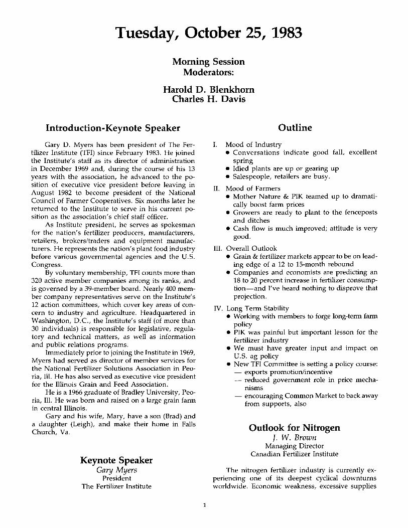
L Mood of Industry • Conversations indicate good fall, excellent

spring • Idled plants are up or gearing up • Salespeople, retailers are busy.

II. Mood of Farmers • Mother Nature & PIK teamed up to dramati­

cally boost farm prices • Growers are ready to plant to the fenceposts

and ditches • Cash flow is much improved; attitude is very

good.

III. Overall Outlook • Grain & fertilizer markets appear to be on lead­

ing edge of a 12 to IS-month rebound • Companies and economists are predicting an

18 to 20 percent increase in fertilizer consump­tion-and I've heard nothing to disprove that projection.

IV. Long Term Stability • Working with members to forge long-term farm

policy • PIK was painful but important lesson for the

fertilizer industry • We must have greater input and impact on

U.S. ag policy • New TFI Committee is setting a policy course:

- exports promotion/incentive reduced government role in price mecha­nisms

- encouraging Common Market to back away from supports, also

Outlook for Nitrogen J. W. Brown

Managing Director Canadian Fertilizer Institute

The nitrogen fertilizer industry is currently ex­periencing one of its deepest cyclical downturns worldwide. Economic weakness, excessive supplies

of nutrients, plant closures, record crop production with resulting high grain inventories and low com­modity prices, the U.S. PIK program with its greatly reduced crop acreage and the inability of many de­veloping countries to finance purchases and generate exchange earnings and the high value of the U.S. dollar relative to other currencies are all contributing factors to a dismal year.

The last two years have been difficult for world producers and traders in nitrogen fertilizers. World production and consumption for total nitrogen in 1982 actually showed a decline and 1983 will probably be little if any better. As a result, world nitrogen prices have shown a continuous decline, many plants based on high cost feedstock both in the U.S. and abroad have been forced to close.

Changing World Supply-Demand Picture

Western Europe, traditionally a net exporter of nitrogen, became a major net importer of nitrogen fertilizer in 1982. The cost/price squeeze on produc~ tion of anhydrous ammonia in Western Europe in 1982 led to a reduction in ammonia output of about 12%.

Japan and Korea were likewise caught in the cost/price squeeze on ammonia production. As a re­sult, they reduced exports to less than half of what they had done in 1980. Japan reduced production from 2.1 million nutrient tonnes in 1980 to 1.7 million tonnes in 1982. Exports declined from 700,000 tonnes nitrogen in 1980 to less than 500,000 tonnes in 1982. Korea reduced production from over 1 million tonnes nitrogen in ammonia in 1980 to about 500,000 tonnes in 1982.

India, in 1982 and continuing into 1983, reduced imports of nitrogen by close to half a million nutrient tonnes. India's production, however, showed a re­markable increase during the past three years. In 1982, ammonia production was 62% higher than 1980.

Pakistan and Bangladesh showed the same gen­eral trends as India with production from their own plants increasing more rapidly than consumption.

Brazil has reduced its imports significantly in 1982-83. Part of the reduction was due to increased domestic production. However, a significant part of the decline in imports was due to internal economic problems which has resulted in a drop in nitrogen fertilizer consumption of one-third between 1981 and 1982 and probably a further decline this year.

Countries with Increased Exports

Mexican ammonia production has increased dra­matically from 1980 to 1982, from 1.5 million nutrient tonnes to over 2 million nutrient tonnes. Consump­tion has increased but not as the same pace at pro­duction.

2

Eastern Europe and the U.S.S.R. are taking an increasing share of total world traded nitrogen mar­kets. Consumption within this region has grown from 10.8 million tonnes of nitrogen in 1975 to 13.5 million tonnes in 1982. Exports of nitrogen in the same pe­riod have increased from 1.7 million tonnes to 4.5 million tonnes. In 1982, the Eastern Bloc countries supplied 25% of the world nitrogen trade.

China's production of fertilizer nitrogen in 1982 of 10.1 million nutrient tonnes was slightly below the previous year. Consumption, however, was down 584 thousand nutrient tonnes with imports down 423 thousand nutrient tonnes.

U.S. Situation

In 1983 fertilizer year, ammonia production of approximately 13.8 million tons was down 22% from the previous year; the lowest level since 1970. This reduced supply came about due to a 15% to 16% reduction in domestic fertilizer consumption (1.8 mil­lion tones N) and an 18% reduction in nitrogen ex­ports (460 thousand tons N). In total fertilizer nitro­gen demand for domestic consumption and exports declined by 2.2 million tons N or 2.7 million tons ammonia equivalent. Imports, on the other hand, increased by 4% (122.3 thousand tons N) or 160 thou­sand tons ammonia equivalent.

Canada

Canadian production of anhydrous ammonia in­creased 3% in fertilizer year 1983 to 2.66 million prod­uct tonnes. Domestic consumption increased 5% to slightly more than 1 million tonnes while exports, mainly to the U.S. market, increased 3% to 995 thou­sand nutrient tonnes.

World Outlook 1983/84

World consumption of fertilizer nitrogen, after two flat years, is forecast to increase by 3.8% in 1984 or 2.36 million nutrient tonnes. A reduction in car­ryover grain and oilseed inventories with improved prices are the principal reasons for the projected re­covery.

U.S. Outlook 1983184

Demand

In contrast to the two previous years where fer­tilizer nitrogen consumption declined by 7% and 16% respectively, prospects for increased nitrogen con­sumption appear particularly bullish at this time. Ag­riculture demand for nitrogen will increase in the 18-20% range during the current fertilizer year. Im­proved commodity prices, created by the drought of the past summer, will lower carryover inventories of corn and soybeans to the lowest levels since the early

seventies. Planted corn acreage is expected to re­bound from 60 million acres in 1983 to approximately 84 million acres in 1984.

Crop prices across the board have improved dra­matically-much faster than nitrogen fertilizer prices. As a result, it takes less bushels of almost any crop to buy a ton of nitrogen fertilizer than at any time since the early seventies.

The corn-nitrogen price ratio is a good example. In the summer of 1982, it took over 100 bushels of corn to buy a ton of ammonia or urea. With changing prices on corn and nitrogen, by August of this year it had changed to 64 bushels. Since August the ratio has improved even further. This ratio now is signif­icantly better than at any time since the early 1970's. The same is true for other crops.

Therefore, the U.S. nitrogen industry can well expect a return on the consumption levels of 1982 or above.

Exports

U.S. exports of nitrogen declined by 18% from 1982 to 1983 or about 460 thousand nutrient tons. The decline was due in most part to greatly reduced shipments of ammonia ( 44%) and urea ( 25%) while nitrogen exports in D.A.P. and M.A.P. were above the previous year. Increased demand for D.A.P. and M.A.P. will increase the nitrogen moving to in­ternational markets during the current fertilizer year whereas ammonia and urea exports are likely to re­main at current levels due to low world prices and stepped-up demand domestically.

Supply

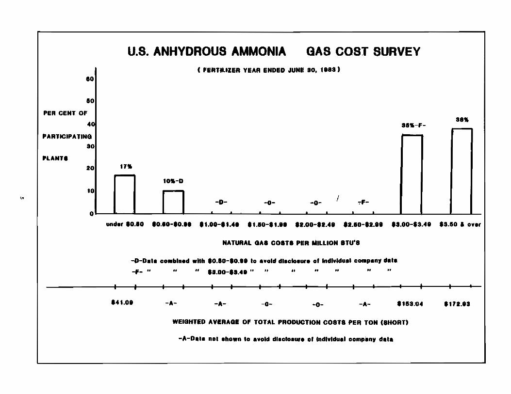
In 1983, U.S. ammonia production was the smallest since 1970 (13.8 million tons contrasted with 17.7 million tons in 1982). This sharply reduced out­put came about due to extended plant turnarounds and permanent and temporary plant shut downs. Natural gas costs going into ammonia production and other down stream products exceeeded the selling price for many producers. The net result was that operating levels as reported by TFI were at the lowest level of the past ten years. We really cannot expect a large increase in this area until ammonia and urea prices climb substantially above current levels.

The question has been asked why some of the plants that are currently closed do not re-open in consideration of the anticipated higher demand this year. It takes only a brief look at the average pro­duction costs of ammonia compared to the current average sales price or anticipated price next Spring to provide the answer. The recent TFI ammonia cost survey showed that 38% of the prodUcing plants, producing 31 % of the volume, have weighted aver­age gas costs of $3.90 per million BTU, and a weighted average production cost of $173 per ton. Ammonia

3

and urea prices will have to climb well above current levels before these plants will come back on stream. Some plants have renegotiated their gas contracts and are coming back into production but ammonia production will not likely reach the levels of 1981 and 1982.

Imports

Imports of fertilizer nitrogen increased by 4% in 1983 due entirely to a 72% increase in urea imports. Ammonia imports were down slightly (-4%) from the previous year. The current world glut in urea has led to a prolonged period of very depressed prices which may run well into the future. An anticipated pick up in world nitrogen demand in 1984 will tighten the supply and should strengthen prices.

U.S. ammonia imports which have been running at approximately 2.24 million tons in 1980-82 dropped in 1983 to 2.14 million tons with most of the decrease originating in the U.S.s.R. Imports from the U.S.S.R. have dropped from a peak of 1.1 million tons in 1981 to 474 thousand tons in 1983. This is a significant trend. U.S. ammonia imports are increasingly being sourced from Western Hemisphere countries-Can­ada, Mexico, Trinidad, and Venezuela. We can expect this supply trend to continue.

U.S. imports of nitrogen could reach the 2.8 mil­lion nutrient tons level during the present fertilizer year. Some of these increased imports are likely to originate in Canada for both ammonia and urea. Two new world-scale ammonia plants in Canada, with combined annual capacity of over 900 thousand short tons of ammonia and 880 thousand short tons of urea commenced production in the second quarter of 1983. If economics permit, the combined output of these two units could make available an additional 500 thousand tonnes of nitrogen for export markets in 1983/84. With the start-up of a new urea plant in Trinidad later this year, more product will be avail­able to the U.S. market from this source.

Summary

The 1982183 year was the second consecutive year of declining nitrogen production, consumption, and exports for the U.S. As a result of the Payment in Kind (PIK) program, agricultural consumption in the U.S. plummeted in 1982183. More than 50 million acres of land was withheld from agricultural pro­duction in 1983. Corn acreage planted alone fell from 82 million level in 1982 to 60 million in 1983.

For the first time in two years, the dominant factors affecting nitrogen consumption-acreage, commodity prices, and farm income-are forecast to make a strong recovery in the 1983/84 fertilizer year.

The summer drought significantly reduced yield expectation for corn, soybeans, and other Spring planted crops. Poor yields and the acreage with-

drawn from produciton due to PIK, particularly for corn, will reduce the excess grain inventories, ex­cluding wheat, that have plagued agriculture for the past two years. Commodity prices have strengthened this summer in response to reduced supplies, and the stronger prices will put acreage back into pro­duction in 1984.

Agricultural demand and prices are forecast to increase throughout the current fertilizer year. The U.S. nitrogenous fertilizer industry is experiencing some relief on gas costs thus reducing the cost of producing ammonia and its derivatives. Urea imports are expected to decline in 1983/84 relative to prior years' levels. It is believed that with the world nitro­gen market recovery, world urea stocks will be re­duced and world trade will increase in traditional markets.

Total nitrogen demand is expected to outstrip available supplies in the current year. Ending inven­tories are expected to decline with nitrogen spot prices strengthening especially in the second quarter of 1984. In total, 1983/84 has all the signs fer a much impro'ved year.

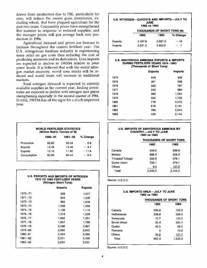
WORLD FERTILIZER STATISTICS (Million Metric Tonnes of N)

1980-81 1981-82 % Change

Production 62.60 62.04 0.9

Imports 13.16 12.46 4.4

Exports 13.15 11.60 11.8

Consumption 60.60 60.44 - 0.3

U.S. EXPORTS AND IMPORTS OF NITROGEN 1970 TO 1983 FERTILIZER YEARS

(Nitrogen Short Tons)

Imports Exports

1970-71 929 1,077 1971-72 843 1,032 1972-73 882 1,508 1973-74 1,068 1.269 1974-75 1.198 1.115 1975-76 1.218 1,239 1976-77 1,842 1,251 1977-78 1,857 1,798 1978-79 2,240 2,467 1979-80 2,565 2,642 1980-81 2,454 3,088 1981-82 2,531 2,498 1982-83 2,654 2,037

4

U.S. NITROGEN-EXPORTS AND IMPORTS-JULY TO JUNE

Exports

Imports

1982 vs 1983

THOUSANDS OF SHORT TONS (N)

1982

2,497.6

2,531.2

1983

2,037.3

2,653.5

% Ch~Jnge

-18

+ 1

U.S. ANHYDROUS AMMONIA EXPORTS & IMPORTS DURING FERTILIZER YEARS 1974-1983

(Thousands of Short Tons)

Exports Imports

1974 645 438

1975 361 598 1976 326 767 1977 546 960 1978 480 1,054

1979 554 1,735

1980 776 2,219

1981 816 2.161 1982 760 2,244

1983 428 2.144

U.S. IMPORTS OF ANHYDROUS AMMONIA BY COUNTRY -JULY TO JUNE

1982 vs 1983

THOUSANDS OF SHORT TONS

1982 1983

Canada 559.5 636.6

Mexico 608.6 528.2

Trinadad Tobago 332.8 378.1

Soviet Union 733.1 474.1

Others 127.2

Total 2,243.5 2.144.2

Source: U.S. D.C.

U.S. IMPORTS UREA-JULY TO JUNE 1982 vs 1983

THOUSANDS OF SHORT TONS

1982 1983

Canada 583.8 720.9 Netherlands 208.8 269.0 Venezuela 12.7 122.5 Soviet Union 35.4 261.7 Quator 42.5 69.5 Romania 0 74.9 Others 30.8 107.7

Total 952.4 1.635.9

Source: U.S. D.C.

'-"

I 80

I

PER CENT Of

.. PARTICIPA TINe

3

.LANT. 2

1

I

J

I

I

•

o

u.s. ANHYDROUS AMMONIA GAS COST SURVEY ( FERTILIZER YEAR ENDED ~UNE ao, 1.8a)

38 .. 31"-f-

"" 1."-0

-0- -0- -0- I ~f-

• . . . . • • • und.r ' •• 80 '0.80-'0." .1.00-...... '1.'0-'1." ••• 00-...... ' •• 10-' •• " .a.00-.3.... .a.lo a ov.r

NATURAL GA' CO'T' PER MILLION BTU"

-O-O.'a co.bln.d with '0.10-' •. " 10 avoid d'.clo.ura o' Indlvldu.' co.panr da.a

-F- " II .. .a .• o-.a .... " .. n " .. .. .. • ~ ______ .I~ ________ L-______ ~ ________ ~ ______ ~ __________ L-______ ~ __________ L-______ ~ __ _ . i... . .

'''1.0' -A- -A- -0- -0- -A- '1Ia.0" 'U2 .• 3

WEIGHTED AYERAGE OF TOTAL PRODUCT'ON C08T8 PER TON (8HORT)

"'A-D ••• nol .hown 10 lVold dl.clo ...... o. individual co.pian, da.a

u.s. NITROGEN FERTILIZER INVENTORIES

Tons Tons (1000)..---_______ ---, (1000),------______ ------, 3800 850 3600 ANHYDROUS 800 UREA SOUD 3400 AMMONIA 750 3200 700 3000 650 2800 600 2600 ~ ~ 550 ~ 2400 500 ~ ~ 2200 450 2000 400

".".~".".".-.-.-.-.'"

JASONDJFMAMJ JASONDJFMAMJ

Tons (1000)..---______ -------. 2950 2800 2650 2500 2350

2050 1900 1750 1600 1450 1300 1150 1000

SOLUTION 28-32% N

J A SON D J F M A M J

Source: TFI, October 1983

6

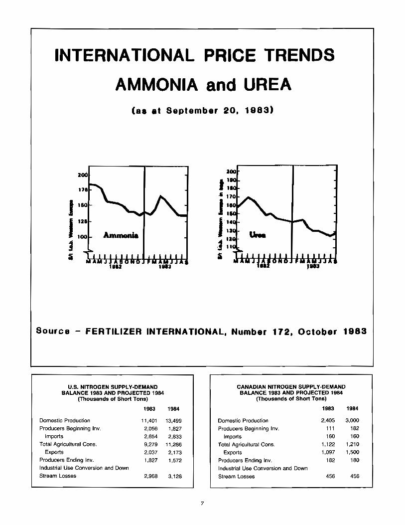
INTERNATIONAL PRICE TRENDS

J J J I

AMMONIA and UREA (a8 at September 20, 1983)

200

Sourc e - FERTILIZER INTERNATIONAL. Number 112, October 1983

U.S. NITROGEN SUPPLY-DEMAND CANADIAN NITROGEN SUPPLY-DEMAND BALANCE 1983 AND PROJECTED 1984 BALANCE 1983 AND PROJECTED 1984

(Thousands of Short Tons) (Thousands of Short Tons)

1983 1984 1983 1984

Domestic Production 11,401 13,499 Domestic Production 2,405 3,000

Producers Beginning Inv. 2,056 1,827 Producers Beginning Inv. 111 182

Imports 2,654 2,833 Imports 160 160

Total Agricultural Cons. 9,279 11,286 Total Agricultural Cons. 1,122 1,210

Exports 2,037 2,173 Exports 1,097 1,500

Producers Ending Inv. 1,827 1,572 Producers Ending Inv. 182 180 Industrial Use Conversion and Down Industrial Use Conversion and Down Stream Losses 2,968 3.128 Stream Losses 456 456

7

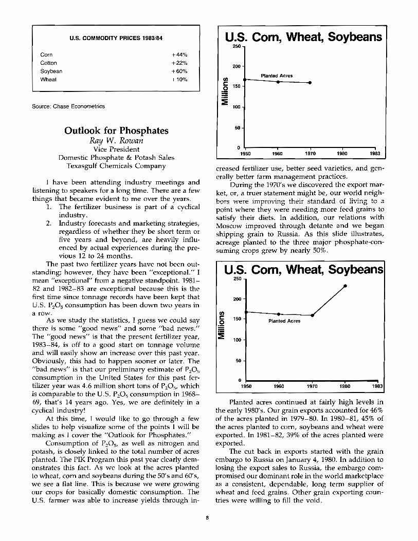
Corn

Cotton

Soybean

Wheat

U.S. COMMODITY PRICES 1983/84

Source: Chase Econometrics

Outlook for Phosphates Ray W. Rowan

Vice President

+44%

+22%

+60%

+10%

Domestic Phosphate & Potash Sales Texasgulf Chemicals Company

I have been attending industry meetings and listening to speakers for a long time. There are a few things that became evident to me over the years.

1. The fertilizer business is part of a cyclical industry.

2. Industry forecasts and marketing strategies, regardless of whether'they be short term or five years and beyond, are heavily influ­enced by actual experiences during the pre­vious 12 to 24 months.

The past two fertilizer years have not been out­standing; however, they have been "exceptional." I mean "exceptional" from a negative standpoint. 1981-82 and 1982-83 are exceptional because this is the first time since tonnage records have been kept that U.S. P20 S consumption has been down two years in a row.

As we study the statistics, I guess we could say there is some "good news" and some "bad news." The "good news" is that the present fertilizer year, 1983-84, is off to a good start on tonnage volume and will easily show an increase over this past year. Obviously, this had to happen sooner or later. The "bad news" is that our preliminary estimate of PZ0 5

consumption in the United States for this past fer­tilizer year was 4.6 million short tons of P20 S' which is comparable to the U.S. P20 S consumption in 1968-69, that's 14 years ago. Yes, we are definitely in a cyclical industry!

At this time, I would like to go through a few slides to help visualize some of the points I will be making as I cover the "Outlook for Phosphates."

Consumption of P20 S' as well as nitrogen and potash, is closely linked to the total number of acres planted. The PIK Program this past year clearly dem­onstrates this fact. As we look at the acres planted to wheat, corn and soybeans during the 50's and 60's, we see a flat line. This is because we were growing our crops for basically domestic consumption. The U.S. farmer was able to increase yields through in-

8

u.s. Com, Wheat, Soybeans 250

200

Planted Acres (I) C 150

~ -

:i 100

50

0 1950 1960 1970 1980 1983

creased fertilizer use, better seed varieties, and gen­erally better farm management practices.

During the 1970's we discovered the export mar­ket, or, a truer statement might be, our world neigh­bors "\A.,rere improving their standard of living to a point where they were needing more feed grains to satisfy their diets. In addition, our relations with Moscow improved through detante and we began shipping grain to Russia. As this slide illustrates, acreage planted to the three major phosphate-con­suming crops grew by nearly 50%.

u.S. Corn, Wheat, Soybeans 250

200

(I) C 150 .2

--Planted Acres

:E 100

50

0 1950 1960 1970 1980 1983

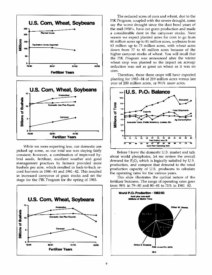
Planted acres continued at fairly high levels in the early 1980's. Our grain exports accounted for 46% of the acres planted in 1979-80. In 1980-81, 45% of the acres planted to corn, soybeans and wheat were exported. In 1981-82, 39% of the acres planted were exported.

The cut back in exports started with the grain embargo to Russia on January 4, 1980. In addition to losing the export sales to Russia, the embargo com­promised our dominant role in the world marketplace as a consistent, dependable, long term supplier of wheat and feed grains. Other grain exporting coun­tries were willing to fill the void.

u.s. Com, Wheat, Soybeans 2SO -200

...... tedAc_

tI)

.§ 150 Equivalent ~ Exported

i 100 -50

0 19180 80/81 81/82 82/83

Fertilizer Years

1S u.s. Com, Wheat, Soybeans

Production

04----------r--------~--------~ 79/80 80181 81/82

Fertilizer Years

While we were exporting less, our domestic use picked up some, so our total use was staying fairly constant; however, a combination of improved hy­brid seeds, fertilizer, excellent weather and good management practices by farmers provided more bushels per acre, which resulted in back-to-back re­cord harvests in 1980-81 and 1981-82. This resulted in increased carryover of grain stocks and set the stage for the PIK Program for the spring of 1983.

u.s. Com, Wheat, Soybeans 15

I 10l-~~~~~~--------~--~~----· m 15 tI) S 5

II O~--------~----------r---------~ 79/80 80181 81/82

Fertilizer Years

9

The reduced acres of corn and wheat, due to the PIK Program, coupled with the severe drought, some say the worst drought since the dust bowl years of the mid-1930's, have cut grain production and made a considerable dent in the carryover stocks. Next season we expect planted acres for corn to go from 60 million acres up to 81 million acres, soybeans from 63 million up to 73 million acres, with wheat acres down from 77 to 65 million acres because of the higher carryout stocks of wheat. You will recall that the PIK Program was announced after the winter wheat crop was planted so the impact on acreage reduction was not as great on wheat as it was on corn.

Therefore, these three crops will have expected planting for 1983-84 of 219 million acres versus last year of 200 million acres, or 9112% more acres.

12.0

10.5

tI) 9.0 C

~ 7.5

'0 6.0 tI) C 4.5 .2 • 3.0

1.5

U.S. P20S Balance

Indwllrlal u.ea, Fields Inventory, ~. Elc .

n n ~ H H n H N • ~ H ~ M Yu, Ending June 30

~ M • H H ~ ~ H • • n n H Ac:Id Plant O ..... 1Ing Rote

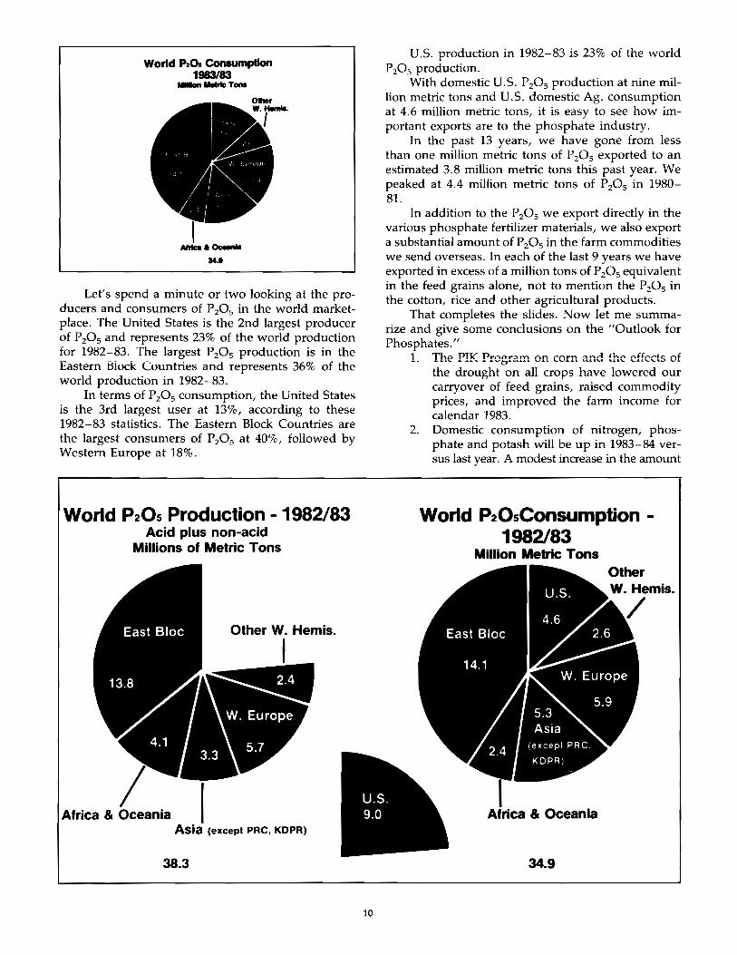
Before I leave the domestic U.5. market and talk about world phosphates, let me review the overall demand for PzOs which is logically satisfied by U.5. production, and compare that demand to the rated production capacity of U.5. producers to calculate the operating rates for the various years.

This slide illustrates the cyclical nature of the fertilizer business. The range of operating rates goes from 98% in 79-80 and 80-81 to 71 % in 1981-82.

World PI.O. ProducUon -1982/83 AcId plus norHICId

MIIIIona of Metnc T_

38.3

World PtO, Consumption 1983183

...". MeIrIc T_

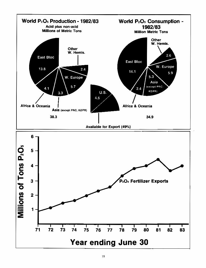
Let's spend a minute or two looking at the pro­ducers and consumers of PzOs in the world market­place. The United States is the 2nd largest producer of PzOs and represents 23% of the world production for 1982-83. The largest PzOs production is in the Eastern Block Countries and represents 36% of the world production in 1982-83.

In terms of PzOs consumption, the United States is the 3rd largest user at 13%, according to these 1982-83 statistics. The Eastern Block Countries are the largest consumers of P zOs at 40%, followed by Western Europe at 18%.

World P20S Production -1982/83 Acid plus non-acid

Millions of Metric Tons

Africa & Oceania I Asia (except PRe, KDPR)

38.3

10

U.s. production in 1982-83 is 23% of the world P 205 production. .. .

With domestic U.S. PzOs productIon at nme mIl­lion metric tons and U.S. domestic Ag. consumption at 4.6 million metric tons, it is easy to see how im­portant exports are to the phosphate industry.

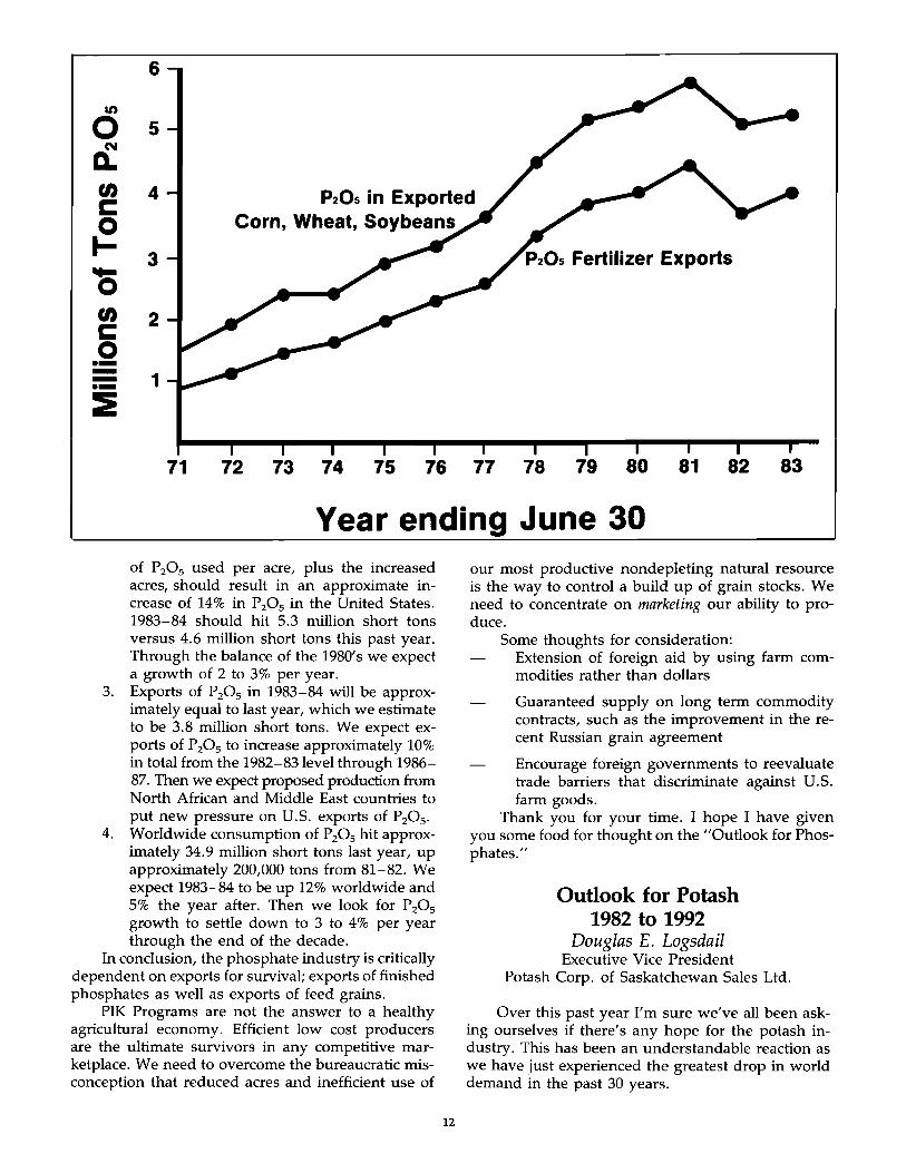
In the past 13 years, we have gone from less than one million metric tons of P zOs exported to an estimated 3.8 million metric tons this past year. We peaked at 4.4 million metric tons of PzOs in 1980-81.

In addition to the P zOs we export directly in the various phosphate fertilizer materials, we also export a substantial amount of PzOs in the farm commodities we send overseas. In each of the last 9 years we have exported in excess of a million tons of P zOs equivalent in the feed grains alone, not to mention the PzOs in the cotton, rice and other agricultural products.

That completes the slides. Now let me summa­rize and give some conclusions on the "Outlook for Phosphates. "

1. The PIK Program on corn and the effects of the drought on all crops have lowered our carryover of feed grains, raised commodity prices, and improved the farm income for calendar 1983.

2. Domestic consumption of nitrogen, phos­phate and potash will be up in 1983-84 ver­sus last year. A modest increase in the amount

World P20sConsumption -1982183

Million Metric Tons Other

Africa & Oceania

34.9

World P20S Production -1982/83 Acid plus non-acid

Millions of Metric Tons

Other W. Hemis.

I

Africa & Oceania I Asia (except PRe, KDPR)

38.3

World P20S Consumption -1982/83

Million Metric Tons

Africa & Oceania

34.9

Available for Export (49%)

6

II)

0 5 C'I

D. en 4 C 0 I- 3 ~

0 en 2 C 0 --- 1 ---::E

71 72 73 74 75 76 77 78 79 80 81 82 83

Year ending June 30

11

6

II)

0 5 N

D.. tn 4 P20S in Exported c:: 0 Corn, Wheat, Soybeans I- 3 ... 0 tn 2 C 0 --- 1 ---

:IE

71 72 73 74 75 76 77 78 79 80 81 82 83

Year ending June 30 of P20 S used per acre, plus the increased acres, should result in an approximate in­crease of 14% in P20 S in the United States. 1983-84 should hit 5.3 million short tons versus 4.6 million short tons this past year. Through the balance of the 1980' s we expect a growth of 2 to 3% per year.

3. Exports of P20 S in 1983-84 will be approx­imately equal to last year, which we estimate to be 3.8 million short tons. We expect ex­ports of P20 S to increase approximately 10% in total from the 1982-83 level through 1986-87. Then we expect proposed production from North African and Middle East countries to put new pressure on U.S. exports of P20 S '

4. Worldwide consumption of P20 S hit approx­imately 34.9 million short tons last year, up approximately 200,000 tons from 81-82. We expect 1983-84 to be up 12% worldwide and 5% the year after. Then we look for P20 S

growth to settle down to 3 to 4% per year through the end of the decade.

In conclusion, the phosphate industry is critically dependent on exports for survival; exports of finished phosphates as well as exports of feed grains.

PIK Programs are not the answer to a healthy agricultural economy. Efficient low cost producers are the ultimate survivors in any competitive mar­ketplace. We need to overcome the bureaucratic mis­conception that reduced acres and inefficient use of

12

our most productive nondepleting natural resource is the way to control a build up of grain stocks. We need to concentrate on marketing our ability to pro­duce.

Some thoughts for consideration: Extension of foreign aid by using farm com­modities rather than dollars

Guaranteed supply on long term commodity contracts, such as the improvement in the re­cent Russian grain agreement

Encourage foreign governments to reevaluate trade barriers that discriminate against U.S. farm goods.

Thank you for your time. I hope I have given you some food for thought on the "Outlook for Phos­phates."

Outlook for Potash 1982 to 1992

Douglas E. Logsdail Executive Vice President

Potash Corp. of Saskatchewan Sales Ltd.

Over this past year I'm sure we've all been ask­ing ourselves if there's any hope for the potash in­dustry. This has been an understandable reaction as we have just experienced the greatest drop in world demand in the past 30 years.

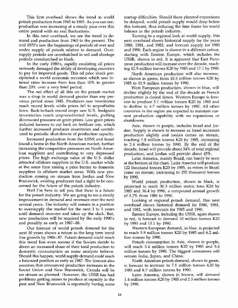
This first overhead shows the trend in world potash production from 1945 to 1965. As you can see, production was increasing at a steady pace over this entire period with no real fluctuations.

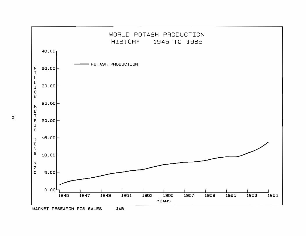
In this next overhead, we see the trend in de­mand and production from 1965 to the present. The mid 1970's saw the beginnings of periods of over and under supply of potash relative to demand. Over­supply periods are crosshatched in red and shortage periods crosshatched in black.

In the early 1980's, rapidly escalating oil prices seriously damaged the ability of developing countries to pay for imported goods. This oil price shock pre­cipitated a world economic recession which saw in­terest rates increase from less than 10% to greater than 20% over a very brief period.

The net effect of all this on the potash market was a drop in world demand greater than any pre­vious period since 1945. Producers saw inventories reach record levels while prices fell to unprofitable lows. Back-to-back record crops saw U.s. feedgrain inventories reach unprecedented levels, putting downward pressure on grain prices. Low grain prices induced farmers to cut back on fertilizer use, which further increased producer inventories and contrib­uted to periodic shut-downs of production capacity.

Increased production from the USSR and Israel found a home in the North American market, further increasing the competitive pressures on North Amer­ican suppliers and contributing to very depressed prices. The high exchange value of the U.S. dollar attracted offshore suppliers to the u.s. market while at the same time raising a price barrier to domestic suppliers in offshore market areas. With new pro­duction coming on stream from Jordan and New Brunswick, existing producers had a right to be con­cerned for the future of the potash industry.

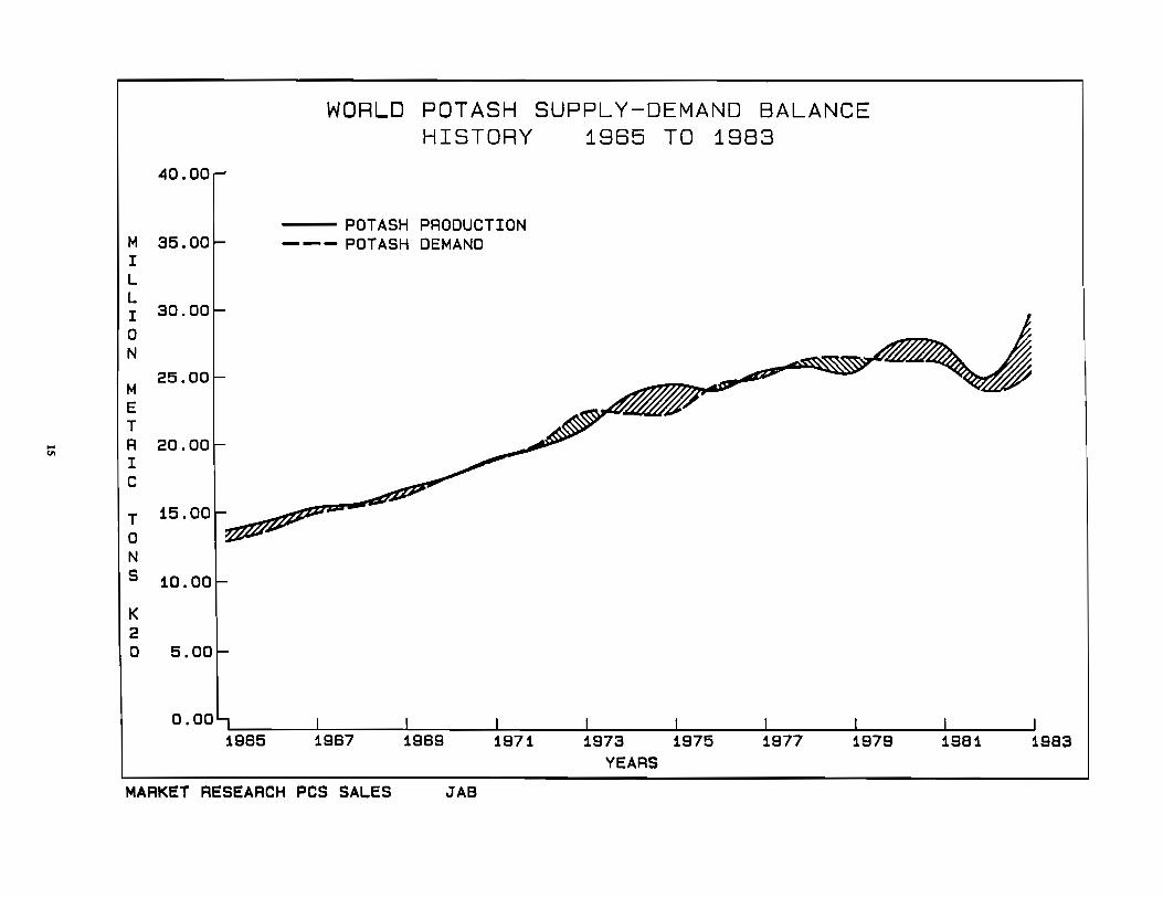
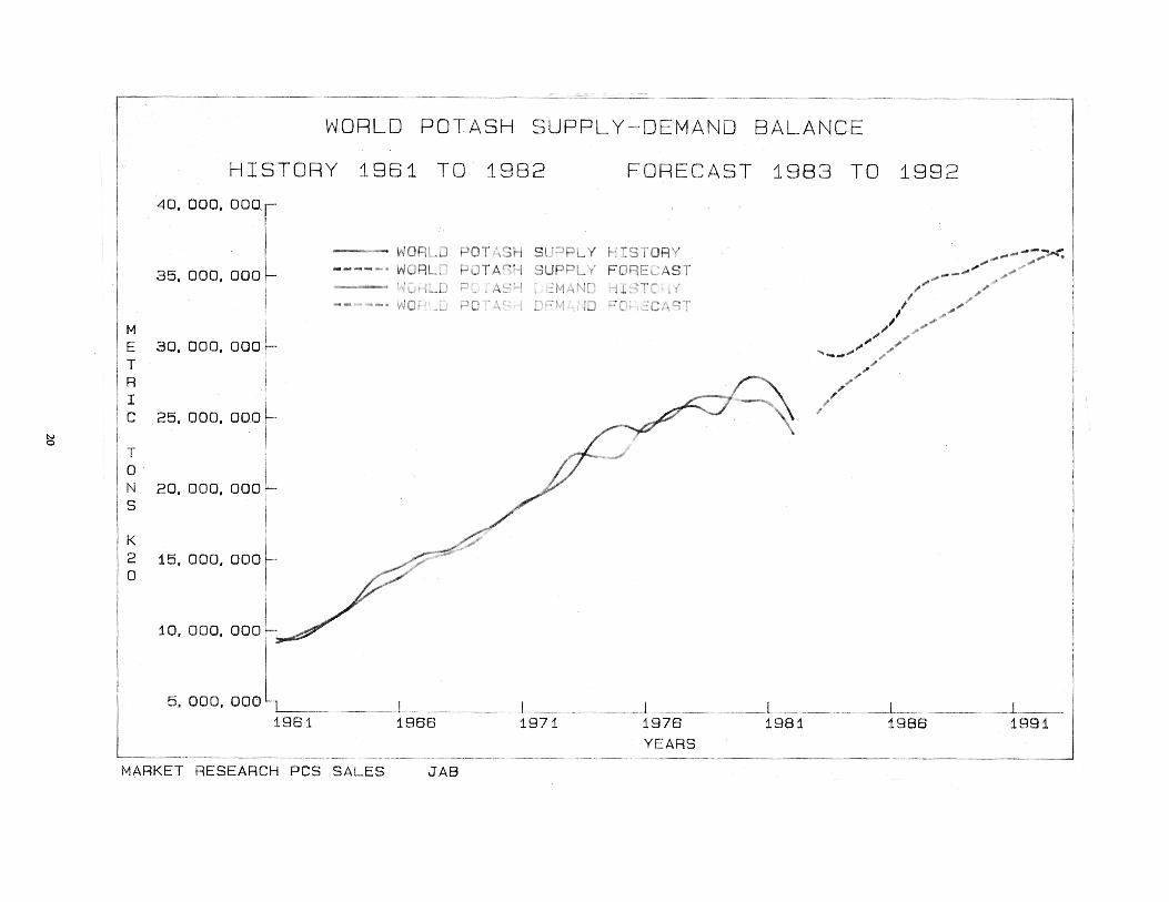
Well I'm here to tell you that there is a future for the potash industry. We are going to see a steady improvement in demand and revenues over the next several years. The industry will remain in a position to oversupply the market for the next 3 to 5 years until demand recovers and takes up the slack. But, new production will be required by the early 1990's and possibly as early as 1987-88.

Our forecast of world potash demand for the next 10 years shows a return to the long term trend line growth by 1986-87. Potash demand could reach this trend line even sooner if the Soviets decide to divert an increased share of their total production to domestic consumption as some analysts believe. Should this happen, world supply-demand could reach a balanced position as early as 1987. The forecast also assumes that announced production increases in the Soviet Union and New Brunswick, Canada will be on stream as planned. However, the USSR has had problems getting mines to produce at capacity in the past and New Brunswick is reportedly having some

13

startup difficulties. Should these planned expansions be delayed, world potash supply would drop below this forecast, thus reducing the time frame for world balance in the potash industry.

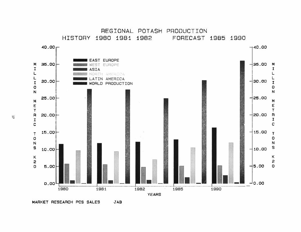
Turning to a regional look at world supply, this next overhead shows historical supply for the years 1980, 1981, and 1982; and forecast supply for 1985 and 1990. Each region is shown in a different colour, starting with Eastern Europe, which includes the USSR, shown in red. It is apparent that East Euro­pean production will increase over the decade, reach­ing 12.9 million tonnes K20 by 1985 and 17.1 by 1990.

North American production will also increase, as shown in green, from 10.5 million tonnes K20 by 1985 to 11.9 million tonnes by 1990.

West European production, shown in blue, will decline slightly by the end of the decade as French production is closed down. Western Europe is fore­cast to produce 5.1 million tonnes K20 by 1985 and to decline to 4.7 million tonnes by 1990. All other countries in the region are expected to maintain cur­rent production capability with no expansions or shutdowns.

Asia, shown in purple, includes Israel and Jor­dan. Supply is shown to increase as Israel increases production slightly and Jordan comes on stream, reaching 1.8 million tonnes K20 by 1985, increasing to 2.4 million tonnes by 1990. By the end of the decade, Israel will provide about 54% of total regional production, and Jordan will provide about 45%.

Latin America, mainly Brazil, can barely be seen at the bottom of the chart. Latin America will produce 122 thousand tonnes K20 by 1985, as mines in Brazil come on stream, increasing to 292 thousand tonnes by 1990.

World potash production, shown in black, is projected to reach 30.3 million metric tons K20 by 1985 and 36.4 by 1990, a compound annual growth of 3.7% from 1985 to 1990.

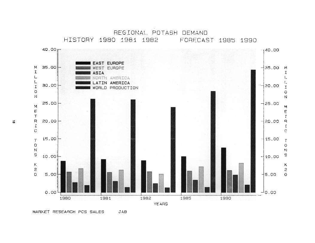
Looking at regional potash demand, this next overhead shows historical demand for 1980, 1981, and 1982, with forecasts for 1985 and 1990.

Eastern Europe, including the USSR, again shown in red, is forecast to demand 10 million tonnes K20 by 1985 and 13.1 by 1990.

Western European demand, in blue, is projected to reach 5.9 million tonnes K20 by 1985 and 6.2 mil­lion tonnes by 1990.

Potash consumption in Asia, shown in purple, will reach 3.4 million tonnes K20 by 1985 and 5.6 million tonnes by 1990. The biggest consumers will remain India, Japan, and China.

North American potash demand, shown in green, is forecast to increase to 7.1 million tonnes K20 by 1985 and 8.7 million tonnes by 1990.

Latin America, shown in brown, will demand 1.4 million tonnes K20 by 1985 and 2.5 million tonnes by 1990.

WORLD POTASH PRODUCTION HISTORY 1845 TO 1~365

40.00

POTASH PRODUCTION M 35.00 I L L I 30.00 0 N

25.00 M E

... IT II>

R 20.00 I C

T 15.00 0 N S 10.00

K 2 0 5.00

0.00 1945 1947 1949 1951 1953 195:7 1959 1961 1963 1965

YEARS

MARKET RESEARCH PCS SALES JAB

....

.."

40.00

I M 36.00 f-I L L I 30.00 0 N

26.00 M E T

IR 20.00 I C

T 16.00

0 N S

K 2 0 6.00

0.00 1986

WORLD POTASH SUPPLY-DEMAND BALANCE HISTORY 1965 TO 1983

POTASH PRODUCTION - - - POT ASH DEMAND

1987 1989 1971 1973 1976 1977 1979 YEARS

MARKET RESEARCH PCS SALES JAB

1981 1983

...... 0-

M I L L I 0 N

M E

IT R I C

T 0 N S

K 2 0

40.00

3s.ool

20.00

15.00

10.00

5.00

WORLD POTASH SUPPLY-DEMAND BALANCE FORECAST 19B3 TO 1992

POTASH PRODUCTION --- POTASH DEMAND

1989 1990 1981 1992 YEARS

MARKET RESEARCH PCS SALES JA8

REGIONAL POTASH PRODUCTION HISTORY 1980 1981 1982 FORECAST 1985 1990

40.00 40.00

EAST EUROPE M 35.00 WEST EUROPE 35.00 M I ASIA I L 4 ',-". ~. \ " L L LATIN AMERICA L I 30.00 WORLD PRODUCTION 30.00 I 0 0 N N

25.00 25.00 M M E E T T

...... R 20.00 20.00 R ~

I I C C

T 15.00 -115.00 T 0 0 N N S 10.00

~ 10.00 S

K ~ n K 2 n 2 0 5.00 • • - - 5.00 0

0.00 0.00 1980 1981 1982 1985 1980

YEARS

MARKET RESEARCH PCS SALES JAB

REGIONAL POTASH DEMAND HISTORY 1980 1981 1982 FORECAST 1985 1990

40.00 I, -,40.00

EAST EUROPE M 35.00 WEST EUROPE 35.00 M I ASIA I L , .. 4 W- t ~('~l7l. ,"",: t1 : .... '~ L L LATIN AMERICA L I 30.00 WORLD PRODUCTION 30.00 I 0 0 N N

25.00 25.00 M M E E T T

>-' R 20.00 20.00 R C»

I I C C

T 15.00 15.00 T 0 0 N N S 10.00 10.00 S

K I. I. I. ._n K 2 . ·n n n 2 0 5.00 ,.., 5.00 0

0.001Lf- - _ 1iO:o:I _- ~ _ _ L-I __ ~ _ _ IlO.J __ ~ _ _ u.J __ ~ _ _ W.:.I __ ---.l0.00

1980 1981 1982 1985 1990 YEARS

MARKET RESEARCH PCS SALES JAB

,... ..0

40.00

M 35.00 I L L I 30.00 o N

M 25.00

E T

IR 20.00 I C

T 15.00 o N S

K 2

10.00

o 5.00

0.00 EAST EUROPE

REGIONAL POTASH SUPPLY-DEMAND BALANCE FORECAST 1884 TO 1880

-:::~ EXPORTABLE SURPLUS eav&Z1 IMPORT DEMAND

WEST EUROPE

ASIA NORTH AMERICA

LATIN AMERICA

AFRICA

MARKET RESEARCH PCS SALES JAB

WORLD SUPPLY-DEMAND

-------.---W-O~-L-~---P~-T-. ;;H-----SU-~~-L~·--D-~-M-A~--D --B- A- L- =N-C E-----i

. HISTORY 1961 TO 1982 F OR E CA ST 1983 TO 199 2 I I 40,OOO,OOQ~ I

I I WORLD POTASH SUPPLY HISTORY _---~~ I

35, 000. 000 i- ----- . WORl. D POT ASH SUPPLY FORECAST ... -_ ......... ...... ,. ... I WOR~D POTASH DEMAND HISTORY /' ",

I -----. WORLD PO:- 4SH DF."1vI4N.J FORECAClT / ... .;,'

I I ... ' M /' "" , , ""

I, E 3D, ODD, 000 r .... ,,.., ,/

I ~- , I T ! ",,/ I R J ~ ,';' i , , I t· / I C 25, ODD, 000 ~ . I'

! : ; T i

o I ~ 20, ODD, 000 I

~

I ~ 15. 000. 000 ~ 1

0 I

L,/ _______ .. _____ 1. .. _. __ __ _

1981 1988 1971 1978 1981 1988 1991 YEARS

._-_._------------------_ .. _-.----._-------------------_._---------------------------------------------- ---------- -MARKET RESEARCH pes SAL ES JAB

African potash demand, not shown here, is fore­cast to reach 380 thousand tonnes K20 by 1985 and 570 thousand tonnes by 1990.

Oceania, also not shown, will consume 260 thou­sand tonnes K20 by 1985, increasing to 280 thousand tonnes by 1990.

World potash demand, shown in black, is fore­cast to reach 28.4 million metric tons K20 by 1985 and 36.2 by 1990. This represents a compound annual growth of 5% from 1985 to 1990.

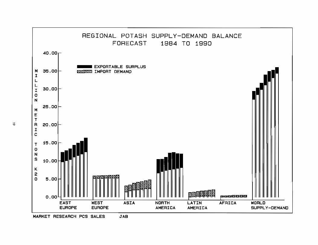
Putting it all together on this next overhead, you can see from the solid green areas representing net regional production available for export, that Eastern Europe, primarily .the Soviet Union, and North America, primarily Canada, will be the net exporting regions for the forecast period.

The crosshatched areas which indicate net im­port demand, show that Asia will remain the largest net importing region followed by Latin America, Western Europe, and finally Africa.

In conclusion let me briefly summarize our out­look for the potash industry. Our forecast of world potash demand for the next 10 years shows a return to the long term trend line growth by 1986-87. Po­tash demand could reach this trend line even sooner if the Soviets decide to divert an increased share of their total production to domestic consumption as some analysts believe. Should this happen, world supply-demand could reach a balanced position as early as 1987.

We are forecasting world potash demand to reach 28.4 million metric tons K20 by 1985 and 36.2 by 1990. This represents a compound annual growth of 5% from 1985 to 1990.

21

We are forecasting world potash production ca­pability to reach 30.3 million metric tons K20 by 1985 and 36.4 by 1990, a compound annual growth of 3.7% from 1985 to 1990.

In the shorter term, the outlook for North Amer­ica is buoyant. Potash consumption in 1984 is ex­pected to increase by about 1 million metric tons K20 over 1983. This increase will result from substantially greater planted acreage, particularily corn, but also aided by increased soybean and cotton plantings. Farmers are coming out of 1983 with relatively high net farm incomes. While a portion of this higher income is going to reduce debt, recent surveys in­dicate that it will also be spent on inputs. Farm ma­chinery seems to be a third priority after inputs. In general, this implies increased potash useage due to greater acreage and higher application rates than in 1983.

There has been some talk that a bumper crop in 1984 could put the industry back into the doldrums. This just isn't so. It took two or three years of bumper crops in the face of falling demand to create the situation we have just experienced. It cannot be re­peated on the basis of one good crop. Certainly a good crop in 1984 will raise grain inventories and cause prices to fall from their current record levels. But prices won't fall to the disastrous levels of 1983. On the other hand, should the 1984 crop be below average for any reason, the world could be facing a grain shortage and todays high prices may not seem so high after all.

Tuesday, October 25, 1983

Afternoon Session's Moderator:

Jean L. Cheval

Urease Inhibitors-Current Status Dr. Roland D. Hauck

Division of Agricultural Development National Fertilizer Development Center

Tennessee Valley Authority

Urea use continues to increase. Solid urea and N solutions that contain urea comprise slightly more than 25% of u.s. agricultural N consumption. The increase in urea production and use stems more from the economies and other advantages of urea manu­facture, storage, and handling than from its agro­nomic characteristics. In fact, under certain condi­tions of use, urea may be less effective as a supplier of N for crops than other N sources, e.g., ammonium nitrate. Problems associated with the use of urea as a fertilizer mainly are the result of rapid hydrolysis of urea to ammonium carbonate in soil through the action of a urease enzyme complex, causing a rise in pH and evolution of ammonia. Problems include damage to germinating seeds and seedling plants, nitrite toxicity, and gaseous loss of N.

Formerly, agronomists advised farmers not to surface-apply urea without incorporating it into the soil, or to place urea with or near seed. Fertilizer and crop management systems now being adopted by farmers sometimes make such restrictions on urea use impractical or undesirable. In no-till or minimum tillage agriculture, fertilizers containing urea are sur­face-applied without incorporation and there is risk of losing urea-N through ammonia volatilization. And for some crops, such as small grains, application of urea with seed would be convenient.

Approaches to minimizing problems of urea use include: (1) coating urea to slow its rate of dissolution; (2) adding substances to urea which lower the pH and otherwise alter the chemistry of the urea-soil micro site; and (3) use of urease inhibitors. Successful coatings have been developed, but coated urea prod­ucts, because of their cost and/or properties are prac­tical only for special situation use. Urea phosphate and urea-urea phosphate formulations, which lower microsite pH, are being developed and widely tested by TVA. These formulations show promise for use with wheat and in minimum tillage cropping systems or other situations where N must be surface-applied

22

without incorporation. However, coating or acidu­lating urea addresses only a small portion of the total urea used. For the bulk of urea use, either as a solid or in N solutions, auuition of an effective urease inhibitor would minimize seedling damage and N loss as ammonia from surface applications.

Many chemicals have been identified which re­tard the rate of urea hydrolysis by interfering with the action of the enzyme, urease. However, most of these chemicals have been shown to be ineffective in soil. Soil urease activity appears to reside in a very large organic complex (molecular weight, perhaps, >600,000 atomic units). Many soil microorganisms and crop residues also exhibit urease activity; chem­icals that may effectively block urea hydrolysis by one enzyme source may be ineffective in blocking the entire soil urease complex. Among the chemicals studied for use with fertilizers are acetohydroxamic acid and its derivatives, various phenols and qui­nones, and phosphoroamides. Chemicals have been found ineffective because: (1) they are inhibitors of purified urease preparations in solution but not of soil urease; (2) they are chemically or biologically unstable; (3) they contain toxic elements or are po­tential carcinogens; and (4) they may be too expen­sive to use at effective concentrations. Phenyl mer­curic acetate is an effective inhibitor of soil urease but would be environmentally unacceptable as a fer­tilizer additive. Quinones found to effectively inhibit soil urease activity include p-benzoquinone and 2,5-dimethyl benzoquinone, but these chemicals have carcinogenic potential. Phenylphosphorodiamidate (PPDA) is the most potent inhibitor of soil urease activity identified to date. It was discovered by an East German research group that screened about 12,000 substances for their potential as urease inhibitors. PPDA has two major limitations. First, it is relatively stable only in a very narrow pH range around neu­trality. It decomposes after addition to urea ammo­nium nitrate solution, but can be incorporated into

urea melt. The dry urea-PPDA mixture apparently is stable for several weeks but gradual decomposition of the PPDA probably occurs during prolonged stor­age. Biological and/or chemical degradation of PPDA in soil appears to be rapid. In many soils, urea hy­drolysis in the presence of PPOA is delayed for a few days, after which time hydrolysis is rapid. Green­house studies indicate that PPOA has promise for use in flooded rice where urea is added directly into the flood water. Under these conditions urea hy­drolysis in the absence of a urease inhibitor can lead to ammonia loss. Ammonia loss from urea amended with PPDA is markedly less. However, the value of PPDA for use in flooded rice systems has not been demonstrated in field experiments.

The second limitation of PPOA is its high cost. Its manufacture probably is through the intermediate compound, POCI, which also is expensive to pro­duce. Phosphorotriamide (PTA) probably can be pro­duced at a lower cost but is considerably less potent than PPOA. Other phosphoroamides also have been tested; none inhibit urease activity in soil as much as does PPDA. Research at TVA and elsewhere is directed toward increasing the stability of PPOA, finding cheaper routes to the manufacture of PPDA and PTA, and identifying related compounds that have potential as urease inhibitors.

In summary, strong arguments can be presented in favor of amending urea and urea-based fertilizers with a chemical that will effectively retard soil urease activity. Although several chemicals show promise as urease inhibitors, none have undergone sufficient development to merit their use with commercial fer­tilizers at this time. However, progress thus far gives reason for believing that effective urease inhibitors will be developed.

Fertilizer Quality Control-Can It Be Achieved in Today's Marketing

System Hilton V. Rogers

Head, Dept. of Fertilizer Analysis and Inspection Clemson University

It is an honor for me to have an opportunity to participate in the Fertilizer Industry Round Table. This is a very important meeting to the fertilizer in­dustry and by the trickle-down method, it is also important to the users of commercial fertilizers. In discussing a topic with Joe Reynolds, several subjects came to mind. We felt that "quality control" as it relates to recent changes was something that could be pursued.

In preparing this paper, I solicited some ideas from several of my fellow control officials. The ideas presented are a combination of my own and other control officials. Most of the data came from South

23

Carolina situations but similar conclusions could be drawn from other states.

First of all, we should define "quality control" as it pertains to commercial fertilizer. The marketing of fertilizer is different from that of many other prod­ucts in that state laws require that fertilizer must be labeled with specific guarantees. Just how close fer­tilizers must come to actually meeting those guar­antees depends on the "investigational allowance" provided in the individual state laws. The Associa­tion of American Plant Food Control Officials has a model fertilizer bill called Uniform State Fertilizer Bill. There is a suggested regulation for investigational allowances, however, all states have not adopted these uniform standards. Some states are much more le­nient than others in how close companies must come to meeting the labeled guarantees. If a company uses "investigational allowances" as a sale standard for quality control then the quality may vary from state to state.

I like to think of quality control as a standard of excellence that each company has decided it will at­tain and will present to its customers. This pertains to both physical and chemical characteristics. It can somewhat be compared to how fast a person will drive regardless of the posted speed limit if he knows there are no highway patrolmen on the road.

At best, some states are sampling 12 to 15 per­cent of the fertilizer tonnage sold and most states are sampling much less than this. Even though some companies complain of penalties, deficiency penalties alone are not enough of a deterrent to force a com­pany to meet guarantees. This is especially true if penalties can be counted as operational expenses. Each company must decide the quality it wants to sell and take the necessary steps to provide that qual­ity.

Now, let us pursue the idea of how important is it that guarantees be fully met? Will crops receiving the fertilizer respond to moderate variations? There is no really good way to determine this since there are various philosophies for applying fertilizer. Some agronomists recommend fertilizer to maintain a me­dium level of soil reserve for phosphorus and potas­sium. With this philosophy the fertilizer could vary widely from the guarantee with no immediate effect on the current crop. Yet, a person wants a certain amount of the various plant nutrients or he would not have ordered the particular grade or the partic­ular amount. He should expect to get what he or­dered within a practical degree of variation.

What is a practical degree of variation? The med­icines we take affect our health. We can get an un­derdose or an overdose if they do not contain a given amount of active ingredients. I examined a copy of The U.s. Pharmacopeia and found there is a great variation in the deviation allowed from the stated contents listed on the medicine container. As ex-

amples, some of the ranges are listed: Warfarin So­dium 97.0-102.0%, Strontium Sr 85,90-110.0%, Po­tassium Chloride 99.0-101.5% KCI, Magnesium Sulfate 99.0-100.5% MgS04' Morphine Sulfate 93.0-107.0% and Streptomycin Sulfate not less than 65.0%. Is it as important to meet the exact labeled amounts of plant nutrients in fertilizer as it is to meet the exact stated ingredients in medicine? I don't think so but this will be discussed later.

Now to get back to the assigned topic "Fertilizer Quality Control-Can It Be Achieved in Today's Marketing System". Some plants in South Carolina are doing exactly that and I am going to discuss some steps they are taking to achieve it. South Carolina has used the AAPFCO investigational allowance for N, P20 S and K20 since 1978. Three of the plants we will discuss are dry blenders, one is a granulating plant and the other a clear liquid plant. Generally, the deficiency percentages are based on those sam­ples which had guarantees for two or more of the primary nutrients.

Tnt! sHoes will iHustrate how the plant is achiev­ing this record. Size of materials are carefully ex-

amined and are matched as closely as possible. The equipment is kept operational making sure gates are not leaking so as to allow accurate weighing of in­gredients. The same person does most of the mixing.

Hopper and scales are kept clean. An electronic type load cell system is used which clears each batch. The same conscientious man has operated the front­end loader for years. This place is kept immaculate and contamination is avoided. A limited number of grades are made and there is little error in formu­lation.

This is a new dry blending plant but there is an old liquid plant at the same location. An electronic type load cell system is used and scales and hoppers are always clean. All excess material is pushed aside so as to not contaminate material bins. A computer is used to formulate grades and the complete formula and guarantee is given to each customer. A copy of the printout is sent to our office and is attached to the registration form for customer mixes. The print­out provides all required information including grade and the guaranteed analysis, list ot materials, weight and manufacturer.

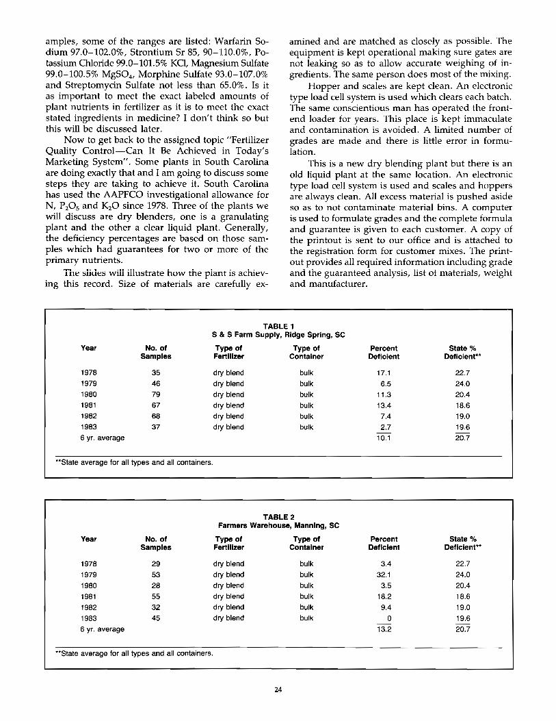
TABLE 1 S & S Farm Supply, Ridge Spring, SC

Year No. of Type of Type of Percent State % Samples Fertilizer Container Deficient Deficient--

1978 35 dry blend bulk 17.1 22.7

1979 46 dry blend bulk 6.5 24.0 1980 79 dry blend bulk 11.3 20.4 1981 67 dry blend bulk 13.4 18.6 1982 68 dry blend bulk 7.4 19.0 1983 37 dry blend bulk 2.7 19.6

6 yr. average 10.1 20.7

"State average for all types and all containers.

TABLE 2 Farmers Warehouse, Manning, SC

Year No. of Type of Type of Percent State % Samples Fertilizer Container Deficient Deficient·'

1978 29 dry blend bulk 3.4 22.7

1979 53 dry blend bulk 32.1 24.0

1980 28 dry blend bulk 3.5 20.4

1981 55 dry blend bulk 18.2 18.6

1982 32 dry blend bulk 9.4 19.0

1983 45 dry blend bulk 0 19.6

6 yr. average 13.2 20.7

"State average for all types and all containers.

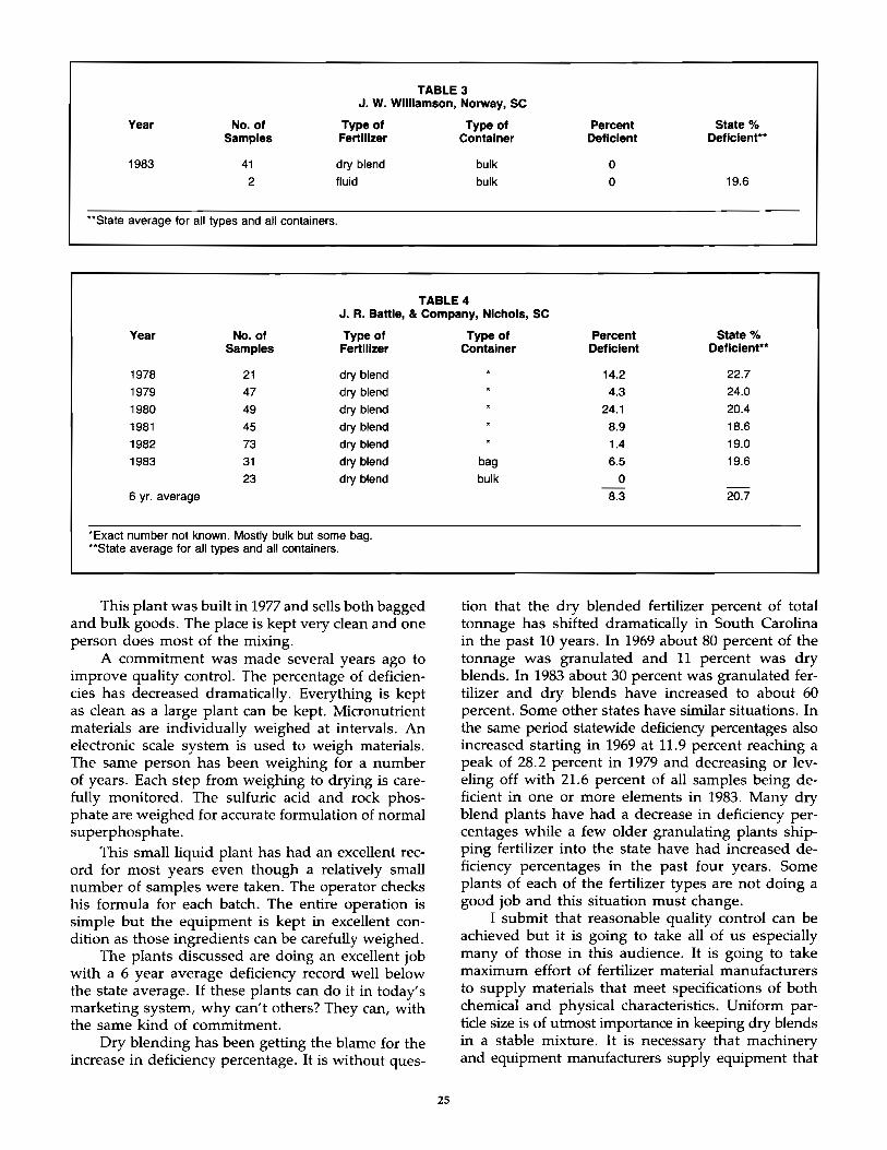
TABLE 3 J. W. Williamson, Norway, SC

Year No. of Type of Type of Percent State % Samples Fertilizer Container Deficient Deficient··

1983 41 dry blend bulk 0 2 fluid bulk 0 19.6

"State average for all types and all containers.

TABLE 4 J. R. Battle, & Company, Nichols, SC

Year No. of Type of Samples Fertilizer

1978 21 dry blend

1979 47 dry blend

1980 49 dry blend

1981 45 dry blend

1982 73 dry blend

1983 31 dry blend

23 dry blend

6 yr. average

'Exact number not known. Mostly bulk but some bag. ··State average for all types and all containers.

This plant was built in 1977 and sells both bagged and bulk goods. The place is kept very clean and one person does most of the mixing.

A commitment was made several years ago to improve quality control. The percentage of deficien­cies has decreased dramatically. Everything is kept as clean as a large plant can be kept. Micronutrient materials are individually weighed at intervals. An electronic scale system is used to weigh materials. The same person has been weighing for a number of years. Each step from weighing to drying is care­fully monitored. The sulfuric acid and rock phos­phate are weighed for accurate formulation of normal superphosphate.

This small liquid plant has had an excellent rec­ord for most years even though a relatively small number of samples were taken. The operator checks his formula for each batch. The entire operation is simple but the equipment is kept in excellent con­dition as those ingredients can be carefully weighed.

The plants discussed are doing an excellent job with a 6 year average deficiency record well below the state average. If these plants can do it in today's marketing system, why can't others? They can, with the same kind of commitment.

Dry blending has been getting the blame for the increase in deficiency percentage. It is without ques-

25

Type of Percent State % Container Deficient Deficient"

14.2 22.7

4.3 24.0

24.1 20.4

8.9 18.6

1.4 19.0

bag 6.5 19.6

bulk 0

8.3 20.7

tion that the dry blended fertilizer percent of total tonnage has shifted dramatically in South Carolina in the past 10 years. In 1969 about 80 percent of the tonnage was granulated and 11 percent was dry blends. In 1983 about 30 percent was granulated fer­tilizer and dry blends have increased to about 60 percent. Some other states have similar situations. In the same period statewide deficiency percentages also increased starting in 1969 at 11.9 percent reaching a peak of 28.2 percent in 1979 and decreasing or lev­eling off with 21.6 percent of all samples being de­ficient in one or more elements in 1983. Many dry blend plants have had a decrease in deficiency per­centages while a few older granulating plants ship­ping fertilizer into the state have had increased de­ficiency percentages in the past four years. Some plants of each of the fertilizer types are not doing a good job and this situation must change.

I submit that reasonable quality control can be achieved but it is going to take all of us especially many of those in this audience. It is going to take maximum effort of fertilizer material manufacturers to supply materials that meet specifications of both chemical and physical characteristics. Uniform par­tide size is of utmost importance in keeping dry blends in a stable mixture. It is necessary that machinery and equipment manufacturers supply equipment that

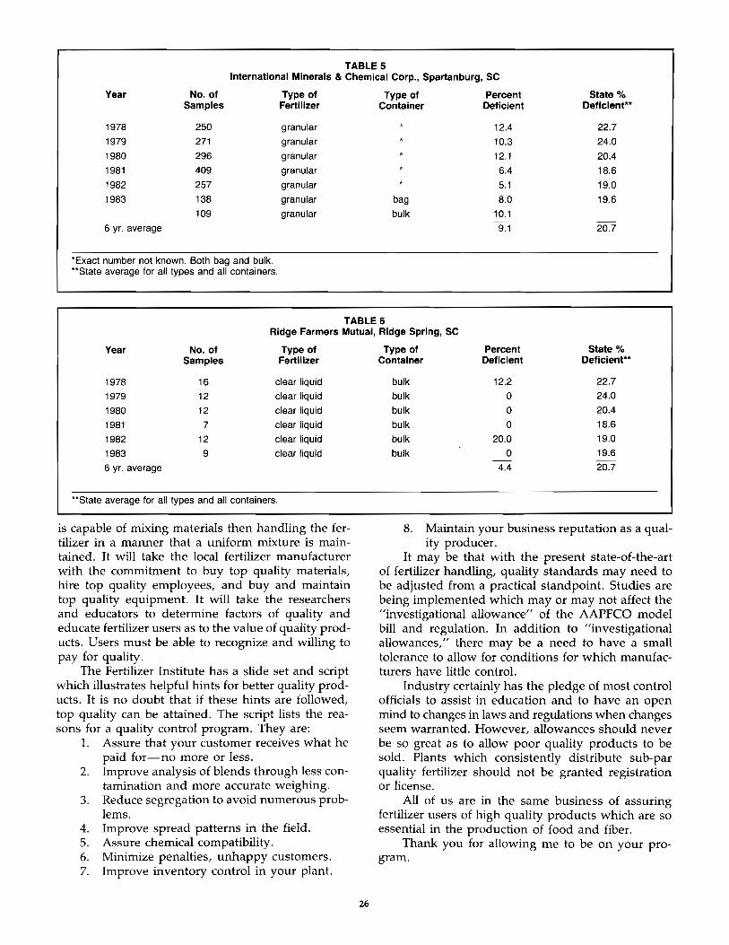
TABLE 5 International Minerals & Chemical Corp., Spartanburg, SC

Year No. of Samples

1978 250

1979 271

1980 296

1981 409

1982 257

1983 138

109

6 yr. average

'Exact number not known. Both bag and bulk. "State average for all types and all containers.

Type of Fertilizer

granular

granular

granular

granular

granular

granular

granular

Type of Container

bag

bulk

Percent State % Deficient Deficient·'

12.4 22.7

10.3 24.0

12.1 20.4

6.4 18.6

5.1 19.0

8.0 19.6

10.1

9.1 20.7

TABLE 6 Ridge Farmers Mutual, Ridge Spring, SC

Year No. of Type of Samples Fertilizer

1978 16 clear liquid

1979 12 clear liquid

1980 12 clear liquid

1981 7 clear liquid

1982 12 clear liquid

1983 9 clear liquid

6 yr. average

"State average for all types and all containers.

is capable of mixing materials then handling the fer­tilizer in a manner that a uniform mixture is main­tained. It will take the local fertilizer manufacturer with the commitment to buy top quality materials, hire top quality employees, and buy and maintain top quality equipment. It will take the researchers and educators to determine factors of quality and educate fertilizer users as to the value of quality prod­ucts. Users must be able to recognize and willing to pay for quality.

The Fertilizer Institute has a slide set and script which illustrates helpful hints for better quality prod­ucts. It is no doubt that if these hints are followed, top quality can be attained. The script lists the rea­sons for a quality control program. They are:

1. Assure that your customer receives what he paid for-no more or less.

2. Improve analysis of blends through less con­tamination and more accurate weighing.

3. Reduce segregation to avoid numerous prob-lems.

4. Improve spread patterns in the field. S. Assure chemical compatibility. 6. Minimize penalties, unhappy customers. 7. Improve inventory control in your plant.

26

Type of Percent State % Container Deficient Deficient··

bulk 12.2 22.7

bulk 0 24.0

bulk 0 20.4

bulk 0 18.6

bulk 20.0 19.0

bulk 0 19.6

4.4 20.7

8. Maintain your business reputation as a qual­ity producer.

It may be that with the present state-of-the-art of fertilizer handling, quality standards may need to be adjusted from a practical standpoint. Studies are being implemented which mayor may not affect the "investigational allowance" of the AAPFCO model bill and regulation. In addition to "investigational allowances," there may be a need to have a small tolerance to allow for conditions for which manufac­turers have little controL

Industry certainly has the pledge of most control officials to assist in education and to have an open mind to changes in laws and regulations when changes seem warranted. However, allowances should never be so great as to allow poor quality products to be sold. Plants which consistently distribute sub-par quality fertilizer should not be granted registration or license.

All of us are in the same business of assuring fertilizer users of high quality products which are so essential in the production of food and fiber.

Thank you for allowing me to be on your pro­gram.

What is Happening to Quality Control in Blending?

(Control Official) Dr. David L. Terry

Assistant Director and Coordinator Fertilizer Program

Division of Regulatory Services University of Kentucky

Introduction

The quality of blended fertilizer has been of con­cern since the beginning of the practice of blending in the late 1930's and 1940's (Hignett 1965). Segre­gation was identified early as the main problem in producing blended fertilizers that were "on grade" and that would stay "on grade" during handling (Hignett 1965). The earliest discussion on bulk blend quality problems that I could find in the Proceedings of the Fertilizer Industry Round Table was in 1959 in which Mr. W. L. Hill of the USDA discussed the problem of segregation in fertilizers (Hill 1959).

The objective of my presentation, however, is not to discuss what causes off-grade blends, but to evaluate the quality of blends produced today in the United States and then to make some suggestions from a control official's viewpoint on bulk blend qual­ity control.

QUALITY OF BLENDS PRODUCED IN THE U.S.

Background

Fertilizers have been sampled and analyzed by control officials since the late 1800's when some of the state fertilizer laws were first enacted. There has also been a real question since the first sample an­alyzed fell below the guarantee as to whether the fertilizer was deficient. How do you determine when a sample is deficient? By definition, a manufacturer's guarantee means that the fertilizer will contain not less than the guaranteed concentration (AAPFCO 1983). For example, if a fertilizer has a guarantee of 20% total nitrogen, then if the fertilizer actually con­tains only 19.9% N then it is deficient and a violation of the law. The manufacturer has the right to ask how confident are you that during sampling, sample reduction and preparation and analysiS that you, the control official, did not cause the result to be below 20% when in fact the true concentration of nitrogen in the fertilizer is 20%.

The real answer to the question as to how con­fident you are in calling a sample deficient can be obtained from use of statistics. Up until 1968 there was no agreement among control officials as to how much an analytical result can be below the guarantee before one can "confidently" say it is deficient. The

27

Association of American Plant Food Control Officials (AAPFCO) adopted a set of "Investigational Allow­ances" in 1968 based on some pioneer work by Miles and Quackenbush that enable a control official to call a sample deficient and make an error no more than one time in 100 (Rund 1974). By definition these "In­vestigational Allowances" take into consideration the inherent variations in sampling, sample preparation and chemical analysis (AAPFCO 1983). It is important to note that the investigational allowances do not allow for the inherent variations in fertilizer manu­facture. This is the responsibility of the manufacturer.

Now, with that brief background, let us try to evaluate the quality of blended fertilizers in the U.S.

Criterion of Quality

The quality of blends can be evaluated in several ways; however, I have chosen to use the sample deficiency rate of official state regulatory samples as the criterion. The deficiency rate is defined as the percentage of samples with one or more deficiencies in the NPK analyses.

It would be easy if every state (1) used the AAPFCO investigational allowances, (2) identified each sample as to whether it was a blend or not and (3) reported the results of the analyses of official samples such that one could determine the deficiency rate of the blend samples. Unfortunately, I found ony two states, South Carolina and Iowa that accomplish all of the above in their publication. We collect this in­formation in Kentucky but do not publish it.

I immediately consulted the "Fertilizer Quality Control Survey" recently conducted by the AAPFCO and The Fertilizer Institute (TFI); however, the results from that survey do not allow one to evaluate the quality of blends under the standard AAPFCO in­vestigational allowances. It became painfully obvious that we do not know what the quality of blended fer­tilizer is in the U.S.!

Quality of Blends-An Estimate

In order to get an estimate of the quality of blends in the U.s., I wrote to 12 states, requested the needed information, and received useable information from 9 states. I was able to identify the blends by either a code in the data sent by the state or by knowing the types of fertilizers manufactured by a particular company. This required a sample by sample evalu­ation. I manually applied the AAPFCO investiga­tional allowances to the data from those states not using them. Very briefly I found that the quality of blends in the 9 states surveyed for the past four fertilizer years ranged from a low of about 25% to a high of about 75%.

The deficiency rates of the blends had no rela­tionship to overall deficiency rates for 1981-82 re­ported in the Quality Control Survey of AAPFCOI

TFL For example, one state reported an overall de­ficiency rate of about 10%, but their blend deficiency rate was over 50%; another whose reported overall deficiency rate was about 17% had a blend deficiency rate of about 40%.

The comparison of the deficiency rates of blends from two states who use different investigational al­lowances is not valid. For example, in the above mentioned survey Kentucky and Missouri reported blend deficiency rates of 34 and 18%, respectively for 1981-82. However, when compared using the AAPFCO investigational allowances, the deficiency rates were 43 and 44% for Kentucky and Missouri, respectively. What appeared at first to be a significant difference in blend quality between the two states turned out to not be significant.

It is my estimate that the blend deficient rate nationwide is in the range of 40-50% when the AAPFCO investigational allowances are applied. As a point of information, a joint sampling study among AAPFCO, TFI, and the Association of Official Ana­lytkill Chemists is now underway to re-evaluate the AAPFCO investigational allowances. The results of this study should be available in about one year.

SUGGESTIONS ON BLEND QUALITY CONTROL

My suggestions relative to bulk blend quality control follow:

(1) Each blend plant should establish and en­force a rigid set of manufacturing practices designed to produce quality blends.

(2) Each plant should sample and have ana­lyzed sometime before the busy season at least 10 samples of each of their most pop­ular mixes. From these analyses they should compute the average analysis, the standard deviation and coefficient of variation. This would provide information on the quality and expected deficiency rate of their pro­duction and a basis for making improve­ments in their process.

(3) Control officials should make a point of pro­viding assistance as well as regulatory con­trol to the industry.

(4) In making comparisons of deficiency rates among states, you should know what in­vestigational allowances are being used by each state so that only valid comparisons are made.

SUMMARY

The quality of blends in the u.s. must be eval­uated using a common set of investigational allow­ances. The estimated quality of U.S. blends using the official sample deficiency rate as the criterion and the AAPFCO investigational allowances is 40-50% de­ficiencies. Suggestions to blenders on quality control

28

emphasized adherence to a set of good manufactur­ing practices. Control officials were encouraged to provide assistance as well as control to the industry.

REFERENCES

1. Assn. of Amer. Plant Food Control Officials. 1983. Official Publication No. 36. Division of Regula­tory Services, University of Kentucky, Lexing­ton, KY 40546. Pages 22-39.

2. Hignett, Travis P. 1965. Bulk Blending of Fertil­isers: Practices and Problems. Proc. The Fertilizer Society No. 87. London. March 25, 1965.

3. Hill, W. L. 1959. Segregation of Fertilizers. Proe. Fertilizer Ind. Round Table. Page 51.

4. Rund, R. C. 1975. The Background and Rationale for AAPFCO Recommended Investigational Al­lowances. In Assn. of Amer. Plant Food Control Officials Official Pub. No. 28. Division of Reg­ulatory Services, University of Kentucky, Lex­ington, KY 40546. Page 67.

What is Happening To Quality Control in Blending? (Blender)

Henry T. McCarley President, Burley Belt Chemical Co.

Burley Belt Chemical Company is an operating company of Top Yield Industries, Inc., operating in the State of Kentucky. Top Yield operates in Ken­tucky and Indiana doing business with wholesale and retail clientele. The corporate headquarters are lo­cated in Lexington.

Burley Belt has thirteen operating facilities in Kentucky. Four of these units operate as wholesale and retail. Nine are retail only.

The eastern Kentucky terrain and the tobacco market dictate that we continue to supply bagged fertilizer to our customers. Our product mix consists of 98% dry products and 2% liquid nitrogen. We therefore dry blend all products for the market place. Our four large plants were converted from ammo­niation units to dry blenders. Extra care had to be given to planning, developing and building dry blenders. Each of our blenders are unique. The equipment's performance is very important in quality controL

Our plant at London handles bulk fertilizer by use of an overhead crain. A special blender had to be built to compensate for this piece of equipment. A series of hoppers was placed in line and, beneath the hoppers, we built a 45 foot holding hopper on scales with an 18" stainless steel drag chain in its bottom. The chain pulls the product to the 2 ton blender located at one end. After blending, the prod­uct is then carried by elevator to the bagging hopper.

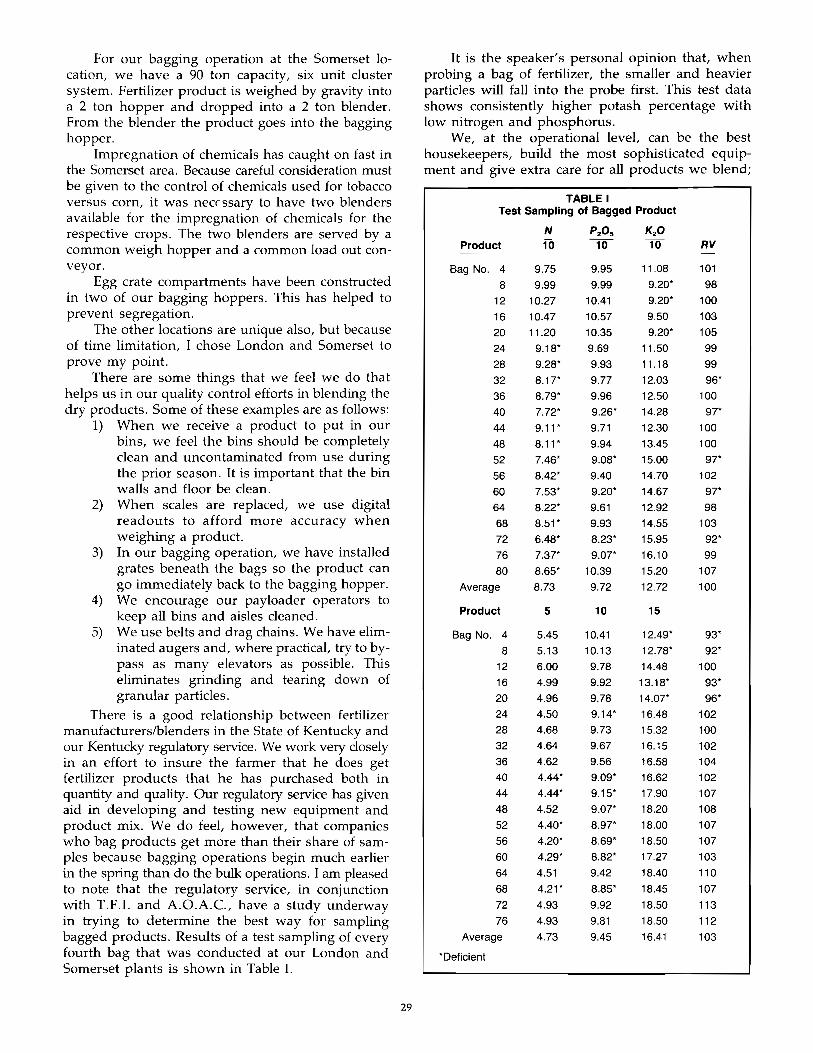
For our bagging operation at the Somerset lo­cation, we have a 90 ton capacity, six unit cluster system. Fertilizer product is weighed by gravity into a 2 ton hopper and dropped into a 2 ton blender. From the blender the product goes into the bagging hopper.

Impregnation of chemicals has caught on fast in the Somerset area. Because careful consideration must be given to the control of chemicals used for tobacco versus corn, it was nec( ssary to have two blenders available for the impregnation of chemicals for the respective crops. The two blenders are served by a common weigh hopper and a common load out con­veyor.

Egg crate compartments have been constructed in two of our bagging hoppers. This has helped to prevent segregation.

The other locations are unique also, but because of time limitation, I chose London and Somerset to prove my point.

There are some things that we feel we do that helps us in our quality control efforts in blending the dry products. Some of these examples are as follows:

1) When we receive a product to put in our bins, we feel the bins should be completely clean and uncontaminated from use during the prior season. It is important that the bin walls and floor be clean.

2) When scales are replaced, we use digital readouts to afford more accuracy when weighing a product.

3) In our bagging operation, we have installed grates beneath the bags so the product can go immediately back to the bagging hopper.

4) We encourage our payloader operators to keep all bins and aisles cleaned.

5) We use belts and drag chains. We have elim­inated augers and, where practical, try to by­pass as many elevators as possible. This eliminates grinding and tearing down of granular particles.

There is a good relationship between fertilizer manufacturerslblenders in the State of Kentucky and our Kentucky regulatory service. We work very closely in an effort to insure the farmer that he does get fertilizer products that he has purchased both in quantity and quality. Our regulatory service has given aid in developing and testing new equipment and product mix. We do feel, however, that companies who bag products get more than their share of sam­ples because bagging operations begin much earlier in the spring than do the bulk operations. I am pleased to note that the regulatory service, in conjunction with T.F.I. and A.O.A.C., have a study underway in trying to determine the best way for sampling bagged products. Results of a test sampling of every fourth bag that was conducted at our London and Somerset plants is shown in Table 1.

29

It is the speaker's personal opinion that, when probing a bag of fertilizer, the smaller and heavier particles will fall into the probe first. This test data shows consistently higher potash percentage with low nitrogen and phosphorus.

We, at the operational level, can be the best housekeepers, build the most sophisticated equip­ment and give extra care for alJ products we blend;

TABLE I Test Sampling of Bagged Product

N P20 5 K20 Product 10 10 10 RV

Bag No. 4 9.75 9.95 11.08 101

8 9.99 9.99 9.20* 98

12 10.27 10.41 9.20' 100

16 10.47 10.57 9.50 103

20 11.20 10.35 9.20* 105

24 9.18' 9.69 11.50 99

28 9.28* 9.93 11.18 99

32 8.17' 9.77 12.03 96'

36 8.79' 9.96 12.50 100

40 7.72" 9.26' 14.28 97-

44 9.11" 9.71 12.30 100

48 8.11 • 9.94 13.45 100

52 7.46- 9.08* 15.00 97*

56 8.42* 9.40 14.70 102

60 7.53* 9.20' 14.67 97*

64 8.22' 9.61 12.92 98

68 8.51 * 9.93 14.55 103

72 6.48' 8.23* 15.95 92*

76 7.37* 9.07* 16,10 99

80 8.65* 10.39 15.20 107

Average 8.73 9.72 12.72 100

Product 5 10 15

Bag No. 4 5.45 10.41 12.49* 93'

8 5.13 10.13 12.78* 92'

12 6.00 9.78 14.48 100

16 4.99 9.92 13.18* 93*

20 4.96 9.78 14.07' 96*

24 4.50 9.14* 16.48 102

28 4.68 9.73 15.32 100

32 4.64 9.67 16.15 102

36 4.62 9.56 16.58 104

40 4.44' 9.09* 16.62 102

44 4.44' 9.15* 17.90 107

48 4.52 9.07* 18.20 108

52 4.40' 8.97' 18.00 107

56 4.20* 8.69* 18.50 107

60 4.29* 8.82* 17.27 103

64 4.51 9.42 18.40 110

68 4.21' 8.85' 18.45 107

72 4.93 9.92 18.50 113

76 4.93 9.81 18.50 112

Average 4.73 9.45 16.41 103

*Deficient

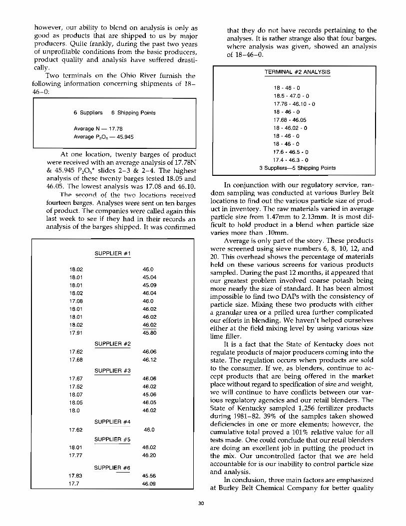
however, our ability to blend on analysis is only as good as products that are shipped to us by major producers. Quite frankly, during the past two years of unprofitable conditions from the basic producers, product quality and analysis have suffered drasti­cally.

Two terminals on the Ohio River furnish the following information concerning shipments of 18-46-0:

6 Suppliers 6 Shipping Points

Average N 17.78

Average P20 S - 45.945

At one location, twenty barges of product were received with an average analysis of 17.78N & 45.945 P20 S* slides 2-3 & 2-4. The highest analysis of these twenty barges tested 18.05 and 46.05. The lowest analysis was 17.08 and 46.10.

The second of the two locations received fourteen barges. Analyses were sent on ten barges of product. The companies were called again this last week to see if they had in their records an analysis of the barges shipped. It was confirmed

SUPPLIER #1

18.02 46.0

18.01 45.04

18.01 45.09

18.02 46.04

17.08 46.0

18.01 46.02

18.01 46.02

18.02 46.02

17.91 45.80

SUPPLIER #2

17.62 46.06

17.68 46.12

SUPPLIER #3 17.67 46.06

17.52 46.02

18.07 45.06

18.05 46.05

18.0 46.02

SUPPLIER #4

17.62 46.0

SUPPLIER #5

18.01 46.02

17.77 46.20

SUPPLIER #6

17.83 45.56 17.7 46.09

30

that they do not have records pertaining to the analyses. It is rather strange also that four barges, where analysis was given, showed an analysis of 18-46-0.

TERMINAL #2 ANAL VSIS

18 - 46 0

18.5 47.0 - 0

17.76 - 46.10 - 0 18-46-0

17.68 - 46.05

18 - 46.02 0

18 - 46 0 18 - 46 0

17.6 - 46.5 - 0

17.4 - 46.3 - 0 3 Suppliers--5 Shipping Points

In conjunction with our regulatory service, ran­dom sampling was conducted at various Burley Belt locations to find out the various particle size of prod­uct in inventory. The raw materials varied in average particle size from 1.47mm to 2.13mm. It is most dif­ficult to hold product in a blend when particle size varies more than .10mm.

Average is only part of the story. These products were screened using sieve numbers 6, 8, 10, 12, and 20. This overhead shows the percentage of materials held on these various screens for various products sampled. During the past 12 months, it appeared that our greatest problem involved coarse potash being more nearly the size of standard. It has been almost impossible to find two DAPs with the consistency of particle size. Mixing these two products with either a granul~r urea or a prilled urea further complicated our efforts in blending. We haven't helped ourselves either at the field mixing level by using various size lime filler.

It is a fact that the State of Kentucky does not regulate products of major producers coming into the state. The regulation occurs when products are sold to the consumer. If we, as blenders, continue to ac­cept products that are being offered in the market place without regard to specification of size and weight, we will continue to have conflicts between our var­ious regulatory agencies and our retail blenders. The State of Kentucky sampled 1,256 fertilizer products during 1981-82. 39% of the samples taken showed deficiencies in one or more elements; however, the cumulative total proved a 101 % relative value for all tests made. One could conclude that our retail blenders are doing an excellent job in putting the product in the mix. Our uncontrolled factor that we are held accountable for is our inability to control particle size and analysis.

In conclusion, three main factors are emphasized at Burley Belt Chemical Company for better quality

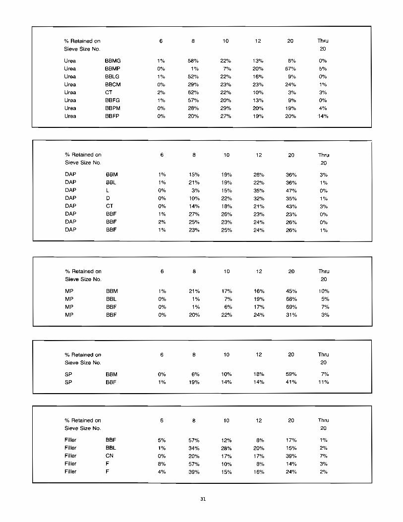
% Retained on 6 8 10 12 20 Thru

Sieve Size No. 20

Urea BBMG 1% 58% 22% 13% 6% 0%

Urea BBMP 0% 1% 7% 20% 67% 5%

Urea BBlG 1% 52% 22% 16% 9% 0%

Urea BBCM 0% 29% 23% 23% 24% 1%

Urea CT 2% 62% 22% 10% 3% 3%

Urea BBFG 1% 57% 20% 13% 9% 0%

Urea BBPM 0% 28% 29% 20% 19% 4%

Urea BBFP 0% 20% 27% 19% 20% -14%

% Retained on 6 8 10 12 20 Thru Sieve Size No. 20

DAP BBM 1% 15% 19% 26% 36% 3% DAP BBl 1% 21% 19% 22% 36% 1% DAP l 0% 3% 15% 35% 47% 0% DAP D 0% 10% 22% 32% 35% 1%

DAP CT 0% 14% 18% 21% 43% 3% DAP BBF 1% 27% 26% 23% 23% 0% DAP BBF 2% 25% 23% 24% 26% 0% DAP BBF 1% 23% 25% 24% 26% 1%

% Retained on 6 8 10 12 20 Thru

Sieve Size No. 20

MP BBM 1% 21% 17% 16% 45% 10%

MP BBl 0% 1% 7% 19% 68% 5%

MP BBF 0% 1% 6% 17% 69% 7%

MP BBF 0% 20% 22% 24% 31% 3%

% Retained on 6 8 10 12 20 Thru

Sieve Size No. 20

SP BBM 0% 6% 10% 18% 59% 7%

SP BBF 1% 19% 14% 14% 41% 11%

% Retained on 6 8 10 12 20 Thru

Sieve Size No. 20

Filler BBF 5% 57% 12% 8% 17% 1%

Filler BBl 1% 34% 28% 20% 15% 2%

Filler CN 0% 20% 17% 17% 39% 7% Filler F 8% 57% 10% 8% 14% 3% Filler F 4% 39% 15% 16% 24% 2%

31

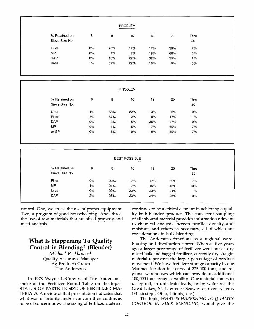
PROBLEM

% Retained on 6 8 10 12 20 Thru

Sieve Size No. 20

Filler 0% 20% 17% 17% 39% 7'% MP 0% 1% 7% 19% 68% 5% DAP 0% 10% 22% 32% 35% 1% Urea 1% 52% 22% 16% 9% 0%

PROBLEM

% Retained on 6 8 10 12 20 Thru

Sieve Size No. 20

Urea 1% 58% 22% 13% 6% 0%

Filler 5% 57% 12% 8%, 17% 1%

DAP 0% 3% 15% 35% 47% 0%

MP 0% 1% 6% 17% 69% 7% or SP 0% 6% 10% 18% 59% 7%

BEST POSSIBLE

% Retained on 6 8 Sieve Size No.

Filler 0% 20% MP 1% 21% Urea 0% 29% DAP 2% 25%

control. One, we stress the use of proper equipment. Two, a program of good housekeeping. And, three, the use of raw materials that are sized properly and meet analysis.

What Is Happening To Quality Control in Blending? (Blender)

Michael R. Hancock Quality Assurance Manager

Ag Products Group The Andersons

In 1978 Wayne LeCureux, of The Andersons, spoke at the Fertilizer Round Table on the topic, STATUS OF PARTICLE SIZE OF FERTILIZER MA­TERIALS. A review of that presentation indicates that what was of priority and/or concern then continues to be of concern now. The sizing of fertilizer material

32

10 12 20 Thru

20

17% 17% 39% 7% 17% 16% 45% 10% 23% 23% 24% 1% 23% 24% 26% 0%

continues to be a critical element in achieving a qual­ity bulk blended product. The consistent sampling of all inbound material provides information relevant to chemical analysis, screen profile, density and moisture, and others as necessary, all of which are considerations in bulk blending.

The Andersons functions as a regional ware­housing and distribution center. Whereas five years ago a larger percentage of fertilizer went out as dry mixed bulk and bagged fertilizer, currently dry straight material represents the larger percentage of product movement. We have fertilizer storage capacity in our Maumee location in excess of 225,000 tons, and re­gional warehouses which can provide an additional 100,000 ton storage capability. Our material comes to us by rail, in unit train loads, or by water via the Great Lakes, St. Lawrence Seaway or river systems (Mississippi, Ohio, Illinois, etc.).

The topic, WHAT IS HAPPENING TO QUALITY CONTROL IN BULK BLENDING, would give the

impression that a change, either positive or negative, had occurred or perhaps was occurring. If change is, in fact, occurring, it is focusing on the area of product awareness or specifically getting the product for which was paid.

As an organization which not only warehouses but blends over 200,000 tons of fertilizer material, we are acutely concerned with the product received and, as indicated earlier, closely monitor this material. Prior to the receipt of product into our facility, it was nec­essary to go through some basic planning stages and ultimate establishment of criteria for material to be received. My discussion will hereon focus on some of those functions we perform prior to and in actually handling product.

Product SelectlOn-This is based on individual re­quirements and marketability of the product and/ or resultant blends. Our basic raw materials are DAP, TSP, UREA, POTASH (Coarse & Granular) and MAP. Product mixes will vary from region to region and, as stated above, reflect specific needs or likes. While product mix may vary from company to company, some considerations will be consistent:

Producers will most always be able to pro­vide product data relevant to analysis, siz­ing and moisture. This data information provides a range where the analysis, siz­ing or moisture may fall and then will provide what is typical, or the norm, for the product. The identification of specific needs based on an individual situation can sometimes be met utilizing the data sheets. It may be necessary, however, to outline per­sonal requirements and select your ma­terial according to a producer who can meet your needs. Particle sizing is most often the critical consideration for blend operations when selecting their raw materiaL The standard today is that there is NO STANDARD. As Wayne LeCureux stated five years ago, "It seems like each basic producer feels he should be the standard." This is not to say some work has not been done to offer some guidelines. Canada, with its Size Guide Number (SGN), tendered an offer to at least bring a method of selecting raw material. The accuracy and feasibility of the SGN is still undergoing extensive re­view. It still rests with the blender to iden­tify their needs. Handling characteristics and product compatibility are also factors which need to be identified. Material which comes into your plant in good condition but breaks down easily in handling will create prob-

33

lems just as if it arrived in poor condition. Once the product mix and material spec­ifications have been identified, the second step and continuous responsibility be­gins-COMMUNICATION. Relaying your needs to prospective suppliers is impor­tant to you and to the suppliers. How often have you heard someone say, "We could have changed that but never knew a need existed." This communication must also take place with your personnel so they know what they should be looking for. The on-going portion of this function can be identified as Documentation and in­volves developing product history (Sam­pling, Screening & Analysis).

Sampling-Implement a systematic program where material received is sampled. We sample most of our product out of rail cars and use a nine probe (three probes per pocket for three gated cars) method. While this is not an AOAC approved method, it has provided a consistent method of evaluating the material. Screening-All sampled material should be screened using either the U.S. or Tyler screens. As we have been using the Tyler screens, I am more familiar with their specifications. The screen siz~s used are +6, 6+8, 8+10, -10+14, -14 + 20, - 20 + 28 and - 28. These sizes have provided us with consistent profile information, but in no way limits you from selecting any other screens as you see fit. Analysis-Your samples should be randomly sent to a laboratory for analysis to ensure the guar­antee nutrient value is present. Most producers will supply you with their analysis if you request it, and this can usually be received prior to prod­uct receipt. I realize what is being said here is probably com­

mon knowledge, but I wonder if it is common prac­tice. It would certainly be nice to be able to give your supplier a rail car number and indicate you would like all your product like that. The predictability of product is the case we are dealing with and is the reason documentation and on-going communication is recommended. In the time period July, 1982 to June, 1983 we obtained over 400 samples of raw ma­terials. It is based on these annual and even semi­annual figures that make it possible to discuss spe­cifics and not generalities.

The importance of this planning, communication and historical documentation goes hand in hand with achieving Quality in Bulk Blending. More impor­tantly it is through this interaction and, hopefully, cooperative effort that it will be possible to produce more compatible, uniform products. As was stated in the 1978 presentation, and is still applicable, ad-

ditional governmental regulations are not desired. The fertilizer industry must attune itself to the users of their products and we need to be certain industry receives the information to stimulate this action.

What is Happening to Quality in Blending? (Produced

Trends in Diammonium Phosphate Particle Size

Mabry M. Handley Technical Services Manager

IMC Corporation

Segregation of bulk blends is a continuing prob­lem in the fertilizer industry. By definition here, we shall consider segregation as a deficiency caused by the incomplete mixing or unmixing of plant food materials where, as a result, a sample taken does not contain the guaranteed chemical analysis. This, of course, presupposes that all of the proper amounts of plant food were introduced into the formula and none were lost during the mixing process.

It is important to recognize that many recorded deficiencies are a direct result .of improper formula­tions; consisting of failure to add the correct quan­tities of constituents or the loss of any of the given plant food values during the mixing step. It is equally important to recognize that sampling techniques can lead to apparent segregation or deficiencies in the analysis. How and where a sample is taken, and the way the sample is prepared, has a definite bearing on the analysis. Many deficiencies are believed to reflect problems with uniformity rather than actual deficiencies in average composition.

Now that we have, more or less, defined seg­regation, let's consider one more basic fact. Segre­gation is virtually impossible to avoid in manufac­turing mixed fertilizer. To completely avoid it, our method of manufacturing mixed fertilizers would re­quire homogeneous materials rather than the hetero­geneous ones we must use. Any heterogeneous product will show tendencies toward segregation. All we can do is to work to reduce this tendency to acceptable tolerances.

It's generallly known, from studies at TVA and by others, that differences in particle size have a greater effect on segregation than any other param­eter, including density and particle shape. Closely size-matched materials produce a blend having a low tendency to segregate. This problem of size-matching is a primary one for the producer. A blender cannot improve the uniformity of blends if the materials supplied by producers vary from load to load or var­ies from producer to producer. In studying the prob­lem, we find ourselves confronted with a wide range of physical conditions under which fertilizer mate­rials are made, handled, stored, and transported.

34

Each has effects on the particle size received by the blender. This study was restricted to a single portion of this, what material from producers look like size­wise and has the size changed with time?

This study is of DAP. This material is used by approximately 95% of all blend plants and is gener­ally considered the base material to which the size of other materials are compared. If DAP is not con­sistent, the blender has no way of selecting the other materials to match it. In addition, DAP production has been changing. The trend has been to large ca­pacity units. Also, the existing units tend to run hot­ter and with higher specific gravities in the preneu­tralizer. All of these could have an effect on particle size.

We have made two studies. The first was in the spring of 1976, the second in the March-April period of 1983. For the surveys, several producers of OAP were contacted and asked to determine the average screens for their plant shipments for a one month period. The information was to be made public but the identities of the producers wele to be kept con­fidential. Eight companies were in the first survey. They represented about 35% of the DAP capacity in this country. Eleven companies assisted in the second survey; here the survey represents over one-half this country's DAP capacity. Most companies weight av­eraged the screens for their one month of shipments; however, at least two producers made up a monthly composite sample. Two producers reported results from two locations or from two plants at the same location. These are identified by adding A and B after the number of that producer. There were some dif­ferences in which screens were reported. Each man­ufacturer has his own convention, but most did re­port on the 6, 8, lO, 14, and 20 Tyler Mesh screens. These are the ones shown. The odd size screens were left out of the table since their inclusion might iden­tify a particular company to some people.

Looking at the 1976 data, one can see uniformity at both extremes, particularly on the small size, but there are large differences between producers on both the 8 and 10 mesh. The greater variations are on the 8 mesh. The control at the extremes is not surprising since almost everyone screens on approximately 6 mesh and slightly above 14. The percentage of fines removal is very high for production screens. Size of material between the extremes depend on equipment configuration and operating techniques.

Next we took a look at this data from a statistical point of view. It was decided to drop one bit of data. Company number 4 is the smallest on the list. The large amount of + 8 reported without any informa­tion on the + 10 was suspect. This one bit of data unbalances the entire information for + 8; therefore, it was left out of the analysis.

Next we've taken the average of each screen size for the data. Although there is quite a difference

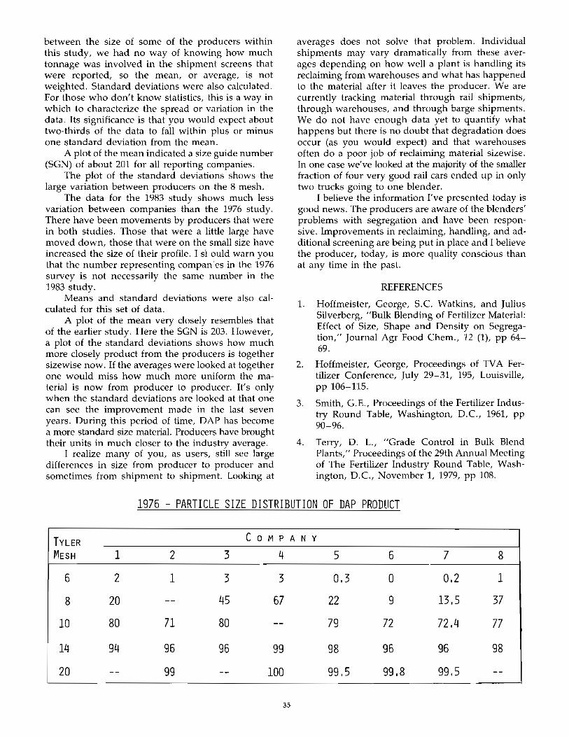
between the size of some of the producers within this study, we had no way of knowing how much tonnage was involved in the shipment screens that were reported, so the mean, or average, is not weighted. Standard deviations were also calculated. For those who don't know statistics, this is a way in which to characterize the spread or variation in the data. Its significance is that you would expect about two-thirds of the data to fall within plus or minus one standard deviation from the mean.

A plot of the mean indicated a size guide number (SGN) of about 201 for all reporting companies.

The plot of the standard deviations shows the large variation between producers on the 8 mesh.

The data for the 1983 study shows much less variation between companies than the 1976 study. There have been movements by producers that were in both studies. Those that were a little large have moved down, those that were on the small size have increased the size of their profile. I s1 ould warn you that the number representing companes in the 1976 survey is not necessarily the same number in the 1983 study.

Means and standard deviations were also cal­culated for this set of data.

A plot of the mean very closely resembles that of the earlier study. Here the SGN is 203. However, a plot of the standard deviations shows how much more closely product from the producers is together sizewise now. If the averages were looked at together one would miss how much more uniform the ma­terial is now from producer to producer. It's only when the standard deviations are looked at that one can see the improvement made in the last seven years. During this period of time, DAP has become a more standard size material. Producers have brought their units in much closer to the industry average.

I realize many of you, as users, still see large differences in size from producer to producer and sometimes from shipment to shipment. Looking at

averages does not solve that problem. Individual shipments may vary dramatically from these aver­ages depending on how well a plant is handling its reclaiming from warehouses and what has happened to the material after it leaves the producer. We are currently tracking material through rail shipments, through warehouses, and through barge shipments. We do not have enough data yet to quantify what happens but there is no doubt that degradation does occur (as you would expect) and that warehouses often do a poor job of reclaiming material sizewise. In one case we've looked at the majority of the smaller fraction of four very good rail cars ended up in only two trucks going to one blender.

I believe the information I've presented today is good news. The producers are aware of the blenders' problems with segregation and have been respon­sive. Improvements in reclaiming, handling, and ad­ditional screening are being put in place and I believe the producer, today, is more quality conscious than at any time in the past.

REFERENCES

1. Hoffmeister, George, S.c. Watkins, and Julius Silverberg, "Bulk Blending of Fertilizer Material: Effect of Size, Shape and Density on Segrega­tion," Journal Agr Food Chem., 12 (1), pp 64-69.

2. Hoffmeister, George, Proceedings of TVA Fer­tilizer Conference, July 29-31, 195, Louisville, pp 106-115.

3. Smith, G.E., Proceedings of the Fertilizer Indus­try Round Table, Washington, D.C., 1961, pp 90-96.

4. Terry, D. L., "Grade Control in Bulk Blend Plants," Proceedings of the 29th Annual Meeting of The Fertilizer Industry Round Table, Wash­ington, D.C., November I, 1979, pp 108.

1976 - PARTICLE SIZE DISTRIBUTION OF DAP PRODUCT

TVLER MESH

6

1

2

8 20

10 80

14 94

20

2

1

71

96

99

COM P A N V

3 4

3 3

45 67

80

96 99

100

35

5 6 7 8

0.3 0 0.2 1

22 9 l3.5 37

79 72 72.4 77

98 96 96 98

99.5 99.8 99.5

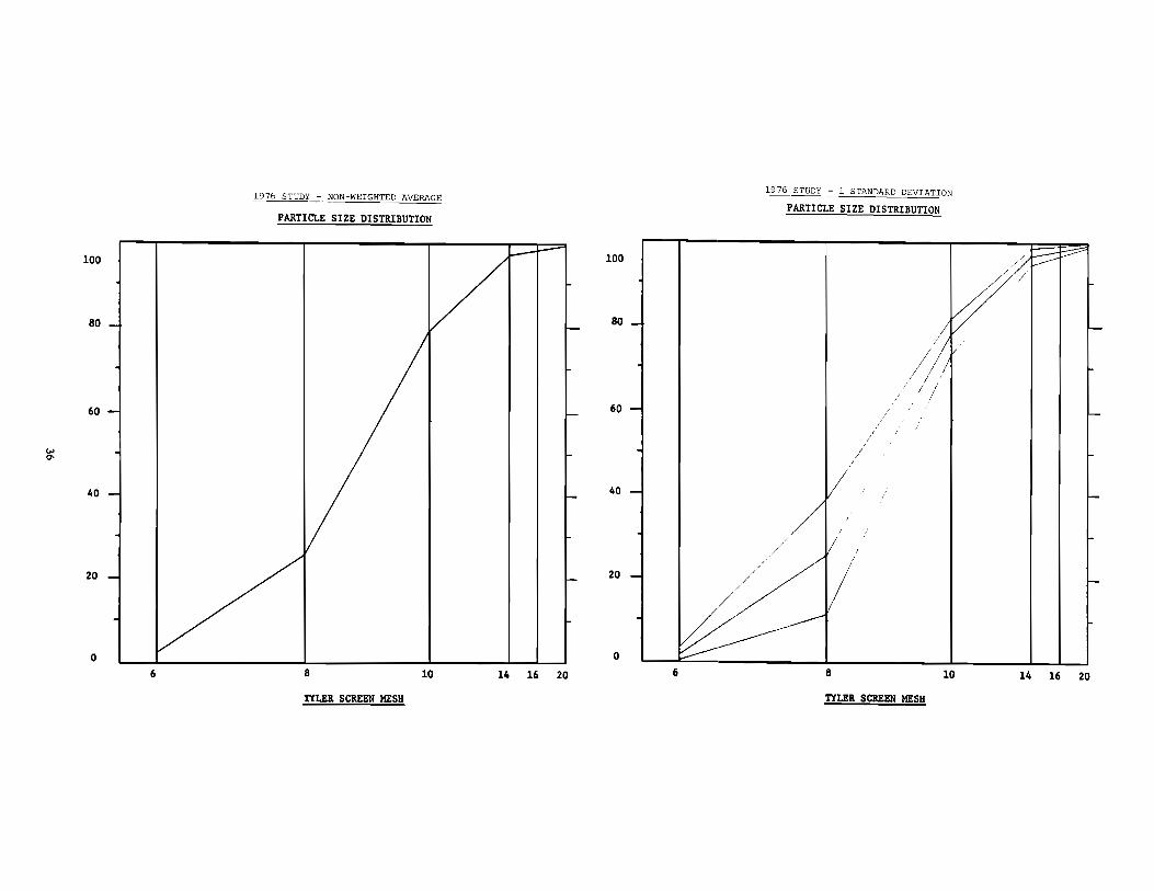
(,,> 0-

100

80

60

40

20

o

~

PARTICLE SIZE DISTRIBUTION

6 8 10 14 16 20

nUll SCREEN MESH

100

80

60

40

20

o 6

PARTICLE SIZE DISTRIBUTION

8

nUll SCREEN MESH

10

// ///

14 16 20

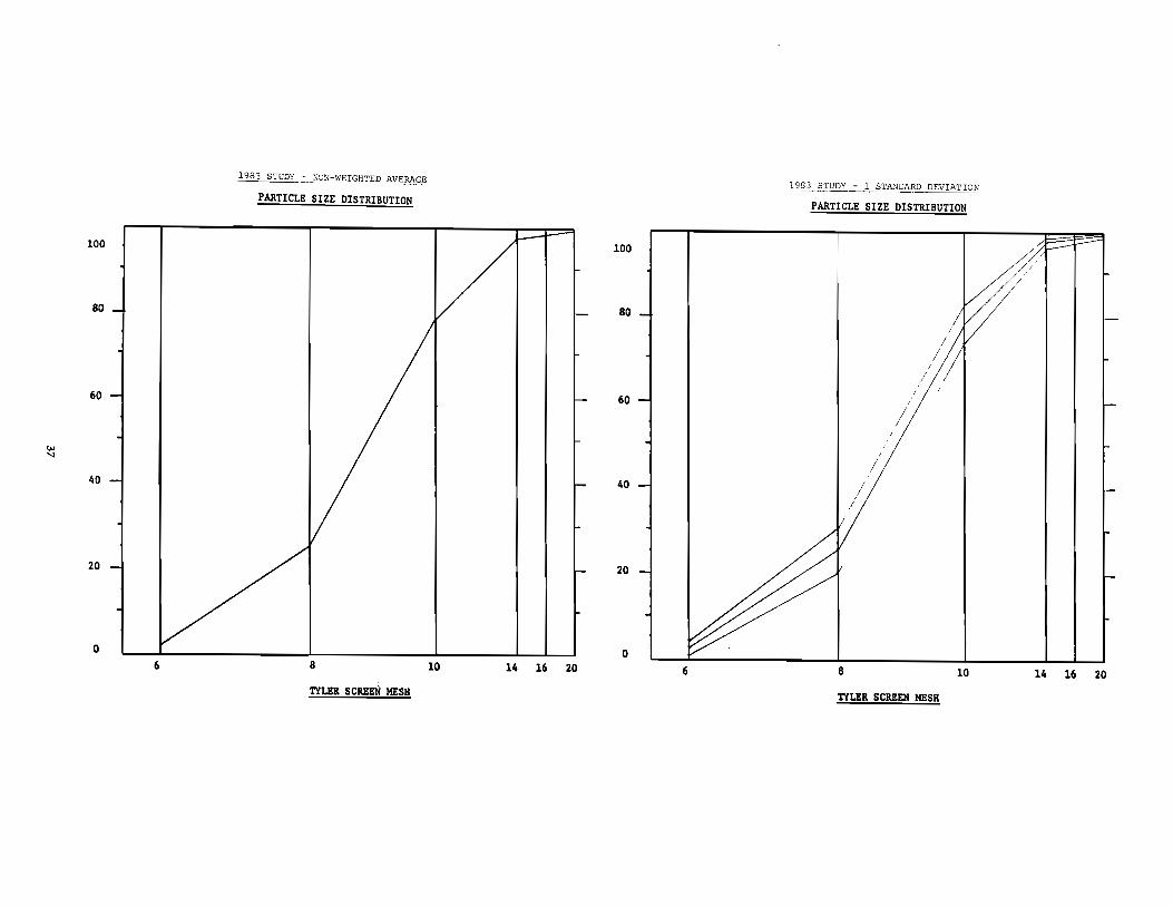
VJ "l

100

80

60

40

20

o

1983 STUDY - __ ~ON-WEIGHTED AVE.~.GE

PARTICLE SIZE DISTRIBUTION

6 8 10 14 16 20

TYLER SCREEN MESH

~3 _ .s_TUDY ..::...LS1'ANDAR.Q._DEVIATI~

PARTICLE SIZE DISTRIBUTION

100

80

60

40 / .'

20

o 6 8 10 14 16 20

TYLEIl SCREEN MESH

~

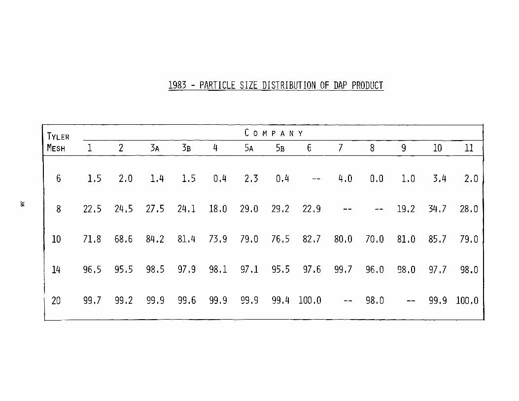
TYLER MESH

6

8

1983 - PARTICLE SIZE DISTRIBUTION OF DAP PRODUCT

COM PAN Y

1 2 3A 3B 4 SA 5B 6 7 8 9 10 11

1,5 2,0 1.4 1,5 0.4 2.3 0.4 4.0 0.0 1,0 3.4 2.0

22.5 24.5 27.5 24.1 18.0 29.0 29.2 22.9 19.2 34,7 28.0

10 71.8 68.6 84.2 81.4 73.9 79.0 76.5 82.7 80.0 70.0 81,0 85.7 79.0

14 96.5 95.5 98.5 97,9 98.1 97.1 95.5 97.6 99,7 96.0 98.0 97.7 98.0

20 99.7 99.2 99.9 99.6 99,9 99.9 99.4 100.0 98.0 99.9 100,0

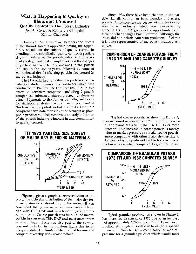
What is Happening to Quality in Blending? (Producer)

Quality Control in The Potash Industry Joe A. Gosselin Research Chemist

Kalium Chemicals

Thank you Mr. Chairman, members and guests of the Round Table. I appreciate having the oppor­tunity to talk on the subject of quality control in blending; more specifically, quality control of particle size as it relates to the potash industry. In my re­marks today, I will first attempt to address the changes in particle size which have occurred in the potash industry in the last 10 years, followed by some of the technical details affecting particle size control in the potash industry.

First I would like to review the particle size dis­tribution study of major dry fertilizers which was conducted in 1973 by The Fertilizer Institute. In this study, 24 fertilizer companies, including 9 potash companies, submitted shipping screen analyses of actual shipments to the Tennessee Valley Authority for statistical analysis. I would like to point out at this time that the potash industry submitted far more comprehensive data than either the nitrogen or phos­phate producers. I feel that this is an early indication of the potash industry'S interest in and commitment to quality control.

TFI 1973 PARTICLE SIZE SURVEY OF MAJOR DRY BLENDING MATERIALS

80 CUMULATIVE

% 60 RETAINED

40

20

GRANULAR POTASH

6

1fI-+-- T S P

8 10 14 20

TYLER MESH

Figure 1 gives a graphical representation of the typical particle size distribution of the major dry fer­tilizer materials analyzed. From this survey, it was concluded that granular potash was compatible in size with TSP, DAP and, to a lesser degree, ammo­nium nitrate. Coarse potash was found to be incom­patible in size with TSP, DAP and most ammonium nitrates. Urea, which was also part of the survey, was not included in the previous figure due to in­adequate data. The limited data reported for urea did compare favorably with coarse potash.

39

Since 1973, there have been changes in the par­ticle size distribution of both granular and coarse potash. A comprehensive survey of the Saskatche­wan potash industry, which was conducted by CANPOTEX in 1982, gives us the opportunity to de­termine what changes have occurred. Although this study did not include American producers, I feel that it is quite representative of the potash industry as a whole.

COMPAmSON OF COARSE POTASH FROM 1973 TFI AND 1982 CANPOTEX SURVEY

100

80

CUMULATIVE % 60

RETAINED 40

20

(-6 + 10 MESH INCREASED BY 40%)

6 8 10 14 20

TYLER MESH

Typical coarse potash, as shown in Figure 2, has increased in size since 1973 due to an increase of approximately 40% in the - 6 + 10 Tyler mesh fraction. This increase in coarse potash is mostly due to market pressures to make coarse potash

more compatible with other major dry fertilizers. Coarse potash is preferred by the blender due to

its lower price when compared to granular potash.

COMPARISON OF GRANULAR POTASH 1973 TFI AND 1982 CANPOTEX SURVEY

100

80

CUMULATIVE % 60

RETAINED 40

(-6 +8 MESH INCREASED BY

60%

6 8 10 14 20

TYLER MESH

Tyical granular produce, as shown in Figure 3, has increased in size since 1973 due to an increase

of approximately 60% in the - 6 + 8 Tyler mesh fraction. Although it is difficult to assign a specific

reason for this change, a combination of market pressure for a granular product which would more

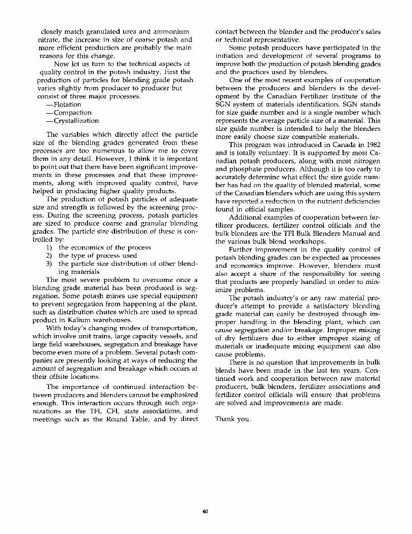
closely match granulated urea and ammonium nitrate, the increase in size of coarse potash and more efficient production are probably the main reasons for this change.

Now let us turn to the technical aspects of quality control in the potash industry. First the

production of particles for blending grade potash varies slightly from producer to producer but consist of three major processes.

-Flotation -Compaction -Crystallization

The variables which directly affect the particle size of the blending grades generated from these processes are too numerous to allow me to cover them in any detail. However, I think it is important to point out that there have been significant improve­ments in these processes and that these improve­ments, along with improved quality control, have helped in producing higher quality products.

The production of potash particles of adequate size and strength is followed by the screening proc­ess. During the screening process, potash particles are sized to produce coarse and granular blending grades. The particle size distribution of these is con­trolled by:

1) the economics of the process 2) the type of process used 3) the particle size distribution of other blend­

ing materials The most severe problem to overcome once a

blending grade material has been produced is seg­regation. Some potash mines use special equipment to prevent segregation from happening at the plant, such as distribution chutes which are used to spread product in Kalium warehouses.

With today's changing modes of transportation, which involve unit trains, large capacity vessels, and large field warehouses, segregation and breakage have become even more of a problem. Several potash com­panies are presently looking at ways of reducing the amount of segregation and breakage which occurs at their offsite locations.

The importance of continued interaction be­tween producers and blenders cannot be emphasized enough. This interaction occurs through such orga­nizations as the TFI, CFI, state associations, and meetings such as the Round Table, and by direct

40

contact between the blender and the producer's sales or technical representative.

Some potash producers have partiqpated in the initiation and development of several programs to improve both the production of potash blending grades and the practices used by blenders.

One of the most recent examples of cooperation between the producers and blenders is the devel­opment by the Canadian Fertilizer Institute of the SGN system of materials identification. SGN stands for size guide number and is a single number which represents the average particle size of a material. This size guide number is intended to help the blenders more easily choose size compatible materials.

This program was introduced in Canada in 1982 and is totally voluntary. It is supported by most Ca­nadian potash producers, along with most nitrogen and phosphate producers. Although it is too early to accurately determine what effect the size guide num­ber has had on the quality of blended material, some of the Canadian blenders which are using this system have reported a reduction in the nutrient deficiencies found in official samples.

Additional examples of cooperation between fer­tilizer producers, fertilizer control officials and the bulk blenders are the TFI Bulk Blenders Manual and the various bulk blend workshops.

Further improvement in the quality control of potash blending grades can be expected as processes and economics improve. However, blenders must also accept a share of the responsibility for seeing that products are properly handled in order to min­imize problems.

The potash industry's or any raw material pro­ducer's attempt to provide a satisfactory blending grade material can easily be destroyed through im­proper handling in the blending plant, which can cause segregation and/or breakage. Improper mixing of dry fertilizers due to either improper sizing of materials or inadequate mixing equipment can also cause problems.

There is no question that improvements in bulk blends have been made in the last ten years. Con­tinued work and cooperation between raw material producers, bulk blenders, fertilizer associations and fertilizer control officials will ensure that problems are solved and improvements are made.

Thank you.

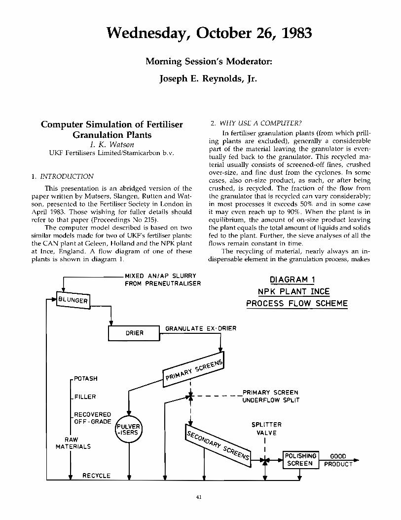
Wednesday, October 26, 1983

Morning Session's Moderator:

Joseph E. Reynolds, Jr.

Computer Simulation of Fertiliser Granulation Plants

I. K. Watson UKF Fertilisers Limited/Stamicarbon b.v.

1. INTRODUCTION

This presentation is an abridged version of the paper written by Mutsers, Slangen, Rutten and Wat­son, presented to the Fertiliser Society in London in April 1983. Those wishing for fuller details should refer to that paper (Proceedings No 215).

The computer model described is based on two similar models made for two of UKF's fertiliser plants: the CAN plant at Geleen, Holland and the NPK plant at Ince, England. A flow diagram of one of these plants is shown in diagram 1.

.-------MIXED AN/AP SLURRY

2. WHY USE A COMPUTER?

In fertiliser granulation plants (from which prill­ing plants are excluded), generally a considerable part of the material leaving the granulator is even­tually fed back to the granulator. This recycled ma­terial usually consists of screened-off fines, crushed over-size, and fine dust from the cyclones. In some cases, also on-size product, as such, or after being crushed, is recycled. The fraction of the flow from the granulator that is recycled can vary considerably; in most processes it exceeds 50% and in some case it may even reach up to 90%. When the plant is in equilibrium, the amount of on-size product leaving the plant equals the total amount of liquids and solids fed to the plant. Further, the sieve analyses of all the flows remain constant in time.

The recycling of material, nearly always an in­dispensable element in the granulation process, makes

FROM PRENEUTRALISER DIAGRAM 1

POTASH

FILLER

RECOVERED OFF-GRADE

RAW MATERIALS

RECYCLE

DRIER

NPK PLANT INCE PROCESS FLOW SCHEME

GRANULATE EX-DRIER

____ __ PRIMARY SCREEN UNDERFLOW SPLIT

41

SPUTTER VALVE

I

GOOD PRODUCT

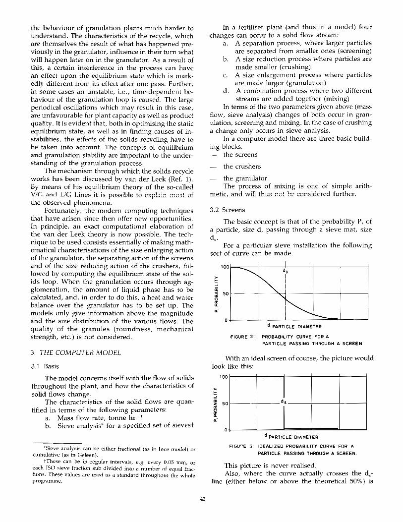
the behaviour of granulation plants much harder to understand. The characteristics of the recycle, which are themselves the result of what has happened pre­viously in the granulator, influence in their turn what will happen later on in the granulator. As a result of this, a certain interference in the process can have an effect upon the equilibrium state which is mark­edly different from its effect after one pass. Further, in some cases an unstable, Le., time-dependent be­haviour of the granulation loop is caused. The large periodical oscillations which may result in this case, are unfavourable for plant capacity as well as product quality. It is evident that, both in optimising the static equilibrium state, as well as in finding causes of in­stabilities, the effects of the solids recycling have to be taken into account. The concepts of equilibrium and granulation stability are important to the under­standing of the granulation process.

The mechanism through which the solids recycle works has been discussed by van der Leek (Ref. 1). By means of his equilibrium theory of the so-called V Ie. and L/G Lines it is possible to explain most of the observed phenomena.

Fortunately, the modern computing techniques that have arisen since then offer new opportunities. In principle, an exact computational elaboration of the van der Leek theory is now possible. The tech­nique to be used consists essentially of making math­ematical characterisations of the size enlarging action of the granulator, the separating action of the screens and of the size reducing action of the crushers, fol­lowed by computing the equilibrium state of the sol­ids loop. When the granulation occurs through ag­glomeration, the amount of liquid phase has to be calculated, and, in order to do this, a heat and water balance over the granulator has to be set up. The models only give information above the magnitude and the size distribution of the various flows. The quality of the granules (roundness, mechanical strength, etc.) is not considered.

3. THE COMPUTER MODEL

3.1 Basis

The model concerns itself with the flow of solids throughout the plant, and how the characteristics of solid flows change.

The characteristics of the solid flows are quan­tified in terms of the following parameters:

a. Mass flow rate, tonne hr- 1

b. Sieve analysis* for a specified set of sievest

'Sieve analysiS can be either fractional (as in Ince model) or cumulative (as in Geleen).

tThese can be in regular intervals, e.g. every 0.05 mm, or each ISO sieve fraction sub divided into a number of equal frac­tions. These values are used as a standard throughout the whole programme.

42

In a fertiliser plant (and thus in a model) four changes can occur to a solid flow stream:

a. A separation process, where larger particles are separated from smaller ones (screening)

b. A size reduction process where particles are made smaller (crushing)

c. A size enlargement process where particles are made larger (granulation)

d. A combination process where two different streams are added together (mixing)

In terms of the two parameters given above (mass flow, sieve analysis) changes of both occur in gran­ulation, screening and mixing. In the case of crushing a change only occurs in sieve analysis.

In a computer model there are three basic build­ing blocks:

the screens

the crushers

the granulator The process of mixing is one of simple arith-

T"nt:ltit" ~nrl "TMill t-h11C -nA*" hOI ro.r\"'nC";;lro...,...r.~ ~""''''''''k~'''' ......... _ ..... ""1 .......... -. "" ....... '-.LI.""""'" J,.L ...... 1. u ..... '-V""lv,l~L.1.\""'\,.t .1.U1. "J.l~..l.

3.2 Screens

The basic concept is that of the probability P, of a particle, size d, passing through a sieve mat, size

d s ·

For a particular sieve installation the following sort of curve can be made.

100

>-!:: ...l iii "" 50 III 0 0: a.. a:

0 d PARTICLE DIAMETER

FIGURE 2: PROBABILITY CURVE FOR A

PARTICLE PASSING THROUGH A SCREEN

With an ideal screen of course, the picture would look like this:

>-I-:J iii

"" til

[ a:

100~-----+------~------+-----~L------1

50 ds

0~ ____ L-____ ~====~====L-__ ~ d PARTICLE DIAMETER

FIGU"E 3: IDEALIZED PROBABILITY CURVE FOR A

PARTICLE PASSING THROUGH A SCREEN.

This picture is never realised. Also, where the curve actually crosses the d s-

line (either below or above the theoretical 50%) is

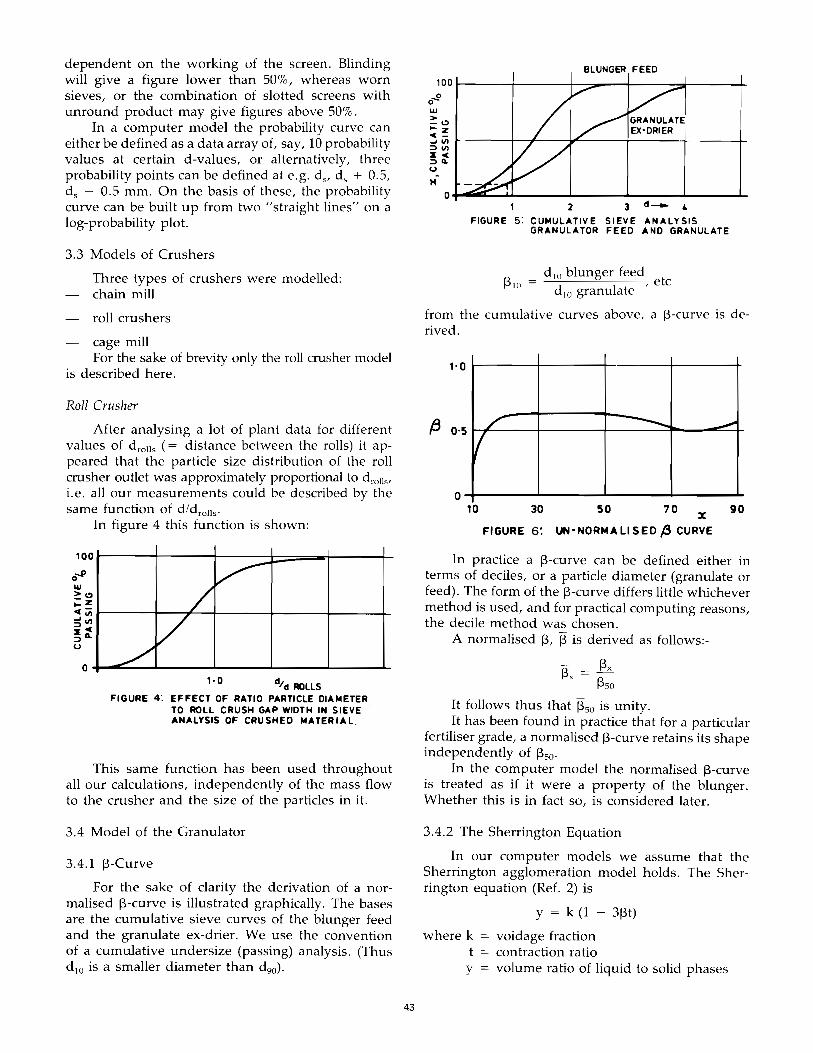
dependent on the working of the screen. Blinding will give a figure lower than 50%, whereas worn sieves, or the combination of slotted screens with unround product may give figures above 50%.

In a computer model the probability curve can either be defined as a data array of, say, 10 probability values at certain d-values, or alternatively, three probability points can be defined at e.g. d s' do, + 0.5, ds 0.5 mm. On the basis of these, the probability curve can be built up from two "straight lines" on a log-probability plot.

3.3 Models of Crushers

Three types of crushers were modelled: chain mill

roll crushers

cage mill For the sake of brevity only the roll crusher model

is described here.

Roll Crusher

After analysing a lot of plant data for different values of d rolls (= distance between the rolls) it ap­peared that the particle size distribution of the roll crusher outlet was approximately proportional to drollSl i.e. all our measurements could be described by the same function of did rolls-

In figure 4 this function is shown:

100r------r------~----=t~-=~------+_

0"'" IU > I!)

;'z "'iiit----t--.;--I----4----+---+ ...Jill ::;)",

~Q. U

o+-~~~~----~------~----~------~

1· 0 d/ d ROLLS

FIGURE 4: EFFECT OF RATIO PARTICLE DIAMETER TO ROLL CRUSH GAP WIDTH IN SIEVE . ANALYSIS OF CRUSHED MATERIAL.

This same function has been used throughout all our calculations, independently of the mass flow to the crusher and the size of the particles in it.

3.4 Model of the Granulator

3.4.1 p-Curve

For the sake of clarity the derivation of a nor­malised p-curve is illustrated graphically. The bases are the cumulative sieve curves of the blunger feed and the granulate ex-drier. We use the convention of a cumulative undersize (passing) analysis. (Thus d 10 is a smaller diameter than d90).

43

BLUNGER FEED

100r-----1-----~~~--_+--___ ~----~

o~ 10.1 > -I!)

~ ! L-____ ~--+_--~~---_+-----~------~ ...J III r :::>111

:.:'" :::>Q. u H

o+-.. ~~------~------~----~------~ 1 2 3 d_ "

FIGURE 5: CUMULATIVE SIEVE ANALYSIS GRANULATOR FEED AND GRANULATE

dIO blunger feed 1310 = , etc

d 10 gran ula te

from the cumulative curves above, a p-curve is de­rived.

1-0

/' ---... ..,.,..,.

( (3 0'5

o 10 30 50 70 X 90

FIGURE 6~ UN-NORMALISED j3 CURVE

In practice a p-curve can be defined either in terms of deciles, or a particle diameter (granulate or feed). The form of the p-curve differs little whichever method is used, and for practical computing reasons, the decile method was chosen.

A normalised 13, (3 is derived as follows:-

1350 It follows thus that (350 is unity. It has been found in practice that for a particular

fertiliser grade, a normalised p-curve retains its shape independently of 1)50'

In the computer model the normalised I)-curve is treated as if it were a property of the blunger. Whether this is in fact so, is considered later.

3.4.2 The Sherrington Equation

In our computer models we assume that the Sherrington agglomeration model holds. The Sher­rington equation (Ref. 2) is

where k t

Y

y = k (1 3pt)

voidage fraction contraction ratio volume ratio of liquid to solid phases

From this the following relationship is derived

13 = 3kt

In our model we assume that 13 is in fact 1350' and that k and t are constants. Thus if y, the fluid phase ratio is known, 1350 can be calculated.

Thus knowing 1350, and having a normalised 13-curve (stored in a data-array), the values 1310,13201 etc. can be calculated. From the cumulative sieve analysis of the blunger feed, the cumulative sieve analysis of the granulate (ex-drier) can be calculated.

3.4.3 "y", the fluid phase ratio

Hunter & Hawksley (Ref. 3) show that y can be calculated from the granulator water content and the solubility of the formulation.

where w

s

Ps Pl

y = (1

weighi of wdier

unit weight of dry solids of solids dissolved

unit weight of water density of solid phase density of liquid phase

3.4.4 Water Content

In our models we suppose that the liquid phase, which is present in the solid particles fed to the blun­ger, does not contribute to the capillary forces caus­ing agglomeration. The water content of these solid particles is, therefore, counted as solid phase.

A complication arises in the calculation of effec­tive granulation water content, and this is the mois­ture loss through evaporation. We can consider gran­ulation to be largely complete before evaporation begins, or the opposite. Either case is a simplification since we are treating dynamic processes in the model as if taking place instantaneously.

The Ince model considers that water evaporation takes place after granulation, and the Geleen model vice versa. In practice the difference is compensated for by the use of different k and t values. In the case of the Ince modet two granulator water contents are thus calculated by the computer:

granulation water content; exclusive of water from the recycle-also no evaporation loss.

ex blunger water content; inclusive of water from the recycle and also corrected for evaporation loss. The first is used for calculating 13, and the second

for comparison with plant measurements.

3.4.5 Solubility

For the CAN Modet the data for pure ammo-

44

nium nitrate are used. Measurements have shown that the Ca(N03h content has no significant influence on the amount of liquid phase which is present under granulation conditions, and can therefore be ignored. In the case of NPK's, the solubility is measured ex­perimentally using a hydraulic press.

The solubility data are stored in the computer as a quadratic function of temperature. (In the case of NPK's the equation constants can be changed).

Thus, in order to calculate solubility, we need to know granulation temperature.

3.4.6 Granulation Temperature

A heat balance over the blunger has to be made, the main processes are:

Mixing of slurry and recycle; the recycle warms up and the slurry cools down until a combined mixed temperature is reached.

Cooling through evaporation of water and pas­sage of air through the blunger. Further, in both models the eHect of heat losses

from the blunger and energy dissipation are taken into account.

4. COMPUTER MODEL: COMPUTERI MATHEMATICAL ASPECTS

4.1 Basic Principles of Calculation Procedure

The calculation procedure is iterative, each it­eration for example being one residence time period round the recycle loop.

Before the calculation begins, all the various process conditions must be known, together with details of the equipment performance. These are read in from an input list or data array in the programme.

The calculation begins with the recycle: in order to start, two assumptions have to be made:

the recycle screen analysis

the recycle quantity Thereafter the calculation proceeds through the

following steps:

• addition of solid raw materials to recycle and calculation of granulator feed sieve analysis.

• heat and mass balance over the granulator; cal­culation of granulation temperature and water content; calculation of solution phase ratio.

• calculation of granulation over granulator plus drier.

• calculations over screens and crushers-

thus end product quantity and sieve analysis

- recycle quantity and sieve analysis. In the Ince model, the quantity of end product

is compared to the quantity of raw materials, and the calculated recycle sieve analysis and quantity is com­pared to the assumed start values. If all three of these values are the same, then the equilibrium situation exists.

4.2 Types of Model, and Methods of Determining Equilibrium

Basic Model Types: The two principal model types are: a static model

a dynamic model

4.2.1 Static Model

The static model concerns itself exclusively with the determination of the equilibrium situation for a particular set of operating conditions. The manner in which the equilibrium is reached is ignored: in other words, the granulation stability is not considered at all.

The model only seeks the granulation equilib­rium, whatever it is, and does not consider whether in real life such an equilibrium is attainable and/or usable. In the static model, at the beginning of each new iteration, new assumed recycle conditions are made. The value of these assumptions is derived from the old value and the difference between cal­culated and assumed value.

4.2.2 Dynamic Model

In contrast to the static model, the dynamic model considers how the plant behaves. Not only what the equilibrium is, but how it is reached, and how quickly.

The Ince model is dynamic, and for Geleen both a static and a dynamic model have been made.

In the lnce dynamic model, the end recycle quantity and recycle sieve analysis from one time­step become the start situation for the next time-step.

In the dynamic model of the Geleen-plant, the residence-time distribution in the rotary-drier is taken into account. Here no start-assumption has to be made. The equilibrium calculated by the static model is the start point for the dynamic model. For a given disturbance (in the AN-temperature, for instance) the computer programme calculates the effect of this dis­turbance as a function of time.

The advantage of a dynamic model is that it can see the effects of disturbance to the process. If an incorrect start assumption is made, then sometimes no equilibrium conditions can be reached. This is purely a reflection of real life-if, for instance, the recycle loop is burdened up with dust, then by set­ting normal feed rates it is indeed unlikely that a granulation equilibrium would be reached-or cer­tainly one which has any practical significance.

45

An example of a calculation with the Ince model is given in Appendix 1 where the effect of a change in plant throughput is demonstrated.

5. COMPARISON OF COMPUTER PREDICTIONS WITH PLANT OBSERVATIONS

Generating data from a computer model is not very difficult. However, collecting reliable data from the plant is. We all know the problems of obtaining representative samples coming from the discharge of a bucket elevator.

Similarly, collecting reliable heat and water data over the blunger so that good k and t values can be found is not simple.

Even allowing for these difficulties, the model and plant situation appears to be in fair harmony. Table 1 presents the average value of six measure­ments on six different days, compared with the re­sults obtained via the model.

TABLE 1

Difference Between Measurement and

Calculation

Granulation Temperature (0 C)

Size enlargement I3so

dso of Granulated Product

Amount of Recycle

+0.3%

+4.4%

+ 1.3%

-1.5%

6. THE USE OF THE MODEL TO PREDICT PLANT CONDITIONS

6.1 Effect of AN melt water content

Appendix 2 shows the effect of changing AN melt water content on medium particle size of the granulate (dso), the granulation temperature (T 6), and the relative amount of product size material in the granulate (~,: relative to normal plant operation).

There are no surprises in this graph: as more water is added, dso increases, whilst the other two decrease.

6.2 Effect of recycle temperature

See Appendix 3. The kink in the lines is caused by the AN crystal

phase (II/III) latent heat. If the recycle is colder than 84°, then the melt in warming up the recycle also has to provide latent heat.

6.3 The Effect of Cage Mill Speed

See Appendix 4. As one would expect, speeding up the mill de­

creases granulate dso . However, not so obvious, is

the fact that it has minimal effect on the amount of product size material in the granulate.

7. CONCLUSIONS

1. Computer models work, and give, within limits, good agreement with plant condi­tions.

2. They can be used to investigate process con-ditions, and so

define bottlenecks predict effects of changes optimise plant operation. (At UKF Ince the production rate of one major produc­tion was considerably enhanced as a result of studying with the computer.

3. Computer models are a useful training aid. 4. The weak point is the model of the granu­

lator

46

use of ~ curves granulation is often not only by agglom­eration

3. REFERENCES

1. J. van der Leek; Proc. ISMA Technical Confer­ence, The Hague, 1976 p.p. 94-114; "Agglom­erate Granulation as an Equilibrium Process".

2. P.J.Sherrington; Chern Engr. (London). July/Aug. 1968, p.p. CE 201-CE 215: "The granulation of sand as an aid to understanding fertilizer gran­ulation".

3. G.Hunter and J. L. Hawksley; Proc.ISMA Spec.Dev.Conference, New Delhi, December 1975: "Some developments aimed at reducing recycle ratios of high-analysis NPK process".

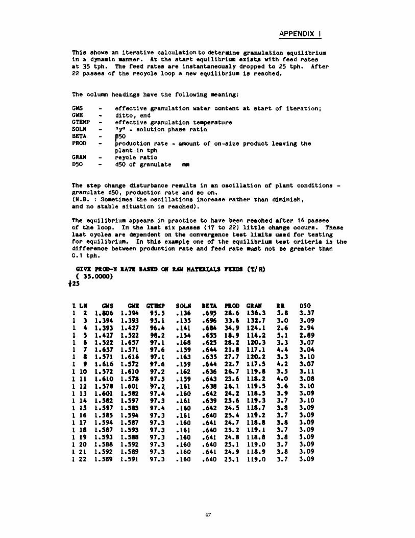
APPENDIX I

This shows an iterative calculation to determne granulat10n 9qu1l1br1um in a dynamic manner. At the start equilibrium exist. with reed rates at 35 tph. The reed rates are instantaneously dropped to 25 tph. Arter 22 passes ot the recycle loop a new equilibrium is reached.

The column headings have the tollowing meaning:

GWS GWE GTEHP SOLN BETA PROD

GRAN D50

etrective granulation water content at start ot iteration; ditto, end ettective granulation temperature "y" = solution pha.se ratio 1350 . production rate - amount or on-size product leaving the plant in tph reycle ratio d50 of granulate mm

The step change disturbance results in an oscillation or plant conditions -granulate d5O, production rate and so on. (N.B. : Sometimes the oscillations increase rather than diminish, and no stable situation is reached).

The equilibrium appears in practice to have be.en reached atter 16 passes ot the loop. In the laat six paasea (17 to 22) little change occurs. These laat cyclea are dependent on the convergence teat limits used tor testing ror equilibrium. In this exampl. one or the equilibrium test criteria is the dirt.rence between production rate and reed rate .us' not be greater than 0.1 tph.

GIft PI.(I)-H UTI lAnD <II lAW MATDlALS rllDS (T/B) ( 35.0000)

Us

ILl ews GWI GT_P SOLI IITA PROD GUN 1.1. 050 1 2 1.806 1.394 95.5 .136 .69~ 2a.6 136.3 3.a 3.37 1 3 1.394 1.393 95.1 .135 .696 33.6 132.7 3.0 3.09 1 4 1.393 1.427 96.4 .141 .684 34.9 124.1 2.6 2.94 1 5 1.427 1.522 98.2 .154 .655 18.9 114.2 5.1 2.89 1 6 1.522 1.657 97.1 .168 .625 28.2 120.3 3.3 3.07 1 7 1.657 1.571 97.6 .159 .644 21.a 117.1 4.4 3.04 1 8 1.571 1.616 97.1 .163 .635 27.7 120.2 3.3 3.10 1 9 1.616 1.572 97.6 .159 .644 22.7 117.5 4.2 3.07 1 10 1.5n 1.610 97.2 .162 .636 26.7 119.8 3.5 3.11 1 11 1.610 1.578 97.5 .159 .643 23.6 118.2 4.0 3.08 1 12 1.578 1.601 97.2 .161 .638 26.1 119.5 3.6 3.10 1 13 1.601 1.582 97.4 .160 .642 24.2 118.5 3.9 3.09 1 14 1.582 1.597 97.3 .161 .639 25.6 119.3 3.7 3.10 1 15 1.597 1.sa5 97.4 .160 .642 24.5 118.7 3.8 3.09 1 16 1.sa5 1.594 97.3 .161 .640 25.4 119.2 3.7 3.09 1 17 1.594 1.587 97.3 .160 .641 24.7 118.8 3.8 3.09 118 1.587 1.593 97.3 .161 .640 25.2 119.1 3.7 3.09 1 19 1.593 1.588 97.3 .160 .641 24.8 118.8 3.8 3.09 1 20 1.588 1.592 97.3 .160 .640 25.1 119.0 3.7 3.09 1 21 1.592 1.589 97.3 .160 .641 24.9 118.9 3.8 3.09 1 22 1.589 1.591 97.3 .160 .640 25.1 119.0 3.7 3.09

47

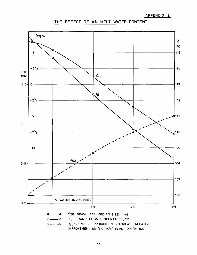
dSO (mm)

I.-a

3-5

3·0

2·5

'0 -x

6"l. %

APPENDIX 2

THE EFFECT OF AN. MELT WATER CONTENT

t5 ~ ,

.. 2 "2

a

- i"2

-5

-7"2

-10

,/ ,/

,/ ;'

~;'

"( .~"" ~" 6"'L ." ~ "

pTG '" "- ~

~ "', '" ....

114

113

112

~, X -' "",,,,,,-

-'"

111

["I<. " - "'" "," ~ ~x, '" "'" ","

" ,,"

10

109 "

" ." ,/

dSO " " " "

"'" "'" " ." "

% WATER IN A.N. FEED'

3-0

.----. o o x--x

3·5

dSO. GRANULATE MEDIAN SIZE ImmJ

TG. GRANULATION TEMPERATURE. °C

4-0

1Tl. % ON-SIZE PRODUCT IN GRANULATE,RELATIVE

IMPROVEMENT ON 'NORMAL- PLANT OPERATION.

48

0

1 08

1 07

106

4-5

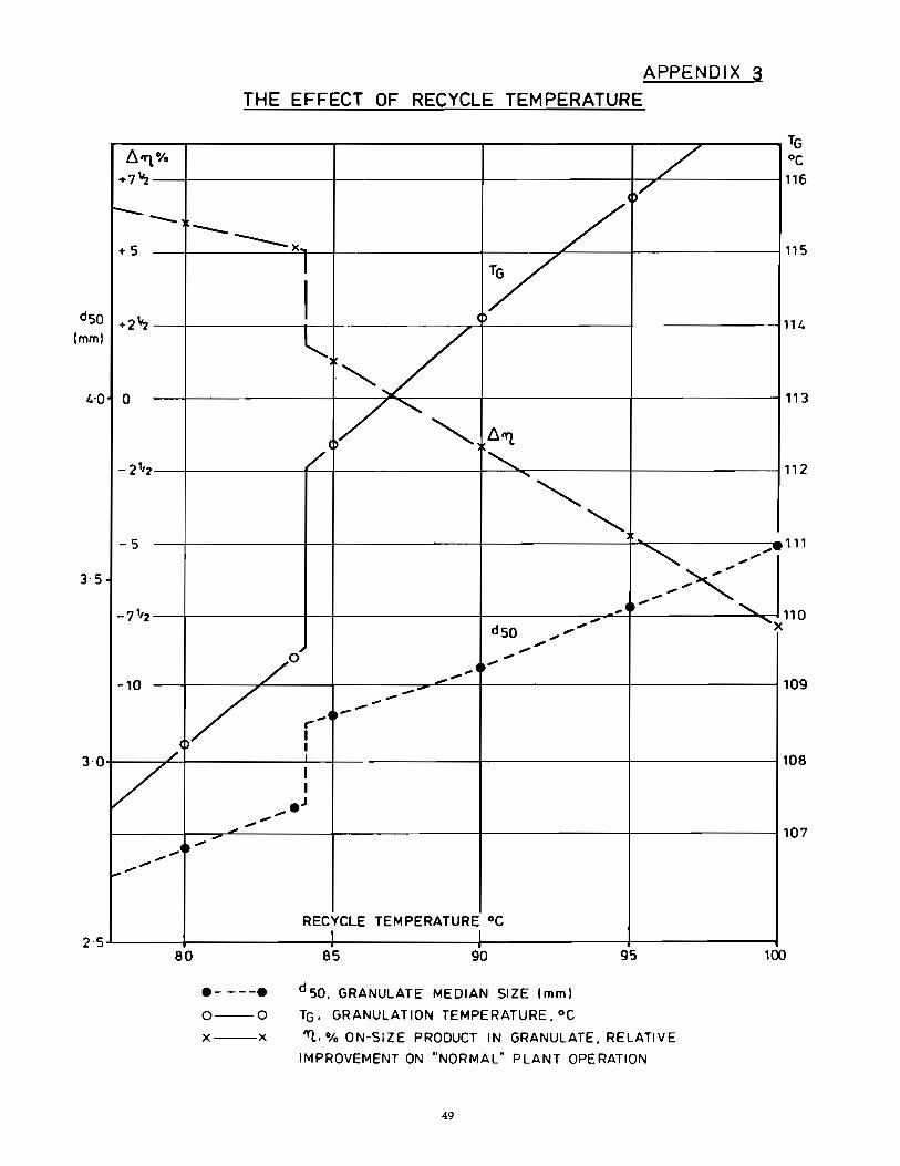
dSO

Imml

4'0

3·5

3-0

2'5

6"1.% +7"z

1-- __

+5

.2'1,2

0

- 2"2

-5

-7"2

APPENDIX 3 THE EFFECT OF RECYCLE TEMPERATURE

/ )/

------ x /' I y I C~

~.

"/ l/ "" /(

61ft

'" '"" '" '" " .... ,. ... 4 ",~ . .........

dSO , .... ' 'X , O~ .," ,

/' ... 4 .' --

115

114

113

112

1 1 1

110

-10

./ --"",---,.. ... /(

I ~

109

/ , .... ~ ,

.... --eo

_ ..... ... _ ...

.- ---. 0--0

x--x

,

I I .J

RECYCLE TEMPERATURE °C 1 I .

85 90

d 50, GRANULATE MEDIAN SIZE (mm I

TG, GRANULATION TEMPERATURE. °C

95

"1.. % ON-SIZE PRODUCT IN GRANULATE, RELATIVE

IMPROVEMENT ON "NORMAL" PLANT OPERATION

49

1 08

107

100

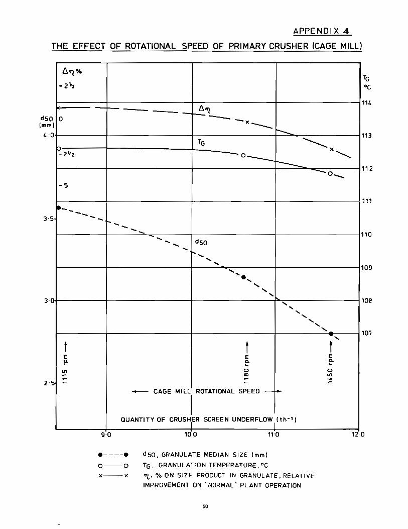
APPENDI X 4

THE EFFECT OF ROTATIONAL SPEED OF PRIMARY CRUSHER (CAGE MILL)

dSO (mm )

4· 0

3· S

3· .... v

2' 5

~1I't%

+ 2"2

0

!'" -2"2

-S

1It __ --

t E a. L.

1.0 .... .... ....

~"l --- -x ---- r-...... TG ~X

-0 _____ "'----- --0"",,-

-- ......... --- -..... dSO ..... -.....

r-- ..... "-

"-"- ..... ....

...... ...... .... ,

.... .... , "- ....

...... -, t t E E a. a. ... L.

0 0 CD 1.0 .... ..., .... .... - CAGE MILL ROTATIONAL SPEED - -

I QUANTI TY OF CRUSH1ER SCREEN UNDERFLOW I (th- 1 )

g·O

.----. 0--0 x--x

. 10-0

d 50. GRANULATE MEDIAN SIZE (mm)

TG. GRANULATION TEMPERATURE. °C

"l. % ON SIZE PRODUCT IN GRANULATE. RELATIVE

IMPROVEMENT ON "NORMAL" PLANT OPERATION

50

,,1.

113

'12

111

"0

109

10e

107

120

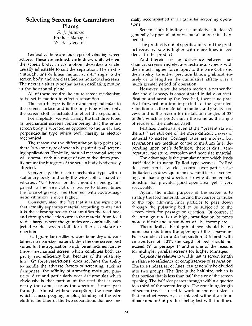
Selecting Screens for Granulation Plants

S. J. Janovac Product Manager W. S. Tyler, Inc.

Generally, there are four types of vibrating screen actions. These are inclined, circle throw units wherein the screen body, in it's motion, describes a circle, usually adjustable to suit the separation. The next is a straight line or linear motion at a 45° angle to the screen body and are classified as horizontal screens. The next is a sifter type that has an oscillating motion in the horizontal plane.

All of these require the entire screen mechanism to be set in motion to effect a separation.

The fourth type is linear and perpendicular to the screen surface and is the only type where only the screen cloth is actuated to effect the separation.

For simplicity, we will classify the first three types as mechanical screens remembering that the entire screen body is vibrated as opposed to the linear and perpendicular type which we'll classify as electro­mechanical.

The reason for the differentiation is to point out there is no one type of screen best suited to all screen­ing applications. Typically, most all mechanical screens will operate within a range of two to five times grav­ity before the integrity of the screen body is adversely affected.

Conversely, the electro-mechanical type with a stationary body and only the wire cloth actuated or vibrated, "G" forces, or the amount of energy im­parted to the wire cloth, is twelve to fifteen times the force of gravity. The Hummer with electro-mag­netic vibration is even higher.

Consider, also, the fact that it is the wire cloth that actually separates material according to size and it is the vibrating screen that stratifies the feed bed, and through the action carries the material from f.eed to discharge where the granules are continually sub­jected to the screen cloth for either acceptance or rejection.

If all granular fertilizers were bone dry and con­tained no near-size material, then the one screen best suited for the application would be an inclined, circle­throw mechanical screen which combines both ca­pacity and efficiency but, because of the relatively low "G" force restrictions, does not have the ability to handle the adverse factors of screening, such as dampness, the affinity of attracting moisture, plas­ticity, dust and particularly near size granules which obviously is that portion of the feed that is very nearly the same size as the aperture it must pass through. Almost without exception, the near size which causes pegging or plug blinding of the wire cloth is the finer of the two separations that are nor-

51

mally accomplished in all granular screening opera­tions.

Screen cloth blinding is cumulative; it doesn't generally happen all at once, but all at once it's hap­pened.

The product is out of specifications and the prod­uct recovery rate is higher with more fines in evi­dence in the product.

And therein lies the difference between me­chanical screens and electro-mechanical screens with their much higher force input to the wire cloth and their ability to either preclude blinding almost en­tirely or to lengthen the cumulative affects over a much greater period of operation.

However, since the screen motion is perpendic­ular and all energy is concentrated initially on strat­ification and aerating the feed bed, there is no prac­tical forward motion imparted to the granules. Vibration sets the material in motion and gravity con­veys and is the reason for installation angles of 33° to 36°, which is pretty much the same as the angle of repose of the material itself.

Fertilizer materials, even at the "present state of the art," are still one of the more difficult classes of material to screen. Tonnage rates are modest, but separations are medium coarse to medium fine, de­pending upon one's definition; there is dust, tem­perature, moisture, corrosion and near-size material.

The advantage is the granular nature which lends itself ideally to using Ty-Rod type weaves. Ty-Rod does not exercise as close control over particle size limitations as does square mesh, but it is freer screen­ing and has a good aperture to wire diameter rela­tionship that provides good open area, yet is very serviceable.

Again, the initial purpose of the screen is to stratify the feed material, forcing the coarser granules to the top, allowing finer particles to pass down through the pulsating bed to be subjected to the screen cloth for passage or rejection. Of course, if the tonnage rate is too high, stratification becomes more difficult and separations will be incomplete.

Theoretically, the depth of bed should be no more than six times the opening of the separation. For example, at an initial separation at 6 mesh with an aperture of .131", the depth of bed should not exceed %" to perhaps 1" and is one of the reasons for multiple, parallel screens for higher tonnages.

Capacity is relative to width just as screen length is relative to efficiency or completeness of separation. The true undersize, or fines, can generally be divided into two groups. The first is the half size, which is that portion that is less than half the size of the screen opening. The half size passes through within a quarter to a third of the screen length. The remaining length of screen travel is used to work on the near size so that product recovery is achieved without an inor­dinate amount of product being lost with the fines.

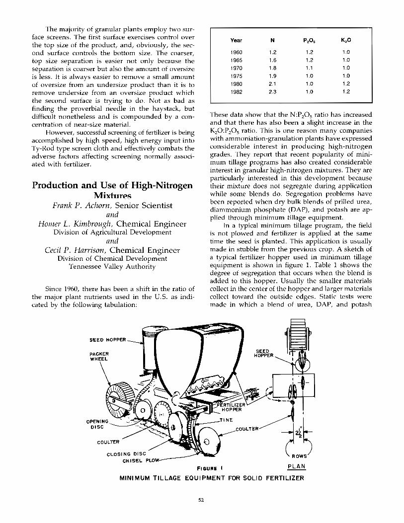
The majority of granular plants employ two sur­face screens. The first surface exercises control over the top size of the product, and, obviously, the sec­ond surface controls the bottom size. The coarser, top size separation is easier not only because the separation is coarser but also the amount of oversize is less. It is always easier to remove a small amount of oversize from an undersize product than it is to remove undersize from an oversize product which the second surface is trying to do. Not as bad as finding the proverbial needle in the haystack, but difficult nonetheless and is compounded by a con­centration of near-size material.

However, successful screening of fertilizer is being accomplished by high speed, high energy input into Ty-Rod type screen cloth and effectively combats the adverse factors affecting screening normally associ­ated with fertilizer.

Production and Use of High-Nitrogen Mixtures

Frank P. Achorn, Senior Scientist and

Homer L. Kimbrough, Chemical Engineer Division of Agricultural Development

and Cecil P. Harrison f Chemical Engineer

Division of Chemical Development Tennessee Valley Authority

Since 1960, there has been a shift in the ratio of the major plant nutrients used in the U.S. as indi­cated by the following tabulation:

OPENING DISC --.....-

CLOSING DISC CHISEL PLOW

Year N P2O. K20

1960 1.2 1.2 1.0

1965 1.6 1.2 1.0

1970 1.8 1 .1 1.0

1975 1.9 1.0 1.0

1980 2.1 1.0 1.2

1982 2.3 1.0 1.2

These data show that the N:P20s ratio has increased and that there has also been a slight increase in the K20:P20 S ratio. This is one reason many companies with ammoniation-granulation plants have expressed considerable interest in producing high-nitrogen grades. They report that recent popularity of mini­mum tillage programs has also created considerable interest in granular high-nitrogen mixtures. They are particularly interested in this development because their mixture does not segregate during application while some blends do. Segregation problems have been reported when dry bulk blends of prilled urea, diammonium phosphate (DAP), and potash are ap­plied through minimum tillage equipment.

In a typical minimum tillage program, the field is not plowed and fertilizer is applied at the same time the seed is planted. This application is usually made in stubble from the previous crop. A sketch of a typical fertilizer hopper used in minimum tillage equipment is shown in figure 1. Table 1 shows the degree of segregation that occurs when the blend is added to this hopper. Usually the smaller materials collect in the center of the hopper and larger materials collect toward the outside edges. Static tests were made in which a blend of urea, DAP, and potash

FIGURE I PLAN

MINIMUM TILLAGE EQUIPMENT FOR SOLID FERTILIZER

52

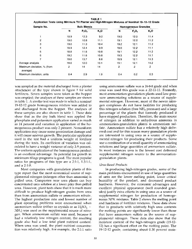
TABLE 1 Application Tests Using Minimum Till Planter and High-Nitrogen Mixtures of Nominal 19-12-12 Grade

Sample No. Bulk Blends

N P20 5

1 18.9 12.3

2 19.0 10.8

3 19.0 11.3

4 18.9 12.4

5 18.8 11.6

6 19.2 11.6

7 19.0 13.7

Average analysis 19.0 12.0

Maximum deviation, % (from 2 14 average)

Maximum deviation, units 0.4 2.9

was sampled as the material discharged from a planter attachment of the type shown in figure 1 for solid fertilizers. Seven samples were taken as the hopper was emptied; the analyses of these samples are shown in table 1. A similar test was made in which a nominal 19-12-12 grade homogeneous mixture was added to and discharged from the hopper. The analyses of these samples are also shown in table 1. These data show that as the dry bulk blend was applied the phosphate and potassium application varied as much as 14 percent and variation in application of the ho­mogeneous product was only 2 percent. Nonuniform application may cause some germination damage and it will cause uneven growth. The particular applicator used in the test had a uniform weight of fertilizer during the tests. Its coefficient of variation was cal­culated to have a weight variance of only 3.9 percent. The uniform application of the homogeneous product is an excellent advantage. Its potential for growth in minimum tillage programs is good. The most popular ratios for programs of this type are a 2:1:1, 1.5:1:1, and a 2:1:0.

Most companies with granulation plants of this type report that the most economical source of sup­plemental nitrogen (nitrogen other than ammonia) is prilled urea. Companies near urea plants can buy concentrated urea solution at a lower price than prilled urea. However, plant tests show that it is much more difficult to produce high-nitrogen grades from urea than from ammonium sulfate or ammonium nitrate. The highest production rate and lowest number of plant operating problems were encountered when ammonium sulfate (either as crystals or as H 2S04 + NH3 ) was used as the supplemental source of nitro­gen. When ammonium sulfate was used, because it had a relatively low nitrogen content, the resulting grade also had a low total plant nutrient content. When urea was used, the plant nutrient concentra­tion was relatively high. For example, the 2:1:1 ratio

53

Homogeneous Granules

K20 N P20 5 K20

9.2 19.0 12.0 11.4

11.1 19.1 12.2 11.2

10.4 19.2 12.1 11.2

9.9 19.0 12.2 11.1

10.8 19.1 12.2 11.2

10.8 19.3 12.2 11.1

8.8 18.9 12.1 11.3

10.1 19.1 12.1 11.2

14 2 2 2

1.9 0.4 0.2 0.3

using ammonium sulfate was a 16-8-8 grade and when urea was used this grade was a 22-11-11. Formerly, most ammoniation-granulation plants used low-pres­sure ammoniating solutions as a source of supple­mental nitrogen. However, most of the newer nitro­gen complexes do not have facilities for producing this nitrogen solution (free NH3 pressure) and a large percentage' of the plants that formerly produced it have stopped production. Therefore, the main source of nitrogen in addition to anhydrous ammonia in ammoniation-granulation plants is ammonium sul­fate. Ammonium sulfate has a relatively high deliv­ered cost and for this reason many granulation plants are interested in using urea as a source of supple­mental nitrogen for producing their products. Some use a combination of a small quantity of ammoniating solutions and large quantities of ammonium sulfate. In most instances urea is the lowest cost delivered supplemental nitrogen source to the ammoniation­granulation plants.

Urea-Based Products In producing high-nitrogen grades, some of the

main problems encountered in use of large quantities of urea are the lower melting point, lower critical humidity of the product, and decreased product hardness. However, the economic advantages and excellent physical appearance (well rounded gran­ules) justify extra efforts in using urea as a source of supplemental nitrogen for production of homoge­neous NPK :mixtures. Table 2 shows the melting point and hardness of fertilizer mixtures. These data show that in products with relatively high urea contents the melting points are significantly lower than those that have ammonium sulfate as the source of sup­plemental nitrogen. These data also show that the moisture content of the high-nitrogen grade (19-12-12) has a significant effect on the melting point. The 19-12-12 grade, containing about 0.30 percent mois-

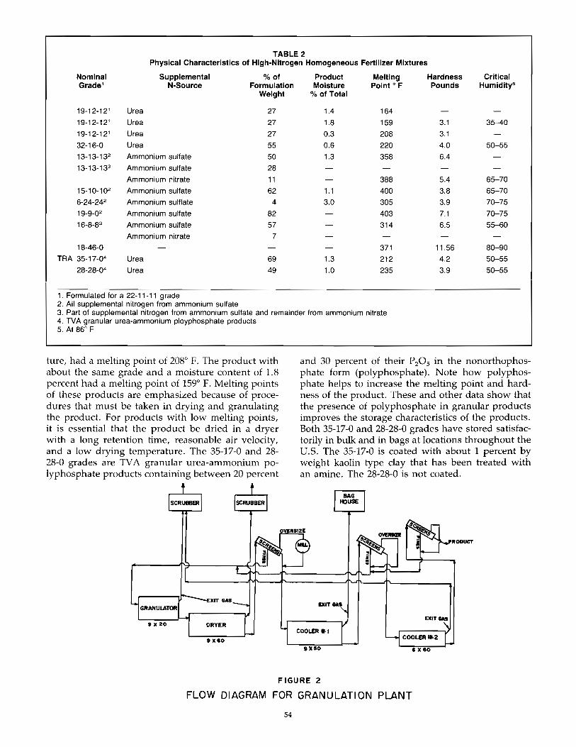
TABLE 2 Physical Characteristics of High-Nitrogen Homogeneous Fertilizer Mixtures

Nominal Supplemental 0/0 of Product Melting Hardness Critical Grade' N-Source Formulation Moisture Point 0 F Pounds Humidity5

Weight 0/0 of Total

19-12-12' Urea 27 1.4 164

19-12-12' Urea 27 1.8 159 3.1 35-40

19-12-12' Urea 27 0.3 208 3.1

32-16-0 Urea 55 0.6 220 4.0 50-55

13-13-132 Ammonium sulfate 50 1.3 358 6.4

13-13-133 Ammonium sulfate 28

Ammonium nitrate 11 388 5.4 65-70

15-10-102 Ammonium sulfate 62 1.1 400 3.8 65-70

6-24-242 Ammonium sulflate 4 3.0 305 3.9 70-75

19-9-02 Ammonium sulfate 82 403 7.1 70-75

16-8-83 Ammonium sulfate 57 314 6.5 55-60

Ammonium nitrate 7 18-46-0 371 11.56 S0-90

TRA 35-17-04 Urea 69 1.3 212 4.2 50-55

28-28-04 Urea 49 1.0 235 3.9 50-55

1. Formulated for a 22-11-11 grade 2. All supplemental nitrogen from ammonium sulfate 3. Part of supplemental nitrogen from ammonium sulfate and remainder from ammonium nitrate 4. TVA granular urea-ammonium ployphosphate products 5. At 86° F

ture, had a melting point of 2080 F. The product with about the same grade and a moisture content of 1.8 percent had a melting point of 1590 F. Melting points of these products are emphasized because of proce­dures that must be taken in drying and granulating the product. For products with low melting points, it is essential that the product be dried in a dryer with a long retention time, reasonable air velocity, and a low drying temperature. The 35-17-0 and 28-28-0 grades are TV A granular urea-ammonium po­lyphosphate products containing between 20 percent

and 30 percent of their P 205 in the nonorthophos­phate form (polyphosphate). Note how polyphos­phate helps to increase the melting point and hard­ness of the product. These and other data show that the presence of polyphosphate in granular products improves the storage characteristics of the products. Both 35-17-0 and 28-28-0 grades have stored satisfac­torily in bulk and in bags at locations throughout the u.s. The 35-17-0 is coated with about 1 percent by weight kaolin type day that has been treated with an amine. The 28-28-0 is not coated.

OIT lAS

EXIT lAS

COOLER .,

9'1160

FIGURE 2

FLOW DIAGRAM FOR GRANULATION PLANT

54

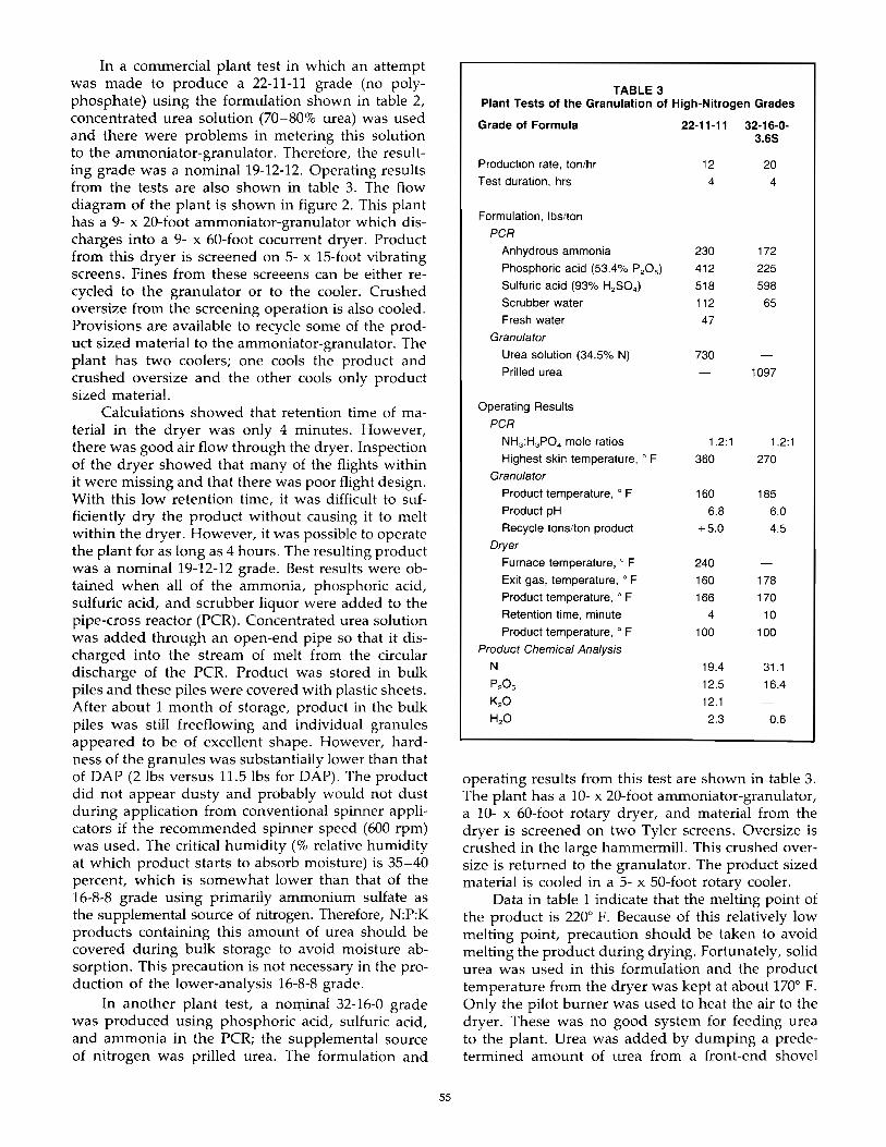
In a commercial plant test in which an attempt was made to produce a 22-11-11 grade (no poly­phosphate) using the formulation shown in table 2, concentrated urea solution (70-80% urea) was used and there were problems in metering this solution to the ammoniator-granulator. Therefore, the result­ing grade was a nominal 19-12-12. Operating results from the tests are also shown in table 3. The flow diagram of the plant is shown in figure 2. This plant has a 9- x 20-foot ammonia tor-granulator which dis­charges into a 9- x 60-foot cocurrent dryer. Product from this dryer is screened on 5- x IS-foot vibrating screens. Fines from these screeens can be either re­cycled to the granulator or to the cooler. Crushed oversize from the screening operation is also cooled. Provisions are available to recycle some of the prod­uct sized material to the ammoniator-granulator. The plant has two coolers; one cools the product and crushed oversize and the other cools only product sized material.

Calculations showed that retention time of ma­terial in the dryer was only 4 minutes. However, there was good air flow through the dryer. Inspection of the dryer showed that many of the flights within it were missing and that there was poor flight design. With this low retention time, it was difficult to suf­ficiently dry the product without causing it to melt within the dryer. However, it was possible to operate the plant for as long as 4 hours. The resulting product was a nominal 19-12-12 grade. Best results were ob­tained when all of the ammonia, phosphoric acid, sulfuric acid, and scrubber liquor were added to the pipe-cross reactor (PCR). Concentrated urea solution was added through an open-end pipe so that it dis­charged into the stream of melt from the circular discharge of the PCR. Product was stored in bulk piles and these piles were covered with plastic sheets. After about 1 month of storage, product in the bulk piles was still freeflowing and individual granules appeared to be of excellent shape. However, hard­ness of the granules was substantially lower than that of DAP (2 lbs versus 11.5 lbs for DAP). The product did not appear dusty and probably would not dust during application from conventional spinner appli­cators if the recommended spinner speed (600 rpm) was used. The critical humidity (% relative humidity at which product starts to absorb moisture) is 35-40 percent, which is somewhat lower than that of the 16-8-8 grade using primarily ammonium sulfate as the supplemental source of nitrogen. Therefore, N:P:K products containing this amount of urea should be covered during bulk storage to avoid moisture ab­sorption. This precaution is not necessary in the pro­duction of the lower-analysis 16-8-8 grade.

In another plant test, a nominal 32-16-0 grade was produced using phosphoric acid, sulfuric acid, and ammonia in the peR; the supplemental source of nitrogen was prilled urea. The formulation and

55

TABLE 3 Plant Tests of the Granulation of High-Nitrogen Grades

Grade of Formula 22-11-11 32-16-0-

Production rate, ton/hr

Test duration, hrs

Formulation, Ibs/ton

peR Anhydrous ammonia

Phosphoric acid (53.4% P20 S)

Sulfuric acid (93% H2S04 )

Scrubber water

Fresh water

Granulator

Urea solution (34.5% N)

Prilled urea

Operating Results

PCR

NH3 :H3 P04 mole ratios

Highest skin temperature, 0 F

Granulator

Product temperature, 0 F

Product pH

Recycle tons/ton product

Dryer

Furnace temperature, 0 F

Exit gas, temperature, C F

Product temperature, 0 F

Retention time, minute

Product temperature, F

Product Chemical Analysis

N

P20 S

K20

H20

12

4

230

412

518

112

47

730

1.2:1

360

160

6.8

+5.0

240

160

166

4

100

19.4

12.5

12.1

2.3

3.65

20

4

172

225

598

65

1097

1.2:1

270

185

6.0

4.5

178

170

10

100

31.1

16.4

0.6

operating results from this test are shown in table 3. The plant has a 10- x 20-foot ammonia tor-granulator, a 10- x 60-foot rotary dryer, and material from the dryer is screened on two Tyler screens. Oversize is crushed in the large hammermill. This crushed over­size is returned to the granulator. The product sized material is cooled in a 5- x 50-foot rotary cooler.

Data in table 1 indicate that the melting point of the product is 2200 F. Because of this relatively low melting point, precaution should be taken to avoid melting the product during drying. Fortunately, solid urea was used in this formulation and the product temperature from the dryer was kept at about 1700 F. Only the pilot burner was used to heat the air to the dryer. These was no good system for feeding urea to the plant. Urea was added by dumping a prede­termined amount of urea from a front-end shovel

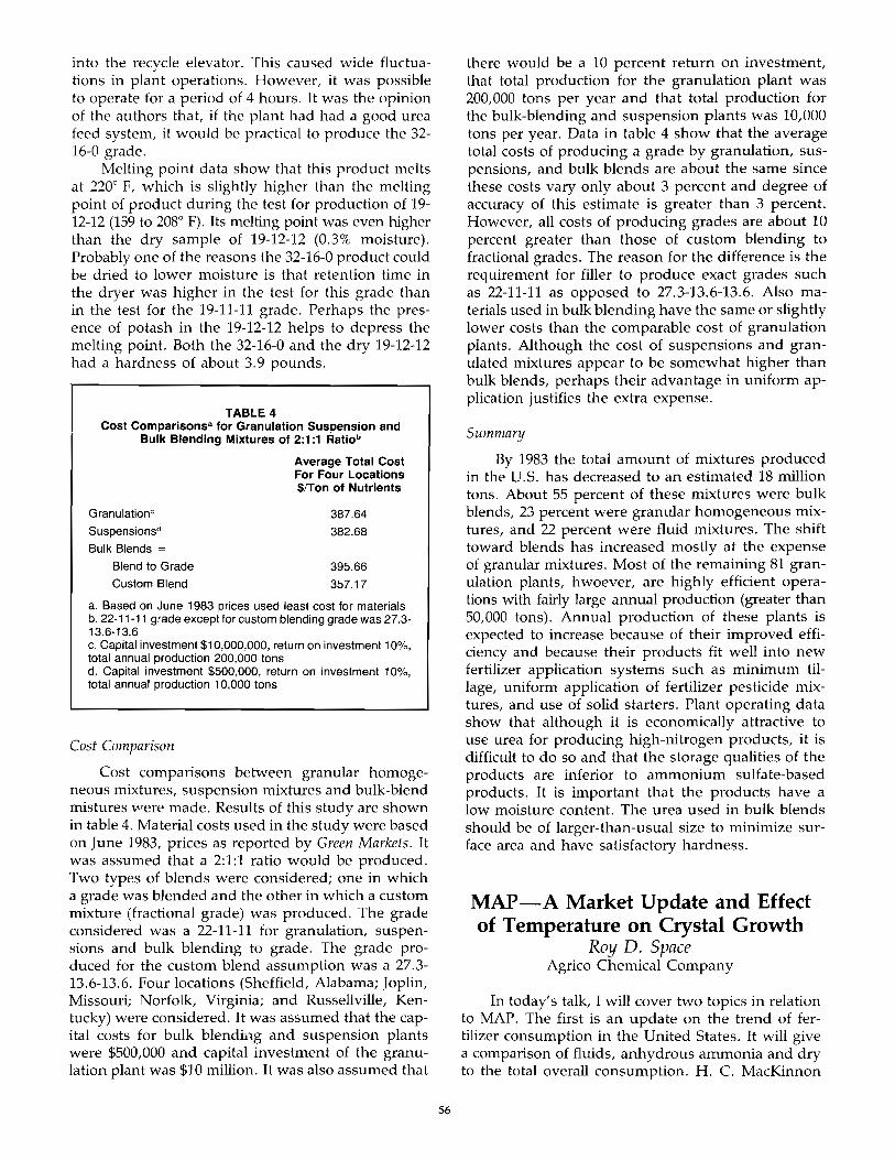
into the recycle elevator. This caused wide fluctua­tions in plant operations. However, it was possible to operate for a period of 4 hours. It was the opinion of the authors that, if the plant had had a good urea feed system, it would be practical to produce the 32-16-0 grade.

Melting point data show that this product melts at 2200 F, which is slightly higher than the melting point of product during the test for production of 19-12-12 (159 to 2080 F). Its melting point was even higher than the dry sample of 19-12-12 (0.3% moisture). Probably one of the reasons the 32-16-0 product could be dried to lower moisture is that retention time in the dryer was higher in the test for this grade than in the test for the 19-11-11 grade. Perhaps the pres­ence of potash in the 19-12-12 helps to depress the melting point. Both the 32-16-0 and the dry 19-12-12 had a hardness of about 3.9 pounds.

TABLE 4 Cost Comparisonsa for Granulation SusDension and

Bulk Blending Mixtures of 2:1:1 Ratlob

Granulation"

Suspensionsd

Bulk Blends =

Blend to Grade

Custom Blend

Average Total Cost For Four Locations $lTon of Nutrients

387.64

382.68

395.66

357.17

a. Based on June 1983 prices used least cost for materials b. 22-11-11 grade except for custom blending grade was 27.3-13.6-13.6 c. Capital investment $10,000,000, return on investment 10%, total annual production 200,000 tons d. Capital investment $500,000, return on investment 10%, total annual production 10,000 tons

Cost Comparison

Cost comparisons between granular homoge­neous mixtures, suspension mixtures and bulk-blend mistures "rere made. Results of this study are shown in table 4. Material costs used in the study were based on June 1983, prices as reported by Green Markets. It was assumed that a 2:1:1 ratio would be produced. Two types of blends were considered; one in which a grade was blended and the other in which a custom mixture (fractional grade) was produced. The grade considered was a 22-11-11 for granulation, suspen­sions and bulk blending to grade. The grade pro­duced for the custom blend assumption was a 27.3-13.6-13.6. Four locations (Sheffield, Alabama; Joplin, Missouri; Norfolk, Virginia; and Russellville, Ken­tucky) were considered. It was assumed that the cap­ital costs for bulk blendin.g and suspension plants were $500,000 and capital investment of the granu­lation plant was $10 million. It was also assumed that

56

there would be a 10 percent return on investment, that total production for the granulation plant was 200,000 tons per year and that total production for the bulk-blending and suspension plants was 10,000 tons per year. Data in table 4 show that the average total costs of producing a grade by granulation, sus­pensions, and bulk blends are about the same since these costs vary only about 3 percent and degree of accuracy of this estimate is greater than 3 percent. However, all costs of producing grades are about 10 percent greater than those of custom blending to fractional grades. The reason for the difference is the requirement for filler to produce exact grades such as 22-11-11 as opposed to 27.3-13.6-13.6. Also ma­terials used in bulk blending have the same or slightly lower costs than the comparable cost of granulation plants. Although the cost of suspensions and gran­ulated mixtures appear to be somewhat higher than bulk blends, perhaps their advantage in uniform ap­plication justifies the extra expense.

Summary

By 1983 the total amount of mixtures produced in the U.S. has decreased to an estimated 18 million tons. About 55 percent of these mixtures were bulk blends, 23 percent were granular homogeneous mix­tures, and 22 percent were fluid mixtures. The shift toward blends has increased mostly at the expense of granular mixtures. Most of the remaining 81 gran­ulation plants, hwoever, are highly efficient opera­tions with fairly large annual production (greater than 50,000 tons). Annual production of these plants is expected to increase because of their improved effi­ciency and because their products fit well into new fertilizer application systems such as minimum til­lage, uniform application of fertilizer pesticide mix­tures, and use of solid starters. Plant operating data show that although it is economically attractive to use urea for producing high-nitrogen products, it is difficult to do so and that the storage qualities of the products are inferior to ammonium sulfate-based products. It is important that the products have a low moisture content. The urea used in bulk blends should be of larger-than-usual size to minimize sur­face area and have satisfactory hardness.

MAP-A Market Update and Effect of Temperature on Crystal Growth

Roy D. Space Agrico Chemical Company

In today's talk, I will cover two topics in relation to MAP. The first is an update on the trend of fer­tilizer consumption in the United States. It will give a comparison of fluids, anhydrous ammonia and dry to the total overall consumption. H. C. MacKinnon

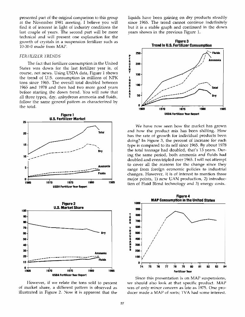
presented part of the original comparison to this group at the November 1981 meeting. I believe you will find it of interest in light of industry conditions the last couple of years. The second part will be more technical and will present one explanation for the growth of crystals in a suspension fertilizer such as 10-30-0 made from MAP.

FERTILIZER TRENDS

The fact that fertilizer consumption in the United States was down for the last fertilizer year is, of course, not news. Using USDA data, Figure 1 shows the trend of U.S. consumption in millions of NPK tons since 1965. The overall total doubled between 1965 and 1978 and then had two more good years before starting the down trend. You will note that all three types, dry, anhydrous ammonia and fluids, follow the same general 'pattern as characterized by the total.

Figure 1 U.S. Fertilizer Market

m~----------------------------------,

Total

15 .... ~.-.-.,

,. ._._._._._._._._._._._._._._._._._._. .;;"

5 Ammonia

---------------------~ _------ Fluids

Of--------r--------,_------.--------1 UBi 1970 1975 1980 1985

USDA Fertilizer Year Report

Figure 2 U.S. Market Share

l00~----------------------------------~

!III

80 r-------M ------________ ~

flO

60

40

30

Dry

Ammonia

-----------------~ _----- • _--"-------- Fluids 10 - -

o+-------~--------~-------,--------~ 1_ 1970 1975 1980 1985

USDA Fertilizer Tear Report

However, if we relate the tons sold to percent of market share, a different pattern is observed as illustrated in Figure 2. Now it is apparent that the

57

liquids have been gaining on dry products steadily since 1965. The trend cannot continue indefinitely but it is a stable graph and continued in the down years shown in the previous Figure 1.

p E R C E N T

I N C R E A S E

mo

2DO

150

100

50

Figure 3 Trend In U.S. Fertilizer Consumption

,-I' ,-./

, ,-

"', Fluids

,.,.."," ,---', ........... .-,,/ 'Total

",.,., """., ~ ",. ----..",-~.".' -,

*",' """'_---.",..,..,..- Dry

.,,~-----O~~----_r--------,_------,,------~ 111615 1970 1975 1980 1985

USDA Fertilizer Year Report

We have now seen how the market has grown and how the product mix has been shifting. How has the rate of growth for individual products been doing? In Figure 3, the percent of increase for each type is compared to its self since 1965. By about 1978 the total tonnage had doubled, that's 13 years. Dur­ing the same period, both ammonia and fluids had doubled and even tripled over 1965. I will not attempt to cover all the reasons for the change since they range from foreign economic policies to industrial changes. However, it is of interest to mention three major points, 1) new UAN production, 2) introduc­tion of Fluid Blend technology and 3) energy costs.

T 0 N S

T H 0 U S A N 0 S

Figure 4

IGOO MAP Consumption in the United States

9110

8011

700 i i

600 I

i i

!!GO .' I

4CIO I i

i 300 i

i 2DO i

.I 100 I

~ 75 ~ n n ~ ~ ~ ~ ~ ~

Fertilizer Year

Since this presentation is on MAP suspensions, we should also look at that specific product. MAP was of only minor concern as late as 1975. One pro­ducer made a MAP of sorts; TVA had some interest.

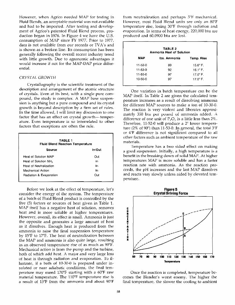
However, when Agrico needed MAP for testing in Fluid Blends, an acceptable material was not available and had to be imported. After testing and develop­ment of Agrico's patented Fluid Blend process, pro­duction began in 1976. In Figure 4 we have the U.S. consumption of MAP since FY 1977. Prior to 1977, data is not available from our records or TVA's and is shown as a broken line. Its consumption has been generally following the overall recent industry trend with little growth. Due to agronomic advantages it would increase if not for the MAP-DAP price differ­ential.

CRYSTAL GROWTH

Crystallography is the scientific treatment of the description and arrangement of the atomic structure of crystals. Even at its best, with a single pure com­pound, the study is complex. A MAP base suspen­sion is anything but a pure compound and its crystal growth is beyond description by a firm set of rules. In the time allowed, I will limit my discussion to one factor that has an effect on crystal growth-temper­ature. Even temperature is so interrelated to other factors that exceptions are often the rule.

TABLE 1 Fluid Blend Reaction Temperature

Source InlOut

Heat of Solution MAP Out

Heat of Solution NH3 In

Heat of Neutralization In

Mechanical Action In

Radiation & Evaporation Out

Before we look at the effect of temperature, let's consider the energy of the system. The temperature of a batch of Fluid Blend product is controlled by the five (5) factors or sources of heat given in Table 1. MAP itself has a negative heat of solution, removes heat and is more soluble at higher temperatures. However, overall, its effect is small. Ammonia is just the opposite and generates a large amount of heat as it dissolves. Enough heat is produced from the ammonia to raise the final suspension temperature by 15°F to 17DF. The heat of neutralization between the MAP and ammonia is also quite large, resulting in an observed temperature rise of as much as 90oP. Mechanical action is from the pump and the turbine, both of which add heat. A major and very large loss of heat is through radiation and evaporation. To il­lustrate, if a bath of 10-30-0 is prepared under in­sulated or near adiabatic conditions, the final tem­perature may exeed 170°F starting with a 600 P raw material temperature. The 110°F temperature rise is a result of 15°F from the ammonia and about 90°F

58

from neutralization and perhaps 5°F mechanical. However, most Fluid Blend units see only an 80°F temperature rise, losing 30°F through radiation and evaporation. In terms of heat energy, 220,000 btu are produced and 60,0900 btu are lost.

TABLE 2 Ammonia Heat of Solution

MAP Ibs. Ammonia Temp. Rise

11-52-0 89 15.6° F.

11-53-0 92 16.1° F.

11-55-0 97 17.0" F.

10-50-0 97 17.0" F.

One variation in batch temperature can be the MAP itself. In Table 2 are given the calculated tem­perature increases as a result of dissolving ammonia for different MAP sources to make a ton of 10-30-0. The reaction is very violent and liberates approxi­ITlalely 350 btu per puund of ammonia added. A difference of one unit of P 205 is a little less than 2%. Therefore, 11-52-0 will produce a 2° lower tempera­ture (2% of 90°) than 11-53-0. In general, the total 3°F or 4°F difference is not significant compared to all other factors such as ambient temperature of the raw materials.

Temperature has a two sided effect on making a good suspension. Initially, a high temperature is a benefit in the breaking down of solid MAP. At higher temperatures MAP is more soluble and has a faster reaction rate with ammonia. As the reaction pro­ceeds, the pH increases and the last MAP dissolves and reacts very slowly unless aided by elevated tem­perature.

c o N C E N T R A T I o N

Figure 5 Crystal Driving Force

60 70 80 90 100 110 1211 130 140 150 160 170

Temperature

Once the reaction is completed, temperature be­comes the Blender's worst enemy. The higher the final temperature, the slower the cooling to ambient

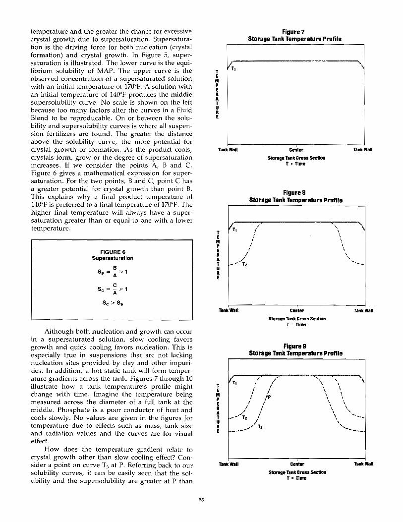
temperature and the greater the chance for excessive crystal growth due to supersaturation. Supersatura­tion is the driving force for both nucleation (crystal formation) and crystal growth. In Figure 5, super­saturation is illustrated. The lower curve is the equi­librium solubility of MAP. The upper curve is the observed concentration of a supersaturated solution with an initial temperature of 170°F. A solution with an initial temperature of 140°F produces the middle supersolubility curve. No scale is shown on the left because too many factors alter the curves in a Fluid Blend to be reproducable. On or between the solu­bility and supersolubility curves is where all suspen­sion fertilizers are found. The greater the distance above the solubility curve, the more potential for crystal growth or formation. As the product cools, crystals form, grow or the degree of supersaturation increases. If we consider the points A, Band C, Figure 6 gives a mathematical expression for super­saturation. For the two points, Band C, point C has a greater potential for crystal growth than point B. This explains why a final product temperature of 140°F is preferred to a final temperature of 170"F. The higher final temperature will always have a super­saturation greater than or equal to one with a lower temperature.

FIGURE 6 Supersaturation

B Sa = ~ 1

A

C Sc = A

Although both nucleation and growth can occur in a supersaturated solution, slow cooling favors growth and quick cooling favors nucleation. This is especially true in suspensions that are not lacking nucleation sites provided by clay and other impuri­ties. In addition, a hot static tank will form temper­ature gradients across the tank. Figures 7 through 10 illustrate how a tank temperature's profile might change with time. Imagine the temperature being measured across the diameter of a full tank at the middle. Phosphate is a poor conductor of heat and cools slowly. No values are given in the figures for temperature due to effects such as mass, tank size and radiation values and the curves are for visual effect.

How does the temperature gradient relate to crystal growth other than slow cooling effect? Con­sider a point on curve T3 at P. Referring back to our solubility curves, it can be easily seen that the sol­ubility and the supersolubility are greater at P than

59

T E M P E R A T U R E

Figure 7 Storage Tank Temperature Profile

"'--------' "---'"-----. ~ ~" T,

Tank Wall Center Tank Wall

Storage Tank Cross Sec1lon T = nme

FigureS Storage Tank Temperature Profile

,,-f I i i

i i

,/

'Ii "

\ \ i '\

\

T E M P E R A T U R E

............... 1-2

Tank Wall Center

Storage Tank Cross SectIon T = nme

figure 9 Storage Tank Temperature Profile

\ "

...............

Tank Wall

I;, > "P C, ~-.. /' I ". \ ,

T I I \ \ i I \ i E I \ i I M \ i

P ; /P \ i i \ \ E I

i I R / I A ..... '·"12 I T I U I

R ",/ T3 E !---_ ....

Tank Wall Center

Storage Tank CI'OS$ sectiOn T = nme

\ \ \ \ \ , , ....

\ , ...... -......

-----

Tillie Wall

T E M p

Figure 10 Storage Tank Temperature Profile

> ..... >

Vrl /' / i ,I

! I /

i I i I

; I .'" I ,.' Tz ,

/

'", '\

\ \ \ \

'<

\ \ \ \

" \ i i i \

\ \ \ , "

\ , ,.,"-

E R A T U R E ----" -,," T3 '-----

Tantl Well Genter

Storage T8IIk Cross Section T = Time

Tank WIllI

at the tank wall. We then have the condition de­scribed in Figure 11, Crystal Growth by Ion Migra­tion. That is, as material is removed from solution by crystal growth at the tank wall, it is replaced by migration from the hot inner part of the tank. The greater the temperature difference the greater the concentration difference and migration. This results in a high degree of supersaturation being maintained and crystals grow. This is not unlike the more familiar osmosis that is also concentration driven.

FIGURE 11 Crystal Growth by Ion Migration

Temperature T2 ;;. T1

Phosphate [DAP] > [DAP] 2 1

What can be done to reduce the temperature or its effect? The product temperature can be reduced by using a product cooler or by adding hot product to a cold heeL This favors nucleation over growth. Circulation is also important to prevent formation of temperature gradients and aid in cooling. Pump cir­culation does a better job of reducing temperature gradients than air sparging. Most Fluid Blend dealers already know that temperature control is important. I hope this has helped to explain why.

Conversion of Commercial Dihydrate to Hemihydrate Phosphoric Acid

Plants Barry Crozier,

Licensing and Consultancy Services, Norsk Hydro Fertilizers

60

Summary

Changes in the cost of raw materials and utilities for phosphoric acid production over the last ten years have increased the importance of energy conserva­tion and P 205 recovery efficiency. As a result, atten­tion has turned to hemihydrate technology for phos­phoric acid manufacture.

Commercial operation of hemihydrate and hem­idihydrate plants is now well established, and op­erating cost savings of over 10% can be demon­strated. With the current drive for profitability in today's competitive market, such a saving can have a major influence on the economic survival of a phos­phoric acid plant.

Because of the current state of the international economy, capital investment in new manufacturing capacity is limited and so restricts the opportunity for phosphoric acid producers to build new hemi­hydrate plants. Therefore, Norsk Hydro Fertilizers has developed technology to allow existing dihydrate phosphoric acid plants to be converted to the he­mihydrate processes.

Recently,'a number of detailed studies have been performed which examine in detail the process and engineering factors involved in the conversion of ex­isting plants. Two of these are described here.

In addition, a section of this paper has been devoted to highlight the first completed conversion of a commercial plant, which took place at Windmill Holland in mid 1983.

MOTIVATION

There have been two developments over the past ten years which have led phosphoric acid producers to consider converting their existing plants to he­mihydrate (HH) and hemidihydrate (HDH) technol­ogy. These are:

(1) Changes in the phosphoric acid production cost structure which have put much greater emphasis on the importance of high P20 S

recovery efficiency and enhanced energy savings, (1, 2).

(2) Commercial production of phosphoric acid utilizing the hemihydrate technology has been firmly established in practice, (3, 4, 5, 6).

Costs

In addition to the reduced energy consumption by production of strong acid directly from the filter, (7), the hemidihydrate (HDH) process can achieve improved P 205 recovery efficiency which results in higher raw material savings.

1983 cost comparisons between a HDH plant and a conventional dihydrate unit are shown in tables 1 and 2 for the case of a typical U.S.A. mine site op-

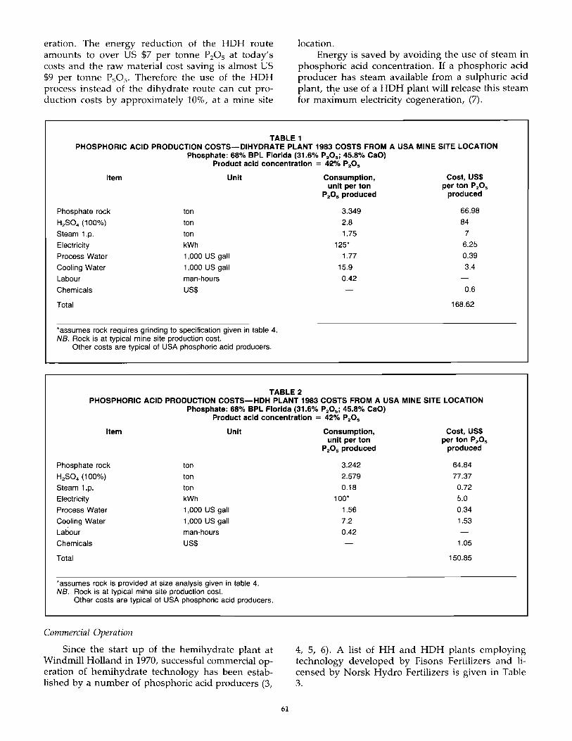
eration. The energy reduction of the HDH route amounts to over US $7 per tonne P20S at today's costs and the raw material cost saving is almost US $9 per tonne P 505' Therefore the use of the HDH process instead of the dihydrate route can cut pro­duction costs by approximately 10%, at a mine site

location. Energy is saved by avoiding the use of steam in

phosphoric acid concentration. If a phosphoric acid producer has steam available from a sulphuric acid plant, t~e use of a HDH plant will release this steam for maximum electricity cogeneration, (7).

TABLE 1 PHOSPHORIC ACID PRODUCTION COSTS-DIHYDRATE PLANT 1983 COSTS FROM A USA MINE SITE LOCATION

Phosphate: 68% BPL Florida (31.6% P2 0 S ; 45.8% CaO) Product acid concentration = 42% P20 S

Item Unit

Phosphate rock ton

H2S04 (100%) ton

Steam 1.p. ton

Electricity kWh

Process Water 1,000 US gall

Cooling Water 1,000 US gall

Labour man-hours

Chemicals US$

Total

'assumes rock requires grinding to specification given in table 4. NB. Rock is at typical mine site production cost.

Other costs are typical of USA phosphoric acid producers.

Consumption, unit per ton

P2 0 S produced

3.349

2.8

1.75

125'

1.77

15.9

0.42

Cost, US$ per ton P20 S

produced

66.98

84

7

6.25

0.39

3.4

0.6

168.62

TABLE 2 PHOSPHORIC ACID PRODUCTION COSTS-HDH PLANT 1983 COSTS FROM A USA MINE SITE LOCATION

Phosphate: 68% BPL Florida (31.6% P20 S ; 45.8% CaO) Product acid concentration = 42% P2 0 S

Item Unit

Phosphate rock ton

H2 S04 (100%) ton

Steam 1.p. ton

Electricity kWh

Process Water 1,000 US gall

Cooling Water 1,000 US gall

Labour man-hours

Chemicals US$

Total

'assumes rock is provided at size analysis given in table 4. NB. Rock is at typical mine site production cost.

Other costs are typical of USA phosphoric acid producers.

Commercial Operation

Since the start up of the hemihydrate plant at Windmill Holland in 1970, successful commercial op­eration of hemihydrate technology has been estab­lished by a number of phosphoric acid producers (3,

61

Consumption, Cost, US$ unit per ton per ton P2 0 S

P20 S produced produced

3.242 64.84

2.579 77.37

0.18 0.72

100' 5.0

1.56 0.34

7.2 1.53

0.42

1.05

150.85

4, 5, 6). A list of HH and HDH plants employing technology developed by Fisons Fertilizers and li­censed by Norsk Hydro Fertilizers is given in Table 3.

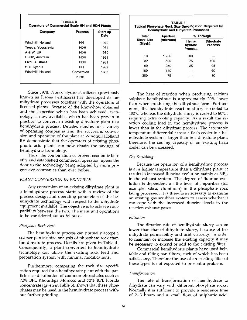
TABLE 3 Operators of Commercial Scale HH and HDH Plants

Company Process Start-up Date

Windmill, Holland HH 1970 Trepea, Yugoslavia HDH 1974 A & W, UK HDH 1980 CSBP, Australia HDH 1981 Pivot, Australia HDH 1981 HCI, Cyprus HH 1982 Windmill, Holland Conversion 1983

to HH

Since 1970, Norsk Hydro Fertilizers (previously known as Fisons Fertilizers) has developed its he­mihydrate processes together with the operators of licensed plants. Because of the know-how obtained and the expertise which has been achieved, tech­nology is now available, which has been proven in practice, to convert an existing dihydrate plant to a hemihydrate process. Detailed studies for a variety of operating companies and the successful conver­sion and operation of the plant at Windmill Holland BV demonstrate that the operators of existing phos­phoric acid plants can now obtain the savings of hemihydrate technology.

Thus, the combination of proven economic ben­efits and established commercial operation opens the door to the technology being adopted by more pro­gressive companies than ever before.

PLANT CONVERSION IN PRINCIPLE

Any conversion of an existing dihydrate plant to a hemihydrate process starts with a review of the process design and operating parameters of the he­mihydrate technology with respect to the dihydrate equipment available. The objective is to achieve com­patibility between the two. The main unit operations to be considered are as follows:-

Phosphate Rock Feed

The hemihydrate process can normally accept a coarser particle size analysis of phosphate rock than the dihydrate process. Details are given in Table 4. Consequently, a plant converted to hemihydrate technology can utilise the existing rock feed and preparation system with minimal modifications.

Furthermore, comparing the rock size specifi­cation required for a hemihydrate plant with the par­ticle size distribution of common phosphates such as 72% BPL Khouribga Morocco and 72% BPL Florida concentrate (given in Table 5), shows that these phos­phates may be used in the hemihydrate process with­out further grinding.

62

TABLE 4 Typical Phosphate Rock Size Specification Required by

Hemihydrate and Dihydrate Processes

Tyler Sieve Size

(Mesh)

10 32 60

100 200

Aperture (microns)

1,700 500 250 150 75

% Through

Hemi- Dihydrate hydrate Process Process

100 75 100 25 95

60 30

The heat of reaction when producing calcium sulphate hemihydrate is approximately 20% lower than when producing the dihydrate form. Further­more, the hemihydrate reaction slurry is cooled to 100°C whereas the dihydrate slurry is cooled to 80°C, reauirin!! extra coolin!! caoacitv. As a result the re­action c~oling load i;:; th~ he~ihydrate process is lower than in the dihydrate process. The acceptable temperature differential across a flash cooler in a he­mihydrate system is larger than in a dihydrate plant; therefore, the cooling capacity of an existing flash cooler can be increased.

Gas Scrubbing

Because the operation of a hemihydrate process is at a higher temperature than a dihydrate plant, it results in increased fluorine evolution mainly as SiF4,

in the exhaust system. The degree of fluorine evo­lution is dependent on the level of impurities (for example, silica, aluminum) in the phosphate rock being processed. It is therefore necessary to examine an existing gas scrubber system to assess whether it can cope with the increased fluorine levels in the reaction exhaust gases.

Filtration

The filtration rate of hemihydrate slurry can be lower than that of dihydrate slurry, because of he­mihydrate permeability and acid viscosity. In order to maintain or increase the existing capacity it may be necessary to extend or add to the existing filter.

Commercial hemihydrate plants have used belt, table and tilting pan filters, each of which has been satisfactory. Therefore the use of an existing filter of these types is not expected to present a problem.

Transformation

The rate of transformation of hemihydrate to dihydrate can vary with different phosphate rocks. Normally it is sufficient to provide a residence time of 2-3 hours and a small flow of sulphuric acid.

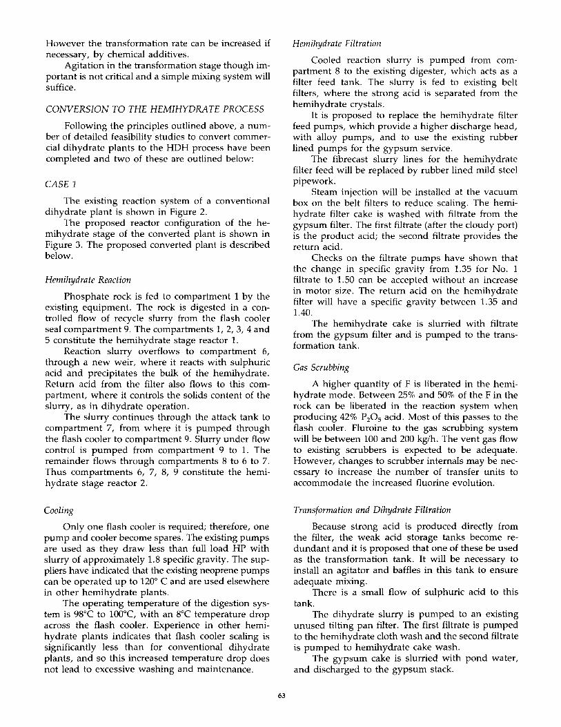
However the transformation rate can be increased if necessary, by chemical additives.

Agitation in the transformation stage though im­portant is not critical and a simple mixing system will suffice.

CONVERSION TO THE HEMIHYDRATE PROCESS

Following the principles outlined above, a num­ber of detailed feasibility studies to convert commer­cial dihydrate plants to the HDH process have been completed and two of these are outlined below:

CASE 1

The existing reaction system of a conventional dihydrate plant is shown in Figure 2.

The proposed reactor configuration of the he­mihydrate stage of the converted plant is shown in Figure 3. The proposed converted plant is described below.

Hemihydrate Reaction

Phosphate rock is fed to compartment 1 by the existing equipment. The rock is digested in a con­trolled flow of recycle slurry from the flash cooler seal compartment 9. The compartments 1, 2, 3, 4 and 5 constitute the hemihydrate stage reactor 1.

Reaction slurry overflows to compartment 6, through a new weir, where it reacts with sulphuric acid and precipitates the bulk of the hemihydrate. Return acid from the filter also flows to this com­partment, where it controls the solids content of the slurry, as in dihydrate operation.

The slurry continues through the attack tank to compartment 7, from where it is pumped through the flash cooler to compartment 9. Slurry under flow control is pumped from compartment 9 to 1. The remainder flows through compartments 8 to 6 to 7. Thus compartments 6, 7, 8, 9 constitute the hemi­hydrate stage reactor 2.

Cooling

Only one flash cooler is required; therefore, one pump and cooler become spares. The existing pumps are used as they draw less than full load HP with slurry of approximately 1.8 specific gravity. The sup­pliers have indicated that the existing neoprene pumps can be operated up to 1200 C and are used elsewhere in other hemihydrate plants.

The operating temperature of the digestion sys­tem is 98°C to 100°C, with an BOC temperature drop across the flash cooler. Experience in other hemi­hydrate plants indicates that flash cooler scaling is significantly less than for conventional dihydrate plants, and so this increased temperature drop does not lead to excessive washing and maintenance.

63

Hemihydrate Filtration

Cooled reaction slurry is pumped from com­partment 8 to the existing digester, which acts as a filter feed tank. The slurry is fed to existing belt filters, where the strong acid is separated from the hemihydrate crystals.

It is proposed to replace the hemihydrate filter feed pumps, which provide a higher discharge head, with alloy pumps, and to use the existing rubber lined pumps for the gypsum service.

The fibrecast slurry lines for the hemihydrate filter feed will be replaced by rubber lined mild steel pipework.

Steam injection will be installed at the vacuum box on the belt filters to reduce scaling. The hemi­hydrate filter cake is washed with filtrate from the gypsum filter. The first filtrate (after the cloudy port) is the product acid; the second filtrate provides the return add.

Checks on the filtrate pumps have shown that the change in specific gravity from 1.35 for No. 1 filtrate to 1.50 can be accepted without an increase in motor size. The return acid on the hemihydrate filter will have a specific gravity between 1.35 and 1.40.

The hemihydrate cake is slurried with filtrate from the gypsum filter and is pumped to the trans­formation tank.

Gas Scrubbing

A higher quantity of F is liberated in the hemi­hydrate mode. Between 25% and 50% of the F in the rock can be liberated in the reaction system when producing 42% PzOs acid. Most of this passes to the flash cooler. Fluroine to the gas scrubbing system will be between 100 and 200 kg/h. The vent gas flow to existing scrubbers is expected to be adequate. However, changes to scrubber internals may be nec­essary to increase the number of transfer units to accommodate the increased fluorine evolution.

Transformation and Dihydrate Filtration

Because strong add is produced directly from the filter, the weak acid storage tanks become re­dundant and it is proposed that one of these be used as the transformation tank. It will be necessary to install an agitator and baffles in this tank to ensure adequate mixing.

There is a small flow of sulphuric acid to this tank.

The dihydrate slurry is pumped to an existing unused tilting pan filter. The first filtrate is pumped to the hemihydrate cloth wash and the second filtrate is pumped to hemihydrate cake wash.

The gypsum cake is slurried with pond water, and discharged to the gypsum stack.

CASE 2

The reaction system of the existing dihydrate plant is shown in Figure 4. The production capacity is 325 tpd P20 S as 28% ex filter concentrated to 42% P20 S in conventional vacuum exaporators. The phos­phate rocks is 72 BPL Florida. Reactor details are given below:-

Reaction volume, total 29,300 ft3 operating = 22,000 ft3

Vessel type single annular vessel with central compartment.

Material of Construction : concrete lined with

rubber and carbon brick.

Agitation:

No agitators in annulus Absorbed power

No. of agitators in

6 5 x 75 HP + 1 x 150 HP at rock feed point

central compartment 1 Absorbed power = 50 HP Material of construction = AISI 317

The proposed reactor configuration of the he­mihydrate stage of the converted plant is shown in Figure 5. The proposed converted plant is described below.

Hemihydrate Reaction

The dihydrate plant reaction vessel provides suf­ficient slurry volume for the hemihydrate stage com­partments 1 and 2. It is proposed to build dividing walls in the vessel (as shown in figure 5) such that the two resulting compartments will have the volu­metric ratio of 2: 1.

Studies have shown that the existing agitation is satisfactory for the hemihydrate duty.

The filter feed tank in the dihydrate plant is suitable for the same duty in the hemihydrate stage.

Phosphate rock is fed to compartment 1 by the existing equipment. Slurry is pumped from com­partment 2 to a flash cooler and is recycled under flow control to compartment 1. Slurry from com­partment 1 overflows to the second compartment where it reacts with sulphuric acid to complete the hemihydrate precipitation. Return acid from the filter also flows into this compartment.

Cooling

The existing flash cooler has the following di-mensions;

diameter straight height

14.0 it. 15.5 ft.

64

It operates in the dihydrate mode under the fol-lowing conditions:

temperature drop 7°F pressure 6 in. Hg absolute slurry circulation = 10,000 gall/min.

In the hemihydrate mode the temperature in the reaction system is 98-100°C and the flash cooler can operate at a temperature drop of 8°C without an increase in scale deposition. As a result, the flash cooler system is satisfactory for a hemihydrate plant capacity up to 600 tpd P20 S -

Hemihydrate Filtration

The existing filter is a horizontal tilting pan type with an effective area of 618 sq. ft. The material of construction of the pans is AISI 316. The hemihydrate slurry is fed to this filter.

Steam injection will be installed in the filter cen­tral valve to reduce scaling.

Two existing slurry filter feed pumps of capacity 750 gall/min are to be used for the hemihydrate duty, one is an installed spare.

The filter ancilliary pumps are satisfactory at the following capacities:

return acid pump : 590 gall/min 1st wash pump : 390 gall/min 2nd wash pump : 390 gall/min 3rd wash pump : 390 galVmin

Gas Scrubbing

As in the previous case, there is a higher quantity of fluorine liberated in the hemihydrate system when producing 42% P20 S acid. Most of this passes to the flash cooler. The existing fume scrubber with a gas flow of 121,000 acfm needs to achieve an efficiency of 99% to remove the increased fluorine evolved.

Transformation and Dihydrate Filtration

Having produced strong acid directly from the filter and thus avoided the need to concentrate the acid further, the weak acid storage tanks are no longer required. It is proposed to use one of these as the transformation tank. It is necessary to install an ag­itator and baffles to ensure adequate mixing.

There is a small flow of sulphuric acid to this tank.

Filtration of the dihydrate slurry will take place on a belt filter of 430 sq. ft. This is a new item of equipment.

FROM DH TO HH IN PRACTICE

In June 1983, Windmill Holland BV completed the conversion of its dihydrate plant to the hemi­hydrate process. Process engineering was carried out

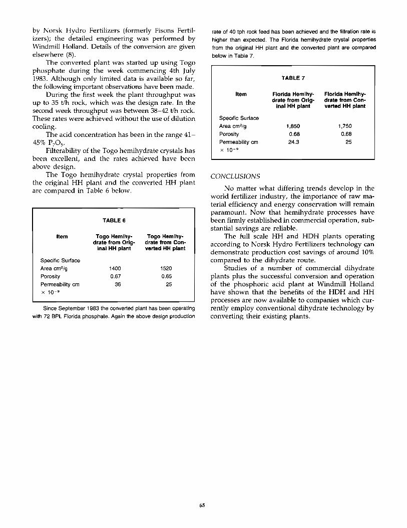
by Norsk Hydro Fertilizers (formerly Fisons Fertil­izers); the detailed engineering was performed by Windmill Holland. Details of the conversion are given elsewhere (8).

The converted plant was started up using Togo phosphate during the week commencing 4th July 1983. Although only limited data is available so far, the following important observations have been made.

During the first week the plant throughput was up to 35 t/h rock, which was the design rate. In the second week throughput was between 38-42 tIh rock. These rates were achieved without the use of dilution cooling.

The acid concentration has been in the range 41-45% P20S'

Filterability of the Togo hemihydrate crystals has been excellent, and the rates achieved have been above design.

The Togo hemihydrate crystal properties from the original HH plant and the converted HH plant are compared in Table 6 below.

TABLE 6

Item Togo Hemlhy- Togo Hemihy-drate from Orig- drate from Con-

inal HH plant verted HH plant

Specific Surface

Area cm2/g 1400 1520

Porosity 0.67 0.65

Permeability cm 36 25 x 10- 9

Since September 1983 the converted plant has been operating

with 72 BPL Florida phosphate. Again the above design production

65

rate of 40 tph rock feed has been achieved and the filtration rate is

higher than expected. The Florida hemihydrate crystal properties

from the original HH plant and the converted plant are compared

below in Table 7.

TABLE 7

Item Florida Hemihy- Florida Hemihy-drate from Orlg- drate from Con-

Inal HH plant verted HH plant

Specific Surface

Area em2/g 1.850 1.750

Porosity 0.68 0.68

Permeability em 24.3 25 x 10- 9

CONCLUSIONS

No matter what differing trends develop in the world fertilizer industry, the importance of raw ma­terial efficiency and energy conservation will remain paramount. Now that hemihydrate processes have been firmly established in commercial operation, sub­stantial savings are reliable.

The full scale HH and HDH plants operating according to Norsk Hydro Fertilizers technology can demonstrate production cost savings of around 10% compared to the dihydrate route.

Studies of a number of commercial dihydrate plants plus the successful conversion and operation of the phosphoric acid plant at Windmill Holland have shown that the benefits of the HDH and HH processes are now available to companies which cur­rently employ conventional dihydrate technology by converting their existing plants.

REFERENCES

1. Fisons Hemihydrate Process-A Decade of Energy Saving.

2. Fisons Hemihydrate Processes-A Decade of Energy Savings.

3. The Commercial Production of 50% Phosphoric Acid by the direct Single Stage Hemihydrate Process.

4. Fisons HDH Phosphoric Acid Process, Operating Experience with a 160 tpd Plant.

5. Full-scale Application of the HDH Phosphoric Acid Process.

6. Recent Experiences in Phosphoric Acid Production by Hemihydrates Routes.

7. Convert to the Direct Production of High Strength, High Quality Phosphoric Acid with Fisons Hem:L~ydrat€ Teclllto!ogy.

8. Conversion to Hemihydrate-A Case Study

B.T. Crozier

B.T. Crozier

H.O. Crawford C.H.M. Vinke P. van Hagen

V. Lasovic et al

H.J. Koenig E.W. Schwehr

M.L. Parker c.R. McDonald

B. T. Crozier

B.T. Crozier

66

IF A, Kallithea, October 1982.

The Fertilizer Industry Round Table, Atlanta, October 1982.

ISMA, Seville, November 1972.

ISMA, The Hague, September 1976.

A.I.Ch.E., Philadelphia, June 1978.

Fertilizer Society, London, October 1982.

American Chemical Society. Kansas City, September 1982.

British Sulphur Corporation Conference, London, November 1983.

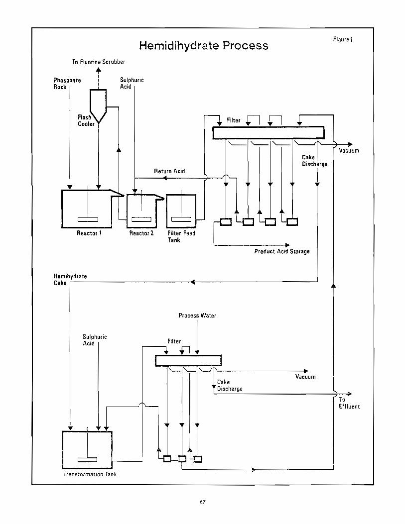
Hemidihydrate Process Figure 1

To Fluorine Scrubber

+ I j

I Phosphate Rock ~

Flash Cooler

1 Reactor 1

Hemihydrate Cake

Sulphuric Acid

1

-

TransformatIon Tanl{

Sulphuric Acid

+ Filter.n n ... I

Cake Discharge

Return Acid ~----~~~------~\r-~0-

Reactor 2 Filter Feed Tank

Process Water

,..-------, Filter 1 • f.l

f

, ~

I

,

Product Acid Storage

'-- "--I "--./"'1...-----------...... Va~um

Cake , Discharge

i' l' .

'" .. '" Vacuum

,.; To ' Effluent

Lr"t r, ~ -Ti-i ~ __________ ~, __________ -J

67

-

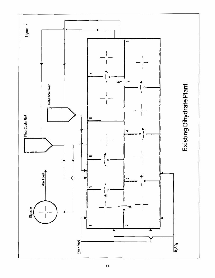
~,( J

-J~\ _________ ~~ __ __ ,-----

I

N o

% ~

8 c;:.:; ..!: "

--L

I - -

I -

-

,...

en

j ~-""'(""

...... -

I -- -I

-(0-

I

~o-

I - -

I

..r)

I I I -- -I

I

..-- 1 :::I - - \ 0

i I

-

I -

\

I I --... I

:::s I

-

--

tL ______________ ~~ - J

t

68

-

-

..... c CO -a. Q) ..... CO ..

"C ~ .r:. .-C 0') c .-t) .-X

W

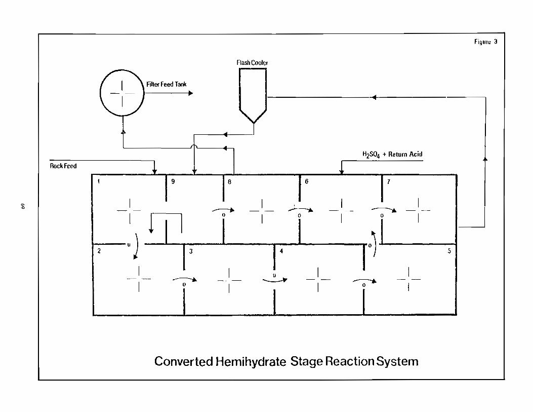
Fi!lUril 3

Flash Coolt'f

( Filter feed Tank

\ 0-

J ... ..... -...,.- y

,r-. ....

I' ... ..... H2S04 + Return Acid

Rock Feed ~ ,lr f 1 9 8 6 7 1

I

I

I

$ I I I I I I . -- ......----.. -- .....---.. -----. I

I fTl 0 I 0 I 0 I

uJ 0) 2 J 4 5

~

I 1 ~ I I -'- --.. -- -- ~

- -I 0 I I I

Converted Hemihydrate Stage Reaction System

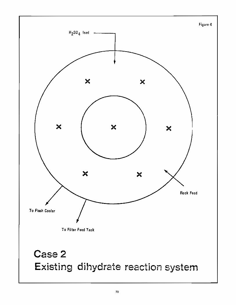
Figure 4

x x

)( )(

Rock Feed

To flash Cooler

To Filter Feed Tank

Case 2 Existing dit,ydrate reaction system

70

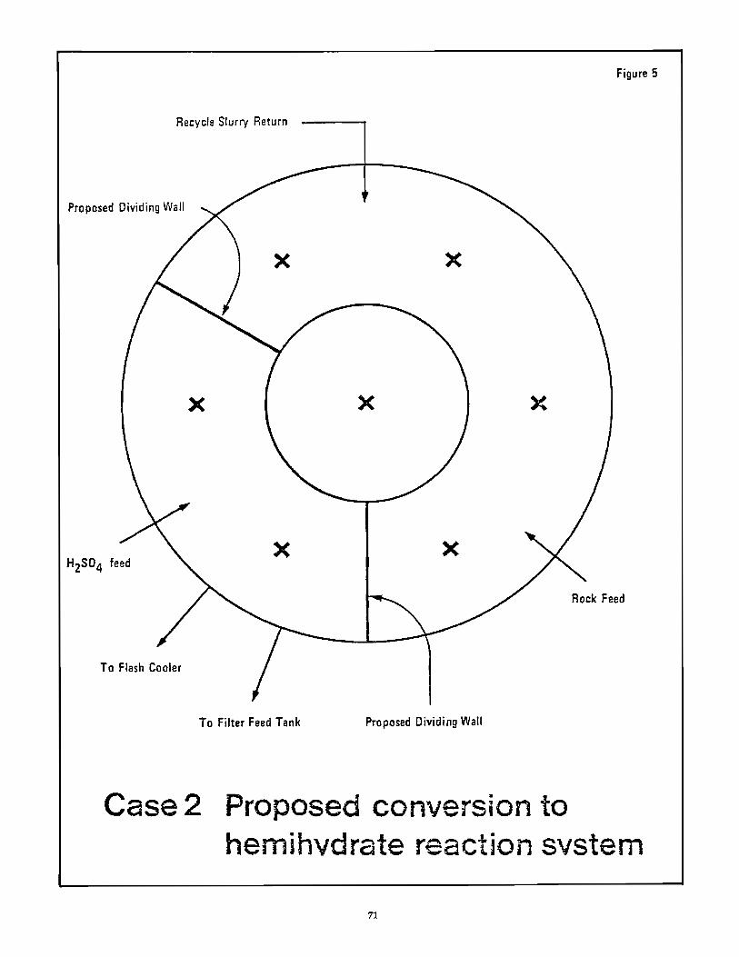
Figure 5

Recycle Slurry Return

Proposed Dividing Wall

x x

x x

Rock Feed

To Flash Cooler

To Filter Feed Tank Proposed Dividing Wall

Case 2 Proposed conversion to hemihvdrate reaction svstem

71

Wednesday, October 26, 1983

Afternoon Session's Moderator:

Herman G. Powers

Fertilizer Plant Safety A. Driver Training

Glenn A. Feagin International Minerals & Chemical Corporation

Unless you represent a company with a total employment of less than 10 people, you are required by law to provide driver training for anyone assigned by you to operate Powered Industrial Trucks. Both OSHA (The Occupational Safety & Health Admin­istration), who supervises general industry, and MSHA (The Mine Safety & Health Administration), who su­pervises both surface and underground mining, have regulations requiring driver training.

In addition, the Department of Transportation and the Interstate Commerce Commission have rules regulating training for over-the-road equipment driv-ers.

I would like to focus mainly on OSHA require­ments. However, most of my remarks will also apply to MSHA-supervised locations.

OSHA Safety & Health Standard 29 CFR 1910.178 covers the operation of Powered Industrial Trucks. There are about 10 pages of general operating rules and safety regulations listed in the June 1981 printing of the OSHA Handbook #2206, "General Industry Safety & Health Standards". One of these rules out­lines the requirements for Driver Training and I quote:

"OPERATOR TRAINING. Only trained and au­thorized operators shall be permitted to operate a powered industrial truck. Methods shall be devised to train operators in the safe operation of powered industrial trucks." A real catch-all statement if I ever read one. It

gives you plenty of rope! Better make sure that you do not hang yourself with it. But, really, it's no prob­lem. All you have to do is devise a program that will adequately train your employees and that will stand up under critical examination by a compliance officer.

OSHA does not completely abandon us with only this short statement as a guide! The National Institute for Occupational Safety & Health (NIOSH) in their booklet, "Outline For Training of Powered Industrial Truck Operators", gives some help. By the way, this booklet is available from the Superintendent of Doc-

73

uments, Washington, D.C. The order number is DHEW (NIOSH) Publication No. 78-199. I l~com­mend that a copy be obtained.

In this booklet, some of the points made are: 1) It is the employer's responsibility to provide

training. 2) Training can either be done by the em­

ployer or an outside firm can be engaged to conduct the program.

3) The employer can devise his own training course. There are no special requirements as long as it works.

4) The only requirement for course instructors is that they must have sufficient knowledge and experience to teach effectively.

5) Training should be updated at least every two years, more often for operators who have poor driving records.

6) Even occasional drivers must be trained, and drivers must be trained to safely op­erate each type vehicle assigned to them.

7) A log of all training activities must be kept. 8) OSHA Compliance Officers may question

employees both to check log information and to determine if employees aTe ade­quately trained.

9) Training should be performed on company time and at least 10 hours practice time is recommended for new drivers.

10) A closely supervised 1 to 2 weeks proba­tionary period for new drivers is recom­mended.

11) Equipment covered under the training re-quirement includes:

***Fork Trucks ***Industrial Tractors ***Platform Lift Trucks ***Motorized Hand Trucks ***Specialized Industrial Trucks

That original short paragraph certainly got long in a hurry; and, I left out a lot of things covered in the booklet.

One might be tempted to say: "That's a lot of work and trouble. I haven't got time for all of that. I'll just let it go. It doesn't matter." DANGEROUS THINKING!! If a serious vehicle accident or a general

OSHA inspection never occurs, you may get away with it. However, if an accident does happen, you could be in real trouble.

For the first accident, you could be cited for a serious violation. Then, if another accident occurred, you might be cited for a willful violation. Serious violations carry fines; willful violations can carry jail terms. Actually, a good training program can save money by increasing production and reducing repair costs.

While the NIOSH booklet gave a lot of inior­mation, it still left the question as to what is a sat­isfactory training course unanswered. As additional information, I would like to describe the program used in our plants. I must state that IMC makes no claims that it would cover all conditions which might exist at your particular location.

Before any IMC employee can operate any ve­hicle, he or she must be trained and licensed to op­erate that particular type tractor. For example, an operator with only a license for a forklift truck would not be alluwed tu operate a front end loader, or vice­versa.

Training consists of: 1) Lecture course on general rules. 2) Written examination on general rules. 3) Specific training and practice on each type

vehicle. 4) An actual operating test conducted by a

qualified examiner. The results of these tests are put into the em­

ployee's personnel file and become a permanent rec­ord. Also, his name is added to the list of qualified drivers which is kept posted at the plant.

A review course is conducted once each year for all drivers. Again, a written account of the training update is placed in the employee'S personnel file.

Each qualified driver is given an IMC Equipment Operation Certificate listing the types of equipment he or she is qualified to operate, and also a pocket­sized copy of a set of Powered Industrial Vehicle Safety Rules.

Special attention is given to the training of new operators. In addition to the general training course, they are given hands-on training and allowed to prac­tice until their instructor feels that they are capable of handling the equipment under plant conditions.

If drivers operate company vehicles off the plant property, we make sure that they have the correct State Driver's License and that the vehicle meets any required safety standards.

OSHA regulations state that farm vehicles are not classified as powered industrial motor trucks. However, I do not know whether or not they have ever ruled that farm-type vehicles used by commer­cial operators are actually exempt. Therefore, we in­clude them in our training course. Also included are operators of any special equipment such as floater-

74

type spreaders. Even if it is not required by law, it is just good business to do so.

A pre-employment physical examination is re­quired by IMC to insure that the potential operator is physically able to safely operate a vehicle.

Driver training is not a one shot deal. Vehicle safety is regularly covered at our plant safety meet­ings. Films and slide programs are very popular.

One last and very important point ... "If it is not in writing, you did not do it." KEEP RECORDS!! It may be a lot of trouble, but I know from personal experience that it is a real comfort to have them when they are needed. Set up a system and see that it is kept up-to-date. This applies not only to driver train­ing, but to all other types of safety training con­ducted.

Fertilizer Plant Safety B. Machinery Guarding and Lockout

F. C. McNeil Corporate Safety Manager

International Minerals & Chemical Corporation

The topics of machine guarding and equipment lockout are two that all of us have heard and read a lot about.

Some may view these subjects as separate or independent, yet their goals are similar. One is de­signed to protect the worker while the equipment is in operation, while the other provides a safe condi­tion while it's inoperative.

By now your company has surely instituted a program for machine guarding . . . and the warnings about hazardous nip and pinch points, danger zones, etc., may be an old story, but believe me the safety message cannot be repeated enough. Each year, far too many workers are injured because of inadequate machine guarding or poor guarding practices.

Guarding means preventing workers from con­tacting moving mechanical parts which could cause physical harm. Guarding may be by means of fencing or a rail enclosure to prevent access to danger points, or it may also be achieved by locating the mechanical hazard to a normally inaccessible place. But fencing and location are limited in effectiveness and accept­ability.

The third, and probably the most effective, is guarding by enclosure, meaning a fixed barrier mounted on equipment to prevent access to danger­ous moving parts.

I am sure that all of you are aware of operations with a good equipment guarding program and you may possibly know of some with a guarding system that is less effective. I would suggest that if a guard of this type exists, it be upgraded to meet standards and a thorough review of safety guarding be per­formed throughout that plant.

When reviewing existing machine protection or designing new guards, we must first identify the:

• Point of operation

• Power transmission

After this has been established, then we must insure that guards conform with the following cri­teria:

• It meets the minimum OSHAIMSHA require­ments

• Protects workers' hands, arms, and other body parts from contact with the dangerous moving parts

• Is firmly secured and not readily removable

• Ensure that objects cannot fall into moving parts

• Permits safe, comfortable, and relatively easy op­eration

• Will allow machinery lubrication without guard removal

• That a system exists for machine shut-down be­fore guard removal

• And finally, determine if the existing guard can be improved.

Metal is usually the best material for guard con­struction. Usually the enclosure is a metal frame of pipe, angle or bar stock with a filler of expanded, perforated or solid-sheet metal. Where visibility is required, plastic or safety glass may be practical.

Wooden guards generally are not recommended because of flammability or lack of durability and strength. However, in highly corrosive atmospheres, wood might be considered.

A problem many plants encounter is the failure to replace guards once they have been removed. But before we lay complete blame on the worker, let's consider a few possibilities as to why this condition may exist.

DOES MANAGEMENT ENFORCE SAFETY RULES?

Does management really enforce guard replacement? Is this safety rule only followed when it is convenient to do so? In other words, does safety become sec­ondary when time becomes a factor in production or shipping schedules?

75

WHAT IS DESIGN OF GUARD?

What is the design of the guard? ... Is it difficult to replace .... too big, too heavy, or poorly fitting? These conditions can make it easy for people to leave if off at start-up.

WHAT IS THE PHYSICAL CONDITION OF GUARD?

What is the physical condition of the guard? ... Is it badly bent out of shape, or broken, making it a major task to remove or replace? We must remember that guards have to be maintained to be effective ... they should be considered an essential part of the equipment.

Yes, management must shoulder the blame. Should any of these situations exist, then the re­sponsibility rests with management to take the nec­essary steps to see that these conditions are properly corrected.

When machine safeguarding requires expertise not readily available at a plant, then there are several avenues where assistance can be sought. Some of these sources are:

EQUIPMENT MANUFACTURER

Equipment manufacturers . . . they can often supply the necessary literature, advice, and possible personal assistance to help solve the problem.

INSURANCE CARRIER

Your insurance carrier will often provide the assis­tance of their safety specialist.

GOVERNMENT AGENCIES

Some government agencies offer consultation serv­ices for on-site evaluations of workplaces and hazard control. OSHA funds one such program that is of­fered free-of-charge to employers in every state. This consultation program is completely separate from the standard OSHA inspection-there are no citations issued or penalties proposed.

CONCEPTS AND TECHNIQUES OF MACHINE SAFEGUARDING BOOKLET

Another good source of information is the book­let, "Concepts and Techniques of Machine Safe­guarding", published by the U.S. Department of La­bor Occupational Safety and Health Administration.

Now let's look at the other side of the coin ... what precautions can be taken to protect employees while working in the danger zone of machinery in its off position.

The standards which require use of lockout! tagout systems are currently being reviewed for pos­sible revisions. Revisions are being considered be-

cause of the alarming number of incidents which tend to demonstrate the seriousness of worker exposure to hazardous situations during maintenance opera­tions. Accidental start-up of equipment during main­tenance and inspection has too often resulted in loss of limbs, electrocutions, severe trauma, chemical or thermal burns, and acute respiratory problems.

In general, anyone working on and around ma­chinery runs a serious risk unless equipment is locked­out, and cannot be accidently started. The best method to prevent accidental injury to employees while per­forming inspections or maintenance on equipment/ machinery is to use a system of lockout devices, cou­pled with a documented lockout procedure.

Typical conditions which require lockout precau­tions are:

• Any time repairs must be performed on electrical circuits.

• Whenever moving parts of machinery or equip­ment are being cleaned or lubricated.

• When it becomes necessary to remove jammed parts or to clear blocked mechanisms.

• To prevent operation by unauthorized persons and/or equipment use during off hours.

• When maintaining lines carrying hazardous liq­uids under high pressure, such lines should be clearly marked. Valves in the system should be capable of being locked out. In the case of high­pressure lines, there should be a means of safely relieving pressure in the blocked sections. There should also be a means available for lines to be capped or blanked. The first phase of a lockout/tagout program is to

establish a realistic written procedure that is appli­cable to all machinery and equipment. This proce­dure will be developed through a thorough study of your particular operation.

After a procedure has been written, an employee training program should be conducted that clearly explains the procedure, emphasizing its importance and includes a full explanation of what disciplinary actions will be taken against violators. A 1979 BLS statistic revealed that of the 554 workers injured while servicing equipment, 61 % had received no instruc­tions on lockout procedures.

A normal lockout procedure will usually consist of 6 basic steps:

1. The notification of all concerned personnel:-Op­era tors, Supervisor, etc., should be advised that the equipment/machinery will be locked out.

2. Review the entire lockout procedure-before any work begins, think through every required

76

step and double check everything. For example: Review shutdown and work authorization to insure the correct system is being locked out and worked on.

• Check to see that all switches are prop­erly marked so that the right ones are locked out.

• Determine if there are any related sys­tems that also need to be shutdown.

• Are the workers wearing the required protective equipment?

3. Identify all energy sources--associated with equipmentlmachinery .

4. Neutralize all energy sources by:

• • • •

Turning off electrical power. Lowering all suspended parts that might be affected by gravity or other forces. Venting pressure from pneumatic lines. Draining or bleeding hydraulic lines. Release or blocking spring energy a

It is important to never rely on secondary protection: Example: Do not lockout the 120 volt auxil­iary service on a 440 volt system; always kill the main power source to a piece of equip­ment.

S. Lockout the power source-against accidental start-up of machinery and prevent equip­ment motion resulting from stored energy. After attaching lock to electrical controls, valves, etc., place a warning tag to alert others to the locked-out status of the machinery/ equipment. No employee should be authorized to re­move the lock and tag unless he/she is the one who originally placed it.

6. Test Machinery/Equipment-Never enter a danger zone until the equipment has been tested to insure it is secure and no danger­ous movement is possible. Means of testing can be:

• Pushing start buttons to verify that the power is off.

• Inspect moving parts to insure that they are at complete rest and properly se­cured.

• Operate valves to be sure no machine parts will be activated by pressure.

• Test electrical circuits to insure that they are dead.

• Double check for other workers who may be located in the danger zone.

• And, perform any other test that may be specifically outlined in the written lockoutltagout procedure.

In the event there may be some source of energy that cannot be locked out, take special precautions such as:

• Using tags.

• •

• • •

Constructing barricades.

De-energizing the power source at the circuit breaker.

Remove fuses.

Posting a co-worker to stand guard if necessary.

Post signs on doors and gates to hazardous areas. If possible, lock these areas off.

Before restarting machine/equipment, check to insure that:

•

• • •

•

• • •

Equipment is in operating condition, properly lubricated, adjusted, set up, and ready for serv­ice.

All guards are in place.

No tools have been left behind.

All blocks, braces, pins, and chains have been removed.

All pressure tubes, pipes, or hoses have been reconnected.

Work areas are clear for normal 0'peration.

All workers are clear of the danger zone.

And, employees are wearing the personal pro­tective equipment required for normal operation.

The supervisor should be notified of any dam­aged or missing parts or of any potential hazard be­fore the equipment is set into motion.

There are four hard and fast rules that all em­ployees should be trained to understand and respect relating to the lockout procedure:

1. DO NOT remove covers or alter warning tags.

2. DO NOT BYPASS or remove locks placed by another person.

3. DO NOT enter the danger zone without au­thorization.

4. DO NOT try to start locked out equipment. The heart of any lockout program is the lock

itself. Decisions will have to be made on such things as the type of lock to use-key or combination; who

77

will be issued a lock; who will have possession of the keys or combination; and how will the lock be identified.

The answers to these questions will vary, but here are some guidelines that you may wish to fol­low:

• Key-operated padlocks are used more often than combination locks because supervisors usually have much better control over keys than com­binations. Locks should be issued to every employee who works on equipment during a shutdown stage. No key or combination should fit more than one lock. A lost lock or key should be immediately re­ported to the supervisor. Another important lockout device often referred

to as a redbird is a useful piece of equipment that should be part of every lockout/tagout program .... We have found that the metal redbird is a lot more durable than the aluminum type because it was dis­covered that the aluminum could be twisted and bro­ken off rather easily.

In closing, I would like to leave you with a couple of good sources of lockout information:

ANSI Z244.1-1982 American National Standard for Personal Protection-LockoutlTagout of Energy sources, and

OSHA's study of Selected Occupational Fatalities Related to Lockout/Tagout Problems.

In-this brief presentation, we have only touched on the high points of machine guarding and lockouts which in turn is only a portion of your overall safety program. It is important to remember that to be ef­fective, safety must have a sincere commitment from every plateau of management-only when safety is encouraged, monitored, and enforced on the same level as the rest of the activities within an organi­zation will its full value be realized. When safety is truly considered a necessary and valuable tool, then not only will it reduce injuries, but it will become a major contributor to the improvement of employee morale, product quality and operation efficiency, while at the same time help to reduce overhead.

Fertilizer-Pesticides Impregnation Operations A. V. Malone

Manager of Engineering & Quality Control Crops Services

Agway, Inc.

Introduction

The production and use of fertilizer-pesticide combinations is not new. My first experience with

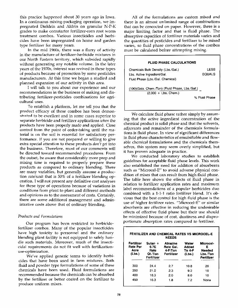
this practice happened about 30 years ago in Iowa. In a continuous mixing-packaging operation, we im­pregnated Dieldrin and Aldrin on granular N-P-K grades to make corns tarter fertilizer-corn root worm treatment combos. Various insecticides and herbi­cides have been impregnated on home and garden type fertilizer for many years.

In the mid 1960s, there was a flurry of activity in the manufacture of fertilizer-herbicide mixtures in our North Eastern territory, which subsided rapidly without generating any notable volume. In the later years of the 1970s, interest was revived in these types of products because of promotion by some pesticides manufacturers. At this time we began a studied and planned expansion of our activity in this area.

I will talk to you about our experience and our recommendations in the business of making and dis­tributing fertilizer-pesticides combinations for agri­cultural uses.

To establish a platform, let me tell you that the product efficacy of these combos has been demon­strated to be excellent and in some cases superior to separate herbicide and fertilizer applications when the products have been properly made and applied. Close control from the point of order-taking until the ma­terial is on the soil is essential for satisfactory per­formance. If you are not prepared or willing to give extra special attention to these products don't get into the business. Therefore, most of our comments will be directed toward recommended procedures. From the outset, be aware that considerably more prep and mixing time is required to properly prepare these products as compared to ordinary blending. There are many variables, but generally assume a produc­tion rate/unit that is 50% of a fertilizer blending op­eration. I will not present any definitive cost analyses for these type of operations because of variations in conditions from plant to plant and different methods and opinions as to the assessment of costs. Certainly, there are some additional management and admin­istrative costs above that of ordinary blending.

Products and Formulations

Our program has been restricted to herbicide­fertilizer combos. Many of the popular insecticides have high toxicity to personnel and the ordinary blending plant facility is not equipped to safely han­dle such materials. Moreover, much of the insecti­cidal requirements do not fit well with fertilization­use-optimization.

We've applied generic terms to identify herbi­cides that have been used in farm mixtures. Both fluid and powder type formulations of some of these chemicals have been used. Fluid formulations are recommended because the chemicals can be absorbed by the fertilizer or better coated on the fertilizer to produce uniform mixes.

78

All of the formulations are custom mixed and there is an almost unlimited range of combinations that can be concocted on paper. However, there is a major limiting factor and that is fluid phase. The absorptive capacities of fertilizer materials varies and the quantities of pesticides and fertilizer to be mixed varies, so fluid phase concentrations of the combos must be calculated before attempting mixing.

FLUID PHASE CALCULATIONS

Chemicals Bulk Density (Lbs.lGal.)

Lbs. Active Ingredient/Gal.

Fluid Phase (Lbs.lGal. Chemical)

LESS

EQUALS

(100)(Gals. Chem.ITon) (Fluid Phase, Lbs.lGal.) _ (2,000 + Lbs. Chern.) -

% Fluid Phase

We calculate fluid phase rather simply by assum­ing that the active ingredient concentratio'n of the chemical product is solid phase and that the solvents, adjuvants and remainder of the chemicals formula­tions is fluid phase. In view of significant differences in fluid phase characteristics of emulsifiable and flow­able chemical formulations and the chemicals them­selves, this system may seem overly simplified, but it has proven adequate in practice.

We conducted laboratory studies to establish guidelines for acceptable fluid phase levels. This work also established the need for addition of absorbents such as "Microcel-E" to avoid adverse physical con­dition of mixes that can result from high fluid phase. The table here shows the effects of fluid phase in relation to fertilizer application rates and maximum label recommendations of a popular herbicides duo combined with a 1-1-1 ratio fertilizer blend. It's ob­vious that the best control for high fluid phase is the use of higher fertilizer rates. "Microcel-E" or similar absorbents are effective in reducing the undesirable effects of effective fluid phase but their use should be minimized because of cost, dustiness and dispro­portionate absorption rates compared to fertilizer.

FERTILIZER AND CHEMICAL RATES VS MICROCEL-E NEEDS

Fertilizer Sutan + Atrazine Water Microcel-Rate Per 6.7E Rate Gal. Added E

Acre Rate 4-FITon To 4-F Needed (Lbs.) at.ITon Fertilizer (Lbs.) Lbs.ITon

Fertilizer Fertilizer

300 24.4 2.7 10.8 26 350 21.0 2.3 9.2 16 400 18.3 2.0 8.0 10 450 16.3 1.8 7.2 None

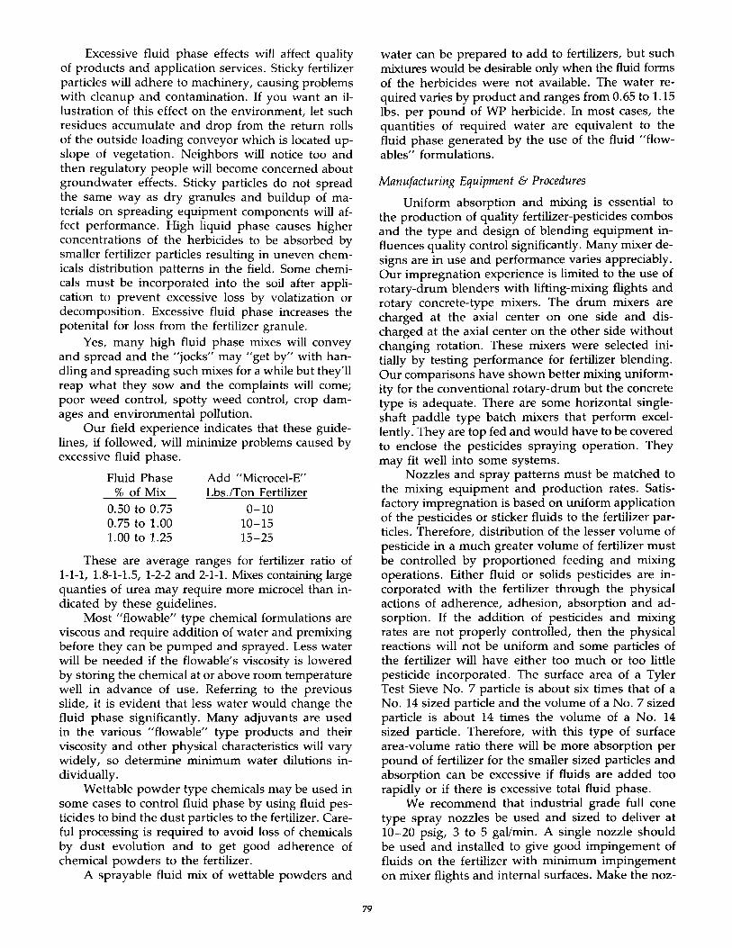
Excessive fluid phase effects will affect quality of products and application services. Sticky fertilizer particles will adhere to machinery, causing problems with cleanup and contamination. If you want an il­lustration of this effect on the environment, let such residues accumulate and drop from the return rolls of the outside loading conveyor which is located up­slope of vegetation. Neighbors will notice too and then regulatory people will become concerned about groundwater effects. Sticky particles do not spread the same way as dry granules and buildup of ma­terials on spreading equipment components will af­fect performance. High liquid phase causes higher concentrations of the herbicides to be absorbed by smaller fertilizer particles resulting in uneven chem­icals distribution patterns in the field. Some chemi­cals must be incorporated into the soil after appli­cation to prevent excessive loss by volatization or decomposition. Excessive fluid phase increases the potenital for loss from the fertilizer granule.

Yes, many high fluid phase mixes will convey and spread and the "jocks" may "get by" with han­dling and spreading such mixes for a while but they'll reap what they sow and the complaints will come; poor weed control, spotty weed control, crop dam­ages and environmental pollution.

Our field experience indicates that these guide­lines, if followed, will minimize problems caused by excessive fluid phase.

Fluid Phase % of Mix

0.50 to 0.75 0.75 to 1.00 1.00 to 1.25

Add "Microcel-E" Lbs.lTon Fertilizer

0-10 10-15 15-25

These are average ranges for fertilizer ratio of I-I-I, 1.8-1-1.5, 1-2-2 and 2-1-1. Mixes containing large quanties of urea may require more microcel than in­dicated by these guidelines.

Most uflowable" type chemical formulations are viscous and require addition of water and premixing before they can be pumped and sprayed. Less water will be needed if the flow able' s viscosity is lowered by storing the chemical at or above room temperature well in advance of use. Referring to the previous slide, it is evident that less water would change the fluid phase significantly. Many adjuvants are used in the various "flowable" type products and their viscosity and other physical characteristics will vary widely, so determine minimum water dilutions in­dividually.

Wettable powder type chemicals may be used in some cases to control fluid phase by using fluid pes­ticides to bind the dust particles to the fertilizer. Care­ful processing is required to avoid loss of chemicals by dust evolution and to get good adherence of chemical powders to the fertilizer.

A sprayable fluid mix of wettable powders and

79

water can be prepared to add to fertilizers, but such mixtures would be desirable only when the fluid forms of the herbicides were not available. The water re­quired varies by product and .ranges from 0.65 to 1.15 lbs. per pound of WP herbicide. In most cases, the quantities of required water are equivalent to the fluid phase generated by the use of the fluid "flow­abIes" formulations.

Manufacturing Equipment & Procedures

Uniform absorption and mixing is essential to the production of quality fertilizer-pesticides combos and the type and design of blending equipment in­fluences quality control significantly. Many mixer de­signs are in use and performance varies appreciably. Our impregnation experience is limited to the use of rotary-drum blenders with lifting-mixing flights and rotary concrete-type mixers. The drum mixers are charged at the axial center on one side and dis­charged at the axial center on the other side without changing rotation. These mixers were selected ini­tially by testing performance for fertilizer blending. Our comparisons have shown better mixing uniform­ity for the conventional rotary-drum but the concrete type is adequate. There are some horizontal single­shaft paddle type batch mixers that perform excel­lently. They are top fed and would have to be covered to enclose the pesticides spraying operation. They may fit well into some systems.

Nozzles and spray patterns must be matched to the mixing equipment and production rates. Satis­factory impregnation is based on uniform application of the pesticides or sticker fluids to the fertilizer par­ticles. Therefore, distribution of the lesser volume of pesticide in a much greater volume of fertilizer must be controlled by proportioned feeding and mixing operations. Either fluid or solids pesticides are in­corporated with the fertilizer through the physical actions of adherence, adhesion, absorption and ad­sorption. If the addition of pesticides and mixing rates are not properly controlled, then the physical reactions will not be uniform and some particles of the fertilizer will have either too much or too little pesticide incorporated. The surface area of a Tyler Test Sieve No. 7 particle is about six times that of a No. 14 sized particle and the volume of a No.7 sized particle is about 14 times the volume of a No. 14 sized particle. Therefore, with this type of surface area-volume ratio there will be more absorption per pound of fertilizer for the smaller sized particles and absorption can be excessive if fluids are added too rapidly or if there is excessive total fluid phase.

We recommend that industrial grade full cone type spray nozzles be used and sized to deliver at 10-20 psig, 3 to 5 gal/min. A single nozzle should be used and installed to give good impingement of fluids on the fertilizer with minimum impingement on mixer flights and internal surfaces. Make the noz-

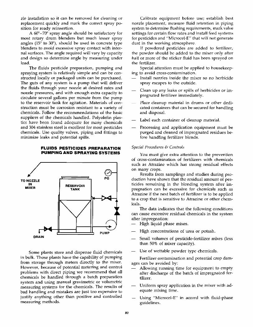
zle installation so it can be removed for cleaning or replacement quickly and mark the correct spray po­sition for ready reinsertion.

A 60°-70" spray angle should be satisfactory for most rotary drum blenders but much lesser spray angles (15° to 30"), should be used in concrete type blenders to avoid excessive spray contact with inter­nal surfaces. The angle required will vary by capacity and design so determine angle by measuring under load.

The fluids pesticide preparation, pumping and spraying system is relatively simple and can be con­structed locally or packaged units can be purchased. The guts of any system is a pump that will deliver the fluids through your nozzle at desired rates and nozzle pressures, and with enough extra capacity to circulate several gallons per minute from the pump to the reservoir tank for agitation. Materials of con­struction must be corrosion resistant to a variety of chemicals. Follow the recommendations of the basic suppliers of the chemicals handled. Polyolefin plas-hrco h~'r.o 'hoa ...... +n.,.,1""11~ "3rlo....,., .......... r;. t,...,. .... ~...,. __ 'lf.,. ...... k ...... ---..; ......... l ... ""'-oJ L1WV"- ..., ..... .....,,11. .lV'-f..ll."'" "'"-''-'1""'-'- .LV.&. J.t.L«"'l] "-,11~.,1LJ,\...U.LC'l

and 304 stainless steel is excellent for most pesticides chemicals. Use quality valves, piping and fittings to minimize leaks and potential spills.

TO NOZZLE IN

MIXER

FLUIDS PESTICIDES PREPARATION PUMPING AND SPRAYING SYSTEMS

RESERVOIR TANK

PG

PUMP DRAIN

Some plants store and dispense fluid chemicals in bulk. Those plants have the capability of pumping from storage through meters directly to the mixer. However, because of potential metering and control problems with direct piping we recommend that all chemicals be handled through a batch preparation system and using manual gravimetric or volumetric measuring systems for the chemicals. The results of bad handling and mistakes are just too expensive to justify anything other than positive and controlled measuring methods.

80

Calibrate equipment before use; establish best nozzle placement, measure fluid retention in piping system to determine flushing requirements, mark valve settings for certain flow rates and install feed systems for pesticides and "Microcel-E" that will not generate dust in the working atmosphere.

If powdered pesticides are added to fertilizer, the powder should be added to the mixer only after half or more of the sticker fluid has been sprayed on the fertilizer.

Special attention must be applied to housekeep-ing to avoid cross-contamination.

Install nozzles inside the mixer so no herbicide spray escapes to the outside.

Clean up any leaks or spills of herbicides or im­pregnated fertilizer immediately.

Place cleanup material in drums or other dedi­cated containers that can be secured for handling and disposal.

Label each container of cleanup material.

Processing and application equipment must be purged and cleaned of impregnated residues be­fore handling fertilizer blends.

Special Procedures & Controls

You must give extra attention to the prevention of cross-contamination of fertilizers with chemicals such as Atrazine which has strong residual effects on many crops.

Results from samplings and studies during pro­duction have shown that the residual amount of pes­ticides remaining in the blending system after im­pregnation can be excessive for chemicals such as Atrazine if the next batch of fertilizer is to be applied to a crop that is sensitive to Atrazine or other chem­icals.

The data indicates that the following conditions can cause excessive residual chemicals in the system after impregnation:

High liquid phase mixes.

High concentrations of urea or potash.

Small volumes of pesticide-fertilizer mixes (less than 50% of mixer capacity).

Use of wettable powder type chemicals.

Fertilizer contamination and potential crop dam-ages can be avoided by:

Allowing running time for equipment to empty after discharge of the batch of impregnated fer­tilizer.

Uniform spray application in the mixer with ad­equate mixing time.

Using "Microcel-E" in accord with fluid-phase guidelines.

Limiting mix quantity to no less than 50% of the mixer capacity, particularly when high fluid phase will be present.

Scheduling production so fertilizer blends that are made immediately after impregnation runs are applied to crops not sensitive to the chemi­cals in the impregnated fertilizer: Two successive fertilizer batches of full mixer capacity are rec­ommended for purging. Or; clean all handling equipment after impregnation so there is no sig­nificant residue-which means that any residue must be restricted to that quantity which in the case of Atrazine would represent a concentration of less than 100 parts per million (0.01 %) in the fertilizer mix that follows the impregnated batch. Because any residues will normally be of small particulate sizing and much higher in pesticide concentration than the formulated concentration of the total mix, we estimate that 10 to 20 times the concentration of the formulated chemical concentration will be found in the residue. Therefore, on this basis only about 4 to 8 lbs. of residue would be allowable in the system when a two-ton batch of fertilizer follows an impreg­nated mix that contained 0.5% Atrazine.

Observing extra precautions when purging the blending system after several batches containing Atrazine, Bladex, Sencor, Simazine or others with high crop sensitivity residuals have been im­pregnated successively. Concentrations of pes­ticides in the residue and the quantity of residue will increase with the number of impregnated batches because of buildup and recycle treat­ment, particularly this will be noticeable for the higher fluid phase mixes.

Clean and purge bulk spreading equipment as done with blending equipment.

Safety & Environmental Controls

All employees should be trained in the safe han­dling of pesticides. Material safety data sheets for each chemical handled should be available and safety recommendations of these data sheets and pesticides labels should be followed. Many sources of infor­mation are available for guidance in the development of a personal protection program and most basic sup­pliers of pesticides and trade associations are very helpful.

Most blend plants' electrical systems are not ex­plosion proof. Therefore, liquid pesticides with low . flash points should not be impregnated. NFPA stand­ards and our insurance people say not less than lOO"F T AGG closed cup flash point unless systems are ex­plosion proof.

As mentioned in the beginning, most herbicides are of relatively low toxicity and engineering controls

81

are not needed in most blend plants to safely handle them. Higher toxicity pesticides must not be impreg­nated in blend plants unless properly designed con­trol equipment is used and special personnel protec­tive procedures are enforced. In most cases, you cannot economically justify the necessary investments and operating costs for such protective systems.

Solids materials cleaned from equipment should be collected and contained and, if in satisfactory physical condition for mixing, it can be added to the next batch of same type pesticide-fertilizer mix.

Cleanup material resulting from leaks and spills, or material from equipment that is not recoverable, and pesticides containers should be disposed of in conformance with procedures and locations ap­proved by local and State regulatory authorities. All cans, pails, jugs and drums should be triple rinsed as soon as empty. Drain the rinseates into the res­ervoir tank of the spray-pumping system and use as flushing fluid when the fertilizer-pesticide mix can tolerate this added liquid phase. If not, store the rinseates in containers and use on a drier mix.

In case of environmental problems involving spills or wastes disposal, your first and primary regulatory official contact is your local agency, next the State then the Federal agencies. However, you should minimize such problems by developing and institut­ing emergency and pollution incident prevention plans. Such plans can be developed with the assis­tance of regulatory officials, trade associations, basic raw materials suppliers and inhouse or outside con­sultants.

Application Procedures & Equipment

All pesticide-fertilizer mixes should be custom applied by the producer. This provides alpha-omega quality control and minimizes the potential of mis­use.

There has been considerable debate as to whether these mixes should be single or double spread. My opinion is that if the spreading equipment is properly calibrated and operated and the mix is properly pre­pared, single spreading should be satisfactory. If your equipment is lousy or poorly operated, then it is questionable whether any type of spreading pattern will be satisfactory. If you are going to indulge in excessive fluid phase mixes, then it is doubtful if the best equipment and operators can consistantly do the right spreading job.

Know your customer! Customers must be ame­nable to certain constraints such as: the mix is made in bulk only to the order of the user; the mix is shipped directly to use and cannot be held in inven­tory; acreages must be accurately measured and iden­tified, and spreading schedules must correlate with weather and soil conditions. If you have any doubts about proper spreading conditions call the customer before you make the mix.

Labeling, Registrations & Records

Be sure the request for a certain fertilizer-pesti­cide combo fits within the allowable limits of the label and EPA registration for the pesticide. The label should include "end-use" directions and suitability for use of the chemical in pest control as an ingredient of a fertilizer-pesticide mixture.

EPA regulations generally exempt custom blended fertilizer-pesticide mixes from product registration if the following conditions are met:

The mix is prepared in bulk only and to the order of the user and is not inventoried.

Pesticide in the mix must have end-use labeling.

Blend is delivered to user with a copy of the end-use labeling of the pesticide and a statement of the composition of the mixture.

Blend is prepared in a registered EPA establish­ment. EPA establishment numbers must be obtained

for any plant producing custom fertilizer-pesticide mixes. In addition, some states require business per­mits or licenses for either or both the manufacturing establishment and the application operations.

Most states require Commercial Certified Pesti­cide Applicator licenses or permits. In some states, requirements are satisfied by licensing one person responsible for all application activities, but more often each truck driver-applicator has to be licensed. Li­censing or permitting usually includes written testing and application

In addition to normal accounting and operating records, a log sheet should be kept on each shipment of impregnated fertilizer. The log should include data about the mix, application rates, acreages, soil, to­pography, crops, boundary lands and crops, weather and many usual conditions. Accounting systems should include provisions for filing the annual EPA establishment report and State reports.

Summary

In summary, we are in the business of producing fertilizer-herbicide combos and presently plan to con­tinue in this business. In a synopsis I have said:

• Efficacy of these products is proven.

• Use proper formulations and mixing techniques.

• Prevent cross-contamination.

• Give special attention to application operations.

• Develop and enforce safety rules.

• Properly dispose of wastes.

82

• Comply with regulatory statutes.

• Keep good records.

• BE REALISTIC ABOUT COSTS.

Look at our recommendations, then use realistic accounting and volume projections to make an op­erating cost analysis. You mayor may not want to get into this business.

And finally! if you have no experience with pes­ticides and your people are not knowledgeable in the quality control and chemistry of pesticides, then ob­tain the services of qualified people to assist you with training and development of your people and oper­ations.

Fertilizer Placement: Improved Efficiency for Reduced Tillage Crops

Larry Ivlurphy-Great Piains Director Potash & Phosphate Institute

Introduction

No two terms characterize the future of crop production under reduced tillage systems as well as the combination "higher yields" and "increased ef­ficiency". Farming today is a special kind of business that depends on narrow margins, has little control over production input costs and little influence on commodity prices.

Profit potential in such a situation depends on producing enough bushels, pounds or tons of crop per acre to keep the production costs below the sell­ing price. Farm management records show that av­erage yields frequently fall below the cost of pro­duction, a fact which is no surprise to anyone familiar with the agricultural sector. Higher yields that are required to lower production costs below the selling price demand an increased commitment to best man­agement practices and close attention to production details. Higher yields in any type of a tillage system aren't all a matter of fertilizer rates or methods of application but fertilizer placement is a tool that can help improve nutrient availability.

While higher yields are better for farmer profits, market development in the fertilizer industry is also benefited from the higher amounts of nutrients re­quired for higher yields. This may sound like double­talk, efficiency of nutrient use through placement, higher yields and higher nutrient requirements, but that is actually the case. Better nutrient use efficiency through placement does not necessarily imply an au­tomatic reduction in rates of application but rather an increased yield from better use of the same amount of nutrients.

Why Placement?

The positive effects of nutrient placement in some specific location relative to the plant have been re­corded for years (5, 17). In the older literature, nu­trient placement was generally considered to imply locating the nutrients close to the plant at seeding, improving the probability of roots encountering the nutrient supply early in the growing season. The use of starter fertilizers is a prime example of this type of placement. Besides the close proximity to the de­veloping plant, utilization of phosphorus (P) in par­ticular was considered, in fact is still considered, to be improved due to reduced soil contact, subse­quently slowing the rate of P fixation reactions which lower water solubility.

Temperature has also been an important factor in the use of starters. It's a fact that nutrient absorp­tion processes operate at a slower rate at lower tem­peratures and that the rate of P diffusion to roots is slower (3, 15). With large amounts of surface residue, soil temperatures can be easily 5 degrees Flower, maybe more. High concentrations of nutrients close to the developing seedling help to overcome the slow development of roots and the low level of energy production in the roots. Energy expenditure is re­quired by processes which concentrate nutrients in the roots, particularly the negatively charged phos­phate, nitrate and sulfate ions.

Soil compaction also depresses nutrients avail­ability. Compaction means that there is less oxygen in the soil, plant roots do not respire normally, en­ergy production is curtailed and nutrient absorption is depressed. Since there is a tendency toward higher bulk density (greater compaction) in soils that are untilled, there is additional nutritional stress under those conditions and plant responses to starter fer­tilizers are increased.

Recently, increased attention has been given to improved nutrient use efficiency especially for re­duced tillage systems (13, 14) through the use of techniques which concentrate nutrients in specific soil zones prior to planting (9, 10, 11). Higher nutrient use efficiency from such pre-plant banding has been largely measured through higher yields compared to conventional broadcast applications. Reasons for these differences and the possibilities they hold for reduced tillage crops will be examined further.

Placement Terminology

Before we go further into the subject, let's sort out the various labels that have been used in con­junction with fertilizer placement.

The term "starter" needs little definition for most people. Starter placement implies concentations of nutrients close to or in direct contact with the seed. "Banding" has been more vague. It has usually meant the same thing as starter but recently "banding" has

83

taken on a new and broader meaning including pre­plant placement. "Dual application" is a term that has developed in the past few years to refer to pre­plant applications of ammonia and liquid mixed fer­tilizers which place the ammonia and the liquid in the soil in the same zone by means of two separate lines on the applicator shank. Usually Nand P have been used in "dual" application but other elements can be involved, depending on the needs of the sit­uation.

Since dual application places the nutrients below the soil surface, synonymous terms such as "deep placement", "deep banding", "knifing", "pre-plant banding", "double shooting", and "root zone band­ing" have come into use. These other terms, exclu­sive of dual application, do not necessarily imply the use of ammonia with some other form of nutrients. Solid, liquid or suspension fertilizers can all be placed below the soil surface with equipment now available.

"Strip placement" and "dribble applications" have been coined to refer to surface, strip applications of liquids or suspensions for new crops, small grains or grasses. These applications may or may not be in­corporated, depending on the cropping system in­volved. Solids can also be applied in the same man­ner with new, specialized equipment. To complicate things even further, applications of large amounts of nutrients at seeding to the side and below the seed may produce essentially the same effects as pre-plant banding and are sometimes termed "starters" even though the amount of nutrients involved are much higher than conventional starter applications.

Let's simplify the situation by using only two of these terms for the remainder of this discussion. Pre­plant banding and banding of large amounts of nu­trients at planting will be "deep placement" regard­less of the forms of fertilizer or type of equipment used. Surface band placement will be "strip" appli­cations regardless of cropping system or form of ma­terial applied. Depending on the type of cropping system, those strip applications mayor may not be incorporated into the soil.

Why Placement for Minimum Tillage Systems?

It's logical to have some concern for the effi­ciency of nutrient use in tillage systems that leave a large amount of plant residue on the surface. That concern is based on impaired penetration of plant nutrients to the soil surface, concentration of nu­trients in a limited amount of soil and rooting zone, positional unavailability of nutrients due to concen­tration at the surface, marked changes in soil chem­istry at the surface such as substantial drops in soil pH, colder soil temperatures at the surface due to the presence of residue and possible losses of nitro­gen by ammonia volatilization or denitrification.

Surface Accumulations of Nutrients. Tillage systems have tremendous effects on the distribution of nu-

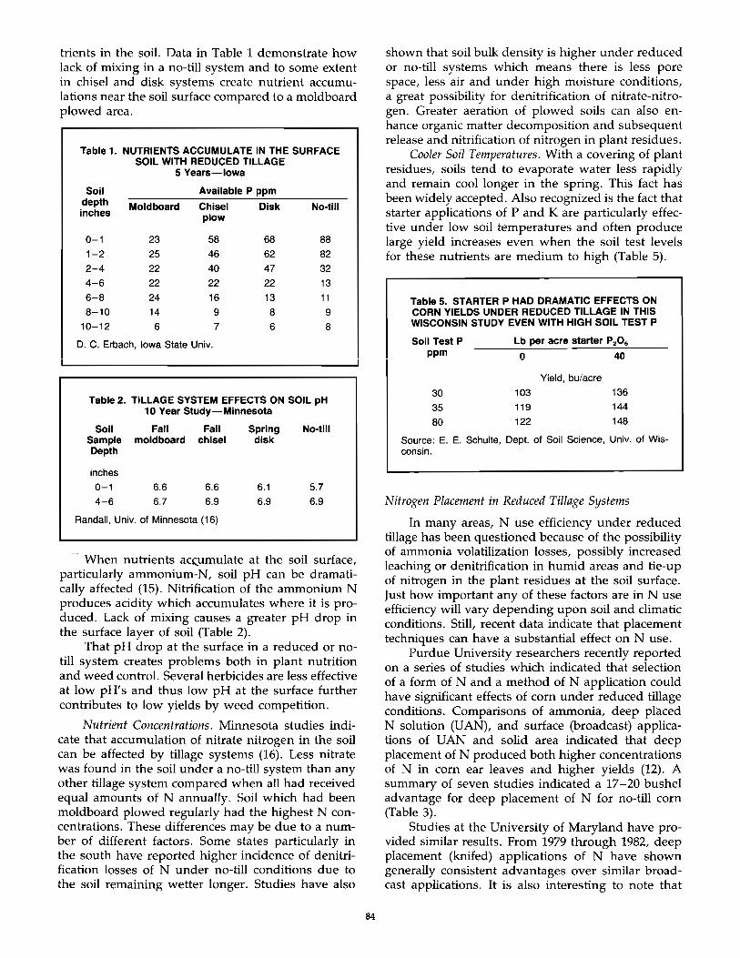
trients in the soil. Data in Table 1 demonstrate how lack of mixing in a no-till system and to some extent in chisel and disk systems create nutrient accumu­lations near the soil surface compared to a moldboard plowed area.

Table 1. NUTRIENTS ACCUMULATE IN THE SURFACE SOIL WITH REDUCED TILLAGE

5 Years-Iowa

Soil Available P ppm depth Moldboard Chisel Disk No-till inches plow

0-1 23 58 68 88 1-2 25 46 62 82 2-4 22 40 47 32 4-6 22 22 22 13 6-8 24 16 13 11 8-10 14 9 8 9

10-12 6 7 6 8

D. C. Erbach, Iowa State Univ.

Table 2. TILLAGE SYSTEM EFFECTS ON SOIL pH 10 Year Study-Minnesota

Soil Sample Depth

inches

0-1 4-6

Fall Fall Spring moldboard chisel disk

6.6 6.7

6.6 6.9

6.1 6.9

Randall, Univ. of Minnesota (16)

No-till

5.7 6.9

When nutrients ac~umulate at the soil surface, particularly ammonium-N, soil pH can be dramati­cally affected (15). Nitrification of the ammonium N produces acidity which accumulates where it is pro­duced. Lack of mixing causes a greater pH drop in the surface layer of soil (Table 2).

That pH drop at the surface in a reduced or no­till system creates problems both in plant nutrition and weed control. Several herbicides are less effective at low pH's and thus low pH at the surface further contributes to low yields by weed competition.

Nutrient Concentrations. Minnesota studies indi­cate that accumulation of nitrate nitrogen in the soil can be affected by tillage systems (16). Less nitrate was found in the soil under a no-till system than any other tillage system compared when all had received equal amounts of N annually. Soil which had been moldboard plowed regularly had the highest N con­centrations. These differences may be due to a num­ber of different factors. Some states particularly in the south have reported higher incidence of denitri­fication losses of N under no-till conditions due to the soil remaining wetter longer. Studies have also

84

shown that soil bulk density is higher under reduced or no-till systems which means there is less pore space, less air and under high moisture conditions, a great possibility for denitrification of nitrate-nitro­gen. Greater aeration of plowed soils can also en­hance organic matter decomposition and subsequent release and nitrification of nitrogen in plant residues.

Cooler Soil Temperatures. With a covering of plant residues, soils tend to evaporate water less rapidly and remain cool longer in the spring. This fact has been widely accepted. Also recognized is the fact that starter applications of P and K are particularly effec­tive under low soil temperatures and often produce large yield increases even when the soil test levels for these nutrients are medium to high (Table 5).

Table 5. STARTER P HAD DRAMATIC EFFECTS ON CORN YIELDS UNDER REDUCED TILLAGE IN THIS WISCONSIN STUDY EVEN WITH HIGH SOIL TEST P

Soil Test P Lb per acre starter P2 O. ppm 0 40

Yield, bu/acre

30 103 136

35 119 144

80 122 148

Source: E. E. Schulte, Dept. of Soil Science, Univ. of Wis­consin.

Nitrogen Placement in Reduced Tillage Systems

In many areas, N use efficiency under reduced tillage has been questioned because of the possibility of ammonia volatilization losses, possibly increased leaching or denitrification in humid areas and tie-up of nitrogen in the plant residues at the soil surface. Just how important any of these factors are in N use efficiency will vary depending upon soil and climatic conditions. Still, recent data indicate that placement techniques can have a substantial effect on N use.

Purdue University researchers recently reported on a series of studies which indicated that selection of a form of N and a method of N application could have significant effects of corn under reduced tillage conditions. Comparisons of ammonia, deep placed N solution (UAN) , and surface (broadcast) applica­tions of UAN and solid area indicated that deep placement of N produced both higher concentrations of N in corn ear leaves and higher yields (12). A summary of seven studies indicated a 17-20 bushel advantage for deep placement of N for no-till corn (Table 3).

Studies at the University of Maryland have pro­vided similar results. From 1979 through 1982, deep placement (knifed) applications of N have shown generally consistent advantages over similar broad­cast applications. It is also interesting to note that

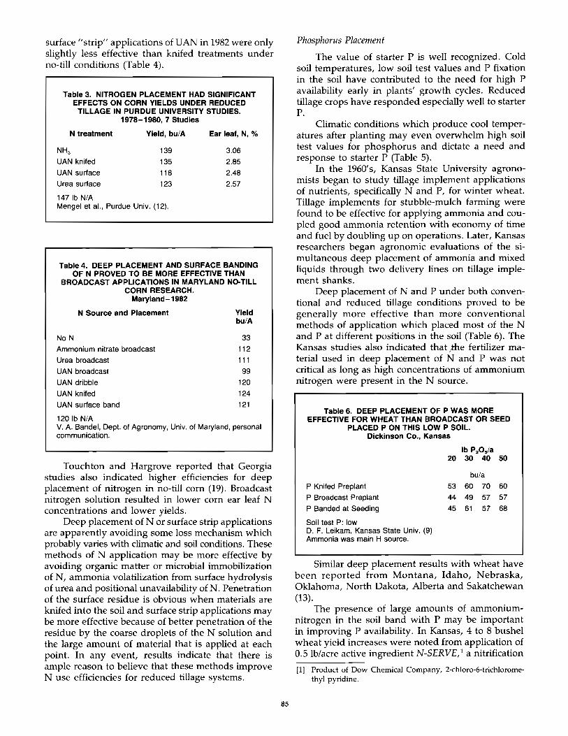
surface "strip" applications of UAN in 1982 were only slightly less effective than knifed treatments under no-till conditions (Table 4).

Table 3. NITROGEN PLACEMENT HAD SIGNIFICANT EFFECTS ON CORN YIELDS UNDER REDUCED

TILLAGE IN PURDUE UNIVERSITY STUDIES. 1978-1980,7 Studies

N treatment Yield, bu/A Ear leaf, N, %

NHa 139 3.06 UAN knifed 135 2.85

UAN surface 118 2.48

Urea surface 123 2.57

147 Ib N/A Mengel et ai., Purdue Univ. (12).

Table 4. DEEP PLACEMENT AND SURFACE BANDING OF N PROVED TO BE MORE EFFECTIVE THAN

BROADCAST APPLICATIONS IN MARYLAND NO-TILL CORN RESEARCH.

Maryland-1982

N Source and Placement

No N

Ammonium nitrate broadcast

Urea broadcast

UAN broadcast

UAN dribble

UAN knifed

UAN surface band

120 Ib N/A

Yield bu/A

33 112

111 99

120

124 121

V. A. Bandel, Dept. of Agronomy, Univ. of Maryland, personal communication.

Touchton and Hargrove reported that Georgia studies also indicated higher efficiencies for deep placement of nitrogen in no-till corn (19). Broadcast nitrogen solution resulted in lower corn ear leaf N concentrations and lower yields.

Deep placement of N or surface strip applications are apparently avoiding some loss mechanism which probably varies with climatic and soil conditions. These methods of N application may be more effective by avoiding organic matter or microbial immobilization of N, ammonia volatilization from surface hydrolysis of urea and positional unavailability of N. Penetration of the surface residue is obvious when materials are knifed into the soil and surface strip applications may be more effective because of better penetration of the residue by the coarse droplets of the N solution and the large amount of material that is applied at each point. In any event, results indicate that there is ample reason to believe that these methods improve N use efficiencies for reduced tillage systems.

85

Phosphorus Placement

The value of starter P is well recognized. Cold soil temperatures, low soil test values and P fixation in the soil have contributed to the need for high P availability early in plants' growth cycles. Reduced tillage crops have responded especially well to starter P.

Climatic conditions which produce cool temper­atures after planting may even overwhelm high soil test values for phosphorus and dictate a need and response to starter P (Table 5).

In the 1960's, Kansas State University agrono­mists began to study tillage implement applications of nutrients, specifically Nand P, for winter wheat. Tillage implements for stubble-mulch farming were found to be effective for applying ammonia and cou­pled good ammonia retention with economy of time and fuel by doubling up on operations. Later, Kansas researchers began agronomic evaluations of the si­multaneous deep placement of ammonia and mixed liquids through two delivery lines on tillage imple­men t shanks.

Deep placement of Nand P under both conven­tional and reduced tillage conditions proved to be generally more effective than more conventional methods of application which placed most of the N and P at different positions in the soil (Table 6). The Kansas studies also indicated that)he fertilizer ma­terial used in deep placement of Nand P was not critical as long as high concentrations of ammonium nitrogen were present in the N source.

Table 6. DEEP PLACEMENT OF P WAS MORE EFFECTIVE FOR WHEAT THAN BROADCAST OR SEED

PLACED P ON THIS LOW P SOIL. Dickinson Co., Kansas

P Knifed Preplant

P Broadcast Preplant

P Banded at Seeding

Soil test P: low D. F. Leikam, Kansas State Univ. (9) Ammonia was main H source.

bu/a

53 60 70 60 44 49 57 57 45 61 57 68

Similar deep placement results with wheat have been reported from Montana, Idaho, Nebraska, Oklahoma, North Dakota, Alberta and Sakatchewan (13).

The presence of large amounts of ammonium­nitrogen in the soil band with P may be important in improving P availability. In Kansas, 4 to 8 bushel wheat yield increases were noted from application of 0.5 lb/acre active ingredient N-SERVE,l a nitrification

[I] Product of Dow Chemical Company, 2-chloro-6-trichlorome­thyl pyridine.

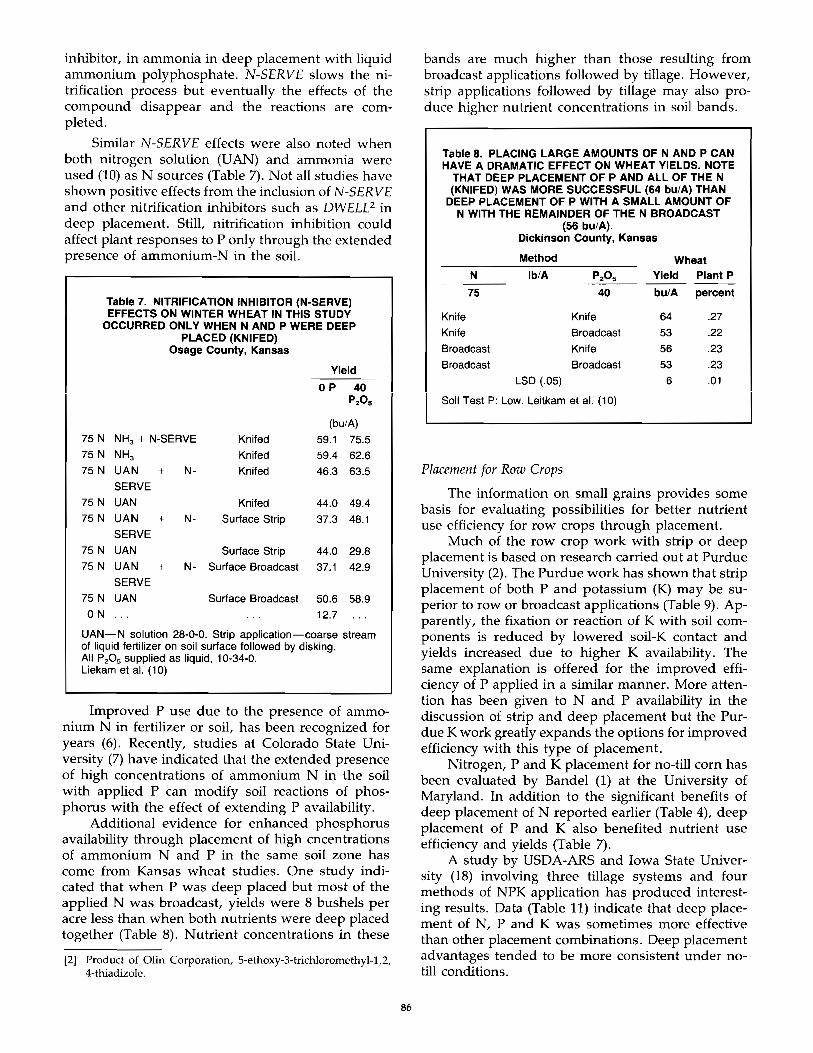
inhibitor, in ammonia in deep placement with liquid ammonium polyphosphate. N-SERVE slows the ni­trification process but eventually the effects of the compound disappear and the reactions are com­pleted.

Similar N-SERVE effects were also noted when both nitrogen solution (UAN) and ammonia were used (10) as N sources (Table 7). Not all studies have shown positive effects from the inclusion of N-SERVE and other nitrification inhibitors such as DWELL 2 in deep placement. Still, nitrification inhibition could affect plant responses to P only through the extended presence of ammonium-N in the soil.

Table 7. NITRIFICATION INHIBITOR (N-SERVE) EFFECTS ON WINTER WHEAT IN THIS STUDY

OCCURRED ONLY WHEN NAND P WERE DEEP PLACED (KNIFED)

Osage County, Kansas

Yield

(bu/A) 75 N NH3 + N-SERVE Knifed 59.1 75.5 75 N

75 N

75 N 75 N

75 N

75 N

75 N

ON

NH3

UAN + SERVE

UAN

UAN + SERVE

UAN

UAN + SERVE

UAN

Knifed 59.4 62.6 N- Knifed 46.3 63.5

Knifed 44.0 49.4 N- Surface Strip 37.3 48.1

Surface Strip 44.0 29.8

N- Surface Broadcast 37.1 42.9

Surface Broadcast 50.6 58.9

12.7

UAN-N solution 28-0-0. Strip application-coarse stream of liquid fertilizer on soil surface followed by disking. All P2 0 S supplied as liquid, 10-34-0. Liekam et al. (10)

Improved P use due to the presence of ammo­nium N in fertilizer or soil, has been recognized for years (6). Recently, studies at Colorado State Uni­versity (7) have indicated that the extended presence of high concentrations of ammonium N in the soil with applied P can modify soil reactions of phos­phorus with the effect of extending P availability.

Additional evidence for enhanced phosphorus availability through placement of high cncentrations of ammonium Nand P in the same soil zone has come from Kansas wheat studies. One study indi­cated that when P was deep placed but most of the applied N was broadcast, yields were 8 bushels per acre less than when both nutrients were deep placed together (Table 8). Nutrient concentrations in these

[2] Product of Olin Corporation, 5-ethoxy-3-trichloromethyl-l,2, 4-thiadizole.

86

bands are much higher than those resulting from broadcast applications followed by tillage. However, strip applications followed by tillage may also pro­duce higher nutrient concentrations in soil bands.

Table 8. PLACING LARGE AMOUNTS OF NAND P CAN HAVE A DRAMATIC EFFECT ON WHEAT YIELDS. NOTE

THAT DEEP PLACEMENT OF P AND ALL OF THE N (KNIFED) WAS MORE SUCCESSFUL (64 bu/A) THAN

DEEP PLACEMENT OF P WITH A SMALL AMOUNT OF N WITH THE REMAINDER OF THE N BROADCAST

(56 bu/A). Dickinson County, Kansas

Method Wheat N Ib/A Yield Plant P ---75 40 bu/A percent

Knife Knife 64 .27

Knife Broadcast 53 .22

Broadcast Knife 56 .23

Broadcast Broadcast 53 .23

LSD (.05) 6 .01

Soil Test P: Low. Leitkam et al. (10)

Placement for Row Crops

The information on small grains provides some basis for evaluating possibilities for better nutrient use efficiency for row crops through placement.

Much of the row crop work with strip or deep placement is based on research carried out at Purdue University (2). The Purdue work has shown that strip placement of both P and potassium (K) may be su­perior to row or broadcast applications (Table 9). Ap­parently, the fixation or reaction of K with soil com­ponents is reduced by lowered soil-K contact and yields increased due to higher K availability. The same explanation is offered for the improved effi­ciency of P applied in a similar manner. More atten­tion has been given to Nand P availability in the discussion of strip and deep placement but the Pur­due K work greatly expands the options for improved efficiency with this type of placement.

Nitrogen, P and K placement for no-till corn has been evaluated by Bandel (1) at the University of Maryland. In addition to the significant benefits of deep placement of N reported earlier (Table 4), deep placement of P and K also benefited nutrient use efficiency and yields (Table 7).

A study by USDA-ARS and Iowa State Univer­sity (18) involving three tillage systems and four methods of NPK application has produced interest­ing results. Data (Table 11) indicate that deep place­ment of N, P and K was sometimes more effective than other placement combinations. Deep placement advantages tended to be more consistent under no­till conditions.

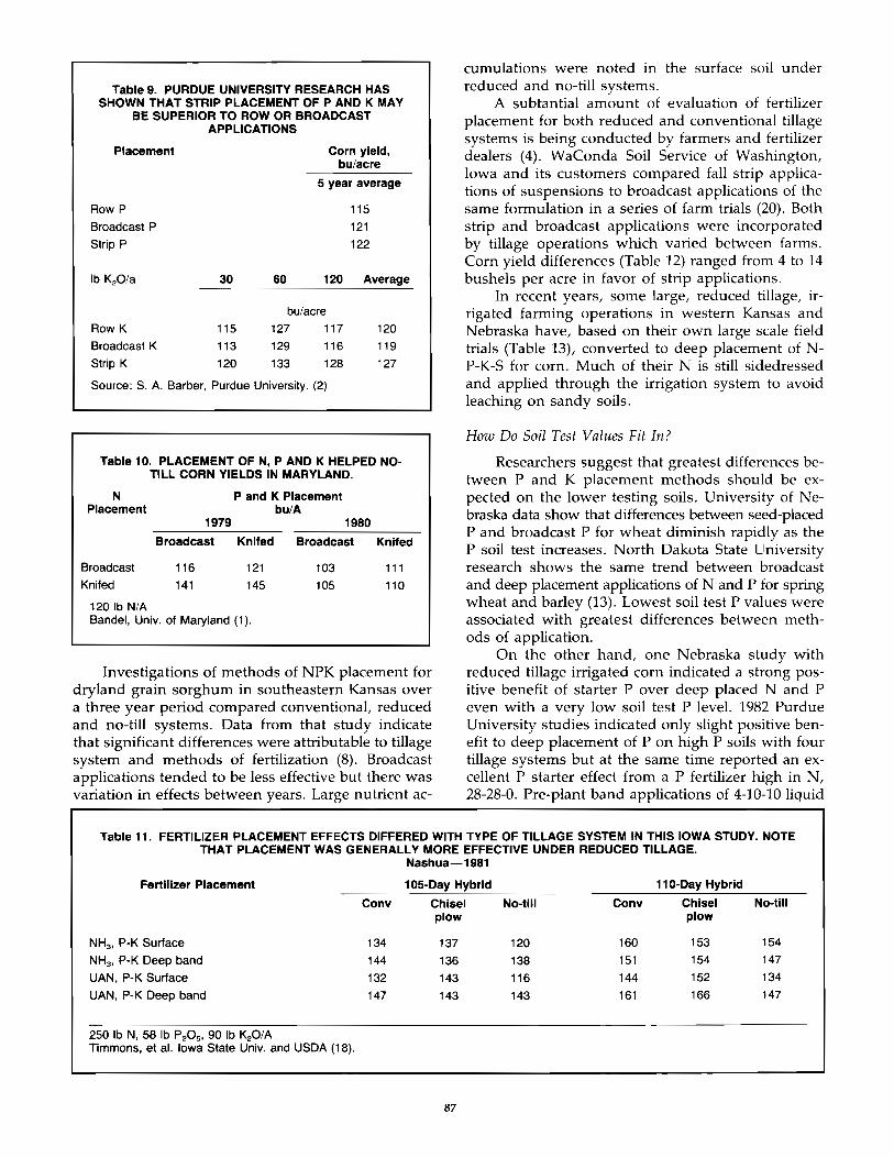
Table 9. PURDUE UNIVERSITY RESEARCH HAS SHOWN THAT STRIP PLACEMENT OF P AND K MAY

BE SUPERIOR TO ROW OR BROADCAST APPLICATIONS

Placement Corn yield, bu/acre

5 year average

Row P

Broadcast P Strip P

Row K

Broadcast K Strip K

30

115

113

120

60 120

bu/acre 127 117 129 116

133 128

Source: S. A. Barber, Purdue University. (2)

115

121

122

120 119

127

Table 10. PLACEMENT OF N, P AND K HELPED NO­TILL CORN YIELDS IN MARYLAND.

N P and K Placement Placement bu/A

1979 1980

Broadcast Knifed Broadcast Knifed

Broadcast 116 121 103 111 Knifed 141 145 105 110

120 Ib N/A Bandel, Univ. of Maryland (1).

Investigations of methods of NPK placement for dryland grain sorghum in southeastern Kansas over a three year period compared conventional, reduced and no-till systems. Data from that study indicate that significant differences were attributable to tillage system and methods of fertilization (8). Broadcast applications tended to be less effective but there was variation in effects between years. Large nutrient ac-

cumulations were noted in the surface soil under reduced and no-till systems.

A subtantial amount of evaluation of fertilizer placement for both reduced and conventional tillage systems is being conducted by farmers and fertilizer dealers (4). WaConda Soil Service of Washington, Iowa and its customers compared fall strip applica­tions of suspensions to broadcast applications of the same formulation in a series of farm trials (20). Both strip and broadcast applications were incorporated by tillage operations which varied between farms. Corn yield differences (Table 12) ranged from 4 to 14 bushels per acre in favor of strip applications.

In recent years, some large, reduced tillage, ir­rigated farming operations in western Kansas and Nebraska have, based on their own large scale field trials (Table 13), converted to deep placement of N­P-K-S for corn. Much of their N is still sidedressed and applied through the irrigation system to avoid leaching on sandy soils.

How Do Soil Test Values Fit In?

Researchers suggest that greatest differences be­tween P and K placement methods should be ex­pected on the lower testing soils. University of Ne­braska data show that differences between seed-placed P and broadcast P for wheat diminish rapidly as the P soil test increases. North Dakota State University research shows the same trend between broadcast and deep placement applications of Nand P for spring wheat and barley (13). Lowest soil test P values were associated with greatest differences between meth­ods of application.

On the other hand, one Nebraska study with reduced tillage irrigated corn indicated a strong pos­itive benefit of starter P over deep placed Nand P even with a very low soil test P level. 1982 Purdue University studies indicated only slight positive ben­efit to deep placement of P on high P soils with four tillage systems but at the same time reported an ex­cellent P starter effect from a P fertilizer high in N, 28-28-0. Pre-plant band applications of 4-10-10 liquid

Table 11. FERTILIZER PLACEMENT EFFECTS DIFFERED WITH TYPE OF TILLAGE SYSTEM IN THIS IOWA STUDY. NOTE THAT PLACEMENT WAS GENERALLY MORE EFFECTIVE UNDER REDUCED TILLAGE.

Nashua-1981

Fertilizer Placement 105-Day Hybrid 110-Day Hybrid

Conv Chisel No-till Conv Chisel No-till plow plow

NH3 , P-K Surface 134 137 120 160 153 154

NH3 , P-K Deep band 144 136 138 151 154 147

UAN, P-K Surface 132 143 116 144 152 134

UAN, P-K Deep band 147 143 143 161 166 147

250 Ib N, 58 Ib P20 5 , 90 Ib K20/A Timmons, et al. Iowa State Univ. and USDA (18).

87

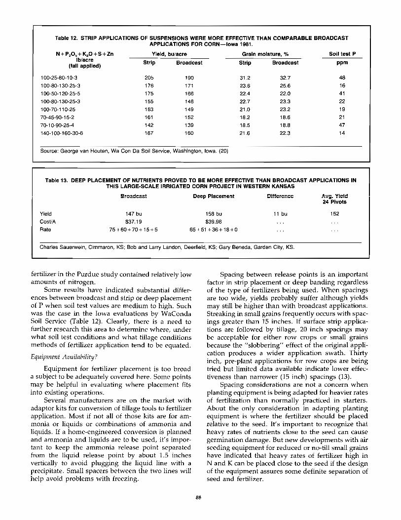
Table 12. STRIP APPLICATIONS OF SUSPENSIONS WERE MORE EFFECTIVE THAN COMPARABLE BROADCAST APPLICATIONS FOR CORN-Iowa 1981.

N+ P20 5 +K2O+S+Zn bu/acre Grain moisture, % Soli test P Ib/acre Strip Broadcast Strip Broadcast ppm

(fall applied)

100-25-80-10-3 205 190 31.2 32.7 48 100-80-130-25-3 176 171 23.6 25.6 16

100-50-120-25-5 175 166 22.4 22.0 41

100-80-130-25-3 155 146 22.7 23.3 22

100-70-110-25 163 149 21.0 23.2 19

70-45-90-15-2 161 152 18.2 18.6 21

70-10-90-25-4 142 139 18.5 18.8 47

140-100-160-30-6 167 160 21.6 22.3 14

Source: George van Houten, Wa Con Da Soil Service, Washington, Iowa. (20)

Table 13. DEEP PLACEMENT OF NUTRIENTS PROVED TO BE MORE EFFECTIVE THAN BROADCAST APPLICATIONS IN THIS LARGE-SCALE IRRIGATED CORN PROJECT IN WESTERN KANSAS

Broadcast Deep Placement Difference Avg. Yield 24 Pivots

Yield 147 bu 158 bu 11 bu 152

CostiA $37.19 $39.98

Rate 75+60+ 70+ 15+5 65+51 +36+18+0

Charles Sauerwein, Cimmaron, KS; Bob and Larry Landon, Deerfield, KS; Gary Beneda, Garden City, KS.

fertilizer in the Purdue study contained relatively low amounts of nitrogen.

Some results have indicated substantial differ­ences between broadcast and strip or deep placement of P when soil test values are medium to high. Such was the case in the Iowa evaluations by WaConda Soil Service (Table 12). Clearly, there is a need to further research this area to determine where, under what soil test conditions and what tillage conditions methods of fertilizer application tend to be equated.

Equipment Availability?

Equipment for fertilizer placement is too broad a subject to be adequately covered here. Some points may be helpful in evaluating where placement fits into existing operations.

Several manufacturers are on the market with adaptor kits for conversion of tillage tools to fertilizer application. Most if not all of those kits are for am­monia or liquids or combinations of ammonia and liquids. If a home-engineered conversion is planned and ammonia and liquids are to be used, it's impor­tant to keep the ammonia release point separated from the liquid release point by about 1.5 inches vertically to avoid plugging the liquid line with a precipitate. Small spacers between the two lines will help avoid problems with freezing.

88

Spacing between release points is an important factor in strip placement or deep banding regardless of the type of fertilizers being used. When spacings are too wide, yields probably suffer although yields may still be higher than with broadcast applications. Streaking in small grains frequently occurs with spac­ings greater than 15 inches. If surface strip applica­tions are followed by tillage, 20 inch spacings may be acceptable for either row crops or small grains because the "slobbering" effect of the original appli­cation produces a wider application swath. Thirty inch, pre-plant applications for row crops are being tried but limited data available indicate lower effec­tiveness than narrower (15 inch) spacings (13).

Spacing considerations are not a concern when planting equipment is being adapted for heavier rates of fertilization than normally practiced in starters. About the only consideration in adapting planting equipment is where the fertilizer should be placed relative to the seed. It's important to recognize that heavy rates of nutrients close to the seed can cause germination damage. But new developments with air seeding equipment for reduced or no-till small grains have indicated that heavy rates of fertilizer high in Nand K can be placed close to the seed if the design of the equipment assures some definite separation of seed and fertilizer.

An entire new generation of applicators for dual application of ammonia and liquids, injection of sus­pensions, deep or strip placement of solids is now available. Recently, custom flotation application equipment has also been adapted to strip applications or deep placement. Modification kits are available for existing flotation applicators allowing that equipment to be used for either strip or broadcast applications.

In Summary

Where does fertilizer placement fit in and why does it seem to work as well as it does? Reduced tillage is particularly adapted to fertilizer placement because of the difficulty of incorporating nutrients adequately and due to residue immobilization of nu­trients. Overall, placement may have advantages be­cause of the following:

(a) Possible delay of fertilizer P and K reactions with the soil due to diminished fertilizer­soil contact.

(b) Deeper placement of nutrients into soil where moisture is less limiting to uptake (posi­tional availability).

(c) Possible delay in fertilizer P reactions with soil components due to the very high con­centrations of ammonium-nitrogen present.

(d) Forced plant uptake of ammonium nitrogen causing a more acid condition at the root surface.

(e) Greater P availability at the root surface due to the acid environment there produced by ammonium-N absorption.

Advantages? Besides the agronomic advantages already considered, doubling up on tillage and fer­tilization operations is attractive. For the custom ap­plicator, strip applications of solutions or suspen­sions on the soil surface followed by some tillage may give some of the same advantages while allow­ing operations on windier days. For reduced tillage systems, this technique may overcome problems as­sociated with large amounts of residue on the soil surface.

Disadvantages? There are more logistical problems in handling two materials in ammonia-fluid or am­monia-solid combinations. For the custom applicator, deep placement means covering less acres per hour compared to broadcast applications. It also means competition for weed and feed combinations. Mount­ing liquid rigging on existing ammonia applicators means increased maintenance problems. Farmers will be faced with the initial costs of equipping tillage implements for handling fertilizers and the mainte­nance that goes with it. Farmer applications of sus­pensions can also be a problem.

What's the final analysis? Recognition that higher yields per acre affect production costs per bushel and overall profitability is a strong incentive for doing a

89

better job in production. More research is needed to better pinpoint where deep placement, strip appli­cations or fertilizer placement in general fits best par­ticularly in relation to high P and K testing soils. While that work is underway, fertilizer placement has demonstrated that it does have a place in efficient crop production and can affect yields and profits.

REFERENCES

1. Bandel, V. A. "Liming and Fertilizing No-Tillage Corn: 4", The Agronomist, University of Mary­land, Department of Agronomy, p. 9-10, June, 1981.

2. Barber, S. A. "Placement of Phosphate and Po­tassium for Increased Efficiency", Fertilizer Placement, 1(1):20-21, 1983. National Fertilizer Solutions Association, Peoria, 11.

3. Epstein, E. "Effect of Soil Temperature on Min­eral Element Composition and Morphology of the Potato Plant", Agron. J. 61:664, 1971.

4. Fee, R. Why Farmers Like Injecting P and K. Successful Farming, October 1983, p. 26P.

5. Follett, R. H., 1. S. Murphy and R. 1. Donahue. "Applying Fertilizers and Soil Amendments", In Fertilizers and Soil Amendments, 1st Ed., Pren­tice-Hall, Inc., Englewood Cliffs, N.J., 1981.

6. Grunes, D. 1. Effect of Nitrogen on the Avail­ability of Soil and Fertilizer Phosphorus to Plants. Advances in Agronomy 11:369-396, 1959.

7. Hanson, R. 1. and D. G. Westfall. Phosphorus Solubility Relationships of Common Nand P Fertilizer Injection Zones. Proe. Western Phos­phate Conference, Ft. Collins, Colorado, March 17-18, 1983, p. 50-52.

8. Lamond, R. E. "Evaluation of Fertility-Tillage Management Systems for Grain Sorghum and Soybeans in Southeast Kansas", Kansas Fert. Res. Rept. of Progress 408, Kansas Agricultural Ex­periment Station, 1981, p. 49-50.

9. Leikam, D. F., R. E. Lamond, P. J. Gallagher and 1. S. Murphy. "Improving N-P Applica­tion", Agrichemical Age, 22 (3):6, 1978.

10. Leikam, D. F., D. E. Kissel, and D. A. Whitney. Nitrification Inhibitor Studies. Kansas Fertilizer Res. Rept. of Progress 372, Kansas Agricultural Experiment Station, p. 11-16, 1979.

11. Leikam, D. F., 1. S. Murphy, D. E. Kissel, D. A. Whitney and H. C. Moser. Effects of Nitrogen and Phosphorus Application Method and Nitro­gen Source on Winter Wheat Grain Yield and Leaf Tissue Phosphorus. Soil Sci. Soc. Amer. Jour. 47:530-535, 1983.

12. Mengel, D. B. "Placement of Nitrogen Fertilizers for No-Till and Conventional Corn", Agron. J. 74:515-518, 1982.

13. Murphy, L. S. "Deep Placement With Minimum Tillage Systems", Tennessee Valley Authority Regional Update, Nov. 3-4, 1982, Omaha, NE.

14. Murphy, L. S. Fertilizer Placement: A Primer. Jour. Soil and Water Conserv. 38:(3):246-259, 1983.

15. Nielsen, K. F., R. L. Halstead, A. J. Maclean, S. J. Bourget and R. M. Holmes. "The Influence of Soil Temperature on the Growth and Mineral Composition of Corn, Bromegrass and Pota­toes", J. Soil Sci. Soc. Amer. 25:369-372, 1961.

16. Randall, G. W. Fertilizer Practices for Conser­vation Tillage, Proceedings 32nd Iowa Fertilizer and Ag Chemicals Dealers Conference, January 8-9, 1980, Des Moines, Iowa.

17. Richard, G. E. "Band Applications of Phosphatic Fertiiizers", Oiin Corp., Agnc. Div., Little Rock, Ark., 1977.

18. Timmons, D. R., T. S. Colvin, T. M. Crosbie, R. M. Cruse and D. C. Erbach. "Fertilizer Manage­ment for Conservation Tillage Systems", Ann. Prog. Rept., Northeast Res. Center, Iowa State University, ORC 81-13, p. 9-10, 1981.

19. Touchton, J. T. and W. L. Hargrove. "Nitrogen Sources and Methods of Application for No-Til­lage Corn Production", Agron. J. 74:823-826, 1982.

20. van Houten, C. "Be Ready for Change With Banding", Fertilizer Placement 1(1):52-53, 1983. National Fertilizer Solutions Association, Peoria, IL.

Effect of Granule Size on Application Michael F. Broder, Agricultural Engineer

and

Hubert L. Balay, Chemical Engineer Division of Agricultural Development

National Fertilizer Development Center

Sixty-two percent (29 million tons) of the fertil­izer applied in the U.S. in 1982 was in the form of dry fertilizer (1). Most of this fertilizer was applied with spinner spreaders. Though most spinner spreaders have the disadvantage of producing un­even distribution, their high capacity, simplicity, and low maintenance have made them the most popular machine for broadcasting dry fertilizer. More than 20 years ago, particle size was recognized as the most important factor for maintaining uniform swaths among raw materials in a blend (2). Small particles travel a shorter distance from the spinning discs than

90

do large particles. This has discouraged the use of materials smaller than conventional granular prod­ucts. Advantages of broadcasting larger-than-con­ventional materials has, up to this time, not been explored. Work described in this paper was aimed at determining the advantages of broadcasting ma­terials larger than the typical minus 6- plus 16-mesh materials.

Literature Review

Hoffmeister conducted a series of tests to deter­mine the extent to which particle shape, density, and size affected segregation of raw materials in blends (2). The overall conclusion was that particle size was by far the most important property that had to be matched to prevent segregation from ballistic action.

Mennel and Reece investigated particle trajec­tories from spinning discs and were able to predict the distance that spherical particles travel (3). Their equations predicted that a Vs-inch-diameter particle (6-mesh) would travel roughly twice as far from a spinner 3 feet above ground than would a V64-inch­diameter (35-mesh) particle. Irregular shaped crystals did not travel as far as spherical particles.

Reints and Yoerger suggested that, if granular fertilizer particles had a wide size range, they would be better distributed laterally from the spreader (4). Cunningham and Chao chose to use discs having blades pitched at different angles to produce more divergence among particles leaving the spinners, thus improving broadcast uniformity (5). Mennel and Reece had already shown that the irregularity of fertilizer particles produces trajectories at large angles to the plane of the disc, thus causing large variation in the distance that particles travel (3).

More recent work by Pitt, et al has shown that variability in particle size has little effect on spread pattern (6). Median particle size is important; how­ever, size variability merely tends to smooth out edges of the distribution pattern.

Facts that can be deduced from previous work is that mathematical modeling of fertilizer spread pat­terns is made difficult by particle irregularity. large particles travel farther because their mass increases with the cube of the diameter while the frontal area on which drag forces act increases with the square of the diameter. Spherical particles travel farther than irregular shaped particles because they have smaller drag coefficients.

Equipment and Procedure

Field spreading tests provided the data for this study. A double-spinner spreader was used for all but two tests. A sketch showing the relative position of the fertilizer delivery system and spinners is shown in figure 1. The delivery chute had three adjustments to control the placement of fertilizer on the two spin-

ners. The entire chute could be moved forward or backward. Depth of the two openings in the bottom of the chute could be varied by moving the rear plate. Width of the two chute openings could be varied by adjusting the width of the inverted vee. Widening the inverted vee placed fertilizer nearer the center of the spinners and decreased the width of the two openings.

The spinner discs were 24 inches in diameter and their axes were tilted 5 degrees from vertical. The outer edges of the discs were, therefore, 2 inches higher above ground than the inner edges. Height of the spinners above ground was about 35 inches.

The other spreader was a high flotation appli­cator with a single spinner about 36 inches above ground.

Three different sizes of urea were used in the tests. The sieve analyses of the three materials are shown in figure 2. The large sizes were curtain-gran­ulated urea from TVA's pilot plant. The prilled urea was produced commercially. The materials were de­noted forestry grades 1 and 2 and prilled urea. For­estry grade 2 was the largest and was nominally minus 2- plus 4-mesh (U.S. Sieve Series). Forestry grade 1 was minus 3- plus 5-mesh. Median particle sizes of the three materials were, respectively, 4.7, 3.94, and 1.71 mm. These materials were chosen be­cause their density, shape, and surface roughness were similar. Variations in spread patterns could, therefore, be attributed to differences in granule size.

Spreading tests were conducted in a level field with wind speeds below 5 mph and relative humidity below 70 percent. Ambient temperatures ranged from 80 to 95°F.

The test pans were rectangular, 17-V2 by 14 inches, and 4 inches d~ep. Compartments for preventing fertilizer ricocheting were square, 3-V2 inches on a side, and the same depth as the trays. Pans were spaced five feet between centers with their long di­mension parallel to the applicator path. Twenty-one pans were used and the spreader was driven astride the center pan. A spreader speed of 5 mph as main­tained during tests and the pan samples were weighed to the nearest 0.1 gram.

To compare spread patterns of different parti­cles, urea granules were spread with several spreader adjustments. This was necessary since some adjust­ments could favor one size particle. Figure 1 shows a sketch of the applicator with normal settings. Two spinner rotational speeds were used, 600 and 800 rpm.

The chute location shown in figure 1 was de­noted the central positon and was based on the spreader manufacturer's recommendation. Three other chute locations were used; 9/16 inches forward of the central position and 9/16 inches rearward and 1 inch rearward of the central position. These chute loca­tions were, respectively, denoted forward, rearward,

91

and rearward-plus. The rear plate was always adjusted so that the

depth of the chute opening was double the height of the gate opening. Gate openings of 1 and 2 inches were used.

Two settings of the inverted vee divider were used. The vee was widened from that shown in fig­ure 1. The wider setting increased the width of the vee from 8 inches to 9 and V2 inches.

Results

Spread patterns were analyzed using a computer program. The program superpositions a spread pat­tern upon itself and the overlapped segments are summed to simulate field application. The driving interval (swath width) must be a multiple of the pan spacing. The optimum swath width is determined iteratively by selecting the driving interval which yields the lowest coefficient of variation. The coefficient of variation is defined as the standard deviation of the sample weights divided by the mean and multiplied by 100. More specifically:

C.V. (%) = 100«V(~ (Xi - x)2)/n l)/x

Where X mean of samples Xi individual sample weights n = total number of samples

A single test consisted of three passes of the applicator over the test pans. Three passes were nec­essary to produce samples large enough to measure. Tests were originally replicated three times but since results were very reproducible the replications were later omitted. Figure 3 shows the reproducibility of a pattern produced with prilled urea. Each curve is the sum of three passes.

Ballistic segregation of urea granules was ob­served by accumulating the samples from spread tests of the prilled and forestry grade 1 urea. Accumulated samples from each pan were sieve analyzed and the median particle size plotted against pan location in figure 4. The median particle size is smallest near the spreader and largest at the outer edges. This shows that small and broken granules remain near the spreader.

Size variation was greater for the prill than for the forestry grade 1. Median size of the forestry sam­ple containing the largest granules was 15 percent larger than the median size of the sample containing the smallest granules (4.02 versus 3.49 mm). For prilled urea the largest median particle size was 49 percent larger than the smallest (2.04 versus 1.37 mm). This size variation is also reflected in the sieve analyses of the two materials (figure 2). Though the slopes of the curves are similar the prilled urea had a greater size variation. The size range between the 10 and 90 percent retained fractions was 1 mm (2.28 to 1.28 mm). The ratio of this range and the median particle

size (1.71 mm) was 0.58:1. The forestry grade 1 had a size range of 1.28 mm but its median size was 3.94 mm. Thus the ratio of the range to median particle size was only 0.31:1. Some researchers believe that size variation is necessary for uniform broadcast ap­plication (5).

Comparisons of forestry grade and prilled urea spread patterns are shown in figures 5 through 14. The chute and spinner adjustments of the 10 tests are listed in table 1. Forestry grade 1 urea was used in tests 1 through 7 (figures 5-11). Swath widths which yielded the lowest coefficient of variation for each material in each test are listed in table 2.

The effect of increasing spinner speed is shown in figures 5 and 6. The higher spinner speed (figure 6) caused the fertilizer to leave the spinner sooner thus increasing the application behind the spreader. Increasing spinner speed had the same effect on the spread pattern as did moving the chute forward (fig­ure 7).

In nearly every comparison, there was more for­estry-size urea at the outer edges of the pattern than prilled urea. There was often, however, a more se­vere accumulation of forestry material in the center of the swath which reduced the swath width. In test 4 (figure 8) the forestry grade 1 urea yielded a swath of 60 feet. The widest swath obtained with prilled urea was 50 feet. Prilled urea spread better with the chute in the rearward plus position (figure 9). The forestry material yielded a more uniform pattern with the chute in the rear position.

In tests 6 and 7 (figures 10 and 11) the gate height was raised to 2 inches. Some manufacturers of dou­ble-spinner spreaders recommend that the chute be moved forward for higher gate openings. The benefit of this adjustment is shown in figure 11. Movement of the chute from the rear position to the center position helped eliminate the W-shaped pattern.

The rates of application of prilled urea in the first seven tests were higher than those for the forestry grade urea. Whether or not this was caused by im­precise gate adjustment, unmatched applicator speed, or flow characteristics of the two materials is not certain. Some custom applicators say that prilled urea tends to meter at higher rates than other materials. This phenomenon may be common of all spherical particles. The effect of granule size and shape on volumetric metering needs to be further studied.

Figures 12 through 14 are patterns produced with the widened vee. This adjustment eliminated the W­shaped pattern which was prevalent among the pre­vious forestry grade patterns. Forestry grade 2 urea was used in these tests. A 65-foot swath width was obtained with the forestry grade urea using the wider inverted vee and the higher spinner speed. These results suggest that larger granules can be broadcast better if placed nearer the centers of double spinners.

Combinations of chute adjustments other than

92

those listed in table 1 were used but the resulting patterns were unacceptable and were thus omitted.

Observations of the departure of fertilizer from the double-spinner spreader revealed some problems that might be eliminated by altering the fertilizer de­livery system or spinner design. A considerable amount of fertilizer is deflected upward during ap­plication. This is verified by the abrasive damage sustained by the lower part of the rear plate and the chute adjustment crank. Fertilizer distribution can be better controlled if the path of fertilizer departing the spinner is not obstructed. Raising the discs would help solve this problem. The 17-inch drop from the apron to the discs (figure 1) enables granules to attain an appreciable vertical velocity. Inns and Reece showed that vertical velocity of granules is not lost during impact with the spinners, thus, particles move up or down on the blade surface until they leave the spin­ner (7).

Tilt of the discs causes granules which bounce upward from the discs to bounce toward the inner edges. The granules then depart from the spinner blades in the rearward direction. Granules bouncing from horizontal discs are not displaced inward and thus are not directed toward the rear of the appli­cator.

Bolts which hold down the blades are on the side of the blades where they will block the path of sliding granules (figure 1). This adds more random­ness to the trajectories of granules and obstructs the path of granules leaving the spinners.

Two pattern tests were made with a single-spin­ner spreader. A granular urea and forestry-size sul­fur-coated urea were used in these tests. Sieve anal­yses of the two materials are plotted in figure 15. Bulk density of the sulfur-coated material was slightly higher than that of the granular urea (54 versus 49 pounds per cubic foot). The difference was not con­sidered significant enough to influence spreading characteristics.

The applicator was driven at a speed of 12 mph and spinner speed was measured at 800 rpm. An application rate of 200 pounds per acre was chosen. Wind speeds varied with gusts approaching 20 mph. The applicator was driven parallel to the wind di­rection to minimize the effect of wind on the lateral distribution of fertilizer.

In these tests forestry-size sulfur-coated urea yielded a swath width of 65 feet with a coefficient of variation of 14.3 percent. Granular urea yielded a 35-foot swath width with a coefficient of variation of 20.7 percent. Spread patterns from the two materials are shown in figure 16.

Conclusions

Granular fertilizer with large particles can be ap­plied in wider swaths than can conventionally sized (minus 6- plus 16-mesh) fertilizer. Spread pattern tests

yielded increases in swath width of up to 30 feet. Adjustment in drop location on some double spin­ners is required. Spreading tests indicated that the large material yielded a wider and more uniform pat­tern if dropped nearer the centers of double spinners. The adjustments required to obtain the optimum pat­tern with large granules may vary for different spin­ner designs. A single-spinner spreader tested under normal use by a dealer produced a swath 65 feet wide with large granules and only 35 feet wide with prilled urea.

Larger granules produced significantly less dust when broadcast than did the prilled urea and thus would be less likely to drift. Problems associated with the buildup of urea dust on the chute in humid weather also could be reduced with the larger granules.

More work is required to determine if any dif­ferences in metering rates will occur with larger ma­terials. If blended with conventionally sized granules, forestry-size granules will segregate; using such ma­terials in blends is not recommended. The advantage of the large granules can be realized in direct appli­cation. The wider swaths attainable with large gran­ules will reduce application costs and shorten the time required to broadcast direct applied fertilizer.

REFERENCES

1. Hargett, Norman L. and Janice T. Berry. 1982 Fertilizer Summary Data. Bulletin Y -180. TV A National Fertilizer Development Center, Muscle Shoals, Alabama, May, 1983.

2. Hoffmeister, George. Compatibility of Raw Ma­terials in Blended Fertilizer-Segregation of Raw Materials. Proceedings of the 12th Annual Meet­ing Fertilizer Industry Round Table, Washing­ton, D.C., October 1962.

3. Mennel, R. M. and A. R. Reece. 1963. The The­ory of the Centrifugal Distributor II: Particle Tra­jectories. Journal of Agricultural Engineering Re­search 8 (1): pp. 78-84.

4. Reints, R. E. and R. R. Yoerger. 1967. Trajecto­ries of Seeds and Granular Fertilizers. Trajecto­ries of ASAE 13 (1): pp. 85-89.

5. Cunningham, F. M. and E. Y. S. Chao. 1967. Design Relationships for Centrifugal Spreaders. Transactions of the ASAE 10 (1): pp. 91-95.

6. Pitt, R. E., G. S. Farmer, and L. P. Walker. 1982. Approximating Equations for Rotary Distributor Spread Patterns. Transactions of the ASAE 25 (6): pp. 1544-1552.

7. Inns, F. M. and A. R. Reece. 1962. The Theory of the Centrifugal Distributor II: Motion on Disc, Off-Center Feed. Journal of Agricultural Engi­neering Research 7(4): pp. 345-353.

93

Table 1. SPINNER AND CHUTE ADJUSTMENTS FOR SPREAD PATTERN TESTS·

Test Spinner Chute Inverted Gate Number Speed Locationb Veee Opening

(RPM) (inches)

1 600 Center Narrow

2 800 Center Narrow

3 600 Forward Narrow

4 600 Rearward Narrow

5 600 Rear Plus Narrow 1

6 600 Rearward Narrow 2

7 600 Center Narrow 2

8 600 Center Wide

9 600 Rearward Wide

10 800 Rearward Wide

a. Applicator speed was 5 mph in all tests. Application rates were 200 and 400 pounds per acre.

b. Center chute location is shown in figure 1. Forward and rearward locations were 9/"3 inch to the front and rear of center. Rear plus was 1 inch rearward of the center position.

c. The narrow vee position is shown in figure 1. The wide vee was 9'12 inches wide instead of 8.

Table 2. SWATH WIDTHS" AND COEFFICIENTS OF VARIATIONb OF THE SPREAD PATTERNS

Test Prilled Urea Forestry Urea Number Swath C.V. Swath C.V.

(ft) (%) (ft) (%)

1 40 12.4 35 20.6 2 35 13.6 35 13.6

3 35 13.8 35 33.7

4 45 14.6 60 18.9

5 50 15.0 60 22.6

6 30 18.4 35 20.2

7 45 17.3 35 23.0

8 35 22.0 55 31.6

9 45 22.8 35 34.8 10 35 22.6 65 19

a. Swath widths are a multiple of the pan spacing (5 feet). A width of 35 feet was the narrowest spaCing for which a coefficient of variation could be calculated.

b. Coefficient of variation is the standard deviation of the sample weights divided by the mean and multiplied by 100. Coefficient of variation is used because of the wide variations in the mean.

~ z W

ff w Q.

c:i w z ... "" .-w II:

.-S 0

~

E !!)

z '" a. II: UJ a. I-:I: f.!) H w ]I;

E J§.

UJ N ..... (I)

W ...l U H ~ II: c(

a. z '" .... c !i!

100

80

80

40

20

0

PARTICLE DIAMETE~ MM

I I I I I _ . .1. 15 6 8 12 18 20

U. S. SCREEN MESH FIGURE 2

SIEVE ANALYSES OF UREA

20

18

16

14

7 12 I .~

10 I ~. . /'

f 8

6

4

30 40 50 60 70 80 90 100 PAN LOCATION (ftl

FIGURE 3

REPLICATIONS OF SPREAD PATTERN PRILLED UREA

4

3

2 ~ PlIILLED

°0~--710~~270~3~0--4~0~5~0~~60~~770-;B~0~9~~O~100 PAN LOCATION ·(ftl

FIGURE 4 BALLISTIC SEGREGATION DUE TO SIZE

E !!)

z '" 0..

a: UJ a. .-:I: l!l H UJ ]I;

E !!)

z '" a. II: w a. ~ :I: l!l ..... W ]I;

E !!)

z '" a. II: UJ 0..

~ :I: l!l H w ]I;

94

20

18

j6 f\ --PRILLED j4 ....... I \

12 ' -4 L

! "', 10

! \ 8

! \ 6

4

I 2

0 0 10 20 30 40 50 60 70 100

PAN LOCATION (ttl

FIGURE 5 SPREAD PATTERN TEST 1

241

! 22

20 ~ / \ --PlIILLED 18

16 i \ 14 ,\ 12

\ 10

\ B

6

4

2 --FORESTRY

0 0 10 20 30 40 50 60 70 100

PAN LOCATION (ftl

FIGURE 6 SPREAD PATTERN TEST 2

24

22 ,~ 20 / \--PlIILLED 18 ."./ \ 16

14 ! '\ ! \ 12

I \ 10 , \ B

f, \. 6 GRADE 1 4

2 'I 0 '/

0 10 20 30 40 50 60 70 80 90 100 PAN LOCATION (ftl

FIGURE 7 SPREAD PATTERN TEST 3

"I 14

e

~1 Sf! 10 z ...

a. e II:

uJ a.

6 \~~1 I--:r (!) .... \ GRADE t UJ 4 3:

\ 2

0 0 0 40 50 60 70 80

PAN LOCATION (ft)

FIGURE 8 SPREAD PATTERN TEST 4

14

~-'~ 12

e .,r-'\ i \. Sf! 10 r \j \ )'--\

i ) \" \ z ...: 9 0.. N \ .\-~, a: Ul

6 Il.

I--:r (!) /' \ GRADEl H 4

/ ! \ UJ 3:

2 ; \ / . , \

0 0 30 40 50 60 70 80 90 100

PAN LOCATION (ft)

FIGURE 9 SPREAD PATTERN TEST 5

32

29

e 24 Sf!

z 20 <[

Il.

a: 16 UJ C-

.... 12 :r <!J H

9 uJ 31:

'" 0

0 10 20 30 40 50 60 70 PAN LOCATION (ft)

FIGURE 10 SPREAD PATTERN TEST 6

9S

32

29

e 24 Sf! z 20 ... Il.

a: 16 UJ a. I--:r 12 t!) H Ul 9 3:

4

0 0 10

FIGURE

10

9

B e

7 Sf!

z 6 « a. a: 5 Ul a.

.4 .... :r <!J 3 H l1J

'" 2

0 0 10

FIGURE

12

10

e Sf! B Z ...: 0..

a: B l1J Il.

l-X .-(!) ... Ul 3:

2

0 0

1. '\ /, i \ --PRILLEO

" J ~ t i V i ' I, /I I / l ..... - \

J I ! \ \

i ~ --FORESTRY GRADE 1

I \ -

30 40 20 50 60 70 PAN LOCATION (ftl

11 SPREAD PATTERN

'! d' 20

12

I --FORESTRY GRADE 2

"-30 40 50 60 70

PAN LOCATION (ft)

SPREAD PATTERN

--FORESTRY GRADE 2

,T ,I--PRILLEO

./ 30 40 50 60 70

PAN LOCATION (ft)

"'-

TEST

TEST

7

8

FIGURE 13 SPREAD PATTERN TEST 9

e-!!! z '" 0-

a: UJ "-... :x: ~ UJ

'"

14

12 i~ ' \ 10 I L-PRILLED f •

B ' \ f \ I \ 6

I \ • "-0 ...... "'\

~

.... z LIJ u a: U..t Q.

d LIJ Z H « .... LIJ a: .... z

~ « 2

0 \ .... 0 30 40 50 60 70 80 90 100

PAN LOCATION (ftl

FIGURE 14 SPREAD PATTERN TEST 10

14

12

10

a

6

4

2

30 40 50 PAN LOCATION

FIGURE 16

100

80

60

40

20

0

~ H ./ :1

.- --y ~-+ i

f- r 1_. 1/ ...1--_

J / 1/ _ .. I J

I /-sCl _._.-f- ~UR ~ ...

..- f-- y _.- ..

II . -----

II ), i

V ! V 5 3 2

PARTIClE DIAMETER. MM

• U. S. SCREEN MESH

FIGURE 15

V

.--

1--

SIEVE ANALYSIS OF SCU

SPREAD PATTERNS SINGLE SPINNER

96

[ --

It -'-1--'-I

-+- '---i

j f----

IJ,= I-! -d [1--

1 L-. 0

Thursday, October 27, 1983

Final Session Moderators:

Paul J. Prosser, Jr. - Joe S. Drewry, Jr., P.E.

Summary of Business Meeting:

Chairman Blenkhorn addressed the meeting briefly. Vice Chairman Medbery commented on the passing of the following members of the Round Table, men­tioning their contributions to the fertilizer industry and The Fertilizer Industry Round Table:

Moderator for Business Meeting - Paul J. Prosser, Jr., Secretary-Treasurer

Leo Cohen Dean R. Gidney Richard Powell O. H. Sale Derrick H. Stassfort

1) The following Financial Statement was read to the membership:

* FINANCIAL STATEMENT *

October 22, 1982 to October 24, 1983

CASH BALANCE-October 22, 1982

Income October 22, 1982-0ctober 24, 1983

Registration Fees-1982 Meeting Sale of Proceedings Contribution-Cocktail Party Fund

Total Receipts October 22, 1982 to October 24, 1983

Total Funds Available October 22, 1982 to October 24,1983

Disbursements October 22, 1982 to October 24, 1983

1981 Proceedings, including postage, etc. 1982 Proceedings, including postage, etc. 1982 Meeting Expenses Miscellaneous Expenses, including

postage, stationery, etc. Directors Meetings 1983 Meeting-Preliminary Expenses Disbursement Cocktail Party Fund

Total Disbursements October 22, 1982 to October 24, 1983

CASH BALANCE-October 24, 1983

Less Reserve for Cocktail Party Fund

Total Cash Available October 24, 1983

Respectfully submitted,

PAUL J. PROSSER, JR. Secretary-Treasurer

97

$14,754.00 2,072.81

300.00

$16,132.88 19.74

2,900.19

363.50 1,121.03 1,198.55

90.72

$23,118.31

$17,126.81

$40,245.12

$21,826.61

$18,418.51

432.74

$17,985.77

2) Mr. Prosser reported that the registration for the 33rd Annual Meeting is 182, off about 25% from the 1982 meeting.

3) Mr. Prosser reported that, for budgetary considerations, the printed Proceedings for the 33rd Annual Meeting would not carry the questions and answers sessions as in previous years.

4) Mr. Joe Reynolds, Jr.-Chairman of the Nominating Committee-presented the fol­lowing slate for consideration as members of the Round Table Board of Directors:

Pierre Becker-COFAZ (France) Donald P. Day-Texasgulf Chemicals Com­pany Michael R. Hancock-The Andersons Mabry M. Handley-I.M.C. Corporation Dr. Ole H. Lie-Norsk Hydro (Norway) William H. Paulson-Royster Company John E. Rednour-Mississippi Chemical Corporation Roy D. Space-Agrico

Upon motion made and seconded, the Round Table members present elected these gentle­men to the Board of Directors.

5) Mr. Tom Athey, Chairman of Meeting Dates and Places Committee, as well as the Enter­tainment Committee, informed the member­ship that the 34th Annual Meeting of the Round Table is scheduled for October 30,31 and November I, 1984 in Baltimore, Mary­land at the Hyatt Hotel. He further thanked the following hosts for the previous night's cocktail Party:

ATLANTA UTILITY WORKS BECHTEL, INC BIRD MACHINE COMPANY, INC COMMONWEAL TH LABORATORIES,

INC DAVY McKEE CORP. FEECO INTERNATIONAL, INC FESCO, INC J&H EQUIPMENT, INC JACOBS-DORRCO DIVISION GILMAN BAG COMPANY KIERNAN-GREGORY CORP. PETROCHEMICALS COMPANY, INC THE PROSSER COMPANY, INC RENNE BURG INTERNATIONAL, INC THE A. J. SACKETT & SONS CO. STEDMAN FOUNDRY AND

MACHINE CO., INC UREA TECHNOLOGIES, INC D. M. WEATHERLY COMPANY HAVER FILLING SYSTEMS. INC SUBSIDIARY OF HAVER & BOECKER, WEST GER!-.1ANY

WEBSTER INDUSTRIES, INC

6) Mr. WaIter J. Sackett, Jr., Chairman of the Public Relations Committee, reported that

98

press releases regarding the Round Table ac­tivities are going to 28 publications, and that advertising in 1983 was printed in Farm Chemicals and Fertilizer Progress.

Update on Operating Experience of Jacobs-Dorrco Two Phosphoric Acid

Plant at Gardinier David W. Leyshon, Technical Manager

Jacobs-Dorrco Div. and Paul S. Waters, Technical Manager

Jacobs Engineering Group, Inc.

In September 1982, Jacobs Engineering Group Inc. announced the successful startup and initial op­eration of their new JACOBS-DORRCO TWO phos­phoric acid reaction system. The reaction system is an integral part of a $39 million phosphoric acid ex­pansion and modernization project which was com­pleted for Gardinier, Inc., rL€ar Tampa, Florida.

The project included the totally new JACOBS­DORRCO plant, which employs wet rock grinding and which also includes two single stage evaporation systems with fluosilicic acid recovery. In addition, Jacobs did the conceptual design and engineering for the conversion of an existing phosphoric acid line to wet rock slurry feed.

ONE OF WORLD'S LARGEST PHOSPHORIC ACID LINES

The JACOBS-DORRCO TWO Phosphoric Acid Plant is rated at a nominal 1,300 short tons of P20 S

per day. Currently, the plant is operating normally at about 1,800 short tons per day which may well make it the world's largest single line plant in terms of P20 5 output.

The plant consists of a JACOBS-DORRCO TWO annular concrete reactor, two vacuum coolers in par­allel and a Bird 30-D tilting pan filter. A view of the reactor, coolers and filter building is shown in Figure 1. The plant is equipped with an overhead crane for reactor maintenance and a cross flow scrubber shown on the right.

SMALL BUT EFFICIENT REACTOR

The JACOBS-DORRCO TWO reactor is similar in configuration to over twenty-five Dorrco Single Tank Reactors built since 1963. It represents an op­timization of modifications made by Jacobs and the owners of many of the reactors, particularly in flor­ida.

Figure 2 shows the flow pattern as it exists in the Gardinier Reactor and indicates where rock slurry and 98% sulfuric acid are added. The Reactor pro­vides a controlled combination of slurry recirculation

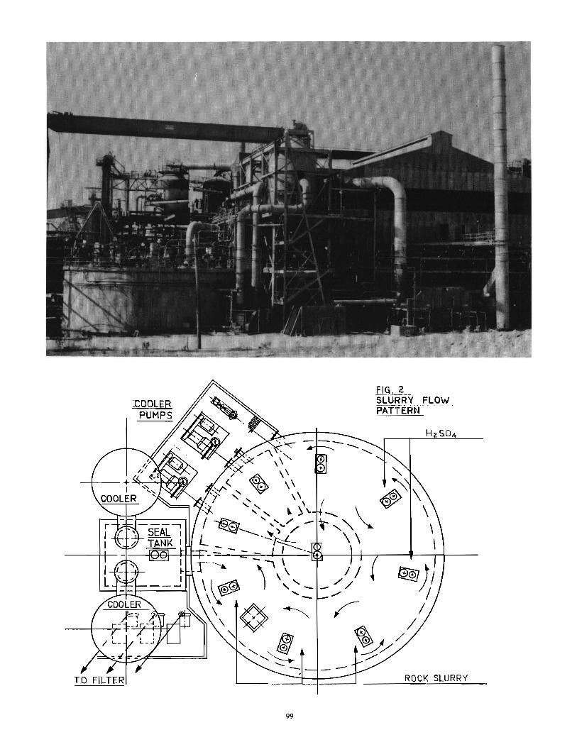
J:OOLER PUMPS

99

-

FIG . 2 SLlJRRY FLOW mfERt·r-- -- - -

ROCK SLURRY

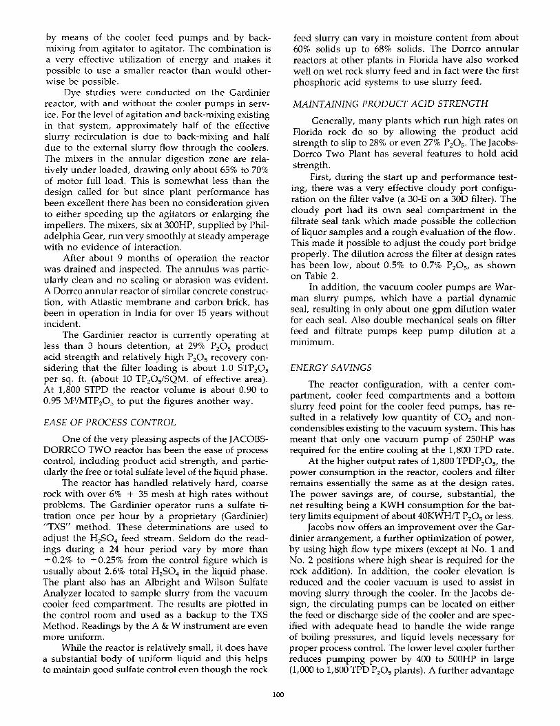
by means of the cooler feed pumps and by back­mixing from agitator to agitator. The combination is a very effective utilization of energy and makes it possible to use a smaller reactor than would other­wise be possible.

Dye studies were conducted on the Gardinier reactor, with and without the cooler pumps in serv­ice. For the level of agitation and back-mixing existing in that system, approximately half of the effective slurry recirculation is due to back-mixing and half due to the external slurry flow through the coolers. The mixers in the annular digestion zone are rela­tively under loaded, drawing only about 65% to 70% of motor full load. This is somewhat less than the design called for but since plant performance has been excellent there has been no consideration given to either speeding up the agitators or enlarging the impellers. The mixers, six at 300HP, supplied by Phil­adelphia Gear, run very smoothly at steady amperage with no evidence of interaction.

After about 9 months of operation the reactor was drained and inspected. The annulus was partic­ularly clean and no scaling or abrasion was evident. A Dorrco annular reactor of similar concrete construc­tion, with AtIastic membrane and carbon brick, has been in operation in India for over 15 years without incident.

The Gardinier reactor is currently operating at less than 3 hours detention, at 29% P20 S product acid strength and relatively high P20 S recovery con­sidering that the filter loading is about 1.0 STP20 s per sq. ft. (about 10 TP20 s/SQM. of effective area). At 1,800 STPD the reactor volume is about 0.90 to 0.95 M 3/MTP20 s to put the figures another way.

EASE OF PROCESS CONTROL

One of the very pleasing aspects of the JACOBS­DORRCO TWO reactor has been the ease of process control, including product acid strength, and partic­ularly the free or total sulfate level of the tiquid phase.

The reactor has handled relatively hard, coarse rock with over 6% + 35 mesh at high rates without problems. The Gardinier operator runs a sulfate ti­tration once per hour by a proprietary (Gardinier) "TXS" method. These determinations are used to adjust the H2S04 feed stream. Seldom do the read­ings during a 24 hour period vary by more than ±0.2% to ±0.25% from the control figure which is usually about 2.6% total H2S04 in the liquid phase. The plant also has an Albright and Wilson Sulfate Analyzer located to sample slurry from the vacuum cooler feed compartment. The results are plotted in the control room and used as a backup to the TXS Method. Readings by the A & W instrument are even more uniform.

While the reactor is relatively small, it does have a substantial body of uniform liquid and this helps to maintain good sulfate control even though the rock

100

feed slurry can vary in moisture content from about 60% solids up to 68% solids. The Dorrco annular reactors at other plants in Florida have also worked well on wet rock slurry feed and in fact were the first phosphoric acid systems to use slurry feed.

MAINTAINING PRODUCT ACID STRENGTH

Generally, many plants which run high rates on Florida rock do so by allowing the product acid strength to slip to 28% or even 27% P20 S • The Jacobs­Dorrco Two Plant has several features to hold acid strength.

First, during the start up and performance test­ing, there was a very effective cloudy port configu­ration on the filter valve (a 30-E on a 300 filter). The cloudy port had its own seal compartment in the filtrate seal tank which made possible the collection of liquor samples and a rough evaluation of the flow. This made it possible to adjust the coudy port bridge properly. The dilution across the filter at design rates has been low, about 0.5% to 0.7% P20 S, as shown on Table 2.

In addition, the vacuum cooler pumps are War­man slurry pumps, which have a partial dynamic seal, resulting in only about one gpm dilution water for each seal. Also double mechanical seals on filter feed and filtrate pumps keep pump dilution at a minimum.

ENERGY SA VINGS

The reactor configuration, with a center com­partment, cooler feed compartments and a bottom slurry feed point for the cooler feed pumps, has re­sulted in a relatively low quantity of CO2 and non­condensibles existing to the vacuum system. This has meant that only one vacuum pump of 250HP was required for the entire cooling at the 1,800 TPD rate.

At the higher output rates of 1,800 TPDP20 s, the power consumption in the reactor, coolers and filter remains essentially the same as at the design rates. The power savings are, of course, substantial, the net resulting being a KWH consumption for the bat­tery limits equipment of about 40KWH/T P 20S or less.

Jacobs now offers an improvement over the Gar­dinier arrangement, a further optimization of power, by using high flow type mixers (except at No.1 and No.2 positions where high shear is required for the rock addition). In addition, the cooler elevation is reduced and the cooler vacuum is used to assist in moving slurry through the cooler. In the Jacobs de­sign, the circulating pumps can be located on either the feed or discharge side of the cooler and are spec­ified with adequate head to handle the wide range of boiling pressures, and liquid levels necessary for proper process control. The lower level cooler further reduces pumping power by 400 to 500HP in large (1,000 to 1,800 TPD P20 S plants). A further advantage

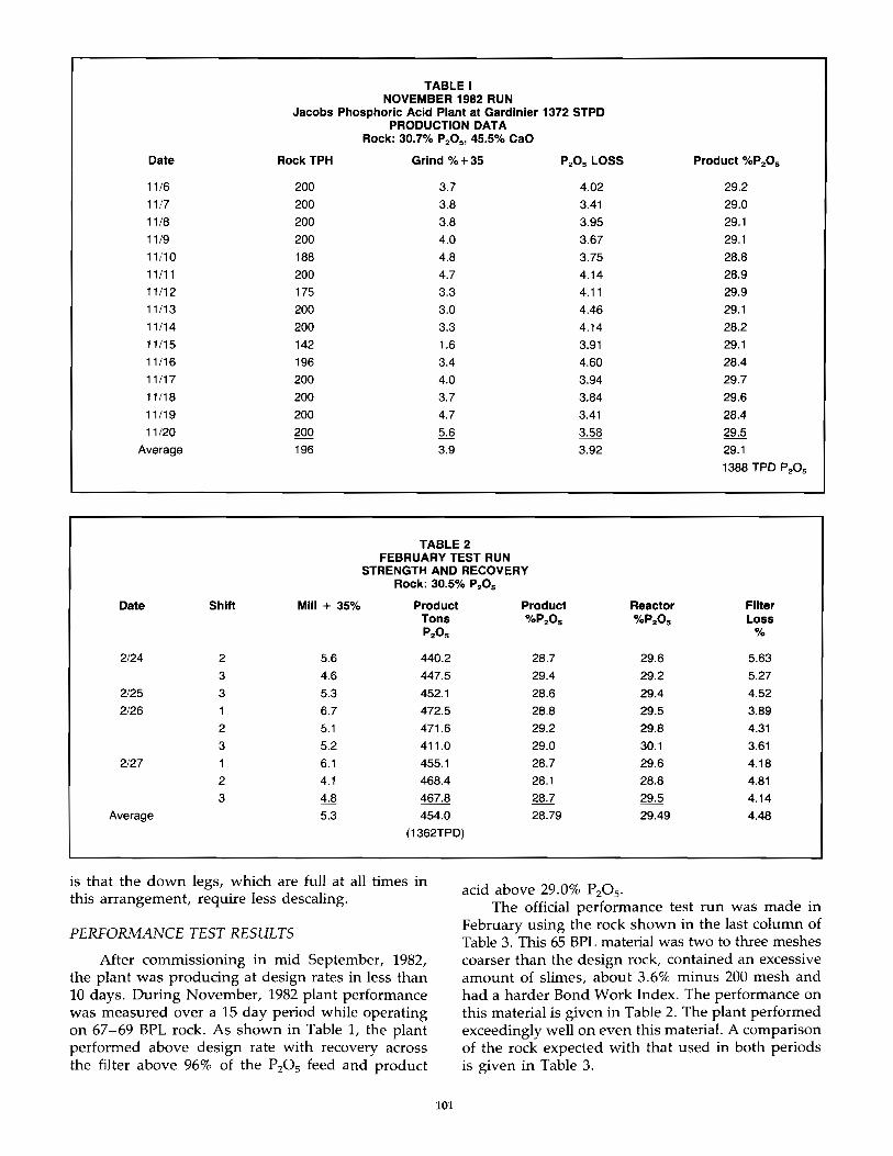
TABLE I NOVEMBER 1982 RUN

Jacobs Phosphoric Acid Plant at Gardinier 1372 STPD PRODUCTION DATA

Rock: 30.7% P20 S' 45.5% CaO

Date Rock TPH Grind %+35 P2 0 S LOSS Product %P2OS

11/6 200 3.7 4.02 29.2

11/7 200 3.8 3.41 29.0

11/8 200 3.8 3.95 29.1 11/9 200 4.0 3.67 29.1

11/10 188 4.8 3.75 28.8 11/11 200 4.7 4.14 28.9 11/12 175 3.3 4.11 29.9 11/13 200 3.0 4.46 29.1 11/14 200 3.3 4.14 28.2 11/15 142 1.6 3.91 29.1 11/16 196 3.4 4.60 28.4

11/17 200 4.0 3.94 29.7

11/18 200 3.7 3.84 29.6

11119 200 4.7 3.41 28.4 11/20 200 5.6 29.5

Average 196 3.9 3.92 29.1

1388 TPD P 205

TABLE 2 FEBRUARY TEST RUN

STRENGTH AND RECOVERY Rock: 30.5% P20 S

Date Shift Mill + 35% Product Product Reactor Filter Tons %P2OS %P2OS Loss P20 S %

2/24 2 5.6 440.2 28.7 29.6 5.63

3 4.6 447.5 29.4 29.2 5.27 2125 3 5.3 452.1 28.6 29.4 4.52 2126 6.7 472.5 28.8 29.5 3.89

2 5.1 471.6 29.2 29.8 4.31

3 5.2 411.0 29.0 30.1 3.61 2/27 1 6.1 455.1 28.7 29.6 4.18

2 4.1 468.4 28.1 28.8 4.81

3 4.8 467.8 28.7 29.5 4.14 Average 5.3 454.0 28.79 29.49 4.48

(1362TPD)

is that the down legs, which are full at all times in this arrangement, require less descaling.

PERFORMANCE TEST RESULTS

After commissioning in mid September, 1982, the plant was producing at design rates in less than 10 days. During November, 1982 plant performance was measured over a 15 day period while operating on 67-69 BPL rock. As shown in Table I, the plant performed above design rate with recovery across the filter above 96% of the PzOs feed and product

101

acid above 29.0% PzOs. The official performance test run was made in

February using the rock shown in the last column of Table 3. This 65 BPL material was two to three meshes coarser than the design rock, contained an excessive amount of slimes, about 3.6% minus 200 mesh and had a harder Bond Work Index. The performance on this material is given in Table 2. The plant performed exceedingly well on even this material. A comparison of the rock expected with that used in both periods is given in Table 3.

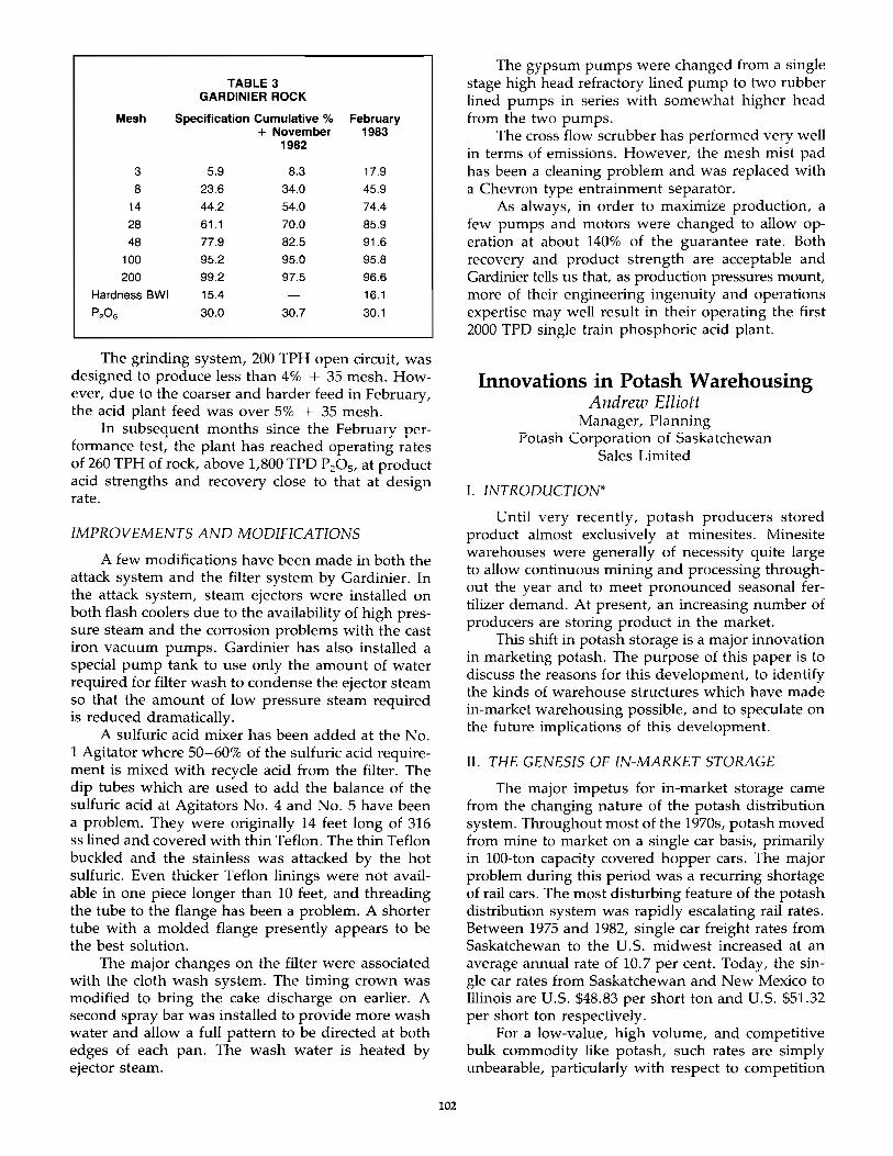
TABLE 3 GARDINIER ROCK

Mesh Specification Cumulative % February + November 1983

1982

3 5.9 8.3 17.9

8 23.6 34.0 45.9

14 44.2 54.0 74.4

28 61.1 70.0 85.9

48 77.9 82.5 91.6

100 95.2 95.0 95.8

200 99.2 97.5 96.6

Hardness BWI 15.4 16.1

P20S 30.0 30.7 30.1

The grinding system, 200 TPH open circuit, was designed to produce less than 4% + 35 mesh. How­ever, due to the coarser and harder feed in February, the acid plant feed was over 5% + 35 mesh.

In subseauent months since the Februarv ner­formance test: the plant has reached operating r~tes of 260 TPH of rock, above 1,800 TPD P 205, at product acid strengths and recovery close to that at design rate.

IMPROVEMENTS AND MODIFICATIONS

A few modifications have been made in both the attack system and the filter system by Gardinier. In the attack system, steam ejectors were installed on both flash coolers due to the availability of high pres­sure steam and the corrosion problems with the cast iron vacuum pumps. Gardinier has also installed a special pump tank to use only the amount of water required for filter wash to condense the ejector steam so that the amount of low pressure steam required is reduced dramatically.

A sulfuric acid mixer has been added at the No. 1 Agitator where 50-60% of the sulfuric acid require­ment is mixed with recycle acid from the filter. The dip tubes which are used to add the balance of the sulfuric acid at Agitators No. 4 and No. 5 have been a problem. They were originally 14 feet long of 316 ss lined and covered with thin Teflon. The thin Teflon buckled and the stainless was attacked by the hot sulfuric. Even thicker Teflon linings were not avail­able in one piece longer than 10 feet, and threading the tube to the flange has been a problem. A shorter tube with a molded flange presently appears to be the best solution.

The major changes on the filter were associated with the cloth wash system. The timing crown was modified to bring the cake discharge on earlier. A second spray bar was installed to provide more wash water and allow a full pattern to be directed at both edges of each pan. The wash water is heated by ejector steam.

102

The gypsum pumps were changed from a single stage high head refractory lined pump to two rubber lined pumps in series with somewhat higher head from the two pumps.

The cross flow scrubber has performed very well in terms of emissions. However, the mesh mist pad has been a cleaning problem and was replaced with a Chevron type entrainment separator.

As always, in order to maximize production, a few pumps and motors were changed to allow op­eration at about 140% of the guarantee rate. Both recovery and product strength are acceptable and Gardinier tells us that, as production pressures mount, more of their engineering ingenuity and operations expertise may well result in their operating the first 2000 TPD single train phosphoric acid plant.

Innovations in Potash Warehousing Andrew Elliott

Manager, Planning Potash Corporation of Saskatchewan

Sales Limited

1. INTRODUCTlON*

Until very recently, potash producers stored product almost exclusively at minesites. Minesite warehouses were generally of necessity quite large to allow continuous mining and processing through­out the year and to meet pronounced seasonal fer­tilizer demand. At present, an increasing number of producers are storing product in the market.

This shift in potash storage is a major innovation in marketing potash. The purpose of this paper is to discuss the reasons for this development, to identify the kinds of warehouse structures which have made in-market warehousing possible, and to speculate on the future implications of this development.

II. THE GENESIS OF IN-MARKET STORAGE

The major impetus for in-market storage came from the changing nature of the potash distribution system. Throughout most of the 1970s, potash moved from mine to market on a single car basis, primarily in 100-ton capacity covered hopper cars. The major problem during this period was a recurring shortage of rail cars. The most disturbing feature of the potash distribution system was rapidly escalating rail rates. Between 1975 and 1982, single car freight rates from Saskatchewan to the U.S. midwest increased at an average annual rate of 10.7 per cent. Today, the sin­gle car rates from Saskatchewan and New Mexico to Illinois are U.S. $48.83 per short ton and U.S. $51.32 per short ton respectively.

For a low-value, high volume, and competitive bulk commodity like potash, such rates are simply unbearable, particularly with respect to competition

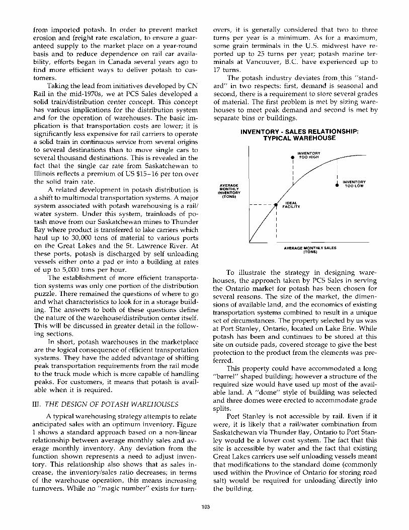
from imported potash. In order to prevent market erosion and freight rate escalation, to ensure a guar­anteed supply to the market place on a year-round basis and to reduce dependence on rail car availa­bility, efforts began in Canada several years ago to find more efficient ways to deliver potash to cus­tomers.

Taking the lead from initiatives developed by CN Rail in the mid-1970s, we at PCS Sales developed a solid train/distribution center concept. This concept has various implications for the distribution system and for the operation of warehouses. The basic im­plication is that transportation costs are lower; it is significantly less expensive for rail carriers to operate a solid train in continuous service from several origins to several destinations than to move single cars to several thousand destinations. This is revealed in the fact that the single car rate from Saskatchewan to Illinois reflects a premium of US $15-16 per ton over the solid train rate.

A related development in potash distribution is a shift to multimodal transportation systems. A major system associated with potash warehousing is a rail! water system. Under this system, trainloads of po­tash move from our Saskatchewan mines to Thunder Bay where product is transferred to lake carriers which haul up to 30,000 tons of material to various ports on the Great Lakes and the St. Lawrence River. At these ports, potash is discharged by self unloading vessels either onto a pad or into a building at rates of up to 5,000 tons per hour.

The establishment of more efficient transporta­tion systems was only one portion of the distribution puzzle. There remained the questions of where to go and what characteristics to look for in a storage build­ing. The answets to both of these questions define the nature of the warehouse/distribution center itself. This will be discussed in greater detail in the follow­ing sections.

In short, potash warehouses in the marketplace are the logical consequence of efficient transportation systems. They have the added advantage of shifting peak transportation requirements from the rail mode to the truck mode which is more capable of handling peaks. For customers, it means that potash is avail­able when it is required.

III. THE DESIGN OF POTASH WAREHOUSES

A typical warehousing strategy attempts to relate anticipated sales with an optimum inventory. Figure 1 shows a standard approach based on a non-linear relationship between average monthly sales and av­erage monthly inventory. Any deviation from the function shown represents a need to adjust inven­tory. This relationship also shows that as sales in­crease, the inventory/sales ratio decreases; in terms of the warehouse operation, this means increasing turnovers. While no "magic number" exists for turn-

103

overs, it is generally considered that two to three turns per year is a minimum. As for a maximum, some grain terminals in the U.s. midwest have re­ported up to 25 turns per year; potash marine ter­minals at Vancouver, B.C. have experienced up to 17 turns.

The potash industry deviates from this "stand­ard" in two respects: first, demand is seasonal and second, there is a requirement to store several grades of material. The first problem is met by sizing ware­houses to meet peak demand and second is met by separate bins or buildings.

AVERAGE MONTHLY

INVENTORY (TONS)

INVENTORY - SALES RELATIONSHIP: TYPICAL WAREHOUSE

INVENTORY • TOO HIGH

I I I I

I I I j INVENTORY

• TOOLOW

IDEAL FACILITY

AVERAGE MONTHLY SALES (TONS)

To illustrate the strategy in designing ware­houses, the approach taken by PCS Sales in serving the Ontario market for potash has been chosen for several reasons. The size of the market, the dimen­sions of available land, and the economics of existing transportation systems combined to result in a unique set of circumstances. The property selected by us was at Port Stanley, Ontario, located on Lake Erie. While potash has been and continues to be stored at this site on outside pads, covered storage to give the best protection to the product from the elements was pre­ferred.

This property could have accommodated a long "barrel" shaped building; however a structure of the required size would have used up most of the avail­able land. A "dome" style of building was selected and three domes were erected to accommodate grade splits.

Port Stanley is not accessible by rail. Even if it were, it is likely that a rail/water combination from Saskatchewan via Thunder Bay, Ontario to Port Stan­ley would be a lower cost system. The fact that this site is accessible by water and the fact that existing Great Lakes carriers use self unloading vessels meant that modifications to the standard dome (commonly used within the Province of Ontario for storing road salt) would be required for unloading· directly into the building.

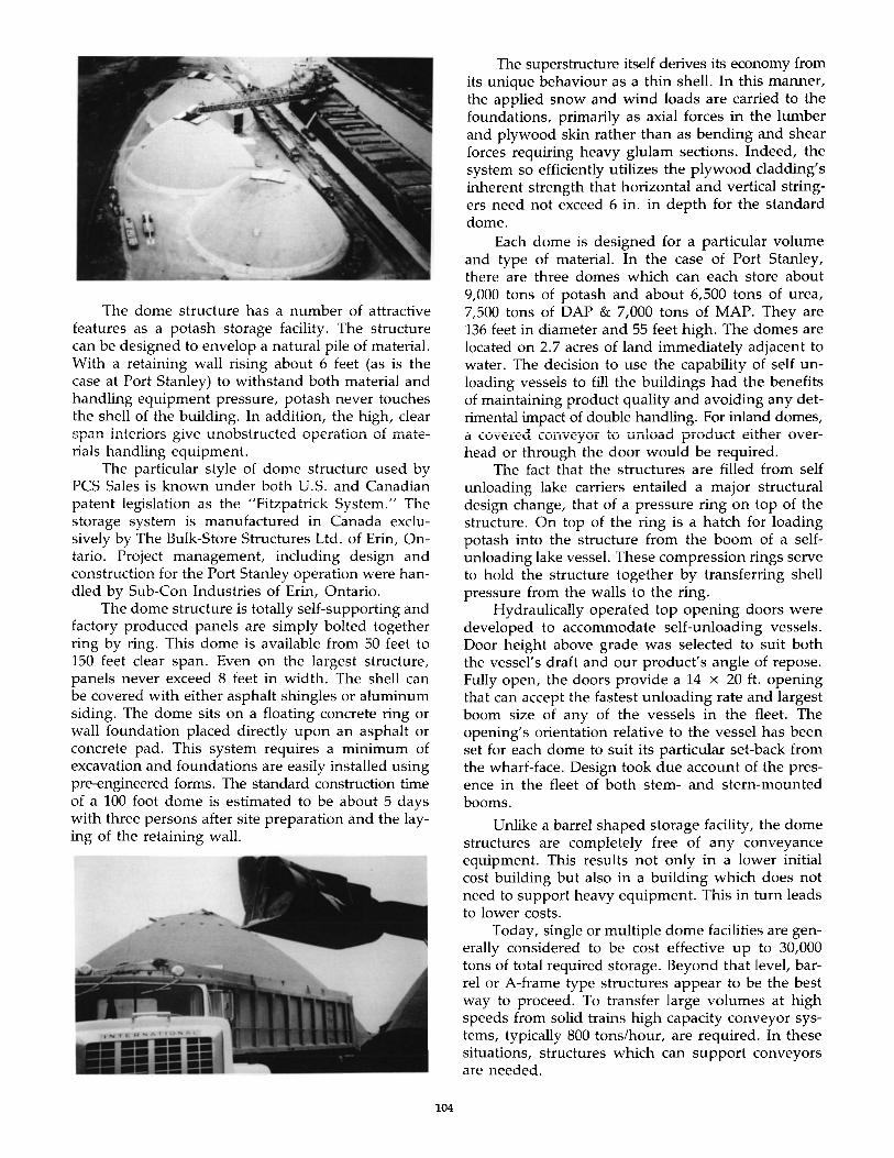
The dome structure has a number of attractive features as a potash storage facility . The structure can be designed to envelop a natural pile of material. With a retaining wall rising about 6 feet (as is the case at Port Stanley) to withstand both material and handling equipment pressure, potash never touches the shell of the building. In addition, the high, clear C' 'V''l~'''''' ; ........ ,.... ~£,,\O .... r" ....... ;'I7~ .. .. ....-- ........ ..... ro .f. ....... ...... ... " ....:1 ....... V"O ...... ... "' .. ; ........ """' ...... c ~ ..... ... ...... ..:J t'u,. U . 1L'-.....l.lU.lo.:l 5.V\.,. \.U. 1VLI,::) l..lU\.,.L'-U Vp\:'.lQ.\'lVl1 VI. l.llQLC-

rials handling equipment. The particular style of dome structure used by

PCS Sales is known under both U.S. and Canadian patent legislation as the "Fitzpatrick System." The storage system is manufactured in Canada exclu­sively by The Bulk-Store Structures Ltd. of Erin, On­tario. Project management, including design and construction for the Port Stanley operation were han­dled by Sub-Con Industries of Erin, Ontario.

The dome structure is totally self-supporting and factory produced panels are simply bolted together ring by ring. This dome is available from 50 feet to 150 feet clear span. Even on the largest structure, panels never exceed 8 feet in width. The shell can be covered with either asphalt shingles or aluminum siding. The dome sits on a floating concrete ring or wall foundation placed directly upon an asphalt or concrete pad. This system requires a minimum of excavation and foundations are easily installed using pre-engineered forms. The standard construction time of a 100 foot dome is estimated to be about 5 days with three persons after site preparation and the lay­ing of the retaining wall .

104

The superstructure itself derives its economy from its unique behaviour as a thin shell. In this manner, the applied snow and wind loads are carried to the foundations, primarily as axial forces in the lumber and plywood skin rather than as bending and shear forces requiring heavy glulam sections. Indeed, the system so efficiently utilizes the plywood cladding's inherent strength that horizontal and vertical string­ers need not exceed 6 in. in depth for the standard dome.

Each dome is designed for a particular volume and type of material. In the case of Port Stanley, there are three domes which can each store about 9,000 tons of potash and about 6,500 tons of urea, 7,500 tons of DAP & 7,000 tons of MAP. They are 136 feet in diameter and 55 feet high. The domes are located on 2.7 acres of land immediately adjacent to water. The decision to use the capability of self un­loading vessels to fill the buildings had the benefits of maintaining product quality and avoiding any det­rimental impact of double handling. For inland domes, a covered conveyor to unload product either over­head or through the door would be required.

The fact that the structures are filled from self unloading lake carriers entailed a major structural design change, that of a pressure ring on top of the structure. On top of the ring is a hatch for loading potash into the structure from the boom of a self­unloading lake vessel. These compression rings serve to hold the structure together by transferring shell pressure from the walls to the ring.

Hydraulically operated top opening doors were developed to accommodate self-unloading vessels. Door height above grade was selected to suit both the vessel's draft and our product's angle of repose. Fully open, the doors provide a 14 x 20 ft. opening that can accept the fastest unloading rate and largest boom size of any of the vessels in the fleet. The opening's orientation relative to the vessel has been set for each dome to suit its particular set-back from the wharf-face. Design took due account of the pres­ence in the fleet of both stem- and stern-mounted booms.

Unlike a barrel shaped storage facility, the dome structures are completely free of any conveyance equipment. This results not only in a lower initial cost building but also in a building which does not need to support heavy equipment. This in turn leads to lower costs.

Today, single or multiple dome facilities are gen­erally considered to be cost effective up to 30,000 tons of total required storage. Beyond that level, bar­rel or A-frame type structures appear to be the best way to proceed. To transfer large volumes at high speeds from solid trains high capacity conveyor sys­tems, typically 800 tons/hour, are required. In these situations, structures which can support conveyors are needed.

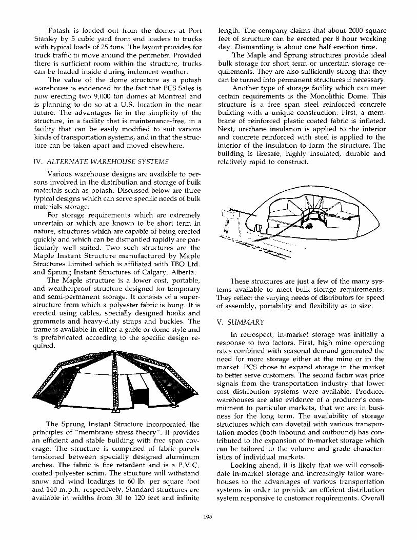
Potash is loaded out from the domes at Port Stanley by 5 cubic yard front end loaders to trucks with typical loads of 25 tons. The layout provides for truck traffic to move around the perimeter. Provided there is sufficient room within the structure, trucks can be loaded inside during inclement weather.

The value of the dome structure as a potash warehouse is evidenced by the fact that PCS Sales is now erecting two 9,000 ton domes at Montreal and is planning to do so at a u.s. location in the near future. The advantages lie in the simplicity of the structure, in a facility that is maintenance-free, in a facility that can be easily modified to suit various kinds of transportation systems, and in that the struc­ture can be taken apart and moved elsewhere.

IV. ALTERNATE WAREHOUSE SYSTEMS

Various warehouse designs are available to per­sons involved in the distribution and storage of bulk materials such as potash. Discussed below are three typical designs which can serve specific needs of bulk materials storage.

For storage requirements which are extremely uncertain or which are known to be short term in nature, structures which are capable of being erected quickly and which can be dismantled rapidly are par­ticularly well suited. Two such structures are the Maple Instant Structure manufactured by Maple Structures Limited which is affiliated with TBO Ltd. and Sprung Instant Structures of Calgary, Alberta.

The Maple structure is a lower cost, portable, and weatherproof structure designed for temporary and semi-permanent storage. It consists of a super­structure from which a polyester fabric is hung. It is erected using cables, specially designed hooks and grommets and heavy-duty straps and buckles. The frame is available in either a gable or dome style and is prefabricated according to the specific design re­quired.

The Sprung Instant Structure incorporated the principles of "membrane stress theory". It provides an efficient and stable building with free span cov­erage. The structure is comprised of fabric panels tensioned between specially designed aluminum arches. The fabric is fire retardent and is a P.V.C. coated polyester scrim. The structure will withstand snow and wind loadings to 60 lb. per square foot and 140 m. p.h. respectively. Standard structures are available in widths from 30 to 120 feet and infinite

105

length. The company claims that about 2000 square feet of structure can be erected per 8 hour working day. Dismantling is about one half erection time.

The Maple and Sprung structures provide ideal bulk storage for short term or uncertain storage re­quirements. They are also sufficiently strong that they can be turned into permanent structures if necessary.

Another type of storage facility which can meet certain requirements is the Monolithic Dome. This structure is a free span steel reinforced concrete building with a unique construction. First, a mem­brane of reinforced plastic coated fabric is inflated. Next, urethane insulation is applied to the interior and concrete reinforced with steel is applied to the interior of the insulation to form the structure. The building is firesafe, highly insulated, durable and relatively rapid to construct.

These structures are just a few of the many sys­tems available to meet bulk storage requirements. They reflect the varying needs of distributors for speed of assembly, portability and flexibility as to size.

V. SUMMARY

In retrospect, in-market storage was initially a response to two factors. First, high mine operating rates combined with seasonal demand generated the need for more storage either at the mine or in the market. PCS chose to expand storage in the market to better serve customers. The second factor was price signals from the transportation industry that lower cost distribution systems were available. Producer warehouses are also evidence of a producer's com­mitment to particular markets, that we are in busi­ness for the long term. The availability of storage structures which can dovetail with various transpor­tation modes (both inbound and outbound) has con­tributed to the expansion of in-market storage which can be tailored to the volume and grade character­istics of individual markets.

Looking ahead, it is likely that we will consoli­date in-market storage and increasingly tailor ware­houses to the advantages of various transportation systems in order to provide an efficient distribution system responsive to customer requirements. Overall

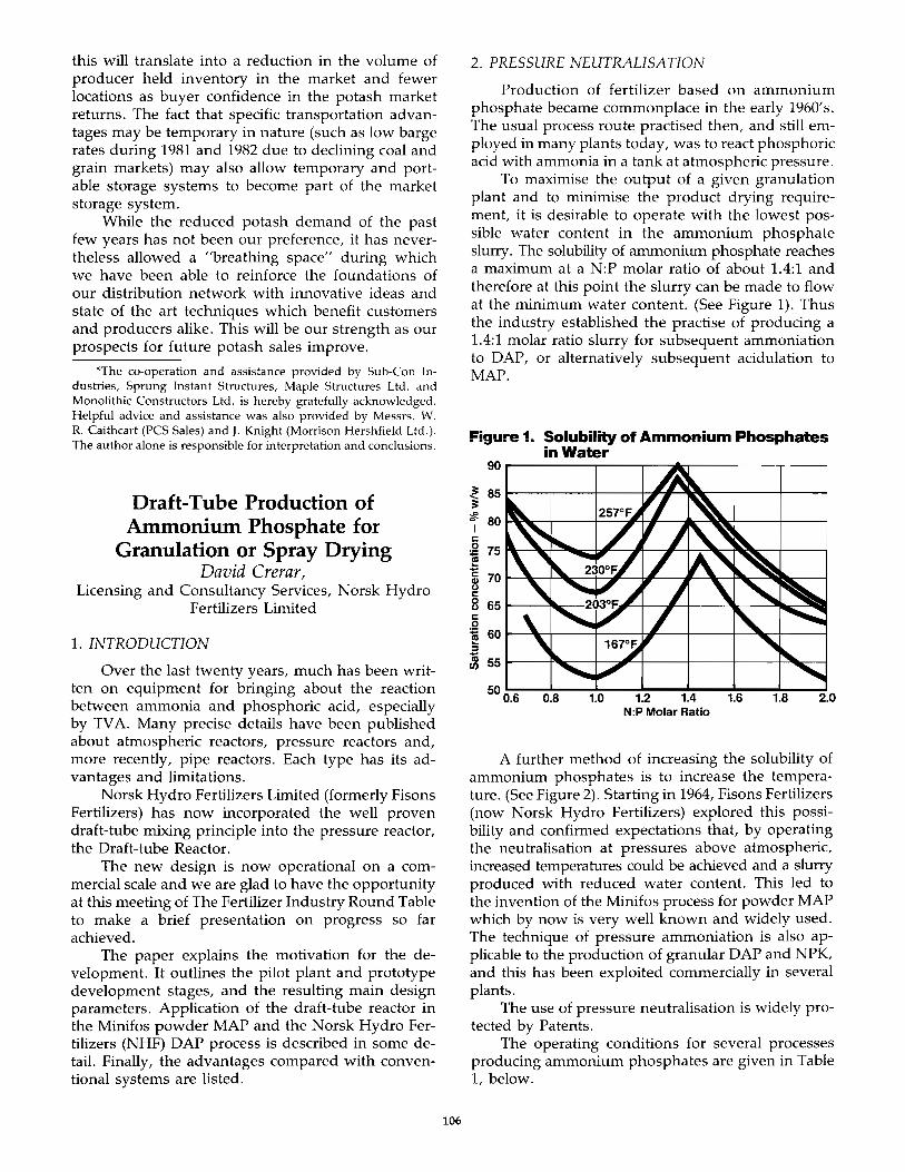
this will translate into a reduction in the volume of producer held inventory in the market and fewer locations as buyer confidence in the potash market returns. The fact that specific transportation advan­tages may be temporary in nature (such as low barge rates during 1981 and 1982 due to declining coal and grain markets) may also allow temporary and port­able storage systems to become part of the market storage system.

While the reduced potash demand of the past few years has not been our preference, it has never­theless allowed a "breathing space" during which we have been able to reinforce the foundations of our distribution network with innovative ideas and state of the art techniques which benefit customers and producers alike. This will be our strength as our prospects for future potash sales improve.

*The co-operation and assistance provided by Sub-Con In­dustries, Sprung Instant Structures, Maple Structures Ltd. and Monolithic Constructors Ltd. is hereby gratefully acknowledged. Helpful advice and assistance was also provided by Messrs. W. R. Caithcart (PCS Sales) and J. Knight (Morrison Hershfield Ltd.). The author alone is responsible for interpretation and conclusions.

Draft-Tube Production of Ammonium Phosphate for

Granulation or Spray Drying David Crerar,

Licensing and Consultancy Services, Norsk Hydro Fertilizers Limited

1. INTRODUCTION

Over the last twenty years, much has been writ­ten on equipment for bringing about the reaction between ammonia and phosphoric acid, especially by TV A. Many precise details have been published about atmospheric reactors, pressure reactors and, more recently, pipe reactors. Each type has its ad­vantages and limitations.

Norsk Hydro Fertilizers Limited (formerly Fisons Fertilizers) has now incorporated the well proven draft-tube mixing principle into the pressure reactor, the Draft-tube Reactor.

The new design is now operational on a com­mercial scale and we are glad to have the opportunity at this meeting of The Fertilizer Industry Round Table to make a brief presentation on progress so far achieved.

The paper explains the motivation for the de­velopment. It outlines the pilot plant and prototype development stages, and the resulting main design parameters. Application of the draft-tube reactor in the Minifos powder MAP and the Norsk Hydro Fer­tilizers (NHF) DAP process is described in some de­tail. Finally, the advantages compared with conven­tional systems are listed.

106

2. PRESSURE NEUTRALISATION

Production of fertilizer based on ammonium phosphate became commonplace in the early 1960's. The usual process route practised then, and still em­ployed in many plants today, was to react phosphoric acid with ammonia in a tank at atmospheric pressure.

To maximise the output of a given granulation plant and to minimise the product drying require­ment, it is desirable to operate with the lowest pos­sible water content in the ammonium phosphate slurry. The solubility of ammonium phosphate reaches a maximum at a N:P molar ratio of about 1.4:1 and therefore at this point the slurry can be made to flow at the minimum water content. (See Figure 1). Thus the industry established the practise of producing a 1.4:1 molar ratio slurry for subsequent ammoniation to DAP, or alternatively subsequent acidulation to MAP.

Figure 1. Solubility of Ammonium Phosphates in Water

~ 85r----+----4-----~~~~--~----+_--~

~ 80~~-+----4=~~hI~~~~~----+_--~ I c ~ 75~~~~~~~~~~~~~~~--+---~

~ ~ 70r-~-+~~~~--~--~~,,~~~ c: 8 65 ~--""~-c:

~ 60~~~----4-----h#~--

~ ~ 55~--~~--4-~~~---50 0.6 0.8

N:P Molar Ratio

A further method of increasing the solubility of ammonium phosphates is to increase the tempera­ture. (See Figure 2). Starting in 1964, Fisons Fertilizers (now Norsk Hydro Fertilizers) explored this possi­bility and confirmed expectations that, by operating the neutralisation at pressures above atmospheric, increased temperatures could be achieved and a slurry produced with reduced water content. This led to the invention of the Minifos process for powder MAP which by now is very well known and widely used. The technique of pressure ammoniation is also ap­plicable to the production of granular DAP and NPK, and this has been exploited commercially in several plants.

The use of pressure neutralisation is widely pro­tected by Patents.

The operating conditions for several processes producing ammonium phosphates are given in Table 1, below.

Figure 2. Solubility of MAP in Water 400

350

u. 300 o

I 250 ! :::I

~ 200 & E 150 {!!.

100

50

20

~ ,

••• ~ ,

~ ~

~ "'" ~" ,

10 20 30 40 50 60 70 80 90 100 Saturation concentration - % w/w

TABLE 1

Mlnlfos DAP

Pressure Conventional

Operating pressure.

psig 30 15 atmos. Operating

temperature. of 335 290 250 Molar Ratio 1.0:1 1.4:1 1.4:1 Slurry moisture.

%H2O 10 15 20 Granulation

Recycle Ratio 4:1 5-6:1 Drier fuel, Iblt DAP 12 18

Apart from the obvious advantages of producing a lower moisture ammonium phosphate solution in the reactor, there are several other benefits of the technique. The lower specific volume of the steam evolved from the reactor reduces the cross sectional area required for disengagement of slurry droplets. This results in a smaller reactor which also reduces space requirements within the plant. Operation under pressure also avoids the need for ammonium phos­phate slurry pumps. When, on discharge from the reactor, the ammonium phosphate solution is let down to atmospheric pressure, steam flashes-off, thus low­ering the moisture content of the material still fur­ther. Thus, the moisture level in the solution does not represent that of the discharged ammonium phosphate. In the case of the Minifos process, the ammonium phosphate solidifies into a powder with­out the need for a separate drying stage at all.

The pressure ammoniation method has been ex­tended to the use of pipe reactors which have been installed for MAP based operations. However the application of pipe reactor technology to DAP sys­tems has not been demonstrated on a significant scale commercially.

107

3. DRAFT-TUBE REACTOR

3.1 Background

The usual type of vessel employed within the industry for neutralisation of phosphoric acid is the Continuous Stirred Tank Reactor (CSTR) . (See Figure 3).

It is normal to have a single central agitator shaft with a single turbine impellor. Phosphoric acid is fed to the surface of the liquor and ammonia introduced through one or more sparge pipes. The ammonium phosphate slurry is discharged from the bottom of the reactor and fed by pump or by gravity to the granulator.

Reaction steam vent

PhosPhori . ..::.c_:=:::::t:,~:n:" acid feed-

Figure 3. Pressure Ammoniator

Ammonia sparger

Liquor level

AlP slurry \",,:C==-discharge

With a pressure reactor an effective and robust seal is required where the agitator shaft passes through the top of the reactor. Minifos plants have employed a wide range of seal, from the simple stuffing-box to sophisticated steam flushed double mechanical seals. Almost universally the seal has been a problem to maintain in a sound condition and has led to main­tenance expense and plant downtime, especially in less developed countries.

The capital cost of agitators and the seal main­tenance problem gave us a strong incentive to de­velop an agitatorless reactor. The Draft-tube Reactor is the outcome.

3.2 Outline Description of Draft-tube Reactor

The objective was to exploit the energy released during the reaction to mix the contents of the reactor. This has been achieved by incorporating a draft-tube into the reactor.

The draft-tube section consists of two concentric tubes (see Figure 4). The outer one is closed at the bottom and forms the wall of the reactor. The inner tube is supported to form an annular channel and with equivalent clearance from the bottom of the reactor.

The outer tube is connected at the top to a wider cylindrical section which forms the upper part of the reaction vessel.

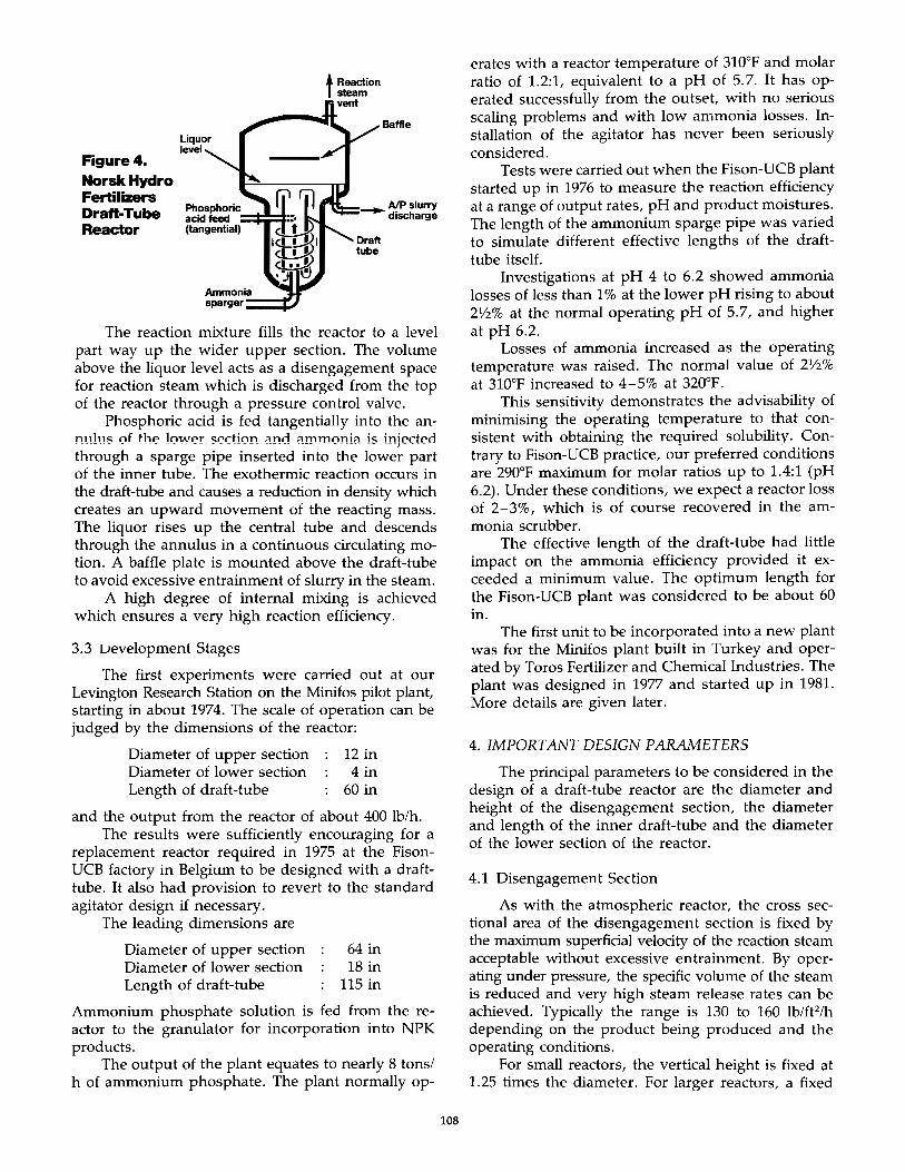
Figure 4. NorskHydro Fertilizers Draft-Tube Reactor

PhOSPhoriC=::::!!!:::I: acid feed (tangential)

Ammonia~=" sparger-

Baffle

The reaction mixture fills the reactor to a level part way up the wider upper section. The volume above the liquor level acts as a disengagement space for reaction steam which is discharged from the top of the reactor through a pressure control valve.

Phosphoric acid is fed tangentially into the an­nulus of the lower section and ammonia is injected through a sparge pipe inserted into the lower part of the inner tube. The exothermic reaction occurs in the draft-tube and causes a reduction in density which creates an upward movement of the reacting mass. The liquor rises up the central tube and descends through the annulus in a continuous circulating mo­tion. A baffle plate is mounted above the draft-tube to avoid excessive entrainment of slurry in the steam.

A high degree of internal mixing is achieved which ensures a very high reaction efficiency.

3.3 LJevelopment Stages

The first experiments were carried out at our Levington Research Station on the Minifos pilot plant, starting in about 1974. The scale of operation can be judged by the dimensions of the reactor:

Diameter of upper section 12 in Diameter of lower section 4 in Length of draft-tube 60 in

and the output from the reactor of about 400 lb/h. The results were sufficiently encouraging for a

replacement reactor required in 1975 at the Fison­UCB factory in Belgium to be designed with a draft­tube. It also had provision to revert to the standard agitator design if necessary.

The leading dimensions are

Diameter of upper section Diameter of lower section Length of draft-tube

64 in 18 in

115 in

Ammonium phosphate solution is fed from the re­actor to the granulator for incorporation into NPK products.

The output of the plant equates to nearly 8 tons/ h of ammonium phosphate. The plant normally op-

108

erates with a reactor temperature of 310"F and molar ratio of 1.2:1, equivalent to a pH of 5.7. It has op­erated successfully from the outset, with no serious scaling problems and with low ammonia losses. In­stallation of the agitator has never been seriously considered.

Tests were carried out when the Fison-UCB plant started up in 1976 to measure the reaction efficiency at a range of output rates, pH and product moistures. The length of the ammonium sparge pipe was varied to simulate different effective lengths of the draft­tube itself.

Investigations at pH 4 to 6.2 showed ammonia losses of less than 1 % at the lower pH rising to about 2Yz% at the normal operating pH of 5.7, and higher at pH 6.2.

Losses of ammonia increased as the operating temperature was raised. The normal value of 2Yz% at 3ID°F increased to 4-5% at 320°F.

This sensitivity demonstrates the advisability of minimising the operating temperature to that con­sistent with obtaining the required solubility. Con­trary to Fison-UCB practice, our preferred conditions are 290°F maximum for molar ratios up to 1.4:1 (pH 6.2). Under these conditions, we expect a reactor loss of 2-3%, which is of course recovered in the am­monia scrubber.

The effective length of the draft-tube had little impact on the ammonia efficiency provided it ex­ceeded a minimum value. The optimum length for the Fison-UCB plant was considered to be about 60 in.

The first unit to be incorporated into a new plant was for the Minifos plant built in Turkey and oper­ated by Toros Fertilizer and Chemical Industries. The plant was designed in 1977 and started up in 1981. More details are given later.

4. IMPORT ANT DESIGN PARAMETERS

The principal parameters to be considered in the design of a draft-tube reactor are the diameter and height of the disengagement section, the diameter and length of the inner draft-tube and the diameter of the lower section of the reactor.

4.1 Disengagement Section

As with the atmospheric reactor, the cross sec­tional area of the disengagement section is fixed by the maximum superficial velocity of the reaction steam acceptable without excessive entrainment. By oper­ating under pressure, the specific volume of the steam is reduced and very high steam release rates can be achieved. Typically the range is 130 to 160 Ib/ftzlh depending on the product being produced and the operating conditions.

For small reactors, the vertical height is fixed at 1.25 times the diameter. For larger reactors, a fixed

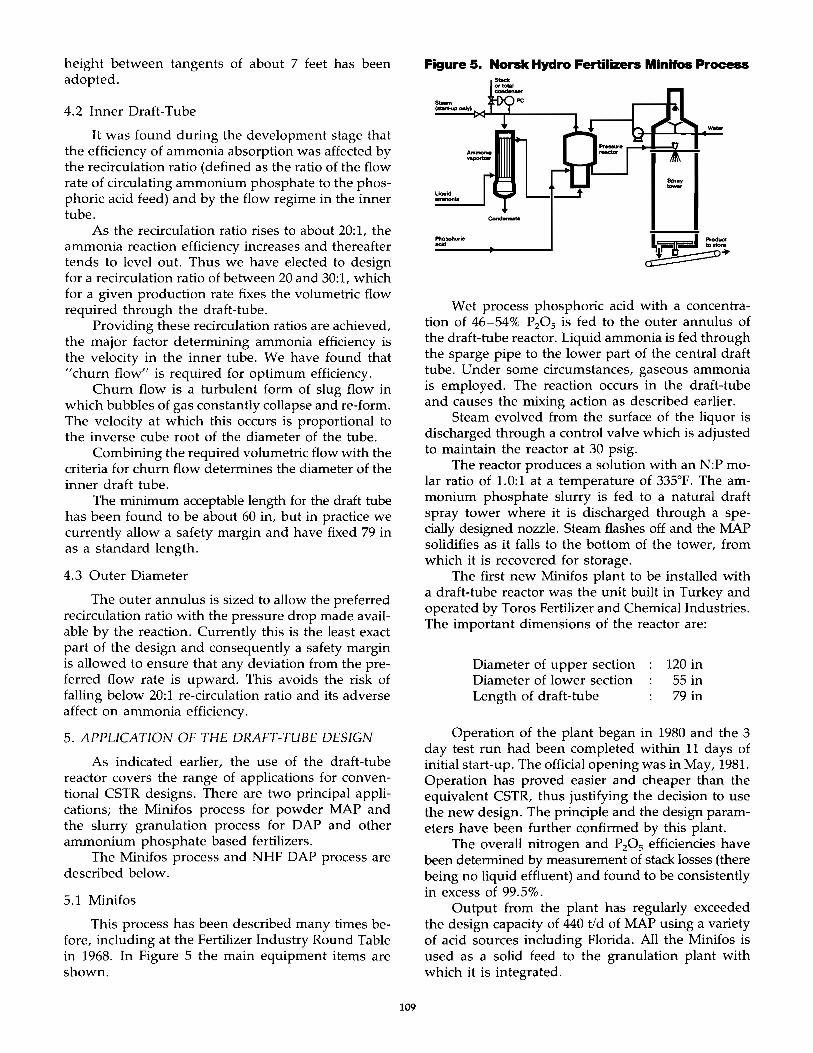
height between tangents of about 7 feet has been adopted.

4.2 Inner Draft-Tube

It was found during the development stage that the efficiency of ammonia absorption was affected by the recirculation ratio (defined as the ratio of the flow rate of circulating ammonium phosphate to the phos­phoric acid feed) and by the flow regime in the inner tube.

As the recirculation ratio rises to about 20:1, the ammonia reaction efficiency increases and thereafter tends to level out. Thus we have elected to design for a recirculation ratio of between 20 and 30:1, which for a given production rate fixes the volumetric flow required through the draft-tube.

Providing these recirculation ratios are achieved, the major factor determining ammonia efficiency is the velocity in the inner tube. We have found that "churn flow" is required for optimum efficiency.

Churn flow is a turbulent form of slug flow in which bubbles of gas constantly collapse and re-form. The velocity at which this occurs is proportional to the inverse cube root of the diameter of the tube.

Combining the required volumetric flow with the criteria for churn flow determines the diameter of the inner draft tube.

The minimum acceptable length for the draft tube has been found to be about 60 in, but in practice we currently allow a safety margin and have fixed 79 in as a standard length.

4.3 Outer Diameter

The outer annulus is sized to allow the preferred recirculation ratio with the pressure drop made avail­able by the reaction. Currently this is the least exact part of the design and consequently a safety margin is allowed to ensure that any deviation from the pre­ferred flow rate is upward. This avoids the risk of falling below 20:1 re-circulation ratio and its adverse affect on ammonia efficiency.

5. APPLICA nON OF THE DRAFT-TUBE DESIGN

As indicated earlier, the use of the draft-tube reactor covers the range of applications for conven­tional CSTR designs. There are two principal appli­cations; the Minifos process for powder MAP and the slurry granulation process for DAP and other ammonium phosphate based fertilizers.

The Minifos process and NHF DAP process are described below.

5.1 Minifos

This process has been described many times be­fore, including at the Fertilizer Industry Round Table in 1968. In Figure 5 the main equipment items are shown.

109

Figure S. Norsk Hydro Fertilizers Minifos Process

---Wet process phosphoric acid with a concentra­

tion of 46-54% P20 S is fed to the outer annulus of the draft-tube reactor. Liquid ammonia is fed through the sparge pipe to the lower part of the central draft tube. Under some circumstances, gaseous ammonia is employed. The reaction occurs in the draft-tube and causes the mixing action as described earlier.

Steam evolved from the surface of the liquor is discharged through a control valve which is adjusted to maintain the reactor at 30 psig.

The reactor produces a solution with an N:P mo­lar ratio of 1.0:1 at a temperature of 335°F. The am­monium phosphate slurry is fed to a natural draft spray tower where it is discharged through a spe­cially designed nozzle. Steam flashes off and the MAP solidifies as it falls to the bottom of the tower, from which it is recovered for storage.

The first new Minifos plant to be installed with a draft-tube reactor was the unit built in Turkey and operated by Toros Fertilizer and Chemical Industries. The important dimensions of the reactor are:

Diameter of upper section Diameter of lower section Length of draft-tube

120 in 55 in 79 in

Operation of the plant began in 1980 and the 3 day test run had been completed within 11 days of initial start-up. The official opening was in May, 1981. Operation has proved easier and cheaper than the equivalent CSTR, thus justifying the decision to use the new design. The principle and the design param­eters have been further confirmed by this plant.

The overall nitrogen and P 20S efficiencies have been determined by measurement of stack losses (there being no liquid effluent) and found to be consistently in excess of 99.5%.

Output from the plant has regularly exceeded the design capacity of 440 tid of MAP using a variety of acid sources induding Florida. All the Minifos is used as a solid feed to the granulation plant with which it is integrated.

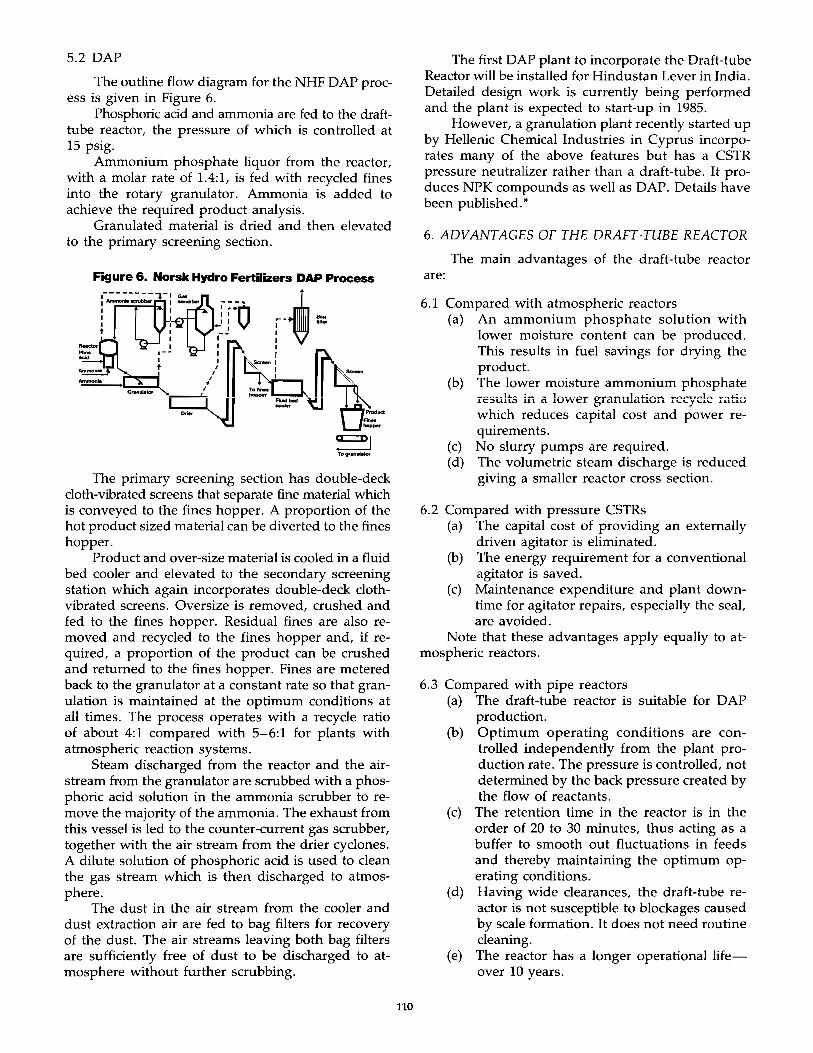
5.2 DAP

The outline flow diagram for the NHF DAP proc­ess is given in Figure 6.

Phosphoric acid and ammonia are fed to the draft­tube reactor, the pressure of which is controlled at 15 psig.

Ammonium phosphate liquor from the reactor, with a molar rate of 1.4:1, is fed with recycled fines into the rotary granulator. Ammonia is added to achieve the required product analysis.

Granulated material is dried and then elevated to the primary screening section.

The first DAP plant to incorporate the Draft-tube Reactor will be installed for Hindustan Lever in India. Detailed design work is currently being performed and the plant is expected to start-up in 1985.

However, a granulation plant recently started up by Hellenic Chemical Industries in Cyprus incorpo­rates many of the above features but has a CSTR pressure neutralizer rather than a draft-tube. It pro­duces NPK compounds as well as DAP. Details have been published. *

6. ADV ANT AGES OF THE DRAFT-TUBE REACTOR

The main advantages of the draft-tube reactor Figure 6, Norsk Hydro Fertilizers DAP Process are:

The primary screening section has double-deck cloth-vibrated screens that separate fine material which is conveyed to the fines hopper. A proportion of the hot product sized material can be diverted to the fines hopper.

Product and over-size material is cooled in a fluid bed cooler and elevated to the secondary screening station which again incorporates double-deck cloth­vibrated screens. Oversize is removed, crushed and fed to the fines hopper. Residual fines are also re­moved and recycled to the fines hopper and, if re­quired, a proportion of the product can be crushed and returned to the fines hopper. Fines are metered back to the granulator at a constant rate so that gran­ulation is maintained at the optimum conditions at all times. The process operates with a recycle ratio of about 4:1 compared with 5-6:1 for plants with atmospheric req,ction systems.

Steam discharged from the reactor and the air­stream from the granulator are scrubbed with a phos­phoric acid solution in the ammonia scrubber to re­move the majority of the ammonia. The exhaust from this vessel is led to the counter-current gas scrubber, together with the air stream from the drier cyclones. A dilute solution of phosphoric acid is used to clean the gas stream which is then discharged to atmos­phere.

The dust in the air stream from the cooler and dust extraction air are fed to bag filters for recovery of the dust. The air streams leaving both bag filters are sufficiently free of dust to be discharged to at­mosphere without further scrubbing.

110

6.1 Compared with atmospheric reactors (a) An ammonium phosphate solution with

lower moisture content can be produced. This results in fuel savings for drying the product.

(b) The lower moisture ammonium phosphate results in a lovver granulation rC~fclc ratio which reduces capital cost and power re­quirements.

(c) No slurry pumps are required. (d) The volumetric steam discharge is reduced

giving a smaller reactor cross section.

6.2 Compared with pressure CSTRs (a) The capital cost of providing an externally

driven agitator is eliminated. (b) The energy requirement for a conventional

agitator is saved. (c) Maintenance expenditure and plant down­

time for agitator repairs, especially the seal, are avoided.

Note that these advantages apply equally to at­mospheric reactors.

6.3 Compared with pipe reactors (a) The draft-tube reactor is suitable for DAP

production. (b) Optimum operating conditions are con­

trolled independently from the plant pro­duction rate. The pressure is controlled, not determined by the back pressure created by the flow of reactants.

(c) The retention time in the reactor is in the order of 20 to 30 minutes, thus acting as a buffer to smooth out fluctuations in feeds and thereby maintaining the optimum op­erating conditions.

(d) Having wide clearances, the draft-tube re­actor is not susceptible to blockages caused by scale formation. It does not need routine cleaning.

(e) The reactor has a longer operational life­over 10 years.

7. CONCLUSION

To avoid the costs associated with electrically driven agitators in ammonium phosphate reactors, whilst retaining the advantages of pressure neutral­isation, Norsk Hydro Fertilizers has introduced the Draft-tube Reactor.

Investigations have been carried out at the pilot plant scale and on a prototype unit which has now been operating for 7 years feeding ammonium phos­phate solution to a granulator. Design data has been developed for the installation of several new plants.

The first, a Minifos unit in Turkey, has been in suc­cessful operation since late 1980. A DAP unit using the technique is currently being engineered for India.

There are significant cost, energy saving and op­erational advantages compared with the alternative reaction systems atmospheric and pressure agitated reactors and the pipe reactor. These advantages are expected to lead to wider adoption of draft-tube re­actors in the future.

.. Recent Experiences in the Granulation of Ammonium Phos­phates by K. J. Barnett, D. M. Ivell and S. F. Smith, presented to the Fertiliser Society, London, 19th October, 1983.

COMMENTS ON 1983 PROCEEDINGS As is the case with many of the major meetings

and conferences connected with the fertilizer indus­try, the attendence at the Round Table during the past two years has been reduced due to the economic downturn which our industry is experiencing at the present time. Consequently, our revenues from reg­istration fees (our only source) have been reduced. At the same time, the cost involved in printing the proceedings of our meetings has increased.

In considering ways to reduce expenses, it was decided at the July 1983 Directors Meeting that we discontinue the practise of including in our proceed­ings the remarks of the chairman, session modera-

111

tors, and questions and answers relating to the pres­entations. This eliminates the considerable expense of tape recording the meetings and serves to reduce the number of printed pages. It also saves the time involved in editing the tape transcriptions, a task which in the past has been diligently and effectively carried out by Mr. Albert Spillman.

The 1983 Proceedings are therefore presented in a simplified format. However, they should serve the basic purpose of preserving a record of the many relevant topics which were covered at the Thirty­third Annual Fertilizer Industry Round Table.

Harold D. Blenkhorn, Chairman 1983-84