probabilistic models of youthful criminal careers

PROBABILISTIC MODELS OF YOUTHFUL CRIMINAL CAREERS

ARNOLD BARNETT Sloan School of Management Massachusetts Institute of Technology

ALFRED BLUMSTEIN School of Urban and Public Affairs Carnegie-Mellon University

DAVID P. FARRINGTON Institute of Criminology Cambridge University

This paper focuses on the characterization of the criminal careers of youthful offenders. I t was found that these criminal careers could be modeled with parameters rejecting constant individual rates of offending and constant probability of career termination; population heterogeneity could be adequately represented by two distinct groups-designated here as ‘ffrequents” and %ccasionals. ” These parameters were estimated for the multiple offenders in a London cohort studied from their first convictions until age 25. In that cohort, the frequents were estimated to have an annual conviction rate of 1.14 convictions per year (constant with age) and a probability of career termination of .I0 following each conviction; the occasionals had an annual conviction rate of .41 and termination probability of .33 following each conviction; the frequents were estimated to comprise 43% of the population, and the occasionals the others 57%. While this parsimonious model structure was adequate for the London cohort, it must still be tested with other offender populations.

THE CRIMINAL CAREER APPROACH

In recent years, there has been increased interest in specifying the nature of criminal careers in terms of changes in offending over time, duration, and diversity across the population of offenders. This is partly because of the discovery that a small proportion of the population accounts for a large proportion of all offenses (Wolfgang, Figlio, and Sellin, 1972). It has been argued that, if prosecution resources and institutional and other treatment facilities could be used more selectively for these high-rate offenders, this might prevent a significant number of crimes. However, the importance of criminal career information goes far beyond the identification of “career criminals.” Detailed information about criminal careers is fundamental to isolating the different facets of the career-initiation, the pattern of offending

CRIMINOLOGY VOLUME 25 NUMBER 1 1987 83

84 BARNETT, BLUMSTEIN, AND FARRINGTON

during the active period, and termination. It is necessary to separate these different facets in order to test various approaches to the prevention or reduc- tion of crime and to investigate different ways in which possible “causes of crime” affect these different aspects of criminal careers.

A “criminal career” refers to the temporal sequence of crimes committed by an offender.1 It has an onset, a duration, and a termination. Between onset and termination, offenders commit crimes at some positive rate, and the rate may or may not vary over time. The aim in this paper is to develop and test various mathematical models to explain observed sequences of crimes in criminal careers.

In any such empirical endeavor, it is important to distinguish between an offender’s true underlying crime rate and the observed rate based on the crimes he actually commits. Because of unpredictable and chance factors such as varying criminal opportunities, an offender with a true constant rate of 10 crimes per year may commit 5 crimes in some years and 15 crimes in others. Similarly, of two offenders, each with a true rate of 10 crimes per year, in any particular year one may actually commit 5 crimes and the other 15.

Also complicating matters is the difficulty of measuring directly even the actual number of crimes committed. Instead, some other indicator of the rate of criminal activity may have to be used, such as an arrest or conviction rate. Hence, the actual crime rate is related to the observed arrest or conviction rate by means of two probabilistic processes: the first relates the true to the observed crime rate and the second reflects the chance that a crime which is committed leads to an arrest or a conviction.

Because of the uncertainties in these processes, making inferences about the true crime rate from some measured crime rate requires assumptions that are expressed in a mathematical model of criminal careers. The adequacy of the model can be assessed according to its consonance with observations of individual crime patterns. The most useful models are often the simplest ones. This is not to deny that criminal careers are influenced by many complex factors. However, in the interests of parsimony, a simple model which predicts observed sequences of criminal events is usually preferable to a more complex one.

In the analyses reported here, the simplest models are tested first and more complex ones are developed when the simple ones fail to accord with the observed data. The approach to explanation is very different from that of delinquency theorists such as Hirschi (1969) and Elliott, Huizinga, and Ageton (1985). Such theorists invoke highly complex models of the causes of

1. There is no suggestion that the offender is necessarily engaged full-time in criminal activity, or that he derives the majority of his income from it.

YOUTHFUL CRIMINAL CAREERS 85

delinquency; their models “explain” many observed relationships but do not lead to testable quantitative predictions.

PREVIOUS MODELS OF CRIMINAL CAREERS

This paper builds on and attempts to synthesize the previous approaches of Blumstein, Farrington, and Moitra (1985) and Barnett and Lofaso (1985). Both attempted to explain and predict the distribution of arrests over juveniles in the classic Philadelphia longitudinal study of Wolfgang et al. (1972). Wolfgang and colleagues drew attention to the existence of chronic offenders: 18% of all those arrested accounted for 52% of all juvenile arrests. However, they identified these chronic offenders only retrospectively, not prospectively. As Blumstein and Moitra (1980) pointed out, even if all the offenders in the Philadelphia cohort had the same true desistance probability, chance factors alone would mean that some would have more observed arrests than others. Retrospectively, those boys experiencing the most arrests would inevitably account for a disproportionate number of all arrests. The key question is whether the chronic offenders can be identified prospectively.

Blumstein, Farrington, and Moitra (1985) attempted to predict observed recidivism probabilities in four cohort studies. The key assumption in their model was that each offender had a constant probability of desisting after each offense. They found that observed recidivism probabilities and, more generally, the distribution of offenses over offenders, could be predicted by a model which partitioned each sample into three subgroups: innocents, who had no offending record; desisters, who had a low recidivism probability; and persisters, who had a high recidivism probability. The observed aggregate recidivism probability increased after each arrest because the desisters tended to drop out and leave a residue composed increasingly of the persisters. They also used observations by age 10 of boys in the Cambridge Study in Delin- quent Development to identify persisters prospectively and formulated two models: (1) an aggregate model in which the entire cohort of active offenders was characterized by three parameters: the recidivism probabilities for the desisters and for the persisters and the fraction of offenders who were desisters; and (2) an individual model in which each boy was characterized as a persister or desister at his first conviction based on individual characteristics measured earlier. The pattern of criminal career continuation under both approaches was found to be consistent with each other and with the observed patterns.

Barnett and Lofaso (1985) focused on individual arrest rates. They tried to predict future arrest rates in the Philadelphia cohort at a specified arrest number. Having examined various attributes of the early criminal career, they concluded that only past arrest rates were systematically related to future rates. They also drew attention to the problems caused by truncation of the arrest record at the 18th birthday. Recidivism probabilities for


juveniles are often calculated on the assumption that all active offenders desist after their last juvenile arrest. However, especially in the case of an individual who was arrested shortly before his 18th birthday, this “desistance” might be false, since it is quite likely that he would have a subsequent adult arrest. Assuming that arrests occurred probabilistically according to a Poisson process, they calculated the probability of no arrest occurring between the last juvenile arrest and the 18th birthday, given that the offender was continuing his criminal career and had not truly desisted. Taking account of the past arrest rate and the time at risk between the last arrest and the 18th birthday, Barnett and Lofaso could not reject the hypothesis that all apparent desistance was false.

The present paper combines the approaches of Blumstein et al. (1985) and Barnett and Lofaso (1985). It avoids the implication that all desistance is true, as in the Blumstein et al. model, or that all desistance is false, as in the Barnett and Lofaso model. The authors aim to investigate how far observed sequences of conviction events can be explained by a model which includes both a conviction rate p and a desistance probability p. They also aim to investigate whether offenders can be treated as homogeneous in their individual crime rates or whether it is necessary to postulate at least two populations of offenders: one with a high conviction rate and the other with a low conviction rate.

THE LONDON COHORT

The present research uses official conviction record data from the Cam- bridge Study in Delinquent Development, which is a prospective longitudinal survey of 411 males. At the time they were first contacted in 1961-1962, these boys were all living in a working-class area of London, England. The sample was selected by taking all boys who were then aged eight and nine and on the registers of six state primary schools which were within a one-mile radius of a research office which had been established. The boys were almost all white, most had parents who had been brought up in the United Kingdom or Ireland, and most were working class according to their fathers’ occupa- tions. The boys were interviewed and tested in their schools when they were aged about 8, 10, and 14, and then interviewed in the research office at about 16, 18, 21, and 24. In 1984-1986, they were interviewed in their homes at about age 31-32. The major results of this survey so far can be found in four books (West, 1969, 1982; West and Farrington, 1973, 1977).

Repeated searches in the central Criminal Record Office in London were carried out in order to obtain information about convictions. Convictions were only counted if they were for offenses normally recorded in this Office, which are the more serious offenses. The most common offenses included were thefts, burglaries, and taking motor vehicles. All traffic offenses and simple drunkenness were excluded, as were status offenses such as truancy,


which are dealt with in civil rather than criminal proceedings in England. The category of crimes included here is slightly wider than index offenses in the United States, since property damage, drug use, receiving stolen property, and sex offenses other than forcible rape are included. Convictions were only slightly less common than arrests in this sample, since the vast majority of arrests were followed by convictions.

Up to the 25th birthday, 136 youths had been convicted (Farrington, 1983). The analyses reported in this paper are based on the date of the offense, not the date of the conviction.2 Ages of offending were recorded to the nearest month. Periods when youths were not at risk of offending were excluded, notably periods spent in penal institutions and periods after death or emigration. The minimum age for conviction in England is 10, and juveniles become adults on the 17th birthday. An advantage of this study is the ability to include both juvenile and adult convictions and thereby build up a complete picture of the criminal career.

The following analyses take no account of types of offenses. However, previous research on this cohort suggests that, in a career, the proportion of serious offenses is independent of the total number of offenses. For example, Langan and Farrington (1983) found that the proportion of burglary, rob- bery, or violence offenses stayed constant with age at about one-third, for convictions at all ages except the earliest (ages 10-11).

MODEL DEVELOPMENT A variety of models of increasing complexity were tested for their applica-

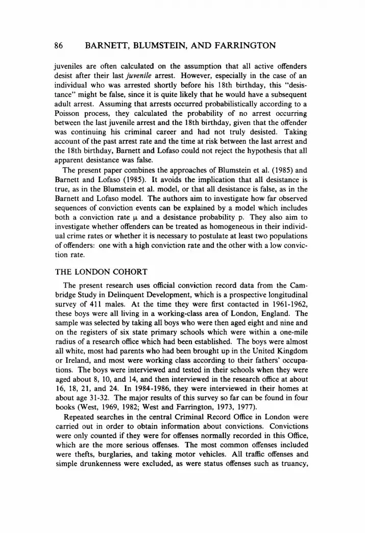
bility to the career patterns of the boys in the London cohort. These models are displayed in Table 1. They are built around two key parameters: (1) p = probability that an offender terminates his criminal career after the kth conviction (for any given offender, p is assumed the same at all k); and (2) p = the underlying annual rate at which the offender sustains convictions while free during his active career.

The models can include only p (as was done by Blumstein et al., 1985), only p (as was done by Barnett and Lofaso, 1985), or both p and p. In the simplest models, the parameters are considered to be homogeneous across a single population of offenders. Since such a formulation overly restricts the opportunity to reflect variation across offenders, greater flexibility is possible in a model that considers two populations, one more active in offending (designated as “frequents” and denoted by the subscript “1”) and the other less active (designated as “occasionals” and denoted by the subscript “2”). The two-population models require an additional parameter, y, indicating the

2. Where a youth was convicted of several offenses on one court appearance, the first date of offending was taken. In almost all cases, multiple offenses were committed close together.

Tabl

e 1.

M

odel

s C

onsi

dere

d, T

heir

Des

igna

tions

, and

Par

amet

ers

Mod

el P

aram

eter

s R

epre

sent

ed

Term

inat

ion

Prob

abili

ty (

p)

Con

vict

ion

Rat

e (p

)

Term

inat

ion

Prob

abili

ty a

nd

Con

vict

ion

Rat

e (p

, p)

Fo

r Tw

o Po

pula

tions

: (a

) p

hom

ogen

eous

, p

(b)

p ho

mog

enou

s, p

(c)

p a

nd p

bot

h di

ffer

ent

diff

eren

t

diff

eren

t

One

-Pop

ulat

ion

Mod

els

Des

igna

tion

Be E

stim

ated

Pa

ram

eter

s T

o Tw

o-Po

pula

tion

Mod

els

Para

met

ers

To

Des

igna

tion

Be E

stim

ated

*

*Fre

quen

ts:

pl, p

I O

ccas

iona

ls:

P~

, pz

+ Z U


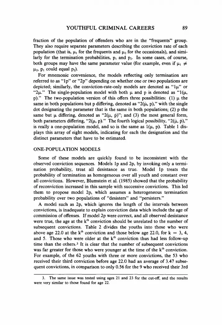
fraction of the population of offenders who are in the “frequents” group. They also require separate parameters describing the conviction rate of each population (that is, pI for the frequents and p.2 for the occasionals), and similarly for the termination probabilities, pI and p2. In some cases, of course, both groups may have the same parameter value (for example, even if pI #

For mnemonic convenience, the models reflecting only termination are referred to as “lp” or “2p” depending on whether one or two populations are depicted; similarly, the conviction-rate-only models are denoted as “ 1 p” or “2p.” The single-population model with both p and p is denoted as “l(p, p).” The two-population version of this offers three possibilities: (1) p the same in both populations but p differing, denoted as “2(k, p),” with the single dot designating the parameter that is the same in both populations; (2) p the same but p differing, denoted as “2(p, p)”; and (3) the most general form, both parameters differing, “2(p, p).” The fourth logical possibility, ‘‘2(P, p),” is really a one-population model, and so is the same as 1(p, p). Table 1 dis- plays this array of eight models, indicating for each the designation and the distinct parameters that have to be estimated.

p2, pI could equal ~ 2 ) .

ONE-POPULATION MODELS

Some of these models are quickly found to be inconsistent with the observed conviction sequences. Models Ip and 2p, by invoking only a termination probability, treat all desistance as true. Model l p treats the probability of termination as homogeneous over all youth and constant over all convictions. However, Blumstein et al. (1985) showed that the probability of reconviction increased in this sample with successive convictions. This led them to propose model 2p, which assumes a heterogeneous termination probability over two populations of “desisters” and “persisters.”

A model such as 2p, which ignores the length of the intervals between convictions, is inadequate to explain conviction data which include the age of commission of offenses. If model 2p were correct, and all observed desistance were true, the age at the kth conviction should be unrelated to the number of subsequent convictions. Table 2 divides the youths into those who were above age 22.0 at the kth conviction and those below age 22.0, for k = 3, 4, and 5 . Those who were older at the kth conviction thus had less follow-up time than the others.3 It is clear that the number of subsequent convictions was far greater for those who were younger at the time of the kth conviction. For example, of the 62 youths with three or more convictions, the 53 who received their third conviction before age 22.0 had an average of 3.47 subsequent convictions, in comparison to only 0.56 for the 9 who received their 3rd

3. The same issue was tested using ages 21 and 23 for the cut-off, and the results were very similar to those found for age 22.

90 BARNEIIT, BLUMSTEIN, AND FARRINGTON

Table 2. Average Number of Convictions Between the kth and Age 25 as a Function of Age at the kth

Age at kIh Conviction"

Above 22 years 0.56 (9) 0.54 (13) 0.17 (6) Below 22 years 3.47 (53) 4.52 (31) 4.19 (27)

k = 3 (62) k = 4 (44) k = 5 (33)

"The table entries show the average number of convictions up to the 25th birthday by the members of each group. The numbers in each group are shown in parentheses.

conviction after age 22.0. This suggests that the truncation of the period at risk at the 25th birthday affected the number of subsequent convictions, caus- ing "false desistance." Hence, it is concluded that the conviction rate, p, should be included in any model.

Model 1p assumes a homogeneous, constant conviction rate generated by a Poisson probability process and ignores career termination. Under this model, the conviction rate should be constant throughout the criminal career, and all offenders should have roughly the same conviction rate up to the kth conviction as after it (up to the 25th birthday).

Table 3 shows the average annual conviction rates per year free for all offenders from the 1st through the kth conviction (bk) and after the kth (sk). (The same individual can be included in several rows of the table; in particular, the 23 youths with 6 or more convictions are included in every row.) The

Table 3. Average Annual Conviction Rates up to and After the kth Conviction

k (N)"

2 (82) .50 .41 3 (62) .62 .47 4 (44) .70 .59

Up to the k'h (bk) After the klh (sk)

5 (33) .78 .67 6 (23) 1.01 .72 "The numbers of youths with at least k convictions for k = 2,3, ..., 6 are shown in parentheses.

conviction rate is approximately the reciprocal of the average time between convictions.4 For example, the 82 youths with at least 2 convictions averaged

4. The conviction rate is not exactly the reciprocal of the average time between convictions, because an unbiased estimate of the conviction rate is based on the total number of time intervals minus 1. Thus, in calculating bk for k = 2, the numerator is 81 intervals, not 82. The time each youth spent in detention was known, and was excluded from the calculation of conviction rate.


almost exactly 2 years between the 1st and the 2nd, leading to a conviction rate bk of S O per year. In calculating sk, a youth with no further convictions after the kIh contributed to the total time at risk but contributed a zero to the total number of further convictions.

It is clear from Table 3 that the value of bk rises steadily with k, roughly doubling as k grows from 2 to 6. The values of sk exhibit a comparable pattern of growth but, at any particular value of k, sk is only about 80% of the corresponding bk. Therefore, the average conviction rate is not constant over the observation period, and model l p seems incorrect. Similarly, model 2p must also be incorrect because, with heterogeneous conviction rates and no termination, there is no reason why bk and s k should differ.

The figures in Table 3 can be explained in two ways: either p decreases with time or some offenders are terminating. If p is constant before desistance, the ending of some criminal careers could produce the decrease with age in measured conviction rates. In attempting to distinguish between these possibilities, Table 4 shows the average time intervals between successive convictions for offenders with at least k convictions. For example, the 62 youths with at least 3 convictions had an average time interval of 1.71 years between the 1st and 2nd and an average interval of 1.50 years between the 2nd and 3rd.

All of the time intervals in Table 4 are consistent with the hypothesis that, for any given minimum number of convictions k, the annual rate of offending is constant over time. Assuming a Poisson process, for all convictions (see the Appendix), all of the time intervals are well within two standard deviations of the mean interval and display no clear trends. Hence, the combination of a constant p during the active career, followed by termination, seems more reasonable than a declining p with no termination.

TWO-POPULATION MODELS

Model l(p, p) thus introduces both a conviction rate, p, and a termination probability, p, and assumes both to be homogeneous and constant over time. If all offenders have the same conviction rate, then an unusually high conviction rate early in a criminal career would represent only random fluctuation and would not foreshadow a high conviction rate later. In testing this, Table 5 divides youths with at least k convictions into two equal groups according to the time taken between the first and the kth conviction, and then shows the total number of convictions of the two groups in the subsequent four years at risk. Thus, the 62 youths with at least 3 convictions were divided into 31 who took less than the median time of 2.7 years to reach their 3rd conviction and 31 who took longer.5

5 . Since the number of youths with 5 or more convictions was an odd number (33), the median youth was deleted in this case.


Table 4. Intervals between Successive Convictions Average Time Interval in Years Between the k-1 and the

k Conviction $ . ).

Offenders with at Least K Convictions k = 2 3 4 5 6 7

K (N)

4 (44) 1.43 1.41 1.49

- - - - - -

3 (62) 1.71 1.50

5 (33) 1.29 1.06 1.56 1.18

6 (23) 1.05 1.13 0.90 1.30 0.54

7 (21) 1.11 0.96 0.83 1.39 0.58 0.88

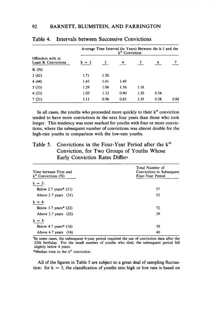
In all cases, the youths who proceeded more quickly to their kth conviction tended to have more convictions in the next four years than those who took longer. This tendency was most marked for youths with four or more convictions, where the subsequent number of convictions was almost double for the high-rate youths in comparison with the low-rate youths.

Table 5 . Convictions in the Four-Year Period after the kth Conviction, for Two Groups of Youths Whose Early Conviction Rates Differ.

Time between First and kth Convictions (N)

k = 3:

Total Number of Convictions in Subsequent Four-Year Period

Below 2.7 years* (31) Above 2.7 years (31)

k = 4: - Below 3.7 years* (22) Above 3.7 years (22)

k = 5 :

57 53

72 39

Below 4.7 years* (16) Above 4.7 years (16)

58

40 "In some cases, the subsequent 4-year period required the use of conviction data after the 25th birthday. For the small number of youths who died, the subsequent period fell slightly below 4 years. *Median time to the kth conviction.

All of the figures in Table 5 are subject to a great deal of sampling fluctuation: for k = 3, the classification of youths into high or low rate is based on


only two time intervals. The classification becomes more accurate for k = 5 , but then the numbers of youths become small (only 16 in each category); hence, the figures shown for k = 4 may be the most reliable. These results suggest that there is heterogeneity in conviction rates rather than random variation around a single rate. Hence, this weakness in models I ( p , p ) and 2(& p) , which assume a homogeneous conviction rate p, encourages a search for models with heterogeneous conviction rates.

The models which are left as possibilities in explaining these conviction careers are: 2(p, p), which assumes a heterogeneous conviction rate and a homogeneous termination probability, with parameters (pI, p2, p, y); and 2(p, p), which assumes that both conviction rate and termination probability are heterogeneous, with parameters (pI, p2, pI, p2, y). The next section will distinguish between these possibilities by estimating the parameters in the more general model 2(p, p). If p1 and p2 are sufficiently close, then the model 2(p, p) is indicated. In a similar way, the parameter estimates will also test the homogeneity of p.

Before calibrating the 2(p, p) model, one should note that it is compatible with all the tables presented so far. In Table 2, the average number of subsequent convictions clearly increases with time at risk, as predicted by a model including annual conviction rates. In Table 3, the conviction rate increases from k = 2 to k = 6 because the k = 6 group should include a higher proportion of the more active offenders than the k = 2 group. Under a 2(p, p) model, the observed drop in the conviction rate after the kth conviction would be expected because some offenders would have terminated. Similarly, in Table 4, the average time between convictions decreases from k = 2 to k = 7 because the k = 7 group should include a higher proportion of the more active offenders. Finally, in Table 5 , offenders with a higher p would reach the kth conviction more quickly and should also have more convictions in the subsequent four-year period.

APPROXIMATE PARAMETER ESTIMATION IN THE GENERAL MODEL

The five-parameter model, 2(p, p), suggests that the youths with at least two convictions can be divided into two populations: those with a higher pI and an associated p1 (the “frequents”) and the less active ones with a lower p2 and an associated p2 (the “occasionals”). The proportion of offenders who are frequents is y. Tests of the model have to begin at the second conviction because this is the first point at which an interval is available from which a conviction rate can be estimated. Because p1 exceeds p2, active frequents amass convictions more rapidly than active occasionals. Moreover, it is reasonable to expect that the termination probability for the frequents, pI, is lower than p2, since the higher-rate offenders are probably more committed to


continued criminal activity. Hence, among the youths with at least k convictions before age 25, the proportion who are frequents should grow with k. Indeed, once k is sufficiently large, those who reach that threshold might be almost exclusively frequents. The analysis therefore concentrates first on the London youths who were convicted six or more times. As an initial approximation, it is assumed that all 23 such youths are frequents, and that working hypothesis is used to make some tentative inferences about (pl, p,) and then

Table 4 shows that the average 6th offender took 4.92 years to accumulate 5 convictions after his 1st one, for a mean time of 0.99 years between successive convictions. The annual conviction rate for these offenders (pI) is estimated at V0.99 = 1.01. This is b6 in Table 3. To estimate the probability of termination, pl, it is noted first that s6 in Table 3 is only .72, which means that the 23 youths averaged 29% fewer convictions per year after the 6th conviction than before it. The youths were observed for a mean time of 5.51 years between the 6th conviction and age 25. Without any termination, therefore, they would have sustained on average 5.51 X 1.01 = 5.56 convictions over that period. In actuality, however, the mean number accumulated was only 91/23 = 3.96.

A way to calculate pI is wanted. The approach here involves calculating for these 23 presumed frequents the number of convictions they might experience between their 6th and the end of the observation period (their 25th birth- days) for various values of pI, and then to choose the value of pI that most closely matches the number of convictions actually observed. For each individual, one can calculate the observation time remaining after the 6th conviction, 25 - a6 (where a6 is the age at the 6th conviction). The expected number of further convictions then depends on the time remaining, the conviction rate pI (which has already been estimated as 1.01 convictions per year), and the unknown value of pI. The expression for this relationship is given in Equation 9 of the Appendix. From this relationship, for example, it can be determined that as pl goes up, the number of further convictions goes down. The 23 youths amassed a total of 91 post-6th convictions or an average of 3.96. The value of pI that most closely corresponds to this total is .09, and so one can approximate pI = .09.

This outcome lends itself to a simple intuitive explanation. If convictions arise at 1 per year and if there is a 9% chance of termination following each one, then about 9% of offenders “retire” from criminal activity per year. Over a period of 5.5 years, therefore, approximately half of the 23 offenders would sooner or later retire. Despite a slight skew toward the start of that period, these terminations should be about uniformly distributed over it. Hence, the “dropouts” forego slightly more than half the convictions that they would have accumulated in the absence of termination. When 50% of

(p2, P2) and Y.


the offenders give up just over 50% of their convictions, an overall shortfall around 29% seems reasonable.

To obtain the other parameters in the 2-population model, one must consider developments prior to the 6th conviction. The termination process for frequents, far from commencing abruptly when k = 6, has been operating since the onset of their careers. If at the 2nd conviction there were a total of A frequents with p = 1.01 and p = .09, then only (1 - .09)4A = .68A would be expected to survive the 4 opportunities to terminate (that is, the 2nd, 3rd, 4th, and 5th convictions) and reach the 6th conviction. In addition, some other frequents who did not terminate under this process could still have fewer than 6 convictions, because their later convictions occurred after the 25th birthday.

Continuing with this initial approximation, let it be assumed that all frequents had enough time to reach the 6th conviction by the 25th birthday if their conviction processes had continued without termination.6 Following the argument of the last paragraph, the estimated number of second offenders with p = 1.01 would be 23/68 = 34. Hence y, the proportion of frequents among the 82 offenders with two or more convictions would be approximately 34/82 = .41.

Once y has been estimated, pz follows readily. The 82 2nd offenders required an aggregate of 164 years to proceed from the 1st conviction to the 2nd. From Table 4, one knows it took the 23 6th offenders an average of 1.05 years each for this transition. Hence, their contribution to the sum was 23 X 1.05, or about 24. The 11 other 2nd offenders (34 - 23 = 11) believed to be frequents should have contributed roughly 11 X 1.01, or about 11 years, since pl = 1.01. It follows that the remaining 48 youths (all occasionals) needed a total of 164 - 24 - 11 = 129 years to make the progression, or about 129/48 = 2.7 years each. This leads to the estimate that p2 = V2.7, or .37 convictions per year.

The only quantity for which even a provisional estimate is lacking is pz. Here one runs into a quandary: with p2 = .37, the average occasional would need 10.8 years to advance from the 2nd conviction to the 6th. Though shortage of time at risk would prevent most occasionals from advancing to the 6th conviction before the 25th birthday, about 12 would have done so in the absence of any true desistance. The termination probability p2, therefore, must be large enough to explain the assumed desistance of all 12 such offenders before k = 6. At the same time, it cannot be too large or extremely few occasionals would have reached the 2nd conviction. The only value of pz that would guarantee no survivors to the 6th conviction would be 1.0. But even if p2 were as low as .32, so few occasionals would be expected to reach the 6th

6. Since the 23 youths with 6 or more convictions reached their 2nd conviction at age 17 on average, this is not an unreasonable assumption.


conviction that an observed outcome of zero would have a probability of at least .05 (that is, would not be statistically significant). As a conservative first estimate, therefore, one can choose p2 = .32.

To summarize, this initial exercise leads to the 2-population model with parameters (pI, pI) of (1.01, .09) and (p2, p2) of (.37, .32), and with y = .41 (that is, 41% of the 82 second offenders are frequents). As is shown in the next section, these parameter estimates are very close to those calculated more precisely.

MORE ACCURATE PARAMETER ESTIMATION A GROUP ASSIGNMENT RULE

A procedure that leads ultimately to more reliable parameter estimates begins with a hypothetical question. Suppose that there is a 2-group criminal population described by the known parameters (pI, p2, pl, p2, y). A 25-year old member of this population is chosen at random, and it is learned that his conviction record shows k events at ages (al, a2. . . ., ak). Based on this information, is it more likely that the youth selected was a frequent or that he was an occasional? An equivalent question is whether the parameter by which he amassed convictions between al and ak was pl or p2.

As explained in Equation 5 of the Appendix, one can use the known values of pI and y to determine P(F), the probability that a youth selected at random would be a frequent and that he would sustain convictions at (al, . . ., ak) under the group’s Poisson process. One can likewise use p2 and y to estimate P(O), the analogous probability for occasionals.

These two probabilities allow one to compute the ratio, R, defined by:

R is a likelihood ratio, for it compares the probabilities of the two possible ways of obtaining the observed conviction record: either it was generated by a frequent or by an occasional. If R > 1, then the observed sequence (al, . . ., ak) is more likely with frequents than with occasionals. This is equivalent to the assessment that, given k convictions at (al, . . ., ak), the chance is greater than 50% that a frequent was responsible for them.

These comments suggest a procedure for using an offender’s R-value to make an assessment of his group status: If R > 1, assign the offender to the frequents. If R < 1, assign the offender to the occasionals. This procedure always assigns the offenders to the group that is more likely to be correct.

Such a likelihood-ratio approach could readily be applied to the London offenders being studied. Among the initial parameter estimates in the previous section were y = .41, p1 = 1.01, and p2 = .37. Using these numbers and formula 6 in the Appendix, one can calculate R-values for each of the 82


multiple offenders, based in every case on the entire conviction record. Each youth could then be classified as a frequent or an occasional depending on the value of his likelihood ratio, R. In effect, one would be assigning to each youth a conviction rate of either .37 or 1.01.

Initially, one might think that such a dichotomy simply reifies the model that has already been calibrated only approximately. But it actually goes somewhat further, for it provides the basis for a new set of parameter estimates. The proportion of multiple offenders who are frequents, y, would be approximated by the fraction of youths with R-values greater than 1. The value of pI would be estimated from the annual conviction rates (during active careers) of those who are now classified as frequents. New estimates of p2 and the termination probabilities, p1 and p2, would likewise be available, as will be indicated momentarily.

These new parameter estimates would have a considerable advantage over the first estimates because the most questionable aspects of the earlier calculation are avoided. No longer is it assumed that no occasional reached a sixth conviction. Nor is it hypothesized that, barring true termination, every frequent has six or more convictions. These questionable assumptions are still not totally abandoned, since they do contribute to the initial parameter estimates that help determine the R-values that create the partition of offenders. But they have far less influence on the new, more precise parameter estimates than on the initial set.

REVISED PARAMETER ESTIMATES

When R-values were computed for the 82 London multiple offenders, 35 were identified as frequents and 47 as occasionals. (In fact, the likelihood ratio discriminated quite sharply between the groups: 63 of the 82 offenders were at least twice as likely to be in one group as the other, that is, R > 2 or R < S.) The value of y is then estimated as 35/82 = .43, very close to the initial estimate of 34/82 = .41. In an even more striking similarity, 22 of the 23 6th offenders were classified as frequents (compared to the original estimate of 23), while 13 of those with between 2 and 5 convictions were so classified (compared to the original estimate of 11).

To estimate kI and pl, it is observed that the 35 youths classified as frequents had a total of 234 convictions after the lst, and that they required a total of 204 years to accumulate them. This leads to an estimated annual conviction rate of pI = 234/204 = 1.14. Setting p1 = 1.14 and applying Equation 9 of the Appendix, one can express in terms of pI the number of convictions after the second that each frequent is expected to amass, given his time at risk. In actuality, these youths sustained 234-35 = 199 convictions beyond the 2nd and before age 25. The value of pi at which they would be


expected to have 199 further convictions is computed from Equation 9 as p, = 0.10.

The parallel calculations for the occasionals yield p2 = .41 and p2 = .33. The new p2 estimate-based on the experience of all 47 occasionals after their 2nd convictions-is surprisingly close to the earlier estimate of .32, which emerged from a rather ad hoc attempt to keep the occasionals below 6 convictions.

The second round of parameter estimation, therefore, ends in the more reliable estimate (pl, pl, p2, p2, y) = (1.14, .lo, .41, .33, .43); this result is displayed in Table 6. None of the five parameters differs much from its earlier

Table 6. Estimated Parameters of the 2(p, p) Model

(PI (I4 Termination (Y)

Conviction Rate Probability per Percent per Year Conviction Frequents

Frequents 1.14 .10 .43 Occasionals .41 .33

approximation. One can imagine further iterations, but investigation reveals that they only negligibly affect the numerical results. One should note that pI and p2 differ so substantially that a model treating them as equal seems implausible; hence, of the models considered, 2(p, p) seems the most defensible.

SOME TESTS OF THE VALIDITY OF THE MODEL

Now that the parameters of a full two-population model have been more carefully estimated, one must test whether that model satisfactorily represents the patterns in the data. That issue is addressed through various tests of the empirical validity of the model just calibrated.

The parameter estimates developed in the previous section were chosen to minimize the aggregate difference between the expected and actual numbers of convictions of all multiple offenders. But they do not necessarily ensure such consistency at the level of individuals. The model implies that, within either group, those whose 2nd convictions occur earliest have the greatest probability of true termination before age 25, because they can expect to have more chances to terminate. It would also be expected that those whose 2nd convictions occur latest (that is, those with the largest values of a2) would accumulate the fewest additional convictions over the span of observation. Examining whether both of these patterns actually are present in the data for individuals can help in further assessing the validity of the model.


Knowing the groups to which a particular offender was assigned, as well as his remaining observation time between his age a2 and 25, one can make estimates of two key quantities:

E = the expected number of further convictions after the 2nd and before age 25 for an offender with career parameters (p, p);

u = the standard deviation of the number of further convictions for each offender.

After calculating these numbers for each offender based on his remaining observation time, (25 - a2 - w), where w is time in detention, and the (p, p) values of his assigned group (based on his R score), one can then compute for the i I h offender the accuracy measure z, defined by:

XI - El z, = ~

Dl

where x, = the ith offender’s observed number of convictions after a2 and before age 25. Here, q expresses, in units of standard deviations, the error in using El as an estimate of the actual number of convictions for each individual

As is well known, a normalized statistic like z, should have a mean 0 and

variance 1 under an accurate model. If the 2-group model were exactly cor- 82

rect, then Y = . z z,, the sum of the z, for all 82 of the 2nd offenders, would 1= 1

have a normal distribution with mean 0 and variance 82. When the actual value of Y for the London offenders was computed, it came to 0.74, which is extremely close to expectation.

Before too much weight is given to this outcome, however, one should rec- ognize the limited strength of the test that produced it. The parameters of the model for each group (p, p) were chosen to minimize the sum Z(x, - E,[p, p]) within each of the two offender groups. Thus, it is not surprising that the sum of the z,’s is small. A more stringent test is desirable. One such test would focus on V, the sum of the absolute values of the various z,’s. An unusually high value of V should detect whether the positive and negative errors, even though they may cancel each other in the Y-score, are too large to be attributed to chance variation. It can be shown (see the Appendix) that the distribution of V should be approximately normal, with a mean of 64.8 and a standard deviation of 5.5, which corresponds to a 95% confidence interval for V from 53.8 to 75.8. The calculated V-statistic of 63.0 is well within that interval, and hence consistent with the proposed model of conviction patterns.

Another test of the model exploits the fact that, within each offender group, the predicted El’s vary from offender to offender. One might therefore divide each subpopulation into two halves based on their individual El’s; then

1.


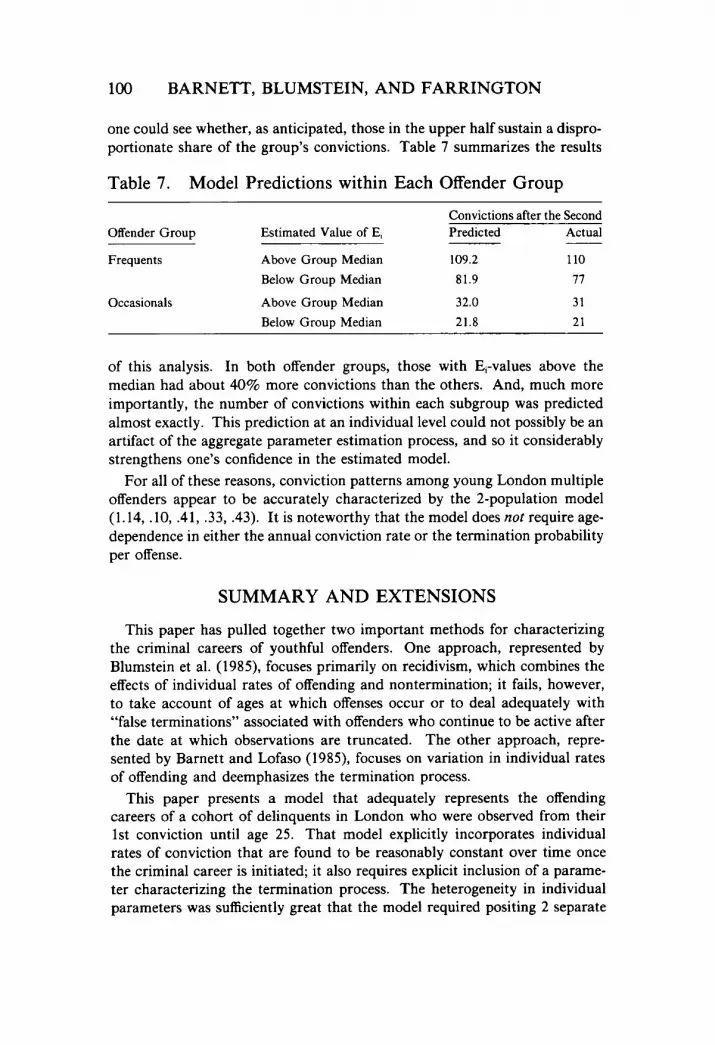
one could see whether, as anticipated, those in the upper half sustain a disproportionate share of the group’s convictions. Table 7 summarizes the results

Table 7. Model Predictions within Each Offender Group

Convictions after the Second Offender Group Estimated Value of E, Predicted Actual

Frequents Above Group Median 109.2 110 Below Group Median 81.9 77

Below Group Median 21.8 21 Occasionals Above Group Median 32.0 31

of this analysis. In both offender groups, those with Ei-values above the median had about 40% more convictions than the others. And, much more importantly, the number of convictions within each subgroup was predicted almost exactly. This prediction at an individual level could not possibly be an artifact of the aggregate parameter estimation process, and so it considerably strengthens one’s confidence in the estimated model.

For all of these reasons, conviction patterns among young London multiple offenders appear to be accurately characterized by the 2-population model (1.14, .lo, .41, .33, .43). It is noteworthy that the model does nor require age- dependence in either the annual conviction rate or the termination probability per offense.

SUMMARY AND EXTENSIONS

This paper has pulled together two important methods for characterizing the criminal careers of youthful offenders. One approach, represented by Blumstein et al. (1985), focuses primarily on recidivism, which combines the effects of individual rates of offending and nontermination; it fails, however, to take account of ages at which offenses occur or to deal adequately with “false terminations” associated with offenders who continue to be active after the date at which observations are truncated. The other approach, represented by Barnett and Lofaso (1985), focuses on variation in individual rates of offending and deemphasizes the termination process.

This paper presents a model that adequately represents the offending careers of a cohort of delinquents in London who were observed from their 1st conviction until age 25. That model explicitly incorporates individual rates of conviction that are found to be reasonably constant over time once the criminal career is initiated; it also requires explicit inclusion of a parameter characterizing the termination process. The heterogeneity in individual parameters was sufficiently great that the model required positing 2 separate


populations to reflect that heterogeneity. Thus, the simplest feasible model had 5 parameters: 2 representing the annual individual conviction rates for each of the subpopulations, 2 for the termination probabilities, and 1 representing the mixing fraction of the subpopulations.

In the London cohort, one group (the “frequents”) had a high annual conviction rate (1.14) and a low probability of termination after each conviction (.lo), and the other (the “occasionals”) had a low annual conviction rate (.41) and a high probability of termination (.33); the frequents were estimated to comprise 43% of the population of offenders and the occasionals the other 57%.

The representation of a single, heterogeneous population as composed of two internally homogeneous populations should be recognized as no more than an efficient and effective device for characterizing the single population’s heterogeneity. It does not mean that there are necessarily only two distinct populations, but rather that the combination of the two appears adequately to reflect the heterogeneity of the original population for analytic purposes.

Individuals can easily be assigned to one of the two groups based on the observation of their total offending patterns. It would be most desirable to be able to make such distinctions early in the criminal career, at or shortly after the first conviction. Using information available at that time, it might then be possible to predict future offending rates and residual lengths of criminal careers.

Even though this research was based on offenders living in London, earlier research (Blumstein et al., 1985) suggests that young offenders in American communities display very similar offending patterns, albeit with somewhat different parameters. Thus, the model developed here should be estimated and tested using comparable offense-history records from a number of Ameri- can communities, including, for example, the two cohorts in Philadelphia and the three in Racine. Also, the small number of offenders in the London sample makes replication in larger samples desirable.

Because this paper has focused on offenders after they have initiated their criminal careers, individual conviction and termination rates have received the primary attention. Further research on the full criminal career should also address the process of initiation. In doing so, it would be necessary to examine the factors that distinguish the “innocents” (that is, those who are never convicted) from those with one or more convictions. Among the offenders, it would be desirable to examine the changes in rates of initiation with age, and especially the ways in which that process differs between the frequents and the occasionals. Presumably, most frequents will have initiated their criminal careers by an early age, whereas those beginning late are more likely to be occasionals. In the London cohort, for example, 80% of those classified as frequents (by the R scale) experienced their first conviction by age 15, compared to 60% of the occasionals.


The model developed here assumes that each offender has an opportunity (with associated probabilities pI and pJ of terminating his criminal career immediately after each conviction. The theoretical implication of this formulation is that events associated with the conviction (perhaps involving societal reaction, rehabilitative treatments, or specific deterrent effects) lead to the termination. Another consequence of this formulation is that the frequents have more opportunities per year to terminate their criminal careers since they have more convictions per year than the occasionals.

It would be interesting to consider termination as an annual process rather than as one associated with each conviction. The annual rate of termination (6) is approximately the product of convictions per year and terminations per conviction (6 = pp). The annual rate of termination for the frequents (1.14 X 0.10 = .114) is quite close to that for the occasionals (0.41 X 0.33 = .135). These annual rates imply an average career length of about 7 to 9 years, with the frequents at the upper end of the range and the occasionals at the lower end. This estimate is reasonably consistent with the estimates of career length developed for U.S. adults by Blumstein et al. (1982).

Extending the model to reflect time-based termination requires further development to assign to each offender an annual termination rate instead of a termination probability, p, per conviction. If this does prove to be a better representation, it would suggest that the termination process, rather than being tied to convictions, is instead a continuous time process that could reflect other life experiences that occur gradually or randomly over time, that are independent of convictions, and that might reflect developmental processes such as maturation, disengagement from a delinquent peer group, or entering into adult life patterns through marriage or employment. Fur- thermore, if the annual termination rates for the two groups are found to be very close, as the above approximation suggests, that would indicate that the factors that contribute to a high or low rate of offending may well be different from those that affect termination.

In summary then, this paper has shown that in modelingtriminal careers, it is necessary to reflect both individual rates of offending and termination, and to reflect population heterogeneity through use of parameters for at least two populations. Further revisions to the model may be warranted and the use of a continuous termination process rather than one tied to the conviction events is worth exploring. The different offense types should be considered separately and parameters should be estimated for each primary type of offense for various identifiable subgroups of any offender population being studied.

In further research, when the relevant parameters are estimated for different populations, the factors that lead to differences in the parameter estimates can be explored, and these should be illuminating from the viewpoint of causal research. It can be expected that different factors will influence the


separate criminal-career parameters in different ways. That information can then be used to develop empirically based, testable theories of criminality that can lead to predictions of future criminal behavior and to suggestions for appropriate forms of intervention.

REFERENCES

Barnett, Arnold and Anthony J. Lofaso 1985 Selective incapacitation and the Philadelphia cohort data. Journal of

Quantitative Criminology 1: 3-36.

Blumstein, Alfred, Jacqueline Cohen, and Paul Hsieh The Duration of Adult Criminal Careers. Final Report to National Institute of Justice.

1982

Blumstein, Alfred, David P. Farrington, and Soumyo Moitra 1985 Delinquency careers: Innocents, desisters, and persisters. In Michael H.

Tonry and Norval Morris (eds.), Crime and Justice: An Annual Review of Research (Vol. 7). Chicago: University of Chicago Press.

Blumstein, Alfred and Soumyo Moitra 1980 The identification of “career criminals” from “chronic offenders” in a

cohort. Law and Policy Quarterly 2: 321-334.

Elliott, Delbert S., David Huizinga, and Suzanne S. Ageton 1985 Explaining Delinquency and Drug Use. Beverly Hills: Sage.

Farrington, David P. 1983 Offending from 10 to 25 years of age. In Katherine T. Van Dusen and

Sarnoff A. Mednick (eds.), Prospective Studies of Crime and Delinquency. Boston: Kluwer-Nijhoff.

Hirschi, Travis 1969 Causes of Delinquency. Berkeley: University of California Press.

Langan, Patrick A. and David P. Farrington 1983 Two-track or one-track justice? Some evidence from an English longitudinal

survey. Journal of Criminal Law and Criminology 74: 519-546.

West, Donald J. 1969 1982 Delinquency: Its Roots, Careers, and Prospects. London: Heinemann.

Present Conduct and Future Delinquency. London: Heinemann.

West, Donald J. and David P. Farrington 1973 Who Becomes Delinquent? London: Heinemann. 1977 The Delinquent Way of Life. London: Heinemann.

Wolfgang, Marvin E., Robert M. Figlio, and Thorsten Sellin 1972 Delinquency in a Birth Cohort. Chicago: University of Chicago Press.


Arnold Barnett is Professor of Operations Research at MIT’s Sloan School of Manage- ment. His research specialty is applied probabilistic modeling, with much of his work stim- ulated by two prime passions of his life: fear of flying and fear of crime.

Alfred Blumstein is J. Erik Jonsson Professor of Urban Systems and Operations Research and Dean of the School of Urban and Public Affairs at Carnegie Mellon Univer- sity. He has chaired the National Academy of Sciences Committee on Research on Law Enforcement and the Administration of Justice and has chaired the committee’s panels on Research on Deterrent and Incapacitative Effects, on Sentencing Research, and on Crimi- nal Careers.

David P. Farrington is a lecturer in criminology at Cambridge University, England. His major research interest is in the longitudinal study of delinquency and crime, and he is director of the Cambridge Study in Delinquent Development.

APPENDIX All the calculations in this paper are based on the assumption that each

offender, while free and active, accumulates convictions under a Poisson process with a rate parameter that is either plor p2 depending on whether he is a frequent or an occasional. Under a Poisson process with an annual rate parameter p, the probability that an event occurs on any given day is p/365. Here, p represents the average number of times the event occurs in one year. Another feature of the Poisson process is that the outcomes on different days are independent-that is the fact that the event did or did not occur on day x has no bearing on the chance that it happens on day y.

In the Poisson process, the probability, Pk, that exactly k events occur over a period of duration T is well known:

The probability of no events at all during the period is obtained by setting k = 0 in (1):

(2) p = e-pT

The Likelihood Ratio R Suppose that a Poisson process is observed between S and T, the time line

having been broken into small increments of length A. One might wish to calculate the probability that exactly j events occur over the period (T-S) during the A’s centered at times t,, t2 ,...., tj.

Under Poisson assumptions, the probability of an event in any particular A is PA, and of having events in each of j A’s at (tl, ...., tj) is (PA)’. The probability of no other events in (S,T) is e-p(T-s-JA). Because jA contributes so negligibly to this last exponent, one can disregard it in writing:

PLj events occur in (S,T) in A’s centered at (tl, ...., t,)] = (pA)j e-p(T-S) (3)


Now, consider an offender whose parameters are (p,p) and who was convicted k times in a A’s centered at ages (al, ..., ad. The youth is assumed to be acting under the Poisson conviction process from just after a, through ak, and so we can write:

(4) P[k- 1 convictions at (a2, ..., aJIfirst conviction at a,] =

One is now in a position to find P(F) and P(0) as defined in Section VI. Since a fraction y of the offenders are frequents, y serves as the prior probability that an offender chosen at random is from this group. The condi- tional probability that, in the ak-a, years after a,, a frequent offender would sustain (k- 1) convictions at ages (a,, ..., a 3 is given by (4), with p set equal to p,. From the joint probability law, one can therefore write:

P(F) = P (randomly chosen youth is a frequent and attains the

- d a k - a 1) e

convictions record observed)

( 5 ) - -a 1) = y (P,A)~-I e

Noting that 1 -y is the chance that a randomly selected youth is an occasional, one can make the similar statement:

p(0) = (1 -y)(p2A)k-I e-’2(ak-a1)

Hence the ratio R follows:

Using y = .41, p, = 1.01, and p2 = .37, R values were computed for each multiple offender in the London cohort. The 35 with R-values greater than 1 were assigned as frequents; the 47 others as occasionals. Under this partition, y is revised to V 8 2 = .43, only slightly different from the original estimate. Subsequently, pI, p,, PI, and P2 were revised as described in Section VI.

In one significant respect, the classifications based on R are incomplete. In assigning people to groups, the analysis considers whether an individual’s p- value is more plausibly equal to 1.01 or to .37. But it pays no attention to whether p1 or p2 seems better to represent his termination probability. Thus, the procedure might be ignoring some useful information for classifying offenders.

This problem seems far less compelling, however, in light of the coarseness of the first p2 estimate. The initial estimate of p, was chosen as the lowest termination probability for which a 100% attrition rate by the 6th conviction was not statistically significant. The approximation p, = .32 was therefore directly tied to the most vulnerable assumption of the earlier calculation: that no occasionals could reach the 6th conviction. Moreover, it depended strongly on treating the 5% level as the standard of statistical significance. In

106 BARNETT, BLUMSTEIN, A N D FARRINGTON

other words, the first approximation of p2 was sufficiently coarse that not using it in computing R is probably preferable.

Calibrating and Testing the Two-Population Model

Some special extensions to these Poisson formulas are needed if an offender’s active period can terminate abruptly following any conviction. Suppose that an offender with conviction rate p and termination probability p has just been convicted a kth time, and let T be his remaining time at risk until age 25. The probability Q, of no further convictions during that period would be:

Q, = p + (l-p)e-pT (7)

Equation (7) arises because there are two mutually exclusive ways such a youth can avoid further convictions: he can terminate at once after the kth conviction (true desistance) or, having failed to do so, he may experience no further convictions before age 25 under his still-active Poisson process (false desistance). The first term on the right of (7) covers the former possibility and the second term the latter.

The reasoning behind (7) can be generalized to yield other results. The chance Qj of exactly j further convictions between the kth and age 25 is given by:

In the right-hand side of (8), the first term represents j events under the Pois- son process uninterrupted by termination, while the second term reflects termination after the jth of a Poisson process that would otherwise have produced more than j.

From (8) and some extensive exercises with algebra, the mean and variance of the number of further convictions, denoted as E and u2, respectively, can be shown to be:

2 P [-1+(1-2pT)e-pTp + - (l-e-pTP)] (10) W 1-P 0 2 = 2 (i-E)ZQ. = -

j=O ’ P

These formulas figures in both the calibration and testing of the 2-population model presented in the main text. Having approximated pI as 1.01 in the 1st parameter estimation, one can then approximate pl. There were 23 youths convicted a 6th time; let Ti be the subsequent observation time for the


ith of these. In terms of p,, their expected total number of further convictions, C, would be given by (9) as:

- 23 1-p,

1 = 1 p, c = .z - (1-e

The actual number of additional convictions was 91. Thus, by setting C = 91, one can solve (1 1) for p1 (by search on a computer) to get the estimate p, = .09.

Also, if one assumes it is known whether a particular youth is a frequent or an occasional, then knowing his observation time after the kth conviction enables one to use (9) and (10) to estimate the mean and variance of his number of further convictions through age 25. These quantities can be used with the number actually observed to compute the zi’s described in Section VII.

Given its definition, zi necessarily has a mean of zero and variance of 1 if Ei and ui are correctly specified. To find the expected value of lzil assuming the validity of the 2-population model derived, one uses the probability distribution in (8) to calculate average absolute spread around the mean. Performing the computation for each youth and dividing by the appropriate ui, one learns that lzil would average .79 for the 82 youths under the hypothesized model. Because the different Izi% are essentially independent, their sum V would be about normally distributed with a mean of 82 X .79 = 64.8. The standard deviation of the sum is computed to be 5.5. These findings provide a yard- stick for assessing whether the absolute “forecast errors” ( [xi - EiI) are sufficiently small that they can reasonably be attributed to chance rather than to deficiencies in the underlying model.

probabilistic models of youthful criminal careers

Documents