On the origin of apparently negative minimum

susceptibilities of hematite single crystals calculated from

low-field anisotropy of magnetic susceptibility

1Faculty of Sciences, Charles University, Albertov 6, CZ-128 43 Prague, Czech Republic

E-mail: jezek@natur.cuni.cz

2AGICO Ltd., Ječná 29a, Box 90, CZ-621 00 Brno, Czech Republic

E-mail: chadima@agico.cz; hrouda@agico.cz

3 Institute of Geology, Academy of Sciences of Czech Republic, Prague, Czech Republic

Josef Ježek1, Martin Chadima1,2, František Hrouda1,2

Supported by the project 19-17442S of the Grant Agency of the Czech Republic.

Introduction

As shown in the literature several times, the calculation of the anisotropy of

magnetic susceptibility (AMS) of hematite single crystals using standard linear

AMS theory (fitting tensor of 2nd rank) reveals that the calculated minimum

principal susceptibility is parallel to the crystallographic c-axis, but is negative,

which has however evidently nothing to do with diamagnetism as found out

through direct measurement of susceptibility along the principal directions.

The problem of negative minimum principal susceptibility can be split in two

parts:

(1) How to represent single crystal AMS in such a case.

(2) How this phenomenon limits standard models of bulk (multi-crystal) AMS.

We investigate these two points, using susceptibility measured in symmetry

planes of hematite crystal. We present our contribution in the original form,

which was aimed as a poster.

Directional susceptibility

https://en.wikipedia.org/wiki/Hippopede

When d > 0 the curve has an oval form and is

often known as an oval of Booth

Nagata, T., 1961. Rock magnetism. Maruzen

Tokyo.

https://www.mathcurve.com/courbes2d.gb/bo

oth/booth.shtml

Curves studied by Fagnano in 1750, Euler in

1751, and Booth in 1877.

James Booth (1810 -1878): British

mathematician.

Other names: Hippopede of Proclus, elliptic

lemniscate (for the ovals) and hyperbolic

lemniscate (for the lemniscates).

Polar equation:

r2=a2cos2a + eb2sin2a

e = 1 for the ovals

e = –1 for the lemniscates

krivka smerove susc. je tedy podobna

elipticke lemniskate, ovsem nejsou tam ty

mocniny u parametru r,a,b zejmena by se muselo udelat sqrt viz lemni_and_spol

kd=d’*k*d

d ... direction cosines of the applied field

k ... tensor of magnetic susceptibility

Tensor of magnetic susceptibility (k) is usually computed from a set of measurements by which

magnetic field (red arrow in Fig. 1a) is applied in different directions. Response in this direction is

represented by the directional susceptibility related to the susceptibility tensor as

kd=d*k*d’ (1)

Fig. 1a. Directional susceptibility (kd = OC) creates

a curve similar to eliptical lemniscate. Adopted from

Nagata (1961):

Fig. 1b. Surface (upper part) of directional

susceptibility.

where d is vector of direction cosines.

Directional susceptibility of hematite

measured in symmetry planes

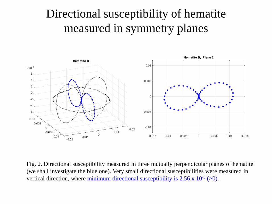
Fig. 2. Directional susceptibility measured in three mutually perpendicular planes of hematite

(we shall investigate the blue one). Very small directional susceptibilities were measured in

vertical direction, where minimum directional susceptibility is 2.56 x 10-5 (>0).

Susceptibility tensor was fitted to measured directional susceptibilities. Its first eigenvector e1 is

slightly deviated (e1=4.5o) from horizontal plane (due to imperfect arrangement of the measurement),

and the maximum eigenvalue kmax = 0.011. Third eigenvector e3 is almost vertical.

The minimum eigenvalue that should serve as minimum principal grain susceptibility is negative,

kmin = - 0.0006. The curve of directional susceptibilities back-computed from the fitted tensor is

distorted near origin (Fig. 3a,b).

Fig. 3a. Directional susceptibilities measured

(blue points) and back-computed (red curve)

from the fitted tensor of susceptibility

according to equation

kd=[cosa, sina]*k*[cosa, sina]’ (2)

Fitting susceptibility tensor

Fig. 3b. Detail. As a consequence of the negative eigenvalue,

the curve of directional susceptibility overshoots through the origin

to opposite halfspace.

kd= kmin+(kmax-kmin)*(cos(a-d))2 (3)

Fig. 4. Directional susceptibilities measured

(blue points) and back-computed (red

curve) from the tensor of susceptibility.

Due to negative eigenvalue of the

susceptibility tensor, the back-computed

directional susceptibilities are negative

for the angle a near 90o (vertical direction).

Directional susceptibilities back-computed from the fitted tensor of susceptibility and

represented by lemniscate in Fig. 3 can be also expressed as a function of the angle (a) betwen

given direction and horizontal plane

where d = e1 (inclination of the first eigenvector).

Directional susceptibility corresponding to

the fitted tensor

Non-tensorial expressions

Several expressions of hematite grain susceptibility are compared in Fig. 5.

The red curve in Fig. 5 corersponding to fitted tensor (the same as in Fig. 4) reveals

insufficiency of tensor-description near minima and maxima of directional susceptibilities.

The green curve shows a naive experiment replacing kmin and kmax in the grain susceptibility

tensor by minimum and maximum measured directional susceptibilities. This fits minimum and

maximum exactly, but produces stronger residuals in between.

The blue curve represents a family of better fits that can be reached by power series involving

even grades of cosine (or equivalently of sine)

kd=a+b*( cos(a-d))2+ c*(cos(a-d))4+... (4)

First two terms correspond to previously examined tensorial representation. Involving more

terms leads to non-tensorial expressions. They are all represented by the blue curve in Fig. 5

(they optically coincide).

Adding the 4th power term improves the fit substantially. Nevertheless, minimum susceptibility

is still negative (a = -1.26e-4). With increasing power, the magnitude of minimum susceptibility

decreases and it becomes positive by 8th power (a = 1.56e-6). This expression could be taken a

proper model of hematite grain investigated.

Note that fitting also the angle d provides results close to the first eigenvector of the tensor of

susceptibility.

Fig. 5. Different expressions

of hematite susceptibility

compared.

Fitting power series is justified by theory. But this more complex description of hematie grain

cannot be expressed by a tensor of second rank and serve as an input in the already ellaborated

models of bulk anisotropy.

How the (small) negative eigenvalues resulting from standard hematite crystal processing will

influence the modelled bulk anisotropy?

Is there a simple correction of the grain susceptibility tensor convenient for fabric modelling?

Fabric modelling

We consider a measured sample containing oriented hematite grains. Bulk directional

susceptibility in any direction is a sum of grain directional susceptibilities in that direction

kbd(a)=Skd,i(a) (5)

By measuring the sample, we obtain kbd(a) in a number of directions a and then, by standard

procedure, we fit the tensor of bulk magnetic susceptibility kb.

Fabric modelling is usually based on a sum of rotated grain tensors. For oblate uniaxial grains

with principal susceptibilities K1 = K2 > K3, tensor of modelled bulk susceptibility can be computed

kbM = K2I - (K1-K3)E (6)

where E is orientation tensor of grain axes (poles to basal planes) and I is identity matrix (Ježek

and Hrouda, 2002).

We can compare the fitted (kb ) and modelled (kbM ) bulk tensors or compare directional

susceptibilities computed from these tensors (using eq. (1)) and the „true“ bulk directional

susceptibilities kbd(a). The latter is presented in Fig. 6.

Fig. xxx. Scheme of fabric modeling

as a sum of directional susceptibilities

of oriented grains

Black, green and red lines are symmetry axes of 3 hematite grains

(poles and basal planes). Each grain poses the same set of directional

suscpetibilities (blue dots; those measured in Fig. 2).

Bulk directional susceptibility in any direction is a sum of directional

susceptibilities

(taken from the blue curves) of mutually rotated grains

kbM = K2I - (K1-K3)E = K1(I – E) + K3E kbM1 = K1(1 – E1) + K3 E1

kbM3 = K1(1 – E3) + K3 E3

PbM = [Pg(1 – E1) + E1 ]/[Pg(1 – E3) + E3]

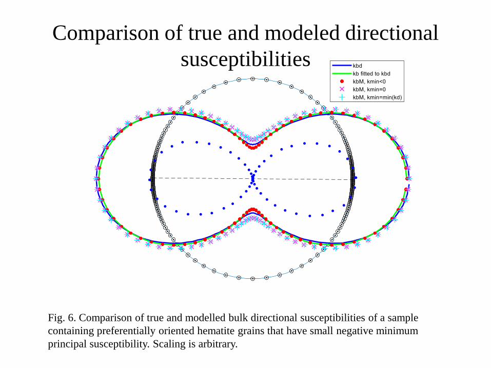
Fig. 6. Comparison of true and modelled bulk directional susceptibilities of a sample

containing preferentially oriented hematite grains that have small negative minimum

principal susceptibility. Scaling is arbitrary.

Comparison of true and modeled directional

susceptibilities

In Fig. 6, black dots on unit circle show preferred orientation of basal planes of hematite grains

caused by vertical compression.

Each grain poses the same set of directional susceptibilities (as in Fig. 2). This is indicated by

blue dots showing directional susceptibilities of a grain whose basal plane is oriented sub-

horizontally. (Directional susceptibilities of other grains are rotated accordingly to grain

orientation.)

Bulk directional susceptibility kbd is plotted by blue curve. Due to preferred orientation, the curve

is squeezed in vertical direction but not as much as grain directional susceptibility (blue dots).

Directional susceptibilities back-computed from the tensor of bulk susceptibility kb create the

green curve. This curve is close to the blue one, only in vertical direction, it tends more towards

origin.

Coloured dots are directional susceptibilities computed from modelled bulk susceptibility kbM .

This is done for several options of grain susceptibility tensor, differing by the choice of minimum

principal susceptibility:

red … K1 = 0.011 and K3 = - 0.0006 (as obtained by tensor fit of the original data, Fig. 3)

magenta … K1 = 0.011 and K3 = 0 (negative value replaced by zero)

cyan … K1 = 0.011 and K3 = min(grain kd) (minimum measured directional susceptibility )

Zkousel jsem i jiné varianty, ale tyto asi postaci.

Results of the comparison and discussion

Red dots in Fig. 6 coincide with the green curve which means that fabric modelling based

on the grain susceptibility tensor containing small negative minimum principal susceptibility

(i.e., when we simply keep this value in the grain tensor) leads to result equivalent to fitting tensor

in true directional susceptibilities of the sample (i.e., what we obtain by standard measurement).

Nevertheless, keeping the negative minimum grain susceptibility is unpleasant (creating a false

feeling of diamagnetic behaviour of hematite in this direction). From this point of view, a

replacement of the negative value by zero or by minimum grain directional susceptibility would be

suitable. Fig. 6 shows such approach provides less accurate fit that keeps principal directions but

decreases degree of fabric (P). By the intensity of preferred orientation shown in Fig. 6, P changes

from approximately 5 to 4.

Important is that in fabric modelling, neither using the small negative grain susceptibility nor its

replacement by zero or small positive value influences orientation of eigenvectors (lineation,

foliation).

Comment: Fig. 6 indicates large value of modelled bulk fabric degree of anisotropy (PbM ~

4 to 6) which corresponds to very large grain degree Pg. We can analyse it by means of

eq. (6). We find

PbM = [Pg(1 – Emin) + Emin ]/[Pg(1 – Emax) + Emax] (7)

PbM = (1 – Emin)/(1 – Emax) (8)

where Emax and Emin are eigenvalues of

the orientation tensor of hematite poles.

This relation is plotted in Fig. 7.

Fig.7 Equation (7) for different intensity

of hematite poles preferred orientation.

This ratio is plotted in Fig. 7 by red broken line. For large Pg, the degree of bulk fabric is almost

independent of Pg. It was observed already by Hrouda 1981 (Fig. 8).

When grain minimum susceptibility is very small (or equal to zero), the grain degree is

large (or infinite) and the formula simplifies to

Bulk degree of AMS, Grain degree of AMS, Concentration Parameter

Effects of Grain AMS and Preferred Orientation: a model

(Hrouda, 1981, JSG)

If Pc>100, knowledge of its precise value plays no role in modelling.

Fig. 8

Fig. 9. Isolinies of directional susceptibility

and its surface (lower part) reconstructed from

all three measured planes. Red square and line (with

arrows) show first eigenvector of susceptibility, black

square and line indicates maxima of the surface of

directional susceptibility

Reconstruction of 3D directional susceptibility

Using data from all three planes, the surface of directional susceptibility was reconstructed.

The result indicates that using full 3D data (that are currently measured by the authors of the

contribution) should lead to analogous mathematical description as the one used above.

(Hrouda et al.,1985, J. Geophys.)

Reflected-light Microscopy

X-ray Pole Figure Goniometry

AMS

HEMATITE ORE, Minas Gerais, Brazil

Theoretical and Measured AMS

measured calculated from X-ray

1. Measured principal susceptibilities are oriented in the

same way as calculated theoretically from the c-axis pattern.

2. Measured degree of AMS and shape parameter are slightly

lower than those calculated theoretically from c-axis pattern.

3. The above differences may result from the fact that the

AMS and X-ray measurements were not executed on exactly

the same specimens and the respective specimen volumes

differed substantially (1 cm3 vs. thin section).

Conclusion

Negative minimum susceptibility of hematite single crystal measured and

calculated using standard AMS technique is an artifact.

It:

- does not invalidate standard models of magnetic fabric

- does not influence orientation of eigenvectors (lineation, foliation)

- can be replaced by zero or a small value > 0 in fabric modelling

- its replacement decreases, proportionally to intensity of preferred orientation,

the parameter P

- in weak preferred orientation of grains this effect is not important