prediction of upper body power of cross-country skiers using support vector machines

Arab J Sci Eng (2015) 40:1045–1055DOI 10.1007/s13369-015-1588-y

RESEARCH ARTICLE - COMPUTER ENGINEERING AND COMPUTER SCIENCE

Prediction of Upper Body Power of Cross-Country SkiersUsing Support Vector Machines

Mehmet Fatih Akay · Fatih Abut ·Shahaboddin Daneshvar · Dan Heil

Received: 12 September 2014 / Accepted: 19 January 2015 / Published online: 1 February 2015© King Fahd University of Petroleum and Minerals 2015

Abstract Upper body power (UBP) is an important deter-minant of cross-country ski race performance. Althoughnumerous studies exist to measure UBP of cross-countryskiers, to date, no study has ever attempted to predict UBPof cross-country skiers. The purpose of this paper was todevelop prediction models for estimating 10-s UBP (UBP10)

and 60-s UBP (UBP60) of cross-country skiers using sup-port vector machines (SVM). Four types of SVMs havebeen considered, they are as follows: SVM using the radialbasis function kernel (SVM-RBF), SVM using the sigmoidkernel, SVM using the polynomial kernel, and SVM usingthe linear kernel. For comparison purposes, UBP predictionmodels based on multilayer perceptron and multiple linearregression have also been developed. The dataset used inthis study includes data of 77 subjects. Age, gender, height,weight, body mass index, maximal heart rate, maximal oxy-gen uptake, and exercise time are the predictor variables, andUBP10 and UBP60 are the target variables. Several UBP pre-diction models have been developed by using the combina-tion of the predictor variables to predict UBP10 and UBP60.By using 10-fold cross-validation on the datasets, the per-formance of the models has been evaluated by calculatingtheir standard error of estimates (SEEs) and multiple cor-relation coefficients (Rs). The results show that SVM-RBF-based UBP prediction models perform much better (i.e., yieldlower SEEs and higher Rs) than the prediction models devel-oped by other regression methods and can be safely used forthe prediction of UBP of cross-country skiers.

M. F. Akay (B) · F. Abut · S. DaneshvarDepartment of Computer Engineering,Çukurova University, Adana, Turkeye-mail: [email protected]

D. HeilDepartment of Human Health and Development,Montana State University, Bozeman, MT, USA

Keywords Support vector machines · Multilayerperceptron · Upper body power · Prediction

1 Introduction

The sport of cross-country skiing is thought to have origi-nated over 4,000 years ago in northern Europe. For the mostpart of the twentieth century, cross-country ski racing con-sisted only of the classical style, in which the skis remainparallel to each other within parallel tracks groomed into thesnow. In this style of skiing, there are several distinct tech-niques (i.e., diagonal stride, double-poling, kick double-pole,and herringbone) that are preferentially used as a function ofterrain steepness, skiing speed, as well as skier fitness. Forexample, the diagonal stride technique, commonly used foreasy-to-moderate uphill, inclines the skier strides uphill byspringing from one ski to another while pushing with theopposing pole in a motion similar to running. The double-pole technique, in contrast, is commonly used while classicalskiing on flat terrain under fast conditions. The double-polingtechnique requires the skier to coordinate the dynamic andsimultaneous downward pole pushing motion of the upperbody with hip flexion to create forward propulsion primar-ily with the upper body. By the mid-1980s, a new cross-country skiing style called “skating” had become popularamong competitive ski racers. The skating style is a motionsimilar to ice skating. Although the two styles appear quitedifferent, they require the same fitness components for suc-cess such as balance, coordination, aerobic and anaerobicendurance, and double-poling UBP.

The need for UBP in cross-country ski racing is a con-sequence of using the poles for propulsion. Power gener-ated by the upper body is transmitted through the polesand assists in forward motion. The reason for researchers’

123

1046 Arab J Sci Eng (2015) 40:1045–1055

focus on the double-poling technique [1–3] is that this pol-ing motion is common to several classical (i.e., kick double-pole and double-poling) and skating techniques. For exam-ple, the upper body has been shown to contribute as much as50 % to the total propulsive force during uphill skating and15–30 % during uphill classical skiing. Laboratory measureof UBP has also been shown to correlate highly with bothskate [4,5] and classic [5,6] ski racing performances. Whiletests for measuring UBP power have varied between 1 and180 s, numerous researchers have concluded that UBP playsa critical role in determining cross-country ski racing abil-ity [4,5]. For example, it has been reported that the highest1-s peak measure of UBP correlated highly with 5- km skat-ing performance, while both 10-s and 60-s measures of UBPcorrelated even higher with 10- km classic performance [6].Collectively, these findings indicate that the ability to gener-ate a high UBP is an important determinant of both skatingand classic ski race performance, regardless of whether thepower output can be sustained for a few seconds or severalminutes.

Despite the frequency with which UBP is reported uponin the research literature, the instrumentation for measur-ing UBP is not yet commonly available. The tests of UBPin the research literature, for instance, have all been basedupon custom-designed ergometers for individual researchlaboratories. Additionally, the measurement of UBP lacksstandardization as it is still a relatively new physiologicalconstruct. For ski coaches and athletes, these limitations rep-resent barriers to the design and tracking training programeffectiveness. Many elite cross-country skiers, for example,have access to standard sports science laboratory testing suchas tests of maximal oxygen uptake (VO2max), maximal heartrate (HRmax), lactate threshold (LT), as well as various mea-sures of muscular strength and lower body power. Test mea-sures of UBP, however, are almost exclusively limited to sportresearch facilities with these custom-designed ergometers.Thus, it may be advantageous to predict UBP using UBP testresults that have been shown to correlate highly with bothskate and classic ski racing performances [5,6].

Given that many elite skiers have access to a standardbattery of laboratory tests, such as VO2 max testing, it is rea-sonable to suggest that measures of UBP could be predictedfrom this collection of tests. In doing so, skiers without accessto direct measures of UBP would be able to predict their UBPand then compare this prediction with measures reported inthe research literature.

In 1997, an innovative artificial intelligence techniquecalled SVM was proposed in order to overcome the short-comings of the neural networks methods [7]. SVM employsthe structural risk minimization (SRM) principle, which is aninduction principle minimizing an upper bound of the gen-eralization error. During the past years, the SVM has beenemployed in wide range of applications such as pattern recog-

nition [8], text categorization [9], financial applications [10],atmospheric science prediction [11], and electrical load pre-diction [12]. However, to the best of our knowledge, SVM hasnever been used for the prediction of UBP of cross-countryskiers.

The purpose of this paper was to develop prediction mod-els for estimating UBP10 and UBP60 of cross-country skiersusing SVM-RBF, SVM using the sigmoid kernel (SVM-Sigmoid), SVM using the polynomial kernel (SVM-Poly),and SVM using the linear kernel (SVM-Linear), and comparethe results with the ones obtained by multilayer perceptron(MLP) and multiple linear regression (MLR). The datasetincludes measured UBP10 and UBP60 values of 77 subjectsas well as the predictor variables age, gender, height, weight,body mass index (BMI), HRmax, VO2 max, and exercisetime. Using combinations of the predictor variables, 28 UBPprediction models have been developed. Performance metricssuch as SEE and R have been used to assess the performanceof the prediction models by using 10-fold cross-validation.The results show that the SEEs of the SVM-RBF-based mod-els for the prediction of UBP10 and UBP60 range from 31.66to 49.11 W and from 18.11 to 37.60 W, respectively, and aremuch lower than the SEEs obtained by other regression meth-ods.

The remainder of the paper is organized as follows: Sect. 2presents an overview of SVM. Section 3 gives details aboutthe procedure of dataset generation. Section 4 describes thedetails of the SVM and MLP prediction model. Section 5gives results and discussions. The last section, Sect. 6, con-cludes the paper along with outlining future directions.

2 Overview of Support Vector Machines

2.1 Linear SVM

Given the training data (xi , yi ), (i = 1, . . . , �), where x is ad-dimensional input with x ∈ �d and the output is y ∈ �.The linear regression model can be written as follows:

f (x) = 〈ω, x〉 + b, ω, x ∈ �d , b ∈ �, (1)

where f (x) is an unknown target function, ω is the normalvector to the hyperplane, b is the bias, and 〈., .〉 denotes thedot product in �d .

In order to measure the empirical risk, we should spec-ify a loss function. The most common loss function is theε-insensitive loss function proposed by Vapnik [7] and isdefined by the following function

Lε(y) ={

0 for | f (x) − y| ≤ ε

| f (x) − y| − ε otherwise(2)

123

Arab J Sci Eng (2015) 40:1045–1055 1047

The optimal parameters ω and b in (1) are found by solvingthe primal optimization problem

min1

2‖ω‖2 + C

�∑i=1

(ξ−i + ξ+

i ) (3)

with constraints

yi − 〈ω, xi 〉 − b ≤ ε + ξ+i ,

〈ω, xi 〉 + b − yi ≤ ε + ξ+i , (4)

ξ+i , ξ−

i ≥ 0, i = 1, . . . , �

where C is a pre-specified value that determines the trade-off between the flatness of f (x) and the amount up to whichdeviations larger than the precision ε are tolerated. The slackvariables ξ− and ξ+ represent the deviations from the con-straints of the ε-tube.

Usually, the dual problem is solved. The correspondingdual optimization problem is defined as

maxα,α∗ −1

2

�∑i=1

�∑j=1

(α∗i − αi )(α

∗j − α j )〈xi , x j 〉

−�∑

i=1

yi (α∗i − αi ) − ε

�∑i=1

(α∗i + αi ) (5)

with constraints

0 ≤ αi , α∗i ≤ C, i = 1, . . . , �,

�∑i=1

(αi − α∗i ) = 0 (6)

The optimal Lagrange multipliers are given by solving theoptimization problem defined by (5) and (6)

α and α∗, while ω and b are given by

ω =�∑

i=1

(α∗i − αi )xi ,

b = −1

2〈ω, (xr + xs)〉 ,

(7)

where xr and xs are support vectors.

2.2 Nonlinear SVM

For nonlinear regression problems, a nonlinear mapping φ

of the input space onto a higher dimension feature space canbe used, and then, linear regression can be performed in thisspace. The nonlinear model is written as

f (x) = 〈ω, φ(x)〉 + b, ω, x ∈ �d , b ∈ �, (8)

where

ω =�∑

i=1

(αi − α∗i )φ(xi ),

〈ω, φ(x)〉 =�∑

i=1

(αi − α∗i ) 〈φ(xi ), φ(x)〉

=�∑

i=1

(αi − α∗i )K (xi , x),

b = −1

2

�∑i=1

(αi − α∗i )(K (xi , xr ) + K (xi , xs)) (9)

where xr and xs are support vectors. Note that we express dotproducts through a kernel function K that satisfies Mercer’sconditions.

Equation (8) can be written as follows: if the term b isaccommodated within the kernel function

�∑i=1

(αi − α∗i )K (xi , x) (10)

Several kernel functions have appeared in the literature. Theradial basis function (RBF) has received significant attention,most commonly with a Gaussian of the form

K (x, x ′) = exp

(−‖x − x ′‖2

2γ 2

), (11)

where γ is the width of the RBF kernel.Other kernel functions are the sigmoid kernel

K (x, x ′) = tanh(αxT x ′ + c), (12)

where α is the slope and c is the intercept constant and thepolynomial kernel

K (x, x ′) = tanh(αxT x ′ + c)d , (13)

where α is the slope, c is the constant term, and d is thepolynomial degree.

3 Dataset Generation

Trained cross-country ski racers with a minimum of 2 yearsof ski racing experience participated in data collection for thisstudy. Participants were primarily collegiate racers from theMontana State University (MSU) ski team and junior racersfrom the Bridger Ski Foundation (BSF) ski team, all of whomwere living in Bozeman, MT (USA), at the time of testing. Alltesting occurred in MSU’s Movement Science/Human Per-formance Laboratory (MSL). As a matter of test scheduling,

123

1048 Arab J Sci Eng (2015) 40:1045–1055

participants were instructed to avoid high-intensity trainingof any kind within 24 h of laboratory testing, as well as toprepare (i.e., rest, hydrate, timing of meals, and warming up)for each laboratory visit as they would for a ski race.

The data for this study were collected as part of the MSL’sannual Athlete Testing Program for both of these local skiteams between 2008 and 2012. Some skiers were representedwithin the dataset more than once because of repeat testingof the same skier over multiple years. However, this wasallowed only if one or more of the following occurred suchas (1) at least two or more years had passed since recordingof the previous test data; (2) the skier’s performance abilitieshad changed considerably (e.g., they had recovered from aninjury or extended bout of sickness; the skier missed a yearof racing for other reasons) since recording of the previoustest data. All skiers read and sign an informed consent doc-ument approved by the MSU internal review board (IRB)prior to participating in the Athlete Testing Program. To col-lect these data, two separate laboratory visits on back-to-backdays were required for all participants. On the first day of test-ing, half of the participants completed the UBP tests, whilethe remaining participants completed a treadmill-based testto measure VO2 max. All demographic measures (age, bodyheight, and body mass), as well as a health history ques-tionnaire, were also completed on the first day of testing.On the second day of testing, the participants switched tests(e.g., those that had completed the UBP tests the previousday were now to complete the treadmill test) such that allparticipants completed both UBP and treadmill tests withina 48- h time span.

The UBP test protocols, as well as data that validate theUBP10 and UBP60 measures as markers of skiing perfor-mance, have been reported previously by Alsobrook and Heil[13]. Briefly, UBP10 involves generating the highest averagepower using a simulated double-poling motion on a custom-designed ergometer. The UBP60 protocol measured the aver-age upper body power generated over 60 s using the samedouble-poling ergometer as for the UBP10 test. The protocolfor measuring VO2 max has also been described previously[14] where the measurements of VO2 max were determinedfrom a ski striding protocol taken to volitional exhaustion.Test completion time, recorded to the nearest second, wasconsidered a measure of time to exhaustion when the partic-ipant could no longer keep up with the treadmill protocol.To be considered a valid treadmill test, each VO2 max testmeasured had to satisfy at least two of these three criteria: 1)a maximal respiratory exchange ratio (RER) ≥1.1; the twohighest VO2 values being within 2.5 ml/kg/min of each other(i.e., plateau of VO2); a HRmax within ±5 bpm of the lastrecorded HRmax (if the VO2 max test was within the previ-ous 2 years), or an HRmax within ±10 bmp of age-predictedmaximal heart rate (i.e., 220 age). The descriptive statisticsof the dataset are summarized in Table 1.

Table 1 Descriptive statistics of the dataset

Variable name Mean ± SD

Gender 0.474 ± 0.504

Age 18.789 ± 1.998

Weight (kg) 67.719 ± 6.988

Height (cm) 174.481 ± 8.264

BMI (kg/m2) 22.265 ± 1.906

Time (s) 11.791 ± 1.002

VO2 max (ml/kg/min) 63.091 ± 8.432

HR (bpm) 195.035 ± 7.263

UBP10 (W) 231.035 ± 73.091

UBP60 (W) 177.491 ± 55.977

4 SVM and MLP Prediction Models

4.1 SVM Models for Predicting UBP

The quality and performance of an SVM model depends onseveral parameters such as the value of C , the type of ker-nel function, parameters of the kernel function, and the valueof ε for the ε-insensitive loss function. The trade-off costbetween minimizing the training error and minimizing modelcomplexity is determined by the parameter C . The numberof training errors increases with a small value for C . On theother hand, a behavior similar to that of a hard-margin SVMis observed with a large C . The nonlinear mapping from theinput space to high-dimensional feature space is defined bythe kernel function parameters [15]. The number of supportvectors is determined by the value of ε. Several kernels (RBF,sigmoid, polynomial, and linear) have been chosen in thisstudy to develop the SVM models for the prediction of UBP.The RBF kernel requires the optimization of the functionparameter γ , the sigmoid kernel requires the optimizationof the function parameters α and c, and the polynomial ker-nel requires the optimization of the function parameters α, cand d.

Before creating an SVM model, one usually cannot knowin advance which values of C , ε, and kernel parameters arethe most suitable best for a given problem. In this sense, somekind of parameter search and optimization should be carriedout with the purpose of finding the optimal values of (C, ε,kernel parameters) so that the testing data can be predictedwith minimum error. Grid search [16], cross-validation, par-ticle swarm optimization [17], and genetic algorithm [18]have been proposed in the literature to select the optimal val-ues of (C, ε, kernel parameters). The grid search method isan efficient method for finding the optimal values of C, ε andkernel parameters for median-sized problems. The principleof grid search was to vary the values of the parameters byfixed step sizes through a range of values. The performance

123

Arab J Sci Eng (2015) 40:1045–1055 1049

of the set of parameters is measured and compared using dif-ferent criteria such as minimizing root mean squared errorand maximizing correlation coefficient.

Cross-validation is a popular and widely used model val-idation technique [19–22] for assessing how the results ofmachine learning analysis will generalize to an independentdataset. It is mainly used in settings where the goal was pre-diction, and one wants to estimate how accurately a predic-tive model will perform in practice. In a prediction problem,a model is usually given a dataset of known data on whichtraining is run (training dataset), and a dataset of unknowndata (or unseen data) against which the model is tested (test-ing dataset). The goal of cross-validation was to define adataset to test the model in the training phase (i.e., the val-idation dataset), in order to limit problems like overfitting,give an insight on how the model will generalize to an inde-pendent dataset. The holdout method is the simplest kindof cross-validation. The dataset is separated into two sets,called the training set and the testing set. The machine learn-ing algorithm fits a function using the training set only. Then,the machine learning algorithm is asked to predict the outputvalues for the data in the testing set (it has never seen theseoutput values before). However, its evaluation can have ahigh variance. The evaluation may depend heavily on whichdata points end up in the training set and which end up inthe test set, and thus, the evaluation may be significantly dif-ferent depending on how the division is made. K-fold cross-validation is one way to improve over the holdout method.The dataset is divided into k subsets, and the holdout methodis repeated k times. Each time, one of the k subsets is usedas the test set, and the other k − 1 subsets are put together toform a training set. Then, the average error across all k trialsis computed. The advantage of this method is that it mattersless how the data get divided. Every data point gets to be ina test set exactly once, and gets to be in a training set k − 1times. The variance in the resulting estimate is reduced as kis increased.

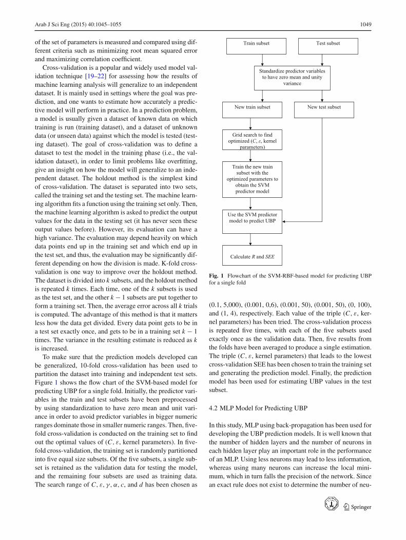
To make sure that the prediction models developed canbe generalized, 10-fold cross-validation has been used topartition the dataset into training and independent test sets.Figure 1 shows the flow chart of the SVM-based model forpredicting UBP for a single fold. Initially, the predictor vari-ables in the train and test subsets have been preprocessedby using standardization to have zero mean and unit vari-ance in order to avoid predictor variables in bigger numericranges dominate those in smaller numeric ranges. Then, five-fold cross-validation is conducted on the training set to findout the optimal values of (C, ε, kernel parameters). In five-fold cross-validation, the training set is randomly partitionedinto five equal size subsets. Of the five subsets, a single sub-set is retained as the validation data for testing the model,and the remaining four subsets are used as training data.The search range of C, ε, γ, α, c, and d has been chosen as

Train subset Test subset

Standardize predictor variables to have zero mean and unity

variance

New train subset New test subset

Grid search to find optimized (C, ε, kernel

parameters)

Train the new train subset with the

optimized parameters to obtain the SVM predictor model

Use the SVM predictor model to predict UBP

Calculate R and SEE

Fig. 1 Flowchart of the SVM-RBF-based model for predicting UBPfor a single fold

(0.1, 5,000), (0.001, 0,6), (0.001, 50), (0.001, 50), (0, 100),and (1, 4), respectively. Each value of the triple (C, ε, ker-nel parameters) has been tried. The cross-validation processis repeated five times, with each of the five subsets usedexactly once as the validation data. Then, five results fromthe folds have been averaged to produce a single estimation.The triple (C, ε, kernel parameters) that leads to the lowestcross-validation SEE has been chosen to train the training setand generating the prediction model. Finally, the predictionmodel has been used for estimating UBP values in the testsubset.

4.2 MLP Model for Predicting UBP

In this study, MLP using back-propagation has been used fordeveloping the UBP prediction models. It is well known thatthe number of hidden layers and the number of neurons ineach hidden layer play an important role in the performanceof an MLP. Using less neurons may lead to less information,whereas using many neurons can increase the local mini-mum, which in turn falls the precision of the network. Sincean exact rule does not exist to determine the number of neu-

123

1050 Arab J Sci Eng (2015) 40:1045–1055

rons in a hidden layer, the optimal number is empiricallyselected based on the experience of the user and the physicalcomplexity of the problem. The number of neurons in the hid-den layers of MLP prediction models has been determinedby trial and error.

As in the SVM model, the inputs and outputs are normal-ized so that they have zero mean and unity variance. Prin-cipal component analysis (PCA) method has been also usedto orthogonalize the components of the input vectors and toorder the resulting orthogonal components so that those withthe largest variation come first [23]. As activation functions,the tansigmoid has been used in the hidden layer, and thelinear function has been used at the output layer. The otherimportant parameters of the MLP models are the number ofepochs (selected as 100), the learning rate (selected between0.3 and 0.7 depending on the prediction model), and momen-tum (selected between 0.1 and 1 depending on the predictionmodel).

For all prediction models, UBP10 and UBP60 havebeen predicted using SVM-RBF, SVM-Sigmoid, SVM-Poly,SVM-Linear, MLP, and MLR. The performance of all pre-diction models has been evaluated by using 10-fold cross-validation and calculating the SEE and R, whose formulasare given in (14) and (14), respectively,

SEE =√∑

(Y − Y ′)2

N

R =√

1 −∑

(Y − Y ′)2∑(Y − Y )2

(14)

In (14) and (14), Y is the measured UBP value, Y ′ is thepredicted UBP value, Y is the mean of the measured UBPvalues, and N is the number of samples in a test subset.

5 Results and Discussion

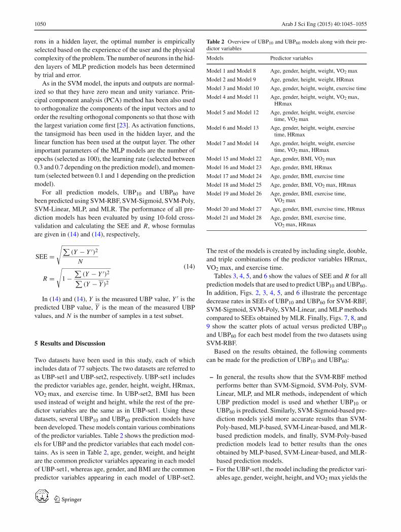
Two datasets have been used in this study, each of whichincludes data of 77 subjects. The two datasets are referred toas UBP-set1 and UBP-set2, respectively. UBP-set1 includesthe predictor variables age, gender, height, weight, HRmax,VO2 max, and exercise time. In UBP-set2, BMI has beenused instead of weight and height, while the rest of the pre-dictor variables are the same as in UBP-set1. Using thesedatasets, several UBP10 and UBP60 prediction models havebeen developed. These models contain various combinationsof the predictor variables. Table 2 shows the prediction mod-els for UBP and the predictor variables that each model con-tains. As is seen in Table 2, age, gender, weight, and heightare the common predictor variables appearing in each modelof UBP-set1, whereas age, gender, and BMI are the commonpredictor variables appearing in each model of UBP-set2.

Table 2 Overview of UBP10 and UBP60 models along with their pre-dictor variables

Models Predictor variables

Model 1 and Model 8 Age, gender, height, weight, VO2 max

Model 2 and Model 9 Age, gender, height, weight, HRmax

Model 3 and Model 10 Age, gender, height, weight, exercise time

Model 4 and Model 11 Age, gender, height, weight, VO2 max,HRmax

Model 5 and Model 12 Age, gender, height, weight, exercisetime, VO2 max

Model 6 and Model 13 Age, gender, height, weight, exercisetime, HRmax

Model 7 and Model 14 Age, gender, height, weight, exercisetime, VO2 max, HRmax

Model 15 and Model 22 Age, gender, BMI, VO2 max

Model 16 and Model 23 Age, gender, BMI, HRmax

Model 17 and Model 24 Age, gender, BMI, exercise time

Model 18 and Model 25 Age, gender, BMI, VO2 max, HRmax

Model 19 and Model 26 Age, gender, BMI, exercise time,VO2 max

Model 20 and Model 27 Age, gender, BMI, exercise time, HRmax

Model 21 and Model 28 Age, gender, BMI, exercise time,VO2 max, HRmax

The rest of the models is created by including single, double,and triple combinations of the predictor variables HRmax,VO2 max, and exercise time.

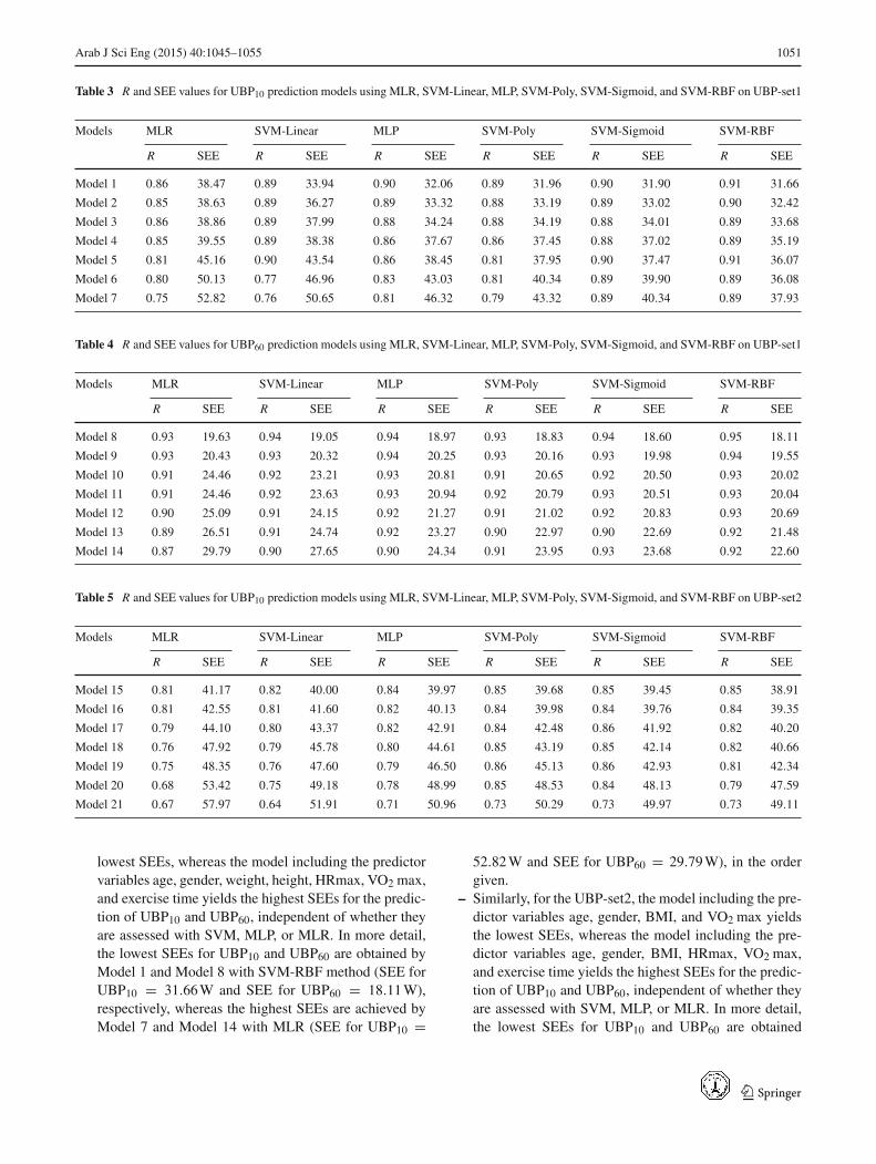
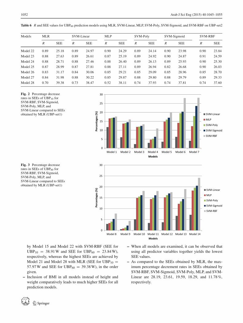
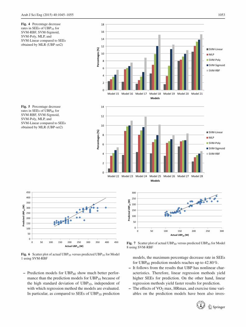
Tables 3, 4, 5, and 6 show the values of SEE and R for allprediction models that are used to predict UBP10 and UBP60.In addition, Figs. 2, 3, 4, 5, and 6 illustrate the percentagedecrease rates in SEEs of UBP10 and UBP60 for SVM-RBF,SVM-Sigmoid, SVM-Poly, SVM-Linear, and MLP methodscompared to SEEs obtained by MLR. Finally, Figs. 7, 8, and9 show the scatter plots of actual versus predicted UBP10

and UBP60 for each best model from the two datasets usingSVM-RBF.

Based on the results obtained, the following commentscan be made for the prediction of UBP10 and UBP60:

– In general, the results show that the SVM-RBF methodperforms better than SVM-Sigmoid, SVM-Poly, SVM-Linear, MLP, and MLR methods, independent of whichUBP prediction model is used and whether UBP10 orUBP60 is predicted. Similarly, SVM-Sigmoid-based pre-diction models yield more accurate results than SVM-Poly-based, MLP-based, SVM-Linear-based, and MLR-based prediction models, and finally, SVM-Poly-basedprediction models lead to better results than the onesobtained by MLP-based, SVM-Linear-based, and MLR-based prediction models.

– For the UBP-set1, the model including the predictor vari-ables age, gender, weight, height, and VO2 max yields the

123

Arab J Sci Eng (2015) 40:1045–1055 1051

Table 3 R and SEE values for UBP10 prediction models using MLR, SVM-Linear, MLP, SVM-Poly, SVM-Sigmoid, and SVM-RBF on UBP-set1

Models MLR SVM-Linear MLP SVM-Poly SVM-Sigmoid SVM-RBF

R SEE R SEE R SEE R SEE R SEE R SEE

Model 1 0.86 38.47 0.89 33.94 0.90 32.06 0.89 31.96 0.90 31.90 0.91 31.66

Model 2 0.85 38.63 0.89 36.27 0.89 33.32 0.88 33.19 0.89 33.02 0.90 32.42

Model 3 0.86 38.86 0.89 37.99 0.88 34.24 0.88 34.19 0.88 34.01 0.89 33.68

Model 4 0.85 39.55 0.89 38.38 0.86 37.67 0.86 37.45 0.88 37.02 0.89 35.19

Model 5 0.81 45.16 0.90 43.54 0.86 38.45 0.81 37.95 0.90 37.47 0.91 36.07

Model 6 0.80 50.13 0.77 46.96 0.83 43.03 0.81 40.34 0.89 39.90 0.89 36.08

Model 7 0.75 52.82 0.76 50.65 0.81 46.32 0.79 43.32 0.89 40.34 0.89 37.93




Model 8 0.93 19.63 0.94 19.05 0.94 18.97 0.93 18.83 0.94 18.60 0.95 18.11

Model 9 0.93 20.43 0.93 20.32 0.94 20.25 0.93 20.16 0.93 19.98 0.94 19.55

Model 10 0.91 24.46 0.92 23.21 0.93 20.81 0.91 20.65 0.92 20.50 0.93 20.02

Model 11 0.91 24.46 0.92 23.63 0.93 20.94 0.92 20.79 0.93 20.51 0.93 20.04

Model 12 0.90 25.09 0.91 24.15 0.92 21.27 0.91 21.02 0.92 20.83 0.93 20.69

Model 13 0.89 26.51 0.91 24.74 0.92 23.27 0.90 22.97 0.90 22.69 0.92 21.48

Model 14 0.87 29.79 0.90 27.65 0.90 24.34 0.91 23.95 0.93 23.68 0.92 22.60




Model 15 0.81 41.17 0.82 40.00 0.84 39.97 0.85 39.68 0.85 39.45 0.85 38.91

Model 16 0.81 42.55 0.81 41.60 0.82 40.13 0.84 39.98 0.84 39.76 0.84 39.35

Model 17 0.79 44.10 0.80 43.37 0.82 42.91 0.84 42.48 0.86 41.92 0.82 40.20

Model 18 0.76 47.92 0.79 45.78 0.80 44.61 0.85 43.19 0.85 42.14 0.82 40.66

Model 19 0.75 48.35 0.76 47.60 0.79 46.50 0.86 45.13 0.86 42.93 0.81 42.34

Model 20 0.68 53.42 0.75 49.18 0.78 48.99 0.85 48.53 0.84 48.13 0.79 47.59

Model 21 0.67 57.97 0.64 51.91 0.71 50.96 0.73 50.29 0.73 49.97 0.73 49.11

lowest SEEs, whereas the model including the predictorvariables age, gender, weight, height, HRmax, VO2 max,and exercise time yields the highest SEEs for the predic-tion of UBP10 and UBP60, independent of whether theyare assessed with SVM, MLP, or MLR. In more detail,the lowest SEEs for UBP10 and UBP60 are obtained byModel 1 and Model 8 with SVM-RBF method (SEE forUBP10 = 31.66 W and SEE for UBP60 = 18.11 W),respectively, whereas the highest SEEs are achieved byModel 7 and Model 14 with MLR (SEE for UBP10 =

52.82 W and SEE for UBP60 = 29.79 W), in the ordergiven.

– Similarly, for the UBP-set2, the model including the pre-dictor variables age, gender, BMI, and VO2 max yieldsthe lowest SEEs, whereas the model including the pre-dictor variables age, gender, BMI, HRmax, VO2 max,and exercise time yields the highest SEEs for the predic-tion of UBP10 and UBP60, independent of whether theyare assessed with SVM, MLP, or MLR. In more detail,the lowest SEEs for UBP10 and UBP60 are obtained

123

1052 Arab J Sci Eng (2015) 40:1045–1055




Model 22 0.89 25.18 0.89 24.97 0.90 24.29 0.89 24.14 0.90 23.98 0.90 23.84

Model 23 0.88 27.63 0.89 26.61 0.87 25.19 0.89 24.92 0.90 24.87 0.91 24.59

Model 24 0.88 28.71 0.88 27.46 0.88 26.40 0.89 26.13 0.89 25.93 0.90 25.30

Model 25 0.87 28.99 0.87 27.81 0.88 27.11 0.89 26.94 0.82 26.68 0.90 26.03

Model 26 0.83 31.17 0.84 30.06 0.85 29.21 0.85 29.09 0.85 28.96 0.85 28.70

Model 27 0.84 31.98 0.88 30.22 0.85 29.87 0.88 29.80 0.88 29.79 0.89 29.33

Model 28 0.70 39.38 0.73 38.47 0.52 38.11 0.74 37.93 0.74 37.81 0.74 37.60

Fig. 2 Percentage decreaserates in SEEs of UBP10 forSVM-RBF, SVM-Sigmoid,SVM-Poly, MLP, andSVM-Linear compared to SEEsobtained by MLR (UBP-set1)

0

5

10

15

20

25

30

Model 1 Model 2 Model 3 Model 4 Model 5 Model 6 Model 7

Perc

enta

ges (

%)

Models

SVM-Linear

MLP

SVM-Poly

SVM-Sigmoid

SVM-RBF


0

5

10

15

20

25

30


Perc

enta

ges (

%)

Models

SVM-Linear

MLP

SVM-Poly

SVM-Sigmoid

SVM-RBF

by Model 15 and Model 22 with SVM-RBF (SEE forUBP10 = 38.91 W and SEE for UBP60 = 23.84 W),respectively, whereas the highest SEEs are achieved byModel 21 and Model 28 with MLR (SEE for UBP10 =57.97 W and SEE for UBP60 = 39.38 W), in the ordergiven.

– Inclusion of BMI in all models instead of height andweight comparatively leads to much higher SEEs for allprediction models.

– When all models are examined, it can be observed thatusing all predictor variables together yields the lowestSEE values.

– As compared to the SEEs obtained by MLR, the max-imum percentage decrement rates in SEEs obtained bySVM-RBF, SVM-Sigmoid, SVM-Poly, MLP, and SVM-Linear are 28.19, 23.61, 19.59, 18.29, and 11.78 %,respectively.

123

Arab J Sci Eng (2015) 40:1045–1055 1053


0

2

4

6

8

10

12

14

16

18

Model 15 Model 16 Model 17 Model 18 Model 19 Model 20 Model 21Pe

rcen

tage

s (%

)Models

SVM-Linear

MLP

SVM-Poly

SVM-Sigmoid

SVM-RBF


0

2

4

6

8

10

12

14


Perc

enta

ges (

%)

Models

SVM-Linear

MLP

SVM-Poly

SVM-Sigmoid

SVM-RBF

0

50

100

150

200

250

300

350

400

450

0 50 100 150 200 250 300 350 400 450

Pred

icte

d U

BP10

(W)

Actual UBP10 (W)

Fig. 6 Scatter plot of actual UBP10 versus predicted UBP10 for Model1 using SVM-RBF

– Prediction models for UBP60 show much better perfor-mance than the prediction models for UBP10 because ofthe high standard deviation of UBP10, independent ofwith which regression method the models are evaluated.In particular, as compared to SEEs of UBP10 prediction

0

50

100

150

200

250

300

0 50 100 150 200 250 300

Pred

icte

d U

BP60

(W)

Actual UBP60 (W)


models, the maximum percentage decrease rate in SEEsfor UBP60 prediction models reaches up to 42.80 %.

– It follows from the results that UBP has nonlinear char-acteristics. Therefore, linear regression methods yieldhigher SEEs for prediction. On the other hand, linearregression methods yield faster results for prediction.

– The effects of VO2 max, HRmax, and exercise time vari-ables on the prediction models have been also inves-

123

1054 Arab J Sci Eng (2015) 40:1045–1055

0

50

100

150

200

250

300

350

400

450

0 50 100 150 200 250 300 350 400 450

Pred

icte

d U

BP10

(W)

Actual UBP10 (W)


0

50

100

150

200

250

300

0 50 100 150 200 250 300

Pred

icte

d U

BP60

(W)

Actual UBP60 (W)


tigated. The outcomes show that inclusion of onlyVO2 max to the common variables including age, gen-der, weight, and height leads to the lowest SEEs. Thisacknowledges the fact that UBP is highly correlated toVO2 max, as discussed in Sect. 1. On the other hand,addition of only exercise time leads to the highest SEEs.

– When double combinations of the three predictor vari-ables are considered, use of VO2 max and HRmaxtogether yields the lowest SEEs, whereas the combina-tion of HRmax and exercise time gives the highest SEEs.

– Use of VO2 max, HRmax, and exercise time togetheryields the lowest SEEs for all prediction models asthe exercise time variable causes noticeable detrimentaleffect on the prediction.

– This is the first study ever in the literature that proposes topredict UBP of cross-country skiers using machine learn-ing methods. The results show that UBP of cross-countryskiers can be predicted with reasonable error rates. All theexisting methods to determine the UBP of cross-countryskiers use measurement methods. Therefore, it is not pos-sible to compare the results of this study with prior ones.However, MLR is the most common method that has beenused by researchers to predict different parameters suchas VO2 max of sportsmen. In this sense, MLR has been

included in this study for comparison purposes, and it hasbeen shown that machine learning methods such as SVMand MLP perform better than MLR for the prediction ofUBP.

6 Conclusion

In this study, numerous UBP prediction models for cross-country skiers have been developed using different datasetsand combinations of the predictor variables age, gen-der, height, weight, BMI, VO2 max, HRmax, and exercisetime. Different regression methods (i.e., SVM-RBF, SVM-Sigmoid, SVM-Poly, SVM-Linear, MLP, and MLR) havebeen applied on the prediction models. By using 10-foldcross-validation on the datasets, the performance of the mod-els has been evaluated by calculating Rs and SEEs. Theresults show that UBP of cross-country skiers can be pre-dicted with reasonable error rates.

Considering the results obtained, one can reach severalconclusions. First of all, SVM-RBF-based prediction modelsshow better performance (i.e., higher R and lower SEE) thanthe models developed by other regression methods. The orderof the regression methods for the prediction of UBP, from thebest to the worst, is SVM-RBF, SVM-Sigmoid, SVM-Poly,MLP, SVM-Linear, and MLR. Due to the nonlinear char-acteristics of UBP, linear regression methods yield higherSEEs for prediction. On the other hand, linear regressionmethods yield faster results for prediction. Inclusion of theBMI predictor variable in the models increases the error ratesof prediction for UBP. Error rates related to the prediction ofUBP60 are always lower than that of UBP10 because of thehigh standard deviation of UBP10.

This is an initial study to show that UBP of cross-countryskiers can be predicted using SVM. Future work can be per-formed in a number of different areas. Other regression meth-ods such as generalized regression neural networks, radialbasis function neural networks, and tree-boosting can be usedfor the prediction of UBP. Different feature selection algo-rithms can be combined with regression methods to identifythe relevant and irrelevant features for the prediction of UBPof cross-country skiers.

Acknowledgments The authors would like to thank Çukurova Uni-versity Scientific Research Projects Center for supporting this workunder Grant No. FYL-2014-1977.

References

1. Lindinger, S.J.; Holmberg, H.C.: How do elite cross-countryskiers adapt to different double poling frequencies at low to highspeeds?. Eur. J. Appl. Physiol. 111, 1103–1119 (2011)

123

Arab J Sci Eng (2015) 40:1045–1055 1055

2. Lindinger, S.J.; Holmberg, H.C.; Muller, E.; Rapp, W.: Changes inupper body muscle activity with increasing double poling veloci-ties in elite cross-country skiing. Eur. J. Appl. Physiol. 106, 353–363 (2009)

3. Lindinger, S.J.; Stoggl, T.; Muller, E.; Holmberg, H.C.: Controlof speed during the double poling technique performed by elitecross-country skiers. Med. Sci. Sports Exerc. 41, 210–220 (2009)

4. Heil, D.P.; Engen, J.; Higginson, B.K.: Influence of ski pole gripon peak upper body power output in cross-country skiers. Eur. J.Appl. Physiol. 91, 481–487 (2004)

5. Heil, D.P.; Willis, S.J.: Determinants of both classic and skate crosscountry ski performance in competitive junior and collegiate skiers.In: Muller, E., Lindinger, S., Stoggl, S. (eds.) Science and Skiing,vol. V, pp. 513–522. Meyer & Meyer, Germany (2012)

6. Alsobrook, N.G.; Heil, D.P.: Upper body power as a determinantof classical cross-country ski performance. Eur. J. Appl. Phys-iol. 105(4), 633–641 (2009)

7. Vapnik, V.; Golowich, S.; Smola, A.: Support vector method forfunction approximation, regression estimation, and signal process-ing. In: Advances in Neural Information Processing Systems, vol.9, pp. 281–287 (1997)

8. Yulan, L.; Reyes, M.L.; Lee, J.D.: Real-time detection of drivercognitive distraction using Support Vector Machines. IEEE Trans.Intell. Transp. Syst. 8(2), 340–350 (2007)

9. La, L.; Guo, Q.: Text categorization using SVM with exponentweighted ACO. In: 31st Control Conference (CCC), pp. 3763–3768 (2012)

10. Cao, L.J.; Tay, F.E.H.: Support vector machine with adaptive para-meters in financial time series forecasting. IEEE Trans. NeuralNetw. 14(6), 1506–1518 (2003)

11. Yu, P.S.; Chen, S.S.; Chang, I.F.: Support vector regression for real-time flood stage forecasting. J. Hydrol. 328(3–4), 704–716 (2006)

12. Tian, N.A.: A novel approach for short-term load forecasting usingsupport vector machines. Int. J. Neural Syst. 14(5), 329–335 (2004)

13. Alsobrook, N.G.; Heil, D.P.: Anaerobic and aerobic upper bodypower as determinants of classical cross-country ski perfor-mance. Eur. J. Appl. Physiol. 105, 633–641 (2009)

14. Howe, S.M.; Camenisch, K.; Dock, M.M.; Jacobson, E.A.; Pick-els, R.J.; Webster, M.D.; Danevski, D.; Heil, D.P.: Predictionof maximal oxygen update in Nordic skiers. Med. Sci. SportsExerc. 40(5), S418 (2008)

15. Ji, L.; Wang, B.: Parameters selection for SVR based on the SCEM-UA algorithm and its application on monthly runoff prediction. In:Proceedings of the 2007 International Conference on Computa-tional Intelligence and Security, pp. 48–51 (2007)

16. Hsu, C.W.; Lin, C.J.: A comparison of methods for multi-classsupport vector machines. IEEE Trans. Neural Netw. 13(2), 415–425 (2003)

17. Guo, X.C.; Liang, Y.C.; Wu, C.G.; Wang, C.Y.: PSO-based hyper-parameters selection for LS-SVM classifiers. In: Proceedings ofNeural Information Processing, pp. 1138–1147 (2006)

18. Friedrichs, F.; Igel, C.: Evolutionary tuning of multiple SVM para-meters. Neurocomputing 64(C), 107–117 (2005)

19. Min, J.H.; Lee, Y.-C.: Bankruptcy prediction using support vectormachine with optimal choice of kernel function parameters. ExpertSyst. Appl. 28(4), 603–614 (2005)

20. Takahashi, Y.; Nishikoori, K.; Fujishima, S.: Classificationof Pharmacological Activity of Drugs Using Support VectorMachine. pp. 303–311. Second International Workshop, Mae-bashi (2003)

21. Hasseim, A.A.; Sudirman, R.; Khalid, P.I.: Handwriting classifica-tion based on support vector machine with cross validation. Engi-neering 5(5B), 84–87 (2013)

22. He, W.; Jiang, Z.; Li, Z.: Predicting cytokines based on dipeptideand length feature. In: 4th International Conference on IntelligentComputing, Shanghai, China, pp. 86–91 (2008)

23. Jackson, A.S.; Blair, S.N.; Mahar, M.T.; Wier, L.T.; Ross, R.M.;Stuteville, J.E.: Prediction of functional aerobic capacity withoutexercise testing. Med. Sci. Sports Exerc. 22(6), 863–870 (2001)

123

prediction of upper body power of cross-country skiers using support vector machines

Documents