predicting eet-vehicle energy consumption with trip ... - crd
TRANSCRIPT
Predicting �eet-vehicle energy consumptionwith trip segmentation
by
Autumn Umanetz
B.A.Sc, University of Waterloo, 1995
A Thesis Submitted in Partial Ful�llment
of the Requirements for the Degree of
Master of Applied Science
in the Department of Mechanical Engineering
©Autumn Umanetz, 2021
University of Victoria
All rights reserved. This thesis may not be reproduced in whole or in part, by photocopy
or other means, without the permission of the author.
Predicting �eet-vehicle energy consumption
with trip segmentation
by
Autumn Umanetz
B.A.Sc, University of Waterloo, 1995
Supervisory Committee
Dr. Curran Crawford, Co-Supervisor
Department of Mechanical Engineering
Dr. Nedjib Djilali, Co-Supervisor
Department of Mechanical Engineering
ii
Abstract
This study proposes a data-driven model for prediction of the energy consumption of
�eet vehicles in various missions, by characterization as the linear combination of a
small set of exemplar travel segments.
The model was constructed with reference to a heterogenous study group of 29 light
municipal �eet vehicles, each performing a single mission, and each equipped with
a commercial OBD2/GPS logger. The logger data was cleaned and segmented into
3-minute periods, each with 10 derived kinetic features and a power feature. These
segments were used to de�ne three essential model components as follows:
� The segments were clustered into six exemplar travel types (called "eigentrips"
for brevity)
� Each vehicle was de�ned by a vector of its average power in each eigentrip
� Each mission was de�ned by a vector of annual seconds spent in each eigentrip
10% of the eigentrip-labelled segments were selected into a training corpus (representing
historical observations), with the remainder held back for testing (representing future
operations to be predicted). A Light Gradient Boost Machine (LGBM) classi�er was
trained to predict the eigentrip labels with sole reference to the kinetic features, i.e.,
excluding the power observation. The classi�er was applied to the held-back test data,
and the vehicle's characteristic power values applied, resulting in an energy consumption
prediction for each test segment.
The predictions were then summed for each whole-study mission pro�le, and compared
to the logger-derived estimate of actual energy consumption, exhibiting a mean absolute
error of 9.4%. To show the technique's predictive value, this was compared to prediction
with published L/100km �gures, which had an error of 22%. To show the level of
avoidable error, it was compared with an LGBM direct regression model (distinct from
the LGBM classi�er) which reduced prediction error to 3.7%.
iii
Contents
Front Matter i
Title Page . . . . . . . . . . . . . . i
Supervisory Committee . . . . . . ii
Abstract . . . . . . . . . . . . . . . iii
Contents . . . . . . . . . . . . . . . iv
List of Figures . . . . . . . . . . . v
List of Tables . . . . . . . . . . . . vi
Glossary . . . . . . . . . . . . . . . vii
Acknowledgements . . . . . . . . . viii
1 Introduction 1
1.1 Overview . . . . . . . . . . . 1
1.2 Project Context . . . . . . . . 4
1.3 Research Structure . . . . . . 8
2 Background 12
2.1 Travel Data . . . . . . . . . . 12
2.2 Machine Learning . . . . . . . 16
2.3 Data Collection . . . . . . . . 23
3 Data Cleaning and Preparation 27
3.1 Raw Data . . . . . . . . . . . 27
3.2 Speed Data Cleaning . . . . . 30
3.3 Power Data Cleaning . . . . . 32
3.4 Regularization . . . . . . . . . 35
4 Methodology 37
4.1 Feature Preparation . . . . . 37
4.2 Clustering . . . . . . . . . . . 41
4.3 Classi�cation Algorithm . . . 42
4.4 Classi�cation Method . . . . 48
4.5 Energy Prediction . . . . . . 49
4.6 Parameter Re�nement . . . . 50
4.7 Comparison Predictions . . . 55
5 Results 57
5.1 Presentation of Error . . . . . 58
5.2 Discussion . . . . . . . . . . . 60
5.3 Application . . . . . . . . . . 65
5.4 Shapley Additive Explanation 68
6 Conclusions 71
7 Recommendations and Future
Work 73
7.1 Assumptions . . . . . . . . . 73
7.2 Cleaning Decisions . . . . . . 76
7.3 Data Structure . . . . . . . . 78
7.4 Modeling . . . . . . . . . . . 81
7.5 Data and Features . . . . . . 83
7.6 Applications . . . . . . . . . . 86
8 Bibliography 88
A Logger features 100
B Embodied energy and Fuel In-
tensity 101
iv
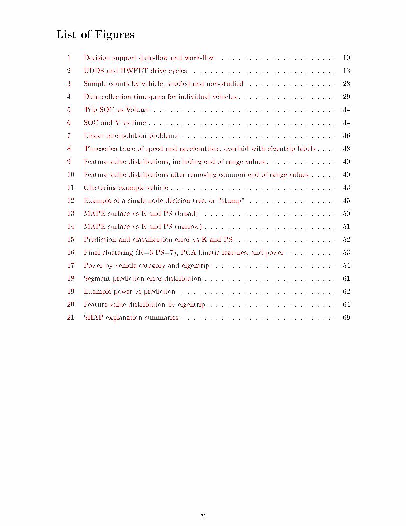
List of Figures
1 Decision support data-�ow and work-�ow . . . . . . . . . . . . . . . . . . . . . 10
2 UDDS and HWFET drive cycles . . . . . . . . . . . . . . . . . . . . . . . . . . 13
3 Sample counts by vehicle, studied and non-studied . . . . . . . . . . . . . . . . 28
4 Data collection timespans for individual vehicles . . . . . . . . . . . . . . . . . . 29
5 Trip SOC vs Voltage . . . . . . . . . . . . . . . . . . . . . . . . . . . . . . . . . 34
6 SOC and V vs time . . . . . . . . . . . . . . . . . . . . . . . . . . . . . . . . . . 34
7 Linear interpolation problems . . . . . . . . . . . . . . . . . . . . . . . . . . . . 36
8 Timeseries trace of speed and accelerations, overlaid with eigentrip labels . . . . 38
9 Feature value distributions, including end-of-range values . . . . . . . . . . . . . 40
10 Feature value distributions after removing common end-of-range values . . . . . 40
11 Clustering example vehicle . . . . . . . . . . . . . . . . . . . . . . . . . . . . . . 43
12 Example of a single-node decision tree, or "stump" . . . . . . . . . . . . . . . . 45
13 MAPE surface vs K and PS (broad) . . . . . . . . . . . . . . . . . . . . . . . . 50
14 MAPE surface vs K and PS (narrow) . . . . . . . . . . . . . . . . . . . . . . . . 51
15 Prediction and classi�cation error vs K and PS . . . . . . . . . . . . . . . . . . 52
16 Final clustering (K=6 PS=7), PCA kinetic features, and power . . . . . . . . . 53
17 Power by vehicle category and eigentrip . . . . . . . . . . . . . . . . . . . . . . 54
18 Segment prediction error distribution . . . . . . . . . . . . . . . . . . . . . . . . 61
19 Example power vs prediction . . . . . . . . . . . . . . . . . . . . . . . . . . . . 62
20 Feature value distribution by eigentrip . . . . . . . . . . . . . . . . . . . . . . . 64
21 SHAP explanation summaries . . . . . . . . . . . . . . . . . . . . . . . . . . . . 69
v
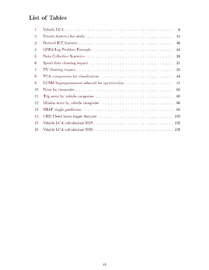
List of Tables
1 Vehicle LCA . . . . . . . . . . . . . . . . . . . . . . . . . . . . . . . . . . . . . . 6
2 Kinetic features for study . . . . . . . . . . . . . . . . . . . . . . . . . . . . . . 15
3 Derived ICE features . . . . . . . . . . . . . . . . . . . . . . . . . . . . . . . . . 16
4 OBD2 Log Problem Example . . . . . . . . . . . . . . . . . . . . . . . . . . . . 24
5 Data Collection Statistics . . . . . . . . . . . . . . . . . . . . . . . . . . . . . . 28
6 Speed data cleaning impact . . . . . . . . . . . . . . . . . . . . . . . . . . . . . 31
7 EV cleaning impact . . . . . . . . . . . . . . . . . . . . . . . . . . . . . . . . . . 35
8 PCA components for visualization . . . . . . . . . . . . . . . . . . . . . . . . . 44
9 LGBM hyperparameters selected for optimization . . . . . . . . . . . . . . . . . 51
10 Error by timescales . . . . . . . . . . . . . . . . . . . . . . . . . . . . . . . . . . 60
11 Trip error by vehicle categories . . . . . . . . . . . . . . . . . . . . . . . . . . . 60
12 Mission error by vehicle categories . . . . . . . . . . . . . . . . . . . . . . . . . 66
13 SHAP single prediction . . . . . . . . . . . . . . . . . . . . . . . . . . . . . . . . 68
14 CRD FleetCarma logger features . . . . . . . . . . . . . . . . . . . . . . . . . . 100
15 Vehicle LCA calculations 2018 . . . . . . . . . . . . . . . . . . . . . . . . . . . . 102
16 Vehicle LCA calculations 2030 . . . . . . . . . . . . . . . . . . . . . . . . . . . . 102
vi
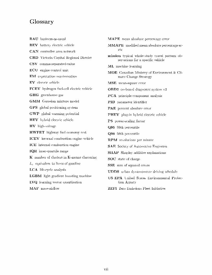
Glossary
BAU business-as-usual
BEV battery electric vehicle
CAN controller area network
CRD Victoria Capital Regional District
CSV comma-separated-value
ECU engine control unit
EM expectation maximization
EV electric vehicle
FCEV hydrogen fuel-cell electric vehicle
GHG greenhouse gas
GMM Gaussian mixture model
GPS global positioning system
GWP global warming potential
HEV hybrid electric vehicle
HV high-voltage
HWFET highway fuel economy test
ICEV internal combustion engine vehicle
ICE internal combustion engine
IQR inter-quartile range
K number of clusters in K-means clustering
Le equivalent to litres of gasoline
LCA life-cycle analysis
LGBM light gradient boosting machine
LVQ learning vector quantization
MAF mass-air�ow
MAPE mean absolute percentage error
MMAPE modi�ed mean absolute percentage er-ror
mission typical whole-study travel pattern ob-servations for a speci�c vehicle
ML machine learning
MOE Canadian Ministry of Environment & Cli-mate Change Strategy
MSE mean-square error
OBD2 on-board diagnostic system v2
PCA principle component analysis
PID parameter identi�er
PAE percent absolute error
PHEV plug-in hybrid electric vehicle
PS power-scaling factor
Q95 95th percentile
Q98 98th percentile
RPM revolutions per minute
SAE Society of Automotive Engineers
SHAP Shapley additive explanations
SOC state of charge
SSE sum of squared errors
UDDS urban dynamometer driving schedule
US EPA United States Environmental Protec-tion Agency
ZEFI Zero Emissions Fleet Initiative
vii
Acknowledgements
In writing this thesis, I have bene�ted from many kinds of assistance from a remarkable
assortment of people at the Victoria Capital Region District (the CRD), the University
of Victoria's Institute for Integrated Energy Systems (IESVic), and the Sustainable
Systems Design Lab (SSDL).
My work could not have been conducted without the CRD's commitment to sustainabil-
ity and green transportation. The CRD's generous funding and donation of logger data
has been the cornerstone of this research, and I am very grateful for the opportunity to
participate in the Zero-Emission Fleet Initiative (ZEFI) and the Smart Fleet project.
In particular I'd like to single out Liz Ferris, Maryanna Kenney, and Dave Goddard for
their enthusiastic advice on practically bringing sustainability to �eet operations.
My supervisors, Dr. Curran Crawford and Dr. Ned Djilali have been excellent advisors,
and enthusiastic providers of advice, instruction, and encouragement. I have deeply
appreciated the opportunity to work closely with them.
I've also bene�ted greatly from my association with Dr. Stephen Neville, who taught
me the skills to perform robust large-scale analysis, and Dr. Ted Darcie, who has helped
me many times to �nd appropriate middle ground between perfect and possible.
My colleagues in the Sustainable Systems Design Lab have created a welcoming com-
munity out of a diverse range of backgrounds and interests, and I've felt privileged to
be part of it. In particular, I'd like to thank Markus and Rad for making it into a com-
munity, and my labmates Julian, Orhan, Charlotte, Marvin, and Graham for creating
a great place to work.
The deepest thanks of all go to my thesis-widow and partner in everything, Sarah,
whose turn it is now.
viii
1 Introduction
1.1 Overview . . . . . . . . . . . . . . 1
1.1.1 Problem statement . . . . . 1
1.1.2 Goals and motivations . . . 1
1.1.3 Document outline . . . . . 3
1.2 Project Context . . . . . . . . . . . 4
1.2.1 CRD ZEFI project . . . . . 4
1.2.2 Operational and embodiedemissions . . . . . . . . . . 4
1.2.3 Simple distance-based fuelconsumption . . . . . . . . 6
1.3 Research Structure . . . . . . . . . 8
1.3.1 Research hypothesis . . . . 8
1.3.2 Model validity and predic-tive power . . . . . . . . . . 9
1.3.3 Preliminary validation . . . 9
1.3.4 Research contributions . . . 9
1.1 Overview
1.1.1 Problem statement
In the e�ort to reduce operational �eet greenhouse gas (GHG) emissions, one important
tool is the selective replacement of individual vehicles with low-emission alternatives.
Given limited capital, it is important to ensure that the correct vehicles are targeted for
replacement in the course of rightsizing, ongoing �eet turnover, or policy-driven phased
replacement of individual high-emission vehicles.
No clear path is seen to directly modelling the GHG emissions of existing and replace-
ment vehicles. However, a change in operational CO2 emissions can be inferred with
reasonable accuracy from the change in the quantity and type of fuel consumed. It
should be possible to predict the change in GHG footprint by modelling the change
in operational energy consumption caused by vehicle replacement, and applying an
appropriate fuel-speci�c emission intensity factor.
1.1.2 Goals and motivations
Fleet vehicles are typically assigned to perform an ongoing speci�c set of duties, com-
monly referred to as a "mission." In order to more easily predict GHG emission changes
resulting from mission-vehicle replacement, this thesis proposes a data-driven model for
1
estimating the change in input energy consumption associated with assigning new ve-
hicles to existing, well-known roles.
In other words, the model will be suitable for estimating the GHG emissions reduction
associated with performing a known mission pro�le with a di�erent vehicle. As discussed
below in �1.2.2, this approach is speci�c to operational emissions, a decision which
is limiting, but appropriate for use with many current policy initiatives, such as the
municipal GHG action plan [1] that inspired this work.
Since one important application is in a decision support tool for non-technical �eet man-
agers, it should be accessible to the end-user without installing custom software. Even
a cloud-hosted service may violate privacy requirements � the movements of individual
vehicles are considered protected private information by many organizations.
The traditional method of predicting vehicle operational energy consumption � apply-
ing distance-based L/100km fuel economy ratings such as those provided by Natural
Resources Canada [2] or the US EPA [3] � is held to be too inaccurate for travel which
does not precisely match the conditions under which the ratings were measured [4, 5].
Conversely, a fully accurate fuel consumption model that infers nonlinear relationships
from a much larger list of operational properties would have impractical data collec-
tion requirements, and would require the distribution and management of specialized
software. The source data may provide information regarding the movements of �eet
users, and there would be signi�cant privacy and security concerns if a model were to
be cloud-deployed [6]. These criteria would make such a model impractical for use as a
�eet procurement decision support tool. Such a model would potentially be so compu-
tationally expensive that the model itself would have a signi�cant GHG footprint.
In short, in order to promote emissions reduction, it is desirable to develop a new
method for predicting operational vehicle energy consumption in �eets, which is:
� simple enough to perform in a spreadsheet
� does not require massive cloud computing overhead
� requires a minimum amount of data collection
2

� is more accurate than distance-based economy ratings
This thesis explores the development of a data-driven model that will meet all of these
criteria, in the context of vehicles with logger data, and mission pro�les which have
been previously logged.
1.1.3 Document outline
This document begins with an extensive Introduction, which (a) lays out the above
overview of the problem, motivation and goals, (b) describes the research context in
terms of municipal partnership that provided the data and informed the motivations,
and (c) explains the structure of the research problem.
The remainder of the document roughly follows the chronology of the research e�ort,
as follows:
�2. The Background section provides a literature review, and a summary of
background material fundamental to understanding the topic and approach.
�3. Data Cleaning and Preparation was a key and challenging element of the work
undertaken, and was su�ciently involved to merit its own section.
�4. The actual machine learning techniques used to build the predictive model
are described in Methodology.
�5. The model's predictive error is evaluated, its value is demonstrated by com-
parison with Le/100km, and avoidable error quanti�ed by comparison to an ML
regression model in Results.
�6. Finally, the �ndings are wrapped up and summarized in the form of a short
section of Conclusions.
�7. Lays out a number of potential topics for further re�nement, exploration and
other Recommendations and Future Work.
3
1.2 Project Context
1.2.1 CRD ZEFI project
As a part of the Victoria Capital Regional District (CRD)'s Zero Emissions Fleet Ini-
tiative (ZEFI) project, a number of vehicles in the CRD �eet were equipped with
FleetCarma on-board diagnostic system v2 (OBD2) telematic logging devices at vari-
ous periods for approximately a year starting in early 2018 [7].
A motivating goal in this project was to determine actions needed to meet the orga-
nization's GHG reduction targets, given that 47% of the CRD's baseline 2007 GHG
emissions resulted from �eet fuel consumption [1]. An early �nding was that, at least
on the restricted basis of range requirements, nearly all of the studied vehicle missions
could be executed by current battery electric vehicles (BEVs) [8].
Further detail on the nature of the data collection and the logged data is presented in
�2.3.1.
1.2.2 Operational and embodied emissions
The intent of this research is to address a core accessibility problem for modelling
�eet operational emissions, as needed to address reduction goals similar to those of the
CRD's ZEFI program.
For internal combustion engine vehicles (ICEVs), this reduces to tailpipe emissions,
calculated by estimating the fuel directly consumed by the vehicle � traditionally called
"tank-to-wheel" energy. For gasoline, the GHG emissions of this energy are estimated
at an intensity of 88.1 g CO2e/MJ [9]. For electric vehicles (EVs), this is a re�ection
of the emissions associated with the grid electricity consumed by the drive motor, at
the utility's published carbon intensity. For BC Hydro, this is 10.67 t CO2e/GWh [10]
(2.96 g CO2e/MJ).
The BC GHG Reduction Act [11] references the 2007 baseline GHG inventory report
[12] as a baseline. Emissions in the inventory report are attributed to the jurisdiction
4
where emission is generated, rather than the jurisdiction where the bene�t of the emis-
sion accrues. E.g. if H2 gas or lithium-ion batteries are used in BC, the associated
manufacturing emissions are attributed to the foreign H2 steam reformation plant or
battery factory, rather than to the BC point of bene�cial use. This may be seen as
constituting a perverse incentive, insulating end-users from any �nancial costs asso-
ciated the embodied emissions of manufactured goods, and driving manufacturing to
under-regulated jurisdictions.
In the late 2010s there were claims in the US popular press such as [13, 14] that BEVs
have a higher lifetime GHG impact than equivalent ICEVs. Anecdotally, the claims are
sometimes echoed by concerned Canadian citizens. The core argument appears to be
that BEV proponents ignore or under-represent emissions associated with manufactur-
ing the battery pack, and the high carbon intensity of some sources of grid electricity.
Although this probably constitutes an example of the "balance-as-bias" fallacy [15],
a short discussion is warranted regarding the full cradle-to-grave lifecycle analysis for
di�erent light vehicle technologies and their fuel sources.
A 2018 comprehensive comparison by Elgowainy et al [16] summarized full cradle-to-
grave GHG emissions (including fuel cycle and manufacturing cycle), for several di�er-
ent types of light vehicles. The study included ICEVs, hybrid electric vehicles (HEVs),
plug-in hybrid electric vehicles (PHEVs), hydrogen fuel-cell electric vehicles (FCEVs)
and BEVs, as well as other vehicle types excluded from this discussion. Retaining that
study's �gures for manufacturing and fuel e�ciency, but applying current and fore-
casted 2030 intensities for the appropriate fuel pathways for BC as follows, it is clear
that alternative fuel vehicles have a signi�cant and improving advantage, shown in table
1. Some discussion of the assumptions and calculations for this comparison appears in
appendix B.
Ultimately, the scope of this research is constrained to local tailpipe emissions as re-
quired for the planning requirements of organizations like the CRD. It explicitly ex-
cludes a full carbon lifecycle analysis, including all carbon emissions embodied in the
vehicle's manufacture and eventual recycling, as well as all carbon emitted or embodied
5
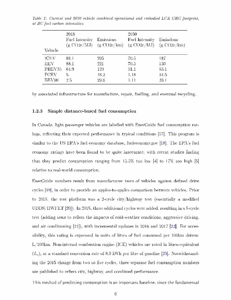
Table 1: Current and 2030 vehicle combined operational and embodied LCA GHG footprint,at BC fuel carbon intensities
2018 2030Fuel Intensity Emissions Fuel Intensity Emissions(g CO2e/MJ) (g CO2e/km) (g CO2e/MJ) (g CO2e/km)
Vehicle
ICEV 88.1 295 70.5 187HEV 88.1 221 70.5 130PHEV35 64.9 129 51.1 83.1FCEV 5. 48.2 1.18 34.5BEV90 2.5 29.6 1.11 23.1
by associated infrastructure for manufacture, repair, fuelling, and eventual recycling.
1.2.3 Simple distance-based fuel consumption
In Canada, light passenger vehicles are labelled with EnerGuide fuel consumption rat-
ings, re�ecting their expected performance in typical conditions [17]. This program is
similar to the US EPA's fuel economy database, fueleconomy.gov [18]. The EPA's fuel
economy ratings have been found to be quite inaccurate, with recent studies �nding
that they predict consumption ranging from 15.5% too low [4] to 17% too high [5]
relative to real-world consumption.
EnerGuide numbers result from manufacturer tests of vehicles against de�ned drive
cycles [19], in order to provide an apples-to-apples comparison between vehicles. Prior
to 2015, the test platform was a 2-cycle city/highway test (essentially a modi�ed
UDDS/HWFET [20]). In 2015, three additional cycles were added, resulting in a 5-cycle
test (adding tests to re�ect the impacts of cold-weather conditions, aggressive driving,
and air conditioning [21]), with incremental updates in 2016 and 2017 [22]. For acces-
sibility, this rating is expressed in units of litres of fuel consumed per 100km driven:
L/100km. Non-internal combustion engine (ICE) vehicles are rated in litres-equivalent
(Le), at a standard conversion rate of 8.9 kWh per litre of gasoline [23]. Notwithstand-
ing the 2015 change from two to �ve cycles, three separate fuel consumption numbers
are published to re�ect city, highway, and combined performance.
This method of predicting consumption is an important baseline, since the fundamental
6
metric for evaluating an individual vehicle replacement will be "avoided emissions�,
which quanti�es the change in operational emissions associated with replacing a current
(incumbent) vehicle, with a lower-emission alternative (replacement) vehicle.
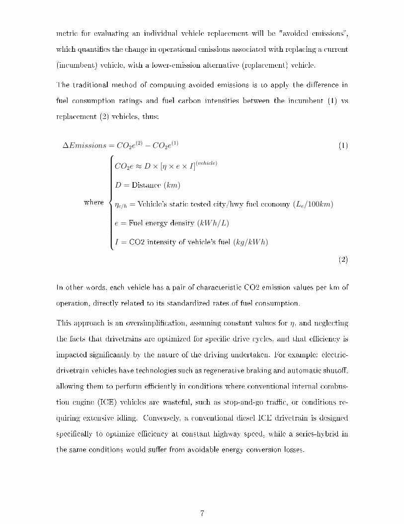
The traditional method of computing avoided emissions is to apply the di�erence in
fuel consumption ratings and fuel carbon intensities between the incumbent (1) vs
replacement (2) vehicles, thus:
∆Emissions = CO2e(2) − CO2e
(1) (1)
where
CO2e ≈ D × [η × e× I](vehicle)
D = Distance (km)
ηc/h = Vehicle's static tested city/hwy fuel economy (Le/100km)
e = Fuel energy density (kWh/L)
I = CO2 intensity of vehicle's fuel (kg/kWh)
(2)
In other words, each vehicle has a pair of characteristic CO2 emission values per km of
operation, directly related to its standardized rates of fuel consumption.
This approach is an oversimpli�cation, assuming constant values for η, and neglecting
the facts that drivetrains are optimized for speci�c drive cycles, and that e�ciency is
impacted signi�cantly by the nature of the driving undertaken. For example: electric-
drivetrain vehicles have technologies such as regenerative braking and automatic shuto�,
allowing them to perform e�ciently in conditions where conventional internal combus-
tion engine (ICE) vehicles are wasteful, such as stop-and-go tra�c, or conditions re-
quiring extensive idling. Conversely, a conventional diesel ICE drivetrain is designed
speci�cally to optimize e�ciency at constant highway speed, while a series-hybrid in
the same conditions would su�er from avoidable energy conversion losses.
7

1.3 Research Structure
1.3.1 Research hypothesis
This study proposes and tests the hypothesis that energy consumption for arbitrary
periods of vehicle travel can be accurately predicted by decomposing the proposed
travel period into a linear combination of characteristic trip segments, each with a
known constant characteristic power consumption for each vehicle type. The prediction
will be the sum of vehicle-speci�c energy consumption totals for that combination of
segments. The prediction should hold for travel periods ranging in duration from a
single trip to a multi-month mission pro�le.
To simplify further discussion, the following terms are de�ned:
�Mission pro�le� refers to the operations typically undertaken by a speci�c vehicle.
Municipal examples include "bylaw supervisor", "meter reader", and pool vehicle".
�Kinetic travel data� refers to a speci�c portion of a vehicle's speed history, or summary
statistics derived from it.
�Eigentrips� are a basis set of vehicle-agnostic travel segments with the following char-
acteristics:
� Each eigentrip is de�ned by characteristic kinetic travel data
� Every vehicle has characteristic energy consumption for each eigentrip
� All historical and predicted travel data can be decomposed into a linear combi-
nation of eigentrips
The primary technical problems addressed in this thesis are:
� Selecting an appropriate basis set of eigentrips using kinetic travel data.
� Evaluating the predictive power of a linear combination of eigentrips, relative to
the observed energy consumption of vehicles on speci�c missions.
8
1.3.2 Model validity and predictive power
The new method's validity will be evaluated by comparing its prediction error to the
real-world energy consumption, as inferred from the full raw dataset. This prediction
error will be contrasted with the prediction error of the traditional distance-based fuel
economy statistic described above in �1.2.3.
It is worth noting that the "observed energy consumption" baseline is an estimate of
unknown accuracy derived from the available proxy values (MAF and SOC) as discussed
in �3.3. This assumption is addressed in �7.5.2.
1.3.3 Preliminary validation
The author conducted a preliminary experiment [24] as a coursework project, studying
300 hours of kinetic travel data and fuel �ow rates inferred from MAF (mass-air�ow)
values, for ten similar vehicles.
In that study, the data was partitioned into 10-minute segments by clock time (segment
boundaries were placed at even 10-minute intervals starting at the top of each hour). A
�ngerprint of representative statistics was then calculated for each segment. K-means
clustering [25, �10.4.3] was performed on the resultant dataset to �nd three clusters.
Based on the clustering results, held back test data was classi�ed with a softmax [25,
�6.6.2] logistic classi�er [26], and engine load was predicted. The average engine load
prediction error using this method was approximately 2%.
Although not proven to generalize, the result was su�cient to suggest that the method
warranted further study.
1.3.4 Research contributions
This research explores and validates a new method for predicting the energy consump-
tion of di�erent vehicle types when used to execute a well-known mission pro�le.
The method requires logger data attainable with nearly any commodity OBD2 logger
� although some care must be taken to assure the quality of fuel / energy consumption
9
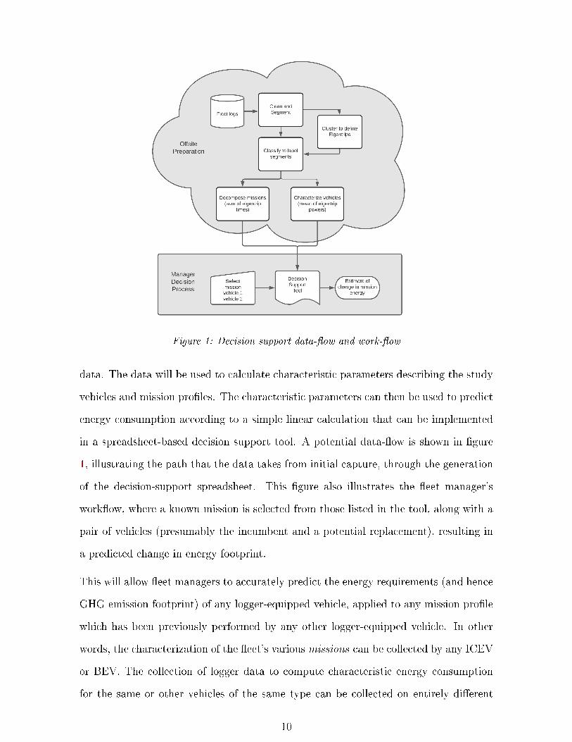
Figure 1: Decision support data-�ow and work-�ow
data. The data will be used to calculate characteristic parameters describing the study
vehicles and mission pro�les. The characteristic parameters can then be used to predict
energy consumption according to a simple linear calculation that can be implemented
in a spreadsheet-based decision support tool. A potential data-�ow is shown in �gure
1, illustrating the path that the data takes from initial capture, through the generation
of the decision-support spreadsheet. This �gure also illustrates the �eet manager's
work�ow, where a known mission is selected from those listed in the tool, along with a
pair of vehicles (presumably the incumbent and a potential replacement), resulting in
a predicted change in energy footprint.
This will allow �eet managers to accurately predict the energy requirements (and hence
GHG emission footprint) of any logger-equipped vehicle, applied to any mission pro�le
which has been previously performed by any other logger-equipped vehicle. In other
words, the characterization of the �eet's various missions can be collected by any ICEV
or BEV. The collection of logger data to compute characteristic energy consumption
for the same or other vehicles of the same type can be collected on entirely di�erent
10

routes/missions, and even by entirely di�erent organizations. Sharing real-world vehicle
performance data between organizations would improve estimation of energy consump-
tion based on di�erent procurement scenarios, including new vehicle models of which a
given organization has no direct experience � in much the same manner as Le/100km
�gures are currently used.
Other research contributions include:
� Shapley additive explanations (SHAP) showing the relative importance of various
input features to the prediction of input power.
� a technique for reconstructing serial OBD2 values that have been tabularized
� evaluation of error inherent in traditional L/100km technique
� comparison to direct regression, to gauge e�cacy & accuracy of both proposed
method and L/100km method
11
2 Background
2.1 Travel Data . . . . . . . . . . . . . 12
2.1.1 Drive cycles . . . . . . . . . 12
2.1.2 Microtrips . . . . . . . . . . 14
2.2 Machine Learning . . . . . . . . . . 16
2.2.1 Feature selection . . . . . . 16
2.2.2 Time-series analysis . . . . 18
2.2.3 Binning and segmentation . 19
2.2.4 Regression analysis . . . . . 19
2.2.5 Clustering . . . . . . . . . . 20
2.2.6 Classi�cation . . . . . . . . 22
2.2.7 Gradient boost and LGBM 23
2.3 Data Collection . . . . . . . . . . . 23
2.3.1 OBD2 logger implementa-tion . . . . . . . . . . . . . 23
2.3.2 Fuel vs air�ow . . . . . . . 25
This section addresses background material fundamental to the topic. Quantitative
analysis of travel patterns is typically performed on data comprising drive cycles and
microtrips, so a brief background on these concepts is presented.
The proposed method involves feature selection, clustering, and classi�cation of multi-
dimensional timeseries data, so various tools for these tasks are discussed.
Finally, this section contains a short background of the technology used for data collec-
tion, and limitations around the collection of fuel �ow rates.
2.1 Travel Data
2.1.1 Drive cycles
A drive cycle (or driving cycle) is the speed-time data that describe a portion of a
vehicle's travel history [27], either measured, generated, or synthesized. A large number
of standardized drive cycles have been published by various government agencies and
private organizations, to facilitate optimization and testing to standardized benchmarks
[28].
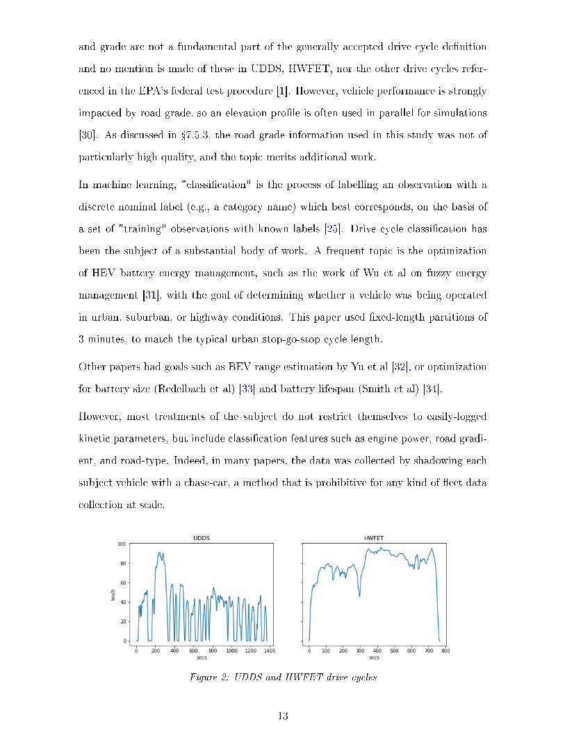
Two of the most heavily-referenced examples are the urban dynamometer driving sched-
ule (UDDS) and highway fuel economy test (HWFET) cycles [29], de�ned by the United
States Environmental Protection Agency (US EPA), and shown in �gure 2. Elevation
12
and grade are not a fundamental part of the generally accepted drive cycle de�nition
and no mention is made of these in UDDS, HWFET, nor the other drive cycles refer-
enced in the EPA's federal test procedure [1]. However, vehicle performance is strongly
impacted by road grade, so an elevation pro�le is often used in parallel for simulations
[30]. As discussed in �7.5.3, the road grade information used in this study was not of
particularly high quality, and the topic merits additional work.
In machine learning, "classi�cation" is the process of labelling an observation with a
discrete nominal label (e.g., a category name) which best corresponds, on the basis of
a set of "training" observations with known labels [25]. Drive cycle classi�cation has
been the subject of a substantial body of work. A frequent topic is the optimization
of HEV battery energy management, such as the work of Wu et al on fuzzy energy
management [31], with the goal of determining whether a vehicle was being operated
in urban, suburban, or highway conditions. This paper used �xed-length partitions of
3 minutes, to match the typical urban stop-go-stop cycle length.
Other papers had goals such as BEV range estimation by Yu et al [32], or optimization
for battery size (Redelbach et al) [33] and battery lifespan (Smith et al) [34].
However, most treatments of the subject do not restrict themselves to easily-logged
kinetic parameters, but include classi�cation features such as engine power, road gradi-
ent, and road-type. Indeed, in many papers, the data was collected by shadowing each
subject vehicle with a chase-car, a method that is prohibitive for any kind of �eet data
collection at scale.
Figure 2: UDDS and HWFET drive cycles
13
2.1.2 Microtrips
Microtrips are "the sections of travel between consecutive stops", �rst used for travel
analysis by General Motors Research in 1976 [35], where it was used to demonstrate
that fuel rate varied linearly with average trip speed (true of the automotive technology
of the time). They are used frequently as an aid to the development of new drive cycles,
as per Kamble et al [36], where synthetic geography-speci�c drive cycles were created
from a number of real microtrips.
The microtrip concept has seen very little use in the problem of drive cycle classi�ca-
tion, with only a couple of examples seen in the literature. One example is described
by Shankar and Marco in [37], which applies neural network classi�cation to determine
the road-type (e.g., highway, arterial, or local), as well as a congestion index, for use in
predicting an input power appropriate to the driving conditions. However, the method
was addressed speci�cally to battery vehicles, and presumes that the only factors in-
�uencing energy consumption are derived from road congestion and type. The method
does not consider the possibility that di�erent travel types in the same context might
have di�erent energy requirements, for example because the mission requires regular
stops or extensive idling.
Shankar and Marco's paper does point out an inherent limitation of microtrips: that
they are de�ned from stop to stop. This means that a single microtrip is likely to
encompass more than one type of travel, and/or to unnecessarily segment a single type
of travel that includes stops.
Another relevant example [38] by He et al extracted microtrips from the de�nitions
of several prede�ned drive cycles, calculated the �rst seven of the aggregated velocity-
derived features shown in table 2, and applied principle component analysis (PCA)
to retain four principal components. These principal components were calculated on
segments of actual travel data, in order to classify the segments in an learning vector
quantization (LVQ) neural net, with very good classi�cation results. The �rst seven
features gave excellent classi�cation results and may be expected to provide an excellent
14
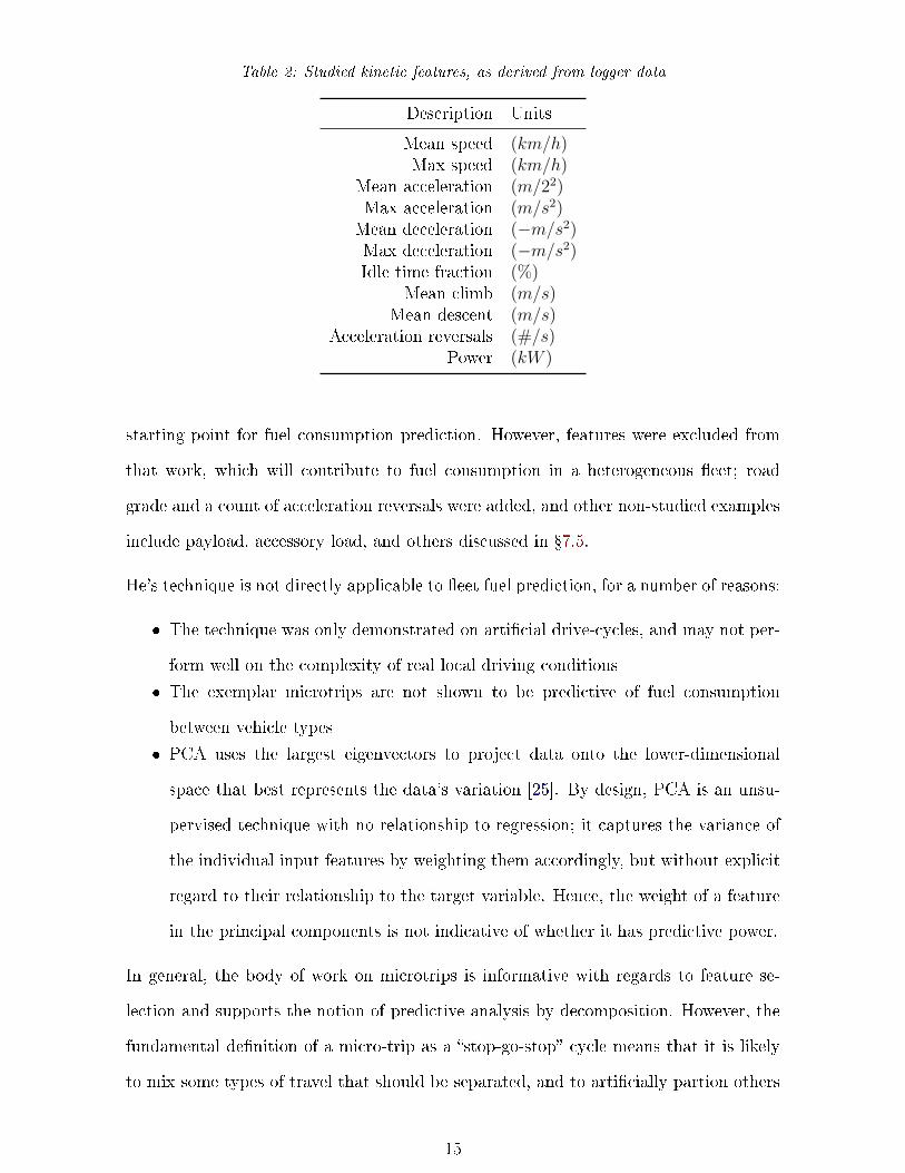
Table 2: Studied kinetic features, as derived from logger data
Description Units
Mean speed (km/h)Max speed (km/h)
Mean acceleration (m/22)Max acceleration (m/s2)Mean deceleration (−m/s2)Max deceleration (−m/s2)Idle time fraction (%)
Mean climb (m/s)Mean descent (m/s)
Acceleration reversals (#/s)Power (kW )
starting point for fuel consumption prediction. However, features were excluded from
that work, which will contribute to fuel consumption in a heterogeneous �eet; road
grade and a count of acceleration reversals were added, and other non-studied examples
include payload, accessory load, and others discussed in �7.5.
He's technique is not directly applicable to �eet fuel prediction, for a number of reasons:
� The technique was only demonstrated on arti�cial drive-cycles, and may not per-
form well on the complexity of real local driving conditions
� The exemplar microtrips are not shown to be predictive of fuel consumption
between vehicle types
� PCA uses the largest eigenvectors to project data onto the lower-dimensional
space that best represents the data's variation [25]. By design, PCA is an unsu-
pervised technique with no relationship to regression; it captures the variance of
the individual input features by weighting them accordingly, but without explicit
regard to their relationship to the target variable. Hence, the weight of a feature
in the principal components is not indicative of whether it has predictive power.
In general, the body of work on microtrips is informative with regards to feature se-
lection and supports the notion of predictive analysis by decomposition. However, the
fundamental de�nition of a micro-trip as a �stop-go-stop� cycle means that it is likely
to mix some types of travel that should be separated, and to arti�cially partion others
15
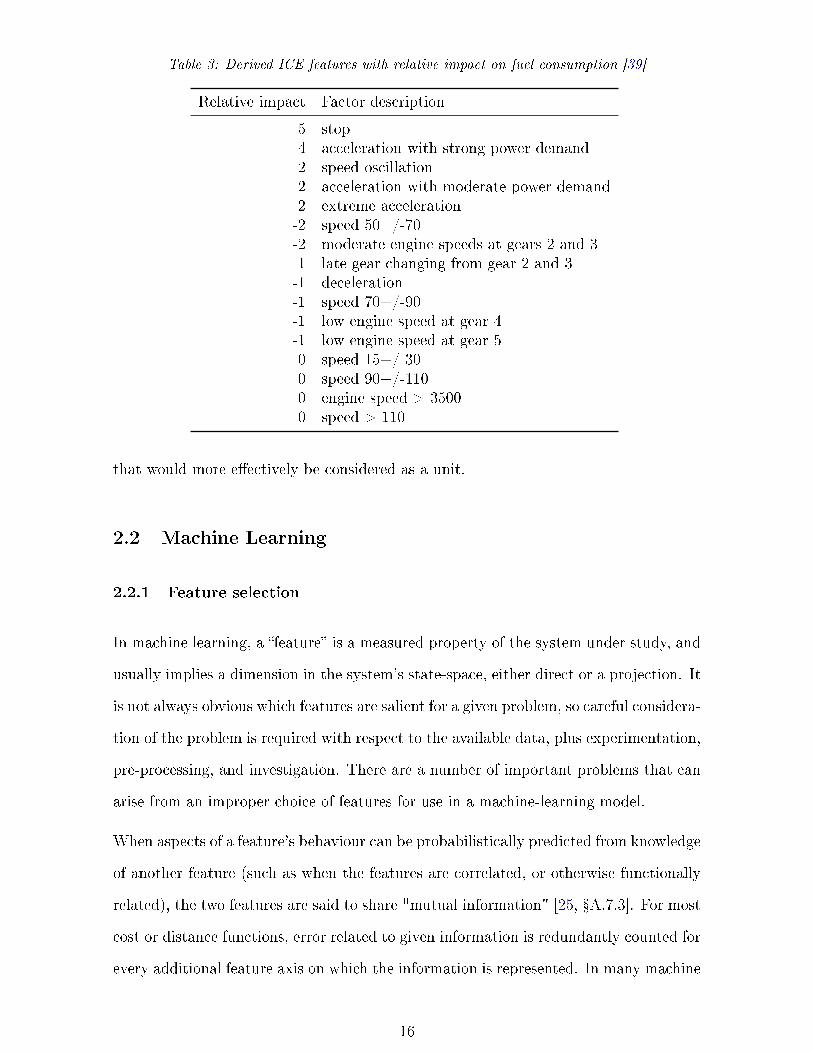
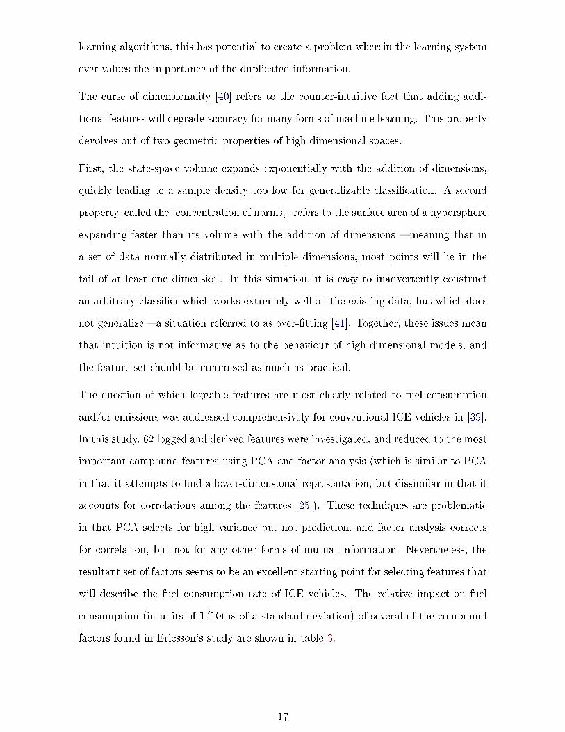
Table 3: Derived ICE features with relative impact on fuel consumption [39]
Relative impact Factor description
5 stop4 acceleration with strong power demand2 speed oscillation2 acceleration with moderate power demand2 extreme acceleration-2 speed 50+/-70-2 moderate engine speeds at gears 2 and 31 late gear changing from gear 2 and 3-1 deceleration-1 speed 70+/-90-1 low engine speed at gear 4-1 low engine speed at gear 50 speed 15+/-300 speed 90+/-1100 engine speed > 35000 speed > 110
that would more e�ectively be considered as a unit.
2.2 Machine Learning
2.2.1 Feature selection
In machine learning, a �feature� is a measured property of the system under study, and
usually implies a dimension in the system's state-space, either direct or a projection. It
is not always obvious which features are salient for a given problem, so careful considera-
tion of the problem is required with respect to the available data, plus experimentation,
pre-processing, and investigation. There are a number of important problems that can
arise from an improper choice of features for use in a machine-learning model.
When aspects of a feature's behaviour can be probabilistically predicted from knowledge
of another feature (such as when the features are correlated, or otherwise functionally
related), the two features are said to share "mutual information" [25, �A.7.3]. For most
cost or distance functions, error related to given information is redundantly counted for
every additional feature axis on which the information is represented. In many machine
16
learning algorithms, this has potential to create a problem wherein the learning system
over-values the importance of the duplicated information.
The curse of dimensionality [40] refers to the counter-intuitive fact that adding addi-
tional features will degrade accuracy for many forms of machine learning. This property
devolves out of two geometric properties of high dimensional spaces.
First, the state-space volume expands exponentially with the addition of dimensions,
quickly leading to a sample density too low for generalizable classi�cation. A second
property, called the �concentration of norms,� refers to the surface area of a hypersphere
expanding faster than its volume with the addition of dimensions � meaning that in
a set of data normally distributed in multiple dimensions, most points will lie in the
tail of at least one dimension. In this situation, it is easy to inadvertently construct
an arbitrary classi�er which works extremely well on the existing data, but which does
not generalize � a situation referred to as over-�tting [41]. Together, these issues mean
that intuition is not informative as to the behaviour of high-dimensional models, and
the feature set should be minimized as much as practical.
The question of which loggable features are most clearly related to fuel consumption
and/or emissions was addressed comprehensively for conventional ICE vehicles in [39].
In this study, 62 logged and derived features were investigated, and reduced to the most
important compound features using PCA and factor analysis (which is similar to PCA
in that it attempts to �nd a lower-dimensional representation, but dissimilar in that it
accounts for correlations among the features [25]). These techniques are problematic
in that PCA selects for high variance but not prediction, and factor analysis corrects
for correlation, but not for any other forms of mutual information. Nevertheless, the
resultant set of factors seems to be an excellent starting point for selecting features that
will describe the fuel consumption rate of ICE vehicles. The relative impact on fuel
consumption (in units of 1/10ths of a standard deviation) of several of the compound
factors found in Ericsson's study are shown in table 3.
17
2.2.2 Time-series analysis
Time-series data consists of sequential measurements of the same feature over time,
with the characteristic property that the data are generated by a process, and are
not statistically independent of earlier samples in the process [42]. A drive-cycle is an
excellent example, describing a trip in terms of measurements of the vehicle's speed
over time.
Time-series data is commonly analyzed by the direct application of time-domain anal-
ysis techniques � �nding patterns and behaviours with respect to temporal ordering.
In the context of trip-segment similarity, it seems intuitively obvious that order does
not much matter, relative to many other aspects of the driving patterns. For example:
the segments of the urban drive cycle, driven in reverse order, could be expected to
have energy consumption very similar to that of the forward-ordered version (stipulat-
ing a similar net elevation pro�le), but it is hard to imagine a meaningful time-domain
measure that would expose the similarity. This intuition suggests that time-domain
analysis techniques will miss important commonalities between trips.
Transforming into the frequency domain can address this problem and give insight into
the relative importance of various cyclical behaviours. Applied to segments of kinetic
driving data, it might give insight into the rate of start-stop or speed-slow cycles,
where they exist. However, since acyclic behaviours might be critical di�erentiators,
and would be lost in the transformation out of the time domain, we certainly cannot
rely on frequency analysis alone.
Apart from the inter-sample interval necessary to calculate acceleration, the key features
used in this research draw no useful information from their time sequencing. Thus, for
the insights to be derived from the data, time series techniques do not provide a great
deal of analytical power, and are left as a topic for future investigation (�7.3).
18

2.2.3 Binning and segmentation
Data binning is the process of grouping data points with similar values together, such
that they can be referenced by a common value. This is useful to reduce the volume
of data for faster processing, or to improve its comprehensibility, as with histograms.
Segmentation is conceptually similar; it consists of partitioning time series data into
time intervals, allowing each segment to be characterized as a group [43].
A key technique used in this research combines both techniques: partitioning the data
into �xed-length segments, which are thereafter treated as non-time series bins. A selec-
tion of representative summary statistics (a �ngerprint) for each segment are calculated,
after which the time information can be discarded or ignored. Similar segments can then
be binned, allowing the application of simple and intuitive non-time series analytical
techniques.
This has the advantage that the similarity measure between segments can be as simple
as Euclidean distance, or as complex as necessary to capture prior understanding of
"similarity" for the system in question.
The primary disadvantages of using bin �ngerprints are di�culties in (a) determining
appropriate statistics such that if two trips are subjectively similar, then their statistics
will have objectively similar values, and (b) �nding segment boundaries, such that
segments do not encompass multiple types.
2.2.4 Regression analysis
Regression analysis is a branch of mathematical statistics concerned with quantifying
the relationships between some number of variables using statistical data [44]. In the
most general sense, this involves �nding the appropriate parameters for a mathematical
model, which will allow it to calculate predicted values for the dependent variable(s)
based on the input values for the independent variables.
The most commonly used example is linear regression, which consists of �nding the
coe�cients b for the independent variables x that will best predict target variable y,
19

typically by minimizing the mean-square error (MSE) for all training values y.
y = b0 + b1x1 + ...+ bnxn + ε (3)
MSE =1
n
∑(y − y)2 (4)
If the relationship between the independent and dependent variables is more complex,
nonlinear techniques are used � either by �tting coe�cients to a more complex formula
that better describes the relationship, or by using some other model entirely, such as a
decision tree or arti�cial neural net [41]. These nonlinear techniques result in a better
�t to the observed data, but at the cost of a more complex formula and the risk of
over�tting.
Traditional regression techniques are not a good �t for the primary stated goals of this
research, as it would not be possible to develop a spreadsheet-deployable model that
could clean and process the millions of rows of logger data. Setting aside the unique
requirements of a deployable decision support tool, tree or neural net regression would
be the simplest path to predicting vehicle energy consumption, and will be used in �5
to provide a basis for comparison of the accuracy of the proposed spreadsheet-capable
model.
2.2.5 Clustering
Clustering is the general name for unsupervised techniques that have the goal of group-
ing similar data samples according to an appropriate de�nition of similarity.
For the problem at hand, it is impractical to manually de�ne a basis set of eigentrips
that will (a) adequately represent all travel in the dataset, and (b) be su�ciently dis-
criminatory with regards to fuel consumption between the studied vehicle types. In
this study, the entire corpus of segmented travel data will be clustered, and the char-
acteristics of each group will be considered to represent one eigentrip. This section will
address appropriate methods for clustering.
20

The simplest and arguably most intuitive clustering technique is K-means clustering,
most easily understood with an interactive visualization, such as the one linked at
[45]. The technique consists of selecting a number (k) of randomly distributed cluster
centroids, assigning every data point to the cluster de�ned by the nearest centroid, and
then iteratively rede�ning each cluster centroid as the mean of its constituent points.
The technique's simplicity is balanced by two signi�cant limitations. First, it must
be provided with a prede�ned cluster count [25], which is a key tuning parameter.
Second, it presumes clusters in normal, spherical distributions; its cost function is most
appropriate for points which have a Gaussian distribution of equal variance in every
dimension.
The technique can be generalized to data in non-spherical distributions by maximizing
the probabilistic membership in each cluster � this is called expectation maximization
(EM) clustering � or more speci�cally, Gaussian mixture models (GMMs) if the clusters
are normally distributed.
Any clustering technique relies on an appropriate de�nition of distance between points
in the feature space. A common and intuitive choice is the L2 norm � Euclidean
distance � applied to appropriately normalized features. This works well, because non-
discriminatory features are likely to balance themselves by virtue of being equally dis-
tributed between the clusters. However, the measure is sensitive to outliers, and cannot
account for desired similarities that can only be described by nonlinear combinations
of features.
K-means also requires a number of clusters (k) as an input. Typically, this number is
found by inspection (the "elbow" method [46]) or by minimizing a loss function such
as silhouette score [47]) against di�erent values for k.
In addition to the advantage of simplicity, K-means has a well-known implementation
in the Scikit-learn library. Although it presumes spherical, normalized clusters [48], this
requirement is also an advantage, since it allows features to be given relative weights
by the simple expedient of linear scaling.
There is an obvious argument against the use of K-means: that the best clusters (for
21

a domain-speci�c de�nition of similarity) may not be normal and spherical. However,
the travel data at hand is continuous, and does not have distinct clusters. For the
immediate goal � selecting "similar" data to train the eigentrip classi�er, we can allow
the clustering algorithm to de�ne the shape of its clusters. Reviewing the impact of
alternate clustering techniques on classi�er accuracy will be an excellent topic for future
re�nement of the model.
2.2.6 Classi�cation
Classi�cation is similar to regression analysis, but with a goal of predicting a discrete
value, rather than a scalar, commonly used for determining which of a �xed number of
categories is the best �t for a particular datum [41].
Classi�cation is a key element of the proposed method: each trip segment will be
classi�ed and labelled with its most similar eigentrip. If the thesis is correct, the
characteristic power of that eigentrip will be similar to the actual power of the trip
segment.
Classi�cation algorithm selection is more art than science, with the "No Free Lunch"
theorem demonstrating that there is no model that is best across domains [41]. In gen-
eral, the researcher must evaluate the characteristics of their data and the requirements
of their model, and attempt to �nd an algorithm that suits both.
In this case, since several of the features have unknown multi-modal distributions,
Bayesian algorithms will not be a good �t. Neural nets require computationally inten-
sive training, have non-explainable results, and do not extrapolate outside their training
volume. The remaining family of classi�ers which seem appropriate are ensemble de-
cision trees. The light gradient boosting machine (LGBM) algorithm is selected for
initial review as demonstrating a good balance between training speed and prediction
accuracy.
22

2.2.7 Gradient boost and LGBM
Model selection is arguably the most di�cult aspect of practical, applied ML. The
proposed model has aspects that make it particularly challenging:
� features are multi-modal and do not follow a common distribution
� features may have unknown mutual information
� target feature has no obvious structure
� explanation of feature impact on prediction may be important for future work
� millions of data points
The unknown distribution renders Bayesian methods impractical. The possible shared
information duplicated between features and potential requirement for explainability
comprise good arguments against arti�cial neural nets. Finally, due to the need for iter-
ative evaluation over the relatively large dataset discussed below in �4.6, slow-training
methods would not be practical. Given these exclusions, an ensemble decision tree
method warranted consideration.
Although at risk of running afoul of Maslow's Hammer [49], the common-sense admo-
nition that practitioners are prone to over-application of familiar tools, the popular
LightGBM model meets all of the above criteria, described in more detail in �4.3.
2.3 Data Collection
2.3.1 OBD2 logger implementation
In order to understand a signi�cant primary data collection issue, the reader will require
some background on the technology used for data collection.
The dataset used in this study was collected by FleetCarma Inc., a commercial com-
pany based in Waterloo, Ontario. FleetCarma uses telematics loggers connected to
the vehicles' OBD2 interface. OBD2 is a protocol de�ned by Society of Automotive
Engineers (SAE) standard J1962 for vehicle data access, and speci�es a female 16-pin
electrical connector for access, commonly known as the OBD2 port. It accesses the
23
vehicle's controller area network (CAN) bus, a serial hardware layer commonly used to
transport vehicle sensor data between various engine control unit (ECU)s. Information
in this subsection is summarized primarily from an instructional website [50] and the
original Texas Instruments application document [51].
Devices on a CAN bus communicate exclusively by broadcast. Some devices may report
their status at a regular interval, while others only report in response to a request
broadcast, and others may communicate by both methods. In essence, the CAN bus
data stream consists of a sequence of (key, value) pairs.
Fleet Carma's logger has a list of parameter identi�er (PID) values that are to be
collected from the OBD2 system. Whenever any of those PIDs appear on the CAN
bus, the logger records and timestamps it. To ensure a data log meeting the speci�ed
resolution requirements (1 second while moving), the logger periodically sends update
requests for over the CAN bus for appropriate PIDs, requesting that a new value be
returned.
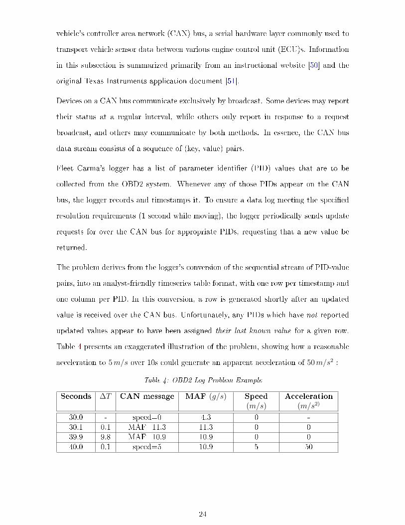
The problem derives from the logger's conversion of the sequential stream of PID-value
pairs, into an analyst-friendly timeseries table format, with one row per timestamp and
one column per PID. In this conversion, a row is generated shortly after an updated
value is received over the CAN bus. Unfortunately, any PIDs which have not reported
updated values appear to have been assigned their last known value for a given row.
Table 4 presents an exaggerated illustration of the problem, showing how a reasonable
acceleration to 5m/s over 10s could generate an apparent acceleration of 50m/s2 :
Table 4: OBD2 Log Problem Example
Seconds ∆T CAN message MAF (g/s) Speed(m/s)
Acceleration(m/s2)
30.0 - speed=0 4.3 0 -30.1 0.1 MAF=11.3 11.3 0 039.9 9.8 MAF=10.9 10.9 0 040.0 0.1 speed=5 10.9 5 50
24
2.3.2 Fuel vs air�ow
Unfortunately, a parameter for fuel-�ow rate is not part of the OBD2 speci�cation [52].
Most vehicle manufacturers supply a proprietary PID for this value, but our FleetCarma
loggers were not con�gured to retrieve it from the individual vehicles. A valuable proxy
for fuel �ow is the standard PID mass-air�ow (MAF), which estimates the mass of air
entering the engine from measurements of airstream temperature and velocity at the
intake. The well-known stoichiometric mass ratio of 14.7 for gasoline combustion is
inferred from the oxidation reaction [53]:
25O2 + 2C8H18 → 16CO2 + 18H2O + E (5)
Since tailpipe emissions are an important design consideration, modern vehicles attempt
to minimize emissions by ensuring good operation of the catalytic converter. One
outcome of this intent is that the vehicle continually modi�es its fuel �ow (a process
referred to as trimming) relative to MAF, in order to maintain clean combustion as
indicated by the oxygen content of the exhaust stream. There do exist standard PIDs
for both the commanded and measured ratios of fuel to air [52], but these values were
unavailable to this study, having not been logged in the CRD's Smart Fleet project.
In any case, a properly operating vehicle should generally have a fuel �ow within 10% of
the stoichiometric ratio relative to the MAF [54]. It is noteworthy that there are certain
events (notably engine-braking) that will be expected to cause signi�cant transient
departures from the stoichiometric ratio. The author's personal experience, having
reviewed trim data logs from �ve personal vehicles, is that short and long-term fuel
trim levels generally remain consistent within 3% for normal driving, outside of a few
minutes for engine warm-up.
The conclusion from this background material is that calculating fuel �ow by applying
the stoichiometric ratio of 14.7 to the measured MAF can be reasonably expected to
have a per-vehicle precision of ±3%, and an absolute accuracy within ±10%.
25

Ultimately, the MAF estimate must stand alone as a ground truth for this work, as no
means of validating the MAF estimate was found. The CRD does track �eet fuel con-
sumption under BC's Climate Action Revenue Incentive Program (CARIP) program,
but not in a manner that could be isolated to speci�c vehicles, or even to the subset
of vehicles under observation. A project was underway to implement a card system
that will ultimate track the fuel consumption of individual vehicles, but no data was
available for the study period.
26
3 Data Cleaning and Preparation
3.1 Raw Data . . . . . . . . . . . . . . 27
3.1.1 Collection . . . . . . . . . . 27
3.1.2 Parsing and selection . . . . 27
3.1.3 Feature selection . . . . . . 29
3.2 Speed Data Cleaning . . . . . . . . 30
3.2.1 Speed data problems . . . . 30
3.2.2 Recurrent speeds . . . . . . 30
3.2.3 Stop-start errors . . . . . . 31
3.2.4 Other errors . . . . . . . . . 32
3.3 Power Data Cleaning . . . . . . . . 32
3.3.1 ICE power . . . . . . . . . 32
3.3.2 BEV power . . . . . . . . . 32
3.4 Regularization . . . . . . . . . . . 35
This section describes the process required to make the timeseries logger data ready
for segmentation and �ngerprinting. This was a key and challenging element of the
research, requiring approximately 4000 lines of python code.
3.1 Raw Data
3.1.1 Collection
As discussed above, the CRD's ZEFI project [7] included telematic loggers installed in
�eet vehicles for approximately a year starting in early 2018. Summary statistics of the
data collection e�ort are shown in table 5, with the distribution of samples between
vehicle-missions shown in �gure 3.
The loggers were capable of logging and transmitting global positioning system (GPS)
locations and a collection of engine data parameters that di�ered from vehicle to vehicle,
but which always included speedometer (wheel) speed. FleetCarma was asked to collect
fuel �ow rates, but as this is not part of the OBD2 standard, FleetCarma instead
collected various proxies for fuel �ow, primarily MAF and AbsLoad.
3.1.2 Parsing and selection
The raw logger data was received in one text �le per trip, where trips comprised periods
of time where the logger was supplied with accessory power from the host vehicle. The
27
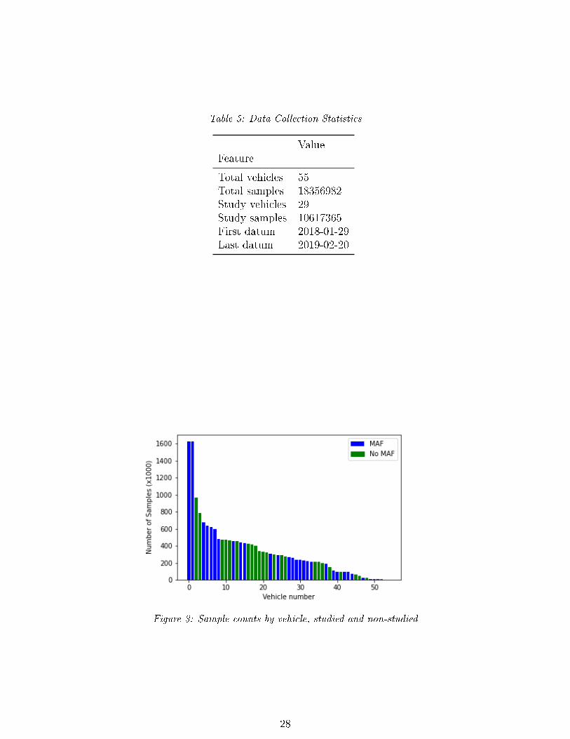
Table 5: Data Collection Statistics
ValueFeature
Total vehicles 55Total samples 18356982Study vehicles 29Study samples 10617365First datum 2018-01-29Last datum 2019-02-20
Figure 3: Sample counts by vehicle, studied and non-studied
28
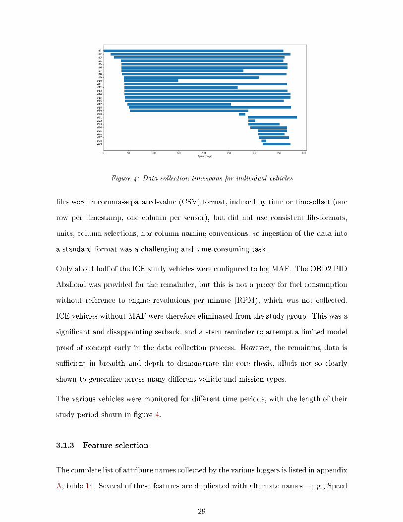
Figure 4: Data collection timespans for individual vehicles
�les were in comma-separated-value (CSV) format, indexed by time or time-o�set (one
row per timestamp, one column per sensor), but did not use consistent �le-formats,
units, column selections, nor column naming conventions, so ingestion of the data into
a standard format was a challenging and time-consuming task.
Only about half of the ICE study vehicles were con�gured to log MAF. The OBD2 PID
AbsLoad was provided for the remainder, but this is not a proxy for fuel consumption
without reference to engine revolutions per minute (RPM), which was not collected.
ICE vehicles without MAF were therefore eliminated from the study group. This was a
signi�cant and disappointing setback, and a stern reminder to attempt a limited model
proof of concept early in the data collection process. However, the remaining data is
su�cient in breadth and depth to demonstrate the core thesis, albeit not so clearly
shown to generalize across many di�erent vehicle and mission types.
The various vehicles were monitored for di�erent time periods, with the length of their
study period shown in �gure 4.
3.1.3 Feature selection
The complete list of attribute names collected by the various loggers is listed in appendix
A, table 14. Several of these features are duplicated with alternate names � e.g., Speed
29
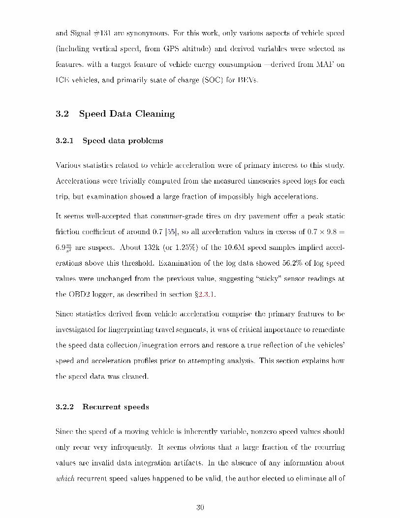
and Signal #131 are synonymous. For this work, only various aspects of vehicle speed
(including vertical speed, from GPS altitude) and derived variables were selected as
features, with a target feature of vehicle energy consumption � derived from MAF on
ICE vehicles, and primarily state of charge (SOC) for BEVs.
3.2 Speed Data Cleaning
3.2.1 Speed data problems
Various statistics related to vehicle acceleration were of primary interest to this study.
Accelerations were trivially computed from the measured timeseries speed logs for each
trip, but examination showed a large fraction of impossibly high accelerations.
It seems well-accepted that consumer-grade tires on dry pavement o�er a peak static
friction coe�cient of around 0.7 [55], so all acceleration values in excess of 0.7× 9.8 =
6.9ms2
are suspect. About 132k (or 1.25%) of the 10.6M speed samples implied accel-
erations above this threshold. Examination of the log data showed 56.2% of log speed
values were unchanged from the previous value, suggesting �sticky� sensor readings at
the OBD2 logger, as described in section �2.3.1.
Since statistics derived from vehicle acceleration comprise the primary features to be
investigated for �ngerprinting travel segments, it was of critical importance to remediate
the speed data collection/integration errors and restore a true re�ection of the vehicles'
speed and acceleration pro�les prior to attempting analysis. This section explains how
the speed data was cleaned.
3.2.2 Recurrent speeds
Since the speed of a moving vehicle is inherently variable, nonzero speed values should
only recur very infrequently. It seems obvious that a large fraction of the recurring
values are invalid data integration artifacts. In the absence of any information about
which recurrent speed values happened to be valid, the author elected to eliminate all of
30
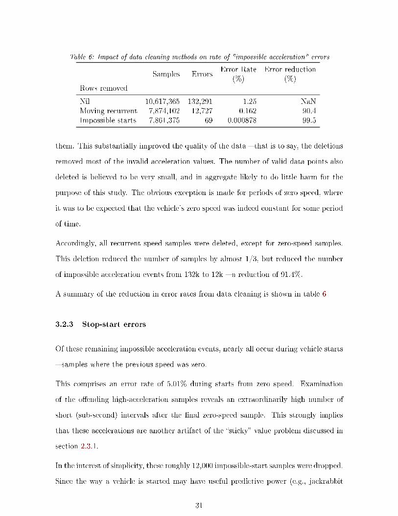
Table 6: Impact of data cleaning methods on rate of "impossible acceleration" errors
Samples ErrorsError Rate
(%)Error reduction
(%)Rows removed
Nil 10,617,365 132,291 1.25 NaNMoving recurrent 7,874,102 12,727 0.162 90.4Impossible starts 7,861,375 69 0.000878 99.5
them. This substantially improved the quality of the data � that is to say, the deletions
removed most of the invalid acceleration values. The number of valid data points also
deleted is believed to be very small, and in aggregate likely to do little harm for the
purpose of this study. The obvious exception is made for periods of zero speed, where
it was to be expected that the vehicle's zero speed was indeed constant for some period
of time.
Accordingly, all recurrent speed samples were deleted, except for zero-speed samples.
This deletion reduced the number of samples by almost 1/3, but reduced the number
of impossible acceleration events from 132k to 12k � a reduction of 91.4%.
A summary of the reduction in error rates from data cleaning is shown in table 6
3.2.3 Stop-start errors
Of these remaining impossible acceleration events, nearly all occur during vehicle starts
� samples where the previous speed was zero.
This comprises an error rate of 5.01% during starts from zero speed. Examination
of the o�ending high-acceleration samples reveals an extraordinarily high number of
short (sub-second) intervals after the �nal zero-speed sample. This strongly implies
that these accelerations are another artifact of the �sticky� value problem discussed in
section 2.3.1.
In the interest of simplicity, these roughly 12,000 impossible-start samples were dropped.
Since the way a vehicle is started may have useful predictive power (e.g., jackrabbit
31
starts), future work should be applied to recovering the information in start samples,
as discussed in section 7.2.1.
3.2.4 Other errors
With the above cleaning methods applied, the corpus contained only 69 remaining
samples with impossibly high acceleration values. Inspection showed these to generally
correspond to high rates of change over short sample periods, but with no obvious
cause. These samples could very well be true values, perhaps due to wheels spinning
under high power or wheel-lockup due to hard braking. These samples have been left
intact.
3.3 Power Data Cleaning
Again, the core problem of this thesis is to predict each vehicle's characteristic input
power for each eigentrip. The model's ground truth will be the input power consumed
during each trip segment, so a new power feature was calculated from the available
features.
3.3.1 ICE power
For ICE vehicles, the energy input is fuel consumed. Fuel consumption was approxi-
mated from logged MAF at the stoichiometric fuel:air ratio, an assumption discussed
in �2.3.2 and �7.1. The energy value was then calculated using the LHV of 46.4 MJkg
[56].
The MAF PID su�ered from the same "stickiness" problem as the other PIDs discussed
above, and had an e�ective sample period of about 2 s. This was addressed by the same
means as for speed: removing all recurrent values, except zero-value periods.
3.3.2 BEV power
For the BEVs, input power is from the high-voltage (HV) main drive battery.
32
Although FleetCarma attempted to provide 1-second resolution power data, the data
su�ered from the same stickiness problem as elsewhere; the real sampling rate was much
lower than expected. SOC was sampled at a median period of 87 s, HV battery current
at 29 s, and HV battery voltage at 30 s. This low sampling frequency complicated
the power calculation; multiplying spot-sampled voltage and current with the elapsed
time would miss transient events, and be unlikely to provide an accurate re�ection of
total consumption. Reported SOC is not perfectly suitable, being unlikely to have been
sampled near a given segment boundary.
A rejected course of investigation was to interpolate SOC along the better-sampled
HV voltage reading, on the assumption that battery voltage would drop linearly with
expended energy. Plots of SOC vs voltage for multiple trips (�gure 5) suggested that
there is a good relationship between these features. However, inspection of a number
of actual time-domain plots of battery voltage and SOC similar to �gure 6 suggest that
the correlation only exists reliably at a scale too broad to be of practical use.
As shown in �gure 6, the HV system's voltage readings are highly variable while the
vehicle is in motion; this reading shows system voltage rather than open-circuit battery
voltage. Furthermore, the system's logging resolution is far too low to estimate energy
consumption (E) from voltage (V) and amperage (I) in the typical manner, as:
∆E =
∫V (t)× I(t) dt (6)
Fortunately the vehicle's on-board computer has high-resolution access to the electrical
sensors, and can make use of a combination of several methods for establishing the
remaining useful charge in the battery [57]. SOC is therefore a reasonably trustworthy
absolute measurement relative to the vehicle's known battery pack capacity, and a
reasonable estimate of energy consumption over time can be obtained from it.
Ultimately, no better method was found than applying vehicle-reported SOC to
manufacturer-published battery capacity of 27 kWh for the Kia Souls [58, 59], and
12 kWh for the Outlander PHEV [60]. This required linear interpolation of SOC to the
33
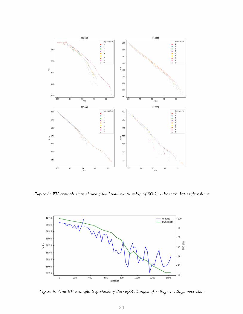
Figure 5: EV example trips showing the broad relationship of SOC vs the main battery's voltage
Figure 6: One EV example trip showing the rapid changes of voltage readings over time
34

Table 7: Number of samples and trips removed by EV data cleaning procedures
EV Samples Removed EV Trips
Nil 817,820 0 2,308Zero power 817,641 179 2,181Charging 796,022 21,619 1,762Zero-time 796,022 0 1,762
segment boundaries as described below in �3.4, a signi�cant assumption that merits
the future work discussed in �7.2.3. Given these assumptions, energy used in a period
is then simply:
∆E = ∆SOC × Capacity (7)
Inspection of the power thus calculated showed a large number of null SOC and V-
I measurements. Nearly all of these were addressed by deleting a small number of
unusable data-logs, presumed to represent data collection artifacts generated by loggers
not well-con�gured for their host BEVs, described in table 7.
3.4 Regularization
In order to reduce the amount of data uploaded over the cellular devices, the supplier
con�gured their loggers to use a sample period of about 1 second while moving, and 30
seconds while stopped. After collection was complete, the "sticky" problem discussed
in �2.3.1 was discovered, and with it the realization that various sensor values were
recorded at di�erent frequencies, and at fractional-second o�sets from each other. The
above process of removing recurrent values adequately eliminated the spurious readings,
but introduced two distinct problems:
1. The longer-than-expected sampling period introduces complexity in handling seg-
ment boundaries � the �nal sample in each segment must be extrapolated across
the boundary in order to be included in the second segment.
2. the sample following a 'stopped' sample may have a non-zero speed; barring the
35
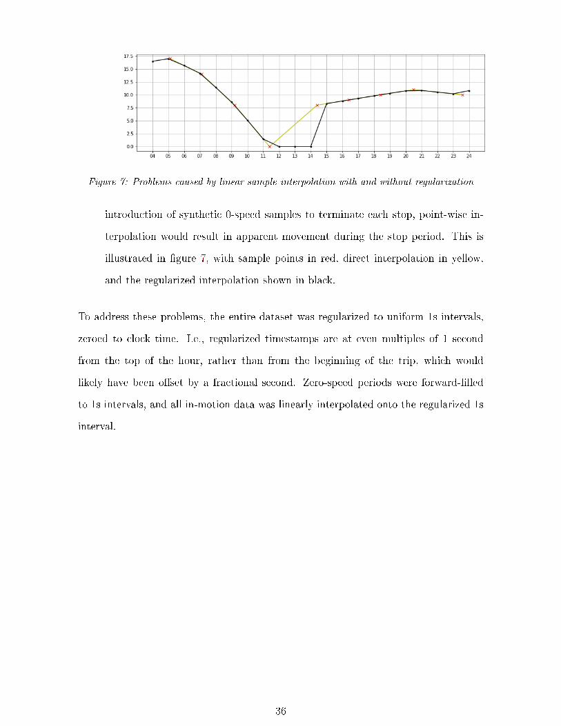
Figure 7: Problems caused by linear sample interpolation with and without regularization
introduction of synthetic 0-speed samples to terminate each stop, point-wise in-
terpolation would result in apparent movement during the stop period. This is
illustrated in �gure 7, with sample points in red, direct interpolation in yellow,
and the regularized interpolation shown in black.
To address these problems, the entire dataset was regularized to uniform 1s intervals,
zeroed to clock time. I.e., regularized timestamps are at even multiples of 1 second
from the top of the hour, rather than from the beginning of the trip, which would
likely have been o�set by a fractional second. Zero-speed periods were forward-�lled
to 1s intervals, and all in-motion data was linearly interpolated onto the regularized 1s
interval.
36
4 Methodology
4.1 Feature Preparation . . . . . . . . 37
4.1.1 Segmentation . . . . . . . . 37
4.1.2 Feature values . . . . . . . 38
4.1.3 Assumptions . . . . . . . . 39
4.1.4 Data review . . . . . . . . . 39
4.2 Clustering . . . . . . . . . . . . . . 41
4.2.1 Intent . . . . . . . . . . . . 41
4.2.2 Key insight . . . . . . . . . 42
4.2.3 Cluster visualization . . . . 42
4.3 Classi�cation Algorithm . . . . . . 42
4.3.1 Algorithm selection . . . . . 42
4.3.2 Decision Trees . . . . . . . 44
4.3.3 Boosting and AdaBoost . . 45
4.3.4 Gradient Boosting Machines 46
4.3.5 LightGBM . . . . . . . . . 47
4.4 Classi�cation Method . . . . . . . 48
4.4.1 Wrong-class error . . . . . . 48
4.5 Energy Prediction . . . . . . . . . 49
4.6 Parameter Re�nement . . . . . . . 50
4.6.1 First pass iteration . . . . . 50
4.6.2 Second pass iteration . . . . 51
4.6.3 Hyperparameter tuning . . 51
4.6.4 Interpretation and param-eter selection . . . . . . . . 52
4.7 Comparison Predictions . . . . . . 55
4.7.1 Published fuel economy . . 55
4.7.2 LGBM regression . . . . . . 55
This section describes the process chosen to build a spreadsheet-compatible energy
prediction model from the cleaned timeseries logger data. In broad terms, the steps
were as follows:
� Divide travel data into segments
� Compute kinetic �ngerprint features and average power
� Select reasonable starting clustering parameters
� Cluster into groups representing eigentrips
� Characterize missions by classifying travel data
� Iteratively re�ne clustering parameters and model hyperparameters
4.1 Feature Preparation
4.1.1 Segmentation
As in Wu's drive cycle classi�er [31], the data was consolidated into 3-minute segments
to match the resolution of a typical urban stop-go-stop cycle. The resampling is relative
37
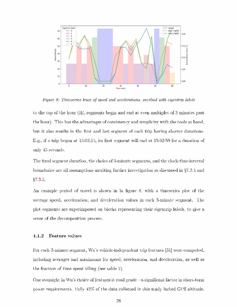
Figure 8: Timeseries trace of speed and accelerations, overlaid with eigentrip labels
to the top of the hour (IE, segments begin and end at even multiples of 3 minutes past
the hour). This has the advantages of consistency and simplicity with the tools at hand,
but it also results in the �rst and last segment of each trip having shorter durations.
E.g., if a trip began at 15:02:15, its �rst segment will end at 15:02:59 for a duration of
only 45 seconds.
The �xed segment duration, the choice of 3-minute segments, and the clock-time interval
boundaries are all assumptions meriting further investigation as discussed in �7.3.4 and
�7.3.5.
An example period of travel is shown in in �gure 8, with a timeseries plot of the
average speed, acceleration, and deceleration values in each 3-minute segment. The
plot segments are superimposed on blocks representing their eigentrip labels, to give a
sense of the decomposition process.
4.1.2 Feature values
For each 3-minute segment, Wu's vehicle-independent trip features [31] were computed,
including averages and maximums for speed, acceleration, and deceleration, as well as
the fraction of time spent idling (see table 2).
One oversight in Wu's choice of features is road grade � a signi�cant factor in short-term
power requirements. Fully 42% of the data collected in this study lacked GPS altitude,
38
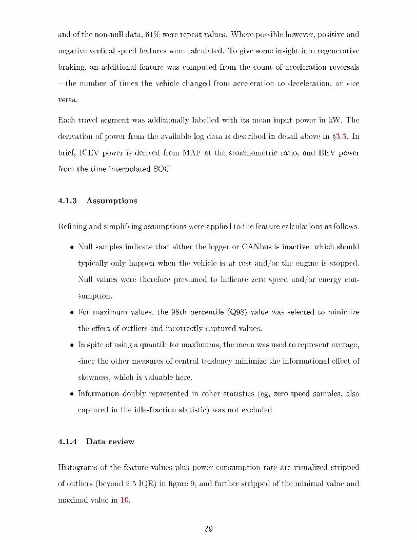
and of the non-null data, 61% were repeat values. Where possible however, positive and
negative vertical speed features were calculated. To give some insight into regenerative
braking, an additional feature was computed from the count of acceleration reversals
� the number of times the vehicle changed from acceleration to deceleration, or vice
versa.
Each travel segment was additionally labelled with its mean input power in kW. The
derivation of power from the available log data is described in detail above in �3.3. In
brief, ICEV power is derived from MAF at the stoichiometric ratio, and BEV power
from the time-interpolated SOC.
4.1.3 Assumptions
Re�ning and simplifying assumptions were applied to the feature calculations as follows:
� Null samples indicate that either the logger or CANbus is inactive, which should
typically only happen when the vehicle is at rest and/or the engine is stopped.
Null values were therefore presumed to indicate zero speed and/or energy con-
sumption.
� For maximum values, the 98th percentile (Q98) value was selected to minimize
the e�ect of outliers and incorrectly captured values.
� In spite of using a quantile for maximums, the mean was used to represent average,
since the other measures of central tendency minimize the informational e�ect of
skewness, which is valuable here.
� Information doubly-represented in other statistics (eg, zero-speed samples, also
captured in the idle-fraction statistic) was not excluded.
4.1.4 Data review
Histograms of the feature values plus power consumption rate are visualized stripped
of outliers (beyond 2.5 IQR) in �gure 9, and further stripped of the minimal value and
maximal value in 10.
39
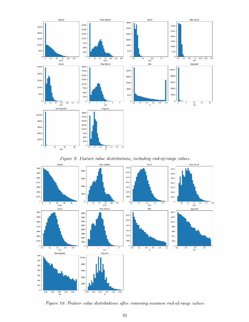
Figure 9: Feature value distributions, including end-of-range values
Figure 10: Feature value distributions after removing common end-of-range values
40

4.2 Clustering
Having established a clean corpus of �ngerprinted travel segments, the next step was
to perform a preliminary clustering of the segments into similar groups.
The individual features did not exhibit signi�cant modalities other than those obviously
caused by segments where the vehicle was idle; there is no reason to expect that the
data is inherently clustered. Since the clusters will be selected arbitrarily to improve
the model's performance, a simple clusterer using Euclidean distance su�ces for initial
validation. K-means clustering was chosen due to its simplicity and the fact that the
Scikit-learn implementation does not scale its inputs, permitting feature weighting by
scaling. Since K-means greedily minimizes within-cluster sum-of-squares [48],
n∑i=0
minµj∈C
(||xi − µj||2) (8)
it tends to result in clusters which are roughly spherical, rather than elongated or
convex. This is a limiting factor deserving additional work (�7.4.1), but it does not
prevent the technique from establishing reasonable cluster centroids, nor from providing
labelled groups which will train a functional classi�er.
4.2.1 Intent
The centroids of these groups de�ne the characteristic travel-type exemplars that we
are calling "eigentrips". The eigentrips are used to estimate a vehicle's input power
according to the vehicle's type, and the kinetic characteristics of the travel it is un-
dertaking. The goal is therefore to �nd a set of eigentrips, each of which represent
a travel regime with both (a) consistent kinetic characteristics, and (b) similar input
power within each vehicle type.
41

4.2.2 Key insight
It was desired that the eigentrips represent regimes of travel with similar power within
each vehicle-type, but not necessarily across vehicle-types, so power was added as a
feature for the purpose of clustering, and weighted to emphasize its importance relative
to the individual kinetic features.
The inter-vehicle di�erence in power for a given travel-type would be a confounding
factor, so the power feature is standardized to Mahalanobis distance (shifted to have a
zero mean, and scaled to number of standard deviations) separately for each vehicle.
4.2.3 Cluster visualization
A preliminary K-means clustering operation was performed with K=10 clusters, and
the power feature weighting increased by applying a power-scaling factor (PS) of 2.0.
The kinetic features were reduced to 2 dimensions with PCA as shown in table 8.
The PCA-reduced kinetic features were visualized on a 3D scatter plot, with the Z
axis showing power, and the cluster labels di�erentiated by colour. Clustering for the
complete training datasest is visualized in �gure 11(a), with power standardized within
each vehicle. The similar sub�gure (b) shows the subset of data for a single vehicle,
with non-standardized power.
4.3 Classi�cation Algorithm
4.3.1 Algorithm selection
The core of the proposed model is the classi�cation of travel segments by their kinetic
features, and labelling them with the most-similar eigentrip. This label permits pre-
dicting a likely vehicle-speci�c characteristic power for the segment. In other words,
the clustering process above has de�ned the eigentrips, and now they can be applied.
The feature histograms (�gure 10) showed the bulk of feature data in well-ordered
distributions, but many with a large additional peak at zero (as well as unity, in the case
42
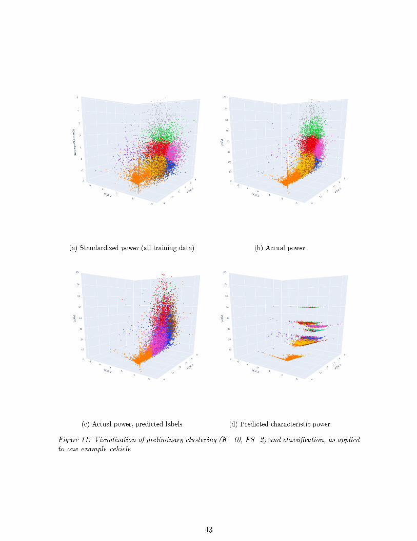
(a) Standardized power (all training data) (b) Actual power
(c) Actual power, predicted labels (d) Predicted characteristic power
Figure 11: Visualization of preliminary clustering (K=10, PS=2) and classi�cation, as appliedto one example vehicle
43
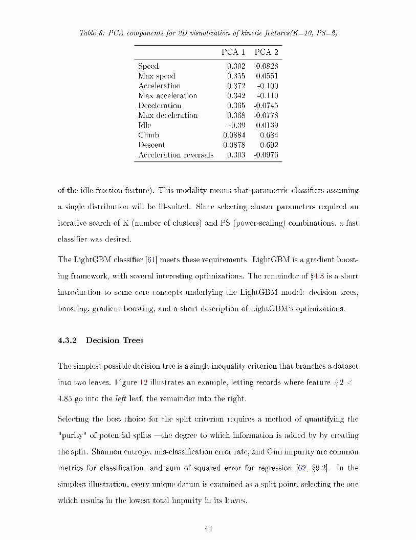
Table 8: PCA components for 2D visualization of kinetic features(K=10, PS=2)
PCA 1 PCA 2
Speed 0.302 0.0828Max speed 0.355 0.0551Acceleration 0.372 -0.100Max acceleration 0.342 -0.110Deceleration 0.365 -0.0745Max deceleration 0.368 -0.0778Idle -0.39 0.0139Climb 0.0884 0.684Descent 0.0878 0.692Acceleration reversals 0.303 -0.0976
of the idle fraction feature). This modality means that parametric classi�ers assuming
a single distribution will be ill-suited. Since selecting cluster parameters required an
iterative search of K (number of clusters) and PS (power-scaling) combinations, a fast
classi�er was desired.
The LightGBM classi�er [61] meets these requirements. LightGBM is a gradient boost-
ing framework, with several interesting optimizations. The remainder of �4.3 is a short
introduction to some core concepts underlying the LightGBM model: decision trees,
boosting, gradient boosting, and a short description of LightGBM's optimizations.
4.3.2 Decision Trees
The simplest possible decision tree is a single inequality criterion that branches a dataset
into two leaves. Figure 12 illustrates an example, letting records where feature #2 <=
4.85 go into the left leaf, the remainder into the right.
Selecting the best choice for the split criterion requires a method of quantifying the
"purity" of potential splits � the degree to which information is added by by creating
the split. Shannon entropy, mis-classi�cation error rate, and Gini impurity are common
metrics for classi�cation, and sum of squared error for regression [62, �9.2]. In the
simplest illustration, every unique datum is examined as a split point, selecting the one
which results in the lowest total impurity in its leaves.
44

Figure 12: Example of a single-node decision tree, or "stump"
4.3.3 Boosting and AdaBoost
Gradient Boosting is the name for a group of methods for building an ensemble of
"weak" learning machines (often small decision trees), each building on the weaknesses
of its predecessors.
It is best illustrated with AdaBoost, the �rst adaptive boosting machine, and arguably
the simplest and best-known [62]. The following pseudocode, derived from [63], uses
the simplest possible real classi�er (a decision tree stump) applied to an input dataset
X with labels y.
1. Start by de�ning the �rst weak learner F1 (a decision tree stump, as discussed in
�4.3.2), trained from the initial input dataset X1 = X, y1 = y
2. Use the F1 to generate predictions y1 against labels y1.
3. Compute loss L1. For classi�cation, this might be the fractional error rate
L1 =1
N
∑|y 6= y| (9)
4. Compute performance value α1, a number that is larger if the classi�er performs
well.
α1 = 0.5log(1− L1
L1
) (10)
5. Halt iteration if stop conditions met (e.g. a predetermined number of iterations).
45

6. Create a new input dataset X2, y2, with a larger proportion of records incorrectly
classi�ed by L1. Selection is pseudo-random, using a weight vector
w2 = e−α1s1 (11)
where s1 =
1, y1 = y1
−1, y1 6= y1
(12)
7. Train a new tree F2 from the new dataset X2, y2, and iterate from step 2.
The �nal classi�cation decision takes the form of a weighted vote between the weak
learners, weighted by each learner's performance metric αi.
4.3.4 Gradient Boosting Machines
Gradient Boosting Machines are a generalization of the AdaBoost concept, allowing
di�erent loss functions, and applying a kind of gradient descent in order to reduce error
in a smaller number of iterations. A gradient boost model is super�cially similar to
AdaBoost, in that it consists of an ensemble of weighted weak learners:
F (X) =F0(X) + F1(X) + ...+ Fm(X) (13)
where
Fi = γiri
ri = −g(L)|i−1 (negative gradient of loss function)
γi = argminγ
L(Fi−1 − γri)
(14)
Where γi are weights and ri are the pseudo-residuals of the preceding weak learners. In
essence, each element Fm is the output of a decision tree trained to predict the pseudo-
residual rm. In the special case where the loss function is sum of squared errors (SSE),
this is the (true) residual of the prior elements. The output is then scaled by a weighting
factor γm, selected to minimize the overall loss.
In other words, gradient boosting is conceptually di�erent from AdaBoost in that each
46
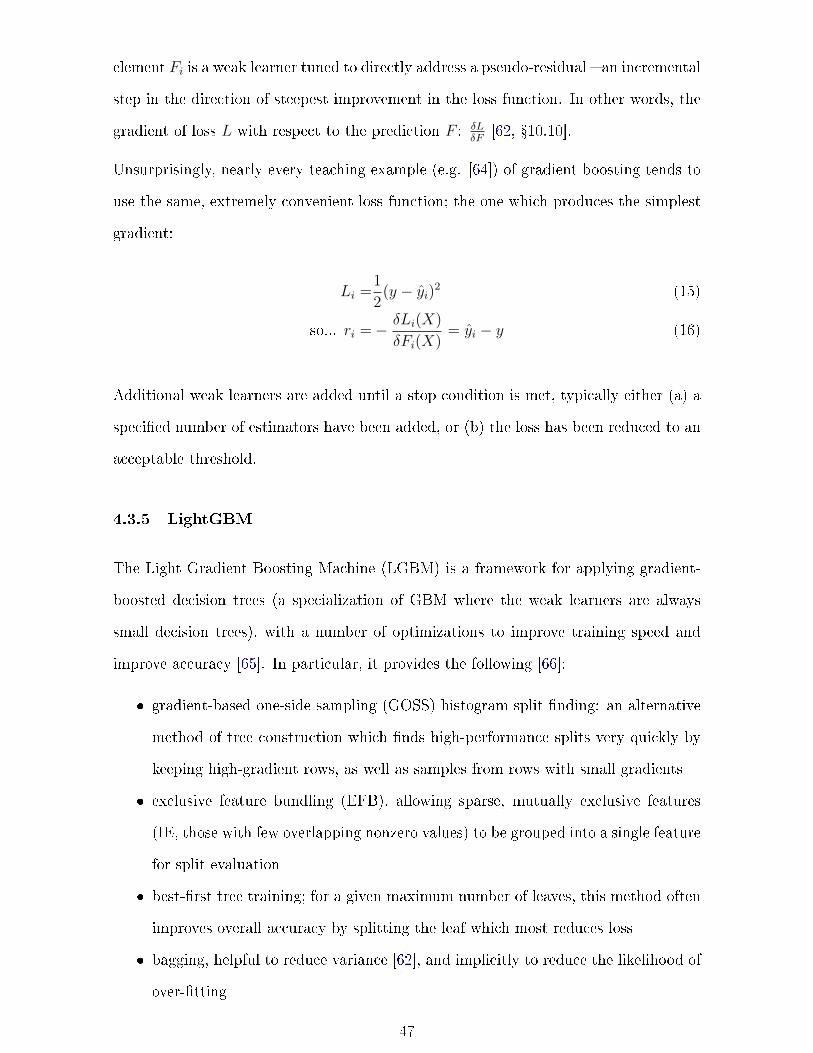
element Fi is a weak learner tuned to directly address a pseudo-residual � an incremental
step in the direction of steepest improvement in the loss function. In other words, the
gradient of loss L with respect to the prediction F : δLδF
[62, �10.10].
Unsurprisingly, nearly every teaching example (e.g. [64]) of gradient boosting tends to
use the same, extremely convenient loss function; the one which produces the simplest
gradient:
Li =1
2(y − yi)2 (15)
so... ri =− δLi(X)
δFi(X)= yi − y (16)
Additional weak learners are added until a stop condition is met, typically either (a) a
speci�ed number of estimators have been added, or (b) the loss has been reduced to an
acceptable threshold.
4.3.5 LightGBM
The Light Gradient Boosting Machine (LGBM) is a framework for applying gradient-
boosted decision trees (a specialization of GBM where the weak learners are always
small decision trees), with a number of optimizations to improve training speed and
improve accuracy [65]. In particular, it provides the following [66]:
� gradient-based one-side sampling (GOSS) histogram split �nding: an alternative
method of tree construction which �nds high-performance splits very quickly by
keeping high-gradient rows, as well as samples from rows with small gradients
� exclusive feature bundling (EFB), allowing sparse, mutually exclusive features
(IE, those with few overlapping nonzero values) to be grouped into a single feature
for split evaluation
� best-�rst tree training; for a given maximum number of leaves, this method often
improves overall accuracy by splitting the leaf which most reduces loss
� bagging, helpful to reduce variance [62], and implicitly to reduce the likelihood of
over-�tting
47

4.4 Classi�cation Method
An LGBM classi�er was constructed by training with the kinetic features using 10% of
the labelled data for each vehicle, with the remaining 90% held back for testing. This
method is at odds with the apparent industry standard method of 80% training / 20%
hold-back, but given a reasonable quantity of data, a small, well-distributed training set
in conjunction with extensive testing serves to ensure that the model is generalizable
and not over-�tted.
Figure 11 shows the results of classi�cation on the sample vehicle. Sub�gure (c) shows
the eigentrip label (colour) of each segment predicted by the classi�er solely with refer-
ence to the kinetic parameters, and sub�gure (d) shows the as-clustered original labels,
but with the predicted power.
4.4.1 Wrong-class error
In general, a multi-class classi�er returns the set of probabilities that a given element
(in this case, a travel segment) belongs to each possible class (in this case, the various
eigentrips). Typically, the class with the highest probability (the maximum likelihood
class) is selected. Applying this technique, the trained classi�er had a label selection
accuracy of 77.9%. The misclassi�cation rate is not as concerning as it might seem:
since the dataset is not in distinct clusters, segments of indeterminate class can be
expected to have an actual power somewhere between the characteristic powers of its
most probable classes.
It seems possible that the correct power may often fall between the highest and second-
highest probability classi�cations. A re�nement for future work (discussed in �7.4.2)
is for cases where membership is unclear, to attempt selecting the two most probable
classes, and pro-rating the segment's eigentrip membership by probability.
48

4.5 Energy Prediction
For the purpose of energy prediction, each travel segment is represented as a time-
weighted vector, where each element represents a time-weighted (and potentially
probability-weighted) count of eigentrips. E.g., if the segment is 180s long, and is best
represented by eigentrip e2, the segment is now represented by S = [0, 180, 0, 0, ...],
where the elements of S represent the number of seconds spent in each of the eigentrip
types. Any period of travel (T ) can now be represented as the sum of its segment
vectors:
T =∑
Si (17)
Given a vehicle's list of characteristic power values for each eigentripCv = [Pv,e1, Pv,e2, ...],
the predicted energy consumption for that travel is:
E = T ·Cv (18)
Accuracy is assessed relative to the logger estimate of observed power for any given
period of travel, in terms of modi�ed mean absolute percentage error (MMAPE):
MMAPE =100%
n
n∑t=1
∣∣∣∣yt − yt1 + yt
∣∣∣∣ (19)
This initial model con�guration (K=10, PS=2) exhibited a per-segment MMAPE of
37.4%, somewhat better than the baseline prediction error of 50.9%, calculated below
in �5.
49
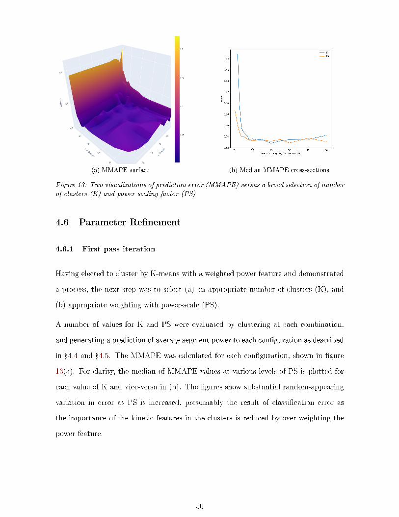
(a) MMAPE surface (b) Median MMAPE cross-sections
Figure 13: Two visualizations of prediction error (MMAPE) versus a broad selection of numberof clusters (K) and power-scaling factor (PS)
4.6 Parameter Re�nement
4.6.1 First pass iteration
Having elected to cluster by K-means with a weighted power feature and demonstrated
a process, the next step was to select (a) an appropriate number of clusters (K), and
(b) appropriate weighting with power-scale (PS).
A number of values for K and PS were evaluated by clustering at each combination,
and generating a prediction of average segment power to each con�guration as described
in �4.4 and �4.5. The MMAPE was calculated for each con�guration, shown in �gure
13(a). For clarity, the median of MMAPE values at various levels of PS is plotted for
each value of K and vice-versa in (b). The �gures show substantial random-appearing
variation in error as PS is increased, presumably the result of classi�cation error as
the importance of the kinetic features in the clusters is reduced by over-weighting the
power feature.
50
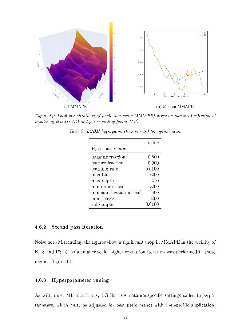
(a) MMAPE (b) Median MMAPE
Figure 14: Local visualizations of prediction error (MMAPE) versus a narrowed selection ofnumber of clusters (K) and power-scaling factor (PS)
Table 9: LGBM hyperparameters selected for optimization
ValueHyperparameter
bagging fraction 0.800feature fraction 0.900learning rate 0.0100max bin 60.0max depth 27.0min data in leaf 39.0min sum hessian in leaf 59.0num leaves 80.0subsample 0.0100
4.6.2 Second pass iteration
Noise notwithstanding, the �gures show a signi�cant drop in MMAPE in the vicinity of
K=8 and PS=5, so a smaller-scale, higher-resolution iteration was performed in those
regions (�gure 14).
4.6.3 Hyperparameter tuning
As with most ML algorithms, LGBM uses data-nonspeci�c settings called hyperpa-
rameters, which must be adjusted for best performance with the speci�c application.
51
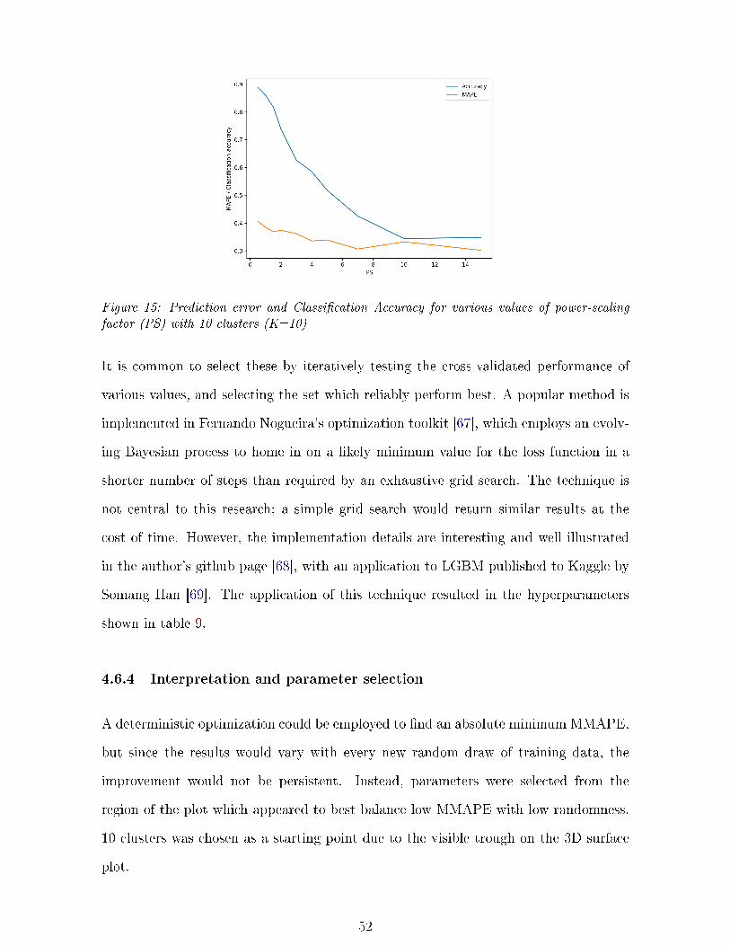
Figure 15: Prediction error and Classi�cation Accuracy for various values of power-scalingfactor (PS) with 10 clusters (K=10)
It is common to select these by iteratively testing the cross-validated performance of
various values, and selecting the set which reliably perform best. A popular method is
implemented in Fernando Nogueira's optimization toolkit [67], which employs an evolv-
ing Bayesian process to home in on a likely minimum value for the loss function in a
shorter number of steps than required by an exhaustive grid search. The technique is
not central to this research; a simple grid search would return similar results at the
cost of time. However, the implementation details are interesting and well illustrated
in the author's github page [68], with an application to LGBM published to Kaggle by
Somang Han [69]. The application of this technique resulted in the hyperparameters
shown in table 9.
4.6.4 Interpretation and parameter selection
A deterministic optimization could be employed to �nd an absolute minimum MMAPE,
but since the results would vary with every new random draw of training data, the
improvement would not be persistent. Instead, parameters were selected from the
region of the plot which appeared to best balance low MMAPE with low randomness.
10 clusters was chosen as a starting point due to the visible trough on the 3D surface
plot.
52
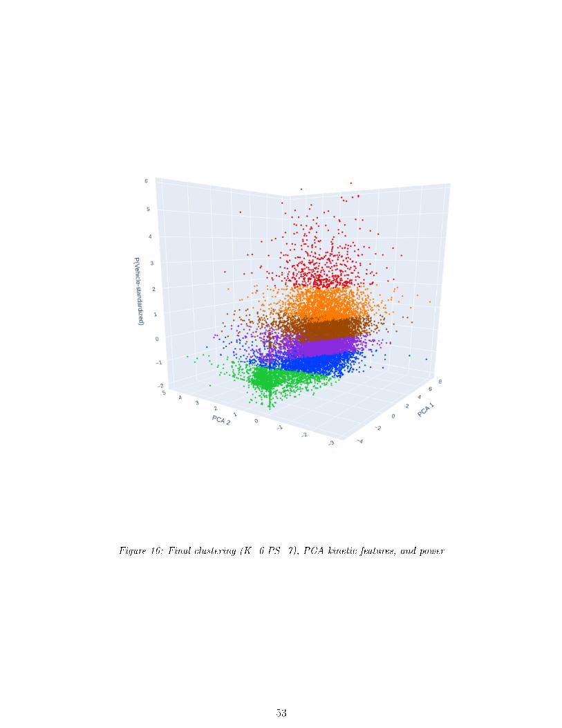
Figure 16: Final clustering (K=6 PS=7), PCA kinetic features, and power
53
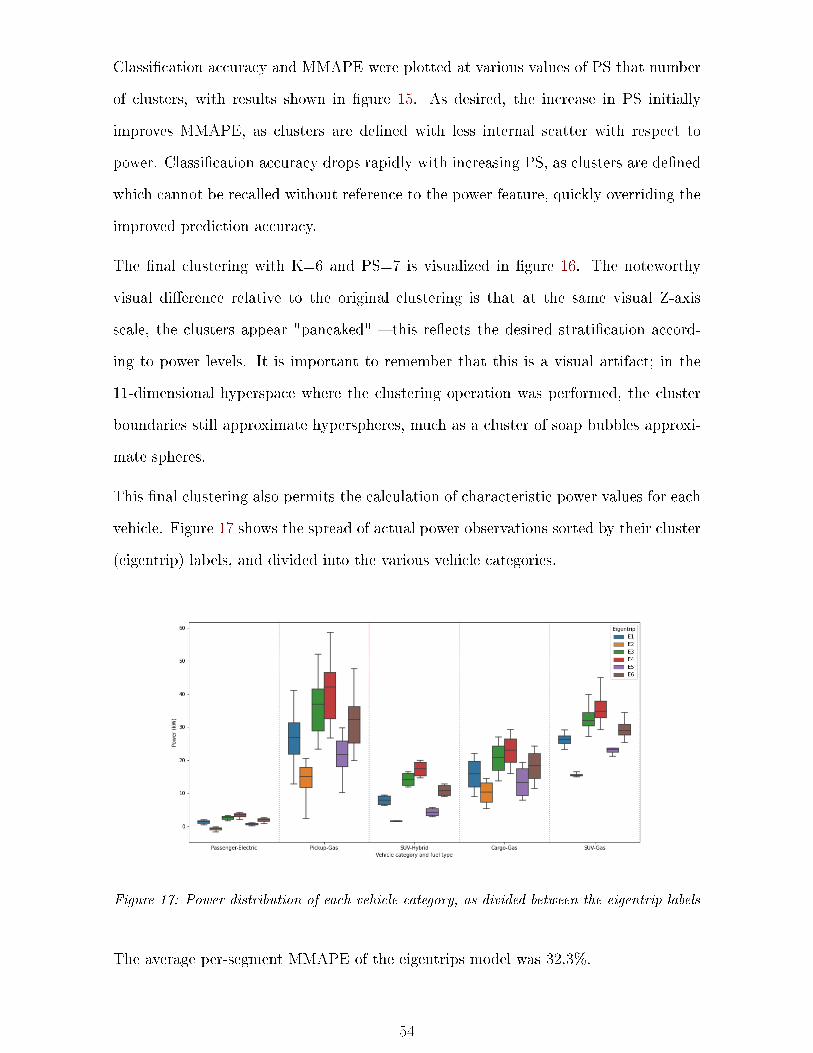
Classi�cation accuracy and MMAPE were plotted at various values of PS that number
of clusters, with results shown in �gure 15. As desired, the increase in PS initially
improves MMAPE, as clusters are de�ned with less internal scatter with respect to
power. Classi�cation accuracy drops rapidly with increasing PS, as clusters are de�ned
which cannot be recalled without reference to the power feature, quickly overriding the
improved prediction accuracy.
The �nal clustering with K=6 and PS=7 is visualized in �gure 16. The noteworthy
visual di�erence relative to the original clustering is that at the same visual Z-axis
scale, the clusters appear "pancaked" � this re�ects the desired strati�cation accord-
ing to power levels. It is important to remember that this is a visual artifact; in the
11-dimensional hyperspace where the clustering operation was performed, the cluster
boundaries still approximate hyperspheres, much as a cluster of soap bubbles approxi-
mate spheres.
This �nal clustering also permits the calculation of characteristic power values for each
vehicle. Figure 17 shows the spread of actual power observations sorted by their cluster
(eigentrip) labels, and divided into the various vehicle categories.
Figure 17: Power distribution of each vehicle category, as divided between the eigentrip labels
The average per-segment MMAPE of the eigentrips model was 32.3%.
54
4.7 Comparison Predictions
4.7.1 Published fuel economy
Business-as-usual (BAU) energy consumption prediction was established by applying
published city/highway Le/100km �gures to the logged travel distances for each seg-
ment. The consumption test protocol [17] drive cycles had a mean speed of 34 km/h for
city driving and 78 km/h for highway, so a dividing speed of 56 km/h was established
midway between those means. Travel segments with an average speed at or below
that dividing speed were predicted at the city �gure, and those above predicted at the
highway �gure.
Fuel economy �gures were selected for each vehicle with reference to NRCan's fuel
consumption rating search tool [70]. In each case, the base model was selected unless
the CRD's vehicle database indicated a speci�c sub-model or trim level.
The average per-segment MMAPE of this method was 50.9%.
4.7.2 LGBM regression
Finally, to establish the level of avoidable error with the information available to the
model, a LightGBM regression model [66] was trained on the 10 kinetic features, as
well as three additional features capturing speci�c information about each vehicle: its
�el type (ICE, HEV, BEV), vehicle category (passenger, pickup, SUV, etc), and an
identi�er for each speci�c vehicle.
The decision to include all three of these additional features was not obvious; the
vehicle ID is over-speci�c, and in a wider application would instead use a detailed
model and trim-level speci�cation. Furthermore, much of the predictive information in
the vehicle's fuel and category is shared with the vehicle ID, and as discussed in �2.2
mutual information and unnecessary features are to be avoided.
The core con�ict is that on one side, some vehicle categories spanned a wide range of
power levels (e.g., a modern F-150 base-model vs an older F-150 4x4 super-duty), best
55

addressed by permitting the model to modify power based on the observations of speci�c
vehicles. On the other hand, some speci�c vehicles were only observed for a short period
of time, and would not generalize well without reference to the information of other
similar vehicles. On the balance, it was decided to include all three, since boosted tree
models split on a single feature at a time, and therefore do not tend to overemphasize
based on mutual information.
Once the feature-set was selected, the regression model's hyperparameters were tuned
as described in �4.6.3, and power predictions made for each segment. The average
per-segment MMAPE of this method matched that of the eigentrips model, at 32.3%.
56
5 Results
5.1 Presentation of Error . . . . . . . . 58
5.1.1 Error measures . . . . . . . 58
5.1.2 Chosen error measure . . . 60
5.2 Discussion . . . . . . . . . . . . . . 60
5.2.1 Error interpretation . . . . 60
5.2.2 BEV prediction . . . . . . . 62
5.2.3 PHEV prediction . . . . . . 63
5.2.4 HEV prediction . . . . . . . 63
5.2.5 Physical interpretation . . . 63
5.3 Application . . . . . . . . . . . . . 65
5.3.1 Replacement by predicteddistance . . . . . . . . . . . 66
5.3.2 Replacement by publishedfuel economy . . . . . . . . 67
5.3.3 Replacement by logged en-ergy . . . . . . . . . . . . . 67
5.3.4 Replacement by best savings 67
5.4 Shapley Additive Explanation . . . 68
5.4.1 SHAP overview . . . . . . . 68
5.4.2 SHAP summary visualiza-tion . . . . . . . . . . . . . 69
5.4.3 SHAP implications . . . . . 70
This section presents the predictive error of the proposed "eigentrips" model relative to
the logger-data estimate of actual power. The eigentrips model is compared with two
alternative means of prediction: �rst, business-as-usual prediction based on standard
L/100km fuel economy �gures, and second, an LGBM regression model trained to
directly predict segment fuel consumption. The eigentrips model is piecewise-constant,
so the regression model is presented to give a sense of the eigentrip model's avoidable
quantization error.
Much of the discussion in this section is with regards to the MMAPE for individual
3-minute segments, since that is the most intuitive initial indicator of the model's
accuracy. For the end user's purpose, trip-level or mission-level (ie, for the duration of
the vehicle's participation in the study) aggregate error is likely to be of more interest,
and that is addressed at greater length in the discussion section, �5.3.
57
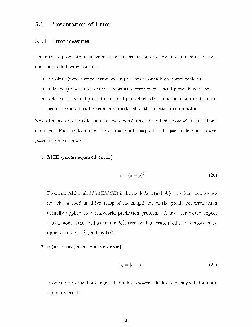
5.1 Presentation of Error
5.1.1 Error measures
The most appropriate intuitive measure for prediction error was not immediately obvi-
ous, for the following reasons:
� Absolute (non-relative) error over-represents error in high-power vehicles.
� Relative (to actual-error) over-represents error when actual power is very low.
� Relative (to vehicle) requires a �xed per-vehicle denominator, resulting in unex-
pected error values for segments unrelated to the selected denominator.
Several measures of prediction error were considered, described below with their short-
comings. For the formulae below, a=actual, p=predicted, q=vehicle max power,
µ=vehicle mean power.
1. MSE (mean squared error)
ε = (a− p)2 (20)
Problem: AlthoughMin(ΣMSE) is the model's actual objective function, it does
not give a good intuitive grasp of the magnitude of the prediction error when
actually applied to a real-world prediction problem. A lay user would expect
that a model described as having 25% error will generate predictions incorrect by
approximately 25%, not by 50%.
2. η (absolute/non-relative error)
η = |a− p| (21)
Problem: Error will be exaggerated in high-power vehicles, and they will dominate
summary results.
58

3. εµ (relative to vehicle-mean)
εµ =
∣∣∣∣a− pµv
∣∣∣∣ (22)
Problem: The mean can be di�erent in similar vehicles, depending on operation.
Some mission pro�les are dominated by idle!
4. εq (relative to vehicle-max)
εq =
∣∣∣∣a− pqv
∣∣∣∣ (23)
Problem: Unintuitive at low power. EG: consider a 100kW vehicle, on a segment
where actual power is 1kW and prediction was 2kW. This measure would return
an error of εq = (2 − 1)/100 = 1%, even though the prediction was double the
observed value.
5. TMAPE (true mean absolute-value percent error)
TMAPE =
∣∣∣∣a− pa∣∣∣∣ (24)
Problem: Segments with zero or near-zero actual power will have excessively high
error. This is of particular concern with EVs and HEVs, which frequently "idle"
at fractional kW power. Almost 1% of EV samples were observed at under 1kW,
causing unreasonably high segment prediction errors.
6. MMAPE (mean absolute-value percent error, modi�ed)
MMAPE =
∣∣∣∣ a− p1 + |a|
∣∣∣∣ (25)
This metric retains much of the intuitive power of TMAPE, while avoiding exces-
sive error at for very small values of actual power.
Problem: The added 1 in the denominator is arbitrary. In the previous example,
59
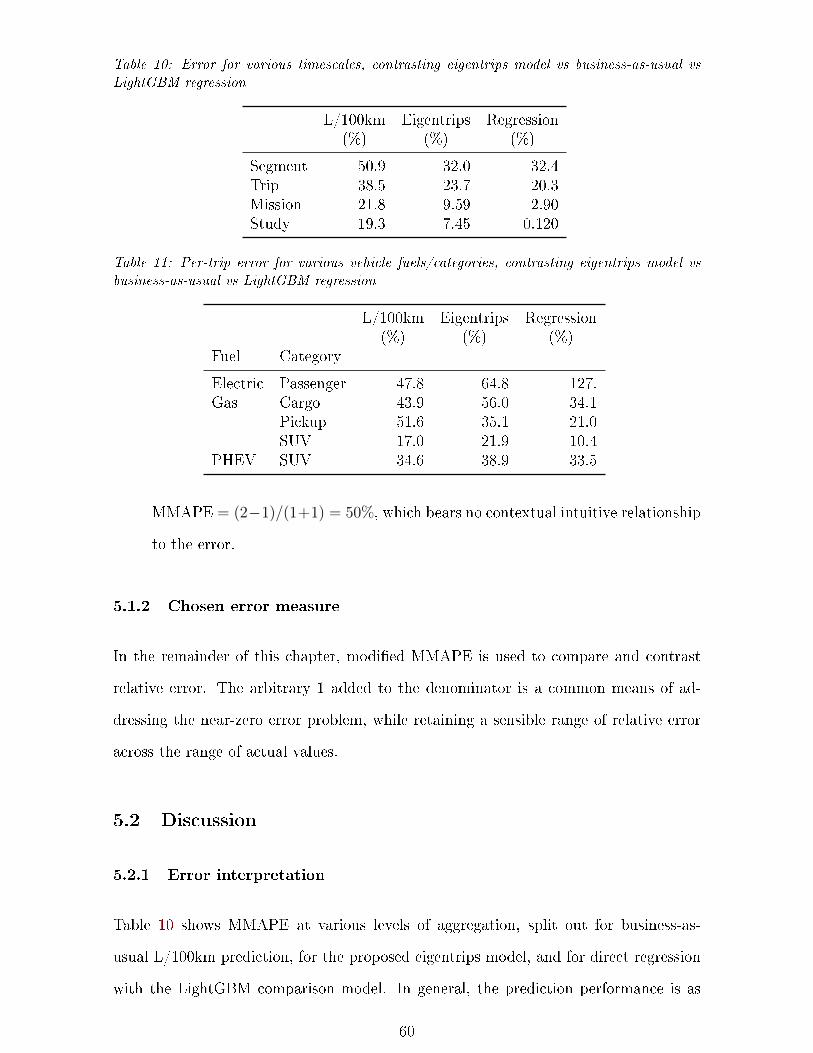
Table 10: Error for various timescales, contrasting eigentrips model vs business-as-usual vsLightGBM regression
L/100km(%)
Eigentrips(%)
Regression(%)
Segment 50.9 32.0 32.4Trip 38.5 23.7 20.3Mission 21.8 9.59 2.90Study 19.3 7.45 0.120
Table 11: Per-trip error for various vehicle fuels/categories, contrasting eigentrips model vsbusiness-as-usual vs LightGBM regression
L/100km(%)
Eigentrips(%)
Regression(%)
Fuel Category
Electric Passenger 47.8 64.8 127.Gas Cargo 43.9 56.0 34.1
Pickup 51.6 35.1 21.0SUV 17.0 21.9 10.4
PHEV SUV 34.6 38.9 33.5
MMAPE = (2−1)/(1+1) = 50%, which bears no contextual intuitive relationship
to the error.
5.1.2 Chosen error measure
In the remainder of this chapter, modi�ed MMAPE is used to compare and contrast
relative error. The arbitrary 1 added to the denominator is a common means of ad-
dressing the near-zero error problem, while retaining a sensible range of relative error
across the range of actual values.
5.2 Discussion
5.2.1 Error interpretation
Table 10 shows MMAPE at various levels of aggregation, split out for business-as-
usual L/100km prediction, for the proposed eigentrips model, and for direct regression
with the LightGBM comparison model. In general, the prediction performance is as
60
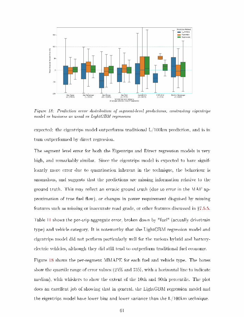
Figure 18: Prediction error distribution of segment-level predictions, contrasting eigentripsmodel vs business-as-usual vs LightGBM regression
expected: the eigentrips model outperforms traditional L/100km prediction, and is in
turn outperformed by direct regression.
The segment level error for both the Eigentrips and Direct regression models is very
high, and remarkably similar. Since the eigentrips model is expected to have signif-
icantly more error due to quantization inherent in the technique, the behaviour is
anomalous, and suggests that the predictions are missing information relative to the
ground truth. This may re�ect an erratic ground truth (due to error in the MAF ap-
proximation of true fuel �ow), or changes in power requirement disguised by missing
features such as missing or inaccurate road grade, or other features discussed in �7.5.5.
Table 11 shows the per-trip aggregate error, broken down by "fuel" (actually drivetrain
type) and vehicle category. It is noteworthy that the LightGBM regression model and
eigentrips model did not perform particularly well for the various hybrid and battery-
electric vehicles, although they did still tend to outperform traditional fuel economy.
Figure 18 shows the per-segment MMAPE for each fuel and vehicle type. The boxes
show the quartile range of error values (25% and 75%, with a horizontal line to indicate
median), with whiskers to show the extent of the 10th and 90th percentile. The plot
does an excellent job of showing that in general, the LightGBM regression model and
the eigentrips model have lower bias and lower variance than the L/100km technique.
61
Figure 19: Example power versus prediction within eigentrips
However, this plot also shows unexpectedly wide variance for HEVs and BEVs, and high
bias and variance for the PHEV, all discussed in detail below. It is also noteworthy
that the Le/100km prediction shows an error of -100% in many cases, since it has no
means to appropriately predict idle power.
Figure 19 uses a single example vehicle to illustrate the variance in actual powers
within each labelled eigentrip, presented in the form of a swarm plot against the power
prediction, taken as the vehicle's characteristic power. The horizontal bar on each
swarm shows the mean actual power, which is seen to be quite close to the quantized
predicted power � which is the vehicle's characteristic power for that eigentrip.
5.2.2 BEV prediction
For the BEVs, this excessive variability is attributed largely to the 90-second low-
resolution power sampling discussed in �3.3. Although the BEVs' onboard SOC com-
putation is presumed to be reliable, it is impossible to know how much power con-
sumption is measured in one segment when it is better attributed to the next. This
lack of accuracy is a key outcome of this research: high-resolution data-driven energy
prediction requires high-resolution input data.
It is noteworthy that since the reported error is relative to actual consumption, the
apparent error of the BEVs is ampli�ed relative to the ICEVs; the 25-75 IQR in �gure
62
18 shows that the eigentrip model has about double the relative error for BEVs as for
ICE pickup trucks � but since the BEV's power is so much lower, this in fact represents
a prediction of 35.7± 7.0 kW for the pickup truck, and 3.0± 0.88 kW for the BEV; the
BEV's absolute error range is in fact much smaller.
5.2.3 PHEV prediction
The single PHEV su�ered from the same low-resolution sampling problem as the BEVs,
and additionally had a very short data-collection period, with only 216 travel segments
recorded, totalling about 10 hours of travel.
Furthermore, the PHEV had no mechanism for capturing the likelihood that a given
segment is in ICE-mode. Future work with PHEVs should attempt to create additional
kinetic features to capture that information, such as total distance travelled this trip,
or total distance today.
5.2.4 HEV prediction
The study included 4 Toyota RAV4 mild HEVs, which were predicted with a reasonable
MMAPE, but a wide spread in the segment level predictions. The loggers in the HEVs
were not con�gured to capture HV battery status, so it can be presumed that the short-
term error included a signi�cant amount of energy consumption being shifted between
adjacent segments, EG, by regenerative braking.
Improving HEV energy prediction would be an interesting extension to this work, and
would require additional feature engineering to capture HEV-speci�c behaviour, such
as regenerative braking and any periods of sub-optimal engine operation.
5.2.5 Physical interpretation
Figure 20 shows a box plot for each kinetic feature, showing the distribution of values
broken down by eigentrip label. Examination of these plots may help with understand-
63
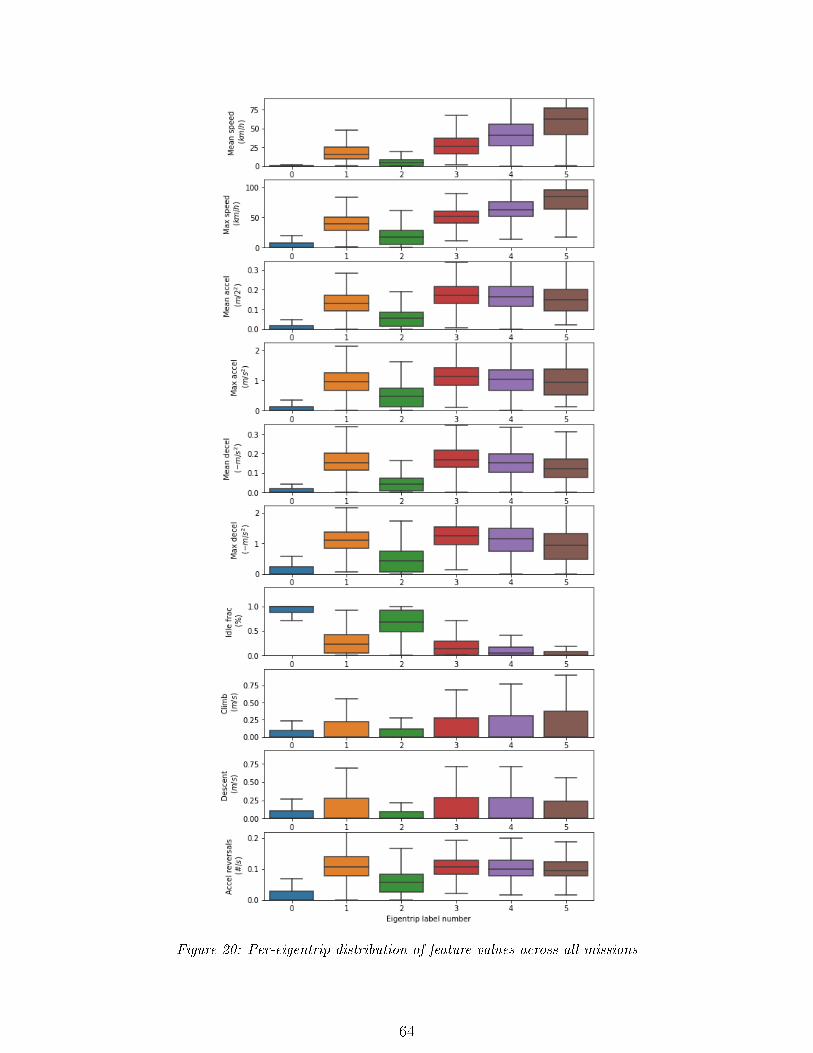
Figure 20: Per-eigentrip distribution of feature values across all missions
64
ing of the physical nature of travel likely to be labelled as most similar to a particular
eigentrip.
5.3 Application
To illustrate the application of the eigentrip model, imagine that a �eet manager has
been allocated budget for three new vehicles, with the explicit goal of minimizing an-
nual carbon-based fuel consumption. The manager is faced with the decision of which
vehicles to replace. Without logger information (and, for this purpose, in the absence of
mission constraints) the decision will be informed by whatever information is at hand.
This section explores the information that the manager might have, the vehicle replace-
ment decisions they might make with various information, and the likely impact of those
decisions in light of the logger data. The impact is given in terms of saved energy in MJ,
and the volume of consumed gasoline for ICEVs. Additionally, to highlight the impact
of high-e�ciency BEVs consuming low-intensity BC grid electricity, the related GHG
emissions are also listed, given global warming potentials (GWPs) of 88.1 g CO2e/MJ
for gasoline [9] and 2.96 gCO2e/MJ for BC Hydro's grid electricity [10].
Fuel consumption in this section is given relative to a power baseline derived from the
logger MAF and SOC data, as described in �3.3. As discussed in �7.5.2, the validity
of this baseline estimate is one of the study's core assumptions � there is no validated
fuelling data from which to calculate error bars.
The prediction estimates are given as maximum likelihood values � given the vehicle's
single characteristic power value for each eigentrip, and a count of the most-probable
eigentrips for the mission, the prediction estimate becomes a simple dot product. As
discussed in �7.3.6, it would be valuable to have a generalized measure of uncertainty
for each mission-vehicle prediction, but this would require characterizing each mission
and vehicle as a probability distribution rather than a singular value, defeating the
model's core goal of simplicity. To give some sense of the prediction reliability and
impact on decision-making, the replacement vehicle's whole-study MMAPE is applied
65
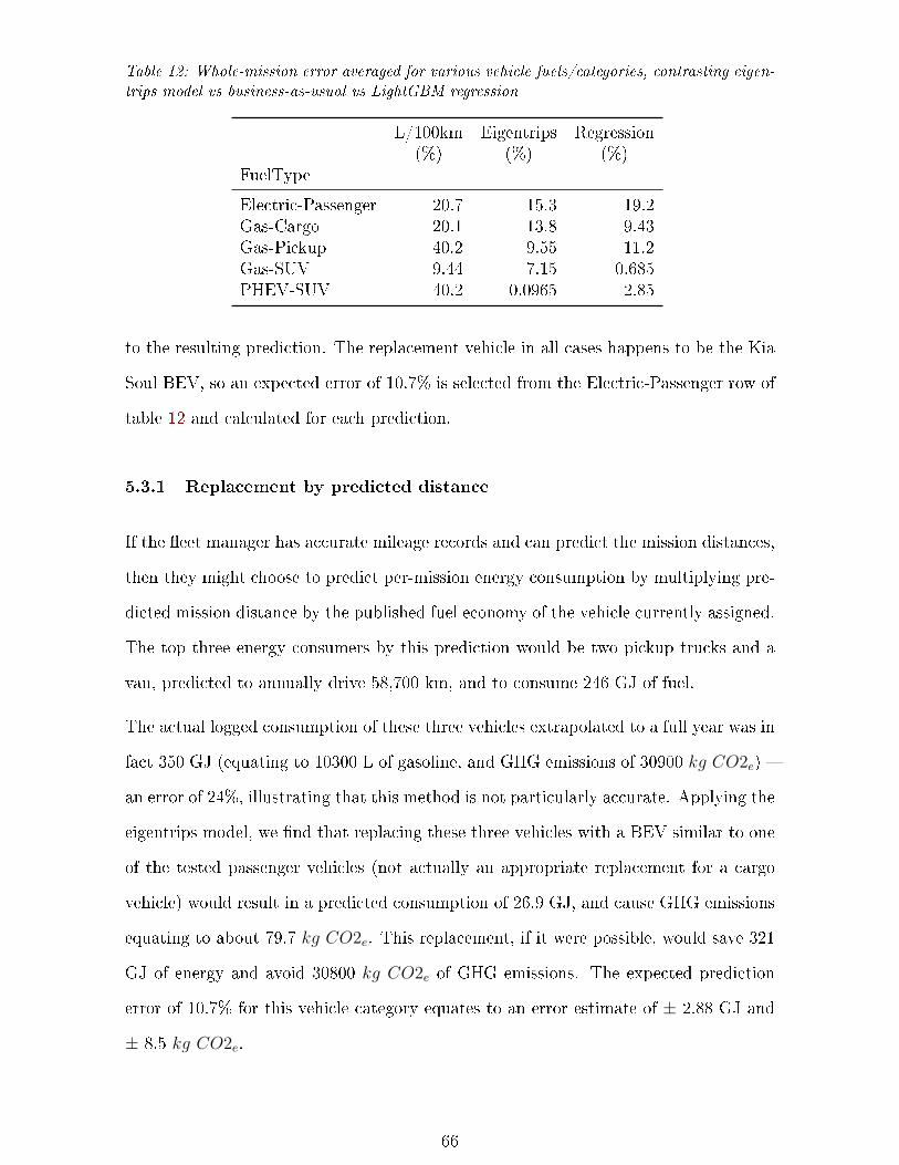
Table 12: Whole-mission error averaged for various vehicle fuels/categories, contrasting eigen-trips model vs business-as-usual vs LightGBM regression
L/100km(%)
Eigentrips(%)
Regression(%)
FuelType
Electric-Passenger 20.7 15.3 19.2Gas-Cargo 20.1 13.8 9.43Gas-Pickup 40.2 9.55 11.2Gas-SUV 9.44 7.15 0.685PHEV-SUV 40.2 0.0965 2.85
to the resulting prediction. The replacement vehicle in all cases happens to be the Kia
Soul BEV, so an expected error of 10.7% is selected from the Electric-Passenger row of
table 12 and calculated for each prediction.
5.3.1 Replacement by predicted distance
If the �eet manager has accurate mileage records and can predict the mission distances,
then they might choose to predict per-mission energy consumption by multiplying pre-
dicted mission distance by the published fuel economy of the vehicle currently assigned.
The top three energy consumers by this prediction would be two pickup trucks and a
van, predicted to annually drive 58,700 km, and to consume 246 GJ of fuel.
The actual logged consumption of these three vehicles extrapolated to a full year was in
fact 350 GJ (equating to 10300 L of gasoline, and GHG emissions of 30900 kg CO2e) �
an error of 24%, illustrating that this method is not particularly accurate. Applying the
eigentrips model, we �nd that replacing these three vehicles with a BEV similar to one
of the tested passenger vehicles (not actually an appropriate replacement for a cargo
vehicle) would result in a predicted consumption of 26.9 GJ, and cause GHG emissions
equating to about 79.7 kg CO2e. This replacement, if it were possible, would save 321
GJ of energy and avoid 30800 kg CO2e of GHG emissions. The expected prediction
error of 10.7% for this vehicle category equates to an error estimate of ± 2.88 GJ and
± 8.5 kg CO2e.
66
5.3.2 Replacement by published fuel economy
Lacking mileage or fuelling records, the �eet manager might select the three vehicles
in the �eet with the worst fuel economy ratings � two pickup trucks and an SUV, in
this example. In the absence of distance or fuelling records, there will be no predicted
consumption better than the manager's educated guess, perhaps by pro-rating the fuel
budget for the entire studied �eet (1167 GJ) by fuel economy numbers, resulting in a
predicted consumption of 203 GJ.
The extrapolated logger data suggests that these vehicles would have a total annual
consumption of 200 GJ (5900 L gasoline, emitting 17600 kg CO2e of GHGs). Their BEV
replacements would result in a new predicted consumption of 14.9 GJ (44.2 kg CO2e)
� a savings of 185 GJ, and avoiding 17600 kg CO2e of GHG emissions. The expected
error of 10.7% equates to an error estimate of ± 1.60 GJ and ± 4.73 kg CO2e.
5.3.3 Replacement by logged energy
In the absence of actual pump-to-tank records, the loggers themselves have the best
record of the energy consumed by each vehicle. Extrapolating each vehicle's actual
logged consumption to a year, the top three consumers will total 388 GJ (11500 litres
gasoline, emitting 34200 kg CO2e). Their BEV replacements would consume 25.7 GJ
(76.3 kg CO2e), saving 362 GJ and avoiding 34100 kg CO2e of GHG emissions. The
BEV's expected error of 10.7% equates to an error estimate of ± 2.75 GJ and ± 8.16
kg CO2e.
5.3.4 Replacement by best savings
The theoretical best solution is to consider all missions, and select the replacements
o�ering the highest predicted savings over the incumbent vehicles. In this case, the
result happens to be the same as the case above: replacing the highest energy consumers
with the most e�cient available alternative. However, this would not be the case if the
highest energy consumers were already relatively e�cient.
67
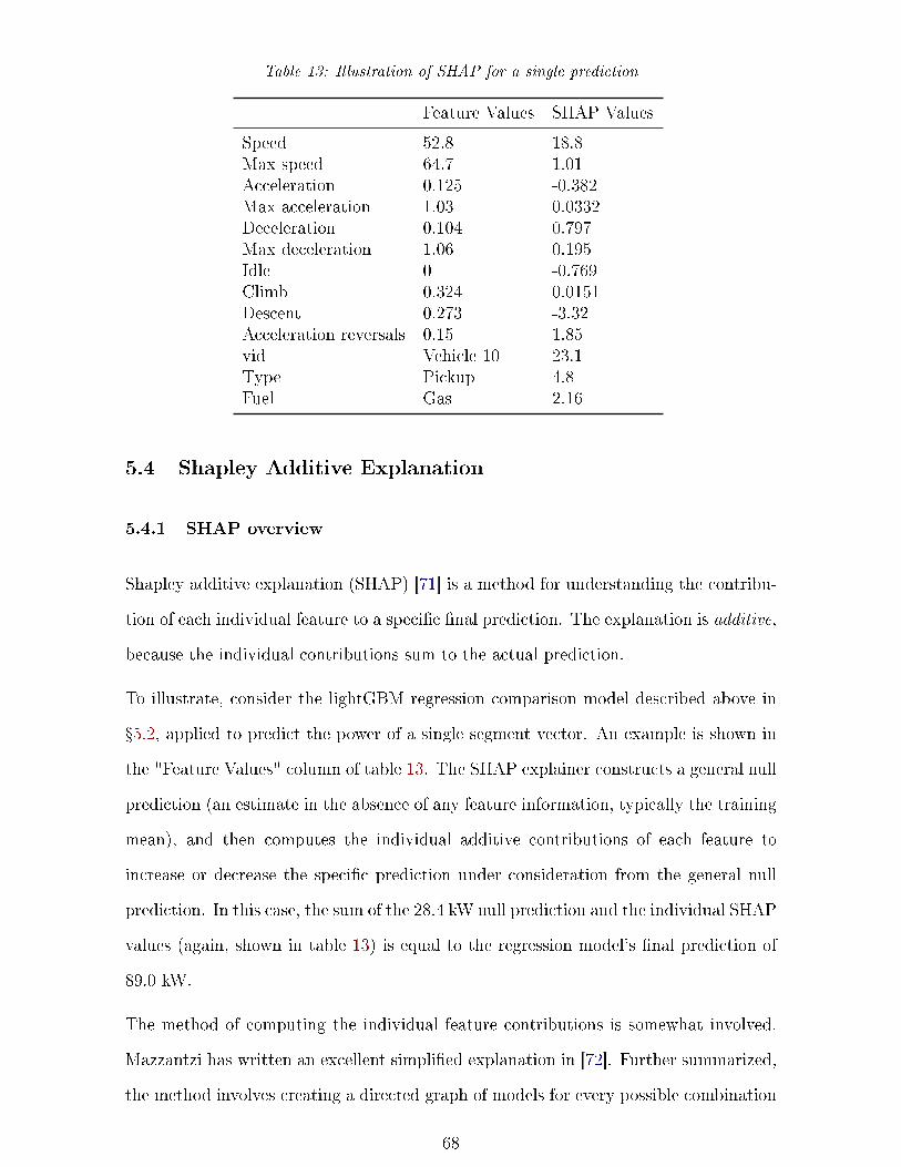
Table 13: Illustration of SHAP for a single prediction
Feature Values SHAP Values
Speed 52.8 18.8Max speed 64.7 1.01Acceleration 0.125 -0.382Max acceleration 1.03 0.0332Deceleration 0.104 0.797Max deceleration 1.06 0.195Idle 0 -0.769Climb 0.324 0.0151Descent 0.273 -3.32Acceleration reversals 0.15 1.85vid Vehicle 10 23.1Type Pickup 4.8Fuel Gas 2.16
5.4 Shapley Additive Explanation
5.4.1 SHAP overview
Shapley additive explanation (SHAP) [71] is a method for understanding the contribu-
tion of each individual feature to a speci�c �nal prediction. The explanation is additive,
because the individual contributions sum to the actual prediction.
To illustrate, consider the lightGBM regression comparison model described above in
�5.2, applied to predict the power of a single segment vector. An example is shown in
the "Feature Values" column of table 13. The SHAP explainer constructs a general null
prediction (an estimate in the absence of any feature information, typically the training
mean), and then computes the individual additive contributions of each feature to
increase or decrease the speci�c prediction under consideration from the general null
prediction. In this case, the sum of the 28.4 kW null prediction and the individual SHAP
values (again, shown in table 13) is equal to the regression model's �nal prediction of
89.0 kW.
The method of computing the individual feature contributions is somewhat involved.
Mazzantzi has written an excellent simpli�ed explanation in [72]. Further summarized,
the method involves creating a directed graph of models for every possible combination
68
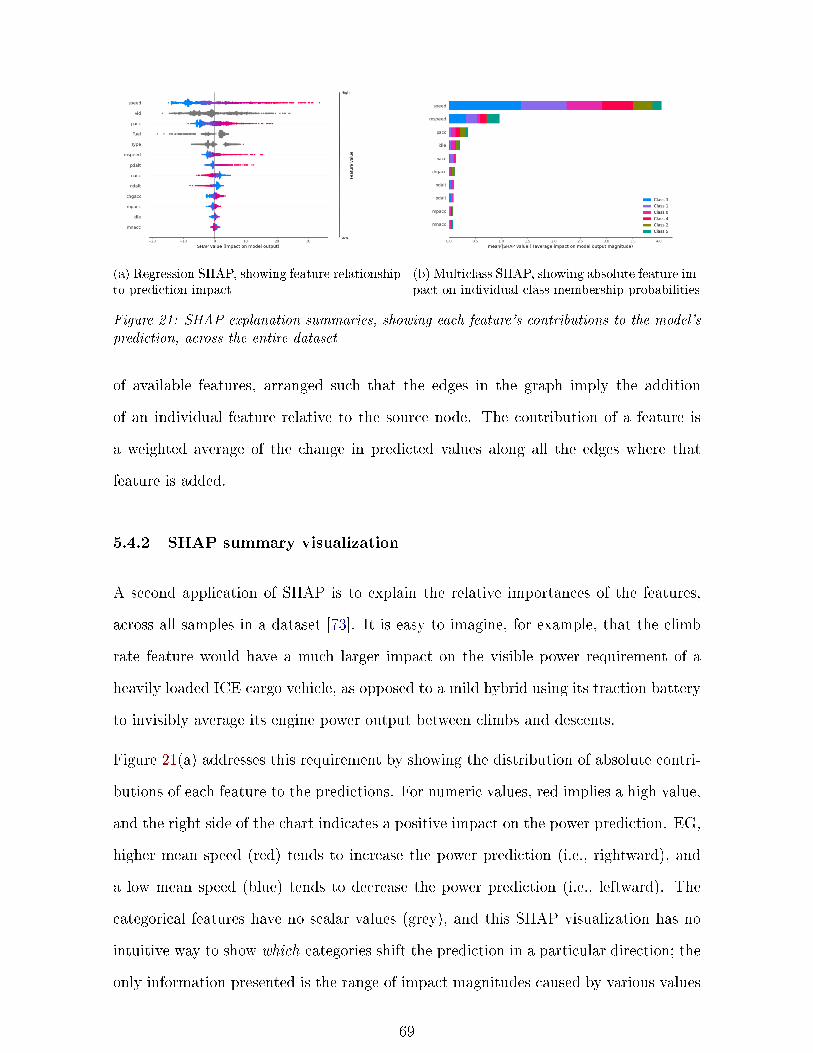
(a) Regression SHAP, showing feature relationshipto prediction impact
(b) Multiclass SHAP, showing absolute feature im-pact on individual class membership probabilities
Figure 21: SHAP explanation summaries, showing each feature's contributions to the model'sprediction, across the entire dataset
of available features, arranged such that the edges in the graph imply the addition
of an individual feature relative to the source node. The contribution of a feature is
a weighted average of the change in predicted values along all the edges where that
feature is added.
5.4.2 SHAP summary visualization
A second application of SHAP is to explain the relative importances of the features,
across all samples in a dataset [73]. It is easy to imagine, for example, that the climb
rate feature would have a much larger impact on the visible power requirement of a
heavily loaded ICE cargo vehicle, as opposed to a mild hybrid using its traction battery
to invisibly average its engine power output between climbs and descents.
Figure 21(a) addresses this requirement by showing the distribution of absolute contri-
butions of each feature to the predictions. For numeric values, red implies a high value,
and the right side of the chart indicates a positive impact on the power prediction. EG,
higher mean speed (red) tends to increase the power prediction (i.e., rightward), and
a low mean speed (blue) tends to decrease the power prediction (i.e., leftward). The
categorical features have no scalar values (grey), and this SHAP visualization has no
intuitive way to show which categories shift the prediction in a particular direction; the
only information presented is the range of impact magnitudes caused by various values
69

in the feature.
The eigentrip technique centrally uses a multiclass classi�er, not a regression model; the
classi�er's output for each prediction is in fact a vector of class probabilities, rather than
a single predicted value. Plot (a) could at best be used to show the absolute impact of
each feature on the probability of predicting one of six eigentrips. Instead, �gure 21(b)
illustrates the mean absolute impact of each feature on each class probability � in other
words the absolute change on the prediction probability if the feature is known, vs not
known. For example, the �gure shows that knowing the Speed value tends to change
the probability of class 3 by an absolute magnitude of about 1.4; it has a large impact,
although the plot gives no information about whether the impact tends to be positive,
negative, or even mixed.
5.4.3 SHAP implications
On the summary �gure(21a), the features for acceleration reversals (chgacc), maximum
positive acceleration (mpacc), idle fraction (idle), and maximum deceleration (mnacc)
are seen to have relatively small contributions to the prediction.
To illustrate that this is valid, the regression and eigentrip models were re-applied with
reference to only the other features. The impact of deleting these less-important fea-
tures from the direct regression model was indeed quite modest, increasing the average
segment MMAPE by only 0.21% � from 32.7% to 32.9%.
The impact on the Eigentrips model was somewhat more signi�cant, increasing from
32.1% to 39.4% � perhaps highlighting the impact of an increased number of marginal
samples no longer being nudged into the correct classi�cation by the additional features.
70
6 Conclusions
The eigentrip approach developed in this research has reasonably good accuracy, and
produces whole-year mission predictions averaging a MAPE of 9.4%. The concept can
be expected in the �eld to give signi�cantly better predictive results than the baseline
(L/100km) method's MAPE of 22%, although there is clearly room for improvement,
as shown by the direct-regression model's average MAPE of 3.7%.
The reduced error of either machine-learning model is balanced against added com-
plexity; adding a new vehicle to the model would require computing the new vehicle's
per-eigentrip characteristic power values. Similarly, adding a new mission pro�le (or
updating a modi�ed one) would require logging some weeks worth of representative
travel data, sanitizing it, and deconstructing it into a combination of eigentrips.
The criterion of spreadsheet-compatibility no longer seems as important as it originally
was, due to the advent of low-barrier options for deploying ML models in the cloud,
such as managed notebook hosting services. Such a model would have better predic-
tive accuracy, and could be designed to facilitate the direct upload of new data � either
representing new vehicles, or in order to better represent the evolution of the �eet's mis-
sion pro�les. That said, a spreadsheet-deployed model would still be helpful to address
potential concerns around the public exposure of individual travel information. This
issue was deeply signi�cant for the CRD, whose requirements informed this research.
The research performed here has been severely limited on several fronts, hampered by
data collection problems and limited by inadequate temporal resolution. One of the
initial goals, choosing the best of several alternative high-e�ciency replacements, has
been rendered impossible by the elimination of alternatives in the source data � the
initial study was intended to include several HFCEVs, PHEVs, and other types of BEV
beyond the Kia Soul EV. None of the desired alternatives were ultimately included in
the logged data, and the single PHEV logged only about 10 hours of travel time before
the data collection phase was terminated.
An important outcome of this research is reinforcement of the idea that any data-driven
71

model for predicting per-trip or per-mission vehicle energy consumption will be limited
in accuracy by the quality of the data that informs it. A good model would require
higher-resolution input data, and an exploratory data campaign facilitating iterations
of the experiment with various sampling frequencies and methods would be yet another
excellent subject for further study.
Ultimately, a data-driven model will be an e�ective recommendation tool for selecting
replacement vehicles to minimize energy consumption and carbon footprint. Careful
design of a data collection strategy will be the foundation of any trustworthy model.
72
7 Recommendations and Future Work
7.1 Assumptions . . . . . . . . . . . . 73
7.1.1 Stationarity and ergodicity 73
7.1.2 Baseline energy consump-tion . . . . . . . . . . . . . 74
7.1.3 Standardized GHG intensity 75
7.1.4 Fixed MAF ratio . . . . . . 75
7.1.5 Clustered eigentrip de�ni-tions . . . . . . . . . . . . . 76
7.2 Cleaning Decisions . . . . . . . . . 76
7.2.1 Smoothing starts . . . . . . 77
7.2.2 Regularization . . . . . . . 78
7.2.3 BEV power interpolation . 78
7.3 Data Structure . . . . . . . . . . . 78
7.3.1 Time-domain features . . . 78
7.3.2 Feature evaluation . . . . . 79
7.3.3 Microtrip boundaries . . . . 79
7.3.4 Clock time segment bound-aries . . . . . . . . . . . . . 79
7.3.5 Iterative segment re�nement 80
7.3.6 Characterize as distributions 80
7.4 Modeling . . . . . . . . . . . . . . 81
7.4.1 Improved clustering . . . . 81
7.4.2 Probabilistic class mem-bership . . . . . . . . . . . 82
7.4.3 Prediction error and miss-ing features . . . . . . . . . 82
7.4.4 Characteristic power byvehicle model . . . . . . . . 83
7.5 Data and Features . . . . . . . . . 83
7.5.1 Data requirements . . . . . 83
7.5.2 High-quality energy inputdata . . . . . . . . . . . . . 83
7.5.3 Road grade . . . . . . . . . 84
7.5.4 Features to support othervehicle types . . . . . . . . 85
7.5.5 Other features . . . . . . . 85
7.6 Applications . . . . . . . . . . . . . 86
7.6.1 Real-time allocation . . . . 86
7.6.2 Information sharing . . . . 86
7.6.3 Connected Vehicles . . . . . 87
This section discusses a number of limitations, assumptions, and other potential im-
provements to the studied process and model.
7.1 Assumptions
Several simplifying assumptions were made that could bene�t from more rigorous treat-
ment, either to quantify the resultant error, or to �nd a more precise method.
7.1.1 Stationarity and ergodicity
This entire study is predicated on two key assumptions: that the power and kinetic
features are stationary (i.e., that the statistics do not change over time) and that they
73
are ergodic (the statistics do not change erratically and inconsistently with respect to
uncontrolled parameters).
All of this is to say that the work assumes that the kinetic features are dictated by the
mission, and not unduly in�uenced by changing factors such as the physical character-
istics of the vehicle, the habits of the driver, and changing tra�c patterns. Future work
should validate and quantify these assumptions by observing the same mission oper-
ated with di�erent vehicles, and con�rming that e.g., a di�erence in power or handling
characteristics doesn't result in a confounding change in the observable kinetic features.
Most power-impacting di�erences in driver habits would likely be captured and ac-
counted for in the speed and acceleration features. However, an exploration of driver-
mission and driver-vehicle stability might be warranted since (a) drivers might a�ect
non-engine power consumption, such as climate control, changing the power character-
ization of a vehicle, and (b) a di�erence in driving technique might be so extreme as to
alter the kinetic pro�le of a measured mission, depending on who is driving it.
The same assumptions apply to the per-vehicle characteristic power values. Future
work should compare data collected from similar or identical vehicles, while driven by
di�erent drivers, in di�erent missions, in di�erent geography, and in di�erent organiza-
tions.
7.1.2 Baseline energy consumption
This thesis evaluates the validity of the new method for predicting energy consump-
tion, as compared to the traditional model-speci�c fuel economy statistic measured in
Le/100km. The validity of the two predictions is compared by measuring error relative
to the best available estimate of "actual" energy consumption, as derived from MAF
and SOC.
It is a signi�cant assumption that the inferred estimate of input energy from logger
values is valid and correct. As discussed in �7.5.2, it would be a signi�cant improvement
to this research to collect actual per-vehicle fuelling records for ICEVs and electrical
74
metering for grid-powered BEVs in order to establish the accuracy of the logged energy
consumption estimates.
7.1.3 Standardized GHG intensity
A primary intended use of this work � the prediction of GHG emissions � presumes that
it is possible to easily convert a known quantity of input energy into a speci�c GHG
footprint in kg CO2e, by applying standard GHG intensities such as those published
by the BC Canadian Ministry of Environment & Climate Change Strategy (MOE) or
BC Hydro [74, 10].
Events such as Volkswagen's "Dieselgate" [75] have made it clear that this is a weak
assumption for ICE vehicles, and that there may be a need for model-speci�c intensity
factors. Further investigation will be necessary to quantify the associated error.
Other factors may impact the emissions calculation for grid-powered BEVs, depending
on how grid emissions intensity is to calculated. BC Hydro reports an overall carbon
intensity of 11 gCO2e/kWh, with speci�c renewable and fossil sources rated at 4g and
593g respectively, and conducts a signi�cant bidirectional trade with Alberta, which is
attributed an intensity of 820g [76]. A 2017 paper found that carbon intensity in New
Zealand should be considered as varying between 32g and 188g depending strictly on
time-of-day [77]. It is easy to imagine a dynamic �eet model with reallocates vehicles
according to changing requirements for calculating emissions, or even from the the
time-dependent change in the carbon intensity attributed to their power sources.
7.1.4 Fixed MAF ratio
Fuel consumption rates were inferred from the OBD2 log values for MAF. This is only
accurate if the fuel:air mixture is known. The stoichiometric ratio of 14.7 is commonly
accepted [54], and as described above in �2.3.2, the author's undocumented personal
experience supports it. No peer-reviewed literature nor authoritative texts were found
supporting or refuting this assumption.
75

Since fuel �ow is not a standard OBD2 PID, it would be an excellent contribution to
the literature to publish a model or a dataset helping to more accurately infer actual
fuel �ow from MAF and other standard OBD2 parameters.
7.1.5 Clustered eigentrip de�nitions
An early assumption was that the eigentrip de�nitions should be inferred from the
data, rather than synthesized from expert knowledge of how di�erent driving patterns
are likely to in�uence fuel consumption. The basis set was therefore constructed using
unsupervised clustering.
It would be possible to instead construct a set of exemplar trips that are representative
of trip-types which a domain expert intuitively believes are likely to be predictive of en-
ergy consumption variability between vehicle types. Examples might include situations
such as
� point-to-point highway travel, o�-peak hours
� highway travel, rush-hour
� point-to-point city travel
� patrolling and parking enforcement
� idling to supply vehicle-mounted equipment
If the eigentrips were modelled on intuitively understandable travel-type exemplars,
users would be better able to infer the nature of new or blended missions, and be better
able to apply sanity checking to unexpected model results.
It would be interesting to repeat the experiment with such a set of intuitive eigentrips,
and contrast the level of error with that found from the inferred ones.
7.2 Cleaning Decisions
The extensive data cleaning and preparation process required a number of judgement
calls and simpli�cations. The most important of those are listed here.
76

7.2.1 Smoothing starts
As discussed above in �3.2.3, a large number of in-motion samples immediately following
an at-rest sample were dropped due to impossibly high accelerations, presumably due
to sampling errors.
Simple rejection of these potentially informative samples was to be avoided. An aborted
attempt was made to impute reasonable speed pro�les to these samples using the fol-
lowing process:
1. Compute a �typical low-speed acceleration� for each vehicle, consisting of the
median of in-motion positive acceleration values at speeds below an arbitrary
threshold of 15 km/h.
2. For vehicle starts with impossibly high logged accelerations, the zero-speed sample
is time-shifted to an earlier time that would re�ect that vehicle's typical acceler-
ation � but never such that it would precede the prior speed sample.
3. If the time-shifting would cause the zero-speed sample to precede a legitimate
logged non-speed sample, then �required acceleration� is computed from that le-
gitimate sample. If that required acceleration is found to have a reasonable mag-
nitude, then the earlier sample time is retained and deemed to be the new start
time.
Unfortunately, many of the error periods were found to bracket other sensor readings,
particularly MAF readings. Inserting an imputed speed value would call into question
the validity of the the subsequent MAF observation, causing irreconcilable discrepancies
between inferred acceleration and inferred fuel �ow. The method has potential, but
requires detailed review of the original datastream to be sure that it was not introducing
more error than it is removing.
77
7.2.2 Regularization
As discussed in �3.4, the entire corpus was regularized to 1s intervals to simplify segmen-
tation. This implies linear interpolation and extrapolation � both of which unavoidably
introduce error relative to the actually-measured real samples.
Given the potential to process variable-length segments as discussed in �7.3.5, it would
instead be possible to divide segments precisely at sample times, minimizing the amount
of interpolation required.
7.2.3 BEV power interpolation
Since sampling of the BEV's power was done at a relatively low resolution, a simple
time-interpolation on SOC was performed to help estimate power consumption within
each trip segment.
Hopefully future work will have direct access to higher resolution BEV power data.
With only the data at hand, a number of techniques might do better at predicting SOC
at the segment boundaries, perhaps using a timeseries regression model inferring from
additional other features such as distance travelled and acceleration pro�le.
7.3 Data Structure
7.3.1 Time-domain features
As discussed in �2.2.2, there are good reasons for this model to be structured as a non-
timeseries problem. However, there are likely to be some time-domain or frequency-
domain features with predictive power. Examples for possible exploration include the
e�ects of stop-and-go tra�c and time-of-day. Possibilities to extract predictive features
from these characteristics include spectral power density [42] as a �ngerprint feature,
and the use of time-domain techniques like Kalman �lters, [78] might help to generate
predictions of otherwise unknowable state features such as the vehicle's kinetic energy
78

or a mild hybrid's drive battery SOC. Another possibility is the employment of dynamic
time warping, [79] or wavelet convolutions [80] in order to �nd recurrences of observed
patterns that might characterize driving segments as being similar.
7.3.2 Feature evaluation
The initial short set of features in �4.1 is based on the work of others [38]. It would be
a valuable contribution to compile an exhaustive list of features directly available from
OBD2 or computed from them, and apply a rigorous evaluation for relative predictive
power. A simple example is the selection of the 98th percentile to illustrate the feature
"maximum acceleration". It is possible that some other quantile (or even the un�ltered
maximum observed value) would be more predictive.
One method for this would be to derive an expanded feature set (such as those listed in
�2.1.2), and apply SHAP [73] analysis to determine which features are most predictive
of energy consumption.
7.3.3 Microtrip boundaries
An early assumption was the rejection of stop-go-stop microtrips as the fundamental
trip segment, due to concern about excessive mixing of trip types. The requirement for
�xed-length segments added signi�cant complexity to the data preparation phase.
It is possible that the presumptive concern is unfounded. It would be interesting to
perform the entire experiment again with microtrips to see the impact on prediction
accuracy.
7.3.4 Clock time segment boundaries
For simplicity, the segments were regularized to clock time, beginning at even multiples
of three minutes from 00:00:00 each day. This assumption results in �nal and initial
segment in each trip being shorter by an average of 50%. Since each segment is given
equal weight in the model, this di�erence over-weights the importance of measurements
79

in those segments. However, since the �rst and last segments might legitimately have
more predictive power than mid-trip segments, it is possible that over-weighting them
is doing more good than harm.
It would be reasonable to validate this assumption by using only segments of precisely 3
minutes' length, discarding a contiguous period of �leftover� modulus samples between
a random segment-pair.
7.3.5 Iterative segment re�nement
Another simplifying assumption was the use of segments of speci�ed (3-minute) constant
duration. This naturally has the following e�ects at the arbitrary boundaries:
� combines disparate travel types into single segments
� arbitrarily splits similar travel types, creating unneeded additional segments
A re�nement to this approach would be to use the boundaries de�ned by the initial
classi�er in order to re-partition the travel data. Given an initial set of characteristic
travel types, it would instead be possible to segment the trip at "type boundaries",
where travel transitions from one type to another. This would result in segments of
variable length, but of more consistent travel types. It is to be expected that this would
result in more accurate energy consumption prediction within each travel type.
7.3.6 Characterize as distributions
The eigentrips model characterizes each vehicle as a vector of characteristic power values
for each eigentrip, and each mission as a vector containing the sum of time spent in each
eigentrip. The prediction of energy for applying a vehicle to a new mission is the dot
product of the two vectors. This value does not give any re�ection of the prediction's
level of uncertainty, and it would be preferable to have some sense of the variance of
the prediction.
Many regression models (including LightGBM) support so-called "quantile regression",
allowing the model to output a prediction interval � eg, the 90th percentile model will
80

return a prediction indicating a value higher than 90% of actual expected values. This
allows the user to intuitively understand the broadness of the prediction, as well as its
central value.
This intuitive simplicity does not transfer to the eigentrips model. Extracting the 90th
percentile energy prediction from a combination of vehicles and missions is not the dot
product of the 90th percentile characteristic powers with the vector of singular mission
times. It would instead require the computing the product of the nonparametric ran-
dom variable representing the distribution of characteristic powers, with the eigentrip
class probabilities, and determining the desired interval limits of the resulting product
distribution.
Given that a primary goal of the eigentrips model is simplicity, this is not a recom-
mended topic for future research. If a prediction interval is required, direct quantile
regression would be a simpler and more reliable path.
7.4 Modeling
7.4.1 Improved clustering
The clustering step was performed by means of the well-known K-means algorithm,
which returned a set of cluster centroids that were e�ective and useful, and which
provided an excellent basis to prove the concept. The number of clusters was selected
by inspection (the "elbow method"), and it would be informative to investigate more
re�ned methods.
Other clustering mechanisms which do not presume spherical, normally distributed
data would be likely to provide more representative centroids, and/or would lead more
directly to an optimal number of clusters. For example, density clustering is a well-
regarded process when the appropriate number of clusters is not known, however it
was deemed unsuitable since the dataset is continuous without sparse regions between
clusters.
81

Finally, the simple method used to select centroids predictive of energy consumption
(adding weight to the energy consumption feature) does not necessarily select the op-
timal centroids for the following criteria:
1. minimize error from the selected fuel consumption model, but
2. are maximally discriminatory on fuel consumption for at least some vehicle fea-
tures
3. provide adequate representation for all vehicle-eigentrip pairs
Finding centroids that meet all of these criteria may require developing a clustering
strategy from �rst principles. A good �rst step would be to implement a GMM clusterer
from �rst principles, in such a way as to allow feature-weighting.
7.4.2 Probabilistic class membership
Multiclass classi�ers initially provide a probability of membership in every class, and
only provide a singular prediction by application of maximum likelihood. A preliminary
experiment with pro-rating segment time to *all* eigentrips by class probability was
found to increase segment MAPE by nearly 50%.
However, for segments which fall close to the boundary between two (or more) segments,
it seems reasonable that the segment's power contribution is likely to fall somewhere
between the characteristic powers of the nearest segments. It might therefore be rea-
sonable to assign the segment a blended contribution to energy consumption, weighted
by the fractional probability of its nearest eigentrips. Since there is no requirement that
a travel segment be characterized by whole numbers of eigentrips, it would be entirely
acceptable to use multiple fractional membership, if it were found to reduce error.
7.4.3 Prediction error and missing features
Evaluating the actual operation associated with clusters that have the highest predictive
error will be an excellent starting point for determining whether additional features are
82
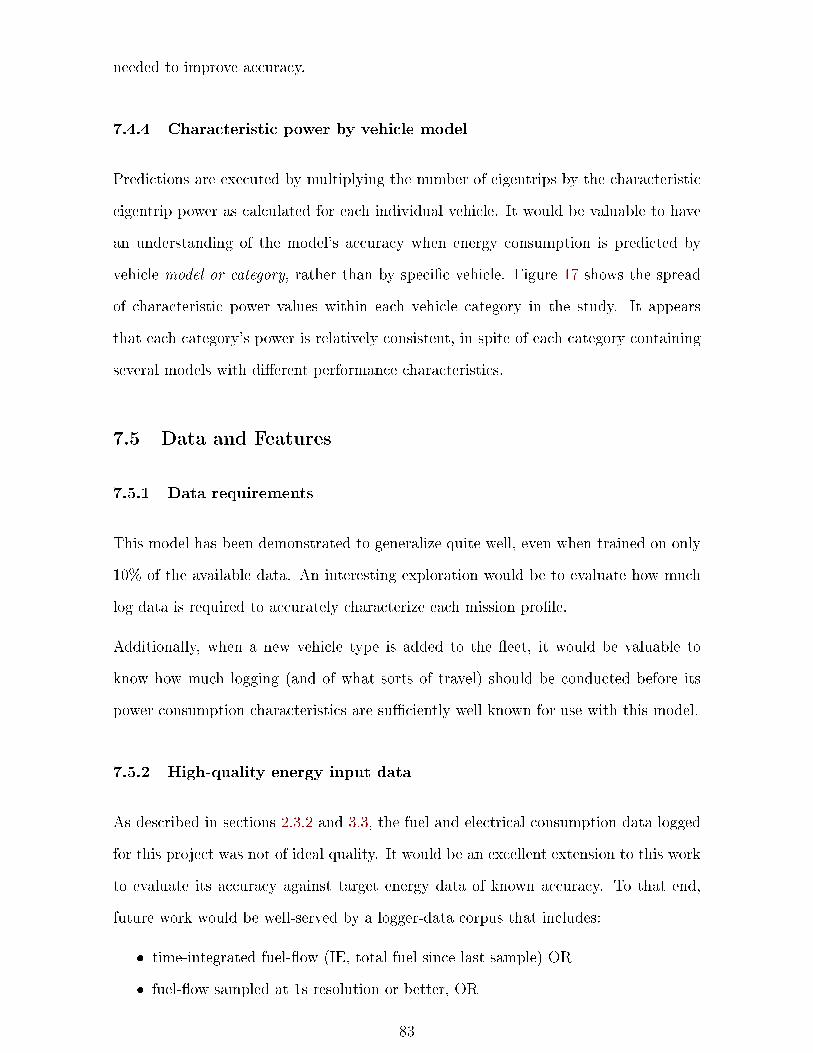
needed to improve accuracy.
7.4.4 Characteristic power by vehicle model
Predictions are executed by multiplying the number of eigentrips by the characteristic
eigentrip power as calculated for each individual vehicle. It would be valuable to have
an understanding of the model's accuracy when energy consumption is predicted by
vehicle model or category, rather than by speci�c vehicle. Figure 17 shows the spread
of characteristic power values within each vehicle category in the study. It appears
that each category's power is relatively consistent, in spite of each category containing
several models with di�erent performance characteristics.
7.5 Data and Features
7.5.1 Data requirements
This model has been demonstrated to generalize quite well, even when trained on only
10% of the available data. An interesting exploration would be to evaluate how much
log data is required to accurately characterize each mission pro�le.
Additionally, when a new vehicle type is added to the �eet, it would be valuable to
know how much logging (and of what sorts of travel) should be conducted before its
power consumption characteristics are su�ciently well known for use with this model.
7.5.2 High-quality energy input data
As described in sections 2.3.2 and 3.3, the fuel and electrical consumption data logged
for this project was not of ideal quality. It would be an excellent extension to this work
to evaluate its accuracy against target energy data of known accuracy. To that end,
future work would be well-served by a logger-data corpus that includes:
� time-integrated fuel-�ow (IE, total fuel since last sample) OR
� fuel-�ow sampled at 1s resolution or better, OR
83
� all PIDs necessary to accurately calculate fuel �ow, such as MAF and commanded
air-fuel equivalence ratio
Additionally, in �eets where vehicle fuelling is controlled and monitored through a per-
vehicle card system, it would be instructive to cross-check logger consumed-fuel totals
against actual pumped-fuel totals.
For EVs, charging totals could be compared to consumption totals to evaluate accuracy
and charge-discharge e�ciency.
7.5.3 Road grade
Road grade has an obvious impact on power requirements, and can be expected to
illustrate a signi�cant di�erence in energy consumption between conventional vs hybrid
or electric vehicles. A reliable road-grade feature would be an excellent addition to this
study.
Positive and negative vertical speed features were calculated from the available GPS
data. Unfortunately, the altitude feature was completely missing from a signi�cant
fraction of travel data. The feature was informative, improving predictive error from
45% to 35% in spite of large gaps in coverage, and the inherently low precision of the
GPS altitude signal.
Since the horizontal accuracy of GPS is better than vertical, consideration was given to
the idea of extracting elevation data from an open elevation dataset, such as NRCan's
High Resolution Digital Elevation Model [81], based on the vehicle's reported coor-
dinates. A preliminary investigation of this technique showed improvement, but still
yielded an unfortunately high fraction of impossible grades, perhaps due to a failure of
the terrain dataset to account for the signi�cant amount of grade smoothing involved
in road building in the Victoria area. This method showed some potential, but was felt
to be a large source of complexity for an unknown amount of predictive power; it may
merit future study, but is neglected in this work.
The best realistic source for road grade would be a barometric altimeter. For example,
84

The Freematics open-hardware logger provides for the direct integration of external
sensors [82]. It would also be an interesting side project to determine whether the
OBD2 PID 0x133 (barometric pressure) [83] has su�cient precision to be used for a
road grade calculation.
7.5.4 Features to support other vehicle types
Prediction was less precise than anticipated for the high-tech, high-e�ciency vehicles.
In particular:
� Prediction was poor for the mild HEVs. Investigation will be required to deter-
mine what additional features are required to capture hybrid performance, such as
HV battery state, or additional kinetic features related to stop-and-go behaviour
that could be impacted by regenerative braking.
� The BEV had a very wide range of error. Higher-resolution power data will be
required, but they might also bene�t from additional features indicating stop-
and-go performance.
� If multi-fuel vehicles become common, a kinetic feature will be needed that can
di�erentiate the circumstances under which they will switch from one energy
source to the other. EG, total travel distance this day, or since last charge would
probably work well for PHEVs.
7.5.5 Other features
There are other known/predictable factors that might be suspected to have a signi�cant
impact on fuel consumption, although most of them would present substantial data-
collection challenges. Examples include:
� payload, particularly in heavy vehicles. It could be estimated given road grade
and high-resolution torque and acceleration.
� di�erent drivers, subject to privacy concerns
� accessory load
85

� environmental load
� vehicle maintenance status
� road type, perhaps inferred from GIS data
� tra�c density by location and time-of-day, perhaps from a data source such as
Google Maps
� rigorous collection of vehicle sub-model and trim level
7.6 Applications
The originally envisioned application was evaluating re-allocation of existing vehicles,
and evaluating procurement decisions for additional copies of existing known �eet ve-
hicles. This subsection addresses additional potential applications.
7.6.1 Real-time allocation
It would be reasonable for a booking system to respond to a request for a pool-vehicle
by preferentially assigning the vehicle which is most energy-e�cient (or most GHG-
e�cient) for the speci�c task at hand. The proposed system is simple enough to be
implemented in a browser-based booking application, allowing the back-end to be sim-
pli�ed to a simple database lookup for availability, potentially requiring no additional
custom back-end software development.
7.6.2 Information sharing
If multiple municipalities (or other organizations) established a shared set of eigentrip
de�nitions, it would allow them to share information about their vehicles and their
missions.
Vehicle information sharing would allow organization A to evaluate the local perfor-
mance of a vehicle model owned by organization B.
On the other hand, sharing mission information sharing might highlight opportunities
to improve operational e�ciency. For example, organization A's parking enforcement
86
mission might have a much more e�cient eigentrip pro�le, as its new optical license
plate reading equipment allows it to spend a much higher portion of its time cruising
rather than idling. The improved energy performance might be su�ciently impressive
to encourage organization B to acquire the same equipment, solely to save the associated
vehicle emissions.
7.6.3 Connected Vehicles
The advent of fully-connected vehicles (e.g., Tesla and other new EV manufacturers)
has potential to provide a ready source of detailed, high-resolution vehicle performance
data. It would be quite simple for a manufacturer to publish real-world samples of
operations logs, allowing potential buyers to evaluate mission-vehicle energy and GHG
performance without any need to purchase an evaluation copy.
It would also be reasonable to establish a universal set of eigentrips, allowing man-
ufacturers to publish statistically veri�able real-world performance statistics for their
vehicles.
Having new vehicles providing logger information by default would provide other op-
portunities when connected to a power-vs-mission analysis. For example, departure
from manufacturer-published vehicle performance statistics could trigger owner alerts,
as a potential indication of required maintenance.
87
8 Bibliography
[1] CRD, �CRD Corporate Climate Action Strategy,� 2016, p. 51. [Online].
Available: https://www.crd.bc.ca/docs/default-source/crd-document-
library/annual-reports/climate/corporateclimateactionstrategy.pdf?
sfvrsn=e2372bca_4.
[2] NRCan. (Oct. 2013). �Fuel consumption ratings by model year,� [Online].
Available: https://www.nrcan.gc.ca/energy/efficiency/11938 (visited on
12/21/2018).
[3] US EPA. �Find and Compare Cars,� [Online]. Available:
http://www.fueleconomy.gov/feg/findacar.shtml (visited on 10/21/2019).
[4] H. Huo, Z. Yao, K. He, and X. Yu, �Fuel consumption rates of passenger cars in
China: Labels versus real-world,� Energy Policy, vol. 39, no. 11, pp. 7130�7135,
Nov. 2011, issn: 03014215. doi: 10.1016/j.enpol.2011.08.031. [Online].
Available:
https://linkinghub.elsevier.com/retrieve/pii/S0301421511006288
(visited on 12/21/2018).
[5] Mark Hu�man. (Jun. 2015). �How accurate is your car's fuel economy rating?�
[Online]. Available: https://www.consumeraffairs.com/news/how-accurate-
is-your-cars-fuel-economy-rating-062615.html (visited on 12/21/2018).
[6] �Zero Emission Fleet Initiative Fleet Logging Project - Summary Report
Capital Regional District . . Autumn Umanetz University of Victoria,� p. 46,
[7] IESVic, �Zero Emissions Fleet Pilot App Feasibility Study,� 2017. [Online].
Available: https://www.crd.bc.ca/docs/default-source/climate-action-
pdf/zefi-feasibilitystudy.pdf?sfvrsn=5a11e0ca_2.
[8] A. Umanetz, �ZEFI Fleet Logging Project - Summary Report,� 2019.
88
[9] M. a. L. C. I. Ministry of Energy. �BC-LCFS Requirements - Province of British
Columbia,� [Online]. Available:
https://www2.gov.bc.ca/gov/content/industry/electricity-
alternative-energy/transportation-energies/renewable-low-carbon-
fuels/fuel-supplier-compliance-50005 (visited on 02/21/2021).
[10] BC Hydro, �Greenhouse Gas Intensities,� p. 1, 2016. [Online]. Available:
https://www.bchydro.com/content/dam/BCHydro/customer-
portal/documents/corporate/environment-
sustainability/environmental-reports/ghg-intensities-2004-2014.pdf.
[11] BC Government. �Greenhouse Gas Reduction Targets Act,� [Online]. Available:
http:
//www.bclaws.ca/civix/document/id/consol22/consol22/00_07042_01
(visited on 08/16/2019).
[12] BC Ministry of Environment, �B.C. Provincial Greenhouse Gas Inventory
Report 2007,� 2007. [Online]. Available:
https://www2.gov.bc.ca/assets/gov/environment/climate-
change/data/provincial-inventory/2007/pir-2007-full-report.pdf
(visited on 12/30/2020).
[13] J. Lesser. �Are electric cars worse for the environment?� The Agenda, [Online].
Available: https://politi.co/2wHrT9T (visited on 02/19/2021).
[14] (Nov. 10, 2017). �Motor Mouth: A few more inconvenient truths about EV CO2
emissions,� Driving, [Online]. Available:
https://driving.ca/auto-news/news/motor-mouth-a-few-more-
inconvenient-truths-about-ev-co2-emissions (visited on 02/20/2021).
[15] M. T. Boyko� and J. M. Boyko�, �Balance as bias: Global warming and the US
prestige press,� Global Environmental Change, vol. 14, no. 2, pp. 125�136, Jul.
2004, issn: 09593780. doi: 10.1016/j.gloenvcha.2003.10.001. [Online].
Available:
89
https://linkinghub.elsevier.com/retrieve/pii/S0959378003000669
(visited on 02/20/2021).
[16] A. Elgowainy, J. Han, J. Ward, F. Joseck, D. Gohlke, A. Lindauer, T. Ramsden,
M. Biddy, M. Alexander, S. Barnhart, I. Sutherland, L. Verduzco, and
T. J. Wallington, �Current and Future United States Light-Duty Vehicle
Pathways: Cradle-to-Grave Lifecycle Greenhouse Gas Emissions and Economic
Assessment,� Environmental Science & Technology, vol. 52, no. 4, pp. 2392�2399,
Feb. 20, 2018, issn: 0013-936X, 1520-5851. doi: 10.1021/acs.est.7b06006.
[Online]. Available: https://pubs.acs.org/doi/10.1021/acs.est.7b06006
(visited on 02/20/2021).
[17] NRCan. (Apr. 30, 2018). �2020 Fuel Consumption Guide,� [Online]. Available:
https://www.nrcan.gc.ca/energy-efficiency/energy-efficiency-
transportation/fuel-consumption-guide/21002 (visited on 12/30/2020).
[18] �FuelEconomy.gov - The o�cial U.S. government source for fuel economy
information.,� [Online]. Available: http://www.fueleconomy.gov (visited on
12/30/2020).
[19] FPInnovations, �Testing and Veri�cation Protocol for Engine and Vehicle
After-market Devices,� 2013. [Online]. Available:
https://etvcanada.ca/wp-content/uploads/2013/08/Report-Protcol-
EAMDs-Testing-and-Verification.pdf.
[20] Transport Canada. (Mar. 10, 2013). �2-cycle testing,� [Online]. Available:
https://web.archive.org/web/20130310085554/http:
//www.tc.gc.ca/eng/programs/environment-fcp-2cycle-517.htm (visited
on 02/13/2021).
[21] ��, (Oct. 18, 2012). �5-cycle testing,� [Online]. Available:
https://web.archive.org/web/20121018023539/http:
//www.tc.gc.ca/eng/programs/environment-fcp-5cycle-530.htm (visited
on 02/13/2021).
90
[22] NRCan. (Apr. 30, 2018). �Fuel consumption testing,� [Online]. Available:
https://www.nrcan.gc.ca/energy-efficiency/energy-efficiency-
transportation/2020-fuel-consumption-guide/understanding-fuel-
consumption-r/fuel-consumption-testing/21008 (visited on 12/29/2020).
[23] ��, (Sep. 11, 2018). �EnerGuide label for battery-electric vehicles,� [Online].
Available: https://www.nrcan.gc.ca/energy/efficiency/energy-
efficiency-transportation-and-alternative-fuels/choosing-right-
vehicle/tips-buying-fuel-efficient-vehicle/energuide-
vehicles/energuide-label-battery-electric-vehicles/21379 (visited on
12/29/2020).
[24] A. Umanetz, �Classi�cation of �eet micro-trips using kinetic parameters.�
[25] R. O. Duda, P. E. Hart, and D. G. Stork, Pattern Classi�cation, 2nd ed. New
York: Wiley, 2001, isbn: 978-0-471-05669-0.
[26] (Jul. 9, 2019). �Logistic Regression For Machine Learning and Classi�cation,�
Kambria, [Online]. Available:
https://kambria.io/blog/logistic-regression-for-machine-learning/
(visited on 01/01/2021).
[27] X. Zhang and C. Mi, Vehicle Power Management: Modeling, Control and
Optimization, ser. Power Systems. London ; New York: Springer Verlag, 2011,
isbn: 978-0-85729-735-8.
[28] P G Boulter, T J Barlow, S Latham, and I S McCrae, �A reference book of
driving cycles for use in the measurement of road vehicle emissions,�
Department for Transport, Cleaner Fuels & Vehicles 4.
[29] EPA. �Dynamometer Drive Schedules | Vehicle and Fuel Emissions Testing | US
EPA,� [Online]. Available: https://www.epa.gov/vehicle-and-fuel-
emissions-testing/dynamometer-drive-schedules (visited on 12/07/2018).
91

[30] NREL. �APPENDICES�ADVISOR Documentation,� [Online]. Available:
http://adv-vehicle-sim.sourceforge.net/advisor_appendices.html
(visited on 12/07/2018).
[31] J. Wu, C. .-H. Zhang, and N. .-X. Cui, �Fuzzy energy management strategy for
a hybrid electric vehicle based on driving cycle recognition,� International
Journal of Automotive Technology, vol. 13, no. 7, pp. 1159�1167, Dec. 2012,
issn: 1229-9138, 1976-3832. doi: 10.1007/s12239-012-0119-z. [Online].
Available: http://link.springer.com/10.1007/s12239-012-0119-z (visited
on 12/08/2018).
[32] H. Yu, F. Tseng, and R. McGee, �Driving pattern identi�cation for EV range
estimation,� in 2012 IEEE International Electric Vehicle Conference, Greenville,
SC, USA: IEEE, Mar. 2012, pp. 1�7, isbn: 978-1-4673-1561-6. doi:
10.1109/IEVC.2012.6183207. [Online]. Available:
http://ieeexplore.ieee.org/document/6183207/ (visited on 12/08/2018).
[33] M. Redelbach, E. D. Özdemir, and H. E. Friedrich, �Optimizing battery sizes of
plug-in hybrid and extended range electric vehicles for di�erent user types,�
Energy Policy, vol. 73, pp. 158�168, Oct. 2014, issn: 03014215. doi:
10.1016/j.enpol.2014.05.052. [Online]. Available:
https://linkinghub.elsevier.com/retrieve/pii/S030142151400367X
(visited on 12/08/2018).
[34] R. Smith, S. Shahidinejad, D. Blair, and E. Bibeau, �Characterization of urban
commuter driving pro�les to optimize battery size in light-duty plug-in electric
vehicles,� Transportation Research Part D: Transport and Environment, vol. 16,
no. 3, pp. 218�224, May 2011, issn: 13619209. doi:
10.1016/j.trd.2010.09.001. [Online]. Available:
https://linkinghub.elsevier.com/retrieve/pii/S1361920910001318
(visited on 12/08/2018).
92
[35] L. Evans, R. Herman, and T. N. Lam, �Gasoline Consumption in Urban
Tra�c,� Feb. 1976. doi: 10.4271/760048. [Online]. Available:
http://papers.sae.org/760048/ (visited on 12/07/2018).
[36] S. H. Kamble, T. V. Mathew, and G. Sharma, �Development of real-world
driving cycle: Case study of Pune, India,� Transportation Research Part D:
Transport and Environment, vol. 14, no. 2, pp. 132�140, Mar. 2009, issn:
13619209. doi: 10.1016/j.trd.2008.11.008. [Online]. Available:
http://linkinghub.elsevier.com/retrieve/pii/S136192090800148X
(visited on 12/07/2018).
[37] R. Shankar and J. Marco, �Method for estimating the energy consumption of
electric vehicles and plug-in hybrid electric vehicles under real-world driving
conditions,� IET Intelligent Transport Systems, vol. 7, no. 1, pp. 138�150, Mar.
2013, issn: 1751-956X, 1751-9578. doi: 10.1049/iet-its.2012.0114. [Online].
Available: https://digital-
library.theiet.org/content/journals/10.1049/iet-its.2012.0114
(visited on 12/07/2018).
[38] H. He, C. Sun, and X. Zhang, �A Method for Identi�cation of Driving Patterns
in Hybrid Electric Vehicles Based on a LVQ Neural Network,� Energies, vol. 5,
no. 9, pp. 3363�3380, Sep. 5, 2012, issn: 1996-1073. doi: 10.3390/en5093363.
[Online]. Available: http://www.mdpi.com/1996-1073/5/9/3363 (visited on
12/07/2018).
[39] E. Ericsson, �Independent driving pattern factors and their in�uence on fuel-use
and exhaust emission factors,� p. 21, 2001.
[40] M. Verleysen and D. François, �The Curse of Dimensionality in Data Mining and
Time Series Prediction,� in Computational Intelligence and Bioinspired Systems,
vol. 3512, Berlin, Heidelberg: Springer Berlin Heidelberg, 2005, pp. 758�770,
isbn: 978-3-540-26208-4. doi: 10.1007/11494669_93. [Online]. Available:
http://link.springer.com/10.1007/11494669_93 (visited on 12/11/2018).
93
[41] E. Alpaydin, Introduction to Machine Learning, 2nd ed, ser. Adaptive
Computation and Machine Learning. Cambridge, Mass: MIT Press, 2010,
537 pp., isbn: 978-0-262-01243-0.
[42] Falk, Michael, A First Course on Time Series Analysis. University of
Würzburg, 2012.
[43] S. L. Sclove, �Time-series segmentation: A model and a method,� Information
Sciences, Institute of Electrical and Electronics Engineers Workshop "Applied
Time Series Analysis", vol. 29, no. 1, pp. 7�25, Feb. 1, 1983, issn: 0020-0255.
doi: 10.1016/0020-0255(83)90007-5. [Online]. Available:
http://www.sciencedirect.com/science/article/pii/0020025583900075
(visited on 01/03/2021).
[44] Encyclopedia of Mathematics. �Regression analysis,� [Online]. Available:
http://encyclopediaofmath.org/index.php?title=%20Regression_
analysis&oldid=17714 (visited on 01/03/2021).
[45] Karanveer Mohan. �Visualizing K-Means Clustering Webpage,� [Online].
Available:
http://stanford.edu/class/ee103/visualizations/kmeans/kmeans.html
(visited on 12/18/2018).
[46] �Elbow Method � Yellowbrick v1.2 documentation,� [Online]. Available:
https://www.scikit-yb.org/en/latest/api/cluster/elbow.html (visited
on 01/01/2021).
[47] T. Alade. (Dec. 23, 2019). �Tutorial: How to determine the optimal number of
clusters for k-means clustering,� Medium, [Online]. Available:
https://blog.cambridgespark.com/how-to-determine-the-optimal-
number-of-clusters-for-k-means-clustering-14f27070048f (visited on
01/01/2021).
94

[48] �KMeans � scikit-learn 0.24.0 documentation,� [Online]. Available:
https://scikit-learn.org/stable/modules/clustering.html (visited on
01/01/2021).
[49] A. H. Maslow, The Psychology of Science: A Reconnaissance. Harper & Row,
1966, 200 pp., isbn: 978-0-8092-6130-7. Google Books: qitgAAAAMAAJ.
[50] �OBD2 Explained - A Simple Intro (2019),� [Online]. Available:
https://www.csselectronics.com/screen/page/simple-intro-obd2-
explained/language/en#OBD2-Intro-Dummies-Basics (visited on
01/13/2020).
[51] Texas Instruments. (2002). �Introduction to the Controller Area Network.�
[52] SAE On-Board Diagnostics for Light and Medium Duty Vehicles Standards
Manual. SAE International, 2010, isbn: 978-0-7680-2173-8.
[53] �The Chemistry of Combustion,� [Online]. Available:
https://www.chem.fsu.edu/chemlab/chm1020c/Lecture%207/01.php (visited
on 01/17/2020).
[54] N. Goodnight and K. VanGelder, Automotive Engine Performance. Jones &
Bartlett Learning, Feb. 2019, isbn: 978-1-284-10206-2. Google Books:
sBmIDwAAQBAJ.
[55] E. R. Jones and R. L. Childers, Contemporary College Physics. Addison-Wesley
Publishing Company, Jan. 1990, isbn: 978-0-201-11951-0.
[56] �Fuels - Higher and Lower Calori�c Values,� [Online]. Available:
https://www.engineeringtoolbox.com/fuels-higher-calorific-values-
d_169.html (visited on 01/17/2020).
[57] W.-Y. Chang. (Jul. 23, 2013). �The State of Charge Estimating Methods for
Battery: A Review,� ISRN Applied Mathematics, [Online]. Available:
https://www.hindawi.com/journals/isrn/2013/953792/ (visited on
01/04/2021).
95

[58] �2017 Kia Soul EV Speci�cations,� [Online]. Available:
https://www.kiamedia.com/us/en/models/soul-ev/2017/specifications
(visited on 01/18/2020).
[59] �2016 Kia Soul EV Speci�cations,� [Online]. Available:
https://www.kiamedia.com/us/en/models/soul-ev/2016/specifications
(visited on 02/02/2020).
[60] Mitsubishi Motor Corp. (2018). �2018-Mitsubishi-Outlander-PHEV-Brochure,�
[Online]. Available:
https://mcarsstatic.cachefly.net/pdf/section/request-a-
brochure/2018-Mitsubishi-Outlander-PHEV-Brochure.pdf (visited on
02/02/2020).
[61] �Welcome to LightGBM's documentation! � LightGBM 3.1.1.99
documentation,� [Online]. Available:
https://lightgbm.readthedocs.io/en/latest/ (visited on 01/18/2021).
[62] Hastie, Trevor, Tibshirani, Robert, and J. Friedman, The Elements of Statistical
Learning. Springer, 2017.
[63] �Jamesajeeth/Data-Science,� GitHub, [Online]. Available:
https://github.com/jamesajeeth/Data-Science (visited on 02/19/2021).
[64] �Gradient Boosting in Python from Scratch | by Carl Dawson | Towards Data
Science,� [Online]. Available: https://towardsdatascience.com/gradient-
boosting-in-python-from-scratch-4a3d9077367 (visited on 02/19/2021).
[65] �Parameters Tuning � LightGBM 3.1.1.99 documentation,� [Online]. Available:
https://lightgbm.readthedocs.io/en/latest/Parameters-Tuning.html
(visited on 02/08/2021).
[66] G. Ke, Q. Meng, T. Finley, T. Wang, W. Chen, W. Ma, Q. Ye, and T.-Y. Liu,
�LightGBM: A Highly E�cient Gradient Boosting Decision Tree,� p. 9,
96

[67] �Scikit-optimize: Sequential model-based optimization in Python �
scikit-optimize 0.8.1 documentation,� [Online]. Available:
https://scikit-optimize.github.io/stable/ (visited on 02/01/2021).
[68] fernando, Fmfn/BayesianOptimization, Feb. 21, 2021. [Online]. Available:
https://github.com/fmfn/BayesianOptimization (visited on 02/21/2021).
[69] �Tuning Hyperparameters Under 10 Minutes (LGBM),� [Online]. Available:
https://kaggle.com/somang1418/tuning-hyperparameters-under-10-
minutes-lgbm (visited on 02/01/2021).
[70] NRCan. �Fuel consumption ratings search tool,� [Online]. Available:
https://fcr-ccc.nrcan-rncan.gc.ca/en (visited on 02/14/2021).
[71] S. Lundberg and S.-I. Lee. (Nov. 24, 2017). �A Uni�ed Approach to Interpreting
Model Predictions.� arXiv: 1705.07874 [cs, stat], [Online]. Available:
http://arxiv.org/abs/1705.07874 (visited on 02/21/2021).
[72] S. Mazzanti. (Apr. 26, 2020). �SHAP explained the way I wish someone
explained it to me,� Medium, [Online]. Available:
https://towardsdatascience.com/shap-explained-the-way-i-wish-
someone-explained-it-to-me-ab81cc69ef30 (visited on 02/21/2021).
[73] S. Lundberg, Slundberg/shap, Jan. 24, 2021. [Online]. Available:
https://github.com/slundberg/shap (visited on 01/24/2021).
[74] BC Ministry of Environment, �2016 B.C. BEST PRACTICES
METHODOLOGY FOR QUANTIFYING GREENHOUSE GAS EMISSIONS,�
2016. doi: 10.1007/s12273-013-0159-y.
[75] C. Atiyeh. (Dec. 4, 2019). �Everything You Need to Know about the VW
Diesel-Emissions Scandal,� Car and Driver, [Online]. Available:
https://www.caranddriver.com/news/a15339250/everything-you-need-
to-know-about-the-vw-diesel-emissions-scandal (visited on 01/02/2021).
[76] Bullfrog Power, Canadian Emission Factors for Grid Electricity, 2015.
97
[77] I. Khan, M. W. Jack, and J. Stephenson, �Use of time-varying carbon intensity
estimation to evaluate GHG emission reduction opportunities in electricity
sector,� in 2017 IEEE Conference on Technologies for Sustainability (SusTech),
Phoenix, AZ: IEEE, Nov. 2017, pp. 1�2, isbn: 978-1-5386-0452-6. doi:
10.1109/SusTech.2017.8333479. [Online]. Available:
https://ieeexplore.ieee.org/document/8333479/ (visited on 02/15/2021).
[78] P. S. Maybeck, Stochastic Models, Estimation and Control, ser. Mathematics in
Science and Engineering v. 141. New York: Academic Press, 1979, 3 pp., isbn:
978-0-12-480701-3.
[79] Mueller, M., Information Retrieval for Music and Motion. Springer, 2007, isbn:
978-3-540-74047-6. [Online]. Available:
http://www.springer.com/978-3-540-74047-6.
[80] D. Li, T. F. Bissyandé, J. Klein, and Y. L. Traon, �Time Series Classi�cation
with Discrete Wavelet Transformed Data: Insights from an Empirical Study,�
presented at the The 28th International Conference on Software Engineering
and Knowledge Engineering, Jul. 1, 2016, pp. 273�278. doi:
10.18293/SEKE2016-067. [Online]. Available: http:
//ksiresearchorg.ipage.com/seke/seke16paper/seke16paper_67.pdf
(visited on 12/07/2018).
[81] NRCan. �High Resolution Digital Elevation Model (HRDEM) - CanElevation
Series - Open Government Portal,� [Online]. Available:
https://open.canada.ca/data/en/dataset/957782bf-847c-4644-a757-
e383c0057995 (visited on 01/01/2021).
[82] Freematics.com. �Freematics ONE+ Model B spec sheet,� [Online]. Available:
https://freematics.com/pages/products/freematics-one-plus-model-b/
(visited on 01/01/2021).
[83] ��, �Freematics Packed Data Format,� [Online]. Available:
https://freematics.com/pages/hub/freematics-data-logging-format/
(visited on 01/01/2021).
98
[84] Ministry of Energy, Mines and Petroleum Resources, Carbon Intensity Records
under the Renewable and Low Carbon Fuel Requirements Regulation.
[85] BC Hydro, �Greenhouse Gas Intensities 2007, 2011-2015,� p. 1,
[86] J. I. Levene, M. K. Mann, R. M. Margolis, and A. Milbrandt, �An analysis of
hydrogen production from renewable electricity sources,� Solar Energy, vol. 81,
no. 6, pp. 773�780, Jun. 2007, issn: 0038092X. doi:
10.1016/j.solener.2006.10.005. [Online]. Available:
https://linkinghub.elsevier.com/retrieve/pii/S0038092X06002635
(visited on 02/21/2021).
[87] A. Umanetz, �Well-to-Wheel GHG Intensity for Vehicular Hydrogen Fuel in
British Columbia,� University of Victoria, (Unpublished), 2018.
[88] B. James, �Current Forecourt Hydrogen Production from Natural Gas (1,500 kg
per day) version 3.101,� NREL, 2012.
[89] O. Schmidt, A. Gambhir, I. Sta�ell, A. Hawkes, J. Nelson, and S. Few, �Future
cost and performance of water electrolysis: An expert elicitation study,�
International Journal of Hydrogen Energy, vol. 42, no. 52, pp. 30 470�30 492,
Dec. 2017, issn: 03603199. doi: 10.1016/j.ijhydene.2017.10.045. [Online].
Available:
https://linkinghub.elsevier.com/retrieve/pii/S0360319917339435
(visited on 02/21/2021).
99
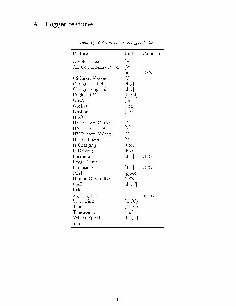
A Logger features
Table 14: CRD FleetCarma logger features
Feature Unit Comment
Absolute Load [%]Air Conditioning Power [W]Altitude [m] GPSC2 Input Voltage [V]Charge Latitude [deg]Charge Longitude [deg]Engine RPM [RPM]GpsAlt (m)GpsLat (deg)GpsLon (deg)HDOPHV Battery Current [A]HV Battery SOC [%]HV Battery Voltage [V]Heater Power [W]Is Charging [bool]Is Driving [bool]Latitude [deg] GPSLoggerNameLongitude [deg] GPSMAF [g/sec]NumberOfSatellites GPSOAT [degC]PckSignal #131 SpeedStart Time (UTC)Time (UTC)Timestamp (ms)Vehicle Speed [km/h]Vin
100
B Embodied energy and Fuel Intensity
This is a discussion of assumptions and sources needed to convert life-cycle analysis
(LCA) �gures by Elgowainy et al [16] to apply study-contemporaneous and forecasted
fuel intensities for BC. Detailed column calculations are shown for 2018 in table 15 and
for 2030 in table 16.
B.0.1 Vehicle assumptions
Elgowainy's (reasonable) PHEV e�ciency �gure was not supported; to properly appor-
tion emissions to gasoline and BC grid electricity, Elgowainy's �gure was decomposed
and found to imply an operational regime of 27.1% in BEV mode for 2018, and at
28.0% BEV mode in 2030.
In order to give a fair apples-to-apples comparison, the BEV90 was given the full lifetime
travel distance of 286,000 km, di�ering from Elgowainy's treatment, which amortized
the vehicle' manufacturing emissions over a much shorter lifetime travel distance.
B.0.2 Legend for LCA tables
Legend for tables 15 and 16:
� MPGGE: miles per gallon, gasoline equivalent, taken directly from Elgowainy
� Le/100km: MPGGE directly converted to metric Gasoline-equivalent litres per
100km
� Fuel Intensity: assumptions and sources are discussed in the remainder of this
section
� Tailpipe: total lifetime tailpipe emissions, at Elgowainy's assumption of a 15-year
vehicle life of 286,000 km (178,000 miles)
� Vehicle: total vehicle manufacturing and decommissioning emissions
� Lifetime: sum of Tailpipe and Vehicle �elds
� Amortized: Lifetime emissions, divided by lifetime travel distance.
101
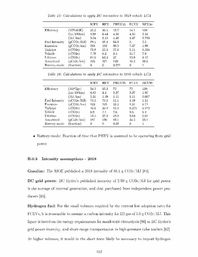
Table 15: Calculations to apply BC intensities to 2018 vehicle LCA
ICEV HEV PHEV35 FCEV BEV90
E�ciency (MPGGE) 26.2 36.5 53.7 54.1 100(Le/100km) 8.98 6.44 4.38 4.35 2.34(MJ/km) 3.04 2.18 1.48 1.47 0.793
Fuel Intensity (gCO2e/MJ) 88.1 88.1 64.9 5. 2.5Emission (gCO2e/km) 268 192 96.3 7.37 1.98Tailpipe (tCO2e) 76.8 55.1 27.6 2.11 0.568Vehicle (tCO2e) 7.78 8.2 9.4 11.7 7.9Lifetime (tCO2e) 84.6 63.3 37 13.8 8.47Amortized (gCo2e/km) 295 221 129 48.2 29.6Battery-mode (fraction) 0 0 0.271 0 1
Table 16: Calculations to apply BC intensities to 2030 vehicle LCA
ICEV HEV PHEV35 FCEV BEV90
E�ciency (MPGge) 34.5 53.5 72 72 120(Le/100km) 6.82 4.4 3.27 3.27 1.97(MJ/km) 2.31 1.49 1.11 1.11 0.667
Fuel Intensity (gCO2e/MJ) 70.5 70.5 51.1 1.18 1.11Emission (gCO2e/km) 163 105 56.5 1.31 0.74Tailpipe (tCO2e) 46.6 30.1 16.2 0.375 0.212Vehicle (tCO2e) 6.9 7.1 7.6 9.5 6.4Lifetime (tCO2e) 53.5 37.2 23.8 9.88 6.61Amortized (gCo2e/km) 187 130 83.1 34.5 23.1Battery-mode (fraction) 0 0 0.28 0 1
� Battery-mode: Fraction of time that PHEV is assumed to be operating from grid
power
B.0.3 Intensity assumptions - 2018
Gasoline: The MOE published a 2018 intensity of 88.1 g CO2e/MJ [84].
BC grid power: BC Hydro's published intensity of 2.50 g CO2e/MJ for grid power
is the average of internal generation, and that purchased from independent power pro-
ducers [85].
Hydrogen fuel: For the small volumes required by the current low adoption rates for
FCEVs, it is reasonable to assume a carbon intensity for H2 gas of 5.0 g CO2e/MJ. This
�gure is based on the energy requirements for small-scale electrolysis [86] at BC Hydro's
grid power intensity, and short-range transportation in high-pressure tube trailers [87].
At higher volumes, it would in the short term likely be necessary to import hydrogen
102

produced by steam-methane reformation, at a probable intensity of 85.3 g CO2e/MJ
[88].
B.0.4 Intensity assumptions - 2030
The following forecasts were were used for 2030 fuel carbon intensities.
Gasoline: 70.51 g CO2e/MJ as required under the BC Renewable & Low Carbon Fuel
Requirements Regulation [9].
BC Hydro grid electricity: 1.11 g CO2e/MJ. In the absence of any public goal or
regulatory target, it seems reasonable to expect to use the intensity of BC Hydro's
directly owned facilities; on the assumption that there will be pressure on external
independent power producers to �nd low-carbon power sources, or require them to
purchase o�sets [85]. This will vary depending on the level of import/export trade,
any changes in the associated carbon accounting practices, and the amortized emission
associated with the Site C hydroelectric project.
Hydrogen fuel: Schmidt et al [89] suggest that H2 electrolysis e�ciency will not
improve signi�cantly. However, the same work states that a solid-oxide electrolyser can
take much of its input energy in the form of heat, and can deliver electrical e�ciencies
in excess of 100%. The assumed 2030 intensity of 1.18 g CO2e/MJ for H2 gas [87] is
a best-case assumption, predicated on the existence of an SOEC plant with a source
of zero-impact industrial heat, and fully powered by electricity at BC Hydro's internal
grid power intensity.
103