1 © 2015 IOP Publishing Ltd Printed in the UK

1. Introduction

The configuration of multiple GNSS (Global Navigation Satellite Systems) antennas and receivers on a common moving platform is widely used for attitude determination (Moon and Verhagen 2006, Buist et al 2009, Chen and Qin 2012, Nadarajah et al 2014). The attitude determination has many applications, including terrestrial, airborne and sea navigation. Two fixed baselines allow for full attitude determination. One known baseline allows for creating a GNSS compass and determina-tion of heading and elevation (Qin and Chen 2013).

On the other hand, a multiple receiver configuration may also be applied in order to enhance the reliability of precise positioning in navigation, geodesy, land surveying and geo-dynamics. Although recent developments in the algorithms of multi-GNSS positioning and atmospheric delay model-ling brings significant improvement in the performance of the

precise positioning (Loyer et al 2012, Wielgosz et al 2012, Zou et al 2013, Odolinski et al 2014, Khodabandeh and Teunissen 2014, Paziewski and Wielgosz 2014, Paziewski and Stępniak 2014), there is still a need for a solution for reliability enhancement, mostly in the ambiguity resolution domain. This is especially required in obstructed observing conditions (Bakuła 2013).

The rigid configuration with nearby antennas in fact imposes several constraints that may be used in order to improve the accuracy of the solution. In particular, known baseline length, relationships between ambiguities on different baselines as well as similar tropospheric and ionospheric delays can be applied to the relative geometry-based positioning model.

There are several recognized approaches which take advan-tage of the multiple receiver configuration in order to enhance the performance of precise positioning or attitude determina-tion. One of the most widely used methods in precise relative

Measurement Science and Technology

Precise GNSS single epoch positioning with multiple receiver configuration for medium-length baselines: methodology and performance analysis

Jacek Paziewski

University of Warmia and Mazury in Olsztyn, Oczapowskiego 1, st. 10–719 Olsztyn, Poland

E-mail: jacek.paziewski@uwm.edu.pl

Received 13 November 2014, revised 9 December 2014Accepted for publication 2 January 2015Published 2 February 2015

AbstractThe configuration of multiple GNSS antennas and receivers on a common moving platform is widely used for attitude determination. This rigid configuration with nearby antennas can form several constraints, which can be used in order to improve the accuracy of the solution. In particular, known baseline length, relationships between ambiguities on different baselines as well as similar tropospheric and ionospheric delays can be applied in the relative positioning model. The objective of the presented research was to develop a method for taking advantage of the abovementioned constraints in order to improve the ambiguity resolution and consequently the performance of the precise GNSS positioning. This study is based on the processing of medium length baselines up to 70 km length in the instantaneous mode. The results show clear improvement in ambiguity resolution domain in comparison to the commonly used ionosphere-weighted troposphere-estimated geometry based model.

Keywords: GNSS, GPS, satellite positioning, satellite geodesy, navigation

(Some figures may appear in colour only in the online journal)

J Paziewski

Printed in the UK

035002

mst

© 2015 IOP Publishing Ltd

2015

26

meas. sci. technol.

mst

0957-0233

10.1088/0957-0233/26/3/035002

Papers

3

measurement science and technology

mt

0957-0233/15/035002+12$33.00

doi:10.1088/0957-0233/26/3/035002Meas. Sci. Technol. 26 (2015) 035002 (12pp)

J Paziewski

2

positioning is to incorporate constraints of the known base-lines in the integer ambiguity search algorithms. Advanced studies in this field are conducted by several research groups (Buist 2007, Wang et al 2009, Teunissen 2010, Qin and Chen 2013). In these cases, standard ambiguity resolution methods are modified like in the C-LAMBDA approach (Teunissen 2006) when nonlinear length constraints are introduced. Some contributions have demonstrated that the applicability of these methods depends on the baseline length (Teunissen 2010). Another method which is MC-LAMBDA utilizes multivariate constrained approach in rigid multi-antenna platform ambi-guity resolution exploiting the known geometry of the antennas (Teunissen 2007, Giorgi et al 2012, Nadarajah et al 2014). The known relationships between multiple antennas can be also used in order to validate whether the fixed solution with a candidate ambiguity set fulfils the baselines length constraint (Bakuła 2013). Another class of methods is the approach of enhancement of the float solution taking advantage of mul-tiple antenna configuration relationships. Recently, extensive efforts were made in order to take advantage of known forma-tions of multiple antennas in position and attitude determi-nation in Precise Point Positioning mode. Teunissen (2012) introduced the A-PPP concept in which after in-platform ambiguity resolution, precise between-antenna pseudoranges were used in enhancement of the absolute pseudorange and carrier-phase observations precision. This may be done by uti-lizing the correlation between in-platform pseudoranges and absolute observations. The generalized approach of the A-PPP method can be also applied to between platform positioning (Teunissen 2012).

The approach presented here also uses early resolved ultra-short baselines. However, the methodology utilizes the geom-etry based relative model for medium length baselines. The aim of the presented research was to develop a methodology for taking advantage of the close antenna relationships in order to improve the float (real-value ambiguities) solution and consequently, the ambiguity resolution performance. In addi-tion, in this approach, beside ambiguity relationships, similar atmospheric conditions at multiple receiver configuration sta-tions are used to improve standard troposphere and ionosphere modelling. The main goal was to strengthen the observational model. Modifying the observational model, in contrast to the integer ambiguity resolution (IAR) algorithm, gives the pos-sibility of using various standard approaches for IAR.

The contribution is organized as follows. Section  2 is devoted to the developed methodology, showing the mathe-matical model of precise relative positioning incorporating the ambiguity, tropospheric and ionospheric delays relationships. Section  3 addresses experimental results of the proposed method together with the comparison to commonly used approaches to network precise positioning. The study is based on processing different length baselines in the instantaneous (Bock 2000) mode with two and three nearby rover receivers/antennas. Finally, the conclusions and recommendations are given in section 4.

All calculations were performed using a modified ver-sion of the GINPOS GNSS postprocessing software devel-oped at UWM (Paziewski 2012). This software operates in

static, kinematic and single-epoch (instantaneous) modes and provides solutions in both multi-station and single-baseline approaches taking advantage of the tightly combined multi-GNSS and multi-frequency observations (Paziewski and Wielgosz 2014, 2015). Additional modules incorporate the modelling of ionospheric and tropospheric delays (Wielgosz et al 2012) as well as the determination of RTK (Real Time Kinematic) corrections in network solution.

2. Methodology

2.1. Functional model and general approach

The carrier phase integer ambiguity resolution is the key factor in precise relative positioning. The common approach uses a three-step procedure of the solution based on the geometry-based model. In the first step, a float solution is obtained, then an ambiguity search procedure is carried out using the resulting variance-covariance (VCV) matrix of the float solution. Finally, the resolved ambiguities are applied to provide a fixed (precise) solution (Leick 2004). Thus, the accuracy of the float solution VCV matrix is an important factor influencing the ambiguity resolution performance.

The approach presented here is based on the geometry-based relative model, thus double-differenced (DD) car-rier phase and pseudorange GNSS observations are used. Equations (1) and (2) introduce a generalized model for pre-cise positioning using double-differenced (DD) carrier phase and pseudorange observations. The model is generalized for n frequencies, however at least dual frequency data are required (Paziewski and Wielgosz 2014). The dual frequency data are required since the approach is based on the ionosphere-weighted mode. In this approach, the DD ionospheric delays are the parameters in the estimation. In order to separate the DD ambiguities and DD ionospheric delays, the dual fre-quency data are used, since the ionosphere is a dispersive medium and ionospheric delay depends on the frequency. The equations are derived for a particular epoch and DD observa-tions from satellites i and j at stations k and l (single-baseline). If the multi-station solution is performed, the equations  are created for each independent baseline. In the model, there are several epoch dependent (time variant) and session dependent (time invariant) parameters. The former are station coordi-nates in kinematic positioning and DD ionospheric delays, the latter are zenith tropospheric delays and DD carrier phase ambiguities.

λ φ ρ α α α α

λ

− − − − +

+ + =

 

 

( )I

f

fN

ZTD ZTD ZTD ZTD

0

n kl nij

klij

ki

k kj

k li

l lj

l

kl nij

nn kl n

ij

,

,12

2 , (1)

ρ α α α α− − − − +

− =

  ( )P

If

f

ZTD ZTD ZTD ZTD

0

kl nij

klij

ki

k kj

k li

l lj

l

kl nij

n

,

,12

2 (2)

where λ is the signal wavelength, φ is the carrier phase observ-able, ρ is the DD geometric distance, α is the troposphere

Meas. Sci. Technol. 26 (2015) 035002

J Paziewski

3

mapping function coefficient, ZTD is the tropospheric zenith total delay, I is the DD ionospheric delay, P is the DD pseudo-range and f1 denotes the first used frequency.

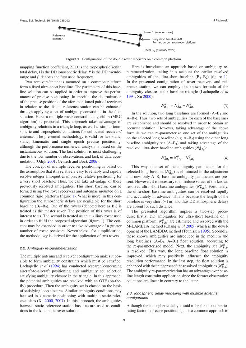
Two receivers/antennas mounted on a common platform form a fixed ultra-short baseline. The parameters of this base-line solution can be applied in order to improve the perfor-mance of precise positioning. In specific, the determination of the precise position of the aforementioned pair of receivers in relation to the distant reference station can be enhanced through applying a set of ambiguity constraints in the float solution. Here, a multiple rover constraints algorithm (MRC algorithm) is proposed. This approach takes advantage of ambiguity relations in a triangle loop, as well as similar iono-spheric and tropospheric conditions for collocated receivers/antennas. The presented methodology is valid for fast-static, static, kinematic and single epoch precise positioning, although the performance numerical analysis is based on the instantaneous solution. The last solution is most challenging due to the low number of observations and lack of data accu-mulation (Odijk 2001, Genrich and Bock 2006).

The concept of multiple receiver positioning is based on the assumption that it is relatively easy to reliably and rapidly resolve integer ambiguities in precise relative positioning for a very short baseline. Thus, we can take advantage of these previously resolved ambiguities. This short baseline can be formed using two rover receivers and antennas mounted on a common rigid platform (figure 1). What is more, in this con-figuration the atmospheric delays are negligible for the short baseline (B1–B2). One of the rovers (denoted here as B1) is treated as the master rover. The position of this rover is of interest to us. The second is treated as an auxiliary rover used in order to fulfil the proposed algorithm (figure 1). The con-cept may be extended in order to take advantage of a greater number of rover receivers. Nevertheless, for simplification, the methodology is derived for the application of two rovers.

2.2. Ambiguity re-parameterization

The multiple antenna and receiver configuration makes it pos-sible to form ambiguity constraints which must be satisfied. Lachapelle et al (1994) has conducted research concerning aircraft-to-aircraft positioning and ambiguity set selection satisfying ambiguity closure in the triangle. In this approach, the potential ambiguities are resolved with an OTF (on-the-fly) procedure. Then the ambiguity set is chosen on the basis of satisfying loop closures. Similar ambiguity conditions may be used in kinematic positioning with multiple static refer-ence sites (Xu 2000, 2007). In this approach, the ambiguities between static reference station baseline are used as condi-tions in the kinematic rover solution.

Here is introduced an approach based on ambiguity re-parameterization, taking into account the earlier resolved ambiguities of the ultra-short baseline (B1–B2) (figure 1). In the presented configuration of rover receivers and ref-erence station, we can employ the known formula of the ambiguity closure in the baseline triangle (Lachapelle et al 1994, Xu 2000):

= −N N NB Bij

ABij

ABij

1 2 1 2 (3)

In the solution, two long baselines are formed (A–B1 and A–B2). Thus, two sets of ambiguities for each of the baselines are established and should be resolved in order to obtain an accurate solution. However, taking advantage of the above formula we can re-parameterize one set of the ambiguities on the selected long baseline (e.g. A–B2) using the other long baseline ambiguity set (A–B1) and taking advantage of the resolved ultra-short baseline ambiguities (NB B

ij1 2

):.

= −N N NABij

ABij

B Bij

2 1 1 2 (4)

This way, one set of the ambiguity parameters for the selected long baseline (NB A

ij2

) is eliminated in the adjustment and now only A–B1 baseline ambiguity parameters are pre-sent. However, it is necessary to introduce values of the known resolved ultra-short baseline ambiguities (NB B

ij1 2

). Fortunately, the ultra-short baseline ambiguities can be resolved rapidly and accurately in advance. This is because the length of the baseline is very short (~1 m) and thus DD atmospheric delays are absent for such distance.

The presented algorithm implies a two-step proce-dure: firstly, DD ambiguities for ultra-short baseline on a common platform (NB B

ij1 2

) are estimated and resolved with the M-LAMBDA method (Chang et al 2005) which is the devel-opment of the LAMBDA method (Teunissen 1995). Secondly, these known ambiguities are introduced in the medium and long baselines (A–B1, A–B2) float solution, according to the re-parameterized model. Next, the ambiguity set (NB A

ij1

) is resolved. This way, the long baseline float solution is improved, which may positively influence the ambiguity resolution performance. In the last step, the float solution is enhanced with the integer set of the resolved ambiguities (NB A

ij1

). The ambiguity re-parametrization has an advantage over base-line length constraint application since the former observation equations are linear in contrary to the latter.

2.3. Ionospheric delay modelling with multiple antenna configuration

Although the ionospheric delay is said to be the most deterio-rating factor in precise positioning, it is a common approach to

Figure 1. Configuration of the double rover receivers on a common platform.

Meas. Sci. Technol. 26 (2015) 035002

J Paziewski

4

employ network ionospheric corrections in the RTK solution (Rizos 2002, Hu 2005). This approach is also applied here. However, mainly due to the interpolation process, the derived network corrections cannot be regarded as errorless. Thus, in the rover solution, we also take into account the unmodelled residuals of the ionospheric corrections. Consequently, addi-tional parameters accounting for DD ionospheric correction residuals are incorporated (IAB

ij ) as stochastic parameters in the estimation process. This approach, often called the iono-sphere-weighted model, was previously investigated by sev-eral research groups (Teunissen 1997, Odijk 2000, Julien et al 2004, Wielgosz et al 2008, Wielgosz 2010).

The procedure of introduction of network ionospheric cor-rections modified and applied here is based on a three-step approach. Although only a brief description is presented here, the details of the approach may be found in (Paziewski and Wielgosz 2014). Firstly, a solution of the reference network is performed. After resolving DD ambiguities, the precise DD ionospheric corrections may be derived by employing geometry-free linear combination (Schaer 1999). In the next step, the ionospheric corrections for the user are derived by means of interpolation. The interpolated DD ionospheric cor-rections are introduced into the rover solution with an addi-tional estimation of residual DD ionospheric delays (IAB

ij ).The ionosphere-weighted model implies an estimation

of the residual DD ionospheric parameters (IABij ), which are

set independently for each of the processed baselines in the multi-baseline solution at each epoch (Odijk 2000). Here, is proposed a slightly different approach. The regular RTK positioning implies a single baseline solution. However, in the approach presented here are created baselines connecting one reference station and user rover stations (A–B1 and A–B1) (figure 1). According to the standard ionosphere-weighted model, two separate DD ionosphere parameters for baselines A–B1 and A–B2 and satellites i–j should be set for each epoch,

− −( ) ( )I I,A Bij

A Bij

1 2 respectively. Taking advantage of the close

distance between the rover antennas, we can assume that the atmospheric delays of the satellite signals at both rover sta-tions (B1, B2) are similar. Thus, we can assume that the DD ionospheric delays for satellite pair i–j at A–B1 and A–B2 baselines are identical and a single DD ionosphere parameter at each epoch can be set for both baselines ( −IA B

ij ):

≅ =− − −I I IA Bij

A Bij

A Bij

1 2 (5)

This results in a clear reduction in the number of the parameters in the least squares adjustment. What is more, the observational model is strengthened, since the same residual DD ionosphere parameter is calculated using a double number of the observations.

2.4. Tropospheric delay modelling with multiple antenna configuration

In precise positioning the commonly applied approach for mit-igation of the tropospheric delay is the application of global models with estimation of the residual zenith tropospheric delays (ZTD) at each of the GNSS sites in the multi-station solution (Dach et al 2007, Wielgosz et al 2011b, Hadas et al

2013). On the other hand, this approach requires long observa-tional sessions as well as a significant distance between sites in order to separate highly correlated ZTD parameters over the network (Bosy et al 2003, Wielgosz et al 2011b, 2012). In contrast to the absolute ZTD estimation, a relative zenith tropospheric delay (RZTD) with respect to the nominated ZTD value may be estimated (Zhang and Lachapelle 2001). Primary research indicates that in precise positioning the best results may be obtained by the introduction of external network-derived tropospheric delays followed by constrained residual ZTD estimation at each of the sites (Wielgosz et al 2011a). The application of the aforementioned approach to the considered configuration of single reference site and double rover would result in establishing three ZTD parameters at each of the sites—A, B1 and B2. Nevertheless, according to our primary assumption of the similar atmospheric delays at both of the close rover stations (B1, B2), we can set one ZTD parameter for both close rovers. That way, we can reduce the number of the model parameters in the adjustment. Otherwise, it would be impossible to reliably estimate separate ZTD parameters for such close rover stations.

≅ =ZTD ZTD ZTDB B B1 2 (6)

In this configuration, we can also apply the same tropo-sphere mapping functions coefficients for both rover B1, B2 receivers.

α α α≅ =Bi

Bi

Bi

1 2 (7)

The a priori values of the tropospheric delays are obtained from standard tropospheric models like Hopfield, Modified Hopfield, Saastamoinen (Hopfield 1971, Saastamoinen 1972, Goad and Goodman 1974). In the presented numerical experiment the UNB3m developed at the University of New Brunswick model was applied (Leandro et al 2008).

2.5. Functional model in the presence of multiple antenna configuration

Let us derive an observational model at a particular epoch for the double rover configuration, taking advantage of the MRC approach. Equations (8)–(11) present the regular observation model derived for A–B1 and A–B2 baselines, respectively, and processed with the geometry-based ionosphere-weighted model with residual ZTD estimation.

λ φ ρ α α α

α λ

− − − −

+ + + =

(

) If

fN

ZTD ZTD ZTD

ZTD 0

n AB nij

ABij

Ai

A Aj

A Bi

B

Bj

B AB nij

nn AB n

ij

, 

,12

2 , 

1 1 1 1

1 1 1 1

(8)

ρ α α α α− − − − +

− =

  ( )P

If

f

ZTD ZTD ZTD ZTD

0

AB nij

ABij

Ai

A Aj

A Bi

B Bj

B

AB nij

n

,

,12

2

1 1 1 1 1 1

1(9)

λ φ ρ α α α

α λ

− − − −

+ + + =

(

) If

fN

ZTD ZTD ZTD

ZTD 0

n AB nij

ABij

Ai

A Aj

A Bi

B

Bj

B AB nij

nn AB n

ij

, 

,12

2 , 

2 2 2 2

2 2 2 2(10)

Meas. Sci. Technol. 26 (2015) 035002

J Paziewski

5

ρ α α α

α

− − − −

+ − =

(

)

P

If

f

ZTD ZTD ZTD

ZTD 0

AB nij

ABij

Ai

A Aj

A Bi

B

Bj

B AB nij

n

, 

,12

2

2 2 2 2

2 2 2

(11)

Taking advantage of the MRC approach, equation  (4) and relations (5–6), we finally obtain the observation equa-tions for the analysed double-rover and single reference sta-tion configuration (double baseline, figure 1) for a particular epoch (equation (12)–(15). These equations include the same unknown tropospheric parameters ZTBB for both rover sta-tion and the same ambiguity (  NAB n

ij,1

) and ionospheric (IAB nij

, ) parameters for both baselines. Additionally, the unknown parameters are stations’ coordinates. What is more, for both baselines the same known mapping function coefficients (αB

i ) may be applied. The short baseline ambiguities (NB B

ij1 2

) are known values since they were previously resolved in the first step baseline solution.

λ φ ρ α α α α

λ

− − − − +

+ + =

 

 

( )I

f

fN

ZTD ZTD ZTD ZTD

0

n AB nij

ABij

Ai

A Aj

A Bi

B Bj

B

AB nij

nn AB n

ij

,

,12

2 ,

1 1

1

(12)

ρ α α α α− − − − +

− =

  ( )P

If

f

ZTD ZTD ZTD ZTD

0

AB nij

ABij

Ai

A Aj

A Bi

B Bj

B

AB nij

n

,

,12

2

1 1

(13)

λ φ ρ α α α α

λ

− − − − +

+ … + + − =

( )

( )If

fN N

ZTD ZTD ZTD ZTD

0

n AB nij

ABij

Ai

A Aj

A Bi

B Bj

B

AB nij

nn AB n

ijB B nij

, 

,12

2 , ,

2 2

1 1 2 (14)

ρ α α α α− − − − +

− =

  ( )P

If

f

ZTD ZTD ZTD ZTD

0

AB nij

ABij

Ai

A Aj

A Bi

B Bj

B

AB nij

n

,

,12

2

2 2

(15)

The observational model parameter estimation is based on a sequential least squares adjustment with a priori parameter constraining (Xu 2007). Thus, we integrate two groups of observations: a linearized observation equation based on DD carrier-phase and pseudorange measurements (equation (1)) with related design, weight matrix and observed minus com-puted vector (A, PL, L, respectively) and a pseudo observation equation  with related design, weight matrix and observed minus computed vector (BW, PW, W, respectively). Here the station coordinates, ZTD as well as DD ionospheric delays are weighted parameters with a priori weight computed on the basis of their respective a priori sigmas. The dX is the vector of the corrections to a priori values of the parameters (station coordinates, DD ambiguities, ZTD, DD ionospheric delays). When creating a weight matrix of DD pseudorange and carrier phase observations (PL), all mathematical correla-tions caused by double-differencing are taken into account.

Finally, the corrections to the a priori values of the param-eters are determined by resolving the known form of normal equations (Xu 2007):

+ − + =( ) ( )A P A B P B d A P L B P W 0TL W

TW W X

TL W

TW (16)

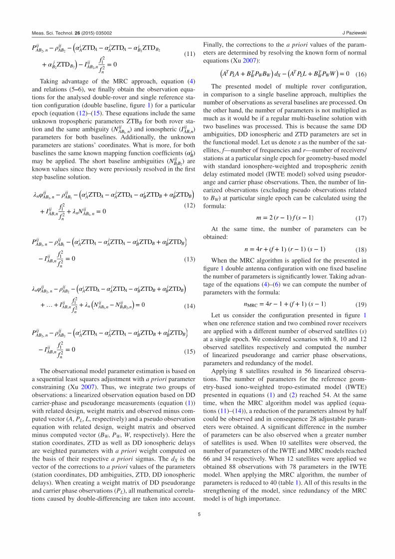
The presented model of multiple rover configuration, in comparison to a single baseline approach, multiplies the number of observations as several baselines are processed. On the other hand, the number of parameters is not multiplied as much as it would be if a regular multi-baseline solution with two baselines was processed. This is because the same DD ambiguities, DD ionospheric and ZTD parameters are set in the functional model. Let us denote s as the number of the sat-ellites, f—number of frequencies and r—number of receivers/stations at a particular single epoch for geometry-based model with standard ionosphere-weighted and tropospheric zenith delay estimated model (IWTE model) solved using pseudor-ange and carrier phase observations. Then, the number of lin-earized observations (excluding pseudo observations related to BW) at particular single epoch can be calculated using the formula:

= − −m r f s2 ( 1) ( 1) (17)

At the same time, the number of parameters can be obtained:

= + + − −n r f r s4 ( 1) ( 1) ( 1) (18)

When the MRC algorithm is applied for the presented in figure 1 double antenna configuration with one fixed baseline the number of parameters is significantly lower. Taking advan-tage of the equations (4)–(6) we can compute the number of parameters with the formula:

= − + + −n r f s4 1 ( 1) ( 1)MRC (19)

Let us consider the configuration presented in figure  1 when one reference station and two combined rover receivers are applied with a different number of observed satellites (s) at a single epoch. We considered scenarios with 8, 10 and 12 observed satellites respectively and computed the number of linearized pseudorange and carrier phase observations, parameters and redundancy of the model.

Applying 8 satellites resulted in 56 linearized observa-tions. The number of parameters for the reference geom-etry-based iono-weighted tropo-estimated model (IWTE) presented in equations  (1) and (2) reached 54. At the same time, when the MRC algorithm model was applied (equa-tions (11)–(14)), a reduction of the parameters almost by half could be observed and in consequence 28 adjustable param-eters were obtained. A significant difference in the number of parameters can be also observed when a greater number of satellites is used. When 10 satellites were observed, the number of parameters of the IWTE and MRC models reached 66 and 34 respectively. When 12 satellites were applied we obtained 88 observations with 78 parameters in the IWTE model. When applying the MRC algorithm, the number of parameters is reduced to 40 (table 1). All of this results in the strengthening of the model, since redundancy of the MRC model is of high importance.

Meas. Sci. Technol. 26 (2015) 035002

J Paziewski

6

3. Experimental proof of the concepts

In this section, the approach introduced above is evaluated on the basis of the experiment carried out on 3 September 2012. This study investigates the performance of the precise posi-tioning with a single, double and triple antenna/receiver rover configuration. Calculations were performed in instantaneous mode, thus each epoch was resolved independently. The single epoch solution is challenging due to lack of data accu-mulation and thus difficulty of ambiguity resolution. On the other hand, this solution is resistant to phase cycle-slips. The receivers were static during the session. This allowed for coor-dinate comparison with respect to the previously determined in the static long session solution reference (benchmark) coor-dinates of the rovers. All calculations were performed using GINPOS research software with the application of the pro-posed approach.

3.1. Experiment design

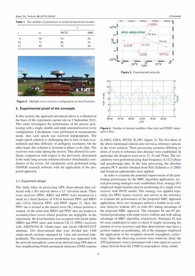
The study relies on processing GPS observational data col-lected with a 30 s interval above a 15° elevation mask. Three rover receivers (PP01, RR03 and PP05) were mounted on a metal in a fixed distance of 0.81 m between PP01 and RR03 and 1.62 m between PP01 and PP05 (figure 2). Here the PP01 site is treated as the master rover (B1) whose position is wanted. At the same time RR03 and PP05 sites are treated as secondary/slave rovers whose positions are negligible. In the experiment, the fixed baseline was occupied with Javad Alpha (RR03 and PP05 sites) and Ashtech UZ-12 (PP01) receivers with ASH701941.B (choke-ring) and Javad GRANT-G3T antennas. 24 h observational data were divided into 1440 single-epoch sessions separated by 1 min and resolved inde-pendently. The instantaneous positioning was supported with the network ionospheric corrections derived using GPS data of four neighbouring Polish permanent reference GNSS stations

(LAMA, DZIA, MYSZ, ILAW) (figure 3). The first three of the above mentioned stations also served as reference stations in the rover solution. Three processing scenarios differing in terms of rovers to reference sites distance were established. In particular, the distances were set to 31, 51 and 70 km. The cal-culations were performed using dual-frequency (L1/L2) phase and pseudorange data. In the data processing, the absolute antenna PCV models obtained from IGS (Schmid et al 2005) and broadcast ephemerides were applied.

In order to examine the potential improvement of the posi-tioning performance by the MRC algorithm application, sev-eral processing strategies were established. First, strategy (#1) employed single baseline precise positioning of a single rover receiver with IWTE model. This strategy was applied sepa-rately for PP01 master receiver and served as the reference to evaluate the performance of the proposed MRC approach application. Next, two strategies utilized a double rover solu-tion, however without (#2) or with (#3) taking advantage of the proposed MRC approach. The strategies #4 and #5 per-formed positioning with triple rovers without and with taking advantage of MRC algorithm, respectively. Strategies #2 and #4 were established in order to check if simply increasing the number of rover receivers (and thus observations) may have a positive impact on positioning. All of the strategies employed the application of the weighted network ionospheric correc-tions. Since the observing sessions were relatively short, the ZTD parameters were constrained with 1 mm sigma to a priori values derived from the UNB3 m tropospheric delay model.

Table 1. The number of parameters in analyzed functional models.

s m

n

IWTE MRC

8 56 54 2810 72 66 3412 88 78 40

Figure 2. Multiple rover receivers configuration on fixed baseline.

Figure 3. Experimental network.

30' 20oE 30' 21oE 30' 53oN

15'

30'

45'

54oN

DZIA

LAMA

MYSZ

ILAW

PP01-RR03-PP05

51 km

31 km

70 km

Lon.

Lat.

Figure 4. Number of tracked satellites (blue line) and PDOP values (green line).

00:00 04:00 08:00 12:00 16:00 20:000

2

4

6

8

10

12

UTC

num

. of

sat

.

0

1

2

3

4

5

PD

OP

Meas. Sci. Technol. 26 (2015) 035002

J Paziewski

7

Processing strategies:

1. single rover solution, IWTE model 2. double rover solution, IWTE model 3. double rover solution IWTE model with MRC algorithm 4. triple rover solution, IWTE model 5. triple rover solution IWTE model with MRC algorithm

The performance of the strategies was evaluated on the basis of several indicators related to coordinate and ambi-guity domains. Specifically, standard deviations (std) and mean coordinate residuals of the correctly fixed solutions were used as the coordinate domain indicators. The coordi-nate residuals were computed as difference between deter-mined and reference coordinates of the rover receiver. The

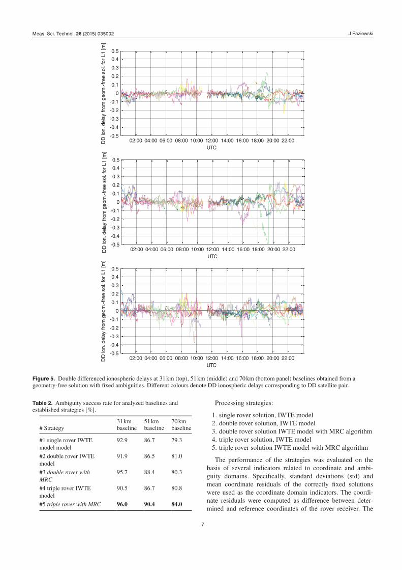
Figure 5. Double differenced ionospheric delays at 31 km (top), 51 km (middle) and 70 km (bottom panel) baselines obtained from a geometry-free solution with fixed ambiguities. Different colours denote DD ionospheric delays corresponding to DD satellite pair.

02:00 04:00 06:00 08:00 10:00 12:00 14:00 16:00 18:00 20:00 22:00-0.5

-0.4

-0.3

-0.2

-0.1

0

0.1

0.2

0.3

0.4

0.5

UTC

DD

ion.

del

ay fr

om g

eom

.-fr

ee s

ol. f

or L

1 [m

]

02:00 04:00 06:00 08:00 10:00 12:00 14:00 16:00 18:00 20:00 22:00-0.5

-0.4

-0.3

-0.2

-0.1

0

0.1

0.2

0.3

0.4

0.5

UTC

DD

ion.

del

ay fr

om g

eom

.-fr

ee s

ol. f

or L

1 [m

]

02:00 04:00 06:00 08:00 10:00 12:00 14:00 16:00 18:00 20:00 22:00-0.5

-0.4

-0.3

-0.2

-0.1

0

0.1

0.2

0.3

0.4

0.5

UTC

DD

ion.

del

ay fr

om g

eom

.-fr

ee s

ol. f

or L

1 [m

]

Table 2. Ambiguity success rate for analyzed baselines and established strategies [%].

# Strategy31 km baseline

51 km baseline

70 km baseline

#1 single rover IWTE model model

92.9 86.7 79.3

#2 double rover IWTE model

91.9 86.5 81.0

#3 double rover with MRC

95.7 88.4 80.3

#4 triple rover IWTE model

90.5 86.7 80.8

#5 triple rover with MRC 96.0 90.4 84.0

Meas. Sci. Technol. 26 (2015) 035002

J Paziewski

8

reference coordinates of the rovers were obtained as a result of static session solution in multistation mode in reference to neighbouring Polish permanent GNSS stations (figure 3). The percentage of sessions with correctly fixed epochs (ASR-ambiguity success rate) served as indicators of the ambiguity resolution domain. Nevertheless, the latter indicator is treated here as essential since evaluates the reliability of ambiguity resolution which is crucial to obtain a precise position.

3.2. Experiment results

In this section the results of precise positioning with multiple rover receiver configuration are presented and discussed. In a first step, the observing conditions are evaluated. During the experiment, 5 to 10 satellites were observed at the rover stations (figure 4). PDOP values at the rover receivers are depicted in figure 4. For most of the duration of the session, PDOP values were oscillating near the value of 2. Thus, we can recognize satellite constellation geometry as relatively good. In the middle of the session can be observed an impor-tant drop of the number of satellites (to five) and thus growth of the PDOP factor. Therefore, difficulties in processing of the data at this time could be expected.

The geomagnetic activity index (Kp) varied from 3+ to 6−  with sum Kp of 33−  , which indicates an active iono-sphere. Figure 5 presents DD ionospheric delays the processed baselines (of 31, 51 and 70 km length). The DD ionospheric

delays were obtained using geometry-free linear combination with fixed ambiguities derived from postprocessing twelve static sessions of 2 h long each. Since in such long sessions the ambiguities were resolved with a high level of reliability, the values of the DD ionospheric delays can be regarded as ‘true’ DD ionospheric delays deteriorating DD observations at processed baselines. For most of the day, the delays did not exceed ±15 and ±20 cm for the shortest (31 km) and longer baselines (51 and 70 km), respectively. On the other hand, between 16:00 and 20:00 UTC, more active ionosphere was observed. Thus the DD ionospheric delays were significantly higher, reaching even ±50 cm over a 51 km baseline (figure 5).

Table 2 presents the key statistics evaluating the instan-taneous ambiguity success rate of the precise positioning with application of the tested strategies for the analysed distance to the reference site. The statistics of the coordi-nate residuals as well as the indicators related to the ambi-guity domain were calculated in each strategy for the master rover B1 (site PP01) since the position of this site is to be determined. MRC approach (strategy #3 and #5) results were compared to standard single rover solution of PP01 (strategy #1). Additionally positioning with double and triple receivers, however without the application of the MRC approach (strategy #2 and #4), were presented.

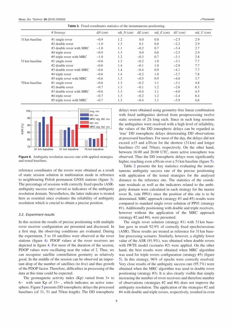
The single rover solution (strategy #1) with 31 km base-line gave in result 92.9% of correctly fixed epochs/sessions (ASR). These results are treated as reference for 31 km base-line processing scenario. Similarly, however, a slightly lower value of the ASR (91.9%), was obtained when double rovers with IWTE model (scenario #2) were applied. On the other hand, the best results were obtained when MRC algorithm was used for triple rovers configuration (strategy #5) (figure 5). In this strategy, 96% of epochs were correctly resolved. Very close results of the ambiguity success rate (95.7%) were obtained when the MRC algorithm was used in double rover positioning (strategy #3). It is also clearly visible that simply increasing the number of rover receivers and therefore number of observations (strategies #2 and #4) does not improve the ambiguity resolution. The application of the strategies #2 and #4 with double and triple rovers, respectively, resulted in even

Table 3. Fixed coordinates statistics of the instantaneous positioning.

# Strategy dN (cm) sdt_N (cm) dE (cm) std_E (cm) dU (cm) std_U (cm)

31 km baseline #1 single rover −0.9 1.2 0.0 0.8 −2.5 2.9#2 double rover −1.0 1.3 0.1 0.8 −2.2 2.9#3 double rover with MRC −1.0 1.1 −0.2 0.7 −3.4 2.7#4 triple rover −0.9 1.3 0.0 0,8 −2.5 2.9#5 triple rover with MRC −1.0 1.2 −0.3 0.7 −3.1 2.8

51 km baseline #1 single rover −0.6 1.3 −0.2 1.0 −3.1 7.7#2 double rover −0.6 1.4 −0.1 1.0 −2.8 7.7#3 double rover with MRC −0.6 1.4 −0.4 0.9 −4.1 7.7#4 triple rover −0.6 1.4 −0.2 1.0 −2.7 7.8#5 triple rover with MRC −0.6 1.3 −0.5 0.9 −4.0 3.7

70 km baseline #1 single rover −0.6 1.3 −0.2 1.1 −3.1 4.8#2 double rover −0.7 1.3 −0.1 1.2 −2.6 8.3#3 double rover with MRC −0.6 1.3 −0.4 1.1 −4.0 4.5#4 triple rover −0.7 1.3 −0.2 1.2 −2.4 8.4#5 triple rover with MRC −0.7 1.3 −0.4 1.1 −3.9 4.6

Figure 6. Ambiguity resolution success rate with applied strategies and tested baselines.

31 km baseline 51 km baseline 70 km baseline75

80

85

90

95

100

AS

R [

%]

sng. rov.

dbl. rov.

MRC alg. dbl. rov.

trpl. rov.

MRC alg. trpl. rov.

Meas. Sci. Technol. 26 (2015) 035002

J Paziewski

9

lower values of the ASR parameter than reference single rover positioning (strategy #1).

When considering a longer baseline (51 km), the ambiguity resolution performance was of lower quality with respect to the 31 km baseline, which was expected. In this scenario, the application of the proposed MRC algorithm again resulted in an improvement in the ambiguity resolution domain. In par-ticular, a clear 3.7% increase of the correctly fixed epochs ratio (ASR) was observed using MRC algorithm with triple rovers (strategy #5) against single rover positioning (strategy #1). Finally, in the case of strategy #5, this parameter was the highest and reached 90.4%. The MRC approach applied for double receivers gave also better ASR results than other strate-gies without application of proposed algorithm.

Mainly due to decorrelation of the ionospheric and tropo-spheric delays, the accuracy and reliability of the relative positioning decrease with growing rover to reference sites distance. Thus, the deterioration in the ambiguity resolution domain is noticeable when considering the longest distance between rovers and reference site (70 km). The reference single rover positioning with IWTE model gave in the result 79.3% of the correctly resolved sessions/epochs, which was the smallest value. On the contrary, the application of the proposed multiple receiver configuration algorithm for triple rovers resulted in 4.7% growth to 84.0% of the ambiguity resolution success rate factor. Strategies from #3 to #4 gave in result similar values of the ASR parameter between 80.3% and 81.0%.

When using the geometry-based relative model it is visible that correct ambiguity resolution provides the precise solution

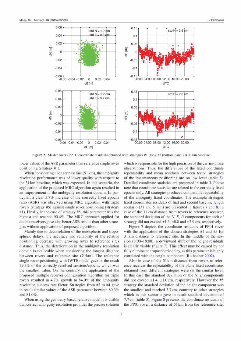
which is responsible for the high precision of the carrier-phase observations. Thus, the differences of the fixed coordinate repeatability and mean residuals between tested strategies of the instantaneous positioning are on low level (table 3). Detailed coordinate statistics are presented in table 3. Please note that coordinate statistics are related to the correctly fixed epochs only. All strategies produced comparable repeatability of the ambiguity fixed coordinates. The example strategies fixed coordinates residuals of first and second baseline length scenario (31 and 51 km) are presented in figures 7 and 8. In case of the 31 km distance from rovers to reference receiver, the standard deviation of the N, E, U components for each of strategy did not exceed ±1.3, ±0.8 and ±2.9 cm, respectively.

Figure 7 depicts the coordinate residuals of PP01 rover with the application of the chosen strategies #1 and #5 for 31 km distance to reference site. In the middle of the ses-sion (8:00–18:00), a downward shift of the height residuals is clearly visible (figure 7). This effect may be caused by not fully eliminated tropospheric delay, as this parameter is highly correlated with the height component (Rothacher 2002).

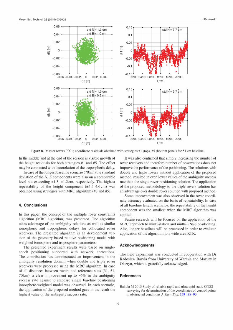
Also in case of the 51 km distance from rovers to refer-ence receiver the repeatability of the plane fixed coordinates obtained from different strategies were on the similar level. In this case the standard deviation of the N, E components did not exceed  ±1.4,  ±1.0 cm, respectively. However the #5 strategy the standard deviation of the height component was the smallest and reached 3.7 cm, contrary to other strategies which in this scenario gave in result standard deviation of 7.7 cm (table 3). Figure 8 presents the coordinate residuals of the PP01 rover, a distance of 51 km from the reference site.

Figure 7. Master rover (PP01) coordinate residuals obtained with strategies #1 (top), #5 (bottom panel) at 31 km baseline.

-0.06 -0.04 -0.02 0 0.02 0.04-0.06

-0.04

-0.02

0

0.02

0.04

0.06

dE [m]

dN [m

]

std N = 1.2 cmstd E = 0.8 cm

00:00 04:00 08:00 12:00 16:00 20:00-0.15

-0.1

-0.05

0

0.05

0.1

0.15

dH [m

]

UTC

std H = 2.9 cm

-0.06 -0.04 -0.02 0 0.02 0.04-0.06

-0.04

-0.02

0

0.02

0.04

0.06

dE [m]

dN [m

]

std N = 1.2 cmstd E = 0.7 cm

00:00 04:00 08:00 12:00 16:00 20:00-0.15

-0.1

-0.05

0

0.05

0.1

0.15

dH [m

]

UTC

std H = 2.8 cm

Meas. Sci. Technol. 26 (2015) 035002

J Paziewski

10

In the middle and at the end of the session is visible growth of the height residuals for both strategies #1 and #5. The effect may be connected with decorelation of the tropospheric delay.

In case of the longest baseline scenario (70 km) the standard deviation of the N, E components were also on a comparable level not exceeding ±1.3, ±1.2 cm, respectively. The highest repeatability of the height component (±4.5–4.6 cm) was obtained using strategies with MRC algorithm (#3 and #5).

4. Conclusions

In this paper, the concept of the multiple rover constraints algorithm (MRC algorithm) was presented. The algorithm takes advantage of the ambiguity relations as well as similar ionospheric and tropospheric delays for collocated rover receivers. The presented algorithm is an development ver-sion of the geometry-based relative positioning model with weighted ionosphere and troposphere parameters.

The presented experiment results were based on single-epoch positioning supported with network corrections. The contribution has demonstrated an improvement in the ambiguity resolution domain when double and triple rover receivers were processed using the MRC algorithm. In case of all distances between rovers and reference sites (31, 51, 70 km), a clear improvement up to ~5% in the ambiguity success rate against to standard single baseline positioning ionosphere-weighted model was observed. In each scenario, the application of the proposed method gave in the result the highest value of the ambiguity success rate.

It was also confirmed that simply increasing the number of rover receivers and therefore number of observations does not improve the performance of the positioning. The solutions with double and triple rovers without application of the proposed method, resulted in even lower values of the ambiguity success rate than the single rover positioning solution. The application of the proposed methodology to the triple rovers solution has an advantage over double rover solution with proposed method.

Some improvement was also observed in the rover coordi-nate accuracy evaluated on the basis of repeatability. In case of all baseline length scenarios, the repeatability of the height component was the smallest when the MRC algorithm was applied.

Future research will be focused on the application of the MRC approach to multi-station and multi-GNSS positioning. Also, longer baselines will be processed in order to evaluate application of the algorithm to a wide area RTK.

Acknowledgments

The field experiment was conducted in cooperation with Dr Radoslaw Baryla from University of Warmia and Mazury in Olsztyn, which is gratefully acknowledged.

References

Bakula M 2013 Study of reliable rapid and ultrarapid static GNSS surveying for determination of the coordinates of control points in obstructed conditions J. Surv. Eng. 139 188–93

Figure 8. Master rover (PP01) coordinate residuals obtained with strategies #1 (top), #5 (bottom panel) for 51 km baseline.

-0.06 -0.04 -0.02 0 0.02 0.04-0.06

-0.04

-0.02

0

0.02

0.04

0.06

dE [m]

dN [m

]

std N = 1.3 cmstd E = 1.0 cm

00:00 04:00 08:00 12:00 16:00 20:00-0.15

-0.1

-0.05

0

0.05

0.1

0.15

dH [m

]

UTC

std H = 7.7 cm

-0.06 -0.04 -0.02 0 0.02 0.04-0.06

-0.04

-0.02

0

0.02

0.04

0.06

dE [m]

dN [m

]

std N = 1.3 cmstd E = 0.9 cm

00:00 04:00 08:00 12:00 16:00 20:00-0.15

-0.1

-0.05

0

0.05

0.1

0.15

dH [m

]

UTC

std H = 3.7 cm

Meas. Sci. Technol. 26 (2015) 035002

J Paziewski

11

Bock Y, Nikolaidis R, de Jonge P J and Bevis M 2000 Instantaneous geodetic positioning at medium distances with the global positioning system J. Geophys. Res. 105 28233–53

Bosy J, Figurski M and Wielgosz P 2003 A strategy for GPS data processing in a precise local network during high solar activity GPS Solut. 7 120–9

Buist P J 2007 The baseline constrained LAMBDA Method for single epoch, single frequency attitude determination applications Proc. 20th ION Int. Meeting, (Forth Worth, TX, September 25–28 2007)

Buist P J, Teunissen P J G, Giorgi G and Verhagen S 2009 Multiplatform instantaneous GNSS ambiguity resolution for triple- and quadruple-antenna configurations with constraints Int. J. Navig. Obs. 2009 1–14

Chang X W, Yang X and Zhou T 2005 MLAMBDA: a modified LAMBDA method for integer least-squares estimation J. Geod. 79 552–65

Chen W and Qin H 2012 New method for single epoch, single frequency land vehicle attitude determination using low-end GPS receiver GPS Solut. 16 329–38

Dach R, Hugentobler U, Fridez P and Meindl M 2007 Bernese GPS software version 5.0 Astronomical Institute University of Bern, Bern

Genrich J F and Bock Y 2006 Instantaneous geodetic positioning with 10–50 Hz GPS measurements: noise characteristics and implications for monitoring networks J. Geophys. Res. 111 B03403

Giorgi G, Teunissen P J G, Verhagen S and Buist P 2012 Instantaneous ambiguity resolution in global-navigation satellite-system-based attitude determination applications: a multivariate constrained approach J. Guid. Control Dyn. 35 51–67

Goad C C and Goodman L 1974 A modified hopfield tropospheric refraction correction model American Geophysical Union Annual Fall Meeting (San Francisco, CA, 12–17 December 1974) (abstract EOS Trans. AGU 55, 1106)

Hadaś T, Kapłon J, Bosy J, Sierny J and Wilgan K 2013 Near-real-time regional troposphere models for the GNSS precise point positioning technique Meas. Sci. Technol. 24 055003

Hopfield H S 1971 Tropospheric effect on electromagnetically measured range: prediction from surface weather data Radio Sci. 6 357–67

Hu G, Abbey D A, Castleden W E, Earls C, Ovstedal O and Weihing D 2005 An approach for instantaneous ambiguity resolution for medium- to long-range multiple reference station GPS Solut. 9 1–11

Julien O, Alves P, Cannon M E and Lachapelle G 2004 Improved triple frequency GPS/Galileo carrier phase ambiguity resolution using a stochastic ionosphere modeling Proc. IONNTM-2004 Institute of Navigation (San Diego, CA, 26–28 Januray 2004) pp 441–52

Khodabandeh A and Teunissen P J G 2014 Array-based satellite phase bias sensing: theory and GPS/BeiDou/QZSS results Meas. Sci. Technol. 25 095801

Lachapelle G, Sun H, Cannon M E and Lu G 1994 Precise aircraft-to-aircraft positioning using a multiple receiver configuration Proc. National Technical Meeting, Institute of Navigation (San Diego, CA, 24–26 January 1994)

Leandro R F, Langley R B and Santos M C 2008 UNB3m_pack: a neutral atmosphere delay package for GNSS GPS Solut. 12 65–70

Leick A 2004 GPS Satellite Surveying 3rd edn (New Jersey: Wiley)Loyer S, Perosanz F, Mercier F, Capdeville H and Charles Marty J

2012 Zero-difference GPS ambiguity resolution at CNES–CLS IGS analysis center J. Geod. 86 991–1003

Nadarajah N, Paffenholz J-A and Teunissen P J G 2014 Integrated GNSS attitude determination and positioning for direct geo-referencing Sensors 14 12715–34

Moon Y and Verhagen S 2006 Integer ambiguity estimation and validation in attitude determination environments Proc. ION GNSS 19th Int. Technical Meeting for Satellite Division (Forth Worth, TX, 26–29 September 2006)

Odijk D 2000 Stochastic modelling of the ionosphere for fast GPS ambiguity resolution Proc. Geodesy Beyond 2000—the Challenges of the First Decade (IAG General Assembly, Birmingham, UK, 19 July 2000)

Odijk D 2001 Instantaneous precise GPS positioning under geomagnetic storm conditions GPS Solut. 5 29–42

Odolinski R, Teunissen P J G and Odijk D 2014 Combined BDS, Galileo, QZSS and GPS single-frequency RTK GPS Solut. 19 151–63

Paziewski J 2012 New algorithms for precise positioning with use of Galileo and EGNOS European satellite navigation systems PhD Dissertation University of Warmia and Mazury in Olsztyn (in Polish)

Paziewski J and Stępniak K 2014 New on-line system for automatic postprocessing of fast-static and kinematic GNSS data 9th Int. Conf. on Environmental Engineering (ICEE) Selected papers (Vilnius, Lithuania, 22–23 May 2014)

Paziewski J and Wielgosz P 2014 Assessment of GPS + Galileo and multi-frequency Galileo single-epoch precise positioning with network corrections GPS Solut. 18 571–9

Paziewski J and Wielgosz P 2015 Accounting for Galileo-GPS inter-system biases in precise satellite positioning J. Geod. 89 81–93

Qin H and Chen W 2013 Application of the constrained moving horizon estimation method for the ultra-short baseline attitude determination Acta Geod. Geophys. 48 27–38

Rizos C 2002 Network RTK research and implementation: a geodetic perspective J. Global Position. Syst. 2 144–50

Rothacher M 2002 Estimation of station heights with GPS Vertical Reference Systems ed H Drewes et al (International Association of Geodesy Symposia vol 124) (Berlin: Springer) pp 81–90

Saastamoinen J 1972 Atmospheric correction for the troposphere and stratosphere in radio ranging of satellites The Use of Artificial Satellites For Geodesy (Geophysical Monograph) ed S Henriksen (Washington DC: AGU) vol 15 pp 247–51

Schaer S 1999 Mapping and predicting Earth’s Ionosphere using Global Positioning System PhD Dissertation Astronomical Institute, University of Berne, Switzerland

Schmid R, Rothacher M, Thaller D and Steigenberger P 2005 Absolute phase center corrections of satellite and receiver antennas GPS Solut. 9 283–93

Teunissen P J G 1995 The least-squares ambiguity decorrelation adjustment: a method for fast GPS integer ambiguity estimation J. Geod. 70 65–82

Teunissen P J G 1997 The geometry-free GPS ambiguity search space with a weighted ionosphere J. Geod. 71 370–83

Teunissen P J G 2006 The LAMBDA method for the GNSS compass Artif. Satellites 41 89–103

Teunissen P J G 2007 A general multivariate formulation of the multi-antenna GNSS attitude determination problem Artif. Satellites 42 97–111

Teunissen P J G 2010 Integer least-squares theory for the GNSS compass J. Geod. 84 433–47

Teunissen P J G 2012 A-PPP: array-aided precise point positioning with global navigation satellite systems IEEE Trans. Signal Process. 60 2870–81

Wang B, Miao L, Wang S and Shen J 2009 A constrained LAMBDA method for GPS attitude determination GPS Solut. 13 97–107

Wielgosz P 2010 Quality assessment of GPS rapid static positioning with weighted ionospheric parameters in generalized least squares GPS Solut. 15 89–99

Meas. Sci. Technol. 26 (2015) 035002

J Paziewski

12

Wielgosz P, Cellmer S, Rzepecka Z, Paziewski J and Grejner-Brzezinska D A 2011a Troposphere modeling for precise GPS rapid static positioning in mountainous areas Meas. Sci. Technol. 22 045101

Wielgosz P, Paziewski J and Baryła R 2011b On constraining zenith tropospheric delays in processing of local GPS networks with Bernese software Surv. Rev. 43 472–83

Wielgosz, P, Krankowski A, Sieradzki R and Grejner-Brzezinska D A 2008 Application of predictive regional ionosphere model to medium range RTK positioning Acta Geophys. 56 1147–61

Wielgosz P, Paziewski J, Krankowski A, Kroszczynski K and Figurski M 2012 Results of the application of tropospheric

corrections from different troposphere models for precise GPS rapid static positioning Acta Geophys. 60 1236–57

Xu G 2000 A concept of precise kinematic positioning and flight-state monitoring from the AGMASCO practice Earth Planets Space 52 831–5

Xu G 2007 GPS: Theory, Algorithms and Applications 2nd edn (Berlin: Springer)

Zhang J and Lachapelle G 2001 Precise estimation of residual tropospheric delays using a regional GPS network for RTK applications J. Geod. 75 255–66

Zou X, Ge M, Tang W, Shi C and Liu J 2013 URTK: undifferenced network RTK positioning GPS Solut. 17 283–93

Meas. Sci. Technol. 26 (2015) 035002