practical significance, meta-analysis and the credibility of
TRANSCRIPT

DISCUSSION PAPER SERIES
IZA DP No. 12458
T.D. StanleyHristos Doucouliagos
Practical Significance, Meta-Analysis and the Credibility of Economics
JULY 2019
Any opinions expressed in this paper are those of the author(s) and not those of IZA. Research published in this series may include views on policy, but IZA takes no institutional policy positions. The IZA research network is committed to the IZA Guiding Principles of Research Integrity.The IZA Institute of Labor Economics is an independent economic research institute that conducts research in labor economics and offers evidence-based policy advice on labor market issues. Supported by the Deutsche Post Foundation, IZA runs the world’s largest network of economists, whose research aims to provide answers to the global labor market challenges of our time. Our key objective is to build bridges between academic research, policymakers and society.IZA Discussion Papers often represent preliminary work and are circulated to encourage discussion. Citation of such a paper should account for its provisional character. A revised version may be available directly from the author.
Schaumburg-Lippe-Straße 5–953113 Bonn, Germany
Phone: +49-228-3894-0Email: [email protected] www.iza.org
IZA – Institute of Labor Economics
DISCUSSION PAPER SERIES
ISSN: 2365-9793
IZA DP No. 12458
Practical Significance, Meta-Analysis and the Credibility of Economics
JULY 2019
T.D. StanleyDeakin University
Hristos DoucouliagosDeakin University and IZA
ABSTRACT
IZA DP No. 12458 JULY 2019
Practical Significance, Meta-Analysis and the Credibility of Economics
Recently, there has been much discussion about replicability and credibility. By integrating
the full research record, increasing statistical power, reducing bias and enhancing credibility,
meta-analysis is widely regarded as ‘best evidence’. Through Monte Carlo simulation, closely
calibrated on the typical conditions found among 6,700 economics research papers, we
find that large biases and high rates of false positives will often be found by conventional
meta-analysis methods. Nonetheless, the routine application of meta-regression analysis
and considerations of practical significance largely restore research credibility.
JEL Classification: C10, C12, C13, C40
Keywords: meta-analysis, meta-regression, publication bias, credibility, simulations
Corresponding author:T.D. StanleyDeakin Lab for the Meta-Analysis of Research (DeLMAR)Deakin Business SchoolDeakin UniversityBurwood VIC 3125Australia
E-mail: [email protected]
1
1. Introduction
The core challenge of economics research is to provide credible estimates or tests of important
parameters and theories. Recently, there has been much discussion about a replication crisis in
the social sciences, largely stimulated by the Open Science Collaboration’s highly-publicized
failures to replicate many of the 100 well-regarded psychology experiments, amplifying long-
expressed, broader concerns about credibility in many fields (OSC, 2015). Economists have also
become concerned about research credibility, selective reporting and replication (e.g., Andrews
and Kasy, 2019; Camerer et al., 2016; Christensen and Miguel, 2018; Ioannidis et al., 2017;
Maniadis et al., 2015; Maniadis et al., 2107;). Low statistical power and research exaggeration is
the norm in economics and psychology, explaining the observed difficulties to replicate (OSC,
2015; Camerer et al., 2016; Ioannidis et al., 2017; Camerer et al., 2018; Stanley et al., 2018;
Andrews and Kasy, 2019).
In response, many economists have called for greater application of meta-analysis
methods to increase statistical power, correct bias, and evaluate the evidence base (e.g., Andrews
and Kasy, 2019; Banzhaf and Smith, 2007; Christensen and Miguel, 2018; Duflo et al., 2006;
Ioannidis et al., 2017). Applications of the meta-analysis of economics research have been
growing for some time—for example, Card and Krueger (1995), Disdier and Head (2008),
Chetty (2012), Hsiang et al. (2013), Havranek (2015), Lichter et al. (2015), Croke et al. (2016),
Card et al. (2018), Andrews and Kasy (2019), among numerous others. This study investigates
the properties of meta-analysis methods under the typical conditions found in economics: low
power, high heterogeneity, and selective reporting. From over 64,000 economic effects, 159
meta-analyses and 6,700 research papers, Ioannidis et al. (2017) find that the typical reported
effect has low statistical power and is exaggerated by a factor of two, which is the same as what
replications in economics and psychology have found (OSC, 2015; Camerer et al., 2018). Very
high heterogeneity from one reported effect to the next is the norm in economics (median
I2=93%).1 Under these conditions, can conventional meta-analysis provide reliable assessments
of economic theory or empirical effects? Can meta-analysis restore credibility to economics
research?
1 I2 measures the proportion of the observed variation across reported research results that cannot be explained by
random sampling error alone (Higgins and Thompson, 2002). Like R2, 0 < I2 < 1, or between 0 and 100%.
2
In this study, we employ Monte Carlo simulations to investigate whether typical levels of
statistical power, selective reporting, and heterogeneity found in economics research will cause
meta-analysis to have notable biases and high rates of false positives; that is, claiming the
presence of economic effects or phenomena that may not exist. Our simulations are intentionally
challenging for multiple meta-regression, forcing it to accommodate: random sampling error,
selective reporting, high levels of random heterogeneity, selected systematic heterogeneity, and
random systematic heterogeneity.
The below simulations are very revealing. When there is high heterogeneity and some
researchers select which results to report based on their statistical significance, we find that
conventional meta-analysis methods break down; they can have highly inflated type I errors. In
contrast, we show that the routine use of practical significance in the place of statistical
significance combined with meta-regression analysis (MRA) diminishes these high rates of false
positives, restoring the reliability of meta-analysis and the credibility of economics research.
All applications of meta-analysis report weighted averages, and in some cases, inference
stops there (e.g. Chetty, 2012, Hsiang et al, 2013, and Disdier and Head, 2008). However,
authors often fail to caution readers about the low credibility of these meta-averages, potentially
creating problems for policy and theory development. Our results identify important changes
needed for current practices.
2. Meta-analysis methods, selection bias, and heterogeneity
Meta-analysis is widely accepted in medicine, psychology, ecology, and other fields as ‘best
evidence’, delivering the evidence for ‘evidence-based’ practice (Higgins and Green, 2008). The
role of conventional meta-analysis estimators is to integrate and summarize all comparable
estimates in a given research record and estimate the mean effect. Our simulations evaluate the
performance of four methods: random-effects (RE), unrestricted weighted least squares (WLS),
the weighted average of the adequately powered (WAAP), and the PET-PEESE.
2.1 Simple weighted averages
Conventional meta-analysis methods – fixed-effect (FE) and random effects (RE) - assume that
the individual reported effect sizes, (e.g., an elasticity), iη̂ , are randomly and normally
distributed around some overall mean, η , and estimated by a weighted average: iii ωηωη ΣΣ= ˆˆ ,
3
where iω is the individual weight for c. Fixed- and random-effects employ different weights and
thereby have different variances. RE is the more widely used method.2
The unrestricted weighted least squares weighted average, WLS, makes use of the
multiplicative invariance property implicit in all GLS models (Stanley and Doucouliagos, 2015;
2017). It is calculated by running a simple meta-regression of an estimate’s t-statistic versus its
precision: iiiii uSESEt +== )/1(ˆ αη , i=1, 2, . . . , m for SEi as the standard error of iη̂ .
Simulations show that WLS is practically as good as and often better than random-effects when
the random-effects model is true (Stanley and Doucouliagos, 2015; Stanley and Doucouliagos,
2017).3
The weighted average of the adequately powered (WAAP) makes further use of statistical
power. Large surveys of economics, psychology, and medical research have found clear
evidence that typical research studies have low statistical power (Turner, et al., 2013, Ioannidis et
al., 2017; Stanley et al., 2018). Yet, it has been long acknowledged that low-powered studies
tend to report larger effects by being “coupled with bias selecting for significant results for
publication” (Camerer et al., 2018, p.4)—also see OSC (2015), Fanelli et al., (2017), and
Ioannidis et al., (2017). Thus, overweighting the highest powered estimates might passively
reduce bias. Ioannidis et al. (2017) and Stanley et al. (2017) introduce a weighted average,
WAAP, that does exactly this. As the name suggests, WAAP calculates the unrestricted WLS
weighted average on only those estimates that have adequate power, following the 80%
convention recommended by Cohen (1977).4 Over a wide range of conditions and types of
2 Fixed effect uses inverse variance weights, iw =1/ 2
iSE , and has variance iwΣ1 ; where SEi is the standard error of
iη̂ . The random-effects weighted average allows the true effect to randomly vary from study to study and thereby
has more complex weights, iw′=1/ )ˆ( 22 τ+iSE ; where 2τ̂ is the estimated between-study heterogeneity variance. RE’s variance is iw′Σ1 . 3 The random-effects model assumes that the observed effect equals the true mean effect plus conventional random sampling errors and an additional term that causes the true effect to vary randomly and normally around the true mean effect, thereby creating random heterogeneity—see equation (7), below. 4 Estimates are adequately powered (80% or higher) if their standard error is less than the WLS estimate divided by 2.8: if SE < |WLS|/2.8 (Stanley et al., 2017). Recall that the conventional z-value is 1.96 for a 95% confidence interval, and z=0.84 for a 20/80 percent split in the cumulative normal distribution, giving 2.8 when added. Thus, to achieve 80% power, we need: η/σi > 2.8 (Ioannidis et al., 2017). Using WAAP as the estimate of mean effect, the reported , iSE as σi and rearranging this inequality implies that an adequately-powered study must have a standard error as small as the absolute value of WAAP divided by 2.8.
4
effects sizes, simulations demonstrate that WAAP reduces bias compared to FE, RE, and WLS
when there is selective reporting (Stanley et al., 2017).
2.2. Correcting for Selective Reporting and Publication Bias
The above methods either ignore selective reporting bias (FE and RE) or passively reduce it
(WAAP). They also largely ignore heterogeneity in the evidence base. For decades, economists,
psychologists, and medical researchers have acknowledged that the selective reporting of
statistically significant findings biases the research record and threatens scientific practice.5
Selective reporting bias (aka: the file-drawer problem, publication bias, small-sample bias, and
p-hacking) is the result of choosing research results for their statistical significance or
consistency with theoretical predictions, causing larger effects to be over-represented by the
research record. A recent survey of over 64,000 economic results finds that reported estimates
are typically inflated by 100% (or more) and one-third by a factor of four (Ioannidis et al., 2017).
Replications of 100 psychological experiments find that the effect size of the replication is, on
average, one half as large as the original experiment; that is, research inflation is 100% (OSC,
2015), while 21 social science experiments from Science and Nature also shrink by half upon
replication (Camerer et al., 2018).
Although widely acknowledged, economics has done little to reduce selective reporting
or publication bias until recent years. Of course, many commentaries and surveys have been
written on subjects surrounding publication bias, selected reporting, and other questionable
research practices (e.g., Leamer, 1983; DeLong and Lang, 1992; Stanley, 2005; Christensen and
Miguel, 2018), better guidelines for reporting statistical findings have been advanced (for
example, Wasserstein and Lazar, 2016), and young researchers have been advised to conduct
extensive robustness checks and to be more transparent (Leamer, 1983; Christensen and Miguel,
2018). While all of these are important and worthwhile steps, they do little to reduce or
accommodate the existing selective reporting biases that inhabit the economics research record.
Ever-increasing pressures to publish provide strong incentives for the continuation of poor
research practices when they are perceived to increase publication success. Several meta-analysis
5 To cite a few relevant references: Feige (1975), Leamer (1983, Lovell (1983), De Long and Lang (1992), Card and Krueger (1995), Ioannidis (2005), Stanley (2008), Maniadis et al. (2104), Brodeur, et al. (2016), and Andrews and Kasy (2019).
5
and meta-regression analysis (MRA) methods has been advanced to reduce these selective
reporting biases. Here we assess the PET-PEESE meta-regression model.
Selective reporting for statistical significance may be seen as incidental truncation
(Wooldridge, 2002; Stanley and Doucouliagos, 2014). When only those estimates that have a
statistically significant p-value (or test statistic) are reported:
(1) )()|ˆ( ctruncationE ii λσηη ⋅+= ; i=1, 2, . . . , m
Where is iη̂ is the ith estimated economic effect (e.g., an elasticity), η is the ‘true’ elasticity (or
economic effect, generally), σi is the standard error of this estimated effect, )(cλ is the inverse
Mills ratio, c = a - iση / , and a is the critical value of the standard normal distribution (Johnson
and Kotz, 1970, p. 278; Green, 1990, Theorem 21.2; Stanley and Doucouliagos, 2014).
The estimate of iσ , SEi, is routinely collected in meta-analysis and can replace iσ in
equation (1). Estimates of effect, iη̂ , will vary by random sampling errors, εi, from the expected
value expressed in equation (1), giving the meta-regression:
(2) iii cSE εληη +⋅+= )(ˆ i=1, 2, . . . , m
The inverse Mills’ ratio, )(cλ , is generally a nonlinear function of σi. Nonetheless, we know
that that this selection bias, )(ci λσ ⋅ , is a linear function of σi , iσδ1 , when η=0 (Stanley and
Doucouliagos, 2014). In which case, equation (2) is reduced to the linear meta-regression:
(3) iii SE εδδη ++= 10ˆ i=1, 2, . . . , m
Medical researchers use the test of H0: 1δ =0 in (3) as a test for publication or small-sample bias
(Egger et al., 1997). This test is also called the ‘funnel-asymmetry test’ (FAT) for its relation to
the ‘funnel’ plot of precision, 1/SEi, against the estimated effect, iη̂ —see the funnel graphs in
the appendix (Stanley, 2008, Moreno et al., 2009; Stanley and Doucouliagos, 2012). Although
FAT is not generally a very powerful test for selective reporting (or publication bias),
simulations show that it is more powerful than alternative tests (Schneck, 2017).
6
Simulation studies have also shown that the WLS estimate of 0δ often serves as a useful
test for whether there is a genuine underlying effect—H0: 0δ = 0 (Stanley, 2008; Stanley and
Doucouliagos, 2014, Stanley and Doucouliagos, 2017). This ‘precision-effect test’ (PET) tests
whether the coefficient on precision, 1/SEi, is different than zero in the WLS-MRA version,
iiiii uSESEt ++== )/1(/ˆ 01 δδη , that divides equation (3) by an estimate of σi.
As iSE approaches 0 in equation (3), studies become objectively better, more powerful
and accurate, and the estimated effects approach 0δ . In this way, 0δ may be considered an
‘ideal’ estimate of effect, where sample sizes are indefinitely large and sampling errors are
infinitesimally small. Meta-regression model (3) has been employed in hundreds of meta-
analyses across economics, psychology and medical research. 0̂δ in MRA (3) tends to
underestimate the true mean effect when there is a nonzero elasticity (i.e., when η≠0), and
selective reporting bias is no longer linear. In these cases, a restricted quadratic approximation to
the nonlinear incidental truncation bias term in (3) reduces this bias (Stanley and Doucouliagos,
2014). Simulations show that replacing the standard error, iSE , in equation (3) by its associated
variance, 2iSE , reduces the bias of the estimated intercept, 0γ̂ ,
(4) =iη̂ γ0 + γ1 2
iSE + υi i=1, 2, . . . , m
with 1/ 2iSE as the WLS weight. 0γ̂ from (4) is the precision-effect estimate with the standard
error (PEESE) (Stanley and Doucouliagos, 2014). When there is evidence of a genuine effect,
PEESE ( 0γ̂ ) from equation (4) is used; otherwise, the mean effect is better estimated by 0̂δ from
equation (3). This conditional estimator is known as ‘PET-PEESE’.
2.3. Heterogeneity and Multiple Meta-Regression
Economic phenomena are rich, diverse, complex, and nuanced. Rarely will any single number
(for example, the elasticity of an alcohol tax) accurately represent the likely response of a policy
intervention under the varying background circumstances that might arise during its
implementation. Even for highly-researched, well-understood economics phenomenon, such as
price or income effects, unforeseen economic conditions or seemingly random political events
can easily overwhelm the most stable and fundamental economic relation. The practical
7
applicability of any single estimate of a fundamental parameter, no matter how well researched,
is dubious. Yet, to justify policy interventions, decision makers demand to know the values of
key policy parameters.
Past surveys of the literature and meta-analyses routinely find wide differences among
the reported estimates of the same economic parameter (Stanley and Doucouliagos, 2012;
Ioannidis et al., 2017). Estimates of well-defined economic effects reported in even highly-
ranked journals often have implausible ranges and extreme values. Great disparity among
research findings is the norm. For example, the reported employment elasticities of minimum-
wage raises are frequently implausible, ranging from -19 to nearly +5, and their standard
deviation (1.1) overwhelms the average reported elasticity, -0.19 (Doucouliagos and Stanley,
2009). Or consider a central parameter for many health, safety, and environmental policies, the
value of a statistical life (VSL). Estimates vary from $461,958 to $53.6 million in 2000 US
dollars (Doucouliagos et al., 2012). The average VSL in one meta-analysis is $9.5 million but the
standard deviation among reported VSL estimates is larger still ($10.3 million). So, what VSL
should policymakers use when assessing whether to regulate some toxic substance?
Heterogeneity is the excess variance among the reported research findings that cannot be
attributed to measured sampling error alone. With heterogeneity, there is no single ‘true’ effect
size but, rather, a distribution of ‘true’ effects. When there are high levels of heterogeneity, then,
by definition, the ‘true’ effect of the next research study or policy intervention can vary widely
from the mean of the true effect distribution, which is what conventional meta-analysis
estimates. Even if there were no biases, high heterogeneity and small mean true effects will
cause the next ‘true’ effect to be frequently in the opposite direction as even the best
econometric, experimental or meta-analysis estimate would indicate. Unless high heterogeneity
can be largely explained and managed, a potentially effective policy intervention could turn
counterproductive and cause harm.
Heterogeneity is often measured by the proportion of observed variation among reported
research results that cannot be explained by sampling errors alone, I2 (Higgins and Thompson,
2002, pp.1546-7). I2 is a relative measure of the variance among reported effects that is due to
differences between the populations from which the samples are drawn, uncontrolled background
conditions, random biases, model misspecification errors, and any other factor that might cause
the phenomenon in question to vary. τ2 is random-effects’ between-study heterogeneity variance;
8
its square root (τ) will have the same units of measurement as the economic results (e.g.,
elasticities, growth rates, partial correlations). Thus, τ can be directly compared to the meta-
analysis estimate of mean of the ‘true’ effects distribution. Although the conventional random-
effects meta-analysis estimates of the mean are known to be highly biased if there is selective
reporting (Moreno et al., 2009; Stanley, 2017), we use the random-effects estimate of τ to
calibrate our simulations.
Typically, in economics, much of the excess heterogeneity is explained through multiple
meta-regression analysis (MRA). Multiple meta-regression analysis is routinely employed to
explain the systematic differences observed among reported economic effects (Stanley and
Jarrell, 1989; Stanley, 2001; Doucouliagos and Stanley, 2009; Stanley et al., 2013; Gechert,
2015; Havranek, 2016). Multiple meta-regression expands MRA model (3) by adding any
number of explanatory or moderator variables, kiZ :
(5) ik
kikii ZSE εγδδη +++= ∑10ˆ i=1, 2, . . . , m
See Stanley and Doucouliagos (2012) for a discussion of the theory of meta-regression analysis.
Moderator variables, kiZ , routinely include dummy (0/1) variables that acknowledge
whether a particular estimating econometric model omitted a potentially relevant variable in the
estimation of iη̂ . In addition to omitted-variable dummies, meta-regression analyses include
variables for: the methods and techniques used, the empirical setting, types of data, and year
(Stanley et al., 2013). In Section 5 we simulate multiple MRAs with two different sources of
systematic heterogeneity in addition to potential publication selection bias and random
heterogeneity in order to capture the richness and complexity of typical MRAs. These
simulations confirm that multiple MRA is likely to reduce selective reporting bias as well as any
associated false positive rates.
3. Simulations of Economics Research
3.1 Calibration and Design
Past simulation studies have found that the amount of heterogeneity and the incidence of
selection for statistical significance are the key drivers of the average selective reporting bias and
9
the properties of meta-analysis estimators (Stanley, 2008; Moreno et al., 2009; Stanley and
Doucouliagos, 2014; Stanley and Doucouliagos, 2017; Stanley et al., 2017; Stanley, 2017).
Although the range of parameter values used by these past simulation studies are plausible, they
were not explicitly based on the prevalence of these research characteristics found by a broad
survey of research results. Recently, Ioannidis et al. (2017) conducted a large survey of bias and
statistical power among more than 64,000 reported economic effects from nearly 6,700 research
papers. The average number of estimated effects reported per meta-analysis is just over 400 (the
median is 191) (Ioannidis et al., 2017, p. F241), the typical relative heterogeneity (I2) is 93%, and
the median exaggeration of reported effects is 100% (i.e., the median reported effect is twice as
large as the median WAAP or PET-PEESE).6
Past simulations have also explored a full range of the incidence of selective reporting
and find, unsurprisingly, that the greater the proportion of results that have been selected to be
statistically significant, the greater the exaggeration of the average reported effect (Stanley,
2008, and Stanley and Doucouliagos, 2014). Here, we focus on a 50% incidence of selective
reporting because it most closely reproduces the observed biases and heterogeneity typically
found among the 64,000 estimates surveyed by Ioannidis et al. (2017).
The distribution of the reported standard errors (SE) is another research dimension that
can influence the statistical properties of all meta-analysis methods (Stanley, 2017). Needless to
say, the size of these SEs determines the power that a study, or an area of research, has to find
the economic effect that it investigates. Furthermore, the reliability of FAT-PET-PEESE meta-
regression depends upon the distribution of SEs. When there is little variation in SE, there is also
limited information upon which to estimate meta-regression models (3) and (4). Because effect
sizes and their standard errors are not comparable across different areas of research that employ
different measures of economic effect: elasticities, wage premiums, growth rates, rates of return,
monetary values, partial correlations, etc., the below simulations use the distribution of SEs in
the most commonly used measure of economic effect, elasticity, found by Ioannidis et al. (2017).
To calibrate our simulations, we focus on the 35 meta-analyses of elasticities from
Ioannidis et al. (2017) and force the distribution of SEs in the simulations to reproduce closely
6 Many areas of research will have no studies that are adequately powered (Turner et al., 2013; Ioannidis et al., 2017, Stanley et al., 2018). Thus, we use a hybrid WAAP estimate in these simulations. It calculates WLS on all reported estimates if one or fewer are adequately powered; otherwise, WLS is computed only for those estimates that are adequately powered.

10
the distribution of SE found in these 35 reference meta-analyses. The median of the 10th
percentiles of the SEs is 0.027 across these 35 reference meta-analyses of elasticities, while
0.056, 0.123, 0.309, and 0.941 are the median 25th, 50th, 75th, and 90th percentiles, respectively.
The distributions of sample sizes, independent variables, and error variances used in the below
simulations are chosen to closely mirror this observed distribution of SEs.
Our simulation design is built upon a foundation laid by past simulation studies but re-
calibrated to better reflect the key research parameters found among 17,160 elasticity estimates,
reported in 1,722 studies and 35 reference meta-analyses.7 First, our simulations generate
random values of the dependent and independent variables. Then, they compute a regression
coefficient, i1̂β , representing one estimated elasticity, iη̂ . This process of generating dependent
and independent variable data and then running the associated regression to calculate i1̂β is
repeated either 100, 400, or 1000 times to represent one MRA sample. m=400 is approximately
the average meta-analysis sample size seen in economics (Ioannidis et al., 2017). Approximately,
one-third of the elasticity meta-analyses have sample sizes either less than 100 or greater than
1,000, so we also use m = {100 & 1,000} to reflect a realistic range of meta-analysis sample
sizes. Differences among MRA sample sizes have no practical effect on bias (see the below
tables), but they do affect power, MSE, and type I errors.
To produce each of these 100, 400, or 1000 estimated elasticities, a random vector
representing individual values of the dependent variable, Yj, is first generated by:
(6) Yj = 100 + β1 X1j +β2 X2j + uj uj ~ N(0, 302), β1 = {0, 0.15, 0.30}, β2 = 0.5, and the number of observations available to the ith
econometric study, ni, is {40, 60, 100, 120, 150, 200, 300, 400, 450, 500}. The target elasticity is
β1, and its estimate is j1̂β . X1 may be thought to represent a variable such as the log of income
and is generated from a mixture of uniform distributions. Econometric theory and past
simulations show that the type of distribution used to generate the independent variable, X1, is
immaterial. However, to mirror the distribution of SEs found in these 35 reference meta-
analyses, we need to vary both the variance of X1 and ni together from one primary study to the
7 The great majority of these 35 meta-analyses concern price, wage, or income demand elasticities.
11
next in an orchestrated way.8 If the vector X1 is set equal to 100 + Ai ∙U(0, 1)∙U(0.5, 1.5) and ni =
{40, 60, 100, 120, 150, 200, 300, 400, 450, 500} with Ai proportional to ni, then the distribution
of the SEs of j1̂β mirror those found among our 35 reference meta-analyses.
X2 is generated in a manner that makes it correlated with X1. X2 is set equal to 0.5X1 plus a
N(0, 102) vector of random disturbances. When a relevant variable, X2, is omitted from a
regression but is correlated with the included independent variable, like X1, the estimated
regression coefficient ( i1β̂ ) will be biased. Here, this omitted-variable bias is known to be 0.5β2.
As in past simulation studies (e.g., Stanley and Doucouliagos, 2017), we use random
omitted-variable biases to generate random heterogeneity. In the meta-analysis literature, the
most commonly used models are random-effects. They assume random, normal heterogeneity.
That is:
(7) 1̂β ενβ ++= , where 1̂β is a mx1 vector of estimates, ε represents the random sampling errors, and ν is the
mx1 vector of random effects, assumed to be N(0, 2τ ) and independent of ε . β is the mean of the
distribution of true effects, which are iνβ + for i=1, 2, ... m. In applied econometrics, omitted-
variable biases are ubiquitous, and the combinations of potentially relevant variables that can
cause omitted-variable biases of varying size often run into the millions and many more—recall
Sala-i-Martin’s (1997) “I just ran two million regressions.” To capture the distribution of biases
that is likely to be introduced from random combinations of omitted variables and the resulting
random heterogeneity induced into j1̂β , our simulations generate 2β in equation (2) as a random
normal variable with a zero mean and standard deviations that vary systematically to reflect
different levels of heterogeneity in different simulation experiments. We select the values of 2β ’s
standard deviation to reproduce the typical levels of heterogeneity that are found in econometric
research. In particular, when 2β ~ N(0, 0.32), τ = 0.15, and average I2 is approximately 94-95%
8 Otherwise, the computational burden would become unnecessarily excessive. If we did not vary the variance of the independent variable but only sample sizes, matrices as large as 106 by 106 would need be inverted approximately 105 times for each of the many dozens of simulation experiments reported the tables below. In actual econometric applications, there is a great deal of variation among the distributions of the independent variables from one study to the next; thus, varying the variance of the independent variable along with sample size is more realistic.

12
(see Table 1). This makes the typical I2 across 10,000 simulation replications close to the median
value observed among our 35 reference meta-analyses. However, we also observe considerable
variation in I2 across our 35 reference meta-analyses; thus, we vary the standard deviation of 2β
to be {0.0375, 0.075, 0.15, 0.3, 0.6}, the largest of which causes I2 to be approximately 98% in
these simulations. We do not make this standard deviation lower than 0.0375 (or τ less than
0.01875), because we do not find smaller I2s among our 35 reference meta-analyses of elasticity,
but I2s as high as 98% are observed. As both these current and past simulations show, the amount
of heterogeneity is the most important driver of bias for a given incidence of selective reporting.
Past simulation studies have allowed the incidence of selective reporting (or publication
bias) to vary from 0 to 100% (Stanley, 2008; Stanley and Doucouliagos, 2014). To conserve
space, we assume that the incidence of selective reporting is either 0 or 50%; 50% selection for
statistical significance yields biases close to what is typically seen widely across the research
record (Ioannidis et al., 2017). This level of selection causes the average reported effect to be
approximately double its true mean value when the true effect is small (elasticity = 0.15) and
there is also the typical level of heterogeneity (I2 ≈ 94%) —see Table 1.9 For the 50% of reported
effects that are selectively reported, only statistically significant positive effects are retained by
our simulations and included in the meta-analysis. If the first estimate is not statistically
significant and positive, new data and random heterogeneity are generated, until a significantly
positive effect occurs by chance. For the other, unselected half, the first random estimate is
retained and used in the meta-analysis calculations regardless of whether it is positive or
negative, statistically significant, or not.10
9 At the highest level of heterogeneity, τ = 0.3, 50% selective reporting and with the true mean elasticity = 0.15, the average reported elasticity is a little more than double this true mean elasticity. The average reported elasticity is a little less than double this true mean elasticity at the second highest level of heterogeneity, τ = 0.15. If the true mean elasticity is 0.125, these conditions cause the average reported elasticity to be almost exactly double. The point, here, is that our simulations encompass typical values seen among actual areas of economics research. It is unlikely that a higher incidence of selective reporting is typical in economics, because the average proportion of results that are statistically significant among Ioannidis et al.’s (2017) 159 meta-analysis is only 57.5%. 10 Figure A1 in the online appendix plots the funnel graph of 100,000 simulated estimated elasticities and their estimated precisions (1/SE) that are randomly generated by this simulation design when the true mean elasticity, η = 0, selection = 50%, and I2 ≈ 94%.
13
3.2 Results
Table 1 reports the bias, MSE, type I error rate, and statistical power of alternative meta-analysis
estimators from 10,000 replications where 50% were selected to be significantly positive. For
convenient comparison, the bias of the average reported effect (Mean) and the level of excess
random heterogeneity, as measured by I2, are also reported. Table A1 in the online appendix
reports the same information as Table 1 but for the case where no result is selectively reported.
Note that the top third of these tables force the mean of the true effect distribution to be zero;
hence, if a meta-analysis estimate rejects the hypothesis of a zero effect, it represents a type I
error (aka false positive). The bottom two-thirds force the mean of the true elasticity distribution
to be either 0.15 or 0.30. Here, the proportion that reject the hypothesis of a zero effect now
represents statistical power. To conserve space and yet to explore the effect of larger meta-
analyses, we report results for only the typical level of heterogeneity (I2 ≈ 94%) when there are
m = 1,000 estimates in a meta-analysis.
TABLE 1 ABOUT HERE
To establish a baseline, note that the average reported effect (Mean) can be greatly
exaggerated (Table 1). For example, when there is the typical amount of heterogeneity (τ = 0.15
and I2 ≈ 94%) but no overall effect, the average study reports an elasticity just over 0.18, and this
bias is approximately the same size when averaged across all 5 levels of heterogeneity. As the
true elasticity gets larger, this bias decreases (less extreme values of heterogeneity or sampling
error are need to be selected to obtain statistical significance), but notable bias remains even
when the true elasticity is 0.3. These biases are especially large at the highest levels of
heterogeneity (I2 = 98%), more than doubling a small elasticity. All conventional meta-analysis
and selective reporting accommodation methods reduce the bias of the average reported effect,
but some do so more than others. Random effects (RE) reduce selective reporting bias by 39%;
whereas, WLS, PET-PEESE, and WAAP reduce this bias by over 70%. Both PET-PEESE and
WAAP have less than half the bias as does RE at the typical level of heterogeneity and across all
conditions. See Figure 1. Nonetheless, all methods retain some bias when half the research
record is selectively reported. The amount of bias is practically zero for WLS, PET-PEESE, and
WAAP at lower levels of heterogeneity. Even at the typical high level of heterogeneity, WLS,
14
PET-PEESE and WAAP’s bias is practically negligible when the true elasticity is 0.3, while
RE’s bias is more than four times larger. When there is no genuine true effect, both PET-PEESE
and WAAP reduce bias to practical insignificance with the possible exception of the very highest
level of heterogeneity.
FIGURES 1 AND 2 ABOUT HERE
More problematic, these remaining biases produce unacceptable high rates of type I
errors (false positives) for all meta-analysis methods. Even though PET and WAAP are
predictably better than WLS and much better than RE, all meta-analysis methods have
unacceptably high rates of type I errors when the mean of the true effects distribution is zero—
see Figure 2. The popular RE is the only meta-analysis method that is always wrong, when there
is no genuine average effect. All three alternative estimators, WLS, WAAP, PET-PEESE, have
better MSE efficiency than RE, consistently halving RE’s MSE (Table 1). The last column of
Table 1, |WAAP-PP|, reflects how close WAAP and PET-PEESE mirror one another. Their
typical difference is typically less than 0.01 and often much less, with two exceptions. In
practice, these two estimators give virtually the same results (Ioannidis et al., 2017).
When the selective reporting of results can be ruled out, our simulations confirm that RE
is the preferred estimator because it is designed exactly for these cases of additive, random
heterogeneity (see the appendix Table A1). Unfortunately, being able to confidently rule out
selective reporting is rare in practice, and all tests for selective reporting bias have low power
(Egger et al., 1997; Stanley, 2008; Schneck, 2017).
In these simulation experiments, the funnel-asymmetry test (FAT) detects a 50%
incidence of selective reporting only 73% of the time, averaged across all of the experiment in
the ‘FAT’ column, Table 1. When there is no mean effect but 50% are selected to be statistically
significant, FAT detects asymmetry 82% of the time, compared to the 89% of significant FAT
tests found among our 35 reference meta-analyses. Although FAT is the most powerful test for
the detection of funnel asymmetry, selective reporting or publication bias (Schneck, 2017), it
successfully identifies publication bias less than half the time when we need to know of its
15
existence the most; that is, at very high levels of heterogeneity (Table 1).11 Also, FAT can have
somewhat inflated type I errors (see appendix Table A1). Thus, on balance, FAT is not
sufficiently powerful or reliable for systematic reviewers to use as the basis about which meta-
analysis methods to employ or how to interpret their results, confidently.
3.3 Discussion and Limitations
The combination of research conditions that are prevalent in economics are likely to cause
conventional meta-analysis to have notable biases and high rates of false positives. All meta-
analysis methods fail to distinguish a genuine effect from the artefact of publication bias reliably
under common conditions found in economics research. The rate of false positives revealed in
our simulations is a serious problem that threatens the scientific credibility and practical utility of
simple meta-analysis. Fortunately, as demonstrated below, most of PET’s type I error inflation
disappears when systematic reviewers give full accommodation to either practical significance
of the effect in question or employ meta-regression to explain the high heterogeneity. Before we
discuss how the integrity of meta-analysis can be restored by employing these accommodations,
it is important to understand why simple meta-analysis methods have such high rates of false
positives.
High rates of false positives (type I error inflation) exist when there is a combination of
substantial selective reporting for statistical significance, high heterogeneity, a wide distribution
of SEs, and hundreds of reported estimates. With hundreds of estimates and widely distributed
standard errors, meta-analysis methods that rely on precision weighting (PET, WAAP, WLS) are
quite sensitive to any imbalance in selected, heterogeneity. When there is no average effect, high
heterogeneity and half are reported only if they are significantly positive, the mass of the
distribution will be substantially greater than zero even at the very highest precisions—see
Figure A1 and its enlarged offset. Figure A1 shows that the top of the funnel does not notably
converge where there is large additive heterogeneity, remaining as wide as this constant
heterogeneity (τ = 0.15) dictates. With zero mean and 50% selection, the mass of the highest
precision estimates never converges to zero with higher precision (lower SE). WLS, WAAP,
and PET-PEESE succeed in reducing selective reporting bias by following where the most 11 When heterogeneity is proportional to sampling error, FAT is notably more powerful—see the appendix Table A2. The fact that FAT is statistical significant for 89% of our 35 reference meta-analyses is consistent the proportional heterogeneity that we see among these 35 reference meta-analyses.
16
precise estimates lead. Unfortunately, simple meta-analysis methods can do no better than to
reflect the best, most precise research.
Perhaps, heterogeneity is correlated with sampling error? Or, the incidence of selective
reporting might depend on sample size or precision. That is, researchers who are careful enough
to gather the largest samples and employ the most efficient econometric methods may be less
inclined to select for statistical significance. These high quality-research characteristics alone
may increase the probability of publication to a point where statistical significance becomes
unnecessary. Also, highly precise studies will have little need to investigate the full array
alternative methods and model specifications, because even minor model refinements or small
unrecognized, random heterogeneity will be sufficient to produce statistically significant
findings. Across thousands of areas of medical research, heterogeneity is correlated with SE and
inversely with sample size (IntHout et al., 2015). We also find that the heterogeneity at the top of
the funnel graphs is significantly smaller than the heterogeneity at the bottom in the majority of
our 35 reference meta-analyses. Thus, it is unlikely that conventional random-effects’ constant-
variance, additive heterogeneity model will be consistent with the economic research record.
To investigate likely departures from the random-effects constant-variance, additive
heterogeneity model, we conduct alternative simulation experiments where random
heterogeneity is roughly proportional to the random sampling error variance while, at the same
time, retaining approximately the same overall levels of observed heterogeneity as measure by I2
– see appendix Table A2. Note how the funnel graph which assumes proportional heterogeneity
is more consistent with what we see in elasticity research (see Figures A2 and A3 in the
appendix). When heterogeneity is roughly proportional to SE, the simple mean and RE have
even larger biases, but the biases of WLS, WAAP and PET-PEESE are much smaller and
practically insignificant (Table A2). As a result of these small biases, the rates of false positives
are correspondingly much lower for WLS, WAAP, and PET; however, their type I errors still
remain unacceptably high at the highest levels of heterogeneity.
In practice, there are several other mitigating considerations that economic meta-analysts
routinely address. For example, the typical econometric study reports multiple estimates (10
estimates per study, on average, in our 35 reference meta-analyses), and cluster-robust standard
errors are often calculated to accommodate this potential within-study dependence
(Doucouliagos and Stanley, 2009; Stanley and Doucouliagos, 2012; Stanley et al., 2013; de
17
Linde Leonard and Stanley, 2016). Cluster-robust standard errors are on average four times
larger than conventional WLS standard errors; thus, employing cluster-robust SEs will likely
reduce these rates of false positives further still. Secondly, the appropriate focus of meta-analysis
is practical importance, as opposed to statistical significance (Doucouliagos and Stanley, 2009;
Stanley and Doucouliagos, 2012; Stanley et al., 2013). Testing for practical significance notably
reduces these rates of the false positives. Thirdly, multiple MRA is almost always used in
economics to address systematic heterogeneity thereby reducing excess heterogeneity. Next, we
explore the effects of these additional practical considerations.
4 Testing for Practical Significance
As the above simulation experiments reveal, there are several ways to reduce selective reporting
bias, and the remaining bias is often small and of little practical consequence. So how do these
limitations actually affect applications in economics? In a series of meta-analyses on the impact
of raising the minimum wage on employment by four independent research teams, all agree that
the effect, although sometimes statistically significant, is so small as to have little practical or
economic consequence (Doucouliagos and Stanley, 2009; Wolfson and Belman, 2014; Chletsos
and Giotis, 2015; Hafner et al., 2017). Consider Doucouliagos and Stanley’s (2009) meta-
analysis of 1,474 estimated employment effects from raising the US minimum wage. The central
finding of this meta-analysis is that the magnitude of the employment effect is practically small
and of little policy consequence regardless of whether it is statistically significant or not. Among
these 1,474 US estimates, all simple meta-analysis estimates of overall effect are significantly
negative, consistently reflecting an adverse employment effect: random-effects = -0.105 (with a
95% margin of error of + 0.006), fixed effect = -0.037 (+ .0015), WLS= -0.037 (+.002), and
WAAP = -0.013 (+.003). Note, however, that FE, WLS and WAAP are all quite small,
economically insignificant, elasticities. For example, FE’s and WLS’s estimate implies that it
would take a sizable raise in the US minimum wage (27%) to cause a 1% reduction in
employment among teenagers.12 For WAAP, the US minimum wage would need to increase by
77% for a 1% employment effect. The consistent finding across many methods and models is
that the adverse employment effect is quite small, practically negligible, for moderate raises to
12 Generally, the effect of raising the minimum wage is isolated to teenagers. For adults 20+, the effect is 0.024 less adverse than for teenagers (Doucouliagos and Stanley, 2009). If there were no effect for adults and a 0.024 adverse effect for teenager, this would be sufficient to produce the size of effects seen by WAAP.
18
the US minimum wage (Doucouliagos and Stanley, 2009). Practical consequence, not statistical
significance, is what matters for policy.
For several decades, McCloskey has emphasized the distinction between statistical
significance and economic importance, or practical significance (McCloskey, 1985; 1995; Ziliak
and McCloskey, 2004). Economic importance concerns the magnitude of an empirical effect, not
merely its sign or statistical significance. For example, a price elasticity of -0.01 is unlikely to
generate any noticeable effect upon sales (or employment) when price (or wage) changes are
only a few percent or even a few dozens of percent, especially when viewed against the backdrop
of a dynamic market economy. For economic policy, practical significance is clearly the relevant
standard. Confusing statistical significance for practical significance is at the heart of much of
the misuse and misunderstanding of p-values and conventional null hypothesis testing, generally
(Wasserstein and Lazar, 2016).
Applied econometric research and meta-analyses should focus on practical significance
rather than statistical significance, which is often naïvely conceived as p < 0.05. As shown in
Table 2 and Figure 3, type I errors for PET and WAAP are greatly reduced when the null
hypothesis is set at a 0.1 threshold for the practical significance of an elasticity, rather than the
conventional level of zero.13 The simulation design generating the findings found in Table 2 is
identical in every respect as those used to produce Table 1, except that the null hypothesis for the
mean of the true effect distribution is set now at 0.10 rather than 0. That is, both power and type I
error rates are calculated relative to 0.10. Results for bias, MSE, and I2 are not repeated in Table
2, because they are the same as those displayed in Table 1. Table 2 differs in its format by
displaying the results for no selective reporting on the left half and the findings for a 50%
incidence of selective reporting on the right. A consideration of the practical effect, rather than
statistically significance, makes the problem of type I error inflation largely disappear for WLS,
PET and WAAP, except at the very highest levels of heterogeneity (I2≅98%) when half the
research record has been selected to be statistically significant—see the last rows for m=100 and
400. Of course, consideration of practical significance causes some loss of power. RE has higher 13 In practice, what is regarded as ‘practically significant’ will vary with the benefits and costs of both type I and type II errors, along with the economic consequences of ‘small’ effects. For example, income elasticities of aggregate savings smaller than 0.1 can have important policy implications. However, price elasticities of alcohol consumption less than 0.1 are likely to make the use of taxes to reduce alcohol abuse ineffective. A 0.1 elasticity will approximate a sensible threshold for practical significance in many, but not all, applications. Obviously, researchers need to decide what effect size might best be regarded as ‘practically significant’ based on their specific area of research.

19
power in detecting a practically significant effect, but it also has high type I error inflation at the
typical level of heterogeneity (see Figure 1).
TABLE 2 AND FIGURE 3 ABOUT HERE
However, practical significance is not the only practical issue to consider. As discussed
above, we have reason to believe that an additive, ‘constant heterogeneity’ is not typical in
economics research. When meta-analysts test for practical significance and heterogeneity is
proportional to sampling errors, then false positives are no longer an issue for WLS, WAAP and
PET—see appendix Table A3. Unfortunately, random-effects can still have unacceptable rates of
false positives even when testing for practical significance. Similarly, if meta-analysts use
cluster-robust standard errors when they test for practical significance (even with additive,
constant-variance heterogeneity), PET has acceptable type I error rates—see appendix Table A3
and Figure A4.14 Note further that WLS, WAAP and PET maintain high levels of power to
detect even small elasticities for areas of research which have the typical number of estimates or
more. With the exception of random effects, if systematic reviewers turn their attention,
appropriately, to practical importance, the high rates of false positives largely disappear.
5. Multiple Meta-Regression Analysis
Our multiple MRA simulation experiments begin with the exact framework and moment-
generating processes as before but adds two systematic sources of heterogeneity to it. In
particular, equation (6) is expanded to:
(8) Yj = 100 + β1 X1j +β2 X2j +β3 X3j +β4 X4j + uj
The generating distributions for X1j, X2j and uj are exactly as before (see section 3.1), and the new
independent variables, X3 and X4, follow an analogous pattern. Similar to X2, X3 is set equal to X1
plus a random N(0, 102) error, and X4 is set equal to X1 plus a different random N(0, 102) error.
To generate systematic heterogeneity, X3 and X4 are sometimes omitted from the estimating
regression by the primary research study. However, unlike X2, each study reports whether X3 and
X4 are included in the estimating model, or not. When either X3 or X4 are omitted from the
14 See the appendix for further information on the design of these supplemental simulation experiments and their
findings.
20
estimating equation, it will produce an omitted-variable bias of β3 or β4. The meta-analyst does
not know the size of these biases (β3 and β4) nor the exact relationship among X1, X3 and X4.
However, she codes whether or not X3 or X4 are omitted from the estimating equation for each
reported elasticity and includes these dummy (0/1) variables, O3i or O4i, into a multiple meta-
regression along with SEi.
(9) iiiii OOSE εδδδδη ++++= 443310ˆ i=1, 2, . . . , m where, again, iη̂ is the estimated effect (elasticity), SEi is its standard error, and 1/ 2
iSE is the
WLS weight. The multiple MRA estimates of δ3 and δ4 ( 3̂δ and 4̂δ ) from MRA (9) are
estimates of these systematic omitted-variable biases, (β3 and β4), and 0̂δ is the estimate of the
mean of the true effect distribution ‘corrected’ for these misspecification biases and selective
reporting.
Omitted-variable biases are an omnipresent challenge to econometrics and observational
studies in the social sciences, generally. In all of our simulation experiments, X2 is omitted from
every estimating model to represent any unknown bias or heterogeneity. As before, the
associated omitted-variable bias is forced to be random N(0, τ2). By design, these biases are
unknowable and thus serve as random heterogeneity. In contrast, whether X3 and/or X4 is omitted
is known, and their associated biases can be estimated and filtered from the research record using
multiple MRA, equation (9). However, before MRA can be employed, the research record must
contain a mix of estimates where X3 and X4 are and are not omitted from some estimating
models. Otherwise, there would be no variation in O3i or O4i upon which to estimate the MRA.
These simulations randomly omit these variables either 25% or 50% of the time.
In Table 3, we report a scenario (S1) where X3 and X4 are randomly omitted from 25% of
the estimating models and β3 and β4 are set to {0.3, -0.3}, respectively, and a second scenario
(S2) where X3 and X4 are omitted from 50% of the estimating models and β3 and β4 are set to
{0.3, 0.15}. The first scenario is selected because it produces results consistent with what is
found among our 35 reference meta-analyses. In S1, there is no overall average misspecification
bias because the bias of omitting X3 is, on average, cancelled by the bias of omitting X4.
However, due to slecti ve reporting, S1 causes WLS, WAAP and PET-PEESE to be
approximately half the size as the average reported estimate, as is typical in economics

21
(Ioannidis et al., 2017). The second scenario was chosen because it induces less desirable results
for all meta-analysis methods, including MRA model (9).15 S2 adds a substantial bias to all
simple meta-analyses, because both β3 and β4 are positive and their biases are additive. As a
result, S2 does not reproduce typical findings found among our 35 reference meta-analyses.
Although S2 presents a challenge for MRA, it is far more problematic for simple meta-analysis
methods that cannot estimate these omitted-variable biases.
TABLE 3 ABOUT HERE
In the 50% selective reporting case, random samples of all of the required variables are
generated along with random heterogeneity through a random value of β2, and a random
omission of X4. X3 is not initially omitted and thereby contributes no positive bias to the
estimation of the target elasticity for the first estimate of a research project. If this first random
estimate is not significantly positive, then X3 is omitted and a regression is run on the same data
and random heterogeneity but without X3. If this second (or first) estimate is statistically
significant, then it is recorded as part of the research record and the process of selecting the next
statistically significant result starts over. If neither of the first two attempts produce a
significantly positive estimate, then random data, random heterogeneity and the random
omission of X4 is freshly generated and this same process continues until a statistically
significant estimate is produced. This process for the selection of a significantly positive estimate
is undertaken for only 50% of the research record. For the other 50%, the first estimate generated
from random data, random heterogeneity and the random omission of both X3 and X4 is included
in the research record and the meta-analysis, regardless of its statistical significance.
The selection process is designed to be complex in order to encompass what some
researchers might do and to present MRA with a serious challenge to accommodate and identify
complex types of selected, random, and systematic heterogeneity. That is, some researchers
might employ model specification as a way to gain statistical significance in a preferred
direction, while others might not engage in any selection whatsoever. Here, excess heterogeneity
15 We experimented with a few additional combinations of omitted-biases (β3 and β4) and frequencies of omissions. Scenario 2 is chosen to represent the more problematic of these combinations. The exact biases and properties of the multiple MRA depend on a complex interaction of conditions that include the level of random heterogeneity and the magnitude and incidence of omitted-variable biases. It is not feasible to report the full array of potential combinations; thus, we report two representative scenarios. If the incidence of omission is near 0 or 1, the MRA model will have little systematic information upon which to estimate these omitted-variable bias and its statistical properties will be worse than those reported in Table 3.
22
comes in three flavors: (i) purely random through β2 and the unknown omission of X2, (ii)
systematic through the random, yet known, omission of X4, and (iii) systematic from the
intentional and known omission of X3. The intentional omission of X3 makes the statistical
properties of MRA model (9) worse (i.e., larger biases and type I errors) than if the omission of
X3 were entirely random, yet known, like X4. This simulation design is made intentionally
challenging for multiple meta-regression, forcing it to accommodate: random sampling error,
selective reporting, high levels of random heterogeneity, selected systematic heterogeneity and
random systematic heterogeneity.
Table 3 displays the results of 10,000 replications of these multiple meta-regression
experiments in a format similar to Table 1. S1 denotes scenario 1 where β3 and β4 are set to {0.3,
-0.3} and X3 and X4 are randomly omitted for 25% of the estimates.16 Note that 0̂δ
underestimates the true mean effect by a practically small amount for low and moderate
heterogeneity and overestimates it by a little at the highest level of random heterogeneity
(τ =.30)—see S1 in the ‘Bias’ columns of Table 3. Also, this multiple MRA model adequately
estimates the omitted-variable biases, known to be {0.30; -0.30}, for low levels of random
heterogeneity but underestimates them at the highest levels of heterogeneity (see the columns
labeled, “S1: OV3” and “S1: OV4”). Because the typical amount of noise exceeds the signal at
the highest levels of random heterogeneity, systematic heterogeneity is obscured in these cases.
MRA’s remaining bias at the highest level of heterogeneity is also seen in the inflated type I
error (12.56%; 27.74%) (see S1 under the “Power/ Type I error” columns). Fortunately, when
testing against practical significance (η = 0.10), there is no type I error inflation (see the last two
columns, labeled “Practical Sig” in Table 3). Testing against practical significance incurs some
cost when the mean of true effects is 0.15 and m=100. For S2, power is typically quite high, and
type I error inflation also vanishes when tested against practical significance.
Lastly, note how the multiple MRA reduces the levels of I2 by comparing the I2 reported
in Table 1 to those in Table 3. This difference represents how much the observed relative
heterogeneity is reduced by explaining the systematic heterogeneity through multiple MRA. For
example, at the highest level of heterogeneity, I2 is reduced from over 98% to approximately
90%, which means the heterogeneity variance decreases from 50 to 10—see H2 in Higgins and 16 X3 and X4 are randomly omitted for 25% of the estimates for those 50% that are not selectively reported. For the selected half, X3 is systematically omitted while X4 remains randomly omitted 25% of the time.
23
Thompson (2002).17 Or, consider the middle level of heterogeneity (τ = 0.075). Here, I2 is
reduced from over 86% to approximately 46%, which means H2 decreases from about 7 to less
than 2.
Next, we turn to scenario 2, where β3 and β4 are set to {0.3, 0.15} and X3 and X4 are
randomly omitted for 50% of the estimates. At the higher levels of random heterogeneity, the
bias and type I error inflation are also higher for S2 than S1 (Table 3). Nonetheless, multiple
MRA greatly reduces the biases of all simple meta-analysis methods in this second scenario
because both omitted-variable biases are in a positive direction, amplifying one another rather
than canceling out, on average. For example, at the highest level of random heterogeneity (τ =
0.30), random-effects weighted averages are biased by 0.330 and WLS by 0.325 while the
multiple MRA reduces this bias to 0.095 (assuming that the average true effect is zero). At the
middle level of random heterogeneity (τ = 0.075), random effects’ bias is 0.327, WLS is biased
by 0.317, and MRA’s bias is -0.002. For S2, the two highest levels of heterogeneity cause the
MRA to have notable bias and type I error inflation, which is again fully accommodated when
testing for practical, rather than statistical, significance—see the last column of Table 3.
Although imperfect, multiple MRA successfully reduces much of the systematic and selected
biases that are likely to be found in the economics research record.
6. Conclusion
Economic research continues to grow and expand rapidly. Reliable summaries and assessments
are needed to make sense of the large and conflicting research record found on nearly any topic.
Conventional narrative reviews are neither reliable nor comprehensive (Stanley, 2001); enter
meta-analysis. Applications of meta-analyses in economics are also rapidly growing, appearing
in all of the leading journals. However, under normal circumstances, conventional meta-analysis
weighted averages have notable biases and unacceptable rates of type I errors. Nonexistent
phenomena and effects can be routinely interpreted as authentic by the statistical significance of
conventional meta-analysis.18 Methods that accommodate selective reporting bias (WAAP and
17 Because random-effects MRA is known to be more biased under these circumstances (Stanley and Doucouliagos, 2017), RE-MRA is not calculated in these simulations. 18 Needless to say, conventional, narrative reviews of the evidence base are even more likely to result in false inferences. It is also important to remind the reader that the source of the problem is not with meta-analysis methods, themselves. Rather, the combination of ubiquitous misspecification biases, high heterogeneity and selective reporting in the research record often overwhelms its signal.
24
PET-PEESE) have been found to consistently reduce the rates of false positives when there is
selective reporting, at little cost when there is no selective reporting (e.g. Stanley et al., 2017).
However, under common conditions found in economics research, these methods will too often
have unacceptable rates of type I errors. The biases and false positive rates of all simple meta-
analysis methods greatly worsen with high heterogeneity. Unfortunately, the typical levels of
heterogeneity found among reported economic research findings are sufficient to make almost
any simple meta-analysis summary problematic, if not interpreted with great care or tested
against practical significance.
We take the issue of false positives seriously and, therefore, recommend that systematic
reviews and meta-analyses test against practical significance. Doing so largely reduces PET’s
type I error rate to acceptable levels for common research conditions in economics. Even at
extreme levels of heterogeneity, the conventional practice of the meta-analysis of economics
research is likely to accommodate these potential problems through calculating cluster-robust
standard errors and/or conducting multiple meta-regression analysis. Using PET to test for
practical significance of an overall effect needs to be combined with cluster-robust standard
errors (or heterogeneity needs to be proportional to sampling errors) to lower false positive rates
to acceptable levels. Typically, economics research studies report multiple estimates (10 per
paper, on average, among our 35 reference meta-analyses), and it is now common practice in
economics to accommodate this potential source of dependence by computing cluster-robust
standard errors (Stanley and Doucouliagos, 2012).
As these simulations show, multiple meta-regression analysis often identifies and filters
out multiple sources of misspecification and selection biases, especially when combined with
testing for practical significance. Practical significance, rather than statistical significance, is the
appropriate benchmark for the relevance of research findings. Mistaking statistical significance
for practical significance is the source of much of the abuse of statistics across the disciplines,
the overuse of p-values, and the resulting selective reporting biases so often found in the social
science research record. To rely on the statistical significance of conventional meta-analysis
methods (fixed and random effects) risks enshrining low-quality, often misleading, research as
‘best evidence’.
These simulation experiments also reveal the long reach of the high levels of research
heterogeneity typically seen in economics. When the vast majority of observed research variation

25
(typically 94%) is due to heterogeneity, no single overall summary will adequately represent
what policy applications, future research, or interventions might find. When heterogeneity is
high, reviewers need to forego reporting any overall summary of research findings or conduct
multiple meta-regression. Conducting multiple meta-regression analysis using many moderator
variables is the norm (Stanley et al., 2013). In economics, there are so many reported estimates
and so much research variation from differences in: methods, models, regions, populations,
institutions, and history that multiple MRA is nearly always viable and necessary. Multiple MRA
that includes all sensible moderator variables can explain much of economics’ high
heterogeneity, identify the larger biases, and thereby reflect what ‘best practice’ evidence implies
about policy.
The purpose of this study is to investigate, evaluate and compare simple meta-analysis
methods and their more sophisticated multiple meta-regression counterparts that summarize
economics research and accommodate selective reporting biases under the typical conditions
(Ioannidis et al., 2017). In the process, we identify serious limitations of conventional meta-
analysis methods and how these limitations can be addressed in practice.
How can economists best respond to these limitations? Be circumspect and modest about
reporting any unconditional summary of a research area, emphasize the practical significance of
meta-analysis, or employ multiple meta-regression analysis (MRA) to explain the large
systematic heterogeneity that is often found among reported economics research findings. Best
meta-analysis practice takes simple meta-analysis findings seriously only when they are
corroborated by several robustness checks, including rigorous multiple MRA that accounts for
potential selective reporting, heteroscedasticity, and within-study dependence (Andrews and
Kasy, 2019; Gechert, 2015; Havranek, 2016; Doucouliagos and Stanley, 2009; Stanley and
Doucouliagos, 2012; Stanley et al., 2013).19 Conventional narrative reviews or simple meta-
analyses should not be taken at face value without further robust corroboration.
19 Although these problems of high heterogeneity are quite common in economics research, we do not mean to imply that they will exist in all areas of economics. For example, experimental studies of behavioral and health economics are likely to have less heterogeneity across experiments. As our simulations clearly reveal, if heterogeneity is low (e.g., I2 < 50%), then WLS, WAAP and PET-PEESE will have little bias but may still have somewhat inflated Type I errors when there are hundreds of such experiments.
26
References
Andrews, I. and Kasy, M. 2019. Identification of and correction for publication bias. American
Economic Review, Forthcoming.
Banzhaf, S. H and Smith, V. K. 2007. Meta‐analysis in model implementation: Choice sets and
the valuation of air quality improvements. Journal of Applied Econometrics 22: 1013–1031.
Begg, CB and Berlin, JA 1988. Publication bias: A problem in interpreting medical data. Journal
of the Royal Statistical Society. Series A 151: 419–463.
Brodeur, A., Le, M., Sangnier, M., and Zylberberg, Y. 2016. Star Wars: The empirics strike
back. American Economic Journal: Applied Economics 8:1–32.
Bruns, S. B. 2017. Meta-regression models and observational research. Oxford Bulletin of
Economics and Statistics 79:637–653.
Camerer, CF, Dreber, A, Forsell, E, Ho, TH., Huber, J, Johannesson, M, Kirchler, Almenberg, J.,
Altmejd, A, Chan, T, Heikensten, E, Holzmeister, F, Imai, T, Isaksson, S., Nave, G, Pfeiffer,
T, Razen, M. and Wu, H 2016. Evaluating replicability of laboratory experiments in
economics. Science 351:1433–1436.
Camerer, C. F., Dreber, A., Holzmeister, F., Ho, T.H., Huber, J., Johannesson, M., Kirchler, M.,
Nave, G., Nosek, B.A., Pfeiffer, T., Altmejd, A., Buttrick, N., Chan, T., Chen, Y., Forsell, E.,
Gampa, A., Heikensten, E., Hummer, L., Imai, T., Isaksson, S., Manfredi, D., Rose, J.,
Wagenmakers E., Wu, H. 2018. Evaluating the replicability of social science experiments in
Nature and Science between 2010 and 2015. Nature Human Behaviour.
https://doi.org/10.1038/s41562-018-0399-z .
Card, D and Krueger, A.B. 1995. Time-series minimum-wage studies: A meta-analysis.
American Economic Review 85: 238–243.
Card, D., Kluve, J. and Weber, A. 2018. What works? A meta-analysis of recent active labor
market program evaluations. Journal of the European Economic Association 16(3): 894–931.
Chetty, R. 2012. Bounds on elasticities with optimization frictions: A synthesis of micro and
macro evidence on labor supply. Econometrica 80(3): 969–1018.
Chletsos, M and Giotis, GP. 2015. The employment effect of minimum wage using 77
international studies since 1992: A meta-analysis. MPRA Paper 61321, University Library of
Munich, Germany.
27
Christensen, G and Miguel, E. 2018. Transparency, reproducibility, and the credibility of
economics research. Journal of Economic Literature 56(3): 920–980.
Cohen, J. 1977. Statistical Power Analysis for the Behavioral Sciences (2nd ed.). New York:
Academic Press.
Croke, Kevin, Joan Hamory Hicks, Eric Hsu, Michael Kremer, and Edward Miguel. (2016).
Does Mass Deworming Affect Child Nutrition? Meta-analysis, Cost-effectiveness, and
Statistical Power. National Bureau of Economic Research (NBER) Working Paper No.
22382. De Linde Leonard, M and Stanley, TD. 2015. Married with children: What remains when
observable biases are removed from the reported male marriage wage premium. Labour
Economics 33:72–80.
De Long, JB and Lang, K. 1992. Are all economic hypotheses false? Journal of Political
Economy 100: 1257–1272.
DerSimonian R and Laird M. 1986. Meta-analysis in clinical trials. Controlled Clinical Trials
7:177–88.
Disdier, AC and Head, K. 2008. The puzzling persistence of the distance effect on bilateral trade.
Review of Economics and Statistics 90: 37–48.
Doucouliagos, H(C) and Stanley, TD. 2009. Publication selection bias in minimum-wage
research? A meta-regression analysis. British Journal of Industrial Relations 47: 406–428.
Doucouliagos, H(C), Stanley TD and Giles, M. 2012. Are estimates of the value of a statistical
life exaggerated? Journal of Health Economics 31: 197–206.
Duflo, E., Glennerster, R., and Kremer, M. 2006. Using randomization in development
economics research: A toolkit. NBER Technical Working Paper No. 333.
Egger M, Smith GD, Scheider M, and Minder C. 1997. Bias in meta-analysis detected by a
simple, graphical test. British Medical Journal 316: 629–34.
Fanelli, D, Costas, R and Ioannidis, JP. 2017. Meta-assessment of bias in science. Proceedings of
the National Academy of Sciences, 201618569. doi:10.1073/pnas.1618569114.
Feige, EL. 1975. The consequence of journal editorial policies and a suggestion for revision.
Journal of Political Economy 83: 1291-1296.
Gechert, S. 2015. What fiscal policy is most effective? A meta-regression analysis. Oxford
Economic Papers 67: 553–580.
28
Greene, WE. 1990. Econometric Analysis. Macmillan, New York.
Hafner, M., Taylor, J., Pankowska, P., Stepanek, M. Nataraj, S. and van Stolk, C. 2017. The
impact of the National Minimum Wage on employment. Santa Monica, RAND.
Havranek, T. 2016. Measuring intertemporal substitution: The importance of method choices and
selective reporting. Journal of the European Economic Association 13:1180-1204.
Higgins JPT and Green, S. (eds) 2008. Cochrane Handbook for Systematic Reviews of
Interventions, Chichester: John Wiley and Sons.
Higgins, JPT and Thompson, SG. 2002. Quantifying heterogeneity in meta-analysis. Statistics in
Medicine 21: 1539–1558.
Higgins, JPT., Thompson, S.G., Deeks, JJ., Altman, D.G. 2003. Measuring inconsistency in
meta-analyses. British Medical Journal 327: 557–560.
Hsiang, S.M., Burke, M. and Miguel, E. 2013. Quantifying the influence of climate on human
conflict. Science 341: 1235367.
Hunter, JE and Hunter, RF. 1984. Validity and utility of alternative predictors of job
performance. Psychological Bulletin 96: 72-98.
Hunter, JE and Schmidt, FL 2004 Methods of Meta-Analysis: Correcting Error and Bias in
Research Findings. 2nd ed. Sage: Thousand Oaks, CA.
Ioannidis, JPA. 2005. Why most published research findings are false. PLoS Medicine 2: 1418–
1422.
Ioannidis, JPA, Stanley, TD and Doucouliagos, C. 2017. The power of bias in economics
research. The Economic Journal 127: F236-265.
IntHout, J., Ioannidis, JPA, Borm, G.F., and Goeman, J.J. 2015. Small studies are more
heterogeneous than large ones: A meta-meta-analysis. Journal of Clinical
Epidemiology 68: 860-869. Johnson N, and Kotz, S. 1970. Distributions in Statistics: Continuous Univariate Distribution.
Wiley, New York.
Leamer, EE. 1983. Let’s take the con out of econometrics. American Economic Review 73: 31–
43.
Lichter, A., Peichl, A. and Siegloch, S. 2015. The own-wage elasticity of labor demand: A meta-
regression analysis. European Economic Review 80: 94–119.
Lovell, MC. 1983. Data mining. The Review of Economics and Statistics 65: 1–12.
29
Maniadis, Z., Tufano, F. and List, JA. 2014. One swallow doesn’t make a summer: New
evidence on anchoring effects. American Economic Review 104: 277–290.
Maniadis, Z, Tufano, F and List, JA. 2015. How to make experimental economics research more
reproducible: lessons from other disciplines and a new proposal, in (C. Deck, E. Fatas and T.
Rosenblat, eds.). Replication in Experimental Economics, pp.15–230. Bingley: The Emerald
Group Publishing.
Maniadis, Z, Tufano, F and List, JA. 2017. To replicate or not to replicate? Exploring
reproducibility in economics through the lens of a model and a pilot study. Economic Journal
127: F209–235.
Moreno, SG., A J Sutton, A E Ades, T D Stanley, K R Abrams, J L Peters, N J Cooper. 2009.
Assessment of regression-based methods to adjust for publication bias through a
comprehensive simulation study. BMC Medical Research Methodology 9:
http://www.biomedcentral.com/1471-2288/9/2, (Accessed May 4, 2018).
Open Science Collaboration. 2015. Estimating the reproducibility of psychological science.
Science 349 (6251), aac4716, doi:10.1126/science.aac4716
Sala-i-Martin, X. 1997. I just ran two million regressions. American Economic Review 87: 178–
183.
Schmidt, FL and Hunter, JE. 1977. Development of a general solution to the problem of validity
generalization. Journal of Applied Psychology 62: 529–540.
Schmidt, FL, Law, K, Hunter, JE, Rothstein, HR, Pearlman, K, and McDaniel, M. 1993.
Refinements in validity generalizations methods: Implications for the situational specificity
hypothesis. Journal of Applied Psychology 78: 3–13.
Schmidt, FL, Oh, I and Hayes, TL. 2009. Fixed- versus random-effects models in meta-analysis:
Model properties and an empirical comparison of differences in results. British Journal of
Mathematical and Statistical Psychology 62: 97–128
Schmidt, FL, Viswesvaran, C, Ones, DS and Huy Le, H. 2017. A failed challenge to validity
generalization: Addressing a fundamental misunderstanding of the nature of VG. Industrial
and Organizational Psychology 10: 488–495.
Schmidt, FL and Oh, I. 2016. The crisis of confidence in research findings in psychology: Is lack
of replication the real problem? Or something else? Archives of Scientific Psychology 4: 32–
37.
30
Schneck, A. 2017. Examining publication bias: A simulation-based evaluation of statistical tests
on publication bias. PeerJ 5: e4115; DOI 10.7717/peerj.4115.
Stanley, TD. 2005. Beyond publication bias, Journal of Economic Surveys 19:309–347.
Stanley, TD. 2008. Meta-regression methods for detecting and estimating empirical effect in the
presence of publication bias. Oxford Bulletin of Economics and Statistics 70:103-127.
Stanley, TD. 2017. Limitations of PET-PEESE and other meta-analysis methods. Social
Psychology and Personality Science 8: 581–591.
Stanley, TD, Doucouliagos H(C), Giles, M. et al. 2013. Meta-analysis of economics research
reporting guidelines, Journal of Economic Surveys 27: 390–394.
Stanley, TD, Carter, E and Doucouliagos, H(C) 2018. What meta-analyses reveal about the
replicability of psychological research. Psychological Bulletin 144(12): 1325–1346. Stanley, TD. and Doucouliagos H(C). 2012. Meta-Regression Analysis in Economics and
Business. Oxford: Routledge.
Stanley, TD and Doucouliagos, H(C). 2014. Meta-regression approximations to reduce
publication selection bias. Research Synthesis Methods 5: 60–78.
Stanley, TD and Doucouliagos, H(C). 2015. Neither fixed nor random: Weighted least squares
meta-analysis, Statistics in Medicine 34:2116–2127.
Stanley, TD and Doucouliagos, H(C). 2017. Neither fixed nor random: Weighted least squares
meta-regression analysis, Research Synthesis Methods 8: 19–42.
Stanley, TD, Doucouliagos, H(C) and Ioannidis, JPA. 2017. Finding the power to reduce
publication bias, Statistics in Medicine 36: 1580-1598.
Stanley, TD and Jarrell, SB. 1989. Meta-regression analysis: A quantitative method of literature
surveys, Journal of Economic Surveys 3: 161-170.
Turner, RM, Bird, SM and Higgins, JPT. 2013. The impact of study size on meta-analyses:
examination of underpowered studies in Cochrane reviews. PLoS ONE, 8 doi:
10.1371/journal.pone.0059202.
Viscusi, WK. 2015. The role of publication selection bias in estimates of the value of a statistical
life. American Journal of Health Economics 1: 27–52.
Wasserstein, R. and Lazar, NA. 2016. The ASA's statement on p-values: Context, process, and
purpose. The American Statistician 70:129–133.
31
Whitener, EM. 1990. Confusion of confidence-intervals and credibility intervals in meta-
analysis. Journal of Applied Psychology 75: 315–321.
Wooldridge JM. 2002. Econometric Analysis of Cross Section and Panel Data. MIT Press,
Cambridge.
Wolfson, P and Belman, D. 2014. What Does the Minimum Wage Do? Kalamazoo, MI: Upjohn
Institute for Employment Research.
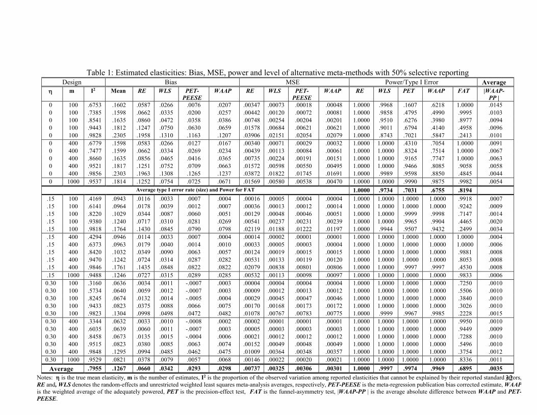
32
Table 1: Estimated elasticities: Bias, MSE, power and level of alternative meta-methods with 50% selective reporting Design Bias MSE Power/Type I Error Average
η m I2 Mean RE WLS PET-PEESE
WAAP RE WLS PET-PEESE
WAAP RE WLS PET WAAP FAT |WAAP-PP |
0 100 .6753 .1602 .0587 .0266 .0076 .0207 .00347 .00073 .00018 .00048 1.0000 .9968 .1607 .6218 1.0000 .0145 0 100 .7385 .1598 .0662 .0335 .0200 .0257 .00442 .00120 .00072 .00081 1.0000 .9858 .4795 .4990 .9995 .0103 0 100 .8541 .1635 .0860 .0472 .0358 .0386 .00748 .00254 .00204 .00201 1.0000 .9510 .6276 .3980 .8977 .0094 0 100 .9443 .1812 .1247 .0750 .0630 .0659 .01578 .00684 .00621 .00621 1.0000 .9011 .6794 .4140 .4958 .0096 0 100 .9828 .2305 .1958 .1310 .1163 .1207 .03906 .02151 .02054 .02079 1.0000 .8743 .7021 .5847 .2413 .0101 0 400 .6779 .1598 .0583 .0266 .0127 .0167 .00340 .00071 .00029 .00032 1.0000 1.0000 .4310 .7054 1.0000 .0091 0 400 .7477 .1599 .0662 .0334 .0269 .0234 .00439 .00113 .00084 .00061 1.0000 1.0000 .8324 .7514 1.0000 .0067 0 400 .8660 .1635 .0856 .0465 .0416 .0365 .00735 .00224 .00191 .00151 1.0000 1.0000 .9165 .7747 1.0000 .0063 0 400 .9521 .1817 .1251 .0752 .0709 .0663 .01572 .00598 .00550 .00495 1.0000 1.0000 .9466 .8085 .9058 .0058 0 400 .9856 .2303 .1963 .1308 .1265 .1237 .03872 .01822 .01745 .01691 1.0000 .9989 .9598 .8850 .4845 .0044 0 1000 .9537 .1814 .1252 .0754 .0725 .0671 .01569 .00580 .00538 .00470 1.0000 1.0000 .9990 .9875 .9982 .0054
Average type I error rate (size) and Power for FAT 1.0000 .9734 .7031 .6755 .8194 .15 100 .4169 .0943 .0116 .0033 .0007 .0004 .00016 .00005 .00004 .00004 1.0000 1.0000 1.0000 1.0000 .9918 .0007 .15 100 .6141 .0964 .0178 .0039 .0012 .0007 .00036 .00013 .00012 .00014 1.0000 1.0000 1.0000 1.0000 .9242 .0009 .15 100 .8220 .1029 .0344 .0087 .0060 .0051 .00129 .00048 .00046 .00051 1.0000 1.0000 .9999 .9998 .7147 .0014 .15 100 .9380 .1240 .0717 .0310 .0281 .0269 .00541 .00237 .00231 .00239 1.0000 1.0000 .9965 .9904 .4465 .0020 .15 100 .9818 .1764 .1430 .0845 .0790 .0798 .02119 .01188 .01222 .01197 1.0000 .9944 .9507 .9432 .2499 .0034 .15 400 .4294 .0946 .0114 .0033 .0007 .0004 .00014 .00002 .00001 .00001 1.0000 1.0000 1.0000 1.0000 1.0000 .0004 .15 400 .6373 .0963 .0179 .0040 .0014 .0010 .00033 .00005 .00003 .00004 1.0000 1.0000 1.0000 1.0000 1.0000 .0006 .15 400 .8420 .1032 .0349 .0090 .0063 .0057 .00124 .00019 .00015 .00015 1.0000 1.0000 1.0000 1.0000 .9881 .0008 .15 400 .9470 .1242 .0724 .0314 .0287 .0282 .00531 .00133 .00119 .00120 1.0000 1.0000 1.0000 1.0000 .8053 .0008 .15 400 .9846 .1761 .1435 .0848 .0822 .0822 .02079 .00838 .00801 .00806 1.0000 1.0000 .9997 .9997 .4530 .0008 .15 1000 .9488 .1246 .0727 .0315 .0289 .0285 .00532 .00113 .00098 .00097 1.0000 1.0000 1.0000 1.0000 .9833 .0006 0.30 100 .3160 .0636 .0034 .0011 -.0007 .0003 .00004 .00004 .00004 .00004 1.0000 1.0000 1.0000 1.0000 .7250 .0010 0.30 100 .5734 .0640 .0059 .0012 -.0007 .0003 .00009 .00012 .00013 .00012 1.0000 1.0000 1.0000 1.0000 .5506 .0010 0.30 100 .8245 .0674 .0132 .0014 -.0005 .0004 .00029 .00045 .00047 .00046 1.0000 1.0000 1.0000 1.0000 .3840 .0010 0.30 100 .9433 .0823 .0375 .0088 .0066 .0075 .00170 .00168 .00173 .00172 1.0000 1.0000 1.0000 1.0000 .3026 .0010 0.30 100 .9823 .1304 .0998 .0498 .0472 .0482 .01078 .00767 .00783 .00775 1.0000 .9999 .9967 .9985 .2228 .0015 0.30 400 .3344 .0632 .0033 .0010 -.0008 .0002 .00002 .00001 .00001 .00001 1.0000 1.0000 1.0000 1.0000 .9950 .0010 0.30 400 .6035 .0639 .0060 .0011 -.0007 .0003 .00005 .00003 .00003 .00003 1.0000 1.0000 1.0000 1.0000 .9449 .0009 0.30 400 .8458 .0673 .0135 .0015 -.0004 .0006 .00021 .00012 .00012 .00012 1.0000 1.0000 1.0000 1.0000 .7288 .0010 0.30 400 .9515 .0823 .0380 .0085 .0063 .0074 .00152 .00049 .00048 .00049 1.0000 1.0000 1.0000 1.0000 .5496 .0010 0.30 400 .9848 .1295 .0994 .0485 .0462 .0475 .01009 .00364 .00348 .00357 1.0000 1.0000 1.0000 1.0000 .3754 .0012 0.30 1000 .9529 .0821 .0378 .0079 .0057 .0068 .00146 .00022 .00020 .00021 1.0000 1.0000 1.0000 1.0000 .8336 .0011
Average .7955 .1267 .0660 .0342 .0293 .0298 .00737 .00325 .00306 .00301 1.0000 .9997 .9974 .9969 .6895 .0035 Notes: η is the true mean elasticity, m is the number of estimates, I2 is the proportion of the observed variation among reported elasticities that cannot be explained by their reported standard errors, RE and, WLS denotes the random-effects and unrestricted weighted least squares meta-analysis averages, respectively, PET-PEESE is the meta-regression publication bias corrected estimate, WAAP is the weighted average of the adequately powered, PET is the precision-effect test, FAT is the funnel-asymmetry test, |WAAP-PP | is the average absolute difference between WAAP and PET-PEESE.
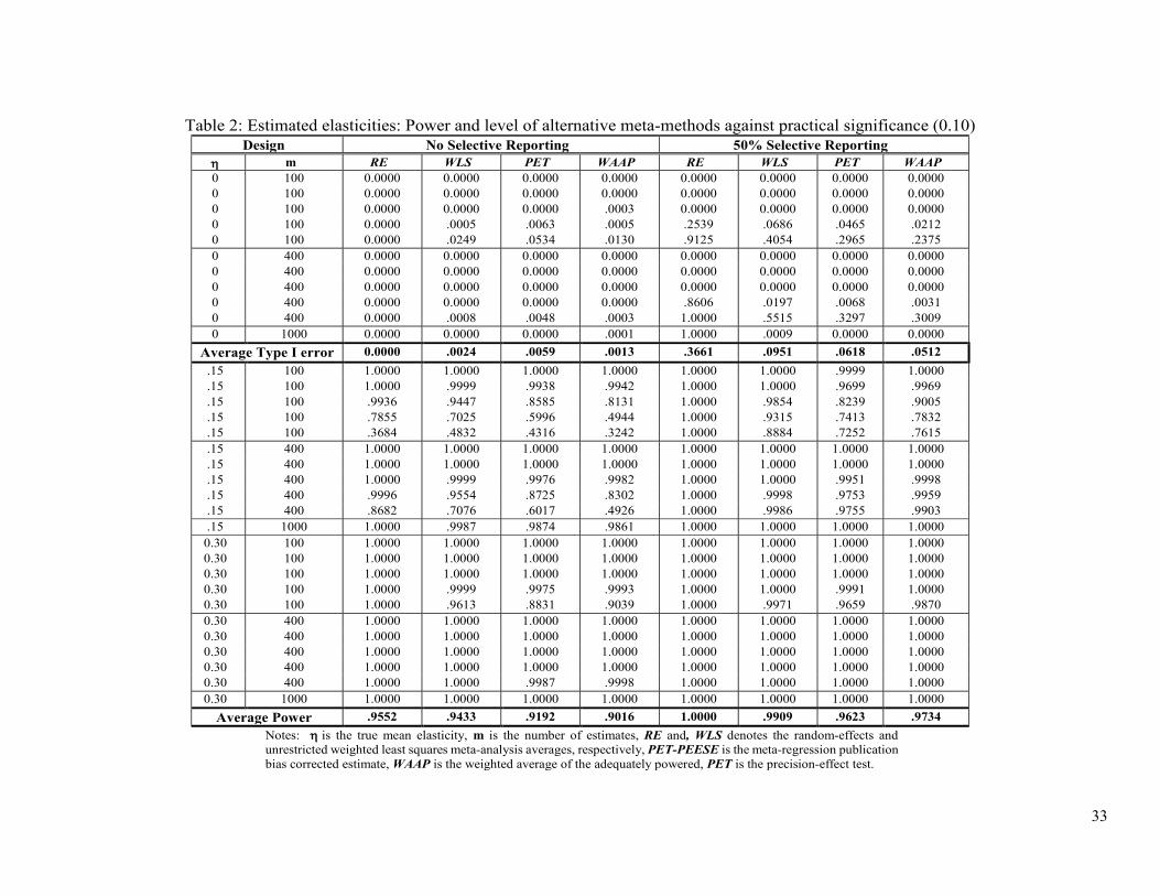
33
Table 2: Estimated elasticities: Power and level of alternative meta-methods against practical significance (0.10) Design No Selective Reporting 50% Selective Reporting
η m RE WLS PET WAAP RE WLS PET WAAP 0 100 0.0000 0.0000 0.0000 0.0000 0.0000 0.0000 0.0000 0.0000 0 100 0.0000 0.0000 0.0000 0.0000 0.0000 0.0000 0.0000 0.0000 0 100 0.0000 0.0000 0.0000 .0003 0.0000 0.0000 0.0000 0.0000 0 100 0.0000 .0005 .0063 .0005 .2539 .0686 .0465 .0212 0 100 0.0000 .0249 .0534 .0130 .9125 .4054 .2965 .2375 0 400 0.0000 0.0000 0.0000 0.0000 0.0000 0.0000 0.0000 0.0000 0 400 0.0000 0.0000 0.0000 0.0000 0.0000 0.0000 0.0000 0.0000 0 400 0.0000 0.0000 0.0000 0.0000 0.0000 0.0000 0.0000 0.0000 0 400 0.0000 0.0000 0.0000 0.0000 .8606 .0197 .0068 .0031 0 400 0.0000 .0008 .0048 .0003 1.0000 .5515 .3297 .3009 0 1000 0.0000 0.0000 0.0000 .0001 1.0000 .0009 0.0000 0.0000
Average Type I error 0.0000 .0024 .0059 .0013 .3661 .0951 .0618 .0512 .15 100 1.0000 1.0000 1.0000 1.0000 1.0000 1.0000 .9999 1.0000 .15 100 1.0000 .9999 .9938 .9942 1.0000 1.0000 .9699 .9969 .15 100 .9936 .9447 .8585 .8131 1.0000 .9854 .8239 .9005 .15 100 .7855 .7025 .5996 .4944 1.0000 .9315 .7413 .7832 .15 100 .3684 .4832 .4316 .3242 1.0000 .8884 .7252 .7615 .15 400 1.0000 1.0000 1.0000 1.0000 1.0000 1.0000 1.0000 1.0000 .15 400 1.0000 1.0000 1.0000 1.0000 1.0000 1.0000 1.0000 1.0000 .15 400 1.0000 .9999 .9976 .9982 1.0000 1.0000 .9951 .9998 .15 400 .9996 .9554 .8725 .8302 1.0000 .9998 .9753 .9959 .15 400 .8682 .7076 .6017 .4926 1.0000 .9986 .9755 .9903 .15 1000 1.0000 .9987 .9874 .9861 1.0000 1.0000 1.0000 1.0000 0.30 100 1.0000 1.0000 1.0000 1.0000 1.0000 1.0000 1.0000 1.0000 0.30 100 1.0000 1.0000 1.0000 1.0000 1.0000 1.0000 1.0000 1.0000 0.30 100 1.0000 1.0000 1.0000 1.0000 1.0000 1.0000 1.0000 1.0000 0.30 100 1.0000 .9999 .9975 .9993 1.0000 1.0000 .9991 1.0000 0.30 100 1.0000 .9613 .8831 .9039 1.0000 .9971 .9659 .9870 0.30 400 1.0000 1.0000 1.0000 1.0000 1.0000 1.0000 1.0000 1.0000 0.30 400 1.0000 1.0000 1.0000 1.0000 1.0000 1.0000 1.0000 1.0000 0.30 400 1.0000 1.0000 1.0000 1.0000 1.0000 1.0000 1.0000 1.0000 0.30 400 1.0000 1.0000 1.0000 1.0000 1.0000 1.0000 1.0000 1.0000 0.30 400 1.0000 1.0000 .9987 .9998 1.0000 1.0000 1.0000 1.0000 0.30 1000 1.0000 1.0000 1.0000 1.0000 1.0000 1.0000 1.0000 1.0000
Average Power .9552 .9433 .9192 .9016 1.0000 .9909 .9623 .9734 Notes: η is the true mean elasticity, m is the number of estimates, RE and, WLS denotes the random-effects and unrestricted weighted least squares meta-analysis averages, respectively, PET-PEESE is the meta-regression publication bias corrected estimate, WAAP is the weighted average of the adequately powered, PET is the precision-effect test.
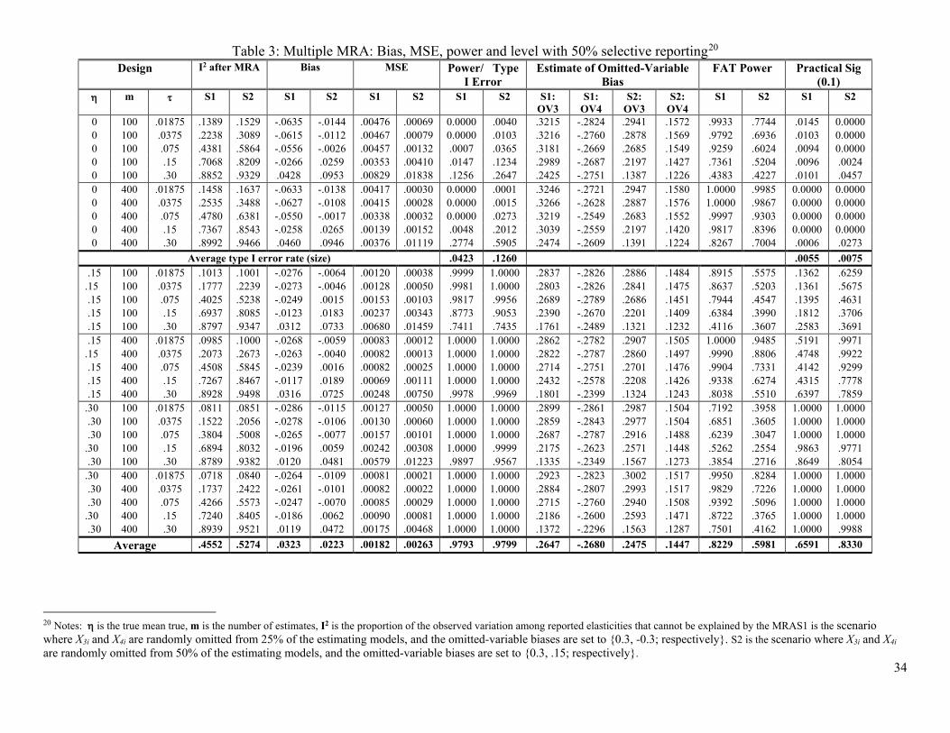
34
Table 3: Multiple MRA: Bias, MSE, power and level with 50% selective reporting20 Design I2 after MRA Bias MSE Power/ Type
I Error Estimate of Omitted-Variable
Bias FAT Power Practical Sig
(0.1) η m τ S1 S2 S1 S2 S1 S2 S1 S2 S1:
OV3 S1:
OV4 S2:
OV3 S2:
OV4 S1 S2 S1 S2
0 100 .01875 .1389 .1529 -.0635 -.0144 .00476 .00069 0.0000 .0040 .3215 -.2824 .2941 .1572 .9933 .7744 .0145 0.0000 0 100 .0375 .2238 .3089 -.0615 -.0112 .00467 .00079 0.0000 .0103 .3216 -.2760 .2878 .1569 .9792 .6936 .0103 0.0000 0 100 .075 .4381 .5864 -.0556 -.0026 .00457 .00132 .0007 .0365 .3181 -.2669 .2685 .1549 .9259 .6024 .0094 0.0000 0 100 .15 .7068 .8209 -.0266 .0259 .00353 .00410 .0147 .1234 .2989 -.2687 .2197 .1427 .7361 .5204 .0096 .0024 0 100 .30 .8852 .9329 .0428 .0953 .00829 .01838 .1256 .2647 .2425 -.2751 .1387 .1226 .4383 .4227 .0101 .0457 0 400 .01875 .1458 .1637 -.0633 -.0138 .00417 .00030 0.0000 .0001 .3246 -.2721 .2947 .1580 1.0000 .9985 0.0000 0.0000 0 400 .0375 .2535 .3488 -.0627 -.0108 .00415 .00028 0.0000 .0015 .3266 -.2628 .2887 .1576 1.0000 .9867 0.0000 0.0000 0 400 .075 .4780 .6381 -.0550 -.0017 .00338 .00032 0.0000 .0273 .3219 -.2549 .2683 .1552 .9997 .9303 0.0000 0.0000 0 400 .15 .7367 .8543 -.0258 .0265 .00139 .00152 .0048 .2012 .3039 -.2559 .2197 .1420 .9817 .8396 0.0000 0.0000 0 400 .30 .8992 .9466 .0460 .0946 .00376 .01119 .2774 .5905 .2474 -.2609 .1391 .1224 .8267 .7004 .0006 .0273
Average type I error rate (size) .0423 .1260 .0055 .0075 .15 100 .01875 .1013 .1001 -.0276 -.0064 .00120 .00038 .9999 1.0000 .2837 -.2826 .2886 .1484 .8915 .5575 .1362 .6259
.15 100 .0375 .1777 .2239 -.0273 -.0046 .00128 .00050 .9981 1.0000 .2803 -.2826 .2841 .1475 .8637 .5203 .1361 .5675 .15 100 .075 .4025 .5238 -.0249 .0015 .00153 .00103 .9817 .9956 .2689 -.2789 .2686 .1451 .7944 .4547 .1395 .4631 .15 100 .15 .6937 .8085 -.0123 .0183 .00237 .00343 .8773 .9053 .2390 -.2670 .2201 .1409 .6384 .3990 .1812 .3706 .15 100 .30 .8797 .9347 .0312 .0733 .00680 .01459 .7411 .7435 .1761 -.2489 .1321 .1232 .4116 .3607 .2583 .3691 .15 400 .01875 .0985 .1000 -.0268 -.0059 .00083 .00012 1.0000 1.0000 .2862 -.2782 .2907 .1505 1.0000 .9485 .5191 .9971
.15 400 .0375 .2073 .2673 -.0263 -.0040 .00082 .00013 1.0000 1.0000 .2822 -.2787 .2860 .1497 .9990 .8806 .4748 .9922 .15 400 .075 .4508 .5845 -.0239 .0016 .00082 .00025 1.0000 1.0000 .2714 -.2751 .2701 .1476 .9904 .7331 .4142 .9299 .15 400 .15 .7267 .8467 -.0117 .0189 .00069 .00111 1.0000 1.0000 .2432 -.2578 .2208 .1426 .9338 .6274 .4315 .7778 .15 400 .30 .8928 .9498 .0316 .0725 .00248 .00750 .9978 .9969 .1801 -.2399 .1324 .1243 .8038 .5510 .6397 .7859
.30 100 .01875 .0811 .0851 -.0286 -.0115 .00127 .00050 1.0000 1.0000 .2899 -.2861 .2987 .1504 .7192 .3958 1.0000 1.0000 .30 100 .0375 .1522 .2056 -.0278 -.0106 .00130 .00060 1.0000 1.0000 .2859 -.2843 .2977 .1504 .6851 .3605 1.0000 1.0000 .30 100 .075 .3804 .5008 -.0265 -.0077 .00157 .00101 1.0000 1.0000 .2687 -.2787 .2916 .1488 .6239 .3047 1.0000 1.0000
.30 100 .15 .6894 .8032 -.0196 .0059 .00242 .00308 1.0000 .9999 .2175 -.2623 .2571 .1448 .5262 .2554 .9863 .9771 .30 100 .30 .8789 .9382 .0120 .0481 .00579 .01223 .9897 .9567 .1335 -.2349 .1567 .1273 .3854 .2716 .8649 .8054
.30 400 .01875 .0718 .0840 -.0264 -.0109 .00081 .00021 1.0000 1.0000 .2923 -.2823 .3002 .1517 .9950 .8284 1.0000 1.0000 .30 400 .0375 .1737 .2422 -.0261 -.0101 .00082 .00022 1.0000 1.0000 .2884 -.2807 .2993 .1517 .9829 .7226 1.0000 1.0000 .30 400 .075 .4266 .5573 -.0247 -.0070 .00085 .00029 1.0000 1.0000 .2715 -.2760 .2940 .1508 .9392 .5096 1.0000 1.0000
.30 400 .15 .7240 .8405 -.0186 .0062 .00090 .00081 1.0000 1.0000 .2186 -.2600 .2593 .1471 .8722 .3765 1.0000 1.0000 .30 400 .30 .8939 .9521 .0119 .0472 .00175 .00468 1.0000 1.0000 .1372 -.2296 .1563 .1287 .7501 .4162 1.0000 .9988
Average .4552 .5274 .0323 .0223 .00182 .00263 .9793 .9799 .2647 -.2680 .2475 .1447 .8229 .5981 .6591 .8330
20 Notes: η is the true mean true, m is the number of estimates, I2 is the proportion of the observed variation among reported elasticities that cannot be explained by the MRAS1 is the scenario where X3i and X4i are randomly omitted from 25% of the estimating models, and the omitted-variable biases are set to {0.3, -0.3; respectively}. S2 is the scenario where X3i and X4i are randomly omitted from 50% of the estimating models, and the omitted-variable biases are set to {0.3, .15; respectively}.

35
Figure 1: Biases for alternative methods when η=0, m=400,
and 50% selective reporting
Figure 2: Type I error rates for alternative methods when
η=0, m=400, and 50% selective reporting
0
.03
.05
.08
.1
.13
.15
.17
.2
.23
.25
Bias
0 .05 .1 .15 .2 .25 .3 .35Heterogeneity
WAAPPET-PEESEWLSREBias
0
.2
.4
.6
.8
1
Type
I Er
ror R
ate
0 .05 .1 .15 .2 .25 .3 .35
Heterogeneity
WAAPPET-PEESEWLSRE
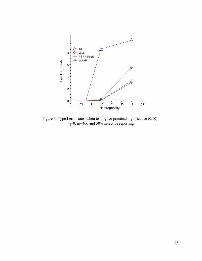
36
Figure 3: Type I error rates when testing for practical significance (0.10), η=0, m=400 and 50% selective reporting
0
.2
.4
.6
.8
1
Type
I Er
ror R
ate
0 .05 .1 .15 .2 .25 .3 .35Heterogeneity
WAAPPET-PEESEWLSRE
37
Appendix List of 35 reference meta-analyses
(* denotes source reporting more than one meta-analysis)
Akgunduz, Y.E. and Plantenga, J. (2011). ‘Child care prices and female labour force participation: a meta-analysis’, Tjalling C. Koopmans Research Institute, Discussion Paper Series 11-08.
Babecky, J., Ramos, R. and Sanromá, E. (2008). ‘Meta-analysis on microeconomic wage flexibility (Wage Curve)’, Sozialer Fortschritt, vol. 57(10), pp. 273-79.
Belman, D. and Wolfson, P.J. (2014). What does the minimum wage do? Kalamazoo, MI: W.E. Upjohn Institute for Employment Research.
Bom, P.R.D. and Ligthart, J.E. (2014). ‘What have we learned from three decades of research on the productivity of public capital?’, Journal of Economic Surveys, vol. 28(5), pp. 889–916.
Castellacci, F. and Lie, C.M. (2015). ‘Do the effects of R&D tax credits vary across industries? a meta-regression analysis’, Research Policy, vol. 44(4), pp. 819-32.
Chetty, R., Guren, A., Manoli, D.S. and Weber, A. (2011). Does indivisible labor explain the difference between micro and macro elasticities? A meta-analysis of extensive margin elasticities. NBER Working Paper No. 16729.
Chletsos, M. and Giotis, G.P. (2015). The employment effect of minimum wage using 77 international studies since 1992: a meta-analysis, MPRA Paper 61321, University Library of Munich, Germany.
Cirera, X., Willenbockel, D. and Lakshman, R. (2011). What is the evidence of the impact of tariff reductions on employment and fiscal revenue in developing countries? A systematic review. Technical report. London: EPPI-Centre, Social Science Research Unit, Institute of Education, University of London.
Clar, M., Dreger, C. and Ramos, R. (2007). ‘Wage flexibility and labour market institutions: A meta-analysis’, Kyklos, vol. 60(2), pp. 145–63.
Dalhuisen, J.M., Florax, R.J.G.M., de Groot, H.L.F. and Nijkamp, P. (2003). ‘Price and income elasticities of residential water demand: a meta-analysis’, Land Economics, vol. 79(2), pp. 292–308.
Doucouliagos, C.(H.) and Stanley, T.D. (2009). ‘Publication selection bias in minimum wage research? a meta regression analysis’, British Journal of Industrial Relations, vol. 47(2), pp.406–28.
Doucouliagos, C.(H.), Stanley, T.D. and Viscusi, W.K. (2014). ‘Publication selection and the income elasticity of the value of a statistical life’, Journal of Health Economics, vol. 33(January), pp. 67–75.
Escobar, M.A.C., Veerman, J.L., Tollman, S.M., Bertram, M.Y. and Hofman, K.J. (2013). ‘Evidence that a tax on sugar sweetened beverages reduces the obesity rate: a meta-analysis’, BMC Public Health, vol. 13, pp. 1072.
Feld, L.P., Heckemeyer, J.H. and Overesch, M. (2013). ‘Capital structure choice and company taxation: a meta-study’, Journal of Banking and Finance, vol. 37(8), pp. 2850–66.
Gallet, C.A. and Doucouliagos, C.(H.) (2014). ‘The income elasticity of air travel: a meta-analysis’, Annals of Tourism Research, vol. 49(November), pp. 141–55.
38
Green, R., Cornelsen, L., Dangour, A.D., Turner, R., Shankar, B., Mazzocchi, M. and Smith, R.D. (2013). ‘The effect of rising food prices on food consumption: systematic review with meta-regression’, British Medical Journal, 346: f3703.
Havránek, T. (2015). ‘Measuring intertemporal substitution: the importance of method choices and selective reporting’, Journal of the European Economic Association, vol. 13(6), pp. 1180-204.
Havranek, T., Irsova, Z. and Janda, K. (2012). ‘Demand for gasoline is more price-inelastic than commonly thought’, Energy Economics, vol. 34(1), pp. 201–7.
Havranek, T. and Kokes, O. (2015). ‘Income elasticity of gasoline demand: a meta-analysis’, Energy Economics, vol. 47(January), pp. 77–88.
Klomp, J. and de Haan, J. (2010). ‘Inflation and central bank independence: a meta-regression analysis’, Journal of Economic Surveys, vol. 24(4), pp. 593-621.
Koetse, M.J., de Groot, H.L.F. and Florax, R.J.G.M. (2008). ‘Capital-energy substitution and shifts in factor demand: a meta-analysis’, Energy Economics, vol. 30(5), pp. 2236-51.
Krassoi-Peach, E. and Stanley, T.D. (2009). ‘Efficiency wages, productivity and simultaneity: A meta-regression analysis’, Journal of Labor Research, vol. 30(3), pp. 262–68.
Lichter, A., Peichl, A. and Siegloch, S. (2015). ‘The own-wage elasticity of labor demand: A meta-regression analysis’, European Economic Review, vol. 80, pp. 94–119. 21.
*Longhi, S., Nijkamp, P. and Poot, J. (2010). ‘Joint impacts of immigration on wages and employment: review and meta-analysis’, Journal of Geographical Systems, vol. 12(4), pp. 355-87. 28.
Nelson, J.P. (2006). ‘Cigarette advertising regulation: a meta-analysis’, International Review of Law and Economics, vol. 26(2), pp. 195-226.
Nelson, J.P. (2011). ‘Alcohol marketing, adolescent drinking and publication bias in longitudinal studies: a critical survey using meta-analysis’, Journal of Economic Surveys, vol. 25(2), pp. 191–232. 30.
Nelson, J.P. (2014). ‘Estimating the price elasticity of beer: meta-analysis of data with heterogeneity, dependence, and publication bias’, Journal of Health Economics, vol. 33, pp. 180-7.
Nijkamp, P. and Poot, J. (2005). ‘The last word on the wage curve’, Journal of Economic Surveys, vol. 19(3), pp. 421–50. 42.
Santeramo, F.G. and Shabnam, N. (2015). ‘The income-elasticity of calories, macro- and micro-nutrients: what is the literature telling us?’, Food Research International, 76(4), pp. 932-7.
*Stanley, T.D. and Doucouliagos, C(H.). (2012). Meta-Regression Analysis in Economics and Business, Oxford: Routledge.
Ugur, M., Solomon, E., Guidi, F. and Trushin, E. (2014). ‘R&D and productivity in OECD firms and industries: a hierarchical meta-regression analysis’, Evaluation of Research and Development (R&D) Expenditures, Firm Survival, Firm Growth and Employment: UK Evidence in the OECD Context. Reference no ES/K004824/1.
39
Figure A1. Funnel Graph of Simulated Elasticities and their Precisions (𝜂𝜂 = 0, 50% Publication Selection, I2=94%, 100,000 replications)
100
105
110
115
120
125
130
Pre
cisi
on
-.5 -.3 -.1 .1 .3 .5Elasticity

40
Table A1: Simulated elasticities: Bias, MSE, power and level of alternative meta-methods when there is no selective reporting Design Bias MSE Power/Type I Error Average
η m I2 Mean RE WLS PET-PEESE
WAAP RE WLS PET-PEESE
WAAP RE WLS PET WAAP FAT |WAAP-PP |
0 100 .2420 -.0002 -.0001 -.0001 -.0005 -.0001 .00003 .00004 .00006 .00004 .0349 .1210 .1264 .1209 .0654 .0021 0 100 .5448 .0001 .0000 .0000 -.0010 .0001 .00005 .00012 .00017 .00016 .0293 .1984 .2047 .1880 .0817 .0029 0 100 .8211 -.0002 .0002 .0001 -.0020 .0001 .00012 .00046 .00066 .00089 .0313 .2414 .2497 .1439 .0969 .0066 0 100 .9469 .0001 .0000 .0002 -.0039 .0002 .00035 .00173 .00245 .00312 .0328 .2529 .2598 .0515 .0954 .0124 0 100 .9851 -.0001 -.0002 -.0003 -.0082 -.0007 .00110 .00635 .00904 .00909 .0369 .2490 .2531 .0838 .0986 .0189 0 400 .2640 -.0001 .0000 .0000 -.0002 .0000 .00001 .00001 .00001 .00001 .0267 .1206 .1309 .1206 .0598 .0010 0 400 .5799 .0000 .0000 .0000 -.0005 .0000 .00001 .00003 .00004 .00003 .0255 .1955 .2033 .1955 .0774 .0013 0 400 .8437 -.0001 .0000 .0000 -.0010 .0000 .00003 .00011 .00016 .00018 .0264 .2324 .2415 .2195 .0825 .0027 0 400 .9546 .0001 .0001 .0000 -.0021 -.0001 .00009 .00044 .00062 .00112 .0308 .2440 .2495 .1326 .0925 .0086 0 400 .9873 .0002 .0003 .0001 -.0038 .0000 .00028 .00159 .00225 .00354 .0322 .2439 .2488 .0428 .0851 .0160 0 1000 .9561 .0000 .0001 .0000 -.0013 .0000 .00003 .00017 .00025 .00042 .0268 .2422 .2489 .2108 .0881 .0046
Average type I error rate (size) .0303 .2128 .2197 .1373 .0839 .15 100 .2414 .0000 .0001 .0001 .0001 .0000 .00003 .00004 .00004 .00004 1.0000 1.0000 1.0000 1.0000 .0617 .0007 .15 100 .5452 .0000 .0000 .0001 .0001 .0000 .00005 .00012 .00013 .00014 1.0000 1.0000 1.0000 1.0000 .0785 .0008 .15 100 .8218 -.0001 -.0001 -.0001 -.0001 -.0006 .00012 .00046 .00048 .00055 1.0000 1.0000 1.0000 .9996 .0967 .0014 .15 100 .9466 .0001 .0002 .0001 -.0006 -.0022 .00035 .00173 .00197 .00220 1.0000 .9974 .9791 .9160 .1007 .0030 .15 100 .9851 .0002 .0005 .0004 -.0070 -.0054 .00108 .00647 .00882 .00838 .9943 .8788 .7694 .6426 .0970 .0075 .15 400 .2642 .0000 .0000 .0000 .0000 .0000 .00001 .00001 .00001 .00001 1.0000 1.0000 1.0000 1.0000 .0615 .0003 .15 400 .5798 -.0001 .0001 .0000 .0000 .0000 .00001 .00003 .00003 .00003 1.0000 1.0000 1.0000 1.0000 .0727 .0004 .15 400 .8437 .0000 .0001 .0000 .0000 -.0001 .00003 .00011 .00012 .00013 1.0000 1.0000 1.0000 1.0000 .0843 .0006 .15 400 .9546 .0001 .0001 .0001 .0001 -.0003 .00009 .00044 .00046 .00052 1.0000 1.0000 1.0000 .9998 .0900 .0012 .15 400 .9874 .0002 .0002 .0000 -.0005 -.0020 .00028 .00158 .00176 .00199 1.0000 .9980 .9858 .9346 .0853 .0028 .15 1000 .9561 .0001 .0001 .0000 .0000 -.0001 .00003 .00017 .00018 .00020 1.0000 1.0000 1.0000 1.0000 .0866 .0007 .30 100 .2414 -.0001 .0000 .0000 .0000 .0000 .00003 .00004 .00004 .00004 1.0000 1.0000 1.0000 1.0000 .0641 .0003 .30 100 .5451 .0001 -.0001 -.0001 -.0001 -.0001 .00005 .00012 .00013 .00012 1.0000 1.0000 1.0000 1.0000 .0842 .0004 .30 100 .8213 .0002 .0003 .0000 .0000 -.0001 .00013 .00046 .00048 .00047 1.0000 1.0000 1.0000 1.0000 .0990 .0004 .30 100 .9468 .0000 .0001 .0004 .0005 .0002 .00034 .00175 .00183 .00181 1.0000 1.0000 1.0000 1.0000 .0993 .0006 .30 100 .9852 -.0003 -.0003 -.0005 -.0015 -.0019 .00111 .00632 .00710 .00685 1.0000 .9991 .9830 .9793 .0977 .0020 .30 400 .2640 -.0001 .0000 .0000 .0000 .0000 .00001 .00001 .00001 .00001 1.0000 1.0000 1.0000 1.0000 .0617 .0002 .30 400 .5798 -.0001 .0000 .0000 .0000 .0000 .00001 .00003 .00003 .00003 1.0000 1.0000 1.0000 1.0000 .0741 .0002 .30 400 .8438 .0000 .0001 .0000 .0000 .0000 .00003 .00011 .00012 .00012 1.0000 1.0000 1.0000 1.0000 .0844 .0002 .30 400 .9545 .0000 .0001 .0001 .0001 .0000 .00009 .00043 .00045 .00045 1.0000 1.0000 1.0000 1.0000 .0904 .0003 .30 400 .9874 .0002 .0003 .0000 .0000 -.0002 .00027 .00158 .00165 .00164 1.0000 1.0000 1.0000 1.0000 .0882 .0005 .30 1000 .9561 .0001 .0002 .0001 .0001 .0000 .00003 .00017 .00018 .00018 1.0000 1.0000 1.0000 1.0000 .0888 .0002
Average .7387 .0000 .0001 .0000 -.0010 -.0004 .00019 .00101 .00126 .00135 .9997 .9942 .9872 .9760 .0840 .0031 Notes: η is the true mean elasticity, m is the number of estimates, I2 is the proportion of the observed variation among reported elasticities that cannot be explained by their reported standard errors, RE and WLS denote the random-effects and unrestricted weighted least squares meta-analysis averages, respectively, PET-PEESE is the meta-regression publication bias corrected estimate, WAAP is the weighted average of the adequately powered, PET is the precision-effect test, FAT is the funnel-asymmetry test, |WAAP-PP | is the average absolute difference between WAAP and PET-PEESE.
41
ADDITIONAL SIMULATIONS
1. Proportional heterogeneity In our core simulation experiments, random normal omitted-variable biases are added to the process of estimating each elasticity. Thus, the heterogeneity variance will be the same for very precisely estimated elasticities (those at the top of the funnel graph) as those with much larger standard errors (those at the bottom of the funnel graph); see Figure A1 above. However, actual meta-analyses in economics typically exhibit lower heterogeneity at the top of the funnel graph (where SEs are smaller) than at the bottom. Publication success might be higher for those studies that use the largest datasets and those that employ methods known to be more efficient, both of which produce smaller SEs. Studies that produce demonstrably ‘better’ estimates would have less need to report statistically significant results. Even if these larger, more efficient, studies selectively report, their authors would require less extreme misspecifications or methods manipulations to produce statistical significance. Thus, the vigor of specification searches and thereby the degree of heterogeneity is likely to be directly related to an estimate’s SE. A selection process that is directly related to SE would also produce heterogeneity roughly proportional to SE. We find such differential heterogeneity in the 35 reference meta-analyses used to calibrate our core simulation design. Heterogeneity is likely to be approximately proportional to SE in many and perhaps most economic research areas. Figure A2 that graphs 1,000 randomly generated estimates when we assume that heterogeneity, τ, is approximately proportional to SE. Compare Figure A2 to Figure A3 that graphs 1,474 estimates of the employment effect from raising the US minimum wage to vs. Figure A1 where estimates are randomly generated assuming that heterogeneity is additive.
These simulations are identical to those summarized in Table 1 in the text except that the standard deviation of heterogeneity is made to be roughly proportional to SE. Table A2 reports these new ‘proportional heterogeneity’ simulations for m=400. We do not display the findings for other meta-analysis sample sizes to conserve space and because the reported false positives rates are higher for m=400. Biases are notably smaller for WAAP and PET-PEESE and PET (see Table A2 and Figure A4). PET has greatly reduced Type I errors (see Table A2 and Figure A5), and its power to detect genuine effects even when they are small (η =.15) is much higher. In general, the properties of PET-PEESE are greatly improved if heterogeneity is approximately proportional to reported sampling errors, because SE is directly correlated with both random sampling errors and heterogeneity, both of which produce larger biases. Nonetheless, PET’s rates of false positives remain unacceptably high for high levels of heterogeneity. Below we show when heterogeneity is proportional and meta-analysts test for practical significance (H0: η =0.10), PET’s type I errors are acceptably low (see Table A3).
2. Cluster-robust standard errors The last variation to our core simulation design concerns the use of cluster-robust standard errors. Economic meta-analysis often calculates cluster-robust SEs because studies routinely report multiple estimates, as well as using unbalanced panel models. To simulate the effect that the use cluster-robust SEs might have on the false positive rates of WLS and PET, we calculated the ratio of cluster-robust SEs to WLS SEs observed in our 35 reference meta-analysis for which
42
we had data to identify their cluster structures. Next, we modified our core simulations (recall Table 1) to randomly sample from the distribution of ratios of cluster-robust SEs to WLS SEs that we observed among actual elasticity meta-analyses. We did not attempt to embed varying cluster structures in our data generating processes, because the SEs that they produce will depend on the average number of estimates per cluster, the correlations within a cluster, and the distribution of each of these across studies within an area of research. Our current research base is not sufficient rich to identify the complex and nuanced cluster structure that is representative of economics research. Instead, we simulate the observed effects that these complexities have on calculated cluster-robust standard errors. We do not adjust RE’s or WAAP’s SEs for clustering. Cluster-robust standard errors are rarely used by random effects estimates, and there are so few adequately-power estimates in an area of economic research that the cluster structure is quite likely to breakdown (Ioannidis et al., 2017). Table A3 reports the simulation results from combinations of proportional heterogeneity with practical significance testing and cluster-robust SEs with practical significance testing. We do not display the findings from using cluster-robust SEs alone because they are similar to what we find for proportional heterogeneity alone (recall Table A.2). Cluster-robust SEs do reduce the rates of false positives for WLS and PET, but, as with proportional heterogeneity, type I error rates remain unacceptable high for high heterogeneity. When combined with testing for practical significance testing (H0: η=0.10), using cluster-robust SEs reduces type I errors to their nominal level (0.05) or below for PET, while WLS’s rates of false positives also quite low except for the highest level of heterogeneity (See Table A6). Because MAER-Net reporting guidelines require the use of either cluster-robust SEs or MRA panel models (Stanley et al., 2013), we suspect that PET and probably WLS have acceptable statistical properties for most economic applications if they test for practical, rather than statistical, significance

43
Figure A2: Funnel plot of 1,000 simulated elasticities (proportional heterogeneity)
0
20
40
60
80
100
120
140
Prec
ision
-5 -4 -3 -2 -1 0 1 2 3 4 5 6Elasticity
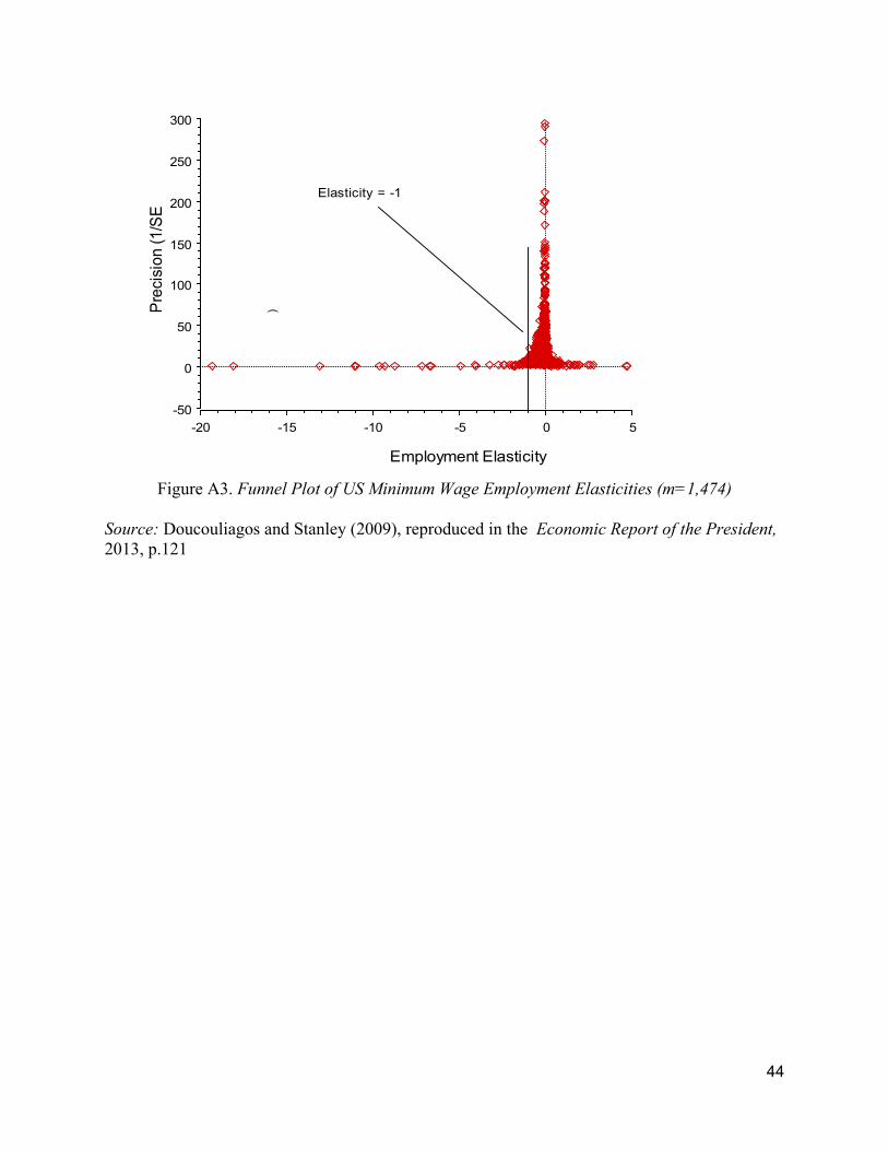
44
Figure A3. Funnel Plot of US Minimum Wage Employment Elasticities (m=1,474)
Source: Doucouliagos and Stanley (2009), reproduced in the Economic Report of the President, 2013, p.121
-50
0
50
100
150
200
250
300
Prec
isio
n (1
/SE
)
-20 -15 -10 -5 0 5
Employment Elasticity
Elasticity = -1

45
Table A2: Bias, MSE, power and level of alternative meta-methods with 50% selective reporting and proportional heterogeneity
Notes: η is the true elasticity, m is the number of estimates, I2 is the proportion of the observed variation among reported elasticities that cannot be explained by their reported standard errors, RE and WLS denote the random-effects and unrestricted weighted least squares meta-analysis averages, respectively, PET-PEESE is the meta-regression publication bias corrected estimate, WAAP is the weighted average of the adequately powered, PET is the precision-effect test, FAT is the funnel-asymmetry test, |WAAP-PP | is the average absolute difference between WAAP and PET-PEESE.
Design Bias MSE Power/Type I Error Average η m I2 Mean RE WLS PET-
PEESE WAAP RE WLS PET-
PEESE WAAP RE WLS PET WAAP FAT |WAAP-
PP | 0 400 .6758 .1562 .0586 .0239 .0009 .0131 .00344 .00057 .00001 .00021 1.0000 1.0000 .0048 .7417 1.0000 .0010 0 400 .7388 .1625 .0665 .0262 .0028 .0136 .00444 .00069 .00003 .00021 1.0000 1.0000 .0370 .7958 1.0000 .0013 0 400 .8461 .1997 .0905 .0322 .0060 .0173 .00822 .00104 .00012 .00032 1.0000 1.0000 .0931 .8866 1.0000 .0027 0 400 .9328 .2885 .1440 .0449 .0137 .0248 .02086 .00204 .00049 .00067 1.0000 1.0000 .1925 .8978 1.0000 .0085 0 400 .9744 .4723 .2487 .0699 .0360 .0420 .06235 .00500 .00241 .00194 1.0000 1.0000 .3830 .8832 1.0000 .0157
Average type I error rate (size) and Power for FAT 1.0000 1.0000 .1421 .8410 1.0000 .15 400 .3938 .0972 .0116 .0036 .0010 .0005 .00014 .00002 0.00000 0.00000 1.0000 1.0000 1.0000 1.0000 1.0000 .0003 .15 400 .5722 .1099 .0193 .0046 .0018 .0010 .00038 .00003 .00001 .00001 1.0000 1.0000 1.0000 1.0000 1.0000 .0004 .15 400 .7895 .1487 .0422 .0079 .0046 .0029 .00182 .00007 .00003 .00002 1.0000 1.0000 1.0000 1.0000 1.0000 .0006 .15 400 .9218 .2372 .0958 .0150 .0116 .0079 .00930 .00027 .00018 .00011 1.0000 1.0000 1.0000 1.0000 1.0000 .0012 .15 400 .9727 .4203 .2011 .0320 .0294 .0224 .04092 .00118 .00102 .00069 1.0000 1.0000 1.0000 1.0000 1.0000 .0028 0.3 400 .2788 .0671 .0034 .0012 -.0007 .0003 .00002 0.00000 0.00000 0.00000 1.0000 1.0000 1.0000 1.0000 1.0000 .0002 0.3 400 .5099 .0787 .0069 .0016 -.0005 .0005 .00006 .00001 .00001 .00001 1.0000 1.0000 1.0000 1.0000 .9999 .0002 0.3 400 .7713 .1137 .0203 .0030 .0004 .0016 .00045 .00002 .00001 .00002 1.0000 1.0000 1.0000 1.0000 1.0000 .0002 0.3 400 .9168 .1967 .0627 .0077 .0048 .0056 .00407 .00011 .00007 .00008 1.0000 1.0000 1.0000 1.0000 .9999 .0003 0.3 400 .9717 .3762 .1628 .0196 .0171 .0162 .02699 .00056 .00047 .00044 1.0000 1.0000 1.0000 1.0000 1.0000 .0005 Average .7511 .2083 .0823 .0196 .0086 .0113 .01223 .00077 .00032 .00031 1.0000 1.0000 1.0000 1.0000 1.0000 .0064
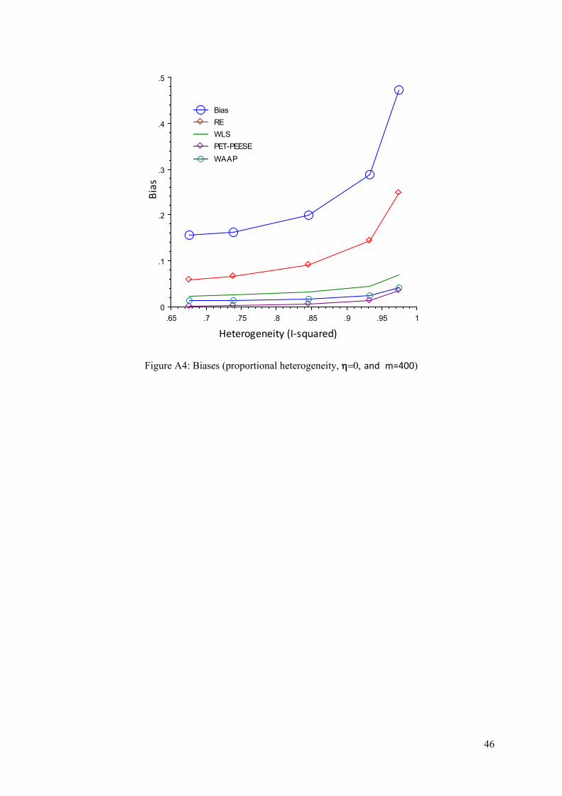
46
Figure A4: Biases (proportional heterogeneity, η=0, and m=400)
0
.1
.2
.3
.4
.5
Bias
.65 .7 .75 .8 .85 .9 .95 1
Heterogeneity (I-squared)
WAAPPET-PEESEWLSREBias
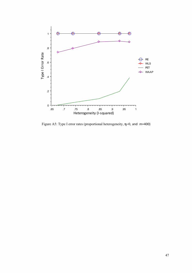
47
Figure A5: Type I error rates (proportional heterogeneity, η=0, and m=400)
0
.2
.4
.6
.8
1
Type
I Er
ror R
ate
.65 .7 .75 .8 .85 .9 .95 1Heterogeneity (I-squared)
WAAPPETWLSRE

48
Figure A6: Type I error rates when testing for practical significance (0.1)
(with cluster-robust standard errors, η=0, and m=400)
-.05
0
.05
.1
.15
.2
.25
.3
Type
I Er
ror R
ate
.65 .7 .75 .8 .85 .9 .95 1Heterogeneity (I-squared)
PETWLS
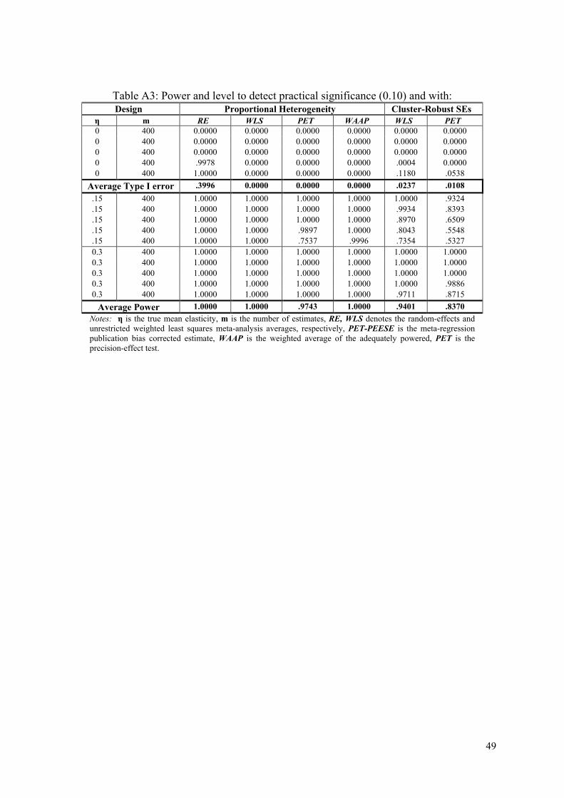
49
Table A3: Power and level to detect practical significance (0.10) and with: Design Proportional Heterogeneity Cluster-Robust SEs
η m RE WLS PET WAAP WLS PET 0 400 0.0000 0.0000 0.0000 0.0000 0.0000 0.0000 0 400 0.0000 0.0000 0.0000 0.0000 0.0000 0.0000 0 400 0.0000 0.0000 0.0000 0.0000 0.0000 0.0000 0 400 .9978 0.0000 0.0000 0.0000 .0004 0.0000 0 400 1.0000 0.0000 0.0000 0.0000 .1180 .0538
Average Type I error .3996 0.0000 0.0000 0.0000 .0237 .0108 .15 400 1.0000 1.0000 1.0000 1.0000 1.0000 .9324 .15 400 1.0000 1.0000 1.0000 1.0000 .9934 .8393 .15 400 1.0000 1.0000 1.0000 1.0000 .8970 .6509 .15 400 1.0000 1.0000 .9897 1.0000 .8043 .5548 .15 400 1.0000 1.0000 .7537 .9996 .7354 .5327 0.3 400 1.0000 1.0000 1.0000 1.0000 1.0000 1.0000 0.3 400 1.0000 1.0000 1.0000 1.0000 1.0000 1.0000 0.3 400 1.0000 1.0000 1.0000 1.0000 1.0000 1.0000 0.3 400 1.0000 1.0000 1.0000 1.0000 1.0000 .9886 0.3 400 1.0000 1.0000 1.0000 1.0000 .9711 .8715
Average Power 1.0000 1.0000 .9743 1.0000 .9401 .8370 Notes: η is the true mean elasticity, m is the number of estimates, RE, WLS denotes the random-effects and unrestricted weighted least squares meta-analysis averages, respectively, PET-PEESE is the meta-regression publication bias corrected estimate, WAAP is the weighted average of the adequately powered, PET is the precision-effect test.
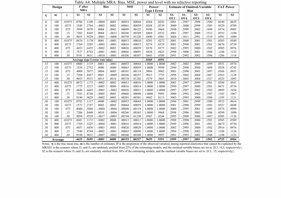
Table A4: Multiple MRA: Bias, MSE, power and level with no selective reporting Design I2 after
MRA Bias MSE Power/
Type I Error Estimate of Omitted-Variable
Bias FAT Power
η m τ S1 S2 S1 S2 S1 S2 S1 S2 S1: OV3
S1: OV4
S2: OV3
S2: OV4
S1 S2
0 100 .01875 .0786 .1109 -.0004 .0001 .00053 .00044 .0264 .0292 .3001 -.2997 .2998 .1500 .0549 .0655 0 100 .0375 .1549 .2764 -.0002 .0002 .00061 .00059 .0268 .0339 .3000 -.3000 .2998 .1503 .0529 .0709 0 100 .075 .3999 .5870 .0004 .0002 .00099 .00122 .0380 .0464 .2998 -.2999 .3002 .1499 .0574 .0905 0 100 .15 .7202 .8445 .0004 -.0013 .00246 .00369 .0469 .0532 .3001 -.2997 .3008 .1512 .0553 .1100 0 100 .30 .9055 .9529 -.0001 -.0008 .00750 .01220 .0490 .0501 .3004 -.3011 .2991 .1519 .0591 .1090 0 400 .01875 .0676 .1170 .0001 -.0001 .00013 .00010 .0293 .0272 .3001 -.3000 .3001 .1501 .0583 .0549 0 400 .0375 .1769 .3203 -.0003 -.0001 .00016 .00015 .0274 .0319 .3001 -.2998 .3001 .1501 .0676 .0739 0 400 .075 .4453 .6435 -.0002 .0003 .00026 .00029 .0370 .0377 .3002 -.2995 .3000 .1502 .0905 .0976 0 400 .15 .7537 .8743 -.0001 -.0001 .00066 .00091 .0438 .0423 .2994 -.3000 .3001 .1504 .1106 .1132 0 400 .30 .9191 .9631 -.0010 -.0001 .00206 .00307 .0443 .0389 .2991 -.2992 .3002 .1506 .1206 .1118
Average type I error rate (size) .0369 .0391 .15 100 .01875 .0800 .1135 .0001 -.0001 .00053 .00044 1.0000 1.0000 .3002 -.3002 .3000 .1499 .0551 .0574 .15 100 .0375 .1556 .2752 .0000 .0000 .00063 .00059 1.0000 .9999 .2996 -.2998 .3000 .1498 .0558 .0745 .15 100 .075 .4009 .5877 .0004 .0005 .00101 .00119 .9984 .9902 .3001 -.2998 .3001 .1497 .0566 .0933 .15 100 .15 .7204 .8457 .0001 -.0009 .00246 .00357 .9013 .7735 .2998 -.3002 .3004 .1487 .0563 .1128 .15 100 .30 .9053 .9531 .0015 .0016 .00739 .01242 .5279 .3865 .3010 -.3003 .3004 .1527 .0525 .1093 .15 400 .01875 .0672 .1173 -.0002 .0002 .00013 .00010 1.0000 1.0000 .3001 -.2997 .2999 .1501 .0594 .0541 .15 400 .0375 .1775 .3215 -.0003 .0000 .00016 .00014 1.0000 1.0000 .2999 -.2997 .3000 .1501 .0671 .0754 .15 400 .075 .4446 .6445 -.0003 -.0002 .00026 .00031 1.0000 1.0000 .2997 -.2997 .3002 .1503 .0889 .1034 .15 400 .15 .7543 .8748 -.0005 .0003 .00066 .00090 1.0000 .9993 .3000 -.2992 .3002 .1507 .1103 .1067 .15 400 .30 .9190 .9629 -.0002 .0003 .00201 .00301 .9402 .8111 .3003 -.2993 .3000 .1508 .1195 .1131 .30 100 .01875 .0792 .1117 .0000 -.0002 .00053 .00043 1.0000 1.0000 .2996 -.3001 .2999 .1500 .0515 .0616 .30 100 .0375 .1572 .2747 .0002 .0002 .00064 .00059 1.0000 1.0000 .3001 -.2998 .2999 .1503 .0527 .0698 .30 100 .075 .4000 .5888 -.0004 -.0004 .00098 .00119 1.0000 1.0000 .3000 -.2995 .3001 .1495 .0574 .0990 .30 100 .15 .7206 .8448 .0010 -.0004 .00246 .00365 1.0000 .9968 .2998 -.2996 .3003 .1506 .0599 .1090 .30 100 .30 .9058 .9529 -.0017 -.0003 .00744 .01230 .9507 .8244 .2995 -.2990 .3006 .1497 .0585 .1126 .30 400 .01875 .0681 .1172 -.0002 .0000 .00013 .00011 1.0000 1.0000 .2998 -.2998 .3000 .1501 .0585 .0589 .30 400 .0375 .1769 .3225 -.0004 -.0001 .00016 .00014 1.0000 1.0000 .2999 -.2996 .3001 .1501 .0672 .0750 .30 400 .075 .4451 .6436 -.0003 .0003 .00026 .00029 1.0000 1.0000 .3002 -.2995 .3000 .1502 .0916 .0976 .30 400 .15 .7540 .8744 -.0002 -.0001 .00065 .00090 1.0000 1.0000 .2994 -.2998 .3002 .1504 .1108 .1126 .30 400 .30 .9190 .9631 -.0007 -.0002 .00206 .00308 1.0000 .9997 .2991 -.2993 .3002 .1508 .1198 .1123
Average .4625 .5695 -.0001 .0000 .00153 .00227 .9659 .9391 .2999 -.2997 .3001 .1502 .0725 .0904 Notes: η is the true mean true, m is the number of estimates, I2 is the proportion of the observed variation among reported elasticities that cannot be explained by the MRAS1 is the scenario where X3i and X4i are randomly omitted from 25% of the estimating models, and the omitted-variable biases are set to {0.3, -0.3; respectively}. S2 is the scenario where X3i and X4i are randomly omitted from 50% of the estimating models, and the omitted-variable biases are set to {0.3, .15; respectively}.