Chapter 3

Significance Tests

Significance Tests

• In order to decide whether the difference between

the measured and standard amounts can be

accounted for by random error, a statistical test

known as a significance test can be employed

• Significance tests are widely used in the evaluation

of experimental results.

Comparison of an experimental mean with a known value

• In making a significance test we are testing the truth of a hypothesis which is known as a null hypothesis, often denoted by Ho.

• For the example, analytical method should be free from systematic error. This is a null hypothesis

• The term null is used to imply that there is no difference between the observed and known values other than that which can be attributed to random variation.

• Assuming that this null hypothesis is true, statistical theory can be used to calculate the probability that the observed difference between the sample mean, and the true value,

u, arises solely as a result of random errors.

• The lower the probability that the observed difference occurs by chance, the less likely it is that the null hypothesis is true.

• Usually the null hypothesis is rejected if the probability of such a difference occurring by chance is less than 1 in 20 (i.e. 0.05 or 5%). In such a case the difference is said to be significant at the 0.05 (or 5%) level.

xx

x

Comparison of an experimental mean with a known value

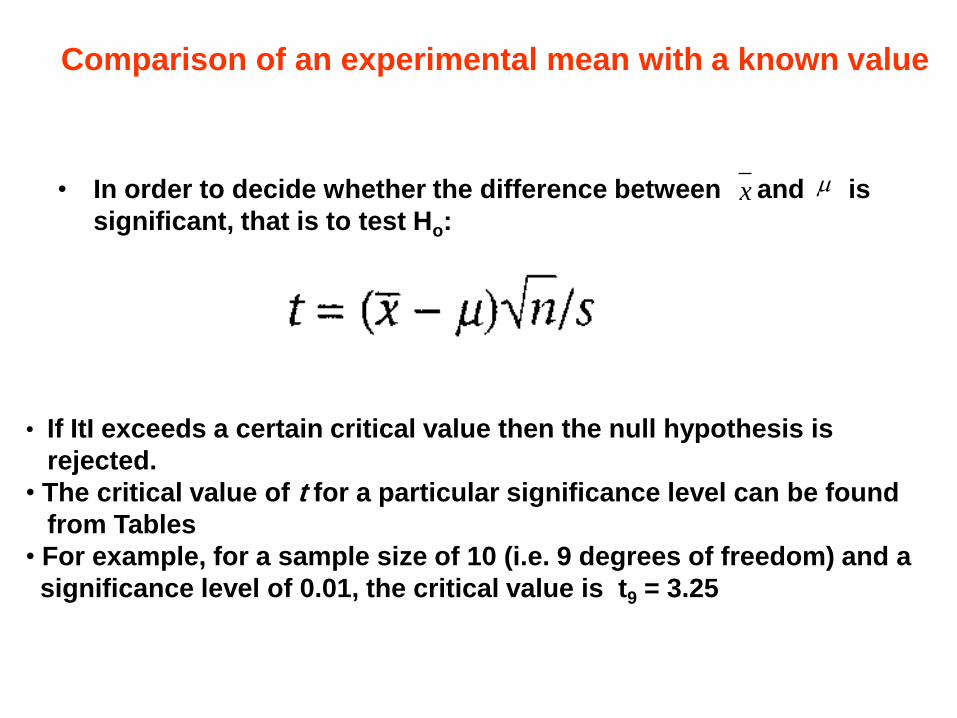
• In order to decide whether the difference between and is

significant, that is to test Ho: x

• If ItI exceeds a certain critical value then the null hypothesis is

rejected.

• The critical value of t for a particular significance level can be found

from Tables

• For example, for a sample size of 10 (i.e. 9 degrees of freedom) and a

significance level of 0.01, the critical value is t9 = 3.25

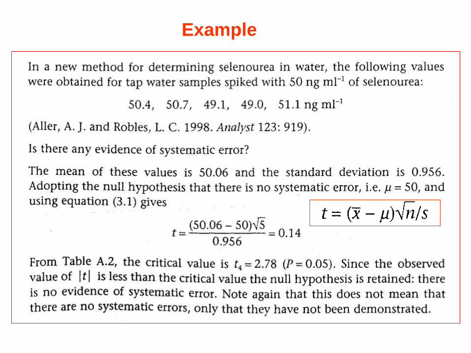
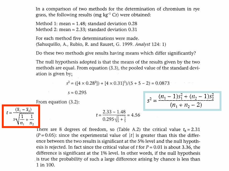
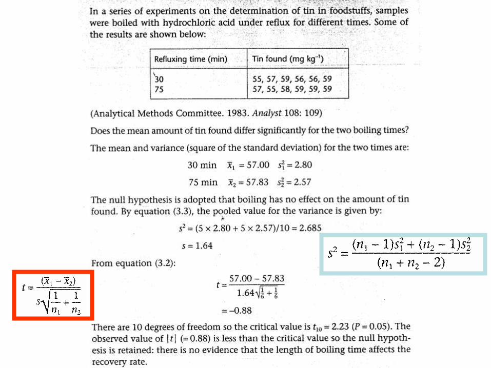
Example

Comparison of two experimental means

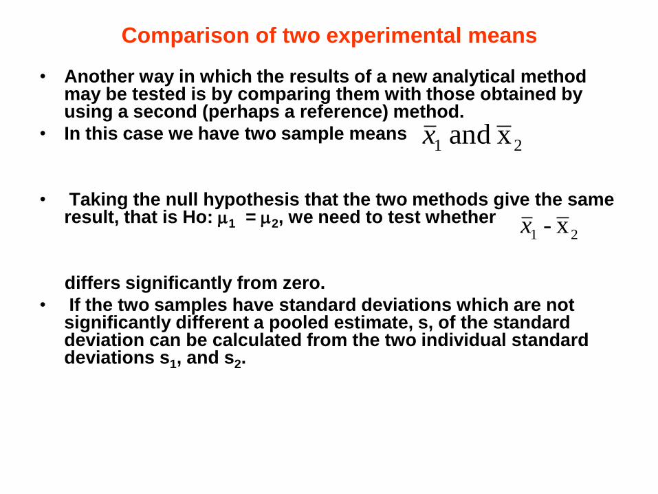
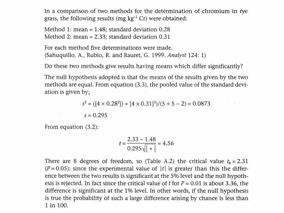
• Another way in which the results of a new analytical method may be tested is by comparing them with those obtained by using a second (perhaps a reference) method.

• In this case we have two sample means

• Taking the null hypothesis that the two methods give the same result, that is Ho: 1 = 2, we need to test whether

differs significantly from zero.

• If the two samples have standard deviations which are not significantly different a pooled estimate, s, of the standard deviation can be calculated from the two individual standard deviations s1, and s2.

21 x and x

21 x - x

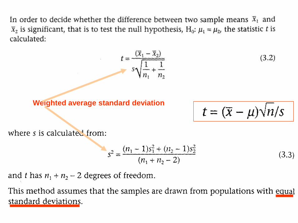
Weighted average standard deviation

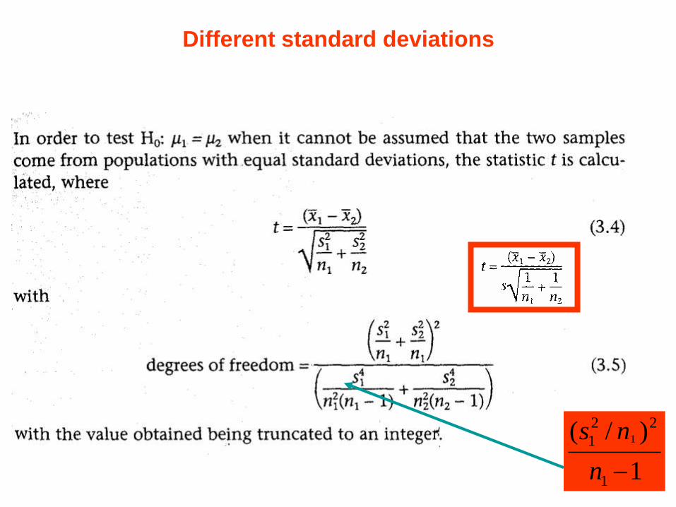
Different standard deviations

1

)/(

1

22

1 1

n

ns

Example

f

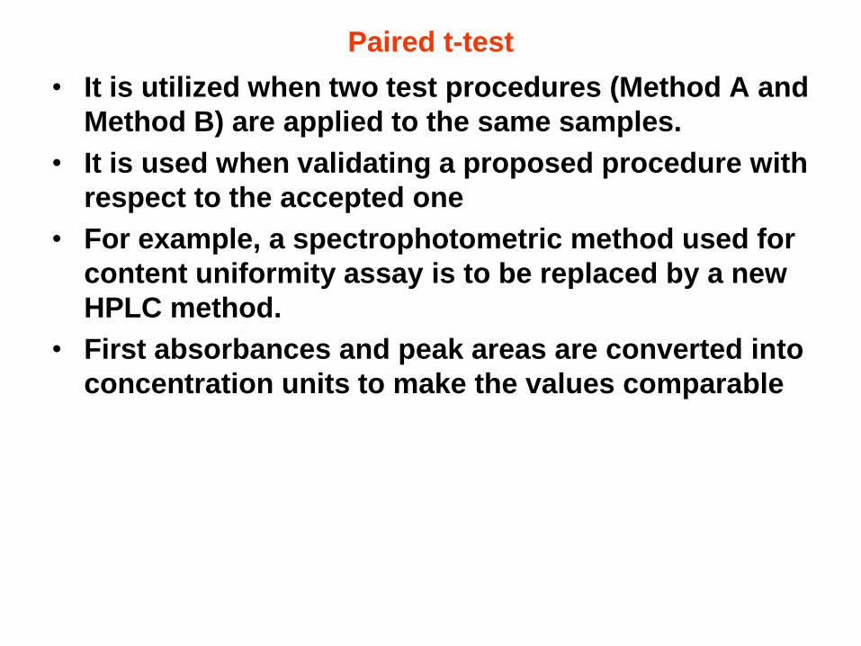
Paired t-test

• It is utilized when two test procedures (Method A and

Method B) are applied to the same samples.

• It is used when validating a proposed procedure with

respect to the accepted one

• For example, a spectrophotometric method used for

content uniformity assay is to be replaced by a new

HPLC method.

• First absorbances and peak areas are converted into

concentration units to make the values comparable

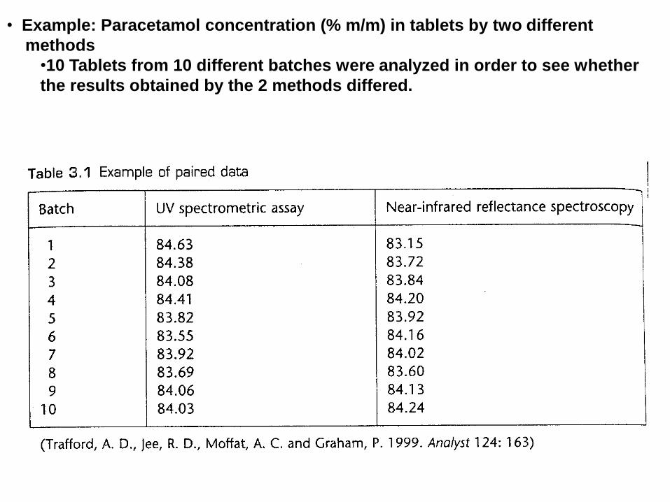
• Example: Paracetamol concentration (% m/m) in tablets by two different

methods

•10 Tablets from 10 different batches were analyzed in order to see whether

the results obtained by the 2 methods differed.

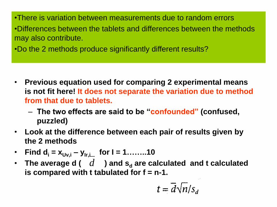
• Previous equation used for comparing 2 experimental means

is not fit here! It does not separate the variation due to method

from that due to tablets.

– The two effects are said to be “confounded” (confused,

puzzled)

• Look at the difference between each pair of results given by

the 2 methods

• Find di = xUv,i – yIr,i for I = 1……..10

• The average d ( ) and sd are calculated and t calculated

is compared with t tabulated for f = n-1.

d

•There is variation between measurements due to random errors

•Differences between the tablets and differences between the methods

may also contribute.

•Do the 2 methods produce significantly different results?

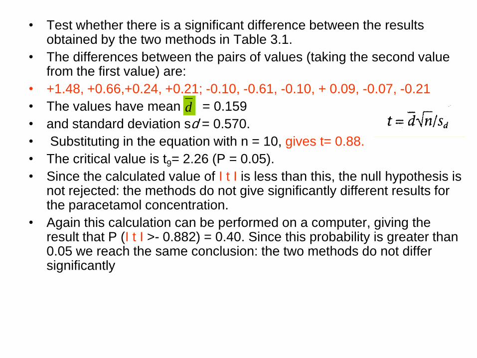
• Test whether there is a significant difference between the results obtained by the two methods in Table 3.1.

• The differences between the pairs of values (taking the second value from the first value) are:

• +1.48, +0.66,+0.24, +0.21; -0.10, -0.61, -0.10, + 0.09, -0.07, -0.21

• The values have mean = 0.159

• and standard deviation sd = 0.570.

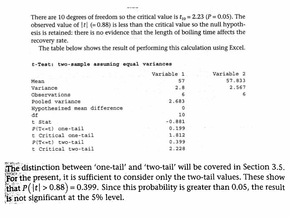
• Substituting in the equation with n = 10, gives t= 0.88.

• The critical value is t9= 2.26 (P = 0.05).

• Since the calculated value of I t I is less than this, the null hypothesis is not rejected: the methods do not give significantly different results for the paracetamol concentration.

• Again this calculation can be performed on a computer, giving the result that P (I t I >- 0.882) = 0.40. Since this probability is greater than 0.05 we reach the same conclusion: the two methods do not differ significantly

d

Example

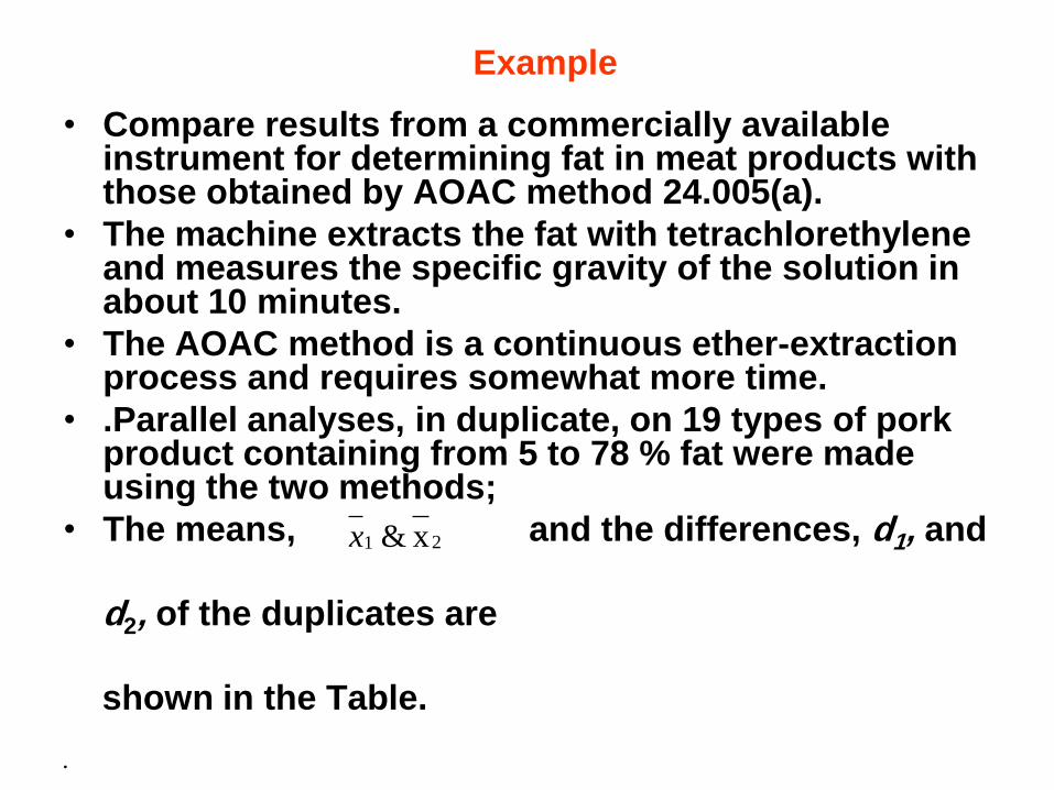
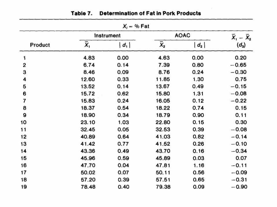
• Compare results from a commercially available instrument for determining fat in meat products with those obtained by AOAC method 24.005(a).

• The machine extracts the fat with tetrachlorethylene and measures the specific gravity of the solution in about 10 minutes.

• The AOAC method is a continuous ether-extraction process and requires somewhat more time.

• .Parallel analyses, in duplicate, on 19 types of pork product containing from 5 to 78 % fat were made using the two methods;

• The means, and the differences, d1, and

d2, of the duplicates are

shown in the Table.

•

21 x & x

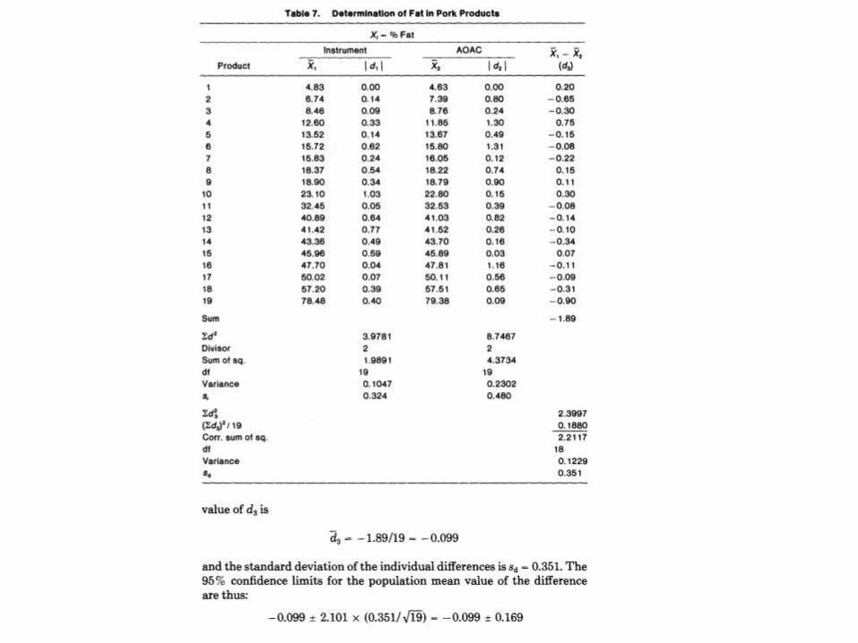
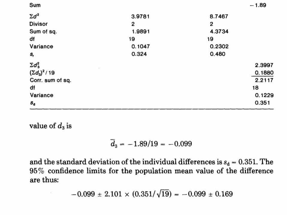
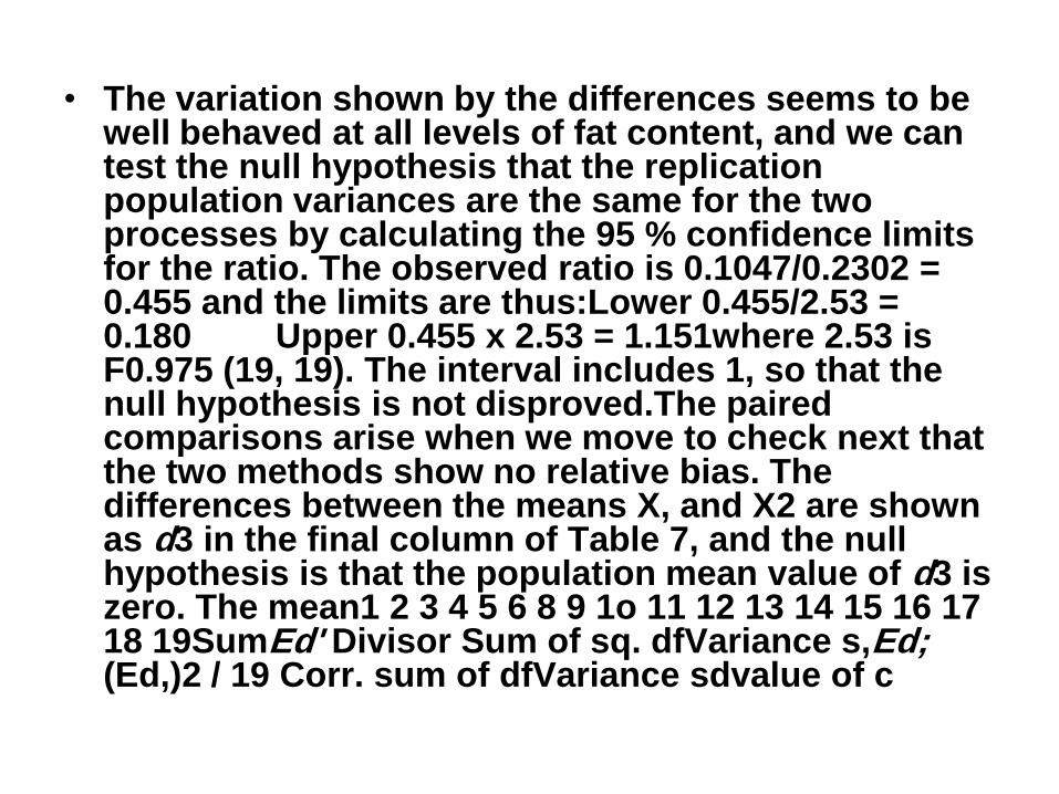
• The variation shown by the differences seems to be well behaved at all levels of fat content, and we can test the null hypothesis that the replication population variances are the same for the two processes by calculating the 95 % confidence limits for the ratio. The observed ratio is 0.1047/0.2302 = 0.455 and the limits are thus:Lower 0.455/2.53 = 0.180 Upper 0.455 x 2.53 = 1.151where 2.53 is F0.975 (19, 19). The interval includes 1, so that the null hypothesis is not disproved.The paired comparisons arise when we move to check next that the two methods show no relative bias. The differences between the means X, and X2 are shown as d3 in the final column of Table 7, and the null hypothesis is that the population mean value of d3 is zero. The mean1 2 3 4 5 6 8 9 1o 11 12 13 14 15 16 17 18 19SumEd' Divisor Sum of sq. dfVariance s,Ed; (Ed,)2 / 19 Corr. sum of dfVariance sdvalue of c

One-sided (tailed) and two-sided (tailed) tests

• Methods described so far in this chapter have been concerned with testing for a difference between two means in either direction.

• For example, the method described in Section 3.2 tests whether there is a significant difference between the experimental result and the known value for the reference material, regardless of the sign of the difference.

• In most situations of this kind the analyst has no idea, prior to the experiment, as to whether any difference between the experimental mean and the reference value will be positive or negative.

• Thus the test used must cover either possibility. Such a test is called two-sided (or two-tailed).

• In a few cases, however, a different kind of test may be appropriate. Consider, for example, an experiment in which it is hoped to increase the rate of reaction by addition of a catalyst. In this case, it is clear before the experiment begins that the only result of interest is whether the new rate is greater than the old, and only an increase need be tested for significance.

• This kind of test is called one-sided (or one-tailed).

• For a given value of n and a particular probability level, the critical value for a one-sided test differs from that for a two-sided test.

• In a one-sided test for an increase, the critical value of t (rather than I t I) for P = 0.05 is that value which is exceeded with a probability of 5%.

• Since the sampling distribution of the mean is assumed to be symmetrical, this probability is twice the probability that is relevant in the two-sided test.

• The appropriate value for the one-sided test is thus found in the P = 0.10 column of Table A.2.

• Similarly, for a one-sided test at the P = 0.01 level, the 0.02 column is used.

• For a one-sided test for a decrease, the critical value of t will be of equal magnitude but with a negative sign.

• If the test is carried out on a computer, it will be necessary to indicate whether a one- or a two-sided test

is required.

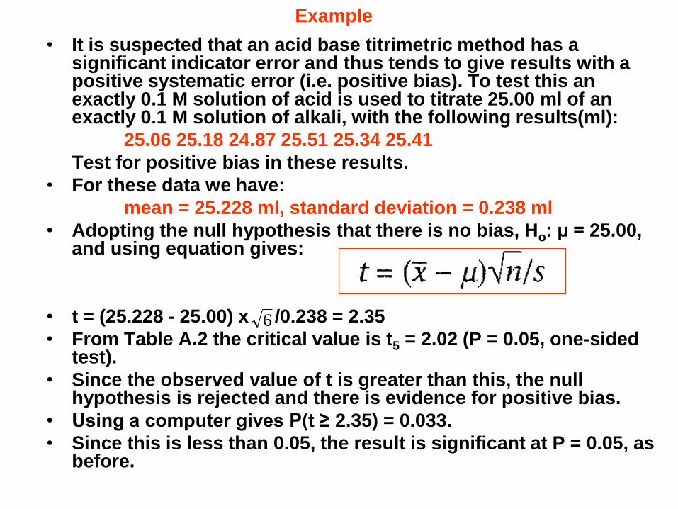
Example

• It is suspected that an acid base titrimetric method has a significant indicator error and thus tends to give results with a positive systematic error (i.e. positive bias). To test this an exactly 0.1 M solution of acid is used to titrate 25.00 ml of an exactly 0.1 M solution of alkali, with the following results(ml):

25.06 25.18 24.87 25.51 25.34 25.41

Test for positive bias in these results.

• For these data we have:

mean = 25.228 ml, standard deviation = 0.238 ml

• Adopting the null hypothesis that there is no bias, Ho: µ = 25.00, and using equation gives:

• t = (25.228 - 25.00) x /0.238 = 2.35

• From Table A.2 the critical value is t5 = 2.02 (P = 0.05, one-sided test).

• Since the observed value of t is greater than this, the null hypothesis is rejected and there is evidence for positive bias.

• Using a computer gives P(t ≥ 2.35) = 0.033.

• Since this is less than 0.05, the result is significant at P = 0.05, as before.

6

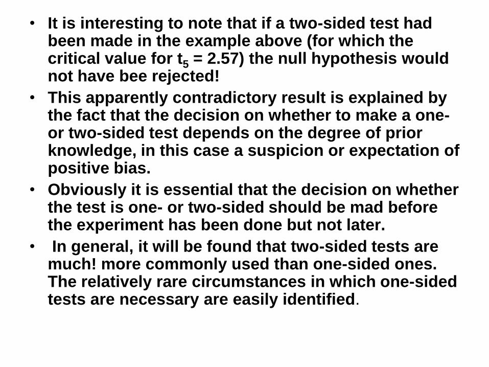
• It is interesting to note that if a two-sided test had been made in the example above (for which the critical value for t5 = 2.57) the null hypothesis would not have bee rejected!

• This apparently contradictory result is explained by the fact that the decision on whether to make a one- or two-sided test depends on the degree of prior knowledge, in this case a suspicion or expectation of positive bias.

• Obviously it is essential that the decision on whether the test is one- or two-sided should be mad before the experiment has been done but not later.

• In general, it will be found that two-sided tests are much! more commonly used than one-sided ones. The relatively rare circumstances in which one-sided tests are necessary are easily identified.

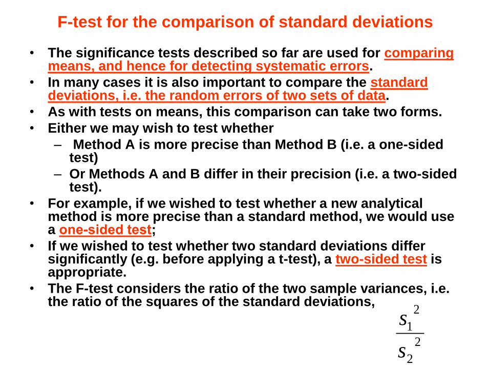
F-test for the comparison of standard deviations

• The significance tests described so far are used for comparing means, and hence for detecting systematic errors.

• In many cases it is also important to compare the standard deviations, i.e. the random errors of two sets of data.

• As with tests on means, this comparison can take two forms.

• Either we may wish to test whether

– Method A is more precise than Method B (i.e. a one-sided test)

– Or Methods A and B differ in their precision (i.e. a two-sided test).

• For example, if we wished to test whether a new analytical method is more precise than a standard method, we would use a one­sided test;

• If we wished to test whether two standard deviations differ significantly (e.g. before applying a t-test), a two-sided test is appropriate.

• The F-test considers the ratio of the two sample variances, i.e. the ratio of the squares of the standard deviations,

2

2

2

1

s

s

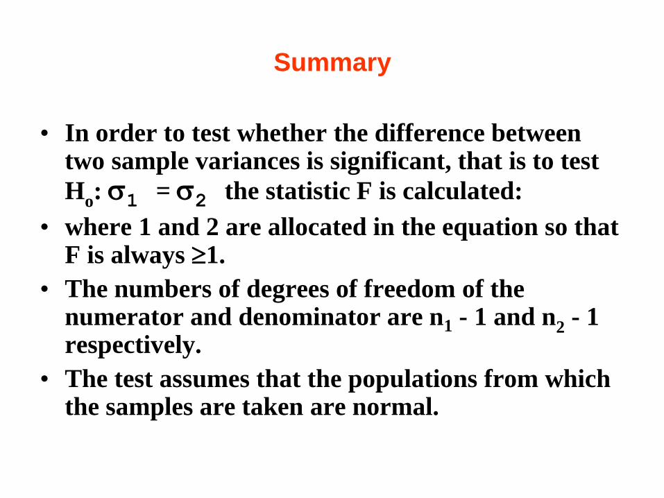
Summary

• In order to test whether the difference between two sample variances is significant, that is to test

Ho: 1 = 2 the statistic F is calculated:

• where 1 and 2 are allocated in the equation so that F is always 1.

• The numbers of degrees of freedom of the numerator and denominator are n1 - 1 and n2 - 1 respectively.

• The test assumes that the populations from which the samples are taken are normal.

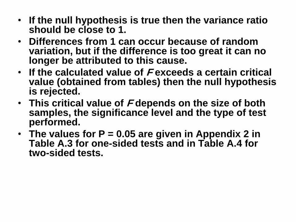
• If the null hypothesis is true then the variance ratio should be close to 1.

• Differences from 1 can occur because of random variation, but if the difference is too great it can no longer be attributed to this cause.

• If the calculated value of F exceeds a certain critical value (obtained from tables) then the null hypothesis is rejected.

• This critical value of F depends on the size of both samples, the significance level and the type of test performed.

• The values for P = 0.05 are given in Appendix 2 in Table A.3 for one-sided tests and in Table A.4 for two-sided tests.

Example

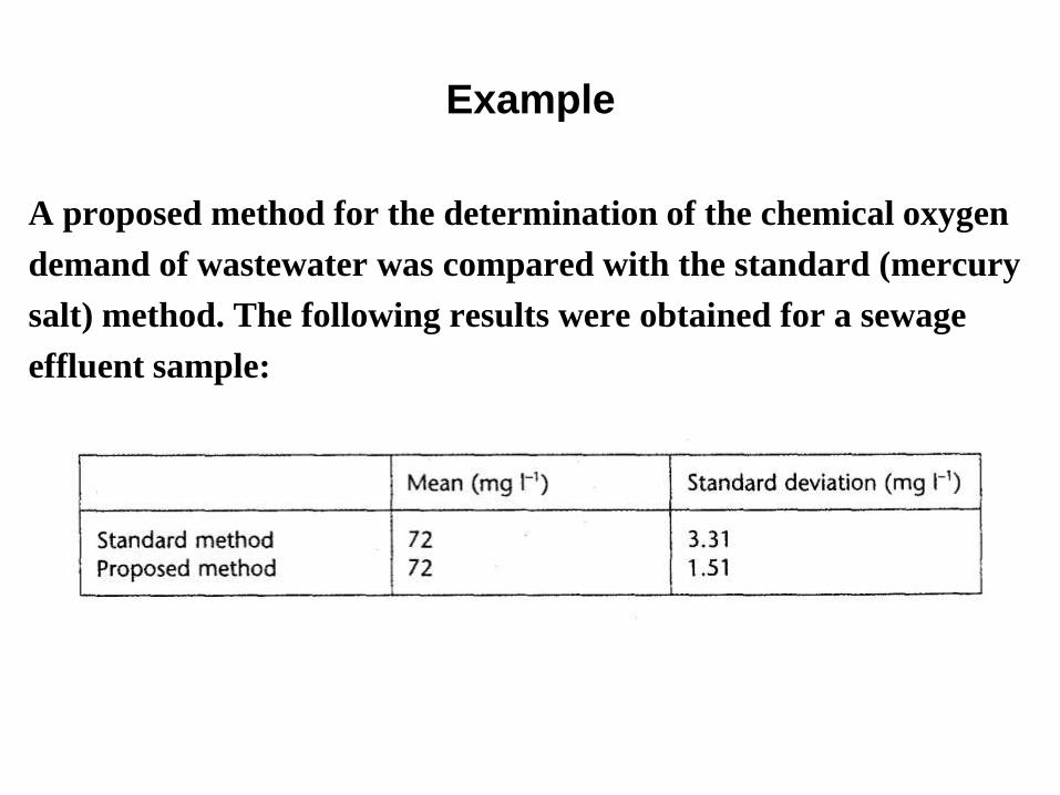
A proposed method for the determination of the chemical oxygen

demand of wastewater was compared with the standard (mercury

salt) method. The following results were obtained for a sewage

effluent sample:

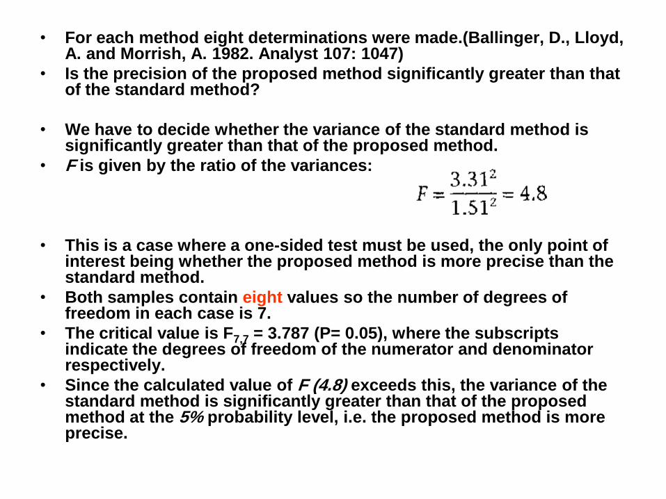
• For each method eight determinations were made.(Ballinger, D., Lloyd, A. and Morrish, A. 1982. Analyst 107: 1047)

• Is the precision of the proposed method significantly greater than that of the standard method?

• We have to decide whether the variance of the standard method is significantly greater than that of the proposed method.

• F is given by the ratio of the variances:

• This is a case where a one-sided test must be used, the only point of interest being whether the proposed method is more precise than the standard method.

• Both samples contain eight values so the number of degrees of freedom in each case is 7.

• The critical value is F7,7 = 3.787 (P= 0.05), where the subscripts indicate the degrees of freedom of the numerator and denominator respectively.

• Since the calculated value of F (4.8) exceeds this, the variance of the standard method is significantly greater than that of the proposed method at the 5% probability level, i.e. the proposed method is more precise.

Example

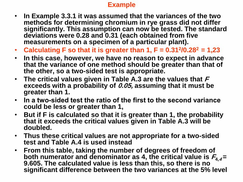
• In Example 3.3.1 it was assumed that the variances of the two methods for determining chromium in rye grass did not differ significantly. This assumption can now be tested. The standard deviations were 0.28 and 0.31 (each obtained from five measurements on a specimen of a particular plant).

• Calculating F so that it is greater than 1, F = 0.312/0.282 = 1,23

• In this case, however, we have no reason to expect in advance that the variance of one method should be greater than that of the other, so a two-sided test is appropriate.

• The critical values given in Table A.3 are the values that F exceeds with a probability of 0.05, assuming that it must be greater than 1.

• In a two­sided test the ratio of the first to the second variance could be less or greater than 1,

• But if F is calculated so that it is greater than 1, the probability that it exceeds the critical values given in Table A.3 will be doubled.

• Thus these critical values are not appropriate for a two-sided test and Table A.4 is used instead

• From this table, taking the number of degrees of freedom of both numerator and denominator as 4, the critical value is F4,4 = 9.605. The calculated value is less than this, so there is no significant difference between the two variances at the 5% level

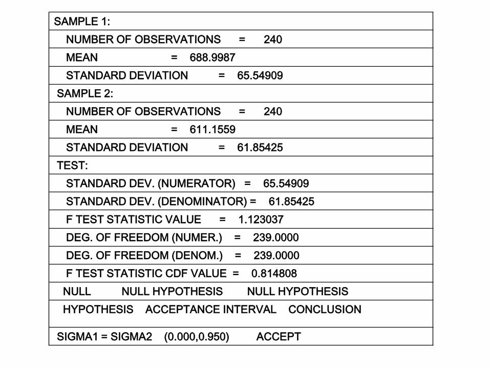
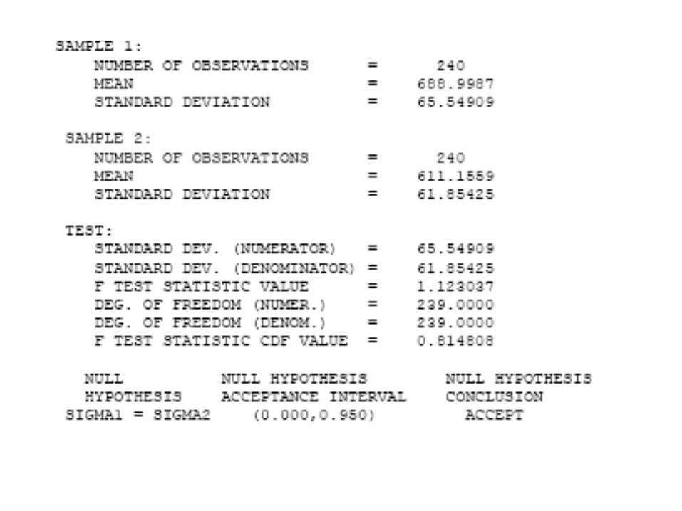
SAMPLE 1:

NUMBER OF OBSERVATIONS = 240

MEAN = 688.9987

STANDARD DEVIATION = 65.54909

SAMPLE 2:

NUMBER OF OBSERVATIONS = 240

MEAN = 611.1559

STANDARD DEVIATION = 61.85425

TEST:

STANDARD DEV. (NUMERATOR) = 65.54909

STANDARD DEV. (DENOMINATOR) = 61.85425

F TEST STATISTIC VALUE = 1.123037

DEG. OF FREEDOM (NUMER.) = 239.0000

DEG. OF FREEDOM (DENOM.) = 239.0000

F TEST STATISTIC CDF VALUE = 0.814808

NULL NULL HYPOTHESIS NULL HYPOTHESIS

HYPOTHESIS ACCEPTANCE INTERVAL CONCLUSION

SIGMA1 = SIGMA2 (0.000,0.950) ACCEPT

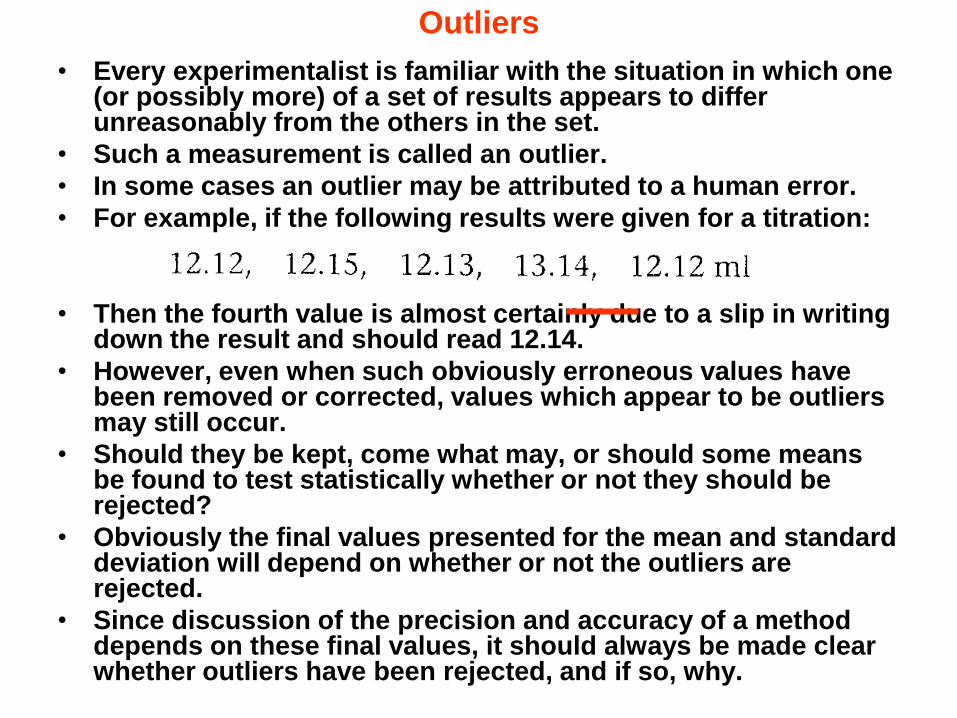
Outliers

• Every experimentalist is familiar with the situation in which one (or possibly more) of a set of results appears to differ unreasonably from the others in the set.

• Such a measurement is called an outlier.

• In some cases an outlier may be attributed to a human error.

• For example, if the following results were given for a titration:

• Then the fourth value is almost certainly due to a slip in writing down the result and should read 12.14.

• However, even when such obviously erroneous values have been removed or corrected, values which appear to be outliers may still occur.

• Should they be kept, come what may, or should some means be found to test statistically whether or not they should be rejected?

• Obviously the final values presented for the mean and standard deviation will depend on whether or not the outliers are rejected.

• Since discussion of the precision and accuracy of a method depends on these final values, it should always be made clear whether outliers have been rejected, and if so, why.

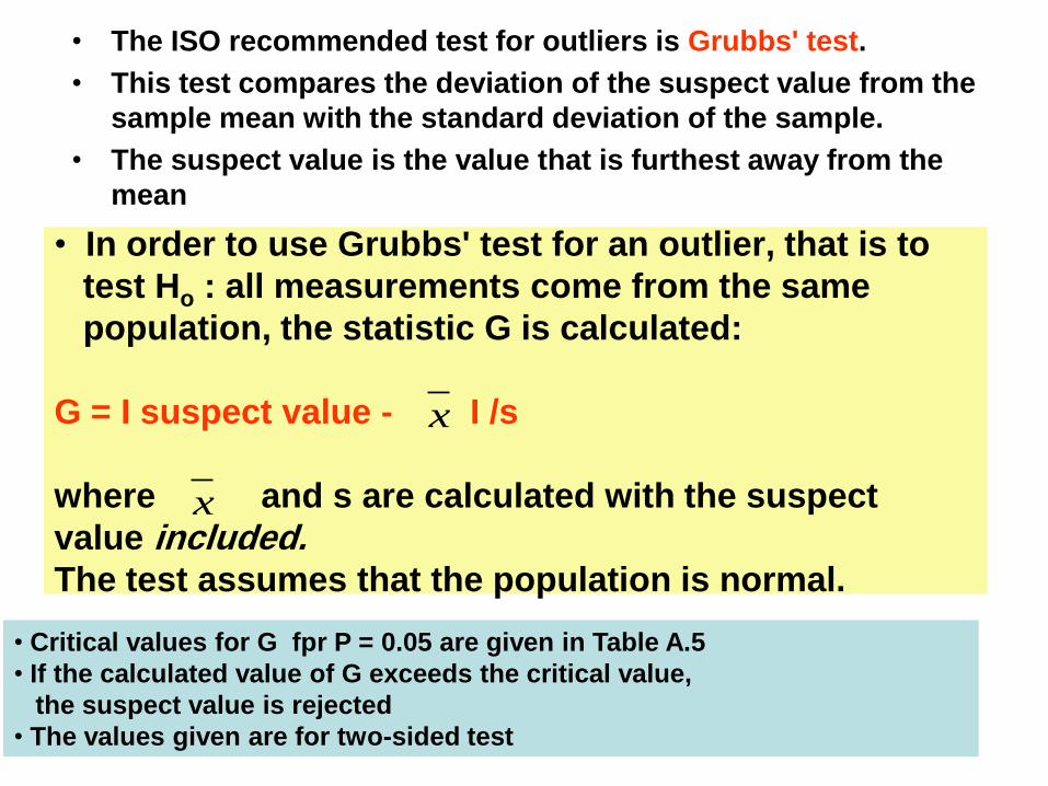
• The ISO recommended test for outliers is Grubbs' test.

• This test compares the deviation of the suspect value from the

sample mean with the standard deviation of the sample.

• The suspect value is the value that is furthest away from the

mean

• In order to use Grubbs' test for an outlier, that is to

test Ho : all measurements come from the same

population, the statistic G is calculated:

G = I suspect value - I /s

where and s are calculated with the suspect

value included. The test assumes that the population is normal.

x

x

• Critical values for G fpr P = 0.05 are given in Table A.5

• If the calculated value of G exceeds the critical value,

the suspect value is rejected

• The values given are for two-sided test

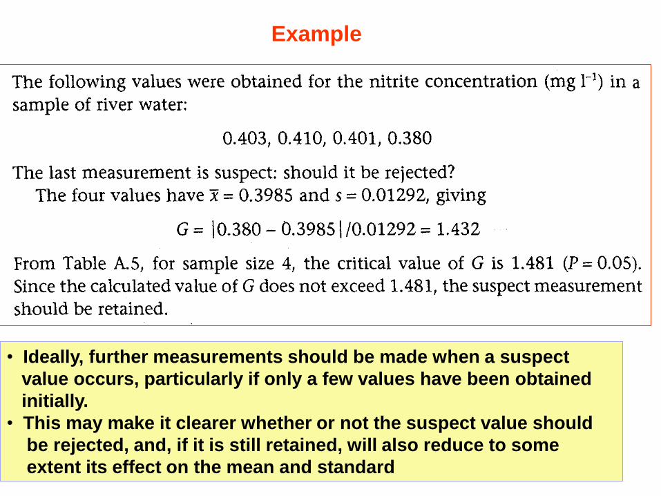
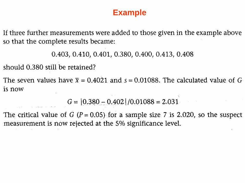
• Ideally, further measurements should be made when a suspect

value occurs, particularly if only a few values have been obtained

initially.

• This may make it clearer whether or not the suspect value should

be rejected, and, if it is still retained, will also reduce to some

extent its effect on the mean and standard

Example

Example

Dixon's test (the Q-test)

• Another test for outliers which is popular because the calculation is simple.

• For small samples (size 3 to 7) the test assesses a suspect measurement by comparing the measurement nearest to it in size with range of the measurements.

• For larger samples the form of the test is modified slightly. A reference containing further details is given at the end of this chapter.)

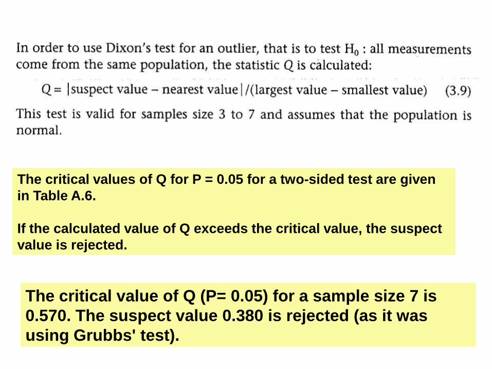
The critical value of Q (P= 0.05) for a sample size 7 is

0.570. The suspect value 0.380 is rejected (as it was

using Grubbs' test).

The critical values of Q for P = 0.05 for a two-sided test are given

in Table A.6.

If the calculated value of Q exceeds the critical value, the suspect

value is rejected.

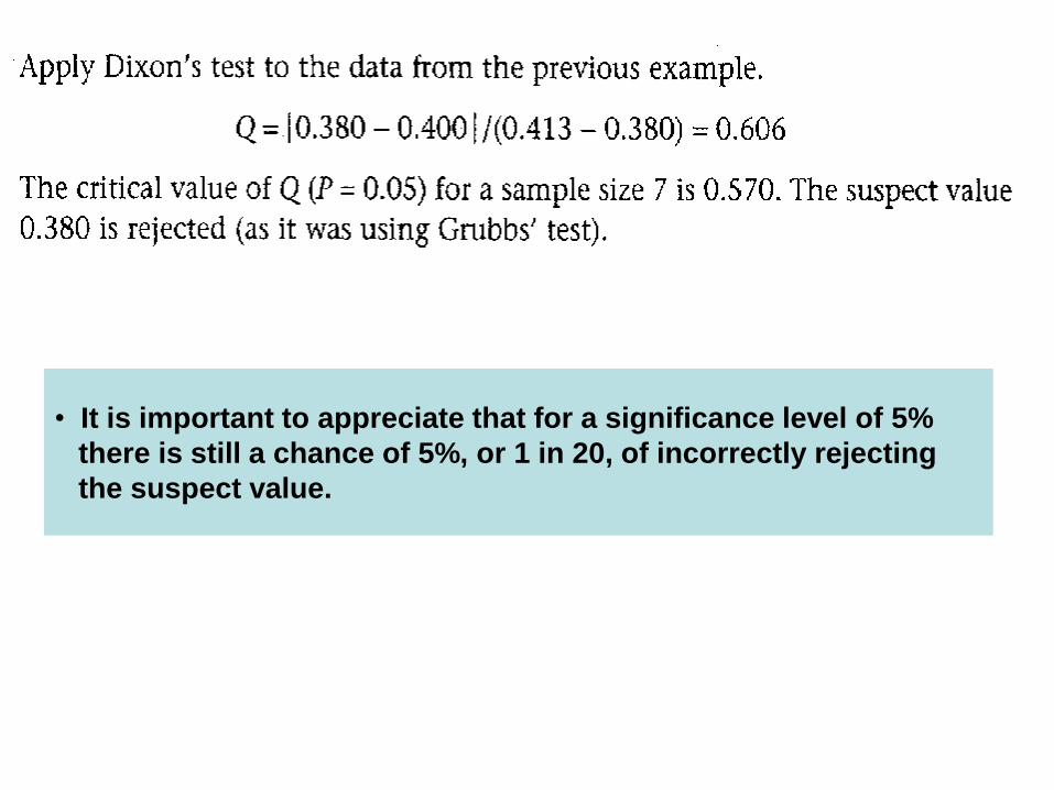
• It is important to appreciate that for a significance level of 5%

there is still a chance of 5%, or 1 in 20, of incorrectly rejecting

the suspect value.

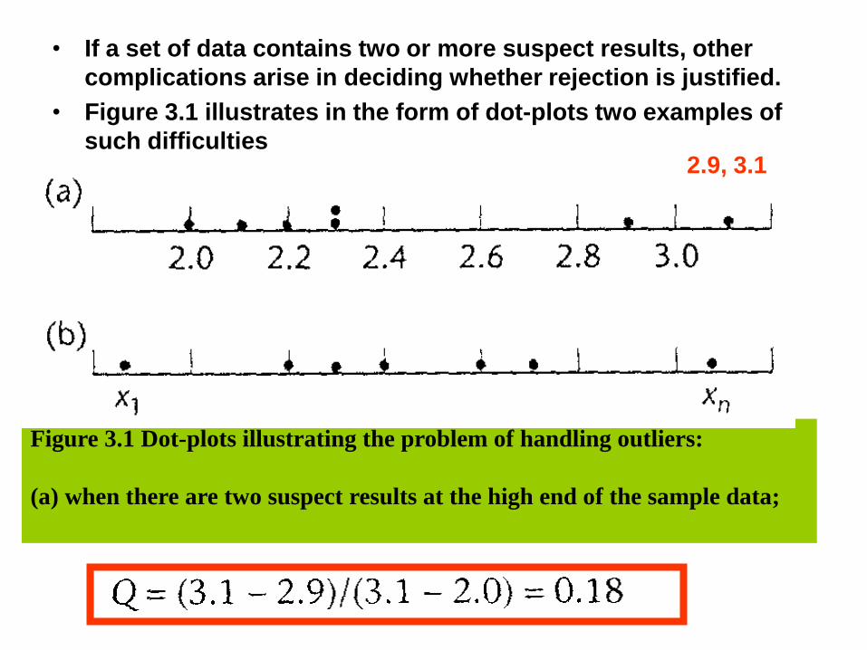
• If a set of data contains two or more suspect results, other

complications arise in deciding whether rejection is justified.

• Figure 3.1 illustrates in the form of dot-plots two examples of

such difficulties

Figure 3.1 Dot-plots illustrating the problem of handling outliers:

(a) when there are two suspect results at the high end of the sample data;

2.9, 3.1

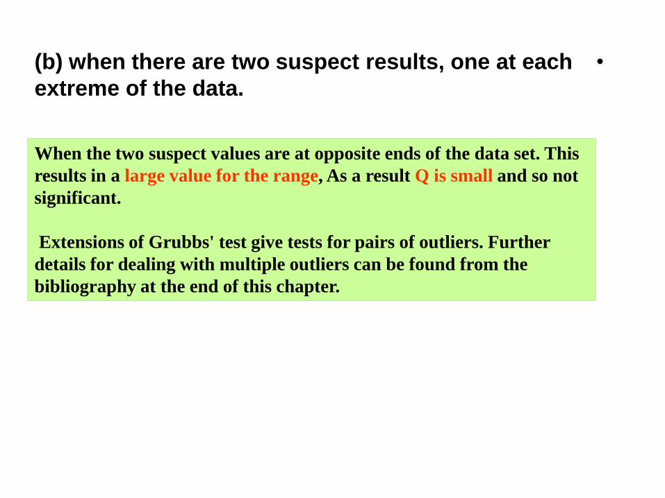
•(b) when there are two suspect results, one at each

extreme of the data.

When the two suspect values are at opposite ends of the data set. This

results in a large value for the range, As a result Q is small and so not

significant.

Extensions of Grubbs' test give tests for pairs of outliers. Further

details for dealing with multiple outliers can be found from the

bibliography at the end of this chapter.

Analysis of Variance-ANOVA

• Previously a method was described for comparing two means to test whether they differ significantly.

• In analytical work there are often more than two means to be compared.

• Some possible situations are: comparing the mean concentration of analyte in solution for samples stored under different conditions; and determined by different methods; and obtained by several different experimentalists using the same instrument.

• In all these examples there are two possible sources of variation. – The first, which is always present, is due to the random

error in measurement. This was discussed previously: it is the error which causes a different result to be obtained each time a measurement repeated under the same conditions.

– The second possible source of variation is due to what is known as a controlled or fixed-effect factor.

Controlled factors

• For example, the conditions under which the solution was stored, the method of analysis used, and the experimentalist carrying out the analysis.

• Thus, ANOVA is a statistical technique used to separate and estimate the different causes of variation.

• For the particular examples above, it can be used to separate any variation which is caused by changing the controlled factor from the variation due to random error.

• It can thus test whether altering the controlled factor leads to a significant difference between the mean values obtained.

• ANOVA can also be used in situations where there is more than one source of random variation.

• Consider, for example, the purity testing of barrelful of sodium chloride.

• Samples are taken from different parts of the barrel chosen at random

• Replicate analyses were performed on these samples.

• In addition to the random error in the measurement of the purity, there may also be variation in the purity of the samples from different parts of the barrel.

• Since the samples were chosen at random, this variation will be random and is thus sometimes known as a random-effect factor.

• Again, ANOVA can be used to separate and estimate the sources of variation.

• Both types of statistical analysis described above, i.e. where there is one factor, either controlled or random, in addition to the random error in measurement, are known as one-way ANOVA.

• The arithmetical procedures are similar in the fixed- and random-effect factor cases: examples of the former are given in this chapter and of the latter in the next chapter, where sampling is considered in more detail.

• More complex situations in which there are two or more factors, possibly interacting with each other, are considered in chapter 7

• ANOVA is used to analyze the results from a-factorial experiment.

• Factorial experiment: an experiment plan in which the effects of changes in the levels of a number of factors are studied together and yields are recorded for all combinations of levels that can be formed. – Factorial experiments are used to study the average effect of each

factor along with the interaction effects among factors.

• The procedure is to separate (mathematically) the total variation of the experimental measurements into parts so that one part represents-and gives rise to an estimate of the variance associated with experimental error, while the other parts can be associated with the separate factors studied and can be presented as variance estimates that are to be compared with the error variance.

• The variance ratios (known as F-ratios in honor of R. A. Fisher, a pioneer of experimental design) are compared with critical values.

• Many types of experimental design exist, each has its own analysis of variance

One-way ANOVA

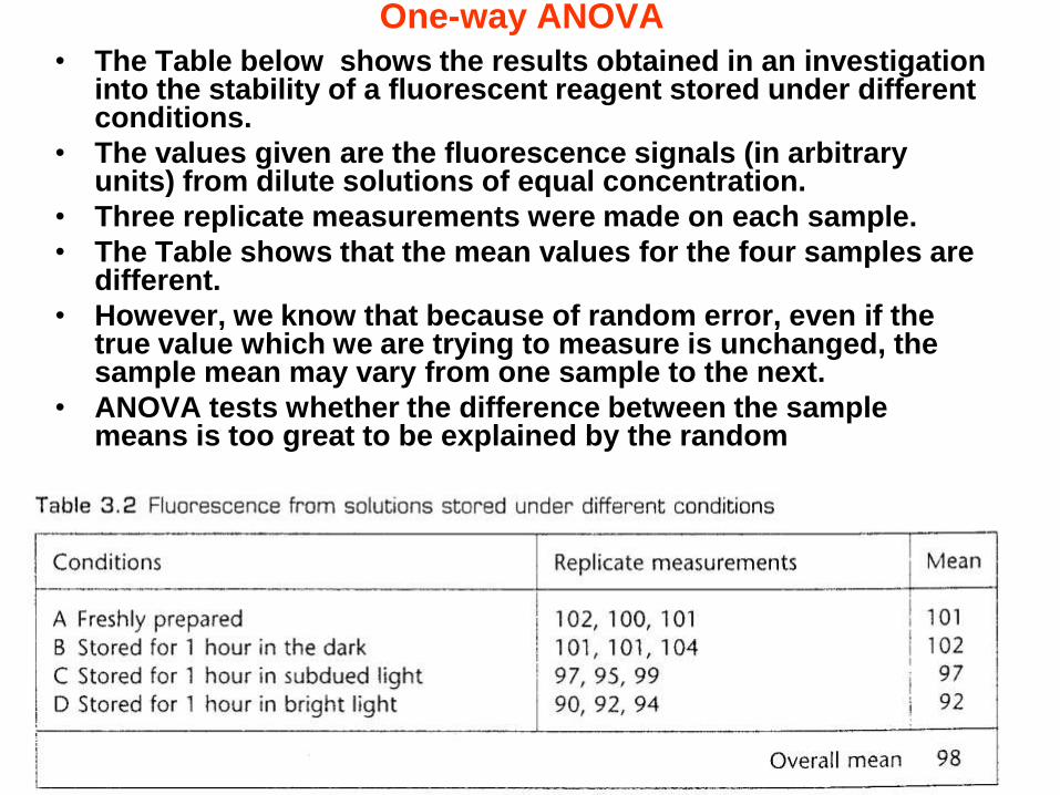
• The Table below shows the results obtained in an investigation into the stability of a fluorescent reagent stored under different conditions.

• The values given are the fluorescence signals (in arbitrary units) from dilute solutions of equal concentration.

• Three replicate measurements were made on each sample.

• The Table shows that the mean values for the four samples are different.

• However, we know that because of random error, even if the true value which we are trying to measure is unchanged, the sample mean may vary from one sample to the next.

• ANOVA tests whether the difference between the sample means is too great to be explained by the random

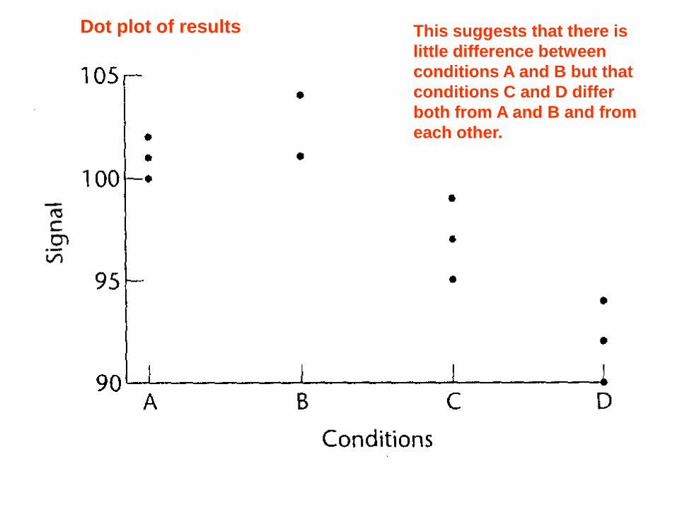
Dot plot of results This suggests that there is

little difference between

conditions A and B but that

conditions C and D differ

both from A and B and from

each other.

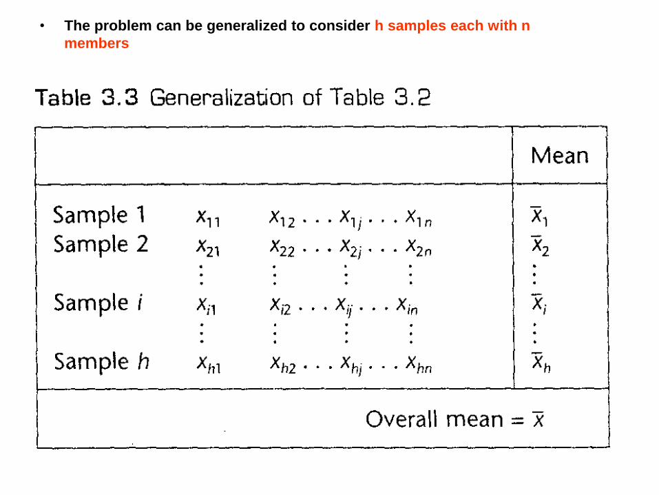
• The problem can be generalized to consider h samples each with n

members

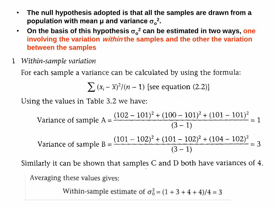
• The null hypothesis adopted is that all the samples are drawn from a

population with mean µ and variance o2.

• On the basis of this hypothesis o2 can be estimated in two ways, one

involving the variation within the samples and the other the variation

between the samples

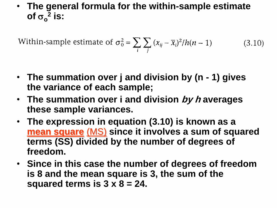
• The general formula for the within-sample estimate of o

2 is:

• The summation over j and division by (n - 1) gives the variance of each sample;

• The summation over i and division by h averages these sample variances.

• The expression in equation (3.10) is known as a mean square (MS) since it involves a sum of squared terms (SS) divided by the number of degrees of freedom.

• Since in this case the number of degrees of freedom is 8 and the mean square is 3, the sum of the squared terms is 3 x 8 = 24.

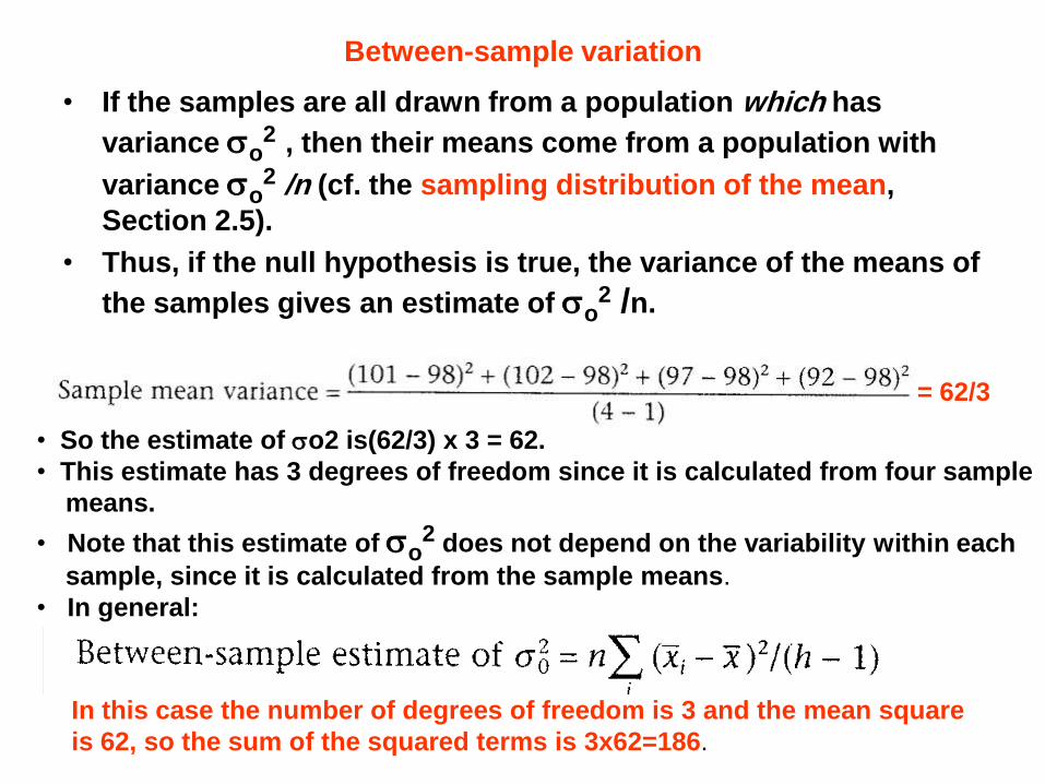
Between-sample variation

• If the samples are all drawn from a population which has

variance o2 , then their means come from a population with

variance o2 /n (cf. the sampling distribution of the mean,

Section 2.5).

• Thus, if the null hypothesis is true, the variance of the means of

the samples gives an estimate of o2 /n.

• So the estimate of o2 is(62/3) x 3 = 62.

• This estimate has 3 degrees of freedom since it is calculated from four sample

means.

• Note that this estimate of o2 does not depend on the variability within each

sample, since it is calculated from the sample means.

• In general:

= 62/3

In this case the number of degrees of freedom is 3 and the mean square

is 62, so the sum of the squared terms is 3x62=186.

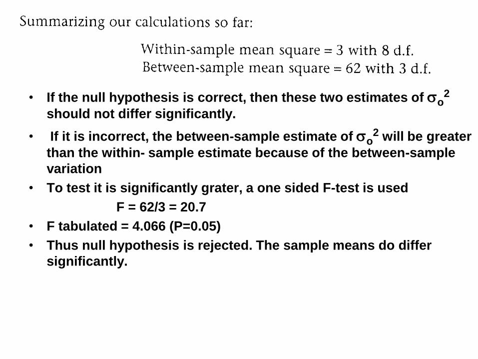
• If the null hypothesis is correct, then these two estimates of o2

should not differ significantly.

• If it is incorrect, the between-sample estimate of o2 will be greater

than the within- sample estimate because of the between-sample

variation

• To test it is significantly grater, a one sided F-test is used

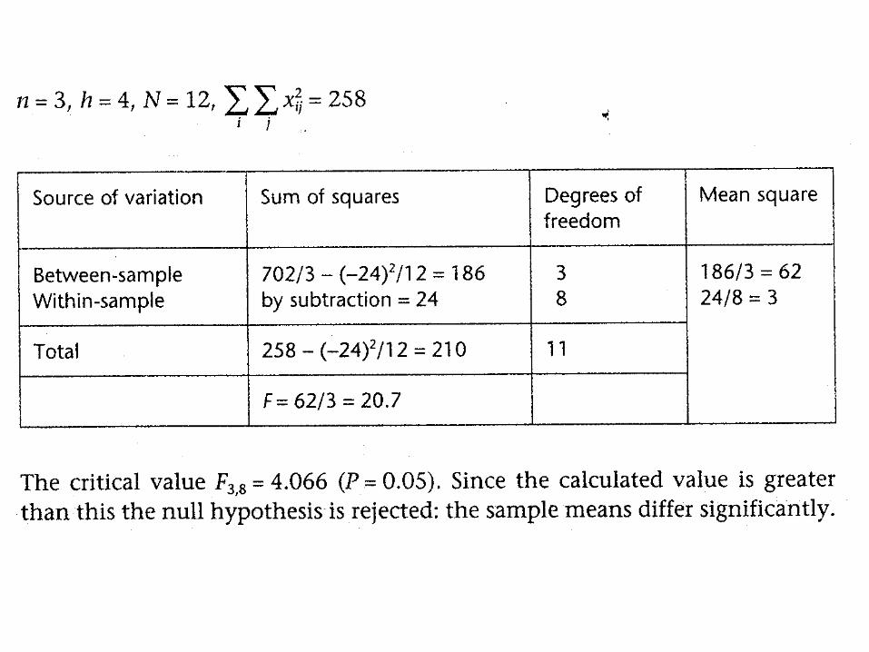
F = 62/3 = 20.7

• F tabulated = 4.066 (P=0.05)

• Thus null hypothesis is rejected. The sample means do differ

significantly.

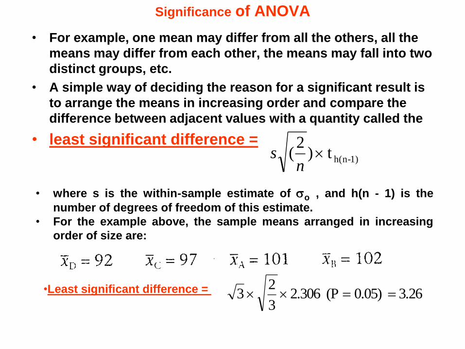
Significance of ANOVA

• For example, one mean may differ from all the others, all the

means may differ from each other, the means may fall into two

distinct groups, etc.

• A simple way of deciding the reason for a significant result is

to arrange the means in increasing order and compare the

difference between adjacent values with a quantity called the

• least significant difference =

• where s is the within-sample estimate of o , and h(n - 1) is the

number of degrees of freedom of this estimate.

• For the example above, the sample means arranged in increasing

order of size are:

1)-h(n t )2

( n

s

•Least significant difference = 3.26 0.05)(P 2.306 3

2 3

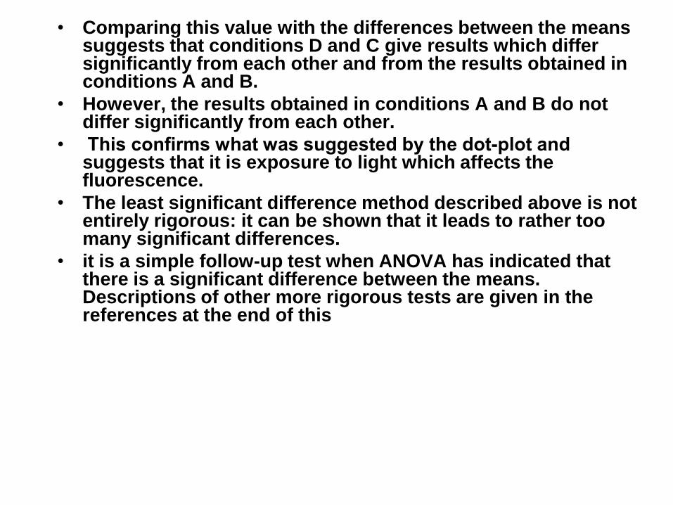
• Comparing this value with the differences between the means suggests that conditions D and C give results which differ significantly from each other and from the results obtained in conditions A and B.

• However, the results obtained in conditions A and B do not differ significantly from each other.

• This confirms what was suggested by the dot­plot and suggests that it is exposure to light which affects the fluorescence.

• The least significant difference method described above is not entirely rigorous: it can be shown that it leads to rather too many significant differences.

• it is a simple follow-up test when ANOVA has indicated that there is a significant difference between the means. Descriptions of other more rigorous tests are given in the references at the end of this

The arithmetic of ANOVA calculations

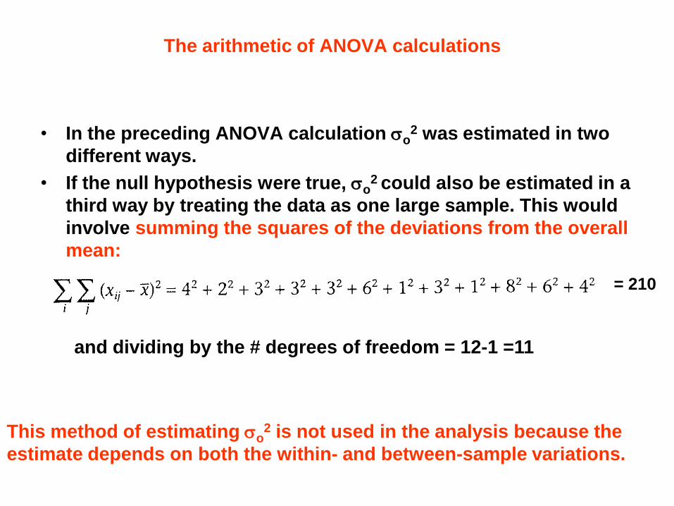
• In the preceding ANOVA calculation o2 was estimated in two

different ways.

• If the null hypothesis were true, o2 could also be estimated in a

third way by treating the data as one large sample. This would

involve summing the squares of the deviations from the overall

mean:

= 210

and dividing by the # degrees of freedom = 12-1 =11

This method of estimating o2 is not used in the analysis because the

estimate depends on both the within- and between-sample variations.

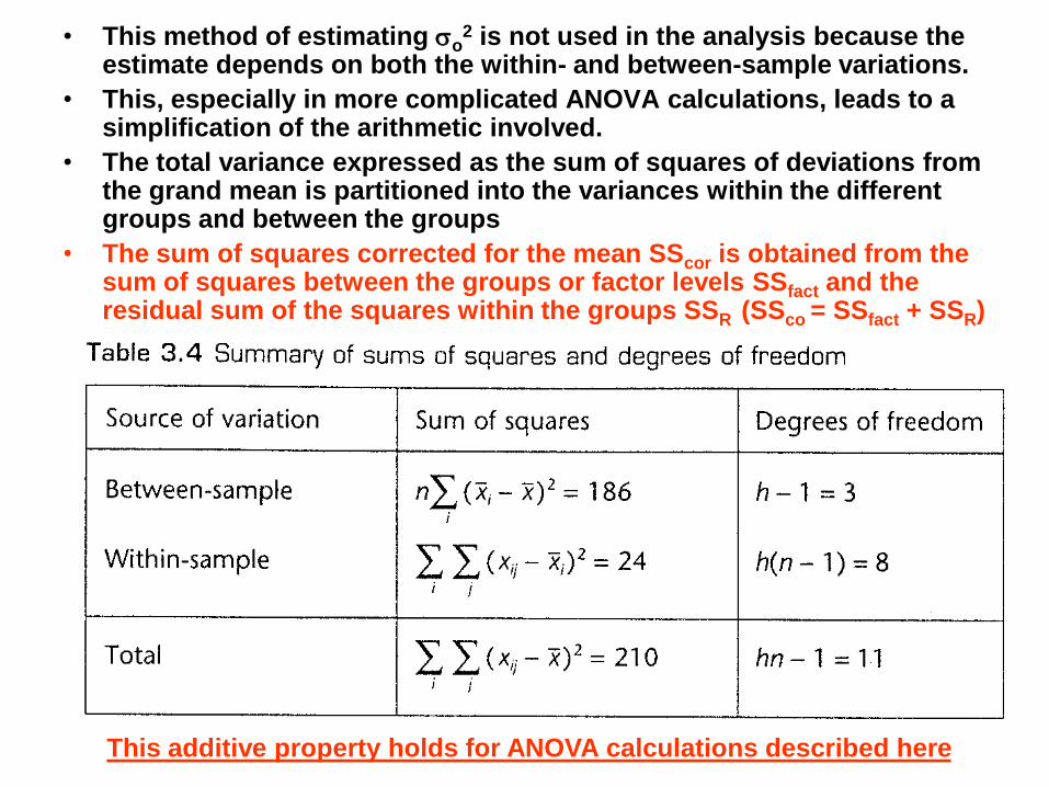
• This method of estimating o2 is not used in the analysis because the

estimate depends on both the within- and between-sample variations.

• This, especially in more complicated ANOVA calculations, leads to a simplification of the arithmetic involved.

• The total variance expressed as the sum of squares of deviations from the grand mean is partitioned into the variances within the different groups and between the groups

• The sum of squares corrected for the mean SScor is obtained from the sum of squares between the groups or factor levels SSfact and the residual sum of the squares within the groups SSR (SSco = SSfact + SSR)

This additive property holds for ANOVA calculations described here

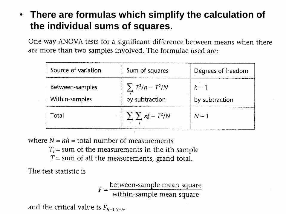
• There are formulas which simplify the calculation of

the individual sums of squares.

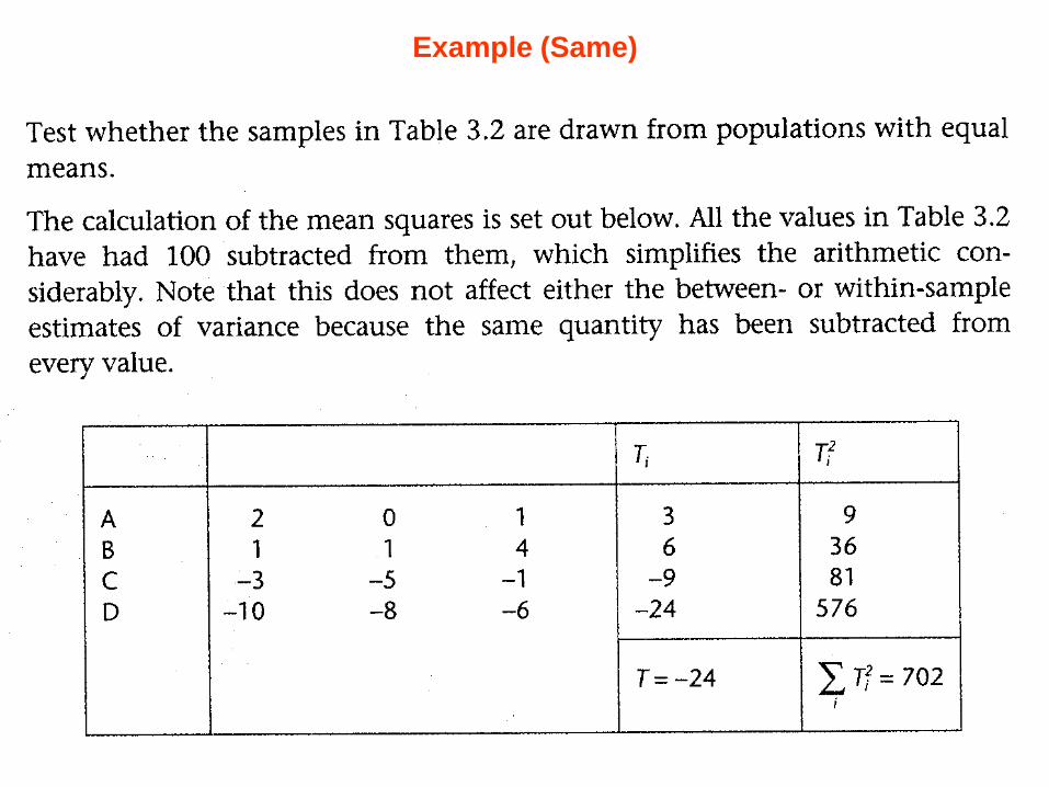
Example (Same)

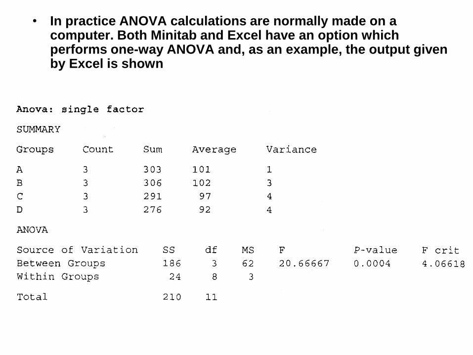
• In practice ANOVA calculations are normally made on a computer. Both Minitab and Excel have an option which performs one-way ANOVA and, as an example, the output given by Excel is shown

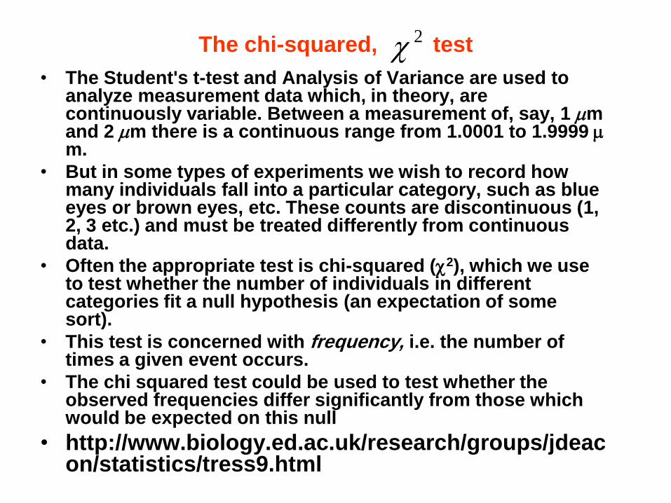
The chi-squared, test

• The Student's t-test and Analysis of Variance are used to analyze measurement data which, in theory, are continuously variable. Between a measurement of, say, 1 m and 2 m there is a continuous range from 1.0001 to 1.9999 m.

• But in some types of experiments we wish to record how many individuals fall into a particular category, such as blue eyes or brown eyes, etc. These counts are discontinuous (1, 2, 3 etc.) and must be treated differently from continuous data.

• Often the appropriate test is chi-squared (c2), which we use to test whether the number of individuals in different categories fit a null hypothesis (an expectation of some sort).

• This test is concerned with frequency, i.e. the number of times a given event occurs.

• The chi squared test could be used to test whether the observed frequencies differ significantly from those which would be expected on this null

• http://www.biology.ed.ac.uk/research/groups/jdeacon/statistics/tress9.html

2c

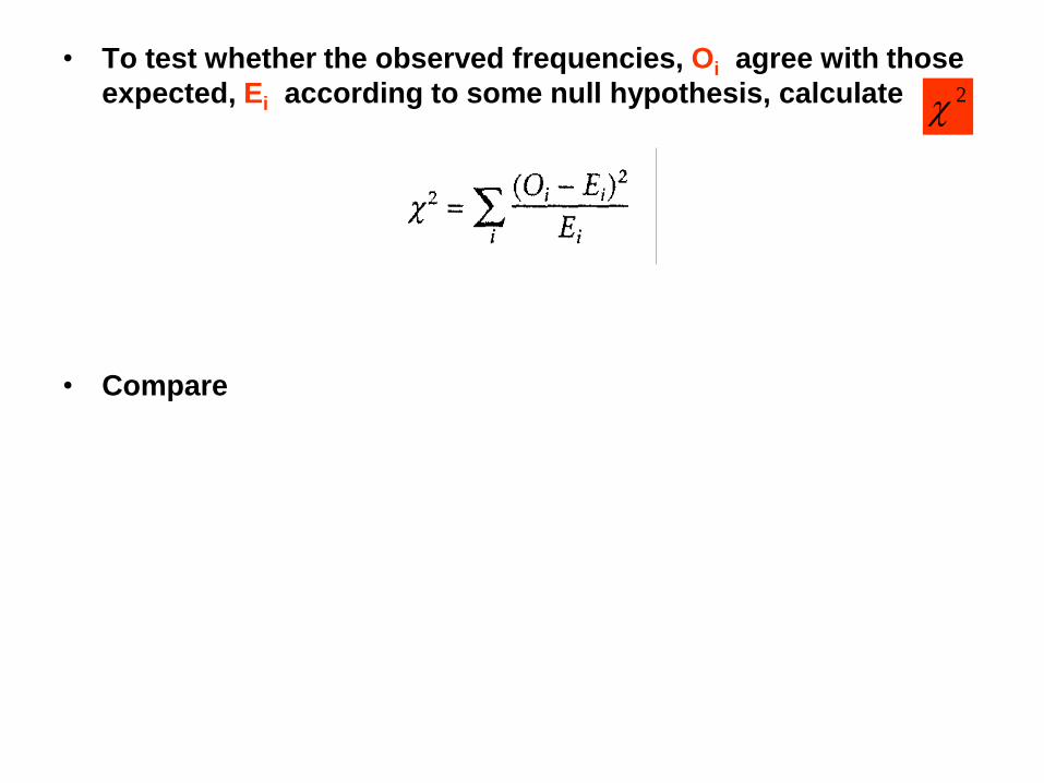
• To test whether the observed frequencies, Oi agree with those

expected, Ei according to some null hypothesis, calculate

• Compare

2c

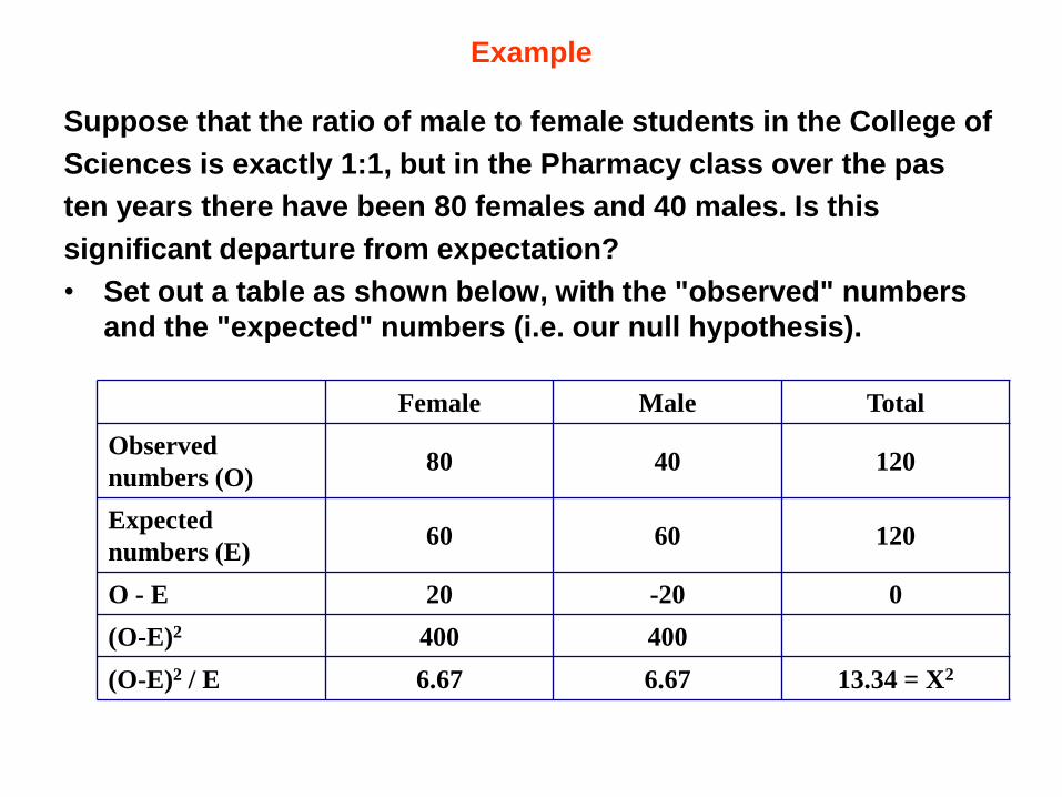
Example

Suppose that the ratio of male to female students in the College of

Sciences is exactly 1:1, but in the Pharmacy class over the pas

ten years there have been 80 females and 40 males. Is this

significant departure from expectation?

• Set out a table as shown below, with the "observed" numbers

and the "expected" numbers (i.e. our null hypothesis).

Total Male Female

120 40 80 Observed

numbers (O)

120 60 60 Expected

numbers (E)

0 -20 20 O - E

400 400 (O-E)2

13.34 = X2 6.67 6.67 (O-E)2 / E

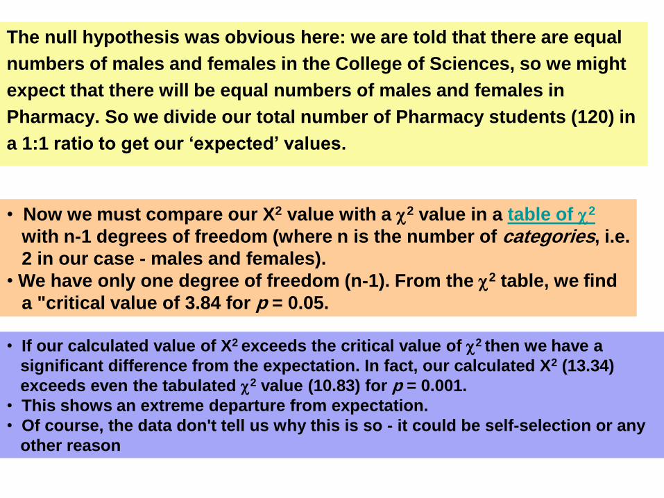
The null hypothesis was obvious here: we are told that there are equal

numbers of males and females in the College of Sciences, so we might

expect that there will be equal numbers of males and females in

Pharmacy. So we divide our total number of Pharmacy students (120) in

a 1:1 ratio to get our ‘expected’ values.

• Now we must compare our X2 value with a c2 value in a table of c2

with n-1 degrees of freedom (where n is the number of categories, i.e.

2 in our case - males and females).

• We have only one degree of freedom (n-1). From the c2 table, we find

a "critical value of 3.84 for p = 0.05.

• If our calculated value of X2 exceeds the critical value of c2 then we have a

significant difference from the expectation. In fact, our calculated X2 (13.34)

exceeds even the tabulated c2 value (10.83) for p = 0.001.

• This shows an extreme departure from expectation.

• Of course, the data don't tell us why this is so - it could be self-selection or any

other reason

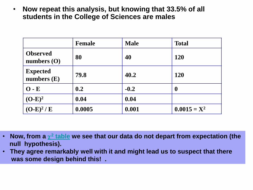
• Now repeat this analysis, but knowing that 33.5% of all students in the College of Sciences are males

Total Male Female

120 40 80 Observed

numbers (O)

120 40.2 79.8 Expected

numbers (E)

0 -0.2 0.2 O - E

0.04 0.04 (O-E)2

0.0015 = X2 0.001 0.0005 (O-E)2 / E

• Now, from a c2 table we see that our data do not depart from expectation (the

null hypothesis).

• They agree remarkably well with it and might lead us to suspect that there

was some design behind this! .

Example

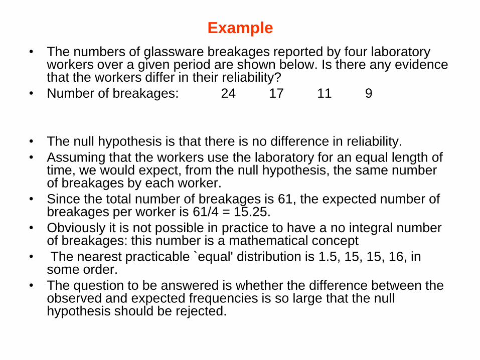
• The numbers of glassware breakages reported by four laboratory workers over a given period are shown below. Is there any evidence that the workers differ in their reliability?

• Number of breakages: 24 17 11 9

• The null hypothesis is that there is no difference in reliability.

• Assuming that the workers use the laboratory for an equal length of time, we would expect, from the null hypothesis, the same number of breakages by each worker.

• Since the total number of breakages is 61, the expected number of breakages per worker is 61/4 = 15.25.

• Obviously it is not possible in practice to have a no integral number of breakages: this number is a mathematical concept

• The nearest practicable `equal' distribution is 1.5, 15, 15, 16, in some order.

• The question to be answered is whether the difference between the observed and expected frequencies is so large that the null hypothesis should be rejected.

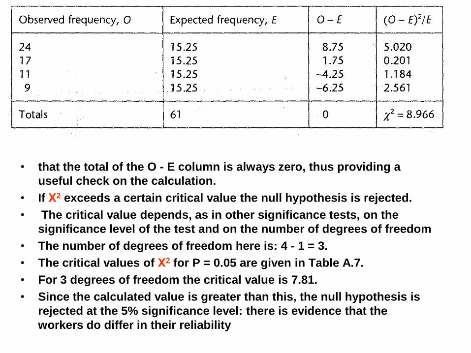
• that the total of the O - E column is always zero, thus providing a

useful check on the calculation.

• If Х2 exceeds a certain critical value the null hypothesis is rejected.

• The critical value depends, as in other significance tests, on the

significance level of the test and on the number of degrees of freedom

• The number of degrees of freedom here is: 4 - 1 = 3.

• The critical values of Х2 for P = 0.05 are given in Table A.7.

• For 3 degrees of freedom the critical value is 7.81.

• Since the calculated value is greater than this, the null hypothesis is

rejected at the 5% significance level: there is evidence that the

workers do differ in their reliability

Testing for normality of distribution

• As has been emphasized in this chapter, many statistical tests assume that the data used are drawn from a normal population.

• One method of testing this assumption, using the chi-squared test, as mentioned above

• Unfortunately, this method can only be used if there are 50 or more data points.

• It is common in experimental work to have only a small set of data.

• A simple visual way of seeing whether a set of data is consistent with the assumption of normality is to plot a cumulative frequency curve on special graph paper known as normal probability paper.

• This method is most easily explained by means of an example.

Example

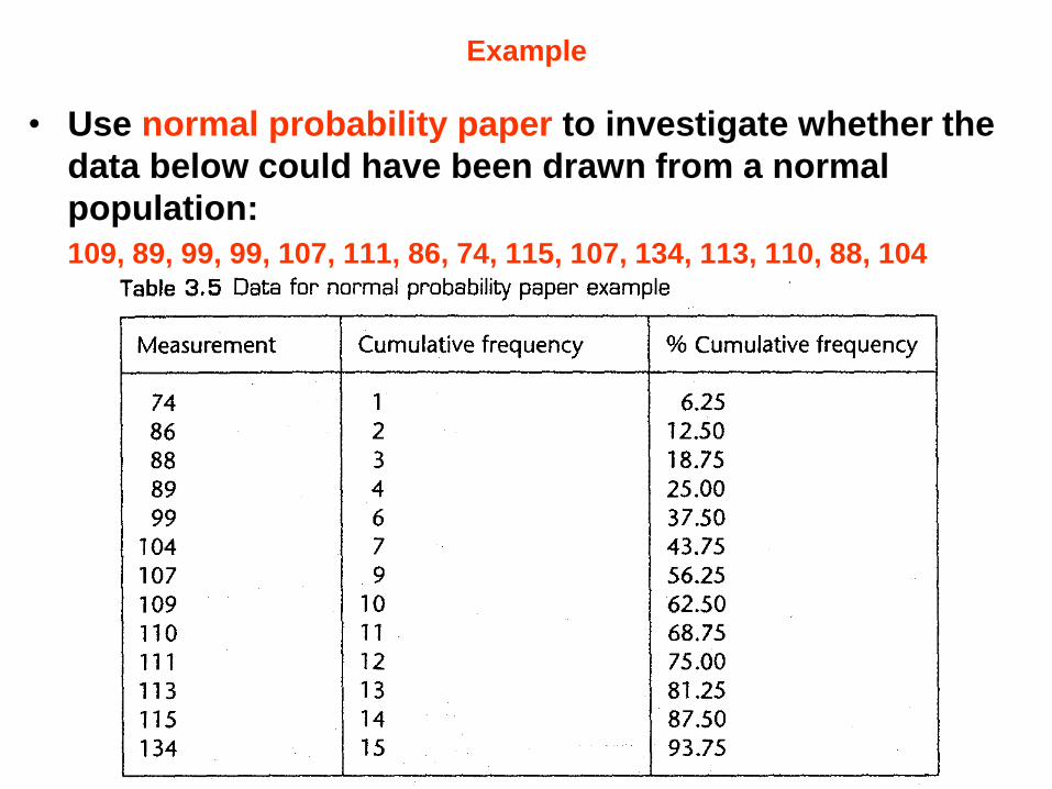
• Use normal probability paper to investigate whether the

data below could have been drawn from a normal

population:

109, 89, 99, 99, 107, 111, 86, 74, 115, 107, 134, 113, 110, 88, 104

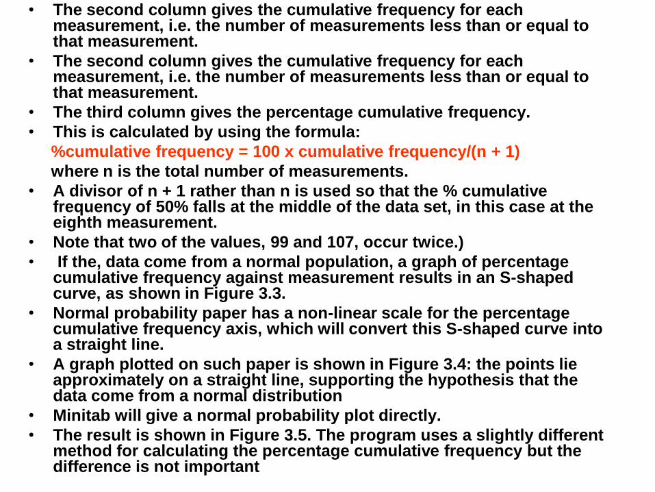
• The second column gives the cumulative frequency for each measurement, i.e. the number of measurements less than or equal to that measurement.

• The second column gives the cumulative frequency for each measurement, i.e. the number of measurements less than or equal to that measurement.

• The third column gives the percentage cumulative frequency.

• This is calculated by using the formula:

%cumulative frequency = 100 x cumulative frequency/(n + 1)

where n is the total number of measurements.

• A divisor of n + 1 rather than n is used so that the % cumulative frequency of 50% falls at the middle of the data set, in this case at the eighth measurement.

• Note that two of the values, 99 and 107, occur twice.)

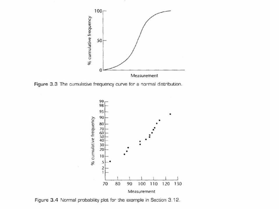
• If the, data come from a normal population, a graph of percentage cumulative frequency against measurement results in an S-shaped curve, as shown in Figure 3.3.

• Normal probability paper has a non-linear scale for the percentage cumulative frequency axis, which will convert this S-shaped curve into a straight line.

• A graph plotted on such paper is shown in Figure 3.4: the points lie approximately on a straight line, supporting the hypothesis that the data come from a normal distribution

• Minitab will give a normal probability plot directly.

• The result is shown in Figure 3.5. The program uses a slightly different method for calculating the percentage cumulative frequency but the difference is not important

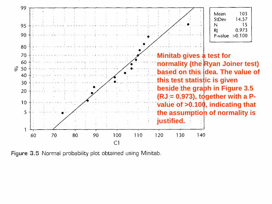
Minitab gives a test for

normality (the Ryan Joiner test)

based on this idea. The value of

this test statistic is given

beside the graph in Figure 3.5

(RJ = 0.973), together with a P-

value of >0.100, indicating that

the assumption of normality is

justified.

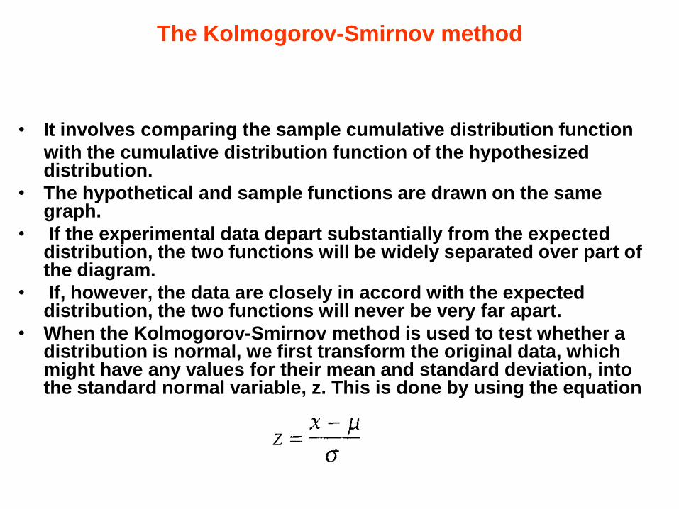
The Kolmogorov-Smirnov method

• It involves comparing the sample cumulative distribution function

with the cumulative distribution function of the hypothesized distribution.

• The hypothetical and sample functions are drawn on the same graph.

• If the experimental data depart substantially from the expected distribution, the two functions will be widely separated over part of the diagram.

• If, however, the data are closely in accord with the expected distribution, the two functions will never be very far apart.

• When the Kolmogorov-Smirnov method is used to test whether a distribution is normal, we first transform the original data, which might have any values for their mean and standard deviation, into the standard normal variable, z. This is done by using the equation

Example

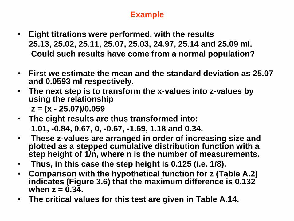
• Eight titrations were performed, with the results

25.13, 25.02, 25.11, 25.07, 25.03, 24.97, 25.14 and 25.09 ml.

Could such results have come from a normal population?

• First we estimate the mean and the standard deviation as 25.07 and 0.0593 ml respectively.

• The next step is to transform the x-values into z-values by using the relationship

z = (x - 25.07)/0.059

• The eight results are thus transformed into:

1.01, -0.84, 0.67, 0, -0.67, -1.69, 1.18 and 0.34.

• These z-values are arranged in order of increasing size and plotted as a stepped cumulative distribution function with a step height of 1/n, where n is the number of measurements.

• Thus, in this case the step height is 0.125 (i.e. 1/8).

• Comparison with the hypothetical function for z (Table A.2) indicates (Figure 3.6) that the maximum difference is 0.132 when z = 0.34.

• The critical values for this test are given in Table A.14.

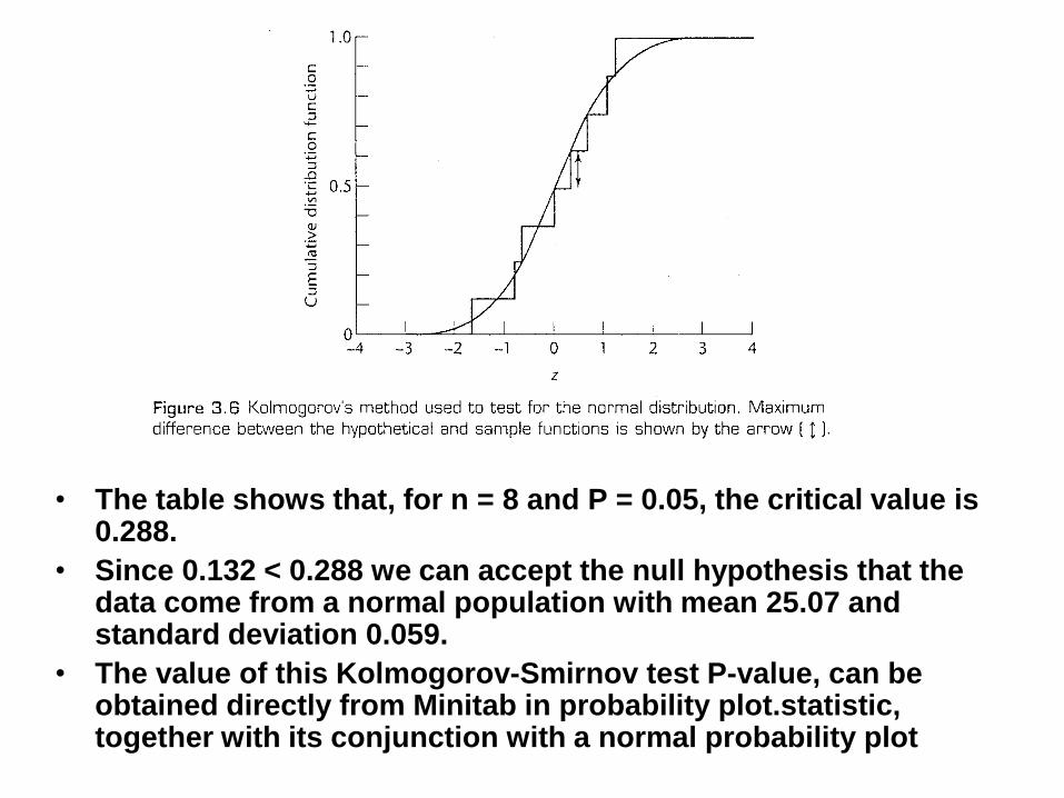
• The table shows that, for n = 8 and P = 0.05, the critical value is 0.288.

• Since 0.132 < 0.288 we can accept the null hypothesis that the data come from a normal population with mean 25.07 and standard deviation 0.059.

• The value of this Kolmogorov-Smirnov test P-value, can be obtained directly from Minitab in probability plot.statistic, together with its conjunction with a normal probability plot