ppp: delusion or reality? evidence from a nonlinear analysis

Electronic copy available at: http://ssrn.com/abstract=1356809

PPP: Delusion or Reality? Evidence from a Nonlinear Analysis♣

Juan A. Jiménez-Martin§ M. Dolores Robles-Fernandez§ [email protected] [email protected].

Abstract

In this paper we analyze the validity of the purchasing power parity (PPP) in a nonlinear framework using data for 18 bilateral US dollar exchange rates. Following Enders and Ludlow (2002), we use unit root and cointegration tests that do not assume a specific nonlinear adjustment. We find evidence of non-linear mean reversion in deviations from the PPP equilibrium in 11 out of 18 currencies. Additionally, to disentangle the respective contribution of exchange rate and prices to the adjustment toward the long run equilibrium, we estimate a Vector Error Correction Model. According to our empirical analysis, there exists a nonlinear mechanism to correct for deviation from the PPP equilibrium that comes mainly from the exchange rates. This is consistent with theoretical arguments on international goods markets under transaction costs as well as with an emerging strand of empirical literature. These results highlight the importance of neglecting the possibility of nonlinearity in the debate about the PPP and provide empirical evidence that supports the scenario of the PPP hypothesis as a reality. Keywords: Unit-root test, Cointegration test, Fourier approximation, nonlinear VECM, exchange rates, purchasing power parity. JEL classification: F31, C22, C32

♣ We are grateful to A. Novales and two anonymous referees for helpful comments. The paper has benefited of

comments from seminar participants at the George Washington University and from participants in the Unit root

and Testing Cointegration conference. We acknowledge the financial support of the Ministerio de Ciencia y Tecnología,

Spain, through the Project SEJ2006-14354/ECON and the Comunidad de Madrid through the Project 940063. § Departamento de Fundamentos del Análisis Económico II, Universidad Complutense, Campus de Somosaguas,

28223, Pozuelo de Alarcón, Madrid, Spain. Tel: +34 913942355. Fax: +34 913942613.

Electronic copy available at: http://ssrn.com/abstract=1356809

PPP: Delusion or Reality? Evidence from a Nonlinear Analysis

Abstract

In this paper we analyze the validity of the purchasing power parity (PPP) in a nonlinear framework using data for 18 bilateral US dollar exchange rates. Following Enders and Ludlow (2002), we use unit root and cointegration tests that do not assume a specific nonlinear adjustment. We find evidence of non-linear mean reversion in deviations from the PPP equilibrium in 11 out of 18 currencies. Additionally, to disentangle the respective contribution of exchange rate and prices to the adjustment toward the long run equilibrium, we estimate a Vector Error Correction Model. According to our empirical analysis, there exists a nonlinear mechanism to correct for deviation from the PPP equilibrium that comes mainly from the exchange rates. This is consistent with theoretical arguments on international goods markets under transaction costs as well as with an emerging strand of empirical literature. These results highlight the importance of neglecting the possibility of nonlinearity in the debate about the PPP and provide empirical evidence that supports the scenario of the PPP hypothesis as a reality. Keywords: Unit-root test, Cointegration test, Fourier approximation, nonlinear VECM, exchange rates, purchasing power parity. JEL classification: F31, C22, C32

1

1. INTRODUCTION

There is a large and growing literature indicating that traditional linear unit root tests do

not work well when there are significant nonlinearities in the data. This is an important problem

that appears frequently in the analysis of the theory of Purchasing Power Parity (PPP), which

states that the real exchange rate should have a tendency to return quickly to the mean when that

long-run ratio is disturbed for some reason. Taylor and Taylor (2004) provide a guide to the PPP

debate over the past three decades.

The rationality behind the PPP is a simple arbitrage hypothesis: When two identical goods

are traded at different prices in different countries, a profitable arbitrage opportunity arises. The

arbitrageurs can buy the good cheaply in one location and sell it at a higher price in the other. In

the absence of arbitrage costs, this process leads to convergence of the deviations from PPP

towards zero. Exchange-rate-adjusted prices are equalized across countries, leaving no room for

profitable arbitrage opportunities. Under this version, called relative PPP hypothesis, one would

expect stationarity in real exchange rate dynamics.

The parity condition rests on the assumption of perfect inter-country commodity

arbitrage and it is a central building block of many theoretical and empirical models of exchange

rate determination. Due to factors like transaction costs, taxation, subsidies, trade restrictions, the

existence of non traded goods, imperfect competition, foreign exchange market intervention, and

the different composition of market baskets and price indices across countries, one may expect

PPP to be valid only in the long run. Under this version, called unrestricted PPP hypothesis, prices

and nominal exchange rate should show a steady long-term relationship, and therefore one would

expect cointegration between them.

Empirical studies over long periods have supported long-run PPP (Diebold et al., 1991,

Taylor 1996, Michael et al., 1997). However, the literature finds mixed results when the recent

floating-rate period is examined. Using standard unit root tests Corbae and Ouliaris (1988),

Meese and Rogoff (1988), Edison and Fisher (1991) and Grilli and Kaminsky (1991) cannot

reject the unit root null hypothesis for real exchange rates in the managed-float regime. In

contrast, Pedroni (1997), Frankel and Rose (1996), Lothian (1997), Oh (1996), Wu (1996) and

Papell and Theodoridis (1998) find strong evidence of mean reversion in real exchange rates by

implementing panel data variants of standard unit-root tests. However, O’Connell (1998) strongly

disputes these mean reversion findings as they fail to control for cross-sectional dependence in

the data. Engel et al. (1997) report additional evidence against reversion to PPP based on panel

data. Papell (1997) and Liu and Maddala (1996) find that evidence of mean reversion in panels of

real exchange rates is very sensitive to the countries considered.

2

Recently, alternative explanations base the persistent deviations from parity on the

presence of market frictions that preclude commodity trade. Dumas (1992), Uppal (1993) and

Sercu et al. (1995) develop equilibrium models of real exchange rate determination that take into

account transaction costs. They show that adjustment of real exchange rate towards PPP is

necessarily a nonlinear process. Due to these frictions, there is an inactive range around parity in

which international arbitrage does not work. The adjustment process starts only when the

exchange rate moves out of this range. This non-linear adjustment to parity can be formulated

using variations of the threshold autoregressive model (e.g. STAR, ESTAR) and significant

empirical evidence has been found that supports these models.

However, as several authors report, even if threshold models had strong theoretical

justification for one tradable good, aggregating over all goods, and using a general price level,

would obscure the form of the implied nonlinearity for the aggregate relationship. For instance,

Juvenal and Taylor (2007) find that SETAR model characterizes well the deviations from the Law

of One Price for many currencies and sectors, although they discover a wide variation in the

results across countries and across sectors. Additionally some countries exhibit low thresholds for

a given sector.

Therefore, it is often difficult to discriminate among alternative nonlinear models using

standard diagnostic tools. For example, Rothman (1998) shows that different nonlinear models

(exponential autoregressive, threshold, smooth transition, etc.) all provide plausible estimates of

the US unemployment rate, yielding similar in-sample properties. Ludlow and Enders (2000) and

Enders and Ludlow (2002) show that Fourier functions allow approximating the different types

of nonlinearities present in time-series data. They point out that Fourier approximation can

capture the type of asymmetric adjustment contained in several macroeconomic variables. The

benefit of this procedure is that the nonlinearity can be estimated without specifying any

particular model.

Based on those findings, this paper uses the generalizations of the Dickey-Fuller and

Engle-Granger tests developed by Enders and Ludlow (2002) and Enders and Hoover (2003), for

analyzing the empirical validity of different versions of the PPP hypothesis using data for 18

bilateral US dollar exchange rates.1 The central idea of the Enders and Ludlow’s tests is to use a

trigonometric expansion to approximate the unknown form of an autoregressive coefficient

believed to be time varying. As Enders and Hoover (2003) and Robles et al. (2004) stress, the

flexibility of this approximation means that the tests are capable of detecting asymmetric

1 Enders and Ludlow (2002) have already provided an empirical evidence of the relative PPP, but it is applied only to the

logarithm of the real French franc/DM exchange rate.

3

adjustment processes that can arise from a number of different sources, namely structural breaks,

transaction costs, seasonality, or stochastic variations. These tests can perform quite well as

compared to Dickey-Fuller or Engle-Granger statistics when the researcher does not know the

form of the nonlinear adjustment mechanism.2

Our contribution to the existing literature is twofold. First, it is well known that

misclassifying a stable nonlinear process as nonstationary can be misleading the debate about

PPP. This paper sheds light on that debate. Our results suggest stronger evidence of non-linear

mean reversion in deviations of the PPP when using the Enders and Ludlow (2002) nonlinear

tests than when applying other linear and non-linear tests. In particular, we analyze the existence

of structural break in unit root and cointegration context. We also study the existence of

threshold autoregression in the exchange rate dynamics applying the Kapetanios et al. (2003,

2006) tests. Our results document that there exist nonlinear dynamics which cannot be solely

attributed to structural breaks, or ESTAR processes.

To prevent confusion, we want to remark that we are only interested in the nature of the

data-generating process (DGP) –linearity versus non-linearity. Hence, the methodology used here

is not an alternative to a TAR or an STAR model or to any other DGP processes. If one knows

the true DGP, then one must use it.

Second, this paper tries to give some insights on the economic mechanisms underlying

the nonlinear adjustment towards PPP. We analyze the relationship between nominal exchange

rates and prices in a multivariate framework. The origin of the PPP relationship lies in

international arbitrage in the goods market. In this sense, the national prices and/or the nominal

exchange rate should contribute to the achievement of the PPP, at least in the long-run. We

analyze the dynamic relationships among prices and exchange rates by estimating a vector error

correction model (VECM) with nonlinear adjustment, which allows studying the respective

contribution of the nominal exchange rate and the domestic and foreign prices to the adjustment

towards the PPP relation. Results of the non-linear VECM estimation indicate that the burden of

the adjustment towards PPP rests mainly on exchange rates and does not on prices. This

confirms the main result of Engel and Morley (2001) that the nominal exchange rate is the

primary adjuster to PPP disequilibria. Additionally, the estimates obtained show non-linear

behavior on the adjustment back to the PPP equilibrium. In summary, all these findings support

the validity of PPP when allowing for non-linear adjustment. 2 Kapetanios et al. (2003), Enders and Siklos (2001) or Bec et al. (2008) propose testing procedures to detect the presence of

nonstationarity against nonlinear stationarity when the nonlinear dynamics process leading the adjustment to the deviations of

PPP is a function of the size of deviations that can be modelized by some kind of threshold model. The Enders and Ludlow’s tests we use in this paper will still detect nonlinearity in such a situation.

https://www.researchgate.net/publication/222416688_Testing_for_a_Unit_Rozot_in_the_Nonlinear_STAR_Framework?el=1_x_8&enrichId=rgreq-06fdc817-140d-4017-a2c8-e0d5f3cb87ea&enrichSource=Y292ZXJQYWdlOzIyNzM0NzcwNTtBUzoxMDIxMzY3MzgyMjIwODNAMTQwMTM2MjcwNDU3MA==

4

The paper is organized as follows: Section 2 presents a brief description of different

version of the PPP hypothesis. Section 3 analyzes the data to be used and preliminary tests of the

PPP hypothesis are carried out. Section 4 outlines the Enders and Ludlow’s tests and shows the

estimation results. Section 5 presents the vector error correction model estimation, which goal is

to identify non-linear adjustments on exchange rates and prices for deviations from PPP. Finally,

Section 6 presents the main conclusions.

2. PURCHASING POWER PARITY: TWO VERSIONS

The key theoretical concept underlying our analysis of the connection between prices and

exchange rate is the Purchasing Power Parity. There are two senses in which the PPP might hold:

the relative version of PPP (RV-PPP)3 that requires movements in the relative prices levels to be

offsets in the same period by movements in the exchange rates that would imply a stationary real

exchange rate. Therefore a common strategy testing RV-PPP consists on analyzing the presence

of a unit root in the real exchange rate.

Additionally, recent studies have focused in an unrestricted version of PPP (UV-PPP) that

states a stable long-run relationship between the nominal exchange rate and prices. Let S be the

nominal exchange rate, measured in domestic currency units per foreign currency units, and P

(P*) the price levels in the domestic (foreign) country, then the UV-PPP can be expressed

statistically as:

β β β= + + +*0 1 2 ,t t t ts p p e (1)

where lower case letters denote that the variables are in logarithmic form, and et is an i.i.d.

stochastic error. UV-PPP involves testing for cointegration among the nominal exchange rate

and prices. The UV-PPP requires that te in (1) be a stationary process, that is, *( , , )t t ts p p should

form a cointegrated system (Engle and Granger, 1987).

Expression (1) also nests the RV-PPP. Imposing the “symmetry” restriction β1=–β2 =β

on the prices coefficients and the “proportionality” restriction β0=0, β=1, we obtain

3 There also exists the absolute version of PPP that posits equality between the price level in one country and the exchange rate

adjusted price level in the other. Strictly speaking, the absolute PPP hypothesis states that the exchange rate between the

currencies of two countries should equal the ratio of the price levels of the two countries. The measures of consumer prices

published by national statistical agencies are typically reported as indexes relative to a base year (say, 1995=100). Thus, they

only measure the rate of change of the price level from the base year, not its absolute level. Therefore, it does not make sense

testing this version of PPP when working with consumer index prices as it is done in this paper.

https://www.researchgate.net/publication/4895535_Cointegration_And_Error-Correction_Representation_Estimation_And_Testing?el=1_x_8&enrichId=rgreq-06fdc817-140d-4017-a2c8-e0d5f3cb87ea&enrichSource=Y292ZXJQYWdlOzIyNzM0NzcwNTtBUzoxMDIxMzY3MzgyMjIwODNAMTQwMTM2MjcwNDU3MA==

5

− − =*( )t t t ts p p e , i. e. the real exchange rate. The RV-PPP would require the stationarity of the

real exchange rate.

In this paper, we test both RV-PPP (i.e. is the real exchange rate stationary?) and UV-PPP

(i.e. is there a stable relationship among the exchange rate and the level of prices?). The UV-PPP

does not impose the homogeneity and proportionality restrictions entailed by the RV-PPP, which

might not hold in practice. A well-known fact in this testing situation is that there is a large loss

of power from estimating the cointegrating vector when it is actually known. So, when these

restrictions are true and cointegration tests are carried out instead of stationary tests, the loss of

power from estimating the cointegration vector increases the probability of failing to reject the

null when it is actually false. Therefore, unit root along with cointegration tests should be carried

out when testing the PPP hypothesis. As we mentioned in the previous section, in this paper we

apply a battery of linear and non-linear tests for both hypothesis to consider potential non-linear

factors behind PPP.

3. Data and preliminary PPP analysis

3.1. Data Description

Our sample includes data for 19 industrialized countries: the US, Austria, Belgium,

Canada, Denmark, Finland, France, Germany, Greece, Italy, Japan, Mexico, the Netherlands,

Norway, Portugal, Spain, Sweden, Switzerland, and the United Kingdom. The database spans the

period from January 1973 to February 2005 for all the countries except Mexico, Greece and the

Netherlands. The sample starts in January 1981 for Mexico, in April 1981 for Greece and in

January 1982 for the Netherlands.4

We use the Consumer Prices Index (CPI) as a proxy for prices. The nominal exchange

rates are end-of-month bilateral US dollar exchange rates. In all cases, the US is the foreign

country. The German CPI data come from the German Federal Statistical Office,5 the remaining

series have been extracted from the International Monetary Fund’s International Financial Statistics

database. 4 The US dollar exchange rate for participating currencies in the single European currency after January 1999 has been calculated

using the official conversion rates announced on December 31, 1998 and the Euro/Dollar exchange rate. Greece joins the

European Economic Community in April 1981. This leads the Bank of Greece to adjust the trade-weighted system adopted

following the collapse of the Bretton-Woods agreement placing a greater weight on European currencies and smaller weight on

the dollar. Greece is joining the euro group as the 12th member on January 1, 2001. The Netherlands fixes its currency to the

German Mark until January 1981. After the country’s public finances went bankrupt in 1982, Mexico began a profound

transformation. The foreign debt crisis of 1981-82 had a severe and irreversible effect on public finances and political thinking.

Until that date, Mexico’s economy was heavily subsidized and protected from competition. 5 Before 1991 the consumer prices refers only to West Germany.

6

Figure 1 shows the 18 real exchange rates for the eighteen currencies against the US

dollar. It is noteworthy that each real exchange rate has exhibited large and persistent deviations

around its mean. Nevertheless, during this period the real exchange rates considered seem to

revert to an unknown reference value.

[Insert Figure 1]

3.2. Preliminary RV-PPP Tests

In this stage of the analysis, we examine the evidence on the RV-PPP testing for

stationarity of the real exchange rates using four tests: two linear tests, a sequential test to detect

structural change and the Kapetanios et al. (2003) test. Firstly, we use the well known Augmented

Dickey Fuller (ADF). We test the null hypothesis of 0θ = from the following regression:

θ δ ε−

− −=

Δ = + Δ +∑1

11

,p

t t i t i ti

y y y (2)

In addition, we use the more efficient Dickey Fuller Generalized Least Squares (DF-

GLS), developed by Elliott et al. (1996)6 who propose to apply the ADF test to the detrended

series, dty . To compute d

ty first we must estimate by OLS the model:

( ) ( )' ( )t t td y a d y a a uφ= +

where ( )t td z a z= if t=1 and 1( )t t td z a z az −= − if t>1, ,t t tz y x= and tx includes a constant

and a trend. Elliott et al. (1996) recommend using 1 13.5 /a T= − . Finally, we

compute ' ˆ( )dt t ty y x aφ≡ − .

Additionally, we include the possibility of one structural change in the real exchange rate

series. We employ the sequential ADF test proposed by Fernández and Peruga (1999) and

applied by Sosvilla and Fernández (2003) and Fernández and Robles (2008) to detect unit roots in

a structural change context. They suggest to estimate the model:

τμ μ θ δ ε− −=

′Δ = + + + Δ +∑11

,p

t tt i t iti

y y yD (3)

where:

{ττ τ λ λτ

<= ∈ −≥

0 [ ] , ( , 1 ) 1 [ ]tt T

D t T (4)

is a dummy variable that places the break date in a window from the τ % initial to (1-τ )% final

observations. For each possible breaking date, τT , we computed two statistics from regression

(2): the standard pseudo t-ratio for testing the null hypothesis of a unit root (θ =0), and the 6 DF-GLS test has substantially improved power when an unknown mean or trend is present. As Elliot et al. (1996) prove, the

modified test works well in small samples.


7

absolute value of the t-ratio for testing the stability of the stochastic trend (μ′= 0). From these

sequences we select the supreme (InfADF) in the first case and the mean (SupMu) in the second

case.

Finally, we consider another kind of non linearity by computing the Kapetanios et al.

(2003) ESTAR unit-root test (KSS). KSS tests the null of θ =0 in the following regression:

θ δ ε−

− −=

Δ = + Δ +∑1

31

1

,p

t t i t i ti

y y y (5)

being the alternative hypothesis an ESTAR process.

Table 1 presents the results of these tests. 7 In all cases we include a constant and a time

trend in the test regression.8 The lag length for the differenced dependent variable on the right

hand side of the test regression is determined using the Akaike information criterion (AIC).

These tests produce little support for RV-PPP. All of them never reject the null of

nonstationarity, whit the exception of the KSS in the case of The Netherlands.

[Insert Table 1]

Cheung et al. (2004) test for unit roots on the French, German, Italian, Japanese, and

British real exchange rates. They find stationarity for all cases, except Japan. For France,

Germany and Italy their sample spans the same period than ours. In contrast to Cheung et al.

(2004), we did not find these real exchange rates stationary, but we use a different specification

since our DF-GLS test includes a constant and trend. Kapetanios et al. (2003) find evidence of

nonlinear mean reversion in real exchange rates for France, Germany, Italy, Japan and the United

Kingdom. Their discrepancies with our result may be related to differences in the analyzed

samples since they use quarterly data covering a larger sample size (1957:1-1198:4). It seems that

a different nonlinear process there exists during the period that we analyzed.

3.3. Preliminary UV-PPP Tests

We also test the UV-PPP using Engle and Granger (1987) methodology (EG test) by

estimating expression (1) and testing for stationarity of the residual using the ADF statistic.

Figure 2 shows the estimated residuals for the 18 exchange rates analyzed.

7 All individual series (nominal exchange rates and prices) have also been tested for the presence of unit root using the ADF and

DF-GLS tests. Consistent with the literature, the null hypothesis of a single unit root cannot be rejected in any case. To save

space, these results are not reported here, but are available upon request. 8 Some researchers, such as Cheung et al. (1998), and Koedijk et al. (1998), have found that the stochastic processes of some of the

real exchange rates cannot be adequately modeled without the inclusion of a linear deterministic time trend. The linear

deterministic time trend is generally interpreted as representing systematic differences in productivity growth between tradable

and non-tradable goods in the two countries. On the other hand, other researchers, for example, Papell and Theodoridis

(1998), and Amara and Papell (2006) consider a linear time trend in the real exchange rate as inconsistent with long-run PPP.

https://www.researchgate.net/publication/222454902_The_re-emergence_of_PPP_in_the_1990s?el=1_x_8&enrichId=rgreq-06fdc817-140d-4017-a2c8-e0d5f3cb87ea&enrichSource=Y292ZXJQYWdlOzIyNzM0NzcwNTtBUzoxMDIxMzY3MzgyMjIwODNAMTQwMTM2MjcwNDU3MA==


8

[Insert Figure 2]

Additionally, we apply other three two-step cointegration tests: the DF-GLS cointegration

test developed by Perron and Rodriguez (2001) (GLS-C), who propose to estimate the

cointegrating relationship using GLS detrended o quasi-differenced data to each variable of the

system,9 and then test for unit roots with ADF in the residual series. Secondly, as in the RV-PPP

case, we consider the possibility of structural change by applying the Gregory and Hansen (1996)

sequential cointegration test (GH), which explicitly permits a regime shift in the cointegrating

relationship:

τ τμ μ β β ε= + + + + ' ' ,t t tt tty x xD D (6)

where τ tD is described in (4) and ( )*,t t tx p p= . GH computes the ADF on the residual series

for all possible break points and select the smallest value obtained (in tables appear as GH test)

along with the mean value (GHmean).

We also consider the cointegration test developed by Kapetanios et al. (2006), which test

the null hypothesis of no cointegration against an alternative of a globally stationary ESTAR

cointegration by testing θ =0 in (5) where now ty are the residuals obtained from the

cointegrating relationship (1).

As Table 2 reports, the linear tests, EG and GLS-C, never reject the null of non-

cointegration but the non-linear ones find evidence in favor of UR-PPP in several cases. For the

Gregory and Hansen (1996) method we show both GH and GHmean. The first of them rejects

the null for France, Greece and Mexico. The estimated dates in which probably a structural

change happens are March-1983, January-2000 and April-1988 respectively. Nevertheless, the

GHmean does not detect cointegration in any case. Finally, the KSS test rejects the null for

Japan, Mexico and Switzerland, indicating the existence of some kind of threshold cointegration

for these countries.

Other authors, as Michael et al. (1997), Baum et al. (2001), employ the exponential smooth

transition autoregression (ESTAR) framework to analyze the dynamic behavior of deviations

from PPP, finding evidence of nonlinear adjustment.

[Insert Table 2]

In summary, the evidence of mean reversion in US dollar-based PPP deviations series is

quite weak (we reject the RV-PPP except for one country (the Netherlands) and only for five 9 Perron and Rodriguez (2001) analyze residual based tests for cointegration. Among other cases, they consider the standard ADF

test, derive their asymptotic distribution assuming a general quasi-differencing parameter, c and tabulate its critical values.

Their simulations reveal an important power gain from using GLS detrended data, especially if the quasi-difference parameter

is set as suggested by Elliot et al. (1996).

https://www.researchgate.net/publication/23564983_Testing_for_cointegration_in_nonlinear_smooth_transition_error_correction_models_Econometric_Theory_22_279-303?el=1_x_8&enrichId=rgreq-06fdc817-140d-4017-a2c8-e0d5f3cb87ea&enrichSource=Y292ZXJQYWdlOzIyNzM0NzcwNTtBUzoxMDIxMzY3MzgyMjIwODNAMTQwMTM2MjcwNDU3MA==

9

cases (France, Greece, Japan, Mexico and Switzerland) we cannot reject the UR-PPP. As

mentioned above, recent studies explain the persistence of managed-float deviations from parity

as the consequence of market frictions that impede commodity trade. Several models take into

account transaction costs and show that adjustment to the equilibrium is necessarily a non-linear

stochastic process. Nevertheless, this non-linear mean-reverting process is hard to detect using

linear unit root tests. Moreover, it is often difficult to discriminate among alternative non-linear

models using standard diagnostic tools. In our case, the non-linear tests applied find evidence in

favor of PPP only for 6 currencies and show two different sources of non-linearity. These results

lead us to explore more deeply the PPP analysis by considering a testing method capable to

detect the null of mean reversion with non-linear adjustment process without specifying the exact

non-linear functional form.

4. NONLINEAR ADJUSTMENT

4.1. Why to use the Enders and Ludlow (2002) test when analyzing PPP?

To analyze the RV-PPP, we apply the Enders and Ludlow (2002) and Enders and Hoover

(2003) unit root test (UR-EL) that suggests the following modification of the Augmented Dickey-

Fuller (ADF) test:

α δ ε−

− −=

= + Δ +∑1

11

( ) ,p

t t i t i ti

y t y y (7)

where { }ty is the process of interest, and ε t is a stochastic error term. The autoregressive

coefficient is a deterministic but an unknown function of time. The key feature is that equation

(7) allows for asymmetric adjustment because the degree of autoregressive decay is not constant.

This specification bridge the two areas of nonstationarity and nonlinearity in the context

of unit root tests and it is specially useful when α(t) sometimes exceeds the unity and yt, exhibits

periods of decay and periods of potentially explosive behavior. This is what makes this approach

sensible in testing real exchange rate stationarity, because empirical analysis reveals that this

variable typically shows huge variability in short to medium terms, and exhibits periods of

oscillating reversion along with explosive behavior periods. International trade is affected by

factors like transaction costs, taxation, subsidies, trade restrictions or official intervention that

could cause asymmetric movements in exchange rates. These effects make deviations from PPP a

mean-reverting non-linear stochastic process, because exchange rates and domestic and foreign

prices adjust to past disequilibria as a function of multiple and complex factors. Sometimes, the

real exchange rate can be stationary but these frictions in international trade introduce some

periods of inaction, within which the misspricing is left uncorrected.

10

Note that although (7) is linear in yt,, α(t) can be a deterministic polynomial expression in

time, a p-th order difference equation, a threshold or a switching function, so the specification is

reasonably general. Several papers posit the nature of the asymmetry and provide a parametric

estimate of this autoregressive coefficient. However, if there is a little a priori information

concerning the actual form of the asymmetry, the estimated model is likely to suffer from

misspecification errors. Therefore, what Ludlow and Enders (2000) suggest is to allow the

asymmetric adjustment,10 α(t), to be an unknown time dependent function that they approximate

using Fourier series. As Ludlow and Enders (2000) note, under very weak conditions, α(t) can be

approximated by a sufficiently long Fourier series even though the sequence in question is not

periodic, 11 allowing us to approximate different types of non-linearities. The advantage of this

procedure is that we can analyze the presence of nonlinear factors in the data without specifying

the particular nonlinear model.

UR-EL test considers equation (7) parameterized as:

1

0 1 1 11

[ sin(2 ) cos(2 )] ,p

t t i t i ti

y a a k t T b k t T y yπ π δ ε−

− −=

= + + + Δ +∑ (8)

where k is an integer number in the interval [1, T/2].12 Note that the traditional Dickey-Fuller test

emerges as a special case when α(t)=a0. Although many frequencies could be needed to mimic the

actual behavior of the time-varying coefficient, for testing purposes, Enders and Ludlow (2002)

consider only using a single frequency. After all, if a1= b1= 0 cannot be rejected for all

frequencies, the null hypothesis of time invariance is rejected.13

10 When the model is linear in parameters, it is not able to account for a number of important properties of time series data, such

as the clustering of large and small errors or thick-tailed distributions. Models with asymmetric adjustment are able to obtain

good forecasts for heteroskedastic time series. As Ludlow and Enders (2000) show, the Fourier approximation captures the

conditional volatility present in the NYSE Transportation Index.

11 Let the function α(t) have a Fourier expansion: ( ) [ sin(2 ) cos(2 )],0 1t a a k t T b k t Tk kk

α π π∞∑= + +=

and define Fs(t) to be

the sum of the Fourier coefficients: ( ) [ sin(2 ) cos(2 )],1

sF t a kt T b kt Ts k kk

π π∑= +=

then for any arbitrary positive

number h, there exists a number N such that: ( )( ) st F t hα − < for all s N≥ .

12 Half the sample size is a natural upper bound arising from the standard deterministic harmonic decomposition. 13 For time series analysis the frequency domain often provides valuable information on the dynamics of the series. The frequency

domain properties of an economic time series may provide a useful complement to its time domain properties. The frequency

approach is useful to identify the length of business cycles and seasonal patters that may be important. There may also be

unknown cycles at other frequencies that should be identified. The method allows quantitative definition of the cycle, and

extraction of long, medium or short term components, according to the researcher’s wish. The frequency information gives

quality insight to the function shape where rapid changes imply high frequencies and gradual changes imply low frequencies.

https://www.researchgate.net/publication/223846366_Estimating_non-linear_ARMA_models_using_Fourier_coefficients?el=1_x_8&enrichId=rgreq-06fdc817-140d-4017-a2c8-e0d5f3cb87ea&enrichSource=Y292ZXJQYWdlOzIyNzM0NzcwNTtBUzoxMDIxMzY3MzgyMjIwODNAMTQwMTM2MjcwNDU3MA==

https://www.researchgate.net/publication/223846366_Estimating_non-linear_ARMA_models_using_Fourier_coefficients?el=1_x_8&enrichId=rgreq-06fdc817-140d-4017-a2c8-e0d5f3cb87ea&enrichSource=Y292ZXJQYWdlOzIyNzM0NzcwNTtBUzoxMDIxMzY3MzgyMjIwODNAMTQwMTM2MjcwNDU3MA==

11

4.2. Mean reverting analysis

A key feature of the UR-EL test is that it allows for different patterns of mean-reverting

behavior: Monotone decay, decay with explosive periods, oscillations, and oscillations with

explosive periods. The nature of reversion depends on the values of c* and r. The sufficient and

necessary condition for non-explosive adjustment process, i.e. for mean-reverting behavior is:

< + ≤ = +2 2 20 1 11 4 for 2, where .a r r r a b (9)

In particular, for a0 > 0 and r < 2 the series reverts to an attractor if a0<1+r2/4.

Additionally, the four different types of decay are related with the values of a0 and r:

- If a0+r < 1, α(t) never exceeds the unity and there is overall reversion that can be either:

(1) Monotone when a0 > r, which means that α(t) is never negative, or

(2) Oscillatory when a0 < r, which implies that there will be periods such that α(t)<0 .

- If a0+r >1, there will be k periods when α(t) exceeds unity. This implies that while the

overall process ultimately reverts to the attractor, the sequence exhibits periods of explosive

behavior that can be either:

(3) Monotone when a0 > r , or

(4) Oscillatory when a0 < r.14 Although this test allows for a number of nonlinear adjustment processes, this is specially

useful when α(t) sometimes exceeds unity so that the series being analyzed exhibits periods of

decay and periods of explosive behavior. Figure 1 shows some evidence of possible explosive

behavior in real exchange rate adjustment toward a long-run equilibrium. Real exchange rates

seem to show significant deviations from the Law of One Price. There are periods when the

process is divergent –explosive- and the exchange rate is away from parity, but then it becomes

mean reverting. In some real exchange rates, the jump to mean-reverting behaviour is sudden (for

instance, Austria, Belgium, Denmark, France, The Netherlands, and Switzerland), while in others

it is smooth (Canada, Portugal, Spain).

In general, in most cases there is little a priori information concerning the actual form of

the adjustment, and the class of nonlinear models is unlimited. For this reason, we use the EL

methodology, which allows us to test PPP in a nonlinear context without needing to pre-specify a

particular formulation for the adjustment process.

14 We can represent ( ) ( )α π π= + + 0 1 1( ) sin 2 cos 2t a a k t T b k t T as ( )α π= + +0( ) cos 2 ,t a r k t T d where

= +2 21 1r a b and ( )= 1arcsin /d a r . If a0+r>1, and since ( )π +cos 2 k t T d can equal unity, there will be k periods

when α(t) exceed the unity, there being explosive periods. Oscillations appear when α(t) <0, that being the case when a0 < r

and ( )π +cos 2 k t T d = –1.

12

4. 3. Relative PPP

To test the RV-PPP, we run a regression of the real exchange rate over a constant and a

linear trend and compute the t̂e series.15 Then, the following regression is estimated for all the

integer values of k in the interval 1 to T/2, to select the most suitable k frequency:

1

1 1 11

ˆ ˆ ˆ[ sin(2 ) cos(2 )] ,p

t t i t i ti

e c a k t T b k t T e eπ π δ ε−

− −=

Δ = + + + Δ +∑ (10)

where c =a0–1 and p–1 is the number of lags needed to completely eliminate residual

autocorrelation.16 We choose the value of k that minimizes the sum of the squared residuals. This

value is denoted by k*, and the coefficients linked to such frequency by c*, a1* and b1

*. The period, */T k , indicates the length of time required for the process to repeat a full cycle. Therefore, the

bigger is k*, the smaller is the period.

Finally, Enders and Ludlow (2002) calculate critical values for three statistics from the

estimation of equation (10): F_all, F_trig, and τ-statistic. The testing procedure is as follow: first,

we compute the F_all statistic, this is an F statistic for the null hypothesis c*= a1*= b1

*= 0. This

statistic is used to test whether the series is a random walk. If the F_all null hypothesis is rejected,

the series in question exhibits mean-reversion, which may be, linear, non-linear or both. Second,

if the F_all null hypothesis is not rejected then we compute the F_trig statistic for the null

hypothesis a1*=b1

*= 0, which implies r = 0. If this hypothesis is rejected, there is a non-linear

mean-reverting behavior in the data. Finally, if the F_trig null hypothesis is not rejected then we

compute the τ-statistic for the null hypothesis c*= 0. Rejecting the hypothesis c* = 0 is a necessary

condition for mean-reversion only when r = 0. 17 If this null hypothesis is also not rejected then

we reject the RV-PPP.

4. 3.1. Results for relative PPP

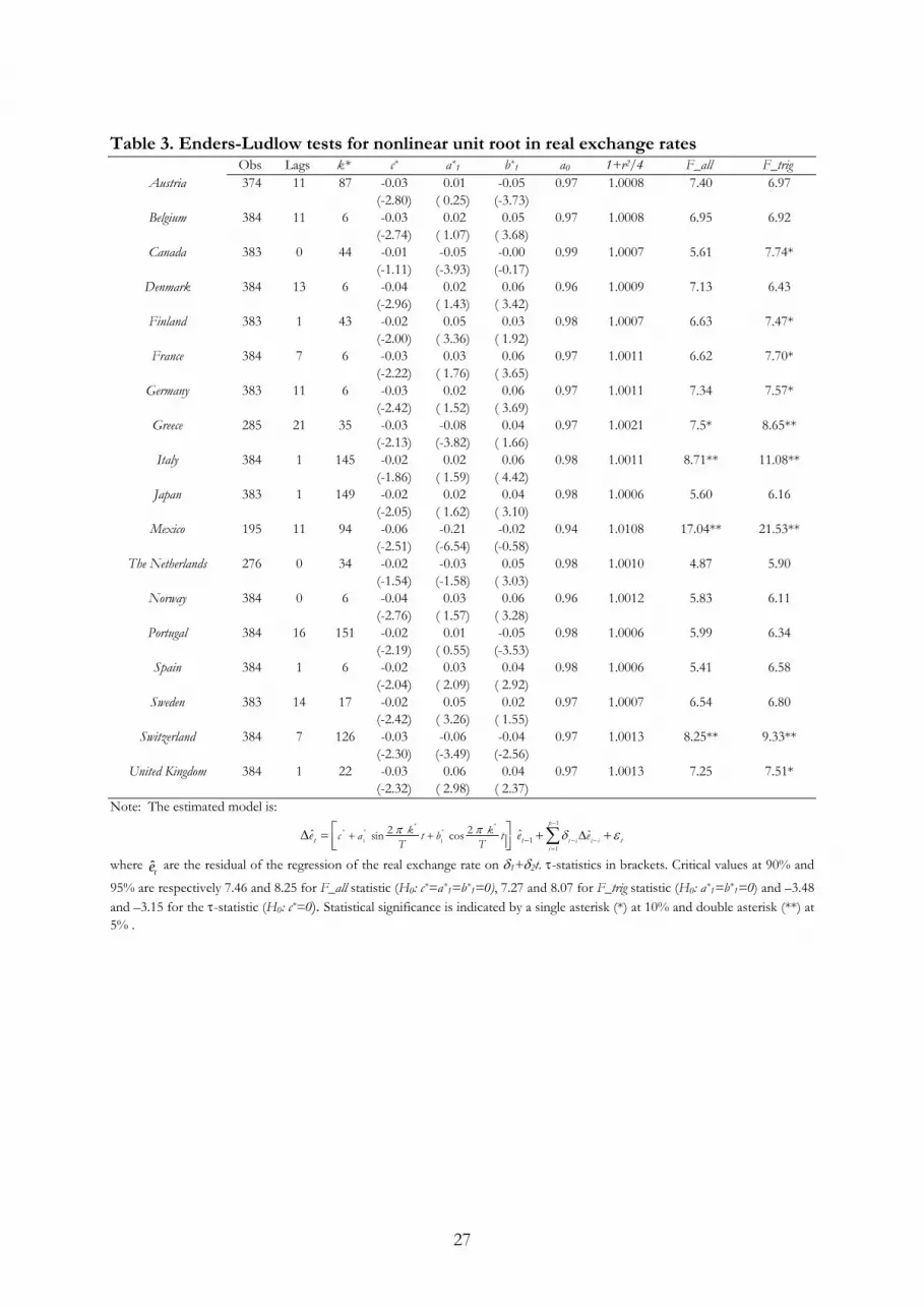
UR-EL test results are shown in Table 3. They provide stronger evidence of mean

reversion in real exchange rates than the preliminary tests in Section 3 do. In particular, F_all and

F_trig reject the null of nonstationary behavior for Greece, Italy, Mexico and Switzerland.

Additionally, the F_trig detects nonlinear adjustment processes for other five countries (Canada,

Finland, France, Germany, and the United Kingdom). In total, we find nonlinearities in 9 out of

18 real exchange rates. This result is equivalent to accepting the hypothesis that the adjustment to

the equilibrium on the real exchange rate follows a nonlinear stochastic process that is mean 15 Additionally, we apply the test on the demeaned real exchange rate. To save space, we only present the demeaned and

detrended case, but results are available upon request. 16 We use differenced data to allow for comparison with the Engle and Granger (1987) test for the linear case. 17 However, if the F_trig test correctly indicates r > 0, rejecting the null of de c* test against the alternative hypothesis c < 0, is

sufficient to guarantee reversion.

13

reverting. Based on structural break tests and the KSS evidence, it seems that neither regimen

changes nor ESTAR processes would be enough to capture the real exchange rate mean

reversion to the equilibrium.

[Insert Table 3]

As Table 3 shows, we cannot reject the null c*= 0 in any case. This test has low power

when a*0 is near 0.9, as is our case. This finding is consistent with the results of the linear unit-

root tests shown in Table 1.

On the other hand, the value of a0* fulfils the reversion condition in (9) for all the

countries. Estimated values of k*, for mean-reverting real exchange rate, fall between 6 and 145

and the period of the cycle goes from 2 and a half months (Italy) up to 5 years (France and

Germany). We did not find frequencies that may be related to a seasonal or calendar effect.

Cycles lasting about 5 years may have a connection to the business cycle. Attaching a structural

economic interpretation to the short cycles that accommodate rapid changes is difficult. On

average we find a two-year cycle.

As for the pattern of decay detected, for all cases we find a*0>r and a*

0+r >1, indicating

the existence of periods of explosive behavior in real exchange rates. These finding indicate the

presence of periods of decay and periods of nonstationarity, this being compatible with the

existence of market frictions and asymmetries that make arbitrage profitable only under some

conditions.

Summarizing, we find stronger evidence in favor of the RV-PPP than in the previous

analysis. UR-EL tests find mean-reversion in nine real exchange rates (Canada, Finland, France,

Germany, Greece, Italy, Mexico, the United Kingdom and Switzerland) whereas the ADF, GLS,

InfADF and KSS tests did not rejected the non-stationarity null in all the countries but the

Netherlands.

4.4. Unrestricted PPP

The UR-EL test can be easily generalized to test for cointegration in the Engle and

Granger (1987) framework. It takes a residual-based two-step approach. In the first stage, we

obtain the residuals β β β= − + + *0 1 2

ˆ ˆ ˆˆ ( ),t t t tu s p p with β β β0 1 2ˆ ˆ ˆ, , and being OLS estimates. In

the second stage, we estimate regression (10) where t̂e is the residual series of the regression of

the deviations from the unrestricted version of PPP, ˆtu , on an intercept and a linear deterministic

trend.

14

The test of the null of no cointegration against the alternative of globally stationary

cointegration (C-EL) is based on three statistics F_all, F_trig, and τ-statistic, which critical values

can be found in the Table 2 of Enders and Ludlow (2002).18

The power of the three tests depends on the values of r and c*. As r increases, the power

of F_all, F_trig and τ-statistic increases. Besides, for small values of c* and r, the power of F_trig is

slightly higher than F-all and the τ-statistic

4.4.1. Results for UV- PPP

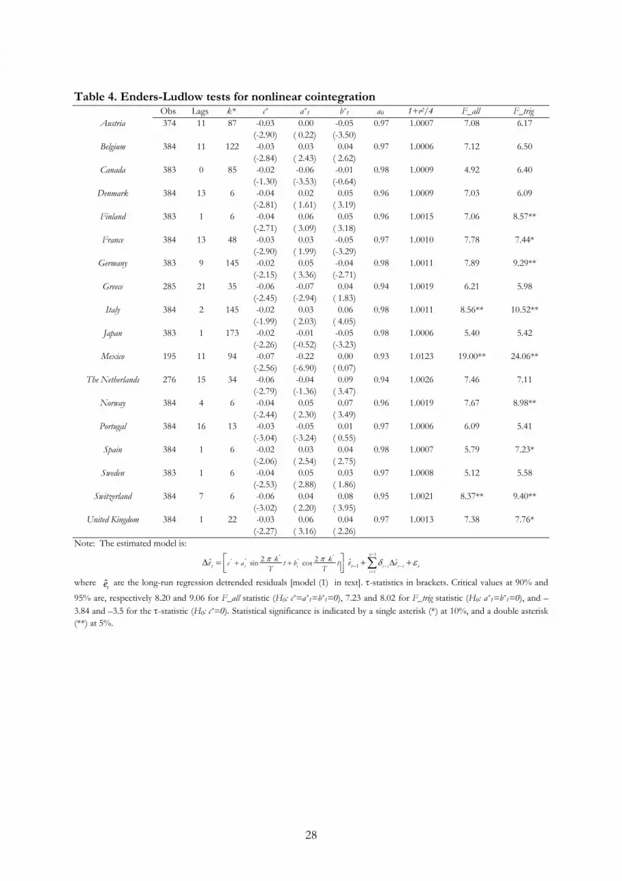
As can be seen in Table 4, the F_all and F_trig statistics provide stronger evidence of UV-

PPP than the preliminary cointegration tests do. In particular, F_all and F_trig reject the null of

no cointegration for Italy, Mexico and Switzerland at 5%. In addition, the F_trig test detects

nonlinearity in the speed of convergence back to equilibrium on other six countries (Finland,

France, Germany, Norway, Spain and the United Kingdom).

[Insert Table 4]

The estimated values of a0* always fulfill the cointegration condition. For all countries we

find a0 > r and a0+r > 1. This means that the deviations from PPP ultimately decay to an

attractor, although the sequence exhibits periods of explosive performance. When PPP holds,

estimated values of k* fall between 6 and 145 and the period of the cycle varies from two and a

half months (Germany, Italy and Mexico) to five years (Finland, Norway, Spain and Switzerland).

The average duration of a cycle is approximately two years.

Thus, C-EL test detects cointegration among prices and the exchange rate for nine

countries, whereas we only detected a cointegrating relationship for five countries (France,

Germany, Japan, Mexico and Switzerland) when considering structural breaks or threshold

cointegration. It is noteworthy that C-EL tests detect cointegration for each currency that

previous tests did, except for Japan. Hence, the Enders and Ludlow (2002) test appear to be very

robust in the sense that it seems to capture non-linearities caused by structural breaks or ESTAR

behavior and additionally, it capture other undetermined forms of the nonlinear factor.

5. A NON-LINEAR ERROR CORRECTION MODEL

We have found evidence of nonlinear mean-reverting behavior in deviations from the

PPP hypothesis (the relative version, the unrestricted version, or both) in 11 out of 18 analyzed

countries. The RV-PPP holds for nine countries (Canada, Finland, France, Germany, Greece,

Italy, Mexico, Switzerland and the United Kingdom) and the UV-PPP for other nine countries

18 We also analyze the demeaned unrestricted PPP. The results are almost the same that in the detrended case. For this reason, to

conserve space, these results are not reported here, but are available upon request.

15

(Finland, France, Germany, Italy, Mexico, Norway, Spain, Switzerland and the United Kingdom).

Note that we find both RV-PPP and UV-PPP for seven countries (Finland, France, Germany,

Italy, Mexico, Switzerland and the United Kingdom), only the RV-PPP for Canada and Greece

and the UV-PPP for Norway and Spain.

These results contrast with those we found in the previous analysis, with evidence of

convergence to long run equilibrium only in six currencies. As expected, for most of these six

cases we also find stationarity in deviations from PPP with the Fourier approximation.

Additionally, our results suggest stronger evidence in favor of the long run PPP than that

found by other authors. For example, Baum et al. (2001) analyze the same panel of countries that

we do, with the exception of Mexico, using a shorter sample. They find nonlinearities only in

seven countries within an ESTAR framework. In our case, we find a nonlinear adjustment to

PPP for the same countries (Finland, France, Germany, Italy, Norway and the United Kingdom).

Additionally, we find nonlinear adjustments in other two cases (Spain and Switzerland).

Overall, we find that the majority of nominal exchange rates and prices are cointegrated

and the adjustment towards the long-term relationship is non-linear. This behavior is surely

related to the existence of transaction cost in international goods market. From a multivariate

perspective, this implies that the domestic price and/or the foreign price and/or the nominal

exchange rate are expected to adjust the departures from PPP in a nonlinear way. To model this

behavior, we propose a cointegrated model with non-linear adjustments. In particular, we

estimate the following vector error correction model (VECM) exhibiting Fourier-decay:

1 1

111 *

1

11 12 13 11 *

21 22 23 22**

33 31 32 33

2

2

1

sin

cos

ˆp t

tti

t

t t

t ti

t t

k tTk t

T

s sp pep p

mmm

π

π

α α α

α α α

α α α

εεε

− −

−−=

−

Δ ΔΔ Δ= + + +Δ Δ

⎛ ⎞⎛ ⎞⎛ ⎞⎛ ⎞ ⎛ ⎞⎛ ⎞⎜ ⎟⎜ ⎟⎜ ⎟⎜ ⎟ ⎜ ⎟⎜ ⎟Φ⎜ ⎟⎜ ⎟⎜ ⎟⎜ ⎟ ⎜ ⎟⎜ ⎟⎜ ⎟⎜ ⎟ ⎝ ⎠⎝ ⎠ ⎝ ⎠⎝ ⎠ ⎝ ⎠⎝ ⎠

∑ (11)

where = −Φ …1, , 1,i i p are 3x3 coefficient matrices. This model allows disentangling the

respective contribution of the nominal exchange rate and the two prices to the adjustment

towards the PPP relationship. In particular, the adjustment process to past disequilibria is split in

three different terms: a linear one, captured by the α 1i , i = 1,2,3 coefficients, and two non-linear

terms, captured by πα*

22sini

k tT and πα

*2

2cosik t

T , i = 1,2,3.

To analyze the role of the variables in the adjustment process and study the dynamic

flows of information among them, we use the short- and long-term Granger causality concepts.

As for the later, according to the Engle-Granger representation theorem, if two variables are

cointegrated, at least one of them must respond to deviations from the long-run equilibrium

relationship (Granger, 1986). The alpha parameters in (11) allow us to examine what variables

16

respond to disequilibria. In particular, a variable will be considered as weakly exogenous if it

does not react to past disequilibria, i. e. the corresponding ijα , j=1, 2, 3, is not significant. On the

other hand, we analyze short-term Granger causality to identify the transmission channels of

information among the variables in the PPP system by testing whether lagged values of the

changes in variable i are relevant for forecasting the variable j.

[Insert table 5]

The model is estimated in two steps. First, we estimate the long-run equation (1) and we

then use the lagged residuals 1t̂e − and the value of k* selected in (5) to estimate model (6). Table 5

presents estimation results of the nonlinear VECM.19 The first three columns show the estimated

coefficients of the long-run relationship (70 % of them have the right sign, β1 >0 and β2 < 0).20

The remaining columns show estimated coefficients, which represent the adjustment to past

disequilibria in the exchange rate equation (columns 5 to 7), in the domestic price equation

(columns 8 to 10) and in the foreign price equation (columns 11 to 13).

The exchange rate responds to past disequilibria in all countries, suggesting that exchange

rates adjust for deviations from PPP.21 This result is in line with those presented by Engle and

Morley (2001), among others. In most of the cases, the response of exchange rates contains a

linear component and a non-linear one, since not only α11, but also α12 or α13 are individually

significant.22 The evidence on price adjustment to deviations from PPP is weaker.

Finally, analyzing the results for domestic price equations we only find significant

response to deviations from PPP for two countries: nonlinear response in Belgium and Norway.

The response of the foreign price is linear for Denmark and France and nonlinear only for

France.

These results suggest that nominal exchange rates take most of the burden of the

adjustments to long-run PPP, in most of the cases through a non-linear correction mechanism.

Most likely, this reflects some degree of stickiness in consumer prices in all countries. This kind

of stickiness is frequently found in the literature.

19 The estimated models appear to pass all the standard diagnostic tests. To save space, we do not include these results but are

available upon request. 20 The explanatory variables in the long run relationship are highly correlated and this may affect to the signs and values of the

estimated parameters.

21 Our previous results on the stability of deviations from PPP only allow to understand the α 1i , i=1,2,3 coefficients as

adjustment coefficient to past disequilibria for those countries with evidence in favor of the PPP. For the other countries, these

coefficients capture responses to changes in a nonstationary relation of the variables. 22 We approximate the distribution of these significance test statistics by a normal standard distribution.

17

Similar conclusions are found in Enders and Dibooglu (2001) who also find support for

the UV-PPP. They estimate asymmetric error correction models using data form the post-Breton

Woods period, focusing on the French franc and the German mark as base currencies against

five European currnencies. They also find asymmetric price and/or exchange rate adjustment to

positive deviations from PPP than for negative deviations. Although exchange rate shows most

of the adjustment to the long-run equilibrium, they find some positive responses on prices (rising

prices) to close the gap between the long-run PPP and its efective rate. Less evidence is found of

negative responses on prices (declining prices)

We also analyze short term linear Granger causality in order to study the temporal flow of

information among changes in the variables in the PPP system. Using the standard definition, a

variable is said to cause another if the introduction of the lags of the causal variable in the model

of the caused one improves the forecast of the caused variable.23 Results are shown in Table 6.

[Insert table 6]

We find little evidence of bi-directional linear causality between nominal exchange rates

and prices. Lagged domestic prices changes are only significant in the equation of exchange rates

for Portugal. Lagged foreign prices changes are significant for Belgium, France, Japan, Norway,

Portugal, Switzerland and the United Kingdom. On the other hand, lagged exchange rate changes

are significant in the case of Germany, Mexico, the Netherlands, Norway and Switzerland in the

equation of domestic prices and only for Denmark, and Portugal in the case of foreign prices. No

significant pattern seems to emerge from these observations.

Remarkably, we find short-term bilateral feedback between domestic and foreign prices

changes, the lags of each one of them being jointly significant in the equation of the other for

almost all the countries in the sample. This result may reflect the presence of exogenous shocks

such as shocks in raw materials prices like petroleum, simultaneously affecting domestic and

foreign prices.

6. CONCLUSIONS

It is clear than neglecting the possibility of nonlinearity when analyzing PPP could lead to

misclassify a stable nonlinear relationship between prices and exchange rates as a nonstationary

process. This is also true when we make a wrong assumption on the nonlinear model driving the

adjustment to the long run equilibrium. This in turn would mislead the debate about the PPP. To

23 To test the existence of short-term causality, we start from the estimated VECM in expression (11) and carry out a joint

significance test of the lags of the causal variable in the equation of the caused one.

18

avoid that, this paper analyzes deviations from the PPP equilibrium allowing a general nonlinear

adjustment as Enders and Ludlow (2002) suggest.

Using the US dollar as the base currency against other eighteen currencies, we find

evidence of nonlinear mean-reverting behavior in real exchange rates and in deviations from long

run PPP, which is consistent with the PPP hypothesis adjusted for market frictions such as

transaction costs. The analysis reveals that there is evidence of the relative version of PPP in nine

countries and of the unrestricted version of PPP in other nine countries. In seven of them we

find evidence of both versions of PPP. Adjustments to deviations from PPP may go trough short

periods of explosive behavior, with overall mean-reverting performance. These results reinforce

the insight of previous studies regarding the possible presence of non-linear, but stationary

adjustment processes to long-run PPP.

Additionally, in order to disentangle the respective contribution of the exchange rate and

prices to the adjustment towards the PPP equilibrium, we estimate a nonlinear VECM. We find

evidence of a nonlinear mechanism to correct for deviations from long-run PPP that comes

mainly from the exchange rate market. In the short term, we find a bi-directional flow of

information between domestic and foreign prices, possibly due to experiencing common shocks,

while we rarely find Granger causality between price changes and nominal exchange rate changes.

As we noted above, our results support the hypothesis that the relationship among

exchange rate and prices contains some form of nonlinearity or structural break. However, these

results provide little information about the exact nature of the nonlinearity. This information is

crucial in order to propose a realistic model for the nonlinear adjustment process. As it has been

pointed in the literature, some models that belong to the threshold family can be good

approximations but this analysis is outside the scope of this paper. In spite of this, future research

should explore the way to discriminate among different structures that could mimic the

nonlinearity observed in the PPP relationship.

19

REFERENCES.

Amara, J., D. Papell (2006). “Testing for purchasing power parity using stationary covariates,”

Applied Financial Economics, 16 (1-2), 29-39).

Bec, F., A. Guay, and E. Guerre (2008). “Adaptive Consistent Unit root Tests Based on

Autoregressive Threshold Model,” Journal of Econometrics, 142 (1), 94-133

Cheung, Y. W., K. S Lai and M. Bergman, (2004). “Dissecting the PPP puzzle: The

unconventional roles of nominal exchange rate and price adjustments”, Journal of

International Economics 64, 135-150.

Cheung, Y. W., K. S Lai and S. Kon, (1998). “Parity reversion in real exchange rates during the

post-Bretton Woods period”, Journal of International Money and Finance, 18, 751-768.

Corbae, D. and S. Ouliaris (1988). “Cointegration and tests of purchasing power parity.” Review of

Economics and Statistics, 70, 508-521.

Davidson, R. and J. MacKinnon (1993). Estimation and Inference in Econometrics. Oxford University

Press, Oxford.

Diebold, F., S. Husted, and M. Rush (1991). “Real exchange rate under the gold standard.” Journal

of Political Economy, 99, 1151-1158.

Dumas, B. (1992). “Dynamic equilibrium and the real exchange rate in a spatially separated

world.” Review of Financial Studies, 5, 153-180.

Edison, H. J. and E. Fisher (1991). “A long-run view of the European monetary system.” Journal

of International Money and Finance, 10, 53-70.

Elliott, G., T. J. Rothenberg and J. H. Stock (1996). “Efficient tests for an autoregressive unit

root.” Econometrica, 64, 813–836.

Enders, W. and S. Dibooglu (2001). “Long-run Purchasing Power Parity with Asymmetric

Adjustment”, Southern Economic Journal, 68, 433-445.

Enders, W. and J. Loudlow (2002). “Non-linear decay: Tests for an attractor using a Fourier

approximation.” Working Paper 01-02-02, University of Alabama.

http://www.cba.ua.edu/efl/working_papers/pdf/WP01-02-02.pdf

Enders, W. and G. A. Hoover (2003). The effect of robust growth on poverty: A nonlinear

analysis. Applied Economics, 35(9), 1063-1071.

Engel, C. and J. Morley. (2001) “The Adjustment of Prices and the Adjustment of the Exchange

Rate.” NBER.

Engel, M. K. Hendrickson and J. H. Rogers (1997). “Intra-national, intra-continental and intra-

planetary PPP.” International Finance Discussion Papers, 589, Washington DC: Board of

Governors of the Federal Reserve System.

20

Engle, R. and C. Granger (1987). “Co-integration and error correction: representation,

estimation, and testing.” Econometrica, 55, 251-276.

Fernández, J. L. and R. Peruga (1999), “Un Contraste ADF Secuencial para la Detección de

Cambios en la Tendencia Estocástica”, WP 5/99, Universidad Europea, Madrid.

Fernández. J. L. and M. D. Robles (2008). “Time-series model forecasts and structural breaks:

evidence from Spanish pre-EMU interest rates,” Applied Economics, 40(13), 1707-1721.

Fernández-Serrano, J. L. and S. Sosvilla (2003). “Modelling the linkages between US and Latin

American stock markets.” Applied Economics, 35(12), 1423-1434.

Frankel, J. and A. Rose (1996). “A panel project on purchasing power parity: mean reversion

within and between countries.” Journal of International Economics, 40, 209-24.

Granger, C. (1986). “Developments in the study of cointegrated variables.” Oxford Bulletin of

Economics and Statistics, 48, 213-228.

Gregory, A.W., Hansen B.E. (1996). “Residual based tests for cointegration in models with

regime shifts.” Journal of Econometrics, 70, 99-126.

Grilli, V. and G. Kaminsky (1991). “Nominal exchange rate regimes and the real exchange rate:

evidence for the United States and Great Britain, 1885-1986.” Journal of Monetary Economics,

27, 191-212.

Juvenal, L., and M. P. Taylor (2007). “The law of one price: Nonlinearities in sectoral real

exchange rate dynamics”, University of Warwick.

Kapetanios, G.; A. Shin and Y. Snell (2003). “Testing for a unit root in the nonlinear STAR

framework”, Journal of Econometrics, 112, 359–379.

Kapetanios, G.; A. Snell and Y. Shin (2006). “Testing for cointegration in nonlinear smooth

transition error correction models”, Econometric Theory, 22, 279–303.

Koedijk, K., P. Schotman, and M. Van Dijk (1998). “The re-emergence of PPP in the 1900’s”,

Journal of International Money and Finance, 17, 51-61.

Liu, P. C., and G. S. Maddala (1996). “Do panel data cross-country regressions rescue purchasing

power parity (PPP) theory?.” Working Paper, Department of Economics, Ohio State

University.

Lothian, J. (1997). “Multi-country evidence on the behaviour of purchasing power parity.” Journal

of International Money and Finance, 16, 19-35.

Ludlow, J., and Enders, W. (2000). “Estimating non Linear ARMA Models Using Fourier

Coefficients,” International Journal of Forecasting, 70, 261-290.

MacKinnon, J. G. (1996). “Numerical distribution functions for unit root and cointegration

tests.” Journal of Applied Econometrics, 11, 601-618.

21

Meese, R. and K. Rogoff (1988). “Was it real? The exchange rate interest differential relation over

the modern floating exchange rate period.” Journal of Finance, 43, 933-48.

Michael, P., A. Nobay and D. Peel (1997). “Transaction costs and non-linear adjustments in real

exchange rates: an empirical investigation.” Journal of Political Economy 105, 862-879.

O’Connell, P. G. J. (1998). “The overvaluation of purchasing power parity.” Journal of International

Economics, 44, 1-19.

O’Connell, P. and S. Wei. (2002) “The bigger they are the harder they fall.” Journal of International

Economics, 56, 21-53.

Obstfeld, M. and A. Taylor (1997). “Non-linear aspects of goods-market arbitrage and

adjustment: Heckscher’s commodity point revisited.” Journal of Japanese and International

Economics, 11, 441-479.

Oh, K. Y. (1996). “Purchasing power parity and unit root tests using panel data.” Journal of

International Money and Finance, 15, 405-18.

Papell, D. H. (1997). “Searching for stationarity: purchasing power parity under the current

float.” Journal of International Economics, 43, 313-32.

Papell, D. H. and H. Theodoridis (1998). “Increasing evidence of purchasing power parity over

the current float.” Journal of International Money and Finance, 17, 41-50.

Pedroni, P. (1997). “Panel cointegration: asymptotic and finite sample properties of pooled time

series tests with an application to the PPP hypothesis (new results).” Working paper,

Department of Economics, Indiana University.

Perron, P., and G. Rodriguez, (2001). “Residual based test for cointegration with GLS detrended

data.” PhD dissertation, University of Montreal.

Robles, M. D.; M. L. Nieto, and A. Fernández, (2004), “Nonlinear Intraday Dynamics in

Eurostoxx50 Index Markets.” Studies in Nonlinear Dynamics & Econometrics, 8(4), art. 3.

Rothman, P. (1998). “Forecasting asymmetric unemployment rates.” Review of Economic and

Statistics, 80, 164-168.

Sercu, P., R. Uppal, and C. Van Hull, (1995). “The exchange rate in the presence of transaction

costs: implications for tests of purchasing power parity.” Journal of Finance, 50, 1309–1319.

Taylor, A., and M. Taylor, (2004). “The Purchasing Power Parity Debate.” The Journal of Economic

Perspectives. 18, 135-158-

Taylor, A. (1996). “International capital mobility in history: purchasing-power parity in the long

run.” Working Paper 5742. National Bureau of Economic Research, Cambridge, MA.

Tong, H. (1990). Non-linear Time Series. Oxford University Press, Oxford.

22

Uppal, R. (1993). “A general equilibrium model of international portfolio choice.” Journal of

Finance, 48, 529–553.

Wu, Y. (1996). “Are real exchange rates non-stationary? Evidence from a panel data test.” Journal

of Money, Credit and Banking, 28, 54-63.

23

Figure 1. Standardized real exchange rates (RV-PPP)

-2

-1

0

1

2

3

4

74 76 78 80 82 84 86 88 90 92 94 96 98 00 02 04

Austria

-3

-2

-1

0

1

2

3

74 76 78 80 82 84 86 88 90 92 94 96 98 00 02 04

Belgium

-2

-1

0

1

2

3

74 76 78 80 82 84 86 88 90 92 94 96 98 00 02 04

Canada

-2

-1

0

1

2

3

4

74 76 78 80 82 84 86 88 90 92 94 96 98 00 02 04

Denmark

-3

-2

-1

0

1

2

3

74 76 78 80 82 84 86 88 90 92 94 96 98 00 02 04

Finland

-2

-1

0

1

2

3

74 76 78 80 82 84 86 88 90 92 94 96 98 00 02 04

France

-2

-1

0

1

2

3

4

74 76 78 80 82 84 86 88 90 92 94 96 98 00 02 04

Germany

-2

-1

0

1

2

3

74 76 78 80 82 84 86 88 90 92 94 96 98 00 02 04

Greece

-3

-2

-1

0

1

2

3

74 76 78 80 82 84 86 88 90 92 94 96 98 00 02 04

Italy

-3

-2

-1

0

1

2

3

74 76 78 80 82 84 86 88 90 92 94 96 98 00 02 04

Japan

-2

-1

0

1

2

3

4

74 76 78 80 82 84 86 88 90 92 94 96 98 00 02 04

Mexico

-2

-1

0

1

2

3

74 76 78 80 82 84 86 88 90 92 94 96 98 00 02 04

Netherlands

-3

-2

-1

0

1

2

3

4

74 76 78 80 82 84 86 88 90 92 94 96 98 00 02 04

Norway

-3

-2

-1

0

1

2

3

74 76 78 80 82 84 86 88 90 92 94 96 98 00 02 04

Portugal

-3

-2

-1

0

1

2

3

74 76 78 80 82 84 86 88 90 92 94 96 98 00 02 04

Spain

-2

-1

0

1

2

3

74 76 78 80 82 84 86 88 90 92 94 96 98 00 02 04

Sweden

-3

-2

-1

0

1

2

3

4

74 76 78 80 82 84 86 88 90 92 94 96 98 00 02 04

Switzerland

-3

-2

-1

0

1

2

3

4

74 76 78 80 82 84 86 88 90 92 94 96 98 00 02 04

United Kingdom

24

Table 1. Unit root tests for the real exchange rate

Obs ADF GLS InfADF Break date SupMu Break date KSS Austria 374 -1.98 -1.87 -2.42 1985:04 2.03 1984:12 -2.69 Belgium 384 -1.83 -1.81 -2.60 1980:06 2.10 1978:09 -2.53 Canada 383 -2.05 -2.24 -2.83 1991:08 2.46 1991:08 -1.18

Denmark 384 -1.94 -1.72 -2.20 1985:07 1.96 1985:01 -2.67 Finland 383 -2.28 -1.45 -2.66 1992:07 2.14 1992:07 -2.12 France 384 -1.90 -1.81 -2.59 1980:07 1.55 1980:07 -1.92

Germany 384 -1.80 -1.86 -2.31 1979:11 1.84 1985:01 -2.27 Greece 286 -2.55 -2.29 -2.95 1985:11 3.80 1985:11 -2.19 Italy 384 -2.08 -2.12 -2.62 1985:07 2.07 1985:01 -1.91 Japan 383 -2.08 -1.69 -3.71 1985:07 3.19 1985:07 -2.04 Mexico 196 -3.03 -1.29 -2.70 1991:10 1.72 1991:10 -3.23**

The Netherlands 277 -1.64 -1.67 -2.51 1985:11 1.92 2001:06 -1.50 Norway 384 -2.25 -2.15 -2.50 1980:06 1.75 1978:08 -1.97 Portugal 384 -1.58 -1.65 -2.01 1989:04 2.41 1985:01 -2.19 Spain 384 -1.72 -1.60 -2.39 1985:05 1.83 1985:01 -1.67 Sweden 383 -1.76 -1.73 -2.50 1992:07 1.97 1992:07 -2.25

Switzerland 384 -2.54 -1.81 -2.94 1985:05 2.16 1985:01 -1.69 United Kingdom 384 -2.54 -2.53 -2.74 1986:09 2.28 1985:01 -2.57

Note: All the tests are performed including constant and time trend in the regression. Asymptotic critical values for cointegration taken from MacKinnon (1996): -3.42 (5 %), -3.13 (10 %). Eliott et al. (1996) propose a simple modification of the GLS tests in which the data are first detrended, so that explanatory variables are “taken out” of the data prior to running the test regression. Asymptotic critical values for GLS taken from Eliott et al. (1996), -2.89 (5%), -2.57 (10%). Asymptotic critical values for InfADF [-4.31 (5%), -4.06 (10%)] and for SupMu [-4.15 (5%), -3.91 (10%)] taken from Fernández and Peruga (1999). Asymptotic critical values for KSS taken from Kapetanios et al. (2003): -3.40 (5 %), -3.13 (10 %): Statistical significance is indicated by a single asterisk (*) at 10%, and a double asterisk (**) at 5%.

25

Figure 2. Standardized deviations from long run PPP (UV-PPP)

-2

-1

0

1

2

3

4

74 76 78 80 82 84 86 88 90 92 94 96 98 00 02 04

Austria

-2

-1

0

1

2

3

4

74 76 78 80 82 84 86 88 90 92 94 96 98 00 02 04

Belgium

-4

-3

-2

-1

0

1

2

3

74 76 78 80 82 84 86 88 90 92 94 96 98 00 02 04

Canada

-2

-1

0

1

2

3

4

74 76 78 80 82 84 86 88 90 92 94 96 98 00 02 04

Denmark

-3

-2

-1

0

1

2

3

4

74 76 78 80 82 84 86 88 90 92 94 96 98 00 02 04

Finland

-2

-1

0

1

2

3

4

74 76 78 80 82 84 86 88 90 92 94 96 98 00 02 04

France

-2

-1

0

1

2

3

4

74 76 78 80 82 84 86 88 90 92 94 96 98 00 02 04

Germany

-4

-3

-2

-1

0

1

2

3

74 76 78 80 82 84 86 88 90 92 94 96 98 00 02 04

Greece

-3

-2

-1

0

1

2

3

4

74 76 78 80 82 84 86 88 90 92 94 96 98 00 02 04

Italy

-3

-2

-1

0

1

2

3

74 76 78 80 82 84 86 88 90 92 94 96 98 00 02 04

Japan

-2

-1

0

1

2

3

74 76 78 80 82 84 86 88 90 92 94 96 98 00 02 04

Mexico

-3

-2

-1

0

1

2

3

4

74 76 78 80 82 84 86 88 90 92 94 96 98 00 02 04

Netherlands

-3

-2

-1

0

1

2

3

4

74 76 78 80 82 84 86 88 90 92 94 96 98 00 02 04

Norway

-3

-2

-1

0

1

2

3

4

74 76 78 80 82 84 86 88 90 92 94 96 98 00 02 04

Portugal

-2

-1

0

1

2

3

4

74 76 78 80 82 84 86 88 90 92 94 96 98 00 02 04

Spain

-3

-2

-1

0

1

2

3

4

74 76 78 80 82 84 86 88 90 92 94 96 98 00 02 04

Sweden

-3

-2

-1

0

1

2

3

4

74 76 78 80 82 84 86 88 90 92 94 96 98 00 02 04

Switzerland

-3

-2

-1

0

1

2

3

4

5

74 76 78 80 82 84 86 88 90 92 94 96 98 00 02 04

United Kingdom

26

Table 2. Linear cointegration tests

Obs ADF GLS-C GH Break Date. GH MEAN KSS Australia 374 -2.43 -2.47 -3.63 1987:02 -2.50 -2.12 Belgium 384 -3.00 -2.84 -3.29 1986:08 -2.37 -2.39 Canada 383 -0.73 -2.58 -2.62 1985:05 -1.91 -0.66

Denmark 384 -2.72 -2.77 -3.98 1986:06 -2.40 -2.86 Finland 383 -2.68 -2.94 -2.99 1986:03 -2.29 -2.26 France 384 -1.86 -1.95 -5.34** 1986:03 -3.01 -2.38

Germany 383 -2.45 -2.50 -3.57 1999:12 -2.33 -3.18 Greece 285 -2.24 -2.80 -5.59** 2000:01 -1.45 -1.72 Italy 384 -1.49 -2.83 -3.44 1986:03 -2.09 -2.56 Japan 383 -2.83 -2.77 -4.41 1986:06 -3.02 -4.18** Mexico 195 -2.03 -1.96 -6.67** 1988:04 -3.08 -3.51*

The Netherlands 276 -2.93 -2.79 -3.18 2000:08 -2.48 -3.21 Norway 384 -2.01 -2.47 -3.81 1986:05 -2.85 -2.13 Portugal 384 -2.02 -2.54 -2.62 1999:10 -2.05 -0.83 Spain 384 -2.48 -2.66 -3.11 1986:04 -2.12 -1.89 Sweden 383 -1.41 -1.86 -2.99 1999:10 -2.11 -1.23

Switzerland 384 -2.91 -2.67 -4.60 1986:10 -2.92 -5.02** United Kingdom 384 -1.99 -2.66 -4.10 1981:11 -2.81 -2.77

Note: All the tests are performed including constant and time trend in the regression. Asymptotic critical values for cointegration taken from Davidson and MacKinnon (1993): -3.78 (5 %), -3.50 (10 %). Asymptotic critical values for GLS-C taken from Perron and Rodríguez (2001): -3.19 (5 %), -3.07 (10 %). Critical values for GH: -4.91 (5 %), -4.63 (10 %) and for the GH mean: -3.78 (5 %), -3.51 (10 %) taken from Gregory and Hansen (1996). Asymptotic critical values for the KSS are taken from Kapetanios et al.(2006): -3.79 (5 %), -3.46 (10 %). Statistical significance is indicated by a single asterisk (*) at 10%, and a double asterisk (**) at 5%

27

Table 3. Enders-Ludlow tests for nonlinear unit root in real exchange rates

Obs Lags k* c* a*1 b*1 a0 1+r2/4 F_all F_trig Austria 374 11 87 -0.03 0.01 -0.05 0.97 1.0008 7.40 6.97

(-2.80) ( 0.25) (-3.73) Belgium 384 11 6 -0.03 0.02 0.05 0.97 1.0008 6.95 6.92

(-2.74) ( 1.07) ( 3.68) Canada 383 0 44 -0.01 -0.05 -0.00 0.99 1.0007 5.61 7.74*

(-1.11) (-3.93) (-0.17) Denmark 384 13 6 -0.04 0.02 0.06 0.96 1.0009 7.13 6.43

(-2.96) ( 1.43) ( 3.42) Finland 383 1 43 -0.02 0.05 0.03 0.98 1.0007 6.63 7.47*

(-2.00) ( 3.36) ( 1.92) France 384 7 6 -0.03 0.03 0.06 0.97 1.0011 6.62 7.70*

(-2.22) ( 1.76) ( 3.65) Germany 383 11 6 -0.03 0.02 0.06 0.97 1.0011 7.34 7.57*

(-2.42) ( 1.52) ( 3.69) Greece 285 21 35 -0.03 -0.08 0.04 0.97 1.0021 7.5* 8.65**

(-2.13) (-3.82) ( 1.66) Italy 384 1 145 -0.02 0.02 0.06 0.98 1.0011 8.71** 11.08**

(-1.86) ( 1.59) ( 4.42) Japan 383 1 149 -0.02 0.02 0.04 0.98 1.0006 5.60 6.16

(-2.05) ( 1.62) ( 3.10) Mexico 195 11 94 -0.06 -0.21 -0.02 0.94 1.0108 17.04** 21.53**

(-2.51) (-6.54) (-0.58) The Netherlands 276 0 34 -0.02 -0.03 0.05 0.98 1.0010 4.87 5.90

(-1.54) (-1.58) ( 3.03) Norway 384 0 6 -0.04 0.03 0.06 0.96 1.0012 5.83 6.11

(-2.76) ( 1.57) ( 3.28) Portugal 384 16 151 -0.02 0.01 -0.05 0.98 1.0006 5.99 6.34

(-2.19) ( 0.55) (-3.53) Spain 384 1 6 -0.02 0.03 0.04 0.98 1.0006 5.41 6.58

(-2.04) ( 2.09) ( 2.92) Sweden 383 14 17 -0.02 0.05 0.02 0.97 1.0007 6.54 6.80

(-2.42) ( 3.26) ( 1.55) Switzerland 384 7 126 -0.03 -0.06 -0.04 0.97 1.0013 8.25** 9.33**

(-2.30) (-3.49) (-2.56) United Kingdom 384 1 22 -0.03 0.06 0.04 0.97 1.0013 7.25 7.51*

(-2.32) ( 2.98) ( 2.37) Note: The estimated model is:

* ** * *

1 1

1

11

2 2 sin cos ˆˆ ˆ p

t i t ii

t t tk kc a t b t

T Tee eπ π δ ε

−

− −=

−+ + Δ⎡ ⎤Δ = + +⎢ ⎥⎣ ⎦ ∑

where t̂e are the residual of the regression of the real exchange rate on δ1+δ2t. τ-statistics in brackets. Critical values at 90% and

95% are respectively 7.46 and 8.25 for F_all statistic (H0: c*=a*1=b*1=0), 7.27 and 8.07 for F_trig statistic (H0: a*1=b*1=0) and –3.48 and –3.15 for the τ-statistic (H0: c*=0). Statistical significance is indicated by a single asterisk (*) at 10% and double asterisk (**) at 5% .

28

Table 4. Enders-Ludlow tests for nonlinear cointegration

Obs Lags k* c* a*1 b*1 a0 1+r2/4 F_all F_trig Austria 374 11 87 -0.03 0.00 -0.05 0.97 1.0007 7.08 6.17

(-2.90) ( 0.22) (-3.50) Belgium 384 11 122 -0.03 0.03 0.04 0.97 1.0006 7.12 6.50

(-2.84) ( 2.43) ( 2.62) Canada 383 0 85 -0.02 -0.06 -0.01 0.98 1.0009 4.92 6.40

(-1.30) (-3.53) (-0.64) Denmark 384 13 6 -0.04 0.02 0.05 0.96 1.0009 7.03 6.09

(-2.81) ( 1.61) ( 3.19) Finland 383 1 6 -0.04 0.06 0.05 0.96 1.0015 7.06 8.57**

(-2.71) ( 3.09) ( 3.18) France 384 13 48 -0.03 0.03 -0.05 0.97 1.0010 7.78 7.44*

(-2.90) ( 1.99) (-3.29) Germany 383 9 145 -0.02 0.05 -0.04 0.98 1.0011 7.89 9.29**

(-2.15) ( 3.36) (-2.71) Greece 285 21 35 -0.06 -0.07 0.04 0.94 1.0019 6.21 5.98

(-2.45) (-2.94) ( 1.83) Italy 384 2 145 -0.02 0.03 0.06 0.98 1.0011 8.56** 10.52**

(-1.99) ( 2.03) ( 4.05) Japan 383 1 173 -0.02 -0.01 -0.05 0.98 1.0006 5.40 5.42

(-2.26) (-0.52) (-3.23) Mexico 195 11 94 -0.07 -0.22 0.00 0.93 1.0123 19.00** 24.06**

(-2.56) (-6.90) ( 0.07) The Netherlands 276 15 34 -0.06 -0.04 0.09 0.94 1.0026 7.46 7.11

(-2.79) (-1.36) ( 3.47) Norway 384 4 6 -0.04 0.05 0.07 0.96 1.0019 7.67 8.98**

(-2.44) ( 2.30) ( 3.49) Portugal 384 16 13 -0.03 -0.05 0.01 0.97 1.0006 6.09 5.41

(-3.04) (-3.24) ( 0.55) Spain 384 1 6 -0.02 0.03 0.04 0.98 1.0007 5.79 7.23*

(-2.06) ( 2.54) ( 2.75) Sweden 383 1 6 -0.04 0.05 0.03 0.97 1.0008 5.12 5.58

(-2.53) ( 2.88) ( 1.86) Switzerland 384 7 6 -0.06 0.04 0.08 0.95 1.0021 8.37** 9.40**

(-3.02) ( 2.20) ( 3.95) United Kingdom 384 1 22 -0.03 0.06 0.04 0.97 1.0013 7.38 7.76*

(-2.27) ( 3.16) ( 2.26) Note: The estimated model is:

* ** * *

1 1

1

11

2 2 sin cos ˆˆ ˆ p

t i t ii

t t tk kc a t b t

T Tee eπ π δ ε

−

− −=

−+ + Δ⎡ ⎤Δ = + +⎢ ⎥⎣ ⎦ ∑

where t̂e are the long-run regression detrended residuals [model (1) in text]. τ-statistics in brackets. Critical values at 90% and

95% are, respectively 8.20 and 9.06 for F_all statistic (H0: c*=a*1=b*1=0), 7.23 and 8.02 for F_trig statistic (H0: a*1=b*1=0), and –3.84 and –3.5 for the τ-statistic (H0: c*=0). Statistical significance is indicated by a single asterisk (*) at 10%, and a double asterisk (**) at 5%.

29

Table 5. Vector error correction model with Fourier Decay

0β 1β 2β Lags 11α 12α 13α 21α 22α 23α 31α 32α 33α

Austria 4.60 -0.44 -0.03 12 -0.03*** 0.01 -0.05*** -0.00 0.00 0.00 -0.00 0.00 0.00 (-2.68) (0.38) (-3.53) (0.47) (0.37) (1.14) (-0.49) (0.94) (0.70)

Belgium 2.05 1.21 -0.82 12 -0.03** 0.03** 0.03** 0.00 -0.00 -0.00** -0.00 0.00 -0.00 (-2.09) (2.06) (2.18) (-0.84) (-0.73) (-2.18) (-0.67) (0.12) (-1.25)

Canada -1.63 -0.86 1.33 1 -0.02* -0.06*** -0.01 -0.00 -0.00 -0.00 -0.00 0.00 -0.00 (-1.75) (-3.42) (-0.86) (-0.20) (-0.15) (-0.66) (-0.44) (0.67) (-1.07)

Denmark 0.83 0.90 -0.58 7 -0.02* 0.02 0.05*** 0.05 -0.00 -0.00 -0.00*** 0.00 -0.00 (-1.74) (1.48) (3.29) (-1.34) (-1.14) (-0.42) (-2.67) (0.49) (-1.00)

Finland -0.36 -0.43 0.91 13 -0.05*** 0.05*** 0.047** 0.00 0.00 -0.00 0.00 -0.00 0.00 (-3.26) (2.71) (2.46) (0.16) (0.14) (-0.18) (0.28) (-0.64) (0.07)

France 2.15 1.46 -1.60 8 -0.03** 0.02 -0.05*** 0.00 0.00 -0.00 -0.00** 0.00* -0.00 (-2.30) (1.40) (-3.30) (0.57) (0.47) (-0.53) (-2.12) (1.78) (-0.30)

Germany -2.31 1.67 -0.92 12 -0.03*** 0.05*** -0.03* -0.00 -0.00 0.00 -0.00 -0.00 -0.00 (-2.81) (2.94) (-1.91) (-1.03) (-0.72) (1.17) (-1.39) (-1.13) (-0.95)

Greece 9.39 0.75 -1.80 12 -0.04** 0.05** -0.05** 0.01 -0.00 0.00 -0.00 -0.00 -0.00 (-2.03) (2.03) (-2.11) (-0.17) (-0.12) (0.65) (-1.27) (-1.13) (-1.09)

Italy 5.84 0.61 -0.24 8 -0.03** 0.03** 0.05*** 0.00 -0.00 -0.00 -0.00 0.00 -0.00 (-2.18) (2.12) (3.60) (-0.34) (-0.26) (-0.05) (-1.57) (0.21) (-0.97)

Japan 6.82 0.08 -0.42 13 -0.03*** -0.01 -0.04*** 0.00 -0.00 -0.00 -0.00 0.00 -0.00 (-2.65) (-0.36) (-2.75) (-0.64) (-0.48) (-0.79) (-0.76) (1.12) (-1.54)

Mexico 12.20 1.26 -3.48 3 0.01 -0.20*** 0.04 0.01 -0.01 0.00 -0.00 -0.00 0.00 (0.15) (-6.11) (1.09) (-2.24) (-2.44) (1.11) (-2.37) (-0.51) (0.76)

The Netherlands -8.10 4.28 -2.13 6 -0.02 -0.06** 0.07*** 0.00 -0.00 -0.00 0.00 0.00 0.00 (-1.06) (-2.26) (2.73) (-2.04) (-1.57) (-0.46) (0.78) (0.04) (0.40)

Norway 0.77 0.21 0.06 12 -0.06*** 0.05** 0.07*** 0.01 -0.00 0.01** 0.00 -0.00 -0.00 (-2.88) (2.38) (3.18) (-0.49) (-0.45) (2.22) (0.31) (-0.69) (-0.41)

Portugal 0.49 0.70 0.55 7 -0.03*** -0.03* 0.01 0.01 0.00 -0.00 -0.00 0.00 0.00 (-2.98) (-1.91) (0.90) (0.81) (0.65) (-0.56) (-1.10) (0.56) (0.62)

Spain 2.38 0.38 0.24 8 -0.03*** 0.03** 0.0327** 0.0016 -0.00 -0.00 -0.00 -0.00 0.00 (-2.28) (2.23) (2.1267) (-0.3938) (-0.33) (-0.73) (-0.66) (-0.70) (0.34)

Sweden -0.93 -0.37 1.04 8 -0.04*** 0.05*** 0.0337** 0.0043 -0.00 0.00 -0.00 -0.00 0.00 (-2.95) (3.11) (1.9701) (-0.5699) (-0.47) (0.67) (-0.28) (-0.31) (0.23)

Switzerland 3.77 -0.26 -0.54 13 -0.06*** 0.04** 0.0756*** -0.0011 0.00 -0.00 -0.00 0.00 -0.00 (-3.03) (2.08) (3.6206) (0.774) (0.68) (-0.05) (-1.11) (0.12) (-0.35)

United Kingdom -1.77 0.39 -0.04 13 -0.06*** 0.07*** 0.0414** 0.0041 0.00 -0.00 -0.00 0.00 -0.00 (-3.36) (3.64) (2.1405) (1.1507) (1.02) (-0.51) (-0.06) (0.76) (-1.01)

Note: t-statistics in brackets. Statistical significance is indicated by a single asterisk (*) at 10%, a double asterisk (**) at 5% and a triple asterisk (***) at 1% (H0: αij=0). The long-run estimated model is β β β= + + +*

0 1 2t t t ts p p e and the non-linear vector error correction model is:

1

11 *

11 12 1311 *

21 22 23 22**

3331 32 33

2

2

1sin

cos

ˆp t i

t iti

t i

t t

t ti

t t

k tTk t

T

s sp pep p

mmm

π

π

α α α

α α α

α α α

εεε

− −

−−=

−

Δ ΔΔ Δ= + +Δ Δ

⎛ ⎞⎛ ⎞⎛ ⎞⎛ ⎞ ⎛ ⎞⎛ ⎞⎜ ⎟⎜ ⎟⎜ ⎟⎜ ⎟ ⎜ ⎟⎜ ⎟+ Φ⎜ ⎟⎜ ⎟ ⎜ ⎟⎜ ⎟ ⎜ ⎟⎜ ⎟ ⎜ ⎟⎜ ⎟ ⎝ ⎠⎝ ⎠ ⎝ ⎠⎝ ⎠ ⎝ ⎠⎝ ⎠

∑

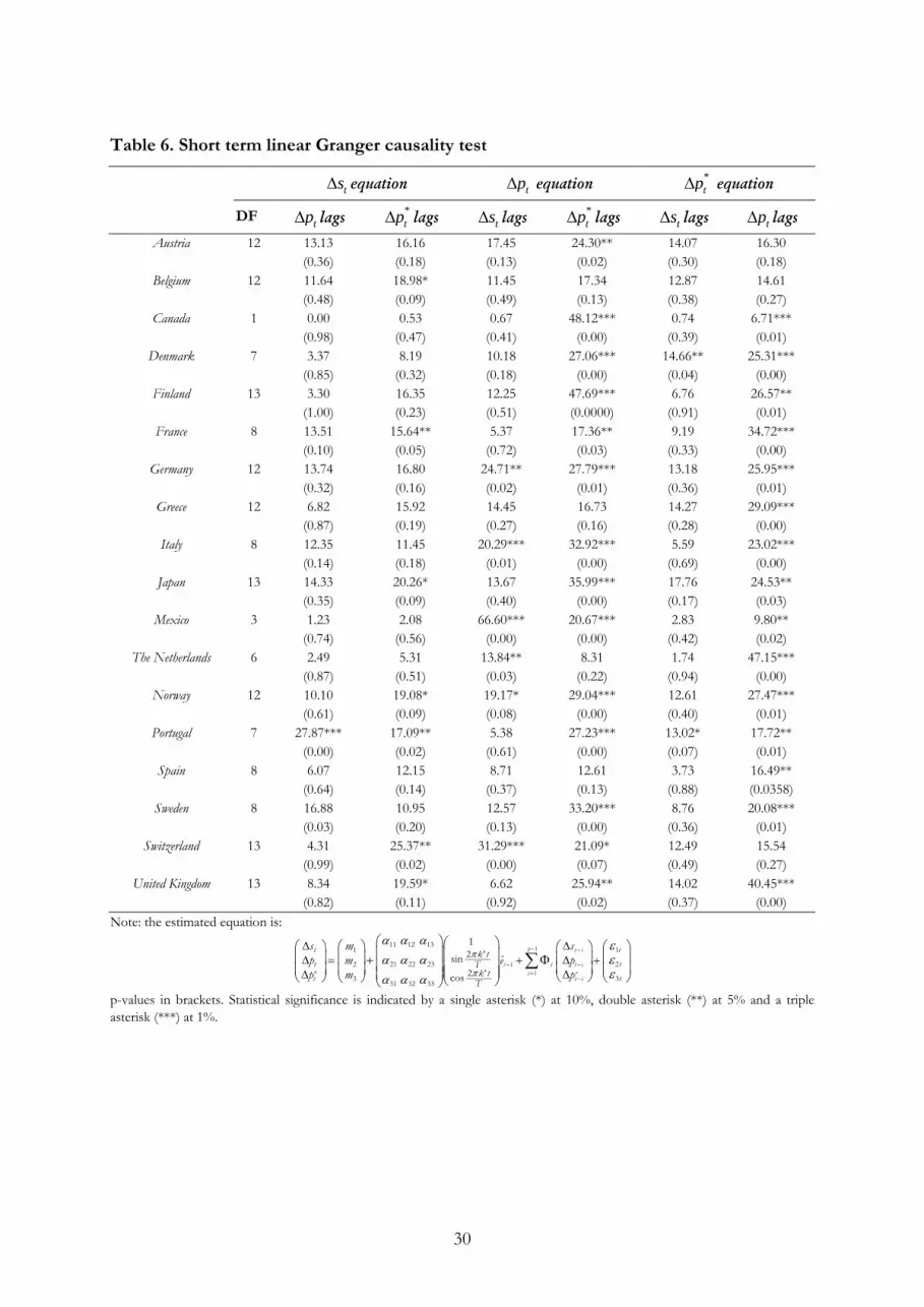
30

Table 6. Short term linear Granger causality test

tsΔ equation tpΔ equation *

tpΔ equation

DF tpΔ lags *tpΔ lags tsΔ lags *

tpΔ lags tsΔ lags tpΔ lags

Austria 12 13.13 16.16 17.45 24.30** 14.07 16.30 (0.36) (0.18) (0.13) (0.02) (0.30) (0.18)

Belgium 12 11.64 18.98* 11.45 17.34 12.87 14.61 (0.48) (0.09) (0.49) (0.13) (0.38) (0.27)

Canada 1 0.00 0.53 0.67 48.12*** 0.74 6.71*** (0.98) (0.47) (0.41) (0.00) (0.39) (0.01)

Denmark 7 3.37 8.19 10.18 27.06*** 14.66** 25.31*** (0.85) (0.32) (0.18) (0.00) (0.04) (0.00)

Finland 13 3.30 16.35 12.25 47.69*** 6.76 26.57** (1.00) (0.23) (0.51) (0.0000) (0.91) (0.01)

France 8 13.51 15.64** 5.37 17.36** 9.19 34.72*** (0.10) (0.05) (0.72) (0.03) (0.33) (0.00)

Germany 12 13.74 16.80 24.71** 27.79*** 13.18 25.95*** (0.32) (0.16) (0.02) (0.01) (0.36) (0.01)

Greece 12 6.82 15.92 14.45 16.73 14.27 29.09*** (0.87) (0.19) (0.27) (0.16) (0.28) (0.00)

Italy 8 12.35 11.45 20.29*** 32.92*** 5.59 23.02*** (0.14) (0.18) (0.01) (0.00) (0.69) (0.00)

Japan 13 14.33 20.26* 13.67 35.99*** 17.76 24.53** (0.35) (0.09) (0.40) (0.00) (0.17) (0.03)

Mexico 3 1.23 2.08 66.60*** 20.67*** 2.83 9.80** (0.74) (0.56) (0.00) (0.00) (0.42) (0.02)

The Netherlands 6 2.49 5.31 13.84** 8.31 1.74 47.15*** (0.87) (0.51) (0.03) (0.22) (0.94) (0.00)

Norway 12 10.10 19.08* 19.17* 29.04*** 12.61 27.47*** (0.61) (0.09) (0.08) (0.00) (0.40) (0.01)

Portugal 7 27.87*** 17.09** 5.38 27.23*** 13.02* 17.72** (0.00) (0.02) (0.61) (0.00) (0.07) (0.01)

Spain 8 6.07 12.15 8.71 12.61 3.73 16.49** (0.64) (0.14) (0.37) (0.13) (0.88) (0.0358)

Sweden 8 16.88 10.95 12.57 33.20*** 8.76 20.08*** (0.03) (0.20) (0.13) (0.00) (0.36) (0.01)

Switzerland 13 4.31 25.37** 31.29*** 21.09* 12.49 15.54 (0.99) (0.02) (0.00) (0.07) (0.49) (0.27)

United Kingdom 13 8.34 19.59* 6.62 25.94** 14.02 40.45*** (0.82) (0.11) (0.92) (0.02) (0.37) (0.00)

Note: the estimated equation is:

1

11 *

11 12 1311 *

21 22 23 22**

3331 32 33

2

2

1sin

cos

ˆp t i

t iti

t i

t t

t ti

t t

k tTk t

T

s sp pep p

mmm

π

π

α α α

α α α

α α α

εεε

− −

−−=

−

Δ ΔΔ Δ= + +Δ Δ

⎛ ⎞⎛ ⎞⎛ ⎞⎛ ⎞ ⎛ ⎞⎛ ⎞⎜ ⎟⎜ ⎟⎜ ⎟⎜ ⎟ ⎜ ⎟⎜ ⎟+ Φ⎜ ⎟⎜ ⎟ ⎜ ⎟⎜ ⎟ ⎜ ⎟⎜ ⎟ ⎜ ⎟⎜ ⎟ ⎝ ⎠⎝ ⎠ ⎝ ⎠⎝ ⎠ ⎝ ⎠⎝ ⎠

∑

p-values in brackets. Statistical significance is indicated by a single asterisk (*) at 10%, double asterisk (**) at 5% and a triple asterisk (***) at 1%.

ppp: delusion or reality? evidence from a nonlinear analysis

Documents