power aware distributed systems - dtic
TRANSCRIPT

AFRL-IF-RS-TR-2004-7
Final Technical Report
January 2004 POWER AWARE DISTRIBUTED SYSTEMS University of Southern California Marina Del Rey Sponsored by Defense Advanced Research Projects Agency DARPA Order No. J874
APPROVED FOR PUBLIC RELEASE; DISTRIBUTION UNLIMITED.
The views and conclusions contained in this document are those of the authors and should not be interpreted as necessarily representing the official policies, either expressed or implied, of the Defense Advanced Research Projects Agency or the U.S. Government.
AIR FORCE RESEARCH LABORATORY INFORMATION DIRECTORATE
ROME RESEARCH SITE ROME, NEW YORK

STINFO FINAL REPORT
This report has been reviewed by the Air Force Research Laboratory, Information Directorate, Public Affairs Office (IFOIPA) and is releasable to the National Technical Information Service (NTIS). At NTIS it will be releasable to the general public, including foreign nations. AFRL-IF-RS-TR-2004-7 has been reviewed and is approved for publication. APPROVED: /s/
ANDRETTA DENNIS, 2LT., USAF Project Engineer
FOR THE DIRECTOR: /s/
WARREN H. DEBANY, JR., Technical Advisor Information Grid Division Information Directorate

REPORT DOCUMENTATION PAGE Form Approved
OMB No. 074-0188 Public reporting burden for this collection of information is estimated to average 1 hour per response, including the time for reviewing instructions, searching existing data sources, gathering and maintaining the data needed, and completing and reviewing this collection of information. Send comments regarding this burden estimate or any other aspect of this collection of information, including suggestions for reducing this burden to Washington Headquarters Services, Directorate for Information Operations and Reports, 1215 Jefferson Davis Highway, Suite 1204, Arlington, VA 22202-4302, and to the Office of Management and Budget, Paperwork Reduction Project (0704-0188), Washington, DC 20503
1. AGENCY USE ONLY (Leave blank)
2. REPORT DATEJANUARY 2004
3. REPORT TYPE AND DATES COVERED Final Aug 00 – Aug 03
4. TITLE AND SUBTITLE POWER AWARE DISTRIBUTED SYSTEMS
6. AUTHOR(S) Brian Schott, Mani Srivastava, Ronald Riley, and Igor Elgorriaga
5. FUNDING NUMBERS C - F30602-00-C-0154 PE - 62301E PR - J874 TA - 37 WU - A1
7. PERFORMING ORGANIZATION NAME(S) AND ADDRESS(ES) University of Southern California Marina Del Ray Information Science Institute 4676 Admiralty Way Marina Del Ray California 90292-6695
8. PERFORMING ORGANIZATION REPORT NUMBER
N/A
9. SPONSORING / MONITORING AGENCY NAME(S) AND ADDRESS(ES) Defense Advanced Research Projects Agency AFRL/IFGA 3701 North Fairfax Drive 525 Brooks Road Arlington Virginia 22203-1714 Rome New York 13441-4505
10. SPONSORING / MONITORING AGENCY REPORT NUMBER
AFRL-IF-RS-TR-2004-7
11. SUPPLEMENTARY NOTES AFRL Project Engineer: Dennis L. Andretta, 2Lt., USAF/IFGA/(315) 330-2926/ [email protected]
12a. DISTRIBUTION / AVAILABILITY STATEMENT APPROVED FOR PUBLIC RELEASE; DISTRIBUTION UNLIMITED.
12b. DISTRIBUTION CODE
13. ABSTRACT (Maximum 200 Words)The goal of PADS was to study power aware management techniques for wireless unattended ground sensor applications to extend their operational lifetime and overall capabilities in this battery-constrained environment. The analysis included embedded systems architectures, signal processing algorithms, simulation and planning tools, and collaborative networking protocols.
15. NUMBER OF PAGES234
14. SUBJECT TERMS Unattended Ground Sensors, Power Aware Systems, Acoustic Beamforming, Wireless Networking 16. PRICE CODE
17. SECURITY CLASSIFICATION OF REPORT
UNCLASSIFIED
18. SECURITY CLASSIFICATION OF THIS PAGE
UNCLASSIFIED
19. SECURITY CLASSIFICATION OF ABSTRACT
UNCLASSIFIED
20. LIMITATION OF ABSTRACT
ULNSN 7540-01-280-5500 Standard Form 298 (Rev. 2-89)
Prescribed by ANSI Std. Z39-18 298-102

TABLE OF CONTENTS 1 Introduction................................................................................................................................................................12 Final Status Report on Architectural Approaches...............................................................................................2
2.1 Power Analysis of Rockwell HIDRA™...........................................................................................................22.1.1 HIDRA Power Instrumentation...............................................................................................................32.1.2 HIDRA Instrumentation Results .............................................................................................................4
2.2 Power Aware Microsensor Architecture...........................................................................................................52.2.1 Implementation Goals..............................................................................................................................62.2.2 Implementation Results ...........................................................................................................................92.2.3 Phase 2 Status Update .............................................................................................................................9
2.3 RSC Power Aware FPGA Radio.....................................................................................................................112.3.1 Modem configuration ............................................................................................................................122.3.2 PAC/C modem architecture...................................................................................................................152.3.3 Differential encoding and decoding......................................................................................................252.3.4 Network processor interface..................................................................................................................312.3.5 Code development and simulation........................................................................................................322.3.6 Testing....................................................................................................................................................33
3 Final Status Report on Middleware, Tools, and Techniques............................................................................363.1 Introduction......................................................................................................................................................363.2 Techniques for Node-Level Power Management...........................................................................................36
3.2.1 Power Aware Resource Scheduling......................................................................................................363.2.2 Power-aware API for RTOS-driven CPU Power Management...........................................................373.2.3 Predictive Dynamic Voltage Scaling for Adaptive CPU Fidelity .......................................................413.2.4 Battery Lifetime Management ..............................................................................................................42
3.3 Techniques for Network-Wide Power Management......................................................................................423.3.1 Energy-aware Packet Scheduling with Dynamic Modulation Scaling................................................433.3.2 Sparse Topology and Energy Management..........................................................................................45
3.4 Sensor Networking Simulation and Planning Tools ......................................................................................464 Final Status Report On Algorithms .....................................................................................................................48
4.1 Introduction......................................................................................................................................................484.2 Acoustic Beamforming....................................................................................................................................48
4.2.1 Acoustic Beamforming Knobs..............................................................................................................494.2.2 Algorithm Optimizations.......................................................................................................................524.2.3 Acoustic Line Of Bearing Results ........................................................................................................524.2.4 Line of Bearing Performance on HIDRA.............................................................................................534.2.5 Spesuti Island Field Test .......................................................................................................................56
4.3 Laplacian Pyramid Image Compression .........................................................................................................565 Deliverables Summary ............................................................................................................................................58
5.1.1 Task 1: Architectural Approaches.........................................................................................................585.1.2 Task 2: Middleware, Tools, and Techniques........................................................................................585.1.3 Task 3: Algorithms ................................................................................................................................60
6 Personnel...................................................................................................................................................................616.1.1 USC Information Sciences Institute Personnel ....................................................................................616.1.2 UCLA Personnel....................................................................................................................................616.1.3 Rockwell Scientific Company Personnel .............................................................................................61
7 Publications ..............................................................................................................................................................628 List of Acronyms......................................................................................................................................................64
i

9 List of Addenda 65 [1] C. Schurgers, V. Tsiatsis, and M.B. Srivastava, "STEM: Topology management for energyefficient sensor networks," IEEE Aerospace Conference, March 2001…….67 [2] A. Savvides, S. Park, and M. Srivastava, "On modeling networks of wireless microsensors,"Proceedings of ACM SIGMETRICS 2001, June 2001………………...77 [3] S. Park, A. Savvides, and M. Srivastava, "Battery capacity measurement and analysis usinglithium coin cell battery," Proceedings of the ACM International Symposium on Low PowerElectronics and Design (ISLPED), August 2001………….79 [4] V. Tsiatsis, S. Zimbeck, and M. Srivastava, "Architecture strategies for energy efficientpacket forwarding in wireless sensor networks," Proceedings of the ACM InternationalSymposium on Low Power Electronics and Design (ISLPED), August 2001……………………………………………………………………………………..85 [5] C. Schurgers, O. Aberthorne, and M. Srivastava, "Modulation scaling for energy awarecommunication systems," Proceedings of the ACM International Symposium on Low PowerElectronics and Design (ISLPED), August 2001………………………..89 [6] C. Schurgers, and M. Srivastava, "Energy efficient routing in wireless sensor networks,"Proceedings of MILCOM 2001, October 2001………………………...……93 [7] C. Schurgers, V. Raghunathan, and M. Srivastava, " Modulation Scaling for Real-TimeEnergy Aware Packet Scheduling," Proceedings of IEEE Globecom, November 2001…………………………………………………………………………………..…98 [8] V. Raghunathan, P. Spanos, and M. Srivastava, "Adaptive power-fidelity in energy awarewireless embedded systems," Proceedings of the IEEE Real-Time Systems Symposium,December 2001……………………………………………………………103 [9] S. Park, A. Savvides, and M. Srivastava, "Simulating networks of wireless sensors,"Proceedings of the 2001 Winter Simulation Conference (WSC 2001), December 2001…………………………………………………………………………113 [10] C. Schurgers, and M.B. Srivastava, "Energy Efficient Wireless Scheduling: AdaptiveLoading in Time," Proceedings of the IEEE Wireless Communications and NetworkingConference (WCNC’02), March 2002. Accepted…………………….122 [11] V. Raghunathan, C. Schurgers, S. Park, and M. Srivastava, "Energy-aware wirelesssensor networks", IEEE Signal Processing (special issue on collaborative signal processing),March 2002…………………………………………………………128 [12] Vijay Raghunathan, Saurabh Ganeriwal, Curt Schurgers, Mani B. Srivastava, "E2WFQ:An Energy Efficient Fair Scheduling Policy for Wireless Systems," International Symposiumon Low Power Electronics and Design (ISLPED'02),
ii

Monterey, CA, August 12-14, 2002…………………………………………………….145 [13] Ronald A. Riley, Jr., Sohil B. Thakkar, Joseph P. Czarnaski, and Brian Schott, “Power-Aware Acoustic Processing,” Military Sensing Symposium: Battlefield Acoustic and SeismicSystems Conference, Columbia, MD, September 23-25, 2002…151 [14] C. Schurgers, V. Raghunathan, and M. B. Srivastava, "Power Management for EnergyAware Communication Systems", accepted for publication in ACM Transactions onEmbedded Computing Systems (special issue on power aware embedded computing)………………………………………………………………….165 [15] V. Raghunathan, C. Pereira, M. B. Srivastava, and R. Gupta, "Energy Aware WirelessSystems with Adaptive Power-Fidelity Tradeoffs", submitted to IEEE Transactions on VLSISystems…………………………………………………………182 [16] V. Raghunathan, S. Ganeriwal, C. Schurgers, and M. B. Srivastava, "Energy EfficientWireless Packet Scheduling and Fair Queuing", submitted to ACM Transactions onEmbedded Computing Systems (special issue on networked embedded computing)…………………………………………………………….……206
iii

LIST OF FIGURES
Figure 1: HIDRA Microsensor..............................................................................................................................................2Figure 2: HIDRA SA110 Processor Module (left) and 900MHz Radio Module (right) ...................................................2Figure 3: HIDRA Sensor Module (left) and Power Module (right) ...................................................................................2Figure 4: Power Instrumentation Board................................................................................................................................3Figure 5: Module Isolation Concept .....................................................................................................................................4Figure 6: Power Aware Communication Subsystem ...........................................................................................................5Figure 7: Modular Power Aware Microsensor .....................................................................................................................6Figure 8: Distributed "System of Systems" Architecture.....................................................................................................7Figure 9: Module Stack Pin Allocation ...............................................................................................................................8Figure 10: Example PXA25x Module ..................................................................................................................................8Figure 11: PXA25x Power Breakdown by Mode.................................................................................................................9Figure 12: PASTA Power Aware Microsensor .................................................................................................................10Figure 13: PASTA Experimentation Results, June 2003...................................................................................................10Figure 14: Packet Format ....................................................................................................................................................13Figure 15: Preamble Format................................................................................................................................................13Figure 16: Header Packet Format .......................................................................................................................................14Figure 17: Functional Diagram of Transmitter Portion of the Modem ............................................................................16Figure 18: Interleaver row wise Byte write operation........................................................................................................17Figure 19: Interleaver column wise bit read operation. .....................................................................................................17Figure 20: Scrambler Implementation ................................................................................................................................18Figure 21: Maximum Length PN sequence generator (15 to 127 chips)...........................................................................18Figure 22: Code Acquisition Portion of the Acquisition Block.........................................................................................19Figure 23: Code Acquisition Algorithm .............................................................................................................................20Figure 24: Bit Synchronization and Code Acquisition Blocks..........................................................................................21Figure 25: Demodulation Architecture ...............................................................................................................................22Figure 26: De-scrambler architecture. ................................................................................................................................22Figure 27: De-Interleaver Write Operation ........................................................................................................................23Figure 28: De-Interleaver Read Operation. ........................................................................................................................23Figure 29: Serial-to-Parallel write/read RAM process.......................................................................................................24Figure 30: Clock Generation Tree ......................................................................................................................................25Figure 31: Block Diagram of the Differential Encoder for BPSK.....................................................................................26Figure 32: Block Diagram of the Differential Decoder for BPSK ....................................................................................26Figure 33: Block diagram of the differential encoder for QPSK.......................................................................................28Figure 34: Block diagram of the differential decoder for QPSK.......................................................................................29Figure 35: Photograph of the Testbed Hardware. ..............................................................................................................34Figure 36: Implementation Resource Utilization Results. .................................................................................................35Figure 37: Coordinated Node-Level Power Management .................................................................................................37Figure 38: Power Aware API Layers..................................................................................................................................39Figure 39: Dynamic Voltage Scaling Testbed....................................................................................................................39Figure 40: XScale NOP Power ...........................................................................................................................................39Figure 41: XScale Add Integer Power................................................................................................................................40Figure 42: XScale Multiply Float Power............................................................................................................................40Figure 43: XScale Memory Read Power ............................................................................................................................40Figure 44: XScale Memory Write Power ...........................................................................................................................40Figure 45: XScale Peripheral Read Power .........................................................................................................................40Figure 46: XScale Peripheral Write Power ........................................................................................................................40Figure 47: MPEG Decode Times........................................................................................................................................41Figure 48: Speech CODEC Decode Times ........................................................................................................................41Figure 49: Predictive Dynamic Voltage Scaling Energy ...................................................................................................41Figure 50: Achieved Battery Capacity Versus Operating Mode .......................................................................................42Figure 51: Data Rate and Battery Capacity Comparisons .................................................................................................42Figure 52: Voltage Scaling Versus Modulation Scaling....................................................................................................43Figure 53: Queue-Based Dynamic Modulation Scaling ....................................................................................................43
iv

Figure 54: Energy per Useful Bit with Dynamic Code Scaling.........................................................................................44Figure 55: Operation of STEM ...........................................................................................................................................45Figure 56: STEM Performance Analysis............................................................................................................................45Figure 57: STEM Simulation Analysis...............................................................................................................................46Figure 58: SensorSim Architecture.....................................................................................................................................47Figure 59: Three Stages of Power Aware Algorithm Development..................................................................................48Figure 60. ARL Baseline Acoustic Array...........................................................................................................................49Figure 61: Beamforming "Knobs" ......................................................................................................................................49Figure 62: RMS Error Versus Number of Microphones....................................................................................................50Figure 63: RMS Error Versus Number of Samples ...........................................................................................................51Figure 64: Accuracy and Energy Versus Number of Beams.............................................................................................51Figure 65: Frequency Domain Beamformer (top) and Time Domain Beamformer (bottom)..........................................52Figure 66: Acoustic Line of Bearing Energy Versus RMS Error......................................................................................53Figure 67: ISI and ARL LOB Versus Ground Truth..........................................................................................................53Figure 68: HIDRA Node Energy to Compute 1 Bearing...................................................................................................54Figure 69: HIDRA Execution Time to Compute 1 Bearing ..............................................................................................54Figure 70: Average Power per Module to Calculate 1 Bearing.........................................................................................55Figure 71: HIDRA Power Breakdown by Module.............................................................................................................55Figure 72: Laplacian Image Coding....................................................................................................................................56Figure 73: Laplacian Pyramid Image..................................................................................................................................57Figure 74: The Laplacian Pyramid Method........................................................................................................................57Figure 75: Laplacian Pyramid Results................................................................................................................................57
iii

LIST OF TABLES
Table 1: HIDRA Power Breakdown ............................................................................................4Table 2: PAC/C Spread Spectrum Modem Specifications .........................................................11Table 3: Available Radio Knobs ...............................................................................................11Table 4: Testbed Platform Characteristics .................................................................................12Table 5: SERVICE Field Definitions ........................................................................................14Table 6: Available Payload Data Rates......................................................................................15Table 7: Ideal BPSK Transmission Case ...................................................................................27Table 8: Single Error BPSK Transmission Case........................................................................27Table 9: N Errors BPSK Transmission Case..............................................................................27Table 10: QPSK Differential Encoding .....................................................................................29Table 11: QPSK Differential Encoding Ideal Case ....................................................................30Table 12: QPSK Differential Encoding Error Case....................................................................30Table 13: QPSK Differential Encoding Demodulation Error Case.............................................30Table 14: QPSK Differential Encoding N-Errors Case ..............................................................31Table 15: QPSK 180-Degree Phase Change (Inversion) Case....................................................31Table 16: Processor-modem Interface Commands.....................................................................32Table 17: FPGA Modem Design Files.......................................................................................32Table 18: Power Aware API Functions .....................................................................................37
iv

1
1 INTRODUCTION
The goal of Power Aware Distributed Systems (PADS) project was to develop and apply
power aware embedded system architectures, algorithms, middleware, simulation tools, and
protocols to unattended wireless ground sensor systems. The PADS project included researchers
from University of Southern California (USC) Information Sciences Institute (ISI), University of
California Los Angeles (UCLA), and Rockwell Science Center (RSC). The multidisciplinary
team included world-class, widely-published researchers with significant industrial experience
and complementary expertise in the areas of embedded systems engineering, network protocols,
real-time operating systems, and DoD application experience for acoustic, seismic, and imaging
sensors. The team established a number of research goals for the PADS effort:
• Identify hardware knobs that can be provided by modules (radio and processor systems) that
can be altered dynamically, and externally readable parameters (power, BER, signal strength,
battery, etc.) that can be provided to a power-aware runtime system.
• Instrument a state-of-the-art sensor node to understand power consumption in current
systems. Where can we expect significant latitude in power tradeoff? Which knobs have the
greatest dynamic range? What baseline will we use for comparison?
• Provide operating system extensions for power management, task scheduling, and task
control on individual SensIT sensor nodes.
• Create reconfigurable communication modules that adapt parameters such as error control,
equalization, data rate, and noise figure in real time according to channel state.
• Design a distributed sensor network control middleware for power-aware task distribution
and hardware/software resource utilization migration.
• Incorporate power trade-off analysis tools into the SensIT platform emulator for power aware
application development and scenario simulation for sensor networks.
• Develop power-aware algorithms for cooperative signal processing that exploit sensor data
locality, multiresolution processing, sensor fusion, and accumulated intelligence.
• Integrate advanced power aware processing and communications technology into the PADS
research platform as it becomes available in the PAC/C community.
The PADS project was organized into three distinct tasks. Task 1: Architectural Approaches
examined the physical “hardware knob” aspects of the research. This included instrumentation
of the baseline platform and development of a power aware communication module. The results
of this task are reported in Section 2. Task 2: Middleware, Tools, and Techniques investigated
software aspects related to real-time operating systems for power aware operation of a single
node as well as collaborative networking protocols to manage energy across a sensor field. This
task also developed simulation and planning tools for networked unattended ground sensors.
Task 2 is covered in Section 3. Finally, Task 3: Algorithms studied power-awareness for signal
processing algorithms used in ground sensor systems. The team looked at a representative
acoustic algorithm and a representative image-processing algorithm. The algorithm studies are
reported in Section 3.4. The report concludes in Section 5 with a summary of deliverables,
publications, personnel, and acronyms.

2
2 FINAL STATUS REPORT ONARCHITECTURAL APPROACHES
The Architectural Approaches task of the PADS project focused on instrumentation and
analysis of a baseline unattended ground sensor system to understand how battery energy is
consumed. The information gathered in this study was used to develop and validate power
consumption models used in the SensorSim power aware simulator. The results of this study
were also used to identify power/performance “knobs” in the hardware and determine their
relative impact on overall system power for intelligent algorithm development. Similarly, the
identification of power/performance “knobs” in the hardware led to microsensor system
architecture insights on how to expose the “knobs” to software control. The team assembled a
microsensor testbed using the commercial HIDRA™ microsensor hardware developed at
Rockwell Science Center. Analysis methods and results are provided in Section 2.1. The
proposed power aware microsensor architecture is described in Section 2.2. Finally, a power
aware software radio was prototyped and analyzed under this task. The software radio is
described in Section 2.3.
2.1 Power Analysis of Rockwell HIDRA™
The PADS team assembled a research testbed using the
HIDRA™ microsensor, which was developed at the Rockwell
Science Center in part under the DARPA Low-Power Wireless
Integrated Microsensors (LWIM) and Adaptive Wireless Arrays
for Interactive Reconnaissance, Surveillance, and Target
Acquisition in Small Unit Operations (AWAIRS) programs.
This system has been used in numerous DoD field experiments
and is representative of other microsensor platforms in the
community. Shown in Figure 1, HIDRA is constructed as a
modular stack of circuit boards measuring 2.5 by 2.5 inches
square. It has a pair of connectors on top and bottom for inter-
module communications and power supply. Initially conceived
for mission configurability and incremental refinements of the platform, the modularity was
found to be extremely useful for subsystem power analysis. The modules could be removed or
isolated and instrumented separately.
The HIDRA processor module shown in Figure 2 (left) has an Intel StrongARM 1100
embedded 32-bit CPU, 1MB of SRAM, and 4MB of flash memory. The processor has a 1.5V
Figure 1: HIDRA Microsensor
Figure 2: HIDRA SA110 Processor Module (left)and 900MHz Radio Module (right)
Figure 3: HIDRA Sensor Module (left)and Power Module (right)
n I™!

3
core voltage and 3.3V I/O. The clock rate is scalable from 59MHz to 133MHz. The SA110 does
not have a floating-point execution unit. Floating-point arithmetic is emulated in software. The
development environment provided by Rockwell Science Center originally used the µCOS real-
time operating system (RTOS). Later releases of the support software used eCOS, an open-
source RTOS maintained at RedHat, Inc. The software release supplied a Hardware Abstraction
Layer (HAL), a set of libraries with standard interfaces to the hardware resources of the system
including the radio and sensor boards. The Rockwell-proprietary radio board shown in Figure 2
(right) transmits and receives in the 900 MHz ISM band at up to a 100kb/s data rate with a
maximum range of approximately 25 meters outdoors. The transmit output power is adjustable.
A number of media access control (MAC) mechanisms were supported by the HIDRA platform,
including Time Division Multiplex Access (TDMA) and Collision Sense/Detect Multiple Access
(CSMA/CDMA) protocol. In Figure 3 (left), the analog sensor board has five channels with 12-
bit resolution. Three are high speed (60KSPS) and two are low speed (<2KSPS). The three
channels are multiplexed with variable gains of 1x, 2x, 5.02x, 10.09x, and 20.12x. The other two
have individual inputs with variable gains of 10x, 43.32x, 30x, 36.68x, and 49.98x. The
selectable gains are tuned to specific sensors that RSC uses for this platform, such as
microphones, geophones, and magnetometers. Finally, the power board Figure 3 (right)
generates regulated 1.5V and 3.3V supplies from two 9V batteries or a DC adapter. The power
board also provides separate analog voltage lines for the radio and sensor modules.
2.1.1 HIDRA Power Instrumentation
Run-time monitoring of the HiDRA node-
level power consumption was made possible by the
development of a power instrumentation board
shown in Figure 4. This board was intended to be
small and inexpensive enough to power-instrument
a large number of sensor nodes in the field. The
power measurement for the entire node was
accomplished by using a low ohm value current
sensing resistor in conjunction with a Burr-Brown
INA138 High-Side measurement current shunt
monitor. The input from this device is connected
to one of four analog inputs of a PIC16C715 8-bit
microcontroller, running at 20 MHz. Other GPIOs of the microcontroller were tied to GPIOs of
the SA1100 processor. These control pins were used start and stop sampling windows from the
application software. The externally powered instrumentation board consumed 15uA typical at
5V. For data logging purposes, the microcontroller interfaced with the serial port of a laptop or
PDA. This instrumentation board was first used in a field text experiment at the SITEX01
experiment funded by the DARPA SensIT program.
A module-level instrumentation concept introduced in our proposal was to design a
power isolation board intended to transparently plug between boards in the stack. In addition to
monitoring power, the instrumentation board would have instrumented bus transactions on the
connectors between modules to correlate power consumption within very small time windows.
Figure 4: Power Instrumentation Board

4
For example, a packet sent from the processor to the radio
could trigger power logging. Figure 5 shows the isolation
board concept. However, this approach turned out to be
impractical. Unfortunately, the HiDRA connector stack was
not symmetric from module to module, so a custom isolation
board would have to have been developed for each module
under test. The development manpower was determined to
outweigh the benefits. Instead, the HiDRA subsystem
analysis was performed by physically removing modules.
First, the baseline application was executed on the processor
entirely alone with interactions with the sensor and radio
modules bypassed in the code. The serial channels to these
modules were driven to include data transfer time in the
analysis, but errors when communicating to the missing
modules were ignored. Second, the processor and sensor
modules were measured together with the radio transactions commented out. Third, the sensor
module was removed and the radio was added with sensor module transactions commented out.
Finally, the measurement process was repeated for the entire stack including processor, radio,
and sensor. The analysis results are provided in the following section.
2.1.2 HiDRA Instrumentation Results
The power measurements of the HiDRA platform in various operational modes are given
in Table 1. Further detailed measurements of power consumption on the hardware are provided
with the Line of Bearing algorithms discussion in Section 3.4. For this experiment, the processor
was operating at 59 MHz, which is the minimum operating frequency. The application
continuously transmitted and received packets over the radio. Although the SA1100 processor
has a sleep mode, this mode wasn’t
available in the hardware abstraction
layer libraries provided by Rockwell.
Even if available, the processor sleep
mode isn’t relevant because neither
the radio nor the sensor will operate
without the processor active in this
architecture. As shown, the average
processor power in this experiment
was 360mW. In this test, the sensor
module had a single seismic sensor.
Compared to the other modules, the
sensor module is inexpensive in terms
of power at 23.3mW. The radio has
the widest dynamic power range. In
receive mode, the radio module
consumes 391.6mW. The transmit
mode varies from 410.5mW at the
lowest amplification to 720.5mW at
the highest.
Figure 5: Module Isolation Concept
Processor Seismic Sensor Radio Power (mW)
Active On Rx 751.6
Active On Idle 727.5
Active On Sleep 416.3
Active On Removed 383.3
Active Removed Removed 360.0
Active On Tx (36.3 mW) 1080.5
Tx (27.5 mW) 1033.3
Tx (19.1 mW) 986.0
Tx (13.8 mW) 942.6
Tx (10.0 mW) 910.9
Tx (3.47 mW) 815.5
Tx (2.51 mW) 807.5
Tx (1.78 mW) 799.5
Tx (1.32 mW) 791.5
Tx (0.955 mW) 787.5
Tx (0.437 mW) 775.5
Tx (0.302 mW) 773.9
Tx (0.229 mW) 772.7
Tx (0.158 mW) 771.5
Table 1: HiDRA Power Breakdown
Bnicr> Pai;k

5
This hardware power utilization analysis yielded in a number of interesting observations
from a systems architecture point of view:
• The transmit-to-receive power ratio ranges from 1:1 to 2:1. So, receive tends to dominate
total communications power if not managed intelligently. There is a natural
power/performance tradeoff between latency, hop count, and duty cycle in time-division-
multiplex-access TDMA communications systems (a traditional way to duty-cycle receivers).
A very low power wake-up receiver could have a significant power/performance impact even
if the wake-up transmitter was highly inefficient.
• Approximately 50% of the receive power in the HiDRA platform is consumed by the
processor. The processor is mostly idling in this operation mode and is wasting power. A
communications subsystem engineered for power awareness should contain sufficient
computational resources to forward packets directly without host processor intervention. The
host processor can wake up periodically to update routing tables (see Figure 6).
CommunicationSubsystem
RadioModem
GPS
MicroController
Rest of the Node
CPU Sensor
MultihopPacket Communication
Subsystem
RadioModem
GPS
MicroController
Rest of the Node
CPU Sensor
MultihopPacket
…zZZ
Figure 6: Power Aware Communication Subsystem
• Similarly, the processor consumes approximately 90% of the power when sampling the
geophone. It is mostly idling in this mode and is wasting power. A sensor subsystem
engineered for power awareness should have sufficient computation resources to perform the
real-time aspects of data acquisition and storage, data filtering, and possibly basic signal
detection or threshold functions to trigger the main CPU. The main processor can sleep and
either wakeup on a schedule or by a positive threshold event to processes a data buffer.
These systems analyses and observations clearly indicated that improved power management
was possible in a microsensor platform. Even with relatively simple changes to we could save
up to 50% or 90% in certain operational modes. The power aware microsensor architecture
concept is described in Section 2.2.
2.2 Power Aware Microsensor Architecture
The power aware microsensor concept developed under this effort centered on the idea
that a distributed “system-of-systems” architecture was a better choice for efficient power
utilization. The traditional CPU-centric methodology for designing embedded systems, although
it used fewer components, introduced unforeseen power consumption overhead because of the
mismatch of high computational resources (a single embedded CPU) and low computational load
in the most common operational modes (receiving and sensor monitoring). The modular
hardware approach exhibited physically in the HYDRA platform was good, but it did not extend
to power management. In order to significantly save power in a microsensor stack, the non-
essential modules (for a specific operational mode) need to be in very deep sleep, or preferably,
electrically disconnected from the power supply to avoid power leakage. In addition, the

6
HYDRA platform had no way for the software to detect what modules were present in the stack
or what their operational modes were. Furthermore, the data connections in the HYDRA stack
were statically defined. In order for the radio and the sensor to interact, the processor needed to
be awake to broker the communication, even though it would be perfectly possible to have two
microcontrollers communicate serially. A better approach would be to allow the modules to
communicate independent of a central processor. Finally, some stack configurations have been
contemplated that don’t require a full-sized CPU for any mode of operation. It should be
possible to build a node without a main processor. This modular power aware microsensor
concept is detailed in Figure 7.
Figure 7: Modular Power Aware Microsensor
2.2.1 Implementation Goals
Implementation of a modular power aware microsensor platform as shown in Figure 7
involves compromises that balance design complexity, system flexibility, connectors and device
counts, power consumption, and performance. The engineering research team debated these
system-design trade-offs and arrived at a reference platform implementation that best met the
requirements and system constraints. A summary of the main issues is provided:
• The primary CPU in the stack should run Linux. Since most of the hard real-time signal
processing would be relegated to DSPs and microcontrollers on the sensor and radio
modules, the processor could afford to migrate to a robust operating system. Memory
density and processor performance has advanced sufficiently to make this feasible in terms of
size and power. The ISI team was involved in the development of embedded Linux for iPAQ
PDAs and realizes the benefits of this immense library of software for embedded devices.
• The main CPU in the stack should support commodity high-speed peripheral interfaces.
Given the PDA and camera markets as technology drivers, Compact Flash (CF) and USB
interfaces were placed high on the priority list. This would enable rapid prototyping with
off-the-shelf hardware (cameras, microdrives, 802.11 radios, etc.) and off-the-internet device
drivers. One of the frustrations of working with the HYDRA platform was the single serial
Fumily ur Inlcrthanucalilc Moiluks D J'icitcsMii. StTiMir, RadiLt. mid Power.
Mix and Match 0 Auto-retonfigurable ihmugh sotlwate discovery,
Misxlon deniable h<)-piii miidiilcs liuvc PC nuwcr cunlml bus and six
switclied MTi;il tloniiL'ls (2xSP[, 2x\-V. &1\UART) a IKO-pin miidiilcs :idd nrutcssor bus, (2) LUmpL'I tlu:,
USB mdKlcr/sUiVL;, l,C 1), and v:irLinLS <iP[()s,
Tracks r/lmager D Radio Module Powerraallery C Sensor* DSP FPGA/lmager Embedded Processor D Compact Flash
Radio Relay Radio Q PowerfSolar
Acoustic Tripwire Radio Module a Sensor + DSP Power/Baltery

7
port to the outside world and dependence of building custom hardware and writing custom
software for any new device.
• The main CPU (or the power-hungry part of any module for that matter) should be able to be
switched off at the connector to minimize power leakage when not being used. Modules
should support a range of power modes from fully off to fully on. Ideally, a module should
manage its own power state in response to its load and schedule.
• Each module should support data interfaces appropriate to their bandwidth and power
requirements. Standardizing on a common network fabric standard for all modules was
considered, but this would have introduced considerable power overhead for the network
interface device. Most microcontrollers, processors, and DSPs have dedicated hardware for
serial interfaces (UART, SPI, and I2C) and some parallel interfaces (memory bus and
cardbus). Since most of these interfaces are point-to-point, the serial connections between
modules should be capable of being dynamically switched.
• Modules should support software discovery and collaborate to manage power and data
connections. This led to the decision to incorporate a small microcontroller on each module
to act as a power controller. The power controllers communicate with each other over multi-
master 2-wire I2C. They provide a low-power control network for the modules over I2C,
manage the power switch to the module, and manage the switch fabric for the serial channels.
A conceptual diagram of the “system of systems” approach is shown in Figure 8.
Figure 8: Distributed "System of Systems" Architecture
Initial design of the physical implementation of this power aware microsensor architecture
started under PADS, but then transitioned to the DARPA PAC/C Phase II program under the ISI-
led Power Aware Sensing Tracking and Analysis (PASTA) effort. The design goal was to build
a compact stack of interchangeable boards (processor modules, radio modules, and sensor
modules) that could expose the maximum number of hardware power “knobs” to software
control. A family of modules would be developed to explore different aspects of power
management in embedded systems. The physical dimensions selected were deliberately
aggressive. The board footprint was just large enough for the stack connector, and a Compact
Flash (CF) socket. The other boards developed would adhere to this footprint. A 180-pin stack
connector was selected to accommodate a parallel memory bus and several serial channels. A
60-pin connector in the same family was plug-compatible with the 180, so the connector
standard was subdivided into a 60-pin region for serial channels and a 120-pin region for the
parallel busses. The 60-pin region 48 pins allocated to six 8-bit “serial” channels. Two each of
the channels were designated as I2C, UART, and SPI. However, the 8-pins per channel could be
used for any purpose. The core 60-pin region also contains the I2C control network for the
PWH
Data Bus '

8
power microcontrollers, power pins, and some miscellaneous control pins. Where the 60-pin
connector is rigidly standardized for any module, the processor module defines the allocation of
the 120-pin “parallel bus”. As shown in Figure 9, in the UP direction from the processor card, the
pins are allocated to the processor memory bus, LCD panel, USB Master and Slave, MMC/SD
card interface, and audio CODEC. In the DOWN direction relative to the processor, the pins are
allocated as two Compact Flash ports and some debug pins.
Figure 9: Module Stack Pin Allocation
Figure 10 shows the power microcontroller and how the processor module is wired to the
serial channels. The module power microcontroller has an I2C (IIC) control network interface
along with clock and reset pins. The regulated 3V power pins supply power to the power
microcontroller, but the remainder of the module resides behind a power switch. The six serial
channels are wired to native interfaces of the PXA250 processor. Bus isolation switches have
been added so that the microcontroller can disconnect the module when a channel isn’t being
used, such as when the module is powered down.
Figure 10: Example PXA25x Module
Other modules in the stack are wired in a similar fashion. A channel can be “allocated” by the
power microcontrollers by turning on switches on the two communicating modules. The two
module devices can then interact directly using their own protocol (SPI, UART, etc.). This
arrangement introduces a minimum number of extra components yet enables dynamic channel
Cmc 60-pin connctior nc I lie iiiAKi I |i-VK"i isM'issi
120-piii expansion connector I'n.LVswxl l.CIl liSHi MMC SiPiinillAJill
tirl. S(H:kcl
lOplioiial expansion cardi'i'|ii^i>^MWMo!!?!iiinmi!!!i^i!Xi^la^^
IfC I lie I UAKTIIIARTI SSI'I SSI r ♦ t ' t t
Pr.jccMiT|[.CD|USli!MMC !Srainill Addl Hiis ,^ Cirl.
iProcessor Card I'\\:MI I S-M II I fliL-h SDHAN
CiiinputEtb-lid , ainipiii;! Flash | "'^'"'S
[Optional CF Card
IICinclllARTIUARTISSPISSI CumpiLl Hash0 Conippd Flash I Fas^
I ojiin^iLl I l.i'nii SoLkt'l
^"^^ Compacl Flash 0
Header
Socket/ UP
Header/ DOWN
Com 6()-pin ciiiiML'ctor ' IK .1.11,, I .t..tV
Module's Power jiC
Always on Low power
• Power uC III nils miKliilc iin/iitT, controls bank iifuuNs • "l.iU'iiL-" nnillj-lxiard moiiiilc oti
Power ' SO-pin connector
Swiich
PXA250 Processor+SA1I11 Full i'aniol
IIC+ s-bii 1-bii SPI
\i r.iri). pSUOri I
JL^l^^l>Ll^:d L
MM< . N(l-piii
nmrlLtltNr
timmmmi Switched Banks
Core 60-pin connector

9
allocation. It also allows individual modules to be completely disconnected from the power
supply (except for the very low overhead of a power microcontroller and the isolation switches).
2.2.2 Implementation Results
The processor selected for this effort is the Intel PXA25x™ XScale family of embedded
processors commonly used in cell phones and personal digital assistants. It is a 32-bit
StrongARM™ instruction set architecture device that operates between 100MHz and 400MHz.
As with the StrongARM, floating point support is emulated in software. The processor supports
dynamic core voltage scaling from 0.95V to 1.5V. The processor module includes 32MB of
Flash and 64MB of Mobile SDRAM. The SDRAM has a programmable number of refresh banks
to save power while in sleep mode. The module also includes the Intel SA1111 peripheral co-
processor for USB Master support, two Compact Flash ports, and other peripheral interfaces.
Figure 11 shows the power breakdown for the PXA250 processor module. The outer graph
shows a dynamic operational power range from 100MHz idling at 200mW to full utilization at
400MHz with 100% memory accesses at about 1.5W. The middle graph shows power
dissipation between 2mW and 7mW depending on the amount of SDRAM that is refreshed. The
inner graph shows about a 0.1mW power overhead for the power microcontroller and associated
switches. This analysis demonstrates that power “knobs” with a wide dynamic range can be
added to a microsensor system without dramatically changing the basic architecture
Figure 11: PXA25x Power Breakdown by Mode
2.2.3 Phase 2 Status Update
The follow-on Phase 2 PASTA effort has undertaken construction of this microsensor
and is validating the results in laboratory and field experiments. A brief summary of the node
development status from the PASTA effort is given here because it shows a reduction to practice
of the concepts developed under the PADS project. Figure 12 shows the PASTA power aware
microsensor. By the end of the PADS project (August 2003), ISI had developed the PXA255
.-.^^ .^^ ..^^ ^^ >
^^^ / /
PXA250 SDRAM n FLASH SAllIl Module uC Module Switch Leakage DCap Leakage DPM Switch Leakage Power yC 32 KHz DDC-DC Conversion
'T ^^ ,.^ ^' ^ ^ ^ ^ o^
.-^ /" Z' -^ ^^*,*' xlOO
x2 X2000
Power Range
^200 mW(ON)
^(SLEEP)
fl^W(OFF)

10
processor module, a four-channel analog-to-digital-converter (ADC) module, a Compact Flash
adapter module, and a power/interface board (not shown).
Figure 12: PASTA Power Aware Microsensor
Figure 13 demonstrates how the switched serial channels (SPI in this case) are used to route data
from the ADC module to the PXA255 module. In the PASTA June 2003 experiment, the ADC
module operated continuously while the processor slept about 97% of the time.
Figure 13: PASTA Experimentation Results, June 2003
Total Size: 25" x 1.75" x -l^" Intel P\A25S Prcicfsijdr Miidulc
D lllt)-4IIIIMH/. (I.i»f;\ -l.5\' con- p Supjxirr fill' (2k C^iiiipidcl l-'liish miidulcit. D (.4MB Mchilf MIRAM, .IIMH FLASH. D Ontiiiuril ixiiMT ciiritroJk'r.
Cunipiii-t Flash Adapter Module
Four Channel ADC Moiliilc a I p III 2()t)kt|)s slrcumint:, liXIktps liufTiTi'd. Priiui'iiminiilik' |;;iin I'linlrnl unil ^ mi^hk'-ciilntT A A tiller. aC)Kniil(KII?]H25M-lill mlcriiioiitrcilkr (a 0-IOllMII/.
iljf ^S l'XA255
ADC Module Amplify (100%), Filter (100%). Sample (100%), Send SPI (3%)
Processor Moidule Read SPI 3%), Run Beamformer (<1%), Sleep (-97%).
Total System ^ Mlle^lant CiOdl •'IDOniW J
LalHiralur) txpi-rimcnt measured running I'IIHM' 1 pimer-aHare Line Ot Beariu); alcorllhiu cnde pnrtrd lu \Scale l.inuv itnd hasellni' telikle data colk'Cli'd rriim PAC/f Phase I Spesiili Isliind txpmmcni.

11
2.3 RSC Power Aware FPGA Radio
The purpose of this report is to explain the development of a reconfigurable, flexible,
spread spectrum modem as part of a power-aware computing and communication system
(PAC/C) requested by ISI for the PAC/C community. The major requirement for such a device is
to be able to dynamically adapt communication processing during runtime according to varying
external conditions. Provide reconfiguration controls to middleware for power aware protocol,
allowing reconfiguration not only at the lower physical layers, but also at the higher layers, such
as link and network. The task presented to Rockwell Scientific to design an energy efficient,
dynamically reconfigurable spread spectrum modem is quite complex without a hardware
platform being defined. In order to be able to complete this task Rockwell Scientific proposed a
parallel path of action. The development of the required modem optimized for an intermediate
testbed platform in parallel to the work in progress of the PAC/C community to define the
hardware platform. A modem with the dynamic reconfiguration capabilities with well-specified
knobs, and architecture optimization for energy efficiency has been developed, tested and
debugged in this testbed platform. The designed modem specifications are shown in Table 2.
Table 2: PAC/C Spread Spectrum Modem Specifications
Type of data modulation DBPSK, DQPSKSpreading User selectable spreading with 0dB, 11.7dB, 14.9dB,
18.0dB and 21dB processing gain.Data rates User selectable from 2.1Mbps for 0dB processing to
8.4Kbps for 21dB processing gain.PN sequences Maximum Selectable Length of 15, 31, 63, 127 phases.Overhead length (preamble +configuration)
78 bits with DBPSK encoding, scrambling and 11.7dBprocessing gain. 1103.7ms.
Payload length Selectable from 1 Byte to 256 Bytes.Scrambler Selectable ON or OFF.Interleaver Selectable ON or OFF.Input clock frequency 25.6 MHz.Chipping frequency 1.067 MHz.Number of samples per chip(Receiver mode)
4 samples per chip
Sample frequency (RX mode) 4.27 MHz.
According to the requirements, the modem should provide different configuration modes,
which can be set by externally selecting from a set of clearly defined knobs. The modem should
be re-configurable for variable data rates, processing gains, selectable modulation and
demodulation schemes. The set of knobs available to the user are displayed in Table 3. Where
data rates are selected by a combination of different knobs.
Table 3: Available Radio Knobs
Processing Gain 0dB, 11dB, 15dB, 18dB and 21dBScrambler ON/OFFInterleaver ON/OFFModulation/Demodulation DBPSK/DQPSKPayload Length From 1 Byte to 256Bytes (2.048Kb)

12
Data Rate Selected by processing gain and modulation scheme.
The test platform implemented by Rockwell Scientific consists of a board with all the
elements necessary to perform testing and debugging without a form factor in mind. This
platform allowed us to make architectural optimizations, leaving hardware dependent
optimization for later development once the final target platforms has been defined. At that, point
hardware dependent parameters can be optimized without major architectural changes. The
characteristics of the test platform are depicted in Table 4.
Table 4: Testbed Platform Characteristics
Type of FPGA Virtex-E from Xilinx (XCV1600E)Number of gates 1,600,000Clock frequency 25.6 MHzProcessor SA-1110Processor – FPGA interface Memory mappedSRAM 2 MBFLASH 16 MBEEPROM 3 x XC18V04 (Xilinx). 12Mb
2.3.1 Modem configuration
The major requirement for this project is to have a highly dynamically reconfigurable
modem. The configuration for each transmission can be changed according to the current
channel conditions or user needs. The modem configuration is performed by two different
methods. The transmitter is directly configured by the controlling unit, in the test bed case the
SA-1110. The receiver is dynamically configured with the data being received through the
channel. The receiver extracts the reconfiguration parameters and once the data has been found
error free, the receiver modem dynamically re-configures itself for reception with those
configuration parameters.
2.3.1.1 Configuration parameters
The configuration parameters allow the user to adapt the transmission to get the
maximum throughput, maximum reliability for the conditions of the channel, or maximum
energy savings for the transmission. Two encoding/decoding methods can be selected
Differential Binary Phase Shift Keying (DBPSK) or Differential Quadrature Phase Shift Keying
(DQPSK). Section 2.3.3 explains the choice of these two encoding schemes rather than using
higher density PSK signals. Processing gain can be adjusted depending on the channel conditions
and desired energy consumption. Higher processing gain allows transmission across hostile
channels trading off data rate as well as energy consumption. Combining different methods of
encoding and decoding as well as processing gains we indirectly select among different data
rates. For added security a scrambler/de-scrambler can be turned on or off. An interleaver has
been implemented which can be turned on or off to allow the spreading of burst errors to allow
error correction schemes to be more efficient.
2.3.1.2 Packet format
The Phy layer packet format is defined to work with the MAC management entity. Each packettransmission has to go through code acquisition, and bit synchronization. This structure makes

13
the modem ideal for burst type networks. Each packet contains a preamble, a configurationheader and a payload of data. The preamble as well as the header is spread with a 15-lengthmaximum length (ML) PN sequence, scrambled and DBPSK encoded.
Preamble Header Payload
30 bits 48 bits Variable number of bits (programmable)
Figure 14: Packet Format
2.3.1.2.1 Preamble
The preamble is divided in two parts, synchronization (SYNC) and delimiter fields. It
serves two purposes, code acquisition (SYNC) and bit synchronization (delimiter). The SYNC
portion of the packet consists of 14 scrambled “0” bits. This field is provided so the receiver can
perform the necessary operations for code acquisition. The receiver searches for the phase of the
received PN sequence, and once acquisition is successfully performed, both received and the
locally generated codes are phase aligned allowing data demodulation. The delimiter field is
used to indicate the receiver modem start of the Header, the bit synchronization function. The
delimiter consists of a 16-bit field [1111 0011 1010 0000], where the LSB is transmitted right
after the end of the SYNC field.
Figure 15: Preamble Format
2.3.1.2.2 Header
The header contains configuration parameters for the transmission of the payload. This
field is extracted by the receiver, which then reconfigures the demodulator. The header is
composed of 32 scrambled; CRC protected, DBPSK encoded bits, and spread with a ML PN
sequence of length 15 chips/bit. The header is divided into four fields; signal, service, length and
a CCITT CRC-16 frame check sequence.
Preamble Header Payload
y ———
Preamble (sync) 14-bits"0"
Delimiter "1111 0011 1010 0000"
< > 424.5 |is

14
Figure 16: Header Packet Format
2.3.1.2.3 Signal field
The signal field consists of 8 bits, which contain the PN code to be used for the spreading
of the payload. The CRC-16 protection starts with the first bit of the signal field.
1. X’83 (msb to lsb) for no spreading 1-chip/bit (0dB processing gain).2. X’98 (msb to lsb) for 15-chips/bit spreading (11.7dB processing gain).3. X’94 (msb to lsb) for 31-chips/bit spreading (14.9dB processing gain).4. X’86 (msb to lsb) for 63-chips/bit spreading (18.0dB processing gain).5. X’83 (msb to lsb) for 127-chips/bit spreading (21.0dB processing gain).
2.3.1.2.4 Service Field
Service field consists of 8 bits, containing information about the spreading length, type of
encoding used, scrambler, and interleaver states. From the information in this field we can
extract the data rate used for the payload as shown in Table 6.
Table 5: SERVICE Field Definitions
b7 b6 b5 b4 b3 b2 b1 b0
Nospreading1=enable0=disable
15 cpbspreading1=enable0=enable
31 cpbspreading1=enable0=disable
63 cpbspreading1=enable0=disable
127 cpbspreading1=enable0=disable
Interleaver
0 = OFF1 = ON
Scrambler
0 = OFF1 = ON
Encoding
0=DBPSK1=DQPSK
When no spreading is selected a ML PN-sequence of length 127 is generated and mixed
with the data at a 1-chip/bit rate. This serves as an extra security measure by scrambling the data
with the PN sequence.
2.3.1.2.5 Length field
The length field is composed of 16 bits. This field is used to indicate to the receiver
modem the size of the payload. This field is divided into two Bytes. The second Byte (bits 8 to
15) is reserved for future expansion. The first Byte contains the number of Bytes used for the
payload. This number can be programmed from 0 to 255. The maximum payload size is 256
Bytes (2.048kbits), and the minimum payload size is 1 Byte (8 bits).
2.3.1.2.6 CCITT CRC-16 field
The CRC-16 field protects the signal, service and length fields from errors occurring
during the transmission. The protection is implemented by the polynomial
I Preamble | Header | Payload
Siunal I Service I Lenuth CRC-16 I bits I 8 bits | 16 bits K 16 bits |

15
151216+++ xxx
The protection starts with the first transmitted bit of the Signal field and ends with the last
transmitted bit of the length field. Once the length field has been transmitted, the computed CRC
code is appended to the packet.
2.3.1.2.7 Payload
The payload contains the encoded, spread, interleaved and scrambled data sent by the
processor according to the header field. The length of the field depends on all the configuration
parameters described in Section 2.3.1.2.2. Using the different combinations the following data
rates can be achieved.
Table 6: Available Payload Data Rates
Spreading 1 chip/bit 15 chips/bit 31 chips/bit 63 chips/bit 127 chips/bitDBPSK 1.06 Mbps 71.1 Kbps 34.4 Kbps 16.9 Kbps 8.4 KbpsDQPSK 2.13 Mbps 142.2 Kbps 68.8 Kbps 33.8 Kbps 16.8 Kbps
2.3.2 PAC/C modem architecture
This chapter provides specific information regarding the modem architecture. First a
description of the overall modem characteristics will be presented. Later a detailed description of
major individual blocks is provided. The modem is divided into major functionality blocks;
transmitter, acquisition and demodulation. The most complex block is the receiver, thus the
report is focused in the receiver architecture.
2.3.2.1 Modem overview
The purpose of the modem is to process data in order to successfully transmit it via a
wireless channel. In order to provide the most flexibility the configuration parameters are
embedded in the transmission packet. The use of embedded configuration data allows change of
parameters without previous exchange of these parameters, thus reducing the network overhead,
and energy consumption. This scheme assumes the transmitter entity has knowledge of the
conditions of the channel, thus it makes the appropriate decision on what parameters to use for
maximum efficiency in terms of throughput, lower energy consumption, etc. The entire modem
is implemented as a state machine. The three major states are transmit, acquisition, and
demodulation. Within these blocks sub-state machines are implemented. For instance in the
acquisition block, code acquisition, bit synchronization and code extraction sub-states are
implemented. The division of the entire modem into different states allows implementation that
maximizes the energy consumption efficiency. For example the state is to receive and sub-state
to bit synchronize. The transmitter, code acquisition, configuration extraction and data
demodulation blocks are disabled, thus not consuming any energy due to switching signals.
2.3.2.2 Transmitter part of the modem
The functional diagram of the transmitter portion of the modem is shown in Figure 17. At
the beginning of the time slot the preamble is generated according to the configuration
parameters programmed by the processor. This preamble consists of the sync, delimiter and
header, as shown in section 2.3.1.2. The sync sequence is generated by scrambling and DBPSK
encoding “0” bits. The length of this Sync sequence is 14 bits, which are spread at a rate of 15
chips/bit. This sequence of bits is intended to provide the receiver modem with the information

16
to process and perform code acquisition. Immediately following the Sync sequence the
transmitter sends the delimiter [1111 0011 1010 0000] LSB to MSB. The delimiter provides bit
synchronization, which signals the boundary between the preamble and the configuration data
(header).
TTXX
DDaattaa
QQ TTXX
SSyynncc//
hheeaaddeerr
ggeenneerraattoorr
SSccrraammbblleerr
SSccrraammbblleerr
PPNNDDBBPPSSKK
EEnnccooddeerr
IInntteerrlleeaavveerr
PPaarraalllleell--
SSeerriiaall
PPNN
DDBBPPSSKK
EEnnccooddeerr
DDQQPPSSKK
EEnnccooddeerr
II TTXX
Figure 17: Functional Diagram of Transmitter Portion of the Modem
The values for the signal and service fields are read from the modem-processor interface,
and directly encapsulated into the header field. The CRC-16 is dynamically computed as the bits
for the header are transmitted. Once the last bit of the service field has been transmitted, the
CRC-16 code is appended to the transmission as part of the header.
Figure 17 shows two independent paths for transmission, on top the preamble and header
data paths, and on the bottom the payload data path. Each of these paths uses independent PN
sequence generators. The top generator is used for the spreading of the preamble and header. It
uses a maximal length (ML) PN sequence of length 15, with polynomial coefficients [001 1000]
and initial state [111 1111]. The payload data PN generator is used for the payload spreading,
the code for the polynomial used is transferred in the signal field, and the initial state is [111
1111].
The payload data transmission path in Figure 17 shows clearly the different configuration
paths according to the configuration parameters selected. Before the transmitter is enabled, the
processor loads the entire payload data into the Interleaver unit or parallel to serial unit. These
units consist of a series of RAM blocks. Once the data has been loaded, the modem is placed into
transmission mode. When the interleaver is enabled, and once the preamble has been sent, the
modem will read the data by columns as shown in section 2.3.2.2.1. When the interleaver is
disabled, the data will be read directly from the RAM blocks in parallel format and converted to
serial format as shown in section 2.3.2.2.2.
The scrambler processes the data in a serial one-bit manner. The data scrambler initial
state is [110 1100], and its architecture is shown in section 2.3.2.2.3. The outcome of this process
is a serial bit output, which is encoded by either of the PSK encoders following the procedure
described in section 2.3.3. After the encoder the data has already been processed and it is ready
for spreading with the PN sequence. The PN sequence generator structure is shown in section
2.3.2.2.4, which for the payload data uses a variable length. The mixing (spreading) function is
implemented by XOR-ing (modulo two addition) of the encoded data, and the PN sequence.

17
The output of the transmitter is selected between the two described paths. When the
transmitter is in the preamble and header transmission state, the top path is selected for ITX and
QTX. Following the transmission of the header the payload data path is selected.
2.3.2.2.1 Interleaver unit
The interleaver unit is a data communication technique used to distribute burst type
errors. The interleaver re-arranges the order in which the data is transmitted. Interleaving
techniques randomize and spread the location of burst errors. This spread of burst errors,
combined with error correction techniques provides better results for data correction.
7 6 5 4 3 2 1 0
..
..
..
Row 0
Row 1
Row 127
7 6 5 4 3 2 1 0
7 6 5 4 3 2 1 0 7 6 5 4 3 2 1 0
7 6 5 4 3 2 1 0 7 6 5 4 3 2 1 0
..
..
..
..
..
..
Bank 0 Bank 1
Figure 18: Interleaver row wise Byte write operation.
The interleaver unit reads data in parallel (8-bit wide) format directly from the processor.
The data is preloaded into the interleaver RAM one Byte at the time (Figure 18). Once all the
data has been preloaded, the modem is ready to be placed in transmission mode. Before the
modem is done transmitting the header, four bits from the interleaver will be preloaded into the
transmitter portion of the modem. These bits are used to pre-compute the DQPSK, and
scrambling of the data. These two blocks have a throughput of 1 bit per cycle, but also a latency
of four cycles, thus the need to pre-compute four bits. At the same instant the transmitter finishes
sending the header, the data path will be activated. The first bit transmitted is the first pre-
computed bit, and followed by new readings from then interleaver. The modem reads the data by
columns one bit at the time as shown in Figure 19.
..
..
..
Row 0
Row 1
Row 127
7 6 5 4 3 2 1 0
7 6 5 4 3 2 1 0
7 6 5 4 3 2 1 0 7 6 5 4 3 2 1 0
7 6 5 4 3 2 1 0
7 6 5 4 3 2 1 0
..
..
..
..
..
..
Bank 1Bank 0
Figure 19: Interleaver column wise bit read operation.
RAM banks are used for the implementation of the interleaver. Each of the blocks has an
8-bit wide data with a depth of 128 addresses. The first bank corresponds to the even Bytes and
the second bank to the odd Bytes.

18
2.3.2.2.2 Parallel to serial unitThe parallel to serial unit converts the Byte format of the processor-modem interface into
the serial input the modem requires. This interface is enabled when the interleaver is turned off.
The implementation of this unit uses a single RAM bank with 8-bit wide data and 256 addresses
in depth. In this case the data is read as it was written, sequentially by rows, one Byte at a time.
Each Byte is loaded into a parallel shift register, and once the modem sends the command to read
data, the shift register flushes serially bits out until emptied. These operations are continuously
performed until all the data has been transmitted.
2.3.2.2.3 ScramblerTwo transmitter scramblers are implemented using the same polynomial (G (z)=z
-7+z
-
4+1). In order to completely define the initial state of the data scrambler, two of these units are
implemented. The feed through configuration of the scrambler and de-scrambler is self-
synchronizing; nevertheless the initial state of the scrambler is set to [001 1011]. Figure 20
shows the scrambler architecture where each delay element (z-1
) is implemented with registers.
Z-1 Z-2 Z-3 Z-4 Z-5 Z-6 Z-7
Serial Data In
Serial Data Out
Figure 20: Scrambler Implementation
2.3.2.2.4 PN sequence generator
The structure of the PN sequence generator is the same regardless of the sequence being
generated. The sequence generated is a function of the code and initial state being programmed.
The code selects the feedback paths, and the initial state is loaded into the delay elements. The
output of the generator is a single bit, which changes each consecutive clock cycle, and it is
illustrated in Figure 21.
Figure 21: Maximum Length PN sequence generator (15 to 127 chips)
2.3.2.3 Receiver part of the modem
The receiver part of the modem performs the most complex operations. The receiver is
divided into two major blocks, acquisition and demodulation. The main purpose of acquisition is
to provide code and bit synchronization as well as extraction of the configuration parameters.
The demodulation block main purpose is to process the incoming data stream and recover the
transmitted data with the extracted configuration parameters.

2.3.2.3.1 Acquisition overviewThe acquisition block is divided into three different sequential states; code acquisition, bit
synchronization, and configuration data extraction. By processing the preamble, which contains
the Sync sequence and the Delimiter, code acquisition and bit synchronization are performed.
The incoming data stream is first dispread with the chipping sequence of length 15, decoded with
DBPSK, and de-scrambled. Code acquisition provides synchronization between the received
spread spectrum signal, and the receiver’s local PN sequence. Once code acquisition has
finished successfully, the exact phase of the received sequence is known, and data dispreading is
possible. In order to reduce overhead, fast acquisition is required. For this purpose dispreading is
implemented with matched filters. Bit synchronization is required to determine the starting
position of the received bits. In order to dispread correctly the incoming data stream, accurate
knowledge of the bit position is required. For this modem data aided bit synchronization is used.
The delimiter, known data pattern on the receiver side, is used to flag the starting position of he
header.
2.3.2.3.2 Code acquisitionCode acquisition is performed by processing the Sync portion of the preamble. There are
two methods of processing an incoming PN sequence to find the correct phase, in parallel or
serially. There are benefits and drawbacks to either method, but in regards to energy savings
there is no considerable difference on the average.
Serial processing is performed using serial correlators, which are low complexity units
with small area implementation cost. On the other hand serial correlators might need to process
long packets until the right phase is acquired. Parallel processing is a high complexity block,
which requires a large area for implementation. The major benefit for parallel processing is that
it only requires a few repetitions of the code in order to find the correct phase.
The architecture selected for code acquisition is a matched filter (MF), which is an
implementation of a parallel processing block. The output of the MF is the cross-correlation
function between this filter impulse response and the incoming data stream. The filter impulse
response is optimized to the transmitted PN sequence. The incoming data stream is a mixture of
the transmitted sequence, noise and interferences existing in the channel. The output
characteristic of the MF is a flat low energy signal, with a high cross-correlation peak when the
desired phase of the sequence is found. Taking into account the major benefit of the MF is the
reduction of the overhead, similar energy consumption as the serial counterpart, and the
availability of area for implementation this option is the optimum for this application.
Figure 22: Code Acquisition Portion of the Acquisition Block
19
jy^
J>yf
Matched Fiher
>1FI out
i /
Peak Search
Assign Peak Position —
6 Matched
Fihcr t^ Threshold
Lock ^~
False Lock
Consecutive peak p comp
osition arison
M—1

20
The inputs for the code acquisition block are I and Q signals represented by 2 bits, 4
times over sampled (4.27Msps), with two’s complement representation. The MF output is
represented by a two’s complement 8 bit wide signal. Both I and Q MF output energy signals are
then combined and used to search for correlation peaks. The search of a correlation peak is
implemented by comparing the output energy of the matched filter to a predetermined threshold.
Once a peak has been detected, a position is assigned to this peak. The code acquisition block
will search for the next peak at the same position (plus or minus one) as the first peak. The peak
position might vary slightly due to the presence of noise in the channel, thus the peak search is
expanded from the first peak position ±1.
The position tracking is implemented by a modulo 60 counter. The acquisition PN
sequence has a length of 15 chips/bit, and the receiver takes 4 samples/chip. Thus the total
number of samples in one entire PN sequence repetitions is 60. This counter is clocked at the
sampling rate (4.27MHz). Three consecutive peaks are necessary in order to declare code
acquisition, which is signaled by the high state of the lock signal. If three consecutive peaks are
not found, false lock is declared. When false lock occurs the code acquisition is reset and returns
to the initial peak search state. The code acquisition algorithm is depicted in Figure 23.
Start Acq SSeeaarrcchh ffoorr 11sstt
ppeeaakk ((ppkk))
AAssssiiggnn ppoossiittiioonn PP11 ttoo
11sstt
ppkk ((11 ttoo 6600))
PPccttrr==PP11±±11
ppkk ffoouunndd??
FFLLCC22==00
FFaallssee LLoocckk
CChheecckk
FFLLCC22==11
PPccttrr==PP11±±11
ppkk ffoouunndd??FFLLCC33==11
FFLLCC33==00
FFLLCC22==00
FFLLCC33==00 LLoocckk
FFaallssee LLoocckk
yyeess
nnoo
yyeess
yyeess
nnoo
nnoo
RReesseett AAccqq
Figure 23: Code Acquisition Algorithm
As soon as the code acquisition lock has been declared, the acquisition PN sequence
generator is enabled. The resulting PN sequence is in-phase with the received I and Q sequences,
thus allowing data demodulation. The MF and code acquisition logic are placed in disable mode,
and serial correlators are enabled to process the incoming data for dispreading replacing the MF.
2.3.2.3.3 Bit synchronization
Bit synchronization starts by enabling the I and Q serial correlators. These correlators
take the two bit wide, two’s complement input samples, and the PN sequence to dispread the
data. The dispread energy signal is an 8-bit value, which is first truncated to 1 bit by making a
hard decision. This bit is then sent for decoding to the DBPSK unit, which outputs a bit to be de-

21
scrambled. The inputs to the serial correlator arrive at the sampling rate (4.27Msps), and the
outputs are processed at the bit rate for the preamble and header (66.67Ksps).
I Processing
Unit
Q2
2
8
8Lock
False
Lock
Acq PN
Serial
Correlator
Serial
Correlator
Acq PN
DPBSK
decoder de-scrambler
CRC
PLCP
Detection
Matched
Filter
Matched
Filter
demod PN
Signal
Service
Length
config OK
demod EN
I/O
4 MHz
Mixed (4Mhz/66KHz)
66.67KHz
Figure 24: Bit Synchronization and Code Acquisition Blocks
The acquisition block performs bit synchronization by searching for the pre-assigned
delimiter pattern [1111 0011 1010 0000]. The search is performed on the dispread, DBPSK
decoded, and de-scrambled received bits. All received bits are entered into a 16 bit wide FIFO,
which compares each single bit to the delimited pattern. Once all the bits have been positively
matched bit synchronization is declared, and the delimiter search state commences.
2.3.2.3.4 Receiver configurationAs soon as the delimiter has been found, the following incoming bits are stored in the
header FIFO. The first 8 bits are assigned to the signal field, the next following 8 bits to the
service field and the final 16 bits to the length field. The CRC block is enabled as soon as bit
synchronization has been achieved, and all bits entering the header FIFO are also sent to the
CRC block for processing. Once the signal, service and length fields have been received, the
receiver part of the modem is configured with those parameters. At the same instant the last bit
of the CRC code is received, the data demodulation block is enabled. At this point the
configuration parameters correctness are uncertain. The CRC needs one more clock cycle (at the
header data rate 66.67KHz) to finish the computation and validate the header. In the mean time
the payload data is received and demodulated. Once the CRC has finished the computation two
lines of action are possible. If the CRC check is positive, configuration OK signal switches to
high state and the demodulation process keeps active. If the CRC check is negative, the
demodulator is disabled, false acquisition is declared, and the receiver modem switches to the
beginning of the code acquisition state.

22
2.3.2.3.5 Data demodulationData demodulation starts right after the last bit of the header CRC has been received.
Since the demodulation process is programmable, the data path varies according to the
configuration parameters selected as shown in section 2.3.1.2.2. The demodulator first takes the
two-bit representation of I and Q and dispreads the signal with a serial correlator. The output of
the correlator is a 10-bit wide signal, which first is truncated to a one-bit signal by performing a
hard decision. The dispread bit is decoded with either DBPSK, or DQPSK decoder. The decoded
bits are sent to the de-scrambler and/or the de-interleaver, as selected by the header, in order to
finish the demodulation process and recover the original transmitted data.
Sampling Rate 4.27MHz
Chip Rate 1.06MHz.
Data Rate (variable clock frequency)
Parallel –
Serial
converter
Rx Data
PN1
Dump
clk
22
10
10
PN2
Dump
clk
22
10
10
DQPSK
Decoder
I
channel
Q
Channel
Bit
Hard
Decision
Samp.
clk
Samp
clk
De-interleaver
De-scrambler
DBPSK
Decoder
Figure 25: Demodulation Architecture
The first portion of the demodulator computes the incoming samples at the sampling rate
(4.27MHz). Once the incoming sequence has been dispread, the decoders, de-scrambler, de-
interleaver and parallel-to-serial blocks process the bits at the data rate. This processing
frequency is a variable rate according to Table 6.
2.3.2.3.6 De-scramblerThe de-scrambler is used when b1 of the service field is set to ‘1’. Figure 26 shows the
implementation for the used de-scrambler. When the de-scrambler is enabled, all the payload bits
are sent to this block. The initial state of the block is [110 1100], same as the transmitter counter
part. The implementation of the delay elements (z-n
) is registers.
Z-1 Z-2 Z-3 Z-4 Z-5 Z-6 Z-7
Serial Data In
Serial Data Out
Figure 26: De-scrambler architecture.

23
When b1 of the service field is set to ‘0’, the de-scrambler is not being used and the delay
elements are disabled.
2.3.2.3.7 De-interleaverThe de-interleaver works in combination with the interleaver used in the transmitter side
and explained in section 2.3.2.2.1. The implementation for de-interleaver block is composed of
16 RAM banks of 1-bit width and depth 128 addresses, similar to the RAM block depicted in
Figure 29. Figure 27 shows a simplified RAM picture to illustrate the write process.
..
..
..
Row 0
Row 1
Row 127
7 6 5 4 3 2 1 0
7 6 5 4 3 2 1 0
7 6 5 4 3 2 1 0 7 6 5 4 3 2 1 0
7 6 5 4 3 2 1 0
7 6 5 4 3 2 1 0
..
..
..
..
..
..
0 1 2 3 4 5 6 7RAM# 8 9 10 11 12 13 14 15
Figure 27: De-Interleaver Write Operation
The write process takes the serial input data from the de-scrambler block. The address
controller computes address changes depending on the length of the payload. For example if the
payload has a length of 4 Bytes only address 0 and 1 will be used for de-interleaving. Received
bits are written into the same RAM block until the maximum address has been reached, 1 in the
previous example. At that point the next incoming bit is sent to the next RAM block address 0.
The operation is repeated until all payload data has been written to the RAM blocks.
7 6 5 4 3 2 1 0
..
..
..
Row 0
Row 1
Row 127
7 6 5 4 3 2 1 0
7 6 5 4 3 2 1 0 7 6 5 4 3 2 1 0
7 6 5 4 3 2 1 0 7 6 5 4 3 2 1 0
..
..
..
..
..
..
0 1 2 3 4 5 6 7RAM# 8 9 10 11 12 13 14 15
Figure 28: De-Interleaver Read Operation.

24
Once all received bits have been written the modem signals the processor (section 2.3.4),
the receiver RAM (FIFO) is ready to be read. The read operation is performed at the processor’s
command. Read data is transferred in a Byte format. The RAM is read by rows, transferring 2
Bytes per row until depleted. The read operation is depicted in Figure 28.
2.3.2.3.8 Serial-to-parallel converterThe function of the serial-to-parallel converter is simply to transform the received data
into the parallel Byte wide format for the processor. The implementation for this block is similar
as for the de-interleaver. In this case 8 1-bit wide RAM blocks with 256 addresses in parallel are
used.
Row 0
Row 1
Row 254
..
..
..
Row 2
Row 255
7
7
7
7
7
..
..
..
6
6
6
6
6
..
..
..
5
5
5
5
5
..
..
..
4
4
4
4
4
..
..
..
3
3
3
3
3
..
..
..
2
2
2
2
2
..
..
..
1
1
1
1
1
..
..
..
0
0
0
0
0
..
..
..
7 6 5 4 3 2 1 0RAM#
Figure 29: Serial-to-Parallel write/read RAM process.
The write process takes the serial input data from the de-scrambler block. A bit is written
each time until the row is completely full. Then the address increases by one. The same write
operation is repeated until all incoming data has been written into the RAM banks. This
operation is shown in Figure 29. The read operation is performed at the processor command.
Data is read one byte at the time. Each Byte is composed with the data contained in all 8 RAM
banks with the same address location.
2.3.2.4 Clock management
The clock management block generates and distributes all clocks throughout the modem.
This block uses several digital delay lock loops (DLL) units available in the VirtexE devices.
The input clock is a stable 25.6MHz clock, which then is divided and multiplied to provide the
modem with a sampling (system) clock of 4.27MHz. Further dividing the system clock by four
we obtain the chipping clock of 1.067MHz. Each DLL provides limited resources of clock
frequency multiplication or division. In order to obtain the desired frequencies the clock network
tree depicted in Figure 30 was developed.
The input clock frequency first is multiplied by 2 to increase the frequency to 51.2MHz.
This clock frequency is divided by 1.5 in order to yield a 34.13MHz; which is further divided by
8 to generate the sampling clock with a frequency of 4.267MHz.

25
IN 2XDDLLLL11 IN DV 1.5DDLLLL22
Chipping clk
generation logic
2255..66MMhhzz 3344..1133MMhhzz
44..2266MMhhzz
11..006677MMhhzz
IN DV 8DDLLLL33
Figure 30: Clock Generation Tree
All DLL block outputs drive a clock buffer with dedicated clock lines. These lines are
low skew and low delay. DLL blocks have the disadvantage of not being able to be dynamically
re-configurable. The receiver chipping clock phase must be adjusted for each acquisition. This
DLL shortcoming means the chipping clock must be manually generated. A manually generated
clock does not have access to the low-skew lines, thus making this clock line vulnerable to high
clock skews and endangering data reliability. In order to solve this problem, a single clock line
(system clock) of 4.27MHz is used throughout the FPGA. The implementation of a slower
processing rate block is as follows. The clock line uses the system clock. The slower rate is
controlled by using an enable signal, which allows the circuitry to process data using the system
clock only during desired periods of time.
2.3.3 Differential encoding and decoding
2.3.3.1 Rationale for using differential PSK
Phase-shift keying (PSK) has a lot of advantages. Potentially, binary PSK (BPSK) is the
most noise resistant type of two-position signals because it comprises antipodal signals, which
have the maximum Euclidean distance between them. For example, BPSK requires twice lower
transmitter power than orthogonal binary frequency-shift keying (BFSK) for achieving the same
bit error rate (BER). Quaternary PSK (QPSK) is a set of 4 bi-orthogonal signals. Potentially, it
provides twice higher channel throughput than orthogonal BPSK with the same transmitter
bandwidth. In addition, PSK is invariant to the signal amplitude. This is especially important in
the channels with fading and multipath propagation. Along with these advantages, PSK has an
inherent problem caused by the initial phase ambiguity. Differential encoding and decoding
allows this problem to be overcome. Differential encoding/decoding in is not the only way to
overcome the problem of the phase ambiguity. However, it is the most effective and efficient
way in the majority of practical situations. Various types of phase-difference modulation
(PDM), especially second order PDM, are also very useful in Doppler channels. Since
differential encoding and decoding are utilized in the HDR-01 modem, their detailed analysis is
provided in the subsequent sections of this chapter.
2.3.3.2 Differential BPSK
2.3.3.2.1 Differential encoding of BPSK
The sequence of symbols intended for transmission is:
a1, a2, a3, …, ak, …

26
where k is a positive integer. Differential encoding is intended to cope with phase ambiguity, i.e.
possibility of phase inversion. Differential encoding transforms sequence ak into sequence
bk according to the following rule:
b1 = a1, b2 = a2 ⊕ b1, b3 = a3 ⊕ b2, …
In general case:
b1 = a1, and bk = ak ⊕ bk –1 for k ≥ 2
The differential encoding procedure for BPSK can be performed by the structure whose block
diagram is shown in Figure 31. The output sequence of the differential encoder bk can be fed
into the modulator immediately or after further processing (for example spectrum spreading).
1-bitdelay
ak bk
Figure 31: Block Diagram of the Differential Encoder for BPSK
2.3.3.2.2 Differential decoding of BPSKThe sequence being received is as follows:
b1*, b2*, b3*, …, bk*, …
Sequence bk* reflects the decisions made in the demodulator. Because of noise and interference,bk* does not always coincide with bk. Differential decoding transforms sequence bk* intosequence ak* according to the following rule:
a1* = b1*, a2* = b2*⊕ b1*, a3* = b3*⊕ b2*, …
In general case:
ak* = bk* ⊕ bk -1*
The differential decoding procedure for BPSK can be performed by the structure whose block
diagram is shown in Figure 32.
1-bitdelay
ak*bk*bk-1*
bk*
Figure 32: Block Diagram of the Differential Decoder for BPSK
2.3.3.2.3 Examples of BPSK differential encoding and decodingTwo examples of BPSK differential encoding and decoding are shown in Table 7 and Table 8.Table 7 illustrates the case of the ideal transmission (i.e. no error and no immediate change of thephase occurs in the system).

27
No. 1 2 3 4 5 6 7 8 9 10 11 12ak 0 1 1 0 1 1 1 0 0 0 0 1bk 0 1 0 0 1 0 1 1 1 1 1 0bk* 0 1 0 0 1 0 1 1 1 1 1 0ak* 0 1 1 0 1 1 1 0 0 0 0 1
Table 7: Ideal BPSK Transmission Case
Table 8 illustrates the case of the transmission with one error in sequence bk* (symbol b3* has
been demodulated incorrectly) and one immediate 1800
change of the phase between symbols
b7* and b8*. All the errors in the table are underlined.
No. 1 2 3 4 5 6 7 8 9 10 11 12ak 0 1 1 0 1 1 1 0 0 0 0 1bk 0 1 0 0 1 0 1 1 1 1 1 0bk* 0 1 1 0 1 0 1 0 0 0 0 1ak* 0 1 0 1 1 1 1 1 0 0 0 1
Table 8: Single Error BPSK Transmission Case
As shown in Table 8, one error in sequence bk* (see symbol b3*) causes two errors in
sequence ak* (see symbols a3* and a4*). Thus, differential encoding and decoding double
single errors. On the other hand, the immediate 1800
change (inversion) of the signal phase in
sequence bk* (see symbols b8*, b9*, b 10*, b 11*, and b 12*) causes only one error in
sequence ak* (see symbol a8*) at the output of the decoder. In principle, this error can occur
in the bit during which inversion takes place or the bit just after inversion. The case of N errors in
sequence bk* following one after another is illustrated in Table 9.
No. 1 2 3 4 5 6 7 8 9 10 11 12ak 0 1 1 0 1 1 1 0 0 0 0 1bk 0 1 0 0 1 0 1 1 1 1 1 0bk* 0 1 0 1 0 1 0 0 0 1 1 0ak* 0 1 1 1 1 1 1 0 0 1 0 1
Table 9: N Errors BPSK Transmission Case
It is easy to notice that when there is an error burst of N errors in sequence bk* following one
after another, there will be only two errors in sequence ak*: one error at the beginning of the
burst and another one immediately after the end of the burst. Due to the doubling of single errors
in the differentially encoded sequence, the employment of codes developed for correction of
doubled errors or interleaving can be useful in the considered case.
2.3.3.3 Differential QPSK
2.3.3.3.1 Differential encoding of QPSKThe sequence of symbols intended for transmission is as follows:
a1, a2, a3, …, ak, …
where k is a positive integer. This sequence should be first converted into two parallel sequences:
i1 = a1, i2 = a3, i3 = a5, …, ik = a 2k -1, …
q1 = a2, q2 = a4, q3 = a6, …, qk = a 2k, …

28
Thus, sequence ik contains all odd bits of sequence ak, and sequence qk contains all evenbits of sequence ak. Differential encoding transforms sequences ik and qk into sequencesIk and Qk according to the following rule:
)()()()( 11 -- ⊕⋅⊕+⊕⋅⊕= kkkkkkkkk QqqiIiqiI
)()()()( 11 -- ⊕⋅⊕+⊕⋅⊕= kkkkkkkkk IiqiQqqiQ
Since Ik-1 = 0 and Qk-1 = 0 when k = 1, it follows that:
1111111 )()( qqiiqiI ⋅⊕+⋅⊕=
1111111 )()( iqiqqiQ ⋅⊕+⋅⊕=
The differential encoding procedure for QPSK can be performed by the structure whose block
diagram is shown in Figure 33. Here, sequences ik and qk are formed from the sequence
ak first. Then, sequences ik and qk are converted into sequences Ik and Qk according
to the equations above. Sequences Ik and Qk from the output of the differential encoder can
be fed into the modulator immediately or after further processing (for example spectrum
spreading). In HDR-1 modem, these sequences from the output of the differential encoder are
fed into the spread spectrum modulator.
Although differential encoders for both BPSK and QPSK require one-symbol delay
elements, there is significant difference between them because one symbol corresponds to one bit
in BPSK and two bits in QPSK (compare Figure 31 and Figure 33).
ik Ik-1
Ik
Qk
qk
Qk-1
Serial-to-parallel
converter
ak
1-symboldelay
1-symboldelay
Figure 33: Block diagram of the differential encoder for QPSK
The structure of a differential encoder for BPSK can be obtained as a special case of a
differential encoder for QPSK when input signal is the same for I and Q components.
2.3.3.3.2 Differential decoding of QPSK
The sequences of symbols being received in the channels of in-phase and quadrature
components are as follows:
I1*, I2*, I3*, …, Ik*, …
Q1*, Q2*, Q3*, …, Qk*, …

29
Sequences Ik* and Qk* reflect the decisions made in the channels of in-phase and
quadrature components. Since noise and interference can cause errors, Ik* does not always
coincide with Ik, and Qk* does not always coincide with Qk. Differential decoding transforms
sequences Ik* and Qk* into sequence ik* and qk* according to the following rules:
)()()()( *
1
****
1
****
-- ⊕⋅⊕+⊕⋅⊕= kkkkkkkkk QQQIIIQIi
)()()()( *********
kkkkkkkkk IIQIQQQIq ⊕⋅⊕+⊕⋅⊕=
Since Ik-1* = 0 and Qk-1* = 0 when k = 1, it follows from (4.7) and (4.8) that
*
1
*
1
*
1
*
1
*
1
*
1
*
1 )()( QQIIQIi ⋅⊕+⋅⊕=
**
1
*
1
*
1
*
1
*
1
*
1 )()( kIQIQQIq ⋅⊕+⋅⊕=
The differential decoding procedure for QPSK can be performed by the structure whose
block diagram is shown in Figure 34.
qk*
ik*Ik-1*
Ik* 1-symboldelay
Qk-1*Qk* 1-symboldelay
Figure 34: Block diagram of the differential decoder for QPSK
In the simplest version of communication system, sequences Ik* and Qk* come from thedemodulator, and sequences ik and qk enter the de-interleaver. Like in the case ofdifferential encoders, there is significant difference between the one-symbol delay elementsrequired for differential decoders for BPSK and QPSK because one symbol corresponds to onebit in BPSK and two bits in QPSK (compare Figure 32 and Figure 34). It is also easy to showthat the structure of a differential decoder for BPSK can be obtained as a special case of adifferential decoder for QPSK when input signal is the same for I and Q components.
2.3.3.3.3 Examples of QPSK Differential Encoding and DecodingAn example of QPSK differential encoding is shown in Table 10.
Table 10: QPSK Differential Encoding
ak 0 1 1 0 1 1 1 0 0 0 0 1 1 0 1 1 1 0ik 0 1 1 1 0 0 1 1 1qk 1 0 1 0 0 1 0 1 0Ik 1 0 1 1 1 1 1 0 1Qk 0 0 1 0 0 1 0 1 1

30
An example of QPSK differential decoding for the case of the ideal transmission (i.e. no
error and no immediate change of the phase occurs in the system) is shown in Table 11.
Table 11: QPSK Differential Encoding Ideal Case
Ik* 1 0 1 1 1 1 1 0 1Qk* 0 0 1 0 0 1 0 1 1ik* 0 1 1 1 0 0 1 1 1qk* 1 0 1 0 0 1 0 1 0
Table 12, Table 13 and Table 14 illustrate the various cases of the transmission with errors in
sequences Ik* and Qk* (the errors in the tables are underlined). In Table 12, the first error
occurs in symbol I2*, Q2*. This symbol should be 0, 0. However, it has been demodulated as
1, 0. As a result of this error, two symbols (i2*, q2* and i3*, q3*) have been distorted at the
output of the QPSK differential decoder. Symbol i2*, q2* (which should be 1, 0) has been
transformed into 0, 0; and symbol i3*, q3* (which should be 1, 1) has been transformed into 0, 1.
The second error in Table 12 occurs in symbol I5*, Q5*. This symbol should be demodulated as
0, 0. However, it has been demodulated as 1, 0. As a result of this error, symbols i5*, q5* and
i6*, q6* have been distorted at the output of the QPSK differential decoder. Symbol i5*, q5*
(which should be 0, 0) has been transformed into 0, 0; and symbol i6*, q6* (which should
be 0, 1) has been transformed into 0, 1.
Table 12: QPSK Differential Encoding Error Case
Ik* 1 1 1 1 1 1 1 0 1Qk* 0 0 1 0 1 1 0 1 1ik* 0 0 0 1 0 0 1 1 1qk* 1 0 1 0 1 0 0 1 0
In Table 13, the 1st, 4
th, and 7
thsymbols have been demodulated incorrectly. The
1st
symbol (I1*, Q1*) has been demodulated as 0, 0 instead of 1, 0. The 4th
symbol (I4*, Q4*) has
also been demodulated as 0, 0 instead of 1, 0. The 7th
symbol (I7*, Q7*) has been demodulated
as 0, 1 instead of 1, 0. As a result of each of these errors, two symbols have been distorted at the
output of the QPSK differential decoder. The 1st
error causes the transformation of i1*, q1*
from 0, 1 into 0, 0 and transformation of i2*, q2* from 1, 0 into 0, 0. The 2nd
error causes the
transformation of i4*, q4* from 1, 0 into 1, 1 and transformation of i5*, q5* from 0, 0 into 0, 1.
The 3rd
error causes the transformation of i7*, q7* from 1, 0 into 0, 1 and transformation of
i8*, q8* from 1, 1 into 0, 0.
Table 13: QPSK Differential Encoding Demodulation Error Case
Ik* 0 0 1 0 1 1 0 0 1Qk* 0 0 1 0 0 1 1 1 1ik* 0 0 1 1 0 0 0 0 1qk* 0 0 1 1 1 1 1 0 0
It follows from Table 12 and Table 13 that all types of single errors in sequences Ik* and
Qk* cause two errors in sequences ik* and qk*. Thus, differential encoding and decoding
QPSK double single errors similarly to the case of BPSK.

31
Table 14 illustrates the case when N errors follow one after another in sequences Ik*
and Qk*. Here, we can see two such error bursts. The first of them consists of the first three
symbols of sequences Ik* and Qk*. The second error burst consists of the 6th
and 7th
symbols of sequences Ik* and Qk*.
Table 14: QPSK Differential Encoding N-Errors Case
Ik* 0 1 0 1 1 1 0 0 1Qk* 0 0 1 0 0 0 1 1 1ik* 0 0 1 1 0 0 1 0 1qk* 0 1 1 1 0 0 1 0 0
As shown in Table 14, N errors following one after another in sequences Ik* and Qk* causethe error burst in sequences ik* and qk*. The length of the error burst is N +1 and itsstructure depends on types of the errors in sequences Ik* and Qk*.
Table 15 illustrates the case of one immediate 1800
change (inversion) of the phase
between symbols I4*, Q4* and I5*, Q5*.
Table 15: QPSK 180-Degree Phase Change (Inversion) Case
Ik* 1 0 1 1 0 0 0 1 0Qk* 0 0 1 0 1 0 1 0 0ik* 0 1 1 1 1 0 1 1 1qk* 1 0 1 0 1 1 0 1 0
As follows from Table 15, the immediate 1800
change of the signal phase in sequences Ik* and
Qk* causes only one error in sequences ik* and qk*. In the case shown in Table 15, this
error occurs in the symbol i5*, q5*. In principle, this error can occur in the symbol during which
inversion takes place or the symbol just after inversion. Due to the doubling of single errors in
the differentially encoded QPSK, the employment of codes developed for correction of doubled
errors or interleaving can increase the reliability of DQPSK transmission.
2.3.4 Network processor interface
The network processor – modem interface is a memory mapped, with the following
signals 8 bits for data command transfer, chip select (CS#), output enable (OE#), write enable
(WE#), write/read select (RD#WR), address line (A04), ready (RDY), net to modem interrupt
(NTM_IRPT), modem to net interrupt (MTN_IRPT).
There are four available commands, transmission enable, modem reset, configuration
(only for the transmitter) and data transfer. A transmission must always start by configuring the
modem, followed by loading the transmit data into the TX FIFO. After this the modem is ready
for transmission. The receiver only needs a command to be placed into receive mode.
2.3.4.1 Command description
A processor to modem transfer starts by first sending an interrupt pulse (NTM_IRPT).
The enable signals follow the data transfer protocol described in section 10.5.5 (variable latency
I/O interface) of Intel SA-1110 microprocessor developer’s manual. The data lines are used for
command as well as data transfer. After the interrupt pulse the processor first sends the command
using the signals according to the SA-1110 manual.

32
Table 16: Processor-modem Interface Commands.
Enable Transmission Configuration Reset Data TransferX’01 X’02 X’04 X’08
The two MSB bits of the command word corresponds to the address of the transmitter
(X’40) or the receiver (X’80). The final command word is composed of the portion of the
modem the command is directed to and the actual command described in Table 16. For example
to configure the transmitter modem send X’42 as the command word.
The configuration of the transmitter modem is performed by first sending the command
and then followed by four Bytes. These Bytes correspond to the signal, service and length (2
Bytes) fields. Data transfer to the modem is performed first sending the data transfer command,
and followed by data Bytes. The number of Bytes has to be the same as in the length field plus 1
(e.g. length =5, number of data Bytes=6). Once the receiver modem has finished processing all
the data and placed it in the RX FIFO, it will signal the processor that this data is available for
retrieval. At this point the modem sends an interrupt (MTN_IRPT) pulse. Once the processor is
ready to retrieve all the data, it will send a command for data transfer (X’88). Once the command
is received the modem will read the RX FIFO and place all the data into the data bus following
the SA-1110 protocols.
2.3.5 Code development and simulation
This modem was developed mainly using VHDL language. All simulations have been
performed using activeHDL from Aldec, synthesis with FPGA compiler II from Synopsys, and
place and route with Xilinx ISE 4.2. Code development has been done from the bottom up,
starting with basic blocks and building to implement the major blocks. The code has been written
in a modular block style. This allows modifying or replacing blocks when changes are necessary.
Several basic building blocks have been implemented using cores from Xilinx LogiCore, which
are area and speed optimized for the specific targeted FPGA. Table 17 enumerates all the files
used for the modem. The indexing represents the hierarchy in the modem. VHDL files have a
.vhd extension and the LogiCore generated files have a netlist file extension .edn.
Table 17: FPGA Modem Design Files
PACC_modem_if.vhd (Top level entity. It contains all FPGA interfaces)
PACC_clk_management.vhd (clock generation block)
CLKDLL, CLKBUF (basic VirtexE blocks).
PACC_selftest_ctrl.vhd (self test unit)
PACC_interleaver.vhd (interleaver block)
Interleaver_RAM.edn (interleaver RAM basic block)
Parallel_to_serial_RAM.edn (parallel to serial RAM block)
PACC_deInterleaver.vhd (de-interleaver unit)
De_interleaver_RAM.edn (de-interleaver RAM basic block)
Parallel_to_serial_RAM.edn (parallel to serial RAM block)
Processor_interface.vhd (modem-processor interface logic)
PACC_modem_core.vhd (Modem block)
PACC_acq.vhd (Acquisition block)
PACC_mf.vhd (Acquisition Matched Filter block)
MFcodegen.vhd (MF code generation block)
mf_add_sub_in2_2_out2.edn (2 bit input MF tap)
mf_add_sub_in2_2_out3.edn (2-bit, 3-bit output MF tap)
mf_add_sub_in2_3_out3.edn (2-bit, 3-bit inputs, 3-bit output tap)
mf_add_sub_in2_3_out4.edn (2-bit, 3-bit inputs, 4-bit output tap)

33
mf_add_sub_in2_4_out4.edn (2-bit, 4-bit inputs, 4-bit output tap)
mf_add_sub_in2_4_out5.edn (2-bit, 4-bit inputs, 5-bit output tap)
mf_add_sub_in2_5_out5.edn (2-bit, 5-bit inputs, 5-bit output tap)
mf_add_sub_in2_5_out6.edn (2-bit, 5-bit inputs, 6-bit output tap)
mf_add_sub_in2_6_out6.edn (2-bit, 6-bit inputs, 6-bit output tap)
mf_add_sub_in2_6_out7.edn (2-bit, 6-bit inputs, 7-bit output tap)
mf_add_sub_in2_7_out7.edn (2-bit, 7-bit inputs, 7-bit output tap)
mf_add_sub_in2_7_out8.edn (2-bit, 7-bit inputs, 8-bit output tap)
mf_add_sub_in2_8_out8.edn (2-bit, 8-bit inputs, 8-bit output tap)
PACC_acq_ctrl.vhd (acquisition control block)
PNgen.vhd (MF/acquisition PN generator)
Acq_intNdump.vhd (Acquisition Integrate & dump)
Acq_int_n_dump.edn (Integrate and dump adder)
DBPSK_dec.vhd (DPBSK decoder)
PACC_scrambler.vhd (De-scrambler)
PACC_plcp.vhd (Header extraction/configuration)
CRC16_codec.vhd (CRC-16 decoding)
PNgen.vhd (demodulation PN generator)
PACC_demodulation.vhd (demodulation top entity)
demod_int_n_dump.edn (adder integrate & dump)
DBPSK_dec.vhd (DBPSK decoder)
demod_DQPSK.vhd (DQPSK decoder)
PACC_scrambler.vhd (De-scrambler)
PACC_tx.vhd (Transmitter top entity)
PNgen.vhd (transmitter PN sequence generator)
PACC_plcp_tx.vhd (Header generation block)
CRC16_codec.vhd (CRC-16 encoding)
PACC_scrambler.vhd (scrambler)
DBPSK_enc.vhd (DBPSK encoding)
PACC_txdata_ctrl.vhd (Transmission control block)
PNgen.vhd (PN sequence generator)
DBPSK_enc.vhd (DBPSK encoding)
mod_DQPSK.vhd (DQPSK encoding)
PACC_scrambler.vhd (scrambler)
2.3.6 Testing
The modem testing has been performed in the test bed platform board. This board
contains all necessary elements in order to fully test the modem, and the flexibility to test
different components and interfaces for future expansions. The board contains a processor, which
allows further testing of networking capabilities for future developments without hardware
changes. This board was used to enable Rockwell Scientific the development of the modem
while the hardware platforms was still undefined. By following this path Rockwell Scientific was
allowed to develop a working modem that once the platform is defined, Rockwell Scientific can
modify the modem to be optimized for such platform.
2.3.6.1 Testbed Description
The testbed board was developed to be flexible in the development and testing of a
modem and its interaction with a network processor via a memory mapped interface. The board
does not conform to any hardware size specifications, rather is a development platform for the
concurrent modem development and final hardware definition. The testbed board is composed of
a Xilinx XC1600E FPGA, an Intel SA-1110 processor, FLASH, SRAM, EPROMS, and clock
generation circuitry for both processor and FPGA. The FPGA has multiple I/O for general
probing purposes as well as future expansions. These I/O signals allow probing of different
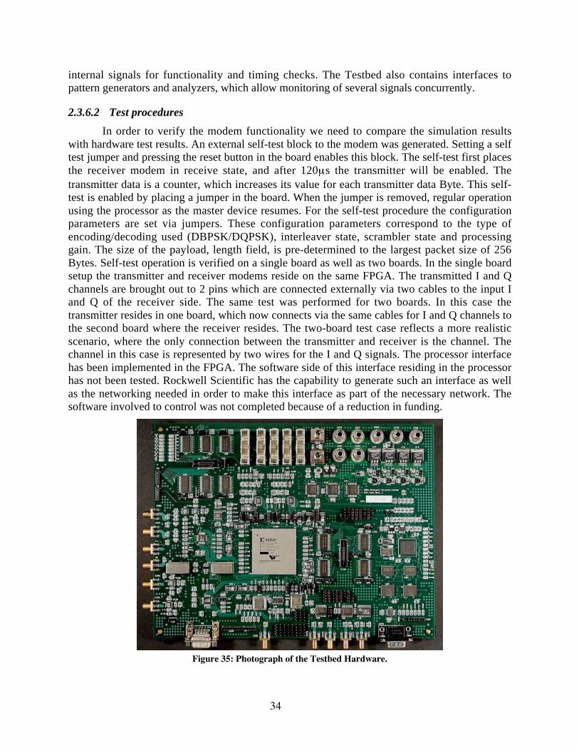
34
internal signals for functionality and timing checks. The Testbed also contains interfaces to
pattern generators and analyzers, which allow monitoring of several signals concurrently.
2.3.6.2 Test procedures
In order to verify the modem functionality we need to compare the simulation results
with hardware test results. An external self-test block to the modem was generated. Setting a self
test jumper and pressing the reset button in the board enables this block. The self-test first places
the receiver modem in receive state, and after 120ms the transmitter will be enabled. The
transmitter data is a counter, which increases its value for each transmitter data Byte. This self-
test is enabled by placing a jumper in the board. When the jumper is removed, regular operation
using the processor as the master device resumes. For the self-test procedure the configuration
parameters are set via jumpers. These configuration parameters correspond to the type of
encoding/decoding used (DBPSK/DQPSK), interleaver state, scrambler state and processing
gain. The size of the payload, length field, is pre-determined to the largest packet size of 256
Bytes. Self-test operation is verified on a single board as well as two boards. In the single board
setup the transmitter and receiver modems reside on the same FPGA. The transmitted I and Q
channels are brought out to 2 pins which are connected externally via two cables to the input I
and Q of the receiver side. The same test was performed for two boards. In this case the
transmitter resides in one board, which now connects via the same cables for I and Q channels to
the second board where the receiver resides. The two-board test case reflects a more realistic
scenario, where the only connection between the transmitter and receiver is the channel. The
channel in this case is represented by two wires for the I and Q signals. The processor interface
has been implemented in the FPGA. The software side of this interface residing in the processor
has not been tested. Rockwell Scientific has the capability to generate such an interface as well
as the networking needed in order to make this interface as part of the necessary network. The
software involved to control was not completed because of a reduction in funding.
Figure 35: Photograph of the Testbed Hardware.

35
2.3.6.3 Implementation results
A major goal in the PAC/C effort is the power awareness. For this reason power
consumption is an important parameter to be measured. Figure 36 shows all utilized resources in
the FPGA. By extrapolating basic power consumption measurements, accompanied with data
obtained from Xilinx data sheets some power reduction estimates can be done.
Target Device: XV1600E
Target Package: BG560
Target Speed: -6
Mapper Version: virtexE
Design Summary
--------------
Number of errors: 0
Number of warnings: 70
Number of Slices: 1,161 out of 15,552 7%
Number of Slices containing
Unrelated logic: 0 out of 1,161 0%
Total Number Slice Registers: 1,503 out of 31,104 4%
Number used as Flip Flops: 1,498
Number used as Latches: 5
Total Number 4 input LUTs: 1,712 out of 31,104 5%
Number used as LUTs: 1,636
Number used as a route-thru: 76
Number of bonded IOBs: 131 out of 404 32%
IOB Flip Flops: 6
Number of Block RAMs: 12 out of 144 8%
Number of GCLKs: 3 out of 4 75%
Number of DLLs: 3 out of 8 37%
Total equivalent gate count for design: 245,301
Additional JTAG gate count for IOBs: 6,288
Figure 36: Implementation Resource Utilization Results.
Examining the implementation data we can clearly see the size of the FPGA is not
appropriate for this design. Only a small percentage of the FPGA resources have been utilized.
Given the FPGA technology the unused resources increase significantly the energy consumption.
FPGAs have a quiescent power consumption, which is the power consumed just to keep the
circuits programmed. This value increases with the size of the FPGA. For example a 1.6 Million-
gate device is rated at 180mW quiescent power consumption, where a 200,000-gate device has
estimated 29mW quiescent power consumption, 84% reduction. Our design after configuration
of the device consumes 73mA at 1.8V, 131mW quiescent power. The modem design would fit in
a 200,000-gate device, which taking the rated power values would reduce the quiescent power
consumption by 84% to 12mA. In the future, once the implementation hardware platform has
been defined, accurate power measurements should be performed. At this point such
measurements are out of the scope of the project, and difficult to measure in the testbed.

36
3 FINAL STATUS REPORT ONMIDDLEWARE, TOOLS, AND TECHNIQUES
3.1 Introduction
The purpose of this task was to examine techniques for energy management that leverage
the interactions between hardware and software on a single node as well as network-wide
interactions among many collaborating nodes in a sensor field. This research was performed
through a combination of simulation-based analysis and platform studies using commercial and
research platforms. For the single node, the research focused on the development of a power
aware Real-Time Operating System (RTOS) and other power management middleware APIs.
Techniques for node-level power management are discussed in Section 3.2. At the field-level,
the areas of investigation include communications techniques such as dynamic modulation
scaling and protocols for collaborative field behavior such as coverage topology management.
Techniques for network-wide power management are discussed in Section 3.3. Finally, the
concept studies in node-level and field-level power management utilized and extended a suite of
sensor network simulation tools developed at UCLA. The SensorSim tool environment is
described in Section 3.4.
3.2 Techniques for Node-Level Power Management
The current state of the art in software-transparent hardware and firmware power
management is limited to shutting down the CPU and peripheral components after a certain idle
time. This technique fails to exploit application knowledge of timing constraints, usage history,
and traffic patterns. It also ignores the possible existence of “power-speed control knobs” (e.g.
CPUs with dynamically controlled frequency and voltage). Therefore, the current methods
cannot fully utilize the dynamic range of power management that could be provided by the lower
layers. This task examined new approaches to address these issues. Since knowledge about
timing, usage, and traffic is often available only at run-time, the logical place for making power
management decisions is in the Real-Time OS (RTOS) resource scheduler. Key to our approach
is task management that guarantees “JIT” (just in time) power through coordinated scheduling
and power management of resources by the RTOS at a microsensor node.
3.2.1 Power Aware Resource Scheduling
Wireless systems have various resources that consume power including CPUs, radios,
and sensors. However, traditional RTOS schedulers have focused on the CPU resource from the
perspective of time (i.e. statically or dynamically scheduling multiple tasks so that timing is
met). Some schedulers manage other resources such as disks, but none manage resources like
radios and sensors, which are critical to the extended operation of a sensor node. In any case,
power is generally ignored. Key to a power-aware sensor node is power management of all node
resources. This effort expanded time-based static and dynamic scheduling to include adaptive
power-management of all accessible sensor node subsystems. It examined both static scheduling
and variants of dynamic scheduling, including fixed priority preemptive scheduling (e.g. rate
monotonic) and dynamic priority preemptive scheduling (e.g. earliest deadline-first). The basic
approach exploits slack time in the schedule to shutdown a resource or to operate it at a lower-
power lower-speed setting. Slack times are gathered by static analysis of the task set and by

37
timing constraint specifications (rates and deadlines), as well as runtime statistical analysis of
resource usage patterns gathered by special hardware or software “monitors”. We investigated
the problem of prediction of resource usage activity, which is essentially a timing series
prediction problem, and explored approaches such as Kalman filtering, voting by multiple
experts, and training a parametric model (e.g. a hidden-Markov model). A meaningful strategy
for scheduling resource mode changes also requires knowledge of the power and/or time cost
associated with the change. For example, changing the radio from idle to transmit mode would
require some latency and would consume energy (e.g. for the frequency synthesizer to stabilize,
or for GPS systems to acquire a lock). Therefore, the RTOS must decide whether the extra power
and latency cost is worth the change. Before shutting down a radio, the RTOS must determine if
wake-up latency can be tolerated (or, if it could be hidden by pre-wakeup). The prediction
accuracy for scheduling resource mode changes can be further enhanced by making use of
information that can be provided by the application. For example, a radio may not know when
the next packet will be received or transmitted, and it may be hard for the radio monitor to learn
this. However, applications potentially have this information and can provide it to the RTOS
when admitted for scheduling, or as they run. Figure 37 shows the hardware resources and
software layers for coordinated node-level power management.
Sensors RadioCPU
Energy-aware RTOS, Protocols, & Middleware
PA-APIs for Communication, Computation, & Sensing
Dynamic
Voltage &
Freq. Scaling
Scalable
Sensor
Processing
Freq., Power,
Modulation, &
Code Scaling
Coordinated Power Management
PASTA Sensor Node Hardware Stack
Figure 37: Coordinated Node-Level Power Management
3.2.2 Power-aware API for RTOS-driven CPU Power Management
While working on adaptive power-fidelity schemes the research team had identified the
need for a common software framework to: a) allow an apples-to-apples comparison of
shutdown and dynamic voltage scaling (DVS) power management schemes, b) provide a
standard interface for developers of power-aware applications, and c) allow easy porting of
implementations to multiple embedded platforms. The team developed a power-aware API that
provides standard software interfaces to exchange power and performance information among
power-aware hardware, operating system, and applications to support task scheduling, admission
control, and run-time adaptation. Table 18 provides a list of power aware API functions.
Table 18: Power Aware API Functions
paapi_sched_create_task_type (real time info) Create a task type given the real time constraints.
paapi_sched_create_task_instance (type) Create a task instance given the type.
paapi_sched_app_started (task instance) Tell the operating system that the task started a new

38
execution.
paapi_sched_app_done (task instance) Tell the operating system that the task is done with
the execution.
paapi_os_timetick_get_minimum_resolution(nsec) Find out what is the minimum resolution the OS
tick can be set to met the timing constraints.
paapi_os_timetick_time_to_ticks(nsec) Convert the time restriction, given in nanoseconds,
into OS ticks.
paapi_sched_set_time_prediction(task instance) Tell the operating system about timing remaining
prediction (specific to predictive scheduling).
paapi_sched_get_time_prediction(task instance) Get the time prediction given by the operating
system (specific to predictive scheduling).
pahal_initialize_processor_power_management() Initialize processor power management internal
data structures.
pahal_processor_get_freqlevels_info() Get processor frequency level information.
pahal_processor_get_currfreq_info() Get current frequency level info.
pahal_processor_pre_set_frequency(current, new) Function that is called before changing processor
frequency (platform dependent).
pahal_processor_set_frequency(current, new) Function to actually change processor frequency.
pahal_processor_set_frequency_and_voltage(new_frequency) Function to actually change frequency and voltage.
pahal_processor_post_set_frequency(current, new) Function that is called after changing processor
frequency (platform dependent).
pahal_processor_get_states_info() Get information about low power states of the
processor.
pahal_processor_set_state() Set the processor to a specific low power state.
pahal_processor_cycles_to_nsec() Convert cycles to nanoseconds.
pahal_processor_nsec_to_cycles() Covert nanosecond to cycle.
pahal_battery_get_info() Get battery related information (for battery based
devices).
pahal_battery_get_percentage_available() Get percentage of battery available in the system.
The power aware RTOS implementation includes three different schedulers. The first is a
rate-monotonic scheduler (based on static priority based preemptive scheduling) with shutdown.
The second is a rate-monotonic scheduler with shutdown and per-task static slowdown factors
according to which voltage and frequency are set at task context switch time. The third is a rate-
monotonic scheduler with shutdown, per-task static slowdown, and a dynamic slowdown based
on run-time task execution time prediction. The latter two schemes are based on algorithms
developed at UCLA under this project. The API was implemented on top of eCos, an open-
source RTOS, as shown in Figure 38. Two different platforms are supported: the StrongARM-
based iPAQ and the Intel XScale 80200 Evaluation Kit. The iPAQ is capable of shutdown and
frequency scaling. The evaluation kit allows software-controlled voltage scaling when combined
with a Maxim 1855 Evaluation kit (MAX1855EVKIT) as power supply (shown in Figure 39).
The RTOS software with power-aware API and hardware reference design specifications for the
XScale dynamic voltage scaling testbed are available to the research community via the web:
http://nesl.ee.ucla.edu/projects/pads.

39
Figure 38: Power Aware API Layers Figure 39: Dynamic Voltage Scaling Testbed
3.2.2.1 Power Analysis of XScale with Dynamic Voltage Scaling
Using the dynamic voltage scaling testbed described above and the power aware software
framework, UCLA performed a detailed power analysis of XScale processor at the instruction
level. The processor has a dynamic power range of approximately 5X as frequency scaled from
333 MHz to 733 MHz, with the voltage being changed concurrently. However, in some cases the
device could be significantly over-clocked for a particular voltage setting. Figure 40 shows
power when the processor is idle (NOP). Figure 41 and Figure 42 give power ranges for integer
addition and floating point multiply. Figure 43, Figure 44, Figure 45, and Figure 46 provide
memory read, memory write, peripheral read, and peripheral write, respectively.
Figure 40: XScale NOP Power
A|l|jtJLdTJilll l.dMM' A|j|jliLdriuii
1 r Afigj^JcjcJuii
\Vrapper WrapptT
1
1S(>( Ul>rdr> WiiilsiiiDn Onilml ['nil API
\dli\t(: API u Power Manager 1 aitk Manager J liilenidl Keriirl A 1*1
Schefliilrr
llmilndri! \lr^ridi:lj"ii l.dver
Slri>ngARM SA-LIUI prficesiior
Core and Analog Power - NOP
crhft
soo
^
^ ^
400 . ^ --'-'^ -^
^ -^ 333MHI -^ ^ ^
I <r^ -""'^ . .(OOMHl
^ <:> -^ 466MMI
I 300 - a
-^-"""^-^ 533MMI
B(inHH7 ^^^ ^^ -^ """"' '"'^ ^^ ---'' _,_ -- '^ e66MH£
2DD . __ -— .^^^^"^ 733MHI
___ --— ^ -- -^ * "lanulacturer Sfiedhni Maximum Fi*quenfy
1 00 - L -"'^
n .
1 oov 05V 1 1 OV 1.1 5V 1 20V 1 2SV 1 30V 1 35V 1 flOV
Supply Voltiga
i 4SV 1 sov

40
Figure 41: XScale Add Integer Power Figure 42: XScale Multiply Float Power
Figure 43: XScale Memory Read Power Figure 44: XScale Memory Write Power
Figure 45: XScale Peripheral Read Power Figure 46: XScale Peripheral Write Power
The measurement approach used by the UCLA team was to insert numbered powermeasurement regions (PMR) in the source code using macros (PMR_START, PMR_END) from
the power aware API. The power aware runtime system logs the PMR and triggers the data
acquisition card (DAQ) with a GPIO. A PC-based analysis tool matches the PMR and DAQ
logs, calculates averages and total energy in each PMR. These basic power/performance datasets
Core and Art^oq POMIVI -Add Snigger
-"^ ^ -^
-^ ' .^-- ^
^ x'-'^
' ,-'- ^
-^ __^ -—- -- -"^ __ ^J -^:^ :^—- —'
c .
Coie dixJ Analog Poimt - Hulhiily Float
:9a .
^
^-- ;^':> DJifHl
ianiiHr
,^ :>- '' _^ ^^ " ^
-^ ___ -—' ^ -^ -^ ___ ^ i:::^ -— —^ - UBmbnSiB^d
"
1 a
l«prl>>«ll«pa
BV 1 31* 1 4CV 1 . ?V 1 s "
Core and Aralcg Power- Uemoiy Read
roo
ton
\ I™
1
^ -^^ -;:- ^ -^ JJJHHJ
fIflMHT
^^ ^^ ^ ^" ^ '-'' ,^ -^
_----- -:::: ::::^ —' —^
'--^ '"^ tJbvtin FiDoirtiV
1 0
i^JFDly VvlUpa
CWB and Analog Pnm - Homorr Wrilo
^ ^ ^ ^ :^
.^- ,^
60MHI
,<; ::^ --^
,^ ^^^ 1
i- --'' ^^^ " ^,_- —-- '^ --"
'" _____ ---- ;::i^ -— -"^ . ri 1 1 "ill
"^ •^
' :s :. , : ^
1
CDIB and An^iiog POWB- - Peripheral Bead
I
3J3Bhtl
l»ElirtJ
&J9H-I]
6CIIMNJ
((hU-J
3^m.J
Core and Andog Power - PofifihefaJ Wnr«
4 . J
«a>pir *vn»«v

41
were used to generate thresholds for predictive task scheduler research and the software
infrastructure was used to validate the scheduler algorithms.
3.2.3 Predictive Dynamic Voltage Scaling for Adaptive CPU Fidelity
Analysis of execution times for a variety of signal processing tasks in embedded systems
shows that the worst-case execution time (WCET) is often several times longer than best-caseexecution time (BCET). For example, Figure 47 shows the difference in MPEG frame decoding
time and Figure 48 plots varying times for audio speech decoding. However, wireless systems
such as sensor networks need to be resilient to packet loss. A crucial observation is that missed
deadlines in many computation tasks on a sensor node are no different than noise in the radio orsensor: it would result in a radio or sensor packet being dropped. This allows a scheduler to
aggressively predict task instance runtime and scale the dynamic voltage accordingly.
Variation in MPEG Frame Decode Times
0
0.02
0.04
0.06
0.08
0.1
0.12
1 5 9 13 17 21 25 29 33 37 41 45 49
Frame #
Dec
ode
Tim
e(s
econ
ds)
Figure 47: MPEG Decode Times
Speech CODEC Frame Decode Time
0
50
100
150
200
250
300
350
400
450
500
0 60 120 180 240 300 360 420 480 540 600 660
R l Ti ( )
Dec
od
eT
ime
(use
cs)
Figure 48: Speech CODEC Decode Times
The result of proactive dynamic voltage scaling with prediction on a variety of signal
processing tasks was a 75% energy reduction over worst-case non-predictive voltage scaling
with a negligible loss in fidelity (up to 4% deadline misses). Figure 49 compares energy
consumed by shutting down hardware on task completion, a WCET non-predictive dynamic
voltage scaling scheduler, and the predictive dynamic voltage scaling scheduler based on BCET.
These results demonstrate that many applications have “energy-speed” or “energy-accuracy”
control knobs that allow a given task to operate at lower energy but over a longer time or with
lower fidelity. An important feature of the power aware API research was exposing these knobs
to the application developer so they can be dynamically managed at runtime.
0
0.1
0.2
0.3
0.4
0.5
0.6
0.55 0.6 0.65 0.7 0.75 0.8 0.85 0.9 0.95 1
Shutdown
Non-predictive DVS
Predictive DVS
Figure 49: Predictive Dynamic Voltage Scaling Energy

42
3.2.4 Battery Lifetime Management
An interesting result of this research was the impact of task scheduling on achieved
battery capacity. An ideal battery’s capacity doesn’t vary with the discharge rate. However, real
batteries have discharge rate dependent characteristics such as the reactants diffusion process, the
rate of electrode reaction, and the battery’s internal impedance. The maximum battery capacity
is only achieved at a low discharge rate.
Operating
Mode
Total
Lifetime
Capacity (in mAh)
consumed from Battery
Capacity (in mAh)
delivered to Sensor
Energy (in Joules)
consumed from Battery
Energy (in Joules)
delivered to Sensor
DC/DC
converter
efficiencyTx .33 hr 8.1 4.1 70.0 49.1 70%
R x .88 hr 15.8 7.9 135.2 96.1 71%
Idle 1.2 hr 18.0 9.0 154.0 109.0 71%
Sleep 7.0 hrs 59.1 28.8 505.1 350.7 69%
Figure 50: Achieved Battery Capacity Versus Operating Mode
The original Mote microsensor developed at UC Berkeley uses an unregulated voltage
supply directly from the battery. Unlike operating with a voltage regulator, this exposes the
battery to dynamic variations in current discharge based on operating mode of the microsensor.
For example, in Figure 50 the total energy extracted from the battery varied from 70 Joules
continuously transmitting to 505 Joules in sleep mode. A number of battery-aware scheduling
approaches were investigated to find optimal performance to maximize total service during the
lifetime of the battery. The best approach achieved an 80% improvement in total number of bits
transmitted over non-battery-aware techniques. Figure 51 shows the measured battery capacity
versus discharge power (left), data rate in kilobits per second versus average power (center), and
total number of bits versus average power (right). This indicates that there is an optimal data rate
of about 5kbps to maximize Mote battery lifetime.
Figure 51: Data Rate and Battery Capacity Comparisons
3.3 Techniques for Network-Wide Power Management
This task also investigated techniques for network-wide distributed power management
that complemented the power aware RTOS and middleware described above. Distributed power
management is essential to sensor fields because of the need to collaborate and communicate for
most sensing applications. There were two main areas of investigation: 1) communication
techniques designed to save energy on the wireless links and multi-hop routes, and
2) collaborative distributed resource allocation strategies to maximize effective sensor field
lifetime while maintaining continuous coverage.
Battery Capacity vs Discharge Power ala Rale V9. Pave
^ 10 IS 20 20 30
s
In . ID' Total N jmber o1 Bils vs Pave
Z\ i i 3 1' /^ \ / V;
s Z' o
I \ 1 ; A i
; \ ; a-*
hXt^ ID 20 30 IQ

43
3.3.1 Energy-aware Packet Scheduling with Dynamic Modulation Scaling
The notion of Dynamic Modulation Scaling (DMS) was based on the observation there is
a strong analogy between voltage scaling of a CPU and bit-per-symbol/bit-per-second scaling for
a radio. Energy and delay of data transmission depends on modulation settings. This was studied
in detail for Quadrature Amplitude Modulation (QAM) radios with adaptive bits-per-symbol.
The tradeoffs for QAM are to adapt b (number of bits per symbol) and operate at maximum Rs
that can be implemented efficiently. Similar tradeoffs are possible for other scalable modulation
schemes Phase Shift Keying (PSK), Differential Phase Shift Keying (DPSK), Amplitude Shift
Keying (ASK), and Orthogonal Frequency Division Multiplexing (OFDM).
Figure 52: Voltage Scaling Versus Modulation Scaling
3.3.1.1 Queue-Based Dynamic Modulation Scaling
Moreover, packet scheduling in radios is analogous to task scheduling on processors. A
key difference is that packets, unlike tasks, are not preemptible. A number of packet scheduling
schemes were investigated for wireless links using dynamic modulation scaling. The first to be
investigated was Queue-Based Dynamic Modulation Scaling. In this technique, modulation
settings were set according to the packet queue status including number of packets and total size
of transmit buffer on the sending end. This is the DMS counterpart to simple queue-based
schemes commonly used in task schedulers.
Figure 53: Queue-Based Dynamic Modulation Scaling
Voltage scaling
Modulation scaling
Rsdro
R,i— => bi—^
DIgrtar Hardware
T
P,-V-l,-e"-
1, V i '
1 «! £'Ps'Pj i
a '&
P" "T" ^ 1 Procc»<sor -t.| 1 1 1 1.L.H- Kudio
A
R-DPM
ISO GOO

44
3.3.1.2 Energy-Aware Real-Time Packet Scheduling
The second scheme, Energy-Aware Real-Time Packet Scheduling, exploits variation in
packet length to perform aggressive dynamic modulation scaling in real-time. This technique
handles the case of multiple applications sending streams of periodic but varying length packets
with deadline constraints. It is suitable for sensor nodes talking to a local gateway. Analysis of
this approach demonstrated up to a 60% reduction in transmission energy. Similar packet
scheduler approaches were investigated, such as an energy-aware variant of the commonly used
weighted fair-queuing based packet schedulers. In the weighted fair-queuing model, weights are
associated with the various packet flows and the scheduler allocates the available bandwidth to
those flows with non-empty queues in proportion to their weights over arbitrarily small time
intervals. Conventionally the scheduler decides which flow to transmit a packet from, and when.
The new scheduler, energy-efficient wireless fair queuing (E2WFQ), exploits the dynamic
modulation-scaling knob to decide at what speed a packet should be transmitted. It does so by
continually monitoring the status of the packet queues, and calculates how fast a packet needs to
be transmitted based on the packets ahead of it and the deadline. The reduction in energy
depends on the traffic condition parameters such as link utilization and burstiness. There is little
gain from the scheme if the link
utilization is near 1 (i.e. there is
little head room left to exploit
DMS as the channel is always
busy even with the radio at
maximum speed) or if the
burstiness is high. However,
gains of 3-4X are observed under
typical traffic conditions and
radio speeds.
3.3.1.3 Dynamic Code Scaling
In addition to Dynamic Modulation Scaling, the research team also investigated Dynamic
Code Scaling (DCS) by changing the rate of the bit-level forward error correction (FEC) within
the same DMS framework. Both DMS and DCS offer a convex energy-throughput control knob
that energy-aware packet scheduling can exploit. Figure 54 shows the compares the energy per
useful bit for fixed and dynamic code rates.
Figure 54: Energy per Useful Bit with Dynamic Code Scaling
a
OS u
B
•- xed Code Route |14
7 12 ,
1 CD ID
B B
a 2
/
10' ID",/
10"
^ .^— -.^—
c LU 1
200 400 600 BOO 1000 1200 1400
Psckel Length (byles)
Optimal CoOe Bate
200 400 600 800 1000 1200 1400
Packet Lengtn (t>ytes)

45
3.3.2 Sparse Topology and Energy Management
Sparse Topology and Energy Management (STEM) improves network lifetime by
exploiting the fact that, most of the time, the network is only sensing its environment waiting for
an event to happen. The motivation is that the energy consumption in sensor network is typically
dominated by the node’s communication subsystem. It can only be reduced significantly by
transitioning the embedded radio to a sleep state, at which point the node essentially retracts
from the network topology. Existing topology management schemes have focused on cleverly
selecting which nodes can turn off their radio, without sacrificing the capacity of the network.
For this they exploit extra node density beyond what is needed for communication connectivity.
However, in sensor networks preserving communication capacity at all times is not a good idea.
Alleviating the restriction of network capacity preservation yields extensive energy savings at the
expense of an increased latency to set up multi-hop paths. The basic STEM scheme is based on
using two radios at each node: one is a regular data radio while the other is a wake-up radio. The
goal of having two radios is that the wakeup radio could be much simpler with a much lower
data rate and lower power on the receive side. However, the scheme works even with two
identical radios with no special differentiation in capabilities. It can also work with a single radio
with two channels or a single radio with one channel with time synchronization at some
degradation in performance. In the two-radio scenario, one radio operates in the data plane, and
the other in the wakeup plane. As shown in Figure 55, receivers in the wakeup plane periodically
listen for beacon packets on a very low duty cycle (0.1%). An initiator issues a train of beacon
packets until the target acknowledges. The data packet then commences on the data plane.
Figure 55: Operation of STEM
As shown in Figure 56, the energy savings for STEM is dependent on the fraction of time the
communications subsystem spends in the forwarding state. In most monitoring sensor systems,
data packets are highly infrequent, so the monitoring state dominates.
Figure 56: STEM Performance Analysis
W.il.viip plar
J \ L_L
JTar
Iiiilulor IIIHIC
Target mnlc
0
0
U 4licup pLinc III
DtupUnc B
Initiator node
I. beacon received
2. beacon acknowledge
Target node
4 \\akrup plane
Oala plane Mnnitnring state 0
Setup latency
ciicr^ Hiviiigik E T^
Appropriate choice
Mostly monttonnf* state: n« I

46
Figure 57 shows STEM performance results from simulation analysis. The approach has beenvalidated on a testbed consisting of iPAQs equipped with 802.11b radios as the primary dataradio and a mote microsensor with the RFM TR1000 radio acting as the wakeup radio. Themotes were connected to the iPAQs over the serial ports. The STEM algorithm performed aspredicted by the simulation models.
Figure 57: STEM Simulation Analysis
3.4 Sensor Networking Simulation and Planning Tools
Under the DARPA SensIT program, ISI and UCLA were funded to develop a simulatorfor networking protocol and systems analysis of distributed sensor networks called SensorSim.An ns-based simulation platform was developed that modeled media access control (MAC), link,and routing protocols used in the SensIT program. A unique and useful feature of this simulationtools was the capability to perform hybrid simulation with both real and simulated nodes in thesame network. In this way, a much larger virtual sensor network could exercise an actualinstrumented hardware node with appropriate traffic. The PADS effort extended this SensorSimsimulation infrastructure with several new capabilities, including:
1) A capability to explicitly model the hardware hierarchy of a networked sensor node,and its power behavior. The original ns simulation tool allows modeling of protocol agents andapplication agents at each networked node, but there was no provision of modeling the powerbehavior of hardware resources such as the processor, sensors, radio, battery etc. The radio,processor, sensors, and other power consumers are now modeled as hardware resources that havemultiple states of operation (sleep, idle, active etc.), each with different levels of performanceand power consumption, and time and power costs associated with transitions from one state toanother. Each resource has an associated API so that the higher level systems agents (protocols,OS, applications) modeled in ns can 1) use the resource for some interval of time, 2) cause thestate of the resource to change, and 3) change their behavior according to system parametersimpacted by the state. On the producer side, the battery model includes the dependence of batterylifetime on discharge current rate and discharge current profile (constant discharge vs. pulseddischarge). Datasets for these models were generated from the power characterization frominstrumented platforms such as the Berkeley Mote, iPAQ, and XScale evaluation board.
^(W)
— Thsary O SlmuliUon
1
1
W/lboul STEM
lo-' \
T^ ft\ \\>, 1
\
*•««*, V H C: T7— —^ ^ ^— —0 Ma
v^ ^"*^ 11
IS - 1..13 Tt U U
10-* \^^^ ()= 13.33
ID W 10 10
Average setup latency of STEM Relative energj' savings of STEM
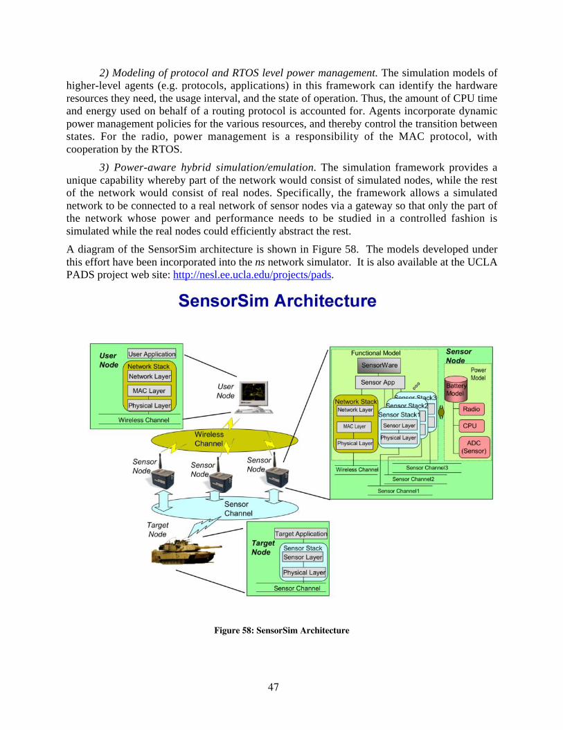
47
2) Modeling of protocol and RTOS level power management. The simulation models ofhigher-level agents (e.g. protocols, applications) in this framework can identify the hardwareresources they need, the usage interval, and the state of operation. Thus, the amount of CPU timeand energy used on behalf of a routing protocol is accounted for. Agents incorporate dynamicpower management policies for the various resources, and thereby control the transition betweenstates. For the radio, power management is a responsibility of the MAC protocol, withcooperation by the RTOS.
3) Power-aware hybrid simulation/emulation. The simulation framework provides aunique capability whereby part of the network would consist of simulated nodes, while the restof the network would consist of real nodes. Specifically, the framework allows a simulatednetwork to be connected to a real network of sensor nodes via a gateway so that only the part ofthe network whose power and performance needs to be studied in a controlled fashion issimulated while the real nodes could efficiently abstract the rest.
A diagram of the SensorSim architecture is shown in Figure 58. The models developed underthis effort have been incorporated into the ns network simulator. It is also available at the UCLAPADS project web site: http://nesl.ee.ucla.edu/projects/pads.
Figure 58: SensorSim Architecture
SensorSim Architecture
Ussr JUaar Applicalionl
Node
Wirelssa Channel
Target Applicatier
Target Node
1
^Sensor Stack ^ 1 Sensor Layer!
1 1 Physical Layer]
^ 1 -' Sensor Channel
Functional Model
ensorWare
Senaor Node
Sensor App
Network Steck NelworK Layer
MAC Layai
1 Phy&ICBl Layer
sensor Slack'
Ssnsor Layer I
^hywcal Layer ]
Power Model
WlrelaaB Channel
Radio
- CPU
ADC (Sensor)
Sensor Chanr>d3
Sensor ChBnnelZ
Sensor Channell

48
4 FINAL STATUS REPORT ONALGORITHMS
4.1 Introduction
Consistent notion of identifying accuracy/energy “knobs” described in the previoussections on hardware and software, power aware algorithm development uses the same approach.In the PASTA effort, the algorithm team realized that there are three distinct phases in poweraware algorithm development: analysis, optimization, and introspection. In the analysis (or“knobs”) phase, the goal is to identify algorithm input parameters that can be adjusted anddetermine their impact on accuracy and energy. In this phase, the input parameters are exposedto manipulation by the software. In the second phase, other optimizations unrelated to inputparameters are investigated such as eliminating domain transforms or introducing domaintransforms to simplify the computation. The third phase, called introspection, incorporates agoals-focused “knob” into the algorithm such as accuracy, false alarm-rate, or target powerconsumption. The “knob” can be set by the application designer at design time, or adjusteddynamically in real-time by some rules-based agent monitoring environment activities andremaining hardware resources (battery lifetime, for example).
Figure 59: Three Stages of Power Aware Algorithm Development
4.2 Acoustic Beamforming
ISI obtained an acoustic beamforming algorithm from the Army Research Laboratory forpower aware analysis. In addition to the algorithm in MATLAB (and ported to C by MIT), theapplication baseline package contained one and two vehicle datasets along with ground truth.The acoustic array contained a total of seven microphones; six evenly spaced on an 8-footdiameter circle and the seventh in the center. The acoustic array is shown in Figure 60. Withpermission of ARL, ISI distributed this baseline algorithm throughout the PAC/C community.
Idi'iitilV alj^orithni and system "knobs" in the application.
Determine energy and accuracy implicaliuns at various settings.
Enable "accuracy" and "energy" focused system tuning.
Eliminate or niininii/e domain transforms.
Analy/v precision of the mathematics and migrate code to llxed point.
Tailor the processor to the precision (32-bit, 16- bit, or 8-bit).
Automate "knob" tuning based on:
D Kiivironmcnt. D Tar^i'l lu'hinior. D Collaboriitiun. n Energy reserves, D Threat assessment.

49
Figure 60. ARL Baseline Acoustic Array
4.2.1 Acoustic Beamforming Knobs
Acoustic beamforming algorithms estimate the line of bearing (LOB) to a distant acousticemitter by shifting signals from microphones at known relative locations to form beams fromselected directions. The LOB is a byproduct of the optimal reconstruction of the signal from anemitter by shifting and adding the signals from a number of microphones. The background noiseand sounds from other emitters will be reduced in proportion to the number of microphones. Theaccuracy of acoustic beamforming depends on a number of parameters, including: 1) the numberof microphones, 2) number of acoustic samples, and 3) number of beams or search angles. Eachof these parameters has a unique impact on accuracy and energy of the system.
Figure 61: Beamforming "Knobs"
4.2.1.1 Number of Microphones (M)
The number and placement of microphones is principally a hardware design parameterbut can also be used as an algorithmic parameter by selecting a subset of the signals collected.The system energy required for beamforming is proportional to the number of microphones, butthere are negligible improvements in accuracy due to adding more microphones at the same
e 9 BEAMFORMING ".\ [jT.v D'''(TvD''"TAIg)(PcPU''"°OveriKad'~
Line of Bearing
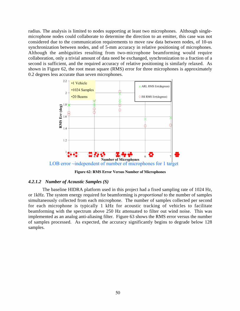
50
radius. The analysis is limited to nodes supporting at least two microphones. Although single-microphone nodes could collaborate to determine the direction to an emitter, this case was notconsidered due to the communication requirements to move raw data between nodes, of 10-ussynchronization between nodes, and of 5-mm accuracy in relative positioning of microphones.Although the ambiguities resulting from two-microphone beamforming would requirecollaboration, only a trivial amount of data need be exchanged, synchronization to a fraction of asecond is sufficient, and the required accuracy of relative positioning is similarly relaxed. Asshown in Figure 62, the root mean square (RMS) error for three microphones is approximately0.2 degrees less accurate than seven microphones.
Figure 62: RMS Error Versus Number of Microphones
4.2.1.2 Number of Acoustic Samples (S)
The baseline HIDRA platform used in this project had a fixed sampling rate of 1024 Hz,or 1kHz. The system energy required for beamforming is proportional to the number of samplessimultaneously collected from each microphone. The number of samples collected per secondfor each microphone is typically 1 kHz for acoustic tracking of vehicles to facilitatebeamforming with the spectrum above 250 Hz attenuated to filter out wind noise. This wasimplemented as an analog anti-aliasing filter. Figure 63 shows the RMS error versus the numberof samples processed. As expected, the accuracy significantly begins to degrade below 128samples.
2,2 1
2-
a
•1 Vehicle
•1024 Samples
•20 Beams y .v-
1,6
1.4
1.2
)h
n
ARI. RMSi:rrldLTii-L-M
0ISI RMS Errtdegrees)
C!
Wf—?://%* t^# Number of Microphones
LOB error -independent ornumbcr ul tnicruphones for I target

51
Figure 63: RMS Error Versus Number of Samples
4.2.1.3 Number of Beams (B)
The beam power is computed at a number of evenly spaced search angles, andinterpolated by a parabolic fit to estimate the angle with maximum power. The number of beamsonly affects the execution speed of the algorithm, not data acquisition. The system energy forbeamforming is linear with, not proportional to, the number of beams searched. As shown inFigure 64, the RMS error is nearly constant over 15 beams.
Figure 64: Accuracy and Energy Versus Number of Beams
32 64 96 128 160 192 224 256 Number of Samples
67
ec 4
•1 Vehicle
64 Samples
•7 Microphones
10
ISI RMS Errtdcgrccs)
ARL RMS Krrt degrees
ARL/ISI Energy Ratio
(.!!(]
5IK)
4(K) o
300
4 200"
Similar RMS Error ^ '«> with ~300x Efficiency
9 OS
15 20 Number of Beams
25 30

52
4.2.2 Algorithm Optimizations
In addition to the power aware algorithm “knobs” described above (microphones,samples, beams), the team investigated the impact of converting from floating point to integermath and eliminating the data transform to the frequency domain. Since floating point isemulated in software on the XScale processor, converting to integer math had the mostsignificant impact on power – approximately 20X. Eliminating the Fast Fourier Transform (FFT)to the frequency domain and performing a time-domain beamform (Figure 65) yielded anotherfactor of 1.5X.
Figure 65: Frequency Domain Beamformer (top) and Time Domain Beamformer (bottom)
4.2.3 Acoustic Line Of Bearing Results
Figure 66 shows the acoustic line of bearing energy according to the RMS error. Usingthis “introspection knob”, the desired accuracy or the desired energy can be chosenindependently and the algorithm parameters (number of beams, number of samples, number ofmicrophones) are adjusted to achieve the best result. It is clear in this graph, that the RMS errorsless than three degrees consume a disproportionate amount of energy. This suggests that anadaptive multi-resolution search strategy would have a significant impact on total system power.The blue line (dotted) shows the ISI algorithm energy performance relative to the original ARLbaseline implementation. The ISI version achieved between 180X and 850X energyimprovement (depending on selected RMS error) on the same hardware.
ARL
ISI
Tificrophone" » HI- 4 Sjiinnli'
o Microphone 2 '
Ml \ Microphone 3
- \
Microphone 4 ^ IDIt Angle
Microphone 5
Microphones
(decrees)
Microphone 7 . 102 FF
4 Samplo
_ Microphone Sclecu _Number of Samples
on Control Conlrol Contro^l
\ Microphone I
Microphone 2
Microphone 3
i ' Timo * Del^ * Microphone 4 A
.T LOB Angle (tiegiucs)
Microphone 5
Microphone 6

53
Figure 66: Acoustic Line of Bearing Energy Versus RMS ErrorFigure 67 plots ISI and ARL location estimates against the GPS-derived ground truth suppliedwith the algorithm. The two versions of the algorithm can be tuned to be identical inperformance. The primary difference is that the ISI version can relax accuracy constraints toconserve more energy.
Figure 67: ISI and ARL LOB Versus Ground Truth
4.2.4 Line of Bearing Performance on HIDRA
The power results reported above were derived from simulation using JouleTrackdeveloped at MIT. However, that tool doesn’t capture the entire system-level energy picture. ISIported a version of the ARL baseline algorithm and the optimized ISI algorithm to HIDRA anddid extensive power analysis in the lab. The next four charts summarize the results. Ofsignificant interest is that although the processing overhead does indeed virtually disappear withthe ISI optimized algorithm, this results in about a 2X total system improvement because of theway that HIDRA was architected for data acquisition. In essence, the CPU is idling for most ofthe data acquisition window and consuming energy needlessly. A truly power aware microsensorarchitecture needs finer power control of all aspects of the system.
s c
S5
800
700
600
500
400
300
200 -.'
100
0
ISI-hng(uJ)
ARL/lSl Eng
3 4
RMSErr(dei)
900
KOO o «>
"'110 « Cfi
fiOO >i Dfl u
Mill u c
400 bJ -
3no t«
2110 Of 100 <
0
-600 -500 -400 -300 -200 -10Q.« 0 IQO 20O 300
L Ground!
ISI
ARL
100
0
00-'
-300-

54
RSC Hidra Node Energy to Compute 1 Beam
0
500
1000
1500
2000
2500
ARL -133MHz
ISI - 133MHz
ARL - 59MHz
ISI - 59MHz
Beamformer Algorithms
To
tal S
ys
tem
En
erg
y (
mJ)
Algorithm Energy (mJ):Processor/Memory On,A/D On, Radio On
Data Acquisition (1024Samples/Sec) Energy(mJ):Processor/MemoryOn, A/D On, Radio On
Figure 68: HIDRA Node Energy to Compute 1 Bearing
Execution Time to Compute 1 Beam
0
500
1000
1500
2000
2500
3000
ARL -133 MHz
ISI - 133MHz
ARL - 59MHz
ISI - 59MHz
Beamformer Algorithms
Tim
e (m
S)
Initialize FFT &Delay (mS)
FFT (mS)
Beamformer(mS)
Data Acquisition(1024Samples/Sec)
Figure 69: HIDRA Execution Time to Compute 1 Bearing

55
Average Power of Individual Modules to Calculate 1 Beam
0
200
400
600
800
1000
ARL -133 MHz
ISI - 133MHz
ARL - 59MHz
ISI - 59MHz
Beamformer Algorithms
Po
wer
(m
W) Radio (mW)
A/D (mW)
Processor/Memory/Power (mW)
Figure 70: Average Power per Module to Calculate 1 Bearing
Average Power for Modes of Operation
0
200
400
600
800
1000
ARL - 133MHz
ISI - 133MHz
ARL - 59MHz
ISI - 59MHz
Beamformer Algorithms
Po
wer
(m
W)
Processor ActiveAD Power On,AcquiringData/
Radio Power On(mW)
Compute Bearing:Processor On/ADPower On/Radio PowerOn (mW)
Compute Bearing:Processor On/ADRemoved/RadioRemoved (mW)
Processor Sleep/ADPower On/Radio PowerOn (mW)
Processor Sleep/ADPower On/RadioRemoved (mW)
Figure 71: HIDRA Power Breakdown by Module

56
4.2.5 Spesuti Island Field Test
In April 2003, the PADS team participatedin a field experiment on Spesuti Island at AberdeenProving Ground, which was organized by BAESYSTEMS for ARL. This date was earlier thanexpected to be ready with a working field system,but the team was able to field two instrumentedRockwell HIDRA nodes to gather three-microphone acoustic array data for labexperiments. At this experiment, ISI also fieldedtwo prototype IPAQ video nodes for imagerycollection. The team collected 14 vehicle runs oftracked and wheeled vehicles, totaling about 8hours. BAE SYSTEMS provided GPS groundtruth. In support of this experiment, RockwellScientific made several modifications, in bothsoftware and in hardware, to the HiDRA wirelesssensor system. Rockewll fabricated a power-supply board capable of dynamic voltage scalingfor use in conjunction with software-selectable processor-core clock frequency scaling to enablepower-savings modes during low computational demanding periods. In addition to the design ofthe power-supply board, a sensor cross-talk issue was debugged and corrected to enable multi-channel sampling on the HiDRA nodes. For this field test, ISI used new packaging that includedan EMI enclosure (with shielding up to 20 GHz) and environmentally sealed connectors.
4.3 Laplacian Pyramid Image Compression
ISI developed multi-resolution image compaction algorithms capable of compressing imageswithout loss. Lossy compression isn’t appropriate because it produces image artifacts that wouldeffect automated target recognition applications. The Laplacian Pyramid format theoreticallyallows an image to be transmitted with incrementally increased spatial resolution to enableremote processing of images at the resolution determined the receiver. The concept is that theimage is successively down sampled by two and subtracted from the previous layer to form apyramid. Averaging blocks of pixels during down sampling is a Gaussian blur, the difference isLaplacian.
Figure 72: Laplacian Image Coding
KA vt;^
Odft ina Image Image Pvram d Laplacidn Pyramid
m r. 3|
-1
-3 -2
-1 1
1 1
-4 -4 4

57
Figure 73: Laplacian Pyramid Image
The Laplacian Pyramid method is described as follows in Figure 74. Performance results arecompared in Figure 75.
Figure 74: The Laplacian Pyramid Method
Figure 75: Laplacian Pyramid Results
Laplacian Pyramid Method
Alternate between horizontal and vertical downsanipling by 2. a Pyramid has nearly twice the number of pixels than original iniat>e.
D For pairs of pixels, save average in lower resolution image and encode difference.
ABC D E
Assume that average of pixel pair (B+C')/2 >vill be available at decoding and that previous pixels have already been decoded.
Estimate difference based on previous pixel and next average (B-C)~(2/7)|A-<D+E)/2|
Force estimated difference to be consistent with current average D If |(B+r)/2 < =128], then force |d| < 2|(B+C)/2| Otherwise force d <5II -2|(B+C)/2|
W eight estimate based on how close current average is to line between previous pixel and next average
Estimated Average bits per pixel
linage Orig B+C 2
A+B+C 3 B+C-A 3(B+C)-2A
4 Pyramid
Lena 7.59 4.91 5.07 5.17 4.90 4.74
Boats 7.19 5.21 5.36 5.42 5.17 5.04
Gold hill 7.48 5.01 5.21 5.16 4.92 5.03
Airplane 6.71 4.36 4.57 4.41 4.23 4.3^)
Bridge 7.67 5.99 6.17 6.20 5.95 (\^)(^

58
5 DELIVERABLES SUMMARY
5.1.1 Task 1: Architectural Approaches
1. Instrumentation board for research platform (RP) with RSC modules.
ß Complete – A small four-channel power instrumentation board has been developed.The module-level isolation board for RSC nodes is also complete.
2. Fine grain instrumented processor module for RP.
ß Complete – We have returned to using the Rockwell HiDRA platform and have wire-modified some nodes to enable power monitoring.
3. Land Warrior streaming multimedia support.
ß Complete.4. FPGA radio prototypes with basic communication modules (modem only).
ß Complete.5. FPGA radio with RF amplifier and b/w adaptive analog interface.
• FPGA radio has been completed. RF amplifier and b/w adaptive analog interfacedeliverable has been abandoned as result of reduction in funding.
6. FPGA radio prototypes with run-time reconfiguration support.
• Complete. Hardware for runtime reconfiguration is available in prototype.
7. Deployable platform (DP) with power aware control “knobs”/monitors.
• This deliverable has been abandoned because of a reduction in funding.
8. DP with advanced RSC processor board and technology from RP.
• This deliverable has been abandoned because of a reduction in funding.
9. RP with sensor-triggered activation to enable ultra-low power sleep mode, andtechnology integrated from RP [RSC/ISI: FY03/Q3].
• This deliverable has been abandoned because of a reduction in funding.
5.1.2 Task 2: Middleware, Tools, and Techniques
1. P-A scheduling in RTOS lab demonstration on RP
• Done – demonstrated on two research platforms: iPAQ, XScale.
2. P-A scheduling in RTOS field demonstration on DP.
• This deliverable has been abandoned because of a reduction in funding.
3. P-A resource management lab demonstration on RP.
• Done – Demonstrated on two research platforms: iPAQ, XScale
4. P-A resource management field demonstration on DP.
• This deliverable has been abandoned because of a reduction in funding.
5. RTOS power management simulation tool evaluation.

59
• Done – we selected PARSEC simulation language
6. RTOS power management simulation tool demonstration.
• Done – simulator with multiple scheduling strategies available
7. RTOS power management simulation tool release.
• Done – already released to UCI.
8. Integration of SensIT P-A protocols into PAC/C.
• Done – Initial integration done on iPaq with 802.11 radios.
9. Basic hybrid simulator with gateway to RSC nodes.
• Done – SensorSim released.
10. Data collection during SensIT field demonstration using software instrumented RSC nodesoftware.
• This deliverable has been abandoned because of a reduction in funding.
11. Power models of RSC sensor nodes, protocols, and network traffic.
• Models are incorporated in the released version of SensorSim.
12. Benchmark scenarios based on RSC nodes and SensIT field data.
• This deliverable has been abandoned because of a reduction in funding.
13. Hybrid simulation/emulation framework release.
• Initial version of SensorSim already released, and is in use by many groups
14. Tool for power-aware RTOS kernel synthesis with static scheduling.
• This deliverable has been abandoned because of a reduction in funding.
15. Synthesis tool with support for dynamically scheduled RTOS kernel.
• This deliverable has been abandoned because of a reduction in funding.
16. P-A network resource allocation simulation demonstration.
• Complete.
17. P-A network resource allocation on DP, field demonstration.
• This deliverable has been abandoned because of a reduction in funding.
18. Algorithms for P-A network migration of H/W and S/W functions, demonstration onnetwork of RP nodes with attached FPGA.
• This deliverable has been abandoned because of a reduction in funding.
19. Field demonstration of network migration using beam forming and multiresolution sensorprocessing algorithms.
• This deliverable has been abandoned because of a reduction in funding.

60
5.1.3 Task 3: Algorithms
1. Algorithm demonstration code in C for compressed image transmission with incrementalresolution based on Laplacian Pyramid.
• Complete.
2. Multi-resolution acoustic beamforming code and demonstration.
• Complete. ISI has added this code to the ARL distribution CD.
3. Multiresolution image target classifier code based on neural networks.
• This deliverable has been abandoned because of a reduction in funding.
4. Multi-resolution, hierarchical sensor cueing and processing algorithm including acousticand/or low-res imaging sensor cueing simulator demonstration.
• This deliverable has been abandoned because of a reduction in funding.
5. Directed high-resolution multi-look image classification/validation demo.
• This deliverable has been abandoned because of a reduction in funding.

61
6 PERSONNEL
6.1.1 USC Information Sciences Institute Personnel
• Robert Parker Director, ISI-E• Brian Schott Project Leader• Carl Worth Researcher• Doe-Wan Kim Researcher• Dong-In Kang Researcher• Joe Czarnaski Researcher• Ron Riley Researcher• Sukjae Cho Graduate Research Assistant
6.1.2 UCLA Personnel
• Mani Srivastava Faculty• Rajesh Gupta Faculty• Cristiano Ligieri Graduate Student• Curt Schurgers Graduate Student• Jin-seong Jeong Graduate Student• Paleologos Spanos Graduate Student• Pavan Kumar Research Assistant• Ravindra Jejurikar Graduate Student• Sung Park Graduate Student• Vijay Raghunathan Graduate Student
6.1.3 Rockwell Scientific Company Personnel
• Charles Chien Program PI• Igor Elgorriaga Program PI• Jim DeMarchi Software Engineer• Maxim Pedyash Technical Manager• Timothy Chow Software Engineer• Victor Lin Researcher• Yefim Poberezhskiy Senior Researcher

62
7 PUBLICATIONS
[1] C. Schurgers, V. Tsiatsis, and M.B. Srivastava, "STEM: Topology management for energyefficient sensor networks," IEEE Aerospace Conference, March 2001.
[2] A. Savvides, S. Park, and M. Srivastava, "On modeling networks of wireless micro-sensors,"Proceedings of ACM SIGMETRICS 2001, June 2001.
[3] S. Park, A. Savvides, and M. Srivastava, "Battery capacity measurement and analysis usinglithium coin cell battery," Proceedings of the ACM International Symposium on Low PowerElectronics and Design (ISLPED), August 2001.
[4] V. Tsiatsis, S. Zimbeck, and M. Srivastava, "Architecture strategies for energy efficientpacket forwarding in wireless sensor networks," Proceedings of the ACM InternationalSymposium on Low Power Electronics and Design (ISLPED), August 2001.
[5] C. Schurgers, O. Aberthorne, and M. Srivastava, "Modulation scaling for energy awarecommunication systems," Proceedings of the ACM International Symposium on Low PowerElectronics and Design (ISLPED), August 2001.
[6] C. Schurgers, and M. Srivastava, "Energy efficient routing in wireless sensor networks,"Proceedings of MILCOM 2001, October 2001.
[7] C. Schurgers, V. Raghunathan, and M. Srivastava, "Modulation Scaling for Real-TimeEnergy Aware Packet Scheduling," Proceedings of IEEE Globecom, November 2001.
[8] V. Raghunathan, P. Spanos, and M. Srivastava, "Adaptive power-fidelity in energy awarewireless embedded systems," Proceedings of the IEEE Real-Time Systems Symposium,December 2001.
[9] S. Park, A. Savvides, and M. Srivastava, "Simulating networks of wireless sensors,"Proceedings of the 2001 Winter Simulation Conference (WSC 2001), December 2001.
[10] C. Schurgers, and M.B. Srivastava, "Energy Efficient Wireless Scheduling: AdaptiveLoading in Time," Proceedings of the IEEE Wireless Communications and NetworkingConference (WCNC’02), March 2002. Accepted.
[11] V. Raghunathan, C. Schurgers, S. Park, and M. Srivastava, "Energy-aware wirelesssensor networks", IEEE Signal Processing (special issue on collaborative signal processing),March 2002.
[12] Vijay Raghunathan, Saurabh Ganeriwal, Curt Schurgers, Mani B. Srivastava, "E2WFQ:An Energy Efficient Fair Scheduling Policy for Wireless Systems," International Symposiumon Low Power Electronics and Design (ISLPED'02), Monterey, CA, August 12-14, 2002.
[13] Ronald A. Riley, Jr., Sohil B. Thakkar, Joseph P. Czarnaski, and Brian Schott, “Power-Aware Acoustic Processing,” Military Sensing Symposium: Battlefield Acoustic and SeismicSystems Conference, Columbia, MD, September 23-25, 2002.
[14] C. Schurgers, V. Raghunathan, and M. B. Srivastava, "Power Management for EnergyAware Communication Systems", accepted for publication in ACM Transactions onEmbedded Computing Systems (special issue on power aware embedded computing).

63
[15] V. Raghunathan, C. Pereira, M. B. Srivastava, and R. Gupta, "Energy Aware WirelessSystems with Adaptive Power-Fidelity Tradeoffs", submitted to IEEE Transactions on VLSISystems.
[16] V. Raghunathan, S. Ganeriwal, C. Schurgers, and M. B. Srivastava, "Energy EfficientWireless Packet Scheduling and Fair Queuing", submitted to ACM Transactions onEmbedded Computing Systems (special issue on networked embedded computing).

64
8 LIST OF ACRONYMS
• ARL – Army Research Labs• ASK – Amplitude Shift Keying• CODEC – Encoder / Decoder• CPU – Central Processing Unit• DARPA – Defense Advanced Research Projects Agency• DSP – Digital Signal Processor• FEC – Forward Error Correction• FFT – Fast Fourier Transform• FPGA – Field Programmable Gate Array• HAL – Hardware Abstraction Layer• ISI – Information Sciences Institute• LOB – Line of Bearing• MAC – Media Access Control• MIT – Massachusetts Institute of Technology• OOK – On/Off Keying• OS – Operating System• P-A – Power Aware• PAC/C – Power Aware Computing and Communications• PCMCIA – Personal Computer Memory Card International Association• PSK – Phase Shift Keying• QAM – Quadrature Amplitude Modulation• RSC – Rockwell Scientific Company (formerly Rockwell Science Center)• RTOS – Real Time Operating System• STEM – Sparse Topology and Energy Management• TDMA – Time Domain Multiple Access• TI – Texas Instruments• UCLA – University of California, Los Angeles• USC – University of Southern California• VLSI – Very Large Scale Integrated

65
9 LIST OF ADDENDA
[1] C. Schurgers, V. Tsiatsis, and M.B. Srivastava, "STEM: Topology management for energyefficient sensor networks," IEEE Aerospace Conference, March 2001.
[2] A. Savvides, S. Park, and M. Srivastava, "On modeling networks of wireless micro-sensors,"Proceedings of ACM SIGMETRICS 2001, June 2001.
[3] S. Park, A. Savvides, and M. Srivastava, "Battery capacity measurement and analysis usinglithium coin cell battery," Proceedings of the ACM International Symposium on Low PowerElectronics and Design (ISLPED), August 2001.
[4] V. Tsiatsis, S. Zimbeck, and M. Srivastava, "Architecture strategies for energy efficientpacket forwarding in wireless sensor networks," Proceedings of the ACM InternationalSymposium on Low Power Electronics and Design (ISLPED), August 2001.
[5] C. Schurgers, O. Aberthorne, and M. Srivastava, "Modulation scaling for energy awarecommunication systems," Proceedings of the ACM International Symposium on Low PowerElectronics and Design (ISLPED), August 2001.
[6] C. Schurgers, and M. Srivastava, "Energy efficient routing in wireless sensor networks,"Proceedings of MILCOM 2001, October 2001.
[7] C. Schurgers, V. Raghunathan, and M. Srivastava, " Modulation Scaling for Real-TimeEnergy Aware Packet Scheduling," Proceedings of IEEE Globecom, November 2001.
[8] V. Raghunathan, P. Spanos, and M. Srivastava, "Adaptive power-fidelity in energy awarewireless embedded systems," Proceedings of the IEEE Real-Time Systems Symposium,December 2001.
[9] S. Park, A. Savvides, and M. Srivastava, "Simulating networks of wireless sensors,"Proceedings of the 2001 Winter Simulation Conference (WSC 2001), December 2001.
[10] C. Schurgers, and M.B. Srivastava, "Energy Efficient Wireless Scheduling: AdaptiveLoading in Time," Proceedings of the IEEE Wireless Communications and NetworkingConference (WCNC’02), March 2002. Accepted.
[11] V. Raghunathan, C. Schurgers, S. Park, and M. Srivastava, "Energy-aware wirelesssensor networks", IEEE Signal Processing (special issue on collaborative signal processing),March 2002.
[12] Vijay Raghunathan, Saurabh Ganeriwal, Curt Schurgers, Mani B. Srivastava, "E2WFQ:An Energy Efficient Fair Scheduling Policy for Wireless Systems," International Symposiumon Low Power Electronics and Design (ISLPED'02), Monterey, CA, August 12-14, 2002.
[13] Ronald A. Riley, Jr., Sohil B. Thakkar, Joseph P. Czarnaski, and Brian Schott, “Power-Aware Acoustic Processing,” Military Sensing Symposium: Battlefield Acoustic and SeismicSystems Conference, Columbia, MD, September 23-25, 2002.
[14] C. Schurgers, V. Raghunathan, and M. B. Srivastava, "Power Management for EnergyAware Communication Systems", accepted for publication in ACM Transactions onEmbedded Computing Systems (special issue on power aware embedded computing).

66
[15] V. Raghunathan, C. Pereira, M. B. Srivastava, and R. Gupta, "Energy Aware WirelessSystems with Adaptive Power-Fidelity Tradeoffs", submitted to IEEE Transactions on VLSISystems.
[16] V. Raghunathan, S. Ganeriwal, C. Schurgers, and M. B. Srivastava, "Energy EfficientWireless Packet Scheduling and Fair Queuing", submitted to ACM Transactions onEmbedded Computing Systems (special issue on networked embedded computing).

STEM: Topology Management for Energy Efficient Sensor Networks 12
Curt Schurgers Vlasios Tsiatsis Mani B. Srivastava University of California, Los Angeles University of California, Los Angeles University of California, Los Angeles Eng. IV Bldg., UCLA-EE Eng. IV Bldg., UCLA-EE Eng. IV Bldg., UCLA-EE Los Angeles, CA 90095 Los Angeles, CA 90095 Los Angeles, CA 90095 1-310-206-4465 1-310-825-7707 1-310-267-2098 [email protected] [email protected] [email protected]
0-7803-7231-X/01/$10.00/© 2002 IEEE 2 IEEEAC paper #260, Updated Sept 24, 2001
Abstract—In wireless sensor networks, where energy efficiency is the key design challenge, the energy consumption is typically dominated by the node’s communication subsystem. It can only be reduced significantly by transitioning the embedded radio to a sleep state, at which point the node essentially retracts from the network topology. Existing topology management schemes have focused on cleverly selecting which nodes can turn off their radio, without sacrificing the capacity of the network. We propose a new technique, called Sparse Topology and Energy Management (STEM), that dramatically improves the network lifetime by exploiting the fact that most of the time, the network is only sensing its environment waiting for an event to happen. By alleviating the restriction of network capacity preservation, we can trade off extensive energy savings for an increased latency to set up a multi-hop path. We will also show how STEM integrates efficiently with existing topology management techniques. TABLE OF CONTENTS
1. INTRODUCTION 2. SPARSE TOPOLOGY MANAGEMENT 3. THEORETICAL ANALYSIS 4. PERFORMANCE EVALUATION 5. COMBINING STEM AND GAF 6. CONCLUSIONS 7. ACKNOWLEDGEMENTS 1. INTRODUCTION Sensor Networks
Sensor nodes are autonomous devices equipped with heavily integrated sensing, processing, and communication capabilities [1][2]. When these nodes are networked together in an ad-hoc fashion, they form a sensor network. The nodes gather data via their sensors, process it locally or coordinate amongst neighbors and forward the information to the user or, in general, a data sink. Due to the node’s limited transmission range, this forwarding mostly involves
using multi-hop paths through other nodes [3]. It is important to point out that a node in the network has essentially two different tasks: (1) sensing its environment and processing the information, and (2) forwarding traffic as an intermediate relay in the multi-hop path. Such sensor networks find applicability in wildlife observation, smart office buildings, and applications such as battlefield or disaster area monitoring. They are also considered to establish sensor grids on distant planetary bodies, relaying information to the interplanetary Internet. In addition, future large-scale networks of resource limited satellites are likely to be governed by similar principles and can benefit from the design methodologies developed for sensor networks. The major design challenge for this type of networks is to increase their operational lifetime as much as possible, despite the limited energy supply of each node [1][2][3]. Indeed, to provide unobtrusive operation, sensor nodes are miniature devices and, as a result, operate on a tiny, non-replaceable battery. Energy efficiency is therefore the critical design constraint. In terms of energy consumption, the wireless exchange of data between nodes strongly dominates other node functions such as sensing and processing [1][3][4]. Moreover, the radio consumes almost as much energy in receive and idle mode as it does in transmit mode [4]. Significant energy savings are only obtainable by putting the node in sleep mode, essentially disconnecting it from the network and changing the topology. This has severe repercussions, as sleeping nodes can no longer function as relays in multi-hop paths. Topology Management
The goal of topology management is to coordinate the sleep transitions of all the nodes, while ensuring adequate network connectivity, such that data can be forwarded efficiently to
67

the data sink. Existing topology management schemes try to do just that: they remove redundancy in the network topology while trying to conserve the data communication capacity [5][6]. Due to this restriction of sacrificing as little of the forwarding capacity as possible, the gains of these schemes are relatively modest, even for extremely dense networks. The underlying reasoning is that they implicitly assume the network has data to forward, which we refer to as being in the ‘transfer state’. However, most of the time, the sensor network is only monitoring its environment, waiting for an event to happen. For a large subset of sensor net applications, no data needs to be forwarded to the data sink in this ‘monitoring state’. Consider for example a sensor network that is designed to detect brush fires. It has to remain operational for months or years, while only sensing if a fire has started. Once a fire is detected, this information should be forwarded to the user quickly. Even when we want to track how the fire spreads, it probably suffices for the network to remain up only for an additional week or so. It is clear that although the transfer state should be energy efficient, it is far more important for the monitoring state to be ultra-low power, as the network resides in this state most of the time. Similar observations hold for applications such as surveillance of battlefields, machine failures, room occupancy, or other reactive scenarios, where the user needs to be informed once a condition is satisfied. Of course, different parts of the network could be in monitoring or transfer state, so, strictly speaking, the ‘state’ is more a property of the locality of node, rather than the entire network. We also note that the network probably needs to transition to the transfer state periodically to exchange network management and maintenance messages [1]. Nevertheless, these sensor networks often spend the vast majority of time in the monitoring state. It is therefore critical to optimize the network’s energy efficiency in this state as much as possible, beyond what is accomplished by existing topology management techniques. We acknowledge that sensor networks could also be designed to periodically send updates to the data sink, or, in general, reside in the monitoring state much less frequent. In this case, the technique presented in this paper is expected to be much less useful. Yet, we foresee that the majority of sensor network applications and scenarios would have significant periods without data forwarding activity, and as such greatly benefit from the topology management technique we will present here. Our Contributions
We observe that in the monitoring state, which we expect to be predominant, the requirement of capacity preservation is
no longer pertinent. Instead, nodes only need the ability to wake up neighbors to perform coordinated sensing or set up a path, with a reasonable latency. As such, the network topology can be much sparser, and nodes spend more time sleeping. In principle, the communication capacity could be reduced to virtually zero, by turning off the radios of all nodes (i.e., putting them in the sleep mode). Note that the sensors and processor can be on at that time, since they are much less power hungry than the communication subsystem. As soon as events are detected, however, nodes need to be woken up quickly to set up the multi-hop communication path to the data sink. This requires nodes to communicate with each other, but this is only possible if they have their radio turned on. We obviously have two contradictory requirements here: on the one hand, nodes should be in sleep mode as often as possible when they are in the monitoring state, yet they should receive requests of other nodes to return to the more active transfer state. In this paper, we propose a new topology management scheme, called STEM (Sparse Topology and Energy Management). It trades off energy consumption in the monitoring state, versus latency of switching back to the transfer state. The resulting energy savings have a significant impact on the network lifetime, which is extended in addition to and beyond existing approaches. Prior Work
For sensor networks, two alternative routing approaches have been considered: flat multi-hop and clustering. Although STEM is applicable to both of them, we mainly focus on flat multi-hop routing [3][7][8]. For clustered approaches [9], which are possibly hierarchical, our scheme can be used to reduce the energy of the cluster heads, although the gains are expected to be less dramatic here. Recently, topology management techniques, called SPAN [5] and GAF [6], have been proposed for flat multi-hop routing. They operate on the assumption that the network capacity needs to be preserved. As a result, the energy consumption is approximately the same whether the network is in the transfer or monitoring state, as no distinction is made between them. In contrast, STEM dramatically improves the energy efficiency in the monitoring state, far beyond what is achieved by SPAN and GAF alone, which can still be used in the transfer state. We can thus claim that STEM is in a way orthogonal to these existing techniques. In SPAN [5], a limited set of nodes forms a multi-hop forwarding backbone, which tries to preserve the original capacity of the underlying ad-hoc network. Other nodes transition to sleep states more frequently, as they no longer carry the burden of forwarding data of other nodes. To balance out energy consumption, the backbone functionality is rotated between nodes, and as such there is a strong
68

interaction with the routing layer. Unlike SPAN, STEM does not try to conserve capacity, resulting in greater energy savings, and also does not impact routing. Geographic Adaptive Fidelity (GAF) [6] exploits the fact that nearby nodes can perfectly and transparently replace each other in the routing topology. The sensor network is subdivided into small grids, such that nodes in the same grid are equivalent from a routing perspective. At each point in time, only one node in each grid is active, while the others are in the energy-saving sleep mode. Substantial energy gains are, however, only achieved in very dense networks. We will discuss this issue further on in this paper, when we integrate STEM with GAF. An approach that is closely related to STEM is the use of a separate paging channel to wake up nodes that have turned of their main radio [10]. However, the paging channel radio cannot be put in the sleep mode for obvious reasons. This approach thus critically assumes that the paging radio is much lower power than the one used for regular data communications. It is yet unclear if such radio can be designed. STEM basically emulates the behavior of a paging channel, by having a radio with a low duty cycle radio, instead of a radio with low power consumption. 2. SPARSE TOPOLOGY MANAGEMENT Basic Concept
In the application scenarios we consider in this paper, the sensor network is in the monitoring state the vast majority of its lifetime. Ideally, we would like to only turn on the sensors and some preprocessing circuitry. When a possible event is detected, the main processor is woken up to analyze the data in more detail. The radio, which is normally turned off, is only woken up if the processor decides that the information needs to be forwarded to the data sink. Now, the problem is that the radio of the next hop in the path to the data sink is still turned off, if it did not detect that
same event. As a solution, each node periodically turns on its radio for a short time to listen if someone wants to communicate with it. The node that wants to communicate, the ‘initiator node’, sends out a beacon with the ID of the node it is trying to wake up, called the ‘target node’. In fact, this can be viewed as the initiator node attempting to activate the link between itself and the target node. As soon as the target node receives this beacon, it responds to the initiator node and both keep their radio on at this point. If the packet needs to be relayed further, the target node will become the initiator node for the next hop and the process is repeated. Dual Frequency Setup
Once both nodes that make up a link have their radio on, the link is active, and can be used for subsequent packets. In order for actual data transmissions not to interfere with the wakeup protocol, we propose to send them in different frequency bands using a separate radio in each band. Sensor nodes developed by Sensoria Corporation [11], for example, are already equipped with a dual radio. Figure 1 shows the proposed radio setup. The wakeup messages, which were discussed in the subsection above, are transmitted by the radio operating in frequency band f1. We refer to these communications as occurring in the ‘wakeup plane’. Once the initiator node has successfully notified the target node, both nodes turn on their radio that operates in frequency band f2. The actual data packets are transmitted in this band, or what we call the ‘data plane’.
Figure 1 – Radio setup of a sensor node
Figure 2 – State transitions of STEM for a particular node
Wakeup plane: f1
Data plane: f2
t1 t2
t3
t4
t5
T TRx
Sleep
Rx Tx Power
Power Time
Time
f1
f2
Tx /Rx Tx /Rx
Sleep
69

STEM Operation
Figure 2 presents an example of typical radio mode transitions for one particular node in the network. Some representative power numbers for the different modes are summarized in Table 1. These numbers correspond to a 2.4 Kbps low-power RFM radio using OOK modulation, with an approximate transmit range of 20 meters [4].
Table 1. Radio power characterization
Radio mode Power consumption (mW) Transmit (Tx) 14.88 Receive (Rx) 12.50
Idle 12.36 Sleep 0.016
At time t1, the node wants to wake up one of its neighbors and thus becomes an initiator. It starts sending beacon packets on frequency f1, until it receives a response from the target node, which happens at time t2. At this moment, the radio in frequency band f2 is turned on for regular data transmissions. Note that at the same time, the radio in band f1 still wakes up periodically from its sleep state to listen if any nodes want to contact it. After the data transmissions have ended (e.g. at the end of a predetermined stream of packets, after a timeout, etc.), the node turns its radio in band f2 off again. At time t4, it receives a beacon from another initiator node while listing in the f1 band. The node responds to the initiator and turns its radio on again in band f2.
Figure 3 – Radio on-time in the wakeup plane
In order for the target node to receive at least one beacon, it needs to turn on its radio for a sufficiently long time, denoted as TRx. Figure 3 illustrates the worst-case situation where the radio is turned on just too late to receive the first beacon. In order to receive the second beacon, TRx should be at least as long as twice the transmit time B1 of a beacon packet, plus the inter-beacon spacing B2 that is required to allow the target node to respond. 3. THEORETICAL ANALYSIS Setup Latency
Before simulating our protocol, we first develop a theoretical model of the system performance. We define the setup latency TS of a link as the interval from the time the initiator starts sending out beacons, to the time the target node has responded to the beacon. Typically the target and originator node are not synchronized, which means that the beacon sending process starts at a random point in the cycle of the target node. As a result, the start of the first beacon is distributed uniformly random in interval T. Figure 4 shows the values of TS, normalized versus B1+2 = B1 + B2, for different start times of the beacon sending process. It is clear that TS only takes on integer multiples of B1+2, as this is the time it takes to send a beacon and receive the response to it. For the region that is labeled i in Figure 4, the setup latency is equal to i·B1+2, since beacon i is the first one to fall entirely within the interval of length TRx when the target node’s radio is on. The probability of being in region i is equal to the length of that region divided by T. As a result, for T > TRx, the statistics of TS can be derived from Figure 4 as: (1)
Figure 4 – Analysis of the setup latency
B1 B1 B2
Rx
min TRx
Sleep
Beacon packets
TBTBTP Rx
S1
21 )( −== +
TBBkTP S
2121 )( +
+ =•=
TBBTBKTBKTP Rx
S21121
21 ))1(( +++
++−•−=•+=
Kk ...2=
T - TRx
TRx
B1 B1 B1+2
1 4 5 3 2 6 7 =+21B
TS
T
70

(2) Based on these equations, we calculate the average setup latency ST for a link. To simplify the expressions, we select TRx equal to its minimum value (see Figure 3): (3) In this case, (1)-(2) reduce to: (4) (5) The average setup latency per hop can be derived from (4) as being equal to (6), where δ is defined in (5). (6) If T is an integer multiple of B1+2, this expression simplifies to: (7) Equations (6) and (7) are valid on condition that T > TRx. For the special case when there is no sleep period, T = TRx and the average setup delay is equal to: (8) Energy Savings
The total energy consumed by a node during a time interval t can be broken up into two components, one for each frequency band. (9) Equation (10) details the energy consumption in the wakeup plane. The first term accounts for the listening cycle, where Pnode is given by (11). In this equation P0
node is a combination of idle and receive power. Since both are very similar, see Table 1, we can approximate P0
node by Pidle. The second term in (10) represents the energy consumption of transmitting beacon and response packets (Psetup is thus a combination of transmit, receive and idle power). (10)
(11) The energy consumption in the transfer plane is given by (12). In this equation, tdata is the total time the radio is turned on in the transfer plane for communicating data. As a result, Pdata contains contributions of packet transmission, packet reception and idle power. (12) Without topology management, the total energy would be equal to (13). Although Pdata also contains contributions of Pidle, we have chosen to split up the energy consumption in analogy with (12) for ease of comparison. The main difference is that the radio is never in the energy-efficient sleep state here. (13) The gain in terms of energy obtained by using STEM is the difference between (13) and (9): (14) Since we consider scenarios where the node is in the monitoring state most of the time, we can roughly disregard tdata and tsetup. By ignoring the minute power of the sleep state and substituting P0
node in (11) by Pidle, we approximate (14) as: (15) Furthermore, by also ignoring tdata in (13), we can reasonably approximate the relative gain in terms of energy as: (16) From (6) and (16), we can derive the general relationship between the setup latency and the relative energy gain for a node. For the special case where T is an integer multiple of B1+2, as in (7), this relationship is given by: (17) Since the node has a finite battery capacity, these energy savings directly correspond to the same relative increase in the lifetime of a node, which ultimately results in a prolonged lifetime of the sensor network.
TT
EEE Rxoriginalnode
nodenode −.=. 1
( )2121
+−•−=.
BTTES
Rxnode
221++= BTTS
++−=
+
+
21
211
BBBTTK Rx
121 BBTRx += +
TBBkTP S
2121 )( +
+ =•= Kk ...1=
transferwakeupnode EEE +=
TTPTTP
P RxnodeRxsleepnode
•+−•=
0)(
setupsetupsetupnodewakeup tPttPE •+−•= )(
datadatadatasleeptransfer tPttPE •+−•= )(
datadatadataidleoriginalnode tPttPE •+−•= )(
nodeoriginalnodenode EEE −=.
)1(T
TtPE Rxidlenode −••.
TBKTBKTP S
2121 ))1(( +
+•−=•+=
δ−=
=
++ 2121 BT
BTK
)1(22
22121 δδ −••
•++= ++
TBBTTS
21+= BTS
datasleepidlenodesleepidle tPPtPPP •−−•−−= • )()(
setupnodesetup tPP •−− •)(
71

4. PERFORMANCE EVALUATION Simulation Setup
In this section, we verify our algorithm through simulations, which were written on the Parsec platform, an event-driven parallel simulation language [12]. We distribute N nodes randomly over a square field of size L x L and each of them has a transmission range R. For a uniform network density, the probability Q(n) for a node to have n neighbors in a network of N nodes is given by the binomial distribution of (18), when edge effects are ignored. In this equation, QR is the probability of a node being in the transmission range of a particular node, given by (19). We use the symbol Q in this paper for probabilities, to avoid confusion with power (denoted by P). (18) (19) For large values of N, tending to infinity, this binomial distribution converges towards the Poisson distribution (20) [13]. The network connectivity is thus only a function of the average number of neighbors of a node, denoted by parameter . . (20) (21) Since the traffic communication patterns depend solely on the network connectivity, we only have to consider . and not N, R and L separately. We have verified this statement through simulations, and therefore can characterize a uniform network density by the single parameter . . In our simulations, we have chosen R = 20 m, which corresponds to the numbers in Table 1. The area of the sensor network is such that for N = 100, we have . = 20. Furthermore, our setup includes a CSMA-type MAC, similar to the DCF of 802.11. Table 2 lists the other simulation settings, where Lbeacon and Lresponse are the sizes (including MAC and PHY header) of the beacon and the response packets respectively.
Table 2. Simulation settings R 20 m Rb 2.4 Kbps L 79.27 m B1+2 150 ms
Lbeacon 144 bits TRx 225 ms Lresponse 144 bits
The node closest to the top left corner detects an event and sends 20 information packets of 1040 bits to the data sink with an inter-packet spacing of 16 seconds. This process will therefore take about t* = 320 seconds. The data sink is the sensor node located closest to the bottom right corner of the field. We have observed that the average path length is between 6 and 7 hops. All reported results are averaged over 100 simulation runs. Simulation Results
Figure 5 shows the average setup latency per hop as a function of the wakeup period T. The dashed curve with the markers is obtained via simulations, while the top solid curve corresponds to (6). There is a constant offset, which is due to the fact that the transmission time of a beacon and response packet is actually 120 ms, while the beacon period B1+2 was chosen conservatively to be 150 ms. The actual setup latency is thus comprised of a number of B1+2 periods, plus the time to transmit a beacon and receive the response, which is about 30 ms less than what is calculated theoretically in (6). From Figure 5, we observe that if we correct (6) by subtracting 30 ms, the correspondence to simulations is indeed very close.
Figure 5 – Average setup latency In Figure 6, the total energy is plotted versus the normalized observation interval t/t*. As a basis for comparison, we included the curve for a scheme without topology management, which corresponds to (13). In this case, there is only one radio, which can never be turned off. The other dashed curves represent the performance for STEM with different values of T. The theoretical results, plotted using solid lines, are obtained by multiplying the curve without topology management by (1-. E), see (16). For all values of t, the same number of packets is sent, meaning that the duration of the transfer state is kept constant, and is approximately equal to t*. When t increases,
22 R
LN π. •=
.. −•= en
nQn
!)(
2
2
LRQR
π=
−•−•= −−
nN
QQnQ nNR
nR
1)1()( 1
ST
T (s)
(s)
Eq. (6) – 30 ms
Eq. (6)
72

the monitoring state becomes more predominant. As a result, tdata and tsetup in (10), (12), (14) are negligible for large t, such that the simulated values start approaching the theoretical ones. We observe that STEM results in energy savings when t > 2·t*, which means that the network should reside in the monitoring state 50% or more of the time.
Figure 6 – Relative energy savings versus the total
observation interval t Figure 7 explicitly shows the tradeoff between energy savings and setup latency. The solid theoretical curves are obtained from (16) and (6), with and without the correction that was introduced in Figure 5. We have plotted the simulated results for values of the different observation period t.
Figure 7 – Simulated energy – setup latency tradeoff For large t, the simulated performance converges to the theoretical one. This corresponds to a regime where the
monitoring state heavily dominates the transfer state, which is the focus of this work. We note, however, that STEM can also be valuable if outside this regime (i.e., for smaller values of t), although the gains are much less pronounced in this case. 5. COMBINING STEM AND GAF As mentioned in the introduction, existing topology management schemes, such as GAF and SPAN, coordinate the radio sleep and wakeup cycles while ensuring adequate communication capacity. STEM can be viewed as being orthogonal to these schemes, and additional gain is achieved by considering combinations STEM-GAF or STEM-SPAN. In this work, we specifically focus on the interaction between STEM and GAF. GAF Behavior
In this subsection, we discuss plain GAF, i.e., without STEM. The GAF algorithm is based on a division of the sensor network in a number of virtual grids of size r by r, see Figure 8. The value of r is chosen such that all nodes in a grid are equivalent from a routing perspective [6]. This means that any two nodes in adjacent grids should be able to communicate with each other. By investigating the worst-case node locations depicted in Figure 8, we can calculate that r should satisfy (22) [6]. (22)
Figure 8 – GAF grid structure The average number of nodes in a grid, M, is given by (23). By combining this with (22), we can see that M should satisfy (24). The average number of nodes in a grid is thus fairly low. Even if r satisfies (22) with equality, which we assume to hold for the remainder of this paper, M is smaller than 2 for densities of . = 31. To put this into perspective, . = 31 corresponds to a topology where each node has 31 neighbors on average. (23) (24) Since all nodes in a grid are equivalent from a routing perspective, we can use this redundancy to increase the
r
r
22 r
LNM •=
π.
5=M
5Rr =
tE (W)
E.
Rx
S
TT
*tt
Without STEM
T = 600 ms
T = 1200 ms
T = 3000 ms
Eq. (6) Eq. (6) – 30 ms
t / t* = 2
t / t* = 102 t / t* = 103
t / t* = 101
73
IV
L
^=# ^ — SItnylMlon — Ttwofy
10^
\ ^_ —'—^
!- ^ ^^_ -
w^
V
. • ttf M' 10^ vf ^^ ttf Kf
1
KB
M
M
•.1
0 1 2 3 4 S B 7

network lifetime. GAF only keeps one node awake in each grid, while the other nodes put their radio in the sleep mode. To balance out the energy consumption, the burden of traffic forwarding is rotated between nodes. For simplicity, we ignore the unavoidable time overlap of this process associated with handoff. If there are m nodes in a grid, the node will (ideally) only turn its radio on 1/mth of the time and therefore will last m times longer. However, equation (24) shows that the redundancy is rather low on average, even for fairly dense networks. When distributing nodes over the sensor field, some grids will not contain any nodes at all. We use . to denote the fraction of used grids, i.e., which have at least one node. As a result, the average number of nodes in the used grids is equal to M’, given by: (25) The average power consumption of a node using GAF,
GAFnodeP , is equal to (26). In this equation, Pon is the power
consumption of a node if GAF would not be used. It thus contains contributions of receive, idle and transmit mode, as the node would never turn its radio off. With GAF, in each grid only one node at a time has its radio turned on, so the total power consumption of a grid, Pgrid, is virtually equal to Pon (neglecting the sleep power of the nodes that have their radio turned off). Since M’ nodes share the duties in a grid equally, the power consumption of a node is 1/M’ that of the grid, as in (26). (26) The average relative gain in energy for a node is thus given by: (27) Alternatively, we see that the lifetime of each node in the grid is increased with the same factor M’. As a result, the average lifetime of a grid, gridt , i.e., the time that at least one node in the grid is still alive, is given by (28), where tnode is the lifetime of a node without GAF. We can essentially view a grid as being a ‘virtual node’, composed of M’ actual nodes. (28) Note that GAF
nodeP and gridt , which are averages over all grids, only depend on M’ and not on the exact distribution of nodes in the used grids! Of course, the variance of both the node power and the grid lifetime depends on the distribution. If we would have full control over the network
deployment, we could make sure that every used grid has exactly M’ nodes, which minimizes the power and lifetime variance. For the special case of a random node distribution, we now calculate the statistics exactly. The probability Q(m) of having a grid with m nodes is given by (29). The derivation is analogous that the one leading to (20). (29) In this case, the fraction . of used grids is equal to: (30) The probability of having m nodes in a used grid is given by: (31) We also know that the probability that power of a node is equal to 1/mth of that in a grid, is the same as the probability of a node being in a grid with m nodes: (32) Alternatively, equation (33) gives the probability that the lifetime of a grid is m times that of an individual node. (33) We can verify from (32) and (33) that the average values of
GAFnodeP and tgrid are indeed equal to (26) and (27) respectively.
Interaction of STEM and GAF
As mentioned before, GAF essentially places one virtual node in each grid, and the physical nodes alternatively perform the functionalities of that virtual node. From this perspective, combining GAF with STEM is straightforward by envisioning the virtual node as running STEM. In real life, nodes alternate between sleep and active states, as governed by GAF. The one active node in the grid, runs STEM in the same way as described in section 2. The only difference is that now the routing protocol needs to address virtual nodes (or grids) instead of real nodes. This insight allows us to directly modify the expressions of section 3 to similar ones for the combination of STEM-GAF. In particular, (16) becomes (34), where the statistics of m are given by (32). (34)
MP
MPP gridonGAF
node ∋=
∋=
Mtt nodegrid ∋•=
Mm
em
MmQ −•=!
)(
M
Mm
ee
mM
mQmQmmQ −
−
−•=
===
1!)1()()1(
Mm
gridGAFnode e
mM
MmQm
mP
PQ −−
•−
=•==)!1(
)()(1
MeQ −−=−= 1)0(1.
.MM =∋
M
Mm
nodegrid ee
mMmmQmttQ −
−
−•===•=1!
)1()(
MtPtPtPE
on
GAFnodeon
node ∋−=
••−•=. 11
TT
mE Rx
node •−=. 11
74

When considering the average behavior over all grids, we get: (35) If T is an integer multiple of B1+2, we can combine (35) with (7) to obtain the following tradeoff between energy savings and setup latency: (36) Figure 9 plots this tradeoff for different values of M’. As argued before, these curves are independent of the exact node distribution, but only depend on M’.
Figure 9 – Theoretical energy – setup delay tradeoff The solid curves are based on (6) and (35). They therefore represent the behavior as averaged over the different grids, for any T > TRx. On these curves, the ‘+’ markers are points obtained from (36), where T is an integer multiple of B1+2. The circles mark the limiting case where the wakeup-plane radio is always on (T = TRx). This case corresponds to a traditional paging channel setup, where a separate paging radio is used to wake up the main data radio [10]. Of course, this only makes sense if the paging radio is substantially more energy efficient than the main one. By looking at (27) and (35), we notice that in this case the energy savings are also the same as those of pure GAF, without STEM, which corresponds to intuition. The circles can therefore be viewed as the (energy) behavior of GAF as well, although, strictly speaking, the setup latency does not have any true meaning here. By comparing (16) and (35), we note that the curve with M’ = 1 can also be viewed as representing the case of STEM without GAF, where essentially no node redundancy is
exploited. So, besides the combination of STEM-GAF, figure 9 also shows the behavior of GAF without STEM (circles) and of STEM without GAF (curve with M’ = 1). We notice that by allowing more setup latency, the energy savings can be increased considerably beyond what is achievable by GAF alone. For a uniform node deployment, the values of M’ in Figure 9 translate to M and . as given by (21), (23) and (25). Table 3 lists the values of these parameters for the curves of Figure 9.
Table 3. Density mapping for a uniform node distribution
M’ M . 1.0 0 0 1.5 0.87 13.7 2.0 1.59 25.0 2.5 2.22 35.0 3.0 2.82 44.3
Note that for moderate node densities (. < 25), the average redundancy in a used grid is fairly low. As a result, GAF alone only results in moderate energy saving, below 34%. On the other hand, by incorporating STEM, we can achieve savings of more than 93%! In other words, the energy is reduced to 66% of the original value by GAF and to a mere 7% by also using STEM. The penalty is of course an increased setup delay. 6. CONCLUSIONS In this paper, we have introduced STEM, a topology management technique that trades off power savings versus path setup latency in sensor networks. It emulates a paging channel by having a separate radio operating at a lower duty cycle. Upon receiving a wakeup message, it turns on the primary radio, which takes care of the regular data transmissions. Our topology management is specifically geared towards those scenarios where the network spends most of its time waiting for events to happen, without forwarding traffic. STEM leverages the fact that, while awaiting events, the network capacity can be heavily reduced, resulting in energy savings. We have shown that STEM integrates directly with other topology management schemes such as GAF, and results in energy savings above and beyond these existing techniques. Compared to a network without topology management, a combination of GAF and STEM can reduce the energy consumption to a mere 7%. Alternatively, this results in a node lifetime increase of a factor 14! However, these
( )21211
+−••
∋−=.
BTT
ME
S
Rxnode
Rx
S
TT
E.
M’ = 3.0 M’ = 2.5 M’ = 2.0 M’ = 1.5 M’ = 1.0
TT
ME Rx
node •∋
−=. 11
GAF alone
(STEM alone)
75

benefits come at the cost of increased setup latency, which is linearly proportional to the number of hops in the multi-hop path. It will depend on the specific applications, how much latency is allowed, and therefore how far the energy consumption can be scaled down. Analyzing the interaction of STEM and SPAN is a topic of future research. Another issue worth investigating is how power control strategies can be incorporated into topology management. 7. ACKNOWLEDGEMENTS We would like to thank Sachin Adlakha for his useful feedback, especially the theoretical analysis section. This paper is based in part on research funded by the NSF CAREER award and by the DARPA Power Aware Computing and Communications (PAC/C) program through AFRL contract # F30602-00-C-0154. The views and conclusions contained herein are those of the authors and should not be interpreted as necessarily representing the official policies or endorsements, either expressed or implied, of the NSF, DARPA, Air Force Rome Laboratory or the U.S. Government. REFERENCES [1] K. Sohrabi, J. Gao, V. Ailawadhi, G. Pottie, “Protocols for self-organization of a wireless sensor network,” IEEE Personal Communications Magazine, Vol.7, No.5, pp. 16-27, Oct. 2000. [2] L. Clare, G. Pottie, J. Agre, “Self-organizing distributed sensor networks,” SPIE - The International Society for Optical Engineering, Orlando, FL, pp. 229-237, April 1999. [3] D. Estrin, R. Govindan, “Next century challenges: scalable coordination in sensor networks,” MobiCom 1999, Seattle, WA, pp. 263-270, August 1999. [4] A. Savvides, C.-C. Han, M. Srivastava, “Dynamic fine-grained localization in ad-hoc networks of sensors,” MobiCom 2001, Rome, Italy, pp. 166 – 179, July 2001. [5] B. Chen, K. Jamieson, H. Balakrishnan, R. Morris, “Span: an energy-efficient coordination algorithm for topology maintenance in ad hoc wireless networks,” MobiCom 2001, Rome, Italy, pp. 70-84, July 2001. [6] Y. Xu, J. Heidemann, D. Estrin, “Geography-informed energy conservation for ad hoc routing,” MobiCom 2001, Rome, Italy, pp. 70-84, July 2001. [7] J.-H. Chang, L. Tassiulas, “Energy conserving routing in wireless ad-hoc networks,” INFOCOM 2000, Tel Aviv, Israel, pp. 22-31,March 2000.
[8] J. Rabaey, J. Ammer, J.L. da Silva, D. Patel, “PicoRadio: Ad-hoc wireless networking of ubiquitous low-energy sensor/monitor nodes,” IEEE Computer Society Workshop on VLSI 2000, Orlando, FL, pp. 9-12, April 2000. [9] W. Rabiner Heinzelman, A. Chandrakasan, H. Balakrishnan, “Energy-efficient communication protocol for wireless microsensor networks,” HICSS 2000, Maui, HI, Jan. 2000. [10] S. Kumar, “DARPA sensor information technology (SensIT),” http://www.darpa.mil/ito/research/sensit/. [11] Sensoria Corporation, http://www.sensoria.com/. [12] R. Bagrodia, R. Meyer, M. Takai, Y.A. Chan, X. Zeng, J. Marting, H.Y. Song, “Parsec: a parallel simulation environment for complex systems,” Computer, Vol.31, No.10, pp. 77-85, October 1998. [13] M. Yacoub, Foundations of Mobile Radio Engineering, CRC Press, 1993. Curt Schurgers received his MSEE summa cum laude from the Katholieke Universiteit Leuven (KUL), Belgium, in 1997. From 1997 to 1999, he worked at IMEC (Interuniversity Micro Electronics Center, Leuven, Belgium) on memory optimization techniques for turbo codes. Currently, he is pursuing his Ph.D. degree UCLA, focusing on energy efficient communication and networking systems. Curt Schurgers has received the F.W.O., the B.A.E.F. and the UCLA fellowships in 1997, 1999 and 2000 respectively. Vlasios Tsiatsis has received his BS degree from the Technical University of Crete, Chania, Greece in 1998, and his M.S. degree in EE from the University of California, Los Angeles (UCLA), in 2001. He is currently pursuing his Ph.D. degree at UCLA, researching low power protocol architectures. In 1998 and 2000, he was honored with the UCLA fellowship. Mani Srivastava is an Associate Professor of Electrical Engineering at UCLA. He received his B.Tech. in EE from IIT Kanpur in India and M.S. and Ph.D. from Berkeley. From 1992 through 1996 he was a Member of Technical Staff at Bell Laboratories in Networked Computing Research. His current research interests are in mobile and wireless networked computing systems, low power systems, and sensor networks. He received the NSF CAREER award in 1997, and the President of India Gold Medal in 1985.
76
ill

On Modeling Networks of Wireless Microsensors
Andreas Savvides, Sung Park and Mani Srivastava Electrical Engineering Department
University of California, Los Angeles asavvide, spark, [email protected]
1. INTRODUCTION Recent advances in low-power embedded processors, radios, and micro-mechanical systems (MEMs) have made possible the development of networks of wirelessly interconnected sensors. With their focus on applications requiring tight coupling with the physical world, as opposed to the personal communication focus of conventional wireless networks, these wireless sensor networks pose significantly different design, implementation, and deployment challenges. Their application-specific nature, severe resource limitations, long network life requirements, and the presence of sensors lead to interesting interplay between sensing, communications, power consumption, and topology that designers need to consider. Existing tools for modeling wireless networks focus only on the communications problem, and do no support modeling the power and sensing aspects that are essential to wireless sensor network design. In this paper, we present a set of models and techniques that are embodied in a simulation tool [1] for modeling wireless sensor networks. Our models are derived with detailed power measurements involving 2 different types of sensor nodes representing two extremes; high-end WINS nodes [2] by Rockwell and low-end experimental nodes that we have built. The WINS nodes have a StrongARM S1100 processor and a 100m-range radio and can carry a wide variety of sensors. The experimental nodes feature an AVR 90LS8535 microcontroller from Atmel and a low power radio 20m-range from RFM Monolithics and a similar to the COTS nodes from UC Berkeley [3]. To instrument sensor network scenarios in a simulation environment, more features need are also introduced. The notion of a sensing channel is used to propagate stimuli to the sensors. Target models are responsible for generating the stimuli that trigger the sensors, which in turn become communication traffic towards a central base station. All these actions affect power consumption, which directly affect the useful lifetime of the network. Since power consumption is a crucial factor we focus our study on empirical measurements of power consumption on sensor nodes that can be use to produce accurate models in a simulation environment. The sections that follow provide a brief overview of the sensor node and battery models and present the results of our power measurements.
2. SENSOR NETWORK AND NODE MODELS A sensor network is modeled as a set of heterogeneous entities. Sensor nodes deployed over the area of interest are triggered by a certain set of stimuli that eventually result in a sensor report that is transmitted to a remote base station. Following this paradigm in a simulation environment, three main types of
sensor nodes need to be created supported: 1) target nodes that stimulate the sensors, 2) sensor nodes to monitor events and 3) user nodes that query the sensors and are the final destination of the target reports. The most interesting model is that of the sensor node. In addition to the communication protocol stack, this node model also includes a sensing stack that provides the interface to the sensor physical layer. The two stacks are connected together with an application layer, and together they constitute the algorithmic component of the node. To model power consumption, power models of the individual components are provided together with a battery model. As the protocols execute on the hardware, a corresponding amount of energy is depleted from the battery. Figure 1 provides an overview of the node model. This provides a flexible parametrizable model that can be applied to different sensor node architectures. The challenge in achieving an accurate sensor node model is to understand how the node consumes power.
3. BATTERY MODELS 3.1 Linear Battery Model In this model, the battery is treated as linear bucket of energy. The maximum capacity of the battery is achieved regardless of what the discharge rate is. Such a model allows the user to examine the efficiency of applications by providing a simple metric of energy consumption. The remaining capacity after
Figure 1 Sensor Node Model
77
FuDcbond Model
P^HHuWaie
SensDiAf^^^on
Hthn^Stuk
Hehn^La^ei
NKCla^ei
Flqscalla^a
L 5eisQt.Sti rlr'? '^I'liTir ^I^rlr9
SenEorla^er
Pli^BicalLa^
mrekss Chanel 3er6orCleimel3
SeiiEor Cliaimel2
SenEorCliaimell
Soisor Node
Power Modd
— Radio
- CPU
— ADC (Sensor)

operation duration of time td can be expressed by following equation. Remaining capacity (in Amp*Hour) =
∫+
=
−=dtt
tt
dttIUU0
0
)(’ , where ’U is the previous capacity and
I(t) is the instantaneous current drawn from the sensor node at time t.
3.2 Discharge Rate Dependent Model The maximum battery capacity is very much dependent on the discharge rate or the rate at which the current is withdrawn from the battery. At high discharge rates, the battery capacity is significantly reduced. To consider this effect of discharge rate dependency, we introduce factor k which is the battery capacity efficiency factor that is determined by the discharge rate. The
definition of k is, tot
eff
CC
k = , where Ceff is the effective battery
capacity and Ctot is the total rated capacity of the battery with both terms expressed in unit of Ampere*hour(Ah).
3.3 Relaxation Model Real-life batteries exhibit a general phenomenon called "relaxation". The relaxation occurs when the discharge current from the battery is cutoff or reduced after draining the battery at high discharge rate. As the discharge rate of the battery drops,
the battery’s cell voltage recovers, and the battery has a chance to recover the capacity lost due to the high discharge rate. The relaxation phenomenon is adapted to our battery model to simulate the behavior of real life battery.
4. POWER CHARACTERIZATION Sensor node power consumption depends on the node’s mode of operation (receive, transmit, sleep, power down). During its lifetime, a node may switch between different operational modes according to a specific task or power management scheme. By measuring the power consumption at the different operational modes accurate models can be constructed and useful insight can be obtained about the individual components of the sensor nodes. Using an HP 1660 oscilloscope and a high precision resistor we measured the power consumption of the radio and CPU of 2 types of nodes (WINS and Experimental nodes) at different operational modes. Table 1 shows the power measurements for the CPUs on the 2 nodes. The power consumption for the WINS radio is shown in table 2. The power consumption for the RFM radio is shown in table 2 and figure 2. These measurements show some notable trends of how power consumption is distributed in a sensor node. In both nodes, the radio consumes the most power; 50-67% of the total power consumption. Furthermore, the difference in power consumption between transmission and reception in low power radios is very small. For the WINS radio the transmission power is at most 2 times greater than reception and 1.4 times greater for the RFM radio. At some power levels, the transmit power is smaller than the receive power (figure 2).
5. REFERENCES [1] ns-2 simulator, http://www.isi.edu/nsnam/ns
[2] Wireless Integrated Networks Systems (WINS), http://wins.rsc.rockwell.com
[3] http://www.cs.berkeley.edu/~jhill/tos/
[4] DR3000 ASH Radio Module, http://www.rfm.com/products/data/dr3000.pdf
Table 1 CPU Measurements for WINS and Experimental Nodes
Table 3 RFM Radio Measurements
Figure 2 RFM Radio Power Comparisons
Table 2 WINS Radio Measurements
78
' CPU Sensor WINS EMperiniEtitalNode |
Current Power Current Power Active On 42.23mA 3E0mW 2 9mA E7mW
Sleep On 7.0mA 54mW 19mA 5 9m"W"
Off On 2,6mA 23.8mW N/A N/A
Power Down
Power Down
lOOiiA 0.9mW l|iA 3|i"W
20 n
Radio Made
TI Power Cm-rent Drawn (raA)
Power CvnsuiiKd (mW)
TK 0 12 4J i,>4 395 99 Tx 0.16 43 liS 396,35 Tx 0.23 43 82 397 61
Tx 0.30 43 95 39S77 Tx 0 44 44 14 400 4S Tx 0 95 45 5 412 6C Tx 1 32 45 95 41672 Tx 1 78 45.86 424 87 Tx 2 51 47.77 433.03 Ti 3 47 48.68 441.18 Ti 10.00 59 59 538.63 Ti 13.80 f.l T^ 571.02 TI 19.05 68 23 615.43 Tx 27,54 73.68 663.70 Ts 36,31 79.14 711.94
Ex 41.41 375.96 Idle 38 68 351,4
^ 14 -
c 12 - o
-2,4kpbsOOK
2,4kbps ASK
19,2kbps OOK
: ASK
sleep mnde poiver = 0,016ttiW
0,0979 0,2396 0,3307 0,3972 0,5506 0,7368
Tx Po^er Level (mW)
Mode Power Level
OOK Modulation ASK Modulation
2.4Kbps 19.2Kbps 2.4Kbps 19.2Kbps 1 mW mA mW mA mW mA mW mA mW
TK 0 7368 4 95 14 88 5 22 15 67 5 63 16 85 5 95 17 76 TK 0 5506 4 63 13 96 4 86 14 62 5 27 15 80 5 63 16 85 Ts 0 3972 4 22 12 76 4 49 13 56 4 90 14 75 5 18 15 54 TK 0 3307 4 04 12 23 4 36 13 16 4 77 14 35 5 04 15 15 Ts 0 2396 3 77 1143 4 04 12 23 4,45 13 43 4 77 14 35 TK 0 0979 3 13 9 54 3.40 10 35 3 81 11.56 4 08 12 36 RK - 4 13 12 50 4 13 12 50 4 13 12 50 4 13 12 50 Idle - 4 08 12 36 4 OS 12 36 4 08 12 36 4 08 12 36 Sleep - 0 005 0 016 0 005 0 016 0 005 0 016 0 005 0 016

Battery Capacity Measurement And AnalysisUsing Lithium Coin Cell Battery
Sung Park, Andreas Savvides, Mani B. SrivastavaNetworked and Embedded Systems Laboratory
Electrical Engineering DepartmentsUniversity of California, Los Angelesspark, asavvide, [email protected]
ABSTRACTIn this paper, we look at different battery capacity models thathave been introduced in the literatures. These models describe thebattery capacity utilization based on how the battery is dischargedby the circuits that consume power. In an attempt to validate thesemodels, we characterize a commercially available lithium coin cellbattery through careful measurements of the current and thevoltage output of the battery under different load profile appliedby a micro sensor node. In the result, we show how the capacityof the battery is affected by the different load profile and provideanalysis on whether the conventional battery models areapplicable in the real world. One of the most significant findingof our work will show that DC/DC converter plays a significantrole in determining the battery capacity, and that the true capacityof the battery may only be found by careful measurements.
KeywordsEmbedded System, Battery, Power Estimation, EnergyEstimation, DC/DC Converter, Coin Cell, Data Acquisition
1. INTRODUCTIONProliferation of battery-powered mobile devices such ashandhelds, cell phones, and pagers has given motivation to lookfor ways to prolong the lifetime of the battery. Furthermore, theslow improvement of the battery technology relative to the growthof power demand from these mobile devices has been fuelingmany studies in characterization and optimization of power usageof mobile devices so that the battery can be efficiently utilized.One of the vital pieces necessary in characterizing the powerusage of the mobile system is the accurate battery model. Anaccurate battery model can reveal the efficiency of wirelessprotocols and power management schemes used in the mobiledevices while an inaccurate model may tell a story far differentfrom reality. However, this vital piece of the puzzle haveremained a stumbling block for many of the electrical engineersand computer scientists due to batteries’ complex technologieswhich involve many intricate highly non-linear electrochemicalphenomenon. Moreover, many factors such as battery dimension,makeup of anode or cathode, and transport or diffusion rate ofactive materials, that contribute to the characteristics of the battery
have kept the battery technology in the domain of electrochemists.
In spite of these difficulties, there have been recent efforts[1],[6],[7] to generalize these complexities of the battery bymodeling batteries’ inherent characteristics. These models rangefrom simple linear model to a complex model that attempts toincorporate the “relaxation” phenomenon. So far, these models,though novel in conceptual sense, lacked the validation in the realworld. Moreover, studying these models does not provide thebottom line for a mobile device designer who simply wants to findout what the maximum lifetime of his or her circuit will be. Muchof this is contributed by the difficulties mentioned in previousparagraph. In an attempt to overcome these difficulties, in thispaper we propose a technique that can be used in characterizingthe battery capacity. The technique is to carefully measure thebattery’s current and voltage output for the duration of the batterylifetime as the embedded board consumes power from the battery.This in turn will provide accurate measurement of the batterycapacity under different load profile generated by the embeddedboard. Not only the technique can help estimating the batterycapacity, but it can also be used to validate some of the batterymodels that have been proposed to see whether the outcomesforeseen by those models are accurate in reality. One primaryfocus of the paper is to look at the impact of the DC/DC converterby finding out whether the capacity delivered to the circuit isactually same as what was consumed from the battery. The paperis organized as follows. We provide an overview of some of thebattery models in interest in section 2, and discuss how themeasurement is done in section 3. We include the results and theanalysis of the measurement in section 4, and we conclude thepaper with section 5.
2. BATTERY MODELSRecent efforts in modeling the battery capacity are captured in thissection. These models can also be viewed as different generationsof battery models with later generations incorporating additionalcharacteristics of the battery technology. The metrics that areused to indicate the maximum capacity of the battery is in the unitof Ah (Ampere*Hour). The metric is a common method used bythe battery manufacturers to specify the theoretic total capacity ofthe battery. Knowing the current discharge of the battery and the
Permission to make digital or hard copies of all or part of this work forpersonal or classroom use is granted without fee provided that copies arenot made or distributed for profit or commercial advantage and thatcopies bear this notice and the full citation on the first page. To copyotherwise, or republish, to post on servers or to redistribute to lists,requires prior specific permission and/or a fee.ISLPED ’01, August 6-7, 2001, Huntington Beach, California, USA.Copyright 2001 ACM 1-58113-371-5/01/0008…$5.00.
†This paper is based in part on research performed under DARPAPower Aware Computing and Communications program throughAFRL contract # F30602-00-C-0154. The views and conclusionscontained herein are those of the authors and should not beinterpreted as necessarily representing the official policiesor endorsements, either expressed or implied, of the DARPA,Air Force Rome Laboratory or the U.S. Government.
79

total capacity in Ah, one can compute the theoretical lifetime of
the battery using the equation ,ICT = , where T=battery
lifetime, C=rated maximum battery capacity in Ah, andI=discharge current. More on this metric can be found in [5],[7].
The following subsections are brief descriptions of three batterycapacity models that we consider.
2.1 Linear Model – 1st GenerationIn Linear Model, the battery is treated as linear storage of current.The maximum capacity of the battery is achieved regardless ofwhat the discharge rate is. The simple battery model allows userto see the efficiency of the user’s application by providing howmuch capacity is consumed by the user. The remaining capacityafter operation duration of time td can be expressed by thefollowing equation.
Remaining capacity (in Ah) = ∫+
=
−=dtt
tt
dttICC0
0
)(' , Eq.(1)
where C’ is the previous capacity and I(t) is the instantaneouscurrent consumed by the circuit at time t. The Linear Modelassumes that I(t) will stay the same for the duration td, if theoperation mode of the circuit does not change ( i.e. radioswitching from receiving to transmit, CPU switching from activeto idle, etc.. ) for the duration td. With these assumptionsequation 1 simply becomes as the following.
dtt
t
tt
tt
tICtICdttICC dd
⋅−=⋅−=−= ++
=∫ '')(' 0
0
0
0
, Eq(2)
The total remaining capacity is computed whenever the dischargerate of the circuit changes. Being the most simplistic model,Linear Model falls short of portraying the behavior of a real lifebattery with characteristics such as rate dependent capacity andrelaxation.
2.2 Discharge Rate Dependent Model – 2nd
GenerationWhile Linear Model assumes that the maximum capacity of thebattery is unaffected by the discharge rate, Discharge RateDependent Model considers the effect of battery discharge rate onthe maximum battery capacity. In [1] [5] [15], it is shown thatbattery’s capacity is reduced as the discharge rate increases. Inorder to consider the effect of discharge rate dependency, weintroduce factor k which is the battery capacity efficiency factorthat is determined by the discharge rate. The definition of k is,
maxCC
k eff= , where Ceff is the effective battery capacity and Cmax
is the maximum capacity of the battery with both terms expressedin unit of Ah. In Discharge Rate Dependent Model, the equation 1is then transformed to the following.
dtICkC ⋅−⋅= ' , Eq.(3)
The efficiency factor k varies with the current I and is close to onewhen discharge rate is low, but approaches 0 when the dischargerate becomes high. One way to find out what the k value is fordifferent current value I is to use the table driven methodintroduced in [7]. With a table driven method, the factor k can belooked up from a plot similar to figure 1 which can be obtainedfrom battery manufacturer’s data sheet [9]. The figure 1 plots thebattery capacity (Ceff) versus different discharge rate I. Using theplot, whenever the remaining capacity is computed (equation 3),the factor k can be obtained from the plot by looking at the totalefficiency of the battery capacity for given current I. One shortfallof Discharge Rate Dependent Model is the fact that it does notportray the behavior of real battery by neglecting the effect ofrelaxation.
2.3 Relaxation Model – 3rd GenerationReal-life batteries exhibit a general phenomenon called"relaxation" explained in [1],[5],[6]. When the battery isdischarged at high rate, the diffusion rate of the active ingredientsthrough the electrolyte and electrode falls behind. If the highdischarge rate is sustained, the battery reaches its end of life eventhough there are active materials still available. However, if thedischarge current from the battery is cutoff or reduced during thedischarge, the diffusion and transport rate of active materialscatches up with the depletion of the materials. This phenomenonis called relaxation effect, and it gives the battery chance torecover the capacity lost at high discharge rate. For a realisticbattery simulation, it’s important to look at the effects ofrelaxation as it has effect of lengthening the lifetime of the battery.[1] introduces an analytical model which takes discharge rate asinput and computes the battery voltage over the simulationduration. On the other hand, [6], [8] introduce a stochasticmodel, where the recovery is modeled as a change of state whichoccurs at a pre-set discharge rate. Obtained using the analyticalmodel from [4], the curve in figure 2 demonstrates the effect of
Figure 1. Capacity vs. Discharge Rate Curve for CR2354
0 100 200 300 400 500 600
time (sec)
2.56
2.58
2.6
2.62
2.64
2.66
2.68
2.7
2.72
Vo
ltag
e(V
)
8.5 mA
1.9 mA
Figure 2. Recovery Effect of Relaxation Model
80
600 60°C(140T) __ -J — ~ — z; = = z
^ -10"C(-14T) r '' -" ^ ^ ~
1 1 1 Cut off voltage
Ml 2.0V
Load: (KO )
(mA)'
20 30 40 60

relaxation. In figure 2 the battery voltage recovers when thebattery discharge rate is reduced to 1.9 mA after being dischargedat 8.5 mA. Although the relaxation model is the mostcomprehensive model that closely describes the behavior a realbattery, there exists considerable difficulty in implementing suchmodel since the relaxation effect involves many electrochemicaland physical properties of the battery. This is demonstrated by theanalytical model from [4] which contains over 50 electrochemicaland physical parameters of inputs that need to be measuredseparately for different types of battery.
This difficulty gives motivation for estimating the battery capacitybased on a measurement based approach.
3. MEASUREMENT SETUP
In this paper, we propose an entirely different approach ofestimating the battery capacity. The approach is to measure thecurrent and voltage output of the battery as an embedded boardconsumes current out from the battery. The measurement isperformed for different load profile until the battery’s cutoffvoltage is reached and the effective capacity of battery iscomputed.
Figure 3 shows the setup of the battery capacity measurementperformed on a lithium coin cell, CR2354. There are total of 4channels that monitor the current and voltage output of the battery(Chan1 and Chan2), and the current and the voltage output(Chan3 and Chan4) of DC/DC Converter. In order to measure thecurrent, we measure the minute voltage drop across two smallresistors, R1test and R2test, which are 2.2 Ω high precisionresistors. While Chan1 and 2 monitor how much current andpower are consumed from the battery, Chan3 and 4 measures howmuch current and energy are actually delivered to the sensor boardbased on different load profiles. The values from the fourchannels are recorded to PC that encloses the PCI-6110E DAQboard. The measurement starts as a freshly charged (factorysealed) battery is placed on the circuit and micro sensor board isturned on. The measurement is stopped when the battery reachesthe minimum voltage of 2.0V at which point DC/DC converterno longer supplies required voltage to the micro sensor board. Thefollowings are the description of each components used in themeasurement.
3.1 Micro Sensor Board
Operation Mode AVR State RFM State Avg CurrentTx ON TX 12.2 mARx ON RX 9.0 mAIdle ON SLEEP 7.8 mA
Sleep SLEEP SLEEP 4.2 mAThe wireless sensor node we have built uses an RFM DR3000radio module [3] and an AVR 90LS8535 microcontroller [2] fromAtmel. The radio can transmit at 2 different data rates (2.4Kbpsand 19.2Kbps) and supports OOK and ASK modulation. Themicrocontroller has 8 Kbytes of flash memory, 512 bytes ofSRAM and 512 bytes of EEPROM. It is also equipped with an 8channel 10 ADC, a programmable UART and an SPI bus. Ourcurrent implementation has a prototyping area that can support awide variety of add on sensors such as magnetometers,thermometers, accelerometers and light sensors. This node is avariant of the widely used Smart Dust [14] nodes from UCBerkeley. The board also includes an array of ultrasound sensorsthat can be used to infer node location. Our main focus is thedifferent power modes of the node that are shown in table 1.
3.2 Lithium Coin Cell Battery – CR2354 1
For the measurement, CR2354 lithium coin cell is used. With highenergy density and relatively flat discharge characteristics, lithiumbatteries are widely used in mobile devices such as cellularphones, digital cameras, and PDAs. Especially for micro sensornodes, small form factor is an essential necessity and the size oflithium coin cell batteries satisfies the stringent requirement ofmicro sensor nodes. Table 2 provides the manufacturer’sspecification of CR2354 which can be obtained from [9].
Table 2. CR2354 SpecificationOutputVoltage
CutoffVoltage
Max.Capacity
DimensionDiam.xHt.
Wt
3.0 V 2.0V 560mAh 23.0mm x 5.4mm 5.9 g
3.3 DC/DC Converter (MAXIM 17712)As the battery is discharged, the voltage across the batteryconstantly decreases. When the battery is directly connected to aVLSI circuit without any form of voltage regulator, the circuits’performance will start to degrade as the voltage across the batterydecreases. Moreover, when the battery’s voltage reaches theminimum input voltage required by the circuit, the circuit willstop functioning even though there may be some capacity left inthe battery. It is the role of DC/DC converter to provide a constantvoltage to the circuit while utilizing complete capacity of thebattery. One type of DC/DC converter is called “switchingregulator”. A switching regulator is a circuit that uses an inductor,a transformer, or a capacitor as an energy-storage element totransfer energy from input to output in discrete packets [13].Switching regulators can be configured to be either step up(boost) or step down (buck) or inverting with respect to the inputvoltage [12]. Due to their efficiency and versatility, switchingregulators have been popular in battery powered mobile devices.When considering battery capacity measurement, it is important to
1 Manufactured by Panasonic2 Manufactured by Maxim Integrated Products, Inc.
Table 1. Node States And Current Consumption at 3.3V
PCI-6110E DAQ
++ ++ - - - -
Chan 2Chan 1 Chan 3 Chan 4
DR 3000Sensor
AS90LS8535
DC/DC ConverterMaxim 1771
R1test
BatteryCR2354
R2test
Micro Sensor Board
SCB-68 Connector Block
Figure 3. Battery Measurement Setup
81

look at the operation DC/DC converters since the convertersdischarge the battery based on its own voltage regulator function.By doing so, DC/DC converters completely change the loadprofile generated by the VLSI circuit. In our measurement, welook at the both input and the output of the DC/DC converter tosee how the operation DC/DC converter impacts the overallperformance of the battery.
The DC/DC converter used in the measurement is MAXIM 1771step up switching controller, which can provide a constant 3.3Vfrom the minimum input of 2V. Maxim 1771 uses the current-limited pulse-frequency-modulation (PFM) where the chargecycle is cut-off when a predetermined peak inductor current isreached and it remains at the cut-off stage for a pre-determinedfixed duration (called one-shot time constant)[13]. The effect ofDC/DC Converter on the battery current and voltage output willbe shown in section 4.
3.4 PCI-6110E 1DAQ Board with SCB-68 3
Connection BlockPCI-6110E board is a real time data acquisition board that canscan up to 4 input channels simultaneously. The board isequipped with 12bit ADC per channel with sampling rate of up to5 Meg Samples/sec. The board uses SCB-68 connection block toconnect to the actual input channel. For the most of themeasurement the board was configured to scan at 5k samples/secfor each channel and some of the detailed measurements weredone at 25k samples/second. Also, in order to measure the minutevoltage drop across R1test and R2test, the precision of the boardwas configured to 97.66 µV for Chan1 and Chan3. The precisionof Chan2 and 4 was set at 2.44 mV. More information on the
DAQ board can be found from [10], [11].
4. RESULTSThis section shows the performance of the battery by configuringthe sensor board into different operation modes displayed in table1. We look at how the battery capacity is affected by thedischarge rate, DC/DC converter’s voltage regulation function,and discharge profile of the sensor board. Figure 4 and 5 showsnapshots (20 msec) of the current and voltage output observedfrom all 4 channels. One noticeable effect shown in figure 4 isthat the current drawn by the sensor board (Chan3) is quitedifferent from the current from the battery (Chan1) as the currentdrawn by the sensor stays around constant 4 mA while the currentdrawn out of the battery ranges from 80 mA to 0 mA. The currentdischarge pulse seen at Chan1 is the direct result of the DC/DCconverters’ PFM switching function which completely changesthe load profile of the sensor board. This difference can also beseen from the voltage outputs shown in figure 5. The relaxationeffect plays a role in the battery as the voltage across the battery(Chan2) drops when the charge cycle starts then recovers whenthe discharge current is cutoff. Compared to the voltage seen atChan2, the voltage output of the DC/DC converter (Chan4)doesn’t vary much as it is kept above 3.3 V.
These differences between the output seen from the battery andthe output seen by the sensor board becomes clearer when thecurrent and voltage values are observed for the complete cycle ofthe battery life time. Figure 6 and 7 show how the battery isutilized as the sensor board stays at sleep mode. The curves infigure 6 and 7 are smoothed by averaging the samples collectedduring one second interval. In figure 6 the current output from
3 Product of National Instruments Corp.
Figure 5. Voltage Output from CR2354 (Chan2) and DC/DCConverter (Chan4) during Sleep Mode – Snap Shot
Figure 4. Current Output from CR2354 (Chan1) andDC/DC Converter (Chan3) during Sleep Mode – Snap Shot
Figure 6. Average Current Output from CR2354 (Chan1) andDC/DC Converter (Chan3) during Sleep Mode - Complete
Figure 7. Average Voltage Output from CR2354 (Chan2) andDC/DC Converter (Chan4) during Sleep Mode – Complete
0 0.004 0.008 0.012 0.016 0.02
Time(in sec)
2.2
2.6
3
3.4
Vol
tage
(V)
Chan2Chan4
0 0.004 0.008 0.012 0.016 0.02
Time(in sec)
-0.01
0.02
0.05
0.08
Cur
rent
(A)
Chan1Chan3
82
Chan1 Chans
a|.i ;[ r 'l'"il ^-
3.S
^_
1
2.S
s \ ~~~^ \
\ Ctun2
0.5 , , , , —. ^ 1
4 6
Tlme(in Hour)
7 4 Tlmfl((n Hourj

the battery increases as much as 32 mA when the DC/DCconverter pulls more and more current out from the battery whilethe voltage across the battery drops (figure 7). This increase incurrent discharge continues until it reaches the cutoff pointswhere DC/DC converter shuts down which occurs afterapproximately 7 hours. One interesting thing to notice in figure 6is that the total capacity of 28.8 mAh (area under the curve)delivered to the sensor board is much smaller than what theDC/DC converter consumed from the battery which is 59 mAh.This difference can be explained by studying the power curvesdisplayed in figure 8. Figure 8 plots the power consumed from thebattery and the power delivered to the sensor board which can becomputed by multiplying the current and the voltage plot. Thedecrease in the voltage across the battery (Chan2 in figure7) ismatched by the increase in the current drawn from the battery(Chan1 in figure6) to give relatively constant power consumptionover the course of the battery lifetime. Another factor thatcontributes to the difference in the current capacity is theefficiency factor of the DC/DC converter. This is demonstratedby the difference in energy (area under the curve) between the twocurves shown in figure 8.
In table 3 the differences between what is consumed from thebattery and what is actually delivered to the sensor board atdifferent operating modes are listed. One trend that can be seenfrom the table is the characteristic that coincides with thedischarge rate dependent model. Higher the discharge current,less capacity is utilized from the battery. This result comesdespite the fact that the actual current discharge from the batterydoesn’t stay constant but fluctuates in discharge and relaxationcycles due to the PFM function implemented in DC/DC converter.Looking closely at the discharge curves in figure 9, it can be seenthat when the sensor board draws a high current (in Tx mode), thebattery doesn’t have a chance to relax as the DC/DC converterpumps the current at high rate whereas in Sleep mode the rate ofdischarging cycle is much lower thus giving the battery more timeto relax.
Shown in figure 10 is the effect of pulse discharging as the sensorboard cycles between Rx mode and the Sleep mode. This casemeasures the battery capacity when a TDMA scheme is used withthe sensor board which will be switching between the Rx modeand the Sleep mode within a fixed TDMA frame. For themeasurement, the Rx duration is set at a fixed slot of 20 msec andthe Sleep duration was varied (in multiple of 20 msec) to observewhat impacts the pulse discharging has on the battery capacity.The result shows that there is 100% increase in the batterycapacity utilization when every Rx slot is followed by one Sleepslot (1:1 ratio). At 1:5 ratio, there is almost 250% improvementon the battery utilization. The increase in the battery utilization issustained with longer duration of Sleep modes but quite neverreaches the battery utilization achieved for Sleep modes even at1:20 ratio. The plot shown in figure 10 can be used in estimatingthe effective battery capacity of a wireless device that uses aTDMA scheme with fixed schedules.
5. CONCLUSIONIn this paper we have looked at various battery models that havebeen introduced so far. Though these models give us qualitativeinsights into how battery’s capacity is influenced by multiple
Table 3. Battery Utilization for Various Sensor Operation Modes
Figure 8. Power Output from CR2354 and DC/DCConverter (Chan3) during Sleep Mode
Figure 9. Current drawn from the battery during SleepMode and Tx Mode
Figure 10. Impact of Pulse Discharging on Battery
O p e r a t i n gM o d e
To t a lL i f e t i m e
C a p a c i t y c o n s u m e df r o m B a t t e r y
C a p a c i t y d e l i ve r e dt o S e n s o r
En e r g y c o n s u m e df r o m B a t t e r y
C a p a c i t y d e l i ve r e dt o S e n s o r
D C /D C c o n ve r t e re f f i c i e n c y
Tx .3 3 h r 8 .1 m A h 4 .1 m A h 7 0 .0 J 4 9 .1 J 7 0 %
R x .8 8 h r 1 5 .8 m A h 7 .9 m A h 1 3 5 .2 J 9 6 .1 J 7 1 %Id l e 1 .2 h r 1 8 .0 m A h 9 .0 m A h 1 5 4 .0 J 1 0 9 .0 J 7 1 %
S l e e p 7 .0 h r s 5 9 .1 m A h 2 8 .8 m A h 5 0 5 .1 J 3 5 0 .7 J 6 9 %
0 4 8 12 16 20
Sleep Duration (in multple of 20 msec slot)
30
40
50
60
Bat
tery
Cap
acity
(mA
h)
Capacity w/ Pulse DischargeCapcity at Sleep
83
pDiverjbiiirary) Poworldcdc)
Illkk-MJMU «U-.aJi lili. .^jjj- i],. 1. . II' 1 1 ; 1 Ml [ri"Tp|-w
" i'""?v—*
(
D.m ! 1
SHP Til
0.07 ''
O.DE
^
!
p 0.D4 1 1 i \,
5 0,03 - i\ I i i\ 0.02
0.D1 \ \ ' ' V "- \ -v "
; \ V 0 =J -^-^ ^'^
1 1 1
Tlm«(ln Hour)
0 0.002 0.004 0.006 O.OOS 0.01 0.017 0.011 0.01G O.OIS 0.07
Tlme(ln sec)

factors, they do not provide a simple way of finding out what thetrue battery capacity running in different operation modes. Oneapproach that we have taken in this paper is based on ameasurement approach, where we measure the capacity of thebattery under different load profile to determine what the realizedcapacity of the battery is. The result shows that there are manyfactors such as the discharge rate, the discharge profile (constantvs. pulsing), and the DC/DC converter that govern the effectivebattery capacity. Especially, the role of the DC/DC converter indetermining the battery capacity is a key factor that theconventional battery models don’t account for. Since DC/DCconverter changes the load profile generated by the sensor boardbased on its own voltage regulator function, we argue that therealistic battery model should consider the impact of DC/DCconverter on the battery capacity. The result also suggests that ameaningful estimation of battery capacity can be achieved bymeasurements and not by just looking up what the manufacturerspecifies. Moreover, when studying a low power design, justconsidering the energy number may not be sufficient as the batterylifetime has a profound dependency on how the battery isdischarged. Our technique introduced in this paper provides areasonable way of estimating the effective battery capacity and themeans of justifying the low power design.
6. REFERENCES[1] T. F. Fuller, M. Doyle, J. Newman, “Simulation and
Optimization of the Dual Lithium Ion Insertion Cell,”Journal of Electrochem. Soc., vol. 141, no. 4, Apr. 1994, pp.1-10.
[2] Atmel AS90LS8535 product website,http://www.atmel.com/atmel/products/prod200.htm lastaccessed on 2/8/2001
[3] RFM Software Designer’s Guide:http://www.rfm.com/corp/apnotes.htm last access on2/8/2001
[4] John Newman’s Website:http://www.cchem.berkeley.edu/~jsngrp/ last accessed on2/8/2001.
[5] H.D. Linden, Handbook of Batteries, 2nd ed., McGrawHill,New York 1995.
[6] C. F. Chiasserini and R. R. Rao, "Pulsed battery discharge incommunication devices," Proceedings of Mobicom 99,Seattle, August 1999
[7] T. Simunic, L. Benini, G. De Micheli, “Energy-EfficientDesign of Battery-Powered Embedded Systems,”Proceedings of International Symposium on Low PowerElectronics and Design, pp 212-217, Piscataway, August1999
[8] D. Panigrahi, C. Chiasserini, S. Dey, R. Rao, A.Raghunathan, and K. Lahiri, “Battery Life Estimation ofMobile Embedded System”, 14th International Conference onVLSI Design, 2001
[9] Panasonic Lithium Coin Data Sheet:http://www.panasonic.com/industrial_oem/battery/battery_oem/chem/lith/lith.htm last accessed on 2/8/2001.
[10] National Instruments Corp., PCI-6110E/6111E User’sManual, April 1998 ed., Austin TX 1998
[11] National Instruments Corp., NI-DAQ User Manual for PCCompatibles, January 2000 ed., Austin TX 2000
[12] M. D. Bruce, “Step-up/Step-down converters power smallportable systems”, EDN, February 3 1994
[13] Maxim Integrated Products, Inc., DC-DC Converter Tutorial,http://dbserv.maxim-ic.com/tarticle/view_article.cfm?article_id=93 last access on2/12/2001
[14] M. Kahn, R.H. Katzand, K.S.J Pister, “Mobile Networkingfor Smart Dust”, ACM|IEEE Int. Conf. on MobileComputing and Networking, Seattle, WA, Aug 1999
[15] M. Pedram, Q. Wu, “Battery-Powered Digital CMOSDesign”, Proceedings of Design, Automation and Test inEurope Conference and Exhibition, Munich, Germany,March 1999
84

Architecture Strategies for Energy-Efficient Packet Forwarding in Wireless Sensor Networks
ABSTRACT The energy-efficient communication among wireless sensor nodes determines the lifetime of a sensor network and exhibits patterns highly dependable on the sensor application and networking software. This software is responsible for processing the sensor data and disseminating the data to other nodes or a central repository. In this paper we propose a node architecture that takes advantage of both the intelligence of the radio hardware and the needs of applications to efficiently handle the packet forwarding. It exploits principles widely used in modern firewall network architectures and as our analysis shows achieves considerable energy savings.
Keywords Energy-efficient packet forwarding, sensor networks
1. INTRODUCTION Recently wireless ad-hoc sensor networks have gained considerable attention by the research community because of the new challenges they pose to researchers. The limited power and computational resources as well as the distinct types of data they carry and the data centric applications[2] running on them call for a different approach in constructing the overall sensor node architecture. Figure 1 shows a simplified version of the overall sensor architecture widely adopted by researchers[6][9][11]. The major parts of a wireless microsensor system are: a) the sensor node processing subsystem running on the sensor node main CPU, b) the sensor subsystem, and c) the communication subsystem. The applications executing on a sensor node utilize all the subsystems to collect, process and receive (transmit) data from (to) other sensor nodes in the vicinity. Our proposed architecture strategies are based on the fact that the distinct communication layers shown in Figure 1 are not actually implemented in one board or device. The network communication functionality is split between the main CPU and the radio board, which are connected together by a slow serial packet link. We show later in the paper that it is because of this fact that a considerable amount of energy is wasted when packets cross the boundary between the two physical
components. A forwarded packet crosses the slow serial link twice regardless of what part (application or network layer) determines the need for forwarding (Figure 1). Although current radio boards have processing power in the form of a microcontroller unit (MCU) [6][9][11], this is only used for the physical and MAC layer implementation. We advocate that part of the functionality of the network layer can migrate from the main sensor CPU to the radio board in an application-defined manner. Devices that incorporate an MCU and some amount of Configurable Logic (FPGA) as the Triscend E520[10] or the Atmel FPSLIC[5], can also be the host of a limited number of network layer functions. The advantage of these devices is that several operations such as link layer destination checking, CRC checking, can be performed in the configurable logic, thus alleviating the MCU and the main node CPU. Higher level and more complex packet processing (network layer specific) can also be performed in the MCU thus allowing more sophisticated packet filtering to take place nearer to the radio hardware. With the advent of these new technology devices, protocol specific processing can be performed in two stages, namely hardware and software inside the same device. A significant number of packets are processed in a simple manner and forwarded to the next hop. For the sake of overall delay and power consumption these packets should be processed as near to the radio hardware as possible[1]. To show this we measured the percentage of received packets (both routing and data from all the nodes) that were accepted, dropped or forwarded for a specific scenario simulated on the NS-2 network simulator. The scenario consists of a sensor terrain of 1000x1000 units inside of which 30 sensor nodes are uniformly placed. The transmission range of the radio of each node is 250 units. Two nodes are picked at random to be the source and the sink of a session of a constant-rate flow
Permission to make digital or hard copies of all or part of this work for personal or classroom use is granted without fee provided that copies are not made or distributed for profit or commercial advantage and that copies bear this notice and the full citation on the first page. To copy otherwise, or republish, to post on servers or to redistribute to lists, requires prior specific permission and/or a fee. ISLPED ’01, August 6-7, 2001, Huntington Beach, California. Copyright 2001 ACM 1-58113-000-0/00/0000…$5.00.
Figure 1. Typical Wireless Sensor Node Architecture
Sensor node CPU Network Layer
Communication Subsystem
Wireless Channel
Sensors
Forwarded Packet Path
Radio board
Slow Serial Link
Application Layer
MAC Layer Physical Layer
Vlasios Tsiatsis, Scott A. Zimbeck, Mani B. Srivastava Networked & Embedded Systems Laboratory, E.E. Dept, UCLA
Los Angeles, CA, 90095
tsiatsis, szimbeck, [email protected]
85

of packets. We used IEEE 802.11 MAC, and DSR[3] as the routing protocol. From this simulation we found that 65.567% of the packets were forwarded and, 34.3% of the packets were accepted. The rest were duplicate packets that were dropped. Sensor networks are application-specific data dissemination networks. Individual applications should have the flexibility of defining their own methods of processing and routing their data and packets. In this paper we present a network communication subsystem architecture which employs multiple levels of packet processing in order to provide: a) Ability for the communication subsystem to stop or redirect packet flow in a sensor node as low in the protocol stack as possible and b) Methods for applications to define their own routing protocols at run time. The rest of the paper is structured as follows: Section 2 describes the proposed architecture. Section 3 presents the analysis and measurements for our prototype. Finally Section 4 concludes the paper.
2. ARCHITECTURE Our proposed application-defined forwarding architecture has its roots in the various packet filtering architectures like the BSD Packet Filter [4]. The user specifies the packet filter as a set of packet field matching rules connected together as an expression tree with AND/OR operators. The packet field matching rules designate the field of the packet to be checked (start byte offset, length, mask), the matching value and the matching operator. Our packet processing architecture consists of two parts: the first located on the radio board and the second on the sensor node (Figure 2). We assume that the radio board contains a MCU as the main processing component and some amount of configurable logic (FPGA). The task of the radio board part is to drop or redirect received packets that, according to the rules dictated by the applications, should not enter the sensor node. The task of the sensor node part (Router Manager) is to perform more sophisticated packet processing and packet flow demultiplexing. Each application dictates the routing rules for each part by using a filter specification explained later in the paper. In this specification it designates the assignment of the rules to each part. We assume that the application programmer has knowledge of the sensor node resources and capabilities, and as a result, s/he should assign the necessary routing rules to the appropriate parts.
2.1 Rules and Actions Applications specify their routing protocols by defining two components: the rules against which a desired packet is matched and the action(s) taken upon a packet match. Simple rules and simple actions are specified using tuples of the general form: byte_offset, bit_length, bit_mask, value, operator. Rules contain either comparison or ALU operations. Using the specified tuple fields, rules perform the operation, Packet[byte_offset : bit_length] & bit_mask OPERATOR value. All rules evaluate to either true or false. Comparison rules are tuples that specify operators that test for equality, inequality or bit settings. These operators are EQ, GT, GTE, LT, LTE, and SET which perform their respective tests on packets. ALU rules use supplied tuple information to perform the following arithmetic operations on packets: ADD, SUB, MUL, DIV, AND, OR, LSH, RSH, NEG. These rules always return true. The result of the evaluation is held in an accumulator A or a register X for evaluation using the above-mentioned comparison rules.
Combining ALU rules allows filters to perform arbitrarily complex operations on packet data. Additionally, there are two operators, LD and ST that perform loads and stores to and from a packet offset, the accumulator, or the register. Actions can be of the following: terminating, and non-terminating. Terminating Actions are actions that, when encountered, stop packet filtering for the current packet. These actions are ACCEPT, DROP, and FORWARD_EX. ACCEPT is used when an application wishes to be the exclusive recipient of a matched packet. DROP simply drops the packet. FORWARD_EX (exclusive) results in the retransmission of the current packet over the radio channel. Non-terminating actions perform operations on a packet and allow subsequent rules and actions to be performed on the packet. These include modification actions, COPY, FORWARD_SH (shared), and RETURN. Modification actions allow the content of any packet to be changed. Modification is realized by using the ALU rules described above in conjunction with the LD and ST operators. COPY is similar to ACCEPT, except that the packet is allowed to continue in processing. In the same manner, FORWARD_SH allows the packet to be further filtered after being forwarded. RETURN is an action that merely marks the end of a sequence of rules and actions. Composite rules and actions are sequences of simple rules and simple actions joined by the logical operators AND/OR. An application will typically specify a number of rules and actions represented as tuples and a separate AND/OR expression tree whose leaf nodes are these specified tuples (see Figure 3). Packet processing, for a given packet and filter specification, is the evaluation of leaf-node rules and actions (tuples) on the data contained in the packet during the traversal of the application filter's expression tree. In Figure 3 we define two rule tuples namely A, B, which are connected together with AND/OR operators (*, + respectively) to construct the following composite rules: a) If rule A is false then the filter falls down to the Drop rule which drops the packet, b) If rules A and B are true then Action1 is executed.
2.2 Two-tier Packet Processing Architecture Our two-tier architecture is presented in Figure 4. We assume that the radio hardware is a simple receiver/transmitter that is able to identify the start of packet and notify the configurable logic (CL) that this event has occurred. It is also capable of streaming the packet bits into the CL. Otherwise all the necessary functionality for packet framing within a continuous bitstream is implemented in the CL. Moreover, upon a packet transmission the CL should be able to notify the radio hardware that a packet is ready for
Figure 2. Two tier architecture
Radio Board
Sensor Node
App1
Slow Packet Link
App2 AppN
Router Manager
MCU Configurable logic
Radio Hardware
86

transmission and next be able to stream the packet bits into the radio hardware. The block diagram of hardware packet processing component residing in the CL is depicted in Figure 4. The hardware architecture consists of the control unit (CU), several packet filed matchers (PFM), a receive (RX_FIFO) and a transmit FIFO (TX_FIFO), a CRC module and a Boolean vector. The CU is responsible for all the control signaling between the MCU and all the hardware modules residing in the configurable logic. This includes the programming of the PFMs and any packet transmissions from the TX_ FIFO. PFMs, are used to match incoming packet fields against fixed values or other packet fields. All the parameters for field matching (start bit, length, mask, fixed value, operator) are downloaded to the PFMs by the CU at the programming stage for the Configurable Logic. The CRC check module performs Cyclic Redundancy Check on every received packet and compares it with the corresponding value stored in the packet. The Boolean vector stores the outcome of the comparison operation performed in each PFM. The supported comparison operators are equal, not equal, greater than, less than, greater than or equal, less than or equal.
When signaled by the radio hardware that a new packet is being streamed in the CL, the control unit enables all the PFMs to start scanning the bitstream and perform the field matching according to their programmed values. At the same time the packet is being stored in the RX_FIFO queue and the CRC is being calculated. Shortly after the packet reception is finished, the
control unit signals the MCU that a new packet is ready in the RX_FIFO queue. When signaled, the MCU extracts the packet from the FIFO and the boolean vector only if the CRC indicates a correct packet reception. One of the novelties of our architecture is the speed up of the rule matching part by the use of the boolean vector. After receiving a signal from the hardware that a packet is ready, the MCU applies higher-level software packet filtering on the received packet. The MCU evaluates the expression tree produced from the filter specification. Some of the simple packet field matching rules are assigned to hardware (CL), and therefore, the outcomes of those rules already exist in the boolean vector. This contributes to the minimization of the delay for processing a packet and the power consumed by the MCU. Clearly the MCU, being more flexible than the configurable logic, can perform more sophisticated operations on packets. Assisted by the CL, the MCU is capable of deciding if a packet is destined for the current node or if it must be forwarded, even for the cases that require complex calculations (e.g. distance calculation). Also the routing protocols that maintain little or no state on the sensor node are implemented in the MCU. Examples of these protocols are flooding without duplicate suppression. The second tier of our architecture lies in the sensor node’s central processing unit where the applications execute. A Router Manager is responsible for assigning the different sets of rules to the appropriate part (radio board, main CPU) and for delivering each packet to the appropriate application All the routing protocols that need to maintain state for their proper functionality are implemented on the sensor node. In order to maintain this required state a routing agent should be executing on each node. The special functions that they need (e.g. CRC check, packet modification) can be provided by the first tier when the agents register with the Router Manager (Figure 2).
3. ANALYSIS AND MEASUREMENTS In our prototype implementation an iKit2000[7] development board is connected to a WINS sensor node[11] through a serial port (115.2Kbps). In our case the built-in radio was not used. Instead our prototype radio board on the iKit2000 was used. The iKit2000 has a Triscend E520 [10] chip, which is essentially a 8032 microcontroller core as well as 40K of FPGA. The development board is connected to an RFM [8] radio module (10Kbps, 256-byte packets), which is the actual radio hardware used. The current stage of prototype implementation includes software packet transmission and reception as well as the first stage of packet processing in the 8032 MCU. The second stage of packet processing is performed on the CPU of the WINS node. We are also in the process of building the hardware filters in the FPGA part of the Triscend E520 device. Next, we present an analytical study and measurement data for the prototype implementation. Our analytical study considers both the incurred delay and the energy consumed by one packet. Suppose that DRX, DTX are the delays to receive and transmit a packet for the software receiver/transmitter respectively. Assume for the MCU that DMCUFW is the filter processing delay for packets that are going to be forwarded to other nodes, DMCUAC is the filter processing delay for packets that are actually accepted by a node, and DSR is the delay of the serial port between the radio board and the main node processor. Also assume that the
tuple_t Tuples[] =
A_offset, A_length, A_mask, A_value, A_operator, // A
B_offset, B_length, B_mask, B_value, B_operator, // B
0, 0, 0, Action1_value, OP_Action1, // Action1
0, 0, 0, 0, OP_DROP // Drop
;
filter_tree_t App_Example_filter
"A*(B*Action1)+Drop;" //expression
;
Figure 3: Example of a C-code application-defined routing filter specification
Figure 4. Configurable Logic Architecture
Boolean Vector
Control Channel
Input Bitstream Output Bitstream
From/To Radio Hardware From/To MCU
Control Unit
Packet Field Matcher
Packet Field Matcher
CRC check
TX_FIFO
RX_FIFO
87

corresponding delays for the main node CPU are DCPUFW and DCPUAC respectively. PrAC and PrFW are the corresponding probabilities of a packet being accepted and being forwarded respectively. We don’t consider the case of the dropped packets because most dropped packets are duplicate packets that are detected in the main sensor node and will cross the serial link anyway. The delays without and with filtering in the MCU are: The difference in delays is: Our prototype implementation measurements are shown in Table 2. Given this data and packet acceptance and forwarding probabilities PrAC, PrFW the difference in delays is: In order for this difference to be zero PrFW must be PrFW=0.0297 PrAC which is satisfied for the simulation data and for most practical sensor network protocols. On the other hand the corresponding energy calculations are: And the difference in energy consumption is: If we assume that the power consumption of the main node CPU is α times the power consumption of the MCU and the serial port power consumption is the sum of the power consumption of the CPU and the MCU (because both devices should be on durinf serial port operation) then the difference in energy is: Typical power consumption values for e.g. the Atmel AVR MCU and the E520 15mW and 470mw respectively. The actual power consumption of the WINS node is 351mW. This data result in two values of α: i) 23.4 for the WINS node/AVR combination and ii) 0.747 for the WINS node/E520 combination. For the two values of α the difference in energy is dominated by the DSR, which is essentially the penalty paid for crossing the boundary between the radio board and the CPU.
The value of α is expected to be much greater than one in most cases of sensor nodes although in one (bad) case above α is less than one. This is due to the fact that the E520 device hosts a 8032 MCU and a small amount of FPGA on the same die. However, for
both values of α, the data on Table 1 and the probabilities of packets being accepted and forwarded (simulation data) we have values of Ediff, which are 1167 and 79 times the value of the MCU power consumption.
4. CONCLUSIONS As we have seen from the simulation data a considerable percentage of packets that enter a node are processed in a straightforward manner and are either redirected to the radio board, forwarded to the main processor or simply dropped. We proposed a two-tier architecture that enables the lower communication layers to perform the simple processing, drop or redirection of the packets as low as the radio board of a sensor node. As an additional feature, our architecture also enables the sensor applications to define methods for routing their own packets. We demonstrated a realization of the two-tier architecture in our prototype implementation, which includes a packet processor in the MCU of a system-on-a-chip.
5. ACKNOWLEDGEMENTS This paper is based in part on research performed under DARPA Power Aware Computing and Communications program through AFRL contract # F30602-00-C-0154 and Sensor Information Technology program through AFRL contract # F30602-99-C-0128.
6. REFERENCES [1] Chien C. et al, “Design experience with an integrated testbed
for wireless multimedia computing”, MoMuC ’96, p.231-8.
[2] Estrin D., Govindan R., Heidemann J., Kumar S., “Scalable Coordination in Sensor Networks”, MobiCOM '99, pp. 263-70.
[3] Johnson D., Maltz D., “Dynamic Source Routing in Ad Hoc Wireless Networks”, Mobile Computing, pp. 153-181, Kluwer Academic Publishers, 1996.
[4] McCanne S., Jacobson V., “The BSD Packet Filter: a New Architecture for User-level Packet Capture”, Proceedings of the Winter 1993 USENIX Conference, pp. .259-69, 1993.
[5] Atmel FPSLIC, http://www.atmel.com/atmel/products/
[6] Cots Dust, http://www-bsac.eecs.berkeley.edu/~pister/SmartDust/
[7] Ikit2000 Development Kit, http://www.ikit2000.com
[8] RF Monolithics, http://www.rfm.com
[9] Sensoria Corporation, http://www.sensoria.com
[10] Triscend Corp, http://www.triscend.com
[11] WINS Architecture, http://wins.rsc.rockwell.com
( )( ) FWTXSRCPUFWSRRX
ACCPUACSRRXNFDDDDD
DDDDPr
Pr⋅+++++⋅++=
( )( ) FWTXMCUFWRX
ACSRMCUACRXFDDD
DDDDPr
Pr⋅++
+⋅++=
( )( ) FWMCUFWCPUFWSR
ACMCUACCPUAC
FNFdiff
DDDDD
DDD
Pr2Pr
⋅−+⋅+⋅−
=−=
FWACdiffD Pr281.68Pr0285.2 ⋅+⋅−=
( )( ) FWTXSRCPUFWSRRX
ACCPUACSRRXNFEEEEE
EEEEPr
Pr⋅+++++⋅++=
( )( ) FWTXMCUFWRX
ACSRMCUACRXFEEE
EEEEPr
Pr⋅++
+⋅++=
( )( ) FWMCUFWCPUFWSR
ACMCUACCPUAC
FNFdiff
EEEEE
EEE
Pr2Pr
⋅−+⋅+⋅−
=−=
( )( )( ) FWMCUMCUFWCPUFWSR
ACMCUMCUACCPUAC
FNFdiff
PDDDPDD
EEE
Pr12Pr
⋅⋅−⋅+⋅+⋅+⋅⋅−⋅
=−=
ααα
Table 1. Measured parameters on prototype Parameter Value(ms) DMCUAC DMCUFW DCPUAC DCPUFW
DSR
4.182 4.894 0.111 0.125
36.532
88

† Networked and Embedded Systems Lab (NESL), EE Dept., University of California at Los Angeles, 56-125 B, Eng. IV Bldg., UCLA-EE Dept., Box 951594, Los Angeles, CA 90095-1594
Modulation Scaling for Energy Aware Communication Systems
Curt Schurgers NESL, EE Dept., UCLA†
Olivier Aberthorne NESL, EE Dept., UCLA†
Mani B. Srivastava
NESL, EE Dept., UCLA†
ABSTRACT In systems that require low energy consumption, voltage scaling is an invaluable circuit technique. It also offers energy awareness, trading off energy and performance. In wireless handheld devices, the communication portion of the system is a major power hog. We introduce a new technique, called modulation scaling, which exhibits benefits similar to those of voltage scaling. It allows us to trade off energy against transmission delay and as such introduces the notion of energy awareness in communications. Throughout our discussion, we emphasize the analogy with voltage scaling. As an example application, we present an energy aware wireless packet scheduling system.
Keywords energy awareness, adaptive modulation, scaling
1. INTRODUCTION In tetherless battery-operated devices, power consumption is a critical design aspect. It has been realized that it is energy awareness, in addition to low power, that is required for most applications [1]. Scaling the supply voltage is the most common circuit technique to offer both low energy consumption and energy awareness [2]. In operating system research, the clock speed and supply voltage are dynamically adjusted based on the predicted workload [3]. Another approach, proposed for self-timed [4] and synchronous [5] systems, is to use the amount of buffered load to steer the adaptation. Furthermore, a lot of these battery-operated devices are equipped with a wireless communication subsystem. A major source of their energy consumption is the actual data transmission over the air. Despite the work on energy awareness in digital electronic circuits, it has been overlooked that the same tradeoffs are present in communications as well. In this paper, we show that the modulation can be scaled much the same way as operating voltage can, reducing the overall energy consumption for transmitting each bit. Although the basic idea of changing the modulation on the fly has been used to increase the throughput in the presence of fading channels [6], it has never been exploited for low power purposes. We have applied this principle towards an energy aware wireless scheduling system.
2. COMMUNICATION THEORY Since we investigate the relationship between modulation and transmission speed, we first need to derive the relevant expressions. We focus on Quadrature Ampitude Modulation (QAM) due to its ease of implementation and analysis [6]. However, our techniques are perfectly extendable to other modulation schemes, only the formulas and curves will change accordingly. The performance of QAM in terms of Bit Error Rate (BER) is given by (1)-(3) [7]. (1) (2)
(3)
The constellation size in number of bits per symbol is represented by b. The received Signal to Noise Ratio (SNR) is defined as (2), where PS is the transmit power and A contains all transmission loss components. The noise power Pn is a function of the symbol rate Rs, the noise power spectral density N0 and a factor ⇓ that takes into account all other elements, such as filter non-idealities. [7]. We can manipulate these equations to obtain the following expression for the required transmit power:
(4)
(5)
(6)
Since our goal is to investigate the energy-delay characteristics while varying the communication parameters we want to keep the system performance constant for a fair comparison. In practical scenarios it makes sense to operate at a target BER. Due to the inverse Q(.) function in (6), Cs is only a weak function of b. An energy aware communication system adjusts b and Rs to reduce the overall energy. The transmit power PS (delivered mainly by the power amplifier), however, is not the only source of
Permission to make digital or hard copies of all or part of this work for personal or classroom use is granted without fee provided that copies are not made or distributed for profit or commercial advantage and that copies bear this notice and the full citation on the first page. To copy otherwise, or republish, to post on servers or to redistribute to lists, requires prior specific permission and/or a fee. ISLPED’01, August 6-7, 2001, Huntington Beach, CA. Copyright 2000 ACM 1-58113-000-0/00/0000…$5.00.
−••
−•=12
32
1142/ bb
SNRQb
BER
APPSNR
n
S •=
Γ⇓•
•=
ANCS
0
( )12 −••= bSSS RCP
Sn RNP ••= ⇓0
( ) ( )21
2/1
2114
13
1
••
−••=−
− BERbQ bΓ
89
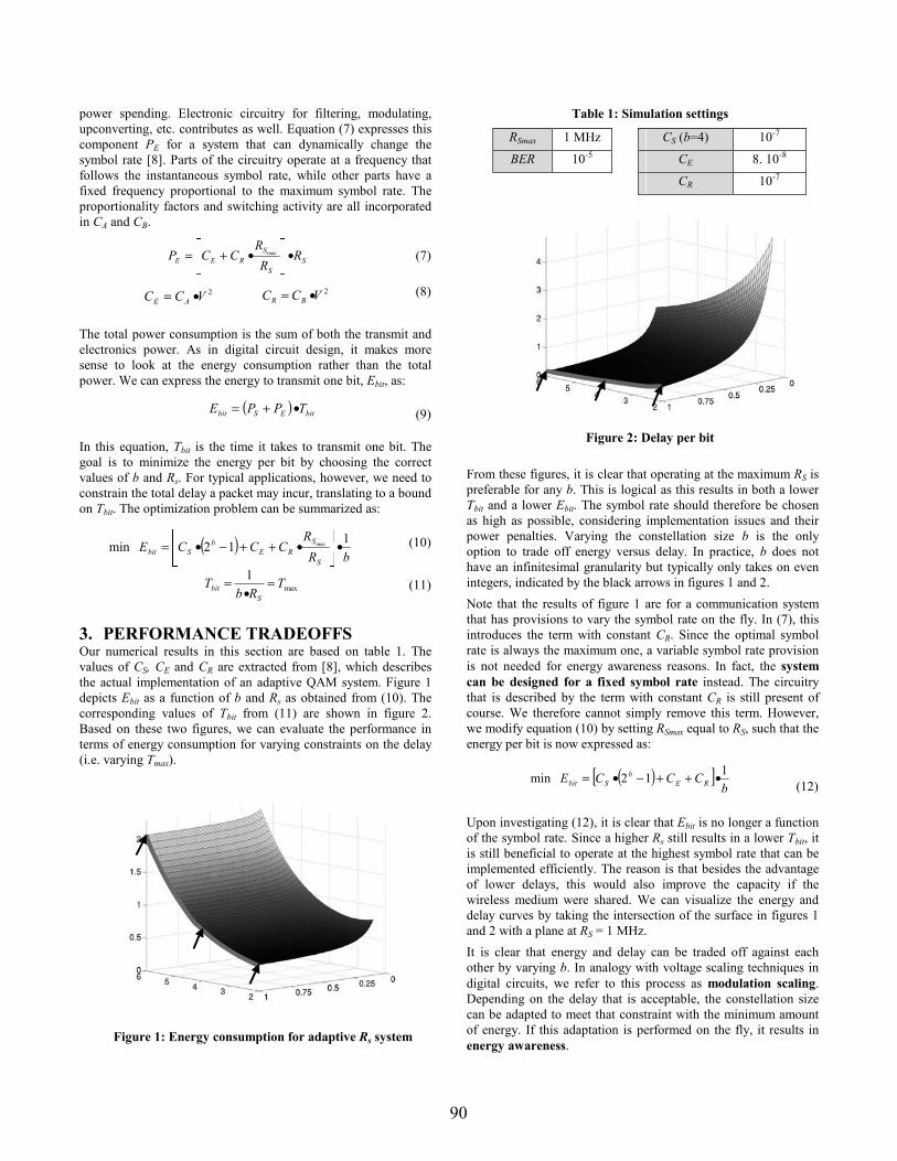
power spending. Electronic circuitry for filtering, modulating, upconverting, etc. contributes as well. Equation (7) expresses this component PE for a system that can dynamically change the symbol rate [8]. Parts of the circuitry operate at a frequency that follows the instantaneous symbol rate, while other parts have a fixed frequency proportional to the maximum symbol rate. The proportionality factors and switching activity are all incorporated in CA and CB.
(7)
(8) The total power consumption is the sum of both the transmit and electronics power. As in digital circuit design, it makes more sense to look at the energy consumption rather than the total power. We can express the energy to transmit one bit, Ebit, as:
(9)
In this equation, Tbit is the time it takes to transmit one bit. The goal is to minimize the energy per bit by choosing the correct values of b and Rs. For typical applications, however, we need to constrain the total delay a packet may incur, translating to a bound on Tbit. The optimization problem can be summarized as:
(10) (11)
3. PERFORMANCE TRADEOFFS Our numerical results in this section are based on table 1. The values of CS, CE and CR are extracted from [8], which describes the actual implementation of an adaptive QAM system. Figure 1 depicts Ebit as a function of b and Rs as obtained from (10). The corresponding values of Tbit from (11) are shown in figure 2. Based on these two figures, we can evaluate the performance in terms of energy consumption for varying constraints on the delay (i.e. varying Tmax).
Figure 1: Energy consumption for adaptive Rs system
Table 1: Simulation settings
RSmax 1 MHz CS (b=4) 10-7
BER 10-5 CE 8. 10-8
CR 10-7
Figure 2: Delay per bit From these figures, it is clear that operating at the maximum RS is preferable for any b. This is logical as this results in both a lower Tbit and a lower Ebit. The symbol rate should therefore be chosen as high as possible, considering implementation issues and their power penalties. Varying the constellation size b is the only option to trade off energy versus delay. In practice, b does not have an infinitesimal granularity but typically only takes on even integers, indicated by the black arrows in figures 1 and 2. Note that the results of figure 1 are for a communication system that has provisions to vary the symbol rate on the fly. In (7), this introduces the term with constant CR. Since the optimal symbol rate is always the maximum one, a variable symbol rate provision is not needed for energy awareness reasons. In fact, the system can be designed for a fixed symbol rate instead. The circuitry that is described by the term with constant CR is still present of course. We therefore cannot simply remove this term. However, we modify equation (10) by setting RSmax equal to RS, such that the energy per bit is now expressed as: (12)
Upon investigating (12), it is clear that Ebit is no longer a function of the symbol rate. Since a higher Rs still results in a lower Tbit, it is still beneficial to operate at the highest symbol rate that can be implemented efficiently. The reason is that besides the advantage of lower delays, this would also improve the capacity if the wireless medium were shared. We can visualize the energy and delay curves by taking the intersection of the surface in figures 1 and 2 with a plane at RS = 1 MHz. It is clear that energy and delay can be traded off against each other by varying b. In analogy with voltage scaling techniques in digital circuits, we refer to this process as modulation scaling. Depending on the delay that is acceptable, the constellation size can be adapted to meet that constraint with the minimum amount of energy. If this adaptation is performed on the fly, it results in energy awareness.
Ebit (∝J)
RS (MHz) b
Tbit (∝s)
RS (MHz) b ( ) bitESbit TPPE •+=
SS
SREE R
RR
CCP •
•+= max
2VCC AE •= 2VCC BR •=
( )bR
RCCCE
S
SRE
bSbit
112min max •
•++−•=
max1 TRb
TS
bit =•
=
( )[ ]b
CCCE REb
Sbit112min •++−•=
90
2 1
0,5-

Communications Digital Circuits
( )b
RGCPb
BSSS12 −•••= 2VfCP LS •••= α
[ ]b
RCCP BREE •+=
TnV
V
L eIVP ••= 0
maxmax
11TR
bT
RS
B •=⇒= ( ) f
kC
VVVf
tLT
d
•=−⇒=
21
( )B
ES RPPE 1•+= ( )
fPPE LS
1•+=
LEPPE nnn
nav
av ••••== ∑8
=
∝.. 1
1
4. COMPARISON BETWEEN VOLTAGE SCALING AND MODULATION SCALING The equations in the previous sections resemble those of voltage scaling, yet there are some key differences. It is important to highlight these differences, as they also contribute to a physical understanding of the tradeoffs of modulation scaling. Figure 3 places both scaling techniques next to each other. In the equations for voltage scaling, PS is the switching power and PL the leakage power [3]. It is clear that the functionality of supply voltage V corresponds to that of the constellation size b (hence the terms voltage and modulation scaling). In the left column, the energy is only dependent on b and not on RB. Equivalently in the right column, the energy term due to the switching power (PS/f) depends on V and not on f. There is however a crucial difference, regarding the interpretation of time. In the digital circuit case, the total effective delay for an operation td has to be smaller than 1/f. Similarly in a communication system the total time it takes to transmit a packet (or a bit) has to be smaller than a certain maximum value. The difference between both systems, however, is the period over which energy is consumed. In a communication system, the power has to be multiplied by the effective time of the operation. In digital circuits, on the other hand, the power is multiplied by the cycle time, which is in effect the maximum delay. As such, there is no true one-to-one mapping between RB (or RS for that matter) and f. However, when considering RB and f as constants of the system, they result in a lower bound on b or V in similar ways (see the third line of equations in figure 3).
5. ENERGY AWARE WIRELESS PACKET SCHEDULING Like energy aware OS scheduling, we can perform energy aware packet scheduling. We study the communication system setup depicted in figure 4, which consists of a point-to-point transmission link. Packets arrive at the sender and possibly need to be buffered before transmission. We assume that both the packet sizes and the intervals between packet arrivals, called inter-arrival times, follow an exponential distribution. Without modulation scaling, this setup corresponds to the well-known M/M/1 queuing system [9].
Figure 4: Setup of the queuing system
The average packet arrival rate is denoted by . . The inverse of the average service time is called the service rate, ∝, which gives the average number of packets that can be sent per unit time. It is expressed by (13), where L is the average packet size.
(13)
Because of the statistical properties of inter-arrival and service times, the number of packets in the buffer may vary considerably. Most of the time, the buffer is empty. In those situations, it is beneficial to scale the modulation down to conserve energy. When the buffer starts to fill up, we can increase b to avoid long queuing times or buffer overflow. This kind of system therefore is a good candidate for modulation scaling. A similar observation has been made for digital circuits, where a queue is introduced to average the rate over several samples in a DSP system [5]. The idea is to choose the constellation size based on the number of packets in the system (i.e. being transmitted or in the queue), which we refer to as the system state. For each state Sn = n, we have a particular constellation size bn, which translates into a value of ∝n through equation (13). The collection of bn for all the possible states determines the average energy consumption and delay of the queuing system. Our goal is to find which bn minimizes the energy for a particular delay constraint. We can analyze this problem using queuing theory. In steady state, the probability of being in state n can be expressed as [9]: (14) In this equation, P0 is a constant such that the sum of Pn over all states is equal to 1. We assume an infinite buffer size, which is a reasonable approximation for real systems, as memory has become rather inexpensive for these applications. For each state the energy consumption per bit is given by (12). The average energy per packet, Eav, is the ratio of the average power per packet and the packet arrival rate. The average power is the product of the probability Pn of being in a state, the rate ∝n in that state and the average energy per packet (En.L) in that state: (15)
Since (13) holds in every state, we can simplify this expression to:
1/f
td
L.Tmax
L/RB
Figure 3: Comparison between adaptive modulation and voltage scaling
.=
•= n
kk
n
n PP
1
0
∝
.
Sender Receiver Queue
. ∝
LRb
LR SB •==∝
91
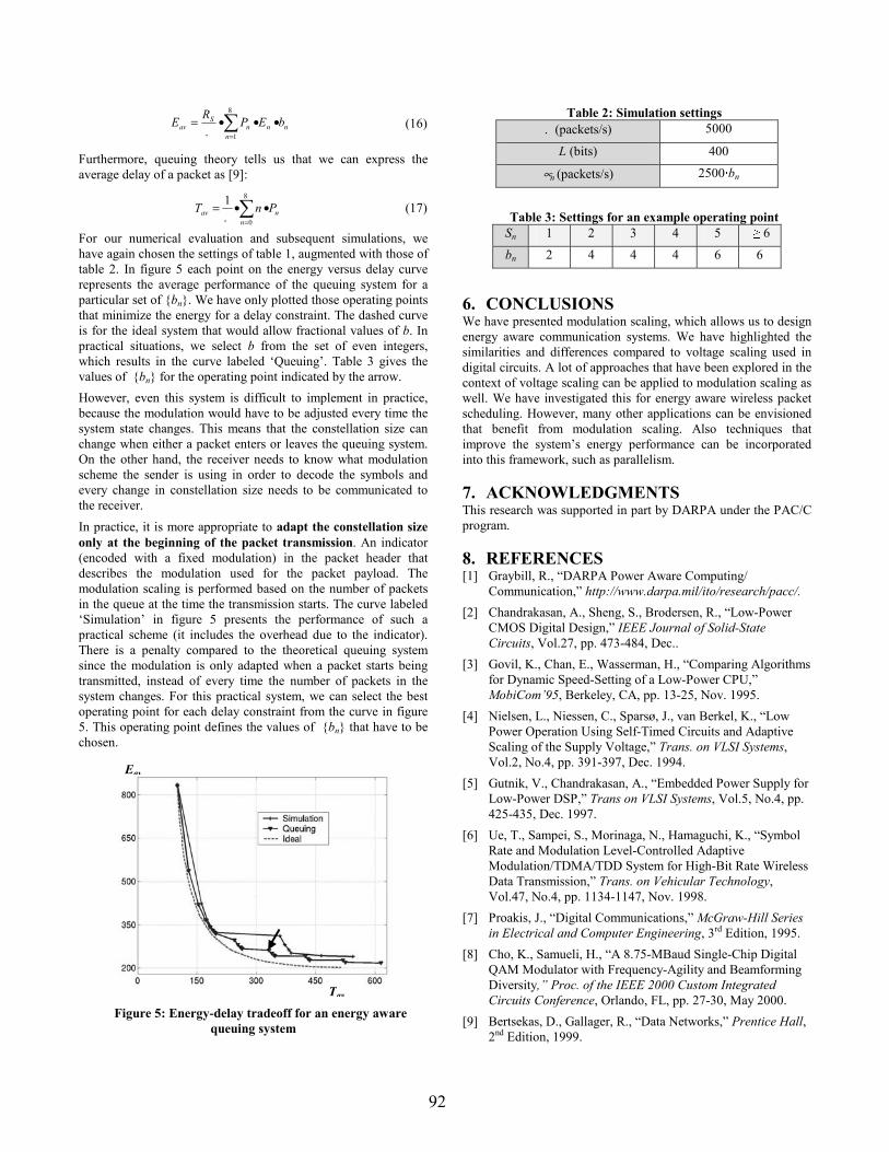
Tav
Eav
(16)
Furthermore, queuing theory tells us that we can express the average delay of a packet as [9]:
(17)
For our numerical evaluation and subsequent simulations, we have again chosen the settings of table 1, augmented with those of table 2. In figure 5 each point on the energy versus delay curve represents the average performance of the queuing system for a particular set of bn. We have only plotted those operating points that minimize the energy for a delay constraint. The dashed curve is for the ideal system that would allow fractional values of b. In practical situations, we select b from the set of even integers, which results in the curve labeled ‘Queuing’. Table 3 gives the values of bn for the operating point indicated by the arrow. However, even this system is difficult to implement in practice, because the modulation would have to be adjusted every time the system state changes. This means that the constellation size can change when either a packet enters or leaves the queuing system. On the other hand, the receiver needs to know what modulation scheme the sender is using in order to decode the symbols and every change in constellation size needs to be communicated to the receiver. In practice, it is more appropriate to adapt the constellation size only at the beginning of the packet transmission. An indicator (encoded with a fixed modulation) in the packet header that describes the modulation used for the packet payload. The modulation scaling is performed based on the number of packets in the queue at the time the transmission starts. The curve labeled ‘Simulation’ in figure 5 presents the performance of such a practical scheme (it includes the overhead due to the indicator). There is a penalty compared to the theoretical queuing system since the modulation is only adapted when a packet starts being transmitted, instead of every time the number of packets in the system changes. For this practical system, we can select the best operating point for each delay constraint from the curve in figure 5. This operating point defines the values of bn that have to be chosen.
Figure 5: Energy-delay tradeoff for an energy aware queuing system
Table 2: Simulation settings . (packets/s) 5000
L (bits) 400
∝n (packets/s) 2500·bn
Table 3: Settings for an example operating point
Sn 1 2 3 4 5 ≥ 6
bn 2 4 4 4 6 6
6. CONCLUSIONS We have presented modulation scaling, which allows us to design energy aware communication systems. We have highlighted the similarities and differences compared to voltage scaling used in digital circuits. A lot of approaches that have been explored in the context of voltage scaling can be applied to modulation scaling as well. We have investigated this for energy aware wireless packet scheduling. However, many other applications can be envisioned that benefit from modulation scaling. Also techniques that improve the system’s energy performance can be incorporated into this framework, such as parallelism.
7. ACKNOWLEDGMENTS This research was supported in part by DARPA under the PAC/C program.
8. REFERENCES [1] Graybill, R., “DARPA Power Aware Computing/
Communication,” http://www.darpa.mil/ito/research/pacc/. [2] Chandrakasan, A., Sheng, S., Brodersen, R., “Low-Power
CMOS Digital Design,” IEEE Journal of Solid-State Circuits, Vol.27, pp. 473-484, Dec..
[3] Govil, K., Chan, E., Wasserman, H., “Comparing Algorithms for Dynamic Speed-Setting of a Low-Power CPU,” MobiCom’95, Berkeley, CA, pp. 13-25, Nov. 1995.
[4] Nielsen, L., Niessen, C., Sparsø, J., van Berkel, K., “Low Power Operation Using Self-Timed Circuits and Adaptive Scaling of the Supply Voltage,” Trans. on VLSI Systems, Vol.2, No.4, pp. 391-397, Dec. 1994.
[5] Gutnik, V., Chandrakasan, A., “Embedded Power Supply for Low-Power DSP,” Trans on VLSI Systems, Vol.5, No.4, pp. 425-435, Dec. 1997.
[6] Ue, T., Sampei, S., Morinaga, N., Hamaguchi, K., “Symbol Rate and Modulation Level-Controlled Adaptive Modulation/TDMA/TDD System for High-Bit Rate Wireless Data Transmission,” Trans. on Vehicular Technology, Vol.47, No.4, pp. 1134-1147, Nov. 1998.
[7] Proakis, J., “Digital Communications,” McGraw-Hill Series in Electrical and Computer Engineering, 3rd Edition, 1995.
[8] Cho, K., Samueli, H., “A 8.75-MBaud Single-Chip Digital QAM Modulator with Frequency-Agility and Beamforming Diversity,” Proc. of the IEEE 2000 Custom Integrated Circuits Conference, Orlando, FL, pp. 27-30, May 2000.
[9] Bertsekas, D., Gallager, R., “Data Networks,” Prentice Hall, 2nd Edition, 1999.
∑8
=
••=0
1
nnav PnT
.
nnn
nS
av bEPRE •••= ∑8
=1.
92
SOD
SOD
350
200 150 300 450 600

1
ENERGY EFFICIENT ROUTING IN WIRELESS SENSOR NETWORKS
Curt Schurgers Mani B. Srivastava
Networked & Embedded Systems Lab (NESL), Electrical Engineering Department
University of California at Los Angeles (UCLA), CA
ABSTRACT
Wireless sensor nodes can be deployed on a battlefield and organize themselves in a large-scale ad-hoc network. Traditional routing protocols do not take into account that a node contains only a limited energy supply. Optimal routing tries to maximize the duration over which the sensing task can be performed, but requires future knowledge. As this is unrealistic, we derive a practical guideline based on the energy histogram and develop a spectrum of new techniques to enhance the routing in sensor networks. Our first approach aggregates packet streams in a robust way, resulting in energy reductions of a factor 2 to 3. Second, we argue that a more uniform resource utilization can be obtained by shaping the traffic flow. Several techniques, which rely only on localized metrics are proposed and evaluated. We show that they can increase the network lifetime up to an extra 90% beyond the gains of our first approach.
I. INTRODUCTION
Recently IC and MEMS have matured to the point where they enable the integration of communications, sensors and signal processing all together in one low-cost package. It is now feasible to fabricate ultra-small sensor nodes that can be scattered on the battlefield to gather strategic information [1]. The events detected by these nodes need to communicated to gateways or users who tap into the network. This communication occurs via multi-hop routes through other sensor nodes. Since the nodes need to be unobtrusive, they have a small form-factor and therefore can carry only a small battery. As a result, they have a limited energy supply and low-power operation is a must. Multi-hop routing protocols for these networks necessarily have to be designed with a focus on energy efficiency.
The proposed approaches lean towards localized algorithms [1][2]. Due to the large number of sensors, network-scale interaction is indeed too energy expensive. Moreover, a centralized algorithm would result in a single point of failure, which is unacceptable in the battlefield. In this paper, we propose two options for localized algorithms to increase the sensor network lifetime: (1)
minimize the energy consumption of transmissions and (2) exploit the multi-hop aspect of network communications.
The first option is to combine/fuse data generated by different sensors [1][2]. In [3] cluster head selection is proposed to perform this task. However, in section IV, we present a robust way of achieving the same functionality without explicit cluster formation.
The second option focuses on the paths that are followed during the data routing phase. The framework presented in [2] advocates a localized model called ‘directed diffusion’. Other work uses information on battery reserve and the energy cost to find the optimal routes [4]. The routing protocol in [5] is based on the node’s location, transmit energy and the residual battery capacity. In contract to this prior work, we propose a guideline that aims at spreading the network traffic in a uniform fashion. Our spreading ideas, although partly tailored towards the underlying routing algorithm we have chosen, should be beneficial for the energy aware routing protocols mentioned above. We discuss these spreading techniques in section V.
However, before discussing our data fusion and spreading, we first focus on the problem statement: how to increase the lifetime of a network of energy constrained devices. This results in a practical guideline, which considers the energy histogram. All of this is treated in section II.
II. PROBLEM STATEMENT
1. Energy Optimal Routing
Traditional ad-hoc routing algorithms focus on avoiding congestion or maintaining connectivity when faced with mobility [6]. They do not consider the limited energy supply of the network devices. The example of figure 1 illustrates how the limited supply alters the routing issue. Nodes A and E first send 50 packets to B. Afterwards, F sends 100 packets to B. From a load balancing perspective, the preferred paths are ADB, ECB and FDB respectively.
However, when the nodes are energy constrained such that they can only send 100 packets, these paths are no longer optimal. Indeed, D would have used up 50% of its energy
93

2
A
B
D C E F
before it can forward packets from F to B. In this case, all packets could have been delivered by choosing paths ACB, ECB and FDB. If, instead of F, node C would have become active, A should have used the original path ADB.
Figure 1: Load versus energy oriented routing
This simple case study highlights the following crucial observation: optimal traffic scheduling in energy constrained networks requires future knowledge. In our example, a maximum number of packets can reach B only if right from the start we know exactly when (and which) nodes will generate traffic in the future.
2. Energy Efficient Routing
Ideally, we would like the sensor network to perform its functionality as long as possible. Optimal routing in energy constrained networks is not practically feasible (because it requires future knowledge). However, we can soften our requirements towards a statistically optimal scheme, which maximizes the network functionality considered over all possible future activity. A scheme is energy efficient (in contrast to ‘energy optimal’) when it is statistically optimal and causal (i.e. takes only past and present into account).
In most practical surveillance or monitoring applications, we do not want any coverage gaps to develop. We therefore define the lifetime we want to maximize as the worst-case time until a node breaks down, instead of the average time over all scenarios. However, taking into account all possible future scenarios is too computationally intensive, even for simulations. It is therefore certainly unworkable as a guideline to base practical schemes on. Considering only one future scenario leads to skewed results, as shown in the example of figure 1.
3. Traffic Spreading Rationale
To derive a practical guideline, we start from the following observation: the minimum hop paths to a user for different streams tend to have a large number of hops in common [7]. Nodes on those paths die sooner and therefore limit the lifetime of the network. Figure 2 presents a typical energy consumption histogram at a certain point in time. Some nodes have hardly been used, while others have almost completely drained their energy.
Figure 2: Undesirable energy histogam
As nodes that are running low on energy are more susceptible to die sooner, they have become more critical. If we assume that all the nodes are equally important (we revisit this assumption in section V.2), no node should be more critical than any other one. At each moment every node should therefore have used about the same amount of energy, which should also be minimized. The histogram of figure 3 is thus more desirable than the one of figure 2, although the total energy consumption is the same.
Figure 3: Desirable energy histogram
Striving for a compact energy histogram translates into the guideline that traffic should be spread over the network as uniformly as possible. Since visualizing the histogram over time is hard, we propose to use the root mean square ERMS as an indicator instead (the lower this value, the better). It provides information on both the total energy consumption and on the spread.
III. BASIC ROUTING
As an underlying routing scheme, we base ourselves on the paradigm of directed diffusion [2]. When a user taps into the sensor network, he announces the type of information he is interested in. While flooding this ‘interest’ possibly using techniques like SPIN [8], gradients are established in each node. These gradients indicate the ‘goodness’ of the
Energy used (%)
0
5
10
15
20
0 10 20 30 40 50 60 70 80 90
Nodes (%)
0
5
10
15
20
0 10 20 30 40 50 60 70 80 90
Energy used (%)
Nodes (%)
94

3
0
2
4
6
8
1 3 5 7 9
no DCEone DCEmore DCE
B/R
Etot (mJ)
0
100
200
300
400
500
1 3 5 7 9
no DCEone DCEmore DCE
B/R
Delay (ms)
different possible next hops and are used to forward sensor data to the user.
We have opted for a simple instantiation of this paradigm, which we call Gradient-Based Routing (GBR). While being flooded, the ‘interest’ message records the number of hops taken. This allows a node to discover the minimum number of hops to the user, called the node’s height. The difference between a node’s height and that of its neighbor is considered the gradient on that link. A packet is forwarded on the link with the largest gradient. Although our techniques to increase the network lifetime are built upon GBR, the main principles are general enough to also be applicable to other ad-hoc routing protocols.
IV. DATA COMBINING
1. Data Combining Entities (DCE)
Individual sensor nodes process their sensor data before relaying it to the user [1]. It is advantageous to combine observations from different nodes to increase the resource efficiency. This process reduces not only the header overhead, but also the data itself can be compacted as it contains partly the same information.
Although this combining can be implemented by explicitly selecting a cluster head [3], we present a scheme that is more robust to random node failures. First note that sensor nodes that are triggered by the same event, are typically located in the same vicinity. The resulting cloud of activated nodes is also in close communication proximity. The routes from these nodes to the user merge early on [7]. Nodes that have multiple streams flowing through them can create a Data Combining Entity (DCE), which takes care of the data compaction. Simulations have shown that the DCEs are located inside or very close to this cloud of activated nodes.
This scheme is highly robust. When a node with a DCE dies, the packets automatically take an alternative route and pass through another node that can create a new DCE.
2. Simulations
Figure 4 depicts the effects of our DCE-based data compaction on the total energy consumption. The nodes in this simulation are distributed randomly over a rectangular area with a constant width of 32 m and a linearly increasing length B. The radio transmission range R is 20 m and the average node density is kept constant at 10-2/m2. The nodes at the top of this area sense a target and notify a user that is located at the bottom end (the transmission of one packet takes 5.76 ∝J). For our numerical results, we assume that a packet that is combined with another one can
be compressed to 60% of its original size. We consider 3 distinct cases: without DCE, with at most one DCE (a compression bit in the packet header signals if the packet has been compressed already) on each route to the user and with no restrictions on the number of DCEs. The reduction in energy consumption is as expected (up to a factor 2 to 3), linearly proportional to the number of bits sent.
Figure 4: Energy comparison for DCE
Figure 5: Delay comparison for DCE
The flip side is the average delay per packet, which is presented in figure 5. Since DCEs have to buffer data for a while, the packet delay will increase with the number of combining stages applied. Whether or not this is acceptable depends on the application.
V. NETWORK TRAFFIC SPREADING
1. Spreading Techniques
Stochastic Scheme: Using a rationale similar to the one of [9], each node can select the next hop in a stochastic fashion. More specifically, when there are two or more next hops with the same lowest gradient, a random one is
95

4
U
B C
A
D
E
F
0
5
10
15
20
0 10 20 30 40 50 60 70 80 90
Standard
Stream based
Energy used (%)
Number of nodes
0
0.05
0.1
0.15
0.2
0.25
1 2 3 4 5 6 7 8 9 10 11
StandardStochasticEnergy basedStochastic energy basedStream based
Time (s)
ERMS (mJ) chosen. This does not increase the length of the path followed, but nonetheless contributes to spreading the network traffic.
Energy-based Scheme: When a node detects that its energy reserve has dropped below a certain threshold (50% in our simulations), it discourages others from sending data to it by increasing its height. This may change a neighbor’s height (since a node’s height is one more than that of its lowest neighbor). It in turn informs other nodes and these updates are propagated as far as is needed to keep all the gradients consistent.
Stream-based Scheme: The idea is to divert new streams away from nodes that are currently part of the path of other streams. A node that receives packets tells all its neighbors except to the one from where the stream originates, that its height has increased. Again, other nodes must make sure the gradients remain consistent. As a result of this scheme, the original stream is unaffected, since those nodes have not updated the height of the next hop. New streams of packets, however, will take other paths as the height of the nodes on the first path has apparently increased.
2. Simulations
Figure 6: Wireless sensor network topology
Scenario 1: Nodes A and B (see figure 6) detect a different target and send packets to the user at regular intervals. After generating 100 packets each (this takes 11.8 seconds), these targets disappear and both nodes become inactive again. At this time, no node has been drained yet completely and the network connectivity is still fully intact. We have assumed a node has only 0.76 mJ of energy at its disposal (which is enough to send about 140 packets). The results can readily be scaled towards more realistic scenarios. Figure 7 shows the evolution of ERMS as a function of time, for 5 different schemes. The unenhanced GBR is called ‘standard’. Besides the three schemes discussed in V.1, we have also studied a combination of the stochastic and energy-based one.
Figure 7: ERMS for scenario 1
It is clear that the stream-based scheme indeed spreads the traffic more uniformly over the network. As soon as the energy of some nodes drops below 50%, the energy-based scheme kicks in. The stochastic routing provides an improvement both on top of the normal GBR and on top of the energy-based scheme.
Figure 8: Energy histogram after 6 seconds
To verify that the ERMS captures the relevant information, figure 8 shows the energy histogram for the standard and the stream-based scheme after 7 seconds. It is clear that spreading balances the energy consumption better.
Finally, we would like to show that the improved energy histogram is able to extend the network lifetime for a particular future scenario, although this does not prove anything about other possible futures. After 11.8 seconds node C starts forwarding packets to the user. Table 1 shows that the schemes that resulted in better traffic spreading also increase total traffic that reaches the user. We have verified that the time the network remains intact is increased by 90% when using the stream-based scheme.
96

5
0
0.05
0.1
0.15
1 2 3 4 5 6 7 8 9 10 11
StandardStochasticEnergy basedStochastic energy basedStream based
Time (s)
ERMS (mJ)
Scheme Packets received Standard 127 Stochastic 133 Energy-based 160 Stochastic energy-based 161 Stream-based 175
Table 1: Packets received for scenario 1
Scenario 2: Nodes D and E (figure 6) each send 100 packets to the user in 11.8 s. Figure 9 illustrates that our traffic spreading schemes again result in a more uniform utilization of the network resources.
Figure 9: ERMS for scenario 2
As before, we investigate one particular future activity scenario: node C becomes active after 11.8 seconds. From table 2, we conclude that spreading the network traffic has a negative effect as fewer packets are received! This is because the route taken by the standard GBR protocol avoids bottleneck node F. On the other hand, preading the traffic of D and E diverts some packets via F and therefore already partly drain this node before C can use it. This illustrates that spreading might increase the lifetime, although this does improve all possible futures. We observe however that the problems in this case are largely due to the fact that node F is critical as it is the only gateway to an entire subnet. Enhanced spreading techniques should therefore try to avoid critical nodes.
Scheme Packets received Standard 217 Stochastic 211 Energy-based 193 Stochastic energy-based 193 Stream-based 176
Table 2: Packets received for scenario 2
VI. CONCLUSIONS
In this paper we have argued that optimal routing in sensor networks is infeasible. We have proposed a practical guideline that advocates a uniform resource utilization, which can be visualized by the energy histogram. We acknowledge however that this is only a first cut at tackling this complicated issue. For example, exceptions must be made when nodes are critical in the overall network connectivity. We also propose a number of practical algorithms that are inspired by this concept. Our DCE combining scheme reduces the overall energy, while our spreading approaches aim at distributing the traffic in a more balanced way. We note that although we have started from GBR, our basic ideas and techniques should be able to enhance other routing protocols as well.
REFERENCES
[1] Sohrabi, K., Gao, J., Ailawadhi, V., Pottie, G., “Protocols for Self-Organization of a Wireless Sensor Network,” IEEE Personal Communications Mag., Vol.7, No.5, pp.16-27, Oct. 2000.
[2] Estrin, D., Govindan, R., “Next Century Challenges: Scalable Coordination in Sensor Networks,” MobiCom’99, Seattle, WA, pp.263-270, Aug. 1999.
[3] Rabiner, W., Chandrakasan, A., Balakrishnan, H., “Energy-Efficient Communication Protocol for Wireless Microsensor Networks,” Hawaii International Conference on System Sciences, Maui, HI, pp.10-19, Jan. 2000.
[4] Chang, J.-H., Tassiulas, L., “Energy Conserving Routing in Wireless Ad-Hoc Networks.,” INFOCOM’00, Tel Aviv, Israel, pp.22-31, Mar. 2000.
[5] Stojmenovic, I., Lin, X., “Power-Aware Localized Routing in Wireless Networks,” Proceedings IPDPS 2000, Cancun, Mexico, pp. 371-376, May 2000.
[6] Broch, J., Maltz, D., Johnson, D., Hu, Y. Jetcheva, J., “A performance comparison of multi-hop wireless ad-hoc network routing protocols,” Mobicom’98, Dallas, Texas, pp.85-97, Oct. 1998.
[7] Pearlman, M., Haas, Z., “Improving the Performance of Query-Based Routing Protocols through ‘Diversity-Injection’,” WCNC’99, New Orleans, LA, pp. 1546-1550, Sept. 1999.
[8] Rabiner, W., Kulik, J., Balakrishnan, H., “Adaptive Protocols for Information Dissemination in Wireless Sensor Networks,” MobiCom’99, Seattle, WA, pp. 174-185, Aug. 1999.
[9] Dattatreya, G.R., Kulkarni, S.S., “Simulation of Adaptive Statistically Multiplexed Routing in Ad Hoc Networks,” WCNC’99, New Orleans, LA, pp. 931-935, Sept. 1999.
97

Abstract— Portable wireless communication systems operate on a limited battery supply, and energy efficiency is therefore crucial. Voltage scaling techniques have been proposed to lower the energy consumption of embedded processors and real-time operating systems have incorporated these schemes in their task scheduling engine. However, the actual data transmission itself constitutes a major portion of the total energy consumption in these wireless communication systems. In this paper, we extend the scaling notion to the realm of wireless communications and propose a novel technique called modulation scaling to decrease the energy consumed during data transmission. Modulation scaling trades off energy consumption against transmission delay and as such, introduces the concept of energy awareness in communications. We investigate how modulation scaling can be exploited to design a dynamic power management engine at the level of the radio. This engine coordinates the packet transmission schedule while optimizing energy efficiency. We demonstrate such a power management module for real-time traffic and show that it reduces the energy consumption of data transmissions by up to 50% through smart traffic scheduling.
I. INTRODUCTION
A. Energy Awareness Due to the proliferation of tetherless battery-operated
devices, power consumption has become a critical aspect in system design. Recently people have come to realize that it is energy awareness, in addition to low power, that is required for most applications [1]. Systems should not be designed based on worst case operating conditions alone, but should dynamically adjust their performance to meet the required level, resulting in energy savings. Dynamically scaling the supply voltage is the most popular digital circuit technique to offer both low energy consumption and energy awareness [2].
Another trend is that wireless communication handhelds have replaced computers as the frontrunners of technology innovations. In addition, networks of embedded autonomous devices (called sensor networks) are on the verge of providing ubiquitous access and sampling to our environment [3]. In all these wireless battery operated systems, a major source of energy consumption is the actual data transmission over the air. Despite the work on energy awareness in digital electronic circuits, it has been overlooked that the same tradeoffs are present in communications as well. We show that the modulation can be scaled much the same way as operating voltage can, reducing the overall energy consumption for transmitting each bit. Although the basic idea of changing the modulation on the fly has been used to
increase the throughput in the presence of fading channels [4], it has never been exploited for low power purposes.
B. Energy Aware Scheduling How scaling brings about energy awareness depends on its
integration into dynamic power management. Power management algorithms orchestrate the operation of the different system components to reduce energy consumption while meeting a specified minimum performance level. One frequently used power management technique is shutting down unused system components. However, it has been realized that dynamically adjusting the clock speed and operating voltage of the processor offers higher energy savings. Embedded processors frequently operate on real-time traffic such as multimedia streams and hence, the power management policy has to take the associated timing constraints (i.e. task deadlines) into account. Dynamic voltage scaling for real-time operating systems (RTOS) in the presence of deadlines has been studied in [5][6].
As the embedded processor is not the only critical component in wireless communication devices, we need to extend the dynamic power management to the communication sub-system as well. Indeed, the processed data streams have to be scheduled for transmission, typically under real-time constraints. This is true for multimedia handhelds and embedded monitoring devices such as sensor networks. We extend the ideas of dynamic power management for RTOS to the realm of communications and propose a real-time dynamic power management scheme for the radio that is based on modulation scaling.
II. COMMUNICATION ENERGY
A. Basics In order to investigate modulation scaling, we need to
know how the energy consumption depends on the modulation level. In this work, we focus on Quadrature Amplitude Modulation (QAM) due to its ease of implementation and analysis [4]. However, our notions of scaling and power management are extendable to other modulation schemes as well. The performance of QAM in terms of Symbol Error Rate (SER) and Bit Error Rate (BER) is given by (1)-(2) [7].
(1)
(2)
Modulation Scaling for Real-Time Energy Aware Packet Scheduling Curt Schurgers Vijay Raghunathan Mani B. Srivastava
Networked and Embedded Systems Lab (NESL), EE-Dept., University of California at Los Angeles (UCLA) curts,vijay,[email protected]
−••
−•==12
32
114. 2/ bbSNRQBERbSER
APPSNR
n
S •=This paper is based in part on research performed under DARPA PAC/C program through AFRL contract #F30602-00-C-0154.
0-7803-7206-9/01/$17.00 © 2001 IEEE
365398

Ebit (∝J)
RS (MHz) b (bits/symbol)
The constellation size in number of bits per symbol is represented by b. The received Signal to Noise Ratio is denoted by SNR and defined as (2), where PS is the transmit power and Pn is the noise power. The factor A contains all transmission loss components. We can solve the above expressions for the transmit power, resulting in (3). The variable Γ is called the ‘gap’ and, for uncoded QAM, is given by (4), as can be derived from (1).
(3)
(4)
Pn is a function of the symbol rate Rs and the noise power spectral density N0 as in (5) [7]. The factor ⇓ takes into account other effects, such as filter non-idealities.
(5)
As a result, we can simplify the expression of PS to (6)-(7). ΓS in (7) is the gap for a fixed system operation point (b, BER). To get a fair comparison, the system performance is kept constant. In practice, it makes sense to operate at a target BER. The gap Γ in (7) is thus only a function of b. Due to the Q-1(.) function in (4), Γ and Gs only weakly depend on b.
(6)
(7)
B. Energy and Delay The goal now is to adjust b and Rs to reduce the overall
energy. The transmit power PS (delivered mainly by the power amplifier), however, is not the only source of power spending by the radio. Electronic circuitry for filtering, modulation, upconverting, etc. contributes as well. Equations (8)-(9) express this component PE for a system that can dynamically change the symbol rate [8]. Parts of the circuitry operate at a frequency that follows the instantaneous symbol rate, while other parts have a fixed frequency proportional to the maximum symbol rate. The proportionality factors are incorporated in CA and CB.
(8)
(9)
The total power consumption is the sum of both the transmit and electronics power. We can express the energy to transmit one bit, Ebit, as (10). In this equation, Tbit is the time it takes to transmit one bit. The term ε accounts for circuitry that is always on. Since this presents a fixed energy offset, we ignore this term in the remainder of this paper.
(10)
The goal is to minimize the energy per bit by choosing the correct values of b and Rs. For typical applications, we need to constrain the total delay a packet may incur, translating to a bound on Tbit. We summarize the optimization problem as:
(11)
(12)
III. PERFORMANCE TRADEOFFS Our evaluation of the performance tradeoffs is based on the
values given in Table 1. These are extracted from [8], which describes the implementation of an adaptive QAM system. Since the system in [8] is designed for high speed rather than low-power applications, it is likely that applying dedicated circuit techniques can reduce these numbers. We only use them here as proof of concept.
Figures 1 and 2 depict Ebit and Tbit as obtained from (11) and (12) respectively. After evaluating the performance for varying constraints on the delay (i.e. varying Tmax), it turns out that operating at the maximum RS is preferable for any b. This is logical as a higher RS results in both a lower Tbit and a lower Ebit. For practical systems, RS should be chosen as high as possible, considering implementation issues and their associated power penalties. Varying the constellation size b is therefore the only option to trade off energy versus delay. In real implementations, b does not have an infinitesimal granularity but typically only takes on even integers, indicated by the black arrows in figures 1 and 2.
TABLE 1 SIMULATION SETTINGS
RSmax 1 MHz CS (b=4) 10-7 J BER 10-5 CE 8. 10-8 J
CR 10-7 J
Fig. 1: Energy consumption for adaptive Rs system
SS ANC Γ⇓ ••= 0
SSG
ΓΓ=
( )12 −•••= bSSSS RGCP
Sn RNP ••= ⇓0
( ) ε+•+= bitESbit TPPE
2VCC AE •= 2VCC BR •=
( )bR
RCCGCE
S
SRE
bSSbit
112min max •
•++−••=
max1 TRb
TS
bit =•
=
( ) ( )21
2/1
2114
13
1
••
−••=−
− BERbQ bΓ
SS
SREE R
RR
CCP •
•+= max
( )12 −••= bnS A
PΓP
365499

Tbit (∝s)
RS (MHz) b (bits/symbols)
A
B
G
Fig. 2: Delay per bit
Since the optimal symbol rate is always the maximum one, the variable symbol rate provision is not needed for energy awareness. The circuitry that is described by the term with CR is still present of course. We cannot simply remove this term, but modify (11) by setting RSmax equal to RS:
(13)
In (13), Ebit is no longer a function of the symbol rate. Since a higher Rs results in a lower Tbit, it is again beneficial to operate at the highest symbol rate that can be implemented efficiently. Besides the advantage of lower delays, this also improves the capacity if the medium were shared. We can visualize the energy and delay curves by intersecting the surface in figures 1 and 2 with a plane at RS = 1 MHz.
Note that there is a minimum in fig.1. In the region where the energy drops for a decreasing b, energy and delay can be traded off against each other. In analogy with voltage scaling techniques in digital circuits, we refer to this process as modulation scaling. Depending on the delay that is acceptable, the constellation size is lowered to meet that constraint with the minimum amount of energy. If this adaptation is performed on the fly, it results in energy awareness. It is useless to scale beyond the energy minimum point, as both delay and energy increase then. The position of this minimum depends on the relative values of CS and (CE +CR). It turns out that, except for systems with a very short transmission range, operating at the smallest value of b is most energy efficient.
IV. REAL-TIME SCHEDULING
A. Real-Time Traffic Applications In practical communication systems data is grouped into
packets. We propose to add a power management module to the radio. Its task is to schedule the packet transmissions, while performing modulation scaling and at the same time maintaining the desired overall performance.
In this paper, we focus on real-time traffic, where each packet has a deadline by which it has to be sent. This model is valid for multimedia streams, such as audio or video. Another type of application that has real-time features is wireless sensor networks [3]. Envisioned uses for these networks of ultra-small autonomous devices are habitat monitoring, smart office and surveillance. A possible task of these networks is to periodically send updates on a condition (like the location of a target, the temperature of a room, etc.) to end users. These periodic updates can have different periods, depending on the application. The users tap into the network via gateway nodes, such as node G in fig. 3. These gateways receive multiple periodic traffic streams (e.g. one from A and one from B) that need to be scheduled on the (long-haul) link to the user in an energy efficient way.
Although we tackle the above scheduling problem in sensor networks, the power management scheme for real-time packet scheduling that we propose in this section is relevant for other classes of real-time traffic as well. In essence, we consider the general problem of energy aware scheduling of real-time traffic streams via modulation scaling.
B. Scheduling Basics We characterize each real-time stream k by a tuple (Lk,Tk),
containing the maximum packet size and the time period. In each stream, the size of the individual packets might vary (e.g. in MPEG video or perceptual audio codecs). For sensor networks, this variation is due to changes in compression or the amount of sensor data. Each packet has to be sent before the next one arrives (so its deadline is its arrival time + Tk).
A similar problem of scheduling in the presence of deadlines has been studied extensively for RTOS. Energy awareness has been introduced there through voltage scaling. Techniques have been proposed that implement preemptive scheduling policies (i.e. tasks can be suspended and resumed later on) with the aim of minimizing the processor energy consumption [5][6]. However, in data transmissions, once a packet transmission has started, the scheduler should not interrupt the ongoing transmission. The condition of non-preemptive scheduling is the key distinction between packet scheduling on a link and task scheduling under an RTOS. Since all work on energy aware RTOS scheduling is preemptive [5][6], we cannot use these results. To the best of our knowledge, energy awareness has not been studied yet in the context of non-preemptive scheduling.
Fig. 3: Sensor network setup
( )[ ]b
CCGCE REb
SSbit112min •++−••=
3655100

Some useful results on the schedulability of task sets under non-preemptive scheduling (without scaling) are given in [9]. Finding the optimal schedule for a particular offset for each packet stream, where offset is defined as the first time a packet arrives, is an NP-complete problem [9]. Luckily, there exists a schedulability condition (14)-(15) (Cj is the transmit time for a packet of size Lj). When both (14) and (15) are satisfied, the set of N streams is schedulable for any offset. Otherwise, they might be schedulable for some, but there is at least one choice of offsets for which they are not. It can be shown that Earliest Deadline First scheduling (EDF) always results in a valid schedule when this condition is satisfied.
(14)
(15)
C. Energy-Aware Non-Preemptive Scheduling Our goal is to make the non-preemptive real-time packet
scheduling energy aware. An optimal scheduling routine would have to consider both the offsets and the variable packet sizes. This is too computationally intensive, since the problem was already NP-complete when only considering offsets. As a solution, we propose a practical algorithm, which consists of two steps.
Admission step: When a new stream is admitted to the system, we calculate a static scaling factor αstatic for the system, assuming all packets are of maximum size. This factor is the minimum possible such that if the modulation setting for each packet would be scaled by it (which results in a uniform increase in Cj), the schedulability test (14)-(15) is still satisfied. In other words, it computes the slowest transmission speed for each packet at which all the packet streams are just schedulable. Fig. 4(a) depicts the original schedule with modulation bmax for three streams A, B and C. The deadline T of the previous packet is also the arrival time of the next packet of that stream. The slowdown in fig. 4(b) is indeed the maximum possible, since the first instance of packet B would otherwise miss its deadline TB.
Adjustment step: During run-time, packets are scheduled using EDF. However, before the transmission starts the actual size of each packet is known, see fig. 4(c). We calculate an additional scaling factor αdyn such that the transmission finishes when that of a maximum size packet would have, see fig. 4(d). Since step 1 assumed the maximum packet size, the schedulability is guaranteed. If the system would still be idle after the packet transmission, we stretch the transmission until the packet’s deadline or the arrival time of a new packet (which is known due to the periodic nature of the traffic). We call this extra scaling factor αstrech. Fig. 4(e) illustrates that
the second instance of packet B can indeed be stretched (while this factor is 1 for the other packets).
Finally, the scheduler combines all three scaling factors to get the overall modulation that is used for the current packet. For practical systems, the scaled constellation size b* of (16) is rounded up to the closest allowable value.
(16)
D. Performance Evaluation In order to evaluate the performance of our scheme, we
have carried out a number of simulations. Unfortunately, for the sensor network application we focus on, no realistic numbers for the characteristics of data streams are available. We have based our simulations on general statistics, which we expect to be sufficiently relevant.
We select the maximum packet size Lk to be the same for each stream and equal to 400 bits. For each packet, its actual size is independently chosen from a uniform distribution between ⇓.Lk and Lk (where ⇓ is a parameter we vary in our simulations). Furthermore, we choose Rs and bmax to be equal to 1 kHz and 6 bits/symbol respectively. All simulations are averaged over an adequate number of offsets.
Scenario 1: Five streams with different periods, listed in table 2, need to be scheduled. For these values, the total link utilization is rather high: 84% when all packets are of maximum size (⇓ = 1). Fig. 5 plots the energy curves, normalized versus a scheme without scaling (b = bmax at all times), of specific variants of our algorithm. When only using αstatic in (16), there are no energy savings as the scaling factor is not enough to lower the modulation to next allowed level without compromising the schedulability.
TABLE 2 STREAM PERIODS
T1 T2 T3 T4 T5 0.20 s 0.25 s 1.50 s 1.00 s 0.50 s
∑=
=N
j j
j
TC
1
1
11
1
−•
+= ∑
−
=j
k
j j
iki C
TtCt
Nk ..1=. )1..(1, −=<•=. kiTTnt kii
stretchdynstaticbb ααα •••= max*
A C B (b) A C B
A C B (c) A C B
A C B (d) A C B
A C B (e) A C B
Fig. 4: Scheduling with modulation scaling
A C B
TA TB TC
(a) A C B
TA
A
3656101

⇓
Relative energy
αstatic.αdyn αstatic
αdyn
αstatic.αdyn.αstretch
1
Fig. 5: Energy in scenario 1
However, adding αdyn results in an energy reduction as the packet size variation increases (⇓ decreases). We also note that the effect of αstrech is significant.
Scenario 2: Now, only the first three streams of table 2 are scheduled. In this case the maximum total link utilization is 64% and the normalized energy is shown in fig. 6. We note that in this case, αstatic alone is large enough such that b can be uniformly set to 4 bits/symbol. Again αdyn and αstretch result in extra energy savings, although smaller.
These simulations illustrate that our dynamic power management scheme actually introduces energy awareness with regard to two distinct phenomena.
1. Variations in overall utilization are handled by the admission step in our algorithm. These are due to changes in number of streams, which are likely to occur over relatively large time scales. The transmission is uniformly slowed down via αstatic to automatically adapt to these changes.
Fig. 6: Energy in scenario 2
2. Variations in individual packet sizes on the other hand occur at much smaller time scales. These cannot be handled during the admission of the streams, but are exploited in the adjustment step of our algorithm via αdyn and αstretch.
V. CONCLUSIONS We have developed the concept of modulation scaling,
which essentially allows us to trade off energy versus delay on the fly. As such, it enables the design of energy aware communication systems. We described how modulation scaling can be integrated into a dynamic power management scheme on the radio. As battery operated wireless communication devices become more proliferated, extending the principles of power management from the realm of embedded processors to embedded radios is indeed crucial.
To this end, we have presented energy aware EDF scheduling for real-time traffic streams. Our non-preemptive algorithm guarantees that no packet deadlines are missed, yet dynamically scales the transmission rate to ensure energy efficient operation. The adaptation leverages both long and short-term traffic dynamics, through a two-stage modulation scaling process.
REFERENCES [1] Graybill, R., “DARPA Power Aware Computing/
Communication,” http://www.darpa.mil/ito/research/pacc /. [2] Pering, T., Bird, T., Brodersen, R., “The simulation and
evaluation of dynamic voltage scaling algorithms,” ISLPED 1998, pp. 76-81, August 1998.
[3] Sohrabi, K., Gao, J., Ailawadhi, V., Pottie, G., “Protocols for self-organization of a wireless sensor network,” IEEE Personal Communications Magazine, Vol.7, No.5, pp. 16-27, Oct. 2000.
[4] Ue, T., Sampei, S., Morinaga, N., Hamaguchi, K., “Symbol Rate and Modulation Level-Controlled Adaptive Modulation/TDMA/TDD System for High-Bit Rate Wireless Data Transmission,” IEEE Trans. on Vehicular Technology, Vol.47, No.4, pp. 1134-1147, Nov. 1998.
[5] Shin, Y., Choi, K., “Power Conscious Fixed Priority Scheduling for Hard Real-Time Systems,” DAC 1999, New Orleans, LA, pp. 134-139, June 1999.
[6] Okuma, T., Ishihara, T., Yasuura, H., “Real-Time Task Scheduling for a Variable Voltage Processor,” ISSS 1999, San Jose, CA, pp. 24-29, Nov. 1999.
[7] Proakis, J., “Digital Communications,” McGraw-Hill Series in Electrical and Computer Engineering, 3rd Edition, 1995.
[8] Cho, K., Samueli, H., “A 8.75-MBaud Single-Chip Digital QAM Modulator with Frequency-Agility and Beamforming Diversity,” IEEE 2000 Custom Integrated Circuits Conference, Orlando, FL, pp. 27-30, May 2000.
[9] Jeffay, K., Stanat, D., Martel, C., “On Non-Preemptive Scheduling of Periodic and Sporadic Tasks,” IEEE Real-Time Systems Symposium, San Antonio, TX, pp. 129-139, Dec. 1991.
⇓
Relative energy
αstatic.αdyn
αstatic
αdyn
αstatic.αdyn.αstretch
3657102
0.2 0.4 0.6 0.8
1
0^
OX-
OV
0.2 0.4 0.6 0.6

103
Adaptive Power-Fidelity in Energy-Aware Wireless Embedded Systems
Vijay Raghunathan, Paleologos Spanos, and Mani B. Srivastava Networked and Embedded Systems Laboratory
Department of Electrical Engineering, UC Los Angeles vijay, paleolog, inbs@ee .ucla . edu
Abstract
Energy aware system operation, and not just low power hard- ware, is an important requirement for wireless embedded sys- tems. These systems, such as wireless multimedia terminals or wireless sensor nodes, combine (soft) real-time constraints on computation and communication with requirements of long bat- tery lifetime. In this paper, we present an OS-directed dynamic power management technique for such systems that goes beyond conventional techniques to provide an adaptive power vs. fidelity trade-off.
The ability of wireless systems to adapt to changing fidelity in the form of data losses and errors is used to tradeoff against energy consumption. We also exploit system workload variation to proactively manage energy resources by predicting process- ing requirements. The supply voltage, and clock frequency are set according to predicted computation requirements of a spe- cific task instance, and an adaptive feedback control machanism is used to keep system fidelity (deadline misses) within specifi- cations.
We present the theoretical framework underlying our approach in the context of both a static priority-based preemptive task scheduler as well as a dynamic priority based one, and present simulation-based performance analysis that shows that our tech- nique provides large energy savings (upto 76%) with littie loss in fidelity (< 4%). Further, we describe the implementation of our technique in the eCos real-time operating system (RTOS) run- ning on a StrongARM processor to illustrate the issues involved in enhancing RTOSs for energy awareness.
1 Introduction
Modem day wireless embedded systems, examples of which in- clude mobile multimedia terminals with wireless LAN cards, 3G cellular phones, self-organizing ad-hoc network grids of wireless sensors, wireless toys and robots etc., involve an integration of high-performance computing and wireless communication capa- bilities, under real-time constraints. The battery operated nature of these systems requires them to be designed and operated in a highly energy efficient manner to maximize the battery lifetime.
In addition to using low-power hardware components [1,2,3], managing the various system resources in a power-aware manner i.e., Dynamic Power Management (DPM), can further reduce en-
ergy consumption considerably, thus increasing battery lifetime. This paper presents a system level pro-active DPM scheme that provides an adaptive trade-off between power consumption and operational fidelity by exploiting the key characteristics of wire- less embedded systems listed below.
• Most wireless systems are resilient to packet losses and errors. The operating scenarios of these systems invari- ably have losses and errors associated with them (e.^., noisy wireless channel conditions lead to packet losses and er- rors). In these systems, the application layer is designed to be adaptive and tolerant to these impairments. Hence, these wireless systems fall under the category of "soft" real-time systems where a small number of task deadline misses are not catastrophic to system performance, but only lead to a small degradation in the user-perceived system fidelity. For example, a small percentage of packet loss is acceptable in mobile multimedia applications like audio or video decod- ing.
• Wireless embedded systems offer a power-fidelity trade- off that can be exploited to suit application needs. For example, the precision of the computation e.g., quality of the audio or video decoding) can be traded off against the power consumed for the computation [21]. Also, the wire- less channel induced error can be reduced by increasing the transmission power of the radio. Thus, these systems inher- ently have a power-fidelity control knob which can be fine tuned to suit application needs.
• Wireless embedded systems have time varying computa- tional loads. Performance analysis studies have shown that for typical wireless applications (e.g., audio and video en- coding/decoding, encryption/decryption etc.), the instance to instance task execution time varies significantly and is often far lower than the worst case execution time (WCET) [4]. Table 1 gives the WCET and best case ex- ecution time (BCET) for a few example benchmarks [4]. Note that, even though the execution times vary signifi- cantly, they depend on data values that are obtained from physical real-world signals (e.g., audio or video streams) and hence are likely to have some temporal correlation be- tween them. This temporal correlation enables us to predict
106 0-7695-1420-0/01 $17.00 © 2001 IEEE

104
Program Description BCET WCET DES Data Encryption 73,912 672, 298
DJPEG JPEG decompression 128x96 color 12, 703,432 122, 838, 368 FDCT JPEG forward DCT 5,587 16, 693 FFl' 1024 point FFT 1,589,026 3, 974, 624
Table 1: Variation in execution times for a few tasks used in multimedia applications [4]
the runtime to a reasonable degree of accuracy. The varia- tion in execution time offers additional potential for energy reduction which we exploit in the proposed work.
Due to the need for flexibility and adaptability to constantly evolving standards, a significant fraction of the functionality of wireless embedded systems is frequently implemented as soft- ware running under a real time operating system (RTOS) on a programmable processor platform. The RTOS is uniquely poised to efficiently implement system power management policies due to the following reasons. Since the RTOS co-ordinates the ex- ecution of the various application tasks, it has global informa- tion about the performance requirements and timing constraints of all the applications. Also, the RTOS can directly control the underlying hardware platform, tuning it to meet specific system requirements.
A commonly used DPM scheme is one in which unused sys- tem components are shutdown or sent into low-power states. Previous work on shutdown based power management has fo- cussed on optimizing the state transition policy [5, 6, 7]. A detailed survey of system level shutdown based power manage- ment techniques is presented in [8]. An alternative DPM tech- nique is Dynamic Voltage Scaling (DVS), where the voltage and operating frequency of the processor are changed dynamically during runtime in order to just meet the performance require- ment. DVS based DPM, when applicable, has been shown to have significantly higher energy efficiency compared to shut- down based DPM due to the convex nature of the energy-speed curve [9,10,11,12,13,14,15,16,17, 18,19, 20,21].
1.1 Paper overview and contributions
This paper presents a system level DVS based power manage- ment technique that exploits the previously described character- istics of wireless systems, namely error-tolerance, power-fidelity tradeoff, and time varying computational loads. The proposed technique consists of an off-line and an online component, that together exploit the task runtime variation by predicting task in- stance execution times and performing DVS accordingly. The few deadline misses that result from occasional erroneous pre- diction are not catastrophic to system performance due to the in- herent error-tolerant nature of these wireless systems. Our algo- rithm uses a novel adaptive feedback mechanism to keep a tight check on the number of task deadline misses. This is done by
monitoring the deadline miss history, and accordingly adapting the prediction to be more aggressive or conservative.
We investigate a commonly used static priority assignment based scheduling scheme (Rate Monotonic priority assign- ment [22]) as well as a dynamic priority assignment based one (Earliest Deadline First priority assignment [22]) and show that our voltage scheduling strategy has a significantly higher energy efficiency compared to conventional WCET based schemes. Ex- periments indicate that the use of our technique results in energy reductions of up to 76% (average of 54%) over a shutdown based technique, and up to 68% (average of 47%) over the WCET based technique of [15]. We have implemented our DPM technique into the kernel of eCos [23], a commercial RTOS from Red Hat Inc., running on a Strong ARM SA-UIO proces- sor from Intel [24] that supports dynamic voltage and frequency scaling. We illustrate the various issues involved in enhancing an RTOS for energy awareness and describe how our implementa- tion tackles these issues.
1.2 Related work
Initial work on DVS was in the context of a workstation-like environment [10, 11] where average throughput is the perfor- mance metric, and latency is not an issue since there are no real- time constraints. A technique to derive an off-line minimum- energy schedule for independent processes with deadlines was presented in [12]. Researchers have also proposed the concept of compiler-directed DVS [25] where the compiler sets the pro- cessor frequency and voltage with the aim of minimizing en- ergy under real-time constraints. There have been several other techniques proposed for energy-efficient real-time task schedul- ing [13, 14,15,16, 17, 18, 19, 20]. However, all of diem perform voltage scheduling assuming that the tasks in the system have hard deadline constraints. Further, most of them assume that ev- ery task instance executes for its WCET. Even the few techniques that take into account task runtime variation [15], leverage it only for processor shutdown and not during voltage scaling. Recently, a DVS technique that attempts to exploit task run-time variation was presented in [26]. However, this technique only targets hard real-time systems, and does not involve any pro-active DPM. Thus, it does not provide any tradeoff between power consump- tion and application fidelity.
The rest of this paper is organized as follows. Section 2 describes the background about real-time task scheduling and
107

105
presents examples to illustrate the power management oppor- tunities that exist during task scheduling. Section 3 presents the CPU power model used. Section 4 discusses our adaptive power-fidelity tradeoff technique. Section 5 describes the sim- ulation based performance analysis and presents simulation re- sults. Section 6 describes our implementation setup (hardware and software), details the changes that have to be made to eCos to implement our power management scheme and presents the implementation results. Section 7 presents the conclusions.
2 Background and illustrative examples We describe the basic scheduling approach adopted in our work, and present examples to illustrate the power management oppor- tunities that arise due to the slack present in the system as well as dynamic variation of task execution times.
2.1 Task scheduling in RTOS
The task scheduler of an RTOS is responsible for scheduling a given set of tasks such that real-time constraints are satisfied. Schedulers differ in the type of scheduling policy they imple- ment. A commonly used scheduling policy is Rate Monotonic (RM) scheduling [22]. This is a fixed-priority based preemp- tive scheduling scheme where tasks are assigned priorities in the inverse ratio of their time periods. Fixed priority based pre- emptive scheduling is commonly used in operating systems like eCos, WinCE, VxWorks, QNX, uC/OS etc., that run on wire- less embedded devices such as handheld multimedia devices and wireless sensors. An alternative scheduling scheme is Earliest Deadline First (EDF) scheduling [22], where task priorities are assigned dynamically such that task instances with closer dead- lines are given higher priorities. No matter which scheduling policy is used, the RTOS ensures that, at any point of time, the currently active task is the one with the highest priority among the ready to run tasks.
2.2 DPIVI opportunities during task scheduling
It has been observed in many systems that, during runtime, even if all task instances run for their WCET, the processor utilization factor is often far lower than 100%, resulting in idle intervals. This slack that inherently exists in the system due to low proces- sor utilization is henceforth referred to as the static slack. It can be exploited for power management by statically slowing down the processor and operating at a lower voltage. While processor slowdown improves the utilization factor, excessive slowdown may lead to deadline violations. Hence, the extent of slowdown is limited by the schedulability of the task set under the Rate Monotonic scheduling scheme at the reduced speed. The follow- ing example illustrates the use of static slowdown and voltage scaling to reduce energy consumption by exploiting the static slack present in the system.
Example 1: Consider a simple mobile multimedia terminal shown in Figure I. The system receives real-time audio and
Figure I: Mobile multimedia terminal used in Examples I and 2.
Task Time Period WCET Deadline Audio decoding
Protocol processing Video decoding
60 70 120
10 15 40
60 70 120
Table 2: Task timing parameters for Examples I and 2
video streams over a wireless link, and plays them out. The three main tasks that run on a processor embedded in this sys- tem are protocol processing, audio decoding, and video decod- ing. The timing parameters for these tasks are given in Table 2. The resulting schedule for the time interval [0, 120] when this task set is scheduled on a single processor using the Rate Mono- tonic priority assignment scheme [22], is shown in Figure 2(a). It can be seen from the figure that the system is idle during time interval [90, 120]. This slack can be utilized to lower the op- erating frequency and supply voltage, thereby reducing the en- ergy consumption. Figure 2(b) shows the schedule for the same task set with the processor slowed down by a factor of |. As seen from the figure, processor slowdown leads to elimination of slack. Note that any further reduction in processor speed will result in the video decoding task missing its deadline. So, for minimum energy operation while satisfying deadline constraints, the processor's operating frequency can be lowered by a factor of I and the supply voltage can be lowered from 5V to 4.08V (using the equations presented in Section 3). The energy con- sumption which is quadratically dependent on the supply voltage is reduced by 33.42%. I
Static slack is not the only kind of slack present in the system. During runtime, due to the variation in the task instance execu- tion times, there is an additional slack created when a task in- stance finishes executing before its WCET. This slack that arises due to execution time variation is henceforth referred to as dy- namic slack. Dynamic slack can be exploited for DPM by dy- namically varying the operating frequency and supply voltage of the processor to extend the task execution time to its WCET. The faster a task instance executes, the more its power management potential. However, to realize this potential, we need to know the execution time of each task instance. As mentioned in Sec-
108

106
Deadline of first instsnce of video decoding task
0 10 20 30 40 50 60 70 (a)
90 100 110 120
0 10 20 30 40 50 60 70 (b)
I \ Audio decoding
90 100 no 120
Protocol processing ^| Video decoding
Figure 2: Task execution schedule for Example 1: (a) Original (b) Statically optimized
tion 1, the temporal correlation between the instance to instance execution times, enables us to predict the runtime of a task in- stance based on recent execution history. The following example illustrates how energy efficiency can be increased by utilizing the dynamic slack.
Example 2: Consider the optimized schedule for the task set of Example 1 shown in Figure 2(b). Figure 3(a) shows the resulting schedule when the first instance of video decoding requires only 20 time units to complete execution. As seen from the figure, there is a slack created due to the execution time variation of the video decoding. This slack can be utilized to reduce energy by dynamically reducing the processor frequency and supply volt- age during the execution of the first instance of the video decod- ing task. If the frequency were to be dropped by a factor of 2 over the already statically optimized value, the slack gets filled up again as shown in Figure 3(b). The voltage can then be de- creased to 2.69V (using the delay-voltage equation given in Ex- ample 1). This gives us an additional energy savings of 56% for that particular task instance, over the statically optimized value.
Deadline of first instsnce of video decoding task
I I Audio Decoding | Protocol processin; Video decoding
Figure 3: Task execution schedule for Example 2: (a) Statically optimized (b) After dynamic slowdown
The above examples illustrated the power management opportu- nities present during real-time task scheduling. We next describe our system model and then present our power-aware scheduling algorithm that exploits these opportunities to result in large en- ergy savings.
3 CPU power model
The power consumed by the processor is dominated by the switching component which is given by Pswitchmg = Ceff x ^dd ^ f where Ceff is the total switched capacitance, Vdd is the supply voltage, and / is the system clock frequency. The gate delay in the system is given by Delay = ivti-v^i,)'^ ^ 7 where Vth is the threshold voltage, and A; is a technology depen- dent constant. The maximum voltage of the system was set to be Vref = 5 volts for the simulation based analysis. The normalized speed of the processor at maximum frequency, and the normal- ized power consumption at maximum frequency and maximum supply voltage were both set to be 1. By combining the above equations, and eliminating V, the normalized power consump- tion (P) as a function of the normalized speed (S) is obtained as
PS) = 0.248 *S^ + 0.225 * 5^ + 0.0256 *S+ (0.014112 *S^ + 0.0064 * 5) * V311.16*S'2-H 282.24* 5
for Vth = 0.8y. We use this equation to calculate the power con- sumption of the system for a given normalized operating speed. However, our implementation (described in Section 6) uses a power model derived from actual measurements [27].
3.1 Variable voltage supply
The variable supply voltage is generated using DC-DC switching regulators in the power supply. Efficient DC-DC regulators with fast transition times were reported in [28,29]. Complimentary to the supply voltage variation is the accompanying variation of the system clock frequency. When the clock frequency is altered, the PLL present in the clock generator circuitry takes a finite amount of time to settle at its steady state value. In our sim- ulation framework, we account for these transition overheads, by setting the transition time for the voltage change and associ- ated frequency change to be 10 microseconds [17]. Further, the processor is stalled for the duration of the frequency change, re- sulting in some amount of wasted energy. We account for this overhead as well in our energy calculations.
4 Algorithm
At the core of our system model is the runtime scheduler that schedules applications as concurrent tasks to run on the proces- sor. We consider a priority based scheduling model where each task is given a priority and higher priority tasks are always ex- ecuted before lower priority ones. The priority assignment is either done statically, in the case of Rate Monotonic schedul- ing [22] or dynamically, in the case of the Earliest Deadline First scheduling [22]. Since other tasks may arrive when a particular task instance is being serviced, there is a queue to store the ready to run tasks. The preemptive nature of the system ensures that if at any instant of time a higher priority task than the active one arrives, the active task is preempted and sent to the ready to run queue and the higher priority task starts executing. Whenever
109

107
a task finishes executing, the highest priority task in the ready queue is selected to be executed next. Task instances that do not finish executing by their deadline are killed.
The pseudo-code of our algorithm is shown in Figures 4 and 5. The crucial steps of our algorithm, namely computation of the static and dynamic slowdown factors and the voltage variation policy, are described in the following subsections.
4.2 Dynamic voltage scaling
The online component of our algorithm invokes the COM- PUTE_DYNAMIC_SLOWDOWN_FACTOR procedure to dynami- cally alter the supply voltage and operating frequency of the sys- tem during task scheduling in accordance with the recent task execution history. The procedure is called each time a new task instance starts executing, and based on an estimate of the task instance execution time, the processor speed and voltage are set accordingly.
4.1 Static slowdown factor computation
This is the off-line component of our algorithm and involves a static analysis of the target task set. It is executed whenever a new task e.g., audio/video decoding) enters the system and reg- isters itself with the scheduler. Given the task set to be sched- uled, the procedure COMPUTE JSTATICJSLOWDOWN-FACTORS
performs a schedulability analysis [30] and computes the mini- mum operating frequency for each task, at which the entire task set is still schedulable. Every task is slowed down uniformly till one or more tasks reach their critical point (i.e., they a.KJust schedulable). Further scaling of any task with higher priority than any of the critical tasks will render at least one critical task unschedulable. Therefore, only those tasks, if any, with lower priority than any of the critical tasks can be scaled further with- out affecting the schedulability of the task set. The procedure continues till there is no further scaling possible while satisfy- ing all task deadlines. This procedure gives us a reduced clock frequency for each task such that the entire task set is just schedu- lable. The online component of our algorithm builds upon this static slowdown to perform dynamic frequency and voltage scal- ing to maximize the energy savings.
Procedure COMPUTE-STATIC-SLOWDOWN-FACTORS
Inputs: Time Jeriods[ ], WCETs[ ], Deadlines! ] Outputs: Static_Slowdown-Factors[ ]
SET S //Tasks that can be further slowed down SET 57 CurrenLScaling-Factor = 1; While (Scalable-tasks ! = 0) f = Scale.WCETs(Periods[ ], WCETs[ ], Deadlines! ]); SI = Tasks that will miss deadlines
with further scaling; CurrenLScaling-Factor = Current Scaling-Factor * f; For each task / in S
Static-Slowdown.Factor[i] = Current Scaling. Factor; S = All tasks with priority < Lowest priority
of tasks in S1;
Procedure COMPUTE-DYNAMIC.SLOWDOWN.FACTOR
Inputs: WCET, Deadline-Miss-History, Execution-History
Outputs: DynamicSlowdown.Factor
P = PREDICT.TIME(Execution.History); a - ADAPTlVE_FACTORDeadline.Miss-History, a); P = P*Q;
Dynamic_Slow.Factor = WCET / P;
Procedure PREDICT-TIME
Input: Execution-History Output: Predicted-time
If (Elapsed-time-fof-task-instance = 0) „ .. , . £, (Runtime of kih task instance) Predicted-time = —^—^ -j^ -; //N is the number of past instances being monitored
Else Predicted-time = Expected value of execution time
distribution from Elapsed,Time to WCET;
Procedure ADAPTIVE-FACTOR
Input: Deadline-Miss-History, Adaptive.Factor Output: Adaptive-Factor
X = Number of deadline misses in past M instances; If (x > Tl) Adaptive-Factor + = 1; If (x < T2) Adaptive-Factor - = D;
Figure 4: Pseudo-code for the off-line component of the pro- posed algorithm
Figure 5: Pseudo-code for the online component of the proposed algorithm
4.2.1 Runtime prediction strategy
A novel feature of our algorithm is that it uses a predictive scheme that exploits the temporal correlation between the in- stance to instance task execution times to determine the run times of individual task instances. The runtime of a task instance is pre- dicted as the mean of the execution times of a fixed number of previous task instances. An execution history database is main- tained for each task, that is updated every time a task instance finishes executing or is killed owing to a deadline miss. This is a very simple predictor that places an extremely light computa- tional load on the scheduler. The use of a more complex predic-
110

108
tor will certainly improve prediction accuracy, and therefore the performance of our algorithm. However, this will significantly increase the computational burden on the scheduler, leading to non-negligible scheduler overhead.
4.2.2 Improving prediction accuracy
In order to improve prediction accuracy while retaining simplic- ity, we extend the prediction strategy to use conditional predic- tion as described below. Every time a task instance is preempted, the predicted remaining time for that task instance is recalculated as the expected value of the past execution history distribution from the already elapsed time to the WCET of the task. This gives the predicted remaining time of the task, given that it has already run for the elapsed time. This improves the prediction accuracy and reduces the probability of under-prediction, in turn reducing the probability of missed deadlines.
4.2.3 Adaptive power-fidelity tradeoff
To further reduce the number of missed deadlines, we introduce a novel adaptive feedback mechanism into the prediction pro- cess. The recent deadline miss history is monitored, and if the number of deadline misses is found to be increasing, the pre- diction is made more conservative, reducing the probability of further deadline misses. Similarly, a low/decreasing deadline miss history results in more aggressive prediction in order to reduce energy consumption. The prediction scheme thus be- comes adaptive to a recent history of missed deadlines, becoming more conservative in response to deadline misses and becoming more aggressive if no deadline misses occur over the past few in- stances. This adaptive control mechanism ensures that the num- ber of deadline misses (which is representative of system fidelity) is kept under tight check at all times.
4.2.4 Voltage variation policy
The pre-computed static slowdown factor for each task is aug- mented with a dynamic slowdown factor for the specific task in- stance that is about to start executing. The dynamic slowdown factor is computed by stretching the task instance's predicted ex- ecution time to reach its WCET. The product of the static and dynamic factors is the final slowdown factor. The processor's operating frequency is then decreased by this factor, the corre- sponding supply voltage is set, and execution of the task instance begins. This dynamic slowdown spreads the execution to fill oth- erwise idle time intervals, enabling operation at a lower supply voltage and frequency, and resulting in reduced energy consump- tion.
5 Simulation based analysis
The proposed DVS based adaptive power management scheme was implemented and simulated using PARSEC [31], a C based discrete event simulator. The system model for the simulation is
shown in Figure 6. The implementation consisted of two paral- lel communicating entities representing the RTOS, and the task source. In addition to performing task scheduling, the RTOS en- tity also maintained and monitored the task instance execution history and the deadline miss history. The task generator, peri- odically generated task instances with run times according to a trace or a distribution, and passed them to the RTOS entity.
/ RTOS \
*" I ENTITY
CD CD\ J
Figure 6: System simulation model in RARSEC
We performed simulations on three different task sets. The first two task sets (henceforth called Task Set 1 and Task Set 2) are based on standard task sets used in embedded real-time ap- plications [32, 33]. The third task set is a multimedia set that has two tasks - MPEG and audio decoding. For the first two task sets, task instance run times were generated from a random Gaussian distribution with Mean = (BCET + WCET) / 2 and Standard De- viation = (WCET - BCET) / 6. The actual run times for the mul- timedia tasks were derived from the discrete probability distribu- tion for these given in [34]. We conducted three experiments on each task set. In the first experiment, only shutdown based DPM was employed and the operating voltage and frequency remain fixed at their maximum values. In the second experiment, we implemented the low-power scheduling technique of [15].
This scheme is a non-predictive one where the voltage scaling is based on the WCET. Finally, the proposed prediction based adaptive power management scheme was implemented and the power savings were recorded. For the first two task sets, each experiment was repeated while varying the BCET from 10% to 100% of the WCET in steps of 10% and the power consump- tion was calculated. Figures 7-9 present the results when RM scheduling is employed and show the power consumed in the various cases, for Task Set 1, Task Set 2 and the multimedia task set respectively. As can be seen from the figures, shutdown based
Figure 7: Normalized power dissipation of various DPM schemes for Task Set 1 under RM scheduling
111

109
BCET/WCET as %
[aShiililo*n WCETbMtd Propoitd]
Figure 8: Normalized power dissipation of various DPM schemes for Task Set 2 under RM scheduling
DShutdown HWCET based Proposed
Figure 9: Normalized power dissipation of various DI schemes for the multimedia task set under RM scheduling
power management is the least energy efficient while the pro- posed DVS based adaptive power management technique results in a high energy savings. The proposed DPM technique results in energy savings of upto 76% (average of 54%) and upto 68% (average of 47%) over the shutdown based scheme and WCET based scheme respectively. The deadline misses that occur due to the predictive nature of the proposed scheme are plotted in Figure 10 for the first two task sets. In the case of the multi- media task set, for the particular runtime distribution used, the percentage of deadline misses was found to be 4%, which is ac- ceptable in speech and video processing applications. Similar results were obtained when EDF scheduling was used. Figure 11 shows the power consumption for Task Set 1 when scheduled using the EDF policy and Figure 12 shows the corresponding deadline miss profile.
It is clear from the above results that the use of our adaptive prediction based DVS technique results in a large savings in the power consumed at the cost of an extremely small percentage of missed deadlines.
6 Implementation issues and experimen- tal validation
We have implemented the proposed adaptive power-aware task scheduling scheme into the task-scheduler of the eCos operat- ing system [23], which is a commercial RTOS from RedHat Inc. We used the Assabet development board [24] from Intel as the hardware platform for porting the eCos operating system. Figure 13 shows a picture of the Assabet development board. We next
10 20 30 40 50 60 70 80 90 100
BCET/WCET as %
-Task Set 1 —Task set 2
Figure 10: Percentage of deadline misses for the Task Set 1 and Task Set 2 under RM scheduling
_.I__I_J_J_ 1 11 11 QShuldDwn bat>d
Figure 11: Normalized power dissipation of various DPM schemes for Task Set 1 under EDF scheduling
highlight some of the issues involved in implementing DVS on an RTOS, and describe our implementation in detail. We present experimental results obtained from our implementation that vali- date and prove the effectiveness of the proposed DPM technique.
6.1 The StrongARM SA-1110 processor
The Intel StrongARM SA-1110 processor is a high-performance, low-power processor for portable wireless multimedia devices. The StrongARM SA-UIO supports dynamic voltage and fre- quency scaling. The core clock frequency is configured by soft- ware through the core clock configuration field in the power man- ager phase-locked loop configuration register (PPCR). It can op- erate from 59MHz to 221MHz, with a corresponding core sup- ply voltage from 0.8V to 1.5V. Voltage scaling has to be done externally using a DC-DC converter. The processor displays a dynamic range of 2X in energy per operation [35] which is in- dicative of the significant energy savings that can be obtained through the use of DVS. The following characteristics of the SA- 1110 have a direct impact on the energy savings obtained.
• Discrete permissible operating frequencies: The SA- 1110 can operate only at 12 discrete frequency values, be- tween 59MHz and 221MHz. Thus, frequency hopping can only be done in discrete steps and not in a continuous man- ner. This leads to a small decrease in the extent of DVS, and hence the energy savings.
112

110
10 20 30 40 50 60 70 80 90 100
BCET/WCETas %
Figure 12: Percentage of deadline misses for the Task Set 1 under EDF scheduling
I?,' :^ r^:.
Figure 13: Photograph of the Assabet development board [25]
• Time overhead associated with frequency changes: Ev- ery time a frequency change is effected, the system clock is frozen, and the processor is stalled for 150 microsec- onds while the on-board PLL locks to the new frequency. During this frequency transition interval, the processor con- sumes some energy, but this is very small since the system clock is frozen, and so the switching power is eliminated. Newer processors such as Intel's XScale [36], and Trans- meta's Crusoe [37] have a much smaller time overhead as- sociated with frequency changes (around 30 microseconds).
• Energy loss in the DC-DC converter: During supply volt- age conversion process, there is some energy loss in the DC-DC converter. In recent years, several high efficiency DC-DC converters have been proposed to power variable voltage systems [28, 29]. In our implementation, we do not actually power the SA-1110 with a variable voltage. This is because the SA-1110 development board is not equipped with a DC-DC converter. However, a board can easily be constructed to provide the required variable supply voltage. For our implementation, we scale the frequency and main- tain a time stamped log of every frequency change, and the corresponding value of the supply voltage. We post-process the log to numerically calculate the power dissipation.
6.2 The eCos operating system
eCos is an open source real-time operating system for embedded applications. At the core of the eCos kernel is the runtime sched- uler that defines the way the various threads run and provides the mechanisms by which they may synchronize. The scheduler which is responsible for the task execution schedule has to be enhanced so that it can alter the processor frequency and voltage while taking scheduling decisions, making the system power- aware. We next illustrate the enhancements that have to be made to eCos to incorporate our voltage scheduling scheme into it.
Application Layer Application T r Application
\\ i':ipi)L>r W riinnir
Q S
ISO C Library Adiiu.s->ion C'oiilrol l.'nit AIM
Native C API u PuHi-i-Miiniigcr Tusk ManastT *J Internal Kernel Al'I
Scheduler
Hardware Abstraction Layer
StrongARM SA-1110 processor
Figure 14: eCos Kernel block diagram showing the enhance- ments to be made
Figure 14 shows the changes that have to be made to eCOS in order to incorporate energy awareness into the task scheduling process. Our main objective while integrating power manage- ment into the RTOS kernel was to create a clean API module that acts as an interface between the user and the eCos kernel and enables the scheduler to make task scheduling decisions in an energy aware manner. Thus, any OS specific information (e.g. names of functions, sequence of function calls, object creation etc.) is hidden from the user. The API also acts as the Admission Control Unit and passes on user specified timing information to the kernel.
• Application Wrapper: Each application has to pass on its timing constraints to the runtime scheduler. For this pur- pose, a wrapper has to be added around every application in order to communicate with the Admission Control Unit.
• Admission Control Unit: Whenever a new task is intro- duced into the system, this unit performs a schedulability analysis, and decides whether to admit the new task or not. If the task is admitted, then this unit also implements the of- fline component of our algorithm. The Admission Control Unit then passes on the static scaling factors, and the asso- ciated task timing information to the manager entities that are inbuilt into the kernel.
• Task Manager: Upon receiving task information from the admission control unit, the task manager generates the var- ious threads and their associated runtime environment. The second important function of the task manager is deadline
113

111
monitoring. Under the current scheduling scheme of eCos, all task instances eventually run to completion. We intro- duce the notion of timing constraints through the task man- ager that monitors each task instance, and kills it if it vio- lates its deadline. The task manager also performs a third function, namely that of dynamic priority-reassignment. When a new task enters the system after being approved by the admission control unit, the task manager locks the scheduler, creates the new task and its associated structures. It then reassigns priorities for all the tasks and re-registers them with the scheduler along with their new priorities. Control is then passed back to the scheduler to continue task execution.
Power Manager: The power manager is responsible for all the DPM decisions made during scheduling. The power manager maintains all the timing information that is used to decide the operating voltage and frequency (history of task execution times, recent deadline miss information etc.). It also implements the runtime predictor based on the timing information. During a context switch, the power manager computes the task instance's scaling factor, and translates it into a valid frequency, which is then written into the PPCR register.
Thread created only once.
Thread created for every task instance
I (I.e. when new data arrives)
Thread is itiUed
15(b), each task instance results in the creation of a new thread. The thread performs the required computation and is then killed along with its runtime environment. Upon the arrival of the next task instance, a new thread is spawned off and the process con- tinues. For our implementation, we used the architecture shown in Figure 15(b), primarily due to ease of implementation.
6.3 eCos implementation results:
Figure 15: Thread implementation alternatives
Figure 16: Execution time for various task instances of MARS encryption algorithm
We performed experiments on two application tasks running under eCos on the SA-UIO, a speech decoder (ADPCM), and an encryption algorithm (MARS). These tasks represent typical applications that run on mobile multimedia embedded systems. The instance to instance execution time variation for the encryp- tion task while running at the maximum operating frequency of 221Mhz is shown in Figure 16. We ran the two tasks con- currently on the SA-1110, and computed the power consump- tion. We used a power model based on actual measurements for computing the power consumption of the StrongARM proces- sor. Figure 17 shows the power consumption of the StrongARM, plotted as a function of the operating frequency. This plot is ob- tained from actual current and voltage measurements reported in [27] for the StrongARM SA-1100 processor. Figure 18 shows the relative power consumption of the two schemes. As seen in the figure, our technique results in significantly higher energy savings than the shutdown based power management scheme.
6.2.1 Implementation architecture
Figure 15 shows two alternative thread implementation archi- tectures. In the first architecture, shown in Figure 15(a), the thread corresponding to each application is created only once, when the task initially enters the system. The thread enters a WAIT state, where it waits for the arrival of new data (i.e. next task instance). The arrival of new data sends the thread into the READY-TO-RUN State. Wheti picked by the scheduler for execu- tion, the task then enters the RUNNING state. After completing one iteration of its computation (corresponding to one task in- stance), the thread goes back to the WAIT state and awaits new data. Thus, the same thread is re-initialized when new task in- stances arrive. In contrast, in the architecture shown in Figure
100 120 140 160 180 200 220 240 Frequency (MHz)
Figure 17: Power consumption as a function of operating fre- quency for the StrongARM processor [27]
114

112
0,2
0.18
^ 0.16 u » 0.14 o = 0.12
S 0.1
g 0.08 •
g 0.06
^ 0.04
0.02 J ID Shutdown based M Proposed DVS based scheme |
Figure 18: Comparison of normalized power consumption for the shutdown based scheme and proposed DVS based scheme running on the StrongARM SA-1110
7 Conclusions
A system level DVS based adaptive power management scheme was proposed for wireless embedded systems. The proposed technique exploits the low processor utilization factor, instance to instance variation in task execution times, and the tolerance to missed deadlines of wireless embedded systems to provide an adaptive power-fidelity tradeoff. The technique has been incor- porated into the kernel of the eCos RTOS to result in a power- aware OS that reduces the energy consumption through aggres- sive DVS. Some ideas for future extensions include:
• Analysis of adaptive scheme: Our adaptive scheme has various parameters built into it whose optimal choice needs to be investigated.
• Extending power management concepts to communica- tion devices such as radios: Radios work in a siinilar sce- nario where they are not needed to function all the time, and their workload varies with time too. So, the same kind of DPM techniques can be applied to radios as well, to mini- mize the energy consumption of wireless data transmission.
Acknowledgements
This paper is based in part on research funded through the DARPA PAC/C Program under AFRL Contract # F30602-00- C-0154, and through Semiconductor Research Corporation Con- tract # 2001-HJ-899.
References [1] A. P. Chandrakasan and R. W. Brodersen, Low Power CMOS Digital De-
sign. Kluwer Academic Publishers, Norwell, MA, 1996. [2] A. Raghunathan, N. K. Jha, and S. Dey, High-level Power Analysis and
Optimization. Kluwer Academic Publishers, Norwell, MA, 1998. [3] L. Benini and G. De Micheli, Dynamic Power Management: Design Tech-
niques and CAD Tools. Kluwer Academic Publishers, Norwell, MA, 1997. [4] Y. -T. S. Li, and S. Malik "Performance analysis of embedded software
using implicit path enumeration" in IEEE Trans, on CAD, vol. 16, iss. 12, pp. 1477-1487, Dec. 1997.
[5] M. B. Srivastava, A. P. Chandrakasan and R. W. Brodersen "Predictive sys- tem shutdown and other architectural techniques for energy efficient pro- grammable computation" in IEEE Trans, on VLSI Systems, March 1996.
[6] T. Simunic, L. Benini, P. Glynn and G. De Micheli "Dynamic Power Man- agement for Portable Systems" in Proc. MOBICOM 2000, Aug. 2000.
[7] G. A. Paleologo, L. Benini, A. Bogliolo, and G. De MicheU "Policy opti- mization for dynamic power management in IEEE Trans, on CAD, pp. 813- 833, June 1999.
[8] L. Benini, A. Bogliolo, and G. De Micheli,"A survey of design techniques for system-level dynamic power management," in IEEE Trans, on VLSI Systems, vol. 8, iss. 3, pp. 299-316, June 2000.
[9] L. S. Nielsen and J. Sparso "Low-power operation using self-timed circuits and adaptive scaling of supply voltage" in Proc. Int. Wkshp. Low Power Design, pp. 99-104, April 1994.
[10] K. Govil, E. Chan, and H. Wasserman "Comparing algorithms for dynamic speed-setting of a low-power CPU" in Proc. MOBICOM, pp. 13-25, Nov. 1995.
[11] M. Weiser, B. Welch, A. Demers and S. Shenker, "Scheduling for reduced CPU energy" in Proc. First Symp. on OSDI, pp. 13-23, Nov. 1994.
[12] F. Yao, A. Demers and S. Shenker, "A scheduling model for reduced CPU energy" in Proc. Annual Symp. on Foundations of Computer Sci- ence, pp.374-382, Oct. 1995.
[13] I. Hong, M. Potkonjak and M. B. Srivastava, "On-line scheduling of hard real-time tasks on variable voltage processors" in Proc. ICCAD, pp.653- 656, Nov. 1998.
[14] T. Ishihara and H. Yasuura, "Voltage Scheduling Problem for Dynamically Variable Voltage Processors, in Proc. ISLPED, pp. 197-202, Aug. 1998.
[15] Y. Shin, and K. Choi,"Power conscious fixed priority scheduling for hard real-time systems," in Proc. Design Automation Conf., pp. 134-139, June 1999.
[16] T. D. Burd, T. A. Pering, A. J. Stratakos and R. W. Brodersen "A Dy- namic Voltage Scaled Microprocessor System" in IEEE Journal of Solid- State Circuits, vol. 35, iss. 11, pp. 1571-1580, November 2000.
[17] T. A. Pering, T. D. Burd and R. W. Brodersen "The simulation and Eval- uation of Dynamic Voltage Scaling Algorithms" in Proc. IEEE ISLPED, pp. 76-81, August 1998.
[18] T. A. Pering, T. D. Burd and R. W. Brodersen "Voltage scheduling in the IpARM microprocessor system" in Proc. IEEE ISLPED, pp. 96-101, 2000.
[19] C. M. Krishna and Y. H. Lee, "Voltage-clock-scaling adaptive scheduling techniques for low power in hard real-time systems in Proc. IEEE RTAS, pp. 156-165, 2000.
[20] J. LUG and N. K. Jha, "Power-conscious Joint Scheduling of Periodic Task Graphs and Aperiodic Tasks in Distributed Real-time Embedded Systems in Proc. IEEE ICCAD, pp. 357-364, 2000.
[21] A. P. Chandrakasan, et. al. "An Architecture for a Power-Aware Distributed Microsensor Node" in IEEE Wksp. on Signal Processing Systems (SiPS), October 2000.
[22] C. L, Liu and J. W. Layland, "Scheduling algorithms for multiprogramming in a hard real time environment" in Journal of ACM, vol. 20, pp. 46-61, Jan. 1973.
[23] www. redhat. com/embedded/technologies/ecos [24] http://developerintel.com/design/strong/ [25] D. Mosse, H. Aydin, B. Childers, and R. Melhem "Compiler-Assisted Dy-
namic Power-Aware Scheduling for Real-Time Applications" in Wkshp. on Compilers and Operating Systems for Low-Power, 2000.
[26] F. Gruian,"Hard Real-Time Scheduling for Low Energy using Stochastic Data and DVS Processor," in Proc. IEEE ISLPED, August 2001.
[27] A. Sinha and A. P. Chandrakasan "Jouletrack: A web based tool for soft- ware energy profiling" to be presented at IEEE/ACM Design Automation Con/, June 2001.
[28] W. Namgoong and T. H. Meng, "A high-efficiency variable-voltage CMOS dynamic dc-dc switching regulator" in Proc. ISSCC, pp.380-381, Feb. 1997.
[29] V. Gutnik and A. .P. Chandrakasan, "Embedded power supply for low- power DSP" in IEEE Trans, on VLSI Systems, Vol.5, No.4, pp.425-435, Dec. 1997.
[30] A. Bums, and A. Wellings, "Scheduling", Chapter 13 in Real-time Systems and Programming Languages (2nd edition). Addison-Wesley, 1996.
[31] http://pcl cs. ucla. edu/projects/parsec/ [32] N. Kim, M. Ryu, S. Hong, M. Saksena, C. Choi, and H. Shin, "Visual
Assessment of a real time system design: a case study on a CNC controller" in Proc. lEEERTSS, Dec 1996.
[33] A. Bums, K. Tindell, and A. Wellings, "Effective analysis for engineering real-time fixed priority schedulers" in IEEE Trans, on Software Engineer- ing, Vol.21, pp.475-480. May 1995.
[34] A. Kalavade and P. Moghe, "ASAP - A framework for evaluating mn-time schedulers in embedded multimedia end-systems" in Proc. ACM Multime- dia Conf, Sept. 1998.
[35] A. P. Chandrakasan, et. al. "Low power wireless sensor networks" in IEEE Intl Conf VLSI Design, January 2001.
[36] http://developer.intel.com/design/intelxscale/ [37] http://www.transmeta.com
115

Proceedings of the 2001 Winter Simulation Conference B. A. Peters, J. S. Smith, D. J. Medeiros, and M. W. Rohrer, eds.
ABSTRACT
Recent advances in low-power embedded processors, ra-dios, and micro-mechanical systems (MEMs) have made possible the development of networks of wirelessly inter-connected sensors. With their focus on applications requir-ing tight coupling with the physical world, as opposed to the personal communication focus of conventional wireless networks, these wireless sensor networks pose significantly different design, implementation, and deployment chal-lenges. In this paper, we present a set of models and tech-niques that are embodied in a simulation tool for modeling wireless sensor networks. Our work builds up on the infra-structure provided by the widely used ns-2 simulator, and adds a suite of new features and techniques that are spe-cific to wireless sensor networks. These features introduce the notion of a sensing channel through which sensors de-tect targets, and provide detailed models for evaluating en-ergy consumption and battery lifetime.
1 INTRODUCTION
The marriage of ever tinier and cheaper embedded proces-sors and wireless interfaces with micro-sensors based on micro-mechanical systems (MEMS) technology has led to the emergence of wireless sensor networks as a novel class of networked embedded systems. Many interesting and di-verse applications for these systems are currently being ex-plored. In indoor settings, sensor networks are already be-ing used for condition-based maintenance of complex equipment in factories. In outdoor environments, these networks can monitor natural habitats, remote ecosystems, endangered species, forest fires, and disaster sites.
The primary interest in wireless sensor networks is due to their ability to monitor the physical environment through ad-hoc deployment of numerous tiny, intelligent, wirelessly networked sensor nodes. Because of the large numbers of sensor nodes required, and the type of applications sensor
networks are expected to support, sensor nodes should be small, tetherless, and low cost. Due to these requirements, networked sensors are very constrained in terms of energy, computation and communication. The small form factor re-quirement prohibits the use of large long lasting batteries. Low production costs and low energy requirements suggest the use of small, low power processors, and small radios with limited bandwidth and transmission ranges. The ad-hoc deployment of sensor nodes implies that the nodes are expected to perform sensing and communication with no continual maintenance and battery replenishment. The en-ergy constraints call for power awareness, which in turn leads to additional tradeoffs. The high-energy costs associ-ated with wireless transmission, made particularly severe for sensor networks because nodes with small antenna heights placed on the ground see 1/r4 wireless link path loss coupled with the ever reducing cost of processing has led to a the adoption of a distributed computing viewpoint for wireless sensor networks. Instead of simply sending the raw data (perhaps compressed) to a gateway node, in typical ap-plications the nodes in wireless sensor networks perform computation for decision making within the network, either individually via techniques such as signature analysis or in local clusters using coherent combining of raw sensor sig-nals (i.e. beam forming) or non-coherent combining of de-cisions (i.e. Bayesian data fusion). By performing the com-putation inside the network, communication may be reduced thus prolonging the network lifetime
We construct a versatile environment in which sensor networks can be studied. This environment employs a wide range of models to orchestrate and simulate realistic scenar-ios. Furthermore, since power consumption is also a key de-sign factor, we emphasize power consumption and battery behavior models. First we create a set of sensor node models that are derived from the empirical power characterization of two different nodes representing two extremes; the WINS node (Rockwell Scientific Company LLC. 2001) from Rockwell Science Center and the Medusa node, an experi-
SIMULATING NETWORKS OF WIRELESS SENSORS
Sung Park
Andreas Savvides Mani B. Srivastava
Networked Emebedded Systems Laboratory
Electrical Engineering Departments University of California, Los Angeles
Los Angeles, CA 90095, U.S.A.
1330113
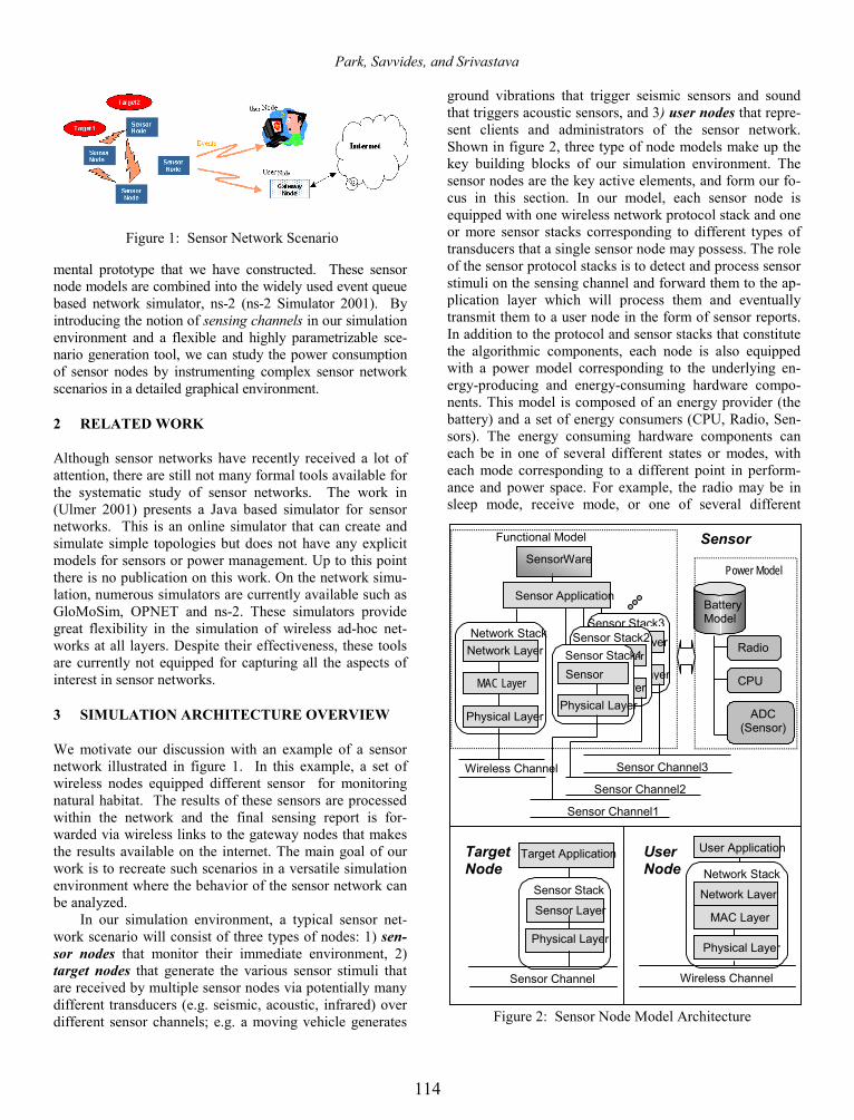
Park, Savvides, and Srivastava
mental prototype that we have constructed. These sensor node models are combined into the widely used event queue based network simulator, ns-2 (ns-2 Simulator 2001). By introducing the notion of sensing channels in our simulation environment and a flexible and highly parametrizable sce-nario generation tool, we can study the power consumption of sensor nodes by instrumenting complex sensor network scenarios in a detailed graphical environment.
2 RELATED WORK
Although sensor networks have recently received a lot of attention, there are still not many formal tools available for the systematic study of sensor networks. The work in (Ulmer 2001) presents a Java based simulator for sensor networks. This is an online simulator that can create and simulate simple topologies but does not have any explicit models for sensors or power management. Up to this point there is no publication on this work. On the network simu-lation, numerous simulators are currently available such as GloMoSim, OPNET and ns-2. These simulators provide great flexibility in the simulation of wireless ad-hoc net-works at all layers. Despite their effectiveness, these tools are currently not equipped for capturing all the aspects of interest in sensor networks.
3 SIMULATION ARCHITECTURE OVERVIEW
We motivate our discussion with an example of a sensor network illustrated in figure 1. In this example, a set of wireless nodes equipped different sensor for monitoring natural habitat. The results of these sensors are processed within the network and the final sensing report is for-warded via wireless links to the gateway nodes that makes the results available on the internet. The main goal of our work is to recreate such scenarios in a versatile simulation environment where the behavior of the sensor network can be analyzed.
In our simulation environment, a typical sensor net-work scenario will consist of three types of nodes: 1) sen-sor nodes that monitor their immediate environment, 2) target nodes that generate the various sensor stimuli that are received by multiple sensor nodes via potentially many different transducers (e.g. seismic, acoustic, infrared) over different sensor channels; e.g. a moving vehicle generates
ground vibrations that trigger seismic sensors and sound that triggers acoustic sensors, and 3) user nodes that repre-sent clients and administrators of the sensor network. Shown in figure 2, three type of node models make up the key building blocks of our simulation environment. The sensor nodes are the key active elements, and form our fo-cus in this section. In our model, each sensor node is equipped with one wireless network protocol stack and one or more sensor stacks corresponding to different types of transducers that a single sensor node may possess. The role of the sensor protocol stacks is to detect and process sensor stimuli on the sensing channel and forward them to the ap-plication layer which will process them and eventually transmit them to a user node in the form of sensor reports. In addition to the protocol and sensor stacks that constitute the algorithmic components, each node is also equipped with a power model corresponding to the underlying en-ergy-producing and energy-consuming hardware compo-nents. This model is composed of an energy provider (the battery) and a set of energy consumers (CPU, Radio, Sen-sors). The energy consuming hardware components can each be in one of several different states or modes, with each mode corresponding to a different point in perform-ance and power space. For example, the radio may be in sleep mode, receive mode, or one of several different
Figure 1: Sensor Network Scenario
Figure 2: Sensor Node Model Architecture
Target Node
Sensor Layer
Physical Layer
Sensor Stack
Sensor Channel
Target Application
Wireless Channel
User Application User Node
Network Layer
Physical Layer
Network Stack
MAC Layer
Sensor Layer
Physical Layer
Sensor Stack3
Sensor Layer
Physical Layer
Sensor Stack2
Functional Model Sensor SensorWare
Power Model
Battery Model
Radio
CPU
ADC (Sensor)
Wireless Channel
Sensor Channel1
Network Layer
MAC Layer
Physical Layer
Network Stack
Sensor
Physical Layer
Sensor Stack1
Sensor Application
Sensor Channel2
Sensor Channel3
1331
114

Park, Savvides, and Srivastava
transmit modes corresponding to different symbol rates, modulation schemes, and transmit power. Similarly, the CPU may be in sleep mode, or one of several different ac-tive modes corresponding to different frequency and volt-age. The algorithms in the network and sensor stack con-trol the change in mode of the power consumers. For example, the MAC protocol may change the radio mode from sleep to receive. In return, the performance of the al-gorithms may depend on the mode. For example, the time taken by the physical layer in the network protocol stack would depend on the data rate of the mode the radio is cur-rently in. All of this is accomplished by having the algo-rithms in the network and sensor stacks issue mode change events to the power consumer entities, and having the algo-rithms read relevant parameter values from those entities. Algorithm-induced changes in the operating modes of power consuming hardware entities in turn affect the cur-rent drawn by them from the battery which delivers the power corresponding to the sum of current (or power) drawn by each power consumer. Internally, the battery en-tity depletes its stored chemical energy according to the ef-ficiency dictated by the battery model.
Figure 3 illustrates how a typical sensor network will be constructed and simulated using our simulation envi-ronment. In figure 3, the wireless channel and sensor chan-nel form separate communication mechanisms where events from different nodes are passed through. A typical scenario will involve a target node passing through a group of sensor nodes deployed in the field. As the target node moves around, it gives out sensor signal in the form of events through the sensor channel and each sensor node detects the events based on propagation model imple-mented in each node’s sensor stack. When sensor nodes determine the sensor signals (events) are noteworthy, they transmit packets (also in the form of events) through the wireless channel destined to the user node.
By separating the sensor channel and the wireless channel, our sensor network model makes easier to simu-
late and analyze the operation of sensor network where the sensor signal detection events and wireless communication events can be received or transmitted concurrently. More-over, by allowing sensor node to connect to multiple sensor channels, our simulation environment provides ability to analyze complex behaviors of sensor nodes’ reaction to multiple sensor signals (i.e. seismic vibration, sounds, temperature, etc..) that can be detected all at the same time. In the following section, we discuss each components of the sensor node model shown in figure 2, and explain how we construct the model of different sensor nodes’ compo-nents.
4 FRAMEWORK OF SENSOR NETWORK SIMULATION
4.1 Node Placement and Traffic Generation
In studying the performance of a wireless sensor network for a given application, a crucial element is the overall deploy-ment scenario which includes the node placement topology, the radio ranges, the sensing ranges, the trajectories of the targets and resultant event traffics, and the trajectories of the user nodes and their query traffics. All these elements con-tribute to the different design trade-offs that can be made, and it is crucial to evaluate the effects of a new algorithm or protocol under diverse deployment scenarios.
To study such effects, we have developed a detailed scenario generation and visualization tool that enables us to construct detailed topologies and sensor network traffic. Our simulation environment enables us to assess the re-quirements of a sensor network under different circum-stances by generating detailed scenario input to our simula-tions. This complements the scenario generation techniques provided in (ns-2 Simulator 2001) which are mainly tar-geted to ad-hoc wireless communication networks. Sensor node placement can vary depending on intended the task on the network. For example, to monitor wildlife in a forest, sensors may be uniformly distributed in the forest. If how-ever, the sensor network is deployed for perimeter defense, then the sensors will most likely be distributed around a specified perimeter in a two dimensional gaussian distribu-tion. In some other cases, the sensors may be manually placed according to the requirements of the user.
Besides placement, the traffic requirements may be even more diverse. Sensor network traffic can be classified into 3 main types: 1) user-to-sensor traffic, which is a re-sult of user commands and queries to the network, 2) sen-sor-to-user traffic, which consists of the sensor reports to the user and 3) sensor-to-sensor traffic, which includes collaborative signal-processing of sensor events in the network before they are reported to the user. The last type of traffic is the most complex, and it depends on the sens-ing method.
Figure 3: Sensor Network Model Architecture
Sensor Node Sensor
Node
Sensor Node
Wireless Channel
Sensor Channel
Target Node
User Node
1332
115
TTT
hH-HH I : :
HTH

Park, Savvides, and Srivastava
4.2 Sensor Stack and Sensor Channel
The sensor stack simulates how a sensor node generates, detects and processes sensor signals. In sensor node model (figure 2), the sensor stack is a signal sink that is responsi-ble for triggering the application layer every time a sensing event occurs. Various trigger functions ranging from sim-ple sensing schemes to elaborate signal processing func-tions can be implemented in the sensor stack. In target node model, the sensor stack acts as a signal source. The sensor stack of a target node will contain a signature that is unique to the type of target the target node is modeling. The signature is then transmitted through various mediums (ground, air, free space, water, etc..) as the target node moves around. figure 4a and 4b show a real and a simu-lated signature obtained from a seismic sensor triggered by ground vibration from a traveling vehicle.
In figure 4, the ground is the medium that transmits the vibrations to the seismic sensor. We refer to this me-dium as the sensor channel, a model of a medium which sensor events such as seismic vibration, sounds, or infrared signals are traveled through. The type of medium can dif-fer based on the type of sensor being modeled (seismic, acoustic, infra red, ultrasonic). Moreover, depending on the medium being modeled, the propagation of signal can differ. For instance, a sound moving through the air will have different propagation as the same sound moving through the water. In order to incorporate all these differ-ent aspects of the sensor network in to our simulation, we implement a simple sensor stack and sensor channel model by modeling the target node as a gaussian source whose signal amplitude is modeled as a gaussian random variable with the mean equal to zero and the variance σ2. As the
target travels through the sensor network, the target exerts the vibration signals (signal events) into the sensor channel periodically. The sensor channel then delivers this events to each sensor node’s sensor stack and each sensor node adjusts the signal strength of the target based on sensor channels propagation model. The figure 4b demonstrates the signal strength variation as a target passes by a sensor node on a straight line. As the target approaches the sensor node, the signal strength increases, and as the target moves away, the signal attenuates rapidly. In this simulation the sensor signal was attenuated at a rate of 1/r where r is the distance between the target and the sensor.
4.3 Hardware Components Characterization
Mode ID
CPU Radio(OOK Modulation)
ADC Total Current
1 Active 2.9mA
Tx-19.2kbps 5.2mA
On 8.1mA
2 Active 2.9mA
Tx-2.4kpbs 3.1mA
On 6.0mA
3 Active 2.9mA
Rx:4.1mA On 7.0mA
4 Sleep 1.9mA
Sleep:5µA On 1.9mA
5 Off 1µA
Sleep:5µA Off 6µA
We construct our power models by performing measure-ments of the hardware power consumption using an HP 1660 oscilloscope, a bench power supply, and a high preci-sion resistor. The measurement setup and power relation-ships are shown in figure 5. By characterizing each com-ponent of the sensor nodes we enable the simulated nodes to operate at different modes in which the power manage-ment schemes can switch different components on and off. Using the configuration in figure 5, the total current con-sumption of our experimental sensor node is obtained in Table 1. The measurements listed in Table 1 provide a bet-ter insight into the power consumption of the sensor nodes since the actual power consumption is oftentimes different from the typical values provided in the manufacturer data sheets depending on the mode of operation.
Table 1: Experimental Node Current Consumption
Figure 5: Power Measurement Configuration
0 10000 20000 30000samples
-30000
-10000
10000
30000
16bi
t AD
C v
alue
a)
0 10000 20000 30000samples
-40000
-20000
0
20000
40000
16bi
t AD
C v
alue
b)
Figure 4: a) Real Target Seismic Signatureb) Simulated Target Seismic Signature
1333
116

Park, Savvides, and Srivastava 4.4 Battery Models
The Battery Model simulates the capacity and the lifetime of the sole energy source of the sensor node, the battery. In reality, battery behavior highly depends on the constitu-ent materials and modeling this behavior is a difficult task. Although the battery can be viewed as a energy storage, the main goal of the sensor network is to increase the life-time of the battery. Thus, in this section, we focus on how battery’s capacity can be modeled based on the energy consumers’ behavior. We propose 3 different types of bat-tery models to study how different aspects of real battery behavior can affect the energy efficiency of different appli-cations. The metrics that are used to indicate the maxi-mum capacity of the battery is in the unit of Ah (Am-pere*Hour). The metric is a common method used by the battery manufacturers to specify the theoretic total capacity of the battery. Knowing the current discharge of the bat-tery and the total capacity in Ah, one can compute the theoretical lifetime of the battery using the equation ,
ICT = , where T=battery lifetime, C=rated maximum
battery capacity in Ah, and I=discharge current.
4.4.1 Linear Model
In Linear Model, the battery is treated as linear storage of current. The maximum capacity of the battery is achieved regardless of what the discharge rate is. The simple battery model allows user to see the efficiency of the user’s appli-cation by providing how much capacity is consumed by the user. The remaining capacity after operation duration of time td can be expressed by the following equation.
Remaining capacity (in Ah) = ∫+
=
−=dtt
tt
dttICC0
0
)(' (1)
where C’ is the previous capacity and I(t) is the instantane-ous current consumed by the circuit at time t. Linear Model assumes that I(t) will stay the same for the duration td, if the operation mode of the circuit does not change ( i.e. radio switching from receiving to transmit, CPU switching from active to idle, etc.. ) for the duration td. With these assumptions equation 1 simply becomes as the following.
dtt
t
tt
tt
tIC'tIC'I(t)dtC'C dd
⋅−=⋅−=−= ++
=∫ 0
0
0
0
(2)
The total remaining capacity is computed whenever
the discharge rate of the circuit changes.
4.4.2 Discharge Rate Dependent Model
While Linear Model assumes that the maximum capacity of the battery is unaffected by the discharge rate, Discharge Rate Dependent Model considers the effect of battery dis-charge rate on the maximum battery capacity. In [15] [16], it is shown that battery’s capacity is reduced as the dis-charge rate increases. In order to consider the effect of discharge rate dependency, we introduce factor k which is the battery capacity efficiency factor that is determined by
the discharge rate. The definition of k is, maxC
Ck eff= ,
where Ceff is the effective battery capacity and Cmax is the maximum capacity of the battery with both terms ex-pressed in unit of Ah. In Discharge Rate Dependent Model, the equation 1 is then transformed to the following.
dtICkC ⋅−⋅= ' (3)
The efficiency factor k varies with the current I and is
close to one when discharge rate is low, but approaches 0 when the discharge rate becomes high. One way to find out corresponding k value is for different current value of I is to use the table driven method introduced in (Simunic 1999).
4.4.3 Relaxation Model
Real-life batteries exhibit a general phenomenon called “relaxation” explained in (Fuller 1994, Linden 1995, Chi-asserini 1999). When the battery is discharged at high rate, the diffusion rate of the active ingredients through the elec-trolyte and electrode falls behind. If the high discharge rate is sustained, the battery reaches its end of life even though there are active materials still available. However, if the discharge current from the battery is cutoff or re-duced during the discharge, the diffusion and transport rate
Figure 6: Capacity vs. Discharge Rate Curve for CR2354 (Matsushita Electric Corp. of America 2001)
1334
117
<
o
600
500
400
CD 300 a CO
^ 200
100
60'C(140T) _^ ^ ^
20°C
y -lOXi-HT)^' -" " IM rj—
1 MINI Cul off voltage: 2.0V
.1 Load: (Kfl)
(mA) 2
3 4 20 30 40 60 100
0.5 0.3 0.2 0,1 0.05 0.03

Park, Savvides, and Srivastava of active materials catches up with the depletion of the ma-terials. This phenomenon is called relaxation effect, and it gives the battery chance to recover the capacity lost at high discharge rate. For a realistic battery simulation, it’s impor-tant to look at the effects of relaxation as it has effect of lengthening the lifetime of the battery. For our simulation, we adapt the analytical model introduced in (Fuller 1994) which takes discharge rate as input and computes the bat-tery voltage over the simulation duration.
5 EXAMPLE STUDY CASE
In this section we demonstrate some of the main capabili-ties of our tool by studying the performance of different battery models with various sensor node operation profile.
5.1 Low Rate/Low Power vs. High Rate/High Power
In this case study, we evaluate the battery consumption of our experimental sensor node by considering different op-eration profiles. In section 4.3, we have discussed how each component of our sensor node has different power consumption depending on its operation mode. In this sec-tion, we examine how the combination of the operation modes of different components affects the aggregate power consumption of the sensor node. The scenario involves two sensor nodes (a transmitter and a receiver) that are within the transmission range of each other (approximately 15 meters apart) where the transmitter needs to transmit a 2MB file to the receiver. For the purposes of our discus-sion we define 5 different operation modes for our experi-mental node shown in table 1. To examine the energy con-sumption and communication tradeoffs we evaluate 3 different data transmission policies.
1)19.2 kbps continuous transmission: The transmitter sends data at the highest data rate without any break. The transmitter will be operating in mode 1 and the receiver
will be operating in mode 3; 2) 2.4 kbps continuous trans-mission: With lower data rate the sender can transmit at a lower power level to reach the receiver. The transmitter will be operating in mode 2 and the receiver will be operat-ing in mode 3; 3) 19.2 kbps pulse transmission: The trans-mitter sends data intermittently at the highest power level. While the transmitter is not transmitting, the transmitter puts the CPU and Radio to sleep. The transmitter power cycle its component by transmitting one 60 byte packet at 19.2 kbps for .025 sec and sleeps for .125 sec until all the data is received by the receiver. The transmitter will be switching between modes 1 and 4, and the receiver will be switching between mode 3 and 4.
Figure 7a shows the effect on each battery model ca-pacity after the 2 MB data transfer for the three transmis-sion methods described above. This experiment was per-formed for all three battery models described in section 4.4. Initially, all batteries were set to a capacity level of 10 mA*hour. The left half of figure 7a describes the remain-ing battery capacity of the transmitter after the file transfer, and the right half shows the receiver battery capacity. The solid bar in the figure indicates the total time for data trans-fer. Looking at the solid bar, it is clear that the sending the file at high data rate takes the least time thus the least bat-tery capacity. Although the 2.4 kbps transmission and 19.2 kbps transmission took the same amount of time to trans-mit the data, 19.2 kbps pulse transmission saved much bat-tery capacity due to the sleep period. Figure 7a also shows how different battery models exhibit different char-acteristics under different transmission methods. The lin-ear model shows how optimum battery will behave as it shows the theoretical capacity of the battery under any dis-charge current. On the other hand, the rate dependent model accurately describes how real batteries will behave when there is a constant discharge for long duration. This is shown in 2.4 kbps transmission where the remaining ca-pacity of rate dependent model is substantially less than the
19.2k 2.4k 19.2k Pulse 0
1E-005
2E-005
3E-005
4E-005
5E-005
6E-005
batte
ry u
tiliz
atio
n/se
c
19.2k 2.4k 19.2k Pulse 19.2k 2.4k 19.2k Pulse
Transmitter Receiver
0
1000
2000
3000
4000
5000
6000
7000
time
(sec
)
0.3
0.4
0.5
0.6
0.7
0.8
0.9
1
remaing capacity (full =1)
Timelinearrate-dependentrelaxation
Figure 7: a) Battery Capacity Usage Under Different Discharge Profiles, b) Battery Utilization Rate
a) b)
1335
118

Park, Savvides, and Srivastava linear model. The other interesting model is the relaxation model which exhibits the both discharge rate dependent capacity and recovery effect. Since the relaxation model has recovery properties, the difference between relaxation model and rate dependent model is shown in the pulsed transmission cases. In figure 7a the relaxation model has the same remaining battery life as rate dependent model for 19.2kbps and 2.4 kbps continuous transmission and recep-tion. However, in 19.2 kbps pulse transmission and recep-tion, the relaxation model has almost equal capacity as the linear model due to the capacity recovery during the sleep mode.
5.2 Monitoring a Moving Vehicle in a Sensor Field
In this implementation we first show the effect of traffic on the sensing and communication traffic and then we evalu-ate simple power management scheme using the same sen-sor node setup as in the previous subsection. For this we have implemented a lightweight protocol stack similar to what one would expect to have on a tiny sensor node. The radio transmission and reception are driven by a TDMA based medium access control (MAC) protocol based on unique slot assignment algorithm derived from [9]. The MAC protocol assigns a unique slot to each node over a 2-hop radius and each node is aware of its one-hop neighbors and their corresponding slot assignment. For routing, we have implemented a very lightweight table-driven routing protocol with table size of one (next hop to user node). The motivation for TDMA scheme comes from our result in section 5.1 where a pulse transmission and reception can improve the battery utilization in the long term. In our power aware TDMA scheme this requirement is met for both the transmission and reception of packets. For trans-mission, a node is only allowed to transmit in its assigned time-slot. For reception, a node only needs to listen to the wireless channel for the duration of the slots that are al-ready assigned to its one-hop neighbors. For the purposes of our discussion we refer to all the other remaining slots as idle slots.
In this scenario, a small cluster of 10 sensors equipped with seismic sensors is deployed to detect a bypassing truck as shown in figure 8a. The seismic sensors run at a sample rate of 400Hz to produce 16 bit samples. The sen-sor nodes are configured to report back to a gateway node that makes the results available on the Internet. Each sen-sor is programmed to transmit a report to the gateway within 5 seconds from the moment the ground vibrations from the truck are detected. If at least 2048 samples are obtained, the node can perform coherent detection and it will transmit a 10 byte to report the target type. This short packet is called “coherent traffic”. If however, the node does not have enough samples at the end of the 5-second period, it enters a non-coherent detection mode and trans-mits all its available samples to the gateway node which performs sensor data combination (called “beamforming” [20]) to improve the detection accuracy. Since the sensor node transmits raw data when it enters non-coherent detec-tion mode, the size of non-coherent data tends to be lot lar-ger than the coherent traffic. This non coherent raw data is referred to as “non-coherent traffic” During the simulation, the network traffic will be consist of coherent and non-coherent traffic depending on whether the individual sen-sors successfully classified the target. We discuss the re-sult of the simulation in the following two sub sections.
5.2.1 Efficiency of Power Management Scheme with TDMA
One apparent advantage of TDMA over other CSMA ran-dom access MAC protocols is the fact that the sensor nodes do not have to be in receive mode during the time slots where none of its neighbors are schedule to transmit. This allows the sensor nodes to perform a simple power man-agement scheme that puts the CPU and radio to sleep dur-ing idle slots to conserve battery capacity. With this setup, we evaluate the efficiency of battery capacity utilization when this simple power management scheme is used. Fig-ure 8a is the scenario used for our evaluation. It consists of 100 nodes uniformly distributed across a sensor field. The
Figure 8: a) 100 Node Test Topology, b) Battery Capacity Usage
0 500 1000 1500 2000 2500
time(sec)
0
10
20
30
40
50
60
70
aver
age
batte
ry c
apac
ity u
sed
(%)
linear [pm]rate-depedent [pm]linear [nopm]rate-dependent [nopm]
a) b)
1336
119
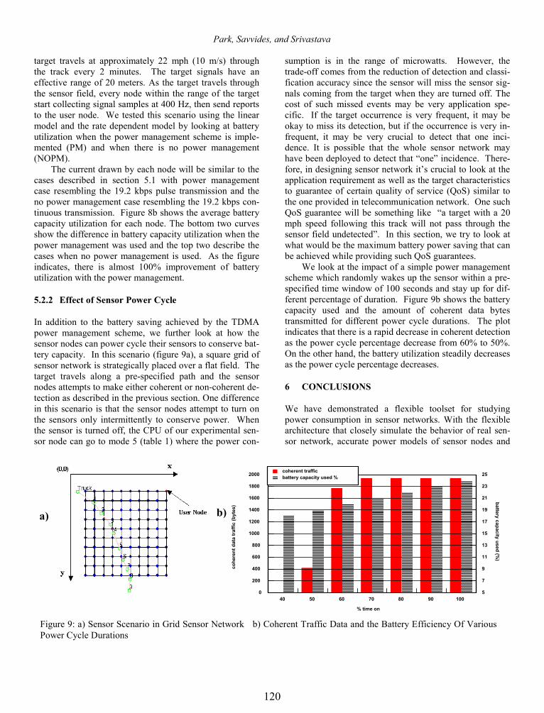
Park, Savvides, and Srivastava target travels at approximately 22 mph (10 m/s) through the track every 2 minutes. The target signals have an effective range of 20 meters. As the target travels through the sensor field, every node within the range of the target start collecting signal samples at 400 Hz, then send reports to the user node. We tested this scenario using the linear model and the rate dependent model by looking at battery utilization when the power management scheme is imple-mented (PM) and when there is no power management (NOPM).
The current drawn by each node will be similar to the cases described in section 5.1 with power management case resembling the 19.2 kbps pulse transmission and the no power management case resembling the 19.2 kbps con-tinuous transmission. Figure 8b shows the average battery capacity utilization for each node. The bottom two curves show the difference in battery capacity utilization when the power management was used and the top two describe the cases when no power management is used. As the figure indicates, there is almost 100% improvement of battery utilization with the power management.
5.2.2 Effect of Sensor Power Cycle
In addition to the battery saving achieved by the TDMA power management scheme, we further look at how the sensor nodes can power cycle their sensors to conserve bat-tery capacity. In this scenario (figure 9a), a square grid of sensor network is strategically placed over a flat field. The target travels along a pre-specified path and the sensor nodes attempts to make either coherent or non-coherent de-tection as described in the previous section. One difference in this scenario is that the sensor nodes attempt to turn on the sensors only intermittently to conserve power. When the sensor is turned off, the CPU of our experimental sen-sor node can go to mode 5 (table 1) where the power con-
sumption is in the range of microwatts. However, the trade-off comes from the reduction of detection and classi-fication accuracy since the sensor will miss the sensor sig-nals coming from the target when they are turned off. The cost of such missed events may be very application spe-cific. If the target occurrence is very frequent, it may be okay to miss its detection, but if the occurrence is very in-frequent, it may be very crucial to detect that one inci-dence. It is possible that the whole sensor network may have been deployed to detect that “one” incidence. There-fore, in designing sensor network it’s crucial to look at the application requirement as well as the target characteristics to guarantee of certain quality of service (QoS) similar to the one provided in telecommunication network. One such QoS guarantee will be something like “a target with a 20 mph speed following this track will not pass through the sensor field undetected”. In this section, we try to look at what would be the maximum battery power saving that can be achieved while providing such QoS guarantees.
We look at the impact of a simple power management scheme which randomly wakes up the sensor within a pre-specified time window of 100 seconds and stay up for dif-ferent percentage of duration. Figure 9b shows the battery capacity used and the amount of coherent data bytes transmitted for different power cycle durations. The plot indicates that there is a rapid decrease in coherent detection as the power cycle percentage decrease from 60% to 50%. On the other hand, the battery utilization steadily decreases as the power cycle percentage decreases.
6 CONCLUSIONS
We have demonstrated a flexible toolset for studying power consumption in sensor networks. With the flexible architecture that closely simulate the behavior of real sen-sor network, accurate power models of sensor nodes and
40 50 60 70 80 90 100
% time on
0
200
400
600
800
1000
1200
1400
1600
1800
2000
cohe
rent
dat
a tr
affic
(byt
es)
5
7
9
11
13
15
17
19
21
23
25
battery capacity used (%)
coherent trafficbattery capacity used %
Figure 9: a) Sensor Scenario in Grid Sensor Network b) Coherent Traffic Data and the Battery Efficiency Of VariousPower Cycle Durations
a) b)
1337
120

Park, Savvides, and Srivastava analysis of battery behavior are utilized in a tool to evalu-ate power consumption in the context of a realistic sce-nario. With these results we can assess the power consumption for new sensor nodes that are currently under development. Furthermore, this tool has been an indispen-sable aid in estimating the resources required for the net-work protocols to function correctly in new node architec-tures. By simulating and validating target protocols we can also get a good indication of code size and memory re-quirements thus resulting in feasible low cost designs. We envision that this set of tools will play an instrumental role in the design and implementation of new application spe-cific sensor networks.
REFERENCE
Chiasserini, C. F., and R. R. Rao. 1999. Pulsed battery dis-charge in communication devices. In Proceedings of Mobicom 99, Seattle, August 1999.
Fuller, T. F., M. Doyle, and J. Newman. 1994. Simulation and Optimization of the Dual Lithium Ion Insertion Cell. Journal of Electrochem. Soc., vol. 141, no. 4, pp 1-10.
Linden, H.D. 1995. Handbook of Batteries. 2nd ed. New York: McGrawHill.
Matsushita Electric Corp. of America. 2001. Panasonic lithium coin cell battery datasheet. Available via http://www.panasonic.com/industrial_oem/battery/battery_oem/chem/lith/lith.htm [accessed July 9, 2001].
ns-2 simulator. 2001. ns-2 Simulator, Available via http://www.isi.edu/nsnam/ns/ [accessed July 9, 2001].
Rockwell Scientific Company LLC. 2001. WINS (Wireless Integrated Network Systems) Project. Available via http://wins.rsc.rockwell.com/ [accessed July 9, 2001].
Simunic, T., L. Benini, and G. De Micheli. 1999. Energy-Efficient Design of Battery-Powered Embedded Sys-tems. In Proceedings of International Symposium on Low Power Electronics and Design, 212-217, Pis-cataway, New Jersey.
Ulmer, C. 2001. Sensor Network Simulator, Available via http://users.ece.gatech.edu/~grimace/research/sensorsimii/ [accessed July 9, 2001].
AUTHOR BIOGRAPHIES
SUNG PARK is a Ph.D. student of Electrical Engineering at University of California Los Angeles. He received his MS from Carnegie Mellon University in 1997. His research interests are network simulation and modeling, low power embedded systems, and sensor network. His email and web addresses are <[email protected]> and <http://www.ee.ucla.edu/~spark>.
ANDREAS SAVVIDE is a Ph.D. student of Electrical Engineering at University of California Los Angeles. He received his MS from University of Massachusetts, Am-herst in 1997. His research interests are adhoc wireless network, embedded system, and sensor network. His email and web addresses are <[email protected]> and <http://www.ee.ucla.edu/~asavvides>.
MANI B. SRIVASTAVA is an Associate Professor of Electrical Engineering at University of California Los An-geles. He received his Ph.D. from U. C. Berkeley in 1992. His research interests are low power VLSI circuits, em-bedded systems, and sensor networks. His email and web addresses are <[email protected]> and < http://nesl.ee.ucla.edu/people/mbs/>.
1338
121

Abstract— When designing wireless systems, one of the major challenges is tackling the time depending fading behavior of the channel. To achieve maximum throughput under a power constraint, techniques have been proposed which adapt the modulation on the fly, based on the instantaneous channel condition. However, when the design goal is minimizing the overall energy consumption under a throughput constraint, we have to tackle a more complex scheduling problem. The reason is that energy optimality might require deliberately decreasing the transmission rate at times, if we know that the rate loss can be compensated for in the future when channel conditions are more favorable. We present a solution to the problem of minimum energy scheduling on wireless links by exploiting an analogy with the adaptive bit loding problem in multicarrier systems. Instead of allocating bits across multiple channels with different quality, we formulate the problem as one of allocating bits at the different time instants. The analogy is however not straightforward because one does not know the future, and therefore cannot simply apply conventional bit loading to the time dimension. We devise a new technique that approximates adaptive loading in time, but only depends on the instantaneous channel condition. Our algorithm is simple to implement, and shows upto 5x reduction in energy over existing approaches.
I. INTRODUCTION
In wireless system, adapting the modulation at runtime has been proposed to maximize the throughput when faced with a variable channel [1]. Indeed, the non-constant fading behavior of the wireless medium results in attenuation variations, which can span orders of magnitude. When the channel is good, the modulation level is increased, while the opposite is done when the channel is bad. This principle of adaptive modulation has been explored extensively and can provide substantial throughput increase [2][3][4][5][6][7][8].
Systems are typically designed around the maximum expected traffic, such that they can handle the worst-case load. This is the operating premise of adaptive modulation: only by adapting to the channel conditions, can they reach the required throughput under a maximum power constraint. However, in typical wireless systems, the actual traffic load is often lower than the worst-case. One option is to transmit the data at the maximum rate, using modulation scaling, and afterwards shutdown the transceiver to save power.
In general, it has been shown that transmitting slower can actually further reduce the energy consumption of radio communications significantly [9]. This principle is analogous to voltage scaling in digital CMOS circuits, where voltage can be seen as a control knob to trade off energy and speed. However, the non-deterministically varying channel makes the problem different from voltage scaling.
In wireless communications, minimizing the energy by adapting the modulation has to take the channel variations into account, and becomes a problem of wireless scheduling. When the goal is to minimize the energy, and at the same time achieve a certain specified average throughput, we need to know the behavior of the channel in the future! The decision on the current rate critically depends on how good or bad the channel will be, i.e., whether it is more efficient to send now or later. This issue does not arise when adapting the modulation to maximize the throughput, since only the current channel condition has to be taken into account there.
If we could magically know the channel over the entire time epoch, the problem reduces to one that has been studied extensively in multicarrier systems like OFDM (Orthogonal Frequency Division Multiplex) and DMT (Discrete Multi-Tone). In these systems, adaptive bit loading algorithms set the modulation level in each frequency band such that a predefined total number of bits are transmitted with minimum power, by leveraging the channel variations in the frequency domain. For our problem, we would simply need to replace the frequency dimension by the time dimension. However, as mentioned before, there is a severe practical problem with this approach: we cannot estimate the channel and then go back in time to set the modulation level. So, although adaptive bit loading in time would theoretically provide the best solution, it is impossible to use the existing techniques.
In this paper, we propose a new scheme that decides upon the modulation level based solely on the current channel condition. Our scheme, which we introduce in the next section, uses a set of thresholds that only depend on the channel statistics. Its performance gets arbitrarily close to that of ideal adaptive bit loading for increasing time windows, as we show in section III. The practical example of section IV illustrates the substantial energy gains that can be achieved.
II. THRESHOLD-BASED ALGORITHM
In the absence of a line-of-sight path between sender and receiver, narrowband wireless radio communications can be modeled as experiencing Rayleigh fading [10]. In this case, the normalized channel power-gain factor α has a probability density function (pdf) and cumulative distribution function (cdf) given by (1) and (2) respectively. These statistics are independent of the channel time-correlation, which is characterized by the Doppler rate.
(1)
(2)
Energy Efficient Wireless Scheduling: Adaptive Loading in Time
Curt Schurgers Mani B. Srivastava
Networked and Embedded Systems Lab (NESL), Electrical Engineering Department, University of California at Los Angeles (UCLA), CA 90095
( ) xexFxP −−==≤ 1)( αα
( ) xexf −=α
0-7803-7376-6/02/$17.00 (c) 2002 IEEE. 702706
122

Equation (3) expresses the required transmit power Pi for Quadrature Amplitude Modulation (QAM) as a function of the modulation level bi in bits per symbol and the channel gain factor αi [10]. The results of this paper can be extended to other modulation schemes as well. The factor C is virtually constant over time and depends on the target error rate and the transmit distance, among others.
(3)
We refer to the transmit time instant of a symbol as a ‘time sample’. In the remainder of this paper, the subindex i enumerates these time samples. In the case of multicarrier systems, the equivalent of a time sample would be the frequency band index.
Since there is no real bound on the number of time samples, we assume an infinite time duration in our analysis. In section III, we revisit the accuracy of this assumption. As a result, the intricacies of adaptive bit loading vanish, such that the task of selecting the correct modulation can be simplified considerably. In Appendix A, we prove this statement and derive a set of thresholds d1, d2, d3, etc., which uniquely couple each possible channel gain factor with its modulation level. This principle is illustrated in figure 1. The thresholds define non-overlapping ranges, each corresponding with a value of b. When the channel gain α is in a particular range, the modulation is set accordingly.
Figure 1: Relationship between thresholds and modulation
The knowledge of the channel gains is obtained through channel estimation, just as for adaptive modulation techniques that maximize the throughput [1]. To track variations, this estimation is updated regularly at a rate fupdate, which is a compromise between overhead and performance degradations of inaccurate estimates. Between estimates, the
modulation level is kept constant. Our scheme is only valuable if the channel changes slowly enough. This is the same applicability range as other adaptive techniques, such as modulation adaptation [1][2][3][4][5][6][7].
In Appendix A, we prove that the thresholds are mutually related according to (4). Furthermore, threshold d1 only depends on the pdf of the channel gains and the required average number of bits per symbol bav. For Rayleigh fading, this relationship is given by (5). For other statistics, similar relationships can be found. We have essentially reduced the problem of knowing the exact behavior of the channel over time to that of finding its statistics.
(4)
(5)
The solid curves in figure 2 show the relationship of the thresholds and bav as calculated from (4) and (5). To validate our derivations, we have also simulated what the threshold values would be when applying an existing loading algorithm for multicarrier systems on a large set of known independent time samples. The circles show to the lowest α that was encountered for each modulation level, which essentially corresponds to the threshold when the number of samples is very high. These simulations use the Hughes-Hartoghs loading algorithm [11], with the number of time samples N equal to 16384. We observe indeed a very tight correspondence between the simulated and theoretical values.
Figure 2: Ideal theoretical thresholds (solid lines) and simulation results for N = 214 (circles)
In practice, we want to know d1 as a function of bav, but it is hard to solve (4) analytically. The approximation of (6), obtained through curve fitting, is accurate down to bav = 1. At
thresholds
bav (bits/symbol)
d1 d4 d3 d2
approximation
( )i
b
i
i
CPα
12 −⋅=
time (s)
b = 0
d1
d2
d3
b = 2
b = 4
b = 6
b = 8 α d4
jj dd 411 ⋅=+
∑
∞
=
⋅−⋅=0
1 )4exp(2j
jav db
0-7803-7376-6/02/$17.00 (c) 2002 IEEE. 703707
123
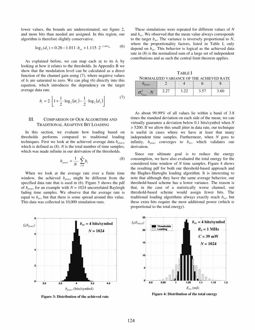
lower values, the bounds are underestimated, see figure 2, and more bits than needed are assigned. In this region, our algorithm is therefore slightly conservative.
(6)
As explained before, we can map each αi to its bi by looking at how it relates to the thresholds. In Appendix B we show that the modulation level can be calculated as a direct function of the channel gain using (7), where negative values of bi are saturated to zero. We can plug (6) directly into this equation, which introduces the dependency on the target average data rate.
(7)
III. COMPARISON OF OUR ALGORITHM AND
TRADITIONAL ADAPTIVE BIT LOADING
In this section, we evaluate how loading based on thresholds performs compared to traditional loading techniques. First we look at the achieved average data bpract, which is defined as (8). N is the total number of time samples, which was made infinite in our derivation of the thresholds.
(8)
When we look at the average rate over a finite time window, the achieved bpract might be different from the specified data rate that is used in (6). Figure 3 shows the pdf of bpract for an example with N = 1024 uncorrelated Rayleigh fading time samples. We observe that the average rate is equal to bav, but that there is some spread around this value. This data was collected in 10,000 simulation runs.
Figure 3: Distribution of the achieved rate
These simulations were repeated for different values of N and bav. We observed that the mean value always corresponds to the target bav. The variance is inversely proportional to N, where the proportionality factors, listed in Table I, only depend on bav. This behavior is logical as the achieved data rate in (8) is the normalized sum of a large set of independent contributions and as such the central limit theorem applies.
TABLE I NORMALIZED VARIANCE OF THE ACHIEVED RATE
bpract 2 4 6 8
2.27 3.22 3.57 3.60
As about 99.99% of all values lie within a band of 3.8 times the standard deviation on each side of the mean, we can virtually guarantee a deviation below 0.1 bits/symbol when N > 5200. If we allow this small jitter in data rate, our technique is useful in cases where we have at least that many independent time samples. Furthermore, when N goes to infinity, bpract converges to bav, which validates our derivation.
Since our ultimate goal is to reduce the energy consumption, we have also evaluated the total energy for the considered time window of N time samples. Figure 4 shows the resulting pdf for both our threshold-based approach and the Hughes-Hartoghs loading algorithm. It is interesting to note that although they have the same average behavior, our threshold-based scheme has a lower variance. The reason is that, in the case of a statistically worse channel, our threshold-based scheme would assign fewer bits. The traditional loading algorithms always exactly reach bav, but these extra bits require the most additional power (which is proportional to the total energy).
Figure 4: Distribution of the total energy
Npractb ⋅2σ
bpract (bits/symbol)
bav = 4 bits/symbol
N = 1024 fb(bpract)
avbavbd ⋅−⋅+⋅−≈ 49.1
12 2115.1011.126.0)(log
( ) ( )
⋅−⋅+⋅= 122 log2
1log
2
112 db ii α
∑=
⋅=N
iipract b
Nb
1
1
Etot (mJ)
bav = 4 bits/symbol
RS = 1 MHz
C = 39 mW
N = 1024
fb(Eblock)
0-7803-7376-6/02/$17.00 (c) 2002 IEEE. 704708
124
3^ 3a 4 4.2 1.0B 1.1 MS U

This same behavior can be observed for the average energy per bit Ebit, see figure 5. The mean value of relative difference between both techniques is equal to zero. The variance of this difference is listed in Table II, and as before, we encounter the same inverse proportionality with N due to the central limit theorem. When N increases, the variance will decrease to zero, and as a result, the behavior in terms of energy per bit of both schemes will become identical. In fact, for N going to infinity, our threshold-based algorithm results in the same solution as the traditional loading ones, such that all performance metrics are equal then.
Figure 5: Distribution of the energy per bit
TABLE II NORMALIZED VARIANCE OF THE RELATIVE
DIFFERENCE IN ENERGY PER BIT bpract 2 4 6 8
0.80 0.96 1.12 1.20
IV. PERFORMANCE EVALUATION FOR A
CORRELATED TIME FADING CHANNEL
In this section, we investigate the energy improvements for a practical wireless scheduling example. We choose a channel with correlated Rayleigh fading, corresponding to a Doppler rate of 50 Hz. Table III lists all relevant simulation parameters. The goal is to send a data file of 400 Mbit within 200 seconds, while minimizing the total energy consumption of this wireless transmission. We have the equivalent of about 10,000 (= Ttot·fd) independent time samples in this case. Besides the transmit power, given (3), we have also included the constant power Pelec of the electronics that perform all the other functionality in the radio, such as upconversion, frequency synthesis, etc. If the transmitter is shut down, no power is consumed.
TABLE III SIMULATION PARAMETER SETTINGS
Ttot 200 s C 39 mW
Ltot 400 Mbit Pelec 180 mW
fD 50 Hz RS 1 MHz
fupdate 1 kHz Pmax 10 W
This system was designed to handle 6 bits/symbol as a maximum average throughput, but the current traffic load is less. Such situations are likely to occur in practical systems. A first option is to use traditional modulation adaptation, i.e. maximize the throughput, and shutdown the transceiver once the communication has finished. Our simulations show that in this case, the entire file is transmitted in 65.5 seconds, which corresponds to an average rate of 6.1 bits/symbol.
However, we could have transmitted the file at a constant rate of only 2 bits/symbol, such that the deadline would just be met. The effects of fading are counteracted by adjusting the transmit power. If this power is above the maximum limit Pmax, no data is sent. As soon as the channel becomes better, we immediately compensate for this loss by temporarily raising the modulation level. This scheme therefore tries to operate with as flat a data rate as possible.
We have compared these two options with our wireless scheduling based on loading in time. The instantaneous modulation level is chosen according to (7). From table I, we work out that the standard deviation of bpract is 0.018 bits/symbol, using N = 10,000. To compensate for the data rate jitter, we select bav equal to 2.1 bits/symbol in (6) when calculating the thresholds. This corresponds to building in a time cushion of about 10 extra seconds. Our particular simulation transferred the file in 195.5 seconds.
TABLE IV TOTAL ENERGY FOR THE FILE TRANSFER
Maximum throughput
Fixed throughput Loading in time
Etot = 341 J Etot = 133 J Etot = 71 J
Although all three options are able to complete the transfer within the specified deadline, their energy consumption vastly differs, as shown in Table IV. In this case, transmitting slower is superior to operating at maximum throughput and then shutting down. On top of the 2.5x reduction due to slowdown, loading cuts half the energy on top of that. Overall, the loading approach consumes about 5 times less than what would be achieved in a shutdown scenario.
NE ⋅∂2σ
* 0.4 * 0.5
Ebit (µJ)
bav = 4 bits/symbol
RS = 1 MHz
C = 39 mW
N = 1024
fb(Ebit)
0-7803-7376-6/02/$17.00 (c) 2002 IEEE. 705709
125
no'
M-
-.^nnlLi »zs 021 0.2V

V. CONCLUSIONS
We have presented a wireless scheduling approach that performs bit loading in time, based only on the instantaneous channel conditions when the statistics of the fading channel are known. It is able to provide the target throughput within a predictable error margin, while greatly reducing the energy consumption.
These energy gains essentially arise from the fact that for a particular average throughput, operating at a slower speed is superior to first transmitting at the highest speed and then shutting down. Strictly speaking, this statement is only valid when the electronics power does not dominate the transmit power. As this transmit power is a strong function of the communication distance, the conclusions presented here hold for typical systems, such a WLAN, cellular, terrestrial radio, etc. However, this situation might be different in ultra-short range communication setups, such as personal area networks [12] or sensor networks [13].
At least in principle, our algorithm can also be used for loading the frequency bands in wireless multicarrier systems. The benefit compared to existing techniques is an extremely simple implementation that only requires a one-shot algebraic operation on the channel gain factors. The disadvantage is the jitter in instantaneous data rate, as the number of independent samples is much less. For N = 256 independently fading subcarriers, the standard deviation would be around 0.1 bits/symbol, for example. Interestingly, the energy fluctuates less than with traditional loading algorithms.
VI. ACKNOWLEDGMENTS
This paper is based on research funded in part by the Office of Naval Research, and by DARPA's PAC/C program under AFRL contract #F30602-00-C-0154. The views and conclusions contained herein are those of the authors and should not be interpreted as necessarily representing the official policies or endorsements, either expressed or implied, of the DARPA, ONR, Air Force Rome Laboratory or the U.S. Government.
APPENDIX A
In this appendix, we derive the analytical relationships that link the thresholds to the target data rate. Since we are considering an infinite number of time samples, the pdf completely describes the channel behavior, as their correlation becomes irrelevant. We have omitted the time subindex i for readability reasons. Expression (3) for transmit power is repeated here as (9). The modulation level is typically an even integer and can thus be written as (10) [10].
(9)
(10)
When the modulation is raised from (2j) to (2j+2), the increase in power is:
(11)
The adaptive loading algorithm [11] increases the modulation level on the samples that require the least extra power, until the target date rate is reached. This way, the solution is optimal in terms of power. We aggregate the samples that have the same j in groups, which are consequently identified by their value j. Since P is inversely proportional to α, the samples in group j+1 all have a value of α that is larger than that of all the samples in group j. As a result, these groups appear as non-overlapping regions on the cdf, see figure 6.
In each group, the sample that has the lowest ∆P, which we call the representative sample for group j, is the first one to receive a higher modulation and therefore switch groups. This is also the sample that has the highest value of α in the group. Since we are considering an infinite number of samples, the ∆P of all the representative samples is always equal, or equivalently:
(12)
In figure 6, we see that threshold dj+1 corresponds to the channel gain α of the representative sample of group j. We can derive the relationship between the thresholds from (11) and (12):
(13)
(14)
Or equivalently, we can write the thresholds as a function of d1, as (15).
(15)
Figure 6 also illustrates that we can write the average data rate as the sum of the data rate in each region, multiplied by the probability of being in that region:
(16)
Together with (2), this equation can be rewritten as (17). By substituting (15), we arrive at the final expression (18) that links the average throughput and threshold d1.
jb ⋅= 2
4411 ⋅=⋅= −++ j
kjkj ddd
jj dd 411 ⋅=+
( )αα
jjjjjj CCPPP
43
22 22211 ⋅⋅=−⋅=−=∆
⋅+⋅++
11 ++ ∆=∆ kj PP ℵ∈∀ kj,
( ) ( ))()(2 11
jjj
av dFdFjb −⋅⋅= +
∞
=∑
( )α
12 −⋅=b
CP
11
43
43
++
⋅⋅=⋅⋅k
k
j
j
dC
dC
⇓
0-7803-7376-6/02/$17.00 (c) 2002 IEEE. 706710
126

(17)
(18)
APPENDIX B
In this appendix, we derive the explicit relationship between the channel gain and modulation level. By reordering the terms of (15), and taking into account (10), we can express the value of b at each threshold as:
(19)
Every encountered channel gain αi is mapped to the next lower threshold. After some algebraic manipulations, we can express this operation as (20), where .* denotes rounding to the next lower integer and saturating negative values to zero.
(20)
Figure 6: Relationship between thresholds and cdf
REFERENCES
[1] Jacobsmeyer, J., “Adaptive data rate communications for high frequency radio channels,” MILCOM’91, McLean, VA, pp. 938-942, 1991.
[2] Webb, W., Steele, R., “Variable rate QAM for mobile radio,” IEEE Trans. on Comm., Vol.43, No.7, pp. 2223-2230, July 1995.
[3] Hamaguchi, K., Kamio, Y., Moriyama, E., “Implementation and performance of an adaptive QAM modulation-level-controlled system for land mobile communications,” VTC’97, Phoenix, AZ, pp. 1214-1218, May 1997.
[4] Goldsmith, A.J., Soon-Ghee Chua, “Variable-rate variable-power MQAM for fading channels,” IEEE Trans. on Comm., Vol.45, No.10, pp. 1218-1230, Oct. 1997.
[5] Zhao, Y., “Theoretical study of link adaptation algorithms for adaptive modulation in wireless mobile communication systems,” ICUPC'98, Florence, Italy, pp. 587-591, Oct. 1998.
[6] Ue, T., Sampei, S., Morinaga, N., Hamaguchi, K., “Symbol rate and modulation level-controlled adaptive modulation/TDMA/TDD system for high-bit rate wireless data transmission,” IEEE Trans. on Vehicular Technology, Vol.47, No.4, pp. 1134-1147, Nov. 1998.
[7] Balachandran, K., Kadaba, S., Nanda, S., “Channel quality estimation and rate adaptation for cellular mobile radio,” IEEE JSAC, Vol.17, No.7, pp. 1244-1256, July 1999.
[8] Kyung-Ho Cho, Samueli, H., “A frequency-agile single-chip QAM modulator with beamforming diversity,” IEEE Journal of Solid-State Circuits, Vol.36, No.3, pp. 398-407, March 2001.
[9] Schurgers, C., Aberthorne, O., Srivastava, M., “Modulation scaling for energy aware communication systems,” ISLPED’01, Huntington Beach, CA, pp. 96-99, Aug. 2001.
[10] Proakis, J., “Digital Communications,” McGraw-Hill Series in Electrical and Computer Engineering, 3rd Edition, 1995.
[11] Hughes-Hartogs, D., “Ensemble modem structure for imperfect transmission media,” U.S. Patents, No. 4,679,227 (July 1987), 4,731,816 (March 1988), 4,833,796 (May 1989).
[12] Siep, T., Gifford, I., Braley, R., Heile, R., “Paving the way for personal area network standards: an overview of the IEEE P802.15 Working Group for Wireless Personal Area Networks,” IEEE Personal Communications, Vol.7, No.1, pp.37-43, Feb. 2000.
[13] Sohrabi, K., Gao, J., Ailawadhi, V., Pottie, G., “Protocols for self-organization of a wireless sensor network,” IEEE Personal Communications Magazine, Vol.7, No.5, pp. 16-27, Oct. 2000.
( ) ∑∑
∞
=
−−−∞
=
⋅=−⋅⋅= +
11
22 1
j
ddd
jav
jjj eeejb
∑
∞
=
⋅−⋅=0
1 )4exp(2j
jav db
Fα(x)
x
j = 0
j = 1 j = 3 j = 2 j =4
d1 d4 d2 d3
2log21
12 +
=⋅= +
d
djb j
*
12 1log
2
12
+
⋅⋅=
db
α
0-7803-7376-6/02/$17.00 (c) 2002 IEEE. 707711
127

INTRODUCTION Self-configuring wireless sensor networks can be
invaluable in many civil and military applications for collecting, processing, and disseminating wide ranges of complex environmental data. They have therefore, attracted considerable research attention in the last few years. The WINS [1] and SmartDust [2] projects for instance, aim to integrate sensing, computing, and wireless communication capabilities into a small form factor to enable low-cost production of these tiny nodes in large numbers. Several other groups are investigating efficient hardware/software system architectures, signal processing algorithms, and network protocols for wireless sensor networks [3], [4], [5].
Sensor nodes are battery-driven, and hence operate on an extremely frugal energy budget. Further, they must have a lifetime on the order of months to years, since battery replacement is not an option for networks with thousands of physically embedded nodes. In some cases, these networks may be required to operate solely on energy scavenged from the environment through seismic, photovoltaic, or thermal conversion. This transforms energy consumption into the most important factor that determines sensor node lifetime.
Conventional low-power design techniques [6] and hardware architectures only provide point solutions which are insufficient for these highly energy constrained systems. Energy optimization, in the case of sensor networks, is much more complex, since it involves not only reducing the energy consumption of a single sensor node, but also maximizing the lifetime of an entire network. The network lifetime can be maximized only by incorporating energy-awareness into every stage of wireless sensor network design and operation, thus empowering the system with the ability to make dynamic tradeoffs between energy consumption, system performance, and operational fidelity. This new networking paradigm, with its extreme focus on energy efficiency, poses several system and network design challenges that need to be overcome to fully realize the potential of the wireless sensor systems.
A quite representative application in wireless sensor networks is event tracking, which has widespread use in applications such as security surveillance and wildlife habitat monitoring. Tracking involves a significant amount of collaboration between individual sensors to perform complex signal processing algorithms such as Kalman Filtering, Bayesian Data Fusion, and Coherent Beamforming. This collaborative signal processing
nature of sensor networks offers significant opportunities for energy management. For example, just the decision of whether to do the collaborative signal processing at the user end-point or somewhere inside the network has significant implication on energy and lifetime. We will use tracking as the driver to illustrate many of the techniques presented in this paper.
PAPER OVERVIEW
This paper describes architectural and algorithmic approaches that designers can use to enhance the energy awareness of wireless sensor networks. The paper starts off with an analysis of the power consumption characteristics of typical sensor node architectures, and identifies the various factors that affect system lifetime. We then present a suite of techniques that perform aggressive energy optimization while targeting all stages of sensor network design, from individual nodes to the entire network. Maximizing network lifetime requires the use of a well-structured design methodology, which enables energy aware design, and operation of all aspects of the sensor network, from the underlying hardware platform, to the application software and network protocols. Adopting such a holistic approach ensures that energy awareness is incorporated not only into individual sensor nodes, but also into groups of communicating nodes, and the entire sensor network. By following an energy-aware design methodology based on techniques such as in this paper, designers can enhance network lifetime by orders of magnitude.
WHERE DOES THE POWER GO? The first step in designing energy aware sensor
systems involves analyzing the power dissipation characteristics of a wireless sensor node. Systematic power analysis of a sensor node is extremely important to identify power bottlenecks in the system, which can then be the target of aggressive optimization. We analyze two popular sensor nodes from a power consumption perspective, and discuss how decisions taken during node design can significantly impact the system energy consumption. The system architecture of a canonical wireless sensor node is shown in Figure 1. The node is comprised of four subsystems: (i) a computing subsystem consisting of a microprocessor or microcontroller, (ii) a communication subsystem consisting of a short range radio for wireless communication, (iii) a sensing subsystem that links the node to the physical world and
Energy Aware Wireless Sensor Networks Vijay Raghunathan, Curt Schurgers, Sung Park, and Mani B. Srivastava
Department of Electrical Engineering, University of California, Los Angeles, CA 90095.
128

consists of a group of sensors and actuators, and (iv) a power supply subsystem, which houses the battery and the DC-DC converter, and powers the rest of the node. The sensor node shown in Figure 1 is representative of commonly used node architectures such as [1], [2]. MICRO CONTROLLER UNIT (MCU) Providing intelligence to the sensor node, the MCU is responsible for control of the sensors, and execution of communication protocols and signal processing algorithms on the gathered sensor data. Commonly used MCUs are Intel's StrongARM microprocessor and Atmel's AVR microcontroller. The power-performance characteristics of MCUs have been studied extensively, and several techniques have been proposed to estimate the power consumption of these embedded processors [7], [8]. While the choice of MCU is dictated by the required performance levels, it can also significantly impact the node's power dissipation characteristics. For example, the StrongARM microprocessor from Intel, used in high end sensor nodes, consumes around 400mW of power while executing instructions, whereas the ATmega103L AVR microcontroller from Atmel consumes only around 16.5mW, but provides much lower performance. Thus, the choice of MCU should be dictated by the application scenario, to achieve a close match between the performance level offered by the MCU, and that demanded by the application. Further, MCUs usually support various operating modes, including Active, Idle, and Sleep modes, for power management purposes. Each mode is characterized by a different amount of power consumption. For example, the StrongARM consumes 50mW of power in the Idle mode, and just 0.16mW in the Sleep mode. However, transitioning between operating modes involves a power and latency overhead. Thus, the power consumption levels of the various modes, the transition costs, and the amount of time spent by the MCU in each mode, all have a significant bearing on the total energy consumption (battery lifetime) of the sensor node. RADIO
The sensor node’s radio enables wireless communication with neighboring nodes and the outside world. There are several factors that affect the power consumption characteristics of a radio, including the type of modulation scheme used, data rate, transmit power (determined by the transmission distance), and the operational duty cycle. In general, radios can operate in four distinct modes of operation, namely Transmit, Receive, Idle, and Sleep modes. An important observation in the case of most radios is that, operating in Idle mode results in significantly high power consumption, almost equal to the power consumed in the
Receive mode [11]. Thus, it is important to completely shutdown the radio rather than transitioning to Idle mode, when it is not transmitting or receiving data. Another influencing factor is that, as the radio's operating mode changes, the transient activity in the radio electronics causes a significant amount of power dissipation. For example, when the radio switches from sleep mode to transmit mode to send a packet, a significant amount of power is consumed for starting up the transmitter itself [9]. SENSORS
Sensor transducers translate physical phenomena to electrical signals, and can be classified as either analog or digital devices depending on the type of output they produce. There exist a diversity of sensors that measure environmental parameters such as temperature, light intensity, sound, magnetic fields, image etc. There are several sources of power consumption in a sensor, including (i) signal sampling and conversion of physical signals to electrical ones, (ii) signal conditioning, and (iii) analog to digital conversion. Given the diversity of sensors there is no typical power consumption number. In general, however, passive sensors such as temperature, seismic etc., consume negligible power relative to other components of sensor node. However, active sensors such as sonar rangers, array sensors such as imagers, and narrow field-of-view sensors that require repositioning such as cameras with pan-zoom-tilt can be large consumers of power. POWER ANALYSIS OF SENSOR NODES
Table I shows the power consumption characteristics of Rockwell’s WINS node [10], which represents a high-end sensor node, and is equipped with a powerful StrongARM SA-1100 processor from Intel, a radio module from Conexant Systems, and several sensors including acoustic and seismic ones. Table II gives the characteristics of the MEDUSA-II, an experimental sensor node developed at the Networked and Embedded Systems Lab, UCLA. The MEDUSA node, designed to be ultra low power, is a low-end sensor node similar to the COTS Motes developed as part of the SmartDust project [2]. It is equipped with an AVR microcontroller from ATMEL, a low-end RFM radio module, and a few sensors. As can be seen from the tables, the power dissipation characteristics of the two nodes differ significantly. There are several inferences that can be drawn from these tables:
Using low-power components and trading off unnecessary performance for power savings during node design, can have a significant impact, up to a few orders of magnitude.
129

The node power consumption is strongly dependent on the operating modes of the components. For example, as Table I shows, the WINS node consumes only around one sixth the power when the MCU is in Sleep mode, than when it is in Active mode.
Due to extremely small transmission distances, the power consumed while receiving data can often be greater than the power consumed while transmitting packets, as is evident from Figure 2. Thus, conventional network protocols which usually assume the receive power to be negligible, are no longer efficient for sensor networks, and customized protocols which explicitly account for receive power have to be developed instead.
The power consumed by the node with the radio in Idle mode is approximately the same with the radio in Receive mode. Thus, operating the radio in Idle mode does not provide any advantage in terms of power. Previously proposed network protocols have often ignored this fact, leading to fallacious savings in power consumption, as pointed out in [11]. Therefore, the radio should be completely shut off whenever possible, to obtain energy savings.
BATTERY ISSUES The battery supplies power to the complete sensor node, and hence plays a vital role in determining sensor node lifetime. Batteries are complex devices whose operation depends on many factors including battery dimensions, type of electrode material used, and diffusion rate of the active materials in the electrolyte. In addition, there can be several non-idealities that can creep in during battery operation, which adversely affect system lifetime. We describe the various battery non-idealities, and discuss system level design approaches that can be used to prolong battery lifetime.
Rated capacity effect
The most important factor that affects battery lifetime is the discharge rate or the amount of current drawn from the battery. Every battery has a rated current capacity, specified by the manufacturer. Drawing higher current than the rated value leads to a significant reduction in battery life. This is because, if a high current is drawn from the battery, the rate at which active ingredients diffuse through the electrolyte falls behind the rate at which they are consumed at the electrodes. If the high discharge rate is maintained for a long time, the electrodes run out of active materials, resulting in battery death even though active ingredients are still present in the electrolyte. Hence, to avoid battery life degradation, the amount of current drawn from the battery should be kept under tight check. Unfortunately, depending on the
battery type (Lithium Ion, NiMH, NiCd, Alkaline, etc.), the minimum required current consumption of sensor nodes often exceeds the rated current capacity, leading to sub-optimal battery lifetime. Relaxation effect
The effect of high discharge rates can be mitigated to a certain extent through battery relaxation. If the discharge current from the battery is cut off or reduced, the diffusion and transport rate of active materials catches up with the depletion caused by the discharge. This phenomenon is called the relaxation effect, and enables the battery to recover a portion of its lost capacity. Battery lifetime can be significantly increased if the system is operated such that the current drawn from the battery is frequently reduced to very low values, or is completely shut off [12]. DC-DC CONVERTER
The DC-DC converter is responsible for providing a constant supply voltage to the rest of the sensor node while utilizing the complete capacity of the battery. The efficiency factor associated with the converter plays a big role in determining battery lifetime [13]. A low efficiency factor leads to significant energy loss in the converter, reducing the amount of energy available to other sensor node components. Also, the voltage level across the battery terminals constantly decreases as it gets discharged. The converter therefore draws increasing amounts of current from the battery to maintain a constant supply voltage to the sensor node. As a result, the current drawn from the battery becomes progressively higher than the current that actually gets supplied to the rest of the sensor node. This leads to depletion in battery life due to the rated capacity effect, as explained earlier. Figure 3 shows the difference in current drawn from the battery and the current delivered to the sensor node for a Lithium-Ion coin cell battery.
NODE LEVEL ENERGY
OPTIMIZATION Having studied the power dissipation characteristics of
wireless sensor nodes, we now focus our attention to the issue of minimizing the power consumed by these nodes. As a first step towards incorporating energy awareness into the network, it is necessary to develop hardware/software design methodologies and system architectures that enable energy-aware design and operation of individual sensor nodes in the network. POWER-AWARE COMPUTING
Advances in low-power circuit and system design [6] have resulted in the development of several ultra low
130

power microprocessors, and microcontrollers. In addition to using low-power hardware components during sensor node design, operating the various system resources in a power-aware manner through the use of dynamic power management (DPM) [14] can reduce energy consumption further, increasing battery lifetime. A commonly used power management scheme is based on idle component shutdown, in which the sensor node, or parts of it, is shutdown or sent into one of several low-power states if no interesting events occur. Such event-driven power management is extremely crucial in maximizing node lifetime. The core issue in shutdown based DPM is deciding the state transition policy [14], since different states are characterized by different amounts of power consumption, and state transitions have a non-negligible power and time overhead.
While shutdown techniques save energy by turning off idle components, additional energy savings are possible in active state through the use of dynamic voltage scaling (DVS) [15]. Most microprocessor-based systems have a time varying computational load, and hence peak system performance is not always required. DVS exploits this fact by dynamically adapting the processor's supply voltage and operating frequency to just meet the instantaneous processing requirement, thus trading off unutilized performance for energy savings. DVS based power management, when applicable, has been shown to have significantly higher energy efficiency compared to shutdown based power management due to the convex nature of the energy- speed curve [15]. Several modern processors such as Intel's StrongARM and Transmeta's Crusoe support scaling of voltage and frequency, thus providing control knobs for energy-performance management.
For example, consider the target-tracking application discussed earlier. The duration of node shutdown can be used as a control knob to trade off tracking fidelity against energy. A low operational duty cycle for a node reduces energy consumption at the cost of a few missed detections. Further, the target update rate varies, depending on the Quality of Service requirements of the user. A low update rate implies more available latency to process each sensor data sample, which can be exploited to reduce energy through the use of DVS. ENERGY AWARE SOFTWARE
Despite the higher energy efficiency of application specific hardware platforms, the advantage of flexibility offered by microprocessor and DSP based systems has resulted in the increasing use of programmable solutions during system design. Sensor network lifetime can be significantly enhanced if the system software, including the operating system (OS), application layer, and network protocols are all designed to be energy aware.
The OS is ideally poised to implement shutdown-based and DVS-based power management policies, since it has global knowledge of the performance and fidelity requirements of all the applications, and can directly control the underlying hardware resources, fine tuning the available performance-energy control knobs. At the core of the OS is a task scheduler, which is responsible for scheduling a given set of tasks to run on the system while ensuring that timing constraints are satisfied. System lifetime can be increased considerably by incorporating energy awareness into the task scheduling process [16], [17].
The energy aware real-time scheduling algorithm proposed in [16] exploits two observations about the operating scenario of wireless systems, to provide an adaptive power vs. fidelity tradeoff. The first observation is that these systems are inherently designed to operate resiliently in the presence of varying fidelity in the form of data losses, and errors over wireless links. This ability to adapt to changing fidelity is used to trade off against energy. Second, these systems exhibit significant correlated variations in computation and communication processing load due to underlying time-varying physical phenomena. This observation is exploited to proactively manage energy resources by predicting processing requirements. The voltage is set according to predicted computation requirements of individual task instances, and adaptive feedback control is used to keep the system fidelity (timing violations) within specifications.
The energy-fidelity tradeoff can be exploited further by designing the application layer to be energy scalable. This can be achieved by transforming application software such that the most significant computations are performed first. Thus, terminating the algorithm prematurely due to energy constraints, does not impact the result severely. For example, the target tracking application described earlier involves the extensive use of signal filtering algorithms such as Kalman filtering. Transforming the filtering algorithms to be energy scalable, trades off computational precision (and hence, tracking precision) for energy consumption. Several transforms to enhance the energy scalability of DSP algorithms are presented in [18]. POWER MANAGEMENT OF RADIOS
While power management of embedded processors has been studied extensively, incorporating power awareness into radio subsystems has remained relatively unexplored. Power management of radios is extremely important since wireless communication is a major power consumer during system operation. One way of characterizing the importance of this problem is in terms of the ratio of the energy spent in sending one bit to the energy spent in executing one instruction. While it is not
131

quite fair to compare this ratio across nodes without normalizing for transmission range, bit error probability, and the complexity of instruction (8-bit vs. 32-bit), this ratio is nevertheless useful. Example values are from 1500 to 2700 for Rockwell’s WIN nodes, 220 to 2900 for the MEDUSA II nodes, and is around 1400 for the WINS NG 2.0 nodes from the Sensoria Corporation that are used by many researchers.
The power consumed by a radio has two main components to it, an RF component that depends on the transmission distance and modulation parameters, and an electronics component that accounts for the power consumed by the circuitry that performs frequency synthesis, filtering, up-converting, etc. Radio power management is a non-trivial problem, particularly since the well-understood techniques of processor power management may not be directly applicable. For example, techniques such as dynamic voltage and frequency scaling reduce processor energy consumption at the cost of an increase in the latency of computation. However, in the case of radios, the electronics power can be comparable to the RF component (which varies with the transmission distance). Therefore, slowing down the radio may actually lead to an increase in energy consumption. Other architecture specific overheads like the startup cost of the radio can be quite significant [9], making power management of radios a complex problem. The various tradeoffs involved in incorporating energy awareness into wireless communication will be discussed further in the next section. ENERGY AWARE PACKET FORWARDING
In addition to sensing and communicating its own data to other nodes, a sensor node also acts as a router, forwarding packets meant for other nodes. In fact, for typical sensor network scenarios, a large portion (around 65%) of all packets received by a sensor node need to be forwarded to other destinations [19]. Typical sensor node architectures implement most of the protocol processing functionality on the main computing engine. Hence, every received packet, irrespective of its final destination, travels all the way to the computing subsystem and gets processed, resulting in a high energy overhead. The use of intelligent radio hardware, as shown in Figure 4, enables packets that need to be forwarded to be identified and re-directed from the communication subsystem itself, allowing the computing subsystem to remain in Sleep mode, saving energy [19].
ENERGY AWARE WIRELESS
COMMUNICATION While power management of individual sensor nodes
reduces energy consumption, it is important for the
communication between nodes to be conducted in an energy efficient manner as well. Since the wireless transmission of data accounts for a major portion of the total energy consumption, power management decisions that take into account the effect of inter-node communication yield significantly higher energy savings. Further, incorporating power management into the communication process enables the diffusion of energy awareness from an individual sensor node to a group of communicating nodes, thereby enhancing the lifetime of entire regions of the network. To achieve power-aware communication it is necessary to identify and exploit the various performance-energy trade-off knobs that exist in the communication subsystem. MODULATION SCHEMES
Besides the hardware architecture itself, the specific radio technology used in the wireless link between sensor nodes plays an important role in energy considerations. The choice of modulation scheme greatly influences the overall energy versus fidelity and latency tradeoff that is inherent to a wireless communication link. Equation (1) expresses the energy cost for transmitting one bit of information, as a function of the packet payload size L, the header size H, the fixed overhead Estart associated with the radio startup transient, and the symbol rate RS for an M-ary modulation scheme [9], [20]. Pelec represents the power consumption of the electronic circuitry for frequency synthesis, filtering, modulating, upconverting, etc. The power delivered by the power amplifier, PRF, needs to go up as M increases, in order to maintain the same error rate.
)1(*log*
)(2 L
HMRMPP
LEEbit
S
RFelecstart +++= (1)
Figure 5 plots the communication energy per bit as a
function of the packet size and the modulation level M. This curve was obtained using the parameters given in Table III, which are representative for sensor networks, and choosing Quadrature Amplitude Modulation (QAM) [9], [20]. The markers in Figure 5 indicate the optimal modulation setting for each packet size, which is independent of L. In fact, this optimal modulation level is relatively high, close to 16-QAM for the values specified in Table III. Higher modulation levels might be unrealistic in low-end wireless systems, such as sensor nodes. In these scenarios, a practical guideline for saving energy is to transmit as fast as possible, at the optimal setting [9]. However, if for reasons of peak-throughput, higher modulation levels than the optimal one need to be provided, adaptively changing the modulation level can lower the overall energy consumption. When the
132

instantaneous traffic load is lower than the peak value, transmissions can be slowed down, possibly all the way to the optimal operating point. This technique of dynamically adapting the modulation level to match the instantaneous traffic load, as part of the radio power management, is called modulation scaling [20]. It is worth noting that dynamic modulation scaling is the exact counterpart of dynamic voltage scaling, which has been shown to be extremely effective for processor power management, as described earlier.
The above conclusions are expected to hold for other implementations of sensor network transceivers as well. Furthermore, since the startup cost is significant in most radio architectures [9], it is beneficial to operate with as large a packet size as possible, since it amortizes this fixed overhead over more bits. However, aggregating more data into a single packet has the downside of increasing the overall latency of information exchange.
The discussion up until now has focused on the links between two sensor nodes, which are characterized by their short distance. However, when external users interact with the network, they often times do so via specialized gateway nodes [22], [23]. These gateway nodes offer long-haul communication services, and are therefore in a different regime where PRF dominates Pelec. In this case, the optimal M shifts to the lowest possible value, such that it becomes beneficial to transmit as slow as possible, subject to the traffic load. In this regime, modulation scaling is clearly very effective [20]. COORDINATED POWER MANAGEMENT TO EXPLOIT COMPUTATION COMMUNICATION TRADEOFF
Sensor networks involve several node-level and network-wide computation-communication tradeoffs, which can be exploited for energy management. At the individual node level, power management techniques such as DVS and modulation scaling reduce the energy consumption at the cost of increased latency. Since both the computation and communication subsystems take from the total acceptable latency budget, exploiting the inherent synergy between them to perform coordinated power management will result in far lower energy consumption. For example, the relative split up of the available latency for the purposes of dynamic voltage scaling and dynamic modulation scaling significantly impacts the energy savings obtained. Figure 6 shows a system power management module that is integrated into the OS, and performs coordinated power management of the computing, communication and sensing subsystems.
The computation-communication tradeoff manifests itself in a powerful way due to the distributed nature of these sensor networks. The network's inherent capability for parallel processing offers further energy optimization potential. Distributing an algorithm's computation
among multiple sensor nodes enables the computation to be performed in parallel. The increased allowable latency per computation enables the use of voltage scaling, or other energy-latency tradeoff techniques. Distributed computing algorithms however demand more inter-node collaboration, thereby increasing the amount of communication that needs to take place.
These computation-communication tradeoffs extend beyond individual nodes to the network level too. As we will discuss in the next section, the high redundancy present in the data gathering process, enables the use of data combining techniques to reduce the amount of data to be communicated, at the expense of extra computation at individual nodes to perform data aggregation. LINK LAYER OPTIMIZATIONS
While exploring energy-performance-quality tradeoffs, reliability constraints also have to be considered, which are related to the interplay of communication packet losses and sensor data compression. Reliability decisions are usually taken at the link layer, which is responsible for some form of error detection and correction. Adaptive error correction schemes were proposed in [24] to reduce energy consumption, while maintaining the bit error rate (BER) specifications of the user. For a given BER requirement, error control schemes reduce the transmit power required to send a packet, at the cost of additional processing power at the transmitter and receiver. This is especially useful for long-distance transmissions to gateway nodes, which involve large transmit power. Link layer techniques also play an indirect role in reducing energy consumption. The use of a good error control scheme minimizes the number of times a packet retransmissions, thus reducing the power consumed at the transmitter as well as the receiver.
NETWORK-WIDE ENERGY OPTIMIZATION
Incorporating energy awareness into individual nodes and pairs of communicating nodes alone does not solve the energy problem in sensor networks. The network as a whole should be energy-aware, for which the network-level global decisions should be energy-aware. TRAFFIC DISTRIBUTION
At the highest level of sensor network, the issue of how traffic is forwarded from the data source to the data sink arises. Data sinks typically are user nodes or specialized gateways that connect the sensor network to the outside world. One aspect of traffic forwarding is the choice of an energy efficient multi-hop route between source and destination. Several approaches have been
133

proposed [3], [23], [25] which aim at selecting a path that minimizes the total energy consumption.
However, such a strategy does not always maximize the network lifetime [26]. Consider the target-tracking example again. While forwarding the gathered and processed data to the gateway, it is desirable to avoid routes through regions of the network that are running low on energy resources, thus preserving them for future, possibly critical detection and communication tasks. For the same reason, it is in general, undesirable to continuously forward traffic via the same path, even though it minimizes the energy, up to the point where the nodes on that path are depleted of energy, and the network connectivity is compromised. It would, instead, be preferable to spread the load more uniformly over the network. This general guideline can increase the network lifetime in typical scenarios, although this is not always the case [26] as the optimal distribution of traffic load is possible only when future network activity is known. TOPOLOGY MANAGEMENT
The traffic distribution through appropriate routing essentially exploits the macro-scale redundancy of possible routes between source and destination. However, on each route, there is also a micro-scale redundancy of nodes that are essentially equivalent for the multi-hop path. In typical deployment scenarios, a dense network is required to ensure adequate coverage of both the sensing and multi-hop routing functionality, in addition to improving network fault-tolerance [11], [27]. It is immediately apparent that there exist several adaptive energy-fidelity tradeoffs here too. For example, in target tracking, denser distributions of sensors lead to increasingly precise tracking results. However, if network lifetime is more critical than tracking precision, tracking could be done using data samples from fewer nodes. In addition to reducing the computational complexity itself, this also reduces the communication requirements of the non- participating nodes since they no longer have to send in their data to be processed.
Despite the inherent node redundancy, these high densities do not immediately result in an increased network lifetime, as the radio energy consumption in Idle mode does not differ much from that in Transmit or Receive mode. Only by transitioning the radio to the Sleep state can temporarily quiescent nodes conserve battery energy. However, in this state, nodes cannot be communicated with, and have effectively retracted from the network, thereby changing the active topology. Thus, the crucial issue is to intelligently manage the sleep state transitions while providing robust undisturbed operation.
This reasoning is the foundation for the time slotted MAC protocol for sensor networks in [22] where the nodes only need to wake up during time slots that they
are assigned to, although this comes at the cost of maintaining time synchronization. An alternative approach advocates explicit node wake up via a separate, but low-power paging channel. In addition, true topology management explicitly leverages the fact that in high node density several nodes can be considered backups of each other with respect to traffic forwarding. The GAF protocol [11] identifies equivalent nodes based on their geographic location in a virtual grid such that they replace each other directly and transparently in the routing topology. In SPAN [27], a limited number of coordinator nodes are elected to forward the bulk of the traffic as a backbone within the ad-hoc network, while other nodes can frequently transition to a sleep state. Both GAF and SPAN are distributed protocols that provision for periodic rotation of node functionality to ensure fair energy consumption distribution. STEM [28] goes beyond GAF and SPAN in improving the network lifespan by exploiting the fact that most of the time the network is only sensing its environment waiting for an event to happen. By eliminating GAF and SPAN’s restriction of network capacity preservation at all times, STEM trades off an increased latency to set up a multi-hop path to achieve much higher energy savings.
COMPUTATION COMMUNICATION TRADEOFFS
Intelligent routing protocols and topology management ensure that the burden of forwarding traffic is distributed between nodes in an energy-efficient, i.e., network lifetime improving, fashion. Further enhancements are possible by reducing the size of the packets that are forwarded. As mentioned earlier, each node already processes its sensor data internally to this end. Consider the target tracking application. Due to high node densities, a target is detected not only by a single node, but also by an entire cloud of nearby nodes, leading to a high degree of redundancy in the gathered data. Combining the information from the nodes in this cloud via in-network processing can both improve the reliability of the detection event/data, and greatly reduce the amount of traffic. One option is to combine the sensor readings of different nodes in a coherent fashion via beam-forming techniques [22]. Alternatively, non-coherent combining, also known as data fusion or aggregation, can be used, which does not require synchronization, but is less powerful. Several alternatives have been proposed to select the nodes that perform the actual combining, such as winner election [22], clustering [23], or traffic-steered [26]. These techniques illustrate the effectiveness of exploiting network wide computation-communication tradeoffs.
134

OVERHEAD REDUCTION
The sensor data packet payload can be quite compact due to in-network processing, with reported packet payloads as low as 8 to 16 bits [22]. Also, attribute based naming and routing are being used [3], where the more common attributes can be coded in fewer bits. Short random identifiers have been proposed to replace unique identifiers for end-to-end functions such as fragmentation/reassembly. Spatial reuse, combined with Huffman-coded representation, can significantly reduce the size of MAC addresses compared to traditional network-wide unique identifiers [21]. Packet headers using attribute-based routing identifiers and encoded reusable MAC addresses are very compact, of the order of 10 bits. This reduction will become more important as radios with smaller startup cost are developed [9].
CONCLUSIONS Sensor networks have emerged as a revolutionary
technology for querying the physical world and hold promise in a wide variety of applications. However, the extremely energy constrained nature of these networks necessitate that their design and operation be done in an energy-aware manner, enabling the system to dynamically make tradeoffs between performance, fidelity, and energy consumption. We presented several energy optimization and management techniques at node, link, and network level, leveraging which can lead to significant enhancement in sensor network lifetime.
ACKNOWLEDGEMENTS This paper is based in part on research funded through
DARPA's PAC/C and SensIT programs under AFRL contracts F30602-00-C-0154 and F30602-99-1-0529 respectively, and through NSF Grants ANI-0085773 and MIPS-9733331. Any opinions, findings and conclusions or recommendations expressed in this paper are those of the author(s), and do not necessarily reflect the views of DARPA, AFRL, or NSF. The authors would like to acknowledge their colleagues at the Networked and Embedded Systems Laboratory, UCLA for several interesting and stimulating technical discussions.
REFERENCES [1] Wireless Integrated Network Sensors, University of California, Los Angeles. (http://www.janet.ucla.edu/WINS) [2] J. M. Kahn, R. H. Katz, and K. S. J. Pister, “Next century challenges: mobile networking for smart dust”, in Proc. Mobicom, pp. 483-492, 1999. [3] D. Estrin and R. Govindan, “Next century challenges: scalable coordination in sensor networks”, in Proc. Mobicom, pp. 263-270, 1999. [4] A. P. Chandrakasan, et al., “Design considerations for distributed microsensor systems”, in Proc. CICC, 1999, pp. 279-286. [5] J. Rabaey, et al., “PicoRadio supports ad hoc ultra low power wireless networking”, in IEEE Computer, July 2000, pp. 42-48.
[6] A. P. Chandrakasan and R. W. Brodersen, Low Power CMOS Digital Design, Kluwer Academic Publishers, Norwell, MA, 1996. [7] V. Tiwari, S. Malik, A. Wolfe, and M. T. C. Lee, “Instruction level power analysis and optimization of software”, in Jrnl. VLSI Signal Processing, Kluwer Academic Publishers, pp. 1-18, 1996. [8] A. Sinha and A. P. Chandrakasan, “Jouletrack: A web based tool for software energy profiling'', in Proc. Design Automation Conf., 2001. [9] A. Wang, S-H. Cho, C. G. Sodini, and A. P. Chandrakasan, “Energy-efficient modulation and MAC for asymmetric microsensor systems”, in Proc. ISLPED, 2001. [10] WINS project, Rockwell Science Center, (http://wins..rsc.rockwell.com). [11] Y. Xu, J. Heidemann and D. Estrin, “Geography-informed energy conservation for ad hoc routing”, in Proc. Mobicom, 2001. [12] C. F. Chiasserini and R. R. Rao, “Pulsed battery discharge in communication devices”, in Proc. Mobicom, 1999. [13] S. Park, A. Savvides, and M. Srivastava, “Battery capacity measurement and analysis using lithium coin cell battery”, in Proc. ISLPED, 2001. [14] L. Benini and G. DeMicheli, Dynamic Power Management: Design Techniques & CAD Tools, Kluwer Academic Publishers, Norwell, MA, 1997. [15] T. A. Pering, T. D. Burd, and R. W. Brodersen, “The simulation and evaluation of dynamic voltage scaling algorithms”, in Proc. ISLPED, pp. 76-81, 1998. [16] V. Raghunathan, P. Spanos, and M. Srivastava, “Adaptive power-fidelity in energy aware wireless embedded systems”, to be presented at IEEE Real Time Systems Symposium, 2001. [17] F. Yao, A. Demers, and S. Shenker, “A scheduling model for reduced CPU energy”, in Proc. Annual Symp. on Foundations of Computer Science, pp.374-382, 1995. [18] A. Sinha, A. Wang, and A. P. Chandrakasan, “Algorithmic transforms for efficient energy scalable computation”, in Proc. ISLPED, 2000. [19] V. Tsiatsis, S. Zimbeck, and M. Srivastava, “Architectural strategies for energy efficient packet forwarding in wireless sensor networks”, in Proc. ISLPED, 2001. [20] C. Schurgers, O. Aberthorne, and M. Srivastava, “Modulation scaling for energy aware communication systems”, in Proc. ISLPED, 2001. [21] C. Schurgers, G. Kulkarni, and M. Srivastava, “Distributed assignment of encoded MAC addresses in wireless sensor networks”, in Proc.MobiHoc, 2001. [22] K. Sohrabi, J. Gao, V. Ailawadhi, and G. Pottie, “Protocols for self-organization of a wireless sensor network”, in IEEE Personal Comm. Magazine, vol.7, no.5, pp. 16-27, Oct. 2000. [23] W. Heinzelman, A. Chandrakasan, and H. Balakrishnan, “Energy-efficient communication protocol for wireless sensor networks”, in Proc. Hawaii Intl. Conf. on System Sciences, Hawaii, 2000. [24] P. Lettieri, C. Fragouli, and M. Srivastava, “Low power error control for wireless links”, in Proc. Mobicom, pp. 139-150, 1997. [25] J.-H. Chang and L. Tassiulas, “Energy conserving routing in wireless ad-hoc networks”, in Proc. INFOCOM, 2000. [26] C. Schurgers and M. Srivastava, “Energy efficient routing in sensor networks”, in Proc. Milcom, 2001. [27] B. Chen, K. Jamieson, H. Balakrishnan, and R Morris, “SPAN: An energy-efficient coordination algorithm for topology maintenance in ad hoc wireless networks, in Proc. Mobicom, 2001. [28] C. Schurgers, V. Tsiatsis, and M. Srivastava, “STEM: Topology management for energy efficient sensor networks,” To appear in the Proceedings of the 2002 IEEE Aerospace Conference, March 2002.
135

BA
TT
ERY
DC
-DC
SEN
SOR
S
AD
CMCU
MEMORY
RA
DIO
ALGORITHMS & PROTOCOLS
REAL-TIME OPERATING SYSTEM
Fig 1. System architecture of a typical wireless sensor node
136

8
10
12
14
16
18
20
1 2 3 4 5 6
Tx Power Level
Co
nsu
med
Po
wer
(m
W)
2.4kpbs OOK
2.4kbps ASK
19.2kbps OOK
19.2kbps ASK
Receive Mode
Fig. 2. Power consumption of an RFM radio in various modes of operation
137

Fig. 3. Current drawn from the battery (Chan 1) and current supplied to the node (Chan 3)
138
0.03 -
Chani Chan3
^ 0.02 \- <
0.01 -
U)+fM^
Time(in Hour)

Communication Subsystem
Multihop awareradio
Main Node
CPU Sensor
…zZZMultihopPacket
Fig. 4. Energy-aware packet forwarding architecture
139
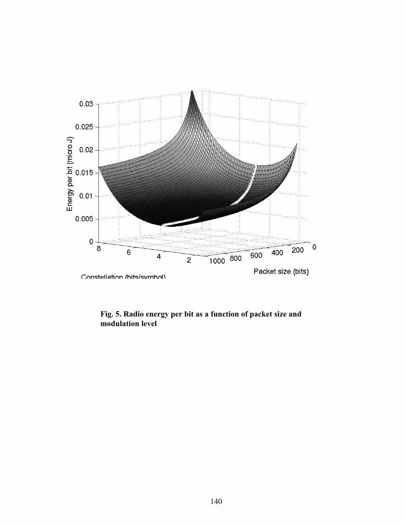
Fig. 5. Radio energy per bit as a function of packet size and modulation level
140
1000
nnnQtollatirin ^hitQ/Qumhnh Packet size (bits)

Sensors RadioCPU
Operating System
Power Manager
Dynamic Voltage Scaling
Coordinated Power Management
Scalable Signal Processing
Dynamic Modulation Scaling
Fig. 6. Coordinated power management at the node level to exploit computation-communication tradeoffs
141

TABLE I
POWER ANALYSIS OF ROCKWELL’S WINS NODES
MCU Mode
Sensor Mode
Radio Mode
Power (mW)
Tx (Power: 36.3 mW) 1080.5 Tx (Power: 19.1 mW) 986.0 Tx (Power: 13.8 mW) 942.6 Tx (Power: 3.47 mW) 815.5 Tx (Power: 2.51 mW) 807.5 Tx (Power: 0.96 mW) 787.5 Tx (Power: 0.30 mW) 773.9
Active
On
Tx (Power: 0.12 mW) 771.1 Active On Rx 751.6 Active On Idle 727.5 Active On Sleep 416.3 Active On Removed 383.3 Sleep On Removed 64.0 Active Removed Removed 360.0
142

TABLE II
POWER ANALYSIS OF MEDUSA II NODES
MCU Mode
Sensor Mode
Radio Mode
Mod. Scheme
Data Rate
Power (mW)
Tx (Power: 0.7368 mW) OOK 2.4 kbps 24.58 Tx (Power: 0.0979 mW) OOK 2.4 kbps 19.24 Tx (Power: 0.7368 mW) OOK 19.2 kbps 25.37 Tx (Power: 0.0979 mW) OOK 19.2 kbps 20.05 Tx (Power: 0.7368 mW) ASK 2.4 kbps 26.55 Tx (Power: 0.0979 mW) ASK 2.4 kbps 21.26 Tx (Power: 0.7368 mW) ASK 19.2 kbps 27.46
Active
On
Tx (Power: 0.0979 mW) ASK 19.2 kbps 22.06 Active On Rx Any Any 22.20 Active On Idle Any Any 22.06 Active On Off Any Any 9.72
Idle On Off Any Any 5.92 Sleep Off Off Any Any 0.02
143

TABLE III
TYPICAL RADIO PARAMETERS FOR SENSOR NETWORKS
Estart 1∝J Pelec 12mW PRF 1mW for 4-QAM RS 1 Mbaud H 16 bits
144
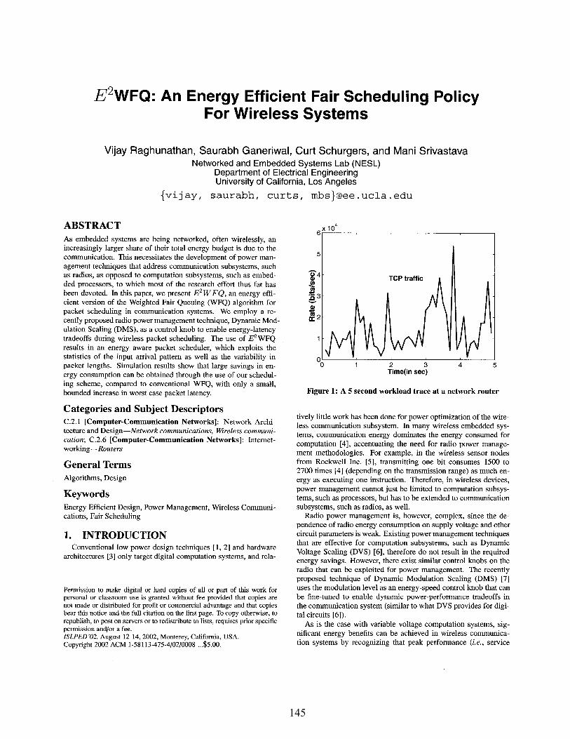
145
E^\NFQ: An Energy Efficient Fair Scheduling Policy For Wireless Systems
Vijay Raghunathan, Saurabh Ganeriwal, Curt Schurgers, and Mani Srivastava Networked and Embedded Systems Lab (NESL)
Department of Electrical Engineering University of California, Los Angeles
vijay, saurabh, curts, [email protected]
ABSTRACT As embedded systems are being networked, often wirelessly, an increasingly larger share of their total energy budget is due to the communication. This necessitates the development of power man- agement techniques that address communication subsystems, such as radios, as opposed to computation subsystems, such as embed- ded processors, to which most of the research effort thus far has been devoted. In this paper, we present E^WFQ, an energy effi- cient version of the Weighted Fair Queuing (WFQ) algorithm for packet scheduling in communication systems. We employ a re- cently proposed radio power management technique, Dynamic Mod- ulation Scaling (DMS), as a control knob to enable energy-latency tradeoffs during wireless packet scheduling. The use of E^^WFQ results in an energy aware packet scheduler, which exploits the statistics of the input arrival pattern as well as the variability in packet lengths. Simulation results show that large savings in en- ergy consumption can be obtained through the use of our schedul- ing scheme, compared to conventional WFQ, with only a small, bounded increase in worst case packet latency.
Categories and Subject Descriptors C.2.1 [Computer-Communication Networks]: Network Archi- tecture and Design—Network communications, Wireless communi- cation; C.2.6 [Computer-Communication Networks]: Internet- working—Routers
General Terms Algorithms, Design
Keywords Energy Efficient Design, Power Management, Wireless Communi- cations, Fair Scheduling
1. INTRODUCTION Conventional low power design techniques [1,2] and hardware
architectures [3] only target digital computation systems, and rela-
Permission to make digital or hard copies of all or part of this work for personal or classroom use is granted without fee provided that copies are not made or distributed for profit or commercial advantage and that copies bear this notice and the full citation on the first page. To copy otherwise, to republish, to post on servers or to redistribute to lists, requires prior specific permission and/or a fee. ISLPED'02, August 12-14,2002, Monterey, California, USA. Copyright 2002 ACM 1-58113-475-4/02/0008 ...$5.00.
,x10
2 3 Time(in sec)
Figure 1: A 5 second workload trace at a network router
tively little work has been done for power optimization of the wire- less coimnimication subsystem. In many wireless embedded sys- tems, communication energy dominates the energy consumed for computation [4], accentuating the need for radio power manage- ment methodologies. For example, in the wireless sensor nodes from Rockwell Inc. [5], transmitting one bit consumes 1500 to 2700 times [4] (depending on the transmission range) as much en- ergy as executing one instruction. Therefore, in wireless devices, power management caimot just be limited to computation subsys- tems, such as processors, but has to be extended to communication subsystems, such as radios, as well.
Radio power management is, however, complex, since the de- pendence of radio energy consumption on supply voltage and other circuit parameters is weak. Existing power management techniques that are effective for computation subsystems, such as Dynamic Voltage Scaling (DVS) [6], therefore do not result in the required energy savings. However, there exist similar control knobs on the radio that can be exploited for power management. The recently proposed technique of Dynamic Modulation Scaling (DMS) [7] uses the modulation level as an energy-speed control knob that can be fine-tuned to enable dynamic power-performance tradeoffs in the communication system (similar to what DVS provides for digi- tal circuits [6]).
As is the case with variable voltage computation systems, sig- nificant energy benefits can be achieved in wireless commimica- tion systems by recognizing that peak performance (i.e., service
30

146
rate) is not always required. Since network traffic is character- ized by a time varying workload requirement, energy can be saved by dynamically adapting the output transmission rate accordingly, through the use of DMS. Figure 1 shows a 5 second snapshot of a real workload trace for a TCP traffic stream at a network router [8], exemplifying the inherent workload variability. For effective system- level power management, we need to develop algorithms that can exploit this variability by using control knobs such as DMS.
1.1 Paper contributions In this paper, we present an energy aware version of the Weighted
Fair Queuing (WFQ) [9] scheduling policy for communication sys- tems, which we call E^WFQ. Our algorithm results in an energy aware packet scheduler, which is capable of operating at hitherto unreachable points on the energy-latency tradeoff curve. Our pre- vious work [10] showed the energy benefits of using DMS in the context of a deadline based real-time scheduling scheme. How- ever, WFQ based packet schedulers are far more widely used than deadline based packet schedulers (both in wired and wireless en- vironments) due to their desirable properties, which are elaborated further in Section 2.1. Therefore, the techniques presented in this paper find applicability in enhancing the energy awareness of a much larger class of communication systems. To the best of our knowledge, this is the first work that attempts to incorporate en- ergy awareness into rate based fair scheduling.
1.2 Related work Several power management techniques have been proposed for
the energy efficient design and operation of computation subsys- tems. One of the most effective techniques is DVS [6], where workload variability is exploited for energy savings by dynami- cally adjusting the processor's supply voltage and clock frequency to match the instantaneous performance requirement. Numerous energy aware task scheduling schemes have also been proposed, which utilize DVS to yield significant energy savings. Variable voltage task scheduling for base station like environments has been explored in [11, 12], while the work described in [13, 14, 15, 16, 17, 18] deals with energy aware real-time task scheduling.
Unlike the large body of work that exists on variable voltage task scheduling, relatively little work has been done for energy efficient wireless packet scheduling. Fair packet scheduling has been an ac- tive research topic in the networking community for a long time. Several fair scheduling schemes have been proposed for both wired (e.g., Weighted Round Robin [19], Start-Time Fair Queuing [20], Worst-Case Fair Weighted Fair Queuing [21]) and wireless (e.g., Channel-State Independent Wireless Fair Queueing [22], Wireless Packet Service [23], Server Based Fairness Approach [24]) envi- ronments. However, all of them are based on the concept of Gener- alized Processor Sharing [25], and its packetized version, Packet- by-Packet Generalized Processor Sharing [26] (PGPS, also known as WFQ [9]). Since network traffic usually displays a high tempo- ral variation, the leaky bucket mechanism [25] is used as a standard way to regulate input streams, and control their extent of variabil- ity. Finally, low power mediimi access protocols based on packet scheduling for wireless ATM networks were proposed in [27].
2. BACKGROUND
2.1 Generalized Processor Sharing (GPS) Since GPS is different from conventional CPU task scheduling
disciplines, we first review some of its basic concepts. A GPS scheduler divides the total link capacity C, among N input streams according to their service requirements. Each stream i is character-
ized by a weight 4>i, such that its service rate, gi, is guaranteed to be [25]':
fli EN xC (1)
GPS has the following attractive features: (i) Different input streams are well-isolated from each other (since each of them is allocated a guaranteed rate). Therefore, a malicious input stream caimot starve other streams of link bandwidth by generating large amounts of traffic, (ii) By varying the 4>i 's, we have the flexibility of changing the fraction of the output link bandwidth that is allo- cated to each stream. As long as the combined average input rate of all the streams is less than C, any positive assigimient of 4>i 's yields a stable system.
2.2 Realizable implementations of GPS: WFQ The GPS service model is an ideal one in which the traffic is con-
sidered to be infinitely divisible, and all streams are served simulta- neously. Although GPS cannot be realized in practice, several real implementations of packet schedulers (for wired, as well as wire- less environments) are based on it, and try to emulate the service provided by GPS as closely as possible.
Let Fp be the time at which a packet would complete service under GPS. Then, a good approximation of GPS is a scheme that serves packets with earliest Fp first. This scheme was proposed in- dependently by two groups of researchers as Weighted Fair Queu- ing [9], and Packetized GPS [26], respectively. The difference in packet delays between GPS and WFQ was shown to be bounded by •'"'y , where L^ax is the maximum packet size, and C is the output rate of the system [26].
2.3 Leaky bucket mechanism The leaky bucket mechanism is often used to regulate and police
the traffic in a network. This model is attractive since it restricts the incoming traffic in terms of average rate, as well as burstiness. For each stream i, the amount of traffic, Ai(T,t) that enters the network in time interval (r, t] conforms to [25]:
Ai(T, t) < ai + \i X (t - T)yt > T > 0 (2)
where A, is a parameter characterizing the average rate of stream i, and cTi is a parameter characterizing its burstiness. When the in- put sources are constrained by leaky buckets, it is possible to give a worst case queuing delay guarantee using GPS (and therefore, WFQ).
Theorem 1: If the input traffic of stream i is constrained using a leaky bucket with parameters (at, \i), and gi is its guaranteed rate, then the maximum delay for a paclcet of stream i, under GPS scheduling is given by [26]:
Di < 1L 9i
(3)
2.4 Dynamic Modulation Scaling We next review the basics of DMS, which was introduced in [7].
To transmit information, bits are coded into charmel symbols. The
^Equation (1) assumes that all streams are backlogged (i.e., have packets waiting to be sent). If a stream is not backlogged, it is not given any share of the link. Further, it does not contribute to the summation in Equation (1). Thus, GPS divides the output link capacity among only those streams that are backlogged.
31

147
3.5 r
3
J"^
1.5
0.5
"?b = 8 : I: - - • Ideal 0 Real constellations Interpolation
\: ^ p : ;\b = 6
; \b = 5 b=.4.; ,..; „ »-^ II -__ „ ~ b.2
; ; ; ; 0.4 0.6 0.8 1 1.2 1.4 1.6 1.8 2
Delay per bit (|xs)
Figure 2: Energy-Delay tradeoff obtained through DMS
number of bits per symbol is given by the modulation level b. This b is the radio control knob that allows DMS to trade off energy versus delay. The average time to transmit one bit is given by Equation (4), where Rs is the symbol rate in number of symbols sent over the channel per second.
Tbit = bx Rs (4)
Although DMS is applicable to other scalable modulation schemes as well, we focus on Quadrature Amplitude Modulation (QAM) as it is both efficient and easy to implement [28]. The energy con- sumed for transmitting one bit is given by [7]:
2° — 1 1 Ebit = Cs X — 1- CB X -
b b (5)
The first term gives the energy consumed in the radio front-end for generating the electro-magnetic waves that carry the information. Parameter Cs depends on the radio implementation, the wireless charmel, the transmit distance, and the required error performance. Strictly speaking, it is also a function of 6, but a very weak one [7], and therefore, we assume it to be a constant. The rest of the ra- dio energy consumption is lumped into the second term of Equa- tion (5), where CE depends on the radio implementation. Although Equation (5) is only exact for even integer values of 6, it is also a reasonable approximation when b is odd. In addition, a packet can be split into two parts, each with a different modulation. In this case, the average energy and delay per bit for the packet as a whole are a linear interpolation between the corresponding values of the two modulation levels.
Figure 2 plots the energy versus delay for the following param- eter values: Rs = 250 KHz, Cs = 100 nj, and CE = 180 nJ. The values of Cs and CE are extracted from [29], which describes the implementation of an adaptive QAM system^. Figure 2 shows the operating points that correspond to real constellations and those that are obtained through interpolation. The curve labeled Ideal is calculated from the above equations. Each modulation scheme
^ Since the system in [29] was designed for high speed rather than low power applications, it is likely that these numbers can be re- duced further through the use of dedicated circuit design tech- niques.
Leaky bucket regulated input streams
Figure 3: E^WFQ scheduler serving leaky bucket regulated streams
has a bmin, which is equal to 2 for QAM. The maximum modula- tion bmax is only bounded by implementation constraints. In our work, we choose bmax equal to 8, and scale the modulation level with a granularity of 0.5 bits/symbol. When the sender changes the modulation, the receiver needs to be told. To avoid a complicated sender-receiver protocol for modulation changes, and to limit the associated overhead, we restrict these changes to be done only at the start of packet transmissions. This finite time-granularity is a crucial difference between DMS and dynamic voltage scaling [6].
3. THE E^WFQ ALGORITHM Having explained the basics of rate based fair scheduling and
DMS, we next present our algorithm, £^^WFQ, which uses DMS to incorporate energy awareness into rate based scheduling. Figure 3 shows a generic block diagram of our system, which consists of an E^V^FQ scheduler followed by a radio that can perform DMS. The scheduling technique can be used either for multiple streams sharing a point-to-point link, or for multiple streams destined to different one-hop neighbors of a wireless node (e.g., a base station sending data to multiple clients). Each stream i is regulated by a leaky bucket with parameters (at, \i). Therefore, each of the A'' input streams produces packets at an average rate of A,. The aver- age rate at which packets arrive at the scheduler is A = X^^^j Aj. The adaptive modulation radio ensures that the scheduler operates at a time varying output rate of Rt). Stream i is allocated a weight 0i, which leads to a corresponding guaranteed rate, gi.
3.1 Energy saving opportunities In many practical scenarios, the average input rate of a stream,
\i, is lower than its guaranteed rate, gi, resulting in a low link utilization. In addition, packet lengths may often be smaller than the maximum value, thereby reducing the utilization even further. Therefore, it is possible to operate at an instantaneous output rate, R(t) that is lower than the maximum rate, C, for most of the time. So, instead of operating at C, and shutting down the radio when idle, we slow transmissions down to a rate Rt). As can be seen in Figure 2, the energy-delay curve is convex, which implies that slowing down the radio is more energy efficient than shutdown (similar to what is observed in DVS [6]).
3.2 Overview of the problem The goal of E^WFQ is to adapt the instantaneous output rate
Rt) to match the instantaneous workload. At the same time, we would like to bound the performance impact that may result. Due to the convexity of the energy-speed curve and Jensen's inequal-
ity (Er) < Ef)], workload averaging results in higher energy
32

148
savings. In fact, maximum energy savings would be obtained if we operated at the long term average input rate, thereby smoothing out all the input workload variations. However, buffering the in- put variations leads to a performance penalty due to an increase in packet delays. Therefore, the crux of the problem reduces to deter- mining the degree of buffering (i.e., how much workload averaging to perform) while still bounding the increase in packet delays.
3.3 Monitoring the input rate We observe that the instantaneous queue size (i.e., number of
packets in the queue) is a good indicator of the instantaneous ar- rival rate. If the input rate suddenly becomes greater than the output rate, the queue size increases. On the other hand, if the input rate suddenly drops below the output rate, the queue gets drained. We introduce a new parameter A, which determines the system's re- sponse to workload variations, by deciding the degree of buffering. As we will see shortly, A also determines the maximum impact that our scheme can have on packet delay.
Definition 1: We define A to be the desired time from a packet's arrival at the end of the queue to its departure from the head of the queue.
We can see that if the input rate remains constant, A is the delay experienced by every packet in the queue.
3.4 Computing the required output rate Whenever a packet arrives, the required rate of the particular
stream is recomputed. Assume that the newly arrived packet is the m'th packet in the queue, and the current time is r. Let the arrival times of the m packets in the queue be given by Ai, ^2,. •. , Am (where Am = r). Then, the required rate (n,/:) for the fc'th packet to have a total delay of A is given by;
ri,h K X X/j
VfcG 1,... ,m (6) (Ak+A- T
where Li is the length of a packet belonging to stream i. Two ob- servations are apparent from Equation (6), (i) The required rate for the newly arrived packet (i.e., last packet in the queue) is '"^ ', and (ii) If the output rate is equal to the required rate, then the re- quired rate of this packet remains constant as it progresses through the queue.
The required rate for a strearri Rout,i is the minimum rate at which Equation (6) is satisfied for all the m packets in the queue. However, to ensure isolation of input streams, this required rate cannot be greater than gi. Therefore, we have:
Rout,i = Min Max (ri,i,ri,: , 'ri,m) , 9iJ (7)
Summing the required rate over all the streams, we get the instan- taneous required rate of the system to be i? = 5^i_i Rout.i.
3.5 Setting the output link speed Although the maximum output link rate is C, the instantaneous
required rate by all the streams together is only R = J2iLi Rout,i. This means that the output link can be slowed down to just meet the instantaneous requirement, thus saving energy. The new modu- lation level for the outgoing packets is given by:
^^instantaneous — ^ ^ t)max (8)
3.6 Accounting for variable packet sizes Quite often, packet lengths in network traffic can be variable.
This is especially true for packets generated by multimedia streams
High A
Low A
Routt) for low A
Routt) forhighA
Figure 4: The effect of A on the output rate
such as variable bit rate audio and video codecs. To exploit the variation in packet lengths to further scale down the modulation level and obtain more energy savings, we generalize the calculation of a packet's required rate. If the length of the fc'th packet in the queue is Lj,j;, and there are a total of m packets in the queue, then the following equation is used to compute the required rate of a packet, instead of Equation (6):
ri,k = (^fc -f A - r)
VA:el,... ,m (9)
3.7 Delay guarantee provided by E'^WFQ Through the choice of the parameter A, our scheduling scheme
provides the following delay bound for packets.
Theorem 2: The maximum delay of a packet of stream i, under the E"^ WFQ scheduling scheme is given by:
D* < fA + A + ^^"j <(^ + A+ ^^^) (10)
where Cmin is the output link capacity at a modulation level hmin. Proof: The proof follows directly from Theorem 1, the bounded difference in packet delays between GPS and WFQ, and the defini- tion of A.
3.8 Analyzing the system's response We next analyze the system's response to a change in workload
to highlight the effect of A. Let the input rate for stream i be equal to RoU. If we set the output rate to be equal to Roid, then the queue soon reaches a steady state, and the number of packets in the queue remains constant. Let the system be at such a steady state at time t, and the number of packets in the queue be 2/(<). In this state, any packet that arrives, sees exactly i/(i) — 1 packets ahead of it in the queue, each of length, say Li. AH these packets (including the one that just arrived) have to complete transmission within a time A. Therefore, the output rate, Routt^ is given by (see first paragraph after Equation (6)):
Routt) yt) X Li
Rold (11)
Now, let the input rate increase abruptly to Rnew. We want to analyze how fast the system stabilizes to its new steady state. After a time 5t, the number of packets in the queue becomes:
y(t + JO = ya)+"""'""^°"*^^^ xSt (12) L/i
The new output rate will be given by Routt + 6t), which after
33

149
0.4 0.6 0.8 Output Link Utilization
Figure 5: Normalized energy consumption of E^WFQ, as function of linlc utilization, for varying degrees of burstiness
o CD Ui
^' g
4—1 CO
DC
<i''''PWtMtM''' 1
j-i
!i
HIHll
M \ :RealR^^, i
*p - .* Ill Time(in sec)
Figure 6: One second snapshot showing how the output rate follows the input rate
some simple substitutions, can be written as:
Routit + St) = Routit) + Rn Routit) X St (13)
Therefore, the rate at which the output rate changes is given by:
SRout 1 St X \itnew ttout\t)) (14)
Solving this differential equation, and applying the initial condition Routit) = Roid, we get:
Rout\t — ^tinew T \-tiold Rnew) X C " (15)
The evolution of Routit) is shown in Figure 4. Therefore, it can be concluded that A is the time constant of the first-order input response of the system. A high value of A means that the sys- tem takes longer to switch to the new steady state, which implies that steep workload transients are filtered out. While this increases the energy savings, the maximum impact on packet delay also in- creases (see Equation (10)). On the other hand, a low value of A means that the system is sensitive to changes in the input rate, and performs lesser workload averaging. This provides lower energy savings, but also results in a smaller impact on packet delay. The best choice of A thus depends on the allowable delay, and the input rate variability. A detailed investigation of the optimal choice of A is beyond the scope of this paper
4. SIMULATION RESULTS To evaluate the impact of our techniques, we carried out a num-
ber of simulations, hi the following subsections, we describe our simulation framework, and present our results.
4.1 Simulation framework We used a C based discrete event simulator, PARSEC [30], and
considered a network scenario where 4 streams share an output wireless Unk. The values of Rs and bmax are the same as in Section 2.4, resulting in a total link capacity C = 2 Mbit/s. The streams are allocated equal weights such that each stream is guaranteed a rate of ^ = 500 Kbit/sec. The maximum packet size is set to be Lmax = 1000 bits, and each stream is leaky bucket constrained with the same maximimi burstiness parameter cr, = 100 packets. For om-
160
140
120
M) 100
g 80
fe 60
40
20
0
J!"!<* H ."!
*3
25 50 75 100 125 150 175 200 225 230
Packet delay (ms)
[NK=6 NH=9 DN^=12
Figure 7: Packet delay histogram for three different levels of burstiness
values, Di is equal to 0.2 seconds. The average rate of the input is varied to change the link utilization. As explained in the previous section, the choice of A offers a tradeoff between energy savings and queuing delay. In our work, we have set A = 0.05 seconds.
4.2 Discussion of the results Figure 5 shows the energy consumed by E WFQ, normalized
against the energy consumed by conventional WFQ, for varying values of output link utilization. As expected, the energy consump- tion of E^WFQ decreases as the link utilization drops. Our al- gorithm reduces to conventional WFQ at a utilization of one, since there are no opportimities for slowing down. The different curves in Figure 5 show the energy consumption for varying degrees of burstiness (variability) in the input workload. Nb gives the number of equally spaced bursts appearing at a stream's input over the ob- servation window of 1000 packets of the stream. A high value of Nb indicates a high degree of burstiness. For a given link utiliza- tion, increasing the level of input burstiness increases the energy consumption, which is intuitive, since bursts at the input cause the output rate to increase, thus decreasing the energy savings. Figure 6 shows how the output rate follows the input rate, for our choice
34

150
of A = 0.05 seconds. The curve mairked Ideal Rout shows the curve predicted by Equation (15). The actual output rate can only increase in increments of ^, which is clearly seen in the curve marked Real Rout in the figure.
Figure 7 shows the distribution of packet delays for varying lev- els of burstiness for a fixed link utilization. The bar at x = x; in- dicates the percentage of packets whose delays lie in the interval xi-i,Xi\. There are three important observations that can be made from this figure: (i) Since the input rate fluctuates around its aver- age rate, most of the packets experience a delay equal to A. (ii) As the level of burstiness increases, the percentage of packets that ex- perience a delay larger than A also increases, and (iii) None of the packets violate the delay boimd given in Theorem 2. Our results (Figures 5-7) show that E^WFQ achieves a significant reduction in energy consumption, at the cost of a relatively small increase in packet latencies.
5. CONCLUSIONS In wireless embedded systems, communication energy is increas-
ingly becoming the dominant component of total energy consump- tion. Power management techniques therefore, should also address communication subsystems such as radios, as opposed to only com- putation subsystems such as embedded processors. DMS is a tech- nique that offers a power-speed control knob for the radio, and can thus be used for communication power management. Higher level techniques are needed that can exploit this control knob to enable system level energy-latency tradeoffs. In this paper, we have tar- geted the packet scheduling process and investigated avenues for making it energy aware. We have presented E^WFQ, an energy efficient version of the Weighted Fair Queuing (WFQ) algorithm for packet scheduling in communication systems. Our algorithm results in an energy aware packet scheduler that provides signifi- cant energy savings (up to a factor of 10) with only a small increase in worst case packet delay.
ACKNOWLEDGEMENTS This paper is based in part on research funded through the DARPA PAC/C Program under AFRL Contract #F30602-00- C-0154, and through Semiconductor Research Corporation System Task Thrust ID 899.001.
6. REFERENCES [1] A. Raghunathan, N. K. Jha, and S. Dey, High-level Power Analysis
and Optimization. Kluwer Academic Publishers, Norwell, MA, 1998. [2] L. Benini and G. De Micheli, Dynamic Power Management: Design
Techniques and CAD Tools. Kluwer Academic Publishers, Norwell, MA, 1997.
[3] A. P. Chandrakasan and R. W. Brodersen, Low Power CMOS Digital Design. Kluwer Academic Publishers, Norwell, MA, 1996.
[4] V. Raghunathan, C. Schurgers, S. Park, and M. B. Srivastava, "Energy aware wireless microsensor networks", IEEE Signal Processing Magazine, vol. 19, iss. 2, pp. 40-50, March 2002.
[5] Rockwell Inc. (http: //wins . rsc . rockwell. com)
[6] T. A. Pering, T. D. Burd, and R. W. Brodersen, "The simulation and evaluation of dynamic voltage scaling algorithms", Proc. ACM /SZ.P£D, pp. 76-81,1998.
[7] C. Schurgers, O. Aberthome, and M. B. Srivastava, "Modulation scaling for energy aware communication systems", Proc. ACM ISLPED, pp. 96-99, 2001.
[8] The Internet Traffic Archive (http: //ita. ee . Ibl. gov).
[9] A. Demers, S. Keshav, and S. Shenker, "Analysis and simulation of a fair queueing algorthm", Internet Res. and Exper., vol. 1, 1990.
[10] C. Schurgers, V. Raghunatiian, and M. B. Srivastava, "Modulation scaling for real-time energy-aware packet scheduling", Proc. IEEE GLOBECOM, pp. 3653-3657, 2001.
[11] M. Weiser, B. Welch, A. Demers, and S. Shenker, "Scheduling for reduced CPU energy", Proc. First Symp. on OSDI, pp. 13-23, 1994.
[12] K. Govil, E. Chan, and H. Wasserman, "Comparing algorithms for dynamic speed-setting of a low-power CPU", Proc. ACM MOBICOM, pp. 13-25, 1995.
[13] T. Ishihara and H. Yasuura, "Voltage scheduling problem for dynamically variable voltage processors, Proc. ACM ISLPED, pp. 197-202, 1998.
[14] 1. Hong, M. Potkonjak, and M. B. Srivastava, "On-line scheduling of hard real-time tasks on variable voltage processors", Proc. IEEE ICCAD, pp. 653-656, 1998.
[15] Y. Shin and K. Choi, "Power conscious fixed priority scheduling for hard real-time systems", Proc. ACM DAC, pp. 134-139, 1999.
[16] V. Raghunathan, P. Spanos, and M. B. Srivastava, "Adaptive power-fidelity in energy-aware wireless systems", Proc. IEEE RTSS, pp. 106-115,2001.
[17] P. Pillai and K. G. Shin, "Real-time dynamic voltage scaling for low power embedded operating systems", Proc. SOSP, pp. 89-102, 2001.
[18] F. Gruian, "Hard real-time scheduling for low energy using stochastic data and DVS processors", Proc. ACM ISLPED, pp. 46-51, 2001.
[19] M. Shreedhar and G. Varghese, "Efficient fair queueing using deficit round robin", Proc. lEEESIGCOMM, pp. 231-242, 1995.
[20] P Goyal, H. M. Vin, and H. Cheng, "Start-time fair queuing: A scheduling algorithm for integrated servicespacket switching networks", Proc. lEEESIGCOMM, pp. 157-168, 1996.
[21] J. C. R. Bennett and H. Zhang, "WF^Q : Woret-case fair weighted fair queueing, Proc. IEEE INFOCOM,pp. 120-128, 1996.
[22] P. Lin, B. Bensaou, Q. L. Ding, and K. C. Chua, "A wireless fair scheduUng algorithm for error-prone wireless channels", Proc. ACM WoWMOM, pp. 11-20, 2000.
[23] S. Lu, V. Bharghavan, and R. Srikant, "Fair scheduUng in wireless packet networks", Proc. IEEE SIGCOMM, pp. 63-74, 1997.
[24] P. Ramanathan and P. Agrawal, "Adapting packet fair queueing algorithms to wireless networks", Proc. ACM MOBICOM, pp. 1-9, 1998.
[25] S. Keshav, An Engineering Approach to Computer Networking: ATM Networks, the Internet, and the Telephone Network. Addison-Wesley, 1997.
[26] A. K. Parekh and R. G. Gallager, "A generalized processor sharing approach to flow control in integrated services networks: The single-node case", IEEE Trans, on Networking, vol. 1, no. 3, pp. 344-357, June 1993.
[27] K. M. Sivalingam, M. Srivastava, P. Agrawal, and J. C. Chen, "Low power access protocols based on scheduling for wireless and mobile ATM networks", Proc. IEEE Universal Personal Communications Conference, pp. 420-433, 1997.
[28] J. G. Proakis, Digital Communications. McGraw Hill, 1989.
[29] K. Cho and H. SamueH, "A 8.75-MBaud Single-Chip Digital QAM Modulator with Frequency-Agility and Beamforming Diversity", Proc. IEEE Custom Integrated Circuits Conference, pp. 27-30, 2000.
[30] PARSEC parallel simulation language (http://pel.cs.ucla.edu/proj ects/parsec)
35

Approved for public release.
Distribution unlimited.
Power-Aware Acoustic Processing
April 25, 2003
Ronald Riley, Brian Schott, Joseph Czarnaski, and* University of Southern California Information Sciences Institute
3811 N. Fairfax Dr., Suite 200, Arlington VA 22203-1707
Sohil B. Thakkar University of Maryland, College Park
ABSTRACT
We investigated the tradeoffs between accuracy and battery-energy longevity of acoustic beamforming on disposable sensor nodes subject to varying key parameters: 1) number of microphones, 2) duration of sampling, 3) number of search angles, and 4) CPU clock speed. Beyond finding the most energy efficient implementation of the beamforming algorithm at a specified accuracy, we seek to enable application-level selection of accuracy based on the energy required to achieve this accuracy. Our energy measurements were taken on the HiDRA node, provided by Rockwell Science Center, employing a 133-MHz StrongARM processor. We compared the accuracy and energy of our time-domain beamformer to a Fourier-domain algorithm provided by the Army Research Laboratory (ARL). With statistically identical accuracy, we measured a 300x improvement in energy efficiency of the CPU relative to this baseline. We also present other algorithms under development that combine results from multiple nodes to provide more accurate line-of-bearing estimates despite wind and target elevation.
1. Introduction Our objective is to develop software and hardware that support dynamic control of the use of energy and computational resources at various levels according to the need for precision and the readiness to expend
* This work was sponsored by the Defense Advanced Research Projects Agency (DARPA) and Air Force Research Laboratory, Air Force Materiel Command, USAF, under agreement number F30602-99-1-0529. The U.S. Government is authorized to reproduce and distribute reprints for Governmental purposes notwithstanding any copyright annotation thereon. The views and conclusions contained herein are those of the authors and should not be interpreted as necessarily representing the official policies or endorsements, either expressed or implied, of the Defense Advanced Research Projects Agency (DARPA), the Air Force Research Laboratory, or the U.S. Government.
151

152
2
the required resources. We envision sensor nodes lying almost dormant for months before a sound emitting target comes within range. During this long quiescent period, the nodes must remain active enough to detect the incursion of an emitter and remain in contact with neighboring nodes to alert them of the detection. At this stage there is no need to determine the direction to an emitter with any accuracy, it is sufficient to detect it as a tripwire.
Once an emitter has been detected, application level algorithms will determine how often the line of bearing (LOB), also referred to as the direction of arrival (DOA), is needed and the accuracy required to track and to identify the emitter. These decisions will depend on the perceived importance of the emitter and the amount of energy needed to provide the required accuracy. This paper summarizes our efforts to find the key parameters in acoustic beamforming and determine their relative contributions to the accuracy and energy consumption.
2. Beamforming Algorithms Acoustic beamforming algorithms estimate the LOB to distant acoustic emitters by time-shifting signals from microphones at known relative locations to form beams from selected directions. The two beamforming algorithms compared in this paper differ primarily in how they implement time-shifting the signals. The LOB can be thought of as a by-product of the optimal reconstruction of the signal from an emitter by shifting and adding the signals from a number of microphones1.
As illustrated in Figure 1, sound from a distant emitter at position xE arrives at two microphones at x1 and x2 with a relative delay
( ) ( )[ ] ( ) ( )[ ] ( ),
sinsin
coscoscos 2,12,12,12,12,1
2,12,1
−
=−=
cd
cd
cd EE
Eθ
θθ
θθθτ (1)
where d1,2≡|x2-x1| is the distance between the microphones, θ1,2 is the direction of the separation vector between the microphones, θE is the LOB of the emitter, and c~332 m/s is the speed of sound in air
( ) ( ).m/s 20.0615.273m/s 20.060 CelsiusKelvin TTc +=≈ (2) Assuming the microphone geometry is either specified by rigid placement and/or calibrated after deployment, and the speed of sound is adjusted to the local climate, the LOB to the emitter, relative to the microphone separation vector, can be calculated from an estimate of this delay as
( ),/cos 2,12,11
2,1 dcE τθθ −±=− (3) where the ambiguity in sign is due to taking the inverse of the cosine, an even function.
The delays can be estimated by minimizing the differences between signals S1 and S2 recorded at microphones 1 and 2,
θE
θ1,2
x2
xE
cτ
x1
d1,2
Figure 1. Beamforming Geometry.

153
3
( ) ( ),2,121 τα −= tStS (4)
where α is the relative gain between the two signals. The search for the best delay is limited by (1) to |τ1,2| < d1,2/c. Once the shift has been determined, the signals from the microphones can be shifted and added to provide an enhanced estimate of the signal from the emitter. The background noise and sounds from other emitters will be reduced in proportion to the number of microphones.
Methods for determining the LOB based on reconstructing the emitted signal, as in (4), from an acoustic array with M microphones can distinguish at most M-1 emitters. The additional uncertainty of the position of the emitters results in an underdetermined system of linear equations if we try to resolve M emitters. Resolving more emitters would require additional constraints such as knowing the power-spectrum of the emitters. Algorithms, such as MUSIC2 and ESPRIT3, which do not attempt to reconstruct the emitted signals can resolve, at most, M emitters from an array of M microphones. These algorithms perform eigenvector decomposition of the MxM covariance matrix of the signals from the M microphones and so do not lend themselves to efficient implementation in integer-math oriented processors in sensor nodes.
Beamforming is accomplished by time-shifting the signals from an array of microphones to a common position with time delays prescribed by (1), for an assumed LOB. Beams are formed for a number of LOB search angles. As the search angle approaches the correct LOB of the emitter, the signals constructively interfere as in (4). As shown in Figure 2, the search angle with the maximum power in the delay-summed signal is selected as the estimated LOB. This LOB estimate is refined by parabolic interpolation of the power over the adjacent search angles.
The two algorithms compared in this paper differ primarily in how they shift the signals. The baseline algorithm from ARL performs a floating-point FFT on each signal then shifts, sums, and computes the beam power in the Fourier domain. Our beamformer performs all of these operations in the time domain in integer math.
Our beamformer assumes a single target and employs common integer code to report the LOB as the direction with the delay-summed combined signal of loudest total acoustic energy. These results do not include code for false alarm rejection such as ARL’s Harmonic Line Analysis. We plan to incorporate these capabilities into future implementations.
Our algorithm is roughly 300x more efficient in the consumption of energy by the CPU than the baseline. The largest contribution to this efficiency (~20x) is due to floating-point emulation on the StrongARM processor. The next most significant contribution (~10x) is our ability to use fewer samples to achieve similar accuracy. Fast Fourier transforms operate on vectors containing integer powers of 2 samples (S=2n). We did not modify the baseline algorithm to vary the number of samples from its hard-coded value of S=1024. Operating in the time domain provided the final contribution of (~3/2x,) by not Fourier transforming the signals.
Figure 2. Power of delay-summed at 18 search angles.

154
4
3. LOB Beyond Beamforming
The algorithms discussed in this section are under development and optimization for sensor nodes. We anticipate that these will lead to significant improvements over beamforming in accuracy/noise insensitivity, false-alarm rejection, and an extended range in tradeoffs between accuracy and energy.
Beamforming makes a number of limiting assumptions 1) that the microphones are fixed on a rigid plane, 2) that the emitter lies on the same plane, and 3) that there is little or no wind. While beamforming uses (1) to construct a set of delays corresponding to various search angles and selects the “best” angle, the LOB can also be estimated directly from (1) based on estimates of the time shifts between pairs of microphones. Given a set of M>2 microphones with synchronized sampling, we can select up to M! / [2 (M-2)!] pairs. For example, three microphones provide three pairs. Assuming that the geometry of the M microphones has been calibrated, (1) provides a system of M! / [2 (M-2)!] equations in two unknowns, the sine and cosine of the LOB divided by the speed of sound. For more than two pairs, the over-determined system of equations can be solved by standard weighted least-squares methods. Increasing the number of microphones and pairs should improve the accuracy.
The LOB and the speed of sound can be extracted from the results in integer math with the CORDIC4 as
( ) ( ),
sin,
costan 1
= −
ccEE
Eθθ
θ (5)
and
( ) ( ).
sincos
122
+
=
cc
cEE θθ
(6)
Although, it may appear that the speed of sound should be constrained to the constant predicted in (2) there are cases in which the apparent speed of sound can vary. When noise results in nonphysical estimates of the apparent speed of sound, the LOB estimated in (5) can be iteratively refined based on small angle corrections with the speed of sound held to the predicted constant in (1) as
( ) ( ) .cossin 2,12,12,12,12,1 θθτδθθθ −−=− EEE dcd (7) The RMS error of the system of equations defined by (7), or (1), provides a measure of the angular uncertainty of the LOB estimate. If some pairs of microphones produce multiple delays due to multiple targets, this error and the apparent speed of sound provided by (6) could be used to select delays into sets for each target.
Figure 3 shows a plot of this uncertainty for a tracked vehicle driving around an oval track. The vehicle is about 600 meters from the sensor node at an LOB of 280° counterclockwise from east (roughly south). This is based on acoustic data collected by USC-ISI at ARL’s Aberdeen Proving grounds with HiDRA nodes, described in section 5, using with three microphones deployed on an equilateral triangle with 7-foot separation.
0
0.5
1
1.5
2
2.5
3
0 60 120 180 240 300 360LOB (degrees) counterclockwise from east
LOB
Unce
rtant
y (d
egre
es)
Figure 3. Uncertainty in LOB of tracked vehicle.

155
5
3.1. Emitter Elevation If the emitter is elevated above the plane on which the microphones are distributed, as shown in Figure 4, this decreases the delays between signals and increases the apparent speed of sound estimated by (6) as
( ) ,cos
0
E
ccφ
= (8)
where φE is the elevation angle of the emitter. As the emitter moves directly above the microphones, the apparent speed would tend toward infinity as all of the time shifts approach zero. The elevation angle of the emitter could be estimated by generalizing our analysis to 3D and elevating one or more microphones above a plane containing three or more microphones5. If we can segregate the contribution due to elevation from other effects, such as wind, by collaboration between sensor nodes, each with three or more microphones, we could estimate the elevation angle from (8).
3.2. Wind-Speed Vector Effects As illustrated in Figure 5, the average wind speed W between the emitter and the microphones will add as a vector to the sound radiating from the emitter at speed c0 resulting in an apparent speed of sound of
( ) ( ),sincos 2220 WEWE WWcc θθθθ −+−+= (9)
where θW is the direction that the wind is coming from. The estimated LOB would also be shifted by
( ) ( )[ ].sin,costan 01
WEWEE WWc θθθθδθ −−+= − (10) Assuming that the wind speed is small compared to that of sound (W<<c0,) we can approximate
( ) ( ) ( ) ( ) ( ) ( ) ,sinsincoscoscos~0 WEWEWE WWWcc θθθθθθ +=−− (11) and
( ) ( ).tan~ 0WEE c
ccθθδθ −
− (12)
A wind speed of 14 mph orthogonal to the LOB would result in an LOB error of about 1 degree.
The difference of apparent from expected sound speed is plotted in Figure 6 for a tracked vehicle driven on an oval track around the sensor node for a number of orbits. These preliminary estimates of the apparent sound speed are based on delays of maximum correlation (15), described in the next section.
φE
c0
Figure 4. Elevation angle of emitter.
W
c
c0
Figure 5. Wind speed geometry.

156
6
These estimates are compared to the expected deviation based on (11) for a wind speed of 30 mph. This is somewhat larger than the 10-mph average wind speed measured during data collection. The wind direction, taken from the ground truth, agrees well with the estimated deviations in sound speed.
Given an estimate of the wind direction, we can estimate and correct the offset in the LOB from (12) based on the apparent speed of sound, if we can assume that there are no other contributions such as elevation of the emitter above the sensor plane.
If we combine the apparent sound speed and estimated LOB from two or more sensor nodes with enough separation transverse to the LOB of the emitter such that they provide significantly different estimated LOBs, and assume that the wind is roughly the same for all sensor nodes, we can solve the resulting system of linear equations given by (11) for the wind vector components. The wind direction can be computed using the CORDIC algorithm as
( ) ( )[ ],sin,costan 1WWW WW θθθ −= (13)
and the result can be used in (12) to infer the offset of the LOB’s due to the wind.
The LOB and apparent speed of sound from three or more nodes can be combined to solve for the wind and elevation simultaneously by combining (8) and (11) as
( ) ( ) ( ) ( ) ( ) .sinsincoscoscos
~ 0WEWE
E
WWc
c θθθθϕ
++
(14)
This assumes that all of the nodes have the same emitter elevation, which could be satisfied if all of the nodes are at the same elevation and roughly the same distance from the emitter. We would have to constrain the added unknown such that the inferred cosine is in the assumed range (0, 1) and would interpret the elevation angle to be positive, forcing the object to lie above the sensor plane.
3.3. Signal-Pair Delay Estimation All of this analysis is based on the ability to estimate the delay between signals collected by a pair of microphones. One estimate of the delays can be obtained by finding the shift between the signals that produces a peak in correlation between the signals from microphone 1 (S1) and 2 (S2)
( ) ( ) ( )∑ −=t
tStSC .2,121
2,12,1 ττ (15)
This estimate is best suited to emissions of short duration, such as gunfire or explosions, and is sufficient for cases with high signal to noise and broad band signals.
0 32 64 96 128 160 192 224 256Freq (Hz)
Figure 7. Power spectrum of tracked vehicle.
-100-80-60-40-20
020406080
100
0 60 120 180 240 300 360LOB (degrees)
Air S
peed
- So
und
(mph
)
Figure 6. Deviation of sound speed vs. angle.

157
7
Much of the recent work in noise-tolerant LOB estimates are based on the fact that many targets of interest, such as ground and air vehicles, emit sound in a number of narrow acoustic bands6, as shown by the acoustic power spectrum of a tracked vehicle shown in Figure 7. If multiple targets emit primarily in different narrow frequency ranges, their LOBs could be determined by a single sensor node with as few as three microphones.
The LOB of frequencies from 32 to 128 Hz is plotted in Figure 8 for a sensor node with three microphones and two tracked vehicles. The average power spectrum of the three microphones is also plotted. The LOBs cluster around 240° and 77° corresponding to the two vehicles. The LOB is plotted as zero for frequencies where it is undefined. Once the LOBs of the two vehicles are estimated, it is straight forward to separate their line-spectra as a basis for target classification.
For each spectral component, the LOB of is based on time shifts of microphone pairs estimated as
( ) ( )[ ] ( )[ ] ,221
2,1 ωπωϕωϕωτ nSS +−
= (16)
where the phase of the Fourier component of the signal φ[S1(ω)] can be computed with the CORDIC algorithm and the time shift is limited to the range [-d1,2/c, d1,2/c]. For higher frequencies (f>c/(2d1,2)), there can be more than one solution to (16). This degeneracy can be resolved by selecting the solution that is most consistent with lower frequency components or is most consistent with the expected speed of sound and error of fit based on the solution to (1). This ambiguity can be avoided by restricting microphone separations to d<c/(2f), where f is the highest frequency of interest in the emitters spectrum.
Our current implementation of the acoustic beamformer operates in the time rather than the frequency domain in order to provide a marginal (3/2x) increase in power efficiency. By using an integer FFT we could achieve comparable efficiency and add an adjustable parameter corresponding to the sampling rate of the acoustic data. Although the sampling rate of the digitizer will probably be fixed at ~1024 Hz, the captured signal can be downsampled to provide significant reductions in energy requirements with little effect on the accuracy of the LOB.
4. Algorithmic “Knobs” The accuracy and energy requirements of acoustic beamforming depend on a number of parameters, as suggested by Figure 9. Some are largely dictated by the application. We have chosen as our set of independent variables: 1) number of microphones M, 2) number of acoustic samples S, 3) number of beams B, and 4) CPU clock speed fCPU.
4.1. Number of Microphones (M) The number and placement of microphones is principally a hardware design parameter but can also be used as an algorithmic parameter by selecting a subset of the signals collected. We will show that the
0
60
120
180
240
300
360
32 48 64 80 96 112 128Freq (Hz)
LOB
(deg
rees
)
0
Pow
er S
pect
rum
Figure 8. LOB of spectral components.

158
8
system energy required for beamforming is proportional to the number of microphones, but there are negligible improvements in accuracy due to adding more microphones at the same radius.
We limit our analysis to nodes supporting at least two microphones. Although single-microphone nodes could collaborate to determine the direction to an emitter, we exclude this case due to the requirements of a large amount of energy to move raw data between nodes, of 10-us synchronization between nodes, and of 5-mm accuracy in relative positioning of microphones. Although the ambiguities resulting from two-microphone beamforming would require collaboration, only a trivial amount of data need be exchanged. Synchronization to a fraction of a second is sufficient, and the required accuracy of relative positioning is similarly relaxed.
4.2. Number of Acoustic Samples (S) For a fixed sampling rate, in our case 1024 Hz, the system energy required for beamforming is proportional to the number of samples simultaneously collected from each microphone. The number of samples collected per second for each microphone is typically selected to be 1 kHz for acoustic tracking of vehicles to facilitate beamforming with the spectrum above 250 Hz attenuated to filter out wind noise. We implemented this as analog anti-aliasing filtering.
4.3. Number of Beams (B) The beam power is computed at a number of evenly spaced search angles, and interpolated by a parabolic fit to estimate the angle with maximum power. The number of beams only affects the execution speed of the algorithm, not data acquisition. The system energy for beamforming is linear with, not proportional to, the number of beams searched.
4.4. CPU Clock Speed (fCPU) The Highly Deployable Remote Access Network Sensors & Systems (HiDRA) provided by Rockwell Science Center (RSC)7,8,9, supports software-control of the clock speed of the StrongARM CPU over the range 59-133 MHz. Unfortunately, voltage scaling is not supported in this hardware. Without voltage scaling, clock scaling may appear to only change how long the algorithms run without changing the energy requirements. However, the power consumed by other components in the system during execution of the algorithm and the power consumed by the CPU during data collection give this parameter utility in reducing system energy required for beamforming.
5. System Power Equation The energy consumed by the HiDRA node to capture data and compute the LOB is modeled by
,133
lg133
+
++= CPU
CPUOvrA
CPUSAD
S
Pff
PTff
fSP
fSE (17)
B E A M F O R M I N G
Line of Bearing360
180
Num. Mikes
Num. Samples
76
2
4 5M
8
12
18 90
1024
512
32
64
128 256
Search Angles
SEW
N
LOB Confidence
3 B2° 3° 4° 5°
PA/DTA/D+(TA/D+TAlg)(PCPU+POverhead)=0.724Joules
S
Figure 9. Beamforming Algorithmic Knobs.

159
9
where fCPU is the clock rate of the StrongARM CPU and f133 = 133 MHz is the maximum clock rate.
This equation reflects that the power required by the A/D board, PAD, is only consumed during the data acquisition time which is the number of samples acquired, S, divided by the sampling rate fS=1024 Hz. Also implicit in this equation is that, for the HiDRA node, the CPU and memory consume power, PCPU, while the samples are acquired, but the algorithm does not begin to run, for a period TAlg, until after data collection is complete. There is also a significant overhead power, POvr, consumed by other supporting components such as the radio.
The CPU power and execution time of the algorithm are proportional and inversely proportional, respectively, to the CPU clock rate, fCPU. The clock rate resulting in the minimal energy consumption can be found by setting the derivative of (17) with respect to fCPU to zero, resulting in
,/lg133 CPUADAOvrCPU PTTPff = (18)
where TAlg is the execution time of the algorithm and PCPU is the CPU power at the CPU clock rate of 133 MHz.
When the CPU and overhead power components are roughly equal and the execution time of the algorithm at 133 MHz is a small fraction of the sampling window, as with our algorithm, the minimum available CPU clock rate of 59 MHz provides the best energy efficiency. When the algorithm runs longer than the sampling window, as with the ARL algorithm, the maximum available CPU clock rate of 133 MHz gives the best results.
6. Power Measurements on the HiDRA Node The power measurement test setup consisted of the HiDRA sensor node and a current sensing resistor placed inline with the input voltage connector. The voltage drop across this resistor was measured using a National Instruments PCI-MIO-16E-1 data acquisition card and triggered from GPIO lines on the node's processor module. The HiDRA node, as shown in Figure 10, contains the following modules:
1) Processor/Memory: SA1100 processor board running eCos at 59-133 MHz., with 4 MB of ROM (flash memory), 1 MB RAM, input voltage 3.3V I/O, and 1.5V core.
2) DC/DC: input voltage from 2 9-V batteries or DC adapter. Our test measurements were taken with a 12-V DC input. This module supplies voltages 3.3V and 1.5V for the I/O lines and processor core respectively and separate analog voltage lines for the A/D and Radio modules.
3) Radio: A 900 MHz Rockwell proprietary radio.
4) A/D: 5 channels, 3 Multiplexed with variable gains of 1x, 2x, 5.02x, 10.09x, 20.12x and 2 individual inputs with variable gains of 10x, 43.32x, 30x, 36.68x, 49.98x. The selectable gains are tuned to specific sensors that RSC uses for this platform. The acoustic data was captured using only the multiplexed sensor input to keep the gains equivalent across all channels. Low-pass anti-aliasing filters with a cutoff
Figure 10. RSC HiDRA sensor node stack.

160
10
frequency of 3 kHz were also added to the inputs of each of these channels to eliminate cross talk between the respective channels.
The current measurements were taken at the full clock rate of 133 MHz, which is the optimal operating frequency for the HiDRA node, and at various increments down to 59 MHz. Other power measurements were taken for the different operating modes required to form a single LOB. These modes include acquiring the data from the input microphones, executing the algorithms, and putting the processor in sleep mode. The individual power consumption of each module was measured by removing boards from the stack and calculating the difference in current through the sensing resistor.
7. Results We evaluated the two algorithms on a test set of acoustic data collected by ARL collected at their Aberdeen Proving Grounds. The data was synchronously collected from six microphones uniformly distributed on a 4-foot radius circle, and a seventh microphone in the center. A single military vehicle was driven by this acoustic array with GPS to provide ground-truth position at 1-second intervals. The signals were collected continuously on a seven-channel digitizer at 12-bits per channel at 1024 samples per second.
For our tests, we broke the acoustic data up into 1-second records associated with the available position ground truth. For each 1-second record, we computed the LOB with both algorithms and measured their errors relative to the ground truth. The results presented are of the Root-Mean-Square of these errors over all of the records in the set.
In addition to validating that our algorithm provided results statistically identical to those of the baseline, we investigated the effect of the various knobs on the accuracy of both algorithms.
As illustrated in Figure 11, increasing the number of microphones on a circle above the minimum of three provides little, if any, improvement in the accuracy of the LOB estimate. Doubling the number of microphones from 3 to 6 reduces the RMS error only by 12% for this single emitter.From the errors plotted in Figure 12, we can see that 32 is the minimum number of samples for which the algorithms can
Figure 11. Beamforming errors of algorithms for 1024 samples, 20 beams, and selected subsets of the seven microphones.
1
1.2
1.4
1.6
1.8
2
2.2
3 4 5 6 7Number of Microphones
RM
S E
rr (d
egre
es)
ARL
ISI
1
2
3
32 64 96 128 160 192 224 256Number of Samples
RM
S Er
ror (
degr
ees)
ISI
ARL
Figure 12. Beamforming errors of algorithms for seven microphones and 20 beams vs. number of samples used.

161
11
provide a useful result. However, using more than 128 samples provides only modest improvements in accuracy.
As shown in Figure 13, the error grows rapidly for fewer than eight beams, but improves only slightly for more than sixteen beams. These results depend on the dominant frequency of the acoustic spectra emitted by the target and the “knee” of the curve is likely to shift for other vehicles.
We optimized the execution time of our code using the web-based JouleTrack10 emulator before porting it to the HiDRA. Although
JouleTrack did not provide identical results to what we measured directly from the hardware, it was useful guide in modifying the code to reduce execution time and energy use.
We electronically measured the power consumed by each component of the node during various modes of operation and we measured the execution time of the two algorithms at the maximum and minimum clock rates, as shown in Figure 14. The results of these measurements are summarized in Table 1.
Assuming three microphones (M=3), twelve beams (B=12), and a full second of data (S=1024), applying the values in this table to (17) results in a total system energy of 1614 mJ for the baseline algorithm and 746 mJ for the ISI algorithm, as shown in Figure 15. Despite a 250x reduction in execution time for the same clock rate, our algorithm results in a modest 2x reduction in overall system energy required to acquire the data and process it to produce a single LOB.
Under similar conditions, but with only 0.125 sec sampling window (S=128), the system energy for the baseline would be 816 mJ and the system energy for the ISI algorithm
2
3
4
5
6 10 14 18 22Number of Beams
RM
S Er
r (de
gree
s)
ISI
ARL
0
500
1000
1500
2000
2500
ARL -133MHz
ISI - 133MHz
ARL - 59MHz
ISI - 59MHz
Beamforming Algorithms
Tota
l Sys
tem
Ene
rgy
(mJ)
Algorithm Energy (mJ):Processor/Memory On, A/D On, Radio On
Data Acquisition (1024Samples/Sec) Energy (mJ):Processor/Memory On, A/D On, Radio On
Figure 15. Acquisition/Proc. Energy to Compute a LOB.
Figure 13. Beamforming errors for 64 samples and seven microphones vs. number of beams.
0
200
400
600
800
1000
ARL - 133MHz
ISI - 133MHz
ARL - 59MHz
ISI - 59MHz
Beamforming Algorithms
Pow
er (m
W)
Data Acquisition:Processor Active/ADPower On, AcquiringData/Radio Power On(mW)Compute Bearing:Processor On/AD PowerOn/Radio Power On (mW)
Compute Bearing:Processor On/ADRemoved/Radio Removed(mW)
Processor Sleep/ADPower On/Radio Power On (mW)
Processor Sleep/ADPower On/Radio Removed(mW)
Figure 14. Power Consumption of Various Node Modes.

162
12
would be 93 mJ. Our algorithm would provide a 9x reduction in system energy over the baseline algorithm under these conditions.
Table 1. Power Measurements for the HiDRA node.
POvr mW PAD mW fCPU MHz PCPU fCPU/f133 mW TAlg f133/fCPU µs ISI 274 252 59 132 M B S 0.0555
ARL 358 252 133 302 M B 14300
8. Conclusions We have demonstrated the ability to perform acoustic beamforming over a range of accuracy requiring a corresponding range of energy by introducing a number of “knobs” into the basic algorithm. This analysis led us to develop an algorithm that is roughly 300x more efficient than the baseline in CPU energy. More importantly, our algorithm provides 9x overall system energy savings when LOB estimates of lower accuracy are sufficient.
We found that adjusting the number of microphones M offered the largest improvements to energy efficiency with the least impact on accuracy of the LOB. However, this parameter can only be effectively adjusted during the design of the sensor node. It is difficult to construct a board capable of collecting a large number of synchronized signals but only capture a selected subset without paying much of the power penalty of sampling all of the signals. We determined that three microphones are the minimum required to perform beamforming without collaboration with other nodes.
The number of samples collected, S, for each microphone offers comparable improvements to system energy efficiency with slightly larger impact on accuracy. However, this parameter can be adjusted over a wide range, 32-1024, resulting in a 16x range of system energy requirements. The memory requirements of future nodes could be reduced by reducing the sampling window and by using our integer algorithm rather than the floating-point baseline.
The number of beams formed in the software, B, only modulates the algorithm execution time which is only a fraction of the sampling window. So this parameter has only a minor effect on the energy efficiency of the whole system.
The clock speed of a CPU, fCPU, typically has a limited range of values, in the case of the HiDRA node 59-133 MHz. We have shown that a faster than real-time algorithm will be most efficient at the lowest available clock speed. This will be even more the case for more power-aware sensor nodes being designed that will be capable of voltage scaling and of computing the algorithm during data collection.
9. Future Work We plan to apply what we have learned from the HiDRA node to developing a more power-aware sensor node under the PASTA contract at USC-ISI funded by DARPA. The PASTA architecture will represent a different approach to a sensor node design. Instead of a processor-centric design, where the main CPU controls all functionality of each module in the stack, the modules will act as independent units in a microcontroller network. Each module will have a low power 8051 based microcontroller operating over an I2C control network operating at 100 kbs. This controller will provide the main communication between modules for power control and module to module communication. There will also be a higher speed data channel between modules for transmissions that require higher data rates. This network will allow each module to perform its required task and, when it is not needed, it will either shutdown or go into a low power sleep condition. Modules that have a higher quiescent-current consumption in their idle

163
13
modes can be removed from the overall power budget if they are not need to perform a required task. An example would be performing data acquisition and computation on a low-power DSP and then sending the results to a radio module over the microcontroller network. The main processor will not be used in this mode and thus will either be turned off or put in a sleep cycle.
Each micro-sensor will have interchangeable hardware with mission specific processing modules, distributed power monitoring, voltage scaling, and sleep management. It will also incorporate techniques and technologies developed under the PAC/C Phase I program (PADS) to include deep-submicron techniques to reduce idle-mode power leakage in digital circuits with minimal or no degradation in performance.
We have collected three-channel raw acoustic data with the HiDRA nodes and we have ported the beamforming codes to these and a variety of sensor nodes. During our next data collect, we plan to have the beamforming code providing realtime LOB results on sensor nodes in the field. The sensor nodes fielded with live acoustic beamforming may include HiDRA, PASTA, and the prototype fabric beamformer11 shown in Figure 16, developed by USC-ISI and Virginia Tech. under the STRETCH e-textile effort funded by DARPA.
10. References 1 D. K. Campbell, Adaptive Beamforming Using a Microphone Array for Hands-Free Telephony. Masters Thesis, Virginia Polytechnic Institute and State University, 1999. Available: http://scholar.lib.vt.edu/theses/available/etd-022099-122645/ 2 R. Schmidt, “Multiple emitter location and signal parameter estimation,” IEEE Trans. Antennas Propagat., vol. AP-34, pp. 276–280, 1986. 3 R. Roy and T. Kailath: “ESPRIT—Estimation of Signal Parameters via Rotational Invariance Techniques,” IEEE Trans. Accoust. Speech and Signal Proc., vol. 37, no. 7, pp.984–995, July 1989. 4 Ray Andraka, “A survey of CORDIC algorithms for FPGAs (121K),”FPGA '98. Proceedings of the 1998 ACM/SIGDA sixth international symposium on Field programmable gate arrays, Feb. 22-24, 1998, Monterey, CA. pp191-200. Available: http://www.fpga-guru.com/cordic.htm 5 M. Walworth and A. Mahajan, “3D Position Sensing Using The Difference In The Time-Of-Flights From A Wave Source To Various Receivers,” ICAR ’97, Monterey, Ca, July 1997. 6 Tien Pham; Sadler, B.M., “Adaptive wideband aeroacoustic array processing,” Statistical Signal and Array Processing, 1996. Proceedings., 8th IEEE Signal Processing Workshop on (Cat. No.96TB10004 , 1996 Page(s): 295 -298. Available: http://eewww.eng.ohio-state.edu/~randy/Microphone_Reading_List/index.html
Figure 16. Fabric Beamformer.

164
14
7 J. Agre, L. Clare, G. Pottie and N. Romanov, "Development Platform for Self-Organizing Wireless Sensor Networks," Proceedings of the SPIE Conference on Unattended Ground Sensor Technologies and Applications, Orlando, FL, April, 1999, SPIE Vol. 3713, pp. 257-268. 8 “Highly Deployable Remote Access Network Sensors & Systems”, Rockwell Science Center. Available: http://www.rsc.rockwell.com/hidra 9 J. Montague and Control Engineering staff, “Progressive Innovations”, Control Engineering, March 1, 2002. Available: http://www.controleng.com/ 10 A. Sinha and A. Chandrakasan. “JouleTrack - A Web Based Tool For Software Energy Profiling.” Proc. 38th Design Automation Conference, June 2001. Available: http://dry-martini.mit.edu/JouleTrack/ 11 Edmison, J., Jones, M., Nakad, Z., and Martin, T. “Using Piezoelectric Materials for Wearable Electronic Textiles,” Proceedings of the Sixth International Symposium on Wearable Computers, Oct. 2002, to appear.

Power Management for Energy-AwareCommunication Systems
CURT SCHURGERS, VIJAY RAGHUNATHAN, and MANI B. SRIVASTAVAUniversity of California, Los Angeles
System-level power management has become a key technique to render modern wireless commu-nication devices economically viable. Despite their relatively large impact on the system energyconsumption, power management for radios has been limited to shutdown-based schemes, whileprocessors have benefited from superior techniques based on dynamic voltage scaling (DVS). How-ever, similar scaling approaches that trade-off energy versus performance are also available forradios. To utilize these in radio power management, existing packet scheduling policies have tobe thoroughly rethought to make them energy-aware, essentially opening a whole new set of chal-lenges the same way the introduction of DVS did to CPU task scheduling. We use one specificscaling technique, dynamic modulation scaling (DMS), as a vehicle to outline these challenges,and to introduce the intricacies caused by the nonpreemptive nature of packet scheduling and thetime-varying wireless channel.
Categories and Subject Descriptors: H.1.1 [Models and Principles]: Systems and Informa-tion Theory—General systems theory; C.2.1 [Computer-Communication Networks]: NetworkArchitecture and Design—Wireless communication
General Terms: Algorithms, Performance, Design
Additional Key Words and Phrases: Energy-efficient, wireless communications, adaptive, scaling
1. INTRODUCTION
1.1 System Power Management
In commercial and research efforts alike, recent trends have shifted the em-phasis in system design away from ever-increasing throughput alone. Instead,energy and power consumption are becoming ever more formidable and impor-tant constraints to address [Benini and de Micheli 1997; Pedram 2001]. Indeed,
This paper is based in part on research funded by the Office of Naval Research, the DARPAPAC/C program through AFRL contract F30602-00-C-0154, and through SRC System Task ThrustID899.001.Present address for C. Schurgers: Electrical and Computing Engineering, University ofCalifornia, San Diego (UCSD), La Jolla, CA; email: [email protected]’ address: Networked & Embedded Systems Lab (NFSL), Electrical Engineering Depart-ment, University of California, Los Angeles (UCLA), Los Angeles, CA; email: vijay;[email protected] to make digital/hard copy of all or part of this material without fee for personal orclassroom use provided that the copies are not made or distributed for profit or commercial advan-tage, the ACM copyright/server notice, the title of the publication, and its date appear, and noticeis given that copying is by permission of the ACM, Inc. To copy otherwise, to republish, to post onservers, or to redistribute to lists requires prior specific permission and/or a fee.C© 2003 ACM 1539-9087/03/0800-0431 $5.00
ACM Transactions on Embedded Computing Systems, Vol. 2, No. 3, August 2003, Pages 431–447.
165

432 • C. Schurgers et al.
technology integration and miniaturization have intensified cooling and pack-aging challenges. In addition, the energy supply itself is often limited to build-in batteries, as untethered operation is desired for mobility and portability. Aclass of systems where this observation holds especially true is that of personalcommunication devices, which are also becoming increasingly prevalent.
To reduce power spending without sacrificing performance, system design-ers have drawn on the concept of “energy or power awareness.” The key idea isthat the system only delivers the performance that is strictly required, therebyavoiding superfluous power consumption. Power and energy awareness aretherefore often paraphrased as “the right power/energy at the right time andthe right place.” When designing according to this concept, there are two as-pects to consider: the technique itself that introduces the awareness, and thepower management strategy that exploits it.
The oldest and most straightforward technique is to shut down unused partsof the system [Benini et al. 1999]. Shutdown-based power management hasbeen explored for hard disks, displays [Lorch and Smith 1998], and commu-nication modules [Wang and Mandayam 2001], among others. For processors,it has been incorporated in the kernel of real-time operating systems (RTOS)[Srivastava et al. 1996]. However, a breakthrough came with the developmentof dynamic voltage scaling (DVS), a technique for digital circuits that is moreeffective than shutdown [Chandrakasan et al. 1992]. The reason is the convexnature of the power–speed curve, which comes about by varying the operat-ing voltage. Numerous DVS-based power management strategies have beenproposed to harness this potential [Burd et al. 2000; Govil et al. 1995; Gruian2001; Gutnik and Chandrakasan 1997; Krishna and Lee 2000; Manzak andChakrabarty 2000; Nielsen et al. 1994; Shin and Choi 1999; Weiser et al. 1994;Yao et al. 1995].
Unfortunately, energy awareness brought forth by DVS is restricted to digitalcircuits, such as processors, which can leverage DVS in their task-schedulingengine. Voltage scaling not being applicable; is it nevertheless possible to finda similar technique for other parts of the system? Or is shutdown the best wecan do?
1.2 Power Management in Communication Subsystems
The search for superior power management techniques is especially relevantfor the communication subsystem, and in this paper, we introduce and discussa powerful scaling-based approach that can be viewed as the counterpart ofDVS.
The importance of radio power management arises from the fact thatcommunication is often the dominant power hog in the complete system[Raghunathan et al. 2002]. While the inherent energy consumption of digitalcircuits is rapidly decreasing due to Moore’s law and ingenious design tech-niques, the power that is radiated to carry information does not follow thistrend. This observation is particularly true for wireless RF (radio-frequency)devices, where the radiated power depends on the transmit distance and isphysically constrained by Maxwell’s laws. With the increasing proliferation
ACM Transactions on Embedded Computing Systems, Vol. 2, No. 3, August 2003.
166

Power Management for Energy-Aware Communication Systems • 433
of cellular phones with Internet browsing capabilities, Bluetooth-connectedPDAs, and wireless LANs, radio power management will undoubtedly gain inimportance.
Radios typically posses a number of control knobs, which gives rise to aconvex power-performance curve. As such, these knobs can be used to intro-duce energy awareness in a similar fashion as the operating voltage in DVS.Possible radio control knobs are the modulation level, the error coding, or com-binations, or both. We refer to the resulting techniques as dynamic modulationscaling (DMS), dynamic code scaling (DCS), and dynamic modulation-code scal-ing (DMCS). To provide energy awareness, they need to be integrated into thesystem power management.
The aim of this paper is to provide insight into such scaling-based radiopower management strategies, the associated challenges, and possible solu-tions. Just as people created energy-aware versions of RTOS task-schedulingpolicies, we investigate energy-aware packet scheduling as part of these powermanagement strategies. As a vehicle for this exploration, we focus on dynamicmodulation scaling (DMS), which we first introduced in Schurgers et al. [2001a].It is a readily accessible control knob in a number of existing communicationsystems.
2. RELATED WORK
DMS for radios can be viewed as the counterpart of DVS for digital circuits,as both exploit the presence of a convex power–speed curve via the notionof scaling. We can therefore find inspiration in the way task scheduling wasextended to make it energy-aware, when developing energy-aware packet-scheduling policies. Nevertheless, a direct correspondence is impossible dueto the inherent differences between radios and digital circuits, which we de-tail in Section 3.4. Voltage scaling was first included in self-timed circuits[Nielsen et al. 1994] and later extended toward synchronous ones [Gutnik andChandrakasan 1997], where a buffer is used to smooth the load and steer theadaptation. The initial DVS work in operation system research was in the con-text of a workstation like environment [Govil et al. 1995; Weiser et al. 1994],with average throughput as the performance metric. Task scheduling underreal-time constraints, that is, the presence of deadlines, is considered in Burdet al. [2000], Gruian [2001], Krishna and Lee [2000], Manzak and Chakrabarty[2000], Shin and Choi [1999], and Yao et al. [1995].
In the realm of communications, a shutdown approach is proposed in Wangand Mandayam [2001], leveraging the time-varying nature of the wireless chan-nel. Transmissions are deferred to times where the channel can support energy-efficient data transmission, while taking into account various delay constraints.A scheduling technique based on code scaling (DCS) is described in Prabhakaret al. [2001]. It finds an energy-efficient schedule for a set of packets that haveto be transmitted before an overall deadline, and is similar to the work onprocessor scheduling presented in Yao et al. [1995]. The basic concept of mod-ulation scaling (DMS) was first proposed by Schurgers et al. [2001a]. Here, webuild upon this concept to describe a complete framework for dynamic power
ACM Transactions on Embedded Computing Systems, Vol. 2, No. 3, August 2003.
167
434 • C. Schurgers et al.
management of the radio communication subsystem in wireless embeddedsystems.
We explore radio power management through DMS, which essentially relieson the ability of the radio to change its modulation on the fly. This is indeedpractically feasible, and appropriate hardware architectures have been devel-oped [Cho and Samueli 2000]. Originally, these architectures were used for adifferent purpose, namely adapting the modulation to maximize the systemthroughput [Balachandran et al. 1999; Ue et al. 1998; Webb and Steele 1995].In this case, the appropriate choice of the modulation level only depends on thecurrent condition of the wireless channel, and does not involve any schedulingdecisions. On the other hand, as we illustrate in this paper, energy awarenessis strongly related to scheduling, where current decisions and future events aretightly interwoven. Although utilizing the same radio control knob, DMS andthroughput maximization not only serve a different purpose, but also requirecompletely different adaptation policies. This change in mindset is similar tothe one that occurred in the CPU world when the design goal was switchedfrom throughput maximization to energy efficiency.
3. DYNAMIC MODULATION SCALING (DMS)
When considering energy-aware techniques beyond shutdown, such as DMS,we require some more insight into the operation of radios. In this section, weintroduce the basics of modulation scaling.
3.1 Energy and Delay Breakdown
The first step in understanding DMS is investigating how energy and through-put depend on the modulation level in a digital wireless communication system.In order to transmit information, bits are coded into channel symbols, whichcorrespond to different waveforms [Proakis 1995]. The number of possible wave-forms determines how many bits are coded into one symbol, which is given bythe modulation level b, expressed in number of bits per symbol. The averagetime to transmit 1 bit over the channel is the inverse of the average bit rate Rb,and is given by (1), where RS is the symbol rate (number of symbols that aretransmitted per second).
Tbit = 1Rb= 1
b · Rs. (1)
The energy associated with the transmission of 1 bit can be expressed as (2).The power needed to generate the information carrying electro-magnetic wavesis delivered mainly by the power amplifier, and is denoted by the transmit powerPS . The remainder of the power consumption of the radio is lumped into PE ,the electronics power.
Ebit = [PS + PE ] · Tbit. (2)
We note that (2) represents the energy consumption of the transmitter device,but it can also be used for the receiver, by setting PS equal to zero. The valueof PE is not necessarily the same as that of the transmitter, of course.
ACM Transactions on Embedded Computing Systems, Vol. 2, No. 3, August 2003.
168

Power Management for Energy-Aware Communication Systems • 435
Table I. Scaling Function f (b) and 0 for Different Modulation Schemes
2b-QAM 2b-PSK 2b-PAM
f (b) 2b − 1 sin(π
2b
)−2 22b−13
0 1/3 ·[
Q−1((
1− 12b/2
)−1 · b·BER4
)]21/2 ·
[Q−1
(b·BER
2
)]21/2 ·
[Q−1
((1− 1
2b
)−1 · b·BER2
)]Expressions (1) and (2) give the delay and energy associated with transmit-
ting a bit over the wireless link, and therefore operate on the level of the OSIphysical layer [Tenenbaum 1990]. These bits do not simply represent the bareapplication information (so-called “useful bits”), but contain contributions fromhigher-layer overhead, such as headers, channel coding, training sequences,control packets, and so on [Lettieri et al. 1999]. As we focus here on DMS, wekeep all other parameters and protocol settings unchanged. The energy anddelay per “useful bit” are thus a linear function of their corresponding val-ues on the physical layer, such that we can focus on (1) and (2). We note thatenergy-efficient techniques on the other layers are still perfectly applicable andbeneficial in addition to DMS.
To analyze DMS, we need to derive the detailed relationship between theenergy and the modulation level. The scheme that is probably most amendableto scaling, due to its ease of implementation and analysis, is quadrature ampli-tude modulation (QAM) [Balachandran et al. 1999; Ue et al. 1998; Webb andSteele 1995]. The resulting bit error rate (BER) is well approximated by (3)[Proakis 1995]. In this equation, EN is the noise energy per symbol, factor Acontains all transmission loss components, and η is the linearized efficiency ofthe power amplifier. The Q(·) function is defined as (4).
BER = 4b·(
1− 12b/2
)· Q
(√3 · A · η
2b − 1· PS
EN · RS
)(3)
Q(x) = 1√2π·∫ ∞
xexp(−1
2· t2)
dt = 12· erfc
(x√2
). (4)
By solving for the transmit power, we obtain (5), where parameter CS isdefined as (6). The expressions for f (b) and 0 are listed in the first column ofTable I.
PS = CS · f (b) · RS (5)
CS = EN
A · η · 0. (6)
EN is a function of the receiver implementation and the operating temper-ature. A depends on distance and the propagation environment, and can varywith time. Neither of them varies with b. In addition, due to the Q−1(.) function,0 is only very weakly dependent on b. Although we do take this dependencyinto account in the simulations, CS is thus approximately a constant when wescale the modulation (i.e., vary b). The main benefits from modulation scalingare due to f (b).
ACM Transactions on Embedded Computing Systems, Vol. 2, No. 3, August 2003.
169

436 • C. Schurgers et al.
Fig. 1. Fractional modulation-level settings.
The power consumption of the electronic circuitry, which is largely analog,PE , can be written as (7) [Cho and Samueli 2000; Schurgers et al. 2001a]. CE isa constant that depends on the radio architecture, the circuit implementation,and the semiconductor technology.
PE = CE · RS . (7)
With (5) and (7), expression (2) becomes an explicit function of the modulationlevel:
Ebit = [CS · f (b)+ CE ] · 1b. (8)
The ratio of parameters CS and CE can thus be viewed as an indication ofthe relative importance of the transmit power versus the electronics power. Ina similar way, we can derive expressions for phase shift keying (PSK) and pulseamplitude modulation (PAM) [Proakis 1995]. With the appropriate definitionsof f (b) and 0 as in Table I, (8) remains valid. In general, DMS is applicable toother scalable modulation schemes as well.
3.2 Granularity Effects
In the previous section, we implicitly assumed the modulation level could bevaried continuously. However, strictly speaking, the expressions in Table I areonly valid for integer values of b. In the case of QAM, they are exact onlyfor even integers, but are reasonable approximations when b is odd (so-called“nonsquare” constellations) [Proakis 1995].
Furthermore, it is impractical to change the modulation level at arbitrarytime instants, since both sender and receiver need to know the exact modula-tion scheme that is used. This requires a kind of negotiation between the two,resulting in protocol overhead. It makes sense to limit the rate of adaptation,for example, by restricting it to periodic instants or the start of packet trans-missions. The implication toward implementation is that the receiver has to bedesigned such that it can appropriately reconfigure its processing for the rightmodulation level. This is one crucial difference between modulation scaling andvoltage scaling, which, as we will see later, also affects the power managementstrategies.
However, in between two modulation updates, we can define a fractionalmodulation level. For example, the first half of the packet could be sent withmodulation b1 and the second half with b2, see Figure 1. As a result, the averageenergy and delay per bit are a linear interpolation between the correspondingvalues of the two modulation levels, as is apparent from (9) and (10).
Ebit = Epacket
L= E1
bit · β + E2bit · (1− β) (9)
ACM Transactions on Embedded Computing Systems, Vol. 2, No. 3, August 2003.
170
^^ (1-0)-L ,
h, t>2

Power Management for Energy-Aware Communication Systems • 437
Fig. 2. Energy-delay trade-off for QAM.
Table II. Simulation Settings
RS 1 MHZBER 10−5
CS (4-QAM) 12 nJCE 15 nJ
Tbit = Tpacket
L= T 1
bit · β + T 2bit · (1− β). (10)
Each modulation scheme has a bmin, which is the minimum practicallyachievable modulation. If we are allowed even more delay per bit, we can shut-down the radio for a while (b = 0). However, as mentioned before, shutdown doesnot reduce the energy per bit. The maximum modulation bmax is only boundedby implementation choices and maximum transmit power. Between bmin andbmax, the modulation can be scaled with granularity δ, which is a design choice.This minimum and maximum level and granularity effect are similar to whatis encountered in voltage scaling as well.
Figure 2 illustrates the energy-delay trade-off for QAM, with the numericalvalues from Table II. CS varies slightly with the modulation level, and the valueat operating point b = 2 is listed in the table. The curve labeled “ideal” corre-sponds to (1) and (8). The circles indicate constellations that can be realized,and the solid line gives the values that are obtained through the interpolationwe just explained. For QAM, bmin is equal to 2. We see that we can use (1) and(8) for analysis purposes as very tight approximations to what is practicallyrealizable.
ACM Transactions on Embedded Computing Systems, Vol. 2, No. 3, August 2003.
171
Eh,> i\li)
— MMI 0 Rail eonstallitlon* Inlarpolated
Th,i (MS)
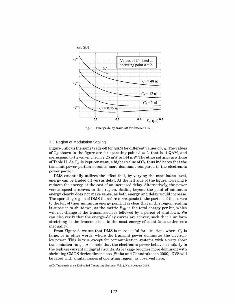
438 • C. Schurgers et al.
Fig. 3. Energy-delay trade-off for different CS .
3.3 Region of Modulation Scaling
Figure 3 shows the same trade-off for QAM for different values of CS . The valuesof CS shown in the figure are for operating point b = 2, that is, 4-QAM, andcorrespond to PS varying from 2.25 mW to 144 mW. The other settings are thoseof Table II. As CE is kept constant, a higher value of CS thus indicates that thetransmit power portion becomes more dominant compared to the electronicspower portion.
DMS essentially utilizes the effect that, by varying the modulation level,energy can be traded off versus delay. At the left side of the figure, lowering breduces the energy, at the cost of an increased delay. Alternatively, the powerversus speed is convex in this region. Scaling beyond the point of minimumenergy clearly does not make sense, as both energy and delay would increase.The operating region of DMS therefore corresponds to the portion of the curvesto the left of their minimum energy point. It is clear that in this region, scalingis superior to shutdown, as the metric Ebit is the total energy per bit, whichwill not change if the transmission is followed by a period of shutdown. Wecan also verify that the energy–delay curves are convex, such that a uniformstretching of the transmissions is the most energy-efficient (due to Jensen’sinequality).
From Figure 3, we see that DMS is more useful for situations where CS islarge, or in other words, where the transmit power dominates the electron-ics power. This is true except for communication systems with a very shorttransmission range. Also note that the electronics power behaves similarly tothe leakage current in digital circuits. As leakage becomes more dominant withshrinking CMOS device dimensions [Sinha and Chandrakasan 2000], DVS willbe faced with similar issues of operating region, as observed here.
ACM Transactions on Embedded Computing Systems, Vol. 2, No. 3, August 2003.
172
£ft«(MJ) ' 1 r -i 1
10' ^ Values or ( s lisiecl ai
operating point A = 2. \. ::::; kft^
L-—.JSs
L i . \^ i i
«'
^ Cv = 48iiJ
L\. rrs^- -4_ .- \ "i—^-—_,^__^
-~~-,___^ C\= 12 nJ \^
V^------: -i ! 0 = 3 nJ
lo-' .^
Lv"-a/:> nj ! i ...
1 . i 1 0.2 0,3 " 7-^,(ns)"

Power Management for Energy-Aware Communication Systems • 439
Table III. Modulation Bounds
bmin (bits/symbol) bmax (bits/symbol) δ (bits/symbol)
2 8 0.5
3.4 Difference Between DMS and DVS
Despite the analogies between DVS and DMS, there are two important dif-ferences. First, a change in modulation level requires communication be-tween sender and receiver. As explained in Section 3.2, the sender cannot de-cide on a new modulation setting midway through the packet transmission.Packet scheduling therefore exhibits this inherent time-granularity effect andcan only be nonpreemptive. However, the exact packet size is known at thestart of the transmission, in contrast to the task execution time in processors[Raghunathan et al. 2001]. We detail these points in Section 4.1.
Second, the wireless channel may vary over time, which means that thefactor A in (6) fluctuates. These variations have to be taken into account inthe packet-scheduling engine. This is akin to a processor where capacity (inMIPS) would change over time, for example, due to interrupt handling. Thisphenomenon is indeed complex, but is beyond the designers’ control in radiopower management.
4. ENERGY-AWARE PACKET SCHEDULING
Just like DVS has driven energy-aware task scheduling beyond shutdown-based approaches [Burd et al. 2000; Govil et al. 1995; Gruian 2001; Gutnikand Chandrakasan 1997; Krishna and Lee 2000; Manzak and Chakrabarty2000; Nielsen et al. 1994; Shin and Choi 1999; Weiser et al. 1994; Yao et al.1995], DMS paves the way toward new energy-aware packet-scheduling poli-cies. The body of literature dealing with packet scheduling is vast, and, inprinciple, is suitable to be extended toward energy-aware versions using DMS[Demers et al. 1989; Lu et al. 1997; Parekh and Gallager 1994]. However, manychallenges lie ahead, since such radio power management must deal with bothtraffic load and channel variations. In the next subsections, we describe two ba-sic scheduling approaches to illustrate some of the challenges. They each high-light one of two different issues, namely the presence of deadlines and channelvariations.
In all simulations reported in this section, a special field in the packet header,encoded with 4-QAM, is used to communicate the modulation level for the restof the packet to the receiver. We chose this option for its simplicity and faulttolerance, assuming we have control over the protocol stack. If this is not avail-able, an alternative is to use separate control packets. The DMS scheduler,residing at the link-layer, might still require channel quality information fromthe lower layers, similar to other adaptive protocols [Balachandran et al. 1999;Lettieri et al. 1999; Thoen et al. 2000]. Table III defines the possible values,which can be encoded into 4 bits. This overhead for each packet is incorporatedin all simulation results.
ACM Transactions on Embedded Computing Systems, Vol. 2, No. 3, August 2003.
173

440 • C. Schurgers et al.
4.1 Real-Time Scheduling in a Time-Invariant Channel
In this section, we consider the problem of scheduling multiple real-time trafficstreams, while the wireless channel does not vary in time. In each stream,packets arrive periodically and have a deadline by which they have to be sent.This is a valid model for multimedia streams. We choose the deadline of eachpacket to be the arrival time of the next packet in that stream. The size of theindividual packets might vary (e.g., in MPEG video or perceptual audio codecs),but there is a maximum known packet size for each stream. As mentionedbefore, the packet scheduler should not interrupt an ongoing transmission suchthat the policy has to be nonpreemptive. This is a new constraint compared tothe energy-aware task scheduling policies for RTOS, which are all preemptive(i.e., tasks can be suspended and resumed later on) [Burd et al. 2000; Gruian2001; Krishna and Lee 2000; Manzak and Chakrabarty 2000; Shin and Choi1999; Yao et al. 1995]. The setup we consider here is analogous to the DVSwork described in Raghunathan et al. [2001]. Besides the preemptive nature,the scheduling algorithm of Raghunathan et al. [2001] deals with task-lengthvariability in a stochastic fashion, as the exact execution time is not known atthe start of the task. However, in packet scheduling, the exact packet length isknown at the start of the transmission.
A condition that guarantees schedulability for nonpreemptive schedulingis derived in Jeffay et al. [1991]. When it is satisfied, earliest-deadline-firstscheduling (EDF) always results in a valid schedule. An optimal energy-awarescheduling routine is too computationally intensive as the problem is NP-complete; but we propose a practical algorithm, which consists of two steps[Schurgers et al. 2001b].
1. Admission step: When a new stream is admitted to the system, we calculatea static scaling factor, αstatic, assuming all packets are of maximum size. Thisfactor is the minimum possible such that if the modulation setting for eachpacket were scaled by it, the schedulability test would still be satisfied. Inother words, it computes the slowest transmission speed at which all thepacket streams are just schedulable.
2. Adjustment step: At run-time, packets are scheduled using EDF. Beforetransmission starts, the actual size of each packet is known. We calculatean additional scaling factor, αdyn, such that the transmission finishes whenthat of a maximum size packet would have. Since step 1 assumes the maxi-mum packet size, the schedulability is guaranteed. If the system were stillidle after the packet transmission, we would stretch the transmission untilthe packet’s deadline or the arrival time of a new packet (which is knowndue to the periodic nature of the traffic). This extra scaling factor is calledαstretch.
The scheduler combines all three scaling factors to get the overall modulationthat is used for the current packet [Schurgers et al. 2001b]. To evaluate the per-formance of our scheme, we have carried out a number of simulations. The basicsettings and modulation settings are those of Tables II and III, respectively. The
ACM Transactions on Embedded Computing Systems, Vol. 2, No. 3, August 2003.
174

Power Management for Energy-Aware Communication Systems • 441
Table IV. Number of Streams with Given Period
20 ms 25 ms 40 ms 50 ms
U = 0.82 8 6 4 4U = 0.77 8 6 2 4U = 0.74 8 4 4 4U = 0.69 6 4 6 4
Fig. 4. Relative energy for real-time energy-aware packet scheduling.
size of each packet is independently chosen in a uniformly random fashion be-tween the maximum packet size Lmax of 8000 bits and a minimum value Lmin,which is a parameter we vary in our simulations. We consider four differentscheduling scenarios. For each of them, a row in Table IV lists the number ofstreams with a given period and the resulting total link utilization when allpackets are of maximum size. For example, in the fourth scenario in Table IV,there are six streams with a period of 20 ms, four with a period of 25 ms, sixwith a period of 40 ms, and four with a period of 50 ms, resulting in a linkutilization U of 0.69 when Lmin = Lmax.
Figure 4 plots the energy consumption of our scheduling scheme, normalizedagainst one without scaling (b = bmax at all times). For U = 0.82, we haveseparated the effect of the different scaling factors. When only using αstatic,the transmissions are slowed down uniformly without exploiting the run-timepacket length variations. These are leveraged through αdyn, where the energydecreases as the packet size variation increases (Lmin decreases). The effectof αstrech is marginal here. For the other utilizations, we only show the resultswhen combining all three scaling factors. As expected, more energy savings areachieved when the utilization is lower.
ACM Transactions on Embedded Computing Systems, Vol. 2, No. 3, August 2003.
175
E, 0
9A
ft2'
7 = 0.82
0.2 0.4
L'=0 6'=0.69
0.6
^^=0.77
0.S

442 • C. Schurgers et al.
The power management scheme described here, essentially exploits trafficload variations on two levels to introduce energy awareness.
1. Variations in overall utilization are handled by the admission step in ouralgorithm through αstatic. These are due to changes in number of streams,which are likely to occur over relatively large time scales.
2. Variations in individual packet sizes on the other hand occur at much smallertime scales. These cannot be handled during admission, but are exploited inthe adjustment step of our algorithm.
4.2 Nonreal-Time Scheduling in Time-Variant Channel
In this section, we highlight a different issue in radio power management,namely the effects of time variations in the wireless channel. The closest equiv-alent in CPU task scheduling is a time-varying processor capacity. To introducesome of the challenges, we consider a rudimentary scenario: the transmissionof a single data stream that has no hard deadline associated with it, but only anaverage data rate constraint. This model is useful in the case of a file transfer,for example. In Schurgers and Srivastava [2002], we also illustrate how thisspecification can be used to provide a soft real-time constraint.
As discussed in Section 3.1, the transmission loss A captures the effect of thewireless channel. In the presence of time variations, this factor is split up intotwo components as in (11), where A represents the long-term average valueand α contains the normalized time variations. The behavior of the gain factorα can be characterized by two statistics: a probability density function and aDoppler rate, which describes the time correlation [Jakes 1994; Proakis 1995].
A = A · α (11)
In all techniques that adapt a radio parameter to channel variations, an es-timate of the current channel condition is needed [Balachandran et al. 1999;Lettieri et al. 1999]. This is obtained through channel estimation, which is up-dated regularly. The update rate fupdate is chosen such that the channel remainsapproximately constant between updates, yet the overhead of the estimationprocess is limited. In addition, predictive compensation techniques can be ap-plied [Thoen et al. 2000]. Although deciding the appropriate update rate, as acompromise between overhead and performance degradation, is an importantissue, a detailed study falls outside the scope of this paper.
In the previous section, DMS turned into a scheduling problem because of theinteraction between multiple streams. Here, we only have one stream, but thepresence of a time-varying channel again makes the choice of the best valueof b a scheduling issue. The current decision critically depends on how goodor bad the channel will be, that is, whether it is more energy efficient to sendnow or later. However, in the specific scenario we consider here, namely that thelocation of the average throughput is the only additional constraint, the problemcan be greatly simplified. In Schurgers and Srivastava [2002], we prove thatthere exists a set of thresholds di that directly link the current channel conditionto the optimal choice of b. Equation (12) presents a direct generalization of theresults presented in Schurgers and Srivastava [2002]. It is not valid for very
ACM Transactions on Embedded Computing Systems, Vol. 2, No. 3, August 2003.
176

Power Management for Energy-Aware Communication Systems • 443
high values of CE/CS , but holds the ones chosen here [Schurgers 2002]. Werefer to the resulting energy-efficient DMS packet-scheduling policy as “loadingin time,” as it was inspired by adaptive bit-loading techniques for a class ofradio systems called multicarrier systems [Chow et al. 1995; Hughes-Hartogs1987]. Note that only those values of b are assigned that did not result fromthe interpolation of Section 3.2. The reason why they are not included in theoptimal assignment is that the energy versus delay curve is no longer strictlyconvex there [Schurgers 2002]. 0 ≤ α < d1 ⇒ b = 0
di ≤ α < di+1 ⇒ b = bmin + (i − 1), i = 1..(K − 1)dK ≤ α <∞ ⇒ b = bmax
K = 1+ bmax − bmin. (12)
Furthermore, the thresholds di are mutually related according to (13) and(14) [Schurgers 2002]. The fact that both transmit and electronics power arezero when b = 0 is taken into account here.
di = max[θ · 2i−1, d1] i = 2..K (13)
θ = bmin ·[
2bmin − 1d1
+ CE
CS
]−1
· 2bmin−1. (14)
There is only one independent parameter left, which can be solved from theconstraint on the desired average data rate bav, expressed in average number ofbits per symbol. This constraint can be written as (15), where G(x) is defined in(16) [Schurgers and Srivastava 2002]. Here, F (x) is the cumulative distributionfunction of the gain factors α.
bav = bi · G(d1)+K∑
i=2
G(di) (15)
G(x) = 1− F (x). (16)
The thresholds thus only depend on the statistics of the wireless channel,which can be estimated online. We no longer have to know the exact behav-ior of the channel over time to achieve the energy-optimal scheduling policy.Figure 5 shows the simulated performance of this radio power managementscheme versus the average throughput constraint. As before, we used the val-ues of Tables II and III. The channel exhibits the correlated Rayleigh fading,such that G(x) is given by (17). This corresponds to the case where there isno line-of-sight path between sender and receiver, which is the predominantmodel used in literature [Proakis 1995]. The time correlation of the channel ischaracterized by a Doppler rate of 50 Hz, and simulated as proposed in Jakes[1994].
G(x) = exp(−x) (17)
We selected an update rate fupdate of 1 kHz for channel estimation, the over-head of which is included in the reported simulation results. The maximum
ACM Transactions on Embedded Computing Systems, Vol. 2, No. 3, August 2003.
177

444 • C. Schurgers et al.
Fig. 5. Energy versus average bit rate for time-varying channel (Rayleigh fading).
possible transmit power is 1 W. Curve 1 in Figure 5 plots the behavior of the“loading in time” scheduling policy that we described in this section. It is supe-rior to scaling with “constant b” (curve 2), where the modulation is uniformlyslowed down based on the average throughput, but channel variations arenot taken into account. The difference between curves 2 and 3, which showsthe same uniform scaling in a nontime-varying channel, illustrates the per-formance degradation associated with channel variations. Beyond bmin = 2bits/symbol, we resort to shutdown, and both these curves flatten out, whichis as expected from our discussion in Section 3.2. However, curve 1 keepson decreasing when lowering bav, and can even outperform scaling in a non-time-varying channel (curve 3). The reason is that we still use shutdown, butonly the very best time intervals (with α > 1) are selected to send informa-tion. For curve 2, the shutdown was periodic, without taking the channel intoaccount.
Finally, we also compare the performance to a scheme that is not energy-aware, but tries to achieve a “maximum throughput” possible. In this case, b isadapted to yield its maximum value without violating the maximum transmitpower [Balachandran et al. 1999; Ue et al. 1998; Webb and Steele 1995]. As thisis only based on the current channel condition, scheduling issues never arise.The benefits of energy-awareness, where a reduced throughput requirement isleveraged to yield energy savings, are again substantial.
5. CONCLUSIONS
Energy efficiency is gaining importance as a system design consideration, es-pecially in portable communication devices. Radio-level power managementbased on shutdown simply turns off the radio when it is not used. However,
ACM Transactions on Embedded Computing Systems, Vol. 2, No. 3, August 2003.
178
0.16
0.12
0.08
0.04
Max. throughput fi)! )^^^
Scaling: : Scaling; \ / / '\ / constant I 1 loading in time >
/:/
. s>^y QA [. Q^^,..^---" : - ^;j,„rfCr r Scaling iti non
time-varying
2 3 4 5 6 RM = bav-Rs (Mbit/s)

Power Management for Energy-Aware Communication Systems • 445
scaling-based techniques have the potential to be vastly superior in termsof energy savings, but necessitate more intricate power management. Packetscheduling has to be rethought to include energy-awareness, similar to the wayvoltage scaling prompted the search for energy-aware task scheduling. Numer-ous wireless packet scheduling techniques exist, which are all candidates tomake it into an energy-aware version.
In this paper, we focused on dynamic modulation scaling, DMS, as just oneof the possible radio control knobs that can be used for scaling. Even in theelementary scenarios we considered here, it illustrates the intricacies and chal-lenges of energy-aware packet scheduling. These will be compounded whenstringent delay/throughput constraints have to be satisfied in the presence ofa time-varying wireless channel, which is inherently stochastic in nature. Itis expected that resulting policies will not be able to guarantee service, but becharacterized by reliability bounds, where the tightness of the bounds can betraded off for energy savings. Radio power management therefore has to takeboth traffic and channel aspects into account simultaneously. Other researchchallenges that remain are enhancing these strategies to also handle multipledevices on a shared channel. This likely requires a distributed manipulationof the radio control knobs, by incorporating it in the medium access controllayer.
The resulting radio power management eventually has to be integrated intoa system-wide solution, where energy and latency can be traded off across thecomputation–communication subsystem boundaries. The overall vision is thusa coordinated power management, intermixing both task and packet schedulingpolicies in a networked system. Furthermore, these ideas, while presented herein the context of radios, are potentially generalizable to wired communicationsas well, which may offer other control knobs for power-speed scaling.
ACKNOWLEDGMENTS
The views and conclusions contained herein are those of the authors and shouldnot be interpreted as necessarily representing the official policies or endorse-ments, either expressed or implied, of the DARPA, Air Force Rome Laboratory,ONR, SRC or the U.S. Government.
REFERENCES
BALACHANDRAN, K., KADABA, S. R., AND NANDA, S. 1999. Channel quality estimation and rate adap-tation for cellular mobile radio. IEEE Journal on Selected Areas in Communications 17, 7, 1244–1256.
BENINI, L. AND DE MICHELI, G. 1997. Dynamic Power Management: Design Techniques and CADTools. Kluwer, Norwell, MA.
BENINI, L., BOGLIOLO, A., AND DE MICHELI, G. 1999. A survey of design techniques for system-leveldynamic power management. IEEE Transactions on VLSI Systems 8, 3, 813–833.
BURD, T., PERING, A., STRATAKOS, A., AND BRODERSEN, R. 2000. A dynamic voltage scaled micropro-cessor system. IEEE Journal of Solid-State Circuits 35, 11, 1571–1580.
CHANDRAKASAN, A., SHENG, S., AND BRODERSEN, R. 1992. Low-power CMOS digital Design. IEEEJournal of Solid-State Circuits 27, 4, 473–484.
CHO, K. AND SAMUELI, H. 2000. A 8.75-MBaud single-chip digital QAM modulator with frequency-agility and beamforming diversity. In Proceedings CICC’00. Orlando, FL (May), 27–30.
ACM Transactions on Embedded Computing Systems, Vol. 2, No. 3, August 2003.
179

446 • C. Schurgers et al.
CHOW, P., CIOFFI, J., AND BINGHAM, J. 1995. A practical discrete multitone transceiver loading al-gorithm for data transmission over spectrally shaped channels. IEEE Trans. on Communications43, 2, 773–775.
DEMERS, A., KESHAV, S., AND SHENKER, S. 1989. Analysis and simulation of a fair queueing algo-rithm. Computer Communication Review 19, 4, 1–12.
GOVIL, K., CHAN, E., AND WASSERMAN, H. 1995. Comparing algorithms for dynamic speed-Settingof a low-power CPU. In Proceedings MobiCom’95. Berkeley, CA (Nov.), 13–25.
GRUIAN, F. 2001. Hard real-time scheduling for low energy using stochastic data and DVS pro-cessor. In Proceedings ISLPED’01. Huntington Beach, CA (Aug.), 46–51.
GUTNIK, V. AND CHANDRAKASAN, A. 1997. Embedded power supply for low-power DSP. IEEE Trans-actions on VLSI Systems 5, 4, 425–435.
HUGHES-HARTOGS, D. 1987. Ensemble modem structure for imperfect transmission media. U.S.Patents, nos. 4,679,227 (July 1987), 4,731,816 (March 1988), 4,833,796 (May 1989).
JAKES, W. 1994. Microwave Mobile Communication. John Wiley, New York.JEFFAY, K., STANAT, D., AND MARTEL, C. 1991. On non-preemptive scheduling of periodic and spo-
radic tasks. In Proceedings IEEE RTSS’91. San Antonio, TX (Dec.), 129–139.KRISHNA, C. AND LEE, Y. 2000. Voltage-clock-scaling adaptive scheduling techniques for low power
in hard real-time systems. In Proceedings RTAS’00. Washington, DC (June), 156–165.LETTIERI, P., SCHURGERS, C., AND SRIVASTAVA, M. 1999. Adaptive link layer strategies for energy
efficient wireless networking. Wireless Networks 5, 5, 339–355.LORCH, J. AND SMITH, A. 1998. Software strategies for portable computer energy management.
IEEE Personal Communications 5, 3, 60–73.LU, S., BHARGHAVAN, V., AND SRIKANT, R. 1997. Fair scheduling in wireless packet networks. Com-
puter Communication Review 27, 4, 63–74.MANZAK, A. AND CHAKRABARTY, C. 2000. Variable voltage task scheduling for minimizing energy
or minimizing power. In Proceedings ICASSP’00. Istanbul, Turkey (June), 3239–3242.NIELSEN, L., NIESSEN, C., SPARSø, J., AND VAN BERKEL, K. 1994. Low power operation using self-
timed circuits and adaptive scaling of the supply voltage. IEEE Transactions on VLSI Systems2, 4, 391–397.
PAREKH, A. AND GALLAGER, R. 1994. A generalized processor sharing approach to flow control inintegrated services networks: The multiple node case. IEEE/ACM Transactions on Networking2, 2, 137–150.
PEDRAM, M. 2001. Power optimization and management in embedded systems. In ProceedingsASP-DAC 2001. Yokohama, Japan, 239–244.
PRABHAKAR, B., BIYIKOGLU, E., AND EL GAMAL, A. 2001. Energy-efficient transmission over a wirelesslink via lazy packet scheduling. In Proceedings Infocom’01. Anchorage, AK (April), 386–394.
PROAKIS, J. 1995. Digital Communications. McGraw-Hill Series in Electrical and ComputerEngineering. McGraw-Hill New York.
RAGHUNATHAN, V., SCHURGERS, C., PARK, S., AND SRIVASTAVA, M. 2002. Energy-aware wireless sensornetworks. IEEE Signal Processing Magazine 19, 2, 40–50.
RAGHUNATHAN, V., SPANOS, P., AND SRIVASTAVA, M. 2001. Adaptive power-fidelity in energy awarewireless systems. In Proceedings RTSS’01. London, UK (Dec.), 106–115.
SCHURGERS, C. 2002. Energy-aware wireless communications. Ph.D. dissertation, University ofCalifornia at Los Angeles.
SCHURGERS, C., ABERTHORNE, O., AND SRIVASTAVA, M. 2001a. Modulation scaling for energyaware communication systems. In Proceedings ISLPED’01. Huntington Beach, CA (Aug.), 96–99.
SCHURGERS, C., RAGHUNATHAN, V., AND SRIVASTAVA, M. 2001b. Modulation scaling for real-timeenergy aware packet scheduling. In Proceedings Globecom’01. San Antonio, TX (Nov.), 3653–3657.
SCHURGERS, C. AND SRIVASTAVA, M. 2002. Energy efficient wireless scheduling: Adaptive loading intime. In Proceedings WCNC’02. Orlando, FL (Mar.), 706–711.
SHIN, Y. AND CHOI, K. 1999. Power conscious fixed priority scheduling for hard real-time systems.In Proceedings DAC’99. New Orleans, LA (June), 134–139.
SINHA, A. AND CHANDRAKASAN, A. 2000. Energy aware software. In Proceedings VLSI Design 2000.Calcutta, India (Jan.), 50–55.
ACM Transactions on Embedded Computing Systems, Vol. 2, No. 3, August 2003.
180

Power Management for Energy-Aware Communication Systems • 447
SRIVASTAVA, M., CHANDRAKASAN, A., AND BRODERSEN, R. 1996. Predictive system shutdown and otherarchitectural techniques for energy efficient programmable computation. IEEE Transactions. onVLSI Systems 4, 1, 42–55.
TENENBAUM, A. 1990. Computer Networks. Prentice-Hall, Englewood Cliffs, NJ.THOEN, S., VAN DER PERRE, L., GYSELINCKX, B., ENGELS, M., AND DE MAN, H. 2000. Predictive adaptive
loading for HIPERLAN II. In Proceedings VTC’00 Fall. Boston, MA (Sept.), 2166–2172.UE, T., SAMPEI, S., MORINAGA, N., AND HAMAGUCHI, K. 1998. Symbol rate and modulation level-
controlled adaptive modulation/TDMA/TDD System for High-Bit Rate Wireless Data Transmis-sion. IEEE Transactions on Vehicular Technology 47, 4, 1134–1147.
WANG, H. AND MANDAYAM, N. 2001. Delay and energy constrained dynamic power control. InProceedings Globecom’01. San Antonio, TX (Nov.), 1287–1291.
WEBB, W. AND STEELE, R. 1995. Variable rate QAM for mobile radio. IEEE Transactions onCommunications 43, 7, 2223–2230.
WEISER, M., WELCH, B., DEMERS, A., AND SHENKER, B. 1994. Scheduling for reduced CPU energy. InProceedings USENIX Symposium on Operating Systems Design and Implementation. Monterey,CA (Nov.), 13–23.
YAO, F., DEMERS, A., AND SHENKER, S. 1995. A scheduling model for reduced CPU energy. In Pro-ceedings 36th Annual Symposium on Foundations of Computer Science. Milwaukee, WI (Oct.),374–385.
Received February 2002; accepted July 2002
ACM Transactions on Embedded Computing Systems, Vol. 2, No. 3, August 2003.
181

Energy Aware Wireless Systems withAdaptive Power-Fidelity Tradeoffs
Vijay Raghunathan, Cristiano L. Pereira, Mani B. Srivastava, and Rajesh K. Gupta
Department of EE, UC Los Angeles, CA 90095Department of ICS, UC Irvine, CA 92697
Department of CSE, UC San Diego, CA 92093vijay, mbs @ee.ucla.edu [email protected] [email protected]
Abstract
Wireless embedded systems, such as multimedia terminals, sensor nodes, etc., combine soft real-time con-straints on computation and communication with requirements of long battery lifetime. Energy aware systemoperation, and not just low power hardware design, is an crucial requirement for these systems. This paperpresents an operating system directed dynamic voltage scaling (DVS) technique that enhances the energy aware-ness of these systems. A key feature of our technique, not addressed in prior work, is that it yields an adaptivetradeoff between energy consumption and system delity .
The proposed algorithm exploits two observations about the operating scenario of wireless embedded sys-tems, namely, (i) they are designed to operate resiliently in the presence of varying delity (data losses, delays,and errors over the wireless link), and (ii) they exhibit signi cant correlated variations in their computation andcommunication processing load due to underlying time-varying physical phenomena. These observations enablethe proposed algorithm to proactively manage energy resources by predicting processing requirements, therebytrading off energy consumption against system delity . The supply voltage and processor clock frequency are setaccording to the predicted execution time of a given task instance, and an adaptive feedback mechanism keeps thesystem delity (deadline misses) within speci cations.
We present the theoretical framework underlying our approach in the context of a static priority based pre-emptive task scheduler. We show through extensive simulations that our technique results in signi cant energysavings compared to state-of-the-art DVS schemes with minimal loss in system delity . We have implemented ourtechnique into the eCos real-time operating system running on an Intel XScale based variable voltage platform.Experimental results obtained through actual power measurements on this platform con rm the effectiveness ofour technique.
Acknowledgements: This paper is based in part on research funded through the DARPA PAC/C Program under AFRL Contract #F30602-
00- C-0154, and through Semiconductor Research Corporation System Task Thrust ID 899.001.
182

1 INTRODUCTION
Embedded systems are increasingly becoming networked, often wirelessly, and demand an integration of high-performance computing and wireless communication capabilities, under real-time constraints. Examples of suchsystems include mobile multimedia terminals with wireless LAN cards, 3G cellular phones, ad-hoc networks ofwireless sensors, wireless toys and robots, etc. The battery operated nature of these systems requires them to bedesigned and operated in a highly energy ef cient manner to maximize their lifetime.
The drive to prolong system lifetime has resulted in the development of several low power hardware designtechniques [1, 2]. In addition to using low power hardware components, managing the various system resources inan energy aware manner can further reduce energy consumption considerably, thereby extending battery life. Onecommonly used approach for energy aware system operation is Dynamic Power Management (DPM) [3], in whichunused system components are shutdown or sent into low power states. The goal of system-level DPM techniques isto obtain an optimized power-state transition policy [4, 5, 6, 7]. An alternative, and more effective when applicable,technique used to increase energy ef cienc y is Dynamic Voltage Scaling (DVS) [8, 9, 10, 11, 12, 13, 14], in whichthe supply voltage and clock frequency of the processor are changed dynamically to just meet the instantaneousperformance requirement.
In order to adapt to constantly evolving standards, a signi cant fraction of the functionality of wireless embeddedsystems is implemented as software running under a real time operating system (RTOS). Each application (e.g., videoencoding/decoding, data encryption/decryption, layers of the protocol stack, etc.) runs as a concurrent task under theRTOS. The RTOS is uniquely poised to ef ciently implement DPM and DVS policies due to the following reasons:(i) since the RTOS coordinates the execution of the various application tasks, it has global information about theperformance requirements and timing constraints of all the applications, and (ii) the RTOS can directly control theunderlying hardware platform, ne-tuning it to meet speci c system requirements.
In this paper, we adopt an RTOS directed approach to power management and DVS, and enable energy awaresystem operation by exploiting the following characteristics of wireless embedded systems:
Most wireless systems are resilient to packet losses and errors. The operating scenarios of these systemsinvariably have losses and errors associated with them (e.g., noisy wireless channel conditions lead to packetlosses and errors), and the application layer is designed to be tolerant to these impairments. Most wirelesssystems, therefore, are “soft” real-time systems where a few deadline misses only lead to a small degradationin the user-perceived system delity .
Wireless embedded systems offer a power- delity tradeoff that can be tuned to suit application needs.For example, the precision of the computation (e.g., quality of the audio or video decoding) can be traded offagainst the power consumed for the computation. As another example, wireless channel induced errors can bereduced by increasing the transmission power of the radio.
Wireless embedded systems have time varying computational loads. Performance analysis studies haveshown that for typical wireless applications (e.g., multimedia encoding/decoding, encryption/decryption, etc.),the instance to instance task execution time varies signi cantly , and is often far lower than the worst case
2
183

Program Description BCET WCETDES Data encryption 73,912 672,298
DJPEG JPEG decompression (128x96, color) 12,703,432 122,838,368FDCT JPEG forward DCT 5,587 16,693
Table 1: Variation in execution times (in clock cycles) for a few multimedia benchmarks [15]
execution time (WCET). Table 1 gives the WCET and best case execution time (BCET) for a few bench-marks [15], and clearly illustrates the large workload variability. Note that, even though the execution timesvary signi cantly , they depend on data values that are obtained from physical real-world signals (e.g., audioor video streams), and are likely to have some temporal correlation between them. This enables us to predicttask instance execution times with reasonable accuracy.
1.1 Paper contributions
The contributions of this paper are threefold:
1. We present an enhanced x ed priority schedulability analysis for variable voltage systems that incorporates thetiming overheads incurred due to voltage/frequency changes and processor shutdown/wakeup. This analysiscan be used to accurately analyze the schedulability of non-concrete periodic task sets, scheduled using theRate Monotonic (RM) or the Deadline Monotonic (DM) priority assignment schemes.
2. We present a proactive DVS technique that exploits the above described characteristics of wireless embeddedsystems to achieve signi cant energy savings. A key feature of our technique, not addressed in prior work, isthat it yields an adaptive tradeoff between energy consumption and system delity/quality .
3. Our DVS technique has been implemented into the kernel of the eCos [16] real-time operating system runningon an Intel XScale [17] processor. We describe our implementation and present measured results to demon-strate the effectiveness of our technique. As part of our implementation, we have also developed a completesoftware architecture that facilitates application-RTOS interaction for ef cient DPM/DVS.
The proposed DVS technique exploits task runtime variation by predicting task instance execution times andperforming DVS accordingly. Most previously proposed predictive DVS algorithms [18, 19] are processor utilizationbased, and hence perform poorly in the presence of latency (i.e., deadline) constraints. In contrast, our techniqueis tightly coupled to the schedulability analysis of the underlying real-time scheduling scheme, thereby yieldingsigni cantly superior results than utilization based approaches. The few deadline misses that result from occasionalmis-prediction are not catastrophic to system performance due to the inherent error-tolerant nature of these wirelesssystems. In addition, our algorithm uses a novel adaptive feedback mechanism to keep a tight check on the numberof task deadline misses. This is done by monitoring recent deadline miss history, and accordingly adapting theprediction to be more aggressive/conservative. A thread based proactive DVS algorithm, which used the idea ofexecution time prediction, was presented in [23] for scheduling sporadic tasks with deadline constraints. Our workdiffers from the work presented in [23] in two ways, (i) while the algorithm of [23] permits missed deadlines, it does
3
184

not provide any control on the number of deadline misses. Through appropriate parameter selection, the proposedalgorithm permits the user to control the number of deadline misses, and trade them off for increased energy savings,and (ii) the algorithm of [23] is a purely online one, and has a complexity of
, where
is the number of tasks
present in the system. In contrast, since the proposed algorithm is based on an of ine schedulability analysis, thecomplexity of the online component is
, i.e., the scheduler overhead is independent of the number of tasks in
the system, resulting in better scalability. This can be signi cant for systems with large number of tasks, especiallysince online DVS algorithms are executed during every context switch.
Finally, since our technique is based on the enhanced schedulability analysis mentioned above, it can even beused to schedule non-concrete task sets, where the initial phase offsets of tasks are unknown. This is unlike mostexisting variable voltage real-time scheduling schemes, which require the initial phase offsets of the tasks to beknown in order to perform hyper-period scheduling.
1.2 Related work
Dynamically scaling the supply voltage was rst proposed for asynchronous circuits [8]. Since then, there has beenextensive research in the area of DVS. This research has spurred (and, in turn, has been spurred by) the emergenceof processors such as Intel’s StrongARM [20] and XScale [17], and Transmeta’s Crusoe [21] that were designed tosupport dynamic voltage and clock scaling.
Initial work on DVS was in the context of a workstation-like environment [9, 10] where average throughput isthe metric of performance, and latency is not an issue since there are no real-time constraints. In these techniques,time is divided into 10-50 ms intervals, and the processor frequency and supply voltage are adjusted by the task-level scheduler based on the processor utilization over the preceding interval. Similar utilization based predictivetechniques were studied in more detail in [18, 19]. A technique to derive an of ine minimum energy schedule,and an average rate heuristic for scheduling independent processes with deadlines was presented in [11]. Sincethen, numerous DVS techniques have been proposed for low power real-time task scheduling, both for uniprocessor[12, 13, 14, 18, 19, 22, 23, 24, 25, 26, 27, 28] as well as multiprocessor [29, 30, 31] systems. A detailed survey ofthese techniques is presented in [32]. Most uniprocessor DVS techniques [12, 13, 14, 24, 25, 26, 27, 28] performvoltage scheduling assuming that systems have hard deadline constraints, and several of them assume that eachtask instance executes for its WCET. Even the few schemes that allow deadline misses [18, 19] involve utilizationbased speed setting decisions, and hence exhibit poor real-time behavior. More importantly, they only considersystems with a single application executing (i.e., a unitasking environment). The authors of [23] discuss a threadbased proactive DVS technique for uniprocessor, multitasking systems. Similar to [23], the technique proposed inthis work considers a uniprocessor, multitasking, real-time environment, and shows that permitting a few deadlinemisses leads to a signi cant increase in energy savings and improves the energy scalability of the system.
The rest of this paper is organized as follows. Section 2 presents examples to illustrate the power managementopportunities that exist during real-time task scheduling. Section 3 describes our system model. Section 4 presentsthe enhanced RM schedulability analysis for variable voltage systems. Section 5 discusses our adaptive power- delity tradeoff technique. Section 6 details our simulation based performance analysis. Section 7 describes ourexperimental setup and the implementation of our technique into eCos. Section 8 presents the conclusions.
4
185

2 BACKGROUND AND ILLUSTRATIVE EXAMPLES
Next, we describe the basic scheduling approach adopted in our work, and present examples to illustrate theDPM/DVS opportunities that arise during real-time task scheduling.
2.1 Task scheduling in RTOS
The task scheduler of an RTOS is responsible for scheduling a given set of tasks such that real-time constraintsare satis ed. Schedulers differ in the type of scheduling policy they implement. A commonly used schedulingpolicy is Rate Monotonic (RM) scheduling [33]. This is a x ed-priority based preemptive scheduling scheme wheretasks are assigned priorities in the inverse ratio of their time periods. Fixed priority based preemptive schedulingis commonly used in operating systems such as eCos, WinCE, VxWorks, QNX, uC/OS, etc., that run on wirelessembedded devices such as handheld multimedia nodes. An alternative scheduling scheme is Earliest Deadline First(EDF) scheduling [33], where task priorities are assigned dynamically such that task instances with closer deadlinesare given higher priorities. EDF can schedule task sets with a higher processor utilization than can be scheduledby a static priority based scheduling scheme such as RM. However, dynamic priority based scheduling is also morecomplex to implement since task priorities keep changing during runtime. No matter which scheduling policy isused, the RTOS ensures that at any point of time, the currently active task is the one with the highest priority amongthe ready to run tasks. The problem of task scheduling on a uniprocessor system in the presence of deadlines isknown to be solvable in polynomial time if the system is preemptive in nature [34]. However, the low energyscheduling problem was shown to be NP-Complete in [35], by a reduction from the “Sequencing with deadlines andset-up times” problem, described in [34]. Therefore, heuristic techniques have to be applied to minimize energy.
2.2 Power management opportunities during task scheduling
2.2.1 Static slack
It has been observed in many systems that, during runtime, even if all task instances run for their WCET, theprocessor utilization is often far lower than 100%, resulting in idle intervals. This slack that inherently exists in thesystem due to low processor utilization is henceforth referred to as static slack. It can be exploited to reduce energyconsumption by statically slowing down the processor and operating at a lower voltage. While processor slowdownimproves processor utilization, excessive slowdown may lead to deadline violations. Hence, the extent of slowdownis limited by the schedulability of the task set at the reduced speed, under the scheduling policy used. The followingexample illustrates the use of static slowdown and voltage scaling to reduce energy consumption.
Task Time Period WCET DeadlineAudio decoding 60 10 60
Protocol processing 70 15 70Video decoding 120 40 120
Table 2: Task timing parameters for Examples 1 and 2
5
186

Wireless link
Audio Video
Protocol processing
Figure 1: Mobile multimedia terminal used in Examples 1 and 2.
Example 1: Consider a simple mobile multimedia terminal shown in Figure 1 . The system receives real-timeaudio and video streams over a wireless link, and plays them out. Thus, the three main tasks that run on a processorembedded in this system are protocol processing, audio decoding, and video decoding. The timing parameters forthese tasks are listed in Table 2. For simplicity, the initial phase offsets for the tasks are set to zero (however, ouralgorithm, presented in Section 5, makes no such assumptions). The resulting schedule for the time interval [0,120] when this task set is scheduled on a single processor using the RM priority assignment scheme, is shown inFigure 2(a). It can be seen from the gure that the system is idle during time interval [90, 120]. This slack can beutilized to lower the operating frequency and supply voltage, thereby reducing the energy consumption. Figure 2(b)shows the schedule for the same task set with the processor slowed down
by a factor of
. As seen from the gure,
processor slowdown leads to a reduction in slack. Note that any further reduction in processor speed will result
in the video decoding task missing its deadline. When the supply voltage is also scaled, this leads to a decrease inpower consumption from 420mW to 184mW, using the power vs. frequency curve for the StrongARM processor,shown in Figure 4. The energy consumption over the interval [0, 120], therefore, decreases by 41%, compared to ashutdown based policy.
2.2.2 Dynamic slack
Static slack is not the only kind of slack present in the system. During runtime, due to the variation in the taskinstance execution times, there is an additional slack created when a task instance nishes executing before itsWCET. This slack that arises due to execution time variation is henceforth referred to as dynamic slack. Dynamicslack can be exploited for DVS by dynamically varying the operating frequency and supply voltage of the processorto extend the task execution time to its WCET. Thus, the lower a task instance’s actual execution time, the more itsenergy reduction potential. However, to realize this potential, we need to know/estimate the execution time of each
The system shown in Figure 1 is only an illustrative example of a multi-tasking, uniprocessor, battery powered embedded system. This
could, in general, be a 3G cell phone or a handheld PC.For simplicity, we assume that such an exact slowdown is possible. Our algorithm handles the case where the processor only has a nite
set of available frequenciesWhile in this example, uniform slowdown of all tasks resulted in a complete elimination of static slack, in general this might not be the
case, and different tasks might require different slowdown factors. Our algorithm does this, if necessary.
6
187

S=1
S=0.75
(b)
(a)0 10 3020 40 50 60 70 80 90 100 110 120
0 10 20 30 40 50 60 70 80 90 100 110 120
of video decoding taskDeadline of first instsnce
Audio decoding Protocol processing Video decoding
Figure 2: Task execution schedule for Example 1: (a) Original (b) Statically optimized
task instance. The following example illustrates how dynamic slack can be exploited for DVS.
Example 2: Consider the statically optimized schedule for the task set of Example 1 shown in Figure 2(b). Figure3(a) shows the resulting schedule when the video decoding task instance requires only 20 time units to completeexecution at maximum processor speed. As a result, the video decoding task now completes execution at time units, and does not get preempted. As seen from the gure, this execution time variation creates somedynamic slack. To utilize this slack, the processor frequency and supply voltage are dynamically reduced furtherduring the execution of the video decoding task. If the frequency were to be dropped by a factor of 2 over the alreadystatically optimized value, the slack gets lled up again as shown in Figure 3(b)
. Accompanied by appropriate
voltage scaling, the energy consumption for the interval [0, 120] now reduces by a further 14% compared to thestatically optimized schedule of Figure 3(a).
S=0.375 S=0.375
S=0.75
S=0.75
(b)
(a)0 10 3020 40 50 60 70 80 90 100 110 120
0 10 20 30 40 50 60 70 80 90 100 110 120
of video decoding taskDeadline of first instsnce
Audio Decoding Protocol processing Video decoding
Figure 3: Task execution schedule for Example 2: (a) Statically optimized (b) After dynamic slowdown
The above examples illustrated the energy reduction opportunities present during real-time task scheduling.We next describe our system model, and present an enhanced RM schedulability analysis for variable voltage sys-tems. Using this analysis, we then present our power aware scheduling algorithm that exploits the above illustratedDVS/DPM opportunities to yield large energy savings.Note that in Figure 3(b), the video decoding task is now preempted at time units, and resumes execution later to complete at time
units.
7
188

3 SYSTEM MODEL
3.1 Task timing model
A set of N independent periodic tasks is to be scheduled on a uniprocessor system. Associated with each task i arethe following parameters: (i) is its time period, (ii) is its worst case execution time (WCET), (iii) is the bestcase execution time (BCET), and (iv) is its deadline. The BCET and WCET can be obtained through executionpro ling or other performance analysis techniques [15]. Our techniques are applicable to the general case where and are unrelated. We discuss this further in Section 4.
3.2 Power model
We use a power model of the StrongARM processor, which is based on actual measurements, for computing thepower consumption. Figure 4 shows the power consumption of the StrongARM, plotted as a function of the operatingfrequency. This plot is obtained from actual current and voltage measurements reported in [36] for the StrongARMSA-1100 processor. Using this curve, the power consumption of the system for a given clock frequency can be
0
50
100
150
200
250
300
350
400
60 80 100 120 140 160 180 200 220 240
Pow
er c
onsu
med
(m
W)
Frequency (MHz)
Figure 4: Power consumption as a function of clock frequency for the StrongARM processor
calculated. By varying the supply voltage and clock frequency, the variable voltage system can be made to operateat different points along this curve. For a given clock frequency (i.e., speed setting), the energy consumption of atask instance can be computed as the product of the power consumption (obtained from the power-frequency curveshown above) and the execution time of the task instance. Further, it is easy to see that the energy-speed curve isconvex in nature [13]. Thus, if two task instances have to be completed by a deadline, due to Jensen’s inequality
[37], it is more energy ef cient to run the two tasks at a constant speed than to change the speedfrom one task to the other. As will be seen in the next section, our algorithm utilizes this fact by attempting to slowdown tasks in a uniform manner, to the extent possible.
3.3 Overheads due to DVS/DPM
The variable supply voltage is generated using DC-DC switching regulators. During a voltage transition, it takesa nite amount of time for the output voltage of the DC-DC converter to transition from the present level to the
8
189

desired level. Ef cient DC-DC regulators with fast transition times were reported in [38, 39]. Complementary tothe supply voltage variation is the accompanying variation of the clock frequency. The phase locked loop present inthe clock generation circuitry also takes a nite amount of time to settle at its steady state value, after a frequencychange. Further, shutting down and waking up the processor involve a non-zero time and power overhead. Theseoverheads have to be explicitly accounted for during task scheduling. For variable voltage real-time systems, thetiming overheads have to be incorporated into the task-set schedulability analysis to guarantee the schedulability oftasks. The energy overheads have to be considered while computing the energy savings obtained through the useof DVS and DPM. Commercial processors till recently had large frequency transition overheads (for example, theStrongARM [20] takes 150 seconds to change its frequency). However, these transition times are considerablylower in more recent processors as designers realize the effectiveness of DVS. The transition overhead is around 30 seconds in the XScale processor [17]. We use a stall duration of 150 seconds in our simulations, since the powermodel used is that of a StrongARM processor. However, in our implementation (Section 7), the stall duration is only30 seconds, since our experimental testbed is based on the XScale processor. Finally, although some processors [23]developed at academic institutions allow the computation to continue while the voltage and frequency are beingchanged, neither the StrongARM nor the XScale processors permit this. Therefore, in our simulations, the processoris stalled for the duration of the frequency change, resulting in some wasted energy (although this is insigni cantsince the processor clock is frozen). We account for all the above mentioned overheads in our energy calculations.
4 RATE-MONOTONIC SCHEDULABILITY ANALYSIS
Several classical results exist on the schedulability analysis for RM scheduling [40]. However, none of them con-sider variable voltage/frequency processors. Since processor shutdown, processor wakeup, and voltage and fre-quency changes take a nite amount of time, they affect the timing behavior of the system. In this section, wepresent an enhanced schedulability analysis for RM scheduling, which takes into account the overheads introduceddue to DPM/DVS. We denote the time taken to shutdown/wakeup the processor by , and the time taken for avoltage/frequency change by .4.1 The case
The schedulability analysis for RM scheduling for the case is presented in [40], in which necessary andsuf cient conditions are derived for the schedulability of a non-concrete (i.e., unknown initial phases for the tasks)periodic task set. The response time of a task instance is de ned as the amount of time needed for the task instanceto nish execution, from the instant at which it arrived in the system. The worst case response time (WCRT), as thename indicates, is the maximum possible response time that a task instance can have. For a conventional x ed speedsystem, the WCRT of a task under the RM scheduling scheme is given by smallest solution of the equation [40]:
(1)
The time taken for a voltage change could be different from the time taken for a frequency change. In that case, "! is the maximum ofthe two values. Further, the voltage/frequency change will be accompanied by a context switch, whose overhead can also be added to ! .
9
190

where denotes the set of tasks with priority greater than that of task, denotes the worst case execution time
of task, denotes the ceiling operator, and
is simply an intermediate variable used in computing the WCRT.Equation (1) can be solved using an iterative technique. The summation term on the right-hand-side of the equationrepresents the total interference that an instance of task
sees from higher priority tasks during its execution. The
non-concrete task set schedulable iff the WCRT of the task is less than or equal to its deadline . Our enhancedschedulability analysis is based upon three observations.Observation 1: Slowing down a task by a factor increases its computation time by the same factor. Therefore,given a set of slowdown factors , the computation time for task
, now becomes
.Observation 2: Each higher priority task instance that arrives during the lifetime of a lower priority task instanceadds either , or to the response time of the lower-priority task instance, where is the time taken tochange the processor frequency/voltage. This is the preemption related overhead of DVS.
It takes time units to change the voltage to execute the higher priority task instance, and another unitsto change back to resume execution of the preempted task instance, and the worst case for a task instance occurswhen this procedure repeats for every higher priority task instance that arrives during its lifetime. So, the worst caseinterference that a higher priority task instance contributes is equal to . However, when the higher priority taskis being executed, suppose a task with priority in between that of the currently running task and the preempted taskarrives. It is easy to see that this task instance only causes an interference of .Observation 3: The maximum amount of blocking that can be faced by a task instance, and which is not preemptionrelated is ! " !# %$%& '" , where (# $%& is the time taken to shutdown/wakeup the processor.
Since the processes of voltage/frequency change or shutdown cannot be preempted, each task instance may beblocked for an amount of time if it arrives just after a voltage/frequency change or a shutdown has been initiated.Based on the above observations, the following theorem can be used as a suf cient condition for the schedulabilityof a task set under RM scheduling on a DVS enabled system.
Theorem 1 (Suf cient RM schedulability condition): A non-concrete periodic task set is guaranteed to be schedu-lable on a variable voltage processor, under the RM scheduling policy if, for every task
, ) where) is the smallest solution of the equation: * +,-. " /0"
1 2" 3 (2)
where !4 is the slowdown factor for task
.
4.2 The 5 case
The schedulability analysis for the case when 76 is more complex. For x ed speed systems, when and are unrelated, the WCRT of task
is given by [40]:
) , !98;:=<>:? ) @ <ACBD E (3)
10
191

where is the smallest non-negative integer value that satis es ) @ ? , and ) @ < is the smallest solutionto the equation:
) @ < B ) @ < (4)
The task set is schedulable if, and only if, ) . Intuitively, the above analysisimplies that the WCRT may not occur for the rst instance of the task, and we may need to check the schedulabilityfor multiple instances of the task. In the case of variable voltage systems, using the three observations listed inSection 3.4, the schedulability test reduces to a suf cient condition, and Equation (4) is changed to:
) @ < B ,-. 0 1 ) @ <
2D 3 (5)
where is the slowdown factor for task. It is worth mentioning that the case is just a special case of this
enhanced equation. When , Equations (3) and (4) are satis ed for . The of ine component of ouralgorithm uses this enhanced suf cient schedulability test to compute static slowdown factors for each task.
5 ALGORITHM
We consider a priority based, preemptive scheduling model where the priority assignment is either done statically,in the case of Rate Monotonic scheduling . Task instances that do not nish executing by their deadline are killed.Our algorithm adjusts the processor’s supply voltage and clock frequency whenever a new task instance rst startsexecuting, as well as every time it resumes execution after being preempted by a higher priority task. Also, ouralgorithm uses a constant speed setting between two points of preemption in order to maximally exploit the convexityof the energy-speed curve. The pseudo-code of our algorithm is shown in Figures 5 and 6. The crucial steps of ouralgorithm are described next.
5.1 Static slowdown factor computation
This component of our algorithm involves a schedulability analysis of the task set. It is executed whenever a newtask (e.g., audio/video decoding) enters the system and registers itself with the scheduler. Given the task set to bescheduled, the procedure COMPUTE STATIC SLOWDOWN FACTORS performs a schedulability analysis (describedin Section 3), and computes the minimum operating frequency for each task, at which the entire task set is stillschedulable. Every task is slowed down uniformly till one or more tasks reach their critical point (i.e., they are“just” schedulable). This is done by the function Scale WCET(). At this juncture, further slowdown of any taskwith higher priority than any of the critical tasks will render at least one critical task unschedulable. Therefore, onlythe tasks, if any, with lower priority than any of the critical tasks can be slowed down further without affecting theschedulability of the task set. The procedure continues till there is no further scaling possible while satisfying alltask deadlines. In summary, this iterative procedure gives us a new reduced frequency for each task such that theAlthough we do not analyze it in this paper, our DVS algorithm is also applicable to dynamic priority scheduling, such as Earliest
Deadline First, using the appropriate schedulability analysis.
11
192

Procedure COMPUTE STATIC SLOWDOWN FACTORSInputs: Time Periods[ ], WCETs[ ], Deadlines[ ]Outputs: Static Slowdown Factors[ ]SET S = //Tasks that can be slowed down furtherSET S1 = //Tasks that will miss deadline upon further scalingCurrent Scaling Factor = 1;For each task i in S
Static Slowdown Factor[i] = 1;While (S )
f = Scale WCET (Time Periods[ ], WCETs[ ], Deadlines[ ], S, Static Slowdown Factor[ ]);S1 = Tasks that will miss deadlines with further scaling;Current Scaling Factor *= f;For each task i in SStatic Slowdown Factor[i] = Current Scaling Factor;
S = All tasks with priority Lowest priority of tasks in S1;
Figure 5: Pseudo-code for the of ine component of the proposed algorithm
entire task set is just schedulable. The online component of our algorithm augments this static slowdown with adynamic slowdown factor, computed at runtime, in order to increase energy savings.
5.2 Dynamic slowdown factor computation
The online component of our algorithm invokes the COMPUTE DYNAMIC SLOWDOWN FACTOR procedure, listedin Figure 6, to dynamically alter the supply voltage and operating frequency of the system in accordance withrecent task execution statistics. Thus, while the of ine component of our algorithm computes task speci c staticslowdown factors, the online component augments this with task-instance speci c dynamic slowdown factors. TheCOMPUTE DYNAMIC SLOWDOWN FACTOR procedure is called each time a new task instance starts, or resumesexecution after being preempted by a high priority task. The algorithm sets the processor speed and voltage basedon an estimate of the task instance execution time.
5.2.1 Runtime prediction strategy
A novel feature of our algorithm is that it involves a proactive DVS scheme. In contrast, most existing techniquesare reactive in nature. Therefore, in conventional schemes, any slack that arises due to a task instance completingexecution early, is distributed to task instances that follow, using (possibly complex) dynamic slack reclamationalgorithms. Our technique, on the other hand, attempts to avoid the creation of slack altogether, through the use of apredictive technique, eliminating the need for slack reclamation. In our predictive scheme, the execution time of atask instance is predicted as some function of the execution times of a x ed number of previous task instances. Anexecution history database is maintained for each task, that is updated every time a task instance nishes executing
12
193

Procedure COMPUTE DYNAMIC SLOWDOWN FACTORInputs: WCET, Deadline Miss History, Execution HistoryOutputs: Dynamic Slowdown FactorP = PREDICT TIME (Execution History); = ADAPTIVE FACTOR (Deadline Miss History, );P = P * ;Dynamic Slowdown Factor = WCET / P;
Procedure PREDICT TIMEInput: Execution HistoryOutput: Predicted timeIf (Elapsed time for task instance == 0)
Predicted time = ! "# $"%&(') +* %,! * -../ ;
//N is the number of past instances being monitored//The coef cients 0 depend on the prediction scheme used
ElsePredicted time = Expected value of execution time
distribution from Elapsed Time to WCET;
Procedure ADAPTIVE FACTORInput: Deadline Miss History, Adaptive FactorOutput: Adaptive Factorx = Number of deadline misses in past WINDOW instances;If (x 1 T1) Adaptive Factor + = I;If (x 2 T2) Adaptive Factor - = D;If (Adaptive Factor 2 ADAPTIVE LB) Adaptive Factor = ADAPTIVE LB;
Figure 6: Pseudo-code for the online component of the proposed algorithm
or is killed due to a deadline miss. The function used to compute the execution time determines the type of predictor.We have evaluated our techniques using a simple average predictor model, as well as an exponentially weightedaverage one. Both these are simple prediction schemes that place a light computational load on the scheduler. Sincethe results were very similar in the two cases, we report only the results obtained using the weighted average model.The use of a more complex predictor will improve prediction accuracy. However, this will increase the computationalburden on the scheduler since the predictor is executed every time a task instance starts or restarts after preemption.
5.2.2 Improving prediction accuracy
In order to improve prediction accuracy while retaining simplicity, we extend the prediction strategy to use condi-tional prediction as described below. Every time a task instance is preempted, the predicted remaining time for thattask instance is recalculated as the expected value of the past execution history distribution from the already elapsed
13
194

time to the WCET of the task. This gives the predicted remaining time of the task, given that it has already run forthe elapsed time. This improves the prediction accuracy, and reduces the probability of under-prediction, in turnreducing the probability of missed deadlines. As a side effect, it also reduces the impact of the original predictionmodel. This explains why we obtained similar results using the simple average and weighted average predictors.
5.2.3 Adaptive power- delity tradeoff
Some applications may not be able to tolerate the number of deadlines that are missed using the above describedpredictive scheme. Therefore, we introduce an adaptive feedback mechanism into the prediction process. Thepredicted execution time of a task instance is altered using an adaptive multiplicative factor, as shown in the pseudocode of Figure 6. Deadline miss history is monitored using a moving window mechanism, and if the number ofdeadline misses is found to be increasing, the prediction is made more conservative, reducing the probability offurther deadline misses. Similarly, a low/decreasing deadline miss history results in more aggressive prediction inorder to reduce energy consumption. This is implemented as follows. If there are more than deadlines misses inthe last ) ) task instances, the algorithm becomes more conservative and increases the adaptive factor by .Similarly, if the number of deadline misses in the last )- ) task instances is less than D , then the algorithmbecomes more aggressive and decreases the adaptive factor by . A lower bound, , dictates themaximum aggressiveness of the algorithm. The prediction scheme is now adaptive to a recent history of misseddeadlines, becoming more conservative in response to deadline misses and becoming more aggressive if no deadlinemisses occur over the past few instances. This adaptive control mechanism ensures that the number of deadlinemisses (which is representative of system delity) is kept under tight check at all times. The choice of the variousparameters depends on how aggressive/conservative the user wants to be in the energy- delity tradeoff, a detailedanalysis of which is beyond the scope of this paper. Note that in order to keep the algorithm and implementationsimple, we have made the deadline miss history and all the parameters of the adaptive algorithm global parameters.An alternative, although more complicated, approach would be to perform the adaptation on a per-task basis. Suchan approach would permit better control on the delity of individual applications. Finally, note that this adaptivescheme is also useful in the case when applications can tolerate more deadlines than missed through the use of thebaseline predictive scheme. In such a situation, the adaptive scheme can be used to obtain further energy savingsat the cost of more deadline misses. Thus, the application can adjust the operating point along an energy- delitycurve, which enhances its energy scalability. For example, as the system runs out of energy, the it can scale down its delity gracefully. To the best of our knowledge, none of the existing DVS schemes provide this capability.
5.2.4 Voltage variation policy
Our algorithm recomputes the voltage setting every time a task instance rst starts executing, or restarts after beingpreempted. The pre-computed static slowdown factor for the task is augmented with a dynamic slowdown factor forthe speci c task instance that is about to start executing. The dynamic slowdown factor is computed by stretchingthe task instance’s predicted execution time to reach its WCET. The product of the static and dynamic factors isthe nal slowdown factor. The processor’s operating frequency is then decreased by this factor, the correspondingsupply voltage is set, and execution of the task instance begins. This dynamic slowdown spreads the execution to ll
14
195

2 13
TASK INSTANCESTASK
ENTITY
RTOS
ENTITYGENERATOR
PARSEC SIMULATION PLATFORM
Figure 7: System simulation model in PARSEC
otherwise idle time intervals, enabling operation at a lower supply voltage and clock frequency.
6 SIMULATION BASED PERFORMANCE ANALYSIS
We next describe our simulation framework, and present simulation results comparing the proposed adaptive power- delity DVS algorithm to several existing DVS/DPM schemes to demonstrate its effectiveness.
6.1 Simulation model
To analyze the performance of the proposed adaptive power- delity DVS scheme, a discrete event simulator was builtusing PARSEC [41], a C based parallel simulation language. The simulation structure, shown in Figure 7, consistedof two parallel communicating entities. The rst one represented the RTOS, and implemented the task scheduler(enhanced with the DVS scheme). In addition to performing task scheduling, the RTOS entity also maintained thestatistics of task instance execution times and deadline misses. The second entity, i.e., the task generator, periodicallygenerated task instances with run times according to a trace or a distribution, and passed them to the RTOS entity.
6.2 Simulation results
We performed simulations on two task sets (henceforth called Task Set 1 and Task Set 2) that are based on standardtask sets used in embedded real-time applications [42, 43]. The task instance execution times were generated using aGaussian distribution with , and
. To demonstrate
that our technique works even for non-concrete task sets, every task
was given a random initial phase offset in theinterval . We performed four experiments on each task set. In the rst experiment, only shutdown based DPMwas employed, and the supply voltage and frequency were x ed at their maximum values. Next, we implementedthe low-power scheduling technique of [14]. This is a WCET based scheme, where DVS is done only when there isa single task remaining to execute. In the third experiment, we implemented the PAST/PEG DVS scheme [18, 19].Similar to our algorithm, this is a predictive DVS scheme. However, all DVS decisions in the PAST/PEG scheme arepurely utilization based, and therefore the PAST/PEG scheme performs poorly in the presence of deadlines. Finally,the proposed adaptive power- delity DVS scheme was implemented. The experiments were repeated while varyingWe also repeated our experiments using a uniform distribution. The results were similar in both cases. Therefore, we present only the
results for the Gaussian distribution case.
15
196

20
30
40
50
60
70
80
90
100
0.1 0.2 0.3 0.4 0.5 0.6 0.7 0.8 0.9 1
Ene
rgy
savi
ngs
(%)
BCET / WCET
Shutdown
20
30
40
50
60
70
80
90
100
0.1 0.2 0.3 0.4 0.5 0.6 0.7 0.8 0.9 1
Ene
rgy
savi
ngs
(%)
BCET / WCET
WCET
20
30
40
50
60
70
80
90
100
0.1 0.2 0.3 0.4 0.5 0.6 0.7 0.8 0.9 1
Ene
rgy
savi
ngs
(%)
BCET / WCET
PAST/PEG
20
30
40
50
60
70
80
90
100
0.1 0.2 0.3 0.4 0.5 0.6 0.7 0.8 0.9 1
Ene
rgy
savi
ngs
(%)
BCET / WCET
Proposed
20
30
40
50
60
70
80
90
100
0.1 0.2 0.3 0.4 0.5 0.6 0.7 0.8 0.9 1
Ene
rgy
savi
ngs
(%)
BCET / WCET
Shutdown
20
30
40
50
60
70
80
90
100
0.1 0.2 0.3 0.4 0.5 0.6 0.7 0.8 0.9 1
Ene
rgy
savi
ngs
(%)
BCET / WCET
WCET
20
30
40
50
60
70
80
90
100
0.1 0.2 0.3 0.4 0.5 0.6 0.7 0.8 0.9 1
Ene
rgy
savi
ngs
(%)
BCET / WCET
PAST/PEG
20
30
40
50
60
70
80
90
100
0.1 0.2 0.3 0.4 0.5 0.6 0.7 0.8 0.9 1
Ene
rgy
savi
ngs
(%)
BCET / WCET
Proposed
(a) (b)
Figure 8: Energy savings of various DVS/DPM schemes under RM scheduling for (a) Task Set 1 and (b) Task Set 2
0
5
10
15
20
0.1 0.2 0.3 0.4 0.5 0.6 0.7 0.8 0.9 1
Dea
dlin
es m
isse
d (%
)
BCET / WCET
PAST/PEG
0
5
10
15
20
0.1 0.2 0.3 0.4 0.5 0.6 0.7 0.8 0.9 1
Dea
dlin
es m
isse
d (%
)
BCET / WCET
Proposed
0
1
2
3
4
5
6
7
0.1 0.2 0.3 0.4 0.5 0.6 0.7 0.8 0.9 1
Dea
dlin
es m
isse
d (%
)
BCET / WCET
PAST/PEG
0
1
2
3
4
5
6
7
0.1 0.2 0.3 0.4 0.5 0.6 0.7 0.8 0.9 1
Dea
dlin
es m
isse
d (%
)
BCET / WCET
Proposed
(a) (b)
Figure 9: Deadline miss percentage for the proposed scheme and the PAST/PEG scheme under RM scheduling for(a) Task Set 1, and (b) Task Set 2
the BCET from 10% to 100% of the WCET in steps of 10%. Each data point was averaged over 50 simulation runs,each run simulating the execution of 50,000 task instances. For the adaptive scheme, the following parameter valueswere used: , ) ) , , ,
, and D . The various parameters aredescribed in Section 5.2.3.
Figure 8 shows the energy savings obtained for the two task sets under RM scheduling, for each of the abovementioned DVS/DPM schemes. The results are normalized to the case when no DVS/DPM is used. As can beseen in the gure, the proposed adaptive power- delity DVS algorithm results in signi cantly higher energy savingscompared to the shutdown, WCET based, and PAST/PEG algorithms. Figure 9 shows the percentage of deadlinesmissed by the proposed algorithm, and the PAST/PEG algorithm. The PAST/PEG scheme results in a large numberof deadline misses because it takes DVS decisions purely based on processor utilization. As mentioned before, inreal-time multi-tasking systems, the schedulability of the task set is only weakly related to the processor utilization.
16
197

0
0.5
1
1.5
2
0.1 0.2 0.3 0.4 0.5 0.6 0.7 0.8 0.9 1
Dea
dlin
e m
isse
s (%
)
BCET / WCET
Non-Adaptive
0
0.5
1
1.5
2
0.1 0.2 0.3 0.4 0.5 0.6 0.7 0.8 0.9 1
Dea
dlin
e m
isse
s (%
)
BCET / WCET
Adaptive (0.8)
0
0.5
1
1.5
2
0.1 0.2 0.3 0.4 0.5 0.6 0.7 0.8 0.9 1
Dea
dlin
e m
isse
s (%
)
BCET / WCET
Adaptive (1.0)
0
0.5
1
1.5
2
0.1 0.2 0.3 0.4 0.5 0.6 0.7 0.8 0.9 1
Dea
dlin
e m
isse
s (%
)
BCET / WCET
Adaptive (1.2)
20
30
40
50
60
70
80
90
100
0.1 0.2 0.3 0.4 0.5 0.6 0.7 0.8 0.9 1
Ene
rgy
savi
ngs
(%)
BCET / WCET
Non-Adaptive
20
30
40
50
60
70
80
90
100
0.1 0.2 0.3 0.4 0.5 0.6 0.7 0.8 0.9 1
Ene
rgy
savi
ngs
(%)
BCET / WCET
Adaptive (0.8)
20
30
40
50
60
70
80
90
100
0.1 0.2 0.3 0.4 0.5 0.6 0.7 0.8 0.9 1
Ene
rgy
savi
ngs
(%)
BCET / WCET
Adaptive (1.0)
20
30
40
50
60
70
80
90
100
0.1 0.2 0.3 0.4 0.5 0.6 0.7 0.8 0.9 1
Ene
rgy
savi
ngs
(%)
BCET / WCET
Adaptive (1.2)
(a) (b)
Figure 10: Impact of the parameter on (a) Percentage of deadline misses and (b) Energy savings,for Task Set 1 under RM scheduling
Therefore, the PAST/PEG algorithm results in a signi cant loss in real-time behavior. Note that this is in contrastto what was observed by Farkas et al. [19]. That is because they only considered a unitasking environment wherethe schedulability is determined completely by processor utilization. The algorithm proposed in this work is tightlycoupled to the schedulability analysis of the underlying real-time scheduling scheme used, resulting in far fewerdeadline misses, as is evident from Figure 9.
56
78
910
1112
1314
15
0.40.6
0.81
1.21.4
1.6
60
65
70
75
80
Window Size
Lower Bound
En
erg
y sa
vin
gs
(%)
56
78
910
1112
1314
15
0.30.5
0.70.9
1.11.3
1.5
0
0.5
1
1.5
2
2.5
3
3.5
4
Lower BoundWindow Size
Dea
dlin
e m
isse
s (%
)
(a) (b)
Figure 11: Variation of (a) Energy savings and (b) Deadline miss percentage with parameters )- ) and for Task Set 1 under RM scheduling
We performed additional experiments with Task Set 1 to illustrate the adaptive power- delity tradeoff that ourscheme provides. We ran our algorithm for three different values of the parameter . Figures 10(a)and 10(b) show the energy savings and deadline miss percentages, respectively, for ,and for a non-adaptive version of our algorithm. From the gures, it is clear that by increasing ,one can trade-off energy savings for fewer deadline misses. Such an adaptive scheme enhances the system’s energy-
17
198

66
68
70
72
74
0 0.5 1 1.5 2
Ene
rgy
savi
ngs
(%)
Deadline misses (%)
ADAPTIVE_LB=0.8
ADAPTIVE_LB=0.6
ADAPTIVE_LB=1.2
Figure 12: Energy savings vs. Deadline misses for )- ) and various values of forTask Set 1 under RM scheduling.
scalability. For example, as the battery drains out, can be decreased, thereby gradually degradingthe system’s delity . Figures 11(a) and 11(b) plot the energy savings and deadline misses as a function of the param-eters and ) ) , for a . It is evident that as increases,the energy savings decrease, and the deadline misses increase. As the window size increases, the energy savingsdecrease and the deadline misses decrease. Also, note that choosing a very low value for is notvery energy ef cient. This is because, the large number of missed deadlines cause the voltage to be increased veryfrequently in response, lowering the energy savings obtained. In order to clearly show the energy- delity tradeoff,we have plotted the energy savings vs. the deadline miss percentage in Figure 12 for ) ) and differentvalues of . As can be seen in Figure 12, a value of 0.8 for seems to yield themaximum energy savings, for this particular task set.
7 IMPLEMENTATION
In addition to validating the proposed adaptive power- delity technique through simulations, we also evaluated itsperformance by implementing it into an RTOS running on a complete variable voltage hardware platform. In thissection, we rst give a brief overview of a structured software architecture that we have developed to facilitateapplication-RTOS interaction for effective energy management. Then, we describe our implementation in detail,and present measured results that demonstrate the effectiveness of our DVS algorithms.
7.1 Software architecture
We view the notion of power awareness in the application and OS as a capability that enables a continuous dialogbetween the application, the OS, and the underlying hardware. This dialog establishes the functionality and per-formance expectations (or even contracts, as in the real-time sense) within the available energy constraints. A wellstructured software architecture is necessary for realizing this notion of power awareness. The power aware softwarearchitecture (PASA) [44, 45] that we have developed is composed of two software layers and the RTOS kernel. Onelayer is an API that interfaces applications with the OS, and the second layer makes power related hardware knobs
18
199

POSIX
HARDWARE
API Level
Application Level
Hardware Level
OS Level
PA-HALRTOS HAL
PA-OSL
Applications
Scheduler
Device Drivers
MemoryManager
Services
PA OSRTOSKernel
PA-API
(a) (b)
Figure 13: (a) Power Aware Software Architecture, and (b) Picture of the experimental setup. The XScale board ison the upper left side, the Maxim board on the upper right side, and the FPGA board, which generates interrupts, ison the lower right side. On the lower left side is a bread board with interconnections to trigger the DAQ board.
available to the OS. Both layers interface to various OS services as shown in Figure 13(a). The API layer is sepa-rated into two sub-layers. The Power Aware Application Programmer Interface (PA-API) sub-layer provides powermanagement functions to the applications, while the other sub-layer, the Power Aware Operating System Layer(PA-OSL) provides access to existing and modi ed OS services. Active entities that are not implemented withinthe RTOS kernel should be implemented at this layer (e.g., threads created to assist the OS in DVS/DPM, such as athread responsible for killing other threads whose deadlines were missed). The modi ed RTOS and the underlyinghardware are interfaced using a Power Aware Hardware Abstraction Layer (PA-HAL). The PA-HAL gives the OSaccess to the power related hardware knobs while abstracting out the details of the underlying hardware platform.
7.2 Experimental setup
Using the PASA presented above, the proposed adaptive power- delity DVS algorithm has been incorporated intothe eCos operating system, an open source RTOS from Red-Hat Inc. eCos was ported to an 80200 Intel EvaluationBoard[46], which is an evaluation platform based on the XScale processor. The XScale processor supports ninefrequency levels ranging from 200MHz to 733MHz. However, two of them (200MHz and 266MHz) cannot be usedin the 80200 board due to limitations in the clock generation circuitry [17]. In addition, the processor supports threedifferent low power modes: IDLE, DROWSY, and SLEEP. The SLEEP mode results in maximal power savings, butrequires a processor reset in order to return to the ACTIVE mode. The IDLE mode, on the other hand, offers theleast power savings but only requires a simple external interrupt to wake the processor up. We use the IDLE powerdown mode in our experiments due to its simple implementation.
Like most RTOSs, eCos requires a periodic interrupt to keep track of the internal OS tick, responsible for thenotion of timing within the system. In the 80200 board, the only source of such an interrupt is the internal XScale
19
200

Clock Frequency (MHz) Supply Voltage (V)733 1.5666 1.4600 1.3533 1.25466 1.2400 1.1333 1.0
Table 3: Frequency-Voltage pairs for the Intel XScale processor used in our implementation
performance counter interrupt. However, the interrupt is internal to the processor, and therefore cannot wake it upfrom the IDLE mode. To overcome this problem, we used a source of external interrupts to wake up the processor.The interrupt pin of the processor is connected to an Altera FPGA board, which generates periodic interrupts towake up the processor. The period of the external interrupt is made equal to that of the smallest time period task toensure that the processor is not woken up unnecessarily. The experimental setup, consisting of the XScale board, theMAXIM DC-DC converter board, the FPGA, and some interface circuitry is shown in Figure 13(b).
7.2.1 Variable voltage supply
The variable voltage supply consists of a MAXIM 1855 DC-DC converter board, and some interface circuitry im-plemented using a PLD. When a voltage change is required, the processor sends a byte through the peripheral bus ofthe 80200 board to the interface circuitry which acts as an addressable latch. The outputs of this latch are connectedto the digital inputs of the Maxim variable supply board. These inputs determine the output supply voltage of theMaxim board, which is fed back to the processor core. For the experiments, the system was con gured to run at sup-ply voltages from 1.0V to 1.5V and corresponding frequencies from 333 MHz to 733 MHz. The frequency-voltagepairs are listed in Table 3. The frequency is changed using the XScale’s internal registers.
7.2.2 Power measurement setup
We used a National Instruments Data Acquisition (DAQ) board to measure the power consumption. We isolated thepower supply to the processor from the rest of the board, and measured the power consumed by the processor alone.For this purpose, we used a shunt resistor (0.02 ohm) and sampled the voltage drop across it at a high sampling rateto obtain the instantaneous current drawn by the processor. We computed the energy consumption by integrating theproduct of the instantaneous supply voltage and current consumption over the interval of interest. Our measurementsetup is similar to the one described in [19]. The DAQ board was triggered by pulling signals out of the peripheralbus of the 80200 board to synchronize the power measurements with the task execution.
7.3 Experimental procedure and results
We implemented and compared three different DVS/DPM schemes, (i) shutdown based DPM, (ii) a non-adaptiveversion of the proposed algorithm, and (iii) the complete adaptive power- delity tradeoff DVS algorithm. As abaseline for comparison, we also conducted an experiment without any DVS/DPM. The following parameter valueswere used for the adaptive scheme,
, , )- ) , , and . We used two
20
201

Task Application Worst case execution time Std. Dev.at max. frequency ( s) ( s)
T1 MPEG2 (wg gdo 1.mpg) 30700 3100T2 MPEG2 (wg cs 1.mpg) 26300 2100T3 ADPCM 9300 3300T4 FFT 15900 0T5 FFT (Gaussian dist.) 13600 800
Table 4: Applications used in the experiments. T1 and T2 both perform MPEG decoding, but on different les.
Task Set Component Task C T D Static Slowdown FactorT2 26300 40000 40000 0.9495
A T3 9300 80000 80000 0.9495T4 15900 120000 120000 0.9495T1 30700 47000 47000 0.8979
B T3 9300 94000 94000 0.8979T4 15900 141000 141000 0.8979T1 30700 45000 45000 0.9207
C T3 9300 90000 90000 0.9207T5 13600 135000 135000 0.9207
Table 5: Task Sets used in the experiments. Each task set is comprised of three tasks. stands for the worst caseexecution time, denotes the time period, and denotes the deadline. All times are in seconds.
different values (0.95 and 0.85) for . We did not explore optimal choices for these parameters.Rather, our goal was to demonstrate the effectiveness of our algorithm by implementing it on a real system.
We used three different applications in our experiments: (i) an MPEG2 decoder, (ii) an ADPCM speech encoder,and (iii) a oating point FFT algorithm. Note that these applications run concurrently in the system. Each applicationexecutes as an eCos thread, and is scheduled using the RM priority assignment scheme. We pro led the executiontime of each application for different input data to collect WCET statistics. For the MPEG2 decoder, different leswere decompressed, and the WCET was measured separately for each one of them. The original FFT algorithmcomputes a x ed number (1024) of FFTs in one execution. In order to increase the variability in execution time,we also implemented a version of the FFT algorithm that computes a random number (obtained using a Gaussiandistribution) of FFTs in each execution. Table 4 shows the characteristics of the applications used. The WCET ofeach application instance was measured with the processor running at maximum frequency. The standard deviation isalso given in Table 4 to show the variability in the execution times for each application. We built three different tasksets using these applications. The task sets, their component tasks, and the individual task characteristics are listedin Table 5. The characteristics indicate the WCET, time period, and deadline, respectively. The static slowdownfactor is also listed for each task.
All the DVS/DPM algorithms shutdown the processor as soon as it becomes idle. The processor is woken upwhen the next external interrupt arrives. A limitation of the processor wake up strategy for our current testbedrequires us to make all task periods a multiple of the highest-rate task. Thus, whenever the processor is woken upthere is useful work to be done. This limitation could be eliminated through the use of a programmable interruptgenerator. Further, note that this is not a limitation of the DVS algorithm or the software architecture itself. Thestatic slowdown factors used by the proposed DVS algorithm are maintained in a table that is internal to eCos. Each
21
202

DVS/DPM scheme used Energy Power Ratio No. of deadlines missed(Joules) (Watts) (T2/T3/T4)
No DVS/DPM 39.085 0.779 1 0/0/0Shutdown 31.504 0.628 0.80 0/0/0
Non-adaptive 28.496 0.568 0.72 1/1/2Adaptive (0.95) 26.581 0.527 0.68 3/2/1Adaptive (0.85) 25.251 0.502 0.64 3/1/4
Table 6: Energy and average power consumption for Task Set A. The total number of task instances is 415,207, and138 for tasks T2, T3, and T4 respectively. For the adaptive schemes, the number in parentheses denotes the value of .
DVS/DPM scheme used Energy Avg. Power Ratio No. of deadlines missed(Joules) (Watts) (T1/T3/T4)
No DPM 12.546 0.798 1 0/0/0Shutdown 11.265 0.716 0.89 0/0/0
Non-adaptive 9.811 0.624 0.78 1/0/1Adaptive (0.95) 9.795 0.623 0.78 1/0/1Adaptive (0.85) 8.828 0.562 0.70 1/1/31
Table 7: Energy and average power consumption for Task Set B. The total number of task instances is 130,65, and43 for tasks T1, T3, and T4, respectively. For the adaptive schemes, the number in parentheses denotes the value of .
task type is associated with a static factor, which is computed during system initialization. The dynamic and adaptivefactors are maintained in a table of task instances. The task type table also contains a speci ed number (10 in ourcase) of execution times of previous task instances. The eCos kernel has full access to these tables. When a contextswitch occurs, the various tables are updated, and the voltage and frequency of the processor are adjusted.
The energy and average power consumption for the three task sets, under various DPM/DVS schemes, areshown in Tables 6, 7, and 8. The column titled Ratio gives the energy consumption normalized to the case when noDVS/DPM is used, and the column titled Dead. missed gives the number of missed deadlines for each task. For theadaptive algorithm, the number in parentheses represents the value of . As expected, the energysavings increase as this parameter decreases, at the cost of more deadline misses. These results indicate that theproposed adaptive power- delity DVS algorithm does indeed result in considerable energy savings at the cost of asmall number of missed deadlines.
8 CONCLUSIONS
This paper presented an RTOS directed DVS scheme to reduce energy consumption in wireless embedded systems.A key feature of the proposed technique is that it yields an adaptive tradeoff between energy consumption andsystem delity . The proposed algorithm exploits low processor utilization, instance to instance variation in taskexecution times, and tolerance to missed deadlines of wireless systems to achieve this tradeoff. The techniquehas been incorporated into the kernel of the eCos RTOS, and an energy ef cient software architecture has beendeveloped that facilitates application aware power management by enabling a dialog between the application andthe RTOS. Involving the application in DVS/DPM can yield signi cant bene ts. In many cases, the execution time
22
203

DPM Scheme Used Energy Avg. Power Ratio No. of deadlines missed(Joules) (Watts) (T1/T3/T5)
No DPM 13.080 0.838 1 0/0/0Shutdown 12.342 0.772 0.94 0/0/0
Non-adaptive 10.892 0.693 0.83 0/1/18Adaptive (0.95) 10.958 0.697 0.83 0/1/18Adaptive (0.85) 9.990 0.637 0.76 11/16/32
Table 8: Energy and average power consumption for Task Set C. The total number of task instances is 130, 65, and43 for tasks T1, T3, and T5, respectively. For the adaptive schemes, the number in parentheses denotes the value of .
is a superposition of several distinct distributions corresponding to different operating modes or distinct values ofdata. For example, a multiplier takes lesser time to compute its output if the operands are powers of two. Anotherexample is an MPEG decoder whose histogram of run times has three distinct peaks corresponding to P, I and Fframes. In such cases, an intelligent task can provide feedback to the OS in the form of a hint on the distributionof run times after the data values are known. As part of future work, we plan to investigate the energy reductionpotential of such interactions in detail.
References[1] A. P. Chandrakasan and R. W. Brodersen, Low Power CMOS Digital Design. Kluwer Academic Publishers, Norwell, MA, 1996.[2] A. Raghunathan, N. K. Jha, and S. Dey, High-level Power Analysis and Optimization. Kluwer Academic Publishers, Norwell, MA,
1998.[3] L. Benini and G. De Micheli, Dynamic Power Management: Design Techniques and CAD Tools. Kluwer Academic Publishers, Norwell,
MA, 1997.[4] M. B. Srivastava, A. P. Chandrakasan, and R. W. Brodersen, “Predictive system shutdown and other architectural techniques for energy
ef cient programmable computation”, in IEEE Trans. on VLSI Systems, March, 1996.[5] C. Hwang and A. Hu, “A predictive system shutdown method for energy saving of event driven computation”, in Proc. IEEE ICCAD,
pp. 28–32, November, 1997.[6] T. Simunic, L. Benini, P. Glynn, and G. De Micheli, “Dynamic power management for portable systems”, in Proc. ACM MOBICOM,
August, 2000.[7] L. Benini, A. Bogliolo, and G. De Micheli, “A survey of design techniques for system-level dynamic power management”, in IEEE
Trans. on VLSI Systems, vol. 8, iss. 3, pp. 299–316, June, 2000.[8] L. S. Nielsen and J. Sparso, “Low-power operation using self-timed circuits and adaptive scaling of supply voltage”, in Proc. Int. Wkshp.
Low Power Design, pp. 99–104, April, 1994.[9] M. Weiser, B. Welch, A. Demers, and S. Shenker, “Scheduling for reduced CPU energy”, in Proc. First Symp. on OSDI, pp.13–23,
November, 1994.[10] K. Govil, E. Chan, and H. Wasserman, “Comparing algorithms for dynamic speed-setting of a low-power CPU”, in Proc. ACM MOBI-
COM, pp. 13–25, November 1995.[11] F. Yao, A. Demers, and S. Shenker, “A scheduling model for reduced CPU energy”, in Proc. Annual Symp. on Foundations of Computer
Science, pp.374–382, October, 1995.[12] I. Hong, M. Potkonjak, and M. B. Srivastava, “On-line scheduling of hard real-time tasks on variable voltage processors”, in Proc. IEEE
ICCAD, pp.653–656, November, 1998.[13] T. Ishihara and H. Yasuura, “Voltage scheduling problem for dynamically variable voltage processors, in Proc. ACM ISLPED, pp.197–
202, August, 1998.[14] Y. Shin and K. Choi, “Power conscious x ed priority scheduling for hard real-time systems”, in Proc. IEEE/ACM DAC, pp. 134–139,
June, 1999.[15] Y. -T. S. Li and S. Malik, “Performance analysis of embedded software using implicit path enumeration”, in IEEE Trans. on CAD, vol.
16, iss. 12, pp. 1477-1487, December, 1997.[16] eCos real-time OS (www.redhat.com/embedded/technologies/ecos)
23
204

[17] Intel XScale microarchitecture (http://developer.intel.com/design/xscale/)[18] T. A. Pering, T. D. Burd, and R. W. Brodersen, “The simulation and evaluation of dynamic voltage scaling algorithms”, in Proc. ACM
ISLPED, pp. 76–81, August, 1998.[19] D. Grunwald, P. Levis, and K. Farkas, “Policies for dynamic clock scheduling”, in Proc. OSDI, 2000.[20] Intel StrongARM processors (http://developer.intel.com/design/strong/)[21] Transmeta Crusoe processor (http://www.transmeta.com)[22] T. D. Burd, T. A. Pering, A. J. Stratakos, and R. W. Brodersen, “A dynamic voltage scaled microprocessor system”, in IEEE Journal of
Solid-State Circuits, vol. 35, iss. 11, pp. 1571–1580, November, 2000.[23] T. A. Pering, T. D. Burd, and R. W. Brodersen, “Voltage scheduling in the lpARM microprocessor system”, in Proc. ACM ISLPED,
pp. 96–101, 2000.[24] A. Manzak and C. Chakrabarty, “Variable voltage task scheduling for minimizing energy or minimizing power”, in Proc. IEEE ICASSP,
June, 2000.[25] C. M. Krishna and Y. H. Lee, “Voltage-clock-scaling adaptive scheduling techniques for low power in hard real-time systems”, in Proc.
IEEE RTAS, pp. 156–165, 2000.[26] P. Pillai and K. G. Shin, “Real-time dynamic voltage scaling for low power embedded operating systems”, in Proc. 18th Symposium on
Operating Systems Principles, October, 2001.[27] F. Gruian,“Hard real-time scheduling for low energy using stochastic data and DVS processor”, in Proc. ACM ISLPED, August, 2001.[28] J. Pouwelse, K. Langendoen, and H. Sips, “Energy priority scheduling for variable voltage processors”, in Proc. ACM ISLPED, pp.
28–33, August, 2001.[29] J. Luo and N. K. Jha, “Power conscious joint scheduling of periodic task graphs and aperiodic tasks in distributed real-time embedded
systems”, in Proc. IEEE ICCAD, pp. 357–364, November, 2000.[30] J. Luo and N. K. Jha, “Battery aware static scheduling for distributed real-time embedded systems”, in Proc. ACM/IEEE DAC, pp.
444–449, June, 2001.[31] D. Zhu, R. Melhem, and B. Childers, “Scheduling with dynamic voltage/speed adjustment using slack reclamation in multi-processor
real-time systems”, in Proc. IEEE Real-Time Systems Symposium, December, 2001.[32] N. K. Jha, “Low power system scheduling and synthesis”, in Proc. IEEE ICCAD, pp. 259–263, November, 2001.[33] C. L. Liu and J. W. Layland, “Scheduling algorithms for multiprogramming in a hard real time environment”, in Journal of ACM,
vol. 20, pp. 46-61, January, 1973.[34] M. R. Garey and D. S. Johnson, Computers and Intractability: A guide to the theory of NP-Completeness. W. H. Freeman and Company,
San Fransisco, CA, 1979.[35] I. Hong, G. Qu, M. Potkonjak, and M. B.Srivastava, “Synthesis techniques for low-power hard real-time systems on variable voltage
processors”, in Proc. IEEE RTSS, pp. 178–187, 1998.[36] A. Sinha and A. P. Chandrakasan, “Jouletrack: A web based tool for software energy pro ling”, in Proc. IEEE/ACM DAC, June, 2001.[37] J. L. W. V. Jensen, “Sur les fonctions convexes et les ingalits entre les valeurs moyennes”, Acta Math., vol. 30, pp. 175–193, 1906.[38] W. Namgoong and T. H. Meng, “A high-ef cienc y variable-voltage CMOS dynamic dc-dc switching regulator”, in Proc. IEEE
ISSCC, pp.380-381, February, 1997.[39] V. Gutnik and A. .P. Chandrakasan, “Embedded power supply for low-power DSP”, in IEEE Trans. on VLSI Systems, vol.5, no.4, pp.425–
435, December, 1997.[40] A. Burns and A. Welling, Real-Time Systems and their Programming Languages. International Computer Science Series. Addison-
Wesley, 1989.[41] PARSEC parallel simulation language (http://pcl.cs.ucla.edu/projects/parsec/)[42] A. Burns, K. Tindell, and A. Wellings, “Effective analysis for engineering real-time x ed priority schedulers”, in IEEE Trans. on
Software Engineering, vol.21, pp.475-480, May, 1995.[43] N. Kim, M. Ryu, S. Hong, M. Saksena, C. Choi, and H. Shin, “Visual assessment of a real time system design: a case study on a CNC
controller”, in Proc. IEEE RTSS, December, 1996.[44] C. Pereira, V. Raghunathan, S. Gupta, R. Gupta, and M. Srivastava, “A Software Architecture for Building Power Aware Real Time
Operating Systems”, Tech. Report #02-07, University of California, Irvine, March, 2002.[45] Power Aware Distributed Systems project, UC Los Angeles and UC, Irvine. (http://www.ics.uci.edu/ cpereira/pads)[46] Intel 80200 Evaluation Board (http://developer.intel.com/design/xscale/)
24
205

Energy Ef cient Wireless PacketScheduling and Fair Queuing
Vijay Raghunathan, Saurabh Ganeriwal, Curt Schurgers, and Mani SrivastavaNetworked and Embedded Systems Lab (NESL)
Department of Electrical EngineeringUniversity of California, Los Angeles, CA 90095
Submitted to the ACM TECS (Special Issue on Networked Embedded Computing)
Contact Author: VIJAY RAGHUNATHANPhone: (310) 206 4465Fax: (310) 825 7928E-mail: [email protected]
Other Authors:
SAURABH GANERIWAL CURT SCHURGERS MANI SRIVASTAVAPhone: (310) 206 5698 Phone: (310) 206 4465 Phone: (310) 267 2098Fax: (310) 825 7928 Fax: (310) 825 7928 Fax: (310) 794 1592E-mail: [email protected] E-mail: [email protected] E-mail: [email protected]
206

Energy Ef cient Wireless PacketScheduling and Fair Queuing
Vijay Raghunathan, Saurabh Ganeriwal, Curt Schurgers, and Mani SrivastavaNetworked and Embedded Systems Lab (NESL)
Department of Electrical EngineeringUniversity of California, Los Angeles, CA 90095
vijay, saurabh, curts, mbs @ee.ucla.eduAbstract
As embedded systems are being networked, often wirelessly, an increasingly larger share of their total energybudget is due to the communication. This necessitates the development of power management techniques that addresscommunication subsystems, such as radios, as opposed to computation subsystems, such as embedded processors, towhich most of the research effort thus far has been devoted. In this paper, we present techniques for energy ef cientpacket scheduling and fair queuing in wireless communication systems. Our techniques are based on an extensive slackmanagement approach that dynamically adapts the output rate of the system in accordance with the input packet arrivalrate. We use a recently proposed radio power management technique, Dynamic Modulation Scaling (DMS), as a controlknob to enable energy-latency tradeoffs during wireless packet transmission. We rst analyze a single input streamscenario, and describe a rate adaptation technique that results in signi cantly lower energy consumption (reductionsof up to 10X), while still bounding the resulting packet delays. By appropriately setting the various parameters of ouralgorithm, the system can be made to traverse the energy-latency- delity tradeoff space. We extend our techniques to amultiple input stream scenario, and present , an energy ef cient version of the Weighted Fair Queuing (WFQ)algorithm for fair packet scheduling. Simulation results show that large energy savings can be obtained through the useof , with only a small, bounded increase in worst case packet latency. Further, our results demonstrate that does not adversely affect the throughput allocation (and hence, fairness) of WFQ.
I. INTRODUCTION
Conventional low power design techniques [1], [2], [3] and hardware architectures [4] only target digital com-
putation systems, and relatively little work has been done for power optimization of the wireless communication
subsystem. In many wireless embedded systems, communication energy dominates the energy consumed for com-
putation [5], accentuating the need for radio power management methodologies. For example, in the wireless sensor
nodes from Rockwell Inc. [6], transmitting one bit consumes 1500 to 2700 times [5] (depending on the transmission
range) as much energy as executing one instruction. Therefore, in wireless devices, power management cannot just
be limited to computation subsystems, such as processors, but has to extend to communication subsystems, such as
radios, as well.
Radio power management is, however, complex, since the dependence of radio energy consumption on supply
voltage and other circuit parameters is weak. Existing power management techniques that are effective for computation
subsystems, such as Dynamic Voltage Scaling (DVS) [7], therefore do not result in the required energy savings.
However, there exist similar control knobs on the radio that can be exploited for power management. The recently
proposed technique of Dynamic Modulation Scaling (DMS) [8] uses the modulation level as an energy-speed control
knob that can be ne-tuned to enable dynamic power-performance tradeoffs in the communication system (similar
1
207
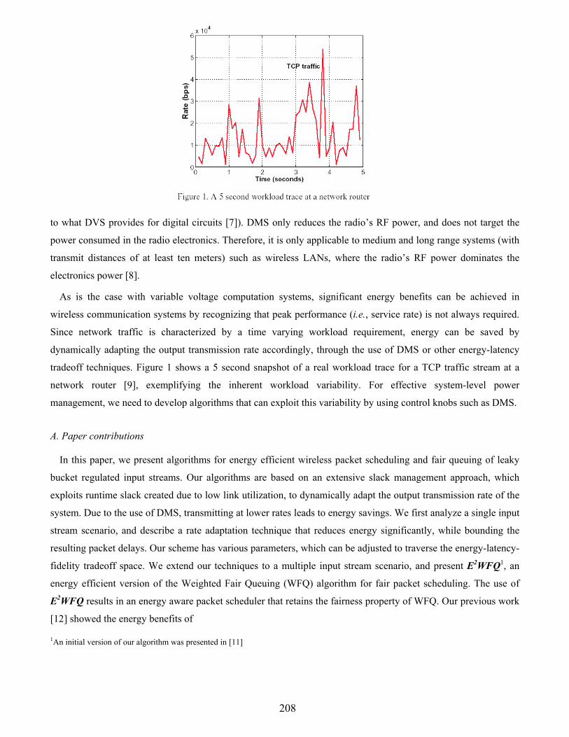
to what DVS provides for digital circuits [7]). DMS only reduces the radio’s RF power, and does not target the
power consumed in the radio electronics. Therefore, it is only applicable to medium and long range systems (with
transmit distances of at least ten meters) such as wireless LANs, where the radio’s RF power dominates the
electronics power [8].
As is the case with variable voltage computation systems, significant energy benefits can be achieved in
wireless communication systems by recognizing that peak performance (i.e., service rate) is not always required.
Since network traffic is characterized by a time varying workload requirement, energy can be saved by
dynamically adapting the output transmission rate accordingly, through the use of DMS or other energy-latency
tradeoff techniques. Figure 1 shows a 5 second snapshot of a real workload trace for a TCP traffic stream at a
network router [9], exemplifying the inherent workload variability. For effective system-level power
management, we need to develop algorithms that can exploit this variability by using control knobs such as DMS.
A. Paper contributions
In this paper, we present algorithms for energy efficient wireless packet scheduling and fair queuing of leaky
bucket regulated input streams. Our algorithms are based on an extensive slack management approach, which
exploits runtime slack created due to low link utilization, to dynamically adapt the output transmission rate of the
system. Due to the use of DMS, transmitting at lower rates leads to energy savings. We first analyze a single input
stream scenario, and describe a rate adaptation technique that reduces energy significantly, while bounding the
resulting packet delays. Our scheme has various parameters, which can be adjusted to traverse the energy-latency-
fidelity tradeoff space. We extend our techniques to a multiple input stream scenario, and present E2WFQ1, an
energy efficient version of the Weighted Fair Queuing (WFQ) algorithm for fair packet scheduling. The use of
E2WFQ results in an energy aware packet scheduler that retains the fairness property of WFQ. Our previous work
[12] showed the energy benefits of
1An initial version of our algorithm was presented in [11]
2
208

using DMS in the context of a deadline based real-time scheduling scheme. However, WFQ based packet schedulers
are far more widely used than deadline based packet schedulers (both in wired and wireless environments) due to their
desirable properties, which are elaborated further in Section II. Therefore, the techniques presented in this paper nd
applicability in enhancing the energy awareness of a much larger class of communication systems. To the best of our
knowledge, this is the rst work that attempts to incorporate energy awareness into rate based fair scheduling.
B. Related work
Several power management techniques have been proposed for the energy ef cient design and operation of com-
putation subsystems. One of the most effective techniques is DVS [7], where workload variability is exploited for
energy savings by dynamically adjusting the processor’s supply voltage and clock frequency to match the instanta-
neous performance requirement. Numerous energy aware task scheduling schemes have also been proposed, which
utilize DVS to yield signi cant energy savings. Variable voltage task scheduling for workstation like environments
has been explored in [13], [14], while the work described in [15], [16], [17], [18], [19], [20] deals with energy aware
real-time task scheduling.
Unlike the large body of work that exists on variable voltage task scheduling, relatively little work has been done
for energy ef cient wireless packet scheduling. The problem of energy ef cient transmission of a number of packets
with deadlines has been addressed in [21], [22], using the concept of Dynamic Code Scaling. An API for power aware
wireless communications is presented in [23] that enables applications to specify their requirements and constraints
which the system takes into account while making power management decisions. Fair packet scheduling has been
an active research topic in the networking community for a long time. Several fair scheduling schemes have been
proposed for both wired (e.g., Weighted Round Robin [24], Start-Time Fair Queuing [25], Worst-Case Fair Weighted
Fair Queuing [26]) and wireless (e.g., Channel-State Independent Wireless Fair Queueing [27], Wireless Packet Ser-
vice [28], Server Based Fairness Approach [29]) environments. However, all of them are based on the concept of
Generalized Processor Sharing [30], and its packetized version, Packet-by-Packet Generalized Processor Sharing [31]
(PGPS, also known as WFQ [10]). Since network traf c usually displays a high temporal variation, the leaky bucket
mechanism [30] is used to regulate and police input streams, and limit their variability. Finally, low power medium
access protocols based on packet scheduling for wireless ATM networks were proposed in [32].
II. BACKGROUND
Since rate based packet scheduling schemes are signi cantly different from conventional CPU task scheduling
schemes, we rst review some of the basic concepts of rate based packet scheduling.
3
209

A. Generalized Processor Sharing (GPS)
A GPS scheduler divides the total link capacity , among input streams according to their service requirements.
Each stream is characterized by a weight , such that its service rate, , is guaranteed to be [30] : !#"$&% $(' (1)
GPS has the following attractive features: (i) Different input streams are well-isolated from each other (since each of
them is allocated a guaranteed rate). Therefore, a malicious input stream cannot starve other streams of link bandwidth
by generating large amounts of traf c. (ii) By varying the ’s, we have the e xibility of changing the fraction of the
output link bandwidth that is allocated to each stream. As long as the combined average input rate of all the streams
is less than , any positive assignment of ’s yields a stable system.
B. Realizable implementations of GPS: WFQ
The GPS service model is an idealized one in which the traf c is considered to be in nitely divisible, and all
streams are served simultaneously. Although GPS cannot be realized in practice, several real implementations of
packet schedulers (for wired, as well as wireless environments) are based on it, and try to emulate the service provided
by GPS as closely as possible.
Let *) be the time at which a packet would complete service under GPS. Then, a good approximation of GPS
is a scheme that serves packets with earliest ) rst. This scheme was proposed independently by two groups of
researchers as Weighted Fair Queuing [10], and Packetized GPS [31], respectively. The difference in packet delays
between GPS and WFQ was shown to be bounded by +-,/.102 , where 3547698 is the maximum packet size, and is the
output rate of the system [31].
C. Leaky bucket mechanism
The leaky bucket mechanism is often used to regulate and police the traf c in a network. This model is attractive
since it restricts the incoming traf c in terms of average rate, as well as burstiness. Intuitively, the leaky bucket can
be thought of as a container holding tokens, which is replenished with tokens at a rate of : tokens per second. The
container can hold at most ; tokens. Whenever a packet of length 3 arrives, it is permitted to pass through only if the
container holds at least 3 tokens. In that case, 3 tokens are pulled out of the container, and the packet is allowed to
pass through. Thus, the container leaks tokens (if present) whenever packets arrive, hence the name leaky bucket. For
a leaky bucket regulated stream, the amount of traf c, <>=@?BA1C9D that enters the network in time interval =@?BA1CFE conforms
to [30]: <>=@?BA1C9DHGI;KJI: ' =LCNMO?D&AQP/CSRI?TRIU (2)VEquation (1) assumes that all streams are backlogged (i.e., have packets waiting to be sent). If a stream is not backlogged, it is not given any
share of the link. Further, it does not contribute to the summation in Equation (1). Thus, GPS divides the output link capacity among only thosestreams that are backlogged.
4
210

where λ characterizes the average rate of the stream, and Β characterizes its burstiness. In real networks, input
traffic streams pay for the network resources according to the quality of service they desire, and the traffic
description that they provide up front. The traffic sources ensure that the traffic they generate conforms to the
specifications. In addition, the network provider uses a leaky bucket to police the incoming traffic, and enforce the
specifications if traffic sources misbehave and deviate from agreed behavior. When the input sources are
constrained by leaky buckets, it is possible to give a worst case queuing delay guarantee using GPS (and therefore,
WFQ).
Theorem 1: If the input traffic of stream is constrained using a leaky bucket with parameter (Β i, λi ), and g i is its guaranteed rate, then the maximum delay for a packet of stream , under GPS scheduling is given by [31]:
(3)
D. Dynamic Modulation Scaling
We next review the basics of DMS, which was introduced in [8]. To transmit information, bits are coded into
channel symbols. The number of bits per symbol is given by the modulation level b . This b is the radio control
knob that allows DMS to trade off energy versus delay. The average time to transmit one bit is given by Equation
(4), where RS is the symbol rate in number of symbols sent over the channel per second.
(4)
Although DMS is applicable to other scalable modulation schemes as well, we focus on Quadrature Amplitude
Modulation (QAM) as it is both efficient and easy to implement [33]. The energy consumed for transmitting one bit
is given by [8]:
(5) 211

The rst term gives the energy consumed in the radio front-end for generating the electro-magnetic waves that carry
the information. Parameter ] depends on the radio implementation, the wireless channel, the transmit distance, and
the required error performance. Strictly speaking, it is also a function of [ , but a very weak one [8], and therefore, we
assume it to be a constant. The rest of the radio energy consumption is lumped into the second term of Equation (5),
where 7i depends on the radio implementation. Although Equation (5) is only exact for even integer values of [ , it is
also a reasonable approximation when [ is odd. In addition, a packet can be split into two parts, each with a different
modulation. In this case, the average energy and delay per bit for the packet as a whole are a linear interpolation
between the corresponding values of the two modulation levels.
Figure 2 plots the energy versus delay for the following parameter values:\^]
= 250 KHz, ] = 100 nJ, and 7i =
180 nJ. The values of ] and 7i are extracted from [34], which describes the implementation of an adaptive QAM
system j . Figure 2 shows the operating points that correspond to real constellations and those that are obtained through
interpolation. The curve labeled Ideal is calculated from the above equations. Each modulation scheme has a [ 4kcl ,
which is equal to 2 for QAM. The maximum modulation [&4m698 is only bounded by implementation constraints. In
our work, we choose [ 47698 equal to 8, and scale the modulation level with a granularity of 0.5 bits/symbol. When the
sender changes the modulation, the receiver needs to be told. To avoid a complicated sender-receiver protocol for mod-
ulation changes, and to limit the associated overhead, we restrict these changes to be done only at the start of packet
transmissions. This nite time-granularity is a crucial difference between DMS and dynamic voltage scaling [7].
III. ENERGY EFFICIENT SCHEDULING ALGORITHM
Having explained the basics of rate based fair scheduling and DMS, we next present our algorithm that uses DMS
to incorporate energy awareness into wireless packet scheduling. We rst discuss the case where there is a single input
stream, and then extend it to a fair queuing scenario where there are multiple input streams that are time-multiplexed
onto a single outgoing transmission link.
A. System model
Figure 3 shows a generic block diagram of our system, which consists of a leaky bucket regulated input stream
being serviced by an energy ef cient scheduler. The scheduler is connected to a radio that supports DMS. As shown
later in Section III.H, this model can be extended to multiple input streams sharing a single outgoing communication
link. The leaky bucket parameters are given by the tuple =n:oA9;pD , which denote the average token arrival rate, and
the bucket size, respectively. Input traf c arrives at a rate <=LC1D , and the adaptive modulation radio ensures that the
scheduler operates at a time varying output rate of\ =LC1D .q
Since the system in [34] was designed for high speed rather than low power applications, it is likely that these numbers can be reducedfurther through the use of dedicated circuit design techniques.
6
212
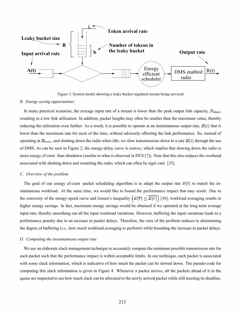
schedulerefficientEnergy
Bb
λ
A(t)radio
DMS enabled R(t)
Number of tokens inthe leaky bucket
Token arrival rate
Input arrival rate
Leaky bucket size
Output rate
Figure 3. System model showing a leaky bucket regulated stream being serviced
B. Energy saving opportunities
In many practical scenarios, the average input rate of a stream is lower than the peak output link capacity,\ 4m698 ,
resulting in a low link utilization. In addition, packet lengths may often be smaller than the maximum value, thereby
reducing the utilization even further. As a result, it is possible to operate at an instantaneous output rate,\ =LC9D that is
lower than the maximum rate for most of the time, without adversely affecting the link performance. So, instead of
operating at\ 47698 , and shutting down the radio when idle, we slow transmissions down to a rate
\ =LC9D through the use
of DMS. As can be seen in Figure 2, the energy-delay curve is convex, which implies that slowing down the radio is
more energy ef cient than shutdown (similar to what is observed in DVS [7]). Note that this also reduces the overhead
associated with shutting down and restarting the radio, which can often be signi cant [35].
C. Overview of the problem
The goal of our energy ef cient packet scheduling algorithm is to adapt the output rate\ =LC9D to match the in-
stantaneous workload. At the same time, we would like to bound the performance impact that may result. Due to
the convexity of the energy-speed curve and Jensen’s inequality rs= tuDSG v=LtuDQw [36], workload averaging results in
higher energy savings. In fact, maximum energy savings would be obtained if we operated at the long term average
input rate, thereby smoothing out all the input workload variations. However, buffering the input variations leads to a
performance penalty due to an increase in packet delays. Therefore, the crux of the problem reduces to determining
the degree of buffering (i.e., how much workload averaging to perform) while bounding the increase in packet delays.
D. Computing the instantaneous output rate
We use an elaborate slack management technique to accurately compute the minimum possible transmission rate for
each packet such that the performance impact is within acceptable limits. In our technique, each packet is associated
with some slack information, which is indicative of how much the packet can be slowed down. The pseudo-code for
computing this slack information is given in Figure 4. Whenever a packet arrives, all the packets ahead of it in the
queue are inspected to see how much slack can be allocated to the newly arrived packet while still meeting its deadline.
7
213

Procedure COMPUTE SLACK/* Executes whenever a new packet arrives.
* The packet is at the xyz position in the queue. +-| denotes the
* length of the ycz packet, and | denotes the slack associated with
* it. ~n ,*. ||& is the remaining transmission time of the packet
* currently being transmitted, ~ ye@ is its time of completion,
* and ~ is the current time. and ,*.10 denote the deadline,
* and maximum output rate, respectively. 8 is the time required
* to transmit all the packets in the queue and all the available
* slack. */if (radio is currently idle)QN1ee
;else QN1ee Y@7 v
;¡¢ O;£ ¥¤ ! ¢§¦¨©ª ¬« ¡ @@®°¯ ±²³/´Fµ « ¶N1ee ;
if ( £¸·¹ ) /* We can tolerate more slack for */¡º¢ © ¹ £ N¯>»7N1¼ ; /* the newly arrived packet */
else½ #¾
; /* We need to delete slack */¿ £ ¹ ; /* from preceding packets */
while ( ¿À ) if ( ¡9ÁSÂÿ )
¡9Á ¡9Á ¿ ;¿ O;Ä
else¿ ¿ ¡ Á ;¡ Á O
;½ ½ ÆÅ;ÄÄÄÄ
Figure 4. Pseudo-code for computing the slack associated with a newly arrived packet
In certain cases, slack might have to be deleted from preceding packets in the queue to ensure that the newly arrived
packet meets its deadline. The slack deletion proceeds in reverse order of packet arrival to retain maximum e xibility
in rate-adaptation. The packet is then tagged with this available slack information. Thus, every packet, , in the queue
has a certain slack, Ç , associated with it.
The slack information is used in the actual rate computation algorithm itself. The output rate computation for a
packet is done when it reaches the head of the queue. We can safely utilize all the slack associated with the Head Of
Line (HOL) packet while guaranteeing the in-time transmission of all the packets currently in the queue. However,
this slack does not account for future packet arrivals. If we use all the available slack for transmitting the HOL packet,
and a burst of packets arrive immediately after transmission has begun, it is quite possible that some of the packets in
the burst will miss their deadlines even if we switch to maximum speed immediately after the current transmission.
8
214

Therefore, we need to set an additional contraint on the amount of slack that can be utilized, to guarantee deadline
satisfaction for the worst case pattern of future packet arrivals. The worst case arrival pattern is a burst that drains the
leaky bucket completely. Under this arrival pattern, the amount of slack ( Ç ) that can be utilized for the HOL packet,
while guaranteeing no deadline misses in the future, is bounded by:
ÇG Z ' \ 47698ÈMÉ[7M xÊ %ÌË 3k (6)
where [ is the number of tokens currently in the leaky bucket, Í is the number of packets in the queue, and 35 is the
length of the bÏÎ packet in the queue.Z
and\ 47698 denote the deadline and the maximum output rate, respectively.
Obviously, the other constraint on the amount of usable slack is ( ÇGÐÇ Ë ), where Ç Ë is the total available slack for
the HOL packet. Any slack distribution approach that satis es these two constraints can be used to allocate slack to
the HOL packet. We have used a slack distribution approach that tries to perform as much workload averaging as
possible, since averaging reduces energy consumption, as mentioned earlier. After a certain amount of slack has been
used to compute the output rate,\
, to transmit the HOL packet, the queue status has to be updated. The pseudo-code
of our rate computation and slack updation algorithms is given in Figure 5.
E. Setting the output link speed
Although the maximum output link rate is\ 4m6Ñ8 , the instantaneous required rate by the input stream is
\. This
means that if (\ÓÒI\ 4m6Ñ8 ), packet transmissions can be slowed down to just meet the instantaneous requirement, thus
saving energy. The new modulation level for the outgoing packet is given by:
[&el bÏ69lbÏ69lÔXÕQÖ \\ 4m6Ñ8 ' [Ñ47698 (7)
F. Packet delay bound
To quantify the impact of our scheme on packet latencies, we introduce a new parameter × , which indicates the
maximum latency hit that the input stream is willing to tolerate in exchange for energy ef cienc y. As we will see
shortly, × determines the system’s response to workload variations, by deciding the degree of buffering.
De nition 1: We de ne × to be the additional latency that packets of the input stream are willing to tolerate, compared
to a scheduling scheme where the radio always operates at the maximum rate.
A x ed rate scheduling scheme would always transmit at the maximum rate\ 47698 . Using properties of the leaky
bucket mechanism, it can be shown [31] that such a scheme provides a packet delay bound of Ø ,*.¶0 . Therefore, from
the de nition of × , the maximum delay of a packet under the energy ef cient scheduling scheme described in Figure
4 and Figure 5, is given by: Z GÐÙ ;\ 4m6Ñ8 JÚ×Û (8)
where ; is the leaky bucket size, and\ 47698 is the maximum output link capacity (i.e., at a modulation level [&4m6Ñ8 ).
9
215

Procedure COMPUTE TRANSMISSION RATE/* Executes whenever the HOL packet begins transmission.
* There are x packets in the queue. +¬| denotes the
* length of the yz packet, and | denotes the
* slack associated with it. denotes the transmission
* rate of the HOL packet. and ,*.¶0 denote the
* deadline and maximum output rate, respectively. */ » O;
for (½ OÝÜ ½ · ¾Ü ½ «Ã« )
» Á » N1¼ ¯ !OÞeßàÞeßáâ Þ!ÞeßàÞeßáÑã â Þä Þå ;if (» Á À » )» » Á ;Ä¡ ª ¨ ¯Ãæ ²³´Xµ² Æźç
;if r ¡HÀ r ¹ ¯»7è9¼ êéë ! ¢e¦¨/ª wBw¡ r ¹ ¯>» N1¼S êéë ! ¢e¦¨/ª w ;» » N1¼ ¯ â áâ áFä ;Ä
Procedure UPDATE SLACK INFORMATION/* Executes whenever the HOL packet begins transmission.
* There are x packets in the queue. is the transmission
* rate of the HOL packet. ~ is the current time, and ~ ye@* is when the HOL packet will finish transmission. +¬| and* | are the length, and slack associated with the yz packet,
* respectively. */ @ O « â á² ;ª ¨m ª ± ;¡ ¨7 ¡ ¨5 ¡ « ¡ ± ;for ( ì ÉÝÜ ìoí O¾BÜ ì «Ã« )
ª î ± ª ;¡ Ïî ± ¡ ;ľ^#¾ï ÆÅ;Ä
Figure 5. Pseudo-code for computing the transmission rate of the HOL packet, and updating slack information
G. Analyzing the system’s response
We next analyze the system’s response to a change in workload to highlight the effect of × . Let the input rate of the
stream be equal to\ Õ¶ð§ñ . If we set the output rate to be equal to
\ Õ¶ðñ , then the queue soon reaches a steady state, and
the number of packets in the queue remains constant. Let the system be at such a steady state at time C , and the number
of packets in the queue be òa=LC1D . In this state, any packet that arrives, sees exactly òÌ=LC9DNM d packets ahead of it in the
queue, each of length, say 3 . All these packets (including the one that just arrived) have to complete transmission
within a time × (since the worst case arrival pattern of future packets is potentially a burst of size ; ). Therefore, the
10
216

Rold
RnewLow ∆
High ∆
Rout (t) for high
Rout (t) for low∆
∆
Figure 6. The effect of ó on the output rate
output rate,\ ÕQÖb9=LC9D is given by: \ ÕQÖb =LC1Dk òÌ=LC9D ' 3× \ ÕQð§ñ (9)
Now, let the input rate increase abruptly to\ lÔXô . We want to analyze how fast the system stabilizes to its new steady
state. After a time õC , the number of packets in the queue becomes:
òa=LCaJÚõC9D5öòa=LC1DoJ \ lÔXô M \ ÕQÖb =LC1D3 ' õC (10)
The new output rate will be given by\ ÕQÖb9=LC JõC1D , which after some simple substitutions, can be written as:
\ ÕXÖb =LCaJÚõC9D5 \ ÕQÖb =LC1D J \ lÔXô÷M \ ÕQÖbÑ=LC9D× ' õC (11)
Therefore, the rate at which the output rate changes is given by:
õ \ ÕQÖbõC d× ' = \ lÔXô÷M \ ÕQÖbÑ=LC1D1D (12)
Solving this differential equation, and applying the initial condition\ ÕQÖbÑ=LC9D5 \ Õ¶ðñ , we get:
\ ÕQÖb9=LC1Dk \ lÔXôêJø= \ Õ¶ðñ M \ lÔXôèD '÷ùaú yû (13)
The evolution of\ ÕQÖbÑ=LC1D is shown in Figure 6. Therefore, it can be concluded that × is the time constant of the
rst-order input response of the system. A high value of × means that the system takes longer to switch to the new
steady state, which implies that steep workload transients are ltered out. While this increases the energy savings, the
maximum impact on packet delay also increases (see Equation (8)). On the other hand, a low value of × means that
the system is sensitive to changes in the input rate, and performs less workload averaging. This reduces the energy
savings, but also results in a smaller impact on packet delays. The best choice of × thus depends on the allowable
delay, and the input rate variability. Another way of explaining the effect of × is to consider the scheduler as a low
pass lter performing some workload ltering on the input traf c. Then, × is inversely proportional to the bandwidth
of the low pass lter . If × is high, the low pass lter has a very low passband, and hence permits only very low
frequency workload transients to pass through.
11
217

H. Handling multiple input streams: Next, we consider a WFQ based scheduling model, and show how the algorithm described in the previous sub-
sections can be extended to the case where multiple input streams are multiplexed onto a single output transmission
link of maximum capacity . Our enhanced scheduling technique, which we call f> , can be used either for
multiple streams sharing a point-to-point link, or for multiple streams destined to different one-hop neighbors of a
wireless node (e.g., a base station sending data to multiple clients). Each input stream is regulated by a leaky bucket
with parameters =@;WQA&:FD . Therefore, stream produces packets at an average rate of : . The average rate at which
packets arrive at the scheduler is :ê !É" % : , where is the total number of streams sharing the output link. Stream is allocated a weight , which leads to a corresponding guaranteed rate, .Taking advantage of the o w isolation property of WFQ, we can treat each input stream independently, and compute
its instantaneous rate requirement. The algorithm presented in Figures 4 and 5 still holds, with\ 47698 being replaced
by , the guaranteed rate of stream . At time C , if\ ÕXÖb@ü ¶=LC9D is the output rate for stream , as computed by our
algorithm, the instantaneous required rate (\
) of the entire system is obtained by summing the output rate over all the
streams. It is given by: \ "Ê % \ ÕQÖb@ü 1=LC9D (14)
If is the maximum output link capacity, the modulation level for outgoing packets is then computed using the
following equation:
[&el bÏ69lbÏ69lÔXÕQÖ \ ' [Ñ47698 (15)
I. Delay guarantee provided by ý WFQ
Through the choice of the parameter × , our scheduling scheme provides the following delay bound for packets.
Theorem 2: The maximum delay of a packet of stream , under the WFQ scheduling scheme is given by:
Zvþ GÿÙ Z JI×fJ 3547698 4kcl ÛhGÿÙ ;W JÚ×J 3547698 4kcl Û (16)
where m4kcl is the output link capacity at a modulation level [&4mel .
As before, increasing the parameter × increases the maximum packet latency incurred by the input streams, while
decreasing the energy consumption due to increased workload averaging.
IV. SIMULATION RESULTS
We have carried out a number of simulations to evaluate our techniques. In the following subsections, we describe
our simulation framework, and present our results.
12
218

0.1 0.2 0.3 0.4 0.5 0.6 0.7 0.8 0.9 10
0.1
0.2
0.3
0.4
0.5
0.6
0.7
0.8
0.9
1
Link utilization
Nor
mal
ized
ene
rgy
cons
umpt
ion
Figure 7. Normalized energy consumption as a function of link utilization
A. Simulation framework
To evaluate the performance of our algorithm, we built a discrete event simulator using PARSEC [37], a C based
parallel simulation language. We considered a leaky bucket regulated input stream being serviced by an energy
ef cient scheduler connected to an output link of capacity = 500 Kbit/s The maximum packet size was set to be = 1000 bits, and the stream was leaky bucket constrained with a maximum burstiness parameter = bits
(corresponding to a maximum burst size of 100 packets). For our values, was equal to 0.2 seconds. The average
rate of the input was varied to change the link utilization. As explained in the previous section, the choice of offers
a tradeoff between energy savings and queuing delay. Unless explicitly speci ed, all the experiments used a value of
seconds. Finally, when multiple input streams are present, our scheme does not require to be a global
parameter. Each stream can choose a different value of , depending on the packet delays acceptable to it.
B. Discussion of the results
Figure 7 shows the energy consumed by our algorithm, normalized against the energy consumed by an energy
unaware scheme, for varying values of output link utilization. This curve was generated with no burstiness present
in the input traf c and packet lengths all set to 1000 bits, although we show later that any burstiness in the input
traf c does not affect our scheme. As expected, the energy consumption decreases as the link utilization drops. Our
algorithm reduces to a x ed speed algorithm at a utilization of one, since there are no opportunities for slowing
down. Figure 8 shows the effect of input traf c burstiness on the performance of our algorithm. As can be seen in
Figure 8(a), the energy savings obtained through our scheme are independent of the burstiness of the input traf c.
By explicitly incorporating information about the state of the leaky bucket during rate adaptation, our scheme is able
to offer signi cant energy savings even for highly bursty traf c. Figure 8(b) plots the resulting packet delays as a
13
219

1 2 3 4 5 6 7 8 9 100.12
0.122
0.124
0.126
0.128
0.13
0.132
0.134
0.136
0.138
0.14
Average burst size (packets)
Nor
mal
ized
ene
rgy
cons
umpt
ion
1 2 3 4 5 6 7 8 9 100.1
0.12
0.14
0.16
0.18
0.2
0.22
0.24
0.26
0.28
0.3
Average burst size (packets)
Pac
ket d
elay
(se
cond
s)
Average delayMaximum delayDeadline
(a) (b)
Figure 8. (a) Normalized energy consumption as a function of input burstiness, and (b) Packet delays as a function of burstiness
0
0.1
0.2
0.3
0.4
0.5
0.6
0.7
0.8
0.025 0.05 0.075 0.1 0.125 0.15 0.175 0.2
Delta (seconds)
No
rmal
ized
en
erg
y co
nsu
mp
tio
n
00.050.10.150.20.250.30.350.40.45
Del
ay (
seco
nd
s)
Normalized energy Average delay
Maximum delay Deadline
Figure 9. Normalized energy consumption, and average and maximum packet delays , as a function of function of the input traf c burstiness. As expected, when the burstiness increases, both the maximum and average
packet delays also increase. However, note that all packets complete transmission before their deadlines, thereby
avoiding any timing violations in the system. Figures 7 and 8 show that the use of our scheduling scheme decreases
the energy consumption of the system by up to a factor of 10X, with a small, bounded increase in packet latency.
As was mentioned in Section III, the parameter determines the amount of buffering that our scheme performs.
Therefore, can be used as a control knob to adjust the operating point on an energy-latency tradeoff curve. We
performed an additional experiment to demonstrate the effect of the parameter , where we observed the energy
consumption and packet delays, as was varied. The results are shown in Figure 9. Increasing increases the
14
220
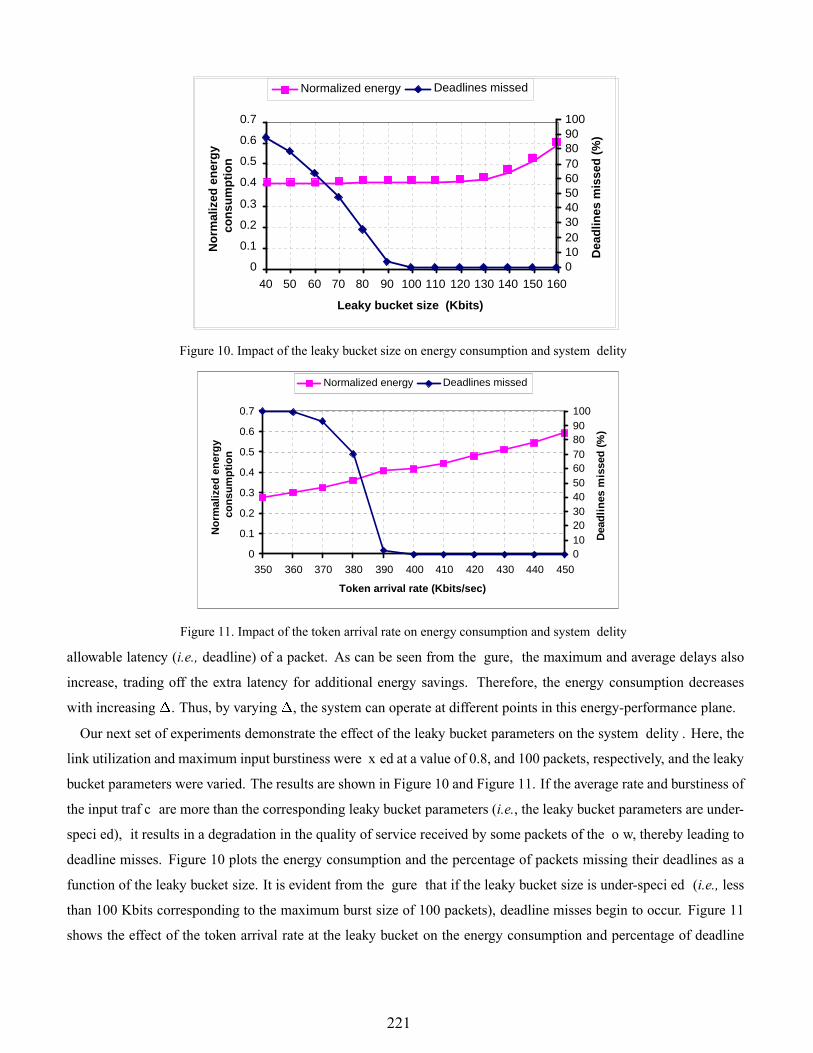
0
0.1
0.2
0.3
0.4
0.5
0.6
0.7
40 50 60 70 80 90 100 110 120 130 140 150 160
Leaky bucket size (Kbits)
No
rmal
ized
en
erg
y co
nsu
mp
tio
n
0102030405060708090100
Dea
dlin
es m
isse
d (
%)
Normalized energy Deadlines missed
Figure 10. Impact of the leaky bucket size on energy consumption and system delity
0
0.1
0.2
0.3
0.4
0.5
0.6
0.7
350 360 370 380 390 400 410 420 430 440 450
Token arrival rate (Kbits/sec)
No
rmal
ized
en
erg
y co
nsu
mp
tio
n
0102030405060708090100
Dea
dli
nes
mis
sed
(%
)
Normalized energy Deadlines missed
Figure 11. Impact of the token arrival rate on energy consumption and system delity
allowable latency (i.e., deadline) of a packet. As can be seen from the gure, the maximum and average delays also
increase, trading off the extra latency for additional energy savings. Therefore, the energy consumption decreases
with increasing . Thus, by varying , the system can operate at different points in this energy-performance plane.
Our next set of experiments demonstrate the effect of the leaky bucket parameters on the system delity . Here, the
link utilization and maximum input burstiness were x ed at a value of 0.8, and 100 packets, respectively, and the leaky
bucket parameters were varied. The results are shown in Figure 10 and Figure 11. If the average rate and burstiness of
the input traf c are more than the corresponding leaky bucket parameters (i.e., the leaky bucket parameters are under-
speci ed), it results in a degradation in the quality of service received by some packets of the o w, thereby leading to
deadline misses. Figure 10 plots the energy consumption and the percentage of packets missing their deadlines as a
function of the leaky bucket size. It is evident from the gure that if the leaky bucket size is under-speci ed (i.e., less
than 100 Kbits corresponding to the maximum burst size of 100 packets), deadline misses begin to occur. Figure 11
shows the effect of the token arrival rate at the leaky bucket on the energy consumption and percentage of deadline
15
221

2 4 6 8 100.12
0.14
0.16
0.18
0.2
0.22
0.24
0.26
0.28
0.3
Average burst size (packets)
Nor
mal
ized
ene
rgy
cons
umpt
ion
ρ = 250 Kb/secρ = 300 Kb/secρ = 350 Kb/secρ = 400 Kb/sec
Figure 12. Effect of input burstiness on the energy consumption for different values of token arrival rate
misses. Again, at token arrival rates that are lower than the average input rate of 400 Kbits/sec (corresponding to a link
utilization of 0.8), the leaky bucket chokes the input stream, resulting in a large number of deadline misses. Finally,
Figure 12 shows the impact of input traf c burstiness on the energy consumption of our scheme, for different values
of the leaky bucket token arrival rate. The average input rate was set to 250 Kbits/sec, resulting in a link utilization of
0.5. As can be seen in the gure, when the token rate is correctly speci ed, our scheme is not impacted by burstiness
in the input traf c. However, if the token rate is under-speci ed, the energy consumption of the system increases
with increasing burstiness. These curves highlight the importance of correctly setting the leaky bucket parameters, if
high system delity is required. In real networks, input traf c streams pay for the network resources according to the
quality of service they desire, and the traf c description that they provide up front to the network service provider.
The network provider polices the incoming traf c using a leaky bucket with parameters set according to the traf c
description, and enforces the speci cations if traf c sources misbehave and deviate from agreed behavior. Therefore,
either the source of the input traf c or the network service provider should accurately estimate the statistics of the
input traf c, which can then be used to set the leaky bucket parameters accordingly. Further, for increased energy
scalability, the leaky bucket parameters can be deliberately tweaked to result in a gradual decrease in system delity
as the system’s energy supply runs out.
Our nal set of experiments involved comparing the performance of our scheme, ! #" with unmodi ed WFQ.
For this purpose, we considered a scenario where two input streams (henceforth referred to as Flow 1 and Flow 2)
shared an output link of capacity 500 Kbps. The o ws were allocated weights in the ratio 2:3, leading to guaranteed
rates of 200 Kbps and 300 Kbps, respectively. Figures 13(a) and 13(b) plot the throughput received by the two o ws as
well as the aggregate throughput, as a function of time, using WFQ and ! #" , respectively. Initially, the o ws do
not require their maximum guaranteed bandwidth, and hence are allocated only so much as they currently require. As
16
222

0 20 40 60 800.5
1
1.5
2
2.5
3
3.5
4
4.5
5x 10
5
Time (seconds)
Th
rou
gh
pu
t re
ceiv
ed (
bp
s)WFQ
Flow 1 Flow 2 Aggregate Input rates
0 20 40 60 800.5
1
1.5
2
2.5
3
3.5
4
4.5
5x 10
5 E2WFQ
Time (seconds)
Th
rou
gh
pu
t re
ceiv
ed (
bp
s)
Flow 1 Flow 2 Aggregate Input rates
(a) (b)
Figure 13. Throughput received by Flow 1 and Flow 2 using (a) WFQ, and (b) $&%('*)&+ . The two gures are identical,indicating that $,%-'*)&+ does not affect the throughput allocation (and hence, fairness) of WFQ.
can be seen from the gure, the throughput allocation obtained by using . /" is identical to that obtained using
WFQ. This shows that our scheme retains the fairness property of WFQ. Figure 14 plots the energy consumption of
the ! #" system over 1 second intervals, normalized to the case when WFQ is used. As can be seen, our scheme
results in signi cant reductions in energy consumption compared to the WFQ case. The curve labelled Ideal denotes
the normalized energy consumption that would have resulted if the system had just one input o w with utilization
equal to the aggregate utilization of Flow 1 and Flow 2. Note that ! #" performs almost as well as the single o w
case, which indicates that our scheme is able to distribute the energy bene ts obtained due to the low link utilization
of one o w, among the other o ws while still maintaining o w isolation for throughput purposes.
V. CONCLUSIONS
In wireless embedded systems, communication energy is increasingly becoming the dominant component of total
energy consumption. Dynamic power management techniques therefore, should also address communication subsys-
tems such as radios, as opposed to only computation subsystems such as embedded processors. DMS is a technique
that offers a power-speed control knob for the radio, and can thus be used for communication power management.
However, higher level techniques are needed that can exploit this control knob to enable system level energy-latency
tradeoffs. In this paper, we have targeted the packet scheduling process and investigated avenues for making it energy
aware. We have presented an energy ef cient packet scheduling algorithm for leaky bucket regulated traf c streams,
which provides signi cant energy savings (up to a factor of 10X) with only a small, bounded increase in worst case
packet delay. We have extended our scheme to a multiple input stream scenario, and have enhanced the Weighted
Fair Queuing algorithm for energy ef cienc y. Our techniques nd applicability for medium and long range wireless
17
223

0 20 40 60 800.1
0.2
0.3
0.4
0.5
0.6
0.7
0.8
0.9
1
Time (seconds)
No
rmal
ized
en
erg
y co
nsu
mp
tio
n
E2WFQIdeal
Figure 14. Normalized energy consumption of $&%-'*)&+communication systems (such as wireless LANs), where DMS is effective in reducing energy consumption, due to
the radio’s RF power dominating the power consumed in the radio electronics. We believe that our work is a rst
step towards the percolation of the more mature computation power management techniques into the communications
realm.
References[1] J. Rabaey and M. Pedram, Low Power Design Methodologies. Kluwer Academic Publishers, Norwell, MA, 1996.[2] A. Raghunathan, N. K. Jha, and S. Dey, High-level Power Analysis and Optimization. Kluwer Academic Publishers,
Norwell, MA, 1998.[3] L. Benini and G. De Micheli, Dynamic Power Management: Design Techniques and CAD Tools. Kluwer Academic Pub-
lishers, Norwell, MA, 1997.[4] A. P. Chandrakasan and R. W. Brodersen, Low Power CMOS Digital Design. Kluwer Academic Publishers, Norwell, MA,
1996.[5] V. Raghunathan, C. Schurgers, S. Park, and M. B. Srivastava, “Energy aware wireless microsensor networks”, IEEE Signal
Processing Magazine, vol. 19, iss. 2, pp. 40–50, March 2002.[6] Rockwell Inc. (http://wins.rsc.rockwell.com)[7] T. A. Pering, T. D. Burd, and R. W. Brodersen, “The simulation and evaluation of dynamic voltage scaling algorithms”,
Proc. ACM ISLPED, pp. 76–81, 1998.[8] C. Schurgers, O. Aberthorne, and M. B. Srivastava, “Modulation scaling for energy aware communication systems”, Proc.
ACM ISLPED, pp. 96–99, 2001.[9] The Internet Traf c Archive (http://ita.ee.lbl.gov).[10] A. Demers, S. Keshav, and S. Shenker, “Analysis and simulation of a fair queueing algorthm”, Internet Res. and Exper.,
vol. 1, 1990.[11] V. Raghunathan, S. Ganeriwal, C. Schurgers, and M. B. Srivastava, “ $&%('*)&+ : An energy ef cient fair scheduling policy
for wireless systems”, Proc. ACM ISLPED, pp. 30–35, 2002.[12] C. Schurgers, V. Raghunathan, and M. B. Srivastava, “Modulation scaling for real-time energy-aware packet scheduling”,
Proc. IEEE GLOBECOM, pp. 3653–3657, 2001.[13] M. Weiser, B. Welch, A. Demers, and S. Shenker, “Scheduling for reduced CPU energy”, Proc. First Symp. on OSDI, pp.
13–23, 1994.[14] K. Govil, E. Chan, and H. Wasserman, “Comparing algorithms for dynamic speed-setting of a low-power CPU”, Proc. ACM
MOBICOM, pp. 13–25, 1995.
18
224

[15] T. Ishihara and H. Yasuura, “Voltage scheduling problem for dynamically variable voltage processors, Proc. ACMISLPED, pp. 197–202, 1998.
[16] I. Hong, M. Potkonjak, and M. B. Srivastava, “On-line scheduling of hard real-time tasks on variable voltage processors”,Proc. IEEE ICCAD, pp. 653–656, 1998.
[17] Y. Shin and K. Choi, “Power conscious x ed priority scheduling for hard real-time systems”, Proc. ACM DAC, pp. 134–139,1999.
[18] V. Raghunathan, P. Spanos, and M. B. Srivastava, “Adaptive power- delity in energy-aware wireless systems”, Proc. IEEERTSS, pp. 106–115, 2001.
[19] P. Pillai and K. G. Shin, “Real-time dynamic voltage scaling for low power embedded operating systems”, Proc. SOSP, pp.89–102, 2001.
[20] F. Gruian, “Hard real-time scheduling for low energy using stochastic data and DVS processors”, Proc. ACM ISLPED, pp.46–51, 2001.
[21] B. Prabhakar, E. U. Biyikoglu, and A. El Gamal, “Energy-ef cient transmission over a wireless link via lazy packet schedul-ing”, Proc. IEEE INFOCOM, pp. 386–394, 2001.
[22] A. El Gamal, C. Nair, B. Prabhakar, E. U. Biyikoglu, and S. Zahedi, “Energy-ef cient scheduling of packet transmissionsover wireless networks”, Proc. IEEE INFOCOM, pp. 1773–1782, 2002.
[23] R. Min and A. P. Chandrakasan, “A framework for energy scalable communication in high-density wireless networks”,Proc. ACM ISLPED, pp. 36–41, 2002.
[24] M. Shreedhar and G. Varghese, “Ef cient fair queueing using de cit round robin”, Proc. IEEE SIGCOMM, pp. 231–242,1995.
[25] P Goyal, H. M. Vin, and H. Cheng, “Start-time fair queuing: A scheduling algorithm for integrated servicespacket switchingnetworks”, Proc. IEEE SIGCOMM, pp. 157–168, 1996.
[26] J. C. R. Bennett and H. Zhang, “W )0% Q : Worst-case fair weighted fair queueing, Proc. IEEE INFOCOM, pp. 120–128,1996.
[27] P. Lin, B. Bensaou, Q. L. Ding, and K. C. Chua, “A wireless fair scheduling algorithm for error-prone wireless channels”,Proc. ACM WoWMOM, pp. 11–20, 2000.
[28] S. Lu, V. Bharghavan, and R. Srikant, “Fair scheduling in wireless packet networks”, Proc. IEEE SIGCOMM, pp. 63–74,1997.
[29] P. Ramanathan and P. Agrawal, “Adapting packet fair queueing algorithms to wireless networks”, Proc. ACM MOBICOM,pp. 1–9, 1998.
[30] S. Keshav, An Engineering Approach to Computer Networking: ATM Networks, the Internet, and the Telephone Network.Addison-Wesley, 1997.
[31] A. K. Parekh and R. G. Gallager, “A generalized processor sharing approach to o w control in integrated services networks:The single-node case”, IEEE Trans. on Networking, vol. 1, no. 3, pp. 344-357, June 1993.
[32] K. M. Sivalingam, M. Srivastava, P. Agrawal, and J. C. Chen, “Low power access protocols based on scheduling for wirelessand mobile ATM networks”, Proc. IEEE Universal Personal Communications Conference, pp. 420–433, 1997.
[33] J. G. Proakis, Digital Communications. McGraw Hill, 1989.[34] K. Cho and H. Samueli, “A 8.75-MBaud Single-Chip Digital QAM Modulator with Frequency-Agility and Beamforming
Diversity”, Proc. IEEE Custom Integrated Circuits Conference, pp. 27–30, 2000.[35] A. Y. Wang, S. H. Cho, C. G. Sodini, and A. P. Chandrakasan, “Energy ef cient modulation and MAC for asymmetric RF
microsensor systems”, Proc. ACM ISLPED, pp. 106–111, 2001.[36] J. L. W. V. Jensen, “Sur les fonctions convexes et les ingalits entre les valeurs moyennes”, Acta Math., vol. 30, pp. 175–193,
1906.[37] PARSEC parallel simulation language (http://pcl.cs.ucla.edu/projects/parsec)
19
225