Inter-American Development Bank

Banco Interamericano de Desarrollo Latin American Research Network Red de Centros de Investigación

Research Network Working Paper #R-498

Poverty, Health Infrastructure and the Nutrition of Peruvian Children

by

Martín Valdivia

Grupo de Análisis para el Desarrollo (GRADE)

March 2004

2

Abstract1

After the Peruvian economic crisis of the late 1980s, the 1990s witnessed a significant pro-poor expansion of the country’s health infrastructure that was instrumental in increasing preventive and primary health care expenditures. Using empirical evidence, this paper discusses the effect of this expansion in health infrastructure on child nutrition in Peru, as measured by the height-for-age z-score. Using a pooled sample from the 1992, 1996 and 2000 rounds of the Peruvian DHS, this analysis controls for biases in the allocation of public investments by using a district fixed effects model. The econometric analysis finds a positive albeit small effect of the expansion of the last decade. After desegregating by type of location, however, the effect was found to be significant only in urban areas. Furthermore, the effect is highly nonlinear and has a pro-poor bias. The estimated coefficient for health infrastructure in less endowed districts is 10 times higher than that in the better-endowed districts. The pro-poor bias refers to the fact that the estimated effect is larger for children of less educated mothers. In this sense, this policy seems to have had a pro-poor bias within urban areas, while at the same time excluding the rural population, a traditionally marginalized population group in Peru. These findings support the idea that reducing distance and waiting time barriers may be necessary, but that more explicitly inclusive policies are required to improve the health of the rural poor, especially indigenous groups, so that they can escape this kind of poverty trap.

1 This paper has benefited from comments by Jere Behrman, Vincent David, Emmanuel Skoufias and all participants at IDB seminars in Puebla, Mexico (October, 2003) and Washington, DC (February, 2004). The author also acknowledges excellent research assistance by Gianmarco León. Any remaining errors are the author’s.

3

1. Introduction High poverty and inequality are still striking features of Peruvian society even after occasional

periods of expansion such as the one experienced during the past decade (1993-97). As of the

year 2000, more than half the Peruvian population remained under the poverty line, with that rate

rising up to two-thirds in rural areas.

During the 1990s, economic growth did lead to significant increases in public health

expenditures, which were mainly allocated to preventive and primary health care for children and

mothers in reproductive age, and to the expansion and enhancement of public health

infrastructure.2 Many average mother-child health indicators showed a significant improvement

in Peru during that time. For instance, the infant mortality rate, which was 76 per thousand live

births in 1986, decreased by more than half by the year 2000.3 Nevertheless, the reduction in

chronic malnutrition rates for children under five was negligible in comparison. According to the

Peruvian Demographic and Health Survey (DHS), chronic malnutrition rates fell only slightly,

from 33 percent in 1992 to 29 percent in 2000. Even more striking is the fact that chronic

malnutrition inequalities over the socio-economic ladder—already already the largest among

child health indicators—increased during that period. The poor-rich deciles ratio was 11.4 in

1992 and 15.4 in 2000.4 That is, by the year 2000, the chronic malnutrition rate among children

in the poorest decile was 15 times higher than that among children in the richest one.5

It seems that the factors that helped reduce mortality rates over the past decade were not

also able to help reduce the persistently high nutritional risk faced by Peruvian children,

especially those poor families. Such inequalities demonstrate the need for studies that can help

elucidate the factors behind the continually high nutritional risk faced by Peruvian children, and

also identify ways to better help public programs or policies to reduce the problem. This is

particularly crucial when considering the vast international evidence on the negative effect that

2 See Cotlear (2000). 3 See Valdivia and Mesinas 2002. Access to reproductive health services by poor women also improved significantly during that period. 4 Valdivia and Mesinas (2002) are able to estimate health inequalities by economic status through the construction of two proxies for household living standards, one based on household long-term wealth (Filmer and Pritchett 2001) and a second that uses information on household assets and per capita expenditures from the 1997 and 2000 rounds of the LSMS to predict household per capita expenditures for the DHS samples. Section 3 below provides more information on the methodologies used there.

4

nutritional deprivation during pregnancy and the first two or three years of life has on a child’s

future performance in school and in the labor market (see, for instance, Behrman, 2000). One of

the reasons these early periods are so important is because the sensitivity of child growth to

deprivation is proportional to the velocity of growth under normal conditions, which is extremely

high in the early years (see Tanner, 1966). Obviously, adverse growth effects due to short-term

mild nutritional deprivation may be overcome in the future through catch-up growth or even an

extension of the growing period (Steckel, 1995), but prolonged and severe deprivation during

those early years does lead to a reduction in adult size.

The other side of the coin is that early childhood interventions stand a very good chance of

breaking the vicious poverty cycle caused by the intergenerational transmission of poverty.

Within the epidemiological literature, the INCAP longitudinal study in rural Guatemala shows

that supplementation via a nutritious beverage increases child height and reduces severe stunting

if provided during a child’s first three years of life. Moreover, nutritional improvements help

reduce mortality and improve cognitive development. Within the socioeconomic literature, the

PIDI study in urban Bolivia estimates that a preschool program that meets 70 percent of a child’s

nutritional needs and provides improved learning environments can affect child growth and have

a significant impact on child psychosocial development. Behrman et al. (2004) use their own

estimates on child growth and cognition, as well as estimates on the effect of height, schooling

and cognition on wages from the literature, to estimate the costs and benefits of this early

intervention. They find that benefits largely outweigh costs when all effects are considered,

underlining the important synergies between health, nutrition and education—within and

between life cycle stages—that that help determine an individual’s productivity.

Much of this recent literature uses experimental designs to estimate the short- and long-run

impacts of specific interventions (programs) on child growth and the resulting performance in

school and the labor market. In Peru, though, no longitudinal study is yet available that would

allow for exploration of the long-term implications of the nutritional status of Peruvian children

on health, cognition or education. Also, no significant intervention program is being

implemented that includes randomization of treatment and control groups so that a proper

5 The chronic malnutrition rate for children of the poorest quintile in 2000 was 54 percent. Malnutrition rates for both groups, poorest and richest quintiles, fell during the period but the reduction was higher in the richest quintile.

5

estimation of its impact can be obtained. Any understanding of the subject, therefore, must rely

on the vast literature that explores the relationship between a child’s nutritional status and

family/environmental characteristics based on the estimation of reduced-form equations. Several

articles have reviewed this literature, and they emphasize the importance of the mother’s human

capital, household income and sanitary infrastructure in determining the nutritional status of

children.6 In the Peruvian context, Valdivia (2002) explores the determinants of nutritional status

for Peruvian children using both the 1996 round of the Peruvian Demographic and Health Survey

(DHS) and the 1997 round of the Peruvian Living Standards Measurements Survey (LSMS). As

expected, child’s characteristics such as gender and age are very important as well as mother’s

human capital, household income, the dwelling’s sanitary infrastructure and the level of poverty

in the district. The results are very similar in both samples, although in the case of the DHS, the

analysis included controls for the mother’s anthropometrics. Using a random effects model to

control for household- and district-level unobservables, household wealth proxies ended up

playing the largest role in explaining health inequalities along the economic ladder, even after

including the most common controls.7

This paper explores the effect of large public investments in health infrastructure made

over the past decade in Peru on the chronic nutrition of children under five, as measured by the

height-for-age z-score. Height-for-age is generally used as a measure of long-term nutritional

status, but it is also an effective measure here given the size and length of the expansion, and the

fact that the focus is on children under five, an age at which they are particularly sensitive to any

type of deprivation. There are several ways through which such an expansion may have affected

child growth. First, it could have facilitated the use of professional health care (regular check-

ups, follow-up consultations or emergency treatments ), by reducing the travel time mothers take

to reach the health facility (distance barrier), or by reducing the time they have to wait to see the

doctor, get the results of requested tests, etc. (waiting time barrier). Second, by putting a health

facility in a locality that did not previously have one, thus improving the delivery of social

services run by the MoH, such as vaccinations campaigns, food supplementation programs, and

other health-related extramural campaigns or activities.

6 See, for instance, Behrman and Deolalikar (1988) and Strauss and Thomas (1998). 7 See note 3 to learn about the two income or expenditure proxies that were used in the referred study.

6

The empirical analysis is based on amerger of the 1992, 1996 and 2000 databases of the

health infrastructure census with those of the 1992, 1996 and 2000 rounds of the DHS. It is

important to note that such policies can hardly be analyzed in the context of an experimental

design. Instead, a district-level fixed effects model was used to control for district-level

unobservables and for biases associated with government rules regarding the allocation of public

resources (see Rosenzweig and Wolpin, 1986).

This paper is organized into five sections, including this introduction. Section 2 discusses

the mechanisms that could link investments in health infrastructure with child nutrition and

presents the conceptual model and the econometric considerations used in the estimation of the

corresponding model. Section 3 describes the datasets used for the empirical analysis and

presents some of the relevant patterns of child nutrition and the use of public health facilities.

Section 4 presents the results of the analysis, with a special emphasis on the differentiated effect

across households’ and mothers’ characteristics. Finally, Section 5 concludes with a summary of

findings and a discussion of implications for policy action and the research agenda.

2. Conceptual Framework and Methodology The mechanisms by which an expansion/enhancement of public health infrastructure could

helped the growth of poor children include not only a reduction in commuting time to receive

health care, but also the enhanced organization of public health and nutritional programs to reach

the poorest, especially in remote rural areas.8 Focusing on children under five years of age makes

sense since they are more sensitive to any type of deprivation during their first years (Tanner,

1966).

In general, the availability of sanitary infrastructure reduces the costs of the household

production of child health. In the case of sanitary infrastructure, the presence of a water and sewage

pipe network in the locality makes it easier for households to install their connection at home, which

also makes it easier to adopt better sanitary practices and generate a safer environment for their

children’s growth. Clearly, the realization of these effects depends on the availability of economic

resources and on a knowledge of the safest sanitary practices.

8 It is important to indicate that all these new and/or improved facilities were run by the Ministry of Health (MoH), which also ran relatively large health and nutritional programs for poor children and their mothers (see Valdivia, 2003).

7

In the case of health infrastructure, it is clear that a convenient health facility makes it cheaper

for a household to obtain health care for its children whenever necessary. Obviously, this effect is

destined to be more important in remote rural areas, but it also requires that the child’s caregiver

properly identify the need for professional care. Lack of proper sanitary education may reduce the

magnitude of this effect for the less educated, although the opposite occurs when one considers that

a health facility also plays a role in facilitating the organization of public programs that transmit

sanitary information as well as food baskets to mothers and children. Obviously, buildings by

themselves would not imply any environmental improvements for the health of individuals;

human and physical resources are needed to make them work.

In what follows, the model considered for the analysis is described and the methodology

used in the estimation of the effect of health infrastructure on child nutrition—as measured by

the z-score of height-for-age—is discussed. First, it is necessary to describe the way health

affects individual and household decisions. This analysis is based on a static household model

with constrained maximization of a joint utility function, following the framework initiated by

Becker (1981). It is assumed that a household with n members is run by the household head who

maximizes a utility function (U), which depends on the consumption, health and leisure of all

members,9

; ) 1, 2,...,i i iiU = U(C ,h , Z i nl = (1)

where

n1,2,..., = i 1 ),...,C,...,C(C=C iJ

ij

ii

i.e., Ci is a J dimensional vector, with elements corresponding to a commodity group, hi denotes

the health status, and li denotes the leisure of member i. It is assumed that the utility function is

continuous, strictly increasing, strictly quasi-concave and twice-continuously differentiable in all its

arguments. Also, it satisfies the Inada condition, i.e., the marginal utility ∞→xU as 0→x , for iii lhcx ,,= , for all i.

The health status of each household member is determined by a general production

function, h .

9 This is equivalent to assuming that household members have identical preferences and that a dictator rules the household—i.e., a unitary household model. Assuming bargaining to explain intra-household allocations complicates the

8

, , , , , , = 1,2,...,i

i i i ii iii ih = h ( , , Z X Z F u u ) i nC lY

−− − (2)

where Yi denotes the consumption of health-related inputs by individual i, Zi denotes the member’s

observed characteristics, such as age and gender. F denotes the availability of sanitary and/or health

infrastructure in the community, and u denotes the vector of unobserved characteristics. Also, X-i

denotes the consumption, health and leisure of the other members of the family, and Z-i, and u-i

denote their vectors of observed and unobserved individual characteristics, respectively. The

specific variables that appear in the health production change if the i-th member is an adult, a child

or an infant. For instance, in a child’s health production function, milk consumption and education

of the parents are important components of Ci and Z-i, respectively, although they would probably

not be important in an adult’s health production function. Since adults tend to take care of

themselves, only their education would matter. In the case of children, the set of unobservable

characteristics may include the mother’s and family’s unobservable characteristics as well as the

health/nutritional status of the child in its earlier years, such as its weight at birth.

Continuing with the description of the model, it is also assumed that households face a full

income constraint, which is derived from the time and income constraints,

∑ ∑ ∑ ∑∑∑+==

=+=++K

Jk i i i

iiikk

J

j i

ijj SVwTwlYpcp

11

(3)

where (P) represents price, (V) is non-labor income, (W) is the wage rate, (Ta) is the total time

available of the adult members, and (S) is the full income. Non-labor income (V) includes net profits

of any home enterprise, as well as other rents.

The reduced-form health demand function for children would have the following form:10

* , , , Z , ; Z , i i i i iC Yh = h (P P S F u u )− − (4)

Although the conditional demand functions have standard properties, the same is not true

for the reduced-form demand equations in (4). The key point is that consumption affects health,

too, and substitution effects may attenuate some of the direct effects. For instance, Pitt and

results without providing additional insights for the goals of this paper, considering that asset tenancy or decision power are not individualized in the LSMS questionnaire. 10 The health production functions are assumed to be twice-continuously differentiable, strictly increasing, and strictly concave in all arguments. The constraint set formed by (2), and the full income constraint (3) are convex and the

9

Rosenzweig (1986) mention that a decrease in the price of health services Py or an improvement

in sanitary or house infrastructure F could generate a substitution in consumption patterns that

can reinforce or attenuate the positive health effects of such changes. Consequently, nothing

conclusive can be said about the effect of prices, or even sanitary infrastructure, upon health

status, before an econometric estimation. However, this paper seeks to estimate precisely this net

effect of household adjustments in relation to the availability of sanitary and health

infrastructure.

The specific variables to be used in the model are the following: Zi is the child’s age and

gender are included; f Z-I is the mother’s schooling and height; S is the household’s wealth, proxied

by the asset index. The asset index is based on Filmer and Pritchett (1999) and is generated using

a principal components technique on household asset tenancy available in all three round of the

DHS; F is proxied by the availability of sanitary (drinking water, electricity and sewage) and health

infrastructure in the district. The health infrastructure index, obtained from a set of variables that

included the number of public health facilities and doctors available in the district, is used.

The empirical model under estimation is the following:

ijtjjtijtjtjtijtijtijtijt FZFFSZZh ευδγγβαα +++++++= 2222

11

22

11 (5)

where hijt is a continuous variable that takes the value of the height-for-age z-score for the

individual i, who resides in district j, and who was interviewed in period t; Fjt denotes the

availablity of infrastructure in district j during period t; and jυ denotes the district j fixed effect.

The key issue here is to try to estimate 2γ and δ , that is, the effect of district health

infrastructure and its interaction with the mother’s human capital. One problem that arises is the

fact that the distribution of the health infrastructure is not random, but follows an optimization

process outlined by the government. Such optimization may imply a systematic bias of that

distribution in favor of either the poorer or richer districts, depending on the relative prevalence

of altruistic motives or the weight of interest groups (Rosenzweig and Wolpin, 1986). Such bias

would, in turn, lead to a biased estimation of the parameters of interest under a pooled regression

in the presence of unobservable district and individual characteristics. If health infrastructure has

optimization of (1) yields a unique solution. Assuming that the health production function satisfies the Inada condition, the solution is guaranteed to be interior.

10

a pro-rich (pro-poor) bias, then the income effect under a pooled regression will be biased

upwards (downwards).

The optimal procedure would be to control for individual unobservable characteristics by

estimating a fixed effects model with longitudinal data because individuals would use the district

information to decide on their utilization of health care. The limitation of the DHS sample is that

it consists of only three cross-sectional datasets, wherein each individual can be observed only

once. Nevertheless, it is possible to partially control for the referred bias by estimating a model

with district-level fixed effects. One advantage is the fact that several of those units were

observed three times, in 1992, 1996 and in the year 2000. That is why the terms in expression (5)

have three subscripts instead of two.

Clearly, it is important to identify whether the effect of the availability of health

infrastructure is the same in urban and rural areas, and whether it has some nonlinearities or

varies with the characteristics of the child, mother or household. That is why interaction terms

are included in expression (5), with special emphasis on the schooling of the mother.

Finally, the question of how to measure the availability of health infrastructure in each

district arises, considering that several factors play a role and that buildings by themselves would

not make a difference. One can try to include all the relevant variables (number of facilities,

doctors, availability of medicines or equipment for tests, etc) to see their separate effect on health

or nutrition of individuals, but it is usually hard to disentangle such effects since these variables

tend to be highly correlated. An alternative is to construct a single indicator that summarize the

changes in health infrastructure in one district. That is accomplished here by constructing a

health infrastructure index based on a principal component analysis of the number of public

health facilities and doctors in public facilities in each district in the three rounds of the census.11

The estimation of the first principal component was done with the whole sample of districts,

which was then merged with the DHS individual data set in order to avoid sampling biases.

11 The census information is by facility but the data had to be collapsed to the district level because it is the maximum level of aggregation for which the INEI reports a unique national code. It would have been better to be able to use community-level data but that will need to be postponed for future research after constructing a national code for localities.

11

3. Analyzing the Data As indicated above, the empirical analysis presented here is based on the combination of

household level data (from the 1992, 1996 and 2000 rounds of the DHS) and census data on

health infrastructure (1992, 1996 and 1999). Several previous papers have used the DHS

database to analyze the size and magnitude of nutritional inequalities by income status or type of

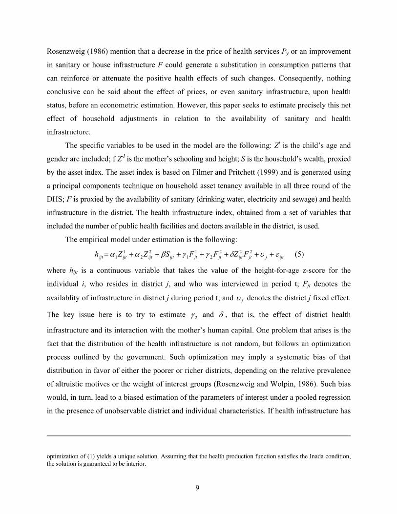
location in Peru (see Valdivia, 2002). In Figure 1, the z-score for height-for-age is disaggregated

by age in months, ethnic background and type of place of residence. Several interesting features

appear. First, the growth retardation occurring among Peruvian children clearly increases with

age, but seems to be significantly sharper among rural children and those from families with an

indigenous background.12

These differences are very important for the purposes of this study because they tend to be

closely related to the lack of access to health services by these population groups. Studies

emphasizing the non-monetary reasons individuals are unable to use these services focus on the

time required to reach the health center (distance barrier) and the waiting time for consultation,

as well as some cultural barriers. Cultural barriers are particularly important in rural areas and

relate to differences in the way ethnic groups understand health and illness, and/or the presence

of discriminatory practices in the provision of health services.13 They are often expressed in the

form of distrust of health professionals and complaints about mistreatment.

12 For this study, a child is defined as having an indigenous ethnic background if the main language spoken at home is not Spanish but another native language. It is clear that such a variable is not an indicator of racial background, but of closedness to certain cultural beliefs and practices as well as lack of proper modern education. 13 See Torres 2001.

12

Figure 1. Height-for-Age and the Age of the Child

by ethnic background urban/rural

-3

-2.5

-2

-1.5

-1

-0.5

0

0.5

0 10 20 30 40 50 60

Age in months

HA

Z

Spanish as home language Other home language

-3

-2.5

-2

-1.5

-1

-0.5

0

0.5

0 10 20 30 40 50 60Age in months

HA

Z

Urban Rural

Source: 2000 DHS.

13

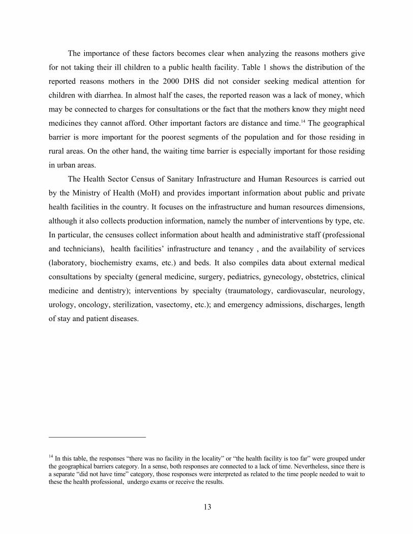
The importance of these factors becomes clear when analyzing the reasons mothers give

for not taking their ill children to a public health facility. Table 1 shows the distribution of the

reported reasons mothers in the 2000 DHS did not consider seeking medical attention for

children with diarrhea. In almost half the cases, the reported reason was a lack of money, which

may be connected to charges for consultations or the fact that the mothers know they might need

medicines they cannot afford. Other important factors are distance and time.14 The geographical

barrier is more important for the poorest segments of the population and for those residing in

rural areas. On the other hand, the waiting time barrier is especially important for those residing

in urban areas.

The Health Sector Census of Sanitary Infrastructure and Human Resources is carried out

by the Ministry of Health (MoH) and provides important information about public and private

health facilities in the country. It focuses on the infrastructure and human resources dimensions,

although it also collects production information, namely the number of interventions by type, etc.

In particular, the censuses collect information about health and administrative staff (professional

and technicians), health facilities’ infrastructure and tenancy , and the availability of services

(laboratory, biochemistry exams, etc.) and beds. It also compiles data about external medical

consultations by specialty (general medicine, surgery, pediatrics, gynecology, obstetrics, clinical

medicine and dentistry); interventions by specialty (traumatology, cardiovascular, neurology,

urology, oncology, sterilization, vasectomy, etc.); and emergency admissions, discharges, length

of stay and patient diseases.

14 In this table, the responses “there was no facility in the locality” or “the health facility is too far” were grouped under the geographical barriers category. In a sense, both responses are connected to a lack of time. Nevertheless, since there is a separate “did not have time” category, those responses were interpreted as related to the time people needed to wait to these the health professional, undergo exams or receive the results.

14

Table 1. Reasons for Not Attending a Public Health Facility when the Child had Diarrhea

By expend. quintile By type of location

Poorest Richest Total Rural Urban Geographical barriers 13.1 5.5 17.3 28.9 1.4 Bad attention/personnel 6.1 6.3 6.4 4.9 8.4 There is no medicine 0.9 9.3 2.4 2.9 1.6 Did not have enough money 57.7 41.6 47.5 39.9 57.9 Did not have time 14.9 15.1 14.3 10.3 19.8 Other 7.3 22.3 12.1 13.0 10.9 Total 100.0 100.0 100.0 100.0 100.0 Reported diarrhea illness rate1 18.2 11.9 15.5 15.7 15.3 No attention rate2 33.0 33.0 36.2 37.3 34.8 Did not consider it necesary3 50.0 61.3 50.9 44.4 57.6 1 All/ill in last two weeks 2 Did not receive attention/ill in last 2 weeks 3 As a proportion of children who were ill Source: 2000 DHS.

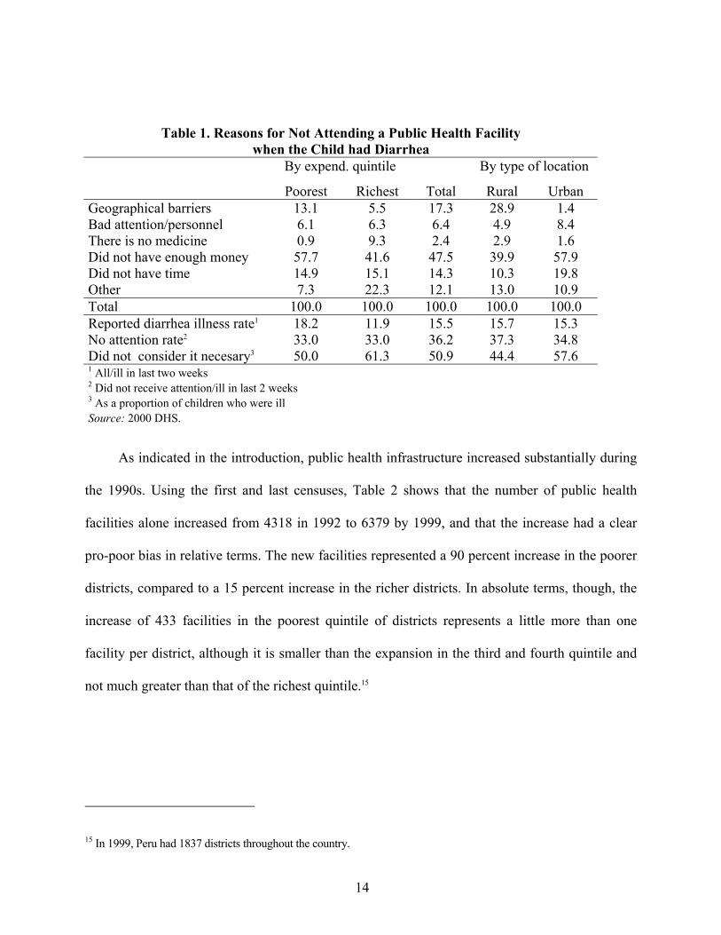
As indicated in the introduction, public health infrastructure increased substantially during

the 1990s. Using the first and last censuses, Table 2 shows that the number of public health

facilities alone increased from 4318 in 1992 to 6379 by 1999, and that the increase had a clear

pro-poor bias in relative terms. The new facilities represented a 90 percent increase in the poorer

districts, compared to a 15 percent increase in the richer districts. In absolute terms, though, the

increase of 433 facilities in the poorest quintile of districts represents a little more than one

facility per district, although it is smaller than the expansion in the third and fourth quintile and

not much greater than that of the richest quintile.15

15 In 1999, Peru had 1837 districts throughout the country.

15

Table 2. Geographical Distribution of Public Health Facilities and Doctors: Peru 1992-1999

Public health facilities District quintiles* 1992 1999 ∆ 92-99 ∆% 92-99 Q1 484 917 433 89.5 Q2 682 1182 500 73.3 Q3 828 1324 496 59.9 Q4 873 1358 485 55.6 Q5 1468 1816 348 23.7 Ratio (Q5/Q1) 3.0 2.0 Total 4335 6597 2262 52.2 Doctors in public health facilities Q1 15 360 345 2300.0 Q2 51 493 442 866.7 Q3 116 657 541 466.4 Q4 543 1298 755 139.0 Q5 11737 14073 2336 19.9 Ratio (Q5/Q1) 782.5 39.1 Total 12462 16881 4419 35.5 * Districts are ranked in quintiles according to the proportion of households

with at least one unmet basic need in 1993, an indicator reported by INEI.

Obviously, public investments in health infrastructure were not limited to building new

primary health care facilities but also to rehabilitating existing ones, improving their equipment

or hiring more health professionals. Table 2 also shows the distribution of the expansion of the

number of doctors in public health facilities, indicating that there was an increase of 35 percent

between 1992 and 1999. In absolute terms, the expansion was very pro-rich, since only 8 percent

of the increase occurred in the districts in the poorest quintile, while 53 percent occurred in the

richest one. Still, inequalities in the distribution of doctors were reduced in the sense that the

distribution of the expansion was far more pro-poor than had been the case in 1992.16

The magnitude of this expansion makes it worthwhile to analyze the kind of impact it may

have had on the health of the population, especially on children, since their health and nutrition

are relatively more sensitive to changes in the sanitary environment. Nevertheless, such an

16

analysis requires a merger of the census database with that of the DHS, which only includes a

sample of districts. Thus it becomes necessary to check the extent to which the sample is

balanced, since cost considerations may imply that the DHS sample represents the level of

poverty but not the distribution of health facilities. The number of districts in the 1992 round of

the DHS was 219 but increased to 530 in 1996 and 691 in 2000. Actually, for methodological

issues, it was necessary to restrict the econometric analysis to a sample of 368 districts that were

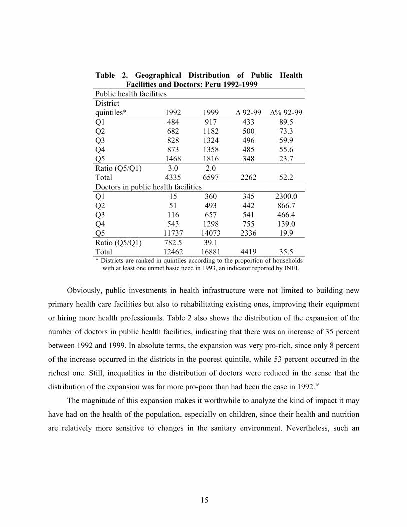
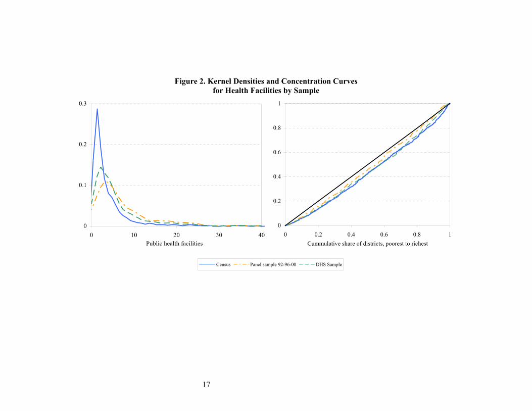
in at least two of the three DHS rounds. The left panel of Figure 2 shows the kernel densities of

the three samples and demonstrates that the 2000 DHS sample’s is bias towards districts that are

better endowed in terms of health infrastructure. The difference between the full 2000 sample

and the sub-sample for the panel of districts is relatively smaller. The right panel in Figure 2

shows the concentration curves for the three samples, showing that the differences are rather

small. The concentration index is 0.14 for the panel sample, while for all other samples it is 0.18.

The situation is similar for doctors in public facilities.

16 It is also clear that the distributional improvement was larger for the number of doctors than for the number of facilties. The rich-to-poor ratio for the former moved from 782 in 1992 to 39 in 1999, while those ratios were 3 and 2, respectively, in the case of the number of facilities.

17

Figure 2. Kernel Densities and Concentration Curves for Health Facilities by Sample

0

0.1

0.2

0.3

0 10 20 30 40Public health facilities

0

0.2

0.4

0.6

0.8

1

0 0.2 0.4 0.6 0.8 1Cummulative share of districts, poorest to richest

Census Panel sample 92-96-00 DHS Sample

18

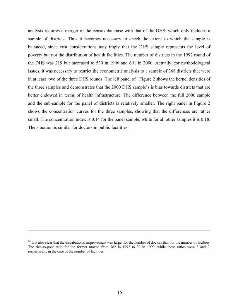
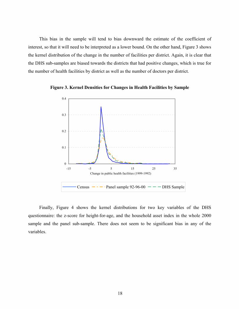
This bias in the sample will tend to bias downward the estimate of the coefficient of

interest, so that it will need to be interpreted as a lower bound. On the other hand, Figure 3 shows

the kernel distribution of the change in the number of facilities per district. Again, it is clear that

the DHS sub-samples are biased towards the districts that had positive changes, which is true for

the number of health facilities by district as well as the number of doctors per district.

Figure 3. Kernel Densities for Changes in Health Facilities by Sample

0

0.1

0.2

0.3

0.4

-15 -5 5 15 25 35Change in public health facilities (1999-1992)

Census Panel sample 92-96-00 DHS Sample

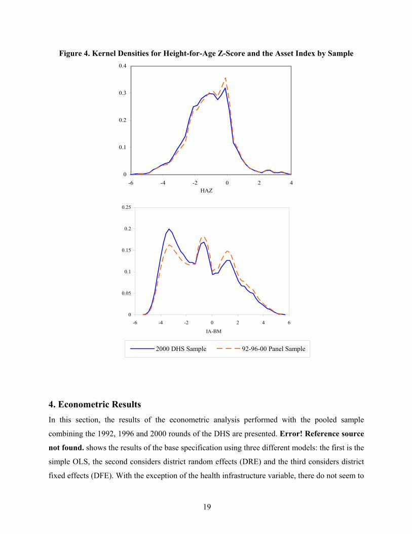
Finally, Figure 4 shows the kernel distributions for two key variables of the DHS

questionnaire: the z-score for height-for-age, and the household asset index in the whole 2000

sample and the panel sub-sample. There does not seem to be significant bias in any of the

variables.

19

Figure 4. Kernel Densities for Height-for-Age Z-Score and the Asset Index by Sample

0

0.1

0.2

0.3

0.4

-6 -4 -2 0 2 4HAZ

0

0.05

0.1

0.15

0.2

0.25

-6 -4 -2 0 2 4 6

IA-BM

2000 DHS Sample 92-96-00 Panel Sample

4. Econometric Results In this section, the results of the econometric analysis performed with the pooled sample

combining the 1992, 1996 and 2000 rounds of the DHS are presented. Error! Reference source

not found. shows the results of the base specification using three different models: the first is the

simple OLS, the second considers district random effects (DRE) and the third considers district

fixed effects (DFE). With the exception of the health infrastructure variable, there do not seem to

20

be major differences between the three econometric specifications; therefore, the following

section first discusses the results of the model with DFE for all the controls considered, and then

compares the coefficients for the health infrastructure variable with the three models.17

In terms of child’s characteristics, age is included through four dichotomical variables

identifying children by years of age, with the ommited variable being for children over four years

(48 months) old. The largest positive coefficient corresponds to the child’s first year, but it

decreases substantially afterward. This finding is consistent with the trend observed in Figure 1,

whereby Peruvian children do not seem to be born significantly underweight, but tend to lose

height in comparison to international standards as time passes, especially during the first two

years. The gender coefficient suggests that male children tend to be shorter than their female

counterparts.

In terms of the mother’s characteristics, schooling and height are included. Mother’s

schooling is included through a set of three dummy variables that indicate her level of education,

with the omitted variable being “no education.” Mothers with only primary education do not

seem to have an impact on child health compared to mothers with no education at all, but further

education does have a positive, increasing and significant effect. A child whose mother has

secondary education is taller by 0.16 standard deviations (SD) than a child whose mother has less

education. The estimated effect of higher education is even larger, with children being 0.38 SD

taller. The height of the mother also appears as strongly significant. With the standardized score

included, a mother 1 SD taller tends to have children taller by 0.3 SD.

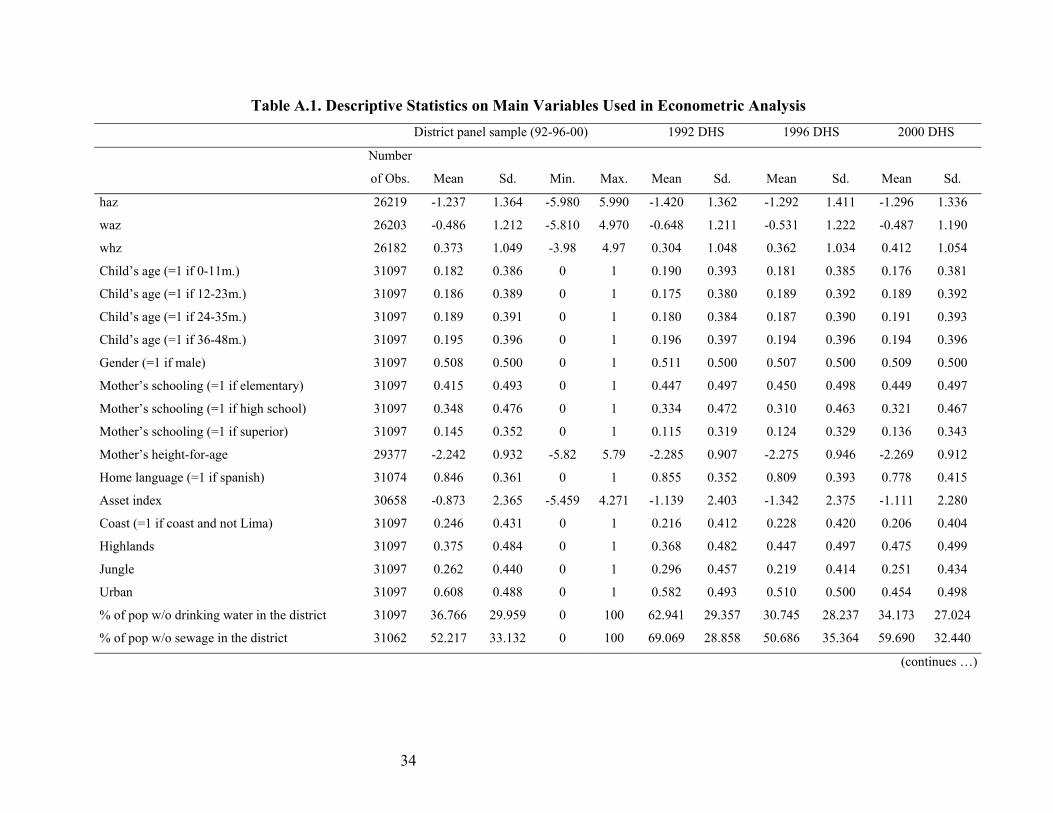
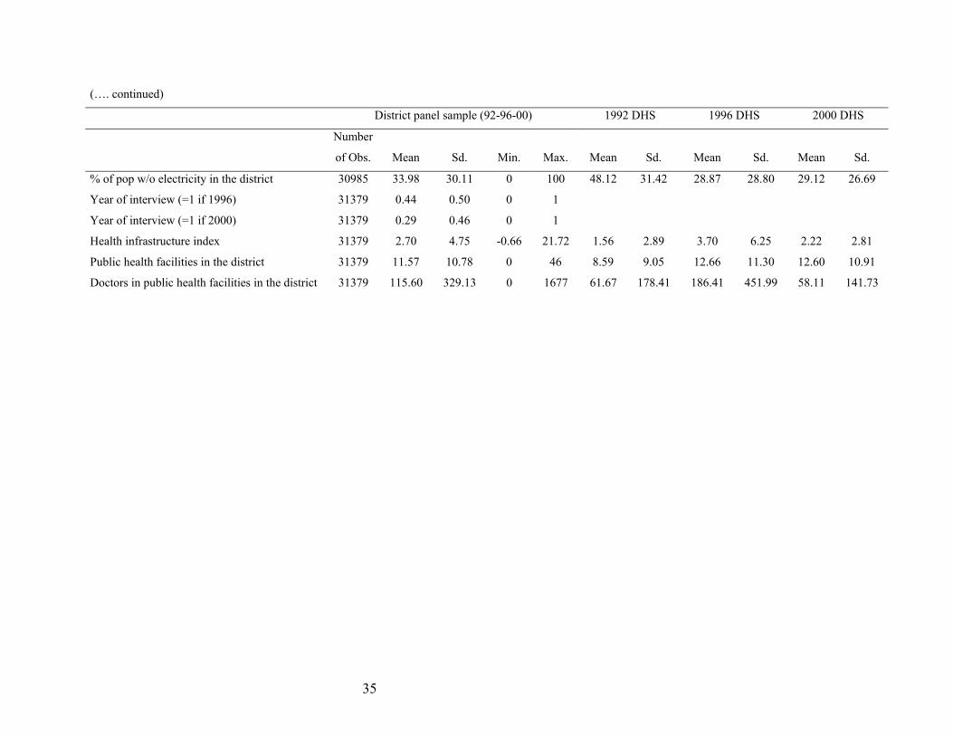
17 Table A.1 in the Appendix shows basic statistics of the variables used in the econometric analysis.

21

Table 3. Determinants of Height-for-Age, with and without District Random and Fixed Effects

(absolute value of t statistics in parentheses)

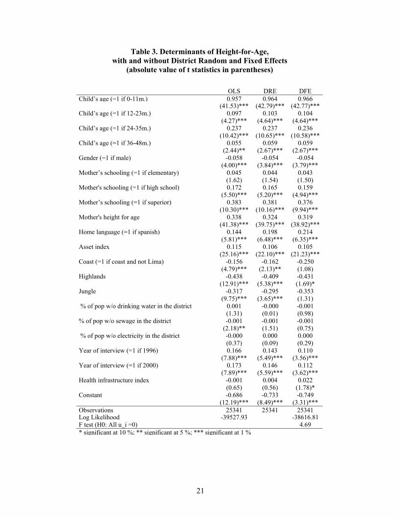
OLS DRE DFE Child’s age (=1 if 0-11m.) 0.957 0.964 0.966 (41.53)*** (42.79)*** (42.77)*** Child’s age (=1 if 12-23m.) 0.097 0.103 0.104 (4.27)*** (4.64)*** (4.64)*** Child’s age (=1 if 24-35m.) 0.237 0.237 0.236 (10.42)*** (10.65)*** (10.58)*** Child’s age (=1 if 36-48m.) 0.055 0.059 0.059 (2.44)** (2.67)*** (2.67)*** Gender (=1 if male) -0.058 -0.054 -0.054 (4.00)*** (3.84)*** (3.79)*** Mother’s schooling (=1 if elementary) 0.045 0.044 0.043 (1.62) (1.54) (1.50) Mother's schooling (=1 if high school) 0.172 0.165 0.159 (5.50)*** (5.20)*** (4.94)*** Mother’s schooling (=1 if superior) 0.383 0.381 0.376 (10.30)*** (10.16)*** (9.94)*** Mother's height for age 0.338 0.324 0.319 (41.38)*** (39.75)*** (38.92)*** Home language (=1 if spanish) 0.144 0.198 0.214 (5.81)*** (6.48)*** (6.35)*** Asset index 0.115 0.106 0.105 (25.16)*** (22.10)*** (21.23)*** Coast (=1 if coast and not Lima) -0.156 -0.162 -0.250 (4.79)*** (2.13)** (1.08) Highlands -0.438 -0.409 -0.431 (12.91)*** (5.38)*** (1.69)* Jungle -0.317 -0.295 -0.353 (9.75)*** (3.65)*** (1.31) % of pop w/o drinking water in the district 0.001 -0.000 -0.001 (1.31) (0.01) (0.98) % of pop w/o sewage in the district -0.001 -0.001 -0.001 (2.18)** (1.51) (0.75) % of pop w/o electricity in the district -0.000 0.000 0.000 (0.37) (0.09) (0.29) Year of interview (=1 if 1996) 0.166 0.143 0.110 (7.88)*** (5.49)*** (3.56)*** Year of interview (=1 if 2000) 0.173 0.146 0.112 (7.89)*** (5.59)*** (3.62)*** Health infrastructure index -0.001 0.004 0.022 (0.65) (0.56) (1.78)* Constant -0.686 -0.733 -0.749 (12.19)*** (8.49)*** (3.31)*** Observations 25341 25341 25341 Log Likelihood -39527.93 -38616.81 F test (H0: All u_i =0) 4.69 * significant at 10 %; ** significant at 5 %; *** significant at 1 %

22

These results are consistent with the previous literature in that the child’s growth is

strongly determined by his/her mother’s characteristics, in what is an important mechanism for

the intergenerational transmission of poverty. The inclusion of her schooling is the most

important control, but the DHS database allows for the addition of her height.18 The schooling

variable suggests the importance of increasing health and sanitary education for mothers with

low schooling, while the height variable points towards the importance of providing nutritional

supplements to mothers during pregnancy. Both are interventions that could attenuate this

vicious circle of poverty.

In terms of other household characteristics, the asset index (proxy of household wealth)

and home language (proxy of their ethnic background) have been included. Both variables are

found to have a significant effect. A household that is 1 SD wealthier tends to have children that

are 0.1 SD taller. In the case of home language, a household that mainly speaks Spanish tends to

have taller children by 0.2 SD, which is significant considering that the model already controls

for the education of the mother and the economic status of the household.

Not all contextual variables have a significant effect on the nutritional status of children.

Children who live in the highlands, for example, tend to have a lower nutritional status, but those

residing in the coast or jungle do not. Other variables that do not appear to be significant are

those related to the lack of available drinking water, sewage and electricity in the district. The

coefficients for the year effects suggest that 1992 was a particularly bad year, which is consistent

with the huge economic crisis of the late 1980s and early 1990s in Peru.

Available health infrastructure does, however, have a positive, albeit small, effect upon

child height, significant at 10 percent. A child raised in a district with 1 SD more in the health

infrastructure index tends to be 0.02 SD taller. It is important to note that the effect estimated

with the OLS and DRE specifications is smaller and not significant. This finding suggests that

fixed district unobservable characteristics tend to underestimate the nutritional effect of the

availability of health infrastructure in the district.

As indicated previously, this result suggests that putting health facilities closer to children

makes it easier for their families to bear the costs of searching for professional medical care. In

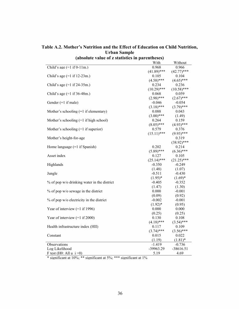
18 Table A.2 in the Appendix shows that the omission of the mother’s height tends to overestimate the effect of her schooling, confirming previous findings in the literature.

23

addition, public health facilities facilitate public programs run by the MoH to better reach

children in remote rural areas. However, it is important to review the robustness of this result

with regard to desegregation by type of location (urban/rural) in Table 4.

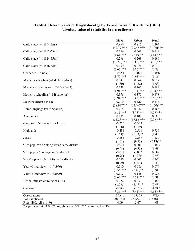
Separately analyzing the determinants of height-for-age of children from urban and rural

areas, results in significant differences in terms of child and contextual variables but not in terms

of household variables. First, the age effect seems to be even more pronounced in rural areas,

and in that sense it may be an indication of some unobserved environmental conditions that

affect the growth of children in rural areas. Second, the gender bias against males is only

significant for children in urban areas.

The year effects and the health infrastructure variable also differ between urban and rural

areas. Both are found to be positive and significant in urban areas but not in rural areas. That is,

after controlling for child, household characteristics and availability of infrastructure, the

economic growth of the 1990s does have an extra effect on urban children but not on rural

children. This result is consistent with previous findings that suggest that rural areas were mostly

excluded from the growth path of the past decade.

With respect to health infrastructure, there are at least two plausible explanations. On the

one hand, although health facilities augmented in the poorer districts, they still tend to locate in

the capital of the district, and in that sense, likely benefit more children living in urban areas.

That is, the reduction in the distance barrier was not enough for rural children. On the other hand,

cultural factors may also explain why rural families did not benefit from the enhancement in

health infrastructure. This is particularly significant insofar as 15 percent of the rural mothers in

the sample stated that Quechua, Aymara or some other native language was their main language.

Several studies have shown that the language barrier limits the use of professional health care,

either because of differences in the way ethnic groups understand health and illness or as a result

of discriminatory practices in the provision of health services (see, for instance, Torres, 2001).

24

Table 4. Determinants of Height-for-Age by Type of Area of Residence (DFE) (absolute value of t statistics in parentheses)

Global Urban RuralChild’s age (=1 if 0-11m.) 0.966 0.815 1.204 (42.77)*** (29.67)*** (31.06)***Child’s age (=1 if 12-23m.) 0.104 0.068 0.158 (4.64)*** (2.49)** (4.14)***Child’s age (=1 if 24-35m.) 0.236 0.268 0.190 (10.58)*** (9.85)*** (4.98)***Child’s age (=1 if 36-48m.) 0.059 0.076 0.030 (2.67)*** (2.86)*** (0.78)Gender (=1 if male) -0.054 -0.071 -0.028 (3.79)*** (4.08)*** (1.16)Mother’s schooling (=1 if elementary) 0.043 0.064 0.037 (1.50) (1.22) (1.03)Mother's schooling (=1 if high school) 0.159 0.165 0.189 (4.94)*** (3.11)*** (3.94)***Mother’s schooling (=1 if superior) 0.376 0.375 0.478 (9.94)*** (6.63)*** (5.65)***Mother's height-for-age 0.319 0.320 0.316 (38.92)*** (32.46)*** (21.60)***Home language (=1 if Spanish) 0.214 0.242 0.183 (6.35)*** (3.73)*** (4.03)***Asset index 0.105 0.108 0.085 (21.23)*** (18.12)*** (7.26)***Coast (=1 if coast and not Lima) -0.250 -0.367 (1.08) (1.59) Highlands -0.431 -0.561 0.726 (1.69)* (2.03)** (1.48)Jungle -0.353 -0.287 1.129 (1.31) (0.93) (2.13)**% of pop. w/o drinking water in the district -0.001 0.001 -0.003 (0.98) (0.53) (1.61)% of pop. w/o sewage in the district -0.001 -0.002 0.002 (0.75) (1.77)* (0.95)% of pop. w/o electricity in the district 0.000 0.002 -0.001 (0.29) (1.01) (0.39)Year of interview (=1 if 1996) 0.110 0.086 0.074 (3.56)*** (2.46)** (0.91)Year of interview (=1 if 2000) 0.112 0.148 0.026 (3.62)*** (4.21)*** (0.31)Health infrastructure index (HII) 0.022 0.033 -0.004 (1.78)* (2.47)** (0.09)Constant -0.749 -0.778 -1.947 (3.31)*** (3.41)*** (4.13)***Observations 25341 15558 9783Log Likelihood -38616.81 -22957.38 -15384.30F test (H0: All u_i =0) 4.69 3.67 4.03* significant at 10%; ** significant at 5%; *** significant at 1%

25

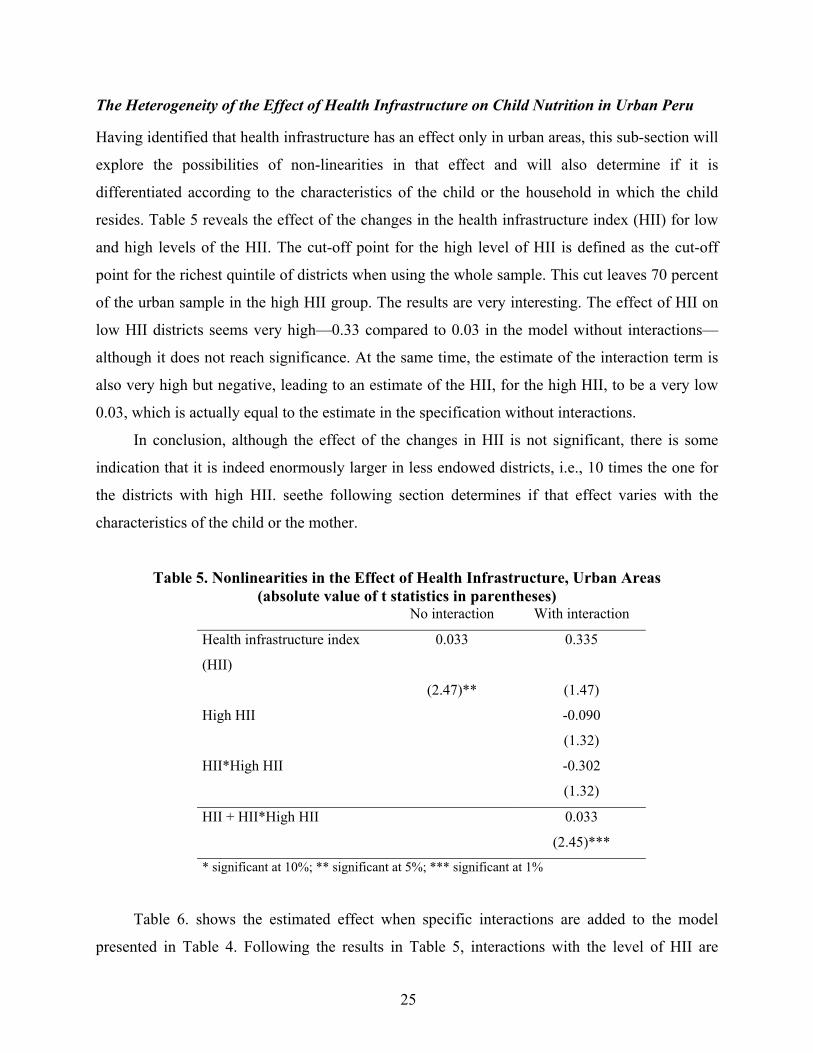
The Heterogeneity of the Effect of Health Infrastructure on Child Nutrition in Urban Peru Having identified that health infrastructure has an effect only in urban areas, this sub-section will

explore the possibilities of non-linearities in that effect and will also determine if it is

differentiated according to the characteristics of the child or the household in which the child

resides. Table 5 reveals the effect of the changes in the health infrastructure index (HII) for low

and high levels of the HII. The cut-off point for the high level of HII is defined as the cut-off

point for the richest quintile of districts when using the whole sample. This cut leaves 70 percent

of the urban sample in the high HII group. The results are very interesting. The effect of HII on

low HII districts seems very high—0.33 compared to 0.03 in the model without interactions—

although it does not reach significance. At the same time, the estimate of the interaction term is

also very high but negative, leading to an estimate of the HII, for the high HII, to be a very low

0.03, which is actually equal to the estimate in the specification without interactions.

In conclusion, although the effect of the changes in HII is not significant, there is some

indication that it is indeed enormously larger in less endowed districts, i.e., 10 times the one for

the districts with high HII. seethe following section determines if that effect varies with the

characteristics of the child or the mother.

Table 5. Nonlinearities in the Effect of Health Infrastructure, Urban Areas (absolute value of t statistics in parentheses)

No interaction With interaction

Health infrastructure index

(HII)

0.033 0.335

(2.47)** (1.47)

High HII -0.090

(1.32)

HII*High HII -0.302

(1.32)

HII + HII*High HII 0.033

(2.45)***

* significant at 10%; ** significant at 5%; *** significant at 1%

Table 6. shows the estimated effect when specific interactions are added to the model

presented in Table 4. Following the results in Table 5, interactions with the level of HII are

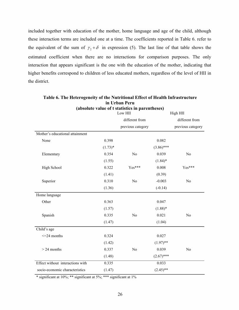
26

included together with education of the mother, home language and age of the child, although

these interaction terms are included one at a time. The coefficients reported in Table 6. refer to

the equivalent of the sum of 2γ δ+ in expression (5). The last line of that table shows the

estimated coefficient when there are no interactions for comparison purposes. The only

interaction that appears significant is the one with the education of the mother, indicating that

higher benefits correspond to children of less educated mothers, regardless of the level of HII in

the district.

Table 6. The Heterogeneity of the Nutritional Effect of Health Infrastructure in Urban Peru

(absolute value of t statistics in parentheses) Low HII High HII

different from

previous category

different from

previous category

Mother’s educational attainment

None 0.398 0.082

(1.73)* (3.86)***

Elementary 0.354 No 0.039 No

(1.55) (1.84)*

High School 0.322 Yes*** 0.008 Yes***

(1.41) (0.39)

Superior 0.310 No -0.003 No

(1.36) (-0.14)

Home language

Other 0.363 0.047

(1.57) (1.88)*

Spanish 0.335 No 0.021 No

(1.47) (1.04)

Child’s age

<=24 months 0.324 0.027

(1.42) (1.97)**

> 24 months 0.337 No 0.039 No

(1.48) (2.67)***

Effect without interactions with 0.335 0.033

socio-economic characteristics (1.47) (2.45)**

* significant at 10%; ** significant at 5%; *** significant at 1%

27

Understanding that education is highly correlated with poverty, it is possible to interpret

these results as indicating a pro-poor bias in the effect of the expansion in health infrastructure.

Along the lines of the Rosenzweig-Schultz matrix, as reported in Barrera (1990), it is clear that

the expansion of health infrastructure favors the provision of health information and the

subsidization of health inputs. In that sense, the reported evidence suggests the importance of

mother’s education in terms of lowering the costs of information and increasing the value of

time. That is, the expansion has a pro-poor bias because it helps provide information that benefits

the uneducated relatively more than the educated. The pro-poor bias can also be explained by the

fact that health facilities help offer food supplementation programs, but they require mothers’

time, either to attend required check-ups or to participate in the delivery itself.

In summary, the pro-poor bias obtained for the urban sample in this empirical analysis

underscores the importance of increasing extramural activities that can be facilitated by new or

enhanced health facilities, and reducing its effect in terms of facilitating access to intramural

health services, such as consultations. Nevertheless, it is important to recall that no significant

effect was found in rural areas.

5. Summary and Final Remarks After the Peruvian economic crisis of the late 1980s, the 1990s witnessed a significant pro-poor

expansion of the country’s health infrastructure that was instrumental in increasing preventive

and primary health care expenditures. . Between 1992 and 1999, the number of public health

facilities increased by 52 percent, while the number of doctors increased by 35 percent. These

increments were concentrated relatively in the poorer districts, however, so that the final

distribution in 1999 was significantly more pro-poor than the initial one in1992.

This paper presents empirical evidence on the effect of this expansion in health

infrastructure upon child nutrition in Peru, as measured by the height-for-age z-score. For that

purpose, a pooled sample from the 1992, 1996 and 2000 rounds of the Peruvian DHS was

merged with the Census of Health Infrastructure in 1992, 1996 and 1999. An analysis of the pool

sample from the DHS, finds that sample to be representative of the socio-economic conditions of

households and children, while showing a significant bias towards the districts better endowed in

terms of health infrastructure, and also towards those that had a positive change in health

28

infrastructure. The first-sample bias tends to bias the coefficient of interest downwards, so that

its estimate can be interpreted as a lower bound for the true coefficient.

The econometric analysis is based on a model with district-level fixed effects, which

allows for the control of biases in the allocation of public investments. There was a positive,

albeit small, effect of the health care expansion of the last decade. Desegregating by type of

location, though, the effect was found to be significant only in urban areas. Furthermore, the

effect is highly nonlinear and has a pro-poor bias. The estimated coefficient for health

infrastructure in less endowed districts is 10 times as high as that in the better-endowed districts.

The pro-poor bias refers to the fact that the estimated effect is larger for children of less educated

mothers. In this sense, this policy seems to have had a pro-poor bias within urban areas, while at

the same time excluding the rural population, a traditionally marginalized population group in

Peru.

These findings support the idea that reducing distance and waiting time barriers may be

necessary, but that more explicitly inclusive policies are required to improve the health of the

rural poor, especially indigenous groups, to help them escape this kind of poverty trap. Also, the

pro-poor bias found in urban areas indicates the relatively higher importance of increasing

extramural activities compared to reducing the time required by mothers seeking medical care

for their children.

29

References

Barrera, A. 1990. “The Role of Maternal Schooling and its Interaction with Public Health

Programs in Child Health Production.” Journal of Development Economics 32: 69-91.

Becker, G. 1981. A Treatise on the Family. (Revised and enlarged in 1991). Cambridge, United

States: Harvard University Press.

Behrman, J. R., Y. Cheng, and P. Todd. 2004 “Evaluating Preschool Programs when Length of

Exposure to the Program Varies: A Nonparametric Approach.” Review of Economics and

Statistics 86 (1): 108-132.

Behrman, J. 2000. “Literature Review on Interactions between Health, Education and Nutrition

and the Potential Benefits of Intervening Simultaneously in All Three.” Washington, DC,

United States: International Food Policy Research Institute.

Behrman, J.R. and A.B. Deolalikar. 1988. “Health and Nutrition.” In: H. B. Chenery and T.N.

Srinivasan, editors. Handbook on Economic Development. Volume 1. Amsterdam, The

Netherlands. North-Holland.

Cotlear, D. 2000. “Peru: Reforming Health Care for the Poor.” Human Development Department

LCSHD Paper Series 57. Washington, DC, United States: World Bank.

Filmer, D., and L.H. Pritchett. 1999. “The Effect of Household Wealth on Educational

Attainment: Evidence from 35 Countries.” Population and Development Review 25(1):

85-120.

----. 2001. “Estimating Wealth Effects without Expenditure Data—or Tears: An Application to

Educational Enrollments in States of India.” Demography 38(1):115-132.

Pitt, M., and M. Rosenzweig. 1986. “Agricultural Prices, Food Consumption and the Health and

Productivity of Indonesian farmers.” In: I. Singh, L. Squire, and J. Strauss, editors.

Agricultural Household Models: Extensions, Applications and Policy, Washington, DC,

United States: World Bank.

Rosenzweig, M., and K. Wolpin. 1986. “Evaluating the Effects of Optimally Distributed Public

Programs: Child Health and Family Planning Interventions.” American Economic Review

76(3).

Steckel, R. 1995. “Stature and the Standard of Living.” Journal of Economic Literature 33: 1903-

40.

30

Strauss, J.; and D. Thomas. 1998. “Health, Nutrition and Economic Development.” Journal of

Economic Literature 36(2): 766-817.

Tanner, J.M. 1966. “Growth and Physique in Different Populations of Mankind.” In P. Baker, and

J. S. Weiner, editors. The Biology of Human Adaptability.. Oxford: Oxford University

Press, 45-66.

Torres, C. 2001. “Etnicidad y Salud: Otra Perspectiva para Alcanzar la Equidad.” In: PAHO.

“Equidad en Salud: Una Mirada desde la Perspectiva de la Equidad.” Washington, DC,

United States: Pan American Health Organization (PAHO) Public Policy and Health

Program, Division of Health and Human Development. Washington D.C.

Valdivia, M. 2002. “Acerca de la magnitude de la inequidad en salud en el Perú.” Documento de

Trabajo 37. Lima, Peru: Grupo de Análisis para el Desarrollo (GRADE).

Valdivia, M., and J. Mesinas. 2002. “Evolución de la Equidad en Salud Materno-Infantil en el

Perú: 1986-2000.” INEI-Macro Inc. International, December.

31

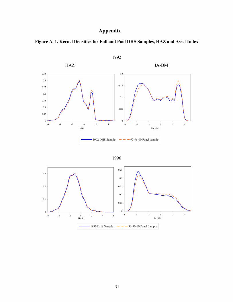
Appendix

Figure A. 1. Kernel Densities for Full and Pool DHS Samples, HAZ and Asset Index

1992

HAZ IA-BM

0

0.05

0.1

0.15

0.2

0.25

0.3

0.35

-6 -4 -2 0 2 4HAZ

0

0.05

0.1

0.15

0.2

-6 -4 -2 0 2 4IA-BM

1992 DHS Sample 92-96-00 Panel sample

1996

0

0.1

0.2

0.3

-6 -4 -2 0 2 4 6HAZ

0

0.05

0.1

0.15

0.2

0.25

-6 -4 -2 0 2 4IA-BM

1996 DHS Sample 92-96-00 Panel Sample

32

2000

0

0.1

0.2

0.3

0.4

-6 -4 -2 0 2 4HAZ

0

0.05

0.1

0.15

0.2

0.25

-6 -4 -2 0 2 4 6

IA-BM

2000 DHS Sample 92-96-00 Panel Sample

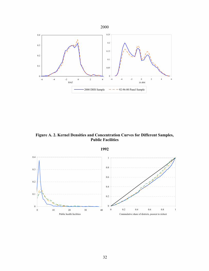
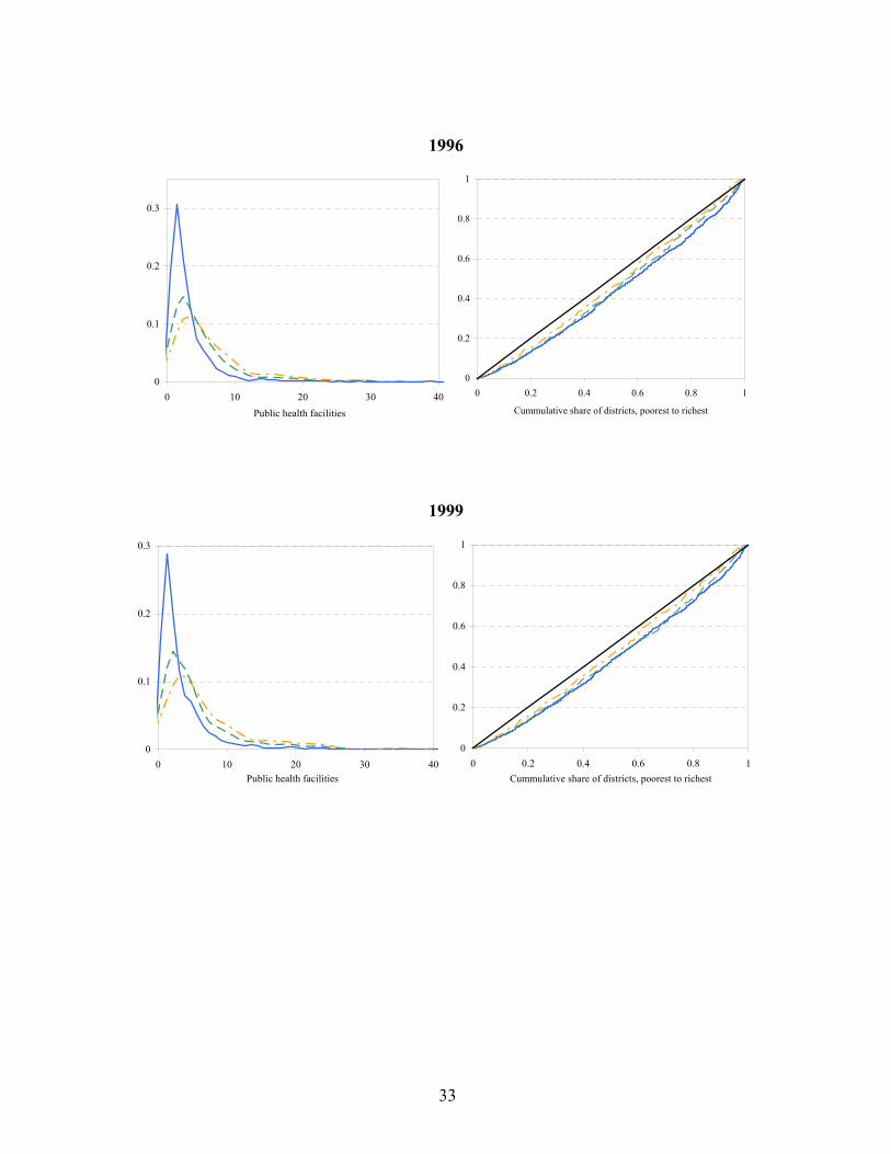
Figure A. 2. Kernel Densities and Concentration Curves for Different Samples, Public Facilities

1992

0

0.1

0.2

0.3

0.4

0 10 20 30 40

Public health facilities

0

0.2

0.4

0.6

0.8

1

0 0.2 0.4 0.6 0.8 1

Cummulative share of districts, poorest to richest

33

1996

0

0.1

0.2

0.3

0 10 20 30 40Public health facilities

0

0.2

0.4

0.6

0.8

1

0 0.2 0.4 0.6 0.8 1

Cummulative share of districts, poorest to richest

1999

0

0.1

0.2

0.3

0 10 20 30 40Public health facilities

0

0.2

0.4

0.6

0.8

1

0 0.2 0.4 0.6 0.8 1Cummulative share of districts, poorest to richest

34

Table A.1. Descriptive Statistics on Main Variables Used in Econometric Analysis District panel sample (92-96-00) 1992 DHS 1996 DHS 2000 DHS

Number

of Obs. Mean Sd. Min. Max. Mean Sd. Mean Sd. Mean Sd.

haz 26219 -1.237 1.364 -5.980 5.990 -1.420 1.362 -1.292 1.411 -1.296 1.336

waz 26203 -0.486 1.212 -5.810 4.970 -0.648 1.211 -0.531 1.222 -0.487 1.190

whz 26182 0.373 1.049 -3.98 4.97 0.304 1.048 0.362 1.034 0.412 1.054

Child’s age (=1 if 0-11m.) 31097 0.182 0.386 0 1 0.190 0.393 0.181 0.385 0.176 0.381

Child’s age (=1 if 12-23m.) 31097 0.186 0.389 0 1 0.175 0.380 0.189 0.392 0.189 0.392

Child’s age (=1 if 24-35m.) 31097 0.189 0.391 0 1 0.180 0.384 0.187 0.390 0.191 0.393

Child’s age (=1 if 36-48m.) 31097 0.195 0.396 0 1 0.196 0.397 0.194 0.396 0.194 0.396

Gender (=1 if male) 31097 0.508 0.500 0 1 0.511 0.500 0.507 0.500 0.509 0.500

Mother’s schooling (=1 if elementary) 31097 0.415 0.493 0 1 0.447 0.497 0.450 0.498 0.449 0.497

Mother’s schooling (=1 if high school) 31097 0.348 0.476 0 1 0.334 0.472 0.310 0.463 0.321 0.467

Mother’s schooling (=1 if superior) 31097 0.145 0.352 0 1 0.115 0.319 0.124 0.329 0.136 0.343

Mother’s height-for-age 29377 -2.242 0.932 -5.82 5.79 -2.285 0.907 -2.275 0.946 -2.269 0.912

Home language (=1 if spanish) 31074 0.846 0.361 0 1 0.855 0.352 0.809 0.393 0.778 0.415

Asset index 30658 -0.873 2.365 -5.459 4.271 -1.139 2.403 -1.342 2.375 -1.111 2.280

Coast (=1 if coast and not Lima) 31097 0.246 0.431 0 1 0.216 0.412 0.228 0.420 0.206 0.404

Highlands 31097 0.375 0.484 0 1 0.368 0.482 0.447 0.497 0.475 0.499

Jungle 31097 0.262 0.440 0 1 0.296 0.457 0.219 0.414 0.251 0.434

Urban 31097 0.608 0.488 0 1 0.582 0.493 0.510 0.500 0.454 0.498

% of pop w/o drinking water in the district 31097 36.766 29.959 0 100 62.941 29.357 30.745 28.237 34.173 27.024

% of pop w/o sewage in the district 31062 52.217 33.132 0 100 69.069 28.858 50.686 35.364 59.690 32.440

(continues …)

35

(…. continued)

District panel sample (92-96-00) 1992 DHS 1996 DHS 2000 DHS

Number

of Obs. Mean Sd. Min. Max. Mean Sd. Mean Sd. Mean Sd.

% of pop w/o electricity in the district 30985 33.98 30.11 0 100 48.12 31.42 28.87 28.80 29.12 26.69

Year of interview (=1 if 1996) 31379 0.44 0.50 0 1

Year of interview (=1 if 2000) 31379 0.29 0.46 0 1

Health infrastructure index 31379 2.70 4.75 -0.66 21.72 1.56 2.89 3.70 6.25 2.22 2.81

Public health facilities in the district 31379 11.57 10.78 0 46 8.59 9.05 12.66 11.30 12.60 10.91

Doctors in public health facilities in the district 31379 115.60 329.13 0 1677 61.67 178.41 186.41 451.99 58.11 141.73

36

Table A.2. Mother’s Nutrition and the Effect of Education on Child Nutrition, Urban Sample

(absolute value of z statistics in parentheses) With Without Child’s age (=1 if 0-11m.) 0.968 0.966 (41.89)*** (42.77)*** Child’s age (=1 if 12-23m.) 0.105 0.104 (4.58)*** (4.65)*** Child’s age (=1 if 24-35m.) 0.234 0.236 (10.29)*** (10.58)*** Child’s age (=1 if 36-48m.) 0.068 0.059 (2.98)*** (2.67)*** Gender (=1 if male) -0.046 -0.054 (3.18)*** (3.79)*** Mother’s schooling (=1 if elementary) 0.088 0.043 (3.00)*** (1.49) Mother’s schooling (=1 if high school) 0.264 0.159 (8.05)*** (4.93)*** Mother’s schooling (=1 if superior) 0.579 0.376 (15.11)*** (9.93)*** Mother’s height-for-age 0.319 (38.92)*** Home language (=1 if Spanish) 0.202 0.214 (5.89)*** (6.36)*** Asset index 0.127 0.105 (25.14)*** (21.25)*** Highlands -0.350 -0.249 (1.48) (1.07) Jungle -0.511 -0.430 (1.95)* (1.69)* % of pop w/o drinking water in the district -0.405 -0.352 (1.47) (1.30) % of pop w/o sewage in the district 0.000 -0.001 (0.09) (0.92) % of pop w/o electricity in the district -0.002 -0.001 (1.92)* (0.95) Year of interview (=1 if 1996) 0.000 0.000 (0.25) (0.25) Year of interview (=1 if 2000) 0.130 0.108 (4.18)*** (3.54)*** Health infrastructure index (HII) 0.117 0.109 (3.74)*** (3.56)*** Constant 0.015 0.022 (1.19) (1.81)* Observations -1.419 -0.736 Log Likelihood -39963.29 -38616.51 F test (H0: All u_i =0) 5.19 4.69 * significant at 10%; ** significant at 5%; *** significant at 1%