port-based modeling of mechatronic systems

Mathematics and Computers in Simulation 66 (2004) 99–127

Port-based modeling of mechatronic systems

Peter C. Breedveld∗Control Engineering Laboratory, Drebbel Institute for Mechatronics, Faculty of Electrical Engineering, Mathematics and

Computer Science, University of Twente, P.O. Box 217, 7500 AE Enschede, The Netherlands

Available online 7 February 2004

Abstract

Many engineering activities, including mechatronic design, require that a multidomain or ‘multi-physics’ systemand its control system be designed as an integrated system. This contribution discusses the background and tools for aport-based approach to integrated modeling and simulation of physical systems and their controllers, with parametersthat are directly related to the real-world system, thus improving insight and direct feedback on modeling decisions.© 2003 IMACS. Published by Elsevier B.V. All rights reserved.

Keywords: Bond graph(s); Modelling and simulation; Mechatronics; System(s); Port-based approach

1. Introduction

1.1. Port-based modeling of dynamic systems

If modeling, design and simulation of (controlled) systems are to be discussed, some initial remarks atthe meta-level are required. It should be clear and it probably will be, due to the way it is phrased next, thatno global methodology exists that deals with each problem that might emerge. In other words, no theory ormodel can be constructed independent of some problem context. Nevertheless, in practice (sub-)modelsof physical components are often considered as constructs that can be independently manipulated, forinstance in a so-called model library. Without some reference to a problem context, such a library wouldbe useless, unless there is an implicit agreement about some generic problem context. However, such afoundation is rather weak, as implicit agreements tend to diverge, especially in case of real-world problems.

Herein, we will focus on the generic problem context of the dynamic (i.e. changing in time) behaviorof systems that belong to the area of the engineer and the mechatronic engineer in particular, like the onesdiscussed in the examples. These systems can be roughly characterized as systems that consist for a largepart of subsystems for which it is relevant to the dynamic behavior that they obey the basic principlesof macroscopic physics, like the conservation laws and the positive-entropy-production principle. Theother part consists of submodels for which the energy bookkeeping is generally not considered relevant

∗ Tel.: +31-53-489-2792; fax:+31-53-489-2223.E-mail address: [email protected] (P.C. Breedveld).

0378-4754/$30.00 © 2003 IMACS. Published by Elsevier B.V. All rights reserved.doi:10.1016/j.matcom.2003.11.002

100 P.C. Breedveld / Mathematics and Computers in Simulation 66 (2004) 99–127

for the dynamic behavior. Such parts are generally addressed as the signal processing part (controller)that is commonly for a large part realized in digital form. This contribution focuses on the description ofthe part for which energy bookkeeping is relevant for the dynamic behavior, while keeping a more thanopen eye for the connection to the signal part, either in digital or in analogue form.

It is argued that port-based modeling is ideally suited for the description of the energic part of amultidomain, sometimes also called multi-physics, system or subsystem. This means that the approachby definition deals with mechatronic systems and even beyond those.

Port-based physical system modeling aims at providing insight, not only in the behavior of systemsthat an engineer working on multidisciplinary problems wishes to design, build, troubleshoot or modify,but also in the behavior of the environment of that system. A key aspect of the physical world around usis that ‘nature knows no domains’. In other words, all boundaries between disciplines are man-made, buthighly influence the way humans interact with their environment. A key point each modeler should beaware of is that any property of a model that is a result of one of his choices, should not affect the resultsof the model. Examples of modeler’s choices are: relevance of time and space scales, references, systemboundaries, domain boundaries, coordinates and metric.

1.2. History

Several attempts to unified or systematic approaches of modeling have been launched in the past. In theupcoming era of the large-scale application of the steam engine, the optimization of this multidomain de-vice (thermal, pneumatic, mechanical translation, mechanical rotation, mechanical controls, etc.) createdthe need for the first attempt to a systems approach. This need for such a ‘mechathermics’ approach wasthen named thermodynamics. Although many will not recognize a modern treatment of thermodynamicsas the first systems theory, it certainly was aimed originally in trying to describe the behavior of sucha system independently of the involved domains. However, it required a paradigm shift or ‘scientificrevolution’ in the sense of Kuhn[14], due to the fact that the concept of entropy had to be introducedfor reasons of consistency, i.e. to be able to properly ‘glue’ these domains together with the concept ofa conserved quantity called energy. The rather abstract nature of the concept of entropy, and to someextent the concept of energy too, has caused that students have considered thermodynamics a ‘difficult’subject ever since, resulting in only a relatively limited number of engineers and scientists actively usingthe thermodynamic approach in modeling of system behavior and system design.

Despite the fact that the first evidence of the use of feedback dates back to 200–100b.c. when waterclocks required the water level in a reservoir to be kept constant, followed by Cornelis Drebbel’s ther-mostat and James Watt’s fly-ball governor, it was not before the late 1920s that feedback was realizedby means of electric signals (Harold Stephen Black’s 1927 famous patent that he wrote on a copy ofthe New York Times). At first, electronic feedback was used internally, to reduce distortion in electricamplifiers, but later, especially during World War II, this concept was used in radar control and mis-sile guidance. One might say that the multidomain approach to feedback was transferred to a signalapproach in which the external power supply did not need to be part of the behavioral analysis. How-ever, a more important paradigm shift was still to come, viz. the idea that the use of feedback allowedthe construction of components, viz. operational amplifiers, with which basic mathematical operationscould be mimicked, leading to analogue computers. This gave a new meaning to the terminology ‘ana-logue simulation’ that until then was conceived as mimicking behavior by means of analogue circuits ormechanisms.

P.C. Breedveld / Mathematics and Computers in Simulation 66 (2004) 99–127 101

Fig. 1. Prof. Henry M. Paynter.

Just after World War II, due to the rapidly increasing demand for electric power, the USA was ingreat need for power plants, in particular hydropower plants, that should be able to deal with large andsometimes rapid fluctuations in the power grid. Obviously, the success of control theory (cybernetics)during World War II inspired many to apply control theory to the dynamic problems involved in electricpower production.

One such a civil engineer by the name of Henry Paynter (Fig. 1; http://www.hankpaynter.com/) triedto use the early analogue computers that he had invented together with James Philbrick, to simulate thedynamics of the power plants to be built (http://www.me.utexas.edu/∼lotario/paynter/paynterbio.html).He used the at that time common description of block diagrams that display the computational structure ofthe differential and algebraic equations being used, as these mathematical operations were to be mappeddirectly on the basic components of the analogue computer. However, for reasons that will become clearin the course of this contribution (viz. related to the concept of so-called computational causality) he raninto formulation problems. At the beginning of the fifties he realized himself that the concept of a ‘port’introduced in electrical circuit theory a few years earlier by Wheeler[19], should be extended to arbitrarypower ports that can be applied domain-independently. Power ports include mechanical ports, hydraulicports, thermal ports, electric ports, etc., i.e. everything Paynter needed for the description of the dynamicbehavior of power plants (http://www.hankpaynter.com/Bondgraphs.html).

In the following decade, after moving to the MIT mechanical engineering department, he designed anotation based on the efficient representation of the relation between two ports by just one line that he called

http://www.hankpaynter.com/

http://www.me.utexas.edu/~lotario/paynter/paynterbio.html

http://www.hankpaynter.com/Bondgraphs.html


a ‘bond’. This so-called ‘bond graph’ notation was completed when he finally introduced the concept ofthe junction in a lecture in 1959[15]. Junctions not only make a bond graph a powerful tool, but theyare rather abstract concepts that require another paradigm shift. Once this shift is made, it often inducesover-enthusiasm and over-expectations that not only lead to disappointment, but also unnecessarily scareoff experienced engineers and scientists who have learned to accept the limitations of modeling.

As a result, just like thermodynamics, bond graphs never became widely popular, although they spreadover the whole world and are still alive and growing after more than 40 years. By contrast, signalprocessing, analogue and later digital computing, were not constrained to physical reality. This allowsmimicking virtually everything, from physically correct or incorrect models to arbitrary mathematicalrelations that described imaginary systems. In the previous decade, this even led to concepts like a ‘cyberworld’, etc. even though the level of physical modeling in most virtual environments is rather low, asdemonstrated by the unnatural features of much virtual behavior.

Nevertheless, the introduction of rapid and flexible machinery for production, assembly, manipulation(including surgery), etc. that has truly taken off in the nineties, raised the need for a systems approachagain. In these application areas physical constraints still limit imagination. The dynamic behavior ofsuch devices heavily leans on the application of digital electronics (microcomputers) and software, buta domain-independent description of the parts in which power plays a role is crucial to make a designeraware of the fact that a considerable part of these systems is constrained by the limits of the physicalworld. This mix of mechanics, or rather physical system engineering in general, at the one hand anddigital electronics, software and control at the other hand has been named ‘mechatronics’.

1.3. Tools needed for mechatronics

Obviously, a smooth connection is needed between the information–theoretical descriptions of thebehavior of digital systems and physical systems theory. Since their introduction bond graphs haveallowed the use of signal ports, both in- and output, and a corresponding mix with block diagrams.As block diagrams can successfully represent all digital operations similar to mathematical operations,the common bond graph/block diagram representation is applicable. This graphical view supports ahierarchical organization of a model, supporting reusability of its parts.

However, many systems that are studied by (mechatronic) engineers differ from the engineering systemsthat were previously studied in the sense that the spatial description of complex geometries often playsan important role in the dynamic behavior, thus including the control aspects of these systems. Thisshows the need for a consistent aggregation of at the one hand the description of the configuration of amechanism and at the other hand the displacements in a system that in some way are related to the storageof potential or elastic energy.

Another aspect of these systems is that only few realistic models can be solved analytically, emphasizingthe important role of a numerical solution (simulation). The aggregation of numerical properties inthe representation of dynamic systems allows that a proper trade-off is made between numerical andconceptual complexity of a model, however, without confusing the two. The approach discussed hereinoffers a basis for making such a trade-off, resulting in both a higher modeling efficiency and numericalsimulation efficiency.

In mechatronics, where a controlled system is designed as a whole, it is advantageous that model struc-ture and parameters are directly related to physical structure in order to have a direct connection betweendesign or modeling decisions and physical parameters[9]. In addition, it is desired that (sub-)models be


reusable. Common simulation software based on block diagram or equation input does not sufficientlysupport these features. The port-based approach towards modeling of physical systems allows the con-struction of easily extendible models. As a result it optimally supports reuse of intermediate results withinthe context of one modeling or design project. Potential reuse in other projects depends on the quality ofthe documentation, particularly of the modeling assumptions.

1.4. Object-oriented modeling

The port-based approach may be considered a kind of object-oriented approach to modeling: each objectis determined by constitutive relations at the one hand and its interface, being the power and signal portsto and from the outside world, at the other hand. Other realizations of an object may contain different ormore detailed descriptions, but as long as the interface (number and type of ports) is identical, they can beexchanged in a straightforward manner. This allows top–down modeling as well as bottom–up modeling.Straightforward interconnection of (empty) submodels supports the actual decision process of modeling,not just model input and manipulation. Empty submodel types may be filled with specific descriptionswith various degrees of complexity—models can be polymorphic[17]—to support evolutionary anditerative modeling and design approaches[18]. Additionally, submodels may be constructed from othersubmodels resulting in hierarchical structures.

1.5. Design phases

Often modeling, simulation and identification is done for systems that already exist. The design of acontroller has to be done for an already realized and given ‘process’. In case of a full design the systemdoes not yet exist, which not only means that there is a large initial uncertainty, but also that there ismuch more freedom to modify the design, not just the controller, but the complete ‘process’, includingthe mechanical construction.

In a design process the following, iterative phases can be distinguished:Phase 1: A conceptual design is made of the system that has to be constructed, taking into account the

tasks that have to be performed and identifying and modeling the major components and their dominantdynamic behaviors, as well as the already existing parts of the system that cannot be modified. The partof the model that refers to the latter parts can be validated already.

Phase 2: Controller concepts can be evaluated on the basis of this simple model. This requires thatthe model is available in an appropriate form, e.g. as a transfer function or a state space description. Ifthis phase provides the insight that modification of some dominant behavior would be quite beneficial,revisiting phase 1 can lead to the desired improvement.

Phase 3: When the controller evaluation is successful, the different components in the system can beselected and a more detailed model can be made. The controller designed in phase 2 can be evaluatedwith the more detailed model and controller and component selection can be changed. If the effects ofthe detailed model prove to distort the originally foreseen performance, revisiting either phase 2 or evenphase 1 with the newly obtained insights can lead to improved performance.

Phase 4: When phase 3 has been successfully completed the controller can be realized electronically ordownloaded into a dedicated microprocessor (embedded system). This hardware controller can be testedwith a hardware-in-the-loop simulation that mimics the physical system (plant) still to be built. It is tobe preferred that the translation from the controller tested in simulations is automatically transferred to,


e.g. C-code, without manual coding; not only because of efficiency reasons, but also to prevent codingerrors. If this phase results in new insights given the non-modeled effects of the implementation of thecontroller, the previous phases may be revisited, depending on the nature of the encountered problem.

Phase 5: Finally the physical system itself can be built. As this is usually the most cost intensive partof the process, this should be done in such a way that those physical parameters that proved to be mostcritical in the previous phases are open for easy modification as much as possible, such that final tuningcan lead to an optimal result.

Given the key role of structured, multidomain system modeling in the above process, special attentionis given to domain-independent modeling of physical systems.

1.6. Multiple views in the design and modeling process

Mechatronic design deals with the integrated design of a mechanical system and its embedded controlsystem. In practice, this ‘mechanical system’ has a rather wide scope. It may also contain hydraulic,pneumatic and even thermal parts that influence its dynamic characteristics. This definition implies that itis important that the system be designed as a whole as much as possible. This requires a systems approachto the design problem. Because in mechatronics the scope is limited to controlled mechanical systems,it will be possible to come up with more or less standard solutions. An important aspect of mechatronicsystems is that the synergy realized by a clever combination of a mechanical system and its embeddedcontrol system leads to superior solutions and performances that could not be obtained by solutions inone domain. Because the embedded control system is often realized in software, the final system will beflexible with respect to the ability to be adjusted for varying tasks.

The interdisciplinary field of mechatronics thus requires tools that enable the simultaneous design of thedifferent parts of the system. The most important disciplines playing a role in mechatronics are mechanicalengineering, electrical engineering and software engineering. One of the ideas behind mechatronicsis that functionality can be achieved either by solutions in the (physical) mechanical domain, or byinformation processing in electronics or software. This implies that models for mechatronic systemsshould be closely related to the physical components in the system. It also requires software tools thatsupport such an approach. In an early stage of the design process simple models are required to makesome major conceptual design decisions. In a later stage (parts of the) models can be more detailed toinvestigate certain phenomena in depth. The relation to physical parameters like inertia, compliance andfriction is important in all stages of the design. Because specialists from various disciplines are involvedin mechatronic design, it is advantageous if each specialist is able to see the performance of the system ina representation that is common in his or her own domain. Accordingly, it should be possible to see theperformance of the mechatronic system in multiple views. Typical views that are important in this respectare: ideal physical models or ‘iconic diagrams’, bond graphs, block diagrams, Bode plots, NyQuist plots,state space description, time domain, animation, C-code of the controller.

This has been formalized as the so-calledmultiple view approach that is particularly well supportedby window-based computer tools: a number of graphical representations like iconic diagrams, whichare domain-dependent, linear graphs, which are more or less domain-independent, but limited to theexistence of analogue electric circuits[16], block diagrams, which represent the computational structure,bond graphs, which are domain-independent, etc. as well as equations, which represent the mathematicalform in different shapes (transfer functions, state space equations in matrix form, etc.) can serve as modelrepresentations in different windows. The tool in which all examples of this paper are treated, 20-sim,


has been designed on the basis of such a multiple view approach. Possible views in 20-sim are: equa-tions, including matrix-vector form, block diagrams (multi-)bond graphs, transfer functions, state-spacerepresentations (system, in- and output matrices), time responses, phase planes, functional relationships,step responses, Bode plots, pole-zero plots, NyQuist diagrams, Nichols charts and 3D-animation. Wherepossible, automatic transformation is provided and results are linked.

The port-based approach has been taken as the underlying structure of 20-sim, formulated in the internallanguage SIDOPS[8], which makes it the ideal tool for demonstration of the port-based and multiple viewapproaches. A more detailed introduction to ports, bonds and the bond graphs representation is given later.This will give the reader sufficient insight in order to exercise it with the aid of a port-based modeling andsimulation software like 20-sim. This tool allows high level input of models in the form of iconic diagrams,equations, block diagrams or bond graphs and supports efficient symbolic and numerical analysis as wellas simulation and visualization. Elements and submodels of various physical domains (e.g. mechanical orelectrical) or domain-independent ones can be easily selected from a library and combined into a modelof a physical system that can be controlled by block diagram-based (digital) controllers. A demonstrationcopy of 20-sim that allows the reader to get familiar with the ideas presented in this contribution can bedownloaded from the Internet (http://www.20sim.com). For more advanced issues the interested readeris referred to the references. However, modeling is first treated in more generic terms.

2. Modeling philosophy

2.1. Every model is wrong

This paradoxical statement seeks to emphasize that any model that perfectly represents all aspects of anoriginal system is not a model, but an exact copy of that system (identity). When modeling one looks forsimple but relevant analogies, not for complex identities. As a result, a model is much simpler than reality.This is its power and its weakness at the same time. The weakness is that its validity is constrained to theproblem context it was constructed in, whereas its strength is the gain of insight that may be obtained inthe key behaviors that play a role. In other words: ‘no model has absolute validity’. The resulting advice isthat one should always keep the limitations of a model in mind and always try to make them explicit first.Especially in an early phase of a modeling or design process, such a focus may result in interesting insights.

2.2. A model depends on its problem context

Models should be competent to support the solution of a specific problem. This also means that any typeof archiving of a model or submodel should always include information about the corresponding problemcontext. Without this context, the model has no meaning in principle. Note that training of specialists andexperts is often related to what is sometimes called a ‘culture’ and that they are said to speak a ‘jargon’.This culture and jargon reflect the existence of a particular (global) problem context, even though thiscontext is not explicitly described when models are made. For electrical circuit designers, this problemcontext consists of the behavior of electric charges and in particular of the voltages and currents relatedto this behavior, in a specific part of the space–time scale. This behavior is such that electromagneticradiation plays no dominant role. Mechanical systems mostly belong to another part of the space–timescale, although there may be considerable overlap, in particular in precision engineering.

http://www.20sim.com


These cultures and jargons easily lead to implicit assumptions, which, in turn, may lead to modelextrapolations that have no validity in the specific problem context at hand due to the danger of ignoringearlier assumptions. These extrapolations often start from well-known classroom problems with analyticalsolutions like the model of a pendulum[6]. In other words: ‘implicit assumptions and model extrapolationsshould be avoided’. The resulting advice is that one should focus at the model’s competence to representthe behavior of interest, not at its ‘truth content’.

2.3. Physical components versus conceptual elements

In all cases it should be clear that (physical) components, i.e. identifiable system parts that can be phys-ically disconnected and form a so-called physical, often visible, structure, are to be clearly distinguishedfrom (conceptual) elements, i.e. abstract entities that represent some basic behavior, even though they aresometimes given the same name as the physical component. For example, a resistor may be an electricalcomponent with two connection wires and some color code (cf.Fig. 2a), while the same name is usedfor the conceptual element (commonly represented byFig. 2b) that represents the dominant behavior ofthe component with the same name, but also of a piece of copper wire through which a relatively largecurrent flows.

Note that this model requires that the problem context is such that the component resistor is part of acurrent loop in a network in which the behavior of the voltages and currents plays a role. By contrast,other realistic problem contexts exist in which the dominant behavior of the component resistor is notrepresented by the element resistor, but by the element ‘mass’ or a combination of mechanical conceptualelements like mass, spring and damper. For example, when this component is to be rapidly manipulatedin assembly processes, i.e. before it is part of an active circuit, this could be a competent model.

Often, not only the dominant behavior of a component has to be described but also some other propertiesthat are often called ‘parasitic’, because they generate a conceptual structure and destroy the one-to-onemapping between components and elements that misleadingly seems to simplify modeling and design (cf.Fig. 2c). Note that those areas of engineering in which materials could be manipulated as to suppress allother behaviors than the dominant one (like electrical engineering), have been the first to apply networkstyle dynamic models successfully. Also note that in our daily life we have learned to make quick intuitive

Fig. 2. Component electrical resistor (a) with two different conceptual models (b and c).


decisions about dominant behaviors (survival of the fittest). This type of learning stimulates implicit andintuitive decisions that may fail in more complex engineering situations (counter-intuitive solutions).

Implicit assumptions are commonly not only made about the problem context, but also about thereference, the orientation, the coordinates, and the metric and about ‘negligible’ phenomena. Famousclassroom examples may have an impact on the understanding of real behavior for generations, especiallydue to the textbook copying culture that is the result of what may be called a ‘quest for truth’ motivation,ignoring model competence. A notorious example is the false explanation of the lift of an aircraft wing dueto the air speed differences and resulting dynamic pressure differences in the boundary layer generated bythe wing profile. This explanation has survived many textbooks, even though the simple observation thatairplanes with such wing profiles can fly upside down falsifies this explanation in an extremely simpleand evident way.

Another example is a model of which the behavior changes after a change of coordinates: as coordinatesare a modeler’s choice, they cannot have any impact on the behavior of the described system. Not keepingan open eye for these aspects of modeling may lead to exercises that are documented in the scientificliterature in which controllers are designed to deal with model behaviors that are due to imperfections ofthe model and that are not observed at all in the real system or rather the actual problem context. . .

3. Ports in dynamic system models

3.1. Bilateral bonds versus unilateral signals

The concept of a port is generated by the fact that submodels in a model have to interact with each otherby definition and accordingly need some form of conceptual interface. In physical systems, such an inter-action is always (assumed to be) coupled to an exchange of energy, i.e. a power. In domain-independentterminology, such a relation is called a power bond accordingly. This bilateral relation or bond connectstwo (power) ports of the elements or submodels that are interacting (Fig. 3).

In the signal domain, this power is assumed to be negligible compared to the powers that do play a role,such that a signal relation may be considered a ‘unilateral’ relation. Note that ideal operational amplifiershave an infinite input impedance and a zero output impedance in order to suppress the back-effect and tobe purely unilateral, but can only be approximated by adding external power. The bilateral nature of thepower relations (as opposed to unilateral signal relations) suggests the presence of two variables that havesome relation to the power represented by the bond. These so-called power-conjugate variables can bedefined in different ways, but commonly they are related by a product operation to a powerP and in thedomain-independent case named efforte and flowf,P = e×f . Domain-dependent examples are force andvelocity in the mechanical domain, voltage and current in the electrical domain, pressure and volume flowin the hydraulic domain, etc. In principle, the flow variable can be seen as the rate of change of some state, or‘equilibrium-establishing variable’, whereas the effort variable can be seen as the equilibrium-determiningvariable. Note that the common approach to use two types of storage, i.e. C- and I-type, prevents thatthis distinction between flow and effort as rate of change of state and equilibrium-determining variablerespectively can be used in modeling straightforwardly. The so-called Generalized Bond Graph (GBG)approach resolves this problem, leaving the discussion about the force–voltage versus force–currentanalogy a non-issue[2,3], although there is a clear didactical preference to introduce this approachusing the force–voltage analogy[11]. This is not further discussed in order to adapt to the conventional


Fig. 3. Bond connecting two ports.

background of the reader, despite the fact that the ‘rate of change’ versus ‘equilibrium-determining’aspects of these variables are powerful tools to support initial modeling decisions.

3.2. Dynamic conjugation versus power conjugation

The two signals of the bilateral signal flow representing a physical interaction are dynamically conju-gated in the sense that one variable represents the rate of change of the characteristic physical property,like electric charge, amount of moles, momentum, while the other variable represents the equilibrium-determining variable. This is called dynamic conjugation. As long as no other domains are of interest,the concept of energy is not particularly relevant, such that these variables do not need to be related toa power like the effort and flow discussed earlier. Examples are: temperature and heat flow (product isnot a power, heat is not a proper state if other domains are involved), molar flow and concentration ormole fraction (product is not a power), etc. The power-conjugated variables effort and flow are a subsetof these dynamically conjugated variables.

This illustrates that the concept of a domain-independent conserved quantity, the energy, is crucialfor the consistent interconnection of physical phenomena in different domains. The discussion of basicbehaviors inSection 6is based on this and thus requires either the consistent use of power-conjugatedvariables or carefully defined domain transitions that are power continuous and energy conserving.

4. Computational causality

In pure mathematical terms one can state that a subsystem with a number of (power) ports, calledmultiport, is a multiple-input–multiple-output (MIMO) system model, of which the set of inputs and the


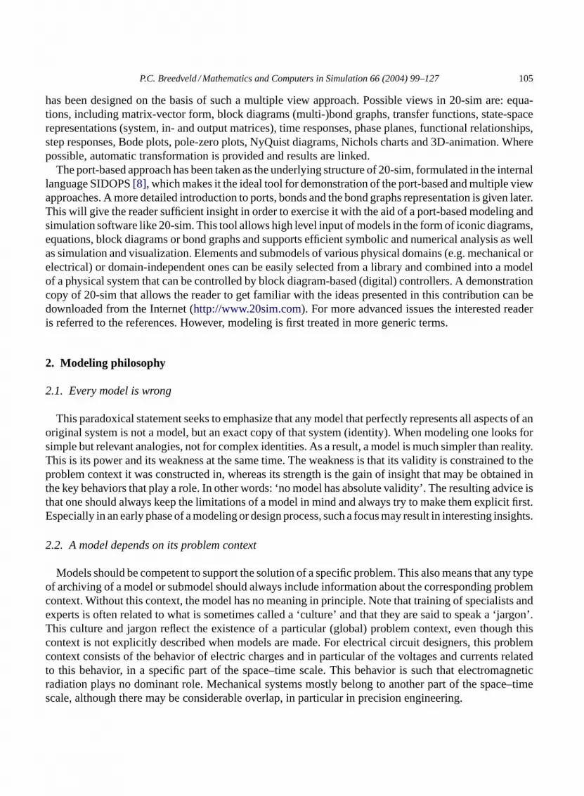
Fig. 4. (a) Conventional MIMO. (b) MIMO system with bilateral power ports and modulating signal ports.

set of outputs is not a priori chosen. The relation between the input and output variables, the so-calledconstitutive relation, determines the nature of this multiport.

If the number of input variables is not equal to the number of output variables, this means that there hasto be at least one unilateral signal port as opposed to a bilateral power port as the latter is by definitioncharacterized by one input and one output. If this signal port is an input signal, the multiport is calledmodulated. Modulation does not affect the power balance, in other words: no energy can be exchangedvia a signal port. Note that situations can exists in which the model is modulated although the number ofinputs equals the number of outputs, because for each modulating signal there is a signal output.

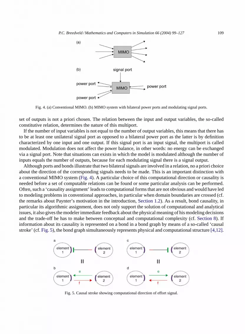
Although ports and bonds illustrate that two bilateral signals are involved in a relation, no a priori choiceabout the direction of the corresponding signals needs to be made. This is an important distinction witha conventional MIMO system (Fig. 4). A particular choice of this computational direction or causality isneeded before a set of computable relations can be found or some particular analysis can be performed.Often, such a ‘causality assignment’ leads to computational forms that are not obvious and would have ledto modeling problems in conventional approaches, in particular when domain boundaries are crossed (cf.the remarks about Paynter’s motivation in the introduction,Section 1.2). As a result, bond causality, inparticular its algorithmic assignment, does not only support the solution of computational and analyticalissues, it also gives the modeler immediate feedback about the physical meaning of his modeling decisionsand the trade-off he has to make between conceptual and computational complexity (cf.Section 8). Ifinformation about its causality is represented on a bond in a bond graph by means of a so-called ‘causalstroke’ (cf.Fig. 5), the bond graph simultaneously represents physical and computational structure[4,12].

Fig. 5. Causal stroke showing computational direction of effort signal.


From the latter point of view a bond graph can be seen as a condensed block diagram. However, althoughany causal bond graph can be converted into a block diagram, the reverse does not hold, as physicalstructure is lost in the first transformation.

The causal stroke is attached to that end of the bond where the effort signal comes out, i.e. where itenters the connected port. This automatically means that the so-called open end of the bond representsthe computational direction of the flow signal (cf.Fig. 5).

5. System versus environment: system boundary

The distinction between system and environment is determined by the role of these parts: the environ-ment can influence the system, but not dynamically interact with it. In signal terminology: the environmentmay influence the system via inputs and observe the system via outputs, but the inputs cannot dependon these outputs at the time scale of interest. In case of normal use, a car battery for example, maybe considered the environment of a dashboard signal light, as the discharge will not affect the voltagein a considerable way. In other words, the car battery in this problem context (regular car use) can bemodeled by a voltage source. However, in a context of a car being idle for 3 months (other time scale!)the car battery has to be made part of the system and dominantly interacts with the resistance of the bulblike a discharging capacitor. The resultingRC-model is competent in this problem context to predict thetime-constant of the discharge process. In severe winter conditions the thermal port of this capacitor willhave to be made part of the system, etc.

Note that, after a particular choice of the separation between infinite environment and finite system, theinfluence of the environment on the system may be conceptually concentrated in this finite system bound-ary by means of so-called sources and sinks, also called boundary conditions or constraints, dependingon the domain background. They are part of the ideal conceptual elements to be discussed next.

6. Elementary behaviors and basic concepts

This section introduces the conceptual elementary behaviors that can be distinguished in the commondescription of the behavior of physical systems, in particular from a port-based point of view. Before theindividual elements are discussed, first the notation for the positive orientation in the form of the so-calledhalf arrow is introduced.

6.1. Positive orientation and the half arrow

Each bond represents a connection between two ports. However, with one loose end it can be used tovisualize the port it is connected to (Fig. 6). The three variables involved, effort, flow and power, may havedifferent signs with respect to this port. In order to be able to indicate this, ahalf arrow, as opposed to thefull arrow that is commonly used for signals, is attached to the bond, expressing the positive orientationof these variables, similar to the plus and minus signs and the arrow that are used for an electric two-poleto represent thepositive orientation of the voltage and the current respectively (Fig. 7). Note that thehalf arrow doesnot indicate thedirection of the flow or the power: the direction is opposite in case thecorresponding variable has a negative value.


Fig. 6. Positive orientation represented by a half arrow (a), direction depends on sign (b, c).

Like the causal stroke the half arrow is an additional label to the bond, but they do not influence eachother (Fig. 7). The causal stroke merely fixates the direction of the individual signal flows in the bilateralsignal flow pair, whereas the half arrow merely represents positive orientation.

6.2. Storage

The most elementary behavior that needs to be present in a system in order to be dynamic is ‘storage’.In mathematical terms one can describe this behavior by the integration of the rate of change of someconserved quantity, viz. the stored quantity orstate, and by the relation of this state with the equilibriumdetermining variable, the so-calledconstitutive relation. Note that in the common classification of do-mains, many domains are characterized by two types of state, viz. the generalized displacement and thegeneralized momentum, following the common approach in the mechanical domain. It has been notedbefore that another classification of domains that for instance separates the mechanical domain into akinetic domain and a potential or elastic domain can easily resolve the paradoxical situation that resultsfrom the common choice[3], but this would be beyond the scope of this contribution. This means thatthe common two types of storage are used:

1. the C-type storage element in which the flow is integrated into a generalized displacement and relatedto the conjugate effort;

2. the I-type storage element in which the effort is integrated into a generalized momentum and relatedto the conjugate flow.

Note that both are dual in the sense that they can be transformed into each other by interchanging theroles of the conjugate variables effort and flow.

Simple examples of C-type storage elements are:

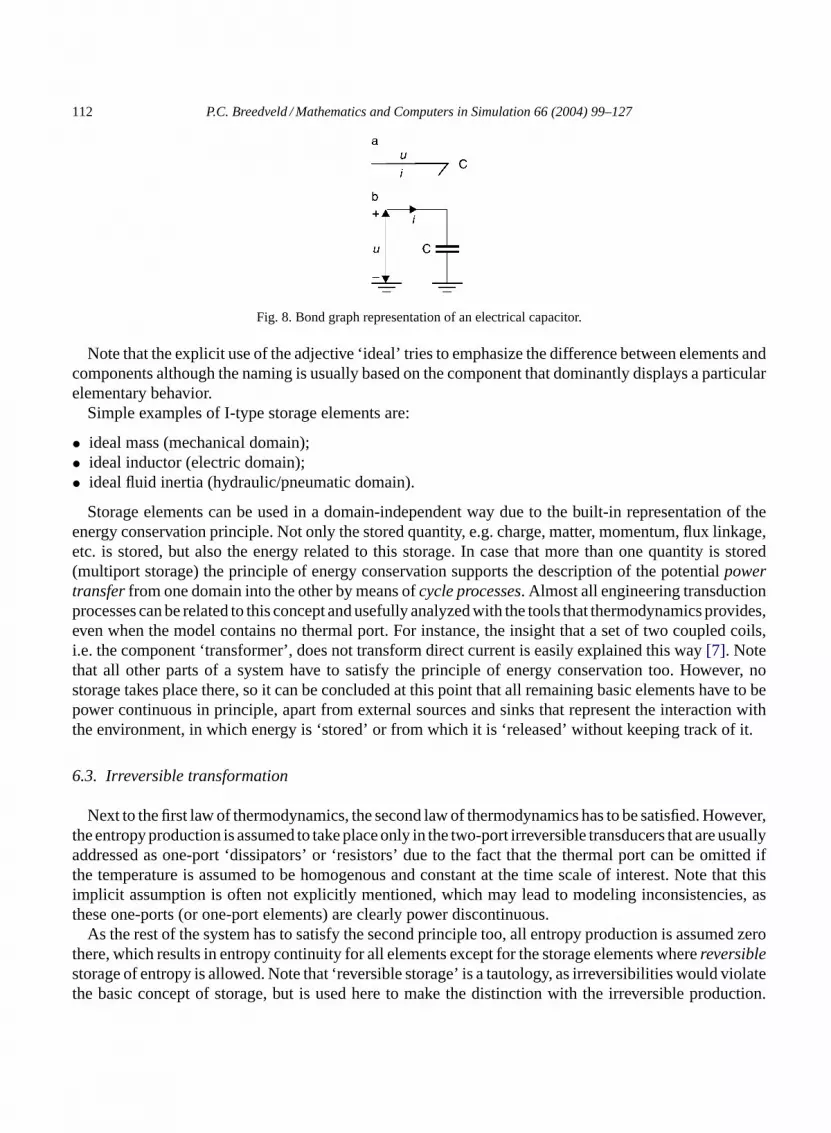
• ideal spring (mechanical domain);• ideal capacitor (electric domain,Fig. 8);• ideal reservoir (hydraulic/pneumatic domain);• ideal heat capacitor (thermal domain).

Fig. 7. Half arrow does not influence causality.


Fig. 8. Bond graph representation of an electrical capacitor.

Note that the explicit use of the adjective ‘ideal’ tries to emphasize the difference between elements andcomponents although the naming is usually based on the component that dominantly displays a particularelementary behavior.

Simple examples of I-type storage elements are:

• ideal mass (mechanical domain);• ideal inductor (electric domain);• ideal fluid inertia (hydraulic/pneumatic domain).

Storage elements can be used in a domain-independent way due to the built-in representation of theenergy conservation principle. Not only the stored quantity, e.g. charge, matter, momentum, flux linkage,etc. is stored, but also the energy related to this storage. In case that more than one quantity is stored(multiport storage) the principle of energy conservation supports the description of the potentialpowertransfer from one domain into the other by means ofcycle processes. Almost all engineering transductionprocesses can be related to this concept and usefully analyzed with the tools that thermodynamics provides,even when the model contains no thermal port. For instance, the insight that a set of two coupled coils,i.e. the component ‘transformer’, does not transform direct current is easily explained this way[7]. Notethat all other parts of a system have to satisfy the principle of energy conservation too. However, nostorage takes place there, so it can be concluded at this point that all remaining basic elements have to bepower continuous in principle, apart from external sources and sinks that represent the interaction withthe environment, in which energy is ‘stored’ or from which it is ‘released’ without keeping track of it.

6.3. Irreversible transformation

Next to the first law of thermodynamics, the second law of thermodynamics has to be satisfied. However,the entropy production is assumed to take place only in the two-port irreversible transducers that are usuallyaddressed as one-port ‘dissipators’ or ‘resistors’ due to the fact that the thermal port can be omitted ifthe temperature is assumed to be homogenous and constant at the time scale of interest. Note that thisimplicit assumption is often not explicitly mentioned, which may lead to modeling inconsistencies, asthese one-ports (or one-port elements) are clearly power discontinuous.

As the rest of the system has to satisfy the second principle too, all entropy production is assumed zerothere, which results in entropy continuity for all elements except for the storage elements wherereversiblestorage of entropy is allowed. Note that ‘reversible storage’ is a tautology, as irreversibilities would violatethe basic concept of storage, but is used here to make the distinction with the irreversible production.


The common acronym for an irreversible transducer is RS, derived from the common acronym in theisothermal case, R, to which an S for source is added to represent the entropy production.

Simple examples of irreversible transducing (resistive) elements are:

• ideal electric resistor;• ideal friction;• ideal fluid resistor;• ideal heat resistance.

Due to the second principle of thermodynamics (positive entropy production), the relation between theconjugate variables at the R-port can be linear or nonlinear as long as the relation remains in the firstand third quadrant. However, the relation at the S-port (always in the thermal domain) is intrinsicallynonlinear, due to the absolute zero-point of temperature.

6.4. Reversible transformation

Irreversible transformation more or less suggests the ‘possibility’ of, or rather the need for, the idealconcept of a reversible transducer. As they cannot store or produce entropy, as these properties are alreadyconcentrated in the storage and RS elements, they have to be power continuous. Their most elementaryform is the two-port. It can be formally proven that, independent of the domain, only two types ofport-asymmetric, i.e. with non-exchangeable ports, power-continuous two-ports can exist, at the onehand the so-called transformer (TF) that relates the efforts of both ports and also the flows of both portsand at the other hand the so-called gyrator (GY) that relates the flow of one port with the effort of the othervice versa. Furthermore, the nature of the relation is multiplicative, either by a constant (regular TF andGY) or by an arbitrary time-dependent variable, the so-called modulating signal (MTF and MGY). Thenotion of a port-asymmetric multiport will be clarified when port-symmetric multiports are discussed.

Simple examples of reversible transforming elements are:

• ideal (or perfect) electric transformer;• ideal lever;• ideal gear box;• ideal piston–cylinder combination;• ideal positive displacement pump.

Simple examples of reversible gyrating elements are:

• ideal centrifugal pump;• ideal turbine;• ideal electric motor.

An ideal, continuously variable transmission is a simple example of a reversible, modulated transform-ing element, while an ideal turbine with adjustable blades is a simple example of a reversible, modulatedgyrating element.

In port-based models of planar and spatial mechanisms specific types of (configuration-)state-modulated(multiport) transformers play a crucial role, which exposes the dual role of the displacement variable oncemore.


6.5. Supply and demand (sources and sinks/boundary conditions)

As already announced, the supply and demand from and to the environment can be concentrated in the(conceptual!) system boundary and represented by sources or sinks. As sinks can be considered negativesources, only ideal sources are used as ideal elements. Given that a port has two kinds of variables, effortand flow, two kinds of sources may exist, sources of effort and sources of flow (Se and Sf). Generallyspeaking, all storage elements that are large compared to the dynamics of interest (note that this cannot beconsidered independently of the resistance of its connection to the rest of the system) may be approximatedby infinitely large storage elements that are identical to sources. An infinitely large C-type storage elementbecomes an Se, an infinitely large I-type storage element becomes an Sf. However, feedback control mayturn a port into a source too, cf. a stabilized voltage source. As the voltage may be adapted or modulated,these kinds of sources are called modulated sources (MSe, MSf).

Simple examples are of (modulated) effort sources are:

• ideal (controlled) voltage source;• ideal (controlled) pressure source, etc.

Simple examples are of (modulated) flow sources are:

• ideal (controlled) current source;• ideal (controlled) velocity source, etc.

6.6. Distribution

In order to be able to distribute power between subsystems in an arbitrary way, distributing el-ements with three or more ports are required. By assigning all energy storage to the storage ele-ments, all entropy production to the irreversible transducers (dissipators) and all exchange with theenvironment to the sources, only the property of power continuity remains. Furthermore, the require-ment that ports should be connectable at will, requires that an interchange of ports of these distribut-ing or interconnecting elements has no influence. This is the property of so-called port-symmetry.It is important to note that it can be formally proven that only the requirements of power continu-ity and port-symmetry result in two solutions, i.e. two types of multiports (i.e. interconnection el-ements with two or more ports) with constitutive relations that turn out to be linear, the so-calledjunctions. The constitutive relations (one per port) of the first type require all efforts to be identicaland the flows to sum up zero with the choice of sign related to their positive orientation, similar toa Kirchhoff current law. Paynter called this junction a 0-junction, due to the similarity between thesymbol for zero and the shape of a node, because like a node in an electric circuit (at that time theonly network type notation) the 0-junction has a common effort and the adjacent flows sum to zero(flow balance).

The constitutive relations of the second type, called 1-junction, are dual: all flows should be identicaland the efforts sum to zero with the choice of sign related to their positive orientation (effort balance),similar to a Kirchhoff voltage law.

However, it is a mistake to say that the junctionsonly represent the generalized Kirchhoff laws, asthe junctions at the same time represent the ‘commonness’ of the power-conjugate variable, such thatthey can be used at the same time to represent that particular variable, which is quite convenient during


modeling. Note that port-symmetric, power continous two-ports are junctions too, which explains whythe assumption of port-asymmetry was required when discussing the TF and GY.

As mentioned before, really manipulating the concept of the junction in a way that supports the modelingprocess, i.e. without using other modeling techniques and translation first, requires some skill as the trueunderstanding of the junctions requires the paradigm shift mentioned earlier. Nevertheless, the results arepowerful, as will be demonstrated after the discussion of the causal port properties.

7. Causal port properties

Each of the nine basic elements (C, I, R(S), TF, GY, Se, Sf, 0, 1) introduced in the previous section has itsown causal port properties, that can be categorized as follows: fixed causality, preferred causality, arbitrarycausality and causal constraints. The meaning of these categories is explained next. The representationby means of the causal stroke has been introduced already (cf.Fig. 5).

7.1. Fixed causality

It needs no explanation that a source of effort always has an effort as output signal, in other words, thecausal stroke is attached to the end of the bond that is connected to the rest of the system (Figs. 9 and10a). Mutatis mutandis the causal stroke of a flow source is connected at the end of the bond connectedto the source (Fig. 10b). These causalities are called ‘fixed causalities’ accordingly. Apart from thesefundamentally fixed causalities, all ports of elements that may become nonlinear and non-invertible, i.e.all but the junctions, may become fixed due to the fact that the constitutive relation may only take oneform. In more advanced causal analysis procedures, the distinction between these two types of fixedcausalities is used[10]. Herein, this distinction will not be made for the sake of clarity, as it is not relevantfor most simple models.

7.2. Preferred causality

A less strict causal port property is that one of the two possibilities is, for some reason, preferred overthe other. Commonly this kind of property is assigned to storage ports, as the two forms of the constitutiverelation of a storage port require either differentiation with respect to time or integration with respect to

Fig. 9. Fixed effort-out causality of an effort (voltage) source.

Fig. 10. Fixed causality of sources.


Fig. 11. Preferred integral causality of a capacitor.

time (Fig. 11). On the basis of numerical arguments the integral form is preferred, due to the fact thatnumerical differentiation amplifies numerical noise, but there are more fundamental arguments too. Afirst indication is found in the fact that the integral form allows the use of an initial condition, while thedifferential form does not. Obviously, an initial state or content of some storage element is a physicallyrelevant property that illustrates the statement that integration ‘exists’ in nature, whereas differentiationdoes not. Although one should be careful with the concept existence when discussing modeling, thisstatement seeks to emphasize that differentiation with respect to time requires information about futurestates in principle, whereas integration with respect to time does not. The discussion of causal analysiswill make clear that violation of a preferred causality gives important feedback to the modeler about hismodeling decisions. Note that some forms of analysis require that the differential form is preferred, butthis requirement is never used as a preparation for numerical simulation.

7.3. Arbitrary causality

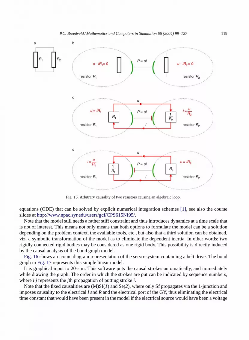
The expected next possibility in the sequence is that the causality of a port is neither fixed nor preferred,thus arbitrary. Examples of arbitrary port causality are linear, thus invertible, resistive ports. For example,the acausal form of the constitutive relation of an ohmic resistor isu − Ri = 0, the effort-out causal formis u = Ri, while the flow-out causal form isi = u/R (cf. Fig. 15).

7.4. Causal constraints

Causal constraints only exist for basic multiports, i.e. elements with two or more ports like the transduc-ers (TF, GY) and the junctions (0, 1). For instance, if the constitutive relation of the two-port transducersis linear (the junctions are intrinsically linear), the first port to which causality is assigned is arbitrary,but the causality of the second port is immediately fixed. For instance, the two-port transformer alwayshas one port with effort-out causality and one with flow-out causality. By contrast, the causalities of theports of a two-port gyrator always have the same type of causality. In graphical terms: a TF has only onecausal stroke directed to it, while a GY has either both causal strokes directed to it or none.

The fundamental feature of the junctions that either all efforts are common (0-junction) or all flows arecommon (1-junction) shows that only one port of a 0-junction can have ‘effort-in causality’, i.e. flow-outcausality, viz. the result of the flow-balance. By contrast, only one port of a 1-junction can have ‘flow-incausality’, i.e. effort-out causality, viz. the result of the effort-balance. In graphical terms: only one causalstroke can be directed towards a 0-junction, while only one open end can be directed towards a 1-junction.


8. Causal analysis: feedback on modeling decisions

Causal analysis, also called causality assignment or causal augmentation, is the algorithmic process ofputting the causal strokes at the bonds on the basis of the causal port properties induced by the nature ofthe constitutive relations. Not only the final result, but also the assignment process provides immediatefeedback on modeling decisions.

8.1. Fixed causality

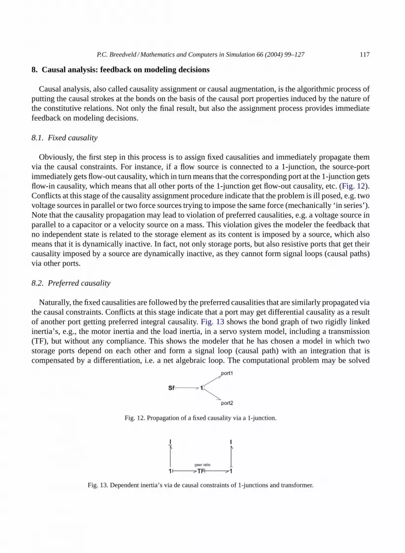
Obviously, the first step in this process is to assign fixed causalities and immediately propagate themvia the causal constraints. For instance, if a flow source is connected to a 1-junction, the source-portimmediately gets flow-out causality, which in turn means that the corresponding port at the 1-junction getsflow-in causality, which means that all other ports of the 1-junction get flow-out causality, etc. (Fig. 12).Conflicts at this stage of the causality assignment procedure indicate that the problem is ill posed, e.g. twovoltage sources in parallel or two force sources trying to impose the same force (mechanically ‘in series’).Note that the causality propagation may lead to violation of preferred causalities, e.g. a voltage source inparallel to a capacitor or a velocity source on a mass. This violation gives the modeler the feedback thatno independent state is related to the storage element as its content is imposed by a source, which alsomeans that it is dynamically inactive. In fact, not only storage ports, but also resistive ports that get theircausality imposed by a source are dynamically inactive, as they cannot form signal loops (causal paths)via other ports.

8.2. Preferred causality

Naturally, the fixed causalities are followed by the preferred causalities that are similarly propagated viathe causal constraints. Conflicts at this stage indicate that a port may get differential causality as a resultof another port getting preferred integral causality.Fig. 13shows the bond graph of two rigidly linkedinertia’s, e.g., the motor inertia and the load inertia, in a servo system model, including a transmission(TF), but without any compliance. This shows the modeler that he has chosen a model in which twostorage ports depend on each other and form a signal loop (causal path) with an integration that iscompensated by a differentiation, i.e. a net algebraic loop. The computational problem may be solved

Fig. 12. Propagation of a fixed causality via a 1-junction.

Fig. 13. Dependent inertia’s via de causal constraints of 1-junctions and transformer.


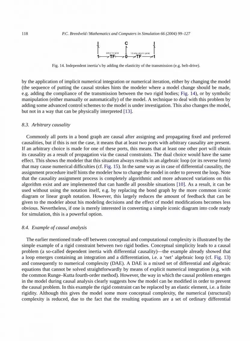
Fig. 14. Independent inertia’s by adding the elasticity of the transmission (e.g. belt-drive).

by the application of implicit numerical integration or numerical iteration, either by changing the model(the sequence of putting the causal strokes hints the modeler where a model change should be made,e.g. adding the compliance of the transmission between the two rigid bodies;Fig. 14), or by symbolicmanipulation (either manually or automatically) of the model. A technique to deal with this problem byadding some advanced control schemes to the model is under investigation. This also changes the model,but not in a way that can be physically interpreted[13].

8.3. Arbitrary causality

Commonly all ports in a bond graph are causal after assigning and propagating fixed and preferredcausalities, but if this is not the case, it means that at least two ports with arbitrary causality are present.If an arbitrary choice is made for one of these ports, this means that at least one other port will obtainits causality as a result of propagation via the causal constraints. The dual choice would have the sameeffect. This shows the modeler that this situation always results in an algebraic loop (or its reverse form)that may cause numerical difficulties (cf.Fig. 15). In the same way as in case of differential causality, theassignment procedure itself hints the modeler how to change the model in order to prevent the loop. Notethat the causality assignment process is completely algorithmic and more advanced variations on thisalgorithm exist and are implemented that can handle all possible situations[10]. As a result, it can beused without using the notation itself, e.g. by replacing the bond graph by the more common iconicdiagram or linear graph notation. However, this largely reduces the amount of feedback that can begiven to the modeler about his modeling decisions and the effect of model modifications becomes lessobvious. Nevertheless, if one is merely interested in converting a simple iconic diagram into code readyfor simulation, this is a powerful option.

8.4. Example of causal analysis

The earlier mentioned trade-off between conceptual and computational complexity is illustrated by thesimple example of a rigid constraint between two rigid bodies. Conceptual simplicity leads to a causalproblem (a so-called dependent inertia with differential causality)—the example already showed thata loop emerges containing an integration and a differentiation, i.e. a ‘net’ algebraic loop (cf.Fig. 13)and consequently to numerical complexity (DAE). A DAE is a mixed set of differential and algebraicequations that cannot be solved straightforwardly by means of explicit numerical integration (e.g. withthe common Runge–Kutta fourth-order method). However, the way in which the causal problem emergesin the model during causal analysis clearly suggests how the model can be modified in order to preventthe causal problem. In this example the rigid constraint can be replaced by an elastic element, i.e. a finiterigidity. Although this gives the model some more conceptual complexity, the numerical (structural)complexity is reduced, due to the fact that the resulting equations are a set of ordinary differential


Fig. 15. Arbitrary causality of two resistors causing an algebraic loop.

equations (ODE) that can be solved by explicit numerical integration schemes[1], see also the courseslides athttp://www.npac.syr.edu/users/gcf/CPS615NI95/.

Note that the model still needs a rather stiff constraint and thus introduces dynamics at a time scale thatis not of interest. This means not only means that both options to formulate the model can be a solutiondepending on the problem context, the available tools, etc., but also that a third solution can be obtained,viz. a symbolic transformation of the model as to eliminate the dependent inertia. In other words: tworigidly connected rigid bodies may be considered as one rigid body. This possibility is directly inducedby the causal analysis of the bond graph model.

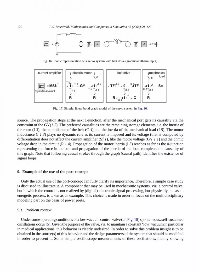
Fig. 16shows an iconic diagram representation of the servo-system containing a belt drive. The bondgraph inFig. 17represents this simple linear model.

It is graphical input to 20-sim. This software puts the causal strokes automatically, and immediatelywhile drawing the graph. The order in which the strokes are put can be indicated by sequence numbers,wherei·j represents thejth propagation of putting strokei.

Note that the fixed causalities are (M)Sf(1) and Se(2), where only Sf propagates via the 1-junction andimposes causality to the electricalI andR and the electrical port of the GY, thus eliminating the electricaltime constant that would have been present in the model if the electrical source would have been a voltage

http://www.npac.syr.edu/users/gcf/CPS615NI95/


Fig. 16. Iconic representation of a servo system with belt drive (graphical 20-sim input).

Fig. 17. Simple, linear bond graph model of the servo system inFig. 16.

source. The propagation stops at the next 1-junction, after the mechanical port gets its causality via theconstraint of the GY(1.2). The preferred causalities are the remaining storage elements, i.e. the inertia ofthe rotor (I3), the compliance of the belt (C4) and the inertia of the mechanical load (I5). The motorinductance (I1.3) plays no dynamic role as its current is imposed and its voltage (that is computed bydifferentiation does not affect the current amplifier (Sf1), like the motor voltage (GY1.1) and the ohmicvoltage drop in the circuit (R1.4). Propagation of the motor inertia (I3) reaches as far as the 0-junctionrepresenting the force in the belt and propagation of the inertia of the load completes the causality ofthis graph. Note that following causal strokes through the graph (causal path) identifies the existence ofsignal loops.

9. Example of the use of the port concept

Only the actual use of the port-concept can fully clarify its importance. Therefore, a simple case studyis discussed to illustrate it. A component that may be used in mechatronic systems, viz. a control valve,but in which the control is not realized by (digital) electronic signal processing, but physically, i.e. as anenergetic process, is taken as an example. This choice is made in order to focus on the multidisciplinarymodeling part on the basis of power ports.

9.1. Problem context

Under some operating conditions of a low-vacuum control valve (cf.Fig. 18) spontaneous, self-sustainedoscillations occur[5]. Given the purpose of the valve, viz. to maintain a constant ‘low’ vacuum in particularin medical applications, this behavior is clearly undesired. In order to solve this problem insight is to beobtained in the source(s) of this behavior and the design parameters of the system that should be modifiedin order to prevent it. Some simple oscilloscope measurements of these oscillations, mainly showing


Fig. 18. Sketch of the low-vacuum control valve.

shape and frequency, are available to the modeler as well as a construction drawing of the valve with dataon geometry and used materials.

9.2. Functional description of the valve

The intended basic operation of this control valve is that an orifice can be opened and closed by avalve body that is connected to a diaphragm loaded by a coil spring. Changing the position of the otherend of this spring with a screw knob can set its pretension. The diaphragm is part of the wall of thevalve chamber that is at one end connected to the ‘supply’ pressure (a relatively high under pressure or‘vacuum’) via the valve opening and at the other end via an orifice and a hose to the ‘mouth piece’ to sucksuperfluous body fluids away as used by dentists and surgeons. Given some desired low under pressure or‘low-vacuum’, the pressure difference over the diaphragm will cause the valve opening to get smaller ifthe actual pressure gets too low compared to the desired pressure. Due to the increasing flow resistance ofthe variable orifice the pressure difference with the supply pressure (‘high’ vacuum) will increase againvice versa.

9.3. Analysis

If this common functional explanation is translated into a block diagram, it becomes clear that theresulting model is not dynamic at all (Fig. 19) as all relations are algebraic. If oscillations occur it istempting to identify a damped second-order system consisting of the valve body, the spring and themechanical damping that is always present. As such a model is not competent to explain sustainedoscillations, it seems obvious to argue that the airflow is likely to drive these oscillations. The next stepthat seems obvious is to conclude that the common chaotic behavior of flow phenomena (turbulence) thatis hard to model deterministically is likely to form the onset of the oscillations, such that no attempt is


Fig. 19. Algebraic model resulting from functional description.

made to create a competent dynamic model and the problem is approached in an ad hoc way by changingthe geometry of the valve by trial and error.

However, if one approaches this problem from a port-based point of view the analysis will make adistinction between power relations and modulation and leads to another result, not only of the analysis,but also of the identification of the actual physics that play a role in such a valve.

In a regular valve a screw modulates the position of the body of the valve. Note that the fluid acts with aforce on this body, trying to move it out of the valve seat. The reason that the fluid cannot displace the valvebody while the human hand can do this, is the presence of the transforming action of the screw/spindle.This amplifies the static friction of the screw seen from the translating port of the screw/spindle. However,as this static friction is only overcome during a hand turning the valve and the dynamics of this processare at a completely different time scale than the flow phenomena in the valve, a change in position ofthe valve body is commonly modeled as a modulation of the flow resistance of the valve. Hence, aposition-modulated resistor can describe the dominant behavior of an arbitrary valve.Fig. 20shows howthe ports and port properties of such a valve can be defined in 20-sim, without having to define the exactconstitutive relations yet.

Feedback can be introduced by a diaphragm (membrane) that transforms the difference in pressure atits sides into a force that can cause a displacement. By connecting the body of the valve to the membranesuch that an increasing pressure difference will close the valve and a decreasing pressure difference willopen it, it will thus have a counteraction in both cases, i.e. a negative feedback. The relation betweenforce and displacement is characterized by the stiffness of the diaphragm. It needs to be increased inorder to attenuate the position changes of the valve body. This is achieved by connecting a spring. Byconnecting the other end of the spring to the screw, the screw can be used to change the setpoint for thepressure difference by changing its pretension. The screw serves as a combination of a (Coulomb) frictionand a transformer that amplifies its effect similar to the regular valve described above. The model of thecomplete valve has to be at least extended by an ideal transformer to represent the dominant behavior ofthe diaphragm, an ideal spring to represent the elasticity of the spring and the diaphragm and a modulatedforce source to introduce the pretension of the setpoint.Fig. 21shows this with a mixed use of bond graph(TF, valve), block diagram (modulation and signal generator) and iconic diagram elements (spring, forcesource and fixed world).

Note that the source of the pressure difference described earlier has not been accurately defined. Onemight conclude that the pressure difference between some supply pressure and the ambient pressure ismeant as these are the two obviously present pressures. However, this would cause the output pressure


Fig. 20. Definition of ports in 20-sim.

to fluctuate with the supply pressure, which is commonly not desired. Furthermore, the output pressureis required to cause some fluid exchange with the environment, i.e. some flow connection to the environ-ment. As a consequence one is usually interested in setting the pressure difference between the outputpressure and the supply pressure. This means that the valve needs to contain a more or less closed vol-ume, the so-called valve chamber, in which the output pressure is allowed to be different from both thesupply pressure and the ambient pressure. Obviously, some opening needs to connect this chamber tothe environment in order to allow the desired flow. The dominant behavior of this restriction is that of anideal (fluid) resistor, whether a hose is attached to the orifice or not. Parasitic behavior as fluid inertia (in

Fig. 21. Mix of block diagram, iconic diagram and bond graph representation (20-sim editor screen).


Fig. 22. Addition of boundary conditions, flow resistor and structural details (pressures).

Fig. 23. Simplification by choosing ambient pressure as reference pressure.

case of a long hose) may be added later when fine-tuning the model. Summarizing, the following idealelements are required in the model: a position-modulated resistor, a transformer, a spring and a resistor(Fig. 22). As the spring is the only dynamic element (containing an integration with respect to time) inthis model, oscillatory solutions are not likely.

Note that the labeled nodes in the bond graph merely represent the elementary behaviors, while theirexact constitutive relations have not been determined yet. Some of them will be nonlinear though. If theambient pressure is chosen as the reference pressure (zero-point), all pressures will obtain negative valuesin a low-vacuum control valve, but the bond graph is simplified into the one inFig. 23.

Note that the flows through the resistors are mainly dictated by the pressures imposed by sources exceptfor the contribution to the valve chamber pressure by the spring. It can be concluded that a linearizationaround an operating point leads to a first-order model characterized by a time constant. At this point onemight be inclined to bring the possibility of oscillatory behavior into the model by adding an ideal massto represent the dominant behavior of the valve body. Together with the ideal spring it forms a (damped)second-order system that has the potential of oscillatory solutions. However, such oscillations are notself-exciting and not self-sustained, unless the system would contain negative damping which wouldviolate the laws of physics. Note the change of position of some of the causal strokes (automaticallygenerated by 20-sim) and the causal path from the R to the valve that indicates an algebraic loop (Fig. 24).

The causality assignment process hints the modeler to put a C-type storage element at the 0-junctionrepresenting the pressure in the valve chamber in order to prevent this algebraic loop. This elementrepresents the compressibility of the air in the valve chamber (Fig. 25) and will appear crucial to obtaina model that is competent to represent self-sustained oscillations.

Fig. 24. Addition of the valve body mass.


Fig. 25. Addition of the compressibility of the air in the valve chamber (C).

Fig. 26 shows that this model contains a third-order loop via the position modulation of the valveand a causal path. It can be interpreted as follows: the position that modulates the valve is (inversely)proportional to the flow through the valve. The capacitance of the valve chamber relates the displacedvolume (first integration!) of this flow to the pressure in the chamber. Via the diaphragm this pressureacts with a force on the valve body. The resulting change of its momentum (second integration!) resultsin a change of its velocity. Finally this velocity causes its displacement (third integration!) and thusresults in the position that modulates the valve resistor (closure of the loop). Under certain conditionsthis third-order loop may have unstable solutions that are bounded by the nonlinearities of the model,like the valve body hitting the valve seat (end stops that can be added to the model easily, but discussionis beyond the scope of this paper). The causality of the ports is derived automatically by 20-sim whiledrawing this graph and automatically results in a computable set of equations for simulation. The sameprocedure is used in case of iconic diagrams and other representations that contain the concept of a port,although in those cases the immediate feedback to the modeler that a third-order loop is present cannotbe obtained immediately.

At this point, this example should illustrate that modeling should be focused on the relevant elementarybehaviors present in a system, not merely on a (one-to-one) translation of the functional relations as thedesigner of the valve intended them, because this would never bring in the compressibility of the air inthe valve chamber. The key elements in this model to represent the observed behavior are: the nonlinear,position-modulated resistor, the valve body, the diaphragm and the capacitance of the valve chamberto create the third-order loop, but also the spring with its adjustable pretension, the fluid resistor at theinlet, the supply pressure and the valve body hitting the valve seat. The number of elementary one- andmultiports is relatively small.

After identification of the proper parameter values from the provided measurement data, first simulationruns showed indeed self-starting and self-sustained oscillations with a shape that coincided with the shapesobserved on the oscilloscope. The frequency of these first results was only 10% off the observed frequency.Fine-tuning of the model allowed these frequencies to be matched. However, the actual problem was al-ready solved before the parameter identification phase, because the process of setting up the model struc-

Fig. 26. Third-order loop (three integrations) via a causal path and the modulation signal.


ture already indicated the crucial role of the valve chamber that was confirmed by an experienced seniorcraftsman at the work floor where these valves were produced and assembled. He then remembered thatlong ago the role of this valve chamber was identified by trial and error. A result that had been forgotten overthe years and did not play a role in the design of the new valve that was causing the oscillation problems.

After this discussion, it should be clear that a bond graph without modulating signals can never resultin three integrations in a loop. A causal path can only exist between at most two storage elements, suchthat the number of integrations in the corresponding signal loop is at most two. Hence, the modulatingsignal of the valve that contains a third integration is also one of the crucial elements to create a modelthat is competent to represent the instabilities.

Note that the possibility of the oscillations that can result from the third-order loop is inherent to thisparticular type of design. None of the parts can be omitted or changed as to break the third-order loop. Forthis reason, every designer of such valves should have the insights discussed above in order to be able tochoose the dimensions of the valve such that it never displays undesired behavior in or near the range ofoperation. This insight is more related to model structure than to particular simulation results, althoughsimulation results can help to identify the influence of the valve chamber size on the modes of operation.

Similar types of valves are not only used as low-vacuum control valves, but also as fuel-injection valves,pressure reduction valves, etc.

This example demonstrates that a port-based approach provides this insight quite easily, although theuse of this approach should be supported by sufficient knowledge of engineering physics.

10. Conclusion

This paper has shown how modern object-oriented modeling of physical systems can help to makeproper decisions during the design of mechatronic systems and to create more insight in the physics ofthe object to be modeled. This approach enables to easily change from finding solutions in the controllerdomain or in the mechanical structure itself, which is the key aspects of mechatronics. Software toolsthat cover the different domains support this process.

Emphasis was on the background of physical modeling in general. In particular the paradigm shift tothe port-based approach via the introduction of the concepts of a port and a junction were discussed. Anexample demonstrated that one of the major achievements is that a tool allowing a multiple-view approachprovides insight into the nature and background of the observed behavior. A bond graph representationgives the user who gained some expertise in this language, feedback about his modeling decisions via therepresentation of computational causality by the causal stroke. Note that the port-based computationalcausality assignment procedure is also used in the iconic diagram notation, but cannot provide the graphicalinsight that is obtained via a bond graph, as the control valve example illustrated. As the approach focuseson insight, it is particularly suited for education[7]. All sorts of generalizations like multi-bond graphs,Generalized Bond Graphs, bi-causality, hybrid systems, etc. exist, but are beyond the scope of this paper.The interested reader is referred to the extensive literature on these topics.

References

[1] U.M. Ascher, L.R. Petzold, Computer Methods for Ordinary Differential Equations and Differential-Algebraic Equations,SIAM, ISBN 0-89871-412-5, 1998.


[2] P.C. Breedveld, Thermodynamic bond graphs and the problem of thermal inertance, J. Franklin Inst. 314 (1) (1982) 15–40.[3] P.C. Breedveld, Physical Systems Theory in Terms of Bond Graphs, ISBN 90-9000599-4, 1984.[4] P.C. Breedveld, Fundamentals of Bond Graphs, in: IMACS Annals of Computing and Applied Mathematics, vol. 3,

Modelling and Simulation of Systems, Basel, 1989, pp. 7–14.[5] P.C. Breedveld, Bond-graph modeling of a low-vacuum control valve, in: P.C. Breedveld, G. Dauphin-Tanguy (Eds.), Bond

Graphs for Engineers, IMACS Transaction Series, Elsevier, Amsterdam, ISBN 0-444-89707-0, 1992, pp. 135–150.[6] P.C. Breedveld, On state-event constructs in physical system dynamics modeling, Simul. Practice Theory 7 (5–6) (1999)

463–480.[7] P.C. Breedveld, Integrated Modeling of Physical systems. Parts 1–3, in preparation, preliminary versions on request, 2003.[8] A.P.J. Breunese, Automated Support in Mechatronic Systems Modelling, Ph.D. Thesis, University of Twente, Enschede,

The Netherlands, ISBN 90-365-0872-X, 1996.[9] H.J. Coelingh, Design Support for Motion Control Systems, Ph.D. Thesis, University of Twente, Enschede, The Netherlands,

alsohttp://www.ce.el.utwente.nl/clh/, 2000.[10] G. Golo, Interconnection Structures in Port-Based Modelling: Tools for Analysis and Simulation, Ph.D. Thesis, University

of Twente, Twente University Press, ISBN 9036518113, 2002.[11] N. Hogan, P.C. Breedveld, The physical basis of analogies in physical system models, in: R.H. Bishop (Ed.), The

Mechatronics Handbook, Chapter 15, CRC Press, Boca Raton, FL, 2002, ISBN 0-8493-0066-5, pp. 15.1–15.10.[12] D.C. Karnopp, R.C. Rosenberg, System Dynamics: A Unified Approach, Wiley, New York, 1975.[13] P.A.J. Koenders, On the Relation Between Equation Formulation of Constrained Systems and Implicit Numerical Integration

and Optimization, M.Sc. Thesis, University of Twente, Control Engineering, 2001.[14] T.S. Kuhn, The Structure of Scientific Revolutions, University of Chicago Press,http://www.emory.edu/EDUCATION/

mfp/Kuhnsnap.html, 1962.[15] H.M. Paynter, Analysis and Design of Engineering Systems, MIT Press, 1961.[16] J.L. Shearer, A.T. Murphy, H.H. Richardson, Introduction to System Dynamics, Addison Wesley, New York, 1971.[17] T.J.A. de Vries, Conceptual Design of Controlled Electro-Mechanical Systems, Ph.D. Thesis, University of Twente,

Enschede, The Netherlands, 1994.[18] P.B.T. Weustink, T.J.A. de Vries, P.C. Breedveld, Object Oriented Modelling and Simulation of Mechatronic Systems with

20-Sim 3.0, in: J. Adolfson, J. Karlsén (Eds.), Mechatronics 98, Elsevier, 1998.[19] H.A. Wheeler, D. Dettinger, Wheeler Monogr. 9 (1949) 7.

http://www.ce.el.utwente.nl/clh/

http://www.emory.edu/EDUCATION/mfp/Kuhnsnap.html

http://www.emory.edu/EDUCATION/mfp/Kuhnsnap.html

port-based modeling of mechatronic systems

Documents