Computers, Environment and Urban Systems 32 (2008) 204–213

Contents lists available at ScienceDirect

Computers, Environment and Urban Systems

journal homepage: www.elsevier .com/locate /compenvurbsys

Planar and spherical hierarchical, multi-resolution cellular automata

A. Ross Kiester a,*, Kevin Sahr b

a Biodiversity Futures Consulting, 5550 SW Redtop Place, Corvallis, OR 97333, United Statesb Department of Computer Science, Southern Oregon University, 1250 Siskiyou Blvd., Ashland, OR 97520, United States

a r t i c l e i n f o

Article history:Received 14 November 2006Received in revised form 16 January 2008Accepted 1 March 2008

Keywords:Discrete global gridsSpatial hierarchyCellular automata

0198-9715/$ - see front matter � 2008 Elsevier Ltd. Adoi:10.1016/j.compenvurbsys.2008.03.001

* Corresponding author.E-mail addresses: rkiester@gmail.com (A.R. Kiester

a b s t r a c t

We present a new generalized definition of spatial hierarchy and use it to create a data structure for spa-tial hierarchies on the plane and the sphere. The data structure is then used as the basis for hierarchical,multi-resolution cellular automata which are topology-independent so that many topologies may bestudied. In these systems the dynamics of a focal cell is dependent on its neighbors and also the cell aboveand below it in the next coarser or finer resolution. Results from a multi-resolution version of the Game ofLife show complex and unexpected behavior which is dependent on the topology chosen and initial con-ditions. These results and the software which produced them provide a proof of concept for the new datastructure and algorithms. These may be especially useful for data analysis and simulation at the globalscale.

� 2008 Elsevier Ltd. All rights reserved.

1. Introduction

A major trend in ecology (Holyoak, Leibold, & Holt, 2005; Molo-ney & Levin, 1996; Tilman & Kareiva, 1997) and many similar dis-ciplines ranging from epidemiology (Lawson, 2006; Waller &Gotway, 2004) to real estate portfolio analysis (Tu, Shi-Ming, &Hua, 2004) has been toward studies that are explicitly spatial. Inaddition, ecologists have routinely begun to see that space mustbe considered at 2 or more resolutions so that a hierarchical spatialapproach is what is needed (O’Neill, DeAngelis, & Allen, 1986). Animportant tool in examining spatial processes is the cellularautomaton (Toffoli & Margolus, 1987; Wolfram, 1986). However,traditional cellular automata (CAs) act on only a single spatial res-olution on the plane. In this paper, we extend the definition of CAsto include CAs that are multi-resolution and defined on both theplane and the sphere, which is an important topology for model-ling geo-referenced phenomena.

A cellular automaton (CA) is a discrete dynamical mathematicalstructure defined on a spatial grid (von Neumann, 1966). A CA ischaracterized by 4 properties.

1. State space: This is the collection of all possible values that a sin-gle grid cell can take on. Frequently the state space is binarytaking the values 1/0, on/off or live/dead.

2. An initial condition: All cells in the grid are populated at timezero with values from the state space.

ll rights reserved.

), sahrk@sou.edu (K. Sahr).

3. A rule set: The rule set is the set of instructions that determine ifa given cell changes from one state into another at a particulardiscrete time step. In traditional CAs the state of each cell at agiven time step is determined by the states at the previous timestep of that cell and the states of the cells immediately adjacentto it.

4. A grid topology: The grid topology is specified by a cell shapeand a rule for determining cell adjacency. Primary attention inthe CA literature has been given to grids of squares with adja-cency specified using either the von Neumann neighborhood/D4 metric (neighbors share an edge, with each cell having fourneighbors) or the Moore neighborhood/D8 metric (neighborsshare an edge or a vertex, with each cell having eight neigh-bors). Increasingly attention is being given to exploring hexa-gon grid topologies because hexagonal grids exhibit spatialisotropy; unlike square cells each hexagon cell has exactly sixneighbors with which it shares an edge and no adjacent cellswith which it shares only a vertex. For studies of many kindsof flow hexagonal grids give the correct answer whereas squaregrids do not (Rothman & Zaleski, 1997).

Historically, research on CAs has focused on rule sets and initialconditions and has not examined alternative topologies as exten-sively. Thus, the main focus of our study is on the effect of topologyon CA behavior. Specifically, in this work we extend CAs to havespatially hierarchical topologies on both the plane and the surfaceof a sphere. Our motivation for developing spatially hierarchicalmodels on the sphere is to provide a basis for modeling processeson the surface of the earth. Our goal here is to provide tools for theanalysis and dynamic simulation of Discrete Global Grid Systems(DGGSs; Sahr, White, & Kimerling, 2003). In the next section, we

A.R. Kiester, K. Sahr / Computers, Environment and Urban Systems 32 (2008) 204–213 205

present the design and implementation of software libraries forworking with discrete grids in a topology-independent fashion,and we describe a dynamics simulation engine built on these li-braries. We then give the results of a simple dynamical model builtas a proof-of-concept for our approach.

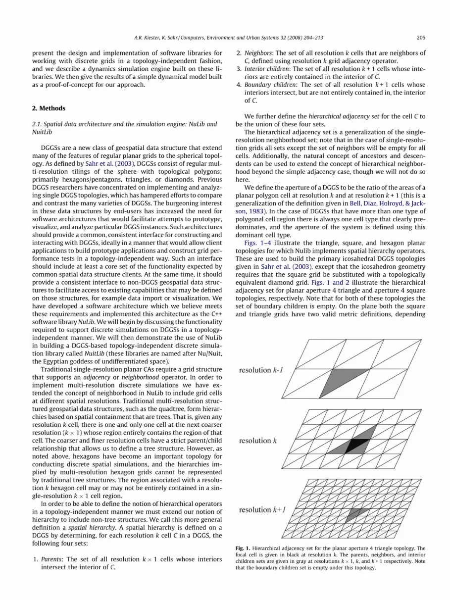
Fig. 1. Hierarchical adjacency set for the planar aperture 4 triangle topology. Thefocal cell is given in black at resolution k. The parents, neighbors, and interiorchildren sets are given in gray at resolutions k � 1, k, and k + 1 respectively. Notethat the boundary children set is empty under this topology.

2. Methods

2.1. Spatial data architecture and the simulation engine: NuLib andNuitLib

DGGSs are a new class of geospatial data structure that extendmany of the features of regular planar grids to the spherical topol-ogy. As defined by Sahr et al. (2003), DGGSs consist of regular mul-ti-resolution tilings of the sphere with topological polygons;primarily hexagons/pentagons, triangles, or diamonds. PreviousDGGS researchers have concentrated on implementing and analyz-ing single DGGS topologies, which has hampered efforts to compareand contrast the many varieties of DGGSs. The burgeoning interestin these data structures by end-users has increased the need forsoftware architectures that would facilitate attempts to prototype,visualize, and analyze particular DGGS instances. Such architecturesshould provide a common, consistent interface for constructing andinteracting with DGGSs, ideally in a manner that would allow clientapplications to build prototype applications and construct grid per-formance tests in a topology-independent way. Such an interfaceshould include at least a core set of the functionality expected bycommon spatial data structure clients. At the same time, it shouldprovide a consistent interface to non-DGGS geospatial data struc-tures to facilitate access to existing capabilities that may be definedon those structures, for example data import or visualization. Wehave developed a software architecture which we believe meetsthese requirements and implemented this architecture as the C++software library NuLib. We will begin by discussing the functionalityrequired to support discrete simulations on DGGSs in a topology-independent manner. We will then demonstrate the use of NuLibin building a DGGS-based topology-independent discrete simula-tion library called NuitLib (these libraries are named after Nu/Nuit,the Egyptian goddess of undifferentiated space).

Traditional single-resolution planar CAs require a grid structurethat supports an adjacency or neighborhood operator. In order toimplement multi-resolution discrete simulations we have ex-tended the concept of neighborhood in NuLib to include grid cellsat different spatial resolutions. Traditional multi-resolution struc-tured geospatial data structures, such as the quadtree, form hierar-chies based on spatial containment that are trees. That is, given anyresolution k cell, there is one and only one cell at the next coarserresolution (k � 1) whose region entirely contains the region of thatcell. The coarser and finer resolution cells have a strict parent/childrelationship that allows us to define a tree structure. However, asnoted above, hexagons have become an important topology forconducting discrete spatial simulations, and the hierarchies im-plied by multi-resolution hexagon grids cannot be representedby traditional tree structures. The region associated with a resolu-tion k hexagon cell may or may not be entirely contained in a sin-gle-resolution k � 1 cell region.

In order to be able to define the notion of hierarchical operatorsin a topology-independent manner we must extend our notion ofhierarchy to include non-tree structures. We call this more generaldefinition a spatial hierarchy. A spatial hierarchy is defined on aDGGS by determining, for each resolution k cell C in a DGGS, thefollowing four sets:

1. Parents: The set of all resolution k � 1 cells whose interiorsintersect the interior of C.

2. Neighbors: The set of all resolution k cells that are neighbors ofC, defined using resolution k grid adjacency operator.

3. Interior children: The set of all resolution k + 1 cells whose inte-riors are entirely contained in the interior of C.

4. Boundary children: The set of all resolution k + 1 cells whoseinteriors intersect, but are not entirely contained in, the interiorof C.

We further define the hierarchical adjacency set for the cell C tobe the union of these four sets.

The hierarchical adjacency set is a generalization of the single-resolution neighborhood set; note that in the case of single-resolu-tion grids all sets except the set of neighbors will be empty for allcells. Additionally, the natural concept of ancestors and descen-dents can be used to extend the concept of hierarchical neighbor-hood beyond the simple adjacency case, though we will not do sohere.

We define the aperture of a DGGS to be the ratio of the areas of aplanar polygon cell at resolution k and at resolution k + 1 (this is ageneralization of the definition given in Bell, Diaz, Holroyd, & Jack-son, 1983). In the case of DGGSs that have more than one type ofpolygonal cell region there is always one cell type that clearly pre-dominates, and the aperture of the system is defined using thisdominant cell type.

Figs. 1–4 illustrate the triangle, square, and hexagon planartopologies for which Nulib implements spatial hierarchy operators.These are used to build the primary icosahedral DGGS topologiesgiven in Sahr et al. (2003), except that the icosahedron geometryrequires that the square grid be substituted with a topologicallyequivalent diamond grid. Figs. 1 and 2 illustrate the hierarchicaladjacency set for planar aperture 4 triangle and aperture 4 squaretopologies, respectively. Note that for both of these topologies theset of boundary children is empty. On the plane both the squareand triangle grids have two valid metric definitions, depending

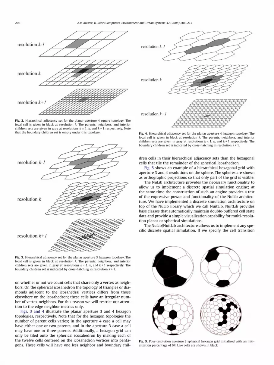
Fig. 2. Hierarchical adjacency set for the planar aperture 4 square topology. Thefocal cell is given in black at resolution k. The parents, neighbors, and interiorchildren sets are given in gray at resolutions k � 1, k, and k + 1 respectively. Notethat the boundary children set is empty under this topology.

Fig. 3. Hierarchical adjacency set for the planar aperture 3 hexagon topology. Thefocal cell is given in black at resolution k. The parents, neighbors, and interiorchildren sets are given in gray at resolutions k � 1, k, and k + 1 respectively. Theboundary children set is indicated by cross-hatching in resolution k + 1.

Fig. 4. Hierarchical adjacency set for the planar aperture 4 hexagon topology. Thefocal cell is given in black at resolution k. The parents, neighbors, and interiorchildren sets are given in gray at resolutions k � 1, k, and k + 1 respectively. Theboundary children set is indicated by cross-hatching in resolution k + 1.

Fig. 5. Four-resolution aperture 3 spherical hexagon grid initialized with an initi-alization percentage of 6%. Live cells are shown in black.

206 A.R. Kiester, K. Sahr / Computers, Environment and Urban Systems 32 (2008) 204–213

on whether or not we count cells that share only a vertex as neigh-bors. On the spherical icosahedron the topology of triangles or dia-monds adjacent to the icosahedral vertices differs from thoseelsewhere on the icosahedron; these cells have an irregular num-ber of vertex neighbors. For this reason we will restrict our atten-tion to the edge neighbor metrics only.

Figs. 3 and 4 illustrate the planar aperture 3 and 4 hexagontopologies, respectively. Note that for the hexagon topologies thenumber of parent cells varies; in the aperture 4 case a cell mayhave either one or two parents, and in the aperture 3 case a cellmay have one or three parents. Additionally, a hexagon grid canonly be tiled onto the spherical icosahedron by making each ofthe twelve cells centered on the icosahedron vertices into penta-gons. These cells will have one less neighbor and boundary chil-

dren cells in their hierarchical adjacency sets than the hexagonalcells that tile the remainder of the spherical icosahedron.

Fig. 5 shows an example of a hierarchical hexagonal grid withaperture 3 and 4 resolutions on the sphere. The spheres are shownas orthographic projections so that only part of the grid is visible.

The NuLib architecture provides the necessary functionality toallow us to implement a discrete spatial simulation engine; atthe same time the construction of such an engine provides a testof the expressive power and functionality of the NuLib architec-ture. We have implemented a discrete simulation architecture ontop of the NuLib library which we call NuitLib. NuitLib providesbase classes that automatically maintain double-buffered cell statedata and provide a simple visualization capability for multi-resolu-tion planar or spherical simulations.

The NuLib/NuitLib architecture allows us to implement any spe-cific discrete spatial simulation. If we specify the cell transition

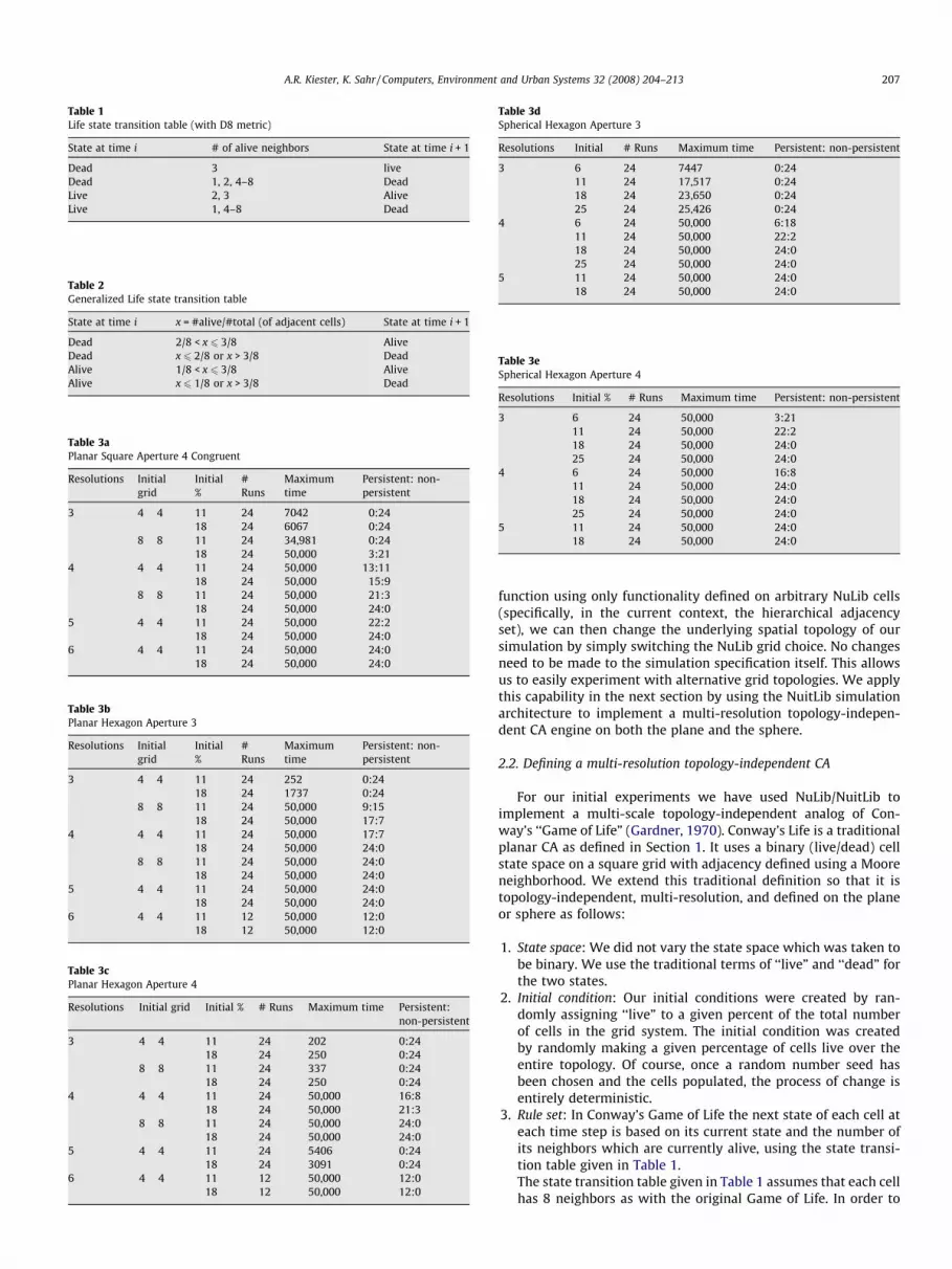
Table 1Life state transition table (with D8 metric)

State at time i # of alive neighbors State at time i + 1

Dead 3 liveDead 1, 2, 4–8 DeadLive 2, 3 AliveLive 1, 4–8 Dead

Table 2Generalized Life state transition table

State at time i x = #alive/#total (of adjacent cells) State at time i + 1

Dead 2/8 < x 6 3/8 AliveDead x 6 2/8 or x > 3/8 DeadAlive 1/8 < x 6 3/8 AliveAlive x 6 1/8 or x > 3/8 Dead

Table 3aPlanar Square Aperture 4 Congruent

Resolutions Initialgrid

Initial%

#Runs

Maximumtime

Persistent: non-persistent

3 4 � 4 11 24 7042 0:2418 24 6067 0:24

8 � 8 11 24 34,981 0:2418 24 50,000 3:21

4 4 � 4 11 24 50,000 13:1118 24 50,000 15:9

8 � 8 11 24 50,000 21:318 24 50,000 24:0

5 4 � 4 11 24 50,000 22:218 24 50,000 24:0

6 4 � 4 11 24 50,000 24:018 24 50,000 24:0

Table 3bPlanar Hexagon Aperture 3

Resolutions Initialgrid

Initial%

#Runs

Maximumtime

Persistent: non-persistent

3 4 � 4 11 24 252 0:2418 24 1737 0:24

8 � 8 11 24 50,000 9:1518 24 50,000 17:7

4 4 � 4 11 24 50,000 17:718 24 50,000 24:0

8 � 8 11 24 50,000 24:018 24 50,000 24:0

5 4 � 4 11 24 50,000 24:018 24 50,000 24:0

6 4 � 4 11 12 50,000 12:018 12 50,000 12:0

Table 3cPlanar Hexagon Aperture 4

Resolutions Initial grid Initial % # Runs Maximum time Persistent:non-persistent

3 4 � 4 11 24 202 0:2418 24 250 0:24

8 � 8 11 24 337 0:2418 24 250 0:24

4 4 � 4 11 24 50,000 16:818 24 50,000 21:3

8 � 8 11 24 50,000 24:018 24 50,000 24:0

5 4 � 4 11 24 5406 0:2418 24 3091 0:24

6 4 � 4 11 12 50,000 12:018 12 50,000 12:0

Table 3dSpherical Hexagon Aperture 3

Resolutions Initial # Runs Maximum time Persistent: non-persistent

3 6 24 7447 0:2411 24 17,517 0:2418 24 23,650 0:2425 24 25,426 0:24

4 6 24 50,000 6:1811 24 50,000 22:218 24 50,000 24:025 24 50,000 24:0

5 11 24 50,000 24:018 24 50,000 24:0

Table 3eSpherical Hexagon Aperture 4

Resolutions Initial % # Runs Maximum time Persistent: non-persistent

3 6 24 50,000 3:2111 24 50,000 22:218 24 50,000 24:025 24 50,000 24:0

4 6 24 50,000 16:811 24 50,000 24:018 24 50,000 24:025 24 50,000 24:0

5 11 24 50,000 24:018 24 50,000 24:0

A.R. Kiester, K. Sahr / Computers, Environment and Urban Systems 32 (2008) 204–213 207

function using only functionality defined on arbitrary NuLib cells(specifically, in the current context, the hierarchical adjacencyset), we can then change the underlying spatial topology of oursimulation by simply switching the NuLib grid choice. No changesneed to be made to the simulation specification itself. This allowsus to easily experiment with alternative grid topologies. We applythis capability in the next section by using the NuitLib simulationarchitecture to implement a multi-resolution topology-indepen-dent CA engine on both the plane and the sphere.

2.2. Defining a multi-resolution topology-independent CA

For our initial experiments we have used NuLib/NuitLib toimplement a multi-scale topology-independent analog of Con-way’s ‘‘Game of Life” (Gardner, 1970). Conway’s Life is a traditionalplanar CA as defined in Section 1. It uses a binary (live/dead) cellstate space on a square grid with adjacency defined using a Mooreneighborhood. We extend this traditional definition so that it istopology-independent, multi-resolution, and defined on the planeor sphere as follows:

1. State space: We did not vary the state space which was taken tobe binary. We use the traditional terms of ‘‘live” and ‘‘dead” forthe two states.

2. Initial condition: Our initial conditions were created by ran-domly assigning ‘‘live” to a given percent of the total numberof cells in the grid system. The initial condition was createdby randomly making a given percentage of cells live over theentire topology. Of course, once a random number seed hasbeen chosen and the cells populated, the process of change isentirely deterministic.

3. Rule set: In Conway’s Game of Life the next state of each cell ateach time step is based on its current state and the number ofits neighbors which are currently alive, using the state transi-tion table given in Table 1.The state transition table given in Table 1 assumes that each cellhas 8 neighbors as with the original Game of Life. In order to

Fig. 6. Time series plots of the number of live cells in Resolution 4 for a simulation of the Planar Square topology with 4 resolutions. The simulations differ only in the randomnumber seed used to initialize the grid at 11% live. (6a) A simulation that persists for 50,000 time steps although it comes close to dying at approximately time step 38,000.(6b) A simulation that persists to time step 49,399 and then collapses to a narrow cyclical pattern. (6c) A simulation that persists to time step 12,471 and then collapses to anarrow cyclical pattern. (6d) A simulation that persists only to time step 171 and decays to a narrow cyclical pattern. All cyclical patterns consist of 4–6 live cells in Resolution3 and 25–30 in Resolution 4.

208 A.R. Kiester, K. Sahr / Computers, Environment and Urban Systems 32 (2008) 204–213

implement Life in a topology-independent manner we mustgeneralize this table so that it can be used with the variableneighbor counts generated by the alternate planar and DGGStopologies. One simple way to do this is to change the secondcolumn so that it uses the fraction of adjacent cells currentlyalive, rather than a discrete count of alive neighbors. The result-ing state transition diagram is given in Table 2.In order to extend the CA concept to multi-scale grids weexpand the notion of adjacency used in specifying a rule setto include the concept of hierarchical adjacency sets as definedin the previous section. Then the cell state at each time step is afunction of the current states of the cell and of the cells in thehierarchical adjacency set of that cell, rather than just of thestates of its neighbors at the same resolution. A rule set maytreat all cells in the hierarchical adjacency set in an equivalentmanner, or it may make a distinction by, for example, weightingcells in each of the sub-sets differently.For our first experimentswe chose to treat all hierarchical adjacency set membersequally. This allows us to use Table 2 to define our state transi-tions. This rule set is quite arbitrary, but can be easily changedin the simulation code. We chose this rule set because of thewidespread use of the Game of Life and because we wantedas simple a rule set as possible for a proof-of-concept exerciseand to focus on the effects of topology.

4. Topology: From among the grid topologies supported by theNuLib library we chose three spatially hierarchical topologieson the plane and four DGGS topologies on the sphere. For theplane, we chose squares with aperture 4 (Fig. 2) and hexagonswith apertures 3 (Fig. 3) and 4 (Fig. 4). Each of these topologieswas studied with resolutions 3–6.

For the planar topologies we note that cells at the edge or cornerof a tessellation have different numbers of neighbors than those inthe center. The existence of boundary cells obviously affects thedynamics of the system. Because the original Game of Life is de-fined solely on finite patches of the plane, the edge cells are usuallygiven special treatment. The most common solution is to defineadjacency as ‘‘wrapping” horizontally and vertically, so that thesimulation is actually being performed on a toroid. In our general-ization of Life our rule set explicitly accounts for differing numbersof cell neighbors, so no ‘‘wrapping” is used.

Since the sphere is a closed surface single-resolution sphericalgrids have no ‘‘edge” cells. But multi-resolution grids, both planarand spherical, have another kind of boundary: cells in the finestand in the coarsest resolutions have different number of neigh-bors than cells in the ‘‘interior” resolutions; at the coarsest reso-lution cells have no parents and at the finest they have nochildren.

Fig. 7. Histogram of the number of live cells for Resolution 4 of 4 for the PlanarSquare topology for times steps 1,000–50,000. (7a) Resolution 1 is a 4 � 4 grid sothat Resoluton 4 is a 32 � 32 grid with 1024 cells. This histogram is assymetric. (7b)Resolution 1 is a 16 � 16 grid so that Resolution 4 is a 128 � 128 grid with 16,348cells. This histogram is almost exactly Gaussian.

A.R. Kiester, K. Sahr / Computers, Environment and Urban Systems 32 (2008) 204–213 209

2.3. Simulation cases

After some initial exploratory runs we chose a maximum of50,000 time steps as a practical limit to the processing time ofthe simulation.

For the planar cases we used two initializing to live percentages(11% and 18%), initial top level grid sizes of 4 � 4 and 8 � 8, and to-tal number of resolutions from 3 to 6. For each set of parameters 24simulations were performed (each using a unique random numberseed) except for simulations on hexagonal grids of 6 resolutions forwhich 12 cases were run. A total of 32 separate parameter combi-nations were simulated for a total of 720 runs.

For the spherical cases we used four initializing to live percent-ages (6%, 11%, 18%, and 25%) for resolutions 3 and 4 and two initial-izing percentages (11% and 18%) for resolution 5. The initial gridsize is always fixed by the iscosahedral basis of the DGG. For eachset of parameters 24 simulations were performed. A total of 20

separate parameter combinations were simulated for a total of480 runs.

3. Results

We were able to perform simulations on planar systems withup to 6 resolutions and a total of 21,840 cells and spherical systemsof 6 resolutions with a total of 10,972 cells on a contemporary per-sonal computer. Multi-resolution systems were simulated for50,000 times in minutes to a small number of hours.

Although the rule set was initially chosen as a proof-of-concept,some results proved of general interest. Here, we report on initialstudies of the persistence and number of live cells at each resolu-tion as they change through time. We form time series from thenumber of cells alive at each time step for each resolution. Wepresent results for all topologies except the spherical diamond 4and triangles cases which are guaranteed to die given the ruleset. These time series exhibit novel behavior.

3.1. Persistence

A run was considered to persist if it reached time = 50,000 with-out degenerating to a set of constant values or a cyclical state involv-ing a narrow range of values. (Systems with resolutions less than 3invariably do not persist for more than a few time steps.) Table 3ashows that whether or not a simulation lives is dependent on theinitial grid size for the planar cases, the number of resolutions,and the percent of cells initialized to live at t = 0. Fig. 6 shows thetime series of the number of live individuals at resolution 4 (a grid128 � 128) for 4 realizations of the 24 runs for the planar square(D8) topology with a top level grid size of 4 � 4, 4 total resolutions,and an initial percent of 11% live. These examples show a greatrange of behavior for this parameter set. They also show that thesesystems exhibit extremely long-term memory (see Section 4). Thisparameter set appears to be on the boundary between persistenceand non-persistence. Other parameter sets showed both mixed(some live, some die) and consistent (all live or all die) results. Anespecially interesting result for the planar case is that for resolution5 hexagons those of aperture 3 all die and those of aperture 4 alllive.

3.2. Counts

Counts of the number alive vary with the same parameters asfor persistence. Fig. 7a shows the distribution of counts of live cellsfor resolution 4 of a Planar Square (D8 metric) system with param-eter values of 4 resolutions, initial top grid size of 4 � 4, initial %live of 11%. The distribution is approximately Gaussian, but witha pronounced tail. Fig. 7b is the distribution of counts for a similarrun using a larger top resolution grid of 16 � 16. This distributionis almost exactly Gaussian. Distributions of counts for larger spher-ical grids are similarly near Gaussian.

3.3. Dynamical properties

3.3.1. Non-linearity and time reversalThe behavior of these systems is strongly suggestive that they

are nonlinear. To test directly for nonlinearity we used the timereversal test described in the TISEAN Package (Diks, van Houwelin-gen, Takens, & DeGoede, 1997; Hegger, Kantz, & Schreiber, 1999;Kantz & Schreiber, 1997). Most time series are non-linear by thistest although as with persistence the details of the pattern of non-linear vs. linear are complex. For example, for the planar case with

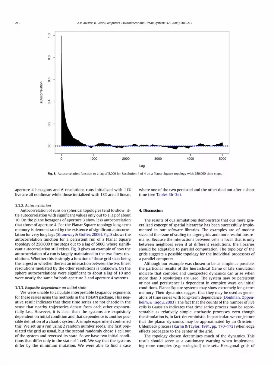
Fig. 8. Autocorrelation function to a lag of 5,000 for Resolution 4 of 4 on a Planar Square topology with 250,000 time steps.

210 A.R. Kiester, K. Sahr / Computers, Environment and Urban Systems 32 (2008) 204–213

aperture 4 hexagons and 6 resolutions runs initialized with 11%live are all nonlinear while those initialized with 18% are all linear.

3.3.2. AutocorrelationAutocorrelation of runs on spherical topologies tend to show lit-

tle autocorrelation with significant values only out to a lag of about10. On the plane hexagons of aperture 3 show less autocorrelationthat those of aperture 4. For the Planar Square topology long-termmemory is demonstrated by the existence of significant autocorre-lation for very long lags (Shumway & Stoffer, 2006). Fig. 8 shows theautocorrelation function for a persistent run of a Planar Squaretopology of 250,000 time steps out to a lag of 5000, where signifi-cant autocorrelation still exists. Fig. 9 gives an example of how theautocorrelation of a run is largely maintained in the two finest res-olutions. Whether this is simply a function of those grid sizes beingthe largest or whether there is an interaction between the two finestresolutions mediated by the other resolutions is unknown. On thesphere autocorrelations were significant to about a lag of 10 andwere nearly the same for both aperture 3 and aperture 4 systems.

3.3.3. Exquisite dependence on initial stateWe were unable to calculate interpretable Lyapanov exponents

for these series using the methods in the TISEAN package. This neg-ative result indicates that these time series are not chaotic in thesense that nearby trajectories depart from each other exponen-tially fast. However, it is clear than the systems are exquisitelydependent on initial condition and that dependence is another pos-sible definition of a chaotic system. A simple experiment confirmedthis. We set up a run using 2 random number seeds. The first pop-ulated the grid as usual, but the second randomly chose 1 cell outof the system and reversed its state. So we have two initial condi-tions that differ only in the state of 1 cell. We say that the systemsdiffer by the minimum mutation. We were able to find a case

where one of the two persisted and the other died out after a shorttime (see Tables 3b–3e).

4. Discussion

The results of our simulations demonstrate that our more gen-eralized concept of spatial hierarchy has been successfully imple-mented in our software libraries. The examples are of modestsize and the issue of scaling to larger grids and more resolutions re-mains. Because the interactions between cells is local, that is onlybetween neighbors even if at different resolutions, the librariesshould be adaptable to parallel computation. The topology of thegrids suggests a possible topology for the individual processors ofa parallel computer.

Although our example was chosen to be as simple as possible,the particular results of the hierarchical Game of Life simulationindicate that complex and unexpected dynamics can arise whenmore than 3 resolutions are used. The system may be persistentor not and persistence is dependent in complex ways on initialconditions. Planar Square systems may show extremely long-termmemory. Their dynamics suggest that they may be used as gener-ators of time series with long-term dependance (Doukhan, Oppen-heim, & Taqqu, 2003). The fact that the counts of the number of livecells is Gaussian indicates that time series process may be repre-sentable as relatively simple stochastic processes even thoughthe simulation is, in fact, deterministic. In particular, we conjecturethat the planar dynamics may be approximated by an Ornstein–Uhlenbeck process (Karlin & Taylor, 1981, pp. 170–173) when edgeeffects propagate to the center of the grid.

The topology chosen determines much of the dynamics. Thisresult should serve as a cautionary warning when implement-ing more complex (e.g. ecological) rule sets. Hexagonal grids of

Fig. 9. Autocorrelations to a lag of 500 for all resolutions of 4 simulations of Planar Square topology with number of resolutions = 4, 5, 6, 7. Note that in each case theautocorrelations of the 2 finest resolutions are higher than any of the lower resolutions.

A.R. Kiester, K. Sahr / Computers, Environment and Urban Systems 32 (2008) 204–213 211

Fig. 9 (continued)

212 A.R. Kiester, K. Sahr / Computers, Environment and Urban Systems 32 (2008) 204–213

Fig. 9 (continued)

A.R. Kiester, K. Sahr / Computers, Environment and Urban Systems 32 (2008) 204–213 213

aperture 3 in the plane may be the best choice since they showthe least autocorrelation and would make it more likely that dy-namic behavior of more complex rule sets was due to the rulesets themselves and not the topology. Hexagonal grids of aper-ture 3 or 4 on the sphere are equivalent with regard to theirlow potential for confusing the effects of topology with thoseof rules sets. We note that these topologies are also useful fornumeric analyses via finite-difference methods (e.g. Heikes &Randall, 1995).

Overall the results of the simple Game of Life simulation dem-onstrate the utility of the NuLib and NuitLib architecture and theirimplementation as C++ libraries. Three topologies on the plane andfour on the sphere show the generality and level of abstraction forimplementing a large class of spatially hierarchical topologiesusing NuLib. Although we only implemented one rule set in thisstudy, the functionality of NuitLib is equally general and abstract,and we are currently studying other rule sets. In particular, ournext goals are to implement rule sets that model multi-scalebiogeographical and ecological processes and epidemiologicalprocesses on the globe. However, as this study has shown resultsmay well be topology dependent so great care will be required inthe choice of the spatially hierarchical topology on whichecological processes will be simulated. At present it appears thatboth aperture 3 and aperture 4 hexagonal grids on the spherecan provide a basis for analysis and simulation at the globalscale.

We invite researchers interested in using and adapting the li-braries to contact us.

Acknowledgement

We would like to thank our many colleagues at the Terra Cog-nita Laboratory in the Department of Geosciences at Oregon StateUniversity. Denis White, Jon Kimerling, and Mark Meyers were par-ticularly helpful. We also thank John Conery and Frank Huntley.We have received support from GRIDS Ltd. (Canada), USDA ForestService, US EPA, University of Oregon, and Southern OregonUniversity.

References

Bell, S. B., Diaz, B. M., Holroyd, F., & Jackson, M. J. (1983). Spatially referencedmethods of processing raster and vector data. Image and vision computing, 1(4),211–220.

Diks, C., van Houwelingen, J. C., Takens, F., & DeGoede, J. (1997). Reversibility as acriterion for discriminating time series. Physics Letters A, 201, 221–228.

Doukhan, P., Oppenheim, G., & Taqqu, M. S. (Eds.). (2003). Theory and applications oflong-term dependance (pp. x+719). Boston, MA: Birkhauser.

Gardner, M. (1970). The fantastic combinations of John Conway’s new solitairegame ‘‘life”. Scientific American, 223, 120–123.

Hegger, R., Kantz, H., & Schreiber, T. (1999). Practical implementation of nonlineartime series methods: The TISEAN package. Chaos, 9, 413–435<http://www.mpipks-dresden.mpg.de/~tisean/TISEAN_2.1/index.html> (See also:).

Heikes, R., & Randall, D. A. (1995). Numerical integration of the shallow-waterequations on a twisted icosahedral grid. Part I: Basic design and results of tests.Monthly Weather Review, 123, 1862–1880.

Holyoak, M., Leibold, Mathew A., & Holt, Robert D. (Eds.). (2005). Metacommunities:Spatial dynamics and ecological communities (pp. xi+513). Chicago, IL: Universityof Chicago Press.

Kantz, H., & Schreiber, T. (1997). Nonlinear time series analysis. Cambridge:Cambridge University Press (p. xvi+304).

Karlin, S., & Taylor, H. M. (1981). A second course in stochastic processes. New York:Academic Press (p. xviii+542).

Lawson, A. R. (2006). Statistical methods in spatial epidemiology, The atrium southerngate (2nd ed.). Cichester, England: John Wiley & Sons Ltd. (p. 424).

Moloney, K. A., & Levin, S. A. (1996). The effect of disturbance architecture onlandscape-level population dynamics. Ecology, 77(2), 375–394.

O’Neill, R. V., DeAngelis, D. L., & Allen, G. E. (Eds.). (1986). A hierarchical concept ofecosystems (pp. 202). Princeton, NJ: Princeton University Press.

Rothman, D. H., & Zaleski, S. (1997). Lattice-gas cellular automata: Simple models ofcomplex hydrodynamics. Cambridge: Cambridge University Press (p. xxii+297).

Sahr, K., White, D., & Kimerling, A. J. (2003). Geodesic discrete global grid systems.Cartography and Geographic Information Science, 30(2), 121–134.

Shumway, R. H., & Stoffer, D. S. (2006). Time series analysis and its applications(second ed.). New York, Berlin: Springer (p. xiii+575).

Tilman, D., & Kareiva, Peter. (1997). Spatial ecology: The role of space in populationdynamics and interspecific interactions. Princeton, NJ: Princeton University Press(p. xiv+368).

Toffoli, T., & Margolus, N. (1987). Cellular automata machines. Cambridge, MA: MITPress (p. ix+259).

Tu, Yong., Shi-Ming, Yu., & Hua, Sun. (2004). Transaction-based office price indexes:A spatiotemporal modeling approach. Real Estate Economics, 32(2), 297–328.

von Neumann, J. (1966). The theory of self-reproducing automata. University ofIllinois Press.

Waller, L. A., & Gotway, C. A. (2004). Applied spatial statistics for public health data.New Jersey: John Wiley & Sons.

Wolfram, S. (1986). Theory and applications of cellular automata. Singapore: WorldScientific (p. 570).