modeling epidemics using cellular automata

Applied Mathematics and Computation 186 (2007) 193–202

www.elsevier.com/locate/amc

Modeling epidemics using cellular automata

S. Hoya White a, A. Martın del Rey b,*, G. Rodrıguez Sanchez c

a Department of Applied Mathematics, E.T.S.I.I., Universidad de Salamanca, Avda. Fernandez Ballesteros 2, 37700-Bejar, Salamanca, Spainb Department of Applied Mathematics, E.P.S. de Avila, Universidad de Salamanca, C/ Hornos Caleros 50, 05003-Avila, Spain

c Department of Applied Mathematics, E.P.S. de Zamora, Universidad de Salamanca, Avda. Requejo 33, 49022-Zamora, Spain

Abstract

The main goal of this work is to introduce a theoretical model, based on cellular automata, to simulate epidemic spread-ing. Specifically, it divides the population into three classes: susceptible, infected and recovered, and the state of each cellstands for the portion of these classes of individuals in the cell at every step of time. The effect of population vaccination isalso considered. The proposed model can serve as a basis for the development of other algorithms to simulate real epidem-ics based on real data.� 2006 Elsevier Inc. All rights reserved.

Keywords: Cellular automata; Epidemic spreading; Mathematical modeling; Rectangular lattices; SIR model

1. Introduction

Nowadays, public health issues have a lot of importance in our society, particularly viral spread throughpopulated areas. Epidemics refer to a disease that spreads extensively and rapidly by infection and affectingmany individuals in an area or a population at the same time. Some examples of epidemics are the BlackDeath during the mid-14th century, the so-called Spanish Flu pandemic in 1918, the Severe Acute RespiratorySyndrome, better known by its acronym SARS, in 2002, or more recently, the Avian Influenza.

Whilst a single infected host might not be significant, a disease that spreads through a large populationyields serious health and economic threats. Consequently, since the first years of the last century, an interdis-ciplinary effort to study the spreading of a disease in a social system has been made. In this sense, mathemat-ical epidemiology is concerned with modeling the spread of infectious disease in a population. The aim isgenerally to understand the time course of the disease with the goal of controlling its spread. Such modelsare used, for example, to guide policy in vaccination strategies for childhood diseases.

Mathematical modeling in epidemiology was pioneered by Bernoulli in 1760 in his work demonstrating theeffectiveness of the technique of variolation against smallpox (see [1]), although the search for understandingof the dynamics of epidemic spreading goes back to ‘Epidemics’ by Hippocrates. Nevertheless, the work due to

0096-3003/$ - see front matter � 2006 Elsevier Inc. All rights reserved.

doi:10.1016/j.amc.2006.06.126

* Corresponding author.E-mail addresses: [email protected] (S.H. White), [email protected] (A.M. del Rey), [email protected] (G.R. Sanchez).

mailto:[email protected]



194 S.H. White et al. / Applied Mathematics and Computation 186 (2007) 193–202

Kermack and McKendrick in 1927 (see [2]) can be considered as the starting point for the design of modernmathematical models. It consists of a SIR model. Specifically, one can consider some types of mathematicalmodels depending on the division of the population into classes. So, we have the SIR models where susceptible(S), infected (I), and recovered (R) individuals are considered. The susceptible individuals are those capable tocontracting the disease; the infected individuals are those capable of spreading the disease; and the recoveredindividuals are those immune from the disease, either died from the disease, or, having recovered, are definitelyimmune to it. For many infections there is a period of time during which the individual has been infected but isnot yet infectious himself; during this latent period the individual is said to be exposed. In this case we have theSEIR model in which the new class of exposed individuals (E) must be considered. Some infections, for exam-ple the group of those responsible for the common cold, do not confer any long lasting immunity. Such infec-tions do not have a recovered state and individuals become susceptible again after infection. Then we have theSIS models. Moreover, there are another variants of these models such as the SIRS model or the SEIRSmodel.

Traditionally, the majority of existing mathematical models to simulate epidemics are based on ordinarydifferential equations. These models have serious drawbacks in that they neglect the local characteristics ofthe spreading process and they do not include variable susceptibility of individuals. Specifically, they fail tosimulate in a proper way (1) the individual contact processes, (2) the effects of individual behaviour, (3) thespatial aspects of the epidemic spreading, and (4) the effects of mixing patterns of the individuals.

Cellular automata (CA for short) can overcome these drawbacks and have been used by several researchesas an efficient alternative method to simulate epidemic spreading (see, for example, [3–13], apart from anotherworks appeared in the life sciences and computing literature). Of special interest are the CA-epidemic propos-als modeling the motion of individuals (see, for example [14–16]). Roughly speaking, cellular automata aresimple models of computation capable to simulate physical, biological or environmental complex phenomena.Consequently, several models based on such mathematical objects have been appeared in the literature to sim-ulate growth processes, reaction-diffusion systems, self-reproduction models, epidemic models, forest firespreading, image processing algorithms, etc. (see, for example, [17]). Specifically, a two-dimensional CA isformed by a two-dimensional array of identical objects called cells, which are endowed with a state thatchanges in discrete steps of time according to a specific rule. As the CA evolves, the updated function (whosevariables are the states of the neighbors cells) determines how local interactions can influence the global behav-iour of the system.

Usually, when a CA-based model is considered to simulate an epidemic spreading, individuals are assumedto be distributed in the cellular space such that each cell stands for an individual of the population. In thiswork, a mathematical deterministic model to simulate epidemic spreading is introduced. It is based on cellularautomata, and three classes of population are considered: susceptible, infected and recovered. Furthermore, ineach cell several individuals are considered instead of only one individual, as is stated in the majority of pro-posals appeared in the literature, since the proposed model try to simulate epidemic spreading in large regions.Consequently, each cell stands for an square portion of the land and its state is obtained from the fraction ofthe number of individuals which are susceptible, infected, or recovered from the disease. Moreover, in the pro-posed model the vaccination process can be considered.

The rest of the paper is organized as follows: In Section 2 the basic results about cellular automata areintroduced; the model to simulate the epidemic spreading is presented in Section 3; in Section 4 somesimulations using artificially chosen parameters are shown, and, finally, the conclusions are introduced inSection 5.

2. Overview of cellular automata

Bidimensional cellular automata are discrete dynamical systems formed by a finite number of r · c identicalobjects called cells which are arranged uniformly in a two-dimensional cellular space. Each cell is endowedwith a state (from a finite state set Q), that changes at every step of time accordingly to a local transition rule.In this sense, the state of a particular cell at time t depends on the states of a set of cells, called its neighbor-hood, at the previous time step t � 1. More precisely, a CA is defined by the 4-uplet (C,Q,V, f), where C is thecellular space:

S.H. White et al. / Applied Mathematics and Computation 186 (2007) 193–202 195

C ¼ fði; jÞ; 1 6 i 6 r; 1 6 j 6 cg; ð1Þ
Q is the finite state set whose elements are the all possible states of the cells; V = {(ak,bk),1 6 k 6 n} � Z · Z,is the finite set of indices defining the neighborhood of each cell, such that the neighborhood of the cell (i, j) is
V ij ¼ fðiþ a1; jþ b1Þ; . . . ; ð�ıþ an; jþ bnÞg: ð2Þ
Moreover, V* = V � {(0, 0)}. Finally, the function f is the local transition function:
stij ¼ f ðst�1

iþa1;jþb1; . . . ; st�1

iþan;jþbnÞ 2 Q; ð3Þ

where stij stands for the state of the cell (i, j) at time t.

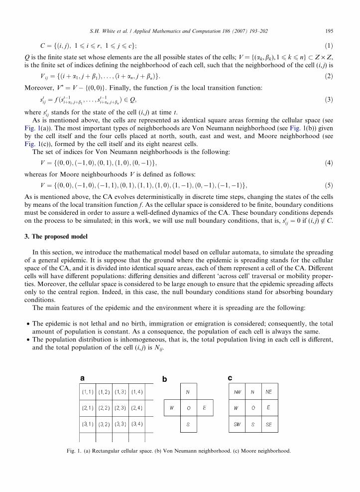
As is mentioned above, the cells are represented as identical square areas forming the cellular space (seeFig. 1(a)). The most important types of neighborhoods are Von Neumann neighborhood (see Fig. 1(b)) givenby the cell itself and the four cells placed at north, south, east and west, and Moore neighborhood (seeFig. 1(c)), formed by the cell itself and its eight nearest cells.

The set of indices for Von Neumann neighborhoods is the following:

V ¼ fð0; 0Þ; ð�1; 0Þ; ð0; 1Þ; ð1; 0Þ; ð0;�1Þg; ð4Þ
whereas for Moore neighbourhoods V is defined as follows:
V ¼ fð0; 0Þ; ð�1; 0Þ; ð�1; 1Þ; ð0; 1Þ; ð1; 1Þ; ð1; 0Þ; ð1;�1Þ; ð0;�1Þ; ð�1;�1Þg; ð5Þ
As is mentioned above, the CA evolves deterministically in discrete time steps, changing the states of the cellsby means of the local transition function f. As the cellular space is considered to be finite, boundary conditionsmust be considered in order to assure a well-defined dynamics of the CA. These boundary conditions dependson the process to be simulated; in this work, we will use null boundary conditions, that is, st
ij ¼ 0 if (i, j) 62 C.

3. The proposed model

In this section, we introduce the mathematical model based on cellular automata, to simulate the spreadingof a general epidemic. It is suppose that the ground where the epidemic is spreading stands for the cellularspace of the CA, and it is divided into identical square areas, each of them represent a cell of the CA. Differentcells will have different populations: differing densities and different ‘across cell’ traversal or mobility proper-ties. Moreover, the cellular space is considered to be large enough to ensure that the epidemic spreading affectsonly to the central region. Indeed, in this case, the null boundary conditions stand for absorbing boundaryconditions.

The main features of the epidemic and the environment where it is spreading are the following:

• The epidemic is not lethal and no birth, immigration or emigration is considered; consequently, the totalamount of population is constant. As a consequence, the population of each cell is always the same.

• The population distribution is inhomogeneous, that is, the total population living in each cell is different,and the total population of the cell (i, j) is Nij.

Fig. 1. (a) Rectangular cellular space. (b) Von Neumann neighborhood. (c) Moore neighborhood.


• It is suppose that the way of infection is the contact between the infected individual and the healthyindividual.

• Once the healthy individuals have contracted the infection and have recovered from it, they acquire immu-nity. That is, they are definitely immune to the disease and consequently they will not be susceptibleindividuals.

• People can move from one cell to another (if there is some type of way of transport), that is, the individualsare able to go outside and come back inside their cells during each time step.

• It is suppose that when an infected individual arrives at a cell, the number of healthy individuals contactedby him/her is the same independently of the total amount of population of the cell.

Let Stij 2 ½0; 1� be the portion of the healthy individuals of the cell (i, j) who are susceptible to infection at

time t; set I tij 2 ½0; 1� the portion of the infected population of the cell at time t who can transmit the disease to

the healthy ones; and let Rtij 2 ½0; 1� be the portion of recovered individuals of (i, j) from the disease at time t,

that will be permanently immunised. As is stated above, the population of each cell is constant, consequently:St

ij þ I tij þ Rt

ij ¼ 1.Moreover, set DSt

ij;DItij, and DRt

ij suitable discretizations of the fractions of the susceptible, infected andrecovered population of the cell at time t, respectively, to get elements of the finite state set Q. In this work,we will consider the state set Q = K · K · K, where:

K ¼ f0:00; 0:01; 0:02; 0:03; . . . ; 0:99; 1g; ð6Þ
which is formed by 101 elements. Consequently, the discretization used is:
DItij ¼½100 � I t

ij�100

; DRtij ¼½100 � Rt

ij�100

; DStij ¼ 1� DIt

ij � DRtij; ð7Þ

where [x] is the nearest integer to x.Then, the state of the cellular automata used in the model is the three-uplet st

ij ¼ ðDStij;DIt

ij;DRtijÞ 2 Q.

The main goal of the model is to compute the factors Stij, I t

ij and Rtij. The local transition function used is the

following:

I tij ¼ ð1� eÞ � I t�1

ij þ v � St�1ij � I t�1

ij þ St�1ij �

Xða;bÞ2V �

N iþa;jþb

N ij� lði;jÞab � I t�1

iþa;jþb; ð8Þ

Stij ¼ St�1

ij � v � St�1ij � I t�1

ij � St�1ij �

Xða;bÞ2V �

Niþa;jþb

Nij� lði;jÞab � I t�1

iþa;jþb; ð9Þ

Rtij ¼ Rt�1

ij þ e � I t�1ij : ð10Þ

where V* = V � {(0, 0)}, and the real parameter lði;jÞab is defined as the product of three factors: lði;jÞab ¼cði;jÞab � m

ði;jÞab � v, where cði;jÞab and mði;jÞab are the connection factor and the movement factor between the main cell

(i, j) and its neighbour cell (i + a, j + b), respectively, and v 2 [0,1] is the virulence of the epidemic. Moreover,the parameter e 2 [0,1] stands for the portion of infected individuals which recover from the disease at eachtime step.

Eqs. (8) and (10) reflect that every loss in the infected population is due to a gain in the recovered popu-lation, while every gain in the infected population is due to a loss in the susceptible population. Roughlyspeaking, the Eq. (8) can be interpreted as saying that the portion of infected individuals of a cell (i, j) at aparticular time step t is given by the portion of infected individuals which have not been recovered fromthe disease (first sum of the summation) and by the portion of susceptible individuals of the same cell at timet � 1 which have been infected by the infected individuals at time t � 1 of the cell (second sum of the summa-tion) taking into account the virulence of the disease. Moreover, some susceptible individuals of the cell (i, j)can be infected by infected individuals of the neighbour cells which have travelled to the cell (third sum of thesummation). Obviously, it depends on some parameters involving the virulence, the nature of the connectionsbetween the cells, the possibilities of an infected individual to be moved from one cell to another, and therelation between the population of the cells. Furthermore, Eq. (10) gives the portion of recovered individualsof the cell (i, j) at time t as the number of recovered individuals of the cell at the previous time step plus the


fraction of infected individuals of the cell which have been recovered in one step of time. Finally, Eq. (9) givesthe portion of susceptible individuals of the cell (i, j) at time step t as the portion of susceptible individuals attime t � 1 which have not been infected.

Note that, as a simple calculus shows: Stij þ I t

ij þ Rtij ¼ 1, for every cell (i, j) and every time step t.

As is mentioned above, the way of infection of the epidemic to be modeled is the contact between two indi-viduals (an infected and a healthy individual). Consequently, the healthy individuals of a particular cell can beinfected by the infected individuals of this cell or by the infected individuals of the neighbour cells that havetraveled to the main cell.

The first case, that is, when an individual is infected by another individual of his/her cell, is reflected in thefirst sum of the summation given in the Eq. (8). In the other case, given by the second sum of the summation of(8), when the infection is carried out by individuals belonging to neighbour cells, some type of connectionbetween the cells must be exist in order to allow the epidemic spreading. In this work, we will consider threeways of transport: by airplane, by train and by car or bus. This connection is given by the coefficients cði;jÞab suchthat:

cði;jÞab ¼

1; if there exist the three ways of transport between the cells;

0:6; if there are two ways of transport between the cells;

0:3; if there is only one way of transport between the cells;

0; if there is not any way of transport between the cells;

8>>><>>>:

ð11Þ

The movement factor mði;jÞab 2 ½0; 1� stands for the probability of an infected individual belonging to the neigh-bour cell (i + a, j + b) to be moved to the main cell (i, j). Note that this parameter is different from the connec-tion factor since it depends on the infected individuals and the other one (the connection factor) depends onthe existing transport infrastructures between the cells considered. Moreover, the movement factor must begiven by the main features of the disease to be modeled.

Finally, it is very important to decide whether or not the outbreak disease occurs. In this sense, we willobtain the values of the parameters for which the epidemic spread from one cell to its neighbor cells. Supposethat in the initial configuration there is only one cell with infected individuals: O, and set N its north neighborcell. Then the infected individuals of N at time step t = 1 is given by the following expression:

I1N ¼

NC

N N� cN

O � mNO � v � I0

O; ð12Þ

since I0N ¼ 0 and S0

N ¼ 1.In our model, we suppose that there are infected individuals in the cell N at a particular time step t when

DItN 2 Q� f0g, that is, when DIt

N P 0:01. Consequently, the following equation must hold:

DI0O P

N N

100 � N C � cNO � mN

O � v¼ q: ð13Þ

As a consequence, the number of infected individuals necessary to extend the epidemic out to the cell dependson the values of the parameters cN

O ; mNO and v. In Table 1 some examples are shown for the case in which the

population is the same in all cells.On the other hand, if

DI0O < q; ð14Þ

then the evolution of the infected population is restricted to the main cell O, and the number of infected indi-viduals becomes zero if I t

O < I t�1O for every t. Consequently, as Eq. (14) holds then a simple calculus shows that

for every t:

I tO ¼ ð1� eÞ � I t�1

O þ v � St�1O � I t�1

O < I t�1O ; ð15Þ

if and only if St�1O < e=v. As a consequence, I t

O ¼ IOðtÞ is a decreasing function which tends to 0 if S0O < e=v, or

equivalently, if

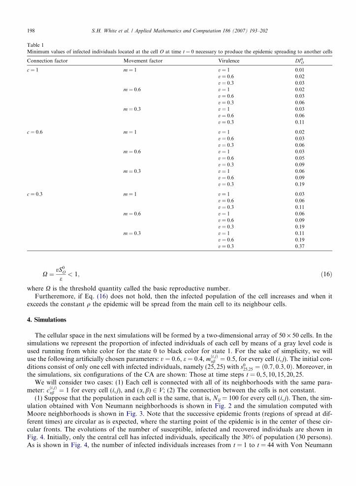
Table 1Minimum values of infected individuals located at the cell O at time t = 0 necessary to produce the epidemic spreading to another cells

Connection factor Movement factor Virulence DI0O

c = 1 m = 1 v = 1 0.01v = 0.6 0.02v = 0.3 0.03

m = 0.6 v = 1 0.02v = 0.6 0.03v = 0.3 0.06

m = 0.3 v = 1 0.03v = 0.6 0.06v = 0.3 0.11

c = 0.6 m = 1 v = 1 0.02v = 0.6 0.03v = 0.3 0.06

m = 0.6 v = 1 0.03v = 0.6 0.05v = 0.3 0.09

m = 0.3 v = 1 0.06v = 0.6 0.09v = 0.3 0.19

c = 0.3 m = 1 v = 1 0.03v = 0.6 0.06v = 0.3 0.11

m = 0.6 v = 1 0.06v = 0.6 0.09v = 0.3 0.19

m = 0.3 v = 1 0.11v = 0.6 0.19v = 0.3 0.37


X ¼ vS0O

e< 1; ð16Þ

where X is the threshold quantity called the basic reproductive number.Furtheremore, if Eq. (16) does not hold, then the infected population of the cell increases and when it

exceeds the constant q the epidemic will be spread from the main cell to its neighbour cells.

4. Simulations

The cellular space in the next simulations will be formed by a two-dimensional array of 50 · 50 cells. In thesimulations we represent the proportion of infected individuals of each cell by means of a gray level code isused running from white color for the state 0 to black color for state 1. For the sake of simplicity, we willuse the following artificially chosen parameters: v = 0.6, e = 0.4, mði;jÞab ¼ 0:5, for every cell (i, j). The initial con-ditions consist of only one cell with infected individuals, namely (25,25) with s0

25;25 ¼ ð0:7; 0:3; 0Þ. Moreover, inthe simulations, six configurations of the CA are shown: Those at time steps t = 0,5,10,15,20,25.

We will consider two cases: (1) Each cell is connected with all of its neighborhoods with the same para-meter: cði;jÞab ¼ 1 for every cell (i, j), and (a,b) 2 V; (2) The connection between the cells is not constant.

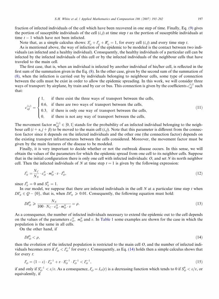
(1) Suppose that the population in each cell is the same, that is, Nij = 100 for every cell (i, j). Then, the sim-ulation obtained with Von Neumann neighborhoods is shown in Fig. 2 and the simulation computed withMoore neighborhoods is shown in Fig. 3. Note that the successive epidemic fronts (regions of spread at dif-ferent times) are circular as is expected, where the starting point of the epidemic is in the center of these cir-cular fronts. The evolutions of the number of susceptible, infected and recovered individuals are shown inFig. 4. Initially, only the central cell has infected individuals, specifically the 30% of population (30 persons).As is shown in Fig. 4, the number of infected individuals increases from t = 1 to t = 44 with Von Neumann

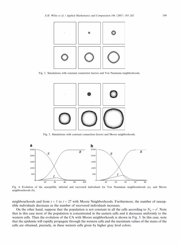
Fig. 2. Simulations with constant connection factors and Von Neumann neighborhoods.

Fig. 3. Simulations with constant connection factors and Moore neighborhoods.

Fig. 4. Evolution of the susceptible, infected and recovered individuals for Von Neumman neighbourhoods (a), and Mooreneighbourhoods (b).


neighbourhoods and from t = 1 to t = 27 with Moore Neighborhoods. Furthermore, the number of suscep-tible individuals decreases as the number of recovered individuals increases.

On the other hand, suppose that the population is not constant in all the cells according to Nij = ej. Notethat in this case most of the population is concentrated in the eastern cells and it decreases uniformly to thewestern cells. Then the evolution of the CA with Moore neighborhoods is shown in Fig. 5. In this case, notethat the epidemic will rapidly propagate through the western cells and the maximum values of the states of thecells are obtained, precisely, in these western cells given by higher gray level colors.

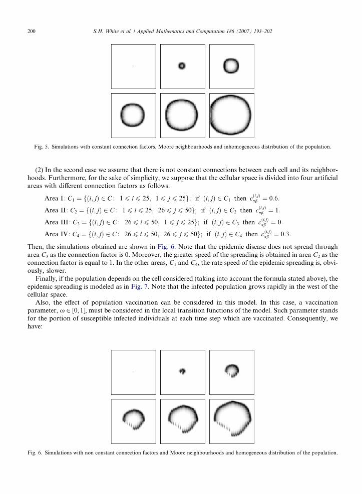
Fig. 5. Simulations with constant connection factors, Moore neighbourhoods and inhomogeneous distribution of the population.


(2) In the second case we assume that there is not constant connections between each cell and its neighbor-hoods. Furthermore, for the sake of simplicity, we suppose that the cellular space is divided into four artificialareas with different connection factors as follows:

Fig. 6.

Area I : C1 ¼ fði; jÞ 2 C : 1 6 i 6 25; 1 6 j 6 25g; if ði; jÞ 2 C1 then cði;jÞab ¼ 0:6:

Area II : C2 ¼ fði; jÞ 2 C : 1 6 i 6 25; 26 6 j 6 50g; if ði; jÞ 2 C2 then cði;jÞab ¼ 1:

Area III : C3 ¼ fði; jÞ 2 C : 26 6 i 6 50; 1 6 j 6 25g; if ði; jÞ 2 C3 then cði;jÞab ¼ 0:

Area IV : C4 ¼ fði; jÞ 2 C : 26 6 i 6 50; 26 6 j 6 50g; if ði; jÞ 2 C4 then cði;jÞab ¼ 0:3:

Then, the simulations obtained are shown in Fig. 6. Note that the epidemic disease does not spread througharea C3 as the connection factor is 0. Moreover, the greater speed of the spreading is obtained in area C2 as theconnection factor is equal to 1. In the other areas, C1 and C4, the rate speed of the epidemic spreading is, obvi-ously, slower.

Finally, if the population depends on the cell considered (taking into account the formula stated above), theepidemic spreading is modeled as in Fig. 7. Note that the infected population grows rapidly in the west of thecellular space.

Also, the effect of population vaccination can be considered in this model. In this case, a vaccinationparameter, x 2 [0, 1], must be considered in the local transition functions of the model. Such parameter standsfor the portion of susceptible infected individuals at each time step which are vaccinated. Consequently, wehave:

Simulations with non constant connection factors and Moore neighbourhoods and homogeneous distribution of the population.

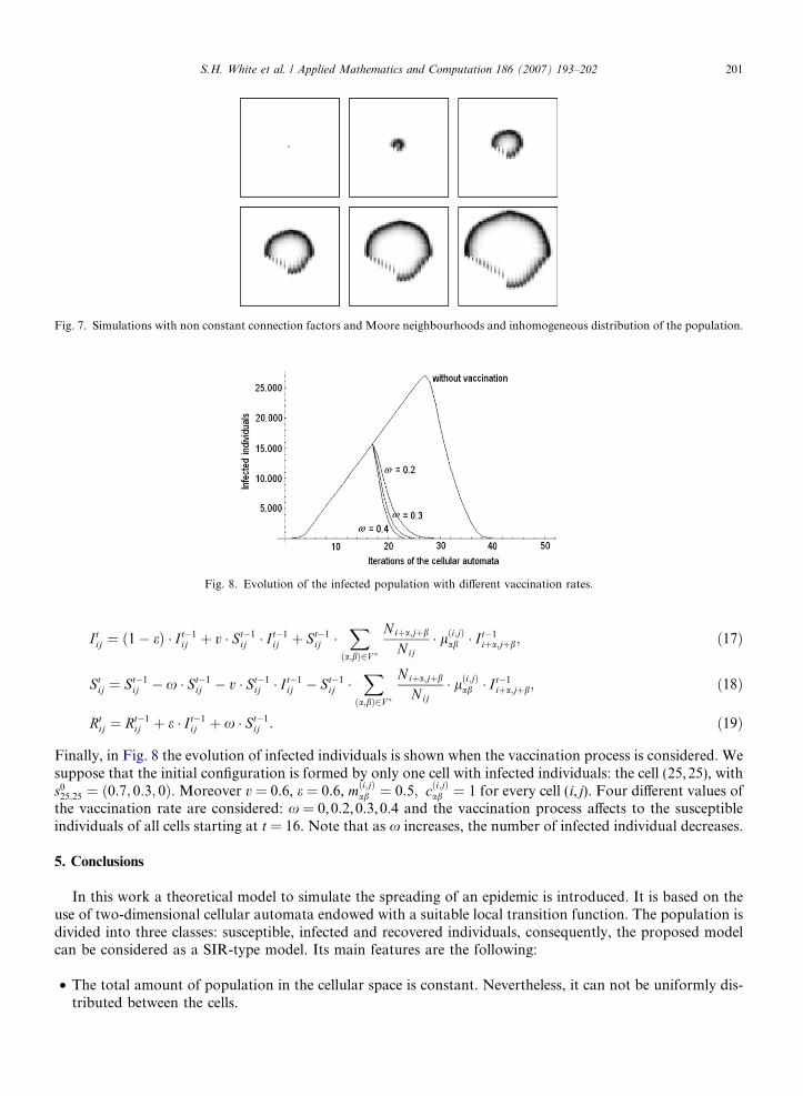
Fig. 7. Simulations with non constant connection factors and Moore neighbourhoods and inhomogeneous distribution of the population.

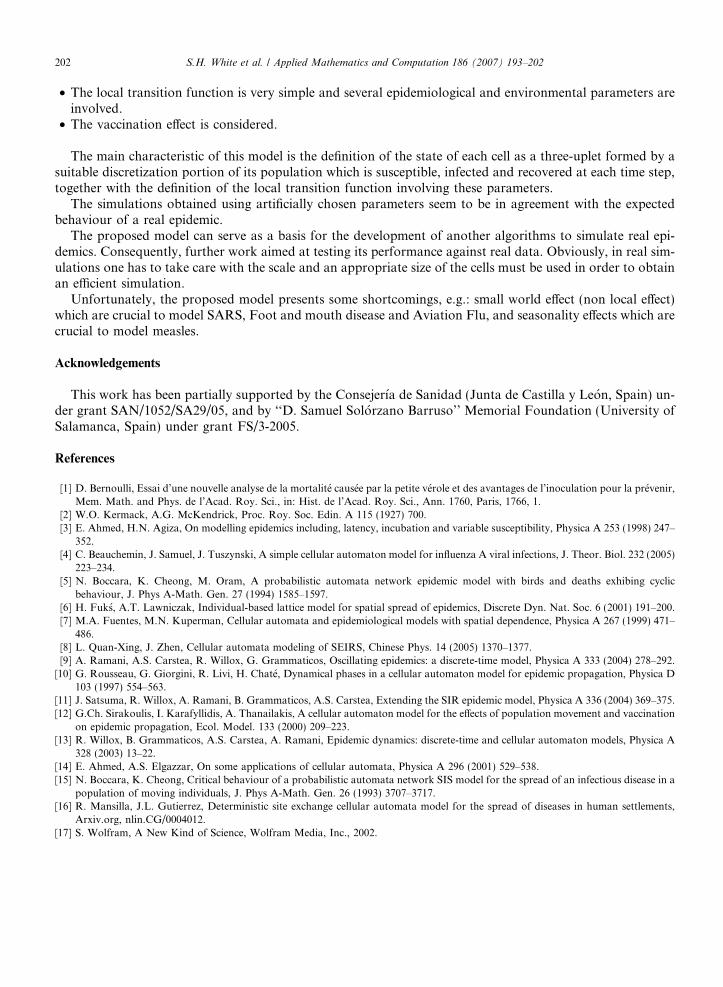
Fig. 8. Evolution of the infected population with different vaccination rates.


I tij ¼ ð1� eÞ � I t�1

ij þ v � St�1ij � I t�1

ij þ St�1ij �

Xða;bÞ2V �

Niþa;jþb

Nij� lði;jÞab � I t�1

iþa;jþb; ð17Þ

Stij ¼ St�1

ij � x � St�1ij � v � St�1

ij � I t�1ij � St�1

ij �Xða;bÞ2V �

N iþa;jþb

N ij� lði;jÞab � I t�1

iþa;jþb; ð18Þ

Rtij ¼ Rt�1

ij þ e � I t�1ij þ x � St�1

ij : ð19Þ

Finally, in Fig. 8 the evolution of infected individuals is shown when the vaccination process is considered. Wesuppose that the initial configuration is formed by only one cell with infected individuals: the cell (25,25), withs0

25;25 ¼ ð0:7; 0:3; 0Þ. Moreover v = 0.6, e = 0.6, mði;jÞab ¼ 0:5; cði;jÞab ¼ 1 for every cell (i, j). Four different values ofthe vaccination rate are considered: x = 0,0.2, 0.3,0.4 and the vaccination process affects to the susceptibleindividuals of all cells starting at t = 16. Note that as x increases, the number of infected individual decreases.

5. Conclusions

In this work a theoretical model to simulate the spreading of an epidemic is introduced. It is based on theuse of two-dimensional cellular automata endowed with a suitable local transition function. The population isdivided into three classes: susceptible, infected and recovered individuals, consequently, the proposed modelcan be considered as a SIR-type model. Its main features are the following:

• The total amount of population in the cellular space is constant. Nevertheless, it can not be uniformly dis-tributed between the cells.


• The local transition function is very simple and several epidemiological and environmental parameters areinvolved.

• The vaccination effect is considered.

The main characteristic of this model is the definition of the state of each cell as a three-uplet formed by asuitable discretization portion of its population which is susceptible, infected and recovered at each time step,together with the definition of the local transition function involving these parameters.

The simulations obtained using artificially chosen parameters seem to be in agreement with the expectedbehaviour of a real epidemic.

The proposed model can serve as a basis for the development of another algorithms to simulate real epi-demics. Consequently, further work aimed at testing its performance against real data. Obviously, in real sim-ulations one has to take care with the scale and an appropriate size of the cells must be used in order to obtainan efficient simulation.

Unfortunately, the proposed model presents some shortcomings, e.g.: small world effect (non local effect)which are crucial to model SARS, Foot and mouth disease and Aviation Flu, and seasonality effects which arecrucial to model measles.

Acknowledgements

This work has been partially supported by the Consejerıa de Sanidad (Junta de Castilla y Leon, Spain) un-der grant SAN/1052/SA29/05, and by ‘‘D. Samuel Solorzano Barruso’’ Memorial Foundation (University ofSalamanca, Spain) under grant FS/3-2005.

References

[1] D. Bernoulli, Essai d’une nouvelle analyse de la mortalite causee par la petite verole et des avantages de l’inoculation pour la prevenir,Mem. Math. and Phys. de l’Acad. Roy. Sci., in: Hist. de l’Acad. Roy. Sci., Ann. 1760, Paris, 1766, 1.

[2] W.O. Kermack, A.G. McKendrick, Proc. Roy. Soc. Edin. A 115 (1927) 700.[3] E. Ahmed, H.N. Agiza, On modelling epidemics including, latency, incubation and variable susceptibility, Physica A 253 (1998) 247–

352.[4] C. Beauchemin, J. Samuel, J. Tuszynski, A simple cellular automaton model for influenza A viral infections, J. Theor. Biol. 232 (2005)

223–234.[5] N. Boccara, K. Cheong, M. Oram, A probabilistic automata network epidemic model with birds and deaths exhibing cyclic

behaviour, J. Phys A-Math. Gen. 27 (1994) 1585–1597.[6] H. Fuks, A.T. Lawniczak, Individual-based lattice model for spatial spread of epidemics, Discrete Dyn. Nat. Soc. 6 (2001) 191–200.[7] M.A. Fuentes, M.N. Kuperman, Cellular automata and epidemiological models with spatial dependence, Physica A 267 (1999) 471–

486.[8] L. Quan-Xing, J. Zhen, Cellular automata modeling of SEIRS, Chinese Phys. 14 (2005) 1370–1377.[9] A. Ramani, A.S. Carstea, R. Willox, G. Grammaticos, Oscillating epidemics: a discrete-time model, Physica A 333 (2004) 278–292.

[10] G. Rousseau, G. Giorgini, R. Livi, H. Chate, Dynamical phases in a cellular automaton model for epidemic propagation, Physica D103 (1997) 554–563.

[11] J. Satsuma, R. Willox, A. Ramani, B. Grammaticos, A.S. Carstea, Extending the SIR epidemic model, Physica A 336 (2004) 369–375.[12] G.Ch. Sirakoulis, I. Karafyllidis, A. Thanailakis, A cellular automaton model for the effects of population movement and vaccination

on epidemic propagation, Ecol. Model. 133 (2000) 209–223.[13] R. Willox, B. Grammaticos, A.S. Carstea, A. Ramani, Epidemic dynamics: discrete-time and cellular automaton models, Physica A

328 (2003) 13–22.[14] E. Ahmed, A.S. Elgazzar, On some applications of cellular automata, Physica A 296 (2001) 529–538.[15] N. Boccara, K. Cheong, Critical behaviour of a probabilistic automata network SIS model for the spread of an infectious disease in a

population of moving individuals, J. Phys A-Math. Gen. 26 (1993) 3707–3717.[16] R. Mansilla, J.L. Gutierrez, Deterministic site exchange cellular automata model for the spread of diseases in human settlements,

Arxiv.org, nlin.CG/0004012.[17] S. Wolfram, A New Kind of Science, Wolfram Media, Inc., 2002.

modeling epidemics using cellular automata

Documents