pickup: calculation of confidence removal goals

PICKUP

Calculation of Confidence Removal Goals

User's Guide

Release 1.0

PICKUP

Calculation of Confidence Removal Goals

User's Guide

Release 1.0

Gradient Corporation44 Brattle Street

Cambridge, MA 02138

February 25, 1994

9212240.Rl/cas -, Gradient Corporation

For instructions on runningthe computer programPICKUP™, go to Section 2

For Technical Assistance call: 617-576-1555• Installation and Software Support - Amy Michelson• Methodology and Technical Approach - Teresa Bowers

9212240.Rl/cas Gradient Corporation

Table of Contents

Page No.

Glossary of Symbols

1 Introduction . . . . . . . . . . . . . . . . . . . . . . . . . . . . . . . . . . . . . . . . . . . . . . . i-i1.1 Definition of Terms . . . . . . . . . . . . . . . . . . . . . . . . . . . . . . . . . . . . . . . 1-11.2 Relationship of Cleanup Levels to Risk . . . . . . . . . . . . . . . . . . . . . . . . . . . 1-31.3 Determining the Need for Remediation . . . . . . . . . . . . . . . . . . . . . . . . . . . 1-51.4 The Confidence Removal Goal . . . . . . . . . . . . . . . . . . . . . . . . . . . . . . . . 1-6

2 Use of PICKUP™; The Computer Software Package to CalculateConfidence Removal Goals . . . . . . . . . . . . . . . . . . . . . . . . . . . . . . . . . . . . 2-1

3 Calculation of Confidence Removal Goals . . . . . . . . . . . . . . . . . . . . . . . . . 3-13.1 Calculation of a Removal Goal when the True Mean of a Distribution

is Known . . . . . . . . . . . . . . . . . . . . . . . . . . . . . . . . . . . . . . . . . . . . . 3-13.2 Calculation of a Confidence Removal Goal when the True Mean of a

Distribution is Uncertain . . . . . . . . . . . . . . . . . . . . . . . . . . . . . . . . . . . . 3-23.2.1 Upper Confidence Limits on a Lognormally Distributed Dataset . . . . . . 3-33.2.2 Comparison off With Various Methods of Calculating UCLs

on Percentiles of the D i s t r i b u t i o n / . . . . . . . . . . . . . . . . . . . . . . . . . 3-63.2.3 Lower Confidence Limits on/ . . . . . . . . . . . . . . . . . . . . . . . . . . . 3-93.2.4 Calculation of the Confidence Removal Goal . . . . . . . . . . . . . . . . . 3-103.2.5 Using the Relationship between the Confidence Removal Goal

and the Sample Size to Assess the Utility of Further Sampling . . . . . . 3-163.3 Advantages of the Analytical Approach . . . . . . . . . . . . . . . . . . . . . . . . . . 3-17

3.3.1 What if the Dataset is not Lognormal? . . . . . . . . . . . . . . . . . . . . . 3-19

4 Mathematical Development of Removal Goals . . . . . . . . . . . . . . . . . . . . . . 4-1

References

9212240.Rl/cas ' Gradient Corporation

Glossary of Symbols

c The contaminant concentration value corresponding to an observation.

C0 The concentration of the contaminant in the clean fill, or back fill.

c* The contaminant concentration corresponding to the removal goal, where all observationswith concentrations greater than c* must be remediated.

/ A lognormal distribution, also referred to as/(c).

f(c) A lognormal distribution of concentrations c, also referred to as/.

/' The lognormal distribution defined by the 95th percent upper confidence limits on themean and geometric mean of the distribution/.

/'' The lognormal distribution defined by the 95th percent lower confidence limits on themean and geometric mean of the distribution/

F(z) The area under the standard normal curve from 0 to i.

g(c) An arbitrary function of concentration.

gm The sample geometric mean of a data set. This value is derived by calculating thearithmetic mean of the natural logarithm of each observation in the data set, andexponentiating the result.

gsd The sample geometric standard deviation of a data set. This value is derived bycalculating the standard deviation of the natural logarithm of each observation in the dataset, and exponentiating the result.

gsdf, The geometric standard deviation of the distribution/', the distribution defined by theupper confidence limits on the mean and geometric mean of the distribution/

G The natural logarithm of gsd, the geometric standard deviation of the data set, equivalentto the standard deviation of the natural logarithm of all observations.

H The H statistic, used for calculating upper confidence limits on the arithmetic mean oflognormal distributions. It is a function of the confidence level (specified here to be 95percent), the standard deviation of the logarithms of observations (G) and of the degreesof freedom (v). Also written HG v. Values are tabulated in statistical textbooks such asGilbert (1987).

k The k statistic, used for calculating upper confidence limits on percentiles of adistribution. It is a function of the confidence level (specified here to be 95 percent), thesample size nj as well as the percentilep. Values for a limited number of percentiles aretabulated in statistical textbooks such as Gilbert (1987).

9212230.glo/cas ' 1 Gradient Corporation

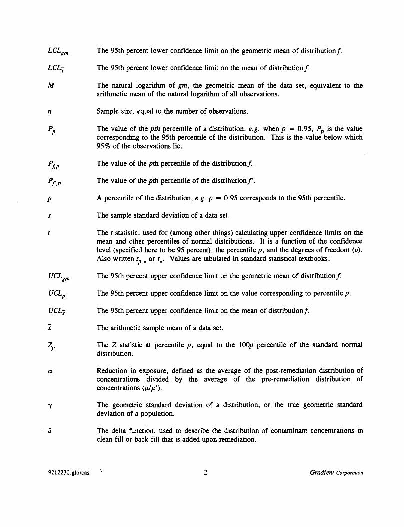
The 95th percent lower confidence limit on the geometric mean of distribution/.

LCL- The 95th percent lower confidence limit on the mean of distribution/.

M The natural logarithm of gm, the geometric mean of the data set, equivalent to thearithmetic mean of the natural logarithm of all observations.

n Sample size, equal to the number of observations.

Pp The value of the/tf/j percentile of a distribution, e.g. when;? = 0.95, Pp is the valuecorresponding to the 95th percentile of the distribution. This is the value below which95% of the observations lie.

Pf The value of the pth percentile of the distribution/.

Pf p The value of the pth percentile of the distribution/'.

p A percentile of the distribution, e.g. p - 0.95 corresponds to the 95th percentile.

s The sample standard deviation of a data set.

t The t statistic, used for (among other things) calculating upper confidence limits on themean and other percentiles of normal distributions. It is a function of the confidencelevel (specified here to be 95 percent), the percentile/?, and the degrees of freedom (v).Also written tp v or tv. Values are tabulated in standard statistical textbooks.

UCLgm The 95th percent upper confidence limit on the geometric mean of distribution/.

UCLp The 95th percent upper confidence limit on the value corresponding to percentile p.

t/CLj The 95th percent upper confidence limit on the mean of distribution/.

x The arithmetic sample mean of a data set.

Zp The Z statistic at percentile p, equal to the lOOp percentile of the standard normaldistribution.

a Reduction in exposure, defined as the average of the post-remediation distribution ofconcentrations divided by the average of the pre-remediation distribution ofconcentrations

The geometric standard deviation of a distribution, or the true geometric standarddeviation of a population.

The delta function, used to describe the distribution of contaminant concentrations inclean fill or back fill that is added upon remediation.

9212230.glo/cas '' 2 Gradient Corporation

The geometric mean of a distribution. This is the true geometric mean of a population.

The arithmetic mean of a distribution, equivalent to the average value. This is the truemean of a population.

The arithmetic mean of a post-remediation distribution.

Degrees of freedom, equal to the sample size (n) - 1.

The (arithmetic) standard deviation of a distribution. This is the true standard deviationof a population.

9212230.glo/cas '' 3 Gradient Corporation

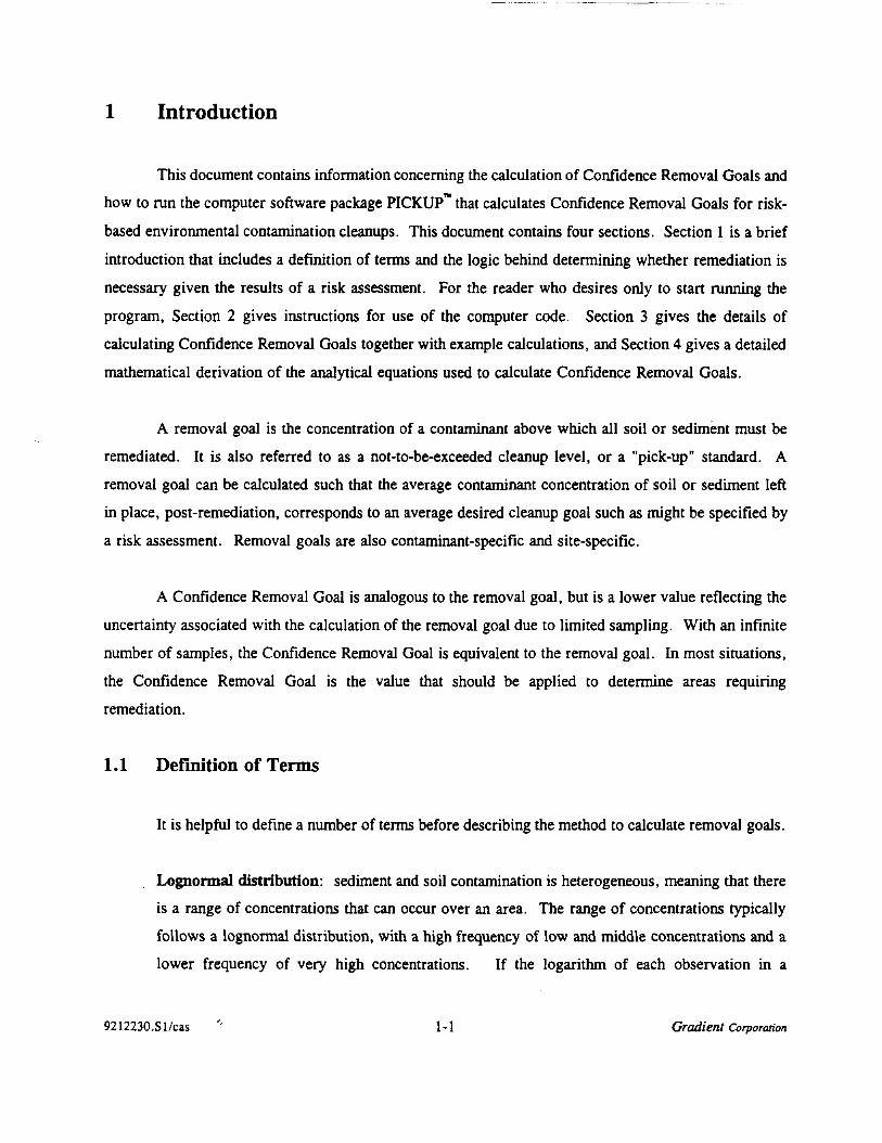
1 Introduction

This document contains information concerning the calculation of Confidence Removal Goals and

how to run the computer software package PICKUP™ that calculates Confidence Removal Goals for risk-based environmental contamination cleanups. This document contains four sections. Section 1 is a briefintroduction that includes a definition of terms and the logic behind determining whether remediation isnecessary given the results of a risk assessment. For the reader who desires only to start running theprogram, Section 2 gives instructions for use of the computer code. Section 3 gives the details ofcalculating Confidence Removal Goals together with example calculations, and Section 4 gives a detailedmathematical derivation of the analytical equations used to calculate Confidence Removal Goals.

A removal goal is the concentration of a contaminant above which all soil or sediment must be

remediated. It is also referred to as a not-to-be-exceeded cleanup level, or a "pick-up" standard. A

removal goal can be calculated such that the average contaminant concentration of soil or sediment left

in place, post-remediation, corresponds to an average desired cleanup goal such as might be specified bya risk assessment. Removal goals are also contaminant-specific and site-specific.

A Confidence Removal Goal is analogous to the removal goal, but is a lower value reflecting theuncertainty associated with the calculation of the removal goal due to limited sampling. With an infinitenumber of samples, the Confidence Removal Goal is equivalent to the removal goal. In most situations,

the Confidence Removal Goal is the value that should be applied to determine areas requiringremediation.

1.1 Definition of Terms

It is helpful to define a number of terms before describing the method to calculate removal goals.

Lognonnal distribution: sediment and soil contamination is heterogeneous, meaning that thereis a range of concentrations that can occur over an area. The range of concentrations typically

follows a lognormal distribution, with a high frequency of low and middle concentrations and alower frequency of very high concentrations. If the logarithm of each observation in a

9212230.Sl/cas '' 1-1 Gradient Corporation

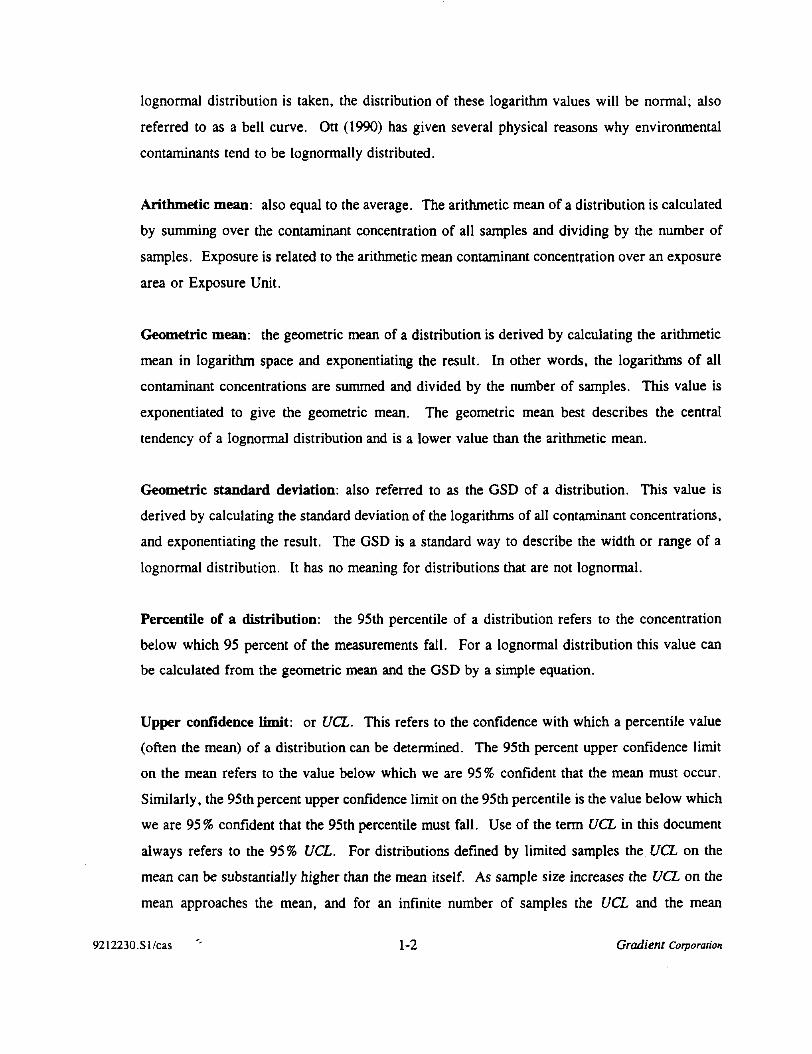
lognormal distribution is taken, the distribution of these logarithm values will be normal; alsoreferred to as a bell curve. Ott (1990) has given several physical reasons why environmentalcontaminants tend to be lognormally distributed.

Arithmetic mean: also equal to the average. The arithmetic mean of a distribution is calculated

by summing over the contaminant concentration of all samples and dividing by the number ofsamples. Exposure is related to the arithmetic mean contaminant concentration over an exposurearea or Exposure Unit.

Geometric mean: the geometric mean of a distribution is derived by calculating the arithmeticmean in logarithm space and exponentiating the result. In other words, the logarithms of allcontaminant concentrations are summed and divided by the number of samples. This value isexponentiated to give the geometric mean. The geometric mean best describes the centraltendency of a lognormal distribution and is a lower value than the arithmetic mean.

Geometric standard deviation: also referred to as the GSD of a distribution. This value is

derived by calculating the standard deviation of the logarithms of all contaminant concentrations,

and exponentiating the result. The GSD is a standard way to describe the width or range of alognormal distribution. It has no meaning for distributions that are not lognormal.

Percentile of a distribution: the 95th percentile of a distribution refers to the concentration

below which 95 percent of the measurements fall. For a lognormal distribution this value canbe calculated from the geometric mean and the GSD by a simple equation.

Upper confidence limit: or UCL. This refers to the confidence with which a percentile value

(often the mean) of a distribution can be determined. The 95th percent upper confidence limiton the mean refers to the value below which we are 95% confident that the mean must occur.

Similarly, the 95th percent upper confidence limit on the 95th percentile is the value below whichwe are 95% confident that the 95th percentile must fall. Use of the term UCL in this documentalways refers to the 95% UCL. For distributions defined by limited samples the UCL on the

mean can be substantially higher than the mean itself. As sample size increases the UCL on themean approaches the mean, and for an infinite number of samples the UCL and the mean


coincide. The method to calculate the UCL on the mean for a normal distribution differs from

the method to calculate the UCL on the mean of a lognormal distribution. The 95th percent UCLshould not be confused with the 95th percentile of the distribution (see above).

Average cleanup goal, or CUG: this value is derived from the risk equation and represents theaverage level of a contaminant that may be left in place over some area without unacceptable risk.Treating this value as a removal goal above which all material must be remediated would onlybe appropriate if the contamination were homogeneous, that is, the same concentration of the

contaminant occurs everywhere in the exposure area. This situation does not occur in reality.

Removal goal: this is the concentration of a contaminant above which all material must beremediated. It is also referred to as a not-to-be-exceeded cleanup level. This value is calculatedon a site- and contaminant-specific basis such that the average contaminant concentration ofmaterial left in place, post-remediation, corresponds to the average desired cleanup goal.

Confidence Removal Goal: this value is analogous to the removal goal, but is a lower valuereflecting the uncertainty associated with calculation of the removal goal due to limited sampling.

1.2 Relationship of Cleanup Levels to Risk

Risk assessment is often used to assess the level of contaminant that may remain on a site withoutposing an undue threat to human health or ecological concerns. Risk is made up of two components:exposure and toxicity, and it is exposure that is a function of the contaminant concentration. The risk

equation can be simply expressed as

Risk - Contaminant Concentration x Other Exposure Factors x Toxicity , W

where other exposure factors include contact rate, days exposed, etc.

The measure of exposure appropriate for a risk assessment is the true average concentration of

a contaminant over an exposure area or Exposure Unit (EPA, 1992). This premise is based on the

9212230.S1 /cas '' 1 -3 Gradient Corporation

assumption that the exposed individual moves randomly over the Exposure Unit and, over time, is

exposed equally to all areas of the Exposure Unit. Clearly this makes it important to define the ExposureUnit such that it truly represents an area over which exposure occurs. Independent cleanup decisionsshould be made for each Exposure Unit.

Agency guidance covering the definition of Exposure Units (EPA, 1989) suggests that ExposureUnits should be homogeneous with respect to prior waste management activities, and that differences inland use, terrain, accessibility, or media type that can affect exposure may require establishment ofdifferent Exposure Units.

For the purpose of the removal goal calculations developed here, we assume that an Exposure

Unit has been adequately defined and that exposure, and therefore risk, is a function of the true averagecontaminant concentration in the Exposure Unit. However, there is always some uncertainty attached

to the measurement of the true average contaminant concentration in an Exposure Unit. Agency riskassessment guidance (EPA, 1992) specifies that this uncertainty be addressed by use of an upperconfidence limit (UCL) on the mean contaminant concentration of the samples, instead of simply the meanof the samples, in the risk equation. The UCL is a function of the sample size, e.g., the number of

measurements of contaminant concentration in the Exposure Unit. The UCL specifies a value that weare confident the true mean is beneath, and the value of the UCL increases with decreasing sample size.As sample size increases, the upper confidence limit decreases until it is equal to the mean at an infinite

number of samples.

Since the upper confidence limit on the mean contaminant concentration is used to assess exposure

in an EPA-guided risk assessment, a higher risk value is calculated than if the sample mean were usedin the equation. This is a conservative approach that increases the probability of estimating thatunacceptable risk is associated with a contaminated site. It also means that in the case of low sample

sizes a determination of unacceptable risk may be made when, in actuality, risks may be acceptable.

Upon completion of a risk assessment, a cleanup level can be derived by solving the risk equation(equation 1) backwards with risk set equal to a specified target value. At Superfund sites EPA specifiesa range of permissible risks from 10"6 to 10"4, with a preference for the target risk for remediation to be

9212230.Sl/cas '- 1-4 Gradient Corporation

set at 10~6 (EPA, 1991). Where risk equals contaminant concentration times other exposure factors timestoxicity, the cleanup goal (CUG) is obtained from

-™ _ ______Permissible Risk______ /2)(Toxicity) x (Other Exposure Factors)

The value of the CUG derived in this manner is an average permissible concentration because it isdirectly analogous to the mean (or UCL on the mean) value used in the risk equation.

1.3 Determining the Need for Remediation

Determination of whether an Exposure Unit requires remediation lies in the comparison of thecalculated risk for that Exposure Unit to a target risk. Given the linearity of the risk equation, this isequivalent to comparing the upper confidence limit on the mean contaminant concentration in theExposure Unit to the CUG (Figure 1.1). If the UCL on the mean does not exceed the CUG, no

remediation of the Exposure Unit is necessary. If the UCL on the mean exceeds the CUG, then

remediation of some portion of the Exposure Unit is required so as to render the true post-remediationmean less than or equal to the CUG.

In the case where the upper confidence limit on the mean does not exceed the CUG, i.e., the

calculated risk does not exceed the target risk, then the risk assessment process deems that no remediationis necessary. Note that there may be individual points or observations under this condition where the

contaminant concentration does exceed the CUG within this Exposure Unit, but as long as the UCL doesnot exceed the CUG, no remediation is required. This same logic can be applied to those Exposure Units

where some remediation is required. The attainment of acceptable risk does not necessitate remediatingevery location in an Exposure Unit where the contaminant concentration exceeds the CUG. Rather,enough remediation must be done such that the CUG, and the target risk, are met on average across theExposure Unit. This can be done by specifying a removal goal, a higher contaminant concentration than

the CUG, such that if remediation of all areas with contaminant concentrations exceeding the removalgoal are carried out, then the CUG would be met on average across the Exposure Unit. If a new risk

9212230.S 1 /cas ' 1-5 Gradient Corporation

assessment were done on the Exposure Unit after remediation of areas where contaminant concentrationsexceeded the removal goal, then a permissible risk would be obtained.

1.4 The Confidence Removal Goal

Because EPA-guided risk assessments use the UCL to represent an upper bound on the trueaverage contaminant concentration, removal goals should be established that take into account that thetrue average contaminant concentration may be as high as the UCL. Thus the term "Confidence RemovalGoal" is used to denote remediation targets that consider the range that the true average contaminantconcentration may fall within. In general, more extensive remediation will be required when the rangethat the true average may fall within is large. The Confidence Removal Goal is, therefore, a functionof sample size. As sample size decreases, the Confidence Removal Goal also decreases to require moreremediation to balance the lack of certainty about the true level of contamination. The Confidence

Removal Goal gives statistical confidence that the true average contaminant concentration in an Exposure

Unit will be less than the CUG after remediation. The Confidence Removal Goal is both site-specific

and contaminant-specific.

The value of the Confidence Removal Goal is bound on the upper side by the removal goal andon the lower side by the CUG. Its value must fall between these two. On the upper side, the removalgoal is calculated from the assumption that the sample mean equals the true mean of an Exposure Unitand this value is only appropriate where the sample size is approximately 200 or greater. On the lower

side the CUG is the target average concentration desired in the Exposure Unit. If there were noinformation concerning the true range of contaminant levels present, then there would be little alternative

other than to remediate an Exposure Unit wherever an observation exceeded the CUG. However, themajority of sites fall between these two extremes, where sampling is sufficient to determine with someassurance the range of contaminant concentrations, but there is some level of uncertainty attached. Inthese instances the Confidence Removal Goal provides a statistically-based calculation that specifies where

remediation is necessary in order to achieve, with confidence, an acceptable risk post-remediation.

This document provides a description of the calculation of Confidence Removal Goals for a

dataset that is lognormally distributed. Although environmental contaminants are commonly lognormallydistributed, the approach described here is general, and the mathematical equations to calculate


Confidence Removal Goals for other (non-lognormal) contaminant distributions can be derived in an

analogous manner. This document also shows the relationship of Confidence Removal Goals to samplesize, and gives several example calculations for a range of contaminant distributions and target cleanuplevels.

9212230.Sl/cas ' 1-7 Gradient Corporation

The Relationship of ContaminantConcentration to Risk

RiskContaminant

Concentration

CalculatedRisk for EU

Target Risk(ROD)

UCL for EU

CUG

Fiqure 1.1

2 Use of PICKUP™; The Computer Software Package to CalculateConfidence Removal Goals1

This section includes instructions to the user on running PICKUP™ to calculate ConfidenceRemoval Goals (CRGs). The disk included with this document contains 19 files. These files include theprograms to calculate CRGs, template files to create input for the programs, and example files. The

contents are listed in Table 2.7 at the end of this section. Contained herein are sections on the following:

• Hardware requirements• Loading the program• Setting up the required input files• Running the program

A flowchart summarizing all the PICKUP™ operations is also included at the end of this text (Figure 2.5).

User Skills

The user of PICKUP™ should be comfortable with basic Paradox skills such as starting Paradox4.0 for DOS, changing the working directory, making minor edits to a script, querying, and creating andediting tables. We suggest that the user also be comfortable working with environmental chemical data.The program is provided "as is" and assumes that the data in the input tables are internally consistent.No error checking is provided to catch misspelled or inconsistent chemical names, errors orinconsistencies in units, presence of duplicate samples, and the like.

Computer Hardware

PICKUP™ and all associated scripts are written in Paradox 4.0 for DOS. Paradox 4.0 and these

scripts require a 100% IBM-compatible, protected-mode capable 80286, 80386, or 80486 personalcomputer with a hard disk and a floppy drive, 4 MB extended memory (RAM), DOS 3.0 or higher, and

0 1994 Gradient Corporation

9212240.S2/cas '• 2-1 Gradient Corporation

free hard-disk space approximately three times the size of the largest input table. For instance, if the

input table is 1 MB, then at least 3 MB of free disk storage must be available for the program to functionproperly.

Initialization

We suggest that the PICKUP™ program software be stored in a directory separate from the dataand Paradox software directories (i.e., C:\PICKUP). Copy the contents of the diskette to the desireddirectory.

You may run PICKUP™ from any directory that contains the input tables. If you are running theprogram off of a network, ensure from your network administrator that you have proper access (both readand write) to the directories where the programs, library, and statistical tables are stored (i.e.,C:\PICKUP). Copy to the working directory, DRIVE.SC, and edit so that the variables statistics_driveand cleanup_drive reflect the path of the directory where you have chosen to store the programs,libraries, and statistical tables on your system. The DRIVE.SC file is provided with a default pathC:\PICKUP as an example. In addition, change the variable, homedrive, to reflect the working directory

where the data reside (i.e., C:\WORKING). Create a subdirectory under that working directory calledPRTV (i.e., C:\WORKING\PRIV). Paradox requires a "private" directory to maintain temporary tables

in a session for the user. Copy also to the working directory the table CLEAN.DB which contains valuesinput for average levels of contaminant concentrations found in clean fill. You may also want to copythe template tables, TMPLT*.*, and example tables, EXAMP*.*, to your working directory (i.e.,C:\WORKING) which have been provided for guidance.

Input Tables for PICKUP™

Two input options are available for PICKUP™. Option 1 is for the case where a dataset ofcontaminant concentrations exists. PICKUP™ will calculate summary statistics directly from the dataset

and use them to calculate Confidence Removal Goals. Option 2 is for the case where no dataset exists,but mean and standard deviations for a dataset are available. This second option may be useful inexploring the effects on the Confidence Removal Goal calculation of changing the mean, the standard

9212240.S2/cas '' 2-2 Gradient Corporation

deviation, or the sample size. Option 2 may also be useful for quick calculations from datasets describedin documents where the entire dataset is not available.

Option 1 (Complete Dataset)

The user must create input tables of cleanup goals (CUG) as well as the dataset (DS) and subsetlist (SL), which allow the program to properly segment the data by chemical and exposure unit. Tofacilitate creating these input tables, template and example tables of each are included on the programdisk. The template tables are called TMPLTDS.DB, TMPLTSL.DB, and TMPLTCUG.DB. The

example input tables are called EXAMPDS.DB, EXAMPSL.DB, and EXAMPCUG.DB (shown inFigures 2.1, 2.2, and 2.3).

Three input tables are required for this option: one containing the data (TMPLTDS.DB) and onecontaining fields to delineate the subsets (TMPLTSL.DB). The data table is required to have theminimum fields as shown in the TMPLTDS.DB file and described below:

Table 2.1Required fields for dataset input table (Option 1)

Field Name

Exposure Unit

Chemical

Value and Limit Units

Value

Det or Quant Limit

Qualifier

Description

Descriptor of exposure unit

Chemical name

Consistent units between detected valueand detection limit

Value of detected concentration

Detection or quantitation limit of non-detected sample

Qualifier associated with measurement(must have U or ND to denote non-detect)

Examples

Res EU1, Occu EU2

Arsenic, PCBs

jig/Kg, ppm

19000, 1.56

10, 5

U, ND (non-detect); DET(detect), J

It is important that all blanks, quality assurance samples, and data qualified as rejected ("R") be excluded

from the analysis. Biasing the dataset by including duplicate samples collected at a single station should

9212240.S2/cas 2-3 Gradient Corporation

also be avoided (i.e., either exclude the duplicate, take the maximum of the duplicates, or represent the

sample by combining the information into an average). Samples in which a chemical was not detectedshould be qualified with a "U" or "ND" and the detection limit should be entered into the Det or QuantLimit field. If no detection limit is given, the sample will be omitted from the analysis. Thealphanumeric fields may be a different width from the template but must be consistent between all theinput tables.

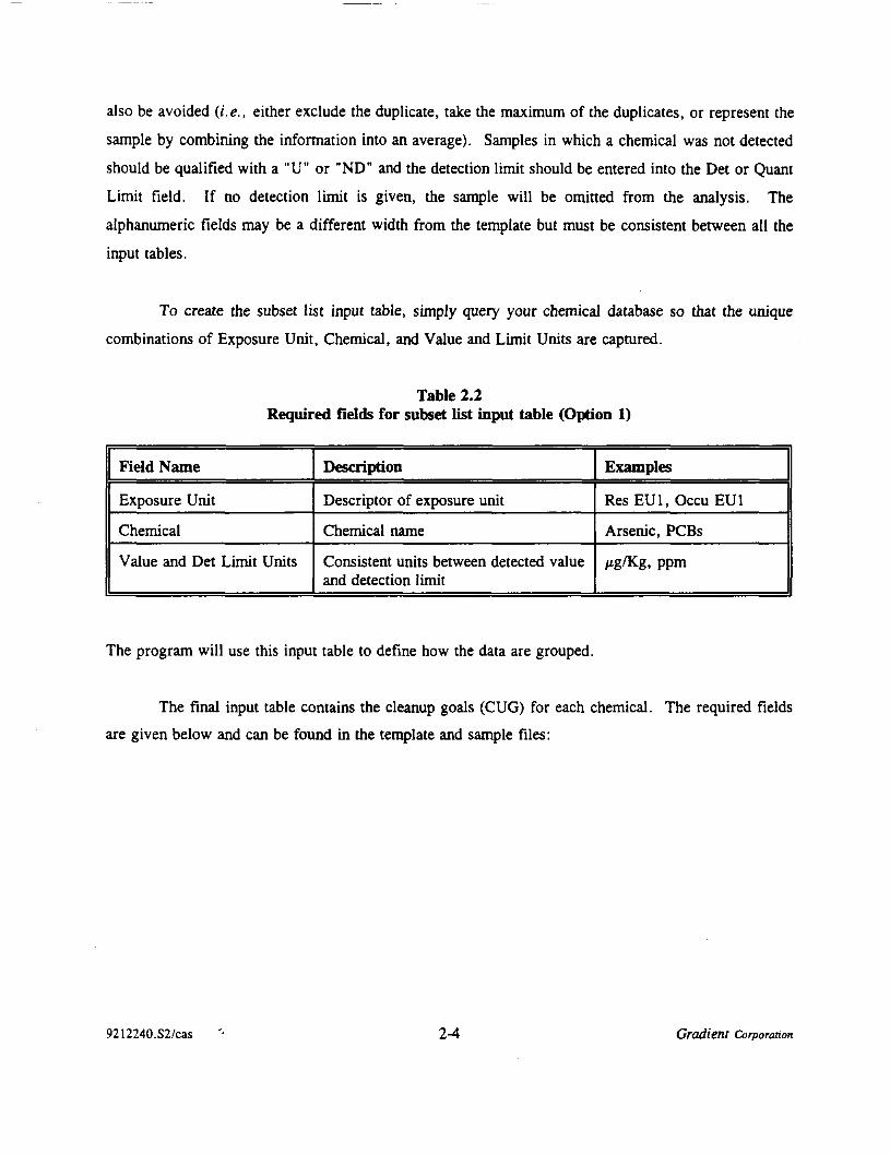
To create the subset list input table, simply query your chemical database so that the uniquecombinations of Exposure Unit, Chemical, and Value and Limit Units are captured.

Table 2.2Required fields for subset list input table (Option 1)

Field Name

Exposure Unit

Chemical

Value and Det Limit Units

Description


Chemical name


Examples

ResEUl, OccuEUl

Arsenic, PCBs

Mg/Kg, ppm

The program will use this input table to define how the data are grouped.

The final input table contains the cleanup goals (CUG) for each chemical. The required fieldsare given below and can be found in the template and sample files:


Table 2.3Required fields for subset list input table (Options 1 and 2)

Field Name

Exposure Unit

Chemical

Value and Del Limit Units

CUG

Description


Chemical name


Cleanup Goal

Examples

ResEUl, OccuEUl

Arsenic, PCBs

Mg/Kg, ppm

27000, 15

Option 2

The user must create input tables of CUGs (as described above) and summary statistics tablecontaining the data size, arithmetic mean, and standard deviation (MM). To facilitate creating thesummary statistics table, a template and example are included on the program disk (TMPLTNM.DB and

EXAMPNM.DB, respectively). The contents of the EXAMPNM.DB is Figure 2.4. The required fieldsare as follows:


Table 2.4Required fields for input table (Option 2)

Field Name

CUG

Exposure Unit

Chemical

Value and Limit Units

# Samples

Maximum DET Cone

Arithmetic Mean

Arithmetic Std Dev

Description

Cleanup goalDescriptor of exposure unit

Chemical name

Consistent units between detected value anddetection limit

The number of samples in dataset

Maximum detected concentration in givenunits (not required)

Arithmetic mean in given units

Arithmetic standard deviation in given units

Examples

27000, 15

ResEUl, OccuEU2

Arsenic, PCBs

Mg/Kg, ppm

21, 16

210000, 145

15.4, 17800

2.35, 680

None of these fields can be omitted in the input table structure; the program will not run unless valuesfor the arithmetic mean and standard deviation are given. If the maximum detected concentration isunknown, the field may be left blank. If a value is given for the maximum detected concentration, it will

be used in the program.

Clean Fill Values (CLEAN.DB)

For either option, clean fill values are assumed to be 0 unless they are provided in the tableCLEAN.DB included on the diskette. Clean fill values represent the average contaminant concentrationexpected in clean fill or backfill used to replace excavated volumes. This table resides in the workingdirectory (i.e., C:\WORKING). To modify or add the appropriate clean fill value, simply edit this tableto include the chemical name (denoted exactly the same way in the other tables including case), the units,and the value of the chemical concentration in the fill.


Running PICKUP™

Once the necessary input tables are complete, you must enter the full path name for where thePICKUP™ script resides when invoking a run from the "working" directory (where the input tables arestored). For example, suppose C:\WORKING is the directory where the data reside and C:\PICKUP is

the directory where the program (PICKUP.SC) and supporting tables reside. To run the program, makeC:\WORKING the current directory and select {Scripts} {Play} from the main menu in Paradox. Type

in "C:\PICKUP\PICKUP" when prompted from the software for the script name. Depending on the

configuration of the hardware used and the size of the dataset, the program can take up to an hour ormore to complete. Messages will flash as the program successfully progresses through all the steps.

Figure 2.5 is a flow chart of the main algorithms of the script. The script first asks for the nameof an output table that will be created, and the name of the input CUG table. Next the script will ask

whether the user wishes to follow Option 1 for calculating Confidence Removal Goals from a dataset orOption 2 for calculating Confidence Removal Goals based on summary statistics. Finally, the script will

ask the user to specify the names of the additional required input tables. After each response, it isimportant to hit the "Enter" key so that program progresses to the next step. The program is set up to

send the output of the calculations directly to the printer during the run. It is also possible to reprint the

report directly in Paradox if the user so desires.

Statistical Calculations

When Option 1 is specified there are a number of statistical calculations performed on the inputdataset. For each subset defined by Exposure Unit, Chemical, and Value and Limit Units, data areextracted from the raw dataset and statistics are calculated using half the detection limit for nondetects.The statistics calculated are: number of detects, number of samples, frequency of detects, maximumdetected concentration, arithmetic mean, transformed mean (mean of the natural logarithm values),geometric mean, transformed standard deviation, geometric standard deviation.

In addition to the calculation of summary statistics, a determination of the lognormality of thedataset is made using the Filliben scheme (Filliben, 1974). The Filliben scheme tests normality by

calculating the correlation between the ordered observations and the median value of the largest


observation in a sample of standard normal random variables. The resulting correlation coefficient is

compared to the correlation coefficient at a 5% significance level. To test lognormality, the variablesare first transformed to log space by taking the natural log and the same procedure is followed. Theoutcome of the Filliben test is either a determination that the dataset is not lognormal, or a determination

that the dataset can be adequately described by a lognormal distribution. If the dataset fails the lognormal

test, the program still calculates the summary statistics but does not calculate Confidence Removal Goal

for the particular chemical in question.

The program is designed to assess an alternative method of designating values for nondetects.After the statistics are calculated using half the detection limit for nondetects, the user has the option toaccess the Minimum Detection Limit (MDL) computer code (Helsel and Cohn, 1988) to calculatestatistics for subsets which contain more than one nondetect. The input to the MDL program is fixedcolumn width fields of Exposure Unit, Chemical, Value and Limit Units, Value (or detection limit fornondetects), and Qualifier. The output from the MDL program is the arithmetic mean, geometric mean,and geometric standard deviation by exposure unit, chemical, and units. The output goes to a comma

separated ASCII file called tmp_mdlo.txt which is imported into Paradox and merged with the previouslygenerated statistics. PICKUP™ is then interrupted to allow the user to compare the statistics. To resumethe program, the user must manually change the line in the code from resuming_after_MDL="N" toresuming_after_MDL="Y". Note that this option is not available at this time because the MDL code

is not included with this release. The MDL code can be obtained from Dennis Helsel at the US

Geological Survey2.

If Option 2 has been specified by the user, the geometric mean and standard deviation are

calculated from the arithmetic mean and standard deviation given in the input table.

Screen Subsets

After calculating statistics, each EU/Chemical subset is reviewed to determine for which cleanupgoals must be calculated. If the CUG is not available, no further calculations are possible. If there are

no detects or the maximum detected concentration is less than or equal to the CUG, no cleanup is

2The code is described briefly in Helsel (1990) where instructions for obtaining it are included.

9212240.S2/cas ' 2-8 Gradient Corporation

necessary. If the distribution of raw data is not lognormal, an alternative method (not supplied at thistime) to determine Confidence Removal Goals must be used.

Calculate Upper Confidence Limit on the Mean (UCLM)

For the subsets for which Confidence Removal Goals will be calculated, the upper 95 percentUCLM on the mean is calculated with the H-statistic based upon the number of samples, geometric mean,and geometric standard deviation. Substitutions are made for the UCLM where it exceeds 1E9 (ppb) or1E6 (ppm) or is greater than the maximum detected concentration, following US EPA guidance (USEPA,

1992).

Calculate Removal Goals

For subsets where the UCLM is greater than the CUG, removal goals are calculated followingthe procedures described in Sections 3 and 4 of this document.

Output Tables

Sample output tables for Options 1 and 2 are shown in Figures 2.6 and 2.7, respectively. The outputgenerated contains identification fields, summary statistics fields, the Confidence Removal Goal, andcomment fields containing information about the generation of the Confidence Removal Goal. Table 2.5summarizes the fields included in the output tables.


Table 2.5Fields given in Output Tables

Field Name

CUG

Exposure Unit

Chemical

Value and Det Limit Units

# Detects

# Samples

Frequency of Detects

Maximum DET Cone

Arithmetic Mean

Arithmetic Std Dev

Geometric Mean

GSD

Lognormally distributed

Statistics calc with

Calculate cleanup ?

UCL on Mean with H

UCL on Meansubstituted?

Description

Cleanup Goal


Chemical Name

Consistent units between detectedvalue and detection limit

The number of detects in dataset

The number of samples in dataset

# Detects divided by # Samples,times 100

Maximum detected concentrationin given units

Arithmetic mean in given units

Arithmetic standard deviation ingiven units

Geometric mean in given units

Geometric standard deviation

Filliben test for lognormality ofdataset

Specifies assumptions used forhandling nondetects or if nodataset available

Gives reason if CRG notcalculated

Upper confidence limit on themean calculated with the Hstatistic

Notes if the UCL is reduced dueto exceeding max det or other(see text)

Option

1 only

1 only

2 only

1 only

Examples

27000, 15

Res EU1, OccuEU2

Arsenic PCBs

Mg/Kg, ppm

20, 12

21, 16

95, 75

210000, 145

15.4, 17800

2.35, 680

7500, 7.8

6.5, 2.7

pass, fail

1/2 det lim for nds;arith mean, std dev

No: distribution notlognormal

3420, 45.7

no; yes: max det


Field Name

Confidence Removal Goal(CRG)

Confidence RG Comment

Limit

# Samples CRG

CRG > maxpos

CRG > Max DET

GSD > 15

Description

The Confidence Removal Goal!

Comment field (see Table 2.6)

Specifies whether the CRG wasfound on the upper (U) or lower(L) confidence side of the mean(see Section 3. 2. 4)

Number of samples correspondingto the UCL or LCL where theCRG is found (see Section 3.2.5)

Notes if CRG exceeds 109 (ppb)or 106 (ppm).

Notes if CRG exceeds max det

Notes if the geometric standarddeviation exceeds 15

Option Examples

3245, 35.4

Clean fill = 0.5

U; L

35, 21

Y(es), N(o)

Y(es), N(o)

Y(cs). N(o)

The last three columns of output on the output table are designed as flags to the user to aid in

thinking about the CRG results and whether or not they are appropriate. The first flag notes if thecalculated value of the CRG exceeds a theoretical maximum of 109 ppb or 106 ppm. Such an exceedenceshould rarely occur, and is most likely to occur for datasets that deviate from lognormality. The Fillibentest for lognormality should prevent calculation of CRGs for datasets that deviate substantially fromlognormality. An exceedence may also occur under option 2 where incorrect and unrealistic summarystatistics can possibly be input. If the user notes this flag, all input should be checked and lognormalityof the dataset should be independently assessed.

The second flag notes if the calculated value of the CRG exceeds the maximum detectedconcentration in the dataset. This is most likely to occur for small datasets. This happens because themethodology assumes that higher, unmeasured, concentrations exist and fill out the presumed lognormal

distribution. A calculated CRG higher than the highest detected value indicates where cleanup shouldoccur if/when such higher concentrations are found. However, if no further sampling is planned, the user

is faced with a need to cleanup, but no single area specified as requiring cleanup. In such a situation,


the user must consider the goals of the project, the probability that further sampling is necessary to better

characterize the site, and other site-specific issues.

The third flag notes if the geometric standard deviation of the dataset is greater than 15. Thisis an arbitrary cutoff that is again aimed at delineating where unreasonable CRG values may becalculated. Environmental datasets that are lognormally distributed rarely have GSD values this high.

Input datasets with high GSD values may fail the Filliben test due to non-lognormality. However, ifOption 2 is used where only summary statistics are supplied and the calculated GSD exceeds 15, the usermay wish to reexamine their specified input, and/or look for further information concerning the datasetfor which summary statistics have been input.

The output table may contain comments in many places. The comments that may occur and anexplanation of them are given in Table 2.6.


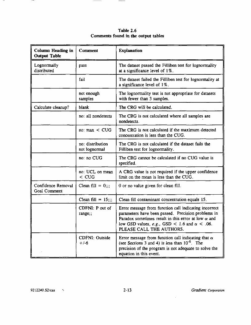
Table 2.6Comments found in the output tables

Column Heading inOutput Table

Lognormallydistributed

Calculate cleanup?

Confidence RemovalGoal Comment

Comment

pass

fail

not enoughsamples

blank

no: all nondetects

no: max < CUG

no: distributionnot lognormal

no: no CUG

no: UCL on mean< CUG

Clean fill = 0;;;

Clean fill = 15;;;

CDFNI: P out ofrange;;

CDFNI: Outside+/-6

Explanation

The dataset passed the Filliben test for lognormalityat a significance level of 1%.

The dataset failed the Filliben test for lognormality ata significance level of 1 % .

The lognormality test is not appropriate for datasetswith fewer than 3 samples.

The CRG will be calculated.

The CRG is not calculated where all samples arenondetects.

The CRG is not calculated if the maximum detectedconcentration is less than the CUG.

The CRG is not calculated if the dataset fails theFilliben test for lognormality.

The CRG cannot be calculated if no CUG value isspecified.

A CRG value is not required if the upper confidencelimit on the mean is less than the CUG.

0 or no value given for clean fill.

Clean fill contaminant concentration equals 15.

Error message from function call indicating incorrectparameters have been passed. Precision problems inParadox sometimes result in this error at low a andlow GSD values, e.g., GSD < 1.6 and a < .06.PLEASE CALL THE AUTHORS.

Error message from function call indicating that a(see Sections 3 and 4) is less than 10"6. Theprecision of the program is not adequate to solve theequation in this event.


Table 2.7Disk files and contents

File Name

PICKUP.SC

DRIVE.SC

RGLIB.LIB

CLEAN. DB

HTABLES.DB

HLTABLE.DB

NTABLE.DB

PRNRG1.DB

PRNRG1.R1

PRNRG2.DB

PRNRG2.R1

TMPLTCUG.DB

TMPLTDS.DB

TMPLTSL.DB

TMPLTNM.DB

EXAMPCUG.DB

EXAMPDS.DB

EXAMPSL.DB

EXAMPNM.DB

Content

Main program

Program for setting relevant directories and paths (editable)

Library containing compiled code necessary for PICKUP™ to run (noteditable)

Empty table ready for clean fill values

Table containing 95 percentile values for H-Statistic (UCL)

Table containing 5 percentile values for H-Statistic (LCL)

Table containing possible sample numbers for use in the ConfidenceRemoval Goal calculation

Table containing the report format for output of Confidence Removal Goalcalculations (Option 1)

Report format for output of Confidence Removal Goal calculations(Option 1)

Table containing the report format for output of Confidence Removal Goalcalculations (Option 2)

Report format for output of Confidence Removal Goal calcuations (Option 1)

Template table giving format for input of CUGs (risk-based cleanup goals)

Template table giving format for database input (Option 1)

Template table giving format for subset list (Option 1)

Template table giving format for input of summary statistics (Option 2)

Example input table of CUGs used in both Option 1 and Option 2 input

Example input table of database input for Option 1

Example input table of subset list for Options 1 and 2

Example input table of summary statistics for Option 2


Exposure Unit Chemical

Figure 2.1Example Dataset Table (Option 1)

Value and Limit Units Value Det or Quant Limit QualifierOccu EU1Occu EU1Occu EU1Occu EU1Occu EU1Occu EU1Occu EU1Occu EU1Occu EU1Occu EU1Occu EU1Occu EU1Occu EU1Occu EU1Occu EU1Occu EU1Occu EU1Occu EU1Occu EU1Occu EU1Occu EU1Occu EU2Occu EU2Occu EU2Occu EU2Occu EU2Occu EU2Occu EU2Occu EU2Occu EU2Occu EU2Occu EU2Res EU1Res EU1Res EU1Res EU1Res EU1Res EU1Res EU1Res EU1Res EU1Res EU1Res EU1Res EU1Res EU1Res EU1Res EU1ResELM

ArsenicArsenicArsenicArsenicArsenicArsenicArsenicArsenicArsenicArsenicLeadLeadLeadLeadLeadLeadLeadLeadLeadCadmiumCadmiumArsenicArsenicArsenicArsenicArsenicArsenicCadmiumCadmiumLeadLeadLeadArsenicArsenicArsenicArsenicArsenicArsenicArsenicArsenicArsenicCadmiumCadmiumCadmiumLeadLeadLeadLead

mg/Kgmg/Kgmg/Kgmg/Kgmg/Kgmg/Kgmg/Kgmg/Kgmg/Kgmg/Kgmg/Kgmg/Kgmg/Kgmg/Kgmg/Kgmg/Kgmg/Kgmg/Kgmg/Kgmg/Kgmg/Kgmg/Kgmg/Kgmg/Kgmg/Kgmg/Kgmg/Kgmg/Kgmg/Kgmg/Kgmg/Kgmg/Kgmg/Kgmg/Kgmg/Kgmg/Kgmg/Kgmg/Kgmg/Kgmg/Kgmg/Kgmg/Kgmg/Kgmg/Kgmg/Kgmg/Kgmg/Kgmg/Kg

9.39.4

11.311.6

1214.815.1

4380.110415

15.816

18.724.928.9

3538.639.9

4.34.44.95.15.25.3

19.51291303.13.38.9

99

9.59.710

10.8

18.518.622.122.8

J

J

J

J

J

J

1.1 U5.8 UJ

JJJJJ

1.1 U1.4 U

J

J

JJ

J1.1 U1.1 UJ1.2 U

J

Gradient

Figure 2.2Example Subset List Input Table (Option 1)

Exposure UnitOccu EU1Occu EU1Occu EU1Occu EU1Occu EU1Occu EU2Occu EU2Occu EU2Occu EU2Occu EU2Res EU1Res EU1Res EU1Res EU1Res EU1Res EU2Res EU2Res EU2Res EU2Res EU2

ChemicalArsenicCadmiumCopperLeadNickelArsenicCadmiumCopperLeadNickelArsenicCadmiumCopperLeadNickelArsenicCadmiumCopperLeadNickel

Value and Limit Unitsmg/Kgmg/Kgmg/Kgmg/Kgmg/Kgmg/Kgmg/Kgmg/Kgmg/Kgmg/Kgmg/Kgmg/Kgmg/Kgmg/Kgmg/Kgmg/Kgmg/Kgmg/Kgmg/Kgmg/Kg

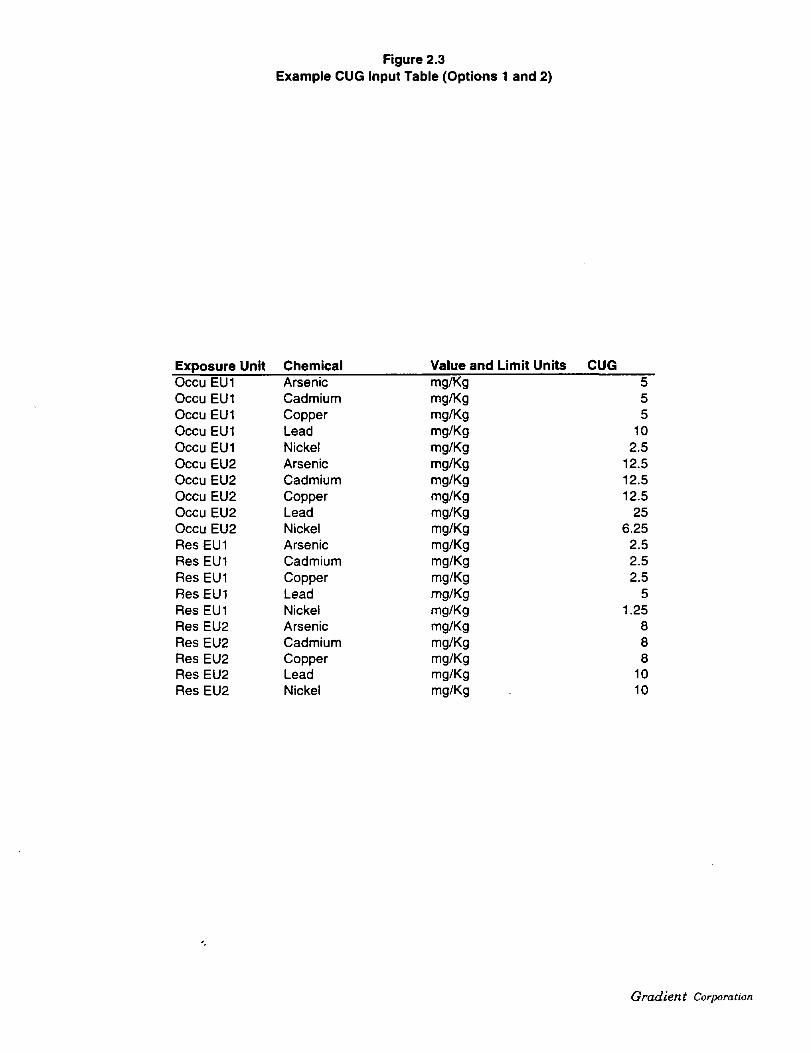
Figure 2.3Example CUG Input Table (Options 1 and 2)

Exposure Unit Chemical Value and Limit Units CUGOccu EU1Occu EU1Occu EU1Occu EU1Occu EU1Occu EU2Occu EU2Occu EU2Occu EU2Occu EU2Res EU1Res EU1Res EU1Res EU1Res EU1Res EU2Res EU2Res EU2Res EU2Res EU2

ArsenicCadmiumCopperLeadNickelArsenicCadmiumCopperLeadNickelArsenicCadmiumCopperLeadNickelArsenicCadmiumCopperLeadNickel

mg/Kgmg/Kgmg/Kgmg/Kgmg/Kgmg/Kgmg/Kgmg/Kgmg/Kgmg/Kgmg/Kgmg/Kgmg/Kgmg/Kgmg/Kgmg/Kgmg/Kgmg/Kgmg/Kgmg/Kg

555

102.5

12.512.512.5

256.25

2.52.52.5

51.25

888

1010

Gradient Corporation

Figure 2.4Example Input Table (Option 2)

CUG Exposure Unit Chemical Value and Limit Units # Samples Maximum PET Cone Arithmetic Mean Arithmetic Std Dev1.25 ResEUI2.5 Occu EU12.5 ResEUI2.5 ResEUI2.5 ResEUI

5 OccuEUI5 OccuEUI5 Occu EU15 ResEUI

6.25 OccuEU28 ResEU28 ResEU28 ResEU2

10 OccuEUI10 ResEU210 ResEU2

12.5 OccuEU212.5 OccuEU212,5 OccuEU2

25 Occu EU2

NickelNickelArsenicCadmiumCopperArsenicCadmiumCopperLeadNickelArsenicCadmiumCopperLeadLeadNickelArsenicCadmiumCopperLead

mg/Kgmg/Kgmg/Kgmg/Kgmg/Kgmg/Kgmg/Kgmg/Kgmg/Kgmg/Kgmg/Kgmg/Kgmg/Kgmg/Kgmg/Kgmg/Kgmg/Kgmg/Kgmg/Kgmg/Kg

15437

146151149363733

15279

999

3299

79797978

133.2960.9411.5634.29

4574.2412.3797.14

5883.16205.41165.54

15.008.39

172.27110.13

1660.5629.8143.8259.29

6877.00184.61

194.3150.1811.7077.34

29289.0913.86

279.9934925.28

444.65310.30

5.635.11

84.22130.55

3246.5711.9382.41

206.6329347.91

341.83


Figure 2.5Flow Chart for Pickup.sc to Calculate Confidence Removal Goals

(bold indicates where user must supply input)

Start

Enter OutputTable Name

Enter CUGTable Name

(Option 1)

yes

1'Enter Subset List

Table Name

(Option 2)

no

Enter Data SetTable Name

Enter SummaryStatistics Table

Name

Calculate statistics for eachsubset in the data set usinghalf the detection limit fornondetects

Calculate statistics fromarithmetic mean andstandard deviation

no

Calculate statistics for eachsubset in the dataset withMDL estimating values fornondetects

noCompare

statistics using'half detects versus MDL

Use MDLstatistics?

yes

Replace statistics withthose calculated by MDL

g:\public\present\9212240.GRF

no / CUGavailable?

no Anydetects?

Nocleanupv^"0Max det >= CUG?

yes

Calculate UCL onmean with H (UCL- )


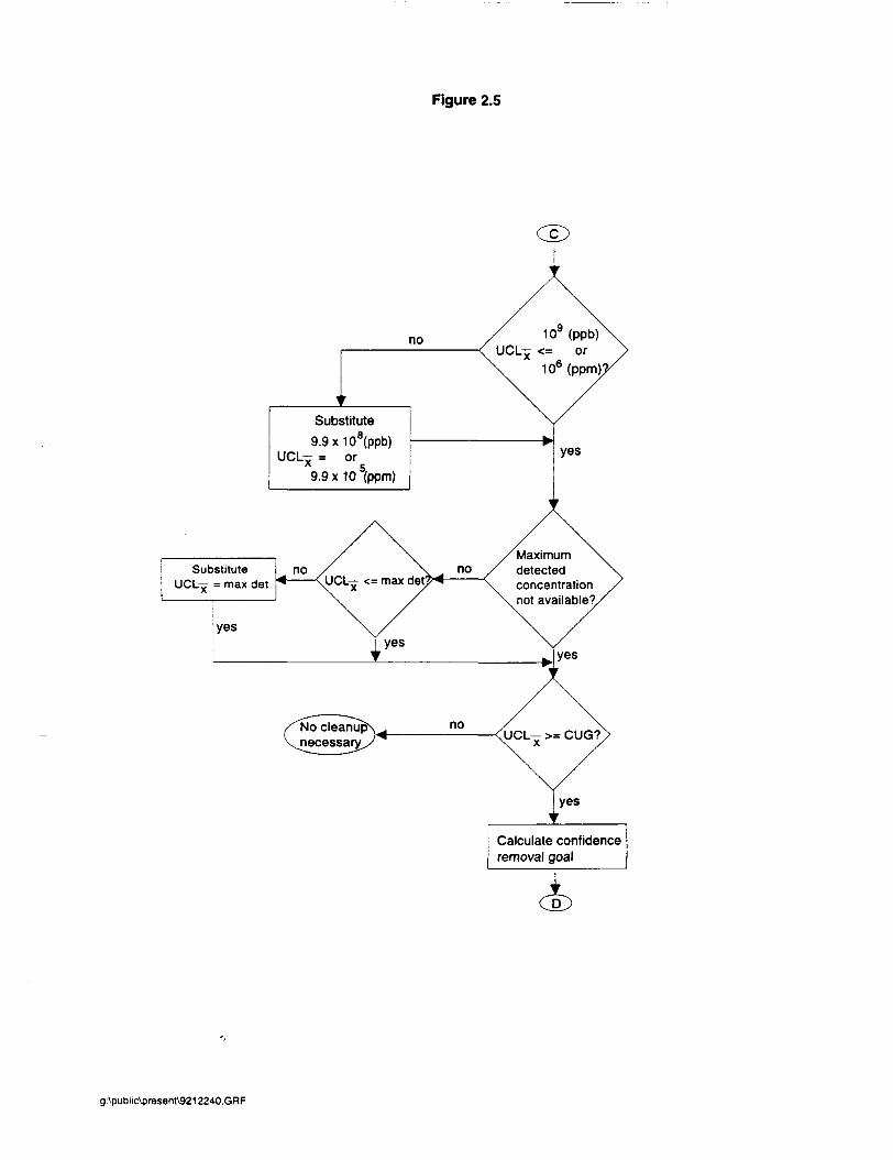
Figure 2.5

Maximumdetectedconcentrationnot available?

no / \ ^ noUCL- <= max det"M

Calculate confidenceremoval goal


Figure 2.5

Initiate confidence removalgoal loop: set n* = n

Do until n" = infinity (1001);Calculate associated UCL*—and RG* x

Do until n* = n:Calculate associated LCL—and RG' x

Print table of CRGsand supporting calculations


Results of confidence removal goal (CRG)calculations(OPTION 1)2/35/94 1 of 4 (Statistics) Page 1 a

[1]cue

2.55.05.05.010.0

6.312.512.512.525.0

1.32.52.52.55.0

8.08.08.010.010.0

ExposureUnit

Occu EU1Occu EU1Occu EU1Occu EU1Occu EU1


Res EU1Res EU1Res EU1Res EU1Res EU1


Chemical

NickelArsenicCadmiumCopperLead



ArsenicCadmiumCopperLeadNickel

Value and DetLimit Units # Detects

mg/Kgnig/Kging/Kgmg/Kgmg/Kg

mg/Kgmg/Kgmg/Kgmg/Kgmg/Kg



3736353332

7979777978

154146148149152

99999

# Samples

3736373332

7979TV7978

154146151149152

99999

Frequency ofDetects

10010095100100

10010097100100

10010098100100

100100100100100

MaximumDET Cone

39910417

79500472

38001330425

59500

Arithmetic [2]Mean Geometric Mean GSD

.0

.0

.7

.0

.0

.0

.0

.0

.01540.0

104001281040

1090003620

2317233673057

.0

.0

.0

.0

.0

.5

.3

.0

.0

.0

60.912.44.0

5883.2110.1

165.543.843.5

6877.0184.6

133.311.623.0

4574.2205.4

15.08.4

172.31660.629.8

43.87.13.2

882.773.7

50.814.212.9

2161.389.2

34.27.26.0

795.367.6

14.27.2

160.2838.827.8

2.12.51.96.72.6

3.43.44.85.63.4

2.92.33.46.93.7

1.41.81.63.51.5

[1] Cleanup Goal[2] Geometric Standard Deviation

Figure 2.6

2 of 4 (Statistics) Page 1b

ExposureUnit





Chemical





Logno finallydistributed

faitfailpasspasspass

faitfailpasspasspass

failfailfailpassfail

passpassfaitpasspass

Statistics calc with

1/2 det lim for nds1/2 det lim for nds1/2 det lim for nds1/2 det tin for nds1/2 det lim for nds

1/2 det lint for nds1/2 det lim for nds1/2 det lim for nds1/2 det lim for nds1/2 det lim for nds

1/2 det lim for nds1/2 det lim for nds1/2 det lim for nds1/2 det lim for nds1/2 det lim for nds

1/2 det lim for nds1/2 det tim for nds1/2 det lim for nds1/2 det lim for nds1/2 det lim for nds

Calculate cleanup?

No: distribution not lognormatNo: distribution not lognormal

No: distribution not lognormalNo: distribution not lognormal

No: distribution not lognormalNo: distribution not lognormalNo: distribution not lognormal

No: distribution not lognormal

No: distribution not tog nor ma I

Figure 2.6 (cont.)

3 of 4 (Removal Goal) Page 1c

ExposureUnit





Chemical





UCL on Confidence Re-Mean with H UCL on Mean substituted? mo vat Goal (CRG)

5.0 no 38.618062.9 no 92.9169.8 no 43.4

73.2 no 60.517157.1 no 249.3264.9 no 94.9

8530.5 no 53.0

19.8 no 15.613.6 no 19.7

6730.0 yes: max det 185.239.9 no 24.0

Confidence

No cleanupClean fillClean fill

Clean fillClean fillClean fill

Clean fill

Clean fillClean fill

Clean f i l lClean fill

RG comment

necessary.; ; ;- .5; ;" -05; ;

- -25; ;= .5; ;« .05; ;

* .5; ;

= .25; ;« .25; ;

= .05; ;= -05; ;

Figure 2.6 (cont.)

4 of 4 (Removal Goat) Page 1d

ChemicalCRG > CRG > GSO >

Limit * Samples CRG maxpos Max DET 15

Occu EU1 NickelOccu EU1 ArsenicOccu EU1 CadmiumOccu EU1 CopperOccu EU1 Lead

373631

Occu EU2 NickelOccu EU2 ArsenicOccu EU2 CadniumOccu EU2 CopperOccu EU2 Lead

3018171


Z01

Res EU2 ArsenicRes EU2 CadniumRes EU2 CopperRes EU2 LeadRes EU2 Nickel

1228

129

Figure 2.6 (cont.)

Results of confidence removal goal (CRG)calculations(OPTION 2)2/16/94 1 of 3 (Statistics) Page la

[1]:UG

2.55.05.05.010.0

6.312.512.512.525.0

1.32.52.52.55.0

B.O8.08.010.010.0

ExposureUnit





Chemical





Value and Det MaximumLimit Units # Samples DET Cone





3736373332

7979797978

ISAU6151149152

99999

ArithmeticMean

60124

5833110

1654343

6877184

1331123

4574205

158

172166029

ArithmeticStd Dev

.9

.4

.0

.2

.1

.5

.8

.5

.0

.6

.3

.6

.0

.2

.4

.0

.4

.3

.6

.8

50133

34925130

31082142

29347341

1941143

29289444

5584

324611

C2]Geometric Mean GSD

.2

.9

.0

.3

.5

.3

.4

.1

.9

.8

.3

.7

.6

.1

.7

.6

.1

.2

.6

.9

4783

97771

772012

156987

7581070586

147

15475627

.0

.2

.2

.2

.0

.9

.6

.7

.0

.7

.4

.1

.8

.8

.1

.0

.2

.8

.2

.7

2.12.51.96.72.6

3.43.44.85.63.4

2.92.33.46.93.7

1.41.81.63.51.5

[1] Cleanup Goal[2] Geometric Standard Deviation Figure 2.7

ExposureUnit

OccuOccuOccuOccuOccu

OccuOccuOccuOccuOccu

ResResResResRes

ResResResResRes

i EU1i EU1i EU1EU1EU1

i EU2EU2EUZ

i EU2i EU2

EU1EU1EU1EU1EU1

EU2EU2EU2EU2EUZ

Chemical





Statistics calc

aritharitharitharitharith




mean.mean.mean.mean.mean,

mean,mean.mean.mean,mean,

mean.mean,mean,mean,mean,

mean.mean.mean.mean.mean,

stdstdstdstdstd

stdstdstdstdstd

stdstdstdstdstd

stdstdstdstdstd

with Calculate cleanup?

devdevdevdevdev

devdevdevdevdev

devdevdevdevdev

devdevdevdevdev

UCL onMean with H

78175

19996163

2336172

12454260

1611329

7571266

1913247907739

.3

.5

.0

.7

.6

.8

.9

.4

.9

.4

.8

.3

.4

.2

.3

.6

.4

.8

.2

.8

UCL on Mean substituted?

nonononono

nonononono

nonononono

nonononono

3 of 3 (Removal Goat) Page 1c

ExposureUnit





Chemical





Confidence Re-moval Goal (CRG)

19.714.656.095.942.7

35.645.960.7216.494.6

20.07.B9.750.733.3

15.519.895.6174.724.0

Confidence

Clean fillClean f i l lNo cleanupClean fillClean fill

Clean fillClean fillClean fillClean fillClean fill

Clean fillClean fillClean fillClean fillClean fill

Clean fillClean fillClean fillClean fi l lClean f i l l

RG comment

= -05; ;= -25; ;necessary.; ; ;= .5; ;= .05; ;

* .05; ;= .25; ;= .25; ;= .5; ;= .05; ;

= -05; ;= .25; ;= .25; ;= .5; ;= .05; ;

= .25; ;" .25; ;= .5; ;= .05; ;= -05; ;

Limit

LLUUL

LLUUL

ULLUL

LUUUL

CRG > CRG > GSD ># Samples CRG maxpos Max OET 15

36161373631

713013017971

154121121149121

1225999

Figure 2.7 (cont.)

3 Calculation of Confidence Removal Goals

This section describes the approach for calculating Confidence Removal Goals. The mathematicalequations that relate the Confidence Removal Goal to the properties of the pre-remediation distributionof contaminant concentrations and the level of contaminant expected in "clean" fill, or back fill, togetherwith the derivation of these equations, are given in Section 4. The sections below describe the calculationof a removal goal when the true mean of a distribution is known (Section 3.1), the calculation of aremoval goal when the true mean of a distribution is uncertain (Section 3.2), and the advantages of theapproach described here (Section 3.3). Although the true mean of a distribution is almost never knownin actual site work, this alternative is presented first because it forms a precursor calculation to the morecomplicated, but common, alternative where the true mean of a distribution is uncertain.

3.1 Calculation of a Removal Goal when the True Mean of a Distribution isKnown

When the sample size is very large (greater than 200 - 300) the true mean and standard deviation

of the dataset can be assumed to be equal to the sample mean and standard deviation, and are consideredto be known quantities. This is a limiting case that seldom occurs in actual field studies due to both

practical and financial constraints on sampling. However, it is the most simple case for which tocalculate a removal goal (the Confidence Removal Goal is not necessary) so it is presented here first.

The initial step in the calculation of a removal goal is to calculate the average contaminantconcentration of the dataset and compare the result to the desired average contaminant level, averagecleanup goal, or CUG1. If the true average contaminant concentration in an Exposure Unit does not

exceed the desired average, no remediation is necessary. If the true average exceeds the desired average,then a removal goal is calculated.

This comparison should be with the UCL on the mean, however for sample sizes in excess of 200 there is little difference.Cases where the UCL becomes important are discussed in the next section.

9212230.S3/cas '- 3-1 Gradient Corporation

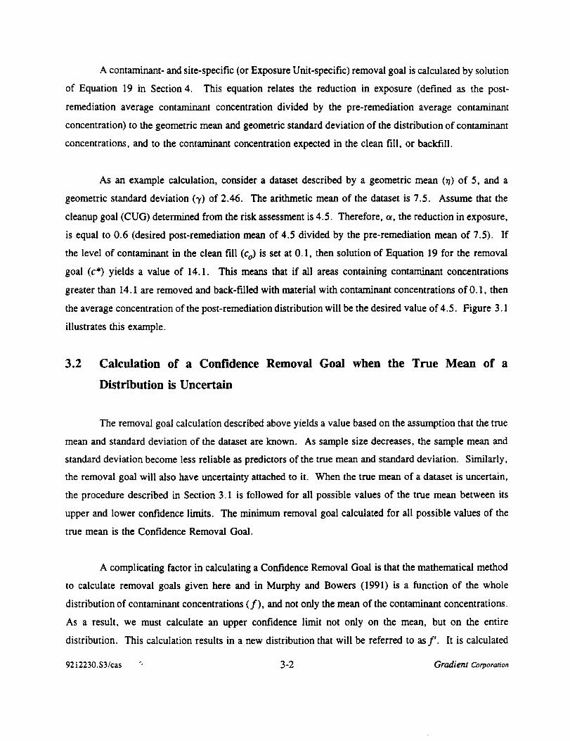
A contaminant- and site-specific (or Exposure Unit-specific) removal goal is calculated by solutionof Equation 19 in Section 4. This equation relates the reduction in exposure (defined as the post-

remediation average contaminant concentration divided by the pre-remediation average contaminantconcentration) to the geometric mean and geometric standard deviation of the distribution of contaminant

concentrations, and to the contaminant concentration expected in the clean fill, or backfill.

As an example calculation, consider a dataset described by a geometric mean (y) of 5, and ageometric standard deviation (y) of 2.46. The arithmetic mean of the dataset is 7.5. Assume that thecleanup goal (CUG) determined from the risk assessment is 4.5. Therefore, a, the reduction in exposure,is equal to 0.6 (desired post-remediation mean of 4.5 divided by the pre-remediation mean of 7.5). Ifthe level of contaminant in the clean fill (c0) is set at 0.1, then solution of Equation 19 for the removal

goal (c*) yields a value of 14.1. This means that if all areas containing contaminant concentrationsgreater than 14.1 are removed and back-filled with material with contaminant concentrations of 0.1, then

the average concentration of the post-remediation distribution will be the desired value of 4.5. Figure 3.1illustrates this example.

3.2 Calculation of a Confidence Removal Goal when the True Mean of aDistribution is Uncertain

The removal goal calculation described above yields a value based on the assumption that the truemean and standard deviation of the dataset are known. As sample size decreases, the sample mean andstandard deviation become less reliable as predictors of the true mean and standard deviation. Similarly,the removal goal will also have uncertainty attached to it. When the true mean of a dataset is uncertain,

the procedure described in Section 3.1 is followed for all possible values of the true mean between its

upper and lower confidence limits. The minimum removal goal calculated for all possible values of thetrue mean is the Confidence Removal Goal.

A complicating factor in calculating a Confidence Removal Goal is that the mathematical methodto calculate removal goals given here and in Murphy and Bowers (1991) is a function of the whole

distribution of contaminant concentrations (/), and not only the mean of the contaminant concentrations.As a result, we must calculate an upper confidence limit not only on the mean, but on the entiredistribution. This calculation results in a new distribution that will be referred to as/'. It is calculated

9212230.S3/cas "• 3-2 Gradient Corporation

from the UCL on both the arithmetic and geometric means of/, where these two values are used to define

the geometric standard deviation of/', and hence, all percentile values of/'.

3.2.1 Upper Confidence Limits on a Lognormally Distributed Dataset

The first step in calculating the Confidence Removal Goal is to calculate an upper confidence limiton the mean of the dataset. Following EPA guidance (EPA, 1992), the UCL on the arithmetic mean ofa dataset that is lognormally distributed (UCL-) is calculated with the H statistic by

where M corresponds to the logarithm of the geometric mean (gm) of the dataset, G represents thelogarithm of the geometric standard deviation (gsd) of the dataset, v is the degrees of freedom (equal tothe sample size minus one), and HG v can be taken from tables such as given in Gilbert (1987) and Land(1975).

The upper confidence limit on the geometric mean of a lognormal dataset is calculated with thet statistic. Since lognormally distributed data become normally distributed when the logarithms of all

observations are taken, UCLs on a percentile (in this case the geometric mean corresponds to the 50thpercentile) of a lognormally distributed dataset are calculated in logarithm (normal) space, and thenexponentiated.

The formula for calculating the UCL on the mean of a normally distributed dataset is

UCL, - ~X + (2)

9212230.S3/cas '- 3-3 Gradient Corporation

where x is the sample mean, 5 is the sample standard deviation, n is the sample size, and tv is the one-tailed t statistic for a confidence level of 95 percent and degrees of freedom v. The UCL on thegeometric mean is obtained by replacing ;c with M, s by G and exponentiating this expression, such that

(3)

These two values, UCL- and UCLom from Equations 1 and 3, are sufficient to define/', the upperA £"•

confidence limit on the distribution. The gsd of/' (gsdf)2 can be calculated from

gsdf - exp^On UCL-X - In UCLgm)) . (4)

Although the values of t/CLj, t/CL , and gsdf provide sufficient information for the calculation of

Confidence Removal Goals, gsdf can be used to estimate other percentiles of/' for sake of illustration.

Percentiles of/' can be calculated from

(5)

where ZD is the lOOp percentile of the standard normal distribution.

2Note that gsdf, does not correspond to the upper confidence limit on the geometric standard deviation of the original

distribution (UCL d), but rather is consistent with the distribution defined by upper confidence limits on the mean and geometricmean of the original distribution (/). This distinction is important because the UCL on a distribution's standard deviationdefined by standard statistical textbooks takes into consideration that some percentiles may be lower than the observed valueinstead of only higher. Therefore, the textbook definition of the UCL on a standard deviation results in a larger value than the

« as defined here.

92 12230. S3/cas 3-4 Gradient Corporation

An example calculation of /' is given for a sample distribution / described by n = 61observations, with gm = 5, and a gsd of 2.46. The arithmetic mean of this distribution is 7.5. Theupper confidence limit on the mean (UCL-) is calculated from Equation 1 to be 9.657. The upper

confidence limit on the geometric mean (UCLgm) is calculated from Equation 3 and is 6.062. Equation4 yields a value of gsd* of 2.625. Percentile values of/' are calculated from Equation 5 and giventogether with percentile values of/in Table 3.1. Figure 3.2 shows the cumulative distribution curves

of/and/'.

Table 3.1Percentiles of /and/' for a distributionwith gm = 5, gsd = 2.46, and n = 61

p0.05

0.10

0.15

0.20

0.25

0.30

0.35

0.40

0.45

0.50

0.55

0.60

0.65

0.70

0.75

0.80

0.85

0.90

0.95

Pf1.137

1.578

1.969

2.345

2.726

3.120

3.536

3.982

4.464

5.000

5.601

6.279

7.071

8.013

9.172

10.660

12.717

15.840

21.982

Pf1.239

1.761

2.427

2.692

3.163

3.656

4.181

4.749

5.368

6.062

6.846

7.738

8.790

10.051

11.617

13.649

16.491

20.869

29.652


3.2.2 Comparison of /' With Various Methods of Calculating UCLs on Percentiles of TheDistribution /

The percentile values of/' can be compared to the results of various methods of calculating UCLson percentiles of/. Note that different methods exist to calculate UCLs on percentiles, all yieldingsomewhat different results. Two methods are briefly reviewed here.

The formula for calculating the UCL of a value P corresponding to the percentile p (UCLp) for

a normally distributed dataset is

UCL - Pp p n 2(/i - 1)

where 5 is the standard deviation of the dataset, tv is the one-tailed / statistic for a confidence level of95% and degrees of freedom u, tp v is the one-tailed t statistic for the ;rth percentile at degrees of

freedom u, and Pp can be expressed as

Pf

or approximated by

- x + (Zp)(s) .

At the 50th percentile of a normally distributed dataset/? = 0.5, tQ 5 = zero, P0 5 — p or Jt, andEquation 6 reduces to the familiar expression for the upper confidence limit on the mean given inEquation 2.


The formula for calculating the UCL of Pp for a lognormally distributed dataset is obtained by

the exponential forms of Equations 6 and 8 where M is substituted for Jt and G is substituted for s:

UCL - exp In Pp + (rv)(G)! *

1 (r,^)2

n + 2(n - 1)J(9)

where

In Pp - M + (Z,)(G) . (10)

Equation 9 can be used to calculate a UCL for each percentile of a dataset. Results for theexample described above are shown in Table 3.2.

A second method of calculating UCLs of percentiles is given by Gilbert (1987) and makes useof the k statistic. This method is described in detail by Stedinger (1983) where he refers to the k statistic

as the f statistic. In this method the UCL of a percentile of a normal distribution is given by

UCLp - (11)

Upper confidence limits of percentiles of lognormally distributed data can be obtained by theexponentiated form of Equation 11 where M is substituted for x and G is substituted for s, such that

UCLp - exp[Af (12)

Both Gilbert (1987) and Stedinger (1983) give limited tables of the k statistic.


Table 3.2 shows a comparison of the percentiles of/' calculated from Equation 5 with the UCLson percentiles calculated by Equations 9 and 12 using the t and k statistics. Results are also comparedin Figure 3.3. Note that most of the percentiles cannot be filled in for UCLp calculated from the kstatistic because tables of the k statistic are not available for these percentiles.

Table 3.2Comparison of percentiles of/' with calculated UCLs on percentiles of/

p.05

.10

.20

.25

.30

.40

.50

.60

.70

.75

.80

.90

.95

Pf.o1.239

1.761

2.692

3.163

3.656

4.749

6.062

7.738

10.051

11.617

13.649

20.869

29.652

VCLD (t statistic)

1.535

2.051

2.937

3.376

3.832

4.842

6.062

7.636

9.844

11.360

13.350

20.589

29.659

UCLp (k statistic)

1.993

21.275

30.853

It is apparent from Table 3.2 and Figure 3.3 that different methods of calculating UCLs ofpercentiles yield different results. The method chosen to define/' here results in percentile values that

are similar to those calculated by the t and k statistics. /' has the advantage of being a lognormaldistribution itself, which is a requirement for the method presented here.


3.2.3 Lower Confidence Limits on/

Calculation of Confidence Removal Goals also requires definition of a lower confidence limit

(LCL) on/. The distribution defined by the lower confidence limits on the mean and geometric mean of/will be referred to as/". The lower confidence limit on the mean (LCL-) is calculated from the analogto Equation 1 by

LCL- - exp + jg2

(13)

where HGv is a negative value taken from a lower 5% confidence limit table (Gilbert, 1987 or Land,1975).

The lower confidence limit on the geometric mean (LCL ) is calculated from the analog toEquation 3

- exp (14)

where the tv statistic used is the same as that for the upper confidence limit.

The geometric standard deviation off" is calculated in the same manner as it is calculated for

/', from

gsdr LCL-X - In (15)


3.2.4 Calculation of the Confidence Removal Goal

The Confidence Removal Goal is calculated from Equation 19 in Section 4 where the pre-

remediation mean value used to assess reduction in exposure (a) lies between the upper and lowerconfidence limits on the sample mean. In the simplest case, the Confidence Removal Goal is calculatedfrom a reduction in exposure equal to the desired post-remediation mean divided by the upper confidencelimit on the pre-remediation mean (UCL-). However, this value is the Confidence Removal Goal onlyin the event that no lower value of the removal goal is found by using any other pre-remediation mean

estimate between the upper and lower confidence limits on the mean. The Confidence Removal Goalcorresponds to the lowest value of the removal goal that results for any estimate of the mean between theupper and lower confidence limits. This means that although the "worst case" exposure occurs when the

true mean contaminant concentration corresponds to the upper confidence limit on the sample mean, the

"worst case" (meaning the lowest) removal goal may correspond to a true mean lying at a point other thanthe upper confidence limit on the sample mean. This point is most easily demonstrated with the use of

some example calculations.

Assume that we have a dataset with 15 observations, with a sample geometric mean of 5, asample geometric standard deviation of 4.4817 (G = 1.5), consistent with an arithmetic mean of 15.40.

The desired post-remediation average concentration, or CUG, is 12.32. Using Equations 1, 3, and 4,we calculate an upper confidence limit on the mean of 65.5, an upper confidence limit on the geometric

mean of 9.9, and a gsd*. of 7.0. The desired ratio of reduction in exposure is 0.19 (12.32/65.5), and

solving Equation 19 in Section 4 with a clean fill concentration of 0.1 yields a removal goal of 77.5. Inthis case, the calculated value of 77.5 is the minimum removal goal that will be calculated for a pre-remediation mean between the upper and lower confidence limits on the mean and the ConfidenceRemoval Goal is therefore 77.5. This value will change with alternative values for the concentration of

the contaminant in clean fill.

In contrast, consider a distribution with identical properties, but consisting of hundreds ofobservations. Reduction in exposure is calculated from the arithmetic mean on the pre-remediationdataset because for a large sample size the upper confidence limit and the mean are essentially equal.The value of the reduction in exposure is 0.8 (12.32/15.40) and solution of Equation 19 in Section 4


yields a removal goal of 167.5. In this example, limiting the number of samples to 15 results in aConfidence Removal Goal that is less than half that which would result with unlimited sampling (77.5

versus 167.5).

To illustrate this case and others where the Confidence Removal Goal does not correspond to theupper confidence limit on the mean, Tables 3.3 and 3.4 summarize the Confidence Removal Goalcalculation as a function of sample size and various CUG values. Table 3.3 shows calculated upper and

lower confidence limits on the arithmetic and geometric means, as well as the geometric standard

deviation off as a function of n for n = 10 and above.

Table 3.3Upper and Lower Confidence Limits on the Mean and Geometric Mean as a Function

of Sample Size; Example 1

n

10

15

21

31

41

61

121

CO

121

61

41

31

21

15

10

*v

1.833

1.761

1.729

1.699

1.684

1.671

1.658

1.645

1.658

1.671

1.684

1.699

1.729

1.761

1.833

HG,v

4.207

3.612

3.311

3.077

2.956

2.828

2.681

-

-2.186

-2.113

-2.061

-2.020

-1.958

-1.896

-1.814

UCL- (LCL-)

126.2088

65.5268

46.7578

35.7700

31.0474

26.6310

22.2324

15.4011

(11.4170)

(10.2293)

(9.4464)

(8.8573)

(7.9861)

(7.2019)

(6.2179)

UCLm (LCLKm)

11.9282

9.8895

8.7941

7.8981

7.4182

6.8920

6.2684

5.0

(3.9882)

(3.6274)

(3.3701)

(3.1653)

(2.8428)

(2.5279)

(2.0959)

gsdf. (gsdf)

8.7768

6.9917

6.2218

5.6865

5.4308

5.1769

4.9099

4.4817

(4.2646)

(4.2205)

(4.2028)

(4.1978)

(4.1762)

(4.2505)

(4.3700)

92l2230.S3/cas 3-11 Gradient Corporation

Table 3.4 shows removal goal calculations for four CUG values, of 12.32, 9.24, 6.16, and 3.08,at various sample sizes. Reduction in exposure (a) is the ratio of the CUG to UCL^ (or LCL^) fromTable 3.3. When UCL- is less than the CUG, a exceeds 1 and no removal goal calculation is made.

The removal goal (labeled RG) is obtained by solution of Equation 19 in Section 4, using a from Table

3.4, and gsdf and UCLgm from Table 3.3, and a clean fill concentration of 0.1. Figure 3.4 shows the

relationship of the removal goal to UCL- and to n.

Table 3.4Removal Goals as a Function of Sample Size and Desired Reduction in Exposure; Example 1

CUG

n

10

15

21

31

41

61

121

oo

121

61

41

31

21

15

10

12.32

«l

0.0976

0.1880

0.2635

0.3444

0.3968

0.4626

0.5541

0.8

-

-

-

-

-

-

-

RGt

79.87

77.53

78.15

80.69

83.37

88.13

97.81

167.52

-

-

-

-

-

-

-

9.24

«2

0.0732

0.1410

0.1976

0.2583

0.2976

0.3470

0.4156

0.6

0.8093

0.9033

0.9782

-

-

-

-

RG2

56.75

53.40

52.42

52.35

52.76

53.81

56.08

69.30

116.22

187.50

479.25

-

-

-

-

6.16

"3

0.0488

0.0940

0.1317

0.1722

0.1984

0.2313

0.2771

0.4

0.5395

0.6022

0.6521

0.6955

0.7713

0.8553

0.9907

RG3

36.36

33.39

32.03

31.17

30.87

30.65

30.66

32.36

37.67

41.82

46.36

51.56

63.37

94.98

590.0

3.08

«4

0.0244

0.0470

0.0659

0.0861

0.0992

0.1157

0.1385

0.2

0.2698

0.3011

0.3261

0.3477

0.3857

0.4277

0.4953

RG4

18.26

16.52

15.63

14.92

14.60

14.24

13.84

13.31

13.32

13.52

13.76

14.05

14.39

15.68

18.05

When the CUG equals 12.32 (columns 2 and 3 in Table 3.4 and the curve labeled a = 0.8 in

Figure 3.4, which corresponds to the a value at n = oo), there is a simple relationship between the

removal goal and the sample size where n is greater than or equal to 15. As the number of samples


decreases the removal goal drops, and the Confidence Removal Goal for any particular n value is the

removal goal calculated at the upper confidence limit on the mean for that sample size.

When the CUG equals 9.24 (columns 4 and 5 in Table 3.4 and the curve labeled ce = 0.6 in

Figure 3.4), the minimum removal goal calculated for pre-remediation mean values between the upperand lower confidence limit on the mean for n = 15 does not correspond to UCL- at n — 15. Rather,

the minimum in the curve of approximately 52.4 occurs at a sample size of approximately 31. In thiscase, whether the sample size is 15, 20 or 30, the Confidence Removal Goal is the same value, at 52.4.

For a sample size of 41 the Confidence Removal Goal increases to 52.8, and for unlimited samples theConfidence Removal Goal increases to 69.3. The effect of remediation to the Confidence Removal Goal

is illustrated in Figure 3.5 A and B for two cases: the distribution / corresponding to n = oo andtruncated at 69.3, and the distribution/' corresponding to n = 15 and truncated at 52.4. In both

diagrams, the desired post-remediation average concentration of 9.24 is shown as a line through thedistribution.

When the CUG equals 6.16 (columns 6 and 7 in Table 3.4 and the curve labeled a = 0.4 inFigure 3.4), a similar case results where the Confidence Removal Goal of 30.7 is found at the minimum

in the curve corresponding to a sample size of about 61. In this case the number of samples makes littledifference in the Confidence Removal Goal, as it will change from 30.7 for sample sizes less than 60 to32.4 at n = oo.

Finally, when the CUG equals 3.08 (columns 8 and 9 and Table 3.4 and the curve labeled ct =0.2 in Figure 3.4), Table 3.4 shows that the Confidence Removal Goal is approximately 13.3 regardless

of sample size.

A second example is used to further illustrate the calculation of Confidence Removal Goals. Thisexample differs from the first example illustrated in Figures 3.4 and 3.5 above only in that the geometricstandard deviation of the distribution is set at 2.46 (G = 0.9). For a geometric mean of 5, this isconsistent with a mean of the distribution of 7.5. Four cases are given in Tables 3.5 and 3.6 and shownin Figure 3.6, with CUGs of 6, 4.5, 3, and 1.5, corresponding to a values of 0.8, 0.6, 0.4, and 0.2 atn = oo. Table 3.5 gives the calculated upper and lower confidence limits analogous to Table 3.3. Table3.6 shows the removal goal calculations.


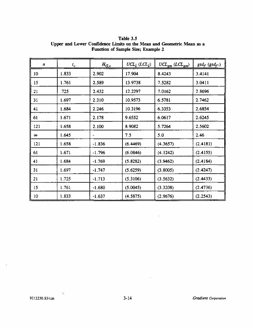
Table 3.5Upper and Lower Confidence Limits on the Mean and Geometric Mean as a

Function of Sample Size; Example 2

n

10

15

21

31

41

61

121

oo

121

61

41

31

21

15

10

'v

1.833

1.761

.725

1.697

1.684

1.671

1.658

1.645

1.658

1.671

1.684

1.697

1.725

1.761

1.833

HG,v

2.902

2.589

2.432

2.310

2.246

2.178

2.100

-

-1.836

-1.796

-1.769

-1.747

-1.713

-1.680

-1.637

t/CLj (LCL-)

17.904

13.9738

12.2297

10.9573

10.3196

9.6552

8.9082

7.5

(6.4469)

(6.0846)

(5.8282)

(5.6259)

(5.3106)

(5.0045)

(4.5875)

UCLsm (LCLsm)

8.4243

7.5282

7.0162

6.5781

6.3353

6.0617

5.7264

5.0

(4.3657)

(4.1242)

(3.9462)

(3.8005)

(3.5632)

(3.3208)

(2.9676)

gsdf (gsdf.)

3.4141

3.0411

2.8696

2.7462

2.6854

2.6245

2.5602

2.46

(2.4181)

(2.4155)

(2.4184)

(2.4247)

(2.4433)

(2.4736)

(2.2543)


Table 3.6Removal Goals as a Function of Sample Size and Desired Reduction in Exposure; Example 2

CUG

n

10

15

21

31

41

61

121

00

121

61

41

31

21

15

10

6.0

«l

0.3351

0.4294

0.4906

0.5476

0.5814

0.6214

0.6735

0.8

0.9307

0.9861

-

-

-

-

-

RG!

22.46

21.21

20.73

20.531

20.538

20.67

21.20

23.95

35.16

62.36

-

-

-

-

-

4.5

a2

0.2513

0.3220

0.3680

0.4107

0.4361

0.4661

0.5052

0.6

0.6980

0.7396

0.7721

0.7999

0.8474

0.8992

0.9809

RG2

16.60

15.42

14.86

14.46

14.27

14.10

13.96

14.07

15.00

15.77

16.59

17.50

19.74

23.94

48.97

3.0

"3

0.1676

0.2147

0.2453

0.2738

0.2907

0.3107

0.3368

0.4

0.4653

0.4930

0.5147

0.5332

0.5649

0.5995

0.6540

RG3

11.52

10.66

10.20

9.85

9.66

9.46

9.25

8.87

8.75

8.77

8.83

8.91

9.10

9.42

10.21

1.5

<*4

0.0838

0.1073

0.1227

0.1369

0.1454

0.1554

0.1684

0.2

0.2327

0.2465

0.2574

0.2666

0.2825

0.2997

0.3270

RG4

6.81

6.36

6.12

5.91

5.79

5.65

5.50

5.16

4.90

4.81

4.75

4.70

4.64

4.60

4.58

An interesting case results when the CUG equals 1.5 (columns 8 and 9 in Table 3.6 and the curvelabeled a = 0.2 in Figure 3.6). Here the minimum in the curve falls on the lower confidence limit sideof the mean where the Confidence Removal Goal is approximately 4.58 at a sample size of 10. As the

sample size increases the Confidence Removal Goal also increases, to 4.75 at n — 41, and to 5.16 atn = oo. In this case, uncertainty about the true mean of the dataset will require more remediation if the

true mean is less than the sample mean and less remediation if the true mean is greater than the samplemean. Because we don't know the true mean, we set the Confidence Removal Goal to correspond to theworst case, and in this instance the worst case is where the true mean is less than the sample mean. This


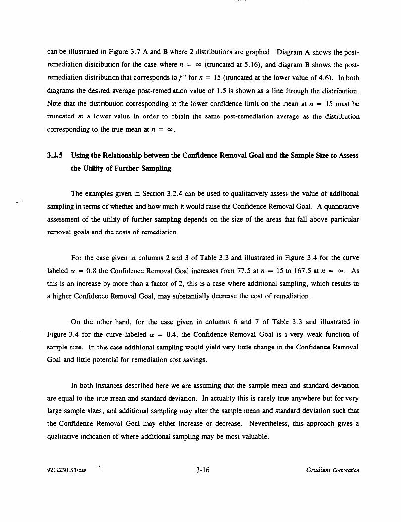
can be illustrated in Figure 3.7 A and B where 2 distributions are graphed. Diagram A shows the post-

remediation distribution for the case where n = oo (truncated at 5.16), and diagram B shows the post-

remediation distribution that corresponds to/" for n = 15 (truncated at the lower value of 4.6). In bothdiagrams the desired average post-remediation value of 1.5 is shown as a line through the distribution.Note that the distribution corresponding to the lower confidence limit on the mean at n = 15 must betruncated at a lower value in order to obtain the same post-remediation average as the distribution

corresponding to the true mean at n = oo.

3.2.5 Using the Relationship between the Confidence Removal Goal and the Sample Size to Assessthe Utility of Further Sampling

The examples given in Section 3.2.4 can be used to qualitatively assess the value of additionalsampling in terms of whether and how much it would raise the Confidence Removal Goal. A quantitative

assessment of the utility of further sampling depends on the size of the areas that fall above particularremoval goals and the costs of remediation.

For the case given in columns 2 and 3 of Table 3.3 and illustrated in Figure 3.4 for the curve

labeled a - 0.8 the Confidence Removal Goal increases from 77.5 at n = 15 to 167.5 at n = oo. Asthis is an increase by more than a factor of 2, this is a case where additional sampling, which results in

a higher Confidence Removal Goal, may substantially decrease the cost of remediation.

On the other hand, for the case given in columns 6 and 7 of Table 3.3 and illustrated inFigure 3.4 for the curve labeled a = 0.4, the Confidence Removal Goal is a very weak function of

sample size. In this case additional sampling would yield very little change in the Confidence RemovalGoal and little potential for remediation cost savings.

In both instances described here we are assuming that the sample mean and standard deviationare equal to the true mean and standard deviation. In actuality this is rarely true anywhere but for verylarge sample sizes, and additional sampling may alter the sample mean and standard deviation such thatthe Confidence Removal Goal may either increase or decrease. Nevertheless, this approach gives a

qualitative indication of where additional sampling may be most valuable.


3.3 Advantages of the Analytical Approach

When the true mean and standard deviation of a log-normally distributed dataset are known asa result of a very large (greater than 200) sample size, the results of the removal goal calculation

described above can be checked by simple hand calculations. This is done by replacing the highest

concentration values in the dataset by values representing the level of contaminant expected in clean fill,and re-calculating the average over the dataset. This calculation is done successively, replacing the nexthighest value, until the re-calculated average meets the target or desired average. This is a "brute force"method of checking that the analytical methodology described here gives a correct answer.

Unfortunately, there is no analogous hand calculation that can be used to check the value of theConfidence Removal Goal developed for smaller sample sizes. This is because the Confidence RemovalGoal is calculated for a distribution that has a mean contaminant concentration different than the mean

contaminant concentration of the dataset, e.g., it could be as high as the upper confidence limit on themean. Since the observed data points do not describe this new distribution that has a mean at the upperconfidence limit, the procedure described above of replacing high values in the dataset and re-averagingdoes not result in the Confidence Removal Goal.

It might be tempting to look at a hand calculation where the target is to replace enough high

values such that the upper confidence limit on the mean of the dataset is less than the target or desired

average. This approach may give an approximate answer in some instances. However, it is not thecorrect procedure because the goal of the Confidence Removal Goal approach is to have the true meancontaminant level in the Exposure Unit to be below the target mean. The upper confidence limit on themean is an indication of where the true mean may fall, but the upper confidence limit itself is a functionof sample size. If the goal were to have the upper confidence limit on a dataset to be less than the targetmean, then this could be achieved by either more remediation, or by more sampling. (More samplinglowers the upper confidence limit, everything else being equal.) It does not make sense to have theattainment of a target dependent on the number of samples taken. Rather, the target must be attained

regardless of the number of samples obtained. Perhaps it's easiest to recall that risk is a function of thetrue mean contaminant concentration, and that the upper confidence limit is used in a risk assessment onlyas an approximation of how high that true mean could be in the face of uncertainty inherent in all


sampling schemes. Remediation is aimed at lowering the true mean, not the upper confidence limit onthe sample mean.

There are at least three advantages to the analytical technique outlined here for the calculationof Confidence Removal Goals as compared to the more simple "brute force" hand calculations. The firstis as described above; the analytical technique allows a calculation that considers the limitations of lessthan perfect sampling, whereas the hand calculations are only useful where the true mean and standarddeviation of a (very large) dataset are well known.

The second advantage of the analytical approach over a hand calculation is that a removal goalcan be estimated even if it falls between two widely disparate analyses. For example, suppose we hada sample with a concentration of 100 and another with a concentration of 500 and the hand calculation

described above suggests that the sample at 500 represents an area that must be remediated. But if one

were to try to delineate where between an area known to have a concentration of 100 and an area knownto have a concentration of 500, there is no information gained from the hand calculation to make this

determination. That is, should an area with a concentration of 400 be remediated? By using theanalytical technique to calculate a removal goal, the samples at 100 and 500 are assumed to form part

of a distribution and a specific removal goal at a concentration level between 100 and 500 can be derived.

A third advantage of this general analytical approach is that an understanding of the nature of thedistribution of contamination can be used to form a predictive model for nondetect values and thusincorporate additional information into the calculation of summary statistics of the dataset, and thereby,the Confidence Removal Goals. Nondetect values are sometimes incorporated into the calculation of

means and other summary statistics by using a substitutional method, where the nondetect value isreplaced by the detection limit, zero, or one half the detection limit. These methods introduce bias into

the result.

Distributional methods represent an alternative approach to handling nondetect values. For

datasets that include nondetect values, it can be assumed that those measurements above the detectionlimit represent a portion of a lognormal (or other type) distribution, from which the entire distributioncan be constructed. Helsel and Cohn (1988) present a method to predict summary statistics forlognormal datasets that include nondetect values at multiple detection limits. Their method and computer


program can be used together with the analytical approach given here to further improve the calculationof the Confidence Removal Goal.

3.3.1 What if The Dataset is not Lognonnal?

The mathematical equations presented here are those required to calculate Confidence RemovalGoals for datasets that are lognormally distributed. In fact, environmental data are commonly

lognormally distributed, and On (1990) explores the physical reasons why this is likely to occur.

However, the general approach described here is not specific to lognormal distributions. Mathematicalequations analogous to those presented in Section 4 can be derived for any type of distribution.

Two types of distributions other than lognormal that may be seen in environmental data arediscussed briefly here. These are normal and "exponential" distributions. A normal distribution issimilar to a lognormal distribution, except that the number of high and low concentrations are equivalent,and evenly distributed about a mean concentration value. An "exponential" distribution arises when thereare a number of high concentration values that tail out very slowly. A combination of two lognormal

distributions, one arising from background and one arising from contamination, has the appearance of

an "exponential" distribution.

If a removal goal is calculated for a dataset that is mistakenly assumed to be lognormal, twooutcomes may occur. The calculated removal goal may be too high, resulting in less reduction in

exposure than required, or the calculated removal goal may be too low, resulting in more reduction inexposure than required. If the calculated removal goal is too low, the result can be used; it is merely a

conservative value that results in more remediation than necessary. If, on the other hand, the removalgoal is too high, the assumption of lognormality should not be applied in this instance and another methodto calculate the removal goal should be sought.

First, let us examine the case in which the assumption of lognormality has been applied for thecalculation of a removal goal to a normally distributed dataset. If the required reduction in exposure is

low (i.e., a is a high value), then the calculated removal goal will be too high and the result cannot beused. If the required reduction in exposure is high (i.e., a is a low value), then the calculated removal

goal will be less than the required removal goal and the result is conservative and can be used in the


absence of a method specifically for normally distributed data. Unfortunately, the division between low

and high required reductions in exposure depends on the parameters of the distribution. That is, thereis no rule to determine whether the calculated removal goal will be an overestimate or an underestimatewithout knowing the mean and standard deviation of the dataset. However, for a specific dataset, we can

determine whether the calculated removal goal is too high or too low.

The opposite situation occurs for datasets that are "exponential" (or the combination of twolognormal distributions representing background and contamination), where again the assumption oflognormality has been applied for the calculation of a removal goal. Here, if the required reduction in

exposure is low (a is a high value), then the calculated removal goal will be too low, the result isconservative, and it can be used in the absence of a method specific for this type of distribution. If therequired reduction in exposure is high (a is a low value), then the removal goal will be too high and the

result cannot be used. Again, the division between low and high a and how it affects theconservativeness of the removal goal depends on the properties of the distribution. We can determinefor a specific dataset whether the calculated removal goal is too high or too low. Note that thesedeterminations are not currently a part of the approach or software package PICKUP™ described herein.


Figure 3.1

Pre-Remediation Contaminant Distribution

Geomean (GM)= 5GSD = 2.46Mean = 7.5

10 15 20 25 30

Concentration fag/Kg}35 40 45

X

51C

0.0.0.0.0.0.0.0.0.0.0.

20 -I18 -161412100806 -0402 -00 -

a

Post-Remediation Contaminant Distribution

i: Co = Clean fillI* y~\.\i \ Meanjf \ (4.5)

• / \ C* = Removal goalF \.

/! \w/; ^^ 14.1^^^^- /; ATI — 1 ————— ( ——————— , —————— ^ —————— , ——————— , ——————— 1 ——————— , ——————— 1 ——————— 1

) 5 10 15 20 25 30 35 40 45

Concentration fag/Kg)

G:\PROJECTS\92122\DATABASE\REMOVAL\FtGURES\CUG31 .XLS 2/23/84 Gradient Corporation

Figure 3.2

1.00 -r

0.90

0.80

0.10

0.00

10 15 20 25 30

Concentration fag/Kg)

35 40 45 50


Figure 3.3

•Qp

1.00 -r

0.90 --

0.80 --

0.70 --

0.60 --

0.50

0.40

0.30 --

0.20

0.10

0.00

10 15 20Concentration (tig/Kg)

25

• Pf',p

• • • • UCLp (t-statistic)

• UCLp (k-statistic)

30 35

(, \PHOJECIS\92122\DAIABASE\HEMOVAI\FIGURES\CUG34 XLS 2/9/94 Gradient Corporation

roO

Removal Goal (ppm)

O)O

00O

oo N)o

ISJo I

53

«S o

3 003 o

oo

CDC/3N*(D

O »CO

00

CQcCD

CO

0)

z0>

11cbe

1111

O)"D3"Q>

II

> O> b>

0)•o3-aiIIO*

1

1

1D3_

3"O)

II

Oio

Figure 3.5

10 20 30 40 50

Concentration fag/Kg}

60 70 80

0.20 r.

10 20 30 40 50Concentration fag/Kg}

60 70 80

G:\PROJECTS\92122\DATABAS6\REMOVAL\FIGURES\CUG36.XLS 2/26/94 Grodiet Corporation

Removal Goal (ppm)NJO

JOC71

CJO

o2Q»

*

C/)0)3

CD

s•n

CO*cCDCO

roo

U•c301

IICbe

1111

01•o3"01

II

> O> b

01T301

II

O'•

1ii

0)•oD-01

IIp"ro

I

Figure 3.7

0.25 t

0.004 5 6

Concentration (tig/Kg)10

0.00

B

4 5Concentration

10

G:\PROJECTS\92122\DATABASe\REMOVAL\FtGURES\CUG37-XLS 2/23/94 Gradient Corporation

4 Mathematical Development of Removal Goals

The mathematical development of removal goals given here closely follows that in Murphy and

Bowers (1991). Murphy and Bowers assumed that remediated volumes were replaced by clean fill orback fill that contained contaminant concentrations of zero. The equations presented here are extendedto allow for "clean" fill with non-zero contaminant concentrations.

We assume that the pre-remedial distribution of contaminant concentrations, f(c)t is lognormalover some pre-defined exposure area. The pre-remedial distribution as a function of c is

f(c)dc - ——————exp-2it(ln y)c

fin -^2/2(ln Y)2 dc,

where 17 is the geometric mean, and 7 is the geometric standard deviation off(c), and

(2)

The post-remedial distribution of contaminant concentrations corresponds to the pre-remedialdistribution between concentrations of zero and c*, where c* is the removal goal, or the concentrationabove which contaminants are remediated. Superimposed on this distribution is a second distributionrepresenting the concentration of the contaminant in "clean" fill (c0), described by a delta function. Thecombined post-remediation distribution can be represented as


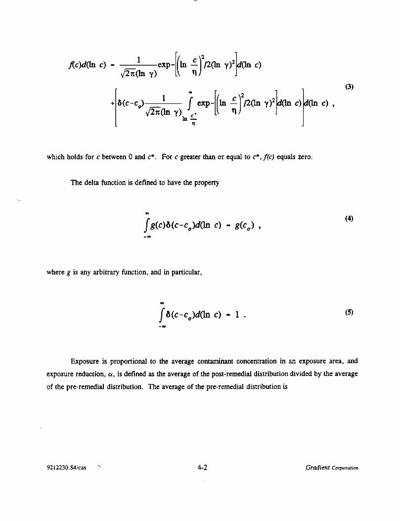
c) -Y/2n(ln y)

exp- In - /2(ln

M

1 t——— \ exp-n_ _\ */On Y) ,.In —

1

c)

/2(ln

(3)

d(ln c) d(ln c) ,

which holds for c between 0 and c*. For c greater than or equal to c*,f(c) equals zero.

The delta function is defined to have the property

c) - g(cg) , (4)

where g is any arbitrary function, and in particular,

Jfft(c-c0)d(ln c) (5)

Exposure is proportional to the average contaminant concentration in an exposure area, andexposure reduction, a, is defined as the average of the post-remedial distribution divided by the average

of the pre-remedial distribution. The average of the pre-remedial distribution is


1 r A c——— / c exp- In —In Y) -. LI 1V^On Y) -

Y)2 (6)

which is equivalent to

1 f———jexp-"- Y)o

/2(In(7)

The average of the post-remedial distribution (n') is

i n /1 r i c——— I c exp- In — /2(ln Y) c)

OQ

i r——— I exp-n_ _.\ *v^rc(ln y) \.

in -/2(ln Y) c)

(8)

c) .

From Equation 4

J c) - c (9)


therefore, using the same transformation as from Equation 6 to Equation 7 together with Equation 9,Equation 8 can be rewritten as

c* r1 t ( c\-———Jexp- In - /27i(lnY)o lV *\)

c» } d c\-——— J exp- In -I

dc

(10)

c)

Exposure reduction, a, is then the ratio of/A' from Equation 10 to p as given by Equation 7.

Equations 7 and 10 can be rewritten as follows. If we make a change in variable from c to z by

z -v/2(ln y)

. c In vIn — - —— L (ID

Equation 7 describing the pre-remedial average becomes

L€ 2 (12)

Similarly, the first term of Equation 10 becomes


-In -

/The second term of Equation 10 is rewritten by making a change in variable from c to y by

y - ——-——In - (14)

such that the term can be expressed as

c* /^_!_fc«:

v/2(ln Y) 1

Combining Equations 13 and 15 and expressing y as z in Equation 15, the post-remedial averageis

(In?)2 v'SOnY) 1 v/22

(16)

_L_to£l


From collecting terms and Equations 12 and 16, the reduction in exposure (/i'//x) can be writtenas

i/3dz

I

Equation 17 can be rewritten in terms of the error function

/1 , c*———In — (17)

(18)

as

o - —2

1 + Erf ——!——In £1 - kjr

c0

n(toy)2

- Erfl——l-——In —Y) 1 >

(19)

using the properties Erf(o°) = 1 and Erf(-x) = -Erflx).

The error function is related to the normal probability function f(t) such that


(20)

Thus, Equation 19 can also be expressed in terms of the area under the standard normal curve as

a - —2

1 c* \ c1 + 2F ——In — - In y + —« 1 - 2F ——In (21)

where F(z) is the area under the standard normal curve from 0 to z, or the negative of the area under thestandard normal curve from -z to 0. Equations 19 or 21 can be solved for the removal goal, c*, as afunction of a, TJ, and 7.

92l2230.S4/cas 4-7 Gradient Corporation

References

Filliben, J.J. The probability plot correlation coefficient test for normality. Technometrics, 17, 111-117,1975.

Gilbert, R. O. Statistical Methods for Environmental Pollution Monitoring. Van Nostrand Reinhold,New York, New York, 1987.

Helsel, D. R. Less than obvious. Environ. Sci. Technol., 24, 1767-1774, 1990.

Helsel, D. R. and T. A. Conn. Estimation of descriptive statistics for multiply censored water qualitydata. Water Resources Research, 24: 1997-2004, 1988.

Land, C. E. Tables of confidence limits for linear functions of the normal mean and variance. SelectedTables in Mathematical Statistics, V. ffl, 385-419, 1975.

Murphy, B. L. and T. S. Bowers. A model relating post remedial soil concentrations to exposure. Proc.Third Annual New England Environmental Exposition, 374-383, 1991.

Ott, W. R. A physical explanation of the lognormality of pollutant concentrations. J. Air WasteManage. Assoc., 40: 1378-1383, 1990.

Stedinger, J. R. Confidence intervals for design events. ASCE J. Hydraulic Eng., 109, 13-27, 1983.

U.S. EPA. Methods for evaluating the attainment of cleanup standards. Volume 1: Soils and SolidMedia, EPA 230/02-89-042, 1989.

U.S. EPA. Role of the Baseline Risk Assessment in Superfund Remedy Selection Decisions. Memo byDon R. Clay. OSWER Directive 9355.0-30, April 1991.

U.S. EPA. Supplemental Guidance to RAGS: Calculating the concentration term. Office of Emergencyand Remedial Response, Intermittent Bulletin, Vol. 1, No. 1, May 1992.

9212230.ref/cas 1 Gradient Corporation

pickup: calculation of confidence removal goals

Documents