pickett_jessica_a_201801_msc.pdf - qspace
TRANSCRIPT

METHOD DEVELOPMENT FOR THE SYSTEMATIC SEPARATION OF
THE <63 µm HEAVY MINERAL FRACTION FROM BULK TILL
SAMPLES
by
Jessica A. Pickett
A thesis submitted to the Department of Geological Sciences & Geological Engineering
In conformity with the requirements for the
Degree of Master of Science
Queen’s University
Kingston, Ontario, Canada
(January 2018)
Copyright ©Jessica A. Pickett 2018
ii
Abstract
Undiscovered ore bodies have become increasingly more difficult to target,
requiring new exploration techniques to pinpoint the undercover location. Sedimentary
overburden in regions of intense glaciation have made exploration difficult, relying on
dispersal-trains for evidence of mineralization. The focus of this study is on the silt-clay
sized material as significant proportions of indicators of mineralization found in
dispersal-trains could be contained within that fraction. This smaller size-fraction could
improve spatial distances associated with ore body’s dispersal-trains and decrease
exploration costs/time. This research examines the physical processes of mineral
dispersal in the <63 µm size-fraction of till, analyzing individual fractions from 45-63,
20-45 and <20 µm. The laboratory research and field orientation case-study, was
investigated by Queen’s University in collaboration with the GSC, to develop novel
methods to examine and characterize the <63µm heavy mineral fraction of till. The
research is broken down into 3 parts: 1) development of methods for separation of the
<63µm size-fraction of HMC by experimenting with settings (mode/oscillation and flow-
rate) using HydroseparatorTM
technology based on different mineral densities and grain
size 2) development of methods for the representative sampling of the <63 µm size-
fraction of sperrylite in blank light-fraction till using controlled and real separation
techniques; and 3) application of methods to real till samples collected from the southern
Core Zone (Northern Québec, Labrador, Newfoundland). Environmental Scanning
Electron Microscopy used in conjunction with Mineral Liberation Analysis was used to
characterize the modal mineralogy of each sample. A comparative study analyzed the
difference between the <63µm fraction (Queen’s University) and the >63 µm fraction
(ODM). Many indicator minerals in bedrock sources are <0.25 mm and are rarely

iii
characterized in glacial sediments because of our inability to separate, visualize, and
chemically analyze these small mineral grains. Using the <63 µm size-fraction, along
with glacial history, dispersal-trains can be detected from distal regions aiding in
exploration targeting below surface deposits. Past studies have begun to examine grains
of similar size however, the approach used in this study differs from techniques
previously used and could expand the usefulness of HMC for exploring mineral deposits
within glaciated terrain.

iv
Acknowledgments
I am very thankful for my supervisors Daniel Layton-Matthews and Beth
McClenaghan for the opportunity to work on such an interesting topic and their guidance
and support over the last 4 years. A special thank you to Agatha Dobosz for her help with
my ESEM-MLA and XRD work. Her constant support and optimism was truly
appreciated. I owe thanks to Louise J. Cabri for the chance to work with the HS-11
software operated HydroseparatorTM
and his guidance through the initial experimentation
with the mineral processing. Thank you to Doug Archibald for successfully teaching me
the fundamentals for a laboratory research based thesis.
This project benefited from the work completed at Overburden Drilling
Management Limited and their insight on mineral separation techniques. This work
wouldn’t have been possible without the resources provided by the Geological Survey of
Canada and the GEM2 project.
Thank you to all the staff and students I have had the pleasure of working with in
the Queen’s Geological and Geological Engineering program. I have made many
valuable friendships along the way and your involvement in my time here at Queen’s has
been valued.
A special thank you to Laurie Dunbar for this excitement and encouragement he
displayed towards this research project.
Finally, I extend my sincere gratitude to my parents, Ann and Michael Pickett,
and sister, Lauren, for always being there for me and pushing me to succeed. I couldn’t
have done it without their constant love and support over this journey.

v
Co-Authorship
This thesis and the manuscripts contain herein are the work of Jessica A. Pickett.
Daniel Layton-Matthews and Beth McClenaghan (thesis supervisors) coauthored chapter
4 and 5 providing scientific and editorial support for this research. The Geological Survey
of Canada carried out the till sampling required for the case study of this project.
Overburden Drilling Management Limited carried out the initial till separation of light
and heavy fractions for the case study as well as contributed to the initial Phase 2
sperrylite separation testing.

vi
Statement of Originality
I hereby clarify that all of the work described within this thesis is the original
work of the author. Any published (or unpublished) ideas and/or techniques from the
work of others are fully acknowledged in accordance with the standard referencing
practices.
(Jessica A. Pickett)
(July 2017)

vii
Table of Contents
Abstract…………………………………………………………………………………..ii
Acknowledgments…………………………………………………………………….....iv
Co-Authorship…………………………………………………………………………....v
Statement of Originality…………………………………………………………………v
List of Figures…………………………………………………………………................xi
List of Tables…………………………………………………………………………...xiv
List of Equations………………………………………………………………………..xv
Abbreviations…………………………………………………………………………..xvi
Chapter 1: Introduction…………………………………………………………………1
1.1 General Introduction………………………………………………………..1
1.2 Structure of Thesis - Objectives………………………………………...….3
1.2.1 Phase 1: HMC in Quartz Experimentation……………………...…4
1.2.2 Phase 2: Sperrylite in Till Experimentation…………………....…..5
1.2.3 Phase 3: Case Study…………………………………………....…..8
1.3 Geological Setting……………………………………………………...…...13
1.4 Thesis Layout……………………………………………………………….17
Chapter 2: Indicator Mineral Separation Background……………………………...18
2.1 Indicator mineralogy……………………………………………………….18
2.2 Heavy Mineral Separation…………………………………………………21
2.1.1 Panning……………………………………………………….......25
2.1.2 Shaking Table………………………………………………...…..25
2.1.3 Heavy Liquid Separation……………………………………...….26
2.1.4 Magnetic Separation…………………………………………...…27
viii
2.3 Previous Work for the <63 µm fraction………………………………......27
2.4 Hydroseparation………………………………………………………...…30
2.5 GSC Till Samples………………………………………………………......36
Chapter 3: Phase 1, HMC in Quartz Experimentation………………………………38
3.1 Objectives………………………………………………………………...…38
3.2 Methods…………………………………………………………………......40
3.2.1 Initial Mineral Preparation……………………………………...…40
3.2.2 Sieving Methods…………………………………………………...41
3.2.3 Hydroseparator Methods…………………………………………..41
3.2.4 Spike Methods………………………………………………....…..43
3.2.5 ESEM-MLA Methods……………………………………………..44
3.3 Results…………………………………………………………………....….47
3.4 Discussion……………………………………………………………....…...50
3.5 Conclusions…………………………………………………………...…….52
Chapter 4: Phase 2, Recovery of Sperrylite from Almonte Till Experimentation....54
4.1 Objectives……………………………………………………………...……54
4.2 Methods………………………………………………………………...…...59
4.2.1 Initial Mineral Preparation…………………………………...……60
4.2.2 Micro Rotary Riffler Methods……………………………………..61
4.2.3 Sieving Methods…………………………………………………...62
4.2.4 Spike Methods……………………………………………………..63
4.2.5 Hydroseparator Methods…………………………………...……...64
4.2.6 ESEM-MLA Methods……………………………………...……...66
4.2.7 Overburden Drilling Management (ODM) Methods……...………67
4.3 Results……………………………………………………………....……....69
4.3.1 Sperrylite in Till Experimentation Results……………....………..69
4.3.2 Overburden Drilling Management (ODM) Results…...…………..73

ix
4.4 Discussion………………………………………………………………......76
4.4.1 Overview……………………………………………………….....76
4.4.1a Blank Data…………………………………………...…..76
4.4.1b Sperrylite Spiked Hydroseparations………………...…...78
4.4.1c Hydroseparation Tailings Data…………………………..80
4.4.2 Problems…………………………………………………………...81
4.4.3 Hydroseparator versus ODM Processing………………………….83
4.4.4 Mounting…………………………………………………………..87
4.5 Conclusion…………………………………………………………………..88
Chapter 5: Phase 3, Case Study………………………………………………………..90
5.1 Objectives……………………………………………………………………90
5.2 Methods……………………………………………………………………...90
5.2.1 Micro Rotary Riffler Methods……………………………………..93
5.2.2 Sieving Methods…………………………………………………...94
5.2.3 Hydroseparator Methods…………………………………………...95
5.2.4 ESEM-MLA Methods……………………………………………...97
5.2.5 X-Ray Diffraction Methods………………………………………100
5.2.6 ODM Separation Processing……………………………………...101
5.3 Results……………………………………………………………………...103
5.3.1 ODM heavy mineral concentrate <125 µm recovery………….105
i Pebble Counts…………………………………………………105
ii Gold & Sulfide Mineral Data………………………………...106
iii Platinum Group Minerals (PGM)……………………………107
iv Kimberlite Data………………………………………………108
Metamorphosed/Magmatic Massive Sulphide Indicator Mineral
Data……………………………………………………..............109
vi Grain Count……………………………………………..........110
5.3.2 X-Ray Diffraction Light Fraction………………………………112
5.3.3 X-Ray Diffraction Heavy Fraction……………………………..112

x
5.3.4 Mineral Liberation Analysis……………………………………113
5.4 Discussion………………………………………………………………….133
5.4.1 Introduction.………………………………………………….….133
5.4.2 Comparison of Mineral Data Sets: ODM, MLA and XRD.…..133
5.4.3 Target Indicator Minerals………………………………………146
5.4.4 MLA versus ODM……………………………………………….159
5.5 Conclusions.………………………………………………………………..160
Chapter 6: Conclusions……………………………………………………………….162
6.1 Final findings………………………………………………………………162
6.2 Future work………………………………………………………………..165
References.……………………………………………………………………………..167
Appendices……………………………………………………………………..………190
Appendix A…………………………………………………………………….190
Appendix B…………………………………………………………………….201
Appendix C…………………………………………………………………….206
Appendix D…………………………………………………………………….219
xi
List of Figures
Chapter 1
Figure 1.1 Phase 2: Sperrylite in Almonte till flowchart………………………...……….7
Figure 1.2 Geological map of the southern Core Zone………………………..………...11
Figure 1.3 Phase 3: Case Study flow chart………………………………………………12
Figure 1.4 Geological map of the southern Core Zone in relation to the Hudson-Ungava
Orogen and the simplified geology of the region………………………………………..14
Figure 1.5 Ice flow map of the southern Core Zone………………………………...…..16
Chapter 2
Figure 2.1 Preconcentrate sample processing flow sheet………………………………..23
Figure 2.2 Simplified NovTecEx processing flow sheet………………………………...29
Figure 2.3 HS-11 Hydroseparator set up………………………………………………...33
Figure 2.4 Stokes law applied to the GSC………………………………………..……...35
Chapter 3
Figure 3.1 Phase 1: HMC in Quartz flow sheet.…………………………………….…...39
Figure 3.2 Mounts used for MLA……………………………………………………......47
Chapter 4
Figure 4.1a Phase 2: Sperrylite in Almonte till flow sheet 1……………………………55
Figure 4.1b Phase 2: Sperrylite in Almonte till flow sheet 2……………………………56
Figure 4.1c Phase 2: Sperrylite in Almonte till flow sheet 3……………………………57
Figure 4.1d Phase 2: Sperrylite in Almonte till flow sheet 4……………………………58
Figure 4.1e Phase 2: Sperrylite in Almonte till flow sheet 5………………………...….59
Figure 4.2 Hydroseparator set up………………………………………………………..66
Figure 4.3 Phase 2 sperrylite recovery for each size fraction………………………...…75
Figure 4.4 Backscatter image displays sperrylite grains found in a blank sample…...…78
Figure 4.5 Phase 2 recovery for real and controlled hydroseparation tests…………......79
Figure 4.6 ESEM backscatter image displaying cementation………………………..….83
Figure 4.7 Phase 2 recovery for hydroseparation and ODM processing…………..……85
xii
Chapter 5
Figure 5.1 Phase 3: Case Study flow sheet………………………………………….…..92
Figure 5.2 ODM sample processing flowsheet…………………………………...……102
Figure 5.3 Bedrock geology map of the southern Core Zone………………………….104
Figure 5.4 Bedrock geology map of the Core Zone with ODM’s lithology of the >2 mm
clasts for each case study sample…………….……………………………………...….106
Figure 5.5 Number of gold grains found in the case study samples by ODM…………107
Figure 5.6 Kimberlite data for the case study samples determined by ODM………….109
Figure 5.7 Modal mineralogy for sample 14-PTA-B005 split D………………………114
Figure 5.8 Modal mineralogy for hydroseparated sample 14-PTA-B005…………..…115
Figure 5.9 Modal mineralogy for sample 14-PTA-B006 split D………………………116
Figure 5.10 Modal mineralogy for hydroseparated sample 14-PTA-B006…………….117
Figure 5.11 Modal mineralogy for sample 14-PTA-B012 split D……………………..118
Figure 5.12 Modal mineralogy for hydroseparated sample 14-PTA-B012………...….119
Figure 5.13 Modal mineralogy for sample 14-PTA-R006 split D……………………..120
Figure 5.14 Modal mineralogy for hydroseparated sample 14-PTA-R006………....….121
Figure 5.15 Modal mineralogy for sample 14-PTA-R011 split D……………………..122
Figure 5.16 Modal mineralogy for hydroseparated sample 14-PTA-R011…………….123
Figure 5.17 Modal mineralogy for sample 14-PTA-R029 split D……………………..124
Figure 5.18 Modal mineralogy for hydroseparated sample 14-PTA-R029…………….125
Figure 5.19 Indicator minerals found from MLA for sample 14-PTA-B005…………..127
Figure 5.20 Indicator minerals found from MLA for sample 14-PTA-B006…………..127
Figure 5.21 Indicator minerals found from MLA for sample 14-PTA-B012…………..128
Figure 5.22 Indicator minerals found from MLA for sample 14-PTA-R006…………..128
Figure 5.23 Indicator minerals found from MLA for sample 14-PTA-R011…………..129
Figure 5.24 Indicator minerals found from MLA for sample 14-PTA-R029…………..129
Figure 5.25 Backscatter images of indicator minerals found from MLA (sperrylite, pyrite,
chalcopyrite and arsenopyrite)……………...……………………………………….….131

xiii
Figure 5.26 Backscatter images of indicator minerals found from MLA (monazite, spinel,
chromite and cassiterite)…………………………………………………………….….132
Figure 5.27 Gold occurrences previously found in Labrador…………………………..152
Figure 5.28 Sperrylite occurrences previously found in Québec and Labrador………..153
Figure 5.29 Spatial distribution for the sperrylite found in the case study samples........154
Appendix A
Figure A1 Almonte till packets used for Phase 2……………………………………....189
Figure A2 Sperrylite rich rock used for Phase 2………………………………………..190
Figure A3 Hydroseparator concentration of sperrylite grains……………………...…..191
Figure A4 Sperrylite crushing………………………………………………...………..192
Figure A5 Sample 14-PTA-B005………………………………………………………193
Figure A6 Sample 14-PTA-B006………………………………………………………194
Figure A7 Sample 14-PTA-B012………………………………………………………195
Figure A8 Sample 14-PTA-R006………………………………………………………196
Figure A9 Sample 14-PTA-R011………………………………………………………197
Figure A10 Sample 14-PTA-R029……………………………………………………..198
Figure A11 Powdered case study till samples used for XRD…………………………..199

xiv
List of Tables
Chapter 1
Table 1.1 Heavy mineral concentrate in the GSC’s Almonte till…………………………8
Chapter 3
Table 3.1 Hydroseparator settings applied to HMC testing……………………………..42
Table 3.2 Hydroseparator settings applied to HMC in quartz testing…………………...44
Table 3.3 Weight percent recovery of HMC from quartz……………………………….48
Table 3.4 Weight recovery of HMC from quartz………………………………………..49
Table 3.5 Percent recovery of HMC from quartz……………………………………......50
Chapter 4
Table 4.1 SelFrag settings used for sperrylite crushing…..……………………………...60
Table 4.2 Phase 2 spiking experimentation………………..…………………………….64
Table 4.3 Weight percent recovery of sperrylite from Almonte till……………………..70
Table 4.4 Total sperrylite weight recovered from Almonte till………………………….71
Table 4.5 Total percent recovery of sperrylite from Almonte till………………………..72
Table 4.6 Number of sperrylite grains found in the blank samples……………………...77
Chapter 5
Table 5.1 Till sample weights for light and heavy fraction……………………………...94
Table 5.2 Hydroseparator settings used for the case study sample………………………96
Table 5.3 Mineral Library List created for the MLA work……………………………...99
Table 5.4 100 grain count completed by ODM……………..………………………….111
Table 5.5 Light fraction XRD analysis……………………………………………....…112
Table 5.6 Heavy fraction XRD analysis………………………………………………..113
Table 5.7 HMC data for the >125 µm fraction for each of the case study samples……126

xv
List of Equations
Chapter 4
Equation 4.1 Stokes Law………………………………………………………………...74

xvi
Abbreviations
BSE – Backscatter electrons
ESEM – Environmental Scanning Electron Microscope
GEM2 – Geo-mapping for Energy and Minerals 2
GSC – Geological Survey of Canada
GSNL – Geological Survey of Newfoundland and Labrador
GST – Glass separation tube
HMC – Heavy mineral concentrate
HS – HydroseparatorTM
LGST – Long glass separation tube
LIS – Laurentide Ice Sheet
MERNQ – Ministère de l’Énergie et des Ressources Naturelles du Québec
MLA – Mineral Liberation Analysis
ODM – Overburden Drilling Management Limited
SEM – Scanning Electron Microscope
SGST – Short glass separation tube
QFIR – Queen’s Facility for Isotope Research

xvii
Qtz – Quartz
WFR – Water flow regulator
XRD – X-Ray Diffraction

1
Chapter 1: Introduction
1.1 General Introduction
Undiscovered ore reserves might be buried under recent unconsolidated sediment
cover. The capacity to see through the complexities of sedimentary cover and to perceive
the ore environment and overall geology has become a fundamental aspect of modern
mineral exploration in glaciated terrains of Canada (Layton-Matthews et al., 2013). This
research examined the physical processes of mineral dispersal in the <63 µm size fraction
of glacial sediment, specifically till. Previous research has examined the physical
dispersal of minerals to identify erosional footprints of underlying mineral deposits
(Averill, 2011). Within mineral deposit footprints, the examination of the physical
dispersal of relatively large and heavy mineral concentrates (HMC) from till samples has
been successful. Till composition is similar to the composition of the bedrock from which
it was derived (Klassen, 2001). Heavy minerals in till can be used to identify targets that
are many times larger than the mineralized bedrock source, however indicator
concentrations in glaciated terrain typically decrease in abundance down ice from the
source (Klassen, 2001). In general, small glacial dispersal trains follow a trend of being
narrow if formed by a single phase of ice flow, are larger in size than that of the ore zone
from which they came, and typically show a down ice decrease in concentration of
mineralized debris from the head of the train to the tail (DiLabio, 1990). Identification of
a dispersal train, however is commonly complex and may involve a number of ice flow
trajectories and variation in time and space (Klassen, 2001). Therefore, it is essential to
understand the glacial history of an area in terms of glacial erosion, transportation and

2
deposition. Glacial sediments are a result of one or more glacial cycles, therefore making
heavy indicator mineral exploration successful when these indicators can be correctly
related back to the bedrock source (Morris and Kaszycki, 1997).
The proposed laboratory research and testing of real samples (case study), was
carried out at Queen’s Facility for Isotope Research (QFIR) by Queen’s University in
collaboration with the Geological Survey of Canada (GSC), to develop novel methods to
examine and characterize the <63 µm heavy mineral fraction of till. Many indicator
minerals in bedrock sources are <0.25 mm and are rarely characterized in glacial
sediments because of our inability to separate, visualize, and chemically analyze these
very small mineral grains (Layton-Matthews et al., 2013). In being able to use the <63
µm size fraction, dispersal trains may be detected in more distal regions (grain size
decreases away from the source) from the mineralized source aiding in exploration of
sediment covered deposits. Investigations of the smaller size fraction of heavy minerals
have been initiated in the last 5 years (Lehtonen et al. 2015; Wilton and Winter, 2012).
However, the approach being used in this study with the use of a Hydroseparator (HS)
differs from the other research and in doing so this could expand the usefulness of heavy
minerals for exploring for mineral deposits within glaciated terrain. The HS has proven to
be a reliable method for recovering these smaller heavy minerals (Cabri et al. 2006). A
new method described here will show how the 45-20 µm and 63-45 µm heavy mineral
fractions, as well as the <20 µm fraction, could lead to new and exciting discoveries both
in mineral exploration.

3
1.2 Structure of Thesis – Objectives
The purpose of this research project was to develop a new method using the HS-
11 software for the CNT Hydroseparator (Cabri et al. 2006) to recover the <63 µm
fraction of heavy minerals from till and then identify key indicator minerals in this finer
grained heavy mineral fraction. The results were then compared with those using
conventional heavy mineral separation on the >0.25 mm fraction of the same till samples
to determine the potential benefits of using this new separation technique for future
exploration.
This thesis was comprised of three different phases of experimentation and
research: Phase 1) development of methods for the separation of the <63 µm fraction of
HMC from a light mineral fraction consisting only of quartz, Phase 2) development of
methods for the representative sampling (split) of the <63 µm HMC of till that had been
spiked with sperrylite, and Phase 3) application of these new methods to real till samples
collected from the southern Core Zone (northern Québec and Labrador) by the GSC. The
first two phases worked towards creating a novel method development for heavy mineral
separation using an HS-11 software controlled HS on the <63 µm fraction. Discoveries
from the initial phases of the research were followed by the application of the developed
methods in the third phase of research, on real till samples.

4
1.2.1 Phase 1: HMC in Quartz Experimentation
A major component of the research completed was the testing the HS settings that
would be optimal for the <63 µm size fraction of light and heavy minerals in till samples.
A system was developed for the use of the HS on HMC of different mineral densities and
mineral grain sizes. The goal of the initial series of tests and experiments was to
understand the efficiency of the HS and determine the software settings that were needed
for different mineral types for different size fractions. This part of the project focused on
the mechanics of the HS and the way in which it can be used for till sample processing to
concentrate heavy minerals. The objective of this phase of testing was to fully understand
the optimal HS settings (mode and flow rate) for concentrating heavy minerals
(hornblende, sphalerite, hematite and galena) so that they are concentrated and remain in
the HS glass separation tube for future examination. The information collected was then
used to guide the hydroseparation of the case study samples. Hydroseparation was tested
by varying the mode and flow rate for individual mineral types, and making visual
observations of when the grains remained within the glass separation tube (GST) versus
when they were removed. The concentrated material was then examined using an optical
microscope and environmental scanning electron microscope (ESEM) after processing to
confirm that the correct minerals had indeed been concentrated. Once the HS settings
were established, a known weight of one heavy mineral (hornblende, sphalerite, hematite
or galena) was mixed with a known weight of quartz and hydroseparated to separate the
two minerals (i.e., quartz and heavy mineral) using the settings previously established.
5
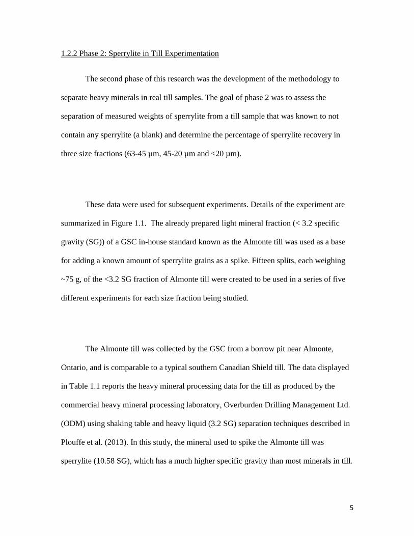
1.2.2 Phase 2: Sperrylite in Till Experimentation
The second phase of this research was the development of the methodology to
separate heavy minerals in real till samples. The goal of phase 2 was to assess the
separation of measured weights of sperrylite from a till sample that was known to not
contain any sperrylite (a blank) and determine the percentage of sperrylite recovery in
three size fractions (63-45 µm, 45-20 µm and <20 µm).
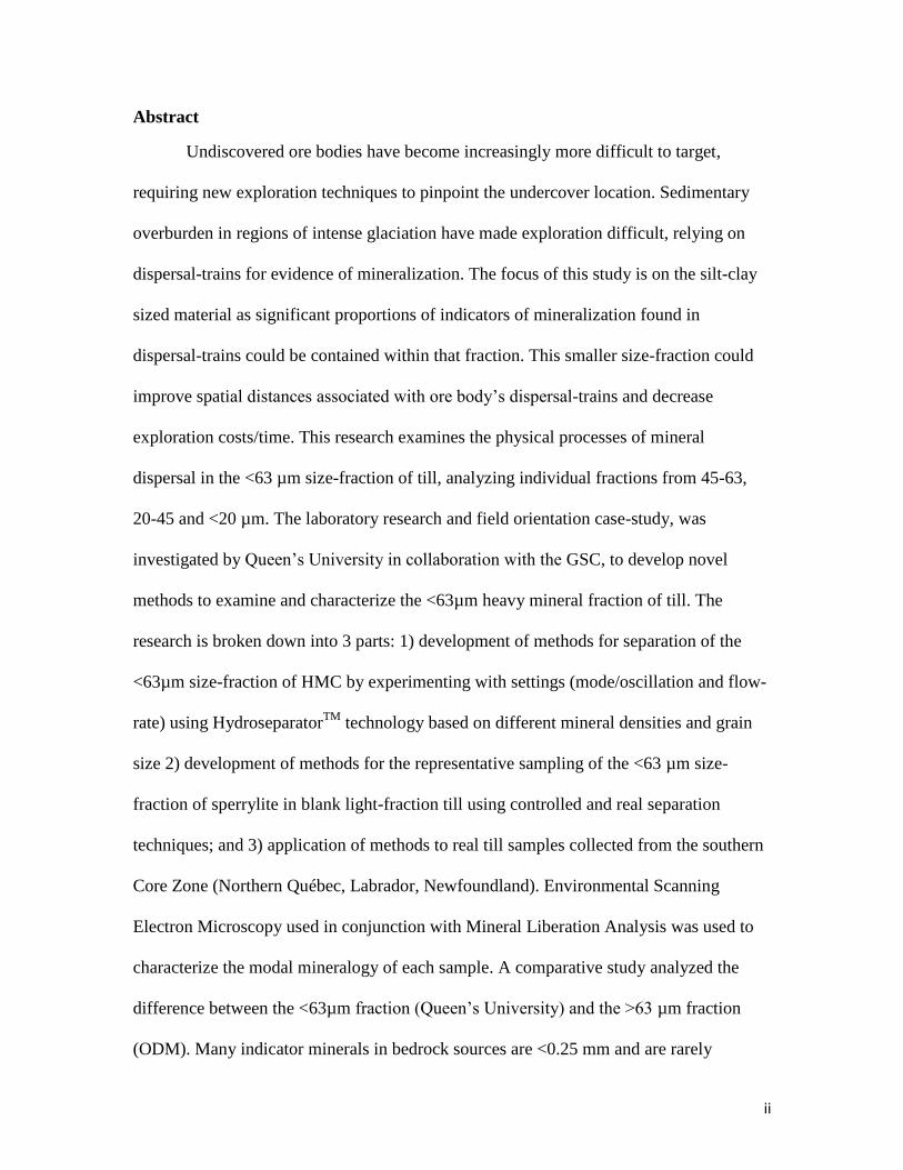
These data were used for subsequent experiments. Details of the experiment are
summarized in Figure 1.1. The already prepared light mineral fraction (< 3.2 specific
gravity (SG)) of a GSC in-house standard known as the Almonte till was used as a base
for adding a known amount of sperrylite grains as a spike. Fifteen splits, each weighing
~75 g, of the <3.2 SG fraction of Almonte till were created to be used in a series of five
different experiments for each size fraction being studied.
The Almonte till was collected by the GSC from a borrow pit near Almonte,
Ontario, and is comparable to a typical southern Canadian Shield till. The data displayed
in Table 1.1 reports the heavy mineral processing data for the till as produced by the
commercial heavy mineral processing laboratory, Overburden Drilling Management Ltd.
(ODM) using shaking table and heavy liquid (3.2 SG) separation techniques described in
Plouffe et al. (2013). In this study, the mineral used to spike the Almonte till was
sperrylite (10.58 SG), which has a much higher specific gravity than most minerals in till.

6
Sperrylite was chosen as a spike because the Almonte till was known to not contain any
of the mineral.
The 15 splits of Almonte till were divided into groups that correspond to different
size fractions to be tested: 63-45 µm (samples JP1-JP5), 45-20 µm (samples JP6-JP10)
and <20 µm (samples JP11-JP15). The first split for each group was used as an
experimental blank (JP1, JP6, JP11) and no sperrylite was added to these sample splits.
These samples were used to test that the cleaning procedures were sufficient and that the
sieves would not cross contaminate samples. The second split of each group (JP2, JP7,
JP12), was first spiked with a known weight of sperrylite (~20 mg for the 63-45 µm and
45-20 µm fractions and ~2 mg for the <20 µm fraction) and then sieved to the specific
size range (i.e. 63-45 µm). The different size fractions were processed through the HS to
recover the sperrylite. The third split of each group was used as the control spikes (JP3,
JP8, JP13). These splits were first sieved to 63-45 µm, 45-20 µm, <20 µm, a known
weight of sperrylite was then added to each sieved split, and then the split was run on the
HS to recover the sperrylite grains. The fourth split of each group (JP4, JP9, JP14), was
physically processed through the HS after sperrylite-rich samples (JP3, JP8, JP13) had
been processed to test the cleaning procedure. Finally, the fifth split (JP5, JP10, JP15) in
each group was spiked with known weights of sperrylite and was sent to ODM for
recovery of sperrylite by traditional heavy mineral separation techniques as described by
Plouffe et al. (2013). The results for the recovery of sperrylite in the fifth set of splits
were compared to that of the second and third splits in each group completed by the use
of the HS technique.

7
Figure 1.1: Procedures followed for phase 2, testing of the recovery of sperrylite in Almonte till
standard. Samples were given the ID name JP with the number referring to the experiment. JP1-
JP5, 63-45 µm; JP6-JP10, 45-20 µm; and JP11-JP15, <20 µm size fraction.

8
Table 1.1: Average heavy mineral content of the Geological Survey of Canada’s (GSC) Almonte
till blank 0.25-2 mm fraction as determined for the >3.2 SG, 0.25-2.0 mm heavy mineral fraction
(Plouffe et al., 2013)
Minor Constituents Major Constituents
Mineral Content Mineral Content
Gold up to 1 grain Silicates -
Sulphides - Hornblende 49%
Chalcopyrite Trace Garnet (almandine & grossular) 17%
Pyrite up to 70 grains Epidote 2%
Silicates - Clinopyroxene 25%
Purple to red garnet Trace Orthopyroxene 1%
Olivine up to 3 grains Sillimanite Trace
Low Cr-diopside up to 14 grains Tourmaline Trace
Chondrodite up to 22 grains Staurolite Trace
Oxides - Titanite (sphene) 4%
Chromite Trace Oxides -
Spinel up to 6 grains Limonite/Goethite Trace
Corundum up to 2 grains Hematite 1%
Red rutile up to 60 grains Phosphate -
Ilmenite Trace Apatite Trace
1.2.3 Phase 3: Case Study
The final phase of research was to apply the developed methods from phases 1
and 2 experimentation to real till samples. Six GSC till samples that had already been
collected from northeastern Québec and western Labrador (Figure 1.2), and overlie a
broad range of bedrock lithologies and potentially contain different heavy minerals.

9
Based on the background geology and the HS settings previously established,
adjustments were made to recover the HMC for each till sample.
The <0.25 mm fraction of each of the six till samples was previously separated
into light and heavy fractions by ODM. Queen’s Facility for Isotope Research at Queen’s
University obtained these light and heavy fractions for each of the six samples and
divided the light mineral fraction and the heavy mineral fraction each into three splits for
testing (Figure 1.3). The first split (heavy fraction only; i.e. 14-PTA-B005 Split 1 H) was
sieved to 63-45 µm, 45-20 µm and <20 µm and each of these size fractions was examined
using the ESEM for mineral liberation analysis (MLA). The second split was the
combination of the light (14-PTA-B005 Split 2 L) and heavy (14-PTA-B005 Split 2 H)
fractions, which was then sieved to 63-45 µm, 45-20 µm and <20 µm and each of these
size fractions were run through the HS to recover the heavy fraction. This heavy mineral
fraction was then examined by ESEM-MLA. Results for splits one and two were
compared to evaluate the ability of the HS to recover the HMC as compared to the
methods used by ODM. The third split (14-PTA-B005 Split 3 H and L) was used for X-
Ray Diffraction (XRD) analysis to determine the bulk mineralogy and additional tests as
needed.
This phase was completed to determine the efficiency of the HS as compared to
ODM’s separation technique, as well as to determine the applicability of using the <0.25

10
mm HMC of till to gain insight into till composition and how it reflects the composition
of the local bedrock geology.
It is hoped that this investigation of the finer HMC (<63 µm) of till will provide
new insights into the bedrock source of the finer grain heavy mineral fraction, which in
turn will aid in the use of heavy mineral concentrates in bedrock mapping and mineral
exploration.

11
Figure 1.2: Geological bedrock map of the southern Core Zone. Geology from Wardle et al.
(1997) and Ministère de l’Énergie et des Resources naturelles (2010).

12
Figure 1.3: Procedure used for phase 3, to process and examine each of six till samples from
northern Québec and Labrador, provided by the GSC. For XRD data see Chapter 4. For MLA
data see Chapter 4.
13
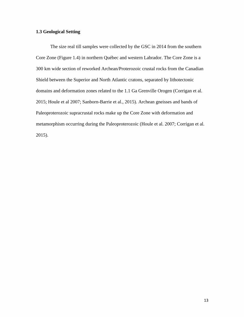
1.3 Geological Setting
The size real till samples were collected by the GSC in 2014 from the southern
Core Zone (Figure 1.4) in northern Québec and western Labrador. The Core Zone is a
300 km wide section of reworked Archean/Proterozoic crustal rocks from the Canadian
Shield between the Superior and North Atlantic cratons, separated by lithotectonic
domains and deformation zones related to the 1.1 Ga Grenville Orogen (Corrigan et al.
2015; Houle et al 2007; Sanborn-Barrie et al., 2015). Archean gneisses and bands of
Paleoproterozoic supracrustal rocks make up the Core Zone with deformation and
metamorphism occurring during the Paleoproterozoic (Houle et al. 2007; Corrigan et al.
2015).

14
Figure 1.4: Geological map of the southern Core Zone. (A) Location of the southern Core Zone bedrock and surficial mapping research area (blue
box) in relation to the Hudson-Ungava orogeny (grey solid line) and adjacent orogeny activity. Core Zone lake sediment geochemical data (red
dashed line) (McClenaghan, et al. 2015). (B) Simplified bedrock geology map for the Core Zone; southern Core Zone research site outlined in red
(McClenaghan, et al. 2014). Bedrock geology modified after James et al. (2003)
15
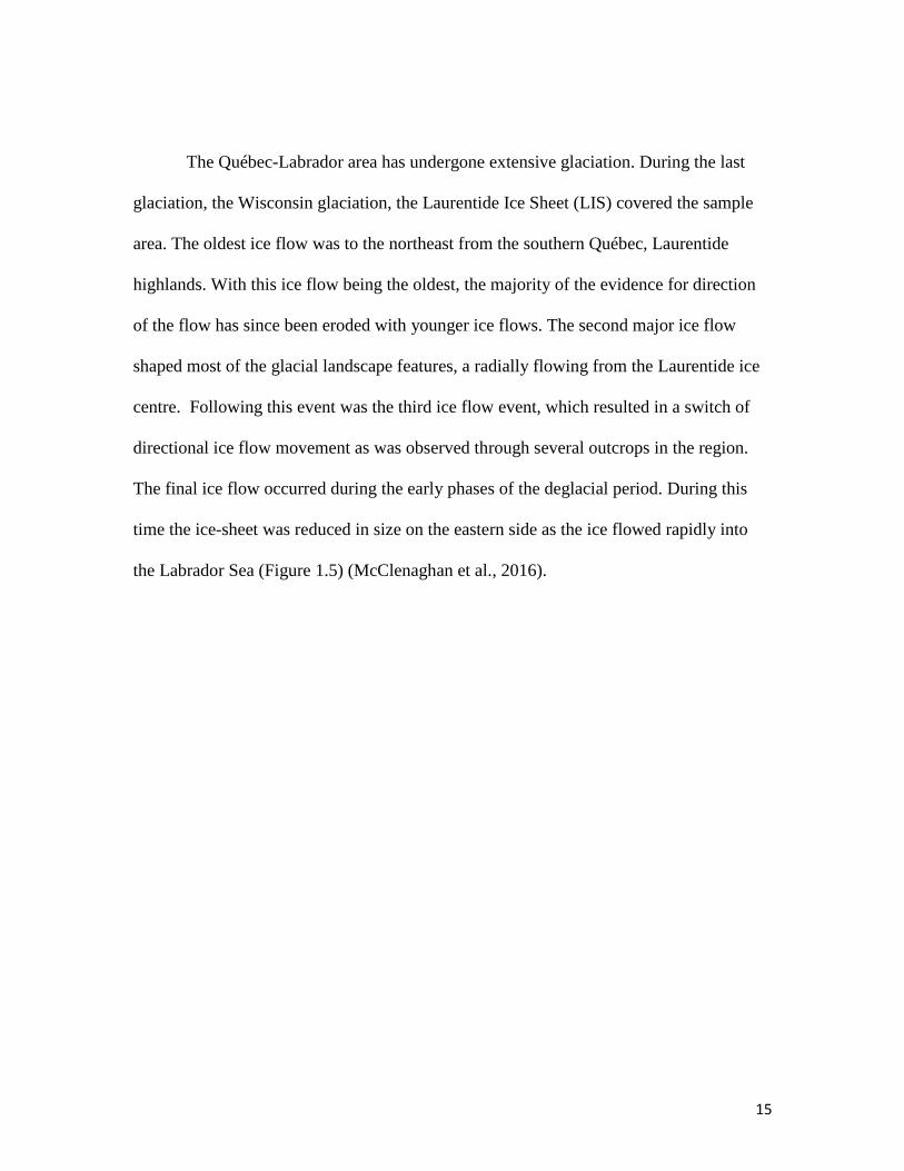
The Québec-Labrador area has undergone extensive glaciation. During the last
glaciation, the Wisconsin glaciation, the Laurentide Ice Sheet (LIS) covered the sample
area. The oldest ice flow was to the northeast from the southern Québec, Laurentide
highlands. With this ice flow being the oldest, the majority of the evidence for direction
of the flow has since been eroded with younger ice flows. The second major ice flow
shaped most of the glacial landscape features, a radially flowing from the Laurentide ice
centre. Following this event was the third ice flow event, which resulted in a switch of
directional ice flow movement as was observed through several outcrops in the region.
The final ice flow occurred during the early phases of the deglacial period. During this
time the ice-sheet was reduced in size on the eastern side as the ice flowed rapidly into
the Labrador Sea (Figure 1.5) (McClenaghan et al., 2016).

16
Figure 1.5: Ice flow chronology for the Core Zone area. Red arrows indicate the oldest ice flow
linked to the Québec highlands (cf., Veillette et al., 1999). Orange arrows represent radial flow
from the Labrador ice centre during the main Wisconsin phase. Yellow arrows indicate radial
flow from the ice centre during deglaciation and the green arrows represent the deglacial ice flow
(McClenaghan et al, 2015).
66°
W64°W
58°N
54°N
14-PTA-B012
14-PTA-R011
14-PTA-R006
14-PTA-R029
14-PTA-B005
14-PTA-B006
17
1.4 Thesis Layout
This thesis is divided into six chapters: introduction, indicator mineral separation
background, phase 1; HMC in quartz, phase 2; sperrylite in Almonte till, phase 3; case
study and conclusions. Chapter 1, introduction, outlines the structure of the thesis (i.e.,
three separate phases of research), and the geographic and geological setting for the six
real till samples that were analyzed. Chapter 2, indicator mineral separation background,
reviews all work previously completed and background information on indicator
minerals, mineral separation techniques, the HS and field work completed in the southern
Core Zone. Chapter 3, phase 1, outlines the objectives, methods, results, discussion and
conclusions determined for the phase 1 research. Chapter 4, phase 2, outlines the
objectives, methods, results, discussion and conclusions determined for the phase 2
research as well as the development and justification for methods used in phase 3.
Chapter 5, phase 3, outlines the objectives, methods, results (which includes the ODM
mineral separation, Hydroseparation, XRD analysis and MLA data), discussion and
conclusions determined for the case study samples analyzed as well as the reviews of
XRD analysis of light versus heavy mineral fractions, HS versus ODM mineral
separation, MLA versus ODM analyses and the surficial sediment problems associated.
Chapter 6, conclusions, discusses the final findings and suggests future work. All data
produced and/or used during the course of this thesis that are not present in the text body
are included in the Appendices (A to D).

18
Chapter 2: Indicator Mineral Separation Background
2.1 Indicator Mineralogy
Indicator minerals are heavy (>2.8 SG) minerals with distinct visual and chemical
characteristics that are recovered from unconsolidated surface sediments and used in
mineral commodity exploration (Averill, 2001; McClenaghan, 2005; Kelley et al., 2011).
Traditionally, visual identification of indicator minerals can be done using the mineral’s
colour, crystal habit, and surface features (McClenaghan, 2014). These minerals can
range in size from coarse grained (2 mm) to silt sized, which is largely dependent on the
bedrock mineralogy, comminution and the target commodity. Indicator mineral methods
are commonly used in exploration programs where glacial sediments (Averill, 2001),
alluvial and stream sediments (McClenaghan, 2005), or aeolian sediments
(McClenaghan, 2005) are sampled to enhance geochemical or geophysical targeting.
Glacial sediment sample collection depends on the landform and terrain, till thickness,
mode and estimated transport distance and landform genesis (McClenaghan, 2013).
Different commodities have different mineral indicators associated with the bedrock
source. Glacial dispersal patterns and associated indicator minerals for specific
commodities vary depending on the commodity. Indicator mineralogy has been used to
explore for gold, diamond (kimberlites), metamorphic/magmatic massive sulphides,
VMS deposits, magmatic Ni-Cu-PGE, Mississippi Valley-type Pb-Zn deposits, porphyry
Cu deposits, intrusion hosted Sn-W deposits and high tech metals (i.e. Nb, Ta, REE)
(Averill, 2001; McClenaghan, 2005; Lehtonen et al., 2015; McMartin et al., 2016; Sharpe
et al., 2017).

19
Gold grains are commonly used in gold exploration, however pyrite, arsenopyrite
and jamesonite can also be used (McClenaghan, 2005). Background abundances range
from less than one to more than twenty grains, as found in a standard 10 kg till sample (or
10 kg normalized sample) (Averill, 2001). The size of the gold indicator mineral grain
will decrease in size at increased distances from the source, however the purity of the
grain will increase (Faulkner, 1986). Gold indicator grains are commonly silt-sized,
which mirrors the parent bedrock mineralization and the common lower size cut-off for
indicator mineral lab work. Gold grain surface features and deformation (i.e, pristine,
modified, etc.) indicates the transport history from the source, with travel distances of
approximately <1 km for major deposits (Averill, 2001).
Kimberlite indicator minerals (KIMs) are used to explore for diamonds and
include specific garnets, and trace mineral chemistry. There are 3 garnets, which are most
commonly used, peridotitic Cr-pyrope, eclogitic pyrope-almandine and megacrystic Cr-
poor pyrope (McClenaghan and Kjarsgaard, 2001, 2007). Along with garnet, Mg-
ilmenite, chromite, Cr-spinel, olivine, enstatite, omphacitic pyroxene, Cr-diopside and
diamond are also used as indicators (McClenaghan and Kjarsgaard, 2001, 2007). All
KIMs are chemically stable (e.g., do not oxidize) in glacial sediments, however some
indicator minerals can occur as highly fractured grains. This will affect the abundance of
grains in addition to the final grain size (Averill, 2001).

20
Metamorphic/magmatic massive sulphide indicator minerals (MMSIMs) are
heavy, coarse grained, weather resistant minerals. As stated by Averill (2011), these
indicators can form from recrystallization of volcano-sedimentary massive sulphide
deposits and the hydrothermal alteration halos through medium to high-grade regional
metamorphism (Spry, 1982) and include ideals such as gahnite (McClenaghan et al.
2016). MMSIM also form from high temperature magmatic metasomatism (skarns and
greisens) or separation of Ni-Cu-Fe sulphides from ultramafic magmas and komatiites
(Averill, 2001). Due to the high resistance to chemical and physical weathering, dispersal
trains for MMSIMs tend to be larger in size (Averill, 2001). Common minerals associated
with MMSIMs are enriched in Mg, Mn, Al, and Cr (i.e., Cr-diopside).
Ni-Cu-PGE indicators come from garnet peridotite mantle, which include
enstatite, olivine, Cr-diopside, chromite and Cr-pyrope garnet mineralogy; minerals that
are enriched in Mg or Cr (Averill, 2001; 2011). Minerals including pyrrhotite, pentlandite
and other Ni and PGE sulphides are metallic indicators that lack weather resistance,
making them hard to use in glaciated terrains. However, these minerals commonly break
down in shallow till and contribute to the chemical signature of the silt and clay fractions
used in bulk till geochemistry. In thick or deeper tills, below the oxidation front, or in till
recently brought to the surface (i.e., frost boils) however, these minerals are commonly
preserved (McClenaghan, et al., 2015). Sperrylite and loellingite have a high resistance to
weathering, however are typically only found in the silt sized, or smaller fraction
(Averill, 2011), largely related to the bedrock size fraction (McClenaghan et al., 2015).

21
Cu-porphyry indicator minerals include red rutile, apatite, rose zircon, blond
titanite, sapphire, corundum, epidote and biotite (Averill, 2011; Plouffe, et al., 2016).
Indicator minerals from these deposits come from specific alteration zones (Averill,
2011). Through recent use of shallow till sampling and porphyry Cu indicator mineral
(PCIM) analysis, concealed porphyry systems are more readily accessed during initial
exploration stages. Determining the specific indicator minerals related to the deposits by
eliminating the common bedrock minerals, aids in the determination of the deposit
present (Kelley et al., 2011). Further research is being completed (McClenaghan et al.,
2016) in the investigation of tourmaline as an indicator of porphyry mineralization as
well as the fine fraction (<0.25 mm) of HMC in till. Tourmaline is a common mineral
associated with porphyry systems and is fairly resistant to weather.
Due to the fact that commodity targets tend to be large and evidence of more than
one mineral commodity can be recovered from a single set of samples, heavy indicator
mineralogy is best used at a reconnaissance to regional scale in exploration (Averill,
2001).
2.2 Heavy Mineral Separation
Heavy mineral separation to recover indicator minerals can be accomplished
using different techniques that will depend on the mineral being studied (McClenaghan,
2005, 2011). Heavy mineral concentrates (HMC) are commonly prepared to recover
indicator minerals for different types of deposits including diamonds, gold, Ni-Cu-PGE,

22
metamorphosed volcanogenic massive sulphides, porphyry copper, uranium, tin and
tungsten (McClenaghan, 2011; Gent, et al., 2011; Plouffe, et al., 2013). The indicator
minerals vary from ore minerals, accessory minerals, and alteration minerals to sparsely
distributed host rock minerals. In trying to recover mineral grains for exploration
processes, the main goal of sample processing is to reduce the volume of material to be
examined, eliminate light minerals, limit contamination, and do so at an affordable cost.
Figure 2.1 displays the generalized mechanism for decreasing reducing volume and
increasing the available heavy mineral concentrate from a bulk till sample.
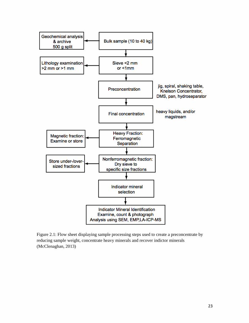
23
Figure 2.1: Flow sheet displaying sample processing steps used to create a preconcentrate by
reducing sample weight, concentrate heavy minerals and recover indictor minerals
(McClenaghan, 2013)
24
Till samples collected for mineral exploration purposed in Canada typically range
from 10-15 kg. This large sample must be reduced in volume by creating a pre-
concentrate, which is then further separated to produce a final heavy mineral concentrate
for the examination of indicator minerals (McClenaghan, 2012). Pre-concentrate
separation techniques include; panning, shaking table separation, dense media separator,
centrifugal concentrator, rotary spiral concentrator, and jigs. Final concentrate
preparation techniques include; heavy liquid separations and magmatic separation. Both
the pre- and final concentrate processing using density separations are used in
combination with sizing and magnetic separation (McClenaghan, 2011).
The grain size used for each separation technique depends on the deposit type and
the minerals available. Typically silt to sand sized particles are used in separation
processes, however this project is focusing on the <63 µm size fraction to try and
increase exploration availability in glaciated terrains. The area of study having undergone
extensive glaciation will have an increased abundance of small grain fractions (<63 µm).
The small grain fractions have more individual grains per sample size and therefore
increase the number of indicators found in that small (<63 µm) fraction (Lehtonen et al.,
2015). It is thought that by using the HS-11 software controlled HS for the <63 µm size
fraction it could increase successful recovery of such small grains including the <20 µm
fraction and reduce the high costs associated with other separation techniques (Cabri et
al., 2006).

25
2.1.1 Panning
Panning is a technique that has been used for 1000s years, dating back to Roman
times. The main indicator minerals recovered from this method include, gold and PGE’s.
The material (i.e. till) being processed is placed in the pan with water while a circular
rotation is applied allowing for the lighter sediments to flow over the top with the heavy
mineral concentrate remaining in the bottom of the pan (English et al., 1987). This
technique is favourable due to its low cost, ease of use, lack of materials required, quick
processing time and ability to be used both in field and laboratory (McClenaghan, 2011).
The downsides to panning are that it is time consuming, only a small portion of material
can be processed at a time, up to 25 grams of material, it is typically used on larger
visible grain sizes which can overcome water surface tension, and it requires practice and
expertise to run with confidence and accuracy in recovery (English et al., 1987; Faulkner,
1986).
2.1.2 Shaking Table
The shaking table is a heavy mineral separation technique that is based on
differences in mineral densities (English et al., 1987). This method works for samples
with grain sizes ranging from silt to coarse-sand and it is capable of sorting samples from
deposit types with different mineral spectrums. The shaking table has a motor driven arm
that shakes the table allowing for the sediments, which are placed in the top corner of the
table to move over the 1 cm high riffles (McClenaghan, 2011). The required parameters
for a Wilfley Table include, inclination/slope, wash water flow rate, material feed table

26
speed and stroke amplitude (Mackay et al., 2015). The water and mineral slurry produced
is pushed along the table, being shaken in a lengthways direction (slow forward stoke and
fast return). This process allows for the grains to move across the table, separate based on
size and density and be collected at the tables edge. This is a favoured technique as it is
cost effective, has a good visibility of grains, and recovery for silt to sand sized particles
and a broad spectrum of minerals can be collected (McClenaghan, 2011). The downside
however, includes the loss of the largest, smallest, and lightest mineral grains.
Additionally, samples need to be sized prior to use, sample runs are slow, and it requires
an acquired skill to run properly similar to that of the panning method (Falconer, 2003).
2.1.3 Heavy Liquid Separation
Heavy liquid separation is commonly used to refine a preconcentrate. This
technique uses specific liquids (methylene iodide (MI) SG 3.3; tetrabromoethane (TBE)
S.G. 2.9; lithium heteropolytungstates (LST) SG 2.9) based on the minerals density that
is to be recovered and the lighter materials in the sample (McClenaghan, 2011). This
method allows for a sharp distinction between the light and heavy minerals in the sample,
with the lighter grains floating and the heavier ones sinking. This method is commonly
used today, however it is costly, may involve the use of carcinogenic reagents and is time
consuming. It limited in that only small volumes of sample can be processed at one time,
making the preconcentration step necessity before indicator mineral examination
(McClenaghan 2011). This method is primarily used on concentrates with minerals from

27
25 mm to 500 µm and can be used for grains as small as 45 µm (silt to sand sized) when
using centrifuge techniques are used (Henderson et al., 1972).
2.1.4 Magnetic Separation
This method will reduce the sample volume to be examined. When using this
technique, samples are usually separated into ferromagnetic and non-ferromagnetic to
reduce the overall sample size and to remove any steel contamination (McClenaghan,
2011). Indicator minerals are then picked from the non-ferromagnetic concentrate
(McClenaghan 2013). The non-ferromagnetic fraction may be further subdivided into
paramagnetic and non-paramagnetic mineral fractions. Indicator minerals can be
subdivided based on the paramagnetic properties. For example, diamond is non-
paramagnetic, pyrope garnet, eclogitic garnet, Cr-diopside and forsteritic olivine are non-
paramagnetic to weakly paramagnetic and Cr-spinel and Mg-ilmenite are moderately to
strongly paramagnetic (McClenaghan and Kjarsgaard, 2007; McClenaghan, 2011).
2.3 Previous Work for the <63 µm fraction
The Geological Survey of Finland (GTK) recently (2015) completed a similar
study to that of the research being completed in this thesis. Heavy mineral separation was
completed on the <63 µm fraction of till collected from the Savukoski-Pelkosenniemi
district in eastern Lapland (Lehtonen et al., 2015). The goal of their research was to
develop a new technique using modern mineral separation processing techniques to

28
determine a time and cost effective method for processing bulk till samples while looking
at the ore potential for the indicator minerals. Their study looked at indicators from a
range of mineralization types found within the study region. Similarly to the research
being completed in this thesis, the <63 µm size fraction was of interest due to the thought
that more individual indicator mineral grains could be found in the finer fraction
compared to the coarser fraction (Lehtonen et al., 2015). The indicators targeted in their
study included gold, PGEs and REEs, allowing for gravity separation techniques to be
applied. The GTK followed a similar procedure to that used at ODM, Figure 2.2.
Overburden Drilling Management Limited (ODM) also received original bulk till
samples and processed heavy mineral samples from the GTK to analyze as reference data
(Lehtonen et al., 2015).

29
Figure 2.2: A simplified processing flowsheet for the NovTecEx samples. The green boxes
indicate optional processing steps that were only carried out on a subset of samples (Lehtonen et
al., 2015).
The preconcentrate phase of the separation could have used either the Knelson
concentrator or the shaking table; the two techniques available to use through the GTK
facilities. The Knelson concentrator can process grains upwards of 10 µm to a maximum
of 6 mm however the greatest average recovery working on <2 mm with the >0.5 mm
size fraction producing nearly 100% recoveries (Chernet, T., et al 1999). This method is
fast and inexpensive however, you must have a silt-sized fraction to produce the slurry
needed to process (McClenaghan, M.B. 2011). The shaking table was favoured for this
research due to its ability to make adjustments for the size and density of the grains in the
sample. In comparison to the Knelson concentrator, the shaking table reduces the

30
breakage of fragile mineral grains during processing (Lehtonen et al., 2015).
After the mineral separation was completed, analysis of the concentrates was
completed. Mineral grains were mounted for ESEM-EDS analysis in one of two ways; 1)
grain mounts, sprinkled grains on carbon tape disks, and 2) polished epoxy mounts. After
some work determined the pros and cons of each method studied, it was determined that
the polished epoxy mounts were best suited for detailed mineralogical analysis while the
grain mounts were best suited for bulk mineralogies. To determine the relativity of one-
grain mount to the sample as a whole, XRF analysis was completed. XRF determines the
mineral compositions within the sample using a pellet of ~7 grams. The amount of
material used for XRF compared to ESEM is ~100x greater in size (with an ESEM disk
containing up to 1000’s of individual grains). The results indicated that the XRF analysis
correlated to the ESEM analysis validating that the grain mounts analyzed were an
accurate representation of the sample as a whole (Lehtonen et al., 2015).
2.4 Hydroseparation
The Hydroseparators HS-01, HS-02, HS-11 were developed by Nikolay
Rudashevsky, and have been used to recover mineral fractions that range from densities
of 2.5 to 20 g/cm3 (anything greater than the density than water) and sizes of 0.4 mm and
smaller, down to the <45 µm industrial flotation size. The sample mass typically ranges
from 100-300 g (depending on the homogeneity of the grains) and result in the collection
of 5-30 mg HMC (Cabri et al., 2006; McClenaghan, 2011). The optimal size used is silt-

31
sized ranging from 300 to 40 µm, however researchers have demonstrated density
separation in small grains (<20 µm) similar to those proposed in this study (Cabri 2008).
The instrument uses water that follows Stokes Law as the fundamental basis for
separation based on density and size (Cabri et al. 2006). The limiting factor with this
form of separation is that the settling velocity focuses on the grain size based on its radius
as well as the density of the grain, which can decrease efficiency based on the sample
grain size variation (Rudashevsky et al. 2002). This form of separation has increased the
efficiency making it 10,000 times more accurate in a laboratory setting (Cabri et al.
2006).
The HS can recover grains from 10-30 µm more consistently than when using a
heavy liquid separation due to the fact that water is less dense than the heavy liquid.
Liberation of individual mineral grains needs to be obtained so that the HS can accurately
collect HMC (Cabri et al. 2006). The HS can be utilized for different materials including
powdered samples, mine waste and tailings, mineral processing concentrates and
environmental monitoring samples (Rudashevsky et al. 2002).
The HS-11 software operated HS, (Figure 2.3), consists of four main
interconnected components, the water source, the water flow regulator (WFR), the HS
and the glass separation tubes (GST). Tap water is used for experimentation and is
collected/stored in an overhead water tank. The tap is turned on while experimentation is
in progress to allow for a constant pressure head to be applied. The water tank has an
32
inflow tube, where the water from the tap enters the tank, an outflow tube where the
water from the tank moves down the system into the flow gauge and an overflow tube
where the water overflows out of the tank into the nearby sink if necessary. The outflow
tube moves from the water tank to the flow gauge, which determines the water flow
pressure that will be used for each sample run. Typically experimental runs use a flow
rate of 50-80 ml/min (Cabri et al. 2006). A tube connects the WFR to the HS box. The
HS determines the oscillation applied to the system as chosen on the computer program.
The water flows through the HS and applies the oscillation through the GST, which holds
the sample. The GST comes in two different sizes, short (SGST) and long (LGST), which
will be interchanged, based on sample size. The HMC is collected within the base of the
GST while the tailings flow out of the GST into the overflow container. The tailings are
retained and can be re-added to the GST if necessary (Cabri et al. 2006).
The hydroseparation process takes approximately 30 minutes to complete a
sample run from start to finish. This includes the cleaning of the GST in between
samples, preparing the sample (weighing out required amount), the sample addition to the
GST, the test itself (typically ranges from 30 seconds to 2 minutes), the recovery of the
tailings and concentrate material and the final clean up process. Some of the water from
the GST is removed to allow space for the sample, while the sample is wet prior to
insertion to the GST. Teflon containers are used to allow for easy transport of the sample
from the container to the GST. Allow time for the grains to settle to the base of the GST
once the sample has been transferred. Hydroseparation relies on the skill of the operator,
making visual observations of when separations have been completed and the application
of the most appropriate settings to be applied based on the sample type. Tests samples

33
should be used prior to real samples to increase familiarity with the process and ability to
separate the HMC.
Figure 2.3: HS-11 software operated Hydroseparator set up with flowmeter (rotameter),
illuminating magnification and long GST.
The means by which the material is separated replicates a natural placer
depositional environment. A natural placer is typically comprised of well-sorted heavy
mineral concentrates of relatively pure mineral grains (Cabri, et al., 1996). Stokes law
states that any object that rises or falls through a fluid will experience a viscous drag
(Figure 2.4). The water follows Stokes law and flows in an upward direction through the

34
GST in a controlled pulsating manner. Flowing, pulsating water (representing the swash
of waves in a placer deposit) moves through the GST and pushes the lighter minerals up
and over the top into the bottom collector, tailings pile, leaving the heavy minerals at the
base of the tube for collection (McClenaghan 2011). This form of separation allows for
the grains to be separated based on the settling velocities, keeping the small denser grains
in the tube and removing the large less dense grains (Cabri et al. 2006). It is the kinematic
flow boundary effect applied to sediment surfaces that allows for an increase in the
separations overall efficiency (Rudashevsky et al. 2002). While running a sample, it is
critical that all air bubbles are removed from the tubing. Air bubbles can interfere with
the sample and experimentation leading to inaccurate results of HMC collection (Cabri et
al. 2006).

35
Figure 2.4: Stokes Law applied to the mineral grains within the HS glass separation tube (GST)
(Pickett et al 2017).
The HS was evaluated as a means to prepare concentrates for this study instead of
the other techniques because of the size of the grains being studied and the ability to

36
separate material based on density differences falling in the range of 3-20 g/cm3. Using
the HS also allows for the operator to make visual observations while a sample is being
processed and adjust settings when necessary during individual sample runs. Panning
would not prove to be useful, as the grains for this project are too small, not creating
enough water surface tension and the accuracy of the method would not be sufficient for
the results required. The shaking table was useful for initial separation (creating a pre-
concentrate) of the heavy minerals in the till samples, however it would not provide the
accurate results needed for the final concentrate phase of this research.
Other heavy mineral separation methods, such as a dense media separator, were
not used in this study because they do not process sample material <0.3 mm in diameter.
A centrifugal concentrator was not utilized for this project as QFIR does not have access
to this method. Jigs could help to separate grains, however the lower size fraction would
be limited, and would likely be unable to separate the <20 µm fraction. The heavy liquid
method would be difficult for the <20 µm and some 45-20 µm sized grains and would be
too costly to run all samples. This method would not be appropriate for assessment of
indicator minerals and modal mineralogy.
2.5 GSC Till Samples
The GSC’s Geo-mapping for Energy and Minerals 2 (GEM 2) carried out surficial
mapping and geochemical studies in the southern Core Zone of northwest Québec and

37
western Labrador to help increase natural resource exploration and development
(McClenaghan et al. 2014, 2015, 2016).
Field data for the surface till samples are reported in McClenaghan et al. (2016).
Till samples, were dug from the non-oxidized C-horizons of the naturally developed soil
profiles in regions lacking permafrost. The <63 µm fraction of six till samples were used
as part of this study (14-PTA-B005, 14-PTA-B006, 14-PTA-B012, 14-PTA-R006, 14-
PTA-R011, 14-PTA-R029; Figure 2.5) (McClenaghan et al, 2014, 2015). Regional ice
flow directions as mapped by GSC in the southern Core Zone are outlined in Figure 1.5.
The six samples were selected from different bedrock lithologies (Figure 1.2) to
reflect the differences in the till sample composition. Sample 14-PTA-B005 overlies a
metagabbro. Sample 14-PTA-B006 overlies rocks of the Labrador Trough that includes
fine-grained sedimentary rocks, mafic volcanic rocks, ironstone, quartzite, dolostone and
chert. Sample 14-PTA-B012 was collected from a basalt and pyroclastic source in the
New Québec Orogen, Doublet Zone. Sample 14-PTA-R006 was sampled from the
Laporte Zone in the New Queébec Orogen, above a muscovite-sillimanite-gypsum
quartzo-feldspathic gneiss. Sample 14-PTA-R011 was collected overlying a mylonitic
tonalite bedrock. Lastly, sample 14-PTA-R029 overlaid a charnockite series bedrock.

38
Chapter 3: Phase 1, HMC in Quartz Experimentation
3.1 Objectives
This chapter is subdivided into 5 different sections; 1) objectives for phase 1
research; 2) methods used in phase 1; 3) results from phase 1; 4) discussion of results
from phase 1; and 5) conclusions gathered from phase 1, experimentation. Figure 3.1
depicts the order in which the initial phase of experimentation was carried out and the
methods used. These procedures were later adapted for application on the case study
samples. Phase 1 conducted the development of methods for the separation of the <63 µm
fraction of heavy mineral concentrate (HMC) from a light mineral fraction consisting
only of quartz. The objective of this phase of research was to apply the knowledge of the
hydroseparator obtained from phase 1 to successfully separate the HMC spike from a
blank till.

39
Figure 3.1: Flow chart showing procedures used for phase 1: A) breakdown, sieving and
concentration of each mineral using hydroseparation; B) recovery of each heavy mineral from the
quartz matrix using hydroseparation. Abbreviations: Heavy mineral concentrate (HMC), quartz
(QTZ), environmental scanning electron microscope (ESEM), mineral liberation analysis (MLA),
back scatter electron (BSE).

40
3.2 Methods
The methods section of this research is a combination of commonly used
procedures (sieving, micro riffling, etc.) as well as project specific novel procedures
designed for these samples (hydroseparation, mounting, and MLA on carbon tape mounts
under low vacuum). The parameters used for each procedure are described based on the
phase of the project being studied. This phase of the research was used to gain a better
understanding of the HS and its application on the <63 µm mineral fraction.
3.2.1 Initial Mineral Preparation
Monominerallic hand samples of 1) hornblende, 2) sphalerite, 3) hematite, 4)
galena, and 5) white vein quartz were selected from the Queen’s University Miller Hall
Museum archive. Each of the six mineral samples was initially broken apart to dime-
sized pieces using a hammer on a steel table. The smaller clasts of the mineral were
further crushed using the Ring & Puck Mill (Retsch, RS-200) for 30-60 seconds at
50/60Hz, 700 RPM. The mill pulp of each mineral was then rinsed and sieved into 63-45
µm, 45-20 µm and <20 µm size fractions (Figure 3.1A).
Each of the three size fractions for the first four minerals listed above was
combined with a separate 0.5 g aliquot of crushed quartz (Fig. 3.1B) to produce 12
separate samples for examination of the heavy mineral using the ESEM. These samples
were prepared to test the hydroseparation method and recoveries. The concentrate
remaining in the GST and the tailings recovered from the overflow were collected, dried

41
and examined using ESEM-MLA to evaluate recovery rates and how much of the heavy
mineral was ending up in the tailings versus the concentrate.
3.2.2 Sieving Methods
The crushed mineral from the initial liberation phase was dry sieved to the 63-45
µm, 45-20 µm and <20 µm, using the sieve shaker for 4-5 minutes at amplitude 6.0
mm/g. After the initial sieving, the monominerallic material (hornblende, sphalerite,
hematite or galena) was wet sieved to remove any clay-sized particles retained from the
63-45 µm and 45-20 µm fractions and increase the recovery of the <20 µm fraction. Wet
sieving was completed at QFIR, by gently spraying the 63-45 µm, 45-20 µm and <20 µm
sieves containing material using a hose and were manually sieved, collecting the smaller
grains in an overflow container. Each sieve was then rinsed to collect the sized minerals
in a separate container and left to dry in a clean environment.
3.2.3 Hydroseparator Methods
A sample of each of the four heavy minerals was put through the HS using
different settings to determine the flow rate and oscillation (mode) that would allow for
the most optimal recovery of each mineral depending on the size and density.
Assumptions were made through visual observation of when the grains would or would
not flow up and out of the GST as outflow. The 11 different modes available on the HS
were tested on each mineral (hornblende 2.9-3.4 S.G., sphalerite 3.9-4.1 S.G., hematite
5.0-5.3 S.G., galena 7.4-7.6 S.G., quartz ~2.65 S.G.) to determine the greatest oscillation
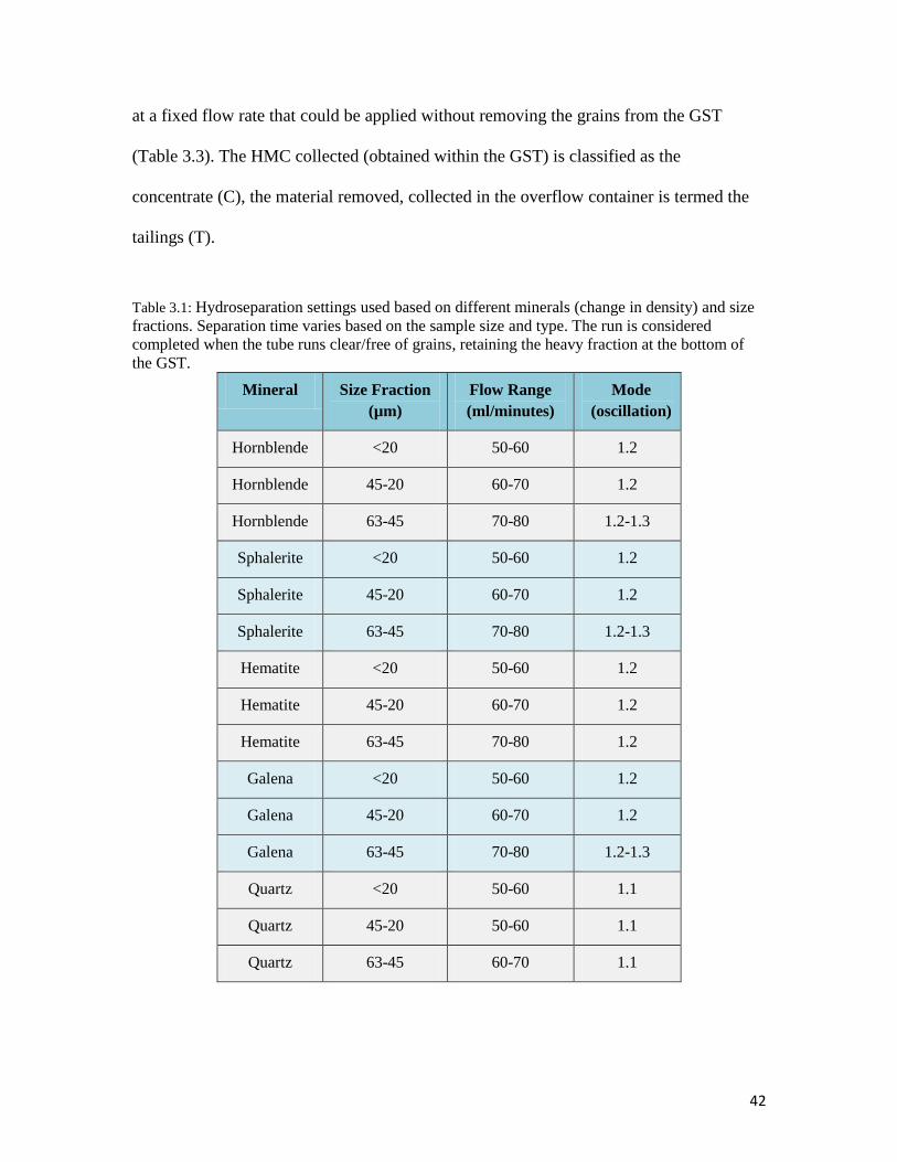
42
at a fixed flow rate that could be applied without removing the grains from the GST
(Table 3.3). The HMC collected (obtained within the GST) is classified as the
concentrate (C), the material removed, collected in the overflow container is termed the
tailings (T).
Table 3.1: Hydroseparation settings used based on different minerals (change in density) and size
fractions. Separation time varies based on the sample size and type. The run is considered
completed when the tube runs clear/free of grains, retaining the heavy fraction at the bottom of
the GST.
Mineral Size Fraction
(µm)
Flow Range
(ml/minutes)
Mode
(oscillation)
Hornblende <20 50-60 1.2
Hornblende 45-20 60-70 1.2
Hornblende 63-45 70-80 1.2-1.3
Sphalerite <20 50-60 1.2
Sphalerite 45-20 60-70 1.2
Sphalerite 63-45 70-80 1.2-1.3
Hematite <20 50-60 1.2
Hematite 45-20 60-70 1.2
Hematite 63-45 70-80 1.2
Galena <20 50-60 1.2
Galena 45-20 60-70 1.2
Galena 63-45 70-80 1.2-1.3
Quartz <20 50-60 1.1
Quartz 45-20 50-60 1.1
Quartz 63-45 60-70 1.1

43
3.2.4 Spike Methods
After each mineral was sieved into three size fractions, the size fractions were
used in a series of experiments as a spike in a simulated ‘till’ consisting of crushed pure
quartz. These quartz samples were used to simulate till to assess the HS in the recovery of
the <63 µm heavy minerals. The quartz plus heavy mineral spike was a constant weight
for all experiments: quartz weight was 0.5 grams and spike grain weight 0.1 grams. There
were a total of 12 experiments run for the initial phase of research. There was a spike for
each of the four heavy minerals tested, hornblende, sphalerite, hematite and galena for
each of the three size fractions being studied, 63-45 µm, 45-20 µm and <20 µm. Each of
the samples was run through the HS using a long GST followed by the short GST to try
and reduce the sample mass and remove the quartz (Cabri, 2008). Based on the settings
determined from testing each of the four minerals and the visual observations made
during the HS processing, the majority of the quartz was removed leaving a concentrate
rich in the HMC. Table 3.2 displays the settings used for each experimental mineral test.

44
Table 3.2: Hydroseparator settings used for each HMC in quartz spike. These settings were
decided on based on the results of the initial testing (Table 3.1)
Size
Fraction
(µm)
Mineral Mineral
Weight
(grams)
Quartz
Weight
(grams)
Mode
(large/small
GST)
Flow
Rate
Time
(seconds)
63-45 Hornblende 0.1 0.5 1.2/1.3 75 20/25
63-45 Sphalerite 0.1 0.5 1.3/1.4 75 20/30
63-45 Hematite 0.1 0.5 1.3/1.4 75 20/25
63-45 Galena 0.1 0.5 1.3/2.1 75 25/25
45-20 Hornblende 0.1 0.5 1.2/1.3 75 20/30
45-20 Sphalerite 0.1 0.5 1.3/1.4 75 20/20
45-20 Hematite 0.1 0.5 1.3/1.4 75 20/25
45-20 Galena 0.1 0.5 1.3/1.5 75 20/30
<20 Hornblende 0.1 0.5 1.2/1.3 75 15/15
<20 Sphalerite 0.1 0.5 1.3/1.4 75 20/10
<20 Hematite 0.1 0.5 1.3/1.4 75 20/10
<20 Galena 0.1 0.5 1.3/1.5 75 20/15
3.2.5 ESEM-MLA Methods
The heavy mineral separates (hornblende, sphalerite, hematite, galena) created by
crushing and sieving, were mounted to double-side carbon tape and examined using the
ESEM-MLA to determine if the sieving accurately separated the material into the
appropriate size ranges. Energy Dispersive Spectroscopy (EDS) was preformed using
random mineral spot analyses on each mineral and size fraction to confirm the
monomineralic purity of the mineral separates. EDS spectral were collected and
interpreted using Esprit 1.9 imaging software. Grain size measurements were also

45
completed to qualitatively determine the accuracy of the size fractions.
Mineral Liberation Analysis (MLA) was completed for the spiked heavy minerals
+ quartz after hydroseparation. This form of analysis usually requires the grains to be
mounted in epoxy, polished and carbon coated, and analyzed under high vacuum in order
to achieve the most accurate results. This mounting process however, was time
consuming and the polishing procedure risked the loss of too many grains especially in
the <20 µm fraction splits. To minimize the perceived losses, the samples were analyzed
by MLA by mounting the hydroseparated grains (separation of quartz from HMC spike)
to double-sided carbon tape disks and analyzed in low vacuum-mode on the ESEM (FEI-
MLA Quanta 650 FEG-ESEM). A single circular disk of doubled sided carbon tape was
placed on a glass slide (27 x 46 mm) for sample mounting (Figure 3.5). The sample (i.e.
63-45 µm hornblende spike sample) was carefully sprinkled on the disk to avoid
clumping of grains. Measurements of the mass of each empty glass/carbon-tape were
made to determine the amount of material being added to the mount.
Different approaches for applying the grains were attempted (i.e., smearing,
dump-and-tap, mesh application), however the “sprinkling” method worked the best with
practice. Each glass slide was labeled with the correct sample name/number. One mount
for each experiment of Phase 1 was produced (12 mounts of the concentrate material; 12
mounts of the tailings material). Mounting on carbon tape also allowed for a more
accurate measurement of sample weights, which was later applied to mineral weights. A

46
mineral library was created for each project with minerals specific to the area of research.
This library is applied to the grain mount, classifying each individual grain as a specific
mineral. The data were organized based on weight percent, area percent, mineral type,
pixels and number of grains. For the purpose of this research, the area percent value was
used as the representative number for each mineral type; this value gives the total area
that a specific mineral covers on the mount as a percent of all mineral grains analyzed.
By using carbon tape mounts, the ability to re-capture and re-analyze or concentrate the
grains after ESEM examination was possible.
ESEM-MLA analyses were completed on the FEI Quanta 650 FEG ESEM at
QFIR, Queen’s University, Kingston, Ontario. Quantitative analyses were done on low
vacuum using MLA Software Suite 3.1, using a beam current of 10 nA, an accelerating
potential of 25 KV and a chamber pressure of 0.45 Torr. The instrument was calibrated to
in–house MLA standards before and after ESEM-MLA runs to achieve a backscatter
electron (BSE) greyscale image equating to ~10 (near black) for the carbon tape disk and
255 (near white) for a Au standard. An in-house quartz standard was calibrated to achieve
BSE detector count rate of 12-20 ms to achieve sufficient counts needed for our ESEM-
MLA runs. Two EDS Bruker XFlash 200 detectors were used in tandem with the Esprit
1.9 software to reduce analytical time. Magnification was set to 150x for XBSE imaging
to produce a constant resolution for each sample mosaic.

47
Figure 3.2: Double sided carbon tape fixed to a glass slide (27 x 46 mm). The sample is mounted
to the tape, applied by sprinkling the material over the disk surface.
3.3 Results
The data collected from the MLA were analyzed to obtain the modal mineralogy
area percent and weight percent recovery of HMC after HS processing (Table 3.6). The
weight percent recovery represents the total percent that the specified mineral (i.e.
hornblende) covers on the mounted carbon tape disk, determined based on the minerals’
chemical formula and the area that the grains cover on the mount. The MLA software
generates the area percent values based on the individual grain sizes perimeter after the
data has been processed with the specified mineral library database. The software
determines the area of all the grains mounted and calculates the percent of each mineral

48
based on the abundance of grains (the carbon tape disk is not included in the calculation).
Then using the area determined and the chemical formula of the associated mineral, the
weight percent of each mineral on the mount is calculated.
Table 3.3: Weight percent recovery of the different HMC obtained from the spiked quartz
mixture. The table is organized based on increasing density, hornblende (2.9-3.4 S.G.), sphalerite
(3.9-4.1 S.G.), hematite (5.0-5.3 S.G.), galena (7.4-7.6 S.G.). The letter “C” represents the
concentrate data; the letter “T” represents the tailings data.
Mineral 63-45
µm
weight%
recovery
Mass on
Mount (63-
45 µm) (mg)
45-20 µm
weight%
recovery
Mass on
Mount (45-
20 µm)
(mg)
<20 µm
weight%
recovery
Mass on
Mount (<20
µm) (mg)
Hornblende C 64.95 18.58 32.33 6.68 17.73 2.27
Sphalerite C 35.08 5.23 25.62 5.93 8.55 3.33
Hematite C 23.18 9.80 35.11 7.52 14.88 4.18
Galena C 63.05 6.24 64.50 8.24 16.59 1.58
Hornblende T 9.35 3.82 27.95 2.39 32.81 1.39
Sphalerite T 6.95 10.99 11.62 3.07 26.58 1.12
Hematite T 5.54 10.19 13.48 6.15 21.49 2.64
Galena T 7.66 2.65 4.74 2.14 50.92 1.56

49
Table 3.4: Total weight of grains determined to be on the grain mount. Weight was determined
from the mass of sample mounted and the weight % recovery of the HMC on each mount.
Mineral 63-45 µm total
weight recovery (mg)
45-20 µm total
weight recovery (mg)
<20 µm total weight
recovery (mg)
Hornblende C 12.07 2.16 0.40
Sphalerite C 1.83 1.52 0.28
Hematite C 2.27 2.64 0.62
Galena C 3.93 5.31 0.26
Hornblende T 0.36 0.67 0.46
Sphalerite T 0.76 0.37 0.30
Hematite T 0.55 0.83 0.58
Galena T 0.20 0.10 0.79
The data reported in Table 3.6-3.7 indicate that the weight percent recovery of the
HMC decreases as the size fraction decreases for all mineral types, with the exception of
hematite and galena, which had the highest recovery in the 45-20 µm size fractions. The
tailings data accurately matches with the concentrate recoveries; the mass of heavy
mineral increases in the tailings as the size fraction decreases which explains the loss of
concentrate in these smaller fractions. The total percent recovery can be determined by
dividing the weight of HMC recovered by the total weight of HMC added (spike size)
however since only one mount was analyzed for each mineral type, the totally recovered
will not be representative of the mineral type in its entirety. Table 3.5 represents the
percent recovery of HMC for the individual mount created based on the weight of
material mounted and analyzed.
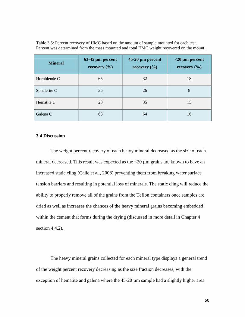
50
Table 3.5: Percent recovery of HMC based on the amount of sample mounted for each test.
Percent was determined from the mass mounted and total HMC weight recovered on the mount.
Mineral 63-45 µm percent
recovery (%)
45-20 µm percent
recovery (%)
<20 µm percent
recovery (%)
Hornblende C 65 32 18
Sphalerite C 35 26 8
Hematite C 23 35 15
Galena C 63 64 16
3.4 Discussion
The weight percent recovery of each heavy mineral decreased as the size of each
mineral decreased. This result was expected as the <20 µm grains are known to have an
increased static cling (Calle et al., 2008) preventing them from breaking water surface
tension barriers and resulting in potential loss of minerals. The static cling will reduce the
ability to properly remove all of the grains from the Teflon containers once samples are
dried as well as increases the chances of the heavy mineral grains becoming embedded
within the cement that forms during the drying (discussed in more detail in Chapter 4
section 4.4.2).
The heavy mineral grains collected for each mineral type displays a general trend
of the weight percent recovery decreasing as the size fraction decreases, with the
exception of hematite and galena where the 45-20 µm sample had a slightly higher area

51
percent recovery than the 63-45 µm fraction. Typically the larger grains had better the
recovery, which is linked to the ability to visually observe individual grains when
transporting from containers as well as during the mounting phase. Area percent
recoveries were generally low for mounts analyzed, however one mount is not a
representative split of the sample as a whole. The material mounted was not a
quantitative representation of the sample as whole. Material was randomly sprinkled on
the mount by hand, trying to fill as much of the carbon tape disk as possible while trying
to avoid clumping the grains.
The tailings data indicated that there were some heavy minerals within the
overflow from HS processing. Table 3.6-3.7 displays the heavy mineral weight percent
recoveries in each of the tailings samples. The tailings data like the concentrate data are
based on one mount of material per mineral type and therefore is a representation of a
fraction of the sample as a whole. Based on the findings here, the weight percent of HMC
increases in the tailings, as the size fraction gets smaller. This result implies that the
settings used for the <20 µm samples was too strong and adjustments needed to be made
in order to try and recover more of the heavy minerals for samples of this size range. All
heavy minerals found within the tailings are less than 25% of the modal mineralogy
based on the mounts analyzed. There was a general trend of a decrease in HMC with an
increase in mineral density. Hornblende, which is the lightest of the four minerals, was
the most abundant heavy mineral in the tailings, while the galena, which is the heaviest
mineral, had the least amount in the tailings (with the exception of the <20 µm samples).

52
Based on the low weight percent recovery found from the tailings data, the
evidence for an overall successful recovery rate for the heavy minerals is indicated. Using
the mass of the material originally mounted and the remaining material (not mounted),
the required number of additional mounts needed to analyze the entire sample can be
calculated. Depending on the sample it takes ~10-12 mounts to analyze the sample
entirely. Extrapolating the data already collected from the 1 mount studied to the
additional mounts required (for full sample analysis), the overall area percent recovery of
each heavy mineral is indicated to have been successful.
3.5 Conclusions
Data collected for phase 1 indicate that the HS is capable of separating the HMC
from the sample. This process is more successful on the larger size fractions with the 63-
45 µm and 45-20 µm fractions producing the best outcome. From this phase 1 test, more
testing of the finer fraction is required. The most successful recoveries came from the
hornblende and galena samples. The settings used for the hornblende processing (Table
3.4) had a smaller mode applied than to that of the sphalerite and hematite which could
have resulted in the increased recovery. The galena also produced high recovery results
(~60% per mount) likely due to the increased density of the grains. Comparing the
hornblende results to that of the sphalerite and hematite implies that a more accurate
recovery rate could be obtained by reducing the mode of flow applied to the sample. The
results from the galena indicate that with high-density minerals, a higher recovery can be
more easily achieved. With the majority of indicator minerals (specifically in this study)

53
having a high density, the use of the HS could be applied effectively to the samples being
processed.

54
Chapter 4: Phase 2, Recovery of Sperrylite from Almonte Till
Experimentation
4.1 Objectives
This chapter is subdivided into 5 different sections; 1) objectives for phase 2
research; 2) methods used in phase 2; 3) results from phase 2; 4) discussion of results
from phase 2; and 5) conclusions gathered from phase 2, experimentation. Figure 4.1a-c
depicts the order in which the initial phase of experimentation was carried out and the
methods used. These procedures were later adapted for application on the case study
samples. Phase 2 conducted the development of methods for the representative sampling
(split) of the <63 µm HMC of till that had been spiked with sperrylite.

55
Figure 4.1a: Procedure used for phase 2, Almonte till preparation for spike. Geological Survey of
Canada (GSC). MI = methylene iodide
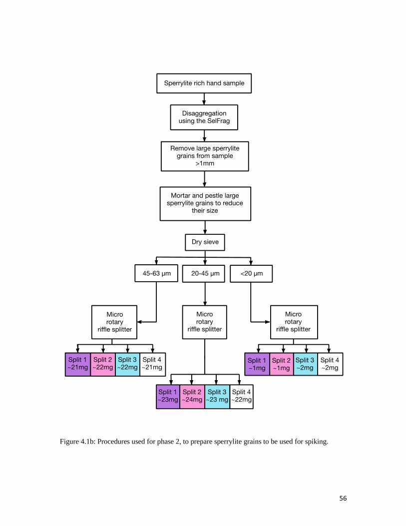
56
Figure 4.1b: Procedures used for phase 2, to prepare sperrylite grains to be used for spiking.

57
Figure 4.1c: Procedures followed for phase 2, testing of the recovery of sperrylite grains that has
been added to the Almonte till standard. Samples were labelled JP with the number referring to
the experiment. JP1-JP5, 45-63 µm grains shown above in flow sheet.

58
Figure 4.1d: Procedures followed for phase 2, testing of the recovery of sperrylite grains that has
been added to the Almonte till standard. Samples were labelled JP with the number referring to
the experiment. JP6-JP10, 20-45 µm grains shown above in flow sheet.

59
Figure 4.1e: Procedures followed for phase 2, testing of the recovery of sperrylite grains that has
been added to the Almonte till standard. Samples were labelled JP with the number referring to
the experiment. JP11-JP15, <20 µm grains shown above in flow sheet.
4.2 Methods
The methods section of this research is a combination of commonly used
procedures (sieving, micro riffling, etc.) as well as project specific novel procedures
designed for these samples (hydroseparation, mounting, etc.). The parameters used for
each procedure are described based on the phase of the project being studied. This phase
of research applied the hydroseparation conclusions drawn from the phase 1 to
experimentation using real till as a base for spiking and further testing of HS methods.

60
4.2.1 Initial Mineral Preparation
A total of ~50 grains of sperrylite (PtAs2) was recovered from the Broken
Hammer regolith samples provided by Beth McClenaghan (GSC) and Jacob Hanley
(SMU). Additional sperrylite was acquired from Alpine Gems, Kingston, in order to have
sufficient sperrylite to complete all experimental testing. The sperrylite-rich hand sample
obtained from Alpine Gems required disaggregation using the selFrag pulse
disaggregator in QFIR, in order to isolate pure sperrylite grains. The settings used for the
SelFrag’s sperrylite disaggregation are listed in Table 4.1. Individual sperrylite grains
were then handpicked from the disaggregated material under a binocular microscope and
further crushed by hand using an agate mortar and pestle. This crushed material was
sieved to >63 µm, 63-45 µm, 45-20 µm and <20 µm and used in a series of experiments
to assess the minimum mass of HMC that would be a representative split of an entire till
HMC when mounted and examined using microanalytical methods. Procedures used to
isolate the sperrylite grains are outlined in Figure 4.1b.
Table 4.1: SelFrag settings used for the disaggregation of the sperrylite rich rock samples in
preparation for Almonte till spiking.
SelFrag Parameter Setting Actual
Voltage (kV) 140 176.4/187.6
Pulse Frequency (Hz) 5 6.2/5.8
Pulses (pulses) 30 60
Electrode Gap (mm) 10 11
61
4.2.2 Micro Rotary Riffler Methods
A series of samples using measured masses of sperrylite and blank processed
Almonte till were created for testing. Processed ‘blank’ till, referred to as the Almonte
till, was provided by the GSC for HMC spiking and testing. The Almonte till had been
previously processed, by the commercial lab ODM because the GSC used this material as
part of their monitoring of heavy mineral processing quality of commercial labs (Plouffe
et al., 2013).
Five ~500 gram Almonte till packets of <3.2 SG material were received from the
GSC for testing. Three of the five Almonte till packets were combined into one and then
split into 15 separates of approximately 75g each using a rotary micro riffler
(Quantachrome) as outlined in Figure 4.1a. The remaining two Almonte till packets were
kept separate for future use in replicate studies. The method used for each of the till splits
is summarized in Figure 4.2c.
The rotary mirco riffler splits a sample equally into eight 25 ml test tubes. The
sperrylite grains for one of the three size fractions were added to the rotary micro riffler
and split into eight even splits. The settings used were a fixed low collector rate at a
medium feed rate, to ensure that the grains did not bounce up and away from the sample
collectors. These eight sample splits were then combined to make four splits for one of
the three size fractions (~20 mg for the 63-45 µm and 45-20 µm fractions, and ~2 mg for
the <20 µm fraction) (Figure 4.1 b). These four splits were used as indicated in flow sheet
4.2b.

62
The rotary micro riffler was then used to ensure the sperrylite grains that were
added to the Almonte till splits were evenly distributed throughout the till. Each sperrylite
+ Almonte till mixture was put into the hopper and split to ensure the sperrylite was
evenly mixed within the till. The 8 vials were then recombined to one vial and this one
vial was then sieved to the required size fraction.
4.2.3 Sieving Methods
Nine of the 75 g Almonte till splits (non-spiked blank, spiked, and control test)
were dry sieved. Each of the sieve sizes, 250 µm, 125 µm, 63 µm, 45 µm and 20 µm
were cleaned (using an ultrasonic bath) and dried before and after use. Sieve gaskets were
placed around the base of each of the sieves and then stacked in increasing size order.
The dry till 75 g split was then added to the top sieve and placed on the shaker (Retsch,
AS-200) for 3 minutes with the amplitude set at an average of 7.5 mm/g. Once the dry
sieve shaking was completed, the material was removed and ready for further analysis.
The sieves require an extensive cleaning process following each of the sample
trials. The sieves are first rinsed with water from the underside. Soap is applied to the
sieve and gently brushed using a toothbrush to remove any grains that may be stuck
within the mesh. The sieves are rinsed again. They were then placed in an ultrasonic bath
for ~10 minutes. Once removed from the bath, the sieves were rinsed a final time with tap
water. They were placed in a dedicated convection oven for heated drying. Once dry, the

63
sieves were examined under binocular microscope to determine if there were any grains
remaining in the mesh. If grain contamination was observed a dry toothbrush was used to
push out these embedded grains through the top of sieve. The sieves were then ready for
sieving the next Almonte till 75 g split. This process ensured that there was no cross-
contamination from previous sieving. Blank runs were preformed in order to view and
monitor this issue. The non-spiked Almonte till was used to carry out the blank run
procedures because it was known to not contain any PGM (i.e. sperrylite). A blank test
was performed in between runs to determine if any HMC was carrying over from test to
test throughout the sieving procedure. The blank runs were analyzed using ESEM-MLA.
4.2.4 Spike Methods
Table 4.2 displays the mass of sperrylite added to each Almonte till split. The <20
µm sample contained the least amount of sperrylite due to the difficulties in obtaining
sufficient material of this size.
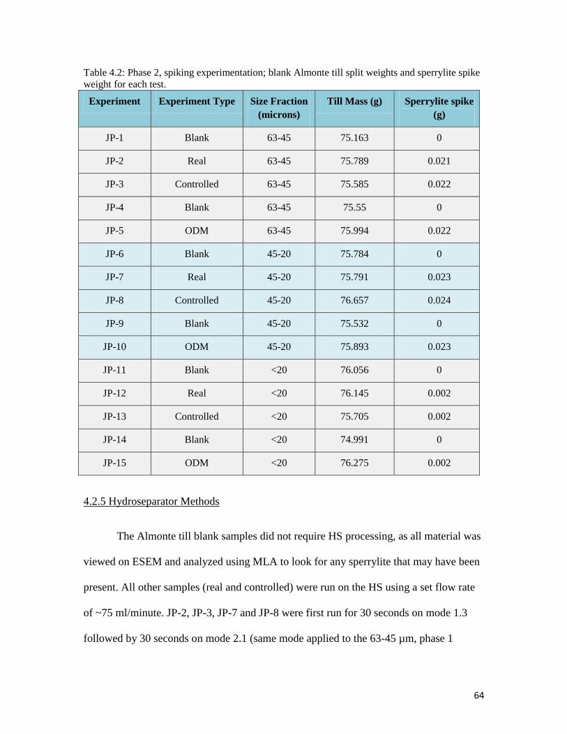
64
Table 4.2: Phase 2, spiking experimentation; blank Almonte till split weights and sperrylite spike
weight for each test.
Experiment Experiment Type Size Fraction
(microns)
Till Mass (g) Sperrylite spike
(g)
JP-1 Blank 63-45 75.163 0
JP-2 Real 63-45 75.789 0.021
JP-3 Controlled 63-45 75.585 0.022
JP-4 Blank 63-45 75.55 0
JP-5 ODM 63-45 75.994 0.022
JP-6 Blank 45-20 75.784 0
JP-7 Real 45-20 75.791 0.023
JP-8 Controlled 45-20 76.657 0.024
JP-9 Blank 45-20 75.532 0
JP-10 ODM 45-20 75.893 0.023
JP-11 Blank <20 76.056 0
JP-12 Real <20 76.145 0.002
JP-13 Controlled <20 75.705 0.002
JP-14 Blank <20 74.991 0
JP-15 ODM <20 76.275 0.002
4.2.5 Hydroseparator Methods
The Almonte till blank samples did not require HS processing, as all material was
viewed on ESEM and analyzed using MLA to look for any sperrylite that may have been
present. All other samples (real and controlled) were run on the HS using a set flow rate
of ~75 ml/minute. JP-2, JP-3, JP-7 and JP-8 were first run for 30 seconds on mode 1.3
followed by 30 seconds on mode 2.1 (same mode applied to the 63-45 µm, phase 1

65
galena sample) on the long GST with visual observation using illuminated magnification
(see figure 4.2) being made for when processing was complete. JP-12 and JP-13 were run
using slightly different settings to try and retain as much of the sperrylite fraction as
possible. JP-12 was run using a flow rate of 50 ml/minute, on mode 0 for 30 seconds
followed by a flow rate of 75 ml/minute, on mode 0 for 20 seconds. The flow rate was
increased to try and isolate as much of the sperrylite as possible. JP-13 was run with a
flow rate of 50 ml/minute, on mode 0 for 30 seconds. Even the 1.1 mode (lowest
oscillating mode) setting was too powerful for this sample processing and the water flow
rate alone provided enough energy to move the Almonte till. The majority of the till was
separated and removed from the HS long GST therefore the short GST did not appear
necessary. All concentrates and tailings were placed in separate Teflon containers and put
on the hot plate until fully dried and ready for mounting for ESEM-MLA.

66
Figure 4.2: Hydroseparator system as set up in Queen’s University Miller Hall, geology
department. The main features are highlighted in red.
4.2.6 ESEM-MLA Methods
Mineral Liberation Analysis (MLA) was completed on the sperrylite + Almonte
till samples. Similarly to the phase 1 testing, samples were mounted on double-sided
carbon tape disks and analyzed in low vacuum-mode on the ESEM (FEI-MLA Quanta
650 FEG-ESEM). The sample grains were loaded onto the mounts using the sprinkling
method described in Chapter 3, Section 3.2.5. Measurements of the weight of each empty
glass/carbon-tape were taken to determine the amount of material being added to the
mount. Each glass slide was labeled with the correct sample name/number. All of the
concentrate material from phase 2 was mounted over several mounts (16 mounts in total).

67
Mounting on carbon tape also allowed for a more accurate measurement of sample
weights, which was later applied to the mineral weight recovered. The mineral library
created for phase 1 was expanded on and used for phase 2, to include mineral spectrums
for the sperrylite mineralogy.
ESEM-MLA analyses were completed on the FEI Quanta 650 FEG ESEM at
QFIR, Queen’s University, Kingston, Ontario. Quantitative analyses were done on low
vacuum using MLA Software Suite 3.1, using a beam current of 10 nA, an accelerating
potential of 25 KV and a chamber pressure of 0.45 Torr. The instrument was calibrated to
in –house MLA standards before and after ESEM-MLA runs to achieve a backscatter
electron (BSE) greyscale image equating to ~10 (near black) for the carbon tape disk and
255 (near white) for a Au standard. An in-house quartz standard was calibrated to achieve
BSE detector count rate of 12-20 ms to achieve sufficient counts needed for our ESEM-
MLA runs. Two EDS Bruker XFlash 200 detectors were used in tandem with the Esprit
1.9 software to reduce analytical time. Magnification was set to 150x for XBSE imaging
to produce a constant resolution for each sample mosaic.
4.2.7 Overburden Drilling Management (ODM) Methods
Prior to this study, the Almonte till sample material was initially processed at
ODM using different separation techniques to obtain the light and heavy mineral
fractions of the <2 mm material. Samples were first processed using the Wilfley Table to
produce a preconcentrate. Following this step, the Almonte till samples were then further

68
refined using heavy liquid separation at a SG 3.2 and then ferromagnetically separated to
obtain a non-ferromagnetic HMC. The Almonte till material provided to QFIR at
Queen’s University was <3.2 SG fraction produced from these procedures.
After the sperrylite grains were added to the Almonte till light mineral fractions,
the samples were processed through rotary micro riffler to produce samples, JP5 (63-45
µm), JP10 (45-20 µm) and JP15 (<20 µm). These spiked samples were then sent to ODM
for sperrylite recovery. ODM panned each sample to recover sperrylite, no heavy liquid
separation was used. The samples being <63 µm in size prevented the use of heavy liquid
separation (McClenaghan, 2011) due to the small grain size eliminating the float sink
efficiency. The results from these three samples were compared to the recovery of the
samples run through the HS, the real and controlled tests. ODM was provided with the
spike weights for each sample and therefore continued processing the samples (i.e. re-
panning) until a representative recovery was achieved. In contrast, the hydroseparated
samples not processed by ODM, were only run once and then analyzed. The comparison
between ODM and the HS methods data are therefore not completely relatable.

69
4.3 Results
4.3.1 Sperrylite in Till Experimentation Results
The sperrylite-spiked Almonte till samples were analyzed using ESEM-MLA
similar to the phase 1 testing. However in phase 2, all of the concentrate for each sample
was mounted over several mounts and analyzed. The area percent provided a modal
mineralogy for the concentrate and tailings data, specifically focusing on the sperrylite
content in each (Table 4.3-4.4).
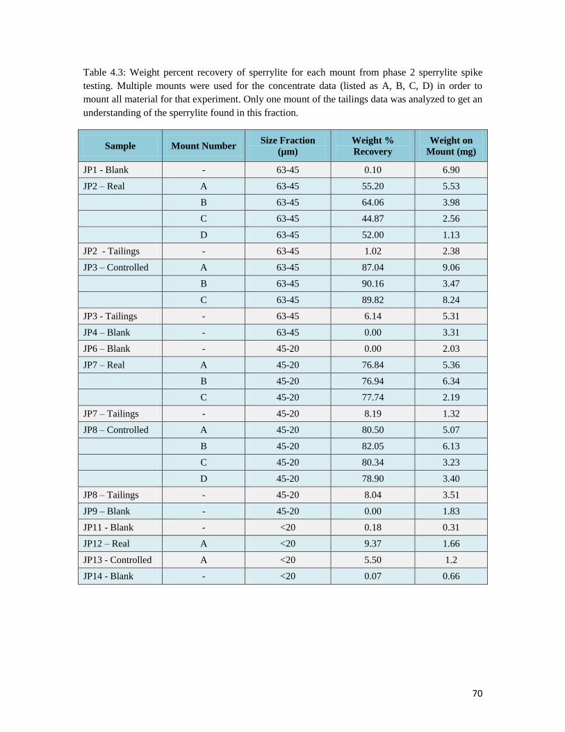
70
Table 4.3: Weight percent recovery of sperrylite for each mount from phase 2 sperrylite spike
testing. Multiple mounts were used for the concentrate data (listed as A, B, C, D) in order to
mount all material for that experiment. Only one mount of the tailings data was analyzed to get an
understanding of the sperrylite found in this fraction.
Sample Mount Number Size Fraction
(µm)
Weight %
Recovery
Weight on
Mount (mg)
JP1 - Blank - 63-45 0.10 6.90
JP2 – Real A 63-45 55.20 5.53
B 63-45 64.06 3.98
C 63-45 44.87 2.56
D 63-45 52.00 1.13
JP2 - Tailings - 63-45 1.02 2.38
JP3 – Controlled A 63-45 87.04 9.06
B 63-45 90.16 3.47
C 63-45 89.82 8.24
JP3 - Tailings - 63-45 6.14 5.31
JP4 – Blank - 63-45 0.00 3.31
JP6 – Blank - 45-20 0.00 2.03
JP7 – Real A 45-20 76.84 5.36
B 45-20 76.94 6.34
C 45-20 77.74 2.19
JP7 – Tailings - 45-20 8.19 1.32
JP8 – Controlled A 45-20 80.50 5.07
B 45-20 82.05 6.13
C 45-20 80.34 3.23
D 45-20 78.90 3.40
JP8 – Tailings - 45-20 8.04 3.51
JP9 – Blank - 45-20 0.00 1.83
JP11 - Blank - <20 0.18 0.31
JP12 – Real A <20 9.37 1.66
JP13 - Controlled A <20 5.50 1.2
JP14 - Blank - <20 0.07 0.66

71
Table 4.4: Total sperrylite weight recovered from the grain mount. Weight was determined from
the mass of sample mounted and the weight % recovery of the sperrylite on each mount.
Sample Mount Number Size Fraction (µm) Total weight
recovery (mg)
JP1 - Blank - 63-45 0.0069
JP2 – Real A 63-45 3.05
B 63-45 2.55
C 63-45 1.15
D 63-45 0.59
- - 7.34
JP2 - Tailings - 63-45 0.02
JP3 – Controlled A 63-45 7.89
B 63-45 3.13
C 63-45 7.40
- - 18.42
JP3- Tailings - 63-45 0.33
JP4 – Blank - 63-45 0.00
JP6 – Blank - 45-20 0.00
JP7 – Real A 45-20 4.12
B 45-20 4.88
C 45-20 1.70
- - 10.70
JP7 – Tailings - 45-20 0.11
JP8 – Controlled A 45-20 4.08
B 45-20 5.03
C 45-20 2.59
D 45-20 2.68
- - 14.38
JP8 – Tailings - 45-20 0.28
JP9 - Blank - 45-20 0.00
JP11 - Blank - <20 0.0006
JP12 - Real A <20 0.16
JP13 - Controlled A <20 0.07
JP14 - Blank - <20 0.0005

72
By using the sperrylite weight percent on each mount with the original mass of
the sample mounted, the total weight recovery of the sperrylite, was determined. The
sperrylite weight percent recovery indicates that each mount differs and is not identical to
the original, as the sample was not representatively split for the mounts but randomly
sprinkled. Therefore, only producing a single mount (i.e. Phase 1) will create some
discrepancy in the findings that could differ from mount to mount. Based on the data in
Table 3.9-3.10, the controlled tests (biased test – sperrylite added after till was sieved)
indicate the highest recovery of sperrylite over the real tests (sperrylite added before the
till was sieved). The total percent recovery was determined from the mass of sperrylite
recovered divided by the original mass of sperrylite added (spike) to each sample. The
results for the sperrylite total percent recovery, is listed in Table 4.5.
Table 4.5: Total percent recovery of sperrylite collected from the hydroseparation processing and
the ODM processing.
Sample Number Size Fraction (µm) Total Percent Recovery (%)
JP2 (Real) 63-45 35
JP3 (Controlled) 63-45 84
JP5 (ODM) 63-45 80
JP7 (Real) 45-20 47
JP8 (Controlled) 45-20 60
JP10 (ODM) 45-20 95
JP12 (Real) <20 8
JP13 (Controlled) <20 4
JP15 (ODM) <20 50
73
4.3.2 Overburden Drilling Management (ODM) Results
After ODM processed the sperrylite spiked samples sent from QFIR at Queen’s
University, they completed a recovery count (Figure 4.6).
1) Sample JP-5 (63-45 µm) contained some smaller grains, <45 µm, which did not
allow for the use of heavy liquid separation due to the elimination of the float sink
efficiency. The smaller grains lead to the use of panning for separation. The initial
mass of sperrylite added to the sample was 20 mg, and 16 mg were recovered for
a recovery rate of 80%.
2) 2) JP-10 (45-20 µm) was panned. Some <20 µm sized grains were observed in
this sample. ODM was aware of the mass of the spike added and therefore the
panning took several attempts to ensure all sperrylite was captured in the
concentrate. There was an initial spike of 20 mg with 19 mg recovered, a 95%
recovery.
3) JP-15 (<20 µm) was panned. The size of the grains observed included grains that
were <10 µm in size. Due to the small size of the grains, panning was repeated
several times as sperrylite was ending up in the panning rejects (tailings). This
was likely due to the small grains being unable to break the water surface tension.
Calgon was added to the panning water to help increase the wetness of the sample
and allow for these grains to break contact with the water surface. This did
increase the recovery rate however it did not fully eliminate the issue. Stokes Law
(Equation 4.1) indicates that for grains of very fine silt to clay sizes, the density of
the grain plays a lesser role in its behavior during gravity separation. The total

74
mass of sperrylite initially added was 2 mg with a recovery of 1 mg, a 50%
recovery rate.
Equation 4.1: Stokes Law; applied through the use of the hydroseparator on the heavy mineral
spiked samples separation processing
(F) = 6
F = frictional force (viscous drag)
η = viscosity of the fluid
r = radius of the grain
v = velocity of the fluid
The data collected from the experimental runs at ODM were biased. Prior to the
separation, ODM was informed of the amount of sperrylite spiked in each sample and as
a result panning was repeated to increase the recovery. The samples that were
hydroseparated however, were only run once, blind and the analysis was based on this
one run. Based on this, the ODM processed sample were expected to have a better
recovery per sample than the hydroseparated samples as multiple procedures were
emplaced to get the best recovery after intermittent recovery checks.
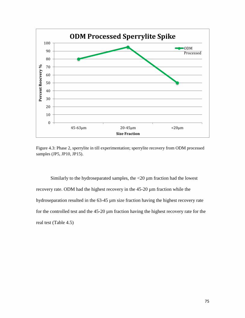
75
Figure 4.3: Phase 2, sperrylite in till experimentation; sperrylite recovery from ODM processed
samples (JP5, JP10, JP15).
Similarly to the hydroseparated samples, the <20 µm fraction had the lowest
recovery rate. ODM had the highest recovery in the 45-20 µm fraction while the
hydroseparation resulted in the 63-45 µm size fraction having the highest recovery rate
for the controlled test and the 45-20 µm fraction having the highest recovery rate for the
real test (Table 4.5)
0
10
20
30
40
50
60
70
80
90
100
45-63µm 20-45µm <20µm
Pe
rce
nt
Re
ocv
ery
%
Size Fraction
ODM Processed Sperrylite Spike
ODM Processed

76
4.4 Discussion
4.4.1 Overview
4.4.1a Blank Data:
The blank samples were analyzed using ESEM-MLA to determine the reliability
of the cleaning methods of the sieves (all sieves were previously used with the sperrylite
spike material to collect the correct size fractions for these tests). Blanks JP-1 (63-45
µm), JP-11 (<20 µm) and JP-14 (<20 µm) did contain sperrylite grains, however, these
grains accounted for only up to <0.10% area recovery in total (Table 4.6). JP-1 was the
first blank produced and analyzed, however 9 sperrylite grains were recovered from the
sample (Figure 4.4). It should have contained no sperrylite, thus the sieve cleaning
procedures following this test became more rigorous in order to fully remove all
embedded grains from the sieves mesh. An examination of each sieve using a binocular
microscope after ultrasonic cleansing was added to the cleaning procedures to try and
reduce contamination. Aside from sample JP-1, the other blank sample for the 63-45 µm
(JP-4) and 45-20 µm (JP-6, JP-9) fractions contained no sperrylite grains. It was the <20
µm fraction that proved to be more difficult, with the <20 µm sieve mesh holes being so
small, the ability to properly ensure all grains were removed became more difficult
resulting in the increased presence of sperrylite within the blanks. Blank test JP-11
contained 12 sperrylite grains, and JP-14 contained 8 grains. Due to the small sieve size,
cleaning becomes harder with less visualization of grain embedment in the sieve mesh.

77
Table 4.6: Number of sperrylite grains (contamination) found in the Phase 2 blank samples after
MLA.
Sample Number of sperrylite grains found
JP1 Blank (63-45 µm) 9
JP11 Blank (<20 µm) 12
JP14 Blank (<20 µm) 8

78
Figure 4.4: ESEM backscatter image (BSE) of sample JP1-Blank (63-45 µm), displaying the 9
sperrylite grains found, highlighted in red.
4.4.1b Sperrylite Spiked Hydroseparations:
There were two different types of spiked experiments completed for this phase of
research. The “real” test samples in which the sperrylite was added to the samples prior to
sieving to the specific size fractions resulted in a lower recovery than that of the
3,175 um
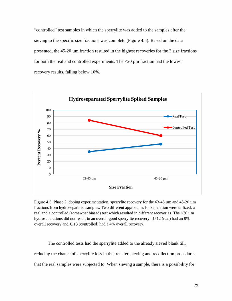
79
“controlled” test samples in which the sperrylite was added to the samples after the
sieving to the specific size fractions was complete (Figure 4.5). Based on the data
presented, the 45-20 µm fraction resulted in the highest recoveries for the 3 size fractions
for both the real and controlled experiments. The <20 µm fraction had the lowest
recovery results, falling below 10%.
Figure 4.5: Phase 2, doping experimentation, sperrylite recovery for the 63-45 µm and 45-20 µm
fractions from hydroseparated samples. Two different approaches for separation were utilized, a
real and a controlled (somewhat biased) test which resulted in different recoveries. The <20 µm
hydroseparations did not result in an overall good sperrylite recovery. JP12 (real) had an 8%
overall recovery and JP13 (controlled) had a 4% overall recovery.
The controlled tests had the sperrylite added to the already sieved blank till,
reducing the chance of sperrylite loss in the transfer, sieving and recollection procedures
that the real samples were subjected to. When sieving a sample, there is a possibility for
0
10
20
30
40
50
60
70
80
90
100
63-45 µm 45-20 µm
Hydroseparated Sperrylite Spiked Samples
Real Test
Controlled Test
Size Fraction
Per
cen
t R
ecover
y %
80
grains to get stuck in the sieve mesh or stuck to larger grains not passing through the
sieve. Due to the small size of the grains being tested (<63 µm), the ability to lose
material is enhanced in all processing phases of testing. Figure 4.5 indicates that the real
and controlled tests mirror one another in terms of the size fraction and HMC collection,
however the real test results in slightly less HMC overall collection. This displays the
probable loss of heavy minerals from the sample collection to final findings.
4.4.1c Hydroseparation Tailing Data
The tailings data displayed a very low percentage of sperrylite recovery (1-8
weight % recovery – Table 4.9-4.10). Similar to the phase 1 testing, the amount of
sperrylite recovered from the tailings increased as the size fraction decreased. The <20
µm fraction tailings data was not analyzed, however, based on the total sperrylite
recovery being so low (JP12, JP13) the tailings are expected to contain the majority of the
HMC. The reduced concentration of sperrylite within the 63-45 µm and 45-20 µm
fractions tailings recovery indicates that the settings applied were successful. This
success in hydroseparation settings can be related to the density of the sperrylite (10.58
SG) being much higher as compared to the minerals used in the phase 1 testing. These
results indicate that the HS settings applied to these test samples were accurately set and
the recovery percent of HMC accurately displays the samples spike amount.

81
4.4.2 Problems
White crystallized cement formed on some samples that were run in the HS and
then dried (Figure 4.6). When the processed sample weight was small, the cement altered
the modal area percent recovery level of heavy mineral found in the concentrate by
coating viable heavy mineral grains. This white cement could be a precipitate from the
tap water using during the HS processing or a chemical reaction between the sample and
the tap water as the main composition was calcium and magnesium rich (ESEM-MLA).
The quartz content could have been the source, creating a reaction with the tap
water to produce orthosilicic acid. Orthosilicic acid has a density between 2-6 SG, falling
in the same range as some of the heavy minerals used. This would alter the ability to
completely remove the quartz and recover true heavy minerals. This reaction will leave a
residue when dried, similar to what was found in a previous study after hydroseparation
of quartz rich samples (Iler, 1979). Tap water in Kingston, Ontario can have high calcium
and magnesium concentration depending on the water’s hardness, and this can cause
calcium carbonate crystallization during the drying phase, producing a white crystalized
material (Utility Kingston, 2015). When samples were analyzed using ESEM-MLA, the
cement was commonly assigned the classification of dolomite, CaMg(CO3)2. The density
of this substance is only 2.8-3 SG, however the formation occurs during the drying phase.
The residue produced acts like a cement, attaching to other grains within with the sample
while drying to form clusters. The cement produced creates undefined grain boundaries
preventing the heavy mineral grains within the sample to be properly portrayed and

82
accounted for through MLA. Therefore the tap water composition is likely the source for
the cementation occurring and found within the hydroseparated samples dried product.
The majority of the cement fragments were manually deleted from the processed datasets,
however some of the cemented material remained. These grains were classified as
“unknowns” and would have been included in the area percent recovery calculations.

83
Figure 4.6: ESEM backscatter image displaying the cementation caused from tap water use
during hydroseparation. The individual grain shape and structure is lost when enclosed within the
cement, therefore altering the recovery percentages for the sample.
4.4.3 Hydroseparator versus ODM Processing
The HS has proven to be a useful tool when concentrating heavy minerals. It can
successfully decrease large (10s g) sample sizes by removing lighter fractions while
retaining the heavier fractions (>2.5 SG) for all three of the different size fractions tested.
The spike specific experiments did not yield a positive outcome for all size fractions
Individual mineral grains,
classified as 1 grain (MLA)
Cemented piece,
multiple grains cemented together,
classified as 1 grain (MLA)
Classified as "unknown"

84
tested, specifically the <20 µm fraction. The sperrylite spike testing indicated that the HS
was most efficient for the 20-45 µm fraction and least efficient for the <20 µm fraction.
The controlled test samples processed by ODM resulted in higher sperrylite
recoveries than the real test samples processed using the HS. However, the recovery of
sperrylite from the <20 µm fraction was a challenge for both ODM and hydroseparation
methods. ODM was provided with the weight of sperrylite spike grains added to each
sample and were requested to continue panning until the best possible recovery was
achieved, therefore biasing their results compared to the experiments completed at QFIR,
Queen’s University. The ODM results provide an indication of what can be achieved
using conventional heavy mineral processing methods.
The phase 1 testing involved working with small sample masses, making the
separations more difficult as the abundance of heavy minerals was reduced. The potential
for grain loss increased as the size fraction as well as sample mass being processed
decreased. The advantage of using small spike masses (<1 gram) did provide insight for
real indicator mineral testing (which will be analysed through the case study) as the
abundance of indicator/heavy minerals, will be reduced in real till samples.
Once ODM separated and analyzed the samples JP-5, JP-10 and JP-15, the
recovery data was collected and compared to the HS separation technique and recoveries.
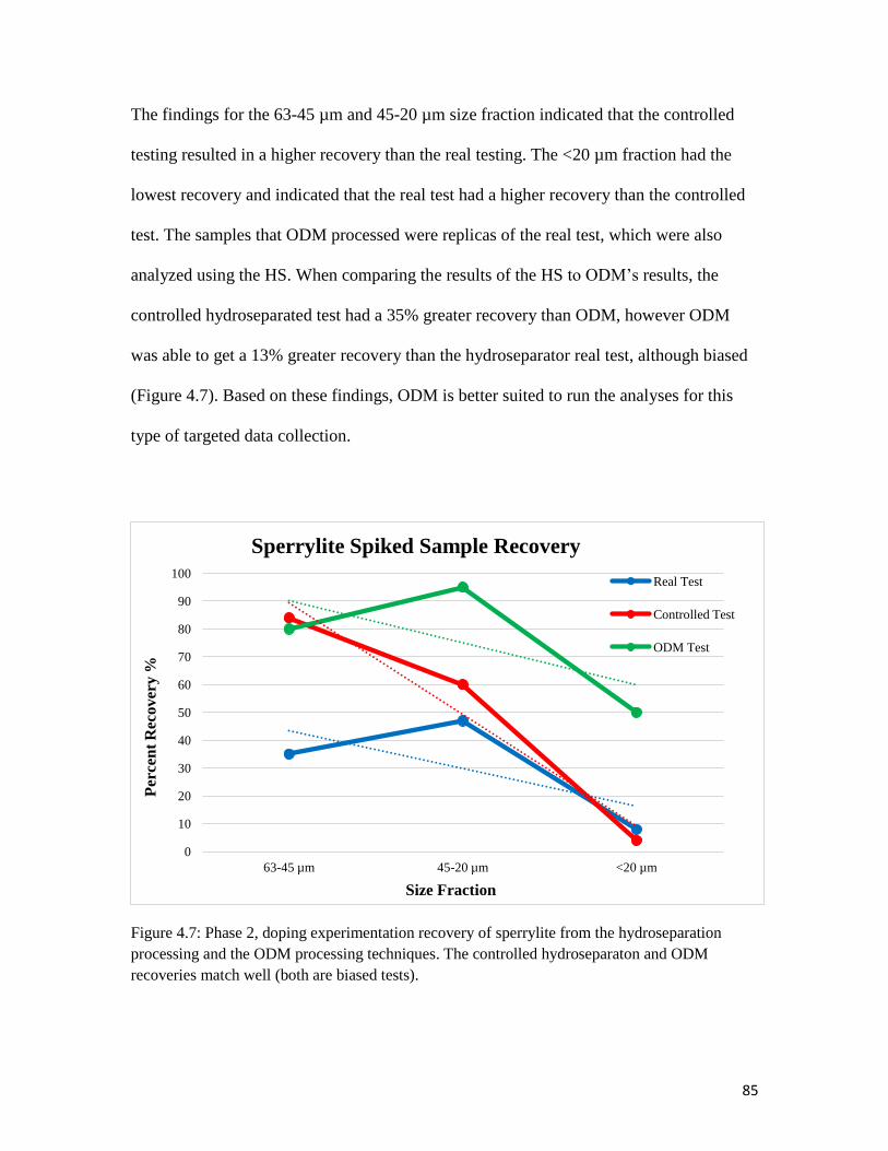
85
The findings for the 63-45 µm and 45-20 µm size fraction indicated that the controlled
testing resulted in a higher recovery than the real testing. The <20 µm fraction had the
lowest recovery and indicated that the real test had a higher recovery than the controlled
test. The samples that ODM processed were replicas of the real test, which were also
analyzed using the HS. When comparing the results of the HS to ODM’s results, the
controlled hydroseparated test had a 35% greater recovery than ODM, however ODM
was able to get a 13% greater recovery than the hydroseparator real test, although biased
(Figure 4.7). Based on these findings, ODM is better suited to run the analyses for this
type of targeted data collection.
Figure 4.7: Phase 2, doping experimentation recovery of sperrylite from the hydroseparation
processing and the ODM processing techniques. The controlled hydroseparaton and ODM
recoveries match well (both are biased tests).
0
10
20
30
40
50
60
70
80
90
100
63-45 µm 45-20 µm <20 µm
Real Test
Controlled Test
ODM Test
Size Fraction
Per
cen
t R
ecover
y %
Sperrylite Spiked Sample Recovery
86
The hydroseparated real test mirrors that of the ODM processed test, however the
recovery values are off by ~35% or more. The controlled test indicates the highest
recovery for the 63-45 µm fraction, however there is a drop in recovery, specifically
associated with the <20 µm fraction. The decrease in HMC recovery made by the HS
could be attributed to the settings applied on the sample, flow-rate and oscillation, being
too high and resulting in a greater loss of HMC. These settings were chosen on the basis
that the increase in specific gravity of the sperrylite would allow for a higher flow-rate
and mode to be applied to increase the loss of the light fraction, therefore producing a
more concentrated HMC recovery. ODM also had an advantage (biased) as they were
aware of the initial spike amount and continued processing until the best possible
recovery was achieved. The loss of HMC could also be related to the preconcentrate
collection. Sieving was used target the size fraction of interest while reducing the sample
size prior to hydroseparation, whereas panning was used to create the preconcentrate
during ODMs testing. The tailings data indicated that the HMC content increased as the
size fraction decreased, which was expected based on the concentrate data decreasing for
those size fractions.
Hydroseparation is relatively quick and easy to use, however it would not be
applicable to use as an in-field tool. Till sampling recovers 10 kg of raw material per
sample site, which would need to be reduced in size before being processed by
hydroseparation. This phase of the study tested material that had already been processed
by ODM; the 10 kg raw sample had been reduced to 500 g. However, small
representative sample sizes could be taken in field and tested by hydroseparation to make

87
visual observations of the material as well as get an idea of the fine fraction heavy
mineralogy. This processing technique cannot be mineral/density specific to target any
one mineral but provides a more bulk heavy concentration. ODM has the ability to use
different processing techniques to look for specific minerals, i.e. heavy liquid separation
based on specific densities or magnetic properties, allowing for the collection of specific
mineral types.
4.4.4 Mounting
Phase 1 and 2 tested the heavy mineral recovery from light mineral material,
however for phase 1 testing only one mount was analyzed using MLA whereas the phase
2 experiment all heavy mineral material in a single sample was mounted on several
mounts (Table 4.10). The mounts created were not riffle split to produce a representative
fraction but were randomly sprinkled on the carbon tape disk. Phase 2 data indicates that
each mount varies in the area percent recovery of the heavy mineral as a result of the
mounting process (representative splits for each mount were not produced). The heavy
mineral found in each mount fluctuates based on the amount of material mounted and the
order in which the mount was created. The initial mounts (A-B) would contain more
sperrylite than the final mount (C-D); this could be linked to the sperrylite having a
higher SG resulting in it being removed from the vials first upon sprinkling. One mount
could be okay to characterize a sample, however it would need to be taken as a
representative sample (i.e. micro rotary riffle). This implies that with the data collected

88
from phase 1, having only one mount produced does not accurately represent the sample
as a whole.
4.5 Conclusions
When comparing the phase 1 to the phase 2 testing there were some differences
noted. The settings that were used in phase 1 were altered for the phase 2 samples based
on visual observations (the sperrylite grains were visibly more distinct) that were being
made over the duration of the test. However, the settings that has been applied to phase 1
would have concentrated the sperrylite, adjustments were made to try and increase the
total recovery. The matrix that was used for the heavy mineral spike (quartz vs Almonte
till) did not change the ability to concentrate the heavy fraction. However, with the
sperrylite being significantly denser than any of the light fractioned material found in the
Almonte till it allowed for more rigorous settings to be applied than in phase 1. Sample
test times differed based on the size fraction being processed and the setting being
applied more so than the sample medium. It was determined that an optimal weight to test
at a given time ranged from 5-10 grams based on the diameter of the GST’s being used.
The results from phase 2 indicate that when separating minerals with a high (>6
SG) density, the recovery increases. Comparing the results from the controlled, real and
ODM analyzed tests indicates a correlation of data. The controlled test resulted in a
higher recovery of sperrylite for the 63-45 µm and 45-20 µm fractions than the real test.
This implies that with a real till sample there would be a loss of heavy minerals when
using the hydroseparation process described above with the settings used. Comparing the
89
real test to the ODM test indicated that ODM had a higher recovery, however both tests
displayed the same trend. ODM was provided with the spiking information prior to their
separation, which allowed for continual processing on the sample until the best recovery
was met, while the real test was analyzed without having any knowledge of the success of
the hydroseparation. Therefore there was a discrepancy from the data sets. Therefore it
could be assumed that the HS could be used to check the optimal settings for the recovery
by continually processing the material until the best recovery is achieved (similarly to
how ODM analyzed the material). From this, the settings for phase 3 would be altered to
try and increase the recovery of indicators found within the case study samples.

90
Chapter 5: Phase 3, Case Study
5.1 Objectives
This chapter is subdivided into 5 different sections; 1) objectives for phase 3
research; 2) methods used in phase 3; 3) results from phase 3; 4) discussion of results
from phase 3; and 5) conclusions gathered from phase 3, case study experimentation.
Figure 5.1 depicts the order in which the initial phase of experimentation was carried out
and the methods used. These procedures were later adapted for application on the case
study samples. Phase 3 applied the methods determined through the phase 1 and 2
research to real till samples collected from the southern Core Zone (northern Québec and
Labrador) by the GSC.
5.2 Methods
In 2014, the GSC collected broadly spaced (10-15 km) till samples across the
southern Core Zone (McClenaghan et al., 2014). Till samples from six sites were chosen
for a detailed study for this project, based on variations in bedrock geology and
mineralogy. The methods section of this research is a combination of commonly used
procedures (sieving, micro riffling, etc.) as well as project specific novel procedures
designed for these samples (hydroseparation, mounting, etc.). Based on the initial

91
experiments conducted in phases 1 and 2, and the data collected, the methodologies for
phase 3 were modified to increase the recovery of heavy mineral fractions. Figure 5.1
displays the methods used to process and analyze the case study samples. The six GSC
samples had previously been processed to produce HMCs and examined by ODM to
determine the indicator minerals present using methods reported in McClenaghan et al.
(2016). The <0.25 mm light and heavy mineral fractions of each of the 6six samples were
provided to QFIR at Queen’s University. The light (<3.2 SG) and heavy (>3.2 SG)
fractions were kept separate and individually bagged. This purpose of this phase of the
research was to compare the separation techniques of ODM to that of the HS.

92
Figure 5.1: Procedure used for phase 3, to process and examine each of six till samples from
northern Québec and Labrador, provided by the GSC. For XRD data see Chapter 4, Section 4.3
and 4.4. For MLA data see Chapter 4, Section 4.5. All >63 µm material collected from split B, D
and E were collected and stored separately.

93
5.2.1 Rotary Micro Riffler Methods
The GSC Core Zone samples were divided into three separate splits using the
rotary micro riffler. The settings used were a fixed low collector rate at a medium feed
rate, to ensure a representative split was obtained. The original weights of each sample
and the derived the split weights are listed in Table 5.1. Both the light and heavy fractions
were divided into three splits, keeping the light and heavy fractions separate from one
another. The first split of the heavy fraction was mounted and examined to look at the
recovery of heavy minerals by ODM. The second split of both the heavy and light
fractions was combined to form a mixture of light and heavy material. This sample would
later be processed using the HS, mounted and analyzed by ESEM-MLA. The third split
of both the heavy and light fractions was kept for additional tests including XRD.

94
Table 5.1: Phase 3, weights for both light (L) and heavy (H) fractions of the 6 GSC till samples
from the southern Core Zone determined at Queen’s University. Weights differ between each
sample because initial field sample collection weights were different.
Sample Light Fraction
Total Weight
(g)
Heavy
Fraction
Total Weight
(g)
Split 1 (g) Split 2 (g) Split 3 (g)
14-PTA-B005 212.8 209.3 L: 79.781
H: 78.247
L: 79.269
H: 78.702
L: 53.018
H: 52.041
14-PTA-B006 134.7 74 L: 50.413
H: 27.490
L: 50.478
H: 27.789
L: 33.388
H: 18.471
14-PTA-B012 163.9 127.3 L: 61.416
H: 47.997
L: 61.057
H: 47.774
L: 40.851
H: 31.672
14-PTA-R006 192.5 227 L: 71.966
H: 85.017
L: 72.017
H: 84.784
L: 48.135
H: 56.727
14-PTA-R011 201.5 184.4 L: 75.390
H: 69.981
L: 75.196
H: 69.867
L: 50.304
H: 46.380
14-PTA-R029 217.5 248.6 L: 81.059
H: 92.823
L: 81.357
H: 93.284
L: 54.306
H: 61.828
5.2.2 Sieving Methods
Split D produced by micro riffling of the heavy mineral fraction was sieved to the
3 separate size fractions, 63-45 µm, 45-20 µm and <20 µm. Splits B and E were
combined into one larger split and then sieved into 3 separate size fractions, 63-45 µm,
45-20 µm and <20 µm. The same sieve cleaning techniques were used for this process as
was used for phase 2 (Chapter 4, section 4.2.3). Each sample was placed on the shaker for
5 minutes with an amplitude of 15 mm/g. Each split was run on the shaker at those
settings three times. After every shaker run the material from each sieve was removed

95
and the sieve was lightly brushed out using a toothbrush to prevent clay sized particles
from building up and blocking the sieve surface. This multiple sieving technique
increased the recovery of each size fraction by allowing all grains several opportunities to
pass through the sieves. The use of a static gun helped to reduce the static charge that any
of the grains may have built up and thus prevented grains from passing through the
appropriate sieve(s).
5.2.3 Hydroseparator Methods
Split B+E for each of the six till samples was processed using the HS using
settings listed in Table 5.2. The “mode” refers to the oscillation set on the HS; 1.1 being
the lowest and 1.5 being the highest intensity. The long GST was used for the 63-45 µm
and 45-20 µm fractions and, the short GST was used for <20 µm fraction. The heavy
minerals collected from each sample split were put into Teflon containers and dried on
the hot plate.

96
Table 5.2: Hydroseparator settings used for the phase 3 case study till samples and weight of the
resulting heavy mineral fraction recovered.
Sample Size Fraction
(µm)
Weight of heavy
minerals (g)
Mode Flow Rate
(mL/min)
Time
(min)
14-PTA-B005 63-45 20.634 1.3
1.4
75
100
1
0.5
14-PTA-B006 63-45 9.395 1.3
1.4
75
100
1
0.45
14-PTA-B012 63-45 13.938 1.3
1.4
75
100
1
0.4
14-PTA-R006 63-45 18.641 1.3
1.4
75
100
1.15
1.15
14-PTA-R011 63-45 14.057 1.3
1.4
75
100
1
0.45
14-PTA-R029 63-45 17.567 1.3
1.4
75
100
1
0.45
14-PTA-B005 45-20 11.106 1.3
1.4
75
100
1
0.45
14-PTA-B006 45-20 3.499 1.3
1.4
75
100
1
0.2
14-PTA-B012 45-20 5.883 1.3
1.4
75
100
0.55
1
14-PTA-R006 45-20 6.772 1.3
1.4
75
75
1
0.25
14-PTA-R011 45-20 5.308 1.3
1.4
75
100
1
0.45
14-PTA-R029 45-20 7.259 1.3
1.4
75
100
1
0.3
14-PTA-B005 <20 0.099 1.5 75 1
14-PTA-B006 <20 0.03 1.5 75 0.2
14-PTA-B012 <20 0.039 1.5 75 0.45
14-PTA-R006 <20 0.032 1.1
1.2
1.3
75
75
75
0.2
0.3
0.3
14-PTA-R011 <20 0.023 1.5 75 0.2
14-PTA-R029 <20 0.039 1.5 75 0.3

97
5.2.4 ESEM-MLA Methods
Splits from each of the case study samples, the ODM tested (D) (Figure 5.1) and
HS processed (B+E), were sprinkle mounted on double-sided carbon tape disks and
analyzed with the ESEM using the MLA software on low vacuum, in the same way the
phase 1 and 2 samples were analyzed. The same settings from phase 1 and phase 2 were
applied for these samples as well (Chapter 3, section 3.2.5; Chapter 4, section 4.2.6)
After the MLA data were collected, a mineral library was created to classify the
minerals in each B+E sample and to create a low-vacuum mode classification library. A
Queen’s University in-house historical MLA library was used in conjunction with sample
collected spectrums and XRD data were used to identify and classify the X-Ray spectra
for mineral grains in each of the grain mounts that were analyzed. These spectra were
cross-referenced with the in-house MLA mineral library list, as well as published spectra
(Severin, 2004). A list of minerals (Project Library) expected to be present in the six till
samples are presented in Table 5.3. The list was created using knowledge of the local
bedrock at each till sample site as well as the spectra originally collected during XRD
analysis. The classification ‘unknown’ mineral was used when the spectra did not match
any of the minerals listed in the table. The chemical formula of each mineral was used to
calculate the weight % (MLA) of each mineral present in a grain mount. After the
mineral list was finalized through iterative projects, it was re-applied to all of the MLA
data, classifying each of the grains based on the spectra that best matched with the master
project mineral library.
98
To aid the MLA software in the classification of the low-vacuum spectral data, a
series of programming scripts were used to isolate and include specific elemental peaks
within each of the spectra. For example, to inhibit the misclassification of sperrylite
(PtAs2) with other arsenic minerals a classification script was created to bin minerals that
include spectra that had an As peak greater than a 5 count percent and lower than a 25
count percent abundance. Ambiguous minerals that were initially classified as
‘unknowns’ by the MLA library were placed back in the ESEM and a manual collection
of EDS spectra was completed to confirm the mineral species and associated spectra.
These named mineral spectra were either added to the master mineral library or the X-
Ray spectra were removed from the MLA data.

99
Table 5.3: Project List of minerals used for the case study MLA analysis. This library was applied
to MLA analysis of the D and B+E split of each till sample.
Mineral Chemical Formula
Albite NaAlSi3O8
Almandine Fe2+3
Al2(SiO4)3
Apatite Ca5(PO4)(F,Cl,OH)
Arsenopyrite Fe3+
AsS
Augite (Ca,Na)(Mg,Fe,Al)(Si,Al)2O6
Biotite KMg2.5Fe2+
0.5AlSi3O10(OH)1.75F0.25
Calcite Ca(CO3)
Carbon C
Cassiterite SnO2
Chalcopyrite CuFe2+
S2
Chlorite (Mg,Fe)3(Si,Al)4O10(OH)2(Mg,Fe)3(OH)6
Chromite Fe2+
Cr2O4
Clinochlore (Mg,Fe2+
)5AlSi3Al2O10(OH)8
Clinopyroxene NaAl0.95Fe3+
0.05(Si2O6)
Diospide CaFe2+
Si2O6
Dolomite CaMg(CO3)2
Enstatite MgSi2O6
Epidote Ca2Al2(Fe3+
Al)(SiO4)(Si2O7)O(OH)
Ferrosilite Fe2+
MgSi2O6
Forsterite Mg2(SiO4)
Galena PbS
Gold Au
Gypsum Ca(SO4)2(H2O)
Hornblende Ca2(Mg,Fe,Al)S(Al,Si)8O22(OH)2
Illite K0.6(H3O)0.4Al1.3Mg0.3Fe2+
0.1Si3.5O10(OH)2(H2O)
Ilmenite Fe2+
TiO3
Iron Oxide Fe3+
O(OH)
Kaolinite Al2Si2O5(OH)4
Kyanite Al2SiO5
Monazite La0.5Ce0.25Nd0.2Th0.05(PO4)
Muscovite KAl3Si3O10(OH)1.9F0.1
Olivine Mg1.6Fe2+
0.4(SiO4)
Orthoclase KAlSi3O8
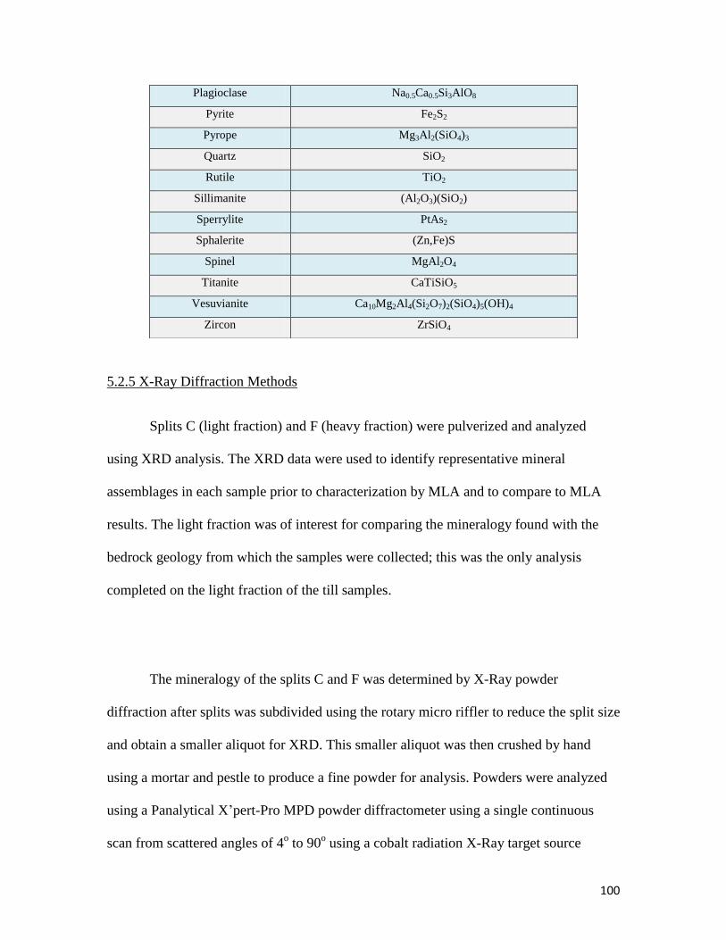
100
5.2.5 X-Ray Diffraction Methods
Splits C (light fraction) and F (heavy fraction) were pulverized and analyzed
using XRD analysis. The XRD data were used to identify representative mineral
assemblages in each sample prior to characterization by MLA and to compare to MLA
results. The light fraction was of interest for comparing the mineralogy found with the
bedrock geology from which the samples were collected; this was the only analysis
completed on the light fraction of the till samples.
The mineralogy of the splits C and F was determined by X-Ray powder
diffraction after splits was subdivided using the rotary micro riffler to reduce the split size
and obtain a smaller aliquot for XRD. This smaller aliquot was then crushed by hand
using a mortar and pestle to produce a fine powder for analysis. Powders were analyzed
using a Panalytical X’pert-Pro MPD powder diffractometer using a single continuous
scan from scattered angles of 4o to 90
o using a cobalt radiation X-Ray target source
Plagioclase Na0.5Ca0.5Si3AlO8
Pyrite Fe2S2
Pyrope Mg3Al2(SiO4)3
Quartz SiO2
Rutile TiO2
Sillimanite (Al2O3)(SiO2)
Sperrylite PtAs2
Sphalerite (Zn,Fe)S
Spinel MgAl2O4
Titanite CaTiSiO5
Vesuvianite Ca10Mg2Al4(Si2O7)2(SiO4)5(OH)4
Zircon ZrSiO4

101
(λ=1.79Å). Basic mineral identification was conducted in Highscore Pro 4.0 software
using the International Center for Diffraction Data PDF-2 2016 database.
5.2.6 ODM Separation Processing
Prior to the <0.25 mm light and heavy mineral fraction of the six till samples
being sent to QFIR, Queen’s University, ODM processed a bulk ~10-15 kg field sample
using methods outlined in Figure 5.2 and McClenaghan et al. (2016). ODM prepared a
2.0-0.25 mm light and heavy fractions. The heavy 0.25-2.0 mm heavy mineral fraction
was examined by ODM to determine the presence and abundance of key indicator
minerals such gold, platinum group minerals (PGM), kimberlite indicator minerals (KIM)
and metamorphosed or magmatic massive sulpides indicator minerals (MMSIM). Each
till sample was first sieved at 2.0 mm and the <2.0 mm material was passed over a
shaking table (Wilfley Table) to produce a preconcentrate. The table concentrate was
further concentrated using heavy liquid separation at SG 3.2 to create a light and heavy
fraction. The ferromagnetic minerals were then removed from the heavy mineral fraction
using a hand magnet. Figure 5.2 indicates where the heavy and light fractions used in
this study were produced by ODM in the sample processing procedure.

102
Figure 5.2: Flowsheet from McClenaghan et al., 2016 outlining the sample processing and
indicator mineral picking procedures used on till samples by ODM.
103
5.3 Results
This section is subdivided into subsection based on techniques used to analyze the
till samples. Hydroseparation and ODM processing were analyzed using XRD and
ESEM-MLA to determine the potential indicator minerals associated with each sample
location (Figure 5.3).

104
Figure 5.3: Bedrock geology map of the southern Core Zone, and location of the six GSC till
samples used in this study. Geology from Wardle et al. (1997) and Ministère de l’Énergie et des
Ressources naturelles (2010).
105
5.3.1 ODM heavy mineral concentrate <125 µm recovery
i) Pebble Counts
Based on the sediment log data collected from ODM tabling (Appendix B), the
>2.0 mm fraction of the six till samples contained volcanics and/or sediments (V/S) and
granitoids (Figure 5.4). Sample 14-PTA-B006, which overlies arkose and conglomerate,
had the highest clast percent of V/S (95%). Sample 14-PTA-B012, which overlies
volcanic rocks, contained 90% V/S. Sample 14-PTA-B005 which overlies metagabbro,
contained 20% V/S. Sample 14-PTA-R006, which overlies quartzo-feldspathic gneiss,
and samples 14-PTA-R011 and 14-PTA-R029 that overlies felsic intrusive rocks, contain
95% - 100% granitoid clasts.

106
Figure 5.4: Lithology of >2 mm clasts in the six till samples as reported by ODM (data from
McClenaghan et al. 2016).
ii) Gold & Sulfide Mineral Data:
All of the table concentrates were panned and gold and other small mineral grains
were counted, measured and qualitatively classified into different grain morphologies.
The grains were then added back into each table concentrate. Only two samples contained

107
visible gold grains, 14-PTA-B005 and 14-PTA-B012, respectively (Figure 5.5). Sample
14-PTA-R006 contained 1 pyrite grain. No other sulphides were observed in any of the
other samples.
Figure 5.5: Number of gold grains found in gold bearing samples with the associated grain
characteristics giving evidence of transport history.
iii) Platinum Group Minerals (PGM:
No PGMs were found in any of the table concentrates of the six samples
examined by ODM.
0
1
2
3
4
5
6
Reshaped Modified Pristine
Nu
mb
er
of
go
ld g
rain
s
Gold grain characteristics
Gold Grain Data
14-PTA-B005
14-PTA-B012

108
iv) Kimberlite Data:
Kimberlite indicators are minerals that come from the disaggregated peridotite
and eclogite mantle xenoliths (diopside, chromite and forsterite) and megacryst mineral
suite (garnets and Mg-ilmenite), which comprise the kimberlite host rock. G9 garnet, Cr-
pyrope (garnet bearing lherzolite source rock); G10 garnet, subcalcic Cr-pyrope (garnet
bearing harzburgite/dunite source rock) (McClenaghan, M.B., 2005). G1 and G2 garnet
(Ti-Cr pyropes); G3 garnet (eclogitic) (Erlich, E.I., and Hausel W.D., 2002). A few
kimberlite indicator minerals (KIMs) were recovered from the >0.25 mm non-
ferromagnetic heavy mineral fraction of sample 14-PTA-B006 (4 chromite grains).
Sample 14-PTA-R006 contained 1 forsterite grain while sample 14-PTA-B006 contained
chromite, and samples 14-PTA-B005, 14-PTA-B012 and 14-PTA-R029 all contained low
Cr-diopside in the 0.25-0.5 mm size fraction (Figure 5.6)

109
Figure 5.6: Kimberlite (diamond bearing) indicator mineralogy determined for each size fraction
for the 0.25-2.0 mm heavy mineral fraction.
v) Metamorphosed/Magmatic Massive Sulphide Indicator Mineral Data:
The >0.25 mm non-ferromagnetic heavy mineral fraction of the six samples, were
examined by ODM for metamorphosed/magmatic sulphide indicator minerals. Sample
14-PTA-B005, 14-PTA-B006 and 14-PTA-B012 contained sulphide/arsenide minerals: 5
chalcopyrite grains, 3 goethite and 2 pyrite grains in 14-PTA-B005, 15 goethite grains in
14-PTA-B006, and 20 goethite grains in 14-PTA-B012. The Mg/Mn/Al/Cr –bearing
indicator minerals present in till samples included red rutile, orthopyroxene and chromite.
Red rutile was found in 14-PTA-B005 (12 grains), 14-PTA-B006 (6 grains), 14-PTA-
B012 (8 grains) and 14-PTA-R029 (12 grains). Percent orthopyroxene was found in
samples 14-PTA-B005 (15%), 14-PTA-B012 (10%), 14-PTA-R006 (40%), 14-PTA-
0
1
2
3
4
5
6
7 N
um
be
r o
f g
rain
s
Kimberlite Data
Low-Cr Diopside
G9/G10 Garnet
G1/G2/G3 Garnet
Cr-Diopside
Mg-Ilmenite
Chromite
Forsterite

110
R011 (30%) and 13-PTA-R029 (70%). Chromite was only found in sample 14-PTA-
B006 (3 grains). Traces amounts of phosphate minerals were found in sample 14-PTA-
B005 (apatite), 14-PTA-R006 (apatite and monazite) and 14-PTA-R029 (apatite) with
14-PTA-R011 having a slightly higher abundance of 2% apatite. The resulting data are
displayed in Figures 5.6 to 5.8.
vi) Grain Counts:
A 100-grain count was completed on 2 of the 6 samples (Table 5.4). This is a
process where 0.25-0.5 mm heavy mineral fraction (>3.2 SG) of the sample is divided
down to a 100-grain split and the grains are analyzed to determine the basic heavy
mineral mineralogy. This process gives a general idea of what the sample consists of and
the relative abundances of each mineral.

111
Table 5.4: Abundances of minerals in a 100-grain aliquot of the 025-0.5 mm non-ferromagnetic heavy mineral fraction of till samples 14-PTA-
B005 and 14-PTA-B012 as determined by ODM (data from McClenaghan et al. 2016)
Sample Garnet* Epidote CPX OPX Hornblende Ilmenite Hematite Limonite/
Goethite**
Zircon
14-PTA-B005 12 2 10 16 48 4 5 3 0
14-PTA-B012 29 7 11 4 19 5 2 22 1
* Mainly almandine but may include andradite, grossular and spessartine
** Includes marcasite obscured by limonite/goethite alteration
CPX = clinopyroxene
OPX = orthopyroxene

112
5.3.2 X-Ray Diffraction Light Fraction
Split C of the light mineral fraction of the six till samples was analyzed to
determine the minerals present in this fraction. Table 5.5 lists the minerals identified by
XRD (See Appendix C for full listing of the XRD data).
Table 5.5: The main minerals identified in split C of the light fraction of each till sample using
XRD analysis. Minerals are listed in order of decreasing abundance.
14-PTA-B005
Light
14-PTA-B006
Light
14-PTA-B012
Light
14-PTA-R006
Light
14-PTA-R011
Light
14-PTA-R029
Light
Albite Albite Quartz Richterite Albite Albite
Clinochlore Richterite Edenite Albite Magnesio-
riebeckite
Magnesio-
riebeckite
Quartz Clinochlore Albite Magnesio-
hornblende
Titanite Orthoclase
Microcline Hematite Clinochlore Quartz Quartz Actinolite
Magnesio-
hornblende
Orthoclase Actinolite Microcline Magnesio-
hornblende
Quartz
Enstatite Quartz Epidote Biotite Rutile
Phlogopite Magnesio-
hornblende
Sodalite
5.3.3 X-Ray Diffraction Heavy Fraction
Split F of the heavy mineral fraction of the six till samples was analyzed to
compare with the ODM results as well as to predict the mineralogy to be identified using
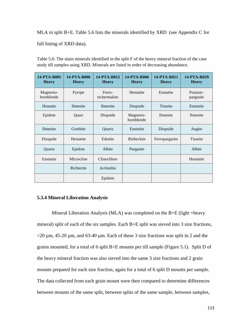
113
MLA in split B+E. Table 5.6 lists the minerals identified by XRD (see Appendix C for
full listing of XRD data).
Table 5.6: The main minerals identified in the split F of the heavy mineral fraction of the case
study till samples using XRD. Minerals are listed in order of decreasing abundance.
14-PTA-B005
Heavy
14-PTA-B006
Heavy
14-PTA-B012
Heavy
14-PTA-R006
Heavy
14-PTA-R011
Heavy
14-PTA-R029
Heavy
Magnesio-
hornblende
Pyrope Ferro-
tschermakite
Hematite Enstatite Potassic-
pargasite
Hemaite Ilmenite Ilmenite Diopside Titanite Enstatite
Epidote Quart Diopside Magnesio-
hornblende
Ilmenite Ilmenite
Ilmenite Goethite Quartz Enstatite Diopside Augite
Diospide Hematite Edenite Riebeckite Ferropargasite Titanite
Quartz Epidote Albite Pargasite Albite
Enstatite Microcline Clinochlore Hematite
Richterite Actinolite
Epidote
5.3.4 Mineral Liberation Analysis
Mineral Liberation Analysis (MLA) was completed on the B+E (light +heavy
mineral) split of each of the six samples. Each B+E split was sieved into 3 size fractions,
<20 µm, 45-20 µm, and 63-40 µm. Each of these 3 size fractions was split in 2 and the
grains mounted, for a total of 6 split B+E mounts per till sample (Figure 5.1). Split D of
the heavy mineral fraction was also sieved into the same 3 size fractions and 2 grain
mounts prepared for each size fraction, again for a total of 6 split D mounts per sample.
The data collected from each grain mount were then compared to determine differences
between mounts of the same split, between splits of the same sample, between samples,

114
and between processing techniques, as well as documenting the minerals related to the
bedrock geology of each sample site. MLA data are summarized in Figures 5.7-5.18. In
these figures, the histograms are colour coded for each size fraction. Data were plotted to
compare the abundance of indicator minerals in each size fraction to determine if
examination of the smaller size fraction of till is beneficial. Tables listing the MLA data
are organized by the mineral abundance of the 63-45 µm fraction in decreasing order in
Appendix D.
Figure 5.7: Modal mineralogy of till sample 14-PTA-B005 split D (heavy minerals) determined
through MLA for three size fractions.
0%
10%
20%
30%
40%
50%
60%
Are
a %
Ab
un
da
nce
HMC Data for 14-PTA-B005 45-63
20-45
<20

115
Figure 5.8: Modal mineralogy of till sample 14-PTA-B005 split B+E (light +heavy minerals)
determined through MLA for three size fractions for sample processed by hydroseparation.
0%
10%
20%
30%
40%
50%
Are
a %
Ab
un
da
nce
Mineral Type
Hydroseparated HMC Data for
14-PTA-B005 45-63
20-45
<20

116
Figure 5.9: Modal mineralogy of till sample 14-PTA-B006 split D (heavy minerals) determined
through MLA for three size fractions.
0%
10%
20%
30%
40%
50%
Are
a%
Ab
un
da
nce
Mineral Type
HMC Data for 14-PTA-B006 45-63
20-45
<20
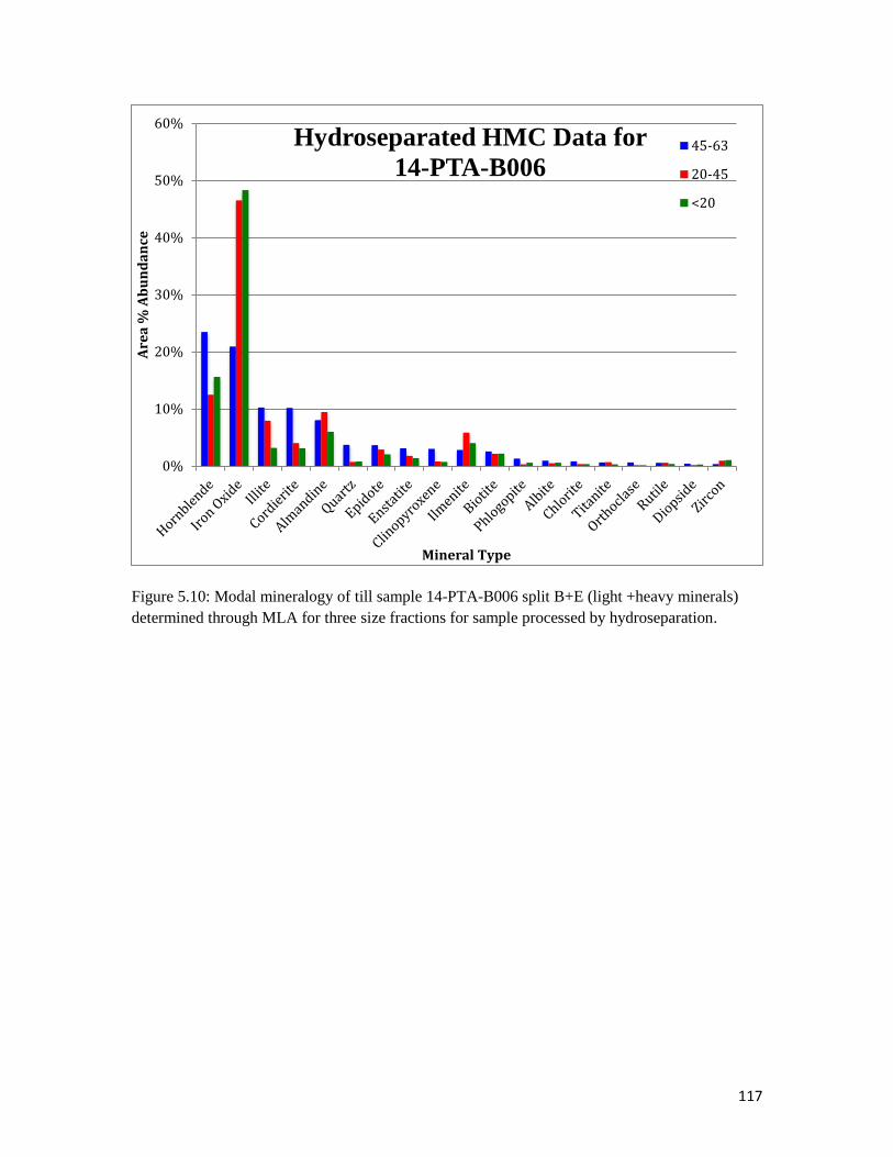
117
Figure 5.10: Modal mineralogy of till sample 14-PTA-B006 split B+E (light +heavy minerals)
determined through MLA for three size fractions for sample processed by hydroseparation.
0%
10%
20%
30%
40%
50%
60%
Are
a %
Ab
un
da
nce
Mineral Type
Hydroseparated HMC Data for
14-PTA-B006 45-63
20-45
<20

118
Figure 5.11: Modal mineralogy of till sample 14-PTA-B012 split D (heavy minerals) determined
through MLA for three size fractions.
0%
10%
20%
30%
40%
50%
60%
70%
Are
a %
Ab
un
da
nce
Mineral Type
HMC for 14-PTA-B012 45-63
20-45
<20

119
Figure 5.12: Modal mineralogy of till sample 14-PTA-B012 split B+E (light +heavy minerals)
determined through MLA for three size fractions for sample processed by hydroseparation.
0%
10%
20%
30%
40%
50%
Are
a %
Ab
un
da
nce
Mineral Type
Hydroseparated HMC for
14-PTA-B012
45-63
20-45
<20

120
Figure 5.13: Modal mineralogy of till sample 14-PTA-R006 split D (heavy minerals) determined
through MLA for three size fractions.
0%
10%
20%
30%
40%
50%
60%
Are
a %
Ab
un
da
nce
Mineral Type
HMC Data for 14-PTA-R006 45-63
20-45
<20

121
Figure 5.14: Modal mineralogy of till sample 14-PTA-R006 split B+E (light +heavy minerals)
determined through MLA for three size fractions for sample processed by hydroseparation.
0%
10%
20%
30%
40%
50%
Are
a &
Ab
un
da
ne
Mineral Type
Hydroseparated HMC Data for
14-PTA-R006 45-63
20-45
<20

122
Figure 5.15: Modal mineralogy of till sample 14-PTA-R011 split D (heavy minerals) determined
through MLA for three size fractions.
0%
10%
20%
30%
40%
50%
Are
a %
Ab
un
da
nce
Mineral Type
HMC Data for 14-PTA-R011 45-63
20-45
<20
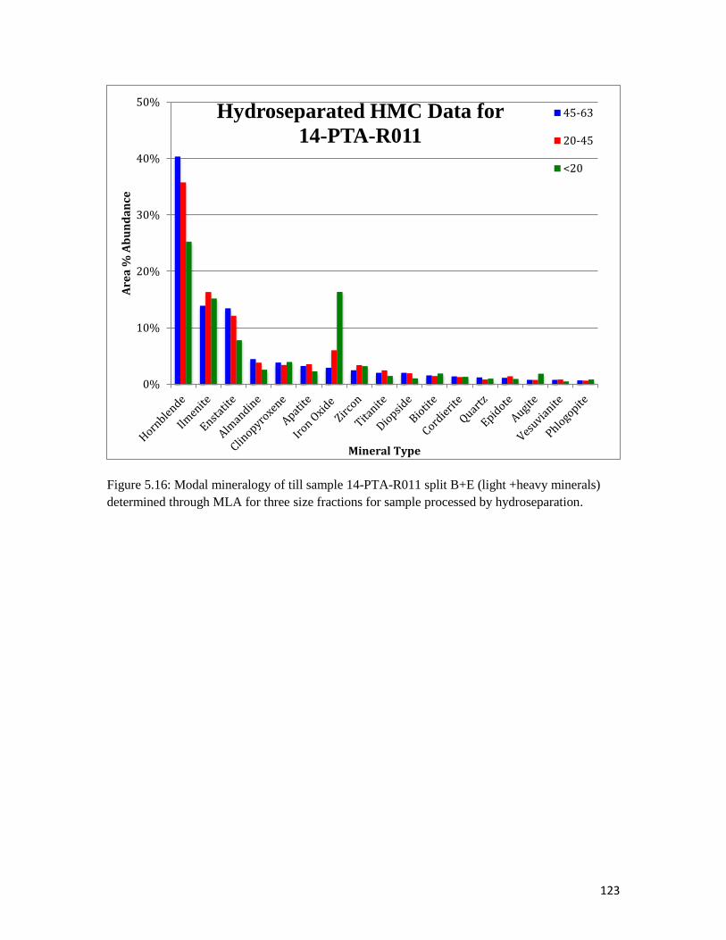
123
Figure 5.16: Modal mineralogy of till sample 14-PTA-R011 split B+E (light +heavy minerals)
determined through MLA for three size fractions for sample processed by hydroseparation.
0%
10%
20%
30%
40%
50%
Are
a %
Ab
un
da
nce
Mineral Type
Hydroseparated HMC Data for
14-PTA-R011
45-63
20-45
<20
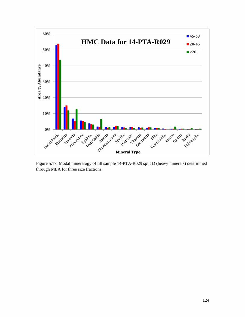
124
Figure 5.17: Modal mineralogy of till sample 14-PTA-R029 split D (heavy minerals) determined
through MLA for three size fractions.
0%
10%
20%
30%
40%
50%
60%
Are
a %
Ab
un
da
nce
Mineral Type
HMC Data for 14-PTA-R029 45-63
20-45
<20

125
Figure 5.18: Modal mineralogy of till sample 14-PTA-R029 split B+E (light +heavy minerals)
determined through MLA for three size fractions for sample processed by hydroseparation.
Indicator minerals of particular significance to mineral exploration were targeted
in each of the samples, including: gold, sperrylite, pyrite, chalcopyrite, chromite,
forsterite, arsenopyrite, galena and sphalerite. The abundance of these target indicators
(listed in alphabetical order) are plotted on the histograms displayed in Figure 5.19 to
5.24. The histograms are colour coded for each size fraction. The data were plotted in this
manner to compare the abundance of indicator minerals in each size fraction, to
determine if looking at the smaller size fraction of till is beneficial. Table 5.8 represents a
compiled version of all indicator data for five size fractions of the ODM processed data
for the six samples. ODM provided data for the indicator mineralogy found for the >125-
0%
10%
20%
30%
40%
50%
Are
a %
Ab
un
da
nce
Mineral Type
Hydroseparated HMC Data for
14-PTA-R029 45-63
20-45
<20

126
63 µm fraction, and the 63-<20 µm data was analyzed by ESEM-MLA within QFIR at
Queen’s University.
Table 5.7: The >125 and 125-63 µm fractions were collected and analyzed by ODM, the smaller
fractions (63-<20 µm) were produced at Queen’s University through sieving and MLA. The <20
µm fraction generally has a higher abundance of minerals and greater diversity.
Sample 0.25-0.5 mm 75 µm 63-45 µm 45-20 µm <20 µm
14-PTA-B005 Pyrite 2 - - Spinel 1 Arsenopyrite 2
Gold 2 - - Chromite 3 Cassiterite 2
Low Cr-
diopside 3
- - - Chromite 6
Chalcopyrite 5 - - - -
Spinel 10 - - - -
14-PTA-B006 Spinel 2 - Chromite 2 Chromite
29
Pyrite 1
Chromite 4 - - - Sperrylite 2
- - - - Chromite 20
14-PTA-B012 Low CR-
diopside 1
- Chromite 1 Chromite
11
Chromite 6
Gold 6 - - - -
Spinel 13 - - - -
14-PTA-R006 Forsterite 1 Pyrite 1 Spinel 3 Spinel 4 Sperrylite 1
Spinel 60 - - Chromite 8 Pyrite 1
- - - - Chromite 2
14-PTA-R011 Low Cr-
diopside 1
- Spinel 1 Chromite 1 Sperrylite 21
Spinel 5 - - - -
14-PTA-R029 Spinel 4 - Chromite 1 Olivine 1 Spinel 1
Low Cr-
diopside 6
- Chalcopyrite
1
Chromite 4 Pyrite 1
- - - - Galena 1
- - - - Sperrylite 4
- - - - Chromite 8

127
Figure 5.19: Indicator minerals found from MLA for each size fraction (ODM and
hydroseparated samples analyzed and results combined)
Figure 5.20: Indicator minerals found from MLA for each size fraction (ODM and
hydroseparated samples analyzed and results combined)
0
2
4
6
8
10
12
14
16 N
um
be
r o
f g
rain
s
14-PTA-B005 Indicator Minerals
45-63 microns
20-45 microns
<20 microns
0
5
10
15
20
25
30
35
Nu
mb
er
of
gra
ins
14-PTA-B006 Indicator Minerals
45-63 microns
20-45 microns
<20 microns
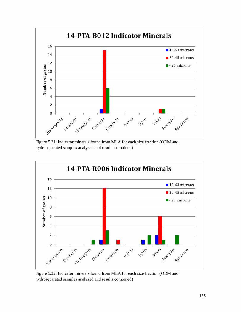
128
Figure 5.21: Indicator minerals found from MLA for each size fraction (ODM and
hydroseparated samples analyzed and results combined)
Figure 5.22: Indicator minerals found from MLA for each size fraction (ODM and
hydroseparated samples analyzed and results combined)
0
2
4
6
8
10
12
14
16 N
um
be
r o
f g
rain
s
14-PTA-B012 Indicator Minerals
45-63 microns
20-45 microns
<20 microns
0
2
4
6
8
10
12
14
Nu
mb
er
of
gra
ins
14-PTA-R006 Indicator Minerals
45-63 microns
20-45 microns
<20 microns

129
Figure 5.23: Indicator minerals found from MLA for each size fraction (ODM and
hydroseparated samples analyzed and results combined)
Figure 5.24: Indicator minerals found from MLA for each size fraction (ODM and
hydroseparated samples analyzed and results combined)
0
5
10
15
20
25 N
um
be
r o
f g
rain
s
14-PTA-R011 Indicator Minerals
45-63 microns
20-45 microns
<20 microns
0
1
2
3
4
5
6
7
8
9
Nu
mb
er
of
gra
ins
14-PTA-R029 Indicator Minerals
45-63 microns
20-45 microns
<20 microns

130
The <20 µm fraction contained the most target indicator minerals as compared to
the 63-45 µm or 45-20 µm fractions. This fact indicates that the <20 µm fraction is the
optimal fraction for detecting these target indicator minerals. Figures 5.25-5.26 display
the BSE image of select indicator minerals with the associated spectra, which were used
to determine the viability of the MLA mineral library.

131
Figure 5.25: Backscatter (BSE) images of: A) Sperrylite (14-PTA-R011, <20 µm); B) Pyrite (14-
PTA-B006, 45-20 µm); C) Chalcopyrite (14-PTA-R029, 63-45 µm); D) Arsenopyrite (14-PTA-
B005, <20 µm).
A
DC
B

132
Figure 5.26: Backscatter (BSE) images of: A) Monazite (14-PTA-R011, 45-20 µm); B) Spinel
(14-PTA-B005, 45-20 µm); C) Chromite (14-PTA-R029, 63-45 µm); D) Cassiterite (14-PTA-
B005, <20 µm).
A B
C D
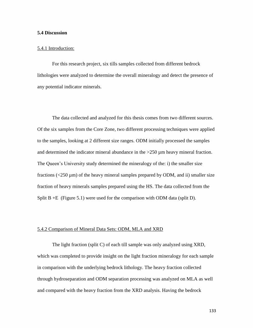
133
5.4 Discussion
5.4.1 Introduction:
For this research project, six tills samples collected from different bedrock
lithologies were analyzed to determine the overall mineralogy and detect the presence of
any potential indicator minerals.
The data collected and analyzed for this thesis comes from two different sources.
Of the six samples from the Core Zone, two different processing techniques were applied
to the samples, looking at 2 different size ranges. ODM initially processed the samples
and determined the indicator mineral abundance in the >250 µm heavy mineral fraction.
The Queen’s University study determined the mineralogy of the: i) the smaller size
fractions (<250 µm) of the heavy mineral samples prepared by ODM, and ii) smaller size
fraction of heavy minerals samples prepared using the HS. The data collected from the
Split B +E (Figure 5.1) were used for the comparison with ODM data (split D).
5.4.2 Comparison of Mineral Data Sets: ODM, MLA and XRD
The light fraction (split C) of each till sample was only analyzed using XRD,
which was completed to provide insight on the light fraction mineralogy for each sample
in comparison with the underlying bedrock lithology. The heavy fraction collected
through hydroseparation and ODM separation processing was analyzed on MLA as well
and compared with the heavy fraction from the XRD analysis. Having the bedrock

134
geology as a background basis, helped to determine if the minerals present in the till were
derived from the local bedrock. Each of the samples XRD data was referenced back to
the underlying bedrock lithology at each site, as well as the ice flow history to look at the
sources for any unexplained mineral data.
From the data collected for the light fractions (Table 5.6), the mineralogy
generally matched well with the bedrock lithology of each sample site (see individual
sample data below). Quartz, being very resistant to erosion and glacial transport due to its
hardness, makes it present and dominant in all samples observed. The light fractions
mineral abundances match with the underlying bedrock geology (i.e. abundant felsic
minerals in till overlying felsic intrusive rocks). The underlying bedrock geology and
light mineral fraction provided more insight for each sample once combined with the
heavy fraction data.
The heavy mineral data reported by ODM and collected as part of this study were
compared for similarities and differences. These separation techniques produced different
size fractions (i.e., <250 >125-63 µm from ODM analyses and split D 63-45 µm, 45-20
µm and <20 µm at Queen’s University). The indicator minerals recovered using each data
set differed and the smaller size fractions typically having an elevated level of indicator
mineral counts. The modal mineralogy determined by ODM, XRD and ESEM-MLA for
each sample is comparable and is representative of the bedrock geology of the area it was
sampled from. The XRD and MLA data are commonly combined to produce a reliable

135
source of information relative to the sample. Each of the samples mineralogical
relationships for the different size fractions is discussed below (Table 5.6 displays the
XRD data).
The area percent data was used for the case study as these values are calculated
based on the grain shape found in the mount. The weight percent data is less reliable as it
accounts for the chemical formula associated with each of the minerals in the mineral
library. Without having microprobe data and specific elemental compositions, the weight
percent data cannot be completely accurate for each mineral. The number of grains was
not used because the MLA software will record an inclusion as an individual mineral
therefore altering the accuracy of the findings. A complete listing of the minerals
identified in splits D and B+E are listed in Appendix D. The data are listed as percent of
the total area analyzed in each mount.
14-PTA-B005
Sample 14-PTA-B005 was collected from the central western region of the Core
Zone overlying Archean/Paleoproterozoic metagabbro bedrock (Figure 1.2). The main
minerals expected in a metagabbro include garnet, hornblende, orthopyroxene, and
plagioclase (Hermes, 1968). The XRD data for the heavy mineral fraction (split F)
indicated that the heavy mineral fraction contained magnesiohornblende, hematite,
epidote, ilmenite, diopside, and enstatite.

136
In the 0.25-0.5 mm heavy mineral fraction, ODM identified hornblende,
orthopyroxene, hematite, epidote, and diopside. In ODM splits D1, D2, D3, MLA
analysis indicated that the heavy minerals consist of dominantly hornblende (~50%) with
lesser amounts of enstatite, epidote, ilmenite, iron oxide and almandine (4-10%) in the
63-45 µm and 45-20 µm fraction. The <20 µm fraction contains less hornblende (~30%)
and more iron oxide (~20%) and ilmenite (~15%).
The MLA analysis of the hydroseparated heavy mineral fractions (split B+E1,
B+E2, B+E3) indicated that the most dominant mineral for all size fractions was
hornblende, which decreased slightly as the size fraction decreased (44-29%). Garnet
(almandine, ~4%) and orthopyroxene (enstatite, ~6%) also identified by MLA, as well as
minor iron oxides, which increased in abundance as the size decreased (7-14%). Epidote,
ilmenite and clinopyroxene, and traces of titanite (Ti bearing) and biotite (Ti and K
bearing), were present in all size fractions of splits D and B+E which was expected, as
the TiO2 and K2O content is slightly higher in a metagabbro compared to a gabbro
(Hermes, 1968). Plagioclase was not detected in the splits because it is a light mineral.
The hydroseparated sample has a slight elevation in the ilmenite content in the larger
fractions, 45-63 (9.5%) and 20-45 µm sizes (9.3%), with lesser volume of epidote and
enstatite than the <20 µm fraction. The MLA, XRD and ODM data included iron oxides,
epidote, enstatite, hornblende (amphibole), ilmenite and pyroxene for the heavy mineral
fraction.
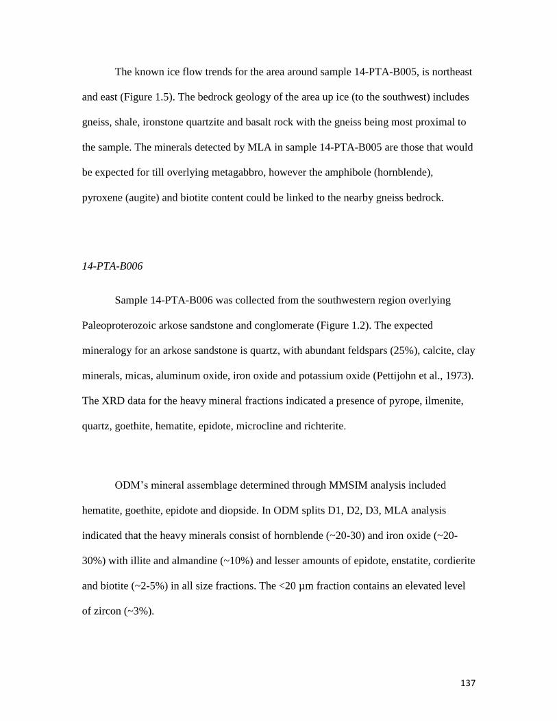
137
The known ice flow trends for the area around sample 14-PTA-B005, is northeast
and east (Figure 1.5). The bedrock geology of the area up ice (to the southwest) includes
gneiss, shale, ironstone quartzite and basalt rock with the gneiss being most proximal to
the sample. The minerals detected by MLA in sample 14-PTA-B005 are those that would
be expected for till overlying metagabbro, however the amphibole (hornblende),
pyroxene (augite) and biotite content could be linked to the nearby gneiss bedrock.
14-PTA-B006
Sample 14-PTA-B006 was collected from the southwestern region overlying
Paleoproterozoic arkose sandstone and conglomerate (Figure 1.2). The expected
mineralogy for an arkose sandstone is quartz, with abundant feldspars (25%), calcite, clay
minerals, micas, aluminum oxide, iron oxide and potassium oxide (Pettijohn et al., 1973).
The XRD data for the heavy mineral fractions indicated a presence of pyrope, ilmenite,
quartz, goethite, hematite, epidote, microcline and richterite.
ODM’s mineral assemblage determined through MMSIM analysis included
hematite, goethite, epidote and diopside. In ODM splits D1, D2, D3, MLA analysis
indicated that the heavy minerals consist of hornblende (~20-30) and iron oxide (~20-
30%) with illite and almandine (~10%) and lesser amounts of epidote, enstatite, cordierite
and biotite (~2-5%) in all size fractions. The <20 µm fraction contains an elevated level
of zircon (~3%).

138
The data collected from MLA indicates that the 45-63 µm fraction was most
abundant in hornblende (23.46%) followed by iron oxide (20.92%). The 20-45 and <20
µm fractions however had a higher iron oxide (46.50-45.69%) content than hornblende
(12.48-14.32%). The iron oxide content increased with decreasing size whereas the
hornblende content decreased. There was also abundant garnet (almandine), illite,
enstatite, epidote, cordierite, ilmenite, biotite and zircon; the zircon content increased as
size decreased. Based on this heavy mineral assemblage, an arkose sandstone would be
the appropriate rock type. Since feldspars are lighter and weather more readily, the
abundance is not preserved however there are traces of albite and orthoclase in the MLA
data as well as the XRD data for this sample. The iron oxide content is the most
abundant, which can also be observed by the red colouring of the sample (Appendix A).
There is evidence of quartz and mica through the presence of cordierite and
biotite provided by the MLA data. The XRD and MLA data for the heavy mineral
fractions both contained hematite, ilmenite and garnet. The MLA, ODM and XRD data
all indicated an abundance of iron oxide, hematite and goethite. The quartz, feldspar and
potassium oxide mineralogy was present in the light mineral fraction data. Combining the
light and heavy mineral data found allowed for the classification of an arkose sandstone
to be an accurate representation of the till sampled.

139
The known ice flow patterns do not directly sample 14-PTA-B006. All forms of
glaciation in this region move away from this location (McClenaghan et al., 2016), which
would imply the till sample was primarily consistent with the bedrock geology. The
hornblende content found from the MLA data would imply that there was some transfer
of sediments over this region however, as hornblende is not commonly found in
sandstones (Odigi, et al., 2008).
14-PTA-B012
Sample 14-PTA-B012 was collected from the western region of the New Québec
Orogen, Doublet Zone in a Paleoproterozoic block of basalts and pyroclastic rocks. Based
on the bedrock geology, the expected mineralogy would include an assortment of mafic
minerals, such as olivine, pyroxene, amphibole and biotite. The XRD heavy mineral data
for this sample included an assemblage of ferrotschermakite, ilmenite, diopside, quartz,
magnesiohornblende, epidote and rutile.
Overburden Drilling Management Limited’s MMSIM analysis identified an
assemblage of almandine, ilmenite, goethite, hornblende, epidote and diopside. In ODM
splits D1, D2, D3, MLA analysis indicated that the heavy minerals consist of hornblende
(~30-60%) and ilmenite (~10-30%), iron oxides and epidote (~10%) and lesser amounts
of biotite, clinopyroxene, rutile and almandine (~3%) for all size fractions. The <20 µm
fraction contained a similar level of hornblende and ilmenite (~30% for each).

140
The MLA data indicated that the most abundant mineral in all size fractions was
hornblende at a constant area percentage for all size fractions at ~45 area%. The MLA
data contained a similar mineral assemblage and relatively similar abundances for each
size fraction. Ilmenite (~10%), epidote (~9%) and iron oxide (~6%) are found in that
order in the 20-45 µm and 45-63 µm size fractions. The <20 µm fraction of 14-PTA-
B012 contained a dominant ilmenite, iron oxide, epidote mineral assemblage. All size
fractions contained an almandine fraction at a ~5% abundance. The less abundant
minerals (<5%) include biotite, clinopyroxene, quartz, cordierite and lesser amounts of
enstatite, titanite, rutile and illite. The zircon content is relatively constant at ~0.60 % in
all size fractions. Olivine was presented in trace amounts (i.e., <0.10%). The olivine grain
count determined from the MLA data contained ~60 grains, producing less than 1 area
percent collection of the mount. The mineralogy includes abundant amphiboles, as well
as pyroxenes, the olivine content is low and the biotite content is low but present,
indicating that the till provenance was likely from a region of mafic rocks, consistent
with the bedrock mapping of basalt up-ice of the till sampling location (Figure 1.5).
Sample 14-PTA-B012 is in close proximity to the non-dominant deglacial flow,
as well as the first radial flow from the Labrador ice centre, which could have an
influence of the mineral findings observed in the till (Figure 1.5). The deglacial ice flow
was moving in a northeast direction while the first radial ice flow moved in a northwest
direction towards the sample location. The bedrock types that were in line with the
glacial flow include metabasalt, orthogneiss, metagabbro, charnockite, quartzo
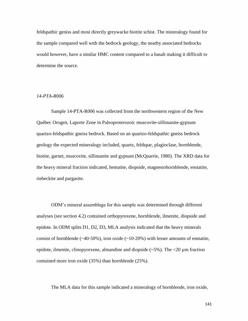
141
feldspathic geniss and most directly greywacke biotite schist. The mineralogy found for
the sample compared well with the bedrock geology, the nearby associated bedrocks
would however, have a similar HMC content compared to a basalt making it difficult to
determine the source.
14-PTA-R006
Sample 14-PTA-R006 was collected from the northwestern region of the New
Québec Orogen, Laporte Zone in Paleoproterozoic muscovite-sillimanite-gypsum
quartzo-feldspathic gneiss bedrock. Based on an quartzo-feldspathic gneiss bedrock
geology the expected mineralogy included, quartz, feldspar, plagioclase, hornblende,
biotite, garnet, muscovite, sillimanite and gypsum (McQuarrie, 1980). The XRD data for
the heavy mineral fraction indicated, hematite, diopside, magnesiohornblende, enstatite,
riebeckite and pargasite.
ODM’s mineral assemblage for this sample was determined through different
analyses (see section 4.2) contained orthopyroxene, hornblende, ilmenite, diopside and
epidote. In ODM splits D1, D2, D3, MLA analysis indicated that the heavy minerals
consist of hornblende (~40-50%), iron oxide (~10-20%) with lesser amounts of enstatite,
epidote, ilmenite, clinopyorxene, almandine and diopside (~5%). The <20 µm fraction
contained more iron oxide (35%) than hornblende (25%).
The MLA data for this sample indicated a mineralogy of hornblende, iron oxide,

142
ilmenite, enstatite, garnet, pyroxene and diopside, with a decrease in hornblende from 41
to 29%, and an increase in iron oxide from 18 to 32% as the size decreases from 63 to
<20 µm. The 45-63 µm fraction was most abundant in hornblende followed by iron
oxide, whereas the <20 µm fraction was most abundant in iron oxide followed by
hornblende. These two minerals make up the majority of the assemblage for all size
fractions, however enstatite, ilmenite, clinopyroxene, diopsode and almandine are
present. Trace minerals (<2%) such as biotite (1.18-1.57%), titanite (0.95-1.2%), quartz
(0.74-1.89%), apatite (0.88-1.24%), rutile (0.68-1.11%), and epidote (1.16-2.03%) are
fairly constant with zircon having a trend of slightly increasing in abundance with
decreasing size (0.75-1.61%). Quartz, feldspar, muscovite, sillimanite and gypsum were
absent from the HMC as the density of the mineral grains were too low for heavy mineral
concentration. However, in the light fraction analyzed through XRD there was no
measurable muscovite and sillimanite, but measurable feldspar and quartz. The heavy
fraction analyzed using MLA, XRD and OMD processed data indicated that there was
hornblende and pyroxene. MLA indicated minor garnet (2.63-4.24 %), which was absent
from the XRD data and ODM analyses. The light fraction contained feldspar, plagioclase
and quartz that likely represent the bedrock mineralogy. Muscovite, sillimanite and
gypsum, however remained absent in the MLA data as well. ODM and MLA results
match with the expected mineralogy for a quartzofeldspathic gneiss as well as the
minerals found from the XRD analysis.
The oldest ice flow as well as the first radial ice flow over the 14-PTA-R006,
sample location could potentially provide minerals from the quartzofeldspathic geniss
143
and more dominantly the orthogneiss (Figure 1.5). This would imply more felsic minerals
including quartz, plagioclase and feldspar with hornblende and pyroxene accessory
minerals. The mineralogy determined from MLA and XRD relates to the ms-sil-gp
quartzofeldspathic bedrock, which underlies the till. Therefore, there does not appear to
be an abundant mixture of sediments from distal sources.
14-PTA-R011
Sample 14-PTA-R011 was collected from the central eastern region of the Core Zone
above a Paleoproterozoic mylonitic tonalite (Figure 1.2). This bedrock geology would
have an expected mineralogy of feldspar (plagioclase), ~20% quartz with amphibole and
pyroxene as accessory minerals (Marzouki et al., 1982). Heavy mineral XRD data
indicated a mineral assemblage of enstatite, titanite, ilmenite, diopside, and ferropargasite
(NaCa2Fe4Al2Si6O22(OH)2).
ODM’s MMSIM analysis determined a mineralogy of hornblende, orthopyroxene
and diopside. In ODM splits D1, D2, D3, MLA analysis indicated that the heavy minerals
consist of hornblende (~40-50%), enstatite (20%), ilmenite and almandine (5-10%) for
the 63-45 and 45-20 µm fractions. The <20 µm fraction contains hornblende (30%),
ilmenite (20%), enstatite (15%) and a higher abundance of zircon (~5%).
The most abundant mineral found in all size fractions from MLA for this sample
was hornblende, which slightly decreased in abundance (40.36 to 19.55%) as size
144
decreased (63 - <20 µm). The remaining MLA mineralogy was relatively constant in
abundance for all size fractions, which involved enstatite, ilmenite, almandine, iron
oxide, zircon, clinopyroxene and apatite. Titanite, biotite, diopside and cordierite were
found in lesser amounts. Collectively, the XRD, MLA and ODM data appear to relate to
the bedrock geology (mylonitic tonalite), containing the expected accessory minerals of
amphiboles and pyroxenes. The light fraction contained the expected quartz and feldspar
as well as other minerals including titanite, magnesio-hornblende and magnesio-
riebeckite. The data (MLA, XRD, and ODM’s analyses) represents a mylonitic tonalite
composition as is expected based on the sampling location.
Sample 14-PTA-R011 is in direct path of the deglacial radial ice flow (Figure
1.5). This ice flow movement was in a north-eastern direction, likely carrying glacial
sediments from the orthogneiss and neighboring amphibolite bedrocks. The amphibolite
bedrock likely contains predominantly amphiboles (hornblende and pargasite) and
plagioclase (Marzouki et al., 1982). This likely resulted in the increase in amphibole
content and mineralogy of the till sample.
14-PTA-R029
Sample 14-PTA-R029 was collected from the central region of the Core Zone in a
Paleoproterozoic charnockite series bedrock. A monzogranite charnockite is an
orthopyroxene-bearing granitoid (Emslie et al., 1994) and with a mineralogy that includes
quartz, alkali feldspar, plagioclase and orthopyroxene. Charnockite series bedrock can
145
include rocks of many different types, some being felsic and rich in quartz and
microcline, others mafic and full of pyroxene and olivine, whereas there are also
intermediate varieties corresponding mineralogically to norites, quartz-norites
and diorites (Williams et al. 2014). Depending on the whether the charnockite series was
felsic or mafic in composition will determine if more felsic or mafic minerals are present.
The XRD data for the heavy mineral fraction indicated potassicpargasite, enstatite,
ilmenite, augite, titanite, albite, and hematite.
ODM’s MMSIM determined a mineral assemblage that included hornblende,
orthopryoxene, diopside and epidote. In ODM splits D1, D2, D3, MLA analysis indicated
that the heavy minerals consist of hornblende (50%), enstatite (15%), ilmenite and
almandine (5%). The <20 µm fraction is comparable to the larger size fractions but also
contains an elevated abundance of iron oxides (5%) and zircon (3%).
The MLA indicated that the most dominant mineral for all size fractions was
hornblende (29.85 to 47.07%), with constant mineral abundance. Enstatite (5-11%) and
ilmenite (9-13%) were found in a constant abundance for all size fractions. Almandine,
epidote and clinopyroxene were present in lesser amounts (<5%) with the iron oxide
content increasing (2.84 to 11.49%) as the size decreased (63 to <20 µm). Traces (<2%)
of biotite, titanite, apatite and diopside were present, with the zircon content increasing
(1.11 to 1.31%) as size decreased (63 to 45 µm). Based on the mineral assemblage
determined by MLA, XRD and ODM analyses, the charnockite series in the bedrock was
likely a more mafic rock. Orthopyroxene was present as observed in the enstatite

146
abundance and other mafic minerals include the hornblende and ilmenite (~65 %), with
some clinopyroxene (~5 %). The heavy mineral fractions for XRD, MLA and ODM
contain orthopyroxene, enstatite, required to relate back to the bedrock geology. The light
fraction was similar to the expected mineralogy for a charnockite series bedrock source,
that included plagioclase, feldspar and quartz.
The known ice flow pattern for this sample was similar to sample 14-PTA-B005
(Figure 1.5). The oldest ice flow in the region was from the Québec highlands and moved
in a northeastern direction over the sample location area (Figure 2.6). The bedrock types
that could contribute to mineralogical changes include gneiss, shale, ironstone, quartzite
and basalt (Figure 1.2). The first radial ice flow moved in a southeast direction over this
sample location as well. Based on the XRD data, the mineralogy relates to the
charnockite bedrock, which underlies the sampling site, however glaciation and sediment
transport could have resulted in a change of the overall mineralogy found.
5.4.3 Target Indicator Minerals
Knowledge of the glacial ice history as well as the local bedrock geology can aid
in the identification of the bedrock source of unexpected minerals in certain regions
(McMartin et al., 2001). The modal mineralogy found for each sample from our study, is
consistent with the bedrock geology from the area immediately up-ice (10-15 km) from
which it was collected. However, through the presence of ex-situ indicator minerals the
discovery of potential ore bodies can be applied from the glacial transport history.

147
Glaciation can disperse minerals metres to 100s of km from the bedrock source
(McClenaghan, 2010). From the ice flow history, the dominant ice flow direction moved
in a north-eastern trend over the Core Zone. Using the indicators found (Table 5.7)
mineral distribution patterns were created to understand the abundance of minerals based
on location. In the following sections, our findings were compared to the regional
geology of Québec and Labrador to determine potential sources for the indicator minerals
found.
Each of the split B+E samples studied did contain target indicator minerals (Table
5.7), which could be indicative of mineralized bedrock up-ice. The abundance of
individual indicator minerals ranged from 1 grain to ~10 grains depending on the sample
and size fraction. The <20 µm fraction contained the most target minerals and the
broadest range of minerals, with the 45-63 µm fraction samples containing the least
(Table 5.8). Each indicator mineral detected using MLA was verified using the ESEM by
EDS. The EDS results for these of minerals were fed back into the MLA classification
library.
Overburden Drilling Management Limited’s 0.25-0.5 mm fraction contained 2
pyrite, 2 gold, 3 low-Cr diopside, 5 chalcopyrite grains and 10 spinel grains. Split B+E of
sample 14-PTA-B005 contained chromite, spinel, arsenopyrite and cassiterite as
determined through MLA. These minerals are indicators of several types of mineral
deposits and cannot be tied to one specific type. The <20 µm fraction contained the

148
majority of the target indicator minerals. Overburden Drilling Management Limited
(ODM) recovered gold, chalcopyrite, pyrite, Mn-epidote, low Cr-diopside and red-rutile
in the 0.25-0.5 mm heavy mineral fraction of this sample (Table 5.8, Figure 5.4-5.8). The
association of gold, pyrite and arsenopyrite in sample indicate that the bedrock source
may be gold mineralization. Cassiterite is found in tin deposits as well as VMS deposits
and may be associated with pyrite and arsenopyrite (Marshall et al., 2004). Gold
mineralization within metagabbro rocks in metamorphic belts is commonly associated
with gold-bearing deposits (Debele et al., 1998). These deposits are commonly linked
with Cu, Pb, Zn, Au, Cu, and Sn occurrences (Groves, et al., 1998). The presence of the
cassiterite and chalcopyrite would support the conclusion that the bedrock source is gold
mineralization. Based on other gold occurrences in Québec and Labrador with the north-
east direction of glacial movement, the presence of gold is likely (Houle et al., 2007).
Overburden Drilling Management Limited’s 0.25-0.5 mm fractions contained 2
spinel and 4 chromite grains. Split B+E of sample 14-PTA-B006 contains chromite,
pyrite, and sperrylite. Pyrite and sperrylite were only found in the <20 µm fraction.
Chromite was found in the 0.25-0.5 mm heavy mineral fraction as reported by ODM,
along with traces of red rutile, kyanite and Mn-epidote. Although no gold was found in
this sample, the presence of pyrite could be indicative of gold mineralization due to its
proximity to sample 14-PTA-B005 as well as with it being in line with the regions
glaciation movement. The sperrylite, pyrite and chromite combination could indicate the
presence of a Ni-Cu-PGE mineralization up ice.

149
Overburden Drilling Management Limited’s 0.25-0.5 mm fraction contained 1
low-Cr diopside, 6 gold and 13 spinel grains. The ESEM-MLA data for sample split B+E
for sample 14-PTA-B012 indicate the presence of chromite. In the 0.25-0.5 mm heavy
mineral fraction, ODM observed spinel, with traces of Mn-epidote, low Cr-diopside and
red-rutile, no significant KIM, and 6 gold grains. Pyrite and arsenopyrite were not
detected by MLA, however the location of this sample falls in a similar location to
sample 14-PTA-B005 and 14-PTA-B006, which do imply some evidence for gold
associated deposits. This sample lacks sperrylite as well as the associated pyrite and
chalcopyrite grains. Gold can be associated with volcanogenic massive sulphide deposits
(Hannington et al., 1999; Galley et al., 2007), however there were no other sulphide
minerals found in this sample. Additionally, the gold grain count was higher for this
sample, compared to14-PTA-B005. From the gold occurrences previously found in
Québec (Figure 5.30) and the associated direction of ice flow (Figure 2.6), the presence
of gold indicators found accurately displays a trend with this sample location and
established gold commodities.
Overburden Drilling Management Limited’s 0.25-0.5 mm fraction contained 1
forsterite and 60 spinel grains. Sample 14-PTA-R006 split B+E contained chromite,
spinel, pyrite and sperrylite as indicator minerals. Chromite was found in the 45-63 µm
and 20-45µm fractions with spinel only found in the 20-45 µm and <20 µm fractions.
Pyrite and sperrylite were only observed in the <20 µm fraction. ODM found spinel,
traces of Mn-epidote and forsterite. Olivine has been be used as an indicator mineral
(McClenaghan, 2005), however the grains found would need further mineral chemistry
150
(i.e., EPMA) to determine elevated elements of interest (i.e., Mg, Ni, Mn: McClenaghan,
2005). Forsterite (the magnesium end member) was listed as an individual mineral in the
MLA mineral library was Fo80 and was identified in sample 14-PTA-R006 for both the
ODM classified and MLA classified data set. The data from both MLA and ODM
indicate the presence of the olivine/forsterite and spinel indicator minerals. Due to the
presence of the sperrylite, pyrite, chromite, and forsterite, these are likely indicators of
Ni-Cu-PGE (Averill S.A., 2009). There have been more recent discoveries of platinum
occurrences found in parts of Québec and Labrador, which could have an affect on the
minerals found in the Core Zone region. The PGE localities can be found in northern
Québec and to the south-east of this sample in Labrador. The ice flow history does not
indicate any link from the Labrador occurrence being related to sample 14-PTA-R006,
however the northern Québec deposit could be a potential link (Cabri et al., 2005;
McDonald et al., 2005; Seabrook et al., 2004).
Overburden Drilling Management Limited’s 0.25-0.5 mm fraction contained 1
low-Cr diopside and 5 spinel grains. Sample 14-PTA-R011 split B+E contained spinel,
chromite and sperrylite. The sperrylite was only observed in the <20 µm size fraction.
This sample contained a significant number of grains of sperrylite as compared to all
other samples (21 grains present in this sample; 1-4 grains present in all other samples),
which was unexpected based on the underlying local bedrock lithologies (mylonitic
tonalite). The current and previous mining activity in the Québec and
Newfoundland/Labrador region do indicate a presence of platinum group elements
however only in select regions (Figure 5.28) (Kelvin et al., 2011; Seabrook et al., 2004).
151
ODM’s MMSIM indicated trace amounts of Mn-epidote and low Cr-diopside, as well as,
spinel. MLA analysis of splits B+E1, 2 and 3 identified 1 chromite grain in the 45-20 µm
fraction.
Overburden Drilling Management Limited’s 0.25-0.5 mm fraction contained 4
spinel and 6 low-Cr diopside grains. Sample 14-PTA-R029 split B+E contained chromite,
chalcopyrite, galena, pyrite, sperrylite and spinel. Chalcopyrite was only observed in the
45-63 µm fraction and the galena, pyrite, sperrylite and spinel in only the <20 µm
fraction. ODM identified traces of Mn-epidote, low Cr-diopside and red-rutile in addition
to spinel grains. No KIM indicator minerals were observed. This sample was collected in
close proximity to 14-PTA-B005 (~25 km), a gold bearing sample. The pyrite found in
14-PTA-R029 does positively relate with the glacial ice flow assumed and potential for
gold mineralization.
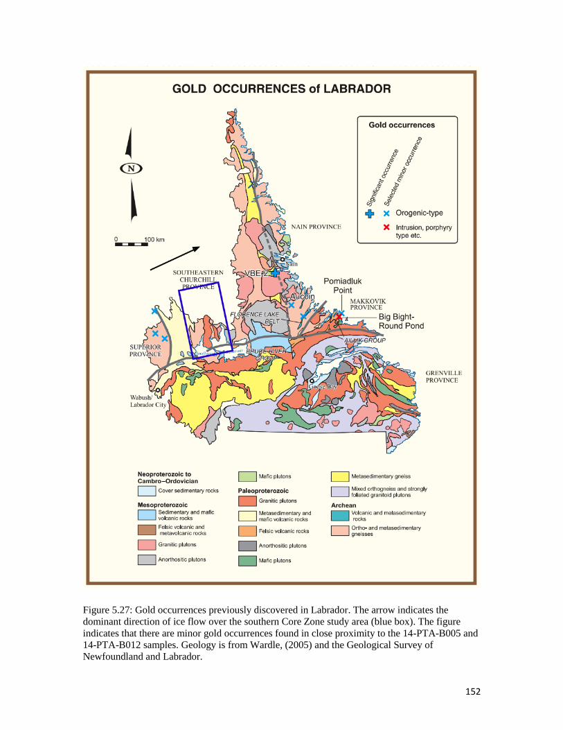
152
Figure 5.27: Gold occurrences previously discovered in Labrador. The arrow indicates the
dominant direction of ice flow over the southern Core Zone study area (blue box). The figure
indicates that there are minor gold occurrences found in close proximity to the 14-PTA-B005 and
14-PTA-B012 samples. Geology is from Wardle, (2005) and the Geological Survey of
Newfoundland and Labrador.

153
Figure 5.28: Sperrylite occurrences previously discovered in Québec (Raglan deposit) and
Labrador (Voisey’s Bay deposit). The arrow indicates the dominant ice flow direction over the
southern Core Zone study area. Map is from the Government of Canada with edits by Pickett
(2017).

154
Figure 5.29: Spatial distribution pattern for the sperrylite grains found within the 6 till samples
studied. Geology is from McClenaghan et al, (2014).
The sperrylite mineral distributions (Figure 5.29) indicate a significant amount of
sperrylite is present in the six till samples. This is unexpected as sperrylite was not found
in the 0.5-0.25 mm fraction of any of the till samples. It is suspected that the sperrylite
was introduced in the till samples by lab equipment that had been contaminated during

155
phase 2 preparation of sperrylite spiking material. The amount of sperrylite present
however does not match with order in which the samples were processed; sample 14-
PTA-R011 being processed near the end of the sample set (number 4).
Till is a sediment deposited directly by ice, which commonly has a direct
relationship with the underlying bedrock. Landform trends and bedrock striations the
transport history of the glacial activity can be determined and cross-references with the
indicator mineral patterns determined. Figures 2.6 summarized the glacial transport
directions for the region and possible flow paths for indicators in till. Samples 14-PTA-
B005 (overlies metagabbro bedrock) and 14-PTA-B012 (overlies basalt bedrock)
contained gold and other indicators of gold mineralization. Both till samples could be
derived from a greenstone-hosted gold mineralization (Robert, et al., 2007).
PGE mineralization is commonly restricted to ultramafic rock types (Yan Wang et
al., 2010). Samples 14-PTA-B006 (overlies sandstone), 14-PTA-R006 (overlies
quartzofeldspathic gneiss), 14-PTA-R011 (overlies tonalite) and 14-PTA-R029 (overlies
charnockite) all contained some evidence leading to a PGE type mineralization. The
elevated felsic abundance associated with all four rock types reduces the chances of the
PGE mineralization being directly linked to the underlying bedrock geology. This would
imply that these grains are a result of transport from a more distal region or another
source. Looking at the producing mines and potential mining projects in Québec and
Labrador, there are other PGE findings in the Core Zone region and the surrounding

156
areas. The Mesamax Northwest deposit in the Ungava region of Queébec has a sperrylite
presence (Cabri et al., 2005; McDonald et al., 2005). The deposit formed at the basal
portion of a dyke along the dyke margins. A hydroseparator HS-02 was used to separate
the heavy mineral fraction from the 0.5 kg sample studied. From this >1000 grains of
platinum group minerals were found, some of which included sperrylite. The size
fractions analyzed ranged from 180-<45 µm (Cabri et al., 2005). Similar to the Core Zone
research conducted, the Mesamax deposit also discovered sperrylite grains, along with
other PGM’s through the use of a HS. The Raglan Ni-Cu-(PGE) sulphide deposit in Cape
Smith, Québec discovered the presence of PGE’s with the most abundant PGE being
sperrylite. The Katiniq and Zone 2 orebodies of the Raglan deposit host these PGE
mineralizations (Seabrook et al., 2004) as well as the Tootoo and Mequillon magmatic
sulphide deposits in the South Ragland Trend (Liu et al., 2016). The Pt-bearing minerals
are more commonly associated with the chalcopyrite-rich ores, however only ~17.5% of
the PGM’s are recoverable as a result of the enclosure in other mineral phases (Seabrook
et al., 2004). However the sperrylite rich deposits in Québec are found more than 1000
km to the north east of the Core Zone. To the east of the Core Zone, the Voisey’s Bay Ni-
Cu-Co Ovoid magmatic sulphide deposit in Labrador has displayed unusual Pt and Pd
elevations up to 0.5 ppm in certain occurrences. These mineral occurrences are being
found in the central part of the Ovoid. The sperrylite grains at this deposit are fine
inclusions enclosed in pentlandite and galena (Kelvin et al., 2011).
Anomalously, all of the <20 µm hydroseparated case study samples except for 14-
PTA-B005 and 14-PTA-B012 contained sperrylite. Sample 14-PTA-R011 in particular

157
caused the most concern as the abundance of sperrylite found within the HMC fraction
was 21 grains. The presence of sperrylite could be attributed to two possible causes 1) a
sample contamination issue involved in our sample preparation and processing (as phase
2 used sperrylite spikes in Almonte till) or 2) the <20 µm fraction is anomalous and being
a newly analyzed size fraction, the presence of the sperrylite could be an accurate display
of the till mineralogy (Marshall, et al., 2004). Examination of the blank experimental
samples for the <20 µm fraction samples of the phase 2 portion of this study, sperrylite in
till spikes, there were remnants of sperrylite found in these blanks. This implies that the
cleaning procedures used for that phase were not reliable enough to fully remove all
sperrylite from either the sieve meshes or from another part of the sample preparation.
Additionally the contamination abundance did not correlate to the order in which samples
were processed. Thorough cleaning was completed in between all sample runs to reduce
the possibility of contamination. The 45-63 µm and 20-45 µm fractions indicate that the
cleaning methods were executed correctly, removing all contamination sources as well as
the <20 µm sample for 14-PTA-B005 and 14-PTA-B012, which did not contain any
sperrylite. The <20 µm sieves were also used on a non-PGE related projects (~2 months,
~5-10 number of samples) between the phase 2 sperrylite experiments (Chapter 4,
Section 4.2.3), and the case study experiments (Chapter 5, Section 5.2.2) implying the
sieves cannot be the source for contamination. All new sample vials were used for each
portion of the project and each sample. The HS glassware and surface area was cleaned
between each sample. The only remaining possibility for a potential source for this
mineral contamination in the <63 µm size fraction was the micro rotary riffler. The micro
rotary riffler was cleaned between each sample and separation. Visual observations were
158
made after use and prior to sample runs to ensure it was properly cleaned. The micro
rotary riffler was however used for both the phase 2 sperrylite spike as well as the case
study portions of the project and is the only possible source of cross contamination. If this
was the source for contamination, the question arises as to why did we not observe any
contamination in the corresponding 45-20 µm and 63-45 µm samples. The geochemical
data collected from fire assay on the six case study samples indicated that all the platinum
and palladium values fell below the lower detection limit except for sample 14-PTA-
R006, which contained 2 ppb palladium (Rice, et al., 2017). Based on our interpretation
the spatial distributions of the sperrylite content found in these smaller size fractions, it
seems most logical that this data is a result of a contamination issue.
Based on the data collected from the case study research the different size
fractions provide different mineralization results. As the size fraction decreased the
diversity of the mineral assemblage increased, yielding more indicator minerals. The 63-
45 µm fraction samples contained the most material to work with and were more easily
hydroseparated, mounted and analyzed with ESEM-MLA, however fewer significant
indicator data was collected. It was the <20 µm samples that produced the most
interesting data set with the least amount of material to work with. With the ability to
collect and analyze the <20 µm fraction along with having a known glacial history, the
visibility of dispersion trains can be further extrapolated and linked to potential sources.

159
5.4.4 MLA versus ODM
The HMC collected from the various forms of mineral density separation
(hydroseparation, tabling, heavy liquid separation, etc.) could be analyzed using ESEM-
MLA or through the method of hand picking grains through optical microscopy (ODM).
Grain picking becomes more challenging however, with the size fraction decreasing to
<63 µm. Both forms of processing are comparable in terms of the data collected (see
Figures 5.9-5.20). However, samples processed with MLA allow for each individual
grain to have an associated EDS spectrum, allowing for the modal classification of
minerals and the creation of elemental abundances as a whole-rock style of analysis
(Fandrich et al., 2006). Samples can be analyzed in a low vacuum mode and not carbon
coated, however it was found that the EDS counts-per-second decreased, which
producing a higher background to noise ratio. However, polished grain mounts could be
produced for these same mounts and analyzed in high vacuum mode after carbon coating
to collect higher EDS counts-per-second and better more refined EDS spectrums. By
creating polished grain mounts, indicator miners found could be further tested using the
microprobe to collect mineral chemistry of specific minerals and other features such as
mineral zoning.
Overburden Drilling Management Limited workflow is optimized for the 0.25-2.0
mm size range, and provides a detailed understanding of the modal indicator mineralogy
for samples. MLA is more efficient for analyzing the smaller fractions, <63 µm, when the
ability to see and understand grain features through optical microscopy becomes
challenging. Mineral Liberation Analysis (MLA) is also more useful when the sample

160
size if significant (i.e., <1 kg). The different size fractions provide varying results as was
determined by comparing the 63 µm (i.e., 14-PTA-B005, 63-45 versus <20 µm
indicators) fraction with the <20 µm fraction. With decreasing size the more resistant
minerals become more prevalent. This implies the data found at the 0.25-2.0 mm level
(analyzed only by optical microscopy) will vary from the data collected from the <63 µm
data (analyzed only by MLA). Optical microscopy as well as MLA are both commonly
used methods for mineral grain analysis, therefore depending on the nature of the project
either separation techniques could be used depending on the underlying needs of the
project and the size range of the grains being studied.
5.5 Conclusions
The samples used in this thesis were collected from a region, which underwent
multiple glaciation events. Due to the lack of complete knowledge of each sample and the
glacial history, a true understanding of the source of potential indicators is lacking.
However with the known glacial movements and the mineralization found in already
research parts of Labrador and Québec, conclusions have been made for the source of the
indicators found during this case study.
Comparing the data collected from ODM to the results from hydroseparation,
helps to build confidence for exploration purposes. The data sets from the Core Zone
samples, ODM processing to hydroseparation, displayed similar trends for each sample.
In using a range of different size fractions, a more complete understanding of the sample

161
as a whole could be understood. Using the indicator mineralogy determined from both
ODM and MLA in combination with the known mineral commodities in the Québec and
Labrador region, conclusions were drawn about the source of these grains and the travel
patterns. Data from ODM and the hydroseparation data for samples 14-PTA-B006, 14-
PTA-B012 and 14-PTA-R006 relate well with one another. The presence of gold found in
ODM’s samples was positively linked with the pyrite, chalcopyrite and arsenopyrite
presence found in these hydroseparated samples, providing more evidence for gold
mineralization associated with 14-PTA-B005 and 14-PTA-B012. Looking at the
distributions for the indicators found in each of these samples in comparison with the
glacial ice flow history, conclusions on the presence of gold mineralization was
confidently related back to previously gold sightings. The sperrylite data found within the
<20 µm fraction was the only outlier and source of concern. The heavy mineral
concentrate data in combination with the light fraction data did correlate for samples 14-
PTA-R006, 14-PTA-R011 and 14-PTA-R029 with the bedrock geology from which each
sample was collected. The forsterite findings in 14-PTA-R006 also matched from both
forms of heavy mineral separation, indicating the MMSIM relationship. However ODM
did not find any evidence of platinum based mineralization in these samples. Overburden
Drilling Management Limited’s findings and the HS indicator findings typically matched
when looking at the 63-45 µm and 45-20 µm sizes, it was the <20 µm samples that
varied. ODM did not look at the <63 µm size fraction however, so a comparison based on
grain size cannot be completed.
162
Chapter 6: Conclusions
6.1 Final Findings
The HS has proven to be a useful tool when trying to reduce till heavy mineral
concentrate without the use of heavy liquids. It was successfully in this study to separate
minerals based on density from the 63-45 µm and 45-20 µm heavy mineral fractions.
The <20 µm fraction was more difficult to work with and therefore the results are less
clear, causing some concerns, mainly relating to complete density separation. The larger
size fractions, 63-45 µm and 45-20 µm, were easier to work with, separate and analyze
because the grains are more visible with the naked eye, making the HS settings easier to
control for optimal recovery of the heavy fraction. The <20 µm size fraction was the most
difficult to work with due to the increased static attraction of the grains as well as the
smaller volume of sample. Hydroseparation applied to this smallest size fraction yielded
lower recovery (~50 % HMC yield, as determined from the phase 2, sperrylite spike) as
compared to the larger size fractions. The HS settings available even at the lowest
oscillation were still very powerful (removing most grains from the GST) when applied
to the smaller size fractions, making close monitoring and short run times necessary.
Without sufficient starting volume, there is a risk of losing all light and heavy fractions to
the tailings pile. Both the concentrate and tailings material is collected after each test run,
thus sample material may be re-run if necessary. It was from the <20 µm size fraction
however, that the most interesting data came from with regards to the heavy mineralogy.
Future hydroseparation research focussed on the <63 µm fraction should investigate the
use of longer and larger diameter GST tubes in order to allow for increased sample size
that can be processed by the system.

163
The advantages of the HS method include that it is quick, easy to use, and can be
used in a field setting with minimal sieving to determine the presence of indicator
minerals and the relative abundance. Disadvantages of the HS method is that it can only
process 10-20 g at a time and the density range of the minerals it can optimally
concentrate is restricted to 3 to 20 SG (Cabri et al., 2006; McClenaghan, 2011).
The HS could be used for selected samples that require further investigation of
heavy minerals, especially those <63 µm. Overburden Drilling Management Limited
however, only performs a crude visual examination of the grains <0.25 mm by panning,
which typically recovers very heavy (SG>5) minerals such as gold and platinum group
minerals.
The advantages of ESEM-MLA over visual mineralogy methods are that it can be
used to determine the mineralogy of both the >0.25 mm and <0.25 mm size fractions of
HMC and it can determine the identity of all minerals present not just those that are
visually distinct.
Comparing the ODM processing versus hydroseparation data sets for the Core
Zone till samples, similar trends are apparent for each sample. The sperrylite abundance
data found within the <20 µm fraction was the only outlier and source of concern. The
164
heavy mineral concentrate data in combination with the light fraction data did correlate
well with the bedrock geology from which each sample was collected. Using the
indicator mineralogy determined from both ODM and MLA in combination with the
known mineral commodities in the Québec and Labrador region, conclusions were drawn
about the source of these grains and the glacial transport patterns. Looking at the spatial
distributions for the indicators found in each of the samples in comparison with the
glacial ice flow history, conclusions on the presence of gold mineralization was
confidently related back to previously gold sightings from the western part of Labrador.
The presence of sperrylite in the Core Zone till samples is likely a result of contamination
from the micro rotary riffler used on the <20 µm sperrylite sample from phase 2. New
cleaning procedures are highly recommended. Cleaning sand could be used in between
each sample, with the use of compressed air to clean out small grooves after washing.
These new methods could reduce the contamination issue and help to ensure the micro
rotary riffler is properly cleaned in between each sample set.
The presence of sperrylite-bearing magmatic Ni-Cu deposits are known in Québec
and Labrador, e.g., the Raglan deposit in northern Québec and Voisey’s Bay deposit in
Labrador. It is possible that other unknown Ni-Cu occurrences are present within or
proximal to the Core Zone samples studied here. However, the pervasive and high
content of sperrylite in four of the six Core Zone till samples regardless of the proximity
to ultramafic rocks indicates that contamination during samples processing during this
study is the likely source.

165
6.2 Future Work
The HS settings for processing the <20 µm fraction of till samples needs to be
further tested for different mineral densities. The data collection for the smaller size
fraction was more accurately applied to the case study samples which consisted of larger
sample sizes and mixed mineralogy. The phase 1 and phase 2 testing however, which
worked with significantly smaller sample sizes required more work to allow for a better
overall recovery of these small size fractions. Reducing the flow rate and mode applied to
the smaller size fractions could increase the overall recovery of HMC. Producing a range
of settings that can be applied to different minerals based on density would be more
beneficial for future studies. Once these settings have been accurately determined, they
could be geared to retain specific minerals depending on the deposit being studied.
For future studies the <63 µm fraction could be include the entire 63-<20 µm
range (without the 3 sub size fractions) to determine the hydroseparators ability to retain
representative HMC from a wider range of mineral grains. If successful, this could reduce
the amount of time to prepare the <63 µm fraction (less sieving) prior to hydroseparation.
Comparison of results from this study could be applied to determine the success of this
idea.
The remainder of each of the case study, concentrate sample material (~5-10
grams per sample), or true representative splits for each size fraction should be mounted
and analyzed using MLA. Analyzing a representative split of each concentrate would

166
allow for a more accurate representation of the sample modal HMC and relative indicator
abundance for each location. This would also provide a more accurate comparison of the
different size fractions HMC content.
A study conducted by the Geological Survey of Finland concluded that individual
mounts with up to 10, 000s of grains could be representative of an entire till sample. A
comparison test could be completed by mounting half of the sample material using epoxy
mounts, running MLA on high vacuum and the other half of the material on the carbon
tape disks, running MLA on low vacuum, similarly to what was carried out at the
Geological Survey of Finland (Lehtonen et al., 2015). This comparison test would display
any discrepancies based on mount type and provide a more detailed understanding of
how low vacuum compares to a high vacuum sample runs.
Finally, more samples collected from the Core Zone region could be analyzed
using the HS to examine the <63 µm fraction. These new data contribute to the
understanding of the regional glacial dispersal patterns. Analyzing samples in proximal
locations to that of the six samples already studied would help to determine connections
between the different sample localities and bedrock geology.

167
References
“2015 Annual Report of Drinking Water Quality.” Large Municipal Residential.
Kingston, Ontario: King St. Water Treatment Plant, City of Kingston, December 1, 2015.
Amor, Steve. “An Overview of Geochemical Methods.” presented at the CIM Short
Course, Geological Survey of Newfoundland and Labrador, 2013.
Antonio, Celis. “Titanite as an Indicator Mineral for Alkalic Porphyry Cu-Au Deposits in
South-Central British Columbia.” BSc. Thesis, University of British Columbia, 2010.
Aucoin, Martin, Georges Beaudoin, Robert A. Creaser, and Paul Archer. “Metallogeny of
the Marco Zone, Corvet Est, Disseminated Gold Deposit, James Bay, Québec, Canada.”
Canadian Journal of Earth Sciences 49, no. 10 (October 2012): 1154.
Averill, S. A. “Viable Indicator Minerals in Surficial Sediments for Two Major Base
Metal Deposit Types: Ni-Cu-PGE and Porphyry Cu.” Geochemistry: Exploration,
Environment, Analysis 11, no. 4 (November 1, 2011): 279–91.
https://doi.org/10.1144/1467-7873/10-IM-022.
Averill, S.A. “Short Course on Implications of Quaternary Geology for Mineral
Exploration.” In Drilling, Sampling and Sample Processing Methods for Deep Till
Geochemistry Surveys: Making the Right Choices, 1990.

168
Averill, Stuart A. “The Application of Heavy Indicator Mineralogy in Mineral
Exploration with Emphasis on Base Metal Indicators in Glaciated Metamorphic and
Plutonic Terrains.” Geological Society, London, Special Publications 185, no. 1 (January
1, 2001): 69–81. https://doi.org/10.1144/GSL.SP.2001.185.01.04.
Belousova, E.A., W.L. Griffin, S.Y. O’Reilly, and N.I. Fisher. “Apatite as an Indicator
Mineral for Mineral Exploration: Trace-Element Compositions and Their Relationship to
Host Rock Type.” Journal of Geochemical Exploration 76, no. 1 (2002): 45–69.
https://doi.org/10.1016.
Brushett, D. “Reconnaissance Sampling for Diamond-Indicator Minerals from Esker,
Western Labrador.” Current Research. Newfoundland and Labrador Department of
Natural Resources, Geological Survey, 2013.
Cabri, L. J., A. M. McDonald, C. J. Stanley, N. S. Rudashevsky, G. Poirier, B. R.
Durham, J. E. Mungall, and V. N. Rudashevsky. “Naldrettite, Pd2Sb, a New Intermetallic
Mineral from the Mesamax Northwest Deposit, Ungava Region, Québec, Canada.”
Mineralogical Magazine 69, no. 1 (2016): 89–97.
https://doi.org/10.1180/0026461056910236.
Cabri, Louis, Vladimir Rudashevsky, and R Lastra. Hydroseparation: “A New
Development in Process Mineralogy of Platinum-Bearing Ores” 99, 2006.
169
Cabri, Louis J. “Electric-Pulse Disaggregation (Epd), Hydroseparation (Hs) and Their
Use in Combination for Mineral Processing and Advanced Characterization of Ores”.
40th Annual Meeting of the Canadian Mineral Processors, 2008
Cabri, Louis J., Donald C. Harris, and Thorolf W. Weiser. “Mineralogy and Distribution
of Platinum-Group Mineral (PGM) Placer Deposits of the World.” Exploration and
Mining Geology 2, no. 5 (1996): 73–167.
Cabri, Louis, Vladimir Rudashevsky, and R Lastra. Hydroseparation: A New
Development in Process Mineralogy of Platinum-Bearing Ores. Vol. 99, 2006.
Callahan, John. “A Nontoxic Heavy Liquid and Inexpensive Filters for Separation of
Mineral Grains: RESEARCH METHOD PAPER.” Journal of Sedimentary Research 57,
no. 4 (1987). http://archives.datapages.com/data/sepm/journals/v55-
58/data/057/057004/0765.htm.
Calle, C.I., J.L. McFall, C.R. Buhler, S.J. Snyder, E.E. Arens, A. Chen, M.L. Ritz, J.S.
Clements, C.R. Fortier, and S. Trigwell. “Dust Particle Removal by Electorstaticand
Dielectrophoretic Forces with Applications to NASA Exploration Missions.” In ESA
Annual Meeting on Electrostatics, 2008.

170
Cameron, Eion M., Stewart M. Hamilton, Matthew I. Leybourne, Gwendy E. M. Hall,
and M. Beth McClenaghan. “Finding Deeply Buried Deposits Using Geochemistry.”
Geochemistry: Exploration, Environment, Analysis 4, no. 1 (February 1, 2004): 7–32.
https://doi.org/10.1144/1467-7873/03-019.
Corrigan, D., D. Van Rooyen, A. Morin, M.G. Houlé, and V.J. McNicoll. “Report of
Activities for the Core Zone and Bounding Orogens: The New Québec Orogen and Its
Relationship with the Core Zone in the Kuujjuaq Area.” Geological Survey of Canada
Open File 7962 (2015). https://doi.org/10.4095/297404.
Corriveau, L., O. Nadeau, J.F. Montreuil, and J.P. Desrochers. “Report of Activities for
the Core Zone: Strategic Geomapping and Geoscience to Assess the Mineral Potential of
the Labrador Trough for Multiple Metals IOCG and Affiliated Deposits, Canada.”
Geological Survey of Canada Open File 7714 (2014). https://doi.org/10.4095/295529.
“Crushers Pulverizers: Manufacturers of Mingins and Geological Laboratory Test
Equipment.” BICO braun international, n.d.
Cummings, Don I., Bruce A. Kjarsgaard, Hazen A. J. Russell, and David R. Sharpe.
“Eskers as Mineral Exploration Tools.” Earth-Science Reviews 109, no. 1 (November 1,
2011): 32–43. https://doi.org/10.1016/j.earscirev.2011.08.001.

171
Dare, Sarah A. S., Sarah-Jane Barnes, and Hazel M. Prichard. “The Distribution of
Platinum Group Elements (PGE) and Other Chalcophile Elements among Sulfides from
the Creighton Ni–Cu–PGE Sulfide Deposit, Sudbury, Canada, and the Origin of
Palladium in Pentlandite.” Mineralium Deposita 45, no. 8 (December 1, 2010): 765–93.
https://doi.org/10.1007/s00126-010-0295-6.
Debele, D., C. Koeberl, and F.J. Kruger. “Geochemistry and Ore Genesis of Probably
Gold-Bearing Rocks, Okote and Moyale Areas, Southern Ethiopia.” Goldschmidt
Conference Toulouse, 1998.
Dilabio, R.N.W. “Classification and Interpretation of the Shapes and Surface Textures of
Gold Grains from Till on the Canadian Shield.” Geological Survey of Canada, 1990.
http://geoscan.nrcan.gc.ca/starweb/geoscan/servlet.starweb?path=geoscan/fulle.web&sear
ch1=R=131269.
“Drinking Water Hardwater Hardness Calcium Magnesium Scale Stained Laundry.”
http://www.water-research.net/index.php/water-treatment/tools/hard-water-hardness.
Dyke, Arthur S., and Victor K. Prest. “Late Wisconsinan and Holocene History of the
Laurentide Ice Sheet.” Géographie Physique et Quaternaire 41 (1987): 237–63.
Ehlers, J., and P. L. Gibbard. Quaternary Glaciations - Extent and Chronology: Part II:
North America. Elsevier, 2004.

172
Emslie, R. F., M. A. Hamilton, and R. J. Thériault. “Petrogenesis of a Mid-Proterozoic
Anorthosite-Mangerite-Charnockite-Granite (AMCG) Complex: Isotopic and Chemical
Evidence from the Nain Plutonic Suite.” The Journal of Geology 102, no. 5 (September
1994): 539–58. https://doi.org/10.1086/629697.
English, B.L., G.A. Desborough, and W.H. Raymond. “A Mechanical Panning Technique
for Separation of Fine-Grained Gold and Other Heavy Minerals.” USGS Numbered
Series. Open-File Report. U.S. Geological Survey, 1987.
http://pubs.er.usgs.gov/publication/ofr87364.
Erlich, Edward, and W. Dan Hausel. “Diamond Deposits: Origin, Exploration, and
History of Discovery” SME, 2002.
Falconer, Andrew. “Gravity Separation: Old Technique/New Methods.” Physical
Separation in Science and Engineering 12, no. 1 (2003): 31–48. https://doi.org/10.1080.
Faulkner. “Introduction to Prospecting.” Geological Survey Branch, no. 0226–9430
(April 1986).
http://www.empr.gov.bc.ca/Mining/Geoscience/PublicationsCatalogue/Papers/Pages/198
6-4.aspx.

173
Fletcher, W. K., and C. H. Loh. “Transport of Cassiterite in a Malaysian Stream:
Implications for Geochemical Exploration.” Journal of Geochemical Exploration,
Geochemical Exploration 1995, 57, no. 1 (December 1, 1996): 9–20.
https://doi.org/10.1016/S0375-6742(96)00012-X.
Fulton, R.J. “Quaternary Geology of the Ottawa Region, Ontario and Québec.”
Geological Survey of Canada 86, no. 23 (1987).
Gadd, Michael G. “Reinterrpretation of the Ambient Paleoenvironmental Redox
Conditions and Timing of Mineralization at sedexZn-PB Deposits in the Howards Pass
District, Yukon.” MSc. Thesis, Queen’s University, 2015.
Galley, Alan G., Mark D. Hannington, and Ian R. Jonasson. “Volcanogenic Massive
Sulphide Deposits.” Goodfellow, W.D., Ed., Mineral Deposits of Canada: A Synthesis of
Major Deposit-Types, District Metallogeny, the Evolution of Geological Provinces, and
Exploration Methods: Geological Association of Canada, Mineral Deposits Devision,
Special Publication, no. 5 (2007): 141–61.
Groves, David I., Frank P. Bierlein, Lawrence D. Meinert, and Murray W. Hitzman.
“Iron Oxide Copper-Gold (IOCG) Deposits through Earth History: Implications for
Origin, Lithospheric Setting, and Distinction from Other Epigenetic Iron Oxide
Deposits.” Economic Geology 105, no. 3 (May 1, 2010): 641–54.
https://doi.org/10.2113/gsecongeo.105.3.641.

174
Groves, David I., Richard J. Goldfarb, François Robert, and Craig J.R. Hart. “Gold
Deposits in Metamorphic Belts: Overview of Current Understandings, Outstanding
Problens, Future Research, and Exploration Significance.” Economic Geology 98 (2003):
1–29.
Groves, D.I., R.J. Goldfarb, M Gebre-Mariam, S.G. Hagemann, and F. Robert. “Orogenic
Gold Deposits: A Proposed Classification in the Context of Their Crustal Distribution
and Relationship to Other Gold Deposit Types.” Ore Geology Reviews 13 (1998): 7–27.
Hannington, Mark D, and C. Tucker Barrie. “The Giant Kidd Creek Volcanogenic
Massive Sulfide Deposit: Western Abitibi Subprovince, Canada” Littleton, CO:
Economic Geology Pub., 1999. http://ebooks.geoscienceworld.org/content/the-giant-
kidd-creek-volcanogenic-massive-sulfide-deposit-western-abitibi-subprovince-canada.
Hareland, G.A. “Evaluation of Flour Particle Size Distribution by Laser Diffraction,
Sieve Analysis and Near-Infrared Reflectance Spectroscopy.” Journal of Cereal Science
20, no. 2 (1994): 183–90. https://doi.org/10.1006.
Hashmi, Sarah. “Quaternary Geology and Drift Prospecting in the Mount Polley Region
(NTS 093A).” BSc. Thesis, Univeristy of Waterloo, 2012.
“Heavy Minerals Processing and Picking.” Overburden Drilling Management Ltd, 2006.
175
Henderson, J. H., R. N. Clayton, M. L. Jackson, J. K. Syers, R. W. Rex, J. L. Brown, and
I. B. Sachs. “Cristobalite and Quartz Isolation from Soils and Sediments by
Hydrofluosilicie Acid Treatment and Heavy Liquid Separation.” Soil Science Society of
America Journal 36, no. 5 (10/01 1972): 830–35.
https://doi.org/10.2136/sssaj1972.03615995003600050038x.
Hermes, O. Don. “Petrology of the Mecklenburg Gabbro-Metagabbro Complex, North
Carolina.” Contributions to Mineralogy and Petrology 18, no. 3 (May 1, 1968): 270–94.
https://doi.org/10.1007/BF00398896.
Hicken, Anna. “Glacial Dispersal of Indicator Minerals from the Izok Lake Zn-Cu-Pb-Ag
VMS Deposit, Nunavut, Canada,” 2012.
https://qspace.library.queensu.ca/handle/1974/6998.
Jordens, Adam, Richard S. Sheridan, Neil A. Rowson, and Kristian E. Waters.
“Processing a Rare Earth Mineral Deposit Using Gravity and Magnetic Separation.”
Minerals Engineering, SI: Physical Separation, 62 (July 1, 2014): 9–18.
https://doi.org/10.1016/j.mineng.2013.09.011.
Keck, W.E. “Process of Separating Valuable Materials from Grinding Dusts and
Sludges,” 1947.
176
Kelley, K. D., R. G. Eppinger, J. Lang, S. M. Smith, and D. L. Fey. “Porphyry Cu
Indicator Minerals in till as an Exploration Tool: Example from the Giant Pebble
Porphyry Cu-Au-Mo Deposit, Alaska, USA.” Geochemistry: Exploration, Environment,
Analysis 11, no. 4 (November 1, 2011): 321–34. https://doi.org/10.1144/1467-7873/10-
IM-041.
Kerr, A. “Mineral Commodities of Newfoundland and Labrador NICKEL.” Geological
Survey Commodities Series. Natural Resources, Mines Branch, 2000.
“Kimberlite Indicator Mineral Chemistry of the Bucke and Gravel Kimberlites and
Associated Indicator Minerals in Till, Lake Timiskaming, Ontario.” Geological Survey of
Canada Open File 5815 (2012): 30. https://doi.org/10.4095/289599.
Layton-Matthews, D, C. Hamilton, and M.B. McClenaghan. “Mineral Chemistry:
Modern Techniques and Applications to Exploration.” Geological Survey of Canada
Open File 7553 (2014).
Lehtonen, M.L., Y Lahaye, H O’Brien, S. Lukkari, J.S. Marmo, and P. Sarala. “Novel
Technologies for Indicator Mineral-Based Exploration.” Geological Survey of Finland 57
(2015): 23–62.

177
Lehtonen, M.L., J.S. Marmo, A.J. Nissinen, B.S. Johanson, and L.K. Pakkanen. “Glacial
Dispersal Studies Using Indicator Minerals and till Geochemistry around Two Eastern
Finland Kimberlites.” Journal of Geochemical Exploration 87 (2005): 19–43.
https://doi.org/http://dx.doi.org/10.1016/j.gexplo.2005.07.003.
Li, Chusi, and Edward M Ripley. “Magmatic Ni-Cu and PGE Deposits: Geology,
Geochemistry, and Genesis” 2011. http://ebooks.geoscienceworld.org/content/magmatic-
ni-cu-and-pge-deposits.
Mackay, D.A.R, G.J. Simandl, P. Luck, B. Grcic, C. Li, M. Redfearn, and J. Gravel.
“Concentration of Carbonatite Indicator Minerals Using a Wilfley Gravity Shaking
Table: A Case History from the Aley Carbonatite, British Columbia, Canada.”
Geological Fieldwork (2014) 1 (2015).
MacLean, Brian, Gustav Vilks, and Bhan Deonarine. “Depositional Environments and
History of Late Quaternary Sediments in Hudson Strait and Ungava Bay: Further
Evidence from Seismic and Biostratigraphic Data.” Géographie Physique et Quaternaire
46, no. 3 (1992): 311–29. https://doi.org/10.7202/032917ar.
MacQuarrie, R.R. “Reconnaissance Bedrock Geology: Wollaston Lake Northeast Area
(Part of NTS 64L),” 1980.

178
Marzouki, F. M. H., N. J. Jackson, C. R. Ramsay, and D. P. F. Darbyshire. “Composition,
Age and Origin of Two Proterozoic Diorite—tonalite Complexes in the Arabian Shield.”
Precambrian Research 19, no. 1 (August 1, 1982): 31–50. https://doi.org/10.1016/0301-
9268(82)90018-3.
McClenaghan, Beth. “Indicator Mineral Methods in Mineral Exploration.” Geological
Scoiety of London, Geochemistry: Exploration, Environment, Analysis, 5 (2005): 233–
245.
McClenaghan, Beth M., and Louis J. Cabri. “Review of Gold and Platinum Group
Element (PGE) Indicator Minerals Methods for Surficial Sediment Sampling.”
Geochemistry Exploration Environment Analysis 11, no. 4 (2011): 251–264.
McClenaghan, Beth M., R.C. Paulen, J.M. Rice, H.E. Campbell, and M. D. Pyne. “Gold
Grains in till Samples from the Southern Core Zone, Québec and Newfoundland and
Labrador (NTS 23-P and 23-I): Potential for Undiscovered Mineralization.” Geological
Survey of Canada Open File 8222 (2017): 1–21. https://doi.org/10.4095.
McClenaghan, M. B., R. C. Paulen, D. Layton-Matthews, A. K. Hicken, and S. A.
Averill. “Glacial Dispersal of Gahnite from the Izok Lake Zn-Cu-Pb-Ag VMS Deposit,
Northern Canada.” Geochemistry: Exploration, Environment, Analysis 15, no. 4
(November 1, 2015): 333–49. https://doi.org/10.1144/geochem2014-317.
179
McClenaghan, M. Beth. “Overview of Common Processing Methods for Recovery of
Indicator Minerals from Sediment and Bedrock in Mineral Exploration.” Geochemistry:
Exploration, Environment, Analysis 11, no. 4 (November 1, 2011): 265–78.
https://doi.org/10.1144/1467-7873/10-IM-025.
McClenaghan, Margaret Beth, P.T. Bobrowsky, G.E.M. Hall, and Cook. Drift
Exploration in Glaciated Terrain. Vol. 185. The Geological Society, 2001.
McClenaghan, M.B., S.A. Averill, I.M. Kjarsgaard, D Layton-Matthews, and G Matile.
“Till Indicator Mineral and Geochemical Signatures of Magmatic Ni-Cu Deposits,
Thompson Nickel Belt, Central Canada.” Proceedings of the 24th Internation Applied
Geochemistry Symposium 1 (2009): 75–78.
McClenaghan, M.B., R.C. Paulen, and J.M. Rice. “Indicator Mineral Abundance Data for
till Samples Form the South Core Zone, Québec and Labrador (NTS 23-P and 23-I):
Samples Collected in 2014.” Geological Survey of Canada Open File 7968 (2016): 13.
https://doi.org/10.4095/297379.
McClenaghan, M.B., R.C. Paulen, J.M. Rice, M.W. McCurdy, S.D. Amor, R.G. Garrett,
F Solgadi, et al. “GEM 2 Hudson-Ungava Project 2016 Report of Activities for the Core
Zone: Surficial Geology, Geochemistry, and Gamma-ray Spectrometry Studies in
Northern Québec and Labrador.” Geological Survey of Canada Open File 8148 (2016):
26.
180
McClenaghan, M.B., R.C. Paulen, J.M. Rice, M.W. McCurdy, R Fortin, W.A. Spirito,
S.W. Adcock, et al. “Report of Activities for the Core Zone: 2015 Surficial Geology,
Geochemistry, and Gamma-Ray Spectrometry Studies in Northern Québec and
Labrador.” Natural Resources Canada, Geological Survey of Canada, Open File 7946,
2015.
McClenaghan, M.B., R.C. Paulen, M. Sanborn-Barrie, M.W. McCurdy, W.A. Spirito,
S.W. Adcock, J.J. Veillette, et al. “GEM 2 Hudson-Ungava Project: Southern Core Zone
Surficial Geology, Geochemsitry, and Bedrock Mapping Activities in Northern Québec
and Labrador.” Geological Survey of Canada Open File 7705 (2014).
https://doi.org/10.4095/295521.
McClenaghan, M.B., A. Plouffe, and D. Layton-Matthews. “Application of Indicator
Minerl Methods to Mineral Exploration.” Geological Survey of Canada, Open File 7553,
2014, 1–74. https://doi.org/10.4095/293858.
McClenaghan, M.B., A. Plouffe, R.C. Paulen, M.G. Houlé, S.E. Jackson, and J.M. Peter.
“Overview of Indicator Mineral Research at the Geological Survey of Canada - An
Update.” Geological Survey of Canada, 2016, 170 edition.
181
McClenaghan, Beth M., A. Plouffe, I. McMartin, J.E. Campbell, W.A. Spirito, R.C.
Paulen, R.G. Garrett, and G.E.M. Hall. “Till Sampling and Geochemical Analytical
Protocols Used by the Geological Survey of Canada.” Geochemistry: Exploration,
Environment, Analysis 13 (2013): 285–301. https://doi.org/10.1144/geochem2011-083.
McClenaghan, M.B., Brent Ward, Ingrid Kjarsgaard, B A. Kjarsgaard, D E. Kerr, and
Lynda Dredge. “Indicator Mineral and till Geochemical Dispersal Patterns Associated
with the Ranch Lake Kimberlite, Lac de Gras Region, NWT, Canada.” Geochemistry-
Exploration Environment Analysis - GEOCHEM-EXPLOR ENVIRON ANAL 2
(November 1, 2002): 299–319. https://doi.org/10.1144/1467-787302-004.
McDonald, Andrew M., Louis J. Cabri, Christopher J. Stanley, Nikolay S. Rudashevsky,
Glenn Poirier, James E. Mungall, Kirk C. Ross, Bruce R. Durham, and Vladimir N.
Rudashevsky. “UNGAVAITE, Pd4Sb3, A NEW INTERMETALLIC MINERAL
SPECIES FROM THE MESAMAX NORTHWEST DEPOSIT, UNGAVA REGION,
QUÉBEC, CANADA: DESCRIPTION AND GENETIC IMPLICATIONS.” The
Canadian Mineralogist 43, no. 5 (October 1, 2005): 1735–44.
https://doi.org/10.2113/gscanmin.43.5.1735.
McMartin, Isabelle, and Beth M. McClenaghan. “Till Geochemistry and Sampling
Techniques in Glaciated Shield Terrain: A Review.” Drift Exploration in Glaciated
Terrain. Geological Society, London, vol. 185, 2001, pp. 19–43.

182
“Mercury Cycling In Perennially Frozen Soils Of Arctic Canada, Kaminak Lake Area,
Nunavut.”
https://www.researchgate.net/publication/2471400_Mercury_Cycling_In_Perennially_Fr
ozen_Soils_Of_Arctic_Canada_Kaminak_Lake_Area_Nunavut.
Michelson, David M., and Patrick M. Colgan. “The Southern Laurentide Ice Sheet.”
Development in Quaternary Science 1 (2003): 1–16. https://doi.org/10.1016/S1571-
0866(03)01001-7.
Mickelson, David M., and Patrick M. Colgan. “The Southern Laurentide Ice Sheet.”
Developments in Quaternary Sciences, The Quaternary Period in the United States, 1
(January 1, 2003): 1–16. https://doi.org/10.1016/S1571-0866(03)01001-7.
“Mineral Exploration Methods in Glaciated Terrain.” ResearchGate.
https://www.researchgate.net/project/Mineral-exploration-methods-in-glaciated-terrain.
Misra, Kula. Understanding Mineral Deposits. Kluwer Academic Publishers, 2000.
Montreuil, J.-F., L. Corriveau, and E. C. Grunsky. “Compositional Data Analysis of
Hydrothermal Alteration in IOCG Systems, Great Bear Magmatic Zone, Canada: To
Each Alteration Type Its Own Geochemical Signature.” Geochemistry: Exploration,
Environment, Analysis 13, no. 4 (November 1, 2013): 229–47.
https://doi.org/10.1144/geochem2011-101.
183
Morris, T.F., and C.A. Kaszycki. “Prospector’s Guide to Drift Prospecting for Diamons
Northern Ontario.” Ontrio Geological Survey, no. 167 (1997).
Nagel, Thorsten J., J. Elis Hoffmann, and Carsten Münker. “Generation of Eoarchean
Tonalite-Trondhjemite-Granodiorite Series from Thickened Mafic Arc Crust.” Geology
40, no. 4 (April 1, 2012): 375–78. https://doi.org/10.1130/G32729.1.
Occhietti, Serge, E Govare, R Klassen, M Parent, and J.-S Vincent. “Late Wisconsinan -
Early Holocene Deglaciation of Québec-Labrador,” 243–73. Elsevier B.V., 2004.
Odigi, Minapuye I., and Levi C. Amajor. “Petrology and Geochemistry of Sandstones in
the Southern Benue Trough of Nigeria: Implications for Provenance and Tectonic
Setting.” Chinese Journal of Geochemistry 27, no. 4 (December 1, 2008): 384–94.
https://doi.org/10.1007/s11631-008-0384-8.
Paulen, R.C., and M.B. McClenaghan. “New Frontier for Exploration in Glaciated
Terrain.” Natural Resources Canada, Geological Survey of Canada, Open File 7374,
2013.
Paulen, Roger. “The GEM-2 Hudson-Ungava Project: Core Zone Surficial Mapping in
Support of Exploration and Discovery, Québec and Labrador.” Conference presented at
the Québec Mines, November 20, 2016.
184
Pilote, Jean-Luc, Stephen J. Piercey, Stefanie M. Brueckner, and David Grant.
“Resolving the Relative Timing of Au Enrichment in Volcanogenic Massive Sulfide
Deposits Using Scanning Electron Microscopy-Mineral Liberation Analyzer: Empirical
Evidence from the Ming Deposit, Newfoundland, Canada | Economic Geology.” Society
of Economic Geologists, Inc. 111 (June 17, 2016): 1495–1508. https://doi.org/10.2113.
“Processing of Glacial Sediments for the Recovery of Indicator Minerals: Protocols Used
at the Geological Survey of Canada (PDF Download Available).”
https://www.researchgate.net/publication/266017591_Processing_of_glacial_sediments_f
or_the_recovery_of_indicator_minerals_Protocols_used_at_the_Geological_Survey_of_
Canada.
Pufahl, P. K., S. L. Anderson, and E. E. Hiatt. “Dynamic Sedimentation of
Paleoproterozoic Continental Margin Iron Formation, Labrador Trough, Canada:
Paleoenvironments and Sequence Stratigraphy.” Sedimentary Geology 309 (July 15,
2014): 48–65. https://doi.org/10.1016/j.sedgeo.2014.05.006.
Rajesh, H. M., and M. Santosh. “Charnockites and Charnockites.” Geoscience Frontiers,
Charnockites and Charnockites, 3, no. 6 (November 1, 2012): 737–44.
https://doi.org/10.1016/j.gsf.2012.07.001.

185
Rice, J.M., B.M. McClenaghan, R.C. Paulen, M.D. Pyne, and M.A. Ross. “Till
Geochemistry Data for the Southern Core Zone, Quebec and Newfoundland and
Labrador (NTS 23-P and 23-I): Samples Collected in 2015 and 2016.” Geological Survey
of Canada Open File 8219 (2017). https://doi.org/https://doi.org/10.4095/304280.
Robert, F., R. Brommecker, B.T. Bourne, P.J. Dobak, C.J. McEwan, R.R. Rowe, and X.
Zhou. “Models and Exploration Methods for Major Gold Deposit Type.” In Proceedings
of Exploration 07: Fifth Decennial International Conference on Mineral Exploration,
691–711, 2007.
Rogers, N. “Targeted Geoscience Initiative 2016 Report of Activities.” Geological
Survey of Canada Open File 8199 (2017). https://doi.org/10.4095/299573.
Rueslåtten, Håkon. “Weathering and Mineral Equilibria.” Seminar, 2016.
Ruiz-Martínez, Gabriel, Germán Daniel Rivillas-Ospina, Ismael Mariño-Tapia, and
Gregorio Posada-Vanegas. “SANDY: A Matlab Tool to Estimate the Sediment Size
Distribution from a Sieve Analysis.” Computers & Geosciences 92, no. Supplement C
(July 1, 2016): 104–16. https://doi.org/10.1016/j.cageo.2016.04.010.
186
Rusk, Brian. “Exploring for Iron Oxide Copper-Gold Deposits: Canada and Global
Analogues. Geological Association of Canada Short Course Notes 20.” Economic
Geology 107, no. 5 (August 1, 2012): 1077–1077.
https://doi.org/10.2113/econgeo.107.5.1077.
Ryan, Bruce. “Regional Geology of the Central Part of the Central Mineral Belt,
Labrador.” Mineral Development Division Department of Mines and Energy Government
of Newfoundland and Labrador, 1984.
Sanborn-Barrie, M., N.M. Rayner, and A. Lion. “Report of Activities for the 2015
Bedrock Component of the GEM Southern Core Zone Activity, Northern Québec and
Labrador.” Geological Survey of Canada Open File 7952 (2015).
https://doi.org/10.4095/297271.
Sand and Sandstone | F. J. Pettijohn | Springer.
//www.springer.com/gp/book/9780387963501.
Sappin, A.- A., C. Dupuis, G. Beaudoin, M. Pozza, I. McMartin, and M. B.
McClenaghan. “Optimal Ferromagnetic Fraction in till Samples along Ice-Flow Paths:
Case Studies from the Sue-Dianne and Thompson Deposits, Canada.” Geochemistry:
Exploration, Environment, Analysis 14, no. 4 (October 9, 2014): 315–29.
https://doi.org/10.1144/geochem2013-212.

187
Seabrook, Charlie L., Hazel M. Prichard, and Peter C. Fisher. “PLATINUM-GROUP
MINERALS IN THE RAGLAN Ni–Cu–(PGE) SULFIDE DEPOSIT, CAPE SMITH,
QUÉBEC, CANADA.” The Canadian Mineralogist 42, no. 2 (April 1, 2004): 485–97.
https://doi.org/10.2113/gscanmin.42.2.485.
Silva, Michael. Placer Gold Recovery Methods. California department of conservation
division of mines and geology, 1986.
Stoll, W. C. “Tertiary Channel Gold Deposits at Tipuani, Bolivia.” Economic Geology
56, no. 7 (November 1, 1961): 1258–64. https://doi.org/10.2113/gsecongeo.56.7.1258.
Storey, C. D., and M. P. Smith. “Metal Source and Tectonic Setting of Iron Oxide-
Copper-Gold (IOCG) Deposits: Evidence from an in Situ Nd Isotope Study of Titanite
from Norrbotten, Sweden.” Ore Geology Reviews, New advances in trace element
geochemistry of ore minerals and accessory phases, 81, Part 4 (March 2017): 1287–1302.
https://doi.org/10.1016/j.oregeorev.2016.08.035.
Sugasawa, Hirosuke, and Hideto Yoshida. “Estimation of Particle Size Distribution
Using the Sedimentation Method Enhanced by Electrical-Potential.” Separation and
Purification Technology 187 (2017): 193–98. https://doi.org/10.1016.
“The Quartz Page: Chemical Properties.” http://www.quartzpage.de/gen_chem.html.

188
“Till Sampling and Geochemical Analytical Protocols Used by the Geological Survey of
Canada (PDF Download Available).” ResearchGate.
https://www.researchgate.net/publication/266019263_Till_sampling_and_geochemical_a
nalytical_protocols_used_by_the_Geological_Survey_of_Canada.
“Till Sampling in the Casa-Berardi Gold Area, Québec: A Case History in Orientation
and Discovery - ScienceDirect.”
http://www.sciencedirect.com.proxy.queensu.ca/science/article/pii/0375674287900549.
Wang, Christina Yan, Mei-Fu Zhou, and Liang Qi. “Origin of Extremely PGE-Rich
Mafic Magma System: An Example from the Jinbaoshan Ultramafic Sill, Emeishan
Large Igneous Province, SW China.” Lithos, The Emeishan large igneous province:
Advances in the stratigraphic correlations and petrogenetic and metallogenic models,
119, no. 1–2 (September 2010): 147–61. https://doi.org/10.1016/j.lithos.2010.07.022.
Wardle, R.J. “Mineral Commodities of Newfoundland and Labrador GOLD.” Geological
Survey Mineral Commodities Series. Natural Resources, Mines Branch, 2005.
Wardle, R.J., and J. Pollock. “Mineral Commodities of Newfoundland and Labrador
COPPER.” Geological Survey Commodities Series. Natural Resources, Mines Branch,
2005.

189
Williams, M. L., G. Dumond, K. Mahan, S. Regan, and M. Holland. “Garnet-Forming
Reactions in Felsic Orthogneiss: Implications for Densification and Strengthening of the
Lower Continental Crust.” Earth and Planetary Science Letters 405 (November 1, 2014):
207–19. https://doi.org/10.1016/j.epsl.2014.08.030.

190
Appendix A
This section contains photos and documentation of the samples obtained and used for
phase 2 and phase 3 of this thesis (Figure A1-A11).
Figure A1: Almonte till packets that were used in the Phase 2, sperrylite spike phase, obtained
from ODM.
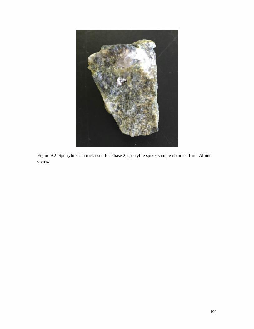
191
Figure A2: Sperrylite rich rock used for Phase 2, sperrylite spike, sample obtained from Alpine
Gems.

192
Figure A3: The sperrylite rich rock was crushed using the SelFrag in QFIR at Queen’s University
and then hydroseparated to produce a sperrylite concentrate. A) crushed rock before
hydroseparation; B) concentrated sperrylite after hydroseparation; C) concentrated sperrylite
contains some impurities which were removed by hand under optical microscope.
A B
C ImpuritiesSperrylite

193
Figure A4: The hydroseparated sperrylite concentrate was then ground to produce a finer fraction.

194
Figure A5: Sample 14-PTA-B005 -0.25mm non-magnetic HMC fraction.

195
Figure A6: Sample 14-PTA-B006 -0.25mm non-magnetic HMC fraction.
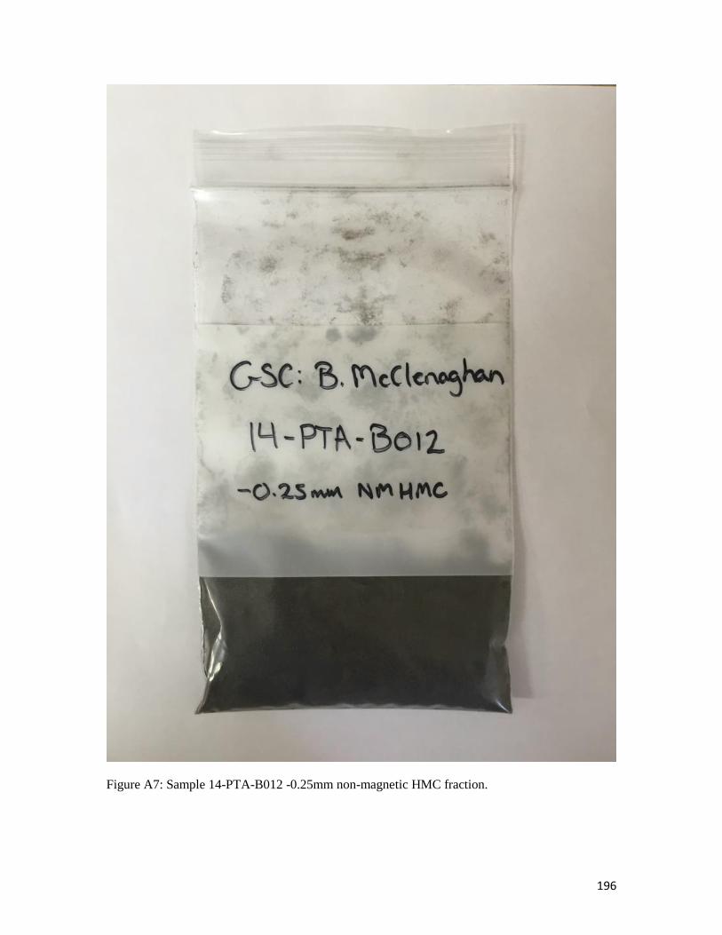
196
Figure A7: Sample 14-PTA-B012 -0.25mm non-magnetic HMC fraction.

197
Figure A8: Sample 14-PTA-R006 -0.25mm non-magnetic HMC fraction.

198
Figure A9: Sample 14-PTA-R011 -0.25mm non-magnetic HMC fraction.

199
Figure A10: Sample 14-PTA-R029 -0.25mm non-magnetic HMC fraction.

200
Figure A11: Powdered sample from each of the heavy mineral fractions of the case study samples.
A.Till = Almonte Till
R006 = 14-PTA-R006
R011 = 14-PTA-R011
R029 = 14-PTA-R029
B005 = 14-PTA-B005
B006 = 14-PTA-B006
B012 = 14-PTA-B012

201
Appendix B
The following graphs and tables represent the data collected for all of the tests
(Kimberlite Indicators, MMSIM’s, Gold and PGM’s) completed by ODM on the analysis
of the six till samples used in this study. Samples were submitted as ~10-15 kg till
samples from which no archival splits were taken. Till samples exceeding 15 kg were
split to 10 kg respectively before tabling; excess material was stored. All samples were
panned for gold and metallic minerals. Heavy liquid separations used a 3.2. The 0.25-2.0
mm nonferromagnetic heavy mineral fraction was picked for indicator minerals. Sample
14-PTA-B005 and 14-PTA-B012 were selected for a 100-grain count analysis.
Gold Summary:

202
Detailed Visible Gold:
Platinum Group Minerals (PGM’s):
Tabling Data:

203
Kimberlite Indicator Mineral Data:
Kimberlite Indicator Mineral Data Footnotes:
Magmatic Massive Sulphide Indicator Mineral (MMSIM) Data:

204
Heavy Mineral Processing Data:
Paramagnetic Mineral Data:
Pebble Count:

205
Abbreviations:

206
Appendix C
The following images display the XRD spectra collected for each of the six till samples
and the associated mineralogical classifications, which match with each of the peaks
presented.

207
14-PTA-B005 (heavy)

208
14-PTA-B005 (light)

209
14-PTA-B006 (heavy)

210
14-PTA-B006 (light)

211
14-PTA-B012 (heavy)

212
14-PTA-B012 (light)

213
14-PTA-R006 (heavy)
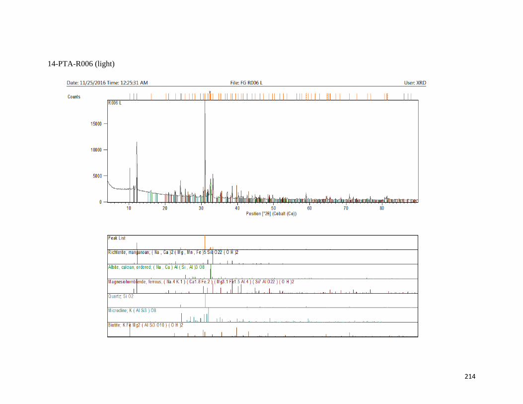
214
14-PTA-R006 (light)
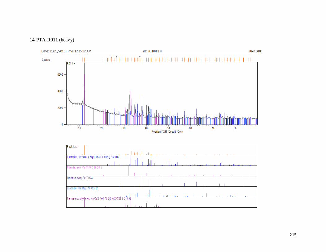
215
14-PTA-R011 (heavy)
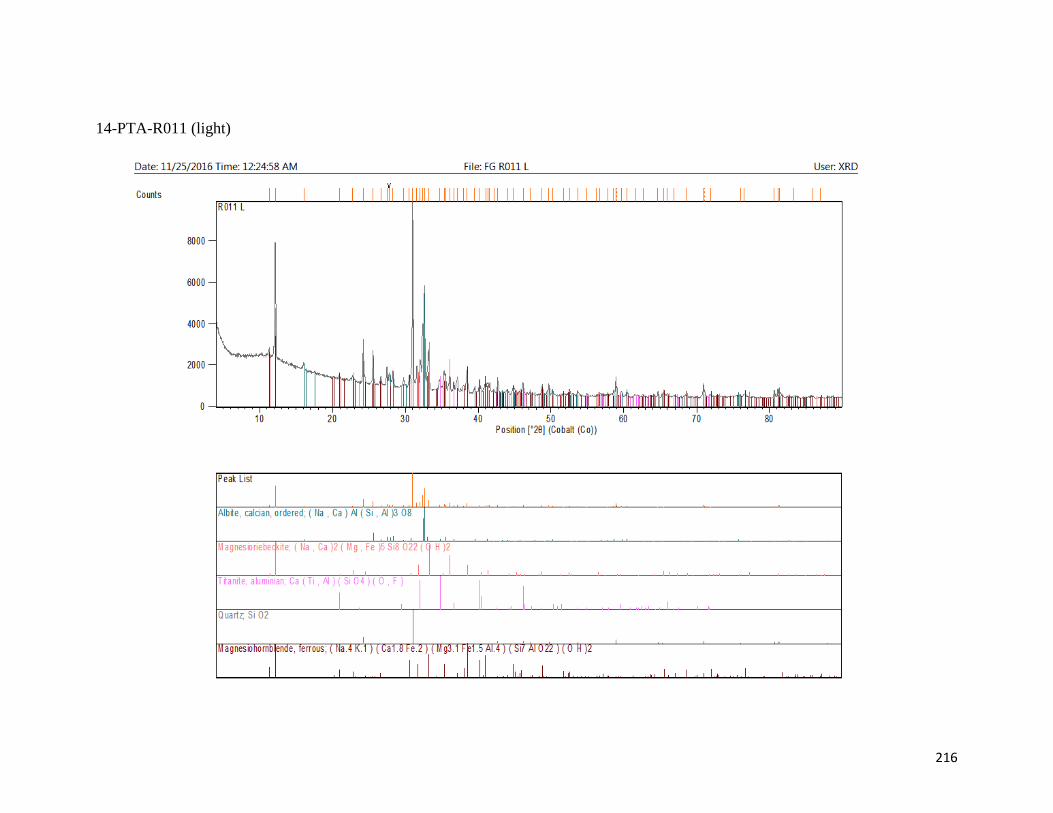
216
14-PTA-R011 (light)

217
14-PTA-R029 (heavy)

218
14-PTA-R029 (light)
219
Appendix D
The following tables represent the modal mineralogy determined for each of the six till
samples analyzed. The data for sample 1 (i.e. 14-PTA-B005-1) refers to the samples
ODM processed data (no hydroseparation work completed) and the sample 2 (i.e. 14-
PTA-B005-2) data refers to the samples processed by hydroseparation.

220
63-45 µm 4-PTA-B005-1
Mineral Particle Count Area% Weight%
Hornblende 9095 51.93% 46.91%
Enstatite 1847 10.39% 10.35%
Epidote 2390 9.55% 10.26%
Ilmenite 1162 6.17% 9.08%
Iron Oxide 1177 5.43% 6.42%
Almandine 2182 4.67% 6.10%
Titanite 474 1.54% 1.67%
Diopside 420 1.39% 1.54%
Biotite 1100 1.28% 1.24%
Illite 674 0.98% 0.84%
Low_Counts 475 0.94% 0.00%
Cordierite 628 0.87% 0.71%
Apatite 181 0.82% 0.81%
Clinopyroxene 386 0.73% 0.75%
Rutile 217 0.56% 0.74%
Quartz 239 0.56% 0.46%
Augite 141 0.50% 0.53%
Zircon 69 0.39% 0.56%
Unknown 338 0.27% 0.00%
Vesuvianite 118 0.22% 0.23%
Chlorite 118 0.22% 0.20%
Albite 190 0.20% 0.16%
Pyrope 57 0.13% 0.15%
Plagioclase 73 0.10% 0.08%
Sillimanite 14 0.06% 0.06%
Phlogopite 55 0.06% 0.05%
Orthoclase 16 0.04% 0.03%
Monazite 16 0.04% 0.06%
Sperrylite 7 0.00% 0.01%
Muscovite 4 0.00% 0.00%
Gypsum 1 0.00% 0.00%
Ferrosilite 3 0.00% 0.00%
No_XRay 29 0.00% 0.00%

221
63-45 µm 4-PTA-B005-2
Mineral Particle Count Area% Weight%
Hornblende 6166 44.03% 39.18%
Ilmenite 1562 9.50% 13.76%
Iron Oxide 1466 7.93% 9.25%
Epidote 1444 6.72% 7.11%
Enstatite 981 6.47% 6.35%
Clinopyroxene 911 4.21% 4.27%
Almandine 1700 3.86% 4.98%
Cordierite 1006 3.36% 2.73%
Quartz 432 2.19% 1.77%
Titanite 408 1.68% 1.80%
Illite 676 1.61% 1.36%
Biotite 1090 1.57% 1.49%
Diopside 237 0.90% 0.99%
Low_Counts 277 0.77% 0.00%
Zircon 107 0.71% 1.01%
Apatite 116 0.63% 0.62%
Albite 367 0.57% 0.46%
Phlogopite 188 0.51% 0.44%
Orthoclase 115 0.47% 0.37%
Rutile 186 0.46% 0.60%
Unknown 390 0.40% 0.00%
Chlorite 127 0.33% 0.30%
Augite 79 0.27% 0.28%
Plagioclase 134 0.23% 0.19%
Pyrope 70 0.21% 0.24%
Vesuvianite 77 0.20% 0.21%
Monazite 19 0.10% 0.15%
Sillimanite 8 0.07% 0.07%
Muscovite 13 0.03% 0.03%
Gypsum 12 0.00% 0.00%
Sperrylite 5 0.00% 0.01%
Dolomite 4 0.00% 0.00%
Carbon 2 0.00% 0.00%
Ferrosilite 3 0.00% 0.00%
No_XRay 12 0.00% 0.00%

222
45-20 µm 4-PTA-B005-1
Mineral Particle Count Area% Weight%
Hornblende 12872 49.53% 44.91%
Enstatite 2289 9.20% 9.21%
Epidote 3421 8.90% 9.60%
Ilmenite 1907 6.45% 9.52%
Iron Oxide 1953 5.76% 6.84%
Almandine 2292 4.36% 5.72%
Clinopyroxene 1078 2.23% 2.30%
Cordierite 1197 1.87% 1.55%
Titanite 681 1.82% 1.98%
Low_Counts 716 1.38% 0.00%
Diopside 484 1.16% 1.28%
Biotite 1022 1.13% 1.09%
Quartz 510 1.04% 0.86%
Illite 768 1.02% 0.88%
Rutile 290 0.67% 0.90%
Zircon 162 0.61% 0.88%
Apatite 195 0.59% 0.59%
Unknown 337 0.32% 0.00%
Albite 286 0.32% 0.26%
Augite 121 0.31% 0.33%
Chlorite 170 0.30% 0.28%
Phlogopite 151 0.24% 0.21%
Vesuvianite 108 0.18% 0.19%
Orthoclase 107 0.17% 0.14%
Plagioclase 131 0.16% 0.13%
Sillimanite 22 0.11% 0.11%
Pyrope 54 0.10% 0.11%
Monazite 22 0.07% 0.11%
Muscovite 8 0.01% 0.01%
Dolomite 1 0.00% 0.00%
Clinochlore 4 0.00% 0.00%
Spinel 2 0.00% 0.00%
Forsterite 1 0.00% 0.00%
Sperrylite 2 0.00% 0.00%
Olivine 1 0.00% 0.00%
Pyrite 1 0.00% 0.00%
No_XRay 13 0.00% 0.00%
Ferrosilite 2 0.00% 0.00%

223
45-20 µm 4-PTA-B005-2
Mineral Particle Count Area% Weight%
Hornblende 9293 42.08% 37.68%
Iron Oxide 2796 9.29% 10.91%
Ilmenite 2167 8.20% 11.95%
Epidote 2563 7.78% 8.29%
Enstatite 1310 5.44% 5.38%
Clinopyroxene 1314 4.45% 4.54%
Cordierite 1521 3.89% 3.18%
Almandine 1850 3.65% 4.73%
Quartz 715 2.55% 2.07%
Titanite 579 1.64% 1.77%
Biotite 1146 1.51% 1.44%
Illite 785 1.41% 1.20%
Low_Counts 432 1.07% 0.00%
Diopside 338 0.95% 1.04%
Zircon 201 0.78% 1.11%
Albite 492 0.75% 0.60%
Apatite 197 0.72% 0.71%
Phlogopite 282 0.68% 0.59%
Rutile 280 0.60% 0.79%
Unknown 433 0.46% 0.00%
Orthoclase 173 0.42% 0.34%
Augite 112 0.42% 0.44%
Plagioclase 207 0.38% 0.31%
Chlorite 158 0.33% 0.30%
Vesuvianite 84 0.15% 0.15%
Pyrope 75 0.12% 0.14%
Monazite 37 0.11% 0.17%
Dolomite 139 0.07% 0.06%
Sillimanite 11 0.06% 0.06%
Muscovite 19 0.02% 0.01%
Clinochlore 4 0.01% 0.01%
Gypsum 21 0.01% 0.01%
Sperrylite 9 0.01% 0.02%
Sphalerite 1 0.00% 0.00%
Spinel 1 0.00% 0.00%
Calcite 4 0.00% 0.00%
Olivine 1 0.00% 0.00%
Carbon 3 0.00% 0.00%
Ferrosilite 4 0.00% 0.00%
No_XRay 2 0.00% 0.00%

224
<20 µm 4-PTA-B005-1
Mineral Particle Count Area% Weight%
Hornblende 10134 30.26% 24.74%
Iron Oxide 9968 23.63% 25.31%
Ilmenite 6611 16.89% 22.48%
Epidote 2767 5.46% 5.31%
Enstatite 1541 4.35% 3.93%
Almandine 2130 3.49% 4.13%
Clinopyroxene 984 1.74% 1.62%
Cordierite 1211 1.69% 1.26%
Titanite 733 1.60% 1.57%
Zircon 686 1.59% 2.08%
Rutile 735 1.55% 1.86%
Biotite 1101 1.34% 1.17%
Illite 689 0.88% 0.68%
Quartz 502 0.77% 0.57%
Low_Counts 460 0.73% 0.00%
Unknown 495 0.58% 0.00%
Monazite 226 0.48% 0.70%
Albite 409 0.47% 0.35%
Diopside 213 0.45% 0.45%
Chlorite 217 0.42% 0.35%
Apatite 145 0.36% 0.32%
Phlogopite 208 0.31% 0.25%
Orthoclase 129 0.20% 0.15%
Augite 70 0.15% 0.15%
Plagioclase 117 0.14% 0.11%
Pyrope 75 0.13% 0.13%
Vesuvianite 71 0.11% 0.10%
Olivine 29 0.06% 0.06%
Sillimanite 21 0.06% 0.05%
Dolomite 23 0.02% 0.02%
Muscovite 16 0.02% 0.01%
Sperrylite 22 0.02% 0.05%
Ferrosilite 7 0.01% 0.01%
Clinochlore 3 0.01% 0.01%
Calcite 7 0.00% 0.00%
Arsenopyrite 1 0.00% 0.01%
Pyrite 2 0.00% 0.00%
Sphalerite 1 0.00% 0.00%
Carbon 2 0.00% 0.00%
Spinel 1 0.00% 0.00%
Chalcopyrite 1 0.00% 0.00%
Galena 1 0.00% 0.00%
No_XRay 17 0.00% 0.00%
Gypsum 1 0.00% 0.00%

225
<20 µm 4-PTA-B005-2
Mineral Particle Count Area% Weight%
Hornblende 3861 31.36% 5389443.9
Unknown 995 0.00% 3496224.63
Iron Oxide 2973 20.24% 2654817.79
Ilmenite 1740 12.04% 1271095.97
Epidote 1098 5.47% 789694.54
Clinopyroxene 645 4.49% 678294.95
Cordierite 718 2.95% 554158.07
Enstatite 639 3.43% 534270.07
Dolomite 1491 2.90% 507741.09
Almandine 819 3.27% 387970.36
Quartz 339 1.67% 317086.59
Biotite 579 1.47% 236203.49
Albite 344 0.99% 188921.43
Phlogopite 222 0.97% 172415.09
Titanite 287 1.14% 163103.15
Illite 244 0.75% 136064.44
Rutile 255 1.15% 135248.88
Low_Counts 342 0.00% 122185.37
Diopside 163 0.82% 114743.39
Zircon 243 1.03% 110534.52
Calcite 258 0.58% 105850.88
Chlorite 158 0.51% 85782.29
Orthoclase 109 0.43% 82974.43
Apatite 79 0.42% 66063.23
Plagioclase 149 0.32% 60316.45
Carbon 84 0.24% 55192.98
Pyrope 88 0.36% 47541.29
Augite 47 0.29% 42458.61
Gypsum 67 0.14% 31291.27
Monazite 69 0.31% 30263.08
Vesuvianite 33 0.09% 12979.05
Sillimanite 11 0.08% 12577.09
Muscovite 20 0.03% 4657.43
Sperrylite 12 0.02% 1036.93
Olivine 3 0.00% 690.31
Arsenopyrite 4 0.01% 582.54
Clinochlore 2 0.00% 547.59
Ferrosilite 8 0.00% 498.07
Cassiterite 2 0.00% 337.87
Chalcopyrite 6 0.00% 273.79
Spinel 1 0.00% 52.43
No_XRay 11 0.00% 46.6
Sphalerite 1 0.00% 34.95
Pyrite 1 0.00% 14.56

226
63-45 µm 14-PTA-B006-1
Mineral Particle Count Area% Weight%
Hornblende 3435 28.30% 24.89%
Iron Oxide 2897 20.89% 24.07%
Almandine 2596 10.66% 13.58%
Illite 2341 9.58% 7.99%
Enstatite 851 5.78% 5.61%
Epidote 739 5.11% 5.35%
Cordierite 1189 5.08% 4.43%
Ilmenite 449 3.09% 4.08%
Biotite 873 2.31% 2.17%
Clinopyroxene 258 1.24% 1.25%
Quartz 159 1.05% 1.10%
Titanite 184 1.04% 0.84%
Low_Counts 171 0.95% 0.83%
Diopside 136 0.78% 0.83%
Rutile 159 0.65% 0.51%
Phlogopite 155 0.60% 0.48%
Chlorite 169 0.54% 0.43%
Albite 226 0.54% 0.40%
Unknown 232 0.36% 0.34%
Augite 42 0.33% 0.20%
Zircon 33 0.28% 0.15%
Orthoclase 65 0.26% 0.14%
Sillimanite 9 0.15% 0.12%
Pyrope 56 0.13% 0.08%
Apatite 12 0.13% 0.05%
Plagioclase 25 0.06% 0.04%
Monazite 15 0.05% 0.02%
Vesuvianite 10 0.03% 0.01%
Muscovite 17 0.03% 0.00%
Clinochlore 4 0.01% 0.00%
Carbon 2 0.00% 0.00%
Sperrylite 2 0.00% 0.00%
Ferrosilite 3 0.00% 0.00%
Olivine 1 0.00% 0.00%
Dolomite 1 0.00% 0.00%
No_XRay 12 0.00% 0.00%

227
63-45 µm 14-PTA-B006-2
Mineral Particle Count Area% Weight%
Hornblende 3342 23.46% 21.19%
Iron Oxide 3112 20.92% 24.75%
Illite 2427 10.23% 8.76%
Cordierite 1770 10.18% 8.40%
Almandine 2480 8.04% 10.52%
Quartz 449 3.69% 3.02%
Epidote 660 3.63% 3.90%
Enstatite 603 3.07% 3.06%
Clinopyroxene 421 3.00% 3.08%
Ilmenite 560 2.81% 4.13%
Biotite 1062 2.53% 2.44%
Phlogopite 322 1.29% 1.13%
Albite 369 0.94% 0.77%
Unknown 351 0.84% 0.00%
Chlorite 203 0.80% 0.74%
Low_Counts 149 0.70% 0.00%
Titanite 169 0.63% 0.68%
Orthoclase 121 0.62% 0.49%
Rutile 163 0.54% 0.72%
Diopside 93 0.41% 0.45%
Dolomite 465 0.38% 0.34%
Zircon 57 0.32% 0.46%
Plagioclase 63 0.26% 0.22%
Clinochlore 4 0.15% 0.12%
Pyrope 69 0.14% 0.16%
Augite 33 0.11% 0.11%
Apatite 7 0.11% 0.11%
Monazite 17 0.09% 0.14%
Muscovite 27 0.05% 0.04%
Sillimanite 2 0.03% 0.03%
Gypsum 41 0.03% 0.02%
Calcite 19 0.01% 0.01%
Vesuvianite 8 0.01% 0.01%
Ferrosilite 5 0.00% 0.00%
Sperrylite 6 0.00% 0.01%
Carbon 3 0.00% 0.00%

228
45-20 µm 14-PTA-B006-1
Mineral Particle Count Area% Weight%
Iron Oxide 9965 34.80% 38.26%
Hornblende 5079 18.67% 15.66%
Almandine 4572 10.08% 12.25%
Illite 3926 8.48% 6.75%
Ilmenite 1594 5.34% 7.30%
Cordierite 1968 4.75% 3.64%
Epidote 1460 4.46% 4.46%
Enstatite 1074 3.00% 2.77%
Biotite 1336 2.15% 1.93%
Clinopyroxene 395 1.03% 0.98%
Titanite 319 0.87% 0.87%
Low_Counts 323 0.84% 0.00%
Rutile 334 0.83% 1.02%
Zircon 219 0.80% 1.07%
Quartz 257 0.76% 0.58%
Albite 364 0.51% 0.39%
Unknown 461 0.49% 0.00%
Phlogopite 214 0.42% 0.34%
Chlorite 211 0.41% 0.35%
Diopside 111 0.33% 0.33%
Orthoclase 89 0.24% 0.17%
Monazite 70 0.22% 0.33%
Pyrope 63 0.12% 0.13%
Augite 36 0.10% 0.09%
Apatite 24 0.09% 0.09%
Sillimanite 12 0.06% 0.05%
Muscovite 29 0.05% 0.04%
Plagioclase 28 0.03% 0.03%
Vesuvianite 12 0.02% 0.02%
Sperrylite 10 0.02% 0.05%
Ferrosilite 11 0.01% 0.01%
Clinochlore 4 0.01% 0.01%
Olivine 3 0.01% 0.01%
Sphalerite 2 0.00% 0.00%
Dolomite 3 0.00% 0.00%
Pyrite 2 0.00% 0.00%
Gypsum 2 0.00% 0.00%
Calcite 1 0.00% 0.00%
Carbon 1 0.00% 0.00%
No_XRay 9 0.00% 0.00%

229
45-20 µm 14-PTA-B006-2
Mineral Particle Count Area% Weight%
Iron Oxide 15771 46.50% 49.85%
Hornblende 4747 12.48% 10.21%
Almandine 5994 9.44% 11.19%
Illite 4643 7.93% 6.15%
Ilmenite 2201 5.86% 7.81%
Cordierite 1960 4.00% 2.99%
Epidote 1188 2.86% 2.78%
Biotite 1721 2.13% 1.86%
Enstatite 982 1.75% 1.58%
Zircon 324 0.93% 1.23%
Unknown 659 0.84% 0.00%
Clinopyroxene 309 0.79% 0.74%
Quartz 273 0.71% 0.53%
Titanite 319 0.66% 0.65%
Low_Counts 404 0.60% 0.00%
Rutile 338 0.57% 0.68%
Albite 349 0.48% 0.35%
Chlorite 168 0.32% 0.26%
Phlogopite 154 0.30% 0.24%
Monazite 92 0.18% 0.27%
Diopside 64 0.16% 0.16%
Orthoclase 60 0.12% 0.08%
Pyrope 67 0.08% 0.08%
Apatite 22 0.07% 0.06%
Dolomite 121 0.05% 0.04%
Plagioclase 28 0.03% 0.02%
Gypsum 43 0.03% 0.02%
Augite 12 0.03% 0.03%
Sperrylite 31 0.02% 0.07%
Muscovite 19 0.02% 0.02%
Sillimanite 5 0.02% 0.02%
Vesuvianite 8 0.01% 0.01%
Carbon 3 0.01% 0.00%
Ferrosilite 7 0.01% 0.01%
Calcite 1 0.00% 0.00%
No_XRay 40 0.00% 0.00%

230
<20 µm 14-PTA-B006-1
Mineral Particle Count Area% Weight%
Iron Oxide 4870 45.53% 48.68%
Hornblende 1608 17.62% 14.38%
Almandine 1497 8.88% 10.50%
Illite 1152 6.43% 4.97%
Ilmenite 397 4.08% 5.42%
Zircon 317 2.85% 3.73%
Epidote 333 2.68% 2.60%
Enstatite 295 2.67% 2.41%
Cordierite 396 2.40% 1.79%
Biotite 322 1.28% 1.11%
Monazite 92 0.76% 1.10%
Clinopyroxene 89 0.70% 0.65%
Low_Counts 112 0.68% 0.00%
Quartz 68 0.59% 0.43%
Titanite 51 0.38% 0.38%
Unknown 120 0.37% 0.00%
Phlogopite 62 0.36% 0.28%
Chlorite 51 0.32% 0.26%
Rutile 48 0.26% 0.31%
Albite 66 0.26% 0.19%
Orthoclase 25 0.19% 0.14%
Diopside 23 0.15% 0.15%
Sillimanite 8 0.13% 0.12%
Pyrope 19 0.11% 0.12%
Dolomite 13 0.11% 0.09%
Augite 10 0.06% 0.06%
Apatite 6 0.04% 0.04%
Plagioclase 16 0.04% 0.03%
Muscovite 6 0.02% 0.02%
Chalcopyrite 2 0.01% 0.01%
Carbon 2 0.01% 0.01%
Calcite 3 0.01% 0.00%
Olivine 1 0.01% 0.01%
Pyrite 2 0.00% 0.01%
Vesuvianite 2 0.00% 0.00%
Ferrosilite 2 0.00% 0.00%
Gypsum 1 0.00% 0.00%
Sperrylite 2 0.00% 0.00%
Clinochlore 1 0.00% 0.00%
No_XRay 2 0.00% 0.00%
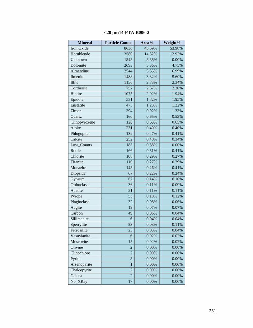
231
<20 µm 14-PTA-B006-2
Mineral Particle Count Area% Weight%
Iron Oxide 8636 45.69% 53.98%
Hornblende 3580 14.32% 12.92%
Unknown 1848 8.88% 0.00%
Dolomite 2693 5.36% 4.75%
Almandine 2544 5.35% 6.99%
Ilmenite 1488 3.82% 5.60%
Illite 1156 2.73% 2.34%
Cordierite 757 2.67% 2.20%
Biotite 1075 2.02% 1.94%
Epidote 531 1.82% 1.95%
Enstatite 473 1.23% 1.22%
Zircon 394 0.92% 1.33%
Quartz 160 0.65% 0.53%
Clinopyroxene 126 0.63% 0.65%
Albite 231 0.49% 0.40%
Phlogopite 132 0.47% 0.41%
Calcite 252 0.40% 0.34%
Low_Counts 183 0.38% 0.00%
Rutile 166 0.31% 0.41%
Chlorite 108 0.29% 0.27%
Titanite 110 0.27% 0.29%
Monazite 148 0.26% 0.41%
Diopside 67 0.22% 0.24%
Gypsum 62 0.14% 0.10%
Orthoclase 36 0.11% 0.09%
Apatite 31 0.11% 0.11%
Pyrope 53 0.10% 0.12%
Plagioclase 32 0.08% 0.06%
Augite 19 0.07% 0.07%
Carbon 49 0.06% 0.04%
Sillimanite 6 0.04% 0.04%
Sperrylite 53 0.03% 0.11%
Ferrosilite 23 0.03% 0.04%
Vesuvianite 6 0.02% 0.02%
Muscovite 15 0.02% 0.02%
Olivine 2 0.00% 0.00%
Clinochlore 2 0.00% 0.00%
Pyrite 3 0.00% 0.00%
Arsenopyrite 1 0.00% 0.00%
Chalcopyrite 2 0.00% 0.00%
Galena 2 0.00% 0.00%
No_XRay 17 0.00% 0.00%

232
63-45 µm 14-PTA-B012-1
Mineral Particle Count Area% Weight%
Hornblende 6455 58.77% 53.45%
Epidote 1620 8.53% 9.23%
Almandine 2226 6.55% 8.63%
Iron Oxide 906 5.45% 6.50%
Ilmenite 897 5.38% 7.96%
Biotite 1381 3.22% 3.13%
Enstatite 367 2.71% 2.72%
Titanite 449 1.88% 2.05%
Cordierite 479 1.13% 0.94%
Illite 468 1.06% 0.92%
Clinopyroxene 349 0.97% 1.00%
Low_Counts 254 0.85% 0.00%
Rutile 125 0.61% 0.81%
Chlorite 199 0.57% 0.53%
Quartz 109 0.46% 0.38%
Diopside 64 0.33% 0.36%
Albite 195 0.32% 0.26%
Apatite 38 0.30% 0.30%
Unknown 253 0.21% 0.00%
Zircon 34 0.20% 0.29%
Augite 21 0.09% 0.09%
Monazite 8 0.07% 0.11%
Plagioclase 47 0.07% 0.06%
Pyrope 41 0.07% 0.08%
Phlogopite 35 0.05% 0.05%
Sillimanite 6 0.05% 0.05%
Muscovite 27 0.05% 0.04%
Vesuvianite 23 0.05% 0.05%
Orthoclase 6 0.01% 0.01%
Clinochlore 4 0.00% 0.00%
Dolomite 4 0.00% 0.00%
Carbon 1 0.00% 0.00%
Ferrosilite 3 0.00% 0.00%
Calcite 3 0.00% 0.00%
Olivine 1 0.00% 0.00%
Sperrylite 3 0.00% 0.00%
No_XRay 2 0.00% 0.00%

233
63-45 µm 14-PTA-B012-2
Mineral Particle Count Area% Weight%
Hornblende 5896 44.46% 39.90%
Ilmenite 1295 9.21% 13.46%
Epidote 1539 8.40% 8.97%
Iron Oxide 995 6.82% 8.02%
Almandine 1821 4.81% 6.25%
Clinopyroxene 845 4.23% 4.32%
Cordierite 1043 4.23% 3.47%
Biotite 1581 3.70% 3.55%
Quartz 542 3.42% 2.78%
Illite 628 1.81% 1.54%
Titanite 424 1.66% 1.79%
Enstatite 241 1.60% 1.58%
Low_Counts 284 1.08% 0.00%
Rutile 146 0.70% 0.91%
Albite 319 0.63% 0.51%
Chlorite 170 0.59% 0.53%
Unknown 380 0.45% 0.00%
Zircon 60 0.42% 0.61%
Diopside 57 0.36% 0.40%
Phlogopite 68 0.27% 0.24%
Plagioclase 115 0.27% 0.23%
Pyrope 61 0.23% 0.26%
Apatite 16 0.13% 0.13%
Monazite 12 0.11% 0.18%
Orthoclase 32 0.11% 0.09%
Augite 11 0.07% 0.08%
Muscovite 22 0.06% 0.05%
Dolomite 108 0.06% 0.05%
Sillimanite 7 0.04% 0.04%
Olivine 10 0.02% 0.02%
Vesuvianite 12 0.02% 0.02%
Clinochlore 7 0.01% 0.01%
Gypsum 10 0.00% 0.00%
Calcite 4 0.00% 0.00%
Sperrylite 3 0.00% 0.00%
Kotulskite 1 0.00% 0.00%
Carbon 1 0.00% 0.00%
No_XRay 6 0.00% 0.00%

234
45-20 µm 14-PTA-B012-1
Mineral Particle Count Area% Weight%
Hornblende 9789 48.22% 42.39%
Ilmenite 2956 11.17% 15.98%
Epidote 3055 9.81% 10.26%
Iron Oxide 1866 7.49% 8.63%
Almandine 2445 5.04% 6.42%
Biotite 1982 2.96% 2.78%
Clinopyroxene 807 2.63% 2.63%
Titanite 803 2.23% 2.35%
Cordierite 808 1.71% 1.63%
Enstatite 446 1.68% 1.37%
Illite 587 1.13% 1.10%
Low_Counts 443 0.98% 0.94%
Quartz 288 0.92% 0.73%
Rutile 341 0.85% 0.63%
Chlorite 234 0.62% 0.55%
Unknown 480 0.47% 0.30%
Zircon 133 0.45% 0.29%
Albite 327 0.36% 0.25%
Apatite 72 0.31% 0.22%
Diopside 70 0.23% 0.15%
Monazite 36 0.14% 0.11%
Plagioclase 107 0.14% 0.07%
Pyrope 82 0.14% 0.05%
Phlogopite 49 0.08% 0.05%
Muscovite 32 0.06% 0.04%
Vesuvianite 30 0.05% 0.03%
Sillimanite 9 0.04% 0.03%
Orthoclase 17 0.04% 0.01%
Augite 18 0.03% 0.01%
Clinochlore 6 0.01% 0.00%
Dolomite 7 0.00% 0.00%
Olivine 3 0.00% 0.00%
Sperrylite 6 0.00% 0.00%
Spinel 1 0.00% 0.00%
Carbon 1 0.00% 0.00%
Gypsum 1 0.00% 0.00%
No_XRay 9 0.00% 0.00%
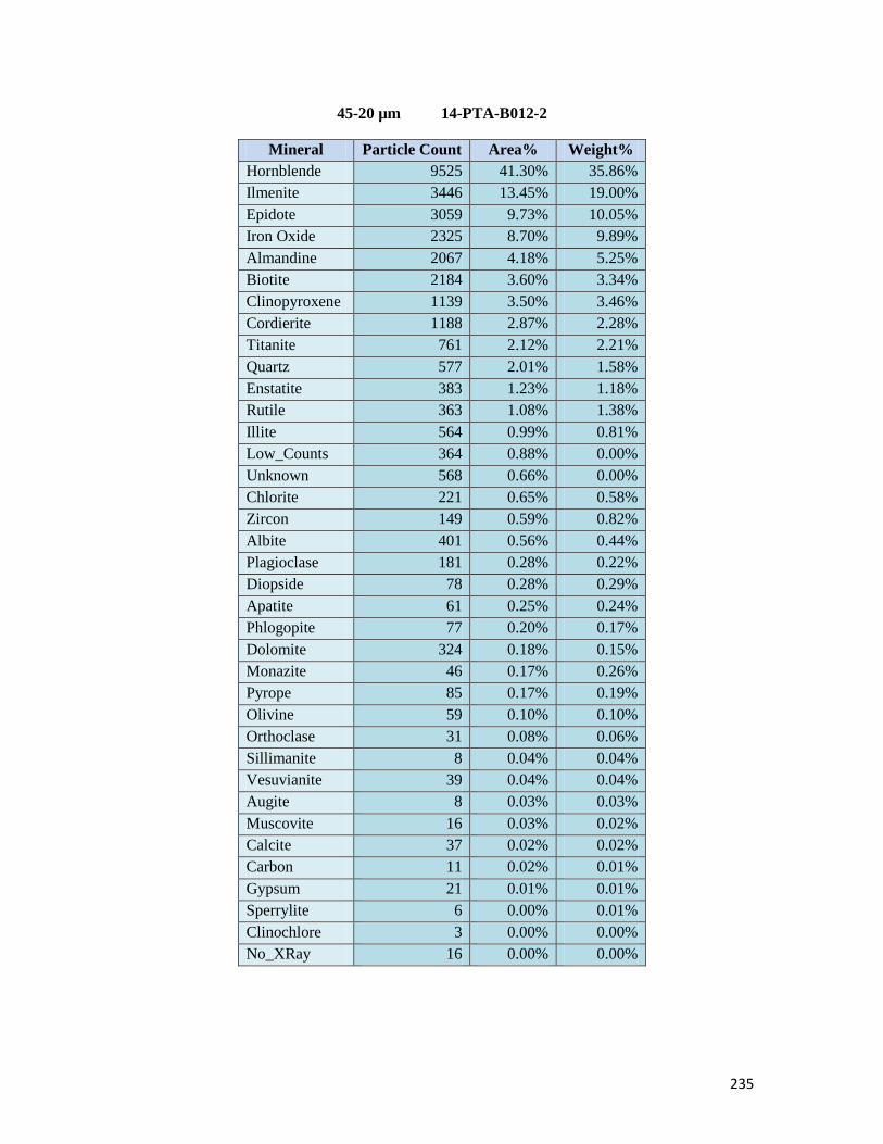
235
45-20 µm 14-PTA-B012-2
Mineral Particle Count Area% Weight%
Hornblende 9525 41.30% 35.86%
Ilmenite 3446 13.45% 19.00%
Epidote 3059 9.73% 10.05%
Iron Oxide 2325 8.70% 9.89%
Almandine 2067 4.18% 5.25%
Biotite 2184 3.60% 3.34%
Clinopyroxene 1139 3.50% 3.46%
Cordierite 1188 2.87% 2.28%
Titanite 761 2.12% 2.21%
Quartz 577 2.01% 1.58%
Enstatite 383 1.23% 1.18%
Rutile 363 1.08% 1.38%
Illite 564 0.99% 0.81%
Low_Counts 364 0.88% 0.00%
Unknown 568 0.66% 0.00%
Chlorite 221 0.65% 0.58%
Zircon 149 0.59% 0.82%
Albite 401 0.56% 0.44%
Plagioclase 181 0.28% 0.22%
Diopside 78 0.28% 0.29%
Apatite 61 0.25% 0.24%
Phlogopite 77 0.20% 0.17%
Dolomite 324 0.18% 0.15%
Monazite 46 0.17% 0.26%
Pyrope 85 0.17% 0.19%
Olivine 59 0.10% 0.10%
Orthoclase 31 0.08% 0.06%
Sillimanite 8 0.04% 0.04%
Vesuvianite 39 0.04% 0.04%
Augite 8 0.03% 0.03%
Muscovite 16 0.03% 0.02%
Calcite 37 0.02% 0.02%
Carbon 11 0.02% 0.01%
Gypsum 21 0.01% 0.01%
Sperrylite 6 0.00% 0.01%
Clinochlore 3 0.00% 0.00%
No_XRay 16 0.00% 0.00%

236
<20 µm 14-PTA-B012-1
Mineral Particle Count Area% Weight%
Hornblende 6039 30.95% 24.71%
Ilmenite 5479 27.42% 35.64%
Iron Oxide 2730 11.79% 12.33%
Epidote 1686 7.47% 7.09%
Biotite 1525 3.91% 3.34%
Almandine 1216 3.70% 4.28%
Rutile 650 2.61% 3.05%
Titanite 475 1.89% 1.81%
Enstatite 279 1.41% 1.24%
Clinopyroxene 480 1.25% 1.14%
Unknown 537 1.10% 0.00%
Zircon 229 1.02% 1.31%
Cordierite 411 1.01% 0.74%
Illite 298 0.70% 0.53%
Low_Counts 240 0.69% 0.00%
Chlorite 163 0.60% 0.49%
Quartz 173 0.54% 0.39%
Monazite 133 0.54% 0.76%
Albite 219 0.42% 0.30%
Diopside 43 0.17% 0.17%
Plagioclase 62 0.13% 0.10%
Apatite 30 0.13% 0.12%
Phlogopite 50 0.11% 0.08%
Pyrope 45 0.10% 0.10%
Sillimanite 8 0.06% 0.05%
Dolomite 19 0.06% 0.04%
Muscovite 16 0.06% 0.04%
Orthoclase 27 0.05% 0.04%
Augite 12 0.03% 0.02%
Calcite 7 0.02% 0.02%
Clinochlore 5 0.02% 0.01%
Olivine 8 0.01% 0.01%
Vesuvianite 11 0.01% 0.01%
Spinel 1 0.01% 0.01%
Sperrylite 5 0.01% 0.02%
Carbon 1 0.00% 0.00%
No_XRay 8 0.00% 0.00%

237
<20 µm 14-PTA-B012-2
Mineral Particle Count Area% Weight%
Hornblende 4597 37.23% 41.72%
Unknown 1732 19.70% 0.00%
Ilmenite 1976 8.31% 15.16%
Iron Oxide 1442 4.76% 6.99%
Epidote 1057 4.08% 5.44%
Dolomite 1928 4.07% 4.48%
Biotite 936 2.81% 3.37%
Clinopyroxene 666 2.73% 3.48%
Cordierite 570 2.49% 2.55%
Almandine 808 2.16% 3.51%
Quartz 251 1.46% 1.49%
Titanite 359 1.11% 1.49%
Rutile 274 1.01% 1.66%
Chlorite 319 0.99% 1.13%
Albite 396 0.98% 0.99%
Low_Counts 343 0.80% 0.00%
Enstatite 172 0.76% 0.94%
Calcite 354 0.73% 0.77%
Illite 197 0.68% 0.72%
Pyrope 190 0.61% 0.89%
Plagioclase 159 0.43% 0.45%
Zircon 118 0.35% 0.63%
Diopside 83 0.35% 0.48%
Apatite 43 0.28% 0.34%
Phlogopite 79 0.23% 0.25%
Gypsum 69 0.22% 0.19%
Monazite 57 0.14% 0.28%
Carbon 79 0.14% 0.11%
Muscovite 59 0.13% 0.14%
Augite 25 0.11% 0.15%
Vesuvianite 23 0.05% 0.06%
Orthoclase 8 0.03% 0.03%
Clinochlore 11 0.02% 0.02%
Sillimanite 2 0.01% 0.01%
Olivine 1 0.01% 0.01%
Galena 2 0.01% 0.02%
Pyrite 3 0.01% 0.01%
Sperrylite 3 0.00% 0.01%
Sphalerite 1 0.00% 0.00%
Chalcopyrite 4 0.00% 0.00%
Ferrosilite 2 0.00% 0.00%
No_XRay 12 0.00% 0.00%

238
63-45 µm 14-PTA-R006-1
Mineral Particle Count Area% Weight%
Hornblende 8539 53.55% 49.13%
Iron Oxide 1951 10.55% 12.69%
Enstatite 1815 9.91% 10.03%
Almandine 1781 4.01% 5.32%
Diopside 983 3.19% 3.58%
Epidote 724 2.85% 3.11%
Ilmenite 709 2.70% 4.03%
Titanite 344 1.62% 1.78%
Clinopyroxene 507 1.47% 1.54%
Biotite 1108 1.44% 1.41%
Apatite 290 1.44% 1.45%
Low_Counts 547 1.11% 0.00%
Augite 322 1.09% 1.17%
Cordierite 503 0.92% 0.78%
Quartz 207 0.70% 0.58%
Rutile 241 0.48% 0.64%
Vesuvianite 228 0.44% 0.48%
Illite 344 0.40% 0.35%
Unknown 295 0.35% 0.00%
Zircon 55 0.34% 0.50%
Chlorite 198 0.30% 0.28%
Sillimanite 43 0.24% 0.24%
Phlogopite 176 0.22% 0.19%
Pyrope 105 0.19% 0.22%
Albite 115 0.14% 0.11%
Orthoclase 51 0.13% 0.11%
Plagioclase 64 0.12% 0.10%
Monazite 16 0.08% 0.12%
Forsterite 8 0.03% 0.03%
Carbon 4 0.00% 0.00%
Galena 1 0.00% 0.01%
Muscovite 4 0.00% 0.00%
Clinochlore 3 0.00% 0.00%
Pyrite 1 0.00% 0.00%
Sperrylite 2 0.00% 0.00%
No_XRay 22 0.00% 0.00%
Ferrosilite 1 0.00% 0.00%
Spinel 1 0.00% 0.00%

239
63-45 µm 14-PTA-R006-2
Mineral Particle Count Area% Weight%
Hornblende 4217 41.26% 36.67%
Iron Oxide 2063 18.48% 21.53%
Enstatite 880 7.91% 7.76%
Clinopyroxene 551 4.19% 4.24%
Ilmenite 673 4.11% 5.94%
Almandine 1202 3.76% 4.84%
Diopside 464 3.01% 3.27%
Cordierite 457 2.22% 1.80%
Epidote 328 2.03% 2.15%
Quartz 266 1.89% 1.52%
Biotite 761 1.57% 1.49%
Apatite 165 1.24% 1.21%
Titanite 173 1.20% 1.28%
Low_Counts 193 0.81% 0.00%
Augite 133 0.77% 0.81%
Zircon 87 0.75% 1.07%
Rutile 230 0.68% 0.89%
Chlorite 140 0.62% 0.56%
Phlogopite 170 0.56% 0.48%
Illite 245 0.51% 0.43%
Orthoclase 90 0.51% 0.40%
Unknown 233 0.32% 0.00%
Plagioclase 98 0.29% 0.24%
Sillimanite 26 0.27% 0.27%
Albite 185 0.27% 0.22%
Vesuvianite 106 0.25% 0.26%
Monazite 23 0.22% 0.34%
Pyrope 94 0.19% 0.22%
Spinel 3 0.03% 0.03%
Muscovite 8 0.02% 0.02%
Clinochlore 3 0.01% 0.01%
Olivine 4 0.01% 0.01%
Sperrylite 7 0.01% 0.02%
Gypsum 10 0.00% 0.00%
Dolomite 5 0.00% 0.00%
Carbon 2 0.00% 0.00%
Galena 1 0.00% 0.00%
No_XRay 6 0.00% 0.00%
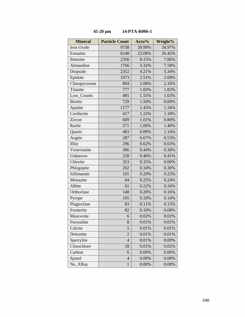
240
45-20 µm 14-PTA-R006-1
Mineral Particle Count Area% Weight%
Iron Oxide 9738 39.99% 34.97%
Enstatite 6148 23.08% 26.45%
Ilmenite 2356 8.15% 7.86%
Almandine 1766 5.32% 7.58%
Diopside 2352 4.21% 5.34%
Epidote 1073 2.51% 2.69%
Clinopyroxene 804 2.08% 2.16%
Titanite 777 1.83% 1.82%
Low_Counts 491 1.55% 1.63%
Biotite 729 1.50% 0.00%
Apatite 1177 1.43% 1.34%
Cordierite 417 1.23% 1.18%
Zircon 609 1.01% 0.80%
Rutile 271 1.00% 1.40%
Quartz 483 0.89% 1.14%
Augite 287 0.67% 0.53%
Illite 296 0.62% 0.63%
Vesuvianite 386 0.44% 0.36%
Unknown 258 0.40% 0.41%
Chlorite 353 0.35% 0.00%
Phlogopite 202 0.34% 0.30%
Sillimanite 191 0.29% 0.25%
Monazite 64 0.25% 0.24%
Albite 61 0.22% 0.34%
Orthoclase 148 0.20% 0.16%
Pyrope 105 0.18% 0.14%
Plagioclase 83 0.11% 0.13%
Forsterite 82 0.10% 0.08%
Muscovite 6 0.02% 0.02%
Ferrosilite 8 0.01% 0.01%
Calcite 5 0.01% 0.01%
Dolomite 2 0.01% 0.01%
Sperrylite 4 0.01% 0.00%
Clinochlore 18 0.01% 0.02%
Carbon 6 0.00% 0.00%
Spinel 4 0.00% 0.00%
No_XRay 1 0.00% 0.00%

241
45-20 µm 14-PTA-R006-2
Mineral Particle Count Area% Weight%
Iron Oxide 11276 41.25% 44.34%
Hornblende 6834 24.44% 20.05%
Ilmenite 2881 8.11% 10.83%
Enstatite 1538 5.22% 4.72%
Almandine 2621 4.24% 5.03%
Zircon 484 1.61% 2.12%
Biotite 1434 1.60% 1.40%
Epidote 640 1.55% 1.51%
Clinopyroxene 573 1.54% 1.44%
Diopside 554 1.25% 1.25%
Titanite 427 1.20% 1.18%
Rutile 731 1.13% 1.36%
Cordierite 508 1.01% 0.76%
Unknown 734 0.89% 0.00%
Apatite 257 0.84% 0.76%
Quartz 273 0.74% 0.55%
Low_Counts 362 0.61% 0.00%
Monazite 144 0.45% 0.65%
Augite 202 0.43% 0.41%
Illite 336 0.32% 0.25%
Albite 226 0.28% 0.21%
Phlogopite 149 0.23% 0.19%
Chlorite 115 0.20% 0.16%
Sillimanite 38 0.15% 0.14%
Plagioclase 120 0.15% 0.12%
Vesuvianite 120 0.15% 0.15%
Orthoclase 73 0.13% 0.10%
Pyrope 114 0.13% 0.13%
Dolomite 108 0.06% 0.05%
Gypsum 45 0.04% 0.03%
Sperrylite 28 0.03% 0.08%
Spinel 5 0.02% 0.02%
Carbon 9 0.01% 0.01%
Forsterite 2 0.01% 0.01%
Ferrosilite 6 0.01% 0.01%
Muscovite 7 0.01% 0.00%
Olivine 3 0.00% 0.00%
Clinochlore 5 0.00% 0.00%
Calcite 2 0.00% 0.00%
No_XRay 7 0.00% 0.00%
Pyrite 1 0.00% 0.00%

242
<20 µm 14-PTA-R006-1
Mineral Particle Count Area% Weight%
Iron Oxide 10666 37.08% 40.26%
Hornblende 6244 25.71% 21.30%
Ilmenite 2672 7.88% 10.62%
Enstatite 1210 4.29% 3.92%
Almandine 1735 3.96% 4.75%
Clinopyroxene 1458 2.76% 2.60%
Biotite 1250 2.45% 2.17%
Zircon 654 1.89% 2.52%
Cordierite 836 1.43% 1.08%
Rutile 503 1.24% 1.51%
Titanite 308 1.15% 1.14%
Illite 566 1.13% 0.89%
Epidote 341 1.09% 1.07%
Diopside 361 0.98% 0.99%
Quartz 329 0.79% 0.59%
Low_Counts 459 0.74% 0.00%
Monazite 254 0.72% 1.06%
Phlogopite 462 0.68% 0.54%
Unknown 319 0.66% 0.00%
Apatite 180 0.57% 0.52%
Chlorite 260 0.53% 0.45%
Albite 396 0.53% 0.40%
Orthoclase 221 0.33% 0.24%
Vesuvianite 118 0.30% 0.29%
Plagioclase 163 0.24% 0.19%
Augite 87 0.24% 0.23%
Pyrope 149 0.22% 0.23%
Sillimanite 57 0.21% 0.20%
Olivine 10 0.07% 0.06%
Muscovite 30 0.04% 0.03%
Dolomite 15 0.03% 0.03%
Sperrylite 13 0.02% 0.07%
Clinochlore 8 0.01% 0.01%
Ferrosilite 5 0.01% 0.01%
Chalcopyrite 3 0.01% 0.01%
Gypsum 5 0.01% 0.00%
Calcite 4 0.01% 0.00%
Spinel 1 0.00% 0.00%
Carbon 4 0.00% 0.00%
No_XRay 27 0.00% 0.00%
Pyrite 1 0.00% 0.00%
Sphalerite 1 0.00% 0.00%

243
<20 µm 14-PTA-R006-2
Mineral Particle Count Area% Weight%
Iron Oxide 3990 32.39% 37.16%
Hornblende 3316 28.78% 25.19%
Enstatite 784 5.35% 5.17%
Ilmenite 1191 5.34% 7.61%
Clinopyroxene 545 4.20% 4.18%
Unknown 692 2.97% 0.00%
Almandine 718 2.63% 3.34%
Cordierite 324 2.07% 1.66%
Quartz 190 1.57% 1.25%
Dolomite 641 1.48% 1.28%
Diopside 295 1.36% 1.46%
Biotite 398 1.18% 1.11%
Epidote 223 1.16% 1.20%
Rutile 296 1.11% 1.42%
Zircon 331 1.08% 1.52%
Titanite 165 0.95% 1.00%
Apatite 142 0.88% 0.85%
Phlogopite 162 0.88% 0.74%
Low_Counts 158 0.72% 0.00%
Monazite 162 0.56% 0.87%
Augite 112 0.54% 0.56%
Albite 173 0.52% 0.41%
Orthoclase 74 0.42% 0.33%
Illite 98 0.36% 0.30%
Chlorite 68 0.26% 0.23%
Plagioclase 85 0.26% 0.21%
Vesuvianite 75 0.25% 0.26%
Sillimanite 37 0.24% 0.23%
Calcite 66 0.16% 0.13%
Pyrope 68 0.13% 0.15%
Gypsum 16 0.05% 0.03%
Olivine 4 0.04% 0.04%
Muscovite 4 0.04% 0.03%
Carbon 22 0.04% 0.02%
Ferrosilite 5 0.02% 0.02%
Pyrite 1 0.01% 0.02%
Sperrylite 14 0.01% 0.03%
Chalcopyrite 3 0.00% 0.00%
No_XRay 10 0.00% 0.00%

244
63-45 µm 14-PTA-R011-1
Mineral Particle Count Area% Weight%
Hornblende 6477 46.25% 41.35%
Enstatite 2815 20.63% 20.36%
Ilmenite 1238 8.75% 12.74%
Almandine 1905 5.47% 7.08%
Diopside 727 2.77% 3.03%
Apatite 450 2.66% 2.62%
Titanite 342 1.90% 2.04%
Iron Oxide 330 1.47% 1.73%
Epidote 293 1.35% 1.43%
Biotite 986 1.29% 1.23%
Zircon 134 1.05% 1.51%
Augite 203 1.04% 1.09%
Clinopyroxene 268 1.00% 1.02%
Low_Counts 481 1.00% 0.00%
Vesuvianite 332 0.68% 0.72%
Cordierite 313 0.59% 0.48%
Illite 325 0.50% 0.42%
Unknown 371 0.43% 0.00%
Quartz 87 0.31% 0.25%
Rutile 89 0.22% 0.29%
Phlogopite 99 0.14% 0.12%
Plagioclase 53 0.10% 0.08%
Chlorite 44 0.10% 0.09%
Orthoclase 38 0.08% 0.07%
Albite 54 0.07% 0.05%
Monazite 17 0.06% 0.10%
Sillimanite 10 0.05% 0.05%
Pyrope 30 0.03% 0.03%
Sperrylite 5 0.00% 0.01%
Dolomite 3 0.00% 0.00%
Ferrosilite 2 0.00% 0.00%
Muscovite 3 0.00% 0.00%
No_XRay 17 0.00% 0.00%

245
63-45 µm 14-PTA-R011-2
Mineral Particle Count Area% Weight%
Hornblende 5268 40.36% 35.06%
Ilmenite 2041 13.90% 19.65%
Enstatite 1957 13.46% 12.90%
Almandine 1535 4.45% 5.59%
Clinopyroxene 662 3.83% 3.78%
Apatite 555 3.22% 3.08%
Iron Oxide 654 2.91% 3.31%
Zircon 353 2.48% 3.46%
Titanite 378 2.02% 2.11%
Diopside 566 2.01% 2.14%
Biotite 1228 1.56% 1.45%
Cordierite 384 1.39% 1.10%
Quartz 198 1.20% 0.94%
Epidote 332 1.13% 1.17%
Augite 189 0.79% 0.81%
Vesuvianite 401 0.78% 0.79%
Unknown 711 0.77% 0.00%
Low_Counts 298 0.74% 0.00%
Phlogopite 217 0.67% 0.56%
Orthoclase 102 0.42% 0.32%
Dolomite 627 0.40% 0.34%
Plagioclase 157 0.33% 0.27%
Albite 176 0.33% 0.26%
Illite 227 0.28% 0.23%
Rutile 94 0.17% 0.21%
Chlorite 46 0.14% 0.12%
Monazite 27 0.10% 0.15%
Pyrope 65 0.06% 0.06%
Sillimanite 7 0.05% 0.05%
Gypsum 48 0.03% 0.02%
Sperrylite 23 0.01% 0.04%
Calcite 32 0.01% 0.01%
Muscovite 4 0.00% 0.00%
Ferrosilite 5 0.00% 0.00%
Carbon 5 0.00% 0.00%
Clinochlore 1 0.00% 0.00%
Spinel 1 0.00% 0.00%
No_XRay 9 0.00% 0.00%

246
45-20 µm 14-PTA-R011-1
Mineral Particle Count Area% Weight%
Hornblende 6833 40.53% 35.49%
Enstatite 3012 18.31% 17.68%
Ilmenite 1921 11.31% 16.12%
Almandine 1639 4.77% 6.04%
Iron Oxide 700 3.40% 3.91%
Apatite 637 3.29% 3.17%
Diopside 723 2.76% 2.96%
Titanite 460 2.36% 2.48%
Zircon 310 2.24% 3.15%
Clinopyroxene 520 1.92% 1.91%
Epidote 389 1.63% 1.70%
Biotite 770 1.30% 1.21%
Low_Counts 439 1.26% 0.00%
Augite 199 0.90% 0.92%
Vesuvianite 330 0.68% 0.70%
Cordierite 292 0.63% 0.50%
Unknown 317 0.49% 0.00%
Quartz 122 0.49% 0.39%
Illite 240 0.40% 0.34%
Phlogopite 125 0.31% 0.26%
Orthoclase 69 0.24% 0.18%
Rutile 70 0.20% 0.26%
Plagioclase 64 0.17% 0.14%
Monazite 26 0.15% 0.23%
Chlorite 36 0.10% 0.09%
Pyrope 27 0.06% 0.06%
Albite 50 0.05% 0.04%
Sillimanite 5 0.02% 0.02%
Dolomite 2 0.01% 0.01%
Sperrylite 8 0.01% 0.02%
Ferrosilite 2 0.01% 0.01%
Spinel 3 0.00% 0.00%
Muscovite 2 0.00% 0.00%
Gypsum 1 0.00% 0.00%
No_XRay 15 0.00% 0.00%

247
45-20 µm 14-PTA-R011-2
Mineral Particle Count Area% Weight%
Hornblende 6270 35.75% 30.45%
Ilmenite 3113 16.33% 22.63%
Enstatite 2286 12.13% 11.40%
Iron Oxide 1365 6.01% 6.70%
Almandine 1522 3.80% 4.69%
Apatite 759 3.52% 3.30%
Clinopyroxene 758 3.41% 3.31%
Zircon 654 3.39% 4.63%
Titanite 541 2.44% 2.50%
Diopside 573 1.95% 2.04%
Biotite 1081 1.43% 1.30%
Epidote 431 1.40% 1.42%
Cordierite 396 1.25% 0.97%
Unknown 639 1.13% 0.00%
Low_Counts 333 0.97% 0.00%
Vesuvianite 421 0.84% 0.83%
Quartz 196 0.82% 0.63%
Augite 202 0.75% 0.75%
Phlogopite 221 0.62% 0.51%
Plagioclase 166 0.36% 0.29%
Orthoclase 124 0.36% 0.27%
Illite 184 0.25% 0.21%
Rutile 102 0.24% 0.30%
Albite 125 0.20% 0.15%
Dolomite 316 0.18% 0.15%
Monazite 50 0.16% 0.25%
Chlorite 49 0.09% 0.08%
Pyrope 48 0.08% 0.09%
Sillimanite 14 0.07% 0.07%
Gypsum 34 0.03% 0.02%
Sperrylite 20 0.02% 0.05%
Muscovite 4 0.01% 0.01%
Ferrosilite 3 0.01% 0.01%
Carbon 8 0.00% 0.00%
Calcite 2 0.00% 0.00%
Sphalerite 2 0.00% 0.00%
No_XRay 3 0.00% 0.00%
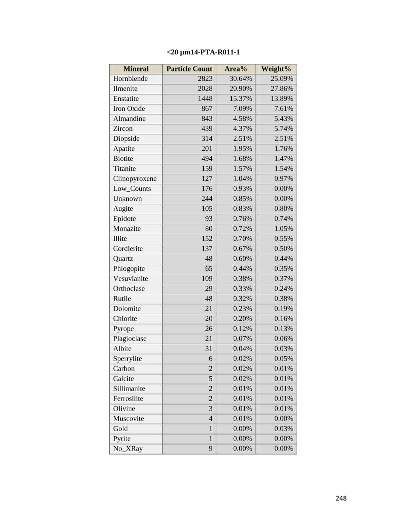
248
<20 µm 14-PTA-R011-1
Mineral Particle Count Area% Weight%
Hornblende 2823 30.64% 25.09%
Ilmenite 2028 20.90% 27.86%
Enstatite 1448 15.37% 13.89%
Iron Oxide 867 7.09% 7.61%
Almandine 843 4.58% 5.43%
Zircon 439 4.37% 5.74%
Diopside 314 2.51% 2.51%
Apatite 201 1.95% 1.76%
Biotite 494 1.68% 1.47%
Titanite 159 1.57% 1.54%
Clinopyroxene 127 1.04% 0.97%
Low_Counts 176 0.93% 0.00%
Unknown 244 0.85% 0.00%
Augite 105 0.83% 0.80%
Epidote 93 0.76% 0.74%
Monazite 80 0.72% 1.05%
Illite 152 0.70% 0.55%
Cordierite 137 0.67% 0.50%
Quartz 48 0.60% 0.44%
Phlogopite 65 0.44% 0.35%
Vesuvianite 109 0.38% 0.37%
Orthoclase 29 0.33% 0.24%
Rutile 48 0.32% 0.38%
Dolomite 21 0.23% 0.19%
Chlorite 20 0.20% 0.16%
Pyrope 26 0.12% 0.13%
Plagioclase 21 0.07% 0.06%
Albite 31 0.04% 0.03%
Sperrylite 6 0.02% 0.05%
Carbon 2 0.02% 0.01%
Calcite 5 0.02% 0.01%
Sillimanite 2 0.01% 0.01%
Ferrosilite 2 0.01% 0.01%
Olivine 3 0.01% 0.01%
Muscovite 4 0.01% 0.00%
Gold 1 0.00% 0.03%
Pyrite 1 0.00% 0.00%
No_XRay 9 0.00% 0.00%

249
<20 µm 14-PTA-R011-2
Mineral Particle Count Area% Weight%
Unknown 1696 24.24% 0.00%
Hornblende 1733 19.55% 21.51%
Ilmenite 1656 12.16% 21.77%
Iron Oxide 1738 11.63% 16.77%
Dolomite 1341 6.38% 6.90%
Enstatite 620 5.28% 6.41%
Clinopyroxene 232 2.75% 3.44%
Zircon 529 2.34% 4.13%
Almandine 409 1.70% 2.72%
Apatite 217 1.61% 1.95%
Calcite 326 1.55% 1.59%
Biotite 431 1.51% 1.78%
Augite 80 1.18% 1.52%
Titanite 176 1.05% 1.39%
Diopside 130 0.97% 1.30%
Cordierite 121 0.90% 0.91%
Quartz 53 0.66% 0.66%
Epidote 108 0.63% 0.83%
Phlogopite 109 0.56% 0.59%
Plagioclase 79 0.54% 0.55%
Albite 104 0.48% 0.48%
Low_Counts 110 0.39% 0.00%
Vesuvianite 71 0.34% 0.43%
Monazite 105 0.30% 0.58%
Carbon 112 0.20% 0.16%
Orthoclase 24 0.19% 0.19%
Rutile 50 0.19% 0.31%
Illite 33 0.18% 0.19%
Pyrope 61 0.13% 0.18%
Pyrite 4 0.12% 0.23%
Gypsum 16 0.09% 0.08%
Sperrylite 43 0.07% 0.28%
Sillimanite 5 0.07% 0.08%
Chlorite 17 0.05% 0.05%
Olivine 3 0.02% 0.03%
Galena 2 0.00% 0.01%
Arsenopyrite 1 0.00% 0.00%
Ferrosilite 3 0.00% 0.00%
Clinochlore 1 0.00% 0.00%
Sphalerite 1 0.00% 0.00%
No_XRay 3 0.00% 0.00%

250
63-45 µm 14-PTA-R029-1
Mineral Particle Count Area% Weight%
Hornblende 9549 53.10% 48.28%
Enstatite 2895 14.11% 14.15%
Ilmenite 1364 6.91% 10.23%
Almandine 2670 5.62% 7.41%
Epidote 1256 3.92% 4.24%
Iron Oxide 523 1.85% 2.20%
Biotite 1609 1.73% 1.68%
Clinopyroxene 569 1.65% 1.71%
Apatite 393 1.60% 1.60%
Diopside 548 1.43% 1.59%
Titanite 396 1.38% 1.50%
Cordierite 647 1.12% 0.93%
Illite 877 1.00% 0.86%
Low_Counts 437 0.81% 0.00%
Vesuvianite 304 0.65% 0.69%
Zircon 86 0.50% 0.73%
Quartz 154 0.49% 0.41%
Unknown 477 0.40% 0.00%
Augite 131 0.39% 0.41%
Phlogopite 144 0.26% 0.23%
Rutile 123 0.26% 0.35%
Albite 177 0.20% 0.17%
Plagioclase 104 0.14% 0.12%
Pyrope 63 0.13% 0.15%
Chlorite 86 0.12% 0.11%
Orthoclase 57 0.10% 0.08%
Monazite 24 0.06% 0.10%
Sillimanite 5 0.03% 0.03%
Forsterite 1 0.01% 0.01%
Dolomite 1 0.00% 0.00%
Clinochlore 1 0.00% 0.00%
Muscovite 3 0.00% 0.00%
Gypsum 1 0.00% 0.00%
Ferrosilite 2 0.00% 0.00%
No_XRay 18 0.00% 0.00%
Calcite 1 0.00% 0.00%
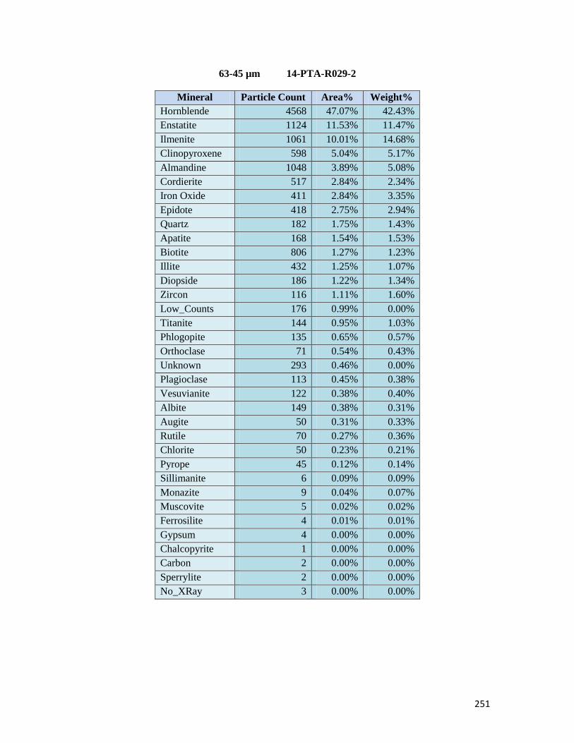
251
63-45 µm 14-PTA-R029-2
Mineral Particle Count Area% Weight%
Hornblende 4568 47.07% 42.43%
Enstatite 1124 11.53% 11.47%
Ilmenite 1061 10.01% 14.68%
Clinopyroxene 598 5.04% 5.17%
Almandine 1048 3.89% 5.08%
Cordierite 517 2.84% 2.34%
Iron Oxide 411 2.84% 3.35%
Epidote 418 2.75% 2.94%
Quartz 182 1.75% 1.43%
Apatite 168 1.54% 1.53%
Biotite 806 1.27% 1.23%
Illite 432 1.25% 1.07%
Diopside 186 1.22% 1.34%
Zircon 116 1.11% 1.60%
Low_Counts 176 0.99% 0.00%
Titanite 144 0.95% 1.03%
Phlogopite 135 0.65% 0.57%
Orthoclase 71 0.54% 0.43%
Unknown 293 0.46% 0.00%
Plagioclase 113 0.45% 0.38%
Vesuvianite 122 0.38% 0.40%
Albite 149 0.38% 0.31%
Augite 50 0.31% 0.33%
Rutile 70 0.27% 0.36%
Chlorite 50 0.23% 0.21%
Pyrope 45 0.12% 0.14%
Sillimanite 6 0.09% 0.09%
Monazite 9 0.04% 0.07%
Muscovite 5 0.02% 0.02%
Ferrosilite 4 0.01% 0.01%
Gypsum 4 0.00% 0.00%
Chalcopyrite 1 0.00% 0.00%
Carbon 2 0.00% 0.00%
Sperrylite 2 0.00% 0.00%
No_XRay 3 0.00% 0.00%
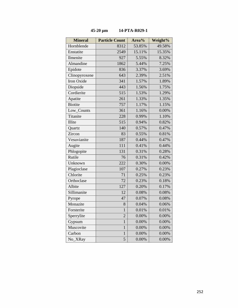
252
45-20 µm 14-PTA-R029-1
Mineral Particle Count Area% Weight%
Hornblende 8312 53.85% 49.58%
Enstatite 2549 15.11% 15.35%
Ilmenite 927 5.55% 8.32%
Almandine 1862 5.44% 7.25%
Epidote 836 3.37% 3.69%
Clinopyroxene 643 2.39% 2.51%
Iron Oxide 341 1.57% 1.89%
Diopside 443 1.56% 1.75%
Cordierite 515 1.53% 1.29%
Apatite 261 1.33% 1.35%
Biotite 757 1.17% 1.15%
Low_Counts 361 1.16% 0.00%
Titanite 228 0.99% 1.10%
Illite 515 0.94% 0.82%
Quartz 140 0.57% 0.47%
Zircon 83 0.55% 0.81%
Vesuvianite 187 0.44% 0.47%
Augite 111 0.41% 0.44%
Phlogopite 131 0.31% 0.28%
Rutile 76 0.31% 0.42%
Unknown 222 0.30% 0.00%
Plagioclase 107 0.27% 0.23%
Chlorite 71 0.25% 0.23%
Orthoclase 72 0.23% 0.18%
Albite 127 0.20% 0.17%
Sillimanite 12 0.08% 0.08%
Pyrope 47 0.07% 0.08%
Monazite 8 0.04% 0.06%
Forsterite 1 0.01% 0.01%
Sperrylite 2 0.00% 0.00%
Gypsum 1 0.00% 0.00%
Muscovite 1 0.00% 0.00%
Carbon 1 0.00% 0.00%
No_XRay 5 0.00% 0.00%

253
45-20 µm 14-PTA-R029-2
Mineral Particle Count Area% Weight%
Hornblende 8308 41.68% 36.65%
Ilmenite 2847 13.12% 18.78%
Enstatite 1908 8.78% 8.52%
Iron Oxide 1543 5.80% 6.68%
Clinopyroxene 1261 4.89% 4.90%
Almandine 1827 4.26% 5.43%
Epidote 1148 3.59% 3.75%
Cordierite 886 2.79% 2.24%
Biotite 1525 2.06% 1.93%
Quartz 315 1.35% 1.08%
Apatite 348 1.33% 1.28%
Zircon 294 1.31% 1.85%
Low_Counts 345 1.12% 0.00%
Titanite 342 1.11% 1.18%
Phlogopite 296 0.92% 0.78%
Diopside 319 0.92% 0.99%
Illite 520 0.84% 0.70%
Unknown 647 0.79% 0.00%
Albite 303 0.50% 0.40%
Orthoclase 134 0.48% 0.38%
Rutile 175 0.45% 0.59%
Vesuvianite 232 0.44% 0.46%
Plagioclase 212 0.39% 0.32%
Augite 63 0.23% 0.24%
Chlorite 74 0.22% 0.20%
Dolomite 240 0.19% 0.16%
Pyrope 78 0.14% 0.16%
Monazite 40 0.13% 0.21%
Sillimanite 10 0.07% 0.07%
Gypsum 25 0.06% 0.04%
Muscovite 6 0.02% 0.01%
Sperrylite 8 0.00% 0.02%
Calcite 3 0.00% 0.00%
Olivine 1 0.00% 0.00%
Carbon 1 0.00% 0.00%
No_XRay 4 0.00% 0.00%

254
<20 µm 14-PTA-R029-1
Mineral Particle Count Area% Weight%
Hornblende 6603 43.72% 37.96%
Ilmenite 2665 12.93% 18.27%
Enstatite 2039 12.05% 11.55%
Iron Oxide 1599 6.57% 7.48%
Almandine 1358 4.72% 5.93%
Epidote 776 3.16% 3.26%
Clinopyroxene 456 2.16% 2.14%
Zircon 341 1.84% 2.56%
Biotite 809 1.70% 1.58%
Cordierite 375 1.35% 1.07%
Titanite 253 1.30% 1.36%
Diopside 221 1.06% 1.13%
Low_Counts 278 1.00% 0.00%
Illite 342 0.90% 0.74%
Apatite 149 0.86% 0.82%
Rutile 194 0.82% 1.04%
Quartz 115 0.61% 0.48%
Unknown 284 0.60% 0.00%
Phlogopite 151 0.56% 0.47%
Monazite 90 0.39% 0.60%
Chlorite 68 0.26% 0.23%
Augite 59 0.26% 0.26%
Orthoclase 65 0.25% 0.19%
Vesuvianite 78 0.24% 0.25%
Plagioclase 86 0.22% 0.18%
Albite 99 0.18% 0.14%
Pyrope 55 0.15% 0.17%
Sillimanite 16 0.08% 0.08%
Olivine 4 0.02% 0.02%
Sperrylite 7 0.01% 0.04%
Calcite 3 0.01% 0.01%
Dolomite 10 0.01% 0.00%
Spinel 2 0.00% 0.00%
Muscovite 2 0.00% 0.00%
Clinochlore 2 0.00% 0.00%
Gypsum 1 0.00% 0.00%
Ferrosilite 3 0.00% 0.00%
Forsterite 1 0.00% 0.00%

255
<20 µm 14-PTA-R029-2
Mineral Particle Count Area% Weight%
Hornblende 3135 29.85% 32.39%
Unknown 1651 20.53% 0.00%
Iron Oxide 2440 11.29% 16.06%
Ilmenite 2175 9.61% 16.96%
Enstatite 947 4.46% 5.34%
Dolomite 1600 4.12% 4.40%
Clinopyroxene 402 2.55% 3.15%
Almandine 954 2.53% 3.97%
Epidote 621 2.11% 2.72%
Biotite 837 1.84% 2.13%
Cordierite 349 1.49% 1.48%
Zircon 436 0.97% 1.69%
Quartz 121 0.96% 0.94%
Apatite 194 0.77% 0.92%
Titanite 213 0.73% 0.94%
Calcite 332 0.66% 0.67%
Plagioclase 166 0.52% 0.53%
Phlogopite 129 0.51% 0.54%
Rutile 219 0.50% 0.79%
Diopside 132 0.49% 0.65%
Illite 162 0.45% 0.46%
Albite 185 0.44% 0.43%
Low_Counts 144 0.40% 0.00%
Sillimanite 30 0.38% 0.46%
Monazite 158 0.31% 0.60%
Chlorite 71 0.28% 0.30%
Pyrope 136 0.23% 0.33%
Carbon 110 0.23% 0.19%
Augite 56 0.21% 0.26%
Vesuvianite 83 0.18% 0.23%
Orthoclase 25 0.17% 0.16%
Gypsum 35 0.16% 0.14%
Muscovite 4 0.03% 0.03%
Sperrylite 39 0.03% 0.10%
Ferrosilite 9 0.01% 0.02%
Spinel 1 0.01% 0.01%
Pyrite 2 0.01% 0.01%
Sphalerite 1 0.00% 0.00%
Galena 2 0.00% 0.00%
Clinochlore 1 0.00% 0.00%
Chalcopyrite 5 0.00% 0.00%
No_XRay 17 0.00% 0.00%