physics at future accelerators - international
TRANSCRIPT
INSTITUTE OF THEORETICAL PHYSICS, WARSAW UNIVERSITY, WARSAWINSTITUTE OF EXPERIMENTAL PHYSICS, WARSAW UNIVERSITY, WARSAW
INSTITUTE FOR NUCLEAR STUDIES, WARSAW
PHYSICSAT FUTURE ACCELERATORS
PROCEEDINGS OF THE X WARSAW SYMPOSIUMON ELEMENTARY PARTICLE PHYSICS
KAZIMIERZ, POLAND, MAY 24 - 30 1987
WARSZAWA 1987
INSTITUTE OF THEORETICAL PHYSICS, WARSAW UNIVERSITY, WARSAW
INSTITUTE OF EXPERIMENTAL PHYSICS, WARSAW UNIVERSITY, WARSAW
INSTITUTE FOR NUCLEAR STUDIES, WARSAW
P H Y S I C S
A T F U T U R E A C C E L E R A T O R S
PROCEEDINGS OF THE X WARSAW SYMPOSIUM
ON ELEMENTARY PARTICLE PHYSICS
KAZIMIER2, POLAND, MAY 24 - 30, 1987
Edited by Z. AJDUK
WftRSZAMA 1987

O r g a n i z i n g C o m m i t t e e
H. ABRAMOWICZ S. POKORSKI
Z. AJDUK R. SOSNOWSKI
G. BIAtKOWSKI A. WROBLEWSKI
D. KIEiCZEWSKA J. ZAKRZEWSKI
This is the tenth volume in the series of Proceedings:
1. Proceedings of the I International Symposium on Hadron
Structure and Multiparticle Production, Kazimierz, 1977;
2. Proceedings of the II International Symposium on Hadron
Structure and Multiparticle Production, Kazimierz, 1979;
3. Proceedings of the III Warsaw Symposium on Elementary
Particle Physics, Jodlowy Dw<5r, 1980 (published in the
journal "Nukleonika",2£, 147, 1095 (1981));
4. Proceedings of the IV Warsaw Symposium on Elementary
Particle Physics, Kazimierz, 1981;
5. Proceedings of the V Warsaw Symposium on Elementary
Particle Physics, Kazimierz, 1982;
6. Proceedings of the VI Warsaw Symposium on Elementary
Particle Physics, Kazimierz, 1983;
7. Proceedings of the VII Warsaw Symposium on Elementary
Particle Physics, Kazimierz, 1984;
8. Proceedings of the VIII Warsaw Symposium on Elementary
Particle Physics, Kazimierz, 198S;
9. Proceedings of the IX Warsaw Symposium on Elementary
Particle Physics, Kazimierz, 1986.

LIST OF PARTICIPANTS
1.H.Abramowicz
2.M.Adanus
3.Z.Ajduk
4.B,Badelek
5.G.Baranko
6.A.Bassetto
7.^.v.Batunin
8.H.Bialkowska
9.D.Bloch
IC.A.Blondel
11.J.Blflmlein
12.w.de Boer
13.G.Bohm
14.A.Breskin
15.R.Budzynski
16.p.Cenci
17.E.Cohen
18.F.Csikor
19.P.Danielewicz
20.J.P.Derendinger
21.N.G.Deshpande
2 2.A.Dubnifikova
23.A.Filipkowski
24.L.Fluri
25.G.E.Forden
26.B.Foster
27.J.M.Gaillard
28.J.Gajewski
- Warsaw
- Warsaw
- Warsaw
- Warsaw
- Stanford
- Padua
- Protvino
- Warsaw
- Strasbourg
- CERN Geneva
- Zeuthen
- Hamburg
- Zeuthen
- Rehovot
- Warsaw
- CERN Geneva
- Saclay
- Budapest
-•Warsaw
- Zurich
- Eugene
- Bratislava
- Warsaw
- Neuchatel
- Stony Brook
- Bristol
- Orsay
- Warsaw
29.Ch.Geich-Gimbel
3O.K.Genser
31.M.Giler
32.R.Gokieli
33.P.Gdrnicki
34.M.G<5rski
35.K.Hahn
36. W. Heck
37.T.Hofmokl
38.R.Holyrtski
39.D.Issler
4O.F.Jewsky
41.E.M.Kabuss
42.J.Kalinowski
43.M.Kalinowski
44.R.Karpiuk
45.J.Kempa
46.J.Kempczyrfski
4/.S.Klimek
48.K.Kolodziej
49.J.Kosiec
5Cl.O.O.Kotz
51.A.Krause
S2.M.Krawczyk
53.P.Krawczyk
54.J.Kr<51ikowski
S5.W.Kr<51ikowski
56.A.Kryg
- Bonn
- Warsaw
- tdd*
- Warsaw
- Warsaw
- Warsaw
- Leipzig
- CERN Geneva
- Warsaw
- Cracow
- Berne
- Hamburg
- Heidelberg
- Warsaw
- Warsaw
- Warsaw
- V6dt
- Warsaw
- Warsaw
- Katowice
- Warsaw
- Hamburg
- Berne
- Warsaw
- Warsaw
- Warsaw
- Warsaw
- V6&i

57.J.H.Kflhn
58.A.Majewska
59.R.Marfka
6O.M.Marlcytan
61.K.Meissner
62 . Ta-Chung Meng
63.D.Milewska
64.P.Minkowski
65.A.G.Minten
66.0.A.Mogilevski
67.R.Nania
68.J.Nassalski '
69.R.Nowak
70.J.Nowicka
71.Yu.W.0bukhov
72.M.01echowski
73.M.Palacz
74.J.Pawelczyk
75.M.Pawlowski
76.R.Peschanski
77.S.Pokorski
78.H.Roloff
79.E.Rondio
80.A.Roussarie
81.A.Sandacz
82.L.Silverman
8 3.Yu.M.Sinyukov
84.S.N.Sokolov
85.R.Sosnowski
- Munich
- Warsaw
- Katowice
- Vienna
- Warsaw
- Berlin
- Warsaw
- Berne
- CERN Geneva
- Kiev
- CERN Geneva
- Warsaw
- Warsaw
- Kielce
- Warsaw
- Warsaw
- Warsaw
- Warsaw
- Warsaw
- Warsaw
- Warsaw
- Zeuthen
- Bialystok
- Saclay
- Warsaw
- Orsay
- Kiev
- Protvino
- Warsaw
86.M.Spalirfski
87.M.Staszel
88.A.Stopczyrfski
89.H.StrSbele
9O.M.Sumbera
91.H.Szczekowski
92.A.Szczepaniak
93.H.Szeptycka
94.R.Szwed
95.P.SzymalSski
96.M.Tamada
97.A.Tsirou
98.T.Tymieniecka
99.H.Walczak
100-R.Walczak
101.J.Wdowczyk
102.R.Weiner
1O3.G.Wilk
1O4.G.Wilquet
105.R.Windmolders
106.Z.Wlodarczyk
1O7.E.De Wolf
108.K.Wo£niak
1O9.A.Wr<5blewski
110.G.Wrochna
III.B.Yuldashev
112.J.Zakrzewski
113.S.Zylberajch
114.A.Zarnecki
Warsaw
Warsaw
Warsaw
CERN Geneva
ftez/Prague
Warsaw
Warsaw
Warsaw
Warsaw
Warsaw
Hamburg
Warsaw
V6&4.
Warsaw
Marburg
Warsaw
Warsaw
CERN Geneva
Kielce
Antwerp
Cracow
Warsaw
Warsaw
Tashkent
Warsaw
Saclay
Warsaw
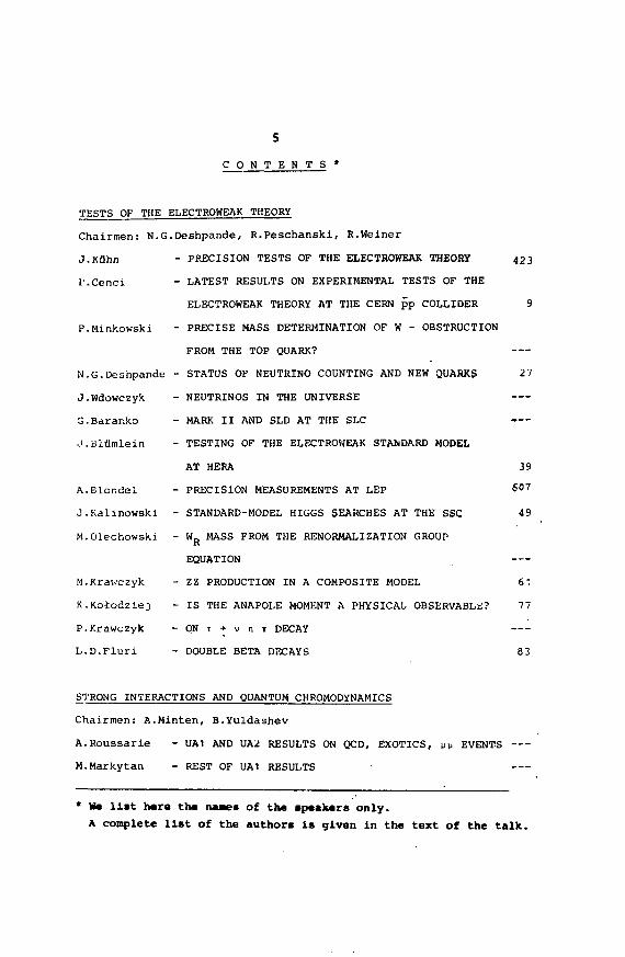
sC O N T E N T S *
TESTS OF THE ELECTROWEAK THEORY
Chairmen: N.G.Deshpande, R.Peschanski, R.Weiner
J.KUhn - PRECISION TESTS OF THE ELECTROWEAK THEORY 423
T.Cenci - LATEST RESULTS ON EXPERIMENTAL TESTS OF THE
ELECTROWEAK THEORY AT THE CERN pp COLLIDER 9
P.Minkowski - PRECISE MASS DETERMINATION OF W - OBSTRUCTION
FROM THE TOP QUARK?
N.G.Deshpande - STATUS OF NEUTRINO COUNTING AND NEW QUARKS 27
J.Wdowczyk - NEUTRINOS IN THE UNIVERSE
G.Barar.ko - MARK II AND SLD AT THE SLC
J.Blflndein - TESTING OF THE ELECTROWEAK STANDARD MODEL
AT HERA 39
A.Blondel - PRECISION MEASUREMENTS AT LEP 6°7
J.Kalinowski - STANDARD-MODEL HIGGS SEARCHES AT THE SSC 49
M.Olechowski - W_ MASS FROM THE RENORMALIZATION GROUPK
EQUATION
M.Krawczyk - ZZ PRODUCTION IN A COMPOSITE MODEL 61
K.Kolodziej - IS THE ANAPOLE MOMENT A PHYSICAL OBSERVABLE? 77
P.Krawczyk - ON T •+ v n v DECAY
L.D.Fluri - DOUBLE BETA DECAYS 8 3
STRONG INTERACTIONS AND QUANTUM CHROMODYNAMICS
Chairmen: A.Minten, B.Yuldashev
A.Roussarie - UA1 AND VA2 RESULTS ON QCD, EXOTICS, up EVENTS
M.Markytan - REST OF UA1 RESULTS •
* We list hare the namea of the spatters only.
A complete list of the authors is given in the text of the talk.
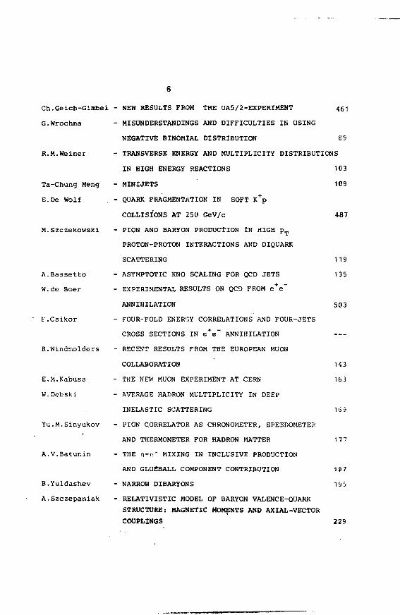
Ch.Ge ich-Gimbe1
G.Wrochna
R.M.Weiner
Ta-Chung Meng
E.De Wolf
M.Szczekowski
A.Bassetto
W.de Boer
F.Csikor
R.Windmolders
E.M.Kabuss
W.Dçbski
Yu.H.Sinyukov
A.V.Batur.in
B.Yuldashev
A.Szczepaniak
NEW RESULTS FROM THE UA5/2-EXPERIMENT 461
MISUNDERSTANDINGS AND DIFFICULTIES IN USING
NEGATIVE BINOMIAL DISTRIBUTION 89
TRANSVERSE ENERGY AND MULTIPLICITY DISTRIBUTIONS
IN HIGH ENERGY REACTIONS 103
MINUETS 109
QUARK FRAGMENTATION IN SOFT K+p
COLLISIONS AT 250 GeV/c 487
PION AND BARYON PRODUCTION IN HIGH p T
PROTON-PROTON INTERACTIONS AND DIQUARK
SCATTERING 11 9
ASYMPTOTIC KNO SCALING FOR QCD JETS 135
EXPERIMENTAL RESULTS ON QCD FROM e + e~
ANNIHILATION 503
FOUR-FOLD ENERGY CORRELATIONS AND FOUR-JETS
CROSS SECTIONS IN e+e~ ANNIHILATION
RECENT RESULTS FROM THE EUROPEAN MUON
COLLABORATION 14 3
THE NEW MUON EXPERIMENT AT CERN 163
AVERAGE HADRON MULTIPLICITY IN DEEP
INELASTIC SCATTERING 169
PION CORRELATOR AS CHRONOMETER, SPEEDOMETEE
AND THERMOMETER FOR HADRON MATTER 17?
THE n-n' MIXING IN INCLUSIVE PRODUCTION
AND GLUEBALL COMPONENT CONTRIBUTION 187
NARROW DIBARYONS 195
RELATIVISTIC MODEL OF BARYON VALENCE-QUARK
STRUCTURE: MAGNETIC MOMENTS AND AXIAL-VECTOR
COUPLINGS 229
HEAVY IONS. HEAVY FLAVORS
Chairmen: R.Windmolders , M.Markytan
H.Strflbele ..
W.Heck "*
O.A.Mogilevski
K.Woiniak
R.Nania
G.Forden
D.Bloch
H.Roloff
S.Zylberajch
- ULTRA-RELATIVISTIC HEAVY ION COLLISIONS 553
LATTICE QCD THERMODYNAMICS: THE NEW STATE
EQUATION FOR QUARK-GLUON PLASMA
CENTRAL COLLISIONS OF 800 GeV PROTONS
WITH HEAVY NUCLEI
LEADING HEAVY FLAVOURED BARYON PRODUCTION
AT THE ISR 237
CHARM MESON LIFETIMES FROM TASSO 633
CHARM PHOTOPRODUCTION IN THE NA14-II
EXPERIMENT 24 7
PRODUCTION OF ye PAIRS IN NEUTRINO INTERACTIONS
AT 3 - 30 GeV NEUTRINO ENERGY 257
TOPONIOM AT LEP 265
EXPERIMENTAL TECHNIQUES AT FUTURE ACCELERATORS
Chairman: E.De Wolf
A.Breskin - NEW METHODS FOR PARTICLE IDENTIFICATION
USING LOW PRESSURE GAS DETECTORS
J.M.Gaillard - UA2 SCINTILLATING FIBRE TRACKING DETECTOR
A.Minten - TIME PROJECTION CHAMBERS AT LEP
U.KfitZ - THE ZEUS URANIUM CALORIMETER
B.Foster - TRACKING DETECTORS AT ZEUS
G.Bohra - PROJECT OF A TAGGED NEUTRINO FACILITY
AT SERPUKHOV
273
287
SUPERSTRINGS
Chairman: P.Minkowski
J .Derendinger - ON SUPERSTRINGS AND THE UNIFICATION OF
PARTICLE INTERACTIONS 29 3
R.Peschanski - SUPERSTRINGS AND FOUR-DIMENSIONAL SUPERGRAVITY
N.G.Deshpande - PHENOMENOLOGY BASED ON SUPERSTRING INSPIRED E, CROUP 575 .o
J.Pawelczyk - EFFECTIVE ACTION FOR STRINGS 313
E.Cohen - THE EFFECTIVE ACTION OF THE BOSONIC STRING
K.Meissner - THE MANDELSTAM STRING AND THE VERTEX OPERATOR
R.Marfka - STRING IN ELECTROWEAK THEORY (SU(2)xU(1)xU(1))
S.N.Sokolov - SPECIFICS OF THE PARTICLE MOTION AND SPREADING
OF PERTURBATIONS IN THE FRONT-FORM
TWO-DIMENSIONAL RELATIVISTIC DYNAMICS 321
B.Humpert - THEOREM PROVING WITH FIRST-ORDER PREDICATE
LOGIC: III 365
P.Minkowski - CONCLUDING REMARKS
Appendix: List of participants of the III Warsaw Symposium
on Elementary Particle Physics, Jodlowy Dwc5r, 1980
THE.CERN fti COLLIDER
Pariza CcncjCERN. 1211 Genera 23. Switzerland
ABSTRACT
The leptome and hadnnk decays of the Intermediate VectorBoaons (IVB) produced it the CERN Pp collider have been studiedby the UAJ and VA2 CoDabontiont. Rouhs on IVB maues andWaoclucu] tasott ofl teploo uuivuiabty and nunbet of ncutnnoiipecac* m pee—ted aod compticd with the piedictioDs of theStandard Modal of unified deettcweak theory. The UA1 and UA2data at* found to b» m food igreetnent with each other and withtheoretkalcaktiktioat.
1. INTRODUCTION10
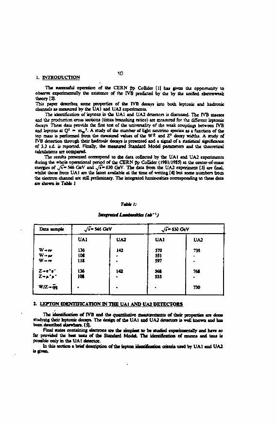
The succeurul operation of the CERN pp Collider [1] has given the opportunity toobtenrt experimeaully the eriitmcr of the IVB predicted by the by the unified electioweaktheory [2].This paps describe* some propertiei of the IVB decayi into both leptorue md hadronicrhiTTP^* as ineuurtd by the UAi lod UA2 ^TTimniiti
The iArr\iifirMirm of leptons is the UA1 and UA2 detecton u d iy^^d The FVB massesu d the production crou lections (times branching ratioi) are measured for the different leptonicdecayi These data provide the first teit of the univerulity of the weak couptiap between IVBu d leptoas it Q* « <&w'- A itudy of the oumber of light neutrino specie* at a function of thetop mass is performed from the measured values of the W* and Z* decay widths. A study ofFVB detection through their hadronic decayi is presented and a «tgw»i of a «t«t «Hi» y significance
F l l h d Mg y p g g
of 3.3 «.i is reported. Finally, the meuured Standard Model parameter! and the theoretical
The resuhs presented correspond to the data collected by the UA1 and UA2 experimentsduring the whole operational period of the CERN pp Collider (1911/1985) at the center-of-massenergies of , / f - 546 GeV and Vf -630 GeV. The dau from the UA2 experiment [3] are finalwhilst those from UA1 are the latest available at the time of writinj [4] but some numbers fromthe electron rhi iwl are Jt£H preliminary. The integrated luminosities corresponding to these datatxt shown in Table 1
Tibkt:
Imu,
Data sample
W-e»
W-TT
Z«e*e-z-.*»-W/Z«?q
^r -546 GeV
UA1
136lOt111
13610t
UA2
142
142
, / r - 630 GeV
UA1
570551597
5615S5
UA2
73S
761
730
2. LEFTON rDENTOTCATION PS THE UAI AND UA3 DETECTOKS
The irlmtifVition oCTVB and the quantitative meuufemenu of their properties arc donestudying their leptonic decayi. The deagn of the UAI and UA2 detecton is wed known and hasbeen described elsewhere. [51.
Final states containing electrons an the amplMt to be studied experimentally and have sotar provided the best tests of the Standard Modal The identity atinn of muou and taus ispossible only in the UAI detector.
In this section a brief description of the kptoo iftoMiVatinn criteria used by UA 1 and UA2i
112.1 Electron kJeorlfleelioo
Electron randidH'** arc selected by a scries of cuts requiring con-ostency betweencuonmetcr, Backing ind (in UA2 only) preshower information. In ad&tk.n the electronr-.rifi,A*ir j required to be 'uoliied' in the seme that only a small amount of energy should beobserved nearby. These cuu reduce the Large background from QCD jet fragmentation.
Both experiments run with high transverse energy showers in the electromagneticcalorimeters (Ef> 15 GeV in LAI, > 11 GeV in UAl). Cuts are then mace on the showerprofile exploiting the four longitudinal samplings available in UAl and the small lateral cell sizeof U A l Small leakage into the hadronic calorimeters U also required, compatible with anelectron of the appropriate energy Wen the presence of a charged track u required, whosemomentum u compatible with the shosva energy. In UA2, track momentum measurement isonly possible in the forward regions (20* < ) < 40* , 140 ' < I < 160 * ) since no magneticfield is present in the centnl detector region. However the detector ii equipped with preshowercounters over the full solid angle of the calorimeters, which art required to give a hi! compatiblewith both the track and calorimeter shower profile. The detailed isolation cuts used can befoua<i in reference [6]. The detection efficiency found by the two experiments is a 75%.
1 2 Neutrino IdentificationThe presence of a non-interacting particle czn be detected from an apparent lack of
momentum conservation. However, sines in a typica1. pp collision a large fraction of the energyis carried out by particles that do not leave the vacuum pipe and therefore remain undetected,only the component of the rnining momentum transverse to the beam direction can be reliablymeasured. _ _For events containing a lepton candidate of transverse momentum ?[• , one defines {>[•" as
where PT1 is a vector with magnitude equal to the transverse enerfy deposited in the i"1 cell ofthe calorimeter and directed from the event vertex to the estimated impact point on the cell. Thesum is extended over all calorimeter ceDs (excluding the charged lepton). In UAl the Ip-j-*]distribution is found to have an almost gaussian resolution, whilst in UA2 thu resolution showsnon-gamsian tails due to the incomplete angular coverage of the calorimeters.
73 M<MO identificationThe UAl detector is equipped to detect muons. The signature for a muon is the existence
of a charged track aligned spatially with signals turn muon chamben after more than 9interaction lenghtj of """"»). and a characteristic minimum ionizing energy deposition in thecalorimeter cells crossed by this track. A strong isolation of the muon ran>tiriat» a required inorder to reduce the background from jets.
Z.4 Tin ideotincatJooThe UAl collaboration exploits its central detector performance to extract a sample of
event* consiitent with the decay W — T»T, T -• rT + hadrons (=r 65% of al! T decays).Since the T mats ii small, time events are characterized by a highly coUim&led single jet withlow chargcd-paxticlc multiplicity. These events are (elected by denning a 'T likelihood'combining three variables:
P : the fraction of jet energy in * cone J(A+' + At') < 0.4r : the angular separation of the l»»dmg track from the jet axisn : the charged multiplicity.
The expected probability distributions of these variables f(F), f(r), Hn), are constructed byMonte Carlo. The r Ekelihood is then defined u
L , -
The final i sample is defined « those events having L, > 0.
3. rVB LEPTONIC DECAYS12
The final data umplea for each experiment are listed in Table 2, together with «,wri»tr»ibackground estimates.
Table 2:
Summary ofWajtfZmmumpU
Process
W— a samplesignalbackground
W-»ji» samplesignalbackground
W-»T» samplesignalbackground
Z-*e*e~ samplesignalbackground
Z-*v*n- samplesignalbackground
546
5952.247.96.8± 1.8
1Q9.4+3.20.6±0.1
4
< 0.1
4
< 0.1
630
UA1
240219.6± 15.620.4±1.7
5754t7.J3±2
3229.7±5.72.3±0J
28
< 0.7
15
< 1.0
S46
4237.916.54.1±0.4
-
-
98.8±3.00.2
630
UA2
206184.6± 14.521.4±2.2
-
3028.9+5.51.1
3.1 TheWsampte
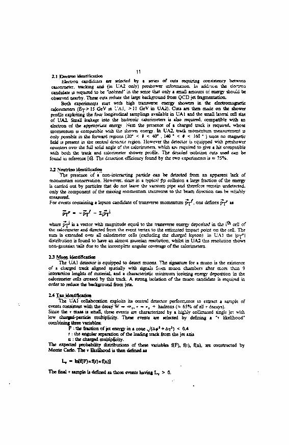
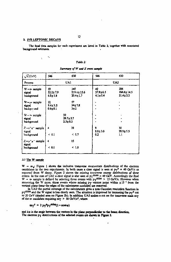
W -» efj.' Figure 1 shows the inclusive transverse momentum distributions of the electroncandidates in the two experiments. In both cases a clear signal is seen at p j e a 40 GeV/c asexpected from W decay. Figure 2 shows the missing transverse energy distributions of theseevents. In the case of UA1 a clear signal is also seen at pj 1 1 1 1 3 1 .^ 40 GeV. Accordingly the finalW •• er sample is defined by selecting those events with p^wwt > 15 GeV/c. However whenmeasuring ths W mass, toose events whose mi<ning p-p vectors point within ± 15 * from thevertical plane (near the edges of the calorimeter modules) are removed
In UA2 the partial coverage of the calorimelen gives a non-Gaussian resolution function inPl"" M and the W signal is less clearly seen. The situation is improved by inr«n«mg the pje cutto 20 CeV (shaded area on Figure 2b). In addition UA2 makes a cut on the transverse mass m jof the w candidate requiring nvr; > SO GeV/c1, when
- 2 l-co>A»)
and i * is the angle between the vecton in the plane rfTrtryfi"'^' to the beam direction.The electron pj distributions of the selected events are shown in Figure 3.
13
The final sample adected by UA1 conuini 299 events with «o estimated background of27.2, while UA2 hai 251 events with a background of 26.4 . Doe to a known trackreconstruction inefficiency, the UA2 sample lued for the crou sectio&i cod man measurementiii reduced to 24S eventi. From these numbers, together wish the known »<B"j>TfYi. accepunceand integrated huninosxties, one can ftfyulate
•w e " »(PP - W+X)xBR(W - er)
The results obtained are given in Table 3 together with the ratioi of the cron jectioni ttthe two JT value* available, and the theoretical prediction* of [7], The quoted error* are thestatistic and the synematic one, respectively. The agreement it good, «hlwmg>i the measurement!are systematically above the prediction!.
Tabk3:
WFreJaabH Crou Sretfow (Eltetnm Otrnd)
UAl
UA2
Theorjr
S46G«V
0
0
0
^ n b )
55*0.08*0
6010.10*0,,•0.1343-0.06
.09
.07
630 Oe»
.w*(nb)
0
0
0
63*0.05*0.
5710.Q5±0., - •0 .17" - 0 . 0 9
10
07
•we(630)/.w
e(S46)
1
0
1
1510.19
95*0.18
23
*) UAi Adf.2«3nb-'111 ««»•< t
m o ? n e n t U m <fi«I*un«'' of mchaive electronn , p k w n h « > | S G V y ( 1 9 Mn,pkwnh
b) UA2 dau lample wnh jGeV/c (full itatiitica)
a
SJII t«j ^ »—•• IJl ml
• 1 »f'
H U M
If 1G1V/0
Fig. 2: Missing transverse energy distributions of the inclusive electron candidates:a) I'At dau (1984 data only)b) LA2 dau (full sutistics) The shaded area corresponds to events with px e > 20 GeV/c.
20
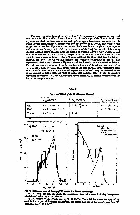
«) UA1w —» tv 290 Evtftts
0 20 1.0 60 80
Electron Et ICtVIFif. 3: Transverse encrjy distributions of electrons in W«e>- events:
i) UA1 data. The curve shows the prediction for m * * U.S GeV/c'. The thaded regionshows the main background contributions.
b) UA2 data. The curve shows the prediction for mw * 10.2 CcV/e' including allluckpounj contributions.
15
The transverse tots* distributions are used by both experiments to measure the mass andwidth of the W. This variable is lea sensitive to the effect of the pj- of the W than the electronPT spectrum which has been used m the p u t UA1 obtains a background free sample of 149events for this measurement by cutting both pf* and p;*1"** at 30 GtV/c. The results of thisanalysis an not yet final Figure 4a shows the 017 distribution for the complete sample togetherwith a prediction fot n ^ - 83.5 GeV A re-cvahiation of the UA1 final sample of data usiagidentical selection criteria i*.«pn iHgtly the number of events at J7~ 546 GeV. Figures 3a and4a ihow the distributions of a preliminary simple of 290 events selected with identical cuts. Thelatest fit value ii given in Table 4. The UA2 experiment, on the other hand, uses the full tn-j-tiw^ tniwi for p r * * 20 GcV/c **** jp^i^f the estimated background in the fit. Theexperimental distribution is shown in Figure 4b, and the fit results are summarized in Table 4.The mam systematic error comes from the absolute calibration of the caloiimsten, being ±3%for UA1 and ± 1.6V. for UA2 These enon cancel in the ratio mj/m^. Both experiments agreewell with each other and with the theoretical expectation (rttnTlatfi "«««»g the measured valuesof the coupHsg cftiwtarrti [161, the value of nnfv from neutrino data [IS] and the radiativecorrections of reference (171). For UA2 the first error ii «»«tt«iH. the second systematic and thethird is the energy scale error.
Ttbk4:
UA1
UA2
Theory
m^GeV/c*)
82.7±l.O±2.7
SO.2±0.6±0.3*1.3
80.310.9
rw(GeV/e»)
2.8*}'**1.3
2.48
r w (upper fimit)
<5.4 (902 CL)
<7.0 (901 Cl.)
40
- M
xI
i»z
to -
UA1 W _ . cv
290 EVENTS
5 20 (.0 60 60 100 120 IM, ICtV/c1)
a) UA1 data. The (ua fin, show* to* expectation fan all aouttaa nciudinc background(shaded a m ) w o t a . - I3J GeV/e«. —«• »-«»««.
' U i ^ "***_!* 7 S 3 ***** w U l I T " > ^ G t V / f c Tht aoBd fine abowi the total of allcontnbutiooj txpacted, mrtinting backgrouad, fl» dashed fine shew* tht contributiaB from W
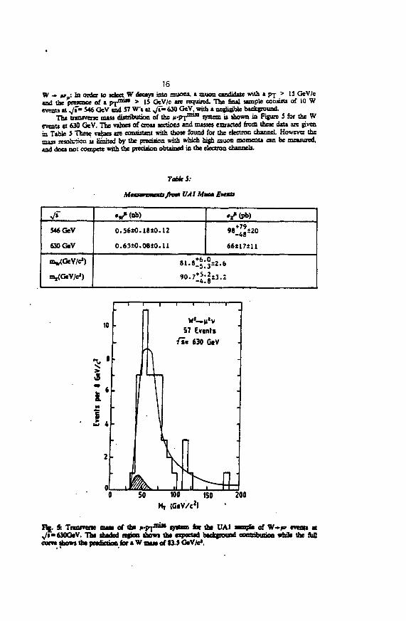
16W - . pr-. In order to select. W decayi into muont, a muon candidate with a p-j- > 15 GeV/cand the y f r f f of a pytmu > 15 GcV/c are required. The final sample coossti of 10 Wevmu at J*m 546 GeV and 57 W't at ^/f- 630 GeV, with a negligible background.
The tnmsvtne mass distribution of the M-pr""** system ii shown in Figure 5 for the Weveoti at 630 GeV. The values of crou sections and muses extracted from these data are givenin Table 5 These values are consistent with those found for the electros channfl However thema.. resolution u limited by the precision with which high muon momenta can be measured,and does not compete with the precision obtained in the electron rhtnnrli
Tahiti:
Mtmrtmnufram VA1 Mm EwaO
546 GeV
630 GeV
mw(GeV/cJ)
m^GeV/e*)
«V(nb)
0.56±0.1St0.12
0.63±0.08*0.11o66tl7±H
8 . «*6.0.
90.7+5'2±3.2
10
•
I'L
2
0
57 Events
/?« 630 GeV
\
L
•
•
50 100 B0«GtV/c2)
200
Fit. & Traurene man of the ^-px™1" system for tht UA1 sample of W»^» events at^s -630GtV. Tht shaded repon ihowi the expected background contribution whik the fuOcon* shows tin prediction far a W mass of 13.5 GeV/c1.
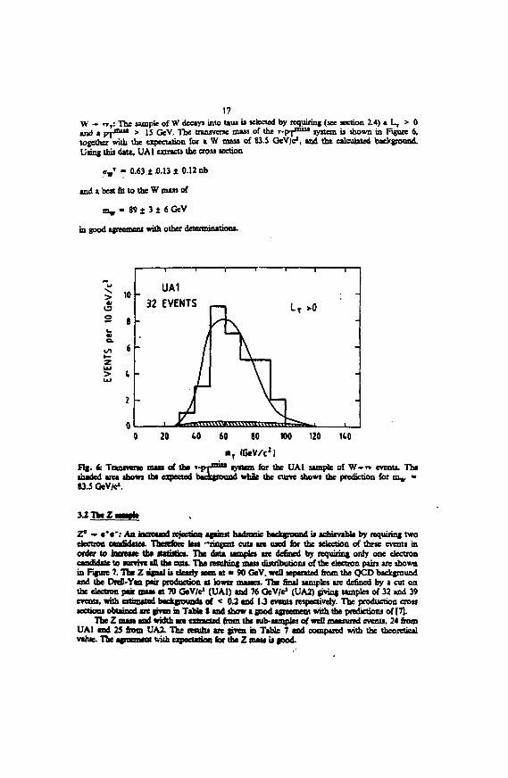
17W - rrT: The sample of W decays into laus is selected by requiring (see section 2.4) » L^ > 0and a y | m ' M > 15 GeV. The transverse mass of the r-pj™31 system is shown in Figure 6,together with the expectation for a W mass of 83.5 GeV/c1, and the raimUtcd background.Using this data, UA1 extracts the cross section
«WT - 0.63 ± -0.13 t 0.12 nb
and a best fit to the W mass of
m,, - S9 ± 3 ± 6 GeV
in good agreement with other determinations.
> ioo
° 8CL
zLU> ILU
2
0
UA1" 32 EVENTS
K\
- / NP"
LT >0-
-
-
—1
20 40 60 80 100 120 110
Fij. ft Trauvene man of the ' - irT z m a iy*cm for the UA1 sample of W - T > events. Theshaded area shorn th* eiprcied backfroand while the curre shows the prediction for m , -83.5 GeV/e1.
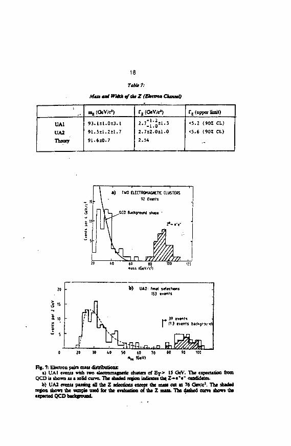
Z* - • *« ' : A s increased rejection apmtt hadronic backjround is achievable by requirinf twoelectron ramtirUtw Theretbre kss Tineent cuts are used for the selection of these eventi inolder to increase th* statistics. The data simples are defined by requirinj only one electroni»Mi^«f» to mifjyg all ths cots. The resuhin( f^«— distxibutions of the electron pairs are shownin Figure ?. The Z sipial is dearly seen at • 90 GeV, well separated from the QCD backgroundand the DreB-Yan pair production at lower masses. The final samples are defined by a cut onthe electron pair mas* at 70 GeV/c2 (UA1) and 76 GeV/e" (UA2) giving samples of 32 and 39events, with estimated backgrounds of < 0.2 and 1J events respectively. The production crosssections obtained are given in Table 8 and show a good agreement with the predictions of (7).
The Z mass and width an extracted from ths sub-samples of well measured events. 24 fromUA1 and 25 bom UA2. The results an gives in Table 7 and compared with the theoreticalvalue. The agreement triifc npmit ion for the Z mass is good.
18
Tahiti:
Mta ad WUtktftktZ (Elton* GktnneQ
UA1
UA2
Theory
m, (GeV/e1)
93.111.0*3.1
91.5*1.2*1.7
91.6*0.7
T2 (GeV/c1)
2.7±2.O±l.O
2.54
Tz (upper limit)
<5.2 (90* CL)
<5.6 (90* CL)
*. 15
a ) TWO ELECTROMAGNETIC CLUSTERS
92 E«nti
b ) UA2 find j»(tttHMij153
r 39(13 <v*nts
so (0 70IGcVI
so 90 100
Fig* 7: Electron pun raw distxibutioiis.i) UA1 event* wiih two ekctnjmijnetic ehuten of Ej> IS GeV. The expecutioo fiom
QCD is ihown u a >ohd curve. The ibaded repoo indicaut tb^ Z-c**" ondiiWln.b) UA2 evenu puang aQ the Z Kfectioas except the man cut at 76 Gev/e2. The shaded
tepon show) the «mpk used for lbs ralnatk» oC the Z man. The daafaed cunt ihowt theexpected QCD background.
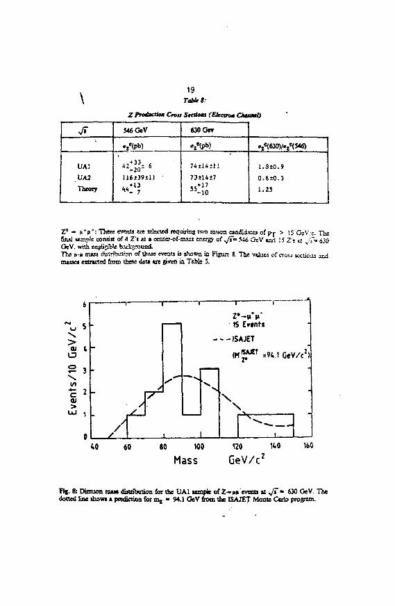
19Table 8:
ZPrUaabm Cna StetioM (Electro* OmmeJ)
UA1
UA2
Theory
«6GeV
116±39il) •
* - 7
630 Get
a^V)
74*14*11
73*1417
5 5 + 1 73 -10
«2«(630)/«j«(S«>
1.8±0.9
O.6±0.3
1.25
Z' -» M*P": These evrnli *re efected requiring two muoa andidrxj of pp > IS GcVc. Thefinal simple consist of 4 Z'l el » cenler-of-nisia Ensrgy of f" 5 « GcV «nd !5 Z1! u -'r=» 630GeV, with negiisiWe b3dtgn)unAThe p-<i nuiM distribirfcrn of thtse events is shown in Figure g. The values of crou icttioiu andmuse) extracted from these deu trt given ia Ttbb 1
6
CU I
S 3
UJ i
0
1 — — - — - | \- i i™
7 ^
15 Events
ISAJET
( M ^ ^ =94.1GeV/c2)
_ ^ - —
"S,
-
x
1
60 80 109
Mass120 N.0
GeV/c2160
Fig. & Dimuon HUM distribution for the UA1 umpte of Z-»(i# eveoti it N/»*" ^ ° G t V
dotted Bne ihowi • predinion for mj - 94.1 GeV from the ISAJET Monte C*rio progism.
20
3 3 Number of HghfniMnwThe expected value of the Z width depends ciucully on the theoretical model used, and in
particular on the number of light neutrinos' (m, < njj/2). The full width is given by
rz - 1 rjitl) + i rz(qq> + jyy.*)
whtr.- i&e fiw sum is over all charged leptons with masses < m^/2, the second tans over allqv-sY flavours, and the third term over a& light neutrinos'. It is assumed that the chargedmi- w of i.iy new families arc too heavy to contribute. UA1 has set a 90% confidence limit[8i including new charged leptons with masses less than 41 GtV/c*. Unfortunately, given thepresent statistics and mass resolution, a direct measurement of I"z (see Table 7) does not yieldstuch information.
A model-dependent method consists of measuring the ratio Rj jp»o we /" 2
e . which iartl:'-i i to the ratio of the total widths by the equation;
Th;5 quanrity is well measured, since the errors on luminosity cancel completely and thoseon efr.ricr.ac; almost completely. The exucK-Uor. of Tz/Tw from thii measutsscnt requires theissump;;oa of the couplings of the Standard Model. Thai the total cross section ratio can ber -Jc-^1.:~. with zn rrror dvc to tiic uncsruinty a ths liructute fiiacticns. TLis cnor does notcar.ee.: una the u ind d quaik strucnuc func-oru cuter difTatsitiy for Z and W production.Both iht cross secvion ratio ind the ratio of the leptonic widths depend on sin'fi,,, but theproduct of the two is insensitive to the value chosen.
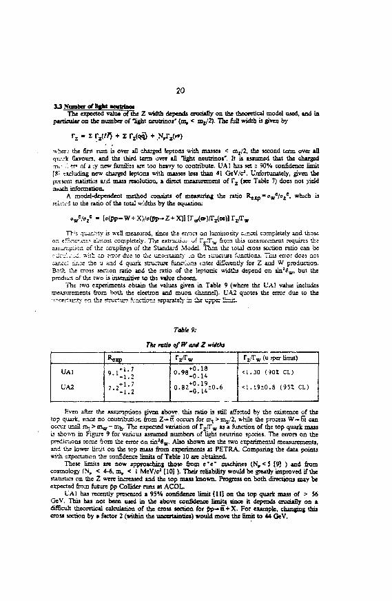
The two experiments obtain the values given in Table 9 (where the UA! value includesmeasurements from both the electron and mucn channel). VA2 quotes the error due to the•!ncttrsL-.»y or. th: rructur? fi.-nctioci separately b i i upper linit.
Table 9:
The note of'WandZ widths
UA1
UA2
rz/rw
0.82^:»S0.6
r z /T w (u jper limit)
<1.30 (90X CD
<1.19±0 .8 (95% CD
Even after the Msumptjous givm above, this ratio u stiU affected by the existence of thetop quark, nnce no contribution from Z-» it occurs for m t >m z /2 , *hiie the process W-»6t canoccur until m. > n , - m^. The expected variation of r z /T w as a function of the top quark massis shown in Figure 9 for various assumed numbers of light neutrino jpsries. The errors on thepredictions come Bom the error on sinJ8w. Also shown are the two experimental measurements,and the lower lieu! on the top mass from experiments at PETRA. Comparing the data pointswith expectation th: confidence limits of Table 10 are obtained
These limits are now approaching those from e*e" machines ( N , < 5 (9} ) and fromcosmology (N, < 4-6, in, < 1 MeV/e2 [10] ). Their reliability would be greatly unproved if thestatistics on the Z were increased arid the top mass known. Progress on both directions may beexpected from future pp Collider runs at ACOL.
LAI has recently presented a 95% confidence limit [II] on the top quark mass of > 56GeV. rhis has not been used in th^ above ^^ fi Tnrr limits, since it 'W^VKII crucially on adifficult theoretical calculation of the cross section for pp-» tt + X. For example, changing thiscross section by a factor 2 (within the uncertainties) would move the limit to 44 GeV.
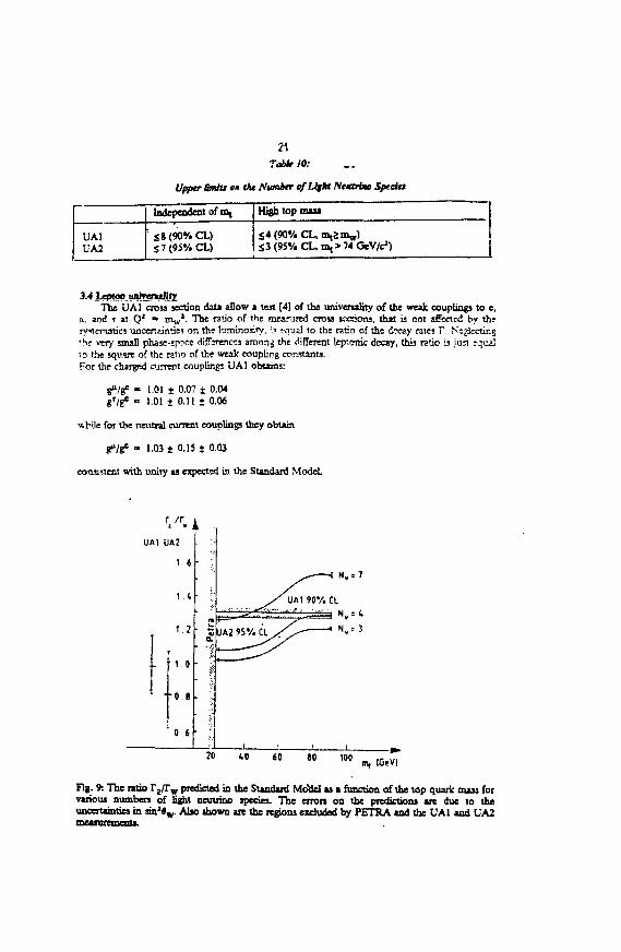
217obit 10:
Upper fimto on tin Number of Ugh* NttarUo Sptdtt
—
UAlUA2
Independent of nit
: $g(90%CL)<7(95%CL)
High top man
£4 (90% CL, m^rn^)S3 (95% CL, m, > 74 GeV/c1)
3.4 LeptooturtrenxHtxThe UAl cross section data allow a test [4] of the universality of tbe weak coupling] to e,
ji, and T it Q' — i ^ , ' . The ratio of the mearured cross sections, that is not affected by thejy^tcmatics uncertainties on tht luminosity, i» ;-,rjil to the ratio of the d?cay raicj r . Nsglccting* V very small phaje-spocc differences among the different kpionic decay, this ratio is jurt equalTO 'he square of th: r?.!io of the weak coupling constants.For the charged current couplings UAl obtains:
•• 101 ± 0.07 ± 0.041.01 + 0.11 ± 0.06
wbile for tbe neutral current couplings they obtain
if If - 1.03 ± 0.15 t 0.03
consistent with unity u expected in the Standard Model
^ 7UAt UA2
1.6
1 .4
1.2
1 0
' t O . «
0 6
N v = 3
20 60 «0 100 m, (GeVI
Fig. 9: The ratio T z /rw predicted in the Standard Model ai a function of the top quark mass forvarious numben of liiht neutrino species. The errors on the predictions are due to theuncertainties in an'«w . Also shown are the regions excluded by PETRA and tbe UAl and UA2measurement*.
22
4. IVB HAPRONIC DECAYS
The IVB are expected to decay into quark-antiquark pain with well H^fin^ [12] bunchingfriction*
n«2o
excluding decays with a top quark m the final state.The observation of such decays is an important check of the Standard Model, and provides
the first test-cue of the ability of future Collider experiments [13) to perform spcctroscopy withhadron jets identified with their parent partonj.
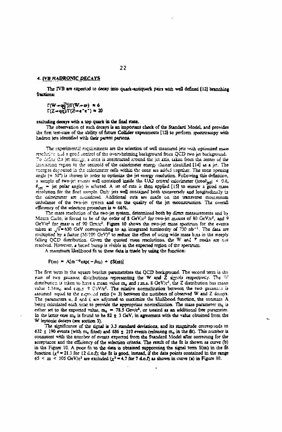
The experimental rtquiiacenu are the selection of well measured jets with optimized massirsclutfr i . J a good control of ths overwhelming background from QCD rwo jet background.To .ic5--~ '.he ;ct cci.-^y, a cccc is constructed around the jet axis, uke& from the center of the'^i:~:x^oz repon to the cectroid of the calorimeter energj cluster ideatified [14] as a jet. Theirscrg-.es deposited in the ^ilorini=-.tr cefls within the race are acl&i ogetiier. The cone openingangle (= SO*) is chosen ir. order to optimize the jet energy resolution. Following this definition,a sample of two-jet events well contained inside ths UA2 central calorimeter (Icojfljj,! < 0-6,Sjjt » jet polar angle) is selected. A jet of cuts is then appHsd [151 to ensure a good massrerolution for the 5ns! i.vnplr. Only jets well contained both trsnsversely and longitudinaJly iathe calorimeter an omiadrred. Additional cuts are made on Lbs transverse moiccnrumunbalance of the two-jet systera and on the quality of the jet reconstruction. The overallefficiency of the selection procedure is a 66%.
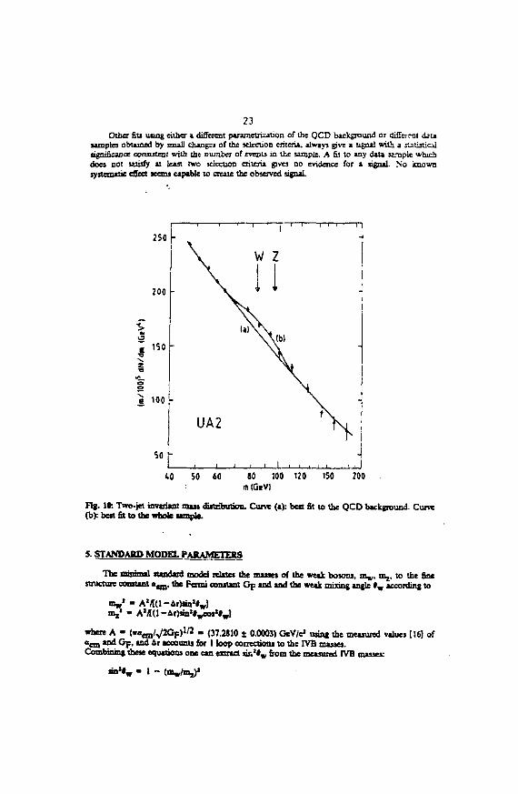
The mass resolution of the two-jet system, determined both by direct measurements and byMont: Cario, is found to be of the order of 8 GeV/c1 for two-jet masses of SO GeV/c1, and 9GeV/c* for mas.':s of 90 Gev/c1. Figure 10 shows the two-jet m»«< spectrum for the eventstaken at jTm 630 GeV corresponding to an integrated luminosity of 730 nb"'. The data aremultiplied by a factor (MM00 GeV)1 to reduce the effect of u-'ing wide mass bjis in the steeplyfalling QCD distribution. Given the quoted mass resolutions, the W and 7 peaks are r.-nresolved. However, a breed bump is visible in the expected region of the spectrum.
A maximum likelihood fit to these data is made by using the function:
The first term in the xjutre bracket parametrizes the QCD background. The second term is th;sum of two gaussisn dhuibutions representing the W and Z sirpjli respective;)'. The 'Vdistribute a is uikcn to have i m a n value m,, and rjri-s. 8 GeV/c*, the Z distribution has nxcaavalue l.Mnic and rjc.j. 9 GsV/c*. The relative normalization between the two gausni;.; isassumed equ^l to tie e^K^ ~-J ratio (a 3) between the numbers of observed W and Z decays.The panmctm a, (I ^cd i ars idi'uted to maximize the likcShood function, the consuxsi Abeic; calculated euh titas to provide the appropriate normalization. The mass parameter m,j beither set to the expected value, mg ™ 78.5 Gev/c1, or beatcd as an additional free parameter.In the latter cue m, is found to be 82 ± 3 GeV, in agreement with the value obtained from theW teptonic decays (see section 3).
The sismfkence of the signal it 3.3 standard deviations, and hi magnitude correipsnds to632 ± 190 events (with m,, fixed) and 686 ± 210 events (releasing m,, in the fit). This number isconsistent with the number of events expected from tee Staadsrd Model after correcting for theacceptance and the efficiency of the selection criteria. The result of the fit is shown as curve (b)in the Figure 10. A poor fit to the dau is obtained suppressing the signal term S(m) in the fitfunction (x2 " 21.1 for 12 d.oS); the fit u good, instead, if the data points contained in the range65 < m < 105 GeV/cJ are excluded <x* " 4.7 for 7 doJ) as shown in curve (a) is Figure 10.
23
Other fits using either * different parametrization of the QCD background or difTerrot d susamples obtained by small changes of the selection criteria, always give a signal with a statisticdsignificance corautent with the number of events in the sample. A fit to any data sample whichdoes not uuisfy at least two selection criteria gives no evidence for a «ign»1 No knownsystematic effect seems capable to create the observed signal.
40 SO 60 80 100 120 150 200m IGtVl
Fig. 10: Two-jet invariant mau distribution. Curve (a): best fit to U>e QCO background. Curve(b): best fit to the whole sample.
5. STANDARD MODEL PARAMETERS
The minimal standard model relates the masses of the weak bosons, m,,, mj, to the finestructure constant aem, the Fermi constant Gp and and the weak mixing angle I w according to
m,,1 - A»/I(l-Ar)iin»#w)
- (»« e m / % /2G F ) l / 2 - (37.2810 ± 0.0003) GeV/c1 using the measured values [!61 ofaem and Gp, and Ar accounts for 1 loop correctionj to the IVB mauet.Combining these equation* one can extract «ii.2»w from the measured [VB masses:
tmJ#w - I
24This method has the advantage of cKmrrating u iun due to absolute energy calibration, as
well as radiative collections, but ii limited by the « " « « " ' error on the Z mass.A more precise remit is obtained by using the measured value of Op asd a e m and the
calculated value of Ar. At present, Collider dau do not constrain the value of Ar (see later) and10 we ttke the value from a recent calculation t! 7]:
to - 0.0711 ±0 .0013 .
assuming m, « 36 GcV/c1 and the mass of the Higjs boson equal to tiij.The final untaown is the value of rin*tw, which must be taken experimentally at Q' - m , /according to
iinJ#w -
The results are given in Table I. AD the values are in good agreement with each other and withprevious determinations [ 18] from the deep inelastic neutrino scattering experiments. Avengingtheir values and »«°"nirg a charmed quark mass of 15 GeV/c1 (with no error) one obtains
an 2»w - 0.232 ± 0.004 ± 0.003
where the Erst error is experimental and the second theoreticalThe only parameter sensitive to the Higgi mrrhaniim used in the Standard Model is
p • OLm'/mzico%'iw
which in the minim.il model with a single Higgs doublet has a value of 1, neglecting smallradiative corrections. The values obtained experimentally (see Table 1) are consistent with thisexpectation.
Finally sa'9v can be from the two definitions given above to yield av
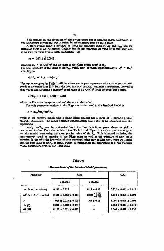
measurement of Ar. The values obtained (see Table 1 xnd Figure 11) tie not precise enough totest the model, even using the most precise value of sm*fw. With iacre-ised statistics, thismeasurement could be sensitive to the Higss miss as well as the existence of new exoticparticles. In the table the first value of Ar is extracted using only collider dai?, while the seconduses the best value of sintw as input. Figure 11 summarizes the msasuremei u of the StandardModel parameters given by UA1 and U A i
Tabk II:
Muvmtmnxs tftht Truftn* AMef psremtun
Parameter
iin'f. • 1 - ml /mi
un'f. • A'/( l-Ar)mi
«
Ar(I)
Ar(H)
UAI
t channel
0.211 * 0.025
0.211 ± 0.009 ± 0.014
1.009 ± 0.021 ± 0 020
0.031 ± 0.100 X 0.067
0.123 ± 0.021 * 0.057
* channel
0.19 ± 0.15
"»:«81.05 * 0.1*
UA2
0.232 t 0.025 * 0.010
0.232 t 0.003 ± 0.001
1.001 X 0.021 ± 0.006
0.061 ± 0.087 x 0.030
0.061 * 0.022 ± 0.032
25
n.
75 77 7» CO 91 62 8] 61m* !GfV/c2l
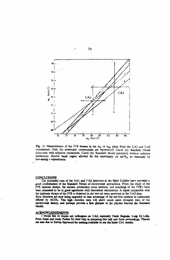
Hg. 11: Measurements of the IVB masses in the n^ vs m^. plane from the UAl and UA2e<reriments. Only thi systematic uncertainties are represented. Curve (a): Standard Modelpieoiction with radiative corrections. Curve (b): Standard Modei prediction without radiativecorrections. Shaded bind: region allowed by the uncertainty on sinJtfw as measured bylow-energy r experiments.
CONCLUSIONSThe successful runs of the UAl and T JA2 detectors at the SppS Collider have provided a
good confirmation of the Standard Model of electroweak interactions. From the study of theIVB leptonic decays, the masses, production cross sections, and couplings of the IVB's havebeen mcajured to be in good agreement with theoretical calculations. A signal compatible withthe hadronic decays of the IVB is observed in the two-jet mass spectrum in the UA2 data.Both detecton are now being upgraded to take advantage of the ten-fold increase in luminosityoffered by ACOL. This high statistics data will allow much more stringent tests of theelectroweak theory, and perhaps provide > first glimpse at the physics beyond the StandardModeL
ACKNOWLEDGEMENTSI would like to thanks my colleagues on UA2, especially Paolo Bagnaia, Luigi Di Leila,
Peter Jenni and Andy Paiker for their help in preparing this t«iv and these proceedings. Thanksare also due to Steven Haywood for malting available to me the latest UAl results.
26
[1] C.Rubbia, D.Œne, P.McInryre, Proc. Int Neutrino Conf., Aachen, 1976 (Vieweg,Braunshweig, 1977), p. 683.
{2] S.L.Glaihow, Nud. Phys. 22 ( 1961), p. 579;S.Weinberg, Phys. Rev. Lett. 19 (1967), p. 1264;A-Saiam, Froc. 8th Nobel Symposium, Aspen-Asgirden (1968), (Almqvijt andWiksell, Stockholm), p. 367.
[ 3] R. Ansah et «L Phys Lett 1S6B (1987) p. 440;R. Ansari et «L CERN-EP/37 - 48 To be published in Physics Letters.
f4] E. Looi (L'Ai Coll.), W/Z &. Standard Model, International Europhysi« Conferenceon High E'-iCTgy Physics, Uppsala, Sweden, June 25-July 1, 1987;Th. Muller ('JAl CoCL), Rencontre de Moriond on Electroweak Interactions ind
. Unified Théories, 1987.[5] X. Eggert et aL (UAI CoU.), Nud. lust, and Methods 176 (1980) p. 217;
J. Timmer. (UAI Coll.), Proc of the 3rd Moriond Workshop on pp Physics (1983) p.609, Editions Frontieres 1983;G. Amison et al. (UAI Coll), Phys Lett B122 (1983) 103, Bi29 (1983) p. 273;P. Bagoaia et al. (UA2 CoU), Z. Phys C 24 (1984) p. 1;B. Mansouiie (UA2 ColL), Proc of the 3rd Morinnd Workshop on pp Physics (1983)p. 609, Editions Frontieres 1983.
[6] G. Amison et al. (UAI ColL), Lett. Nuovo Cimento 44 (1985) p. 1;P. Bagnaia et al. (UA2 ColL). Z. Phys. C 24 (1984) p. 1.
[7] G. AltareUi et al., NucL Phys. B246 (1984) and Z. Phys. C27 (1985) p. 617.[8] C. AlbajaretaLPbysLettB 185 (1986) p. 241.[9] J.F. Grivas, Rencontre de Moriond on Electroweak Interactions and Unified Theories,
1987.[10] D. Schramm, Rencontre de Moriond on Electroweak Interactions and Unified
Theories, 1987.[I !] M. Delia Negra, 2nd Topical Seminar on Heavy Flavours, San Miniato, Italy (1987).[ill J. Ellis et al., Ann. Rev. Nud. Part. Sc. 32 ( 1982) p. 443.113] T-Akesson et al., Detection of jets with calorimeters at future accelerators, Proceedings
of the CERN-ECFA Workshop on Physics at Future Accelerators, La Thuile,January 1987.
[14] P. Bagnaia et aL (UA2 Coll.), Z. Phys. C20 ( 1983) p. 117;P. Bagnaia et al., Phyi. Lett. 138B (1984) p. 430;P. Bagnaia et aL, Phyt. Lett 144B (1984) p. 291;J.A.Appel et aL (UAI ColL), Phys. Lett. 160B (1985) p. 349.
[15] R. Aiuari et t l (UA2 CoU.), Phys. Lett. 186B (1987) p. 452.[16] Review of Particle Properties. Phys. Lett. 170B (1986) p. 1.[17] W. Marciano XXIII International Conference on High Energy Physics, Berkeley,
California, July 1986, quoting F. Jegerlehner, BERN preprint 1985.[ 18] CDHSW Collaboration. H. Abramowicz et al., Phys. Rev. Lett. 57 (1986) p. 298;
CHARM Collaboration. J.V. Allaby et aL Phys. Lett. 177B (1986) p. 446;CCFR Collaboration, presented by F. Merrit Proc of the 12th Intl. Conf. onNeutrino Physio and Astrophysics, Sendai, Japan, June 1986;FMMF Collaboration, presented by R. Brock, as above.
27
STATUS OF NEUTRINO COUNTING AND NEW QUARKS
N.G. DeshpandeInstitute of Tneoretical Science
University of OregonEugene, OR 97403
ABSTRACT
We review the recent limits on the number of neutrino species Nv obtainedfrom e+e" colliders and from pp colliders. If majorons exist, they contribute two unitsto Nv in e+e- colliders and conflict with the 90% CL of Nv < 4.8. We study theconsequence of a fourth family of quarks and leptons on neutrino counting at ppcolliders. Useful conclusions are drawn at 90% and 95% CL. Jiffcrt of majorons onneutrino counting at pp colliders is also reviewed.
I. INTRODUCTION
Three methods have been useful in setting useful limits on Nv , the number ofneutrino species. These methods are complimentary to each other and do not measurethe same quantity except in the standard model. The methods are
A. Nucleosynthesis and Cosmology
This method relates primordial Helium abundance to the number of neulrinospecies. It is sensitive to light neutrinos of mass less than a MeV, and the sensitivity toright-handed neutrinos depends on their coupling strength. The traditional bound fromthis method is Nv < 4.
B. Electron-Positron Colliders
The data comes from e+ + e- - t v + 7 - t v reaction at \'s = 29 Ge V and 42GeV. It is sensitive in principle to mv < \s/2 although there is a cut on photon energywhich reduces the mass limit somewhat. It is sensitive to all species of neutrinos thatoccur in e+ + e' -» v + v reaction.
C. Proton-Antiproton Collider
This is an indirect method of determining rz/T\y. It is sensitive to my < mz/2
and to only those neutrinos that occur in Z -» w decay. This includes right handedneutrinos, for example.
In this talk we shall focus only on the latter two methods.
26
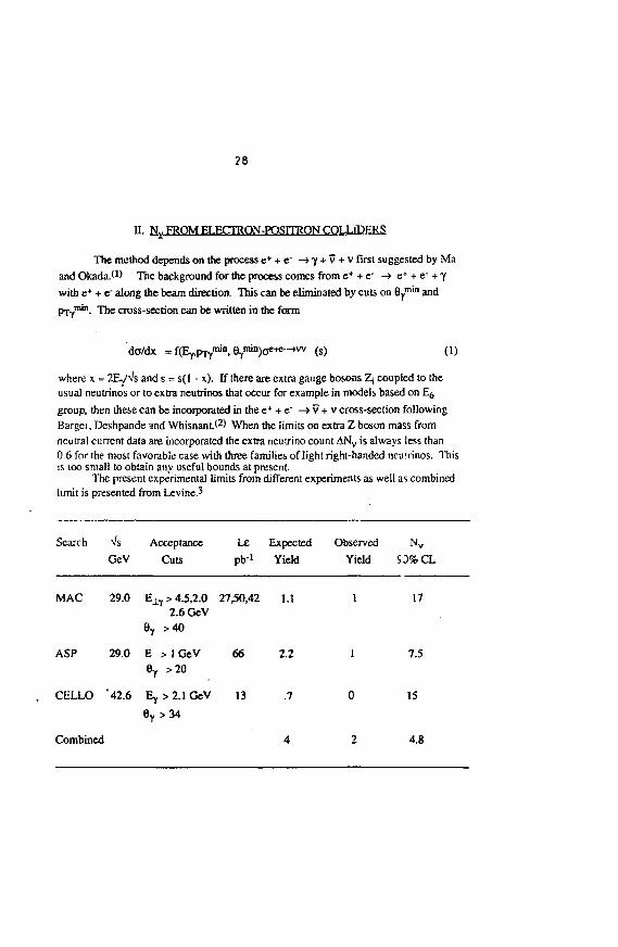
H. K. FROM ELECTRON-POSITRON COLLIDERS
The method depends on the process e+ + e" -» y + v + v first suggested by Ma
and Okada.C) The background for the process comes from e+ + e" -» e+ + e" + y
with e+ +1~ along the beam direction. This can be eliminated by cuts on
Pry1™"- The cross-section can be written in the form
do/dx = f(Ey,pTrmia,Qy™a)Oe+ (s) (1)
where x = 2Ey%'s and s = s(l - x). If there are extra gauge bosons Z; coupled to theusual neutrinos or to extra neutrinos that occur for example in models based on E§group, then these can be incorporated in the e* + e" -» v + v cross-section followingBargei, Deshpande and Whisnant/2' When the limits on extra Z boson mass fromneutral current data are incorporated the extra neutrino count ANV is always less than0.6 for ihe most favorable case with three families of light right-handed neuirinos. Thisis loo small to obtain any useful bounds at present.
The present experimental limits from different experiments as well as combinedlimit is presented from Levine.3
Search Vs Acceptance Le Expected Observed Nv
GeV Cuts pb"1 Yield Yield 50% CL
MAC 29.0 Ely> 4.5,2.0 27,50,42 1.12.6 GeV
6 r >40
ASP 29.0 E > I GeV 66 2.26Y >20
CELLO '42.6 Ey>2.1GeV 13 .7
6T >34
Combined 4
17
7.5
15
4.8
29
We thus have a combined limit of
N v < 4 . 8 (90%CL) (2)
This limit is already useful to put bounds on majorons however. The model by
Gelmini and RoncadelliW has a Higgs triplet witli surviving particles X ++> X +> X °
and M° where M° is a pseudo-scalar Goldstone particle associated with lepton number
violation and x ° is a scalar particle whose mass is less than 100 keV from
astrophysical considerations. Zg -t M ° x ° decay yields/5 '
r(Z - • M«x °) = 2F(Z -> vv) (3)
Since M° and X° will escape from the detector like neutrinos, the existence ofmajorons increases N v by two units. We then see that N v = 5 is not compatible with thedata at 90% CL.
ID. LIMITS FROM SppS
Neutrino counting at SppS depends on an estimate of r z / T ^ using theoretical
information on production of W - versus Z° . The original method'6) suggested byHalzen and MUrsula; and Cline and Rholf has been used to Limit new physics byDeshpande, Eilara, Barger and Halzen.O The method follows from the equation:
(number of ev from W±)/(number of e+e-from Z°) (4)
= [a(W+ + W-) / C(Z)][T(W -> ev) / T(Z -> e+e-)] [r z /Tw ]
The first two ratios in the right hand side of the equation are determined using protonstructure functions and standard model with xw = 0.23. These are respectively 3.3 ±
0.2 and 2.685- For Rexrx WL use the most recent limits® obtained by UA2 with
combined data of 142nb"' at 546 GeV and 768 nb"1 at 630 GeV. The limits are
+ 1.7Re*P« = 7.2 (5)
-1.2
30
< 952 <90%CL)
< 10.42 (95%CL)
When combined with theoretical uncertainities we have
T z / r w < 1.16 at90%CL
< 1.27 at95%CL (6)
We shall discuss various consequences of these limits in the next three sections. Thediscussion is largely based on a recent paper by the author with Barger, Han andPhfflips.W
A- Ny and mass of t quark
Because I"w is a function of t mass, the ratio r z / T w is a function of mt and Nv.
We calculate r z using standard model fermion couplings with x ^ = sin2 6w = 0-23,and M z = 91.9 GeV. The contribution of each neutrino, charged leplon and quark are
r z ° = (GFMz3)/(12icV2) =0.17 GeV (7a)
r(Z -> LL) = rOfvnJ/M*) (7b)
HZ -> QQ) = 3r z° FdiiQZ/M^d + ds/it) (7c)
where
FW = 8p[gv2(l + 2r) + iAH I - 4r)] (8)
Here
p = (1 - 4r)>/2 , gv = T j ^ - xwQ, gA= -T3/2.
We then find
r z = 2.04 + 0.17 N v+.51 F, (9)
where F t = [0.59 - 1.93r,l[l - 4rJ l / 2 and r, =We calculate fw using m w = 80.6 GeV and the standard formulas
f(W -> ev) = GpMv^ / 6* V 2 = Tw° = 0.23 GeV (10a)
TfW -» Lv) = rw0H(mL2/mw
2) (10b)
TfW -» tb) = 3rw°(l + <Vit) H (V/raw2) (10c)
where H(r) = 1 - 3r/2 + r /2 for r £ 1 and H(r) = 0 for r > 1. The formula can besummarized as
T w = 2.12 +0.72 H, (11)
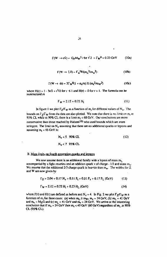
In figure I we plot I~z/rw as a function of m, for different values of Nv. The
bounds on rz/I\v from the data are also plotted. We note that there is no limit on m, at95% CL while at 90% CL there is a limit m, < 68 GeV. Our conclusions are moreconservative than those reached by Halzerf10) who used bounds which are morestringent The limit on Nv assuming that there are no additional quarks or leptons andassuming mt = 45 GeV is:
N v < 5 90% CL (12)
Nv<7 95%CL
B. Mass limits on fourth generation quarks and leptons
We now assume there is an additional family with a lepton of mass mL
accompanied by a light neutrino and an addition quark v of charge -1/3 and mass mv.We assume that the additional 2/3 charge quark is heavier than mw. The widths for Zand W are now given by
T z = 2.04 + 0.17 Nv + 0.51 Ft + 0.51 Fv + 0.17 FL (GeV) (13)
r w = 2.!2 + O.72Ht + O.23HL(GcV) (14)
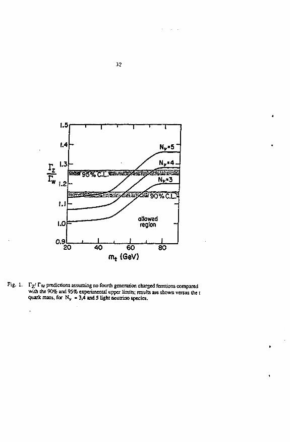
where F(r) and H(r) are defined as before and Nv = 4. In Fig. 2 we plot Pz/r w as afunction of mt for three cases: (a) when mi, 2 m\v. "iv = 24 GeV, (b) mi, = 41 GeVand mv = Mz/2 and (c) mL = 41 GeV and mv = 24 GeV. We arrive at the interestingconclusion that if m, = 24 Ge V then m, < 45 GeV (60 GeV) regardless of mL at 90%CL (95% CL).
32
1.5
0.9
90% CD
allowedregion
I I I20 40 60 80
mt (GeV)
Fig. 1. Tj/ Vf/ predictions assuming no fourth generation charged fennions comparedwith the 90% and 95% experimental upper limits; results are shown versus the tquark mass, for Nv « 3,4 and 5 light neutrino species.
33
(a)
(b)
(c)
4
4
4
M1
41
411.5
1.0-
0.9 I
24
24
I
allowedregion -
_ • I20 40 60
mt(GeV)80
Fig. 2 Tz/ T w predictions for three illustrative cases of fourth generation fermions- (a)nv - 24 GeV, mL > Mw; (b) nn, = 41 GeV, my > Mz/2; (c) nv = 24 GeV, m, =41 GeV. 90% and 95% limits are shown for comparison.
40 60m t (GeV)
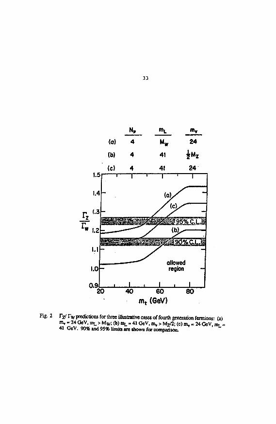
Fig. 3 90% limits (dashed curves) and 95% limits (solid curves) in the ( n \ my) plane forthree illustrative cases:
(a) nn. - 24 GeV m(yO - 5 GeV,
(b) niL - 41 GeV, m(yO - 0 GeV,(c) mL>M w . The allowed regions are to the left of the curves.
35
In Figure 3 we plot the allowed regions in mv vs m, plane for different values ofmL at 90% CL and 95% CL.
C. Majorons and Neutrino counting.
If majorons exist in triplet Higgs representation, the widths of W and Z arcaltered. We have to include
W+ -» %* +
as well as
+ x~Assuming three generation, the widths for W and Z are affected as
(17)
r w = r ws o « b r i + 8TW (18)
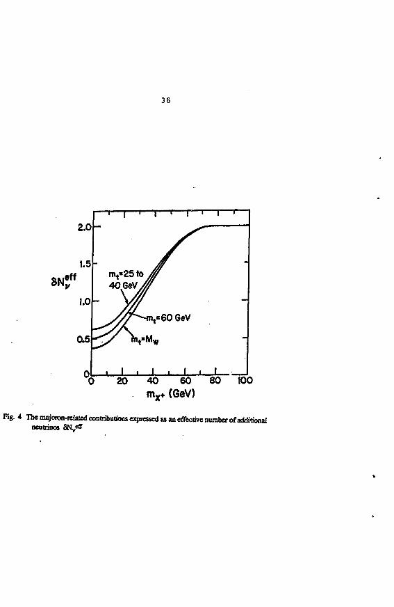
We define the effective neutrino count due to these additional channels as
(19)
This quantity depends on mx+, m,++ and weakly on m,, but can be shown tolie within the range
1/2 < 6Neff<2 (20)
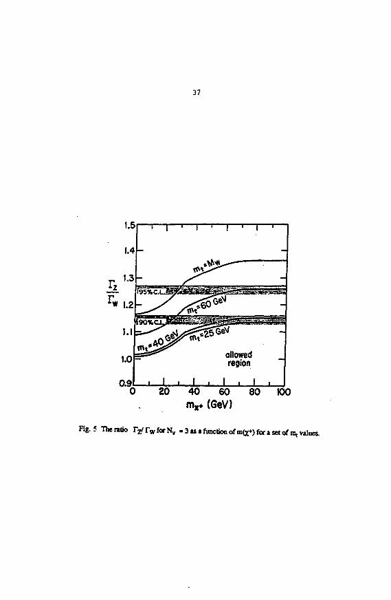
with value approaching 2 as nVj + > mw , and 1/2 as m^ and n^++ 0. If m, < 45GeV (60 GeV) there is no constraint on the model at 90% CL (95% CL). If m, > m w
however m ^ < 30 GeV at 95% CL. We show results in figures 4 and 5.
36
SNeff
2.0
1.5
1.0
0.5
0
1 I
mt»25 to4OGeV>0w
. I .
i * i * i •
•
nt=606eV
I . I . I"6" 20 40 60 80 100
mx* (GeV)
Fig. 4 The majoron-relalcd contributions expressed as an effective number of additionalneutrinos
37
0.9
Fig. 5 "nienuio rz /rwforNv - 3 « a function of m(x+) for a set of m, values.
20 40 60 80 tOO(GeV)
38
IV. CONCLUSIONS
1. From e+ + e" data Nv < 4.8 at 90% CL. Majoron excluded at 90% CL.2. From pp data, if m, = 45 CeV and no other light particles, Nv < 5 (7) at
90%CL(95%CL)3. If Nv = 3, m, < 68 GeV at 90% CL and no limit 95% CL.4. If Nv = 4 and no other light particles, m, < 55 GeV (75 GeV) at 90% CL
(95% CL).5. IfNv = 4 and my = 24 GeV and mL arbitrary, m,< 45 GeV (60 GeV) at
9C% CL (95% CL).6. If mx + >Mwthenm,<45GeV(60GeV)at90%CL(95%CL)7. If m, > mw then nij + < 30 GeV at 95% CL.
REFERENCES
1. E. Ma and J. Okada, Phys. Rev. Lett 4JL, 287 (1978); K.J.F. Gaemers, R.Gastmans and F.M. Renerd, Phys. Rev. H12, 1605 (1979).
2. V. Barger, N.G. Deshpande and K. Whisnant, Phys. Rev. Lett 52, 2109(1986).
3. T.L. Lavine, University of Wisconsin Ph.D. Thesis, December 1986, WISC -EX - 86/275.
4. G.B. Gelmini and M. Roncadelli, Phys. Lett. 29JL 411 (1981). H.M. Georgi,S.L. Glashow and S. Nussinov, Nucl. Phys. B193. 297 (1981V
5. V. Barger, H. Baer, W.-Y. Keung and R.J.N. Phillips, Phys. Rev. D2fi, 218(1982).
6. F. Halzen and K. Mursula, Phys. Rev. Lett. SL 857 (1983) D. Cline and J.Rohlf, unpublished.
7. N.G. Deshpande, G. Eilam, V. Barger and F. Halzen, Phys. Rev. Lett. 54,1757(1985).
8. UA2 collaboration: CERN-EP/87-05.9. V. Barger, T. Han, N.G. Deshpande and R.J.N. Phillips, University of
Wisconsin preprint, MAD/PH/335, (1987), to be published in Phys. Letts.(1987).
39
TESTING THE ELECTKOlVGAK STANDAKO MODEL
AT HERA
3.QLUMLEIN
Institute for High energy Physics
Academy of Sciences of the GDR
Platanenallee 6, Berlin-Zeuthen,1615
GDR
Abstracf
The results are presented of a systematic study/1/ of HERA's. po-tential to test the electroweak standard model. The neasurtimntof sin^e and M appear to be possiblu with statistical preci-sions of .002 and 100 MeV. The theoretical errors are dominatedby the quark distribution uncertainties and are estimated to boless than the statistical errors. Limits can be set for the top-quark mass and the Higgs-boson mass. Gxtensi >-, j of the minimummodel can be tested with high precision.
1. Int roduct ion
The investigation of deep inelastic neutral and charged current
e—p-reactions at HERA /2/ provides the possibility to study the
electroweak standard theory at high Q . A test of the minimum
SU(2) xU(l)-model has to take into account the existence of the
various parameters of the theory and their mutual dependence.
Among the quantities defining the electroweak sector (the Fernii-
constant G_,the weak mixing angle 8, the fine structure constant
yand the weak boson masses M and M ) only three are independent.
Conceptually, measuring one of these quantities one has to fix
two others.which are precisely known,and to express the remaining
parameters in terms of the basic set choosen, e.g. one can fix2
OC and G_ and measure sin 8 or M . With M determined at LEP /3/
with better than 1% one can as well replace Gf by Mz«
As the sensitivity of the measurement to a parameter depends
on tho choice of the fixed parameters due to tlie different functio-
nal dependences implied a systematic search for the best statisti-
cal precisions has to bu performed.
The theoretical errors of the analysis are implied by the
experimental errors of tho input parameters, the ratio R=O"/Q"Ti
quark mass effects, the experimental errors of the Kobayashi-
Maskawa matrix elements and the uncertainty of tie quark distri-
40
bution parametrizatlons.
The kinematic area has been limited to a region where calo-
rimeter resolution effect are tolerably small /4/. Still.a valid
estimate of the potential systematic error is beyond the aim of
this study as it would require detailed detector orientated Monte
Carlo calculations. We have also disregarded the effect of radia-
tive corrections /5/. Currently,these topics are under investi-
gation in different working groups in prepearing the workshop
"Physics at HERA", Oct. this year.
The outline of this tolk is as follows: Section 2 summarizes
basic relations used. In section 3 the statistical errors of
different electroweak quantities are derived assuming an integra-
ted luminosity of 200pb~ .Section 4 deals with the theoretical
errors of the analysis. In section 5 the strict parameter rela-
tions of the standard model are given up and the sensitivity of
modifications of the minimum theory 1% studied to a varying Q -
parameter, for nonvanishing right handed weak isospin components,
additional W- and Z-bosons and on eventual compositeness scale of
the weak bosons.
• 2. Basic relations
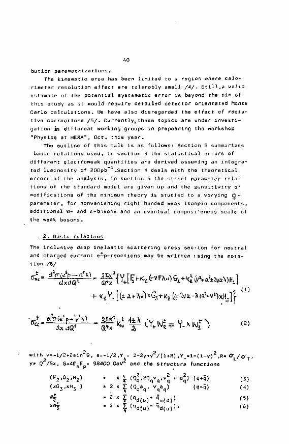
The inclusive deep inelastic scattering cross sec ion for neutral
and charged current e—p-reoctions may be written ising the nota-
tion /6/
with v=-l/2*2sln2G. a=-l/2,Y = 2-2y+y2/(l+R),Y_=l-(1-y)2,R«<^L/O'T
Y= Q /Sx, S=4EeE = 98400 GeV and the structura functions
(F2,G2.H2) . x T (Q2.2Qqvq.V2 • a2) (q+q) ( 3 )
(XGJ.XHJ ) « 2 x £ (Qqaq. vqaq) (q.q) (4)
W? ' 2 x 5^d(u) + 5u(d)) (5)* 2 x $ ^d(u)" 5 d ( u ) ) . (6)
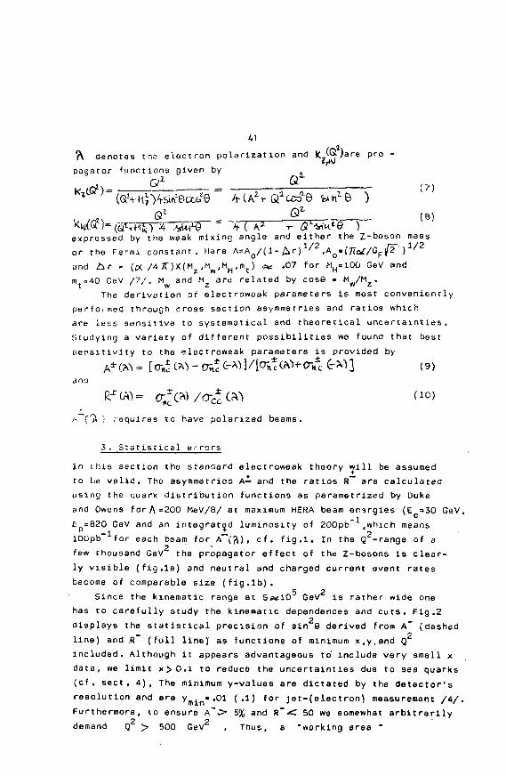
7\ denotes the electron polar izat ion and fc (Q)are pro -
pogator functions given by
( Q f c ) 4 ^ = > ( A1 +-expressed by the weak mixing angle and ei ther the Z-boson mass
or the Fermi constant. Hare A=AQ/( 1 - & r ) 1 / 2 ,AQ» (TTc^/Gp/F ) 1 / 2Q/
and 2ir = (# /4 7C)X (M_, -MW.MH .<",.) -° 7 f o r MH=100 GeV and
m =40 GeV /7/. M and M are related by cos8 » Mw/
Mz•
The derivation of electroweak parameters is most conveniently
performed through cross section asymmetries and ratios which
are less sensitive to systematical and theoretical uncertainties.
Studying a variety of different possibilities we found that best
sensitivity to the electroweak parameters is provided by
A*(W = [crn* Ws ~ o£ C-A)]/[Ont W^Oifc t ^ ] (9)dno
^ ^ do)
;-~{^ ; raqulres to have polarized beams.
3. Statistical errors
In this section the standard elactroweak theory will be assumed
to be valid. The asymmetries A— and the ratios R~ are calculated
using the quark distribution functions as parametrized by Duke
and Owens for A =200 MeV/8/ at maximum HERA beam er.-jrgies (E =30 GeV,
E =820 GeV and an integratjd luminosity of 200pb ,which means
lOOpb" for each beam for A~t'JU , cf. fig.l. In the Q -range of a
few thousand GeV the propagator effect of the Z-bosons is clear-
ly visible (fig.la) and neutral and charged current event rates
become of comparable size (fig.lb).5 2
Since the kinematic ranga at SASIO GeV is rather wide one
has to carefully study the kinematic dependences and cuts. Fig.2
displays the statistical precision of sin 6 derived from A~ (dashed
line) and R~ (full line) as functions of minimum x.y.and Q
included. Although it appears advantageous to' include very smell x
data, we limit x>0.1 to reduce the uncertainties due to sea quarks
(cf. sect. 4), The minimum y-values are dictated by the detector's
resolution and ere ymin« .01 (.1) for jet-(electron) measurement /A/.
Furthermore, to ensure A~,> 5% and R~<T 50 we somewhat arbitrarily2 2
demand Q > 500 GeV • Thus, a "working area "
42
is defined by x>.l, y > .01 and Q 2 > 500 GeV2.
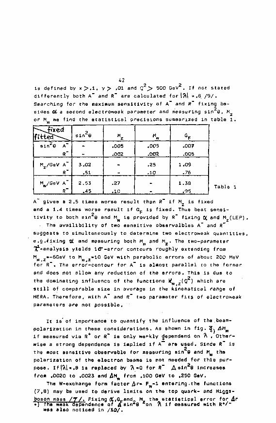
differently both A~ and R~ are calculated for I'
If not stated
I » .6. /9/ .Searching for the maximum sensitivity of A~ and R fixing be-
sides 06 a second electroweak parameter and measuring sin 3, M
or M we find the statistical precisions summarized in table 1.
^\f>xed
s in 2 e A"
R"
M2/GeV A"R"
Mw/GeV A"
R"
sin2G
-
3.02
.51
2.53
• 45
M z
.005
.002
-
.27
.10
Mw
.005
.002
.25
.10
-
GF
.007
.005
1 .09.76
1.38
.95Table 1
A~ glvae a 2.5 times worse result than R~ if Mz is fixed
end a 1.4 times worse result if G_ is fixad. Thus best sensi-2 -
tlvity to both sin 9 and M is provided by R fixing OC and M (LEP),
• The avallibillty of two sensitive observalbles A" and R*
suggests to simultaneously to datermine two electroweak quantities,
e.g.fixing OL and measuring both M and M . The two-parameter
'Xr-'analyeis yields lC"-error contours roughly extending from
M »-6GeV to M -10 GeV with parabolic errors of about 200 MeVn t 2. W t Z
for R~. The error-contour for A~ is almost parallel co the former
and does not allow any reduction of the errors. This is due to
the dominating influence of the functions H '(Q ) which are
still of comparable size in average in the kineoiatlcal range ofHERA. Therefore, with A~ and R~
parameters are not possible.
two parameter fits of electroweak
It is of importance to quantify the influence of the.beam-
polarization in these considerations. As shown In fig.^. /JMH
if measured via R* or R~ ia only weekly d/spendend on A . Other-
wise a strong dependence is Implied if A*" aro used. Since R~ is
the most sensitive observable for measuring sin 8 and Mw the
polarization of the electron beams is not needed for this pur-
pose. IffAl',8 is replaced by ?i »0 for R~ A sin G increases
fro* .0020 to .0023 and AMW from ,100 GeV to .250 GeV.
The W-exchange form factor £r» F y-1 entering.the functions
(7,6) may be used to derive limits on the top quark- and Higgs-
boson mass / 7 / . Fixing dCG.and M the statistical error for 4r+) The weak dependence of /T8inz8 on ft if measured with R+/~
was also noticed in /XQ/.
43
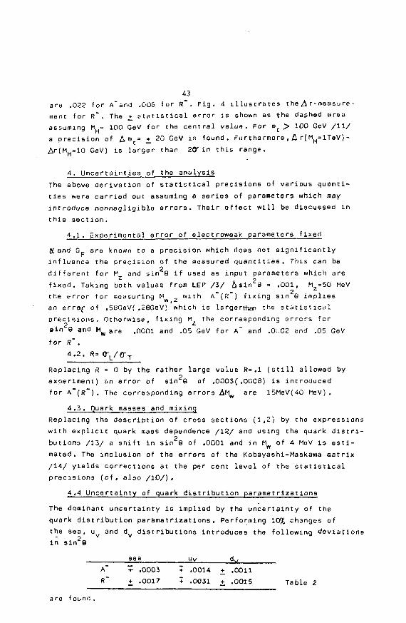
are .022 for A~and .DOS for R~. Fig. 4 illustrates the^r-maasure-
ment for R~. The + statistical error is shown as the dashed area
assuming M = 100 GeV for the central value. For n>t > 100 GeV /ll/
a precision of A m =• +_ 20 GeV is found, ru rths rmore , & r(MH=lTaV) -
£r(MH=10 GeV) is larger than Zff in this range.
4. Uncertainties of the analysis
The above derivation of statistical precisions of various quanti-
ties were carried out assuming a series of parameters which may-
introduce nonnegllgible errors. Their effect will be discussed in
this section.
4-.1 . Experimental error of electroweak parameters fixed
(Hand G are known to a precision which does not significantly
influence the precision of the measured quantities. This can be
different for M_ and sin 8 if used as input parameters which are
fixed. Taking both values from LEP /3/ isin 8 = .001, M =50 MeV- 2
the error for measuring M^ 2 with A (i? } fixing sin 6 implies
an error of ,58GeV( .26GeV) which is largerthan the statistical
precisions. Otherwise, fixing M the corresponding errors for
sin 9 and H w a r Q .OCOI and .05 GeV for A" and .0L02 and .05 GeV
for R~ .4.2. R= O-L/<Xj
Replacing R = 0 by the rather large value R=> .1 (still allowed byo
experiment) an error of sin 8 of ,OOO3(.OCO8) is introduced
for A~(R~) . The corresponding errors AM are 15MeV(40 MeV) .
4.3. Quark masses and mixing
Replacing the description of cross sections (1,2) by the expressions
with explicit quark mass dependence /12/ and using the quark distn-p
butions /13/ a shift in sin 8 of .0001 and in Mw of 4 MeV is esti-
mated. The inclusion of the errors of the Kobayashi-Maskawa matrix
/14/ yields corrections at the per cent level of the statistical
precisions (cf. also /ID/).4.4 Uncertainty of quark distribution parametrlzations
The dominant uncertainty is implied by the uncertainty of the
quark distribution parametrlzations. Performing 10% changes of
the eea, uv and dv distributions introduces the following deviations
in sin2G
A t- .0003 + .0014 + .0011
R~ i .0017 + .0031 + .0015 Table 2
are found ,
This uncertainty thus remains only smaller than the statisti-
cal precision if the parton distributions can be controlled at
the 5$ level. As outlined in /I/ (cf. also /15/) this seems
to be possible using F2(Q2 < 10C0 GeV2) and O"cC/0"cC'
which
can be determined without reference to electroweak parameters,
as constraints. Furthermore,one will calculate the electroweak
quantities under differnt cuts and from different quantities
(A", R+,R~) which further minimizes this uncertainty.
5.Extensions of the model
In this section we will give up the strict parameter relations
of the minimum theory and allow for different type extensions.
s.i. 9 t i
Giving up the relation Q = (Mw/Mzcos6) =1 and fitting (9 .sin^
one finds parabolic errors A ^ = .01 andAsin 9= .006 (CCF=-.96).
Fixing sin 9 yields 59=.003 /16/.
5.2. M and M, fitted from the propagators
Ignoring the relation between M (M and sin 9 one can fie thew z g
gauge boson masses from the propagator terms only fixing sin 9
in The couplings. One obtains A M = 3GeV(5.6 GeV) for A~(R )
and the interesting number A M =450MeV for R~5.3. Right handed isospin components
Modifying the vector- and axialvector couplings v and a to
v= Ij + I, -2Qsin29, a ^ - I ^ the sensitivity to I^'e,u,d) is
determined. Best precisions are obtained from l\*'~ with
£Ij(e,u,d) = ( .056, .034, .010) for A'; for A+ Alj(e) improves
to .03 which is comparable to the present world average/17/.
5.6 . New W- and Z-bosons and the scale of weak boson •
composlteness
Assuming one extra W- or Z-boson resp. and fixing the masses
and couplings thus that the standard model low energy limit is
conserved R allows to detect an additional W-bo^on for
Mw. < 190GeV(390GeV) at the 3cr(ltf-) level. Similarly, A~ can
be used to detect an additional Z-boson if M , < 23OGeV(400GeV),
assuming in both cases the same coupling far the standard and
additional gauge boson,(The explicit coupling dependence is _al-
culated in / I / ) . According results for an addition W'-boson have
been obtained also in /18/. In a first approximation the compo-
sitenass scale of the weak bosons should show up as an additional2 2
factor x 1/(1+Q / A ) in the functions K" . Whereas A~ can" i
not be used to set significant limits for A ( c f . / 1 / ) , R" is sensi-
45t i v o I O A S ' A O GeV at ths 2<X l e v e l .
6 .Conclusions
Referring to the standard theory bost sensitivity to the electro-
weak parameters was found for R~ . Assuming a luminosity of 200 pb
sin 8 and M can be determined with a statistical precision of
.002 and 100 MeV resp. in a kinematic range where the systematics
can be controlled adequately. The corresponding precisions for A
are 2 to 3 times worse. The theoretical error is dominated by the
uncertainty of the quark distribution functions and is estimated
to be less than the statistical precisions. While the measurement
of A~ requi res highly polarized electron beams the measurement
of ths electroweak parameters via R~ is only weakly Hependend on
the electron polarization. Extensions of the minimum thaory can
be tested with high precision. HERA should allow for meaningful
tebto of the dloctroweak theory complementary to e+e~-colliders
and more accurately than the presently existing pp-experiments .
Acknowlodqoment. For discussions I would like to thank W.Hollik
and J .Kiihn .
Re ferences
/I/ .I.Slumlein, M .Klein ,T .Riemann , PHE 87-03
/2/ DESY HERA 81/10 (1981)
/3/ "Physics at LEP", CERN 86-02 Vol .1,11 ,ed . : 0 . Ellis and R.Peccei
/4/ D.Foltesse, Hl-Notes 4/85-04(1985);5/85-17(1985),HI Technical
proposal, March 1986
/5/ M.Bohm, H. Spiesberger, Wurzburg preprints April and December 1986
D.Y. Bardih et al. Dubna preprint Duly 1987 ;CJ .Phys . 07(1981)133-.
3.Feltesse, DESY HERA 83/20, ,ct. 1983,371
/6/ M.Klein,T.Riemann, Z.PHys. 024(1904)151
/7/ W.HoUik, OESY 86-049 and references therein ;D .Y .Bardin et al.,
Z.Phys. 032(1986)121
/8/ D.W. Duke, D.F.Owens, Phys. Rev. 030(1984) 49
/9/ DESY HERA 81/10
/10/ 3.F. Wheater, Nucl.Phys. 8233(1984) 365
/ll/ A value for the top quark mass of 0(100 GeV) is not unprobable
from the recent results on B°-§2 mixlng( cf- G.Altarelli, Summa-
ry talk, EPS HEP'87, Uppsala.SWEDEN, Ouly 1987).Furthermore,it
is lower than the currently obtained upper limit of 200 GoV
(cf. U. Amaldi et al., CERN EP-87/93 ).
/12/ H.Georgi.H.D.Politzer, Phys .Rev. 014 ,1829f 1976) ;R .Barnett .Phvs.
Rev. Dl£( 1976)70;R.Brock,Phys.Rev.Lett.44(1980)1027
/13/ E.Eichten et al. Rev .Mod .Phys. 56(1984)247;58(1986)1065
/14/ K .Kleinknecht,B.Ronk,Proc.Int.Symp.Prod.Decay of Heavy Hadrons,
Heidelberg 1986, DESY 1986, 150
46/15/ D. Blumleln at al.,ln preparation
/16/ A measurement of <J to this precision could also allow to
set precise limits for mt (cf. G.Altarelli in ref./ll/)
/17/ M.Klein,S.Schlenstedt, Z.Phys. C29(1905}235
/18/ R.Cashmore et al.( Phys , Rep. 0122(1985)275
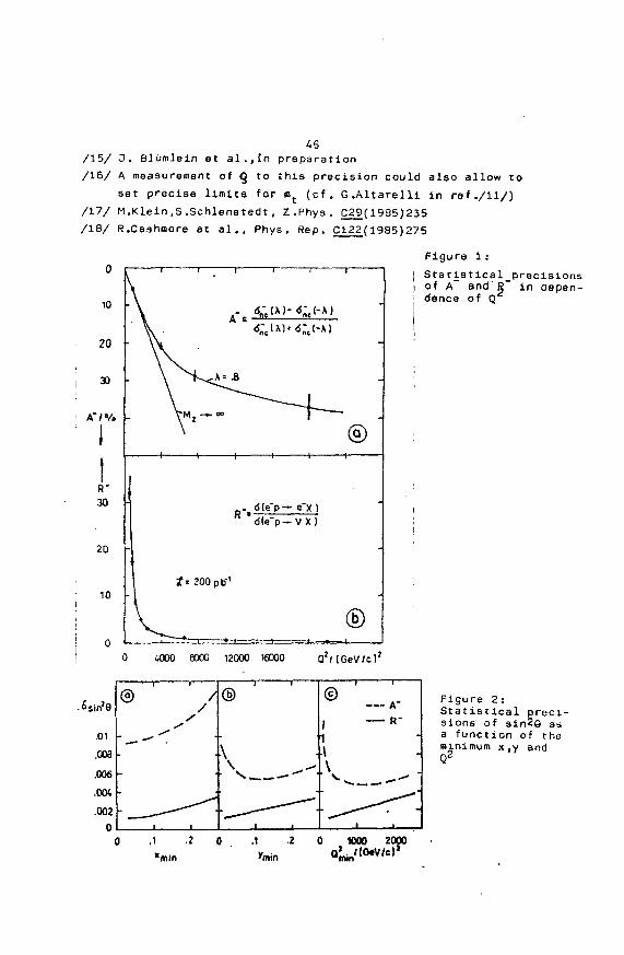
Figure 1 :
0 4000 8000 12000 16000 QJMGeV/c)2
Statistical_precisionsof A and R in aepen-dence of Q
Figure 2:Statistical preci-sions of sin*9 asa function of theminimum x.y andr>2
6 Mw /GeV
1.4
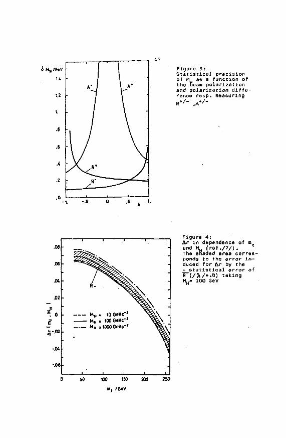
Figure 3:Statistical precisionof M as a function ofthe Beam polarizationand polarization diffe-rence resp. measuring
.OS
.06
M
.02
=foe
i-«-04
-.06
1 1 1 1 1
• ^ ^ s "MN « lOGeVc-2 ^ ^ V "
MH .lOOOOeVe-* ^ ^ \
-
I 1 1 1 11
Figure 4sAr in dependence of mand M H (ref./7/).
l
The snaded area corres-ponds to the error in-duced for hr by thei statistical error ofR~(/a/=.8) takingMH» 100 GeV
100 ISO 200 250
ZZ PRODUCTION IN ft COMPOSITE MODEL
Maria Krawczvk
Institute of Theoretical Fhysics
Warsaw University, Warsaw .Poland
~c.t: The? effective olectroweafc theorv with composite 1 in
the version proposed by Boudjema and DomDey C13 leads to
the predicton that the electromagnetic couplings c-f the Z
are substantially larger than they are in the standard
t?l(?ctroweal'. theorv.
• We -found that this anomalous Zlr coupling may be
observed in the process e e —>ZZ at energy Ys bigoer
than 270 6eV .
This couplinij may as well be seen in the inclusive ZZ
production in p p collision for °tt\r a t e n e r i 3 v ^ s >90C>
tieV.ln the p • distribution the large contribution due to
composite Z may be observed in p p — > ZZ X already at
Vs = 630 GeV for p ? larger than 7oGeV/c.
Supported in part by Ministry of Science and Higher Education,
Research Problem CPBP 01.03.
50
Introduction
The standard electroweak theory works perfectly in full
agreement with experimental data. Nevertheless there are attempts
to investigate other models which would share the success of the
standard theory having at the same time less parameters and
avoiding the introduction of Hiqqs particles , not seen so tar
experimental 1y.
Here we consider the composite model by Boudjema and Oombey
Cll. where massive vector bosons W and Z are assumed to be bound
states of elementary constituents called haplons . The y and
other basic objects of the electroweak theory -leptons and quarks-
are elementary particles and are described in a conventional
manner. Similar ideas were discussed some timoa ago by Breenb'-rg
and Sjcher C2], Chen and Sakurai 133, Kritnsch and Mandelbau.n L-Ij,
Abbott and Fahri C53.
Haplons are assumed to have spin 1/2 , they carry color (N =3 >
and flavour ( N ='2 > quantum numbers. To reproduce known results
for law energy electroweal: processes < say for "/& up to ft ) they
have to carry new quantum numoerf called hypercclaur Cl =3).
According to the prescription done by Boudjema and Dorabey C1J,
which we adopt here, all parameters tor these hypothetical
particles are estimated using the old vector dominance idea .
The nan-elementary structure of vector borons W, Z leads to
the effective 'three boson couplings due to the haplon loop.
These couplings happen to be quite large in contrast to the
corresponding couplings due to lepton and quark loops in the
51
standard theory. In the work 111 the possible observation of the
effective ZZy coupling with one virtual 2 (ZZ r> in the process
e+e~—>Zy has been discussed .
Here we propose to consider the ZZy effective vertex with
virtual >- <ZZr*> in the high enerqy process e e —>2Z and the
related hadronic process p p — > 11 X.
We start with tht; description of general features Df standard
and composite contributions to the ZZ production in fermion
-antifermion annihilation processes. Then we will present the
comparison of the composite and standard approaches to the process
e e —>ZZ . Next we discuss the inclusive Z2 production in the
high enerqy p p scattering.
r alr(?mar ks
We would like to test the effective ZZf coupling by comparing
the lowest order predictions for the process ff >ZZ in the
composite model C13 and in the standard electroweak theory
ff stands for atn electron or a quark ) .Our aim is to answer the
question whether and "where this anomalous coupling may be
observed. Therefore^we will simjlify the computation of composite
and standard contribution as much as possible .The more detailed
analysis will be given elsewhere .
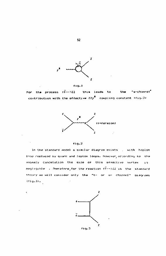
In the composite model this effective coupling is due to the
haplon loop diagram (fig.l)
Similar method of testing the compositness of gauge boson Z was
dicussed in ref.C7J.
52
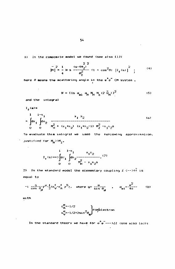
For the process +f—>ZZ this leads to the "s-channel
contribution with the e-f-fective ZZy coupling constant
<t=fermion)
•fig.2
In the standard model a similar diagram esists . with haplon
loop replaced by quark and lepton loops. Hawcver( ac:ordin<j to the
anomaly cancelation the size o-f this ettective vertex 13
negjigible . Therefore,-for the reaction f* — >LL in the standard
thr?ory we will consider only the "t— or u— channel" diagrams
(f ig .3) .
53
Since we are intereEteo in high energy processes we neglect in
the -following analysis masses tor all standard +ermions . For the
boson Z wi? tale M, = f2 GeV . The other standard parameters
are talen in a simple way :
a =1/128 , sin2© =1/4 . <1>el W
To describe the composite Z contribution we follow the approach
of ref.C13 where the couplings of haplons to boson Z , a, .are
determined (as well as their mass t\, , charge CU and other0
attributes) from the experimental low energy data using the y-W
mixing and the idea of vector dominance. We refer for details to
the original work CU.
Fur the composite model we consider in detail only the
•'optimistic parameters" (giving the largest chance for the
observation in the near future) from C13:
0^=3 (g£=g£=qH , g2/4n = ^ ^=200 B e V QH=l/6 NH=3 , (2)
where 6 is the average electric charge for hapIon doublet,rl
O =1/6 corresponds to the charge assignment tor haplons similarrl
to that for u and d quarks.
He will consider also this set of parameters
with different values for mass of haplon : M =400 and 6OO (ieV.H
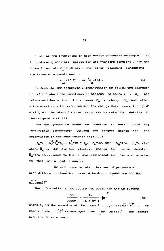
The differential cross section is equal (in the CM system)
*<" p7 _ 2
_ £ j M | ( 3 )
dcos© 16 n s1/ s ,
where p^ is the momentum of the boson Z , . p = l /^yi-4~M2 . The
matriK element |ii j " i s averaged over the i n i t i a l and summed
over the f i n a l spins
1 ) I n t h e c o m p o s i t e m o d e l w e f o u n d ( s e e a l s o C 1 J )
2 2- 2 1 (S-4M ) 2
|M| = - N s ~— (1 + cos 6) |I ,<s> |4 M^ '
here 6 means the scattering angle in the e e CM system ,
and the
If <s>
1
JdxO
1-x
o
N =
integral
1
2 2H 1
C16 a
xl X2
•x ) ' xi +
To evaluate this integral we used the toi-lowinq approximation,
justi-fied for *\i>>H2*
<*)==> jd::0 O MH " X1 X2 5
2) In the standard model the elementary coupling I <—>f-f is
equal to
with
5 i v A "3= srs-s-I" W
„ fiui/alectron
In the standard theory we have for e e >Zl (set? also C&J):
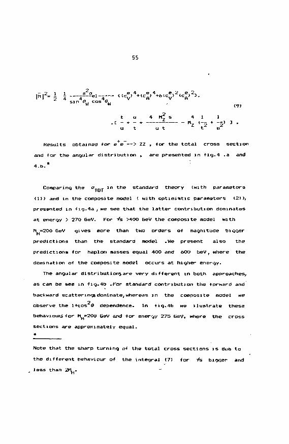
55
|S|2= i I «f«el• I 2 4 4 4^s,n aM cos ew
t u 4 M s 4 1 1. C - + - + liz 1-5 + -5) 3 .
u t u t t u
Results obtained tor e e — > ZZ , for the total cross section
and far the angular distribution , are presented in -fig.4 .a and
4.b.* :
Comparing the "-rnj l n t h e standard theory (with parameters
<1)> and in the composite model ( with optimistic parameters (2))/
presented in fig.4a , we see that the latter contribution dominates
at energy > 270 GeV. For Vs >400 BeV the composite model with
M =200 GeV gives more than two orders of magnitude biggerH
predictions than the standard model .Me present also the
predictions for hapIon masses equal 4OO and 6OO beV, where the
domination of the composite model occurs at higher energy.
The angular distribution}are very different in both approaches,
as can be see in -fiq.4b .For standard contribution the forward and
backward scatterings dominate, whereas in the composite model we2
observe the 1+cos & dependence. In fig.4b we llustrate these
behaviours for MH=200 GeV and tor energy 27l> beV, where the cross
sections are approximately equal.
Note that the sharp turning of the total cross sections is due to
the different behaviour of the integral <7> for Vs bigger and
less than 2 ^ .
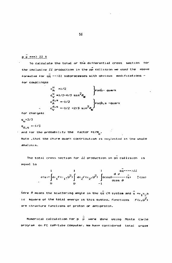
56
To calculate the total or the differential cross section tor
the inclusive Zl production in the pp collision we used the above
formulae for qq —>Z2 subprocesses with obvious modifications -
for couplings!
-for charges:
qu=2/3
"d.s ="1 / 3
uCA
c d >
cv'
= 1/2
=1/2-4/3 sin2eM
,s =_iy2
S =-1/2 +2/3 sir
1VforAi- quark
yfor^J.s -qua
and for the probability the factor =1/N .
Note .that the charm quark contribution is neglected in tne whole
analysis.
The total cross section for LL production in pn collision is
equal to
1 1 1 qq >
IdcosO <s>ocos e
-1
= lcli: F(:: .Cl2) I di:,f(K .U2) Id
here 6 means the scattering angle; in the qq CM system and s =x :<,,s
is square of the total energy in this system. Functions F(x,CI2)
are structure functions of proton or antlproton.
Numerical calculation for p p were done using Monte Carlo
program on PC IBM-type computer. We have ccn?.idw-ed total cross
57
sections and p - distributions for Z bosons. We used the Duke
and Owens parametr1zation of structure functions C9] (set 2.
denoted by D02 with the energy scale Q=li .We have checked ^>st
the other choices of Q (equal to p^ or invariant mass M = Vs )
would not change the results in a visible way. This same is true
if one changes the parametr1zation to the parametri2ation by
Eichten et al.tlO] (set 2, Ei2> with the energy scale Q = Mz>
PT or M.
The results obtained -for the composite model with the
optimistic parameters and for the standard model with parameters
(1> Are presented in figs.5. The total cross section in the
composite model starts to be greater than in the standard case
already at 900 GeV , at higher energy there is one order of
magnitude difference between these two approaches (fig.S.a).
In the p - distribution (tig.5 b,c) the composite model dominates
the large p tail. For the scattering energy Ys = 630 GeV the
cross over of the predictions of the composite and standard model
occurs at p "• 1OO GeV/c for the l/pTd<?.'dPT (fig. 5.b> and for pf~
70 GeV/c for the integrated p - distribution <fig.5.c).0
We see that the possible signature of the composite Z production
in the high energy pp scattering for the energy Vs<l feV would bethan standard
the higher/production rate for the events with large p 2 .One may
expect a similar e-ffect for the W production in the same process.
We consider the anomalous effective coupling lit, reflecting
the composite structure of gauge boson Z. in the high energy e e
annihilation and in the inclusive pp scattering.
For these processes the predictions of tha composite model in
58
version proposed by Boudjema and Dombey C1J <with the optimistic
parameters ) and the standard theory are compared.
For e e —>ZZ these two approaches give similar predictions tor
the total cross section at yk=27O GeV ; there are two orders of
magnitude difference for the energy Vs > AOO 6eV . Unfortunately ,
even the energy 270 GeV will not be reach in near future for this
process..
The situation in pp—>ZZ looks more promising .Here the
composite contribution may dominate in the p - distribution even
at the energy accessible now. At energy Vs=630 6eV this may happen
in 1/p dff/dp for p MOO GeV/c and in the integrated p
-distribution already -for p >70 GeV/c. The composite "L may show up
rather soon also in the total cross section — for Vs > V00 BeV.
For higher energy the standard contribution is approximately an
ordor of magnitude smaller than the one with composite Z.
Probably the signature of the anomalous coupling ZZf may be
registered in the e e or pp data before the cross over of the--;;;
two competitive model predictions tales place .that means at
lower energy or transverse momentum p quoted above.
Is there any relation of the results for the p distribution in
pp--."ZZ with unusual events with large p T Z and W production from
UA1 collaboration C8J 7 To obtain any reliable estimation in this
caio the more detailed analysis has to be done for ZZ as well as
for the WW and WZ production and for the passible bacltgrout
<noM under preparation).
Ac knowledoement s
This work is based on the collaboration with dr. N.Dombey and
59
dr K.Boudjema. I would like to thanl them for useful discussions
and comments.
I have enjoyed conversation with prof. Krolikowski ,prof.
Pol-orski and dr. Mahka and dr.Koiodziej .
1 would like to thank dr. M.Markytan tor sending me preprints
on Uhl results and dr. Jan Kalinowski for very useful comments and
reading the manuscript.
References
l.F.Boudjema and N.Dombey, An effective theory of a composite Z,
preprint ,January 1987
2.U.W.Greenberg and J. Sucher, Phys.Lett. 99B 33V (1981)
3.P.Chen and J.J.Sakurai, Phys.Lett. HOB 481 (1982)
4 H.Fntzsch and li.Mandelbaum , ftiys.Lett. 102B Z19 tlVt31> ,Phys.
Lett. 109B 224 (1982)
S.L.Abbott and H.Farhi .Phys.Lett. 101B 6V <1V81>
6-R.W.Brown and K.U.Mikselian, phys. Hev.Dl9 922 (1979)
7.P.Mery .M.Perrottet and F.tt.Renard Anomalous effects in e e
annihilation into boson pairs: (IX) e+e~—>ZZ,}'Z,yj-.CERN-rH.4741/a7
B.C.Albajar et al.(UA1 -Collaboration) .Production of W's with
large Transverse momentum at the CtHN Proton—ftntiproton
Collider, CtRN-EP/87-82, April 24th, 1987
9.D.W.Dul:e and J.F.Owens, Phys.Rev.D3O 49 (1984)
l'J.E.J-tichten, X.Hinchcl i-ffe, 1.1). Lane and C. Ouigg. Rev. Mod. Phys.
56 579 (1984)
l.The induced IZr coupling via hapIon loop
2.ff—>ZZ in the composite nodol
3.*?—>ZZ in tho mtandard electroweak theory

60
4.Results tor e e —>ZZ in the composite model (- - -) and in tlie
standard theory (——)
a.total cross section
b.angular distribution
5.Results for pp->2Z in the composite model (- ) and in the
standard theory ( >
a. total cross section
b. p.- distribution l/p-do/dP-j.
c. p_ —distribution \ f o J l / p dff/dpT
O p,.>p,-
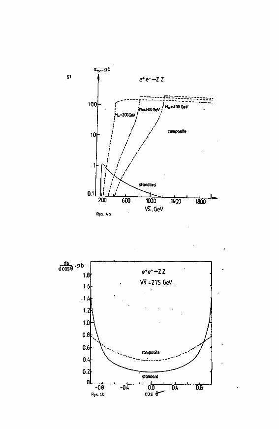
61T.pb
e+e"-ZZ
100
10
r""
/
composfe
0.11200
Rys. 1.
600 1000 K00Vs.GeV
1800
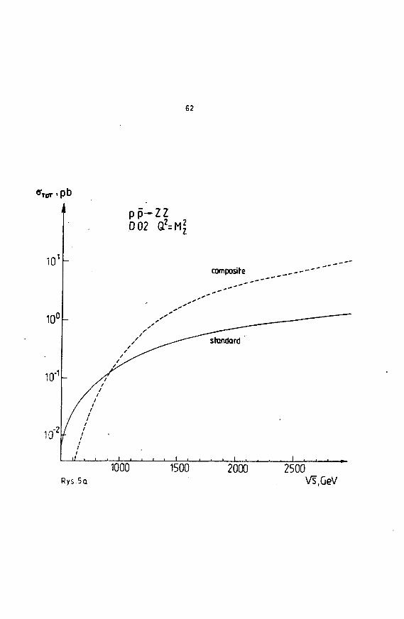
62
10'
10°
10"2
pp-ZZD02 Q2=M*
-
S
- /(I
composite ___-- -*" '"
_ _ — — - ~____—, .
standard
1000 1500 2000 2500Rys.Sa Vs.GeV
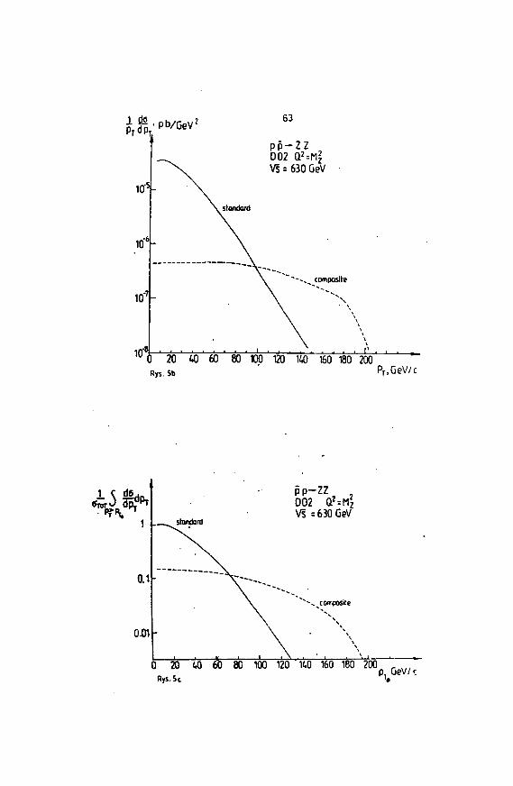
Iff5
10"
10'
101
63
p p - Z ZD02 Q2=M£Vs = 630 GeV
. standard
6 2 0 «) 60 80 100 120 140 160 180 200Rys.Sb ' Pf.GeV/t
PP-ZZ 2
002 Q?--»\Vs =630 GeV
20Rys.5c
80 100 120 K.0 160 180 200 r U.p GeV/r
65
Standard-Model HlQQS Searches *t the SSC
Jan Kalinowski 1
Institute for Theoretical Physics, Warsaw University
Hoia 69, 00681 Warsaw, Poland
Abstracts The procedures for exploring the Higgs sector of the
standard model at the ESC are shortly reviewed. The comparison of
the effective-W approximation with the exact calculation for the
process ff •» ffWW shows that it reproduces the Higgs signal, while
the continuum background can only reliably be computed in the
exact calculation. The ability to isolate longitudinal W decay
modes is discussed.
Introduction. With the discovery of the W and Z gauge bosons
the model of Glashow, Salam and Weinberg has been accepted as a
standard model (SM> of the electroweak interactions. Certain
aspects of the model, however, have not been tested so far
experimentally, for example the structure of the triple-gauge-
boson coupling, the properties of the Higgs sector and the origin
of mass. In the model the symmetry breaking is achieved by the
Higgs mechanism and a. single neutral Higgs particle emerges.
Unfortunately, the present theory does not constrain its miss mu.H
In the minimal three—generation SM the Higgs boson mass should be
greater than about 10 GeV C13. If a top quark mass m > 50 GeV or
if a fourth generation of fermions exists, this lower limit
disappears C23. There is no upper limit to m... Nevertheless, it is
generally assumed that m^ is somewhat below 1.5-2 TeV. Otherwise
Supported in part by the Ministry of Sciencei, Higher Education,
Research Problem 01.03.
66the Higgs self-energy coupling becomes strong and the perturbation
theory breaks down. Even in such a case, however, use o-f ordinary
perturbation theory may be justified by the fact that the
deviations from the perturbative calculations will signal new
physics.
For m < 4O ReV, the Higgs boson can be found at S!_C or LEP ifH
these machines reach their designed luminosity. With LEP II the
range can be extended to about SO GeV. The process considered
there is the associated production e e •+ H + Z followed by Z •*
1 1 . For a review of these topics see for example ref. 3.
In high energy hadron collisions the Higgs boson will be
ccpiously produced, fit the SSC, a pp collider with energy of 40
TeV and luminosity of 10 cm s , a large number of GM Higgs
bosons is expected, of order 1O /yr for m.. S: 300 GeV E43. However,
tt turns out that it will be more difficult to detect it because
of strong SM and QCO background. Thus hadron colliders will
primarily be of interest if sitj *S above the reach of e e
rtiafihines. I-f 2m < ffl < ^mu» n o W«*V has been found to overcome the
OCD/SM background C53. In this paper we will discuss the case of a
heavy Higjs boson, m^ > 2i\,- The heavy Higgs boson decays almost
exclusively into WW and ZZ pairs. Only purely leptcnic decays of
the 2 boson ^re background free. However, they suffer from low
event rate. Assuming that both p*s and e's can be identified, H ••
ZZ • (1 1 )< 1 1) has a branching ratio = 1.2 » 1O " which leads
to 12 events in a standard SSC year. The mixed hadronic/leptonic
Higgc decays have a higher rate. Although the separation of the
signal from the background appears to be a serious problem, we
will see that it may be possible to study the Higgs sector at the
SSC for m < 1 TeV. Purely hadronic decay modes are overwhelmed byM
the QCO background events.

67
There are two significant production mechanisms -for a heavy
Higgs boson in the SSC energy range. The first is the gluon-gluon
fusion 161 in which two gluons couple to a fermion loop and the
Higgs boson is emitted from the loop.The second is the WW fusion
mechanism C73 in which W's or Z's emitted by incident quarks
collide and form the Higgs boson. It has been pointed out C4J that
the latter mechanism dominates for m £ 300 GeV, because the
coupling of the Higgs boson to longitudinal W's or Z's is
proportional to m... Duncan, Kane and Repko C83 have studied the
properties of the on-shell WW scatering and the Higgs boson signal
using the effective-W approximation C93 in which distribution
functions for W's inside colliding protons are folded together
with the on—shell WW amplitudes. The validity of this
approximation has been found to be of order 207. for total cross
section calculations for W+W~ •» H C103 and qg •» q'UD C113 (where U
and D are the quarks of a new generation). It has not been tested
for the WW scattering. Moreover, in the context of Higgs boson
searches the effective-W approximation cannot be reliably used to
assess the impact of possible triggers on spectator quarks present
in the final state. Such triggers may prove to be critical to
isolate certain aspects of the WW scattering at the SSC, as
advocated in ref.12. In addition, the W's in the final state will
be identified by its decay products and it is important to assess
the impact of kinematical cuts imposed to ensure that W's are
reconstructed and their polarization measured.
To address the above issues the complete gauge invariant set of
amplitudes for an arbitrary process ff + ffWW has been computed
C133 without the effective—W approximation. Below I will present
main results of this work. (For another exact calculations see
ref .14.)
68
The calculations have been done using the massless spinor
techniques of ref. 15 in which the final state W*s are
automatically decayed to massless fermions, so that the results
include the full spin density matrix correlations -for all final
state particles. We have tested the gauge invariance by examining
the scaling behaviour of our results. In refs. 13 we have focused
exclusively on the charged current reactions to which WW •• WW
scattering diagrams contribute. The charged current sector has
more singular structure in the effective-W approximation fa
Coulomb pole from the photon exchange in the t channel) than e.g.
ZZ * WW and therefore should yield the most sensitive comparison
with the exact calculation. For simplicity explicit numerical
results have been presented for the quark scattering subprocess
us •* dcW*W~. . (*)
Comparison of the exact and the effective-W calculati ons. The
comparison between the effective-W approximation and the exact
calculations has been done both at the subprocess (*> level and
after folding with the proton's quark distribution f-inctions and
we focused on a single center of mass energy for each reactions
E =Vs = 1 TeV and Vs = 40 TeV, respectively. We consideredcm us pp
only m = 0.5 TeV or oa. Our results are illustrative of those forn
other energies and Hi 13.33 masses. In order to make? a comparison, it
is necessjiry to impose a cut in the effective-W calculations to
avoid the t-chanriel singularity from the photon exchange. We hav£?
chosen to restrict the WW centei—of-mass scattering angle 0* >
#nin* Although the exact calculation is free of this singularity
for comparison the same cut has been used.
The m w v W-pair mass spectrum at the subprocess level is
presented in fig.1 and for pp collisions in fig. 2. In the case of
pp collisions only the single subprocess <*) is incorporated, the
69
EHLQ, N = 2 , structure functions with the scale Q = in are
used jnd no rapidity cut on the W's is imposed. The angular cuts,
at 0 = 10°, 30° and 60°, are imposed on the effective-Wmi n
calculations at subprocess level and after folding and on the
e::act computations only at the subprocess level. Both figures show
that the effective-W spectra normalization is very sensitive to
this cut, while that of the exact calculation is much less so. The
continuum level for «L. = oo varies by a factor of 1O-20, as © -n inx n
changes from 10° to 60°, whereas for the exact calculations it
varies by a factor 1.5-2, depending on m value. Note, however,
that at any given 6 - the excess of the m,=0.5 TeV peak over ths
in,, - oi> continuum is nearly the same in both methods and mildly
dependent on the 8 . cut. This confirms the results of ref. 10.
Similar results to the above apply in the case of rapidity cuts.
Me anticipate that there will be a better level of agreement
between the effective-W and exact calculations in sectors ZZ -> WW
and ZZ -> ZZ, due to the absence of the singular photon exchange
diagram. Therefore one can hope to identify those channels and
cuts for which the effective-W appro:: i mat ion can reliably be used
to evaluate not only the Higgs signal, but also the magnitude of
the vector-boson scattering amplitudes.
Propertigs of the exact calculations. The Higgs boson decays
almost exclusively to longitudinally polarized gauge bosons.
Therefore in searches for Higgs it may prove very useful to
measure polarization of W's. The polarization of the final state W
can be detected by the decay distribution of the ff pair in the
rest frame of the W, which should be of sin*fl* form for longi-
tudinal W and l+co=20 for transverse. Fig.3 shows that at m =
0.5 T B V th« decay is predominantly longitudinal i-f t^ » 0.5 TeV,
while is predominantly transverse for iry, « «, as expected.
70
In the hadronic decay mode, W •» jet • jet, the above angular
distribution cannot be used due to strong QCD/electroweat' back-
ground from events containing W + two jets that simulate a second
W. It was shown in ref. 16 that in such a case the longitudinal
W's can be revealed by a careful study of correlations between
transverse momenta of the two jets, pT, and PT->- The longitudinal
W's populate the region of constant r . + rmax' ***He transverse
and other backgrounds contribute mainly to the r . = 0 region,
w h e r e r.in " PTl'"vv' rmax * PT2/mwv' PT1 < PT2' T a k i n q "vv = °-5
TeV, r = 0.225, we observe in fig.4 a peaking in the r 4
distribution at large r . for la. - 0.5 TeV (so that longitudinalnin r»
W's are copiously produced), whereas it falls rapidly at high rm I n
for m = on
The totally new feature of the exact calculation is the ability
to discuss the p distribution of the spectator quarks present in
the process <*). In the effective-W approximation spectator quarks
and W's are necessarily emitted in the forward direction. It has
been suggested in ref.12 that triggering on the pT of the
spectator quarks cftn significantly reduce the background to the
H:y.js signal, because tht? background processes tend to have1 owspectator jets at law p . In fig.5 the p_ spectrum is
presented, where p T is the smallest p_ of the spectator jets. We
find that a PT cut on spectator quarks, while improving quality of
the selected Higgs sample (stronger r -r correlations),
tends to increase the background/signal ratio, as seen in fig.5.
Finally, I would like to mention that potentially dangerous
^gluon exchange diagrams with W's emitted from quarks do not, in
fact, present a problem, if rapidity cuts on the M's are imposed .

71
Ç.ijrir 1 u-j.r ... • IV-1 cc '. ion of a standard model Higgs at an e e
llicJtr j != re la t i ve ly -i i n! çjlit f or ward, but l imited to m ^ BO SeV
. I J.iiini?.f acrclorators. !n f.p c o l l i t i o n s detection of Hi ggs i s
< .ir ^rii.;i >r y. Only piirtl y leptonic decays are background f r e e .
!l»f nn-•• i_-i1 lOd^olli c/) c-pt.on x c modes moy be accesible for" 2 mw < m <
1 lev, Ü suif < ic jpnt ly &tronQ cuts and resolutions can be imposed.
•Mie (--f fe< ti VL' -W i<ppro<im.ition r e l i a b l y reproduces the Hiqgs
•jii,-.). ! !uduc.tion of tho longitudinal W's in the hadronic decay
-'1-.- '..rn bc rovcalet) by examining correlat ions between the
'. r 1-ri-,vfT"'..-e MuT-ufiiÙ Cif the two decay product j e t s . The imposition
.•f cut«* on the üppclittor je ts n.ust be done with care to avoid the
!><u î.rjr rjunrJs In the Hi ggo c
Tick now
1 could like to thank J.F. Gunion and A. Tofighi—Niaki for the
important contribution to the effords summarized herein. I thank
also G. Kane, S Willcnbrock, F. 01ness and W. Rep I o for helpful
ronvRrsflti on*.
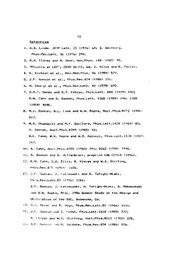
72Fief ereoces
J. A.D. Linde, JETP Lett. 23 (J976) 64; S. Weinberg,
Phys.Rev.Lett. 3t <197ó> 294.
2. R.A. Flores and M. Sher, Ann.Phys. 143 '1983/ 95.
S. "Physics at LEP", CERN 36-O2, ed. J. Ellis and R. Peccai.
4. E. Eichten et al., Rev.Mod.Phys. 56 C1984) 579.
5. J.F. 6union et al., Fhys.Rev.D34 (1936) 101.
6. H. Georgi et al., Phys.Rev.Lett. 40 (197S) 692.
7. D.R.T. -Jones and S.T. Petcov, Fhys.Lett. 84B (1979) 440;
R.N. Cahn and S. Dawson, Fhys.Lett. 136B (1984) 196; 13SB
(1984) 464E.
8. M.J. Duncan, G.L. Kane and W.W. Repko, Nucl.Phys.B272 (19BÈ;
517.
9. M.S. Chancswitz and M.K. Gai l lard, Phys.Lett.142B (1^84) 85;
G. Dation, Nucl-Phys.P249 (1985) 42;
6.L. r.'ane, W.U.'. Pepko and W.B. Rolnick, Fhys. Lett . 14;.E( '198îi
7A7.
10. R. Cahn, Nucl .Phys. BZ55 (19S5) 341; B262 C985? 744E.
11. S. Dawson and S. Ui I lenbrocl.., preprint LBL-2191,4 <iy3ó).
IT. F.N. Cahn, S.D. E l l i s , R. Kleîss and W.J. S t i r l i n g ,
Phys.Rev. DTï <19fjS' ;62<>.
IZ. Cf. Oumon, J . > JlinoMSh and A. To* ighi—Niaki,
rtivi.fie v .Let t . 57 U'36) 27-51 ;
J.K. Gun ion, J . K.al inowskj, A. To-f ighi -Niaki , A. Abbasabadi
wil W.W. Repio, Proc. 1986 Summer Study on the design and
Ut i l isa t ion of the SSC, Snowmass, Co.
11. D.A. Dicur jnd R. Vega, Phys.Rev.Lett.57 (19S6) 1110.
'5 . J.F. Gumon t<nd Z. 'unst, Fhys.Lett. lblB (1905) 333;
R. i lnis!: anrj W.J. S t i r l i n g , Nucl. Phy*.B2i2 <1?5S) 235.
\',. t.r . f.i.iriir.i. .vl M. ioldate, Phys.Rev.D34 11986) 0?6.
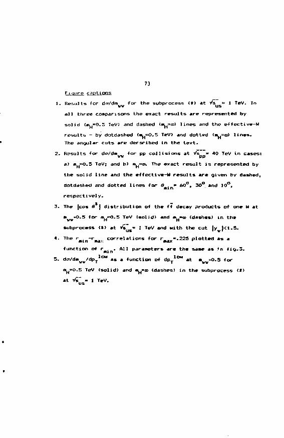
73
Fiourg cautions
1. Results -for fSc/dm for the subprocess <»> at Vs = 1 TeV. In
al l three comparisons the exact results are represented by
solid («=0.5 TeV) and dashed <.m=a>t lines and the effective-W
results - by dotdashed <ny=O.5 TeV) and dotted (m=a>) l ines.
The angular cuts are dersribcd in the text.
2. Rpsults for do/da for pp collisions at Vs "= 40 TeV in cases:
a) Hi =0.5 TeV; and b) nt=tu The exact result is represented by
the solid l ine and the effective-W results arm given by dashed,
dotdashed and dotted lines for S - i n - 60°, 3O° and 10°,
respectively.
3. The |cos 8 | distribution of the ff decay products of one W at
•WV*O.5 for (»H=O.S TeV (solid) and •.,•<» <dashes> in the
subprocess <») at * 'su s- 1 TeV and with the cut |ywj<1.5.
4. The r . - r correlations for r «.225 plotted as a
function of rmin- All parameters *rm the sane as ;n f i g . 3 .
5. dci/dmvv/dpT1OM as a function of dpT
l o w at »vw=O.5 for
mH=0.5 TeV (solid) and *H"<» (dashes) in the subprocess (*)
at Vi~ s - 1 TeV.
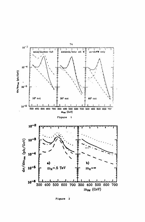
FTrmTr"T"T"T¥T"T"T"T"T2'!: dotdosh/doLs: eff. W? us- dcWW only
300 400 500 600 700 300 400 500 600 700 300 400 500 600 70Cmn (GeV)
Figure 1
10-2
10-3 „a>
Si
10"6
; T
: v.
li
•
a)m H =
'1 — I'
\\
5 TeV•
i i i n
_ >
, |
, . . . ( . . . . j . . . . j . . . . j . |
~>. **" • 1
b) ^ "^ -
mH=» -;
. . . L . . . I . . . . I . . . . I . .
300 400 500 600 700 300 400 500 600 700(GeV)
Figure 2
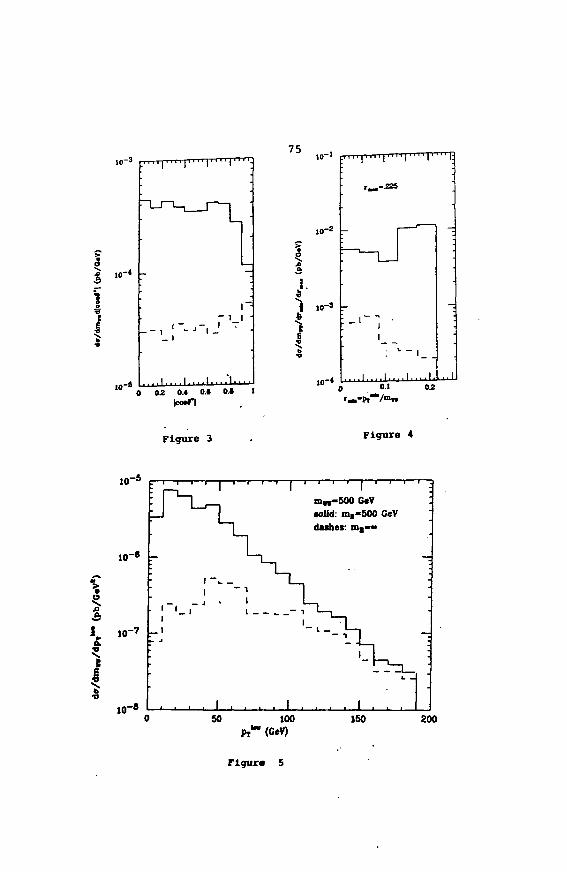
75I0"3 n-rx
w-s , I , , , , I , . . . 1 . . • . ' I • . .
0 02 0.4 O.t 0J t
j
E
to-'
10"^
10-3
r1-,-JS25
~ 1 _
I - 1 " 1 . 'i
. . . . 1 . . , . ! . .
" 1 " ' ' 1 • " ' 1:
• • - 1
1 ,
•
, , |
O.I 02
Figure 3 Figure 4
10- 5
10,-« u
I10,-7
10,-e
\
1
' ! " ' - " J
i
"L,
1I
1 ' ' ' ' 1 •mn-500 G«V(olid: ml«SO0dkshes: m,»~
* \
1 . . . . 1 .
CeV
Trm
rrr
-
SO 100PT1
150 200
Figure 5
77
IS THE ANAPOLE MOMENT A PHYSICAL OBSERVABLE ?
H. Czyz, K. KolodzieJ+,M. Zralek
Dept. of Theoretical Physics, Silesian University, ul. Uniwersytecka 4
PL-4O-OO7 Katowice , Poland
and P. Christova
Dept. of Physics, High Pedagogical Institute, Shouaen, Bulgaria
f.- dependence of the charged lepton anapole moment is investigated.
Tt is shown that the anapole moment is a gauge dependent quantity.
Thirty years ago Zeldovich fl] repoted that a spin- j particle
in a parity-violating but CP-conserving theory, apart from well
Krovm static electromagnetic characteristics such as charge or
Giagnetic moment, has another characteristic, that is coupling with
an external electromagnetic field which he called the anapole moment
of the particle. This has prompted certain researchers £2] to
invpstigate the electron anapole moment within the standard theory
of electroweak interactions. As weak interactions violate parity,
electroweak radiative corrections to the basic electromagnetic
interaction would give rise to an anapole moment, as in fact occurs.
Theoretical predictions both for electron and muon magnetic
monsnts provide an excellent tool for testing a theory (QED) against
experiment hence it was tempting to essay a simple test of weak
radiative corrections by numerical evaluation of the electron anapole
moment and then to compare this with an experimental findings.
+ Talk presented by K. Kolodzl«J.
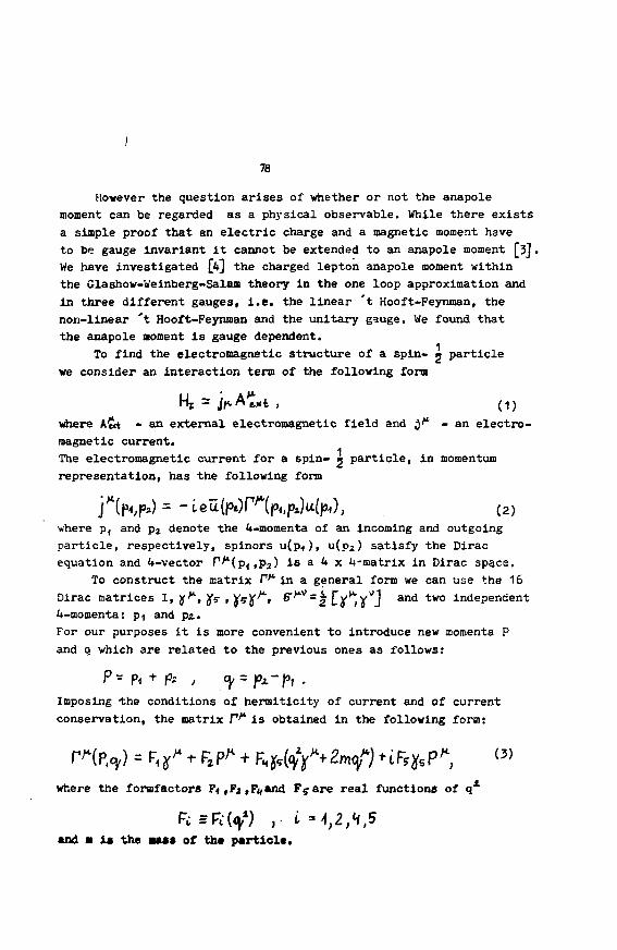
78
However the question arises of whether or not the anapole
moment can be regarded as a physical observable. While there exists
a simple proof that an electric charge and a magnetic moment have
to be gauge invariant it cannot be extended to an anapole moment [3J.
We have investigated [k] the charged lepton anapole moment within
the Glashow-Weinberg-Salam theory in the one loop approximation and
in three different gauges, i.e. the linear 't Hooft-Feynman, the
non-linear 't Hooft-Feynman and the unitary gauge. We found that
the anapole moment is gauge dependent.
To find the electromagnetic structure of a spin- particle
we consider an interaction term of the following form
Hj = JftA ext , (.,)
where A&t - an external electromagnetic field and j* - an electro-
magnetic current.
The electromagnetic current for a spin- m particle, in momentum
representation, has the following form
(2)
where •p1 and pi denote the it-momenta of an incoming and outgoing
particle, respectively, spinors u(p,), u(pj) satisfy the Dirac
equation and it-vector P^(p op 2) is a k x 4-matrix in Dirac space.
To construct the matrix f^ in a general form we can use the 16
Dirac matrices I, y'*, jJV , ^^"t &***' = 2 CY**! YVJ a n d t w o independent
4-motaenta: p^ and p*.
For our purposes it is more convenient to introduce new momenta P
and q which are related to the previous ones as follows:
Imposing the conditions of hermiticity of current and of current
conservation, the matrix P^ is obtained in the following form:
where the formfactors Fi,Fj,F^and Pyare real functions of q*
and • is the MISS of th« particle.
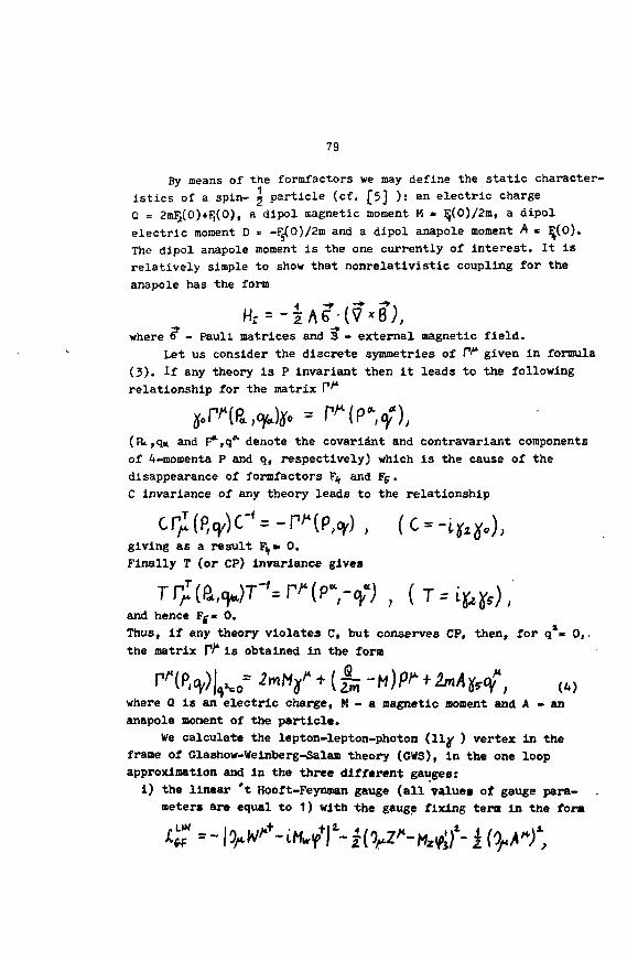
79
By means of the formfactors we may define the static character-
istics of a spin- j particle (cf. [5] ): an electric charge
Q = 2mFi[0)+F,(0), a dipol magnetic moment H = ^(0)/2m, a dipol
electric moment D = -^(0)/2m and a dipol anapole moment A = (0).
The dipol anapole moment is the one currently of interest. It is
relatively simple to show that nonrelativistic coupling for the
anapole has the form
where o - Pauli matrices and B - external magnetic field.
Let us consider the discrete symmetries of P'4 given in formula
(3). If any theory is P invariant then it leads to the following
relationship for the matrix P'*
(R<.,q« and F*,q* denote the covarlant and contravariant componentsof 4-momenta P and q, respectively) which is the cause of thedisappearance of formfactors fy and Fp.C invariance of any theory leads to the relationship
giving as a result F^» 0.Finally T (or CP) invariance gives
and hence Fj« 0.
Thus, if any the
the matrix P/4 is obtained in the form
Fj
Thus, if any theory violates C, but conserves CP, then, for q*« 0,.
where Q is an electric charge, M - a magnetic moment and A - ananapole nonent of the particle.
We calculate the lepton-lepton-photon (lly ) vertex in theframe of Glashow-Weinberg-Salan theory (GWS), in the one loopapproximation and in the three different gauges:
i) the linear 't Hooft-Feynman gauge (all value* of gauge para-meters are equal to 1) with the gauge fixing tern in the form
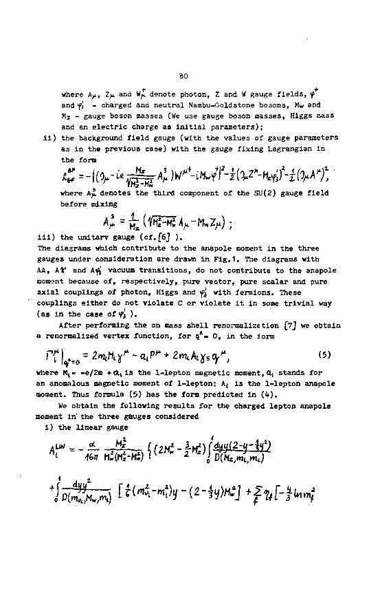
80
where A^, Zyu. and W,. denote photon, Z and W gauge fields, fand *fj - charged and neutral Nambu-Goldstone bosons, Kw andMz - gauge boson masses (We use gauge boson masses, Higgs massand an electric charge as initial parameters);
ii) the background field gauge (with the values of gauge parametersas in the previous case) with the gauge fixing Lagrangian inthe form
where AjL denotes the third component of the SU(2) gauge field
before mixing
iii) the unitary gauge (cf. [6j ).
The diagrams which contribute to the anapole moment in the three
gauges under consideration are drawn in Fig.1. The diagrams with
AA, kV and A$ vacuum transitions, do not contribute to the anapole
moment because of, respectively, pure vector, pure scalar and pure
axial couplings of photon, Higgs and yj with fermions. These
couplings either do not violate C or violate it in some trivial way
(as In the case of <fj ).
After performing the on mass shell renormalizEtion f7j we obtain
a renornalized vertex function, for q1- 0, in the ionn
where Mt= -e/2m + al is the 1-lepton magnetic moment, Ct( stands foran anomalous magnetic moment of 1-lepton; A{ is the 1-lepton anapolemoment. Thus formula (5) has the form predicted in (U).
We obtain the following results for the charged lepton anapolemoment in the three gauges consideredi) the linear gauge
f««t--Or
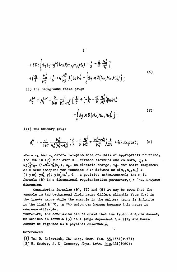
81
ii) the background field gauge
(7)
ill) the unitary gauge
where mi and m^ denote 1-lepton mass and mass of appropriate neutrino,
the sum in (7) runs over all fermlon flavours and colours, ^f •
Q^(^^»- (1-Mw/Mi)Qi ), Op- an electric charge, Tjf- the third component
of a weak isospin; the function D is defined as Dtm^mjjm^) «=
(1-y)mJ'+yii4-y(1-y)m-itl , e' - a positive infinitesimal; the g in
formula (8) is a dimensional regularization parameter,£ = 4-n, n-space
dimension.
Considering formulae (6), (7) and (8) it may be seen that the
anapole in the background field gauge differs slightly from that in
the linear gauge while the anapole in the unitary gauge is infinite
in the limit fc~*O, (n~»4) which can happen because this gauge is
nonrenormalizable.
Therefore, the conclusion can be drawn that the lepton anapole moment,
as defined in formula (3) is a gauge dependent quantity and hence
cannot be regarded as a physical observable.
References
[1] Ya. B. Zeldovich, Zh. Eksp. Teor. Fiz. 33., 1531 (1957);
[2] N. Dombey, A. D. Kennedy, Phys. Lett. 91B,428(1980);
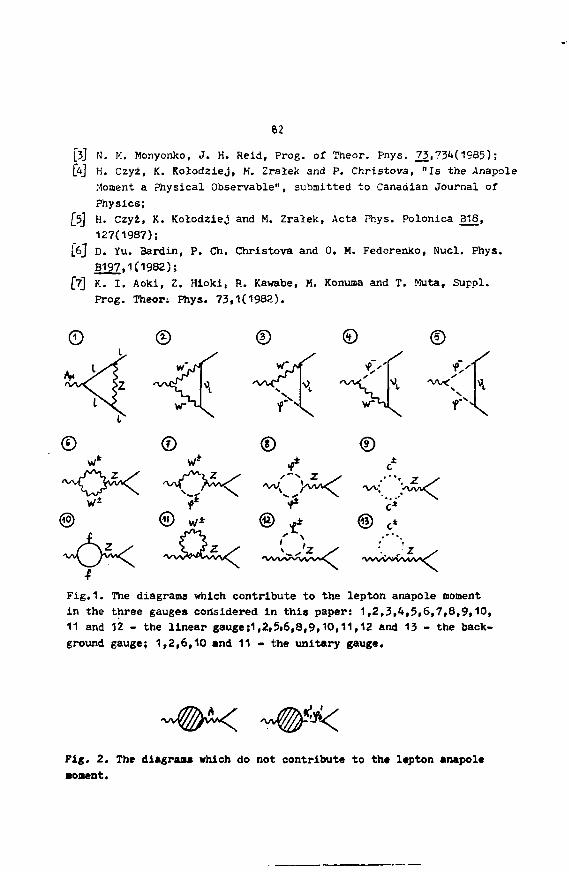
82
[3j N. K. Monyonko, J. H. Reid, Prog, of Theor. Phys. 73,?3<*(1985) ;(ÂJ H. Czyz, K. Kolod2ieJ, M. Zralek and P. Christova, "Is the Anapole
Moment a Physical Observable", submitted to Canadian Journal ofPhysics;
[5] H. Czyz, K. Kolodziej and M. Zralek, Acta Fnys. Polonica 318,127(1987);
[s] D. Yu. Bardin, P. Ch. Christova and 0. M. Fedorenko, Nucl. Phys.B197.1(1982);
[7j K. I. Aoki, Z. Hioki, P.. Kawabe, M. Konuma and T. Muta, Suppl.Prog. Theori Phys. 73,1(1982).
'we' >
vr
c*
Fig.1. The diagrams which contribute to the lepton anapole momentin the three gauges considered in this paper: 1,2,3,4,5,6,7,8,9,10,11 and 12 - the linear gauge;1,2,5i6,8,9,10,11,12 and 13 - the back-ground gauge; 1,2,6,10 and 11 - the unitary gauge.
™&*<Fig. 2. The diâgraa» which do not contribute to th« ltpton anapol«•oaent.
83DOUBLE BETA DECAYS
Presented by L.-D. FluriInstitut de Physique de1'University de MeuchStelRue A.-L. Breguet 1
CH - 2000 HEUCHATEL(Switzerland)
IHTROOUCTIOH
Heutrinos being very light, neutral and weakly interacting, they arestill poorly known objects: we don't know yet if they are massive ormassless, if they are Oirac or Hajorana spinors and we have littleinformation about the flavour mixings of their mass eigeratates. Tryingto investigate those problems is not merely curiosity but addressesfundamental questions in both paticle physics and cosmology.
Experimentally the neutrino properties are tested in direct massmeasurements, in oscillation experiments, in searches for neutrinodecays, in cosmic underground detectors and in double beta decayexperiments. We will deal here only with the last item. The interestedreader is refered to VU86 for a general and detailed survey of theproperties of neutrinos.
This report is intended for people not familiar with the subject. Inthe first chapter, we introduce notions of Dirac and Hajorana spinorsand of flavour mixing. In chapter 2, ue present the basic backgroundspecific to double beta decays. Chapter 3 reviews the experimentalmethods of double, beta decays and chapter 4 overviews the presentexperimental results. The report ends with a short summary.
1. THEORETICAL FRAMEWORK
Our present knowledge of the neutrino charged currents (CC) iscompatible with a Lagrangian interaction term
L 0 0 - T r " (*t • JJ-V, ) V • h.c.
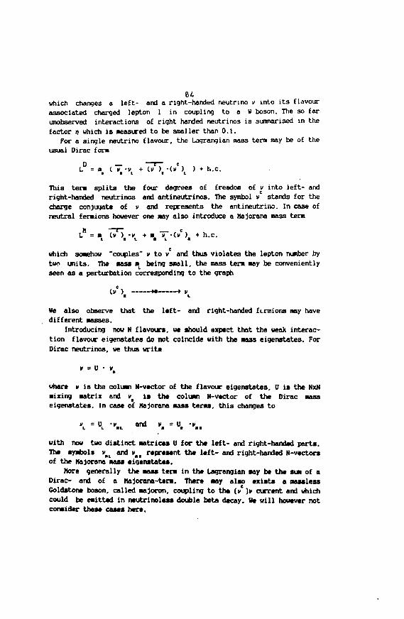
84which changes a left- and a right-handed neutrino v into its flavourassociated charged lepton I in coupling to a W boson. Ttie so farunobserved interactions of right handed neutrinos is summarised in thefactor i) which is measured to be smaller than 0.1.
For a single neutrino flavour, the Lagrangian mass tern may be o£ theusual Dirac fora
L = a> ( T -vt + (n ),•(»'),_ ) + h.c.
This tera splits the four degrees of freedom of v into left- andright-handed neutrinos and antineutrinos. The symbol v stands for thecharge conjugate of v and represents the antineutrino. In case ofneutral feraions however one may also introduce a Hajorana mass tern
L = »t (K )t-vt + mf TT-d*' ) t • h.c.
which somehow "couples" v to v and thus violates the lepton number bytwo units. The mass BL being snail, the mass tera aay be convenientlyseen as a perturbation corresponding to the graph
(»' ) >e > n
Ve also observe that the left- and right-handed fi.rmions may havedifferent aasses.
Introducing now N flavours, we should expect that the weak interac-tion flavour eigenstates do not coincide with the Haas eigenstates. ForDirac neutrinos, we thus writ*
v = U • v^
where v is the column N-vector of the flavour eigenstates, U is the NxNaixing aatrix and vf is the column H-vcctor of the Dirac masseigenstates. In case of Hajorana mass teras, this changes to
»i = Uv "v.c a n d ". " u. '%.
with now two distinct Matrices U for the left- and right-handed parts.The symbols vmL and vmt represenof the Hajorana mass eigenstates.
More generally the aass t e n in the Lagrangian aay be the SUM of aDirac- and of a Hajorana-tera. There aay also exists a aasslessColdstone boson, called aajoron, coupling to the (yC)v current and whichcould be eaitted in neutrinoless double beta decay. We will however notconsider these cases here.
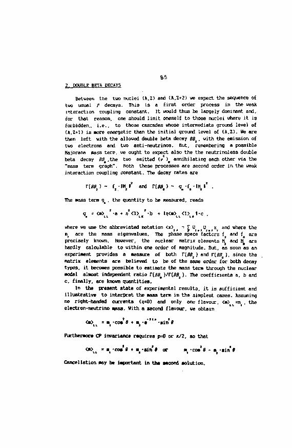
ft52. DOUBLE BETA DECAYS
Between the two nuclei (A,Z) and (A.Z+2) we expect the sequence oftwo usual f decays. This is a first order process in the weakinteraction coupling constant. It would thus be largely dominant and,for that reason, one should limit oneself to those nuclei uhere it isforbidden,, i.e., to those cascades whose intermediate ground level of(A.Z+1) is »ore energetic than the initial ground level of (A.Z). We arethen left uith the allowed double beta decay BBI. with the emission oftwo electrons and two anti-neutrinos. But, remembering a possibleHajorana mass term, ue ought to expect also the the neutrinoless doublebeta decay B$B ,the two emitted (v ) t annihilating each other via the"mass term graph". Both these processes are second order in the weakinteraction coupling constant. The decay rates are
r(BB2) ~ f2 • IH l' and r(» #) - g. •£, • IM, l' .
The aass tern g , the quantity to be measured, reads
where we use the abbreviated notation <x> - [I) U x and where the«i( are the mass eigenvalues. The phase space factors f and f areprecisely known. However, the nuclear matrix elements H2 and M( arehardly calculable to within one order of magnitude. But, as soon as anexperiment provides a Measure of both r[BB}) and r[LBBf ), since thematrix elements are believed to be of the same order for both decaytypes, it becomes possible to estimate the mass tern through the nuclear•odel alnost independent ratio r[BBe )/r{0B1). The coefficient* a, b andc, finally, are known quantities.
In the present state of experimental results, it is sufficient andillustrative to interpret the M a s term in the simplest cases. Assumingno right-handed currents (ij=0) and only one flavour, <i»> =a , theelectron-neutrino qass. With a second flavour, ue obtain
<«>tt = mf -cos's • Bf ••"*" -tin 8
Furthermore CP invariant* requires p=0 or x/2. so that
<*\t = mt -com 8 * uf -sin** or «it -cos*« - mf -sin*»
Cancellation nay be iaportant in the second solution.
66
ttorth noticing, finally, is the tact that the possible candidates fordouble beta decay are transitions from an initial 0 state into either a0* or a 2 final state. Whereas the 0 transitions are possible withKajorana mass terns only, the 2* transitions may have contributions fromright-handed currents also.
3. EXPERIMENTAL METHODS
A. Geochenical MethodsThe geccheraical method consists in comparing the isotopic abundancies
in old ore with the atmospheric abundancies. Results are available sofar on w ° T e into "°Xe. on "*Te into * *Xe and on Se into Kr. Oneof the Te experiment (KI83) finds a large excess of Xe and no excessof "*Xe, leading to the ratio of half-life times T(128)/T(130) > 3040.The nuclear matrix elements are believed tc be roughly the same forthose two nuclei so that they cancel in this ratio. The theoreticalcalculations indicate that such a large value can only be reproduced byBBt transitions. The other experiment (HE78) on Te findsT(128)/T(130)=1580, a lower value which could accomodate BB transitionsalso. The two experiments on Se also find an evidence for BB decayscorresponding to the half-life times T=(2.76±0.88)-lu" y (SR73) andTsd.lSsO.ISVto" y (K184). In that case houever no nuclear independentratio is available and the mass term is thus more difficult to extract.
The rather large spread of these results should give an idea of theircredibility.
B. lonisation detectorsA group at Irvine is presently running a time projection chamber
whose central cathode plane contains Se. The BB candidates should havethe rather clean signature of tuo tracks spiralising in the magneticfield and flying in opposite directions from the central plane towardthe anode uire planes. Measuring the energy of the transition, thisexperiment should be able to separate, in the energy distribution, theBBt peak fro* the broad BBt spectrum. The experiment houever may not beable to distinguish 0* from 2 transitions.
Other time projection chambers or multiuire cells are developed bygroups from Caltech, NeuchaUl and SIN and from Hilano.
C. Ge crystalsUp to 200 cm single crystals of Ge have been used as both high
resolution intrinsic semi-conductor detectors and as sources of BB decayof Ge. whose natural abundance is about 7.7k. The advantage of thismethod is its vary good energy resolution, typically 3 KeV at the BB
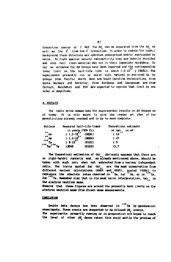
87
transition energy of 2 HeV. The BB} can be separated from the BBc aswell as the 0* £rom the 2 transition. In order to reduce the cosmjcbackground these detectors are operated underground and/or surrounded byvetos. To fight against natural radioactivity they are heavily shieldedand only very clean material may sit in their immediate neighbour. Sofar no evidence for BB decays have been reported and the correspondinglower limit on the half-life time is about l.O-lo" y (BE86). Theexperiments presently run or built with natural or enriched Ge. bygroups from Pacific North West and South Carolina Universities, fromSanta Barbara and Berkeley, from Bordeaux and Zaragossa and fromCaltech, Heuchatel and SIN are expected to improve that limit by oneorder of nagnitude.
4. RESULTS
The table below summarises the experimental results on BB decays asof today. It is only meant to give the reader an idea of thesensitivities already reached and is by no mean complete.
Nucleus' Measured half-life tines Theoretical estimateyers (9 ) <m\v in eV
'*Ge ""so"*Te
The theoretical estimation of <m>iL obviously assumes that there areno right-hand*! currents and, as already mentionned above, should betaken with much cars when not extracted from a nuclear independentratio. The limits quoted for <*>LL are the most conservative fro*different nuclear calculations (HA84 and GR85), scaled (VU86O toreproduce the absolute rates observed in Se, for Ge, or in * Te,for Te. Remember also that in its most naive interpretation, <m> isthe electron neutrino BOSS.Observe that those figures are around the presently best limits on theelectron neutrino mass fro* direct mass Measurements.
CONCLUSION
Double beta decays has been observed in ' Te by geochemicalexperiments. These events are suspected to be allowed BB1 events.The experiments presently running or in preparation are hoped to reachthe level of other BBJ decay rates: this would settle the problem of
in years> i.o-io"> 1.4-10"> 8-10**>3040
(90k CL)(BE86)(H084)(KI83)(KI83)
of<<<<5
<m>10479.7
86nuclear matrix elements calculation and lead to much more credibleestinates of the mass term. But the real breakthrough would be theobservation of 88 events uhich would incontestably establish theexistence cf Hajorana mass terms in the Lagrangian.
While preparing this seminar, I have greatly benefited from thepatient and very competent help of Prof. J.-L. Vuilleumier. I resthowever solely responsible for any mistake or awkwardness left in spiteof his collaboration. 1 would also not miss to thank the organisers ofthe 1987 Kaziaierz Symposium for their warm, generous and stimulatinghospitality.
References
BE86 Bellotti et al, 1986, Nuov. Cin. A95, 1GR85 Grotz and Klapdor, 1985, Phys. Lett. 157B, 242HA84 Haxton and Stephenson, 1984, Prog. Part. Nucl. Phys. 12,409HE78 Hennecke, 1978, Phys. Rev. C17, 1168KI83 Kirsten et al, 1983, Phys. Rev. Lett. 50,474KI84 Kirsten, 1984, Proc. Conf. Neutrino 84 in Dortmund, 145H0B4 Hoe et al, 1984, UC-Irvine Neutrino report 133SR73 Srinivasan et al, 1973, Econ. Geol. 68, 252VU86 Vuilleumier, 1986, Rep. Prog. Phys. 49, 1293
89
Misunderstandingsand Difficulties in using
Negative Binomial Distribution
Grzegorz Wrochna
Institute of Experimental Physics, University of Warsaw
Warsaw, Poland
ABSTRACT
' new way of describing Uie multiplicity distri-
butions by using the Negative Binomial Distribution is
critically discussed. Some misunderstandings often
encountered in literature are pointed out.
J. Introduction
During the last two years, the Hcgative Binomial
Distribution made a rapid career as a parametnzation of
multiplicity distributions and a candidate for the new empirical
law of physics 111-
I would like to point out some mi sunderstandines and
diiliculties in this approach. Presented worK has keen dune in
collaboration with R. Szwed and A. WroblewsKi. More details \>n this
subject can be found in Ref. [2).
The paper is organized as follows:
In Section 2 the problem of using the so-called "Fake negative
Binomial Distribution" instead of the true Negative Binomial
Distribution is discussed. Section 3 contains the discussion of
the question: "Is £NO-scalinc really accidental?" section i is
devoted to the comment on a "new method" to subtract diffractive
component from multiplicity distributions. The last section
contains a short discussion on the energy dependence oi the k-
parameter and ltr interpretation.
All remarks will be illustrated by the pp n^n-diffractlve
data f5) and the pp crs Collider non-dlffractlve data 16,7].
90
2. "FaKe leeatlve Blnonla) Distribution'
The negative Binomial Distribution (HBD) is described by the
following formula:
n*H-i\P"BD(n) = / I («)
n
It has two parameters. The n parameter has the interpretation of
the average. The k-parameter is connected with the dispersion
and the second central moment c.'ni2=n*/n* by formulae:
• 1/n « 1/K (3)
where n taxes values of 0,1,2,3
The NBD can be used to describe distributions of charged
particle multiplicities P(nch), but for the pp data neh is always
even, so nchi2,4,6... The theoretical probability distribution
function is defined for all non-negative integers. Thus, instead
of nch , the genuine multiplicity measure n should be used,
according to the formula n c h - Zn * Z . Bote, that genuine
multiplicity measure n <n=0, 1, 2, 3, . . . ) coincides in case of pp
data with the number of negative prongs in an event n=n_
Unfortunately. another procedure of calculation of the
probabilities based on the HBD is very often encountered in the
literature (6,7). The authors taXe from the NBD only
probabilities P(n) for even integers and renormalize the whole
distribution. This procedure, strictly speaking, leads to the
fitting of the different theoretical distribution, which we call
"Fake Negative Binomial Distribution* (FNBD). Let me stress that
for the FNBD formulae (2) and (3) for the dispersion and the C2
moment are no longer valid. Nevertheless, the name "NBD* is used
by many authors also when they fit FHBD, which leads to
misunderstandings.
The argument that the FHBD approximates the NBD for large rt
is not useful, because it is valid only in the SPS Collider
energy range. Figure 1 illustrate how different are those two
distributions. It shows the ratio of the k-parameters obtained by

91
fitting the FUhV and the NBD to the pp and pP data. It is seen
triL.t Cllirlt-r roints arc close to the unity, but deviations are
rir.iiiijt ical ly increasing at smaller energies.
Thus, in fact there are two different distributions: the HBD
and the F«BD.
3. is EHO-scaling really accidental?
TJ-:e statement that the ITHO-seal ing was accidental has
.ij-j-.:.•>! *.-(.' firstly in the UA5 Collaboration paper f6). TKe way of
,-r;u;ii; l.y the au<2iors of Ref. [&) is schematically shown in Fig. 2
. /.s sc-'.n in FJC- 3a the dependence i/ntJ/K vs fs has a flat
rciiunium m the cnero range between 10 and 60 GeV. Hence (based
oi the- forraula (3)) the authors conclude that the Cn 2 moment
I'KJ £.?)•> has a similar flat minimum. Then, using the statement
that the JIHO- seal ing requires Cr.ehj2 to be constant, they arsue
that Kilo-seal ins is accidental.
The aJ>cvc arcumentation contains inconsistencies:
Firrtly: formula (3) is valid only for the HBD, and for the
'•"i.,z "•'•-''nptit defined for the genuine multiplicity n. But in the
I'A I Collaboration paper the FNBD and the C n c h > 8 moment are used.
It should be stressed, that the sum I4i/n*l/k is not the same as
the C n c h j 5 (compare Fig. 3a and 3b).
Secondly: Fie. 3b shows that C n c h j 2 has no minimum! This can
!.,•• proven by the three lowest energy points, omitted in original
i'A5 publication [6). Moreover, simple arithmetic shows that at
the energy threshold C n c h i 2 goes to unity in contradiction with
hypothesis about the minimum.
Thirdly: in the original formulation I9J KNO-scaline
requires Cncttl. to be constant only for asymptotic energies.
Properly formulated KHO-scallng flO] correctly describes the rise
of the C n c h > i moments from the enerey threshold up to ISR
energies [11].
In conclusion: The statement that KHO-scaling is accidental
seems to be a triple misunderstanding.

92
4. A 'new method* to obtain the non-dlftractive event samples
Separation of the dlffractive and non-diffractlve component
is usually difficult. Recently a new method has been proposed
[7], based on a supposition, that the HBD describes very well
Just the non-diffractave data. This method is illustrated in
Fig.4, showing the multiplicity distributions for 800 Gev/c pp
collisions. The open points corresponds to the inelastic sample.
The dlffractive component is limited to the events with few
lowest multiplicities. Hence, one can taKe inelastic data, omit 3
or 4 lowest multiplicities, fit the HBD and take the result as
the non-dlffractlve data (full points).
We have tested such procedure for the world pp data 14) and
we have compared the results with those obtained by the standard
methods [5) (missing mass plots etc. ). The comparison if
illustrated in Fig. 5 which shows the total dlffractive cross
section. Open circles represent standard methods and full circles
- HBD method. It is seen that the points corresponding to the
standard methods are self-consistent within errors, whereas
fluctuations of the HBD method are gigantic (up <-.o 15 standard
deviations).
There is a more direct way to prove this in tability. One
can compare the HBD fit to the full non-dlffractlve distribution
and to the same distribution without few lowest multiplicities.
An example of the result of omitting 5 from 20 points of the
distribution at energy 62 GeV is illustrated in the Fig. 6. The A"2
contours presented as a function of the n and K show the goodness
of the fit. The full distribution (Fig. 6a) has a quite well
localized minimum, with n and K not strongly correlated. After
omitting 5 points (Fig. 6b) the correlation rapidly rises and the
minimum radically shifts (note the change of the scale) in spite
of fitting to the same non-dlffractive distribution. Conclusion:
the mentioned NBD-method is completely unusable.

93
5. Energy dependence of the K-parameter and lti interpretatlop
Figure 7 shows i/k dependence on energy for the NBD (open
circles) and for the FNBD (full circles).
in existing models [11 the k-parameter is treated as the
number of clusters or as a probability. So, it should be
positive. But as seen from Fig. 7 this is not the case. It is
difficult to understand in terms of models why at certain energy
the K-parameter changes sign although other experimental
observables do not show any such violent change in the mechanism
of multlparticle production.
Moreover, the NBD does not have any predictive power since
it Involves two free parameters for each multiplicity
distribution and has no build-in scaling. There is no model to
predict the dependence of the k on the energy, particle type or a
phase-space region in agreement with experiment.
For the full phase-space pp data the only proposition of a
parametrization for k was given by the UA5 Collaboration to,8].
The authors propose the linear dependence of the i/k vs In s.
They fitted data for energies higher than 10 Gev. However the
proposition has weak points because, firstly, as illustrated in
Fig. 7 the 3 lowest energy data points are in contradiction with
this dependence, and secondly, the FNBD was used instead of the
NBD. For the HBD the linear dependence is even less convincing.
At the end of this section I would like to underline one
more difficulty of the NBD approach. The NBD does not describe
the pp data as good as it is often claimed. Figure 8 shows the
ratio of the experimen al probabilities and the probabilities
calculated with the NBD. at the 1SR energy range. The points
should be randomly scattered around the unity which is not the
case. The explicit systematic deviations are seen.

6. Conclusion
Concluding this paper, I would like to point once again a
list of misunderstandings and difficulties of the NBD approach:
Many authors use the FHBD instead of the NBD without clear
distinction.
The minimum of the l/fi-tl/K has nothing to do with the KNO-
scallnc, so the conclusion that the KHO-scaling is accidental is
just a misunderstanding.
The NBD-flt method to obtain non-diffractive multiplicities
is unusable.
There is no model to predict the dependence of the K-
parameter on the energy, particle type or a phase space region
and its reasonable interpretation.
Lastly, the NBD does not describe the pp data so good.
Thus, in my opinion, the NBD can be treated as one of
possible parametrizations of data, but by no means the best.

RBFEREBCES
li) A. Giovannlm and L. Van Hove. Z. Phys. C30, 391 (1986)
L. Van Hove and A. Giovannlm, "Negative Binomial Hultlpli-
city Distributions, a Hew Empirical Law for High Energy
Collisions* Proceedings of the XVII International Symposium
on Multlparticle Dynamics, seewinKel, Austria,
16-20 June 1986, p. 561.
A.Glovanninl, "Multipartlcle Phenomenology", Invited talK
at the Sixth International Conference on Physics
in Collision, Chicago, 3-5 September. 1986.
Torino University preprint DFTT 86/31
[2} R. Szwed, G.Wrochna, A. Wr«blewsKl, "Mystery of the Negative
Binomial Distribution", Warsaw Univ. preprint 1FD/3/87,
submitted to Z. Phys. c
[«) pp inelastic data:
4 GeV/c L. Bodlni et al. . Huovo Cim. 58A, 475 (1968)
5.5 GeV/c G.Alexander et al. , Phys. Rev. 154, 1284 (1967)
6.6 GeV/c E. R. GeJlert, LBL-749 (1972)
is GeV/c v. Blobel et al. , Hucl.Phys. B69, 454 (1974)
19 GeV/c H. Boggild et a]., Hucl.Phys. B4J, 285 (1972)
24 Qev/c V.Blobel et al., Hucl.Phys. B52. 221 (1975)
35. 7 GeV/c I. V. Boguslawskl et al. , JIHR1-1O134 (1976)
50 GeV/c V. V. Ammosov et al. , Phys. Lett. 42B, 519 (1972)
60 GeV/c C.Bromberg et al., Phys. Rev. DJ5, 64 (1977)
69 GeV/c V..V, Babintsev et al. , IHEP H-25 (J976)
100 GeV/c J. Erwin et al. , Phys. Rev. Lett. 32, 254 (1974)
loo GeV/c W.M.Morse et al. , Phvs.Rev.- D15, 66 (1977)
102 GeV/c C.Bromberg et al. , Phys. Rev. Lett. 31. 1563 <1973)
205 GeV/c S. Barlsh et al. , Phys. Rev. D9. 2689 (J974)
250 GeV/c H. Adarnus et al. , Z. Phys. C32, 476 (1986)
303 Gev/c A.Firestone et al. , Phys. Rev. Dio, 2080 (1974)
303 GeV/c F. T. Dao et al. , Phys. Rev. Lett. 29. 1627 (1972)
360 GeV/c J. L. Ballly et al., Z. Phys. C23, E05 (19«4)
400 GeV/c R.D.Kass et al. . Pnys. Rev. D20, 6050 (1979)
400 GeV/c W. S. Toothacker, UMBC77-77
405 GeV/c C.Bromberg et al. , Phys. Rev. Lett. 31, 1563 (1973)
405 GeV/c T. Ferbel (private communication)
96
[5]
«00 GeV/c R. Aranar et al.. Phys. Lett. B178, 124 (1986)
493, 1032, 1471, 2062 GeV/c
A. BreaKstone et al., Phys. ReV. D30, 52e (1984)
PP non-diftractive data:
12 Gev/c
19 GeV/c
24 GeV/c
69 GéV/C
J. BenecKe et al. ,
H. Boggild et al. ,
J. BenecKe et al. ,
Nucl. Phys.
Nucl. Phys.
Nuc 1. Phys.
B76,
B27,
B76,
29 (1974)
285 (1971)
29 (1974)
v. V. Babintsev et al., IHEP H25 (1976)
J.Wtutmore et al., Phys. Rep. 10C, 273 (1974) and
W.H.Morse et al., Phys. Rev. D15. 66 (1977)
C. Bromberg et al. , Phys. Rev. Lett. 3J, 1563 (1973)
S. Barish et al. , Phys. Rev. D9, £689 (1974)
A.Firestone et al., Phys. Rev. DJO, 2080 (1974)
C. Bromberg et al. . Phys. Rev. Lett. 3S, 1563 (1973)
1471, 2062 GeV/c
A. BreaKstone et al.,' Phys. ReV. D30, 526 (1984)
UA5 non-diffractlve data:
G. J. Alner et al., Phys. Lett. I60B, 199 (1985)
R. Ammar et al., Phys. Lett. B178, 124 (1986)
200 and 900 GeV UA5 non-diffractive data:
G. J. Alner et al.. Phys. Lett. 16"B. 476 (1986)
Z. Koba, H.B.Nielsen. P. Olesen, Hucl Phys. B4'», 317 (1972)
A. I. GoloKhvastov, Sov. Jour. Nucl. PYiys. 27, 430 (1978)
Sov. Jour. Hucl. Phys. 30, 128 (1979)
R. Szwed and G. Wrochna, Z. Phys. C29, 255 (1985)
mC8)
19)
110]
un
100 Gev/c
102 GeV/c
205 GeV/c
303 GeV/c
405 GeV/c
493, 1032,
[6) 540 GeV
97
FIGURE CAPTIOUS
Fig. 1
The ratio'of tiN»p/KrMeo v s ~s-
Fig. 2
Scheme of the way of arguing in Ref. [&) (left part of
diagram) and conrtrarsuraents (the right part).
Fig. 3
a) The values of 1 + 1/n * 1/K from the FKBD fits to non-
diffractive sample. The curve shows the UA5 Collaboration
interpolation fii).
b) The values of Cnc/),2 moment for the same sample.
FJg. 1
The LEBC-HPS Collaboration pp inelastic data (800 Gev/c) and
the "nondiffractive data" obtained by using the FHBD fit.
Fie 5
Comparison of the experimental dlffractive cross section
with the "dlffraciive component" obtained i>y subtracting the HBD
fitted cross sections from Inelastic topologlc cross sections for
"ch -> '0;
Fig. 6
The contours of constant Xz values in the FHBD fit to the
non-diffractive pp multiplicity distribution at X% = 62 OeV as a
function of parameters n and K;
a) all data points used;
bj data for net> i 10 omitted. Hotice the shift in the best
value of K between a) and b).
Fig. 7
The 1/K parameter of the HBD (open circles) and FHBD (full
circles) fits for the non-diffractive sample. The straight line
Illustrates fit to the data with fs < 10 GeV, done by the UA5
Collaboration [11).
Fig. a
The ratio of PEXP(nch)/PNBC>(ncb) plotted as a function of
reduced multiplicity neh/<nch> for the pp data at 30.4 < fs <
62.2 GeV
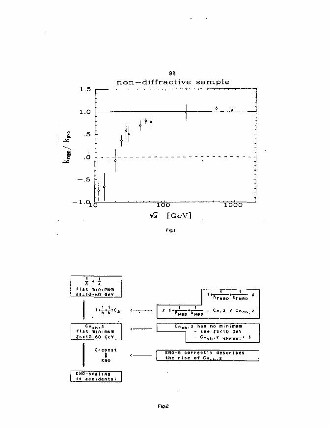
1 .5
1.0
.5
.0
- . 5 -
-1.0,
98non —diffractive sample
100
VS" [GeV]
Fig.1
1OOO
1 1ft K
flat minimumfS;10T60 GeV
C"eh' 2
flat minimumfs=10*60 GeV
C=const
1KNO
KNO-sca)ingis accidental
1 ' ' ' 1 f"TNBP KFNBD
- = C n , 2 f C n c h 2
C n e h , 2 has no minimum
ee fs<io Gev
KNO-G correctly describesthe rise of C n , K , 2
Fig.2
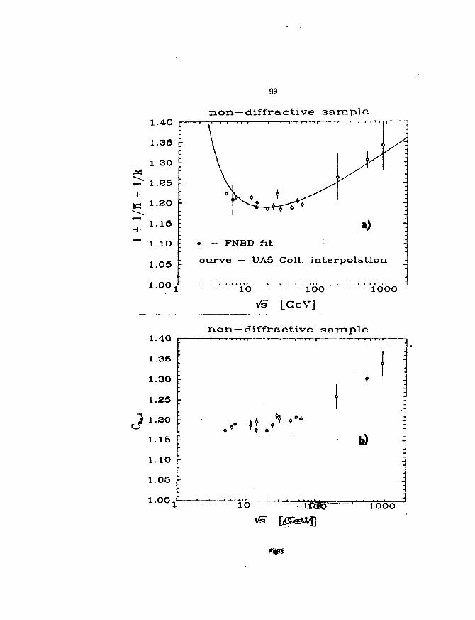
99
non-diffractive sample1.40
1.35
1.30
1.25
1-2O
1 1 5
1.10
1.05
l.OO
1.4O
1.35
1.30
1.25
Jl.ZO
1.15
1.10
1.05 h
1.00
o — FNBD fit
curve — UA5 Coll. interpolation
1O 1OO
Vs [GeV]
10OO
non—cliff r active sample
b)
i(5 ' ' •-limr*1*--' ' ibbo
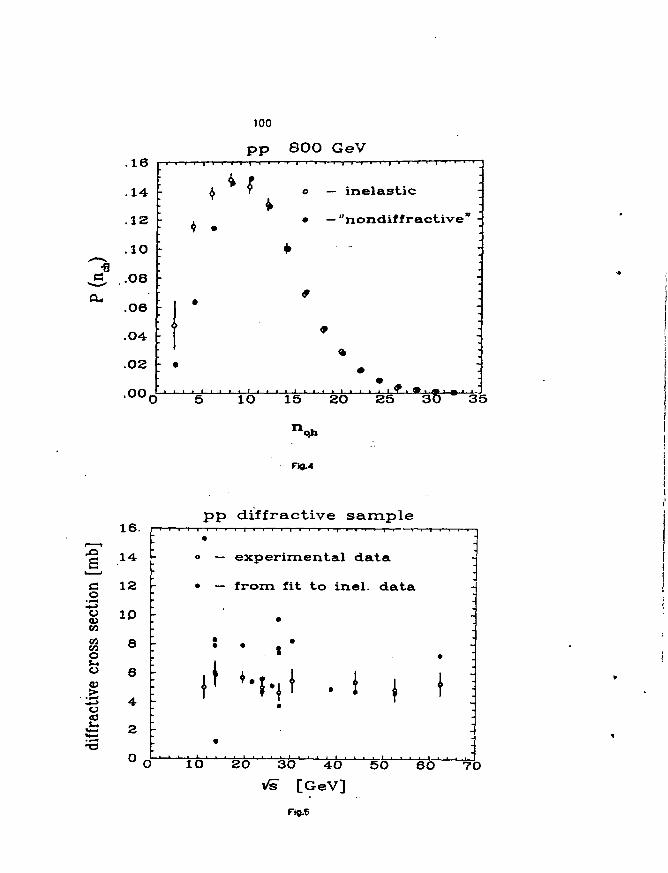
.16
.14
.12
.10
.08
.06
.04
.02 \- •
,oo,
100
pp 8OO GeV
o — inelastic
• -"nondiffractive*
lb' " 15 " 2O" ' ' 25 ' 3$ * ' 35
16.
JO
B' i
ion
oCO
*OSS
o
iffr
actn
T 3
1 4
1 2
I D
8
6
4
2
0
pp diffractive sample
o — experimental data
• — from fit to inel. data
M • i• •I t, I. J. l _ ) — I 1, I I—I_J—I_J • I I t • • • t . . • . I . . , •
1O 2O 3O 4O 50 6O 7O
Vi" [GeV]Fi«.5
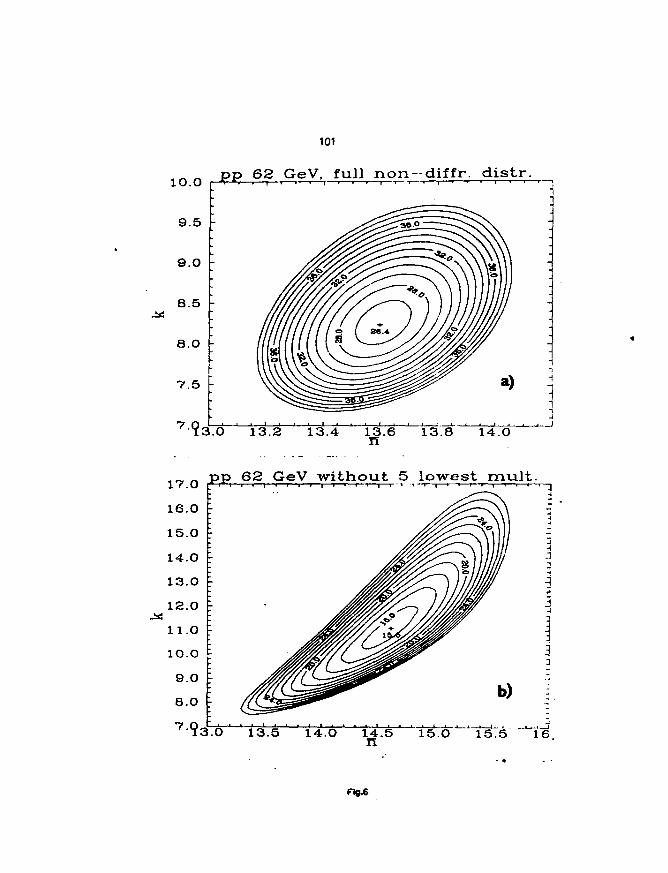
101
10.0
9 . 5
9 . 0
8 .5
8.O -
7.5 -
pp 62 GeV, full non —diffr. distr.
79.3 .0 13.2 13.4 13.6Ti 13.8 14.0
-ij
17.0
16.0
15.0
14.0
13.0
12.0
11.0
1O.O
9.0
8.O
pp 62 GeV without 5 lowest mult.
7<?3.0 13.5 14.0 14.5 "157 1 6
Fig*
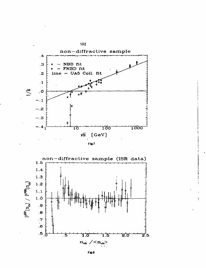
102
non —diffractive sample
.3
.2
.1
•O
— .1
— .2
- . 3
— .4.
T ! - » - • - » . . I T T " • '
- o - NBD fit: • - FNBD fit: line - UA5 Coll.
; ^ %
-
: *
<>
1O
-i—r t i i i f— • • -t- —
fit ^^•r"
1OO
iHH
1OOO
i/s [GeV]
non —diffractive sample (ISR data)
2 . 5
Fifl.8
103
Transverse En«£gy_.and Multiplicity Distributions
In High Energy Reactions
by
M. PlUmer*' and R.M. Wolner
Physics Dept.
University of Marburg
Malnzer G&sse 33
D-3550 Marburg
Federal Republic of Germany
Under rather weak assumptions a set of analytical relations
between the moments of the transverse energy distribution and
the moments of the underlying multiplicity distribution is es-
tablished for high energy collisions. Where applicable, the re-
lations are in good agreement with data.
In the last years, the study of transverse energy distribu-
tions in high energy collisions has attracted considerable inte-
rest, among other things because at high energies and/or with
heavy ions calorimetric measurements gain more and more impor-
tance and thus transverse energy distributions become one of
the main sources of information about multiparticle dynamics.
Therefore it is of high theoretical and practical interest to
relate the transverse energy distribution with other physical
observables.
As far as we can gather correlations between multiplicities
and transverse energies have been obtained so far only via Monte-
Carlo calculations ' '. The present contribution represents an
attempt to derive an analytical relation between the transverse
energy and multiplicity distributions.
Postdoctoral Fellow of the Deutsche Forschungsgeraelnschaft
104
In a given rapidity interval, the transverse energy distribu-tion, w(E_) s - i|r-, is related to the corresponding multiplicity
T o dE
distribution, P(n) z — , as follows (o * £om is the inelastic
° across section)
mw(E_) - I P(n) f(Ejn) (1)
1 n-0
where
f(ET|O) - «(ET); (2)
f(ET|n) « /deT1 ••-/dEirn {*( E tT^ ~ Ey) •
1 dorr dp dp°n O ET1•"' eTn
is the conditional probability to observe a transverse energy E_
at a given multiplicity n and e T is the single particle transver-
se energy. Since experimental data on — -is— in general do not
contain the zero multiplicity contribution, from here on only
the modified distribution
w(ET) * Z P<n) f(ET|n),
P(n) s P(n)/n-P(0))
will be considered; moments like <E?> or <nm> will always refer
to w{ET) and P(n), respectively.
If the single particle transverse momentum is weakly or not
at all correlated with multiplicity as it is the case at Fermi-
lab and ISR energies , one finds for the first moments
<ET> = r P(n) • n • <£„>„ * <n> <eT> (4)n
In order to obtain corresponding relations for the higher
moments, one has to make assumptions about the n-particle in-
clusive transverse energy distribution. He shall assume here
that it factorizes into a product of n single particle trans-
verse energy distributions g(e T), i.e. that the transverse
energies e , of individual particles are uncorrelated:
105
1 do n
S , JI qic \ (5)°n dcT1...dcTn 1-1
The validity of this assumption has been tested ' up to
enc-ry.es of >s -- 30 GcV in Monte Carlo calculations of corre-
lations between E T, <n> and <pT>.
Together with (5), (1) and (2) yield
m
ith
Vj
a.. = <eT>2 2 (7)
a22 = " V ' a21 * « V etC"
With an exponential ansatz,
2 " | i eTg(cT) = u2 cT • e T (8)
the results further simplify to 2 n_ 1
w(ET) « J $(n) • (i • - • e (9)
and
<E°> * (^)m • <n • (n+j) - — • (n+2^1)> (10)
In the following, this formalism will be applied to the discus-
sion of experimental data.
For pp-colllsions at /s • 31 GeV, the charged , neutral '
and total transverse energy distributions in the central rapi-
dity region have all been measured in separate experiments. A
customary parametritatiJn is
• — 2 — (aE-)1*"1 • (11)T(a)
The value of <ET>,a and p as well as the respective rapidity
interval for the 31 GeV data are given in table 1, where we have
also included data obtained at 27.4 GeV61. In ref. 2, the char-
ged ET-di3tribution has been observed for |n|<0.8. Integration
over that distribution yields
<ESh> - 1.38, <{E$h)2> - 3.12
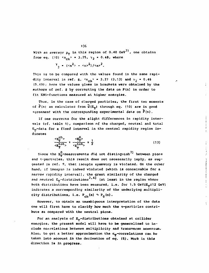
106
With an average p T in this region of 0.40 GeV , one obtains
from eq. (10) <n . > • 3.25, -r2 • 0.48, where
Y2 - (<n2> - <n>2)/<n>2.
This is to be compared with the values found in the same rapi-
dity Interval in ref. 8. <" c n> " 3.2? (3-13) and y2 • 0.46
(0.49); here the values given in brackets were obtained by the
authors of ref. 8 by correcting the data on P(n) in order to
fit KNO-functions measured at higher energies.
Thus, in the case of charged particles/ the first two moments
of P(n) as calculated from w(ET) through eq. (10) are in good
agreement with the corresponding experimental data on P(n).
If one corrects for the slight differences in rapidity inter-
vals (cf. table 1), comparison of the charged, neutral and total
E_-
dicates
< Eto t > < Eto t > 2
Since the E_,-measurements did not distinguish between pions
and n-particles, this result does not necessarily imply, as sug-
gested in ref. 9, that isospin symmetry is violated. On the other
hand, if isospin is indeed violated (which is conceivable for a
narrow rapidity interval), the great similarity of the charged
and neutral E_-distributions {at least in the region where
both distributions have been measured, i.e. for 1.S GeV£E_,£12 GeV)
indicates a corresponding similarity of the underlying multipli-
city distributions, i.e. P h(n) * Pft(n).
However, to obtain an unambiguous interpretation of the data
one will first have to clarify how much the n-particles contri-
bute as compared with the neutral pions.
For an analysis of redistributions obtained at collider
energies, the present model will have to be generalized to in-
clude correlations between multiplicity and transverse momentum.
Also, to get a better approximation the eT~correlations can be
taken into account in the derivation of eq. (6). Work in this
direction is in progress.
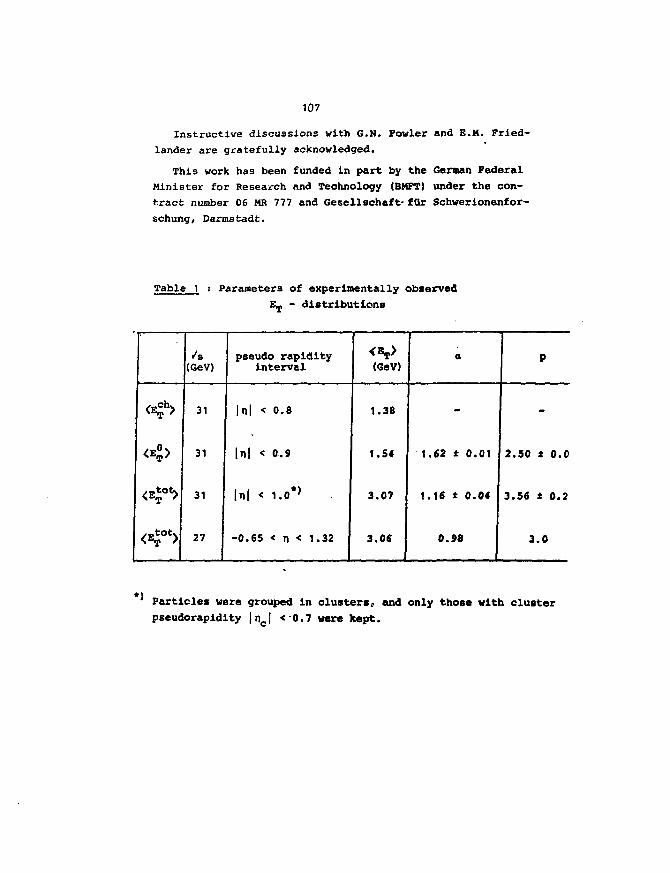
107
Instructive discussions with G.N. Fowler and E.M. Fried-
lander are gratefully acknowledged.
This work has been funded in part by the German Federal
Minister for Research and Technology (BMFT) under the con-
tract number 06 MR 777 and Gesellschaft- fur Schverionenfor-
schung, Darmstadt.
Table 1 : Parameters of experimentally observed
E T - distributions
*
/s(GeV)
31
31
31
27
pseudo rapidityinterval
In| < 0.8
|n| < 0.9
Inl < i.o*> .
-0.65 < n < 1.32
(GeV)
1.38
1.54
3.07
3.06
a
1.62 t 0.01
1.16 t 0.04
0.98
P
2.50 t 0.0
3.56 t 0.2
3.0
*) Particles were grouped in clusters,, and only those with cluster
pseudorapidity |n | <0.7 were kept.

108
R é f é r e n ç a s
1. C. De Marzo et al., Nucl.Phys. B211, 375 (1983).
2. B. Gordon et al., Phys.Rev. D28, 2736 (1983).
3. A. Breakstone et al., Phys.Lett. 132B, 463 (1983).
4. A.L.S. Angelis et al-, Phys.Lett. 141B, 140 (1984);
A.L.S. Angelis et al., Phys.Lett. 168B, 158 (1986).
5. B. Callen, in Quark Hatter 84, ed. K. Kajantie, Sprin-
ger 1985, p. 133.
6. H.S. Hiettinen, Nucl.Phys. A418, 315c (1984).
7. M. Tannenbaum et al., Preprint BNL-38470 (1986).
8. T. Akesson et al., Phys.Lett. 119B, 464 (1982).
9. S.Y. Shœakov and V.V. Uzhinskii, JINR-Dubna-Preprint
E2-87-5.
109
Hiniiets *
Heng Ta-chungFachbereich Physik der FU Berlin, Berlin
/1 -3 /Recently there has been much interest in "minijets* or
"low-transverse energy jets" in hadron-hadron collisions. Why
do they attract so much attention? What are they?
Perhaps I should begin this discussion by reminding you: Mulri-
particle production processes take place in approximately 80%
of the high-energy hadron-hadron collision events. An event of
this kind can be characterized by the multiplicity (n) of the
produced charged hadrons and/or the energy flow (Ey) in the
transverse direction of the beam. Distributions of n and £y
have been measured for various processes (pp, pp, up etc.) at
various (total cms) energies (/i) in different kinematical
regions (defined by the pseudorapidity n and the azimuth angle $
of the final state hadrons).
It has been observed by UA1 collaboration that a considerable
fraction (approximately B% at /s~=200 GeV, 17% at 900 GeV) of
minijet-events exist in the data sample of minimum-bias events.
Minijets were found when the n- and the Ey-distributions were
measured in the kinematical region lr|l<2.5 under the condition
that at least 5 GeV enters the trigger cone of radius
R=[(in)2+(4*)2]'/2= 1 in the n-* space. The characteristics of
the minijet data sample are indeed very striking: It is seen in
particular that the average multiplicity of minijet-events is
approximately twice as high as that in non-minijet-events; and
that the multiplicity distribution of the ninijet-events, when
plotted in the KNO form is much narrower than the corresponding
•Supported in part by Deutsche Forschungsgcmtinschaft(OFG: He 470/5-1)

110
curve for minimum-bias events. Perhaps this is the reason why/2 /it is expected that minijets should have very much in common
with the jets (high-E_-jets) in hard collisions.
Chao, Pan and myself took a closer look/3/at the data'1/. The/3/result of our analysis' strongly suggests that the minijet-
events and the ordinary minimum-bias events are closely related
to one another, and that their relationship can be described by
standard statistical methods.
The attempt of applying standard statistical methodsI A I
to the minijet problem is motivated by the observation
that such methods can be used to describe the rapidity-dependenceIK I
of multiplicity distributions in hadron-hadron' as well as in
other collision processes. Having learned that the multi-
plicity distribution data in limited rapidity intervals ("rapi- \
dity window") can be described simply by the binomial distri- !
bution law, provided that the multiplicity- and the rapidity- I
distributions of the particle-producing system(s) are known, it !•
is rather natural for us to ask whether the minijet pheno- I
menon ' can be understood in a similar way.
There are several reasons which make us expect that statistical
fluctuation should play an important role in this phenomenon.
(a) It is known empirically that transverse energy E_ and charge
multiplicity n are approximately proportional to each other.
(b) High-energy hadron-hadron as well as the collision experi- i
ment ' show that multiplicity fluctuations in small rapidity
windows are larger than .those in larger windows, (c) The procedure •
used by UA1 collaboration' ' is in fact a measurement of n- and .
^-distributions in a given rapidity window under the condition
that a minimum amount (EJ-Q=5 GeV) of E- enters the trigger cone
where the trigger cone itself is a window in the n-* space.
Consider an inelastic nondiffractive hadron-hadron collision at
cms energy /s. Let P{E-;s) be the E.-distribution of the emitting
system that dominates the rapidity region under consideration.
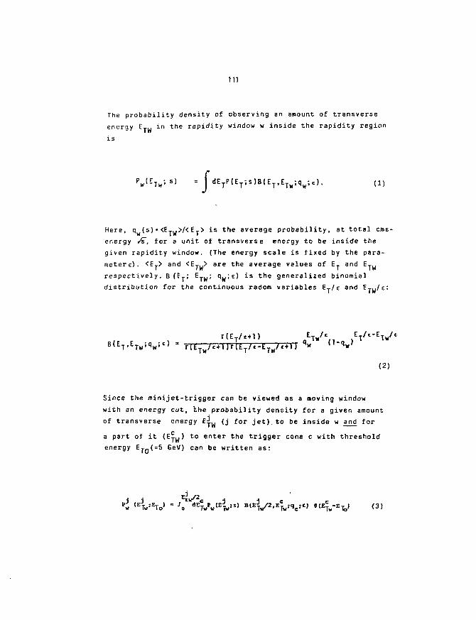
in
The probability density of observing an amount of transverse
energy E T U in the rapidity window w inside the rapidity region
P w ( E T w ; s ) = j dE TP(E T; S)B(E T,E T w;q w;e). (i)
Here, qy(s) = <ETW>/< ET> is the average probability, at total cms-
energy /s~, for a unit of transverse energy to be inside the
given rapidity window. (The energy scale is fixed by the para-
meters). <E^> and ^Ejy* a r e t n e average values of E. and E-w
respectively. B (Ej.; ETW; 9^'^ *s t n e generalized binomial
distribution for the continuous radom variables E./e and ETy/e:
r(ET/£+1) ll*/c. ,ET/t"ETw/c
t|)rttTA-ETt>yc*U q» (1'qw'
(2)
Since the minijet-trigger can be viewed as a moving window
with an energy cut, the probability density for a given amount
of transverse energy E^w <j for jet).to be inside w and for
a part of it (Eyo) to enter the trigger cone c with threshold
energy Ej.Q{=5 GeV) can be written as:
B(ETv/2'ET»'Ve)
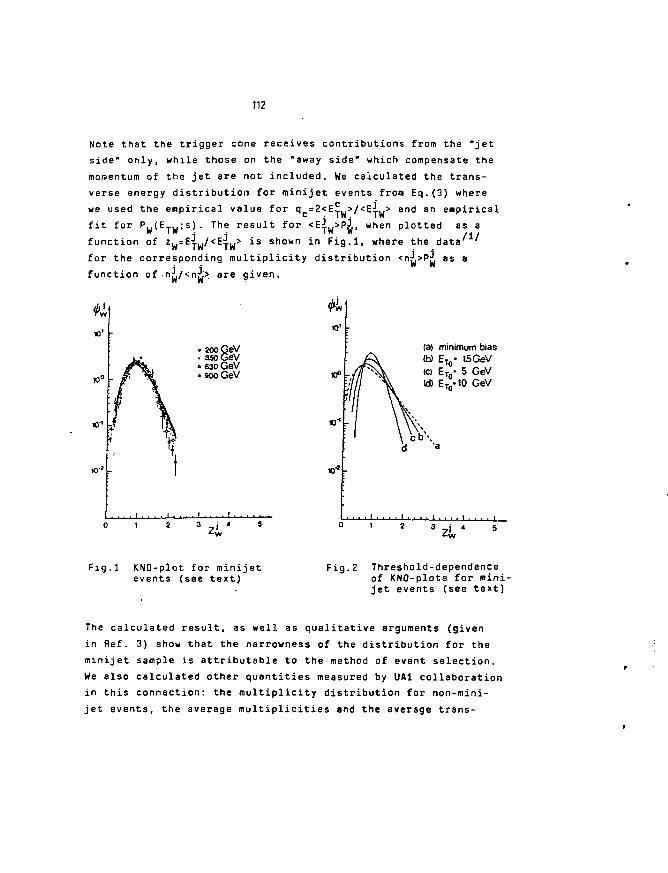
112
Note that the trigger cone receives contributions from the "jet
side" only, while those on the "away side" which compensate the
momentum of the jet are not included. We calculated the trans-
verse energy distribution for minijet events from Eq.(3) where
we used the empirical value for q =2<E£,.>/<Ei,.> and an empiricalc . i w i w
fit for Pu(ETU;s). The result for <Eiu>P.L when plotted as a
function of zw=E|w/<E^w> is shown in Fig.l, where the data' '
for the corresponding multiplicity distribution <nP.>Pr. as ai i
function of nu/<njj^ a r e given.
4b
. 200 GeV
. 3so GeVo 630 GeV• aoo GeV tfi
W
(a) minimum bias(b) ET<3- ISGeVid ET()- 5 GeVId) ET()-10 GeV
F i g . l KNO-plot for minijetevents (see text}
Fig.2 Threshold-dependenceof KNO-plots for mini-jet events (see text)
The calculated result, as well as qualitative arguments (given
in flef. 3) show that the narrowness of the distribution for the
minijet sample is attributable to the method of event selection.
We also calculated other quantities measured by UA1 collaboration
in this connection: the multiplicity distribution for non-mini-
jet events, the average multiplicities and the average trans-
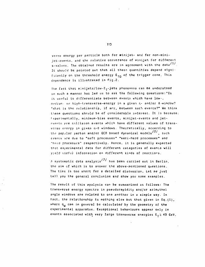
113
verse energy per particle both for minijet- and for non-mini-
jct-events, and the relative occurrence of minijet for different
s-valucs. The obtained results are in agreement with the data
It should be pointed out that all these quantities depend signi-
ficantly on the threshold energy E T Q of the trigger cone. This
dependence is illustrated in Fig.2.
The fact that minijets/low-ET-jets phenomena can be understood
in such a manner has led us to ask the following questions: "Is
it. useful to differentiate between events which have low-,
nu'i.'ium- or hioh-t.ransverse-energy in a given r,- and/or ^-window?
"What is the relationship, if ary, between such events?" We think
these questions should be of considerable interest. It is because:
Fxperimentally, minimum-bias events, minijet-events and jet-
events are collision events which have different values of trans-
verse energy in given n-<J windows. Theoretically, according to/2 /
the popular parton and/or QCD based dynamical models , such
events are due to "soft processes" "semi-hard processes" and
"iisrd processes" respectively. Hence, it is generally expected
that experimental data for different categories of events will
yield usefu] information on different kinds of reactions.
A systematic data analysis has been carried out in Berlin,
the aim of which is to answer the above-mentioned questions.
The time is too short for a detailed discussion. Let me just
tell you the general conclusion and show you some examples.
The result of this apalysis can be summarized as follows: The
transverse energy spectra in pseudorapidity and/or azimuthal
angle windows are related to one another in a simple way. In
fact, the relationship is nothing else but that given in Eq.(l),
where qw can in general be calculated by the geometry of the
experimental apparatus. Exceptional behaviours appear only in
events associated with very large transverse energies £..£40 GeV.
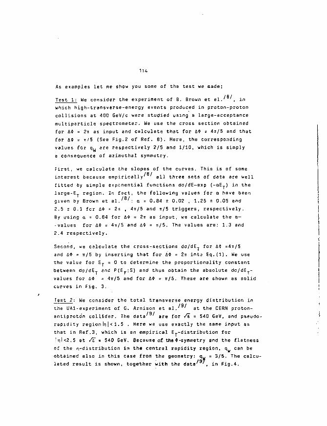
m
As examples let me show you some of the test we made:
/ 8 /Test 1: We consider the experiment of 8. 8rown et el. , in
which high-transverse-energy events produced in proton-proton
collisions at 400 GeV/c were studied using a large-acceptance
multiparticle spectrometer. We use the cross section obtained
for A* = 2n as input and calculate that for A* = 4u/5 and that
for A* = TI/5 (See Fig.2 of Ref. 8 ) . Here, the corresponding
values for qw are respectively 2/5 and 1/10, which is simply
a consequence of azimuthal symmetry.
First, we calculate the slopes of the curves. This is of some/ 8 /
interest because empirically all three sets of data are well
fitted by simple exponential functions do/dE-exp (-o£_) in the
large-E T region. In fact, the following values for a have been
given by Brown et al.' ': a = 0.84 ± 0.02 , 1.25 ± 0.05 and
2.5 t 0.1 for A* = 2n , 4n/5 and TI/5 triggers, respectively.
By using a = 0.84 for A* = 2TT as input, we calculate the a—
-values for A* = 4TT/5 and A* = 7i/5. The values are: 1.3 and
2.4 respectively.
Second, we calculate the cross-sections da/dE, for A* =4n/5
and A* = TI/5 by inserting that for A<t = 2i into Eq.(l). We use
the value for E, = 0 to determine the proportionality constant
between da/dE, and P(E-;S) and thus obtain the absolute do/dE_-
values for A* = 4n/5 and for A* = TT/5. These are shown as solid
curves in Fig. 3.
Test 2: We consider the total transverse energy distribution in/ 9 /
the UAl-experiment of G. Arnison et al.' ' at the CERN proton-
antiproto'n collider. The data are for /s = 540 GeV, and pseudo-
rapidity region In | < 1.5 . Here we use exactly the same input as
that in Ref.3, which is an empirical E.-distribution for
InI<2.5 at /T = 540 GeV. Because of the^-symmetry and the flatness
of the n-distribution in the central rapidity region, qw can be
obtained also in this case from the geometry: q u = 3/5. The calcu-
lated result is shown, together with the data , in Fig.4.
Tes'- 3: We consider the transverse-energy distribution over the
D5SL;crapidity interval J n1<1 and an azimuthal range &$ = 300° in
the UA2 experiment by H. Banner et al./10/. In this proton-anti-
proton collision experiment at /s = 540 GeV, a segmented calori-
meter is used to study large ET-jets. Here, we use as input the
U«l data/9/ for |nl< 1.5 and A* = 360° for the same reaction at
the same energy. The values for qw are determined from the geo-
metry, where the symmetry in * and.the flatness in the n -distri-
bution are taken into account. They are: I x l£2t = | and £ x SSI
j J Jbu 9 3 360°
= 5 respectively. The calculated result for 4* = 300° and that
for if = 60° are shown in Fig.S toget/ier with the UA2 data/10/.
10
10'
10-
pp=400GeV/c
12 16 20
ET(GeV24
Fig.3 Cross section obtainedwith three different azimuthalacceptances as a function oftransverse-energy contained withthe trigger modules. Data aretaken from Ref.8. The solidlines for the fl* =4»/5 and theA* = IT/5 data set are the cal-culated result of Test 1. Thedashed line is explained inRef. 7.
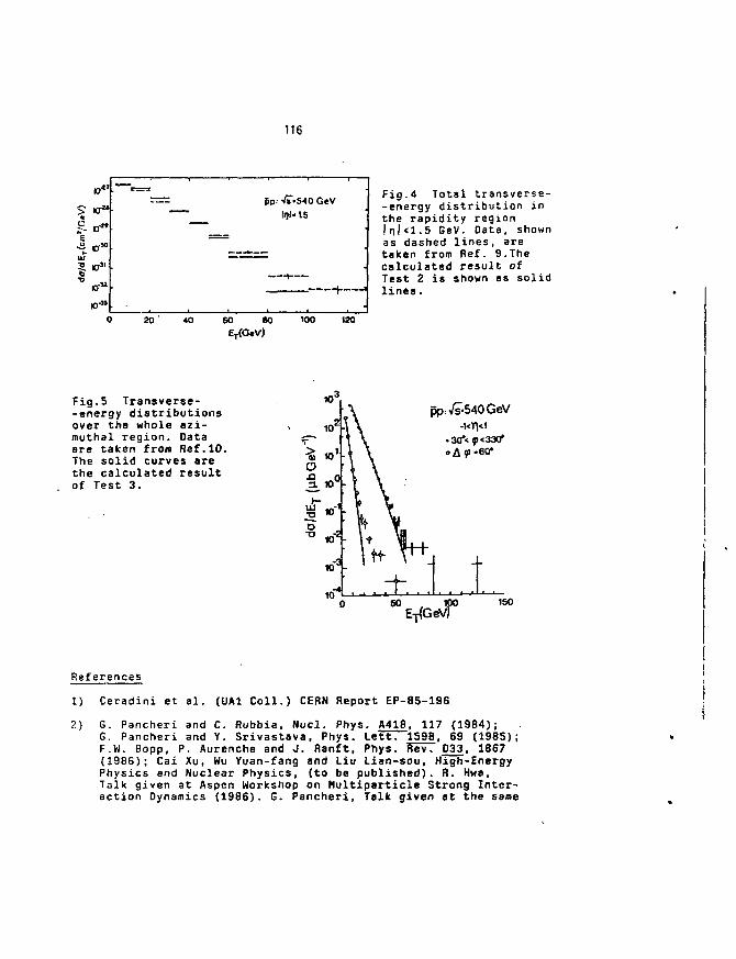
116
60 80ET(G.V)
Fig.4 Total transverse--energy distribution inthe rapidity regionIHI<1- 5 GeV. Data, shownas dashed lines, aretaken from Ref. 9.Thecalculated result ofTest 2 is shown as solidlines.
100 120
Fig.5 Transverse--energy distributionsover the whole azi-muthal region. Dataare taken from Ref.10.The solid curves arethe calculated resultof Test 3.
»"
10
oXI
UJ
10°
« 1
10"
pp:1/s-540GeV
.30*<p<330*«A f •60*
i- 1 .. 1.50 100 1S050 E-^GeV)
References
1) Ceradini et al. (UA1 Coll.) CERN Report EP-85-196
2) G. Pancheri and C. Rubbia, Nucl. Phys. A418, 117 (1984);G. Pancheri and Y. Srivastava, Phys. Lett. 159B, 69 (1985);F.W. Bopp, P. Aurenche and J. Ranft, Phys. Rev. 033, 1867(1986); Cai Xu, Wu Yuan-fang and Liu Lian-sou, High-EnergyPhysics and Nuclear Physics, (to be published). R. Hwa,Talk given at Aspen Workshop on Hultiparticle Strong Inter-action Dynamics (1986). G. Pancheri, Talk given at the same
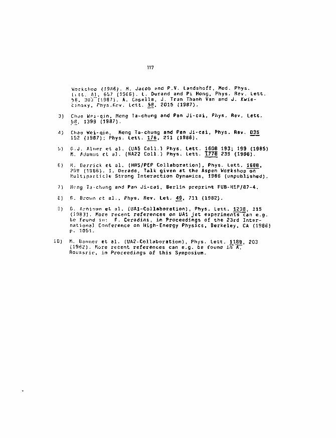
117
Worfcohop (19S6). M. Jacob end P.V. Landshoff, Mod. Phys.t.tt. A], 657 {1966). L. Ourand and Pi Hong, Phys. Rev. Lett.56, 303 "(1987). A. Capella, J. Tran Thanh Van and J. Kwie-cinsky, Phys.firv. Lett. 58, 201S (1987).
3) Chdo Wei-qin, Meng Ta-chung and Pan Ji-cai, Phys. Rev. Lett.&8, 1399 (3987).
•1) Choo Wei-qin, Meng Ta-chung and Pan Ji-cai, Phys. Rev. D3515? (1987); Phys. Lett. 176, 211 (1986).
;.) G.J. ftlner et al . (UA5 Coll.) Phys. Lett. 160B 193; 199 (198S)M. Aiiaiinis ct al. (NA22 Coll.) Phys. Lett. T77I 239 (1986).
6) M. Derrick et al. (HflS/PEP Collaboration), Phys. Lett. 168B,?99 (1986). I. Oerado, Talk given at the Aspen Workshop onI'.ultiparticle Strong interaction Dynamics, 1986 (unpublished).
'/) Hi:ng Tachung and Pan Ji-cai, Berlin preprint FUB-HEP/87-4.
8) n. Brown ct al., Phys. Rev. Let. 49, 711 (1982).
D) G. ArniEon et al. (UAl-Collaboration), Phys. Lett. 1238, 115(5983). More recent references on UA1 jet experiments can e.g.be found in: F. Ceradini, in Proceedings of the 23rd Inter-national Conference on High-Energy Physics, Berkeley, CA (1986)p. 1051.
10) M. Banner et al. (UA2-Collaboration), Phys. Lett. 118B, 203(1982). More recent references can e.g. be found in A.Roussrie, in Proceedings of this Symposium.
119
*f / i l ' IJ k> i\ U V * i • ~ 4 • V v • * k* . i • • • ! . « * * • • f rf\
'TK: .-: K ACT i '.. : : J AJ; D D I CU ARI: SCATTEÄIKC *
V-, Ssczekov.'ski
Institute of Kuclear Studier, Karsaw, Poland
Collaborât ie:
few exar.;plee of recent data on h:?h p„ pion ar.d protcr.
production frea Split Field "agnst detector at 123 erc-
presc-nted. The feat;;re3 of tnclaoive particle production
ii.d corrclaticiE observed betv9?fcn particles in trirror
r.'-.i Ej'.ctator Jets eupp.irt the co^je:ture of hrr: 'M^M-vk
p.c.i'. taring an a source of hi^h r.„, baryoris.
Submitted to the Symposium
120
i. in? so DUCT ion
Hard scattering of elementary particles with production of
high trp-ngverse momentum jets is one of the nost important
t^ete for parton models and Quantum Chronodynasics (QOD) [i].
Studies of leading particles in Jet3 showed that knowledge
of the particle identity directly gives information about
the underlying parton scattering [2]. Identification of loading
neoons in large pm Jets allowed the separation of gluon
scattering from other high p , processes [3]. The behaviour
of leading baryons produced at high p , showed new features
unexplained within a standard parton model: the relative
proton yielda c(p)/0"(7T) depend on p™ at fixed scattering
angle 0 , on 6 at fixed p , , and on c.m.s energy TP at
fixed ^ = ?P^/ /"a"* and Q ; In contrast, relative K and p
yields are nearly independent of kinematic variable [ft].
In this short report I will present th« recent reculto of
the analysis of high p T processes at ISR energise obtained
in the i.'?lit Field Ha^aet detector by ABCDK'n Collaboration [5j.
3hs experiment is briefly described in section 2. In section 3
the ratios of Inclusive cross sections for negative and
positive pior.o separately are disscus3«d. In phase space
regions United by geometric acceptance of ChcrenkJV counters
the ratios are etudied as functions of transverse 1i03er.vu.rr.
pm , reduced lorgitudinal momentvua x « 2p. / VT 1 ajd
scattering sngla B and compared with parton tuodel ;al.?ulatior.;.
The data on correlations between theidentifled trigger
particle and the properties of spectator jets are presented
in sect. A.
2. EX? SHIKETT
The e-}orir;f:at was performed with th» Split Field Macnet
CS:-':.') Detector at the CERI? Intersecting Storage Rings (IiR).
The detector consists of a systea of multiwire proportional
c''ioabers and an array of scintillaticr. counters for
fiirht mca'Turcaents [6b).
121
A throe seep t r i ;>" ? r logic selects: r. •: r.\.s vrilh a hi;:h ?T
treci: rit a c .n .o . scatv:r:i":" t-:.fiC fci>~, , <.J\, o: -j> .
These tri-cks C M be i-U-.nii'icd •.;ith th:-jr:;old Churer.iu-v
counters [5,G'oJ. '.'he present st t li!.:ticL i c r racsn.;-; .-uctc-d
high pT events ia of the order of 10' .
3. PAT JOS 0? IKCLITSIVK CROSS-SiJC-IO'-'.S
J ion ra t ion of inclusive cre.-.?-sectier.:; A = O" (7C*)/
O-(7iT+"+ i"r + p) -r.d K" = cr(7C)/ 6' ( A~+ >•" + ?) for protcn-
pi-\>i-./.; i i . to r -c t icns ;.t ©-10° , : c ° and 45° v.-ere i.:cac-jre-- a-
t . i c . a . c . cr.erri'os; \fp= 31 " C : 7 ^-^ 63 G e V as functions
of x and p.p.
T;.c y. c!c:pendence of the dat?1. i s i l l u r t r t t e d in f: •;:: t ,2
..-d 3 :"ijr different fixed v&Iusc of p.-,. I:idcpe::de:>t oi' a ul.osar.
;... vr.lui;, the f ract ion o;' negative ;ic::f R~ i s a eiecply
rii'ii>g function of x. At :>: = C 5 only a few j-.aroor.t of the
civ a.? i^ction i s l e f t for hc-nvi-r yarticjles 0 ' " , " ) fcr- o i l
v-v.luc i of pa,» Xhe f r sc l icn of posi t ive pione sh3v;a the cp--r;:5ite
telu-.vioar. S tar t ing fro-n R ^ 0.6 at x "^ 0 i t decreavc.-
vrith iucreasing x.
'ilie- dependence of R and R" on r., observed here at nediua
and hich values of p , , resembles closely the behaviour ofpositive and negative pion fractions at low trynsverji' nciaer.ta.In the soft hadronic interaction thi3 behaviour is generallyunderstood as a reflection of the leading protor: effect [7.1.In ths quark models of soft hadrcn scattering this effectis explained by the diquork cos tent of the forv;ard-b;vcr:v.\.i'CJets in proton-proton collisions. Similar propsrtiea of pionproduction at lew and hi ~h p^ Eu^gest a cc-sizon origir; ofthis behaviour* the frac--&Rtatisn of diqur.Wcs riih e fubstaniislcontribution of faet protor.3 which suppreases the rolt.'.ivepositive pion contribution at higher x. For negative particlesthis process ia absent and pions dominate.
To describe the p T dependence cf R+ and R" shov.n in flcs 4
end 5 for different fixed values of the -hard 3otttericr; c-fquarks and.glaor-j was simulated by the locate Cor.1- programdoscribod in detail ia rsf.lQ]. The procsos of diquarknststterins vvos not included in this version of the simulation
122
pregran. The model describe reasonably well the negative
picn ratios at both energies cut the positive pion ratios are
not deacribed properly by the model. The discrepancy between
the Gcdftl asd the data is i&crcp.cing for smaller angles (8^20°).
A similar discrepancy wc.a observed previously for the coiEplenen-
tory data on high p~ baryos pi'oducti«.a in proton-proton
ccllisicrs [lit]. Although the production of antiprotonB waa
well described by the standard quark model$ in the case of
proton pr«ducticn this c,od«l failed to describe the magnitude
cs<i Q and p T depend^aca of the protou relative yields.
The contribution from diquark -scattering [9] was proposed to
explain the features of high p , protor. production [10].
The model e.pplitra to perticlse with p^ > 2.5 GeV/c. The predic-
tions of this nod's 1 fcr P. showu in fi. s i and S are in good
tii-rccr.ent vrtth the hiTh pw, end of the data. About 90%.
of tl.c- high p., protons originate from diquark scattering in
this phase space region. ;
We conclude that the qualitative and quantitative predictions \
cf the diquark node7. are in good agreement with the data at ?
hirher vtilueg of p_. Tl.is indicates the presence of diquark >
fragrientaticn also in high p T jets. The confirmation of thie
hyvothesis should cone from tha correlation data.
k. co?.:?.n.A'?io?-s esrv.'s^-: TRIGGER AITD SPECTATOR JETS
j"or *he events v/ith high p ? baryon production a typical 1
h.r: Gcatterir.r; four jet structure ie observeds scattered
pirtons fracaor.t into hiph p-, "triggar" and "away" jets ;
and nonVnteractlng parton3 form two low p m epoctator jeta.
•".-.» hype thesis that hicis p T baryons are produced by hard diquark '
c ttcrir.r- ].-?;.c.;. to the prediction of well defined correlations ;
tr;v..-:cr. tho^e Jets aa shown in fie. 6. The spectator jets,
z.: B fc 0°, rl.ould be due to a system of two valence quarka
ir. the c.:;:is of positive nienou triggers and to single valence
",';;.r»r i'-::r proton triggers from diqusrks fragmentation.
A sv>y ef the ratioa R+{p/7t+) « ^ + ( p ) / + (K*) of densities
of pesi'.ive pi.rticleo asRociated ».ith proton and TT^meson
123
triggers respectively allows to discriminate between fragmentatioc
of diquarko and quarks in spectator jet region (x > 0.3).
If high pT protons are diquaric fragments R (p/7C*") should
decrease with x since for large x positive fragments are
doiainantly protons which are easily produced in diquark
fragmentation and are suppressed in quark3 fragmentation til].
Thia kind of behaviour is indeed observed in fig.7,8 and 9
for triggers at 0 * 10°, 20° and 45° respectively. These data
are in qualitative agreement with hard diquark scattering
giving rise to high p_ protons. Similar correlations have
been observed recently for events with high pT trigger
particles detected at £)«-900[i2j.
If high pT protons indeed originate from diquark scattering
the correoponding spectator fragments should be compared to
charge densities from single quark (current) jets in deep
inelastio lepton scattering (DIS). For pion triggers on the
other hand the spectator particles should behave like target
jets in DIS. The correlation between the fragmentation
variable z and the reduced longitudinal momentum z as measured
in this experiment can be obtained from straightforward
parton model calculations [13]. The ratio Be> 5~/g* turns
out to be a very sensitive indicator of the nature of the
parent partoris. In fig.10 acceptance oorrected values of
B^ are shown as a function of x for different trigger {X*tX~, p)
particles and compared with predictions from deep inelastic
neutrino scattering [14]. The agreement for (uu) and (ud)
Jets in Vp, 7p and ;c""and 7T**trlggor3 la Indeed striking.
On the other hand R* >for proton triggers «hovra an increase
of negative charge density j~at large x. By comparison of
these data with models the nature of corresponding scattered
diquarlca can be investigated« if only (ud) systems are involved
in high pT diquark scattering then R^ should correspond to
single u - quark scattering. As can be seen in fig. 11 the data
fall well above this prediction and Indicate a substantial
contribution from scattered {uu) dlquarks. Further evider.se
for the scattering of (uu) diquarks comes from the appearance
of /^resonances in the trigger jet ae shown in fig. 12.
124
5. CCMCLUSIOKS
The conjecture of hard diquark scattering leading to
substantial production of high. p_ baryons in high energy
proton-proton collisions gaina further support from the
recent data from Split Field Kagnet detector. Both the peculiar
properties of the inclusive high pT proton production and
the charge correlations between trigger and spectator jets
can be explained by the scattering of tightly bound two quark
objects, Further confirmation of the existence of such objects
should come from studies ot baryon production in deep inelastic
leptcn scattering and e e" annihilations.
125
[1] K.Jacob, Proceedings of 22nd int. Conf. OK High Energy
Physics, Leipzig (1984), 150.
[2] ABCDHtY Collaboration,
A.Breakstone et al., Zeitschr. fur Phys.C27(i985)205.
[3] A.Breakstone et al., Phys. Lett. 1353(1984)510.
[4] A.Breakstone et al., Phys.Lett. 1473(1984)237.
D.Antreasyan et al., Phye.Rev. Lett. 38(1977) 112, 115.
[5] A.Breakstone et al., CEKN preprint CERK/EP 87-23
to be published in Zeitschr. fur Pliys.C
A.Breakstone et al., CERH preprint CEHN/EP 87-8
to be published in Zeitachr. fur Phys. C.
[67 a) M.Delia Kegra et al., Phys.Lett. 593(1975)481.
b) D.Drijard et al., Hucl.Phys. B2O3(1982)1.
[7] A.Breakstone et al., Phys.Lett.132B(19S3)45S.
J.L.Bailly et al., Zeitschr. fur Fnys.C31(1986)367.
[S] T.Lohse, Diploma Thesis, University of Dortmund (1982).
[9j S.Ekelin and S.Predrikeson, Fays.Lett.1483(1984)5C9.
[10] A.Breakstone et al., Zeitschr. fur Pliys.C2b(i9S5)335.
[11] 3.J.Brodsky ;_nd G.R.Parrar, Phye.Rev.Lett. 31(1573)1153.
S.J.Brodsky and J.P.Gunion, Phys.Rev.D17(1978)343.
[12] A.M.Smith et al., Phys.Lett. 1843(1987)293.
[13] ?•:. Delia Negra et al., Hucl.Phys. B127(1977)1.
[14] P.Allen et al., Hucl.Phys. B214(1933)369.
J.Dell et al., Phys.Rov. D19(1979)1.
M.Derrick et a l . , Phyo.Rev. D24(1981>1071.
126
FIGURE CAPTIONS
Pig. 1 Pion ratiO3 R+ = ff (X1')/**-{ 7t+ + K+ + p) and R" =ff(7C")/+ K~ + p) at fixed p_ • 2.1 GeV/o and two e.n.a.
energies YT 1 » 31 GeV *»d )fiP • 62 GeV as functionsof a reduced longitudinal momentum x.
Fig.2 Pion raties R+ - Q (7C*")/<y (7r*"+ K + + p) and R" - «r (A~)/<T(7T~ + K" + -p) at fixed p T - 2.5 GeV/c (R") andp T • 2.9 GeV/c (R ) and two c.m.s. energies Vs"1" 31 GeVand fe 1- 62 GeV as functions of a reduced longitudinalmoaentun x.
Fig. 3 Pion ratios R+ - *T (n*)/©" (7C*+ K + + p) and R~ « <5" ( 7 0 /K" + p") at fixed p T « 1,3 GeV/c (R") and p T - 1.5
GeV/c (E ) and two c m . s . energies fa"1* 31 GeV and
62 GeV as functions of a reduced longitudinaluomoatua x. The R data from the experiment [6a] atfi~* • 53 GeV are shown for comparison.
Fig. h Positive and negative pion fractions at ITs"1* 62 GeVand fixed scattering angle &* 26° for R + and & » 18°for R~ shown as functions of transverse momentum.The predictions of the parton models described in thetext are also presented.
Fig. 5 Positive and negative pion fractions at yiP- 31 GeVyand a fixed scattering angle £ « 20° for R and&* H for R shown as functions of transverse momentum.The predictions of the parton models described in thetext are also presented.
Fig. 6 Expected flavour composition of spectator jets forpion and proton triggers.
Fig. 7 ' Ratios of positive spectator secondaries associatedwith proton and 7C*triggers at (9 *• 10° with p, b >13 GeV/c. The error bands indicated at large x arepredictions from deep inelastic neutrino scattering.
Fig. .S Ratios of positive spectator secondaries associatedwith proton and Tt*"triggers at Q^ZO0 and p, . > 13GeV/c.
127
Fig. 9 See fig. 8, but for proton and 7T+ueson triggers
at e*-45O and p? > 3.5 GeV/c (<pT> •= 3.9 GeV/c).
Pig.10 Charge density ratio j"7£* a3 a function of x for pion and
proton triggers. The shaded strips are predictions froa
deep inelastic neutrino and antlneutrinc scattering
experiments for (ud) and (uu) target Jet systems.
Pig. 11 Charge density ratio f/^" for proton triggers compared
to predictions from deep inelastic neutrino scattering
for pure u - quark fragmentation and for a mixture
of 33% d - quark and 67%>u - quark.
Pig.12 Uncorrected invariant pJT* - mass distributiona for proton
trigger particles at (a) $ «*. 10° and 13 GeV/e < p. . <
18.1 GeV/c, (b) ©•*- 20° and 13 GeV/c < p 1 & b < 18.1 GeV/c,
(c) Q** 45° and pT > 4 GeV/c.
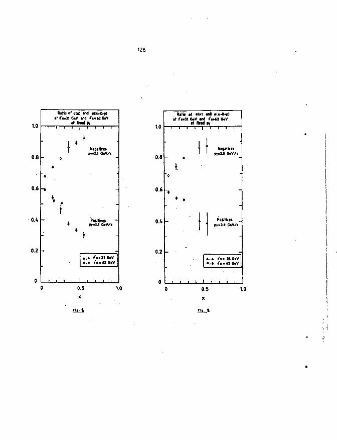
126
1.0
0.8 -
0.6
•0.4 -
0.2 -
Ratio of e(») and alx^c.a)»t/».31 GaV and / i .MGiV
at rant prI 1 1
0
4
4
1 1 J
1 | t 1 1 1
• INigativu
PT*1.1 GaV/c
-
PosffimPfiA GaV/c
4
».A /a .J I GaV
i 1 i i i •
1.0
0.8
0.6
0.4
0.2
0
Rati* af «l»> wiat /*>H GtV and /
at fbtd PiI i
0
t
"4
• •
-
-
1 i
i
i i
1
II
! •
A.O,
MM CaV
l l 1
NcgalhfitBT.1.5 GaV/c
-
Potitnts _Or-H GaV/c
« <T<> HGaV• /t>«2CaV
i* t i i
0.5x
1.0 0.5
x
1.0
Hi. *
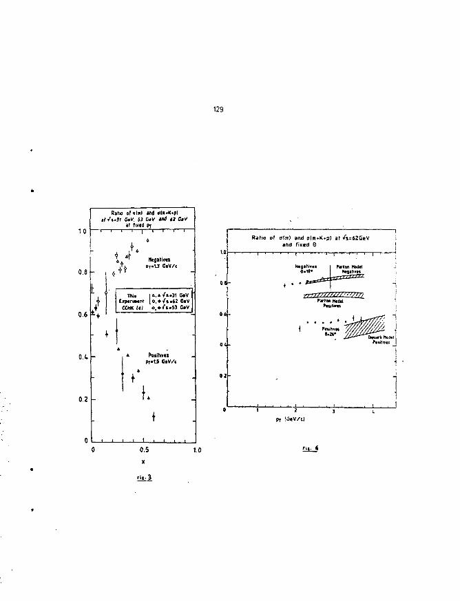
129
0.8
06
O.C -
0.2 -
R»tK> of olnl and <lx>K.p)j ( / l - 3 l CtV. S3 C«V M<j «2 ClV
it fixed Pr
L +
1
1 1 ) 1 1 1 1
j 4<^ Negiliv«J A P I . U OtV/t
Thii | 4 , A / » . 3 1 CaVEnpirwinf 10. • /» >62 CtVCCHK !êl o.»/i>S3 CaV
I*• Positives
PT-L5 C t V A
4
* f .t
i i . i i ,
10
oa-
0.6-
0.2-
Rifio of
i
-
-
. . . i . .
1
Olli)
and
and oln»K+p) at /s=62GeVfixed e
[ ' • • i [ • . . i
Nag»fiv«s i Parion nodet8-11" 1 Htgarivi»
PirIM nodllPtuh.ti
f " ' 'PML. É ?
1 . . . . 12 1
1 • :
-
-
^Vk Hotel
-
:
0.5
x
1.0 Fit. «
Fit. 3
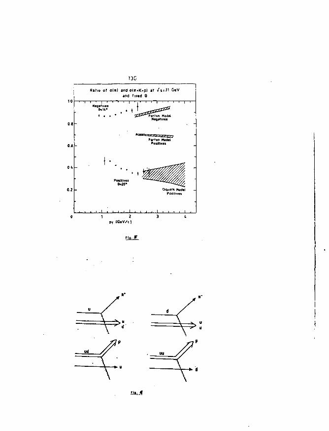
10
08
0 6 •
13C
Ratio of olnl and oln.K.p) at /s=31 G«Vand fixed 8
0 1
0.2
Petilivts8.20'
1 2pT [GtV/c l
ud
\
V
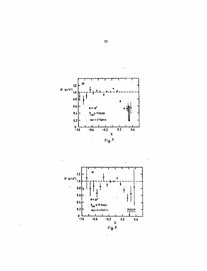
131
R* tp/n*)12
1.0
0.8
0.6
0.1
0.2
A
1
al
T—r
t I '---
-1.0
i i i i > i
-
l.^_Lf._.._fcl-»
W t 3 G 'v /<<Pr>*17GiV/c
A -[• .
1 1 I 1 1 1 1
-0.6 -0.2 0.2
X
0.6
R* Ip/s*)
1.2
1.0
0.8
0.6
o!;
0.2
g
-
i i i i i i i
L I 1 '
I i f •
L i • ' » 1 -
"* <p^>=4AGeV/c TRIGGCR -
-1.0 -0.6 -0.2 0.2X
0.6
Viq.S
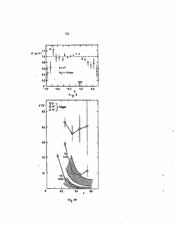
132
R* ip/iT)
;~Lti-il<-"M
-1.0 -0.6 -0.2 0.2 0.6
j . 4°
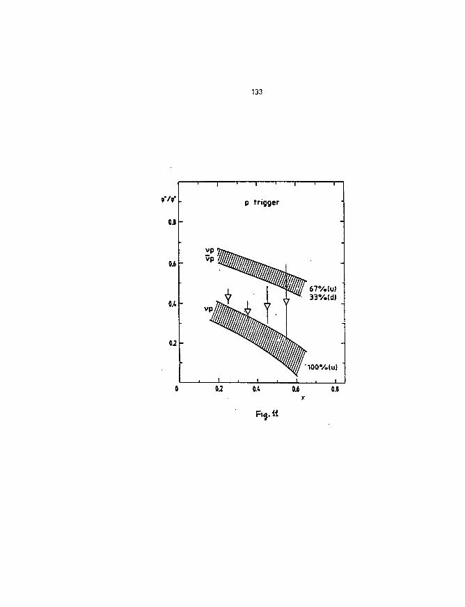
0.8 -
133
p trigger
Oih
o.;h
67V.lu)33V.(d)
0.4 0.6
"100 %(u)
O.J
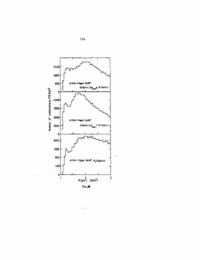
2400
1600
800
0
1000
3000
2000
1000
proton triggw 8zW*
UGtV/c Sp^S W.iGeV/c
proton trigger 8=20*
UGeV/cSp 2 1l.1G«V/c
135
ASYMPTOTIC KNO SCALING FOR QCD JETS
by
Antonio Bassetto
Dipartimento di Fisica 'G.Galilei'
Via Marzolo 8, 3S131 Padova (Italy)
Istituto Nazionale di Fisica Nucleare
Sezione di Padova
Abstt act
We exhibit the asynptotic KNO pmfile function for QCD
jots in e*e" annihilation.
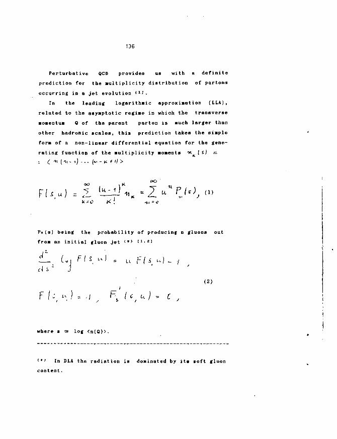
136
Perturbative QCD provides us with a definite
prediction for the Multiplicity distribution of partons
occurring in a jet evolution HJ.
In the leading logarithmic approximation (LLA),
related to the asymptotic regime in which the transverse
momentum Q of the parent parton is much larger than
other hadronic scales, this prediction takes the simple
fora of a non-linear differential equation for the gene-
rating function of the multiplicity moments tt (sj =
K !
Pn(s) being the probability of producing n gluons out
from an initial gluon jet <•> H.2J
JT- J s
(2);
F /:( u ) = ., _ \-% (C/ u) -- C ,
where s = log <n(Q)>.
<*> In DLA the radiation is dominated by its soft gluon
content.
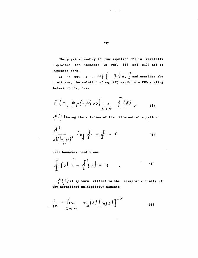
137
The physics leading to the equation (2) is carefully
explained for instance in ref. [1] and will not be
repeated here.
If we set M. = £-<j« I - ^/^ -Ji > J and consider the
1 init s+<», the solution of eq. (2) exhibits a KNO scaling
behaviour f 3 ], i.e.
/ /'<* > ' s "'/ " I j J (3)
Q' (5 ) being the solution of the differential equation
tof i= = <i - •/ (4)
with boundary conditions
= A (5)
o) is i.n turn related to the asymptotic li«it« ofi
the noraalized aultiplicity aoaenti
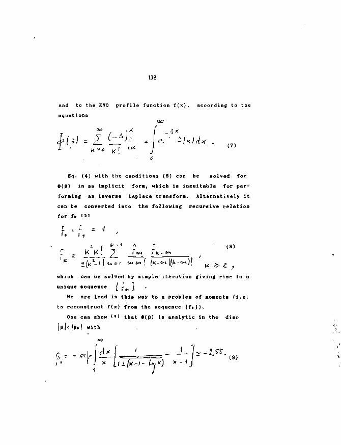
138
and to the KNO profile function f(x), according to the
equationsOC
\ i ^ — — - i - - • ( 7 )
K ;
Bq. (4) with the conditions (5) can be solved for
t(p) in an implicit fora, which is insuitable for per-
forming an inverse Laplace transform. Alternatively it
can be converted into the following recursive relation
for fn 1 a J
z 1 U.-4 2 - 2 ( 8 )
which can be solved by si«ple iteration giving rise to a
unique sequence ] - 1u f *M J
We are lead in this way to a problem of aoaents (i.e.
to reconstruct f{x) from the sequence {fk}).
One can show ( 3 1 that *(p) is analytic in the disc
||</Bo| with
( 9 )
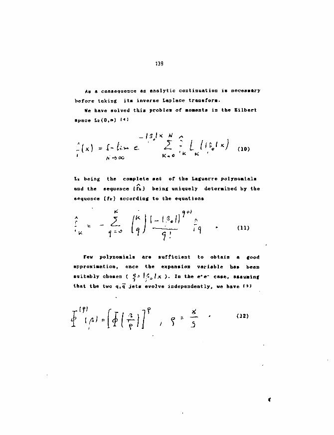
139
As a consequence an analytic continuation is necessary
before taking its inverse Laplace transfers.
We have solved this problea of aoaents in the Hilbert
space 1.2(0,<») <«3
_ / Sj * V ^
:- <— ~ L i ' \ Kl (io)
Ln being the complete set of the Loguerre polynoaials
and the sequence {fk} being uniquely determined by the
sequence {fit} according to the equations
(11)
Few polynoaials are sufficient to obtain a good
approximation, once the expansion variable has been
suitably chosen ( Jj» 15 / x ). In the e*e~ case, assuming
that the two q,q jets evolve independently, we have ' "
(12)
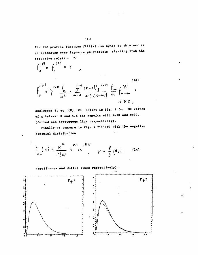
The KNO profile function f<»>(x) can again be obtained as
an expansion over laguerre polynomials starting fro- the
recursive relation l31
' 9 'I
(13)
aoaloifous to eq. (8). We report in fij. 1 for 90 values
of x between 0 and 4.5 the results with K=10 and N=30.
(dotted and continuous line respectively).
Finally we compare in tig. 2 f<P>(x) «ith the negative
binoaial distribution
*2I3
(continuous and dotted lines respectively).
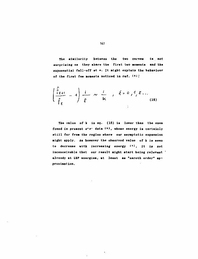
141
The similarity between the two curves is . not
surprising as they share the first two moments and the
exponential fall-off at ». It sight explain the behaviour
of the first few moments noticed in ref. (5)r
_ Ai i .
(15)
The value of k in eq. (15) is lower than the ones
found in present e*e~ data ( 6 ], whose energy is certainly
still far from the region where our asymptotic expansion
might apply. As however the observed value of k is seen
to decrease with increasing energy t 7 ), it ia not
inconceivable that our result Might start being relevant
already at LEP energies, at least as "zeroth order" ap-
proximation.
162
References
[1] A. Bassetto, M. Ciafaloni, G. Marché«ini, Phys. Reports
100 (1983) 201.
[2] Yu.L. Dokshitzer, V.S. Fadin, V.A. Khoze, Z. Phya. Ç15.
(1983) 325.
[3] Tu. I. Dokshitzer, V.S. Fadin, V.A. Khoze, Z. Phys. C18
(1983) 37.
[4] A. Bassetto, Proceedings of the XXII Rencontres de
Moriond, Les Arcs 1987 (France).
[S] B.D.Malaza and B.R. Webber, Nucl. Phys. B267 (1986) 702.
[6] M. Derrik et al., Preprint ANL-HEP-PR 86-03 (1986).
[7] TASSO collab.- M. Althoff et al.- Z. Phys. Ç22 (1984)
307.
RECEMT RESULTS FROM THE EUROPEAH KUOM COLLABORATIOM
R. Wlndmolders
Universlte da l'Btat, Hons, Belgium
The results presented in this report have been obtained in recent
phases of the experimental program developed at CERN by the European
Huon Collaboration (EHC). In the first two sections we will discuss
spin asymmetries measured in interactions on a polarised target. The
spin dependent structure function g it derived frott the ouon
asymmetry and its integral compared with sum rule prediction!. The
asymmetries observed for positive and negative hadrons give further
information on the contribution* of the conatituent quarks to the
nucleon spin. In the third section w» analyse the profile of the
hadron jet resulting from the fragmentation of the struck quark and
-derive- a value of the QCD coupling constant a in the context of
the Lund string model. Properties of baryon and antibaryon production
in the fragmentation process are derived in- Mi» ln> atellr.ni.
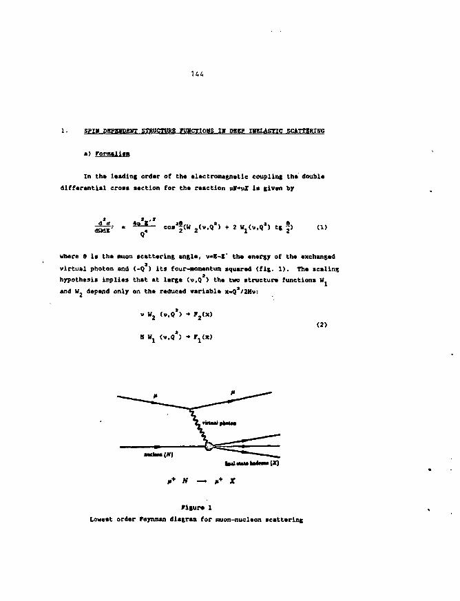
1. SPM DSPCTDKBT STRUCTURE FUMCTIOMS IK DBKP IHKLASTIC SCATTBRIHG
a) FormalisM
In the leading order of th« electromagnetic coupling the doubla
diffarantlal cross saction for th« reaction vV+vI is given by
d adQdl*
tg (1)
where e Is tha muon scattering angla, v>B-E' tha energjr of tha exchanged
virtual photon and (-Q ) Its four-mom»ntum squared (fig. 1). Tha sealing
hypothesis implies that at large (v,Q ) the two structure functions W
and W, depend only on the reduced variable x>Q2/2Mv:
v W2 (v.Q ) •• F2(x)
K H x (v.Q
(2)
figure 1
Lowest order Feynman diagraa for muon-nucleon scattering
When spins are taken into account the right-hand side of formula1 dJo dJo
(1) defines the average - tj^dg7** * dQdE'*'*'* f o r beam and target
spins parallel (ft) or antlparallel (tl).
.1 3
In a similar way, the difference (Tjrjf-t+ - ^. tt) can also
be written as s function of two structure functions G and G [1]:
O)
with scaling properties given under the same conditions by:
M* v G1 Cv.Q*) -»
(*)
E2(x)
In this experiment we measure the asymmetry, defined as the ratio of
(3) to (1), for projectile and target spins along the beam direction:
dot* - dqftdot* + dott " ( 5 )
In the quark-parton model the structure function* T (x) and
G (x) are given by the probability of finding a quark of flavour i
carrying a fraction x of the nucleon momentum and having its spin
projection along (q^) or opposite (q.) to the nucleon spin:
x I •*i (q^<X> + q^(x)) (6)
« r •* (q*(x) - q^(x)) (7)
146
By meaiurins tha asymmetry A(x> we thua Investigate tha spin structure
of tha eonstltuant quark*.
Tha Bjorken sua rula [2], derived from light cone algebra,
predicts that the difference of the integral* of g.<x) for protons
and neutrons i* proportional to the ratio of the axial and vector
coupling constant* G and G measured in B decay. Including a
correction for QCO radiative effects, the relation becones [1]:
G
dx - I | *| (1 - «gCQ*)/«> . (8)
p nSeparate predictions also exist for the integrals of g' and g..
The Ellis-Jaffe sua rule [3], based on SU(3) current algebra and
assuming an unpolarlsed strange quark sea, predicts the values:
ll E} (X) dx « 0.200 ± 0.005
(9)
I* g? (x) dx - -0.010 ± 0.005
b) Experimental Data
The EMC has evaluated the spin asymmetry (5} by collecting large
samples of interactions of polarised nuons on nueleons polarised in the
direction of the beaa or in the opposite direction.
The positive sgion beam, obtained fron plon decay, was polarised
to -BOX. The target consisted of two 38 cm long sections of irradiated
ammonia cooled to 0.3*K and located in a 2.5T nagnatic field produced
by a superconducting coil (4). The two sections were polarised in
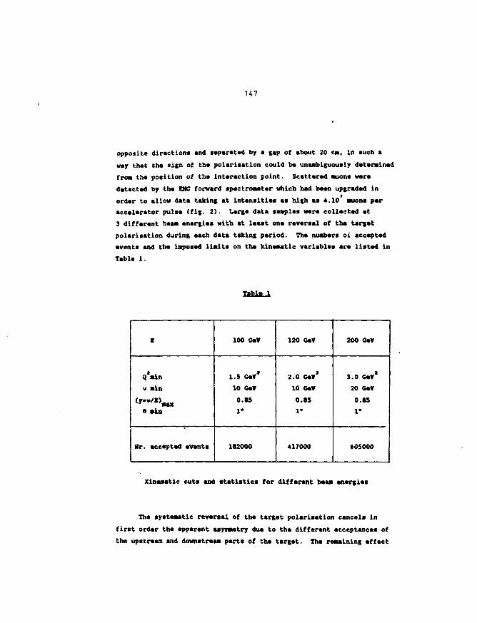
H7
opposite directions and separated by a sap of about 20 cm, in such a
way that the sign of the polarisation could be unambiguously determined
from the position of the interaction point. Scattered auons war*
detected by the CMC forward spectrometer which had bean upgraded in
order to allow data taking at intensities as high as 4.10 muon* per
accelerator pulse (fig. 2). Large data samples Mere collected at
3 different beam energies with at least one reversal of the target
polarisation during each data taking period. The numbers oi accepted
events and the imposed limits on the kinematic variables are listed in
Table 1.
Table 1
I
Q*mln
v mln
» min
Hr. accepted events
100 GaV
l.S GeV*
10 GeY
0.8S
1*
182000
120 CeV
2.0 GeV*
10 GaV
o.as1*
417000
200 CeV
3.0 GeV*
20 GeV
o.as1'
605000
Kinematic cuts and statistics for different beam energies
The systematic reversal of the target polarisation cancels in
first order the apparent asymmetry due to the different acceptances of
the upstream and downstream parts of the target. The remaining effect
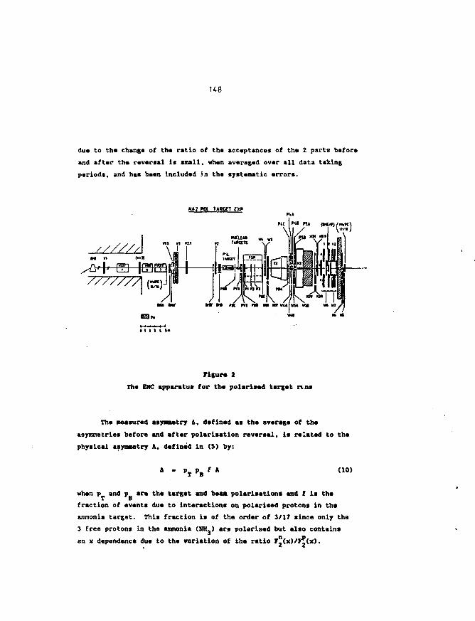
ue
due to the change of the ratio of the acceptances of the 2 parts before
and after the reversal is small, when averaged over all data taking
periods, and has been included in the systematic errors.
MA; pa. umstT tap
Figure 2
The EHC apparatus for the polarised target n n i
The measured asymetry &, defined as the average of the
asymmetries before and after polarisation reversal, is related to the
physical asynaetry A, defined in (5) by:
when p and p are the target and beam polarisations and f is the
fraction of events due to interactions on polarised protons in the
ammonia target. This fraction is of the order of 3/17 since only the
3 free protons in the ammonia (NH,) are polarised but also contains
an x dependence due to the variation of the ratio r"(x)/F?(x).
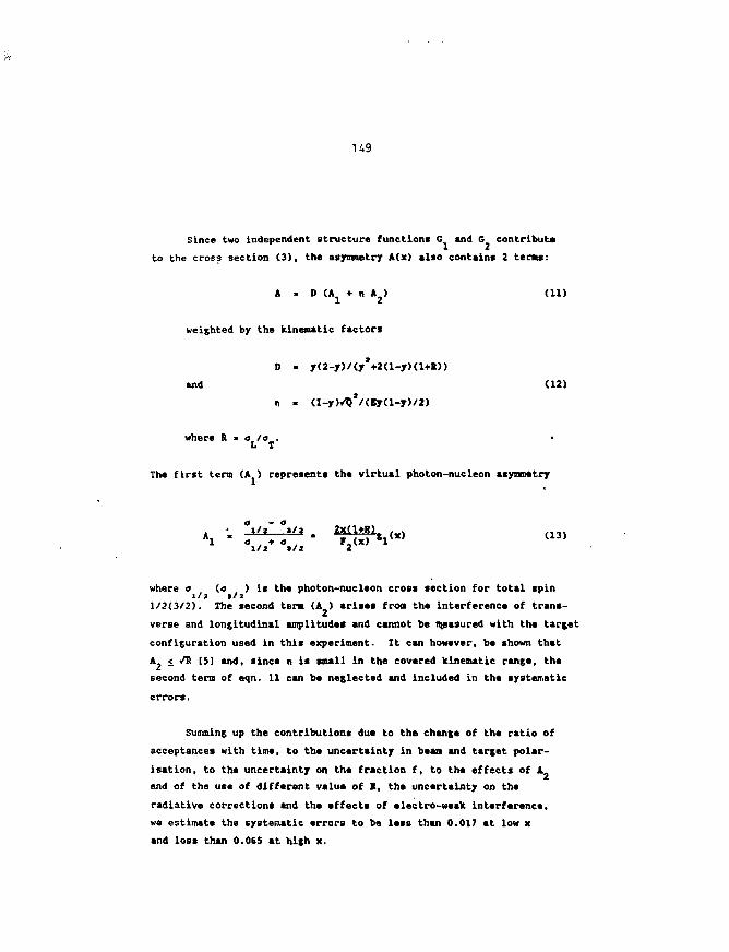
U9
Since two independent structure functions G and G contribute
to the cross section (3), the asymmetry A(x) also contains 2 terns:
A . D tA + n *2> (11)
weighted by the kinematic factors
and (12)
where R » o /a . •
The first term (A ) represents the virtual photon-nucleon asymmetry
, ' V?"*1 a . + a , r,(x)
where a (o ) is the photon-nucleon crocs section for total spinl/a »/J
1/2(3/2). The second term (A ) arises fron the interference of trans-
verse and longitudinal amplitudes and cannot be measured with the target
configuration used in this experiment. It can however, be shown that
A, < /8 [S] and, since n is small in the covered kinematic range, the
second term of eqn. 11 can be neglected and Included in the systematic
errors.
Summing up the contributions due to the change of the ratio of
acceptances with time, to the uncertainty in bean and target polar-
isation, to the uncertainty on the fraction f, to the effects of A
and of the use of different value of K, the uncertainty on the
radiative corrections and the effects of electro-weak interference,
we estimate the systematic errors to be lass than 0.017 at low x
and loss than 0.0(5 at high x.
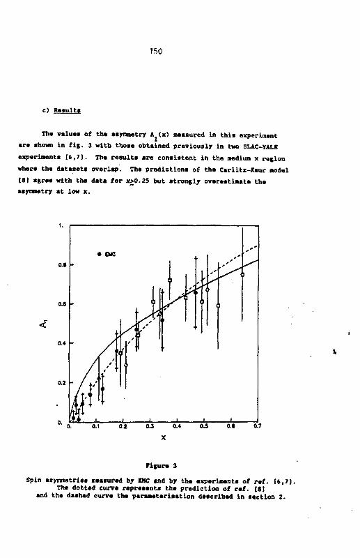
150
c) Results
The value* of the asynmetry A (x) measured in this experiment
are shown in fig. 3 with those obtained previously in two SLAC-YALS
experiments [6,7]. The results are consistent in the aediun x region
where the datasets overlap. The predictions of the Carlitz-Kaur model
(8| agree with the data for x>0.25 but strongly overestimate the
•symmetry at low x.
0.1 0.2 0J 0.4 0.J 0.1 0.7
Figure 3
Spin asymmetries neasured by IMC and by the experiments of ref. [6,7).The dotted curve represents the prediction of ref. (<]
and the dashed curve the paramterlsation described in section 2.
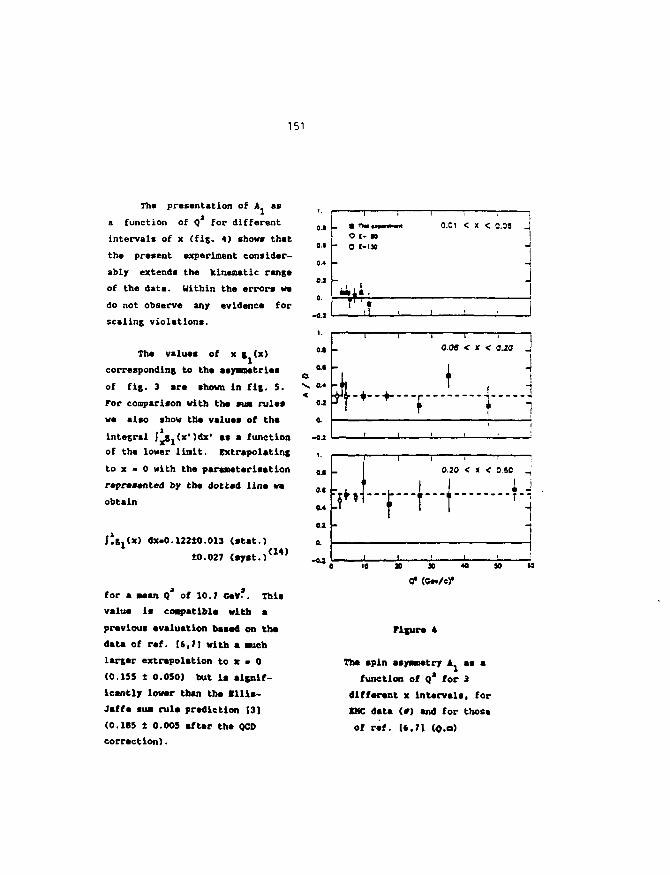
151
The presentation of A as
a function of Q for different
intervals of x (fig. 4) shows that
the present experiment consider-
ably extends the kinematic range
of the data. Within the errors we
do not observe any evidence for
scaling violations.
The values of x g (x)
corresponding to the asymmetries
of fig. 3 are shown in fig. 5.
For comparison with the sua rules
we also show the values of the
integral f^Cx'jdx' as a function
of the lower limit. Extrapolating
to x » 0 with the paranetarisation
represented by the dotted line we
obtain
|tg1<x) dx«O.12210.013 (stat.)
±0.027 <«Y«t.) a 4 )
for a aaan Q* of 10.7 G«V*. This
value is compatible with a
previous evaluation based on the
data of ref. [6,7] with a such
larger extrapolation to x • 0
(0.1SS t 0.050) but ia signif-
icantly lower than the Illis-
Jaffa sua rule prediction (31
(0.185 t 0.005 after the QCD
correction).
oa
o.t
0.4
OJ
-0.2
1.
Oc-n- O E-130
-
T ' •
i . i 10.0! < X < 0.06 _|
1-1
i
1
.. 0.4
0.2
0.
-0J
04
04
14
0.2
0.
-0J
I0.M < X < 0.20 J
• 1
•
1 1
1!
0.20 < X
1T
< o.sc1sr
_
I
20 X
01
Figure 4
The spin asysaietry A as a
function of Qa for 3
different x intervals, for
BMC data (») and for those
of ref. (*,?! (0,o)
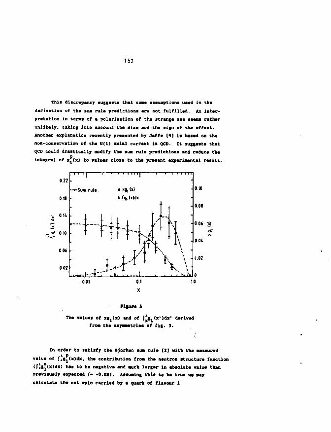
152
This discrepancy suggasts that sona assumptions usad In tha
derivation of the sum rule predictions are not fulfilled. An inter-
pretation in t e n s of a polarisation of the strange sea seen* rather
unlikely, taking into account the size and tha sign of tha effect.
Another explanation recently presented by Jaffa [9] is based on the
non-conservation of tha U(l) axial currant in QCD. It suggests that
QCD could drastically modify tha sua rule predictions and reduce thep
integral of s ^ x ) to values close to the present experimental result.
0 22
018
Oil
0 10
0 06
0 02
T-rrry-
—Sum rule:
* /g, lx)dx
+ H 1I
0.10
0.08
0 06 3
oo;
(.02
001 0.1 10
x
Figure S
The values of xg1<x) and of J^Cx'Idx' derivedfroa the asysaetries of fig. 3.
In order to satisfy tha Bjorken sua rule (21 with the Measured
value of f'g'(x)dx, the contribution frcw the neutron structure function
<li»"(x)dx) has to be negative and such larger In absolute value than
previously expected (- -0.01). Assualng this to be true we M y
calculate the net spin carried by a quark of flavour 1
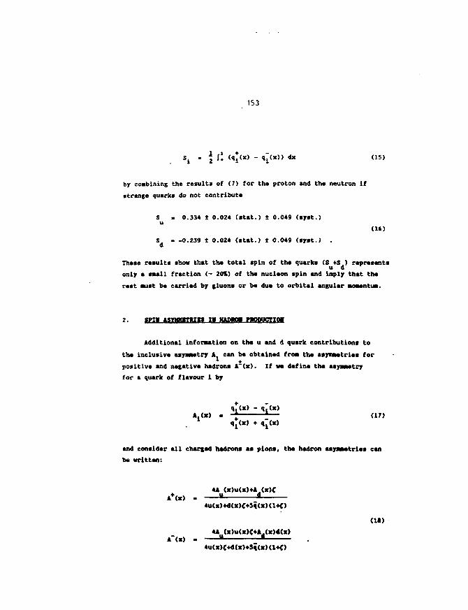
153
* S\ (q*<x) - q~(x)) dx (15)
by combining the result* of (7) for th* proton and the neutron if
strange quarks do not contribute
S > 0.334 t 0.024 (stat.) t 0.049 (ayst.)u
(It)
S^ - -0.239 t 0.024 (atat.) ± 0.049 (syst.) .d
These results show that the total apin of the quarks (S +S ) representsu d
only a small fraction (- 20%) of the nueleon spin and Imply that the
rest sust be carried by gluona or be due to orbital angular aoawntusj.
2. SPIM AS»MHI.T1TH HI K A M W MIODOCTKHI
Additional information on the u and d quark contributions to
the inclusive asyssMtry A can be obtained froa the asyntetriea for
positive and negative hadron
for a quark of flavour 1 by
positive and negative hadrona A±(x). If we define the aayaaatry
q.(x) - q.Cx)A,(x) . -* * (17)
qT(x) • q7(x)
and consider all charged hadrone aa pions, th* hadron asyssMtrles can
ba written:
4A (x)u(x)+A(x)CA+(X> - » «
4u(x)+d(x)C+5q(x)(lK)
(U)4A(x)u(x)C*Ail(x)4(x)
A"<x)
4u(x)C+d(x)4-9q(x)(lK>
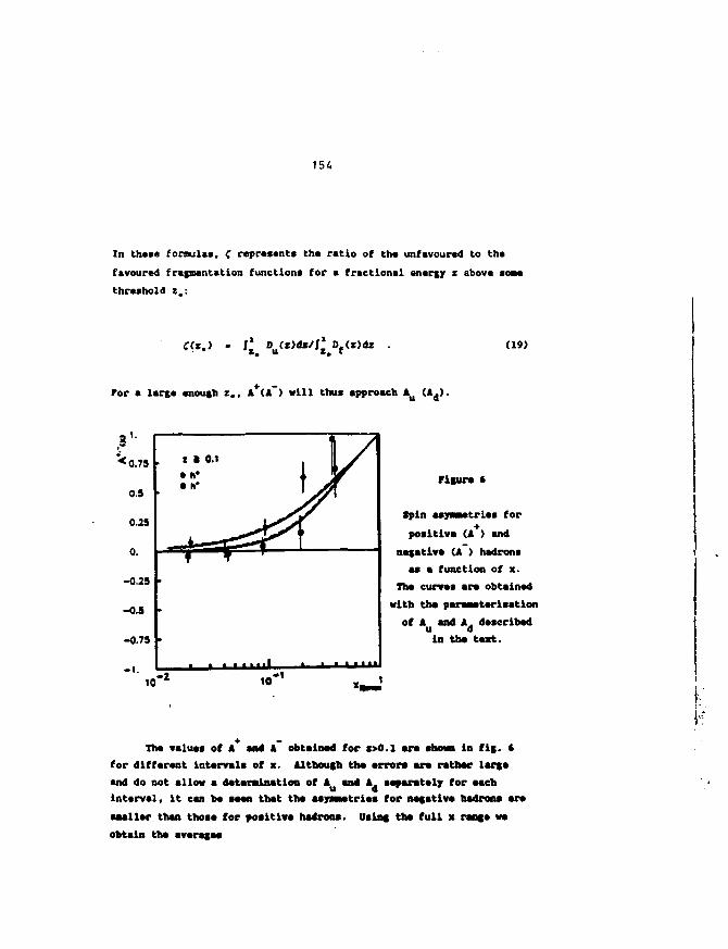
154
In thc>a formulas, C represents the ratio of tha unfavoured to tha
favoured fragmentation functions for a fractional energy z above soae
threshold z.:
D <X)dX . (19)
For a large enough z., A (A ) will thus approach « u
rigure •
Spin asyaaetrles for
positive (A+) and
negative (A ) hadrons
as a function of x.
The curves are obtained
with the parsaeterlsation
of A and A. describedu ain the text.
The values of A and A obtained for t>0.1 are shown in fig. *
for different intervals of x. Although the error* are rather large
and do not allow a determination of A and A. separately for each
Interval, it can be seen that the asysswtrles for negative hadrons are
•seller than those for positive hadrons. Using the full x range we
obtain tha average*
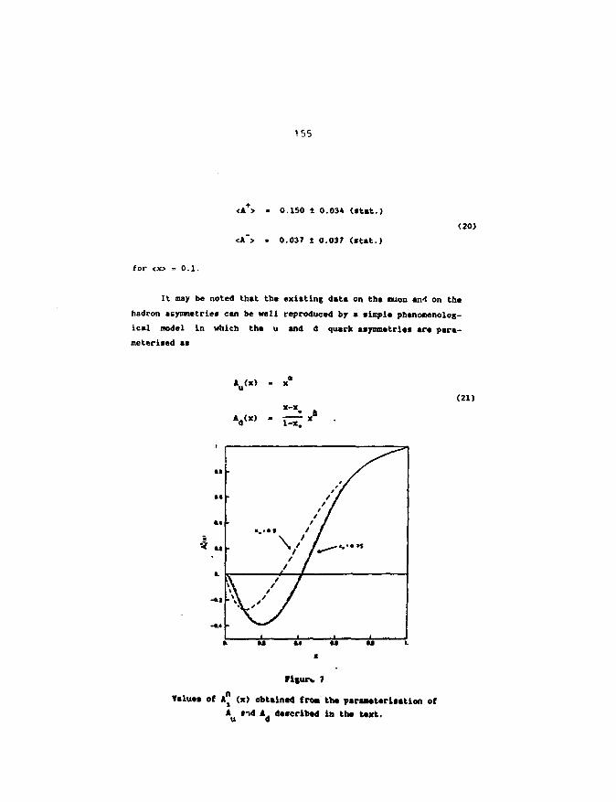
155
<A > « 0.150 1 0.03* (atat.)
<A~> « 0.037 ± 0.037 (ttat.)
(20)
for <x> =0.1.
It may be noted that the existing data on the w o n an4 on th«
hadron asymmetric* can be well reproduced by a staple phenonenolog-
ical model in which tha u and d quark asynntetri«« are para-
met«rised as
AU(X)
V*>
(21)
1-x.
M
I t
«.«
M
- M
•
/
k //a u
/
//n M aa «.
Values of A" (x) obtained froa the paraMtarltatlon of
* u t-A At described la the text.
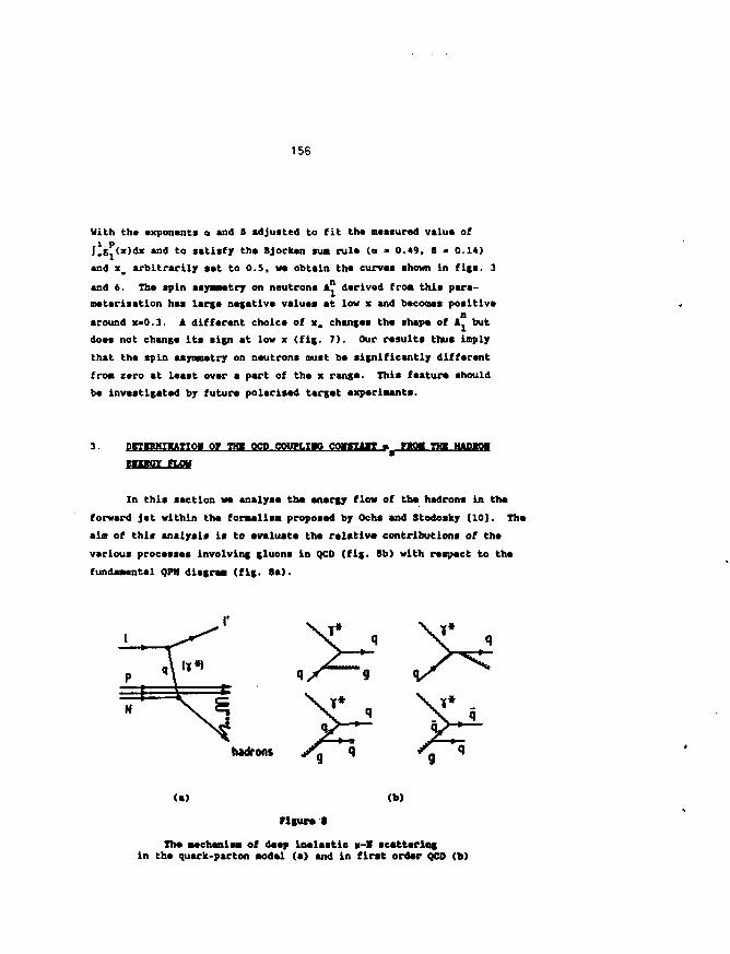
156
With th* exponents a and B adjusted to fit th* measured valu* of
/ls^Cx)dx and to satisfy th* Bjorken SUB rule (a =• 0.49, ft > 0.14)
and xm arbitrarily sat to O.S, we obtain th* curves shown in figs. 3
and 6. Th* spin asyssMtry on neutrons A™ derived from this para-
roeterisation has large negative values at low x and becomes positiven
around x-0.3. A different choice of x. changes the shape of A. but
does not change its sign at low x (fig. 7). Our results thus imply
that the spin asymmetry on neutrons oust be significantly different
from zero at least over a part of the x range. This feature should
be investigated by future polarised target experiments.
3. DETHUHEATIOM OF THI OCD cooPLna? CTfffTAlT r_ no* t m HADIOM
EMEKGt FLOH
In this section w* analyse the energy flow of the hadrons in the
forward jet within the formalism proposed by Ochs and Stodosky (10). The
aim of this analysis is to evaluate the relative contributions of the
various processes involving gluons in QCD (fig. 8b) with respect to the
fundamental QPM diagram (fig. Sa).
hadrons
(b)
Figure •
The mechanism of deep inelastic n-V scatteringin the quark-parton model (a) and in first order QCD (b)
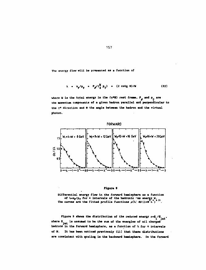
15?
The energy flow will be praaented aa a function of
xr/pT PT> (2 cotg 6>/H (22)
where W ia the total energy in tha (y*t) ra*t fraae, J> and p ara
the aonentuB conponents of a given hadron parallel and perpendicular to
the T* direction and 0 the angle between tha hadron and tha virtual
photon.
FORWARD
15
to
W, = UW< SGeV Wj=8<W<12GeV
KWj=12<W <16 GeV
• v• \
: \
^ Wt=16<W < 20GeV
. \V
0 — X — 1 — X " 1 — 0 0 — X — 1 — X ' 1 — 0 0 — X — 1—X'1—0 0—X — 1 — X"'—0
Figure •
Differential energy flow in tha forward headaphere aa a function
of X-x,,/pT for 4 interval* of the hadronic -ms energy W.Tha curves ara the fitted profile functions /><V •M/(l+M X*)*'*.
Figure 9 *hows tha distribution of tha reduced energy c l /I, ,
where B is aasuaed to be the aua of tha energies of all charged
hadrona in the forward hemisphere, as a function of X for 4 intervals
of W. It has been noticed previously [11] that these distributions
are consistent with scaling in th* backward headaphere. In tha forward
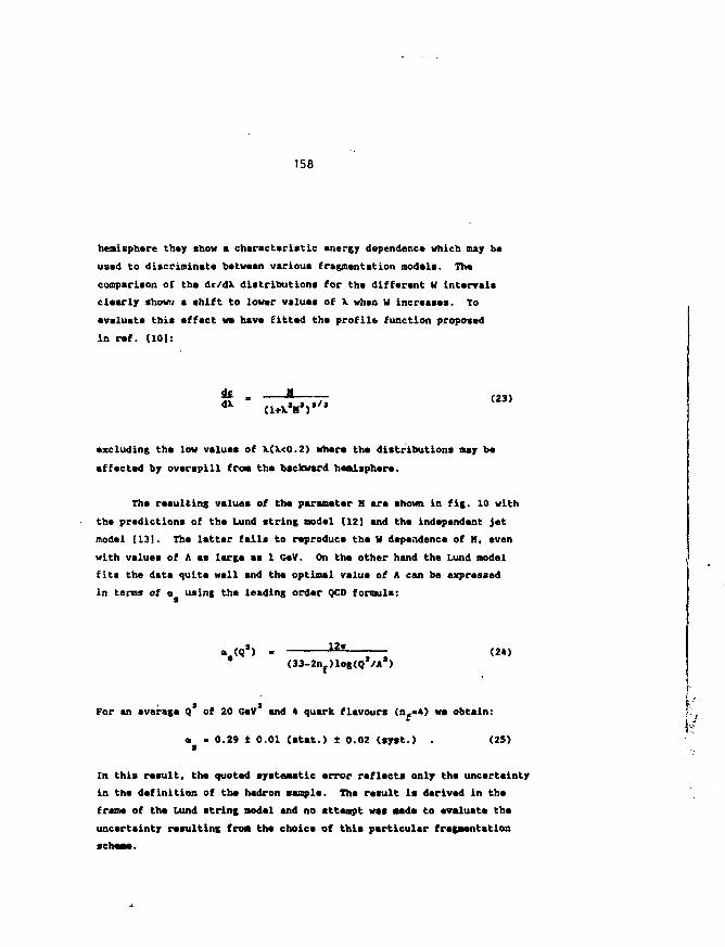
156
hemisphere they show a characteristic energy dependence which may be
used to discriminate between various fragmentation models. The
comparison of the dc/dX distributions for the different V intervals
clearly shown a shift to lower values of X when W increases. To
evaluate this effect we have fitted the profile function proposed
in ref. [10]:
" v 7 t / j C23)
excluding the low values of X(X<0.2) where the distributions may be
affected by overspill from the backward healsphere.
The resulting values of the parameter M are shown in fig. 10 with
the predictions of the Lund string model (121 and the independent jet
model [13]. The latter fails to reproduce the W dependence of M, even
with values of A as large as 1 GeV. On the other hand the Lund model
fits the data quite well and the optimal value of A can be expressed
in terms of a using the leading order QCD formula:
(33-2nf>log(Q*/A*)
For an average Q of 20 GeV and 4 quark flavours (n,»4) we obtain:
a - 0.29 ± 0.01 (stat.) ± 0.02 (syst.) . (25)
In this result, the quoted systematic error reflects only the uncertainty
in the definition of the hadron sample. The result is derived in the
frame of the Lund string model and no attempt was «ade to evaluate the
uncertainty resulting from the choice of this particular fragmentation
scheme.
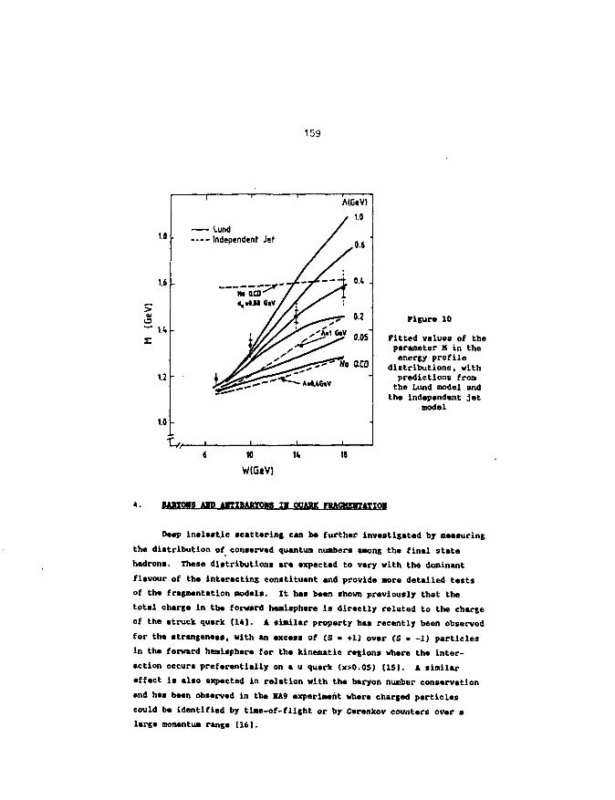
159
1.8
1.6
U -
1.2 -
1.0 -
— Lund- - Independent Jet
6 10
W(GtV)
Klgura 10
Fitted values of theparameter M in theenergy profile
dictributions, withpredictions fromthe Lund model andtha independent jet
model
MJQFORS AID ARIBAItXOKS IM OUASK nUOCEHTATTOM
Deep inelastic scattering can be further investigated by measuring
the distribution of conserved quantum numbers among the final state
hadrona. These distributions are expected to vary with the dominant
flavour of tha interacting constituent and provide more detailed tests
of the fragmentation models. It has been shown previously that the
total charge In the forward hemisphere is directly related to the charge
of the struck quark [14]. A similar property has recently been observed
for the strangeness, with an excess of (S > +1) over (S « -1) particles
In the forward hemisphere for tha kinematic regions where the inter-
action occurs preferentially on a u quark <x>0.0S) CIS]. A similar
effect is also expected in relation with the baryon number conservation
and has bean observed in the IA9 experiment where charged particles
could be identified by time-of-fUght or by Cerenkov counters over a
large momentum range (161.
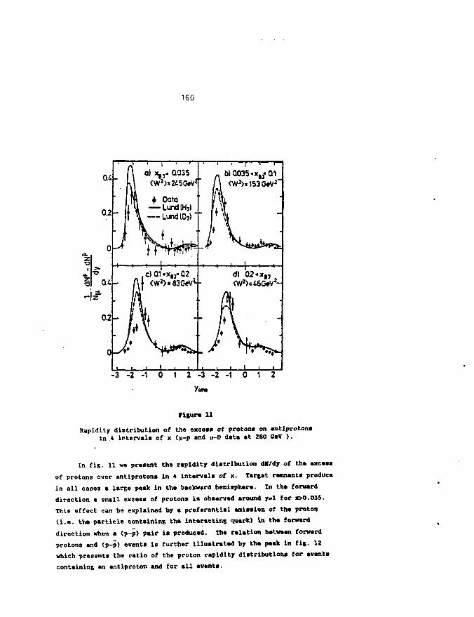
160
Figure 11
Rapidity distribution of the «xcess of proton* on antiprotonsin * intervals of x (u-p and JI-D data at 280 GeV ).
In fig. 11 we present the rapidity distribution dM/dy of the excess
of protons over sntiprotons in 4 intervals of x. Target remnants produce
in all cases a large peak in the backward hemisphere. In the forward
direction a small excess of protons is observed around y«l for x>0.035.
This effect can be explained by a preferential emission of the proton
(i.e. the particle containing the interacting quark) in the forward
direction When a (p-p) pair is produced. The relation between forward
protons and (p-p) events is further illustrated by the peak In fig. 1Z
which presents the ratio of the proton rapidity distributions for events
containing an antlproton and for all events.
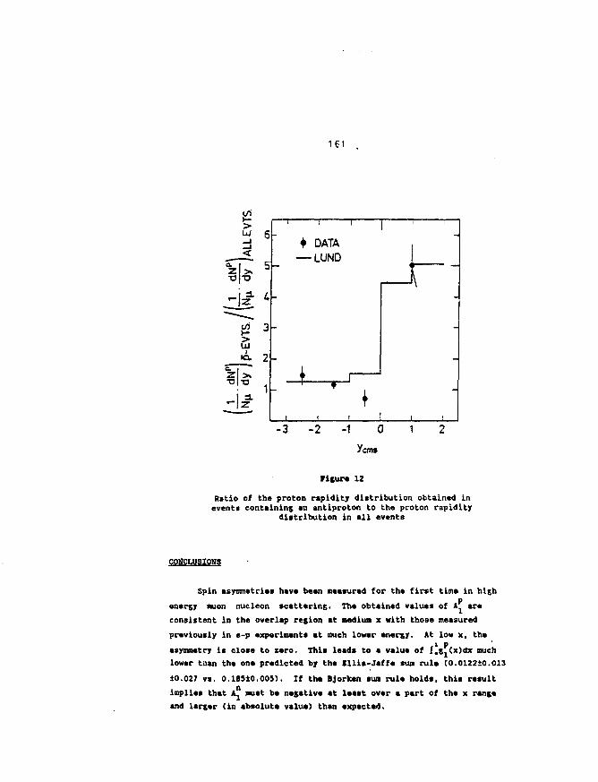
161
- 3 - 2 - 1
Figure 12
Ratio of the proton rapidity distribution obtained inevents containing an antiproton to the proton rapidity
distribution in all events
C0HCLU3IOMS
Spin asymmetries have been measured for the first time in highp
energy muon nucleon scattering. The obtained values of A1 are
consistent in the overlap region at medium x with those measured
previously in e-p experiments at much lower energy. At low x, the* p
asymmetry is close to zero. This leads to a value of J.g,(x)dx much
lower tnan the one predicted by the Illls-Jaffe sun rule (0.0122+0.013
to.027 vs. 0.18510.005). If the Bjorken sum rule holds, this result
implies that A. must be negative at least over a part of the x range
and larger (in absolute value) than expected.
162
The spin asymmetry Is larger for positive than for negative
hadrons suggesting that the d quark has a negative asymmetry in the
low x region.
The hadron energy flow in the forward hemisphere is consistent
with the Lund string model expectations with a •O.29±0.01±0.02 for
an average Q* of 20 GeV* and 4 flavours.
The proton and antiproton rapidity distributions show that in p-p
production the nature of the struck quark favours the production of
leading protons.
ACCTOWLKD0B1BIT3
I would like to thank the organisers of the symposium and my Polish !colleagues for their hospitality. I am indebted to all my colleagues in :the EMC and especially to V. Papavassiliou and L. Ropelewski for their ihelp during the preparation of this talk. :
ii
RgFERKBCBS
[1] V.W. Hughes and J. Kutl. Ann. Rev. Vucl. Part. Sci., 33 (1983) 611.[2] J.0. Bjorken, Phys. Rev. 248. (1966) 1467.[3] J. Ellis and R.L. Jaffa, Phys. Rev. D9 (1974) 1444.[4] S.C. Brown et mi., Proc. 4th Int. Workshop on Polarised Target
Material* and Techniques, Bonn, p.103 ed. W. Meyer (1984).[5) H.G. Ooncel and E.de Rafael, Suovo Cia. 4J (1971) 363.[6] M.J. Alguard et al., Phys. Rev. Lett. 37 (1976) 1261;
M.J. Alguard et al., Phys. Rev. Lett. Al (1978) 80.(7) G. Baua et al., Phys. Rev. Lett. 51 (1983) 1135.(8) R. Carlitc and J. Kaur, Phys. Rev. Lett. 3J (1977) 673.[9] R.L.Jaffa, Phys. Lett. 19JB. (1987) 101.
[10] W. Ochs and L. Stodolsky, Phys. Lett. 69g (1977) 22S;H. Fesefeldt, W. Ochs. L. Stodolsky, Phys. Lett. 748 (1978) 389.
(Ill P.B. Renton, Review of Hadron Production in Lepton KuclaonScattering, Proc. of the IX Warsaw Symposium on ElementaryParticle Physics.
(12] B. Andersson et al., Phys. Rep. 22 (1983) 31;G. Ingelman, The Lund Monte Carlo for Deep Inelastic LeptonUucleon Scattering. LEPTO Version 4.2
[131 P. Hoyer et al., Huel. Phys. B U I (1979) 349;A. All et al., Phys. Lett. £38. (1980) 155.
[14] J.P. Albanese et al., Phys. Lett. 144B (1984) 302.(IS] M. Arneodo et al.. Zeits. Phys. £3J (1987) 283.[161 J.P. Albxnete et al., llucl. Instr. and Meths. 212 (1983) 111.
163
THE KV MUOH PPERIMEMT AT CgM
Eva-Maria KabuB
Max-Planck-Instltut für Kernphysik, P.O. Box 103980,
D-&900 Heidelberg 1, F.H. Genuity
•ew Muon Collaboration
AMTtACT
The extension of the muon programme at CEKM by the «A37
collaboration will mainly study two aspects of deep inelastic
muon-nudeua scattering. Firstly, a simultaneous high luminosity
measurement of the hydrogen and deuterium structure functions
will allow to determine the neutron structure function FÎ,
t^-f^ <nd *°/|r2 with hish pcecislon over a large Q* and x range.
Secondly, detailed studies of the nuclear dependence of the
structure function ratios F./F., of R>o,/o_ and the cross section
for J/f production will provide a basis for understanding the
D K effect.
HOTIYATIOB
The proton structure function r? has been Measured with great
precision by several experiments and QCD analysis perforned for the
coabined data [1,21. Unfortunately the existing deuteriua data are
much more Halted in the Q* range [2,3] so that no unique deter-
mination of the neutron structure functions T^ is possible. In
addition f" IS distorted by the systematic errors of both the hydrogen
and the deuteriua data and the relative normalisation uncertainties.
It is necessary to clarify this situation by a simultaneous aeasurenent
on hydrogen and deuterlua over a large range in x (0.005<x<0.75) and
Q*(l<Qa< 200 CeV*/c*> to extract the Q* dependence of F°, *£-'" «no
F^/F* (4|.
This vill allow us study a lot of problem: ji
P n1. *2~rZ l t * p u r* n o n~* i nt 1* t structure function, if the
seaquark distribution of neutrons and protons are Identical. i
A QCD analysis over a large Q 1 and x rang* Mill therefore ,'
result in a determination of the QCD scale parameter A
independent of the shape of the gluon distribution ind
heavy quark thresholds.
2. The Gottfried mam rule
2 ) t a ' \
essentially tests the flavour sysaetry of the aea distri-
bution. The large error on the present value of °-235_n
is mainly due to the necessary extrapolation to low x.
3. At x>0.3S the ratio F^/F^ allows to determine the ratios
of the down to up quark distributions. The values at very
low x can provide a test of the assuaptlon of a flavour
syaaatrlc sea In proton and neutron.
165
In addition a possible difference between J/» production on hydrogen
and deuterium can be investigated.
Another result of deep Inelastic auon nucleus scattering was
the discovery of the EHC effect, that the structure function*
obtained froa free and bound nucleons are different (5]. It was
shown for the first tine that the nuclear aediua perturbs the quark
and gluon structure of the nucleon. This has given rise to a lot of
experimental and theoretical activity but the current experimental
information is insufficient to understand the origin of the EHC
effect [6]. A high statistic experiment with small systematic errors
covering a large x range can help to solve the following problem*.
1. The A dependence at nediusi x(x~0.6) is well established
to be proportional to lot * I'' but the Q dependence is
not known yet. A measurement can help to decide whether
the EHC effect at mediua x is governed by perturbative QCD
which would predict
2. The A dependence «t low x (x~0.1S> seems to be weak. But
discrepancies exist between different experiments so that
it is not clear yat whether there is a Q* dependence in
this region [8]. The A and Q dependence has not yet
been established especially in the shadowing region at
very low x and Q
3. There have been soae speculations about an A dependence of
R*a /<* which is needed to extract F. froa the measuredL T 2
cross sections. However, a recant acasurenent at low Q*
finds no evidence (91 for a difference between Iron and
deuteriua larger than 2-3%.
4. ror x>l only low Q1 results on '*»/'** • x U t ll01>
5. The study of J/» production allows to Invastlgata a
possible A dependence of the gluon distribution.
166
In addition the measurement of hadron distribution* fron nuclear
target* can give further information on the possible source of the
DfC effect.
Ttif farrffHin
The HA37 collaboration (Amsterdam-Bielefeld-Freiburg-Heldelberg-
Indlana-Mainz-Mons-Neuchatel-Santa Cruz-Sin-Torino-Uppsala-War*aw-
Wuppertal) uses the EMC spectrometer at the CERH M2 muon beam (11].
Several changes and upgrades have been made especially to decrease
the systematic error*.
The spectrometer (fig. 1) consists of a beam spectrometer (BUS,
BHA, BHB), the target platfora and the forward spectrometer magnet (FSK)
surrounded by wire chambers to measure the track* leaving the target.
Some wire planes have been added to improve the track measurement at
low angles.
The trigger is split into two part*, a low and a high angle
trigger. The efficiency of the large angle trigger (H . H , H ),
which was previously used by the EMC, was improved considerably.
The small angle trigger using the hodoscopea H ', H ', H ' ha*
been added to cover a large Q* and x range in a single experiment.
To achieve low systematic error* on ratio* it is crucial to measure
pairs of nuclei simultaneously. A special target platfora was designed
which houses complementary target setups of 2 or 3 different nuclei.
It allows frequent changes of the target position so that an equal
acceptance is ensured for all targets.
To reduce the error on the bean momentum from -0.3X to <0.1X a
second beam spectrometer of about 35m length using a high precision
magnet <MR>2«) has been added.
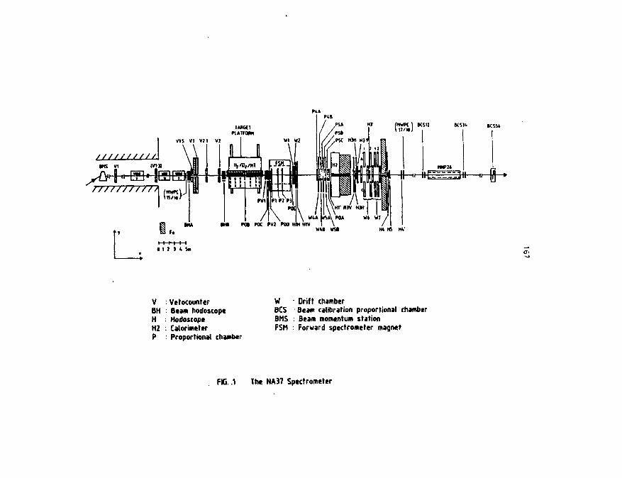
jMWPt ) KS1J MSX.
V : Vetocounter8H : Beam hodoscopeH : HodoscopeH2 . CalorimeterP : Proportional chamber
W : Drift chamberBCS - Seam calibration proportional chamberBUS : Beam momentum stationFSM : Forward spectrometer magnet
FIG. .1 The NA37 Spectrometer

168
The experiaental program* splits Into three parts:
1. The hydrogen-deuteriua aessureaent uses liquid targets of
3a length. With 101' Incoming auons and thrae beam
energies (90, 200, 280 GeV) it should be possible to achieve
an error on the neutron structure function of 1% at wall x
and about 10% at the largest x.
2. The 'thin target' aeasureaent uses pairs or triples of
targets of about 100 gr/ca . It is planned to measure
with D . He, Li, C. Si, Ca, Bb, Ho to study ratios at
saall x and hadron distributions.
3. To study the A and Q dependence at large x, K>o /o
and the J/* production it is necessary to use a 'thick
activa target* (C, Pb) of about (00 gr/ca*.
Data taking started in 198( covering the first two lteas and is
continuing this year. The thick target aeasureaent is scheduled
for 1988.
1) EMC, J.J. Aubert at si.. Hud. Phys. B2S9, 189 (198S).
2) For exaaple, A. Bodetc et al., Phys. lev. 020, 1471 (1979),
B.D. Mestayer et al., Phys. lev. D27, 285 (1983).
3) EMC. J.J. Aubert et al.. CER> preprint, CIRB-KP/87-M.
*) BMC. Proposal to the SPSG, Cm/SPSC 8S/18.
5) EMC. J.J. Aubert et al., Phys. Lett. 123B, 275 (1983).
1) D.v. Harrach, Invited talk at XI Int. Conf. on Particles and
Buclei, Kyoto (1987).
7) «.C. Arnold et al., Phys. Rev. Lett. 52, 727 (1984).
8) BCOMS. A.C. Benvenuti et al., CEK" preprint, CBBB-SP/87-13.
9> A. Bodek, Talk at n i l Reeontres des Moriond, Les Arcs (1987).
10) D. Day, Talk at XI Int. Conf. on Particles and duelei.
Kyoto (1987).
11) BMC, O.C. Allkofer et al., Bud. Instr. Math. 179, 445 (1981).
169
Average Hadron Multiplicity in
Dt»ep Inelastic Scattering
Wojciech Debski
Institute for Theoretical Physics
Polish Academy or Sciences, Warsaw, Poland
Abstract
The problem of the x dependence of the average charged
hadron multiplicity in the deep inelastic lepton-hadron
scattering is 'investigated in the first order of
perturbative QCD.
170
The hadron multiplicity is known to be one of the simplest
characteristic of the final hadron state. However even such a
simple quantity can give us useful information about the final
hadron state formation especially when a few mass scales are
involved in a process under consideration.
In this paper we consider the total charged hadron
multiplicity CN J in the deep inelastic fj-p scattering
CDIS3. Ths kinematics of the process is shown in flg.l and the
following standard variables are introduced :
virtuality of the exchanged photon
center-of-mass hadron energy.
The problem of the multiplicity of hadrons produced in DIS
has already been investigated by Bassetto C13 and
Independently by Kisielev and Petrov C2.3]. They were able to
sum up infinite series of Feynman diagrams in the leading log
approximation CLLA3 and using the soft hadronisation
hypothesis (4.53 have obtained asymptotical prediction for
very large Q2 and x far from klnematlcal boundaries. They claim
that the growth of the hadron multiplicity with Q* in DIS is
asymptotically the same as In •*- * annihilation. Recently the
EMC collaboration has published CS] a new data on the average
multiplicity of the charged hadrons produced in the deep
inelastic p-p scattering. As can be seen from fig. 2 the
multiplicity depends not only on W* but also on x Cor Q23 at
fixed W2. Unfortunately, the LLA results cannot be simply
compared with experimental data because in the LLA :
According to this hypothesis an average hadron
multiplicity Is proportional to the par ton one.
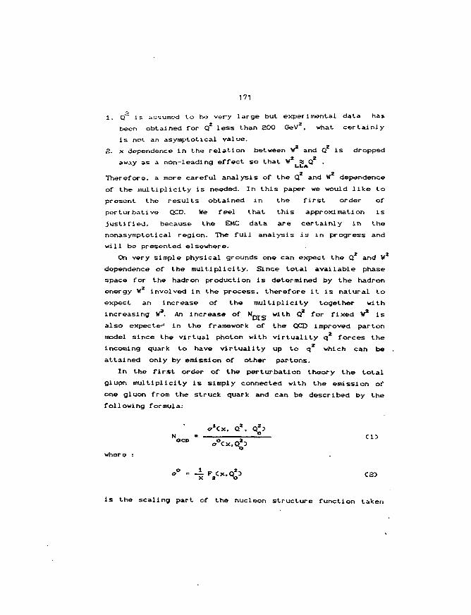
171
1. Q'~ is assumed to bo very large but experimental data has
been obtained for Q2 less than 3OO GeV2, what certainly
is not an asymptotical value.
2. x dependence in the relation between Vr and Q is dropped
away as a non-leading effect so that " 2U^ AQ
2 •
Therefore, a more careful analysis of the Q and W dependence
of the multiplicity is need&d. In this paper we would like to
present the results obtained in the first order of
perturbative QCD. We feel that this approximation is
Justified, because the EMC data are certainly in the
nonasymptotical region. The full analysis is in progress and
will be presented elsewhere.
On very simple physical grounds one can expect the Q and V
dependence of the multiplicity. Since total available phase
space for the hadron production is determined by the hadron
energy W2 involved in the process, therefore it is natural to
expect an increase of the multiplicity together with
increasing W*. An increase of N__s with Q* for fixed W2 is
also expected in the framework of the QCD improved parton
model since the virtual photon with virtuality q forces the
incoming quark to have virtuality up to q2 which can be
attained only by emission of other partons.
In the first order of the perturbation theory the total
glupn multiplicity is simply connected with the emission of
one gluon from the struck quark and can be described by the
following formula:
o'Cx, Q*. Q23
wher e :
4 F,c*-Qo> <=»
is the scaling part of the nucleon structure function taken
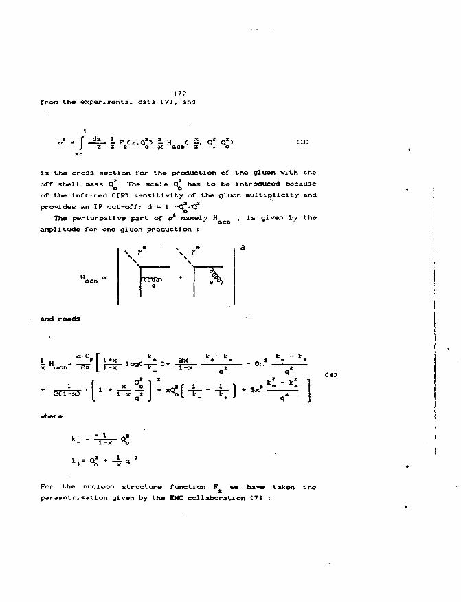
172from the experimental data [73. and
H C - . Q'aco z . C3D
x d
i s the cross section for the production of the gluon with theoff-shell mass Q2. The scale Q2 has to be introduced becauseo oof the infr-red CIRD sensitivity of the gluon multiplicity andprovides an IR cut-off: d = 1 +Q2/Q2.
The perturbative part of a* namely Hamplitude for one gluon production :
i s given by the
and reads
l r - ^ : ) * ^ ^ ]C43
where
For the nucleon struc'.ure function F we have taken theparametrisatlon given by th» EMC collaboration C7] :
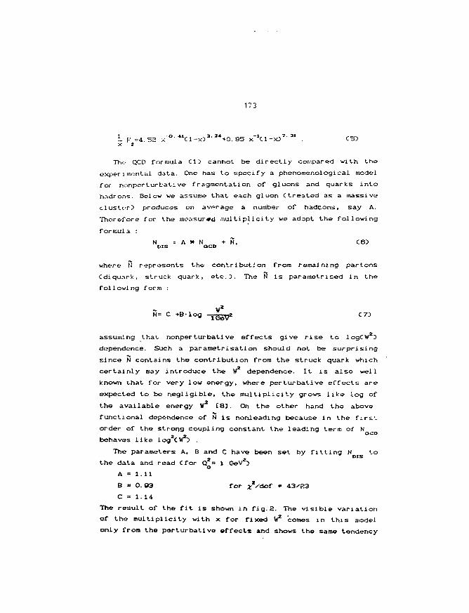
173
L F =4 52 x " ° " c i - x J a " + O . 85 x~*C 1-X}7 '31 . CSDX 2
The- QCD formula C15 cannot be d i r e c t l y compared with the
expenmivnlal data. One has to speci fy a phenomenological model
for nonporturbat ive fragmentation of gluons and quarks i n t o
h.idrons. Below we assume t h a t each gluon ( t r e a t e d as a massive
c l u s t e r ? produces on average a number of hadijons, say A.
Therefore for the measured .mul t ip l ic i ty we adopt the following
formula :
N = A * N • N, C6DDIS QCD
where M represents the contribution from remaining partons
Cdiquark, struck quark, etc.3. The N is parametrised in the
following form :
N= C +B-log
assuming that nonpar turbative effects give rise to logCW2}
dependence. Such a parametrisation should not be surprising
since N contains the contribution from the struck quark which
certainly may introduce the w dependence. It is also well
known that for very low energy, where perturbative effects are
expected to be negligible, the multiplicity grows like log of
the available energy W [8J. On the other hand the above
functional dependence of N is nonleading because in the firs',
order of the strong coupling constant the leading term of N
behaves like log2CW23 .
The parameters A, B and C have been set by fitting N to
the data and read Cfor Q2= 1 GeV*io
A = 1.11
B = 0. 93 for *Vdof = 43-^3
C = 1.14
The result of the fit is shown in fig. a. The visible variation
of the multiplicity with x for fixed W2 comes in this model
only from the parturbativo effects and shows the same tendency
as is seen in data. Also quite good agreement with the data
has been obtained. For comparison the dashed lines represent
the results of the Lund model C6]. The results presented in
fig. 3 have been obtained for Q 2 = 1 GeV2. In fact the
parameters A, B and C are Q dependent and their dependence is
depicted in fig. 3. The strong Q z dependence of A is easily
under z *. ood : the heavier off—shell gluon can on average
produce more hadrons. In the model Q 2 is introduced by hand to
separate perturbative and nonpertubative part of the gluon
cascade, so that the cancellation of Q dependence between A
and N is expected Cphysical quantities should be Q2
QCZ> O
independent 3. The stability of B and C as functions of Q2
indicates that such a cancellation really takes place.
Concluding, we have shown that the first order QCD
calculation with the proposed phenomenological model of the
hadronisation can explain the observed x. dependence of the
charged hadron multiplicity
Acknowledgement
I would like to express my appreciation and gratitude to prof.
S. Pokorski and to dr. J. Kalinowski for many stimulating
discussions and help in preparation of this paper and also to
prof. A. Bassetto for illuminating discussions during the
conference.

i . A. K^.utvtto. Uuci. Pliyt;. B203, 493 Cl 0033
.'.. A. V. Kisolcv, V. A. Pelrov, Sov. J. Nucl. Phys. 38, 13O4
C l £».':•<>
3. C. :.:h. tfchapai-idzo, A. V. Kisele-v, A. Petrov Sov. J. Nucl.
l-hyn. 3!5, 927 C19823
A. V. Kiselev, V. A. Petrov, O. P. Yushchenko, CERN
l_i ,..-py i nt CERN-TH-4684/87
•".. /.. PiJi ' i t to, M. Ci^faloni, G. Marcheaini, Phys. Rep. 100,
,:>'! ( v e «'.. Y... I . A-.-.imov, Yu. L. DokshiLzer, V. A. Khoze,
:~. 1. It cyan, 2. Phys. C2/ , 63 C19853
•:. t'.y.C. M. Ai r.oodc a t a l . Phys. L e t t . 165B, 22 C198S5
7. l-.w., . i .J . .".'berl a t a l . Nucl. Phys. B272, 158 Cl QGCO
ii. S . U a l a g .it al , Z. Phys. Cll , 283 C1982J.
,-• i t .'il i i-r i ivj i n t l i o o n c - p h c i t o n a p p r o x i m a t i o n .
• ' • '••!•• • hr i rg i - - : t . s d r o n m u l t i p l i c i t y a s a f u r . . . ' i o n of .< Cor
: ; . : -i-l V . I'-.-II.., . I-,., l a t e n f r o m t h e t'MC c o l l a b o r a t i o n [ 6 ) . Tl..v
'- ' : <l }.!..-:•. i i - ; - . - i r v . ' . t h e p r e d i c t t o n s ;.f t h e p r o p - J i t - d mowl .
•'•• !• • • I n . . - I . : : - , .-c-di.-.t j .-Jim C the- L u n d modtvi Ct.-kt.-n : r •.-,».
I i... / .
0 * f ' - i - .iJir..;..- t : M:o par.-iir.i-.-tf.i-s o f t h e m o d e l .
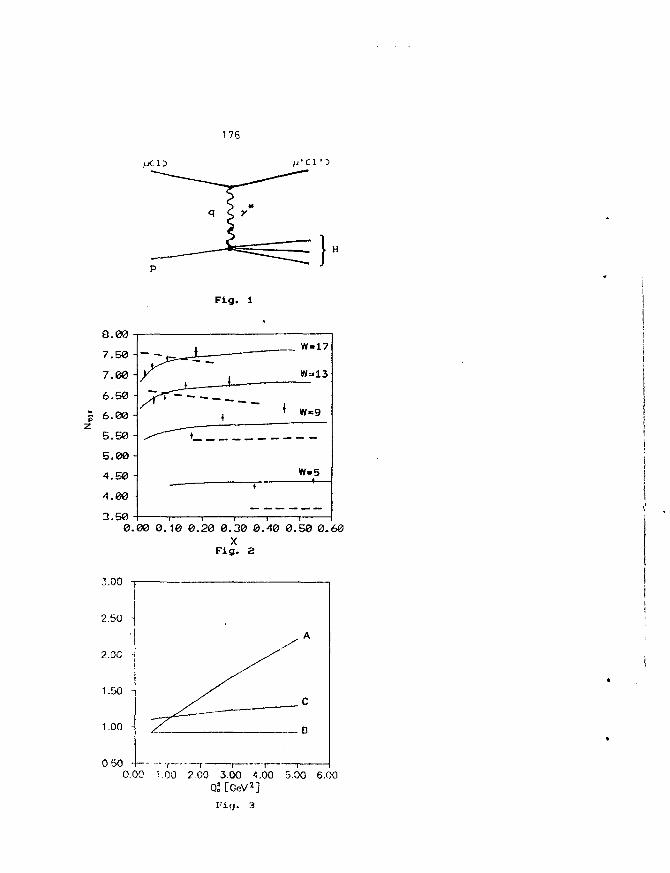
17G
Fig. 1
.00 0.10 0.20 0.30 0.40 0.50 0-60X
Fig. 2
2.00
2.50
2.00
1.50 -
1.00 -
0 500.00 1.00 2.00 3.00 4.00 5.00 6.00
Qoa [GcV1]
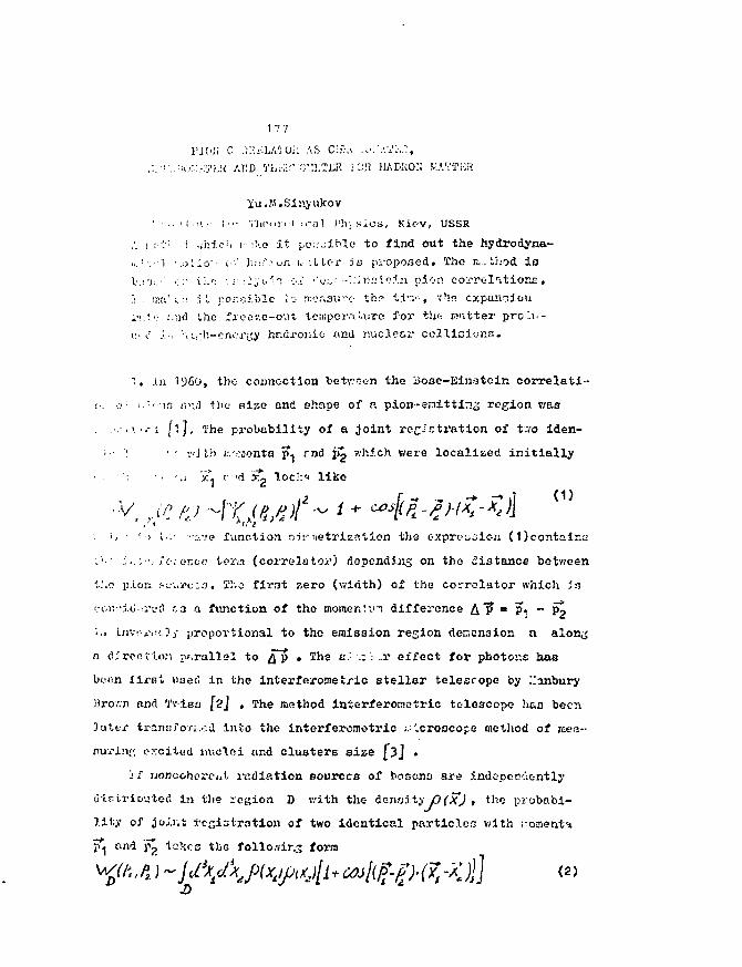
1 77
I'JC'Ji C :t".L.hA'iVli. AS C:!"v. .>.».'.-.*'i,.":,
Yu .M.S inyukov
• -... • i - • i . • !-• ' Tlu>..ri:l i r a i P h y s i c s , K i e v , USSR
'. ).:••':'• i ..'McM i•• :V.o i t j..o.;jiblo to jfind out the hydrodyna-
,./•. 1 :.oiio -- (••••' h^iV'on i.-iLtor i s proposed. The n,, thod i o
-.:•)..• •; ;• i;.f; -. • -Jjhi": -z-± :'<.•;.•• -J.'inr; t f i n piori c o r r e l a t i o n s .
-, IBUH:! i I ror.-aJ.ble io measure- th? t.i-:;--, T'IS cxpamiot i
••.•!••.• :.ad the fi GGv.e-oyt tetr.per.il.uro fo r tli<-: ETitter p ro l i i -
:•••: j . . . 'lU.^h-cnor/yr hr.dronic and n u c l e a r c o l l i s i o n s .
, in 1360, the coimoction betv/oen the iioae-Einstein correlati-
i : ' in a'-.d tlie Rise and shape of n pion-emittlag region was
. T J [ i ] . The probability of a joint rec-;ctratlon of t.vo iden-
• - vlth i./raonta p* rnd i> which were localized init ial ly
}-* r 'd j ; ^ loc!:5" l ike
<D
. ii•• 'o 1.-.' -:,y<? function rn's-ietrisation the exprt'^oioii (1)contair.s
'.'•' ;.. - •rli-i QT.tji) iori.i (correlatoi1) depending on the distance botv;een
\u? p.lon scure;.T. K'.o first zero (width) of the correlator which in
rori-io.-a-fil r.3 a function of the moiner.:-.n difference A"? «« p« " Po
'..j Lnv-i^'.Dy proportional to the emission region densnsion a alon^
n d.:rcotl.o:i parallel to p . Ths cJ -.; J -r effect for photor.s has
boon Ilrst uaetl in the interferometric stellar telescope by :ianbury
JJro-.vn and Tv.-isa [2] , The method interferonietric telescope lias been
jatt-r transformed into the interferonietric ;. .croocope method of mea-
nuriiir', excited m.clRi and clusters size f"3j •
j £ uonaoherciii lY.diation sources of bosona are indopcccicntly
u-lstrioutorf in the region D v/ith the donoity D(Xj , the probabi-
lity of joj.iit; registration of two identical particles with /-o
jl and f^ takes the follo.vir.3 form
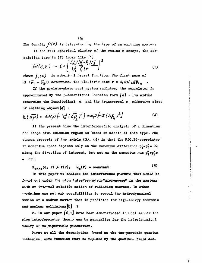
176
The density P(*) is determined by the type of an emitting system.
If the rest spherical claster of the radius r decays, the cor-
relation term in (2) looks like [i]
JM 2
v/here jt (xj is spherical Be33el function. The first zero of
S{ 11?.. - Pj>/) determines the claster1 s size r « 4,49/ }Kv\ „ •
If the prolate-shape rest system radiates, the correlator ia
approximated by the 3-dementional Gaussian form [4J • Its widths
determine the longitudinal a and the transversal r effective sizes
of emitting object[4] :
At the present time the interferometrie analysis of a dimentlon !
and shape ofo.1 emission region is based on models of this type. The
connaon property of the models (3), (4) is that the R(Q,P)-correlator i
in momentum space depends only on the momentum difference Pi'-PjJ
along the direction of interest, but not on the momentum outs p'
• 2P :
Rrest(Q» p ) * f(p)» Qo ( p ) " o o n s t* n t ( 5 )
In this paper we analyse the interference picture that would be
found out under the pion interferometric"mlcroacope" in the systems
with an internal relative motion of radiation sources. In other
v/ords,has one get any possibilities to reveal the hydrodynamlcal
motion of a hadron matter that is predicted for high-enor^y hadronic
and nuclear collisions[5J ?
2* In our paper [6,7J have been demonstrated in what manner the
pion intcrferometry theory can be generalize for the hydrodynamical
theory of multipartlcle production.
First at all the doocription 'based on the two-particle quantum
mechanical weve function must be replace by the quantum- field doa-
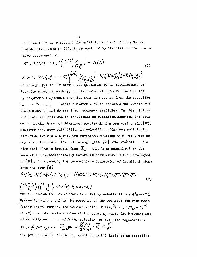
170
( T j . Lien *i }:<:n i..'.o account the multipionic Until otatea. So vli"
]'i-ob-iliiliti«•••' f'lieii UF. ("0,(2) ia replaced by the differential inclu-
sive c:-.-o.',«-rj'jction
,r
where R(p 1 (p ?) ia the correlator generated by en interference of
identity pious. Socoi'Av.ry, vc oust take into account that ^n the
hydrcdynciaie/il approach the pior; cm.i;-~ion occurs frora the spacelike
);yi :.-, u.rfncp Z. i v;here a hadronic fluid achieves the freose-out
tci.ipfi-.'iturc CO find docny» into .econuary particles. In this picture
the fluid clt.'wenta cuv. be conaidered Q S radiation sources. Tne sour-
ce;; generally have not identical opectra in its own rest ."ystira fip],
moreover thiy move with different velocities iv"(x) ana rndiate in
different tlTrico i <• t (x). T'1© ra^iifition duration tine A t ( the de-
cay tinto of a fluid element) ••:; negligible foj .The rof/iation of a
pi on field from a hypers«rf»ce 2LL have been considered on the
lui-cii of tho relativiatically~invariant etatistloal method developed
in[9J . .' i a result, the two-perticle correlator of identical pions
have the fora [6.]
(7)
hr cxprcof/ioi-i (6) nov/ differs fro:n (?) \rj nubatitutionas d^x ->
* U(im(x)) , ond by the presence of the relativlst ic kinematic
factor b-if-jT<: cotsine. The thcmial Sector £«(2jr)^(c?.p(py/T ) - 1)~1
in (V) iiuvc tho muxii.ww VOIMC et the point xg whex'e the hydrodynw;!ic-
c l velocity cir.I./.JCir v.-j.th vhe velocity o.f the pio« r ec l s t r a t ed i•-*• ii(x») zi _ P
Vf.o proconcc.. of a /,»v«.-lociiy grii-lltnt in (7) lcada to an offoctiva
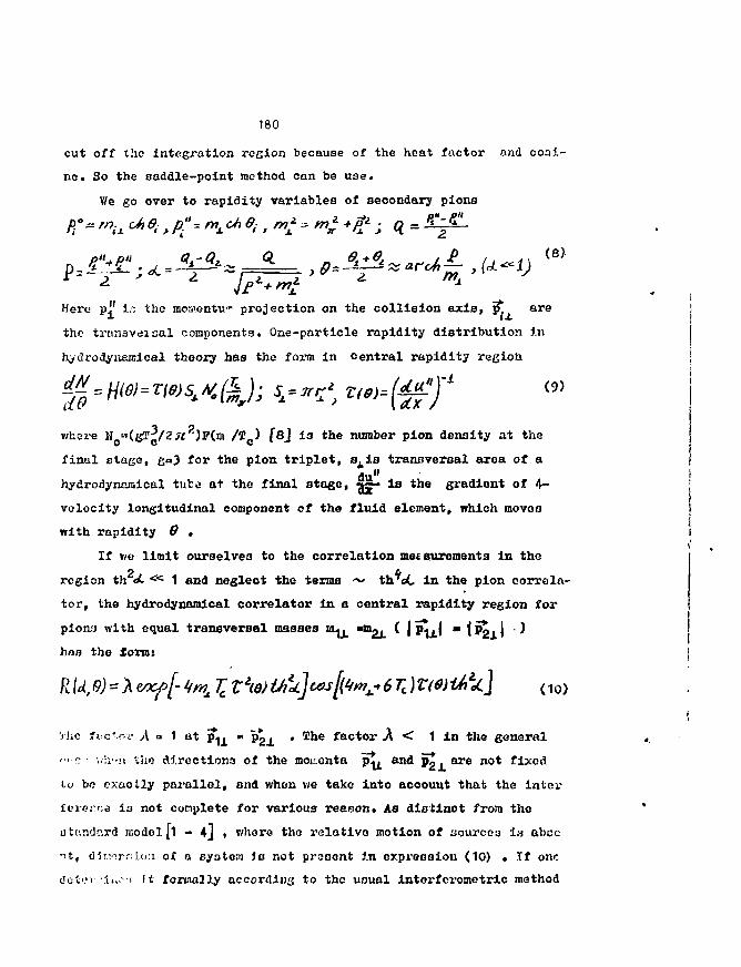
180
cut off the integration region because of the heat factor and cosi-
ne. So the saddle-point method can be use.
¥/e go over to rapidity variables of secondary piona
Here pi' i.r. the momentv!"' projection on the collision axis, p*! are
the trtmsvdisal components. One-particle rapidity distribution In
hydrodyuareical theory has the form in Central rapidity region
v/liore H "(gTp/2il )P(m /3?c) f8j ia the number pion density at the
finul stage, gcO for the plon triplet, s^ia transversal area of adu" '
hydrodyncnical tuta at the final stage, g-- Is the gradient of 4~ :
velocity longitudinal component of the fluid element, which moves )
with rapidity & . I
If y/e limit ourselves to the correlation measurements in the
region th d- <<; 1 and neglect the terms ~ th'oC in the plon correla-
tor, the hydrodynamical correlator in a central rapidity region for
piomj with equal transversal masses
has the form:
'j'ic fi:c'.r--f A = 1 at p!jj_ i pgjL • n e factor X < 1 In the general
' •> r: - -..-li'-.n the directions of the momenta p ^ and p^.are not fixed
ti» be exactly parallel, and when we take into account that the intei'
fererce io not complete for various reason. As distinct from the
attindard n;odel[i - 4j , v/hore tho relative motion of sources ia abec
•it, dlrvir/i i.o:i o£ a system Ja not prooent in expression (10) . If one
det'.'v-i,,,---! Jt formally accordiHi; to tho uaual interfc vome trie method
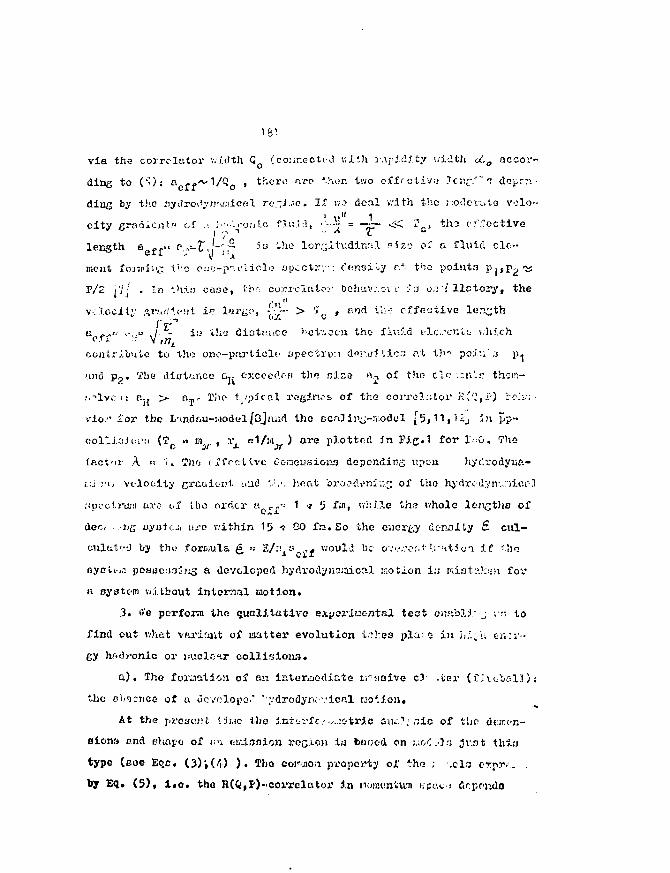
via tha correlator width QQ (connected Kith rapidity width oi.o accor-
ding to (^)s R rf'v '1 ' /Q0 . there n-po ihur. two offfctivo ?cr.c-J~^ doprn•
dine by the iiyilro^vnv.-iicfil re.-J.ic. If '.v.? deal with the MOderuto volo--
city gradient:.' of .-. ••• .-oj.i.c flv.'A, •-•- = - ~ << ?,,• t l« e l e c t i v e
length a , . . . f .„*-£..'-' ;~ '» i } i e Ioi\>tudiru2l ."ize o" a fluid clc—
went fonniiv' t':Q o.-io-pr.i'liol.? fjpcctr;•: Cunsxij c.+- t'ic pointn P j , ^ 1 ^
3?/2 |7j . In t'liH case, ih<' corrclntoj- bohav.\cvv :r3 o.Tt l l e to ry , the
v;Tccitv ar^fit^Mt if? l i r^o , • '}-• > 'J , and ti;-: efffiotivo length} > J
is the diatiaicc boV.vocn the- fluid E-lc^cnit \.h.ich
oontribuic to the one—particle .'jpectxu:; dRr.ji l i e ; r.t t!'" poi-.r. 3 p^
uno p^. The diolf.in.co OJJ cxcce<\cn tlio nir.e n.j of the t in ::.i\\;: them-
,'.->lv,- i: B.{ > n.jf Die topical re^inos of the correlator K;''''|.i"O veh". •
via" i'or the L-tndfxU-i'iodul Ojnud the ecali;^-:i.odol [5,11|"'ij in KP™
oolliajui'ii (T n m,.. , 1^ nr1/)'i ) are plotted in Fi.c«1 for l'.-:0. Tho
{ftct'ir A 1- 1. "ho effective ric-ricusioiis dependir^ xipon hyt'.rodyua-
r:j ru velocity crcuiont uiid t1;-- hP.nt bro.?.dt'?ii-.: of the h3"drc-d;;n-..v)icrO
;!pt-Gt.ruiii arc of tho order 1{-C,?£" 1 •<• 5 fuit while the whole longthe of
dec- :•}>(; oyaioi :u-o v;ithin 15 t 00 fn.So tho onor^y dc-nnXty S cul-
eul(it'-0. by the .formula g, >-• E / ^ s , ^ would l)c ov'.'.?cr.t.\;-'ttion if -ho
nyoi.i-;.-i posao.i.ii'jig a developed hydrodynojaical motion i:j rdst'.'.k^ji foi*
a system without internal motion.
3. tVe perform tho qual i tat ive expcriuc-ntal tcot cny.'oli: j, in to
find out v.'hat \-firitait of matter evolution tr?he3 pla^o IJI ii.l 'n en-:r--
Gjr hfidj-onlc or imclcir co l l i s ions .
a ) . The formation of a:a intorjjodiate tr-siaivo c3' .tei- (f;t<.bal1);
the obqcrico of u ocvclopo." ••ydrodywvical notion.
At the pro3«;it t^i.ic ilio j .ntorfc •.-..:c-tri.c aii;..1.';;ic of tho dtms-n-
sions and ehnpo of «ii oi.-.loninn rocion i.-a bnocd on i.,f/';.Or, Ji'.ot thi:j
type (eoe Eqc. (3);(/f) ) . Tho corujon property of tho ; xlr; orpr.-.. .
by Eq. (5) , i . e . the R(Q,P)-coi'rclator i.n noisunUvn wpec J dr.pr-ndo
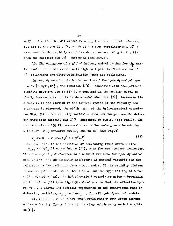
i e ?.
only on the morontvn difference 2Q along the direction of interest,
but not on the- yum 21? . -he width of tho sar.e correlator R(oi,& )
expressed in the repidity variables decrcr.nes according to Eq. (8)
v.-hen the rapidity sum 2 0 increases (see Pig.2).
b ) . The emergence of a global hydrodynamical regime for the mat-
ter evolution in the events with high multiplicity fluctuations of
>-p- collisions and ultra-relativistic heavy ion collisions.
In accordance with the basic results of the hydrodynamical ap-
proach [5,8,11,12J , the function Z"(0) connected with one-particle
rapidity spectm'^a via Eq.(7) is a constant in the scaling-nodel or
rlov.ly decreases as in the Landau- model when the ( 9 f increases (in
c.n.o. ) . If the plateau in the central region of the rapidity dea-
tiibution io observed, the width cLo of the hydrodynamical correla-
tor R( d., 0 ) in the rapidity variables does not change when the detec-
tci-pe.rticles rapidity sura 26 increases in c.m.s. (see Fig.2). The
r:••.:••) correlator R(Q,P) in Konien-tun variables undersoee a broadening
v.ith inc:- -.-.ainj momentum eum 2P, due to (8) (see Pig.3)
Q 0(W 0) n Qo(P0) / + P / m
\hi:.i ",i\-Q!j vi.ar: to the initatton of decreasing inthe aourc-..-a size
v- „ , ~ 1/Q (?) Rccr.v-.Ung to (11)» when the moraantuni sura increases ,
O'hur -iho v-;V "i.ty cii'"eronce i s a natural variable for hydrfxlynamical
r.orr..:!" to-r-.-i, r: • \ the aci-.-intum difference io natural variable for tho
.'ntorfev.v::.n -iho radiation icora a rest media. If the rapidity plateau j1
in o'^i.-;,; (tho J-.liac.u-ir.oclol Ier.d3 to a Gaussian-type fa l l ing of a ra-
r vM'.y c'iatrf'--, ' an) , t ) ; : ltydrofynrjiic?.?. correlator gains a broadening
n?.'itioi:5l io (11) (see P i g . 2 , 3 ) . v/e alno note that the effective hyd-
rct'.••".• . -ul lciv^tii hns specific dopondonce on the transversal mass oS
'k-tcctj..-•', pnrt. iclos, a, .* r*s ^/JiA^ , fox' a l l hydrodynamical models,
c ) . llto 'r;i .••i';: ': : hot ni'tirk-cluon matter iuto drops becauoe
of Jv-\;o tier :.ty fluotnationa ttt 'ie otngo of phase qg -» h trans i t i -
on f i i j .
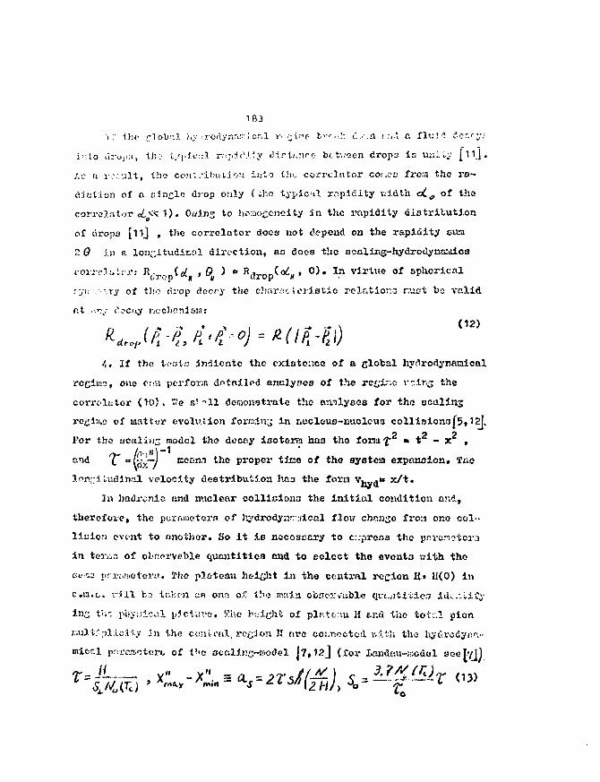
1 8 3
j ." t h e r - l o b r a i.v .rori}T.f..-.:.i.cM r ^ v - p &>•<••,-.:: Cs.a t , v i a f lu . "* , da.'y:
i';to droja, tli-:' l/pic:;! r'^iOX'y i!tnt/.nro btt-.-oen dropo in ujii^y [11J«
l.z u r.v.ult, the co.'itvibutioji it:to lii<_ corrcli". tor coi.ca fro:n the ra-
diution of a single drop only (iho typical rapidity width cCa of the
correlator oL« 1). Osvins to homogeneity in the rapidity distribution
of urons [ i i] , the correlator does not depend on the rapidity svun
2 0 in a longitudinal direction, aa does the ocaling-hydrodynsaics
correlate r : ^ ^ ^ ( ^ » Qu ) B R<irop(oii» • 0 ) * I n v l r t u e o f spherical
ryi.-v-iTy of tlso cU-op decry the charac ieris t ic relatior.a r.uiit ba valid
r.t .-. .,f ('ccny nechoni&m:
/,, If the testa indicate the existence of a global hydrodynemical
regiins, one <:.n perform dotnilod eaalyoea of the rc£;ir.e v-inj the
corrc-lator (10) . V/e s' "11 demonstrate the analyses for tho
i;oe of matter evolution Jfornin^ in nucleus-nuolouo collision3f5»12|.
For tho ocalin^ model tho decey isoterra haa the fona-f • t - x ,
and t "(g>r~7 nsean.T the proper tiiae of the system expansion* '£ao
loj\;.i ludin.-al velocity deetribvitioa hca the forn V ^ J B x / t .
In liadronic and nuclear colllciona the i n i t i a l condition and,
thereforei the pia-fimetern of Jjj'drodyarr.uicel tloxt chenfjo from or.e col-
lision evont to another. So i t i s neceseary to c::prcas tho pr:-ranotor.3
in terijs of ol.'fiorveble quantities cud to eolcct tho eventa v;ith tho
et-aa prruiuetovij. Tho pl&tcau height In the central recion IJ» H(0) in
c.a.L. •::ii\ b3 tfi5;cn afi one o.f ibv main observable qvt.atiiie.? ldc.-.iity
i«3 t'i': pi?\;;ical pjctuve. iChc hui^ht of pl:-tc'.u H tncl the totc.l pion
j:.u3.t:-!)licl•!•;>• In the c.miral, region 31 nro co:.rioctcd with the hyfircaynrv-
mical pRivjEotcrb of t»ro scclirs-tf-oclel (7,12j (for landau-:sodel
-Ji . y"
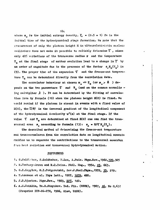
184
where BQ is the Initial entropy density, Ta • (0.5 * 1) fm is the
initial time of the hydrodynamical stage formation. V/e note that the
roaourc-ment of only the- plateau height H in ultrarelativistic nuclear
coilisior.3 does not moke it possible to reliably determine X , since
only 40£ variations of the transverse radius r and the temperature
Tc at the final stage of matter evolution lead to a change in T by
an order of magnitude due to the presence of the factor BJ.NO(TC) i*1
(9). The proper time of the expansion T and the freeze-out tempera-
ture T can be deternincd directly from the correlation date.
The correlator behaviour at chosen a^ =-> To (or m^ > 5 ) de-
pends on the two parameters T and T (and on the common normalis -
lTi& multiplier A )• It can be determined by the fitting of correla-
tion iata by foiciula (10) when the plateau height H(0) Is fixed. We
v.ould remind If the plateau is absent in events with a fixed value of
21(0), the V(0) Is the inversal gradient of the longitudinal component
of the hydrodynamlcal 4-velocity u^x) at the final stage. If the
value T and TQ are determined at fixed H(0) one can find the tran-
sversal area BX according to formula (13): B
x
The described method of determining the freeuo-out temperature
and transversalarea from the correlation data on longitudinal momenta
enables us to separate the contributions to the transversal momentumi
froa heat radiation and transversal hydrodynamlcal motion. '
REPSREHCSS~ . j
1. G.Coldl.rbcr, S.Ooldhaber, V/.Leo, A.Pais. Phys.Rev..I960.120.325
?. H.Hanbuxy-Brovm and R,Q.Twi3s. Fhil. Mag., 1954, £%, 663.
3. G.I.Kopylov, U.l.Podgorotski, Sov.J.Nucl.Phy».,1972, ,15, 219.
4. T.Acesson et al. Phyo Lett., 1987, 187B. 420. ,
5. J.D.Qjorkon. PJiys.Rev., 1983, S21» '40.
6. A.K.Knkhlin, Yu.M.Sinyukov. vnd. Piz. (USSR), 1987, £&, No 0,637
(Preprint ITP-C6-27E, 1986, Kiev, USSR).
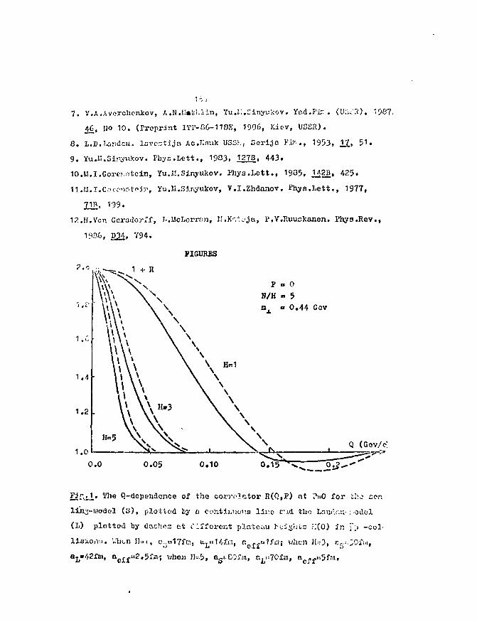
7. V.A.Averchenkov, A.N.I.iakUlin, Yu.L:.Sinyukov. 5fftd.Fi:. (U:^'.t), 198?.
/)6, Ho 10. (Preprint I?r-G6-118E, 1906, Kiev, USSR).
8. l.B.Landau, lsvc.-tija Ac.nnuk U35K, Serija ¥&., 1953, i l , 51 .
9. Yu.I".Siro'v.kc.v. Pliyc.Lett., 1933, 127B, 443.
1O.!,(.I.Gorc!.-;tein, Yu.H.Sinyukov. Phys.Lett . , 1905, H2B. 425.
n.M.i .Corc ' istPir , yu.IJ.Sirsyukov, V.I.Zhdanov. Phys.Lett . , 1977,
12.H.Von Gcrsdorrf, h.LlcLemm, J.!.K'-.ijja, P.V.Ruuskanen. Phya.Rev.,
1?36, D21, 794.
FIGURES
P » 0N/H « 5
a 0.44 Ccv
Q (Gev/c!
L'he Q-dependonce of the corre la tor R(Q,P) at TV.0 for thj ccf.
(S), plotted by a coatiMio'ia lij^.e cud tho Landr.u-:-odel
(I.) plotted by dachos et c'ifCerent plateau t'tigJits :.'(O) a'.n ".) -col-
ioiVJ. \,'hcnllai, c;.Bi7fni, u^i'Hfn, ne£tt*lfa; when H--?3, e.r'-ZOim,
-£-2.5xiS{ when II----5, Bgi.COxin, r.ji="i
2.0
1.8
1.6
1.4
1.2
1 + R 1&6
0.05
0.1
H - 3
H/H - 6
m, » 0.44 Ger
1.0
0.0 1.0 <s 0Zin.12.* T h e $ -dependence of the correlator R(aL , 0 ) at differentfor S-, h- models and the roat cluster (C) model (dots).
1 + R
H - 3H/H . 5m x • 0.44Gev
1 •—-~ -^— s<tev/c)
0.0 0.1 0.2 0.3 0.4 0.5 0.6
:•" -3. Yho correlator R(Q,P) at different vnluin P for S-,L-, anrt
C-i.oacln, She hydrodynamical S-,L- correlators at different valu-
ca P aio f-ppro";imated by i<ho olautor nodel v/ith different olaatej.-
radiii r1t1,3lm> jf9«»1 .-Vii, r-nO.Ofin. At P«O the curves of S-,L-,
C-raodolo i.ro indietlncuishable in the figure aoale.
18?
-i .vurj.;- .-.."., LiU.~<odcd .'.. K. , I'eii'OY V..'..
InclituSc fcr High Energy Physics
Lerpuknov,". otscov.' region, 142234,U3£3
1. j'iie uiiiu:u;;l properties of the G-jneson found in the 5t"p ex-
vrri-CLR;-/!/ i-^iiifoat t'nei:.selves, in particular, ir. the enhanced
rjT 1 dec.iy i.e-dc. In ref./2/ tho givc-i. property is related with
...>;c:.;,.- loi jiy li.r»_:c I'.'ori compo'ient of ihe fl -r.oGor/3/. Hecontly,
L./.C inclusive cross ccccion ox" t.'ie St° nnd n-;r.eson production
• :..: p'.cli;.: .•,-.:•>• estimates of xhe (^-meson yield v/ere obtained
:r. 5t~p interaction tit 360 GeV/c /4/« The unusually lcr^c (]_'-
;.'.j::oii LO'ouucticn obaerved iii t'r.i.3 cxperiir.eni requires a detailed
r.;.-.\y:: •.;• j;; ijic fraao of reliable r.oael. ?or this case ve ckcoce
L;:o :.ic.d-.'l Tor iiidusive hadror. product ion/5/ vriiich is rocs-ntly
c:Tcrcd b;,- us r.r.d based on the dual topologic&l unitftrisction
(i/j'li/ «chc.je '.vivh a quark-gluon picture of the hadron intersc-
tio:io. J'HG main results of the model are the following: 1) the
vj.loucc- quurJc concributicn is dominant in the fragmentation re-
;_-Io.-. of ••>.e initial hadron; 2) in the same region (x,-,3>Oi5) the
Oirt'ctly produced particles are dominant, so the contribution
:'ycr.. ihu higher rt-otjunces decay products can be neglected. The
latier, ;.t the acune ti!::e, explcino the essential difference in
Vho ratios of the f_ and 5t-uoson production in the cet.tral
region (where © 1 / 5 * * = 0.07 i 0.055, see ref./6/) and ir. tho
rrt-CiBentutiori one (where ihs sarse ratio is equal to 0.45 - O.C5,
see ref./4/).
2. Jhuij according to the rcodel/5/ the inclusive cross section
of the 5t and ft -mooon production is of the form:
188
where D0.rsJneter3 €i (s) and n-particle distribution function
t^ (x) of the quark i'in the hadron a were defined earlier/5/.Ci f ll *" —
The probability of the particle c emission from the sheet (ij)
•.VQS defined ir. the form;
:• =1/2(/Z 2 + 4m2c/s +z), z=2p»/^.)
coefficients /£ define the relative f]
lity of the quark i to the particle c. In our case:
The coefficients y3^ define the relative fragmentation probabi-
+ 1 ) -1 (3)
v.-hero >f is the singlet-octet mixing angle, -^=35,26? and the
ratio of the vector meson production to pseudoscalar one V/PS
is 1.3 /5/. Latter follows from the quark combinatorics ru-
lea. The parameter g was defined by us earlier (g =1.1+ 0.2)
v/hen describing the vector meson spectra in Kp interaction /5/»
V/e obtain the best description of the x-dependense and absolu-
te value of SC-meaon production (at x^0.4 at 3 50 GeV/C) at
g"=1.3 < which coincides within the error with t iose found ear-
lier.
As nay easily be seen, at high energy in the fragmentation
region of tho initial hadron probability (2) admits a simple
interpretation of the form of the fragmentation functions;
dz l^-D^^Cz) , z^-0.5
Theoretical curve (dashed line on Pig.1) for the directly
produced St-meson3 (using formula (3)) goes through experime-
ntal points at x^O.8 - just in the region where prompt 5C°
mesona are dominant. Ehe total SC meson production in the

169
rc.-.v,••••vi ' . . r u s p ' ' ' ••• i o c;-J ual .- i tcd V.;- a d i i ; . - t h e cor.*;ribi;t:".cn fro:-.
Vho dcc -v o-: fV- ' - . vvc ".} : . : . « : W , ^ :i!-.i ^ ' . - c L o a j ( t h e h • t - h a d
'.•:] v-"n:.: '',9.7 - 1.0 - 1.1 /'</. i'.-ien fit--'.:.:; tae c;;peri/"atai "'.e-
:;o;i prooucticn j."ji;i;a at x^G./ (curve 2 on fic.1) uning (3) v:o
obtain • •;.»»''(»f -*$) = 0.62 - 0.0? , which corresponds to vj> =
(_ iy i 3; •. Tni;; value coincides practically with the establi-
shed one -1o° (.'J'.;'J, TOZ exa:;iple, ref./V/;.
i'auc there ia KG asr«?o.::ent bev.veen JC° and I] -r.osoji producti-
on rate. In the case of comparison of fj' and n -r.eson one v;e
!i:;vn to i vpt-ci. : n t'ne fraiiie of usual h -tt mixing at *y = -17°:
i
i. = & /S"^- = ctg'Xsp-fo) = 0.60 (5)
.u.- a .li. i r . c l u a i v e exp.i ihr .fnt a- p-^.-.. = 360 GcV/o t h i ; i - c t i o io:
K = 3.6 i 1.3 a t ; ; > 0 . 3 , ( 6 ;
• i . e . eaci.r. 'cialy l a r g e r . •
3 . j.c - a.; t r y fco rci.,cve -ha di::." jrec?:"2':t bofvcc;.'. t h e t h e o r y
i-.:.u i-lie •.:-,or:;:.e:it;'.l ror-.-.l; ( 6 ; l''r t h e coj ;s id- : ; rs t ion oi' t he t h r e e
d:<::ci:::i o: :al j).ctL;>-e ci' t h e 1 _ ~ ^ " ^ '•'•"'"•-tVJ/'(V > vi'.iore one ir.tr.—
J iCi;.'j i.ti f:ddiuio::£.l s l u e b ^ l i co;;ipo:ii'iiv C- o_• :hcjo".i>".l t o -.•:o p l 1 - -i
::•':]• t~X. °---"1--i i'het. inclctad oi trie ov.l;/ ri* ^l-^:.-;>'•;;•'t i.-.ixiii^:;njle tiv:ro aTip;:..r three dli 'ierent ci-'. 1 or (like- the'Kulor 'a r*t>-ij3.ec/. L-.telr, one carried out ^r.e Mi-Si?sir/')/ in t.ie three d i -::.oi!sion:-.l ;^i:ci!, - picture of the r:)ark ca.:;po.iition of tl:o f] av.c
t|_ -i.-.e.'-or.:;, ij:>lleatinj cl^iost .vice- lo:::; cotitenis cf the iifjh'u,u-quiii-ka in t:i-3 iV-jr.ecou wave fvmctio:i cquurua |VjV->[ in co:..--r;'.rinou wici: the n -laoaon. i'his fact i s in e good agrecaent v/i :hrenuli/ (5/ ij" Oi o coKsideru the 0 , n -iseson pi'oducticn as arot-a.lt only of ihe u,d-quark Xrc^ncntatioti £rw the ir.itiGl had-ronpj but j'.t i s obviously in contradiction with rc.rult (6) . On
190
the othar hand ;just that r.nc.lysio/9/ reveals a considerable gluo-ball admixture in the f 1-meson W/3 |V /_i| ) and almostabaence o f t h g c l u e b n l l s- at e s in the 1^-meson C^O.05 lT\l 2> •
Then it follows that we have a possibility to understand both (5)
and (6) by taking into account the glueball component contributi-
on into 0 -meson production, which becomes visible only with in-
creasing energy.
4. The glueball states arise naturally in the D'WJ scheme cutting
off the diagrams witfe-handles in the 1/E expansion/10/ in the t-
channel (see Fig.2). Such diagrams join to the action on the two-
cylinder level and that is why they have a strong energy-thres-
hold dependence. How does one take explicitly into account the
glueball production in the frame of our "JDTU-standart" model/5/
(in the sense of cutting off only cylinder diagrams) ? For this
purpose we used the analogy with QCD. The two-gluon annihilation
is known to give the main contribution to the 1[c, f .JCymeson
produetion,which decay then into the J/y-meson plus photon. Prom
experiments we know the energy dependence x d<5 /dx|^_Q^'at Vs=
10-63 GeV, and thus one can derive the dressed gluon distribution
functions in the initial hedrons and also their fragmentation fu-
nctions into the two-gluon states (like glueballs) /1O/. She only
remaining task is to find the normalization parameter A. , corres-
ponding to the probability of the revealing cylinder with handle
instead of two cylinders at cutting off in the third order of the
1/2.' expansion. The unexplained anomalously large photon producti-
on rate effect in the SppS collider/12/ may help us* . V/e attri-
V-jitj the additional photons to the K-decay production of the
Cluebnll produced mesor.s. The lightest candidate for this role is
-he above mentioned (^-meson, and thus there is a possibility to
She cumber of photons is expected to be approximately aqualzo the sum of charged SC-i.iesons fro.T the naive' isotopic invari-ance. i'his sta cement is right for the low energy, but in the OppScollider 30,i-exceeding of the photons have beer, found.
191
present the "iipp-J-ef fcct"/12/ as a result of reaching full capa-
city Glucb-.ai actic;:,- ••.Die trace has hardly been perceptible et
;-.!.O GeV/c. .Then v;o obtain by the fit to the photon inclusive spe-
clruro c.t V^T = 540 0c'/ /12/ (see Pig. 3) ia accordance with pre-
script: on/10/ ^ , = 0.03 - 0.01. The daeliad curve corresponds to
tn<? tot«!l photon production at the Ul.K energy Va = 6 IcV (3er-
]:iik.iov,UJ;>iC) i v/iiere the gluebtll mechanism £S~*1 -• )f+.. .yields
:,L'iv timti half of the observed photons in the pseudorapidity in-
terval
i i cue comas buck to P l at= 3^0 GeV/c with the obti.ir.ed value
X r= 0.03 one is able to calculate the glucball meciiar.isii- cor t r i -
kution in the reaction 5C"p-*t^X :6 ' f^g^(x^> 0.3j = 0.12 3b.
J:ii.c value di:ninishca lightly the discr-rp;.:.cy betiveen tiiecry tn-i
••por J^ci.t/.;/ (0.52 mb ai.d 2.9 - 1 o ir.s.rccpec-ivsly}, j;\i i t c.-.r.
. o; rewovc i t completely beceuse of conoeritre.tion of t.ie sluubr-ll
contributicti iii t.'io central region of the n|-:i.ason speot:-.;jr..
thus if further iirocesair.^ of the datf. cr. l '-meson productior.
does not decrease preliminary result (6) then the nev." phenoneron
tiscurti it". 5t~p—*0X, which can not be explained even by att'rc.c-
lins the ^l^sball mechanism of the rf-meson production.
5. Acknovvlodyeineuts.
V<e ave pleased to acknov.'ledge iS.P.Kistenev, M.L.Hekrasov, V.A.
otopcaeriko and V.R.Zoller for interesting discussions.
References
1.3inon ?.et aa.-Sov.J.Yad.Piz.39(1934)831S.Gcrshtein 3,o. ,Likhoded A.K. .Prokoshkin */u.D.-3ov. J. i'ad.?iz.
39(1904)2513.iiovikov V.et al.-Kupl.Hiys.Si65( 1950)554.Aguilar-Benitez i,'. et al.-Preprint C*ai:/iiP 36-165,Geneva, 1336•']. :iatanin A.V. .Likhoded A.K. .Tolstenkov A.ii.-Sov. J.Ytid.Piz.
42(1935)4-24O.Ar.oRson :i. et al.-Preprint CiiSi;/ P 86-34,Geneva, 19867..'.pol W.j.et al.-Phyg'.Lett.833(1979) 131;. .iT.-iciiiro Kav<ai-Phys.i-3tt. 12.-',3{1 f33)262>l.Jo.'::ier J.-i-.iys.Sev.D27( 1933) 1101
:>..ltru£3aitis a.il.et al.-rnys.?.ev.D3?C19S5)283310. jnojuin ik.V. jjjikhoded A..u. ,Petrov V.A.-Preprint IH2? 66-233,
.Sn.vj.u',;!iov,19S6n.Cai..i.-llu A.,Iran Thanh Van J.-a.Phys.010(1931)243
Kfiidilov A.3. ,2cr-i.'.artiroayaa K.A.-Phys'.Lets. 1173(1932)247iJ.lbo Coliaborution.nlpgard J..at d.-Phys.iiefc.i 15.'j(1^cJ2)71
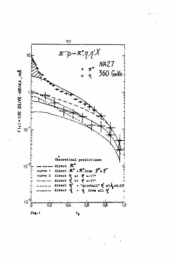
Theoretical predictions:
L — direct 5C°p curve 1 direct 31* +5t#from P + & ?~^ curve 2 direct r at «f »-17°i- direct lj[ at >f .-17°
direct 1 ' + "glaeball" l( atJLidirect 1 + 0 from all f)|
10-3
direct
1
.0.0?j
• I . ,
0Pi«. 1
0.2 0.4 0,6 0,8 1.0
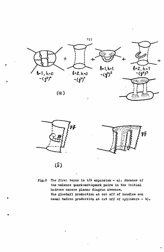
(a)
(S)
Fig.2 The first terms in 1/N expansion - a). Absence of
the valence quark-antiquark pairs in the initial
hadrons causes planar diagram absence.
The glueball production at cut off of handles and
usual hadron production at cut off of cylinders - b),
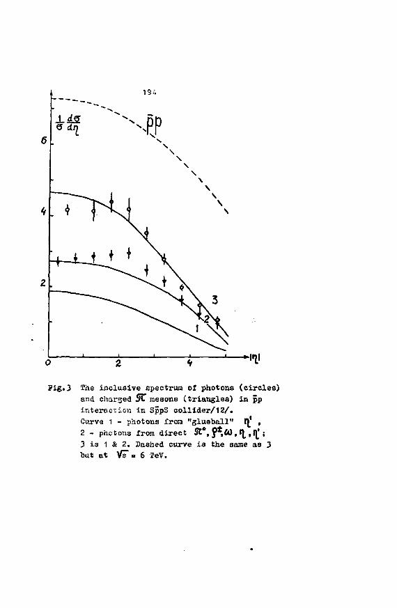
\
Fig.3 The inclusive spectrum of photons (circles)
and charged SC mesons (triangles) in pp
interaction in SppS collider/12/.
Curve 1 - photons from "glueball" fj| ,
2 - phctona from direct St°, $*,<*}, <\ ,lj|;
3 is 1 & 2. Dashed curve is the same as 3
but at VS~= 6 TeV.
NARROW DIBARYONS
Bekkzad S. Yuldashev
High Energy Division
Physical Technical Institute
Tashkent, 700084, D.S.S.E.
Ab.itr.ict
A short review of recent experimental data on
search of the narrow dibaryon resonances is presented.
196
1. INTRODUCTION
It is well known that tbo problem of the possible existen-
ce of dibaryon resonances is not & new one and is discussing
from time to tine for a long period [i-vj . In last decade this
question has been raised again and mainly due to observation [6]
of structures in cross-section differences between parallel and
antiparallel longitudinal ( A C L ) and transverse ( A 6 ^ ) total
cross sections in pp interactions <\s well as froa polarisation
measurements. These results and data from other experiments [7-
-9] (see also references in [1Ctf ) can be interpreted as a ref-
lection of the possible existence of'D^, ?« and 16^ proton -
-proton resonances with masses about 2.14, 2.26 and 2.4? GeV
and with rather high ( T Js 100-200 Bar) widths.
The indirect evidence for dibaryona elso comes froa an ana-
lysis of data on the production of so-called cumulative secon-
daries £11,12] ,i.e. hadrons produced into kinematical region
forbidden by kinematics of scattering on a single nucleon bound
into a nucleus. In addition, the flJC-effect f3j does not con-
tradict an assumption of the existence of dlbaryons or 6-
-quark bound states. The similar conclusion can be drawn froa
an analysis of high four-momentum transfered scattering of nuc-
leons on the light nuclei [14 J •
Froa the theoretical point of view there are no serio-
us objections against dlbaryons. Indeed, several models like,
for example, the quark bag model [15J , the model of nonadiaba-
tic rotational bands [161 , the string model p7J «** aomo others
predict the existence of multibaryon resonant states.
In this report I will present a short summary of recent expe-
197
vi:.:cntal rcr-vltr* pC-'fiJ en search of n>rrow ( P £ 50 I'cv'j non-
~sli\.-ji;;r. (iibiOj'o.'s resonances in h^Jron-nucleus said nuclooa-nuc-
loor. luAV-ictio:::> in the primary monc.itum rango v<.= (1.0-.JO0)
Go//c. The evidence for direct observation of narrow dibaryons
cane out now from launy oxperiacnts performed with primary pion,
proton and heavy ion beams at different energies and many typos
of targets.
Dae to space -limit in this review I have restricted oyself
by consideration of low-mass (M 4 2 ^ t )*r ) dibaryon candida-
tes. More information about dibaryons with masses U>2.1 Gev
can be found in
2. DI-PHOIOK MASS SPECTRA
The routine way to look for dibaryons is a study of effec-
tive xa£S distribution of nucleon pairs produced in nucleon scat-
tering or in interactions of primary particles with nuclei. Froa
this point of view the bubble chamber experiments have some ad-
vantage. Indeed, in this case selecting protons stopped in the
visual volume one can reach a good accuracy (^ 1-2 yi) is the ao-
montuJ" determination of protons viimX Beans one rill have a rela-
tively high effective nass resolution.
2.1 IKTERAOTIOirs WITH HOCLEI
Apparently, the first indication on the possible observa-
tion of narrow dibaryon signal caae out froa early bubble cham-
ber experiments £18,193 i*1 which the two-proton correlations had
been studied in hadron-nucleus interactions. There have been se-
en narrow peaks in the distributions of two-proton effective
nass spectra at U(pp) s* 1.92 - 1.95 GeV. However, due to United
198
statistics an interpretation of these peaks 83 possible sig-
nals o£ diproton resonances was doubtful.
Recently, the new high statistics data were reported [21-Mj.
Our group has looked £i9»25,26,56,40,413 for diproton resonant
atatos in or"12C, p20!*, P1^O, d12C, <rf12C and 012C - interac-
tions in the primary momentum range from *• to 500 GeV/e. It
turns out that Independently of the type of projectile, its ener-
gy and a sort of target In the H(pp) distribution there are nar-
row peaks exceeding a background for more than 4 standard devia-
tions. Is an example Figs 1 a,b show the U(pp) distributions in
X~12C at 4 and 40 GeV (data at both energies are combined) and
in p^Te interactions at 500 GeV. The dashed lines represent cor-
responding background distributions obtained by random ***?*^
of protons from different events of the given type (Jf C or pHe)
but at fixed proton topology in final state* It should be stres-
sed that in this analysis no cuts nave been applied to emission
angles of protons and their momenta have been restricted to In-
terval 0.22 i pn 2 * 0.40 GeV/c. In tills range the momenta of
about 92 % of secondary protons were determined by range in a
bubble cLuriber. That leads to the resolution in determination of
U <pp) to be less than 2.7 HeV.
As one can see in both types of interactions at U(pp)=r2»r,
1922,1939 and,poo3ibly, at 1930 Uev there are narrow peaks which
become statistically more significant if one combines together
the *~C and plfe data (Fig.ic). The first peak at H(2p) = 2m^t
as it is w e n known [42-44] , is 4ue to the final state interacti-
on between secondary protons. The other peaks can be interpreted
as a manifestation of narrow dibaxyons.
199
'ii)-.' :>i:oolj-- l ine re?rer.aatc tï-a np;>r>o::is>ation of tho coia-
l-iHcU ;: U'l>) distribution v-;th t; ; nun of ivro .'^clt-v/i^cr
function.-; «n.l i:ho bacV.jj.ound cpccfcrca. In result of approxi-
mation ( , / ^/ .'j>r eO.Ô1) for tho nacuoo and widths of possible
dibaryona was obtained
« 1922 Î 1 . J lieV, r , = 11 i 3.6 ISov;
= 19*0 i O.'f «cv f., = 10 t * .5 KoY
It uliould be uodcrliQod thst the probability to describe
the txpcriiBsntul I!(PP) distribution by the smooth curves (sbo-.vii
3n iiG-1=) l ike f(3')s KZ** expf ~ ' ^ Z • f Z2)J , wbero Z «
= Ji (2p) - 2ni , i s too low {J^/Y.jj - 2.6 when K i s 2ixed by
no;«iali::<ition condition to the experimental nucbor of combina-
t iens , end > 2/jI.I),P. = 1 . 7 v.îiea. K i s free) . ïhs pa ais ore
ctwj-lLi'ü over baclcgrcuna for 'f.1 CJÎA ^.5 standard deviations
at iys 1922 îîoV and KgsiCVO KoV respectively.
•i;io r.iuilar results were obtained by our Group £3&J la
i!-.c .••.i.'i.v.ijs cC scni- icdusivc rasctic. : (p,d, c< , C) • 12C —
-•-pp •» X at 4 . 2 . GeV/c. ïîiece daîa co::2 Tron ." .& iaa propane
bul'Mo chrsotr crcposc-d ct Dubtux accelerator to heavy ion beasts.
Fic.2 Î;:IOV.'S tlvj ii(pp) epecï" • obfcaiasd for d:X£erent corAiaafi-
ons of prAto-i i ' . ira. Tl.s :"c:'.?>.ins notcüiOKs have been used :
p e - slow protors, hovlni; wxienta. of 0.2 â pÄ 0.5 GsV/c; p f -
« fact jn-o'vor.c nith nor:uva 0.3 £ pssO.7 GoV/cj iü c H i t i c n ,
)? (pf.) »Sims e l ' . protens oaittcd iu^o ror.vaxM. (baci:*..£ i )
hci-*iipher: ar.<*. p . (pS) - fest protons ecittcd sc §- - «c 90 -
(%a>, ^ 90*) in the laboratory systen. Only c-vcr.ta coacaining
at lesr-t one yrnscsi eiiitted into bae'erard heaisi^are wore con-
sidc-r^r'. As one ceo s»^ froa K.ß.2 there are ceals as
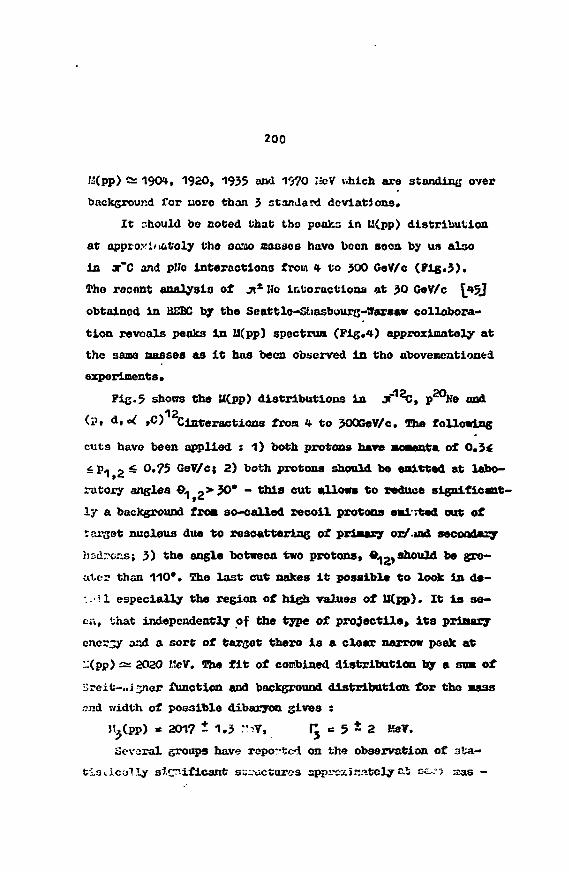
200
K(pp) 2:1904, 1920, 1955 and 1970 IJeV tvhich are standing over
background for uoro than 3 standard deviations*
It should be noted that tho poaks in U(pp) distribution
at appro"inatoly the oaao saosos havo boon soon by us also
in x'C and pMo interactions from 4 to $00 GeV/c (Flg.5).
Tho recent analysis of jt* Ho interactions at 30 CeV/c f45j
obtained in BEBC by the Seattlo-Shasbourg-Warsaw collabora-
tion reveals peaks in U(pp) spectrum (Fig.4) approximately at
the same masses as it has been observed in tho abovenentioned
experiments.
FiG-5 shows the U(pp) distributions in Jt"1 ;, p^Ke and
(Pt d, d ,C) Ciateractions from 4 to JOOGeV/c. The following
cuts havo been applied : 1) both protons have aoaenta of O.5i
~ P1 2 ~ °*^ Ge7/c; 2) both protons should be eaitted at labo-
ratory angles <^ 2> ^ ° * " t b i a c u t * 1<>"* to reduce significant-
ly a background froa so-called recoil protons emi ;t«d out of
target nucleus due to rescattering of priaary or/utd secoodasy
•lidrons; 3) the angle between two protons, p f should be gre-
ater than 110*. The last cut makes it possible to look in d«-
.. il especially the region of high values of U(pp). It is se-
en, that independently of the type o£ projectile, its prinary
energy and a sort of target there is a clear narrow peak at
::(pp) £s 2020 I'eV. The fit of combined distribution by a SUB of
;;r-eit-..j ner function and background distribution for tho mass
and width of possible dibaryon gives :
Jt Cpp) = 2017 i 1.3 riT, V5 = 5 * 2 KsV.
Sevsral groups have reported on the observation of sta-
tistically siCTVificant s«_%ac»aro3 apprcxi-rately r.S EC-.-; :r.as -
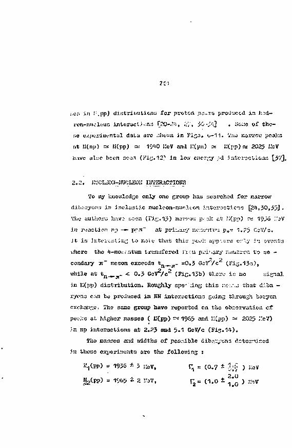
01
:.<j.s in !\pp) Ui«trii»uticna for proton aa^rs produced i a h:;d-
rcn-niiclc-uc interact.'*-n.', PPO-.?"';, ',:',, '/u ->'J . Scio of thc -
iio c/.j>ciliiiM.intal data ure ,;hov.ji in Pica. o-11. VMO narrow pca
tit «(np) =* M(pp) =•• 19'<0 !:cV and l.!(p«) a «(rp) « 2025 l!o
Ji.ivc alue been nc-'i-T (i'i(;. 12N in low C3iejy,y ;>4 5n1:cr3
2.2. i:xiiio:ir«uotBoi: IIKSRACTIOHS
To iry imowlcdGe only one croup has searched for narrow
dil»;:iyo;>:; in ine l a s t i c nuclc-on-nurlcon i^tc
l'htf auLJioi-j havo .'ioen (i ' ir-15) nara-ov; x
in jvaction np -»• pr.n~ at primary ricrJCitiTi po-r 1.?.5 C0V/0.
J t i s 3ntfj:<.;;t.jni; to no I t tha t th i s v-cvi: appiavs or'.y in c-voni:.-;
i;hcrc the 4-moj:> ntuia tranafcred Jxria pvi'iary nuucrcu to se -
condary 3t~ ncson exceedo *n^_J t- =0.3 Cfc'/Vc
\7hlle a t t j j ^ ^ - ^ 0.3 Goi^/c2 (FiC«13b) there i s no signal.
in M(pp) t l ictr ibution. Rongh-ly spe' any th i s r.c-:.-.j tha t diba -
vyona c:<n b« pi"od«ced in HI? in terac t ions G^i-n3 tlaroush baryon
exchange. The soiao group have reported on the observation ct
pvil:s at Mglier nassea ( li(pp) — 19&5 and U(pp) ^ 2025 .".cY)
.'•n np interact ions a t 2.23 and 5.1 GeV/c (Fij.i-'t-).
Tho oarincs and vAAt'aa of posr-ible dibaryons dotcr.-iir.cd
in thcao experinsnta are the following :
= 1955 * 3 :^.Vf i ; = (0.7 ± 2;i; ) ;«sV
* 2 !.^V, T^= (1 .0 i 1 [ ° ) I: V
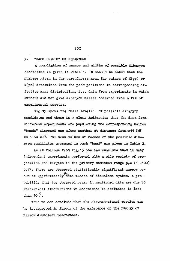
202
3. "MASS LEVELS" OF DIBARYOHS
A compilation of masses and v/idths of possible dibaryon
candidates is given in Table 1. It should be noted that the
numbers given in the parentheses mean the values of M(pp) or
M(pn) determined from the peak positions in corresponding ef-
fective mass distribution, i.e. data from experiments in which
authors did not give dibaryon masses obtained from a fit of
experimental spectra.
Pig.15 shows the "mass levels" of possible dibaryon
candidates and there is a clear indication that the data from
different experiments are populating the corresponding narrow
"bands" disposed one after another at distance from os15 MeV
to oi 60 Me-V. The mean values of masses of the possible diba-
ryon candidates averaged in each "band" are given in Table 2.
As it follows from Fig.15 one can conclude that in many
independent experiments performed with a wide variety of pro-
jectiles and targets in the primary momentum range po~ (1 -500)
GcV/c there are observed statistically significant narrow pe-
aks at approximately same masses of dinucleon system. A pro -
bability that the observed peaks in mentioned data are due to
statistical fluctuations in accordance to estimates is less
than 10""7.
Thus we can conclude that the abovementioned results can
be interpreted in favour of the existence of the family of
narrow dinucleon resonances.
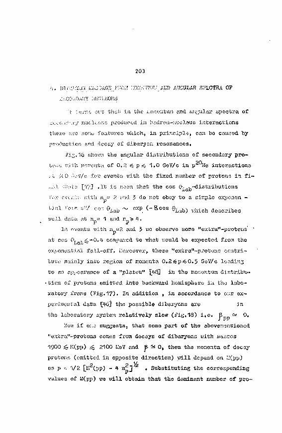
203
OF
::'t '•ur.'iG ovt that in the L-.o/x-ntun and uri»;ular spectra of
-I.I.O.I:-••.!-•,/ nucltor.o produced iu badro:i--nucleus Interactions
there arc none features v/iiich, in principle, caJi be causod by
pvoOucticn and decay of dibaryon resonances.
JTaG-'i sjhov.'G the angular distributions of secondary pro-
to.is with i-.o^cuta of 0.2 $ p ^ 1.0 GeV/c in p Ke interactions
; I; ;X0 .VoV/c :Cc>r events vdtli the fixed number of protons in f i -
;.;..'. ;i;;u:c: £ir/J »l't is noon that the cos (?•- ^-distributions
!>:e ovci'-.t:-. v:ith ri ••- ,? ;.incl 5 do not obey to a simple ejajoaon -
lirJ. i"o^. ^/ co" 0 I iab ~ exp (-&C03 9 i ( a b ) s M c h d e s c r i b e s
•.veil data at n. = 1 and r. > 'I.
In events with iXj-2 and 3 v;e observe some "exbra"-protons '
at cos Oj. ^^.-0«-'t conipai'cd to what v;ould be expected from the
oxixmou.ti.KL fall-off, Ho.voover> these "extra"~protonc
Vutc mainly into region of nonenta O.2£pso0.5 GeV/c lcadins
to an appearance of a "plsteu" \ttfQ in the moi*.entum distribu-
• tion or protons eaitted into backward heinispliero iu tho labo-
rafcory iCroras (Fig, 17). In additioa , in accordance to our ex-
periwental data \46] the possible dibaryons are in
the laboratory systen relatively slow (?ig,18) i . e . B,_n ^ 0,
Sow if or.o suggestsi that somo part of the aboverientioned
"extra"-protons coiaos fi om decays of dibarj'ons with masses
1900 <~ f.iCpp) ^ 2100 MeV aiid f ^ O, then the iaoaenta of decay
protons (omitted in opposite direction) will depend on ii(py)
as p =. 'i/2 [H2(pp) - 4 nip J z . Substituting the correspondiog
values of U(pp) we will obtain that the dominant number of pro-
2CU
tons from decays of possible dibaryons should be in the ran-
ge 0.2 ;£ p 0.5 GeV/c, i.e. in the recior; where we have ob-
served th-j "extra"-protons.
Another evidence for the existence of narrow structures
in the momentum spectra of secondary nucleons also cones from
the precise measurements performed with use of lov/-energy pi-
on beam at TRIUilF £4-93 . In this experiment the momentum
spectra of protons and neutrons emitted out of the Carbon nuc-
lcua after absorbtion of slow Jr~ mesons have been measured.
rhe narrow structures in the kinetic energy distributions of
protons and neutrons have been seen (Fig.19). The authors
claim that the evident structures observed at 50>60 and 70MeV
"...can. not be exhaustively understood only in terms of the
t'.vo-nucleon absorption model".
By arrows in Fig.19 I have shown the expected positions
of structures appearance of which one would see if there is a
contribution from decays of slow (_p=* 0) dibaryons with mass-
es mentioned in Table 2. As it is seen, the expected values
of nucleon kinetic energy aLaost correspond to the posi-
tions of the observed structures,
Xhe author3 of this experiment [47J claimed that struc-
tures below the threshold of reaction JT~(2N) -*- WS (like
x+ci ~t~ pp, jr~d-f mi) can. be ascribed, for example, to
nrvutroiis coiains fron pior. captures by o^-clusters with the
aouteron o;id one of the aeutrens acting as "spectator" respec-
tively. In my opinion this hypothesis contradicts data on
the observation of carrov; peaks around IJ(pp) 2^ U(pn) "*
=;1940 and 1965 UeV in np and pd interactions
205
<v.:-i the discussed structiuvs rather could be a reflection of
a production of dibaryons.
'j. OIT TIlS HPIN_ OF DI3ARTOKS
There are no conclusive results on spin (J) and pari-
ty (P) of possible dibaryon candidates and the main reason forp
this is relatively low statistics. An attempt to determine J
for dibaryons with masses H(PP) = 1922 li-'V and M(EP) =1939
I'.'ICV has been made by our group [46J . Fig.20 shows the cos •& -
distributions of decay pi'otons after substraetion of background
in the rest system of dibaryon with a given na33. The angle -Q-
was determined as an angle between the vectors of the total di-
bitryon momentum arid the aomantum of one of decay protons. There
ii. possible indication of non-zero spin for both resonant sta-
t!ss. The curves in Pig.20 represent best fits of data by func-
tions correspondins to the J^-states : 1~ and 2+. As one can
ace for dibciryon candidate tti M(P-P )' = 1922 15eV neither 1" nor
2 ccm be ruled out, while for the second candidate at H(PP) =
= iyW MeV the Jp = 2+ state looks preferable.
The similar analysis have been carried out for dibaryon
candidate with the mass M(HP) = 19S6 I.'eV in Ref. \?2] . The
authors conclude that this possible resonance can be conside-
red as the two-proton system in P-wavo state with the total spin
J = 2.
6. M B WIDTH 0? DIBARYONS
As it follows from data in Table 1 no unambiguous conclu-
206
sion can be done on the width. , P , of possible dibaryon
candidates because of large errors. However, it seems that
for all discussed candidates the value of P is not greater
than several tens of MeV.
7. CONCLUSION
In many independent experiments there were observed the
similar narrow resonant-like structures in the effective
mass distributions of nucleon-nucleon system. Since the
positions of these peaks and their widths do not depend upon
either the type of interaction (HN, hA) or the primary ener-
gy these results can be considered as a strong evidence in
favour of the existence of narrow dibaryon resonances.
I would like to thank S.A.Azimov, V.U.Chudakov, E.L.Fein-
berg, A.B.Kaydalov, L.A.Kodratyuk, G.A.Leksin, E.M.Levin,
V.A.Liatveev, I.Siemwrczuk, S.Tkaczyk, A.A.Yuldashev and P.
Zielinski for helpful discussions.
Special mention must be made of the truly excellent
organisation of conference at Kazimierz by A.Wrdblewski and
his colleagues from Warsaw.
207
1. G.A.LelUiifl, JVeprl:ii. ÏTHP ;J «54, Moscow, 1971.
;2. l.ï.n.!.:;i.karov, UcpdOù Fi.-;, îiayk (U1W), \^> (19U2) 135;3ov, Phys. Ur.p. 2^ (19»::) U3.
3 . A.Yokooavia , Phy3.Reporta, M (1980) 47.
'I-. K.K.oot'h, 'j.'j-lk given at 198'i V/ox-kfäliop en Hlochron and Rio-
taii Interact ions at î'odiuii Energios, Bonn.
5. B.Tatischcff, Report IPHO-Mîu 85-19, Orsay, 1905, presented
at the XI th Europhysics Cont. ,July 1-5, 1935, Par i s ,
li- I.P.Auer et a l . , E;/i,.r;ov.Lctt. 41 (197S) 1455; .ibid ^1
(197U) 358»
I.P.Auer et al. ,Phys.Lett. ,2OB (197/) 475;iMû 67.B (1977)
I.P.Auer et a l . , Phys. Eev., D2'+(1981) 2008
7. K.Hidaka et a l . , Phys.lei-t% 22g (1977) 479-
8. T.Kamae et a l . , Pbys.Rov.Lott. ^8 (1977) 463.
9. T.S.Bhafia et al., Pbys.Rev.Lett. ±1 (1982) 1135.
1O.E..a\ii.i;-.cheffet al., Report IFOO-oas 85.1*., Orsay, 1985
11. A.M.Baldin et al., Sov.J.IÏucl.Bij-s.i-ï (1975) 79.
12. A.U.Baldin, Prop.of tho XX-th lat.Conf.on High. Eaei^yPhysics, ïokyo, 1980.
G.A.Lelcsiai, Preprint ITEP, If 147, Moscow, 1978.
V.V.Stavin.-;3ci, Elem.Part. and Atoiaic Ifticl.,8 (1977) 429.
15. J.J.Aubort et a l . , Fnys.Lst t . , 123B (1983) 275.
A.Bodek et a l . , Phys.Rev.Lstt. JjO (1983) 1431; ibid 21
(1903) 534.
K.G.Arnold et a l . , SLAC-::ab-3257 (1983).
14. 1. \.Kondratyuk, in the book "Hucloon-ïïuclooa and Had on-
208
-Nucleus Interactions at Intermediate Energies", ed.A.A.
Vorobijev et al., Leningrad, 1984, p.402.
15. E.L.Jaffa, 2hys.Rev.Lett., £8 (1977) 195.
P.Mulders et al., Phys.Rev.Lott. f(O (1973) 15*3.
V.A.Uatveev, P.Sorba, Nuovo Cim., 11£A (1978) 217.
16. K.H.Mao Gregor, Pfcys.Rev. D20 (1979) 1G16.
17. M.Iraachi et al., Prog.Theor.Phys. 55.(1976) 551;
ibid. 51(1977) 517.
18. V.S.Verebryusov et. al., Preprint ITBP-273, Moscow, 1964.
19. S.A.Azimov et al., Sov.J.Hucl.Phys. 19. (1974) 317.
20. B.S.Aladashvlli et a l . , ïïuol.Phys. A274, (1976) 'tô6.
21. A.A.Bairamov et a l . , J1HR Preprint PI-83-2O7, Dubna, 1983.
22. T.Siemiarczuk et a l . , Phys.Lett. 128B (1983) 367; ibid.
1-äZp (1984) 434.
2jJ. V.V.Glagolev et a l . , JIHR Preprint EI-63-59? 1-83-556}
PI-S3-565» Dubna, 1983. Sov.J.Nucl.Phys.40 (1984) 482.
24. K.Beshliu ot a l . , JIÎJR Preprint DI-83-815, Dubna, 1983.
25. S.A.Azimov et a l . , Preprint PII 27-84-FVS, Tashkent,1984;
Sov. J.Nucl.Phys.42 (1985) 913.
26. S.A.Azimov et a l . , JETP Letters, 40 (1984) 316.
27. V.B.Aüakisliiev et a l . , JliSE Preprint, I-84-103, Dubna, 1984.
23. B.Tatiacheff et a l . , Phys.Rev.Lett. $2 (1984) 2022.
29. V.V.Glosolev et a l . ,2e i t . f.Piiys. 3J£A (1984) 335«
50. K.Boshliu et a l . , JIIJK Preprint, 3JI-85-433, Dubna, 1985.
31. K.N.Krmakov et al, .Preprint H 1039, Leningrad Inst.Hucl.
Fhys., Leningrad, 1985.
32. O.B.Abdinov et a l . , JIHR Rapid Cc N 15-86, 34, Dubna,
1986.

•j$. /..I..'-.--1.in c t ; i l . , JiN1? ;-::ti:t>iv., ig (193-J> -'-OS.
;".•>. V.V. ' . •..•.- .v e l i=l., Kc:L. = -\ P h y s . , £ ; . _ (TVA>)
;>;>. j.'u.A,'J'roDaii, JII!i? P r e p r i n t , 1'2-8S~35, J>a"ui.a, 1906.
••.:. i:.:./.\j>wv c t a l . , r . \vor in : . : VH 5J>-S7-J!"Vii, a?a.';hix«n*
i>7. V,A•'•...'.vXvcrv f t a l t , i n the boolc:"IT?? aad Hadron-ITuclcus I n -
t.'.-J-..ot.'.oi'!!j a t Intor.~i:.i:ip.l-o j-Morcica", od.A.A,Vorobljuv e t
a ! . , .Tcn.i.r-j-o.d, 198G, p . 8 0 .
i/b. /.,;:, !v.!.-o;:.o./..;•/, I..7:.yitr.-.:lcov:;;y, .is: t he boo;: "HIT and hA I n -
i."u:iv..ot.P-0"". .it ir-x< •:::-3.ii'i:;c >• ••cr^ieo", ed . A.A. Vorobijcv e t
;•.!., L::nir ; :rr;d, 1'JsS't, p . ? .
;>V'. ' . J ' . i ' i ' o b ' i j - v i ':..l,£'--tr:-::o/;;):y, r.i! tho fcc-o?: "Hi? yoc. nA J. Vox.*
^ i K C i r L; Inl.3jvvc.di.-ta J^rcr^ ies" , r.d.A«A.Vorobij;v r/.- ''?.••.
7'. :i.' " •. i. u'i j IQc'ibj ';''«!?•
•'iO, J-..'J/.i'10".f;i^v, Pj.>octo£ t-iio XVH IOib.Sj's,.on '.,\:\1 ^xnsx-'cl "Xe
JJjrjja;-.ica,. Sccv.iJJkel, A u s t r i a , 16-20 Jiuie 1936, 3:d. i ; , : . .ar^-
tri.'i ct ;CL,, Vfe.fld Sciont.Pub,, SiiiGaporOf 19^7, p.7C9t
"A. l:-.S.\vlu>:.'-:;vt Talk Given at tbo I I ViorJcsliop "Quarka and
J- .1 <.•!", I-::!:lr^.v..df 20--24 April 19f>7. xm
-V. ::.,.••,. •.uon.in-.l'.tiy:,. Let t . 2SS. (1977) '&<
•';>. ij.'x3*.3<••:'.>)•', . ' . V.'.pob].--,v.j3d., p r i v a t e r o - : . i ' i : i c a t i o n .
' ; r . . S .AtA ' / s ino ' . ' e t a J . . , P r e p i r i J i . * lfT:r. • i^-37-X-•» r :", ' •'•"•: .. -:^ ..
'V/. )-..L./.n^..:-Mln et a l . , Sov.J.ITucl.Pliyo.^S. C19"!>-} t'S;?,
'•.':•. r,:'-,/iJ..rX>cj.il:hi ...t i l l , , Sov.J.Macl.Kiys. J>9_ ('"iSS'O B;0.
•':';. O.Cc-:. ?.;.lJoi c t a l . , Pi'erir.v.-.t; liJSj'y.VB-8a'9» .Hcf.icio dr 'Uric:;-
tr>, 1902.
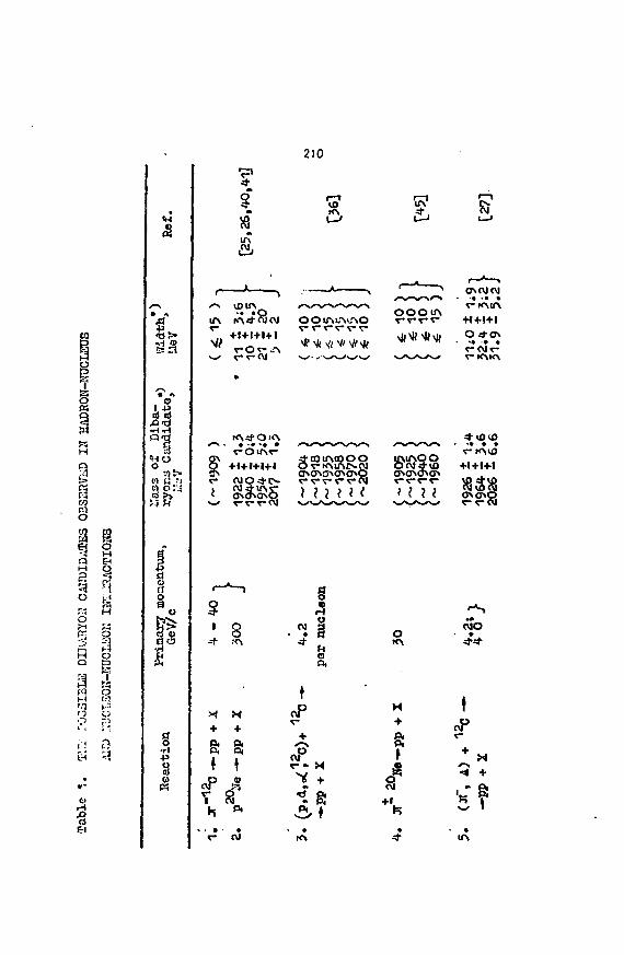
I
&
210
s te.a.
ONOJOl
+1 + 1+1
8.3
2 §
f
oTo
a a
• • • - •
ScxP
+1
«if
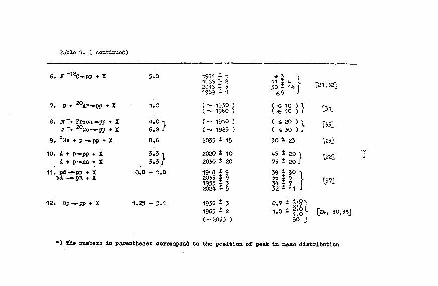
Table 1, ( continued)
6. 3T "12C-*pp + X
7. P + 20Ar-»Pp • X
3 • JT + Fxc on * pp + IX"+ 20ffo—pp + X
9. ^He + p -~pp + X
10. d • p—pp + Xd + p-»nn + X
11. pd-*«pp + Xpd - * p n + X
12. np-*pp + X
5 . 0
1 .0
4 .0 - ,6.2 J
8 . 6
3.3 i3.3/
0.8 - 1.0
1.25 - 5.1
1961 i 11SGS - 22015 £ 51939 - 1
( ~ 1950 )( ~ 19&0 )
( ~ 1910 )( ~ 1925 )
2035 £ 15
2020 £ 102030 £ 20
1948 £ 92055 £ 91953 £ 32024 £ 5
1936 £ 31965 £ 2(-2025 )
{%( £( 6
30 1
45 *75 *
39 ;
8?32^
0.71.0
4 1;1*J
10 ) \10 ) J
20 ) I30 ) J
• 23
• 20")• 20J
in+ 3«QT
50
[21,52]
[31]
[33]
125]
[223
137]
[24, 50,55]
•) The numbers in parentheses correspond to the position of peak in mass distribution
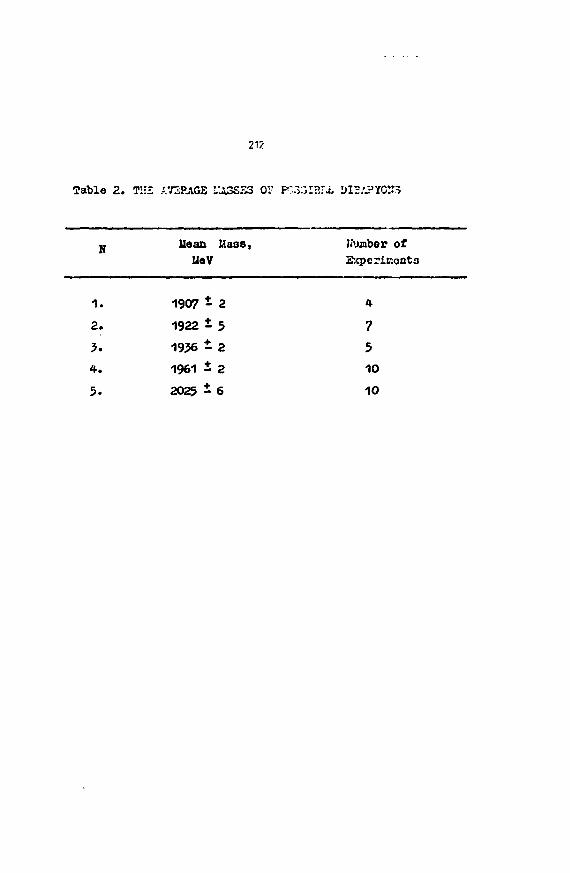
217
T a b l e 2 . 711Z AVERAGE "JV3SH3 OV PC3:3II>ri.
K
1 .
2 .
5.
4 .
5.
Uoan Uass,UttV
1907 - 2
1922 i 5
1956 i 2
1961 £ 2
2025 £ 6
1< unbox* ofStpcriEonta
4
7
510
10
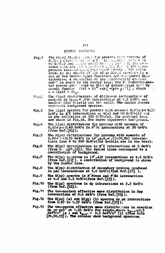
213
FlOU'iS OAV-i'I'ii-'J
Wg.1 The J.:(ip) d i i l r l t .in;:; for p r o t c o v-.rh *-?r«:rta ofO . 2 2 t j ' i û . ' i - ' i'..'./f j r J('C i^.^-;..Ui'.-;-. 1:-••.-.'( \"O' * o G o i ' ( t ) i u i u ; . . ; . : . f cc<i'..-.ic-<:•• .•: y<j~< ) v . t-.-j c c > -
„•^i w o ; ;.n.-l ..'i ?' '• . ' . l i e dr.' C 1.1 r. .«, ro—iprevent, C0Viv.:jVC'i -n ;; tv»(:-;\v."C .'?
curve i a the rc::nlï c-f *"it of cc-foiivji. upc-ctY-yi 5 / aou.a of tv;o MreiU-'-icacr fui«tio!»a Aivl l>"•c; aroivMÎ d iû -tT.ibution. A pi'(..iici:icn or ti'.o ::it"r.X' i cleat* er.; «-fi'iaM«lr\ iu OJJOVM t'.v the dotted l i t te . rihù à'• h-donMî-dot-ted curves co;v - nond to fit1; of o^parii ,*atul ùr..v: by
(a) s K::" c^p [ -(^'/.* y > ' ) j . wJ
KA4;.;J ÏJie li(]»i>) rtiaï.vibucio.no of difrcj-Piifc cor.bAnatiovs ofprotona in (p.ci,<< ,C)C intcractio. is a t ':.2 CcV/^ Pûi*nucloor: (for d e t a i l s see tto^ i:cj:t). The dashed CJXvesre;irc:;onl; l;acksround spectva.
Pig.5 The L'.(pp) spectra for protons v.ifch po.rieiu« O.?Zn-p& 0.75GcV/c in 3fC Interact ions ac 4(a) and ';0 6cV/c(b) r;.->din DHO colDdsions a t 300 G^V/cfc). ïhe ccabiaod d
/ c in 3fC interactions ac 4(a) and ';0 6cV/c(b)in pHo colDAsions at 300 G-;V/c(c). 'She ccabiaod dasaare shcvoi in Fißöd. ïbe curve icpresents oac'öi-caiid.The J-(cp) distribution for protons with aoacnta af0.22tfpïs0.4O GeV/c in jr l l e intoractions at 30 GeV/c(from Kef. [453).
Fig.5 Tho !i(l>p) dictri'jutioas for protons with soaenta of0.306-> £0.75 GeV/c in (jr~fp,d,o< ,C)+(C,Me) interac-t i o n fron 4 to 300 GeV/c(for detai ls see in Vbo t ex t ) .
Fig.6 Tho Ji(pp) dir.i-ributions in Or~C interactions at 5 GeV/c(from Kc J ^ 2 1 , P 2 3 ) . Ihc dashed l ines correspond to acontribution of background.
Fig.7 The U(pp) sj.>jctrua in (Jr~,A)C interactions a« 4,2 GcV/c(fron fief.g7J). A contribution of background i s shornby the dashed l ine .
Fig. 8 The li(pp) distribution of secondary protons producedin pAr interactions at 1.0 GeV/c(froa Bof.[31] ) .
Fig. 9 The U(pp) spectra in j f Fréon and *~tio interactionsat 4.6 and 6.2 GeY/c(fxoa fief.{>3]).
Fig. 10 Th« ll(pp) spectn» in dp interactions at 3.3 CeV/c(froH Bef. p23)
Fig.11 The two-nucleon effective aass distribution in Hepinteractions at 8.6 G*V/c (fron Eef.£23j).
Fig.12 The U(pn) (a) and U(pp) (b) spectra in pd interactionsfro» 0.97 to 1.37 G«V7c (fron Hef.[37j).
Fig.13 The two-proton effective m s s distributions in reactionnp 5fBP*~ at 1.25 GeV/ç for events_«faere ^»^.,-^0.3Ge?2/c2^/a ) «na tjM. < 0 . 3 GeV^c2 (b) (fron Refa
C24.30.35J ) . Tbe crosses snow backeround spectrum.
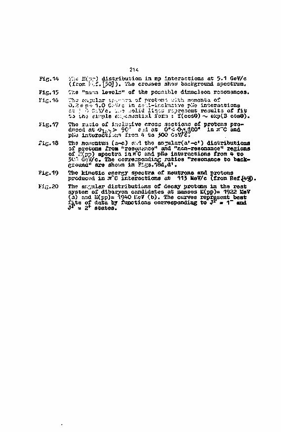
7U.^ '--e I!(?r) distribution in up interactions at 5-1 GeV/c
(from i-',f.[3Oj). i'lio crosses show background spectrum.Fig. 15 CL'i;e "aar.3 levels" of the possible dinucleoa resonances.FiG.16 '-b» wijUlar %:-,••--V-J. of proton- -..•j.'ch momenta of
0,?.sn-i1.0 C;-V/c in. cc-i-inclucivc j>I«o interactionscu • *'; o:.V/c. V.J? .;olid U K S rcpre.'soat results of f i t*;o the- sinple e;:.'Cwntial I o n : f(cosO) ~ ezp(B cos©).
i'ig.17 Ilho rajio of inclusive cross 3£ctio:is of protous pro-duced 4t •Oi-,%> 90' c.:d at 0° -Oj<ft80* ia JT~C andpl.'o interact; ij;i"J froa * to j>00 GoV/c.
Tic.13 Tha mo;i;entu;3 (a~c) c.i'l tho as^ularCa'-c') distributionsof protons from "rasonw.ee" and "non-resonance" regionsof "(pj>) spectra iniTC and pita intoractions fron 4 to3C" GcV/c. The corre^pondiric ratios "resonance to back-ground" are shovm in Pis3.18d,dl.
Fig.19 The kinotic energy spectra of neutrons and protonsproduced in aTc interactions at 113 UeV/c (fron Ref{4-<Jp.
iG.20 The angular distributions of decay protons in the restsystem of dibaryon candidates at masses li(pp)= 1922 ileV(a) aad K(pp)= 19^0 I'.eV (b). The curves represent bestfits of data by functions corresponding to Jp » 1" andJ* a 2+ states.
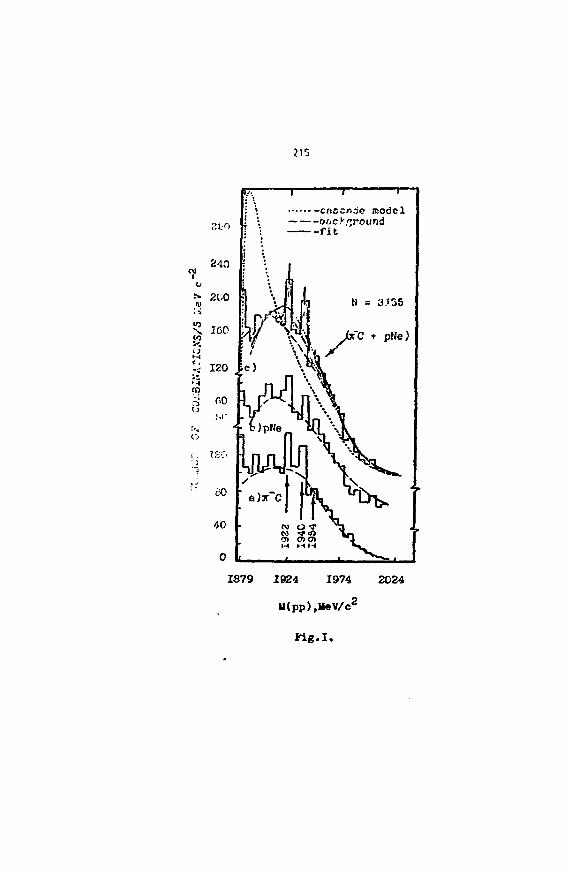
-cnocncio modelbticy.groundfit
1879 1924 1974 2024
U(pp),ileV/c<i
Fig.I .
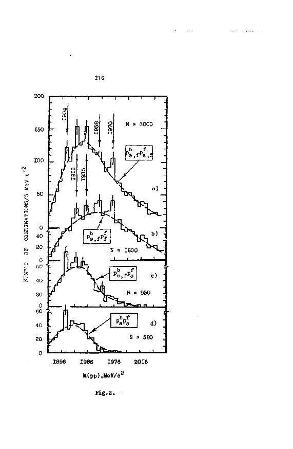
216
200
150N = 3000
d)
N = 580
1896 1986 1976 2016
M(pp),MeV/c2
Fig. 2.
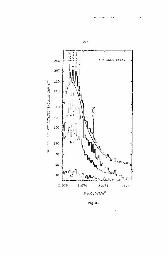
217
0)O
OO
pto
oO
120
dO
10
1.879 2.074
2
1.974
!-i(pp),GoV/c
Fig.3 .
£,.174
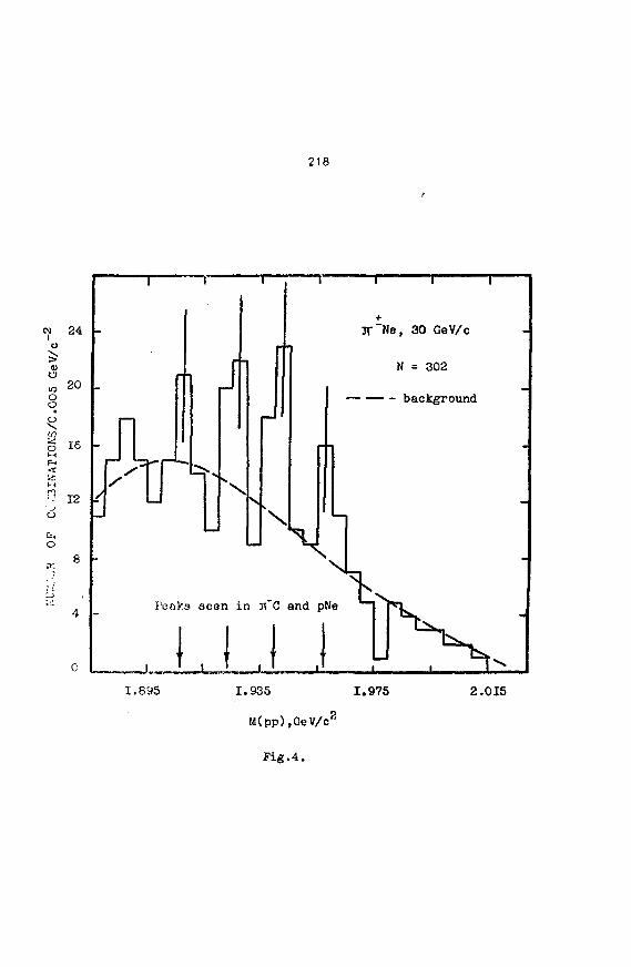
218
egi
u
0)
o
).00
J
v?
F-i
M
O
24
20
16
12
n Jl
\
3T"Ne, 30 GeV/c
N = 302
- —— - background
Peaks seen in 3\"C and pNes1.895 1.935
M(pp),GeV/e2
Fig.4.
1.975 2.015
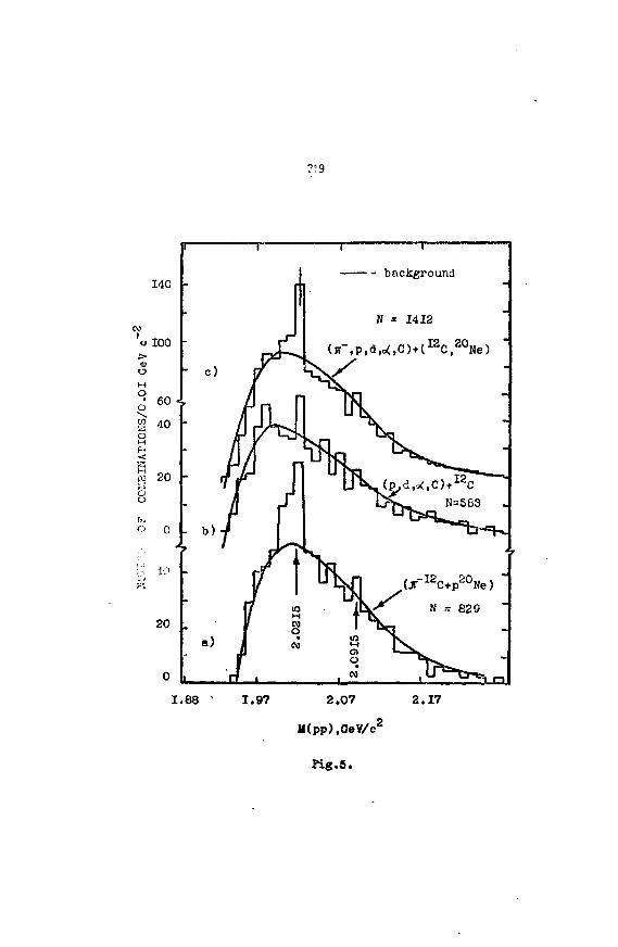
O i Q
140
o 100>OM
o
« 20
o o
20
1.88 s
• - background
N = 1412
(jr-,p,d lO(,C)+(I2C,20Ne)
1.97 2.07
M(pp),GeV/e2
2.17
Fig.5.
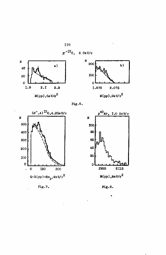
220
40
20
0
I .
[• 19
lA\
2 .
M(pp)
X
a)
v1 •
I 2 .3
,GeV/c2
C, 5 GeV/c
M aXV
200
100
r\
I . 875
M(pp)
b)
2.075
,GeV/o2
Fig.6.
(jr"",A)I2C,4.2GeV/c ATI
p w Ar , I.Q GeV/c
100 •
. 0 ISO 300
Q=M(pp)-2m ,
F i g . 7 .
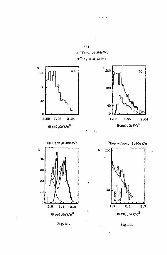
221
OX' "t'rcon, 4 .6Ue V/c
3T~Ke, 6.2 GeV/c
I2C
60
40
0
a)
Sr T_• i • i
1.88 1,96 2.04
M(pp),GeV/c2
K200 .
120
X.88 1.96 2.04
•• 9 .
dp-~ppn,3.3GeV/c
X.9 2.1 2.3
M(pp),GeV/c2
Hep-^-dppn, 6.6GeV/c
K 100 f
10
1.9 2.3 2.7
M(NN),GeV/c2
Pig.10. Fig .II .
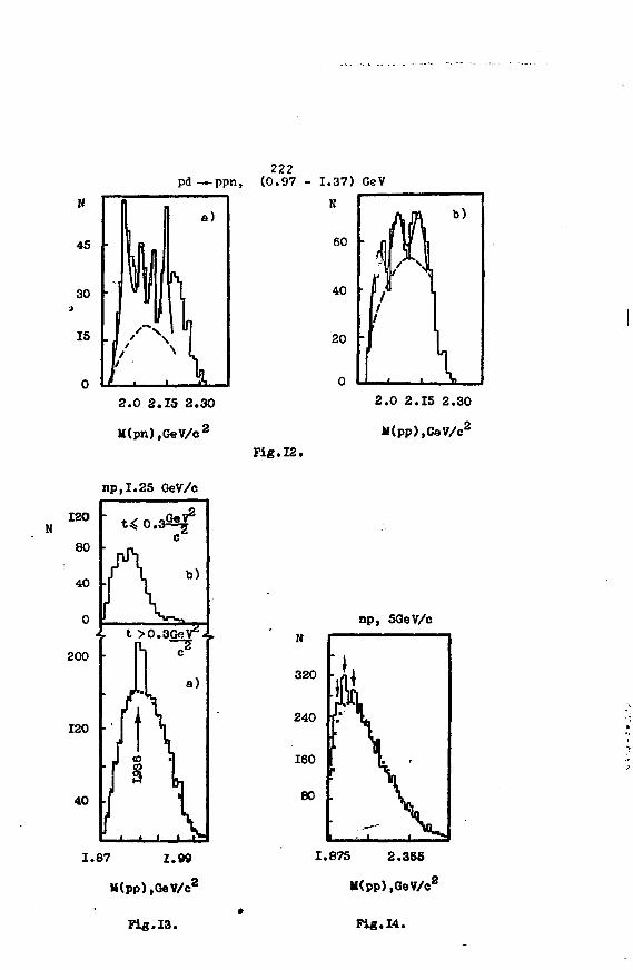
222pa—-ppn, (0.97 - 1.37) GeV
2.0 2.15 2.30
U(pn),GeV/c2
120
80
40
0
200
120
40
np,1.25
' t«0
Ar ^, t >0
n
I Ij S
GeV/c
gGeV2
c
b)
.SGeV2-c
a)v\1.87 1.99
M(pp),GoV/c2
60
40
20
0
Ah
f•
1 , ,
b)
1
t\2.0 2.15 2.30
M(pp),GeV/c2
Pig.12.
np, 5GeV/e
160
80
1.875 2.355
M(pp),GeV/c2
Fig.13. Fig. 14.
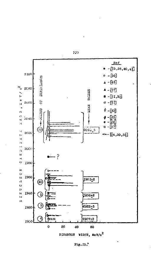
223
2IOO
CMo 2C60
(U
to
2OG0
2040
2O2C
M
2000
53M
i
-. a
202j.5
Ret
© -[25,26,40,41]
o -[36]
a -[21,32]
a -[Si]
0 -[33]
a -[31?]
-=—{24,30,35]
aoM
o
O
1980
I960
1940
o-
1920 .©ft?1900
1961+2
6+2
922+5
j 6=== keo7+:Li I I I i J > , —|
0 20 40 60
DIBARX0N WIDTH, MeV/cS
Fig . 15 . '
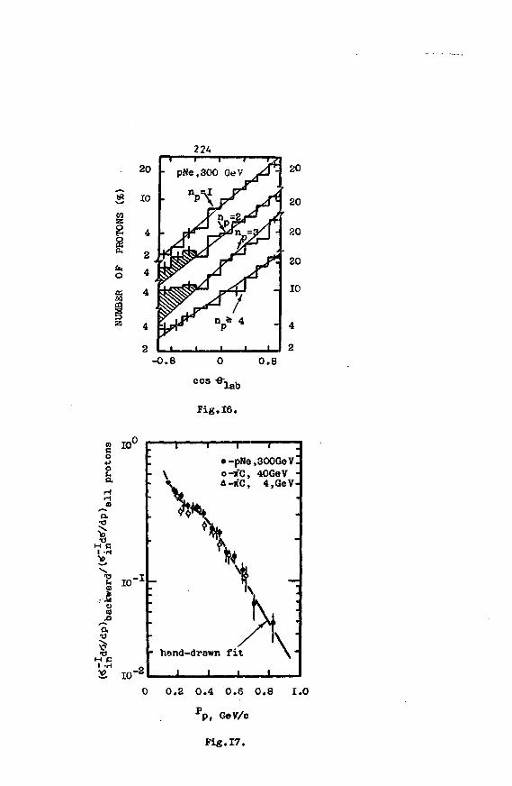
at
1
g IOV
o
I
Joa
£ 10
^ 1
-2
• -pNe,300GoVO-TC, 40GeV
fC 4,GeV
- hand-drawn f i t
0.2 0.4 0.6 0.8 1.0
r p, GeV/c
Fig.17.
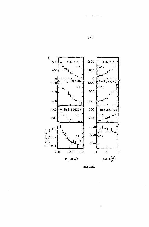
225
i
IC>00
800
0
1000
GOO
200
COO
200
1.2
;' «o
0 . 4
H-. ALL p ' a •
4_ a)
•y BACKGROUND
1 b) .
^-i RES .REG ION"
K, c)
• s• > ^ d ) •
1600
eoo
01000
600
2 0 0
600
200
1 . 2
0 . 8
0 . 4
' ALL p ' 8 "
"a 1 ) pT
•
BACKGROUND;
b') J
• RES.REGION
C1) r^~
"d')
0.23 0.48 0.73
Pp,GeV/e
-I 0
cos
Fig.18.
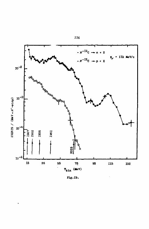
226
10-2
o.o10 - 3
a
10 -5
- JT"I2C — n + X
- X~ I 2C —- p + X113 MeV/c
15 35 55 75 95 115 135
T kin
F i g . 1 9 .
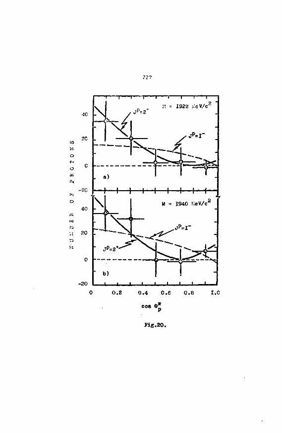
'10
-2C
40
14ra:; 20
-20
1922 .''.eV/c^
a)
• b)
0.2 0.4 0.6 0.8 1.0
cose*
ng.20.
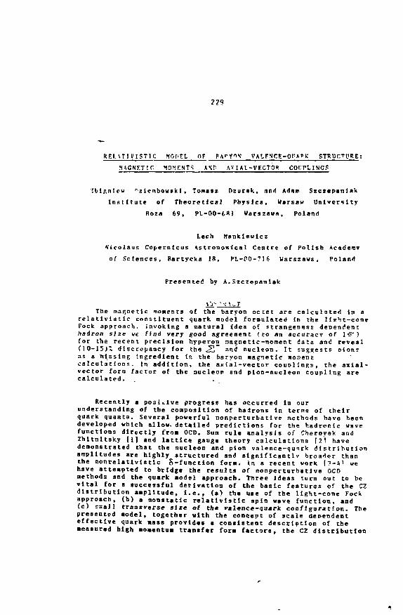
229
REI. \TI FISTIC MOT-EL Of H M " S VAlFSCE-prAPK
MACNETTC IO*!EMT< A\r AVIAI-VF.CTOR COITLING?
'.blf.nlcu "z lembouski , Tomasz Dzurak, and Adam Szczepanlak
Institut« of Theoretical Physics, Warsaw University
Hoza 69, PL-00-fcRl Warszawn, Poland
Lech Manklewicz
Nicolaus Copernicus Astronoitical Centre of Polish Acadeav
of Sciences, Bartycka IS, PL-00-716 Uarszaws, Poland
Presented by A.Szczepanlak
The magnetic nouent! of the baryon octet are calculated in arelatlvistic constituent quark model formulated in the Huht-coneFock approach. Invoking a natural idea of strangeness dependenthadron size we find very good agreement (to an accuracy of 1 ©" )for the recent precision hyperon laagnettc-moment data and reveal(10-15); discrepancy for the ST and nucléon. It suggests Dionsas a missing Ingredient In the baryon »agnetic moaenccalculations. In addition, the axial-vector couplings, the axial-vector form factor of the nucléon and pion-nucleon coupling arecalculated.
Recently a positive progress has occurred In ourunderstanding of the composition of hadrons in terms of theirquark quanta. Several powerful nonperturbative methods have beendeveloped which allow, detailed predictions for the hadror.ic uavefunctions directly fro» OCD. Sun rule analysis of ChernyaV andZhitnltsky (I] and lattice gauge theory calculations [2' havedemonstrated that the nucléon and pion valence-qunrk distributionamplitudes are highly structured and stgnificantlv broader thanthe nonrelatlvistlc S-functlon for». In a recent work (?-4i wehave attempted to bridge the results of nonperturbative OCDnethods and the quark »odel approach. Three ideas turn out to bevital for a successful derivation of the basic features of the CZdistribution amplitude, i.e., (a) the use of the light-cone Fockapproach, (b) a nonstatlc relativistlc spin wave function, and(c) saall transverse size of the valence-quark configuration. Thepresented »odel, together with the concept of scale dependenteffective quark »ass provides a consistent description of the•easured high »oaentua transfer for» factors, the CZ distribution
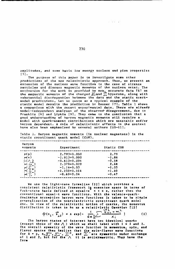
230
amplitudes, and some basic low energv nucleon and pion properties15].
The purpose of this paper is to investigate some otherpredictions of the new relatlvistic approach. Thus, we present anextension of the nucleon wave function to the case of strangeparticles and discuss magnetic moments of the nucleon octet. Themotivation for the work is provided by new, accurate data f61 onthe magnetic moments of the charged £2 and 31hyperons, along withsubstantial discrepancies between the data and the static quark-model predictions. Let us quote as a typical example of thestatic model results the prediction bv Rosner f7l. Table 1 showsa comparison with the recent experimental data. There are alreadymodel-independent analyses of the observed- disagreement, due toFranklin [8] and Lipkin [91. They come to the conclusion that agood understanding of baryon magnetic moments will require amodel with quark-moment contributions which are nonstatic and/orbaryon dependent. A role of relativistic effects in the contexthave also been emphasized by several authors [10-111.
Table 1. Baryon magnetic moments (in nuclear magnetons) in thestatic constituent quark model (COM).
Baryonmomen ts
HP)*4n)MA )'u( ZT)
We use the light-cone formalism [121 which provides aconsistent relativistic framework io_ momentum space in terns ofFock-state basis defined at equal-x « t + z, rather then theconventional equal-t wave functions. With the valence-quark-dominance assumption baryon wave functions Is taken to be simplegeneralization of the nonrelativistic constituent quark modelone. In view of the relativistic motion of quarks, the momentumdistribution is taken to be as a relativistic Gaussian f12 ?
Experiment
2.793+0.0001.913+0.0000.613+0.0042.379+0.020-1.14+0.051.250+0.014-0.69+0.04
Static COM
2.79-1.86-0.582.68
-1.05-1.40-0.47
Xx,, kxl) - A exp[- — ^ — ] (1)^—'
The baryon states of interest have two Identical quarks(except those o f the A ) which we shall label with 1 - 1 and 2.The overall symmetry of the wave function in momentum, spin, andflavor spaces then implies that the spin-flavor wave functionsfor B • p, n ,.?"'.*, JS"*.", 2°> a n d S ~ t r e symmetric under exchangeof 1 and 2, but for the A It Is antisymmetric. They have theform
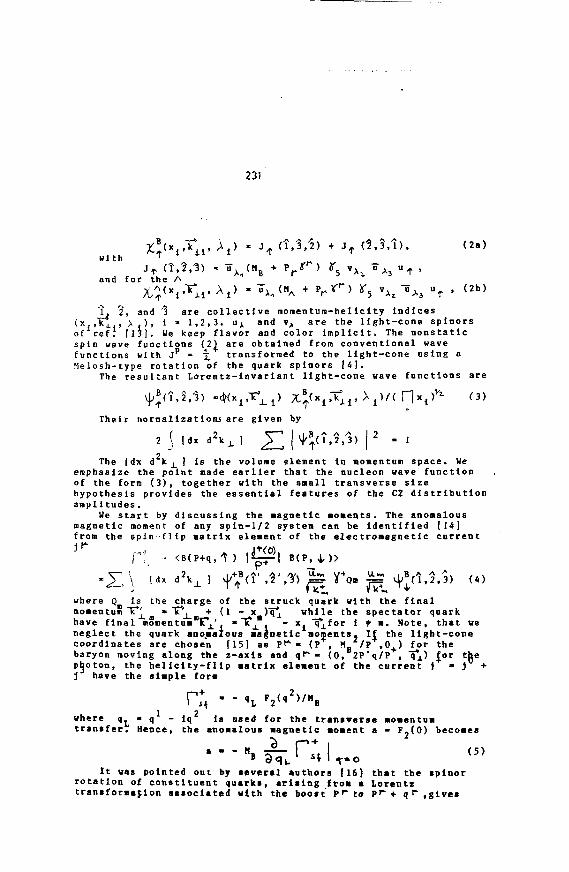
231
( 2 a )
and for the A
1,
v,, TT
and "1> . ) , i
are collective momentum-helicity indices(x, .Tti-, > . ) , i - 1,2,3. u^ and vA are the light-cone spinorsof ref. (13]. We keep flavor and color implicit. The nonstaticspin wave functions (2) are obtained from conventional wavefunctions with Jp - \ transformed to the light-cone using aMelosh-type rotation of the quark spinors 14).
The resultant Lorentz-invariant light-cone wave functions are
Their normalizations are given by
|dx 1
The [dx d k x ) is the volume element in momentum space. Weemphasize the point made earlier that the nucleon wave functionof the form (3), together with the snail transverse sizehypothesis provides the essential features of the CZ distributionamplitudes.
We start by discussing the magnetic moments. The anomalousmagnetic moment of any spin-1/2 system can be identified [141from the spin-flip matrix element of the electromagnetic current
r! • <B(P+q,>t )
where Q ismomentum IT*
the charge of the struck quark with the finalTT"^ + (1 - x Vq^ while the spectator quarkmomentum IT » TT^ + (1 - x Vq^ while the spectator quark
have final momentum"!^' «"^j."t " xi ~^xfoT t t "• Note, that weneglect the quark anomalous magnetic moments. If the light-conecoordinates are chosen [151 as P»* - (P , M /P ,0 ) for thebaryon moving along the z-axls and qf* - (0, 2P'q/P , Tj.) £°r thephoton, the helicity-flip matrix element of the current ) - j +j have the simple form
where 1 2q - lq i« used for the transverse momentum^ qtransfer. Hence, the anomalous magnetic moment a F.(0) becomes
It was pointed out by several authors [16] that the splnorrotation of constituent quarks, arising from a Lorentztransformation associated with the boost P >* to pf + q r , gives
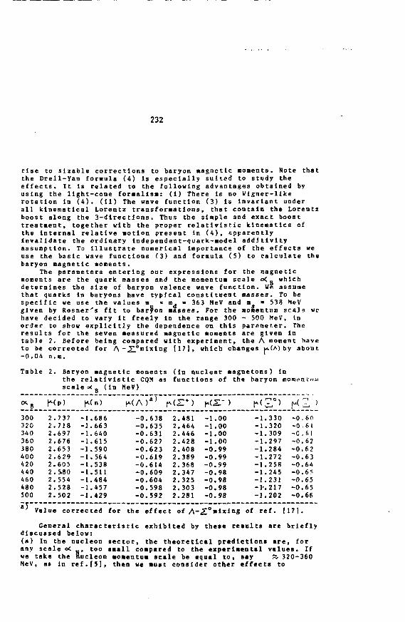
232
rise to sizable corrections to baryon Magnetic moments. Note thatthe Drell-Yan formula (4) is especially suited to study theeffects. It Is related to the following advantages obtained byusing the light-cone formalism: (1) There is no Wigner-likerotation in (4). (11) The wave function (3) is Invariant underall kinematical Lorentz transformatlons, that contain the Lorentzboost along the 3-dlrectlons. Thus the simple and exact boosttreatment, together with the proper relatlvis tic kinematics ofthe Internal relative action present in (A), apparentlyInvalidate the ordinary independent-quark-model addStlvityassumption. To Illustrate numerical importance of the effects weuse the basic wave functions (3) and formula (5) to calculate thebaryon magnetic moments.
The parameters entering our expressions for the magneticmoments are the quark masses and the momentum scale o<& whichdetermines the size of baryon valence wave function. Ve assumethat quarks in baryons have typical constituent masses. To bespecific we use the values m « ra. » 363 HeV and m • 538 MeVgiven by Rosner's fit to baryon masses. For the momentum scale wehave decided to vary it freely in the range 300 - 500 MeV, Inorder to show explicitly the dependence on this parameter. Theresults for the seven measured magnetic moments are given intable 2. Before being compared with experiment, the A moment haveto be corrected for A -J^°mixlng [17], which changes w.(A) by about-0.04 n.m.
Table 2. Baryon magnetic moments (In nuclear magnetons) inthe relatlvlstlc CQN as functions of the baryon momentum
<*.
3003203403 6 03804 0 04 2 04 4 04 6 04 8 0500
s c a l e o< . ( I n
fMP>
2 . 7 3 72 . 7182 . 6 9 72 . 6 7 62 . 6 5 32 . 6 2 92 . 6 0 52 . 5 . 8 02 . 5 5 42 . 5 2 82 . 5 0 2
- 1 . 6 8 6- 1 . 6 6 3- 1 . 6 4 0- 1 . 6 1 5- 1 . 5 9 0- 1 . 5 6 4- 1 . 5 3 8- 1 . 5 1 1- 1 . 4 8 4- 1 . 4 5 7- 1 . 4 2 9
MeV)
*(A)a) |
-0.638-0.635-0.631-0.627-0.623-0.619-0.614-0.609-0.604-0.598-0.592
2.4812.4642.4462.4282.4082.3892.3682.3472.3252.3032.282
-1.00-1.00-1.00-1.00-0.99-0.99-0.99-0.98-0.98-0.98-0.98
-1.330-1.320-1.309-1.297-1.284-1.272-1.258-1.245-1.231-1-.217- 1 . 2 0 2
-0,60-0.61-C.6I-0.62-0.6 2-0.6 3-0.64-0.65-0.65-0.65-0.66
a) Value corrected for the effect of A-£°ilxlng of ref. fl7].
General characteristic exhibited by these results are brieflydiscussed below:(a) In the nucleon sector, the theoretical predictions are, forany scale oi too small compared to the experimental values. Ifwe take the nucleon momentum scale be equal to, say ~ 320-360MeV, as In ref.[5], then we must consider other effects to
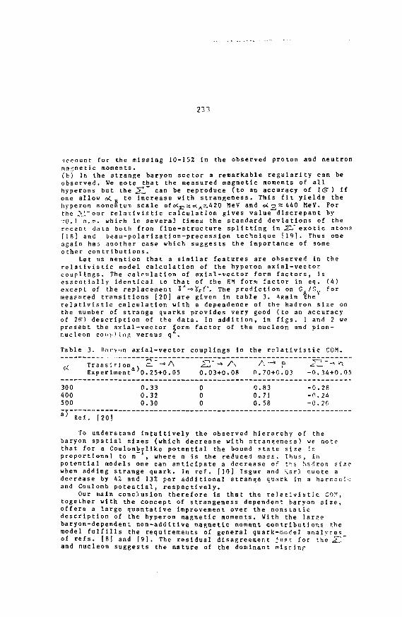
233
lcrount for the missing 10-152 in the observed proton and neutronmagnetic moments.(bj In the strange baryon sector a remarkable regularity can beobserved. We note that the measured magnetic moments of allhyperons but the X L " c a n be reproduce (to an accuracy of IS") Ifone allow <*. to increase with strangeness. This fit yields thehyperon momentum scale ofc<£;=cc<A^.42O MeV and o<-^~ 440 MeV. Forthe .V'our relativistic calculation gives value discrepant by-0.1 n.ra. which is several times the standard deviations of therecent data both from fine-structure splitting In S." exotic atom?[18] and beain-polarizatlon-precession technique Fl9]. Thus oneagain has another case which suggests the importance of someother contributions.
Let us mention that a similar features are observed in therelattvistic model calculation of the hyperon axial-vectorcouplings. The calculation of axial-vector form factors, isessentially identical to that of the Eh form factor in eq. (4)except of the replacement !!'*-»Vj-^". The prediction on G /G formeasured transitions [20] are given in table 3. Again therelativistic calculation with a dependence of the hadron size onthe number of strange quarks provides very good (to an accuracyof 2S") description of the data. In addition, in figs. 1 and 2 wepresent the axial-vector form factor of the nucleon and plon-nucleon coup.Mng versus q .
Table 3. Rarvin axial-vector couplings in the relativlstic COM.
300400500
Transi r1 onExperiment
000
.25 + 0
.33
.32
.30
A.05 0.
000
2~-* A.03+0.08 0
000
A-*.70 + 0
.83
.71
.58
c>
.03
• ^ —
-0.
-0.-0.-0,
34+0.05
28242 0
IT Ref. |20]
To understand intuitively the observed hierarchy of thebaryon spatial sizes (which decrease with strangeness) we notethat for a Coulombrllke potential the bound state size isproportional to m , where ID is the reduced moss. Thus, inpotential models one can anticipate a decrease of ths hadron sizewhen adding strange quark. In ref. [10) Isgur and Ksrl quote adecrease by k% and 13% per additional strange quark in a h a n s o n kand Coulomb potential, respectively.
Our main conclusion therefore is that the relativistic COM,together with the concept of strangeness dependent baryon size,offers a large quantative improvement over the nonstaticdescription of the hyperon magnetic moments. With the larp.ebaryon-dependent non-additive magnetic moment contrlbutions themodel fulfills the requirements of general quark-nooel snalyresof refs. 18 J and [9], The residual disagreement jupt for the 2Z~and nucleon suggests the nature of the dominant niscinr
234
ingredient in the baryon wave functions. It is known from work ofseveral authors [21] that for those three baryons magnetic momentcontributions from a nonvalence <J(f component with plon quantumnumbers are of numerical importance.
REFERENCES[1] V.L.Chernvak and A.R.Zhitnitsky, Phys. Rep. 112 (1979)
173; Nucl'. Phys. B201 (1982) 492; V.L.Chernyak andI.R.Zhitnitsky, Nucl.Phys. B246 (1984) 52.
[2] I.D.King and C. t'. Sachra jda, Nucl. Phys. B279 (1987) 785;G.Hartinelli and C.T.Sachrajda, Phys.Lett. B190 (1987) 151.
[3] Z.Dziembowski and L.Mankiewicz, Phys. Rev. Lett. 58 (1987)2175.
[4j Z.Dziembowski, Warsaw University Preprints IFT/24/87 andIFT/25/87.
[51 Z.Dziembowski.Warsaw University Preprint IFT/26/87;Z.Dziembowski and L.Mankiewicz, In Proceedings of the SecondInternational Conference on Hadron Spectroscopy, Hadron'87,edited by K.Takamatsu (KEK, Tsukuba, Japan, 1987), p.222;J.Bienkowska, Z.Dziembowski, and H.J.Weber, Phys. Rev. Lett.59 (1987) 624.
|6) H.Aguilar-Benitez et al.(Particle Data Group), Phys. Lett.170B (1976) 1.
[7] J.Rosner,In High Energy Physics-1980, edited by L.Durand andL.G.Pondrom, AIP Conference Proceedings No 68 (AmericanInstitute of Physics, New York, 1981).
!S] J.Franklin, Phys.Rev. D20 (1979) 1742, and D29 (1984) 2648.[9] H.Lipkin, Phys. Rev. D24 (1981) 1437, and Kacl. Phys. B214
(1983? 136.[10J N. Isgur and C.Karl, Phys. Rev. D21 (1980) 3175.[11! J.Franklin, Phys. Rev. Lett. 45 (1980) 1607; H.Georgi and
A.Manohar, Phys. Lett. 132B (1983) 183; Z.Dziembowski andL.Mankiewicz, Phys. Rev. Lett. 55 (1985) 1839.
112] S.J.Brodsky, T.Huang, and G.P.Lepage, in Quarks and NuclearForces, edited by D.Fries and B.Zeitnitz, Springer Tracks inModern Physics, Vol. 100 (Springer-Verlag, Berlin, 1982);J.M.Namyslowski, Prog. Part. Nucl. Phys. 14 (1984) 49.
[]3| C.P.Lepage, and S.J.Brodsky, Phys. Rev. D22 (1980) 2175.I M l S.J.Brodsky, and S.D.Drell, Phys. Rev.D22 (1980) 2236.!J5J S.D.Drell and T.N.Yan, Phys. Rev. Lett. 24 (1970) 181.! 1') I U-Y.P.Hwang, Z. Phys. C16 (1983) 327; I.Picek and D.Tadlc,
Phys. Rev. D27 (1983) 665.[I7| R.H.Oalitz and F.von Hippel, Phys. Lett. 10 (1964) 153;
A.J.Macfar1ane and E.C.G.Sudarshan, Nuovo Clmento 31 (1964)1176; J.Franklin, D.Llchtenberg, W.Namgung, and D.Carydas,Phys. Rev. D24 (1981) 2910.
[18] D.V.iiertzog et al . , Phys. Rev. Lett.51 (1983) 1131.[191 G.Zapalec et al., Phys. Rev. Lett. 57 (1986) 1526.[20] M.fiourquin et al., Z. Phys. C21 (1983) 27.[21] J.O.Eeg and H.Pilkuhn, Z. Phys. A287 (1978) 407; G.E.Brown,
H.Rho, and V.Vento, Phys. Lett. 97B (1980) 434; F.Myhrer,

235
ibid. 125B (1983) 359; G.E.Brown and F.Wyhrer, Ibid. 128B(1983) 229; S.Theberge and A.K.Thomas, Nucl. Phys. A393(1983) 252; Z.Dzieabowskl and L.Hanklewlcz. Phy*. Rev. D36(1987)
122] A.Del Guerra et al., Nucl. Phys. B107 (1976) 365; W.A.Bannet al., Phys. Rev. Lett. 31 (1973) 844; S.Bariah et al.,Phys. Rev. D16 (1979) 3103; N.J. Baker et al., Phys. Rev.D23 (1981) 2499.
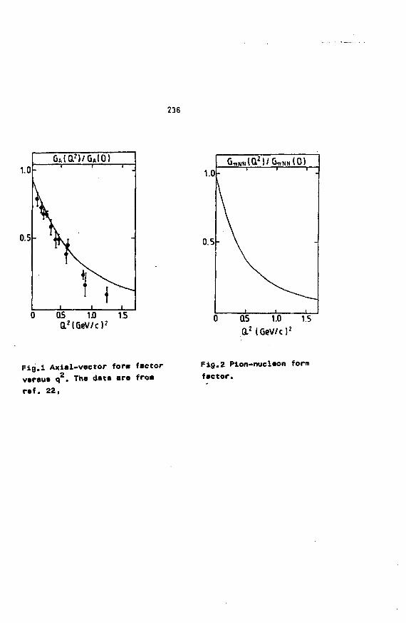
236
0 Q5 1.0 1.5
az(Gev7c)2
Fig.l Axial-vector fora factor
versus q2 . The data are froa
ref. 22,
Fig.2 Pion-nucleon form
fector.
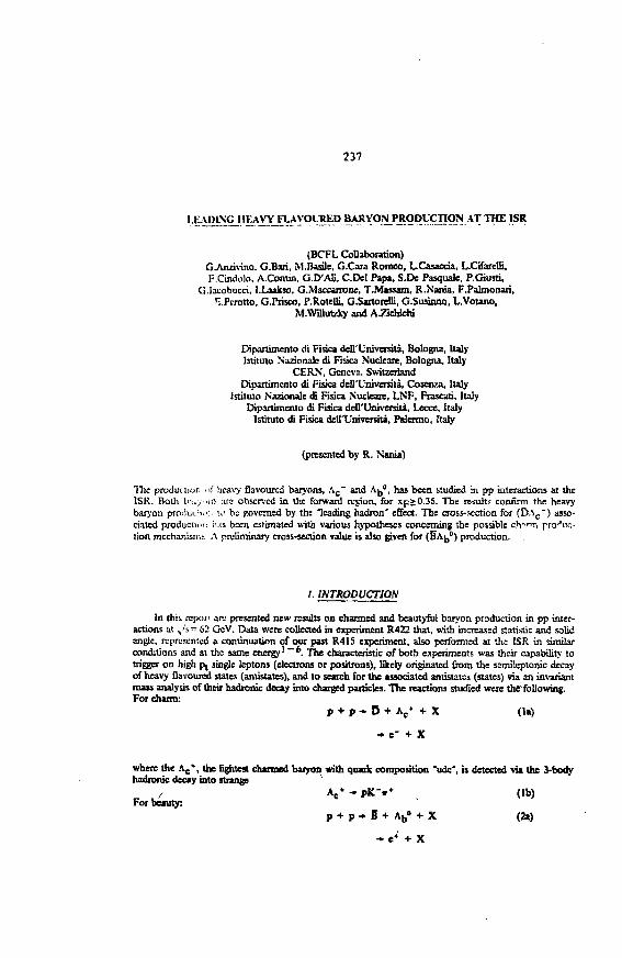
237
LEADING HEAVY FLAVOURED BARYON PRODUCTION AT THE ISR
(BCFL Collaboration)CAnrivino, G.Bari, M. Basile, G.Cara Romeo, UCasacria, L.Cifarclli,F.Cindolo. A.Comin, G.D'Ali, C.Del Papa, S.De Pasquale. P.Giusti,
G.Iacobucri, I.Laakso, G.Maccarronc, T.Massam, R.Nania, F.Palmonari,fi.Pcrotto, G.Prisco, P.Rotelli, G.Sartorelli, G.Susinno, L.VoUno,
M.Willutzky and A.Zichichi
Diparümento di Fisica dcll'Lnivcrsità. Bologna, ItalyIstituto Nazionale di Fisica Nucleare, Bologna, Italy
CERN, Geneva, SwitzerlandDipartimcnto di Fisica deli'Universilà, Cosenza, Italy
Istitmo Nazionale di Fisica Nucleare, LNF, Frascati, ItalyDiparümento di Fisica delTUniversità, Lecce, Italy
Istituto di Fisica delTUniversti, Palermo, Italy
(presented by R. Narria)
The production ni' heavy Savoured baryons, Ac~ and Aj,°, has been studied in pp interactions at theISR. Bolh b..;. ii> are observed in the forward region, for xp>0.35. The result? confirm the heavybaryon pro;luL;v:, u* be governed by ths leading hadron' effect. The cross-section for (DAe*) asso-ciated product;«, ins been esiimated with various h}pothescs concerning the possible ch-"n pro iTc-tion mechanism: A preliminary cross-section value is also given for (BAJ,0) production.
/• INTRODUCTION
In (hit rcpoji arc presented new results on charmed and beautyful baryon production in pp inter-actions at y's" 62 GeV. Data were collected in experiment R422 that, with increased statistic and solidangle, represented a continuation of our past R415 experiment, also performed at th: ISR in similarconditions and at the same energy' ~*. The characteristic of both experiments was their capability totrigger on high Pt single leptons (electrons or positrons), likely originated from the semilcptonic decayof heavy flavoured states (antistates), and to search for the associated antistates (states) via an invariantmass analysis of their hadtonic decay into charged particles. The reactions studied were the following.For charm:
p + p » D + Ac* + X (la)
- e " + X
where the Ac*, the lightest charmed baryon with quark composition 'udc', is detected via the 3-bodyhadronic decay into strange
/ A c * - p K - » * , (Ib)For beauty:
p + p -» B + Ab° + X (2»)
- e4' + X
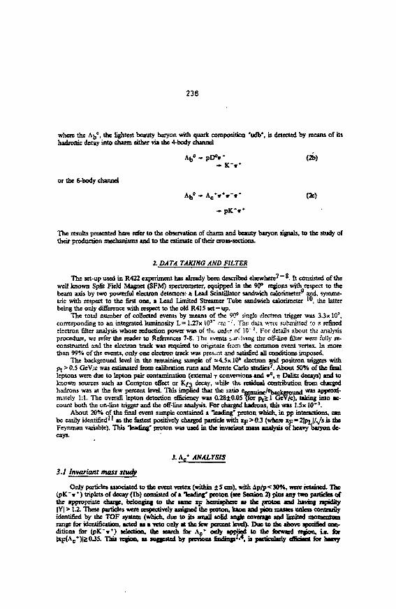
238
where the A),°, the lightest beauty baryon with quark composition "udb*, is detected by means of itshadronic decay into charm either via the 4-body channel
or the 6-body rha^pri
Ao° -. Ac*»*»-«" (2c)
The results presented here refer to the observation of charm and beauty baryon signals, to the study oftheir production mechanisms and to the estimate of their cross-sections.
2. DATA TAKING AND FILTER
The set-up used in R422 experiment has already been described elsewhere7 ~ 8 . It consisted of thewell known Split Field Magnet (SFM) spectrometer, equipped in the 90° regions with respect to thebeam axis by two powerful electron detectors: a Lead Scintillator sandwich calorimeter9 and, symme-tric with respect to the first one, a Lead Limited Streamer Tube sandwich calorimeter '", the latterbeing the only difference with respect to the old R415 set—up.
The total number of collected events by means of the 90° single electron trigger was 3.3x 10',corresponding to an integrated luminosity L= 1.27x I0!" ra"'. The data were submitted to a refinedelectron filter analysis whose reduction power was of the urd'T of i0~2 . For details about the analysisprocedure, we refer the reader to References 7-8. The events s*> iving the off-line filter were fully re-constructed and the electron track was required to originate from the common event vertex. In morethan 99% of the events, only one electron track was preset and satisfied all conditions imposed.
The background level in the remaining sample of =4,5x 10s electron and positron triggers withPf > 0.5 GeV/c was estimated from calibration runs and Monte Carlo studies'. About 50% of the finalleptons were due to lepton pair contamination (external T conversions and «°, TJ Dalitz decays) and toknown sources such as Compton effect or K/3 decay, while the residual contribution from chargedhadrons was at the few percent level. This implied that the ratio e—miaf/eb^ta—und was approxi-mately 1:1. The overall lepton detection efficiency was 0.28±0.0S tfor p,> lGeV/c), taking into ac-count both the on-line trigger and the off-line analysis. For charged hadrons, this was 1.5x 10"5.
About 20% of the final event sample contained a leading' proton which, in pp interactions, canbe easily identified" as the fastest positively charged particle with xp>0.3 (where xp-2]pi_J/./s is theFeynman variable). This leading' proton was used in the invariant mass analysis of heavy baryon de-cays.
3. Ae» ANALYSIS
3.1 Invariant mass study
Only particles associated to the event vertex (within ± 5 cm), with Ap/p<30%, wen retained. The(pK~«*) triplets of decay (Ib) consisted of a leading' proton (see Section 2) plus any two particles ofthe appropriate charge, belonging to the same xp hemisphere at the proton and having rapidity|Y| > 1.2. These particles were respectively assigned the proton, kaon and pion manes unless conlrarilyidentified by the TOF system (which, due to its small solid angle covenie and limited momentumrange for identification, acted at a veto only at the few permit level). Due to the above q—nffiil con-ditions for (pK~»*) selection, the search for Ae* only applied to the forward region, i t . far|xp(Ac*)|£0J5. This region, as suggested by previous findings1'*, is particularly efficient for heavy
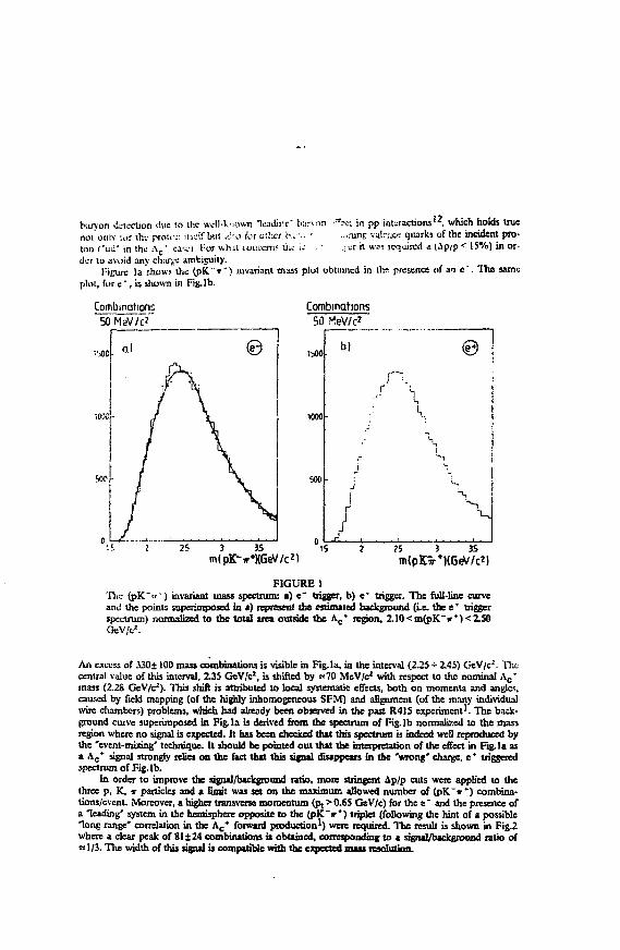
baryon Election due to the WCII-VMOWT. TiaJinr" br-Min •T:x-. in pp infractions12, which holds truenoi oulv Mr thv prou-;- msif but :i!:o for utl-.fr tr..-. - .:i.-unr va!:-ucc quarks of the incident pro-ton Cud' in the Ac" civ) !;or v.hil lonccms the '.-• . ' .; ur it was required a (Ap/p < 15%) in or-der to avoid any charge ambiguity.
Figure la shows the ( p K . i i ' ) iiivariant mass plot obttincd in the presence of an e ' . The sameplot, for c ' , is shown in Fig.lb.
Combination;
50 MeV/r/~
Combinations
50 MeV/c'
isao
1000
500
b)
3
r
j
—
\
x1
1
V?5 35
FIGURE I'IV- ( p K ~ v ) invariant mass spectrum: a) e~ trigger, b) e ' trigger. The full-line curveand the points superimposed in a) represent the estimated background (i.e. the e* triggerspectrum) normalized to the total area outside the Ac* region, 2.I0<m(pK"it*)<2.SOGsV/cz.
An accsi of 330± 100 mass combinations is visible in Fig. la, in the interval (2.23-^-2.45) GeV/c :. HILcentral value of this interval, 2.35 GeV/c2, is shifted by =«70 MeV/c2 with respect to the nominal Ac*mass (2.2S GcV/c2). This shift is attributed to local systematic effects, both on momenta and angles,caused by field mapping (of the highly inhomogencous SFM) and alignment (of the many individualwire chambers) problems, which had already been observed in the past R415 experiment'. The back-ground curve superimposed in Fig. la is derived from the spectrum of Fig.lb normalized to the massregion where no signal is expected. It has been checked that this spectrum is indeed well reproduced bythe "event-mixing' technique. It should be pointed out that the interpretation of the effect in Fig. la asa Ac* signal strongly relies on the fact that this signal disappears in the 'wrong* charge, e * triggeredspectrum of Fig.lb.
In order to improve the signal/background ratio, more stringent Ap/p cuts were applied to thethree p, K, r particles and a limit was set on the maximum allowed number of (pK"»*) combina-tions/event. Moreover, a higher transverse momentum (Pt > 0.65 GeV/c) for the e " and the presence ofa leading' system in the hemisphere opposite to the (pK~r*) triplet (following the hint of a possiblelong range" correlation in the Ac* forward production1) were required. The result is shown in Fig.2where a dear peak of 81 ±24 combinations is obtained, corresponding to * signal/background ratio of= 1/3. The width of this signal is compatible with the expected mass resolution.
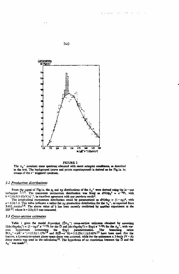
240
Combmorions
FIGURE 2The A c ' invariant nuss spectrum obtained with more stringent conditions, as describedin the ten . The background (curve and points superimposed) is derived aa for Fig. la, bymeans of the e* triggered spectrum.
3.2 Production distributions
outwith
From the signal of Fig.la, the p, and xp distributions of the Ac* were derived using the i n - otechnique 2,3,8 •\\a transverse momentum distribution was fitted as dN/dpf2 « e'^Pt, wib - 2.6+U.5 (GeV/c)",'. in excellent agreement with our previous result^.
The longitudinal momentum distribution could be parametrized as dN/dxp K (1—xp)a, witha = 2.3± 1.3. This value indicates a rather flat xp production distribution for the A c*, as expected fromR415 results3'6. The above value of b has been recently confirmed by another experiment at the
13, where b=2.0±0.5 was measured.
33 Cross-section estimates
Table 1 gives the model dependent ( D A C * ) cross-section estimate! obtained by a winning(Edo/dxpdp,2) <r (1 - x p ) 1 e"2-'Pt for the D and (dfl/dxpdp,2) <c iptp) e-*-»Pt Sir the A?*. with var-ious hypotheses concerning the <{xp) parametrization. The branching ratiosB ( A c * - p K i r * ) = (2.2+I.l)%14rand B(D-e-X)=(12.2S±l . l+0.6)% 1 5 have been used. For theban on, a Lorcntz-invariant phase-space decay was assumed, while for the antimcion a 3-body ( V - A )decay matrix was used in the calculation16. The hypothesis of no correlation between the D and theAr* wasmade'7.
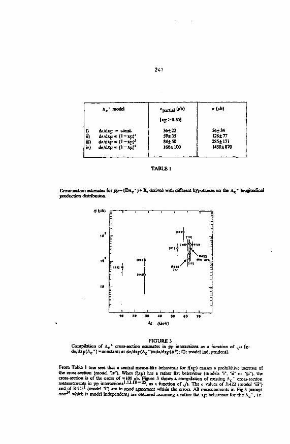
24!
Ac* model
i) do/dxp - const,ii) do/dxp«(l-xp)'iii) do/dxp«(l-xp)1
iv) d»/dxF«(l-XF)J
"partial 0*)
Up > 0.35]
36±2259+3584250166+100
• 0*)
56+34128±77285±1711450+870
TABLE 1
Cross-section estimates for pp-(DA c") + X, derived with different hypotheses on the A c* lonptodinalproduction distribution.
o-(ub)
H
1 * 2« M 40 SO CO 7«
Vs (GeV)
FIGURE 3Compilation of Ac* cross-section estimates in pp interactions as a function of js [o:do/dip(Ac*)=-constant; • : dVMxp(Ac*)!sdi>/dxj:(A0); • : modei indcpmdcntl.
From Table 1 one sees that a centiai meson-like behaviour for f(*p) causes a prohibitive increase ofthe cross-section (model "iv"). When flap) has a rather Qat behaviour (models V, "ii" or "Si"), thecross-section is of the order of =100 ub. Figure 3 shows a compilation of existing Ac* cross-sectionmeasuremenu in pp interactions1'13-'8"25, as a function of , / s . The o values of R422 (model "m")and of R41S* (model *i") are in good agreement within the errors. AD measurements in Fig.3 (exceptone-4 which is model independent) are obtained assuming a rather Bat xp behaviour for the Ac*. i.e.
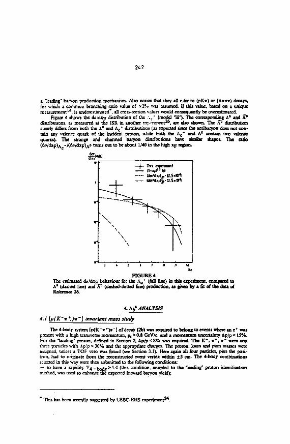
242
a leading' baryon production mechanism. Also notice that they aD r,fer to (pK*) or ( A m ) decays,for which a common branching ratio value of =2% was assumed. IT this value, based on a uniquemeasurement'4, is underestimated*, all cross-section values would consequently be overestimated.
Figure 4 shows the do/dxp distribution of the .'.." (model "iii*). The correspondinf A° and A°distributions, as measured at the ISR in another tr, -nment26, are also shown. The A° distributionclearly differs from both the A° and Ac* distributions (as expected since the antibaryon does not con-tain any valence quark of the incident proton, while both the Ac* and A" contain two valencequarks). The strange and charmed baryon distributions have simitar shapes. The ratio(do/dxp)A •/(do/dxp)Ao turns out to be about 1/40 in the high xp region.
FIGURE 4The estimated do/dxp_behaviour for the A c * (full line) in this experiment, compared toA' (dashed line) and A0 (dashed-dotted line) production, as given by a fit of the data ofReference 26.
4. Ab* ANALYSIS
4.1 [p(K~r*.)v~] invariant mass study
The 4-body system [p(K "»*>"] of decay (2b) was required to belong to events where an e* waspresent with a high transverse momentum, P( > 0.8 GeV/c, and a momentum unceitainty Ap/p < 15%.For the leading* proton, defined in Section 2, Ap/p< 8% was required. The K~. **, w~ were anythrc: panicles with Ap/p < 30% and the appropriate charges. The proton, Icaon and pion masses wereassigned, unless a TOF veto was found (sec Section 3.1). Here again all four particles, plus the posi-tron, had to originate from the reconstructed event vertex within ±S cm. The 4-body combinationsselected in this way were then submitted to the following conditions:- to have a rapidity Y 4 _j ) o i jy> 1.4 (this condition, coupled to the leading' proton identificationmethod, was used to enhance the expected forward baryon yield);
* This has been recently suggested by LEBC-EHS experiment^4.
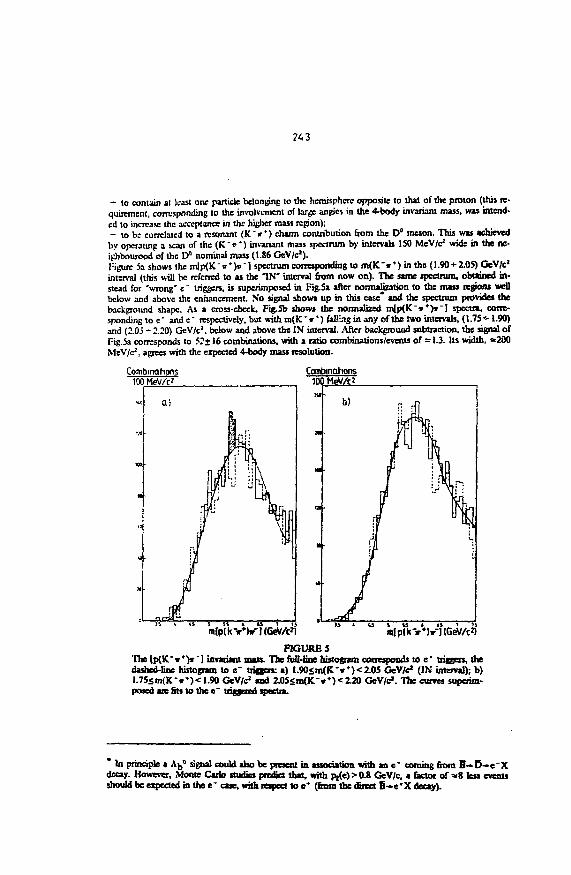
- to contain al least one partick belonging to ihc hemisphere opposite to thai of the proton (this re-quirement, corresponding to the involvement of large angles in the 4-body invariant mass, was intend-ed to increase the acceptance in the higher mass region);- to be correlated to a resonant (K'»*) charm contribution from the Oa meson. This was achievedby operating a scan of the (K"*') invariant mass spectrum by intervals ISO MeV/c* wide in the ne-ijihbourood of the D° nominal mass (1.86 GeV/c*).I:igurc 5a shows the m|p(K"»*)ir"l spectrum corresponding to m(K'»*) in the (1.90+2.05) GeV/c1
interval (this will be referred to as the IN" interval from now on). The same spectrum, obtained in-stead for 'wrong' c ~ triggers, is superimposed in Fig.Sa after normalization to the mass regions wellbelow and above the enhancement. No signal shows up in this case* and the spectrum provides thebackground shape. As a cross-check, Fig.5b shows the normalized mlp(rC~»*)»~] spectn, corre-sponding to e* and e' respectively, but with m(K~ir*) fal&ig in any of die two intervals, (1.75 *• 1.90)and (2.03 * 2.20) GeV/c2. below and above the IN interval. After background subtraction, the signal ofPig.5a corresponds to 52+16 combinations, with a ratio combinations/events of = 1.3. Us width, =*200MeV/c-, agrees with the expected 4-body mass resolution.
Combinations100MeV/c?
Combinations100 IWc*
FIGURESThe lp(K'i*)»~] invariant mass. The full-line histogram corresponds to e* triggers, thedashed-Cne histogram to e" triggeri: a) t.90<m(K~»*)<2.05 GeV/c3 (IN interval); b)l.75<m(K-»*)< 1.90 GeV/c1 and 2 0 5 < m ( K - O < 2 . 2 0 GeV/c". The curves superim-posed are fits to the e" triggered spectra.
In principle * AD° signal could also be present in association with an e~ coming 60m B-B—e~Xdecay. However, Monte Carlo studies predict that, with p,(e) > 0.8 GeV/c, a factor of « 8 less event]should be expected in the e" case, with respect to e* (from the direct S - e * X decay).
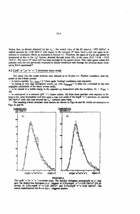
Notice that, as already observed for the Ac*, the central value of the IN interval. 1.975 GeV/c1, isshifted upwards by =100 MeV/c* with respect to the nominal D° mass. Such a shift can again be at-tributed to systematic effects, as explained in Section 3.1. Therefore, the signal of Hg.Sa can indeed beinterpreted as due to the Aj,° baryon, detected through decay (2b), at the mass (S.6S +0.10 —0.21)GcV/c2. The above D° mass shift has been included in the quoted errors. This value agrees within fewpercents with the one previously measured in similar conditions and through the identical decay chan-nel in R415 experiment*.
4.2 [(pK'v*)v*v~ir~] invariant mass study
For decay (2c) the single particles were selected as in Section 4.1. Further conditions were im-posed on the 6-body system:— to hare a rapidity Yg _ bodv > 1-? (here again leading" conditions were required);- to belong to very high multiplicity events, i.e. with nj-harged > 12 (this was motivated by the nonnegligible multiplicity of the decay system itself);— to be related to a visible energy in the opposite xp hemisphere with the condition .25 < |2xpi <.65;- to correspond to a resonant ( p K ~ O charm system. All these three particles were required to be-long to the same hemisphere and here again a scan was made of the m(pK~ir*) spectrum, by intervals200 MeV/c: wide, this time around the Ac* nominal mass value.
The resulting 6-body invariant mass spectra are shown in Figj 6a and 6b, which art analogous toFig.s 5a and 5b.
Contain
FIGURE 6The [(pK~T')**n~i7-l invariant mass. The full-line histogram corresponds to e* trig-gers, the dashed-tine histogram to e~ triggers: a) 2.23£m(pK"w*)<2.43 GeV/e1 (IN in-terval); b) 2.03<m(pK-#*)<2.23 GeV/c2 and Z43sm(pK-»*)<Z63 GeV/c». Thecurves superimposed are fits to the e ~ triggered spectra.
245
An enhancement is visible in the ml {pK~v')v'*'*'] spectrum of Fig.6a. in the region (5.5-^-5-8)GcV/c ;, only for e ' triggered events when 2.23<m(pK IT") <2.43 GcV,c2 (IX inter..!]). It corre-sponds tn (90± 19) combinations, with a combinations/events ratio of =2.5 (a value hijher than inSection 4.1 due to the increased decay n.iiiiplirity). The peak width is now =300 MeV/c2. The centralvalue of the IN interval (which contains the A c ' nominal mass value) is 2.3J GcV,c2. It should benoticed that, in this case also, this value is shifted upwards by =50 MeV/c1 with respect ;o the nomi-nal A c ' mass. The mass of the signal in Fig.6a. once the Ac * mtss shift is taken into accouni, can bequoted as (5.6* +0.15 -0.20) GcV/c*, in excellent agreement with the mass value derived by meansof the D° deesy channel (2b) of Section 4.1. Due to its characteristics, the 6-body signal of Fij;.6a CMagain be interpreted as an evidence for the observation of the Aj,° in a different decay channel.
4.3 Af," mass
A summary t.f the theoretical situation concerning the Aj," mass estimales is given in Refcrcnc27. Five theoretical predictions obtained in the framework of potential models are reported, topsthe:with their corresponding lower and upper bounds. The corresponding average Aj," mass value is (J.S9+ 0.07 -0.211 GeV/c2. The weighted average relative to thu three experimental (R41S and R422)measurements is (5.57 +0.23 -0.22) GeV/c2. Despite the errors involved, from thvse numbers we caneasily conclude that there is a very significant agreement between experiment and tlmcry. An additionaltheoretical value, obtained instead using 'scalar lattice QCD"-°, strongly disagrees both with the pie-viously quoted theoretical estimates and with the experimental measurements.
4.4 Cross-section estimales
A preliminary attempt has been made to estimate the (BAj,0) cross-section for reaction (la). Onlythe data of the D° decay channel (2b) have been used. The hypotheses assumed for the E and the So°arc identical lo those relative to the D and the AC
T in Section 3.3: for the antuncson, a 'central' pro-duction, and, for the baryon, a leading" production (model "i", see Table 1). In Qrst approximation,the transverse momentum distribution of charm (da/dpj « e~2*sPt) has b^en applied to the beautycase". Foi the branching ratios, the following values have been taken: B(iJ-»e*X) = (l2.3±0.8)%-™and B(D°->K"ir*) = (S.4+0.4)%^''. Only a partial cross-section will be given here, working out theacceptance of the apparatus under the same conditions (see Section 4.1) which allowed the Aj,° to beobserved, i.c. YIp(K"ir+)i-]> 1.4 and Xp(p)>0.3. The result is B(A^0-»pD c ir-)i ip 3 r <^= (0.15-5-0.5) jib. The same value, in the past R415 experiment5, once the corrections for the updatedD°—K~ir* branching ratio and for slight analysis differences are applied, is (0.45-1.25) jib. Thepresent B-o-artja] value is lower due to the fact that the number of observed Aj,0 events is a factor of=3 smaller than what expected from R41S extrapolation.
i. CONCLUSIONS
The results of experiment R422 are a confirmation of R415 results. The Ac* baryon is again ob-served with increased statistics. Its r>, and xp production distributions compare well with previousfindings. Also the open beauty state Aj,0 is newly observed, by means of two different decay channels.Its mass (averaged over R422 and R41S measurements) is found to be =5.6 GeV/c2, in very goodagreement with theoretical predictions. The leading' effect dominates charm and beauty baryon pro-duction in pp interactions. Finally, the cross-section estimates indicate, once more, that heavy flavoursare copiously produced in the ISR energy range.
* A different panmetrization, like e-0-"Pt, could be used29. This would lead to a lower cross-sectionvalue due to the presence of the p, > 0.8 GeV/c cut for the e+.
246
REFERENCES1) M.Basile ci a!.. Nuovo Cimento 63A (1981) 230.2) M.Basiic c! al., Nuovo Cimento Lett. 30 (1981) 481.3) M.Basiic et al., Nuovo Cimento Lett. 30 (1981) 487.4) M.Basils et al., Nuovo Cimento Lett. 31 (1981) 97.5) M.Basile ct al., Nuovo Cimenlo 65A (1981) 391.6) M.Basile et al., Nuovo Cimento 65A (1981) 408.7) M.Basile ct al., Nuovo Cimcnto 65A (1981) 421.8) G.Anzivino ct al., 'A new measurement of Ac * baryon production in proton-proton interactions at
N/s = 62 Ge \" , preprint CERN-EP (1987), in preparation.9) M.Basile et al., Nucl. Instr. and Meth. 169 (1979) 93.10) M.Basile et al., Nucl. Instr. and Mcth. 235A (1985) 74.11) P.Capiluppi et al.. Nucl. Phys. B70 (1974) 1.12) M.Basile et al., Nuovo Cimento 66A (1981) 129.13) A.Mcdinnis, private communication.15) MARK II, G.S.Abrams et al., Phys. Rev. Lett. 44 (1980) 10.15) MARK III, R.M.Baltrusaitis ct al., Phys. Rev. Lett. 54 (1985) 1976.16) A.AU and E.Pietarincn, Nucl. Phys. B154 (1979) 519.17) LEBC-EHS, M.Aguilar-Benilcz et a!., Phys. Lett. 164B (1985) 404.18) K.L.Giboni ct al., Phys. Lett. 85B (1979) 437.19) J.lrion et al., Phys. Lett. 99B (1981) 495.20) W.Lodcman et al.. Phys. Lett. 85B (1979)443.21) D.Drijard ct al., Phys. Lett. 85B (1979) 452.22) M.Hciden, Thesis, University of Heidelberg, FRG (1981).23) BIS-2, A.N.Alecv et al., Zcit. Phys. C23 (1984) 333.24) LEBC-EHS, M.Bcgalli ct al., submitted to Phys. Lett. (1987), and A.Goshaw, private communi-
cation.25) T.Aziz ct al., Nucl. Phys. B199 (1982) 424.26) S.Erhan et al., Phys. Lett. 85B (1979) 447.27) A.Martin and J.M.Richard, preprint CERN-TH 4584/86.28) S.Samuei and KJ.M.Moriarty, Phys. Lett. 17SB (1986) 197.29) Y.Afek, C Ixroy and B.Margolis, Phys. RevvD22 (1980) 86.30) M.Aguilar-Benitez ct al., 'Review of particle properties". Phys. Lett. 170B (1986) 1.
CHARM pHOTOPnODUCTipN JN..IHE NA14-||_EXPERIMENT
N>M4-II Collaboration: Athens Technical University, Universidad AutonomaBarcMon.;. CCRN, Imperial College London, Orsay LAL, Paris College deFranc---, Saclay. Southampton University, Strasbourg CRN et Universite LouisPasteur, Warsaw University.
presented by D. BLOCH, CRN Strasbourg, France.
-Abstract:
The aim M the CERN-NA14-II experiment is the study of charm
pliotoproductron mechanisiia and the lifetime measuron.-'nt of charmed mesons.
The peculiarity of this experiment is the combined use of a microvertex
'ihccn detector where primary and secondary vertices are measured with a
riinh precision, a^d a large acceptance spectrometer where charged tracks and
photonr arc fully analysed and identified. We present preliminary results based
•.m n p;irt ct the total statistics acquired in ' 985-1986.
i/_xpcrimenta{ details'.
The experiment was performed in the E12 e-T beam at the CERN SPS.
I hi! NAM spectrometer, whose complete description can be found elsewhere .
>•••?• ;ueviously .perated for the study of the deep inelastic Compton scat-
• ":-v; . Now it is associated with a silicon active target and a stack of
• •in "v.li ip hodoscopes (Fig. 1).
The bremsstrahlung photon beam is provided in 3 steps
i> • i ' • ' ' ) •• o •- Y which allow a large reduction of the hadronic contami-
nation (li/r 10 ) and '*ie energy measurement for photons above 50 GeV.
The high flux photon beam (1.2 x 10 y/cycle > 50 GeV. mean energy-80 GeV)
is incident on a silicon active target of 10 % X f , installed in a 1 T. m magnet
which sweeps the electromagnetic background.
Primary interaction and charm decays occur in this target composed of
32 silicon planes of 300 pm thickness and 200 pm interspace, each segmented
in 2+ vertical strips of 2.1 mm wide (Fig. 2) ' . The particle multiplicity is
measured in each strip allowing: to reject electromagnetic events and those
with a secondary interaction, to reconstruct independently the main vertex
when "grey tracks" from the target nucleus are emitted, to flag secondary
vortices by a jump in multiplicity (Fig. 5a).
Immediately 1 cm downstream of the target Is a slack of 10 .-nicrostrip
plants comprising 4 Y-Z and 1 U-U1 f. ± 30°) doublets, 1000 strips of SO um
Pitch per plane (Fig 2). Thus the track projections can be matched in space,
improving the reconstruction very close to the primary interaction and redialing
a charm decay by the measurement of an offset (Fig. 5b-c) . In order to
reduce the cost of the electronics, 2 strips from different regions are read on
the same channel.
The spectrometer itself has an angular acceptance up to 275 mrad in
the laboratory both to charged particles and to photon.".. 70 MWPC planes in
between and downstream of the two magnets allow to analyse charged tracks
from - 2 up to 100-GeV/c. Three electromagnetic calorimeters measure
p otons and electrons in the same acceptance. For the purpose of this present
charm search, only the threshold Cerenkov counter^ 2 is used to disentangle it
from KIP in the range 6.3 < P < 21.S GeV/c, and n/K from P above 21.6
GeV/c.
The trigger requires a hadronic interaction, asking for some minimal
multiplicity in the active target and for the detection of at least 1 upward
and '. downward charged track thiougli scintillator hodoscopes We have
recorded S M events in 1985 and 12 M events in 1986. The electromagnetic
contamination is 10 %. The trigger efficiency is 35 % for hadronic interac
t'ons, increasing with the beam energy and thus leading to a factor ?. yn.-icn
ment for charm. But 35 charm photoproduction represents only about 1 °i cf
th? total cross section, a large effort was devoted to the filtering procedure.
Charm signals:
Fir;,t we process all raw data events through a fast pattern program
which reconstructs charged tracks using only a part of the MWPC planes. Then
two filtering philosophies are considered:
• ) A specific filter requiring n very clean active target selects 3 % from 5
M event", recorded in 1985. The corresponding K~n n* invariant mass distribu-
tion is presented in figure 3 for different cuts in L/o, where the decay length
1. is measured with an error o typically s 500 urn (throughout the paper, the
charge-conjugate states are implicitly included). The D+ signal is clearly
visible with a low background, but the statistics is poor .
?) The second method is used on our 1986 data. Combining the charged
tracks with the active target and the micros trips informations, criteria *r*
defined to select events with an offset track or with a secondary vertex .
We retain thus 20 % of the events which are processed through the full
pattern recognition program, taking about 1.5 */event on an IBM 3090.
According to our Monte-Carlo simulation the filtering efficiency is 70 % for D
249
meson:., inoependently of the decay length and of the transverse momentum P,-.
The K~ir*n* mass spectrum is shown on figure 4, for 4.5 M envents from
1986. The S/B ratio is 3 and 60 D* are measured in the mass range (1.81S.
1.90C) GeV. We have imposed a flight L > 10 o.
Figure 5 is the illustration of a charmed event candidate with a decay
D" - K + I I~R~ observed in the microvertex silicon detector. A grey track is
emitted at large angle in the active target and an other it* is reconstructed.
Based on all 12 M events from 1986, figure 6 represents the K~n + mass
distribution from those 0" mesons which are produced by a D*+ decay. Asking
for a Kttn-Kn mass difference between 143 and 149 MeV and a flight > 2 o,
we get 88 D" and a ratio S/B * 4.4.
Figure 7 shows the cumulated available invariant mass distribution of
charged and neutral D mesons, including all 0 ° - K~n from 1986 data with a
4 o flight cut. We observe a signal of 510 D mesons in the mass range
(1.815, 1.905) GeV with a ratio S/B = 1.
D* meson lifetime:
The D" meson signal produced by a D decay (Fig. 6) presents a low
background and allows a limited cut on the time of flight. Figure 8 shows the
time of flight distribution for - 80 Oc mesons. An exponential fit gives a
lifetime tD<> (4.4S + " ^ )• 10~1 3 s (errors are statistical only) ' 6 ' quite in
agreement with the 1986 world average (4.3 * ^ )• 10~1 3 s , but with
larger errors than a recent FNAL-E691 result: (4.35 ± .15 ±.10)- 10" 1 3 s ( 8 \
PT distribution of D masons:
The cumulated statistics of 510 D meson signals is compared in figure
9 with the normalized background, taken in the same mass range but with no
cut on flight (dashed line). Charmed mesons are produced at higher PT than
ordinary hadronic states whose distribution is compatible with an exp(-6mT)
dependance.
Comparison is also made on the same figure with the Lund Monte-Carlo
simulation of the lowest order QCD prediction: the fusion f 9 - cc . For
two choices of the charmad quark mass (m = 1.2 or 1.5 GeV, full curves),
this model is in good agreement with our data, Howevar in order to get a
detailed comparison with the theory, second order QCD predictions should have
to bt takan into account.
25C
Conclusion:
We have observed a clear signal of charmed 0 ° , D + mesons which will
be completed this year by exploiting our full statistics, and by using the
calorimeter informations in order to analyse decay channels with a i ° .
Lifetime measurements will be pursued and Pj, X p , Y distributions for D
mesons will allow a more detailed comparison with QCO predictions.
Acknowledgements:
I gratefully acknowledge the organizing committee, and especially
T. HOFMOKL, for their invitation and hospitality. I thank P. ROUDEAU for
providing me our last results and J.P. ENGEL for revising the manuscript
which was typed by Mrs. L. SEIFERT.
References
1. E.Auge, These de 3e cycle, Orsay, LAL 83-09 (1983)
D.BIoch, These de doctorat d'Etat, Strasbourg, CRN-HE 85-06 (1985)
C.Seez, Ph. O. Thesis, imperial College, London, HEP T 118 (1983)
G.Wormser, These de doctorat d'Etat, Orsay, LAL 84-45 (1984)
2. P.Astbury et al. , Phys. Lett. 152B (1985) 419
3. R.Barate et al., Nucl. Instr. and Methods, A235 (1985) 235
A. S.Petrera, G.Romano, Nucl. Instr, and Methods, A174 (1980) 61
5. M.Primout, NA14-II internal note (1987)
6. C.Krafft, These, Orsay, LAL 87-28 (1987)
7. Review of Particle Properties, Particle Data Group, Phys. Lett. 170B (1986)
8. J.C.Anjos et al. , Phys. Rev. Lett. 58 (1987) 311
9. L.Jones, W.Wyld, Phys. Rev. D17 (1978) 759
H.Fritzsch, K.H.Streng, Phys. Lett. 72B (1978) 385
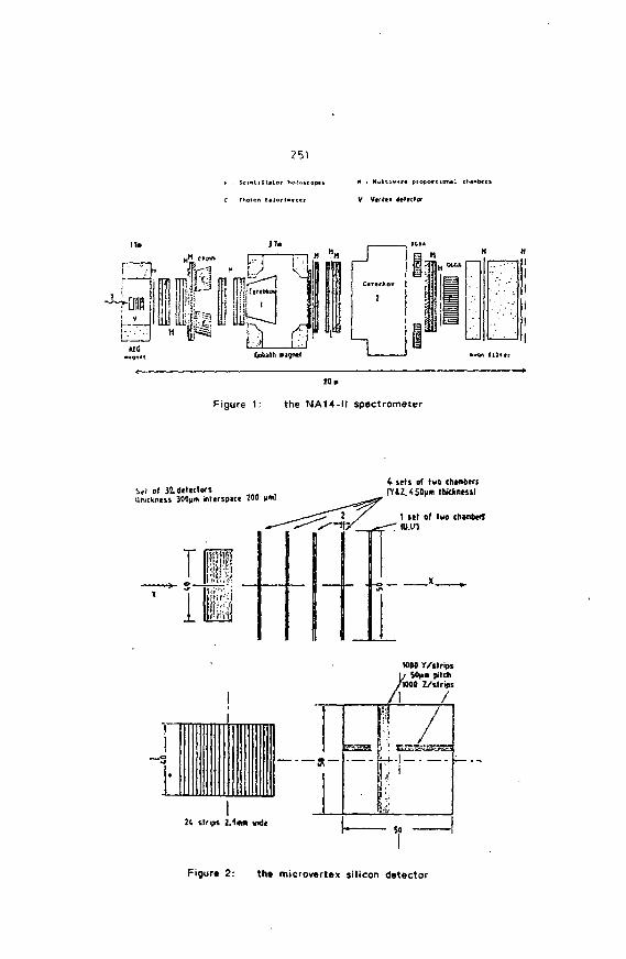
251
Urn
np33pit to
-7—1 M ?M
I/Jja elm
l!lif«—I
Got.jlh Nqixl
Figure 1: the NA14-II spectrometer
ie i ol 32. detectorsIllutkness 300|iin inlerso«« JOT
To1
«! i
4 sets of two chamber!IYIZ. <oO|iin thkknessl
WOO T/ltripi50M» pitch
'WOO Z/itrips
3; strips 2 . 1 * * writ
s—
Figur* 2: th« microvertex silicon detector
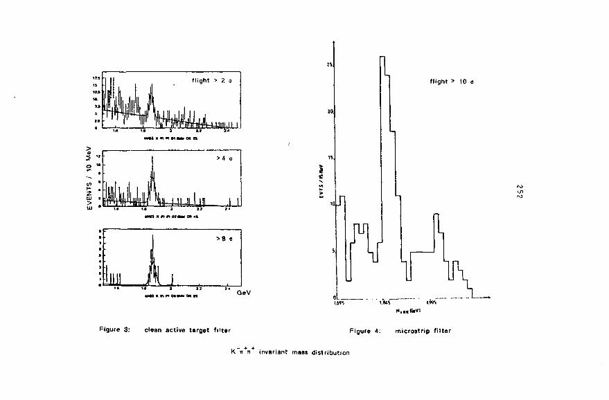
flight > 10 o
HWS K Pi PI »«MM M IGoV
IV)en
Figure 3: clean active target filter Figure 4: microstrip filter
K it n invariant mass distribution
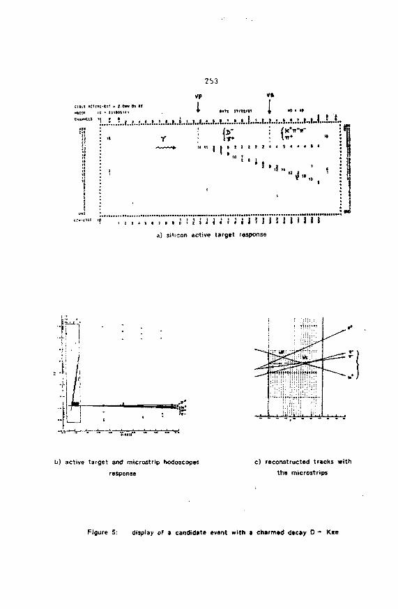
253
t*1| IV01/H
IT*• 11 i i I I i i •
10 I
\ir*
!
1
, . , i! j 111 i i i i i ? J J J i n 1 1 1a) silicon active target response
b) active target and microstrip hodoscopes
response
c) reconstructed tracks with
the microstrips
Figure 5: display of a candidate event with a charmed decay 0 - KRIT
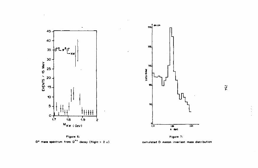
1.7
K T (GeV)
Figure 6:
O* mass spectrum from D*+ decay (flight > 2 o)
dN/6M
fl
Figure 7:
cumulated D meson invariant mass distribution
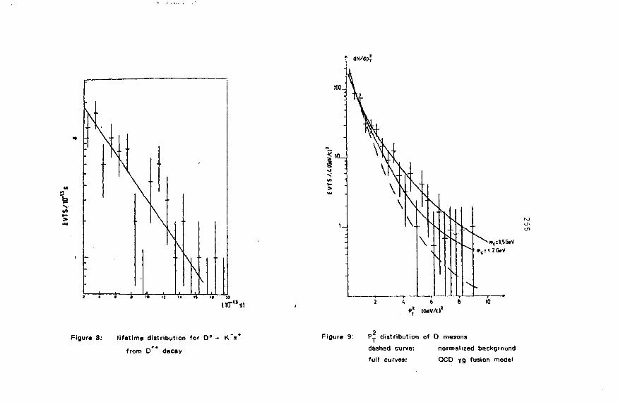
Figure 8: lifetime distribution for D ' - K'n*
from 0 decay
t dN/dp?
>0OJ
Figure 9: Pf distribution of D masons
dashed curve: normalized background
full curves: OCD yo, fusion model
257
l'i l " i t i o r i "I yU.-. (M i i r i n m - . i l i iuu i l i t i ' " «ii: t i o n 1 -
. i t ; • 7>.> (".-'.' ."n.'Utf i n o • . • n . T g y
EKAT - Co 11 oibor ah i on
<Tlire B(.-r iin-Zeiitnt-Ti -- II1CP Serpukhov)
pr e-c-nted by H.fi. Roloff
! . l l i l r uductiOll
iliu pi iitjuctiun of 4jfj|ji.i;.i i.e :>iqn di 1 cojjtanti in neutrino
t n tt?r .ju !. t uir; ut high c-iieriji a~. \^. vtel 1 i..tncic-r:itood ^3 being dt-:'
to < tiui' m pr odnct ioii with suet t-cU ing semi 1 cjptOni c decay. Muat
other e;:por i ir.r nt* study the di lepton production in an energy
i aiujt.' t i tart i inj at about 30 Gt'V. Our data allow the study of
charm production near the charm threshold.
for tho production of like—sign dileptor>^ there is up to
now no theoretical explanation for the measured rates. Iht:
o.'.' .ot i •>icii 'rhariii production e.g. givc?s a rate lt'^c. by ^ factor
nf ^b(5ut. 10- Other sources as B- production c.-in bo *»>:cludt?d ot
our eniv gii i. fin our resul ts w i l l bt? c r i t i c a l l y v.inc-
o':-pQc: i .al I y Ht;- .issociated chctrm production ir. oxpnetc-ti t>j bu
r>troncjly u-t'.ppr c . ccJ at aur low ener cjicor,.
'^ . Soluction of ^x^-eve^nts
Wo ur.ed the neutrino wide band beam of the? Serpukhov
accelerator with an averaged neutrino energy < E ^ > » 7 GeV. As
dt?ttjir.tor we u?ad the heavy l i qu id bubble chamber SKAT /%/.

258
We started from about 10060 charged current events which were
selected as described in /2/. To increase the efficiency of
muon—selection we applied the momentum cut p« > 1 6eV/c:. A
track is accepted as e*/e" -candidate i-f two of the? -following
criteria are satisfied: characteristic apiralization or strong
multiple scattering, high energetic J-electrons, Brenus- jj's
pointing to the track, annihilation <only G*~) . To reduce the*
background from photons converting near the? primary vorte;: v.o
required that the e-track has to bi? clearly visibli? .>'_ .)
distance of 1.5 cm from the primary vertex and that there i •-.
no other e?-track at the vt>rte)..
To reduce the background from misselassified leaving ~'
for the At~e' -events w© required in addition that p^ : p w ,
and for /—electron background reduction we introduced an
angle cut for the angle between the muon- and electron
direction. After correcting for losses and efficiencies wo tjot
from
for > ^"e+X
and (or V.M > IA e~X t
10060 events
18 events + 15. 1 V.
b events + 8.6 7.
The background sources re estimated as given in the following
table <the numbers given are number of events).
lackgr.
• •
at,ymm. ^ EDalitz pairs
0.8 t O.3
o.et 0.3
<3e'Ncc-inter.
O.OAi 0.02
1.1 t 0.4
compton-•lectrona
1.6SO.5
J-«l*ctr.
0.24i0.O2
total
0.9t0.3
3.710. 7
259
3. Results for ^N > ju~e*X
Hit? ra t io o-f opposite siijn dilcpton production normalized
to our charyoil current ri.ita sample corn*-?s out to be
<2.0 I <>. S)tf ( ^ H - . yu" X (
•.J) I h (dp vs. pur inipri tal c u t s ti > 3 Gt;V, p > 1 GoV/c , p«
•"(.-? (",-V/i.:. I- >tttiirint) Hint tin:- mAr5r» of the r iddronic system
i n h» • ijr iS^.jiin i-ji t»i the-
ts thr? r - j t i o ..IJOVB the; cluna tlire-il iot d
(4 .6 i 1.2) • to-"*• < v.. fl
l i t ..--t-rLil t.'ispw imurits /'"'•/ i l i t- ' re ;.\r o I i i i t : a t i uric fi»r l l t t :
(•/•ijijui. h i Qd of channod baryf jns. I'Jo '.:oivipdr t?ii uur -!-••'. ; u i t h <»
ItunU: t ' . i r l u • ample.' 1 ur thu (.uu pri>c«!E.:..f^
-•> / i "DX
In f i Jin c; 1 the con t r t bu t : i ons uf / \ t (d.r.:liLcl l i iu.O an-cl D-
|.r .jij.i^ i ion ',1 ...hoil <J(.>I.tc>ij I J I K ? ) d ro uhovm. I t ,:,\n tv.; .•..-•n l:h.>'
' " ' " ^ W ' ~.4J CJL'V uop«»r;ilt?:i (t ic Ivjt- |JI w:t •_;.(?:, t o .. h i i j l i
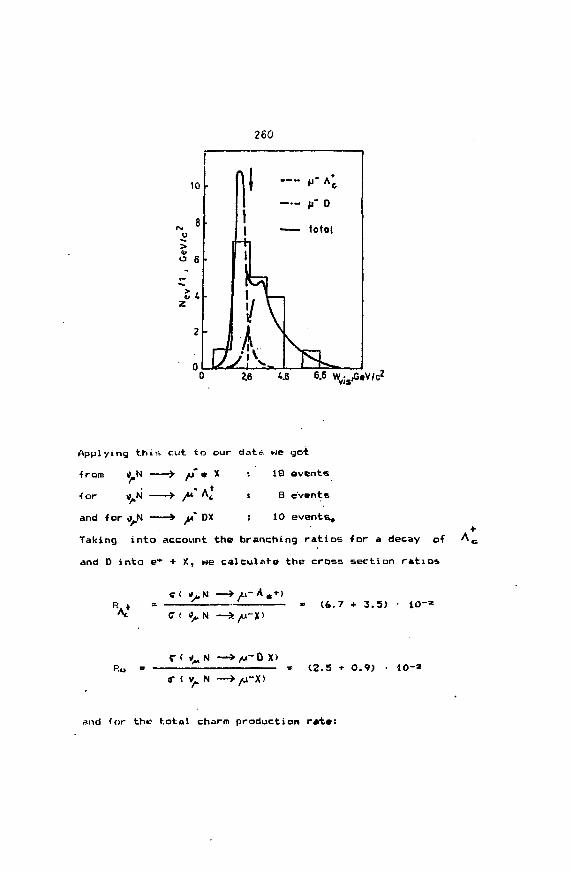
260
10
<uo 6
z
2
n
11
• fjjm
rJ AK/sV
—- p* 0
— totat
26 I.& 6.6 Wy;s,G«V/c2
Applying thi^» cut to our data we got
from tf.N /u"« X : 18 events
•far v N > /* Ac ' 9 event*
and -for jN > jf DX : 10 events^
Taking into account the branching ratios for a decay o-f A c
and 0 into e* + X, we calculate the cross section ratios
» (i.7 + 3.5) - 10"=C ( »A N
/U"0 X)= <2.5 + 0.9) • 10-3
S- ( (J.. N
and far the total charm production r«t«:
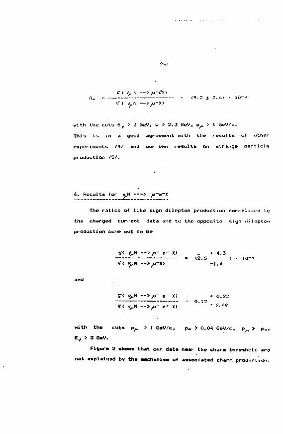
•-•- <9.2 j 3.6) • 1 0 - -
C < j N —>/*i~X)
with the cuts Bv > 3 GeV, W > 2.3 GeV, p^. > 1 6eV/c.
This »•> in a good agreement with the results of other-
experiments /4/ and our own results on strange par title?
production /5/.
4. Result* for wN >
The ratios of like sign dilepton production normal i;trd to
the charged current data and to the opposite 'iign dilupten
production come out to be
(J..N — > fi~ e~ X) + 4.3- (2.5
£.N -->//u-X> -1.4
and
i- e" X) + 0.22^ 0 1 2
u- e' X) * "• "*
with the tuts Pp. > 1 GoV/c, p. > O.O4 GeV/c, p > p.,
E^ > 3 G«V.
Figure 2 shows that our data near the charm threshold are
not explained by the Mchanism of associated charm pro.dur.lion.
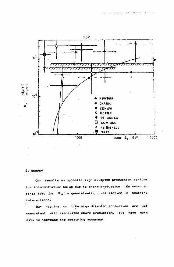
262
HPWPOR
CHARM
• CDHSWCCFRR
• 15 BSHSW• OGM BCS* 15BM-COL• SKAT
1000 2000 e v , GeV 3CC0
5. Sunxnoy
Our r e s u l t s on opposi te sign d i l c p t o n product ion con-firm
the i n t e r p r e t a t i o n being due t o charm product ion . We measured
f irst time the A «• - quasielastic cross section in neutrino
interactions.
Our results on like sign dilepton production are not
consistent with associated charm production, but need more
data to increase the measuring accuracy.
263
/I/ Kusritft?:t>v,F.P. et al. , Preprint IHEP 71-75, Serpukhov
/2/ Caranov, D.S. ot al., Z.f.Phys. , C21 (1984>, 189
Luranov, D.S. et al., Z.f.Phys., C21 (1984), 197
/3/ B l:rr ot al. , Phys.Rev. D Vol. 32, No.3, Particle and
Fields, 1985
/•%/ Ballagh, M.C. et al. , Phys.Rev. D24, No. 1 (1981)
/5/ AIMIOSSOV, V.V. et al., Z.f.Physik, C30 <1986), 183
265
TOPON1UMATLEP
S.Zylberajch
CEN S a c l a y , F r a n c e
Abstract We present a brief survey of Toponium studies done at the CERN LEP I and
UEP It Physics workshops^] . If produced at the LEP energy, the first toponium S-states could
be detected in less than one year in the present LEP experiments. Detailed studies on spectroscopy
and polarization will be far more difficulLToponium could be a very good tool to look at non
standard physics.
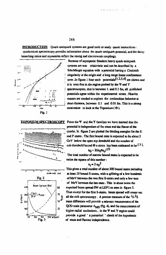
266
INTROW JCTION Quark-amiquark systems are good tools to study quark interactions:
quarkonium spectroscopy provides information about the quark-anriquark potential, and the decay
branching ratios and asymetries reflect the strong and electroweak couplings.
Because of asymptotic freedom heavy quark-antiquark
systems are non relativistic and can be described by a
SchrSdinger equation with a potential having a Coulomb
singularity at the origin and along range linear confinement
term .In figure ] four such potentialsH'23.4] are shown and
it is seen that in the region probed by the *F and Y
spectroscopies, that is between 1. and 0.1 fm, all published
potentials agree within the experimental errors. Heavier
masses are needed to explore the coulombian behavior at
short distance, between 0.1 and 0.01 fm. This is a strong
motivation loJookattheToponium(8).
Fig. 1
TOPONTIJM SPECTRQSCOPY From the V and the Y families we have learned that the
potential is independent of the mass and the flavor of me
quarks. In figure 2 arc plotted the binding energies for the S-
andP-states. The first bound state is expected to lie about 2
GeV below die open top threshold and the number of
sub-threshold bound 6 s-statcs has been estimated to be f ' 1:
The total number of narrow bound states is expected to be
twice the square of this number:
It
401
i 2> 300
•i
2 200
100
it le
Fig. 2
auMt MASS
Bom Spread I6W1\
GeVV 26 W • •""•
\ ,\
50 100 150Fie. 3
V///'/
IGri
100
75
50
25
200 WIGtVI
n
a
This gives t total number of about 200 bound states including
it least 10 bound S-states, with a splitting of » few hundreds
of MeV between the two first S-staies and only a few tens
of MeV between the last ones. This is about twice the
expected beam spread 5W at LEPI as seen in figure 3.
Thus except for the first S-states, beam spread will smear out
all the rich spectroscopy. A precise measure a! the 'S-^S
mass difference will provide a relevant measurement of die
QCD scale parameter A M S (fig. 4), and the measurement of
higher radial excitations, in the ¥ and Y region could
provide a good ' a posteriori ' check of the hypothesis
of mass and flavour independence.
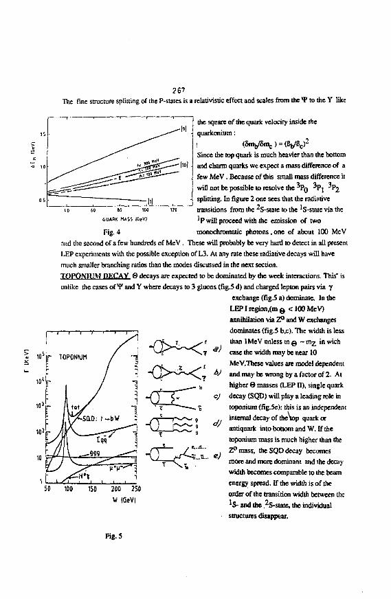
267The fine structure splitting of the P-states is a relativistic effect and scales from the ¥ to the Y like
the square of the quark velocity inside the
quarkonium:
ao IOO
GIMRK MASS IGeV)
Fig. 4
Since the top quark is much heavier than the bottom
and charm quarks we expect a mass difference of a
few MeV . Because of this small mass difference it
will not be possible to resolve the ^PQ •'PJ ^ 2
splitting. In figure 2 one sees that the radiative
transitions from the 2S-state to the ^S-state via the
^P will proceed with the emission of two
monochromatic photons, one of about 100 MeV
and the second of a few hundreds of MeV . These will probably be very hard to detect in all present
LEP experiments with the possible exception of L3. At any rate these radiative decays will have
much smaller branching ratios than the modes discussed in the next section.
TOPONIUM DECAY 9 decays are expected to be dominated by the week interactions. This" is
unlike the cases of V and Y where decays to 3 gluons (fig.5 d) and charged lepton pairs via y
exchange (fig.5 a) dominate. In the
LEP I region,(m 9 < 100 MeV)
annihilation via Z° and W exchanges
dominates (fig.5 b,c). The width is less
than lMeV unless m Q - m^ in wich
case the width may be near 10
MeV.These values are model dependent
and may be wrong by a factor of 2. At
higher 6 masses (LEP II), single quark
decay (SQD) will play a leading role in
. •£ toponium (fig.5e): this is an independent
internal decay o f thetop quark or
antiquark into bottom and W. If the
toponium mass is much higher than the
Z ° m a s s , the S Q D decay becomes
more and more dominant and the decay
width becomes comparable to the beam
energy spread. If the width is o f the
order o f the transition width between the] S - and the 2S-state. the individual
structures disappear.
ej
200 250
W IGeV)
Fig.S
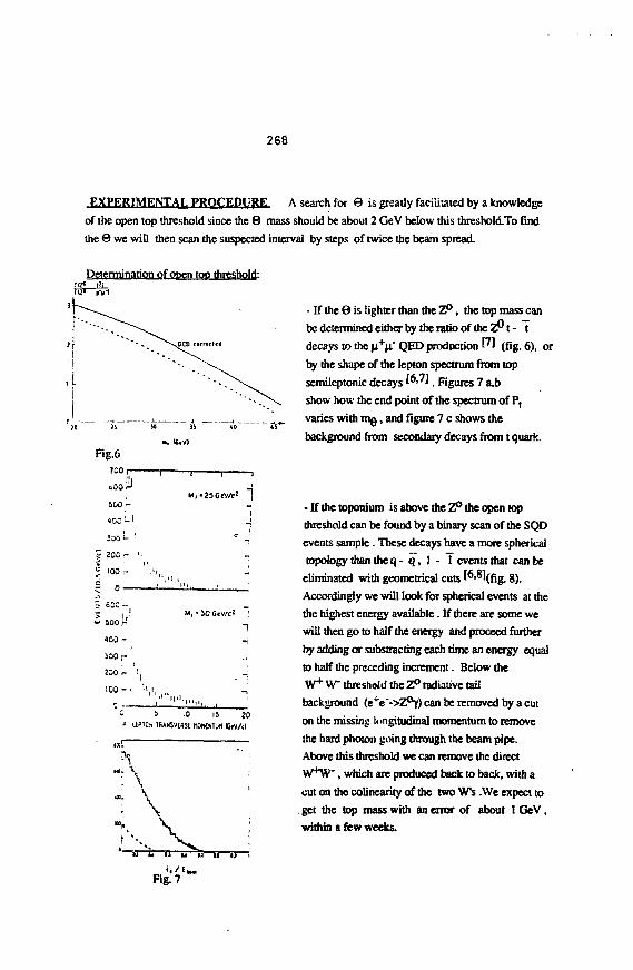
268
EXPERIMENTAL PROCEDURE A search for 9 is greatly facilitated by a knowledge
of the open top threshold since the 6 mass should be about 2 GeV below this thresholcLTo find
the 0 we will then scan the suspected interval by steps of twice the beam spread.
Determination of open top threshold:
it ii~
Fig.6rooi—
HioOOH
500 j -
yjo'i- '
g 200 r '•
I -00 rI 0 \ " i '
<- 500 r
400 -
loo ri
200 f- '!
M.-JOGev/c' ;
1
' ^ " - • • . . • . „ . , . .
5 IO IS 20
- If the 9 is lighter than the Z ° , the top mass can
be determined either by the ratio of the z P t - t
decays to the \i+)i~ QED production f l (fig. 6), or
by die shape of the lepton spectrum from top
semileptonic decays l&W . Figures 7 a,b
show how the end point of the spectrum of P,
varies with ing, and figure 7 c shows the
background from secondary decays from t quark.
- If the toponium is above the Z° the open top
threshold can be found by a binary scan of the SQD
events sample. These decays have a more spherical
topology than the q - q, J - 1 events that can be
eliminated with geometrical cuts ["'"(fig. 8).
Accordingly we will look for spherical events at the
the highest energy available. If there are some we
will then go to half the energy and proceed further
by adding or substracting each time an energy equal
to half the preceding increment. Below the
W* W" threshold the Z° radiative tail
background (e*e"->Z°y) can be removed by a cut
on the missing longitudinal momentum to remove
the hard photon going through the beam pipe.
Above this threshold we can remove the direct
W*W", which are produced back to back, with a
cut on the colinearity of the two Ws .We expect to
. get the top mass with an error of about 1 GeV ,
within a few weeks.
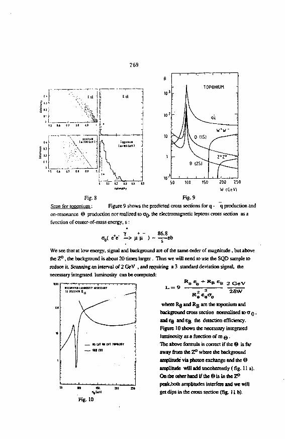
269
Fig. 8 Fig. 9
Scan for toponium : Figure 9 shows the predicted cross sections for q - q production and
on-resonance © production nor malized to OQ, the electromagnetic leptons cross section as a
function of centcr-of-mass energy, s :
, + . Yao( e e — >
, 86.8) - — n b
We see that at low energy, signal and background are of the same order of magnitude, but above
the Z° , the background is about 20 times larger. Thus we will need to use the SQD sample to
reduce it. Scanning an interval of 2 GeV , and requiring a 3 standard deviation signal, the
necessary integrated luminosity can be computed:R e e e "*" R B 2 GeV
R2 e2
a 2SW
where Rg and Rg are the toponium and
background cross section normalised to o Q ,
and Eg and eg the detection efficiency.
Figure 10 shows the necessary integrated
luminosity as a function of m Q .
The above formula is correct if the 6 is far
away from the Z° where the background
amplitude via photon exchange and the 6
amplitude will add uncoherently (fig. 11 a).
On the other hand if the ©is in the Z°
peak,both amplitudes interfere and we will
get dips in the cross section (fig. 11 b).
Fig. 10
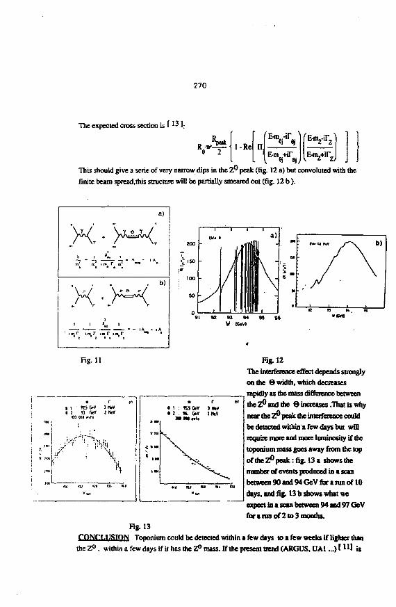
270
The expected cross section is f 13 J.
JWe 2
1-Re nr * a)
This should give a serie of very narrow dips in the zP peak (fig. 12 a) but convoluted with the
finite beam spread.this structure will be partially smeared out (fig. 12 b ).
1 1 8»T 1
' > ' ! , >
a)
- i A
, b)
r
l A «- i A .
200
ISO
0 0
SO
I i
IW. t
/
•
i
• ia)
iv -1 \9 ~
l i H n ,
1 ' « S CiV 7 11«V8 I « <*V 2 Ilev
( 1 : KS 6.V 3 NeV• 2 . H. CV I HcV
M M o h
92 93 94 9S 96W (O.VI
Fig. 11 Rg.12
The interference effect depends strongly
on the 6 width, which decreases
rapidly as the mass difference between
the z " and the 6 increases .That is why
near the ZP peak the interference could
be detected within a few days but will
require more and more luminosity if the
topomum mass goes away from the top
of the zP peak: fig. 13a shows the
number of events produced in a scan
between 90 and 94 GeV for a run of 10
days, and fig. 13 b shows what we
expect in a scan between 94 and 97 GeV
for a run of 2 to 3 months.
Fig. 13
CONCLUSION Toponium could be detected within a few days to a few weeks if lighter thant h e Z 0 . within a few days if it has the Z° mass. If the present trend (ARGUS, UAI...) HJ] is
iu nj >?f
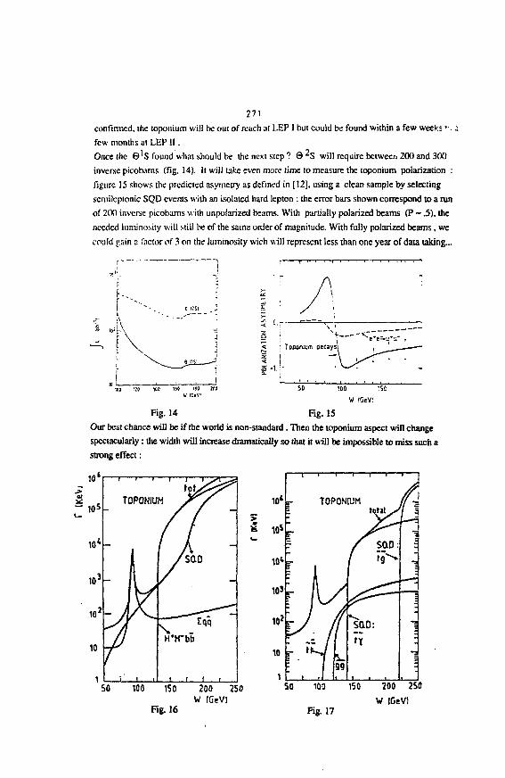
271
confirmed, the loponium will be out of reach at LEP 1 but could be found within a few weeks '• :
few months at LEP II.
Once the ©'S found whal should be the next step? Q^S will require between 200 and 300
inverse picobarns (fig. 14). It will take even more time to measure the toponium polarization :
figure 15 shows the predicted asyinetry as defined in [12J, using a clean sample by selecting
scmilcptonic SQD events with an isolated hard lepton : the error bars shown correspond to a run
of 200 inverse picobams with unpolarized beams. With partially polarized beams 0? - .5). the
needed luminosity will still be of the same order of magnitude. With fully polarized beams, we
could gain E factor of 3 on the luminosity wich will represent less than one year of data taking...
f\a -1. :-
ICO 110 UC 160 180 ZCS 50 '.00 ISC
V IGeV!
Fig. 14 Fig. 15
Our best chance will be if the world is non-standard . Then the toponium aspect will change
spectacularly: the width will increase dramatically so that it will be impossible to miss such a
strong effect:
10*
fi 105
103
10'
10
1
r- TOPONIUM ((-.L torj lX/ 3
• f ?£ D :
'* Is\J ft
99t t |
-I
1SO 100 150 200 250
W (GeV)Fig. 16
SO 100 ISO 200 250
W IGeV)Fig. 17

272
Figure 16 shows what will happen if the sopon/jm can decay irijo two charged higgs The decay
width will rise sharply and erase the resonance structure, and figure 17 shows what will happen
with SUSY particles. W's will find extremly large decay raits, missing energy and momentum,
carried away by the lightest susy particle, and no individual resonance. Such a big effect will be a
clear indication of new physics.
TOPONTUM Phvsics will be difficult..
The minimum we can expect will be a better understanding of electrc>wchk and strong interactions
within the Standard Model. With luck we could also open a window on a new physics domain
within a few months. Discrimination between the different theories will require much more time
and effort.
Acknnledpements
I am grateful to P.Igo-Kemenes, J.Mallet, J.Rander and J.Rich for their help in preparing this
repoa I would like to thank all organizers of ihe Symposium for their hospitality in Poland.
References
[1] A.Martin, Phys. Lett 100B (1981) 511.
(2) W.Buchmiiller.G. Grunberg and S.-H.H.Tye, Phys. Rev. Lett. 4Jj_ (1980) 103.
[3] G.Bhanot and S. Rudaz, Phys. Lett ZIB (1978) 119.
|4] E.Eichten et al., Phys. Rev. E H (1979) 3090. and £ 2 1 (1980) 203.
(5] C.Quigg and L.Rosncr, Phys.Len._Z2fi (1978) 462.
(6] W.Buchmiiilerecal., CERN-EP/86-02 , 21 february 1986.
[7] T.Himel. SLAC-PUB-3510, november 19S4.
[8] P.Igo-Kemcnesetal., CERN-EP/87-49, 2 march 1987.
[9J J.L.Richardson, Phys.Lett. £2£ (1979).
[10] K.Igi and S.Ono, Phys.Rev. £>22 (1986).
[111 J.Ellis and J.S.Hagelin , CERN-TH.4679/87
112J S.Gusken et al., Nucl.Phys. B262 (1985) 393.
[13] A.Manin. Phys. Lett J56E (1985) 411.
An extensive bibliography can be found in T61 and f 81.
273
TIME PROJECTIOM CHAMBERS AT LEP
A. Hinten
CEBN, European Organization for Nuclear Research, Geneva, Swltrerland
1. INTRODUCTION
In 1989 the e+e~ storage ring LEP at CEEN will (tart operation.
Four LEP experiments are under construction. Two of then, ALEPH and
DELPHI, use a Tiae Projection Chamber (TPC) as a central tracking detector.
In the following we will first recall the principles of TPC, and then
describe the technical solutions applied in the case of the two LEP
detectors.
2. THE TIME PROJECTION CHAMBER. GENERAL PROPERTIES II]
2.1 Principle of operation (fig. 1)
The TPC consists basically of a cylindrical barrel, closed by a
negative high voltage' electrode at one end and a set of wire chambers at
the other. The axial electric field E is degraded linearly along the axis
of the cylinder by Beans of a resistor chain, and a solenoidal magnetic
field B parallel to E is superinposed. Tolerances for homogeneity and
parallelism of the f J*ld i and b is of the order of 10"*.
3696H/AM/*d
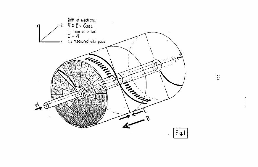
Drift of electrons'.$ S £~ Const.T time of arrival.Z-= vTx,y measured with pads
Fig.1
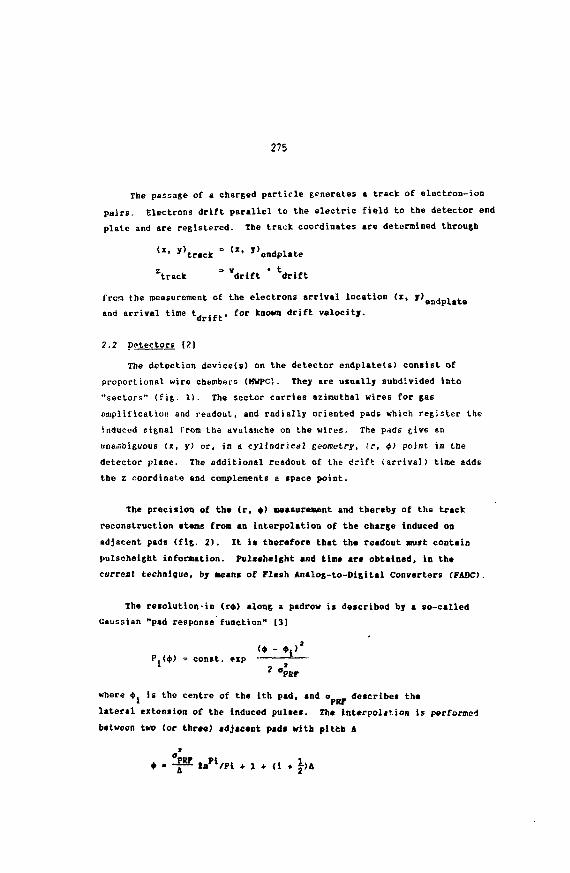
275
The passage of a charged particle generates a track of electron-ion
pairs. Electrons drift parallel to the electric field to the detector end
plate and are registered. The track coordinates are determined through
U - y)tr.ck " («' y)endpl.te
*track = "drift * ldrift
from the measurement of the electrons arrival location <x,
and arrival time t. .... for known drift velocity,drift
The detection device(s) on the detector endplate(s) consist of
proportional wire chambers (KWPC). They are usually subdivided into
"sectors" (fig. 1>. The sector carries azimuthal wires for gas
iimplification and readout, and radially oriented pads which register the
induced signal from tha avalanche on the wires. The pads cive on
unambiguous (x, y! or, in a cylindrical geometry, (r, $) point in the
detector plane. The additional readout of the drift (arrival) time adds
the z coordinate and complements a space point.
The precision of the (r, +) measurement and thereby of the track
reconstruction stems from an interpolation of the charge induced on
adjacent pads (fig. 2). It ia therefore that the readout mist contain
pulseheight information. Pulaeheight and tine are obtained, in the
current technique, by Beans of Flash Analog-to-Oigital Converters (FADC).
The resolution-in (r*> along a padrow is described by a so-called
Gaussian "pad response function" 13]
(• - •«>*P.(<t>> = const, exp
where <t>^ is the centre of the ith pad, and o describes the
lateral extension of the induced pulses. The interpolation is performed
between two (or three) adjacent pads with pitch A
*nPl/Pi + 1 + (1 • ht
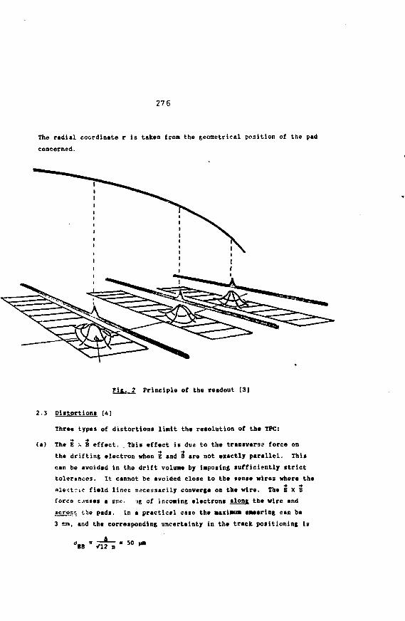
27 6
The r«di*l coordinate r is taken froa the geometrical position of the pad
concerned.
Fit. 2 Principle of the readout [3]
2.3 Diitortiont [4]
Three types of distortion* linit the retolution of the TPC:
(a) The E ~ B effect. . This effect if due to the transverse force on
the drifting electron when E and B are not exactly parallel. This
can be avoided in the drift volume by iaposing sufficiently strict
tolerances. It cannot be avoided close to the sense wires where the
electric field lines necessarily converge on the wire. The B X B
force c.<uses a srr.c- if of incoming electrons alone, the wire and
across the pads. In a practical case the Maxima shearing can be
3 inn, and the corresponding uncertainty in the track positioning Is
IB /12 nm 50 V»
277
where n = ;00 is the number of primary electrons d-ifting to a 3 cm
long pad.
(b) Diffusion. Transverse diffusion due to electron gas collisions
result an approximately gaussian smearing with 12)
•T * /2DtD = 6 mm
for 1 a of drift (D is the gas dependent diffusion coefficient).
The track centre can be determined to
a <
<£ . « 350 um . j
A further improvement comes from the trapping of transversely O
drifting electrons by the magnetic field. This causes a spiraling
with the cyclotron frequency u * e/m B around the electric field <
lines. The diffusion is thereby reduced to ".
where t i« the mean tine between collisions. (_O
o(c) Positive ions. Primary ionization in the TPC, and, much sore
important, gas amplification at the sense wires produce positive
ions. These ions drift in the direction opposite to the electrons to
the high voltage electrode. The drift velocity is, depending on gat
composition, of the order of 1 a/s. Positive ions generate a static
(pace charge and thereby an electric field, which by superposition
distorts the external field and thereby the drift trajectories.
Microscopic distortions of the order of several centimetres, apparent
track displacement have been observed IS]. In order to avoid space
charge and the distortions connected to it the concept of "gating"
has been deviled. Toe "(etc" consists of as additional wire grid in
front of the HUPC (fit,. 3). The gating grid is usually closed to
drifting ions and electron!, and no gis amplification takes place.
The gating grid it opened at the occurrence of a trigger indicating a
good event (calorisetric trigger, beam crossing trigger) and stays
open for a time *D'v • where I Is the active length of the
chamber.
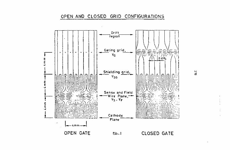
OPEN AND CLOSED GRID CONFIGURATIONS
EE
EE
iiSlili\~m—4mm—»H
OPEN GATE
_ Dr if t_region
Gating g r id ,
Shielding g r id .
Sense and Field ^ ^ ^ . £ < , ^ .—Wire Plane,—"" fc\i-~.%^. -'^^•~~s: I
i / ' i ' i i r i i!; '- ' ;!
Cathode"Plane
Fig. 3
l l . i l M i ! ; '' I I Il i i i i ' l
IS)
81
CLOSED GATE
279
2.4 TPC prformanc*
Th« performance of the TPC to a large extant detcribed by itf:
- Easolution. Th* overall (r+) reiolution it given by
a - •to2 * <J* * er* = ISO pm.r+ o EB D
Her* th» a term contains variations and fluctuations due to tracko
angles, track curvature, and readout sensitivity. Th* longitudinal
•resolution is determined by longitudinal diffusion, provided that th*
FADC clock runs sufficiently fast empirically
« : 1 • 141
Other positiv* performance criteria are:
- Almost full solid angle coverage.
- 3 dimensional readout with space point reconstruction and no ambiguities
in track recognition.
- Many sample* of dl/dx readout along a track.
On th* other hand, certain properties limit th* TPC performance.
These ar*:
- A long lifetime of about 20 us/a of an event drifting through the
chamber.
- Field distortions by positive ions.
This makes altogether th* TPC a powerful detector, but adapted mainly
to low rat* *xp*rim*nts, and perfectly matched to a *+e~ collider.
3. APPLICATION Of TIH> PtOJtCTIOH CH*Jff|*f
3.1 Overview
Th» main application of th* tim* projection method if in the frame of
• e experiments. Th* method was introduced for the PEP* experiment at
SLAC by D. Nygren and coll. from LBL Berkeley. Another device was butlt
for th* TOPAZ experiment at TKISTAH (KIK). V* will dascrlb* her* in torn*
detail th* two chambers used in th* ALEPH [6) and DELPHI [7] experiments
280
at LEP (CERN). Ve v.ll discuss TPC de*ign«, paraneters, coaponants,
readout, calibration, and terminât« with an Indication of tba statut of
construction and planning-
Th« TPC datectori ar* built by conaortiua which ar* a lubset of th«
collaboration« preparing th* «xperiaants.
- ALEPH: CESM, Glasgow. Mainz, MPI MDnchan, Pisa, Triait«, Wisconsin
(Projact Laad«r: J. Bay).
- DELPHI: CBKN, Collega da Franca, Orsay, Saclay (Projact Leader:
J.I. Augustin).
3.2 Dasiitn and paraaeter«
Both ALEPH and DELPHI TPC's ara of cylindrical shapa, with an inner
bora to contain vacuua tuba and innar dataetors, and with a eantral high
voltage elactroda and two datactor andplatas.
Tba paraaatars of th« two datactor» ar« listad balow:
ALKPH DELPHI
- Total length (•)
- External diameter (a)
- Bora disjaatar [•]
- Magnetic field (T)
- Gas
- Drift field IV/cm)
- Vuaber of detector scalart
- HuBber of. electronic channels
3.3 TPC coaponents
Th« aechanical and electrical components of the TPC are:
(a) The field cas.es. i.e. the inner and outer field cage. The purpose of
the field cage is threefold:
- To provide a unifora (io"*> axial electric field in the cylindrical
volus« between th* central HV electrode and th* «ndplate* on ground
potential. This Is achieved by excellent aechanical tolerances and
a highly linear voltage dividing resistor chain.
«.40
3.60
0.60
l.S
A + 91 CH
13$
36
4SOO0
2.68
2.32
0.65
1.2
A + 20%
220
12
22000
281
- To provide a tight gas containment with less than 10 ppra 0
contamination. The two LEP TPC's are layed out for atmospheric
pressure operation, but the DELPHI field cage can stand evacuation.
- To insulate the high voltage on the inner side of the cage from the
ground potential on the outer side, without punch through between
the electrodes. This insulation (and the gas tightness) is to be
achieved with a ninimum amount of matter in the cage walls- The
construction methods applied make use of Cn electrodes on G10
foils, of honeycomb structures for stability, and of mylar and
aluminium foils for gas scaling. The thickness of 20 (35)mm and
0.017 (0.027)1 are reached for ALEPH (DELPHI),o
(b) The detector endplates. The two endplates are subdivided into 18 (6)
sectors for ALEPH (DELPHI). Each sector carries on the inside a
proportional chamber with azinuthal sense wires, field wires parallel
to then and with radially orianted cathode pads. The pads yield the
r$ coordinates, the wires serve essentially for JE/dx measurements.
The sense/field wire grid is preceded by a decoupling shielding grid
and a (pulsed) gating grid (figs 4, S).
(c) The magnet. It hat to be of tolenoidal type, with highly homogeneous
field (10 ), and to the tane tolerance parallel to the electric
field. Both the ALEPH and DELPHI nagnets are equipped with
superconducting coils which provide l.S and l.Z T, respectively.
3.4 Readout
The detector signal is sensed by a preamplifier which is adapted to
the negative wire pulse or to the positive (and smaller) pad pulse. The
signal is then transported via twisted pair cables to e. shaper and to the
digitization unit. There a FADC scans the signal advanced by a 1?.S
(15.0) MHz clock. The dynamic range is 256 (512) channels, as given by a
8 (9) bit ADC. This range is appropriate to accommodate the variations in
pad response and from ionisation (logarithmic rise, Landau fluctuation and
angular effects).
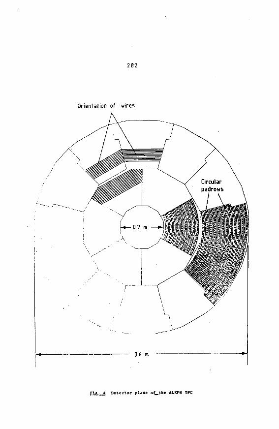
282
Orientation of wires
FU. » Detector plane o£_the ALEPH TPC
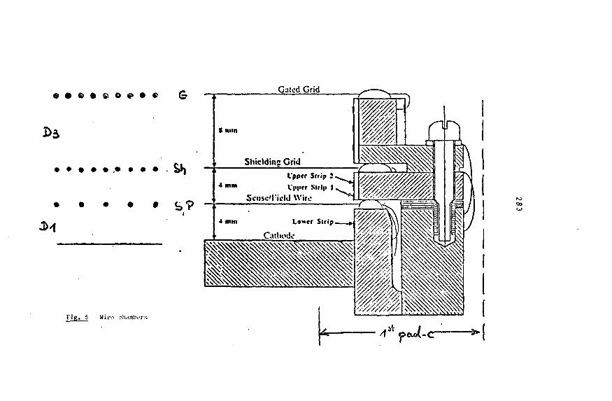
• 6 f t « O ( P » «Gated Grid
• •
F i g . 5 Wire ehrfinfcer.s
4 mm Lower Strip
Cathode
284
Digitized data are further processed by local HC 63020 processors.
This "local intelligence" assumes the tasks of system check, data
acquisition and calibration.
3.5 Calibration
The calibration aspect enters at two distinct and independent levels:
(a) Electronic calibration is required in order to make the sensitivity
of the readout channels equal and known. This is necessary since
spatial resolution is obtained by interpolation between adjacent
pads. The measurement of energy loss is another reason. Electronic
calibration is achieved by applying a standard signal at the input
(e.g. pulsing the field wires) and adjusting the slope of the ADC
such that, equal digitizations are obtained. The change of slope is
achieved by adjustments through. * Digital-to-Analog Converters (DAC).
lb> Geometrical calibration is needed in order to recognize and correct
for geometrical distortions due to mechanical! electrical or magnetic
imperfections. The calibration method consists of introducing a
laser beam into the sensitive volume of the chamber and to detect the
necessarily straight ionised tracks. The ALEPH TPC is equipped with
two Nd-YAG lasers, the beam of which is each split into 15 fubbeams
in one half chamber (fig. 6).
4. STATUS AND PLANNING
Both DELPHI and ALEPH TPC are in an advanced stage of construction.
The field cages are complete, the detector sectors are in part built,
readout electronics is industrially produced and delivered.
The ALEPH TPC is operating as a system with cosmic ray* and laser
beams, but only partially equipped with detector sectors and readout.
Completion is expected for early 1988, underground installation is
foreseen towari. the end of 1988.
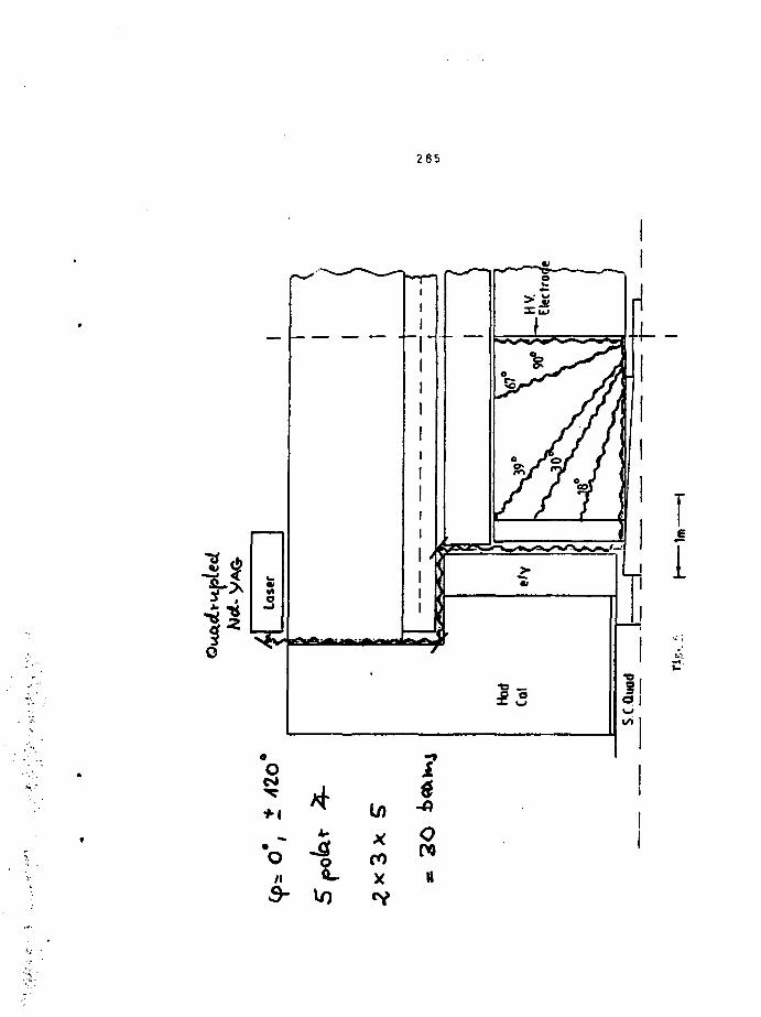
285
11
286
REFERENCES
[1] Vancouver Workshop 1983, AIP Conference Proceedings 108 (1984).
12) Y. Sauli. CERN Yellow report, CERK 77-09 (1977).
13} J. Richstein, Theiis, Universitat Dortmund (1986).
(4) J. Mijf. Stanford Workshop on Collider Detectors (1987) unpublished.
[5] ALEPH TPC, private conrunication.
[6] ALEPH Technical report, CEEM/LEPC 83-2 (1983).
[7] DELPHI Technical proposal, CEBN/LEPC 83-3 (1983).
2S7
Project of «i Tagged Veutrino Facility at Serpc^hov
G. Dohn, HUP Berlin - Zcuthen t GDR
The tagged neutrino facility at the 1HEP Serpukhov Is being built
by o Scrpukhov-Dubna-Pisa-Bcrlin/Zeuthen - collaboration. It should
start physics in ' to 2 years from now with the U-70 accelerator.
In tli.- niore distant future It could possibly be used at the UNK,
beini) one of the main experimental roods to -physics there.
In the first section of this talk, I hall Introduce the principle
of this new kind of v -beams. The second section is a short review
of the cxpcriui'ritnl technics, the third will concern the possibilities
for i> -physics, the fourth a proposal to itudy charged kaon decays
in a first stage of the experiment.
1. f.'nrking principle
At present two ways are well known to produce energetic i/-oearas in
t.'iu laboratory. Storting from a colllmated, but not monoenergetlc
eliui-ijrri or neutral hadron beam, after a decay tube and a muon
shield, ivlcJc-hand ( vy , \>t ) beams are formed; narrow-band beams use
.J iiioiio'.-neryelic chnryeil hadron beam instead. The neutrinos ( Vi,,
rcs|i, Vp from the clmrye conjugated beam) are produced by 7C-»(<V
and K->{*Odetovs' The radial distance of the vertex In the V-detector
is then used to constrain the v-momentum. The uncertainty of the
liurenl particle (iTorK) and its decay kinematics - the decay point
mid therefore the angle of the v* against the beam direction Is
only known to be in a certain interval - determine the errors of
primary V-energy and direction.
The togging principle, which will be used here, rests on simultaneous
measurement of the decay partners of the v> for charged Kw iresp. Ke,
decays in an intense momentum selected unseparated beam of about
35 GeV/c. In the former case, the muon angle against the beam direction,
in the latter, angles and energies of the electron and the two photons
from ir* decay will be determined. Using a long beam spill, the i>-events
will he related to their parent decays by time and geometrical in-
formation. The tagging station Is required to keep the information
from all candidate decays preceding a trigger signal from the j»-detector.
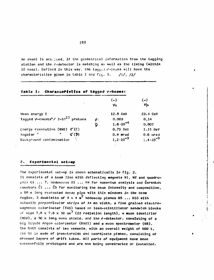
288
An event Is ace*,-led, If the geometrical information from the tagging
station and the ^-detector is matching as vtell as the timing (within
10 nsec). Defined in this way, the taijtjv..! -Uejms will have the
characteristics given in table I and fi<j. 1. /I/, / 2 /
Table I: Characteristics of tagged v-beaas:
Mean energy E13Tagged v>-events'/ 3»10 protons
Energy resolution (RMS) C ( E )
Angular * S* (5>)
Background contamination
Ve
9V
12.5 GeV0.0031.6-10"*0.75 GeV0.4 mrad1,2-10" 3
230
0
1
0
.4 GeV, 1 4
.007
.15 GeV
.6 (tired,4-10" 3
Z. Experimental set-up
The experimental set-up is shown schematically In fig. 2.
It consists of a beam line with deflecting magnets Ml, M2 and quadru-
pols 01 ... 7, hodoscops HI ... H4 for momentum analysis and Cerenkov
counters Cl ... C5 for monitoring the beam intensity and composition,
a 60 m long evacuated decay pipe with thin windows in the bean
region, 3 doubletts of 4 x 4 m hodoscop planes H5 ... H10 with
mutually perpendicular strips of 14 mm width, a fine grained electro-
magnetic calorimeter (TAS) based on lead-scintillator sandwich blocks
of size 7,6 x 7,6 x 32 cm3 (22 radiation length), a muon identifier
(MID), a 30 m long muon shield, and the v>-detector, consisting of a
big liquid Argon colorimeter (BARS) and a muon spectrometer (MS).
Tne BARS consists of two vessels, with an overall weight of 600 t,
the MS is made of iron-toroids and coordinate planes, consisting of
crossed layers of drift tubes. All parts of equipment have been
successfully prototyped and are now being constructed or installed.
289
3. Physics goals
The v'-phvslcj, which may be contemplated for this experiment, can
reasonably be based on a statistics of 2-10 v> -events; V>e-events
are down by a factor-^40 and Ve again by factors ~20 resp.
This disadvantage of a rattier limited statistics is compensated by
the fact, that systematic errors arc much lower than in other y>-beams,
because all parameters of tho incur'ri'j y will 1)0 dot >.:rr.in«rl fit tin;
level of on individual event.
More quantitatively, the following advantages apply:
- pure V4 , V* , Vg , iL -beams with 2 - 3 orders of magnitude less
flavour contamination than in conventional beams. High energy
^ , "\>e -beams are practically not existing.
- better (by factor 3 T 4 ) estimation of primary energy
- better (by factor 54-10) estimation of V -angles
- absolute normalisation better by an order of magnitude
- l;notvn v>-production vertex
The most obvious goals will be
- Detailed investigation of \?e - \L universality by (differential)
cross-section ratios for CC and \'C
- Measurement of absolute cross sections as functions of energy
(this is not at all obsolete in the lower energy ramje considered
here. Moreover it will improve conventional experiments by
checking their Monte-Carlo-correctlons).
- search for >>-osz£l lations (v>c-» Vr) and lepton mixing.
for other items - ueasurement of structure functions, study of
roro processes (dilepton-channels, large missing energy)-
thc statistics may be low, but nevertheless the rlir.ve mentioned
advantages apply as well.
4. Study of K* -decays
An obvious way to use the tagging station b.:.fcrc the '.<< rlctiliar, of
the large V-detector is to study charged K-decays.
After all, the U-70 with booster intensity is a good kaon ractorv -
and kaon decay studies, esp. v,ith high statistics - ho<>; always been
and continue to be of high value for the development - af.o restricticn
2 90
of elementary particle theories. •
On the experimental side, with hadron beam Intensity 10 /a, we can
have up to 10 K-oe;;ays/s in the vacuum pipe. With the hodoscopa,
TAS and a ,u-identif ier alone we have already very fast and efficient
possibilities for angular measurements and y-spectroscopy.
Most important for useful physics will be a fast and sophisticated
multilevel trigger and efficient data reduction - this is also under
development.
A3 a further upscale, there are designs for a large gas Cerenkov
counter for electron detection at the end of the decay pipe, an
ironfree toroidal magnet in between the first two hodoscop planes and
a hadron calorimeter instead of the passive ,u-shield for yu-identlfi-
cation. Among the proposed items are the following:
CP-violation: measurement of differences in partial nonleptonic
decay rates resp. Dalitz-plot densities between K* and K~.
Because such differences in AS » 1 channels can only exist,
IP t'4 0, this would be the most direct test of the Wolfenstein
mode 1.
Lcpton-nb violation: search for K^ITCf*, K--»T*e* e".
Radiative K-decays: search for K^ft^vV and K 4-* 1^"^ f*
study of K*-» IT e*e~ and K*-* rx0Y
The latter studies are of importance for theoretical models in the
framework of chiral effective Lagrangians.
Other more or less iiutomaticnl ly occnrauloted data on the life times of
K~ can be used to test CPT, and on the branching ratio for K e 3
decays lo improve the Koboyashi-Maskava matrix element Vus.
The start of this decay programme is - in minimal stage' - proposed
for the next year.
Ri>f rrenccs:
/ ] / A.A. ooikov et al., preprint IHEP 80 - 156, Serpukhov, 1980
A.A. Boikov et al., preprint IHF.P 80 - 158, Serpukhov, 1980
/2/ ?.P. Denioov et al., preprint IIIEP 81 - 98, Serpukhov, 1981
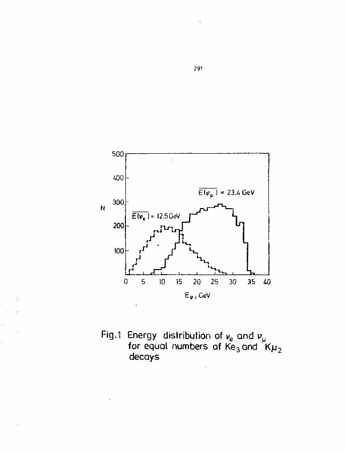
291
N
DUU
400
300
200
100
-
-
E(v«-
- r '
)
J
r
= 12.5 GeV
\ M
J i 1
X -T
= 23.4 GeV
\
1L
0 5 10 15 20 25 30 35 40
EW/GeV
Fig.1 Energy distribution of ve and i>for equal numbers of Ke3anddecays
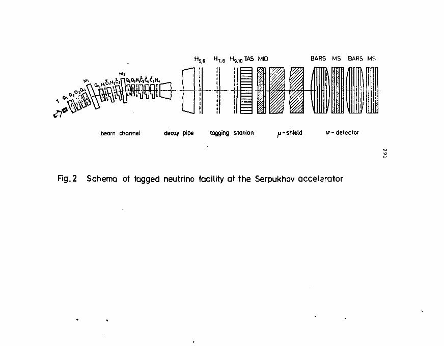
H5l6 H 7 i 8 H9i,0TAS MID BARS MS BARS MS
beam channel decay pipe tagging station i-shield V - detector
Fig. 2 Schema of tagged neutrino facility at the Serpukhov accelerator
293
On Superstrings and the Unification of Particle Interactions
Jean-Pierre Drrcndinger
lnflitut fur Theoretischc Physik
ETH Honggerbcrg
CII - 8093 Zurich. Switzerland
1. Introduction
Anomaly-free supemring theories }1.2- rould bring 2 solution to the long-stan-
ding problem of quantum gravity. This is the main motivation to consider the pos-
sibility of unifying all interactions in a fundamental supcrslring theory, ,">t a scale
close to the scale of quantum gravity, Mp — 10" CfV. However, the choice of
the fundamental superstring theory is far from unique. There is first the choice
of the space-time dimension. The most symmetric anomaly-Tree supersirings are
characterized by a ten-dimensional Minkowski space. But many other theories ca::
be constructed in lower dimensions, and they could as well lead to attractive uni-
fied theories. Many of the lower dimensional theories are related to ten-dimensional
strings by compactification, but many of them are new, independent theories. There
are two extreme options. Insisting on the unicily of the fundamental supcT5tr:i:g
leads to consider ten-dimensional theories, with a necessary dynamical compactifica-
tion of the extra dimensions. But one can also require staying with four-diincnsional
space-lime, avoiding compactification.
In the framework of ten-dimensional superstrings, only two theories satisfy both
the requirements of supersynunetry and absence of anomaly, which is related to the
absence of divergences. They are characterized by the gauge groups SO(32) and
E, ® E\. In fact, S0(32) can be realized either with open superstrings [3] or with
294
brtcrotic strings j<jj. while only helerolic strings can accomodate Et 3 £"J- These two
string theories possess the same iniusless scclor. Their effective low-energy theories
will differ only when higher order effects induced by the massive string modes are
computed. For phenomenologicaJ reasons, £» ® E't has proven to be much more
attractive than SO(32). At the level of the ten-dimensional theory, the choice is
then essentially unique. However, the process of compactification from ten to four
dimensions doe* not preserve this uniqueness. The geometry of the six compactined
dimensions is not fully determined by the equations of motion of the string theory.
Many possibilities exist, including Calabi-Yau spaces [5] and orbifolds [6|. Starting
from a unique theory, one then gets several possible particle contents and gauge
groups at energies much lower than the Planck scale where compactification occur*.
This scale is also the scale of the massive string modes, which should then have some
implications for the discussion of compactification and of the low-energy effective
theory.
In the case of four dimensions, there it no compactification, but man/ anomaly-
free string theories exist and there it no prescription for selecting a model out of the
several possibilities. The construction of four-dimensional string theories essentially
proceeds by imposing suitable boundary conditions on the string coordinates [7],
This method has been shown to provide many new one-loop finite string models, ,'
with various gauge groups and various spectra of massless states (7-9).
These notes are divided in two parts. First, some of the characteristic features of
the effective Lagrangian of superstrings will be discussed, essentially focussing oo the
case of compactified ten-dimensional heterotic strings, under the assumption that the
effective theory is supersymmetric. At energies much smaller than the Planck scale
Up, the superstring unified theory corresponds to an effective field theory describing
the interactions of the massless modes of the strings. To be realistic, the spectrum of
massless states must contain quarks, leptons, gauge bosons and the Weinberg-Salam
liiggs scalar*, and the parameters <' the effective Lagrangian should also 'predict*
the correct values of masses, coupling constants aad scales of symmetry breaking.
Supcrsytnmetry is a basic ingredient in understanding the scales of a unified theory
of strong and electroweak interactions (10]. It is also present in the fundamental
superstring, and could then survive the processes of low-energy field theory limit
295
a ml'or comji.Kiifiratiusi. Also, imposing supersymmetry at energies lower than the
IMaruk scale restrict* v.ry iiiurh tlir arbitrariness of the effective Lagraugian, matin?
mm li <«-icr Ilic <li-.cn»M":. of i!« irlaiion to lh>- fundamental Mipcrstrirtg theory. Al
prc.-.cnf *l*ee, no firm prediction exist for a non supersymir.etric effective theory.
In id'- ii<-c nil p.tri, *<<:IIC Ji::pccl« of the construction of four-domrniiicnaj tujjrr
• ttuiKK will l>e |»rr»cntrd. In p.itii- iilnr, thir procedure timed rn-{t«f—40)-to obtain
K.vii'r groups v.itli l«w rank* will be summarireH , i . • t ' » •",
2. The effective theory
I'p to :iov , most of tlic inveMigationi of the effective p.cld theory of super strings
.• Millie thai itic 'iin<laiuental t t n r j is the helcrotic slri-.ig with gause group EtQEf.
Ihi- rcAsou is ilia' tiicrc arc compactifirations of <he hcterc'tic siring whicL lead to
g.mgr groups .->!:d massless states very dose to a realistic extension of the Standard
M -<lrl. Tin* is the c&se of ro:::e Calabi-Yau spaces i l l ' jiudied in Rr{. }12J, ami
also of some orhifokls |C,13]. Tltr^e different possibilities arc in fact the only realistic
<-.- ulnl;;«'s for a unified supentiing theory known at present.
' / I . Gmi^c groups and spectra
Tlir icn-riiiii- iitioiu.l he'.Toiic string possesses many different rompactification
f acua which preserve one tupersj intuclrj in f-im liuncnsions. These vacua are proba-
bly all degenerate because of supersyinnuUt M- -,; of !ii< :n would lead to disastrous
phenomenology. Realistic cases are indco! uiii> • --""•'' minority of aM vacua, but
they show common features which offer the oppoi i <mu> of a global <i<s. u; sion of the
phenomenological implications of hcterotic supcistnng.s.
String dynamics requires the six coinpactified dimensions to live on a Hicci flat
compact space [5]. Supersymmetry in four dimensions implies lli.-t the hoionomy
group of the compact space is SU(3). It also requires the space to be itahlrnan. Two
classes of such spaces are known. Manifolds satisfying the above requirements arc
railed Calabi-Yau spaces. Even though there exists a large number of Calabi-Yau
spaces, there is probably a unique manifold producing three masslcss generations
of rjuarls and leptons and their supersymmetric partners, and compatible with a
realistic symmetry brr&kiiig pattern 1!'. Several cv-r- ;>-e k:!own with four i*nera-
tions (5*. The gauge ti^oup of Caljbi-Yau compact!frit- it '.- Jwejs a subgroup of
Ef d) K[. This is related to the necessary embedding of .he connection v.iiii SU(3)
holonomy into one of the £ • factors of ihr heteroiic 5:1 • ge P'«II:U. The choice of Ihe
subgroup is suggested by phenomenology rm)tiirvi(<>*ii!t and n'A, a: present, by dy-
namical «:,:nii)ciil». One rnns! require thiu a convcnirii'. :•> •:.,>••••• . lircaki'tg pattern
into SU(3) K St'(2) 9 V(l) rxi»lt with the S'aJar fi~l«!» c'«:'iii:'"tl in the *[<ectruin
of mnsslcM states. As !> consequence, £« h>s to be brc!.^::. b-j" many rluicef of
subgroup exis'. |14). The smallest gauge Ktuup cc>-:laini-.g 5"-V(3) S S''{2) & U[l)
compatible with j.hcnc-mcnolo.r y is in fact 5f ; (3)® S f ' U } s t r ( l ) ® t ' i l ) ' , with anew
f'(!) factor with f.pcr fie qua::lun. numbers for quarks a;;<l leptons. Nolire that F[
)•• a hi«''lri: scrlor in th? srnc- that the spe.irum of massitss slates docs not <or,'dn
'tai--.- with Sfr(3) S S{/(2) 5J I (I) as well as E't interactions.
I'lic sccond class of compa<-l spaces lea&og to supersy.runctric couipacl.:*r<:i:ojis
of tl;<? heterot'e strini;«= corroiponrfs to orbifclds !6j. These spaces are obtained :••
i1i%ic'!n(; by a dis-rrlr rrcup a manifold which, in the case "f strings, is in general .1
six-toi us. Orbifolds arc not manifolds. They have singularities. It is however possible
to define properly the propagation of strings on such spaces. Their prediction!; for
the low-energy effective theory are quite similar to those of Cidabi-Y&u spaces. T V
gauge group is t si^.croup of Ef ® St/(3) 55 JBJ. The SU{3) factor is not broken as ii
was the rase with Calabi-Yau spaces. As in the case of Calabi-Yau compaclificalions,
thr »-ffrctivr, low energy gauge group is always larger than SU(Z) ® SU(2) ® V(l).
The same new U(\) group is always present below the Planck scale, but much larger
symmetries can also arise. A potential problem with orbifoldi is that they produce
in general a (00 lutve number of quarl-lepton generations. More realistic orbifolds
require more sophisticated constructions [13].
The spectra of massless states of hcterotic strings compactified on Calabi-Yau
manifold? and on orbifolds are essentially similar. The states are naturally classified
in siiprrsyimnrtry multiplcts, since by assumption compactification leaves one super-
symmetry in four dimensions. The gauge multiplet of local lupersymmetry is the
suptrgranty multiplct, with the spin 2 graviton and its spin 3/2 partner, the grav-
itino. A Yang-MilU multiplet (gauge bosons and spin one-half gauginos) is associated
297
to the effective gauge group, which is always larger that SU(3] ® SU(2) ® U(1). The
chiral matter multipleU (left-handed spin one-half states and scalars), which should
contain quarks, leptons and Higgs scal-irs, are classified in replications of generations
of 27 states. This is the consequence of the embedding of SU(3) g SU(2) <8 U(l) in
Ef. Each quark-lepton generation is enlarged to a 27 multiplet of Es, even though
Ei is broken. The SU(3) 0 SU(2) ® U(l) quantum numbers of the 27 states are the
following: we first have the 15 quarks and leptons:
+(1,2,-1/2) + (1,1,1).
In addition, we have twelve new states transforming according to
(3,1,-1/3)+ (3,1,1/3)
+(1,2,1/2) + (1,2,-1/2) + 2(1,1,0).
An important result is that the new U(l) gauge group which is always present in
both Calabi-Yau and oroifold compactifications imposes that all the 27 states remain
massless as long as this new symmetry is not broken. The scale of the new neutral
gauge boson is then also the scale of the new (spin 0 and 1/2) states enlarging each
quark-lepton generation. The number of generation is related to the geometry of
the compact space used to compactify heterotic strings. The spectrum of massless
states can also contain some chiral multiplets in real representations of the gauge
group. Their number and their classification depend very much on the choice of the
compact space. These multiplets are essential for spontaneous symmetry breakings at
intermediate scales (M\y < J < Mp), which must also preserve supersymmmetry.
Calabi-Yau compactifications always produce such states, while orbifolds forbid them
in general. As a consequence the scale of the new U(l) gauge boson (and of the new
states enlarging each fermion generation) should be close io the weak interaction
scale in orbifold compactifications. This scale can however be very large (even close
to the Planck scale) in Calabi-Yau compactifications. A firm prediction of this scale
relics upon a precise knowledge of the effective Lagrangian.
String compactification also produces some gauge singlet chiral multiplets. Their
number depends on the geometry of the compact space, but two of these singlets
play a particular role, and are associated with classical symmcirics of the underlying
298
string theory [5,15]. The scale invariancc of the string theory generates a dilaton
massless mode with specific couplings directed by scale invariance. Also, compactified
superstrings have a reseating property related to the fact that string equations of
motion do not fix (classically) any scale. The radius of the compact space can then
be freely rescaled. This symmetry generates a 'breathing' massless mode. Once
redefined in a way appropriate to the supergravity formalism, these two gauge singlets
correspond to two chiral mul'.iplets 5 and T with Very specific couplings. These two
multiplets play a crucial role when the explicit form of the effective supergravity
Lagrangian is investigated.
2.2. The effective supergravity Lagrangian
At energies much smaller than the Planck scale, the interactions of the mass-
less modes of compactified superstrings are described by an effective supergravity
Lagrangian. Again, compactification is assumed to preserve one supersymmetry in
four dimensions. This Lagrangian contains different components. It can be split
(somewhat arbitrarily) into two parts:
Ct/f = C0+Ci. (1)
Co contains all terms with at most two space-time derivatives. In particular, it in-
cludes all terms of dimensions up to four, but some terms of higher dimensions,
without derivatives are also present. £ 0 has the familiar form of four dimensional
supergravity theories [16]. It is fully described by two functions of the chiral multi-
plets, the Kahler function Q(z,z') and the function defining the gauge field kinetic
terms, /o^fz). These two functions introduce in general interactions of arbitrary
high dimensions, but without .derivatives.. C\ contains all higher derivative terms
(like Loreniz Chern-Sitnons forms) and their supersymmetrization. The presence of
t hese cotit ributions requires an extension of the formalism of four-dimensional super-
cravity [17). On the other hand, these new terms are a crucial feature of superstring
theories, since the mechanism of anomaly cancellation appears essentially in this
sector of the effective theory.
At the classical level, the form of Co is essentially determined by the classical
symmetries of the string theory, Ar = 1 supersymmetry and the origin (in terms of
299
ten-dimensional states) of the massless fields [15,18). At this order, A also receives
contributions, which are only partly known. Determining £o means obtaining the
two functions , .g(S,S',T,T',C',cr),
(2)fa0(S,T,C),
where C' represents all matter multiplets with gauge quantum numbers (mainly the
states of 27 and 27*). The only gauge singlet multiplets which we keep in this
discussion are the two 'geometrical' singlets S and T. The complex fields S and T
have imaginary, pseudoscalar components originating from the antisymmetric tensor
of the ten-dimensional massless supergravity multiplet. They have then axion-lihe
symmetric! of the form:
Im S,T-* ImS,T + constants. (3)
As a consequenceg = g{s+s*,T+T%c\ct)
(4)
where a and 6 are constants, and F is an arbitrary function. The two classical
symmetries, scale invariance and the reseating property, mean that
Q = - ln(S + S') - Zln(T + 2")
The superpotential W takes the form
i kU , (6)
up to higher dimension terms, suppressed by Mp ",n > 1. This form is due to the
Ee and Es gauge symmetry. The only arbitrary function is g. The function fa0 is
fully determined:
fafl = cS6afi, (7)
where c js a constant. In simple truncations [15], which are related to orbifold com-
pactifications but probably not to Calabi-Yau compactifications, the function g reads
(8)
300
so that finally [15,19]:
g = ~ln(S + S')- 3ln (T + T'~ 2&CI) + in(WW),
W = \ijkCiCiCk+w (9)
fafl = cS6a0-
The coupling constants A,yt contain the Yukawa couplings of quarks and leptons,
which are in principle calculable from the superseding theory. The corresponding
supergravity Lagrangian is the starting point for the so-called superstring inspired
modelt.
The scalar potential, including terms bilinear in the gaugino fields, is a sum of
positive terms:
where» = ReS=-(S+S'),
2 (11)
and Wi is the derivative of W with respect to C*. The positivity of the scalar kinetic
terms removes the apparent singularity in a and tc, and ensures the positivity of
the potential. This potential has remarkable properties: the necessary breaking of
supersymmetry is induced only by gaugino condensation [20,21]:
< T V >= K* / 0. (12)
The minima of the potential have zero cosmological constant, < Vtjj > = 0. Possible
vacuum expectation values of thp scalar fields C* will in general induce intermediate
symmetry breakings of the gauge group to finally obtain SU(3) ® SU(2) ® 17(1). It
is remarkable that all directions in C" which can be used for a realistic symmetry
breaking satisfy< XijkC'Ck >~< Wl >= 0
(13)< \ijkC
iC'Ck >= 0
Then, for relevant directions, < W > = u», and the vacuum expectation values < C" >
are not determined by minimizing the potential. The potential has flat directions
301
and the scales of intermediate breakings are free (at the classical level at least). The
minimization of the potential in supcrsymmetry breaking directions will cause u, A*
and < »tc > to adjust themselves in order to have < V > = 0. The potential has also
flat directions in the singlet sector, leaving all breaking scales undetermined at the
classical level. This is a remnant of the scale invariance of the superstring theory.
As already mentioned, supersymmetry is broken only when gauginos condensate,
and, from the structure of the potential, when the superpotential W contains a
constant term u> [20]. Gaugino condensation will occur in general in the hidden
sector. The hidden gauge group is an asymptotically-free force. The gauginos of the
hidden sector will then form condensates at a scale Ac close to the scale where this
force becomes confining.
At this point, there is an important difficulty. The scale of supersymmetry
breaking is fully determined by the hidden sector. It will then induce supersymme-
try breaking corrections to the visible sector of the theory. However, the classical
Lagrangian does not contain any toft breaking term, even when gaugino condensation
is included [21]. Then, only higher order loop corrections can transmit the effect of
supersymmetry breaking to the visible sector. Ultimately, the soft breaking terms
generated by higher order corrections should induce the breaking of 527(2) ® 1/(1) at
the right scale, ~ 100 GeV. This will be feasible only with a large scale Ae of gaugino
condensation, which is fixed by the hidden sector. Thus, finding the right scales
involves a subtle interplay of the visible and hidden sectors, controlled by quantum
corrections. This situation corresponds essentially to no-teaU tupergravity models
[22], except that all parameters are now in principle calculable in terms of the fun-
damental superstring theory. Numerical predictions rely heavily upon higher order
quantum corrections. These corrections fall in different classes. Supergravity loop
corrections have a physical cut-off at the Planck scale Mp, where the full superstring
theory turns on. They are in principle easily calculable. For instance the one-loop
effective potential has been computed [23], and shows a tendency to curve the flat di-
rections and to push the vacuum expectation values towards the Planck scale, where
the calculation loses its validity. In this region, we face real superstring corrections
and a complete analysis is missing. Notice that one-loop superstring corrections are
in principle calculable since the string theory is finite at this order at least.
302
More precise, numerical predictions, like for instance values of Yukawa couplings,
require a deeper understanding of the compactification process. The unique known
model which can be made realistic as far as gauge groups, massless slates and sym-
metry breaking are concerned, is the Calabi-Yau compactification of heterotic strings
found in Ref. [11]. Its structure and predictions have bean analyzed [12] under sev-
eral assumptions concerning the compactification vacuum. Even for a well defined
Calabi-Yau space, this vacuum is far from unique. There is an infinite number of
vacua leading to the same symmetry breaking pattern, but with several different
discrete symmetries applying in the effective theory. These discrete symmetries are
in general important to avoid unwanted Yukawa couplings, or to forbid disastrous
processes like, for instance, fast nucleon decay. Details of the effective theory will
then strongly depend on the choice of the real vacuum, which results from string
dynamics and can hardly be investigated with present technology.
3. On four-dimensional superstrings
String theories are constructed from two basic building blocks: the bosonic string
containing 24 real, light-cone string coordinates X1, and the superstring made of 8
real light-cone bosonic coordinates and 8 two-dimensional (world-sheet) spinorial
coordinates Sa. Notice that the crucial number is twenty-four, since a spinor corre-
sponds to two real degrees of freedom. The superstring brings naturally supersym-
metry, whose interest for low-energy phenomenology has bees already mentioned.
It is also an essential ingredient in understanding the vanishing of the cosmological
constant. For each of these two cases, the string Lagrangian is a two-dimensional
field theory, and the right- and left-movers form independent sectors. Then, for in-
stance, heterotic strings [4] are obtained by associating the left-movers of the bosonic
string and the right-movers of the superstring. The number of components of the
string theory is a consequence of two-dimensional conforms! invariance, which is the
remnant of the reparametrization invariance of the world-sheet, necessary for a phys-
ically satisfactory model. The conformal anomaly will only cancel for this critical
number of string coordinates, and this cancellation has to occur separately for left-
and right-movers.
This critical number of string fields can be translated into a critical space-time
303
dimension once boundary conditions are imposed. We will only consider here closed
strings: open strings are a particular subcase with identical left-and right-movers.
Imposing thai nil string coordinates are periodic functions of r ± a leads to the most
symmetric sit- itioti, with the largest space-time symmetry. In this case, one can
construct a full LorenU algebra in space-time dimension 26 for the purely bosonic
string or 10 for lh« yurrly superslring case. There are however many other possible
boundary conditions which will lead to different space-time properties. These more
general boundary conditions sometimes correspond to compact.ificat.ions of the most
symmetric model, with the largest space-time dimension. This is the case if left-
and right-mover coordinates are treated symmetrically, with the same boundary
conditions. However, a string theory with different boundary conditions for left- and
right-movers is not in general equivalent to a compactified, larger dimensional theory.
For closed strings, the adinissible boundary conditions are of the form
2\r ± a - IT) = ('**''Z*(T ± c) + v' (14)
for bosonic coordinates, and
i" (15)
for fermions. They contain two different quantities, the shifts v1 and the twists 8. The
shifts v are characteristic of compactification, when space-time has the geometry of
a generalized torus. The simplest example arises when one space direction XA is a
circle of radius R. Then the boundary condition for a closed string coordinate in this
spatial direction is naturally written
XA(<r = 0, T) = XA(a = r,r) + 2xRn. (16)
The integer n counts how many times the string coordinate loops around the circle.
The shifts v1 are the generalization of this simple situation to the case of an arbitrary
number of string coordinates, which can be either left- or right-movers. They span a
lattice and introduce new string states corresponding to winding sectors which often
contain massless states leading to large, non abelian gauge groups. The twists 9 are
present for instance in orbifold models [6]. In these cases, they correspond to the dis-
crete symmetries used in defining the orbifold. The role of twists is crucial to reduce
the rank of the gauge group. In general, in a string th~>< -y •.••'.thou* *wi' H bosons,
the rank of the gauge group is the same as the number of 'iitpi uaV rnr^dinates. To oe
complete, one should consider a matrix of twists. Here, we will only consider abelian
twists 0! associated to the coordinate Zl, or to a givrn jjjinor. Notice also that twists
require working with complex bosonic string fields. Twists- generate twisted sectors,
with new string states which are in general massive. Th^y cio not generate new gauge
symmetries, but can produce new massless matter (i. e. .f>in 0 or 1/2) slates.
However, choosing boundary conditions is not enough to provide a physically
satisfactory model. The string theory must satisfy additional conditions. The con-
sistency of the quantum theory (i. e. the finiteness property) corresponds to the
iiivariance of loop amplitudes under modular transformations of the world-sheet of
loop diagrams. At one-loop, the world-sheet if a torus. Modular invariance leads then
to constraints on the boundary conditions along to the two non ccatractible loop..
on the torus. There is a further condition arising at two loops. The corresponding
world-sheet is obtained by 'gluing' two tori. There is then a new non contractible
loop connecting the two handles, leading ia general to a new constraint on boundary
conditions. Higher loop diagrams are obtained by gluing further tori, but only re-
peating the same conditions of modular invariance. There is then no new constraint
beyond two loops. The one-loop path integral is essentially the partition function for
the string states. Modular transformations act on the partition function and mix in
general different boundary conditions. The problem is then to find a set of twists and
shifts such that modular transformations close on this set. The sum of the partition
functions for all boundary conditions in the set is then modular invariant at one loop.
The last step ia then to impose two-loop modular invariance, which may introduce
further constraints.
Many four-dimensional string theories can be constructed along this line, by
choosing boundary conditions such that the space-time symmetry contains only four-
dimensional Lorentz transformations, all other string coordinates corresponding to
internal degrees of freedom [7-9]. They possess various gauge groups and massless
sp> tra. The rank of the gauge group is ia general very large, and in most cases
(7,8) it is twenty-two. This is certainly far too large for a realistic unified model,
containing the standard SU(Z) ® 5(7(2) 817(1) model. Reducing the rank it then an
305
important issue, and can be obtained with twisted bosons, generalizing orbifold com-
pact ificat ions. The most interesting theories use the same set of string coordinates
a» the hetcrotic string. The bosonic sector is used to produce the gauge group, which
can l>c physically attractive in many cases, and the fermionic sector allows space-time
supcrsymmelry in four dimensions, an important feature of many unified models of
strong and electroweak interactions. We will now summarize the construction of
twisted four-dimensional supcrstrings [9J, leading to many string theories with lower
rank gauge groups. In particular, rank eight or sixteen are favoured by the solution
of the constraints of modular invariance.
The strategy to construct twisted four-dimensional supcrstrings is then as fol-
lows. We start with the following set of string coordinates: the left-movers are purely
bosonic:X'{r + tr) a ^ 1 , 2
(17)Z'{r + <r) 7 = 1 , . . . .11 ,
while the right-movers are those of the superstring:
X*(r-<r) a =1,2
S"(r-a) a = 1,2(18)
Zk(T-O) * = 1,2,3
S"k(r-a) Jb = 1,2,3
Real and complex bosons are respectively denoted by X and Z. The four-dimensional
space-time light-cone coordinates are X*, a = 1,2, and should then be fully periodic.
We then assign a twist S and a shift v to the other complexified boson coordinates.
We also assign a twist to each right-moving fermion. The requirement of N = 1
space-time supersymmetry implies that the four right-moving spinors should have
the same twists as the right-moving bosons. The space-time spinoria! coordinate Sa
is then periodic. The other right-mover states will however be twisted in order to
avoid a larger (N — 2 or 4) supersymmetry. The full set of boundary condition is
then specified by
W = (0,<Mflk,t>*)!(«/,w)), * = 1,2,3, 7 = 1,. . . . 11 , (19)
where the entries coreespond respectively to 5", Sai, Zk and Zl. This vector IV
can be splitted into a rotation rector R containing the twists, and a shift vector V.
306
We omit the transverse, periodic bosons X". In addition the closure of Lorentz and
supersymmeiry algebras imposes that
0t + 9t + 0t = 0 mod 1 (20)
for the fermion twists. At this point, requiring N = I supersymmetry is not essential
for the rest of the formalism. It is only an assumption, due to 'phenomenological'
motivations. One could as well twist the spinor 5" and break all supersymmetries,
or obtain N = 2 by choosing, say, dj = 0. This would not lead to any fundamental
change of the following discussion.
The next and most important problem is to solve the constraints of modular
invariance. The procedure is to combine partition functions of string fields with
given boundary conditions in a modular invariant way. The method we follow is
analogous to the discussion of Ref. [24], generalized to allow for twisted bosons.
There is however an important complication: the partition function of a sero twist
boson (which can however have a shift) is not the $ = 0 case of the partition function
of a twisted boson. This is essentially due to winding states, which are anyway
absent for non trivial twists. This is apparent in the mode expansion of a boson with
boundary condition (14), which reads
L I ^ t ™ * \ (21)
with
j'-.'fl-e-""*)"1- (22)
This last expression cannot be used for 0 = 0. Twisted bosons have no zero modes,
corresponding to the quantized momenta of shifted bosons. This difficulty can be
circumvented with the help of a projector
Vti = SMSM = 1 for sero twists(23)
= 0 otherwisewhich allows to treat all cases simultaneously. The full partition function for a
particular pair of boundary conditions W and W is
•n[(i--p.,,t)z--1=1
307
in terms of the partition functions for a twisted fermioo {£ ' ) and a shifted boson
(Zl). We then impose modular invariance on combinations
A.B
and volve for the coefficients CjJ£. One-loop modular invariance is in general not
sufficient to ensure having a physically satisfactory string theory. Anyway, it does not
fully determine the coefficients. A further condition arises from two-loop diagrams.
We use a generalized GSO projection (in analogy with (24}) to take this last constraint
into account. As already mentioned, a modular invariant combination (25) involves in
general many different boundary conditions. The corresponding string theory always
contains an untwisted sector and several twisted sectors, with different projectors V.
The equations of modular invariance applied on combinations (25) are very com-
plicated to solve in general. They are however much simpler in the case where all
relevant projectors V satisfy the condition
where the indices a =JK u n1- 1<- ;J1 possible vectors Wm and W». This particular
condition restricts the possible values of the rank of the gauge group to 16 or 8 (or
even 0). There are probably more general solutions leading to other values of the
rank, but a more sophisticated treatment of the conditions of modular invariance is
necessary.
The solution of the equations of modular invariance assuming Eq. (26), associ-
ated with the mass formula allow us to construct explicitly the massless states as
well as the massive levels, and then to obtain the gauge group and the massless chiral
tnultiplets for each set of shifts and twists. As an example, the construction of the
Z, orbifold strtng theory, with gauge group E,®SU(H)<gsE, [6] begins with the four
shift vectors* = ((1/2)»|(1/2)M)
t,, = (0»|0",(l/2)»)f27)
v, = (0V(l/2)'0*) l >
», 1/3,1/3,2/3),
308
and with the twist vector
R = ( 0 , ( l / 3 ) \ ( l / 3 ) ' | ( l / 3 ) ' , 0 t ) , (28)
where the superscripts indicate the multiplicity of the entries. Modular transforma-
tions then generate all possible combiuations, with entries denned modulo I, of these
basic vectors. The vector c» alone corresponds to the SOI44) model with N = A
supersymmelry. The effect of t>, and cj is to break SO(44) into SO(12) ® 50(16) ®
5O( 16), but also to generate new massless states enlarging each 5O( 16) factor to
£t. At this point, the gauge group is then 9O(12)®E,®Et. Adding vt then breaks
the second £"« group icto E, ® SU(Z). The twists are then used to break completely
the SO[ 12) part, reducing the rank to sixteen. At every step of the construction,
some new massless states are created, but some others are projected out by modu-
lar invariance. Notice that the rotation vector R carries the Zj discrete symmetry
used to define the orbifold. This discrete symmetry is relevant when the full states
are constructed as products of left-movers and right-movers. The orbifold case corre-
sponds to the subsrt .A states which are Z% invariant. The set of vectors (27) and (28)
ci»n indeed lead to different string theories depending on the prescription of discrete
symmetries used to define the product states. With the help of this Z\ symmetry,
one can check that the spectrum of massless states obtained by our construction is
identical to the spectrum described in Ref. [6]. This theory is however not very
attractive since tlie number of quark-lepton generations is 38.
Using this example as a starting point, one can now construct a theory with a
rank eight gauge group by completing the set of basic shift and twist vectors. We
then add the vector
(29)
fhere
R, = | 0 . - , - - - . - . -10* f - ) 4 04 I
' (30)
The shift vrctor V, is used to break the Et part of the gauge group of the Z3 orbifold
into SO( 101 @ tf( 1). However, the introduction of the new rotation vector JZj means
that the £* part will completely disappear. We then obtain the rank eight gauge
group SO{\0)f: vl'l3)&U(l). which it tlr^ady murh closer tc f.inuliar Grand I'nifici:
'I'hrt.rirs. Ttii> iirw theory itas tmwever the same fal.il prm icra as our previous
example: the number o.' qunrk-Ieplun generations is far too large. Notice that the
twisi vrrtnr Hi treats xtytunictrically left- and right-mover:'. The corresponding
firing theory ran not be obtained by compartifiration of a larger dimensional string.
In gr Titi, our analyst thowt that gauge groupi with rank eight or sixteen
Arc c;.'.i!y o'*l->;ncd. Theie gauge groupi arc also quite often attractiw unifying
symmetries and the inasklcss matter multiplets fall also <juif rRurally into quark-
Icpton generations, at most enlarged to the 27-dimensional Et mulliplet. It is however
more difficult to obtain a small enough number of generations. This is a genera!
problem in the framework of supcrstring theories. Compartifications of the heterotic
st rings have the same tendency, even though a few examples with lh;ee generations
are known. Finding a realistic four-dimensional suprrstring theory with a small rank
gauge group is still an open issue.
There are many ph»nomeno!ogical reason* to insist in reducing the size of the
gauge group of superstring unified models. For instance, a 1-rge gauge group is
much harder to break into 5(7(3) ® SU(2) 8 (7(1) by the Higgs mechanism. As we
have seen in Section 2, a hidden sector can be very useful when generating super-
symmetry breaking. However, a satisfactory scale for this breaking can be obtained
only if the hidden sector does not contain large non abelian (simple) components
[19). There is no necessity, and certainly no evidence of a very large gauge group.
Pour-dimensional rupentrings with twisted bosons may ultimately provide a minimal
supcrstring extension of the Standard Model. Such a theory would be very hard to
distinguish from the minimal sapersymmetric extension of the Standard Model, at
energies much smaller than the Planck scale.
References1
[1] M. B. Green and J. H. Schwan, Pbjrs. Lett 149 B (1984) 117; 151 B (1985)
21; Noel. Phyt. B 2SS (1985) 93.
[2] For reviews see: J. H. Schwan, Phyt. Rep. 89 (1982) 223.
M. B. Green, Surveys in High Energy Physics 3 (1983) 127.
310
M. B. Green, J. R. Schwarz and E. Witten, Superstring Theory (Cambridge
Universiiy Press, 1987).
|3i M. B. Gro-m and J. H. Schwarz, N-JCI. Phys. B 181 (1981) 502; B 108 (1982)
252; B 108(1982)441.
(4j D. J. GroM, J. A. Harvey, B. Martincc and R. Rohm, Phyt. Rev. Lett. 54
(1985) 502; Nud. Phyt. B 250 (1985) 253; B 267 (1986) 75.
[5i P. Candelat, G. T. Horowitz, A. Strominger and E. Witten, Nad. Phyt. B 258
(1985) 46.
J6! L. Dixon, J. A. Harrey, C. Vafa and E. Witten, Nud. Phys. B 261 (1985) 651;
B 274 (1986) 285.
[7] K. S. Narain, Phys. Lett. 100 B (1986) 41.
[8] K. S. Narain, M. H. Sarmadi and E. Witten, Nud. Phys L. 278 (1987) 369.
H. Kawai, D. C. Lewellen and S. H. Tye, Phys. Rev. Lett. 57 (1986) 1832;
Nud. Phys. B 288 (1987) 1.
M. MeuUer and E. Witten, Princeton preprint, (1986).
Da-Xl-Li, Phys. Rev. D 34 (1986) 3780.
W. Urche, D. Lûst and A. N. ScheUekeni, Nud. Phyt. B 287 (1987) 477.
I. Antoniadis, C. P. Bâchas and C. Kommas, Nud. Phyt. B 288 (1987) 87.
K. S. Narain, M. H. Sarmadi and C. Vafa, Harvard preprint BUTP-86/A089
(1986).
[9] A. H. Chamseddine and J.-P. Derendinger, preprint ETH-PT/87-2 (1987).
[10] For a review see: H. P. Nilles, Phyt. Rep. 110 (1984) 1.
(lij S.-T. Yau, ia Proceedings of the Argonne Symposium on Anomalies, Geometry
and Topology (World Scientific, Singapore, 1985).
[12] B. R. Greene, K. H. Kirklin, P. J. Miron and G. G. ROM, Piiy*. Lett. 180 B
(1986) 69; Nud. Phys. B 278 (1986) 667; B 202 (1987) 606.
[13] L. E. Ibinez, H. P. Nilles and F. Queredo, Phys. Lett. 187 B (1987) 25.
L. E. Ibànex, J. E. Kim, H. P. NiDer and F. Qnevedo, Phyt. Lett. 191 B (1987)
311
282.
L. E. Ibânez, H. P. Nilles and F. Quevedo, Phys. Lett. 192 B (1987) 332.
[14] E. Witten, Nucl. Phys. B 258 (1985) 75.
S. Cecotti, J.-P.Derendinger, S. Fenrara, L. Girardello and M. Roncadelli, Phys.
Lett. 156 B (1985) 318.
M. Dine, V. Kaplunowsky, M. Mangano, C. Nappi and N. Seiberg, Nucl. Phys.
B 259 (1985) 519.
J. D. Breit, B. A. Ovrut and G. Segrè, Phys. Lett. 158 B (1985) 33.
[15] E. Witten, Phys. Lett. 155 B (1985) 151.
[16] E. Cremmer, S. Ferrara, L. Girardello and A. Van Proeyen, Nucl. Phys. B 2 1 2
(1983) 413.
[17] S. Cecotti, S. Ferrara, L. Girardello and M- Porrati, Phys. Lelt. 164 B (1985)
46.
S. Cecotti, S. Ferrara, L. Girardello, A. Pasquinucci and M. Porrâti, Phys- Rev.
D 33 (1986) 2504.
|18] C. P. Burgess, A. Font and F. Quevedo, Nnd. Phys. B 272 (1986) 661.
[19] J.-P. Dersndingcr, L. E. Ibâfiez and H. P. Nilles, Nucl. Phys. B 267 (1986) 365.
[20] J.-P. Derendinger, L. E. Ibâfiez and H. P. Nilles, Phys. Lett. 155 B (1985) 65.
[21] M. Dine, R. Rohm, N. Seiberg and E. Witten, Phys. Lett. 156 B (1985) 55.
[22] J. EUis, C. Kounnas and D. V. Nanopoulos, Nucl. Phys B 241 (1984) 406; B
247 (1984) 773; Phys. Lett. 143 B (1984) 410.
A. B. Labanas and D. V. Nanopoulot, Phys. Rep. 145 (1987) 1.
[23] J. D. Breit, B. A. Ovrut and G. Segrè, Phys. Lett. 162 B (1985) 303.
P. Binétniy and M. K. Gaillard, Phy§. Lett. 168 B (1986) 347.
M. Quiros, Phys. Lett. 173 B (1986) 265.
Y. J. Ahn and J. D. Breit, Nuci. Phyt. B 273 (1986) 75.
P. BinetniT, S. Dawson, I. Hinchliffe and M. K. Gaillard, Berkeley preprint LBL-
22339 / ÜCB-PTH-86/31 (1986).
312
A. Font, F. iuevedo and M. Quiros, PJiys. Lett. 188 B (1987;
[24] H. Kawai, D. C. LeweUen and S. H. Tye, in [8].
313
EFFECTIVE ACTION FOR STRINGS *
K.Meissner, J.Pawelczyk and S.Pokorski
Institute of Theoretical Physics
Warsaw University
Hoza 69, 00-681 Warsaw, P o l a n d
( presented by J.Pawelczyk )
Abstract: The construction of the effective action for SST IT
is discussed. The one-loop corrections are calculated.
* Supported in part by Polish Ministry of Science and High
Education, Research Problem CPBP 01.03
314
Let us consider a theory described by a classical action
S = S'<^O'CF>H' which depends on a certain number of light states
4> o and heavy states <£H. The states <{> Q are light in a sence
that their typical mass is much smaller then the typical mass
(let call it M) of the heavy states <|>H . We define an effective
action S e f f ( <t>o) for the light states <t»Q by
In string theory we do not know the form of Sf^r ^JJ) so we can
not construct S«^ explicity. What we can do is to study S
matrix elements of the theory and construct such an effective
action that reproduces them. In practice this corresponds to
calculation of the appropriate set of Feynman diagrams which have
heavy states on the internal lines only. The results for the light
states exchange are reproduced by quantization of $«ff .
The exact effective action S .- is, (even in ordinary field
theory) very complicated, non-local functional of < . In the case
when we are interested in the low energy physics (compare to the
scale M) we can expand S f, in powers of E/M where E is the
energy of the typical process with the light states only. This
corresponds to the expansion of S ,_ in derivatives. Such - t{f 'eff
turns out to be local and its components can be calculated term
by term useing symmetries of the theory. For such an effective :
action wo define the effective lagrangian by S „ = \dx.Cef£ 'x> < -f
whore dx is an invariant measure over space-time.
The Fermi interaction is an example of such a construction.
In the GSW model four lepton interaction with energies much smaller
then the masses of W, Z bosons can be approximated by zz^i'M M
315
This is the first step in expansion in powers of derivatives.
The next term in «C e f f is proportional to -p^ ( V Y ) ( V ^ K 3 M " f ) ,
Now we turn our attention to the SST II case. For this case M
is the Planck mass. M " r ^ ~ 10 GeV. The light states are massless
and they form N = 2 supermultiplet of 10 D supergravity £i} .
The expansion parameter is <*!k where k represents typical mo-
mentum of external particles. In the lagrangian this expansion
will correspond to increasing number of derivatives of the fields.
From now on we restrict our considerations only to that part of
X ff which describes self-interactions of gravitons.
The lowest order process (in ot-'k ) is three graviton interaction.
The result is proportional to ct'k . In order to reproduce this
result from an effective lagrangian «C e j f we need three graviton
vertex with two derivatives. In addition S^_ has to be invariant
under general coordinate transformation because the string theory
is. This uniquely determines the effective action to be the stan-
dard Einstein action [2} .
(1)
where K = 8 at G = 4g*(«.') , G is the gravitational constant
g - the string coupling. This result is not renormalized by the
string loops because three particle Green's functions vanish at
loop level £3} . There can not appear square and cube of curvature
2 'J ?
tensor terms, because they would give (ot'k ) , ( ac'k ) J contribu-
tions to the g three graviton vertex. (The above argument is not
appropriate to the special "Gauss-Bonnet combination" for R
tensor, but it has been shown [4] that such term do not appears
also). It is easy to see now that up to terms of the order ( rf'k2)3
316
SST II theory has the effective lagrangian of N=2 supercrjvity.
= ( N»2. 10D SUG-RA ) (2)
Now we consider four graviton process. The tree level result for
SST II theory is [i"J :
I 4 t 1 I3 I • If*'*1*AV**
where \'% are polarization tensors for gravitons, K is standard
kinematic factor K*~ *"> = k,^ • ... • k<, j^ t ^ ' S ' ^ S i ^ S i ^ S n ^,5].
In the above amplitude we have to separate massless from massive
contributions. Only the latter may contribute the correction to
J_ ,,. It has been shown [6} that the lowest order correction is
where Y = t * " * - ^8 k**+.- '8
This correction is of order { «c'k ) . The lower order terms from
A (including the massless states exchange) are obtained from the
uncorrected effective action given by eq.(1).
Now we descuss one-loop SST II scattering amplitude for four-
-gravitons. The result for the amplitude is the following [i],[9]
where F i& the fundamental domain, z>' = *;t»n;, -iT,*Lt.. ,
O £ 6ii <£; $ 1 , G is the Green's function.
As in the previous case we have to separate massless from massive
contributions to A o n e " l o o P . Massa-ve part will give correction
to the effecti/e lagrangian. We expect that massless contribution
to the scattering amplitude will be reproduced by quantization
of string field analog of the <£ e f £ given by eq.(2). Of course
one can try to quantize this effective lagrangian directly consider-
ing it as a quantum field theory. In this case one has to cut the
momentum in the massless loop at the scale —, in order to have
the finite result. Even if one could do it preserving all symmetries
of this supergravity it is hardly to expect that one may get the
same result as from string field theory £?]
How one can destinguish massive from massless intermediate states
in the string loop ? One way is to use the operator formalism of
Green and Schwarz [1] for which one can directly recognize massless
modes [/}] . Here we utilize less apparent but much simpler method.
The scattering amplitude (5) contains the following factor
One can easely see that due to the t 2 interaction the first expo-
nential on the r.h.s. of eq.(6) can not be expanded in powers of
momenta. We shall call it "zero modes" tarm and we shall show that
this factor produces non-analytical behaviour of the scattering
amplitude. It is commonly know that such behaviour signals the
318
appearance of massless intermediate states. Thus we identify this
exponential with the massless modes in the loop.
Explicit calculations fs] shows that the "zero mode" term
integrated over F gives the following result.
2. dr, (i- r,rv* ( e~ b - b
where b = -r(.4-T«)^ it*' {
eo
The logarythmic part of the above represents the non-analyticity.
The question now arise about the interpretation of the terms in
eq. (7) (plus the kinematical factors K from (5)). The part indepen-
dent on the Mandelstam variables in eq.(7) is proportional to — .
It corresponds to the quadratic divergency of the appropriate N=2
supergravity one-loop amplitude [1,7] . The imaginary part is
connected to the existance of the non-analy ticity.
The infinite series in (7) appears due to the modular cut-off which
in fact works like a momentum cut-off. When oC—> 0 the contribu-
tion from this series vanishes.
The massive states contribution come from the second exponential
on the r.h.s. of eq. (6) / They give the following corrections to
L8]
It is worth noticing that the above correction has the same tensor
structure as the (et'k ) correction from the tree process.
319
Note added. We- also want to mention that recently Sakai and Tanii
[9] have considered this subject from different point of view.
References
[1]. J.H.Schwarz, Phys.Rep. 89C (1982)223
[2*\. J.Scherk and J.H.Schwarz, Nucl.Phys. B81 (1974) 118
[3] E.Martinec, Phys.Lett. 171B (1987) 189,
{4] Tetsaver and Tseythln, PL 185B (1987) 52
[b] J.Atick and Sen , SLAO preprint, SLAC-PUB-4815, Jan.1987
[.61 D.Gross and E.Witten, Nucl.Phys. B277U986) 1
^7} K.Meissner and J.Pawelczyk, in preparation
^8l K.Meissner, J.Pawelczyk and S.Pokorski, in preparation
[9] N.Sakai and V.Tanii, Nucl.Phys. B287 (1987) 457
32i
SI^CIFiCSJJj-' Tor; rARTICLE_M0TI0H_AKp_SPa::.ipI1.0 JP
RI;LAII7ISTIC PCTAMICS
A.^.i-iayorov, S.K. Sokolov
Inotitute for High Energy Fhyaics, Serpukhov, USSR
V.I. Tretyak
Institute of Applied Problems of Mechanics and
Mathematics, L'vov.USSR
Abstract
tlotion of classical particles connected by a direct rela-
tivistic interaction is analysed. The front form of reistivis -
tic Lagrongian dynamics and its Hamiltonian analogue are used.
For the two-particle system with interaction depending only on
the invariant relative coordinate, the emergence of pathologie3
(i.e. sudden stops of trajectories, formation of nonphysical
and tachionic regions, superlight velocities) at large coupling
constants is investigated. For the interactions having field
interpretation, the dependence of dynamics on the rack of
field is studied. The Lagrangian and Kaailtonian phase portrait
of the system are compared and the Hsmiltoniar. description is
shown to embrace a larger class of nonpathological systems. For
the many-particle systems, the spreading out of acoustic per -
turbetions is studied and it is shown that only the longwave
components of the perturbation can pass large distance and
their speed is soaller than the velocity of light, -ilocg the
string (obtained by the limiting procedure), the 3peed of sound
is limited by the velocity of light. The results r-i illuss -
rated by the numerical calculations of the one— dimensional cry-
stals of finite length.
IHIRODUCTIO1I
The relativistic theory of direct interactions (RTCI) is
complicated, and little is known aboui the dyiiuniica of systems
described by RTDI though this subject is touched in many papers
322
{ace, e.g., paperc ic / 1 / ) . In rot. /2/, the L jran iiin KTDI :. r.
the two-dimensional spuce-tisie in the front form of dynamics -.vas
constructed and its relations with the predictive and Kamilto -
nian mechanics were established. The Lagrangian in thi3 theory
depends only on the first derivatives of the particle coordi -
nates. So this theory is technically relatively simple. This
offers a possibility to reveal specific features of the rela -
tlviotic dynasties and to start studyng some of the principal
problems of RTDI.
One of the most Important problems of RTDI is the validity
of the causality principle. RTDI respects this principle in the
sense that in this theory the Cauchy problem can be solved : the
present state of the dynamical system determines all future ones
so nothing like an influence of the future on the past may happea.
However, it is not clear how the causality in the Gauchy sense
is related with the "macro" causality formulated in terns of
events and signals registrated with the help of thermodynamically
irreversible processes.
Let us suppose the existence of a short-range direct ins -
tantanious interaction between nucleons at the distances of the
order of one Pm. To what speed of the shock-wave a direct inter-
nucleon interaction can lead ? If this speed is limited, then
how and why ? If it may exceed the velocity of light, how can it
be reconciled with the reaaonigs of Einstein concerning signal
transmission ?
Another problem is the space-time description of the motion
of an electron near the Coulomb centre at the distances smaller
than the classical electron radius. Can STDI give such a desc -
ription ? If not, are the difficulties technical or funda.mor.tal
There also exist many problems related to bound states -.vith . [
zero, neGf-tive, or even imaginary rest masses. *
Besides, a number of more theoretical questions have to be .--:
answered before the formalism of RTDI can be used with some confi-
dence. V/hat are qualitative differences between the relatives -
tic and nonrelativi3tic equations of motion ? What pathologies
cuy be encountered in the solutions of these equations ? '.Vhat
happends to pathologies, if one pasoes from the Lesrangian den-
323
cription to the Haailtonian one ?
In this paper. the3e questions will be considered with the
help or a number of examples, calculated analytically or nume -
rically.
1. LEAST A.CTIOM PRDICIPLE
In the aingle-tiae ralotiviotlc mechanics, th« action has
pwhere the Lagrangian L satisfies the set of the Poincare-inva -
rience conditions '•*',*C is an evolution parameter, and integ -
ration is made from "C* to T* along the path f which is fol -
lowed by the configuration of the system (as a function of T ).
If the particles interact, the invariance conditions require, ge-
nerally speaking, the dependence of L on the derivatives of coor-
dinates of all orders with respect to X f*'. Ihis hampers the
formulation of the equations of motion and the investigation of
the dynamical properties of systems. The only important excep -
tion is a front form of dynamics in the two-dimensional
space-time (with coordinates t,x), for which the Poincare-inva -
riance conditions permit interaction Lagrangians depending on
x. and v.»di./dT only. The class of such Lagrangians is suffi -
ciently large (as large as in the nonrelativistic mechanics),end
we will consider below only such Lagrangiana. For them, the Poin-
care-invariance conditions (If c*1 and X. «t-x) read
L (1-1?
The general solution of (1.1) for the two-particle sycte.-smay be written as:
where handle,-Higkg, n^are particle masses, lcl=(1+2vi)1^2 are the
Lorentz-factors of particles, O =rm/h is an invariant reltti -
ve distance (passing into r=x1-x2 in the nonrelativistic linit),
m=m1+m2, i^=(lc1-k2)/(k1+k2) Is an invariant relative velocity
(passing into (v1~v2)/2 in the nonrelativlstic limit), Y is an
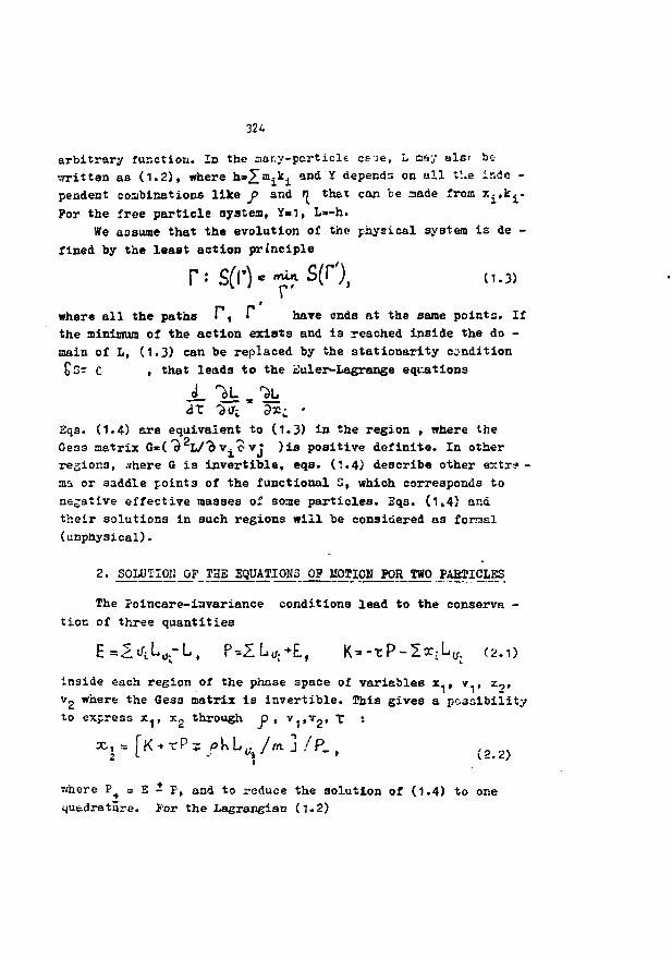
324
arbitrary function. In the aany-particle ce-se, L csy alsr be
written as (1.2), where h - ^ m ^ a n d Y depends on ull tl.e inde -
pendent combinations like J> and 0 thex can be made from x^,k^.
Por the free particle system, Y«1, L»-h.
We assume that the evolution of the physical system is de -
fined by the least action principle
where all the paths T, P have ends at the sane points. If
the miniiaum of the action exists and is reached inside the do -
main of L, (1.3) can be replaced by the stationarity condition
£s- C , that leads to the i-luler-Lagrange eqc.ations
J- Us.lkdX 'dlT;, 3X; •
Eqs. (1.4) are equivalent to (1.3) in the region , where the
Gess matrix G*(D L/'b v^cvj )is positive definite. In other
regions, .vhere G is Invertible, eqs. (1.4) describe other extra -
ma or saddle points of the functional S, which corresponds to
negative effective masses o* some particles. Eqs. (1,4) and
their solutions in such regions will be considered as foraal
(unphysical).
2. SOLUIIOi; OF THE EQUATIOH3 OF MOTION POR TWO PARTICLES
The Foincare-invariance conditions lead to the conserve -
tioc of three quantities
inside each region of the phase space of variables x., v-, x.o,
Vg where the Gess matrix is invertible. This gives a possibility
to express x^, Xg through p , V1>
T2' **• :
x p [K*rP5 pkL^/ial/p., ,22)
where P+ = S - P, and to reduce the solution of (1.4) to one
quadrature. For the Lagrangian (1.2)
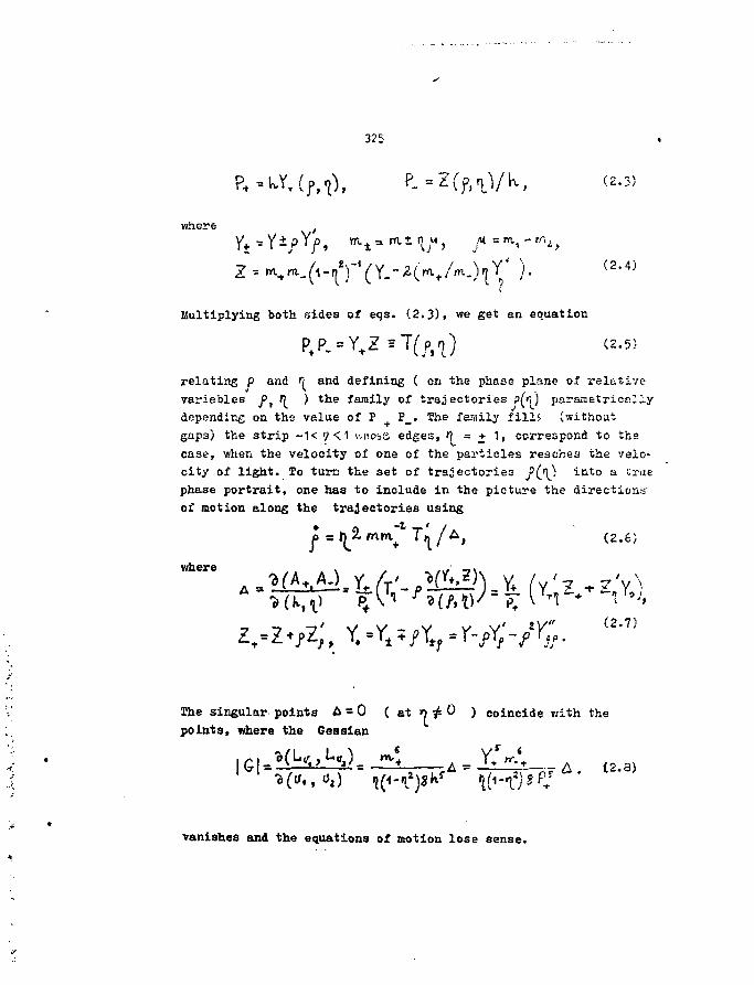
325
(2.3)
where
Multiplying both sides of eqs. (2.3). we get an equation
relating p and 0 and defining ( on the phase plane of relative
variables f>t f[ ) the family of trajectories P(*I) parasetricaliy
depending on the velue of P + P_. She family fills (without
gaps) the strip -1< 7<1 whose, edges, t = + 1, correspond to the
case, when the velocity of one of the particles reaches the velo-
city of light. To turn the set of trajectories f(j\) into a true
phase portrait, one has to include in the picture the directions'
of motion along the trajectories using
j 2 T
w h e r e
(2.7)
The singular points A = 0 ( at r> ± 0 ) coincide with the
points, where the Gesaian
1 l~n**i) tc<-i*)« i^-fA^
vanishes and the equations of motion lose sense.
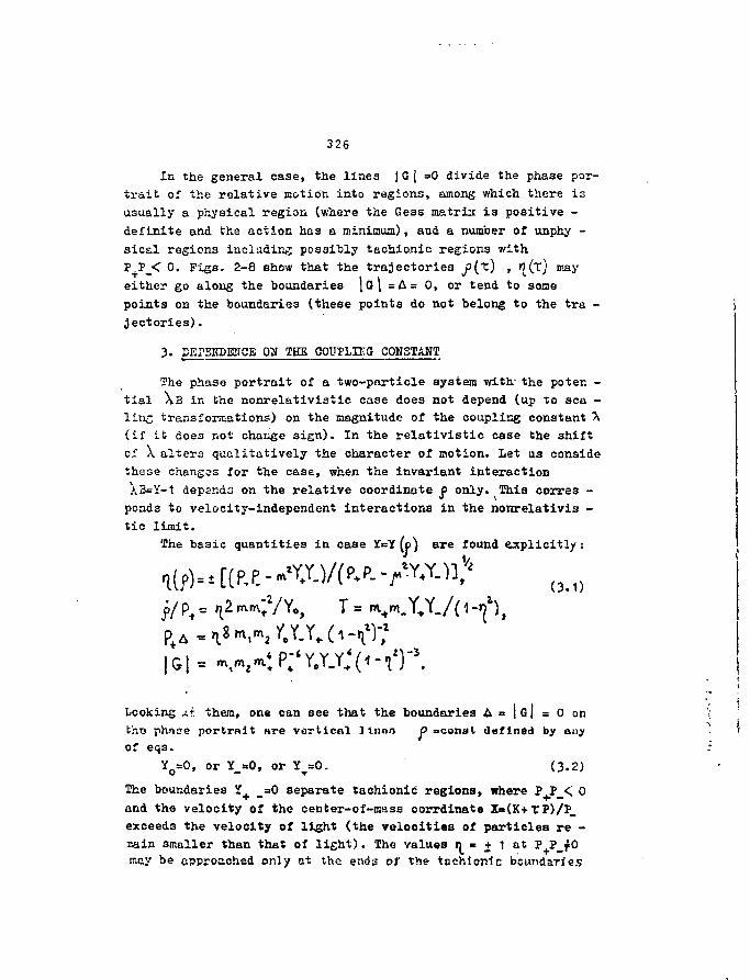
326
In the general case, the lines ]G 1 =0 divide the phase por-
trait oS the relative action into regions, among which there is
usually a physical region (where the Gess matrix is positive -
definite and the action has a minimum), and a number of unphy -
sical regions including possibly tachionic regions with
P+P_< 0. Figs. 2-8 show that the trajectories j3(t) , fl(t) may
either go along the boundaries \G\ =A= 0, or tend to some
points on the boundaries (these points do not belong to the tra -
jectories).
3. SEPBTOENCE OH THE OOUPLIKS COKSTAIIT
The phase portrait of a two-particle system with" the poten -
tial \ B in the nonrelativietic case does not depend (up to sea -
line transformations) on the magnitude of the coupling constant "X
(if it does not change sign). In the relativistic case the shift
of X alters qualitatively the character of motion. Let us conside
these changes for the case, when the invariant interaction
A3=Y-1 depends on the relative coordinate £> only. This corres -
ponds to velocity-independent interactions in the nonrelativis -
tic limit.
The basic quantities in case Y=Y (p) are found explicitly :
T = •v*.Y.Y.
Looking xi. them, one can see that the boundaries A = JGJ = 0 onthe ph.-iae portrait are varticnl linoo p =ootiat defined by anyof eqs.
Yo=0, or Y_«0, or Y T = 0 . (3.2)
The boundaries Y.. =0 separate tachionic regions, where P P < 0
and the velocity of the center-of-mass corrdinate Xo(K+TP)/P_
exceeds the velocity of light (the velocities of particles re -
aain smaller than that of light). The values r • + 1 at P+?_f0nay be approached only at the ends of the toehionic boundarfe.?
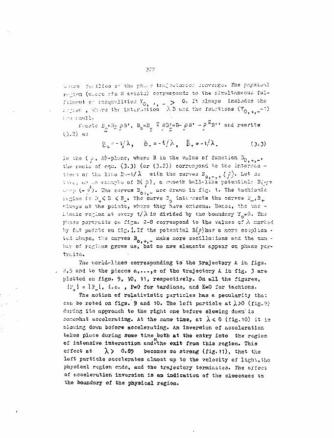
3:7
:.:r:ro £,,.-.-ilioa o ( t h e ;&,;<• ti-^J •.->,,• to2-ior. C5Eve;-£i . 1'he p.-:y.-5i.;'»l
r'..- ;i.on (v.^.c-t .-.••it: S exists) corresponds to the sir.ultaneoiu ful-
; U M i t c: i-cqu^lit iuj v^ _ > 0. It always includes >hc-
j- • -< ui> , v,-:i-o th-- interaction ,X B e.:~d the functions (Yo -1)
LV-IL,V'.O'.O B "•-"3t pB', B. =13 + o.d!=B~ p 3 ' - ?' B' ' av.d rewrite
B^-1/X, 5.=-4/A, B +»-VX. (3.3)
In :,ho ( r, 7i)-piano, where E is "she value of function 3,, _,
Vat- roots; of cqi:. (3.3) (or (3-2)} correspond to th* intor.rco -
iioi-5 ol ti:--j liv.e I(-:-1/A with tho curves B _ + ( j p ) - Lst us
•t >.-:,., (.:< i.n o.r::: ":c' of B( p) , Q ;-;;:ooti: bell-like potential: 3£*•;::
...-...., (_ i ) . The corves 3 arc drawn in fig. 1. The tachioaioo +, —
i-t^ior! is H < 2 < B_. i'hc curve P Q into.-.-scta the curves i_,3 T
r-.lv,-!iya ut the points, wh^ro they have extseasa. Henc-i, the tac -
;.-:.c!iic region at ovory 1/A is divided by The boundary Y 0=G. :-he
p:;aao portraits on i'ic3* 2-8 correspond to the values of A narirud
Vy ftit points on fig. i. If the potential Bio)has a more couplica -
ted tlsapc, the curves B make siore oscillations ar;d the nur.i -o, +,-
bcr of re;:i:us grows us, but no new elements appear on phiise por-
ti-.ito.
1'hu v;orid-lines corresponding to'the .trajectory A in figs.
;3,5 and to the pieces a,...,e of the trajectory A in fig. 3 are
plotted on figs. 9» 10, 11, respectively. On all the figures,
!?+i = lP_l, i.e. , P=0 for tardions, and E=0 for tachions.
The motion of relativistic particles has a pecuiarity that
cau be noted on figs. 9 and 10. The left particle at A > 0 (fig.9)
during its approach to the right one before slowing down' is
r.ovnewhat accelerating. At the soae time, at A < 0 (fig. 10) it ia
blowing down before accelerating. An inversion of acceleration
takes piece during some time both at the entry into the region
of intensive interaction and/the exit from this region. This
effect at X > 0.85 becomes so strong (fig. 11), that the
left particle accelerates clmost up to the velocity of light,the
physical region ends, and the trajectory terminates. 1'he effect
of ccceleration inversion is an indication of the closeness to
the boundary of the physical region.
32 6
r.s io cr.c-'vc in i st:iriiri£ fro:;i the -•iVO-di.ia«Ksional
field th&ory with the action integral o .' the Fc^er type and
with tht Green function containing 9''--,-t;.j or 6(^t , - t j j
cign r; , arid cor.3idering two pariicT: &o in:, erecting via the local
3liS3s i'ield of the rani n, on; can oil.;.."" r= 'he Lasrangiat.'i
l m + (I-'1? J (1-'; ; .j (4.1;
The Lagrtr.sian (4.1) Tor r:=1 was obtair.ea by Ctaruszkiev/ioz '^'-'
for the representation of "two iiistor.:.:T»" OI particles, ir,ter;-.c-
tirjg ccsordir^c to the electrom&gnstic aciion of Viheeler-Feyn-iiun
v;ith the half-sms of the retarded and advanced Green functions.
lo:.,c- properties of sunh description for a number of ifitemctiops
zvrc oo:i3iderod in ' • the corresponding quantum problere is
considered in / n > " . iHe equations of notion ia cass of rer.ul -
-icu <:TS inugruted for the syn.r.«tric electromagnetic (n-V, ai;ci
3?-..;ur (n=C) interactions ir. av.i , respectively. ThO'i 'i
the concept of the front forni of dynamics is not used in thece
j.:ips.-rc s;:plicitly, the rear-onings in 'b>°' are very close to this
concept and the evolution parameter t = t-x ( or X =t+:-: • i.=
actually used.
Xh» Lasri.5^ians (4.1) are remarkable in many v:ays. Ir par-
ticular , the solutior.3 of the motion equations can be found for
thorn in <iti analytic fora for any n. Note, that (4.1), (2.6) and
the relation * 0=Y + - P Y + give
Y o - ^ - 1 , (4.2) .i
v.her:ce tie immediately obtain ^ ( \ ,^ )/3 ( °, ) = 0 , which ac - •
cording to (2.8), (2.9) gives . ;'
Eq. (4.2) also means that P+ = K>0 and T-E . Note that the*ros Lasrangian i s a conjorved quantity . Calculating explicitiy
(4.4)
329
and solving the equation P+P_3T with respect to p , we find
where 6=P +P."W4, C s P+P.-/<
4 . obviously, <f>//=/lft)<^,where A(i)= p M ' /p ("}) is a rational expression of
:n > therefore \he quantity
ris always expressed in elementary functions.
The phase portraits of all the Lagrangians (4.1) have some
common features. It immediately follows from (4.1) that they
are symmetric with respect to the sign of f> and, up to an ove -
rail scale, do not depend on |<<! . According to (4.4) they are
symmetric with respect to the sign of n as well. Since J> > 0
at rt >0 , the motion along the phase trajectory in the upper
half-plane i3 realized always in the direction of growth of J> .
In case of attraction (at vi < 0 ), there is always n tachi-
onic region since T(/>, O) = nz-t 2*m/l o\<0 at ljs|<-2o£/m.
The lines f-fc^X) » where the Gessian IQl = O , are
defined by the equation JT/n Jn = 0 from which ct I pi 4 0
we get i -« » n-i » M
t •L IA 1 / 4 - h V C D / " (4.7)
At n.=.0,1
In case of repulsion , at a»0,1 and at ^ 0 A has no aerc
and the phase portraits have no unphysical regions. The distance
between particles at the turing points !^lmin = 2c<m/b
is arbitrary small at sufficiently large energy.
In case of attraction, the phase portraits look essentially
different at lt = 0 (fig. 12) and at iv--1 (fig.13). At rt.= O ,
330
the factor A entring the Gesaian becomes zero at lineslpl=!-olrft/m1n'li = P< • At ifi<f'i there is an unphy -sical region (including tachionic region). The trajectoryj>M for any given value of P+P. consists of two or threedisconnected pieces ending in the corners of the unphysicalregion.
At n-\ , the factor A does not depend on P and at r>tO
may not become zero, the Gessian IQl - w » W ( m ^ » ) (i*l)~
is positive, and the matrix G is positive definite, which isstill true in the tachionic region (T<0) as well. Promthis view- point the latter can be classified as a physicalsubregion. Thus, the trajectories may nowhere be interruptedexcept at the line f-0 , where neither the Lagrangian, northe quantities derived from it are defined. For n^2 see figs. M,f5.
5. DISTINCTIONS OP THE HAMILTOHIAE FORMALISM
The Hamiltonian description has a number of qualitativedistinctions from the Lagrangian one in the relativistic case.Here we briefly consider the distinctions related to the emer-gence of nonphysical regions.
The Hamiltonian description in two-dimensional space-time in the front form of dynamics can be specified by threefunctions P*, P., K of coordinates x. and of the canonicmomenta X. , satisfying commutation relations
where LjJ , is the Poisson bracket. For our purposes it isconvenient to choose P+,-,K in the form
(5.2)
where the function W is invariant in the sense f P. W]-,=
= L ^ j ^ J ' j " 0 and may depend on invariant relativecoordinates only. In case of two particles , we take K P_es collective coordinates and
331
S * /-. \ (R -5}
and the combination
of momenta, as relative ones. It is easy to check that R ^
are canonically independent from K, P. :
She Hamiltonian of the relative motion is the function
In the case W. a 0 ,which will be considered , the
phase trajectories £(R) and the direction of motion along
them are defined by expressions
(5.7)
The regions, where P+P. < 0 , will be called tachi-
onic, the rest ones, tardionic.
Let us consider the transition from the Lagrangian picture
to the Hamiltonian one. This transition (the Legendre transfor -
nation ) needs solving the system of equations
(5-9)
with respect to velocities lT . These equations are solvable in
the regions where the Gessian |Q| a*5/JT)>...)/t(\f< „.) is di-
fferent from zero. In the relativistic case, eqa. (5.9) due to 2.
kinetnatical dependence of the interaction Lagrangian on veloci -
ties, are nonlinear, and, if the boundaries, where the Gessian
vanishes, and nonphysical regions, separated by these boundaries,
332
are present , the mapping 3i*-*C is nonuuique. Let us construct
this mapping formally.
The cons«rvation laws (2.5) for the Lagrangian L = -nY in
the two-particle case give
t/ i), (5.10)
and eqs. (5.10) take form
™yt' + 1**l?<''O\Ul- • (5.1D
At Y« = 0 , the ratio ^\j^z depends on \ only, whilethe combination cj a m*/jr4 * m'/ JT2 depends only on h (and I"),
, and we obtain
!! = £>, (5.12)
k/ Y - ( r / f c ) - - 2«5/x- fc. (5.13)
Eqs. (5.11), (5.13) entail
and (5.14) after dividing by r turns into
/Y.(f)=ft. (5.15)The substitution of the solution f*?(^) of eq. (5-15) into(5.1*0 completes formally the Legendre transformation:
(5.16)
The solution j»(R) f rks et the points, where
and the Gessian equals ii,ero. If the portrait in j»f n variablescontains no unphysical regions, its mapping on the (&., < ) -plane occupies the strip |^l<1 and does not differ qualite -tively from the initial portrait (compare these strips on fig.16, 17 and 2,5). However, in the Hamiltonian case there is aformal possibility to extend the region of variation of the
333
variable <$ up to all £ £ JR , and, using (5.7), to construct
the phase portrait outside the strip |^l < 1 , adding regi -
ons with no counterpart in the Lagrangian description (figs.
16, 17). Theso regions turn out to be tachionic in the given
case.
If the phase portrait of the Lagrangian system contains
nonphysicai regions, t!ie corresponding phase portrait turns out
to be folia;ed. For example, the dependence of R on f for the
Lagrancian L =-K. [i+Xexp (- JD at X=1.53 is unmonoto -
nous and the portrait in R,^ -variables consists of several
partially overlapping regions (fi->. 18). In particular, at
2.55 < |R|<2.95 one has three different seta of trajectories
2, (ft) corresponding to different solutions of eq. (5.15) (sub-
stituted into 17}. It should be stressed that among the regions
that partially overlap there are two regions corresponding to
physical regions (where the Gess matrix is positive-definite)
on the Lagrangian phase portrait. Hence, the fixation of the
state of a system by the variables 32^, JT; in the given case
does not permit the unambiguous calculation of the system evolu-
tion , even if only the physical regions are considered.
Let us see now how the behaviour of a dynamical system de -
pends on the magnitude of interaction in the Hamiltonian forma -
lism. We take W of the form W = -11- 2A& (*) , B-exp(-R*j.
At IXI <£< 1 , the Harailtonian with such interaction is
approximately equivalent to the Lagrangian L~-k [1 + &(j>^l
(the phase portraits of the Harailtonian at X*i0.6 do not
differ perceptibly from figs. 16, 17). When I XI is growing, no
• qualitative changes occur with the phase portrait in case of rep-
ulsion. In case of attraction, if IXl is large enough (in the
given case at A < -\ ) a tachionic region in the strip
\Z,\ < 1 appears , and tardionic regions are inserted into
the tachionic regions outside this strip (fig. 19, A= -2). In a
more general case, the replacement of the function B(R) by a
function with more extrema give rise at large Ml to a number
of tardionic and tachionic regions forming a chess-board pattern.
As it follows from (5.9), trajectories cannot have interruption;:
inside the regions (they have ends in the corners of techionic
regions, where they converge). While the superlight velocities
334
V- in the Lagrangian case are Impossible, in the Haniiltonien case
they are admissible and may arise even in tardionic regions. The
calculation of the velocities ir^s^H/W; gives
1 +2.ir: = W . /jr-,\ (5.18)
where W . * W - R W R . Since A+2.^>0 corresponds to the
motion with a sublight velocity, while 1-ȣv7; <0 corres-
ponds to the motion with a superlight velocity, at W. -C both
particles simultaneously (in f ) reach the velocity of light,
and at W » < 0 both particles move faster than light. Since
the sign of W . may differ fron the sign of W , the super -
light velocities may happen in the tardionic region P+P- '>0>vl>0.
For instance, we have for the chosen W at A'a-O.S everywhere
W > 0 , but there are sectors of ft , where W . < 0 and the
world-lines Xj("fc) have superlight pieces (fig. 20). Note ,
that there are no irregularities at the points W_=0 , where
the particles reach the velocity of light.
Since K- and j> at 1 -r 2»«Tj < 0 are imaginary, there are
no Lagransians equivalent to the Hamiltoniana with W- < 0
In fact, the equivalence is ruined even for positive,but suffi -
ciently sin/. 11 W. . To see this fact, let us take an arbitrary
W(R) and perfom formally the inverse Legendre transformation.
Eqa. (2.1) and (5-3) lead to
where < = m*/JT, +
K or p the equationswhere
(5.19)
. Eq. (5.18) gives
, whence we got for
hr-<f, • faR/F(*\ (5.20)
Finding the solution R*R(,f) and using the relation
r
, we finally get
where r
the transformation la. The Gessian of
335
where Y = -(F,W/F)/Z , Y . - V - f Y > . At finite
VV W ' W " ,the Gessian has no zeroes, and the phase
portrait of the Lagrangian contains no boundaries Yo = C
separating the unphysical regions, but it contains the lines
W. = 0 , W_-RW.'/2-rO , where lfil-«°. Consider the cas»
when W > 0 i W- >0 , but W. is small in some region.
In this case, the dependence of o on is nonraonotonous , and
the solution &(/) at some J> is triple-valued. A.t such ptone Homiltonian description corresponds to three different
Lagrangian3 and the fixation of the state in terms of *••, (T-
does not define the motion uniquely. The phase portrait of the
system in variables j>f f[ becomes foiled (see fig. 21).
Mote that the above case W > 0 , W. > 0 ia a physisil
one according to all main criteria : the velocities of partic-
les are always smaller than that of light, the motion is regu-
lar everywhere, no ruptures occur, no tachionic regions are
present. Therefore the absence of a (unique) Lagrangian des -
cription is, seemingly , a deficiency of the approach itself,
or, to be more precise, of its inherent assumption that the
state of the system is fully fixed by coordinates and veloci-
ties (and not by higher derivatives dB3t/dr" or by mo -
menta). The Hamiltonian formalism is applicable to a larger
class of system : an equivalent Hamiltoniandescription exists
for any nonpathalogical (i.e., without nonphysical regions)
Lagrangian description (due to C ^ 0), but there are Hamil-
tonian systems, ind'.ding the ones with interactions depending
only on the invariant distance, for which no equivalent Lugrun-
gian descriptions exist.
6. PROPAGAIIOH Of SOUMD WAVES
One of the postulates of the special relativity is an
assertion that signals propagate with a limited speed. Diffe-
rent papers on the relativistic theory of direct interactions
treat this assertion differently : some of them put it in the
336
of the formalism aasmnii^ Chat only retarded interaction
propagating wit)- the velocity of light :. '.cting between par-
ticles '10', other ones adnit an advuroto .nten.ction but try
to eliminate its open manifestation .':.i the help of an ab -
sorber , the third ones leave the qi~e3vion open and re -
quire only the Lorentz-Invariant formulation of the theory.Urn
The front of dynamics, which is adopted In t';is paper,
assumes the presence of both retarded interostio;i (from the
left particle on the right one ) and udvcr-.oed intera-tion
(from the right particle on the left one). The presence of ad-
vanced interaction in, as a rule, considered as an indication
ot the advanced propagation of signals. However, the question
of the velocity of the signal propagation is much less obvi -
ous.
Strictly speaking, to fcecone a signal the transferred
perturbation hns to influence many particles and induce the
irrevercible processes that register the perturbation. In a
purely mechanical system, one of the most important kinds of
perturbations suitable for the signal transfer is a sound wave
It can be registered and may propagate at large distances.
Consider a system of N identical particle with a paired
interaction described by a Lagrangian
L = -"«^K; ~.^(lV>y)8(f;;,'(:<j)> b(o,o)*o. (6.1)
The equations of motion of such a system have form
2 ^i *i " Y i » (6*2}where (-- and Y- may be expressed through C;j = tfdi, "III ) »
B(/ij, vf}+ i'j^A,~T*i)f ^"'•Af ~ y' j*SJ a n d s o on«
Let this system make a (one-dijnensional) crystal (chain),
i.e., be in the state close to the stable equilibrium. The
invariant distances a; = lj>;t;»,| in equilibrium are de-
fined by the conditions
Yl=°t Tii = °- (6.3)
We uocur.0 that particles interact vii:'r. tht- nearest neighbours
only ( Cj:rC. if Ji-j| > 1 ) and function C {*,'*)
.\us only two minima at / = • a . Then the equilibria's of
the fi?o: particle give3 a, - a , and that of other pt-r -
tides Gives &;*& • The Gess matrix in the equilib -
riom position has form
!,,-£ -£/2 0 0 *\(6.4)
where ^
OJ a n^ Y,here have taken into account that the require -
men', of the existence ot snail harmonic oscillations entails
The condition of poaitive-definiteness of G puts a limita-
tion on the ratio ct*-6/2(M-£) : at £>0 and M,>M
1QJ>O at any M, if
. (6.5)
This inequality, clearly, leads to aome limitations on the velo-
city of sound.
Let us obtain the equations of motion for the case of small
perturbations of a crystal. In contrast to the nonrelativistic
case, when it is sufficient to require the smallness of only
the deviations from the equilibrium positions, while the velo -
cities may be arbitrary, in the relativiatic case the s:r.r.lr:eos
of the relative velocities (the velocity if= P/P_ of the cen -
tre-of-mass coordinate X = (K + T^J/P. of the crystal,
aa a whole, may be large). Putting «*;*xi-3c.;>jEc=X»-a'i-3ifN*i)/2
and leaving in (6.2) only the terms of the first order ir yy <5
we get for internal particles the linearized equations of aotior.
of the form
338
where f * Z a tpf ( a.,0).Let us pacs to the limit of continuous matter
i.e., to the case of relativistic string. Let there exist the
limits
Then (6.6) at Q.-+0 passes into eq.
* 4 - * ^ . (6.7)
where M, = H(- 2. o is a density of medium and f, is the Young
modulus. The equantity JJ (**, *) in (6.7) is a deviation
not from the immobile point, x., but from the point moving with
the velocity tf . Passing to the deviations t(ttx)-» *(*,*(<>)'**
from immobile points and taking into account that )fx,-'I-Xf
-"'X2*x. , we get
Passing from the variables of the front form of dynamicsto the usual variables i.y X by means of substitutions
) [ ] y
we finally get the equation
' * (6.9)
which is a usual relativistic equation of the sound propagation
it* the medium moving with the velocity S : In particlar, at
S *0 we have
whence one can see that the sound propagates in both directions
with the same velocity w-fa/Hl}*^1 • Tne Vb&se andgroup velocities coincide. In the limit of continuous medium
339
(6.7) gives fa £ No • Accounting for the
condition of resolvability of eq. (6.7) with respect to |
(that excludes the equality ^ , f\*c ), we obtain the limi -
tation
[t < M ^ v.vt<1 . (6.11)
Hence, the velocity of sound in the continuous medium ( in the
relativistic string) may approach the velocity of light , but
cannot reach it. Note that eq. (6.7) corresponds to small os -
cillations of the string with the Lagrangian
Let us now return to eq. (6.6) describing the evolution of
acoustic perturbations in an infinite crystal and see what bap -
pens, if the wavelength becomes compareble with the distance
betv/eon particles. Let the crystal be at rest. She substitution
of the solution of the form ye= e>p[l(coi: ~ P»O^ into (6.6)
relates with p by meand of a dispersion equation
tol[M-£(n- ws pa.) = 2.f [a'^-cos pa)+ a* us*, pi] >which
can be solved both with respect to cj , and with respect to p:
(6.12)
where J - ^ M , J=f/M' M°-(-«*2C)A.These relations, as usual, make sen3e (i.e., uniquely cor -
respond to the solution of initial eq. (6.6)) only inside tr.c
first Brillouin zone 12j^: Ipo-K S or l©l<oo
We illustrate the main features of the oound propagntion
in the relativistic crystal v;ith the results of computation or
motion for the system of forty identical particles described by
the Lagrangian (6.1) with B (p) =X[arctg (p-a-a)-
- arc tg (f-a.-*S)J , Initially, the system wa3 at reat.
Then it was perturbed by a particle coming from the right that
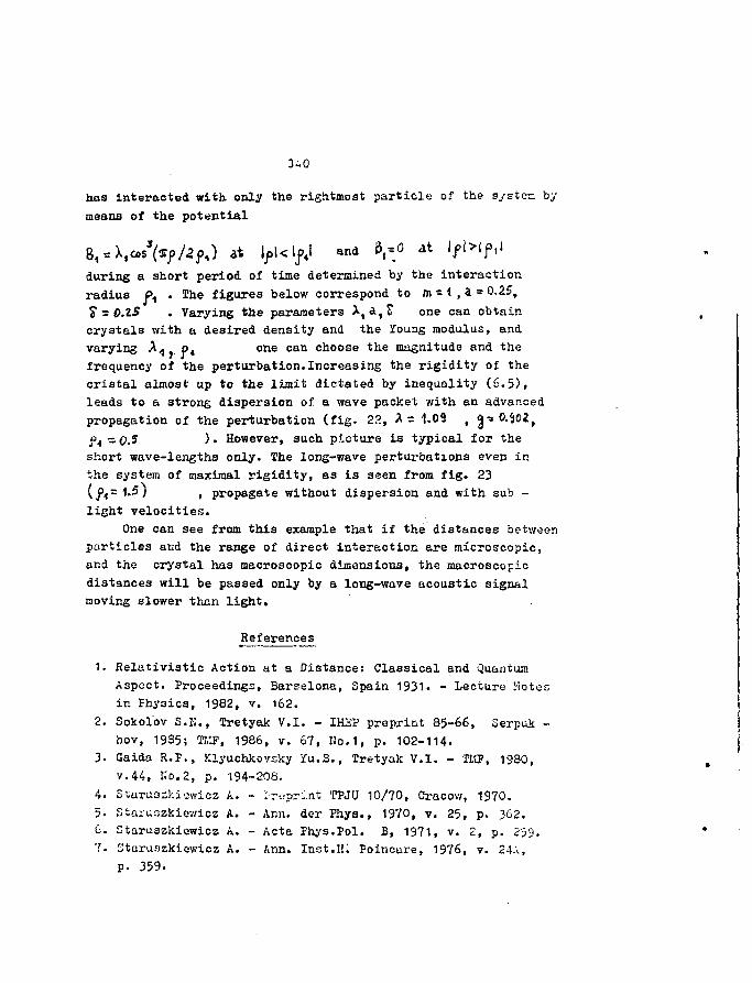
340
haa interacted with only the rightmost particle of the system by
means of the potential
at \p\<[ft\ and B,*0 atduring a short period of time determined by the interaction
radius p, . The figures below correspond to » « ( , } * 0,25,
S" = 0.2.5 . Varying the parameters X,a,F one can obtain
crystals with a desired density and the Young modulus, and
varying XA . p4 one can choose the magnitude and the
frequency of the perturbation.Increasing the rigidity of the
cristal almost up to the limit dictated by inequality (6.5),
leads to a strong dispersion of a wave packet with an advanced
propagation of the perturbation (fig. 22, >•- 1-09 , 0.402,
?i-Q.S )• However, such picture is typical for the
short wave-lengths only. The long-wave perturbations even in
the system of maximal rigidity, as is seen from fig. 23
(^=1.5) t propagate without dispersion and with sub -
light velocities.
One can see from this example that if the distances between
particles and the range of direct interaction are microscopic,
and the crystal has macroscopic dimensions, the macroscopic
distances will be passed only by a long-wave acoustic signal
moving slower then light.
References
1. Kelutivistic Action at a Distance: Classical and Quantum
Aspect. Proceedings, Barselona, Spain 1931. - Lecture Kotes
in Physics, 1982, v. 162.
2. Sokolov S.K., Tretyak V.I. - IHSP preprint 85-66, Serpui -
hov, 1935; Tiff, 1986, v. 67, Ho.1, p. 102-114.
3. Gaida R.F., Klyuchkovsky jfu.B., Tretyak V.I. - TUP, 1980,
v.44, Ko,2, p. 194-208=
4. Starii3skiuwicz A. - "Iropr:.nt TPJU 10/70, Cracow, 1970.
5. Staruszkiewicz A. - Ann. dor Phys., 1970, v. 25, p. 362.
6. Staruazkiewicz A. - Acta Phys.Pol. B, 1971, v. 2, p. 253.
7. Staruszkiewicz A. - Ann. Inst.H. Poincure, 1976, v. 24.V.,
p. 359.

341
8. Rudd R.A., Hill fl.M. - J. Kath.Phys., 1970, v. 11,
p. 2704.
9. Stephas P. - Phys.Rev. D., 1985, v. 31, p. 319.
10. Poincare H. - Rend. Circ.liat. Palermo, 1906, v. 21,
p. 129.
11. V/heeler J.A., Feynman R.P. - Rev. Mod. Phys., 1949, v. 21,
p. 425.
12. Dav.uov A.S. Theory of Solid Body (in ruasian) -M.: Hauka,
1976.
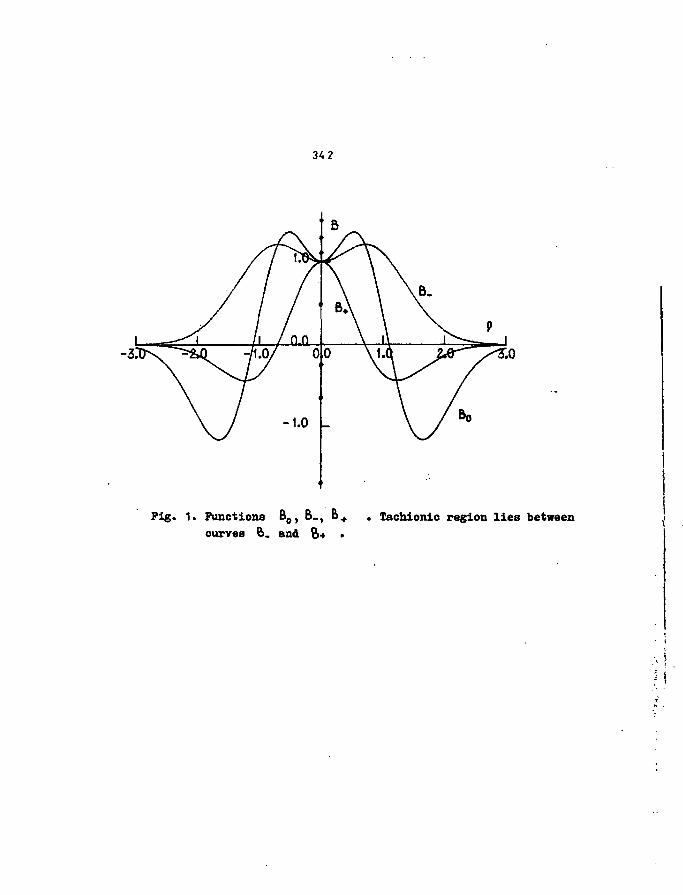
34
Fig. 1. Functions B 0 ) B_, & + . lachionic region lies betweencurves 6. and B+ •
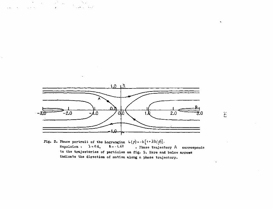
Fig.
1.0 lil
2. Phase portrait of the Lagrangian L(f) = -K['i ^
Repulsion : > = 0.6, E>=-1.6? . phase trajectory A correspondg
to the trajectories of particles on fig. 9. Here and below arrowa
indicate the direction of motion along a phase trajectory.
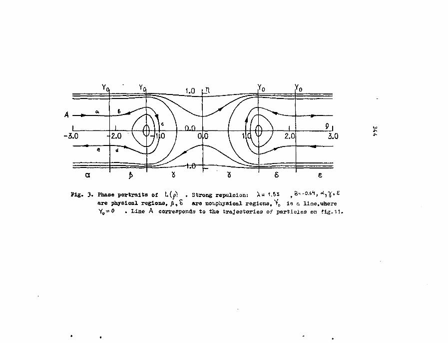
a
Pig. 3. Phase portraits of L(f) . Strong repulsion: X= 1.53 ? S---0.61, <*,^, E
are physical regions, £,S are nouphyaical regions, >0 is & line,where
Y o=0 . line A corresponds to the trajectories of particles on fig.11.
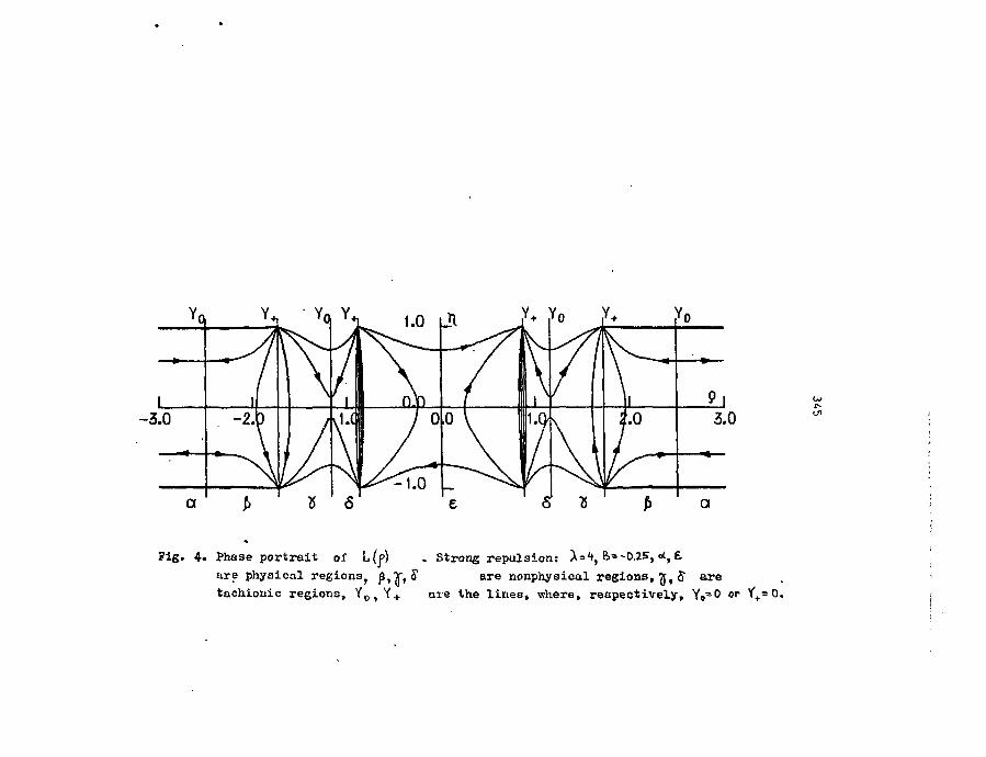
Q a
Fig. 4. Phase portrait or L(j>) . Strong repulsion: A=4, B>=-0.25, <*, £
are physical regions? p^, S are nonphysical regions, ,5" are
taohionic regions, Yc, Y + ore the lines, where, respectively, Yo=0 or y+=0.
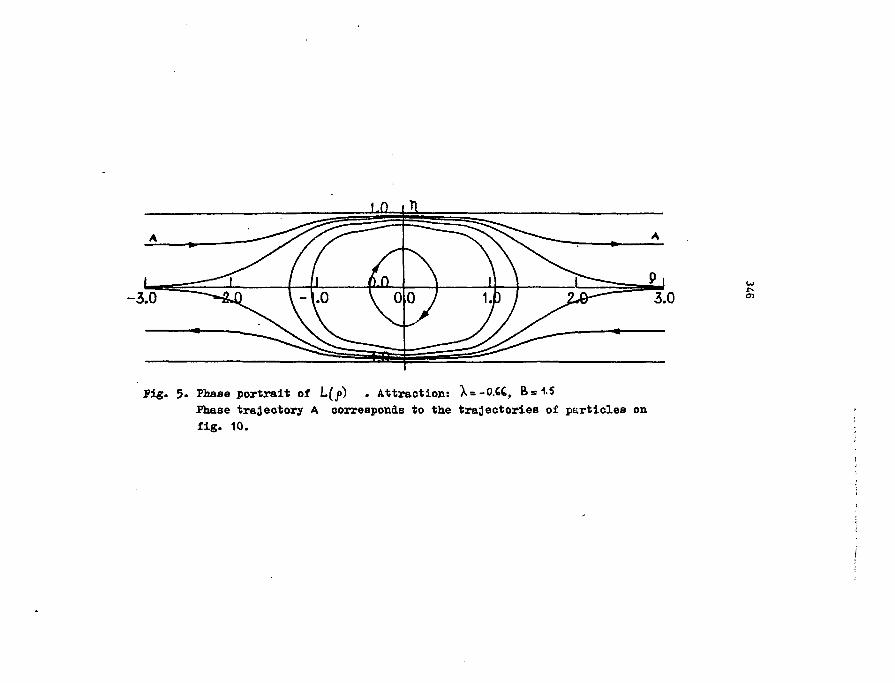
i.n in
Pig. 5. Phase portrait of L(j>) . Attraction: X*-O.CC, B=15
Phase trajectory A corresponds to the trajectories of particles on
fig. 10.
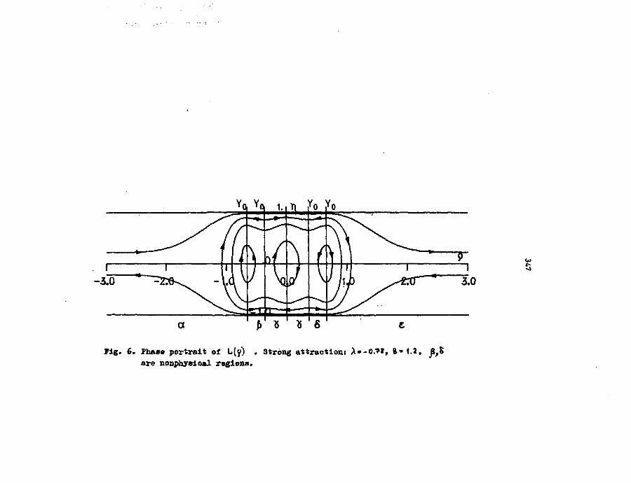
o
?ig. 6. Phaao portrait of L(y) . Strong attraction! A»-O.?», ft-* 1.2are nonptaysioal regions.
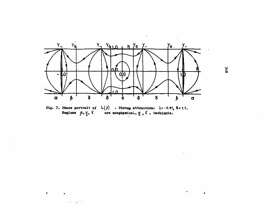
Y.
a
Yo Y-
Fig. 7. Phase portrait of L(j>) . Strong attraction* \*-0.9\y 8*1.1.Regions a, Y, f ar« nonphyaical, J , 5" , taohionio.
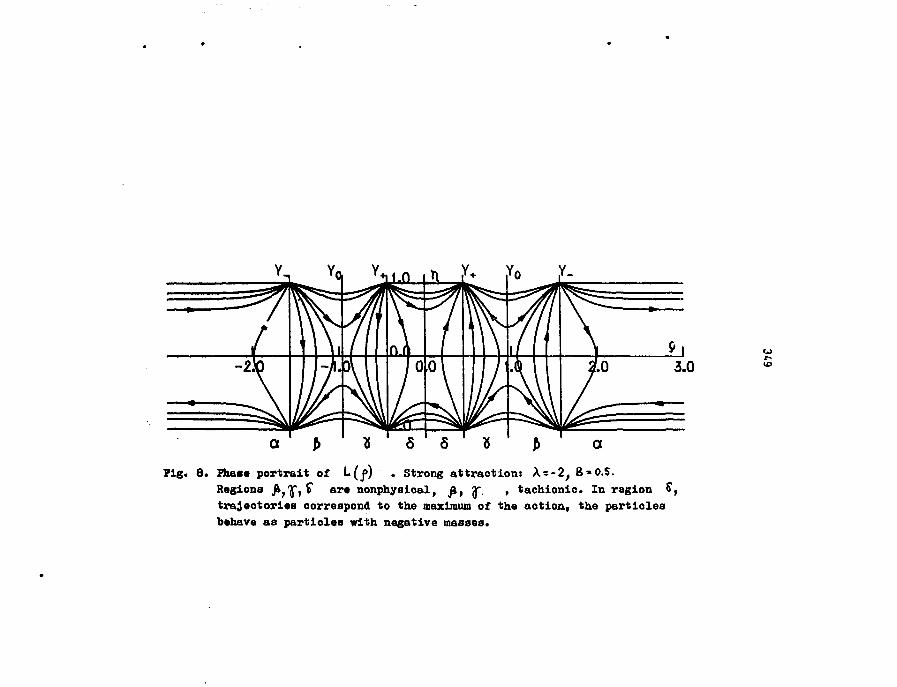
to
Pig. 8. Phase portrait of '-(f) . Strong attraction: X = -2, 8*0.5.Regions J^if)^ are nonphysioal, fit T- » tachionio. In ragion &trajectories correspond to the maximum of the action, the particlesbehave as particles with negative masses.
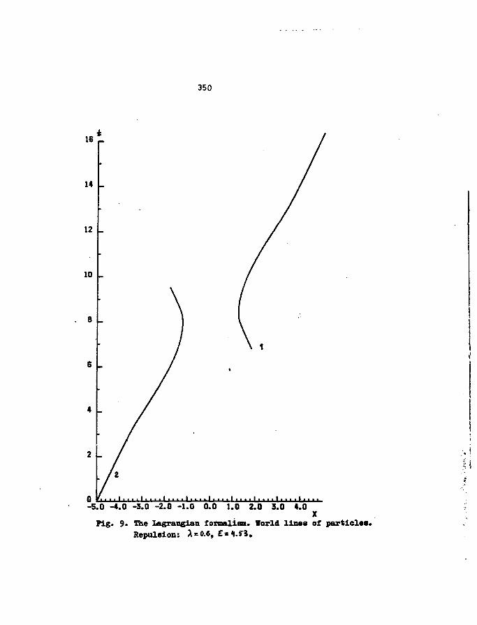
350
I i
-5.0 -4.0 -S.0 -2.0 -1.0 0.0 1.0 2.0 3.0 4.0
Fig. 9. The Lagrangian formalism. World lines of particles.Repulsion: A = 0.6, £*4.?3.
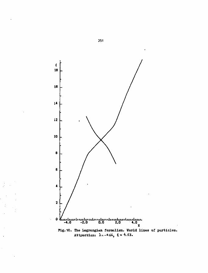
351
t18
16
14
12
10
1.0 -2.0 0.0 2.0 4.0
Fig.10. The Lagrangian formalism. World lines of particles.Attraction: X= 4
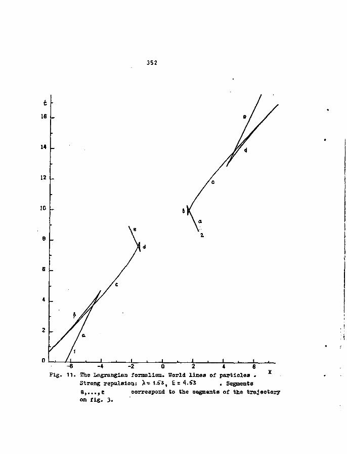
352
i.
16
14
12
10
- 6 - 4 - 2 0 2 4 6y
Pig. 11. The Lagrangian formalism. World lines of particles .
Strong repulsion: >•* 1.S"3t E=4.<»3 . Segments
a,...,e correspond to the segments of the trajectory
on fig. 3.
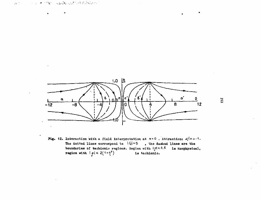
• • • * , ' . . , ; . . ; . : * ; ,,•„••.••>•.•>';:•<<:.<
Pig. 12. Interaction with a field interpretation at n = 0 . Attraction: rf/ms-1.The dotted lines correspond to IQl-O , the dashed lines are theboundaries of tachionic regions. Region with lj>l<4.5 i 8 nonphyaical,region with I P I < 2 ( 1 + I | * ) ia taohionio.
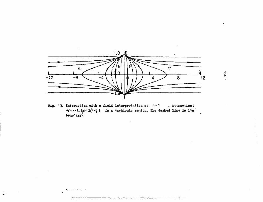
Pig. 13. Interaction with a field interpretation at n = 1 . Attraction:«</m*-t, lp|< 2^1-0 ) is a tachionic r.egion. The dashed line is itsboundary.
CO
.t-
1. , J -.- n ' i
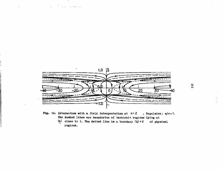
en
Pig. 14. Interaction with a field interpretation at n = 2 . Repulsion: «yV»
The dashed lines are boundaries of tachionio regions lying at
Ifl close to 1. The dotted line ie a boundary IG-l — 0 of physical
regions.
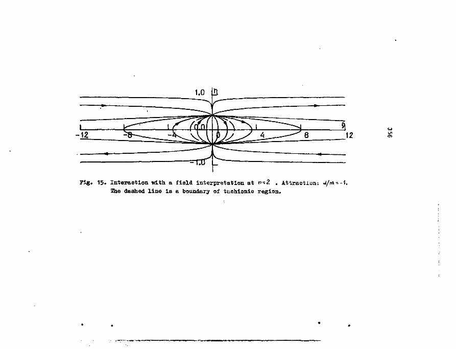
toCP
Pig. 15. Interaction with a field interpretation at n-Z . Attraction; J/m --1.
The dashed line is a boundary of tachionic region.
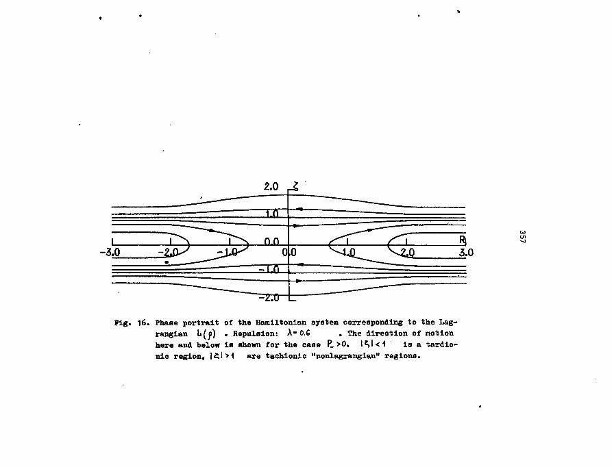
3.0 -ZS*S
2.0 ,
or"
^ i ^ ^ v nn^X&s 0
"~— — — _ _-z.u
• — — ^ .
o ^ ^ L ^
—-—
V.2J) 3.0
_—
Fig. 16. Phase portrait of the Hamiltonian system corresponding to the Lag-
rangian L(j>) . Repulsion: X- 0.6 . The direotion of motion
here and below is shown for the case R_>0. |£>l<1 is a tardio-
nle region, l^l>1 are tachionic "nonlagrangian" regions.
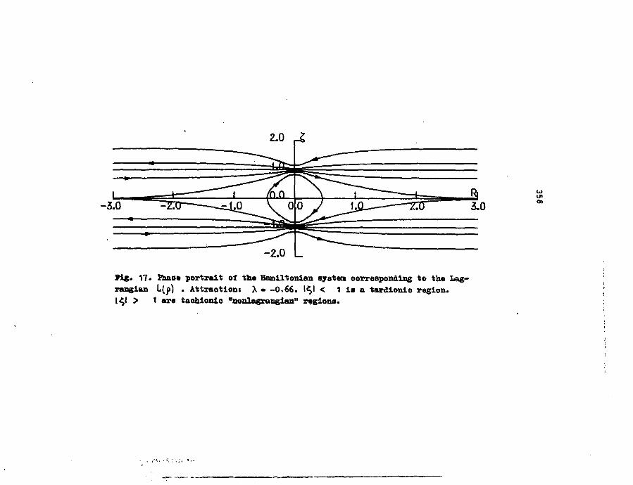
2.0 J.
OS
17* Shase portrait of th« Hamiltonian system corresponding to the Lag-ranglan L(j>) . Attraction: X • -0.66. l l < 1 is a tardlonlc region.1 1 > 1 are taohlonlc "nonlagrangian" regions.
. / ' . . • • • • . : . ; !
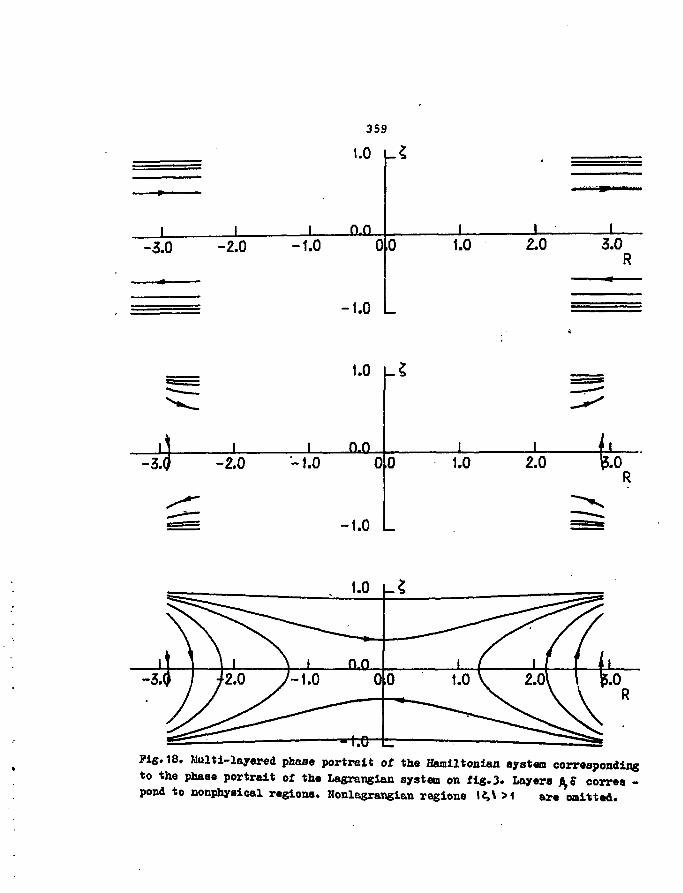
1-3.0
i-2.0
i-1.0
359
1.0
n.n0
-1.0
0i
1.0i •
2.01
3.0R
1.0 L-Z
i n.n-2.0 -1.0
-1.0
1.0 2.0
Pig.18. Multi-layered phase portrait of the Harailtonian system correspondingto the phase portrait of the Lagrangian system on fig.3. Layers J^S correa -pond to nonphysical regions. Honlagrangian regions \t>\ >1 are omitted.
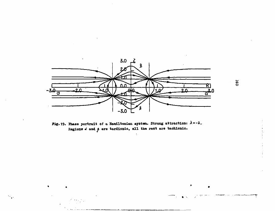
19. Phase portrait of a Hamlltonlan system. Strong attraction: A*-2.Regions «< and ft are tardlonlc, all the rest are tachlonic.
o
*T
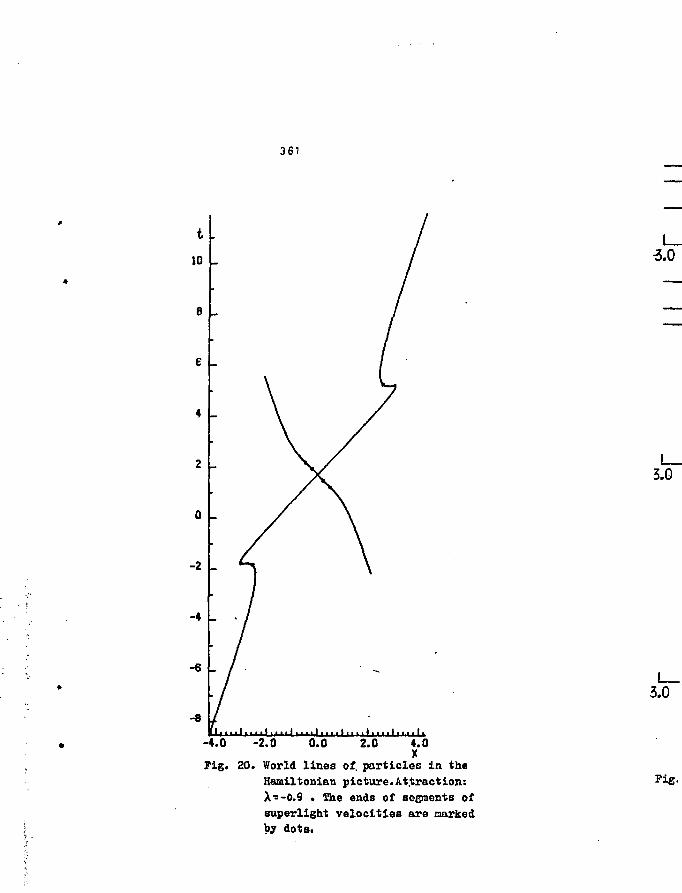
361
-6 .
-8
3.0
3.0
3.0
-4.0 -2.0 0.0 2.0 4.0X
Pig. 20. World lines of. particles in theHeuailtonian picture.Attraction:X--0.9 . The ends of segments ofsuperlight velocities are markedby dots.
Pig.
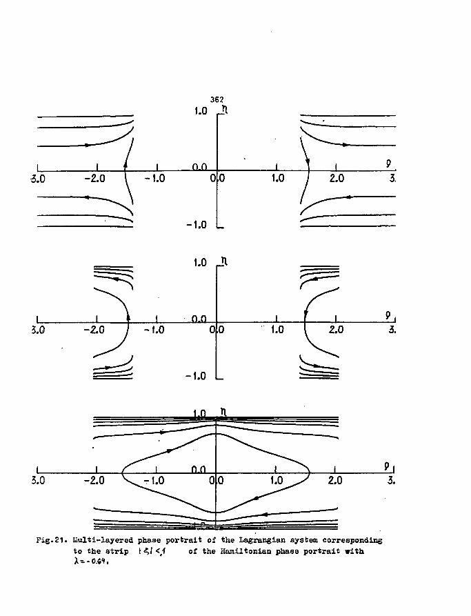
1
3.01
-2.01 ,
362
i.o _n
n.n0
-1.0
0 "I "—•— »
2.0P3
1.0 Jl
i n.n3.0 -2.0 / -1.0
-1.0
1.0 3.
Pig.21. Iiulti-layered phase portrait of the Lagrangian system corresponding
to the strip I AI </l of the Hamiltonian phase portrait with
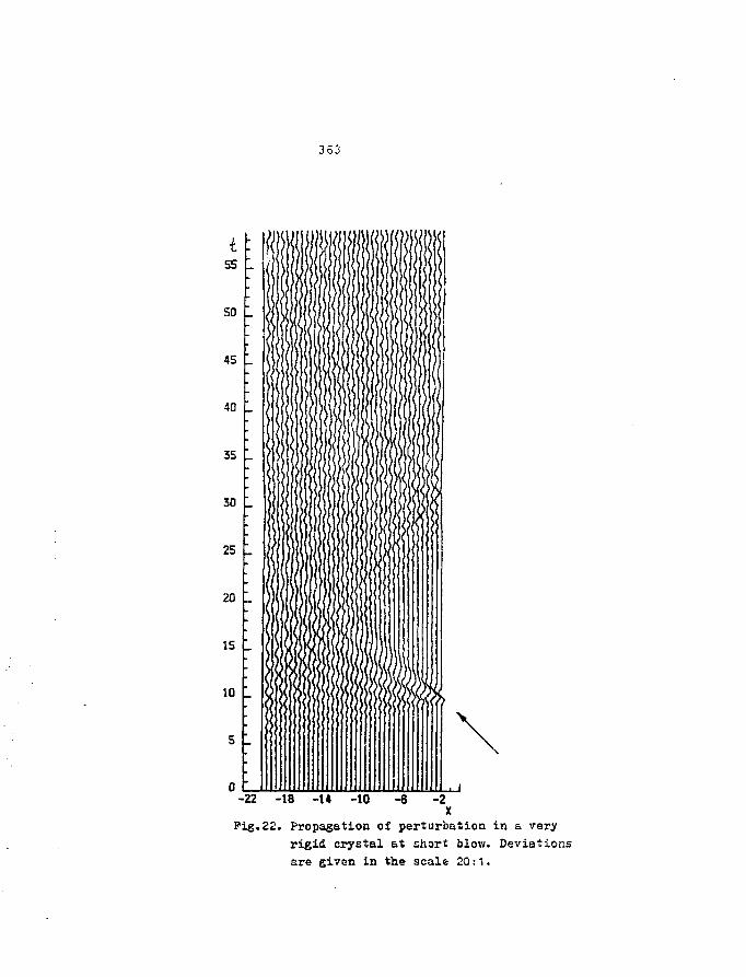
363
-22 -18 -14 -10
Pig.22. Propagation of perturbation in a very
rigid crystal at short blov/. Deviations
are given in the scale 20:1.
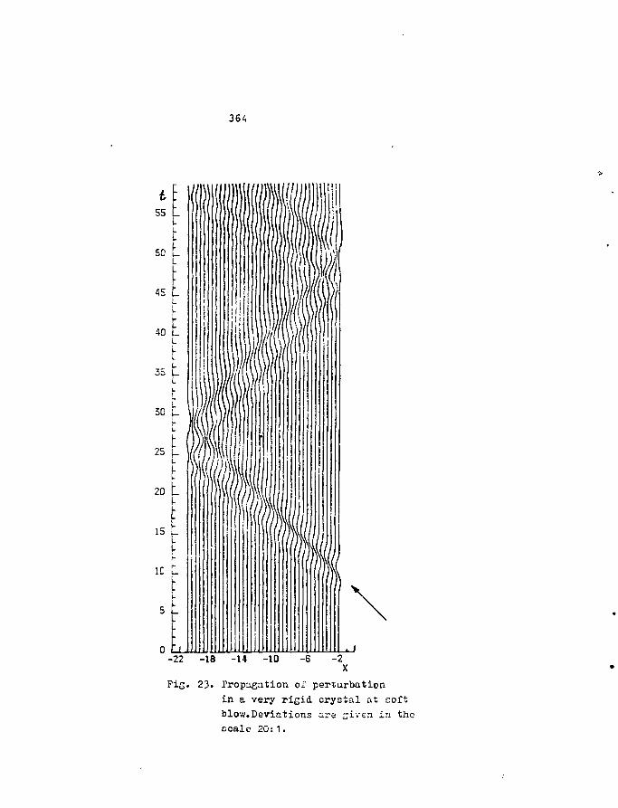
364
Pig. 23. Propagation oi perturbatioti
in a very rigid crystal at
blow.Deviations are {;iven in the
scale 20:1.
365
THEOREM PROVING WITH FIRST-ORDER PREDICATE LOGIC: III.*
B.Humpert
IKOSS Research & DevelopmentCH-8048 ZURICH, Switzerland
55, Albulastr.
and
CERH Theory DivisionCH-1211 GENEVA, Switzerland
ABSTRACT
We give an introduction into 'Theorem Proving/AutomatedReasoning' by presenting in this third paper a numberof explicit examples. A variety of (simple) 'ThinkingProblems' were chosen to illustrate several points: (i)how a problem is translated into the language of first-order predicate logic, (ii) how an actual deduction-chainproceeds: length, complexity,..., and (iii) how the dif-ferent resolution techniques can be applied most efficient-ly. The selected examples, however, do not represent thespectrum of the possible applications of the AutomatedTheorem Proving (ATP) systems.
Submitted to the Symposium

366
Overview
1. Introduction
2. Simple Job-Assignment
3. Complex Job-Assignment
4. Lion and Unicorn
5. Truth-Teller (Knights) and Liars (Knaves)
6. Schuberts Steamroller
7. School Boys
8. Salt and Mustard
9. Tiles plus Holes
10. Checkerboard
11. Missionaries and Cannibals
12.. Billiard Ball Weighing
13. Some Insights
14. Conclusions
367
1. Introduction
There exist computer systems which allow for highly comp-lex deductions: conjectured 'Theorems' can be proved from aset of 'Axioms'. This field of "Automated Theorem Proving(ATP)" or "Automated Reasoning (AR)" has meanwhile reached aquite high level of performance which sometimes goes substan-tially beyond the human abilities.
Contrary to our earlier papers [1,2] which focused on thepresentation of the theoretical concepts and particular de-duction schemes, we here are concerned with the applicationof these systems on a set of illustrative examples. This pa-per thus aims to give insight into the utility, power andflexibility of the ATP-systems for the solution of problemswhich demand for a great deal of logical reasoning, or whichneed repeated trials to come closer to a solution path. Wehere limit ourselves to a set of "Thinking Problems" whosepresentation should not primarily be considered as a sourceof entertainment, but rather as an abstraction of real-lifeproblems. Their closer inspection makes obvious that they donot allow for easy.solutions by conventional mathematicaltechniques", but instead, they typify classes of problems wherethe solutions are found by trial-and-error. Our subsequentpresentation therefore aims to discuss a set of such problemsin order to illustrate their formulation in the framework offirst-order predicate logic, such that they admit for logicaldeductions by the inference techniques. Having, in addition,excellent ATP-systems [3,4] at hand, we furthermore give in-sight into their use in solving unusual problems which, andthis is an essential condition, allow for their formulationin the language of first-order predicate logic.
Our subsequent presentation has a second aim: whilst pre-paring the description of a problem for an ATP-system, thehidden and sometimes unknown assumptions in the axiom systemof that problem have to be recognized. That this is not easy,leading frequently to wrong formulations, or that one or theother important information completely falsifies the originalproblem, should also become more clear from our presentation.There is no doubt that the translation of a problem into thelanguage of an ATP-system is one of the more difficult tasks.The constants, functions and predicates have to be defined ina 'natual', meaning problem-appropriate way, allowing for anefficient deduction of new clauses and finally the soughtcontradiction. Furthermore, the axioms .and constraints of theproblem must be formulated such as to allow for easy insightand an optimal deduction.
366
Let as make a few introductory remarks on some of theexamples [3-11]. In sections 2 and 3 we consider the problemof assigning a set of jobs to several parsons such that anumber of defining constraints are satisfied. In section 4 weshow how the selection of a particular element out of the setof week days proceeds according to several intricate selec-tion criteria. The problems concerning true and un-true sta-tements ('Knights and Knaves', etc.), as discussed in section5, are unusual in that they present a first-order descriptionof a higher-order problem. We here give details of the deduc-tion steps. Schubert's Steamroller problem of section 6 showssome of the arising ambiguities if a problem is cast in theclause form of first-order predicate logic. Until recentlythis problem was considered a challenge to existing ATP-systems. From the schoolboy problem of section 7 we learnthat some problems allow even for a solution in propositionallogic if the encoding is chosen appropriately. The problem ofsection 8 again asks for some object-person identificationaccording to specified criteria. The 'Tiles plus Hole' prob-lem in section 9 requires the shifting of tiles according towell specified rules which simply express the physical con-straints of this system. The actual search of the most opti-mal solution is left to the ATP-system. The description andsimulation of such a system by purely mathematical techni-ques, doubtless would pose problems even to an experiencedresearcher. The checkerboard problem of section 10 leads tothe investigation whether an arbitrarily shaped area can becovered by a set of elementary bulding blocks, and it can beviewed as an abstraction of similar problems in circuitlayout-design. Thinking problems like 'Missionaries and Can-nibals' (section 11), require determining who must go whereat what time and their solution indicates how problems ineveryday scheduling must be approached. The 'Billiard Ball'problem of section 12 demonstrates in a nice way how far onecan get with ATP-systems if the set of axioms is optimallychosen. It presents difficulties which are also encounteredwhen planning for instance a trip in a city with visits toseveral people, taking traffic constraints etc. into account,whereby the trip must be completed in a specified amount oftime. Section 13 summarizes some general insights from ATP-experiments, and section 14 is reserved for the summary.
After these general introductory remarks let* us go to theexamples I
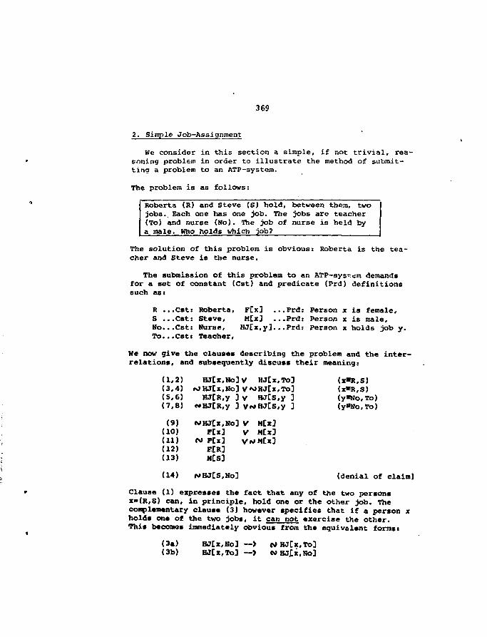
369
2. Simple Job-Assignment
We consider in this section a simple, if not trivial, rea-soning problem in order to illustrate the method of submit-ting a problem to an ATP-system.
The problem is as follows:
Roberta (R) and Steve (S) hold, between them, twojobs.. Each one has one job. The jobs are teacher(To) and nurse (No). The job of nurse is held bya male. Who holds which job?
The solution of this problem is obvious: Roberta is the tea-cher and Steve is the nurse.
The submission of this problem to an ATP-syst^m demandsfor a set of constant (Cst) and predicate (Prd) definitionssuch as:
R ...Cst: Roberta, FCx] ...Prd: Person x is female,S ...Cst: Steve, M[x] ...Prd: Person x is male.Ho...Cst: Nurse, HJtx.yJ.. .Prd: Person x holds job y.To.. .Cst: Teacher,
We now give the clauses describing the problem and the inter-relations, and subsequently discuss their meaning:
(1,2) HJ[x.HoDV HJCX.TO ] (X*R,S)
(3,4) iOHJ[x,Ho] V*>HJ[x,To] (x*R,S)(5,6) HJCR.y 3v HJ[S,y ] (y»No,To)(7,8) «»HJ[R,y ] ywHJCs.y ] (ySNo.To)
( 9 )(10)(11)(12)(13)
(14)
«OHJ[x,No]FCx]
t» FCx]E£R]M£S]
<s»HJ[S,No]
VVV*
MCx]MCx]
(denial of claim)
Clause (1) expresses the fact that any of the two personsx»(R,S) can, in principle, hold one or the other job. Thecomplementary clause (3) however specifies that if a person xholds one of the two jobs, it can not exercise the other.This becomes immediately obvious from the equivalent forms:
HJ[x,No] — > cv»HJ[x,To](3b) HJ[x,To3 — >
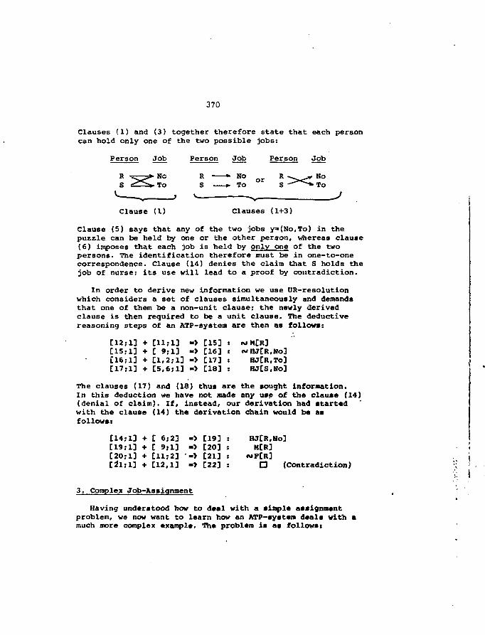
370
Clauses (1) and (3) together therefore state that each personcan hold only one of the two possible jobs:
Person Job Person Job Person Job
R »• No R -*. „ NoS » To
R -=cp=«s ^<,
V .
Clause
• N o• TO
(1 ) Clauses (1+3)
Clause (5) says that any of the two jobs y=(No,To) in thepuzzle can be held by one or the other person, whereas clause(6) imposes that each job is held by only one of the twopersons. The identification therefore must be in one-to-onecorrespondence. Clause (14) denies the claim that S holds thejob of nurse; its use will lead to a proof by contradiction.
In order to derive new information we use UR-resolutionwhich considers a set of clauses simultaneously and demandsthat one of them be a non-unit clause; the newly derivedclause is then required to be a unit clause. The deductivereasoning steps of an ATP-system are then as follows:
[12;1] + [11;1] -> [15] : IM M[R][15;1] + C 9;13 -> [16] : ~HJ[R,No]Ll6;l] + [1,2;1] -> [17] : HJ[R,To][17;1] + [5,6;1] •> [18] : HJ[S,No]
The clauses (17) and (18) thus are the sought information.In this deduction we have not made any use of the clause (14)(denial of claim). If, instead, our derivation had startedwith the clause (14) the derivation chain would be asfollow*:
ri4;l] + [ 6; 2] «> [19] : HJ[R,No][19;1] + [ 9;1] -> [20] : M[R] I[20;l] + [11;2] -> [21] : ft»F[R] \[2"1;1] + [12,1] «> [22] s • (Contradiction) '•; '
i \3. Complex Job-Assignment ,
Having understood how to deal with a simple assignmentproblem, we now want to learn how an ATP-systera deals with amuch more complex example. The problem is as follows:
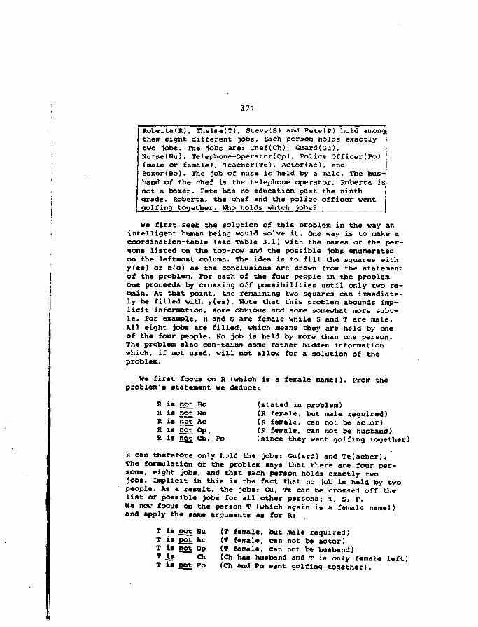
37:
Rcberta(R), Thelma(T), Steve(S) and Pete(P) hold amongthem eight different jobs. Each person holds exactlytwo jobs. The jobs are: Chef(Ch), Guard(Gu),Nurse(Nu), Telephone-Operator(Op), Police Officer(Po)(male or female). Teacher(Te), Actor(Ac), andBoxer(Bo). The job of nuse is held by a male. The hus-band of the chef is the telephone operator. Roberta isnot a boxer. Pete has no education past the ninthgrade. Roberta, the chef arid the police officer wentgolfing together. Who holds which jobs?
We first seek the solution of this problem in the way anintelligent human being would solve it. One way is to make acoordination-table (see Table 3.1) with the names of the per-sons listed on the top-row and the possible jobs enumeratedon the leftmost column. The idea is to fill the squares withy(es) or n(o) as the conclusions are drawn from the statementof the problem. For each of the four people in the problemone proceeds by crossing off possibilities until only two re-main. At that point, the remaining two squares can immediate-ly be filled with y(es). Note that this problem abounds imp-licit information, some obvious and some somewhat more subt-le. For example, R and S are female while 5 and T are male.All eight jobs are filled, which means they are held by oneof the four people. Ho job is held by more than one person.The problem also con-tains some rather hidden informationwhich, if uot used, v-ill not allow for a solution of theproblem.
He first focus on R (which is a female namel). From theproblem's statement we deduce:
R is not Bo (stated in problem)R is not Nu (R female, but male required)R i» not Ac (R female, can not be actor)R is not Op. (R female, can not be husband)R is not Ch, Po (since they went golfing together)
R can therefore only hjld the jobs: Gu(ard) and Te(acher).The formulation of the problem says that there are four per-sons, eight jobs, and that each parson holds exactly twojobs. Implicit in this is the fact that no job is held by twopeople. As a result, the jobs: Gu, Te can be crossed off thelist of possible jobs for all other persons: T, S, P.We now focus on the person T (which again is a female name!)and apply the same arguments as for R:
T is not Nu (T f«mal«, but male required)T is not Ac (T female, can not be actor)T is not Op (T femal*. can not be husband)T is Ch (Ch has husband and T is only female left)T is not Po (Ch and Po went golfing together).
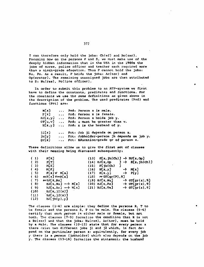
372
T can therefore only hold the jobs: Ch(ef) and Bo(xer).Focusing now on the persons P and S, we must make use of thedeeply hidden information that in the USA in the 1980s thejobs of nurse, police officer and teacher each required morethan a ninth-grade education. Thus P cannot hold the jobstNu, Po. As a result, P holds the jobs: Ac(tor) andOp(erator). The remaining unassigned jobs are then attributedto S: Nu(rse), Podice officer).
In order to submit this problem to an ATP-system we firsthave to define the constants, predicates and functions. Forthe constants we use the same definitions as given above inthe description of the problem. The used predicates (Prd) andfunctions (Fct) are:
M[x] ... Prd: Person x is male.F[x3 ... Prd: Person x is female.
HJ[x,y] Prd: Person x holds job y.GT[u,v] ... Prd: u must be greater than v.H[x,y] ... Prd: x is the husband of y.
jlCx] ... Fct: Job jl depends on person x.jh[y] ... Fct: Jobholder-person jh depends on job y.gr[x3 ... Fct: Education-grade gr of person x.
These definitions allow us to give the first set of clauseswith their meaning being discussed subsequently:
( 1)( 2)( 3)( 4)( 5)( 6)( 7)( 8)( 9)(10)(11)(12)
FCR3F[T3M[S3M[P3F [ X 3 V MCX3
f»F[x3 V««MCX3WHJ[R,Bo3
HJ[x,Nu3 —> M[x3HJ[x,Ac3 —> M[x3HJCx,jl(x)3HJ[x,j2(x)3HJ[jh(y),y3
(13)(14)(15)(16)(17)(18)(19)(20)(21)
H[x,jh(Ch)3HJ[x,Op 3
FCjh(Ch) 3H[x,y3H[x.y3r* GT[gr(P),S
HJ[x,Nu3HJ[x,Po3HJ[x,Te3
-> HJ[x,Op3-> H[x,jh(Ch)3
-> M[x3-> F[y3
)3-> GTCgr(x),-> GT[gr(x),-> GTCgr(x).
939393
The clauses (1-6) are simple; they define the persons R, T tobe female and the persons S, P to be male. The clauses (5-6)certify that each person is either male or female, but notboth. The clauses (7-9) formalize the condition that R is nota Bo(xer) and that the jobs: Nu(rse), Ac(tor), must be holdby a male. The clauses (10-12) stats that for every paraon xthere ".xist two different jobs jl and j2 which, in fact de-pend on the particular person x; equivalently, for every joby there is a person (jobholder) which aJso depends on the joby. The clauses (13-16) formalize the statement: the husband
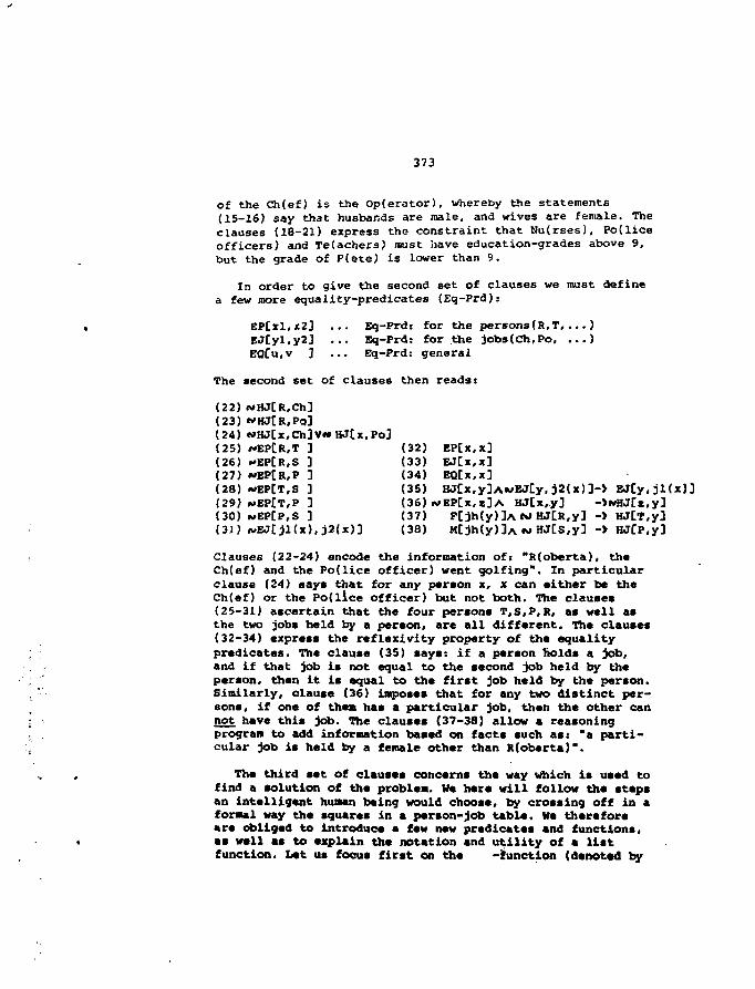
373
of the Ch(ef) is the Op(erator), whereby the statements(15-16) say that husbands are male, and wives are female. Theclauses (18-21) express the constraint that Nu(rses), Po(liceofficers) and Te(achers) must have education-grades above 9,but the grade of P(ete) is lower than 9.
In order to give the second set of clauses we must definea few more equality-predicates (Eq-Prd)s
EP[xl,x2] ... Eq-Prd: for the persons(R,T, )EJ[yl,y2] ... Eq-Prd: for the jobs(Ch,Po, ...)EQ[u,v ] Eq-Prd: general
The second set of clauses then reads:
(22) ~HJ[R,Ch](23) «*HJ[R.PQ]
(24) e»HJtx,Ch]V«HJCx,Po](25) wEPCR.T ] (32) EP[x,x](26) *EP[R,S 3 (33) EJCx.x](27) ««EPtR,P ] (34) EQ[x.x](28) wEPtT.S ] (35) HJ[x,y]A«EJ[y. j2(x)]-> EJCy.jl(x)](29) IWEP£T,P 3 (36) IS»EP[X,E]A HJ[x,y] ->NHJ[r.y3(30) «EP[P,S ] (37) P[jh(y)]AeoHJ[R,y] -> HJtT.y](31) A.EJ[jl(x),j2(x)3 (38) M[jh(y)]A~HJ[S,y] -> HJ[P,y]
Clauses (22-24) encode the information of: "R(oberta), theCh(ef) and the Pot lice officer) went golfing". In particularclause (24) says that for any person x, x can cither be theCh(ef) or the Po(lice officer) but not both. The clauses(25-31) ascertain that the four persons T,S,P,R, as well asthe two jobs held by a person, are all different. The clauses(32-34) express the reflexivity property of the equalitypredicates. The clause (35) says: if a person holds a job,and if that job is not equal to the second job held by theperson, then it is equal to the first job held by the person.Similarly, clause (36) imposes that for any two distinct per-sons, if one of them has a particular job, then the other cannot have this job. The clauses (37-38) allow • reasoningprogram to add information based on facts such as: "a parti-cular job is held by a female other than R(ob«rta)*.
The third set of clauses concerns the way which is used tofind a solution of the problem. W* here will follow the stepsan Intelligent human being would choose, by crossing off in aformal way the squares in a person-job table. Me thereforeare obliged to Introduce a few new predicates and functions,as well as to explain the notation and utility of a listfunction. Let us focus first on the -function (denoted by
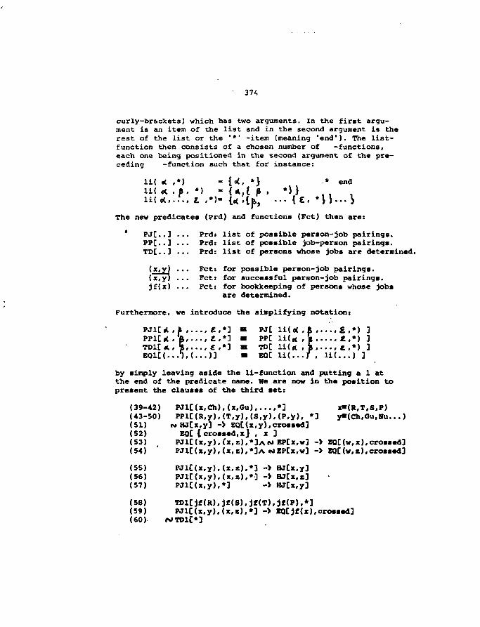
374
curly-brackets) which has two arguments. In the first argu-ment is an item of the list and in the second argument is therest of the list or the '*' -item (meaning 'end'). The list-function then consists of a chosen number of -functions,each one being positioned in the second argument of the pre-ceding -function such that for instance:
li( •( .*)li< * . p .li( tt.,...,
*)i*.*) end
it. *The new predicates (Prd) and functions (Fct) then are:
* PJ[..] ... Prd: list of possible person-job pairings.PP[..] ... Prd: list of possible job-person pairings.TD[..] ... Prd: list of persons whose jobs are determined.
(x,y) ... Fct: for possible person-job pairings.(x,y) ... Fct: for successful person-job pairings.jf(x) ... Fct: for bookkeeping of persons whose jobs
are determined.
Furthermore, we introduce the simplifying notation:
PJ1C* ,*,....£.*] B PJCPPlCi( .'&...., £.*] • PPCTDlC*. »,...,£.*] m TDCEQ1C(...T,(...)] • EQC
li(e(,* £,*) ]li(« , • £,*) ]li(ft , B ..... t .*) ]Xi(...f . li(...) 3
by simply leaving aside the li-function and putting a 1 atthe end of the predicate name. We are now in the position topresent the clauses of the third set:
(39-42) PJl[{x,Ch),(x,Gu),...,•] x»(R,T,S,P)(43-50) PPl[(R,y).(T,y),(S,y),(P,y), *3 y»(Ch,Gu,Hu...)(51) c»HJCx,y] -> EQC(x.y),crossed](52) EQC { crossed,xj , x 3(53) PJlC(x,y),(x,s),*3AWEPCx,w3 -> EQC(w,x),crossed](54) PJlC(x,y),(x,E),*]A cOEPCx.w] -> EQC(w,z),crossed]
(55) PJU(x.y),(x.s).*3 -> HJCx.y](56) PJlC(x,y).(x.*),«] -> BJCx.r](57) PJlC(x,y),*3 -> HJCx,y3
(58) TDl[jf(R).jf(S),jf(T).jf(P),*](59) PJlC(x,y),(x,t),*] -> EQCjf(x),crossed](60)
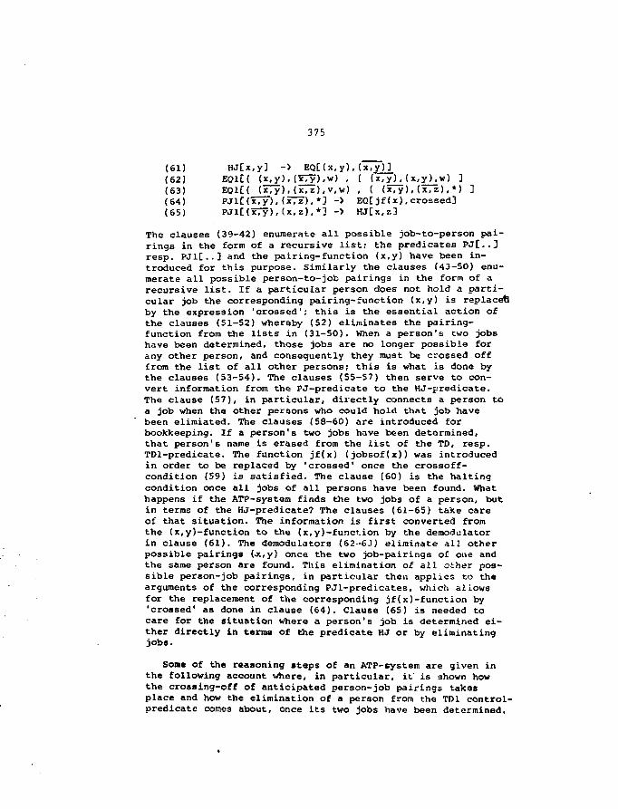
375
(61) HJ[x.y] -> EQ[(x.y).(x,y)](62) EQ1[( (x,y), (x7y),w) , ( (x,yK(x,yKw) 3(63) EQ1[( (x,y),(x,z),v,w) , ( (x,y). (x, z), *) ](64) PJl[(x7y).(x7z).*l -> EQlifix),crossed](65) PJlt(xTy),(x,z).*] -> HJ[x,z]
The clauses (39-42) enumerate all possible job-to-person pai-rings in the form of a recursive list; the predicates PJ[..3resp. PJ1C..3 and the pairing-function (x,y) have been in-troduced for this purpose. Similarly the clauses (43-50) enu-merate all possible person-to-job pairings in the form of arecursive list. If a particular person does not hold a parti-cular job the corresponding pairing-function (x,y) is replace*by the expression 'crossed1; this is the essential action ofthe clauses (51-52) whereby (52) eliminates the pairing-function from the lists in (31-50). When a person's two jobshave been determined, those jobs are no longer possible forany other person, and consequently they must be crossed offfrom the list of all other persons; this is what is done bythe clauses (53-54). The clauses (55-57) then serve to con-vert information from the PJ-predicate to the HJ-predicate.The clause (57), in particular, directly connects a person toa job when the other persons who could hold that job havebeen elimiated. The clauses (58-60) are introduced forbookkeeping. If a person's two jobs have been determined,that person's name is erased from the list of the TD, resp.TDl-predicate. The function jf(x) (jobsof(x)) was introducedin order to be replaced by 'crossed' once the crossoff-condition (59) is satisfied. The clause (60) is the haltingcondition once all jobs of all persons have been found. Whathappens if the ATP-system finds the two jobs of a person, butin terms of the HJ-predicate? The clauses (61-65) take careof that situation. The information is first converted fromthe (x.y)-function to the (x, y)-funct.ion by the demodulatorin clause (61). The demodulators (62--6J) eliminate all otherpossible pairings (-x,y) once the two job-pairings of one andthe same person are found. This elimination of all other pos-sible person-job pairings, in particular then applies to thearguments of the corresponding PJl-predicates, which allowsfor the replacement of the corresponding jf(x)-function by'crossed' as done in clause (64). Clause (65) is needed tocare for the situation where a person's job is determined ei-ther directly in terms of the predicate HJ or by eliminatingjobs.
Soma of the reasoning steps of an ATP-system are given inthe following account where, in particular, it' is shown howthe cros«ing-off of anticipated person-job pairings takesplace and how the elimination of a person from the TD1 control-predicate comes about, once its two jobs have been determined.
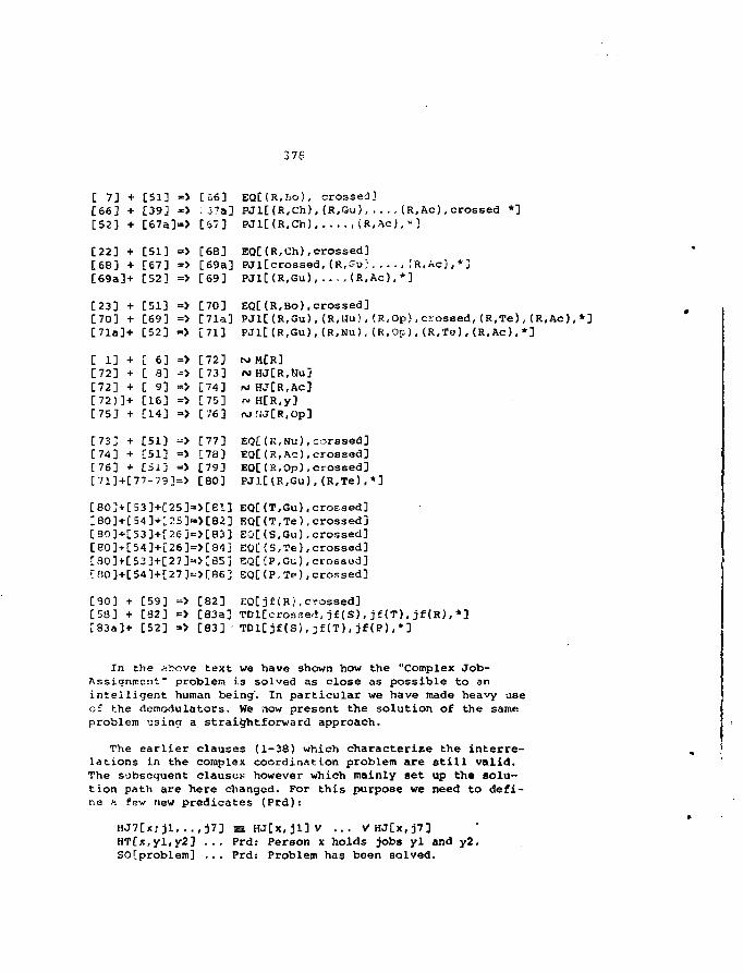
376
C 7] + [51] => [£6][66] + [39] «> . i7a[52] + [67a]=> [67]
EQ[(R,Bo), crossed]PJ1[(R,Ch),(R,Gu),...,(R,Ac),crossed *]PJl[(R,Ch) ,(R,Ac),«]
[22] + [51] => [6B] EQ[(R,Ch),crossed][68] + [67] => [69a] PJl[crossed,(R,Gu) tR.Ac),*][69a]+ [52] => [69] PJl[(R,Gu), (R,Ac),*]
[23] + [51] => [70] EQ[(R,Bo),crossed][70] + [69] => [71a] PJ1[(R,Gu),(R,Nu!,(R,Op),crossed,(R,Te),(R,Ac),*][71a]+ [52] => [71] PJl[(R,Gu),(R,Nu),(R.Op),(R,Te),(R,Ac),*]
[ 1] + [ 6] => [72][72] + [ 8] -> [73][72] + [ 9] => [74][72J]+ [16] => [75][75J + [14] => [76]
[733 + [51] => [77][74] + [51] => [78][76] + [51] => [793[71]+[77-79]=> [80]
t\> M[R]<\> HJ[R,Nu]M HJ[R,Ac]r* H[R,y]rj:!J[R,Op]
EQ[ (R,Nu),corssed]EQ[(R,Ac).crossed]E0[(R,Op),crossed]PJJ.[(R,Gu),(R,Te),*]
[80]+[53]+[25]=>[ei] EQ[(T,Gu).crossed][80]+[54]+[:5]=>[82] EQ[(T,Te),crossed][30]+[53]+[26J=>[83] EQ[(S,Gu).crossed][80]+[54]+[26]=>[84j EQ[{3,Te),crossed][30]-t-[53]+[2 7]=>[35] EQ[(P,Gu),crossed]
EQ[(P,Te),crossed]
+ [59] => [82] EQ[jf{R},crossed]+ [82] => [83a] TDlCcrosse*,j£(S),jf(T),jf(R),*]
[80][58][83a]+ [52] => [83] TD1[jf(S),jf(T),jf(P),*]
In the above text we have shown how the "Complex Job-Assignment" problem is solved as close as possible to anintelligent human being'. In particular we have made heavy useof the demodulators. We now present the solution of the sameproblem using a straightforward approach.
The earlier clauses (1-38) which characterize the interre-lations in the complex coordination problem are still valid.The subsequent clauses however which mainly set up the solu-tion path are here changed. For this purpose we need to defi-ne * few new predicates (Prd):
HJ7[x; jl, . . , J7] =HJ[x,jl]V ... VHJ[x,j7]HT[x,yl,y2] ... Prd: Person x holds jobs yl and y2.SOfproblem] ... Prd: Problem has been solved.
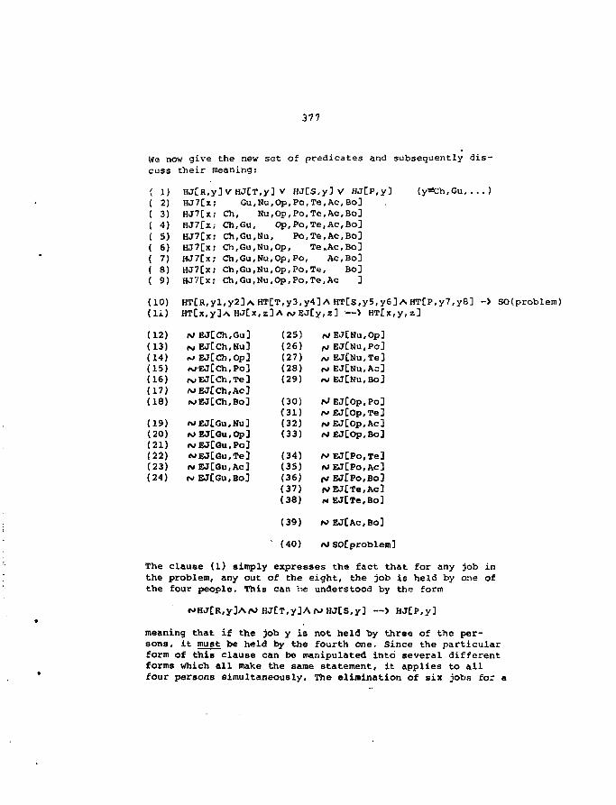
377
We now give the new set of predicates and subsequently dis-cuss their meaning:
( 1)( 2)( 3)( 4)( 5)( 6)( 7)( 8)( 9)
(10)( l i )
(12)(13)(14)(15)(16)(17)(16)
(19)(20)(21)(22)(23)(24)
HJCR.y] VHJ[T,y] V HJ[S,y] V HJ[P,y] (y«Ch,Gu,.HJ7[x; Gu,Nu,Op,Po,Te,Ac,Bo]HJ7[x; Ch, Nu,Op,Po,Te,Ac,Bo]HJ7£x; Ch,Gu, Op,Po,Te,AC,Bo]HJ7[x; Ch,Gu,Nu, Po,Te,Ac,Bo]HJ7[x; Ch,Gu,Nu,Op, Te.Ac.Bo]HJ7[x; Ch,Gu,Nu,Op,Po, Ac,Bo]HJ7[x; Ch,Gu,Nu,Op,Po,Te, Bo]HJ7[x; Ch,Gu,Nu,Op,Po,Te,AC ]
HT[R,yl,y2]AHT[T,y3,y4]A HT[S,y5,y6] A HT[P,y7,y8]HT[x,y]A HJ[x,z]A rv>EJ[y,z] —> HT[x,y,z]
-> SO(problem)
rJ EJ[Ch,Gu]is> EJ[Ch,Nu]OJ EJ[Ch.Op]«viEJ[Ch,Po]rvEJCCh.Te]
f>jEJ[Ch,Bo]
MEJ[Gu,0p]<vEJ[Gu,Po]
iv EJ[Gu,Ac](v EJ[Gu,Bo]
(25)(26)(27)(28)(29)
(30)(31)(32)(33)
(34)(35)(36)(37)(38)
& EJCNu.Po]*> EJ[Nu,Te]t» EJ[Nu,Ac]rj EJ[Ku,Bo]
fitEJ[0p,Te3rst EJ[Op,Ac]«s»EJ[Op.Bo]
r>» EJ[Po,Te]W EJ[Po,Ac]
|VEJCTe,Ac]N EJ[Te,Bo]
(39) N»EJ[AC,Bo]
(40) «j SOtproblein]
The clause (1) simply expresses the fact that for any job inthe problem, any out of the eight, the job is held by one ofthe four people. This can be understood by the form
*JHJ[R,y]Arf»J HJtT,y]A/UHJ[S,y] — > HJ[P,y]
meaning that if the job y is not held by three of the per-sons, it must be held by the fourth one. Since the particularform of this clause can be manipulated into several differentforms which all make the same statement, it applies to allfour persons simultaneously. The elimination of six jobs for a
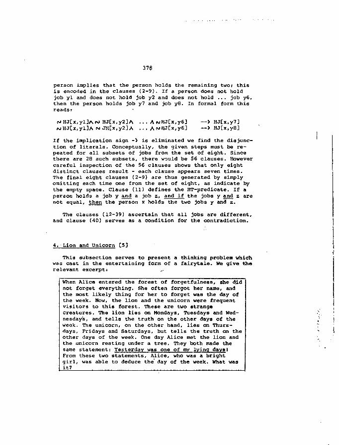
376
person implies that the person holds the remaining two; thisis encoded in the clauses (2-9). If a person does not holdjob yl and does not hold job y2 and does not hold ... job y6,then the person holds job y7 and job yS. In formal form thisreads:
pJHJ[x,yl]AfN» HJ[x,y2]AOjHJ[x,yl]A
A wHJ[x,y6]A«v»HJ[x,y6]
— > HJ[x,y7]— > HJ[x,y8J
If the implication sign -> is eliminated we find the disjunc-tion of literals. Conceptually, the given steps must be re-peated for all subsets of jobs from the set of eight. Sincethere are 28 such subsets, there would be 56 clauses. Howevercareful inspection of the 56 clauses shows that only eightdistinct clauses result - each clause appears seven times.The final eight clauses (2-9) are thus generated by simplyomitting each time one from the set of eight, as indicate bythe empty space. Clause (11) defines the HT-predicate. If aperson holds a job y and a job z, and if the jobs y and z arenot equal, then the person x holds the two jobs y and z.
The clauses (12-39) ascertain that all jobs are different,and clause (40) serves as a condition for the contradiction.
4. Lion and Unicorn [5]
This subsection serves to present a thinking problem whichwas cast in the entertaining form of a fairytale. We give therelevant excerpt: .-
When Alice entered the forest of forgetfulness, she didnot forget everything. She often forgot her name, andthe most likely thing for her to forget was the day ofthe week. How, the lion and the unicorn were frequentvisitors to this forest. These are two strangecreatures. The lion lies on Mondays, Tuesdays and Wed-nesday's, and tells the truth on the other days of theweek. The unicorn, on the other hand, lies on Thurs-days, Fridays and Saturdays, but tells the truth on theother days of the week. One day Alice met the lion andthe unicorn resting under a tree. They both made thesame statement: Yesterday was one of my lying days IFrom these two statements, Alice, who was a brightgirl, was able to deduce the' day of the week. What wasit?
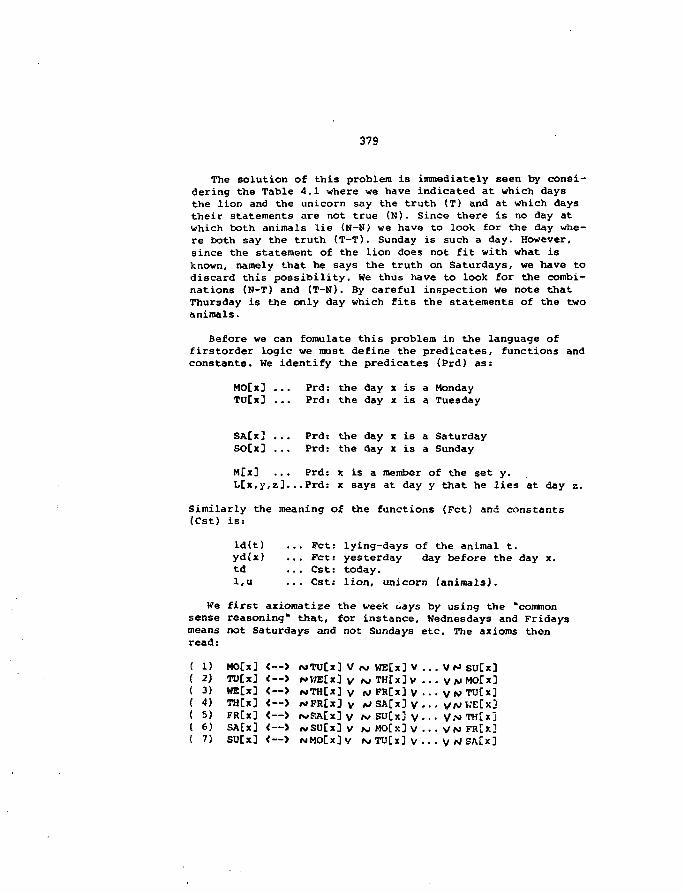
379
The solution of this problem is immediately seen by consi-dering the Table 4.1 where we have indicated at which daysthe lion and the unicorn say the truth (T) and at which daystheir statements are not true (N). Since there is no day atwhich both animals lie (N-NJ we have to look for the day whe-re both say the truth (T-T). Sunday is such a day. However,since the statement of the lion does not fit with what isknown, namely that he says the truth on Saturdays, we have todiscard this possibility. We thus have to look for the combi-nations (N-T) and (T-N). By careful inspection we note thatThursday is the only day which fits the statements of the twoanimals.
Before we can fomulate this problem in the language offirstorder logic we must define the predicates, functions andconstants. We identify the predicates (Prd) as:
MO[x] ... Prd: the day x is a MondayTU[x] ... Prd: the day x is a Tuesday
SA[x] ... Prd: the day x is a SaturdaySO[x] ... Prd: the day x is a Sunday
M[x] ... Prd: x is a member of the set y.L[x,y,z] Prd: x says at day y that he lies at day z.
Similarly the meaning of the functions (Fct) and constants(Cst) is:
ld(t) ... Pet: lying-days of the animal t.yd{x) ... Pet: yesterday day before the day x.td ... Cst: today.l,u ... Cst: lion, unicorn (animals).
We first axiomatize the week cays by using the "commonsense reasoning* that, for instance, Wednesdays and Fridaysmeans not Saturdays and not Sundays etc. The axioms thenread:
1)2)3)4)5)6)7)
MOCx]TU[x3WE[x]THCx]FRCx]SA[x]SU[x]
<—><—><—><—><—><--><—>
MTUCX]f»V7E[xJroTH[x]*»FR[x]frfSACx]rjSU[x]NMOCX]
Vy
vV
VV
«M WE[x]r» TH[xJlOFR[x]rJ SA[x]is/ SU[x]<vi MO[x]IS/TUCx]
VVv . . .v . . .
v . . .V • • .
VrJ
V N
V N>
V NV N
V fJ
SUCx]MOtx]TUCx]WE[X3TH[XJFR[X]SA[X]
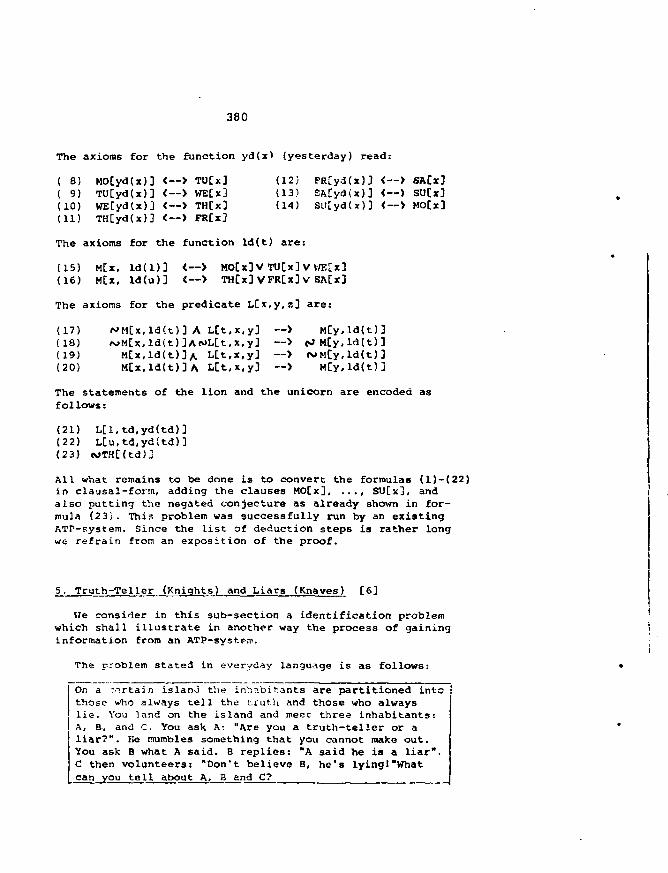
380
The axioms for the function yd(x> (yesterday) read:
( 8)( 9)(10)(11)
MOCyd(x)] <--> TU[x] (12)TUtyd(x)] <--> WE[x3 (13)WE[yd(x)] <—> TH[x] (14)TH[yd(x)] <-->
FRCyd(x)} <--> SACxJSA[yd(x)] <--SO[yd(x)3 < —
SU[x]MOCx]
The axioms for the function ld(t) are:
(15)(16)
M[x,M[x, ld(u)] I— >
MO[x]V TU[x] VWE[x]THCx] VFR[x] V SA[x]
The axioms for the predicate L[x,y,z] are:
(17)(18)(19)(20)
A L[t,x,y]/v>MCx,ld(t)]ANL[t,x,y]M[x,ld(t)]A Ltt,x,y]M[x.ld(t)]A L[t,x,y]
M[y,ld(t)]
iMM[y,ld(t)3M[y,ld(t)]
The statements of the lion and the unicorn are encoded asfollows:
(21) L[l,td,yd(td)3(22) L[u,td,yd(td)](23) WTH[(td)]
All what remains to be done is to convert the formulas (l)-(22)in clausal-form, adding the clauses MO[x], ..., SU[x], andalso putting the negated conjecture as already shown in for-mula (23). This problem was successfully run by an existingATP-system. Since the list of deduction steps is rather longwe refrain from an exposition of the proof.
5. Truth-Teller (Knights) and Liars (Knaves) [6]
We consider in this sub-section a identification problemwhich shall illustrate in another way the process of gaininginformation from an ATP-system.
The problem stated in everyday language is as follows:
On a -r>rtain islana the inhabitants are partitioned into !those who always tell the truth and those who alwayslie. You land on the island and meet three inhabitants:A, B, and C. You ask A: "Are you a truth-teller or aliar?". He mumbles something that you cannot make out.You ask B what A said. B replies: "A said he is a liar"C then volunteers: "Don't believe B, he's lyingl"Whatcan you tell about A. B and C?
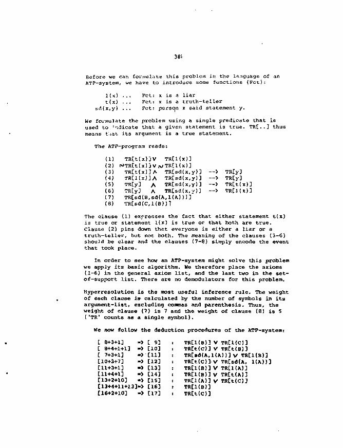
381
Before we can formulate this problem in the language of anATP-system, we have to introduce some functions (Fct):
l(x) ... Fct: x is a liart(x) ... Fct: x is a truth-teller
sd(x,y) ... Fct: person x said statement y.
We formulate the problem using a single predicate that isused to indicate that a given statement is true. TR[..2 thu6means t.iat its argument is a true statement.
The ATP-program reads:
(1) TR[t(x)]V TR[l(x)](2) PJTR[t(x)] V/viTRCKx)](3) TR[t(xHA TR[sd{x,y)] --> TR[y](4) TR[l(x)JA TR[sd(x,y)] —> TR[y](5) TR[y] A TR[sd(x,y)] —> TR[t(x)](6) TR[y] A TR[sd(x,y)] —> TR[l(x)](7) TR[sd(B,sd(A,l(A)))](8) TR[sd(C,l(B))l
The clause (1) expresses the fact that either statement t(x)is true or statement l(x) is true or that both are true.Clause (2) pins down that everyone is either a liar or atruth-teller, but not both. The meaning of the clauses (3-6)should be clear and the clauses (7-8) simply encode the eventthat took place.
In order to see how an ATP-system might solve this problemwe apply its basic algorithm. We therefore place the axioms(1-6) in the general axiom list, and the last two in the set-of-support list. There are no demodulators for this problem.
Hyperresolution is the most useful inference rule. The weightof each clause is- calculated by the number of symbols in itsargument-list, excluding commas and parenthesis. Thus, theweight of clause (7) is 7 and the weight of clause (8) is 5('TR1 counts as a single symbol).
We now follow the deduction procedures of the ATP-system:
[ 8+3+1] «> [ 9] : TR[1(B)] V TR[1{C)][ 8+4+1+1] -> [10] : TR[t(C)] V TR[t(B)3[ 7+3+1] -> [11] : TR[sd(A,l(A))3 V TR[1(B)][10+3+7] -> [12] : TR[t(O] V TR[sd(A, 1(A))][11+3+1] -> [13] : TR[1(B)] V TR[1(A)][11+4+1] -> [14] : TR[1(B)] V TR[t(A)][13+2+10] -> [15] : TR[1(A)3 V TR[t(C)3[13+4+ll+13» [16] j TR[1{B)3[16+2+10] -> [17] : TR[t(C)]
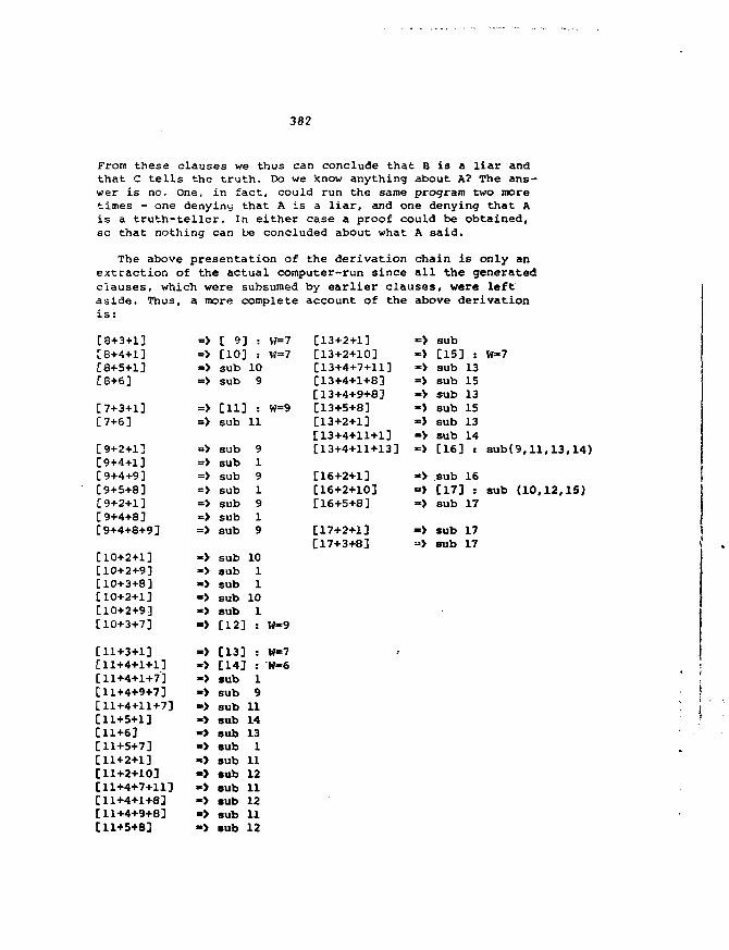
382
From these clauses we thus can conclude that B is a liar andthat C tells the truth. Do we know anything about A? The ans-wer is no. One, in fact, could run the same program two moretimes - one denying that A is a liar, and one denying that Ais a truth-teller. In either case a proof could be obtained,so that nothing can be concluded about what A said.
The above presentation of the derivation chain is only anextraction of the actual computer-run since all the generatedclauses, which were subsumed by earlier clauses, were leftaside. Thus, a more complete account of the above derivationis:
[8+3+1][8+4+1][8+5+1][8+6]
[7+3+1][7+6]
[9+2+1][9+4+1][9+4+9][9+5+8][9+2+1][9+4+8][9+4+8+9]
[10+2+1][10+2+9][10+3+8][10+2+1][10+2+9][10+3+7]
[11+3+1][11+4+1+1][11+4+1+7][11+4+9+7][11+4+11+7][11+5+1][11+6][11+5+7][11+2+1][1H-2+10][11+4+7+11]C11+4+1+8][11+4+9+8][11+5+8]
=>=>=>=>
=>=>
=>=>=>=>=>=>=>
«>
«>»>«>->
«>»>»>»>->«>»>«>«>«>«>»>a )
[ 9][10]subsub
[11]sub
subsubsubsubsubsubsub
subsubsubsubsub[12]
[13]C14]subsubsubsubsubsubsubsubsubsubsubsub
::
109
:11
9191919
1011101
•
•
191114131111211121112
W=7W=7
W=9
W-9
W=7W-6
[13+2+1][13+2+10][13+4+7+11][13+4+1+8][13+4+9+8][13+5+8][13+2+1][13+4+11+1][13+4+11+13]
[16+2+1][16+2+10][16+5+8]
[17+2+1][17+3+8]
=> sub-> [15]«> sub=> sub-> sub»> sub=> sub=> sub=> [16]
*> sub=> [17]=> sub
«> sub-> sub
: W-7131513151314: sub(9,ll,13,14)
16: sub (10,12,15)17
1717
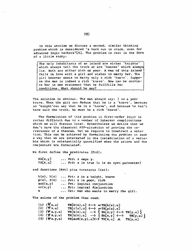
383
In this section we discuss a second, similar thinkingproblem which is considered "a hard nut to crack, even foradvanced logic hackers"[63. The problem is cast in the formof a little story:
The only inhabitants of an island are either 'knights'which always tell the truth or are "knaves' which alwayslie. Both are either rich or poor. A man of this islandfalls in love with a girl and wishes to marry her. Thegirl however wants to marry only a rich 'knave'. Suppo-se the man is indeed a rich 'knave'. How can he convin-ce her in one statement that he fullfills herconditions. What should he say?
The solution is obvious. The man should say: I am a poorknave. Then the girl can deduce that he is a 'knave', becauseno 'knight'can say that he is a 'knave', and because he can'thave said the truth, he must be a rich 'knave*.
The formulation of '.his problem in first-order logic israther difficult due to a number of inherent complicationswhich we will discuss later. Nevertheless we notice that wedon't have the classical ATP-situation of proving the co-rrectness of a theorem, but we require to construct a solu-tion. This can be achieved by formulating the problem in sucha way that we are interested in the instantiation of a varia-ble which is existentially quantified when the axioms and theconjecture are formulated.
We first define the predicates (Prd):«
SA[x,y] ... Prd: x says y.
TR[x,u] ... Prd: x is true (u is an open parameter)
and functions (FCt) plus constants (Cst):
k(x), h(x) ... Fct: x is a knight, knave
p(x), r(x) ... Fct: x is poor, richand{x,y) ... Fct: logical conjunctionor(x,y) ... Fct: logical disjunctiona ... Cst: man who wants to marry the girl.
The axioms of the problem then read:
(1) (Vx.u) TR[k(x),u] <—> iOTRCh(x),u3(2) (Vx,u) TR£r(x),u3 <—> NTR[p<x),u](3) (Vx.y.u) TR[k(x),u] —> { SA[x,y] <—> TRLy.u]}(4) (Vx,y,u) TR[h(x),u3 —> { SA[x,y] <--> TR[y,u]j(5) Cfx.y.u) TR[and(x,y),u3<-> TR[x,u] A TR[y,u]

384
and the conjectu e i s given the form:
(6) O x ) SA[a,x] <—> TR[ar,a(V.o.ra),Xj
Note, in the above formula we have introduced the simplifyingnotation: h(a) ha, which we also will use lateron.Let us comment on the formulas (l)-(C) where »:he theorem (6)is the most difficjlt part. Pirst-order logic ha*, limitationswhich become transparent in this example: fi) it is not real-ly constructive, usually one proves the correctness of a pos-sible solution for a problem; (ii) quantification xa allowedonly over individuals, not over functions, predicates andformulas; (iii) an implication is true even if the premise isfalse. A remedy for (i) has been indicated earlier •• we simp-ly introduce an existentially quantified variable and let thededuction mechanism determine its value. The remedy for (ii)consists in the introduction of a predicate TR[x] (whichmeans "it is true that ..."; and the redefinition of all pre-dicates and logical connectives, as Boolean functions: k(x),h(x), p(x!, i(x), and(x,y), or;x,y), wherc-by the action o£the latter two Boolean 'operators' has to be axiomstized exp-licitly. As a result of (lii), tha formulation of the theorem(6) poses problems. Using the implication-sign instead of thefiuivalence-sign lends, after a few deduction steps, to theconclusion that nobody can say that he is a 'knave': SA[z,V. (z) ] . The equivaience-sign is still not «nough. the reasonbeing that the variable x appears only on the left-hand sideof (6). Thus <_;ener.-2l.i:iing TS[I,UJ such that it has two argu-ments* as it wouJd be for instance in relevance logic, leadsto the expected result. The meaning of (6) is as follows:"There exists a statement x from the man (named 'a') whichshall be equivalent to the fact that he really is a rich'knave'".
Putting the axioms' and the negated 'conjecture' in conjunc-tive normalform leads to the following set of clauses:
C i )( 2)( 3)( 4)( 5)( 6)( 7)( 8)( 9)(10)(11)(12)(13)
MTR[k(x),y] VTR[k(x),y] v
r>»TR[r(x),y] vTR[r(x),y3 y
PJTR[k(x),z] VAjTR[k(x),z] VMTR[k(x),z3 V<\>TR[and(x,y),s3(\>TR[and(x,y),
fO TR[h(x),y]TR[h(x),y3
CJ TR[p(x),y]TR[p(x),y3
ro SA[x,y] v TR[y,z3SA[x,y] y/\>TR[y,z3
fv SA[x,y3 VfNJTRCy<z3SA[x,y3 V TR[y,z]
V TR£x,z3„ . V TR[y,z]
TR[and(x,y),z3 Vc<J TR[x,z3v/\) TR[y,z3SA[a,x3 V r\» TRCand(ka, ra) ,x3SA[a,x3 V TR[andOca,ra),xj
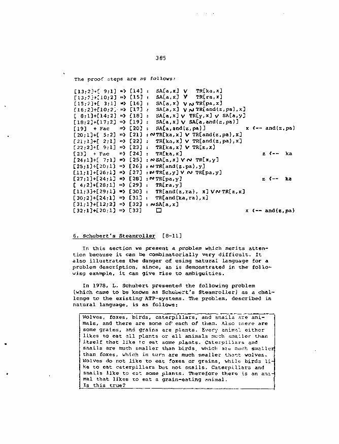
385
The proof steps are as follows:
[16;23+[1O;2;;
[19] + Fac[20;l]+[ 5;2][21;l]+[ 2;1][22;2]-)[ 9;1][23] + Pac[24;1]+C 7;1][25;l]+[20;l][ll;lj+[26;l][27;1]+[24;1][ 4;2]+[28;l]
[30;2]+[24;l][31;1]+[12;2][32;l]+[20;l]
=> [14] : SA[a,x] V TR[ka,x]=> [15] : SA[a,x] V TR[ra,x]=> [16] : SA[a,x] Vi\>TR[pa,x]
'=> [17] : SA[a,x] v rJ TR[and(z,pa), x]=> [18] : SA[a,x] V TR[y,x] v SA[a,y]=> [19] : SA[a,x]v SACa,and(z,pa)]=> [20] : SA[a,and(z,pa)] x <— and(z.pa)=> [21] :NTR[ka,x] V TR[and(z,pa), x]=> [22] : TR[ka,x] V TR[and(z,pa),x]=> [23] : TR[ka,x] V TR[z,x]=> [24] : TR[ka,x] z <— ka=> [25] :NSA[a,x]VN TR[x,y]=> [26] :MTR[and(zrpa),y]=> [27] :MTR[z,y]V /v TRCpa.y]=> [28] :~TR[pa,y] z <-- ka=> [29] : TR[ra,y]=> [30] : TR[and(z,ra), x]V<VTR[z,x]=> [31] : TR[and(ka,ra),x]=> [32] : i«SA[a,x]=> [33] P x <-- and(z.pa)
6. Schubert's Steamroller [8-11]
In this section we present a problem which merits atten-tion because it can be combinatorially very difficult. Italso illustrates the danger of using natural language for aproblem description, since, as is demonstrated in the follo-wing example, it can give rise to ambiguities.
In 1978, L. Schubert presented the following problem(which cane to be known as Schubert's Steamroller) as a chal-lenge to the existing" ATP-systems. The problem, described innatural language, is as follows:
Wolves, foxes, birds, caterpillars, and snails are ani-mals, and there are some of each of them. Also there aresome grains, and grains are plants. Every animal eitherlikes to eat all plants or ail animals nuch smaller thanitself that like to eat some plants. Caterpillars andsnails are much smaller than birds, which are much smallerthan foxes, which in turn are much smaller thar.t wolves.Wolves do not like to eat foxes or grains, while birds li-ke to eat caterpillars but not snails. Caterpillars andsnails like to eat some plants. Therefore there is an ani-mal that likes to eat a grain-eating animal.Is this true?
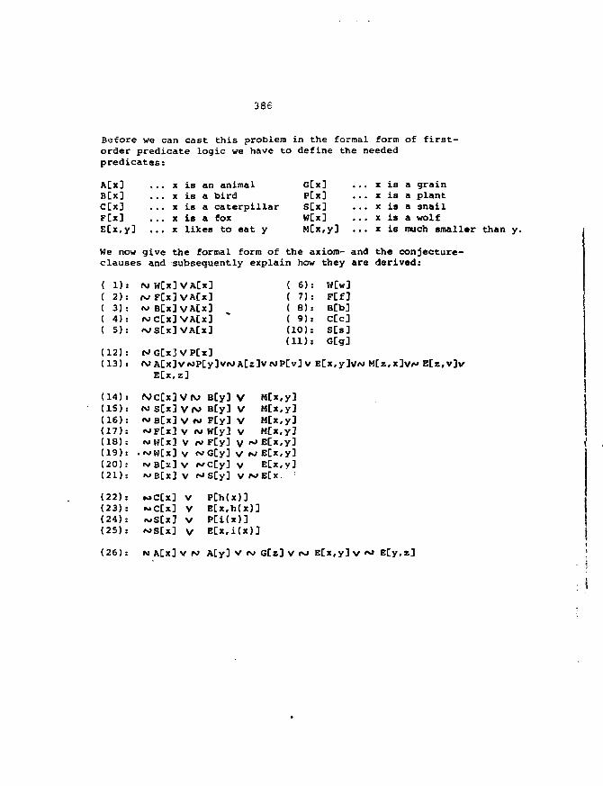
386
Before we can cast this problem in the formal form of first-order predicate logic we have to define the neededpredicates:
A[x] ... x is an animal G[x] ... x is a grainB[x] x is a bird P[x] ... x is a plantC[x] ... x is a caterpillar S[x] ... x is a snailP[x] ... x is a fox W[x] ... x is a wolfE[x,y] ... x likes to eat y M[x,y] ... x is much smaller than y.
We now give the formal form of the axiom- and the conjecture-clauses and subsequently explain how they are derived:
( 1 ) :( 2 ) :
( 3 ) :
( 4 ) :
( 5 ) :
( 1 2 ) :( 1 3 ) :
( 1 4 ) :( I S ) :( 1 6 ) :( 1 7 ) :( 1 8 ) :( 1 9 ) :( 2 0 ) :( 2 1 ) :
( 2 2 ) :( 2 3 ) :( 2 4 ) :( 2 5 ) :
M W[x] VA[x]rJ F[x] VACx]w B[x] VA[x]NC[l]VA[l]*JS[x] VA[x]
N G[xj VP[x]fv A[x]VAJP[y]vfvj
E[x,z]
<VC[x]V(VJ B[y]*>S[x] VfN* B[y]~B[x] V «x» P[y]MF[x] v iv W[y]«vW[x] V fJ F[y]
• *JW[x] v *>» G[y]«v B[x] v <^C[y]
>A[z]
VVVVV ^V rJVV /v
MC[l] V PCh(x)]~C[x] V E[x,h(x)]N S [ X ] v P[i(:<N»S[X] v E[x,i
c ) ]L ( x ) ]
M[x,M[x,M[x,MCx,E[x,E[x,E[x,E[x.
( 6)( 7)( 8)( 9)(10)(11)
'[v]v
y ]y3y ]y3
y ]y ]
: WLw]: FCf]: B[bJ: CCc]: S[s]: G[g]
' E[x,y]V<v» E[SS,V]V
(26 ) : n A[x] v M A[y] V iv G[z] V OJ E[x,y3 V «s» ECy,z]
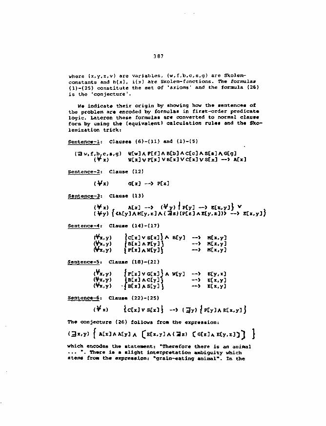
387
where ( x , y , z , v ) a re v a r i a b l e s , ( w , f , b , c , s , g ) a re Skolem-cons tan t s and h ( x ) , i ( x ) a re Sfcolem-functions. The formulas( l ) - ( 2 5 ) c o n s t i t u t e the s e t of "axioms' and the formula (26)i s the 'conjecture1.
We indicate their origin by showing how the sentences ofthe problem arc encoded by formulas in first-order predicatelogic. Lateron these formulas are converted to normal clauseform by using the (equivalent) calculation rules and the Sko-lemization trick:
Sentence-1: Clauses (6 ) - ( l l ) and ( l ) - (5)
C3w,f ,b,c ,s ,g) W[w3A F[f]AB[b] AC[c] AS[«]/vG[g]
(Vx) W [ X ] V P C X ] V B C X ] V C [ X ] V S [ X ] ~> ACX]
Sentence-2: Clause (12)
(Vx) G[x3 —> P[x]
Sentence-3: Clause (13)
(Vx) A[x] —> (Vy) | p [ y ] ~> ECx.y}} V(Vy) {<KZylAKty,zjACaz)(Pt*lABly,zl)> —>
Sentence-4: Clause (14)-(17)
(Vx.y) 1 C [ X ] V S [ X ] } A B[y] --> M[x.y]<V».y) {BCxDAFCy]} --> H[x.y](•/x.y) iFCx3AWCy]J —> M[x.y]
Sentence-5: Clause (18)-(21)
( . y ) f C ] £ 3 3 A Wty] --> E[y,x](¥x,y) tB[x]AC[y3) --> Etx.y](Vx.y) fB[x]AS[y]} --> E[x,y]
Sentence-6; Clause (22)-(2S)
(Vx) i c [ x ] V S [ x 3 | --> ( 3 y ) {Pry3AE[
The conjecture (26) follows fro* the expression:
<3*.y> f A[x3A*ty3 A ^
which encodes the statement: "Therefore there is an animal... '. There is a slight interpretation anbiguity whichstems from the expression: "grain-eating animal". In the
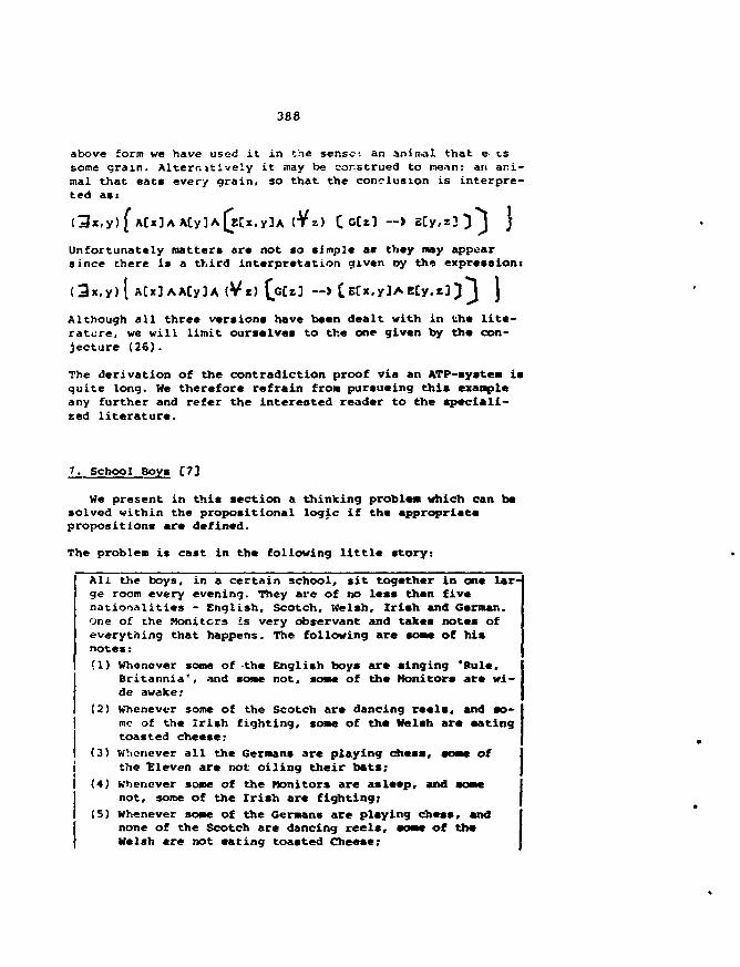
388
above form we have used it in the sense-, an anin.al that e cssome grain. Alterr. jt ively it may be construed to mean: an ani-mal that eats every grain, so that the conclusion is interpre-ted as:
3x,y)f A[x]AAty]A[ECx.y]A —> EC
Unfortunately matters are not so simple a« they may appearsince there is a third interpretation given i?y the expression:
(3x .y ) { A[x]AA[y]A (Vs) E[x,y]A
Although all three versions have been dealt with in the lite-rature, we will limit ourselves to the one given by the con-jecture (26).
The derivation of the contradiction proof via an ATP-system isquite long. We therefore refrain from pursueing this exaapleany further and refer the interested reader to the speciali-zed literature.
7. School Boys [73
We present in this section a thinking problem which can besolved within the propositional logic if the appropriatepropositions are defined.
The problem is cast in the following little story:
All the boys, in a certain school, sit together in one large room every evening. They arc of no less than fivenationalities - English, Scotch, Welsh, Irish and German.One of the Monitors is very observant and takes notes ofeverything that happens. The following are some of hisnotes:
(1) Whenever some of -the English boys are singing 'Rule,Britannia', and some not, some of the Monitors are wi-de awake;
(2)
(3)
I (4)
I (S)
Whenever some of the Scotch are dancing reels, and so-me of the Irish fighting, some of the Welsh are eatingtoasted cheese;
Whenever all the Germans are playing chess, some ofthe 'Eleven are not oiling their bats;Whenever some of the Monitors are asleep, and somenot, some of the Irish are fighting;Whenever some of the Germans are playing chess, andnone of the Scotch are dancing reels, som* of theWelsh are not eating toasted Cheese;
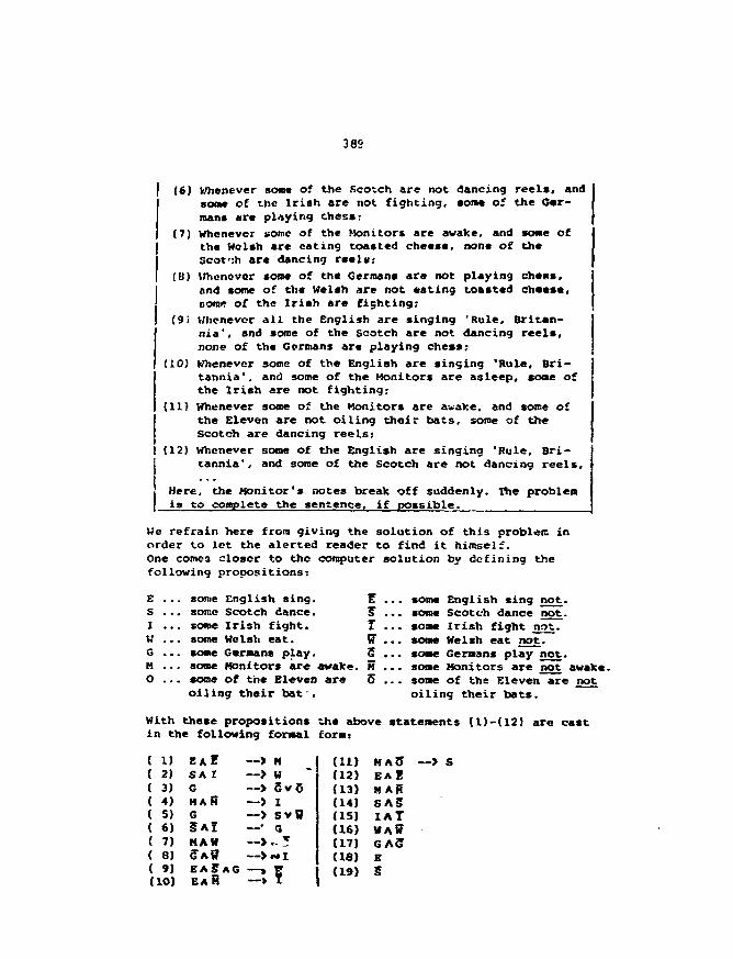
389
(6) Whenever some of the Scotch are not dancing reels, andsome of the Irish are not fighting, som* of the Gar-roan* are playing chess;
(7) whenever some of the Monitors are awake, and soae ofthe Welsh are eating toasted cheese, none of theScotch ar« dancing re«l«;
(U) V/henovor some of th« Germans are not playing chens,and some of the Welsh are not sating toasted ch««s«>DOtnn of the Irish »re fighting;
(9< Whenever all the English are singing 'Rule, Britan-nia', and tome of the scotch are not dancing reels,none of the Germans are playing chess;
(10) Whenever some of the English are singing 'Rule, Bri-tannia', and some of the Monitors are asleep, sone ofthe Irish are not fighting;
(11) Whenever some of the Monitors are awake, and some ofthe Eleven are not oiling their bats, some of theScotch are dancing reels;
(12) Whenever some of the English are singing 'Rule, Bri-tannia', and some of the Scotch are not dancing reels.
Here, the Monitor's notes break off suddenly. The problemis to complete the sentence, if possible.
We refrain here from giving the solution of this problem inorder to let the alerted reader to find it himself.One comes closer to the computer solution by defining thefollowing propositions:
E ... some English sing. ES ... some Scotch dance. S*I ... some Irish fight. IW ... some Welsh eat. w"G ... some Germans play. 3H ... sone Monitors are awake. HO ... some of the Eleven are 5
oiling their bat-.
some English sing not,some Scotch dance not,soaa Irish fight not,some Welsh eat not,sone Geraans play not,sone Monitors are not awake.some of the Eleven are notoiling their bats.
With these propositions the above statements (1)-(12J are castin the following formal fora:
( 1) E * E —> M( 2 ) S A I —> W
3) G — > g 54) MAM —> I5) G ~> SVB6) §AI — ' g7} HAH — > . - ?8) G"AS — >**I
. 9) EA§AG —> V(10) E A H —» T 1
(11) MATS(12) EAE
(13) HAH(14) SA3(15) IAT(16) WAW"(17) GAG"(18) E(19) 5
—> S
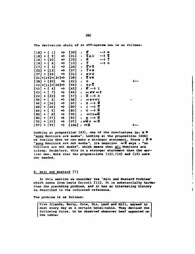
390
The derivation chain of an ATP-systea now is as follows:
[18] + [ 1] -> [20] s F — > M[18] + [ 9] -> [21] : S A G --> E[18] + CIO] -> [22] : B --> T[19] + C 6] -> [23] : T --> C[17] • [ 3] -> [243 t 5V3[22] • [13] -> [27] i TVM[273 • [23] -> £31] i MVC[21]+[19>C31» [38] t FVM[38] + [20] -> [43] » M <--[43]+[ll]+[24]»> [44] : SvS[43] + [ 4) -> [45] : R* --> I[43] + [ 7] -> [46] : M H V N S
[23] + [22] -> [57] : H --> G[46] + [ 2] -> [68] : NSVNI[46] • [16] -> [69] : S —> ff[68] + [44] -> [80] : 1 —> TS[69] + [ 5] -> [83] : G —> W[80] + [ 8] »> [90] : NlvmH[83] + [57] -> [93] : M --> W[90] + [45] »> [97] :MHV MMC97) + [93] -> [106] :
Looking at proposition (43), one of the conclusions is: H •*aoire Monitors are awake". Looking at the proposition (106)we realize that we can make a stronger statement. Sine* : 8 •'aome Monitors are not awake", its negation M H says t "noMonitors are not awake", which means that all Monitors areasleep. Doubtless, this is a stronger statenent than the ear-lier one. Note that the propositions (12),(14) and (15) werenot needed.
8. Salt and Mustard [7]
In this section we consider the 'Salt and Mustard Problea'which comes from Lewis Carroll [13]. It is substantially harderthan the preceding problem, and it has an interesting historyas described in the indicated reference.
The problem is as follows:
Five friends, Barry, Cole, Oix, Land and Mill, agreed tomeet every day at a certain hotel-table. They devised thefollowing rules, to be observed whenever beef appeared onthe table:
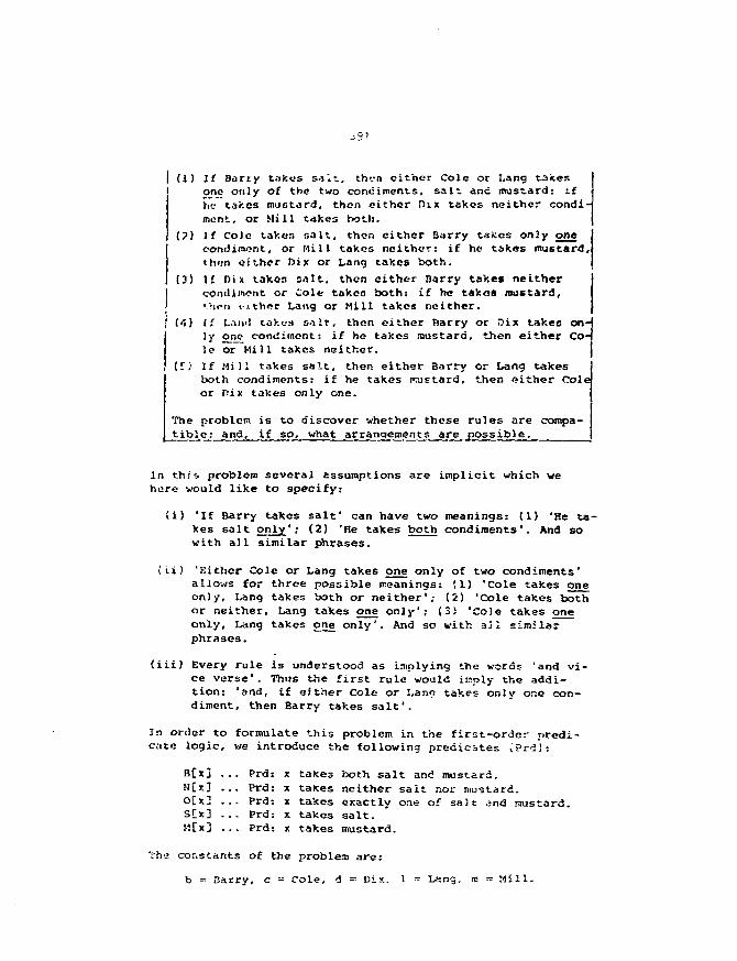
j'S?
I (1) If Barry takes sa'.t, thvn either Cole or Lang takesone only of the two cone intents, salt and mustard: ifhe takes mustard, then either Dix takes neither condi-ment, or Mill takes both.
(?) If Cole takes salt, then either Barry takes only oneooniJim<?nt, or Kill taKcs neither: if he takes mustard,then ei i.hor Dix or Lang takes both.
(3) I£ Dix taken salt, then either Barry takei neithercondiment or Cole taken both: if he takes mustard,•.'•ion i-ithor Lang or Mill takes neither.
(1) If L.-uvi takes salt, then either Barry or Dix takes on-ly one condiment: if he takes mustard, then either Co-le or Mill takes neither.
(f) If Mill takes salt, then either Barry or Lang takesboth condiments: if he takes mustard, then either Coleor Pix takes only one.
The problem is to discover whether these rules are compa-tible: and, if so, what arrangements are possible.
In this problem several assumptions are implicit which wehere would like to specify:
(i) "If Barry takes salt' can have two meanings: (1) "He ta-kes salt only'; (2) 'He takes both condiments'. And sowith all similar phrases.
\ii) 'Either Cole or Lang takes one only of two condiments'allows for throe possible meanings: (1) 'Cole takes oneonly, Lang takes both or neither'; (2) 'Cole takes bothor neither, Lang takes one only'; (3) 'Cole takes oneonly, Lang takes one only'. And so with ai1 similarphrases.
(iii) Every rule is understood as implying the words 'and vi-ce verse1. Thus the first rule would imply the addi-tion: 'and, if either Cole or Lano takes only or.e con-diment, then Barry takes salt'.
In order to formulate this problem in the first-order predi-cate logic, v/e introduce the following predicates
B[x] ... Prd: x takes both salt and mustard.N[x] ... Prd: x takes neither salt nor mustard.0[x3 ... Prd: x takes exactly one of salt and raustard.S[x] ... Prd-. x takes salt.K[x] ... Prd: x takes mustard.
The constants of the problem are:
b = Carry, c = Cole, d - Cix. 1 = Lsng, re = Mill.
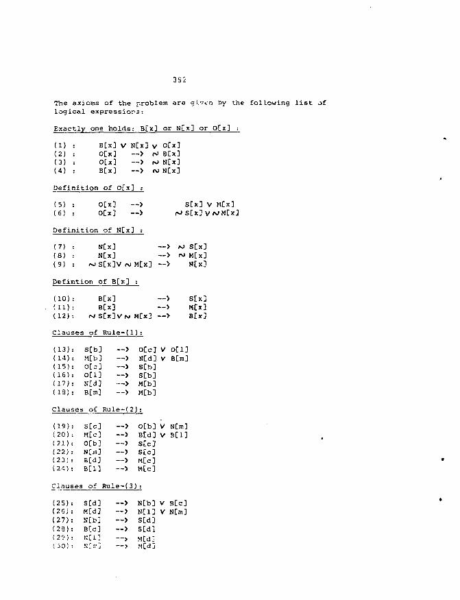
3S2
The axioms of the problem are given by the following list oflogical expressions:
Exactly one holds: B[x] or H[x] or 0[x] :
(1) :(2) :(3) :(4) :
B[x] V N[x] vO[x] --> r.0[x] — > rvB[x] -~> (\
Definition of 0[x] :
(5) :(6) :
O[x] -->O[x] -->
Definition of N[x] :
(7) :(8) :(9) :
N[x3H[x3
<VJS[X3V <M M[X3
Defintion of B[x3 :
(10):(11):(12):
B[x]B[x3
rJ S[x3V(v M[x3
Clauses of Rule-(l):
(13):(14):(15):(16):(17):(18):
sCb3 --> o[c3M[b] —> N[d3o[ = ] —> S[b3o[l3 --> S[b3N[d] — > M[b3B[m3 —> M[b3
Clauses of Rule-(2):
(19):(20) :(21):(22):(23):(24) :
s[c3 --> o[b3M[c] ~> B[d3o[b3 —> s[c3N[m3 —> S[c3B[d3 —> M[c3B[l] — > M[c]
Clauses of Rule-(3):
(25):(26):(27):(23):( 21?) :! i 0 ! :
s[d3 —> N[b3M[d3 — > N[13S[b] --> s[d3B[c3 — > S[d3H[l] —> M[d]KCrr] —> Mtdj
0Cx3' B[x3» N[x3J N[x3
s[x3 v M[x3(viS[x3vwM[x]
—> ^ stxl— > (v» M[x3—> NCx]
—> S[X]—> M[x3—> B[x3
V 0[l]V B[m]
V N[m3V B[13
v B[C3v mLm]
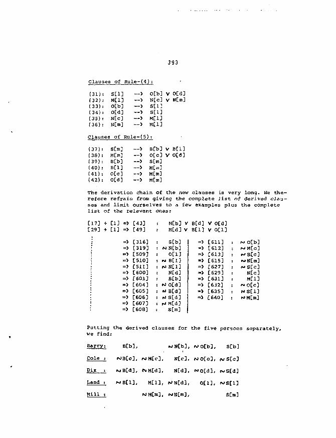
393
Clauses of Rule-(4):
(31):(32):(33):(34):(35):(36):
Clauses
S[l] —> 0[b]M[l] —> N[c]0[b] — > S[l]O[d] ~ > S[l]N[c] — > M[l]N[m] — > M[l]
of Rule-(5):
V 0[d]V N[m]
(37): S[m](38): M[n>](39): B[b](40): B[l](41): 0[c](42): 0[d]
y
B[b] V B[i]0[c] V O[d]S[m]
M[m]M[m]
The derivation chain of the new clauses is very long. We the-refore refrain from giving the complete list of derived clau-ses and limit ourselves to a few examples plus the completelist of the relevant ones:
[17] + [1] =>[29] + [1] =>
: =>=>=>=>=>=>=>=>=>=>=>=>
[43][49]
[316][319][509][510][511][600][601][604][605][606][607][608]
: M[b] VM[d] V
S[b]M N[b]O[l]
: IM B[l]PJ N[l]
N[d]B[b]
fJO[d]*J B[d]fOS[d]rJ M[d]S[m]
B[d]B[l]
=>=>=>=>=>
=>->=>
V 0[d]V 0[l]
[611] -.[612] :[613] :[615] :[627] :[629] :[631] :[632] :[635] :[640] :
~ O[bl^M[c;•^B[c:<N»N[m:
<«S[cJN[c]M[l]
f«0[c]NS[1]MM[m]
Putting the derived clauses for the five persons separately,we find:
Barry: B[b], *»N[b], wo[b], S[b]
Cole : N»B[c], MM[c], N[c], MO[c], «M S[c]
Dix : MB[d], r\>M[d], N[d], <«0[d], <vS[d]
Land : MB[1], M[l], N>N[d], O[l], «s»S[l]
Mill : N M [ m ] , r«»H[m]/ S[m]
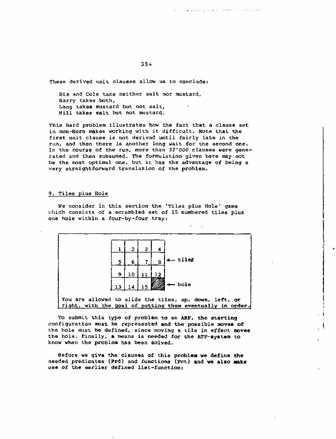
39/.
These derived unit clauses allow us to conclude:
Dix and Cole take neither salt nor mustard,Barry takes both,Lang takes mustard but not salt.Mill takes salt but not mustard.
This hard problem illustrates how the fact that a clause setin non-Horn makes working with it difficult. Note that thefirst unit clause is not derived until fairly late in therun, and then there is another long wait for the second one.In the course of the run, more than 32'000 clauses were gene-rated and then subsumed. The formulation given here may notbe the most optimal one, but it has the advantage of being avery straightforward translation of the problem.
9. Tiles plus Hole
We consider in this section the 'Tiles plus Hole1 gamevhich consists of a scrambled set of 15 numbered tiles plusone hole within a four-by-four tray:
1
5
9
13
2
6
10
14
3
7
11
15
4
8
12
iff
tiles
hole
You are allowed to slide the tiles, up, down, left, orright, with the goal of putting them eventually in order.
To submit this type of problem to an ARP, the startingconfiguration must be represented and the possible moves ofthe hole must be defined, since moving a tile in effect movesthe hole. Finally, a means is needed for the ATP-system toknow when the problem has been solved.
Before we give the clauses of this problem we define theneeded predicates (Prd) and functions (Fct) and we also makeuse of the earlier defined list-functions
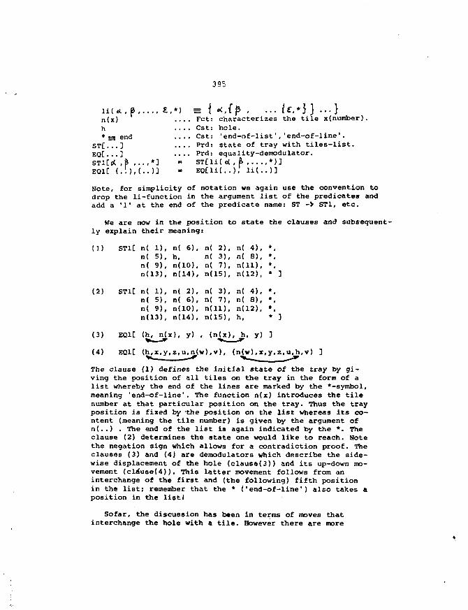
395
lit CL.& £,*) = {n(x) Fct:h Cst:* s end Cst:
ST[...] •••• Prd:EQ[...] .••• Prd:
,{(3 , ...{€.*]}...}characterizes the tile x(number).hole.'end-nf-list','end-of-line'.state of tray with tiles-list,equality-demodulator.qy
ST[li(o( , fr ,...,*)]EQ[li() l i ( ) ]EQ1[ (.!),(..)]
Note, for simplicity of notation we again use the convention todrop the li-function in the argument list of the predicates andadd a '1' at the end of the predicate name: ST -> ST1, etc.
We are now in the position to state the clauses and subsequent-ly explain their meaning:
(1) ST1[ n( 1), n< 6), n( 2), n( 4), *,n( 5), h, n( 3), n( 8), *,n( 9), n(10), n( 7), n(ll), *,n(13), n(14), n(15), n(12), * ]
(2) ST1[ n( 1), n( 2), n( 3), n( 4), *,n( 5), n( 6), n( 7), n( 8), *,n{ 9), n(10), n(ll), n(12), *,
h, • ]
(3) EQ1[ y) , (n(x). h. y) ]
(4) EQ1[ (h,x,y,z,u^n(w),v), (n(w),x,y,z, u,h,v) ]
The clause (1) defines the initial state of the tray by gi-ving the position of all tiles on the tray in the form of alist whereby the end of the lines are marked by the *-symbol,meaning 'end-of-line'. The function n(x) introduces the tilenumber at that particular position on the tray. Thus the trayposition is fixed by 'the position on the list whereas its co-ntent (meaning the tile number) is given by the argument ofn(..) . The end of the list is again indicated by the *. Theclause (2) determines the state one would like to reach. Notethe negation sign which allows for a contradiction proof. Theclauses (3) and (4) are demodulators which describe the side-wise displacement of the hole (clause(3)) and its up-down mo-vement (clause!4)). This latter movement follows from aninterchange of the first and (the following) fifth positionin the list; remember that the * ('end-of-line') also takes aposition in the listl
Sofar, the discussion has been in terms of moves thatinterchange the hole with a tile. However there are more
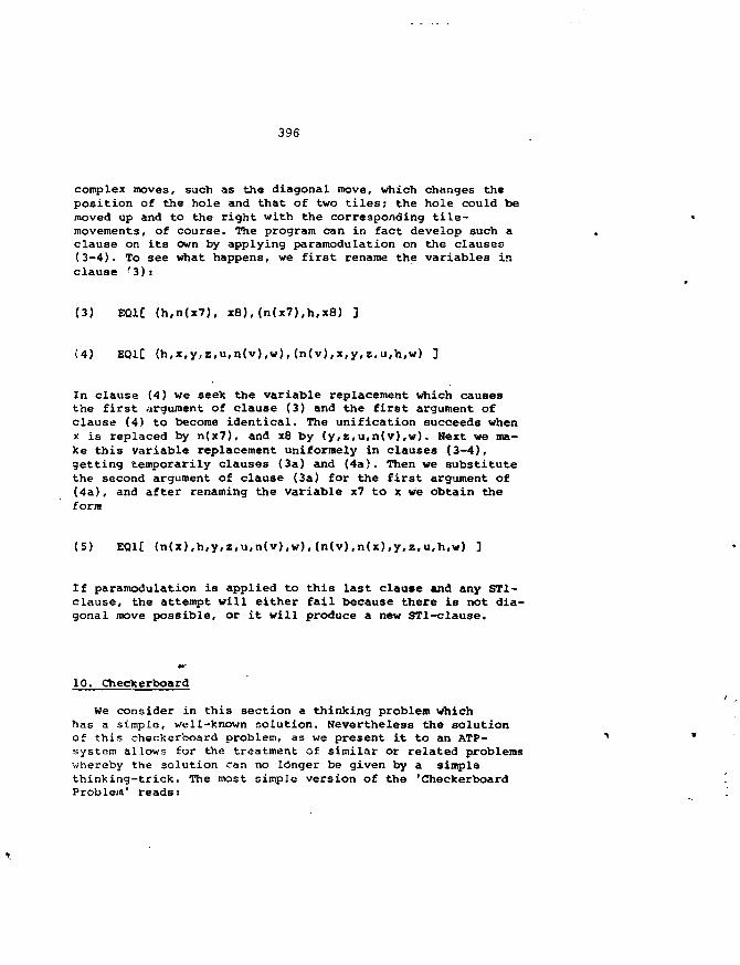
396
complex moves, such as the diagonal move, which changes theposition of the hole and that of two tiles; the hole could bemoved up and to the right with the corresponding tile-movements, of course. The program can in fact develop such aclause on its own by applying paramodulation on the clauses(3-4). To see what happens, we first rename the variables ir.clause '3):
(3) EQ1C (h,n(x7), x8),(n(x7),h,x8) ]
(4) EQlC (h,x.y,s,u,n(v),w),(n(v),x,y,z,u,h,w)
In clause (4) we seek the variable replacement which causesthe first argument of clause (3) and the first argument ofclause (4) to become identical. The unification succeeds whenx is replaced by n(x7), and x8 by (y,z,u,n(v),w). Next we ma-ke this variable replacement uniformely in clauses (3-4),getting temporarily clauses (3a) and (4a). Then we substitutethe second argument of clause (3a) for the first argument of(4a), and after renaming the variable x7 to x we obtain theform
(5) EQ1[ (n(x),h,y,z,u,n(v),w),(n(v),n(x),y,z,u,h,w) ]
If paramodulation is applied to this last clause and any ST1-clause, the attempt will either fail because there is not dia-gonal move possible, or it will produce a new STl-clause.
10. Checkerboard
We consider in this section a thinking problem whichhas a simple, well-known solution. Nevertheless the solutionof this checkerboard problem, as we present it to an ATP-system allows for the treatment of similar or related problemswhereby the solution can no longer be given by a simplethinking-trick. The most simple version of the 'CheckerboardProblem' reads:
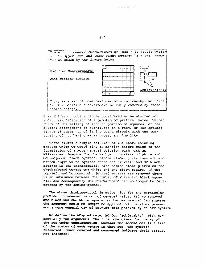
i ""r.ere _r :. squarec. checker&oar; of: 8xe = 64 fields where-!i o-. its. .;poer ieft and lower right, squares have been remo-1 v.-j as shown by the figure below:
i Modified Checkerboard:
witn missing squares
-
[ i
1
1!i i i
| There is a set of domino-stones of size: cne-by-two units.lj Can the modified checkerboard be fully covered by these !i aomino-stones? j
This thinking problem can be considered as an abstractionand/or siraplif icatior. of a problem of praticai value. We canthink of the selling of land in portion of squares, or theoptimal arrangement of furnitures in a room, or the optimallayout of pipes, or of laying out a circuit with the con-straint of not having wires cross, and the like.
There exists a simple solution of the above thinkingproblex which we would like to mention before going to theformulation of a more general solution path with anATP-system. Imagine the checkerboard consists of white andnon-adjacent black squares. Before removing the top-left andbottom-right white squares there are 32 white and 32 blacksquares on the checkerboard. Each domino-stone placed on thecheckerboard covers one white and one black square. If thetop-left and bottom-right (white) squares are removed thereis an imbalance between the number of white and black squa-res, and consequently the checkerboard can no longer be fullycovered by the domino-stones.
The above thinking-trick is quite nice for the particularproblem: it however is not of general value. Had we removedone black and one white square, or had we removed ten squaresthe argument could no longer be applied. We therefore presentnow a more general way of solving this problem by an ATP-system.
We define the AC-predicate, AC for "achievable", with es-sentially two arguments. The first one gives the number ofthe row under consideration, whereas the second one is a listof the status of each square in that row: the symbolsr»removed, n«not_covered and ccovered indicate their status.For instance:

396
AC[ row(l), sq(r,n,n,n,n,n,c,c) ]
represents the state of the checkerboard where row 1 has itsfirst square removed, and the last two squares are covered bya domino-stone. Note that the functions: row( ) and sq( ) we-re introduced for convenience. For clearness of presentationwe drop the first one, but keep in mind that the first AC ar-gument gives the row-number.
Notice that the particular arrangement of the domino-stones does not matter; they thus can be placed horizontallyand vertically. If we now were to consider all possible se-quences of plays, the program would be forced to examine morethan six trillion sequences. By choosing an order in which toplay the domino-stones, and also by ignoring dublicate pathsto the same particular covering, fewer than 500 partial cove-rings result. In order to illustrate our notion of 'dublicatepaths' we show in Fig. 10.1 two possible ways of coveringrows 1 arid 2 (with other coverings being possible) which areconsidered as equivalent. The important points for the twoland all other) different ways of placing the domino-stonesare, that square 1 in row 1 has not been touched (because itwas removed) and that square 1 of row 2 still needs to becovered.
In the placing of the domino-stones, we will have theATP-program observe a few simplifying rules:
1; The program shall start placing domino-stones at the topof the checkerboard with row 1 where the left-most squarehas been removed.
2; A row will not be left until all of its available squareshave been covered.
3) All horizontal plays that the program wishes to make mustprecede any vertical play.
4) When a vertical play is made, all the remaining squares(in a row) are also covered, and this simultaneously, byvertical plays.
As a result, this latter rule 4) allows domino-scones to beplaced vertically, and consequently to cover squares in thenext row. It, however, does not allow, for example, a domino-stone to be placed horizontally in a row unless all of theprevious rows had their available squares covered. The rule4) is obeyed by, for example, playing domino-stones horizo-ntally in a row as far as possible, and then playing verti-cally into the next row. The above set of rules leads, forany newly derived AC-clause, to implications.
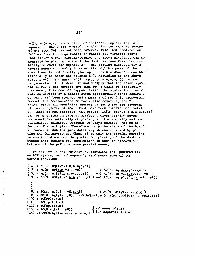
399
AC[2, sq(n,n,n,n,n,c,c,c)], ior instance, implies that allsquares of row 1 are covered. It also implies that no squareof the rows 3-8 has yet been covered. This last implicationfollows from the requirement of making ell vertical plays,that affect a row, simultaneously. The above AC-clause can beachieved by placing in row 1 the domino-stones first horizo-ntally to cover the squares 2-7, and placing subsequently adomino-stone vertically to cover the eighth square of therows 1 and 2, and finally placing in row 2 a domino-stone ho-rizontally to cover the squares 6-7. According to the aboverules l)-4) the clause: AC[2, sq(c,c,n,n,n,n,n,n)] can notbe generated. If it were, it would imply that the seven squa-res of row 1 are covered and that row 3 would be completelyuncovered. This can not happen: first, the square 1 of row 2must be covered by a domino-stone horizontally since square 1of row 1 had been removed and square 1 of row 3 is uncovered.Second, the domino-stone on row 2 also covers square 2.Third, since all remaining squares of row 2 are not covered,uJ1 seven squares of row 1 must have been covered horizontal-ij, which is not possible. The clause: AC[2, sq{n,c,c,c,c,c,c,c)]car. be generated in several different ways: playing seven•iuraino-stones vertically or placing six horizontally and onevertically. Whichever sequence of plays occured, has no ef-fect on the next play. Therefore, only the state of the boardis recorded, not the particular way it was achieved by pla-cing the domino-stones. Thus, since only the partial coveringis considered and not the particular placing of the domino-stones that achieve it, subsumption is used to discard allbut one of the paths to each partial cover.
We are now in the position to formulate the program foran ATP-systeir,, and subsequently we discuss some of itsparticularities:
( 1) : AC[1, sq(r,n,n,n,n,n,n,n) ]( 2) : AC[x, sq(.n,nJy3...y8)] —> AC[x, sq(.e.c,y3. .. v8)3( 3) : AC[x, sq(yl,£tii,y4. ..y8)] —> AC[x, sq(yl..c,cf.y4. ..y8)3( 4) : AC[x, sq(yl,y2,.n,n..y5...y8)] --> AC[x, sq(yl,y2,.c. c.,y5. . ,y8)]
— > AC[x, eq(yl. . .y6,.c.c.)3— > AC[x+l,sq(cpl(yl).cpl(y2),...cpl(y8))]
subsuner Clause(in separate liste)
( 8)( 9)(10)(11)(12)(13)(14)
: AC[x, sq(yl. . ,y6..n,n: AC[x, »q(y l . . .y8) ]: EQCcpl(c),n]: EQ[cpl(n),e3: EQ[epl(r),nJ: AC[9,sq(yl...y8)3:MAC[8,sq(c,c,c,c,c,c
~ > AC
. c .n ) ]
400
The clause (1' gives the initial condition of row 1 beforeany domino-stones have been placed. The clauses (2-8) permitan ATP-prograrc to place domino-stones horizontally whereby thestatus of two adjacent squares is changed from n to c. Notethat there is a variable in the first argument of the AC-predicate meaning that these clauses can, in principle, beapplied to any row. The clause (9) serves to place domino-stones vertically. A domino-stone placed vertically coversone square in each of the two adjacent rows, and the squareshave the same number between 1 and 8. If, in a row under con-sideration, the status of a square is c or r, then a domino-stone can not be placed vertically starting with that square.These properties suggest that an AC-clause is defined to ad-vance the row number and to give the status of each square inthe r.ew row, based on the status of the squares on the prece-ding row. The employed mechanism is 'complementation*. Acomplement-function: cpl( ) is defined which switches thestatus of a square: c <—> n and r -> n. The idea is that if asquare is c(overed) or r(emoved), then the one below it cannot be c(overed) by placing a domino-stone vertically. Thisprocedure thus implies that the placing of several verticaldomino-stones proceeds simultaneously. The clauses (10-12)serve as demodulators to define or rewrite the AC-clauses co-ntaining a cpl-function to new ones with the constants r,nand c only.
There is one problem left. Without any additional clausesthere is the possibility that some domino-stones could beplaced vertically into the non-existing row 9. To preventsuch an occurence, one relies on subsumption such that it im-mediately removes any new AC-clause which plays into row 9,meaning that it classifies that newly generated clause asless general than itself. To block clause (13) from partici-pation it is placed on a special list that is kept separatefrom those clauses that are consulted by the inference rules.Clause (14) denies that the checkerboard can b« fully coveredby domino-stones placed horizontally and vertically, and ittherefore serves as the'termination condition. Note, that thestatus of its last square is n. This results from the form ofthe clauses that enable* the program to make vertical and ho-rizontal plays, and hence from the form of the clauses gene-rated by a reasoning program.
As for choosing the appropriate inference rule, note thatthe object is to find AC-states which are represented by po-sitive unit clauses. Thus, two inference mechanisms come tomind:UR-resolution yields a unit clause from a set of unit clausesplus one non-unit clause (these may be positive or negative),whereas Hyperresolution yields a positive clause (with one or
more literals) from a set of positive clauses plus one non-positive clause. Employment of the set-of-support strategywith clause (1) or the clauses (1) and (14) in the set-o£-support will further strengthen the search process.
The submission of the above program to an ATP-systero didnot lead to a contradiction proof, but instead the programexhausted all. of the sequences of plays restricted by the or-dering rules l)-4) ijiven earlier, and it therefore generatedall of the possible AC-states. Since the ordering ru3.es donot rule out any covering, the conclusion, that no coveringexists, is correct. The subsumption-trick td recognize that aparial covering has been obtained by one sequence of playing,a'id that any other sequence of producing the same partial co-vering is unneeded, proved to be of valuable help to reducedrastically the combinatorics of the problem.
The above program has also be tested on a modified chec-kerboard which in fact can be covered by domino-stones, wr.e-reby the placing of the domino-stones can be reconsTructedfrom the actual computer-run by following the generatedAC-clause.
To this point we have considered checkerboards that are on-ly slightly modified. We now would like to show how morecomplicated and perhaps more realistic cases can also be dealtwith by an ATP-system. Suppose for example we wish to considercovering a checkerboard with one-by-two domino-stones, thatmay have a number of its squares missing. Subsequently, wealso will treat the same problem where however the doraino-stones are of size: on-by-three. And finally we wil considerthe problem of covering a modified checkerboard consisting ofexactly 26 squares, with a possible choice of the checkerboardas shown in Fig. 10.2(a). Suppose, seven one-by-two and four one-by-three domino-stones are given. Can the above defined chec-kerboard be covered? -In Fig. 10.2{b) we have given a particularsolution. The first of the above-mentioned extensions is sol-ved by using the {\ -function (defined by curly-brackets)which has two Argument*. In the first argument is the firstitem of the list or is the 'end'-iten which, for ease of no-tation, is again abbreviated by the asterixi '*'. The list-function: li(..) then consists of a chosen nuaber of {..}-function*, each one being positioned in the second argumentof the preceding {..} -function such that Cor instance
liU .*) *{*.*} (••end)IK*. B.*> -l«. U ,*J),f *.*) -[*.{f .... {£.*}! ..•>
402
Gy using this list-function we represent the status of thecheckerboard as
li(n,n, ...,c* (row 1)n,r,...,n,* (row 2)
n,n,...,n,*) (row 8)
In this exanplo, th« first row of the checkerboard Is comple-tely uncovered except for the last square, and the secondsciv.r-.ro in row 2 has been r(emoved); all other squares are n(ot-coverd). The end of each row is narked by the constant) *end. Thus, an arbitrarily modified board can easily be repre-sented by one of the huge lists. We now enploy the conventionthat any leading arguments (in the list) that are 'c(overed)'or '*'-ed are removed from the list. This mean* that theinitial argument will always be an 'n' as long as at leastone uncovered square remains on the board. He shall rely onthe demodulators to remove undesirable leading arguments inthe deduced clauses and thus 'trim' the clauses by the app-ropriate EQ-claases. With the above introduced simplifiedlist-notation the ATP-program is rather short and simple:
(1) : AC[li(n,n,r,n,n,n,n,n,*,
n,n,n,n,n,n,n,n,*)]
(2) : AC[li(n,n,xrest)] —> ACCtrim(xrest)](3) : ACCli(n,y2...y9.n,xrest)] —> AC[trim(li(y2,...y9,c,xre*t))](4) : EQ[trim(li(c,x)),triiii(x)](5) : EQ[trim(li(*,x}).trim(x)](6) : EQ[tri»(li{n,x)),li(n.x)](7) : EQ[trim(*).* ](8) : NACt*]
The clause (IV gives the initial state of the checkerboard,and the clauses (2-3) place domino-stones horizontally andvertically. The clauses (4-7) serve as demodulators to 'trim*the list. The clause (8J denies that the checkerboard can becompletely covered with one-by-two domino-stones and it thusserves for a contradiction proof.
Suppose the domino-stones are now of sizet one-by-three.This can be easily accomodated in the preceding formulationby replacing the clauses (2-3) by tit* following expressions:
(2): ACDi(n,n,n,xrest)3 — > ACCtrlm(xrest)](3) i AC[li(n,.y2.. .y9.,n..yll. . .yl8,n.xrest)3
--> ACLtrim(li(jr2. . .y9,c.yll.. .yl8.c.xrest) ) J
403
The last extension of the checkerboard problem consists infinding the domino-stone coverage of a 26-square board where-by a limited number of one-by-two and one-by-three domino-stones is used. This problem is solved with the precedingtechnique. The AC-predicate is given two more arguments whichgive the number of the unplayed one-by-two and one-by-threedomino-stones. Thus the initial state clause is replaced by
(1) > AC[7/4; li(n,n....)3
whereby the first two arguments give the number of unplayedone-by-two and one-by-three domino-stones. The clauses forplaying horizontally and vertically are almost the saw*.
(2) : AC[u.v;li(n,n,xrest)3 A GT[u.o3 -> ACC(u-l), v;trijn(xrest)3(3) ; AC[u.v;li(n,.y2.. .y9,n,xrest)3 ACT[u,oJ
— > AC[(u-l).vrtrim(lUy2..-y9f.C*r«st))3(4) : AC[u.v;li(n,n,n,xrest)3A GT[v.o3 -> AC[u,{v-l);tri»<xrest)'(5) : AC[u.v;li(n.,v2...y9,n,yll. ...y!8..u,xrest)3 GT[v,o3
— > ACtu.(v-l);lifo2...y9.,c..yll...yia.,c,xrest)3
where (2-3, place one-by-two domino-stones and the clauses(4-5) place one-by-three domino-stones. All the other clausesand demodulators can be taken over from the earlier program inunchanged form.
There are many more of this kind of problems which we willleave to the interested reader. He can think of covering thecheckerboard with "domino-stones" of different shape such asfor instance a right-angle, or of leaving certain areas comp-letely uncovered, and so on.
11. Missionaries and Cannibals
We consider in this section a scheduling problem which re-veals some of the characteristics one often meets, and weshow its description and elegant solution. The essence ofsuch problems is contained in the folowing "Missionaries andCannibals" problem:
There are three missionaries and thr« cannibals on thewest bank of a river. There is a boat on the west-bankthat can hold no more than two people. The missionarieswish to cross to the east-bank. But they have a problem:If on either bank the cannibals can ever outnumber themissionaries, the outnumbered missionaries will be eaten.Is there a way for the missionaries to get their wish -to get to east-bank without loosing anyone? ___
404
This proble.-, is somewhat similar to the scheduling difficult-ties one is faced if a number of meetings sust be held wheresome of the* must run in parallel. Suppose that various con-straints exist on scheduling all the meetings, whereby somemust proceed others while some sust not be held in parallel.Certain speakers have prior travel arrangements and must givevarious talks consistent with their prior plans. The questionisi with all of the constraints, does a schedule exist thatconforms to the requirements?
The solution of the above thinking problem proceeds inthree steps. We first must represent the starting situationat the beginning of the problem. Next, the clauses must befound which enable an ATP-system to move the missionaries,cannibals and the boat from one side of the river to theother and back, whereby the program must take the constraintsinto account that the missionaries always must outnumber thecannibals, and that the boat can not take more than twopersons. Finally, the ATP-system must be able to tell whenthe thinking problem has been solved, or determine, if possi-ble, that it can not be solved. If the problem is solvabel,then an arrangement is found in which the three missionariesare on the east-bank of the river. If it is not solvable,then every sequence of boat trips results at some point.inthe solution where the cannibals outnumber the missionaries.or it leads to a sequence of boat trips that simply result inrepeating a missionaries-cannibals assignment where, forexample, one cannibal goes forth and back on the river, for-ever.
The setup of an efficient ATP-program for this problem ma-kes use of the so-called "successor function" s(x) which hasas value: x incremented by one unit. Thus the successor of Ois 1, of 1 is 2, and of 2 is 3. Therefore ss(0) s(s(O)) actslike the number 2. We furthermore introduce the functions:west(x,y), east(x,y) which give the number of missionariescannibals in their first/second argument and this for thewest- and.the east-bank separately. As a last essential in-gredient we define the predicate AC[west(..),e/w, east(..)]which stands for "achievable". Its firs argument contains thefunction west(..) giving the number of persons (missionariesand cannibals) on the west-bank, and its third argument, withthe function east(..), gives the same information for theeast-bank. The letters e a d w in the second argument indica-te where the boat is on the west- or the east-bank.
We are now ready to fomulate the ATP-program and subse-quently discuss some of its particularities:
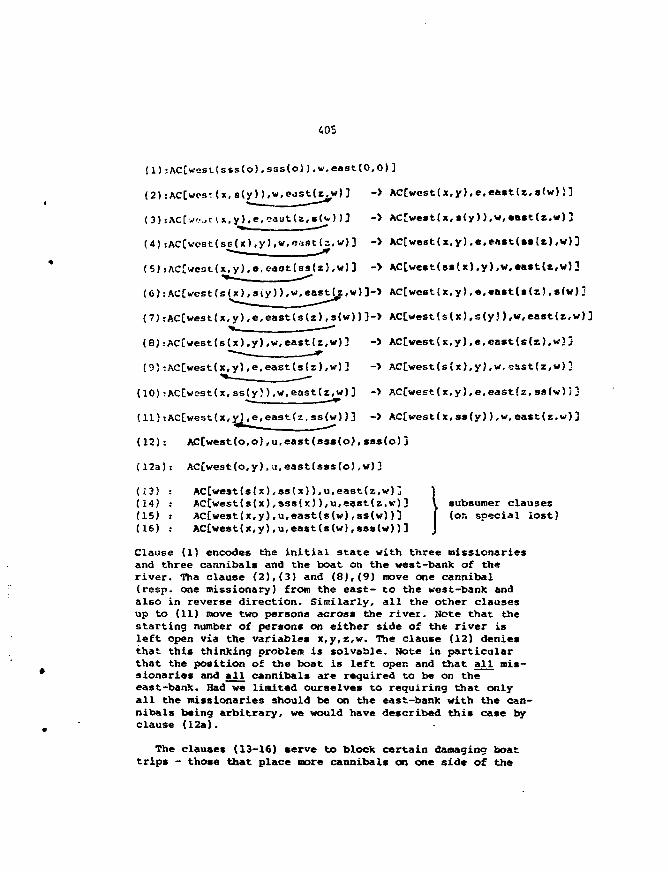
405
(1);AC[west(sss(o),sss(o)).w.east(0,0)3
(2):AC[wost ix.styM.v.eastU^w)] -> AC[west( x.y) ,e.east(z, s(w)) ]
(3):AC[v<:,Ux,y),e,<jastU,s(v))3 -> AC[west(x,s(y)),w,*ast(z,w)3
(4) :ACCwcst(so(x),y),w,cast( = .w)] -> AC[west( x.y) .e,east(ss(z) ,
(5):ACCwcst(x,y).e,east(ss(z),w)3 -> AC[west(ss(x),y),w,«ast(*,w)2
]-> AC[wcst(x,y),e,east(s(z),a(w)]
{?):AC[west(x,y),e,east(s(z),s(w))3-> AC[west(s(x),s(y)),w,east(z,v) ]* . —
(8):AC[west(s(x),y),w.east(z.w)3 -> AC[west(x,y),e,east(s(z),w)j
(9):AC[west(x,y),e,east(s(z),w)3 -> AC[west(s(x),y),w,eastfz.w}]
(10):AC[wost(x,ss(y)),w,east(z,w)3 -> AC[west(x,y),e.easttz,sslv)5]
(H):AC[westtx,y)/e,east(z,ss(w))] -> AC[west(x,sa(y)),v.east(z.w)]
(12): AC[west(o,o),u,east(as»(o),»3s(o)j
(12a): ACCwest{o,y),a. east(sssto),w)3
(13) : AC[west(s(x),ss(x)),u,eastU.w)] 1
(14) .- AC[west(s(x),sss!x)),u,east(z,w)3 V subsumer clauses(15) .- AC[west(x,y),u,east(s(w),ss(w))3 | (on special lost)(16) .- AC[west(x,y),u,east(s(w),sBs(w))3 J
Clause (1) encodes the initial state with three missionariesand three cannibals and the boat on the west-bank of theriver. Tha clause (2),(3) and (8),(9) move one cannibal(resp. one missionary) from the east- to the west-bank andalso in reverse direction. Similarly, all the other clausesup to (11) move two persons across the river. Note that thestarting number of persons on either side of the river isleft open via the variables x,y,z,w. The clause (12) deniesthat this thinking problem is solvable. Note in particularthat the position of the boat is left open and that all mis-sionaries and all cannibals are required to be on theeast-bank. Had we limited ourselves to requiring that onlyall the missionaries should be on the east-bank with the can-nibals being arbitrary, we would have described this case byclause (12a).
The clauses (13-16) serve to block certain damaging boattrips - those that place more cannibals on one side of the
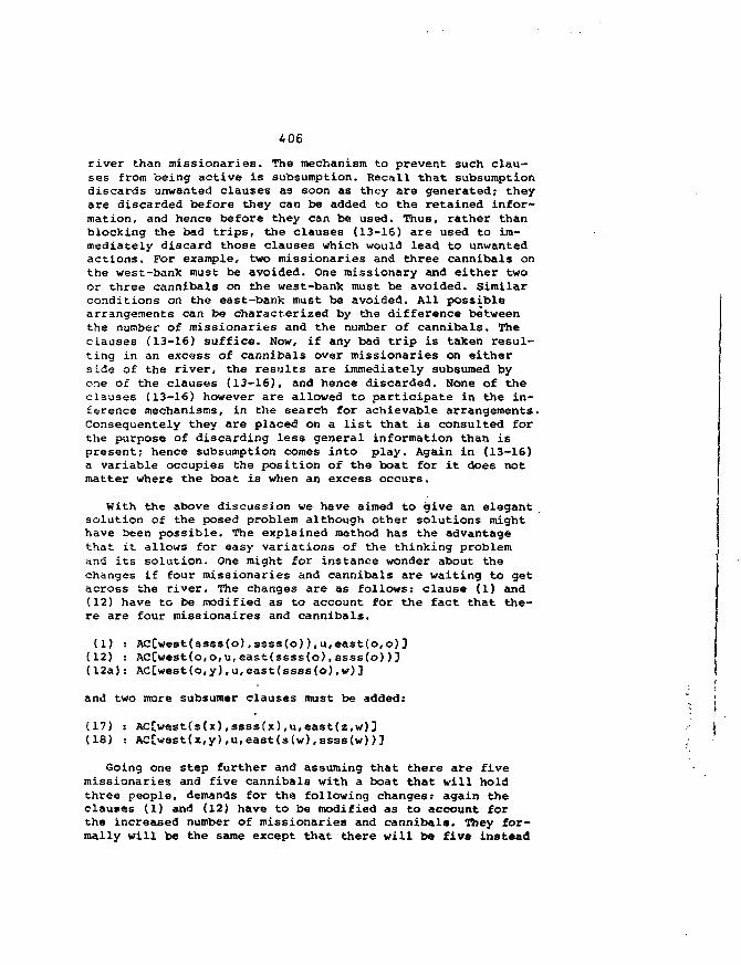
406
river than missionaries. The mechanism to prevent such clau-ses from being active is subsumption. Recall that subsumptiondiscards unwanted clauses as soon as they are generated; theyare discarded before they can be added to the retained infor-mation, and hence before they can be used. Thus, rather thanblocking the bad tripe, the clauses (13-16) are used to im-mediately discard those clauses which would lead to unwantedactions. For example, two missionaries and three cannibals onthe west-bank must be avoided. One missionary and either twoor three cannibals on the west-bank must be avoided. Similarconditions on the east-bank must be avoided. All possiblearrangements can be characterized by the difference betweenthe number of missionaries and the number of cannibals. Theclauses (13-16) suffice. Now, if any bad trip is taken resul-ting in an excess of cannibals over missionaries on eitherside of the river, the results are immediately subsumed byone of the clauses (13-16), and hence discarded. None of theclauses (13-16) however are allowed to participate in the in-ference mechanisms, in the search for achievable arrangements.Consequentely they are placed on a list that is consulted forthe purpose of discarding less general information than ispresent? hence subsumption comes into play. Again in (13-16)a variable occupies the position of the boat for it does notmatter where the boat is when an excess occurs.
With the above discussion we have aimed to give an elegantsolution of the posed problem although other solutions mighthave been possible. The explained method has the advantagethat it allows for easy variations of the thinking problemand its solution. One might for instance wonder about thechanges if four missionaries and cannibals are waiting to getacross the river. The changes are as follows: clause (1) and(12) have to be modified as to account for the fact that the-re are four missionaires and cannibals,
(1) : AC[west(ssss(o),ssss(o)),u,east(o,o)J(12) : AC[west(o,0,u,east(ssss(o),ssss(o))](12a): AC[west(o,y),u,east(ssss(o),w)]
: i
and two more subsumer clauses must be added: " j
(17) : AC[west(s(x),ssss(x),u,east(z,w)] - i(18) : AC[west(x,y),u,east(s(w),ssss(w))]
Going one step further and assuming that there are fivemissionaries and five cannibals with a boat that will holdthree people, demands for the following changes; again theclauses (1) and (12) have to be modified as to account forthe increased number of missionaries and cannibala. They for-mally will be the same except that there will be five instead
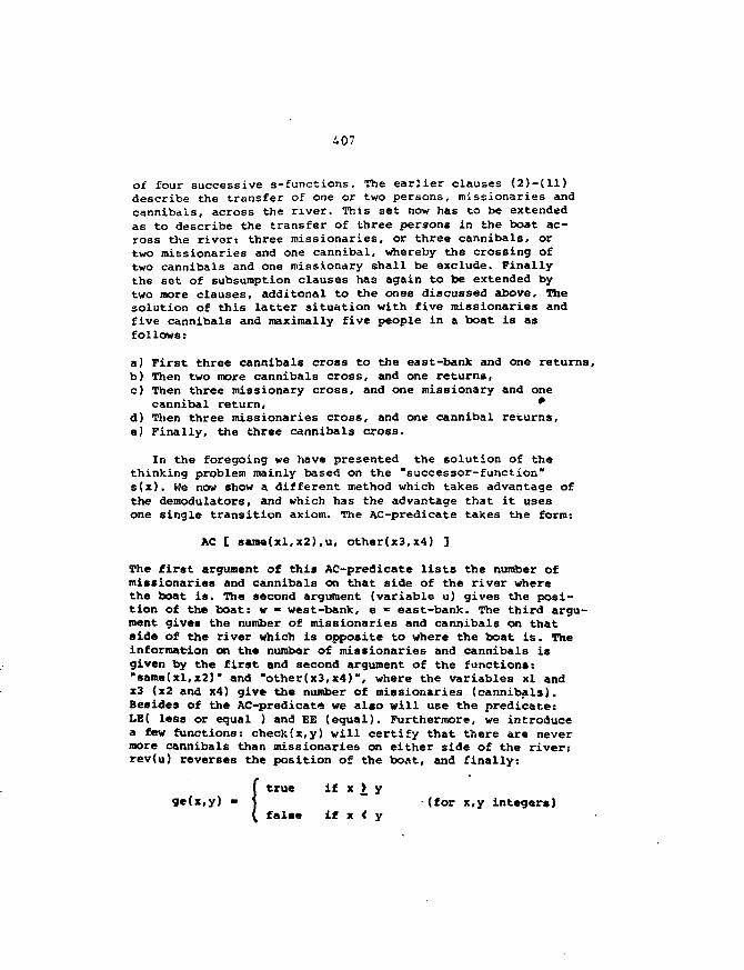
407
of four successive s-functions. The earlier clauses (2)-(ll)describe the transfer of one or two persons, missionaries andcannibals, across the river. This set now has to be extendedas to describe the transfer of three persons in the boat ac-ross the river: three missionaries, or three cannibals, ortwo missionaries and one cannibal, whereby the crossing oftwo cannibals and one missionary shall be exclude. Finallythe set of subsumption clauses has again to be extended bytwo more clauses, additonal to the ones discussed above. Thesolution of this latter situation with five missionaries andfive cannibals and maximally five people in a boat is asfollows:
a) First three cannibals cross to the east-bank and one returns,b) Then two more cannibals cross, and one returns,c) Then three missionary cross, and one missionary and one
cannibal return, *d) Then three missionaries cross, and one cannibal returns,e) Finally, the three cannibals cross.
In the foregoing we have presented the solution of thethinking problem mainly based on the "successor-function"s(x). We now show a different method which takes advantage ofthe demodulators, and which has the advantage that it usesone single transition axiom. The AC-predicate takes the form:
AC [ same(xl,x2),u, other(x3,x4) ]
The first argument of this AC-predicate lists the number ofmissionaries and cannibals on that side of the river wherethe boat is. The second argument (variable u) gives the posi-tion of the boat: w » west-bank, e •» east-bank. The third argu-ment gives the number of missionaries and cannibals on thatside of the river which is opposite to where the boat is. Theinformation on the number of missionaries and cannibals isgiven by the first and second argument of the functions:"same(xl,x2)" and "other(x3,x4)", where the variables xl andx3 (x2 and x4) give the number of missionaries (cannibals).Besides of the AC-predicate we also will use the predicate:LE( less or equal ) and EE (equal). Furthermore, we introducea few functions: check(x,y) will certify that there are nevermore cannibals than missionaries on either side of the river;rev(u) reverses the position of the boat, and finally:
( true if x > y(for x,y integer*)
false if x < y
408
We now are in the position to give the ATP-program, and wesubsequently will discuss some of its particularities:
(1) AC[same(3,3),u,other(o,o)]
(2) ACCsame(xl,x2),x,other(x3(x4)]A P[XBI]A PCXC]
LE[xm,xl] ALE[xc,x2] ALE[ (xm+xc), 2] AEE[check((xl-xm),x2-xc)),true]AEE[check((x3+xm),(x4+xc)),true]—> AC[same((x3+xra), (x4+xc) ),rev(u),other((xl-xm), (X2-JCC))]
(3) P[0](4) P[l]IS) PC2]
(6) EQ[check(o,x),true](7) EQ[check(x:.y),ge(x,y)](8) EQ[rev(w),e](9) EQ[rev(e),w]
(10) CJ ACCsame(3,3),e,other{o,o)3
The "pick"-predicates P[..3 give the acceptable numbers ofmissionaries and cannibals to be transferee! over to the otherside of the river. The E0[..] serve as demodulators for the"check" -and "rev(erse)"-functions. The clause (1) gives thestarting state and the clause (10) denies that the soughtstate can be reached. The clause (2) is the transition axiomwhich leads to new AC-states whereby the LE-predicates certi-fy that the number of persons in the boat is below 3, and theEE-predicatea certify that the number of cannibals is alwayssmaller than the number of missionaries on either aid* of theriver. Note that the number of missionaries (and alsocannibals) changes side from "same" to "other", as it shouldbe.
12. Billiard Ball Weighing
We are in this section concerned with a thinking problemof a more difficult nature than what we have considered so-far, because each move must add a maximum of possible new in-formation in order to arrive at a solution. It therefor* asksfor some kind of optimisation of information. The formulationof the "Billiard Ball* problem is as follows:
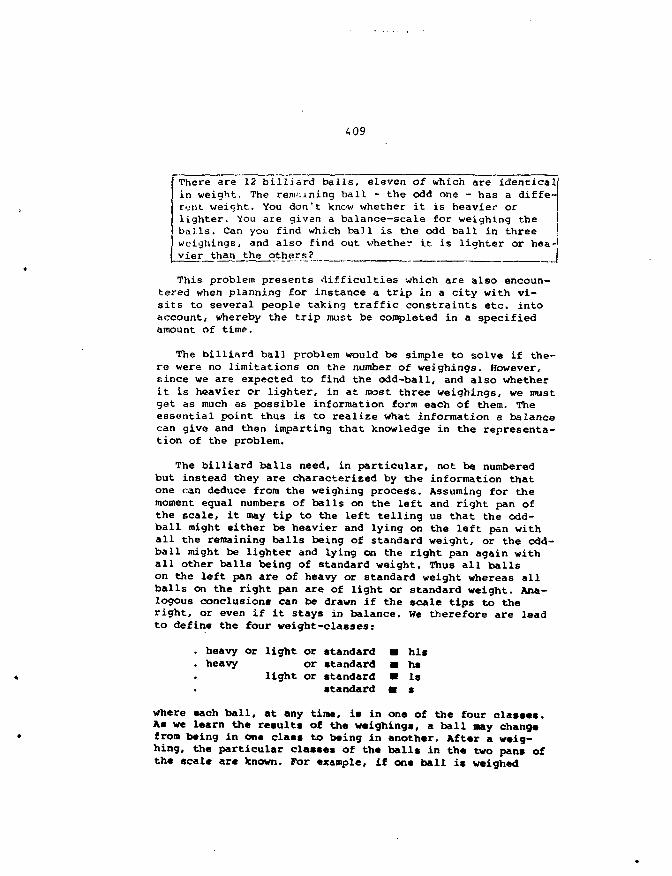
409
There are 12 billiard balls, eleven of which are identicalin weight. The remaining ball - the odd one - has a diffe-rent weight. You don't know whether it is heavier orlighter. You are given a balance-scale for weighing theballs. Can you find which ba31 is the odd ball in three ?weighings, and also find out whether it is lighter or hea-'vier than the others? j
This problem presents difficulties which are also encoun-tered when planning for instance a trip in a city with vi-sits to several people taking traffic constraints etc. intoaccount, whereby the trip must be completed in a specifiedamount of time.
The billiard bal) problem would be simple to solve if the-re were no limitations on the number of weighings. However,since we are expected to find the odd-ball, and also whetherit is heavier or lighter, in at most three weighings, we mustget as much as possible information form each of them. Theessential point thus is to realize what information a balancecan give and then imparting that knowledge in the representa-tion of the problem.
The billiard balls need, in particular, not be numberedbut instead they are characterised by the information thatone can deduce from the weighing process. Assuming for themoment equal numbers of balls on the left and right pan ofthe scale, it may tip to the left telling us that the odd-ball might either be heavier and lying on the left pan withall the remaining balls being of standard weight, or the odd-ball might be lighter and lying on the right pan again withall other balls being of standard weight. Thus all ballson the left pan are of heavy or standard weight whereas allballs on the right pan are of light or standard weight. Ana-logous conclusions can be drawn if the scale tips to theright, or even if it stays in balance. We therefore are leadto define the four weight-classes:
. heavy or light or standard • his
. heavy or standard • h«light or standard • Is
standard m s
where aach ball, at any time, is in one of the four classes.As we learn the results of the weighings, a ball nay changefrom being in one class to being in another. After a weig-hing, the particular classes of the balls in the two pans ofthe scale are known. For example, if one ball is weighed
410
against another and the scale tips to the left - the left ai-de goes down and the right side goes up - then the ball onthe left is in the hs-class and the one on the right is inthe ls-class. Note however that the weighing of one ballagainst another does, in general, not provide sufficient in-formation to arrive at a determination of the odd-ball in th-ree weighings. Obviously, each weighing may change the clas-sification of the balls that are being weighed. In the ini-tial state, all balls are in the hls-class since nothing isknown about them.
As a result of the above insight, we define a state-predicate which gives the number of balls in the above defi-ned classes and also lists the number of remaining weighings.The initial state for instance is described by
ACC state f his(12), hs(0), ls(O), s(0), re(3) } ] ••AC1[12, 0, 0, 0; 3]
AC stand for "achievable". For ease of notation we drop the"state"-functions and simply list the number of balls in thefour classes plus the remaining number of weighings: (his, ha.Is, s; re), and we indicate this simplified notation with a '1'at the end of the predicate name.
In order to present the basic idea of solving the problemunder investigation, we first discuss the transition axiom.Starting from an AC-state with the ball-setting:(xhls,xhs,xls,xs), it picks the setting: (yhls,yhs,yla,ys), forthe right pan and the setting:(zhla,zhs,zla), for the leftpan out of the starting ball-sets. Three different situationscan now occur: the scale may stay in balance, it nay tip tothe left or it may tip to the right. For these three situa-tions we can determine the number of balls in the four clas-ses as shown in Table 12.1.
If the scale stays in balance, we know that all the ballswe have just weighed are in the s-class. Consequently, those 'selected 'from amoung the starting hls-class and put in the •'{two pans are now Jcnowns- to be in the s-class. The remaining :number of balls in the hls-class thus is: xhls-(yhls+rhla). •Similar arguments apply for the remaining nuiaber of ball* inthe ha- and ls-classes. The total number of balls in thes-class is equal to the sum of the original set xs plus thosein the two pans (since the scale balances) which are not inthe s-class.
If the scale tips left, no balls will remain in the hls-class since all balls taking part in the weighing processmust be either in the hs- or ls-class, and all those not ta-king part in the weighing process must be in the s-class.Those in the left pan are obviously in the hs-class, and tho-se in the ight pan must be in the ls-class. As a result, ncball is leit in the hls-class whereas the hs-classcontains:(zhls+zls) balls (from the left pan) and thereare:(yhls+yls) balls in the ls-class (from the right pan).The s-class is composed of the original set xs plus the zlsballs in the left pan (which tipped) and the yhs balls in theright pan (which moved up) plus all those balls in the his-,hs- and ls-classes which did not take part in the we ghingprocess.
If the scale tips right/ the above arguments apply in ananalogous way. No balls remain in the hls-class since allballs taking part in the weighing process must be either inthe hs- or ls-class, and all those not taking part in theweighing process are in the s-class. The number of balls inhs-class is:(yhls+yhs) (from the right pan), and the ls-classhas: (zhls + zls) balls (from the left pan). The s-class iscomposed of the original set xs plus the yls in the right pan(which tipped) and the zhs balls in the left pan (which wentup) plus all those balls in the his-, hs- and ls-class whichdid not take part in the weighing process.
The actual formulation of the transition axiom takes intoaccount several points Which we now discuss:- By convention no standard balls are ever placed in the leftpan. There is not point in putting standard balls in boththe left and the right pan of the balance scale, since thissimply would doublicate a weighing in which the smallernumber of standard balls in the two pans is removed fromboth.
- Assuming that the odd-ball is only slightly different inweight from the standard balls, it only makes sense toweight the same number of balls in each pan of the scale.Thus the number of points in the two pans are the same,between 0 and 6s
0 ± (yhla+yh«+yls+y«) - (shls+zhs+zls) < 6
- Since we are interested only i-n states which eventuallylead to the identification of the odd-ball, some of the AC-states must be discarded, if it can be shown that they de-finitely will not lead to an identification of theodd-ball. There is no point in pursueing the consequencesof such non-solvable states. The transition axiom therefore
contains a numerical test which allows for the detection ofa great many (but not all I) of such states. The test con-sists of comparing the number of possible solutions, mea-ning the number of possibilities for the odd-ball, with thenumber of possible outcomes that can occur for the remai-ning weighings. The first number is given by twice the num-ber of balls in the hls-class plus the number of balls inthe hs-and ls-classes. Since each weighing can produce th-ree outcomes, the second number is equal to 3 n where n isthe number of remaining weighings. Thus, if for a state: (2hls+ hs+ls) > 3n, then that state is definitely non-solvable, meaning that the odd-ball can not be determinedwithin the remaining number of weighings, and it conse-quently is prevented by this test, from being generated viathe transition axiom.
In summary, new AC-states can be generated by applying atransition axiom to the initial state. Since a transitionaxiom corresponds to a weighing, and since a weighing canproduce three possible outcomes - the scale may tip to theleft, tip to the right, or it may stay in balance - three newAC-states are obtained from the original one. In actualfact, the transition axiom first generates a record-predicate (RD) which collects together all the.possible out-comes of the weighing process and which allows for the subse-quent deduction of the resulting AC-states. These latter AC-states give rise to new RD-predicates which again allow forthe derivation of new AC-states and so on.
Having understood the AC-state and its transition axiom.we now also need the SO- (or SOI-} predicate to characterizeand find the "solvable" states which definitely will allowfor the determination of the odd-ball. The generation of newAC-states is not sufficient to assure the determination ofthe odd-ball. Instead, the problem requires that a sequenceof weighings, regardless of which of the three outcomes mayoccur at each weighing, finally leads to the determination ofwhich is the odd-ball. We emphasize that it is not enoughthat only one or two of the three possible outcomes eventual-ly will lead to the odd-ball. The idea is that of choosing aweighing so well that each of the three outcomes leads to thenext weighing, where the next weighing is based on which ofthe three outcomes actually has occured. The next weighingnust.also have this same property of leading to goodweighings. Finally, the last weighing must be such that theodd-ball can be identified. A state is called "solvable" ifit is one of the type just described. Three states can be im-mediately classed as solvable:
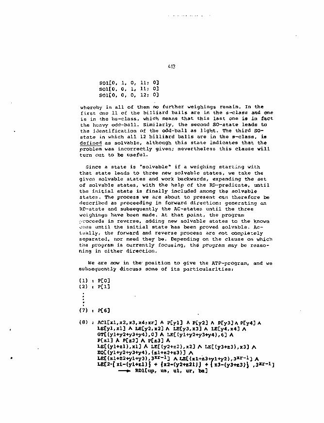
'.13
S01[0, 1, O, 11; 0]SOlCO, 0, 1, 11; 0]S01[0, 0, 0, 12; 0]
whereby in all of them no further weighings remain. In thefirst one 11 of the billiard balls are in the s-class and oneis in the hs-class, which means that this last one is in factthe heavy odd-ball. Similarly, the second SO-state leads tothe identification of the odd-ball as light. The third SO-state in which all 12 billiard balls are in the s-class, isdefined as solvable, although this state indicates that theproblem was incorrectly given; nevertheless this clause willturn out to be useful.
Since a state is "solvable" if a weighing starting withthat state leads to three new solvable states, we take thegiven solvable states and work backwards, expanding the setof solvable states, with the help of the RD-predicate, untilthe initial state is finally included among the solvablestates. The process we are about to present can therefore bedescribed as proceeding in forward direction: generating anRD-state and subsequently the AC-states until the threeweighings have been made. At that point, the programproceeds in reverse, adding new solvable states to the knownones until the initial state has been proved solvable. Ac-tually, the forward and reverse process are not completelyseparated, nor need they be. Depending on the clause on whichthe program is currently focusing, the program may be reaso-ning in either direction.
We are now in the position to give the ATP-program, and wesubsequently discuss some of its particularities:
(1) : P[0](2)
(7) : P[6]
(8) : ACl[xlfx2,x3,x4;xr] A P[yl3 A P[y23 A P[y3]A Pty4]ALE[yl,xl] A LECy2,x2] A LECy3,x3] A LE[y4,x4] AGT[(yl+y2+y3+y4),0] A LE[(yl+y2+y3+y4),63 APCzl] A PU2] A P[z3] ALE[(yl+zl),xl3 A LE[(y2+z2),x2] A LE[(y3+z3),x3] AEQC(yl+y2+y3+y4).(zl+z2+z3)3 ALEt(sl+Z2+yl+y3),3Jtr-1] A LEC(zl+z3-lyl+y2), 3 « - l ] ALEC2-fxl-(yl+sl)J + {x2-(y2+z2l)J + fx3-(y3+*3)J
»• RDlCup, ua, ul, ur,- ba]
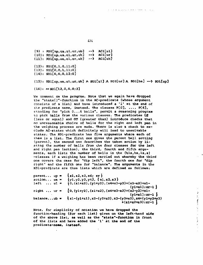
AH
(9) J RDlCup.ua,ul.ur.ub] —> AClCul](10): RDlCup.ua,ul.ur.ub] —> AClCur](11): RDlCup.ua,ul.ur.ub] —> AClCub]
(12): S01[0 , l , 0 , l l ;0 ](13): SOlC0,0,l , l l;0](14): S01CO,0,0,12;0]
(15): RDlCup.ua,ul.ur.ub] A SOlCul] A SOlCur] A. SOlCba] — > SOlCup]
(16): *»S01[12,0,0,0;3]
We comment on the program. Note that we again have droppedthe "state()"-function in the AC-predlcate (whose argumentconsists of a list) and have introduced a '1' at the end ofthe predicate name, instead. The clauses P[0], .... PC6],standing for "pick 0...6 balls", permit a reasoning programto pick balls from the various classes. The predicates LB(less or equal) and GT (greater than) introduce checks thatno unreasonable choice of balls for the right and left pan inthe weighing process are made. There is also a check to ex-clude AC-states which definitely will lead to unsolvablestates. The RDl-predicate has five arguments where each ofthem is a list. The first one gives the parent ball setting(parent), the second ona describes the taken action by li-sting the number of balls from the four classes for the leftand right pan (action), the third, fourth and fifth argu-ments, each lists the number of balls in the (hls,h3,Is,s)-classes if a weighing has been carried out whereby the thirdone covers the case for "dip left", the fourth one for "dipright" and the fifth one for "balance". The arguments in theRDl-predicate are thus lists which are defined as follows:
{xl,x2,x3,x4; xr}Iyl,y2,y3,y4), {8l.z2.i3)10,(zl+z2),(yl+y2),(x4+x3-y3)+(x2-*2)+xl-
(yl+sl)fxr-l }{o,(yl+y2),{rl+z2),(x4+x3-*3)+(x2-y2)+xl-
}
parent..action..left ..
right ..
balance.
. up
. ua
. ul
. ur
..ub( y ) }
Ixl-(yl+zl)(x2-(y2+z2),x3-(y3+s3).x4+(yl+y24y3)+{zl+«2+z3);xr-l }
Note, for simplicity of notation we have dropped thefunction-heading (for each list) given on the left-hand 3ideof the above list, as well as the "state"-function in frontof the lists and have added the '1' at the end of thepredicate-name, instead.
415
The clauses following the transition axiom, derive thethree ACl-states corresponding to the three possible outcomesof a weighing. The subsequent clauses define the three initial"solvable"-states whereas the next clause allows for the de-rivation of new solvable states which are defined in closeanalogy to the AC- (reap. AC1-) states. The last clause deniesthat the initial state is solvable. It enables a reasoningprogram to know that the puzzle has been solved, since it al-lows for a proof by contradiction.
The best approach to solve this problem with an ATP-sy«temis to use "Hyperresolution" combined with the SS-strategy,whereby the initial state and the one that denies that theinitial state is solvable are placed in the set-of-support.
Attempts to solve the above problem with an ATP-system havelead to its solution, and, in fact, have revealed more than40 non-trivially distinct solutions within less than 22 se-conds on an IBM 3033 computer.
13. Some Insights
The above examples give several insights which we wouldlike to summarize:
1) Replacing in an ATP-systero the specific with the general,is preferable. If the constants in a clause can be repla-ced by variables one may expect a gain in efficiency. Fur-thermore, a ATP-system discards all instances of existingor new information, retaining the more general fact only.This process is called subsumption, and it preserves inmost (but not all) resolution refinements the completenessproperty.
2) If several copies of the same literal (with identical ar-guments) occur in a clause, the extra copies are deletedfrom the clause by a process called "collapsing duplicateliterals".
3) The process of finding a solution might seem to an unexpe-rienced person surprisingly long for such a trivialproblem. This comes simply from the fact that an ATP-system can not leave out all the (many) intermediate stepswhich a human being undergoes in his thinking process, butusually is not aware of.
416
4) A mechanism exists, called weighting, which allows an ATP-system to consider certain facts more important thanothers. The program thus can be told to key on this fact,at least at the start.
5) Adding a denial clause (which was left aside in the aboveexample) has the advantage that the ATP-system seeks acontradition which then acts as a convenient terminationcondition.
6) It is important to realize that a problem must be comple-tely characterized by the set of initial clauses in orderto avoid logically wrong conclusions. Furthermore a viablepath to a solution can easily be overlooked.
7) it can well arise that there is redundant information amongthe clauses defining the problem, which means that some ofthe original clauses can, in fact, be derived from theother clauses. Redundancy and dependence are present in anATP-system and they often contribute to a much more effi-cient reasoning of a program as compared to the case wherethe initial clause set is completely independent.
8) The fact that there is missing information in the descrip-tion of a problem can in most cases be deduced from thefact that obvious facts are missing from the program's wayof reasoning.
9) Finding extra information whilst solving a prob. em is quit*common in an ATP-system's attempt. However if too much ex-tra information is found, the problem never gets solved.Thus one important item one needs to pay attention whilstusing an ATP-system is how to curtail the finding of extrainformation.
14. Conclusions • I
This paper is the third part of an introductory tutorial jon "Theorem Proving/Automated Reasoning". It focuses on the » ;use of Automated Theorem Proving (ATP)-systems by showing howthinking problems of various degrees of complexity aresolved. Our presentation has several aims: to demonstrate howa problem is cast into the language of first-order predicatelogic, how it then is submitted to an ATP-system, and finally *
417
how the deduction process proceeds. From the wide field ofpossible applications including mathematics (group-, set-,number-,., theory), real-time systems control, robotics, au-lom.it. ic programming, logic circuit design/validation, programiJ-.'L'jgying/verification, expert systems, communication proto-col, hardware verification, ant' so on, we h.;ve limited our-selves to a set of thinV.ing problems or puzzles which do notrequire any specialized knowledge. A presentation of more"practical" problems and their solution will be given in aforthcoming article.
What have we learnt? The solution of a problem with an ATP-system is not straightforward! The first difficulties beginif a formulation in first-order predicate logic is sought.Thp problem at hand however could well be of higher-order lo-gic, or it might ask for suggestions not only a proof. Once aproblem is in the appropriate first-order form, a second dif-ficulty arises as to the most appropriate resolution method,the right emphasis on particular clauses, the choice of thebest search-strategy, and so on. If a proof is found, we havesolved the problem we have submitted to the ATP-system. Howe-ver we might not yet have the answer to our overall problembecause the chosen axiom-system does not fully represent theactual problem situation.If no proof is found, the thirddifficulty becomes transparent: one doesn't know whether onesconjecture is incorrect, or whether the system simplycouldn't find the right deduction-chain.
With these critical remarks we didn't intend to cause dis-couragment or disappointment but rather aimed to caution theinterested reader that ATP is a field of high interest andpotential which however has not yet reached the point of itsultimate perfection. And still, there are exciting new deve-lopments ahead... [12].
Acknowledgement*:
The author thanks Profs. C. Joseph, C.P. Ens and «. Jacob fortheir kind interest and encouragements.The author also thanks the CERN Theoretical Physics Division,where part of this work was done, for its kind hospitality.
References
1) B. Humpert"Theorem Proving with First-Order Predicate Logic: I."Proc. of the Sth Warsaw Symposium on Elementary ParticlePhysics (1185), Warsaw University Press, (Ed. Z.Ajduk)
2) B. Humpert"Theorem Proving with First-Order Predicate Logic: II."Proc. of the 9th Warsaw Symposium on Elementary ParticlePhysics (1986), Warsaw University Press, (Ed. Z.Ajduk)
3) L. Wos, R. Overbeek, E. Lusk and J. Boyle"Automated Reasoning; Introduction and Application"Prentice Hall (1984)
4) R.S. Boyer and J.S. Moore -"A Computational Logic"Academic Press, NY (1979)
5) H.J. Ohlbach and M. Schmidt-Schauss"The Lion and the Unicorn"Journ. Autom. Reasoning ± (1985) 327
6) H.J. Ohlbach"Predicate Logic Hacker Tricks"Journ. Autom. Reasoning _1 (198S) 435
7) E. Lusk and R. Overbeek"Non-Horn Problem"Journ. Autom. Reasoning X (1985) 103
8) M.E. Stickel"Schubert's Steamroller Problem: Formulations and Solutions"Journ. Autom. Reasoning £ (1986) 89
9) C. Walther"A Mechanical Solution of Schubert's Steamroller byMany-Sorted Resolution"Artificial Intelligence 26 (1985) 217
10) A.G. Cohn"On the solution of Schubert's Steamroller in many-sorted logic"Proc. 9th IJCAX, Los Angeles, CA (1985) 1169
11) C. Walther"Schubert"* Steamroller - A case Study in Many Sorted Resolution*Universiti't Karlsruhe {1984)
12) CADE-8 Conference, Oxford, 1986
13) L. Carroll"Symbolic Logic"Publ. Clarksen N. Potter, Inc. [Ed. W.W.Bartley IIIj
Table Captions
Table 3.1 : Person-to-job coordinations of the complex job-assignment problem.
Table 4.1 : Days of truth and non-truth of the lion andunicorn problem.
Table 10.1 : A particular placing of the domino-stone* inthe checkerboard problem.
Table 10.2 : The domino-stone covering of a modifiedcheckerboard consisting of 26 squares.
Table 12.1 : Number of billiard balls in the { hls,hs,Is,s}-classes after a weighing has taken place.
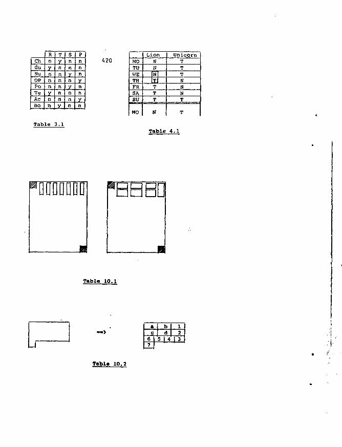
ChGuNuOPPoTeAcBo
Rnynnnynn
Table
TYnnnnnny
3.1
Snnynynnn
PnnnYnnYn
420 MOTUWETHFRSASU
MO
LionN»NTTTT
N
UnicornTTTNNNT
T
Table 4.1
Table 10.1
ae67
bd
12
5 |4 I 3
Table 10.2

balanc*
tips l«ft
tips right
hla - class
xhls-(yhls+zhls)
0
0
hs-class
xhs-(yhs+zhs)
zhls+ehs
yhls+yhB
Is - class
xls-(yls-t-zls)
yhls+yls
zhls+zls
s - class
xs+yhls+zhls+yhs+zhs+yls+zls
xs+zlB+yhs+(xhls-yhls-zhls)+(xhs-yhs-zhs)+(xls-yl3-zlB)
x8+zha+yl8+(xhls-yhl8-zhla)+(yhs-yhs-zhs)+(xls-yls-zls)
T a b l e 1 2 . 1
423
Precision Tests of the Electroweak Theory*
J. H. KUHN
Mzx-Plapck-lnstitut fur Pbysik uad Astrophysik
- Wenxer-Heisenberg-Insthat /ur Physik -
P.O-Box 40 12 12, Munich (Fed. Rep. Germany)
ABSTRACT
The present status and further perspectives for precision tests of the elcctroweak
theory are discussed with emphasis on future experiments at e + e~ colliders. Ambi-
guities in the theoretical predictions for the W mass and the left-right asymmetry
are scrutinized and the interplay between QED and QCD corrections is studied in
detail. It is shown that the theoretical predictions are well under control at the
precision level envisaged for future experiments. Various methods to determine the
weak couplings of heavy quarks are compared. Asymmetries on a toponium reso-
nance are free from hadronic uncertainties. They could be measured to an accuracy.
sensitive to electroweak radiative corrections.
'Lectures presented at the "X. Warsaw Symposium on Elementary Particle Phy-sics", Kazimierz, Poland, May 25-29, 1987, and at the "Workshop on TopicalProblems of Testing the Stanford Model in High Energy Reactions", Budapest,Hungary, June 15-19, 1987.
TABLE OF CONTENTS
1. Introduction 3
2. Windows to 'New Physics" 5
3. Uncertainties in the Theoretical Predictions 7
3.1. Weak Corrections 7
3.2. Af^-Determination and Initial State Radiation 8
3.3. Mw Determination 9
4. ALR From Hadronic Final States 10
4.1. The Experimental Setup 11
4.2. QCD Corrections to the Left-Right Asymmetry 13
4.3. QED Corrections 16
4.4. Bremsstrahlung and Helicity Nonconserving Beam Polarization! . . . . 27
5. Heavy Quark Couplings from e + e~ Annihilation Experiments 29
5.1. The Forward Backward Asymmetry 30
5.2. Asymmetries on Toponium 31
6. Summary 33
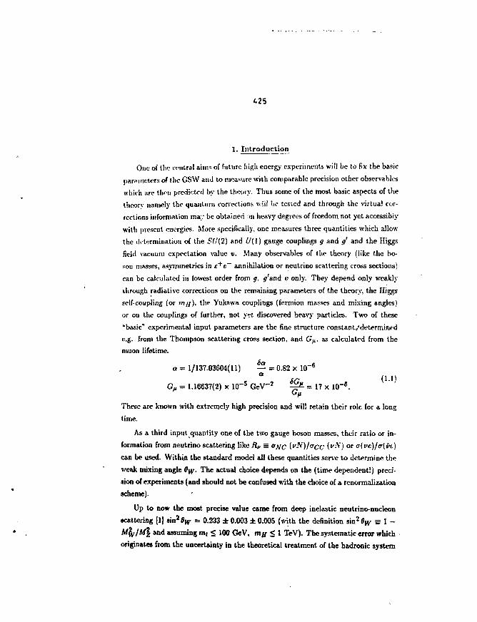
425
1. Introduction
One of the central aim* of future high energy experiments will be to fix the basic
parameters of the GSW and to measure with comparable precision othor observables
which arc then predicted by the theory. Thus some of the most basic aspects of the
theory namely the quantum correction? wiil be tested and through the virtual cor-
rections information may be obtained on heavy degrees of freedom not yet accessibly
with present energies. More specifically, one measures three quantities which allow
the ilrterniinatioii of the 577(2) and i/(l) gauge couplings g and g' and the Higgs
field vacuum expectation value v. Many observables of the theory (like the bo-
son masses, asymmetries in e+e~ annihilation or neutrino scattering cross sections)
can be calculated in lowest order from j , y'and v only. They depend only weakly
through radiative corrections on the remaining parameters of the theory, the Higgs
self-coupling (or >n//), the Yukawa couplings (fermion masses and mixing angles)
or on the couplings of further, not yet discovered heavy particles. Two of these
'•basic" experimental input parameters are the fine structure constant/determined
e.g. from the Thompson scattering cross section, and Gp, as calculated from the
muon lifetime.
o = 1/137.03604(11) — = 0.82 x 10"6
** onGa = 1.16637(2) x 10~5 GeV"2 ^ = 17 x lO"8.
GpThese are known with extremely high precision and will retain their role for a long
time.
As a third input quantity one of the two gauge boson masses, their ratio or in-
formation from neutrino scattering like Rv = a/ic {VN)I<JCC {"^) o r o{vt)l<r{,ve.)
can be used. Within the standard model all these quantities serve to determine the
weak mixing angle %•. The actual choice depends on the (time dependent!) preci-
sion of experiments (and should not be confused with the choice of a renormalization
scheme).
Up to now the most precise value came from deep inelastic neutrino-nuclcon
scattering [1] s in 2 % = 0.233 ± 0.003 ± 0.005 (with the definition sin2 0w = 1 -MwfMZ mA assuming mt < 100 GeV, mjf < 1 TeV). The systematic error which
originates from the uncertainty in the theoretical treatment of the hadronic system
426
limits any further improvement of this measurement. The determination of sin 0\y
from M\y (or Mz) "n conjunction with a and Gp starts to compete [2]
\ Mz = 91.0 ± 1.2 ± 1.7 /a.Cu
whereas the determination from the W-Z mass ratio suffers still from significant
statistical and systematical errors of about 0.025 and 0.01 respectively. In the near
future this ratio will be determined at the pp collider [3] to an accuracy of ±0.003±
0.002, which translates into an error of twice this size for sinrOiy. The Z-mass
determination at the e+e~ colliders LEP (and SLC) with an ultimate goal of SMg ss
20/50 MeV (with/without transverse beam polarization for the energy calibration)
will lead to a drastic improvement. This translates into a prediction for M\y and
sin2 $w
[Ar incorporates the radiative corrections discussed below] with an error from SMg
SMW = MJ oT**9™ i a SAfz w 1.26MZ = 24/60 MeVMz cos2%sin''% * '
6 sin 8\y =0\y
^ , 0.6- ^ . 3 1 , 3 . 3{•••*>)
(where the entries refer to SMg = 20 and 50 MeV respectively). An important
quantity to be measured in e+e~ annihilation is the left right asymmetry Am,
defined as the asymmetry in the production cross sections for right-handed and
left-banded polarized electron beams oi and <r/j
It can be predicted from Mz to an accuracy of
6 ALR » 8 6sm2Ow = 1.1/2.7 x 10~3. (1.7)
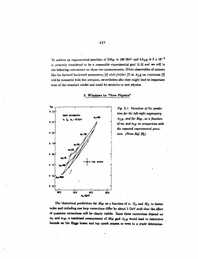
427
To achieve an experimental precision of 6Mw * 100 MeV and 6Am w 3 x 10
is presently considered to be a reasonable experimental goal [4,5] and we will in
the following concentrate on these two measurements. Other observable* of interest
like the forward backward asymmetry, [6] <r(ve)/<r(i>e) [7] or AIR on toponium [8]
will be measured with less precision, nevertheless also they might lead to important
tests of the standard model and could be sensitive to new physics.
2. Windows to "New Physics"
I II -
0.17 -
0 . 1 *
1.15 -
Fig. S.I: Variation of the predic-
tion for the left-right asymmetry
Am, and for Mw, as a function
ofmt and rng in comparison with
the expected experimental preci-
sion. (From Ref. [9]).
tt.l
The theoretical predictions for Mw as a function of a, G,, and Mz to lowest
order and including one loop corrections differ by about 1 GeV such that the effect
of quantum correction* will be dearly visible. Since these corrections depend on
m( and mH, a combined measurement of Mw jnd Am would lead to restrictive
bounds on the Higgs boson and top quark masses or even to a crude determin*-
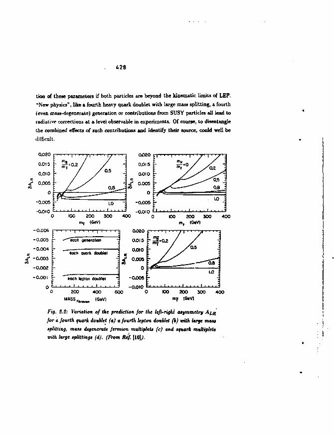
428
tioo of these parameters if both particles are beyond the kinematic limits of LEP.
"New physics", like a fourth heavy quark doublet with large mass splitting, a fourth
(even mass-degenerate) generation or contributions from SUSY particles all lead to
radiative corrections at a level observable in experiments. Of course, to disentangle
the combined effects of such contributions and identify their source, could well be
difficult.
i-
c
m, ' ' ' /
__ -"* 0.8_J
LO J
100 200 300
mT (GeV)
400 0 0 200 300m, (GeV)
400
-0.006
-0.005
-0.004
-0.003 r
-0.002 i-
-0.001 r
0
each generation
eoch quark doublet
each lepton doublet
, , i . . . . i . .
200
MASS Ftrmion
400
(GeV)600 200 300
(GeV)400
Fig. 3.S: Variation of the prediction for the left-right asymmetry
for a fourth quark doublet (a) a fourth lepton doublet (b) with large mass
splitting, mass degenerate fermion multiplet* (e) and aquark multiplets
with large splittings (d). (From Ref. [10]/
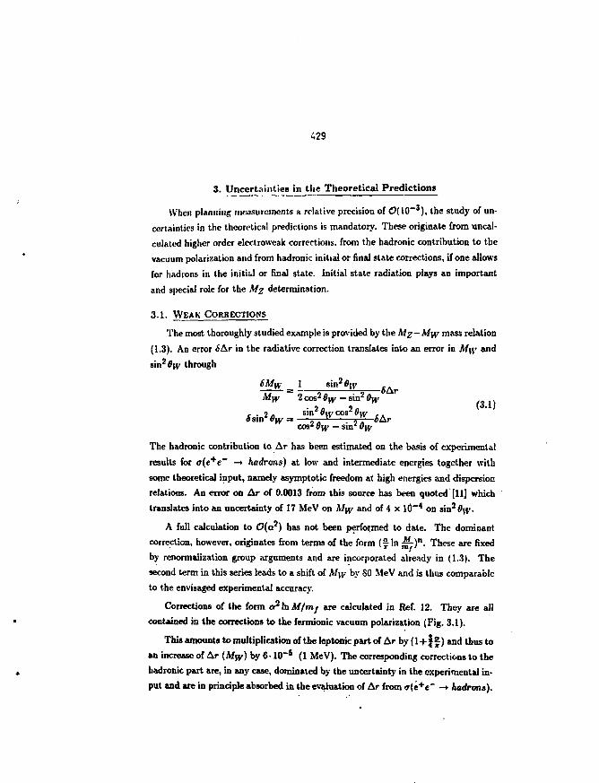
429
3. Uncertainties in the Theoretical Predictions
When planning measurements a relative precision of 0(1O~J), the study of un-
certainties in the theoretical predictions is mandatory. These originate from uncal-
culated higher order electroweak corrections, from the hadronic contribution to the
vacuum polarization and from hadronic initial or final state corrections, if one allows
for hadrons in the initial or final state. Initial stale radiation plays an important
and special role for the M% determination.
3.1. WEAK CORRECTIONS
The most thoroughly studied example is provided by the Mg—Mw mass relation
(1.3). An error 6Ar in the radiative correction translates into an error in M\y and
sin20(f through
Mw 2 cos2 0w - sin2 %
sin* % * %cos' 6]\' - sin* Ow
The hadronic contribution to Ar has been estimated on the basis of experimental
results for <r(e+e~ —t hadrons) at low and intermediate energies together with
some theoretical input, namely asymptotic freedom at high energies and dispersion
relations. An error on Ar of 0.0013 from this source has been quoted [11] which
translates into an uncertainty of 17 MeV on Myy and of 4 x lfl~* on sin2 0\\'.
A full calculation to O(a2) has not been performed to date. The dominant
correction, however, originates from terms of the form ( f i n jjjf-)". These are fixed
by rcnormalization group arguments and are incorporated already in (1.3). The
second term in this series leads to a shift of My,- by SO MeV and is thus comparable
to the envisaged experimental accuracy.
Corrections of the form oPlnAf/mj are calculated in Ref. 12. They are all
contained in the corrections to the fermionic vacuum polarization (Fig. 3.1).
This amounts to multiplication of the leptonic part of Ar by ( 1 + 1 1 ) and thus to
an increase of Ar {Mw) by 6-10~5 (1 MeV). The corresponding corrections to the
badronic part are, in any case, dominated by the uncertainty in the experimental in-
put and are in principle absorbed in the evaluation of Ar from <r{e+e~ -» hadrons).
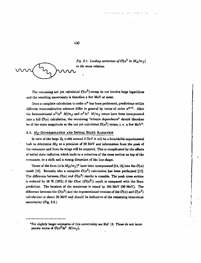
430
Fig. S.I: Leading correction ofO(a In
to the mass relation.
The remaining not yet calculated O(a )-terms do not involve large logarithms
and the resulting uncertainty is therefore a few MeV at most.
Once a complete calculation to order a" has been performed, predictions within
different renormalization schemes differ in general by terms of order a B + 1 . After
the forementioned o 2 In Mjmj and a In1 A//my terms have been incorporated
into a full O{a) calculation, the remaining "scheme dependence" should therefore
be of the same magnitude as the not yet calculated O(a2) terms, i. e. a few MeV*.
3.2. M^-DETERMINATION AND INITIAL STATE RADIATION
In view of the large Zg width around 3 GeV it will be a formidable experimental
task to determine Mz to a precision of 20 MeV and information from the peak of
the resonance and from its wings will be required. This is complicated by the effects
of initial state radiation which leads to & reduction of the cross section on top of the
resonance, to a shift and a strong distortion of the line shape.
Terms of the form (alnMz/mf)n have been incorporated [14,15] into the O(a)
result [16]. Recently also a complete O{a2) calculation has been performed [17].
The difference between O(a) and 0(0*) results is sizeable. The peak cross section
is reduced by 26 % (29%) if the O(a) (O{a2)) result is compared with the Born
prediction. The location of the maximum is raised by 184 MeV (96 MeV). The
difference between the O(a2) and the exponentiated versions of the O(a) and O(a2) i
calculations' is about 20 MeV and should be indicative of the remaining theoretical j
uncertainty (Fig. 3.2.) i
'For slightly larger estimates of this uncertainty see Ref. 13. These do not incor-porate terms of <?(a* In1 M/ntf).
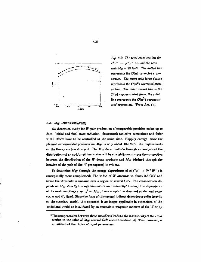
4 31
Fig. 3.2: The total cross section for
e+f~ —» fiTft~ around the prak
with Mz = 93 GeV. 7%e dotted lint
represents the 0{a) corrected cross-
section. The curve with large dashes
represents the O(o2) corrected cross-
lection. 77>e otfeer dashed line is the
C(o) exponentiated form, the solid
fine represents the O(a ) ezponenti-
aiei/ eipression. (From Ref. IT).
3.3. Mw DETERMINATION
No theoretical study for W pair production of comparable precision exists up to
date. Initial and final state radiation, electroweak radiative corrections and finite
width effects have to be controlled at the same time. Happily enough, since the
planned experimental precision on M\y is only about 100 MeV. the requirements
on the theory are less stringent. The M\y determination through an analysis of the
distributions of eu and/or qq final states will be straightforward since the connection
between the distribution of the IV decay products and A% (defined through the
location of the pole of the W propagator) is evident.
To determine M\p through the energy dependence of <r(e+e~ •-» W*W~) is
conceptually more complicated: The width of W amounts to about 2.5 GeV and
hence the threshold is smeared over a region of several GeV. The cross-section de-
pends on M\v directly through kinematics and indirectly* through the dependence
of the weak couplings g and g' on Myy, if one adopts the standard model and keeps
e.g. a and G/, fixed. Since the form of this second indirect dependence relies heavily
on the standard model, this approach is no longer applicable in extensions of the
nodel and would be invalidated by an anomalous magnetic moment of the W or by
*The compensation between these two effects leads to the insensitivity of the crosssection to the value of M\y several GeV above threshold [4], This, however, isan artifact of the choice of input parameters.
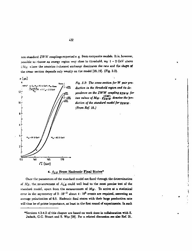
432
non-standard ZWW couplings expected e. g. from composite models. It is, however,
possible to choose an energy region very close to threshold, say 1 - 2 GcV above
-M\\ where the neutrino /-channel exchange dominates the rate and the ship? of
the cross- section depends only weakly on the model [18,19]. (Fig. 3.3).
Fig. 3.3: The cross section for W pair pro-
duction in the threshold region and its de-
pendence on the ZWW coupling gzww i°T
two values of Mw • SzwW ^CKotts the'pre-
diction of the standard model for gzww•
(From Ref. 18.;
155 160 165
fl [Gev]
4.
170
From Hadronic Final States*
Once the parameters of the standard model are fixed through the determination
of My, the measurement of Am could well lead to the most precise test of the
standard model, apart from the measurement of Mw- To arrive at a statistical
error in the asymmetry of 3 • 10~3 about 4 • 105 events are required, assuming an
average polarization of 0.5. Hadronic final states with their large production rate
will thus be of prime importance, at least in the first round of experiments. In such
•Sections 4.2-4.5 of this chapter are based on work done in collaboration with S.Jadach, G.G. Stuart and S. Was [20]. For a related discussion see also Ref. 21.
433
a situation large and uncalculable corrections from hadron physics could appear in
principle. There is, furthermore, a complicated interplay between QED corrections
and hadronii effects such that both have to be controlled simultaneously. Section
2 of this chapter will therefore be concerned with QCD corrections to Am for
masslcss and massive quarks. The effect of initial state radiation on Am will be
discussed in section 3. Section 4 is devoted to a discussion of Z — 7 and 7 - 7
box diagrams and their influence on the cross section and the asymmetry. It will
be shown that their influence is small on top of the Z. The discussion on helicity
nonconserving spin configurations in section 5 concludes this chapter. In view of the
importance of these measurements the brief discussion of the experimental setup in
section I may be justified.
4.1. T H E EXPERIUENTAL SETDP
Polarized electron beams have been produced and accelerated by the linear ac-
celerator at SLAC since long ago. The main task for SLC will be to preserve the
electrons' polarization on their complicated way from the source through the accel-
erator, the damping and the bending rings to the interaction region and to measure
the degree of plarization with sufficient precision. (SALR — ALR6P/P, such that
an experimental accuracy on Am of 3 • 10~3 requires the determination of P to
about 10~2.) The positrons remain unpolarized. Since the cross section for elec-
trons and positrons with opposite spins vanishes in the ultra relativistic limit, this
configuration is sufficient for a Am measurement.
At LEP, like at any other e + e~ storage ring, the Sokolov-Ternov effect may be
exploited. Synchrotron radiation from electrons and positrons flips their respective
spins, such that their magnetic moments are aligned with the external field of the
bending magnets. This leads to transverse polarization of e + and e~ with opposite
relative sign. Spin rotators will then transform these to electrons and positrons with
longitudinal spins pointing into opposite direction. This is most easily understood
as a consequence of CT invariance (Fig. 4.1). Let us assume a set of spin rotators
(consisting of a sequence of magnetic fields) which turns the transversely oriented
spins (say in direction J j j °f electrons with momenta p into longitudinally oriented
spins of direction jg at the interaction region and back to their original direction
afterwards. A CT operation leaves the magnetic fields of the spin rotators invariant,
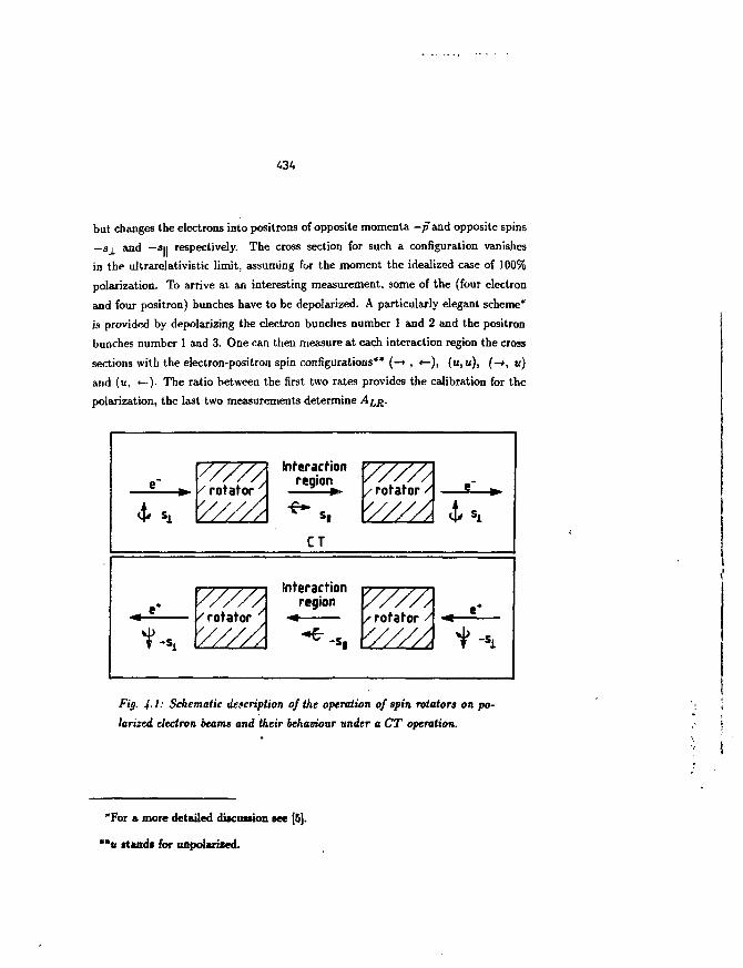
but changes the electrons into positrons of opposite momenta — /Tand opposite spins
—s_i_ and —SII respectively. The cross section for such a configuration vanishes
in the ultrarelativistic limit, assuming for the moment the idealized case of 100%
polarization. To arrive at an interesting measurement, some of the (four electron
and four positron) bunches have to be depolarized. A particularly elegant scheme*
is provided by depolarizing the electron bunches number 1 and 2 and the positron
bunches number 1 and 3. One can then measure at each interaction region the cross
sections with the electron-positron spin configurations** (—» , «-), (u, u), (-», u)
and (it, <—)• The ratio between the first two rates provides the calibration for the
polarization, the last two measurements determine AIR.
Fig. 4-1: Schematic description of the operation of spin rotators on po-
larized electron beams and their behaviour under a CT operation.
'For a more detailed discunion see [5].
**« standi for unpolarized.
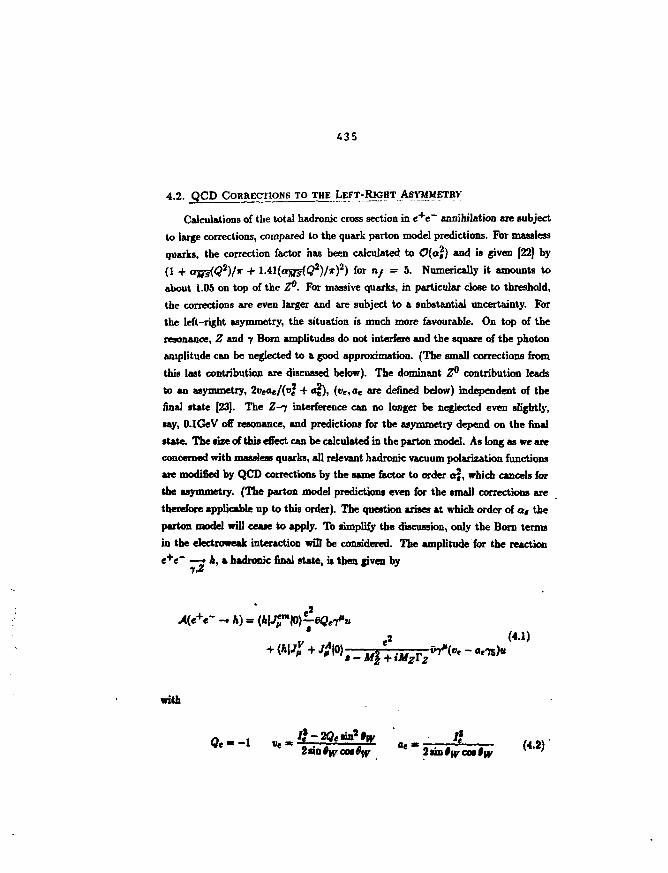
635
4.2. QCD CORRECTIONS TO THE LEFT-RIGHT ASYMMETRY
Calculations of the total hadronic cross section in e+e~ annihilation are subject
to large corrections, compared to the quark parton model predictions. For massless
quarks, the correction factor has been calculated to O(aj) and is given [22] by
(1 + trgziQ2)/* + 1 . 4 1 ( Q J ^ ( ? 2 ) / T ) 2 ) for n/ = 5. Numerically it amounts to
about 1.05 on top of the Z°. For massive quarks, in particular close to threshold,
the corrections are even larger and are subject to a substantial uncertainty. For
the left-right asymmetry, the situation is much more favourable. On top of the
resonance, Z and -y Born amplitudes do not interfere and the square of the photon
amplitude can be neglected to a good approximation. (The small corrections from
this last contribution are discussed below). The dominant Z° contribution leads
to an asymmetry, 2vtae/(v% + a£), (ve,at are denned below) independent of the
final state [23]. The Z-^ interference can no longer be neglected even slightly,
say, O.lGeV off resonance, and predictions for the asymmetry depend on the final
state. The size of this effect can be calculated in the parton model. As long as we are
concerned with massless quarks, all relevant hadronic vacuum polarization functions
are modified by QCD corrections by the same factor to order a j , which cancels for
the asymmetry. (The parton model predictions even for the small corrections are
therefore applicable up to this order). The question arises at which order of a, the
parton model will cease to apply. To simplify the discussion, only the Born terms
in the electroweak interaction will be considered. The amplitude for the reaction
e+e~ —-» A, a hadrooic final state, is then given by
h).
with
~
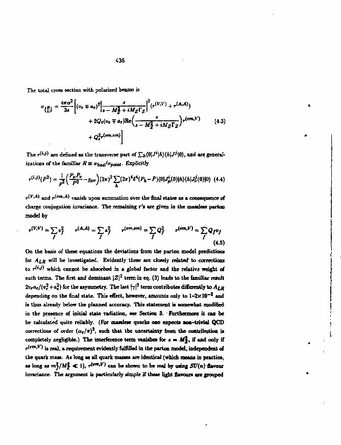
436
The total cross section with polarized beams is
The r(*J) are denned as the transverse part of £fc{0|JI'|A)(A|/'|0), and are general-
izations of the familiar R = Ohadfopoint- Explicitly
(4.4)
r("n,A) vanish upon summation over the final states as a consequence of
charge conjugation invariance. The remaining r's are given in the masdess partoo
model by
Y;} Y,} T.$ T.(4.5)
On the basis of these equations the deviations from the parton model predictions
for Am will be investigated. Evidently these are closely related to corrections
to r(»j) which cannot be absorbed in a global factor and the relative weight of
such terms. The first and dominant |Z|2 term in eq. (3) leads to the familiar result
2tva e /(t 'f+a|) for the asymmetry. The last H 2 term contributes differently to j4jyj
depending on the final state. This effect, however, amounts only to l -2xlO~ J and
is thus already below the planned accuracy. This statement is somewhat modified
in the presence of initial state radiation, see Section 3. - Furthermore it can be
be calculated quite reliably. (For massless quarks one expects Ma-trivial QGD
corrections of order (a#/*) 3 , such that the uncertainty from the contribution is
completely negligible.) The interference term vanishes for • « M\, if and only if
r(emy) u Teaj a requirement evidently fulfilled in the parton model, independent of
the quark mass. As long as all quark masses are identical (which means in practice,
as long as m^/Aff < 1), r<*m'K) can be shown to be real by using SV(n) flavour
invariance. The argument is particularly simple if these light flavours are grouped
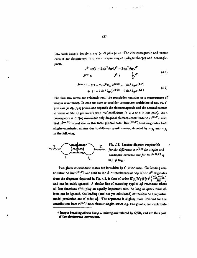
437
into weak isospin doublets, say (u.rf) plus (c,s). The electromagnetic and vector
current are decomposed into weak isospin singlet (=hypercbarge) and nonsinglet
parts.Jv =2(1 - 2sin2%)73 - 2 sin2 6WJY
, 1 yJem = J3 + j / y
,.<"»."> = 2(1-2sin2%)r<3'3)-
The first two terms are evidently real, the remainder vanishes as a consequence ofisospin invariaocef. In case we have to consider incomplete multiplets of say, (u,d)
plus a or (u, d), (c, s) plus b, one expands the electromagnetic and the neutral currentin terms of SU(n) generators with real coefficients (n = 3 or 5 in our case). As aconsequence of SU(n) invariance only diagonal elements contribute to Aem'V\ suchthat r(em'*r) is real also in this more general case. ]mAm'V) thus originates fromsinglet-nonsinglet mixing due to different quark masses, denoted by my, and m 2
in the following.
- Fig. i.t: Leading diagram responsible
for the difference in A*'^ for singlet and
nonsinglet currents and for ImAem'V) if
Two gluon intermediate states are forbidden by C-invariance. The leading con-tribution to Im r(em>v) and thus to the Z-7 interference on top of the Z° originates
from the diagrams depicted in Fig. 4.2, is thus of order p
and can be safely ignored. A similar line of reasoning applies off resonance whereall four functions r W play an equally important role. As long as quark mass ef-fects can be ignored, the leading (and not yet calculated) corrections to the partonmodel prediction are of order a}. The argument is slightly more involved for thecontribution from AA>A) since flavour singlet state* e.g. two gluons, can contribute
t bospin breaking effects likef-w mixing are induced by QED, and are thus partof the dectroweak corrections.
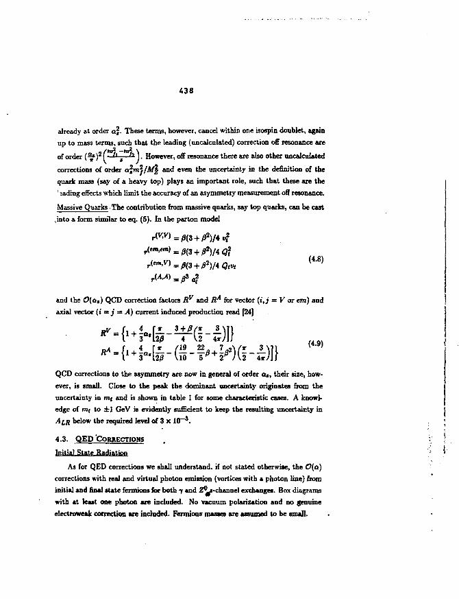
438
already at order a j . These terms, however, cancel within one isospin doublet, again
up to mass terms, such that the leading (uncalculated) correction off resonance are
of order (&• )2 ( h~ f* ). However, off resonance there are also other uncalculated
corrections of order aJm^/AfJ and even the uncertainty in the definition of thequark mass (say of a heavy top) plays an important role, such that these are the1 wading effects which limit the accuracy of an asymmetry measurement off resonance.
Massive Quarks The contribution from massive quarks, say top quarks, can be cast
into a form similar to eq. (5). In the parton model
and the O(a,) QCD correction factors Ry and R for vector (t,j = V or em) andaxial vector (»' = j = A) current induced production read [24]
( 4 9 )
QCD corrections to the asymmetry are now in general of order a,, their size, how-ever, is small. Close to the peak the dominant uncertainty originates from theuncertainty in mt and is shown in table 1 for some characteristic cases. A knowl-edge of mt to ±1 GeV is evidently sufficient to keep the resulting uncertainty inAIR below the required level of 3 x 10~3. \
4.3. QED 'CORRECTIOMS . : f
Initial State Radiation ; '
As for QED corrections we shall understand, if not stated otherwise, the O(a)corrections with real and virtual photon emission (vertices with a photon line) frominitial and final state fermioni for both 7 and Z*Lt-channel exchanges. Box diagramswith at least one photon are included. No vacuum polarization and no genuineelectroweak correction are included. Fermions masses are assumed to be small.
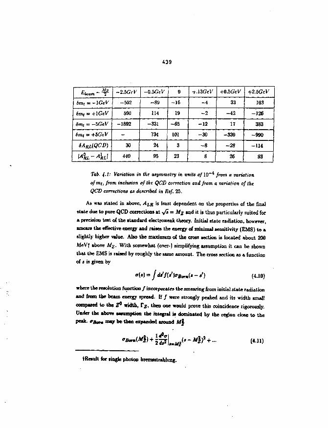
IT Mz^beam ~ "TT
6m, = -lGeV
6mt = +lGeV
Smt = -5GeV
Smt = +5GeV
-2.56VV
-502
590
-1892
-
30
440
-0.5GeV
- 8 9
114
-331
734
24
95
0
- 1 6
19
-65
101
3
23
+.13GeV
- 4
- 2
-12
-30
- 8
8
+0.5Gel^
33
-42
17
-330
-28
26
+2.5GeV
103
-126
383
-990
-114
93
Tab. 4.1: Variation in the asymmetry in units of 10~* from a variation
ofmt, from inclusion of the QCD correction and from a variation of the
QCD corrections as described in Ref. 25.
As was stated in above, Am is least dependent on the properties of the final
state due to pure QCD corrections hly/i= Mz and it is thus particularly suited for
a precision test of the standard electroweak theory. Initial state radiation, however,
smears the effective energy and raises the energy of minimal sensitivity (EMS) to a
slightly higher value. Also the maximum of the cross section is located about 200
MeVf above Mg. With somewhat (over-) simplifying assumption it can be shown
that the EMS is raised by roughly the same amount. The cross section as a function
of s is given by
«(») = J ds''/(»')«rflorn(« - «') (4.10)
where the resolution function / incorporates the smearing from initial state radiation
and from the beam energy spread. If / were strongly peaked and its width small
compared to the 2 ° width, Tz, then one would prove this coincidence rigorously.
Under the mbove awumption the integral is dominated by the region close to the
Pert- "Bon may be then expanded around M\
(4.11)
tResuIt for tingle photon bremsstrahlung.
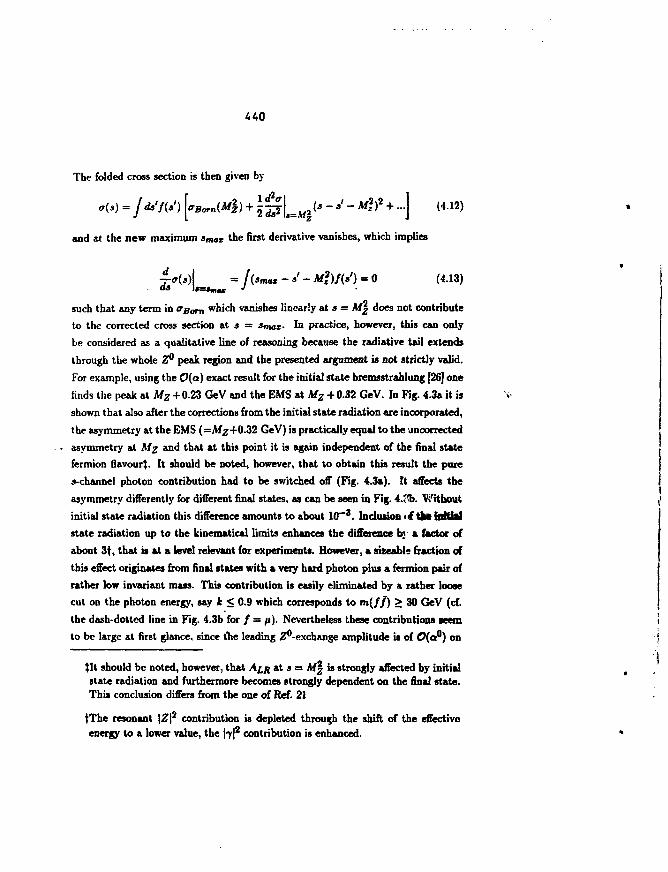
440
The folded cross section is then given by
C(s) = jds'f{3') \fBvrnWl) + \^[=M2J* ->'- *?)' + •••] (4.12)
and at the new maximum Smaz the first derivative vanishes, which implies
such that any term in °Born which vanishes linearly at a = Mg does not contribute
to the corrected cross section at s = Smax- In practice, however, this can only
be considered as a qualitative line of reasoning because the radiative tail extends
through the whole Z° peak region and the presented argument is not strictly valid.
For example, using the O(a) exact result for the initial state bretnsstrahlung [26] one
finds the peak at Mz + 0.23 GeV and the EMS at Mz + 0.32 GeV. In Fig. 4.3a it is
shown that also after the corrections from the initial state radiation are incorporated,
the asymmetry at the EMS (=A#z+0.32 GeV) is practically equal to the vincorrected
asymmetry at Mz and that at this point it is again independent of the final state
fermion flavour}. It should be noted, however, that to obtain this result the pure
j-channel photon contribution had to be switched off (Fig. 4.3a). It affects the
asymmetry differently for different final states, as can be seen in Fig. 4.3b. Without
initial state radiation this difference amounts to about 10~3. Inclusion < I tfct initialstate radiation up to the kinemmtical limits enhances the difference br a factor of
about 3f, that is at a level relevant for experiments. However, a sizeable fraction of
this effect originates from final states with a very hard photon plus a fermion pair of
rather low invariant mass. This contribution is easily eliminated by a rather loose
cut on the photon energy, say k < 0.9 which corresponds to m( / / ) > 30 GeV (cf.
the dash-dotted line in Fig. 4.3b for / = ft). Nevertheless these contributions teem
to be large at first glance, since t"he leading Z°-exchange amplitude is of O(aP) on
|It should be noted, however, that Am at 9 = M\ is strongly affected by initialstate radiation and furthermore becomes strongly dependent on the final state.This conclusion differs from the one of Ref. 21
tTbe resonant |Z|2 contribution is depleted through the shift of the effectiveenergy to a lower value, the H 2 contribution is enhanced.
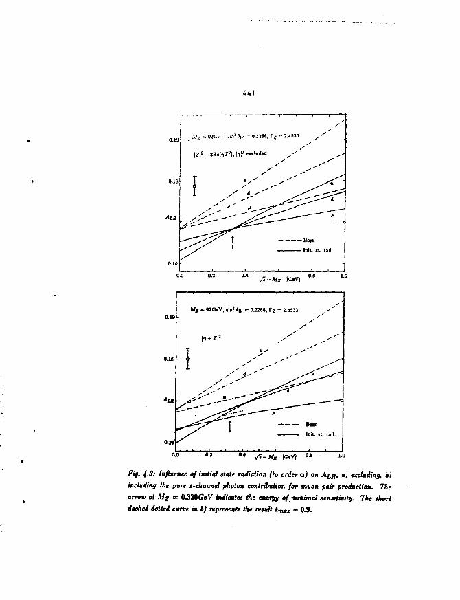
j
0.19 - • *
0.18 j-
lLR
0.16
— ~
Mi - 9
l 2 , ! + 3
\
/ , -
(;,•..,,,,2e„• -•= 0.2288, Tz
^ -
= 2.4533
- ^ _ _ _ —. — •
Born
Init
/y
^ *
^ —
•
0.0 0.2 |G,V) ° e
0.19
0.1S
*M
0.M
" ' •
1-
I
92G*V,un*l|K = 0.2288,1
^ -
? = 2.4533
ss
_ — - — •
S
s
Born
Init. it. rad.
IG.V) 0-8
Fig. 4-3: Influence of initial state radiation (to order a) on Am, a) excluding, b)
including Ike pure s-channcl photon contribution for mvon pair production. The
arrow at M% = 0.320GeV indicates the energy of minimal sensitivity. The short
dashed dotttd curve in bj represents the result kmaz = 0.9.
the top of Z° while the photonic amplitude is of O(o') and the non-interfering |-y|2
correction is thus of O(c?). It shouid be noted, however, that the Z°-amplitude
is supressed by the large Z° width — a consequence of the large number nj of
open fermionic channels — such that its magnitude is characterized by cfi/nj. No
corresponding suppression operates for the photon, so that the alleviation of the a 2
suppression is easily understood.
Initial/Final State QED Interferences and Box Diagrams
Final state QED bremsstrahlung by itself is not able to influence Am because it
factorizes off the cross sectionf. The interference of the QED bremsstrahlung from
initial and final state fermions and the interference of photonic box diagrams with the
Born amplitude involve the couplings of the photon to the final state fermions and
is therefore sensitive to the final state flavour. This dependence may, in principle,
show up in the integrated cross sections and therefore in ALR. One generally does
not expect these contribution.s to be large because, at the level of the differential
cross sections, they do not contain large logs of the type J ln(a /m| ) , however, the
integration over the photon spectrum in the presence of the Z° resonance might
perhaps produce ~ ln(M^/T^) terms.
Technically, in the one-loop/single-bremsstrahlung calculations, an infrared free
result is obtained by adding the contributions from box diagrams (in fact their in-
terference with Born amplitude) to the corresponding initial/fuul state h u d bran*
strahlung interference contribution integrated over the photon OMCgy op to tome
maximum value, possibly up to the pbMe space taut, f t a e two contributions,
virtual and real, correspond to two possible ways of cutting across one generic di-
agram, see Fig. 4.4. We shall consider four QED interferences shown in Fig. 4.4
which correspond to four assignments for 5-channel exchanges. They are denoted
in the Mowing as (Zy) ® Zt (Zf) ® 7, (77) ® Z and (77) ® 7. The last one is,
however, trivially equal zero due to charge conjugation invariance.
Most of ingredients necessary for numerical evaluation of the above QED inter-
ferences can be found in the literature. The relevant exact analytical expressions
I A very small influence ~ 10 * may arise for strong cut-off on photon energydue to competition of the initial and final state hard photon emission, see laterin this section.
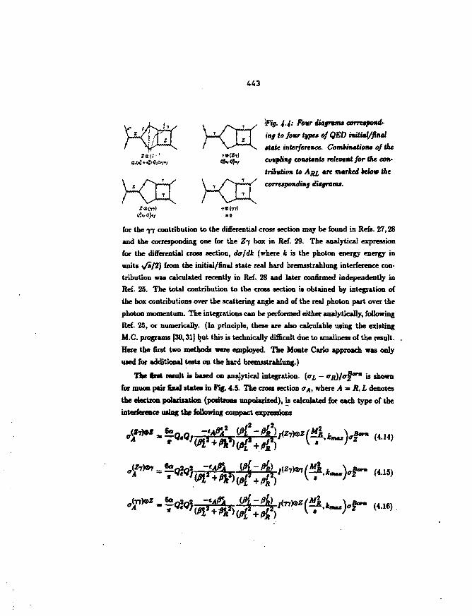
463
Kfi
Fig. 4.4: Four diagrams correspond-
ing to four types of QED initial/final
state interference. Combinations of the
coupling constants relevant for the con-
tribution to ARI art marked Mow the
corresponding diagrams.
for the 77 contribution to the differential cross section may be found in Refs. 27,28
and the corresponding one for the Z~i box in Ref. 29. The analytical expression
for the differential cross section, dojdk (where k is the photon energy energy in
units V*/2) from the initial/final state real hard bremsstrahlung interference con-
tribution was calculated recently in Ref. 28 and later confirmed independently in
Ref. 25. The total contribution to the cross section is obtained by integration of
the box contributions over the scattering angle and of the real photon part over the
photon momentum. The integrations can be performed either analytically, following
Ref. 25, or numerically. (In principle, these are also calculable using the existing
M.C. programs [30,31} but this is technically difficult due to smallness of the result.
Here the first two methods were employed. The Monte Carlo approach was only
used for additional tests on the hard bremsstrahlung.)
The f n t result is based on analytical integration. (01 - 9jHfo§orn is shown
for muon pair final state* in Fig. 4.5. The cross section <rA, where A = R,L denotes
the electron polarization (positrons nnpoUrized), is calculated for each type of the
interference using the following compact expressions
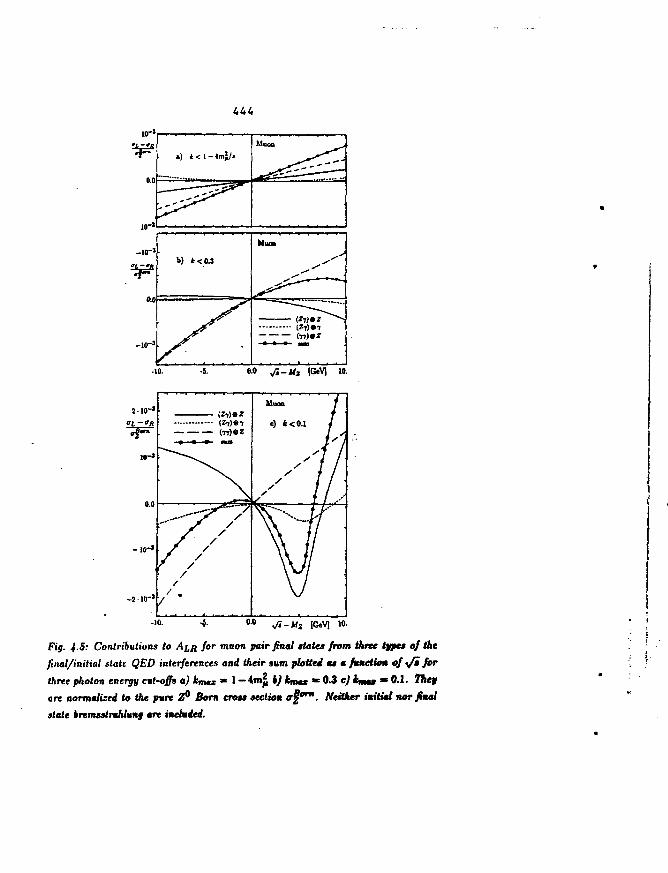
0.0
») KI-4mJ/«M U O D ^ ^
Muo>
(Zi)»T
(nfz
-10. 00 (GeVl 10.
- 2 • 1 0 " '
(G«V) 10.
Fig. 4.5: Contributions to AIR for muon pair final states from three types of the
final/initial slate QED interferences and their sum plotted w « function of ifi for
three photon energy cut-offs a) Jfcnwi =* 1 -4">J ») *mox * 0.3 c) km** * 0.1. They
are normalized to the pure Z° Born cross section af0"*. Neither initiml nor final
state iremsstrthlunf are included.
445
where A - R.L, tR = 1, tL - - 1 and
Re[z(z
Re[(l - *•)(*(* + l)b *=S*±Lzl r u _ i)(i -*„„«)- ln(*) - 2k*„,„)]
/<rrt®*(*, kma) = Re(l- r)(-21n * „ « + imax + | ) (4.19)
for which,
M% = M$- iMzVz (4.20)
^ and (SJj denote respectively the left and right band couplings of the Z° to the
electron in units of e
- = / l - s i n g t y Q e ^ = - sin 9!vQe£ sin0|frcos% R s i n % c o s % l " ;
d[ and ;9jj denote the corresponding quantities for the outgoing fermion. Theexpression for <T(ZT)®T can be obtained directly from <T( ? T' 3 Z (c.f. Ref. 25) bysuitably modifying the couplings and propagators. For <T(T>®^ the situation isslightly different since there are two 77 box diagrams compared to four Z7 boxes.Hence one must return to the amplitude level and resum the contributing diagramsappropriately.
In Fig. 4.5 the size of the interference contribution is shown and the relativeimportance of the three terms is compared. Three different cut-offs inuu are applied.The quantity plotted in Fig. 4.5 is normalized with respect to <r§orn and representsroughly the influence of each of the three terms on Am- The normalization withrespect to <rtd, the total cross section, with photonic corrections, integrated up tokmoz, will be used in all other plotsf. The following conclusions can be drawn fromFig. 4.5:
tThe advantage of the normalization with respect to 0%°™ in Fig. 4.5 is thatthe figure can be easily reproduced using eqs. (15)-(16).
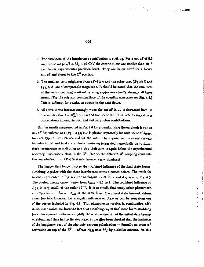
446
1. The smallness of the interference contribution is striking. For a cut-off of 0.3
and in the range >/> = Mz ± 10 GeV the contributions are smaller than 10~3
i.e. below experimental precision level. They are below 10~4 for a looser
cut-off and closer to the Z° position.
2. The smallest term originates from (Zj) ® f and the other two, (Zf) ® Z and("If) ® Z, are of comparable magnitude. It should be noted that the smallness
of the vector coupling constant ve = V/i suppresses equally strongly all three
terms. (For the relevant combinations of the coupling constants see Fig. 4.4.)
This is different for quarks, as shown in the next figure.
3. All three terms increase strongly when the cut-off kmax •» decreased from its
maximum value 1 — mJ/3 to 0.3 and further to 0.1. This reflects very strong
cancellations among the real and virtual photon contributions.
Similar results are presented in Fig. 4.6 for u-quarks. Here the emphasis is on the
cut-off dependence and (<7£ — <rs)/<rtot is plotted separately for each value of kmax,
for each type of interference and for the sum. The unpolarized cross section crtot
includes initial and final state photon emission integrated numerically up to kmax-
Each interference contribution and also their sum is again below the experimental
accuracy, particularly close to the 2°. Due to the different Z® coupling constants
the contribution from iZf) ® Z interference is now dominant.
The figures that follow display the combined influence of the final state brems-
strahlung together with the three interference terms dicussed before. The result for
muons is presented in Fig. 4.7, the analogous result for u and d quarks in Fig. 4.8.
The photon energy cut-off varies from kmax = 0.1 to 1. The combined influence on
Am is very small, of the order 10~*. It is so small, that many other phenomena
are expected to influence A^g at the same level. Even final state bremsstrahlung
alone (no interferences) has a similar influence on Am as can be seen from one
of the curves included in Fig. 4.7. This phenomenon results, in combination with
initial state radiation, from the fact that switching on/off final state bremsstrahlung
(modulus squared) influences slightly the relative strength of the initial state bremt-strahlung and thus indirectly also Am. It has 0eo been checked that the inclusionof tbe imaginary part of the photonic vacuum polarization — formally an order a2
correction on top of the Z° — affects Am near Mg by a similar amount. At this
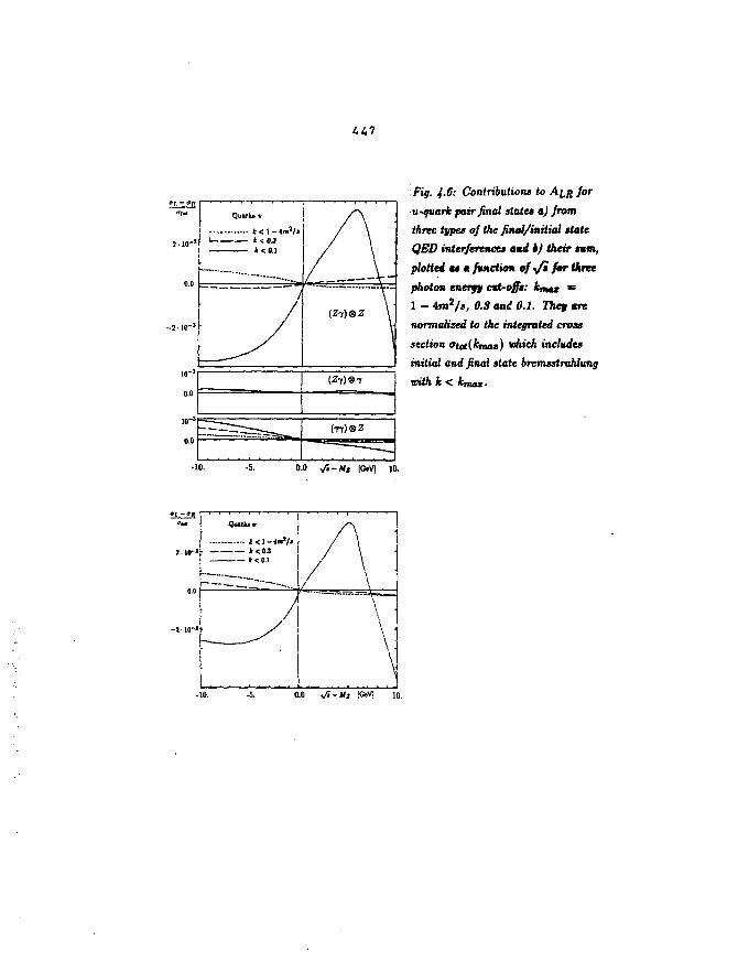
i.t.1
0.0 "
io-J
0.0
Quarks u
Kl-W/J1 *<OJ
*<0.1 A-(Zi)8Z \
(77) ®Z
Fip. ^.C: Contributions to
u-ovark pair final states a) from
three types of the final/initial state
QED interferences and h) their turn,
plotted «t • function of </* for three
photon energy cut-offs: kmax =
1 - 4m2/J, 0.8 and O.I. They are
normalized to the integrated cross
section (rtct(kmaz) which includes
initial and final state bremsstrahlung
with k <
-5. 0.0 y/i-Mt [GeV] 10.
2-I0-"-Kl-4m'/M*<OJK0.1 / \ i
\\\.-10. -5. 0.0 -fi-Mz !<3eV| 10.
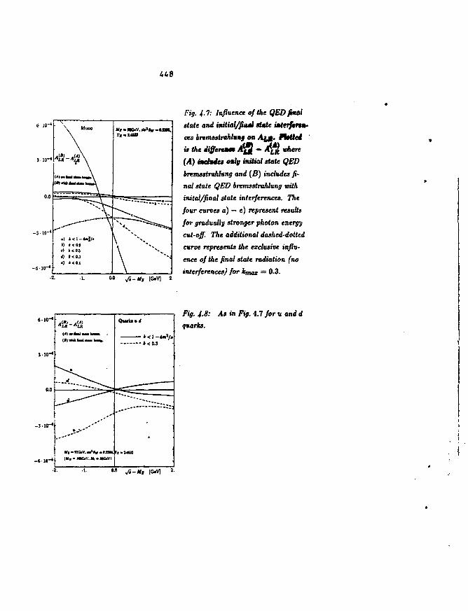
3 JO-1
- 3 . 1 0 " *
FJJ. 4.7: Influence of the QED final
state and initial/final state imttrfert*-
ces bremsstrMung on A|j |- tttUed '
is the differ*** A^ - A ^ where
(A) mdtdt» only initial state QED
bnmsstrahfong and (£) includes fi-
nal state QED bremsstrahlung with
inital/final state interferences. The
four curves a) — e) represent results
for gradually stronger photon energy
cut-off. The additional dashed-dotted
curve represents the exclusive influ-
ence of the final state radiation (no
interferences) for kmat — 0-3.
JO-
l o -
om
1 6 -
^>-
m.''
in
W6)V.^*»V
tMCiV, JU, -
to.
• tan.
*<0.3
. . . .
^.ft As in Fig. 4.7 /or u and rf
• 1 . «JI IG.V)
order of magnitude most probably other higher order QED corrections come into
play.
The following comments should be added:
The relative size of the interference contributions is given by VfttfQf lor 0(zy)®Z
and by (??«/ for ff(Zy)®y alM* a(n)®Z' Neglecting mass terms these contributions
vanish upon summation over all members of one generation as a consequence of
anomaly cancellation. Of course, when measuring the cross section experimentally,
the members of one generation (neutrino, heavy quark) will not be included with
equal weight to allow for the exact cancellation.
All the contributions from initial/final state interference vanish for s ~ A/| or
are at most of order f (F^/A/j)2 as compared to the Born cross section. This fea-
ture holds true also for general hadronic states. The reason for this is easily seen
for O{Zi)®Z- T° e momentum flow in one of the two interfering ^-propagators re-
mains unaffected by photon emission and the corresponding amplitude is thus purely
imaginary for s = A/|. TO assure interference with the remaining contribution (the
box amplitude for virtual and the amplitude with initial state radiation for real
photon emission), the phase space of the photon is strongly restricted, namely to
|£> I r>/2 for real and to \By - k2/2Mz\ < Tz/2 for virtual emission.
To summarize: QED initial/final state interference contributions to Am aroundthe Z-peak are for loose cuts an order of magnitude below 3 • 10~3, the anticipatedprecision of future experiments.
4.4. BREMSSTRAHLUNG AND HELICITY NONCONSERVING BEAM POLARIZATIONS
Tests of electroweak theory by means of the measuring left-right asymmetry with
an experimental error 3 • 10~3 will require the beam polarizations to be measured
with a precision of 10 . In LEP/SLC experiments this will be achieved either by
means of Compton backscatteringf off a polarized laser beam [33] and by scattering
e* beams with four sets of polarizations (some of them zero) (34] where the polar-
ization can be deduced indirectly from the four measured cross sections. Helicity
conservation is an important ingredient in this analysis and will be inspected more
closely now.
f For QED corrections to this method ef. Ref. 32.
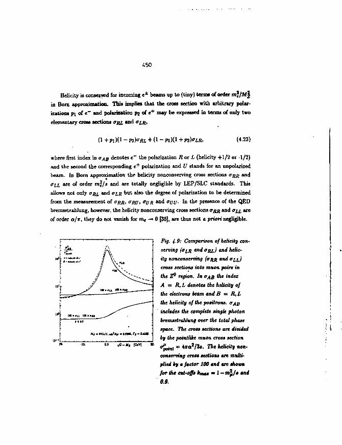
450
Helicity is conserved for incoming e* beams up to (tiny) terms of order m\fhl\
in Bom approximation. This implies that the cross section with arbitrary polar-
izations pi of e~ and polarization P2 of e + may be expressed in terms of only two
elementary crow sections aju and <>IR,
- P 2 ) a R L + ( l - (4.23)
where first index in a^g denotes e~ the polarization R or L (helicity +1/2 or -1/2)
and the second the corresponding e + polarization and U stands for an unpolarized
beam. In Born approximation the helicity nonconserving cross sections aim aa^
°LL * r e °f <wder m\fs and are totally negligible by LEP/SLC standards. This
allows not only ORI and am but also the degree of polarization to be determined
from the measurement of a/m, any, ayR and ayy. In the presence of the QED
bremsstrahlung, however, tbe helicity nonconserving cross sections CRR and an, are
of order a/x, they do not vanish for m , - + 0 [35], are thus not a priori negligible.
Fig. 4-9: Comparison of helicity con-
serving (am and ORL) and helic-
ity nonconserving (ajm and an)
cross sections into muon pairs in
the Z6 region. In aj^s the index
A = R,L denotes the helicity of
the electrons beam and B = R,L
the helicity of the positrons, o^g
includes the complete single photon
bremsstraklung over the total phase
space. The cross sections are divided
by the pointlike muon cross section
ff^,,, = Ana2/3s. The helicity non-
conserving cross sections art multi-
plied by a factor 100 and are shovn
for the cut-off* W » 1 - mJ/« and0.9.
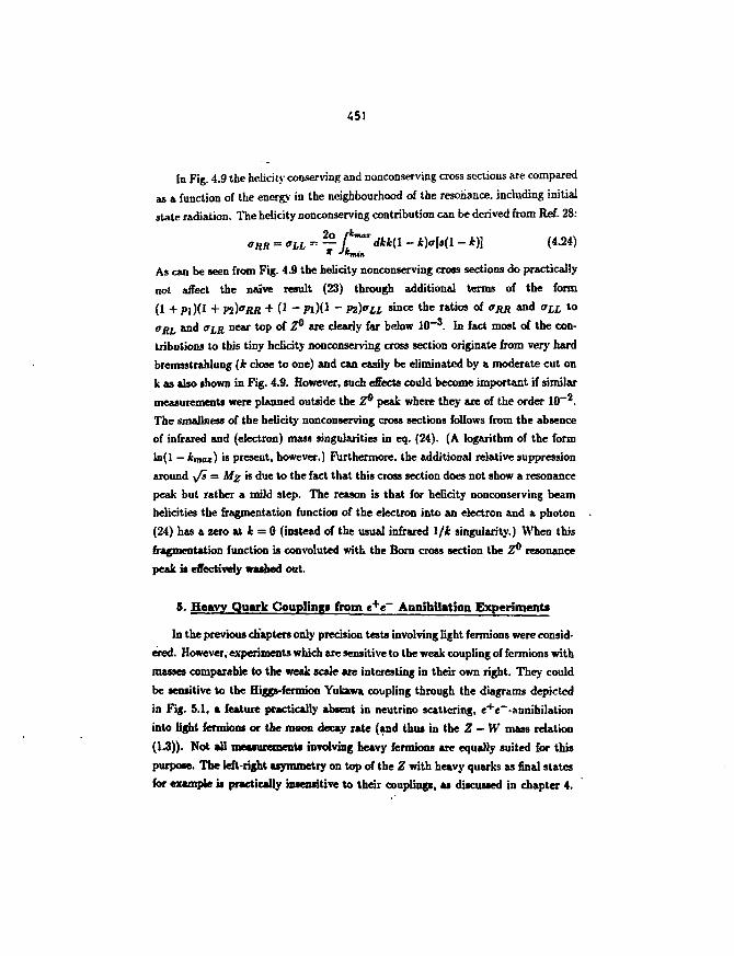
451
In Fig. 4.9 the helicity conserving and nonconserving cross sections are compared
as a function of the energy in the neighbourhood of the resonance, including initial
state radiation. The helicity nonconserving contribution can be derived from Ref. 28:
2o- Jfc)<rKl - *)] (4.24)
* Jtmin
As can be seen from Fig. 4.9 the helicity nonconserving cross sections do practically
not affect the naive result (23) through additional terms of the form
(1 -f- pi)(l + P2)'rRR + (1 ~ Pl)(l ~ P2)lrLL since the ratios of ORR and <T££ to
ORI and <JIR near top of Z° are clearly far below 10~3. In fact most of the con-
tributions to this tiny helicity nonconserving cross section originate from very hard
bremsstrahlung (k close to one) and can easily be eliminated by a moderate cut on
k as also shown in Fig. 4.9. However, such effects could become important if similar
measurements were planned outside the Z° peak where they are of the order 10~2.
The smallness of the helicity nonconserving cross sections follows from the absence
of infrared and (electron) mass singularities in eq. (24). (A logarithm of the form
ln(l - kmax) is present, however.) Furthermore, the additional relative suppression
around y/s = Mz is due to the fact that this cross section does not show a resonance
peak but rather a mild step. The reason is that for helicity nonconserving beam
helicities the fragmentation function of the electron into an electron and & photon
(24) has a zero »t fc = 0 (instead of the usual infrared l/k singularity.) When this
fragmentation function is convoluted with the Born cross section the Z° resonance
peak is effectively washed out.
5. Heavy Quark Couplings from e+e~ Annihilation Experiment!
In the previous chapters only precision tests involving light fermions were consid-
ered. However, experiments which are sensitive to the weak coupling of fennions with
masses comparable to the weak scale are interesting in their own right. They could
be sensitive to the Higgs-fermion Yukawa coupling through the diagrams depicted
in Fig. 5.1, a feature practically absent in neutrino scattering, e+e~-annihilation
into light fennions or the muon decay rate (and thus in the Z - W mass relation
(1.3)). Not all measurements involving heavy fennions are equally suited for this
purpose. The left-right asymmetry on top of the Z with heavy quarks as final states
for example is practically insensitive to their couplings, as discussed in chapter 4.
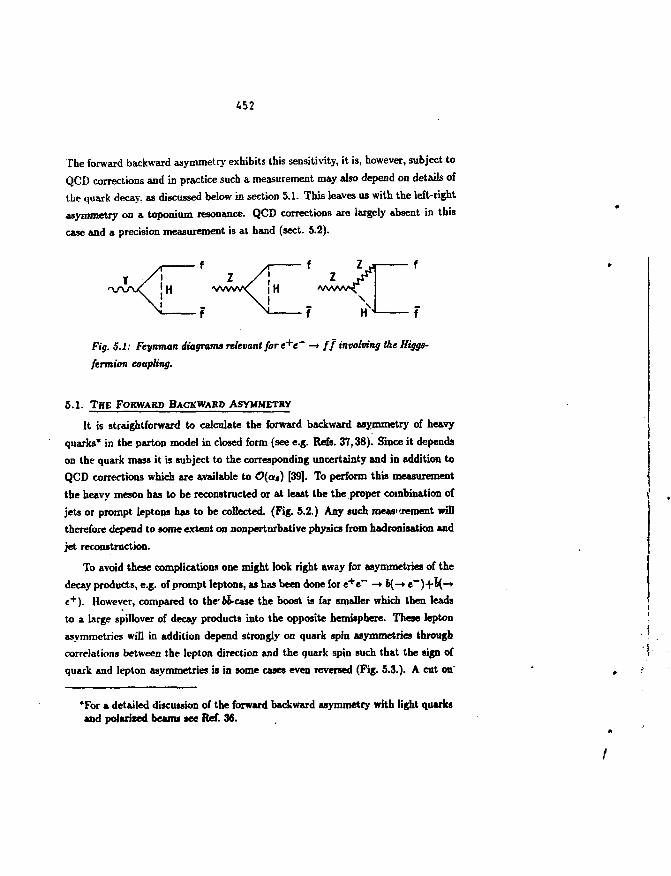
452
The forward backward asymmetry exhibits this sensitivity, it is, however, subject to
QCD corrections and in practice such a measurement may also depend on details of
the quark decay, as discussed below in section 5.1. This leaves us with the left-right
asymmetry on a toponium resonance. QCD corrections are largely absent in this
case and a precision measurement is at hand (sect. 5.2).
Fig. 5.1: Feynman diagrams relevant for e+e~ —t ff involving the Higgs-
ftTtnion coupling.
5.1. THE FORWARD BACKWARD ASYMMETKY
It is straightforward to calculate the forward backward asymmetry of heavy
quarks* in the parton model in closed form (see e.g. Refs. 37,38). Since it depends
on the quark mass it is subject to the corresponding uncertainty and in addition to
QCD corrections which are available to O(a$) [39]. To perform this measurement
the heavy meson has to be reconstructed or at least the the proper combination of
jets or prompt leptons has to be collected. (Pig. 5.2.) Any such meas>irement will
therefore depend to some extent on nonperturbati ve physics from hadronisation and
jet reconstruction.
To avoid these complications one might look right away for asymmetries of the
decay products, e.g. of prompt leptons, as has been done for e + e~ —* 4(-* e~)+5(—*
e+). However, compared to the-66-case the boost is far smaller which then leads
to a large spillover of decay products into the opposite hemisphere. These lepton
asymmetries will in addition depend strongly on quark spin asymmetries through
correlations between the lepton direction and the quark spin such that the sign of
quark and lepton asymmetries is in some cases even reversed (Fig. 5.3.). A cut on"
*For a detailed discussion of the forward backward asymmetry with light quarksand polarised beam* see Ref. 36.
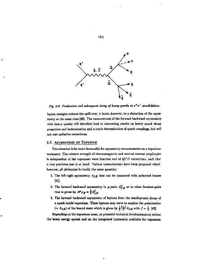
«53
Fig. 5.8: Production and subsequent decay of heavy quarks in e+e~ -annihilation.
lepton energies reduces the spill-over, it leads, however, to a distortion of the asym-
metry at the same time [40J. The measurement of the forward backward asymmetry
with heavy quarks will therefore lead to interesting results on heavy quark decay
properties and hadronization and a crude determination of quark couplings, but will
not test radiative corrections.
5.2. ASYMMETRIES ON TOPOMUM
The situation is far more favourable for asymmetry measurements on a toponium
resonance. The relative strength of electromagnetic and neutral current amplitude*
is independent of the toponium wave function and of QCD corrections, such thai
a true precision test is at hand. Various measurements have been proposed which
however, all determine basically the same quantity:
1. The left-right asymmetry Am that can be measured with polarized beam;
[41].
2. The forward backward asymmetry in /i-pairs Apg or in other fermion-pain
that is given by A*FB = \A\R-
3. The forward backward asymmetry of leptons from the semileptonic decay of
a quark inside toponium. These leptons may serve to analyse the polarization
(= AIR) of the bound state which is given by \*Y-AL,R with / = J. [42).
Depending on the toponium mass, on potential technical developments to reduce
the beam energy spread and on the integrated luminosity available for toponium
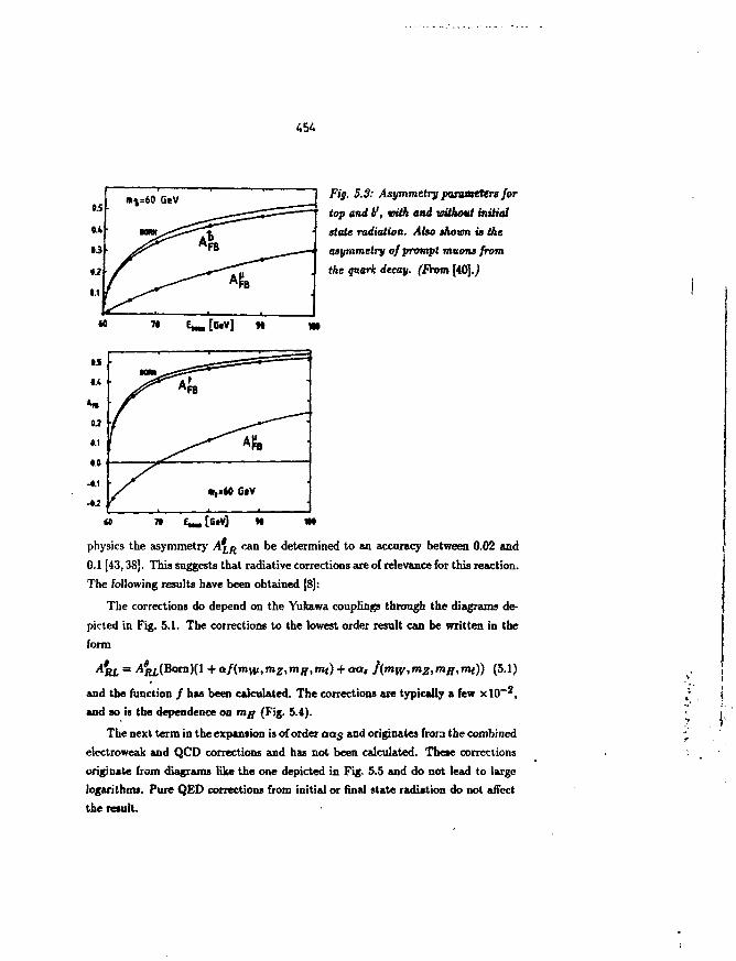
/fy. 5.5; Asymmetry poreawters/or
top and V, vith and without initial
state radiation. Also shown is the
asymmetry of prompt muons from
the quark decay. (From [40].)
physics the asymmetry ALIi can be determined to an accuracy between 0.02 and
0.1 [43.38). This suggests that radiative corrections are of relevance for this reaction.
The following results have been obtained [8]:
The corrections do depend on the Yukawa couplings through the diagrams de-
picted in Fig. 5.1. The corrections to the lowest order result can be written in the
form
A*RL ~ ^KifBonOO + otf(mw,mz,mH,mt) + act, f(mw,mz,mff,mt)) (5.1)
and the function / has been calculated. The corrections are typically a few xlO~2 ,
and so i« the dependence on mff (Fig. 5.4).
The next term in the expansion is of order aag and originates from the combined
electroweak and QCD corrections and has not been calculated. These corrections
originate from diagrams like the one depicted in Fig. 5.5 and do not lead to large
logarithms. Pure QED corrections from initial or final state radiation do not affect
the result.
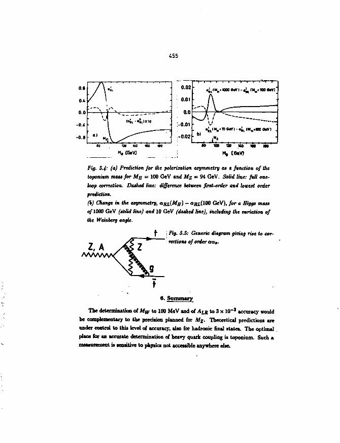
455
o.«
0.1
0.4
0.8
AH
" -AM no «o HO no
M, CCeVJ
0.02
: 0.01
n n
-0.01
-0.02
so
A\j
m
rMOOewi-a^fM
f—
no HO ' I N
M, [6tV)
^too^y)'
WO 0 ^ 1 .
m'
Fig. 5.4: (a) Prediction for the polarization asymmetry as a function of the
toponium mast for MH = 100 GeV and Mz = 94 GeV. Solid line: full one-
loop correction. Da$hed line: difference between first-order and lowest order
prediction.
(h) Change in the asymmetry, amiMg) - « R L ( 1 0 0 GeV), for a Biggs mass
o/lOOO GeV (solid line) and 10 GeV (dashed line), including the variation of
the Weinberg angle.
2, A
Fig. 5.S: Generic diagram giving rise to cor-
rections of order aat.
8. Summary
The determination of Mw to 100 MeV and of ALR to 3 x 10~ } accuracy would
be complementary to the precision planned for Mz. Theoretical predictions are
under control to this level of accuracy, also for hadronic final states. The optimal
place for an accurate determination of heavy quark coupling is toponium. Such a
measurement is sensitive to physics not accessible anywhere else.
456
ACKNOWLEDGEMENTS
I am indebted to B. Grzadkowski, Z. Hioki, S. Jadach, P. Krawczyk, R. Stuart,
Z. Was and P. Zerwas for enjoyable collaborations on various topics treated in this
report. Instructive discussions on experimental techniques at LEP with A. Blondel
and W. Blum have strongly stimulated my interest in this field. Last but not least
I would like to thank the organizers of the "X. Warsaw Symposium on Elementary
Particle Physics" at Kazimierz and of the "Workshop on Topical Problems of Testing
the Standard Model" at Budapest for their kind hospitality.
457
REFERENCES
[1] A. Sirlin, Plenary Talk at the International Symposium on Lepton and
Photon Interactions at High Energies, Hamburg 1987.
[2] P. Jcnni, Plenary Talk at the International Symposium on Lepton and
Photon Interactions at High Energies, Hamburg 1987.
[3J P. Jenni, invited talk at the LEP 200 Workshop, Aachen 1986.
[4] P. Rondeau, Report of the W Mass Study Group, LEP 200 Workshop,
Aachen 1986, J. Bijnens et al., Orsay preprint LAL 87-07.
[S] G. Alexander et al., Polarized e + and e~ Beams at LEP, Working Group
Report, CERN/LEPC/87-6.
[6] G. Altarelli et al., in "Physics at LEP", CERN Report 86-02 (1986).
[7] CHARM II proposal, G. Busi et al., CERN/SPS C/83-24 (1983).
[8] B. Grzadkowski, P. Krawczyk, J.H. Kiihn and R.G. Stuart, Phys. Lett.
163 B (1985) 247, Phys. Lett. 176 B (1986) 456, Nud. Pbys. B 281 (19S7)
18.
[9J Report of the Study Group on "Electroweak Radiative Corrections at LEP
Energies", LEP 200 Workshop, A. Barroso et al., CERN-EP/87-70.
[10] B. Lynn, M. Peskin and R.G. Stuart, in "Physics at LEP", CERN Report86-02 (1986).
[11] F. Jegerlehner, Z. Phys. C32 (1986) 195.
[12] A. Sirlin, Phys. Rev. D29 (1987) 89.
[13] F. Hollik and W. Tinune, Z. Phys. C 38 (1986) 125,F. Jegerlehner, Z. Pbys. C 32 (1986) 425.
[14] E.A. Kuraev and V.S. Fadia, Sov. J. Nucl. Phys. 41 (1985) 466.
458
[15] G. AltareUi and G. Martinelli, in "Physics at LEP", CERN Report 86-02
(1986).
[16] G. Bonueau and F. Martin, Nue/. Phya. B 27 (1971) 381.
(17] F.A. Berends, G.J.H. Burgers and W.L. van Neerven Phys. Lett. 185 B
(1987) 395.
[18] B. Grzadkowski, Z. Hioki and J.H. Kühn, Preprint MPI-PAE/PTh 47/87.
[19] K. Hagiwara and D. Zeppenfeld, Preprint KEK-TH-1963.
[20] S. Jadach, J.H. Kühn, R.G. Stuart and Z. Was, Preprint MPI-PAE/PTh
71/87.
[21] B. W. Lynn and C. Verzegnassi, Nuovo Cimento 94A (1986) 15;
B. W. Lynn and C. Verzegnassi, Phys. Rev. D35 (1987) 3326.
[22] D.W. Duke and R. G. Roberts, Phys. Rep. 120C (1985) 277.
[23] B.W. Lynn and R.G. Stuart, JVud. Phys. B 253 (1985) 216;
B.W. Lynn, M.E. Peskin and R.G. Stuart, In "Physics at LEP", CERN
86-02, eds. J. Ellis and R. Peccei. (1986) 90;
M. Böhm, W. Hollik and H. Spiesberger, Z. Phys. C27 (1985) 523.
[24] S. Gûsken, J.H. Kühn and P.M. Zerwas, Phys. Lett. 155 B (1985) 185.
[25] J. H. Kühn and R.G. Stuart, MPI-PAE/PTh 53/87.e
{26] G. Bonneau and F. Martin, Nucl. Pbys. B 27 (1971) 381.
[27] I. B. Kriplovich, Sov. J. Nucl. Phys. 17 (1973) 298;
R.W. .Brown, V.K. Cung, K.O. Mikaelian and E.A. Paschos, Pbys. Lett.
43 B (1973) 403.
[28] Z. Was, Cracow Preprint TPJU-U/86; to appear in Act* Phys. Poloa.
[29] M. Böhm and W. Hollik, Nucl. Pbys. B 204 (1982) 45;
R. W. Brown, R. Decker and E. A. Paschos, Pbys. Rev. Lett. 52 (1984)
1192.
459
[30] S. Jadach, R. G. Stuart and Z. Was, KORALZ, Monte Carlo program for
r and n pair production at LEP/SLC, (August 1987) unpublished.
[31] R. Kieiss, B. W. Lynn, R. G. Stuart, BREMUS Monte Carlo program,
(January 1987) unpublished.
[32] R.G. Stuart and A. G6ngora-T., MPI-PAE/PTh55/87, July 1987.
[33] C. Y. Prescott, SLAC Technical note SLAC-TN-73-1 (1973).
[34] ALEPH Collaboration, In "Polarized e + e " Beams at LEP", unpublished
report CERN/LEPC/87 - 6 (1986).
[35] T.D. Lee and M. Nauenberg, Phys. Rev. 133 (1964) 1549.
[36] A. Blondel, B.W. Lynn, F.M. Renard and C. Verzegnassi, preprint Mont-
pellier PM/87-14 (1987).
[37] J.H. Kuhn, A. Reiter and P.M. Zerwat, Nucl. Phys. B 272 (1966).
[38] P. Igo-Kemenes et al., Report of the Study Group on Heavy Quarks and
Leptons, LEP 200 Workshop, Aachen 1986, CERN-EP/87-49.
[39] J. Jersak, E. Laennann and P.M. Zerwas, Phys. Lett. 98 B (1981) 363.
[40] S. Jadach and J.H. Kuhn, Pbys. Lett. 1 9 1 B (1987) 313.
[41] I.I.Y. Bigi, J.H. Kuhn and H. Schneider, Preprint MPI-PAE 28/78 1978;
J. Bernabeu and P. Pascual, Nucl. Phys, B 172 (1981) 93;
L.M. Sehgal and P.M. 2erwa», Nud. Pb'yt. B 183 (1981) 417.
[42] J.H. Kuhn and K.H. Streng, Nucl. Phyt. B 1 9 8 (1982) 71.J. H. Kuhn and
R. G. Stuart, Phys. Lett. 190 B (1987) 208.
[43] W. Buchmuller et al.. Study Group on "Toponium Physics at LEP", MPI-
PAE/PTh 85/85 and CERN Report 86-02.
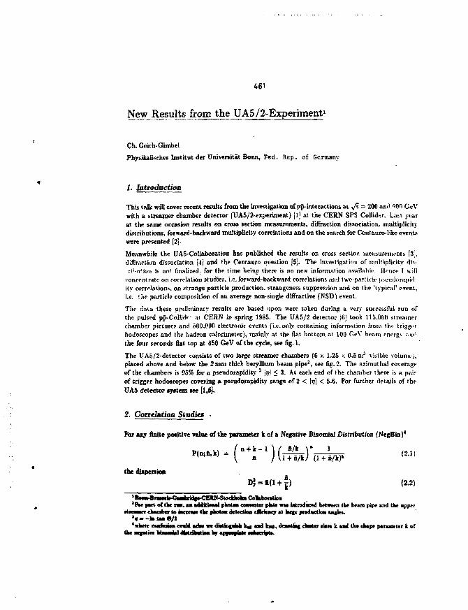
461
New Results from the UA5/2-Experiment1
Ch. Geich-Gimbel
Physikaiiscltes Institut der Universitat Bonn, Fed. Rep. of Germany
1. Introduction
This talk will cover recent results from the investigation of pp-interactions at v/s = 200 am' 900 GcVwith a streamer chamber detector (UA5/2-experiment) [l] at the CER.N SPS Collider. Lau yearat the same occasion results on cross section measurements, diffraction dissociation, multiplicitydistributions, forward-backward multiplicity correlations and on the search for Centauro-like eventswere presented [2j.
Meanwhile the UA5-Coliaboration has published the results on cross section measurements |3j.diffraction dissociation [<i and the Centauro question J5J. The investigation of multiplicity dK-iri'-niioi! is noi finalized, for the time being there is no new information available. Hence I willconcent rate on correlation studies, i.e. forward-backward correlations and two-particle <>:.cudorapv1-Hy correlation*, on strange particle production, strangeness suppression and on the 'typical' event,i.e. !ii» particle composition of an average non-single diffractive (NSD) event.
The data these preliminary results are based upon were taken during a very successful run ofthe pulsed pp-Collidr- at CER.N in spring 1985. The UA5/2 detector [6] took U5.000 streamerchamber pictures and 500,000 electronic events (i.e. only containing information from the- triggerhodoscopes and the iiadron calorimeter), mainly at the flat bottom at 100 GcV beam energ> .irn!the four seconds flat top at 450 GeV of the cycle, see fig. I.
The UA5/2-detector consists of two large streamer chambers (6 x 1.25 x 0.5 m3 visible volume j ,placed above and below the 2mm thick beryllium beam pipe2, see fig.2. The azimuthal coverageof the chambers is 95% for a pseudorapidity 3 ITJI < 3. At each end of the chamber there is a pairof trigger hodoscopes covering A pseudorapiditv range of 2 < |i)| < 5.6. For further details of theUA5 detector system see (1,6).
2. Correlation Studies •
For any finite positive value of the parameter k of a Negative Binomial Distribution (NegBin)*
(2.1)
the 4iBpenkm
r) (2.2)
T m Ttnwib f f t n i i ^ i TT1IH TtnrM ini "nhtinnlin.'F»r put at the vm, am aMkioul phot«l cowotcr phtc w« iMtodooed betwera the beam pipe and the upper
itn—cr chvnbtr to i n u m tht photos detection eftchacf at laiic yndactkm uigln.' l e /* /'whtcc eoafitrieB eoali Mbt wt dirtiooUi k^ o d km, dewtiac ckMer m n k aW th* dupe paruneln k of
OK mtgnin VmmUldfattibthw by nii i i ihl i mUtniy.
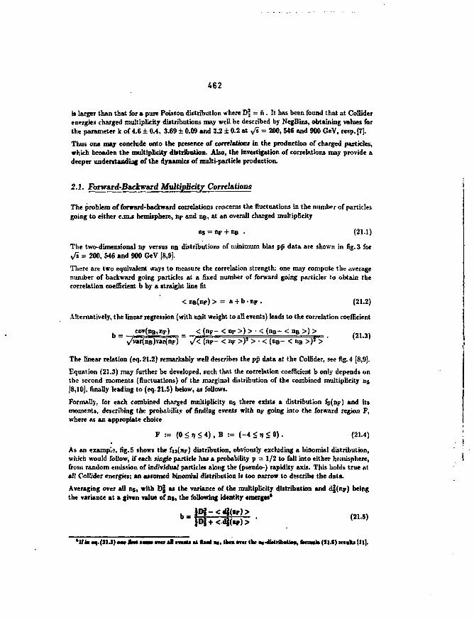
462
a larger than that for a pure Poisson distribution where D | = n. It has been found that at Colliderenergies charged multiplicity distributions may well be described by NegBins, obtaining values forthe parameter k of 4.6 i 0.4, 3.69 ± 0.09 and 3.2 ± 0.2 at y/s = 200, 546 and 900 GeV, resp.(7].
Thus one may conclude onto the presence of correlations in the production of charged particles,which broaden the multiplicity distribution. Also, the investigation of correlations may provide adeeper understanding of the dynamics of multi-particle production.
2.1. Forward-Backward Multiplicity Conehtions
The problem of forward-backward correlations concerns the fluctuations in the number of particlesgoing to either c n u hemisphere, np and HB, at an overall charged multiplicity
ns = np + ns • (21.1)
The two-dimensional np versus ns distributions of minimum bias pp data are shown in fig. 3 forv-s = 200, 546 and 900 GeV [8,9].
There are two equivalent ways to measure the correlation strength: one may compute the averagenumber of backward going particles at a fixed number of forward going particles to obtain thecorrelation coefficient b by a straight line fit
< nB(np) > = a + b • np . (21.2)
Alternatively, the linear regression (with unit weight to all events) leads to the correlation coefficient
b = ""("Binr) _ < (n F - < nF >) > • < (n B - < nB >) > ( 2 1 ./var(nB)var(nF) /< (np- < nF >)a > • < (n B - < nB >)* > '
The linear relation (eq. 21.2) remarkably well describes the pp data at the Collider, see fig. 4 [8,9).
Equation (21.3) may further be developed, such that the correlation coefficient b only depends onthe second moments (fluctuations) of the marginal distribution of the combined multiplicity ns|8,1OJ, finally leading to (cq. 21.5) below, as follows.
Formally, for each combined charged multiplicity ns there exists a distribution fs(nf) and itsmoments, describing the probability of finding events with np going into the forward region F,where as an appropiate choice
F := (0 < f < *) . B := (-4 < IJ < 0) . (21.4)
As an exampi», fig. 5 shows the fu(nF) distribution, obviously excluding a binomial distribution,which would follow, if each single particle has a probability p = 1/2 to fall into either hemisphere,from random emission of individual particles along the (pseudo-) rapidity axis. This holds true atall Collider energies; an assumed binomial distribution is too narrow to describe the data.
Averaging over all ns, with Dj as the variance of the multiplicity distribution and d§(m>) beingthe variance at a given value of ns, the following identity •merges*
+ fj
'If fc «4.(31.)) MM *»t m ml* mats >t (bud M, taw i w the ts-dittrilHitiM, brawl* (11.1) tnalu (11).
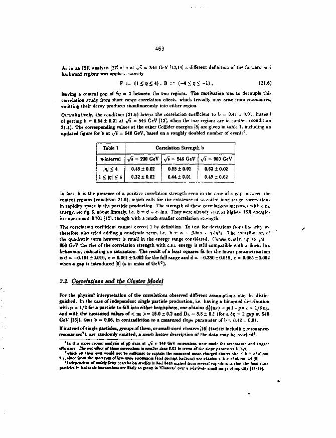
463
As in aii ISR analysis [12; a'-o at v'7 = 546 GeV [13,14] a different definition of the forward an-.;
backward regions was applies, riamely
F := ( l < i ? < 4 ) . B := ( - 4 < » ) < - l ) , (21.6)
leaving a central gap of <n = I between the two regions. The motivation was to decouple thiscorrelation study from short range correlation effects, which trivially may arise from resonances,emitting their decay products simultaneously into either region.
Quantitatively, the condition (21.6) lowers the correlation coefficient to b = 0.41 s. 0.01. insteadof getting b = 0.54 ± 0.01 at y/s = 546 GeV [13]. when the two regions are in contact (condition21.4). The corresponding values at the other Collider energies [8j are given in table 1, including anupdated figure for b at y/s = 546 GeV, based on a roughly doubled number of events6.
Table 1
n-interval
1 < \i\ < i
Correlation Strength b
y/i = 200 GeV
0.48 ±0.02
0.32 ± 0.02
y/i = 546 GeV
0.56 ± 0.01
0.44 ± 0.01
y/s = 900 GeV
0.63 ± 0.02
0.49 ± 0.02
In fact, it is the presence of a positive correlation strength even in ihc case of a gap between thecontrol regions (condition 21.6), which calls for the existence of so-called long range rorrelation»in rapidity space in the particle production. The strength of these correlations increases with cm.cimgy, bee fig. 6. about linearly, i.e. b = d + o In s. They were already wen at higliesl 1SR energit'"in experiment R701 [12], though with a much smaller correlation strength.
The correlation coefficient cannot exceed 1 by definition. To test for deviations from linearity v.ctherefore also tried adding a quadratic term, i.e. b = a * 3-\ns - i-tors. The contribution ofthe quadratic term however is small in the energy range considered. Consequently. >ip <» 4/s900 GeV the rise of the correlation strength with cm. energy is still compatible with a linear lit sbehaviour, indicating no saturation. The result of a least squares fit for the linear parametrisationbd = -0.184+0.016, c = 0.061 ±0.002 for the full range and d = -0.380*0.019, c = 0.065-0.002when a gap is introduced [8] (s in units of GeV2).
2.2. Correlations and the Cluster Model
For the physical interpretation of the correlations observed different assumptions may bv distinguished. In the case of independent single particle production, i.e. having a binomial distributionwitlip = 1/2 for a particle to fall into either hemisphere, one obtains d|(np) - p(] -p>iis = 1/4 ns,and with the measured rallies of < ns >= 16.0 x 0.2 and D$ = 8.8 ± 0.1 (for a iq - 2 gap at 540GeV |15|), thus b = 0.66, in contradiction to a measured slope parameter of b - 0.12 i 0.01.
If instead of single particles, groups of them, or small-sized clusters [16] (tacitly including resonancesresonances7), are randomly emitted, a much better description of the data may be rrarhed*.
' U thia moic teccat aaalrM *f pt dut it yfi = 54« GeV corKdions ««e nixie for acccpiaiice and triusc;cflkinicr. I V act dfcet «f Ikew cvmetiou • fmScr lh«n 0J01 in term of llif ilopt paranirirr l> 's,'J,.
'•hick M Ihtic » l mild Mt be tv/kitrt to explain tie roeuiirrd mean charted clutter sitr < It > of alioul2.2, »i»c« £rom Ike •pectnmi at low-mau nwauKU (and prompt kadi ont) one obtains < k> of about 1.4 |B]
'ladcpmdcut or imkiplcfcjr comblioa •tiutkt it had been argued from tevetal eip'rinienta cltal liir final .i.utpanklei in htdroak iMctactioM ace likely to »to»p ia "ClnHett' over a relatively iniall range of rapidity [17-19].
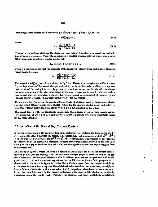
Assuming a fixed duster sixe k one would get d|(np) = p(l - p)kns = 1/4kns, or
I-- 4dl(nr)/ns , (22.1)
hence
This picture is still unrealistic, at the cluster size may vary, at least due to various decay multiplic-ities of known resonances. Under the assumption of clusters of mixed size the cluster size k in eq.(22.2) turns into an effective cluster size V*t [20]
k « c = < k > + v a r ( k ) / < k > , (22.3)
which is a function of the first two moments of the (unknown) cluster decay multiplicity. Equation(22.2) finally becomes
D|/<ns>-k«, .b - D | / < n s > + k* • ( 2 2 4 )
This quantity 4d|(np)/ns = k«f >* plotted in fig. 7 for different cm. energies and different spansAIJ. in dependence of the overall charged multiplicity ns in the intervals considered. It appearsthat, provided the multiplicity ns is large enough as well as the interval Ai>, the effective clustersize saturates at krf ~ 2.5, also independent of the cm. energy. As for smaller intervals and/orsmaller multiplicities the relative probability for clusters to emit particles outside the control regions(leakage effects) is enhanced, naturally smaller values for k r emerge.
The curves in fig. 7 represent the results of Monte Carlo simulations, based on independent clusteremission (UA5 Cluster-Monte-Carlo [6,21]). There for the charged cluster decay multiplicity atruncated Poisson distribution was input, with < k >= 1.8, resulting in Kf ~ 2.6.
This result ties in with the conclusions drawn from the analysis of two-particle pseudorapiditycorrelations (22] at Ji = 540 GeV and also with earlier ISR results [23], wh re compatible valuesfor kdr were obtained.
2.3. Variation of the Central Gap Size and Position
A further investigation of the nature of long range multiplicity correlations has been carried out bydetermining the slope b between two regions in pseodorapidity thai are one unit wide (j ijj'B - ijf'B |- 1) and separated by a central gap Jijp>B = I 9^ - i f ! of varying size. Furthermore we have studiedthe behaviour of the correlation coefficient for fixed forward/backward intervals of one unit in 1/decoupled by a gap of fixed fixe of 2 units in f>, and moving the center of the separating gap fromfj=O towards 9=2.
.A 5 is shown in figure 8. where the slope b is plotted as a function of the size of the central pseudo-rapidity gap for 200, 546 and 900 GeV, the correlation strength decreases monotonically as the gapsi2c is increased. The observed behaviour of b for different gap sizes are in agreement with modelprediction). [24.25J, and is also well reproduced by the UA5 cluster Monte Carlo program [6,21)'illustrated by the curves in figure 8). In this Monte Carlo program first the charged limitiplicityof the event is drawn from a negative binomial distribution and then tlie cluster decay multiplicityfrom a Poisson distribution with a mean value of ~2.3 charged particles/duster, wlwren* the numbrr of clusters is determined by the charged multiplicity of the event and the flusters are randomlydistributed along the rapidity axis. Therefore the observed long range multiplicity correlations
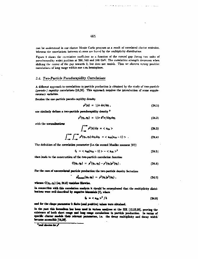
465
can be undrrstood in our cluster Monte Carlo program as a result of correlated cluster emission,whereas the correlations between clusters are forced by the multiplicity distribution.
Figure 9 shows the correlation coefficient as a function of the centra] gap (bring two units ofpseuiioraniditr wide) position at 200, 546 and 900 GeV. The correlation strength decreases whenshifting tin center of the gap towards 2, but does not vanish. Thus we observe strong positivecorrelations of long range within one cm. hemisphere.
2.4. Two-Particle Pseadonpidity Correlations
A different approach to correlations in particle production is obtained by the study of two-particle(pseudo) rapidity correlation* (16,26). This approach requires the introduction of some supple-mentary variables.
Besides the one-particle pseudo-rapidity density
l/<rckr/di7, (24.1)
one similarly defines a two-particle pteudorapidity density *
/»'(•&.*) = lf<r d'ff/drnim (24.2)
with the nonnaBiatioM m
~A (24.3)
The definition of the correlation parameter (i.e. the second Mueller moment 127])
h - < n*(nd, - 1) > - < n * >» (24.5)
then leads to the construction of the two-partic/e correlation function
Cfai ,*) = ?*(<h,ih) -/>'(*)fHm) • (24.6)
For the case of ttacomlatod particle prodaction the two-particle density (actorizes
«•«•<* C(%, IJ,) (ca, 24 J ) naishw tttwfce.
la connection with this correlation analysis it tbould be remembered that the multiplicity distri-*~*8 P ^-rrrn-tii t r t l f f thf hianwiah [7], irhsn
6 » < a* >* fit (24.8)
aad for the shape aaramttar k fcttc (aa« aoskirt) wbai wtr* obtained.
la the past this fonnattsm has a«ta w a i ia wioas aaatyies at the ISR [12,23,28), prortac theexistence of both short raafi and long r a n * cotraiatloM ih particle production. Ia Unns of
chwter BKMICIS thfir n l m a t aanawtm, Lc. the decay multiplicky and decay widthbecame accessible (t«^»).
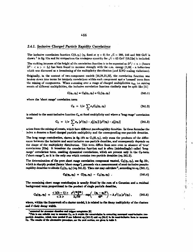
466
2.4.1. Inclusive Charged Particle Rapidity Correlations
The inclusive correlation function 0(0,773) (iji fixed at IJ = 0) for ,/s = 200, 546 and 900 GeV isshown 1 in fig. 10a and for comparison the analogous quantity for y s = 63 GeV (19,23a! is included.
The striking increase of the height of the correlation function is to be expected as D3 / < n > (henceD J - < n > = fj) has been found to increase strongly with the cm. energy [7,30] - a behaviourwhich was discussed as a broadening of the multiplicity distribution (and KNO scaling violations).
Originally, in the context of two-component models [16,29,31,32], the correlation function wasbroken down into terms for intrinsic correlations within each component and a 'crossed' term fromthe mixing of components. When summing over a range of charged multiplicities nd,, i.e. mixingevents of different multiplicities, the inclusive correlation function similarly may be split like [31]
(241.1)
where the 'short range' correlation term
Cs = V* 5>.C.(»Ji,ift) (241.2)a
is related to the semi-inclusive function C. at fixed multiplicity and where a long range' correlationterm
C t = V* S o*\?Xlfc) -AM) [/»*(*)-/».(»»»)) (241.3)•
arises from the mixing of events, which have different pseudorapidky densities. In these formulae theindex n denotes a fixed charged particle multiplicity and the corresponding one-particle densities.
The Icng range contribution, shown in fig. 10b as CL(0,I») , only sums the products of the differ-ences between the inclusive and semi-inclusive one-particle densities, and consequently depends onthe shape of the multiplicity distribution. This term diners from xero even in absence of 'true'correlations [23a]. It broadens the correlation function and is often (misleadingly) called long-range' correlation term, masking dynamical correlations, which are present only in the Cj-term('short-range'), as it is the only one which contains two-particle densities (eq. 241.2).
The determination of the pure short range correlation component wanted, Ct(th,tt)< *ee fig. 10c,which is sharply peaked (hence 'short-range'), proceeds via a measurement of semi-inclusive pseudo-rapidity densities to obtain Ct(ih, <b) («!• 241.J). Then one may calculate *, according to eq. (241.1),
Csfa**) = C(ifc,ijj) - CL(ihi*j) • (241.4)
The remaining short range contribution is usually fitted by the sum of a Gaussian and a residualbackground term proportional to the product of single particle densities,
(241.5)
where, within the framework of a duster model, k Is related to the decay multiplicity of the dustersasrfJ their decay width.
yriitlr J—U*, whtsh mm asstsa sT eat hitmi ->(ttlJ) at n.(H..) k Ituwsi ladflw hnu u • m mCs. TW fsseks eftht antssatiM esMsaaM, M* tW aol MCUM, HI ftna ki tekitt.
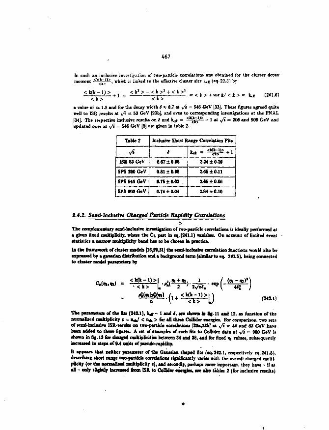
467
In such an inclusive invest iration of two-particle correlations one obtained for the cluster decaymoment , which is, linked to the effective cluster size i^g (eq.22.3) by
+ 1 =< k3 > - < k >' -K k >'
= < k > - h v a r k / < k > = (241.6)
a value of a 1.5 and for the decay width S a 0.7 at yfi = 546 GeV [33]. These figures agreed quitewell to ISR results at v'* = 53 GeV [23bj, and even to corresponding investigations at the FNAL(34]. The respective inclusive remits on t and k«, = <k§g& + 1 at Js = 200 and 900 GeV andupdated ones at Ji = 546 GeV [8] are given in table 2.
Table 2
ISR 53 GeV
SPS 200 GeV
SPS 546 GeV
SPS M0 GeV
Inclusive Short Range Correlation Fits
i
0.67 ±0.05
0.81 ±0.06
•.75 ±0.03
0.74 ±0.04
W = ^ ^ + 12.24 ±0.20
2.65 ±0.11
2.C5±0.06
2.84 ±0.10
2.4.2. Senu'-Iaclusire Ciutrgtd Particle Rapidity Correlations%
The complementary semi-mclnsive investigation of two-particle correlations is ideally performed ata given fixed multiplicity, where the CL patt in eq. (241.1) vanishes. On account of limited erentstatistics a narrow multiplicity band has to be chosen in practice.
In the framework of cluster models [16,29,31] the semi-inclusive correlation functions would ako beexpressed by a gaatsian distribution and » background t*nn (similar to eq. 241.5), being connectedto cluster model parameters by
<k>-1)>I e x p l -
11+ <k> U (242.1)
The parameurs of the Its (242.1), k* - 1 and S, are shorn in ng. 11 and 12, as function of thenormalized multiplicity * = • * / < n* > for all three Collider energies. For comparison, two setsof semi-inclusive ISR-resdts on two-particle correlations [23a£3b] at y/s = 44 and 63 GeV havebeen added to these figures. A set of examples of such fits to Collider data at v? = 900 GeV isshown in fig. 13 for charged multiplicities between 34 and 38, and for fixed ft values, subsequentlyincreased in steps of 0.4 writ* of pseudo-rapidity.
It appears that neither parameter of the Gaussian shaped fits (eq. 242.1. respectively eq. 241.5).describing short range two-particle correlations significantly varies with the overall charged multi-plicity (or the normalised multiplicity i) , and secondly, perhaps mow important, they have - if atall - only slightly Increased from ISR to Collider energies, see also tables 2 (for inclusive results)
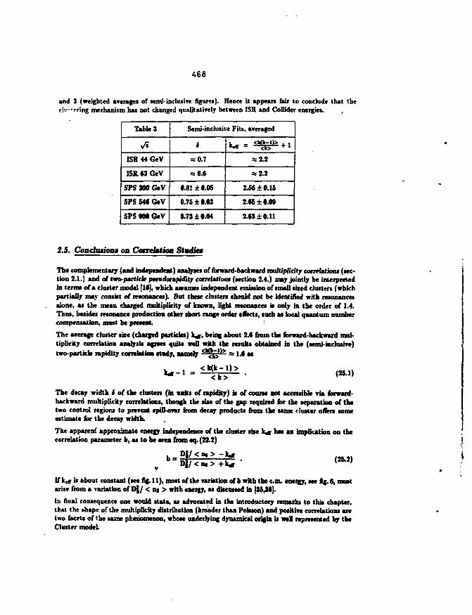
468
and 3 (weighted averages of semi-inclusive figures). Hence it appears fair to conclude that thecindering mechanism has not changed qualitatively between ISR and Collider energies. ,
Table!
ISR 44 GeV
ISR 63 GeV
SPS 200 GeV
SPS 5M GeV
SPS 9M GeV
Semi-inclusive Fits, averaged
*
a 0.7
a 0.6F •.81±«.O5
0.75 ±t.M
6.73 ±0.04
=s2.2
= 2.2
2.56 ±0.15
2.65 ±#.09
2.(310.11
2.5. Conclusions on Correlmtion Studies
The complementary (and independent) analyses of forward-backward multiplicity correlations (sec-tion 2.1.) and of two-particle pscudorapidity correlations (section 2.4.) may jointly be interpretedin terms of a cluster model [16], which assumes independent emission of small sited clusters (whichpartially may consist of resonances). But these chillers should not be identified with resonancesalone, as the mean charged multiplicity of known, light resonances is only in the order of 1.4.Thus, besides resonance production other short range order effects, such as local quantum numbercompensation, must be present. :
The average cluster size (charged particles) k*, being about 2.6 from the forward-backward mul-tiplicity correlation analysis agrees quite well with the results obtained is the (semi-inclusive)two-particle rapidity correlation study, namely <>P^I>> as 1.6 a*
^ UL — 1» >(25.1)
The decay width * of the clutters (m units of rapidity) is of course art accessible via forward-backward multiplicity correlations, though the silt of the gap required for the separation of thetwo control regions to prevent spill-over from decay products from the same cluster offers someestimate for the decay width.
The apparent approximate energy independence of the cluster sue k* has an implication on thecorrelation parameter b, as to be seen from eq.(22.2)
b = (26.2)
is about constant (sec Kg. 11), most of the variation of b with the cm. energy, see fig. 6, mustarise from a variation of Dj / < n« > with energy, as discussed in [35,36].
In final consequence one would state, as advocated in the introductory remarks to this chapter,thai the shape of the multiplicity distribution (broader than Poisson) and positive correlations areiwo facets of the same phenomenon, whose underlying dynamical origin is weB represented by theCluster model
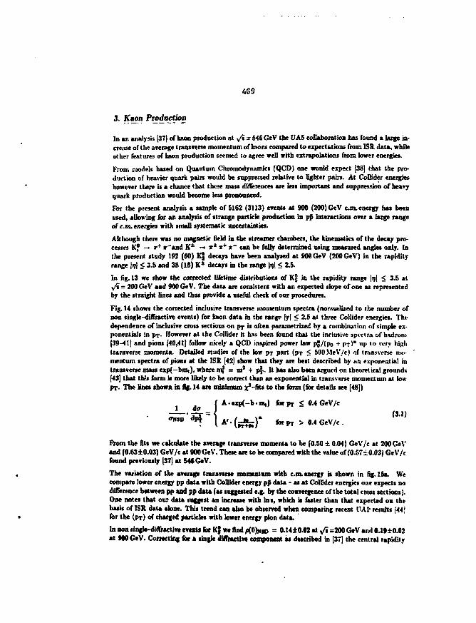
469
3. Kaon Production
In »n analysis [37) of bum production at y/i = 546 GeV the UA5 collaboration has found a large in-crease of the average transverse momentum of loons compared to expectation* from ISR. data, whileother features of kaon production seemed to agree well with extrapolations from lower energies.
From models based on Quantum Chromodynamies (QCD) one would expect (38) that the pro-duction of heavier quark pairs would be suppressed relative to lighter pairs. At Collider energieshowever there is a chance that these mass differences are less important and suppression of heavyquark production would become less pronounced.
For the present analysis a sample of 5162 (3113) events at 900 (200) GeV cm. energy has beenused, allowing for an analysis of strange particle production in pp interactions over a Urge rangeof cm. energies with small systematic uncertainties.
Although there was no magnetic field in the streamer chambers, the kinematics of the decay pro-cesses KJ — r* r'and K* -< *•* »+ x~ can be fully determined using measured angles only. Inthe present study 192 (60) Kj decays have been analysed at 900 GeV (200 GeV) in the rapiditynnge |v| < 3.5 and 38 (18) K* decays in the range |IJ! < 2.5.
In fig. 13 we show the corrected lifetime distributions of Kg in the rapidity range |IJ| < 3.5 aty/j = 200 GeV and 900 GeV. The data are consistent with an expected slope of one as representedby the straight tines and thus provide a useful check of our procedures.
Fig. 14 shows the corrected inclusive transverse momentum spectra (normalised to the number ofnon single-dUTractive events) for loton data in the range |y| < 2.5 at three Collider energies. Thedependence of inclusive cross sections on pr is often parametrized by a combination of simple ex-ponentials in PT- However at the Collider it has been found that the inclusive spec* ra of hadroiis(39-41] and pions {40,41} follow nkely a QCD inspired power law p*/(po +• pT)" up io very higlitransverse momenta. Detailed studies of the low pr part (PT < 500MeV/c) of transverse mo-mentum spectra of pions at the ISR [42] show that they are best described by an exponential intransverse mass exp(-bmt), where mj = m* + pj. It has also been argued on theoretical grounds(43] that this form is more likely to be correct than an exponential in transverse momentum at lowPT. The lines shown in fig. 14 are minimum x*-fits to the form (for details see [48])
.txrf-b.m,) forpr < 0.4GeV/c
From the fits we calculate the avenge transverse momenta to be (0.50 i 0.04) GeV/c at 200 GeVand (0.63±0.03) GeV/c at 900 GeV. These are to be compared with the value of (0.57=0.03) GeV/cfound previously (37] at 546 GeV.
The variation of the average transverse momentum with cm. energy is shown in fig. 15a. Wecompare lower energy pp data with Collider energy pjt data - as at Collider energies one expects nodifference between pp and pp data (as suggested e.g. by the convergence of the total cross sections).One notes that our data suggest an increase with la*, which Is (aster than that expected o« thebasis or ISR data alone. This trend can also be observed when comparing recent IT At- results (44!for the (pr) of charged particles with lower energy pion data.
In son »ingle-dil&active events for Kj we tad />(0)NID = 0.1410.02 at y/i =200 GeV and 0.1t±0.02at »00 GeV. Correcting for a tingle diffraetive component as described in [37] the central rapidity
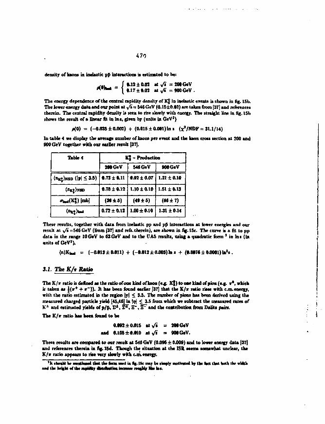
470
density of kaons in inelastic pp interactions u estimated to be:
/ 0.12 ±0.02 at y/i = 200 GeV\ 0.17 ±0.02 at V» = 900 GeV .
The energy dependence of the central rapidity density of K| in inelastic events is shown in fig. 15b.The lower energy data and our point at \fi = 546 GeV (0.15±0.02) are taken from [37] and referencestherein. The central rapidity density is sees to rise slowly with energy. The straight line in fig. 15bshows the result of a linear fit in Ins, given by (units in GeV1)
MO) = (-0.035±0.002) -I- (0.016±0.001)Ins (x'/NDF = Jl.1/14)
In table 4 we display the average number of kaons per event and the kaon cross section at 200 and900 GeV together with our earlier result [37].
Table 4
<nK;)h5D (|*| < 3.5)
("K;)NK>
oiUKS) [mb|
Kj - Production
290 GeV
0.73 ± 0.11
0.78 ± 0.12
(30 ±6)
0.72 ± 0.12
548 GeV
0.92 ±0.07
1.10 ± 0.10
(49 ±S)
1.00 ±0.10
900 GeV
1.21 ±0.10
1.51 ± 0.13
(W±7)
1.31 ±0.14
These results, together with data from inelastic pp and pp interactions at lower energies and ourresult al yfi=546 GeV (from [37] and refs. therein), are shown in fig. 15c. The curve is a fit to ppdata in the range 10 GeV to S3 GeV and to the UA5 results, using a quadratic form 3 in b s (inunits of GeV1),
( n ) K u = (-O.«13± 0.011) + (-t.O12±0.00J)lns + (0.007* ±0.0001) la's .
3.1. The K/t RMtio
The K/r ratio is deCnwI as the ratio of one kind of kaon (e.g. Kj) to one kiad of pion (e.g. r*, whichis taken as \{r* + r~)). It has been found earlier [37] that the K/r ratio rises with cm.energy,with the ratio estimated in the region |y| < 3.5. The number of pions has been derived using themeasured charged particle yield [45,46} in |IJ| 1_3.5 from which we subtract the measured rates ofK* and estimated yields of p/p, £*, S 7 , H", 3~ and the coatributiM from Daltti pain.
The K/r ratio has W a found to be
0.992 ±0.015 a ty^ = 209 GeVand 0.105 ±0.010 at -fi = 909 GeV.
These results are compared to our result at M< GeV (0.095 ± 0.009) and to lower energy data [37)and references therein in Jig. 15d. Though the situation at the ISR seems somewhat unclear, theK/r ratio appears to rite very slowly with e t a energy.
'It ih—M he imsstws* t»t 1W turn med U If. l»c B»J be tlmpiT suttnui fcy tkt bet tktt bath the wMth•a* the hc ht of la* miUkj «HstssWU*a inewtw m«Ur life bs.
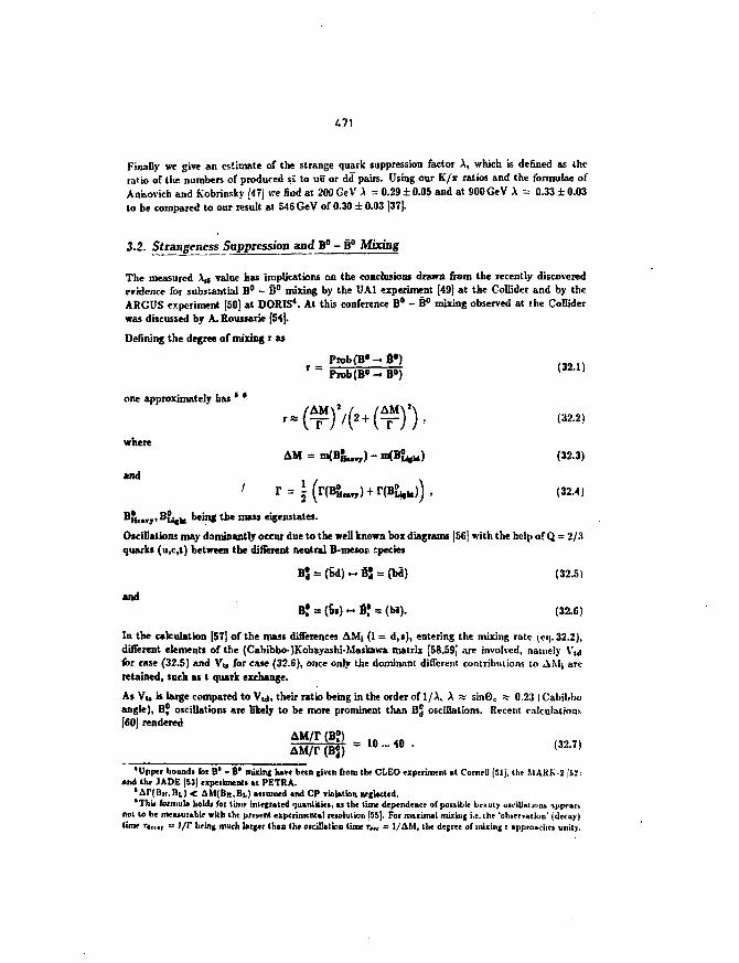
471
Finally we give an estimate of the strange quark suppression factor A, which is defined as theratio of the numbers of produced ss to uu or dd pairs. Using our K/x ratios and the formulae ofAnisovich and Kobrinsky [47] we find at 200GeVA = 0.29 ± 0.05 and at 900 GeV A ~ 0.33 + 0.03lo be compared to our result at 546 GeV of 0.30 ± 0.03 [37].
3.2. Strangeness Suppression and B" - B° Mixing
The measured A,i value has implications on the conclusions drawn from the recently discoveredevidence for substantial B° - 6° mixing by the UA1 experiment [49] at the Collider and by theARGUS experiment [50] at DORIS4. At this conference B° - B° mixing observed at the Colliderwas discussed by A. Rousiarie [54].
Defining the degree of mixing r as
Pr»b(B*~8»)r " Piob(B<>-B<>) ( 3 2 1 )
one approximately has ' *
where AM = m(BS,w) - mfBL,!,) (32.3)
" * 1 / \
' r = i ( r ( a t ^ ) + r(B8hl,))> (32.4)BH«rj>Bu»ki being the mass eigenstates.
Oscillations may dominantly occur due to the well known box diagrams |56] with the help of Q = 2/3quarks (u,c,t) between the different neutral B-meson cpeeies
Bj = (bd) " fij = (bd) (32.5)
andB? = (bi) « SJ = (bi). (32.6)
In the calculation [57] of the mass differences AM; (i = d,s), entering the mixing rate (eq. 32.2),different elements of the (Cabibbo-)Kobayashi-Maskawa matrix [58.59] are involved, namely \'nfor case (32.5) and Vt» for ease (32.6), once only the dominant different contributions to AMj areretained, such as t quark exchange.
As Vu is Urge compared to Via, their ratio being in the order of I/A. A % sinOc % 0.23 I Cabibboangle), Bj oscillations are likely to be more prominent than Bjj oscillations. Recent calculations|60J rendered
jj'Upper boundi for B' - 8 ' miiin{ have b « n (iven bom the CLEO experiment *1 Cornell [51], the MAKK-Z [5.':
»nd Ihe JADE (53) eipeiimenli «t PETRA.'ArfBu.B, . ) < A M ( B K , B I . ) Msumed >nd CP TioUtion neglected.*Thi< fotmuU liolJj for time intefnted <]u>nlitiei, u the time dependence of possible benuty oscillaiions ippratv
not lo be meuurable witll the present uperiroenUl lewlution [55). For maximal miiin( i.e. the 'observation' (decay)time T4ttAt = J/P bein( much larger (ban the osdJJation time rMC = I/AM, the degree of mixing E approaches unity.
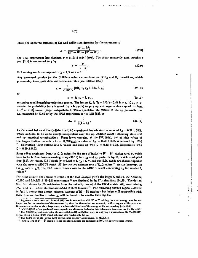
472
From the observed numbers of like and unlike sign dimuons for the parameter x
> B°) ' ( 'the UA1 experiment has obtained x = 0.121 ± 0.047 [49b]. The other commonly used variable r(eq. 32.1) is connected to x by
» = ~ • (32-9)
Full mixing would correspond to x — 1/2 or r = 1.
Any measured Rvalue (at the Collider) reflects a combination of Bd and B, transitions, whichpresumably have quite different oscillation rates (see relation 32.7):
X = — ^ [BRa fa xt + BR, U X.\ (32.10)
or
X = Uxi+Ux. . (32.11)
assuming equal branching ratios into muons. The factors f,, fj (fa = 1/2(1 - f,) if fa = ful fc,b,i = 0)denote the probability for a b quark (or a b quark) to pick up a strange or down quark to forma BJ or a BjJ meson (resp. antiparticles). These quantities are related to the Xti parameter, ase.g. measured by UA5 or by the SFM experiment at the ISE [62], by
As discussed before at the Collider the UA5 experiment has obtained a value of A,, = 0.30 ± 20%,which appears to be quite energy-independent over the pp Collider range (including statisticaland systematical uncertainties). From lower energies, at the ISR [62a], but at high values ofthe fragmentation variable z (z = Ej/£EH.d), a value of A* = 0.50 ± 0.05 is inferred by [62b|r . Converting these results into f, values one ends up with f, = 0.13 ± 0.02, respectively with4 = 0.20 ± 0.02.
Some effect originates from the f.,fa values for the case of inclusive B° - 6 ° nixing rates \ , whichhave to be broken down according to eq. (32.11) into Xd and \'i parts. In fig. 16, which is adoptedfrom |55l, the central UA1 result (x = 0.121 = fa Xi + U Xt ***& o n e S.D. bands are shown, togetherwitli the newest ARGUS result [50] for the two extreme lets of [,,[4 values ' . As the intercept onthe x, axis is y/f,, the UA1 result comes closer to the ARGUS result concerning Xd for smaller f,values 9 .
For completeness the combined results of the UA1 analysis (with the larger f, value), the ARGUS,C'I.EO and M ARK-2 [49-52] experiments 1 0 are displayed in fig. 17, taken from [54,55]. The dottedline, first shown by [55] originates from the unitarity bound of the CKM matrix [64], constrainingV,,) anil IV,, .vithin in standard model of three families " . The remaining allowed region is dotted
in fig. IT. demanding almost maximal amount of B? - Bj mixing - but being still compatible withthree fermion faniilies - unless X. will be found to be smaller than say 0.4.
r Argument* have been put forward [63] that in connection with B* — 8* mixing the cm. energy may be k »important for the usefulness of the measured An than the kinematkal environment, i.e. the z region, as the producedB-tiifsons carry, i!ur to their large mass, a substantial fr&tlion of the energy of the surrounding jet [49,55],
'In M9.S5] HI';; of the produced beauty quarks aie allowed to hadroniie into B-baryons, hence one has f, + 2£i = 0.9.'The A RGUS experiment, being the susceptible to B' oscillations only, as studying B mesons from the T<s( 10575)
decay, which b below Bf Bf threshold, may give results only for Xi'°Thr JADE rpsult [53] is less tight on the same quantity as measured by MARK-2.M Implications of B* - B* mixing to non-standard models are discussed in [65], see also references therein.
£73
4. The Average Event
Here t!>e knowledge obtained so f;ir on the pp.rlicle composition of a typical event in inejastir(non-sin^lc diffractive, to be precise) pp collisions at Collider energies will be summarized.
The inforu .'lion is most complete from the first runs at v's = 546 GcV. the corresponding figuresfn>mlli> <i;iii> taking at v? '•"- 200 and POO GeV are coming in. as (he mo'hods to '1 ••."ermine mcli'skerriiss >i I-MMII-. for specific particles. lot.»l multiplicities [or charged p.irtic!i:> and ill* like .ire knowr.and (es'e-l. For the CAS expcrini'-(i<. for which oae goal was a rapid survey on part kta productionat Collider i-ncrgi<>s :f.i),67], these methods have been .lescribed in various, publications, the Monte•' .irin jrrogf.t.n.'. involved are presented in a dedicated article [21].
Mniiy of the figures given in table 5 {abbrevi.'.iod from (61,0. which contains rates for individualkinds of j;.ir( iclw in ii"n-smg!c diffractive even's at the Collider, and for rnmparison. at highestiSK i-ncr^. •.•., an- deduced by indirect methods. This will be explained in detail later, togetherxvilh individual references. As far as data from th'.1 Collider are concerned, they were obtainedwilli the I'Aa deteclor jf>,f'Si, un!es? explicittly stated otherwise. We Live to warn the reader thai.•.nine figures presented in tahle 5 might well be updated in between now- and the printing of thoseproceedings.
lea-ling particles (i.e. one haryon and anti-baryor. per event, with eqiu l pro'iiiiitilies for protnrjand neutron) are always excluded frnn, (.hat table. Throughout isospin symmetry K .T«IIII.--VJ. e.j;.to mfer n()j -, p) from <r(n •> fi) measureinentb. Finally the average numhtt of ,-i;arei-<) pious i-;".tiinaUd by subtracting ail other sources of charged particles from the total rhar^t') muitiplicity
Kro.n t.i'ile 5 one may nr.Lici' a discrepancy between J<T(T-1 and \c(f) (- T(T"; - «ssi!Fni»g allphr.niK originate from ir" decays). One possible origin of this discrepancy is th< iroductjon of»; unisons, which on average deliver 2.65 more photons than charged pions when H>v;iving. flicnumber cC ti's given in table 5 has been adjusted to account for the photon excess at each energj' . One cm> jjut, of course, exclude other sources for this exceFs of photons, or the intTesting casi-.that for unknown reasons there are more primary 7r°'s produced than r* or x".
In (he Inst roiv of tabled vie have given estimates for the average number ol stab]'; particles producedin total, which is at least fifty panicles at highest Collider energies. Into the term stable particles'we have uicludm: k, p, n, A, E, H (and their anti-particles), ;/ and r if not coming frjin the decayof n mesons. As the H, S, A and nudeon rates are given inclusively, i.e. not corrected for hyperondecay, one could remove about two particles (nucieons and pions) from the stable psrtic'e roum.
In a very first approximation, the relative abundance of the different kinds of [jar! ides does notchange between -/i = 53 and 900 GeV, if it were not for baryons, whose contribution is quite srnal'at ISR energies, see also table 6.
In tahle 6 rates for some kinds of particles and particle ratios in their dependence on the cm.energy are collected. One may notice that surprisingly the relative kaon content in the final stateremains constant (within errors) at a level of about 9% • or. when compared to 'direct pious' (asfrom the bottom part of table 5) docs not change much, either.
1 Concerning the number of fj's estimated this way the measured photon yield *\ ,/i = 546 GeV fG9,7Oj now app'.'Hi:.rather high, when combated with the corresponding figures at the other Collider energies, sre tablr T,. The niob&birreason b>> in the photon detection tyttem of the UAS apparatus itself. The data on which the former pholon analviuwas based originated from conversions in the corrugated steel beam pipe'only, whilst for the newer photon anitiysLi[71 j one could make use of a photon converter plate [72,73], which was added in view of the Cemauro question.
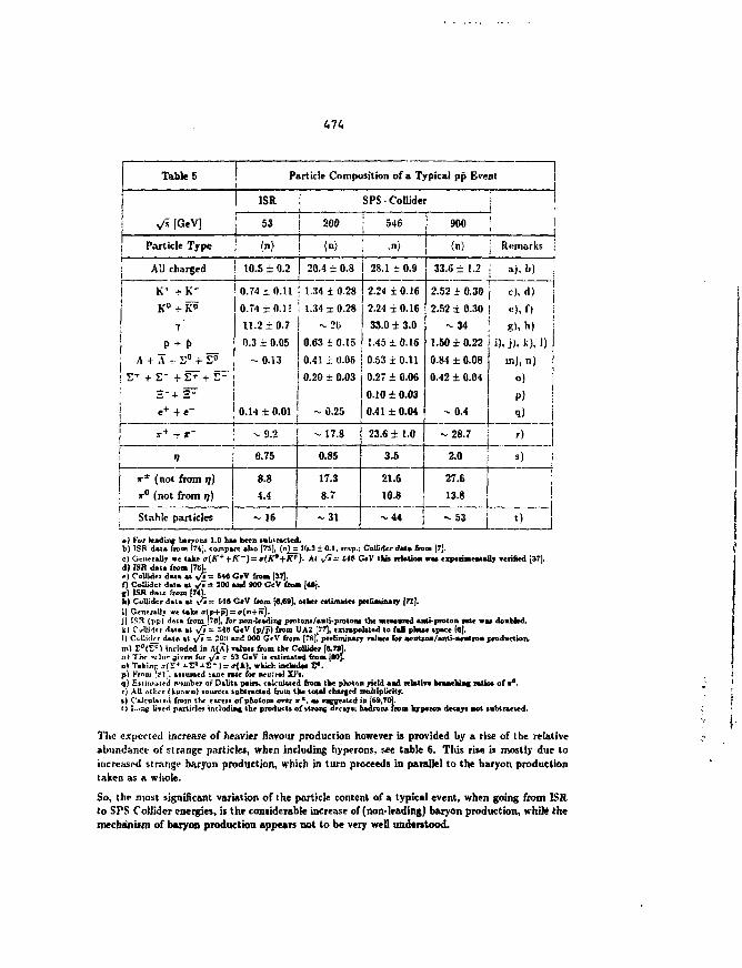
Table 5
Js [GeV!
Particle Type
: AD charged
K1 +K"
iP + P
' A t A r S ' + F
-t-
ID
e + + e -
IT1 (not from 17)ir° (not from IJ)
Stable particles
Particle Composition of a Typical pp Eventt
ISR
S3
(•>
10.5 ± 0.2
0.74 -0.110.74 ±0.1!
11.2 ±0.7
0.3 i 0.05-0.13
0.H ± 0.01
- 9 . 2
0.75
8.84.4
~ 16
I1
j 2C0
w20.4 ± 0.8
1.34 ±0.281.34 1 0.28
- 2 0
0.63 ±0.15
0.41 1 0.060.20 ± 0.03
-0.25
- 17.8
0.85
17.38.7
- 3 1
SPS-Collide
| 546
; ..•>}
28.1 ± 0.9
2.24 ±0.16
2.24 ± 0.163S.0 ± 3.0
1.45 ±0.160.53 ± 0.110.27 i 0.06
0.10 ± 0.030.41 ± 0.04
23.6 ± 1.0
3.5
21.610.8
- 4 4
900
(n)
33.6 ± 1.2
2.52 ± 0.30
2.52 ± 0.30- 3 4
1.50 ±0.22
0.84 ± 0.080.42 ± 0.04
- 0.4
-28.7
2.0
27.613.8
- 5 3
Remarks
a), b) ;
c), d) j
«), 0 ig) , l> )
i),)), k), 1)m), n)
0 )
P)q)
r)
s)
1
I• J For leading barvcni 1.0 hms been inbtr«eted.b) 1SH d . t . from t74j. compare >bo [75], (nJUl&.3±0.1, i«,r.; ColMcrd.l. from [7J.c) C«irr«llv we tike »(«"+ +*r~)= irfA^+A'"). At y ? - E«P GeV Ihis rtl.tio. « w e ipeaneMd; rtiifini 1371.d) ISR d.c. from [76).<) Collider <9>t« « V ' = » » GeV Iro» (37].0 Collider d . l . u ^7= 200 u d 900 GeV torn [4«j.( ) ISR daii. from [HIh) Collider d«i« i l , S = S4S GeV bom !«,«»]. other eitimOei pnEmUuiy |71).i) OenrrftUv we Islce <rlp+p) = 7(n+fr).i) ^ ^ {VP) < 4fk ^ n t {TffJ, for non-leading prolons/aati-proloM the MeMTUtii aati-proton rate vat doabled.k) CMv'.tr dala al >/7- Me GeV (p/p) from UA2 [77], enrapolated to fml pkafe apace (Sj.I) Ci-likl^r dat« at V* = 203 *n<! 000 GeV from [78j, preliminaxr ralne* Ibf iieiiiroii/anli-AeatioB production.tn) T"fZ') included in A£A) nines from the Collider [8.7»J.a* The vein- jiven for y"* - S3 CeV it eitimated irom {SO].01 T.kiiv,: .T(L'* i r ° J - r - ) = <r(A), wkich inctadet f.p) Krom [ 1;. atftumed1 sane rate for netrfral Xi't.q) EuiiamtA number of DalitK pain, calculated from the photon jrield aad relatiTe brajiclamt ratio* of **.r) All i>ilirr (kjinwn) soitrcet labtracted from tke total charged1 multiplicity.• ) Calculate'! from the ttcttt of photons over IT*, a* taggested in [6fi,7O).t) l-'ttg lived particles including the products of strong decays; hadrons front hjrperon decays Mot tubtraeted.
The expected increase of heavier flavour production however is provided by a rise of the relativeabundance of strange particles, when including hyperons, see table 6. This rise is mostly due toincreased strange baryon production, which in turn proceeds in parallel to the baryon productiontaken as a whole.
So, the most significant variation of the particle content of a typical event, when going from ISRto SPS Collider energies, is the considerable increase of (non-leading) baryon production, white themechanism of baryon production appears not to be very well understood.
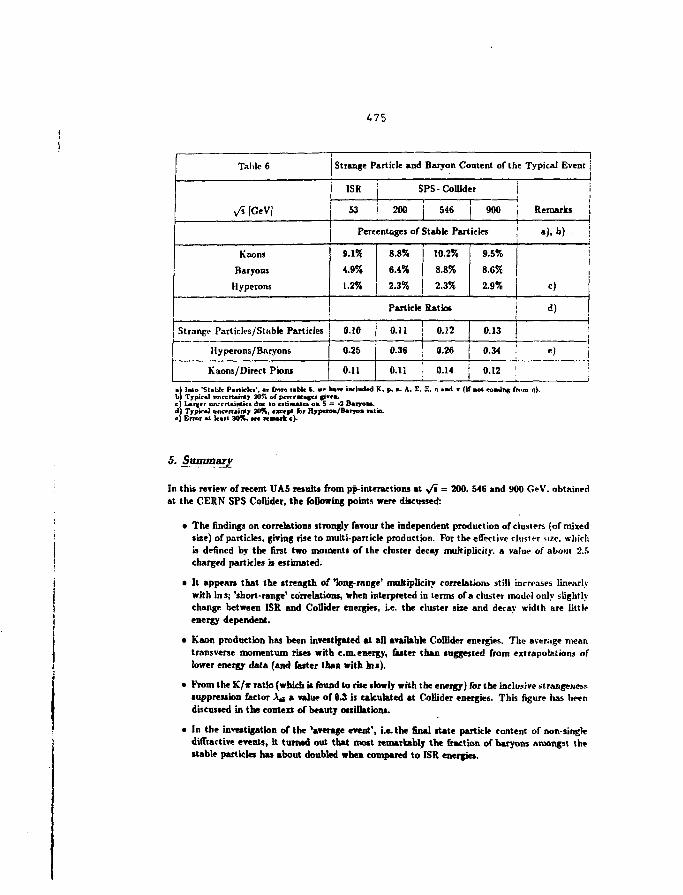
475
Table 6
•/i [GeV]
Kaons
Raryons
Ilyperons
Strange ParticU-s/Stable Particles
Ilypcrons/Baryons
Kaons/Direct Pions
Strange Particle and Baryon Content of the Typical Event
ISR
53
SPS- Collider
200 j 546 900
Percentages of Stable Particles
9.1%
4.9%
1.2%
0.10
0.25
0.11
8.8%
6.4%
2.3%
10.2%
8.8%
2.3%
Particle Ratios
0.11 0.12
0.36 0.26
0.11 1 0.14i
9.5%
8.6%
2.9%
0.13
0.34
0.12
Remarks
«),b)
j
c)
d)
Into 'Stable Psitklcf'. at from taMc S. w hkvc included K. p, ft. A. E, E. >) and * (if aol coming from rj).Typical tincertairtfy 70% of perreMages fjre*.Larger uncertainties doe to estimates a i 5 = -2 Baryoaa.Typical uncertainly 30%, except lot Hjperoa/Baryoa tatio.Error at least 30%, Me fesftatk c).
5. Summary
In this review of recent UA5 results from pp-interaetions at v's = 200. 546 and 900 G«-V. obtainedat the CERN SPS Collider, the following points were discussed:
• The findings on correlations strongly favour the independent production of clusters (of mixedsize) of particles, giving rise to multi-particle production. For the effective cluster size, whirl:is defined by the first two moments of the cluster decay multipliciiv. a value of about 2.5charged particles it estimated-
• It appears that the strength of 'long-range' multiplicity correlation* still increases linearlywith Ins; 'short-range' correlations, when interpreted in terms of a cluster model only slightlychange between ISR and Collider energies, i.e. the cluster size and decay width are littleenergy dependent.
• Kaon production has been investigated at all available Collider energies. The average meantransverse momentum rises with cm.energy, (aster than suggested from extrapolations o flower energy data (and fatter than with bis).
• From the K/» ratio (which it found to rise .lowly with the energy) for the inclusive strangenesssuppression factor \j a value of 0.3 is calculated at Collider energies. This figure has beendiscussed in the context of beauty ossillations.
• In the investigation of the 'average event', i.e. the final state particle content of non-singlediffractive events, it turned out that most remarkably the fraction of baryons amongst thestable particles has about doubled when compared to ISR energies.
47«
References
[1| CERN/SPSC/82-75, SPSC/P184, UA5-Collaboration, 15 October 1982.[2! C. Geich-Gimbel, IX. Warsaw Symposium on Elentary Particle Physics, Kazimierz, Poland,
May 25-31, 1986, Proc., p. 173.[3] G.J. Alner et aL, UA5-CoUaboration, Z.Phys.C 32 (1986), 153.|4) R.E. Ansorge et aL, UA5-Collaboration, Z. Phys. C 33 (1986), 175.{51 G.J. Alner et aL, UAS-Collaboratlon, Phy>. Lett. B 180 (1988), 415.[6] G.J. Alner et »1., UA5-Collaboratkm, submitted to Physics Report.|7j G.J. Alner et aL, UA5-Collaboratk>n, Phys. Lett. B 167 (1986), 476.[8] UA5-Collaboration, 'Charged Particle Correlations at the Collider', in preparation for sab-
mission to Zeitschrift fur Physik C, 1987.[9] B. Holl, UA5-Collab., 6th Int. Conf. on pp Physio, Aachen, Germany, June 30 - July 4,
1986; Proc. p. 500.B. Holl, PhD-Thesii, Bonn University, in preparation.
[10] G. Ekspong, 3rd Top. Workshop on pp Collider Physics, Rome, Italy, January 12-14, 1983;eds. C. Bacci and G. Salvini, CERN 83-04 (Yellow Report), 1983; p. 112.
[11? G. Ekspong, UA5-CoUabor«tion, UA5-Memo A, Oct. 1982.[12] S. Uhlig et al., NucL Phys. B 132 (1978), 15.[13! K. Alpgird et al., UA5-Collaboration, Phys. Lett. B 123 (1983), 361.[14; B. Eckart, XVIIL Rencontre de Moriond, La Plagne, March 19-25,1983; ed. J. Tran Thanh
Van, Editions Frontieres, Gif-sur-Yvette, 1983; p. 155.[15] G.J. Alner et aL, UA5-Collaboration. Phys.Lett.B 160 (1985), 193.[16] E.L. Berger, NucL Phys. B 85 (1975), 61.[17] G. Giacomelli and M. Jacob, Phys. Rep. 55 (1979), 1.1181 i. Wrdtmore, Phyi. Rep. 27 (1976), 187.J19i L. Foa, Phys. Rep. 22 (1975), 1..'201 G. Ekspong, Proc. of the 3rd Topical Workshop on Proton-Antiproton Collider Physics,
CERN Yellow Report 83-04, 1983, p. 112.[2i; G.J. Alner et al.. UA5-Collab., CERN-EP/86-213, Dec. 1986 ('The U W High Energy pp-
Simulaeion Program'); Nncl.Phys.B 291 (1987), 445.[22 B. Eckart. XVIII. Rencontre de Moriond. La Plagne, March 19-25,1983; ed. J. Tran Thanh
Van, Editions Frontieres, Gif-sur-Yvette, 1983; p.155.K. Bockmann and B. Eckart, XV. Int. Symp. on Multiparticle Dynamics, Lund, Sweden,June 10-16. 1984; Bonn University, BONN-HE-84-22.
[n} S.R. Antendolia et aL, Nuovo Cimento 31A (1976),17.D. Drijard et aL, Nucl.Phys.B 155 (1979),269.W. Bell et al., Z.Phys.C 22 (1984),IO9.
124] A. CapeUa and J. Tran Thanh Van, Z. Phyi. C 18 (1983), 85.125, Meng Ta-chung et aL, Phys. Rev. D 27 (1983), 2640.
Meng Ta-chung et al., Phys. Rev. D 33 (1U86), 1287.J26' For further references on Two-Particle Rapidity Correlations' see reft. [1,2] of ref. [16].[27; A.H. Mueller, Phys. Rev. D 4 (1971), 150.!2»: K. Eggert et al., NucLPhys.B 86 (1975), 201.[29! J. Benecke and J. Kuhn, Nncl.Phys.B 140 (1978), 179.[30' G J. Alner et aL, UA5-Collaboration, Phys. Lett. B 160 (1985), 199.|31 A. Bialas, Proc. IVth INT. Symp. Multiparticle Hadrodynainics, Pavia 1973, Italy; p. 93.[321 P. Pirila and S. Pokorski, Phys. Lett. B 43 (1973), 302.[33] K. Bockinann and B. Eckart, XV. Int. Symp. on Multiparticle Dynamici, Lund, Sweden,
un
Juno 10-16, 1981; Boj.n .'• diversity, BONNHE-84-22, Sept. 1984.|34j T. Kafka et AI.. l'hys. Jiev. D 16 (1977). 1261.|.ir>| G. F.'i.spong. 3rd Top. Workshop on pp Collider Physics, Rome. Italy, January 12-14. 1983;
«Is. C. Barri and G. S.ilvini. CERN 83-04 f Yellow Report), 1983; p. 112.|3li) P. Carlson, I'A5-Collab., XI. Int. Winter Meeting on Fundamental Physics, Toledo. Spain.
April 1116, 1983.|»ïj C..J. Airier et al., UA.VCollab., Nucl.Phys.B 258 (1985), 505.[:I8J A. Casher et al., Phys.Iîev.D 20 (1979), 179.[39] Ci. Ariiison et al., UA1 Collab., Phys .Utt .B 118 (1982), 167.1-10'. M. Banner et al., UA2 Coliab., E.Pliys.C 27 (1985), 329.j-flj M. Banneret al., UA2 CoUab., Phys.Lett.B 122 (1983), 322.j-12; K. Guctller et al., Nud. Phys.B 116 (1976), 77.[\3\ R. Hagedorn, Rev.Nuovo Cim. 6 (1983) no. 10.[44] G. Ciapetti, UAl-Collab., Procof The Quark Structure of Matter, Karlsruhe-Strasbourg
1985; p. 455.(45) G.J. Alner et al., ÜA5-CoUab., Phys. Lett.B 167 (1986), 476.[4Cj K.E. Ansorge ct aL, UA5-Collah., in preparation.
C. Fuglesang, UA5 Collab., Proc. of the 17th Symposium on Multipartite Dynamics.Seewinkel, Austria (1986),p. 553.
(171 V.V. Anisovich and M.N. Kobrinsky, Phys.Lett.B 52 (1974), 217.[48] R.E. Ansorge et al., UA5-Colîab., 'Kaon Production at 200 and 900 GeV c m . Energy', to
appear in Phys. Lett. B.1-19) C. Albajar et al., Phys.Lett.B 186 (1987), 237.
C. Albajar et al., Phys. Lett. B 186 (1987), 247.[50] H. Albrecht et al., ARGUS Coll., Phys.Lett.B 192 (1987), 245.|51] A. Bean et aL, PRL 58 (1987), 183.[52| T. Schaad «t al., Phys. Lett. B 160 (1985), 188.[53] W. Bartel et al., Phys. Lett. B 146 (1984), 437.[54] A. Ronssarie, at this conference.
!55] K. Eggcrt and H.G. Moser, UAl-CoIL, 1st Int. Symp. on the 4th Family of Quarks and Lep-tons, Santa Monica, USA, Feb.26-28, 1987; RWTH Aachen, PITHA 87-10, Juni 1987; seealso: K. Eggert, Proc. of 'New Particles 1985', Wisconsin, ed. by V. Barger et al.. WSPC.p. 207; K. Eggert, Proc. 21th Rec.de Moriond, Les Arcs, France, 1986, 'Progress in Elec-troweak Interaction', Ed. Frontières, p. 369; H.G. Moser, Proc. 21th Rec.de Moriond, LesArcs, France, 1986, 'Strong Interactions and Gauge Theories', Ed. Frontières, p. 331.
[56] M.K. Gaillard and B.W. Lee, Phys.Rev.D 10 (1974), 897.|57] A.J. Buras, W. Slominski and H. Steger, NucL Phys. B 245 (1984), 369.
A.l. Buras, W. Slominski and H. Steger, NucLPhy». B 238 (1984), 529.J.S. Hagelin, Nucl.Phys.B 193 (1983), 123.
[58] N. Cabibbo, Phys. Rev. Lett. 10 (1963), 531.[59] M. Kobayashi and T. Maikawa, Progr. Theor. Phys. 49 (1973), 652.|60] A. Ali, Dety 85-107.
A. Ali and C. Jarlskog, Phys.Lett.B 144 (1984), 266.V. Barger and R.J.N. Phillips, Phys.Lett.B 143 (1984), 259.V. Barger and RJ.N. Phillip», Phy». Re». Lett. 55 (1985), 2752.I.I. Bigi and A.I. Sanda, NucLPhyi.B 193 (1981), 85.I.I. Bigi and A.I. Sanda, Phy«. Rev. D 29 (1984), 1393.
[61] C. Geich-Gimhci, 'Particle Production at Collider Energies', University of Bonn, in prepa-ration (1987).
478
(62j A. Breakstone et al., Phys. Lett. B 135 (1984), 510.W.M. Geist, 22th Rene, de Moriond, Les Arcs, France, March 15-21, 1987.
[63] K. Eggert. UAl-ColL, private communication, June 1987.[64] G. Altarelli and P.J. Franiini, CERN-TH.4745/87, May 1987.(65! K. Kleinknecht and B. Rerdc, Z. Phys. C 34 (1987), 209.[66] UA5-Proposal CERN/SPSC/78-70/P 108, and addenda.(67) UA5/2-Proposal CERN/SPSC/82-75/P 184.[68] Bonn-Brussels-Cambridge-CERN-Stockholro Collaboration, presented by J.G. Rushbrooke,
Phys. Scr. 23 (1981), 642.[69] K. Alpgard et al., UA5-CoUab., Phys. Lett. B115 (1982), 71.[70] Th. MSUer, Ph.D.Thesis, Bonn University, BONN-IR-83-21, Aug. 1983.[71] UA5-Collaboration, 'Photon Production at 200 and 900 GeV cm. energy', in preparation
for submission to Zeitschiifl lur Physik C, 1987.[72] K.A. French, C. Geich-Gimbel, W. Pelzer. M.A.H. Tucker and D.R. Ward, UA5-Collab.,
CERN/EP/SCE-R703T/UA5/P84-7, July 1984.[73] W. Pelzer, UA5-Collab., Dipl. Thesis, Bonn Univ., BONN-IR-85-39, Dec. 1985.[74] K. Alpgard et aL, UA5-Coll., Phys.Lett.B 112 (1982), 183.175] W. Thome ,Ph.D. Thesis RWTH Aachen, PITHA 80/4, Feb. 1980.[76] A.M. Rossi et al., Nucl. Phys. B 84 (1975), 269; and references therein.|77] M. Banner et aL, UA2-Coll., Phys. Lett. B 122 (1983), 322.[78] R.S. DeWolf, UA5-Collab., Thesis, University of Cambridge, Dec. 1986.
L. Burow, UA5-Collab., Thesis, Bonn University, BONN-IR-87-25, July 1987.[79] UA5-Collaboration, 'Hyperon Production at 200 and 900 GeV cm. energy', in preparation,
1987.[80] S. Erhan et al., Phyi.Lett.B 85 (1979), 447.|81] G J . Amer et aL, UA5-ColL, Phys.Lett.B 151 (1985), 309.
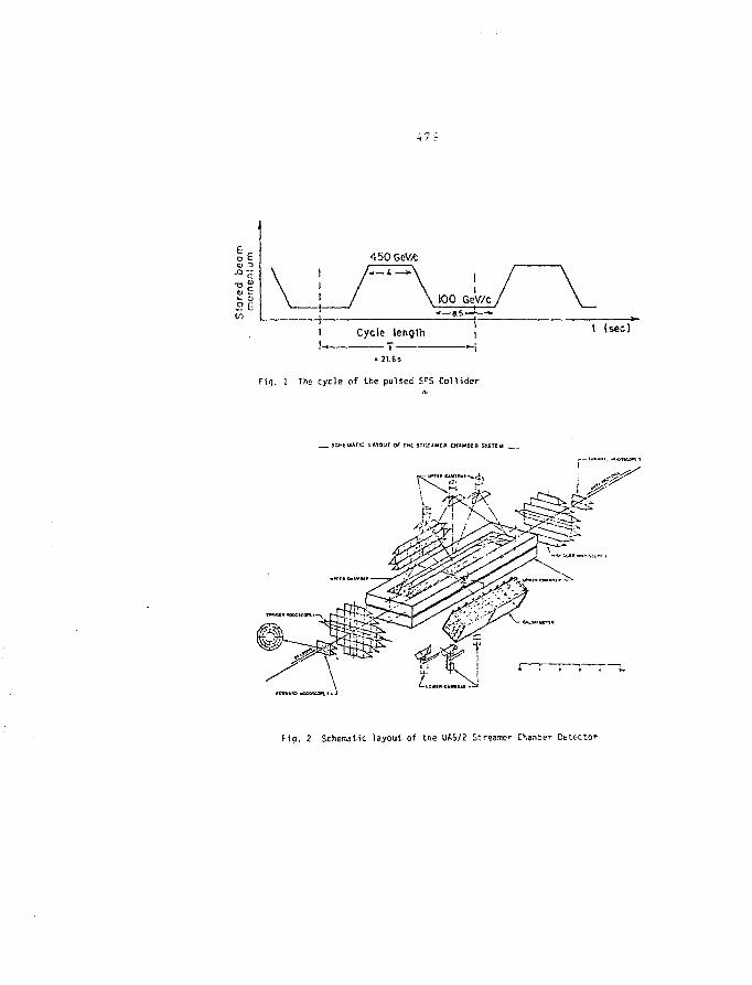
t (sec)
Fig. 1 The cycle of the pulsed SP5 Collider
SCHEMATIC H Y O u r OF THC 5'REJMEfl OfAMSEfl SYSTEM
Fia. 2 Schematic layout of tne UA5/2 Streamer Chairtoer Detector
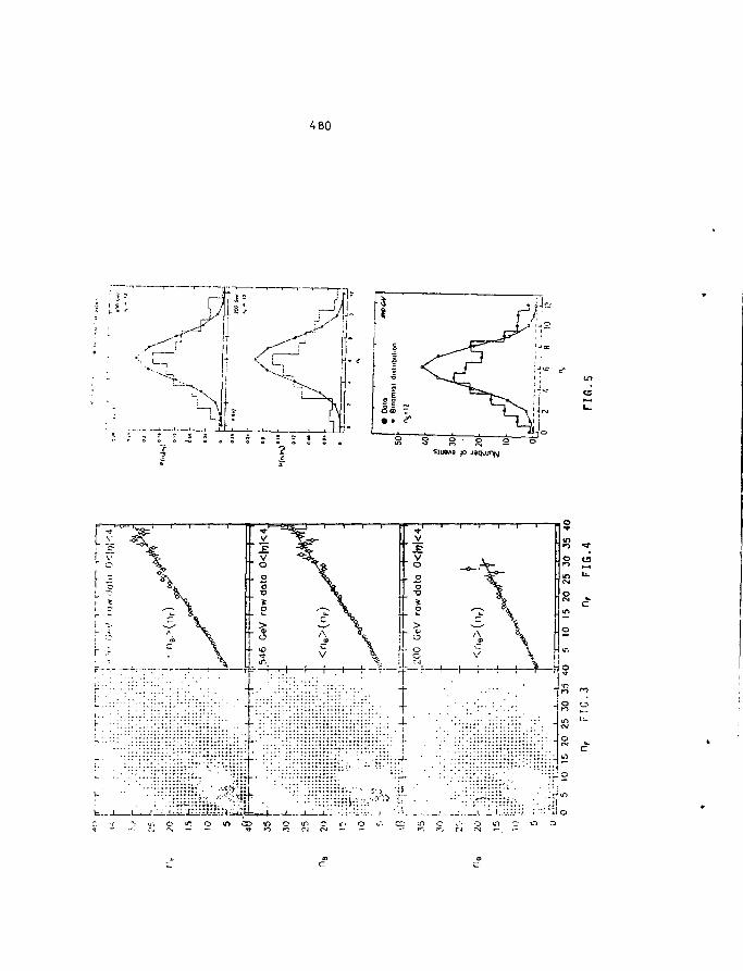
480
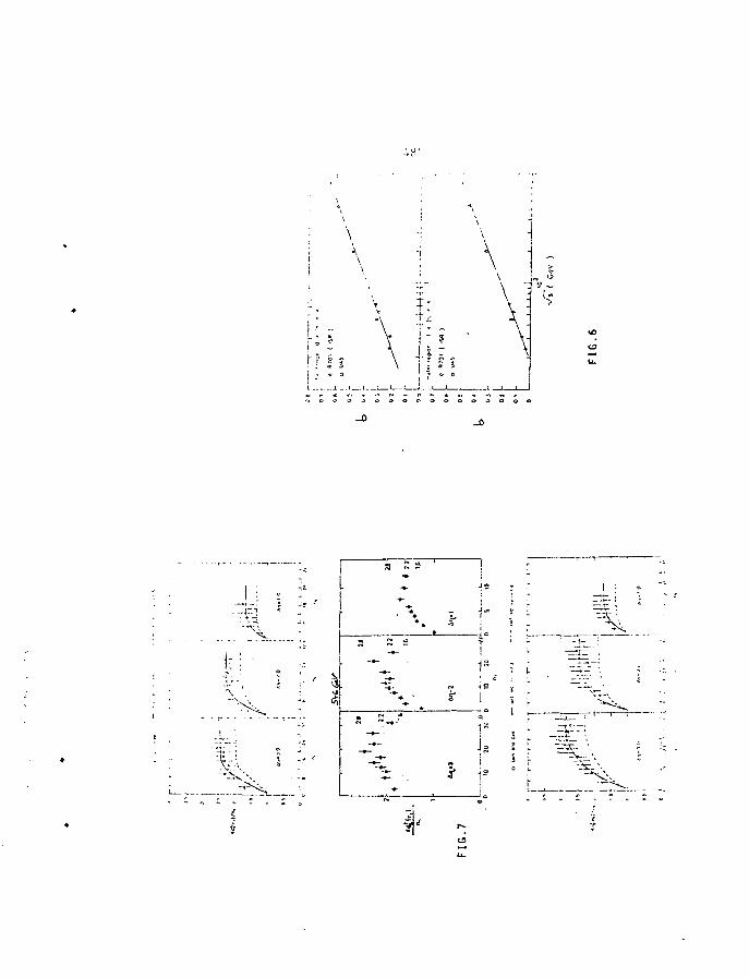
r r i s
I J. _.l-_.i-_
I S
• i *
I
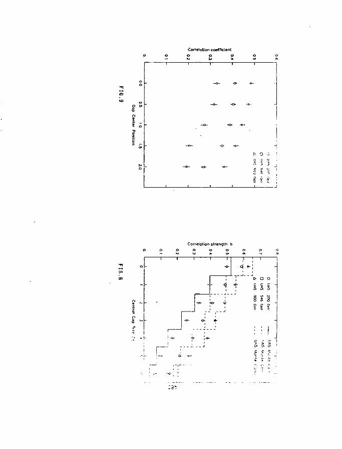
Correlolion coefficient
aUS
-
t 1
e1
- o -
-o-
1
- * ~
0.4
1
-o-
1
>
>
o
<i
D O
> •>
, 3
V <T
Correlotion strength b
D> a o jui m in
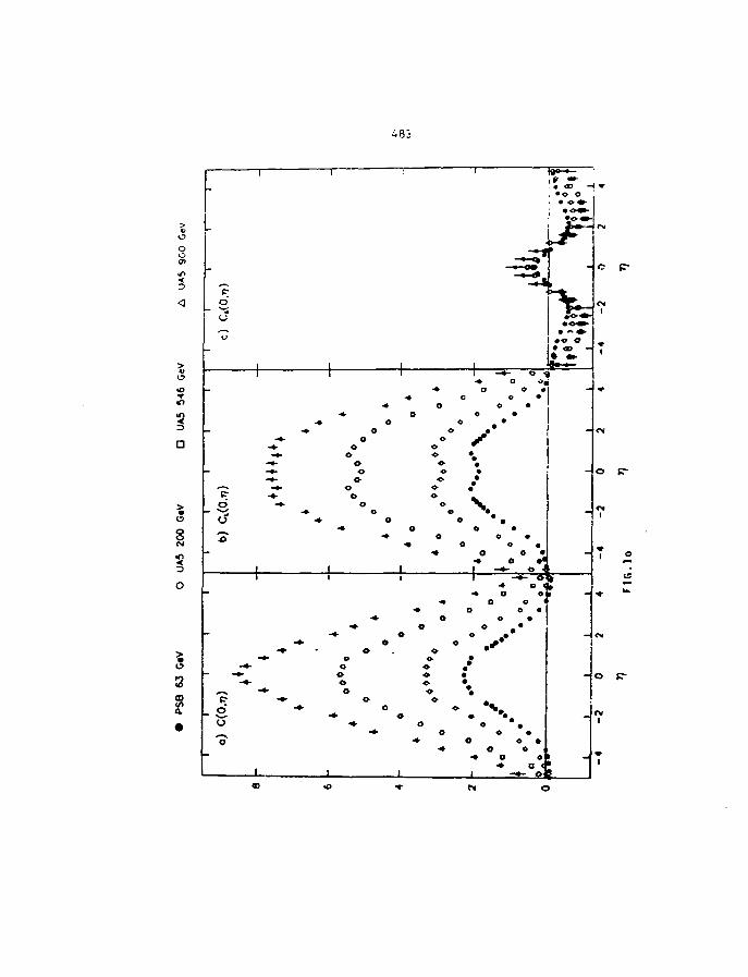
485
o
«o
i
d
3"
ft m-
o •
oo
ooo
ooo
o
• \> m
o
ao o
* o < « O O
•• o o <•» o o • I
o o •o « •
o • • •
oooo
o •o o •
o o•* o - -
•• o <•' - * -
o p-
H * »
O C-
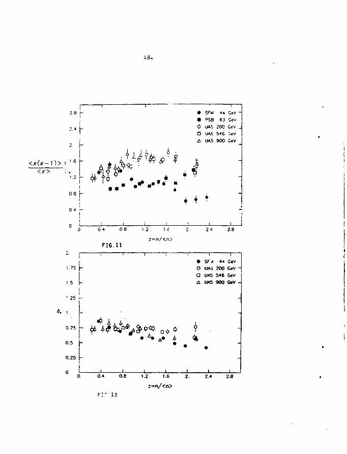
43*
2.8 r-
»h
1.2 t-
0.8
04 -I
0 o"
1.75
1.5
'.25 r-
1.
0.75
0.5
0.25
0
* •
•oo
SFM
PSBUAi
UAi
UA5
••-•
6320054 e
900
I
GeV -
CeV
GeV _
r,cv
—
-
0 * 08
FIG.11
1.2 2.8
r=n/<n>
• S F / 44 GeV
O UAo 200 GeV
O 0*5 5*6 GeV
/I UAS 900 GeV
Q O
0.4 0.8
FI" 12
1.2 1-6 2.
2=n/<n>
2.4 2.8
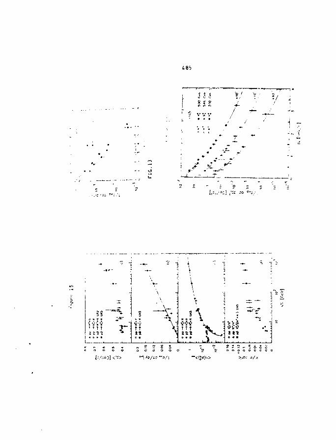
4 8b
ll O U
9, •£ 9
H _
<L
J i
I « o • •
t f
«1
3 i .
V Y V
• • • •
L-.f . L
. : : ] 5 o c- o o o o o c s c c
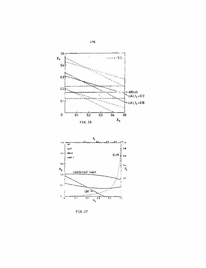
O.i
0 O.I 0.2 0.3 0.4 05
FIG.16 X s
FIG.17
487
QUARK FRAGMENTATIONin
SOFT K+p COLLISIONS AT 250 GeV/c
EHS-NA22 Collaboration
E.A. De WolfDepartment of Physics. University of Antwerpen, Belgium
ABSTRACT
Inclusivo data <ir» presented on p°. p+. a.1. A''0fSOJi and *f 10201. pro-duced in A+.» interactions at 250 O V / c . for /J4" and *• for tin- first limein a A'+p experiment. In the forward cm. hemisphere, the pT. p° andu; differential production rates are equal within errors, and remarkablysimilar to muon-inelastic scattering data on p° and *> at 280 GeV/c Inthe K+ fragmentation region, i > ".2. the ratio of <p to A'"°(892) isused to estimate the strangeness suppression factor A. with the resultA = 0.17 ± 0.02 (stat) i 1.01 (syst). We see no evidence for an energydependence of A in the cm. energy range 7.8 < ,/s < 21.7 GeV. -
1 Quark Fragmentation in Soft Collisions ?
In this talk I shall discuss new data on production cfiaracteristics of resonances insoft K*p collisions, and their interpretation in terms of quark fragmentation.
The subject of '•quark fragmentation" is most naturally studied in point-likoprocesses: e+e~ annihilations, deep-inelastic -scattering. For such reactions. QCDprescribes the dynamics at its earliest slage in terms of quarks and gtaons. Thefragmentation of these coloured objects enters in the evolution of the '"primordial-final state towards the observable world of hadrons. Such a two-stage picture is
remarkably successful in spite of some basic theoretical difficulties. It would besurprising indeed if nature has not invented a smoother and more elegant procedurethan the abrupt transition from quantum mechanics to Monte Carlo, as imaginedin present-day phenomenology !
Returning to soft hadron hadron interactions, it is well known that these sharemany similarities with point-like processes. Similarities, however, are more surpris-ing than the observed differences, since the dynamics is apriori more complicatedin the former. In a soft hadronk collision, ensembles of valence quarks and gluonsof beam and target most of the time interact at relatively large distances. Finalstate hadrons emerge in "jets" collimated along the line of Bight of the colliding ob-jects. However, experiment reveals that the inclusive production properties alongand transverse to these axes resemble strikingly those found in point-like processesalone the direction of the fragmenting quark (or diquark) systems. Are such sim-ilarities the reflection of common hadronisation dynamics or are they accidental ?At prfMnt. the former explanation seems prefered. but clear-cut evidence is stilllacking. If we adopt an optimistic point of view and assume that quark hadronisa-'lon is "universal", then we should address the question of the fate of valence quarksin a soft hadron hadron interaction.
Consider a K+p collision as an example. A beam of 1 and a valence quarks andfiuons infracts with a proton composed of three valence quarks and gluons. In afirst Ha-n of models, one imagines that the collision is initiated by gluonic nterac-tions. The valence quarks loose some energy but essentially behave as spc ;tators.The original valence quarks may either "recombine* into a "fast" particle or frag-ment independently. In the first case, we expect the beam fragmentation region tobe populated mainly by particles or resonances with the quantum numbers of theA'* beam: A'+>s. A"+(892.1420). In the second case, the * and u valence quarksfragment and produce roughly equal amounts of A'+'s and A'°'s. A'*+Is and A'"0
etc. N'aively. we expect the momentum distributions to be softer in the latter casesince two valence quarks have to share the available beam momentum.
In a second class of models, the interaction is viewed as a collison of one of thevaJence quarks (say the v quark of the A'+) with proton constituents. This quarkloows most of its energy whereas the ? quark continues as a spectator carryingits original momentum. Forward particle production is then dominated by thehadrmiisaiion of a single (3) quark. Alternatively, if the s quark interacts, we observe(lie (raijnientalion of the u quark. This picture implies that particle production inthe A * fragmentation region is a superposition of s- and u-quark hadronisation.
Which of these alternatives is chosen by nature ? This question has been thesubject of several investigations with A'+ and (more recently) JT+ beams. The
499
riwiiMi- ^ 1 nctictl arc:
r—O , v . [1~ n 892.1420 + Ji- \-l
at 32(1,2.31 and 70 GeV/c[4]. and
K+p - A'+.Y, (3)
- K$ + X: (4)
at 70 GeV/c[5j, and
A"> - p°+X. (5)
- p+ + X: (6)
at 210 CcV/c[G].
What has been learned from these studies can be summarized as follows:
• The total and differential cross sections of the pairs of reactions (1-2). (34), (5-6) are very similar in absolute vaiue and in shape. This excludes an
jmportant contribution from so-called "two-valence recombination".
• The data are well reproduced by a simple model which assumes that hadronproduction in tlie beam fragmentation region results from a superposition ofsingle quark hadronisation, whereby the fragmenting quark carries most ofthe momentum of the incident meson.
We therefore conclude that the second class of models (see above) conies clos-est to a description of the hadix final state in soft hadron hadron collisions.This further implies that the soft meson-proton interaction can be used as a ton)to study quark fragmentation. With kaon beams, this gives us the possibility tostudy f-quark fragmentation with better precision than is possible in other types ofinteractions.
In the rest of this talk, I shall briefly describe the data now being analyzed bythe EHS-NA22 collaboration (sect.2). In sect.3, I present new results on p+, p°and u resonances and a comparison with recent EMC data. Sect. 4 is devoted toa discussion of a new measurement of the strangeness suppression using data on •and A"0 resonances in A"+p collisions.
4 90
2 The JExperiment
The experiment (NA22) has been performed at CERX in the European HybridSpectrometer (EIIS). equipped with the Rapid Cycling Bubble Chamber (RCBC)as an active vertex detector and exposed to a 250 GoV/c tagged positive mesonenriched beam. In data taking, a minimum bias interaction trigger lias been used.The experimental set up and the trigger conditions are described in [7] and referencestherein.
The detector consists of RCBC embedded in a 2T magnetic field and a down-stream spectrometer composed of an additional IT magnet, a wire-chamber and sixdrift chambers. Charged particles are measured over the full solid angle with themoment inn resolution (Ap/p) varying from 2.5% at 30 GeV/c to 1.5% above 100GeY/r. Particle identification is supplied by RCUC. the Cerenkov counters SADand r e . I he ionization sampling device ISIS and the transition radiation detectorTH1)[7], The photon detection in the intermediate ami forward gamma detectors.IGI) and KGD. is described in detail in [ft]. Tlic combined acceptance of the 7detectors allows to measure T°'S for Z(JT°) > 0.025. The acceptance for p+ and u> is'lion restricted t o r > 0.06. For the p+ the sigral to background ratio is very small {for 1 < 0.2 and we have to limit ourselves to the region x > 0.2. '
In this analysis, events arc accepted when the measured and the reconstructedmultiplicity 11 are consistent, charge balance is satisfied no electron is detectedand the ;r.iiiibcr of badly reconstructed tracks is less than n/3 and smaller than•I. There arn 3(j.1()l) such inelastic h'+p cu'itts. corresponding to a sensitivity of2.0'> wi i ts / / /b . Charged particles for which the \-piobability of the best mass-hyptitlieMs is at l>-ast 10 times larger than that for any other mass hypothesis areconsidered "uniquely identified". To these we add protons and ?r+'s with laboratory-nionienium smaller than 1.2 GeV/c. idn '.ified in RCBC by ionization. All otherparticles are considered unidentified and taken to be pions.
3 Inclusive /)+0 and -• production
In spite of its importance for parton models, little is known about similarities ordifferences in the production o( p±, p° and u>. Tin's is mainly due to difficulties inthe identification and measurement of neutral pions.
In deep-inelastic lepton-nucleon scattering, p° and ui production are measuredfor the first time in the same experiment by the European Muon Collaboration)!)].The authors conclude that, in u-quark fragmentation, the differential production
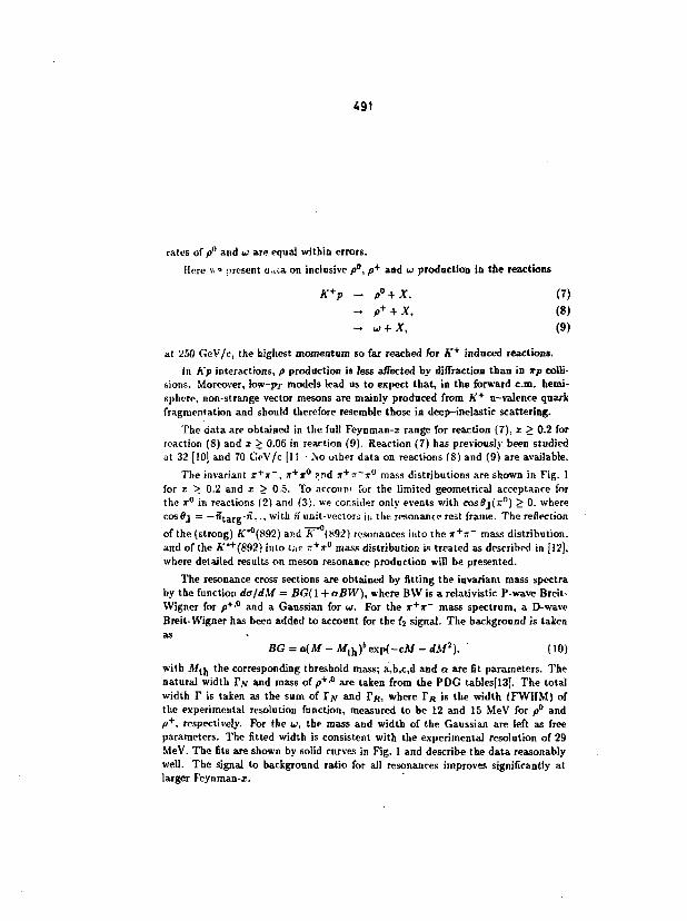
491
rates of p° and u are equal within errors.
Here \\ * .irrscnt u«a on inclusive />", p* and u> production in the reactions
K+p - />° + X. (7)- P+ + X, (8)- w + X, (9)
at 250 GfiV/c, the highest momentum so far reached for A'+ induced reactions.
In h'p interactions, p production is less affected by diffraction than in ffp colli-sions. Moreover, low-pr models lead us to expect that, in the forward cm. hemi-sphere, non-strange vector mesons are mainly produced from A'+ u-valence quarkfragmentation and should therefore resemble those in deep-inelastic scattering.
The data are obtained in the full Feynman-i range for reaction (7), x > 0.2 forreaction (8) and x > 0.06 in reaction (9). Reaction (7) has previously been studiedat 32 [10] and 70 GrV/c [11 -No other data on reactions (8) and (9) are available.
The invariant x+x~, J + T ° ?nd JT+T-X0 mass distributions are shown in Fig. 1for i > 0.2 and x > 0.5. To account for the limited geometrical acceptance forthe T° in reactions (2) and (3). we consider only events with COS0J(JT°) > 0. wherecosOj = — «targ""--' w ' lh " "nit-vectors in the resonance rest frame. The reflectionof the (strong) K"°(892) and A' (892) resonances into the ir+jr~ mass distribution,and of the A'*+(892) into l:,e ST+T0 mass distribution is treated as described in [12],where detailed results on meson resonance production will be presented.
The resonance cross sections are obtained by fitting the invariant mass spectraby the function dafdM = BG(\ + aBW), where BW is a relativistic P-wave Breit-VVigner for p+i° and a Gaussian for w. For the T+JT" mass spectrum, a D-waveBreit-Wigner has been added to account for the fj signal. The background is takenas
BG = a(M - Mth)bexp(-cM - dM2). (10)
with A/tn the corresponding threshold mass; a,b,c,d and or are fit parameters. Thenatural width I > and mass of p+fl are taken from the PDG tables[13]. The totalwidth T is taken as the sum of T \ and TR, where TR is the width (FWHM) ofthe experimental resolution function, measured to be 12 and 15 MeV for p" andp+, respectively. For the w, the mass and width of the Gaussian are left as freeparameters. The fitted width is consistent with the experimental resolution of 29MeV. The fits are shown by solid curves in Fig. 1 and describe the data reasonablywell. The signal to background ratio for all resonances improves significantly atlarger Feynman-x.
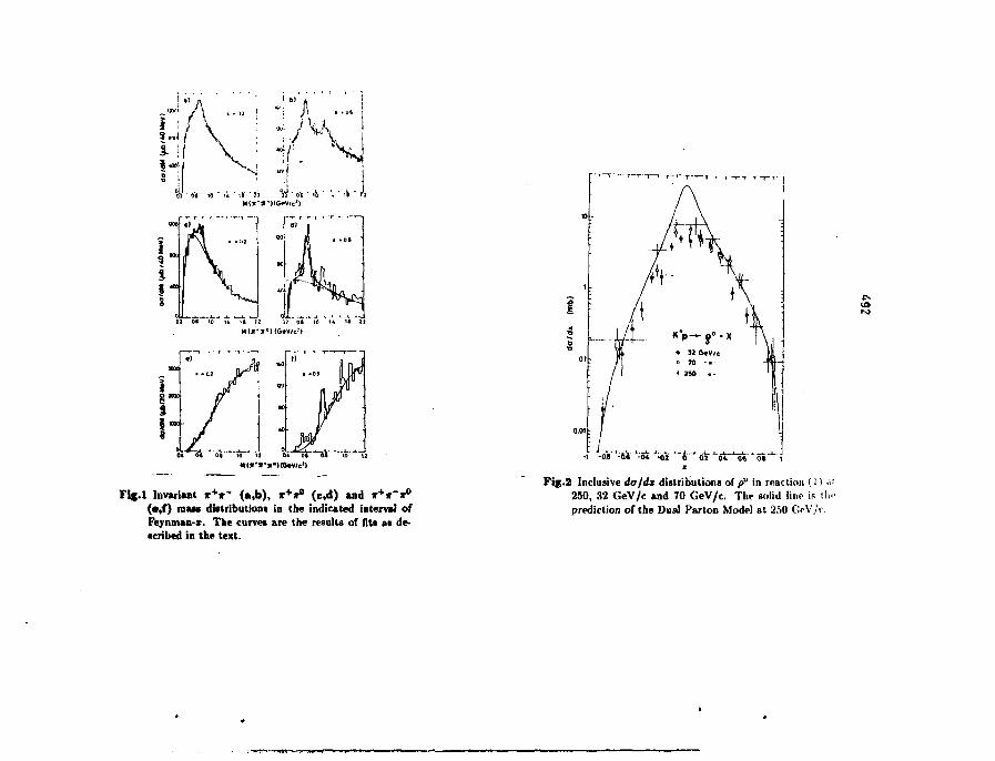
i
in '" io ' ii o* o* oi * ID "*~utit* •*-»•) (O»V(c'l
Fig.l Invariant »+*" (•,b), T+JT0 (e,d) and x+iTir0
(e,f) maw distributions in the indicated interval ofFeynman-x. The curves are the results of fits as de-scribed in the text.
.cto
-M'^-OS '-8* 4«
Fig.2 Inclusive da/dx distributions of pu in reaction (1) •*<250, 32 GeV/c and 70 GeV/c. The solid line is ih.-prediction of the Dual Parton Mode] at 250 GrV/V.
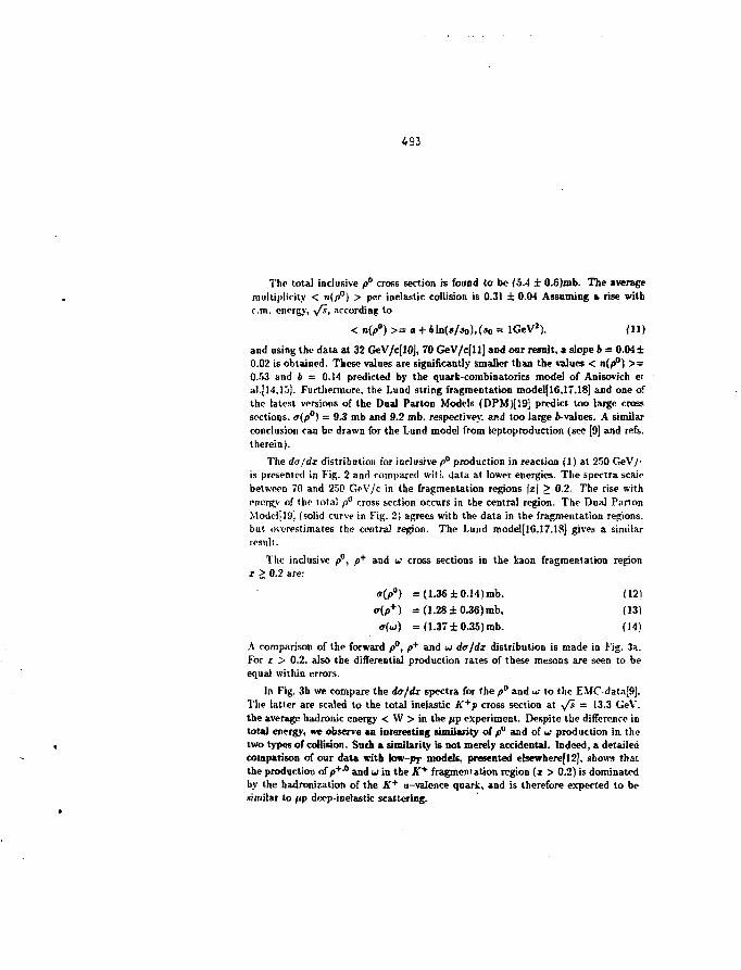
493
The total inclusive p° cross section is found to be (5.4 ± 0.6)mb. The averagemultiplicity < n(/>°) > per inelastic collision is 0.31 ± 0.04 Assuming a rise withr.m. energy, ^/s, according to
< „ ( / • ) > = a+ 61n(«/«o),(Jo= lGeV2). (11)
and using the data at 32 GeV/c[10], 70 GeV/c[ll] and our result, a slope b = 0.04±0.02 is obtained. These values are significantly smaller than the values < n(p°) >=0.53 and b = 0.14 predicted by the quark-combinatorics model of Anisovkh etal.jl4.15). Furthermore, the Lund string fragmentation model[16.17,18] and one ofthe latest versions of the Dual Parton Models (DPM)[*9] predict too large crosssections. a(p°) = 9.3 mb and 9.2 mb, respective}-, and too large t-values. A similarconclusion can be drawn for the Lund model from leptoproductton (see [9] and refs.therein).
The da/dz distribution for inclusive f>° production in reaction (1) at 250 GeV/'is presented in Fig. 2 and compared wits, data at lower energies. The spectra scalebetween 70 and 250 GPV/C in the fragmentation regions \x\ > 0.2. The rise withenergy of the total ffi cross section occurs in the central region. The Dual PartonModcl[19] (solid curve in Fig. 2) agrees with the data in the fragmentation regions,but overestimates the central region. The Lund model[16,17.18] gives a similarresult.
The inclusive p", />+ and u cross sections in the kaon fragmentation regioni > 0.2 are:
o(p°) =(1.36±0.14)mb. (12)<r(p+) = (1.28 ± 0.36)mb, (13)
= (1.37± 0.35)mb. (14)
A comparison of the forward />", p+ and u> da/dx distribution is made in Fig. 3a.For x > 0.2. also the differential production rates of these mesons are seen to beequal within errors.
In Fig. 3b we compare the dojdx spectra for the p° and ui to the EMC-data|9).The latter are scaled to the total inelastic K*p cross section at y/i — 13.3 GeV.the average hadronic energy < W > in the /ip experiment. Despite the difference intotal energy, we observe *n interesting similarity of p° and of u> production in thetwo types of collision. Such a similarity is not merely accidental. Indeed, a detailedcomparison of our data with low-pr models, presented elsewhere[12], shows thatthe production of p+'° and w in the K+ fragmentation region ( i > 0.2) is dominatedby the hadronization of the A"+ u-valence quark, and is therefore expected to besimilar to fip deep-inelastic scattering.
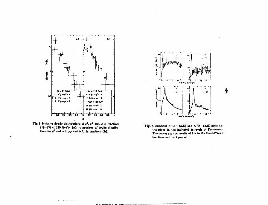
D
O.I
a)
/i«2!7G»Vo K'p-y*. X• K*p—w • X
I + K*p-J>**X
' QJ o.!i ' as ' o's
'tH
b)
fiT> 21.7 G«Vo K'p—f*. X> K*p-»-u • X
<W»"1MG»Va ^jp«j*•xm fif>—» . X
' M M M M
Fig.3 Incluaive dujdx distributions of />°, p + and w in reactions(l)-<3) at 250 GeV/c («); comparison of do/dx distribu-tions for p° and ui in pp and A'+p interactions (b).
09 10 t * " |i
Fig. 4 Invariant A'+A"~ (a,b) and A'**~ (c / l ) mam dis-tributions in the indicated intervals of Feyninan-x.The curves are the results of fits to the Breit-Winnerfunctions and background.
495
4 Strangeness Suppression
It is known since long that .trangc hadrons are less copiously produced than non-strangc hadrons. in hadron-hadron collisions, and in deep-inelastic processes. Pre-cise knowledge about the suppression of strange quark-pair creation is importantfor topirs such as quark fragmentation, heavy flavour production or the observa-tion of a quark-gluon plasma. It plays a critical role in present phenomenology ofBd,, - Hi., mixing(20j.
To characterize this violation of SU(3) symmetry, the strangeness suppressionparameter A is introduced and defined as the ratio of the probabilities of producingan .iT-pair to that of producing a (mi)- or (rfrf)-pair in the hadronic vacuum. Ifrelated to finite energy mass effects, one may expect[21] an increase of A at suffi-ciently large energies. If explained as a quantum tunneling effect, as in QCD[I6.I7|,the suppression is expected to be independent of energy provided the field energydensity is constant.
Recent analyses based on A'/* ratio's from lor--' • :i-hadron ro!lisions[22.23] give aA-value of as 0.2, while a value around 0.3 is obl.t-.ird for '4 f~ anni!)i].ition[21.25].
For hadron-hadron collisions, A may be mildly increasing •>'• low v/s to reach anaverage of 0.20 ± 0.03 at i/» = 20 GeV[26]. However, considerably higher values arereported from the collider[27] and, in particular, for high pr jets at the ISR[28]
The NA22 collaboration has obtained data on inclusive <% 1020), A*°(892) andA'•°(892) production in the reactions
K+p - *(1020) + Jf, (15)K+p - £*($92) + ;r, (16)K+p - . A'-°(892) + X, (17)
at 250 GeV/c. Reactions (15) and (16) are particularly well suited to determine thestrangeness suppression directly from the data, while reaction (17) helps to estimatecentral A"°(892) production.
At lower energies, reactions (1)—(3) were systematically studied by the Mirabellecollaboration at 32 GeV/c[l ,2,29,3) and by the BEBC collaboration (WA27) at 70GeV/c[30,4]. High statistics data on ^-production in K+Bt interactions at 12"and 200 GeV/c were recently presented by the ACCMOR collaboration for theFeynman-i range 0 < z < 0.3[31].
From Drcll-Van production at relatively low Q1, i t » known that the longitudinalmomentum distribution in the A'+ is harder for the 3-valence quark than for the
496
o-valence quark(32j. This implies that K+ beam fragmentation at moderately largeFeynman-z is mainly due to strange flavour fragmentation. Additionally, modelcalculations indicate that for z > 0.2, the A" and 4 fragmentation functions foru-qaark jets are about an order of magnitude smaller than those for 3-quark jets.
In reaction (1), the <p-me*on is dominantly produced through 3 fragmentationvia the creation of an (as) quark pair from the vacuum. Furthermore, there is noexperimental evidence that the observed <£-meson is a decay product of higher massresonances.
As to A'"°(892), besides prompt production through 3- quark fragmentation, via(dd) pair production, other contributions must be considered. As discussed below,they are relatively small in the fragmentation region z > 0.2 and can be subtracted.
The cross sections for reactions (l)-{3) are determined by fitting the invariantK+K~. h'+ir~ and K~r+ mass distributions by the expression
dojdM = BG(M){\ + faBWi(M) + /hBW,(M)), (18)
where BW\{M) and BWrfM) are relativistic P- and D-wave Breit-Wigner func-tions. 9i and A lit-paraiaeten (A is fixed to 0 in the absence of a tensor mesonsignal). The background function BG(M) is parametrized as
BG(M) = Q , ( W - Mo,)"* exp(-a3A# - <nM7). (19)
The Q, are free parameters and MD, is the threshold mass.
To account for the reflection of a given resonance into the distribution of an-other invariant-mass combination doe to K/r misidentification, we use the methodsdeveloped in[30,4] and discussed in detail in[12].
The total width of K"° and K"° is taken to be the sum of the nataral width[I it) and the width (FWHM) of the resolution function TB = 25 MeV/c2, For thenarrow ^-signal, the natural width is folded with a Gaussian for the experimentalresolution with a FWHM = 14 MeV/c2. For illustration, we show tke K+K~and h'*it- invariant mass distributions in Fig. 4 (or t > 0.2 and x > 0.5 . Theyoxliibit clear 6. A"°(S92) and A'2"°(1430) signals. The signal-to-noise ratio improvessignificantly as z — 1. The best-fit results (solid lines) are seen to describe theexperimental spectra. With our statistics and meant of particle identiScation, weare able to determine the z-spectram for A'*0 in the fall z-nage and for <* i« theregion x > 0. For A*0, we present a total inclusive crats section only.
The inclusive cross sections of A"°(892), ~K*(892) and <t> are summarized in
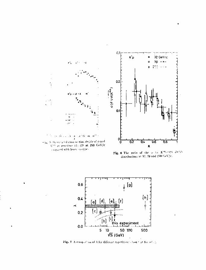
0.3 r-
K'p -(( • X V
Vs.
' ii'<l irc»i. « • lion ita/th of (."•.IMIIr w n n t . ' ( 1 : (2^ at 250 GeY'/c
"d with i t w r •r^T.-v-F i g . 6 The ratio of the v !•• A ' u ' •''•'I «"'••'•
distrihutions n: W. 70 ar.ci 2'.n <;<-V/c.
0.6
(U
0.2
0.0
I I I [ f l » | 1 1 I ) l l l l | T ) I | I • ,T1
[o] M, [e]a [f]
Fig. 7 A
6 -
this experiment* > i I 11 n i i . i i i n i !
5 10 50 100 500\fS (GeV)
i of A for di[7oi»:jii oxporlni
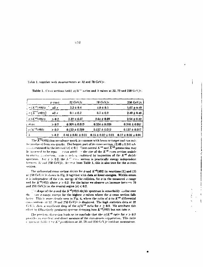
-.3 8
Table 1. locether willi measurements at 32 and 70 GeV/c.
Table 1. ( W s sections (inb). «•>//''" <<itios and A-values at 32, 70 and 250 CiV/c.
1• " i'A'"''fsa2n
i " (A"W|)j e(A*°(S92)J
1 -»0
x-raiie
" ail x
all x
>0.2
>0.2
>0.2
>0.2
.12 GeV/c
3.2 ± 0.4
0.1 ±0.2
2.32 ±0.07
0.30* ±0.019
0.133 ±0.009
0.16 ±0.01 ±0.01
70 GeV/c
4.0 ± 0.5
0.7 ± 0.2
2.64 ± 0.09
0.334 ± 0.028
0.127 ±0.012
0.15 ±0.02 ±0.01
250 GeV/c
5.07 ± 0.49
2.49 ± 0.48
2.54 ± 0.12
0.348 ± 0.037
0.137 ±0.017
0.17 ±0.02 ±0.01
The h'uf S92) has no valence-quark in common with beam or target and can oul\h-1 nrnduo'd from sea-quarks. Tlie larpesl part of its cross section. (2.40 = 0.31) tn!>i. .,:.(cntraiod in the interval \i\ < 0." ":nce central A'"0 ami A'*° proauclion mayb* :usnvf<l to bo e*)ii.i •• ma allrii •• the rise of the A'*0 cross section mainlyto remr.i. ;..<>cinction. i ni> i- in'Uu .ounrmixl by inspection of the A""0 rfff/rfrspoctnini K>r i > 0.2. the A '" t'i>..- section is practically energy independentlifivrifi, .1:' .n<i '230 Ge\'/c. A.« '<•.» !rom Table 1, this is also true for the ©-crosssection.
Thr oWiWential cra>s section de/ilx for <ft and A'"°(892) in reaction! (1) and (2)at •J.'iO Gi-V/c i« shown in Pig. 5 togoiher with data at bwer energies. Within errorsi: i< inilfpeudrui of the cm. Piicrg.'. of the collision, for 6 in the measured x-rangean<! for A'"°(S°2i above x > 0.2- For the latter *e observe an increase betwTi 70jnd 2'i0 GeV/c in the central region | i | < 0.2.
•• shape of the i> and the A ""("OS) da/dx spectrum is remarkably -miilar overtin lire J-r;iiit;e. except for the highest r-valuos where the 6 cross section fallsfii-i'T. This i< ipor<- clearly seen in Kip. 0. whore the ratio of <J to A'"° differentiali-Mi.-.- seriinti' at 'VI. 70 and 2r;0 GeV/r h displayed. Tin- high statistics data at 32Ci'V/i >IK.VI H siniiific^rit drop of the o/A'"° ratio for x > 0.9. We attribute thisi'll'-ct io dilirjitivfly produced systems decaying into A"*°(892) but not into o.
rin> prcvii.ii-. di.<rii<Nion l«ads us to conclude that the o/A'"° rati" for x > 0.2[ir<tvi'!#-* .•»(. r\r'-'!'-i!! a!)»i fiirert measure of the str?i*£eiii>ss stippre.s«iuii. This ratioi KIV-II i;i l,:l.i' ! *'ir K f p < iillision^ al 32. 70 ami 2>l) (\>\ jr inci<ii-nl moment .inn.
ptaMc d»u Mill for K~p iatent. liow at 1 0 u d 16,32 u d 110 GeV/c. wberrthe rum o / F 3 i> found to be 0.12±0.02(33). O.ia±O.O3[34.35) and 0.20±0.04(36).reipTlivrly.
To obtain a proper estimate of A. account kat to be take* of the "»on-pron>pt*romponent of the A'"0 cross sections due to Kj*t>(l4X) decay* aad diflnctivrproduction. The /JfJ°(1430) crow lection at 250 GeV/c araoaats to (1.04 ± 0.27)mb fnr x > 0.2(12]. Assuming equal JfJ+(M30) aad tfJ°(1430| cross tedious, atol.serw.i «: lower energies[l,29,4], and taking iato accoaot branching fractions toA-ci *<*•_>), yields a cross section for *T*-+fl430) — *-°(892) + X of (0.35 • u.09)mb. rhllractive A'*°(892) aad 9 production was measured to be (232 ± 15)pb(37]and (17±5)/ib[3], respectively at 32 GeV/c. We assnme these to be energy indepen-dent between 32 and 250 GeV/c. After removal of the A'2*
+o( 14301 and diifractiwcontributions, we estimate A. the ratio of "prompt1" d> to -prompt' A**°(892). tobe equal to 0.17 ± 0.02(st«)±0.01(tyst). The corresponding A-valups ?.( 32 and 70GcV/c are given in Table 1. Within errors, no energy dependence of thp strangene'fsuppression is observed in the cm. energy range 7.8 < y/s < 21.7 GeV.
A detailed comparison of the A-vaiues determined in tlif. and in ilif wo inwp: »»-orgj' A'^pexperiments wiih other recent measurements will be presf:.:(-d '•lsowberejr.1].A compilation of > nicasiiremrnts is shown in Fig. 7. It is been thai lii" recent vp.Vp and fip measurements give a value in agreement with our result. Mea.suremeiiufrom t*e~ annihilation tend to favour a somewhat larger value.
Many estimat"- in partknlar those extracted from measured A'/r-ratios. arebased on model comparisons. Adopting similar techniques to describe oor A'"0
and 4> data, we find A = 0.16 ± 0.02 from the Statistical Quark Modelj38j andA = 0.18 ± 0.03. osiag either tke O«al P«r on Model(39.40] or the Lnnd Fritiofroodel[41]. The latter two oiod*<c describe the data at 32. 70 and 250 GeV/c withthe same A-valoe. All model-'..sed valoes are seen to be in good agreement withthe model-independent estimate presented above.
In summary, in the kinematical region z > 0.2. A"°(892) and d mes";> arepredominantly produced off tke straage valeace^qaaik of tke beam by creation ofa (<M)-. respectively (*7}-pair from tke vacuum. This allows us to estimate thestrange quark npprestkm factor, aa imponast parameter in present hadronizaironphenomeaology. We obtain A = 8.17±0.02x0.01 at 250 GeV/c. in good arnvmpntwith results at 32 and 70 GeV/c. indicating tl'at tlf oncrp,- dcponH<=ncp of A. if any.is v<;ry weak in thp encrg>' range considered
500
References
(I) I.V.Ajinenkoel al. Z. Phy».. C26:103. 1984.
[2] P.V.CIiUapnJkov et ai. Phys. Utl.. I30B432. 1983.
|3] I.V.Ajinenko et al. Sov. J. \vcL Phr*.. 39:914. 1984.
[4] M.Barth et al. Nvct. Phy:, B223:296, 1983.
[5] E.A.De Wolf et al. Z. Phy*., C31:13, 1986.
[6] M. Adamus et al. Phys. Lett., 183B:425. 1987.
[7j M.Adamus et al. Z. Phy»., C32:475. 1986.
18] NA22 Collaboration: M.Adamos et al. Inclusive ir° Production in T+p. *'-yand pp Interactions at 250 GeV/c. 1987. Z. Phy». C (in press).
19] EMC Collaboration: M. Arneodo et al. Z. Phys.. C33:167. 1986.
jlOj P.V. Chliapnikov et al. Nucl. Phys.. Bl7«:303. 1980.
ill) M.Barth et al. Xvcl. Php»., B223:296, 1983.
[12] NA22 Collaboration:. Inclusive Mrton Resonance Production in K*p Interac-tions at 250 Ge V/c. to be submitted to Z. Phys. C.
|13] Particle Data Group: M-Agnilar-Bonitez et al. Phys. Lett.. B170:l, 11S6.
(14] V.V.Anis-jvich. M.Kobrinsky. JJIyiri. Yad. Fiz.. 34:195, L981.
(IS] V.V.Anisovich, M.Koórinsky, J.Nyiri. Yad. Fiz.. 35:151, 1982.
il6j B.Andersson « al. Nvd. Phy*., B178:242. 1S81.
(17] B.Andersson et al. Phy*. Report», CS7:31. 1963.
[18] T.Sjôstrand. Comp. Phtt. Cornm.. 27:243, 1982.
(19] A.V.Batunin. A.K.Likhoded. A.'iV.Tolstenkov. Yad. Fiz.. 42:42-]. 1985.
i'JOj A.Ali. Dilcptons, Eleftrowcak Charge Asyjnmrlry and B —B Mixings. InJ.(«run(iHU>. ciiitor. Prurctrlinçs XVIth Int. Syrnp. on .\fultipartirle Dynamics.[>:IBP fi-J.1. Kilitioiis Frontières (Gif-sur-Yvette I and Wor?4 Scientific (Singa-pore). 19«.i.
,;n\ Y.V. Amsovitch. V.M.Shekhler. Nucl. Phy».. B5S:455. 1973.
':£!; Ci.I Jnnos ft al. Z. Phy».. C27:43. 1985.
50!
[23] RAVindmolders. Recent Result" from the EMC collaboration. In Proc. XthWarsaw Symposium on Elementary Particle Pkysics . Kazimierz, Poland, 1987.
[21] W.Barteletal. Z. Phys., C2O:187, 1983.
j2\] H.Aiharael'iaJ. Phys. Rev. Lett., 53:2378, 1984.
,'26] A-VVroblewski. Ada Phys. Pol. B16:37&, 1985.
[27] G.J.Alncr »t al. Nncl. Phys.. B258:505, 1985.
(28) A.Brearkstfi is e i ai. Phys. Lett.. 135B:51O, 1984.
[•»!)j I.V.AjinenKo et al. Z. Phys.. C5:i77. 1980.
,'30j M.BartL " aj. 1'liys. Utt.. 117B:267, 1982.
[31] H.Dijkstra et al. Z. Phys.. C31:375. 1986.
[32] J.Badier et al. Phys. Utt., B93:354. 1980.
[33] P.Sixel or ai. A'uc/. Phys.. Bl»9:381. 1982.
|34j Yu.Arestov et al. / . Phys., C6:101. 1980.
[35] Yu.Areslov ei al. Z. Phys., C8:283. 1981.
[36] S.Banerjee et al. Z. Phys., C31:401. 1986.
[37] P.V.Chliapnikov et al. Z. Phys.. C12:113. 1982.
|3SJ V.Shekhter. L.Sdicglova. Yad. Fiz.. 27:1070. 1978.
[39] A. Capella. In R.T. Van de Walle, editor. Europhysics Study Conf. on Partnnyand Soft Hadmnic Interactions (Ericej, page 199. World Scientific Singapore.1982.
MOj E.A.De Wolf. In G.Gustafson. editor, Prof. XVth Int. Symp. on MultipartipliDynamics (Lund), page 2. W •••Id Scientific, Singapore.. 19&4.
[41] B.Andpr^soa, G.Gustafsou, B.Nillson-Almqvist. SucL Phyt.. B281:289. 19S7.
503
Experimental Results on QCD from e+e Annihilation
W. de Boer *
Max-Planck-Institut fur Phyrik und Astrophysik,Werncr-Hcisenbcrg-Institut fur Physik, D 8000 Munich 40
andStanford Linear Accelerator Center
Stanford University, Stanford, CA 94305
Abrtract
A review i» fives os QCD retain from (todying t*t~ annihilation with the PEPand PETRA storage ringi with special emphasu on jet physics and the determinationof the a b » f coupling constant a,.
1 IntroductionThis paper reviews the progress on the theory of hadronic interactions duringthe eight years of PEP atid PETRA physics. This is an appropriate time, sincea new generation of e+e~ storage rings is underway (SLC and LEP) or ready(TRJSXAN)j which wili extend the maximium centre of mass energies reachedsofar to the Z° mass and beyond, thus opening a whole new field of physics. I willrestrict myself to results from hacronic events from e^c' annihilation and neglectQCD results from two photon physics. The emphasis will be on newer resultsabout the determination of the strong coupling constant, since other topics, likesearches for new phenomena, jet properties, heavy quark fragmentation, and gluonfragmentation have been discussed in detail elsewhere [lj.
In order to appreciate how much progress was made, let us review what wasknown some 10 years ago[2] :
• In 1972 Quantum Chromodynamics (QCD) was proposed by Fritzsch anuGell-Mann[3] as a gauge invariant field theory of the strong interactions: thegauge bosons are 8 coloured gluons, which are responsible for the strongforces between the quarks very much like the exchange of photons yields theelectromagnetic force between charged particles.
'Work npporled in part by the Department of Energy contract DE-ACO3-76SF00515Maffiat addnw: SLAC (Bin 61), P.O. Boj 4349, Stanford, " \ M3O5, USABitnet addrew: m r WDB at node SLAC"M
504
• QCD was given an enormous boost by the discovery of asymptotic freedomby Gross and Wilczekl4j and Politzer[5], the subsequent, observation of scaleinvaiiance which offers a justification for the highly successful quark par-ton model (QPM), and the observation of logarithmic deviations from thisinvariance as predicted by QCD.
• The discovery of the J / * in 1974 at SLAC[6] and Brookhaven(7j and theproof that it corresponded to a bound state of ti quarks completed the quarkpicture and left little doubt to the idea that the mathematical objects orig-inally proposed by GeU-Mann[8] and Zweig(9] to classify the hadrons werereal, existing quarks.
• The channed quark fitted beautifully into the SU[2)®U(1) unified theory ofthe electroweak interactions, proposed by Glashow, Salam and WeinbergJlO]and proven to be renormalizible by't Hooft[ll], since in this model the matterfields are arranged in left-handed doublets and right-handed singlets, so therewas an 'empty' slot in the doublet structure of this so-called Standard Made!for the charmed quark. Actually from the absence of stangeness changingneutral currents Glashow, Biopoulos and Maiani (GIM) had predicted theexistence of the charmed quark[12j.
• After 1974 a new heavy lepton. 'called r) with its own neutrino was discoveredby Perl and collaborators at SLAC[Hj and a new quark (called bottom) wasdiscovered by Ledcrman's group at Fermilab[l3j. Given the succes of theStandard Model, one was in the same situation of having an 'empty' slot fora new quark (called top) in a thirth generation of quarks and leptona. So bythe time of proposal writing for the PETRA experiments the quark picturewas well established and the detectors were all optimized to do 'top' physics.
However, what was going to be one of the major discoveries at PE'.'RA, namelythe discovery of the gluon, was not even considered in the proposal: as a physicstopic. The main reason is that jet physics at thai time was not very advanced,for the simple reason that the jet energies were too small to see jets on an eventby event basis, so the idea that one might observe gluons as jets was not obvious,although it was proposed by several theorists[loj. ""he main evidence for jetsin ere~ annihilation at that time came from the .'*RK-T Collaboration116],who observed a deviation of the sphericity of hadroT.< <»vent£ from phase space.Furthermore, the beams at SPEAR turned out to he polarized, which yielded anazimuthal variation of the sphericity axis, as expected for spin 1/2 quarks.
The outline of this paper is as follows:
• After summarizing the predictions of the Standard Model we discuss the mainfeatures of jet physics. We will be short, since this topic has been reviewedmany times.
• We then proceed to the discussion of the more ambitious task of the de-termination of the strong coupling constant a,. Note that within QCD the
505
coupling between all quarks and gluons is supposed to be the same, so thereis only one coupling constant to be determined.
• We conclude with a summary.
2 Standard Model Predictions
Even at present energies the effects of Z° exchange are noticeable, so one hasto take the complete Standard Model of SU{3)C ® SU{2)L ® V(l) into account.This model has 4 fundamental parameters (aside from masses and mixing angles) :three coupling constants for SU(3), SU(2) and U(l), respectively, and the vacuumexpectation value of the Higgs doublet. If the model contains Higgs representationsother than doublets, the theory has an additional parameter, usually parametrizedby the -parameter. To make comparisons with experiments easier, one should useparameters closely related to physical processes. Two of the parameters can bechosen as follows: the fine structure constant a = 1/137.036 as obtained from theJosephson effect, and the Fermi coupling constant Gf = 1.16637 10"sGeV~J, asderived from the muon lifetime after applying the appropriate radiative corrections.As a third parameter one can take cither mass of the neutral gauge boson Mz orthe electro weak mixing angle 8W defined by costw = Mw/Mz, where Mw is themass of the charged gauge bosons. In both cases Mw is predicted in case p = 1.else one has to use costf^ — Mw/(pMz). Mz and 6w are related via a and GF
by:G r(l - &r)M} = 1 .
Here Ar « 0.07J17J are one-loop radiative corrections, which have not been ab-sorbed in Gf. They depend on the unknown top- and Higgs mass. E.g. they varyfrom «»7 % to 6 % (3%, 0%) for top masses varying from 45 GeV to 90 (180, 240)GeV and for a Higgs mass equal to the £°-mass. The fact that these correctionsare so large comes mainly from the fact that a has been renormalized at low energyand its value increases by about 7% if it is calculated at the W-mass.
Of course, one could use different choices of parameters, e.g. Miv, but experi-mentally the previous choices can be better determined. The fourth parameter iscither the value of the running strong coupling constant a, at a given energy orthe QCD scale parameter A, which determines the running of a, and can be usedto calculate a, for a given energy.
2.1 howett order prediction!
From the Feynman diagram for the production of quarks, as shown in Fig. la,one obtains the lowest order differential cross-section for the production of a pair
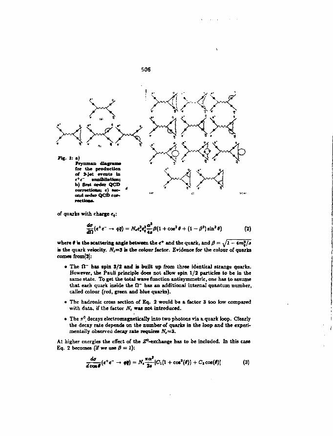
506
XXKg. 1: •)
Peynman diagram*for the productionat 3-jet eventa In
b) Brat order QCDcorractiona; c) aac- 'ondordar QCD cor-rections.
of quarks with charge ef:
da& «) = J/?( l + coe2 $ + (1 - /?') sin* 0) (2)
where t is the scattering angle between the e+ and the quark, and /? = Jl — imf/sis the quark velocity. iVe=3 is the colour factor. Evidence for the colour of quarkscomes from[2]:
a The fl~ has spin 3/2 and is built up from three identical strange quarks.However, the Pauli principle does not allow spin 1/2 particles to be in thesame state. To get the total wave function antisymmetric, one has to assumethat each quark inside the 0~ has an additional internal quantum number,called colour (red, green and blue quarks).
a The hadronic cross section of Eq. 2 would be a factor 3 too low comparedwith data, if the factor AT, was not introduced.
a The JT°. decays electromagnetically into two photons via a quark loop. Clearlythe decay rate depends on the number of quarks in the loop and the experi-mentally observed decay rate requires Nc—3.
At higher energies the effect of the ^-exchange has to be included. In this caseEq. 2 becomes (if we use $ = 1):
dada»t[ + C,cos(«)] (3)
507
= 4e,e(a,atK(x) + 8».a,t>fof |x*|+ /*)-4«fsin*#ir
tf)
1 - Ar
with
* ~ Sy/2*a * — M\ + iMgVf 1 — Ar1 y~'Here 7f and /," are the 3th components of the weak isospin (see Table 1). In Eq.6 the 1 - Ar1 term represents the loop corrections to the Z° propagator. SinceAr' «s Ar we can neglect both corrections in the fits to the hadronic cross section.Note that R-values are not corrected for 1 - Ar1, although asymmetry values aresometimes corrected for this factor in an indirect way1. In this case one has toapply only the correction factor 1 - Ar[18]. Then Eq. 6 becomes equal to itssin* Ow parametrixation (using Eq. 1):
. , _<? , ( ! -Ar ) *Mj _ 1 s
A summary of these radiative corrections can be found in Ref.[19j.The terms proportional to 9t(x) represent the interference between Z° and 7
exchange and the terms proportional to |x|* the direct Z° exchange. The ratio ofthe total cross section contributions from Z° and 7 exchange ((Ci - «/)/«') isshown in Table 1 for the various matter fields together with the coupling constants.
fermion
neutrinop,r Upton
u,c,t quarksd,s,b quarks
%
1/2-1/2
1/2-1/2
I?
00
00
a1
- 11
- 1
V
1—1 + 4sin* tw = —0.08
—1 + i&\n*$w = —0.69
t ,
0- 1
+2/3- 1 / 3
•?00
1.2961.8S6
11.096
A
0.12-0.15-0.23-0.41
Table 1: Summary of couplings and asymmetry for Mg=9i GeV and «in3 fur =0.23
and theFrom Eq. 3 the total cross section is found to be NcCi4xa*/Zsforward-backward asymmetry in the differentia) cross section equals:
, _
For leptonic final statee the vector coupling t> is small and only the interferenceterm needs to be taken into account at PETRA energies. In this case the asym-metry in Eq. 8 depends only on the axial vector couplings. However, for quarksthe vector couplings are large and the direct Z°-exchange term (oc |x|l) is largerthan the interference term at the highest PETRA energies.
"n» loop corrections u d th* Inltltl ftatt ndialhr* correction! (or tht Z*-«ch»ngi k m u oppo-•ite lii* nut an iimilar In mifsHtdt 4t PETRA enerpei, to if on> neglecti them both, th« nmainiogcntribatioi ]• n«fl!glbk[is| u d oat c u fbcftt aboit U* 1 - Ar' cornctioi.
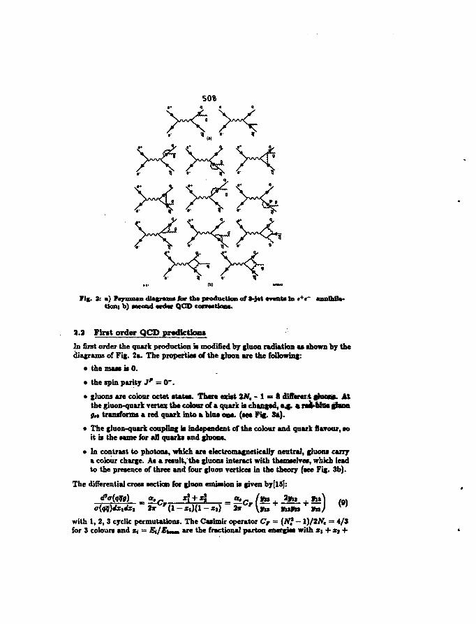
50%4 •
Tig. 3: •) F«jrnm«n diagrams for tht production of S-J«t avaste In «+«~tlon; b) sotimd ordar QCD corrections.
2.7 Firat order QCD prediction*
In first order the quark production ia modified by glnon radiation «a ahown by thediagrams of Fif. 2a. The properties of the (luon are the following:
• the maw if 0.
• the spin parity Jp = 0".
• gluons are colour octet atataa. Thera cadst 2N, - 1 s t diffareri g4oon«. Aithe gluon-quark vertex the colour of a quark it changed, e4 . «raiVUttag1ao(ift.» transform* a, red quark into a blua ooa. (see Fif. S*)-
• The gluon-quark coupDng ia independent of the colour and quark flavour, aoit is the same for all quark* and glnons.
• In contrast to photon*, which are electromagnetkaUy neutral, gluons carrya colour charge. Aa a result/the gluons interact with themselves, which leadto the presence of three and four gluon vertices in the theory (aee Fig. 3b).
The differential cross section for gluon emission is given by[15]:
with t, 2, 3 cyclic permutations. The Caslmir operator C, = (N* - 1)/2JV, = 4/3for 3 colours and x, = Ei/E^mm are the fractional parton energjea with x% + x, +
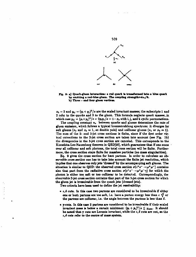
509
Fig. S: •) Quark-gfoon Interaction: a red quark to transformed Into a bloc quarkby emitting a red-Mo* (loon. The coupling otr«ngth=4a,/*.b) Three - and four gloom vertices.
zs = 2 and y,j = (ft + p,)*/« are the scaled invariant masses; the subscripts 1 and2 refer to the quarks and 3 to the gluon. This formula neglects quark masses, inwhich case ]/„• = (ft+p,-)1/* = 2P*Py/* = 1—*i with i, j , and k cyclic permutations.
The coupling constant a, between quarks and gluons determines the rate ofgluon emission, which follows a typical bremsstrahhmg spectrum: it diverges forsoft gluons (zi and xj as 1, so double pole) and collinear gluons (zj or i j ss 1).The sum of the 2- and 3-jet cross sections is finite, since if the first order vir-tual corrections to the 2-jet cross section are taken into account (see Fig. lb)the divergencies in the 3-jet cross section are canceled. This corresponds to theKinoshita-Lee-Nauenberg theorem in QED[2O], which guarantees that if one sumsover all collinear and soft photons, the total cross section will be finite. Further-more, the cross section stays finite for massless particles (no mass singularities).
Eq. 9 gives the cross section for bare partons. In order to calculate an ob-servable cross section one has to take into account the finite jet resolution, whichimplies that one observes only jets 'dressed' by the accompanying soft gluons. Thesituation is similar to QED: the observed cross section a(«+e~ -»/*+/*~) containsalso that part from the radiative cross section <r(e+e~ ~»/*+/i~ir) for which thephoton is either too soft or too collinear to be detected. Correspondingly, theobservable 2-jet cross section contains that part of the 3-jet cross section for whichthe gluon jet b irresolvable from the quark jets (dressed jets).
Two criteria have been used to define the jet resolvibility:
• i,S cuts. In this case two partons are considered to be irresolvable if eitherone or both partons are too soft, i.e. have a parton energy less than t ^ orthe partons are collinear, i.e. the angle between the partons is less than 6.
• y-cuts. In this case 2 partons are considered to be irresolvable if their scaledinvariant mass is below a certain minimum: (ft + Pi)1/-* < ]/•*•»• It shouldbe noted that y cuts are Lorentz invariant, while the e,6 cuts are not, so thet, 4 cuts refer to the centre of mass system.
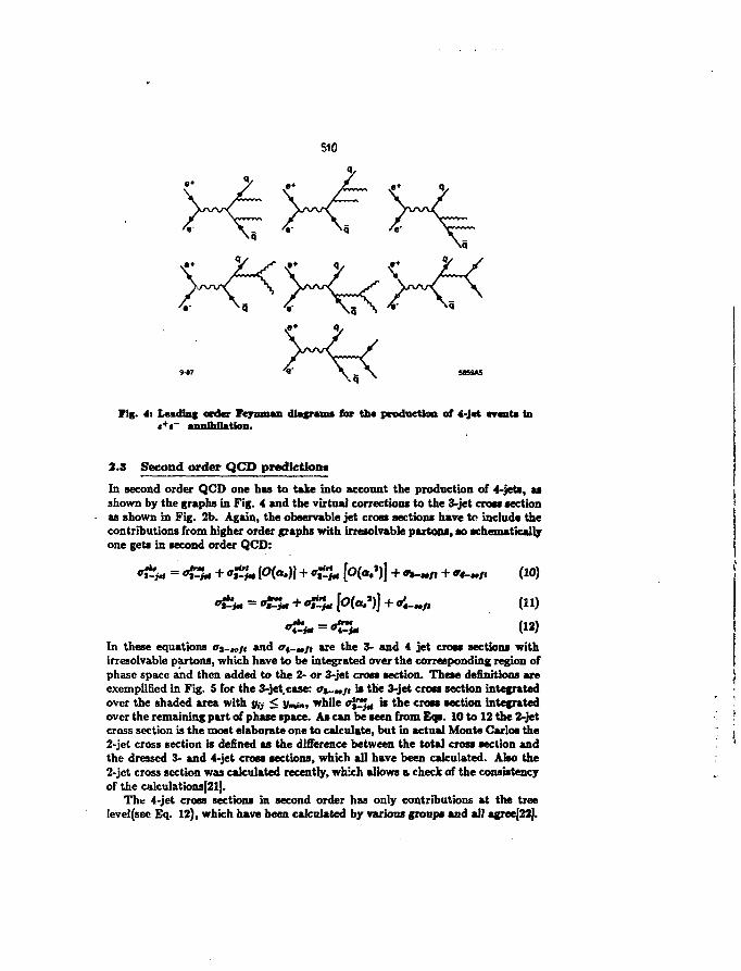
510
Fig. A: Leading order Feymnan diagrasu for the production of *-J«t events in«+«- annihilation.
2.3 Second order QCD prediction*
In second order QCD one has to take into account the production of 4-jets, asshown by the graphs in Fig. 4 and the virtual corrections to the 3-jet cross sectionas shown in Fig. 2b. Again, the observable jet cross sections have to include thecontributions from higher order graphs with irresolvable partons, so schematicallyone gets in second order QCD:
[] * (10)
(12)
In these equations ffs-»/i and W1-../1 are the 3- and 4 jet cross sections withirresolvable partons, which have to be integrated over the corresponding region ofphase space and then added to the 2- or 3-jet cross section. These definitions areexemplified in Fig. 5 for the 3-jet case: <rt--/t is the 3-jet cross section integratedover the shaded area with y,-, < ymir,, while "j'-fj* is the cross section integratedover the remaining part of phase space. As can be seen from Eqs. 10 to 12 the 2-jetcross section is the most elaborate one to calculate, but in actual Monte Carlos the2-jet cross section is defined as the difference between the total cross section andthe dressed 3- and 4-jet cross sections, which all have been calculated. Also the2-jet cross section was calculated recently, which allows a check of the consistencyof the cakulations|2l).
The 4-jet cross sections in second order has only contributions at the treelevel(see Eq. 12), which have been calculated by various groups and all agree(22].
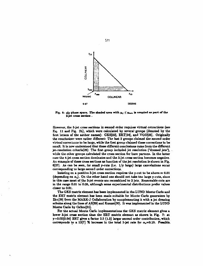
S11
5toI
Inlrared
987
COU.WEAR
58S9A8
Fig. 6: qqg phase space. The (haded area with y,, < **» is counted aa part of theJ-Jet eroat —ctlan .
However, the 3-jet cross sections in second order requires virtual corrections (seeEq. 11 and Fig. 2b), which were calculated by several groups (denoted by thefirst letters of the author names): GKS|23], ERT[24], and VGO[25). Originallythe conclusion? were rather different: The last 2 groups claimed the second ordervirtual corrections to be large, while the first group claimed these corrections to besmall. It is now understood that these different conclusions came from the differentjet-resolution criteria[26j: The first group included jet resolution ('dressed jets'),while the other groups calculated the cross section for bare partons. In the lattercase the 4-jet cross section dominates and the 3-jet cross section becomes negative.An example of these cross sections as function of the jet resolution is shown in Fig.6[27j. As can be seen, for small y-cuts (i.e. 1/y large) large cancelations occurcorresponding to large second order corrections.
Insisting on a positive 3-jet cross section requires the y-cut to be above « 0.01(depending on a,). On the other hand one should not take too large y-cuts, sincein this case most of the 3-jet events are recombined to 2 jets. Reasonable cuts arein the range 0.01 to 0.05, although some experimental distributions prefer valuescloser to 0.01.
The GKS matrix element has been implemented in the LUND Monte Carlo andthe ERT matrix element has been made suitable for Monte Carlo generators byZhu[28] from the MARK-J Collaboration by complementing it with a jet dressingscheme along the lines of Ali[29] and Kunzst[30]. It was implemented in the LUNDMonte Carlo by Csikor[31].
For the actual Monte Carlo implementations the GKS matrix element gives alower 3-jet cross section than the ERT matrix element as shown in Fig. 7: aty=0.02(0.04) ERT gives a factor 2.5 (1.5) larger second order contribution, whichcorresponds to a 12(7) % increase in the total 3-jet rate for a,=0.15. Possible.
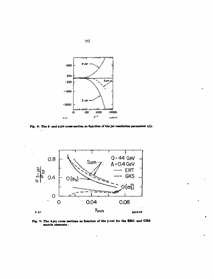
512
1000 -
-1000 -
-2000
10 100 1000 10000
Tig. «: The *- and *-jet croa* section as function of tha jet rcsolatlon parameter 1/y.
0.8
1?r 0A
0
IQ = 44GeV ~A=0.4GeV
v-... / / ERT— GKS J
0(a|) -
0 0.04 0.08
9-87 S»S«A«
Fig. ?: The 3-jet croas aections as ftmctlon of tha y-eut for tha BUT- and GKSmatrix element*.
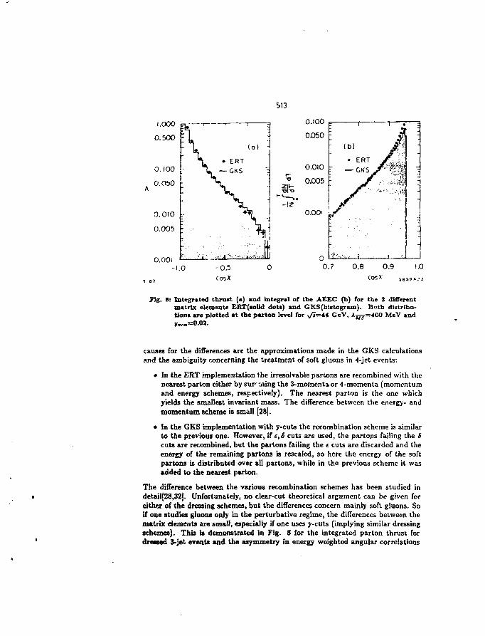
513
O.OOiH.O
211-I
0.7 0.8 0.9 1.0
cosX i e i s A c ?
Pig. 8: Integrated thrust (a) and integral of the AEEC (b) for the 2 differentmatrix elements ERT(»olld dots) and GKS(histogram). Both distribu-tion* are plotted at the parton level for y/l=** GeV, AJJ^=400 MeV and
02
causes for the differences are the approximations made in the GKS calculationsand the ambiguity concerning the treatment of soft gluons in 4-jet events:
• In the ERT implementation the irresolvable partons are recombincd with thenearest parton either by summing the 3-momentaor 4-momenta (momentumand energy schemes, respectively). The nearest parton is the one whichyields the smallest invariant mass. The difference between the energy- andmomentum scheme is small [28].
• In the GKS implementation with y-cuts the recombination scheme is similarto the previous one. However, if e,S cuts are used, the partons failing the 6cuts are recombined, but the partons failing the t cuts arc discarded and theenergy of the remaining partons is rescaled, so here the energy of the softpartons is distributed over all partons, while in the previous scheme it wasadded to the nearest parton.
The difference between the various recombination schemes has been studied indetail[28,32|. Unfortunately, no clear-cut theoretical argument can be given forcither of the dressing schemes, but the differences concern mainly soft gluons. Soif one studies gluons only in the perturbative regime, the differences between thematrix elements are small, especially if one uses y-cuts (implying similar dressingschemes). This is demonstrated in Fig. 8 for the integrated parton thrust fordreased 3-jet events and the asymmetry in energy weighted angular correlations
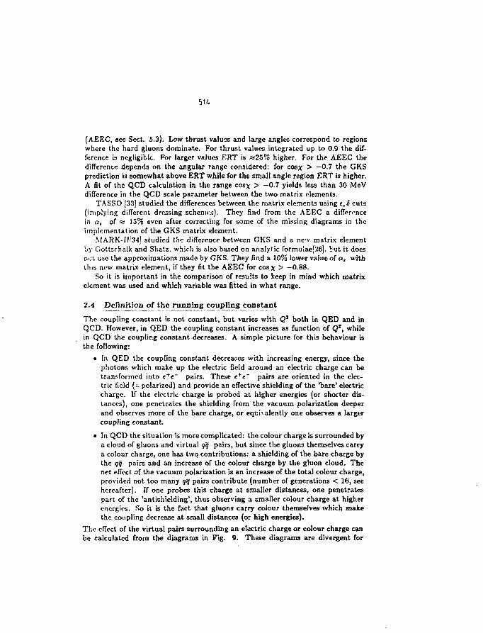
(AEEC, see Sect. 5.3). Low thrust values and large angles correspond to regionswhere the hard gluons dominate. For thrust values integrated up to 0.9 the dif-ference is negligible. For larger values ERT is «25% higher. For the AEEC thedifference depends on the angular range considered: for cosx > -0.7 the GKSprediction is somewhat above ERT while for the small angle region ERT is higher.A fit of the QCD calculation in the range cosx > -0.7 yields less than 30 McVdifference in the QCD scale parameter between the two matrix elements.
TASSO [33] studied the differences between the matrix elements using t,S cuts(implying different dressing schemes). They find from the AEEC a diffpn-ncein a, of « 15% even after correcting for some of the missing diagrams in theimplementation of the GKS matrix element.
MARK-IH34J studied the difference between GKS and a ncv matrix elementby Goltschalk and Shatz. which is also based on analytic formulae[26]. but it doesnet use the approximations made by GKS. They find a 1095 lower value of a, withtins new matrix element, if they fit the AEEC for cosx > -0.88.
So it is important in the comparison of results to keep in mind which matrixelement was used and which variable was fitted in what range.
2.4 Definition of the running coupling constant
The coupling constant is not constant, but varies with Q* both in QED and inQCD. However, in QED the coupling constant increases as function of Q1, whilein QCD the coupling constant decreases. A simple picture for this behaviour isthe following:
• In QED the coupling constant decreases with increasing energy, since thephotons which make up the electric field around an electric charge can betransformed into e+c~ pairs. These e+e" pairs are oriented in the elec-tric field (^polarized) and provide an effective shielding of the 'bare' electriccharge. If the electric charge is probed at higher energies (or shorter dis-tances), one penetrates the shielding from the vacuum polarization deeperand observes more of the bare charge, or equhalently one observes a largercoupling constant.
• In QCD the situation is more complicated: the colour charge is surrounded bya cloud of gluons and virtual qq pairs, but since the gluons themselves carrya colour charge, one has two contributions: a shielding of the bare charge bythe qq pairs and an increase of the colour charge by the gluon cloud. Thenet effect of the vacuum polarization is an increase of the total colour charge,provided not too many qq pairs contribute (number of generations < 16, seehereafter). If one probes this charge at smaller distances, one penetratespart of the 'antishiclding', thus observing a smaller colour charge at higherenergies. So it is the fact that gluons carry colour themselves which makethe coupling decrease at small distances (or high energies).
Tho effect of the virtual pairs surrounding an electric charge or colour charge canbe calculated from the diagrams in Fig. 9. These diagrams are divergent for
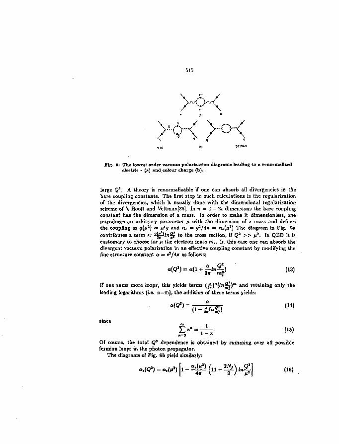
515
q " q 0
9 87 5859AS
Fig. 9: The lowest order vacuum polarization diagrams leading to a renormalizedelectric - (a) and colour charge (b).
large Q*. A theory is renormalizable if one can absorb all divergencies in thebare coupling constants. The first step in such calculations is the regularizationof the divergencies, which is usually done with the dimensional regularizationscheme of 't Hooft and Veitman[35l. In n = 4 — 2e dimensions the bare couplingconstant has the dimension of a mass. In order to make it dimensionless, oneintroduces an arbitrary parameter /i with the dimension of a mass and definesthe coupling as ?(/**) = n'g and a, — g^/Ax — a,(/*J) The diagram in Fig. 9acontributes a term ss ^jj-^rc^ to the cross section, if Q2 » ix*. In QED it iscustomary to choose for ft the electron mass mt. In this case one can absorb thedivergent vacuum polarization in an effective coupling constant by modifying thefine structure constant a = e2/4x as follows:
If one sums more loops, this yields terms iii)n(ln$p)m &nd retaining only theleading logarithms (i.e. n=m), the addition of these terms yields:
<»>
Of course, the total Q* dependence is obtained by summing over all possiblefermion loops in the photon propagator.
The diagrams of Fig. 9b yield similarly:
i -
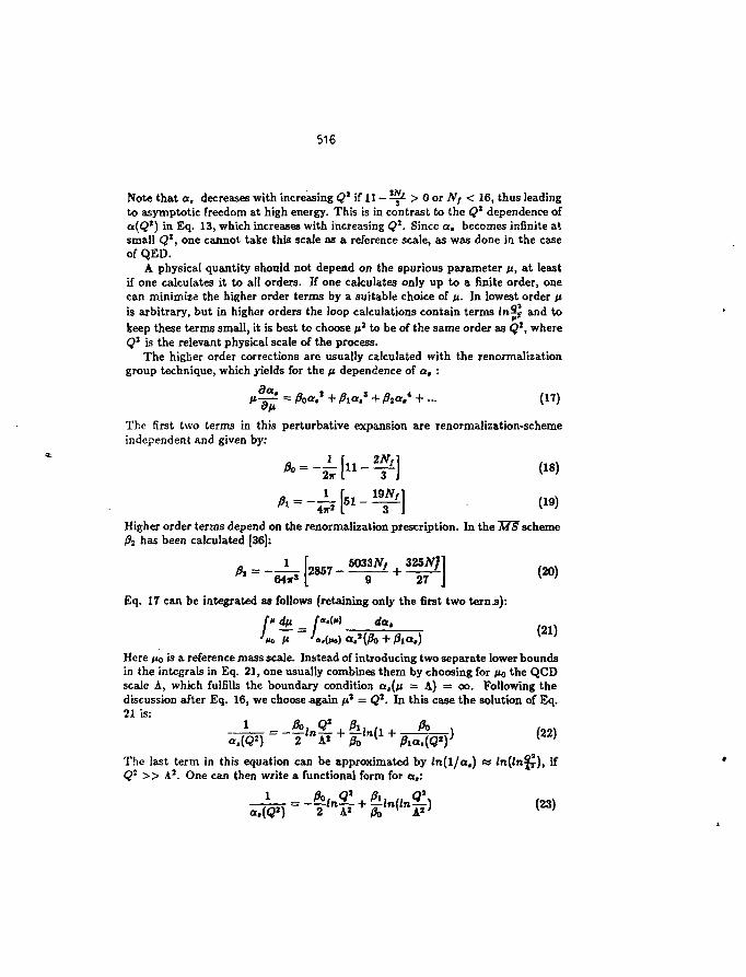
516
Note that a, decreases with increasing Q* if 11 - ~L > 0 or Nf < 16, thus leadingto asymptotic freedom at high energy. This is in contrast to the <?' dependence ofa(Q*) in Eq. 13, which increases with increasing Q1. Since a, becomes infinite atsmall Q1, one cannot take this scale as a reference scale, as was done in the caseof QED.
A physical quantity should not depend on the spurious parameter n, at leastif one calculates it to all orders. If one calculates only up to a finite order, onecan minimize the higher order terms by a suitable choice of ft. In lowest order nis arbitrary, but in higher orders the loop calculations contain terms ln^ and tokeep these terms small, it is best to choose p} to be of the same order as Q1, whereQ2 is the relevant physical scale of the process.
The higher order corrections are usually calculated with the renormalizationgroup technique, which yields for the ft dependence of a, :
f^~ = A><*.' + / W + A«.4 +.- (n)
The first two terms in this perturbative expansion are renormalization-schemeindependent and given by:
(19)
Higher order terms depend on the renormalization prescription. In the MS scheme02 has been calculated (36):
Eq. 17 can be integrated as follows (retaining only the first two tern J ) :
f«.(M) da.I" ** = f"A._ It * ~
(21)
Here na is a reference mass scale. Instead of introducing two separate lower boundsin the integrals in Eq. 21, one usually combines them by choosing for Mo the QCDscale A, which fulfills the boundary condition ct,(fi = A) = oo. Following thediscussion after Eq. 16, we choose again /** = Q2. In this case the solution of Eq.
The last term in this equation can be approximated by ln(l/a,) wQ1 >> A1. One can then write a functional form for a,:
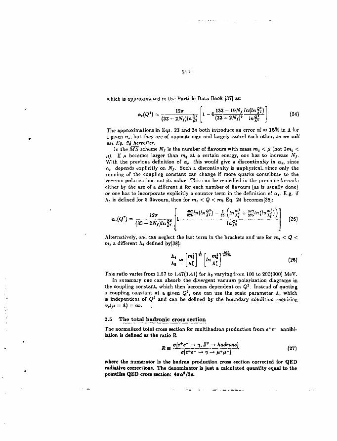
517
which is approximated in the Particle Data Book [37j as:
( 3 3 -
The approximations in Eqs. 23 and 24 both introduce an error of as 15% in A fora given a,, but they are of opposite sign and largely cancel sach other, so we willuse Eg. Sj hereafter.
In the MS scheme Nf is the number of flavours with mass m4 < fi (not 2m, <fi). If fi becomes larger than m, at a certain energy, one has to increase Nf.With the previous definition of a,, this would give a discontinuity in a,, sincea, depends explicitly on Nf. Such a discontinuity is unphysical, since only therunning of the coupling constant can change if more quarks contribute to thevacuum polarization, not its value. This can be remedied in the previous formulacither by the use of a different A for each number of flavours (as is usually done)or one has to incorporate explicitly a counter term in the definition of a,. E.g. ifA5 is defined for 5 flavours, then for mc < Q < mt Eq. 24 becomes[38]:
(33 - I " ;l -ing
Alternatively, one can neglect the last term in the brackets and use for m, < Q <mi a different A4 defined by[38j:
3]*NfTThis ratio varies from 1.57 to 1.47(1.41) for A5 varying from 100 to 200(300) MeV.
In summary one can absorb the divergent vacuum polarization diagrams inthe coupling constant, which then becomes dependent on Q'. Instead of quotinga coupling constant at a given Q7, one can use the scale parameter A, whichis independent of Q1 and can be defined by the boundary condition requiringn,{n = A) = oo.
2.5 The total hadronic cross section
The normalized total cross section for multihadron production from e+e" annihi-lation is defined as the ratio R
R = ffle+e~ -*1,Z°-* hadrons]a\e+e~ —»i —» /*T/t~]
where the numerator is the hadron production cross section corrected for QEDradiative corrections. The denominator is just a calculated quantity equal to thepointlike QED cross section: ixa'/Zs.
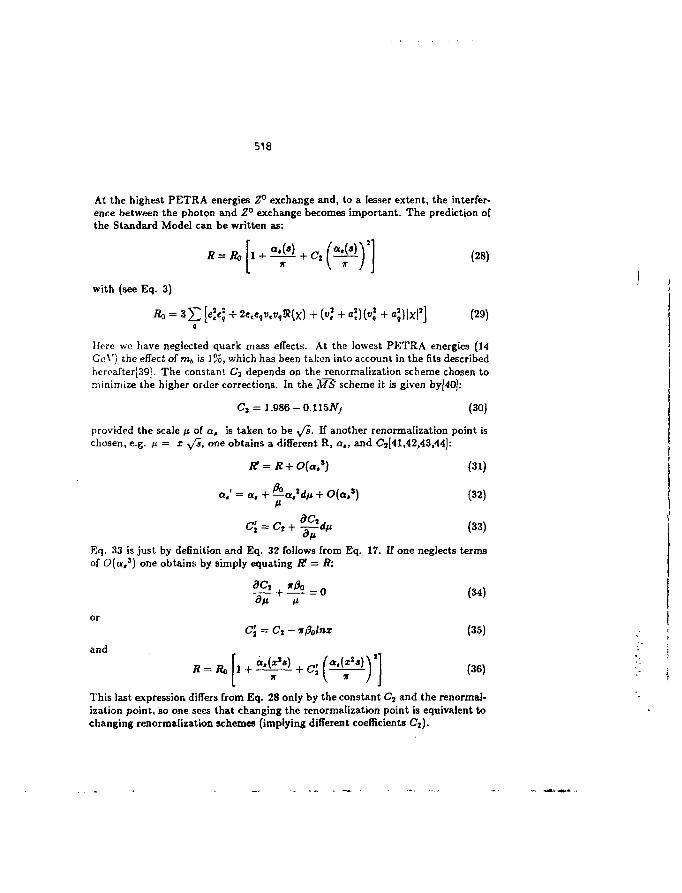
518
At the highest PETRA energies Z° exchange and, to a lesser extent, the interfer-ence between the photon and Z° exchange becomes important. The prediction ofthe Standard Model can be written as:
(28)i n \ n i i
with (see Eq. 3)
aj)|xl2] (29)
Here wo have neglected quark mass effects. At the lowest PETRA energies (14GoV) the effect of mj is 1 %, which has been taken into account in the fits describedherpafter[39l. The constant C3 depends on the renormalization scheme chosen tominimize the higher order corrections. In the MS scheme it is given by[40):
C2 = 1.986 - 0.115AT/ (30)
provided the scale fi of a, is taken to be y'S. If another renormalization point ischosen, e.g. fi = x yi, one obtains a different R, a,, and Cj[41,42,43,44]:
R = R+ O(a,s) (31)
a,' = a. + — a.'d/i + O(a,s) (32)
Cl = Ct+ -^-dp. (33)Ofi
Eq. 33 is just by definition and Eq. 32 follows from Eq. 17. If one neglects termsof O{a,3) one obtains by simply equating R = R:
^1 + ?h = o (34)
or
Cj = Cj - -isfalnx (35)
and
(36)
This last expression differs from Eq. 28 only by the constant Ct and the renormal-ization point, so one sees that changing the renormalization point is equivalent tochanging renormalization schemes (implying different coefficients Cj).
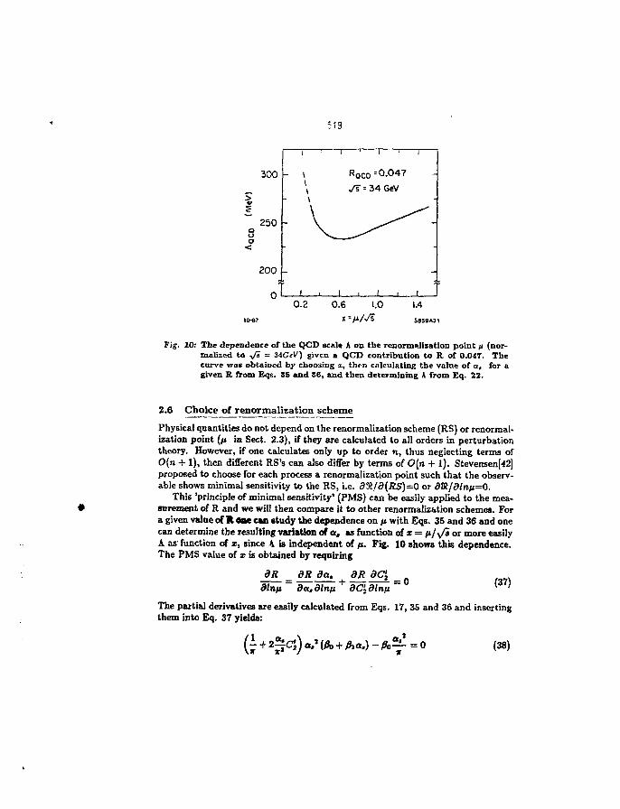
519
300
250
200
n
- \\\\\
- \
! i
1 '
Roco
V ^
1 1
1 I 1
= 0.04714 6eV
l i i
0.2 0.6 1.0 1.45859*31
Fig. 10: The dependence of the QCD scale A on the renormalization point ji (nor-malized to y/s = 34GcV) given a QCD contribution to R of 0.047. Thecurve was obtained by choosing x, then calculating the value of a, for agiven B. from Eqs. SB and 36, and then determining A from Eq. 22.
2.6 Choice of renormalization scheme
Physical quantities do not depend on the renormalization scheme (RS) or renormal-ization point (ft in Sect. 2.3), if they are calculated to all orders in perturbationtheory. However, if one calculates only up to order n, thus neglecting terms of0(n + 1), then different RS's can also differ by terms of O[n + 1). Stevensen[42]proposed to choose for each process a renormalization point such that the observ-able shows minimal sensitivity to the RS, i.e. d^H/d(RS)=0 or 9»/3/n/i=0.
This 'principle of minimal sensitivity' (PMS) can be easily applied to the mea-surement of R and we will then compare it to other renormalizbtion schemes. Fora given value of X one CM study the dependence on n with Eqs. 35 and 36 and onecan determine the resulting variation of a, as function of x = ixjy/i or more easilyA as' function of z, since A is independent of ft. Fig. 10 shows this dependence.The PMS value of z is obtained by requiring
dR_ (37)
The partial derivatives are easily calculated from Eqs. 17, 35 and 36 and insertingthem into Eq. 37 yields:
i + 2^^) a,' (A, + Aa.) - A ^ = 0 (38)
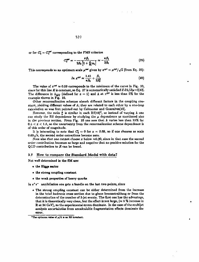
520
or for C't = CJ* corresponding to the PMS criterion
This corresponds to an optimum scale n0" given by x"1 = ft^/y/s (from Eq. 35):
The value of i"** * 0.59 corresponds to the minimum of the curve in Fig. 10,since for this iine R is constant, so Eq. 37 is automatically satisfied if dk/dp -0(43).The difference in A ^ (defined for x = 1) and A at i"" is less than 5% for theexample shown in Fig. 10.
Other renormalization schemes absorb different factors in the coupling con-stant, yielding different values of A; they are related to each other by a one-loopcalculation as was first pointed out by Celmaster and Gonsalves[45|.
However, the ratio £ is similar in each RS[42J!, so instead of varying A onecan study the RS dependence by studying the ft dependence as mentioned alsoin the previous section. From Fig. 10 one sees that A varies less than 15% for0.5 < x < 1.5, so the uncertainty from the renormalization scheme dependence isof this order of magnitude.
It is interesting to note that CJ = 0 for i = 0.69, so if one chooses as scale0.69i/a, the second order corrections become zero.
Note also that one cannot choose x below «0.20, since in that case the secondorder contribution becomes so large and negative that no positive solution for theQCD contribution to R can be found.
2.7 How to compare the Standard Model with data?
Not well determined in the SM are:
• the Higgs lector
• the strong coupling constant
• the weak properties of heavy quarks
In e+e~ annihilation one gets a'handle on the last two points, since
• The strong coupling constant can be either determined from the increasein the total hadronic cross section due to gluon bremsstrahlung or from thedetermination of the number of 3-jet events. The first one has the advantage,that it is theoretically very clean, but the effect is not large, (as 5 % increase inR at 34 GeV), so the experimental errors dominate. In the case of the multijetanalysis uncertainties from {incalculable fragmentation effects dominate theerror.
3Th« optimum n l i t of 41/A U u RS Invariant.
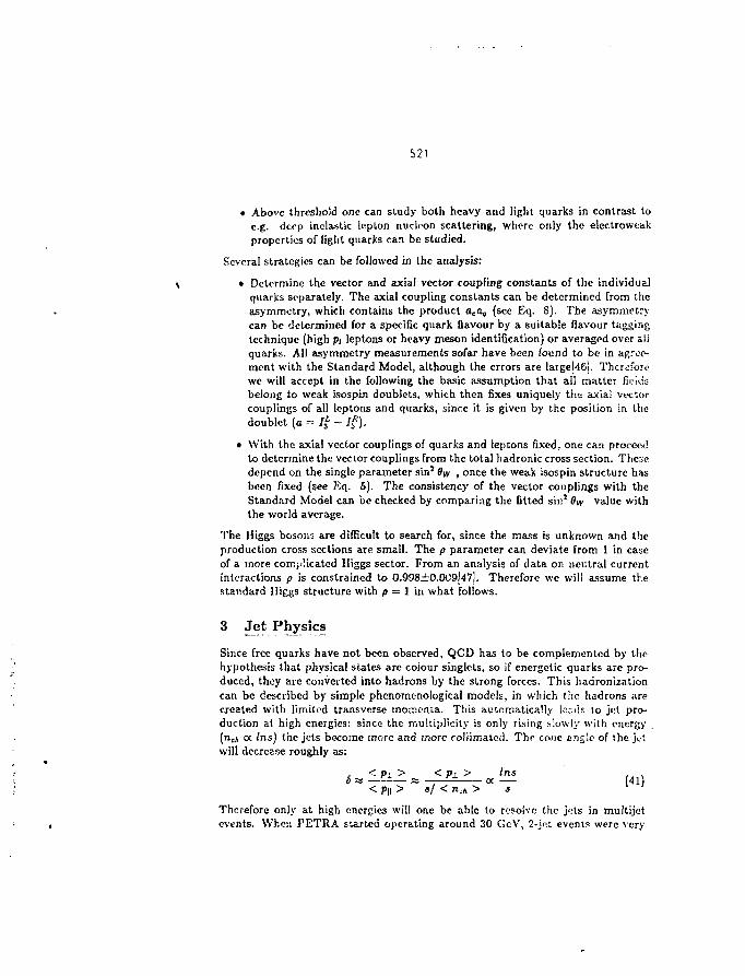
521
• Above threshold one can study both heavy and light quarks in contrast toe.g. deep inelastic lepton nucloon scattering, where only the electroweakproperties of light quarks can be studied.
Several strategies can be followed in the analysis:
• Determine the vector and axial vector coupling constants of the individualquarks separately. The axial coupling constants can be determined from theasymmetry, which contains the product aea, (see Eq. 8). The asymmetrycan be determined for a specific quark flavour by a suitable flavour taggingtechnique (high pt leptons or heavy meson identification) or averaged over allquarks. AH asymmetry measurements sofar have been found to be in agree-ment with the Standard Model, although the errors are large[46i. Thereforewe will accept in the following the basic assumption that all matter fieldsbelong to weak isospin doublets, which then fixes uniquely the axia! vectorcouplings of all leptons and quarks, since it is given by the position in thedoublet (a - Ij? - / f ) .
• With the axial vector couplings of quarks and leptons fixed, one can proceedto determine the vector couplings from the total hadronic cross section. Thesedepend on the single parameter sin' Bw , once the weak isospin structure hasbeen fixed (see Kq. 5). The consistency of the vector couplings with theStandard Model can be checked by comparing the fitted sin1 9vr value withthe world average.
The Higgs bosons are difficult to search for, since the mass is unknown and theproduction cross sections are small. The p parameter can deviate from 1 in caseof a more complicated Higgs sector. From an analysis of data on neutral currentinteractions p is constrained to 0.998i0.009J47j. Therefore we will assume thestandard IJiggs structure with p = 1 in what follows.
3 Jet Physics
Since free quarks have not been observed, QCD has to be complemented by thehypothesis that physical states are coiour singlets, so if energetic quarks are pro-duced, they are converted into hadrons by the strong forces. This hadronizationcan be described by simple phenomenoiogica! models, in which the hadrons arecreated with limited transverse momenta. This automatically loads to jet pro-duction at high energies: since the multiplicity is only rising slowly with energy(nc» a Ins) the jets become more and more roliimated. Thr cone angle of the jetwill decrease roughly as:
J±L*< pi, > sj < n;k >
(41)
Therefore only at high energies will one be able to resolve the jets in multijetevents. When PETRA started operating around 30 GcV, 2-jnl events were very
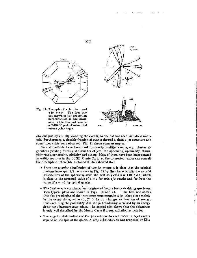
522
usso
Fig. 11: Example of a 2- , 3- , and4-jct event. The firBt twoare shown in the projectionperpendicular to the beamaxis, while the last one iaa 'LEGO' plot of azimuthalversus polar angle.
obvious just by visually scanning the events, so one did not need statistical meth-ods. Furthermore, a sizeable fraction of events showed a clean 3-jet structure andsometimes 4-jets were observed. Fig. 11 shows some examples.
Several methods have been used to classify multijet events, e.g. cluster al-gorithms yielding directly the number of jets, the sphericity, aplanarity, thrust,oblateness, spherocity, triplicity and others. Most of them have been incorporatedas uiility routines in the LUND Monte Carlo, so the interested reader can consultthe descriptions thereJ48j. Detailed studies showed that:
• From the angular distribution of two jet events it is clear that the originalpartons have spin 1/2, as shown in Fig. 12 by the characteristic 1 + acos*$distribution of the sphericity axis: the best fit yields a = 1.01 ± 0 . 1 , whichis close to the expected value of a = 1 for spin 1/2 quarks and far from thevalue of a = - 1 for spin 0 quarks.
• The 3-jet events are planar and originated from a bremsstrahlung spectrum.Two typical plots are shown in Figs. 13 and 14. The first one showsthat the broadening of the transverse momentum in a jet takes place mainlyin the event plane, while < pfl > hardly changes as function of energy,thus excluding the possibility that the p, broadening is caused by an energydependent fragmentation effect. The second plot shows that the oblatenessis only well described by the Monte Carlo if gluon radiation is included.
• The angular distributions of the jets relative to each other in 3-jet eventsdepend on the spin of the gluon. A simple distribution was proposed by Ellis
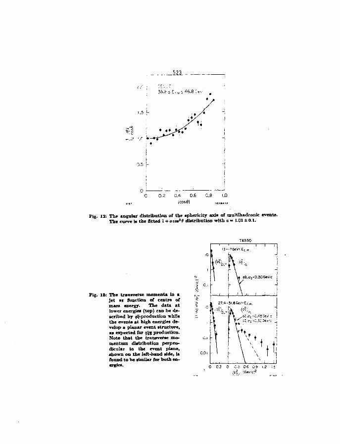
0.5 r
0 0.2 0.1 0.6 0.8 1.0ICOS0I 5M...3
Pig. 12: The angular distribution of the sphericity axis of multihadronic events.The curve is the fitted l + acoaae distribution with a= 1.01 ±0.1.
TASSO
Fig. IS: The transverse momenta in ajet as function of centre ofmass energy. The data atlower energies (top) can be de-scribed by ^-production whilethe events at high energies de-velop a planar event structure,as expected for qq% production.Note that the transverse mo-mentum distribution perpen-dicular to the event plane,shown on the left-hand side, isfound to be similar for both en-ergies. I ,
0 0.3 0 OS 06 O.S 1.2
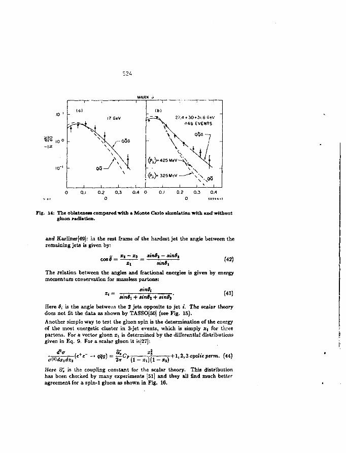
524
10la )
00"
1 1
1 1
17 GcV
L /--0Q6
X
(t>)
' i^ lv c/.4 + 50*51.6 GeV
l i d < ) 6 E V E N T S
\ Tk OSG —i
< > • V V i '- P i ; 4 2 j M e v ~v. % _<p y 325 K»V _ ^ - * x X -
1 1 1 v 1
10"
0 0.1 0.2 0.3 0.4 0 0.1 0.2 0.3 0.49-8/ 0 0 5flS»A!2
Fig. 14: The oblatenen compared with a Monte Carlo simulation with and withoutgluon radiation.
and Karliner[49j: in the rest frame of the hardest jet the angle between theremaining jets is given by:
2COB$ — - xs— ainOs
sin$i(42)
The relation between the angles and fractional energies is given by energymomentum conservation for massless partons:
(43)
Here 0, is the angle between the 2 jets opposite to jet <". The scalar theorydoes not fit the data as shown by TASSO[50] (see Fig. 15).
Another simple way to test the gluon spin is the determination of the energyof the most energetic cluster in 3-jet events, which is simply Xi for threepartons. For a vector gluon x\ is determined by the differential distributionsgiven in Eq. 9. For a scalar gluon it is[27j:
JSr+1,2,3 cyclic perm. (44)
Here 3", is the coupling constant for the scalar theory. This distributionhas been checked by many experiments [51] and they all find much betteragreement for a spin-1 gluon as shown in Fig. 16.
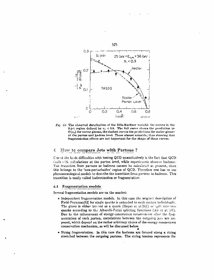
525
^
25 Gev < Ee.m.< 36 Gev !X, < 0.9
Fig. J5: The observed distribution or the Ellis-Karlincr variable for events in the3-jet region defined by ij < 0.9. The full curve sliows the prediction toO(o.) for vector gluons, the dashed curves the predictions /or scalar g]non°at the parton and hadron level. These almost coincide, thus showing thatfragmentation effects are not important for the shape of these curves.
•1 How tc compare Jets with Partons ?
Cao ot the basic difficulties with testing QCD quantitatively is the fact that QCDi'oc.!s v'tr. calculations at the parton level, while experiments observe hadrons.The transition from partons to hadrons cannot be calculated at present, sincethis belongs to the 'non-perturbative' region of QCD. Therefore one has to usephenomenological models to describe the transition from partons to hadrons. Thistransition is usally called hadronization or fragmentation.
4.1 Fragmentation models
Several fragmentation models are on the market:
• Independent fragmentation models. In this case the origin,-*! description ofField-Feynman[52j for single quarks is extended to each pari.cn individually.The gluon is either trcrted as a quark (Iloyer cL zl.i53j) or iplit into tv.oquarks according to the Altarelli-Parisi splHt'mj; functions (AH ct a!. J-i').Due to the enforcement of energy-momentum conservation afier the frag-mentation of each parton, correlations between the outgoing jt:s are im-posed, which depend on the rather arbitrary choice of the energy-momentumconservation mechanism, as will be discussed below.
*• String fragmentation. In this case the hadrons axe formed along a string
stretched between the outgoing partons. The string tension represents the
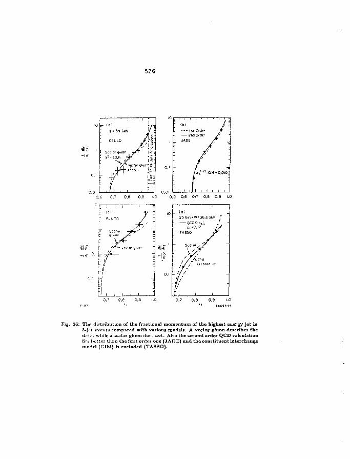
526
- (ol
s • 34 GeV
CELLO
n• — Hi Orle- B -I- 2n0Orttt- /l -j
JADE ^
\ Scalar giuon
: x2130.6
^ ^/ , vc:'o'9iucn-S
0.6 C.r 0.3 0.9 !.O 0.5 0.6 0:7 0.8 0.9 1.0
0.7 G.6 0.5 i.'
Fig. 1C: The distribution of the fractional momentum of the highest energy jet inS-jct events compared with various models. A vector gluon describes thedMn, while a Kcalar gluon docs not. Also the second order QCD calculationfits better than the first order one (JADE) and the constituent interchangemocicl (CIM) is excluded (TASSO).
strength of the colour field (growing linearly with distance) and as soon as thelonsion becomes large enough, the energy is converted into mass by the for-mation of qq pairs at the breakpoints of the string. Such a model introducesexplicitly correlations between the outgoing partons, which are experimen-t.-.lly testable, as will be discussed later. The string fragmentation has beenimplemented in a widely used program written by T. Sjostrand[48].
• Parton shower generation. In this case leading log calculations are used togenerate event.* with many partons in the initial state in contrast to theprevious);- mentioned Monte C'.:rlos, which generate states with at most 4partons {O(at-)). Because of the leading log approximation, the hard gluonproduction does not correspond to the exact QCD first or second order matrixclement. Therefore one has to do a joining of the exact matrix element and theleading log approximation, but one has to be careful to avoid double count ing.This joining of the first order QCD and leading log matrix elements hr-* beenimplemented in the new Monte Carlo of ihe LUND group[48j. Furthermore,this version JETSETO." has the possibility to switch on and oil inlorfcr?r.r>!effects between the initial partons, which were among the difference? of eariicrversions of shower Monte Carlos by Golls'-1iaikj55j and Webber'SC .
4.2 Can one distinguish between the models?
The main difference between independent fragmentation (IF) and string fragmen-tation (HF) is in the different treatment of the gliiun. So a difference can onlybe observed in 3-jet and 4-jct events. The parameters used for the description of2-jct events arc the stime: a fragmentation function to describe the longitudinalmoii'icntum speclm of the hadrons, the variance of the gaussian us«d to goner-ate limited transverse momenta, the ratio of vector to pscudoscalar rnr.ioiis, theamoujil of s- and c-quar!;s generated during fragmentation, amount of diquar'ss(yielding baryems), and others.
In the SF model the s'iuon is pa>t of a string stretched between the quarks. Ifthe gluon is soft, the main effect will be to give some transverse momentum to thestring, but the event remains 2-jet like. If the gluon is hard and at a large angle,it will give a large pi to the. siring and Kenerate a 3-jet-like event. However, since(he gliion is connected via a string to both quarks ii. will drag both s:ring picresin the direction of the gluon, thus depleting she particle density on the other side;,(see Fig. 17).
This string effect was first observe! by JADE and later confirmed by severalother expcriments[57]. It is shown in Fig. 18: After selecting the hf.rdtst jet in3-jct events, the particle density with respect to this direction (0" in Fig. IS) isclearly higher in the region between the most energetic and least energetic jet ascompared to the particle density in the region between the two most energeticjets. The least energetic jet has the highest probability to be the gluon jet. It iscompared with several models: clearly the siring fragmentation mode! describesthe data, while the independent fragmentation model decs not. However, some
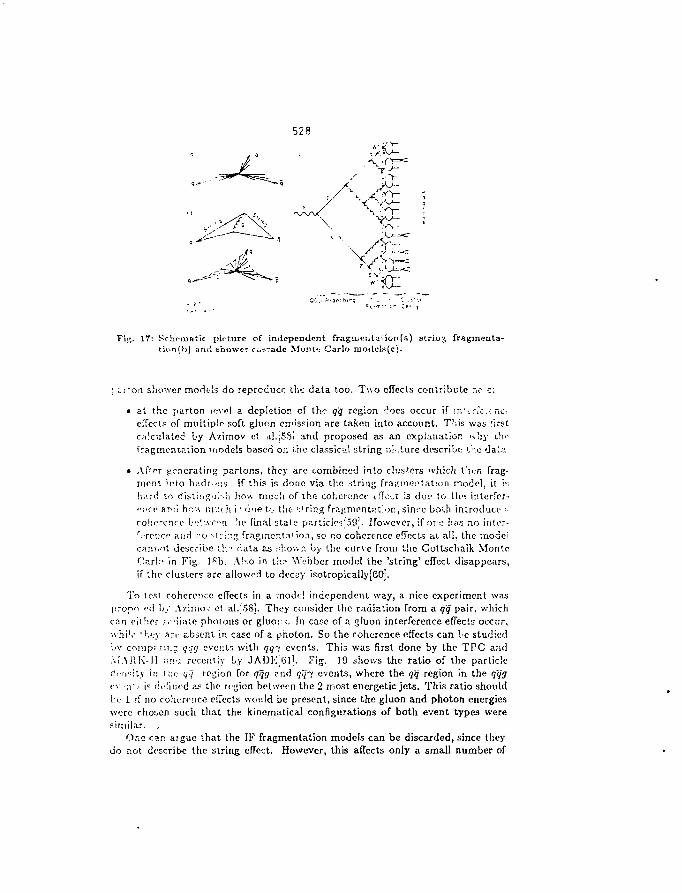
528
Fig. IT: Schematic picture of independent fragoiei.tai ion(a) striuj fragmenta-
tion(li) ami shower c;.»-adc Mositi; Carlo moiicls(cj.
; L:',an shower modi's do reproduce the data too. Two effects contribute nc e:
e at the parton level a depletion of the qq' region ;'oes occur if iri'"_rfc.< na.effects of multiple soft giuon emission are taken into account. This was rirstcalculated by Azirnov e' iil.lSSi and proposed as an explanation '\!iy ch<-
rragraentrLtion 'iiodels based o;i the classics! string pi-.ture describe the da;..i
• After generating partons. they are combined into clusters which tV-n frag-ment ipto h;'.dr-'::s if this is done via the itrin;; fragmentation model, it !•;h.'.rti to disliiig'ji'-h hov. much of the coherence ifT.v.i is due to th™ interfcr-"i'ce ar>ii ho-v m'Jt h i' cine to the ':'rir;g fr?.j;rnentr.t:or., sinrc both introduce -coiicrcnre bo'.'.vr"n !H- final stale p.irticlos'59j. However, if ore lias no intor-'[•renci' and ro ?t: ::•£ fraginer.t^vio.i, so no coherence effects <u all, the rnodeicannot describe th" riata as nhov.r. by the curve from the Gottschalk MonteCarle in Fig. 18b. Also in th.'* \\'cbber raodel the 'string' effect disappears,if the clusters arc allowed to d«?cay isotropically[60].
Tn icM coherence effects in a mode! independent way, a nice experiment waspropn fd by Aziniov ot al.|58j. They consider the radiation from a qq pair, whichcan either .-."lime photons or gluo.'.-:. Fn case of a gluon interference effects occur,whiV ''•,'.•>• arc absent in case of a pnoton. So the coherence effects can be studied:<v compr-ni:; q~.;<j even Is with 957 events. This was first done by the TPC andMAHK-II ani recently by JADK;S1]. Fig. JO shows the ratio of the particlefjcri ity in v,:c q-~j region for qqg and qq-< events, where the qq region in the qq'gev-a'.-. is di'tiucd a? the region between the 2 most energetic jets. This ratio shouldl:c 1 if no coherence effects would be present, since the gluon and photon energieswere chosen such that the kinematical configurations of both event types weresimilar. .
One can argue that the IF fragmentation models can be discarded, since theydo not describe the string effect. However, this affects only a small number of
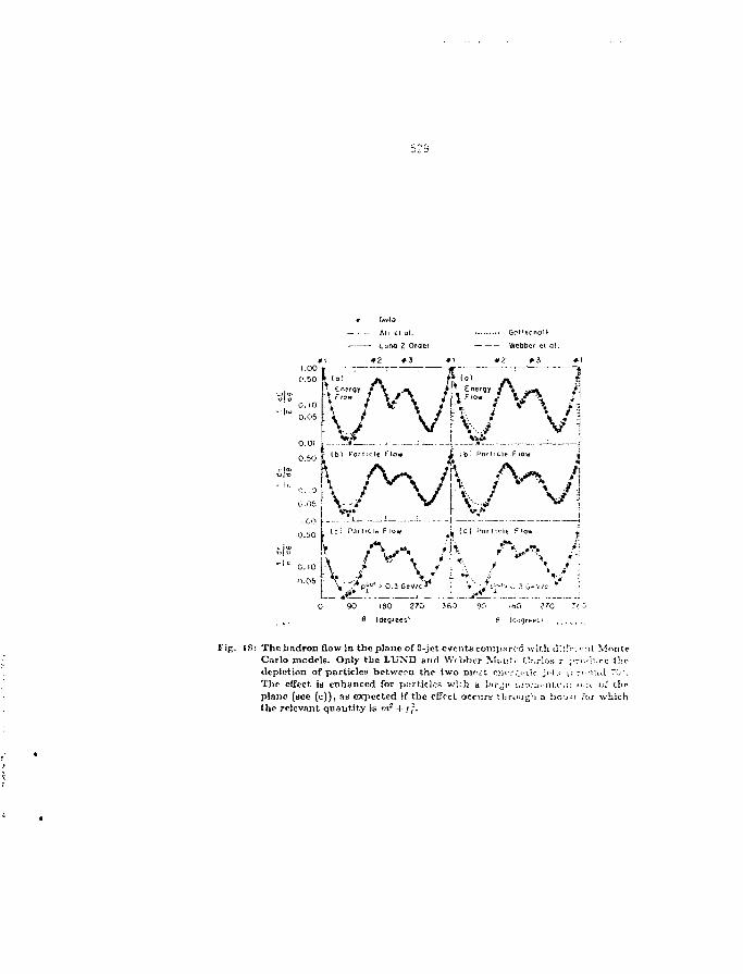
— - — A l l £1 a l .
Lund 2 Oraei
• 2 #3 #1
WeDDer ei a!.
42 # 3 #1
M="/V\ /j\ j V i
ib" PoMicle fiow
(c i Panicle Flo«
| c 0.10
O.Ob
( c ) f o r l icl« F'Ov.
\ ./ " \/[\ / Vi0 90 iBO 270 J60 90 iiu ??0 ?<-0
6 laegrees! £ lot-qreec./
Fig. IS: The badron flow ia t hop lane of 2-jct cvcuta compnrod v,ith iJ*:!>••. r-r.t MnritfCarlo tncdcls. Only the LUND and Webber Mi.uf.- c:r.:-!o.H r- ;r.-.'!:ir,? U.Cdepletion of particles betwe-pu the two nif»£t ciicr.it-Lir jet.-. \: r>. •i:ij 70 .Tho effect id enhanced for particlos w:;.h a ]-:ir,jc i.io::i-ni.r.;: n.:t. oi" Llir>plane (sec (c)), as expected if the effect occurs tln-oiig'i 3 br.-j-i for which(he relevant quant i ty is m2 + p;.
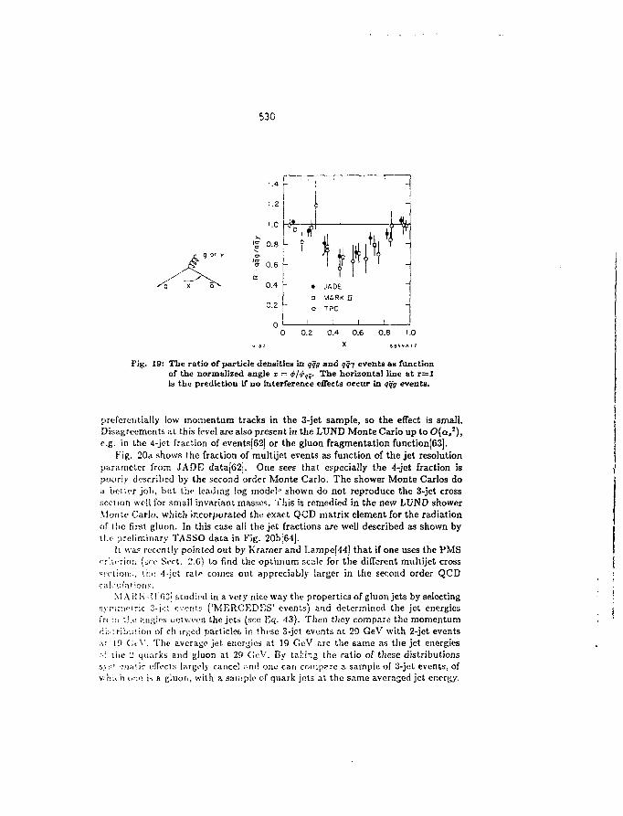
530
I1.2 h
' I 0.8 I- ?
I 0.6or
0.4
0.2
• JADE
• MARK U
O TPC
0.2 0.4 0.6 0.8 1.0
Fig. 19: The ratio of particle densities in qqg and qqi events as functionof the normalized angle i = <j>/<f>^- The horizontal line at r=lis the prediction if no interference effects occur in qqg events.
preferentially low momentum tracks in the 3-jet sample, so the effect is small.Disagreements at this level are also present in the LUND Monte Carlo up to O(a,2),e.g. in the 4-jct fraction of cvents[62j or the gluon fragmentation function(63].
Fig. 20a. shows the fraction of multijet events as function of the jet resolutionparameter from JADE data[62i. One sees that especially the 4-jet fraction ispoorly described by the second order Monte Carlo. The shower Monte Carlos doa bcli«r job. but the leading log mode!' shown do not reproduce the 3-jet crosssection well for small invariant masses, ihis is remedied in the new LUND showerMonti- Carlo, which incorporated the exact QCD matrix element for the radiationof the first gluon. In this case all the jet fractions are well described as shown byil.c preliminary TASSO data in Fig. 20b[64j.
It was recently pointed out by Kramer and Lampe[44] that if one uses the PMS'•riii'rion (s''« Sort. 2.6) to find the optimum scale for the different multijet crossseciion:-, is;.; 4-jet rate comes out appreciably larger in the second order QCDc;i!\'ui;i* ions.
MARK-il r>3'i studied in a very nice way the properties of gluon jets by selectingsyrii'.H'iric 3-jot events ( 'MERCEDES' events) and determined the jet energiesi>< :•: the ftnglos ueiv.cen the jet= (sec Eq. 43). Then they compare the momentumd;:--:ribuMon of cli-ir^ed particles in tVirse 3-jet events at 29 GeV with 2-jet eventsA: 10 Gi'V. The average jet energies at 10 GeV are the same as the jet energies•'.•' liie - quarks and gluon at 29 Ge.V. By taking the ratio of these distributionss>.-•'-Tiisiiir effects largely cancel ;\m! olio can compere a sample of 3-jet events, ofv.'hii h one is a gluon, with a sample of quark jets at the same averager! jet energy.
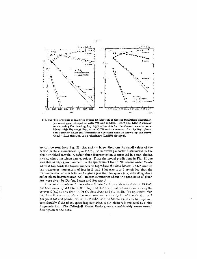
531
_.- - - - *
001 002 003 OOi 005 Q06 007 0080.01
C.I" O.Oi 0.03 O.i;« 0.05 O.Ot 0.07 0.06
FIR. 20: The fraction of multijot events as function of the jet resolution (invariantjet mass ym>n) compared with various models. Only the LUND showerniotj.'-l using the Loadmg Log Approximation for the shower cascade com-bined with the exiict first order QCD matrix elcmeut for the first gluoncan describe all jet multiplicities at the same tizzir .is shown by the curveO(a.) + LLA through the preliminary TASSO data (04).
As can be seen from Fig. 21, this ratio is larger than one for small values of thescaled [>ar'.icie momentum z, = Pi/Bja, thus proving a softer distribution in thegluoit enriched sample. A softer gluon fragmentation is expected in a non-abelianmode), where the gluon carries colour. From the model predictions in Fig. 21 onesees that at high gluon momentum the spectrum of the LUXD second order MonteCarlo is too hard; the shower models do reproduce the data better. JADE studiedthe transverse momentum of jets in 2- and 3-jet events and concluded that thetransverse momentum is larger for gluon jets ihar; for quark jets, indicating also asofter gluon fragmentation !C5l. Recent summaries about the properties of gluonjet? were giver by Dorfan. faxon and Sugano'l1.
A recent cc:r:parison of he various Monte C;. !o rrr>dels with data at 29 GeVha.s been m.-.-.iio '_y MARK-lf:00j. They find that •:•,•:• I.U.\D shower niooe! using thecorrect O(a,] ni.-itrix elcrr-. it for thfl first ^luor. ar.d :,..? lead in;; k'g apjiroxim.-'ionfor the soft ghiTis provic • i.,e mos'. roE-scna'.'o d';;ci;ptior. <>r the dala'.x1 "s 2per point for 4oO points), while the Webber she . 'cr Mor.te Carlo tia be in.pr -vciconsiderably if the phase space fragmentation of!!\o clusters is replaced by siringfragmentation. The Caltech-II Monte Carlo gives a consiJorably worse overalldescription of the data.
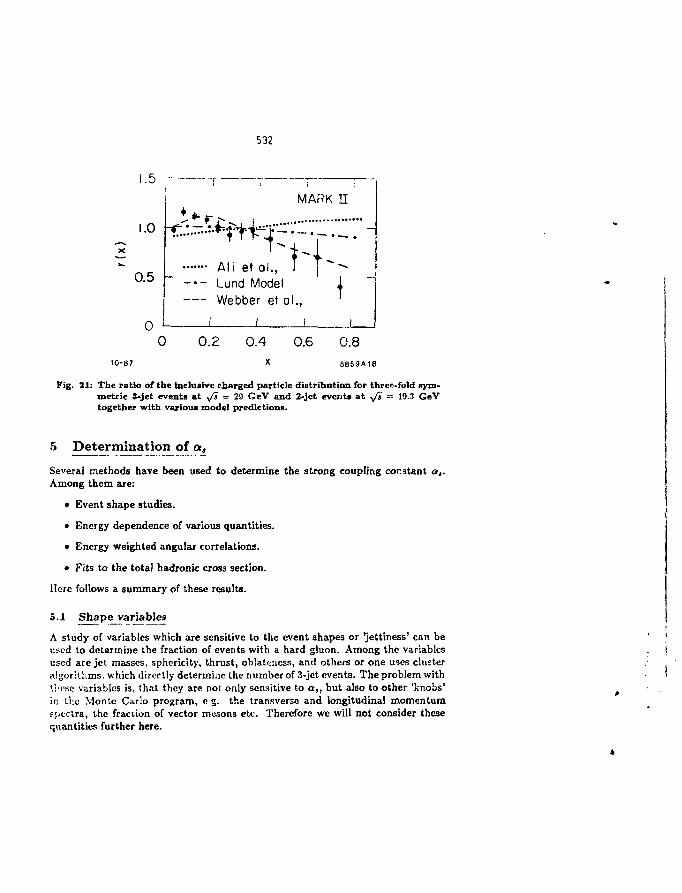
0
532
1.5
1.0
0.5 -
MARK H
Ali et ol.,Lund Mode!Webber et al.,
0 0.2 0.4 0.6
10-87
0.85859A18
Fig. 21: The ratio of the inclusive charged particle distribution for three-fold gym-metric 8-jet events at •/> = 29 CeV and 2-jet events at •/£ = 19.3 GeVtogether with various model predictions.
5 Determination of a.
Several methods have been used to determine the strong coupling cor.3tant a,.Among them are:
• Event shape studies.
• Energy dependence of various quantities.
• Energy weighted angular correlations.
• Fits to the total hadronic cross section.
Here follows a summary of these results.
5.1 Shape variables
A study of variables which are sensitive to the event shapes or 'jettiness' can beused to determine the fraction of events with a hard gluon. Among the variablesused are jet masses, sphericity, thrust, oblatwiess, and others or one uses clusteralgorithms, which directly determine the number of 3-jet events. The problem withticse variables is, that they arc not only sensitive to a,, but also to other 'knobs'in ihc Monte Carlo program, e g. the transverse and longitudinal momentumejicclra, the fraction of vector mesons etc. Therefore we will not consider thesequantities further here.
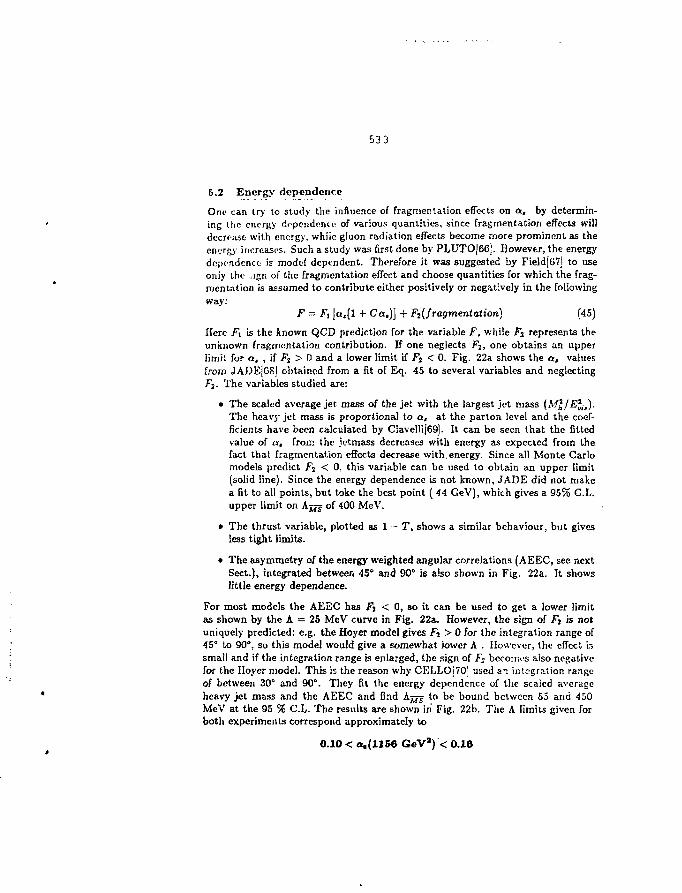
533
5.2 Energy dependence
One can try l o study the influence of fragmentation effects on a, by determin-ing the energy dependence of various quantities, since fragmentation effects willdecrease with energy, while giuon radiation effects become more prominent as theenergy increases. Such a study was first done by PLUTOJ66). However, the energydependence: is model dependent. Therefore it was suggested by Field[67j to useonly the -ign of the fragmentation effect and choose quantities for which the frag-mentation is assumed to contribute either positively or negatively in the followingway:
F = Fi |a,(l + Ca.)] + Fi{fragmentation) (45)
Here Fj is the known QCD prediction for the variable F, while Fj represents theunknown fragmentation contribution. If one neglects F?, one obtains an upperlimit for a, , if F2 > 0 and a lower limit if F2 < 0. Fig. 22a shows the a, valuesfrom JADEJGS] obtained from a fit of Eq. 45 to several variables and neglectingFj. The variables studied are:
• The scaled average jet mass of the jet with the largest jet massThe heavy jet mass is proportional to a, at the parton level and the coef-ficients have been calculated by ClavelHJ69]. It can be seen that the fittedvalue of a, from the jetmass decreases with energy as expected from thefact that fragmentation effects decrease with.energy. Since all Monte Carlomodels predict F2 < 0, this variable can be used to obtain an upper limit(solid line). Since the energy dependence is not known, JADE did not makea fit to all points, but toke the best point ( 44 GeV), which gives a 95% C.L.upper limit on Ajjg of 400 MeV.
• The thrust variable, plotted as 1 - T, shows a similar behaviour, but givesless tight limits.
• The asymmetry of the energy weighted angular correlations (AEEC, see nextSect.), integrated between 45" and 90" is also shown in Fig. 22a. It showslittle energy dependence.
For most models the AEEC has Fa < 0, so it can be used to get a lower limitas shown by the A = 25 MeV curve in Fig. 22a. However, the sign of Fj is notuniquely predicted: e.g. the Hoyer model gives F% > 0 for the integration range of45° to 90°. so this model would give a somewhat lower A . However, the effect issmall and if the integration range is enlarged, the sign of F» becomes aiso negativefor the Iloyer model. This is the reason why CELLOJ70' used an integration rangeof between 30° and 90°. They fit the energy dependence of the scaled averageheavy jet mass and the AEEC and find AJJJ to be bound between 55 and 450MeV at the 95 % C.L. The results are shown'in Fig. 22b. The A limits given forboth experiments correspond approximately to
0.10 < a,(1158 GeV9) < 0.16
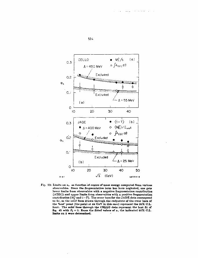
0.3
0.2
O.I
i
—
CELLO
A - 4 5
<^/
(a)
OMeV
Excluded
11 Excluded
• Mi/s
i
'///
55
(a)
MeV
10 20 30 40
0.3
0.2
0.'
_ JADE <1-T> (b) j
7I77777777777ri™777rm^Excluded /
(b)
10 20 30 40
(GeV)
50
Fig. 22: Limits on a, as function of centre of xnasfl energy computed from variousobecrvableB. Since the fragmentation term has been neglected, one get*lower limits from observable* with a negative fragmentation contribution(AEEC) and upper limits from observable* with a positive fragmentationcontribution [Mj; and l-T). The error bars for the JADE data correspondto 2u, so the solid lines drawn through the endpoints of the error ban ofthe 'best' point (the point at 44 GeV in this case) represent the 95% C.L.limit. The solid lines through the CELLO data represent the best fit ofEq. 45 with F2 = 0. From the fitted values of a, the indicated 95% C.L.limits on A were determined.
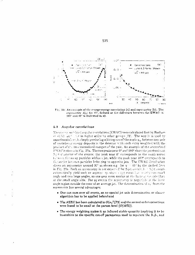
535
*C 50 60 7
X voeorees
23: An <x.-i;nj>Ie of t!ii' i-icrgy-cncrrgy correlation (a) and asymmetry (b). Thefrsyini.ietry A[\) for -IT', defined as the difference between the EVVAC r;t135- siiid 45J is indicated in a).
5.3 Angular correlations
Tbi' <•:'<••"'. ivi : ':hlr>: s rnu ' .a r f i r ro ln t ions (EWAC) were calculated first by Basham(i .il.'Vl, <JI: : ' i r in high'.-r order Vy o the r gr^i:;-"; [72 ;. T h e way it is useri byexporiinont. i l i -1-, it i imply producing a hiEiogram of the angle x,j be tween any pairof parliclos ur o;.'Tgy deposi ts in ' h e detector with each ontry wr ig l i t rd w i th theproii i ir t of O.i two normal ized energies of the pai r . An exarnpl<- of thf normalizedKU'AC is SIKM1- i: in Fi>;. '2'Ja.. T h e two poaiis jiear 0° and 180° sbov-' tii-i ;>rrdomir..mt'?•;. \ c!..ir;ider tif the evenls : the peak near 0* r o r r f s p o n d s to the ?;<iali Rriple::1.. :-.M-i i: tl:!1 !!:;• iiv par l ic ies wi'liiii ;L jot , while the peak near 180° cnrrclspo.-..-!s tolli.1 n!i'/.\i'S ti!'i .vofn part icles l>o!o; ; ing :o oppof i te j e t s . T h e K\ \ 'AC di^triV'ijtionsl.tii',s an asyinnictfy a r o u n d 90" a1; shown e.g for \ •- •15r' by the- dB.shfd iim-,in Kir.- 2/ln. Such an a s y m m e t r y ' s r ! n t ex[«-c'••.•! fc>r 2-jct t-i'-'.'it.1-'. !• ' T-j-'t i-'.fiitse'U'.omi-tically )ie!d sue!', an asymn;- ry. sir,c• • > r-;z even; /•.;- i- :;•::;.• urn-. ?i;ia!langle and two large angles , so one geis more entr ies at thv In::'..' .r "•• ; itic tha:;at the small angle side. For gtj events th.- a:•yir.rnftry is no^ii-".!::!'-- '.;• the- i;:,"vai^'le region outs ide the cone of an average j e t . T h e G e t e r m n u t i o n 'A :•, from thea s y m m e t r y has several advan tages :
• One can sura over all even ts , so n o special j e t axis de t e rmina t ion or cluil iT
algorithrn has to be applied beforehand
• The AKEC has been calculated in O(a,2)[72l and the second order correctionswere found to be small at the parton level (O(10%)).
• The energy weighting makes it an infrared stable quantity implying it to beinsensitive to the specific cut-off parameters used to separate the 2-,3-, and
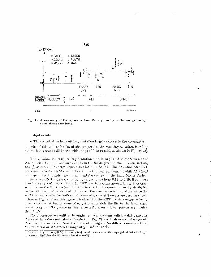
536
a s (3£GeV)
0.2
01 —
• JADf ^ TASSOoCEL!.-.; v PLUTOQMAPKO O MAC
MODEL NEGLECT £ l.'i/si
FKSS/GKS
ERi
ALI
FKSS/ F:;TGKS
LUND
Fig. 2ir A summary of the a, values frouicorrclationa (see text).
asymmetry in the euerg> - m-r-gy
4-jet events.
• The contribution from qq fragmentation largely cancels in the asyrr_meli\.!-. ; iU ill" this impressive list of nice properties, the resulting a3 values founil hitin' vaiiob- groups still have a wide rftrgo of n i 2 i:> 0.3S, ;i> sliown i'i T'rj 24;73j.
Thi1 -i, vaiin.. iri'licaled a> 'rags/icntati.in MIOHI Is 'neglected' coma !ro;;i a fit ofK'l. '1:i wit!; / '; !., ':,' .•.;.' co;-.-. pond-. Lu l];u
!!.;ijts givi.n in the /ions section,and ';_ a.; u -.•: ."' i? ••.icr;;> tlopeiiiln.'M'''; f-.-r '•'• in Eq. '15. The indication Alt ' UUTrori-ot;ioi.j.5 :o tht Ali M-vju-f '"arl;-. •*'•! '••• .!-P Kt'.T ;nalrb: eiernont, v/hile Ali f GKS~o?rt~. -[jc.iis to the indcprini- ;i fra£!ncnfa!.io:i option in the Lund Monte Carlo.
i-or i;;e LUND Monte Car. > i.ie c , VLIJOS '•;)r.}ie from 0.14 to 0.19, if summedirt'er U> matrix el'Tucnts. Sine •• the J.'ii'f [p.ilri*. '.:!••;:;ent gives a larger 3-jet cross.-<•:•!-pp. t>-a', Oie CKS one fsc<> Fis. 7 in S'x.. 2.3), thi? spread is usually attributedio (lie iilT'r<nt 'ii.-itrix elcmcnto. However, this conclusion is premature, since t!ieAEKC is -'*::y s;rni!a: :"or woth iiutrix plernonts, at lenst if y-cuts are used, as shownbefore in Ki.,.;. 8. From tiiis :i^ure it is clear that the ERT matrix element .it'iuiiiyi;l-( a eotiii-what higher vaiue of a , , if one restricts the fits to the largo a;:gv-ra.igc (cos.\ > - 0.7), since in this range EFT gives a lower parton asymmetrythan GKS 3.
Thi- differences are nnlilclv to originate from problems with the data, since in<]-.\r case the value? indicated a.1" 'ju'ijlrct' in Fig. 24 would show a similar spread,['ossihli- •Jiffcrcijccs come froi i :.l«r different tuning and/or different versions of theMonte Carios or the different range of x used in the fit.
nAu .v'.ii..! !U to the CELLO iHta with both matrix r, va!-ic ' . ERT, but the dilTirence i« le"s than O.OO2j74[.
in this rr-.nge yielded indeed a \w
537
The influence of various fragmentation models on the AEEC has been sum-marized in Fig. 25 as function of a, for yfs = 44 GeV. The curves labeled Aliend lloycr were generated with the options for independent fragmentation in theLUND program, so they all use the same GKS matrix element. It can be seenthat the Hoyrr model increases the asymmetry of the hadrons as compared to theparlon asymmetry (line labeled partons), while the other models (Ali and LUND)decrease the asymmetry compared with the value at the parton level. Conse-quently, the observed asymmetry requires'for the Hoyer model a lower value ofa, than for the Ali and LUND models. As can be seen from Fig. 25 from theaveraged data at 44 GeV from CELLO[74], JADE[68j and TASSO[75] one finds:
a'H « 1.4 (-to)
while the ration Lwd
is appreciably smaller.The large difference between the two independent fragmentation models Ali
and lloyer comes mainly from the different mechanism of energy momentum con-servation (EMC), as was Crst discovered by CELLO(76j and later studied in moredetail by Sjostnindj'i"!. In IF models the partons fragment independently, so en-ergy and momentum cannot be conserved simultaneously, because one generatesa massive jet from a massless parton. One then has to apply an EMC mechanismto the ensemble of the jets after fragmentation. The difference between Ali andHoyer can be qualitatively explained as follows: The fragmentation of each par-ton is stopped below a certain energy, say 1 GeV. Then overal energy momentumconservation can be imposed in several ways:
• In Hoyer it is done by rescaling the jet energy of each jet separately in such away that ihe jet directions are not changed, so the hadrons follow the originalparton directions.
• in Ali it is done by performing first s. boost in the direction of the missingmomentum and then reseating the energies.
For 2-jei cnts the effects are not important, since on the average the missingmomemtum in opposite jets compensates. However, in case- of 3-jct events, themissing momentum in the 2 opposite jets still cornpons.ucs on l ho average, sothe missing momentum tends to po<at in the direction of the third jet ('is'jally thegluon jet). In the hoyercas-.' tnore energy is t fieri given lo 'lie giuon to compensatethe missing momentum, thus increasing the 3-jettir.css. ;:> the Ali case a boost isperformed in the direction of the rr.issir.g momentum, which is preferentially thegiuon. This has a similar effect as the boost of the string? 'in the LUND program,namely it decreases the average angle between the quark and gluon jet. Since thebrcinsstraWungspectrum of the gluon is a s'.eep function of this angle, one shouldnot be surprised to find a, to be sensitive to such effects m fragmentation models.
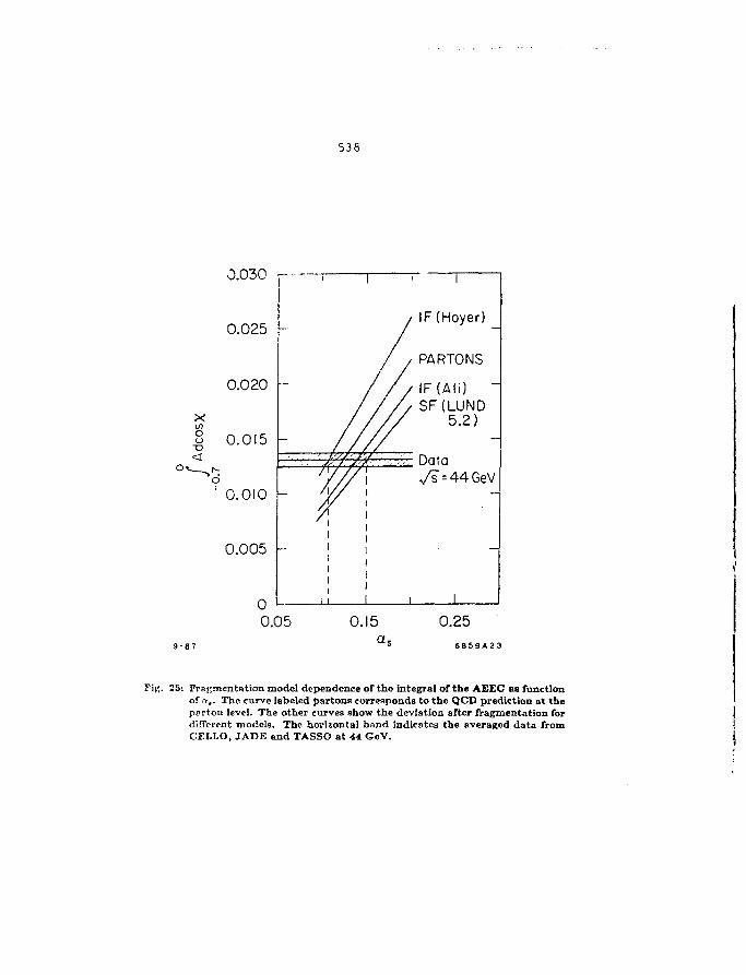
538
0.030
0.025 -IF(Hoyer)
PARTONS
IF (Ali)SF(LUND
5.2)
0.05 0.15 0.25
FIR. 25: Fragmentation model dependence of the integral of the AEEC as functionof a,. The curve labeled partonB corresponds to the QCD prediction at theparton level. The other curves show the deviation after fragmentation fordifferent models. The horizontal band indicates the averaged data fromCELLO, JADE and TASSO at 44 GcV.
539
5.4 Conclusion on the asymmetry in angular correlations
What should be the conclusion of all this? Different collaborations give differentanswers. MARK-J|78| and PLUTO[79j maintain that one can determine a, wellfrom the AEEC. However, they estimate the systematic uncertainty from fragmen-tation models by cleverly picking the models which give very similar results: Aliand Lund, thus ignoring the Hoyer model.
JADEJ80], MAC|81) and MARK-II[34] find a large difference in the a, val-ues between SF and IF models, but they find that IF models describe the databadly. However, this must be partly due to a poor tuning, since CELLO[76j andTASSO|33t Gnd that their IF models describe the data reasonably well, at least inthe angular range of interest *.
The comparison of data with the Hoyer model is shown in Fig. 26 for CELLOand JADE data. JADE's tuning of the IF model disagrees everywhere, whilethe CELLO tuning of IF describes the data as well as SF in the angular rangeof interest (30° to 150°). The angles near 180° are not well described by the IFmodel, since ymin = 0.03 was used in that case, while for SF Jim,,. =0.015 was used.The SF model would not describe the 'inside jet' region either with ymin=0.03[S0].
However, it is difficult to use such a small ymm for the IF model, since in thatrase most events would have a soft giuon of a few GeV and IP models are notdesigned to fragment partons of a few GeV. The SF model has the nice propertyto absorb such soft gluons in the string, so their only effect is to generate sometransverse momentum.
Note that even a small !/„,„ of 0.015 eliminates already most angles below 20°at the parton level, so one should not be surprised to find disagreements in the"inside jet' region at the hadron level. It is somehow fortuitous, that one can finda t/m,n for the SF model such that the 'hole' at the parton level is filled by thehadrons moved into this range by the string effect.
In conclusion, since all models can be tuned to describe the bulk of the data (the2-jct and hard 3-jet events) reasonably well, there seems to be no convincing ar-guments to eliminate some models in the estimate on the systematic uncertaintiesof a,. Therefore, the uncertainty in a, from fragmentation models is appreciablylarger than the uncertainties from the different matrix elements and the differentparton dressing schemes (see Sect. 2.3). Especially, the two most widely usedmatrix elements (ERT and GKS) give the same results for the AEEC in the largeangle region, if y-cuts are used.
Considering the HOYER model and LUND mode! to be extremes, one findsfrom Fig. 25 for the a, determinations at y/s = 44 GeV:
0.11 < a, (1036 GeVJ) < 0.16'One obvious difference between the tuning used by the different experiment! if thai JADE, MAC and
MARK-I1 ill me a very small >_,,. cut Of 0.015, while CELLO and TASSO use larger values. A y» . n of0.015 implies that most events hav« a fluon of a few GeV and fragmenting such low energy jets requiresa delicate tuning. Furthermore, the last 2 experiments use the Petereen fragmentation function for heavyquarks, while the others use the LUND fragmentation function- tor heavy and light quarks, thus havingless degrees of freedom.
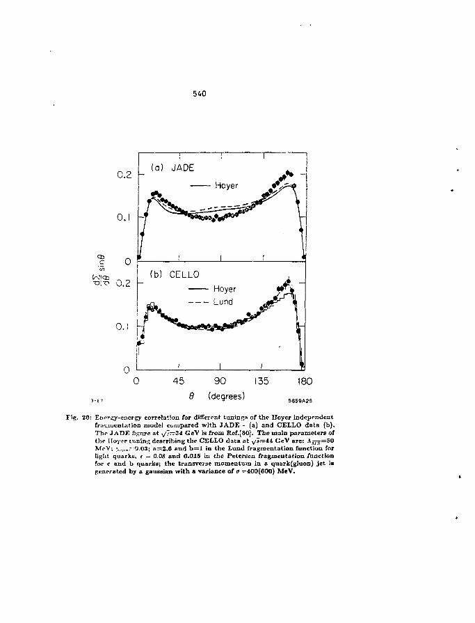
540
0.2
0.1 -'
? 0K'lCD
l 0.2 h
0.1
0
(a)
j s
(b)
1
JADE
CELLO
- Hoyer
1
- Hoyer- Lund
i
I0 45 90 135
5 (degrees)
180
SB59A25
Fig. 26: EncriQr-encrgy correlation For different tunings of the Hoyer independentfr«u.iucntatiou model compared with JADE - (a) and CELLO data (b).The JADE figure at ^ = 3 4 GeV is from ltof.[80j. The main parameters ofDie lloyer tuning describing the CELLO data at y/5=44 GeV are: A ^ = 5 0McV; •,,.lln:-:0.03; n=2.6 and b = l in the Lund fragmentation function forli^ht quarks, e = 0.08 and 0.0X5 in the Petcrsen fragmentation functionfor <• and b quarks; the transverse momentum in a quark(gluon) jet isgenerated by a gaussian with a variance of tr =400(600) MeV.
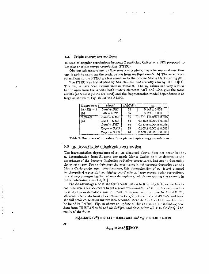
5.6 Triple energy correlations
Instead of angular correlations between 2 particles, Csikor el al.[82j proposed touse planar triple em-rgy correlations (PTEC).
Obvious advantages are: a) One selects only planar particle combinations, thusonr is able to suppress the contribution from multijet events, b) The acceptancerorrccliojiS to the PTEC are less sensitive to the precise Monte Carlo tuning jS3j.
The 1'TEC was first studied by MARK-J|S1] and recently also by CELLO[74j.The results have been summarized in Table 2. The or, values are very similarto the ones from the AEEC; both matrix elements ERT and GKS give the sameresults (at least if y-cuts are used) and the fragmentation model dependence is aslarge as shown in Fig. 25 for the AEEC.
hitpfimcnlMARK - J[841
CELLO[74]
ModelLund + BUTAii+ERT
Lund + GKSLund-i-GKSLund + ERTHoyer + GKSHoyer+GKS
Ji(GeV)35353544443544
<*.0.147 ±0.0050.112 ±0.005
0.151 ±0.003 ±0.0060.145 ±0.004 ±0.0060.143 ±0.004 ±0.0060.103 ± 0.002 ± 0.0060.100 +0.004 ±0.003
Table 2: Summary of a, values from planar triple energy correlations.
5.6 a, from the total hadfonic cross section
The fragmentation dependence of a, as discussed above, does not occur in thea. determination from R, since one needs Monte Carlo? only to determine theacceptance of the detector (including radiative corrections), but not !o determinethe event shape. For 47T detectors the acceptance is not strongly dependent on theMonte Carlo model used. Furthermore, this determination of a, is not plaguedby theoretical uncertainties, 'higher twist' effects, large second oider corrections,or a strong renormalization scheme dependence, which are among the caveats inother determinations of a,[4lj.
The disadvantage is that the QCD contribution to R is only 5 %, so one has tocombine several experiments to get a good determination of R. In this case one n.isto study the systematic errors in detail. This was recently done by CBT.I.O[30 ,who combined data from all experiments for ,/J between 14 and -IS Ct:V and lookthe full error correlation matrix into account. More details about the method canbe found in Ref.[85]. Fig. 27 shows an update of this analysis after including newdata from TRISTAN at 50 and 52 GeV[86| and data below y/1 < 10 GeV('87j. Theresult of the fi*. is:
a.(H56GeVa) = 0.141 ± 0.021 and sin* Sw = 0.240 ± 0.019
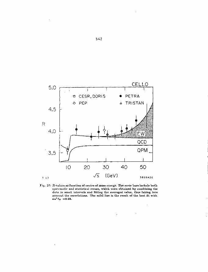
R
5.0
4.5
4.0
3.5 -
CELLO
D CESR,DORIS
O PEP
• PETRA
A TRISTAN
10 50
5859A26
Fig. 27: It-values as function of centre of mass energy. The error bars include bothsystematic and statistical errors, which were obtained by combining thedata in small intervals and fitting the averaged value, thus taking intoaccount the correlations. The Bolid line is the result of the best fit withsin2 lw =0.23.
5 4 3
This value of sin* Ow is in good agreement with the world average of 0.23 |85]. Weused as addit ionat input only Gp and a, so this value of sin3 6w is determined onlyby the vector coupling of the quarks and has no large loop corrections, becauseof the Ar cancellations in Eq. 6. Since the quark couplings are apparently inagreement with the Standard Model expectations, we can keep sin3 $w fixed atthe world average of 0.23. Refitting yields:
a,(1156 GeVa) = 0.145 ± 0.019
A-m = *»*SgMeV.The value of a, including the data around and below the T-region is somewhatlower than the result from the fit restricted to the energy above 10 GeV[39).However, since the difference is within one standard deviation and both fits givean excellent x2 of about 0.7 per degree of freedom, there seems to be no reason toexclude part of the data.
Several points are worth mentioning:
• The result of the global fit describes well the single experiments. For examplea fit of the normalization factor of each experiment was always compatiblewith the quoted normalization error.
• No correlations between different experiments were assumed, but the effectof an hypothetical common correlation error was estimated by introducinga correlated normalization error of 1% for all experiments in the full errorcorrelation matrix. The effect on the fitted parameters was found to be small.
• Within one experiment , the measurements at different cm. energies arecertainly correlated. However , how much of the systematic error has to beconsidered common normalization error and how much point-to-point sys-tematic error is not defined precisely. Therefore, the amount of splitlingbetween normalization and point-to-point error was varied by :: 509c. Theresulting change in the parameters is small as can be seen from the. differenterror contours in Fig. 28.
Note that these error contours correspond to Xmin + * • ^ h° extremes of theerror contours, projected onto each axis correspond to ± la, i.e. f><?% C.L. foreach of the parameters ( not to be confused with the C.L. inside the contour,which is 39% |46j.)
• The value of a, from R is in agreement with recent a, values from deepinelastic scattering [88] and quarkonium decays[89j (see Table 3) and fromlimits on a, presented in the previous section.
• The numerical value of a, depends on the renormalization scheme. To givean experimental value of the QCD contribution independent of the rcnormal-ization scheme, it was fitted by a linear expression
R = REW(O. + b(E - 3iGeV)).
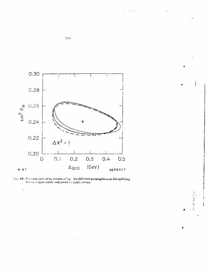
0.30
CD
c1/1
0.28
0.25
0.24 |-
0.22
0.200 0.
9 - 8 7
.;. 28: Cmitour plot; of a, versus sin" (»• for different, assumptions on the splitting1><-I .-.•(..• n Hj-sumatic and point U) poiur. urrors.
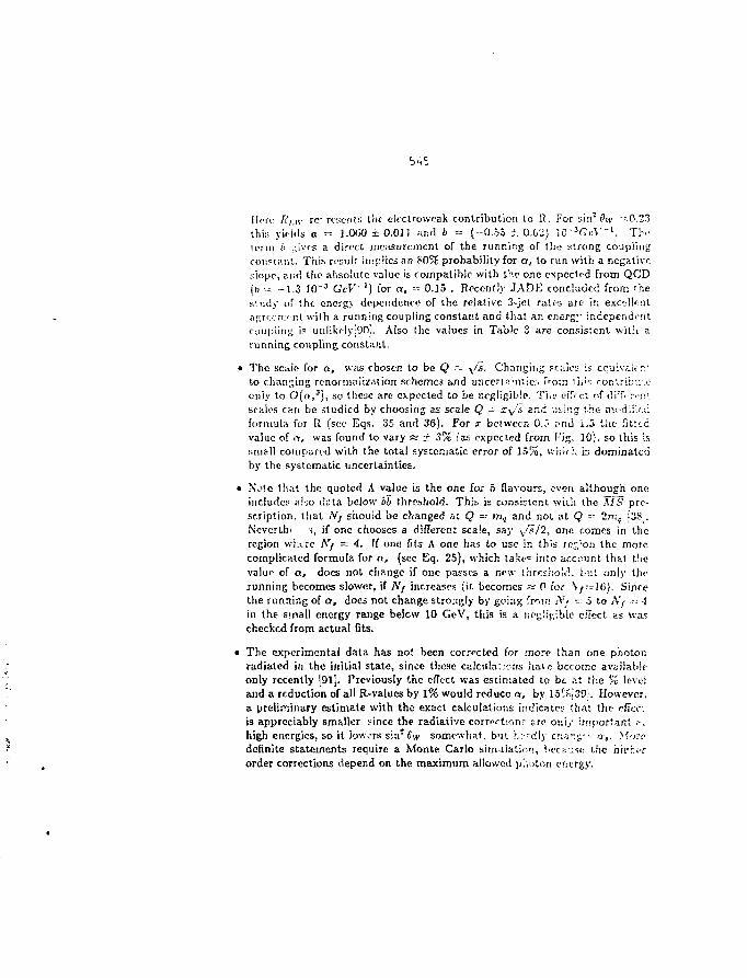
Here Rr.w rf" rcse.'iin the ciectroweak contribution to tt. For sin2 Ow -0.23thin yields a ~~- 1.060 ± 0.01] ;;nd 6 - (-0.55 ± O.G'Jj iG^GtV"1. TN:term (i .-.ivfs a direct measurement of the running of the strong couplingconstant. This result im;:!ics an £0% probability for a, to run with a negativeslope, and the absolute value is compatible with the one expected from QCD(b •.- -1.3 1 0 3 GcV'1) for a, - 0.15 . Recently JADE concluded from thestudy of the cnerg\ dependence of the relative 3-jet rates are in excellenta;;rct n-:--nl with a running coupling constant and that an energy independentcotipiint; is unlikelyjOOj. Also the values in Table 3 are consistent with arunning coupling constant.
• The scaic for a, was chosen to be Q = \/s. Chaiigii,^ FCJI'ICS is cquivriiir"to changing renormaiization schemes and uucert?.;nlie:i from th'1; conlribuioonly to O(ft,3j, so these are expected to be negligible. Tiis ctTrct of diii'Ti'n'.scales can be studied by choosing as scale Q - Sy/s and .i.'.ing the med ;!•':;:formula for R (see Eqs. 35 and 36). For x. between 0.3 ;<nd i.5 tiie fittedvalue of ci, was found to vary a ± 3% (as expected from I'"i,<;. 10). so this issmall compared with the total systematic error of 155S, vvhirh b dominatedby the systematic uncertainties.
• N'ole that the quoted A value is the one for 5 flavours, even although oneincludes also data below 44 threshold. This is consistent with the \IS pre-scription, that Nf should be changed at Q ~ m, and not at Q -- 2rnt (38 .Kcvcrtln -s, if one chooses a different scale, say i/i/2, one comes in theregion where A'/ = i. If one fits A one has to use in this lojron the morecomplicated formula for n, (see Eq. 25), which take into account thai thevalue of a, does not change if one passes a nc,v ihrcs-hoH. but only therunning becomes slower, if Nf increases (it. becomes « 0 for Y/ —16). Sincethe running of a, docs not change strongly by going froir: A7- =•• 5 to A"/ •• fin the small energy range belcw 10 GeV, this is a negligible effect as waschocked from actual fits.
• The experimental data has not been corrected for more than one photonradiated in the initial state, since these ca!ciila:;ons have become availableonly recently [91]. Previously the effect was estimated to bt at the % leveland a reduction of all R-vahies by 1% would reduce o, by 15%\39}. However.a preliminary estimate with the exact calculations indicates that the cficc:is appreciably smaller :;ince the radiative correction- tre av.'iy important •-.high energies, so it lowors sin" Ow somewhat, but h::"dly cr.a".;:-1- a,. M'ircdefinite statements require a Monte Carlo simaia'Jc"., bee p. -;sc the hifh.-rorder corrections ciepend on the maximum allowed p'.,r,ton energy.
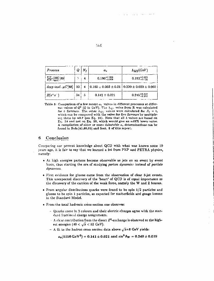
Process
r(T-.p»1 | g 0 ;
deep inel. tiC\88]
R{e+e-)
Q
10
34
4
oc,
U.18U_0 0 0 8
4 j 0.160x0.003 ±0.011
5 i 0.141 ±0.021i
0.182:°;^
0.230 ± 0.020 ± 0.060
n 9.1S+0-250
Table 3: Comparison of a few recent a, values izi different processes at differ-ent values of Q2 (Q in GeV). The A-,yr value from R was calculatedfor £ flavours. The oilier AT/v values were calculated for Nj - 4,which can be compared with the value for five flavours by multiply-ins them by a0.7 (see Eq. 2G). Note that all A values are based onEq. 24 and not on Eq. 23, which would give an »15% lower value.A compilation of older or more debatable at determinations can befound in Rcfs.[41,88,80] and Sect. G of this report.
6 ^Conclusion
Comparing our present knowledge about QCD with what was known some 10years ago, it is fair to say that we learned a lot from PEP and PETRA physics,namely:
• At high energies partons become observable as jets on an event by eventbasis, thus starting the era of studying parton dynamics instead of particledynarr>ics.
• First evidence for gluons came from the observation of clear 3-jet events.This unexpected discovery of the 'heart' of QCD is of equal importance asthe discovery of the carriers of the weak force, namely the W and Z bosons.
• From angular distributions quarks were found to be spin 1/2 particles andgluons to be spin I particles, as expected for matterfields and gauge bosonsin the Standard Model.
• From the total hadronic cross section one observes:
- Quarks come in 3 colours and their electric charges agree with the stan-dard fractional charge assignments.A clear contribution from the direct ^"-exchange is observed at the high-est energies (40 < y/s < 52 GcV).
- A fit to the hadron cross section data above y/s=8 GeV yields:
a,(1156 GeV*) = 0.141 ± 0.021 and sin' $w = 0.240 ± 0.019
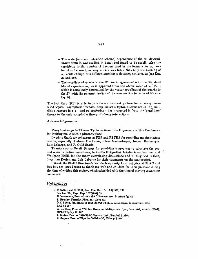
547
- The scale (or re-normalization scheme) dependence of the as determi-nation from R was studied in detail and found to be small. Also thesensitivity to the number of flavours used in the formula for a, wasfound to be small, as long as care was taken that only the running of%, could change for a different number of flavours, not is value (see Eqs.25 and 26).
- The couplings of quarks to the Z° are in agreement with the StandardMode) expectations, as is apparent from the above value of sin2 8w ,which is completely determined by the vector couplings of the quarks tothe Z° with the parametrization of the cross section in terms of G> (seeEq. 6).
The fact that QCD is able to provide a consistent picture for so many unre-lated topics - asymptotic freedom, deep inelastic lepton-nucleus scattering, mul-tijet structure in e+e~ and pp scattering - has promoted it from the 'candidate'theory to the only acceptable theory of strong interactions.
Acknowledgements
Many thanks go to Therese Tymienidsa and the Organizers of this Conferencefor inviting me to such a pleasant place.
I wish to thank my colleagues at PEP and PETRA for providing me their latestresults, especially Andreas Dieckman, Klaus Gamerdinger, Jochen Hansmeyer,Luis Labarga, and F. Ould-Saada.
Thanks also to Gerrit Burgers for providing a program to calculate the sec-ond order radiative corrections, to Giulio D'Agostini, Gunter Grindhammer andWolfgang Hollik for the many stimulating discussions and to Siegfried Bethke,Jonathan Dorfan and Luis Labarga for their comments on the manuscript.
I thank the SLAC Directorate for the hospitality I am enjoying at SLAC andlast but not least I want to thank my wife and children for their patience duringthe time of writing this review, which coincided with the time of moving to anothercontinent.
References[1] P. Soding and G. Wolf, Ann. Rev. Nucl. Sci. 31(1981) 231
S«n L*n Wu, Phyi. Rep. 107(1984) 59H. Yamamoto, Proc. of 1985 SLAC Summer Inst. Stanford (1985)F. BatTeiro, Fortschr. Phy.. 34 (1986) 503D.H. Saxon, Int. School of High Energy Phyi., DuilovoSplit, Yugoslavia, (1086),RAL-86-057W. de Boer, Proc. of 17th Int. Symp. on Multiparticle Dyn., Seewinkel, Austria (1980),MPI-PAE/Exp.Ei. 167J. Dorfwi, Proc of 1988 SLAC Summer but., Stanford (1986)K. Sugano, Proc. of Phy«. in Collision VI, Chicago (1986)
548
P. Mattig, DESY Report 86-161, Cracow Schoo! of Theor. Phys., Zakop.tne, Poland, 1986J. Chrin, DESY Report 87-040
[2| Details and ref. can be found in standard text books:F.E. Close, An Introduction to Quarks and Partons, Academic Press (1979)L.B. Okon, Leptons and Quarks, Noth Holland Publ. Comp. (1982)K. Huang, Quarks, Leptons and Gauge Fields, World Scientific. (1982)C. Quigg, Gauge Theories of the strong, weak and electromagnetic Forces, Benjamm-Cummings Publ. Comp. Inc. (1983)J.E. Dodd, The ideas of Particle Physio, Cambridge Univ. Press (1984)F. Ifalzen and A.D. Martin, Quarks and Lcpions, An introductory course in ModernParticle Physics, John Wiley and Sons, Inc. (1984)D.H. Perkins, Introduction to High Energy Physics, Addison Wesiey Publ. Comp. (1987)
|3j H. Kritisch and M. Gell-Mann, 18th Int. Conf. on High Energy Physics, Chicago (1972)H. Frilisch, M. Gell-Mann and H. Leutwyler, Phys. Lett. 47B (1973) 365
[4j D.J. Gross and F. Wilciek, Phys. Rev. Lett. 80 (1973) 1343
[51 H.D. Politier, Phys. Rev. Lett. SO (1973) 1346
|6j G.S. Abrams et al., Pbys. Rev. Lett. 33 (1974) 1452
|7| J.J. Aubert et »1., Phys. Rev. Lett. SS (1974) 1404 '
J8l M. Gell-Mann, Phys. Lett. 8 (1964) 214
10] G. Zweig, CERN report 8419TH 412 (1964)
110] S. Weinberg, Phys. Rev. Lett. 19 (1967) 1264A. Salam, Elem. Part. Theory: Relativistic Groups and Analyticity (8th Nobel Sympo-sium), Ed. N. Svartholm et al. (1968) 367For a historical account, roe S. Col em an. Science 20ft (1979) 1290
1X1] G. 't Hooft, Nucl Phys. B SS (1971) 167
112; S.L. Glashow, J. Uiopoulos and L. Maiani, Phys. Rev. D2 (1970) 1285
j!3j S.W. Herb ct al., Phys. Rev. Lett. SO (1977) 252
jl4' M. Perl et al., Phys. Rev. Lett. 35 (1975) 1489; Phys. Lett. 63B (1976) 366
[15] J. Ellis, M.K. Gaillard, and G.G. Ross, Nucl. Phys. B i l l (1976) 253; ibid. B1S0 (1977)516;
116] Mark-I Coll., G. Hanson et al., Phyj. Rev. Lett. 35 (1975) 1609
j!7 | A. Sirlini J'hys. Rev. D22 (1980) 891W.J. M.vrciano and A. Sirlin, Phys. Rev. D29 (1981) r \S
;18j W. Itolhk, DESY Report 86-019 , Proc. 21st Rene, de Moriond. Les Arcs, France (1986)M. JSOiwn el al., Fon.-cli. Phys. 34 (1986) 687
19; A. Parroio et al., CEIt.N-EP/87-70, prfseiitfd by F. Dydak at LEP200 ECFA Workshop,Aachtn (1986)
[20! T. Kinoshita, J. Math. Phys. 3 (1962) 650T.D. Lee and M. Nauenberg Pliys. Rev. DlSS (1964) 1549
[21] G. Kramer and B. Lampe, DESY Reports 86-103 and S6-HD
)22j A. Ali ft al., Nad. Phyr. B167 (19l!0) 454, Phyi. Lelt. 82B (1979) 285J.G. Körner et al., Nucl. Pliy». B1S5 (1981) 365K.J.F. Gacniert and J.À.M. Vcrniassren, Z. Phys. CT (1980) 81O Naclitinann and A. Reiter, Z. Phys. C14 (1982) 47; ibid. C16 (1982) 45
|23! F. Gutbrod. G. Kramer, G. Schicrhob, Z. Phys. C22 (1984) 235
J24J R.K. Ellis, D.A. Roos, E.A. Terrano, Phys. Rev. Lett. 45 (1980) 1225;Nucl. Phys. B178 (1981) 421
|25j J.A.M. Vermascrcn, K.J.F. Gacmerr, S.J. Oldham, Nucl. Phys. B187 (1981) 301
[2C| T D. Gottschalk, Phys. Lett. 1O9B (1982) 331T.D. Gottschalk and M.P. Shalt, CALT-68-1172,-1173,-1199; Phys. Lett. 15OB (H>t;.)451
J27j G. Kramer, DESY Report T-8S-01 and Theory of Jet? in Electron-Positron Annihilation.Springer Tract» in Modern Physics, Vol. 102 (1984)
(28) R.Y. Zhu, P i . O. Thesis, MIT (1983
J29| A. Ali, Phys. Lett HOB (1982) 67
J30] Z. Kunsjt, Phys. L-.lt. 90B (1981) 429; ibid. 107B (1981) 123
(3lj F. Csikor, private communication
|32| C. Rudolph, Habilitationsschrift, lürabruck (19Sij)F. Gutbrod el al., 0ESY Report 87-047
|33] TASSO Coll., M. Althoff et al., Z. Phys C26 (1984) 157
|34| MARK-I1 Coll., D.R. Wood et al., SLAC-PUB 4374, to be published
[35] G. 't îlooft and M. Veltmin, Nucl. Phys. B44 (1972) 189
136] O. Tarasov, A. Vladimirov, and A. Zharkov, Phys. Lett. 9SB( 1980)429
(37| Particle Data Group, M. Aguilar-Benitex et al., Phys. Lett. B170 (19S6) 78
[38] W.J. Marciano, Phys. Rev. Lett. 29 (1983) 580
|39] CELLO Coll., 1I.J. Behrend et al., Phys. Lett. B18J (1987) 400
|40| M. Dine, J. Sapiratein, Phyj. Rev. Lett. « (1979) 608A.L. Katacv, F.V. Tkacfcov, Phys. Lett. B85 (1979) 277W. Celmaster, R.J. Gonsalves, Phys. Rev. Lett. U (1980) 5C0
|41| D.W. Duke, R.G. Roberts, Phy«. Report« 120 (1985) 275
[42] P.M. Stevenson, Phys. Rev. D2S (1981) 2916
[43] G. Grindhammer, F. LeDibwder and 1. Haissinski, CELLO Note 0-83
f44j G. Kramer and B. Lampe, DESY Report 87-106
ssc
[45,' W. Celmaster and R J . Gonealves, Phys. Rev. D20 (1979) 1420; Phys. Rev. U u . (42(1979) H J J
|46j R. Marshall, RAL-87-031 (1987)
|47j U. AmaMi et al., UPR-O331T (1987)
|48j B. Andersen et a!. Phys. Rep. 97 (1983) 31T. Sjostrand, Computer Phys. Comm. 27 (1986) 243T. Sjostrand, Computer Phys. Comm. 28 (1936) 229T. Sjostrand, Computer Phys. Comm. 89 (1986) 347T. Sjostrand and M. Bengtsson, Computer Phys. Comm. 43 (1987) 367
|49j J. Ellis and I. Karliner, Nud. Phys. B148 (1979) HI
[50; TASSO Coll., R. Brandelik et al. Phys. Lett. 97B (1980) 453
[51] CELLO Coll., H.J. Bchrend et al. Phys. Lett. HOB (1982) 329JADE Coll., W. Bartel et al. Phys. Lett. 119B (1982) 239PLUTO Coll., Ch. Bcrger et al., Phys. Lett. 9TB (1980) 459P. Soding, AIP Conf. Proc, APS-meeting, Santa Crui (1981)
[52] R. D. Field and R.P. Feynman, Nad. Phys. B1S6 (1978) 1
(53; P. Hoyer et al., Nucl. Phy». B161 (1979) 349
|54i A. Ali et al. Phys. Lett. 93B (1980) 155
!S5) T.D. Gottschalk, Nucl. Phye. B214 (1983) 201; ibid B2S9 (1984) 349T.D. Gottschalk and D. Morris, Nucl. Phys. B288 (1987) 729
J56j G. Marchcsini and B.R. Webber, Nacl. Phys. B2S8 (1984) 1
|57) JADE CoU. W. Bartel et al., Z. Phys. C21 (1983);Phys. Lett. 1S4B (1984) 275; ibid. 15TB (1985) J40TPC CoU., M. Aihira et al., Z. Phys. C28 (1985) 31TASSO Coll., M. Althoff et al., Z. Phys. C29 (1985) 29
[581 Y.I. Aiimov et al., Phyo. Lett. 165B (1985) 147
|59j M. Bengtsscn and T. Sjostrand, Nud. Phya. B289(1987)810
(G0| MARK-II Coll., A. Petersen et al., SLAC-PUB-4290, submitted to Phys. Rev. D
(61) TPC Coll., M. Aihara et al.,Phys. Rev. Lett. 57 (1986) 945MARK-II Coll., P. Sheldon et al.Phys. Rev. Lett. 67 (1986) 1398JADE Coll., W. Bartel et al., Contr. to Int. Symp. on Leplon and Photon Int., Hamburg(1987)
|C2| JADE Coll., W. Bartel et »L, Z. Phys. CSS (1986) 23
|63] MARK-II Coll., A. Peterwn et al., Phya. Rev. Lett. 55 (1985) 1954
[C4j TASSO Coll., Contr. to lot. Symp. on Lepton and Photon Int., Hamburg (1987)
|65j JADE CoU., W. Bartel et al., Phyt. Lett. 123B (1983) 460
(66) PLUTO Coll., Ch. Berger « al., Z. Phy». C13(1981) 297
551
(07) R.D. Field, Troc. Ijit. Symp. on Lepton and Photon Int. , Cornell (1983)
[OS] A. nïrckmana, Ph.D. thesis. Heidelberg (10S7)
[69] L. Clavelliand D. Wyler, Phys. Lett. 103D (1981) 383
|70j J. Ilaii.sincycr, Ph.D. thesis, Karlsruhe (1987)
(71| Cl . . Busham et al., Pliys. Rcv. D17(1978)2298
{72! A. Ali and F.Barreiro, Phys. Lett U 8 B (1982) 155; Nucl. Phys. B238 (1984) 269D.CS. Richards, W.J. Stirling, Nucl. Phya. B229 (1083) 317
[73| S. Bcthke, Proc. of 23th Conf. on High Energy Phys-, Berkeley (3-J86)B. Naroska, Phys. Rep. 148 (1987) 67
(7-lj K. Gamerdinger, Ph.D. thesis, Karlsruhe, in preparation
[75] TASSO Col!., W. Braunschweig et al., DESY Report 87-081
J7G| CKLLO Coll. H.J. Behind et al-, Nucl. Phys. B218 (19S3) 269;Phys.lett. 1S8B (19M) 311
|77j T. Sjôstrand, Z. Phys. C26 (1984) 93
|78) MARK-J Coll., B. Adeva et al., Phys. Rcv. Lett.54 (1985) 1750
|79j PLUTO Coll.,Ch. Berger et al., Z. Phys. C28 (1985) 365
[80] JADE Coll., W. Bartel et al., Z. Phys. C25 (1984) 231
[81] MAC Coll., E. Fernande» et al., Phys. Rev. D ï l (1985) 2724.
[82] F. Csikor .-t al., Phys. Rev. DS1 (1985) 1025
|Wl M. Chen and L. Carrido, Phys. Lett. 180B (1986) 409
I«',' -MARK-J Coll., B. Adeva et al., Phys. Lett. I80B (1986) 181
[S5| W. de BOM, Proc. o! 17th Int. Symp. on Multiparticle Dyn., Scewinkcl, Austria (1986);' MPI-PAE/Exp.El. 167
G. D'Aeostini, Proc. of Rene, de Morioad, (1987) to be published
(8C| Results on R from the AMY-, TOPAZ- and VE.VÜS-Coll. were presented hy S. Ozaki atthe Int. Symp. on Lepton and Photon Interactions, Hamburg (1987)
|87) Cryäta! Ball Coll., Int. Symp. on Lepton and Photon Interactions, Hamburg (1987)CLEO Coll., R. Giles et al., Phys. Rev. D29 (1984) 1285CUSB Coll., E. Rice, Ph. D. thesis, Columbia University (1982)DASP2 Coll., S. WcEcler, Diploma thesis, University of Heidelberg (1981)DASP2 Coll., H. Albredit et al., DESY Report 82-037 (1932), unpublishedDESY-Hamburg-Hcidelberg-MPI Munich Coll., P. Bock et al., Z. Physik CG (1980) 125LENA Coll., B. Niczyporuk et al., Z. Physik C15 (1982) 299PLUTO Coll., L.Criceee and G. Knies, Phys. Rep. 83 (1982) 151
|88] A.C. Benvenuti et al., CERN-EP/87-101, submitted to Phys. Lett. B
|89j Kwong et al., EFI 87-31, Chicago, 1987

|90! JADE COD., Jin. Symp. on Lcpton and Photon Interaction. Hamburg (1D87)
[91j F. Berenda et ai , Phys. Lett. 2S5B (1987) 395
ULTia RELATIVISTIC HEAVY IOlf COLLISIONS
W. Heck and H. Strobele
University of Frankfurt; GS1, Darmstadt and CERJJ. Geneva
HA3S Collaboration
.» this-e«ntribution the first experimental results from the CERN heavy ion
program are presented. A short introduction into the field of high energy
heavy ion collisions is given,whieit-«heuld be considered as an experlnentalisfs
approach to. siap-lrfy an otherwise complex and far reaching subject. A -mere
•professional introduction into the field can be found > references '. At
the end--af—the introduction we outline briefly ths> history of the CERN heavy
ion program. The second part of this contribute j:. is devoted to the
experimental results. During the oral pres acion the authors showed data
from various experiments. However, we i'....red to reproduce here only HA35
data, since we believe that the use <• • eliminary data from other groups
should remain at their discretion. ;<sra we rather give the available
references.
Astrophysics and Cosmology deal with, among other subjects, several
phenomena which are closely connected to the noMon of compressed nuclear
matter. Looking as far in tin* as the beginning of the Universe with the big
bang, or in space as far as to the "dark" spots in the galaxies, which might
be black holes or neutron stars, leads to the assumption that nuclear matter
can be compressed to many times its normal density. Accepting this one has to
ask for the laws governing the corresponding dynamical processes. It is
unlikely that Nuclear Physics provides all the means to find these laws,
because at high density the nucleon-nucleon distance in nuclear matter may
become much smaller than the nucleonlc six* implying that the constituents
must play an important role. Thus th» study of compressed nuclear matter
leads to an extension of nuclear physics in direction to particle physics.
On the other hand, in particle physics, one of the unsolved problems is the
long range forces between the constituents of hadrons. It is conceivable
that nuclear medium effects will help to understand better this part of the
underlying Quantum-Chromo-Dynamics. This becomes even more obvious if one
considers the aspect of the long range problem which addresses the question of
the physical versus perturbative vacuum. It has been mentioned already a long
time ago that the vacuum is not uniquely defined and that its features may
depend on its surrounding . The question of how to explain the
confinement of quarks and gluons in the hadrons is the continuation of a
problem formulated more than ten years ago.
Apart from indirect evidence from eosmological studies nuclear compression
can be looked at only in collisions between energetic nuclei. This had been
done so far either only in rare cosmic ray events with it* limited statistical
significance or at relatively low beam energies (2-4 AGeV) which l«ada to a
compression of only ~ 2 times normal density. With the advent of 200 AGeV
oxygon and sulphur beams from the CERN SPS much higher nuclear densities ar«
expected.
However, before one can address the related fundament:-1 questions the
experimenters have to cope with the special features of heavy ion interactions
at high energies. These are:
- in each reaction many particles are involved. Whereas It is impossible
to separately detect and identify each particle (which Is a sever*
limitation) their large number is an advantage in so far as the
fluctuations due to unseen or unidentified particles are reduced.
- enormous amounts of energy are in principle available in the collision.
Fixed target 200 AGeV S - S interactions have a nominal 640 GeV cm.
energy. This energy is distributed over large volume* in configuration space.
Once the experiments can handle the large multiplicities and catch a significant
amount of the liberated energy, the following specific questions may be asked:
- Are " s + " s interactions different from an appropriate convolution of
(d + d) (we know already that If + Fe * H + d). If indeed a difference is
found the density dependence of the strong interaction can be studied by varying
projectile mass and/or energy.
55 r>
- To what degree is thermal and chemical equilibrium reached in the
reaction zone?
- Is the confinement of the nucieon's constituents locally modified or even
suspended? This would result in a hot plasma of quarks and gluons.
The Quaik-Gluon Plasma or Quark Matter is a fictitious or expected,
(depending on your point of view!) new state of matter with the following
features (an experimentalists simplified point of view).
In an extended (reaction) volume, which is lar^a compared to the size of a
nucieon, quarks and gluons
- are in (near) equilibrium,
• rcove freely, i.e. unaffected by the physical vacuum,
- and contribute individually to the available degrees of freedom.
Lattice QCD predicts a transition temperature, at which the hadrons
"melt" into partons, of 200-250 HeV at energy densities of ~ 3.5 GeV/fro .
On the basis of these predictions simple quark counting gives an estimate
of the required beam energy to produce the Q.G. Plasma: in the initial state 3
quarks per nucieon are present at normal nuclear density. In order to triple
the density in the final state 6 more quarks per nucieon have to be created
each with a temperature of 250 MeV or better an average energy of 750 KeV;
thus around 7 GeV per nucieon incident energy would suffice if its conversion
into thermal energy and quark production is perfect. At 200 ACeV the cm.
energy per nucleons is 10 GeV.
Even if one is now ready to believe that the Q.G. Plasma can be produced it
still remains open how it will manifest itself and what are its signals.
Without going into the details we just mention in table I the most popular
predictions together with the corresponding references. To conclude this
section we have to point out at least some of the principal problems connected
with the detection of Quark Matter:
- the deconfined fraction of the reaction volume will vary event by event
- the transition from the plasma to the hadron stat* will liter most
observable* in the final state by an unknown amount.
- It is a priori unknown whether the expf-ris'.'.-ntal results are representing
more normal hadronic or unusual plasma behaviour. Or, turning the
argument around, there is no clear prediction of how the rpsults should
look in case there is no plasma formed.
Before turning to the experimental results we give 3'; outline of the
history of the heavy ion program at CERBt.
(41The first detected signal was a study of Hase-oth in 1977/78 on light
ions in the PS. This triggered a proposal from E. Stock and others for16 [5]
C experiments at the PS in 1980 . The feasability if such a program
•as confirmed in January 1983 and the original proposal approved in
September of this same year. After some delay other groups joined tiie heavy
ion program and. triggered by technical reasons, the SPS was taker: into
consideration which lead to a SPS programme with oxygen at 60 and 200 ACeV.
The ion source, provided by GSI and 1.BL, was installed in January 1986.
Two months later a 12 AMeV beam emerged from LIKAC I. In the two following
months the Booster (280 AHeV) and the PS (10 AGeV) had their turn until
finally the 9th September 1986 the SPS accelerated an oxygen beam to the
envisaged energy of 200 AGeV. The physics run then took place in November
1986, with a S beam for physics being scheduled for September 1987.
2. EX.FERIMEHTAL RESULTS
Instead of describing the experimental setup of the various collaborations
with our own words we include here as reference the corresponding descriptions
from the official CERH List of Experiments , in the appendix.
Figure 1 shows an artist's view of NA35's experimental setup. The major
components are the Streamer Chamber in the 1.5 Tesla Vertex Magnet, the
i-id-rapidity calorimeters consisting of electromagnetic and hadronic parts,
and the Veto calorimeter covering laboratory angles between 0* and 0.3".
557
High multiplicity events show lar&e measuring losses also in the forward cone
corresponding to rapidities betw>o". 4 and 6. With these restrictions the
Strenirer Chamber "..•Lector is well suited to yield information about transverse
momentum spectra and rapidity distributions, for negative particles, the
rapidity being calculated assuming the pion mass thus neglecting admixtures of
kaons and antiprotons. Electrons from »° decay into 2Y'S and subsequent
conversion in the target are corrected for. A first result on proton spectra
is obtained by subtracting from the distributions of positively charged
particles (P, K ,ir ) the appropriate distribution of negatively charged— — +
particles (K , r ) neglecting possible differences between the *and it yields.
2... Jb__2;_ Results
Figure 2 shows the distribution 1/Pt <SU/dp for central collisions of
" o + Au at 200 AGeV. The solid line represents the corresponding results
from p + p collisions at .':40 GeV in the interval 0 < p < 1 GeV/,.. Above 300
Mel',;.the agreement is surprisingly good. The deviation from the straight line
(note the log-scale!) for momenta above 1 GeV/c is also similar to the
findings in pp collisions . Below 300 HeV£the 0 + Au data exhibit a
significant enhancement, which is also seen in p + Au collisions (fig- 3).
We can conclude from both figures, that there is no difference in the spectral
shape of negative, i.e. produced, particles between p + Au and 0 4 Au
collisions at 200 AGeV beam momentum. Above 300 HeV/c the transverse momentum
spectra reproduce the finding of a previous pp experiment.
It is interesting to see how our results fit into the systematics of
different projectiles and energies. Instead of comparing spectral shapes we
look at the mean transverse momentum of pions as function of beam momentum
(figure 4). The solid line is an eyeball fit to results from low energy AA[9]
collisions and a-a, a-p data from the ISR . The two crosses are our
findings at 60 AGeV and 200 AGeV. Ho drastic deviation front the common
behaviour is observed. At 200 AGeV 0 + Au interactions produce very few
nucleon pairs, therefore the transverse momenta of protons are well suited to
study the dynamics of the interaction or, more specifically, the process of
transforming the initially longitudinal momentum of the nucleons in the
projectile and target nuclei into transverse momentum. Figure S shows the
proton tramverse momentum spectrum of 0 + Au collision at 60 AGeV.
558
The corresponding mean transverse momentum is 630 MeV/c which, in a thermal
picture, corresponds to about the same temperature as found for the pions.
Figs. 6a,b show the rapidity distributions of pions in central 0 t- Au
interactions at 200 and 60 AGeV. The qualitative finding is that the mean of
the distributions is shifted to values lower than the position of the mean in
pp collisions. Simple kinematical considerations correlate the mean rapidity
(or the velocity of the centre-of-mass system) to the number of participating
target nucleons (assuming that all nucleons of the projectile participate
which is a reasonable assumption in central collisions). From the positions
of the means of the distributions in figures 6a (<y> = 2.4) and b (<y> = 2.0)
we infer that at 200 AGeV 55 nucleons and at 60 AGeV 40 nucleons from the
target participate in the interaction. From this we conclude that the
olowing-down of the interacting fireball at 200 AGeV is at least as effective
ds at 60 ACeV. The width of the- rapidity distribution provides another piece
o: information about the nuclear stopping power. In pp collisions pions
exhibit a rather pronounced plateau in the rapidity distribution which is not
reproduced in 0 •• Au interactions. Comparing the full-width-half-maximum
values at 200 AGeV (60 AGeV) for A -f A and pp yields 3.2 and 3.5.(2.4 and
2.8). Thus o + Au interactions yield significantly smaller widths than
yy Interaction-.; if the rapidity distributions of pions are considered.
Whether this difference is of a dynamical nature or originates from an
appropriate convolution of pp interaction remains to be seen.
The HA3S Calorirc
Results from calorimetry of the NA35 experiment at the CEHH SPS for x*0 + A
at 200 and 60 AGeV on transverse energy spectra for different targets and a
comparison of p + Au with 0 t Pb will be given after a description of[10J
the? relevant detector parts. Fig. 8 shows the experimental setup
Targets of Al, Cu, Ag, Au, and Pb (11 interaction length thickness) were
mounted in front of the streamer chamber.
A set of electromagnetic and hadronic calorimeters measured the reaction
products. The angular domain 8 < 0.3* (nuclear projectile fragmentation) is
covered by a 4-segment "Veto" calorimeter. The subsequent Interval, 0.3* - 2.2*
is seen by a continuous single-cell EH + hadronic calorimeter. The larger
angle domain Is covered by a Photon Position Detector (PPD) consisting of
5 59
alternating layers of lead and planes of proportional tubes read out by 3072
ADC channels, backed up by a Ring Calorimeter divided into 240 cells (24 in
azimuth and 10 in radius with ring sizes chosen to cover equal units of
pseudorapidity). This set of calorimeters is movable: at 200 AGeV it covered
approximately a 2.3" - 12.5* angular range corresponding to 2.2 < n < 3.8,
and at 60 AGeV it covered a 4.3* - 20.5* range corresponding to 1.7 < n < 3.3.
Two principal trigger modes were employed. Both worked reasonably well with
and without the field of the vertex magnet. From the Veto Calorimeter various
levels of projectile energy degradation could be selected, ranging from
"minimum bias" to "central collision", the later requiring &veto < 0.1
E . The other trigger was obtained from the transverse energy of thebeam
produced w's. recorded as photons in the PPD. At incident energies of 60
and 200 AGeV, a total of about 2,500,000 calorimeter events were recorded.
Tn addition, data were taken for 200 GeV incident protons and » .
First results have been published
2- Jk.JL^ Results
T-T.3Jlsye.rse_ Energy Distribution
Figure 9 shows the differential transverse energy (E ) distribution for
l*0 + Pb at 200 /• ,0V, as summed from the PPD and Ring calorimeters, with
the magnetic field off . The value of E is calculated for each event
as the appropriately weighted sum of the energies found in individual PPD and
Ring Calorimeter channels. The data points with E < SO GeV were obtained
with additional streamer chamber information. Systematic uncertainties in the
ET scale and normalization are estimated to be about 10%. The range of
pseudorapidities included in the data is approximately 2.2 < i < 3.8. The
HXJET Prediction is also shown in figure 9 for comparison. This distribution
is much narrower. The peak near 50 GeV arises in this model from impact
parameters b < 4fm. The data exhibit the same "central collision" peak.
A variety of models has been used to describe the measured E spectra '
In order to understand the C spactr* further, the same measurement was
made for p + Au, using • tagged 200 GeV proton beam. To eliminate surface
56C
interactions the value of E was required so be less than 150 GeV,Veto
corresponding to a p-Au cross section of 1.3 haras, or impact parameter b < 6fm.2.36
The result is described by an analytic fit d o/tiE = O.173.E
exp(-O.727.E ) bam/GeV. A 16-fold convolution of this analytic function is
shown in figure 9, where it provides a fit to the "central collision" peak,
both as regards position and shape at high E . The difference between Au
and Pb for the purpose of this convolution is not expected to be significant.
Dependence of E on Beam EnergyT
Figure 10, shows the E spectra measured for 0 + Au at 60 AGeV
(2.0 < n < 3.5) and at 200 AGeV (2.2 < n < 3.8). The energy calibration
is revised upwards from that of figure 2., but is still preliminary. The mean
E for central collisions is approximately 45 and 90 CeV at 60 and 200 AGeV
respectively. To have a scale for these values, we consider the total era.
energy available (/s) in the 16 + 50 system consisting of the projectile
nucleus and the tube of participant nucleons in the target nucleus for a
central collisions. This is 318 and 582 GeV respectively. An upper limit for
F might be the value for an isotropic emission of that energies, i.e.,
/ * E : 250 and 457 GeV respectively. Since the experimental
acceptance is about one half, these values would be reduced to 125 and 229
CeV. The average E for central collisions is therefore, at both energies,
about 40% of the value for an isotropic fireball. It is also interesting to
note that the observed E is approximately proportional to /s.
Estimate of Energy Density
From the E measurement we can make an estimate of the energy density in[161
the interaction volume, using the formula of Bjorken
AB 2c ~ T/. / <• r T )
An
where 6£ is tha transverse energy observed in th« ptaudorapidity interval
An, r is the radius of tha **0 nucleus and T IS tho tina that has
elapsed fines tha beginning of tha collision. For t • lfa/c, and tha
observed 4ET > 90 GaV i
density of 2.0 GaV/fsi*.
observed AE_ > 90 GaV in 2.2 < n < 3.8 at 200 AGaV, wa find an anargy
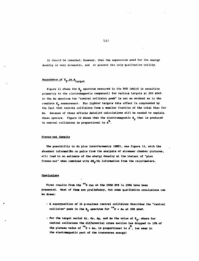
561
It should be remarked, however, that the expression used for the energy
density is very schematic, and at present has only qualitative utility.
Dependence of E on A
Figure 11 shows the E spectrum measured In the PPD (which is sensitive
primarily to the electromagnetic component) for various targets at 200 AGeV.
In the Au spectrun the "central collision peak" Is not so evident as in the
complete E measurement. For lighter targets this effect is compounded by
the fact that central collisions fora a smaller fraction of the total than for
Au. Because of these effects detailed calculations will be needed to explain
these spectra. Figure 12 shows that the electromagnetic E that is produced
in central collisions is proportional to A .
Free2c-out density
The possibility to do pion interferometry (HBT), see figure 13, with the
abundant Information on pairs froa the analysis of streamer chamber pictures,
will lead to an estimate of the energy density at the instant of "plon
freeze-out" when combined with <J«_/dn information from the calorimeters.
Conclusions
First results fro* the " o run at the CERH SP3 in 198* have bean
presented. Host of them are preliminary, but some qualitative conclusions can
be drawn:
A superposition of li p-nucleus central collisions describes the "central
collision" peak ID the Ij spectrum for 0 • Au at 200 AGeV.
For the target nuclei Al, Cu, At, and Au the value of • , where for
central collisions the differential cross section has droppad to 10% of
the plateau value of " o • Au, is proportional to A , (as seen in
the eleetomagnetle part of the transverse energy)

562
- For central 0 + Au collisions E roughly doubles between 60 and
200 AGeV as does the available energy, i.e., we find similar stopping for
both energies.
- With the Bjorken formula one finds that energy densities for average
central collisions In 0 + Au at 200 AGeV are of the order of 2 GeV/fm'.
- Pion interferometry (HBT) can be used to study tha size of the
"freeze-out" voluae.
We look forward to the upcoming run in September/October 1987 whan a
**S beam will ba used.
REFEREHCES
[1] Proceedings of 5. Quark Batter conf., Asllomar 198*. And references,
therein.
(21 T.D. Lee: Abnormal nucleon states; Rev. Hod. Phy«. 47, 2*7, 1975.
(3) J.B. Bogut, Kiel. Phys. A418 (1984) 381c. H. tatz Ibid. p. 447c.
[4] Haseroth et al. CKtM/n/tU 77-23 (1977).
151 R. Stock et al. Letter «f Intent to tha PSCC-14S0.
(tj H. Haseroth CEtU/PS/LI/83-7 (1983).
[7] Experiments at CERM In 198»; Geneva, *oveaber 1«8».
[8] Van Hal, Vljmagm thesis 1987.
[91 R. frwed, CIRJ-KP/84-125.
(10) A. (andoval at al., Kiel. Phys. A4tl (1«J 4«Se.
563
[111 A. Bamberger et al Phys. Lett., B184 (1987) 271.
[12] A.D. Jackson. H.B*sgild NORDITA - B7/11M preprint.
[13] G. Baym, P. Braun Hunzinger, V. Ruuskanen, preprint (1987).
[1*] J. Ranft. Phys. Lett. B188 (1987) 379.
115) H. Gyulassy CER1I - TH. 4794 preprint.
(161 J-D. Bjorken. Phys. Rev. D27 (1983) 140.
FIGURES. CAPJTIOHS
Fig- 1 Artist's view of the NA3S experimental setup.
Fig. 2 Transverse momentum spectrum 1/pt dn/dpt of « for 0 4- Au
events at 200 AGeV. The data were obtained with a hard veto trigger,
i.e. they represent central collisions. The solid line is the result
from pp interactions at 240 GeV/c.
NFig. 3 Same as fig. 2 but for p + Au events.
Fig. 4 Compilation of mean transverse momentun of v's as function of bean
momentum.
Fig. 5 Difference of the transverse momentum spectrum of positive minus
negative particles representing some approximation of the proton
spectrum.
The data come from 0 • Au interaction at intermediate impact
parameters at (0 AGeV.
Fig- 6 Rapidity distribution of »~ for central l*0 + Au collisions.
Fig. 7 Sane as Fig. 6, but for p + Au.
Fig- 8 The HA3S experimental setup.
Fig. 9 BT distribution for 1*0 + Pb at 200 AGeV in the acceptance
2.2 < it < 3.8. The full line is a 16-fold convolution of the E
distribution for inelastic p + Au collisions at 200 GeV, measured with
the same apparatus. The dashed curve gives the HIJET prediction.
A gamma function has been fitted to the p + Au data, the analytic52.8 - 0.727 t
16-fold convolution gives d/dE E efor the central collision peak for 1*0 + Pb.
Fig. 10 Transverse energy distributions for " o + Au at 60 AGeV (2.0 < n < 3 5)
and at 200 AGeV (2.2 < n < 3.8). The energy calibration (still
preliminary) is different Erosi Fig. 9.
Fig. 11 Transverse energy found in the PPD for x*0 — Al, Cu, Ag, Au, at
200 AGev. the horizontal 1 vie indicates 10% of the plateau value for
'*0 *• Au (see Fig. 12).
Fig. 12 PPO ET at 10% of the 0 + Au cross section plateau versus
At.rg.t ( " e F i * - ">•
Fig. 13 Two-pion correlation function with Gaussian fit projected onto the
Qi - axis for 200 AGeV **0 + Au. central events.
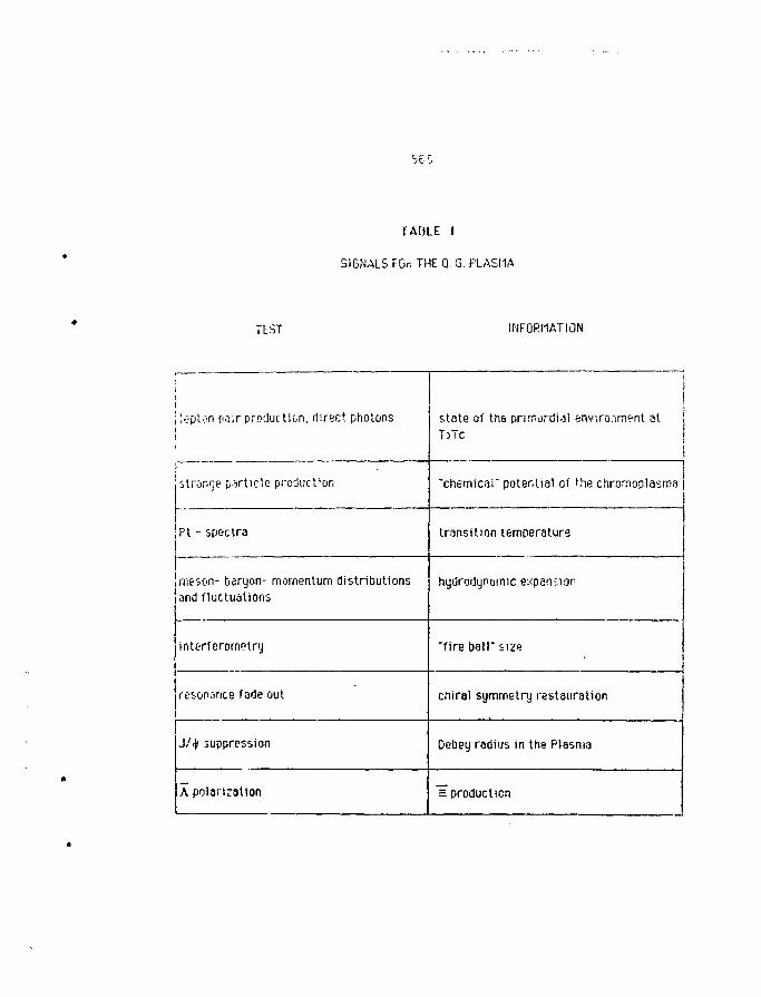
sec.
TABLE I
SIGNALS FOK THE Q. G. PLASMA
TEST INFORMATION
ilc-pton pair production, riirec' photons
ilror.rje jj.irticle production
1Ft - spectra
1meson- baryon- momentum distributionsand fluctuations
interferornetry
resonance fade out
J/.Jf suppression
A polarization
state of the primordial environment atT>Tc
"chemical" potential of the chrornoplasma
transition temperature
hydrodyoamic expansion
"fire ball" size
chiral symrnetnj reslauration
Debey radius in the Plasma
= production
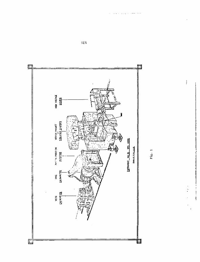
O_
566
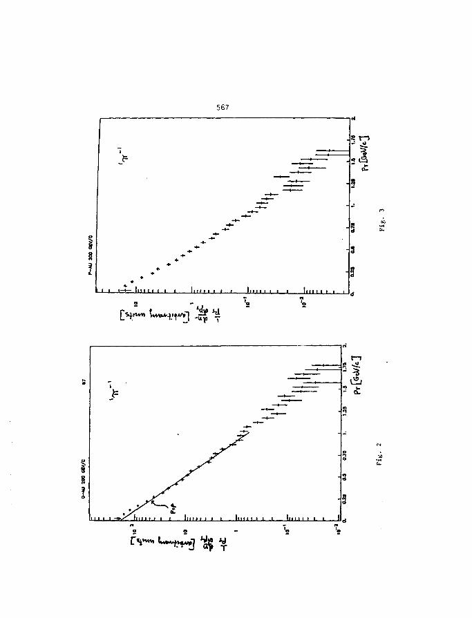
567
I
lit 11 t t i i I I I I III i i In 11 i i i i In i i i t i i !
- *
2 £
T
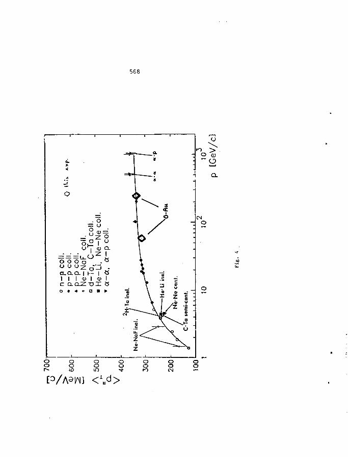
568
4 .X•I
o. o.
^°°l
o
oo
0 o oCLQ.Q. | \— |1 I I <U I Oc aaZtilO • 4
oQ.
oo oo oo oo ooO
ooCNJ
oo
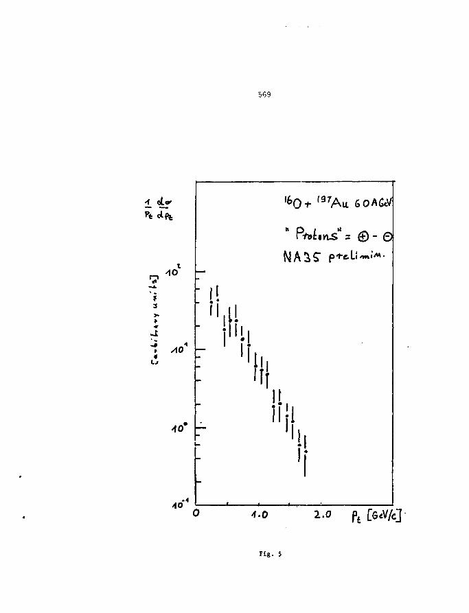
569
AO"
f l l l l
f 6 0 + f 9 7Au 6 0ACcV
PtoLns* = © - 6
NA^S"
»« i
4-0 2.0 pfc [GeV/cJ
Fig. 5
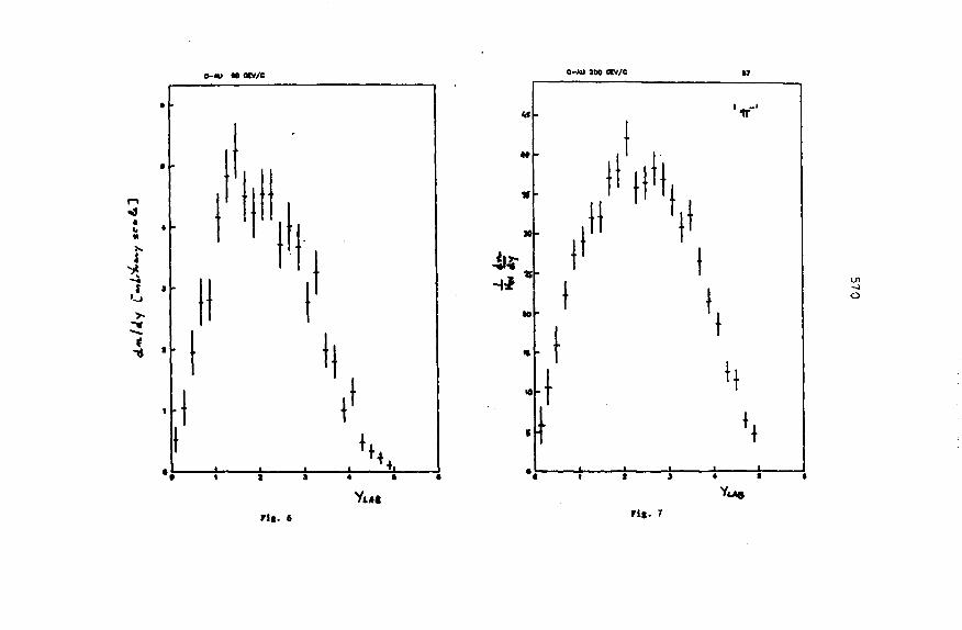
O-MI «0 OtV/C
Fit.
O-AU 100 CCV/C
«. r
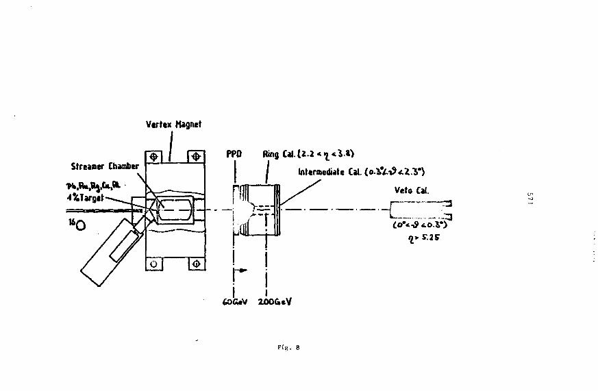
Streamer ChamberPPO Ring Cal. U-2 * ^ * i « >
/ Intermediate Cal.
rf" Veto Cal.
IZOOGieV
f,. 8
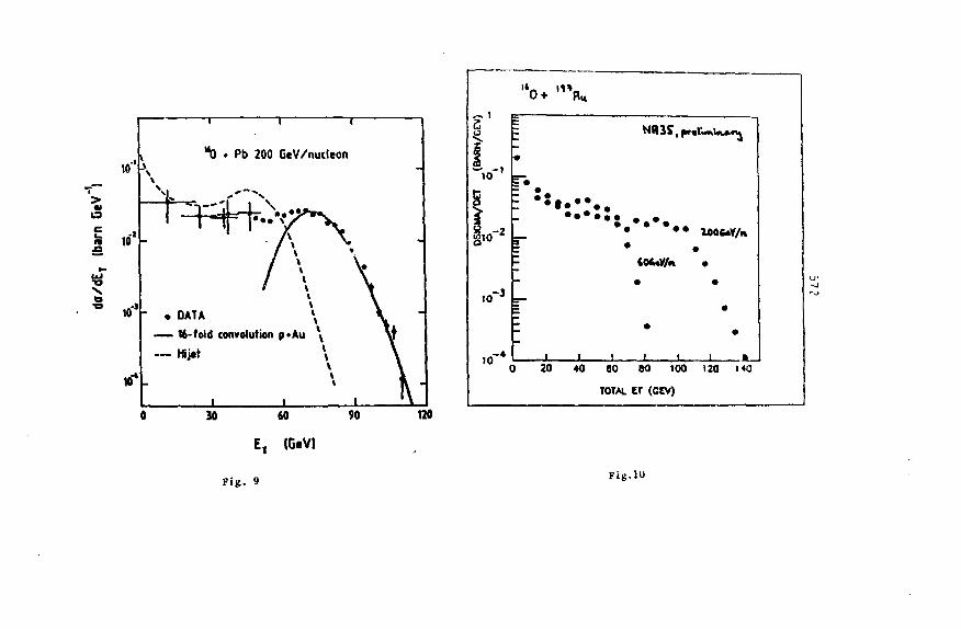
"0 • Pb 200 GeV/nucteon
» • *
/GE
V)
%
gio"2
to"3
. « -
=
nn
in
>
: : .
i
20
• • •• • •
1
40
«
I
80
TOTAL
NR3S |Pr,
• • • • • •
•
•
BO 100
ET (GEV)
lOOUV/n
•
•
•
•
•
i •
120 MO
E, (GeV)
Fig. 9Fig.10
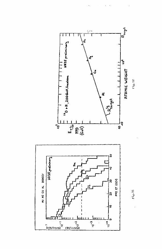
s8a3(J
2
rs
uuim
J3/
H i l l 1
130 A
i
1
1i
i Innbi i tN' o
'.iOlSO
1
_J—
JlllHI \
tr
r1
-
o
on
s
o
*o
b£0.
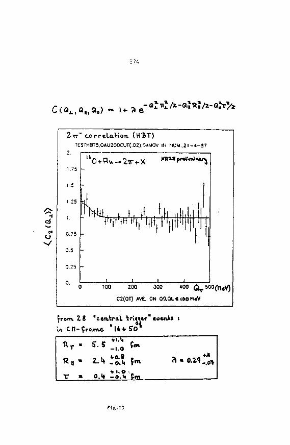
2TT" "correlation. (HBT)T E S 7 H 8 T 5 . O A U 2 0 0 C I J T ( . 0 2 ) . G A M O V IN NUM..21-4— 37
-> ._ . , , , .
1.75
1.5
1.25
0.75
0.5
0.25
°- o
ma, , i. |( .t|i .,11.1,1• l l/i« S Ml, 1 'iill'IFII-
I
i i i i
100 20Q 300 400 ( S i
C2(0T) AVE. ON OO.QL«IOOH*V
from. Zi "central fcrlU Cn-frame "
eo*a*s :
Fig.13
575
PHENOMENOLOGY BASED ON SUPERSTRING INSPIRED E6 GROUP
N.G. Deshpande
Institute of Theoretical Science
Eugene, OR 97403
USA
ABSTRACT
We present mass limits and properties of extra gauge bosons that miglit occur at
low energy in superstring inspired E6 models. Both rank 5 and rank 6 cases are
considered. We then present the properties of the quark singlets that also occur ;n these
models.
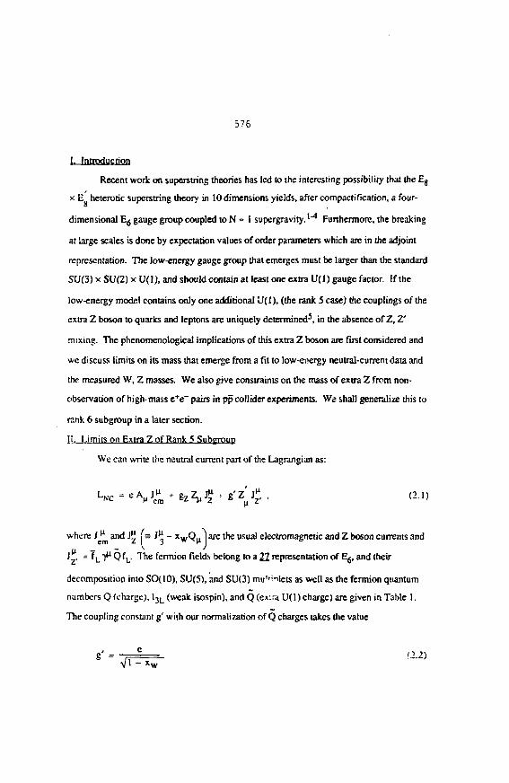
576
1. Introduction
Recent work on superstring theories has led to the interesting possibility that the Eg
x E heterotic superstring theory in 10 dimensions yields, after compactification, a four-
dimensional E6 gauge group coupled to N = 1 supergravity.1"4 Furthermore, the breaking
at large scales is done by expectation values of order parameters which arc in the adjoint
representation. The low-energy gauge group that emerges must be larger than the standard
SU(3) x SU(2) xU( l ) , and should contain at least one extra U(l) gauge factor. If the
low-energy model contains only one additional U(l), (the rank 5 case) the couplings of the
extra Z boson to quarks and leptons are uniquely determined5, in the absence of Z, Z'
mixing. The phenomenologica! implications of this extra Z boson are first considered and
we discuss limits on its mass that emerge from a fit to low-energy neutral-current data and
the measured W, Z masses. We also give constraints on the mass of extra Z from non-
observation of high-mass e+e" pairs in pp collider experiments. We shall generalize this to
rank 6 subgroup in a later section.
11. Limits on Extra Z of Rank 5 Subgroup
We can write the neutral current part of the Lagrangian as:
where J ^ and J^ ! = i*J - x w Q j are the usual electromagnetic and Z boson currents and
j£, = 7L "r" QfL. The fermion fields belong to a 22 representation of E6, and their
decomposition into SO(10), SU(5), and SU(3) muT''->Iets as well as the fermion quantum
numbers Q (charge), 1 J L (weak isospin), and Q (ex;ra U(1) charge) arc given in Table 1.
The coupling constant g' with our normalization of Q charges takes the value
a.2)
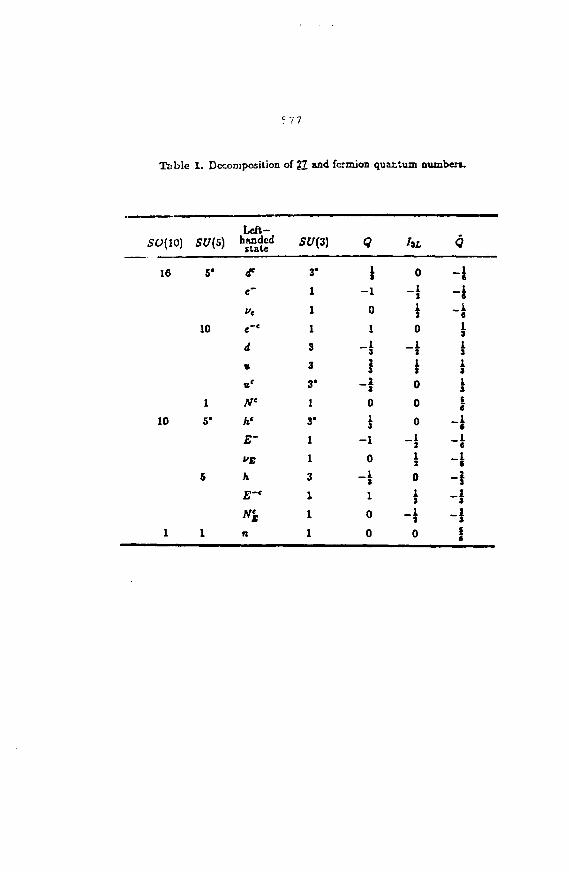
c 77
1. Decomposition of 2Z and fermion quantum number*.
50(10) SU{5)
16 5*
10
1
10 5*
5
1 1
Left-fa nsdcdstate
<et~
ft
e"
d
%
v'
rrh<
E~
VB
h
E-'
N%
n
SU{3)
3*
1
1
1
3
3
3 '
1
3*
1
1
3
1
1
1
Q
1- l
0
i
~s1
~ *0
i- 1
0
-J1
0
0
hi
0
-i*0
-I\0
0
0
1
0
1
-i0
Q
-i~ 6
~ «
I1i!e
~»
~ 6
~ «
~ J
~ J
-i1
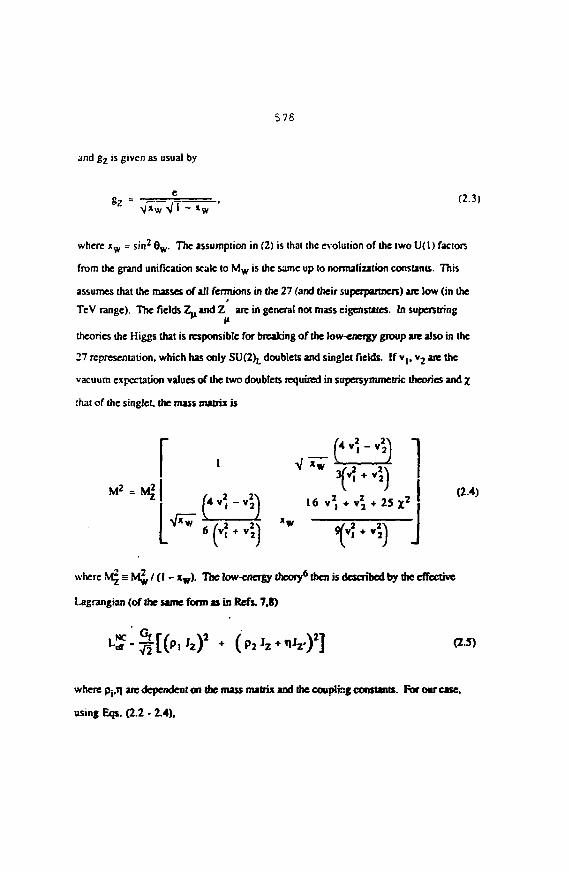
578
and g z is given as usual by
(2.3)
where x w .- sin2 8W. The assumption in (2) is that the evolution of the two U( I) factors
from the grand unification scale to Mw is the same up lo normalization constants. This
assumes that the masses of all fermions in the 27 (and their supeipartners) are low (in the
TeV range). The fields Z^ and Z are in general not mass eigenstates. In superstring
theones the Higgs that is responsible for breaking of the low-energy group are also in the
27 representation, which has only S U ( 2 ) L doublets and singlet fields, [f v,, v2 are the
vacuum expectation values of the two doublets required in supersynunetric theories and x
that of the singlet, the mass matrix is
M2 = M*16
6 ( V ' + V 2 )
(2.4)
where M J s M ^ / ( l - x w ) . The low-energy theory6 then is described by the effective
Lagrangian (of the same form as in Refs. 7,8)
(2S)
where Pj.T are dependent on die mass matrix and the coupling constants. For our case,
using Eqs. (2.2 - 2.4),
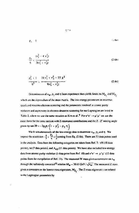
.-.6a)
(v; - 4 v")\ , (2.6b,
3(v; . v p
p; * i 16 v- + v22 * 25 x 2
— T — - 1 j (2.6c)
IX'icrminaiion of xw , p-. and rj from experiment then yields limits on MZi and M ^
which arc the eigenvalues of the mass matrix. The low-energy parameters in neutnno-
quark and neutrino-electron scattering and the parameters involved in atomic parity
violation and asymmetry in elcctron-deuieron scattering for our Lagrangian arc listed in
Table 2, where wo use the same notation as Kim et al..9 For e*e" —»n*|i~ we use the
cxaci form for the cross section with Z-resonance contributions and the Z - X mixing angle
given by tan 29 = - 2p2ri l(\ + p \ - p2 T) \
We fit simultaneously all the low-energy data to determine xw , p, and rj. We
impose the rcsiriciion - r < — < -coming from Eq. (2.6b). There are 53 data points used3 T| 3
in the analysis. Data from the following categories arc taken from Ref. 7: vN (18 data
points), vc (7 data points), and A c D (11 data points). We have also included low-energy
data from atomic parity violation (1 data point from Rcf. 10) and e*e* -» n*jr (12 data
points from the compilation of Ref. 11). The measured W mass gives a constraint on xw
through the radiativcly corrected12 relation Mw = 38.65 GeV / ^/xw. The measured Z mass
gives a constraint on the lowest mass eigenstate, M7 . The Z-mass cigensiaic :• are related
to the Lagrangian parameters by
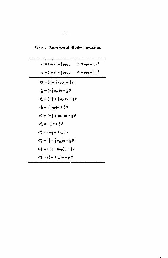
Table 2. PtTzmclen of effiactive Lig.'&ngiin.
fff, = ( - 1 + 2 x ^ ) 0 - 1
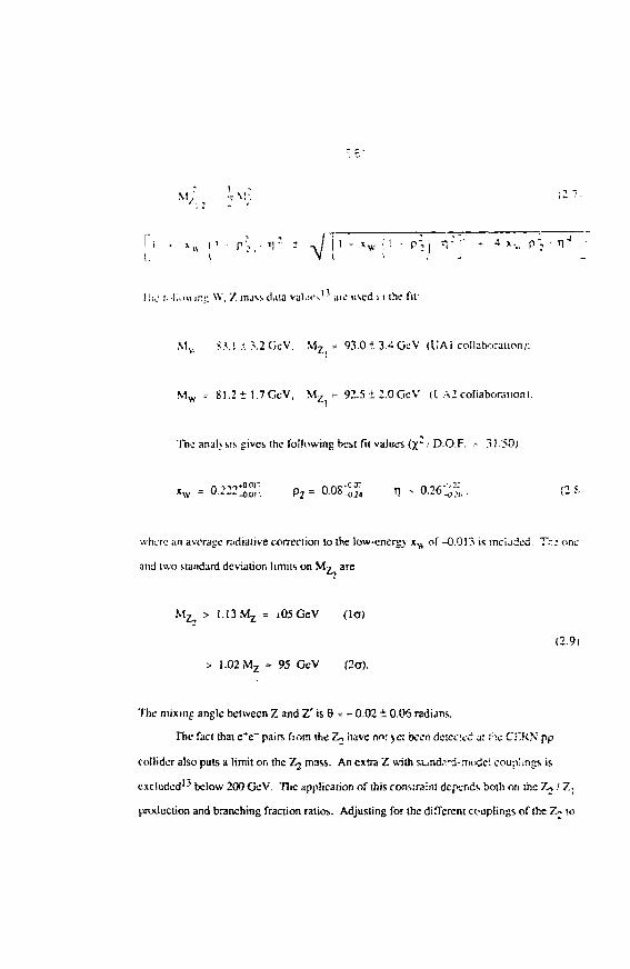
: •• I7T~- ~ ~ ; v . 4 x I
lie !.•!..mii::: W, / . mjs:. d.ita v a l . i r , " aio used 11 the fif
Mv, S?.l A ?.2GcV, M7 = 93.0 ±3.4 GeV (UA1 colbboranonj:
Mw - 81.2 ± 1.7 GcV, M z - 92.5 ±2.0 GcV (I A2 collaboration!.
The analysis gives the following best fit values (x~ i D.O.F. - 3! 50)
(2 f.
WIKTC ;in average radiative correction lo the low-energy xw of -0.013 is included Th-- one
and iwo standard deviation limits on Mv are
M ^ > 1.13 M z = iO5GeV (lo)
(2.9)
> 1.02 M z = 95 GcV (2a).
The mixing angle between Z and Z' is 8 = - 0.02 ± 0.06 radians.
The fact that C'e" pairs from the Z-> have no; ye: been dcieciec' a! i;c Ci'RN pp
collider also puts a limit on the Zj mass. An extra Z with siund.—d-modc! couplings is
excluded'' below 200 GeV. The application of this consiraint depends both on the Z , / 7.,
production and branching fraction ratios. Adjusting for Ihe different couplings of the Z-% ro
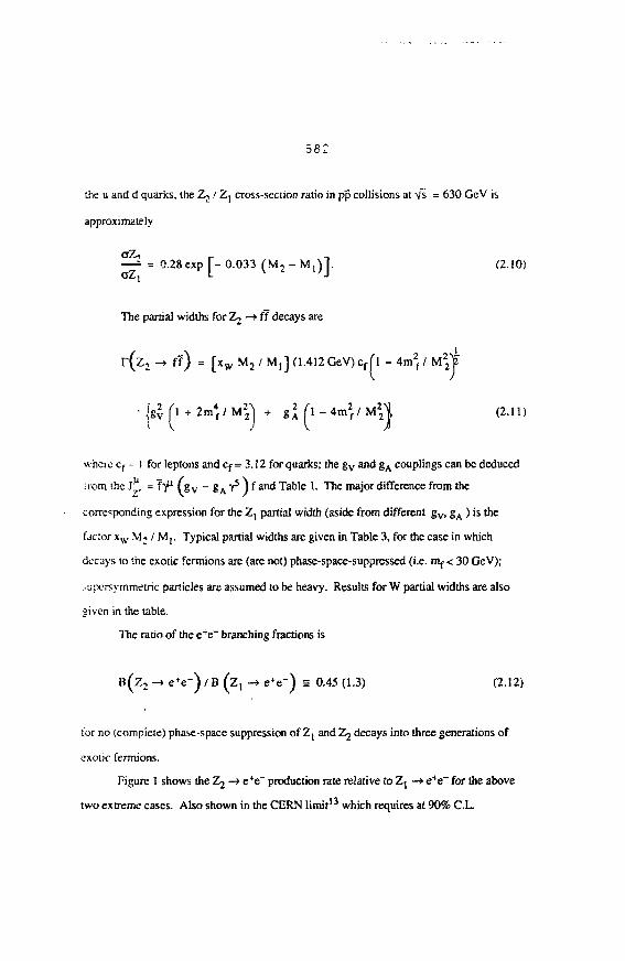
58 2
the u and d quarks, the Zj / Zj cross-section ratio in pp collisions at V s = 630 GeV is
approximately
^ = 0.28 exp[-0 .033 ( M j - M , ) ! . (2.10)
The partial widths for 'L^ —»ff decays are
r ( z 2 -> ff) = [xw M2 / M,] (1.412 GeV)cf(l - 4m2f /
• \gl- (\ + 2 m * I M 2 ^ + z \ ( \ - 4m 2f / M2A (2.11)
where cf = I for leptons and cf = 3.12 for quarks; the g v and gA couplings can be deduced
aom the j£, = 1-f1 fg v - gA Y5 ) f and Table 1. The major difference from the
corresponding expression for the Zj partial width (aside from different gv , g A ) is the
factor x w MWMj. Typical partial widths are given in Table 3, for the case in which
decays to the exotic fermions are (are not) phase-space-suppressed (i.e. m^ < 30 GeV);
>upcrsymmetric particles are assumed to be heavy. Results for W partial widths are also
aiven in the table.
The ratio of the e+e~ branching fractions is
B ( Z 2 -> e + e " ) / B ( z , -> e + e " ) = 0.45 (1.3) (2.12)
for no (compieie) phase-space suppression of Z t and Zj decays into three generations of
exotic fermions.
Figure 1 shows the Zj -* e+e" production rate relative to Zj -» e+e~ for the above
two extreme cases. Also shown in the CERN limit13 which requires at 90% C.L.
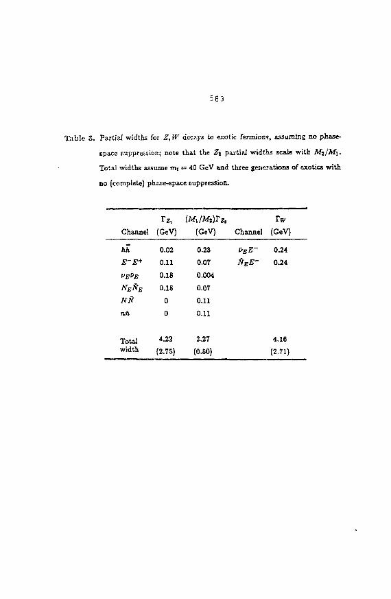
5 6 3
Table 3. Partial widths for Z, W decays to exotic fennions, assuming no phase-
space suppression; note that the Z% partial widths scale with M%jM\.
Total widths assume mt = 40 GeV tad three generations of exotics with
no (complete) phase-space suppression.
Channel
hh
E-E+
vE*B
NENE
NN
nii
Totalwidth
(GeV)
0.02
0.11
0.18
0.18
0
0
4.22
(2.75)
(«i/Aft)r«(GeV)
0.23
0.07
0.004
0.07
0.11
0.11
2.27
(0.50)
i
Channel
PEE~
NEE~
Tw(GeV)
0.24
0.24
4.16
(2.71)
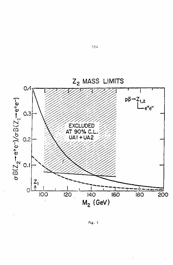
CD+CD
\
M
<D
IM
Z2 MASS LIMITS
eTe
100 140 160
9 (GeV)200
Fig. 1
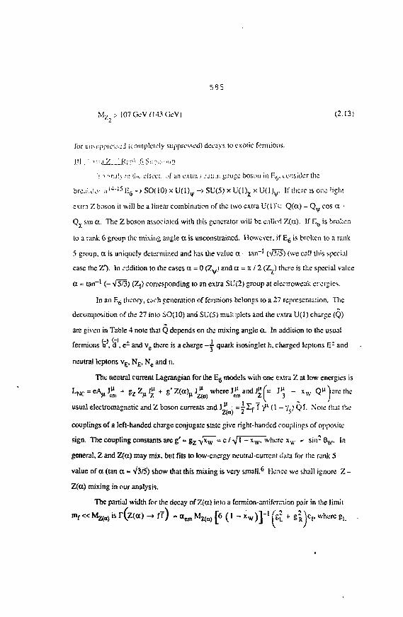
58 5
M 2 i > 107 GeV f 143 GcV) (2.13)
for u!!s;ijipic>s.jd « ompletely suppressed) decays to exotic fermions.
MJ . ' v.:j_Z_J<;:;>V.fi J-.:?,:..-.:j,3
i " 'njK .•:: tin., eflect. ..>f i;n extra >::uH .ii y^ujc boson in F. . consider the
bre.il.ifo- . i1 4 '1 5 E6 -* SOf 10) x U( l ) v -> SU(5) x U(l)x x U(l) y . If there is one light
cxirn Z boson it will be a linear combination of the two extra U(lVi: Q(a) = CL,cos a '
<X sin a. The Z boson associated with this generator wili be called Z(a). If E^ is broken
to 3 rank 6 group the mixing angle a is unconstrained. However, if E6 is broken to a rank
5 group, a is uniquely determined and has the value a •• tan"1 (V3/5) (we call this special
case the Z'). In;:edition to the cases ot = 0 (Z^.i and a = Tt / 2 (Z^) there is the special value
a = tan"1 (- V5/3) (Zt) corresponding to an extra SU(2) group at eiectroweak energies.
In an Eg theory, e;ich generation of fcrmions belongs to a 27 representation. The
decomposition of the 27 into SO(10) and SU(5) mu!;iplets and the extra U(l) charge (Q)
arc given in Table 4 note thai Q depends on the mixing angle a. In addition to the usual
fermions u , d , e* and ve there is a charge -4- quark isosinglet h, charged leptons E r and
neutral leptons vE, NE, Ne and n.
The neutral current Lagrangian for the Eg models with one extra Z at low energies is
' - N C ^ V ^ + ? z V £ + S ' Z ( a ) ^ a ) where J* and J ^ ju _ X w Q ^ a r c t h t .
usual electromagnetic and Z boson currents and J y =rX f7"/ ' (1 -",'-) Qf- N"0'"-" that theZ(a) I ' r»
couplings of a left-handed charge conjugate state give right-handed couplings of opposite
sign. The coupling constants are g' = g z -\/xw = e / sj 1 - x w , where x w = si:i-Gw. In
general, Z and Z(a) may mix, but fits to low-energy neutral-current data for the rank 5
value of a (tan a = V3/5) show that this mixing is very small.6 Hence we shall ignore Z -
Z(cc) mixing in our analysis.
The partial width for the decay of Z(ct) into a fermion-antifermion pair in the limit
m f « Mz(a)« r(z(a) -> ff) = atm M^j [6 (I - x w ) ] - ] (£ + &\\cs, where gL
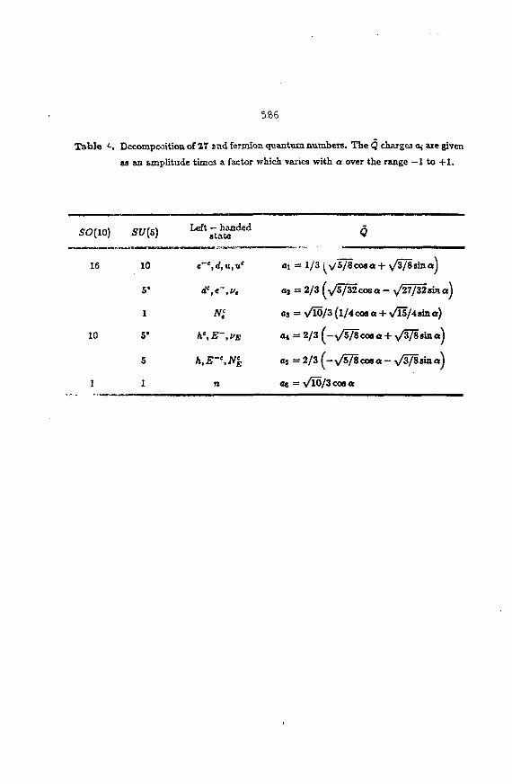
586
Table *•. Decomposition of 37 snd fermioa quantum numbers. The Q chargea a,- are given
as an amplitude time3 a factor which varies with a over the range - 1 to +1.
a/~iftn\ CTT(Z\ Left — handed50(10) SU(S) g t a t e
16 10 e~e,d,u,uc O! = 1/3 i v"5/8cosa+ y/3/Ss\naj
5' <F,e~,vt oj = 2/3 f y ' s / 3 2 c o s a - v^27/
1 Nl at = t/lO/Z (1/4 cos a + y/lS/4 sin a)
10 5' ke,E~,us a* = 2/3 (-y/~5/8coaa + y/3/8ainaj
S h, E~e, N% as = 2/3 ( - y/h}l cos a - y/zjitin. a)
1 1 n at = i/W/3coea
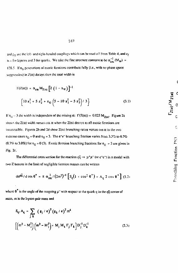
567
and £E arc the left- and right-handed couplings which can be read off from Table 4, and c f
is i for lcptons and 3 for quarks. We take the fine structure constant to be a~m (Mw) =
128.5. If n c generations of exotic fcrmions contribute fully (i.e., with no phase space
suppression) in Z(ct) decays then the total width is
1*10 a* + 5a22 + nG (5 - 10 a2 - 5 a " ] / 3 J (3.1)
If n c = 3 the widlh is independent of the mixing a: P(Z(a))= 0.025 M2 f a V Figure 2a
shows ihe Z(a) width versus cos a when the Z(a) decays to all exotic fermions are
inaccessible. Figures 2b and 2d show Z(cc) branching ratios versus cos a in the two
extreme cases nG = 0 and nG = 3. The e+e~ branching fraction varies from 3.3Co to 6.7%
(0.7% to 3.0%) for nG = 0 (3). Exotic fermion branching fractions for nG = 3 are given in
Fig. 2c.
The differential cross section for the reaction qq -» (l+|l~ (or e+e~) in a model with
two Z bosons in the limit of negligible fermion masses can be written
doW/dcosG* = it ae2
n/(2m2)"1 [ s ^ l + cos2 9*) * Aq 2 cos 6*] (3.2)
r > * •where 8 is the angle of the outgoing \i~ with respect to the quark q in the qq center of
mass, m is the lepion-pair mass and
i) fa* ~ M j MJ Mk r j r k ] D ] ' Dk
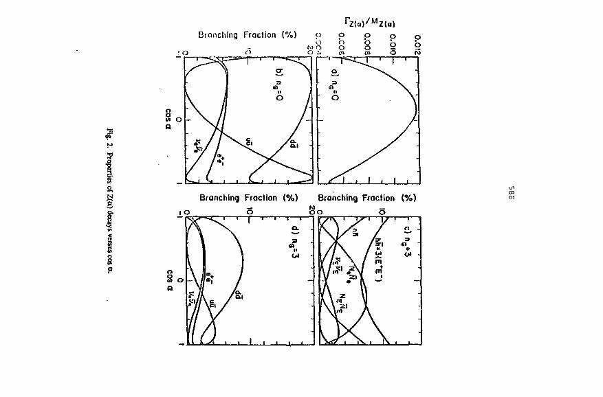
3!90
2,
It
rZ(a) /MZ(a)Blanching Fraction (%)
• o a
ab
to o
o ,\
oI/I O
—r *
yr
cr
nO
• y
1
I 'Ckl
Branching Fraction (%) Branching Fraction (%)
IO 5 So o
SoR
1K
v'/
1 1 '
)
• 1 1
I I I
a.3
O -
ao» -
;
• i
CD
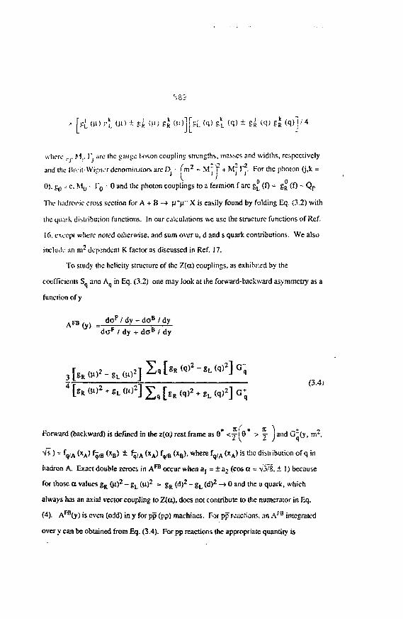
OD
where ... M,.1" are ihc gauge loson coupling strengths, masses and widths, respectively
and (he fiivit-Wipivr denominators arc Dj = (m2 - Mj r + M^ P2. h'or the photon (j,k =
0 0
0). g0 - c. Mo -- r 0 - 0 and Uie photon couplings to a fermion f arc gL (0 = gR (0 = Qp
The hadroi'ic cross section for A + B —» fi*n~ X is easily found by folding Eq (3.2) with
the quaik distribution functions. In our calculations we use the structure functions of Ref.
16, except where noted otherwise, and sum over u, d and s quark contributions. We also
include an m- dependent K factor as discussed in Ref. 17.
To study the helicity structure of the Z(a) couplings, as exhibited by the
coefficients S,, ana A. in Eq. (3.2) one may look at the forward-backward asymmeoy as a
function of y
daf I dy + d o B / dy
4 [gR m 2 + gL u o : ] ^ q [gR (q)2 + gL ( q ) 2 ] G;
(3-4)
Forward (backward) is defined in the z(a) rest frame as 6 <y l 6 > -f jandG±(y, nv-.
^ ) = V A <XA> {q/B (XB> ± ^/A <XA) fq/B (XB>>wnere fq/A(xA^ i s ti"lC distribution of q in
hadron A. Exact double zeroes in A r e occur when a, = ± a2 (cos a = Y3/S, ± 1) because
for those a values gR (n)2 - gL (\i)2 = gR (d)2 - gL (d)2 -» 0 and the u quark, which
always has an axial vector coupling to Z(a), does not contribute to the numerator in Eq.
(4). AFB(y) is even (odd) in y for pp (pp) machines. For pp reactions, an Ar'B integrated
over y can be obtained from Eq. (3.4). For pp reactions the appropriate quantity is
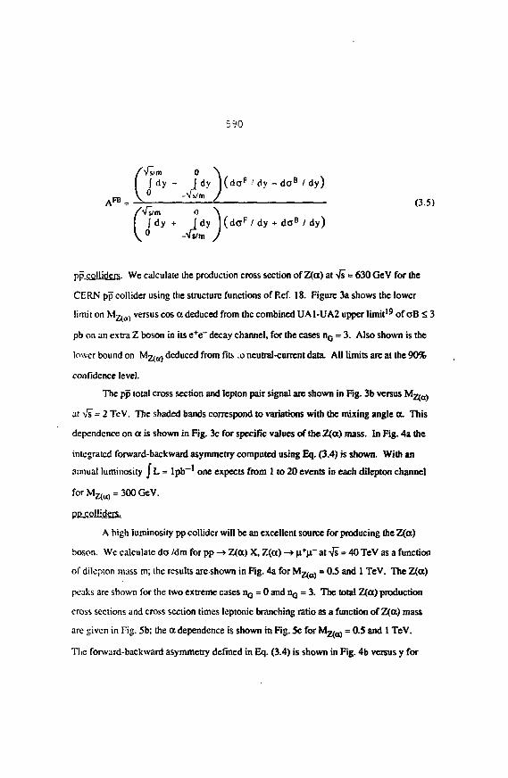
5S0
•fs/m 0 \J d y - f d y | ( d o F •'dy - d o B / d y )
ldkJ.J dy + Jdy ] ( d a F / dy + d o B / dy)
<» -4m J
pp colliders. We calculate the production cross section of Z(cc) at Vs = 630 GeV for the
CERN pp collider using the structure functions of Rcf. 18. Figure 3a shows the lower
!i mi t on M ^ versus cos a deduced from the combined U A1-UA2 upper limit19 of oB S 3
pb on an extra Z boson in its c+e~ decay channel, for the cases nG = 3. Also shown is the
lower bound on M ^ j deduced from fits :o neutral-current data. All limits are at the 90%
confidence level.
The pp total cross section and lepton pair signal are shown in Fig. 3b versus M ^ ^
at vis = 2 TeV. The shaded bands correspond to variations with the mixing angle a. This
dependence on a is shown in Fig. 3c for specific values of the Z(a) mass. In Fig. 4a the
integrated forward-backward asymmetry computed using Eq. (3.4) is shown. With an
annual luminosity J L = lpb~' one expects from 1 to 20 events in each dilepton channel
for Mz,a) = 300 GeV.
pp colliders.
A high luminosity pp collider will be an excellent source for producing the Z(a)
boson. We calculate do /dm for pp -» Z(a) X, Z(a) -» | i+n~ at Vs = 40 TcV as a function
of dilepton mass m; the results are shown in Fig. 4a for M ^ j = 0.5 and 1 TeV. The Z(a)
peaks are shown for the two extreme cases IIQ = 0 and IIQ = 3. The total Z(cc) production
cross sections and cross section limes leptonic branching ratio as a function of Z(a) mass
are given in Fig. 5b; the a dependence is shown in Fig. 5c for M ^ = 0.5 and 1 TeV.
The forward-backward asymmetry defined in Eq. (3.4) is shown in Fig. 4b versus y for
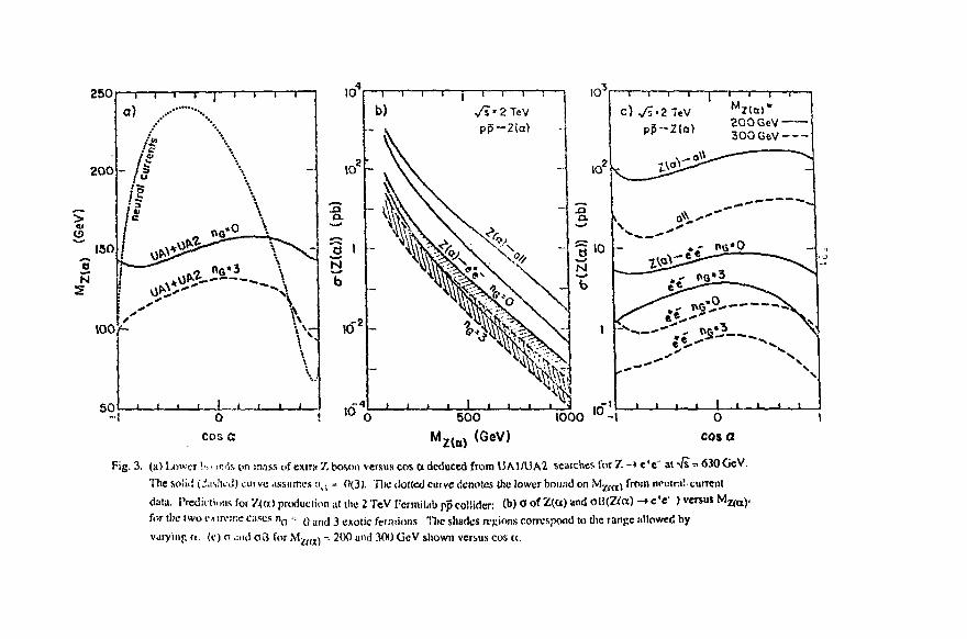
250
200
150t»N
5
100/-
"• 1
a) ,.••••"
/
- 1/*/'
1 1 I
" • • • • •
...-••••••••
•0
\
^ ^ \
f t
-
V0
cos ato
MZ(o)
Fig. 3. (a) I/)wor !>,• :nls on mass of extra '/. boson versus cos a deduced from UA1AJA2 searches for 7. - • e ' e at -fe~ 630 GeV.
The soiiii (J;IS!K-J) cuive assumes :i i ; = 0(3). 'Die dotted cuive denotes the lower bound on My./ft) from newtra! current
data. I'rwlicti. .us for Z<«) production at tlie 2 TeV Fcrmilab pp collider: (>>) o of Z(a) and o»(Z((i) -+ c*e" ) versus M^a).
for the two <•* in-ir.c cases n0 •= 0 i lnc | 3 e x o t i c lermi^s Ti,e shades regions correspond to Oic range allowed by
varyinp «. (c) o .;nd oil for M^^j - 200 ami 300 GeV shown versus cos «.
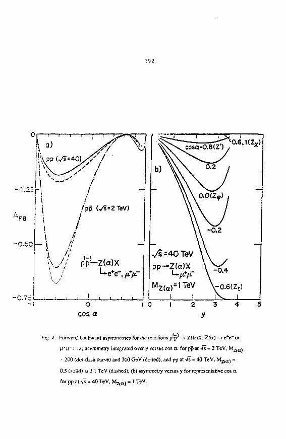
:9 2
-O.25K,
F3
-0.50
-C.75<
tQ.6,HZx)
M Z ( a ) = t T e V \ -a6{Zj)I I
Tig i. F-'orward backward asymmetries for the reactions p-p' -* Z(a)X, Z(a) -> e+e" or
|i*u" : (a) asymmetry integrated over y versus cos a for pp at Vs = 2 TeV, Mz^ay
-- 200 (dci-dash curve) and 300 GeV (doited), and pp at Vs = 40 TcV, M^^ =
0.5 (solid) and 1 TeV (dashed); (b) asymmetry versus y for representative cos a
for pp at Vs = 40 TeV, M ^ j = 1 TeV.
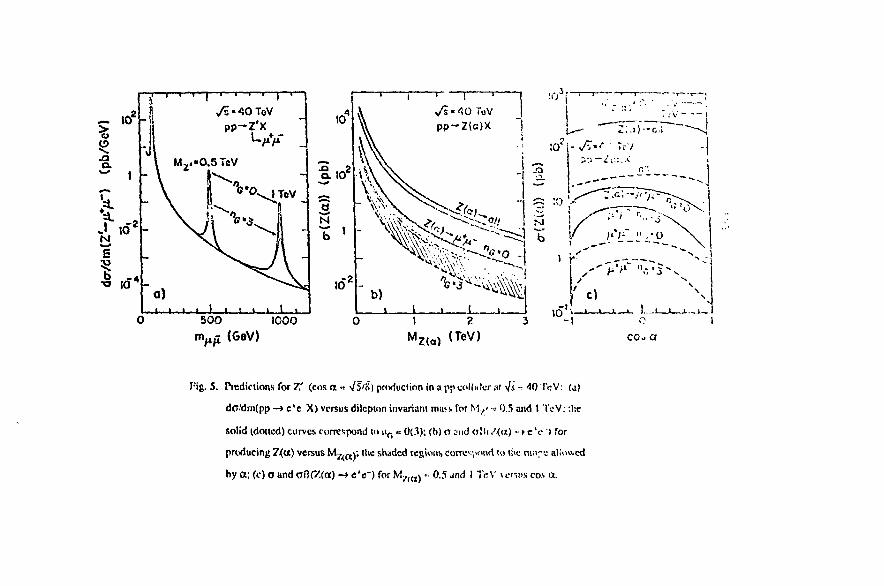
500 1000m ^ (GeV) co- a
I:ig. 5. Piediclions for Z ' (cos a = /5/K) priiduction in a pp collulcr;« i/s - 10 TeV: (j)
da/dm(pp -> c*c X) versusdilcptnn invariant mavs for M z ' -. 0.5 und I TeV; :!ie
solid (dotted) curves correspond to n 0 = 0(3): (b) cr and <j'i( / ( « ) - » c V") for
producing Z(«) versus M j . , ^ ; the shaded regioii!> eonrc>.;>onrt to tJic nui-c alinwed
by a; (c) O and oB(Z(o) -+ e'e~) for M^,rt) ~ 0.5 and I TcV versus CON a
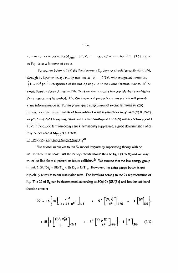
vjrwjs values or cos a. for M/ IH) = 1 TcV; t1.-. lejrated asymmetry of bq. (3.5) is g;te:'
rn [i£ 4a as a function of cos Ot.
l:or m.'Asc tvlov. •; TcV the Y:u.) bosun <>i L(l I!K"I '<>S should be easily riev.V'.He
through its lep'.i-'.ic decays m J pp macl'.snc a! r(s) 40 TcV wiili inie^raltd Imnmr.u'.y
I I. - 10"' p b " \ ::TCspecuvc of ;hc mining ann * u or the exotic fcrmion nusscs. If the
exotic fcrmion decay channels of the 7-tu) arc Vinemaucally inaccessible then even higher
7.Cwj masses may be probed. The 7x,o.) mass and production cross section will provide
s-.me information on a. For no phase space suppression of exotic fermions in Z(a)
decays, accurate measurements of forward-backward asymmetries in pp -» Z(o) X, Z(a)
- > ji"u~ and Z(a) branching ratios will further constrain a for Z(a) masses below about I
Te V; if the exotic fcrmion decays are kinematicaliy suppressed, a good determination of a
may be possible if MZ(O, < 1.5 TeV.
il±. fVop-TT'es of Quark Singlet from E62 0
We restrict ourselves to the E6 model inspired by superstring theory with no
intermediate mass scale. All the 27 superfields should then be light (STeV) and we may
evnect to find them at present or future colliders.21 We assume that the low energy group
s :vnk 5, SL'(3)C x SU(2\ x U(1)Y x U(l) n . However, the extra gauge boson is not
cxvcially relevant to our discussion here. The fermions belong to the 27 representation of
E6. The 27 of E6 can be decomposed according to SO(10) {SU(5)} and has the left-hand
fcrmion content
27 = 16^101 ' C , . . • - , , . . . .(u,d) uc J l /3 L d c J - l / 6 L J5/6
5/6
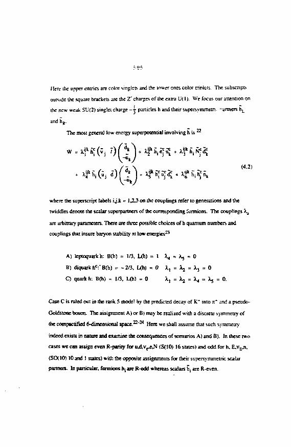
Here the upper entries are color <.inglc& and the lower ones color tnnltls. The subscripts
ouiside the square brackets arc the Z' charges of the extra U( 1). We focus our attention on
the new weak SU(2) singlet charge - y panicles h and their supersymmem. -armers hL
and hR.
The most general low energy superpotential involving h is H
(4.2)• xf hjfo
where the superscript labels i jJt = 1.2,3 on the couplings refer to generations and the
twiddles denote the scalar superpartners of the corresponding fcrmions. The couplings /.a
are arbitrary parameters. There are three possible choices of b quantum numbers and
couplings that insure baryon stability at low energies23
A) leptoquark h: B(h) = 1/3, L(h) = 1 \4 = ^ = 0
B) diquark hc:" B(h) = - 2/3, I/h) = 0 X, = J^ = X3 = 0
C) quark h: B(h) = 1/3, L(h) = 0 X., = \ = 3L4 = \ = 0.
Case C is ruled out in the rank 5 mode! by the predicted decay of K~ into iC and a pseudo-
Goldstone boson. The assignment A) or B) may be realized with a discrete symmetry of
(he compactified 6-dimensional space.22"24 Here we shall assume that such symmetry
indeed exists in nature and examine the consequences of scenarios A) and B). In these two
cases we can assign even R-panry for uutve^,N (S(10) 16 states) and odd for h. E.vE,n,
(SCX 10) 10 and 1 states) with tbe opposite assignments for their supersymmetric scalar
partners. In particular, fermions hj are R-odd whereas scalais h, are R-even.
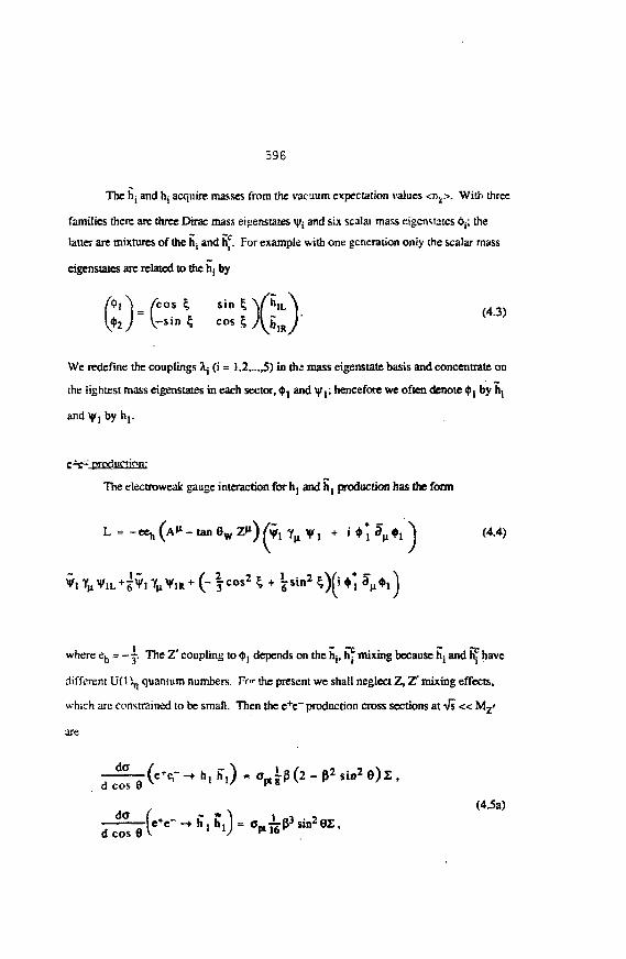
596
The hj and hj acquire masses from the vacuum expectation values <n!s>. With three
families there are three Dirac mass eijienstates V; and six scalar mass eigeiMates tif. the
latter are mixtures of the hj and hf. For example with one generation only the scalar mass
eigenstates are related to the hj by
We redefine the couplings Xj (i = 1,2,...,5) in the mass eigenstate basis and concentrate on
the lightest mass eigenstates in each sector, $, and Vj; hencefore we often denote 0 t by h,
a n d y j b y h , .
e-1^ production:
The electroweatc gauge interaction for hj and h, production has the form
6W Z») j y , T|l v , + i •*,L = -eefc ( A * - tan 6W Z») j y , T|l v , + i •*, 3^ j (4.4)
+ (~ f cos2 \ + L s
where eh = - ~ The Z' coupling to <t>, depends on the hj, h? mixing because h ; and h? have
different U(l )n quantum numbers. Fw the present we shall neglect Z, Z' mixing effects,
which are constrained to be small. Then the e+e~ production cross sections at -\/s « M z '
are
dad cos 9
_jc_' * (4-53)
dcos 6
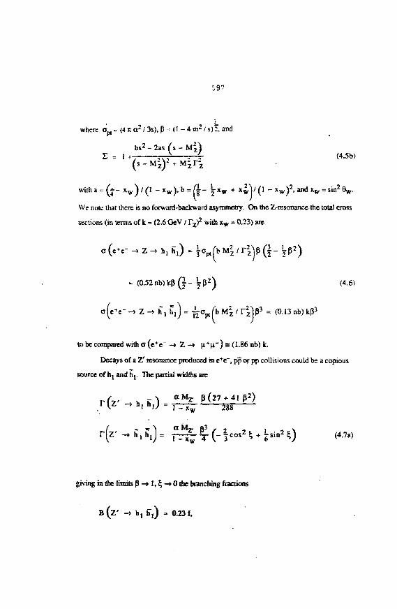
597
1_where Op,* (4 7t or / 3s), P = (1 - 4 m2 / s) 2. and
bs2 - 2as (i - M z )Z = 1 4 - r ^ ^ ^r~- (4.5b)
w i t h a = ( j - x w ) / ( l - x w ) , b = f l - ' ? x w + X w V 0 - x w )
We note that there is no forward-backward asymmetry. On the Z-resonance the total cross
sections (in terms of k = (2.6 GeV / Tjf with xw = 0.23) arc
o (e*c- -» Z -» h,
= (0.52nb)kp(|- ' jp 2 ) (4.6)
-» Z ^ h, h,] = •^o^j 'bMl/r^P 3 = (O.13nb)kp3
to be compared with <r (e+e" -» Z -» H*H") = <1.86nb) k.
Decays of a Z' tesonance produced in e+c", pp or pp collisions could be a copious
source of hj and ht. The partial widths arc
mh, h,) = %^£- §• ( - |cos 2 t + ^sin2 %) (4.7a)
giving in the limits P -»1, % -»0 (be branching fiactions
B ( Z ' ^ h, h"i) » 0.23 f,
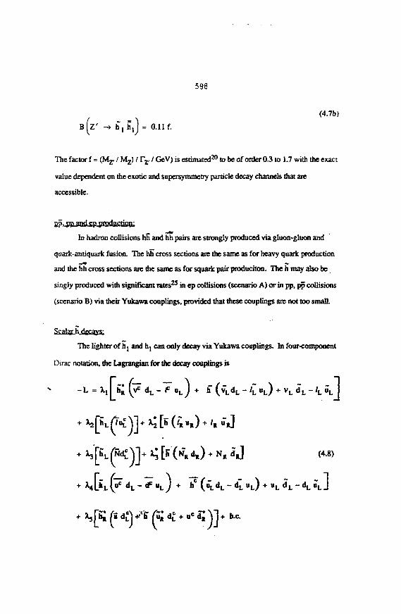
B ( Z ' -» h, h,j = 0.11 f.
598
(4.7b)
The factor f = (Mz. / Mz) / T r / GcV) is estimated20 to be of order 0.3 to 1.7 with the exact
value dependent on the exotic and supersymmetry particle decay channels that are
accessible.
pp. pp and ep production:
In hadron collisions hh and hh pairs are strongly produced via gluon-gluon and
quark-antiquark fusion. The hh cross sections are the same as for heavy quark production
and the hh cross sections are the same as for squark pair produciton. The h may also be
singly produced with significant rates25 in ep collisions (scenario A) or in pp, pp collisions
(scenario B) via their Yukawa couplings, provided that these couplings are not too small.
Scalar h decays:
The lighter of hj and h, can only decay via Yukawa couplings. In four-component
Dirac notation, the Lagrangian for the decay couplings is
^ [h (<R»») + '* • J
^ [H (NR dR) + NB d J (4.8)
+ *4lj>L (uC dL~ ^ « L J + fcC (»LdL ~ dL O + UL d L ~ dL »L J
h-c.
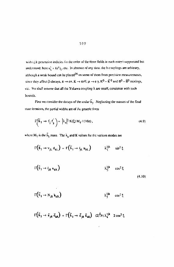
J O Q
with t.j.k generation indicies fin the order of the three fields in each entry) suppressed but
understood; here u£ - (uc)L, etc. In absence of any data, the h couplings are arbitrary,
although a weak bound can be placed26 on some of them from precision measurements,
since they affect (J-decavs, J: -> ev, K -» 7tvv, ji - »e y, K° - K ° and B° - B° mixings,
etc. We shall assume that all the Yukawa coupling X are small, consistent with such
bounds.
First we consider the decays of the scalar h j . Neglecting the masses of (he final
slate fermions, the partial widths are of ;he generic form
i f h , -> fj f'k \~ \%a\2 K © M, / (lftc), (4.9)
where M, is the hj mass. The Xa and K values for ths various modes are
(4.10)
(S i -» uj8 d a ) = r (h , -» djR u j (2)V) Xf 2 cos2 %
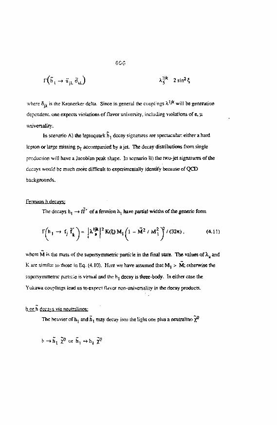
6CG
where 5jk is the Kroneckcr delta. Since in general the couplings Xljlc will be generarion
dependent, one expects violations of flavor university, including violations of e, [l
universality.
In scenario A) the leptoquark h, decay signatures are spectacular either a hard
lepton or large missing r>j. accompanied by a jeL The decay distributions from single
production will have a Jacobian peak shape. Iii scenario B) the two-jet signatures of the
decays would be much more difficult to experimentally identify because of QCD
backgrounds.
Fermion h decays:
The decays hj —» ff' of a fermion hj have partial widths of the generic form
(4.1!)
where M is the mass of the supersymmctric particle in the final state. The values of Xa and
K are similar to those in Eq. (4.10). Htre we have assumed thatM, > M; otherwise the
supcrsymmetnc particle is virtual and the hi decay is three-body. In either case the
Yukawa couplings iead us to expect flavor non-universality in the decay products.
h orh decays via neutralinos:
The heavier of h, and h t may decay inio the light one plus a ncutralino x°
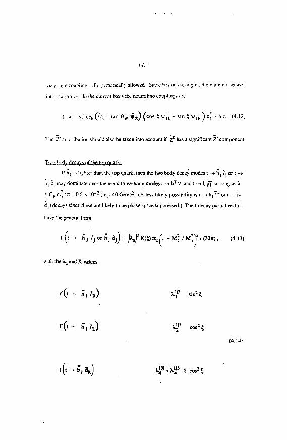
bC"
via j . i!L-c couplings, if i jicmaucally allowed Since h is an isosirjic;. there are no decay?
into .iarginio".. In (he current basis the neutralino couplings are
L ^ - \"2 eeh ( % - tan 9 W V j ) (cos % v 1 L - sin % y 1 R ) <p| + h.c. (4.12)
The '/.' ci iiribution should also be taken into account if %' has a significant Z' component.
Tw'ibi.-xj'N decays of the top quark:
Ifhj is lij-htcr than the top quark, then the two body decay modes t - • hj /:Ort—>
hj d, may dominate over the usual three-body modes t - » b7 v and t —»bqq' so long as "K
> GF n:^ / K = 0.5 x l f r ; (m, / 40 GeV)2 . (A less likely possibility is i - » h , ? - or t - * h,
d , ) decays since these are likely to be phase space suppressed.) The t-decay partial widths
have the generic form
r ( t -» h j 7j or h, dj) - \\a\2 K(%) i^fl - M] / U]f I (32x), (4.13)
with the Xj and K values
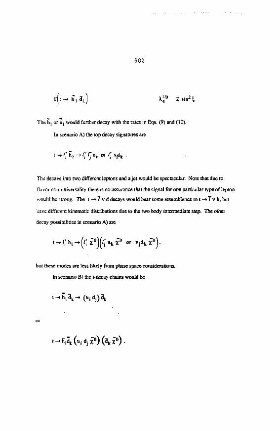
602
rft -* h , dLl k™' 2 sin2
The h, or h, would further decay with the rates in Eqs. (9) and (10).
In scenario A) the top decay signatures are
The decays into two different leptons and a jet would be spectacular. Note that due to
flavor non-universality there is no assurance that the signal for one particular type of lepton
would be strong. The t -* 7 v d decays would bear some resemblence to t -» 7 v b, but
have different kinematic distributions due to the two body intermediate step. The other
decay possibilities in scenario A) are
or VA*0)-
but these modes are less likely from phase space considerations.
In scenario B) the t-decay chains would be
t -»h ,d k -> ( n i d j ) ^
603
The first decays above would be essentially impossible to search for ai a hadron collider but
the second may be detected through the missing transverse momentum.
Qlmnodeu.ys:
If the masses should satisfy the inequality
then the two body decays
g -»h , h, or iij iij
via the strong interaction should be dominant and swamp all conventional gluino signals.
This would totally alter xtrateeie'; for gluino detection at hadron colliders.
In summary we have pointed out several surprising effects which arise form the
exoiic quark singlet of E6, sur:> as flavor non-universality and two body decays of the top
quark. Most new particles expected in straight-forward extensions of the standard model
(such as fourth generation quarks and leptons, superpartners of ordinary '•-:'•'•:' and £-;;;.;.•
bosons) decay via gauge interactions that preserve e, n, t universality. Even heavy Hi jK-
particles would decay predominantly into heavy fermions or weak bosons and then e, .u
universality still holds for the final decay products. Consequently the observjnon ofe, )LI
universality violation would indicate the existence of totally new interactions, buch as ihosc
obtained in superstring theory from the compactification of hidden dimensions.
REFERENCES
1. E. Witten, Phys. Lea 155B, 151 0985): Nucl. Hiys. B2S8, 75 (1935).
2. P. Candelas, G.T. Horowitz, A. Strominger, and E. Witter., Nucl. Piiys. B258,
46 (1985).
3. J.D. Breil, B.A. Ovrut and G. Segre, Phys. Lett. 158B, 33 (1985).
4. A. Sen, Phys. Rev. Lett. 55, 33 (1985).
5. J. Rosner, Comments on Nuc. and Pan. Phys. 15, 195 (1986); R. Robinett,
University of Massachusetts report UMHEP-239 (1985).
6. V. Barger, N.G. Deshpande, K. Whisnant, Phys. Rev. Letts 56, 30 (1986);
E. Cohen. J. Ellis, K. Enquist, and D.V. Nanopoulos, CERN report TH4222/85;
L.S. Durkin and P. Langacker, Phys. Lett. I66D, 436 (1986).
7. V. Barger, E. Ma, and K. Whisnant, Phys. Rev. D26, 2378 (1982).
8. V. Barger, E. Ma, and K. Whisnant, Phys. Rev. D28, 1618 (1983).
9. J.E. Kim, P. Langacker, M. Levine, and M.M. Williams, Rev. Mod. Phys. S3,
211(1981).
10. M.A. Bouchiat et al., Phys. Lett. 134B, 463 (1984).
11. G. Barbiellini and C. Santoni, CERN Report EP/85-117.
12. A. Sirlin, Phys. Rev. D29, 89 (1984); W.J. Marciano and A. Sirlin, Phys. Rev.
D29. 945 (1984).
13. L. Di Leila and C. RubbU. talks at Kyoto Conference (1985).
14. D. London and J.L. Rosner, Pbys. Rev. D34, 1530 (1986); P. Langacker, R.W.
Rjibiicn and J L. Rosner, Phys. Rev. D30. 1470 (1984).
!5. V. Rarger. N.G. Deshpande, J. Rosner, K. Whisnant, Phys. Rev. D3S, 2893
(1987).
16. F. Eichtcn. i. Hinchliffe. K. Lane and C. Quigg, Rev. Mod. Phys. 56, 579
(1984).
605
17. V. Bargcr, p. 95, Proceedings of the Oregon Meeting, Eugene, OR (1985),
published by World Scientific.
18. D.W. Duke and J.F. Owens, Phys. Rev. D30, 49 (1984).
19. S. Geer, report at the XXin International Conference on High Energy Physics,
Berkeley, CA (1986).
20. This section is based on V. Barger, N. Deshpande and K. Hagiwara, Univ. of
Wisconsin preprint MAD/PH/347.
21. V. Barger, N.G. Deshpande, and K. Whisnant, Phys. Ref. Lett 56,30 (1086);
Phys. Rev. D33, 1912 (1986); J. Ellis, K. Enqvist, D.V. Nanopoulos and F.
Zwirner, Nucl. Phys. B276, 14 (1986) and Mod. Phys. Lett. Al, 57 (1986); R.
W. Robinett, Phys. Rev. 33,1908 (1986); J.L. Hewett, T.G. Rizzo, and J.A.
Robinson, ibid D33,1476 (1986)
22. B. Campbell, J. Ellis, M.K. Gaiilard, D.V. Nanoponlos and K. Olive, Phys. Lett
B180, 77 (1986).
23. V. Barger, N.G. Deshpande, JJ\ Gunion et al., in Proceedings of 1986
Snowmass Workshop, p. 216.
24. M. Mangano,. Phys. CM,613 (1985); A. Joshipura and U. Sarkar, Phys. Rev.
Lett 57,33 (1986); P. Binetniy, S. Dawson, I. Hinchliffe and M. Sher, Nucl.
Phys. B273,501 (1986); B. Greene, K. Kirlin, P. Miron and G.G. Ross, NucL
Phys. B278,667 (1986); M. Drees and X. Tata, UW Madison report
MAD/FH/344(l987).
25. V.D. Angctopoulos, J. Ellis, H. Kowalski, D.V. Nanopoulos, ND. Tracas and F.
Zwirner, CERN-TH.4578 (1986).
26. A. Masiero, D.V. Nanopouk* and A. L Sanda, Phys. Rev. Lett 57,663 (1986);
W. Buchmuller and D. Wyler, Phys. Lett. B177,377 (1986); SM. Barr and A.
Masiero, Phys. Rev. Lett. 5S, 187 (1987); Y. Kizukuri, Phys. Lett. B185,183

606
(1987); B.A. Campbell, J. Ellis, K. Enqvist, MK. Gaillaid and D.V. Nanopoulos,
CERN-TH.4473 (1986).
6 07
PRECISION MEASUREMENTS OF
STANDARD ELECTROWEAK MODEL PARAMETERS IN LEF
Alain BLONDEL
CERN, Geneva, Switzerland
ABSTRACT
A combined knowledge of the Z mass, the W mass, and the
fennion couplings to the Z will be obtained in the Large Electron-
Positron storage ring (LEP) with unprecedented accuracy, providing
information about physics beyond our energy scale. The question of
the feasibility in LEP of longitudinally polarized beams, which are
essential for accurate measurements of the couplings at the Z, is
briefly considered.
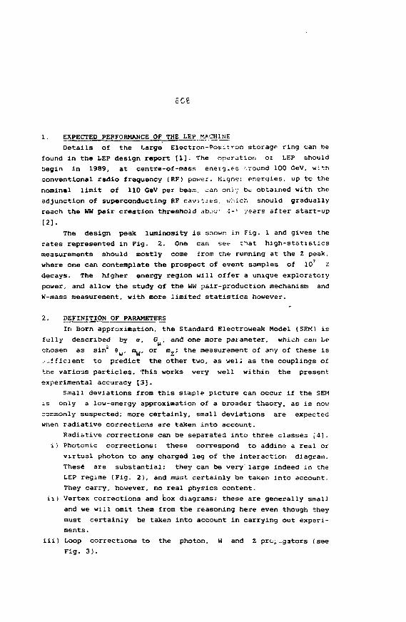
1. EXPECTED PERFORMANCE OF THE LEP MACHINE
Details of the Large Electron-Positron storage ring can be
found in the LEP design report [1]. The operation ot" LEP should
begin in 1989, at centre-of-mass enetg.e-s --round 100 GeV, with
conventional radio frequency (RF) power. Hiqne: pnerqies, up tc the
nominal limit of 110 GeV per beam, can on]y be obtained with the
adjunction of superconducting RF cavj'jes. which should gradually
reach the WW pair creation threshold abov •',-'• years after start-up
[2].
The design peak luminosity is snowr. in Fig. 1 and gives the
rates represented in Fig. 2. One can see that high-statistics
measurements should mostly come from the running at the Z peak,
where one can contemplate the prospect of event samples of 10 z
decays. The higher energy region will offer a unique exploratory
power, and allow the study of the WW pair-production mechanism and
W-mass measurement, with more limited statistics however.
2. DEFINITION OF PARAMETERS
In Born approximation, the Standard Electroweak Model (SEM) is
fully described by a, G , and one more parameter, which can be
chosen as sin' 6 , nu., or ra_; the measurement of any of these is
efficient to predict the other two, as well as the couplings of
tne various particles. This works very well within the present
experimental accuracy [3].
Small deviations from this simple picture can occur if the SEM
is only a low-energy approximation of a broader theory, as is now
commonly suspected; more certainly, small deviations are expected
when radiative corrections are taken into account.
Radi&tive corrections can be separated into three classes ;4].
i) Photonic corrections: these correspond to addino a real or
virtual photon to any charged leg of the interaction diagram.
These are substantial: they can be very large indeed in the
LEP regime (Fig. 2), and must certainly be taken into account.
They carry, however, no real physics content.
ii) Vertex corrections and box diagrams: these are generally small
and we will omit them from the reasoning here even though they
must certainly be taken into account in carrying out experi-
ments.
iii) Loop corrections to the photon, W and Z prc;._gators (see
Fig. 3).
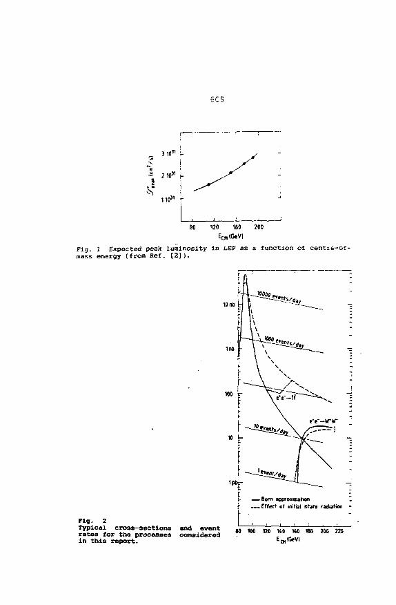
SCS
f110" j-
80 120 160 200
Fig. 1 Expected peak luminosity in LEP as a function of centre-ofmass energy (from Ref. [2)).
i- — B o m approximation Z— Effect of initial state radiation -
Fig. 2Typical cross-sections and eventrates for the processes consideredin this report.
SO W 120 HO K0 180 200 220
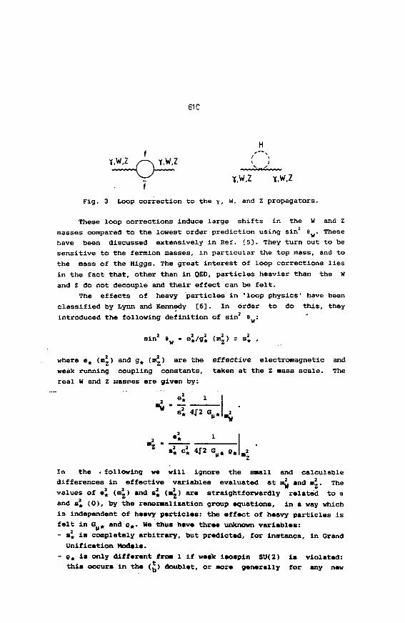
61C
T.W.Z
T,W,Z
Fig. 3 Loop correction to the y, w- a n d z propagators.
These loop corrections induce large shifts in the W and Z
masses compared to the lowest order prediction using sin2 8w- These
have been discussed extensively in Ref. [5]. They turn out to be
sensitive to the fennion aasses, in particular the top mass, and to
the mass of the Hlggs. The great interest of loop corrections lies
in the fact that, other than in QED, particles heavier than the W
and Z do not decouple and their effect can be felt.
The effects of heavy particles in 'loop physics' have been
classified by Lynn and Kennedy [6]. In order to do this, they
introduced the following definition of sin2 ew:
ei/g2 (mi) = s2, ,
where e+ (mi) and g# (m,) are the™ it " t o
weak running coupling constants,
real W and Z washes are given by:
e2 '
"w " if
effective electromagnetic and
taken at the Z mass scale. The
4J"2 Gu »W
ci 4f2 G
the • following we will ignore the small and calculableIndifferences in effective variables evaluated at raj. and mi. The
2 2 2 2
values of e* (mz> and s* (»z) are straightforwardly related to a
and s2* (0), by the rationalization group equations, in a way which
is independent of heavy particles; the effect of heavy particles is
felt in G j, and c*. We thus have thraa unknown variables:
- s2t is completely arbitrary, but predicted, for instance, in Grand
Unification Models.
- o* is only different froa 1 if weak isospin SU(2) is violated:
this occurs in the (£) doublet, or more generally for any new
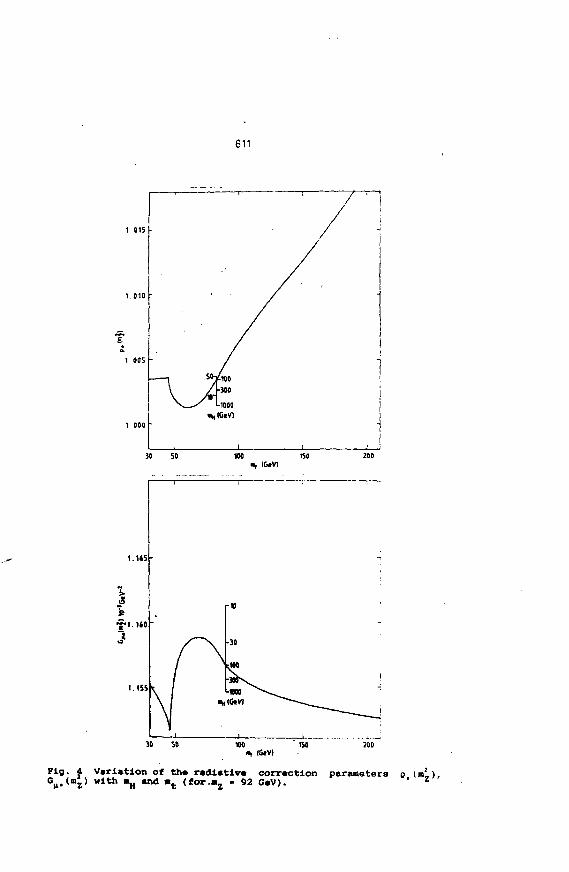
611
1 015
1 010
1 005
1 OOO
— 1 1 r
/
\*-*S MOOO
"" I O ' V I
t i i
/ '
/
-
-
-
30 50
30 SOIStV)
200
Fig. 4 Variation of th« r«dl«tiv« correction parameters o (mi),^ . ^ z ' with "H *"* "t ( f o r- -z " 92 G»v> '
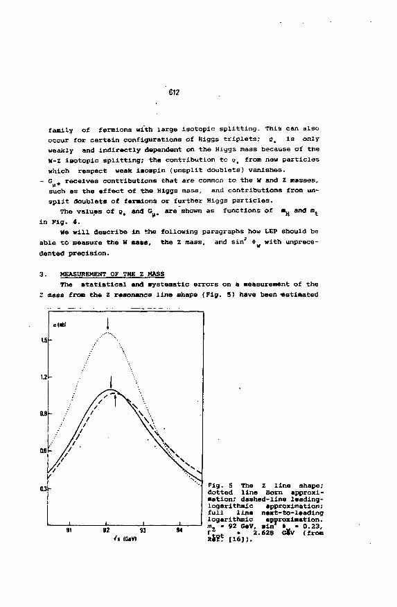
612
family of fennions with large lsotopic splitting. This can also
occur for certain configurations of Higgs triplets: e. is only
weakly and indirectly dependent on the Higgs mass because of the
W-Z isotopic splitting; the contribution to Q, from new particles
which respect weak iaospin (unsplit doublets) vanishes.
- G ^ receives contributions that are common to the H and Z nasses,u*such as the effect of the Higgs mass, and contributions from un-
split doublets of formions or further Higgs particles.
The values of e, and G are shown as functions of m^ and m^
in Fig. 4.We will describe In the following paragraphs how LEP should be
able to measure the W mass,
dented precision.
the Z mass, and sin e with unprece-
3. MEASUREMENT OF THE Z MASS
The statistical and systematic errors on a measurement of the
2 mass from the Z resonance line shape (Fig. 5) have been -estimated
L5-
Ut-
Fig. 5 The Z line shape;dotted line Born approxi-mation; dashed-line leading-logarithmic approximation;full line naxt-to-laadinglogarithmic approximation.m - 92 GeV, sin1 I • 0.23,rrnf. - 2.628 GHv (fromRS?*= [16]).
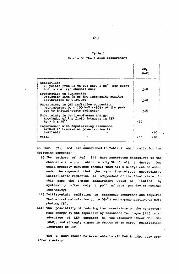
613
Table 1
Errors on the Z mass measurement
Statistics:13 points from 82 to 106 CoV, 2 pb per point,e* e" -• n*|i" (Y) channel only
Systematlcs on luminosity:Variation with Js of the luminosity monitorcalibration by 0.2*/GeV
Uncertainty in QED radiative correction:Displacement by - 100 MeV (+10%) of the peakdue to initial-state radiation
Uncertainty in centre-of-mass energy:Knowledge of the field integral in LEPto • 3 x 10"
Improvement with depolarizing resonancemethod if transverse polarization isavailable /
Total
(MeV)
1
+ 10
+10
+10
+30
+ 10
+35 +20
in Bef. [7], and are summarized in Table 1, which calls for the
following comments:
i) The authors of Ref. [7] have restricted themselves to the
channel e'e" -• u*(T, which is only 3% of all Z decays. One
could probably convince oneself that all z decays can be used,
under the argument that the mala theoretical uncertainty,
initial-state radiation, is independent of the final state. In
this case the Z-mass measurement would be limited by
systematic? after only 1 pb"1 of data, one day at nominal
luminosity!
ii) Initial-state radiation is extremely important and requires
theoretical calculation up to O(s 2) and exponentiation of soft
photons [83.
iii) The possibility of reducing the uncertainty on the centre-of-
nass energy by the depolarizing resonance technique [23] is an
advantage of LEP compared to the Stanford Linear Collider
(SLC), and strongly argues in favour of an early polarization
programme at LEP.
The Z mass should ba measurable to +20 MeV in LEP, very soonafter start-up.
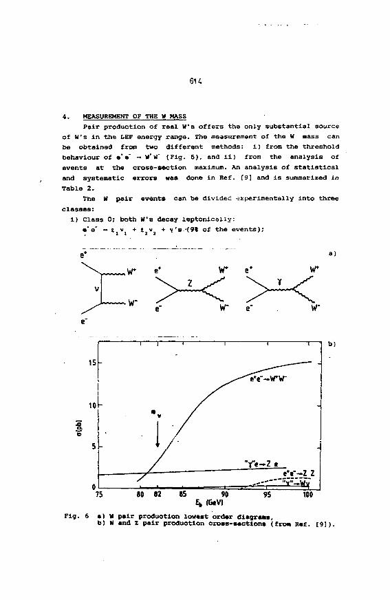
4. MEASUREMENT OF THE W MASS
Pair production of real W's offers the only substantial source
of W's in the LEF energy range. The measurement of the W mass can
be obtained from two different methods: i) from the threshold
behaviour of e* e' -• W*W" (Fig. 6), and il) from the analysis of
events at the cross-section maximum. An analysis of statistical
and systematic errors was done in Ref. [9] and is summarized in
Table 2.
The W pair events can be divided experimentally into three
classes:
i) Class 0; both W's decay leptonlcally:
e'e" - llvl + t,V2 • Y'S-(9% of the events);
a)
I I r T 1 b)
(GcV)100
Fig. 6 •) W pair production lowaat order diagrams,b) W and z pair production cross-sactiona (froa Ref. [9]).
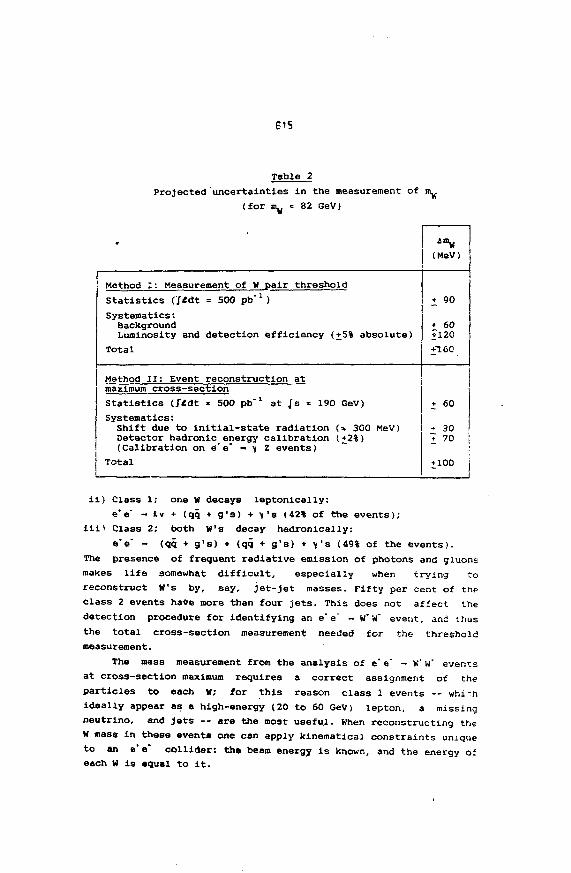
Table 2
Projected uncertainties in the measurement of
(for BL, >= 82 GeV)
*
Method I: Measurement of W pair threshold
Statistics (St&t = 500 pb"1)
Systematics:BackgroundLuminosity and detection efficiency (+5% absolute)
Total
Method II: Event reconstruction atmaximum cross-sectionStatistics (J/dt - 500 pb'l at Js * 190 GeV)
Systematics:Shift due to initial-state radiation (* 300 MeV)Detector hadronic energy calibration (+2%)(Calibration one's' •» \ Z events)
Total
(MeV)
+ 90
+ 60+ 120
£160
+ 60
+ 30+ 70
+ 100
il) Class 1; one H decays leptonically:
e*e" -» Iv + (qq + g's) + \'s (42% of the events);
ill) Class 2; both W's decay hadronically:
e*e' - (qq + g's) + (qq + g's) + \'s (49% of the events).
The presence of frequent radiative emission of photons and gluons
makes life somewhat difficult, especially when trying to
reconstruct W's by, say, jet-jet masses. Fifty per cent of thp
class 2 events have more than four jets. This does not affect the
detection procedure for identifying an e'e" - w'w' event, and thus
the total cross-section measurement needed for the threshold
measurement.
The mass measurement from the analysis of e' e" - w" w" events
at cross-section maximum requires a correct assignment of the
particles to each W; for this reason class 1 events -- whi ~.h
ideally appear as a high-energy (20 to 60 GeV) lepton, a missing
neutrino, and Jets -- are the moat useful. When reconstructing the
I* mass in these events one can apply kinematlcal constraints unique
to an e"e" collider: the beam energy is known, and the energy of
each H is aqual to it.
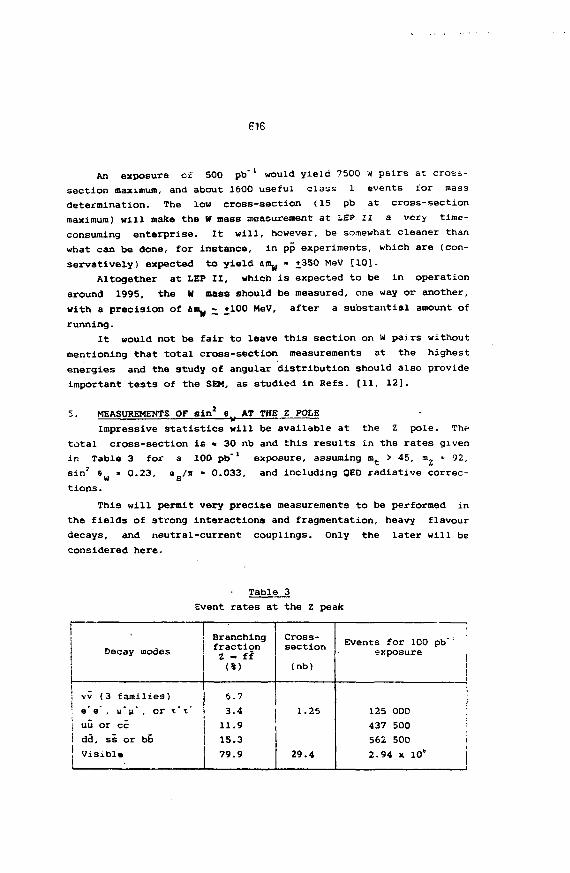
616
An exposure oi 500 pb'l would yield 7500 M pairs at cross-
section maximum, and about 1600 useful class 1 events for mass
determination. The low cross-section <15 pb at cross-section
maximum) will make the W mass measurement at LEP II a very time-
consuming enterprise. It will, however, be somewhat cleaner than
what can be done, for instance, in pp experiments, which are (con-
servatively) expected to yield Aniy = +350 MeV [10].
Altogether at LEP II, which is expected to be in operation
around 1995, the W mass should be measured, one way or another,
with a precision of Am^ z +100 MeV, after a substantial amount of
running.
It would not be fair to leave this section on w pairs without
mentioning that total cross-section measurements at the highest
energies and the study of angular distribution should also provide
important tests of the SEM, as studied in Refs. [11, 12].
5. MEASUREMENTS OF sin' 8y AT THE Z POLE
Impressive statistics will be available at the Z pole. The
total cross-section is % 30 nb and this results in the rates given
in Table 3 for a 100 pb"x exposure, assuming mt > 45, m2 - 92,
sin2 e * 0.23, o /n • 0.033, and including QED radiative correc-w stions.
This will permit very precise measurements to be performed in
the fields of strong intoractions and fragmentation, heavy flavour
decays, and neutral-current couplings. Only the later will be
considered here.
Table 3
Event rates at the Z peak
Decay modes
vv (3 families)
! e" e" , u" ii* , or T' t"
| uu or cc
dd, ss or bb
! Visible
•
BranchingfractionZ - ff
(%)
6.7
3.4
11.9
15.3
79.9
Cross-section
(nb)
1.25
29.4
Events for 100 pb" ;
exposure
125 000
437 500
562 500
2.94 x 10*
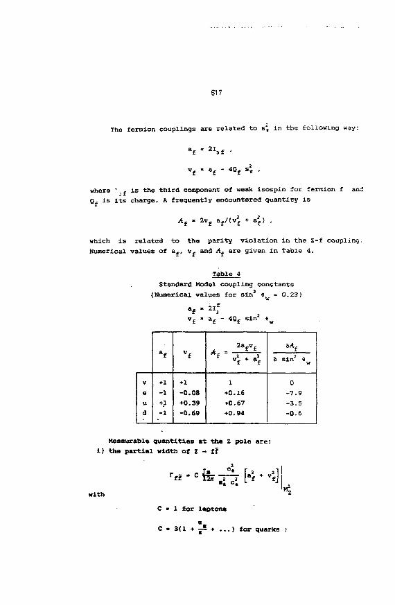
617
The ferniion couplings are related to s* in the following way:
af " 2l3f '
vf - af - 4Qf si ,
where " f is the third component of weak Isospin for fermion f and
Q is its charge. A frequently encountered quantity is
2vf a) ,
which is related to the parity violation in the Z-f coupling.
Numerical values of af, vf and jtf are given in Table 4.
Table 4
Standard Model coupling constants
(Numerical values for sin2 e =0.23)
vf . af - 4Qf sin »w
V
eud
af
+1
-1
+1
-1
+1
-0
+0
-0
f
.08
.39
.69
£
1
+0
+0
+0
2a
.16
.67
.94
fVf
• • *a sin2
0
-7.
-3.
-0.
6w
9
5
6
Measurable quantities at the Z pole are:
i) the partial width of z - ff
with
C • 1 for laptona
C • 3(1 + ji • ...) for quarks ;
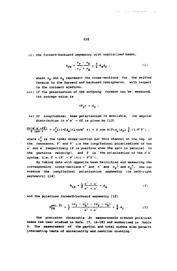
616
the forward-backward asymmetry with unpolarized beams.
°B 3
where o_ and o_ represent the cross-sections for the emittedr o
fermion in the forward and backward hemispheres, with respectto the incident electron.
iii) If the polarization of the outgoing fermion can be measured,
its average value is
<Pf> - ,tf .
iv) If longitudinal beam polarization is available, the angular
distribution in e*e' - ff is given by [13]
a ". e—SL2- » a [{1*$A ) ( l + c o s 8 ) + 2 c o s 9($+A ) 4 _ ] f ( 1 - P P") ,d c o s e u e e r o
where a is the total cross-section for this channel at the top of
the resonance, P* and P" aire the longitudinal polarizations of the
e' and e" respectively (P is positive when the spin is parallel to
the particle velocity), and if is the polarization of the e* e"
system, i.e. 3" « (P* - P')/(l - P* P').
By taking data with opposite beam helicities and measuring the
corresponding cross-sections o* and o" and o_- and on-, one can
measure the longitudinal polarization asymmetry (or left-right
asymmetry) [14]
A e (2)
and the polarized forward-backward asymmetry [15]
pB g 4 f
Tha precision obtainable in maasurements without polarized
beans has baon studied in Refs. [7, 16-18] and summarized in Table
5. The measuraaent of the partial and total widths also permits
interesting tests of universality and neutrino counting.
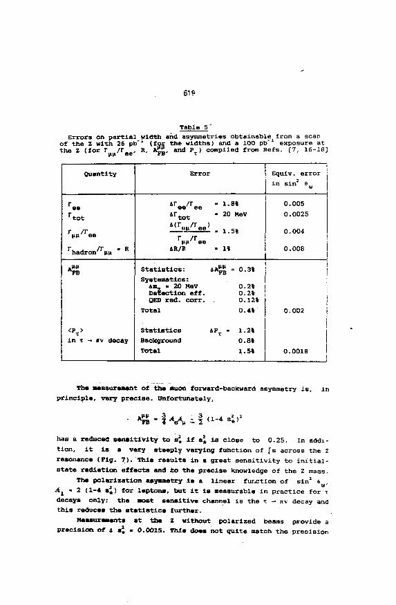
61?
Table 5"
Errors on partial width and asymmetries obtainable from a scanof the Z with 26 pb"1 (for the widths) and a 100 pb* exposure atthe Z (for r /r e e. R, A £ £ , and P T) compiled from Refs. [7, 16-18]
Quantity
reertot
rhadron/r(in * B
A1"1FB
<Pt>
in T - itv decay
Error
i ree / ree "artot
** mi' ee
AR/R -
Statistics: AAJ
Systematics:Am. - 20 MeVDetection off.QEO rad. corr.
Total
Statistics 4Px
Background
Total
1.
20
1%
V
8%
MeV
5%
= 0.3%
0.2%0.2%0.12%
0.4%
1.2%
0.8%
1.5%
Equiv. error
in sin2 « M
0.005
0.0025
0.008
0.002
1i
0.0018
1
Tha measurement of tha muon forward-backward asymmetry is,
principle, very precise. Unfortunately,
has a reduced sensitivity to 8^ if s» is close to 0.25. In addi-
tion, it is a very steeply varying function of fs across the z
resonance (Fig. 7). This results in a great sensitivity to initial-
state radiation effects and to the precise Knowledge of the Z mass.
The polarization asymaetry la a linear function of sin2 s
At ' 2 (1-4 si) for leptons, but it is measurable in practice for x
decays only; the most sensitive channel is the i - o decay and
this reduces the statistics further.
Measurements at the Z without polarized beams provide a
precision, of t ai « 0.0015. This does not quite match the precision
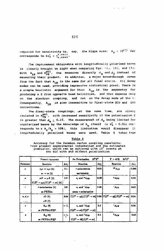
62C
required for sensitivity to,2 0 0 0 13
corresponds to 6s* - to\ooo,
say, the Higgs mass: ' - Gev
The improvement obtainable with longitudinally polarized beams
is clearly brought to light when comparing Eqs. (1;, (2), and (3).
With A and A™ 1/ one measures directly AQ and A{ instead of
measuring their product. In addition, a major breakthrough comes
from the fact that A._ Is the same for all final stai.es. All decaybit
modes can be used, providing impressive statistical power. There isa simple heuristic argument for this: ALR is the asymmetry for
producing a Z from opposite beam helicities, and thus depends only
on the electron coupling, and not on the decay mode of the ?..
Consequently, A,R is also insensitive to final-state OCD and OED
corrections.
The final-state couplings, .at the same time, are nicely
with increased sensitivity if the polarization $isolated in A*)?1,rois greater than jt ^0.15. The measurement of A{ being limited for
unpolarized beams by the knowledge of AQ itself (4 s\ - 0.002 cor-
responds to A A /A = 10%), this limitation would disappear if
longitudinally polarized beams were used. Table 6 taken from
Table 6
Accuracy for the fermion vector coupling constants:From present experimental information and £he estimatedprecision, which can be achieved with 10 events at
the SL.C with and without polarization
Fennions
t
M
T
c
t
Present Accuracy
Reaction
!/„« -. !/„« (1)« - « (2)
MJV - M* (3)
r-polarization (5)
at PETBA
«D(6)
at PETRA/PEP
at PETRA/PEP
A»,
0.1
0.3
2.8
0.04
-*•
No Polarixation 10*Z°
Reaction
r-polariiation
uymmctrj.
v, and "An
t>( and TA^jj
mean r-polariiation
Vg and 'An
r(z°—ci)/r{z° -.«)», and ' A M
A . ,
0.05
0.08
0.05
0.04
0.2
0.1
P = 45% 10*2"
Reaction
M ™
r(,«-.«,/r(^-.«,
Av/
0.005
0.02
0.02
0.04
0.10
0.05
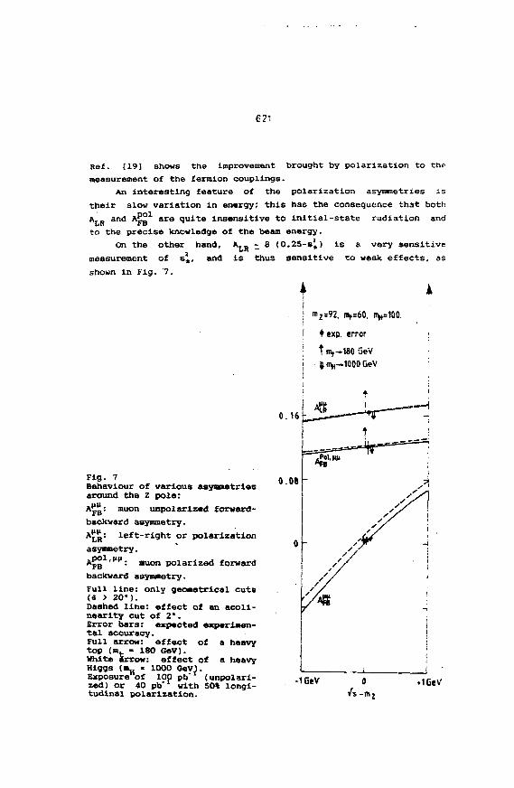
621
Ref. [19] shows the improvement brought by polarization to the
measurement of the fermion couplings.
An interesting feature of the polarization asymmetries is
their alow variation in enargy; this has the consequence that both
A,, and A S S 1 a r a quite insensitive to initial-state radiation and
to the precise knowledge of the beam energy.
On the other hand, K^R - 8 (0.2S-s») is a very sensitive
measurement of 6», and is thus sensitive to weak effects, as
shown in Fig. 1.
Fig. 7Behaviour of various asymmetries
around the Z pole:
Apg: muon unpolarizad forward-
backward asymmetry.
A £ £ : left-right or polarization
asymmetry.'**'': auon polarized forward
backward asymmetry.
Full line: only geometrical cuts(« > 20').Dashed line: effect of an acoli-nearity cut of 2*.Error bars: expected experimen-tal accuracy.Full arrow: effect of a heavytop (m. - 180 GeV).White arrow: effect of a heavyHiggs (•„ * 1000 Gey).Exposure of 100 pb (unpolari-zed) or 40 pb with 50% longi-tudinal polarization.
mZ=92, ify=60, R^
• exp. error
11%-IBO GeV
jt cn —1000 GeV
0.16K
0.08 "
0 -—
ft
t-—IT"
<
-
!
1f
1
i
!
I
1-IGeV 0
/ s -m2
«1GeV
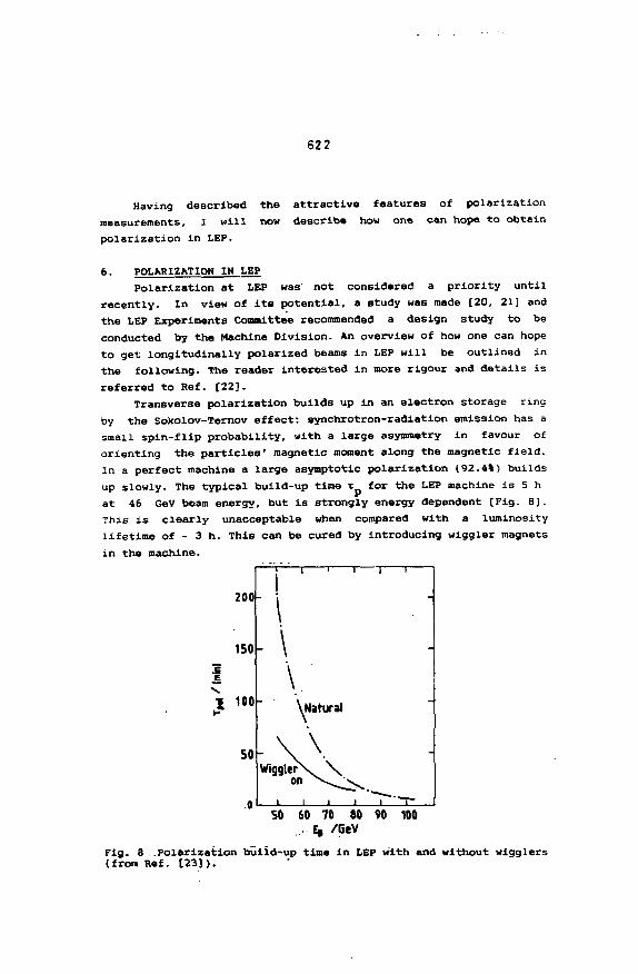
622
Having described the attractive features of polarization
measurements, I will now describe how one can hope to obtain
polarization in LEP.
6. POLARIZATION IN LEP
Polarization at LEP was not considered a priority until
recently. In view of its potential, a study was made [20, 21] and
the LEP Experiments Committee recommended a design study to be
conducted by the Machine Division. An overview of how one can hope
to get longitudinally polarized beams in LEP will be outlined in
the following. The reader interested in more rigour and details is
referred to Ref. [22].
Transverse polarization builds up in an electron storage ring
by the Sokolov-Ternov effect: synchrotron-radiation emission has a
small spin-flip probability, with a large asymmetry in favour of
orienting the particles' magnetic moment along the magnetic field.
In a perfect machine a large asymptotic polarization (92.4%) builds
up slowly. The typical build-up time x for the LEP machine is 5 h
at 46 GeV beam energy, but Is strongly energy dependent [Fig. 8).
This is clearly unacceptable when compared with a luminosity
lifetime of - 3 h. This can be cured by introducing wiggler magnets
in the machine.
200-
150
1 100
50-
S0 60 70 SO 90 100.... E, /GeV
Fig. 8 .Polarization build-up tine in LEP With and without wigglers{fron Ref. [23]).
1
• \
- \
\
" VWiggleN
oni i
> i i >
-
-
btural
\\
I • " 7 T-
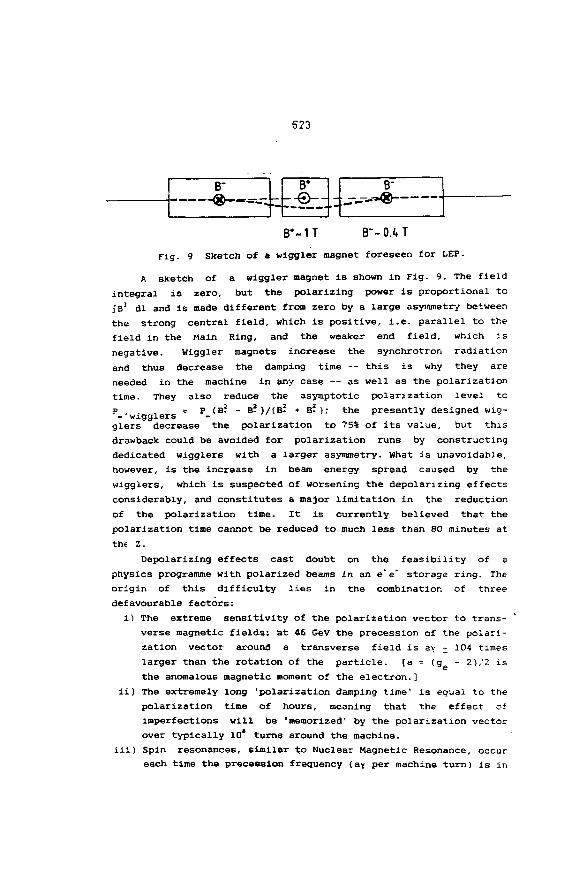
623
B"
B*-1 T B--0.4TFig. 9 Sketch of a wiggler magnet foreseen for LEP.
A sketch of a wiggler magnet Is shown in Fig. 9. The field
integral is zero, but the polarizing power is proportional to
JB3 dl and is made different from zero by a large asymmetry between
the strong central field, which is positive, i.e. parallel to the
field in the Main Ring, and the weaker end field, which is
negative. Wiggler magnets increase the synchrotron radiation
and thus decrease the damping time -- this is why they are
needed in the machine in any case — as well as the polarization
time. They also reduce the asymptotic polarization level tc
p = P (B? - B-)/(B- • B- ); the presently designed wio--'wigglers
glers decrease the polarization to 75% of its value, but this
drawback could be avoided for polarization runs by constructing
dedicated wigglers with a larger asymmetry. What is unavoidable,
however, is the increase in beam energy spread caused by the
wigglers, which is suspected of worsening the depolarizing effects
considerably, and constitutes a major limitation in the reduction
of the polarization time. It is currently believed that the
polarization time cannot be reduced to much less than 80 minutes at
tht 2.
Depolarizing effects cast doubt on the feasibility of a
physics programme with polarized beams in an e"e* storage ring. The
origin of this difficulty lies in the combination of three
defavourable factors:
i) The extreme sensitivity of the polarization vector to trans-
verse magnetic fields: at 46 GeV the precession of the polari-
zation vector around a transverse field is ay -- 104 times
larger than the rotation of the particle. [a = (g - 2)/2 is
the anomalous magnetic moment of the electron.]
ii) The extremely long 'polarization damping time' is equal to the
polarization time of hours, meaning that the effect of
imperfections will be 'memorized' by the polarization vector
over typically 10* turns around the machine.
iii) Spin resonances, similar to Nuclear Magnetic Resonance, occur
each time the precession frequency (ay per machine turn) is in
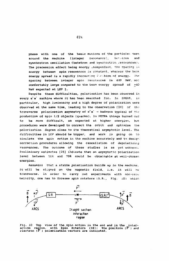
624
phase with one of the basic motions of the partic3e: turn
around the machine (integer resonance), be'jtron and
synchrotron oscillation (betatron and synchrotron resonances).
The precession effect being energy independent, the spacing U\
energy between spin resonances is constant, whereas the bean.
energy spread is a rapidly increasing i .nction of energy. The
spacing between integer spin resonances is 440 MeV, no."
comfortably large compared to the beam energy spread of +40
MeV expected at LEP I.
Despite these difficulties, polarization has been observed in
every e*e* machine where it has been searched for. In SPEAR, in
particular, high luminosity and a high degree of polarization were
observed at the same time, leading to the observation [24] of the-
transverse polarization asymmetry of e' e" -• hadrons typical of the
production of spin 1/2 objects (quarks). In PETRA things turned out
to be more difficult, as expected at higher energies, bat
procedures were developed to correct the orbit and optimize the
polarization degree close to its theoretical asymptotic level. The
difficulties in LEP should be bigger, and work is going on TO
simulate the spin motion in the machine accurately and to design
correction procedures allowing the cancellation of depolarizir.g
resonances. The outcome of these studies is as yet unknown.
Preliminary estimates [25] indicate that an asymptotic polarization
level between 504 and 70% could be obtainable at well-choser.
energies.
Assuming that a stable polarization builds up in the machine,
it will be aligned on the magnetic field, i.e. it will be
transverse. In order to carry out experiments with non-zero
helicity, one has to foresee spin rotators (S.R., Fig- 10) which
ARCS
P*
Sfaight sectioninteraction
region
Fig. 10 Top view of the spin motion in the arc and in the inter-action region. with Spin Rotators (SR); the positron (?') andelectron (P ) polarization vectors are indicated.
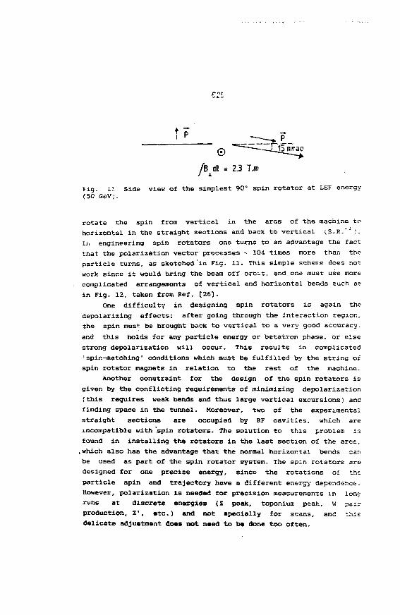
C25
/B dl = 2.3 T.n>J X
fig. 1?. Side view of the simplest 90° spin rotator at LEF energy(50 GeV;.
rotate the spin from vertical in the arcs of the machine to
horizontal in the straight sections and back to vertical iS.K."* ;.
In engineering spin rotators one turns to an advantage the fact
that the polarization vector processes - 104 times more than the
particle turns, as sketched in Fig. 11. This simple scheme does not
work since it would bring the beam off orc-t, and one must use more
complicated arrangements of vertical and horizontal bends such as
in Fig. 12, taken from Bef. [26].
One difficulty in designing spin rotators is again the
depolarizing effects: after going through the interaction region,
the spin must be brought back to vertical to a very good accuracy.
and this holds for any particle energy or betatron phase, or else
strong depolarization will occur. This results in complicated
'spin-matching' conditions which must be fulfilled by the string of
spin rotator magnets in relation to the rest of the machine.
Another constraint for the design of the spin rotators is
given by the conflicting requirements of minimizing depolarization
(this requires weak bends and thus large vertical excursions) and
finding space in the tunnel. Moreover, two of the experimental
straight sections are occupied by RF cavities, which are
incompatible with 'spin rotators. The solution to this problem is
found in installing the rotators in the last section of the arcs,
.which also has the advantage that the normal horizontal bends can
be used as part of the spin rotator system. The spin rotators are
designed for one precise energy, since the rotations of tht
particle spin and trajectory have a different energy dependence.
However, polarization Is needed for precision measurements in lone
runs at discrete energies (Z peak, toponiuir. peak, w pair
production, Z', »tc.) and not specially for scans, and this
delicate adjustmant doas not need to b* done too often.
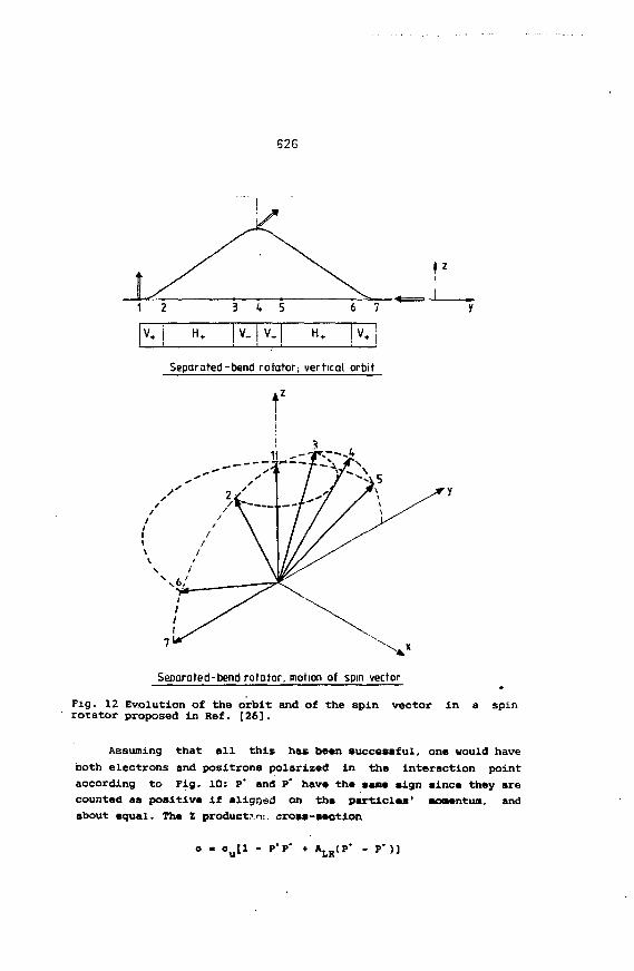
626
1 2 3 4 5 6 7
V+ . H + | V . j V .
Separated - bend rotator; vertical orbit
Separated-bend rotator, motion of spin vector
Fig. 12 Evolution of the orbit and of the spin vector in a spinrotator proposed in Ref. [26].
Assuming that all this has bean successful, one would have
both electrons and positrons polarized in the interaction point
according to Fig. 10: P* and P" have the same sign since they are
counted as positive if aligned on the particles' momentum, and
about equal. The Z productrou cross-section
ou[l - P* P* - P")]
527
is both independent of A L R ana considerably reduced; it even
vanishes if P* « P' - 1. In order to obtain non-zero helicity at
the interaction point it has been suggested [27] that some bunches
be depolarized selectively and not the others.
The principle of the depolarizer [28] is to continuously
excite an artificial spin resonance by applying a small (~ 1 G m)
transverse field in phase with the spin precession period. Because
the field is small, the device can be gated and guarantees a
polarization level of < 10"i for any set of the eight bunches
circulating in the machine. Depolarization is indeed much easier
than polarization.
This facility can be used to obtain all combinations of
helicities [29]: by depolarizing the electron bunches 1 and 3 and
positron bunches 2 and 3, one obtains in turn in the experiment the
following four combinations:
' Electron bunches 1 2 3 5
Positron bunches 1 2 3 3
Cross-sections o^ o2 oa of
«, * V 1 + P*o3 « ou(l - P"
°3 * °U
o, • ou[l - P-P- • ^ ( P - - P")]
p* r p"
This is a vary favourable experimental situation:
1) The tot•i * cross-sections are measured from data taken
simultaneously, in the same detector and with beams
circulating in the same machine: a nearly perfect cancellation
of detector efficiency, luminosity systematics, etc., is
expected; this is true up to possible small systematic
differences from one bunch to another, the exact effect and
monitoring of which is presently being scrutinized,
ii) Tha four equations above can ba solved to extract ArD, a , p*LiK U
and P* from tha data thamsslves, avoiding the need to rely on
an independent external measurement of tha polarization; this
is In contrast with tha situation in SLC [19] where positrons
cannot ba polarized, and only oi and o2 ara measurable, and
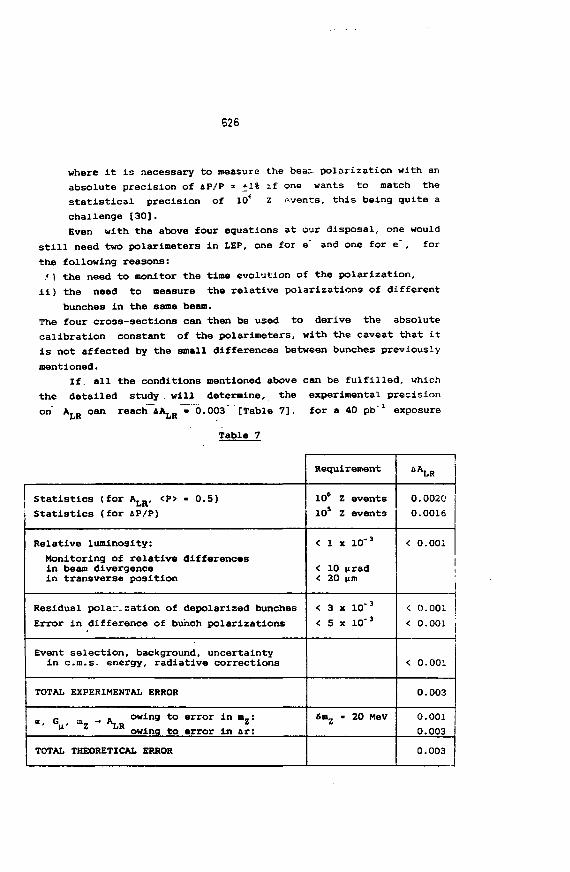
S26
whore it is necessary to measure the bear., polarization with an
absolute precision of AF/P « ±1% if one wants to match the
statistical precision of 10* Z .-.vents, this being quite a
challenge [30].
Even with the above four equations at our disposal, one would
still need two polarimeters in LEP, one for e' and one for e , for
the following reasons:
<) the need to monitor the time evolution of the polarization,
ii) the need to measure the relative polarizations of different
bunches in the same beam.
The four cross-sections can then be used to derive the absolute
calibration constant of the polarimeters, with the caveat that it
is not affected by the small differences between bunches previously
mentioned.
If. all the conditions mentioned above can be fulfilled, which
the detailed study . will determine, the experimental precision
on A,R can reach 4A,R • 6.003 [Table 7], for a 40 pb"* exposure
Table 7
Statistics (for A ^ , <P> - 0.5)
Statistics (for iP/P)
Relative luminosity:
Monitoring of relative differencesin beam divergencein transverse position
Residual polar.zation of depolarized bunches
Error in difference of bunch polarizations
Event selection, background, uncertaintyin c.m.s. energy, radiative corrections
TOTAL EXPERIMENTAL ERROR
«, G , a.- - A.- ° W l n 9 t O mtTOr i n V11 owing to error in ar:
TOTAL THEORETICAL ERROR
Requirement
106 Z events
10s Z events
< 1 i 10'J
< 10 iirad< 20 nm
< 3 x 10"3
< 5 x 10 3
6mz - 20 MeV
i ALR
0.002C
0.0016
< o.oo:
< 0.001
< 0.001
< 0.001
0.003
0.001
0.003
0.003
629
(10* Z events), corresponding to A sin* 6w = +0.0004. This matches
the main theoretical error 4 sin2 e = +0.0004 encountered when
predicting sin2 « from mz. This uncertainty arises when estimating
the electroweak radiative correction, ir, 4(ar) = +0.0013 [31] and
is mostly due to light quark loops. The corresponding contributions
to ir can be related to the measurement of o(e"e" — hadrons); the
error ij dominated by the experimental error in this cross-section,
especially at low energies. A more precise measurement of this
quantity would improve our knowledge of Jr by a factor of 2 [32]
and would certainly be welcome.
Many problems still need to be studied in detail concerning
measurements with polarized beams, and most of all much work is
necessary to convince ourselves that stable operation of the
machine with polarized beams and decent luminosity is more than a
dream. The theoretical and experimental cleanliness of the
polarization asymmetries and their sensitivity to physics beyond
our energy scale make this work highly motivating.
7. CONCLUSION
Precision measurements, albeit difficult, are appealing if
they produce fundamental results: the power of a combined
measurement m_, IL,, and A.R, with the above-mentioned precision, is
emphasized in Fig. 13. The order of magnitude of the Higgs mass and
the top quark mass, if it is not known then, would be severely
constrained. The existence of physics beyond the SENS, such as Z'
133], charged Higgs [34], supersymmetric particles [35], and
compositeness, would be likely to be visible or, in any case,
severely constrained. Tho additional information gained from
measurements of the individual weak couplings could be used to
disentangle the 'various origins if a discrepancy were to be
observed [36].
Altogether a very large improvement over existing measurements
should be obtained from LEP data.
Acknowledgements
This conference offered me an excuse to set foot in Poland for
the first time. It was a wonderful experience to live in this
beautiful little village, walk along by the Vistula, and share the'
warn and fun-loving friendship of our hosts. To Halina Abramowicz
in particular goes my deep gratitude.
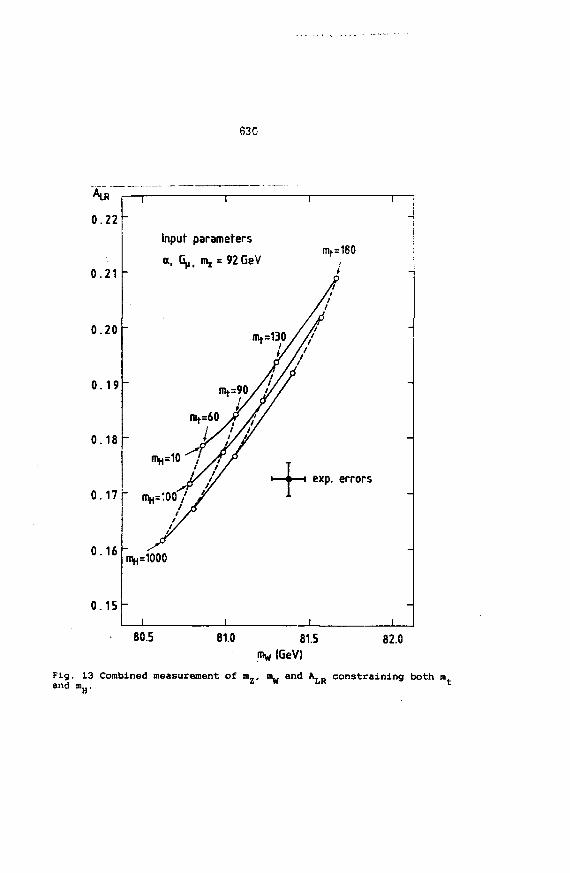
63G
0.22
0 .21
0.20
0 . 1 9
0.18
0.17
0.16
0.15 -
Input parameters
a, G,,, mz = 92GeV
exp. errors
11^=1000
80.5 81.0 81.5 82.0(GeV)
Fig. 13 Combined measurement of m_, DL. and A, constraining both mand nij,. *
531
REFERENCES AND FOOTNOTES
[1] IEP design report, CERN-LEP/84-01 (19B4).
[21 E. Keil, in Proc. ECFA Workshop on LEP 200. CERN 87-08, ECFA
87/108 (1987), p. 17.
[3] F. Dydak, preprint CERN-EP/86-121 (1986).
U. Amaldi et al., Pennsylvania preprint PRO331T (19B7).
A. Blondel, preprint CERN-EP/87-174 (1987).
[4] F. Dydak et al., in Proc. ECFA Workshop on LEP 200, CERN 87-06
(1987), p. 157.
[5] B.W. Lynn, M.E. Peskin and R.G. Stuart, in Physics at LEP.
CERN 86-02 (1986), p. 90.
[6] B.W. Lynn and R.C. Kennedy, SLAC-Pub 4039 (1987).
[7] A. Blondel, F. Dydak, A. Para and W. Blum, in Physics at LEP,
CERN 86-02 (1986), p. 35.
[8] F.A. Berends, W.L. van Neerven and C.J.H..Burgers, preprint
CERN-TH.4772 (1987).
[9] P. Roudeau et al., in Proc. ECFA Workshop on LEP 200, CERN
87-08. ECFA 87/108 (1987), p. 49.
[10] P. Jenni, ibid, p. 486.
[11] E. Treille et al., ibid, p. 414.
[12] M. Davifir et al., ibid, p. 120
1131 K. Bohm and W. Hollik, Nucl. Phys. B204, 45 (1982).
[14] C.Y. Prescott. in Proc.- 1980 Int. S. DSium on High-Energy
Physics with Polarized Beans and Polarized Targets.
Lausanne, 1980, eds\ C. Joseph and J. Soffer (Birkhatiser,
Basle, 1981). p. 34.
B.W. Lynn and C. Verzegnassi, SLAC-Pub 3967 (1986).
[ID] A. Blondel, B.W. Lynn, F.H. P.enard and C. Verzegnassi,
MontpelHer -preprint PM/87-14 (1987;, to appear in Nuclear
Physics.
[16] G. Altarelli, in Physics at LEP, CERN 86-02 (1986;, p. 3.
[17] P. Baillon et al., ibid, p. 172.
Also M. lentilm. Ecole Polytechnique, Palaiseau, France.
Ph.D. Thesis. University de Paris VI (1987), unpublished.
J18] ;. Chauveau, in Physics at LEP, CERN 86-02 •".986, p. 177.
rial D. Blockus et ai., SLC Polarization Proposal, SLAC-SLC-Prop-:
(1986).
[20] G. Alexander et al.. Working group report CERN/LEPC/87-6,
LEPC/M81 (1987).
[21) J. Badler et al., ALEPH Note 87-17 (1987).
532
[22] B.W. Montague, Phys. Rep. 113, No. 1 (1984).
J. Buon, Orsay preprint LAL/RT/86-02 i1986).
B.W. Montague, CERN LEP-TH/86-19.
See also the Machine Section in Ref. [20].
[23] C. Bovet, B. Montague, M. Placidi and R. Rossmanith, i.n
Physics at LEP, CERN 86-02 (1986), p. 58.
[24] R.F. Schwitters et al., Phys. Rev. Lett. 35, 1320 (i975).
G. Hanson et al., Phys. Rev. Lett. 35, 1611 (1975).
[25] J.-P. Koutchouk, CERN LEP Note 573 (1987>.
[26] B.W. Montague, CERN LEP Note 256 (1980).
[27] M. Placidi and R. Rossmanith, CERN LEP Note 545 (1985).
[28] J. Buon and J.M. Jowett, CESN LEP Note 584 (1987).
[29] A. Blondel, ALEPH Note 168 (1986).
[30] H. Steiner, Berkeley preprint LBL-23452 (1987).
[31] C. Verzegnassi, Phys. Lett. 147B, 455 (1984).
B.W. Lynn, G. Penso and. C. Verzegnassi, SLAC-Pub 3742 C19851.
F. Jegerlehner, Z. Phys. C32, 195 and 425 (1986).
[32] C. Verzegnassi, Trieste, private communication.
Measurement of very . low energy e* e~ data is foreseen at
Novosibirsk (M. May, Brookhaven, private communication).
[33] W. Hollik, Z. Phys. C8, 149 (1981).
P. Franzini and P. Gilman, Phys. Rev- D32, 237 (1985), jna
SLAC-Pub 3932 (1986).
J. Blgi and M. Cvetic, Phys. Rev. D34, 1651 (1986).
F. del Aguila, M. Quiros and F. 2wirner, in Physics at future
accelerators, CERN 87-07 (1987), Vol. 2, p. 165.
[34] W. Hollik, DESY .57-068 (19H7).
[35] The efiect of supersymmetrlc particles has been studied i-:
Ref. [5] and in J. Ellis, S. Rudaz and N. Tracas, CESN
TH.4657/87 (1987).
[36] S. Narlson, CERN-TH.4700/87, PM87/19 (1987).
{37] M. Cvetic and B.W. Lynn, SLAC Pub 3900 (1986).
B.W. Lynn, F. Renard and C. Verzegnassi. Montpellier preprint
PM 37/45 (1987).
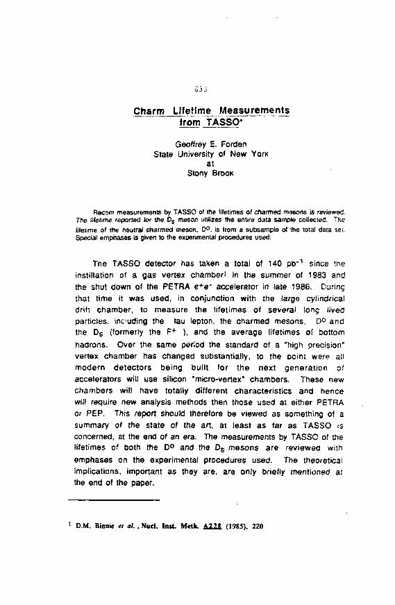
Charm Lifetime Measurementsfrom TASSO'
Geoffrey E. FordenState University of New York
atStony Brook
Recant measurements by TASSO of the lifetimes of charmed masons is reviewed.The lifetime reported for the Ds meson utilizes the entire data sample collected. Thelifetime of the neutral charmed meson. D°. is from a subsampie of the total data setSpecial emphases is given to the experimental procedures used.
The TASSO detector has taken a total of 140 pt r 1 since theinstillation of a gas vertex chamber* in the summer of 1983 andthe shut down of the PETRA e + e ' accelerator in late 1986. Duringthat time it was used, in conjunction with the large cylindricaldrift chamber, to measure the lifetimes of several long livedparticles, ineeding the tau lepton, the charmed mesons, D° andthe Ds (formerly the F+ ), and the average lifetimes of bottomhadrons. Over the same period the standard of a "high precision"vertex chamber has changed substantially, to the pcint were allmodern detectors being built for the next generation ofaccelerators will use silicon "micro-vertex" chambers. These newchambers will have totally different characteristics and hencewiil require new analysis methods then those used at either PETRAor PEP. This report should therefore be viewed as something of asummary of the state of the art, at least as far as TASSO isconcerned, at the end of an era. The measurements by TASSO of thelifetimes of both the D° and the Ds mesons are reviewea withemphases on the experimental procedures used. The theoreticalimplications, important as they are, are only briefly mentioned atthe end of the paper.
1 DM. Binnie a al., Nucl. Imt. Meth. A228 (1985), 220
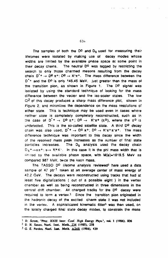
The samples of both the D° and Ds used for measuring theirlifetimes were isolated by making use of decay modes whosewidths are limited by the available phase space at some point intheir decay chains. The neutral D° was tagged by restricting thesearch to only those charmed mesons resulting from the decaychain D*+ -» D° i t+ ; D° -+ K~n+. The mass difference between theD*+ and the D° is only 145.45 MeV, just greater than the mass ofthe transition pion, as shown in Figure 1. The 0 ° signal wasisolated by using the standard technique of looking for the massdifference between the vector and the iso-scaler states. The lowQ 2 of this decay produces a sharp mass difference plot, shown inFigure 2, and minimizes the dependence on the mass resolutions ofeither state. This is technique may be used even in cases whereneither state is completely completely reconstructed, such as inthe case of D*+ - * D° n + ; D° -» K"K+ (JI<>), where the JT° is
undetected. This is the so-called satellite state. A third D° decaycr.ain was aiso used, D*+ -» DO K + ; D ° -» K"j t+ j r j i+. The massdifference technique was important to this decay since the widthof the resolved mass peak increases as the number of final stateparticles increases. The Ds analysis used the decay chainDs
+-^o7:+-, a>-» K+K-. In this case it is the phi mass width that islimted by the available phase space, with M(4>)-1019.5 MeV ascompared 987 MeV, twice the kaon mass.
The TASSO 0 ° lifetime analysis reviewed1 here used a datasampie of 47 pb~1 taken at an average center of mass energy of42.2 GeV. The decays were reconstructed using tracks that had atleast five digit izations ( out of a possible eight ) in the vertexcnamber as well as being reconstructed in three dimensions in thecentral drift chamber. All charged tracks for the 0 ° decay wererequired to form a vertex.2 Since the transition pion originated inthe hadromc decay of the excited charm state it was not includedIn the vertex. A sophisticated kinematic fitter3 was then used, onthe totally charged final state decay modes, to constrain the mass
1 D. Strom, "Proc. XXIII Inter. Conf. High Energy Pbyt.\ voL 1 (1986), 8062 D. H. Saxon, Nucl. I nit. Meth.JLM (1985). 2583 G. E. Forden. Nucl. Inst. Meib. A248 (1986), 439
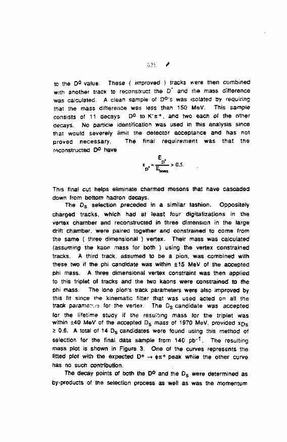
to the D° value. These ( improved ) tracks were then combinedwith another track to reconstruct the D* and the mass differencewas calculated. A clean sample of D°'s was isolated by requiringthat the mass difference was less than 150 MeV. This sampleconsists of 11 decays D° to K"JI+ , and two each of the otherdecays. No particle identification was used in this analysis sincethat would severely limit the detector acceptance and has notproved necessary. The final requirement was that thereconstructed D° have
E „
This final cut helps eliminate charmed mesons that have cascadeddown from bottom hadron decays.
The Ds selection preceded in a similar fashion. Oppositely
charged tracks, which had at least four digitalizations in thevertex chamber and reconstructed in three dimension in the largedrift chamber, were paired together and constrained to come fromthe same ( three dimensional ) vertex. Their mass was calculated(assuming the kaon mass for both ) using the vertex constrainedtracks. A third track, assumed to be a pion, was combined withthese two if the phi candidate was within ±15 MeV of the acceptedphi mass. A three dimensional vertex constraint was then appliedto this triplet of tracks and the two kaons were constrained to thephi mass. The lone pion's track parameters were also improved bythis fit since the kinematic fitter that was used acted on all thetrack parame:',.'-*- for the vertex The Ds candidate was accepted
for the lifetime study if the resulting mass for the triplet waswithin ±40 MeV of the accepted Ds mass of 1970 MeV. provided XQS
> 0.6. A total of 14 Ds candidates were found using this method ofselection for the final data sample from 140 pb"1. The resultingmass plot is shown in Figure 3. One of the curves represents thefitted plot with the expected D+ -> 4>7t+ peak while the other curvehas no such contribution.
The decay points of both the D° and the Ds were determined as
by-products of the selection process as well as was the momentum
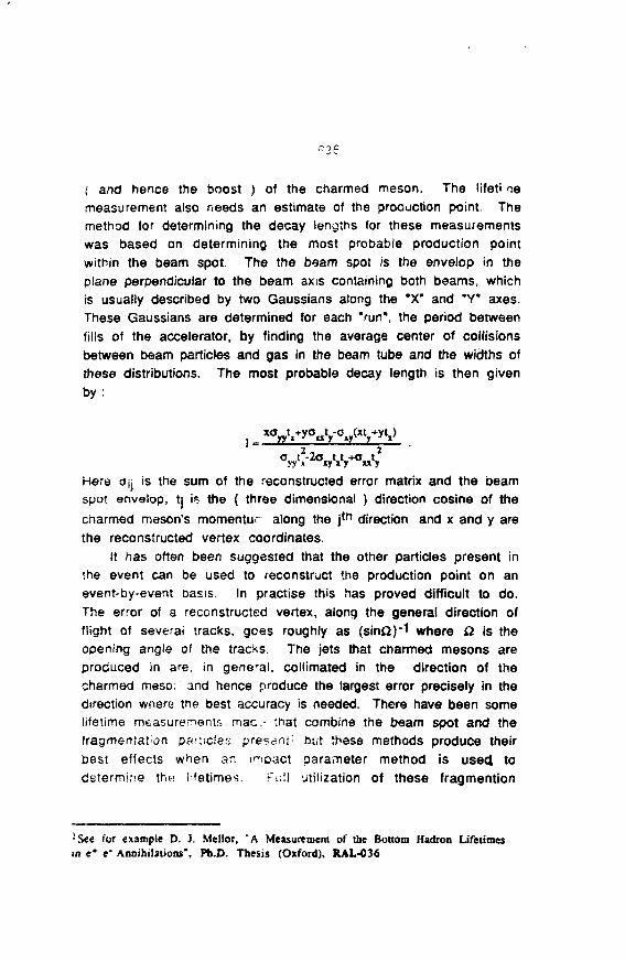
i and hence the boost ) of the charmed meson. The lifeti i emeasurement also needs an estimate of the proouction point. Themethod for determining the decay lengths for these measurementswas based on determining the most probable production pointwithin the beam spot. The the beam spot is the envelop in theplane perpendicular to the beam axis containing both beams, whichis usually described by two Gaussians along the "X" and "Y* axes.These Gaussians are determined for each "run", the period betweenfills of the accelerator, by finding the average center of collisionsbetween beam particles and gas in the beam tube and the widths ofthese distributions. The most probable decay length is then givenby:
Here oy is the sum of the reconstructed error matrix and the beamspot envelop, tj i* the ( three dimensional ) direction cosine of thecharmed meson's momentur along the j t n direction and x and y arethe reconstructed vertex coordinates.
It has often been suggested that the other particles present inthe event can be used to reconstruct the production point on anevent-by-event basis. In practise this has proved difficult to do.The error of a reconstructed vertex, along the general direction offlight of severai tracks, gees roughly as (sinQ)"1 where Q is theopening angle of the tracks. The jets that charmed mesons areproduced in are. in general, collimated in the direction of thecharmed meso. and hence produce the largest error precisely in thedirection where the best accuracy is needed. There have been somelifetime measurements mac- that combine the beam spot and thefragmentation pamcies present- but these methods produce theirbest effects when an impact parameter method is used todetermine the lifetimes. Fi;!l utilization of these fragmention
'-See for example D. J. Mellor, "A Measurement of the Bottom Hadron LifetimesID e+ e" Annihilations", Pb.D. Thesis (Oxford), RAL-036
particles will have to wait until the nexi generation of vertex
chambers.The decay times of the individual charmed mesons in the
samples, see Figure 4 far the Ds and Figure 5 for the D°, weredetermined using the most probable decay length, as calculatedabove, but the average lifetimes of the samples had to use amaximum likelihood approach. The likelihood function took intoaccount the background probability of an event being a randomcombination of fragmenation particles, a real charmed mesonresulting from a cascading B decay, and a real primary charmmeson but of the wrong type ( eg. D+ instead of a Ds.) The relativeprobabilities of these backgrounds have to be determined fromMonte Carlo studies but in general can be normalized to the datathrough side bands. The overall background fraction for the Ds
meson is 30%, as datermined by the side bands. This inciudes, forexample, 7% of the Ds candidates which are misidentified D+'s. asdetermined by Monte Carlo.
The Monte Carlo contains assumptions about the production anddecay of charmed ( and bottomed ) mesons which have been tunedas well as possible.1 This was done by comparing otherdistributions of the data, such as mean charged multiplicity etc.,with the Monte Carlo. Individual parameters ,m the Monte Carlowere varied by amounts corresponding to their uncertainty and theeffects on the calculated lifetime were added in quadrature todetermine the Monte Carlo's contribution to the systematic error ofthe measurements- The complete absence of the Cabibbosuppressed D+ -»$* + peak, for instance, changes the Ds lifetime by0.2x10"13 sec. and this was included in the reported systematicerror.
The largest contribution to the systematic error of theselifetime measurements was the uncertainty about the effectiveresolution of the drift chamber system and the trackfinding/fitting routines in the environment of a hadronic event.This problem is exasterbated at TASSO by the large amount ofmaterial between the vertex and the central drift chambers,
1 M. Althoff, TASSO Collaboration, Z. Phyi. £21 (1984), 307
53c
necessitating a scattering angle in the middle of each track. Thescattering between the two drift chambers has the effect ofincreasing the momentum dependency of the resolution function. Inaddition, the high probability of tracks crossing over each other inthe vertex chamber reduces the number of digitalizations availableto each track and hence degrading the resulting resolution. Theappropriate resolution to use in track and vertex fitting wasdetermined by observing the control samples for the differentcharmed mesons.
In the case of the Ds meson, track pairs whose mass is in therange: 1.05 GeV < m(K+K") < 1.15 GeV were used to construct falsephi candidates and then combined with assumed pions to createcontrol Ds combinations. The acceptable D-j mass range wasincreased to achieve a higher statistics sample. The same lifetimealgorithm as that used for the Ds was repeatedly applied to thiscontrol sample assuming a series of vertex chamber resolutionvalues between 100 and 150 microns. This range around thenominal value of 120 microns represents the limits where theassumed resolution increases the width of the control sample'slifetime distribution significantly. The average lifetime of thisia-ge statistics control sampit was not effected by the assumedvertex chamber resolution. The limited Ds sample was effectedwhen the same range of resolutions was used in the algorithmproducing a contribution to the systematic uncertainty of±0.7x10"13 sec. The dependence of the lifetime on this assumedresolution was not a smoothly varying function, as was the casefor the control sample. Instead, there were sudden small jumpscorresponding to individual digitalizations being deleted fromtracKs during the track and vertex fitting algorithms. It wasdetermined from Monte Carlo studies that these discontinuitiesdisappear for large enough samples. It is also true that for alarger hadronic sample the range of possible effective resolutionscould have been reduced significantly.
In concluding the experimental discussion, the lifetimes of thecharmed mesons, as measured by TASSO are, for the D°:
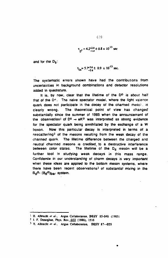
t e
and for the Ds:
t_ = S.T3-6 ± 0.9 x 10"13 sec.O* - 1 6
The systematic errors shown have had the contributions fromuncertainties in background combinations and detector resolutionsadded in quadrature.
It is, by now, clear that the lifetime of the 0° is about halfthat of the D+. The naive spectator model, where the light valencequark does not participate in the decay of the charmed meson, isclearly wrong. The theoretical point of view has changedsubstantially since the summer of 1985 when the announcement ofthe observation1 of D° -» *K° was interpreted as strong evidencefor the spectator quark being annihilated by the exchange of a Wboson. Now this particular decay is interpreted in terms of arescatteringz of the mesons resulting from the weak decay of thecharmed quark. The lifetime difference between the charged andneutral charmed mesons is credited, to a destructive interferencebetween color states. The lifetime of the Ds meson will be a
further tool in studying weak decays in this mass range.Confidence in our understanding of charm decays is very importantwhen these ideas are applied to the bottom meson systems, wherethere have been recent observations3 of substantial mixing in theB<j°- (Bd°)bar system.
1 H. Albrecht it at., Argus Collaboration, DESY 85-048 (1985)2 J. F. Doooghue, Ptiys. Rev. D33 (1986), 1516* H. Albrecht et at., Argus Collaboration. DESY 87--029
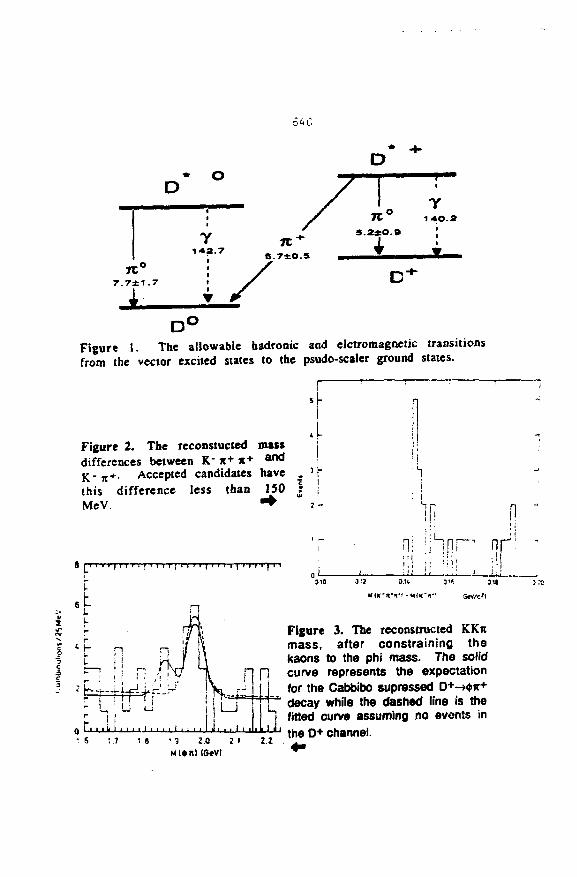
• o
I
a.7±o.s
2 ± O
y1 «O.2
Figure 1. The allowable hadronic and elctromagnetic transitionsfrom the vector excited states to the psudo-scaler ground states.
4i
Figure 2. The reconstucted mas*differences between K" it+x+ a n d
K-K+- Accepted candidates have .this difference less than 150 IMeV. • *
i |
IS
ni!ii !i
Figure 3. The reconstructed KKnmass, after constraining thekaons to the phi mass. The solid
f l p curve represents the expectationft r- | I j for the Cabbibo supressed D+-><Mt+
L J H L d e c a y w h i l e t h e d a s h e d l i n e is t h e
i fitted curve assuming no events in1 ' ' ' • ' ^ the0+ channel.
2 1 22
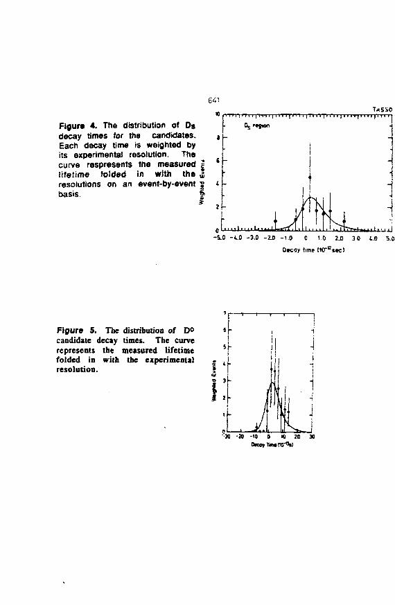
Figure 4. The distribution of Dsdecay times for the candidates.Each decay time is weighted byits experimental resolution. Thecurve respresents the measuredlifetime folded in with theresolutions on an event-by-eventbasis.
• • «
2 -Ir
Q 111 iiIir ii
j
ill
TASSOi-p-m-i
j
-5.0 -1.0 -3.0 -2.0 -1.0 1.0 2.0 3C t.O 5.0
Decoy time l1Q"°sec)
Figure 5. The distribution of D°candidate decay times. The curverepresents the measured lifetimefolded in with the experimentalresolution.
SI-
utr
j ; i
1
i- 1
4
J
-jI
1
in1"'30 -20 -10 0 10 20 X

6HS
:•:"" Of PARTICIPANTS
of the IÎ! Warsaw SympcÄimr. on riemen tar- Particle Physics
Jodiowy Dwót, May -2-2ti» 1980
I.Z.Ajduk
2.J.Bartelski
3. !.. Seeker
4.G.3eîîectini
S.G.hiaikowski
6.S.Brandt
7. j .iiranson
B.J.Ciborowski -
9.G.Cicuta
lO.A.Czechowski -
H.F.Oittroann
i2.K.I'oroba
i3.P.Drijard
14.A.Dubnickova -
IS.F.Dydak
lö.P.Falkcnstei: • •<•-
17.J.Finiord
18.H.G.Fischer
t9.E.rloratos
2O.M.G.-iurdin
21 .J.K.Gunion
22.F.Gutbrod
23.J.Gwizdz
24.Z.Horvath
25.B.Humpert
26.A.Jachotkov,-ska-
27.A.Jachoikowski-
28.M.Jezabek
29.M.Jçdrzejczak -
30.J.K.alinowski -
31.R.Kirschner
32.«.Koch
33.P.Kosiriski
34.D.Kisielewska -
35.K.Krawczyk
36.P.Krawczyk
37.W.Krzyzanowski-
38.M.Kuroda
Warsav
Warsav
Zcuthen
Frascati
Warsav
MIT Cambridge
Warsav
Milan
Warsav
Hamburg
Warsaw
CERK Geneva
Bratislava
Heidelberg
•V ienna
Berne
CERK Geneva
Saclay
Paris
Davis
Hamburg
Warsaw
Budapest
Geneva
Warsaw
Warsaw
Cracow
Warsaw
Warsaw
Leipzig
Hamburg
fcddi
Cracow
Warsaw
Warsav
Warsaw
Bielefeld
39.H.Lubatti
4C.L.i.ukaszuk
42.D,Mazurek
43,S.Mikocki
4 5 . S .Mrowe zy riski
46.P.Minkowsk:
47.R.Messner
48.J.Nassalski
49.B.Jsiczyporuk
50. R. Nowak
51.A.Okopinska
52.K.Otwinowska
53.S.Pokorski
54.J.Raines
55.G.Ranft
56.J.Ranf£
57.K.Redlich
58.J.Rembie1iriski
59.E.Rondio
6O.K.Rith
bi.R.Rllckl
62.I.Sakrejda
63.W.G.Scott
64.R.Sosnowski
65.H.Spitzer
66.M.Staszel
67.J.Stepaniak
68.L.R.Sulak
69.M.Szczekowski
70.L.Szymanowski
7I.M.Svi«cki
72.K.Tanaka
73.T.Taylor
75.S.Tkaczyk
76.L.Turko
- Warsaw
- iódé
- Warsaw
- Cracow
- CERN Geneva
- Warsaw
- Berne
- Pasadena
- Warsaw
- Cracow
- Warsaw
- Warsaw
- Warsaw
- Warsaw
- Prague
- Leipzig
- Leipzig
- Wroclaw
- tódi
- Warsaw
- CERK Geneva
- Munich
- Cracow
- CERN Geneva
- Warsaw
- Hamburg
- Warsaw
- Warsaw
- Harvard
- Warsaw
- Warsaw
- Warsaw
- Columbus
- Warsaw
- Hamburg
- Warsaw
- Wroclaw

77.A.Iurski - Warsaw78. - .Tymier.iecka - Warsaw79.S.Wolirain - Pasadena80.A.Wroblevski - Warsaw
31.r.J.Y;v.i'.irait;S2.j.Zar.rzc-\.i-ki
- Madrid
- Warsaw
V* ble|