978-1-4244-1694-3/08/$25.00 ©2008 IEEE

1

Modeling and Predicting Application Performanceon Parallel Computers Using HPC Challenge Benchmarks

Wayne Pfeiffer and Nicholas J. WrightSan Diego Supercomputer Center, La Jolla CA 92093-0505, USA

{pfeiffer, nwright}@sdsc.edu

Abstract

A method is presented for modeling applicationperformance on parallel computers in terms of theperformance of microkernels from the HPC Challengebenchmarks. Specifically, the application run time isexpressed as a linear combination of inverse speedsand latencies from microkernels or system characteris-tics. The model parameters are obtained by an auto-mated series of least squares fits using backwardelimination to ensure statistical significance. If nec-essary, outliers are deleted to ensure that the final fitis robust. Typically three or four terms appear ineach model: at most one each for floating-point speed,memory bandwidth, interconnect bandwidth, and in-terconnect latency. Such models allow prediction ofapplication performance on future computers fromeasier-to-make predictions of microkernel perform-ance.

The method was used to build models for fourbenchmark problems involving the PARATEC andMILC scientific applications. These models not onlydescribe performance well on the ten computers usedto build the models, but also do a good job of predict-ing performance on three additional computers withnewer design features. For the four applicationbenchmark problems with six predictions each, therelative root mean squared error in the predicted runtimes varies between 13 and 16%.

The method was also used to build models for theHPL and G-FFTE benchmarks in HPCC, includingfunctional dependences on problem size and corecount from complexity analysis. The model for HPLpredicts performance even better than the applicationmodels do, while the model for G-FFTE systematicallyunderpredicts run times.

1. Introduction

Predicting application performance on forthcomingparallel computers is often required as part of largehigh-performance computing (HPC) system acquisi-

tions. Typically benchmarks are run on one or moreexisting systems, and some form of extrapolation ismade to predict future performance. The effectivenessof such extrapolations depends upon having suitableperformance models for the benchmarks.

Here we explore a modeling method based on theassumption that application run time can be approxi-mated as a linear combination of inverse speeds andlatencies mostly obtained from microkernels, in par-ticular, those contained in the HPC Challenge bench-mark set [1]. This allows application performanceprediction from easier-to-make predictions of microk-ernel performance.

Such a method is similar to that described byMcCalpin [2] for computation performance, but con-siders communication performance as well. Ourmethod has the advantage of simplicity over moreelaborate methods, such as those of Clement andQuinn [3], Kerbyson, et al. [4], Snavely, et al. [5], andTikir, et al. [6].

The question, of course, is: “How accurate are themodels that result from such a simple method, i.e.,how well do they capture the dominant computationand communication performance behavior of applica-tions?” That is the subject of this paper.

2. Model equation

In general, the run time, t, of an applicationbenchmark can be represented as the sum of three com-ponents:

€

t = tcomp + tcomm + tio . (1)Here

€

tcomp ≡ the computation time,

€

tcomm ≡ the communication time that is not over-lapped with computation, and

€

tio ≡ the I/O time that is not overlapped withcomputation or communication.

The computation time can be further separated intocomponents associated with floating-point performanceand memory access. Similarly, the communication

2

time can be separated into components related to theinterconnect bandwidth and latency. For the bench-marks considered here, the I/O time is negligible.

Our modeling method assumes that

€

ti, the meas-ured run time of an application benchmark on com-puter i can be approximated by

€

ˆ t i, the correspondingmodel run time, where

€

ˆ t i = c j tijj∑ . (2)

Here

€

tij is the inverse speed or latency for systemcharacteristic j on computer i, and the application-specific coefficients or parameters,

€

c j , are taken to beindependent of computer.

For a given computer i, the

€

tij are the predictorvariables in the model described by Eq. (2). Some ofthese will be associated with computation and somewith communication, in accordance with the separationexpected from Eq. (1). We take most of the possiblepredictors from the HPCC benchmark set, though twoare specified directly from the system design. To beuseful for predicting application performance on futurecomputer systems, the predictors need to be easy toestimate in advance of system availability and few innumber. In each of our models, we expect no morethan four predictors.

3. Transformations for least squares fits

The model defined by Eq. (2) is linear in the pre-dictor variables. Thus, given measured values for

€

ppredictors and the application run time on each of

€

ncomputers (or distinct configurations, with

€

p ≤ n ), themodel parameters in Eq. (2) can be fit via leastsquares (or regression analysis) using standard statisti-cal techniques [7]. In conventional terminology, theapplication run time is the response variable.

We make two transformations of Eq. (2) before per-forming the least squares fits. The first normalizes thetimes (and parameters) to dimensionless form and ismerely a convenience. The second weights the runtimes consistent with our expectation of their impor-tance and has a modest effect on the resulting fits.

In the first transformation we normalize the timesto those for an arbitrarily chosen, reference computer rwithin our model-building set. Thus Eq. (2) is rewrit-ten as follows:

€

ˆ y i ≡ˆ t itr

= c jtij

trj∑ = c j

trj

tr

j∑ tij

trj= b j Xij

j∑ , (3)

where

€

b j ≡ c jtrjtr

, and (4)

€

Xij ≡t ijtrj

. (5)

Also, the normalized value of the measured run time(or response) is

€

yi ≡ ti tr . (6)For the reference computer, the normalized re-

sponse,

€

yr , and the normalized predictors,

€

Xrj , areequal to one. Hence, Eq. (3) shows that the normalizedparameters,

€

b j , should sum to approximately one fora good fit. This provides one of several checks on thegoodness of fit.

An important assumption in least squares analysisis that the residuals (measured minus fit values) have acommon variance. Since the run times can vary byseveralfold for the computers considered here and arealways positive, it seems more plausible that the rela-tive residuals (or percentage errors) have a commonvariance. This leads us to adopt a weighted fit, withthe weights chosen inversely proportional to thesquares of the measured run times. This will mini-mize the sum of the squares of the relative residuals.

The weighting is implemented by a second trans-formation. Specifically, we introduce a diagonalweight matrix with elements

€

Wii ≡ 1/ yi2 (7)

and multiply Eq. (3) by

€

Wii1/ 2 (

€

= 1/ yi ). (See Ref.[8].) This transforms Eq. (3) to the following:

€

ˆ y w,i ≡ˆ y iyi

= b jXij

yij∑ = b j Xw,ij

j∑ , (8)

where

€

Xw,i ≡Xijyi

. (9)

Eq. (8) can now be fit with least squares in theusual way, since the variance of the relative residuals isexpected to be constant. Note that the measured runtime after normalization and weighting is equal to one,i.e.,

€

yw,i ≡Wii1/ 2yi = 1. (10)

Another assumption in least squares analysis is thatthe elements of the predictor matrix X are error-free.This is not the case for most of the columns of X ,which are obtained from HPCC measurements. Herewe assume that the errors in X are small compared tothose in the application run time and so can be ne-glected.

4. Least squares fits for model building

Important issues in performing least squares fits aredeciding which predictors to include (in this case,HPCC metrics and system characteristics) and check-ing that the fits are consistent with the data and robust.

3

4.1. Picking the predictors

The number of possible predictors that we consideris comparable to the number of computers used tobuild our models (as discussed in the next two sec-tions). However, the number of predictors in anygiven model is smaller and is obtained by the succes-sive application of two routines in MATLAB [9].

1. For each application benchmark being modeled,a least squares fit of Eq. (8) to the measured run timesof Eq. (10) is made enforcing the constraint that theparameters of the fit must be positive. This is doneusing the lsqnonneg routine and eliminates some ofthe possible predictors.

2. Although the resulting fit is suggestive and maybe very good, typically some of the parameters (andassociated predictors) are not statistically significant.To prevent such overfitting, backward elimination [7]is then applied, successively removing the least sig-nificant parameters until all that remain are statisticallysignificant (i.e., greater than zero) at the 95% confi-dence level. This is done using the regstats rou-tine and the model matrix to specify which predictorsare retained at each step.

4.2. Checking goodness and robustness offit

Once a fit is obtained, various checks on the qualityof the fit (and hence of the implied model) need to bemade. The first thing to check is the root meansquared error:

€

RMSE ≡1

n − p(yi − ˆ y i)

2

yi2

i∑

1/ 2

. (11)

This is the quantity that is minimized in our weightedleast squares fits. With the weighting adopted here,the RMSE is an estimate of the relative error, and thefrequently-used

€

R2 statistic is no longer meaningful.In general, the smaller the RMSE, the better the fit.

By convention, the residual of a measurement isthe measured value minus the fit value, i.e.,

€

yi − ˆ y ihere. Thus the residual is positive when the measure-ment is greater than the fit. Because of our weighting,the summation in Eq. (11) is over the squares of therelative residuals.

A more detailed check is to examine the individualresiduals for outliers and influential measurements.Outliers have large relative residuals (either positive ornegative), which increase the RMSE. Influential meas-urements (which are often outliers) significantly per-turb the fitted parameters and can lead to a fit that isnot robust. Outliers frequently suggest a measurementproblem, in which case they can be omitted. Alterna-tively, they may indicate a limitation of the model.

To increase our confidence in the validity of amodel, we require that the fit be robust against allsingle-measurement deletions, i.e., the fit should notchange significantly upon deletion of a single meas-urement. We take this to mean that the predictors re-main the same and that the parameters vary by at mosta few percent. If this is not the case, then we selec-tively delete one or more measurements from themodel data set until the remaining data are consistentenough to give a robust fit.

Specifically, if the fit is not robust, then we iden-tify the two most extreme outliers, i.e., the ones withthe most positive and negative relative residuals. Wethen delete each separately, perform two new fits, andtest for robustness. If either is robust, we are done. Ifnot, we delete the most extreme outliers from thesenew fits and continue as before. Provided sufficientdata are available, this procedure generally converges toa robust fit, as was found to be the case for all of thebenchmark problems discussed here.

4.3. Collecting enough data for robust fits

A major challenge in model building is collectingsufficient data to have robust fits. For building ourmodels of application performance, we have used twotechniques to obtain additional data with only a mod-est number of computers.

First, on some computers we have made two sets ofHPCC and application runs: the standard ones usingall cores per node and additional ones using half thecores per node, but twice as many nodes. Typically,better performance is obtained with half the cores pernode because there is less memory and interconnectcontention. In such cases, each additional set of runsprovides another effective computer configuration andanother equation to be fit.

A second technique to obtain more fitting data in-volves using the IPM tool [10]. Among other things,IPM measures the communication run time (and hencecommunication fraction). Since IPM has negligibleoverhead, it can be used in the same run that measuresthe total run time. Each IPM measurement thus pro-vides another equation to be fit similar to Eq. (2), withthe communication time on the left and only commu-nication terms in the sum on the right. In practice,more outliers appear to arise from the communicationtimes than from the total times. This may be associ-ated with modest amounts of load imbalance or over-lap of communication with computation, which intro-duce more variability in the communication times.

When more information or alternate models existthat indicate how the terms in Eq. (2) vary with corecount, it is then possible to combine data from multi-ple core counts into a single fit. We have used thisthird technique to build models for the HPCC com-plex synthetics.

4

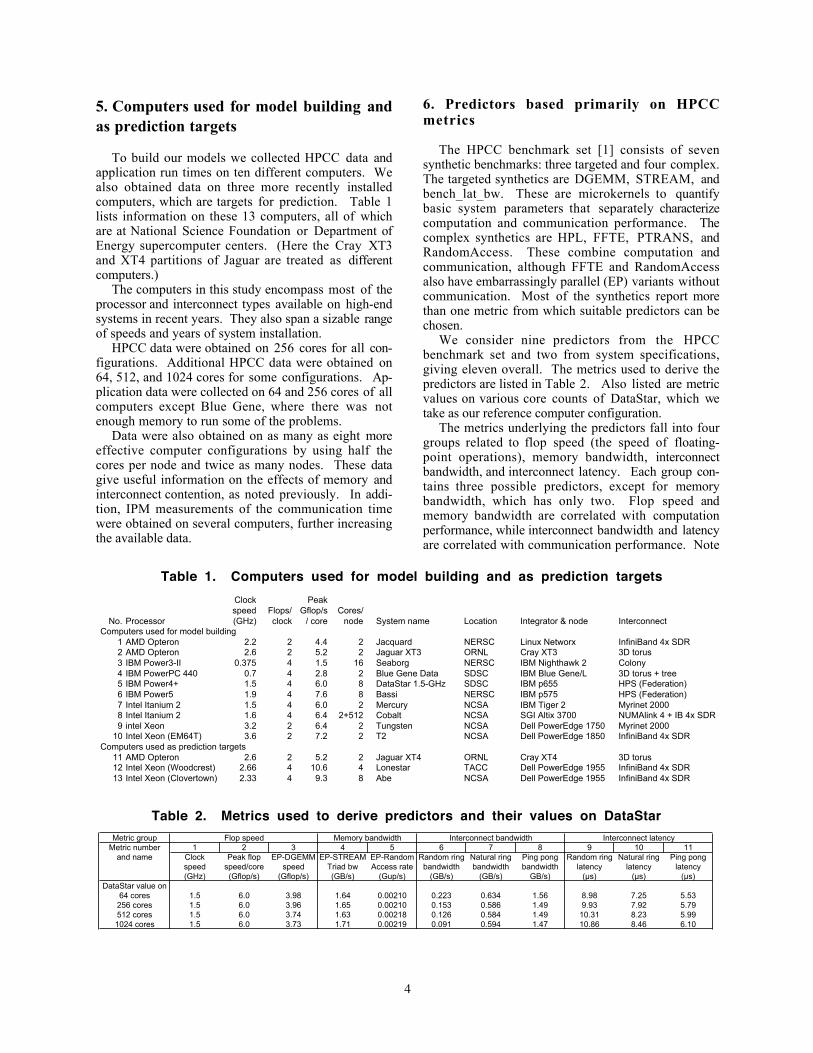
Table 1. Computers used for model building and as prediction targetsClock Peakspeed Flops/ Gflop/s Cores/

No. Processor (GHz) clock / core node System name Location Integrator & node InterconnectComputers used for model building

1 AMD Opteron 2.2 2 4.4 2 Jacquard NERSC Linux Networx InfiniBand 4x SDR2 AMD Opteron 2.6 2 5.2 2 Jaguar XT3 ORNL Cray XT3 3D torus3 IBM Power3-II 0.375 4 1.5 16 Seaborg NERSC IBM Nighthawk 2 Colony4 IBM PowerPC 440 0.7 4 2.8 2 Blue Gene Data SDSC IBM Blue Gene/L 3D torus + tree5 IBM Power4+ 1.5 4 6.0 8 DataStar 1.5-GHz SDSC IBM p655 HPS (Federation)6 IBM Power5 1.9 4 7.6 8 Bassi NERSC IBM p575 HPS (Federation)7 Intel Itanium 2 1.5 4 6.0 2 Mercury NCSA IBM Tiger 2 Myrinet 20008 Intel Itanium 2 1.6 4 6.4 2+512 Cobalt NCSA SGI Altix 3700 NUMAlink 4 + IB 4x SDR9 intel Xeon 3.2 2 6.4 2 Tungsten NCSA Dell PowerEdge 1750 Myrinet 2000

10 Intel Xeon (EM64T) 3.6 2 7.2 2 T2 NCSA Dell PowerEdge 1850 InfiniBand 4x SDRComputers used as prediction targets

11 AMD Opteron 2.6 2 5.2 2 Jaguar XT4 ORNL Cray XT4 3D torus12 Intel Xeon (Woodcrest) 2.66 4 10.6 4 Lonestar TACC Dell PowerEdge 1955 InfiniBand 4x SDR13 Intel Xeon (Clovertown) 2.33 4 9.3 8 Abe NCSA Dell PowerEdge 1955 InfiniBand 4x SDR

Table 2. Metrics used to derive predictors and their values on DataStarMetric group Flop speed Interconnect bandwidth Interconnect latency

Metric number 1 2 3 4 5 6 7 8 9 10 11and name Clock Peak flop EP-DGEMM EP-STREAM EP-Random Random ring Natural ring Ping pong Random ring Natural ring Ping pong

speed speed/core speed Triad bw Access rate bandwidth bandwidth bandwidth latency latency latency(GHz) (Gflop/s) (Gflop/s) (GB/s) (Gup/s) (GB/s) (GB/s) GB/s) (µs) (µs) (µs)

DataStar value on64 cores 1.5 6.0 3.98 1.64 0.00210 0.223 0.634 1.56 8.98 7.25 5.53

256 cores 1.5 6.0 3.96 1.65 0.00210 0.153 0.586 1.49 9.93 7.92 5.79512 cores 1.5 6.0 3.74 1.63 0.00218 0.126 0.584 1.49 10.31 8.23 5.991024 cores 1.5 6.0 3.73 1.71 0.00219 0.091 0.594 1.47 10.86 8.46 6.10

Memory bandwidth

5. Computers used for model building andas prediction targets

To build our models we collected HPCC data andapplication run times on ten different computers. Wealso obtained data on three more recently installedcomputers, which are targets for prediction. Table 1lists information on these 13 computers, all of whichare at National Science Foundation or Department ofEnergy supercomputer centers. (Here the Cray XT3and XT4 partitions of Jaguar are treated as differentcomputers.)

The computers in this study encompass most of theprocessor and interconnect types available on high-endsystems in recent years. They also span a sizable rangeof speeds and years of system installation.

HPCC data were obtained on 256 cores for all con-figurations. Additional HPCC data were obtained on64, 512, and 1024 cores for some configurations. Ap-plication data were collected on 64 and 256 cores of allcomputers except Blue Gene, where there was notenough memory to run some of the problems.

Data were also obtained on as many as eight moreeffective computer configurations by using half thecores per node and twice as many nodes. These datagive useful information on the effects of memory andinterconnect contention, as noted previously. In addi-tion, IPM measurements of the communication timewere obtained on several computers, further increasingthe available data.

6. Predictors based primarily on HPCCmetrics

The HPCC benchmark set [1] consists of sevensynthetic benchmarks: three targeted and four complex.The targeted synthetics are DGEMM, STREAM, andbench_lat_bw. These are microkernels to quantifybasic system parameters that separately characterizecomputation and communication performance. Thecomplex synthetics are HPL, FFTE, PTRANS, andRandomAccess. These combine computation andcommunication, although FFTE and RandomAccessalso have embarrassingly parallel (EP) variants withoutcommunication. Most of the synthetics report morethan one metric from which suitable predictors can bechosen.

We consider nine predictors from the HPCCbenchmark set and two from system specifications,giving eleven overall. The metrics used to derive thepredictors are listed in Table 2. Also listed are metricvalues on various core counts of DataStar, which wetake as our reference computer configuration.

The metrics underlying the predictors fall into fourgroups related to flop speed (the speed of floating-point operations), memory bandwidth, interconnectbandwidth, and interconnect latency. Each group con-tains three possible predictors, except for memorybandwidth, which has only two. Flop speed andmemory bandwidth are correlated with computationperformance, while interconnect bandwidth and latencyare correlated with communication performance. Note

5

that inverse speeds, i.e., reciprocals of speed, are usedas predictors in the first three groups. Out of the elevenpossible predictors, we expect that no more than fourwill typically have statistically significant parametersfor a given application model. These would be atmost one from each of the four groups.

The first two flop-speed metrics that we considerare the clock speed and peak flop speed per core.These are determined from system specifications ratherthan HPCC. The third flop speed considered is the EPvariant of DGEMM, which measures the speed of ma-trix-matrix multiplication.

The two memory-bandwidth metrics we use are theEP variants of the STREAM Triad bandwidth and theRandomAccess rate. The former measures the band-width for unit-stride memory access. The latter meas-ures the bandwidth for random memory access and isinversely proportional to the memory latency.

The EP or “Star” metrics in HPCC are measuredwith all cores in a node doing the same computationsimultaneously. Doing so accounts for the memorycontention that is typical of applications.

To model communication performance, we considersix predictors, all obtained from three pairs of meas-urements by bench_lat_bw in HPCC. The relevantpairs are the interconnect bandwidth and interconnectlatency for the randomly ordered ring (RR), naturallyordered ring (NR) and average ping pong (PP) tests.

All five of the computation predictors are essen-tially independent of core count (as can be seen fromthe DataStar data in Table 2). Likewise, apart from theRR bandwidth, the interconnect bandwidths and laten-cies vary little with core count (except on Abe and on1024 cores of Cobalt, where the interconnect topologychanges). Consequently, predictors measured at onecore count can often be used for other core counts aswell.

All of our HPCC results are for baseline runs. Thatis, no code changes were made. The only tuning wasthe use of optimal compiler flags and optimized librar-ies for the Basic Linear Algebra Subprograms (BLAS).

Some of the possible predictors are highly corre-lated with each other, especially within each of fourgroups. An important consideration is how well ourmethod selects between such correlated predictors toobtain a robust fit.

7. Models for applications

To assess the quality of the models generated byour method, we consider two scientific applications –PARATEC [11] and MILC [12]. These materials sci-ence and physics codes are used extensively at NSFand DOE supercomputer centers. Moreover, recentsystem acquisitions have required performance predic-tions for benchmark problems on both of these applica-

tions, so having models to make such predictionswould be very useful.

For each application we collected results for twoproblem sizes run on different core counts: mediumproblems on 64 cores and large problems on 256 cores.

The PARATEC results are for baseline runs, withcode changes made only to ensure correct execution.Tuning consisted of the use of optimal compiler flagsand optimized libraries for LAPACK, ScaLAPACK,BLACS, and FFTW. No changes were made to theinput files.

For MILC, some code changes were made to opti-mize performance, especially on systems with AMDprocessors.

7.1. PARATEC

PARATEC “performs ab initio quantum-mechanical total energy calculations using pseudopo-tentials and a plane wave basis set.” [11]

We consider the two standard benchmark problems,both for silicon in the diamond structure [13]. Themedium problem has 250 silicon atoms, while thelarge problem has 686 atoms. We modeled the me-dium problem on 64 cores and the large problem on256 cores.

7.1.1. Medium problem. We begin with the mediumproblem on 64 cores, for which slightly more run-timedata are available. HPCC predictor data were obtainedon 64 cores for only some of the computers (includingDataStar). We used 64-core predictors normalized toDataStar when available and 256-core normalized pre-dictors otherwise. In addition, we excluded the RRbandwidth from our predictor set, since the correspond-ing data on 256 cores may not be appropriate for 64cores.

First we fit the total run-time data for computerswith all cores per node. We have such data for nine ofthe ten model-building computers; the computer withmissing data is Blue Gene, which does not haveenough memory to run this problem using both coresof its nodes. lsqnonneg indicates that a fit withseven positive parameters is possible (excluding theRR bandwidth). However, backward eliminationleaves only four parameters that are statistically sig-nificant. These parameters and their values are listedin the first row of data in Table 3 along with theRMSE of 3.9%, which indicates an excellent fit.(Throughout the text, we report RMSE and relativeresidual values in percent.)

With so few data, the four-parameter fit is not ro-bust. We confirmed this by deleting each run-timemeasurement in turn and repeating the fit. The ninefits so obtained (of eight measurements each) havewidely varying parameters and values.

6

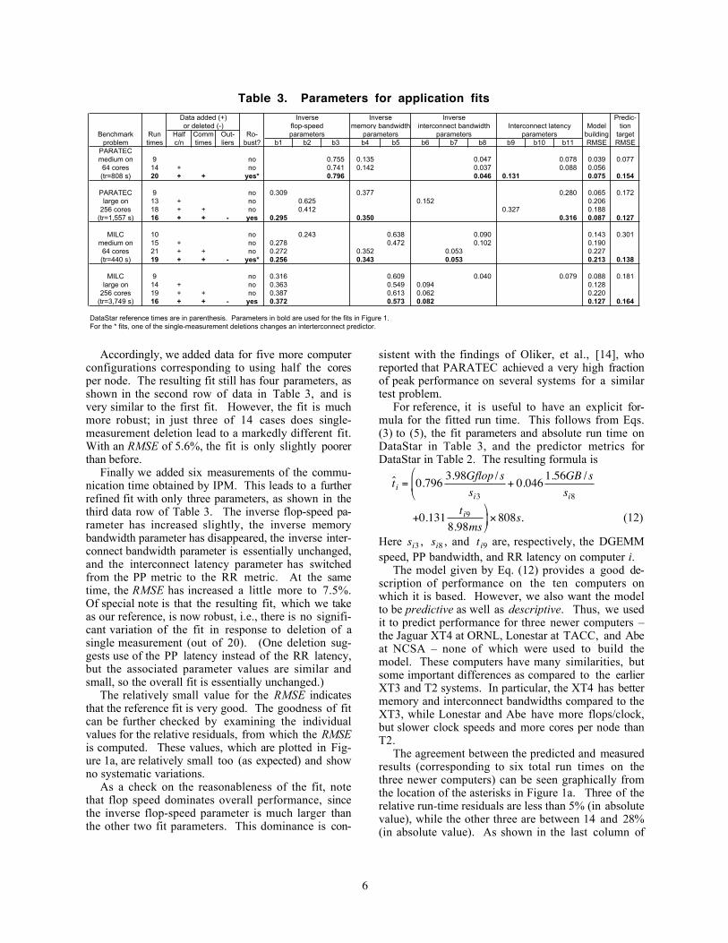
Table 3. Parameters for application fitsData added (+) Inverse Inverse Predic-or deleted (-) flop-speed interconnect bandwidth Interconnect latency Model tion

Benchmark Run Half Comm Out- Ro- parameters parameters parameters building targetproblem times c/n times liers bust? b1 b2 b3 b4 b5 b6 b7 b8 b9 b10 b11 RMSE RMSE

PARATECmedium on 9 no 0.755 0.135 0.047 0.078 0.039 0.07764 cores 14 + no 0.741 0.142 0.037 0.088 0.056(tr=808 s) 20 + + yes* 0.796 0.046 0.131 0.075 0.154

PARATEC 9 no 0.309 0.377 0.280 0.065 0.172large on 13 + no 0.625 0.152 0.206

256 cores 18 + + no 0.412 0.327 0.188(tr=1,557 s) 16 + + - yes 0.295 0.350 0.316 0.087 0.127

MILC 10 no 0.243 0.638 0.090 0.143 0.301medium on 15 + no 0.278 0.472 0.102 0.19064 cores 21 + + no 0.272 0.352 0.053 0.227(tr=440 s) 19 + + - yes* 0.256 0.343 0.053 0.213 0.138

MILC 9 no 0.316 0.609 0.040 0.079 0.088 0.181large on 14 + no 0.363 0.549 0.094 0.128

256 cores 19 + + no 0.387 0.613 0.062 0.220(tr=3,749 s) 16 + + - yes 0.372 0.573 0.082 0.127 0.164

DataStar reference times are in parenthesis. Parameters in bold are used for the fits in Figure 1.For the * fits, one of the single-measurement deletions changes an interterconnect predictor.

Inverse

parametersmemory bandwidth

Accordingly, we added data for five more computerconfigurations corresponding to using half the coresper node. The resulting fit still has four parameters, asshown in the second row of data in Table 3, and isvery similar to the first fit. However, the fit is muchmore robust; in just three of 14 cases does single-measurement deletion lead to a markedly different fit.With an RMSE of 5.6%, the fit is only slightly poorerthan before.

Finally we added six measurements of the commu-nication time obtained by IPM. This leads to a furtherrefined fit with only three parameters, as shown in thethird data row of Table 3. The inverse flop-speed pa-rameter has increased slightly, the inverse memorybandwidth parameter has disappeared, the inverse inter-connect bandwidth parameter is essentially unchanged,and the interconnect latency parameter has switchedfrom the PP metric to the RR metric. At the sametime, the RMSE has increased a little more to 7.5%.Of special note is that the resulting fit, which we takeas our reference, is now robust, i.e., there is no signifi-cant variation of the fit in response to deletion of asingle measurement (out of 20). (One deletion sug-gests use of the PP latency instead of the RR latency,but the associated parameter values are similar andsmall, so the overall fit is essentially unchanged.)

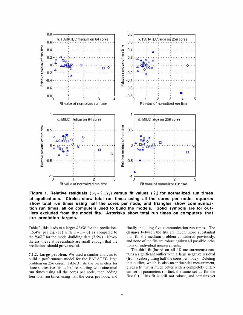
The relatively small value for the RMSE indicatesthat the reference fit is very good. The goodness of fitcan be further checked by examining the individualvalues for the relative residuals, from which the RMSEis computed. These values, which are plotted in Fig-ure 1a, are relatively small too (as expected) and showno systematic variations.

As a check on the reasonableness of the fit, notethat flop speed dominates overall performance, sincethe inverse flop-speed parameter is much larger thanthe other two fit parameters. This dominance is con-

sistent with the findings of Oliker, et al., [14], whoreported that PARATEC achieved a very high fractionof peak performance on several systems for a similartest problem.

For reference, it is useful to have an explicit for-mula for the fitted run time. This follows from Eqs.(3) to (5), the fit parameters and absolute run time onDataStar in Table 3, and the predictor metrics forDataStar in Table 2. The resulting formula is

€

ˆ t i = 0.796 3.98Gflop / ssi3

+ 0.046 1.56GB / ssi8

€

+0.131 ti98.98ms

× 808s. (12)

Here

€

si3 ,

€

si8 , and

€

ti9 are, respectively, the DGEMMspeed, PP bandwidth, and RR latency on computer i.

The model given by Eq. (12) provides a good de-scription of performance on the ten computers onwhich it is based. However, we also want the modelto be predictive as well as descriptive. Thus, we usedit to predict performance for three newer computers –the Jaguar XT4 at ORNL, Lonestar at TACC, and Abeat NCSA – none of which were used to build themodel. These computers have many similarities, butsome important differences as compared to the earlierXT3 and T2 systems. In particular, the XT4 has bettermemory and interconnect bandwidths compared to theXT3, while Lonestar and Abe have more flops/clock,but slower clock speeds and more cores per node thanT2.

The agreement between the predicted and measuredresults (corresponding to six total run times on thethree newer computers) can be seen graphically fromthe location of the asterisks in Figure 1a. Three of therelative run-time residuals are less than 5% (in absolutevalue), while the other three are between 14 and 28%(in absolute value). As shown in the last column of

7

Figure 1. Relative residuals (

€

(y i − ˆ y i )/y i ) versus fit values (

€

ˆ y i ) for normalized run timesof applications. Circles show total run times using all the cores per node, squaresshow total run times using half the cores per node, and triangles show communica-tion run times, all on computers used to build the models. Solid symbols are for out-liers excluded from the model fits. Asterisks show total run times on computers thatare prediction targets.

Table 3, this leads to a larger RMSE for the predictions(15.4%, per Eq. (11) with

€

n − p = 6) as compared tothe RMSE for the model-building data (7.5%). Never-theless, the relative residuals are small enough that thepredictions should prove useful.

7.1.2. Large problem. We used a similar analysis tobuild a performance model for the PARATEC largeproblem on 256 cores. Table 3 lists the parameters forthree successive fits as before, starting with nine totalrun times using all the cores per node, then addingfour total run times using half the cores per node, and

finally including five communication run times. Thechanges between the fits are much more substantialthan for the medium problem considered previously,and none of the fits are robust against all possible dele-tions of individual measurements.

The third fit (based on all 18 measurements) con-tains a significant outlier with a large negative residual(from Seaborg using half the cores per node). Deletingthat outlier, which is also an influential measurement,gives a fit that is much better with a completely differ-ent set of parameters (in fact, the same set as for thefirst fit). This fit is still not robust, and contains yet

8

another outlier, this time having a large positive resid-ual (from the Seaborg communication time). Deletingthis second outlier gives a fit (based on 16 measure-ments) that is better still and robust against all single-measurement deletions. With an RMSE of 8.7%, thisfinal fit (which we take as our reference) is onlyslightly poorer than the final fit for the medium prob-lem. The goodness of the fit is also evident from therelative residuals of the run times shown in Figure 1b.(Note that the outliers are included in the figure, eventhough they were not used in the final fit.)

Although the values of the parameters are similarfor both the initial and final fits, the robustness of thefinal fit provides greater confidence in its predictiveability. Indeed, the predicted run times for the sixnewer computer configurations are in reasonableagreement with the measured run times, as shown bythe relative residuals plotted as asterisks in Figure 1b.The RMSE for the predictions is 12.7%, and all of thepredictions have relative residuals smaller than 23% (inabsolute value).

A further observation is that the model for the largeproblem is appreciably different from that for the me-dium problem. There is a sizeable parameter for theinverse memory bandwidth, and communication ismore important (as reflected by the magnitude of theinterconnect latency parameter). Indeed, the threemodel parameters for the large problem are all of com-parable magnitude. Moreover, the appearance of theinverse memory bandwidth parameter is apparentlyassociated with the buffering of MPI data in memory,which is a side effect of communication.

The communication time can be reduced and scal-ing improved by adjusting the parameter num-ber_bands_fft in the input file, thereby allowingmessages to be aggregated. We did not take advantageof this, because we only had a complete set of datawith the default input file.

7.2. MILC

“The MILC Code is a body of high performance re-search software written in C for doing SU(3) latticegauge theory on several different (MIMD) parallelcomputers in current use.” [12]

There are three standard benchmark problems corre-sponding to increasingly large lattices [13]. We con-sider two of these: the medium problem using a 32^4lattice and the large problem using a 64^4 lattice.Similarly to PARATEC, we modeled the mediumproblem on 64 cores and the large problem on 256cores.

To develop models for the MILC problems, we fol-lowed the same procedure as for the PARATEC prob-lems. That is, we successively pooled the availablerun-time data from the first ten computers in Table 1to develop model fits. Also, we prevented the RR

bandwidth from appearing in the fits for the mediumproblem.

The initial fits were not robust for either problem,so we selectively deleted outliers until robust fits wereobtained. The evolution in the values of the parame-ters and the RMSE over four successive fits for eachMILC problem are listed in Table 3.

The final, reference fits have RMSE values over themodel-building data that are somewhat worse thanthose obtained before: 21.3% for the medium problemand 12.7% for the large problem (excluding the out-liers). These are still reasonable, however, as are theRMSE values for the predictions: 13.8% for the me-dium problem and 16.4% for the large problem. Theselatter values are comparable to those obtained forPARATEC. Graphical displays of the goodness of fitare shown in Figures 1c and 1d,

Examination of the parameter values listed in Table3 shows that performance is dominated by the memorybandwidth, especially for the large problem. This isconsistent with the observation of Gottlieb [15] andwith scaling scans that show superlinear speedup athigher core counts. Also, the appearance of the clockspeed rather than the other flop speed parameters sug-gests that the code can make only limited use of theextra flops/clock on many of the computers.

8. Models for HPCC complex synthetics

As a further test of our modeling method, we applyit to two of the HPCC complex synthetics: HPL andG-FFTE. On the one hand, their code is much simplerthan that of full applications. On the other hand, theyintroduce a further complication, in that their problemsize varies between computers depending upon thememory available.

Thus we need to correct for the varying problemsize to compare run times between computers at thesame core count. We will also find it useful to com-pare performance for runs made at different core counts,so we make another correction for that as well.

Making such corrections requires complexity for-mulas for the relevant algorithms, i.e., formulas for theoperation count dependence on the numerical parame-ters of the algorithm. Such formulas are equivalent toperformance models, once the constants or coefficientsof each term are known. Thus, our models can beviewed as calibrating the coefficients in the complexityformulas.

The formulas we use involve one computation termand two communication terms. These formulas, whichmodify Eqs. (2) and (3), are discussed in the appendix.

8.1. HPL

HPL is the high-performance version of the Linpackbenchmark [16]. It solves a dense linear system of

9

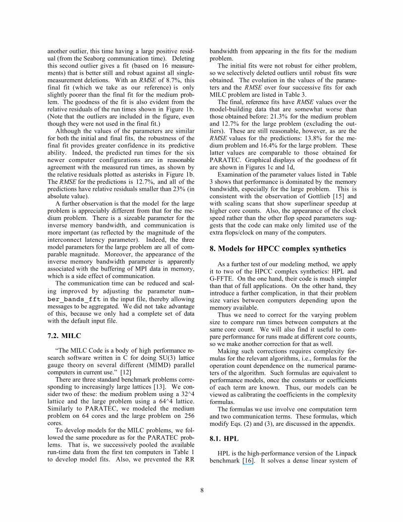
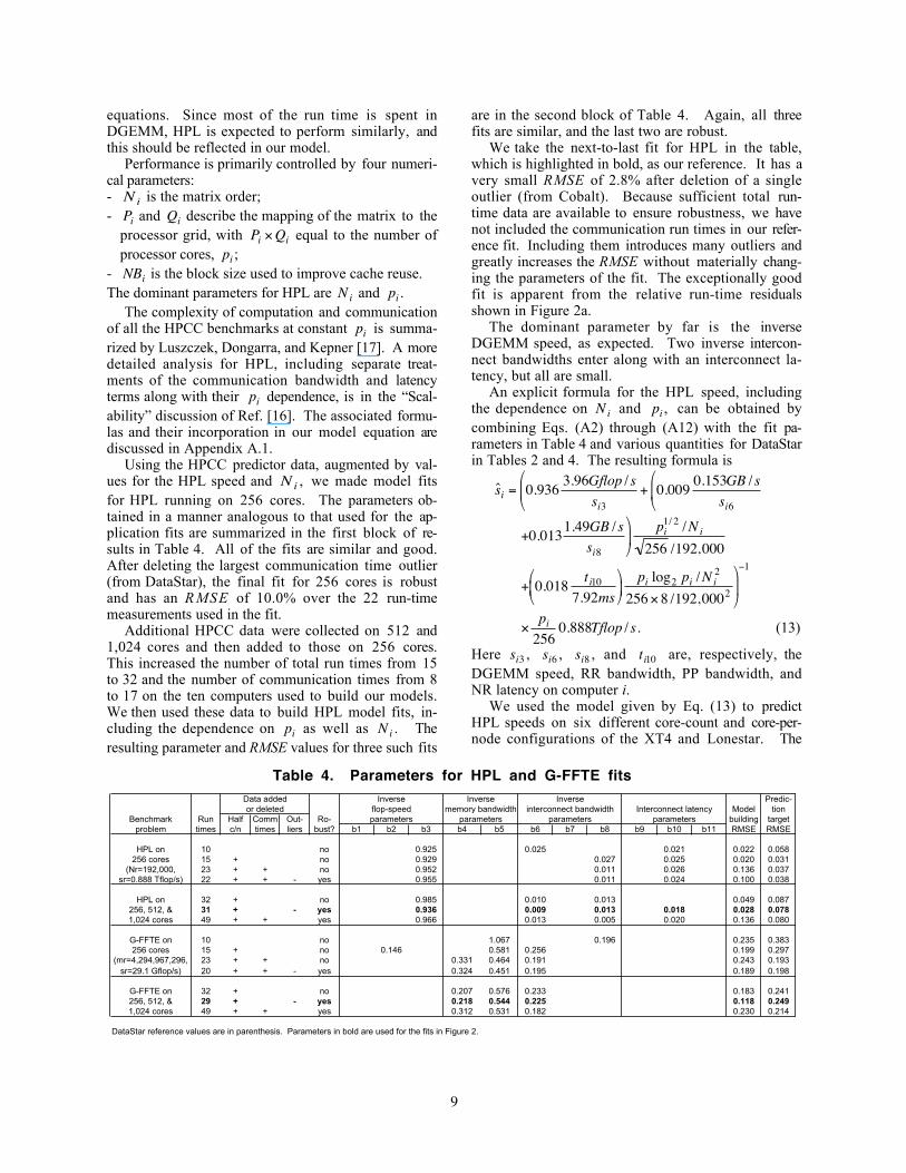
Table 4. Parameters for HPL and G-FFTE fitsData added Inverse Inverse Predic-or deleted flop-speed interconnect bandwidth Interconnect latency Model tion

Benchmark Run Half Comm Out- Ro- parameters parameters parameters building targetproblem times c/n times liers bust? b1 b2 b3 b4 b5 b6 b7 b8 b9 b10 b11 RMSE RMSE

HPL on 10 no 0.925 0.025 0.021 0.022 0.058256 cores 15 + no 0.929 0.027 0.025 0.020 0.031

(Nr=192,000, 23 + + no 0.952 0.011 0.026 0.136 0.037sr=0.888 Tflop/s) 22 + + - yes 0.955 0.011 0.024 0.100 0.038

HPL on 32 + no 0.985 0.010 0.013 0.049 0.087256, 512, & 31 + - yes 0.936 0.009 0.013 0.018 0.028 0.0781,024 cores 49 + + yes 0.966 0.013 0.005 0.020 0.136 0.080

G-FFTE on 10 no 1.067 0.196 0.235 0.383256 cores 15 + no 0.146 0.581 0.256 0.199 0.297

(mr=4,294,967,296, 23 + + no 0.331 0.464 0.191 0.243 0.193sr=29.1 Gflop/s) 20 + + - yes 0.324 0.451 0.195 0.189 0.198

G-FFTE on 32 + no 0.207 0.576 0.233 0.183 0.241256, 512, & 29 + - yes 0.218 0.544 0.225 0.118 0.2491,024 cores 49 + + yes 0.312 0.531 0.182 0.230 0.214

DataStar reference values are in parenthesis. Parameters in bold are used for the fits in Figure 2.

Inversememory bandwidth

parameters

equations. Since most of the run time is spent inDGEMM, HPL is expected to perform similarly, andthis should be reflected in our model.

Performance is primarily controlled by four numeri-cal parameters:-

€

Ni is the matrix order;-

€

Pi and

€

Qi describe the mapping of the matrix to theprocessor grid, with

€

Pi ×Qi equal to the number ofprocessor cores,

€

pi ;-

€

NBi is the block size used to improve cache reuse.The dominant parameters for HPL are

€

Ni and

€

pi .The complexity of computation and communication

of all the HPCC benchmarks at constant

€

pi is summa-rized by Luszczek, Dongarra, and Kepner [17]. A moredetailed analysis for HPL, including separate treat-ments of the communication bandwidth and latencyterms along with their

€

pi dependence, is in the “Scal-ability” discussion of Ref. [16]. The associated formu-las and their incorporation in our model equation arediscussed in Appendix A.1.

Using the HPCC predictor data, augmented by val-ues for the HPL speed and

€

Ni , we made model fitsfor HPL running on 256 cores. The parameters ob-tained in a manner analogous to that used for the ap-plication fits are summarized in the first block of re-sults in Table 4. All of the fits are similar and good.After deleting the largest communication time outlier(from DataStar), the final fit for 256 cores is robustand has an RMSE of 10.0% over the 22 run-timemeasurements used in the fit.

Additional HPCC data were collected on 512 and1,024 cores and then added to those on 256 cores.This increased the number of total run times from 15to 32 and the number of communication times from 8to 17 on the ten computers used to build our models.We then used these data to build HPL model fits, in-cluding the dependence on

€

pi as well as

€

Ni . Theresulting parameter and RMSE values for three such fits

are in the second block of Table 4. Again, all threefits are similar, and the last two are robust.

We take the next-to-last fit for HPL in the table,which is highlighted in bold, as our reference. It has avery small RMSE of 2.8% after deletion of a singleoutlier (from Cobalt). Because sufficient total run-time data are available to ensure robustness, we havenot included the communication run times in our refer-ence fit. Including them introduces many outliers andgreatly increases the RMSE without materially chang-ing the parameters of the fit. The exceptionally goodfit is apparent from the relative run-time residualsshown in Figure 2a.

The dominant parameter by far is the inverseDGEMM speed, as expected. Two inverse intercon-nect bandwidths enter along with an interconnect la-tency, but all are small.

An explicit formula for the HPL speed, includingthe dependence on

€

Ni and

€

pi , can be obtained bycombining Eqs. (A2) through (A12) with the fit pa-rameters in Table 4 and various quantities for DataStarin Tables 2 and 4. The resulting formula is

€

ˆ s i = 0.936 3.96Gflop / ssi3

+ 0.009 0.153GB / s

si6

€

+0.0131.49GB / ssi8

pi1/ 2 /Ni

256 /192,000

€

+ 0.018 t i107.92ms

pi log2 pi /Ni2

256× 8 /192,0002

−1

€

×pi256

0.888Tflop / s . (13)

Here

€

si3 ,

€

si6 ,

€

si8 , and

€

ti10 are, respectively, theDGEMM speed, RR bandwidth, PP bandwidth, andNR latency on computer i.

We used the model given by Eq. (13) to predictHPL speeds on six different core-count and core-per-node configurations of the XT4 and Lonestar. The

10

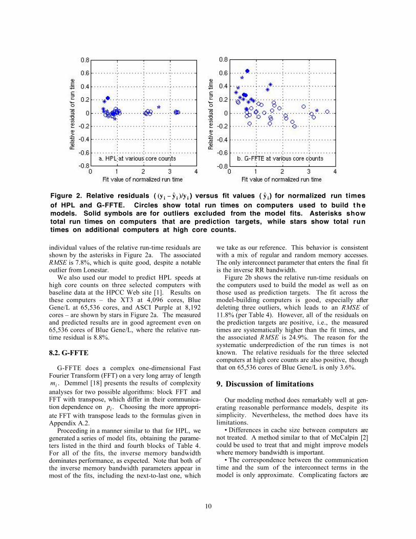
Figure 2. Relative residuals (

€

(y i − ˆ y i )/y i ) versus fit values (

€

ˆ y i ) for normalized run timesof HPL and G-FFTE. Circles show total run times on computers used to build t h emodels. Solid symbols are for outliers excluded from the model fits. Asterisks showtotal run times on computers that are prediction targets, while stars show total runtimes on additional computers at high core counts.

individual values of the relative run-time residuals areshown by the asterisks in Figure 2a. The associatedRMSE is 7.8%, which is quite good, despite a notableoutlier from Lonestar.

We also used our model to predict HPL speeds athigh core counts on three selected computers withbaseline data at the HPCC Web site [1]. Results onthese computers – the XT3 at 4,096 cores, BlueGene/L at 65,536 cores, and ASCI Purple at 8,192cores – are shown by stars in Figure 2a. The measuredand predicted results are in good agreement even on65,536 cores of Blue Gene/L, where the relative run-time residual is 8.8%.

8.2. G-FFTE

G-FFTE does a complex one-dimensional FastFourier Transform (FFT) on a very long array of length

€

mi . Demmel [18] presents the results of complexityanalyses for two possible algorithms: block FFT andFFT with transpose, which differ in their communica-tion dependence on

€

pi . Choosing the more appropri-ate FFT with transpose leads to the formulas given inAppendix A.2.

Proceeding in a manner similar to that for HPL, wegenerated a series of model fits, obtaining the parame-ters listed in the third and fourth blocks of Table 4.For all of the fits, the inverse memory bandwidthdominates performance, as expected. Note that both ofthe inverse memory bandwidth parameters appear inmost of the fits, including the next-to-last one, which

we take as our reference. This behavior is consistentwith a mix of regular and random memory accesses.The only interconnect parameter that enters the final fitis the inverse RR bandwidth.

Figure 2b shows the relative run-time residuals onthe computers used to build the model as well as onthose used as prediction targets. The fit across themodel-building computers is good, especially afterdeleting three outliers, which leads to an RMSE of11.8% (per Table 4). However, all of the residuals onthe prediction targets are positive, i.e., the measuredtimes are systematically higher than the fit times, andthe associated RMSE is 24.9%. The reason for thesystematic underprediction of the run times is notknown. The relative residuals for the three selectedcomputers at high core counts are also positive, thoughthat on 65,536 cores of Blue Gene/L is only 3.6%.

9. Discussion of limitations

Our modeling method does remarkably well at gen-erating reasonable performance models, despite itssimplicity. Nevertheless, the method does have itslimitations.

• Differences in cache size between computers arenot treated. A method similar to that of McCalpin [2]could be used to treat that and might improve modelswhere memory bandwidth is important.

• The correspondence between the communicationtime and the sum of the interconnect terms in themodel is only approximate. Complicating factors are

11

load imbalance and overlap of communication withcomputation, which evidently lead to an appreciablenumber of communication time outliers.

• Differences in the level of software tuning,whether via compiler flags, mathematical libraries, orreprogramming, are not explicitly modeled.

• Sufficient data are needed to get robust fits. Ourexperience suggests that 15 to 20 measurements areneeded for a given benchmark problem to fit three orfour parameters.

10. Summary and conclusions

We have presented a performance modeling methodthat approximates the run time of an application on aparallel computer as a linear combination of predictors.Each predictor is an inverse speed or latency obtainedfrom a microkernel or system characteristic, with all ofthe microkernels from the HPCC benchmark set.Model generation begins with measured values for thepredictors and application run times on a collection ofcomputers at a common core count. Then an auto-mated series of least squares fits is made using back-ward elimination to ensure statistical significance ofthe model parameters. If necessary, outliers are deletedto ensure that the final fit is robust.

We constructed performance models for fourbenchmark problems involving the widely usedPARATEC and MILC applications. In all cases, thefits describe the measurements well on the ten comput-ers on which they are based, and the dominant parame-ters in the fits are those expected from separate investi-gations. In addition, the fits predict performance wellon three newer computers not used to build the mod-els. For the four application benchmark problems withsix predictions each, the relative RMSE in the predictedrun times varies between 12.7 and 16.4%. This isonly moderately higher than the RMSE of 11.7% (cor-responding to an average absolute value of the relativeerror of 9.3%) obtained by Tikir, et al. [6] on anotherset of application benchmarks using a more elaborateand time-consuming method.

We also used our method, augmented by complex-ity analyses, to construct models for two of the HPCCcomplex synthetics: HPL and G-FFTE. These modelsaccount for variations in problem size and core count.The model for HPL is quite good, while that for G-FFTE systematically underpredicts run times. Bothmodels predict performance well on 65,536 cores ofBlue Gene/L, even though the model-building datawere collected on ≤1,024 cores.

In summary, our method offers a straightforwardway to capture the dominant performance behavior ofapplications in models that are easy-to-understand andreasonably accurate in most cases.

11. Acknowledgments

Insightful discussions with Tzu-Yi Chen and AllanSnavely at SDSC were most helpful and greatly appre-ciated at the outset of this project. Greg Bauer andNahil Sobh of NCSA provided many results on sys-tems with Intel processors as part of the Cyberinfra-structure Partnership supported by the National ScienceFoundation. John Shalf, Harvey Wasserman, and An-drew Canning of NERSC provided results on systemsat Department of Energy sites. Valuable help in mak-ing additional benchmark runs was generously givenby Bauer, Kent Milfeld of TACC, and Roger Golliverand Mike Greenfield of Intel. The work described herewas supported, in part, by NSF, which together withDOE funded operation of the computers used in thisstudy.

12. References

[1] HPCC, icl.cs.utk.edu/hpcc.[2] J.D. McCalpin, “Composite Metrics for SystemThroughput in HPC,” www.cs.Virginia.edu/~mccalpin/SimpleCompositeMetrics2003-12-08.pdf.[3] M.J. Clement and M.J. Quinn, “Automated perform-ance prediction for scalable parallel computing,” ParallelComputing, vol. 23, pp. 1405-1420 (1997).[4] D.J. Kerbyson, H.J. Alme, A. Hoisie, F. Petrini, H.J.Wasserman, and M. Gittings, “Predictive Performance andScalability Modeling of a Large-Scale Application,” Proc.SC2001 , Denver, CO (2001), www.sc2001.org/papers/pap.pap255.pdf.[5] A. Snavely, L. Carrington, N. Wolter, J. Labarta, R.Badia, and A. Purkayastha, “A Framework for ApplicationPerformance Modeling and Prediction,” Proc. SC2002,Baltimore, MD (2002),www.supercomp.org/sc2002/paperpdfs/pap.pap201.pdf.[6] M.M. Tikir, L. Carrington, E. Strohmaier, and A.Snavely, “A Genetic Algorithms Approach to Modelingthe Performance of Memory-bound Applications,” Proc.SC2007 , Reno, NV (2007), sc07.supercomputing.org/schedule/pdf/pap255.pdf.[7] N.R. Draper and H. Smith, Applied Regression Analy-sis (Third Edition), John Wiley & Sons (1998).[8] R.D. Cook and S. Weisberg, Residuals and Influencein Regression, p. 209, Chapman and Hall (1982).[9] The MathWorks – MATLAB – The Language of Tech-nical Computing, www.mathworks.com/products/matlab.[10] IPM: Integrated Performance Monitoring,ipm-hpc.sourceforge.net.[11] PARAllel Total Energy Code (PARATEC),www.nersc.gov/projects/paratec.[12] C. Detar, The MILC Code (version: 6.20sep02),www.physics.utah.edu/~detar/milc/milcv6.html.[13] NERSC5 Benchmarks, www.nersc.gov/projects/SDSA /software/?benchmark=NERSC5.[14] L. Oliker, et al., “Leading Computation Methods onScalar and Vector HEC Platforms,” Proc. SC|05, Seattle,WA (2005), http://sc05.supercomputing.org/schedule/pdf/pap293.pdf

12

[15] S. Gottlieb, MILC QCD Code Benchmarks,physics.indiana.edu/~sg/milc/benchmark.html.[16] A. Petitet, R.C. Whaley, J. Dongarra, and A. Cleary,HPL – A Portable Implementation of the High-Performance Linpack Benchmark for Distributed-MemoryComputers, www.netlib.org/benchmark/hpl.[17] P. Luszczek, J. Dongarra, and J. Kepner, “Design andImplementation of the HPC Challenge Benchmark Suite,”CTWatch Quarterly, vol. 2 (4A), pp. 18-23 (November2006), www.ctwatch.org/quarterly/articles/2006/11/design-and-implementation-of-the-hpc-challenge-benchmark-suite.[18] J. Demmel, CS 267 Applications of Parallel Comput-ers Lecture 24: Solving Linear Systems arising from PDEs– I, www.cs.berkeley.edu/~demmel/cs267_Spr99/Lectures/Lect_24_1999-new.ppt.

Appendix: Formulas for HPCC complexsynthetics

The formulas we use involve one computation termand two communication terms. Accordingly, we mod-ify Eq. (2), the basic form of the model, as follows:

€

ˆ t i =ncomp,i / pi

ncomp,r / prc j tij

j

comp

∑ +ncomm,bw,i / pi

ncomm,bw,r / prc j tij

j

comm,bw

∑

€

+ncomm,lat,i / pincomm,lat,r / pr

c j tijj

comm,lat

∑ . (A1)

Here

€

ncomp,i ,

€

ncomm,bw,i , and

€

ncomm,lat,i are the opera-tion counts for computation, bandwidth-limited com-munication, and latency-limited communication, re-spectively, while

€

pi is the number of processor cores.Eq. (A1) reduces to Eq. (2) when computer i solves thesame problem as computer r on the same number ofcores. Note that

€

ncomm,bw,i and

€

ncomm,lat,i typicallydepend explicitly upon

€

pi , whereas

€

ncomp,i does not.Proceeding as in Section 2, Eq. (A1) can be rewrit-

ten in normalized form as follows:

€

ˆ y i ≡ˆ t i /(ncomp,i / pi)tr /(ncomp,r / pr )

=pi / ˆ s ipr / sr

= b j Xijcomp

j

comp

∑

€

+ b j Xijcomm,bw

j

comm,bw

∑ + b j Xijcomm,lat

j

comm,lat

∑ . (A2)

Here

€

b j is given by Eq. (4), as before, but nowthere are three variants of the normalized predictors:

€

Xijcomp ≡

tijtrj

, (A3)

€

Xijcomm.bw ≡

(ncomm,bw,i /ncomp,i)(ncomm,bw,r /ncomp,r )

tijtrj

, (A4)

€

Xijcomm.lat ≡

(ncomm,lat,i /ncomp,i)(ncomm,lat,r /ncomp,r )

tijtrj

. (A5)

Also appearing in Eq. (A2) is the overall speed:

€

si ≡ ncomp,i / t i . (A6)Likewise, the normalized value of the measured runtime is now

€

yi ≡ti /(ncomp,i / pi)tr /(ncomp,r / pr )

=pi / sipr / sr

. (A7)

Before fitting Eq. (A2) by least squares, we also in-troduce weights that are inversely proportional to thesquares of the normalized values of the measured runtime. This weighting is done by another transforma-tion, just as described in Section 3.

A.1. HPL

The complexity of computation and communicationof all the HPCC benchmarks at constant

€

pi is summa-rized by Luszczek, Dongarra, and Kepner [17]. A moredetailed analysis for HPL, including separate treat-ments of the communication bandwidth and latencyterms along with their

€

pi dependence, is in the “Scal-ability” discussion of Ref. [16]. The latter implies that

€

ncomp,i ∝Ni3, (A8)

€

ncomm,bw,i ∝Ni2pi1/ 2 , (A9)

€

ncomm,lat,i ∝Ni pi log2 pi , (A10)so

€

ncomm,bw,i /ncomp,i ∝ pi1/ 2 /Ni , and (A11)

€

ncomm,lat,i /ncomp,i ∝ pi log2 pi /Ni2. (A12)

The last two equations give the expressions neededfor the corrections in Eqs. (A4) and (A5), assumingthat the constants of proportionality are the same forcomputers i and r. (Careful examination of the formu-las in Ref. [16] shows that the constants of proportion-ality in Eqs. (A11) and (A12) have a weak dependenceupon

€

Pi /Qi . This ratio differs depending uponwhether

€

Pi ×Qi = pi is an even or odd power of 2, butthe effect on the constant is small and ignored here.)

A.2. G-FFTE

For the FFT with transpose, the complexity analy-sis results of Demmel (on Slide 37 of Ref. [18]) leadto the following formulas:

€

ncomp,i ∝mi log2 mi , (A13)

€

ncomm,bw,i ∝mi , (A14)

€

ncomm,lat,i ∝ pi2 , (A15)

so

€

ncomm,bw,i /ncomp,i ∝1/ log2 mi, and (A16)

€

ncomm,lat,i /ncomp,i ∝ pi2 /(mi log2 mi) . (A17)