phd proposal - cd++ - carleton university
TRANSCRIPT
Verification Methodology for DEVS Models
By
Hesham Saadawi
A PhD thesis submitted to
The Faculty of Graduate and Postdoctoral Affairs
In partial fulfillment of
The degree requirements of
Doctor of Philosophy in Computer Science
Ottawa-Carleton Institute for
Computer Science
School of Computer Science
Carleton University
Ottawa, Ontario, Canada
Fall 2012
Copyright © 2012
Hesham Saadawi
ii
Abstract
Modeling is an effective tool for studying the behaviour of a system. When modeling, the
system’s descriptions are usually abstracted into simpler models. These models can then
be analyzed and solved (manually or automatically) by using different mathematical
techniques. However, sometimes the models become too complex to analyze formally. In
those cases, computer Modeling and Simulation (M&S) can help designers to understand
the behaviour of these systems better. One example of such complex systems are Real-
Time (RT) systems, which are usually composed of a digital computer executing
software that interacts with the external physical environment with tight timing
constraints.
In studying these systems, M&S has proven to be an essential tool. However, when
simulating RT models, the required interactions could quickly grow beyond the ability of
human observation and analysis. Instead, formal methods for verifying these systems can
guarantee the correct and timely function of these systems.
Due to the benefits of formal verification of RT simulation models, this thesis
introduces a methodology to enable performing formal verification of simulation models
based on the Discrete Event System Specification (DEVS) formalism. The thesis
introduces a road map for a complete methodology to formally verify DEVS models, thus
enabling better methods for M&S validation and verification and making M&S a better
tool for RT-embedded systems development.
iii
Acknowledgements
I’m indebted for this work to the continuous support and encouragement of my
supervisor Dr. Gabriel A. Wainer. I am grateful for his time and effort in supporting my
professional and personal development.
iv
Table of Contents
Abstract ii
Table of Contents iv
List of Tables vii
List of Figures viii
Acronyms xi
Chapter 1: Introduction 1
1.1 Objectives ................................................................................................................. 5
1.2 Originality of the Research ....................................................................................... 7
1.3 Structure of the Thesis .............................................................................................. 8
Chapter 2: Survey of State of the Art 10
2.1 Discrete Event System Specification (DEVS). ....................................................... 10
2.2 Timed Automata (TA) ............................................................................................ 17
2.2.1 TA and Model Checking .................................................................................. 20
2.3 Related work on DEVS verification techniques. .................................................... 22
2.4 Hybrid DEVS models ............................................................................................. 30
2.4.1 The Quantized State Systems (QSS) method................................................... 32
2.5 Introduction to Interval Arithmetic ......................................................................... 42
v
2.6 Summary Discussion of the State-of-the-Art .......................................................... 44
Chapter 3: Thesis contribution 46
3.1 List of Published Contributions .............................................................................. 50
Chapter 4: The RTA-DEVS formalism 54
4.1 Rational Time Advance DEVS (RTA-DEVS) ....................................................... 58
4.2 Estimate of Expressiveness Difference between DEVS and RTA-DEVS ............. 62
4.3 RTA-DEVS to Timed Automata Behavioural Equivalence. .................................. 63
4.3.1 RTA-DEVS internal transition semantics ........................................................ 73
4.3.2 RTA-DEVS external transitions semantics ..................................................... 80
4.3.3 An Alternative way to show bisimulation between RTA-DEVS Internal
Transition and TA Transition.................................................................................... 82
4.4 An algorithm for behavioural equivalence ............................................................. 83
4.5 Resolving rational numbers in RTA-DEVS model ................................................ 88
4.6 DEVS to RTA-DEVS ............................................................................................. 89
4.7 Estimation of Approximation to Verification Results ............................................ 92
4.8 Case study: an Elevator Control System ................................................................. 95
4.9 Known Methodology Limits ................................................................................. 106
Chapter 5: Hybrid DEVS Systems Verification. 107
5.1 Continuous-Discrete systems Verification ........................................................... 107
5.1.1 Transforming QSS DEVS models to TA ....................................................... 112
5.1.2 Case Study of a Hybrid Elevator System ....................................................... 120
vi
5.1.3 Verifying general QSS ................................................................................... 128
5.1.4 Advantages of using QSS/DEVS to verify Hybrid Models ........................... 147
Chapter 6: Conclusion & Future Research 148
6.1.1 Possible Future Research ............................................................................... 149
REFERENCES ........................................................................................................... 153
vii
List of Tables
Table 1: Related Work of DEVS Verification and Contribution ...................................... 28
Table 2: Transformation of RTA-DEVS to Behaviourally Equivalent TA. ..................... 87
Table 3: UPPAAL arithmetic operators .......................................................................... 137
Table 4: User defined functions for the UPPAAL TA model of figure 48 ..................... 141
Table 5: User defined functions for the UPPAAL TA model of figure 49 ..................... 142
viii
List of Figures
Figure 1: DEVS atomic component state transition sequence (extracted, with ................ 13
Figure 2: DEVS Model Hierarchy. ................................................................................... 15
Figure 3: Timed Automaton.............................................................................................. 19
Figure 4: Quantization Function with Hysteresis (extracted, with permission, from [51]).
........................................................................................................................................... 36
Figure 5: QSS Block Diagram Model ............................................................................... 39
Figure 6: Continuous function of exponential Decay ....................................................... 41
Figure 7: Linear approximation of Decay formula ........................................................... 41
Figure 8: Quantized representation of Exponential Decay ............................................... 42
Figure 9: Thesis Contribution ........................................................................................... 49
Figure 10: Coffee-Team-Machine 1 (CTM1). .................................................................. 65
Figure 11: User Behaviour ................................................................................................ 66
Figure 12: Coffee-Team-Machine 2 (CTM2). .................................................................. 66
Figure 13: (a) RTA-DEVS model. (b) Timed Automata model .................................... 68
Figure 14: Direct delay transition from s1 to s'1 and corresponding eventual delay
transition from s2 to s'2. ..................................................................................................... 71
Figure 15: Direct action transition from s1 to s'1, and corresponding eventual action ...... 72
Figure 16: Direct delay transition from s2 to s'2 and corresponding eventual delay
transition from s1 to s'1. ..................................................................................................... 72
Figure 17: Direct action transition from s2 to s'2, and corresponding eventual action ...... 73
ix
Figure 18: RTA-DEVS Internal Transition. ..................................................................... 74
Figure 19: TA model for an Internal RTA-DEVS transition. ........................................... 75
Figure 20: RTA-DEVS External transitions on action a. ................................................. 80
Figure 21: TA model for RTA-DEVS external transition. ............................................... 81
Figure 22: A coupled DEVS model. ................................................................................. 90
Figure 23: RTA-DEVS component with External Input. ................................................. 91
Figure 24: Overlap of two intervals because of approximating irrational value. ............. 94
Figure 25: Elevator RTA-DEVS Model. .......................................................................... 96
Figure 26: Elevator TA model. ......................................................................................... 97
Figure 27: Elevator Controller Model as DEVS Graphs. ................................................. 98
Figure 28: TA Controller model in UPPAAL................................................................... 99
Figure 29: Environment inputs (Button and Sensor). ..................................................... 101
Figure 30: Elevator Verification Results in UPPAAL .................................................... 102
Figure 31: Elevator-Controller in DEVS Graphs notation with irrational value. ........... 104
Figure 32: TA Controller model with Non-deterministic behaviour. ............................. 105
Figure 33: Exact solution for the exponential decay formula. ........................................ 109
Figure 34: Quantized representation of exponential decay............................................. 112
Figure 35: Example of real numbers over-approximation with integer numbers. .......... 116
Figure 36: TA model of exponential decay formula. ...................................................... 119
Figure 37: Elevator braking. De-acceleration: 0.5 m/s2. ................................................. 121
Figure 38: Elevator speed under braking. ....................................................................... 121
Figure 39: Quantized braking-elevator speed. ................................................................ 122
x
Figure 40: TA model of braking elevator motion. .......................................................... 123
Figure 41: Modified elevator TA model- scale of 1/100 second.. .................................. 124
Figure 42: Elevator speed, acceleration= - 0.12 m/sec2. ................................................. 126
Figure 43: Quantized speed, acceleration= - 0.12 m/s2. ................................................. 126
Figure 44: Exact solution for exponential decay formula. .............................................. 129
Figure 45: QSS linear approximation ............................................................................. 130
Figure 46: Over-approximation of QSS trace. ................................................................ 131
Figure 47: Safety zones with QSS over-approximation. ................................................ 132
Figure 48: TA model of a QSS general Integrator .......................................................... 138
Figure 49: TA Model of a QSS Input function generation ............................................. 140
Figure 50: Definition template of u(t) in UPPAAL. ....................................................... 146
xi
Acronyms
DEVS Discrete EVent System Specification
P-DEVS Parallel DEVS
RT-DEVS Real-Time DEVS
FD-DEVS Finite and Deterministic DEVS
SP-DEVS Schedule Preserving DEVS.
M&S Modeling and Simulation
RC Root Coordinator
TA Timed Automata
E-CD++ Embedded CD++
IDE Integrated Development Environment
GGAD Generic Graphical Advanced environment for DEVS modeling and
simulation
RTA-DEVS Rational Time Advance DEVS
QSS Quantized State Systems method
STDEVS Stochastic DEVS
CTL Computation Tree Logic
PTCTL Probabilistic Timed computation Tree Logic
RT Real-Time
RTS Real-Time Systems
1
Chapter 1: Introduction
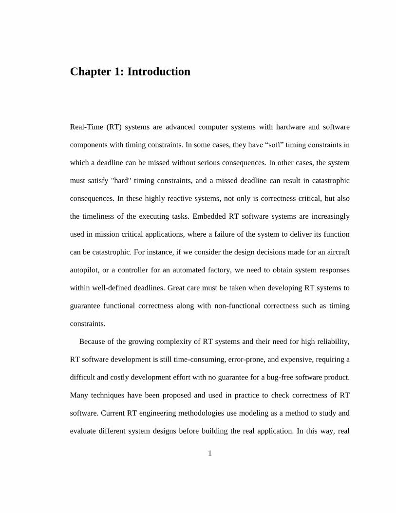
Real-Time (RT) systems are advanced computer systems with hardware and software
components with timing constraints. In some cases, they have “soft” timing constraints in
which a deadline can be missed without serious consequences. In other cases, the system
must satisfy "hard" timing constraints, and a missed deadline can result in catastrophic
consequences. In these highly reactive systems, not only is correctness critical, but also
the timeliness of the executing tasks. Embedded RT software systems are increasingly
used in mission critical applications, where a failure of the system to deliver its function
can be catastrophic. For instance, if we consider the design decisions made for an aircraft
autopilot, or a controller for an automated factory, we need to obtain system responses
within well-defined deadlines. Great care must be taken when developing RT systems to
guarantee functional correctness along with non-functional correctness such as timing
constraints.
Because of the growing complexity of RT systems and their need for high reliability,
RT software development is still time-consuming, error-prone, and expensive, requiring a
difficult and costly development effort with no guarantee for a bug-free software product.
Many techniques have been proposed and used in practice to check correctness of RT
software. Current RT engineering methodologies use modeling as a method to study and
evaluate different system designs before building the real application. In this way, real
2
systems would have a very high predictability and reliability. In order to apply this
methodology, a designer must abstract the physical system at hand and build a model for
it, then combine this with a model of the proposed controller design. Then, different
techniques can be used to reason about these models and gain confidence in their
correctness. Informal methods usually rely on extensive testing of the systems based on
system specifications [1]. These methods have limitations because, in order to guarantee
software reliability, we need to apply exhaustive testing to the software component, using
all possible input combinations, which is a costly process. Many techniques have been
proposed to enable a practical alternative to this exhaustive software testing [2].
However, we cannot guarantee a full coverage of all possible execution paths in a
software component, thus leaving us with limited confidence in software correctness.
Therefore, informal techniques can reveal errors, but they cannot prove the non-existence
of errors.
The use of formal software analysis is growing as an alternative, as this technique
allows full verification that software components are free of errors. In the last few
decades, these techniques have matured and been used in some industrial capacity for
software and hardware correctness verification [3]. Formal techniques can be used to
prove the correctness of systems specifications. Nevertheless, they are usually
constrained in their application, as they do not scale up well. Likewise, the designers
need a high level of expertise to apply these techniques. Another drawback of formal
techniques is their need to be applied to an abstract model of the real system, which
3
means that what is being verified is not the final implementation. Even if the abstract
designed model is proven correct, there is a risk that some errors creep in during the
development process through the manual implementation of the design into executable
code [1].
Formal verification techniques are of two main types, deductive or algorithmic [4].
Deductive techniques rely on representing the system and its specification with logic
rules, and then trying to deduct a proof of system correctness. In this method, the user
needs to find a sequence of deductions to reach the proof; hence, deductive technique
needs more creativity and expertise with formal methods from the user than algorithmic
one. This becomes a disadvantage with the growing size of systems, as manual
intervention, required from the user, also grows. The advantage of this technique,
however, is that it can deal with systems of infinite state space, which usually is the case
found in hybrid systems. Algorithmic techniques rely on modelling the system in a
graphical form, and coding the specifications in logical queries. Then an algorithm for
reachability analysis searches the graph space for nodes that satisfy specification queries
and are reachable from the initial system configuration. This method is also called model
checking. For a system composed of multiple components, the model checking algorithm
combines these models to build one graph representing the system overall behaviour that
is called a reachability graph. By traversing this graph, the model checking algorithm can
check the satisfaction of a given query against the given system model. However, for the
algorithm to terminate, the reachability graph must be finite, otherwise termination would
4
not be guaranteed, and the model checking problem would be undecidable. The
advantage of this method is its complete automation, and the user does not need to be an
expert in formal methods. New theoretical advances in model checking allow engineers
to guarantee certain properties about the models of such systems using a formal approach.
Model checking techniques can be automated to improve the work of the software
engineer. Timed Automata (TA) theory [5], in particular, has provided many practical
results in this area. However, there is still a gap between a system model that is checked
as an abstract entity, and the actual system implementation code to be run on a target
platform. More work is still needed to prevent errors from creeping into the final
implementation as the programmer translates the requirements captured and modeled in
TA into code. TA and other formal methods have showed promising results, but they are
still difficult to apply and have limited power when the complexity of the system under
development scales up.
A different approach to deal with these issues considers using Modeling and
Simulation (M&S) to gain confidence in the model correctness. The use of M&S is not
new, and systems engineers have often relied on these methods in order to improve the
study of experimental conditions during model definition. The construction of system
models and their analysis through simulation reduces both end costs and risks, while
enhancing system capabilities and improving the quality of the final products. M&S let
users experiment with “virtual” systems, allowing them to explore changes and test
dynamic conditions in a risk-free environment. This is a useful approach, especially
5
considering that testing under actual operating conditions may be impractical and, in
some cases, impossible. Nevertheless, no practical, automated approach exists to perform
the transition between the modeling and the development phases, and this often results in
initial models being abandoned, resulting in increased initial costs that project managers
try to avoid. Simultaneously, M&S frameworks are not as robust as their formal
counterparts.
Using M&S for RT systems enables testing real life scenarios, even for those cases in
which real-life testing might be too costly or impossible to achieve [6]. If the models used
for M&S were formal, their correctness would also be verifiable, and a designer could see
the system evolution and its inner workings even before starting a simulation. Another
advantage of executable models is that they can be deployed to the target platform, thus
giving the opportunity to use the model not only for simulations, but also as the actual
implementation deployed on the target hardware. This avoids any new errors that could
appear during the implementation from transformation of the verified models into an
implementation, thus guaranteeing a high degree of correctness and reliability.
1.1 Objectives
Considering the issues in the previous section, RT system designers need a methodology
to help them in the modeling and analysis of any complete design of an RT system. It is
useful if the same methodology can be used to formally verify a system against its
requirements, and also used to simulate individual scenarios. Finally, after complete
6
verification of the correctness of the designed system, the methodology should ensure
that the exact verified design could be deployed and executed on the target platform.
The objective of this thesis is to provide such a practical methodology to build and
verify RT systems. This methodology uses two main formalisms to model systems
specifications. The first one of them is the Discrete Event System Specifications (DEVS)
formalism [7], which is based on systems theory. DEVS is the most general discrete
event specification, and one can build complex models as a composite of different
methods for the various components (Cellular Automata, Petri Nets, Timed Finite State
Machines, Modelica, PDEs and other continuous components) that can be then translated
into a DEVS representation. These DEVS models can then be simulated using DEVS
abstract simulation algorithms. DEVS simplifies building complex models by its
hierarchical building of coupled models out of atomic models. DEVS models are directly
executable on many DEVS simulators including an RT DEVS kernel such as e-CD++
[8]. However, DEVS simulators lack formal verification capability and this was the
motivation to this thesis.
The second formalism used in our methodology is Timed Automata (TA) [5]. The TA
formalism, which is based on finite automata theory, was proposed to specify RT reactive
systems. TA provides a solid theory and algorithms for model checking, and many
existing tools implement these algorithms (for instance, UPPAAL, Kronos and others [9],
[10]). TA’s main concern is building an abstract formal description of the system that is
verifiable by model checking, and is not focused on simulating discrete systems; thus, its
7
tools lack many functions that usually exist in DEVS simulators and allow simulating
different systems.
Given the strengths and weaknesses of these two formalisms, the objective of this
thesis is to develop a methodology that combines both formalisms to allow the designer
to model, simulate, verify, and deploy RT systems. This is achieved by guaranteeing the
correctness of the model with a methodology that verifies DEVS models with TA model-
checking techniques and tools. The verified DEVS models would then execute directly
on an RT DEVS kernel, thus eliminating the risk of introducing errors in the final system
implementation on the target platform. This methodology gives a model-based approach
in which the user can move the original verified models to a target platform to execute
them in RT without any changes. The resulting systems developed with this methodology
would have a higher correctness and reliability of the actual code executing in the RT
system. During this research this concept is demonstrated in actual elevator controllers
running in real-time scenarios.
1.2 Originality of the Research
The originality of this research relies in the introduction of a new practical methodology
to verify DEVS models. The methodology introduced here differs from other existing
approaches in that it targets the verification of classic DEVS models and not a subset of
DEVS formalism. This allows the modeller to use the classic full DEVS formalism and
makes this methodology a good option to be used in an embedded systems development
lifecycle methodology.
8
The verification of DEVS introduced in this thesis is done on multiple stages. First, it
defines a new class of DEVS, called RTA-DEVS, which is close to classic DEVS in
semantics and expressive power. Then, the methodology defines a transformation to
obtain a TA that is behaviourally equivalent to RTA-DEVS. The advantage of doing so is
that many classic DEVS models would satisfy the semantics of RTA-DEVS models.
Thus, they could be simulated with any DEVS simulator. Likewise, it could be
transformed to TA to validate the desired properties formally. RTA-DEVS is close to
general DEVS, in its expressiveness; nevertheless, as we will show later in the
methodology, it is a verifiable subset of DEVS.
The second stage in the verification deals with the approximations and abstractions
carried out for transforming DEVS models into RTA-DEVS. To assess their effect on
verification accuracy, we propose a method to estimate if any errors were introduced
during the transformation that may affect the verification step, or the validity of the
resulting RTA-DEVS model.
A new approach is also introduced to build on the above results to enable the formal
verification of hybrid systems (composed of discrete and continuous components) built
with DEVS formalism. All of these research topics are original research ideas that have
not been found in the literature of this domain.
1.3 Structure of the Thesis
This thesis is structured as follows: Chapter 2 provides the reader with a review of the
state of the art of literature related to the research. In this chapter, we also introduce the
9
main concepts used, including an introduction to the DEVS formalism, related work of
different approaches used to verify DEVS models, an introduction to Timed Safety
Automata, and to the QSS method, which will be used to model continuous systems with
discrete DEVS models. We also introduce a summary of this thesis contribution in this
chapter.
Chapter 3 presents the proposed RTA-DEVS formalism, and it shows how it is
mapped to TA for the purpose of formal verification. An example is introduced to show
the proposed methodology and algorithm. We also describe a method to transform DEVS
models to RTA-DEVS with the ability to tell if this transformation would cause an effect
to verification results.
Chapter 4 discusses the work to verify hybrid systems built with Quantized State
Systems method QSS and DEVS components.
In chapter 5, we present the conclusion for this research, and potential future research.
10
Chapter 2: Survey of State of the Art
In this chapter, we will introduce a brief state of the art related to our thesis research.
This includes a brief introduction to DEVS formalism, coverage of different techniques
that have been used in literature for verification and testing of DEVS models, a brief
introduction to timed automata theory and formalism, and an introduction to a topic of
interest to our methodology that is modeling hybrid systems with a discrete event
representation using DEVS components.
These topics would constitute an essential background to understand our
methodology and to introduce our thesis in the following chapters.
2.1 Discrete Event System Specification (DEVS).
[7] is an accepted framework for understanding and supporting the activities of
modeling and simulation. DEVS is a sound formal framework based on systems theory. It
includes well-defined coupling of components, hierarchical, modular construction,
support for discrete event approximation of continuous systems, support for stochastic
systems, and enables component reuse. DEVS theory provides a rigorous methodology
for representing models, and it does present an abstract way of thinking about the world
independent of simulation mechanisms, underlying hardware and middleware. A real
system modeled with DEVS is described as a composite of sub-models, each of them
being atomic (behavioural) or coupled (structural).
11
The basic modelling unit of DEVS is called an atomic model. A DEVS atomic
component is formally defined as:
AM = < X, S, Y, δext, δint, λ, ta > (Eq. 2.1)
Where:
X: a set of external input event types
S: a sequential state set
Y: an output set
δext: Q × X → S, an external transition function
Where Q is the total state set of M = {(s, e) | s S and 0 ≤ e ≤ ta(s)}
δint: S → S, an internal transition function
λ: S → Y , an output function
ta: S → +0,∞, a time advance function
Where the +0,∞ is the non-negative real numbers with ∞ adjoined.
An atomic component AM is a model that is affected by external input events X, and
it generates output events Y. The state set S represents the unique description of the states
of the model. The internal transition function δint and the external transition function δext
compute the next state of the model. If an external event arrives at elapsed time e which
is less than or equal to a value specified by the time advance function ta(s), a new state s′
is computed by the external transition function δext. Then, a new ta(s′) is computed, and
the elapsed time e is set to zero. Otherwise, if no external event arrives before the state
lifetime elapses, a new state s′ is computed by the internal transition function δint. In the
12
case of an internal event, the output specified by the output function λ is produced based
on the state s. As before, a new ta(s′) is computed, and the elapsed time e is set to zero.
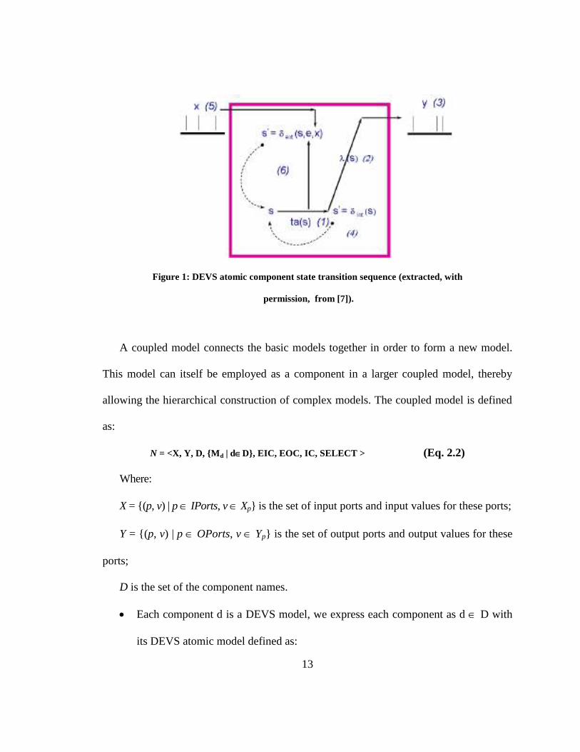
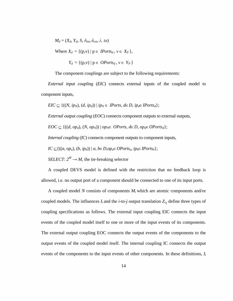
Figure 1 illustrates the state transition of an atomic component. This diagram
describes the behaviour of an atomic model as sequence of steps indicated by the
numbers on the diagram. In the first step (1) on the diagram, the atomic component is in
state s for a specified time ta(s). If the atomic component passes this time without
interruption, it will execute its output function λ(s) (step 2) to produce an output y (step 3)
at the end of this time and will change state based on its δint function (complete transition)
to state s` in step 4, and then this new state becomes the component state and we consider
it as state s which now is the component state (this is indicated by the dotted arrow from
s` to s on the bottom of the diagram) . Continuing from this new state s, if the
component receives an input x (step 5) during the state s time life ta(s) it will change its
state which is determined by its δext function (step 6) and does not produce an output
(incomplete transition). Again we consider this new state the component state s (this is
indicated by the dotted arrow from s` to s on the left of the diagram) and the component
waits in this state for the next event to repeat the previous cycle.
13
Figure 1: DEVS atomic component state transition sequence (extracted, with
permission, from [7]).
A coupled model connects the basic models together in order to form a new model.
This model can itself be employed as a component in a larger coupled model, thereby
allowing the hierarchical construction of complex models. The coupled model is defined
as:
N = <X, Y, D, {Md | dD}, EIC, EOC, IC, SELECT > (Eq. 2.2)
Where:
X = {(p, v) | p IPorts, v Xp} is the set of input ports and input values for these ports;
Y = {(p, v) | p OPorts, v Yp} is the set of output ports and output values for these
ports;
D is the set of the component names.
Each component d is a DEVS model, we express each component as d D with
its DEVS atomic model defined as:
14
Md = (Xd, Yd, S, δint, δext, λ, ta)
Where Xd = {(p,v) | p IPortsd , v XP },
Yd = {(p,v) | p OPortsd , v YP }
The component couplings are subject to the following requirements:
External input coupling (EIC) connects external inputs of the coupled model to
component inputs,
EIC {((N, ipN), (d, ipd)) | ipN IPorts, dD, ipdIPortsd};
External output coupling (EOC) connects component outputs to external outputs,
EOC {((d, opd), (N, opN)) | opN OPorts, dD, opdOPortsd};
Internal coupling (IC) connects component outputs to component inputs,
IC {((a, opa), (b, ipb)) | a, bD,opaOPortsa, ipbIPortsb};
SELECT: 2M → M, the tie-breaking selector
A coupled DEVS model is defined with the restriction that no feedback loop is
allowed, i.e. no output port of a component should be connected to one of its input ports.
A coupled model N consists of components Mi which are atomic components and/or
coupled models. The influences Ii and the i-to-j output translation Zi,j define three types of
coupling specifications as follows. The external input coupling EIC connects the input
events of the coupled model itself to one or more of the input events of its components.
The external output coupling EOC connects the output events of the components to the
output events of the coupled model itself. The internal coupling IC connects the output
events of the components to the input events of other components. In these definitions, Ii
15
represents set of components that are connected to the input, while Zi,j represents any
connections from an output of a component to the input of another component. The
SELECT function is used to order the processing of the simultaneous events for
sequential events. Thus, all the events with the same time in the system can be ordered
with this function.
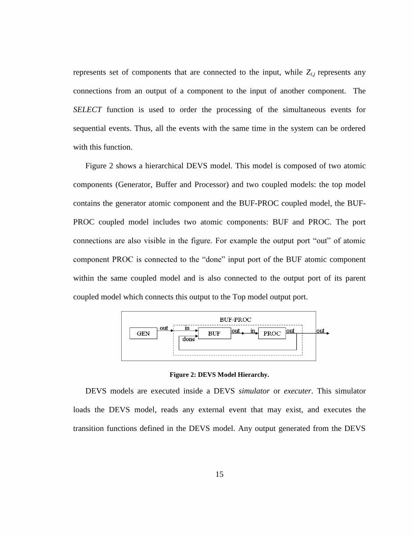
Figure 2 shows a hierarchical DEVS model. This model is composed of two atomic
components (Generator, Buffer and Processor) and two coupled models: the top model
contains the generator atomic component and the BUF-PROC coupled model, the BUF-
PROC coupled model includes two atomic components: BUF and PROC. The port
connections are also visible in the figure. For example the output port “out” of atomic
component PROC is connected to the “done” input port of the BUF atomic component
within the same coupled model and is also connected to the output port of its parent
coupled model which connects this output to the Top model output port.
Figure 2: DEVS Model Hierarchy.
DEVS models are executed inside a DEVS simulator or executer. This simulator
loads the DEVS model, reads any external event that may exist, and executes the
transition functions defined in the DEVS model. Any output generated from the DEVS
16
model is produced to the environment from the DEVS simulator. Some examples of
DEVS simulators are CD++ [11], PowerDEVS [12], adevs [13] and DEVSJAVA [14].
DEVS simulators are also available to run on embedded platforms allowing DEVS
models to run as embedded software in RT. Some initial work on executing DEVS
models in real time was done in [15] to execute DEVS models on a chip. More advanced
simulators were developed, for example PowerDEVS [16]. PowerDEVS has the ability to
execute models on a RT operating system with synchronization of simulation time to RT
clock. With its ability to model continuous systems within DEVS, the RT execution of
DEVS allows simulation of physical systems in RT.
RTDEVS/CORBA [17] is a RT simulator designed to model and simulate large-scale
distributed RT systems. This simulator supports the concept of model continuity that
means the same model of a system can be used through all design phases. This simulator
provides RT modeling & simulation environment so that the system under study can be
simulated with its environment model in real-time. Zeigler in [7] describes the internal
architecture of such RT simulator and some differences of RT simulator from the classic
DEVS simulator to increase performance and enable interaction with underlying
operating system to support concurrent execution threads.
E-CD++ [8] is an embedded DEVS simulator that can execute DEVS models in RT
and interacts with external sensor and actuators as shown in a case study in [18]. Using
DEVS models as executable models on an embedded platform closes the gap between
modeling and implementation, thus avoiding errors that may be introduced by the manual
17
translation of models into executable code. This approach can be greatly enhanced with
the ability to validate DEVS models not only through simulation, but also with the ability
to formally verify the model against the initial requirements. In this case, DEVS models
would be proven free of defects, and its direct execution on embedded platform
eliminates any possible creep of defects into the executed code. The goal of this thesis
therefore, is to present a robust methodology to formally verify DEVS models using
different formal techniques and methods, and giving the system modeller a robust method
to estimate the effect of any approximations necessary to achieve that goal.
2.2 Timed Automata (TA)
A Timed Automaton can be defined as in [10]:
A = (N, lo, E, I) (Eq. 2.3)
– N is a finite set of locations (or nodes),
– lo N is the initial location,
– E N (C) 2C N is the set of edges and
– I: N→β(C) assigns invariants to locations
Here, C is a set of clock variables (with x, y,... representing clock variables from the set
C). We use a, b, etc. to represent the actions from a set of the finite alphabet Σ. Let us
assume a finite set of real-valued variables C ranged over by clocks x, y,... and a finite
alphabet Σ (with actions a,b,...). Let us call a clock constraint to a conjunctive formula of
atomic constraints of the form x~n or x-y ~ n where x,y are clock variables, ~ is one of {≤,
<, =, >, ≥} and n is a natural number. The clock constraints can be used on transitions,
18
where they are called guards; or in a location (state), where they are called invariants.
Invariants are constraints on the form x ≤ n, or x< n to restrict time spent in a TA
location. β(C) denotes set of clock constraints. We use the notation u ┤I(l) to mean that
clock valuation u satisfies the invariant defined in location l. We also define a TA state as
a pair of (location, clock valuation) such as (L,u).
TA are Timed Transition Specifications in which the states are pairs <L,u>, where L is
a location, and u is a clock valuation. We write ll rag ,, when (l,g,a,r,l) E with g a
clock constraint, a an action, and r a set of clocks to be reset to zero.
TA uses two types of transitions:
- Delay Transitions: duLuL d ,, , where the time passage d causes a
transition from a start location L to an end location L if u ┤I(L) and (u+d) ┤ I(L).
- Action transitions: uLauL ,, , where an action a causes a transition from
a start location L, to an end location L’, and u ┤ I(L).
19
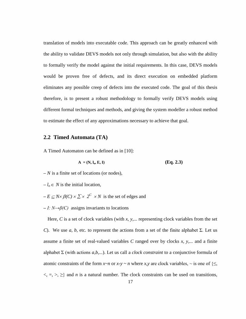
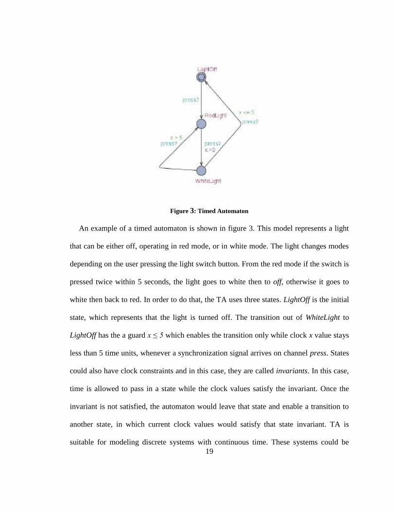
Figure 3: Timed Automaton
An example of a timed automaton is shown in figure 3. This model represents a light
that can be either off, operating in red mode, or in white mode. The light changes modes
depending on the user pressing the light switch button. From the red mode if the switch is
pressed twice within 5 seconds, the light goes to white then to off, otherwise it goes to
white then back to red. In order to do that, the TA uses three states. LightOff is the initial
state, which represents that the light is turned off. The transition out of WhiteLight to
LightOff has the a guard x ≤ 5 which enables the transition only while clock x value stays
less than 5 time units, whenever a synchronization signal arrives on channel press. States
could also have clock constraints and in this case, they are called invariants. In this case,
time is allowed to pass in a state while the clock values satisfy the invariant. Once the
invariant is not satisfied, the automaton would leave that state and enable a transition to
another state, in which current clock values would satisfy that state invariant. TA is
suitable for modeling discrete systems with continuous time. These systems could be
20
composed of a single TA model, or multiple models that interact together. The latter case
is called a network of TA.
2.2.1 TA and Model Checking
One of the most successful techniques for systems formal verification is model checking
[19]. In this method, the system to be verified is modeled by a suitable formalism such as
I/O automata or TA, which can be represented in a graphical notation. Each state of the
model assumes some valid system property(ies) at this state.
System requirements are specified as a temporal logic formula called query. The
model checking technique then uses an algorithmic approach to traverse the model
graph, and it checks the satisfaction of the query against the properties defined at each
state. For a system composed of multiple components, the model checking algorithm
combines these models to build one graph representing the system overall behaviour that
is called a reachability graph. By traversing this graph, the model checking algorithm can
check the satisfaction of a given query against the given system model. However, for the
algorithm to terminate, the reachability graph must be finite, otherwise termination would
not be guaranteed, and the model checking problem would be undecidable. With timed
formalisms such as TA, the time elapse is modeled by a continuous clock variable. This
variable value increases when TA is waiting in a state. Even for a bounded Real interval,
the number of Real values would be infinite as shown by the famous Cantor’s diagonal
method. However, TA model checking for finite state machines [20][21][22] was enabled
by extending symbolic model checking techniques [23][24] to build a finite reachability
21
graph with continuous time. Nevertheless , the state explosion problem still limits the size
of actual problems that can be solved. The state explosion problem is a term describing
the exponential growth of the reachability graph size with the growing number of
components and states of each component in a network of TA. This renders the
techniques of model checking practically limited to small and medium industrial
problems unless combined with other techniques to overcome this exponential growth of
the reachability graph.
Recent techniques to reduce this problem have been proposed and these results were
implemented in a number of tools for TA model checking with a success to check models
of increasing sizes. One of these tools is UPPAAL [9][10] that have extended TA with
integer variables, urgent channels and user-defined functions. These extensions increase
the conciseness of the model, but not the expressiveness power as shown in [25].
UPPAAL uses a subset of TCTL (Timed Computation Tree Logic) [24] to specify
queries for properties in the TA model.
Timed safety Automata is the version of TA used in the UPPAAL model checker
[10]. This thesis used this class of TA as it suffices for the verification purpose to
represent DEVS models and it is verifiable within UPPAAL tool.
In the methodology introduced in this thesis, if UPPAAL (or any other model checker)
faces a problem of state explosion, and no answers can be obtained in finite time, the user
can use model checking on a rough abstract of the system. From this step, some
requirements may not be satisfied in the rough abstract model. These would generate a
22
trace that can be used as a seed input to a simulated mode to test the models using DEVS
simulation. Subcomponents can be verified using TA model checkers, improving the
overall quality of the system.
2.3 Related work on DEVS verification techniques.
There have been several proposals to verify DEVS models, ranging from formal model-
checking of restricted classes of DEVS, the generation of traces from DEVS models for
testing, the specification of high-level system requirements in TA (and verifying DEVS
model against those requirements), or introducing clock constructs to DEVS to conform
with TA. In this section, we give an overview of these techniques and compare different
approaches. From this comparison, we show how the methodology introduced in chapter
3 closes an existing gap in current techniques.
In [26], Wainer et al. presented the verification of DEVS models, checking the
consistency of model structure, the correct coupling of components, and the correct
definition of the transition functions. These checks were done statically before executing
the models and introduced a component to monitor execution for some verification.
However, this approach has a limited ability, as it needs to simulate all possible
executions of a model to verify all interactions with the model.
In [27], Hernandez and Giambiasi showed that verification of general DEVS models
through reachability analysis is undecidable. They based their deduction on building a
DEVS model that simulates a Turing machine. Since the halting problem for Turing
machines is undecidable (i.e. with only static analysis, we cannot know if a Turing
23
machine would be in a halting state after execution), Hernandez and Giambiasi concluded
that this is also true for DEVS models. Therefore, if we start from an initial state in the
DEVS model, we cannot know if we would reach a particular state, and hence
reachability analysis for general DEVS is impossible. However, reachability analysis
would be possible only for restricted classes of DEVS with finite state space, as the
undecidability result was obtained by introducing state variables into DEVS formalism
with infinite number of values.
Because of the above undecidability result, many approaches have created restricted
DEVS subclasses that are verifiable, and in some cases extend original DEVS definition
with specific properties for RT systems.
One of these approaches is the Real-Time DEVS formalism (RT-DEVS) [28] that
extends classic DEVS definition by introducing a time advance function that maps each
state to a time-range with maximum and minimum time values. In [29], RT-DEVS was
used to model a RT system of train-gate-controller. Song and Kim introduced an
algorithm to build a timed reachability tree to check model safety analysis. This work
however did not focus on restricting infinite state-space of DEVS for reachability
analysis decidability, and it assumed practical RT-DEVS models simulated with modern
computers to be an approximation of general DEVS that enables decidable reachability
analysis.
In another approach, Hwang defined a subclass of DEVS to enable verification
analysis of its models. This was called Schedule-Preserving DEVS (SP-DEVS)
24
[30][31][32][33]. SP-DEVS puts the following restrictions on DEVS to obtain finite
reachability graph and thus a decidable reachability analysis:
The sets of states, input, and output events are finite.
The lifespan of a state can only be a rational number or an infinite time value.
Preserving the internal transition function schedule after taking any external
transition, i.e. if a state transition is caused by an input event, the lifespan and
elapsed time are preserved after moving to the new state [33].
These restrictions limited the expressiveness of SP-DEVS to be less than that of
classic DEVS; in particular, the last restriction above. Moreover, this restriction caused a
problem known as OPNA (Once an SP-DEVS model becomes Passive, it Never returns
to become Active), as shown in [30]. This problem results from the restriction of
preserving the schedule of the internal transition. Hence, if that schedule was infinity, any
subsequent external event will not be able to change it; thus, any passive state can never
be interrupted (by the means of assigning a finite time advance value to it).
To solve these issues with SP-DEVS, another sub-class of DEVS was introduced,
called Finite-Deterministic DEVS (FD-DEVS) [34]. In this work, Hwang mapped the
time advance function states only to rational numbers, and prohibited the external
transition function to use the elapsed time to compute its result. It also removed the
previous restriction of SP-DEVS of preserving the internal schedule, thus avoiding the
OPNA problem. With the other restrictions, reachability analysis of FD-DEVS became
decidable. Hwang in [34] also introduced an algorithm for verification through
25
reachability analysis similar to the algorithms and techniques used for TA. However, the
restrictions introduced in FD-DEVS for the definition of its external function restricted
the expressiveness of FD-DEVS to be much less than classic DEVS. The reachability
analysis algorithm introduced for FD-DEVS uses similar techniques as TA, while Hwang
and Zeigler in [34] have not claimed an advantage over TA reachability algorithms and
tools in time and space complexity. Thus, this approach lacks the support of robust TA
model checking tools like UPPAAL or KRONOS, without gaining a tangible advantage.
Another approach for verifying another class of DEVS which is RT-DEVS, is done
using TA and UPPAAL. Using this approach, Furfaro and Nigro[35][36] and Cicirelli
and Furfaro [37] introduced a transformation from RT-DEVS to UPPAAL. This
transformation allows Weak synchronization between components of TA model as RT-
DEVS semantics uses Weak synchronization. Once the transformation is done, one
obtains a TA model that can be verified with available tools for TA model checking.
However, the transformation given did not formally show an equivalence of timed
behaviour between RT-DEVS and TA models, and did not introduce a mechanism to
approximate irrational values that may be defined in RT-DEVS models, or how to
evaluate the impact of such approximation on verification results.
The work presented in [38] by Han and Huang used a different approach to
verification of classic parallel DEVS models, based on a method to map DEVS models to
TA. However, this was different from the previous approaches, as in this approach, the
conversion method mapped both DEVS model and also a representation of the DEVS
26
simulator to TA. The approach suggests trace equivalence as the basis for parallel DEVS
and TA model equivalence. This approach considers not only the DEVS model, but also
the execution engine semantics and structure to be part of the transformation to TA. As
Zeigler et al. shown in [7], in a DEVS simulator, every atomic component has a
coordinator component responsible for routing messages from and into the atomic
component. Hence, in the verification approach of [38], each atomic model translated to a
TA would also need a model of its coordinator translated to TA. Thus, a coupled model
composed of n atomic DEVS components translated to TA by this approach would also
need at least n+1 local coordinators interacting with the global coordinator of the
simulator. As each introduced coordinator contains few states and transitions to model its
behaviour, the introduction of these n+1 coordinators increases the total number of states
in the resultant TA model exponentially, and this adds to the state-space explosion
problem. This would limit the practical size of any problem that can be verified by this
approach. Another drawback is the notion of trace equivalence between Timed Transition
Systems (TTS) as shown by Aceto et al. in [39] . This equivalence is less suitable for
reactive systems as it may not reveal subtle errors in the models that would not be
observed externally. This was shown in [39] by Aceto et al., as well it was shown that
only bi-simulation equivalence can reveal such errors. Also Timed Computational Tree
Logic TCTL, which is used to model queries in timed model checking tools such as
UPPAAL and Kronos, is not preserved by trace equivalence. This means TCTL queries
that are satisfied on TA model may not be satisfied on the original DEVS model.
27
Dacharry and Giambiasi [40] introduced a similar approach based on TA to verify
subclasses of DEVS formalism. They introduced a new class of DEVS called Time
Constrained DEVS (TC-DEVS), which expanded the DEVS atomic model definition
with multiple clocks incremented independently. Classic DEVS atomic models can be
seen as having only one clock that keeps track of elapsed time in a state, and is reset on
each transition. TC-DEVS also added clock constraints similar to TA (functioning as
guards on external and internal transitions). However, it expands on TA guards by
allowing clock constraints as state invariants to contain clock differences. TC-DEVS is
then transformed to an UPPAAL TA model. However, there is no restriction on the
constant values defined in TC-DEVS to be rational numbers. Hence, the resulting TA
model from transformation of general TC-DEVS formalism may have undecidable
reachability.
Other than proposing verifiable subclasses of DEVS, some other approaches used TA
to model high-level system requirements while using the DEVS formalism to model
lower-level system design. Then these approaches would build a refinement relation
between a DEVS model and a TA model. This approach was followed by Giambiasi et al.
in [41]. System requirements are then verified through the simulation of the DEVS
model. This approach differs from others in that it does not use formal methods to verify
DEVS or TA models, but relies on exhaustive testing through simulation of scenarios.
The problem with this is that it is very difficult to cover all scenarios for a system, and it
is a resource-intensive exercise to cover even a portion of these scenarios.
28
Other approaches use semi-formal DEVS verification techniques. Hong and Kim [42]
and Labiche and Wainer [43] proposed to analyze the DEVS model formally, and then to
generate test scenarios that can be used to verify the DEVS models. These testing
scenarios or sequences are generated from model specifications and then applied against
the model implementation to verify the conformance of implementation to specifications.
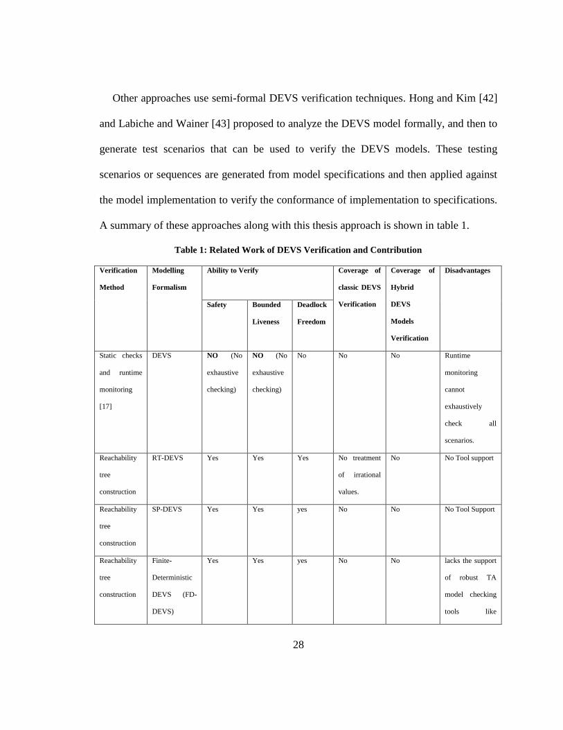
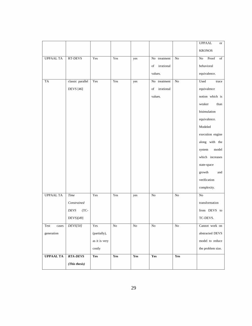
A summary of these approaches along with this thesis approach is shown in table 1.
Table 1: Related Work of DEVS Verification and Contribution
Verification
Method
Modelling
Formalism
Ability to Verify
Coverage of
classic DEVS
Verification
Coverage of
Hybrid
DEVS
Models
Verification
Disadvantages
Safety Bounded
Liveness
Deadlock
Freedom
Static checks
and runtime
monitoring
[17]
DEVS NO (No
exhaustive
checking)
NO (No
exhaustive
checking)
No No No Runtime
monitoring
cannot
exhaustively
check all
scenarios.
Reachability
tree
construction
RT-DEVS Yes Yes Yes No treatment
of irrational
values.
No No Tool support
Reachability
tree
construction
SP-DEVS Yes Yes yes No No No Tool Support
Reachability
tree
construction
Finite-
Deterministic
DEVS (FD-
DEVS)
Yes Yes yes No No lacks the support
of robust TA
model checking
tools like
29
UPPAAL or
KRONOS
UPPAAL TA RT-DEVS Yes Yes yes No treatment
of irrational
values.
No No Proof of
behavioral
equivalence.
TA classic parallel
DEVS [46]
Yes Yes yes No treatment
of irrational
values.
No Used trace
equivalence
notion which is
weaker than
bisimulation
equivalence.
Modeled
execution engine
along with the
system model
which increases
state-space
growth and
verification
complexity.
UPPAAL TA Time
Constrained
DEVS (TC-
DEVS)[49]
Yes Yes yes No No No
transformation
from DEVS to
TC-DEVS.
Test cases
generation
DEVS[50] Yes
(partially),
as it is very
costly
No No No No Cannot work on
abstracted DEVS
model to reduce
the problem size.
UPPAAL TA RTA-DEVS
(This thesis)
Yes Yes Yes Yes Yes
30
The techniques we showed so far concern the verification of hard real-time systems.
In these systems, we cannot tolerate any response missing its deadline. However many
real-time systems can tolerate some occasional missing of deadlines, and in this case, the
system can still perform its function with some degraded performance. These system are
called soft real-time. In these systems, a verification question would be “with probability
0.99 or better, the system would respond within 10 time units”. Answering this question
requires modeling the system in a formalism that allows probabilistic behaviour such as
stochastic DEVS [44] and Probabilistic Timed Automata [45].
2.4 Hybrid DEVS models
Hybrid models are particularly important in modeling digital control systems where the
controlled environment obeys the laws of physics, while the controller can be a digital
discrete system or a combination of both digital and analog. The study of such systems
requires the verification of the resulting hybrid system.
A major problem in verification of hybrid systems is the lack of a unified theory to
model and solve both continuous and discrete components together [46]. As a result,
modeling and simulation is still one of the most useful methods to verify this kind of
systems [47] [48] [49]. Hybrid systems simulation was enabled within the DEVS
formalism by using a new method, called Quantizes State System (QSS) that will be
covered in section 2.4.1, which allows modeling continuous components [50][51][52].
However, simulation does not guarantee the absence of defects from the system under
31
study. Simulation verifies the system for particular scenarios chosen by the system tester.
As many hybrid systems are embedded in nature, and their failure could cause
catastrophic results, it is of most importance to verify these systems for their adherence to
requirements and their absence from defects. Formal methods can be used to provide
such a guarantee. In doing so, a hybrid system needs to be modeled and verified within a
formal framework.
In order to use this algorithmic method (model checking through reachability analysis)
to verify hybrid systems, the focus would be to find a suitable finite abstraction of the
hybrid system that could be verified, and hence the reachability algorithm could be
guaranteed to terminate. Different types of labelled transition systems were proposed to
model hybrid systems abstractions including Petri Nets [53], hybrid automata [54] and
TA [4].
Some research has used hybrid TA for modeling hybrid systems and verifying them.
This type of automata describes the system with a Timed Labelled Transition System
(TLTS) and linear differential equations [54]. However, as Henzinger et al. shows in
[55], Hybrid TA verification through reachability analysis is not decidable in general. For
this reason, recent research has concentrated on modeling the hybrid system in some form
with a decidable verification such as TA. In doing so, a technique must be used to model
the continuous component in a discrete finite form. As continuous system variables are
real values and dense in time (i.e. time scale is continuous and we have infinitely many
time points in any bounded interval), their state space could be infinite. An
32
approximation to a finite representation is needed to enable the decidability and
termination of reachability analysis. Many techniques have been proposed to approximate
the continuous-time systems into a discrete representation of TA [56] [57][58][59].
Although DEVS is a discrete-event system specification, some work has been done to
represent continuous systems in a discrete format that can be modeled and simulated with
DEVS. One of these methods is Quantized State Systems (QSS) method [51]. Using QSS
enables modeling and simulation of hybrid systems with DEVS formalism.
2.4.1 The Quantized State Systems (QSS) method
This section is devoted to give a general introduction to the QSS method, as introduced in
[50] and [51]. The QSS is an approximation method to model and simulate continuous
systems, which are usually modeled with Ordinary Differential Equations (ODE) and
Algebraic Equations. This combination of equations describing the system behaviour is
generally called Differential Algebraic Equations (DAE). Obtaining a detailed description
of the system behaviour entails solving these equations simultaneously. In doing so,
many different techniques of numerical integration have been proposed to solve ODEs;
namely Euler, Runge-Kutta, etc [60]. These methods approximate the solution of ODEs,
and they limit the error to an acceptable range based on the choice of its discrete
integration step. All these methods rely on discrete-time integration of ODEs. In this way,
time is allowed to progress in small steps, and at each step, an approximation is computed
for the ODEs solution. When a system modeled by DAE has a discontinuity (i.e. a sudden
jump in its variables values with regard to time), the numerical integration method may
33
produce unacceptable errors [52]. Unfortunately, this kind of discontinuity are normal
properties of hybrid systems, which can be seen as operating in different modes, each
described with a specific ODEs. An example of such a system would be a heating system
with an on-off thermostat switch; in this system, the ODEs describing the system in the
heating state (i.e., when the thermostat is in on position) are different from those
describing cooling state (i.e., the thermostat is in the off position).
The Quantized State Systems QSS [50][51][60] is a different method for
approximation, a quantization-based method that models hybrid systems as discrete-event
systems and not as discrete-time. In the quantization-based method, instead of fixing a
time step and calculating the value of the state variable at the next time step, we calculate
when the state variable reaches a certain value. This value is called a quantization level,
and the difference between two quantization levels is called the quantum. Obviously with
a quantization-based method, the time it takes for a state variable to reach a quantization
level depends on the state variable slope. The greater the slope, the less time it takes to
reach the next level. This produces a variable time-step integration, which becomes an
advantage when the system has a vector of state variables, in which each variable has a
different change rate (slope). In this case, a variable with large slope would generate
more events per unit time, than a variable with a flat slope. As DEVS is an event-based
formalism, meaning it would only react to generated or received events, thus a slow-
changing variable would need less computations, than a rapidly-changing variable. This
event-based property of DEVS also solves the above problem around discontinuities
34
found while solving hybrid systems. In fixed time-step integration methods, the step
boundary has to exactly match the point in time in which the discontinuity (or a system
jump) happens. Otherwise, the integration would suffer major error if it assumes a
continuous trajectory around the discontinuity and handles this in single time step. This
problem however, disappears with discrete-event system simulation such as DEVS
because whenever an event triggers a discontinuous transition in the system state, DEVS
simulator would react to this event and calculate the system state resulting from that
event as discussed in [51]. Thus, the integration slope (which is a part of the system state)
before the event would be different from that after the discontinuity event. This would
guarantee the correct calculation of the system variables before and after the system
jump. Consider a continuous system modeled by a time-invariant Ordinary Differential
Equation (ODE), and its State Equation System (SES) representation:
x˙ (t) = f[x(t), u(t) ) ] (Eq. 2.4)
Here x(t) n represents the system state vector such as (x1(t),x2(t),x3(t),…xn(t)) and
u(t) m represents an input vector , which is a known piecewise constant function.
With the QSS method, we simulate an approximate system, which is called the Quantized
State System:
x˙ (t) = f[q(t), u(t) ) ] (Eq. 2.5)
Where q(t) is a vector of quantized variables (q1(t), q2(t), …, qn(t)) that are obtained
with the quantization function q from the state variables x(t).
35
Each component of q(t) is related to the corresponding component of x(t) by a
hysteretic quantization function, which is defined here as given in [51]:
“Definition 1. Let Q = {Q0,Q1, ...,Qr} be a set of real numbers where Qk−1 < Qk with 1
≤ k ≤ r. Let Ω be the set of piecewise continuous real valued trajectories and let xi Ω be
a continuous trajectory. Let b: Ω → Ω be a mapping and let qi = b(xi) where the
trajectory qi satisfies:
qi (t) =
otherwiset
kt
rkt
i
kiki1k
ki1ki1k
0m
q
0Qq -Q (t) xif Q
Qq Q (t) xif Q
t t if Q
Where:
- Qm : is the initial quantization value at start of time t0.
- Qk+1: is the next quantization level at time t if the function slope is positive and
last quantization level the function has crossed was Qk.
- Qk-1: is the next quantization level at time t if the function slope is negative, the
last quantization level the function crossed was Qk, and the function value xi(t) is
less than quantization level Qk by the hysteresis value ε.
- t- is a point in time such that t- < t
The index m is described by:
m =
1 j0i j
r0i
00i
Q )(txQ if j
Q )(t xif r
Q )(t xif 0
36
Then, the map b is a hysteretic quantization function.
The discrete values Qk are called quantization levels and the distance between two
successive quantization levels (Qk+1 − Qk) is defined as the quantum, which is usually
constant. The width of the hysteresis window is ε. The values Q0 and Qr are the lower and
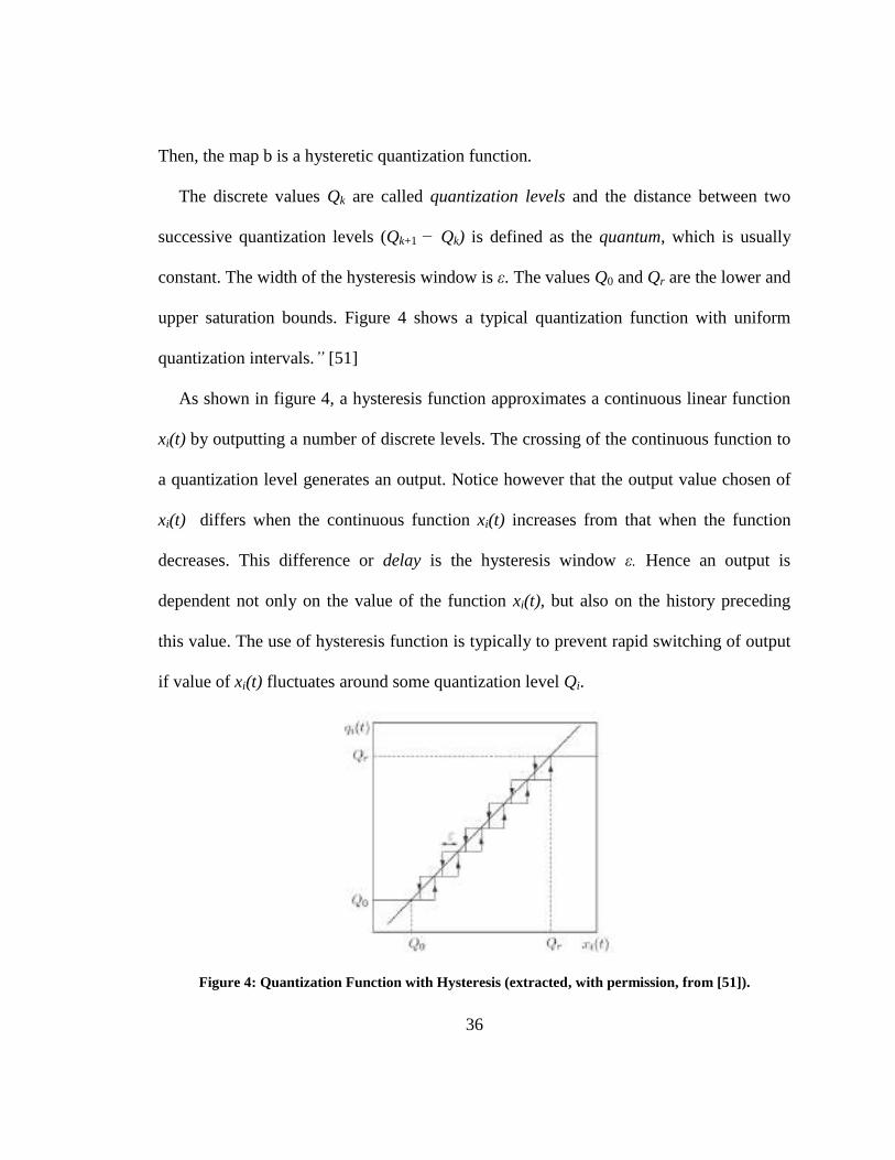
upper saturation bounds. Figure 4 shows a typical quantization function with uniform
quantization intervals.” [51]
As shown in figure 4, a hysteresis function approximates a continuous linear function
xi(t) by outputting a number of discrete levels. The crossing of the continuous function to
a quantization level generates an output. Notice however that the output value chosen of
xi(t) differs when the continuous function xi(t) increases from that when the function
decreases. This difference or delay is the hysteresis window ε. Hence an output is
dependent not only on the value of the function xi(t), but also on the history preceding
this value. The use of hysteresis function is typically to prevent rapid switching of output
if value of xi(t) fluctuates around some quantization level Qi.
Figure 4: Quantization Function with Hysteresis (extracted, with permission, from [51]).
37
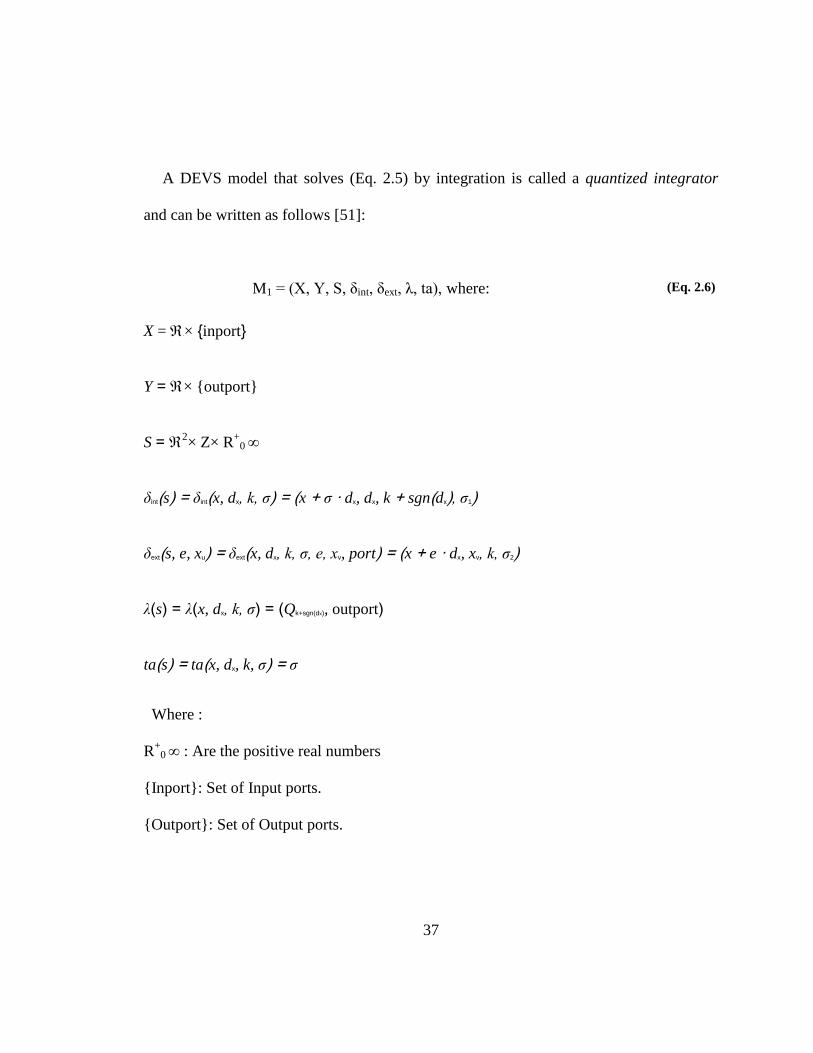
A DEVS model that solves (Eq. 2.5) by integration is called a quantized integrator
and can be written as follows [51]:
M1 = (X, Y, , δint, δext, λ, ta), where:
X = R× {inport}
Y = × {outport}
S = 2× Z× R+0 ∞
δint(s) = δint(x, dx, k, σ) = (x + σ · dx, dx, k + sgn(dx), σ1)
δext(s, e, xu) = δext(x, dx, k, σ, e, xv, port) = (x + e · dx, xv, k, σ2)
λ(s) = λ(x, dx, k, σ) = (Qk+sgn(dx), outport)
ta(s) = ta(x, dx, k, σ) = σ
(Eq. 2.6)
Where :
R+0 ∞ : Are the positive real numbers
{Inport}: Set of Input ports.
{Outport}: Set of Output ports.
38
σ1 =
0
0)1(
0)1(2
xdif
xdifxdkQkQ
xdifxd
kQkQ
and
σ2 =
0
0)().(
0).(1
vxif
vxifvx
kQxdex
vxifvx
xdexkQ
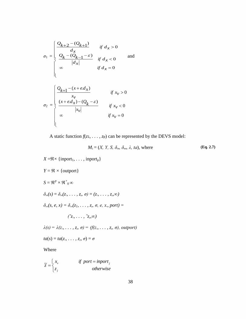
A static function f(z1, . . . , zp) can be represented by the DEVS model:
M2 = (X, Y, S, δint, δext, λ, ta), where
X =× {inport1, . . . , inportp}
Y = × {outport}
S = p × +0 ∞
δint(s) = δint(z1, . . . , zp, σ) = (z1, . . . , zp,∞)
δext(s, e, x) = δext(z1, . . . , zp, σ, e, xv, port) =
(˜z1, . . . , ˜zp,∞)
λ(s) = λ(z1, . . . , zp, σ) = (f(z1, . . . , zp, σ), outport)
ta(s) = ta(z1, . . . , zp, σ) = σ
Where
otherwisez
inportportifxz
j
jv~
(Eq. 2.7)
39
As indicated in [51], this combined DEVS model of M1 and M2 simulates the QSS
system.
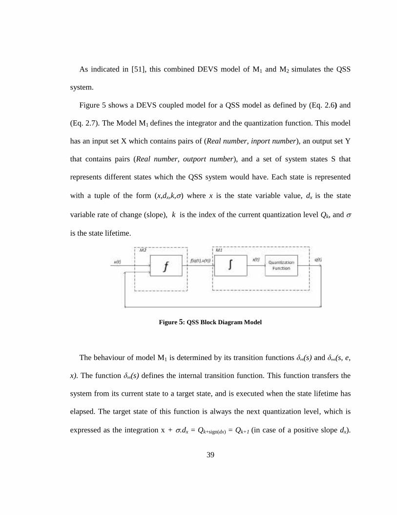
Figure 5 shows a DEVS coupled model for a QSS model as defined by (Eq. 2.6) and
(Eq. 2.7). The Model M1 defines the integrator and the quantization function. This model
has an input set X which contains pairs of (Real number, inport number), an output set Y
that contains pairs (Real number, outport number), and a set of system states S that
represents different states which the QSS system would have. Each state is represented
with a tuple of the form (x,dx,k,) where x is the state variable value, dx is the state
variable rate of change (slope), k is the index of the current quantization level Qk, and
is the state lifetime.
Figure 5: QSS Block Diagram Model
The behaviour of model M1 is determined by its transition functions δint(s) and δext(s, e,
x). The function δint(s) defines the internal transition function. This function transfers the
system from its current state to a target state, and is executed when the state lifetime has
elapsed. The target state of this function is always the next quantization level, which is
expressed as the integration x + .dx = Qk+sign(dx) = Qk+1 (in case of a positive slope dx).
40
The lifetime of this target state 1 is the time needed to reach the next quantization level
Qk+2 and is calculated as shown above in (Eq. 2.6). δext(s, e, x) defines the external
transition function, and it is triggered whenever an input reaches an inport. In this model,
the input is a pair (xv,port) where xv is the slope calculated as xv = f(q(t),u(t)), as shown in
the diagram of Figure 5. The target state of this function is a new state with an updated
value of the state variable xi+1 = xi+e.dx, new slope xv, and a new calculated lifetime 2
equals to the time needed to reach the next quantization level. λ(s) in M1 is the output
function and when triggered, it sends the value of the current quantization level to the
outport. M2 models a static function that accepts q(t) and u(t) as inputs and calculates
f(q(t),u(t).
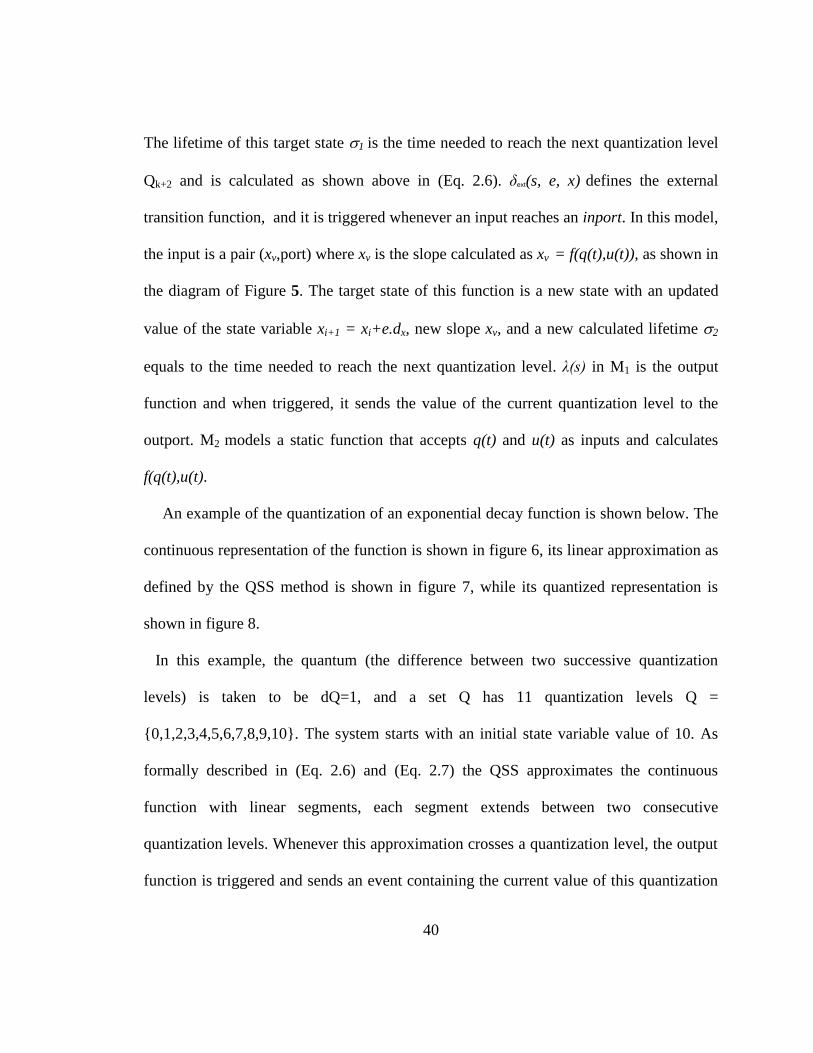
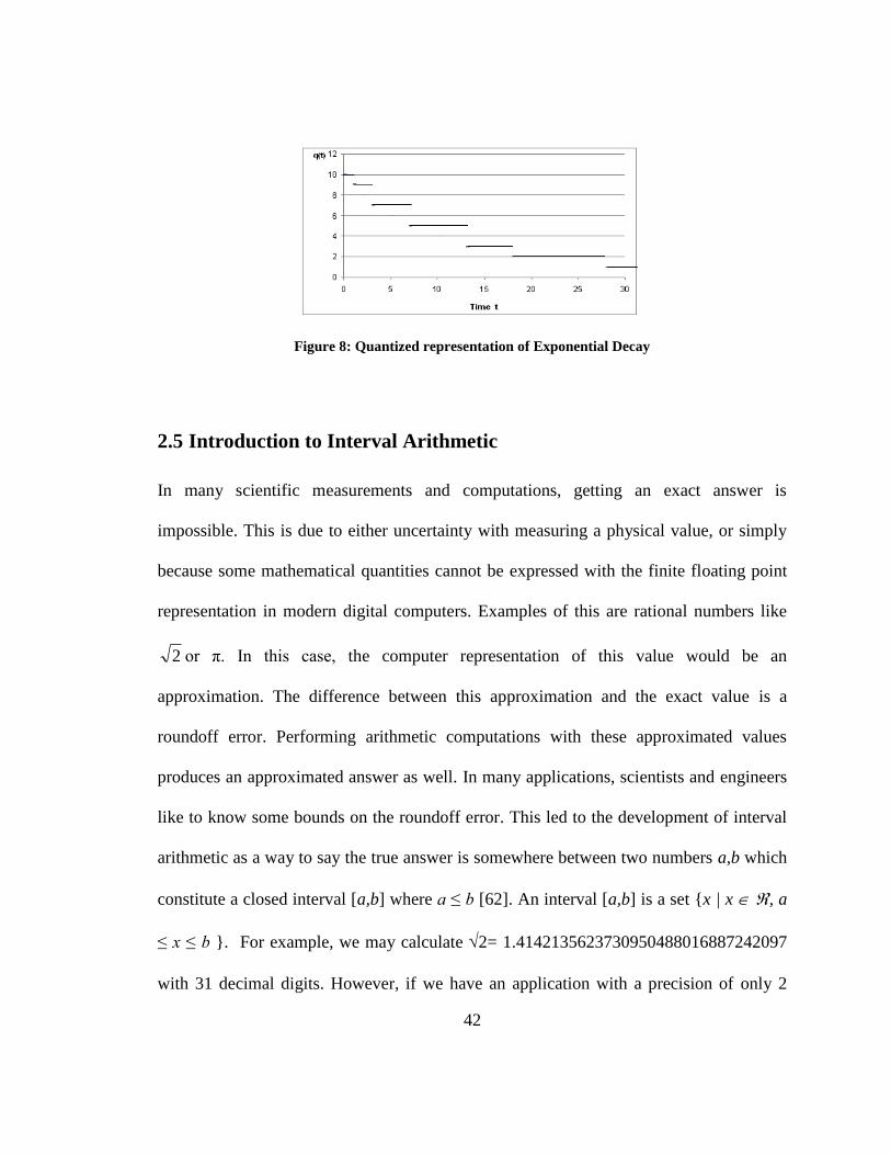
An example of the quantization of an exponential decay function is shown below. The
continuous representation of the function is shown in figure 6, its linear approximation as
defined by the QSS method is shown in figure 7, while its quantized representation is
shown in figure 8.
In this example, the quantum (the difference between two successive quantization
levels) is taken to be dQ=1, and a set Q has 11 quantization levels Q =
{0,1,2,3,4,5,6,7,8,9,10}. The system starts with an initial state variable value of 10. As
formally described in (Eq. 2.6) and (Eq. 2.7) the QSS approximates the continuous
function with linear segments, each segment extends between two consecutive
quantization levels. Whenever this approximation crosses a quantization level, the output
function is triggered and sends an event containing the current value of this quantization
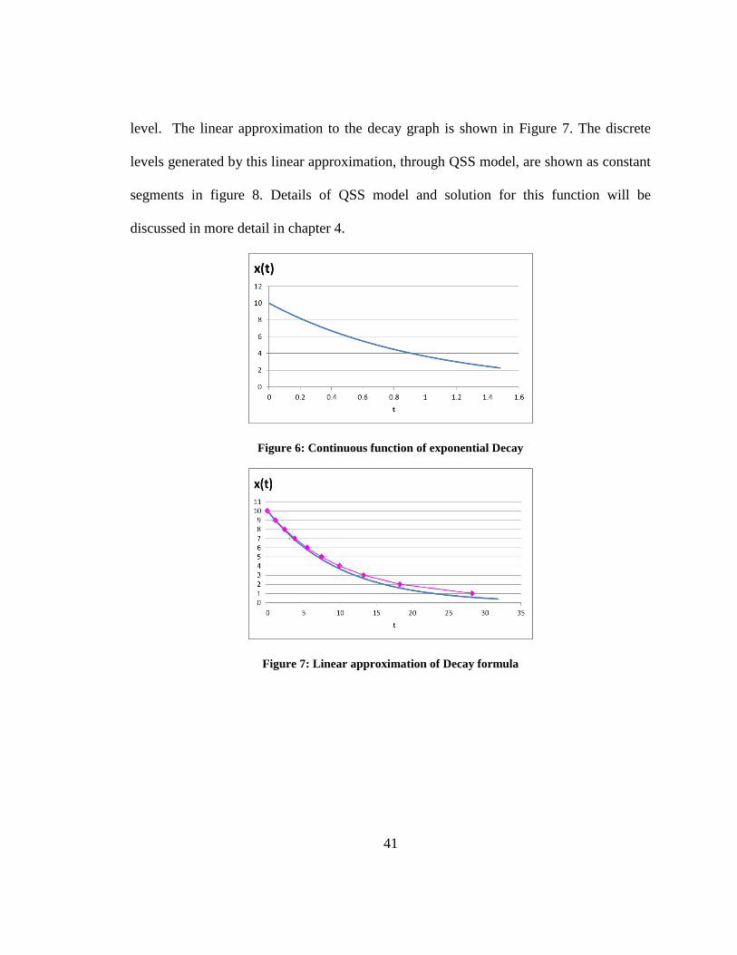
41
level. The linear approximation to the decay graph is shown in Figure 7. The discrete
levels generated by this linear approximation, through QSS model, are shown as constant
segments in figure 8. Details of QSS model and solution for this function will be
discussed in more detail in chapter 4.
Figure 6: Continuous function of exponential Decay
Figure 7: Linear approximation of Decay formula
42
Figure 8: Quantized representation of Exponential Decay
2.5 Introduction to Interval Arithmetic
In many scientific measurements and computations, getting an exact answer is
impossible. This is due to either uncertainty with measuring a physical value, or simply
because some mathematical quantities cannot be expressed with the finite floating point
representation in modern digital computers. Examples of this are rational numbers like
2 or π. In this case, the computer representation of this value would be an
approximation. The difference between this approximation and the exact value is a
roundoff error. Performing arithmetic computations with these approximated values
produces an approximated answer as well. In many applications, scientists and engineers
like to know some bounds on the roundoff error. This led to the development of interval
arithmetic as a way to say the true answer is somewhere between two numbers a,b which
constitute a closed interval [a,b] where a ≤ b [62]. An interval [a,b] is a set {x | x , a
≤ x ≤ b }. For example, we may calculate 2= 1.4142135623730950488016887242097
with 31 decimal digits. However, if we have an application with a precision of only 2
43
decimal digits, we may get an answer of 1.41, or 1.42 depending on the way the
calculator rounds the result down or up. In either way, we do not get the true answer, and
this may not be acceptable for many applications. Using an interval to express the answer
as [1.41, 1.42] guarantees the inclusion of the true answer.
Ordinary mathematical operators can be defined for intervals, for example if A = [a,b],
B = [c,d], then the following operations are defined for intervals [61] [62][63]:
A + B = [a,b] + [c,d] = [a+c,b+d]
A – B = [a,b] + [c,d] = [a-c,b-d]
A * B = [a,b] * [c,d] = [min(a*c, a*d, b*c, b*d),max(a*c, a*d, b*c, b*d)]
A / B = [a,b] / [c,d] = [a,b] * [1/d,1/c] if 0 [c,d]
If we know that a,b,c,d are all positive numbers, then multiplication rule can be
simplified as:
A * B = [a,b] * [c,d] = [ (a*c) , (b*d)]
Arithmetic calculations for complex functions are also defined for intervals. There are
about 18 different comparison operators for intervals, of which many do not exist for
Real numbers. Moore [63] details many operations on interval arithmetic, properties of
interval arithmetic, and computation algorithms for computing ODE solutions based on
intervals.
This brief introduction of interval arithmetic is sufficient for our purposes for this
thesis as details of this analysis is beyond the thesis scope. We will propose to use
44
intervals and some of its arithmetic in section 5.1 for QSS verification as a way of
bounding the true value calculated by QSS within some closed integer interval.
2.6 Summary Discussion of the State-of-the-Art
The approaches for the verification of DEVS that was covered during state-of-the-art
survey have the following disadvantages when compared to the methodology introduced
in this thesis:
1. Subclasses of DEVS (as SP-DEVS, FD-DEVS or TC-DEVS) constrain classic
DEVS in such a way that it reduces expressiveness, and thus their usefulness to
the system modeller. This limits what the modeller can do, and renders some
portions of existing DEVS models to be non-verifiable, unless they are re-
defined to match the subclass definition (and only when this is possible).
2. The above subclasses of DEVS try to define their own reachability analysis by
defining algorithms for building reachability graphs. These algorithms are
based on basic model-checking algorithm, thus suffering from the same basic
state-space explosion problem, and offer the same space-time complexity as
standard model checking algorithms. These DEVS verification algorithms are
implemented in ad-hoc model checking tools. Instead, there is a number of
well-established model checking tools like UPPAAL and KRONOS, which
have a large community of users and developers. These tools have
implemented efficient data structures and optimizations that accumulated
through years of research to optimize their performance. Nevertheless, such
45
tools cannot verify DEVS subclasses with DEVS-specific reachability
algorithms because unless DEVS subclasses are translated to TA, which is the
input language of these tools, DEVS subclasses verification cannot be handled
by these tools.
3. Some other approaches have translated DEVS models into another verifiable
form such as TA, and then verified TA models by standard TA model checking
tools like UPPAAL. These approaches, however, did not provide
transformation based on formal behavioural equivalency between DEVS and
TA. As a result, their transformation is not guaranteed to produce
behaviourally equivalent TA for a given DEVS model.
4. Translation from DEVS to TA in previous approaches did not specify a
method to translate DEVS models that may be unverifiable because it contains
irrational values, and hence did not provide a method to estimate any effect of
approximation irrational values on the verification results.
5. Previous translations approaches from DEVS to TA did not handle cases where
DEVS model has continuous system components approximated with the QSS
method. This excludes the hybrid systems from these verification approaches.
46
Chapter 3: Thesis contribution
In order to deal with the multiple limitations of other approaches discussed in section 2.6,
this thesis introduces a new set of methods for modeling, simulation and verification. The
main objectives are the following:
1. Defining a methodology to translate models of DEVS to models of TA. This
methodology can handle DEVS models that may contain irrational values, thus it
could be used to verify any existing DEVS model without the need to re-write it
with a different DEVS subclass.
2. The proposed approach translates DEVS to TA, through sound formal translation.
This allows the use of standard tools like UPPAAL [9] to verify the resulting TA
models. This approach takes advantage of numerous optimizations implemented
in TA verification tools such as UPPAAL. TA was chosen for this research as it
has strong theoretical background and mature verification tools such as UPPAAL
and KRONOS. TA is also suited to state transition systems such as DEVS, while
Timed Petri nets are suited more to process flow modeling [64]. The UPPAAL
tool offers proven record of verification of industrial size problems with an easy
interface that allows the user to enter the model and see the verification results.
3. The proposed approach uses a translation methodology that is based on
bisimulation as a basis of behavioural equivalency between DEVS and TA. This
47
equivalence relation is stronger than the trace equivalence [39], and it preserves
all properties through the translation between the two models.
4. The approach provides a method to approximate any irrational values that may
exist in a DEVS model. It also bases its reasoning on the effect of this
approximation on the well-known results of robust TA [65][66][67] as we will
show later. This gives the modeller a way to know if this approximation would
affect the verification results for the given DEVS model or not.
5. The methodology extends existing verification methods to handle continuous
systems modeled with DEVS through the QSS method. This enables the
verification of hybrid DEVS models that contain discrete and continuous
components.
At present, the methodology introduced in this thesis has achieved the goals above.
This was done by first providing a definition of a new class of DEVS, called RTA-DEVS
[68], which is very close to classic DEVS in semantics and expressive power. RTA-
DEVS has followed FD-DEVS in restricting the time advance function to nonnegative
rational numbers, but also relaxed the restriction of FD-DEVS on external transition
functions. This makes RTA-DEVS closer to general DEVS than FD-DEVS. This enables
the modeller to use a formalism that is more expressive than FD-DEVS to model a
system and it is still formally verifiable.
As a second step, this thesis also discusses a transformation from RTA-DEVS models
to TA models based on the bisimulation relation between the two models. This
48
guarantees behavioural equivalence between the two models and preserves properties
from RTA-DEVS into the resulting TA, and vice versa. This preservation is an important
requirement to ensure that the verification results of TA are mapped back to RTA-DEVS
models. Many classic DEVS models satisfy the semantics of RTA-DEVS models. Thus,
they can be simulated with any DEVS simulator, and they can be transformed to TA to
validate the desired properties formally.
As third step, we enable the verification of classic DEVS models that may contain
irrational values and thus cannot directly be transformed to RTA-DEVS (and
consequently to TA). To do so, this thesis proposed a method to transform DEVS to
RTA-DEVS , and an approximation of DEVS models to RTA-DEVS as we showed in
[68]. We used an approximation technique for irrational values to maintain the behaviour
of the original DEVS model. In addition, we propose a method to estimate any effect the
approximation may have on the final DEVS verification results [70][71].
Finally, a general method is proposed to model any QSS system with TA, thus
enabling formal verification to continuous components modeled with the QSS method. A
full list of published contributions, resulting from this work, is shown in the next section.
In Figure 9, we show the thesis contribution on a diagram representing expressive
power and decidability. In this diagram, different formalisms are shown as ellipses. The
containment relationship between a larger ellipse and a smaller one indicates that the
expressiveness of the small is less than the larger one. In this diagram, we show some of
DEVS subclasses (SP-DEVS, FD-DEVS and RTA-DEVS). These subclasses are less
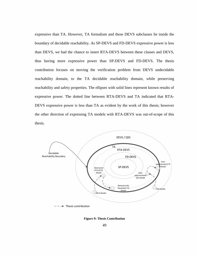
49
expressive than TA. However, TA formalism and these DEVS subclasses lie inside the
boundary of decidable reachability. As SP-DEVS and FD-DEVS expressive power is less
than DEVS, we had the chance to insert RTA-DEVS between these classes and DEVS,
thus having more expressive power than SP-DEVS and FD-DEVS. The thesis
contribution focuses on moving the verification problem from DEVS undecidable
reachability domain, to the TA decidable reachability domain, while preserving
reachability and safety properties. The ellipses with solid lines represent known results of
expressive power. The dotted line between RTA-DEVS and TA indicated that RTA-
DEVS expressive power is less than TA as evident by the work of this thesis; however
the other direction of expressing TA models with RTA-DEVS was out-of-scope of this
thesis.
FD-DEVS FD-DEVS
SP-DEVSSP-DEVS
DEVS / QSS
TA
Decidable Reachability Boundary
RTA-DEVS
Thesis contribution
DEVS Model
Abstracted RTA-DEVS
Model
Behaviourally Equivalent TA
ModelQSS Model
Over approximated TA
Model
Over approximated
QSS Model
Figure 9: Thesis Contribution
50
3.1 List of Published Contributions
Hesham Saadawi, Gabriel A. Wainer. 2009. “ erification of real-time DEVS
models”. Proceedings of DEVS Symposium 2009. San Diego, CA [72]. In this
paper, we introduced a methodology for verifying Real-Time DEVS models. Our
methodology applies recent advances in theoretical model checking to DEVS
models. The methodology also handles the cases where theoretical approach is not
feasible to cross the gap between abstract Timed Automata models and the
complexity of the DEVS Real-time implementation by empirical software
engineering methods. This contribution is described in chapter 4.
Hesham Saadawi, Gabriel A. Wainer. 2010. “Rational time-advance DEVS
(RTA-DEVS)”. Proceedings of DEVS Symposium 2010. Orlando, FL. 2010. This
paper was selected as the runner-up best paper in the Symposium. In this paper,
we introduced a new extension to the DEVS formalism, called Rational Time-
Advance DEVS (RTA-DEVS). The basic idea of this new formalism is to permit
modeling the behavior of systems that can be modeled by classical DEVS;
however, RTA-DEVS models could be formally checked with standard model-
checking algorithms and tools. In order to do so, we introduce a procedure to
create Timed Automata models that are behaviorally equivalent to the original
RTA-DEVS models [68]. This contribution is described in chapter 4.
51
Hesham Saadawi, Gabriel A. Wainer. 2010. “From to RTA- ”. In
Proceedings of the 2010 IEEE/ACM 14th International Symposium on
Distributed Simulation and Real Time Applications (DS-RT '10). IEEE Computer
Society, Washington, DC, USA, 207-210 [73]. In this paper we defined the RTA-
DEVS formalism to model and verify real-time embedded systems. In order to
enable the formal verification of DEVS models, we introduced a procedure to
approximate DEVS with RTA-DEVS. We also included the conditions for the
valid approximated RTA-DEVS models and a calculation method for
approximation errors that may be introduced. This contribution is described in
chapter 4.
Hesham Saadawi, Gabriel A. Wainer. 2011. “Principles of Models
erification”. Accepted for publication in: SIMULATION: Transactions of the
Society for Modeling and Simulation International [70]. In this journal paper, we
introduced our methodology to verify real-time embedded systems modeled with
DEVS formalism. This is composed of a procedure to create Timed Automata
models that are behaviorally equivalent to the original RTA-DEVS models, then,
we described the use of the available TA tools and theories for formal model
checking. Further, we introduced a methodology to transform classic DEVS
models to RTA-DEVS, thus enabling formal verification of classic DEVS with an
acceptable accuracy. This contribution is described in chapter 4.
52
Hesham Saadawi, Gabriel A. Wainer, Mohammad Moallemi. 2012. “Principles
of DEVS Models Verification for Real-Time mbedded Applications”. Real-Time
Simulation Technologies: Principles, Methodologies, and Applications. K.
Popovici, P. Mosterman Eds. Taylor and Francis. CRC Press. 2012 [71]. In this
book chapter, we explained our proposed methodology to verify real-time DEVS
models of embedded systems. A case study of mechanical robot and its controller
was defined and verified using our methodology. This contribution is described in
chapter 4.
Hesham aadawi, Gabriel Wainer. 2012. “On the verification of hybrid
models”. In Proceedings of the 2012 Symposium on Theory of Modeling and
Simulation - DEVS Integrative M&S Symposium (TMS/DEVS '12), Orlando,
FL,USA. March 26-28. In this paper [81], we introduced a new verification
methodology, based on RTA-DEVS, Timed Automata and the QSS method,
which allows verifying real-time hybrid systems modeled by DEVS formalism.
This contribution is described in chapter 5.
Hesham aadawi, Gabriel Wainer. 2013. “Hybrid Systems Modeling and
Verification with DEVS”. In Proceedings of the 2013 Symposium on Theory of
Modeling and Simulation - DEVS Integrative M&S Symposium (TMS/DEVS '13),
San Diego, CA, USA. April 7-10. Submitted for publication. In this paper, we
introduce a methodology to verify hybrid systems modeled with DEVS and using
53
general QSS method to model the continuous components. This contribution is
described in chapter 5.
54
Chapter 4: The RTA-DEVS formalism
In chapter 1 and chapter 2, we have discussed the issues that are faced by the developers
of RT embedded systems, and we gave a brief background about current techniques and
formalisms that we plan to use to solve some of these issues. To accomplish the objective
stated in chapter 1, we need a simulation technique that is formally verifiable and has
executable models. The latter is a property of Discrete-Event Systems Specification
(DEVS) formalism [7], namely the facility to generate executable models from a discrete-
event specification. For DEVS to be also verifiable, this thesis proposes a complete
methodology to verify different types of DEVS, thus enabling full life cycle of RT
systems development using DEVS. This development life cycle can be described with
traditional software development cycle where phases of analysis, design can use formal
verification as part of its activities. The verification methodology proposed here is based
on a technique of formal software verification called model checking [19]. The advantage
of this technique is that it is fully automated and does not need human intervention to
reveal errors in system design.
As discussed earlier, the reason for introducing a new DEVS verification methodology
is that existing methods limit verification to constrained subclasses of DEVS. This
prevents the verification of wide range of existing DEVS models, and limits the modeller
to use less expressive subclasses. In addition, the verification algorithms proposed for
55
these subclasses need specially written verification tools. However, these specially
written verification tools may not add much value over standard timed model checking
tools. This is because these algorithms have the same time and space complexity as those
of timed model checking algorithms, and thus DEVS special verification tools do not
provide any advantages over timed model checking verification. On the other hand,
verification tools for timed model checking are widespread and they usually contain
many performance optimizations [25].
In order to do formal verification of DEVS, the methodology proposed is comprised of
a few steps. The first step is to introduce a new formalism based on DEVS, but restricted
in its behaviour to be less than DEVS to be verifiable. The reason why we use a restricted
class of DEVS as a first step, is that the formal verification of general classic DEVS is
undecidable as Hernandez and Giambiasi shown in [27] (and we would discuss this in
more detail later). Creating a restricted subclass of DEVS is a way to enforce some
restrictions into the model that can be created according to this subclass. This would
guarantee the ability to verify any model belonging to this restricted DEVS subclass. We
decided to use the model checking method due to its advantages over other formal
software verification methods such as deductive methods. As we discussed in chapter 1,
the main advantage of model checking is that it is fully automated without human
intervention, thus, it does not need advanced expertise in formal methods or formal
proofs as opposed to deductive formal methods. As DEVS is a timed formalism (i.e.
transition functions defining DEVS behaviour contain time in their domain), timed model
56
checking was chosen to verify the proposed subclass of DEVS called Rational-Time
Advance DEVS (RTA-DEVS) as published in [68] and we describe in this thesis in
chapter 4. RTA-DEVS has followed FD-DEVS [34] in restricting the time advance
function to nonnegative rational numbers, but also relaxed the restriction of FD-DEVS on
external transition functions. This makes RTA-DEVS more expressive than FD-DEVS.
However, RTA-DEVS still restricts the model in a way to remove the obstacles to formal
verification. This restriction enables having RTA-DEVS models which are verifiable
with standard formal verification tools for timed systems. In this way, the introduction of
RTA-DEVS can be seen as imposing restrictions on the type of DEVS models that can be
verified.
The second step shows a transformation from RTA-DEVS to TA. TA formal
verification is decidable, and there are academic and industrial tools implementing this
verification. However, TA is not designed to simulate complex systems, the physical
systems around the embedded software, or to be deployed as executable models on target
platforms. Instead, there are various DEVS environments that allow these; consequently,
DEVS has been used in various efforts to model and simulate systems in their design
phase. The transformation proposed here is based on the notion of bisimulation between
RTA-DEVS and TA, which gives behavioural equivalency between the two formalisms,
and it guarantees that any property in the RTA-DEVS model is preserved in the
transformed TA model. The results of this work were published in [68].
57
The third step in the methodology is to find a way to verify any DEVS models that
their definitions may not be restricted to RTA-DEVS specifications. To do so, a
transformation from DEVS to RTA-DEVS is presented to obtain verifiable RTA-DEVS
models as published in [73]. In that transformation process, we need to obtain an
approximation to the DEVS model. In order to do so in a safe way, we introduce a
mechanism to avoid introducing defects into RTA-DEVS when transforming from DEVS
[73]. However, a question arises about the validity of transformed RTA-DEVS
verification results when we apply it to the original DEVS model. In other words: how
much confidence do we have in these results and what effect the approximation may have
on the verification results?
The fourth step is to answer the above questions using theoretical results of TA, and
to apply this theory to the model under verification, in order to estimate any verification
error that may result from the approximations. These results were shown in [73].
In the methodology defined in this thesis, we use timed model checking because of its
advantages as a practical method in industrial systems. As mentioned earlier, one of these
advantages is the full automation without a need from a practitioner to be fluent in formal
method or mathematical proofs. Some of widely used tools for TA models verification
are UPPAAL [9] and KRONOS [74][75].
A final fifth step includes the use of a methodology to verify Continuous systems
modeled by the Quantized Sate Systems (QSS) [51] method and DEVS. This would
58
enable verification of hybrid systems (with discrete and continuous components modeled
with DEVS).
With this, we provide a complete methodology that covers discrete and continuous
DEVS components that can enable the formal verification of DEVS models. DEVS has
the advantages of being based on a formal definition, with component-based hierarchical
model construction, and is platform-independent. DEVS models are simulated within a
DEVS simulator, which isolates the model from the implementation. This gives the
advantage of avoiding any error that may creep between the steps of model verification
and implementation by executing the verified model directly without mapping it to an
executable code. This methodology gives the designer a comprehensive road map to
verify different classes of DEVS models using standard formal verification tools.
The following sections explain the RTA-DEVS definition, its transformation to TA
using the bisimulation relation to guarantee behavioural equivalence, the transformation
of any classic DEVS model into RTA-DEVS, and the estimation of any effect that this
last transformation may have on the verification results of RTA-DEVS. Verification of
QSS models are described in chapter 5.
4.1 Rational Time Advance DEVS (RTA-DEVS)
In [68], we proposed the RTA-DEVS formalism, a verifiable subclass of DEVS, with
very much of the expressive power of DEVS. The difference in expressive power comes
from the fact that RTA-DEVS does not accept irrational constants in its transition
functions. However, as we see later, this difference in behaviour can be easily
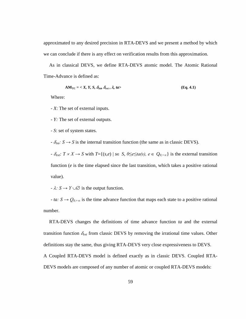
59
approximated to any desired precision in RTA-DEVS and we present a method by which
we can conclude if there is any effect on verification results from this approximation.
As in classical DEVS, we define RTA-DEVS atomic model. The Atomic Rational
Time-Advance is defined as:
AMTC = < X, Y, S, int, ext , ta> (Eq. 4.1)
Where:
- X: The set of external inputs.
- Y: The set of external outputs.
- S: set of system states.
- int: S → S is the internal transition function (the same as in classic DEVS).
- ext: T X → S with T={(s,e) | s S, 0≤e≤ta(s), e Q0,+∞} is the external transition
function (e is the time elapsed since the last transition, which takes a positive rational
value).
- : S → Y is the output function.
- ta: S → Q0,+∞ is the time advance function that maps each state to a positive rational
number.
RTA-DEVS changes the definitions of time advance function ta and the external
transition function ext from classic DEVS by removing the irrational time values. Other
definitions stay the same, thus giving RTA-DEVS very close expressiveness to DEVS.
A Coupled RTA-DEVS model is defined exactly as in classic DEVS. Coupled RTA-
DEVS models are composed of any number of atomic or coupled RTA-DEVS models:
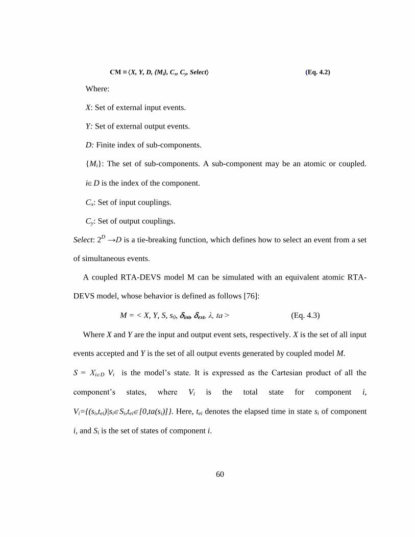
60
CM ≡ X, Y, D, {Mi}, Cx, Cy, Select (Eq. 4.2)
Where:
X: Set of external input events.
Y: Set of external output events.
D: Finite index of sub-components.
{Mi}: The set of sub-components. A sub-component may be an atomic or coupled.
iD is the index of the component.
Cx: Set of input couplings.
Cy: Set of output couplings.
Select: 2D →D is a tie-breaking function, which defines how to select an event from a set
of simultaneous events.
A coupled RTA-DEVS model M can be simulated with an equivalent atomic RTA-
DEVS model, whose behavior is defined as follows [76]:
M = < X, Y, S, s0, int, ext, λ, ta > (Eq. 4.3)
Where X and Y are the input and output event sets, respectively. X is the set of all input
events accepted and Y is the set of all output events generated by coupled model M.
S = ХiD Vi is the model’s state. It is expressed as the Cartesian product of all the
component’s states, where Vi is the total state for component i,
Vi={(si,tei)|siSi,tei[0,ta(si)]}. Here, tei denotes the elapsed time in state si of component
i, and Si is the set of states of component i.
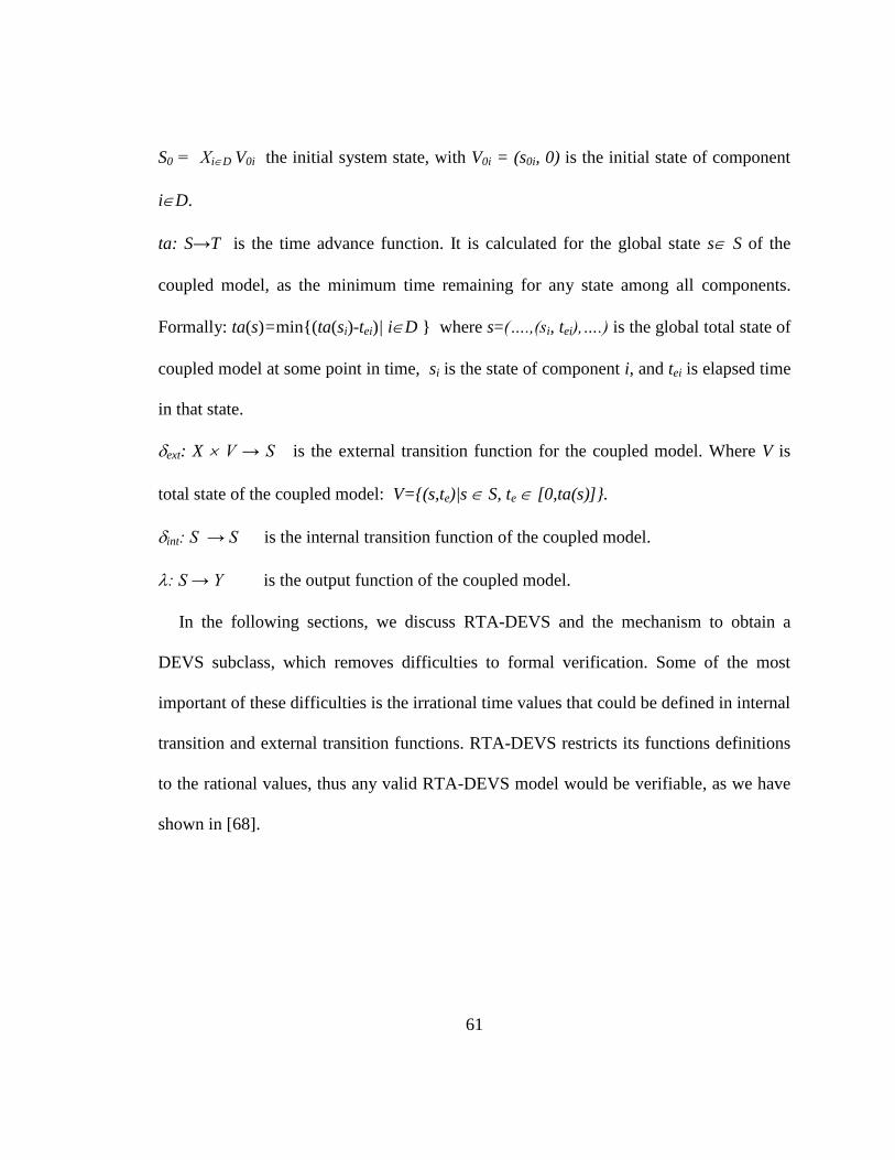
61
S0 = ХiD V0i the initial system state, with V0i = (s0i, 0) is the initial state of component
iD.
ta: S→T is the time advance function. It is calculated for the global state s S of the
coupled model, as the minimum time remaining for any state among all components.
Formally: ta(s)=min{(ta(si)-tei)| iD } where s=(….,(si, tei),….) is the global total state of
coupled model at some point in time, si is the state of component i, and tei is elapsed time
in that state.
ext: X V → S is the external transition function for the coupled model. Where V is
total state of the coupled model: V={(s,te)|s S, te [0,ta(s)]}.
int: S → S is the internal transition function of the coupled model.
: S → Y is the output function of the coupled model.
In the following sections, we discuss RTA-DEVS and the mechanism to obtain a
DEVS subclass, which removes difficulties to formal verification. Some of the most
important of these difficulties is the irrational time values that could be defined in internal
transition and external transition functions. RTA-DEVS restricts its functions definitions
to the rational values, thus any valid RTA-DEVS model would be verifiable, as we have
shown in [68].
62
4.2 Estimate of Expressiveness Difference between DEVS and RTA-
DEVS
There have been many proposed DEVS subclasses we shown in section 2.3. These
classes restricted the original DEVS behaviour in order to achieve decidable reachability.
In doing so, some of the expressive power of original DEVS is lost. Although we cannot
quantify how much expressive power is lost, we can devise a relative measure for how far
the expressive power of a DEVS subclass from the original DEVS. If we look at the
diagram shown in Figure 9, we observe that the wider the gap between the subclass and
the DEVS, the more subclasses can be inserted in this gap. Therefore, we can take an
relative measure of the gap width, from the ability to insert a number of DEVS subclasses
in this gap. For example, SP-DEVS has much less expressive power than DEVS. This is
evident by the fact that two other DEVS subclasses (FD-DEVS and RTA-DEVS) can be
inserted between SP-DEVS and DEVS in the expressiveness diagram of Figure 9. Thus, a
DEVS subclass “X” is closest to DEVS expressiveness when no other subclass “Y” can
be inserted in the gap between X and the original DEVS. We claim this is the case here
for RTA-DEVS as it is the closest DEVS subclass in its expressive power, and still has
decidable reachability.
Theorem: RTA-DEVS is the closest expressive and verifiable subclass to DEVS.
Proof:
We use induction to prove the above theorem. Assume there is another DEVS
subclass, we call it X-DEVS, that is more expressive than RTA-DEVS and its
63
reachability is decidable. From RTA-DEVS definition, we know that ta(s) = such that
RTA-DEVS { Q0,+∞ }, where Q0,+∞ is the set of positive rational numbers. Also from
DEVS definition we have DEVS { }, i.e. DEVS { Q0,+∞ IR0,+∞ } where IR is the
set of positive irrational numbers: IR = {2, 3, 5, ,…}. To define X-DEVS to be
more expressive than RTA-DEVS, we extend its set of possible values of to be more
than RTA-DEVS. Any possible such extension to RTA-DEVS would have X-DEVS {
Q0,+∞ { x | x IR0,+∞ } }. The least possible extension would be with only one element
from the set IR, i.e. X-DEVS { Q0,+∞ { 2} }. However, this makes reachability
analysis of this subclass of DEVS undecidable as it can have an irrational value in its
time advance function domain. This contradicts our assumption above, therefore we
conclude that we cannot have any subclass of DEVS which is more expressive than RTA-
DEVS and still has a decidable reachability.
4.3 RTA-DEVS to Timed Automata Behavioural Equivalence.
To verify RTA-DEVS by applying existing theories and the tools for TA, a TA model
must be constructed from the RTA-DEVS model in a way that guarantees its behavioural
equivalency. DEVS, RTA-DEVS, and TA are all instances of Timed Labelled Transition
Systems TLTS, and thus we would use here the methods of TLTS behavioural
equivalence to move from one modelling formalism to another. We start our discussion
here with a special case of TLTS which is the untimed LTS, and then we generalize our
findings to TLTS.
64
Generally there are two methods to check this (i.e., to see if two Labelled Transition
Systems (LTS) are behaviourally equivalent), namely Trace Equivalence and
Bisimulation. In [39], it was shown that, for RT Systems, trace equivalence is not enough
to show the complete equivalence of two LTS. Although one can show the trace
equivalency of two LTS (based on their acceptance or the generation of event traces),
RTS usually have multiple concurrent components working together. Those components
may go into a deadlock state in which no external event is observable. To show this, we
will use an example that was introduced in [39] with some modifications. In this
example, a user is interacting with an automated beverage machine that takes a coin and
serves either coffee or tea. A LTS diagram representing the machine behaviour is shown
in figure 10. The machine CTM1 shown in this diagram waits at state P0 for a coin to be
inserted, then after coin insertion, it moves to state P1 to give the user a selection of tea or
coffee. After serving the beverage, the machine returns to the waiting state P0. The
behaviour of a user who always requires coffee can be represented in the LTS diagram in
figure 11. This user puts the coin into the machine, and waits for the coffee to come out.
We can see that CTM1 and the User would work together for the desired results of
serving coffee. However, if we replace CTM1 with another machine with same
observable behaviour (trace equivalent), we may replace it with something like CTM2 as
shown in figure 12. Both CTM1 and CTM2 have the same observable trace for an
outside observer, as both machines accept a coin and then dispense either tea or coffee.
However if the user uses CTM2, it is possible to CTM2 to take the coin and then reach
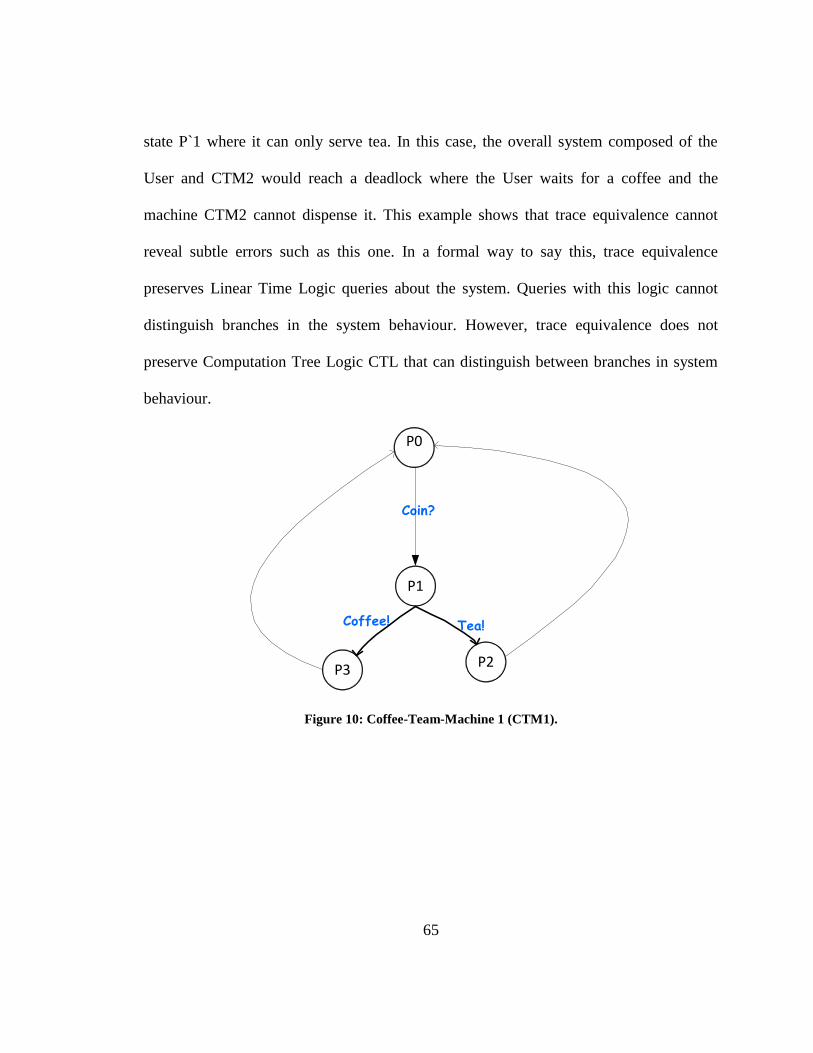
65
state P`1 where it can only serve tea. In this case, the overall system composed of the
User and CTM2 would reach a deadlock where the User waits for a coffee and the
machine CTM2 cannot dispense it. This example shows that trace equivalence cannot
reveal subtle errors such as this one. In a formal way to say this, trace equivalence
preserves Linear Time Logic queries about the system. Queries with this logic cannot
distinguish branches in the system behaviour. However, trace equivalence does not
preserve Computation Tree Logic CTL that can distinguish between branches in system
behaviour.
P0
P1
P2
Coin?
Tea!
P3
Coffee!
Figure 10: Coffee-Team-Machine 1 (CTM1).
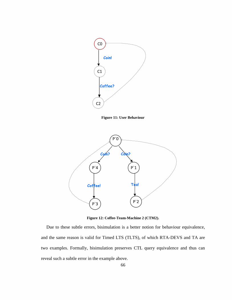
66
C0
C1
Coin!
Coffee?
C2
Figure 11: User Behaviour
P`0
P`4 P`1
P`2
Coin?
Tea!
P`3
Coin?
Coffee!
Figure 12: Coffee-Team-Machine 2 (CTM2).
Due to these subtle errors, bisimulation is a better notion for behaviour equivalence,
and the same reason is valid for Timed LTS (TLTS), of which RTA-DEVS and TA are
two examples. Formally, bisimulation preserves CTL query equivalence and thus can
reveal such a subtle error in the example above.
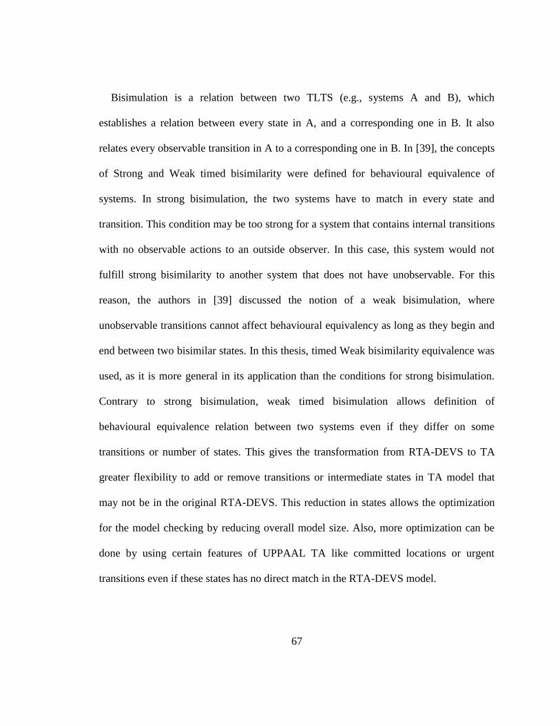
67
Bisimulation is a relation between two TLTS (e.g., systems A and B), which
establishes a relation between every state in A, and a corresponding one in B. It also
relates every observable transition in A to a corresponding one in B. In [39], the concepts
of Strong and Weak timed bisimilarity were defined for behavioural equivalence of
systems. In strong bisimulation, the two systems have to match in every state and
transition. This condition may be too strong for a system that contains internal transitions
with no observable actions to an outside observer. In this case, this system would not
fulfill strong bisimilarity to another system that does not have unobservable. For this
reason, the authors in [39] discussed the notion of a weak bisimulation, where
unobservable transitions cannot affect behavioural equivalency as long as they begin and
end between two bisimilar states. In this thesis, timed Weak bisimilarity equivalence was
used, as it is more general in its application than the conditions for strong bisimulation.
Contrary to strong bisimulation, weak timed bisimulation allows definition of
behavioural equivalence relation between two systems even if they differ on some
transitions or number of states. This gives the transformation from RTA-DEVS to TA
greater flexibility to add or remove transitions or intermediate states in TA model that
may not be in the original RTA-DEVS. This reduction in states allows the optimization
for the model checking by reducing overall model size. Also, more optimization can be
done by using certain features of UPPAAL TA like committed locations or urgent
transitions even if these states has no direct match in the RTA-DEVS model.
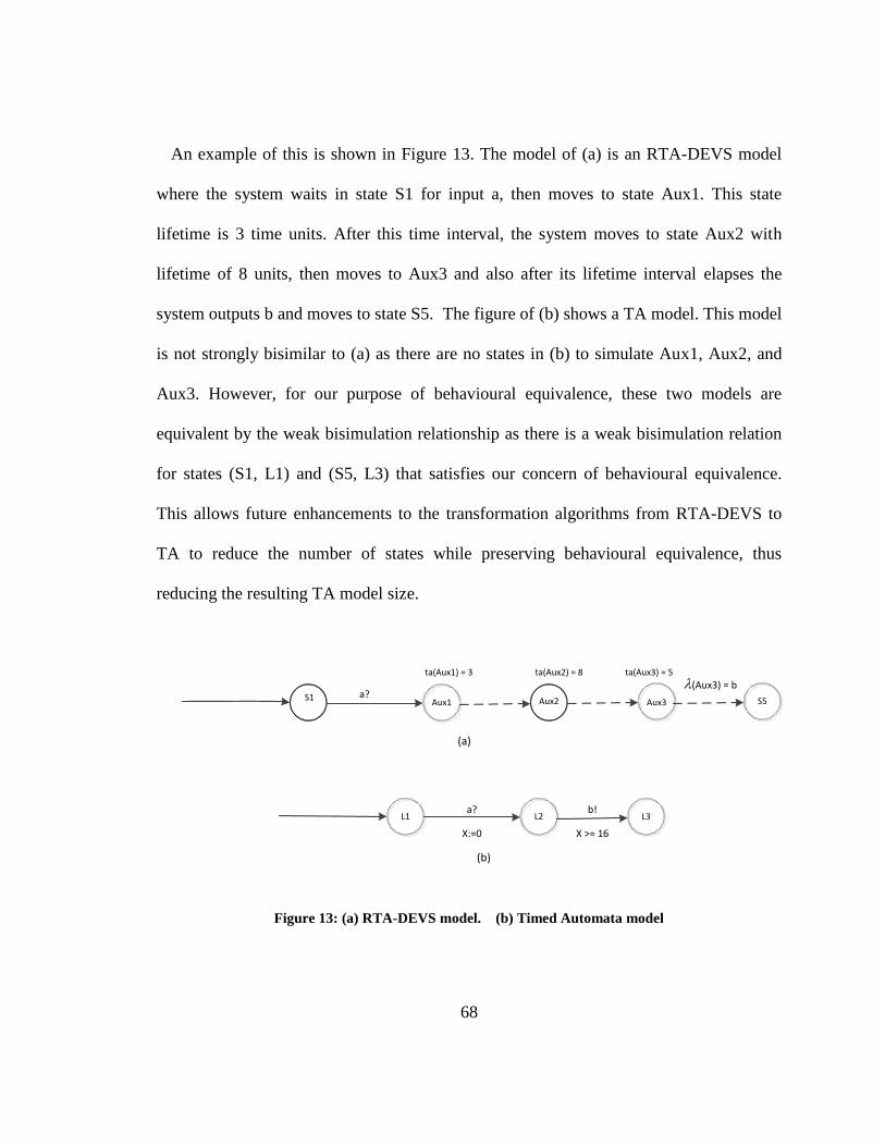
68
An example of this is shown in Figure 13. The model of (a) is an RTA-DEVS model
where the system waits in state S1 for input a, then moves to state Aux1. This state
lifetime is 3 time units. After this time interval, the system moves to state Aux2 with
lifetime of 8 units, then moves to Aux3 and also after its lifetime interval elapses the
system outputs b and moves to state S5. The figure of (b) shows a TA model. This model
is not strongly bisimilar to (a) as there are no states in (b) to simulate Aux1, Aux2, and
Aux3. However, for our purpose of behavioural equivalence, these two models are
equivalent by the weak bisimulation relationship as there is a weak bisimulation relation
for states (S1, L1) and (S5, L3) that satisfies our concern of behavioural equivalence.
This allows future enhancements to the transformation algorithms from RTA-DEVS to
TA to reduce the number of states while preserving behavioural equivalence, thus
reducing the resulting TA model size.
S1Aux1 Aux2 Aux3 S5
L1 L2 L3
a?
ta(Aux1) = 3 ta(Aux2) = 8 ta(Aux3) = 5
a?
X:=0 X >= 16
(Aux3) = b
b!
(a)
(b)
Figure 13: (a) RTA-DEVS model. (b) Timed Automata model
69
In the following paragraphs, we define behaviour equivalency based on timed Weak
bisimulation. Then, following the conditions of this bisimulation, a TA model for the
basic behaviour elements of RTA-DEVS is constructed with some unknown constants in
its guards and invariants. Then, we construct equations for these constants, based on the
definitions of bisimulation, to determine the values of these constants.
Definition 2. Eventual transition relation ‘’:
In a TLTS with states, s and t, the eventual transition relation defines a transition from
state s to state t that may contain one or more of direct transitions labelled with non-
observable events to the outside world. If we have an observable action a, a non-
observable action , and a transition label , then, for any TLTS [39], the eventual
transition relation between two states s and t on action (written ts
) is defined if
any of the following conditions is true:
1. ts : There is a transition from s to t only composed of transitions labelled with
non-observable actions. E.g., for the non-observable action , there is a transition
ts *)( , (where * defines one or more occurrences of these transitions).
2. tsa : There is a transition from s to t composed of one transition labelled with an
observable action =a, and one or more eventual transitions labelled with non-
observable actions. E.g., tsa
ss 21
for some states s1 and s2;
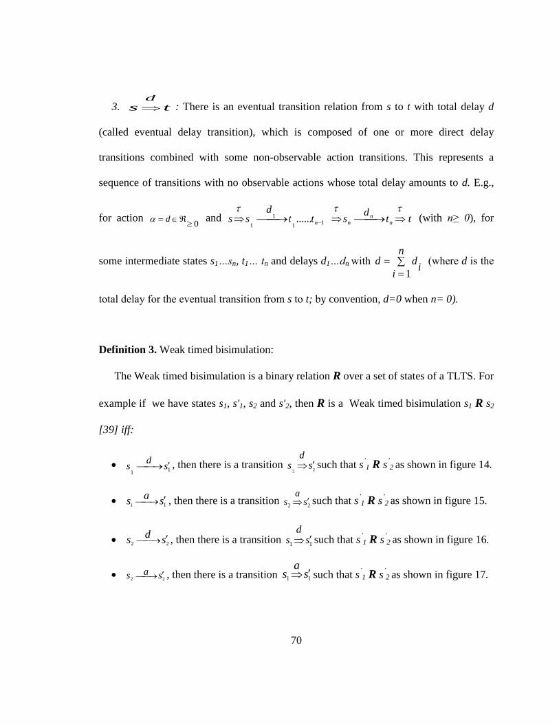
70
3. tsd : There is an eventual transition relation from s to t with total delay d
(called eventual delay transition), which is composed of one or more direct delay
transitions combined with some non-observable action transitions. This represents a
sequence of transitions with no observable actions whose total delay amounts to d. E.g.,
for action 0
d and ttd
sttd
ss nn
nn
11
1
1...... (with n≥ 0), for
some intermediate states s1…sn, t1… tn and delays d1…dn with
n
ii
dd1
(where d is the
total delay for the eventual transition from s to t; by convention, d=0 when n= 0).
Definition 3. Weak timed bisimulation:
The Weak timed bisimulation is a binary relation R over a set of states of a TLTS. For
example if we have states s1, s'1, s2 and s'2, then R is a Weak timed bisimulation s1 R s2
[39] iff:
11
sd
s , then there is a transition 22
sd
s such that s’1 R s’2 as shown in figure 14.
11 sas , then there is a transition 22 sa
s such that s’1 R s’2 as shown in figure 15.
22 sds , then there is a transition 11 sd
s such that s’1 R s’2 as shown in figure 16.
22 sas , then there is a transition 11 sa
s such that s’1 R s’2 as shown in figure 17.
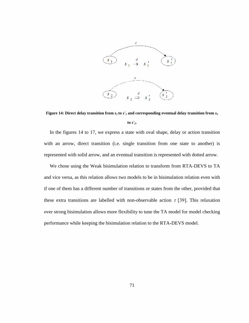
71
Figure 14: Direct delay transition from s1 to s'1 and corresponding eventual delay transition from s2
to s'2.
In the figures 14 to 17, we express a state with oval shape, delay or action transition
with an arrow, direct transition (i.e. single transition from one state to another) is
represented with solid arrow, and an eventual transition is represented with dotted arrow.
We chose using the Weak bisimulation relation to transform from RTA-DEVS to TA
and vice versa, as this relation allows two models to be in bisimulation relation even with
if one of them has a different number of transitions or states from the other, provided that
these extra transitions are labelled with non-observable action . This relaxation
over strong bisimulation allows more flexibility to tune the TA model for model checking
performance while keeping the bisimulation relation to the RTA-DEVS model.
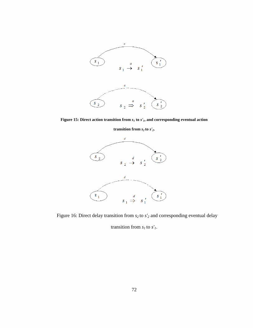
72
Figure 15: Direct action transition from s1 to s'1, and corresponding eventual action
transition from s2 to s'2.
Figure 16: Direct delay transition from s2 to s'2 and corresponding eventual delay
transition from s1 to s'1.
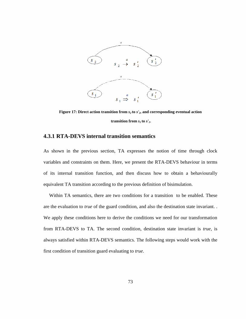
73
Figure 17: Direct action transition from s2 to s'2, and corresponding eventual action
transition from s1 to s'1.
4.3.1 RTA-DEVS internal transition semantics
As shown in the previous section, TA expresses the notion of time through clock
variables and constraints on them. Here, we present the RTA-DEVS behaviour in terms
of its internal transition function, and then discuss how to obtain a behaviourally
equivalent TA transition according to the previous definition of bisimulation.
Within TA semantics, there are two conditions for a transition to be enabled. These
are the evaluation to true of the guard condition, and also the destination state invariant. .
We apply these conditions here to derive the conditions we need for our transformation
from RTA-DEVS to TA. The second condition, destination state invariant is true, is
always satisfied within RTA-DEVS semantics. The following steps would work with the
first condition of transition guard evaluating to true.
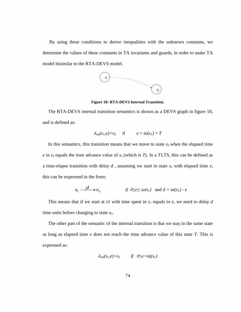
74
By using these conditions to derive inequalities with the unknown constants, we
determine the values of these constants in TA invariants and guards, in order to make TA
model bisimilar to the RTA-DEVS model.
Figure 18: RTA-DEVS Internal Transition.
The RTA-DEVS internal transition semantics is shown as a DEVS graph in figure 18,
and is defined as:
δint(s1,e)=s3 if e = ta(s1) = T
In this semantics, this transition means that we move to state s3 when the elapsed time
e in s1 equals the time advance value of s1 (which is T). In a TLTS, this can be defined as
a time-elapse transition with delay d , assuming we start in state s1 with elapsed time e,
this can be expressed in the form:
31 sds if 0≤e≤ ta(s1) and d = ta(s1) - e
This means that if we start at s1 with time spent in s1 equals to e, we need to delay d
time units before changing to state s3.
The other part of the semantic of the internal transition is that we stay in the same state
as long as elapsed time e does not reach the time advance value of this state T. This is
expressed as:
δint(s1,e)=s1 if 0≤e<ta(s1)
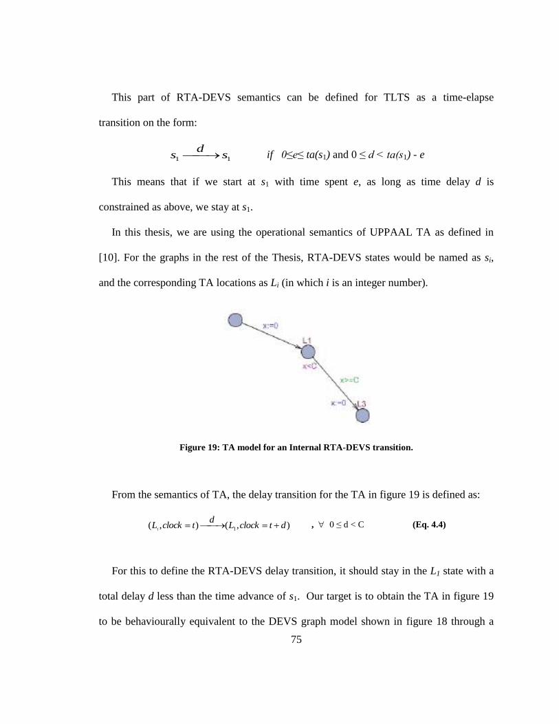
75
This part of RTA-DEVS semantics can be defined for TLTS as a time-elapse
transition on the form:
11 sd
s if 0≤e≤ ta(s1) and 0 ≤ d < ta(s1) - e
This means that if we start at s1 with time spent e, as long as time delay d is
constrained as above, we stay at s1.
In this thesis, we are using the operational semantics of UPPAAL TA as defined in
[10]. For the graphs in the rest of the Thesis, RTA-DEVS states would be named as si,
and the corresponding TA locations as Li (in which i is an integer number).
Figure 19: TA model for an Internal RTA-DEVS transition.
From the semantics of TA, the delay transition for the TA in figure 19 is defined as:
),(),( 11dtclockL
dtclockL , 0 ≤ d < C (Eq. 4.4)
For this to define the RTA-DEVS delay transition, it should stay in the L1 state with a
total delay d less than the time advance of s1. Our target is to obtain the TA in figure 19
to be behaviourally equivalent to the DEVS graph model shown in figure 18 through a
76
timed bisimulation relation. To do this, we will show that the state s1 is bisimilar to
location L1, and state s3 is bisimilar to location L3. This is done using the definition of the
Weak timed bisimulation relation (from RTA-DEVS to TA, and from TA to RTA-
DEVS). We do these in steps 1 and 2 below.
In this TA model, two locations are defined (L1 and L3), along with a transition from
L1 to L3. L1 has an invariant on clock x (x < C) that allows the TA to stay in that location
as long as the invariant is true. The transition from L1 to L3 has a guard (x ≥ C) that must
be true for the transition to be enabled, and c is a rational number. The transition also has
an update rule for clock variable x to reset it to zero before entering location L3. By
applying the condition above to weak timed bisimulation, first from RTA-DEVS to TA
and then from TA to RTA-DEVS, a value for the constant C to preserve the bisimulation
relation can be determined
Step1: from RTA-DEVS to TA
For the bisimulation of the states shown in figure 18 and figure 19, we have the
following requirements:
s1 R L1: This is a delay transition from s1 to itself. If 11 sd
s for some value of d
where 0≤ e ≤ ta(s1) and 0 ≤ d < ta(s1) - e ; then to satisfy the bisimulation
relation we should have a transition in TA as: ),(),( 11dexL
dexL for the
same value of d. Therefore from the invariant of state L1 we get x<C , then by
substituting for x and d, we get:
77
ta(s1) ≤ C (Eq. 4.5)
s3 R L3: Bisimilarity between s3 and L3 gives us the following:
For the delay transition from s1 to s3, let us consider the execution of the DEVS
internal transition )0,(),( 31s
des , where 0≤e≤ ta(s1) and d=ta(s1)–e by the
TA transition ),(),(31
dexLd
exL , with the reset statement x:=0 on
the transition.
In order for these two delay transitions to be equivalent, they need to start from
bisimilar states, and after same amount of time delay, they reach two bisimilar states. To
achieve this, the same value of delay d is used on both transitions. From this we deduce
the constant C in the TA clock constraint to give the condition for bisimulation. The TA
transition above starts from location L1, with the clock x valuation equals that of elapsed
time e at the RTA-DEVS transition above; then after delay d of the RTA-DEVS
transition, it transitions to L3, and the value of clock x increases by d.
By applying the conditions for this delay transition on TA transition above, we get
(Eq. 4.6) from the TA guard (x ≥ C) and the valuation of clock x (x = e + d):
ta(s1) ≥ C (Eq. 4.6)
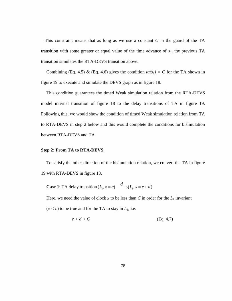
78
This constraint means that as long as we use a constant C in the guard of the TA
transition with some greater or equal value of the time advance of s1, the previous TA
transition simulates the RTA-DEVS transition above.
Combining (Eq. 4.5) & (Eq. 4.6) gives the condition ta(s1) = C for the TA shown in
figure 19 to execute and simulate the DEVS graph as in figure 18.
This condition guarantees the timed Weak simulation relation from the RTA-DEVS
model internal transition of figure 18 to the delay transitions of TA in figure 19.
Following this, we would show the condition of timed Weak simulation relation from TA
to RTA-DEVS in step 2 below and this would complete the conditions for bisimulation
between RTA-DEVS and TA.
Step 2: From TA to RTA-DEVS
To satisfy the other direction of the bisimulation relation, we convert the TA in figure
19 with RTA-DEVS in figure 18.
Case 1: TA delay transition ),(),( 11 dexLd
exL
Here, we need the value of clock x to be less than C in order for the L1 invariant
(x < c) to be true and for the TA to stay in L1, i.e.
e + d < C (Eq. 4.7)
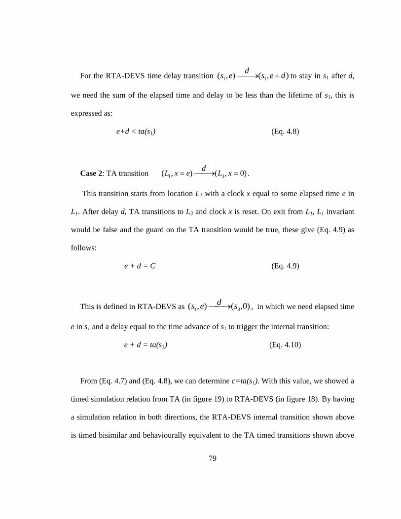
79
For the RTA-DEVS time delay transition ),(),( 11 desd
es to stay in s1 after d,
we need the sum of the elapsed time and delay to be less than the lifetime of s1, this is
expressed as:
e+d < ta(s1) (Eq. 4.8)
Case 2: TA transition )0,(),( 31 xLd
exL .
This transition starts from location L1 with a clock x equal to some elapsed time e in
L1. After delay d, TA transitions to L3 and clock x is reset. On exit from L1, L1 invariant
would be false and the guard on the TA transition would be true, these give (Eq. 4.9) as
follows:
e + d = C (Eq. 4.9)
This is defined in RTA-DEVS as )0,(),( 31 sdes , in which we need elapsed time
e in s1 and a delay equal to the time advance of s1 to trigger the internal transition:
e + d = ta(s1) (Eq. 4.10)
From (Eq. 4.7) and (Eq. 4.8), we can determine c=ta(s1). With this value, we showed a
timed simulation relation from TA (in figure 19) to RTA-DEVS (in figure 18). By having
a simulation relation in both directions, the RTA-DEVS internal transition shown above
is timed bisimilar and behaviourally equivalent to the TA timed transitions shown above
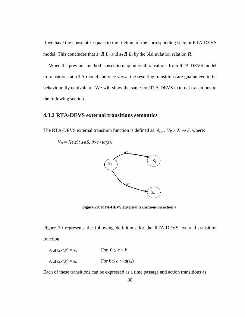
80
if we have the constant c equals to the lifetime of the corresponding state in RTA-DEVS
model. This concludes that s1 R L1 and s3 R L3 by the bisimulation relation R.
When the previous method is used to map internal transitions from RTA-DEVS model
to transitions at a TA model and vice versa, the resulting transitions are guaranteed to be
behaviourally equivalent. We will show the same for RTA-DEVS external transitions in
the following section.
4.3.2 RTA-DEVS external transitions semantics
The RTA-DEVS external transition function is defined as: δext : VD X S, where:
VD = {(s,e): sS, 0≤e<ta(s)}
Figure 20: RTA-DEVS External transitions on action a.
Figure 20 represents the following definitions for the RTA-DEVS external transition
function:
δext(s4,a,e) = s5 For 0 ≤ e < k
δext(s4,a,e) = s6 For k ≤ e < ta(s4)
Each of these transitions can be expressed as a time passage and action transitions as:
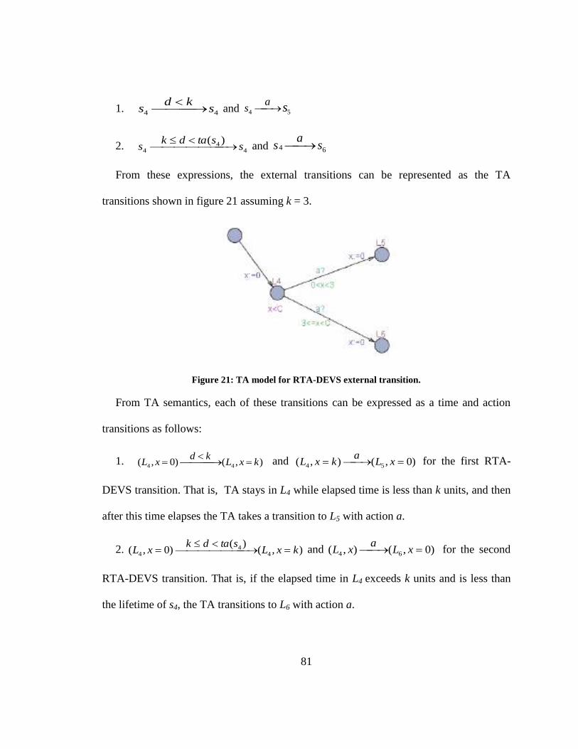
81
1. 44 skd
s
and 54 sas
2. 44
4
)(s
stadks
and 64 sa
s
From these expressions, the external transitions can be represented as the TA
transitions shown in figure 21 assuming k = 3.
Figure 21: TA model for RTA-DEVS external transition.
From TA semantics, each of these transitions can be expressed as a time and action
transitions as follows:
1. ),()0,( 44 kxLkd
xL
and )0,(),( 54 xLa
kxL for the first RTA-
DEVS transition. That is, TA stays in L4 while elapsed time is less than k units, and then
after this time elapses the TA takes a transition to L5 with action a.
2. ),()(
)0,( 44
4 kxLstadk
xL
and )0,(),( 64 xLa
xL for the second
RTA-DEVS transition. That is, if the elapsed time in L4 exceeds k units and is less than
the lifetime of s4, the TA transitions to L6 with action a.
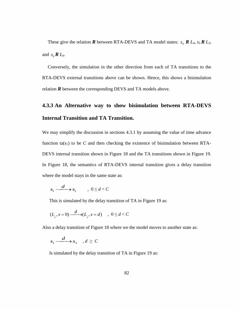
82
These give the relation R between RTA-DEVS and TA model states: 4s R L4, s5 R L5,
and 6s R L6.
Conversely, the simulation in the other direction from each of TA transitions to the
RTA-DEVS external transitions above can be shown. Hence, this shows a bisimulation
relation R between the corresponding DEVS and TA models above.
4.3.3 An Alternative way to show bisimulation between RTA-DEVS
Internal Transition and TA Transition.
We may simplify the discussion in sections 4.3.1 by assuming the value of time advance
function ta(s1) to be C and then checking the existence of bisimulation between RTA-
DEVS internal transition shown in Figure 18 and the TA transitions shown in Figure 19.
In Figure 18, the semantics of RTA-DEVS internal transition gives a delay transition
where the model stays in the same state as:
11 sd
s , 0 ≤ d < C
This is simulated by the delay transition of TA in Figure 19 as:
),()0,(11
dxLd
xL , 0 ≤ d < C
Also a delay transition of Figure 18 where we the model moves to another state as:
31 sd
s , d ≥ C
Is simulated by the delay transition of TA in Figure 19 as:
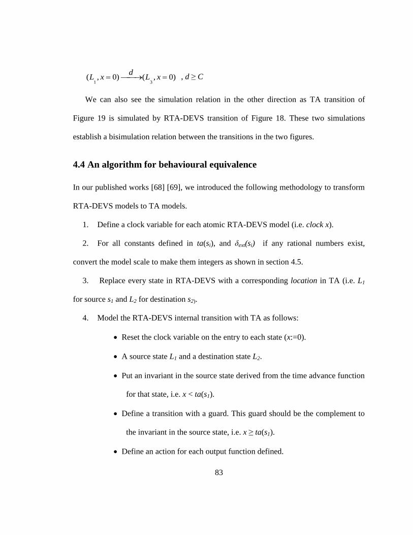
83
)0,()0,(31
xLd
xL , d ≥ C
We can also see the simulation relation in the other direction as TA transition of
Figure 19 is simulated by RTA-DEVS transition of Figure 18. These two simulations
establish a bisimulation relation between the transitions in the two figures.
4.4 An algorithm for behavioural equivalence
In our published works [68] [69], we introduced the following methodology to transform
RTA-DEVS models to TA models.
1. Define a clock variable for each atomic RTA-DEVS model (i.e. clock x).
2. For all constants defined in ta(si), and δext(si) if any rational numbers exist,
convert the model scale to make them integers as shown in section 4.5.
3. Replace every state in RTA-DEVS with a corresponding location in TA (i.e. L1
for source s1 and L2 for destination s2).
4. Model the RTA-DEVS internal transition with TA as follows:
Reset the clock variable on the entry to each state (x:=0).
A source state L1 and a destination state L2.
Put an invariant in the source state derived from the time advance function
for that state, i.e. x < ta(s1).
Define a transition with a guard. This guard should be the complement to
the invariant in the source state, i.e. x ≥ ta(s1).
Define an action for each output function defined.
84
5. The RTA-DEVS external transition is modeled in TA with the following items:
A source state and some destination state(s), i.e. L1 for source s1 and L2 for
destination s2.
A clock reset on the entry to each state.
An invariant in the source state that corresponds to time advance function for that
state, i.e. x<ta(s1).
For the external transition(s) with guards of clock constraints, these constraints
should be disjoint to obtain a deterministic TA model.
The action label on TA transitions for each RTA-DEVS input event to source
state s1.
A formal definition of the algorithm is given as follows:
Transform_RTA-DEVS_To_TA(in RTA-DEVS, out TA)
{
1. Declare a set of clocks C = {xi | 1≤ i ≤ |D| }, where i is the index of component
dD
2. Convert rational numbers defined in RTA-DEVS model to integers as described in
section 4.5.
3. Define a TA location for each RTA-DEVS state and define location invariant if
necessary:
For each d D do
Nd = {lj | dj Ss , dD} //component N of TA model corresponding to component d
85
β( C )lj = { xi ≤ ta(sj) | dj Ss , 1≤ i ≤ |D|, ta(sj)< ∞}
end do
4. Define a set of channels for communication between TA components:
H = {aj | j IC}
5. Define set of TA transitions for RTA-DEVS internal transitions:
set E = Ø; //Initialize the set of TA Transitions
For each d D do
For each sj Sd do
If ( ta(sj) < ∞ && δint(sj) = sk && λ(sj) = a ) then
E = E (lj, xd ≥ ta(sj), a!, xd := 0, lk);
end if
end do
end do
6. Add TA transitions corresponding to RTA-DEVS external transitions:
For each d D do
For each sj Sd do
If (δext(sj, a, cond(e)m ) = sk m) then
E = E (lj, cond(xd)m ), a?, xd := 0, lkm);
end if
end do
end do
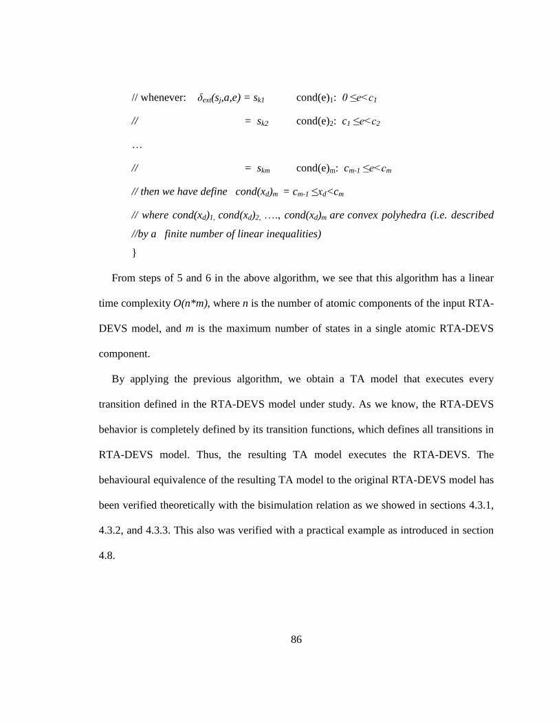
86
// whenever: δext(sj,a,e) = sk1 cond(e)1: 0 ≤e<c1
// = sk2 cond(e)2: c1 ≤e<c2
…
// = skm cond(e)m: cm-1 ≤e<cm
// then we have define cond(xd)m = cm-1 ≤xd<cm
// where cond(xd)1, cond(xd)2, …., cond(xd)m are convex polyhedra (i.e. described
//by a finite number of linear inequalities)
}
From steps of 5 and 6 in the above algorithm, we see that this algorithm has a linear
time complexity O(n*m), where n is the number of atomic components of the input RTA-
DEVS model, and m is the maximum number of states in a single atomic RTA-DEVS
component.
By applying the previous algorithm, we obtain a TA model that executes every
transition defined in the RTA-DEVS model under study. As we know, the RTA-DEVS
behavior is completely defined by its transition functions, which defines all transitions in
RTA-DEVS model. Thus, the resulting TA model executes the RTA-DEVS. The
behavioural equivalence of the resulting TA model to the original RTA-DEVS model has
been verified theoretically with the bisimulation relation as we showed in sections 4.3.1,
4.3.2, and 4.3.3. This also was verified with a practical example as introduced in section
4.8.
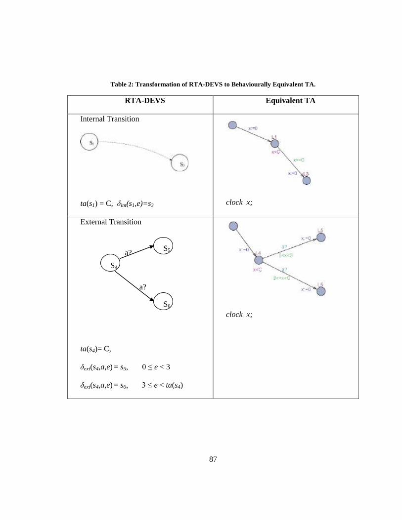
87
Table 2: Transformation of RTA-DEVS to Behaviourally Equivalent TA.
RTA-DEVS Equivalent TA
Internal Transition
ta(s1) = C, δint(s1,e)=s3
clock x;
External Transition
ta(s4)= C,
δext(s4,a,e) = s5, 0 ≤ e < 3
δext(s4,a,e) = s6, 3 ≤ e < ta(s4)
clock x;
S4
S5
S6
a?
a?
88
4.5 Resolving rational numbers in RTA-DEVS model
Timed safety automata, as defined in section 2.2.1, only deals with bounded integer
variables. This restriction is made to guarantee the finiteness of state-space, and hence
termination of reachability algorithm [5]. This may seem a limitation when one is trying
to verify RTA-DEVS models which have constant values of type Real, in their transition
functions. However, this is not much limitation, as any group of real rational numbers
can always be represented as integer numbers. This is done in TA model by changing the
model time scale. For example, imagine we have the following values as constants
defined in RTA-DEVS transition function to represent time in minutes (1/2, 3/5, 3/8). To
convert these to integer numbers on an equivalent TA model, we multiply each of them
by the least-common-multiple of all the denominators. The resultant automaton would be
equivalent modulo time scaling. This makes the TA having the values (1/2 * 40, 3/5 * 40,
3/8 * 40) = (20, 24, 15) and its time scale is 1/40 of a minute. For a network of TA, i.e.
many TA models interacting together in a larger model, the scaling has to be done in all
the models in the network. Therefore, all constants in a network of TA would be
multiplied by the scaling factor. This should not affect the verification results as long as
any requirement to be verified is expressed as a system query, in which its constants are
scaled with the same factor as well.
89
4.6 DEVS to RTA-DEVS
One of the main obstacles in verifying classic deterministic DEVS models through
transformation to TA is the possibility of DEVS models to have irrational constant values
in their internal or external transition functions. When doing the previous transformation
from DEVS model to TA, this would produce TA model with irrational constant values
in its guards or state invariants. However, such TA model reachability analysis would be
undecidable as shown in [69]. This implies that for any DEVS model containing state
lifetime of irrational values, it will not be possible to directly apply the transformation
shown in table 2. In this case, the irrational values would need to be approximated to the
nearest rational value according to the modeller’s choice, based on the required precision
for the equivalent RTA-DEVS model. In doing so, the transformation should take into
account the following rules. These rules when applied, avoid building invalid RTA-
DEVS or TA models containing time-action locks (that prevent the model execution
progress), or loops where execution progresses infinitely without allowing time to
advance [77].
Rule I: When approximating an irrational value of a state lifetime, and the internal
transition output of this state is coupled with an external transition, the choice of the
approximation value should be consistent for all constants using this irrational number.
Formally, if the DEVS coupled model as shown in figure 22 is defined as the following:
δA
int(Si,Cirr)=Sj , λA(Si) = a , taA(Si) = Cirr
δB
ext(Sk,e,a)=(Si,0) Cirr ≤ e < ∞
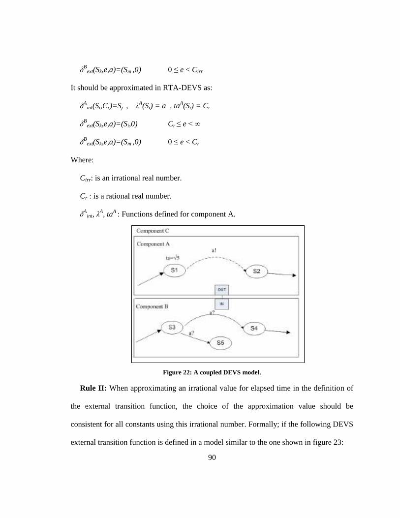
90
δB
ext(Sk,e,a)=(Sm ,0) 0 ≤ e < Cirr
It should be approximated in RTA-DEVS as:
δA
int(Si,Cr)=Sj , λA(Si) = a , taA(Si) = Cr
δB
ext(Sk,e,a)=(Si,0) Cr ≤ e < ∞
δB
ext(Sk,e,a)=(Sm ,0) 0 ≤ e < Cr
Where:
Cirr: is an irrational real number.
Cr : is a rational real number.
δA
int, λA, taA : Functions defined for component A.
Figure 22: A coupled DEVS model.
Rule II: When approximating an irrational value for elapsed time in the definition of
the external transition function, the choice of the approximation value should be
consistent for all constants using this irrational number. Formally; if the following DEVS
external transition function is defined in a model similar to the one shown in figure 23:
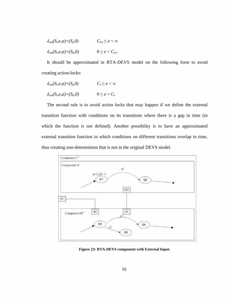
91
δext(Si,e,a)=(Sj,0) Cirr ≤ e < ∞
δext(Si,e,a)=(Sk,0) 0 ≤ e < Cirr
It should be approximated in RTA-DEVS model on the following form to avoid
creating action-locks:
δext(Si,e,a)=(Sj,0) Cr ≤ e < ∞
δext(Si,e,a)=(Sk,0) 0 ≤ e < Cr
The second rule is to avoid action locks that may happen if we define the external
transition function with conditions on its transitions where there is a gap in time (in
which the function is not defined). Another possibility is to have an approximated
external transition function in which conditions on different transitions overlap in time,
thus creating non-determinism that is not in the original DEVS model.
Figure 23: RTA-DEVS component with External Input.
92
4.7 Estimation of Approximation to Verification Results
When we approximate irrational values that may exist in a DEVS model to obtain the
equivalent RTA-DEVS model, we get an approximation error Δ between irrational value
and its approximated number. The next question is how the approximation of irrational
constants in ta or ext affect the formal verification of RTA-DEVS models. Would a result
obtained from model checking RTA-DEVS models apply to the original DEVS?
When we approximate an irrational constant Cirr with a rational constant Cr, we
introduce an error ∆ such that Cirr = Cr ± ∆. This error appears whenever Cirr is used in a
time advance function or in an external transition function. Verification of RTA-DEVS
through transforming it to an equivalent TA is done through reachability analysis. Would
this analysis differ by introducing the error ∆ when we move from DEVS to RTA-
DEVS? Answering this question directly requires applying reachability analysis to the
original DEVS with irrational constant values, and again for the transformed RTA-DEVS
model with the rational values, then comparing results. This approach however is not
feasible as reachability analysis for timed models with irrational constants is proven to be
undecidable as shown in [69].
Therefore, there is a need to use an approximate approach to estimate the effect of ∆
on the reachability analysis. This problem is equivalent to the problem of TA robustness
[65]. A robust TA model accepts an input sequence of events within a time interval. Each
event is accepted within a bounded time interval instead of an exact point in time as per
93
normal TA. This is called a bundle of events that are close in time and the model still
behaves the same with this bundle input.
Puri [78] extended the notion of robust TA to include models that their reachability
analysis is unaffected with small drifts in clock models. In this definition, a model is not
robust if for any small drift in clock rate, the reachability results change. In [66], De Wulf
et al. proved that clock drifts in TA are equivalent to having a reaction delay by the
implementation. This delay can be seen as an increase of guard constants by a small
positive value Δ. The robustness problem is then transformed to a problem in which one
needs to find a value Δ that keeps verification results correct. Further work by De Wulf et
al. [67] showed a methodology to assess a model for implement-ability by using standard
TA model checking tools, and also showed a proof that if a model is tolerant to a certain
value Δ, it would also be correct with any value Δ′ such that Δ′ < Δ.
We used the results from the robustness theory of TA to check if formal verification
results of a RTA-DEVS model correctly applies to the original DEVS model, and this
work was published in [69]. Given an error Δ introduced by approximating irrational
numbers in a DEVS models, we use an enlarged time interval with Δ to model the
possible transition from a state in a non-deterministic fashion. For example if we have the
following definition of DEVS external function δext:
δext(Si,e,a)=(Sj,0) Cirr ≤ e < ∞
δext(Si,e,a)=(Sk,0) 0 ≤ e < Cirr
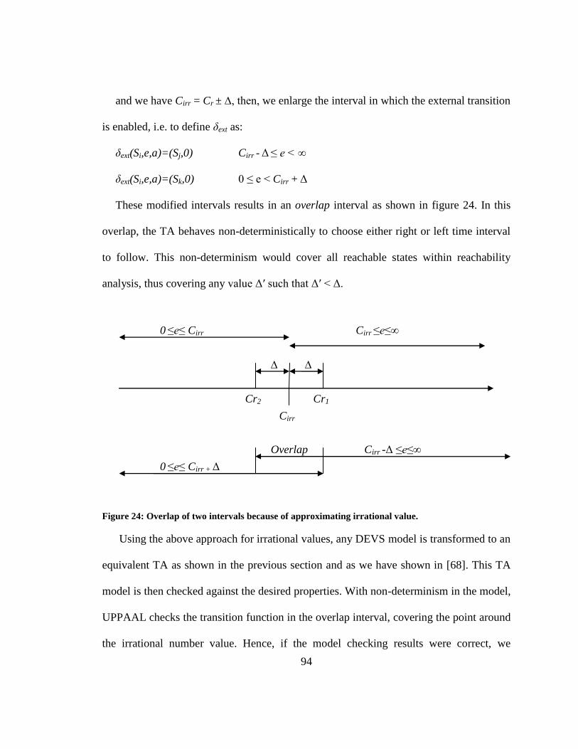
94
and we have Cirr = Cr ± ∆, then, we enlarge the interval in which the external transition
is enabled, i.e. to define δext as:
δext(Si,e,a)=(Sj,0) Cirr - Δ ≤ e < ∞
δext(Si,e,a)=(Sk,0) 0 ≤ e < Cirr + Δ
These modified intervals results in an overlap interval as shown in figure 24. In this
overlap, the TA behaves non-deterministically to choose either right or left time interval
to follow. This non-determinism would cover all reachable states within reachability
analysis, thus covering any value Δ′ such that Δ′ < Δ.
Figure 24: Overlap of two intervals because of approximating irrational value.
Using the above approach for irrational values, any DEVS model is transformed to an
equivalent TA as shown in the previous section and as we have shown in [68]. This TA
model is then checked against the desired properties. With non-determinism in the model,
UPPAAL checks the transition function in the overlap interval, covering the point around
the irrational number value. Hence, if the model checking results were correct, we
Cirr
∆ ∆
Cr1 Cr2
Cirr ≤e≤∞ 0 ≤e≤ Cirr
Cirr -Δ ≤e≤∞
0 ≤e≤ Cirr + Δ
Overlap
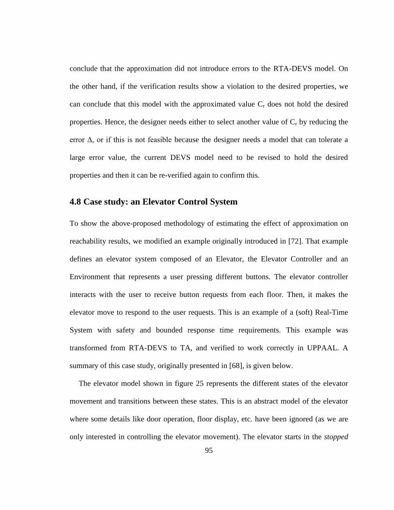
95
conclude that the approximation did not introduce errors to the RTA-DEVS model. On
the other hand, if the verification results show a violation to the desired properties, we
can conclude that this model with the approximated value Cr does not hold the desired
properties. Hence, the designer needs either to select another value of Cr by reducing the
error Δ, or if this is not feasible because the designer needs a model that can tolerate a
large error value, the current DEVS model need to be revised to hold the desired
properties and then it can be re-verified again to confirm this.
4.8 Case study: an Elevator Control System
To show the above-proposed methodology of estimating the effect of approximation on
reachability results, we modified an example originally introduced in [72]. That example
defines an elevator system composed of an Elevator, the Elevator Controller and an
Environment that represents a user pressing different buttons. The elevator controller
interacts with the user to receive button requests from each floor. Then, it makes the
elevator move to respond to the user requests. This is an example of a (soft) Real-Time
System with safety and bounded response time requirements. This example was
transformed from RTA-DEVS to TA, and verified to work correctly in UPPAAL. A
summary of this case study, originally presented in [68], is given below.
The elevator model shown in figure 25 represents the different states of the elevator
movement and transitions between these states. This is an abstract model of the elevator
where some details like door operation, floor display, etc. have been ignored (as we are
only interested in controlling the elevator movement). The elevator starts in the stopped
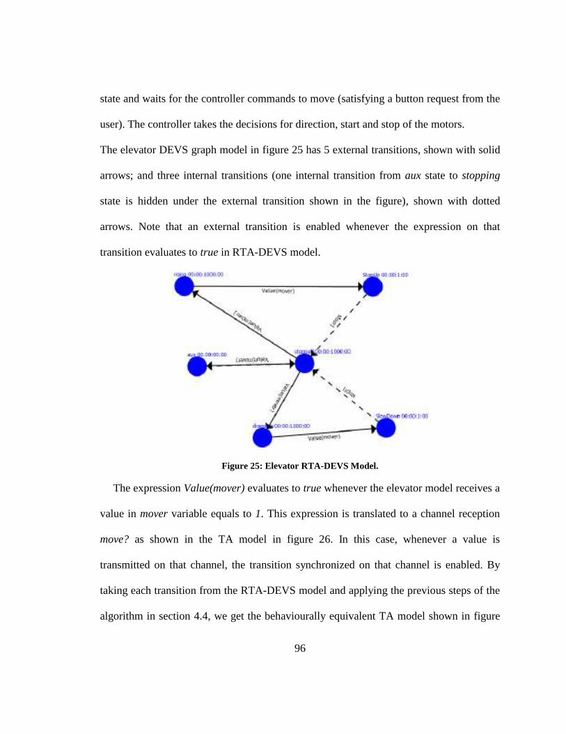
96
state and waits for the controller commands to move (satisfying a button request from the
user). The controller takes the decisions for direction, start and stop of the motors.
The elevator DEVS graph model in figure 25 has 5 external transitions, shown with solid
arrows; and three internal transitions (one internal transition from aux state to stopping
state is hidden under the external transition shown in the figure), shown with dotted
arrows. Note that an external transition is enabled whenever the expression on that
transition evaluates to true in RTA-DEVS model.
Figure 25: Elevator RTA-DEVS Model.
The expression Value(mover) evaluates to true whenever the elevator model receives a
value in mover variable equals to 1. This expression is translated to a channel reception
move? as shown in the TA model in figure 26. In this case, whenever a value is
transmitted on that channel, the transition synchronized on that channel is enabled. By
taking each transition from the RTA-DEVS model and applying the previous steps of the
algorithm in section 4.4, we get the behaviourally equivalent TA model shown in figure
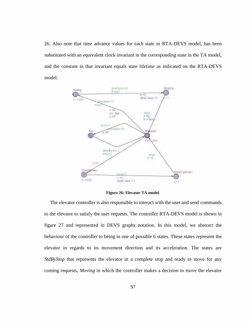
97
26. Also note that time advance values for each state in RTA-DEVS model, has been
substituted with an equivalent clock invariant in the corresponding state in the TA model,
and the constant in that invariant equals state lifetime as indicated on the RTA-DEVS
model.
Figure 26: Elevator TA model.
The elevator controller is also responsible to interact with the user and send commands
to the elevator to satisfy the user requests. The controller RTA-DEVS model is shown in
figure 27 and represented in DEVS graphs notation. In this model, we abstract the
behaviour of the controller to being in one of possible 6 states. These states represent the
elevator in regards to its movement direction and its acceleration. The states are
StdByStop that represents the elevator in a complete stop and ready to move for any
coming requests, Moving in which the controller makes a decision to move the elevator
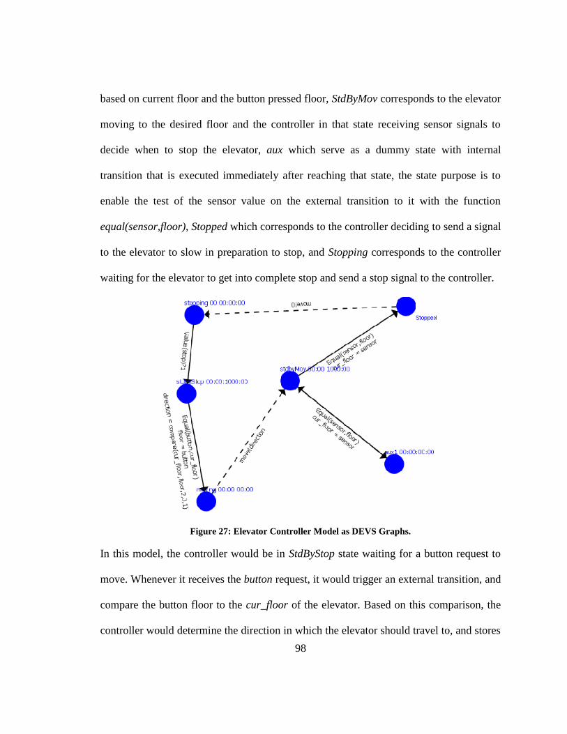
98
based on current floor and the button pressed floor, StdByMov corresponds to the elevator
moving to the desired floor and the controller in that state receiving sensor signals to
decide when to stop the elevator, aux which serve as a dummy state with internal
transition that is executed immediately after reaching that state, the state purpose is to
enable the test of the sensor value on the external transition to it with the function
equal(sensor,floor), Stopped which corresponds to the controller deciding to send a signal
to the elevator to slow in preparation to stop, and Stopping corresponds to the controller
waiting for the elevator to get into complete stop and send a stop signal to the controller.
Figure 27: Elevator Controller Model as DEVS Graphs.
In this model, the controller would be in StdByStop state waiting for a button request to
move. Whenever it receives the button request, it would trigger an external transition, and
compare the button floor to the cur_floor of the elevator. Based on this comparison, the
controller would determine the direction in which the elevator should travel to, and stores
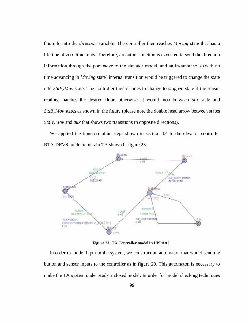
99
this info into the direction variable. The controller then reaches Moving state that has a
lifetime of zero time units. Therefore, an output function is executed to send the direction
information through the port move to the elevator model, and an instantaneous (with no
time advancing in Moving state) internal transition would be triggered to change the state
into StdByMov state. The controller then decides to change to stopped state if the sensor
reading matches the desired floor; otherwise, it would loop between aux state and
StdByMov states as shown in the figure (please note the double head arrow between states
StdByMov and aux that shows two transitions in opposite directions).
We applied the transformation steps shown in section 4.4 to the elevator controller
RTA-DEVS model to obtain TA shown in figure 28.
Figure 28: TA Controller model in UPPAAL.
In order to model input to the system, we construct an automaton that would send the
button and sensor inputs to the controller as in figure 29. This automaton is necessary to
make the TA system under study a closed model. In order for model checking techniques
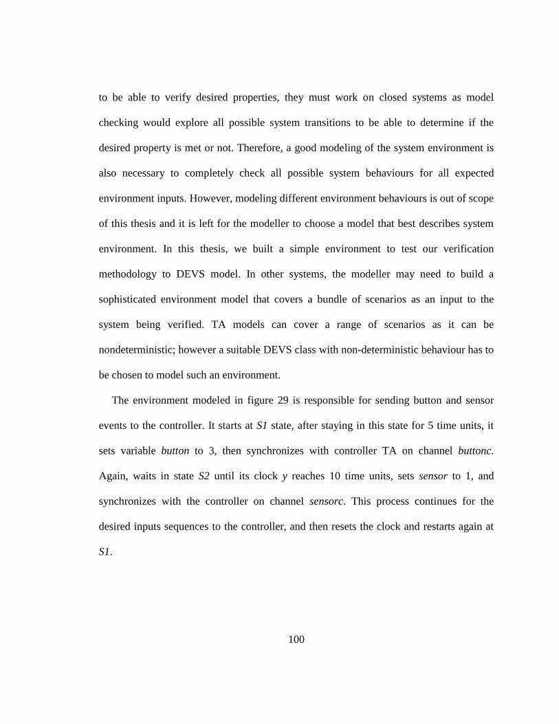
100
to be able to verify desired properties, they must work on closed systems as model
checking would explore all possible system transitions to be able to determine if the
desired property is met or not. Therefore, a good modeling of the system environment is
also necessary to completely check all possible system behaviours for all expected
environment inputs. However, modeling different environment behaviours is out of scope
of this thesis and it is left for the modeller to choose a model that best describes system
environment. In this thesis, we built a simple environment to test our verification
methodology to DEVS model. In other systems, the modeller may need to build a
sophisticated environment model that covers a bundle of scenarios as an input to the
system being verified. TA models can cover a range of scenarios as it can be
nondeterministic; however a suitable DEVS class with non-deterministic behaviour has to
be chosen to model such an environment.
The environment modeled in figure 29 is responsible for sending button and sensor
events to the controller. It starts at S1 state, after staying in this state for 5 time units, it
sets variable button to 3, then synchronizes with controller TA on channel buttonc.
Again, waits in state S2 until its clock y reaches 10 time units, sets sensor to 1, and
synchronizes with the controller on channel sensorc. This process continues for the
desired inputs sequences to the controller, and then resets the clock and restarts again at
S1.
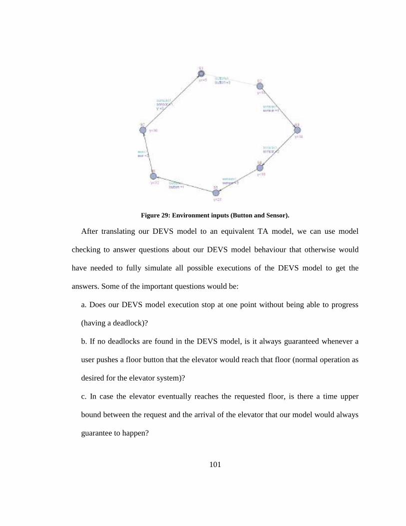
101
Figure 29: Environment inputs (Button and Sensor).
After translating our DEVS model to an equivalent TA model, we can use model
checking to answer questions about our DEVS model behaviour that otherwise would
have needed to fully simulate all possible executions of the DEVS model to get the
answers. Some of the important questions would be:
a. Does our DEVS model execution stop at one point without being able to progress
(having a deadlock)?
b. If no deadlocks are found in the DEVS model, is it always guaranteed whenever a
user pushes a floor button that the elevator would reach that floor (normal operation as
desired for the elevator system)?
c. In case the elevator eventually reaches the requested floor, is there a time upper
bound between the request and the arrival of the elevator that our model would always
guarantee to happen?
102
In order to answer these questions, we formulated these questions into formal queries
to the TA model. For the first question, we applied the UPPAAL verifier to our model to
check for any deadlocks that may be present in the elevator model. To check for that
failure, we have formulated a simple query in UPPAAL. It is expressed in UPPAAL
Computation Tree Logic CTL query language [9] as:
A[] not deadlock
After running the checker, it shows that this property is satisfied, i.e. there is no
deadlock in the DEVS model as results shown in figure 30.
UPPAAL version 4.0.6 (rev. 2986), March 2007 -- server.
A[] not deadlock
Property is satisfied.
Figure 30: Elevator Verification Results in UPPAAL
To answer the second question, we need to check for the liveness property, i.e.
something would eventually happen. In our case, for the proper operation of the
controller within the coupled system, we are interested to check if by pressing a certain
floor button, the elevator would eventually reach that floor. For example, if the user
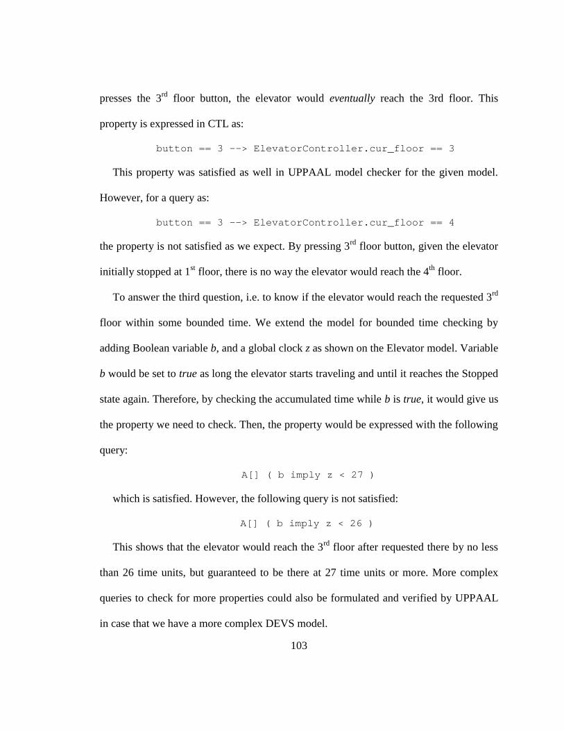
103
presses the 3rd floor button, the elevator would eventually reach the 3rd floor. This
property is expressed in CTL as:
button == 3 --> ElevatorController.cur_floor == 3
This property was satisfied as well in UPPAAL model checker for the given model.
However, for a query as:
button == 3 --> ElevatorController.cur_floor == 4
the property is not satisfied as we expect. By pressing 3rd floor button, given the elevator
initially stopped at 1st floor, there is no way the elevator would reach the 4th floor.
To answer the third question, i.e. to know if the elevator would reach the requested 3rd
floor within some bounded time. We extend the model for bounded time checking by
adding Boolean variable b, and a global clock z as shown on the Elevator model. Variable
b would be set to true as long the elevator starts traveling and until it reaches the Stopped
state again. Therefore, by checking the accumulated time while b is true, it would give us
the property we need to check. Then, the property would be expressed with the following
query:
A[] ( b imply z < 27 )
which is satisfied. However, the following query is not satisfied:
A[] ( b imply z < 26 )
This shows that the elevator would reach the 3rd floor after requested there by no less
than 26 time units, but guaranteed to be there at 27 time units or more. More complex
queries to check for more properties could also be formulated and verified by UPPAAL
in case that we have a more complex DEVS model.
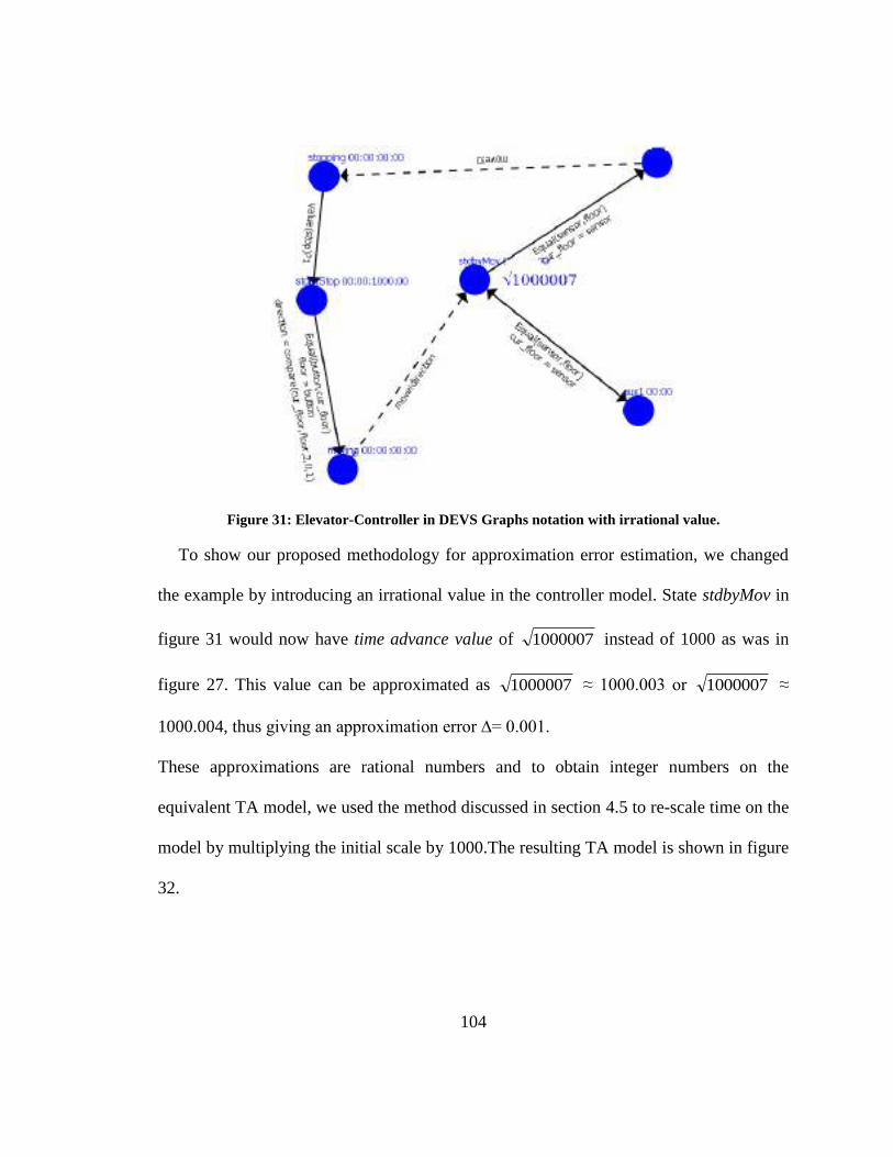
104
Figure 31: Elevator-Controller in DEVS Graphs notation with irrational value.
To show our proposed methodology for approximation error estimation, we changed
the example by introducing an irrational value in the controller model. State stdbyMov in
figure 31 would now have time advance value of 1000007 instead of 1000 as was in
figure 27. This value can be approximated as 1000007 ≈ 1000.003 or 1000007 ≈
1000.004, thus giving an approximation error ∆= 0.001.
These approximations are rational numbers and to obtain integer numbers on the
equivalent TA model, we used the method discussed in section 4.5 to re-scale time on the
model by multiplying the initial scale by 1000.The resulting TA model is shown in figure
32.
105
Figure 32: TA Controller model with Non-deterministic behaviour.
In this model, we added node E and a transition from StdByMov to E that is enabled at
elapsed time of x ≥ 1000003. This TA is semantically equivalent to the DEVS model in
figure 31. However, this TA allows the transition from node StdByMov to node Stopped
to be taken non-deterministically in the interval [0,1000004] while transition to E is
enabled in [1000003,∞]. This ensures covering the interval [0, √1000007] in UPPAAL
model checking.
The model checker was run to verify the non-deterministic version of the elevator-
controller model along with the other components in the elevator system as we showed in
[68]. The verification results were successful as was before for the deterministic version
in figure 28. This indicates that the approximation error did not affect the verification
results. Hence, for any value smaller than 0.001, the results would not be affected as was
proven by De Wulf in [67].
106
Although we could not verify the DEVS model in figure 31 directly as a result of the
irrational value of time advance function, our methodology approximated this model to a
behaviourally equivalent TA, which could be used to verify the TA model.
4.9 Known Methodology Limits
It is a well-known problem of all model checking techniques that the number of nodes
in the reachability graph grows exponentially in the number of components and number
of states of each component. This is called the state-space explosion problem. Model
checking algorithms need to store a representation of the full reachability graph to be able
to terminate after visiting all nodes of the graph. Due to the exponential growth of
reachability graph, even if timed model checking is decidable with TA, there is a
limitation of the practical size of models that can be checked with current tools and
hardware.
This limitation also limits the size of DEVS models that can be verified with our
methodology. However, as we show in section 6.1.1, our methodology can be extended
by some techniques that reduce the size of reachability graph and hence scale the
methodology to verify larger sizes of DEVS models.
107
Chapter 5: Hybrid DEVS Systems Verification.
5.1 Continuous-Discrete systems Verification
In chapter 3 of this thesis, we introduced a methodology to enable the verification of
deterministic and discrete DEVS models. Although the method is useful for deterministic
discrete systems, in the case of RT embedded systems a discrete controller needs to
interact with some physical environment that is continuous in nature. Examples of these
are automobile cruise-control systems, boiler temperature or pressure control systems,
heating and air conditioning systems, and power-plant systems. The controlled variables
in these environments are continuous, and they are modeled using differential algebraic
equations. However, the computer controller system is a discrete digital system. This
makes the models of control systems a hybrid between continuous and discrete
component models.
In order to overcome the problem shown in section 2.4 for hybrid systems verification,
we introduced a technique within the DEVS formalism to model, simulate and verify
hybrid systems. This technique uses the QSS method shown in section 2.4.1 to provide a
way to model the continuous components. With this ability, we have an overall
methodology in which a designer is able to model and simulate hybrid control and
embedded systems within DEVS. Then, with this research results, the designer would be
108
able to formally verify the hybrid model to guarantee the system correctness. This
methodology is built on the verification of DEVS & RTA-DEVS models discussed in
chapter 3 and also on the use of the QSS method. As a DEVS model is executable on any
embedded DEVS platform, for instance the CD++ engine (e-CD++) [8], the verified
digital controller component can be deployed as an executable on the target system
running e-CD++.
To accomplish the above goal of the thesis, we extend the previous work of
verification of DEVS models done in chapter to include a special method for
transforming continuous models expressed in QSS to TA. This enables the verification of
hybrid DEVS models through model checking tools like UPPAAL.
To show the main ideas for hybrid systems verification within DEVS & QSS, and
potential problems and challenges that we need to solve, we present here a simple
example of a simple continuous formula that is used for modeling many physical and
natural systems. This is an exponential decay formula that describes an amount
decreasing exponentially with regard to time. Some of the natural systems that follow this
are [79]:
Radioactive decay, where a radioactive material undergoes a nuclear change, the
number of remaining atoms, from an initial amount, follows the exponential decay
formula.
The decrease of a temperature of a hot object cooling in a natural convective
mode, such as a space-heating radiator.
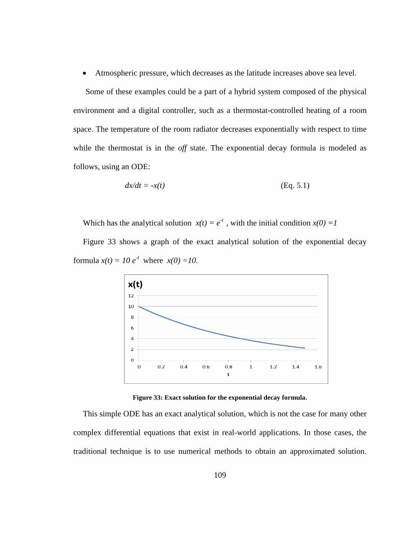
109
Atmospheric pressure, which decreases as the latitude increases above sea level.
Some of these examples could be a part of a hybrid system composed of the physical
environment and a digital controller, such as a thermostat-controlled heating of a room
space. The temperature of the room radiator decreases exponentially with respect to time
while the thermostat is in the off state. The exponential decay formula is modeled as
follows, using an ODE:
dx/dt = -x(t) (Eq. 5.1)
Which has the analytical solution x(t) = e-t , with the initial condition x(0) =1
Figure 33 shows a graph of the exact analytical solution of the exponential decay
formula x(t) = 10 e-t where x(0) =10.
Figure 33: Exact solution for the exponential decay formula.
This simple ODE has an exact analytical solution, which is not the case for many other
complex differential equations that exist in real-world applications. In those cases, the
traditional technique is to use numerical methods to obtain an approximated solution.
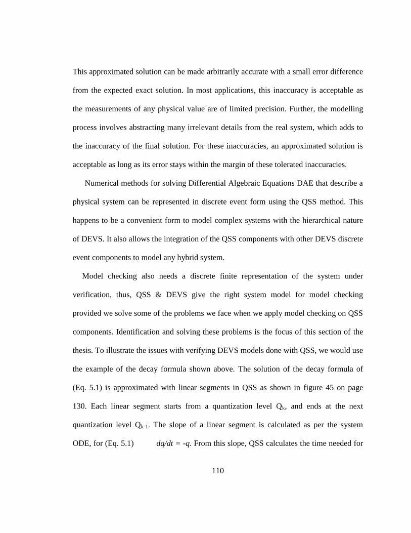
110
This approximated solution can be made arbitrarily accurate with a small error difference
from the expected exact solution. In most applications, this inaccuracy is acceptable as
the measurements of any physical value are of limited precision. Further, the modelling
process involves abstracting many irrelevant details from the real system, which adds to
the inaccuracy of the final solution. For these inaccuracies, an approximated solution is
acceptable as long as its error stays within the margin of these tolerated inaccuracies.
Numerical methods for solving Differential Algebraic Equations DAE that describe a
physical system can be represented in discrete event form using the QSS method. This
happens to be a convenient form to model complex systems with the hierarchical nature
of DEVS. It also allows the integration of the QSS components with other DEVS discrete
event components to model any hybrid system.
Model checking also needs a discrete finite representation of the system under
verification, thus, QSS & DEVS give the right system model for model checking
provided we solve some of the problems we face when we apply model checking on QSS
components. Identification and solving these problems is the focus of this section of the
thesis. To illustrate the issues with verifying DEVS models done with QSS, we would use
the example of the decay formula shown above. The solution of the decay formula of
(Eq. 5.1) is approximated with linear segments in QSS as shown in figure 45 on page
130. Each linear segment starts from a quantization level Qk, and ends at the next
quantization level Qk-1. The slope of a linear segment is calculated as per the system
ODE, for (Eq. 5.1) dq/dt = -q. From this slope, QSS calculates the time needed for
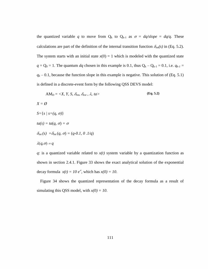
111
the quantized variable q to move from Qk to Qk-1 as = dq/slope = dq/q. These
calculations are part of the definition of the internal transition function int(s) in (Eq. 5.2).
The system starts with an initial state x(0) = 1 which is modeled with the quantized state
q = Q0 = 1. The quantum dq chosen in this example is 0.1, thus Qk – Qk-1 = 0.1, i.e. qk-1 =
qk – 0.1, because the function slope in this example is negative. This solution of (Eq. 5.1)
is defined in a discrete-event form by the following QSS DEVS model:
AMD = <X, Y, S, int, ext , ta> (Eq. 5.2)
X = Ø
S={s | s=(q,)}
ta(s) = ta(q,) =
int (s) =int (q,) = (q-0.1, 0 .1/q)
q: is a quantized variable related to x(t) system variable by a quantization function as
shown in section 2.4.1. Figure 33 shows the exact analytical solution of the exponential
decay formula x(t) = 10 e-t, which has x(0) = 10.
Figure 34 shows the quantized representation of the decay formula as a result of
simulating this QSS model, with x(0) = 10.
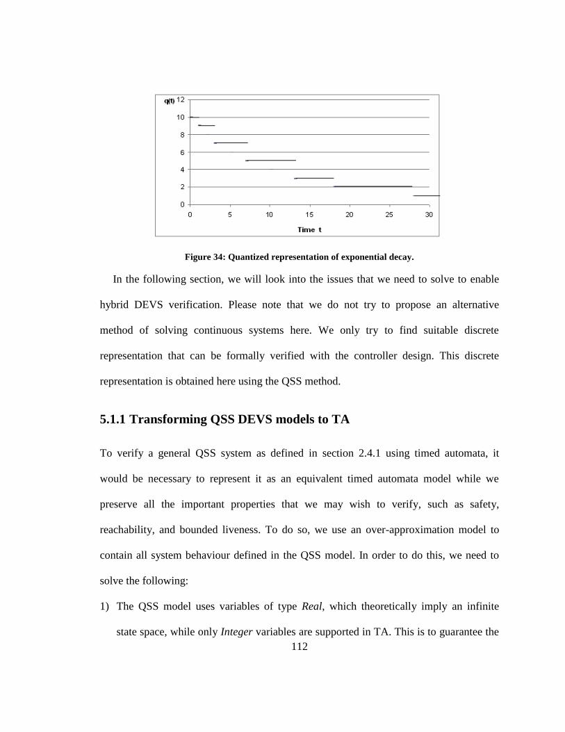
112
Figure 34: Quantized representation of exponential decay.
In the following section, we will look into the issues that we need to solve to enable
hybrid DEVS verification. Please note that we do not try to propose an alternative
method of solving continuous systems here. We only try to find suitable discrete
representation that can be formally verified with the controller design. This discrete
representation is obtained here using the QSS method.
5.1.1 Transforming QSS DEVS models to TA
To verify a general QSS system as defined in section 2.4.1 using timed automata, it
would be necessary to represent it as an equivalent timed automata model while we
preserve all the important properties that we may wish to verify, such as safety,
reachability, and bounded liveness. To do so, we use an over-approximation model to
contain all system behaviour defined in the QSS model. In order to do this, we need to
solve the following:
1) The QSS model uses variables of type Real, which theoretically imply an infinite
state space, while only Integer variables are supported in TA. This is to guarantee the
113
finiteness of reachability state space, and hence the termination of TA reachability
algorithm. Thus, we need an abstraction mechanism to reduce the infinite state-space
of QSS variables to the bounded finite state-space of UPPAAL. However, this
abstraction should preserve the critical properties in the hybrid system that we need to
verify.
2) The exact behavioural equivalency between a continuous system modeled in QSS and
TA cannot be done with bisimulation, as the QSS state variables are Real numbers,
while TA have only Integer variables to represent the model states. We need to find a
simulation relation between the continuous system and the QSS/TA model that
preserves the important safety requirements.
3) A change of a variable representing a continuous system state is often described with
arithmetic functions that return a Real number, and whose domain is also a Real
number. These functions would need to be represented with approximated Integer
arithmetic functions (for example, trigonometric, logarithmic or exponential
functions).
To solve the first challenge, we need to represent the infinite continuous state-space
with a reduced finite state space. This is easy as practical considerations put a limit to the
number of states a QSS system would have for its variables. For example, it is common
to use some variable x to represent the value of a physical measure in a system. From the
modelling process, it is possible to identify lower and upper bounds on the values of this
variable in a given model. Further, any measured physical property would have a finite
114
precision according to the measurement method. This limited precision would lead to a
measurement error |err| ≤ xi+1 - xi, i.e. the least possible observed difference between two
successive values of variable x, is equal or greater than the measurement error.
Therefore, these observations provide a finite state system where the bounds would
constitute lower and upper saturation bounds Q0 and Qr, and the quantum ≥ |err|.
Thus, we obtain the finite set Q of the quantization levels defined for a QSS model:
Q = {Q0,Q1, ...,Qr} a set of real numbers where Qk−1 < Qk with 1 ≤ k ≤ r,
Qk – Qk-1 ≥ |err|. In this case, the number of states of a QSS system would be at most
r+1 states.
In order to meet the second requirement, we do not need total equivalence of
behaviour between QSS model and TA model. To verify the QSS model behaviour, we
need to include this behaviour within TA model, i.e. one way simulation relation (the TA
model simulates the QSS model). This is obtained with an approximation that includes all
QSS model behaviour and thus preserves the properties we wish to verify. This can be
done with an over-approximation of the QSS model that contains all behaviours of the
original QSS model plus some extra behaviour due to the over-approximation. One way
to do this is to abstract each Real number with an integer interval, and this can be done to
any degree of precision required. This produces an over-approximation that guarantees
full inclusion of the QSS model behaviour. This, in turn, guarantees any reachability
verification results on the over-approximation are true for the original QSS model.
115
An over-approximation preserves safety and bounded liveness properties as Berard et
al. have shown in [80]. These properties are very important when verifying hybrid
systems. The safety property says that there is (are) no unsafe (or bad) state(s) reachable
from the system initial state(s). The bounded liveness property says that, whenever an
event occurs, the system would always respond within a specific time bound t.
An example of how safety and bounded liveness properties are preserved, by over-
approximating the original model, is given in [80]. As these properties are the most
important in an embedded control system, we claim that over-approximation would
suffice for our purpose, and the main purpose of this stage of the research will be to
verify such a claim.
To illustrate the over-approximation, figure 35 shows an example of over-
approximation of Real numbers with an Integer interval. In this figure, the “small”
bubbles (states) represent the Real values of a system state variable that changes during
system evolution. To approximate the system behaviour, all states where the state
variable in the closed interval x=[1.0,2.0], could be represented by a single state, S, in
which, the state variable value is over-approximated to this single state representing the
values [1,2]. The state S thus contains all possible system dynamics for variable x in the
interval [1.0,2.0]. Assume that the state where x=1.4 is a “bad” state, and we wish to
check the safety of our system, expressed as a condition to never reach this state from the
initial system state. Then, if the reachability analysis of the over-approximation shows
that the state S is not reachable from any initial system state, then we can guarantee that
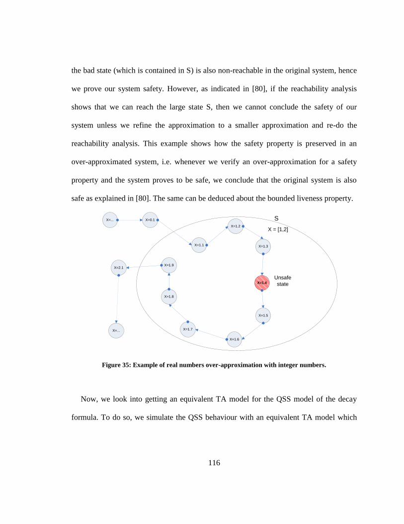
116
the bad state (which is contained in S) is also non-reachable in the original system, hence
we prove our system safety. However, as indicated in [80], if the reachability analysis
shows that we can reach the large state S, then we cannot conclude the safety of our
system unless we refine the approximation to a smaller approximation and re-do the
reachability analysis. This example shows how the safety property is preserved in an
over-approximated system, i.e. whenever we verify an over-approximation for a safety
property and the system proves to be safe, we conclude that the original system is also
safe as explained in [80]. The same can be deduced about the bounded liveness property.
X=1.1
X=1.2
X=1.3
X=1.4
X=1.5
X=1.6
X=1.7
X=1.8
X=1.9X=2.1
X = [1,2]
X=0.1X=...
X=...
S
Unsafe state
Figure 35: Example of real numbers over-approximation with integer numbers.
Now, we look into getting an equivalent TA model for the QSS model of the decay
formula. To do so, we simulate the QSS behaviour with an equivalent TA model which
117
contains this behaviour. First, we look at the semantics of the QSS model of (Eq. 5.2)
which represents a loop as follows:
1. Initial values are assigned to q=1 and = 0, resulting in initial state So=(1,0).
2. After a time elapse of e = the output function is triggered to send the value of q
to the outport, and then δint is triggered to calculate the next state s, which is composed of
the new values of q and : s = (q-0.1, 0.1/q).
3. Repeat step 2 in the loop until s = (0,10).
To transform this DEVS model to a TA, we need to solve the following issues:
1. The TA variables can only be of bounded integer type, in order to guarantee the
finiteness of state space and hence the termination of the reachability algorithm.
However, in QSS, state variables are real numbers and thus have infinite values.
2. The time of next quantum event (is approximated to an integer number. However,
in doing so we need to preserve the original behaviour of the QSS model, and hence
preserve the properties we need to formally verify.
The first issue is handled by converting rational Real numbers to Integers by
multiplying all the values by the least common multiple of all the denominators. For any
irrational values, we can use the technique we introduced in section 4.5. For the second
issue, we use abstraction by over-approximation [39]. With this technique, we
approximate the real value of the event time ti with a bounded time interval such that ti
[TL,TH], where TL =floor(ti) , TH = ceiling(ti). This guarantees that the resulting TA
would include all possible event timings in that interval.
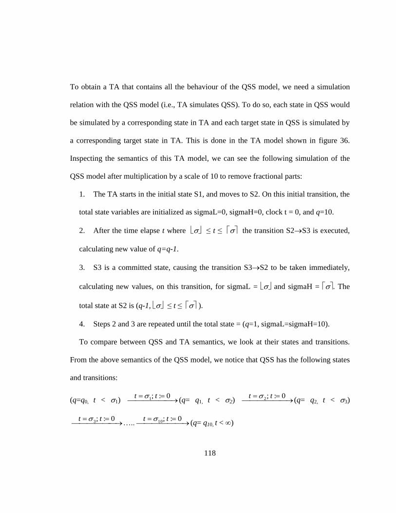
118
To obtain a TA that contains all the behaviour of the QSS model, we need a simulation
relation with the QSS model (i.e., TA simulates QSS). To do so, each state in QSS would
be simulated by a corresponding state in TA and each target state in QSS is simulated by
a corresponding target state in TA. This is done in the TA model shown in figure 36.
Inspecting the semantics of this TA model, we can see the following simulation of the
QSS model after multiplication by a scale of 10 to remove fractional parts:
1. The TA starts in the initial state S1, and moves to S2. On this initial transition, the
total state variables are initialized as sigmaL=0, sigmaH=0, clock t = 0, and q=10.
2. After the time elapse t where ≤ t ≤ the transition S2S3 is executed,
calculating new value of q=q-1.
3. S3 is a committed state, causing the transition S3S2 to be taken immediately,
calculating new values, on this transition, for sigmaL = and sigmaH = . The
total state at S2 is (q-1, ≤ t ≤ ).
4. Steps 2 and 3 are repeated until the total state = (q=1, sigmaL=sigmaH=10).
To compare between QSS and TA semantics, we look at their states and transitions.
From the above semantics of the QSS model, we notice that QSS has the following states
and transitions:
(q=q0, t < 1) 0:;1 tt (q= q1, t < 2)
0:;2 tt (q= q2, t < 3)
0:;3 tt
….. 0:;10 tt (q= q10, t < ∞)
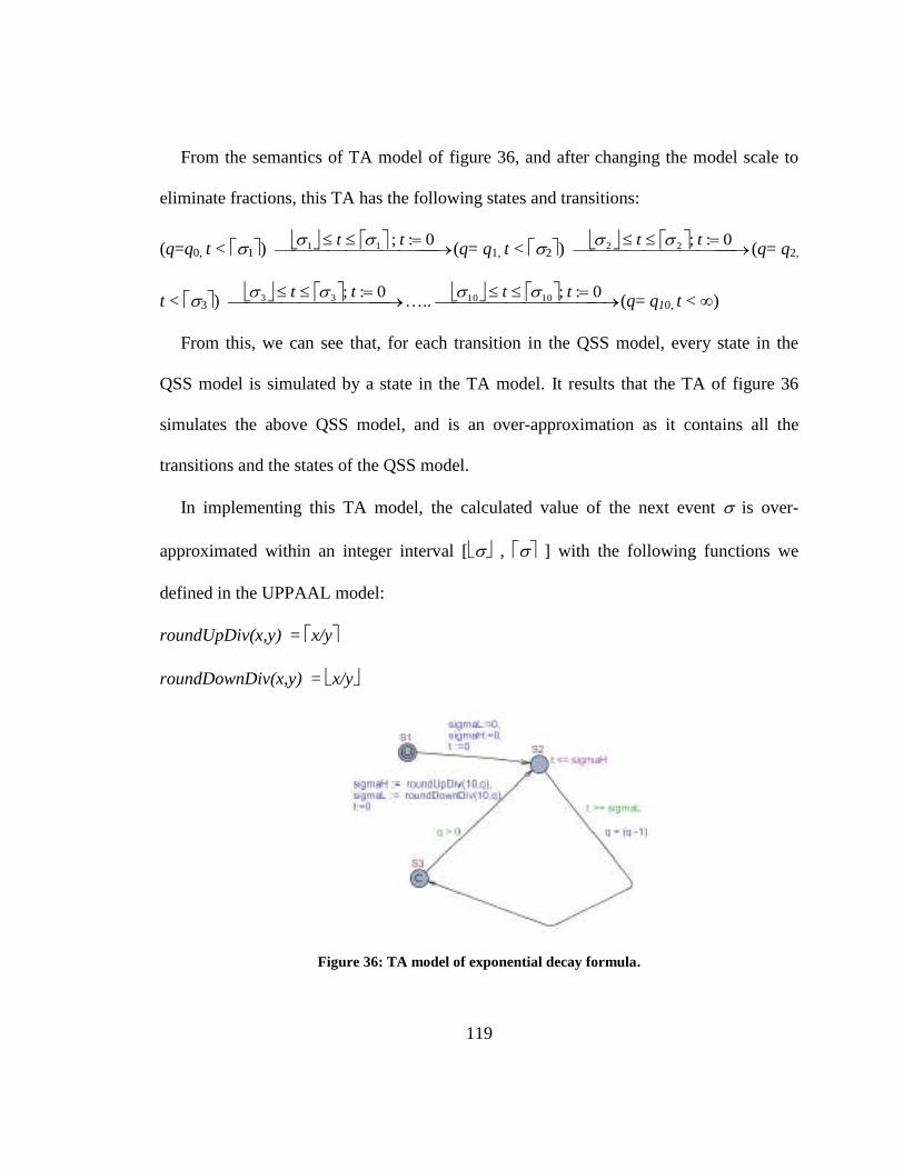
119
From the semantics of TA model of figure 36, and after changing the model scale to
eliminate fractions, this TA has the following states and transitions:
(q=q0, t < 1) 0:;11 tt (q= q1, t < 2)
0:;22 tt (q= q2,
t < 3) 0:;33 tt
….. 0:;1010 tt (q= q10, t < ∞)
From this, we can see that, for each transition in the QSS model, every state in the
QSS model is simulated by a state in the TA model. It results that the TA of figure 36
simulates the above QSS model, and is an over-approximation as it contains all the
transitions and the states of the QSS model.
In implementing this TA model, the calculated value of the next event is over-
approximated within an integer interval [ , ] with the following functions we
defined in the UPPAAL model:
roundUpDiv(x,y) = x/y
roundDownDiv(x,y) = x/y
Figure 36: TA model of exponential decay formula.
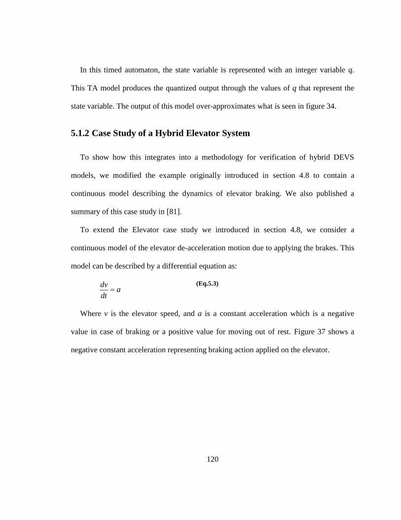
120
In this timed automaton, the state variable is represented with an integer variable q.
This TA model produces the quantized output through the values of q that represent the
state variable. The output of this model over-approximates what is seen in figure 34.
5.1.2 Case Study of a Hybrid Elevator System
To show how this integrates into a methodology for verification of hybrid DEVS
models, we modified the example originally introduced in section 4.8 to contain a
continuous model describing the dynamics of elevator braking. We also published a
summary of this case study in [81].
To extend the Elevator case study we introduced in section 4.8, we consider a
continuous model of the elevator de-acceleration motion due to applying the brakes. This
model can be described by a differential equation as:
adt
dv
(Eq.5.3)
Where v is the elevator speed, and a is a constant acceleration which is a negative
value in case of braking or a positive value for moving out of rest. Figure 37 shows a
negative constant acceleration representing braking action applied on the elevator.
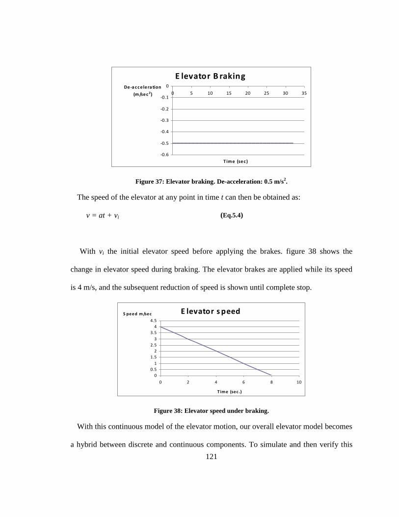
121
E levator B raking
-0.6
-0.5
-0.4
-0.3
-0.2
-0.1
0
0 5 10 15 20 25 30 35
T ime (sec )
De-a c c e lera tion
(m/sec 2)
Figure 37: Elevator braking. De-acceleration: 0.5 m/s2.
The speed of the elevator at any point in time t can then be obtained as:
v = at + vi (Eq.5.4)
With vi the initial elevator speed before applying the brakes. figure 38 shows the
change in elevator speed during braking. The elevator brakes are applied while its speed
is 4 m/s, and the subsequent reduction of speed is shown until complete stop.
E levator s peed
0
0.5
1
1.5
2
2.5
3
3.5
4
4.5
0 2 4 6 8 10
T ime (sec .)
S peed m/sec
Figure 38: Elevator speed under braking.
With this continuous model of the elevator motion, our overall elevator model becomes
a hybrid between discrete and continuous components. To simulate and then verify this
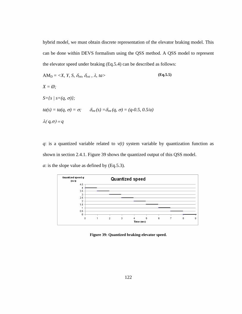
122
hybrid model, we must obtain discrete representation of the elevator braking model. This
can be done within DEVS formalism using the QSS method. A QSS model to represent
the elevator speed under braking (Eq.5.4) can be described as follows:
AMD = <X, Y, S, int, ext , ta> (Eq.5.5)
X = Ø;
S={s | s=(q,)};
ta(s) = ta(q,) = int (s) =int (q,) = (q-0.5, 0.5/a)
q: is a quantized variable related to v(t) system variable by quantization function as
shown in section 2.4.1. Figure 39 shows the quantized output of this QSS model.
a: is the slope value as defined by (Eq.5.3).
Figure 39: Quantized braking-elevator speed.
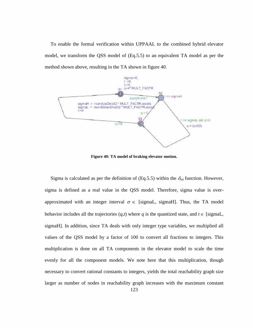
123
To enable the formal verification within UPPAAL to the combined hybrid elevator
model, we transform the QSS model of (Eq.5.5) to an equivalent TA model as per the
method shown above, resulting in the TA shown in figure 40.
Figure 40: TA model of braking elevator motion.
Sigma is calculated as per the definition of (Eq.5.5) within the int function. However,
sigma is defined as a real value in the QSS model. Therefore, sigma value is over-
approximated with an integer interval [sigmaL, sigmaH]. Thus, the TA model
behavior includes all the trajectories (q,t) where q is the quantized state, and t [sigmaL,
sigmaH]. In addition, since TA deals with only integer type variables, we multiplied all
values of the QSS model by a factor of 100 to convert all fractions to integers. This
multiplication is done on all TA components in the elevator model to scale the time
evenly for all the component models. We note here that this multiplication, though
necessary to convert rational constants to integers, yields the total reachability graph size
larger as number of nodes in reachability graph increases with the maximum constant
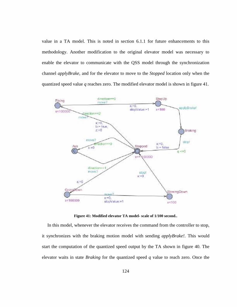
124
value in a TA model. This is noted in section 6.1.1 for future enhancements to this
methodology. Another modification to the original elevator model was necessary to
enable the elevator to communicate with the QSS model through the synchronization
channel applyBrake, and for the elevator to move to the Stopped location only when the
quantized speed value q reaches zero. The modified elevator model is shown in figure 41.
Figure 41: Modified elevator TA model- scale of 1/100 second..
In this model, whenever the elevator receives the command from the controller to stop,
it synchronizes with the braking motion model with sending applyBrake!. This would
start the computation of the quantized speed output by the TA shown in figure 40. The
elevator waits in state Braking for the quantized speed q value to reach zero. Once the
125
elevator speed reaches zero, the transition from Braking to Stopped is enabled and
executed, and then, the elevator sends a synchronization signal on the channel stop! to the
elevator-controller to let it know it has stopped. The rest of the model executes exactly as
shown before in section 4.8. This model of the originally hybrid system allows the
designer to verify the control system with different parameters of the elevator’s physical
system, such as different braking values of de-accelerations, different elevator initial
speeds, or other parameters in a more detailed QSS model. This is an important addition
to the elevator system verification as relevant physical factors to the controller
performance can be identified and formally verified during the design phase.
In section 4.8, we showed how to verify a number of desired properties for the DEVS
model (such as deadlock freedom, bounded response time, and safety properties) for the
elevator coupled model. We used Computational Tree Logic (CTL) to construct queries
with the requirements and submitted it to UPPAAL to get an answer and hence verify
that requirement. Here we show how to check one of these required properties here with
the hybrid system modeled in the previous section. We start with an elevator model as the
one described in figure 41with its speed decrease as in figure 39.
One such requirement is the freedom of deadlocks expressed in CTL as
A[] not deadlock.
This means for all paths, there should be no deadlocks.
After running the checker, it shows that this property is satisfied, i.e. there is no deadlock
in the DEVS model:
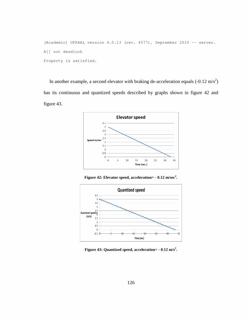
126
(Academic) UPPAAL version 4.0.13 (rev. 4577), September 2010 -- server.
A[] not deadlock
Property is satisfied.
In another example, a second elevator with braking de-acceleration equals (-0.12 m/s2)
has its continuous and quantized speeds described by graphs shown in figure 42 and
figure 43.
Figure 42: Elevator speed, acceleration= - 0.12 m/sec2.
Figure 43: Quantized speed, acceleration= - 0.12 m/s2.
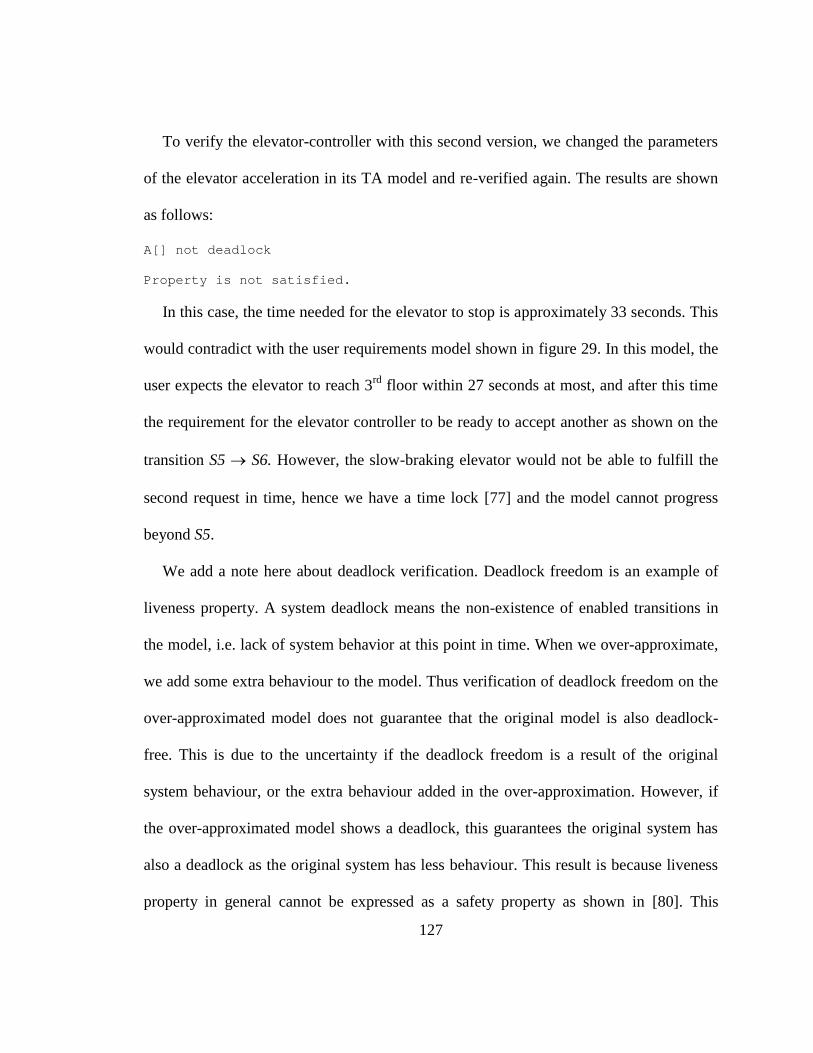
127
To verify the elevator-controller with this second version, we changed the parameters
of the elevator acceleration in its TA model and re-verified again. The results are shown
as follows:
A[] not deadlock
Property is not satisfied.
In this case, the time needed for the elevator to stop is approximately 33 seconds. This
would contradict with the user requirements model shown in figure 29. In this model, the
user expects the elevator to reach 3rd floor within 27 seconds at most, and after this time
the requirement for the elevator controller to be ready to accept another as shown on the
transition S5 S6. However, the slow-braking elevator would not be able to fulfill the
second request in time, hence we have a time lock [77] and the model cannot progress
beyond S5.
We add a note here about deadlock verification. Deadlock freedom is an example of
liveness property. A system deadlock means the non-existence of enabled transitions in
the model, i.e. lack of system behavior at this point in time. When we over-approximate,
we add some extra behaviour to the model. Thus verification of deadlock freedom on the
over-approximated model does not guarantee that the original model is also deadlock-
free. This is due to the uncertainty if the deadlock freedom is a result of the original
system behaviour, or the extra behaviour added in the over-approximation. However, if
the over-approximated model shows a deadlock, this guarantees the original system has
also a deadlock as the original system has less behaviour. This result is because liveness
property in general cannot be expressed as a safety property as shown in [80]. This
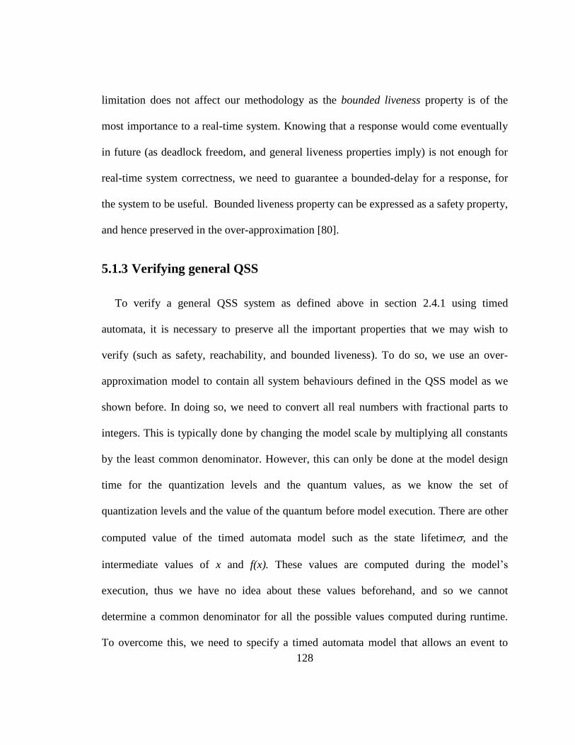
128
limitation does not affect our methodology as the bounded liveness property is of the
most importance to a real-time system. Knowing that a response would come eventually
in future (as deadlock freedom, and general liveness properties imply) is not enough for
real-time system correctness, we need to guarantee a bounded-delay for a response, for
the system to be useful. Bounded liveness property can be expressed as a safety property,
and hence preserved in the over-approximation [80].
5.1.3 Verifying general QSS
To verify a general QSS system as defined above in section 2.4.1 using timed
automata, it is necessary to preserve all the important properties that we may wish to
verify (such as safety, reachability, and bounded liveness). To do so, we use an over-
approximation model to contain all system behaviours defined in the QSS model as we
shown before. In doing so, we need to convert all real numbers with fractional parts to
integers. This is typically done by changing the model scale by multiplying all constants
by the least common denominator. However, this can only be done at the model design
time for the quantization levels and the quantum values, as we know the set of
quantization levels and the value of the quantum before model execution. There are other
computed value of the timed automata model such as the state lifetime, and the
intermediate values of x and f(x). These values are computed during the model’s
execution, thus we have no idea about these values beforehand, and so we cannot
determine a common denominator for all the possible values computed during runtime.
To overcome this, we need to specify a timed automata model that allows an event to
129
occur at any possible time between and , or in case of another variable x, the true
variable value would be in a closed interval [x, x]. This effectively gives us an over-
approximation model to the QSS that includes all possible behaviours of the original QSS
model.
We show in more detail this over-approximation with the exponential decay formula
we introduced in section 2.4.1. This formula has the analytical solution x(t) = e-t, with the
initial condition x(0) =1. Figure 44 shows a graph of the exact analytical solution of the
exponential decay formula x(t) = 10 e-t where x(0) =10.
Figure 44: Exact solution for exponential decay formula.
QSS approximates the continuous system with linear segments, and generates events
whenever the approximated solution crosses a quantization level. Figure 45 shows the
QSS approximate solution versus the exact solution of the decay formula.
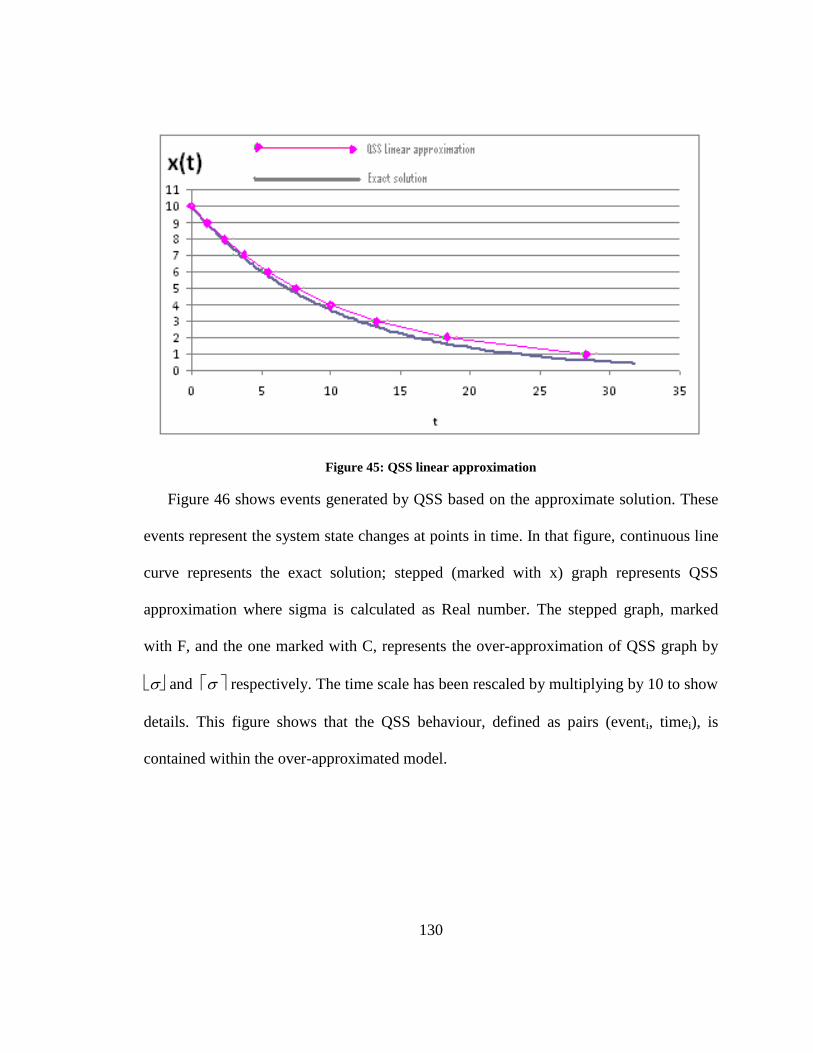
130
Figure 45: QSS linear approximation
Figure 46 shows events generated by QSS based on the approximate solution. These
events represent the system state changes at points in time. In that figure, continuous line
curve represents the exact solution; stepped (marked with x) graph represents QSS
approximation where sigma is calculated as Real number. The stepped graph, marked
with F, and the one marked with C, represents the over-approximation of QSS graph by
and respectively. The time scale has been rescaled by multiplying by 10 to show
details. This figure shows that the QSS behaviour, defined as pairs (eventi, timei), is
contained within the over-approximated model.
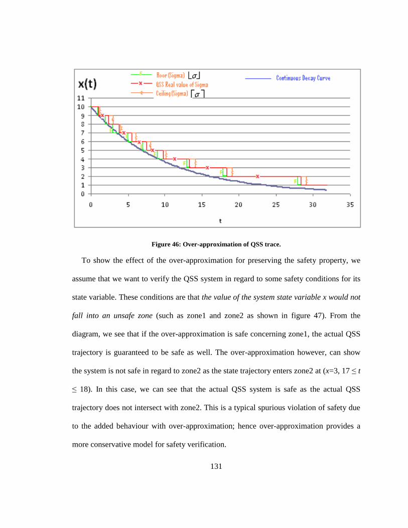
131
Figure 46: Over-approximation of QSS trace.
To show the effect of the over-approximation for preserving the safety property, we
assume that we want to verify the QSS system in regard to some safety conditions for its
state variable. These conditions are that the value of the system state variable x would not
fall into an unsafe zone (such as zone1 and zone2 as shown in figure 47). From the
diagram, we see that if the over-approximation is safe concerning zone1, the actual QSS
trajectory is guaranteed to be safe as well. The over-approximation however, can show
the system is not safe in regard to zone2 as the state trajectory enters zone2 at (x=3, 17 ≤ t
≤ 18). In this case, we can see that the actual QSS system is safe as the actual QSS
trajectory does not intersect with zone2. This is a typical spurious violation of safety due
to the added behaviour with over-approximation; hence over-approximation provides a
more conservative model for safety verification.
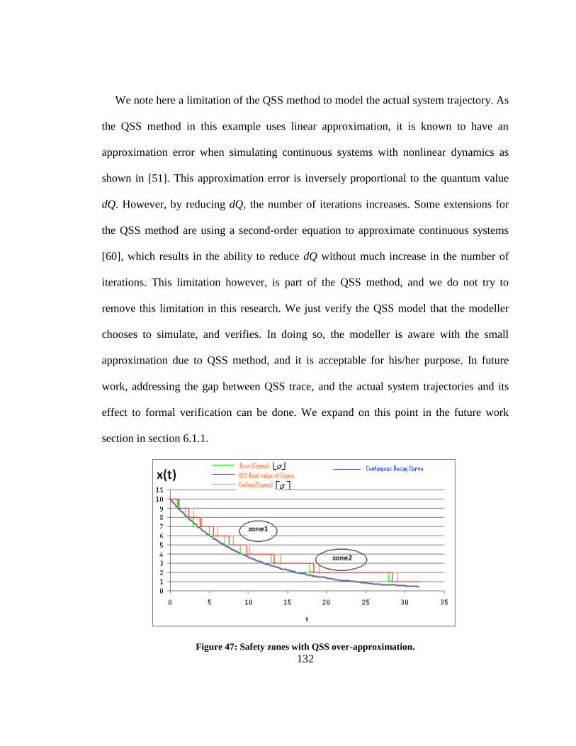
132
We note here a limitation of the QSS method to model the actual system trajectory. As
the QSS method in this example uses linear approximation, it is known to have an
approximation error when simulating continuous systems with nonlinear dynamics as
shown in [51]. This approximation error is inversely proportional to the quantum value
dQ. However, by reducing dQ, the number of iterations increases. Some extensions for
the QSS method are using a second-order equation to approximate continuous systems
[60], which results in the ability to reduce dQ without much increase in the number of
iterations. This limitation however, is part of the QSS method, and we do not try to
remove this limitation in this research. We just verify the QSS model that the modeller
chooses to simulate, and verifies. In doing so, the modeller is aware with the small
approximation due to QSS method, and it is acceptable for his/her purpose. In future
work, addressing the gap between QSS trace, and the actual system trajectories and its
effect to formal verification can be done. We expand on this point in the future work
section in section 6.1.1.
Figure 47: Safety zones with QSS over-approximation.
133
To extend these ideas to a general QSS system, a major obstacle to model general QSS
models with TA is that QSS uses variables of type Real, while TA has only Integer type
variables. This necessitates an approximation of all Real-valued variables in QSS to an
equivalent Integer values. When faced with obtaining an Integer approximation to a Real
value, we need to round the Real value to nearest Integer. However, in doing so, we lose
the actual value as it is in the QSS model, and this may render TA verification results not
applicable to the original QSS system.
To include the actual value of the QSS variables in our approximation, we
approximate any QSS Real-value with a closed interval between two Integers [L,U],
where L is the mathematical floor function of the Real-value, and U is the mathematical
ceiling. This would constitute an over-approximation that contains the true trajectory
produced by the QSS. This over-approximation, when transformed to a TA model, would
contain all possible behaviours in the QSS model. Thus it would simulate the original
QSS system. In the resulting over-approximation QSS model, any calculations would use
interval arithmetic as introduced in section 2.5.
To show this, we construct a QSS model where only integers and integer intervals are
used. Thus, the QSS system of (Eq. 2.6) on page 37 may be written as:
M1OA = (X, Y, , δint, δext, λ, ta), where
X = 2 × {inport}
Y = × {outport}
(Eq.5.6)
134
S = 4× Z× Z2 +0 ∞
δint(s) = δint([xL, xU], [dxL , dxU], k, [σL, σH] ) =
(Qk+1, [dxL , dxU] , k + sgn(dxL), [ σ1L ,σ1H])
δext(s, e, xu) = δext(x, dx, k, σ, e, xv, port) =
([xL, xU], [xvL, xvL ], k, [ σ2L ,σ2H])
λ(s) = λ(x, dx, k, σ) = (Qk+sgn(dx), outport)
ta(s) = ta(x, dx, k, σ) = [σL, σH]
xL = x + e · dxL
xU = x + e · dxU
σ1L =
0
0)(
0)(
1
12
xU
xUxU
kk
xU
Ux
kk
dif
difd
difd
(Eq. 5.7)
σ1U =
0
0)(
0)(
1
12
xL
xLxL
kk
xL
Lx
kk
dif
difd
difd
135
σ2L =
0
0)().(
0).(1
vL
vLvL
kxLL
LvvL
xLLk
xif
xifx
Qdex
xifx
dexQ
(Eq. 5.8)
σ2U =
0
0)().(
0).(1
vU
vUvU
kxUU
UvvL
xUUk
xif
xifx
Qdex
xifx
dexQ
and from (Eq. 2.4) on page 34, we calculate current
function slope as:
dxL = f[q(t), u(t)]
dxU = f[q(t), u(t)]
xvL = f[xL(t), u(t)]
xvU = f[xU(t), u(t)]
(Eq. 5.9)
In the model of (Eq.5.6),(Eq. 5.7),(Eq. 5.8),(Eq. 5.9) we replaced every computed
Real-valued quantity with a bounded Integer interval. Formally, for any calculated Real-
value r, we replace it with a closed interval [r , r]. This makes the model of (Eq.5.6),-
(Eq. 5.9) an over-approximation to the QSS model of (Eq. 2.6) on page 37. Thus, it
would contain all behaviours of (Eq. 2.6) model, along with some added behaviour due to
the over-approximation. Preservation of behaviour into the over-approximation is vital to
136
verification. As this guarantees that any safety, and bounded liveness property that is
verified in (Eq.5.6)-(Eq. 5.9) model, would also be true for (Eq. 2.6) model.
We also note here that in replacing Real-valued quantities with integer intervals, we
did not need to do this for quantization levels Q ={Q0,Q1,….Qn}, quantum value dQ, or
hysteresis value , assuming all these values are rational numbers. These values are
parameters of any QSS model and are known before runtime, thus these values can be
represented as integers by changing the model scale by multiplying all these numbers by
least-common-multiple denominator as we described in chapter 3.
Another obstacle in representing general QSS models with TA is the nature of the
function f of (Eq. 2.4) on page 34. In UPPAAL, users can define functions with a syntax
close to that of C language. However, the available operators are limited to the primary
mathematical operators, as shown in table 3. Furthermore, operands and expression
results are all integers. This puts a limit on the functions that can be expressed in
UPPAAL TA. Similar restrictions on the system dynamics also exist with other
formalisms for hybrid systems verification such as Linear Hybrid Automata [82], where
derivatives are limited by linear constraints. To model QSS systems whose dynamics are
described by complex function, the modeller would need to approximate the complex
function with a polynomial formula that uses only preliminary operators of UPPAAL.
This approximation may use one of the series expansion methods such as the Maclaurin
Series, and can be done up to the desired precision. In this case, the system function
137
would have to be differentiable and the types of functions we can use are limited by
Maclaurin series limitations. However, it should be noted that the more precision we get,
the higher values are obtained for constants in the resulting TA model and hence more
resources (memory and time) would be needed to verify the model as we discuss in
section 6.1.1. This approximation, however, is out of the scope of this thesis.
Table 3: UPPAAL arithmetic operators
++ Increment (can be used as both prefix and postfix operator)
-- Decrement (can be used as both prefix and --> --postfix operator)
- Integer subtraction (can also be used as unary negation)
+ Integer addition
* Integer multiplication
/ Integer division
% Modulo
<< Left bitshift
>> Right bitshift
<? Minimum
>? Maximum
The integrator automaton representing the QSS model of (Eq.5.6) is shown in figure
48. The structure of this automaton would be fixed for any QSS system, and thus can be
considered as a template representing the DEVS model of (Eq.5.6). This template has the
following parameters that are part of the QSS model definition:
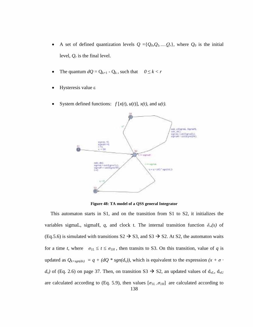
138
A set of defined quantization levels Q ={Q0,Q1,….Qr}, where Q0 is the initial
level, Qr is the final level.
The quantum dQ = Qk+1 - Qk , such that 0 ≤ k < r
Hysteresis value
System defined functions: f [x(t), u(t)], x(t), and u(t).
Figure 48: TA model of a QSS general Integrator
This automaton starts in S1, and on the transition from S1 to S2, it initializes the
variables sigmaL, sigmaH, q, and clock t. The internal transition function δint(s) of
(Eq.5.6) is simulated with transitions S2 S3, and S3 S2. At S2, the automaton waits
for a time t, where σ1L t σ1H , then transits to S3. On this transition, value of q is
updated as Qk+sgn(dx) = q + (dQ * sgn(dx)), which is equivalent to the expression (x + σ ·
dx) of (Eq. 2.6) on page 37. Then, on transition S3 S2, an updated values of dxL, dxU
are calculated according to (Eq. 5.9), then values [σ1L ,σ1H] are calculated according to
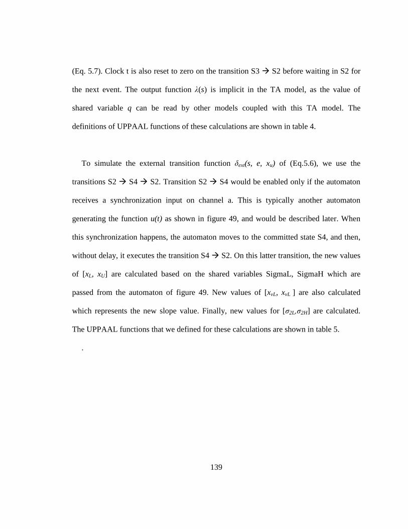
139
(Eq. 5.7). Clock t is also reset to zero on the transition S3 S2 before waiting in S2 for
the next event. The output function λ(s) is implicit in the TA model, as the value of
shared variable q can be read by other models coupled with this TA model. The
definitions of UPPAAL functions of these calculations are shown in table 4.
To simulate the external transition function δext(s, e, xu) of (Eq.5.6), we use the
transitions S2 S4 S2. Transition S2 S4 would be enabled only if the automaton
receives a synchronization input on channel a. This is typically another automaton
generating the function u(t) as shown in figure 49, and would be described later. When
this synchronization happens, the automaton moves to the committed state S4, and then,
without delay, it executes the transition S4 S2. On this latter transition, the new values
of [xL, xU] are calculated based on the shared variables SigmaL, SigmaH which are
passed from the automaton of figure 49. New values of [xvL, xvL ] are also calculated
which represents the new slope value. Finally, new values for [σ2L,σ2H] are calculated.
The UPPAAL functions that we defined for these calculations are shown in table 5.
.
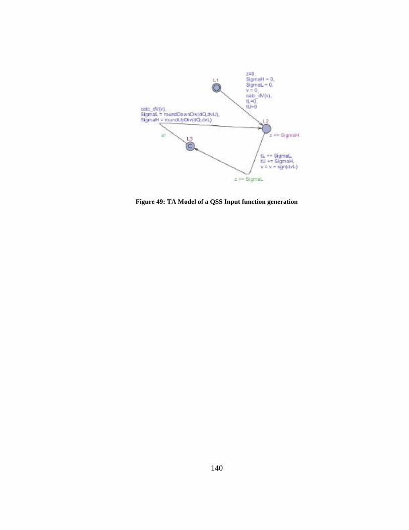
140
Figure 49: TA Model of a QSS Input function generation
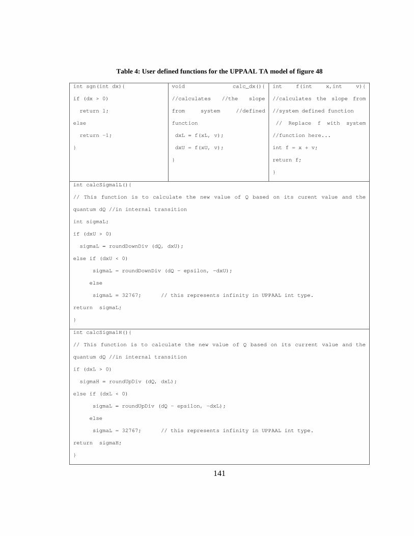
141
Table 4: User defined functions for the UPPAAL TA model of figure 48
int sgn(int dx){
if (dx > 0)
return 1;
else
return -1;
}
void calc_dx(){
//calculates //the slope
from system //defined
function
dxL = f(xL, v);
dxU = f(xU, v);
}
int f(int x,int v){
//calculates the slope from
//system defined function
// Replace f with system
//function here...
int f = x + v;
return f;
}
int calcSigma1L(){
// This function is to calculate the new value of Q based on its curent value and the
quantum dQ //in internal transition
int sigmaL;
if (dxU > 0)
sigmaL = roundDownDiv (dQ, dxU);
else if (dxU < 0)
sigmaL = roundDownDiv (dQ - epsilon, -dxU);
else
sigmaL = 32767; // this represents infinity in UPPAAL int type.
return sigmaL;
}
int calcSigma1H(){
// This function is to calculate the new value of Q based on its current value and the
quantum dQ //in internal transition
if (dxL > 0)
sigmaH = roundUpDiv (dQ, dxL);
else if (dxL < 0)
sigmaL = roundUpDiv (dQ - epsilon, -dxL);
else
sigmaL = 32767; // this represents infinity in UPPAAL int type.
return sigmaH;
}
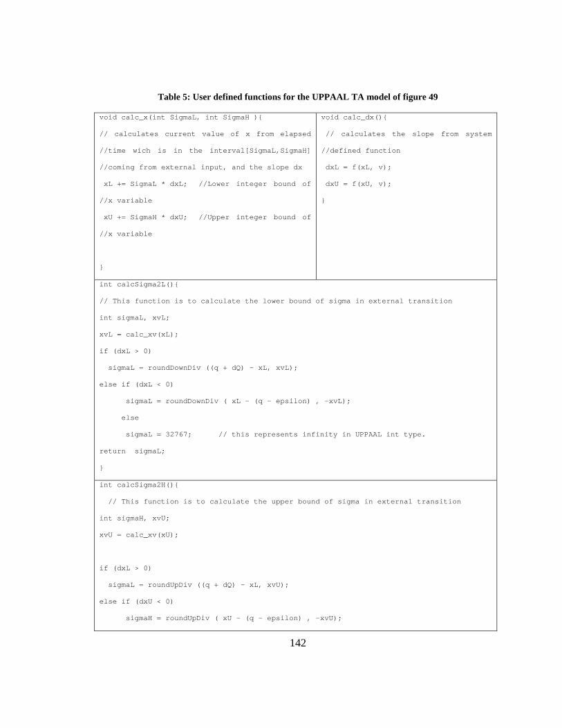
142
Table 5: User defined functions for the UPPAAL TA model of figure 49
void calc_x(int SigmaL, int SigmaH ){
// calculates current value of x from elapsed
//time wich is in the interval[SigmaL,SigmaH]
//coming from external input, and the slope dx
xL += SigmaL * dxL; //Lower integer bound of
//x variable
xU += SigmaH * dxU; //Upper integer bound of
//x variable
}
void calc_dx(){
// calculates the slope from system
//defined function
dxL = f(xL, v);
dxU = f(xU, v);
}
int calcSigma2L(){
// This function is to calculate the lower bound of sigma in external transition
int sigmaL, xvL;
xvL = calc_xv(xL);
if (dxL > 0)
sigmaL = roundDownDiv ((q + dQ) - xL, xvL);
else if (dxL < 0)
sigmaL = roundDownDiv ( xL - (q - epsilon) , -xvL);
else
sigmaL = 32767; // this represents infinity in UPPAAL int type.
return sigmaL;
}
int calcSigma2H(){
// This function is to calculate the upper bound of sigma in external transition
int sigmaH, xvU;
xvU = calc_xv(xU);
if (dxL > 0)
sigmaL = roundUpDiv ((q + dQ) - xL, xvU);
else if (dxU < 0)
sigmaH = roundUpDiv ( xU - (q - epsilon) , -xvU);
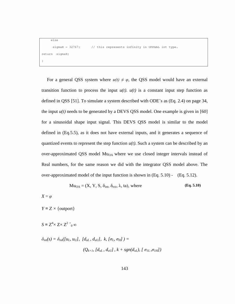
143
else
sigmaH = 32767; // this represents infinity in UPPAAL int type.
return sigmaH;
}
For a general QSS system where u(t) ≠ φ, the QSS model would have an external
transition function to process the input u(t). u(t) is a constant input step function as
defined in QSS [51]. To simulate a system described with ODE’s as (Eq. 2.4) on page 34,
the input u(t) needs to be generated by a DEVS QSS model. One example is given in [60]
for a sinusoidal shape input signal. This DEVS QSS model is similar to the model
defined in (Eq.5.5), as it does not have external inputs, and it generates a sequence of
quantized events to represent the step function u(t). Such a system can be described by an
over-approximated QSS model MuOA where we use closed integer intervals instead of
Real numbers, for the same reason we did with the integrator QSS model above. The
over-approximated model of the input function is shown in (Eq. 5.10) - (Eq. 5.12).
MuOA = (X, Y, S, δint, δext, λ, ta), where
X = φ
Y = × {outport}
S = 4× Z× Z2 +0 ∞
δint(s) = δint([uL, uU], [duL , duU], k, [σL, σH] ) =
(Qk+1, [duL , duU] , k + sgn(duL), [ σ1L ,σ1H])
(Eq. 5.10)
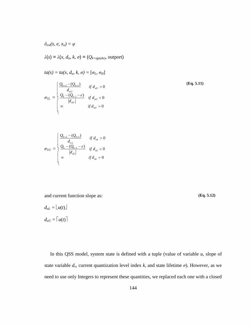
144
δext(s, e, xu) = φ
λ(s) = λ(x, du, k, σ) = (Qk+sgn(du), outport)
ta(s) = ta(x, du, k, σ) = [σL, σH]
σ1L =
0
0)(
0)(
1
12
uU
uUuU
kk
uU
Uu
kk
dif
difd
difd
(Eq. 5.11)
σ1U =
0
0)(
0)(
1
12
uL
uLuL
kk
uL
Lu
kk
dif
difd
difd
and current function slope as:
duL = u(t)
duU = u(t)
(Eq. 5.12)
In this QSS model, system state is defined with a tuple (value of variable u, slope of
state variable dv, current quantization level index k, and state lifetime σ). However, as we
need to use only Integers to represent these quantities, we replaced each one with a closed
145
integer interval. The integer interval is chosen to include inside it the quantity we are
approximating. We do this by choosing the lower bound of the interval with the Floor
function of the quantity, and the upper bound to be the Ceiling function. Thus the
corresponding intervals to describe the QSS state would be ([uL, uU], [duL , duU], k, [σL,
σH]). As this model has no external input, then we know, from the semantics of QSS
method, that the state variable u would always take a value from the set Q of the
quantization levels. Thus the term [uL, uU], of the state, would be the current quantization
level Qk+1. Calculation of the state lifetime σ, is done with arithmetic intervals in
(Eq. 5.11) as the slope of the function is expressed as an interval, which in turn is
calculated in (Eq. 5.12).
We follow the same steps we did for the QSS model of the integrator above to
simulate this QSS model with timed automata, resulting in the TA model shown in figure
49. The transition L1 L2 initializes clock z, the lower and upper time constraints [σ1L
,σ1H], the quantized output variable v , and calculates the initial slope from the function
definition of u(t) by invoking user defined function calc_dV(v). The slope is calculated as
a closed integer interval [dvL,dvU] to represent the over-approximation of slope value, as
defined in (Eq. 5.12).
δint(s) is simulated by transitions L2L3L2. On these two transitions, new value of v
is calculated, the function calc_dV(v) calculates the values of u(t), then the new values of
next event timing is calculated [ σ1L ,σ1H]. We note here that to calculate u(t) we need the
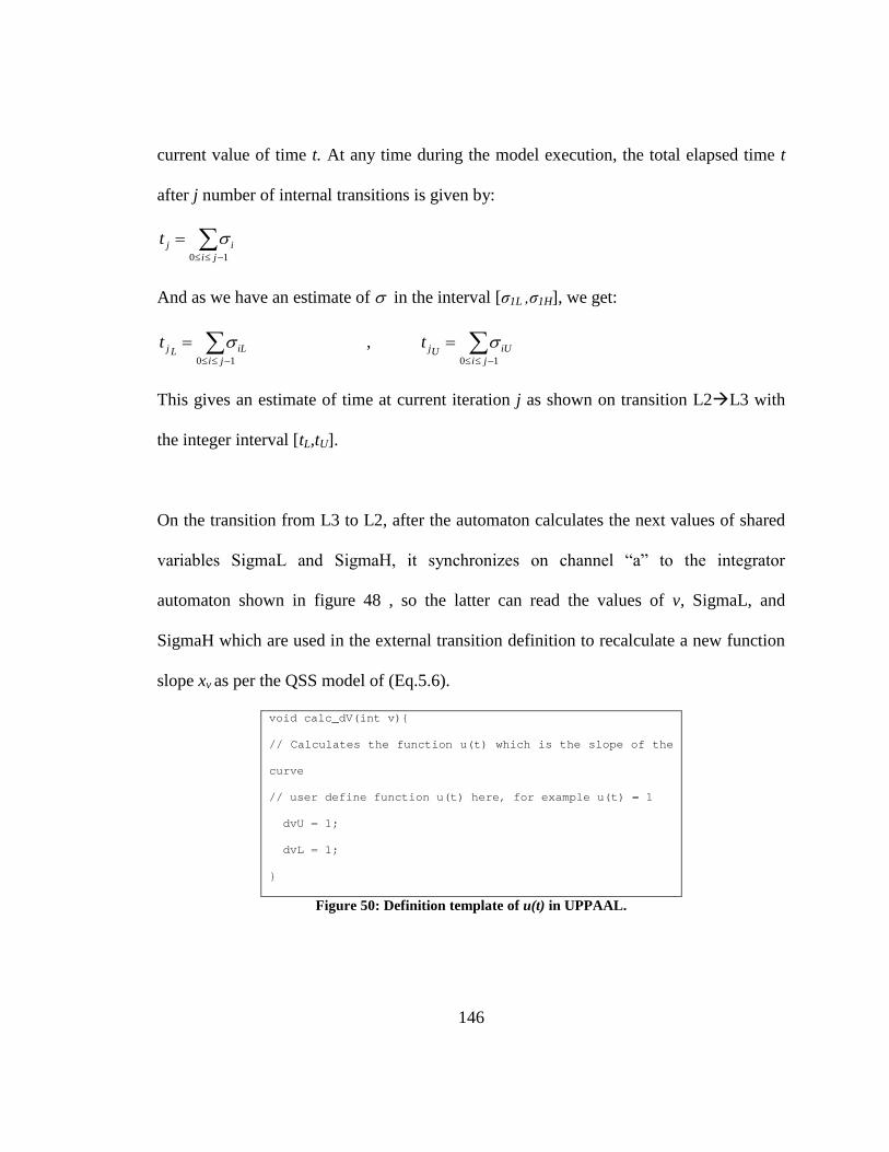
146
current value of time t. At any time during the model execution, the total elapsed time t
after j number of internal transitions is given by:
10 ji
ijt
And as we have an estimate of in the interval [σ1L ,σ1H], we get:
10 ji
iLLjt ,
10 ji
iUUjt
This gives an estimate of time at current iteration j as shown on transition L2L3 with
the integer interval [tL,tU].
On the transition from L3 to L2, after the automaton calculates the next values of shared
variables igmaL and igmaH, it synchronizes on channel “a” to the integrator
automaton shown in figure 48 , so the latter can read the values of v, SigmaL, and
SigmaH which are used in the external transition definition to recalculate a new function
slope xv as per the QSS model of (Eq.5.6).
void calc_dV(int v){
// Calculates the function u(t) which is the slope of the
curve
// user define function u(t) here, for example u(t) = 1
dvU = 1;
dvL = 1;
}
Figure 50: Definition template of u(t) in UPPAAL.
147
5.1.4 Advantages of using QSS/DEVS to verify Hybrid Models
Enabling approximation to system dynamics in timed automata models using QSS opens
the door to more complex verification queries and better controller designs. For example,
the following research directions can be built on results of hybrid systems verification
using QSS, as we introduced earlier in this chapter:
System dynamics are presented in a fine-grain in the TA model. This would
enable verification of more advanced types of controllers than an On-Off
controller. For example, advanced control algorithms could use the information
about the state variable change with respect to time.
Optimization controller designs could also be verified in UPPAAL based on some
optimization constraints on the values of state variables.
TA controller synthesis techniques could use the fine-grained information of
system dynamics to synthesis advanced controllers based on QSS environment
models.
148
Chapter 6: Conclusion & Future Research
In this thesis, we have presented a methodology for the verification of different DEVS
models. This methodology covers different components, including both deterministic
classic DEVS and continuous components, which were modeled as DEVS using the QSS
method (the QSS method was selected as the way to discretize the continuous behaviour
using DEVS; however, other current or future methods within DEVS could be used in a
similar fashion).
The contributions of this work include a verification methodology for deterministic
classic DEVS. Although, as identified in the State of the Art section, other groups have
used TA to verify DEVS in parallel with our research, the work introduced in this
research is different. The main contribution is the provision of a complete method that
deals with the issues that prevent a full verification of DEVS models as shown in section
4.1. It also provides a formal methodology to convert DEVS models into behaviourally
equivalent TA models. Finally, the methodology provides an estimation method for any
errors that could have occurred due to the conversion and the approximation process.
Hybrid DEVS verification presented in this thesis is also an original result. These
contributions resulted in numerous publications, listed in section 3.1.
149
6.1.1 Possible Future Research
This dissertation lays the groundwork for the formal verification of DEVS models
based on their transformation into TA. Based on this basic ability to verify DEVS
models, further enhancements to the methodology are possible. Such enhancements
would increase the model checking efficiency by decreasing the total state-space
traversed during the model checking analysis. Such increase in efficiency would translate
into a practical ability to verify larger DEVS models than what is currently possible, thus
making formal DEVS verification possible for industrial-size models.
These enhancements are based on exploiting some properties that are specific to the
TA models resulting from the transformation of DEVS models. Such properties are not
valid in general in TA. One of these properties is the nature of any embedded DEVS
execution engine such as e-CD++. These engines usually run on a single processor
machine and thus use a single physical clock to measure the elapsed time for all atomic
DEVS components executing on this platform. Another observed property of many
practical DEVS models is the re-use of the same atomic or coupled component many
times in a complex DEVS model. Thus, the use of symmetry reduction techniques would
reduce the number of distinct components to be verified. We expand on these two main
possible future directions below:
Reducing state-space through reducing model complexity. Model checking
timed automata models depends on building a finite reachability graph called
Region Graph. Answering queries about system properties is done through
150
traversing this graph and validating the desired property at each node. Thus
the complexity of the reachability algorithm depends on the size of the region
graph. Aceto and Laroussinie [83] showed that this size is in the order of
O(|C|! + M|C|), where |C| is the total number of clocks in both the TA model
and the query, and M is the maximum constant appearing in the TA model or
the query. Hence a great reduction in region graph size can be achieved by
reducing the number of clocks in a TA model. This may be done in several
ways as follows:
o Checking safety and reachability properties of a DEVS model on an
abstraction of untimed finite automata. This untimed finite automata
model would be obtained by removing all the timing information from
the DEVS model. This untimed version would constitute a rough
abstraction of the DEVS model that contains all behaviors of the
original DEVS model, plus some extra behavior due to removing the
restrictions of timings. However, checking untimed model would be
much more efficient than the timed model. This approach does not
work for checking bounded-liveness properties on DEVS models. If
verifying these properties is required, then next optimization would
help.
o In our methodology, as well as in all others as introduced in literature,
each atomic DEVS model is transformed to a TA model with a clock
151
that measures the model elapsed time. One-clock automata can use
efficient model-checking algorithms, as shown in [84]. However, any
coupled DEVS model would be composed of many atomic models,
each with its own clock. Therefore, the resulting equivalent composed
TA for the coupled model would contain more than one clock, and
thus cannot be considered a one-clock TA model. On the other hand,
in most embedded simulators and runtimes, the coupled DEVS model
would execute on a single processor using a single global clock. This
assumption can be used to obtain an equivalent TA model with only
one global clock for the complete coupled model. This would enable
the efficient verification of such TA models, and thus scale up the size
and number of DEVS components that can practically been verified. If
the assumption of single processor cannot be guaranteed, as in the case
in clustered systems for example, we would need a single clock for
each component, and this optimization technique would not apply.
Symmetry in DEVS coupled models could be used to reduce state-space. As
any typical system is normally composed of many components, it is common
to find the same type of component replicated in many places in the system. A
DEVS model of such system would contain replicated components. An
intelligent conversion method from DEVS to TA could identify identical
152
DEVS components, and flag them for symmetrical analysis in the resulting
TA model, thus greatly reducing state-space during reachability analysis.
Another possible future research is related to the verification of continuous systems
modeled with the QSS method. As described in section 5.1.3, the QSS method
approximates the actual system trajectory. This approximation results in an error |E|
which is the difference between the true system trajectory and the QSS approximated
trajectory as can be seen in Figure 46. We can find a bound on this error as per [51]
that depends on the quantization step dQ. For formal verification of hybrid system, it
is desirable to verify the true system trajectory against safety requirements, and not
only the approximation. To extend our verification methodology to do this, we can
increase QSS intervals outwards with the estimated approximation error |E|. This
would guarantee the true system trajectory is covered inside the trajectory being
verified. Future research would look into formal models for this enhancement, effect
of this on the verification complexity and the TA implementation. In case of highly
non-linear functions, the error |E| can be large. In this case, another extension could
be using QSS2 method in which the system trajectory is approximated with second
order segments as shown in [51].
153
REFERENCES
[1] M. J. Rehman, F. Jabeen, A. Bertolino, and A. Polini. 2007. “Testing oftware Components for
Integration: a urvey of Issues and Techniques”. Software Testing,Verification and Reliability
17(2): 95–133.
[2] R. Gerlich, R. Gerlich, T. Boll. 2007. “Random Testing: From the Classical Approach to a Global
iew and Full Test Automation”. In Proceedings of the 2nd international Workshop on Random
Testing, Co-Located with the 22nd IEEE/ACM international Conference on Automated Software
Engineering (ASE 2007), Atlanta, Georgia.
[3] M. B. Dwyer, J. Hatcliff, R. Robby, C. S. Pasareanu, and W. Visser. 2007. "Formal Software
Analysis Emerging Trends in Software Model Checking". In Proceedings of the 2007 Future of
Software Engineering (FOSE '07). IEEE Computer Society, Washington, DC, pages 120-136.
[4] S. Kowalewski. 2002. “Introduction to the Analysis and Verification of Hybrid Systems”.
Modelling, Analysis, and Design of Hybrid Systems. Lecture Notes in Control and Information
Sciences, 279: 153-171.
[5] R. Alur, . ill. 1994. “Theory of Timed Automata". Theoretical Computer Science, 126: 183-
235.
[6] G. Wainer, . Glinsky, and P. Mac Ien. 2005. “A Model-Driven Technique for Development of
Embedded ystems Based on the Formalism”. In Model-driven Software Development -
Volume II of Research and Practice in Software Engineering, edited by S. Beydeda and V. Gruhn.
Springer-Verlag.
[7] B. P. Zeigler, T. Kim, and H. Praehofer. 2000 . Theory of Modeling and Simulation. San Diego,
CA: Academic Press, ISBN-10: 0127784551.
154
[8] Y. H. Yu, G. Wainer. 2007. "eCD++: an engine for executing DEVS models in embedded
platforms". In Proceedings of the 2007 SCS Summer Computer Simulation Conference, San
Diego, CA July 15-18.
[9] G. Behrmann, A. David, K Larsen. 2004. “A Tutorial on Uppaal”. Proceedings of the 4th
International School on Formal Methods for the Design of Computer, Communication, and
Software Systems. LNCS 3185.
[10] J. Bengtsson, W. Yi. 2004. “Timed Automata: emantics, Algorithms and Tools”. Lectures on
Concurrency and Petri Nets, 3098.
[11] G. Wainer. 2002. "CD++: a toolkit to develop DEVS models". Software: Practice and Experience
32 (13): 1261-1306.
[12] E. Kofman, M. Lapadula, and E. Pagliero. 2003. “Powerdevs: A devs-based environment for
hybrid system modeling and simulation”. Technical Report LSD0306, School of Electronic
Engineering, Universidad Nacional de Rosario, Rosario, Argentina.
[13] Muzy, J. Nutaro. 2005. “Algorithms for efficientcient implementations of the devs & dsdevs
abstract simulators”. In proceedings of 1st Open International Conference on Modeling &
Simulation: 401-407, ISIMA / Blaise Pascal University, France, June 2005.
[14] B. P. Zeigler, H. arjoughian. 2002. “Introduction to modeling and simulation with JAVA:
A simplified approach to HLA compliant distributed simulations”. Tucson: University of Arizona,
Accessed March 2011. http://www.acims.arizona.edu
[15] X. Hu; B.P. Zeigler, J. Couretas. 2001. “DEVS-on-a-chip: implementing DEVS in real-time Java
on a tiny Internet interface for scalable factory automation”. In: proceedings of IEEE
155
International Conference on Systems, Man, and Cybernetics, Tucson, AZ , USA, 2001(5): 3051 –
3056.
[16] F. Bergero, E. Kofman. 2011. :PowerDEVS: a tool for hybrid system modeling and real-time
simulation”. SIMULATION 87 (1-2): 113-132.
[17] Cho, Y. K., X. Hu, and B. P. Zeigler. 2003. The RTDEVS/CORBA environment for simulation-
based design of distributed real-time systems. SIMULATION 79 (4).
[18] F. R. Sadeghi, G. Wainer, and M. Moallemi. 2010. "Modeling and Controlling a Robotic Arm
with E-CD++". Poster, SummerSim 2010 Conference - July 2010.
[19] A. almari. 2009. " oftware model checking is a rich research field”. International Journal on
Software Tools for Technology Transfer (STTT) 11(1): 1–11.
[20] L. Aceto, A. Bergueno, and K. G. Larsen. 1998. “Model Checking via Reachability Testing for
Timed Automata”. In Proceedings, Fourth Workshop on Tools and Algorithms for the
Construction and Analysis of Systems, Lisbon, Portugal, LNCS 1384.
[21] R. Alur, C. Courcoubetis, D. L. Dill. 1990. “Model-Checking for Real-Time ystems”. In
Proceedings, Fifth Annual IEEE Symposium on Logic in Computer Science, Philadelphia, PA.
[22] R. Alur, C. Courcoubetis, D. L. Dill. 1993. “Model-Checking in Dense Real-Time”. J. of
Information and Computation 104(1): 2–34.
[23] T. A. Henzinger, X. Nicollin, J. Sifakis, S. Yovine. 1992. “ ymbolic Model Checking for Real-
Time ystems”. Proc. of 7th Annual IEEE Symposium on Logic in Computer Science, Santa Cruz,
CA.
156
[24] T. A. Henzinger, X. Nicollin, J. Sifakis, S. Yovine. 1994. “ ymbolic Model Checking for Real-
Time ystems”. Journal of Information and Computation 111(2): 193–244.
[25] P. Bouyer and F. Laroussinie. 2008. “Model Checking Timed Automata”. In Modeling and
Verification of Real-Time Systems, edited by N.Navet and S. Merz 111-140. ISTE Ltd. - John
Wiley & Sons, Ltd.
[26] G. Wainer, L. Morihama, and V. Passuello. 2002. "Automatic verification of DEVS models", In
Proceedings of SISO Spring Interoperability Workshop, Orlando, FL. U.S.A. March 10-15.
[27] Hernandez, N. Giambiasi. 2005. "State Reachability for DEVS Models", Proc. of Argentine
Symposium on Software Engineering (2005).
[28] J. . Hong, H. . ong, T.G. Kim, K.H. Park. 1997. “A realtime iscrete vent ystem
Specification formalism for seamless real-time software development”. Discrete Event Dynamic
Systems 7 (4): 355-75.
[29] H.S. Song, T.G. Kim. 2005. "Application of Real-Time DEVS to Analysis of safety-Critical
Embedded Control Systems: Railroad Crossing Control Example", SIMULATION 81(2):119-136.
[30] SP-DEVS on Wikipedia accessed Feb.28, 2011 at http://en.wikipedia.org/wiki/SP-DEVS.
[31] M. H. Hwang. 2005. "Tutorial: Verification of Real-time System Based on Schedule-Preserved
DEVS". In Proceedings of 2005 DEVS Symposium, San Diego, April 2-8.
[32] M. H. Hwang. 2005. "Generating Finite-State Global Behavior of Reconfigurable Automation
Systems: DEVS Approach". In Proceedings of 2005 IEEE-CASE, Edmonton, Canada, Aug. 1-2.
[33] M. H. Hwang, S.K. Cho, B.P. Zeigler, and F. Lin. 2007. "Processing Time Bounds of Schedule-
Preserving DEVS". Arizona Center of Integrative Modeling & Simulation Technical Report.
157
[34] M-H. Hwang, B.P. Zeigler. 2009. “Reachability Graph of Finite and eterministic DEVS
Networks”. IEEE Transactions on Automation Science and Engineering 6 (3): 468 – 478.
[35] A. Furfaro, L. Nigro. 2008. "Embedded Control Systems Design based on RT-DEVS and temporal
analysis using UPPAAL". Proceedings of Computer Science and Information Technology, 20-22
Oct. 2008, IMCSIT 2008: 601-608.
[36] A. Furfaro, L. Nigro. 2009."A development methodology for embedded systems based on RT-
DEVS". Innovations in Systems and Software Engineering 5: 117-127.
[37] F. Cicirelli, A. Furfaro, L. Nigro, and F. Pupo. 2010. “Temporal verification of RT-DEVS models
with implementation aspects”. In Proceedings of the 2010 Spring Simulation Multiconference
(SpringSim '10), Orlando, FL, USA, April 11 - 15, 2010.
[38] S. Han, K. Huang. 2007. "Equivalent Semantic Translation from Parallel DEVS Models to Time
Automata", In Proceedings of the 7th international conference on Computational Science, Part I:
ICCS 2007 (ICCS '07).
[39] L. Aceto, A. Ingólfsdóttir, K. Guldstrand Larsen, J. Srba. 2007. Reactive Systems: Modelling,
Specification and Verification. Cambridge University Press.
[40] H. Dacharry, N. Giambiasi. 2007. "Formal Verification Approaches for DEVS". Proceedings of
Summer Computer Simulation Conference, San Diego, CA, USA July 15-18, 2007.
[41] N. Giambiasi, J-L. Paillet, F. Châne. 2003. "From Timed Automata To DEVS Models".
Proceedings of the 2003 Winter Simulation Conference, Phoenix, AZ, Dec. 7-10.
[42] K.J. Hong T. G. Kim. 2005. "Timed I/O Test Sequences for Discrete Event Model Verification".
Artificial Intelligence and Simulation 3397: 275–284.
158
[43] Y. Labiche, G. Wainer. 2005. “Towards the erification and alidation of Models”.
Proceedings of the 1st Open International Conference on Modeling & Simulation. Clermont-
Ferrand, France: 295-305.
[44] R. Castro, E. Kofman, and G. A. Wainer. 2008. “A formal framework for stochastic DEVS
modeling and simulation”. In Proceedings of the 2008 Spring simulation multiconference
(SpringSim '08). Society for Computer Simulation International, San Diego, CA, USA, 421-428.
[45] M. Kwiatkowska, G. Norman, R. Segala, and J. Sproston. 2002. “Automatic verification of real-
time systems with discrete probability distributions”. Theor. Comput. Sci. 282, 1 (June 2002), 101-
150.
[46] M. S Branicky. 2005. “Introduction to Hybrid Systems” D. Hristu-Varsakelis and W.S. Levine
(eds.), Handbook of Networked and Embedded Control Systems, 91-116. Boston: Birkhauser.
[47] A. Donzé, O. Maler. 2007. “Systematic simulation using sensitivity analysis”. In Proceedings of
the 10th international conference on Hybrid systems: computation and control (HSCC'07) :174-
189.
[48] A. Donzé. 2007. “Trajectory-Based Verification and Controller Synthesis for Continuous and
Hybrid Systems”. PhD thesis, University Joseph Fourier.
[49] A. Donzé, B. Krogh, and A. Rajhans. 2009. “Parameter synthesis for hybrid systems with an
application to simulink models”. In Proceedings of the 12th International Conference on Hybrid
Systems : Computation and Control (HSCC'09), San Francisco, CA, USA, April 13-15, 2009.
[50] E. Kofman, S. Junco. 2001."Quantized State Systems. A DEVS Approach for Continuous Systems
Simulation". Transactions of SCS. 18(3): 123-132.
159
[51] E. Kofman. 2004. "Discrete Event Simulation of Hybrid Systems". SIAM Journal on Scientific
Computing 25(5): 1771-1797.
[52] M. Otter, F. Cellier. 1996. The Control Handbook, chapter Software for Modeling and Simulating
Control Systems, 415–428. CRC Press, Boca Raton, FL.
[53] G. Decknatel, R. Slovák, E. Schnieder. 2002. “Definition of a Type of Continuous-Discrete High-
Level Petri Nets and Its Application to the Performance Analysis of Train Protection Systems In
S. Engell, G. Frehse, and E. Schnieder (Eds.), Modelling, Analysis, and Design of Hybrid Systems,
Lecture Notes in Control and Information Sciences 279: 355–367.
[54] T. Henzinger. 1996. “The Theory of Hybrid Automata”. Lecture Notes in Computer Science 278.
[55] T. A. Henzinger, P. W. Kopke, A. Puri, and P. araiya. 1995. “What's decidable about hybrid
automata?”. In Proceedings of the twenty-seventh annual ACM symposium on Theory of
computing, STOC ’95, New York, NY, USA, 373–382.
[56] J. Lunze and J. Raisch. 2002. “Discrete Models for Hybrid Systems. Modelling, Analysis, and
Design of Hybrid Systems”. Lecture Notes in Control and Information Sciences, 279: 67-80.
[57] R. Alur, T.A. Henzinger, G. Lafferriere, G.J. Pappas. 2000. “Discrete abstractions of hybrid
systems”. Proceedings of the IEEE, 88(7): 971-984.
[58] E. Barke, D. Grabowski, H. Graeb, L. Hedrich, S. Heinen, R. Popp, S. Steinhorst, and Y. Wang.
2009. “Formal approaches to analog circuit verification”. In Proceedings of the Conference on
Design, Automation and Test in Europe (DATE '09), European Design and Automation
Association, 3001 Leuven, Belgium, Belgium, 724-729.
160
[59] Oded Maler and Grégory Batt. 2008. “Approximating Continuous Systems by Timed Automata”.
In Proceedings of the 1st international workshop on Formal Methods in Systems Biology (FMSB
'08), Cambridge, UK, Jasmin Fisher (Ed.). Springer-Verlag, Berlin, Heidelberg, 77-89.
[60] F. Cellier , E. Kofman. 2006. Continuous System Simulation. ISBN 978-0-387-26102-7, Springer
publishing.
[61] J. G. Rokne. 2001.” Interval arithmetic and interval analysis: an introduction”. In Granular
computing, Witold Pedrycz (Ed.). Physica-Verlag GmbH, Heidelberg, Germany.
[62] B. Hayes, 2003.“Lucid Interval”, Scientific American, November-December 2003, 91(6): 484.
[63] R. E. Moore, R. B. Kearfott, and M. J. Cloud, 2009."Introduction to Interval Analysis". Society for
Industrial and Applied Math., Philadelphia, PA, USA.
[64] J. Srba. 2008. “Comparing the Expressiveness of Timed Automata and Timed Extensions of Petri
Nets”. In Proceedings of the 6th international conference on Formal Modeling and Analysis of
Timed Systems (FORMATS '08), Franck Cassez and Claude Jard (Eds.). Springer-Verlag, Berlin,
Heidelberg, pages 15-32.
[65] V. Gupta, T. A. Henzinger, R. Jagadeesan. 1997. "Robust timed automata". Hybrid and Real-Time
Systems 1201: 331-345.
[66] M. De Wulf, L. Doyen, N. Markey. 2004."Robustness and Implementability of Timed Automata"
Formal Techniques, Modelling and Analysis of Timed and Fault-Tolerant Systems : 359-374.
[67] M. De Wulf, L. Doyen, J-F. Raskin. 2004. "Almost ASAP Semantics: From Timed Models to
Timed Implementations" Hybrid Systems: Computation and Control : 296-310.
161
[68] H. aadawi, G. Wainer. 2010. “Rational time-advance DEVS (RTA-DEVS). In Proceedings of
DEVS Symposium 2010, Orlando, FL., April 11-15.
[69] J. Miller. 2000. "Decidability and complexity results for timed automata and semi-linear hybrid
automata". Hybrid Systems: Computation and Control, LNCS 1790.
[70] H. Saadawi, G. Wainer. 2011. “Principles of Models erification”. SIMULATION:
Transactions of the Society for Modeling and Simulation International, October 23, 2011, doi:
10.1177/0037549711424424.
[71] H. Saadawi, G. Wainer, M. Moallemi. 2012. “Principles of Models erification for Real-
Time mbedded Applications”. Real-Time Simulation Technologies: Principles, Methodologies,
and Applications. K. Popovici, P. Mosterman Eds. Taylor and Francis. CRC Press. 2012.
[72] H. Saadawi, G. Wainer. 2009. “ erification of real-time models”. In Proceedings of DEVS
Symposium 2009. San Diego, CA, March 22 – 27.
[73] H. Saadawi, G. Wainer. 2010. “From DEVS to RTA-DEVS”. In Proceedings of the 2010
IEEE/ACM 14th International Symposium on Distributed Simulation and Real Time Applications
(DS-RT '10), Fairfax, VA. USA, Oct.17-20: 207-210.
[74] C. Daws, A. Olivero, S. Tripakis, and S. Yovine. 1996. “The tool KRONOS”. In Proceedings of
the DIMACS/SYCON workshop on Hybrid systems III : verification and control: verification and
control, Secaucus, NJ, USA, 208–219.
[75] .Yovine. 1997. “Kronos: A verification tool for real-time systems”. Springer International
Journal of Software Tools for Technology Transfer 1(1-2): 123–133.
[76] Wikipedia. DEVS behavior. http://en.wikipedia.org/wiki/ Behavior_of_Coupled_DEVS
[Accessed: Aug. 2009].
162
[77] H. Bowman, R. Gomez. 2006. Concurrency Theory: Calculi and Automata for Modelling Untimed
and Timed Concurrent Systems. Springer-Verlag London.
[78] Puri. 1998. "Dynamical properties of timed automata", Formal Techniques in Real-Time and
Fault-Tolerant Systems 210-227.
[79] http://en.wikipedia.org/wiki/Exponential_decay wikipedia, 2011, "Exponential decay", accessed
Sept. 2nd 2011.
[80] B. Berard, , M. Bidoit, A. Finkel, F. Laroussinie, A. Petit, L. Petrucci, Ph. Schnoebelen and P.
McKenzie. 2001. Systems and Software Verification: Model-Checking Techniques and Tools.
Springer Verlag.
[81] H. Saadawi, G. Wainer. 2012. “On the verification of hybrid models”. In Proceedings of
the 2012 Symposium on Theory of Modeling and Simulation - DEVS Integrative M&S Symposium
(TMS/DEVS '12), Orlando, FL,USA. March 26-28.
[82] Henzinger, T.A.; Pei-Hsin Ho; Wong-Toi, H.; , "Algorithmic analysis of nonlinear hybrid
systems," Automatic Control, IEEE Transactions on , vol.43, no.4, pp.540-554, Apr 1998.
[83] L. Aceto and F. Laroussinie, 2002. “Is your model checker on time? On the complexity of model
checking for timed modal logics”. Journal of Logic and Algebraic Programming, 52-53:7-51,
August 2002.
[84] F. Laroussinie, N. Markey and Ph. Schnoebelen. “Model Checking Timed Automata with One or
Two Clocks”. CONCUR 2004 – Concurrency Theory, Lecture Notes in Computer Science 3170:
387-401.