Automatica 44 (2008) 15–27www.elsevier.com/locate/automatica

Performance of convergence-based variable-gain control ofoptical storage drives�

N. van de Wouwa,∗, H.A. Pastinkb, M.F. Heertjesc, A.V. Pavlovd, H. Nijmeijera

aDepartment of Mechanical Engineering, Eindhoven University of Technology, P.O. Box 513, 5600 MB Eindhoven, The NetherlandsbOcé Technologies, P.O. Box 101, 5900 MA, Venlo, The Netherlands

cPhilips Applied Technologies, Department Mechatronics Technologies, 5600 MD Eindhoven, The NetherlandsdNTNU, Department of Engineering Cybernetics, N7491 Trondheim, Norway

Received 1 September 2005; received in revised form 28 January 2007; accepted 18 April 2007Available online 20 August 2007

Abstract

In this paper, a method for the performance assessment of a variable-gain control design for optical storage drives is proposed. The variable-gain strategy is used to overcome well-known linear control design trade-offs between low-frequency tracking properties and high-frequencynoise sensitivity. A convergence-based control design is proposed that guarantees stability of the closed-loop system and a unique boundedsteady-state response for any bounded disturbance. These favourable properties, guaranteed by virtue of convergence, allow for a uniqueperformance evaluation of the control system. Moreover, technical conditions for convergence are derived for the variable-gain controlledsystem and a quantitative performance measure, taking into account both low-frequency tracking properties and high-frequency measurementnoise sensitivity, is proposed. The convergence conditions together with the performance measure jointly constitute a design tool for tuning theparameters of the variable-gain controller. The resulting design is shown to outperform linear control designs.� 2007 Elsevier Ltd. All rights reserved.

Keywords: Optical storage drives; Variable-gain control; Convergent systems; Performance assessment

1. Introduction

Optical storage drives, such as CD or DVD, either ROM oraudio, drives, are generally controlled using linear (PID-type)control strategies. Especially for portable or automotive appli-cations, the requirements on the control design relate to bothtracking requirements and disturbance attenuation properties.In this scope, two types of disturbances can be distinguished.Firstly, low-frequent shock disturbances are inevitable in auto-motive applications due to engine vibration or road excitation.Secondly, high-frequent disturbances are due to the fact thatthe measurement of the position of the disc tracks relative tothe lens position, by the optical pick-up unit, is corrupted bythe presence of finger prints, scratches and dirt spots (i.e. discdefects).

� This paper was not presented at any IFAC meeting. This paper wasrecommended for publication in revised form by Associate Editor MasakiYamakita under the direction of Editor Mituhiko Araki.

∗ Corresponding author.E-mail address: n.v.d.wouw@tue.nl (N. van de Wouw).

0005-1098/$ - see front matter � 2007 Elsevier Ltd. All rights reserved.doi:10.1016/j.automatica.2007.04.004

When applying linear control, the following fundamental de-sign trade-off is inherently present: increasing the closed-loopbandwidth improves the low-frequency disturbance rejectionproperties at the cost of deteriorating the sensitivity to high-frequency measurement noise (Freudenberg, Middleton, &Stefanopoulou, 2000). Nonlinear control, or more specifically,nonlinear PID control, see also the work of Armstrong, Neevel,and Kusid (2001), Jiang and Gao (2001), Fromion and Scorletti(2002) and Armstrong, Gutierrez, Wade, and Joseph (2006)combines the possibility of having increased performance interms of shock attenuation without unnecessarily deterioratingthe time response under disc defect disturbances. In Heertjesand Steinbuch (2004) and Heertjes, Pastink, van de Wouw, andNijmeijer (2006), variable-gain control strategies are proposedto overcome the practical implications of such design limita-tions. In those papers, the comparison between control designsis based on time- and frequency-domain simulations and ex-periments. Such analyses do not directly support a quantitativecomparison of the performance of different variable-gain and

16 N. van de Wouw et al. / Automatica 44 (2008) 15–27

linear control designs. On the other hand, the power of lin-ear control strategies lies in the fact that essential closed-loopproperties, such as stability and performance, can readily bechecked. It should be noted that generally the design of non-linear control systems is merely aiming at closed-loop stabil-ity and the performance assessment is confined—if present atall—to simulation-based reasoning.

For linear control systems, frequency-domain analysis playsa central role in the performance assessment of these systems.Such analysis hinges on the fact that an asymptotically stablelinear time-invariant system exhibits a unique bounded steady-state solution for any bounded disturbance. Nonlinear systemsdo generally not exhibit such properties. Instead, perturbed non-linear systems can exhibit multiple steady-state solutions. Thesefacts seriously hamper a performance analysis of such nonlin-ear control systems. The class of convergent systems, however,exhibits such favourable properties; see Demidovich (1967),Pavlov, Pogromsky, van de Wouw, and Nijmeijer (2004) andPavlov, van de Wouw, and Nijmeijer (2005) for more informa-tion on the notion of convergence.

Convergence implies stability (of an equilibrium point) inthe absence of disturbances and it guarantees the existence ofa unique bounded globally asymptotically stable steady-statesolution for every bounded disturbance. Obviously, if such asolution does exist, all other solutions, regardless of their ini-tial conditions, converge to this solution, which can be con-sidered as a steady-state solution (Demidovich, 1967; Pavlovet al., 2004). Similar notions describing the property of solu-tions converging to each other are studied in literature. Thenotion of contraction has been introduced in Lohmiller andSlotine (1998) (see also references therein). An operator-basedapproach towards studying the property that all solutions of asystem converge to each other is pursued in Fromion, Monaco,and Normand-Cyrot (1996) and Fromion, Scorletti, and Fer-reres (1999). In Angeli (2002), a Lyapunov approach has beendeveloped to study the global uniform asymptotic stability ofall solutions of a system (in Angeli, 2002, this property is calledincremental stability).

We propose a variable-gain control design, which ensuresconvergence (and therefore stability) of the closed-loop system,and therefore allows for a unique performance evaluation in theface of disturbances. Still, a definition of a performance mea-sure is needed for a quantitative comparison of control designs.We propose such a performance measure and use it to support aperformance-based control design for variable-gain controlledoptical storage drives. It will be shown that stability-based andperformance-based control synthesis may lead to different de-signs and that the variable-gain strategy can outperform linearcontrol strategies. In Fromion et al. (1999) and Fromion andScorletti (2002), the concept of incremental stability is used toassess the performance of nonlinear control systems. The per-formance is studied by investigating the L2-norms of inputsand outputs of the control system. This approach is less suitablefor the performance assessment for optical storage drives be-cause the performance of such systems is closely related to theL∞-norm of the tracking error since that determines whetherthe disc read-out is terminated or not. Moreover, a view on per-

formance based on gains between norms on inputs and outputscan be a rather conservative one. Therefore, we adopt the per-spective of exactly computing the steady-state responses (whichare unique by virtue of the convergence property) to distur-bances from the specific class of harmonic disturbances anddefining the control performance on the basis of these quantita-tive data. The performance in the face of harmonic disturbancesis specifically important for optical storage drives. For example,in practice the performance is tested experimentally by con-structing so-called ‘drop-out-level curves’ (Heertjes, Cremers,Rieck, & Steinbuch, 2005), which show the level of the har-monic disturbance for which a termination of the disc read-outoccurs for varying disturbance frequencies.

The paper is organised as follows. In Section 2, the opticalstorage drive is introduced and a simple model for the dy-namics (in radial direction) is proposed. Moreover, a conven-tional linear control design and the related fundamental designlimitations are discussed. The variable-gain control strategy isintroduced in Section 3. Section 4 introduces the class of con-vergent systems and proposes conditions for convergence. Sub-sequently, the closed-loop behaviour is studied both in the timedomain and in the frequency domain in Section 5. In Section 6,the performance measure is introduced and used to discriminatebetween different control designs. Finally, a discussion of theobtained results and concluding remarks are given in Section 7.

2. Modelling and control of optical storage drives

Optical storage drives obtain information from a disc usingthe principles of optical read-out. Hereby, information is storedon the disc’s surface by means of a sequence of reflective landsand non-reflective pits contained in a track. The informationis read from the disc via a light path guided by a lens in aso-called optical pick-up unit. The light is reflected by the pitand land structure on the disc. We focus on the control ofthe lens in radial direction. The tolerance on the tracking tobe preserved in playing is dictated by the track width whichamounts 0.74 �m for a DVD. A model for the lens dynamicsin radial direction is depicted schematically in Fig. 1. Herein, rrepresents the position of the track to be read, since the turntablewith the disc is mounted on the base frame. The two-stagecontrol strategy of the optical pick-up unit consists of a so-called long-stroke motion of a sledge containing the lens (pls)

and a short-stroke motion of the lens with respect to the sledge(pss). We primarily focus on the control of the short-strokemotion (i.e. pls is assumed fixed). The lens dynamics in the

Fig. 1. Model of the dynamics in radial direction.

N. van de Wouw et al. / Automatica 44 (2008) 15–27 17

sledge are modelled by a mass–spring–damper system withmass m, stiffness k and damping b.

A block-diagram of a linearly controlled optical storage driveis given in Fig. 2. Herein, n represents measurement noise andu is the control action. It should be noted that in optical storagedrives the error e (the difference between disk position r andthe actual lens position p) is the measured variable. Since it iscorrupted by the measurement noise it is denoted by e. More-over, HP (s) represents the transfer function related to the lensdynamics and actuator dynamics:

HP (s) = p(s)

u(s)= �a

(ms2 + bs + k)(s + �a), s ∈ C.

Note that the actuator dynamics are modelled using a low-passfilter, where �a is the breakpoint of the filter. This low-passcharacteristic is due to the actuator inductance from voltage tocurrent, see Bittanti, Dell’Orto, Di Carlo, and Savaresi (2002).The transfer function HC(s) representing the PID-controllersatisfies

HC(s) = u(s)

e(s)= kp�2

lp(s2 + (�d + �i )s + �d�i )

�d(s3 + 2��lps2 + �2lps)

,

where �i is the breakpoint of the integral action, �d is thebreakpoint of the differential action, �lp and � denote the break-point and the damping parameter of the low-pass filter, respec-tively, and kp is a gain. The parameter values related to the lensdynamics, actuator dynamics and the control design for a typ-ical DVD player are m = 7.0 × 10−4 kg, kp = 9.0 × 103 N/m,b = 2.0 × 10−2 Ns/m, �i = 1.3 × 103 rad/s, k = 32.2 N/m,�d =1.8×103 rad/s, �a=1.3×105 rad/s, �lp=2.8×104 rad/sand � = 0.7, see Heertjes et al. (2005, 2006) for related exper-imental validation results.

The issue of disturbance modelling will be addressed in moredetail in Section 6. It should be noted that we consider two typesof disturbances denoted by r and n. The position of the disctrack, r, is considered as a disturbance since the disc is (rigidly)attached to the turntable of the optical storage drive, which vi-brates due to external disturbances. The servo-error e is mea-sured through a reconstruction mechanism using a so-called ex-tended S-curve (Stan, 1998) and n is the related measurementnoise. The low-frequency disturbances r typically occur in afrequency range of 10–200 Hz and the high-frequency distur-bances typically have a frequency content between 3–45 kHz.

In such linearly controlled motion systems, increasing thegain kp results in improved tracking performance and dis-turbance rejection in the low-frequency range. However, atthe same time the disturbance rejection properties in the

Fig. 2. Block diagram of a linearly controlled optical storage drive.

high-frequency range deteriorate.The latter represents a fun-damental design trade-off in linear control design. In order toovercome such fundamental design limitations, in Heertjes andSperling (2003) and Heertjes and Steinbuch (2004) variable-gain strategies are proposed.

3. Variable-gain control design

The basic idea behind the variable-gain control design is that,firstly, when the error is small a low-gain design should be ineffect to ensure low sensitivity to high-frequency measurementnoise and, secondly, when the error becomes large due to low-frequency shocks a high-gain design should be active to ensurea high level of low-frequency tracking performance. In Fig. 3,the variable gain strategy is depicted schematically. It differsfrom Fig. 2 through the addition of the variable-gain element�(e) = (� − ��/ | e |)H(| e | −�), with H(·) the Heavisidefunction. Herein, the control design parameters ��0 and ��0represent the additional gain and a dead zone length, respec-tively. The variable gain �(e) and the output of the variablegain block �(e) = �(e)e =: ��(e)[e − �sign(e)] are depicted inFig. 4.

For the stability analysis, a state-space notation will beadopted for the feedback loop shown in Fig. 3:

x = Ax + B�(e) + Bq(t), e = q(t) − Cx, (1)

with q(t) = r(t) + n(t) ∈ R, the state vector x ∈ R6, themeasured radial error signal e ∈ R and the scalar nonlinearity�(e) due to the variable-gain element. The state x in system (1)

Fig. 3. Block diagram of a variable-gain controlled optical storage drive.

00

0

0

�(e)[-]

γ(e)[-]

e [m]e [m]−� � −� �

atanα

Fig. 4. Variable gain �(e) and the output of the variable gain block �(e).

18 N. van de Wouw et al. / Automatica 44 (2008) 15–27

is defined as

x = [x1 x2 x3 x4 x5 x6]T

=[�dD

1

1 + �i/�d

P1

�i

I F p p

]T

.

The variables x1, x2 and x3 correspond to the derivative, pro-portional and integral action of the PID controller, all filteredby the low-pass filter installed in series with the PID controller;x4 denotes the force that actuates the lens mass; x5 and x6represent the radial position and the radial velocity of the lensmass, respectively. In (1), C = [0 0 0 0 1 0],

A=

⎡⎢⎢⎢⎢⎢⎢⎢⎢⎢⎢⎢⎢⎢⎣

−2��lp −�2lp 0 0 −kp�2

lp 0

1 0 0 0 0 0

0 1 0 0 0 0

�a

�d

�a

(1+ �i

�d

)�a

�i

−�a 0 0

0 0 0 0 0 1

0 0 01

m− k

m− b

m

⎤⎥⎥⎥⎥⎥⎥⎥⎥⎥⎥⎥⎥⎥⎦

and B =[kp�2lp 0 0 0 0 0]T. Since the disturbances r(t) and

n(t) enter the system as r(t) + n(t), for stability analysis ofthe closed-loop system they are merged into one signal q(t) :=r(t) + n(t).

In stability analysis of the closed-loop system we are inter-ested in the following question: under what conditions on thecontroller parameters do all solutions of the closed-loop sys-tem (1) corresponding to a bounded input signal q(t) convergeto a unique bounded steady-state solution? This property of theclosed-loop system—the so-called convergence property—aswell as an answer to the above stated question are discussed inthe next section.

4. Convergent systems

In this section we give a definition of convergent systems,discuss some properties of such systems and provide sufficientconditions under which a system of the form (1) is convergent.Consider the system

x = f (x, w(t)), (2)

with state x ∈ Rn, piecewise-continuous input w : R → Rm

and locally Lipschitz function f (x, w).

Definition 1 (Demidovich (1967) and Pavlov et al. (2004)).System (2) with a given input w(t) is said to be (exponentially)convergent if

i. all solutions x(t) are well-defined for all t ∈ [t0, ∞) andall initial conditions t0 ∈ R, x(t0) ∈ Rn;

ii. there exists a unique solution xw(t) defined and boundedfor all t ∈ (−∞, ∞);

iii. the solution xw(t) is globally (exponentially) asymptoti-cally stable.

The solution xw(t) is called a steady-state solution. As fol-lows from the definition of convergence, any solution of a con-vergent system “forgets” its initial condition and converges tosome steady-state solution xw(t) which is determined only bythe input w(t). Moreover, if the input w(t) is periodic withperiod T, then the corresponding steady-state solution xw(t) isalso periodic with the same period T, see Demidovich (1967)and Pavlov et al. (2005).

For systems of the form (note that this form conformswith (1))

x = Ax + B(y) + w1(t), y = w2(t) − Cx, (3)

with state x ∈ Rn, input w=[wT1 , w2]T ∈ Rn+1 and scalar non-

linearity (y) depending on the scalar output y, the exponentialconvergence property can be verified with the following result.

Theorem 1. Consider system (3). Suppose the matrix A is Hur-witz and the nonlinearity (y) satisfies the incremental sectorcondition

0� (y1) − (y2)

y1 − y2� ∀y1, y2 ∈ R|y1 − y2 �= 0, (4)

where ∈ [0, ∞). If the system satisfies the condition

R{G(j� − �)} > − 1

∀� ∈ R, (5)

for some ��0, where G(s) := C(sI − A)−1B, then system(3) is exponentially convergent for any bounded piecewise-continuous input w(t). Moreover, the steady-state solution isglobally exponentially stable with an exponent � satisfying� > �, i.e. it holds that

‖xw(t) − x(t)‖��e−�(t−t0)‖xw(t0) − x(t0)‖ ∀t > t0, (6)

for some � > 0 independent of the particular input w(t).

Proof. For the case that w2(t) ≡ 0 this theorem was provedin Yakubovich (1964). For the case that w2(t) /≡ 0, notice thatfor all x1, x2 ∈ Rn such that Cx1 − Cx2 �= 0 the time-varyingnonlinearity (w2(t) − Cx) satisfies

(w2(t) − Cx1) − (w2(t) − Cx2)

−Cx1 + Cx2

= (w2(t) − Cx1) − (w2(t) − Cx2)

(w2(t) − Cx1) − (w2(t) − Cx2).

Therefore, by condition (4) we obtain

0� (w2(t) − Cx1) − (w2(t) − Cx2)

−Cx1 + Cx2�

∀t ∈ R, x1, x2 ∈ Rn|Cx1 − Cx2 �= 0. (7)

Once condition (7) is established, the proof of exponential con-vergence and inequality (6) repeats the proof from Yakubovich(1964) for the case of w2(t) ≡ 0. �

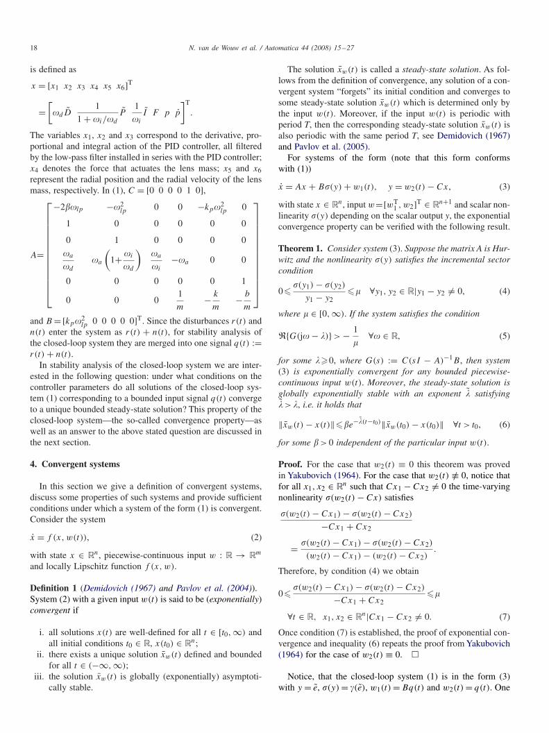
Notice, that the closed-loop system (1) is in the form (3)with y = e, (y) = �(e), w1(t) = Bq(t) and w2(t) = q(t). One

N. van de Wouw et al. / Automatica 44 (2008) 15–27 19

−1 0 1 1.5

−1.5

0

0.25

1.5 1.6 1.7 1.8 1.9

10−3

10−1

101

103

Fig. 5. Left: Nyquist plot of G(j�− �) for �= 10, and graphical investigation of frequency-domain condition (5). Right: relation between � and the maximumlevel of � when condition (5) is satisfied.

can easily verify (see Fig. 4) that the nonlinearity � satisfies theincremental sector condition

0� �(e1) − �(e2)

e1 − e2�� ∀e1, e2 ∈ R|e1 − e2 �= 0, (8)

with � ∈ [0, ∞) representing the additional gain. Moreover, thesystem matrix A is Hurwitz. In order to guarantee the exponen-tial convergence property, we require that system (1) satisfiesthe following condition:

R{C((j� − �)I − A)−1B} > − 1

�, ∀� ∈ R, (9)

for some ��0 and for the matrices A, B and C defined inSection 3. This condition allows for a graphical investigation.The left part of Fig. 5 displays the Nyquist plot of G(j� − �)

for � = 10. Condition (5) is satisfied if the Nyquist plot ofG(j� − �) is entirely on the right side of the line l verticallypassing through −1/�. Hence, � can be increased up to the valueat which l is just tangent to the Nyquist plot of G(j� − �). Forsystem (1), in case �=10, � is restricted to a maximum value of�max =1.82. Condition (5) is fulfilled for various combinationsof � and �. The right part of Fig. 5 depicts a curve in the (�, �)

space, which establishes what maximum value of � can be as-sured if condition (5) is satisfied, given a particular value of �.The latter curve indicates a convergence (and thereby stability)region just like the Nyquist plot in the left part of Fig. 5. Namely,for all � on the left side of the vertical asymptote at � ≈ 1.82,condition (5) is satisfied. In this context it is important to notethat � is a lower bound for the exponential convergence rate ofthe solutions to the steady-state solution. Clearly, the right partof Fig. 5 expresses the fact that increasing � yields a lower guar-anteed exponential convergence rate �, which also constitutes atrade-off in terms of the transient response of the control system.

Finally, by Theorem 1 we conclude that if the additional gain� ∈ [0, 1.82) then the closed-loop system (5) is exponentiallyconvergent with the rate of exponential convergence � satisfy-ing ��10. Notice, that � does not affect the exponential con-vergence property provided that � ∈ [0, 1.82). Therefore, fromthe convergence point of view ��0 can be chosen such thatimproved performance of the closed-loop system is attained.

It should be noted that a bound on the state (and thus on theerror and position of the lens) can be computed, given bounds onthe disturbances, based on Theorem 1, see Yakubovich (1964).The proof of this theorem is based on the fact that under theconditions of the theorem there exists a quadratic Lyapunovfunction for the unperturbed system of the form: V = xTPx,with P = P T > 0. Given such matrix P an ultimate bound forthe state of the perturbed system can be formulated. Hereto, wedefine the set

E ={x|‖x‖P � 1

�supt∈R

‖B�(q(t)) + Bq(t)‖P

}, (10)

where ‖x‖P = √xTPx is called the P-norm of x. The set E

is a positively invariant set and all solutions of the perturbedsystem starting outside this set will converge to it. Therefore,given bounds on the disturbances q(t) a bound on the P-normof x is provided.

For practical implementations, it is important to note that theconvergence property is robust for model uncertainties if onechooses the additional gain � below �max . The ultimate choicefor � is based on both robustness and performance considera-tions. The desired level of robustness is attained by choosing�max − � such that a sufficiently high level uncertainty on thelinear dynamics (typically related to the level of uncertainty inthe identification procedure used to identify these dynamics) ispermitted by the circle criterion.

5. Closed-loop behaviour

In this section, the closed-loop behaviour of the variable-gaincontrolled optical storage drive will be investigated for a rangeof the control design parameters � (the dead-zone length) and �(the additional gain). These parameters are chosen such that theclosed-loop system is exponentially convergent. Consequently,stability is guaranteed and the steady-state performance of thecontrol design can be assessed in a unique fashion. Here weadopt the perspective of periodic disturbances, which will, dueto the convergence property, induce unique, globally asymptot-ically stable periodic responses of the same period time.

The periodic responses of the closed-loop system are eval-uated in two ways: firstly using the shooting method and the

20 N. van de Wouw et al. / Automatica 44 (2008) 15–27

−7.93

0

7.93x 10

−7

−7.93

0

7.93x 10

−7

−7.93

0

7.93x 10

−7

0 5

x 10−3

−7.93

0

7.93x 10

−7

0 5

x 10−3

−7.93

0

7.93x 10

−7

0 5

x 10−3

−7.93

0

7.93x 10

−7

Fig. 6. Closed-loop response e(t) to a harmonic disturbance for a decreasing dead-zone length � (� = 1, Q = 10−5 m and �/(2 ) = 200 Hz); simulation (boldlines), describing function approximation (dash-dot lines).

path-following method (Parker & Chua, 1989) to numericallycompute the periodic responses of the full nonlinear systemand, secondly, using a describing function approximation. Fora more detailed derivation of the describing function of thevariable-gain element, see Heertjes et al. (2006). Response ap-proximation using describing functions is pursued for reasonsof numerical efficiency in evaluating performance for a widerange of the parameters � and � and for a range of excitationfrequencies and amplitudes. It will be shown that the describingfunction approximation is also accurate for the system underinvestigation.

The harmonic disturbance is denoted by q: q(t)=Q sin(�t).In Fig. 6, the periodic error signal e(t) is depicted for � = 1,Q = 10−5 m and �/(2 ) = 200 Hz and for a decreasing dead-zone length �. Note that for � = 1 the closed-loop system isexponentially convergent, for all �, and that Fig. 6 depicts theunique globally asymptotically stable periodic steady-state so-lutions (with a frequency of 200 Hz). The upper left figure re-lates to � → ∞ (the low-gain linear control design) and thelower right figure relates to � = 0 (the high-gain linear controldesign). In both designs no gain-switching occurs and the re-sponse of such linear control systems is purely harmonic. Theintermediate figures express results for various variable-gaindesigns, where the responses are no longer harmonic (thoughperiodic with the period time of the disturbance). The hori-zontal lines express the dead-zone length � and Fig. 6 showsthat the error is attenuated when the controller applies highergains for errors beyond the dead-zone length. Moreover, the re-sults of simulations with the full nonlinear model and results ofthe describing function approximation are shown. Clearly, thedescribing function approximation is sufficiently accurate. Fi-nally, Fig. 6 may lead to the conclusion that the high-gain lineardesign is favourable since it results in the lowest tracking errorresponse for the low-frequency disturbance of 200 Hz. How-

ever, the higher linear gain implies a deterioration of the mea-surement noise sensitivity at higher frequencies with respect tothe low-gain linear design. The choice of the dead-zone lengthin the variable-gain design provides additional design free-dom in weighting the performance in terms of low-frequencytracking and the performance in terms of high-frequency mea-surement noise sensitivity depending on the disturbance char-acteristic at hand.

In order to quantify this trade-off, simulations are performedfor a whole range of excitation frequencies �. To enhance thephysical meaning of the choice of the dead-zone length, weintroduce a scaled dead-zone length � = �/Q. It can easilybe shown that the dependency of the scaled position of thelens p/Q and the scaled error e/Q on the parameters � and Qcan be characterised by a dependency on only one parameter:�=�/Q. In Fig. 7, the results of these simulations are depictedfor � = 1. In the upper figure the infinity-norm of the periodicerror signal (scaled by Q) is plotted against the disturbancefrequency. It is important to note that the infinity-norm of theerror is crucial in the performance of the optical storage drive,since the read-out will be terminated when the absolute valueof the error becomes larger than the half track width; the lattercriterion is related to the servo-error reconstruction mechanismusing an extended S-curve (Stan, 1998). In Fig. 7, results forthe low-gain linear control design (� → ∞), the high-gainlinear design (� = 0) and several variable-gain control designsare plotted. For the linear control designs, the upper figure ofFig. 7 merely depicts the absolute value of the sensitivity func-tion S(j�) = 1/(1 + HP (j�)HC(j�)) and the lower figure ofFig. 7 merely depicts the absolute value of the omple-mentary sensitivity function T (j�) = HP (j�)HC(j�)/(1 +HP (j�)HC(j�)). Clearly, for low frequencies the high-gainlinear design exhibits better disturbance rejection propertiesthan the low-gain linear design. However, in accordance with

N. van de Wouw et al. / Automatica 44 (2008) 15–27 21

101

102

103

104

105

10−5

10−4

10−3

10−2

10−1

100

101

101

102

103

104

105

10−4

10−3

10−2

10−1

100

101

Δ = 10−1

Δ = 0

Δ = 0

Δ = 10−2

Δ = 10−3

Δ = 1

Δ = 0.5

Fig. 7. Generalized sensitivity and complementary sensitivity with � = 1 (DF = describing function).

the fact that S(j�) + T (j�) = 1, ∀� ∈ R, the low-gain lineardesign achieves a lower high-frequency noise amplification.For the variable-gain control design we will call the function inthe upper plot of Fig. 7 the generalised sensitivity function andit expresses both frequency and amplitude dependency. Thisamplitude dependency can be recognised in the fact that if thedisturbance amplitude Q becomes larger, the scaled dead-zonelength � = �/Q becomes smaller, which induces differentclosed-loop behaviour. The behaviour of the variable-gain de-sign equals that of the low-gain linear design for ‖e‖∞ < �.Beyond that level the results of the variable-gain design differfrom that of the low-gain linear design.Once the error responseof the variable-gain controlled system is such that it spendsmost of its time outside the dead-zone, the results will resemblethat of the high-gain linear design. Consequently, the variable-gain design improves the low-frequency rejection propertieswith respect to the low-gain linear design (� → ∞); however,it can never improve upon the low-frequency disturbance re-jection properties of the high-gain linear design (� → 0). Inthe lower plot of Fig. 7, the infinity-norm of the periodic lensdisplacement signal (scaled by Q) is plotted against the dis-turbance frequency. For the linear control designs, this is thecomplementary sensitivity function T (j�) and for the variable-gain design we will call this the generalised complementarysensitivity function. This figure expresses the superiority ofthe low-gain linear design in terms of high-frequency (mea-surement noise) disturbance rejection properties. Moreover,the variable-gain design improves upon the high-frequencydisturbance rejection properties of the high-gain lineardesign.

Fig. 7 expresses the fact that the variable-gain design cannegotiate between low-frequency tracking properties and high-

frequency measurement noise sensitivity in a way not availableto the linear control designs. Of course, the choice for the bestdesign (either linear or variable-gain) is largely determinedby the actual frequency- and amplitude-range of both thelow-frequency vibrations and the high-frequency measurementnoise. Moreover, mere visual inspection of the data plottedin Fig. 7 cannot provide a means to discriminate between thedesigns in this respect. Therefore, a quantitative performancemeasure accounting for both low-frequency tracking propertiesand high-frequency measurement noise sensitivity is neces-sary to support a performance-based control design strategy.Given the disturbances acting on the system, such performancemeasure should allow to find the control parameters � and �achieving optimal performance in terms of both low-frequencytracking properties and high-frequency measurement noisesensitivity.

A performance measure based on computed responses al-lows to discriminate between the different control designs, seeFig. 7. It should be noted that a (conservative) approach to-wards performance assessment based on merely providingbounds on the response, given bounds on the disturbances,will not allow to discriminate between the different control de-signs. Namely, the frequency-dependency expressed by Fig. 7cannot be accounted for and the bound on the response wouldalways be larger (or equal) than the maximum over the frequen-cies. Clearly, the upper plot in Fig. 7 shows that the differencein the tracking performance of the different designs is promi-nent in a frequency range significantly separated from thefrequencies for which the maximum (generalised) sensitivity isobserved. Therefore, the discrimination between the differentcontrol designs can best be assessed through these computedresponses.

22 N. van de Wouw et al. / Automatica 44 (2008) 15–27

6. Performance assessment

For optical storage drives, satisfactory performance isachieved when the disc read-out is never stopped, given thedisturbances acting on the system. A stop in the disc read-outis directly related to the tracking error exceeding the half trackwidth. Therefore, as mentioned before, the infinity norm of thetracking error should play a central role in the performancemeasure. Two types of disturbances affect this error: low-frequency vibrations of the disc and high-frequency measure-ment noise. In optical storage drives, generally performanceis increased, firstly, by reducing the influence of measurementnoise on the lens position and, secondly, by increasing thecapability of the lens to follow the desired disc track in thepresence of disc vibrations. Performance in terms of a devi-ation with respect to the desired disc track is then quantifiedby a weighted sum of the radial position p of the lens undermeasurement noise and the radial error e resulting from discvibrations.

We adopt the perspective of exactly computing the uniquesteady-state responses to disturbances from the specific classof harmonic disturbances and defining the control performanceon the basis of these quantitative data. The latter computationsare performed efficiently using describing function approxima-tions, see Section 5. The performance in the face of harmonicdisturbances is specifically important for optical storage drivessince in practice the performance is tested experimentally byconstructing so-called ‘drop-out-level curves’ (Heertjes et al.,2005), which show the level of the harmonic disturbance forwhich a termination of the disc read-out occurs for a range ofdisturbance frequencies. It is worth noting that Theorem 1 alsoallows one to compute bounds on the responses given boundson arbitrary inputs, see the discussion at the end of Section 4and Yakubovich (1964). This allows one to consider more gen-eral classes of disturbances, however, only yielding a conser-vative view on performance.

6.1. Disturbance modelling

In this section, the disturbance modelling is discussed indetail. At this point, we revert to the notation introduced inSection 2: r represents disc vibrations and n denotes the mea-surement noise. Once more, the perspective of harmonic distur-bances is taken: r(t, �r , Qr) = Qr |Fr(j�r )| sin(�r t), ∀t ∈ R,∀�r × Qr ∈ [�−

r , �+r ] × [Q−

r , Q+r ] and zero elsewhere, and

n(t, �n, Qn) = Qn|Fn(j�n)| sin(�nt), ∀t ∈ R, ∀�n × Qn ∈[�−

n , �+n ] × [Q−

n , Q+n ] and zero elsewhere, where Qr and Qn

represent the amplitudes of the disc vibrations r and the mea-surement noise n, respectively. Similarly, �r and �n representthe frequencies of the disc vibrations r and the measurementnoise n, respectively. The linear filters Fr(j�r ) and Fn(j�n)

enable appropriate frequency weighting. The choice for rep-resenting both the shock disturbances and the measurementnoise by means harmonic disturbances (with a range of fre-quencies) is motivated by, firstly, the fact that the sensitivity toshock disturbances is commonly specified in practice throughits sensitivity to harmonic disturbances (Heertjes et al., 2005)

(in automotive applications engine- and road-induced vibra-tions are essentially narrow-banded when arriving at the opticalstorage drive), secondly, the fact that a specific disc defect in-duces a disturbance in a pronounced frequency band, whereasthe entire considered class of disc defects will represent dis-turbances in a broad frequency range and, thirdly, the bene-fit of representing both types of disturbances within the sameframework.

The variables e(t, �, Q) and p(t, �, Q) denote the error re-sponse and the displacement of the lens to a harmonic distur-bance with amplitude Q and angular frequency �, respectively.Moreover, by ‖e(t, �, Q)‖∞=supt∈[0,T ]{|e(r(t, �, Q))|}, withT = (2 )/� being the period time of the disturbance (and ofthe response), we denote the maximum absolute error occurringon the periodic steady-state solution induced by the periodicdisturbance. A similar notation is adopted for p.

The modelling of r(t, �r , Qr) is motivated in the follow-ing way. According to the drop-out-level curve (Heertjes et al.,2005), the spectral content of radial disc displacements is inthe range from 10 to 200 Hz, i.e. [�−

r , �+r ] = [10 × 2 , 200 ×

2 ] rad/s. Moreover, this frequency range of disturbances isparticularly of interest for automotive applications in whichthe suspension dynamics filters higher disturbances frequen-cies present in the road excitation. The maximum amplitudeof the disc vibrations Q+

r and the filter Fr(j�r ) are chosensuch that the combination induces the occurrence of a termi-nated disc readout (commonly called a mute). The occurrenceof a mute conforms to the maximum radial error level in op-tical disc drives. Now, we choose the filter Fr(j�r ) such thatfor a maximal disc vibration amplitude of Q+

r = 4 × 10−7, thedisc readout is terminated for all disturbance frequencies whenthe low-gain control design is implemented. For the low-gainlinear design, ‖e(r(t, �r , Qr))‖∞ is related to the disturbancethrough the low-gain sensitivity function Slg(j�):

‖e(r(t, �r , Qr))‖∞ = ‖F−1{Slg(j�)R(j�, �r , Qr)}‖∞

= Qr |Slg(j�r )Fr(j�r )|, (11)

where R(j�, �r , Qr) = F{r(t, �r , Qr)} is the Fourier trans-form of r(t, �r , Qr). By choosing |Fr(j�r )| = |S−1

lg (j�r )|,∀�r ∈ [10 × 2 , 200 × 2 ], we guarantee that the disc read-out is terminated for Qr = Q+

r , ∀�r ∈ [10 × 2 , 200 × 2 ].Consequently, we have constructed a maximum disturbancelevel (higher disturbance levels are of no interest since thedisc readout will already be terminated at lower disturbancelevels). Note that |S−1

lg (j�r )| has a low-pass characteristic for�r ∈ [10×2 , 200×2 ], see left figure in Fig. 8. Motivated bythe foregoing line of thought, we model the low-frequency discvibrations according to r(t, �r , Qr) = Qr |S−1

lg (j�r )| sin(�r t),

∀t ∈ R, ∀�r × Qr ∈ [10 × 2 , 200 × 2 ] × [0, 4 × 10−7].The modelling of n(t, �n, Qn) is motivated as follows. We

presume the frequency content of measurement noise due todisc defects starts at 3 kHz, see Vidal, Andersen, Stoustrup,and Pedersen (2001) and Helvoirt, Leenknegt, Steinbuch, andGoossens (2004), i.e. �−

n =3×103 ×2 rad/s. The latter boundis motivated by a disc defect (e.g. a black dot) of maximum sizeof 0.002 m encountered while reading an outer track of the DVD

N. van de Wouw et al. / Automatica 44 (2008) 15–27 23

10 20 100 200

10−6

10−5

10−4

10−3

10−2

3000 6000 45000 90000

10−8

10−7

10−6

Fig. 8. Design weighting filters and maximum levels of disturbance as a function of frequency.

(at a radius of approximately 0.06 m) while rotating at 15 Hz.In such case the black dot is crossed in approximately 1/3000 s,leading to a lowest disturbance frequency of 3 kHz. The highestfrequency at which measurement noise can possibly disturb theoutput is dictated by half the sample frequency which amounts45 kHz maximum. Consequently, we define �+

n = 4.5 × 104 ×2 rad/s. Measurements are performed to show that, when onlymeasurement noise disturbs the output, generally the measuredradial error e does not exceed 10−7 m in case the low-gain linearcontrol design is applied. For such a linear control design, thetransfer function from n to e is given by the sensitivity function.Using this fact, it is obtained that

‖e(n(t, �n, Qn))‖∞ = ‖F−1{Slg(j�)N(j�, �n, Qn)}‖∞

= Qn|Slg(j�n)Fn(j�n)|, (12)

where N(j�, �n, Qn) = F{n(t, �n, Qn)} is the Fouriertransform of n(t, �n, Qn). To respect the maximum levelof e experienced in practice, Q+

n is upper bounded throughQ+

n |Slg(j�n)Fn(j�n)| = 10−7, �n ∈ [3 × 103 × 2 , 4.5 ×104 × 2 ] which is guaranteed if we set Q+

n = 10−7 mand define |Fn(j�n)| = |S−1

lg (j�n)|, ∀�n ∈ [3 × 103 ×2 , 4.5 × 104 × 2 ], see the right figure in Fig. 8. Moti-vated by the foregoing reasoning, we model n(t, �n, Qn)

through n(t, �n, Qn) = Qn|S−1lg (j�n)| sin(�nt), ∀t ∈ R,

∀�n × Qn ∈ [3 × 103 × 2 , 4.5 × 104 × 2 ] × [0, 10−7].Note that [�−

r , �+r ] ∩ [�−

n , �+n ] = ∅, which avoids conflicting

goals otherwise encountered when both disturbances show afrequency-range overlap.

6.2. Performance measure

The performance measure should reflect the aim to minimiseboth the effect of the disc vibrations on the tracking error andthe effect of the measurement noise on the position of the lens.Moreover, it has been motivated that the infinity-norm of thesevariables determines whether or not a termination of the discread-out will occur. Consequently, the performance measureP, which we will call the integral deviation formulation, isformulated as follows:

P = Ir + In

I refr + I ref

n

, (13)

with

Ir =∫ Q+

r

Q−r

∫ �+r

�−r

‖e(r(t, �r , Qr))‖∞ d�rdQr ,

In =∫ Q+

n

Q−n

∫ �+n

�−n

‖p(n(t, �n, Qn))‖∞ d�ndQn,

I refr =

∫ Q+r

Q−r

∫ �+r

�−r

‖eref (r(t, �r , Qr))‖∞ d�rdQr ,

I refn =

∫ Q+n

Q−n

∫ �+n

�−n

‖pref (n(t, �n, Qn))‖∞ d�ndQn. (14)

Herein, we accounted for the fact that [�−r , �+

r ]∩[�−n , �+

n ]=∅for the disturbance modelling proposed in the previous sec-tion. The first integral in the equations in (14), i.e. the integralover Q, is incorporated to account for the conceivable ampli-tude dependency inherent to the variable-gain control design.The second integral, i.e. the integral over �, is incorporated toaccount for the frequency dependency of the closed-loop be-haviour. Note that in defining (13), (14) it is presumed thatthe integrands are integrable with respect to � and Q, whichis guaranteed by the convergence properties of the closed-loopsystem. The response of an arbitrary reference design is indi-cated by means of the subscript ref in the denominator of (13).The integral deviation formulation is defined as a relative mea-sure to facilitate the interpretation of its outcome. Namely, ifthe control design under evaluation (related to the numerator of(13)) and the reference design yield equal performance, a valueP = 1 is obtained. If, however, P < 1, the control design underevaluation yields a better performance than the reference de-sign. For the remainder of this paper the low-gain linear designis chosen to serve as the reference design.

Note that one could also model the disturbances by aparametrised family of signals consisting of multiple harmon-ics. Then, the same approach can be adopted to assess theperformance. Namely, still the convergence properties ensurethe existence of a unique and bounded globally asymptoticallystable steady-state solution for every bounded disturbance andagain this fact allows for a unique performance assessment.However, the performance measure itself will be considerablymore complex. Namely, in the case of harmonic disturbances

24 N. van de Wouw et al. / Automatica 44 (2008) 15–27

10−3

10−2

10−1

100

101

0.2

0.4

0.6

0.8

1

= 1.82

� = 0

� = 2·10−7

� = 6·10−8

� = 10−7

� = 4·10−8

� = 2·10−8

� ≥ 4·10−7

� = 8·10−8

� = 3·10−7

Fig. 9. Pr for a range of linear and variable gain control designs (� in [m]).

10−3

10−2

10−1

100

101

1

2

3

4

5

6

= 1.82

� = 0

� = 2·10−8

� = 4·10−8

� = 6·10−8

� = 8·10−8

� ≥ 4·10−7

Fig. 10. Pn for a range of linear and variable gain control designs (� in [m]).

only two parameters (amplitude and frequency) need to betaken into account in the performance measure (see (13),(14)), whereas in the case of multiple harmonics the numberof parameters will change accordingly.

6.3. Performance-based control design

Let us now use the performance measure to assess, andcompare, the performance of both linear and variable-gaincontrol designs given the type of disturbances described inSection 6.1. In order to illuminate qualitative contributionsof improvements/deteriorations with respect to low-frequencydisturbance rejection properties and high-frequency measure-ment noise sensitivity to the performance P, the followingquantities are introduced: Pr = Ir/I

refr and Pn = In/I

refn . Pro-

vided �+r is below the bandwidth of the reference design, by

means of Pr the conceivable improvement in low-frequencydisturbance rejection properties is studied. Furthermore, pro-vided that �−

n is above the bandwidth of the reference design,Pn enables a quantification of the possible deterioration ofmeasurement noise sensitivity. Note that P �= Pr + Pn.

Fig. 9 depicts the value of Pr as a function of �. Herein,� ∈ [0, 1.82] as to guarantee convergent system properties, seeSection 4. Furthermore, Pr is evaluated for several levels of thedead-zone length �. If ��4×10−7 m, it is obtained that Pr =1,∀� ∈ [0, 1.82], because the error due to radial disc displacementis upper-bounded by 4 × 10−7 m, see Section 6.1. Therefore, if��4×10−7 m, the dead-zone will not be exceeded. For smallervalues of �, Pr < 1 ∀� ∈ [0, 1.82] implying an improvement of

low-frequency disturbance rejection properties. The monotonicdecrease of Pr with � follows from the fact that we evaluate theradial error merely for frequencies below the bandwidth of thereference design. Not surprisingly, Pr is minimal if (i) �=0 m,i.e. for the high-gain linear design, and (ii) � = 1.82; hencemaximal low-frequency disturbance attenuation is attained.

Fig. 10 depicts the value of Pn as a function of �. For��10−7 m, it is obtained that Pn = 1, ∀� ∈ [0, 1.82] becausethe measured radial error resulting from measurement noise isupper-bounded by 10−7 m, see Section 6.1. For smaller valuesof �, it is obtained that Pn �1, ∀� ∈ [0, 1.82], indicating a dete-rioration of measurement noise sensitivity. The monotonic in-crease of Pn with � is caused by considering the measurementnoise sensitivity only for frequencies above the bandwidth ofthe reference design. The measurement noise sensitivity is de-teriorated to a maximum extent if (i) � = 0 m hence for thehigh-gain linear design, and (ii) � = 1.82.

Fig. 11 depicts the outcome of (13) evaluated for the distur-bances, modelled in Section 6.1, as a function of �. Further-more, P is evaluated for several levels of the dead-zone length�. The figure indicates that the performance depends stronglyon both � and �. If ��4×10−7 m, it is obtained that P =1 ∀� ∈[0, 1.82]. Initially, a reduction of � will enhance performancebecause low-frequency disturbance rejection properties are im-proved whereas the measurement noise sensitivity remains un-altered, see the curves for � ∈ {10−7, 2 × 10−7, 3 × 10−7} m.For these levels of �, P decreases monotonically with � andtherefore maximum performance, i.e. minimum P, is obtainedif � = 1.82.

N. van de Wouw et al. / Automatica 44 (2008) 15–27 25

10−3

10−2

10−1

100

101

0.8

1

1.2

1.4

1.6 � = 0

� = 2·10−8

� = 4·10−8

� = 6·10−8

� = 8·10−8

� = 10−7

� = 2·10−7

� = 3·10−7

� ≥ 4·10−7

= 1.82

Fig. 11. The performance measure P for a range of linear and variable gain control designs (� in [m]).

A further decrease of � results in a deterioration of per-formance compared to the design with � = 10−7 m. Namely,if � < 10−7 m, the measured radial error resulting from mea-surement noise will exceed the dead-zone length and hence, adeterioration of the measurement noise sensitivity is effected.Consequently, P no longer monotonically decreases with � andtherefore, maximum performance is no longer obtained formaximum �. If � ∈ {6 × 10−8, 8 × 10−8} m, the variable gaincontrol design under evaluation still accomplishes better per-formance than the reference design for all � ∈ [0, 1.82]. Notethat the level of the dead-zone length on the boundary betweenperformance deterioration and improvement strongly dependson the (relative) level of the two types disturbances (shock dis-turbances and disc defects). However, for � ∈ {0, 2×10−8, 4×10−8} m there exist values for � for which P > 1, implyinga deterioration of the performance compared to the low-gainlinear design. For these levels of �, the improvement in low-frequency disturbance rejection properties is canceled by thedeterioration of the measurement noise sensitivity. Therefore,for smaller levels of �, the increase of the gain � within therange for which convergence is guaranteed, does not lead to animproved performance. In order not to arrive at a worsening ofperformance compared to the low-gain linear design for theselevels of �, one must select � carefully.

Depending on the combination of � and �, the variable gaincontrol design can outperform both the low-gain and the high-gain linear design. Given the performance measure (13), theweighting filters in Fig. 8 and the disturbance modelling pro-posed in Section 6.1, Fig. 11 clearly shows that nonlinear con-trol can prevail over linear control.

The proposed performance-based design strategy allows tocompute settings of the control parameters � and � that guar-antee ‘optimal’ performance given the plant and disturbancemodel. In practice, the sensitivity of the optimality of such con-trol settings with respect to model uncertainties is an importantissue. However, the dynamics of the system under study can bemodelled with high accuracy by exploiting simple frequency-domain identification procedures, see, for example, Heertjeset al. (2006). Moreover, if large deviations in the controlledmechanics would occur, a redesign of the nominal (low-gain)control design would be in effect in practice aiming at the sametype of nominal closed-loop dynamics (e.g. in terms of nominalbandwidth).

7. Conclusions

In this paper, a variable-gain control design for opti-cal storage drives is studied from a control performanceperspective. The variable-gain strategy is adopted to over-come well-known linear control design trade-offs betweenlow-frequency tracking properties and high-frequency noisesensitivity.

The contribution of this paper lies in the following aspects.Firstly, a convergence-based control design is proposed, whichguarantees stability of the closed-loop system and a uniquebounded steady-state response for any bounded disturbance.These favourable properties, induced by convergence, allowfor a unique steady-state performance evaluation of the con-trol system. Secondly, technical conditions for exponentialconvergence are proposed for the variable-gain controlledsystem. Thirdly, a quantitative performance measure, tak-ing into account both low-frequency tracking properties andhigh-frequency measurement noise sensitivity, is proposed tosupport the design and tuning of the nonlinear (non-smooth)control design.

The proposed performance measure is based on the com-puted steady-state responses to a class of harmonic distur-bances, which allows for an accurate performance comparisonbetween different control designs. Such a performance mea-sure is consistent with industrial performance specifications foroptical storage drives which are given in terms of the levelof harmonic disturbances for which the data read-out is ter-minated. The convergence conditions together with the perfor-mance measure jointly constitute a design tool for tuning theparameters of the variable-gain controller. The resulting de-sign is shown to outperform linear control designs. The latterstatement is based on the steady-state behaviour of the controlsystem under harmonic excitation and is supported by measure-ments in Heertjes et al. (2006).

As a final remark, the trade-off between low-frequency track-ing properties and high-frequency measurement noise sensitiv-ity is not unique for optical storage drives but can be recognisedin a wide variety of motion control systems, such as pick andplace machines, robots, etc. As a consequence, the method to-wards performance assessment proposed here can support thedesign of variable-structure controllers for other applicationsas well.

26 N. van de Wouw et al. / Automatica 44 (2008) 15–27

The discriminative nature of the performance evaluation canbe further improved by future work on enhanced disturbancemodelling.

References

Angeli, D. (2002). A Lyapunov approach to incremental stability properties.IEEE Transaction on Automatic Control, 47, 410–421.

Armstrong, B., Neevel, D., & Kusid, T. (2001). New results in NPID control:Tracking, integral control, friction compensation and experimental results.IEEE Transactions on Control Systems Technology, 9(2), 399–406.

Armstrong, B. S. R., Gutierrez, J. A., Wade, B. A., & Joseph, R. (2006).Stability of phased-based gain modulation with designer-chosen switchfunctions. International Journal of Robotics Research, 25, 781–796.

Bittanti, S., Dell’Orto, F., Di Carlo, A., & Savaresi, S. M. (2002). Notchfiltering and multirate control for radial tracking in high-speed DVD-players. IEEE Transactions on Consumer Electronics, 48(1), 56–62.

Demidovich, B. P. (1967). Lectures on stability theory. Moscow: Nauka, (inRussian).

Freudenberg, J., Middleton, R., & Stefanopoulou, A. (2000). A survey ofinherent design limitations. In: Proceedings of the American controlconference (pp. 2987–3001). Chicago, Illinois, USA.

Fromion, V., Monaco, S., & Normand-Cyrot, D. (1996). Asymptotic propertiesof incrementally stable systems. IEEE Transactions on Automatic Control,41, 721–723.

Fromion, V., & Scorletti, G. (2002). Performance and robustness analysis ofnonlinear closed-loop systems using nl analysis: Applications to nonlinearPI controllers. In: Proceedings of the 41st IEEE conference on decisionand control (pp. 2480–2485). Las Vegas, Nevada, USA.

Fromion, V., Scorletti, G., & Ferreres, F. (1999). Nonlinear performance ofa PI controlled missile: An explanation. International Journal of Robustand Nonlinear Control, 9, 485–518.

Heertjes, M. F., Cremers, F., Rieck, M., & Steinbuch, M. (2005). Nonlinearcontrol of optical storage drives with improved shock performance. ControlEngineering Practice, 13(10), 1295–1305.

Heertjes, M. F., Pastink, H. A., van de Wouw, N., & Nijmeijer, H. (2006).Experimental frequency-domain analysis of nonlinear controlled opticalstorage drives. IEEE Transactions on Control Systems Technology, 14(3),389–397.

Heertjes, M. F., & Sperling, F. B. (2003). A nonlinear dynamic filter toimprove disturbance rejection in optical storage drives. In: Proceedingsof the 42nd conference on decision and control (pp. 3426–3430). Maui,Hawaii, USA.

Heertjes, M. F., & Steinbuch, M. (2004). Stability and performance ofa variable gain controller with application to a DVD storage drive.Automatica, 40, 591–602.

Helvoirt, J., Leenknegt, G. A. L., Steinbuch, M., & Goossens, H. J.(2004). Classifying disc defects in optical disc drives by using time-series clustering. In: Proceedings of the American control conference (pp.3100–3105). Boston, Massachusetts, USA.

Jiang, F., & Gao, Z. (2001). An application of nonlinear PID control to aclass of truck ABS problems. In: Proceedings of the 40th IEEE conferenceon decision and control (pp. 516–521). Orlando, Florida, USA.

Lohmiller, W., & Slotine, J.-J. E. (1998). On contraction analysis for nonlinearsystems. Automatica, 34, 683–696.

Parker, T. S., & Chua, L. O. (1989). Practical numerical algorithms forchaotic systems. Berlin: Springer.

Pavlov, A., Pogromsky, A., van de Wouw, N., & Nijmeijer, H. (2004).Convergent dynamics, a tribute to Boris Pavlovich Demidovich. Systemsand Control Letters, 52, 257–261.

Pavlov, A., van de Wouw, N., & Nijmeijer, H. (2005). Uniform outputregulation of nonlinear systems: A convergent dynamics approach. Boston:Birkhäuser. (in Systems & Control: Foundations and Applications (SC)series).

Stan, S. G. (1998). The CD-ROM drive, a brief system description. Dordrecht:Kluwer Academic Publishers.

Vidal, E., Andersen, P., Stoustrup, J., & Pedersen, T.S. (2001). A study on thesurface defects of a compact disk. In: Proceedings of the IEEE conferenceon control applications (pp. 101–104). Mexico City, Mexico.

Yakubovich, V. A. (1964). The matrix inequality method in the theory of thestability of nonlinear control systems—I. The absolute stability of forcedvibrations. Automation and Remote Control, 7, 905–917.

Nathan van de Wouw (born, 1970) obtainedhis M.Sc. and Ph.D. degree in Mechanical Engi-neering from the Eindhoven University of Tech-nology, Eindhoven, the Netherlands, in 1994and 1999, respectively. From 1999 until nowhe has been affiliated with the Department ofMechanical Engineering of the Eindhoven Uni-versity of Technology in the group of Dynam-ics and Control as an assistant professor. In2000, Nathan van de Wouw has been working atPhilips Applied Technologies, Eindhoven, TheNetherlands, and, in 2001, he has been working

at the Netherlands Organisation for Applied Scientific Research (TNO), Delft,The Netherlands. He has held a visiting research position at the Universityof California Santa Barbara, U.S.A., in 2006/2007. Nathan van de Wouwhas published 26 publications in international journals, 5 book contributionsand 40 refereed proceedings contributions at international conferences. Re-cently he published the book ‘Uniform Output Regulation of Nonlinear Sys-tems: A convergent Dynamics Approach’ with A.V. Pavlov and H. Nijmeijer(Birkhauser, 2005). His current research interests are the analysis and controlof non-smooth systems and networked control systems.

Erik Pastink was born in Amsterdam, TheNetherlands, in 1978. He received the M.Sc.degree in mechanical engineering (cum laude)from Eindhoven University of Technology, Eind-hoven, The Netherlands, in 2004. The work forhis thesis, entitled “Stability and Performanceof Variable Gain Controlled Optical StorageDrives,” was carried out at Philips Applied Tech-nologies. Currently, he is a Mechatronics DesignEngineer with the R&D Department, Océ Tech-nologies, Venlo, The Netherlands. Mr. Pastinkreceived the Unilever Research Award in 2005

and the Royal Institution of Engineers’ Control Award in 2005.

Marcel Heertjes was born in Goes, the Nether-lands in 1969. He received both his M.Sc. andPh.D. degree in mechanical engineering fromthe Eindhoven University of Technology in 1995and 1999, respectively. In 2000, he joined thePhilips Centre for Industrial Technology in Eind-hoven. Since 2007 he is with ASML, Mecha-tronics Development, in Veldhoven and with thecontrol system technology group at the Eind-hoven University of Technology. He has pub-lished over thirty refereed papers and receivedover ten patents. His main field of interest is the

control of industrial motion systems with special attention for variable gaincontrol systems and learning control.

Alexey Pavlov (born 1976) received the M.Sc.degree (cum laude) in Applied Mathematicsfrom St. Petersburg State University, Russia in1998. In 1999 he was a part-time researcher inthe group Control of Complex Systems at theInstitute for Problems of Mechanical Engineer-ing, Russian Academy of Sciences. In 2000 hewas a visiting research scientist at Ford Re-search Laboratory, Dearborn, USA. In 2004 hereceived the Ph.D. degree in Mechanical En-gineering from Eindhoven University of Tech-nology, The Netherlands. Currently he holds an

Assistant Professor position at the Norwegian University of Science andTechnology, Department of Engineering Cybernetics. Alexey Pavlov has co-authored 34 journal and conference publications, 2 patents and a monograph“Uniform output regulation of nonlinear systems: a convergent dynamics

N. van de Wouw et al. / Automatica 44 (2008) 15–27 27

approach” (Birkhauser, 2005). His research interests include control of non-linear and hybrid systems, nonlinear output regulation theory, convergentsystems and cooperative control.

Henk Nijmeijer (1955) obtained his M.Sc. andPh.D. degrees in Mathematics from the Univer-sity of Groningen, Groningen, the Netherlands,in 1979 and 1983, respectively. From 1983 un-til 2000 he was affiliated with the Departmentof Applied Mathematics of the University ofTwente, Enschede, the Netherlands. Since, 1997he was also part-time affiliated with the Depart-ment of Mechanical Engineering of the Eind-hoven University of Technology, Eindhoven, theNetherlands. Since 2000, he is a full profes-sor at Eindhoven, and chairs the Dynamics and

Control section. He has published a large number of journal and con-ference papers, and several books, including the ‘classical’ Nonlinear

Dynamical Control Systems (Springer Verlag, 1990, co-author A.J. van derSchaft), with A. Rodriguez, Synchronization of Mechanical Systems (WorldScientific, 2003), with R.I. Leine, Dynamics and Bifurcations of Non-SmoothMechanical Systems (Springer-Verlag, 2004), and with A. Pavlov and N.van de Wouw, Uniform Output Regulation of Nonlinear Systems (Birkhauser2005). Henk Nijmeijer is editor-in-chief of the Journal of Applied Mathemat-ics, corresponding editor of the SIAM Journal on Control and Optimization,and board member of the International Journal of Control, Automatica, Jour-nal of Dynamical Control Systems, International Journal of Bifurcation andChaos, International Journal of Robust and Nonlinear Control, and the Jour-nal of Applied Mathematics and Computer Science. He is a fellow of theIEEE and was awarded in 1990 the IEE Heaviside premium.