performance evaluation of atm networks carrying constant and variable bit-rate video traffic

IEEE JOURNAL ON SELECTED AREAS IN COMMUNICATIONS, VOL. 15, NO. 6, AUGUST 1997 1115

Performance Evaluation of ATM Networks CarryingConstant and Variable Bit-Rate Video Traffic

Ismail Dalgıc, Member, IEEE, and Fouad A. Tobagi,Fellow, IEEE

Abstract—In this paper, we present the performance of asyn-chronous transfer mode (ATM) networks supporting audio/videotraffic. The performance evaluation is done by means of acomputer simulation model driven by real video traffic generatedby encoding video sequences. We examine the glitching thatoccurs when the video information is not delivered on time atthe receiver; we characterize various glitching quantities, such asthe glitch duration, total number of macroblocks unavailable perglitch, and the maximum unavailable area per glitch. For varioustypes of video contents, we compare the maximum number ofconstant bit-rate (CBR) and constant-quality variable bit-rate(CQ-VBR) video streams that can be supported by the networkwhile meeting the same end-to-end delay constraint, the samelevel of encoded video quality, and the same glitch rate constraint.We show that when the video content is highly variable, manymore CQ-VBR streams than CBR streams can be supportedunder given quality and delay constraints, while for relativelyuniform video contents (as in a videoconferencing session), thenumber of CBR and CQ-VBR streams supportable is about thesame. We also compare the results with those obtained for a100Base-T Ethernet segment. We then consider heterogeneoustraffic scenarios, and show that when video streams with differ-ent content, encoding scheme, and encoder control schemes aremixed, the results are at intermediate points compared to thehomogeneous cases, and the maximum number of supportablestreams of a given type can be determined in the presence of othertypes of video traffic by considering an “effective bandwidth” foreach of the stream types. We consider multihop ATM networkscenarios as well, and show that the number of video streamsthat can be supported on a given network node is very weaklydependent on the number of hops that the video streams traverse.Finally, we also consider scenarios with mixtures of video streamsand bursty traffic, and determine the effect of bursty traffic loadand burst size on the video performance.

Index Terms—Asynchronous transfer mode, carrier sense mul-tiple acess, computer network performance, multimedia commu-nications.

I. INTRODUCTION

I N THIS PAPER, we address the performance of asyn-chronous transfer mode (ATM) networks supporting au-

dio/video traffic, and provide a comparison with the perfor-mance of Ethernets. Among all the medium types, audio andvideo have the distinct property that the information must bepresented at the receiver according to a timing relationship;

Manuscript received May 1, 1996; revised December 30, 1996. This workwas supported in part by Pacific Bell.

I. Dalgıc was with the Department of Electrical Engineering, StanfordUniversity, Stanford, CA 94305 USA. He is now with the TechnologyDevelopment Center, 3Com Corporation, Santa Clara, CA 95052 USA.

F. A. Tobagi is with the Department of Electrical Engineering, StanfordUniversity, Stanford, CA 94305 USA.

Publisher Item Identifier S 0733-8716(97)04201-7.

i.e., an audio sample must be played back at each samplingperiod, and a video frame must be displayed at each frameinterval. Accordingly, the audio/video information generatedat one end must be presented at the other end within acertain end-to-end delay. The maximum end-to-end delayrequirement depends on the interactiveness of the application,and may range anywhere from 100 ms (as is the case forvideoconferencing) to upwards of 1 s (as may be the case forone-way broadcasting).

If some information arrives at the destination past themaximum allowed delay, then such information cannot bedisplayed, and thus is considered lost. Video informationloss leads to quality degradation in the displayed video inthe form of discontinuities referred to as glitches. Whilepacket loss rate could be used as a measure of such qualitydegradation, it would not constitute a good choice for tworeasons. First, it does not translate easily to perceived videoquality degradation. Second, due to the dependence that existsin the encoded video bit stream, the loss of a packet hasimpact that extends beyond just the information containedin that packet; conversely, given that packet loss is oftenbursty, the loss of several packets may account for the sameperceived degradation as that due to the loss of a subset ofthese packets. Accordingly, one must use measures of videoquality degradation that are more accurate and relevant thanpacket loss rate.

We have previously published results addressing the per-formance of Ethernets carrying video traffic in [1], where wehave defined some glitch statistics which represent the videoquality degradations due to packet loss more accurately thanpacket loss rate. Our approach in that paper has been to usecomputer simulation. Given the dependencies that exist in theencoded video bit stream (which differ from one compressionscheme and its syntax to another), and given the interest toderive glitch statistics, the simulation model is driven by realvideo traffic traces consisting of sizes and dependencies ofindividual macroblocks, as opposed to artificially generatedtraffic using analytical models (such as those presented in [2]and [3]) or video frame size traces.

In this paper, we follow the same methodology as in [1].We obtain statistics of glitching for various network and trafficscenarios. We also determine the maximum number of videostreams supportable for a given maximum delay requirementand a minimum level of video quality to be maintained. Weconsider the quality degradations both due to video encodingand due to packet loss in the network; this allows us tocompare the network performance for different video encoder

0733–8716/97$10.00 1997 IEEE

1116 IEEE JOURNAL ON SELECTED AREAS IN COMMUNICATIONS, VOL. 15, NO. 6, AUGUST 1997

control schemes, in particular, constant bit rate (CBR) andconstant-quality variable bit rate (CQ-VBR) [4]. We cover awide range of end-to-end delay requirements (20–500 ms),different types of video content, and two video encodingschemes (H.261 and MPEG-1). We also consider scenarioswhere audio/video traffic is mixed with bursty traffic (whichmay be generated either by traditional data applications, or bysome multimedia applications such as image browsing), anddetermine the effect of one traffic type over the other. Notethat in [1] we have given results for Ethernets pertaining tothe same aspects. However, given the differences between thetwo network types, the nature of some of the results presentedhere is quite different.

Furthermore, in this paper, we address two new aspects.First, we determine the number of streams supportable for traf-fic scenarios consisting ofheterogeneousvideo traffic sourcesin terms of the video content, video encoding scheme, andencoder control scheme, as well as the end-to-end delayrequirement. Second, we consider multihop ATM networkscenarios, and provide admission control guidelines for videowhen the network topology is an arbitrary mesh.

There is a great deal of prior work studying the statisticalmultiplexing of video traffic on an ATM multiplexer [5]–[14].The approach in the prior work is usually based on computersimulation driven either by analytical models or by videoframe size traces. The network performance is measured bycell loss rate, which is given as a function of the load offeredto the network. (In [5], signal-to-noise ratio (SNR) results alsoare given.) What differentiates our work from the prior studiesis as follows. First, we investigate the effect of cell losses onthe perceived video quality degradations in terms of glitchstatistics. Second, we consider heterogeneous video trafficscenarios, which consist of mixing video streams with differentcontents, different encoding schemes, different encoder controlschemes, and different delay constraints. Third, we examineATM multihop scenarios, while in the previous work on au-dio/video performance of ATM, only a single ATM multiplexeris considered. Conversely, in the papers that have consideredmultiple hops (e.g., [15], [16]), simple traffic models have beenused, which are not representative of video traffic. Fourth, weprovide a comparison of multiplexing performance for VBRand CBR video, under the conditions that the video qualityand end-to-end delay requirements are the same for both CBRand VBR video streams. We encode the CBR and VBR videosequences such that they both meet a given minimum level ofencoded video quality; this allows a fair comparison betweenthe two schemes. Some of the previous studies have also madea comparison of CBR and VBR [9], [11]. However, in thosestudies, the quality degradation due to video encoding has notbeen considered. The authors first start with a VBR-encodedvideo trace, and then consider artificially generated CBR videostreams with a data rate equal to the peak rate of the VBR tracecomputed over a sliding window of a predetermined size. Withthis approach, the encoded video qualities for CBR and VBRstreams are not necessarily equivalent, and therefore the com-parison does not have a good basis. Finally, we consider sce-narios involving a mixture of video and bursty traffic, and de-termine the effect of bursty traffic load and burst size on video.

The remainder of this paper is organized as follows. InSection II, we describe the network scenario under consider-ation. In Section III, we discuss our simulation methodology.In Section IV, we confirm the inadequacy of packet lossrate as a measure of degradations in the displayed videofor ATM networks. We develop more accurate and relevantmeasures, and characterize the statistics of glitches that occurdue to packet loss. In Section V, we examine the networkperformance for CBR and constant-quality VBR video traffic,using glitch rate as the primary performance measure, underthe condition that all of the video streams in the network areof the same type. We give the number of streams supportablefor both CBR and CQ-VBR traffic, and compare them atthe same encoded video quality. We show that when thevideo content is highly variable, many more CQ-VBR streamsthan CBR streams can be supported under given quality anddelay constraints for both ATM and Ethernet (for a networkbandwidth equal to 100 Mbits/s), while for relatively uniformvideo contents (as in a videoconferencing session), the numberof CBR and CQ-VBR streams supportable is about the same.We also show that for small values of end-to-end delayrequirement, ATM networks can support up to twice as manyvideo streams of a given type as Ethernets. For relaxed end-to-end delay requirements, both networks can support aboutthe same number of video streams of a given type. In SectionVI, we consider traffic scenarios where there is a mixture ofdifferent types of video traffic, the differences pertaining to thevideo encoding scheme and its control, the video content, andthe end-to-end delay requirement. We show that an effectivebandwidth can be defined for each video stream which isindependent of the mixture of the streams as long as thestreams have the same delay requirement. In Section VII, weconsider multihop network scenarios for ATM networks, andshow that the number of streams that can be supported on agiven link is very insensitive to the number of hops that thestreams travel. In Section VIII, we consider scenarios wherethere is a mixture of video and data traffic on the network.We examine the effect of one traffic type over the other. Ourconclusions are presented in Section IX.

II. SYSTEM DESCRIPTION

The system model considered in this paper follows closelythe one defined in [1]. Due to space limitations, here we onlygive a brief summary of the key points, and describe the newaspects of the system model considered in this paper (whichmainly pertain to the network scenario).

The components of the end-to-end video communicationssystem considered in this paper are shown in Fig. 1. Weconsider all of the components in the system to be streamlinedto the fullest extent possible so that the end-to-end delay isminimized. We have shown in [1] that the total latency dueto the video capture, encoding, decoding, and display in sucha streamlined system can be as small as a few milliseconds,and can be neglected.1 Therefore, the main components of the

1If the system is not fully streamlined, and thus those delays cannot beignored, then they can be considered constant for each macroblock, and theirvalue may be subtracted from the end-to-end delay constraint to determinethe maximum network delay that can be allowed.

DALGIC AND TOBAGI: PERFORMANCE OF ATM NETWORKS 1117

Fig. 1. Components in the end-to-end data path traversed by the video signaland the corresponding delay components.

end-to-end delay are the packet formation and network delays,and a packet is considered to be received on time only if thesum of these two delays does not exceed the end-to-end delayconstraint, denoted by

The network scenario under consideration is an ATM switchinterconnecting a number of workstations (see Fig. 2). Weconsider that the switch is nonblocking, and therefore the onlyshared resources in the switch are the buffers at the output portsand the output links. We focus in particular on one output port.We denote the output port buffer size by (bits), and the ca-pacity of the output link by (bits/second). We consider thatthe buffer operates according to a FIFO scheduling policy. Anycells that arrive when the buffer is full are considered dropped.

We consider that there are video stations, each ofwhich generates a video stream destined to another station on

Fig. 2. ATM network scenario under consideration.

that output port. We also consider that there arestationsgenerating bursty background traffic; each such station isconsidered to generate fixed size messages comprisingbitseach, with uniform interarrival times, the average of which isdenoted by The aggregate bursty traffic load (in bits/second)for all stations is denoted by where

In order to minimize the delay due to packet formation, weconsider that the streaming mode [17] is used when formingthe AAL-PDU’s so that, as soon as a cell payload is deliveredto the AAL, the payload is placed into a cell and transmitted.We do not consider any particular AAL protocol, and ignorethe overhead due to AAL-PDU headers or trailers.

If the video is generated according to the CBR rate control,then an immediately obvious method of packetization is togenerate cells at regular intervals (denoted by seconds)such that (48 bytes)/ bits/second (where is the bitrate of the CBR video stream); the first cell in a stream isformed seconds after the encoder starts putting the bits itgenerates into the output buffer. We refer to this method asconstant-rate cell formation (CRCF).

Another method of packetization is to simply form a cellas soon as the encoder generates 48 bytes of data. We referto this method asvariable-rate cell formation (VRCF). Theidea behind this method is to make use of the ATM networks’capability to accommodate variable rate packets in order toreduce packet formation delay.

III. SIMULATION METHODOLOGY

In order to determine the statistics of discontinuities in thedisplayed video, the dependencies that exist in the encodedvideo bit stream must be considered (those dependencies differfrom one compression scheme and its syntax to another).Accordingly, in this paper, we simulate the network with videotraffic obtained from encoding real video sequences, recordingthe lost packets and the macroblocks contained in them.

We use three video sequences as the source material, each ofthem about 1 min long. The first one is a videoconferencing-type sequence, where a person is sitting in front of a camerain a computer room, talking, and occasionally showing a few


objects to the camera. Given the small amount of motion,this sequence can be encoded at relatively low bit rateswithout incurring significant quality degradation. Furthermore,its content does not vary too much over time, which results ina relatively uniform video traffic. The second sequence is fromthe motion pictureStar Trek VI: The Undiscovered Country; itcontains a combination of fast action scenes and other, slower-moving scenes. This sequence requires somewhat more bits tobe encoded to achieve acceptable quality. The third sequencecontains three different commercial advertisements; of those,the first two have very fast movement and contain animatedscenes, which are complex to encode (i.e., they require morebits to be encoded for a given level of quality). Among thethree sequences, the scenes in the commercials’ sequenceexhibit the highest variability in the bit rate required to achievea given quality objective.

The video sequences are encoded using the H.261 andMPEG-1 standards. When a cell is lost, the recovery fromthe loss is achieved by means of intraframe coding. The par-ticular video encoding standard used determines the particularintra/interframe coding pattern; for MPEG-1, we use the groupof pictures (GOP) pattern of andfor H.261, we intracode one group of blocks (GOB) per frame,cyclically changing the intracoded GOB from frame to frame(each frame consists of ten GOB’s for SIF encoding used inthis study).

We consider that the video sources are controlled accordingto either CBR, CQ-VBR, or open-loop variable bit-rate (OL-VBR) encoder control schemes [4]. In CBR encoding, ahypothetical rate control buffer of size is considered toexist at the output of the encoder, which is drained at thetarget bit rate In order to minimize the likelihood of bufferunderflows or overflows, the buffer occupancy level is used asfeedback to control the encoder’s quantizer scale. While thereare short-term variations in the number of bits produced by theencoder per time interval, these variations are absorbed by therate control buffer. In particular, for MPEG video, the buffer ischosen to be large enough to accommodate theframes whichare encoded using more bits compared toand frames.

In CQ-VBR encoding, the video quality level is used asfeedback to control the quantizer scale so as to maintaina target level of quality. The quality is measured using aquantitative quality measure developed at the Institute forTelecommunication Sciences (ITS) which agrees closely withsubjective evaluations [18]. This measure is denoted byandtakes values in the range between one and five (one being veryannoying and five imperceptible). In OL-VBR encoding, thequantizer scale is simply kept at a constant level.

Due to space limitations, we are not able to give herenumerical values pertaining to the traffic characteristics of theencoded video sequences. For this, the reader is referred to[4]. However, what is important to note is the following. Fora given video content, in order to achieve a given minimumquality level at all times, CBR encoding in generalrequires using a greater data rate compared to the averagedata rate for CQ-VBR encoding (and the average data ratefor OL-VBR encoding lies somewhere in between). On theother hand, the CQ-VBR encoded sequences are more bursty

Fig. 3. Histogram of the aggregate traffic for 50 sources, each of them gen-erated using the commercials sequence, CQ-VBR encoded atstarget = 4:5.

compared to CBR encoded sequences (i.e., they have a greaterpeak-to-average rate, and the deviations from the average lastlonger); therefore, it is not clear whether the network canstatistically multiplex a sufficient number of CQ-VBR streamsto achieve a significant gain over CBR streams. Thus, wecompare the number of CBR and CQ-VBR video streams thatcan be supported by the network when the two schemes are toachieve the same (where the quality is measured over1 s intervals, as appropriate to the rate of changes in the scenecontent and the response time of the human visual system).

For traffic scenarios involving one type of video source, weuse the same video sequence to generate all streams for a givenrun of simulation. We use random starting points for eachstream so as to decrease the correlations between the streams.We repeat the runs multiple times (with different starting pointsin each run), until the desired confidence levels are reached(within 10% with 90% probability).

In order to validate that using the same video sequence togenerate all of the sources gives a good approximation to theaggregate traffic generated by independent and identically dis-tributed (i.i.d.) traffic sources, we have examined the histogramand the autocorrelation function of the aggregate traffic (whichis defined as the total number of bits produced in each frameinterval). If one were to generate traffic by i.i.d. sourceswhich have the same frame size histogram and autocorrelationfunction as the original video sequence, then the aggregatetraffic would have a histogram that is equal to the framesize histogram of the original sequence convolved by itselftimes, and an autocorrelation function that is equal to the framesize autocorrelation function of the original sequence. We havedetermined that the aggregate traffic produced by our approachindeed gives a good approximation to such histogram andautocorrelation values. As a representative example, considerthe commercials sequence, H.261 encoded using CQ-VBRat the target quality . In Fig. 3, we show thehistogram of the aggregate traffic for 50 sources, obtainedboth by convolving the original histogram 50 times, and by


Fig. 4. Autocorrelation function of the aggregate traffic for one source andfor 50 sources, each of them generated using the commercials sequence,CQ-VBR encoded atstarget = 4:5.

adding together 50 sources with random starting points. It isclear that the two curves are in very good agreement. For thesame case, in Fig. 4, we show the autocorrelation function ofthe original sequence and the aggregate traffic again obtainedby adding together 50 sources with random starting points.Again, the two curves are in good agreement. Thus, as faras the probability distribution and autocorrelation functions ofthe aggregate traffic are concerned, our approach is a goodapproximation.

IV. GLITCHING AS A MEASURE OF VIDEO

QUALITY DEGRADATION DUE TO PACKET LOSS

In this section, we introduce several glitch statistics asmeasures of video quality degradation due to packet loss, andwe investigate the effect of video encoding, video content,traffic load, and end-to-end delay constraint on the glitchstatistics. We begin by showing that packet losses indeed occurin bursts, which confirms the inadequacy of packet loss rate asa measure of video quality degradation. We then characterizethe discontinuities in the displayed video caused by packetloss. As a result of this characterization, we develop accurateand relevant video quality degradation measures.

A. Clustering of Packet Loss

In [1], we have shown that for Ethernet, the packet lossesin video traffic occur in clusters. It is clear to see that thisis also the case for a FIFO multiplexer in a packet-switchednetwork for any packet arrival process. Indeed, when a packetis lost, the multiplexer buffer is full, and the likelihood ofthe subsequent packet arrivals to find the buffer full is greatercompared to some arbitrary point in time.

Some researchers have quantified the cell loss clusteringin an ATM network using artificially generated traffic basedon analytical models, and have proposed the use of therate of cell loss clusters as a measure of performance forvideo traffic [19], [20], [7]. While cell loss cluster rate isa more refined measure of quality degradations comparedto packet loss rate, its definition is somewhat arbitrary. Forexample, there may be groups of lost cells separated by arelatively small number of received cells such that the two

(a)

(b)

Fig. 5. Buffer occupancy during a congested period for the commercialssequence, H.261, CQ-VBR,starget = 4:5, Dmax = 25 ms, W = 100

Mbits/s.

lost cell groups contribute to the same discontinuity in thevideo bit stream. Moreover, the cell loss clusters only giveinformation about the number of bits lost per cluster, whilefrom an applications point of view, it is more important todetermine how much information is lost in the video bitstream in terms of the area and duration of the discontinuities.Therefore, our approach in this paper is to map the packetlosses into information loss in the video bit stream, andexamine several quantities to characterize the perceived effectof such information loss.

As a preliminary step, we give an example of cell lossclustering in an ATM multiplexer. In Fig. 5, we show foran ATM multiplexer a typical trace of the multiplexer bufferoccupancy for the commercials sequence, H.261 encodedusing the CQ-VBR control scheme with , for

ms and 100 Mbit/s; part (a) of the figureis for 65, and part (b) is for . (Note that therespective cell loss rates are 1.8 10 and 5.5 10It is clear that the cell losses occur in clusters which lastseveral tens of milliseconds. Those clusters are separated bytens or hundreds of seconds. Furthermore, within a cluster,not all of the cells are lost; this is different from the Ethernet,


where the packet losses within a cluster usually occur insuccession. Note that the cluster for is longer thanthe one for . This is in general true, and it is asexpected since increasing the offered load to the networkprolongs the congestion period. For these two scenarios, wehave determined that the time between each subsequent cellloss per source occurs within 10 ms for 95% of the cell losses.For the remaining 5%, the time between subsequent cell lossesis in a range from a few seconds to several hundreds ofseconds. Therefore, an appropriate definition of a cell losscluster could be a group of lost cells where the time betweensubsequently lost cells is less than 10 ms.

B. Definition of Glitch Statistics andSome Illustrative Examples

We define aglitch as an occurrence which begins whena portion of a frame cannot be displayed while its pre-ceding frame is fully displayed, and continues as long aseach subsequent frame contains a portion which cannot bedisplayed.2

In [1], we have defined several quantities that characterizethe information loss per glitch. To summarize, these quantitiesare: 1) the number of macroblocks that are contained in the lostcells (denoted by ; 2) theglitch duration defined as thenumber of frames that are part of the glitch; 3) themaximumnumber of undisplayed macroblocks per frame(denoted by

; 4) the average number of undisplayed macroblocksper frame (denoted by ; and 5) the total number ofundisplayed macroblocks, . In addition to these quantitieswhich are defined per glitch, another quantity of interest is theglitch rate which is defined as the number of glitches thatoccur per unit time.

Now, we consider two example glitches. In Fig. 6, we showa typical glitch for a scenario consisting of H.261 encoding thecommercials sequence using CQ-VBR encoder control with

, for ms, , cells.In the figure, the black regions correspond to macroblocksthat are contained in the lost cell, the gray regions correspondto macroblocks that depend on the lost macroblocks, andthe white regions correspond to the macroblocks that arereceived and available to be displayed. In this particular glitch,information in 13 cells is lost. The glitch statistics of interestare macroblocks, frames,macroblocks, macroblocks, andmacroblocks.

Now, consider the same scenario as above, but this timewith . In Fig. 7, we show a typical glitch for thatcase. In this particular glitch, information in 131 cells islost. Accordingly, the glitch affects a larger area and lastslonger. In particular, macroblocks, frames,

macroblocks, macroblocks, andmacroblocks. As we show in the next subsection,

in ATM networks in general, the glitch statistics become largeras the network load is increased.

2Note that the “subsequent” frames here refer to the transmission order ofthe frames, which in the case of MPEG may be different from the displayorder due toB frames.

Fig. 6. Example glitch for ATM,W = 100 Mbits/s, H.261, CQ-VBR,starget = 4:5, Dmax = 25 ms,Nv = 65.

Fig. 7. Example glitch for ATM,W = 100 Mbits/s, H.261, CQ-VBR,starget = 4.5,Dmax = 25 ms,Nv = 67.

C. Effect of Various Factors on Glitch Statistics

Having defined the glitch quantities of interest and shownsome example scenarios, we now investigate the effect ofvarious factors on the glitch statistics for both ATM andEthernet. The particular factors we focus on are the videoencoder scheme, the video encoder control scheme, the trafficload (i.e., the number of video sources multiplexed), videocontent, and for ATM multiplexers, the switch outputbuffer size

First, consider an ATM multiplexer. We first show how theselection of the multiplexer buffer size affects the glitches.In Fig. 8(a), we plot the glitch rate as a function of forthe commercials sequence, H.261 encoded using the CQ-VBRscheme with , , and ms. Asthe figure indicates, the glitch rate decreases asis increasedwhen is less than about 4500 cells (for that buffer size, themaximum delay a cell experiences in the buffer is about 19ms). Beyond that point, the glitch rate remains fairly constant.


TABLE IGLITCH STATISTICS FOR ATM, V ARIOUS TRAFFIC SCENARIOS

On the other hand, consider Fig. 8(b), where we plotaveraged over all glitches recorded in the simulation (denotedas as a function of when is increased beyond 4500cells, increases sharply. This causes both the glitch durationand the total number of undisplayed macroblocks per glitch toincrease. Therefore, in order to obtain the lowest glitch rateand the smallest per-glitch quantities, the output buffer size

should be chosen such that the maximum delay incurredin the buffer is about minus 5–6 ms. (The reason it isnot exactly equal to is the time spent forming a cell.)In the remainder of the paper, the results are given for thatchoice of

Now, let us examine how the glitch rate varies with thetraffic load for both ATM and Ethernet. In Fig. 9, we plotversus for both ATM and 100Base-T, for the commercialssequence, encoded as above. It is interesting to note that theglitch rate increases very sharply beyond a certain point inATM, while for 100Base-T, the increase is not as sharp. Forexample, in ATM, the glitch rate is roughly equal to 0.2/minfor ; by decreasing only to 62, the glitch ratebecomes negligible. In contrast, in Ethernet, the value offor which the glitch rate is 0.2/min is 47, and the number ofstreams should be reduced down to about 30 for the glitchrate to become negligible. Therefore, in ATM, it does not payoff very much to permit glitching to occur; instead, one mustdetermine exactly where the knee of theversus curveis, and operate just below the knee. In contrast, in Ethernet,the number of video streams that can be supported increasessignificantly if some glitching is allowed.

The above result suggests that for ATM, the per-glitchstatistics defined above are of secondary importance comparedto the glitch rate. Nevertheless, it is still interesting to deter-mine the effect of the video encoding scheme, encoder controlscheme, video content, traffic load, and on the per-glitchstatistics so as to have a better understanding of the impactof glitches. In Table I, we show the cell loss rate glitchrate and the average values of and (denotedby and respectively) for various video encoderschemes, encoder control schemes, contents, network loads,and values.

First, consider the effect of the traffic load. In the firstthree rows, we consider the commercials sequence encoded

(a)

(b)

Fig. 8. Effect of switch output buffer size on glitching for commercials,H.261, CQ-VBR,starget = 4:5,Dmax = 25 ms,Nv = 65, ATM, W = 100

Mbits/s.

as above, for ms, and for and ,respectively. It is clear that increasing the traffic load increasesthe per-glitch quantities significantly, thus making the impactof each glitch more noticeable.

Now, let us investigate the effect of the other factorsmentioned above, using the scenario depicted in the secondrow of Table I as a baseline. Consider the effect of changing

. In row 4 of the same table, we set ms and


Fig. 9. Glitch rate versusNv for ATM and 100Base-T, commercials, H.261,CQ-VBR, starget = 4.5,Dmax = 25 ms.

( or smaller results in negligible cell loss forthat value). It is interesting to note that the cell loss ratehere is almost an order of magnitude greater compared to thecase of ms and , and yet the glitch rateis smaller (0.58/min as compared to 0.90). Also,andare much larger in this case. These differences are becausethe cell losses in this case tend to occur in larger clusters.Indeed, when we have a large we can put several morestreams on the network without causing cell loss. But whena cell loss occurs, the cells arriving shortly afterwards have agreater likelihood of being lost because of the larger traffic loadoffered. Therefore, the cell losses tend to be more correlated.

Now, consider using open-loop VBR. In order to achievethe same minimum quality at all times, this sequence hasto be encoded at 8 (found by iteration). At that value,the average rate of the OL-VBR encoded sequence is 1.64Mbits/s. Thus, in order to have the same network load as in thebaseline case, here we use . The glitch statistics forthat case are shown in the fifth row of Table I. It is interestingto note that the cell loss rate and all of the glitch statistics arequite similar in this case to the CQ-VBR. Therefore, the OL-VBR and CQ-VBR schemes give similar results for the samenetwork load; however, the number of streams supportable issmaller for the OL-VBR due to the larger data rate requiredto achieve the same minimum quality level.

As for comparing MPEG-1 and H.261, in the sixth row ofthe table, we give the glitch statistics for MPEG-1 again usingCQ-VBR with , for , which results inabout the same network load as in the baseline case. (Note that,here, is chosen to be 125 ms, given the 100 ms additionaldelay introduced by the use of frames.) It is interesting tonote that, here, the glitch rate is somewhat larger comparedto the H.261 case; however, and are somewhatsmaller. This is mainly because some of the glitches in MPEGare confined only to the frames.

Finally, we consider using a different video content, namely,the videoconferencing sequence. In the seventh row of Table I,we show the glitch quantities for that sequence. We have firsttried setting the average network load equal to the baselinecase. However, the videoconferencing sequence is less variable

compared to the commercials sequence; as a result, there areno cell losses for that case. So, we have increased the networkload until the knee of the cell loss rate is reached. The kneeis around – (i.e., a network utilization of about85 Mbits/s). We show in the table the packet loss rate andglitch statistics for and . For 194, thecell loss rate is 4.0 10 which is similar to the baselinecase; however, the glitch rate is only 0.20/min. The three per-glitch quantities are in this case similar to the baseline. For

, the cell loss rate is 1.9 10 and the glitchrate is about 0.99/min. The three per-glitch quantities are allgreater than those for the baseline. This indicates that the celllosses are more clustered here compared to the baseline case.It is also interesting to note that the cell loss rate increases verysignificantly for such a small increase in the network load.

Now, consider Ethernets. Table II is analogous to TableI, but for 100Base-T. In the first two rows, we have thecommercials sequence, H.261 CQ-VBR encoded, and25 ms. The two rows correspond to and . For those

values, the glitch rates are 0.08 and 0.92, respectively.However, in both cases, the per-glitch statistics are about thesame. Indeed, we have observed that in Ethernets, in general,the per-glitch statistics are independent of the network loadas long as the glitch rate is not more than a few glitches perminute. As for the effect of the third row indicates thatwhen is increased to 500 ms, the per-glitch statisticsincrease very significantly. This is because at such large valuesof the packets that are dropped at the MAC layer due toexceeding the maximum number of collisions are resubmittedby the transport layer several times; this may lead to prolongedperiods of congestion due to the backlog caused at the stations.As for the video encoder control scheme, the encoding scheme,and the video content, we have found that the per-glitchstatistics are fairly independent of those factors, as indicated bythe results shown in Table II. We have found similar resultsalso for 10Base-T.

To summarize, for ATM, the glitch rate increases verysharply with the traffic load beyond a certain knee. Fur-thermore, the per-glitch statistics also increase as the trafficload is increased beyond the knee. Therefore, it is importantto operate just below the knee of the versus curve.In contrast, for Ethernet, the glitch rate increases relativelyslowly with the traffic load, and it therefore pays off topermit some amount of glitching to achieve better networkutilization. Furthermore, for Ethernet, the per-glitch statisticsdo not significantly depend on the traffic load. These findingsindicate that for both ATM and Ethernet, the glitch rate canbe used as the primary measure of quality degradations due toinformation loss in the network.

We have also applied the ITS measureto the regionswhere glitching occurs. We have measuredfor every glitch,including several frames prior to and after the occurrence ofthe glitch such that the total period over whichis measuredis 30 frames (i.e., 1 s) for each glitch. For the glitcheswith a duration greater than 30 frames, we have appliedsuccessively 30 frames at a time. In all cases considered, the

values ranged from 1.0 to 3.4. Therefore, all of the glitcheswould be perceived as being annoying. This also confirms that


TABLE IIGLITCH STATISTICS FOR 100Base-T, VARIOUS TRAFFIC SCENARIOS

the glitch rate by itself is sufficient to measure the networkperformance.

V. PERFORMANCE OFATM M ULTIPLEXERS AND

ETHERNETS CARRYING CBR AND VBR VIDEO TRAFFIC

Having characterized the glitch characteristics and estab-lished that glitch rate is an appropriate measure of ATMnetwork performance carrying video traffic, in this section, weaddress the performance of CBR and VBR video transmissionover an ATM multiplexer. The main question that we seekto answer is how do CBR and VBR video encoding schemescompare in terms of the number of streams that can be carriedby the network while meeting given quality and end-to-enddelay constraints.

A. CBR Video Traffic

First, we consider an ATM multiplexer. As a preliminarystep, consider that the CBR video is multiplexed over a circuitof bandwidth and as soon as a macroblock is generated,it is passed to the multiplexer buffer. We ignore any overheaddue to framing. In this case, one possibility is to allocate eachCBR stream a bandwidth equal to this would result in adelay in each source equal to the rate control buffer delay[4]. Another alternative is to statistically multiplex the CBRstreams, with the goal of reducing the end-to-end delay byallowing the multiplexer buffer to absorb the fluctuations inthe CBR rate, as opposed to using a separate buffer at eachsending station. We have shown in [4] that such fluctuationshave a relatively small magnitude and short duration; thissuggests that by statistically multiplexing even a very smallnumber of CBR streams, the end-to-end delay can be reducedsignificantly. As examples which confirm this observation,consider the videoconferencing and commercials sequences.We have encoded them such that they have a reasonable qualityat the source at all times). For videoconferencing,this is accomplished with kbits/s and the ratecontrol buffer size kbits, and for commercials,

kbits/s and kbitss [4]. We have simulatedseveral video sources using those sequences as the source, andchoosing a different, random starting point in the sequence for

(a)

(b)

Fig. 10. Histogram ofmaxkfD(W;k)g for videoconferencing and com-mercials, various values ofW andNv such thatV Nv = 0:96W:

each source in order to reduce correlations among them. Wehave repeated the simulation many times, each time choosingdifferent random starting points, and have recorded in eachsimulation run the maximum delay incurred by any source inthe multiplexer buffer (denoted by where

is the delay incurred by macroblock In Fig.10, we show the histogram of for both


TABLE IIINmax (AND CORRESPONDINGNETWORK UTILIZATION ) FOR ETHERNET, CBR

sequences, and for various values of and such thatthe network utilization is 96% in each case (i.e.,

It is clear that even at relatively small bandwidths,statistical multiplexing of CBR sources reduces the delaysignificantly.

For an ATM network where the bandwidth is considerablylarger, and therefore many more streams can be multiplexed,the reduction of end-to-end delay would be expected to be evengreater. Indeed, we have simulated statistically multiplexingseveral CBR sources by using the VRCF scheme using allthree video contents, with data rates ranging from 270 kbits/sto 2 Mbits/s, rate control buffer sizes ranging from 38.4 kbitsto 768 kbits/s, and values ranging from 25 to 500ms. In all cases, we have found that the number of streamsthat can be multiplexed in the network without incurringany measurable cell loss is equal to (theterm 48/53 is due to the cell header overhead). Clearly,with the CRCF scheme, the same number of streams canbe sent over the network, but for a small such as25 ms, a very small rate control buffer size must be cho-sen, which results in a significantly reduced source quality[4].

As for the Ethernet, we have used a similar variable sizeand rate packetization [1], and have determined that there,too, such an approach reduces the glitch rates compared tothe approach of using constant size and rate packets. Forcomparison purposes, the maximum number of CBR streamsthat can be multiplexed on an Ethernet (denoted byand the corresponding utilization are shown in Table III forvarious values of maximum glitch rate constraintand for the three video sequences under consideration. It isclear that for ms, the ATM networks can carryabout twice as many CBR streams as in Ethernet. Asbecomes about 60 ms or larger, the difference between the twonetworks becomes small. This is because at ms,small packet sizes are forced to be used in Ethernet, and theperformance of CSMA/CD is not very good when the packetsize is small. For greater values, greater packet sizescan be used.

TABLE IVCOMPARISON OF AVERAGE BIT RATES OF CQ-VBR

AND CBR ENCODED SEQUENCES FOR THESAME smin

B. CQ-VBR Video Traffic

In Table IV, we show the average data rates for CQ-VBR for the three video sequences encoded at

and (resulting in a minimum level ofquality and , respectively). In thesame table, we also show the data rate for CBR whenit achieves the same as the CQ-VBR scheme. Thetable indicates that for the commercials sequence, the CQ-VBR average rate is about one-half of the CBR rate. Forthe Star Trek sequence and for , the ratio ofCBR rate to the CQ-VBR average rate is about 1.5, andfor the same sequence, for , the two ratesare nearly the same. For the videoconferencing sequence,the data rates for CQ-VBR and CBR are nearly the samefor both target quality values. The ratio of the average datarates for CQ-VBR and CBR represents the maximum amountof multiplexing gain that can be achieved when sendingvideo over a network. The multiplexing gain over a networkapproaches this maximum for large network bandwidths andlarge values. Given the numbers in Table IV, it can


TABLE VCOMPARISON OFNmax FOR CQ-VBR AND CBR ON AN ATM M ULTIPLEXER, W = 100 Mbits/s

TABLE VINmax FOR ETHERNET, CQ-VBR

be expected that the greatest amount of gain in using CQ-VBR compared to CBR can be achieved for the commercialssequence, and almost no gain should be expected for thevideoconferencing sequence.

In Table V, we show the maximum number of CQ-VBRstreams supportable in an ATM network and the correspondingnetwork utilization for various values of andand for the three video sequences. It is interesting to notethat does not depend on very significantly inthe range considered. Furthermore, as stated in the previoussection, also does not depend significantly onwhich suggests that could be chosen just below the “knee”such that the glitch rate is negligible. In almost all cases, thenumber of CQ-VBR streams supportable is greater than thatof CBR streams, in some cases up to a factor of 2. In fact,the theoretical maximum multiplexing gain (i.e., the ratio ofthe average CBR and CQ-VBR rates for the same isattained for the relatively large values.

Now, compare these results with those for Ethernet. InTable VI, the similar numbers as in Table V are shown fora 100Base-T segment. It is clear that, again, forms, ATM can support about twice as many CQ-VBR streamsas in Ethernet, but for larger values, the difference issmall. In fact, for the commercials sequence, ,

the number of streams supported by the Ethernet is somewhatgreater compared to ATM (due to the cell header overhead inATM).

VI. STATISTICAL MULTIPLEXING OF

HETEROGENEOUSVIDEO SOURCES

In the preceding sections, we have considered that all ofthe video sources are generated by using the same videosequence. Here, we investigate the effect of mixing videostreams with different contents, encoding schemes, encodercontrol schemes, and values.

First, consider an ATM multiplexer at which multiple videostreams generated by two different video contents are mixed;both of the video sequences are H.261 and CQ-VBR encoded,and both types of streams have ms. In TableVII, we show various mixtures of the videoconferencing andcommercials sequences under those conditions. The numbersare chosen such that the cell loss rates remain roughly thesame. The first point to be made is that the glitch statistics alsoremain about the same over all the mixtures considered. Sec-ond, the network utilization for the mixtures is at intermediatepoints compared to the homogeneous cases.

Most importantly, the results indicate that one can specifya simple admission control criterion in case of heterogeneous


TABLE VIIMIXING OF DIFFERENT VIDEO CONTENT (COMMERCIALS AND VIDEOCONFERENCING),

H.261, CQ-VBR, starget = 4:5

TABLE VIIIMIXING OF MPEG AND H.261 VIDEO STREAMS, COMMERCIALS, CQ-VBR, starget = 4:5

TABLE IXMIXING OF CBR AND CQ-VBR STREAMS, H.261, COMMERCIALS, smin = 4:3

video contents by means of an “effective bandwidth,” which isdefined for a given content, a given and a givenas follows. Let the average rate of the video stream with agiven content be bits/second, and let the maximum networkutilization that can be achievable by multiplexing a number ofsuch streams (with the same content) while meeting their delayand glitch rate constraints be bits/second. Then the effectivebandwidth is defined as The admission controlcriterion is then to admit a new stream as long as the totaleffective bandwidth in the network does not exceedIndeed,for all of the mixtures in Table VII, the sum of the effectivebandwidths is equal to 100 Mbits/s. The importanceof this result is that it allows one to determine whether aheterogeneous mixture of video streams can be supported ornot by simulating the network under homogeneous scenarios,and determining the effective bandwidth for each stream.

We have also verified this result with mixtures consistingof five different video contents, and have observed that the

effective bandwidth approach holds there as well. Furthermore,similar results also apply for mixing video sequences withdifferent encoding schemes and encoder control schemes. Ex-amples of these are shown in Tables VIII and IX, respectively.

Note that some researchers have previously shown thatone can determine an effective bandwidth for artificiallygenerated traffic based on various models. The first twopapers to introduce the notion of effective bandwidth are [21]and [22]. In [21], the traffic is considered to be generatedaccording to either independent Poisson streams (possiblywith different means), or slotted independent burst arrivals.In [22], on–off sources are considered. It is later shownanalytically in [23] that for sources with multiple time-scalevariations (as is the case with variable bit-rate video), aneffective bandwidth can also be determined. All of these papersconsider the multiplexer buffer to be infinite, and use a largedeviations approximation; therefore, for a finite buffer sizeand a finite number of streams, the effective bandwidth is


TABLE XMIXING OF STREAMS WITH DIFFERENT Dmax VALUES FOR H.261, CQ-VBR, COMMERCIALS, starget = 4:5

only an approximate notion. Our experimental results indicatethe validity of this approximation for the ranges of valuesconsidered here; i.e., video streams with an average data rate of270 kbits/s–1.8 Mbits/s, a network bandwidth of 100 Mbits/s,and buffer sizes corresponding to a maximum buffer delay inthe range of 25–500 ms.

As for mixing streams with different delay constraints,consider first that the multiplexer buffer is still a FIFO, withno priority among streams with different delay constraints.In this case, the network utilization should not exceed thevalue that would satisfy the delay and glitch rate requirementsfor the streams with the most stringent delay requirement.Another possibility is to assign a high priority to those streamsthat have a more stringent delay requirement. This allowsmore of the streams with the relaxed delay requirement tobe admitted without degrading the performance for the otherstreams; however, the additional network utilization that can begained is fairly small, considering that the number of streamssupportable does not increase significantly with

The next issue then is to determine what buffer size to use.If one uses a buffer size that is optimum for the stringent delayrequirement, then the streams with a relaxed requirement alsoincur the same type of cell losses as those with a stringentdelay requirement. If, on the other hand, one uses a buffersize that is optimum for the relaxed delay requirement, thenthe streams with a stringent requirement would experiencemore packet losses, which translate into glitches with largerand but the streams with a relaxed requirement wouldexperience much less cell loss than the former case. Therefore,the buffer size in this case is a tradeoff between the cellloss rate for the streams with a stringent and a relaxeddelay requirement. In Table X, we show an example casefor commercials, H.261, CQ-VBR, and for values of25 and 500 ms. In this example, the buffer size is chosen tobe 117 500 cells, which is optimum for ms. Itis clear that the streams with ms suffer muchlonger glitches compared to the case where the optimumfor ms is used. On the other hand, when the twotypes of streams are mixed such that the glitch rate is keptunder 1/min for the streams with ms, then thestreams with ms experience no cell loss.

As for the Ethernets, again, a similar effective bandwidthapproach applies, which is as expected given the insensitivityof network utilization to the video content, encoding scheme,and encoder control scheme. For streams with differentvalues, the admission control criterion should correspond to

Fig. 11. Worst case scenario for ATM multihop traffic.

the most stringent value since prioritization is notpossible among streams transmitted by different sources overan Ethernet segment.

VII. M ULTIHOP ATM NETWORKS

Since ATM networks are envisioned to be deployed both inthe local and wide area environments, it is also interesting tostudy cases where the video streams traverse multiple ATMswitches. The general problem that we address can be statedas follows. Consider a number of ATM switches connected inan arbitrary mesh topology, over which some video traffic iscurrently being sent (according to an arbitrary traffic matrix).When a new video stream is requested to be transmitted overthe network, the problem is to determine whether or not thestream can be carried while meeting the delay and qualityrequirements of all current video streams, as well as the newlyrequested one.

Some researchers have studied multihop ATM scenarios inthe past either by means of analytical models or computersimulations driven by artificially generated traffic [15], [16].An important conclusion that is reached in those papers is thatwhen a burst of cells belonging to a source passes througha multiplexer, the spacing between the cells belonging tothe burst becomes greater at the output of the multiplexercompared to its input. Thus, traffic offered to a multihopnetwork has the highest degree of burstiness in the first hoptraversed, and the burstiness decreases as more and more hopsare traversed.

This result allows us to construct a worst-case scenarioin terms of the number of streams that can be supportedin a multihop environment. As shown in Fig. 11, in thisscenario, multiple ATM switches are connected in tandem,interconnected by channels with a bandwidth of bits/s.We denote the number of switches by We assume that

streams go through hops, thus traversing through allof the switches. In addition, in every hopthere arestreams that are generated by stations directly connected tothe switch i.e., they enter and exit the network at switchWhen , this is a worst case scenario from the point


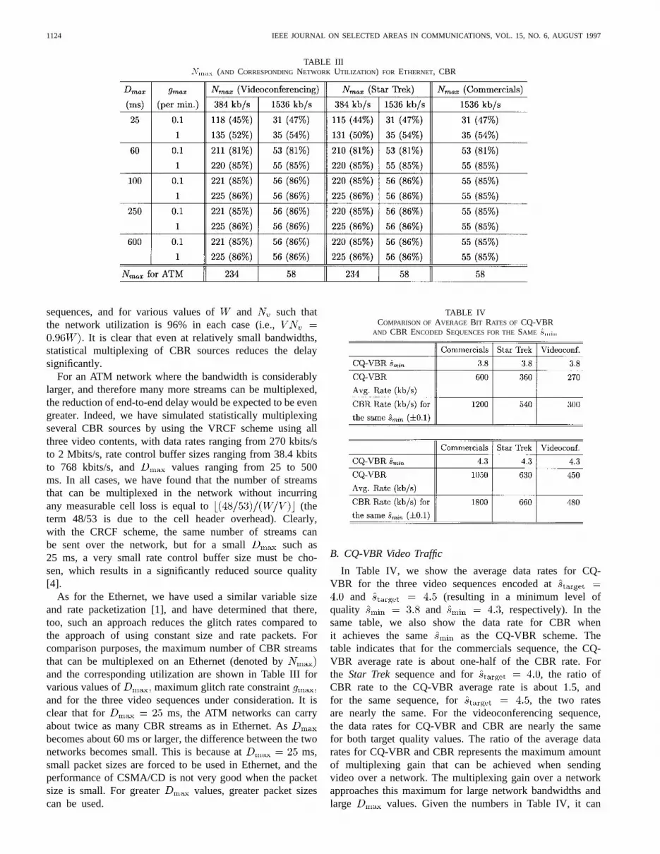
Fig. 12. Glitch rate versus the number of video streams per hop forH = f1, 2, 4, 8, 16g;W = 100 Mbits/s, commercials, H.261, CQ-VBR,starget = 4:5; Nete = 1:

of view of the single video stream that travels multiple hopssince it encounters video traffic that is the most bursty. Thus,if we denote by the value of for which still thevideo streams’ delay and loss requirements can be satisfied,then for any arbitrary mesh topology, at least streamscan be supported on every link as long as all of the streamstravel at most hops.

We have simulated the network for this scenario where allof the video streams are generated using the commercialsand videoconferencing sequences, H.261 encoded using theCQ-VBR control scheme at . We have chosen

Mbits/s and . We consider tobe the same in every hop, and we denote it by

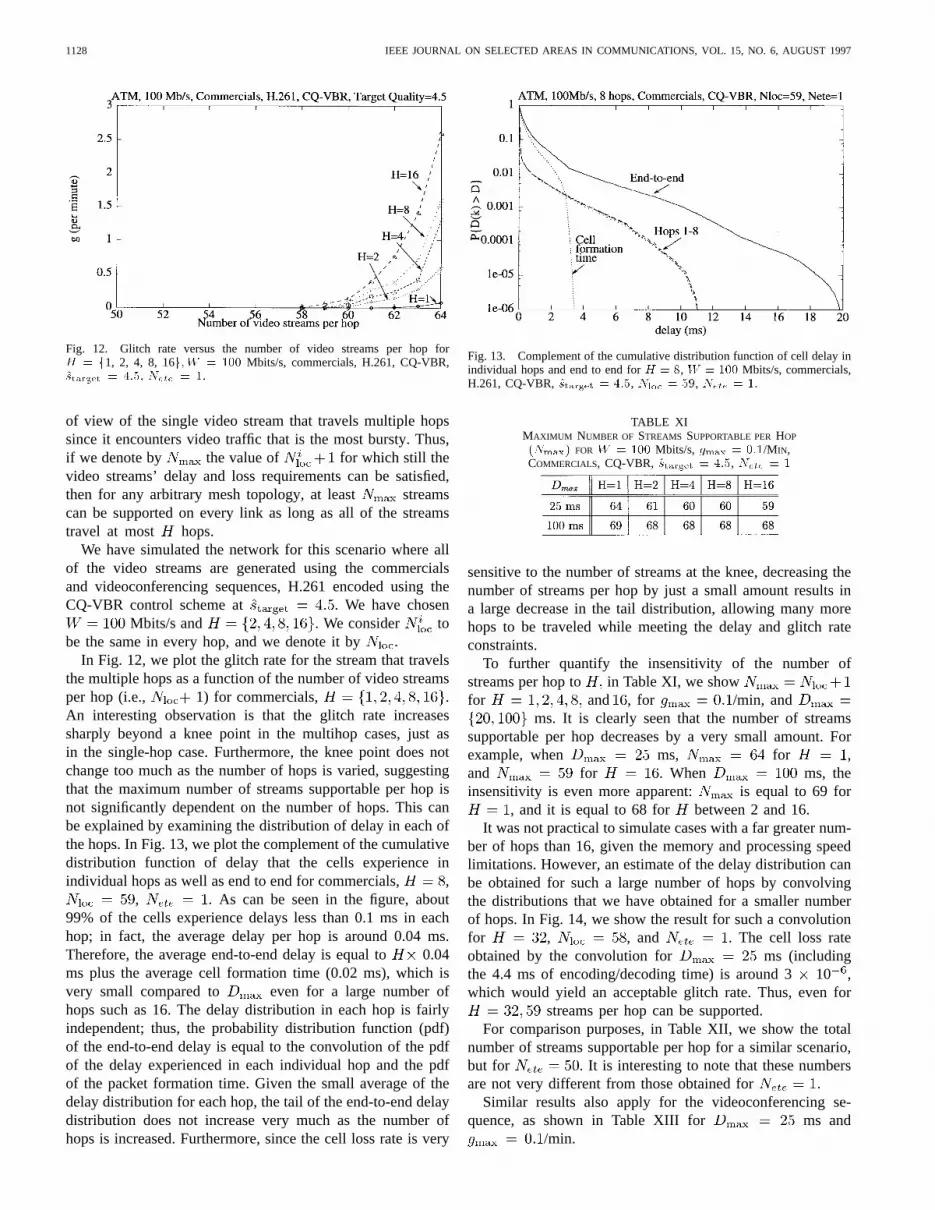
In Fig. 12, we plot the glitch rate for the stream that travelsthe multiple hops as a function of the number of video streamsper hop (i.e., 1) for commercials, .An interesting observation is that the glitch rate increasessharply beyond a knee point in the multihop cases, just asin the single-hop case. Furthermore, the knee point does notchange too much as the number of hops is varied, suggestingthat the maximum number of streams supportable per hop isnot significantly dependent on the number of hops. This canbe explained by examining the distribution of delay in each ofthe hops. In Fig. 13, we plot the complement of the cumulativedistribution function of delay that the cells experience inindividual hops as well as end to end for commercials, ,

, . As can be seen in the figure, about99% of the cells experience delays less than 0.1 ms in eachhop; in fact, the average delay per hop is around 0.04 ms.Therefore, the average end-to-end delay is equal to 0.04ms plus the average cell formation time (0.02 ms), which isvery small compared to even for a large number ofhops such as 16. The delay distribution in each hop is fairlyindependent; thus, the probability distribution function (pdf)of the end-to-end delay is equal to the convolution of the pdfof the delay experienced in each individual hop and the pdfof the packet formation time. Given the small average of thedelay distribution for each hop, the tail of the end-to-end delaydistribution does not increase very much as the number ofhops is increased. Furthermore, since the cell loss rate is very

Fig. 13. Complement of the cumulative distribution function of cell delay inindividual hops and end to end forH = 8, W = 100 Mbits/s, commercials,H.261, CQ-VBR,starget = 4:5, Nloc = 59, Nete = 1.

TABLE XIMAXIMUM NUMBER OF STREAMS SUPPORTABLE PERHOP

(Nmax) FOR W = 100 Mbits/s, gmax = 0:1/MIN,COMMERCIALS, CQ-VBR, starget = 4:5, Nete = 1

sensitive to the number of streams at the knee, decreasing thenumber of streams per hop by just a small amount results ina large decrease in the tail distribution, allowing many morehops to be traveled while meeting the delay and glitch rateconstraints.

To further quantify the insensitivity of the number ofstreams per hop to in Table XI, we showfor and , for /min, and

ms. It is clearly seen that the number of streamssupportable per hop decreases by a very small amount. Forexample, when ms, for ,and for . When ms, theinsensitivity is even more apparent: is equal to 69 for

, and it is equal to 68 for between 2 and 16.It was not practical to simulate cases with a far greater num-

ber of hops than 16, given the memory and processing speedlimitations. However, an estimate of the delay distribution canbe obtained for such a large number of hops by convolvingthe distributions that we have obtained for a smaller numberof hops. In Fig. 14, we show the result for such a convolutionfor , , and . The cell loss rateobtained by the convolution for ms (includingthe 4.4 ms of encoding/decoding time) is around 310 ,which would yield an acceptable glitch rate. Thus, even for

streams per hop can be supported.For comparison purposes, in Table XII, we show the total

number of streams supportable per hop for a similar scenario,but for . It is interesting to note that these numbersare not very different from those obtained for

Similar results also apply for the videoconferencing se-quence, as shown in Table XIII for ms and

/min.


Fig. 14. Probability distribution function of end-to-end delay forH = 3232, W = 100 Mbits/s, commercials, H.261, CQ-VBR,starget = 4:5,Nloc = 58, Nete = 1. (Obtained by convolution.)

TABLE XIIMAXIMUM NUMBER OF STREAMS SUPPORTABLE PER

HOP(Nmax) FOR W = 100 Mbits/s, gmax = 0.1/MIN,COMMERCIALS, CQ-VBR, starget = 4:5; Nete = 50

TABLE XIIIMAXIMUM NUMBER OF STREAMS SUPPORTABLE PERHOP

(Nmax) FOR W = 100 Mbits/s, gmax = 0:1/MIN,VIDEOCONFERENCING, CQ-VBR, starget = 4:5, Nete = 1

These results indicate that the number of streams support-able per hop is only weakly dependent on the number of hopsthat the individual streams traverse. This is a useful result interms of admission control: it suggests that in any arbitrarymesh topology, one can simply determine if a given videostream can be admitted by checking the number of streams inevery hop independently.

VIII. I NTEGRATED VIDEO AND DATA SERVICES

In this section, we consider a mixture of video streams andbursty traffic to be present on the network, and we examinethe effect of the bursty traffic load and burst size on the videoperformance.

As described in Section II, we assume that bursty trafficsources generate messages with a fixed sizewith uniforminterarrival times, the average of which is denoted by.3 Thenumber of bursty traffic sources in the network was fixed at 20.

3The simulator was also run with exponentially distributed interarrivaltimes, and exponentially distributed message sizes. The results did not differsignificantly from those obtained with the uniform distribution with fixedsize messages. The uniform distribution was chosen over the exponentialdistribution for its lower complexity and faster convergence properties.

Fig. 15. Video cell loss rate versusNv for ATM, videoconferencing, H.261,CQ-VBR, starget = 4.5,Dmax = 25 ms,Gd = 10 Mbits/s.

One could also use data traffic traces taken from a realnetwork for generating the bursty data traffic, and indeed thereis merit in doing so. However, our goal is to consider notonly the current data applications, but the future multimediaapplications as well, for which it is very difficult to predictwhat an accurate model can be. While we do not claim that thesimple model used in this paper is an accurate representationof any application, at least it captures a very importantcharacteristic, the burst size. We consider a range of burstsizes that can cover both traditional data traffic applicationsand multimedia applications such as image transfers.

In the following, we give all of our results using the video-conferencing sequence, H.261 CQ-VBR encoded at

. As far as the effect of data traffic on video is concerned,we have determined this case to be representative of allof the other video contents, encoder control schemes, andpacketization schemes considered in this paper.

In Fig. 15, we plot for ATM the cell loss rate for the videosources as a function of for Mbits/s, for

kbytes. It is clear that as is increased, the cellloss rate also increases. In particular, for kbytes,video packets start to experience losses for much smallervalues of compared to the case with kbytes.We have also collected the glitch statistics forkbytes, and have observed that the glitches in this case havemuch smaller duration and for example, for ,

/min, frames, macroblocks, andmacroblocks. This indicates that the cell losses

here are not clustered as much; hence, for a given packet lossrate, more glitches are experienced compared to the case forvideo alone, but the glitches affect only about one-tenth of aframe. The reason is that for a relatively small value ofsuch as 45, cell losses occur only when a data burst is beingtransmitted. Since the burst duration at 100 kbytes isonly 8 ms, cell losses occur only during a small portion ofa frame.

Now, consider Fig. 16, where we plot as a functionof for ms, /min, and various valuesof It is clear that for small the number of streamssupportable decreases gradually asis increased. In contrast,for kbytes, it decreases rapidly as is increased.


Fig. 16. Nmax versusGd for ATM, videoconferencing, H.261, CQ-VBR,starget = 4.5,Dmax = 25 ms, gmax = 1/min.

These results suggest the usefulness of giving priority to videotraffic over data traffic, as it would normally be the case in anATM network.

As for Ethernets, we have determined in [1] that the numberof streams supportable is more sensitive to the burstiness ofthe data traffic compared to the ATM networks.

IX. CONCLUSIONS

We have presented the performance of ATM networkscarrying video traffic, and have compared the results with thoseobtained for 100Base-T Ethernet segments. The evaluation isdone by computer simulation, using real video sequences. Thesequences are encoded using the H.261 and MPEG-1 videoencoding standards, with constant bit-rate and constant-qualityvariable bit-rate encoder control schemes. We measured theeffect of cell loss on the displayed video in terms of glitch rate,duration, and the total number of macroblocks unavailable perglitch, which are measured by considering the dependences inthe video bit stream.

For ATM networks, we have determined that the best choiceof the multiplexer buffer size is such that the maximum delaythrough the buffer is equal to the maximum tolerable networkdelay; with smaller buffer sizes, the glitch rate is greater,and with greater buffer sizes, the glitch duration and the totalnumber of macroblocks affected by a glitch increase.

We have shown that in ATM, once the cell losses becomenonnegligible, the rate of glitches increases very sharply asthe video traffic load increases. The rate of increase for theglitch rate is not as sharp in Ethernet. We also have shownthat for ATM, the statistics per glitch depend significantly onthe video load, the video encoding scheme, and the end-to-end delay constraint. In contrast, for Ethernet, the per-glitchstatistics are fairly independent of the traffic load.

We have shown that for ATM when the video content ishighly variable, a 100 Mbits/s ATM multiplexer can supportmany more CQ-VBR streams than CBR streams. When thevideo content is not much variable, such as in videoconfer-encing sequences, the numbers of CBR and CQ-VBR streamsthat can be supported are comparable.

We have also compared the number of streams support-able in ATM and Ethernet for a network bandwidth of 100

Mbits/s. For low values of end-to-end delay requirement, ATMnetworks can support up to twice as many video streamsof a given type as Ethernets. For relaxed end-to-end delayrequirements, both networks can support about the samenumber of video streams of a given type.

We have also considered scenarios consisting of mixturesof heterogeneous video traffic sources in terms of the videocontent, video encoding scheme, and encoder control scheme,as well as the end-to-end delay requirement. When videostreams with different content, encoding scheme, and encodercontrol schemes are mixed, the results are at intermediatepoints compared to the homogeneous cases, and the maxi-mum number of supportable streams of a given type can bedetermined in the presence of other types of video trafficby considering an “effective bandwidth” for each of thestream types. As for mixing streams with different delayconstraints, the multiplexer buffer size represents a tradeoffbetween glitches of the streams with stringent and relaxeddelay constraints.

We have considered multihop ATM network scenarios aswell, and have determined that the number of streams sup-portable on a given multiplexer in an arbitrary mesh topologyis only weakly dependent on the number of hops that the mul-tiplexed video streams traverse. Therefore, a simple admissioncontrol mechanism that treats each hop independently can beemployed.

When bursty traffic is introduced in an ATM network, wehave observed that the number of video streams is not severelyaffected as long as the burst size is small relative to the buffersize. When the burst size is large enough to be a significantfraction of the buffer size, the bursty traffic severely reducesthe number of streams that can be supported. One way ofovercoming this adverse effect is to give higher priority tovideo traffic compared to the bursty data traffic.

REFERENCES

[1] F. A. Tobagi andI. Dalgıc, “Performance evaluation of 10Base-T and100Base-T Ethernets carrying multimedia traffic,”IEEE J. Select. AreasCommun., vol. 14, pp. 1436–1454, Sept. 1996.

[2] B. Maglaris, D. Anastassiou, P. Sen, G. Karlsson, and J. D. Rob-bins, “Performance models of statistical multiplexing in packet videocommunications,”IEEE Trans. Commun., vol. 36, pp. 834–844, July1988.

[3] R. Rodriguez-Dagnino, M. Khansari, and A. Leon-Garcia, “Predictionof bit rate sequences of encoded video signals,”IEEE J. Select. AreasCommun., vol. 9, pp. 305–314, Apr. 1991.

[4] I. Dalgic and F. A. Tobagi, “Characterization of video traffic and videoquality for various video encoding schemes and various encoder controlschemes,” Comput. Syst. Lab., Stanford Univ., Stanford, CA, Tech. Rep.TR-96-701, Aug. 1996.

[5] M. W. Garrett and M. Vetterli, “Joint source/channel coding of statis-tically multiplexed real-time services on packet networks,”IEEE/ACMTrans. Networking, vol. 1, pp. 71–80, Feb. 1993.

[6] D. P. Heyman, A. Tabatabai, and T. Lakshman, “Statistical analysisand simulation study of video teleconference traffic in ATM networks,”IEEE Trans. Circuits Syst. Video Technol., vol. 2, pp. 49–59, Mar. 1992.

[7] D. M. Cohen and D. P. Heyman, “Performance modeling of videoteleconferencing in ATM networks,”IEEE Trans. Circuits Syst. VideoTechnol., vol. 3, pp. 408–420, Dec. 1993.

[8] D. Heyman and T. Lakshman, “Source models for VBR broadcast-videotraffic,” in Proc. IEEE INFOCOM ’94, pp. 664–671, 1994.

[9] A. R. Reibman and A. W. Berger, “Traffic descriptors for VBR videoteleconferencing over ATM networks,”IEEE/ACM Trans. Networking,vol. 3, pp. 329–339, June 1995.


[10] M. Krunz, R. Sass, and H. Hughes, “Statistical characteristics andmultiplexing of MPEG streams,” inProc. IEEE INFOCOM’95, pp.455–462.

[11] E. Knightly, D. Wrege, J. Liebeherr, and H. Zhang, “Fundamentallimits and tradeoffs of providing deterministic guarantees to VBR videotraffic,” in Proc. ACM SIGMETRICS’95/PERFORMANCE’95, Ottawa,Ont., Canada, May 1995, pp. 98–107.

[12] D. Reininger, D. Raychaudhuri, B. Melamed, B. Sengupta, and J. Hill,“Statistical multiplexing of VBR MPEG compressed video on ATMnetworks,” inProc. IEEE INFOCOM’93, pp. 919–926.

[13] O. Rose, “Delivery of MPEG video services over ATM,” Inst. Comput.Sci., Univ. Wurzburg, Germany, Res. Rep. Ser. 86, Aug. 1994.

[14] P. Pancha and M. El Zarki, “Bandwidth-allocation schemes for variable-bit-rate MPEG sources in ATM networks,”IEEE Trans. Circuits Syst.Video Technol., vol. 3, pp. 190–198, June 1993.

[15] Y. Ohba, M. Murata, and H. Miyahara, “Analysis of interdepartureprocesses for bursty traffic in ATM networks,”IEEE J. Select. AreasCommun., vol. 9, pp. 468–476, Apr. 1991.

[16] M. D’Ambrosio and R. Melen, “Evaluating the limit behavior of theATM traffic within a network,” IEEE/ACM Trans. Networking, vol. 3,pp. 832–841, Dec. 1995.

[17] B-ISDN ATM Adaptation Layer (AAL) Specification, ITU-T Recommen-dation I.363, Mar. 1993.

[18] A. A. Webster, C. T. Jones, M. H. Pinson, S. D. Voran, and S. Wolf, “Anobjective video quality assessment system based on human perception,”in SPIE Human Vision, Visual Processing, and Digital Display IV, vol.1913, San Jose, CA, Feb. 1993, pp. 15–26.

[19] I. Cidon, A. Khamisy, and M. Sidi, “Analysis of packet loss processes inhigh-speed networks,”IEEE Trans. Inform. Theory, vol. 39, pp. 98–108,Jan. 1993.

[20] R. Nagarajan, J. Kurose, and D. Towsley, “Finite-horizon statisticalquality-of-service measures for high speed networks,”J. High SpeedNetworks, vol. 3, no. 4, pp. 351–373, 1994.

[21] F. Kelly, “Effective bandwidths at multi-class queues,”Queueing Syst.,pp. 5–16, Sept. 1991.

[22] R. Guerin, H. Ahmadi, and M. Naghshineh, “Equivalent capacity andits application to bandwidth allocation in high-speed networks,”IEEEJ. Select. Areas Commun., vol. 9, pp. 968–981, Sept. 1991.

[23] D. Tse, R. Gallager, and J. N. Tsitsiklis, “Statistical multiplexing ofmultiple time-scale Markov streams,”IEEE J. Select. Areas Commun.,vol. 13, pp. 1028–1038, Aug. 1995.

Ismail Dalgıc (SM’94–M’95) received the B.S. de-gree from the Department of Electrical Engineering,Middle East Technical University, Ankara, Turkey,in 1987, the M.S. degree from the Department ofComputer Science, Stanford University, Stanford,CA, in 1989, and the Ph.D. degree from the Depart-ment of Electrical Engineering, Stanford University,in 1996.

He is currently with the Technology DevelopmentCenter, 3Com Corporation, Santa Clara, CA, onmultimedia networking and communications.

Fouad A. Tobagi (M’77–SM’83–F’85) received theEngineering degree from Ecole Centrale des Arts etManufactures, Paris, France, in 1970, and the M.S.and Ph.D. degrees from the University of California,Los Angeles, in 1971 and 1974, respectively.

From 1974 to 1978, he was a Research StaffProject Manager with the APRA Project at theDepartment of Computer Science, University ofCalifornia, Los Angeles, and engaged in modeling,analysis, and measurements of packet radio systems.In June 1978, he joined the faculty of the School

of Engineering, Stanford University, Stanford, CA, where he is a Profes-sor of Electrical Engineering and, by courtesy, Computer Science. He isalso a Co-Founder of Starlight Networks, Inc., a venture concerned withmultimedia networking, where he serves as the Chief Technical Officer.His research includes fast packet switching, broad-band integrated servicesdigital networks, ATM, multimedia networking, video servers, modeling andperformance evaluation, and VLSI implementation of network components.He has served as an Associate Editor for Computer Communications for theIEEE TRANSACTIONS ONCOMMUNICATIONS for the period 1984–1986, Editor forthe packet radio and satellite networks for theJournal of TelecommunicationsNetworksfor the period 1981–1985, Co-Editor of the Special Issue on LocalArea Networks of the IEEE JOURNAL ON SELECTED AREAS IN COMMUNICATIONS,Co-Editor of the Special Issue on Packet Radio Networks of the PROCEEDINGS

OF THE IEEE, and Co-Editor of the Special Issue on Large Scale ATMSwitching Systems for B-ISDN of the IEEE JOURNAL ON SELECTED AREAS

IN COMMUNICATIONS. He is Co-Editor ofAdvances in Local Area Networks,abook in the SeriesFrontiers in Communicationspublished by the IEEE Press.

Dr. Tobagi is the winner of the 1981 Leonard G. Abraham Prize paperAward in the field of communications systems for his paper “MultiaccessProtocols in Packet Comunications Networks,” and co-winner of the IEEECommunications Society 1984 Magazine Prize Paper Award for the paper“Packet Radio and Satellite Networks.” He is a member of the Associationfor Computing Machinery, and has served as an ACM National Lecturer forthe period 1982–1983.

performance evaluation of atm networks carrying constant and variable bit-rate video traffic

Documents