performance evaluation of a convex relaxation approach to the quadratic assignment of relational...

Performance Evaluation of a Convex Relaxation Approachto the Quadratic Assignment of Relational Object Views

Christian Schellewald, Stefan Roth, Christoph Schnorr

CVGPR–GroupDept. of Mathematics and Computer Science

University of MannheimD-68131 Mannheim, Germany

��

Abstract

We introduce a recently published convex relaxation approach for the quadratic as-signment problem to the field of computer vision. Due to convexity, a favourable prop-erty of this approach is the absence of any tuning parameters and the computation ofhigh–quality combinatorial solutions by solving a mathematically simple optimizationproblem. Furthermore, the relaxation step always computes a tight lower bound of theobjective function and thus can additionally be used as an efficient subroutine of an exactsearch algorithm.

We report the results of both established benchmark experiments from combinato-rial mathematics and random ground-truth experiments using computer-generated graphs.For comparison, a recently published deterministic annealing approach is investigated aswell. Both approaches show similarly good performance. In contrast to the convex ap-proach, however, the annealing approach yields no problem relaxation, and four parame-ters have to be tuned by hand for the annealing algorithm to become competitive.

Keywords: Quadratic assignment, weighted graph matching, combinatorial optimization,convex programming, object recognition

1 Introduction

1.1 Motivation

Visual object recognition is a central problem of computer vision research. A key questionin this context is how to represent objects for the purpose of recognition by a computer vi-sion system. Approaches range from view-based to 3D model-based, from object-centeredto viewer-centered representations [1], each of which may have advantages under constraintsrelated to specific applications. Psychophysical findings however provide evidence for view-based object representations [2] in human vision, and so we will focus on this representationin this paper.

1

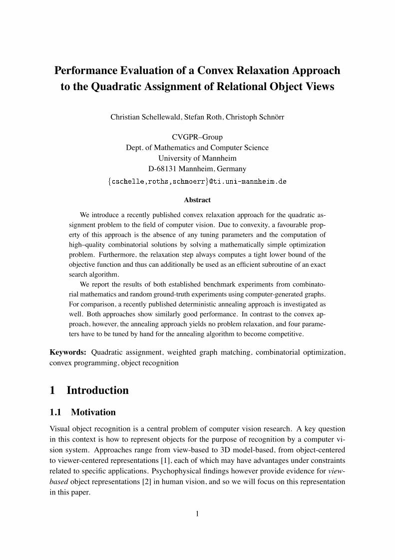
Figure 1: Image features and binary relations computed for an object view using the FEX–system (cf. [3] and http://www.ipb.uni-bonn.de/ipb/projects/fex/fex.html). The underlyinggraph has �� nodes.

A common and powerful structure for representing object views is to define a set oflocal image features � along with pairwise relations � � � � � (spatial proximity and(dis)similarity measure) in terms of a weight function � � � � �� , that is an undirectedweighted graph � � �� (see Figure 1). Accordingly, a core routine of any recogni-tion system is to compare graphs in different images, or to match graphs against prototypicalgraphs in some object database.

Finding a good match between two graphs�� amounts to compute a permutation of thevertices of one graph so as to become similar to the other one (cf. section 2). It is well-knownthat this quadratic assignment problem is NP-hard [4] and cannot be solved to optimality evenfor moderately sized problem instances. For the graph shown in Figure 1, for instance, about�� possible permutations of its vertices exist.

The task of developing good matching algorithms amounts to make a compromise betweentwo contradictory requirements: Firstly, a high-quality solution close to the (unknown) globaloptimum should be efficiently computable in polynomial time. Secondly, since the matchingalgorithm is only a particular module of a computer vision system, there should be no need formanual interaction (selection of a starting point or tuning parameters) in order to obtain goodperformance. It seems to us that this latter algorithmic aspect has received less attention inthe computer vision literature than the former one. This motivated us to look for an approachsatisfying both requirements.

1.2 Related Work

The quadratic assignment problem is a classical problem in the field of combinatorial opti-mization which is very general in the sense that several well-known problems, for example

2

the traveling salesman problem, are special cases of it. For a comprehensive review of thequadratic assignment problem we refer to [5].

Classical approaches to the quadratic assignment problem include

– linearizations [6, 7] which can be efficiently solved in polynomial time at the cost of aconsiderably larger number of variables,

– the use of exact search algorithms, like the cutting plane method [8] or branch-and-bound [9], which are based on lower bounds [10, 6] of the objective function but canonly be applied to small problem instances, or

– heuristic search algorithms like tabu search, simulated annealing, or genetic algorithms[11].

A separate class of approaches is formed by relaxations of the quadratic assignment problem.Typically, these approaches aim at computing a lower bound of the objective function based oneigenvalue problems [12, 13, 5]. Recently, an convex relaxation approach has been proposed[14] which can be used to compute both a lower bound and the corresponding approximateminimizer. A favorable property due to the convexity of this approach is that the relaxedsolution can numerically be computed without the need to select good starting points andtuning parameter values. This will be studied in more detail below.

Another important approach to the quadratic assignment problem is based on the deter-ministic annealing strategy. This approach has been extensively investigated in the neural-network literature [15, 16, 17, 18, 19, 20, 21, 22]. In the context of image segmentation,piecewise-smooth restoration and clustering, deterministic annealing is well-known in thecomputer vision literature as well [23, 24, 25, 26, 27, 28]. A favorable feature of deterministicannealing is that this strategy can be derived in a theoretically sound way using the maximumentropy principle (e.g., [27]). On the other hand, an obvious disadvantage from the viewpointof algorithm design are the complex bifurcation phenomena encountered when lowering theannealing parameter [29]. To the best of our knowledge, no control strategy is known whichguarantees to reach a “good” local minimum. While excellent experimental results have beenreported using deterministic annealing, the dependence of these results on various tuning pa-rameters apparently has not received much attention in the literature. In view of this importantaspect we present a thorough comparison of a deterministic annealing approach tailored to thequadratic assignment problem [20, 22] with a convex programming approach [14].

Further important work on the graph–matching problem includes alternative algorithmicapproaches like probabilistic relaxation [30], genetic search [31], error–correcting matching[32] or two–step iterative approaches [33], and also specialized work like, for example, si-multaneous estimation of transformation geometry [34], or matching trees in terms of themaximum clique of the association graph [35]. A comparison of this variety of approaches isbeyond the scope of this paper. We also do not discuss variations of the optimization criterion(see, e.g., [30, 36]), nor do we investigate the task to determine the weight function� in some

3

optimal way. Rather, by focusing on the optimization problem, we wish to emphasize theadvantages of parameter–free convex relaxation in the context of graph–matching and to re-veal its performance in comparison to recent approaches which are based on the well–knowndeterministic annealing framework.

1.3 Contribution

Our work contributes under the aspects relaxation, algorithm design and performance evalu-ation.

Relaxation has a context–dependent meaning. In this paper, relaxation refers to the strategy ofmaking a combinatorial problem computationally tractable by keeping exactly the objectivecriterion with respect to feasible combinatorial solutions but weakening the combinatorialconstraints. Concerning the quadratic assignment problem, a typical example is to optimizeover the orthogonal set of matrices instead of the set of permutation matrices, possibly subjectto further constraints like requiring non–negative entries or fixing row and column sums.

Solving (approximately) a combinatorial problem by relaxation has several advantages.Firstly, it is mathematically comprehensible where and how approximations are introduced inorder to solve the optimization problem. By contrast, many other approaches are based onalgorithmic modifications, making a theoretical understanding and comparison more difficult.Secondly, relaxed problem formulations compute a lower bound of the objective function,because weakening the constraints gives more degrees of freedom for minimization. As aconsequence, different problem relaxations can be ranked based on the lower bound theycompute: The larger the lower bound, the better the relaxation. Thirdly, relaxations can beused either to directly compute approximate solutions to the original combinatorial problem,or as subroutines in exact branch-and-bound search algorithms. In the latter case the tightnessof the lower bound also largely determines the overall performance. Due to these advantages,this paper focuses on relaxations of the quadratic assignment problem.

Algorithm design. A common problem of many approaches concerns the selection of tun-ing parameters in order to obtain good performance. Concerning the quadratic assignmentproblem, a representative example – the deterministic annealing strategy – will be examinedin more detail below. In this context, convex optimization approaches provide an attractivealternative, because the global optimum exists under mild conditions and can be computed byestablished numerical algorithms in polynomial time [37] without any additional parameters.

Performance evaluation. A widely–used collection of difficult, real–life benchmark prob-lems exists in the field of combinatorial optimization [38], which has become a standardduring the last years. Apparently, this database has not been used in the computer vision liter-ature so far in order to evaluate approaches to the weighted graph matching problem. Besidesextensive random ground–truth experiments, our performance evaluation was carried out forproblem instances of this database.

4

1.4 Organisation of the Paper

After stating the problem formally in section 2, we present a hierarchy of relaxations in sec-tion 3, the most strongest one being a convex relaxation. For comparison, we sketch twoalternative approaches from the literature in section 4, a simple but fast approach based oneigenvalue decomposition, and a more sophisticated deterministic annealing strategy. In or-der to stress the difference to these non–convex approaches, various aspects of the convexrelaxation approach are visualized for a toy example in section 5. In section 6, the results ofnumerous experiments for both real-life benchmarks from the field of combinatorial optimiza-tion and for ground-truth experiments based on computer-generated graphs are summarized.We conclude and indicate further work in section 7.

2 Problem Statement and Definitions

2.1 Notation

We will use the following notation:

�� transpose of the matrix�� unit matrix� set of orthogonal matrices � , i.e. �� set of matrices with unit row and column sums set of non-negative matrices set of permutation matrices � � � � vector of all ones: � � ��

Tr�� trace of the matrix�� scalar product of two matrices �� : � � � � Tr��

� Frobenius norm of the matrix�: � � Tr��

vec�� vector obtained by stacking the columns of the matrix�� Kronecker product �� vector of the eigenvalues of the matrix�� vector of the row sums of the matrix�� sum of all elements of the matrix �Æ�� Kronecker delta: Æ�� if � �, and � otherwise

2.2 Problem Statement

In this paper, we consider undirected graphs � � �� with nodes � � �� andedges � � � � � . The weight function � � � � �

�� typically encodes a similarity measure

with respect to pairs of features �� . This measure along with the structure of the graph isrepresented by the adjacency matrix ��: �� . Since �� ,adjacency matrices are symmetric: �� .

5

Let � � �� and � � �� denote two given graphs. In order tomatch these two graphs, we want to compute a permutation � � �� of the nodes of �such that the following distance measure is minimized:

��

�� (1)

Representing the permutation � by a permutation matrix � , this cost function takes thefollowing form [39] in terms of the adjacency matrices of � and�:

�� (2)

For isomorphic graphs exists a permutation matrix such that the minimum value �� ofthe objective function is attained. For features �� supplied by an image pre–processingstage, it is unlikely that � and � are isomorphic. In this case we define as the best matchthe permutation matrix �� which minimizes � over . Thus, the graph matching problemformally reads:

��

�� (3)

The minimization problem (3) has a close relationship to the quadratic assignment prob-lem (QAP) in combinatorial mathematics (for a survey, see [5]):

��

Tr�� (4)

Provided that the graphs have the same number of nodes, this relationship can be seen byreformulating the graph matching objective function as follows:

��

� Tr�� Tr��

�� Tr��

��

��

� �� Tr��

��

(5)

Dropping the constant terms �� Tr�� and �� Tr��

�� , we recognize the graph

matching problem (3) as a special case of the quadratic assignment problem (4) with� � �� ,� � �� and � � �. Throughout the remainder of this paper, we can therefore consider thefollowing optimization problem:

��

Tr�� (6)

Remark 1 We note that (1) corresponds to (6) only if �� . In this paper,we make this simplifying assumption (as did Umeyama [39], for instance) in order to as-sess the techniques which have been developed for the quadratic assignment problem for theweighted graph matching problem in computer vision. The issue of extending the techniquesto subgraph matching will be taken up in section 7.

6

3 Relaxations and Lower Bounds

In this section, we consider various relaxations of problem (6). We will see that a ranking ofthese approaches can be obtained by virtue of the corresponding lower bounds.

3.1 Orthogonal Relaxation

Relaxing the set to � � , Finke et al. [12] suggested the so–called Eigenvalue Bound(EVB) which gives a lower bound for the minimization problem (6):

(EVB) ��

Tr�� (7)

Here, � �� denotes the so–called minimal scalar product. This is the scalar productof the vectors �� and �� containing the eigenvalues of the adjacency matrices � and �ordered as follows: �� and �� .The matrix � for which the bound (EVB) is attained can be calculated as well. If �� diagonalize the adjacency matrices � and �, respectively, and this columns are arrangedaccording to the order of the eigenvalues mentioned above, then� � �� . It turned out thatin many cases this relaxation yields a bound for the minimization problem (6) which is tooweak to be useful in practice.

3.2 Projected Eigenvalue Bound

Hadley et al. [13] improved the lower bound (7) by taking into account the constraint set � inaddition to�. To this end, they parameterized matrices� �� based on ��

orthogonal matrices �� and the relationship

� � � ��

��

where � � � and the � � � columns of the � � �� matrix � form a basis of thesubspace orthogonal to the vector . Conversely, for any �� matrix �� wehave � � � ��

�� . The � � �� matrix � can be calculated using the

following scheme:

� �

��

� � � � � � �

� � � � � � � � �...

... � � � ......

� � � � � � � � �

��with � � � ��

�and � � � �

� ��

Using this parameterization, the objective function can be rearranged as follows:

Tr�� Tr �� Tr�� (8)

7

where �� , �� , � � �� and ��

��. The authors

of [13] suggested to optimize the first two terms on the right hand side of (8) separately, thefirst one over �� , and the second one over� . The latter problem amounts tosolve the linear assignment problem

LAP��

Tr�� (9)

which can be solved using any linear programming solver. As a result, the Projected Eigen-value Bound as a lower bound for the minimization problem (6) is obtained:

(PEVB) � � �� LAP�� (10)

However, a major drawback of this bound is that due to separately minimizing the twoterms in (8), a corresponding minimizing matrix � cannot be computed in general. The nextsubsection shows how one can overcome this drawback by convex relaxation and even achievea better lower bound than (10).

3.3 Convex Relaxation

Following the work of Anstreicher, Brixius and Wolkowicz [40, 14], we focus on a convexrelaxation of the minimization problem (6) in this section. Besides the general argumentsdiscussed in section 1.1, the main motivation for this approach is its ability to compute botha tight lower bound and the corresponding matrix � where this bound is attained. In generalthis is not possible for the bound (10).As a starting point reconsider the minimization of the first term of the right hand side ofequation (8) over the set �� :

��

Tr ��

s.t. �� (11)

��

The Lagrangian dual of this problem reads[40]:

��

Tr ��

s.t. �� (12)

��

Here �� means that �� has to be positive semidefinite. The optimal solution for (11),according to (7), is

��

Tr �� (13)

8

The duality gap between the optimal solutions of (11) and (12) is zero since interior pointsexist for both problems (see, e.g., [37]). Hence, the optimal values are the same:

��

Tr �� (14)

The objective function in (11) can be reformulated as follows:

Tr �� vec� �� vec� �� Tr� �� vec� ��vec� ��

�� (15)

where� � vec� ��vec� ��

For arbitrary matrices �� and �� and �� the following equations hold:

Tr �� Tr �� Tr �� Tr �� Tr� �� Tr �� Tr �� Tr ��

Using this, a positive semidefinite form containing �� from (12) can be introduced into theobjective function Tr �� , if we assume that �� and �� are a feasible solution for thedual problem (12):

Tr �� Tr �� Tr �� Tr �� Tr �� Tr �� vec� �� vec� ��

Choosing �� and �� as the optimal solution to (12) we obtain with (14):

Tr �� vec� �� vec� ��

Finally, substituting this expression as well as all the non–projected variables ��

etc. into (8), we obtain after an elementary but tedious calculation the Quadratic ProgrammingBound:

�� Tr�� vec��vec�� (16)

A comparison with (8) shows that now we have just a single term on the right hand sidecomprising the unknown matrix� and (16) allows the computation of both a lower bound andthe corresponding minimizing matrix � . For the linear term in (8), minimizing over the set (cf. (9)) is equivalent to minimizing over � � . Accordingly, Anstreicher and Brixius [14]suggest to minimize the quadratic form in (16) over � � , i.e. to solve the convex quadraticproblem:

�� vec��vec��

s.t. � � ��

� � �

(17)

9

Here � � � means that all entries of the matrix � have to be non-negative. The followingrelationship between the bounds (7), (10) and (16) holds[14]:

��

Tr�� (18)

Consequently the bound (16) computed by convex programming cannot perform worse thanthe other bounds. The quality of the corresponding solution � in comparison to other ap-proaches (see next section) will be assessed in section 6.

3.4 Computing a Combinatorial Solution

To obtain a permutation matrix � from the non-integer solution � � � to (17), agood permutation matrix close to � has to be found. A simple way of doing this is to solvethe following linear programming problem:

��

Tr�� (19)

In this paper, we use a slightly different idea which takes into account that in most cases a lin-ear approximation of the original problem leads to an improvement of the obtained objectivefunction. To this end, we add an unknown matrix � to the relaxed solution� so as to give apermutation matrix:

� � ��

Next, we expand the objective function Tr�� around � up to linear terms with re-spect to �:

Tr�� Tr��

� Tr�� Tr�� Tr�� Tr��

� Tr�� Tr�� Tr��

� �Tr�� Tr�� Tr��

� �Tr�� Tr��

As a result, we have to minimize the term Tr�� to obtain the combinatorial solution� from the relaxed solution� . This problem can again be solved by linear programming:

��

Tr��

To see the difference to (19), we put� � �� and finally have:

��

Tr�� (20)

3.5 The 2opt Post-Processing Heuristics

A simple heuristics called 2opt was proposed in [22] in order to further improve combinatorialsolutions computed by more expensive methods. This greedy strategy iteratively exchangespairs of assignments in the permutation until no further improvement is possible.

10

4 Non–Convex Approaches

In this section we briefly sketch two approaches that we used for comparison with the con-vex relaxation approach of section 3.3. The first one was proposed by Umeyama [39] andresembles the spectral relaxation approach of [12]. Furthermore, we consider the determinis-tic annealing approaches [20] and [22] for which excellent performances are reported in theliterature.

4.1 The Approach by Umeyama

Based on the Eigenvalue Bound (7), Umeyama [39] proposed the following estimate for thesolution of (6):

��

Tr�� (21)

Here, � and � diagonalize the adjacency matrices� and�, respectively, with the eigenvaluessorted according to (EVB), and � � � denotes the matrix consisting of the absolute values takenfor each element. (21) is a linear assignment problem which can be efficiently solved by usingstandard methods like linear programming.

4.2 Graduated Assignment

Gold and Rangarajan [20] and Ishii and Sato [22] independently developed a technique com-monly referred to as graduated assignment or soft assign algorithm. The set of permutationmatrices is replaced by the convex set � � � � of positive matrices with unit row andcolumn sums (doubly stochastic matrices). In contrast to previous mean-field annealing ap-proaches, the graduated assignment algorithm enforces hard constraints on row and columnsums, making it usually superior to other deterministic annealing approaches.

The core of the algorithm is an iteration scheme, which computes an approximative so-lution matrix � at each step of the decreasing annealing schedule. In our description � �

denotes the current annealing parameter; ! is a fixed “self-amplification” parameter, whichenforces that the minimum on the set � is also in . Denoting the iteration time step by thesuperscript, the matrix�� is calculated as follows (for � fixed):

�� "�#�$

�� with $��

��

�� Æ��Æ��!��

(22)

The scaling coefficients "�� #� are computed so that �� is projected on the set � usingSinkhorn’s algorithm [20] as inner loop:

$��

$�� $

��

� $��

$�� $

��

(23)

11

Stopping criteria based on convergence bounds or the number of iterations have to be estab-lished for the inner projection loop and the iteration scheme. For more details, we refer thereader to [20, 22].

Rangarajan et al. [21] showed that this scheme locally converges under mild assumptions.Several studies revealed excellent experimental results. In our experiments, we improved theobtained results with the local 2opt heuristics.

A drawback of the graduated assignment algorithm is that the selection of several “tuning”-parameters is necessary to obtain optimal performance. An annealing schedule has to be setup, which is usually described by three parameters: an initial temperature, the annealing rate,and a final temperature or other stopping criterion [20]. There are theoretically motivatedmethods that give a lower bound for reasonable initial temperatures based on an analysis ofthe bifurcation structure of the problem [22]. Nevertheless, careful selection of the parametergreater than this bound can improve the results. The self-amplification parameter also has alower bound that guarantees the above property that the minimizer of the objective function isin . An exhaustive parameter search for the annealing schedule, even below the theoreticalbound, may increase the performance. Finally, the stopping criteria also influence the qualityof the results. All parameters have in common that their optimal values vary for differentproblem instances (cf. [22]).

5 Convex Relaxation: An Illustrative Numerical Example

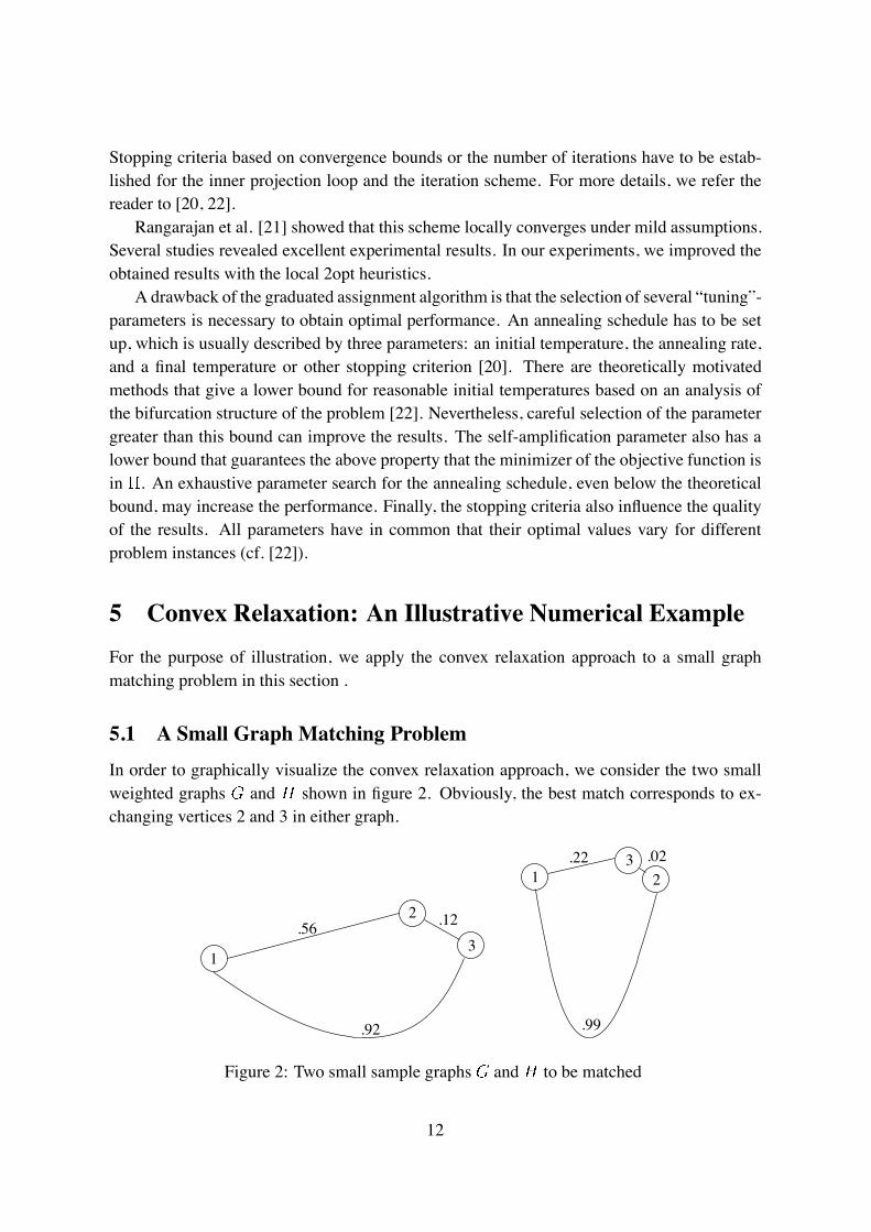
For the purpose of illustration, we apply the convex relaxation approach to a small graphmatching problem in this section .

5.1 A Small Graph Matching Problem

In order to graphically visualize the convex relaxation approach, we consider the two smallweighted graphs � and � shown in figure 2. Obviously, the best match corresponds to ex-changing vertices 2 and 3 in either graph.

1

2

3

.12.56

.92

321

.02

.99

.22

Figure 2: Two small sample graphs � and � to be matched

12

The adjacency matrices of the graphs � and � are:

��

��

��

��

��

��

��

��

��

In this example the objective function of the graph matching problem (3) attains the followingvalues for each of the six possible permutations:

1.370, 3.077, 2.01, 3.365, 0.613, 0.261

Thus the optimum of this graph matching problem is

OPT � ��

Tr��

with � � �� ,� � ��, �� Tr�� and �� Tr��

�� .

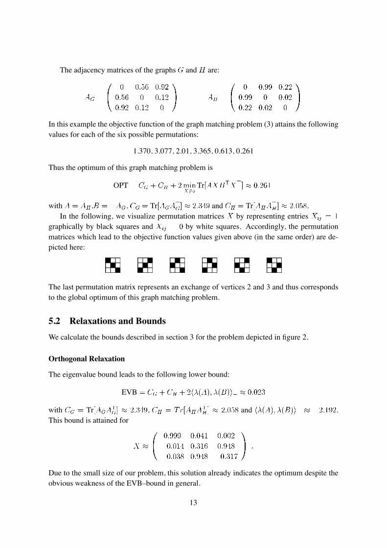
In the following, we visualize permutation matrices � by representing entries ��

graphically by black squares and �� by white squares. Accordingly, the permutationmatrices which lead to the objective function values given above (in the same order) are de-picted here:

The last permutation matrix represents an exchange of vertices 2 and 3 and thus correspondsto the global optimum of this graph matching problem.

5.2 Relaxations and Bounds

We calculate the bounds described in section 3 for the problem depicted in figure 2.

Orthogonal Relaxation

The eigenvalue bound leads to the following lower bound:

EVB � ��

with �� Tr�� , ��

�� and � �� .

This bound is attained for

� ��

��

��

��

Due to the small size of our problem, this solution already indicates the optimum despite theobvious weakness of the EVB–bound in general.

13

Projected Eigenvalue Bound

Using the Projected Eigenvalue Bound, we obtain the following lower bound for our smallgraph matching problem:

PEVB � �� LAP��

where � � �� , LAP�� , �� . Note that this boundis much stronger than the EVB–bound. On the other hand, as mentioned in section 3.2, thisapproach does not allow to compute a corresponding matrix� for which the PEVB–bound isattained.

Quadratic Programming Bound

The Quadratic Programming Bound gives:

QPB � ��

vec��vec��

Here the minimization of the quadratic term results in �� vec��vec�� and the bound is attained for

� ��

��

��

��

As predicted, this bound is superior to the PEVB–bound. So summarizing, for the numericalexample considered here the ranking (18) of these bounds reads:

EVB � �� PEVB � �� QPB � �� OPT � �� (24)

5.3 Visualization

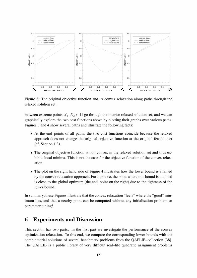
To illustrate how the convex relaxation approximates the original combinatorial problem, weinspect graphically the original objective function

�� Tr��

along with its convex relaxation

�� vec��vec��

for a few one–dimensional paths��%� through the relaxed solution set defined by� �� .It is well known (Birkhoff–von Neumann theorem) that this set is just the convex hull of theoriginal feasible set, i.e. the permutation matrices� . Hence, all paths

��%� � %�� %�� % ��

14

0.2 0.4 0.6 0.80

0.5

1

1.5

2

2.5

3

3.5

obje

ctiv

e va

lue

convex func.original func.lower bound

��

0.2 0.4 0.6 0.80

0.5

1

1.5

2

2.5

3

3.5

obje

ctiv

e va

lue


��

0.2 0.4 0.6 0.80

0.5

1

1.5

2

2.5

3

3.5

obje

ctiv

e va

lue


��

Figure 3: The original objective function and its convex relaxation along paths through therelaxed solution set.

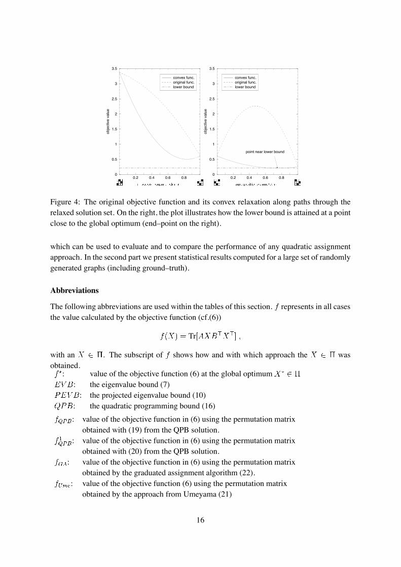
between extreme points �� go through the interior relaxed solution set, and we cangraphically explore the two cost functions above by plotting their graphs over various paths.Figures 3 and 4 show several paths and illustrate the following facts:

� At the end–points of all paths, the two cost functions coincide because the relaxedapproach does not change the original objective function at the original feasible set(cf. Section 1.3).

� The original objective function is non convex in the relaxed solution set and thus ex-hibits local minima. This is not the case for the objective function of the convex relax-ation.

� The plot on the right hand side of Figure 4 illustrates how the lower bound is attainedby the convex relaxation approach. Furthermore, the point where this bound is attainedis close to the global optimum (the end–point on the right) due to the tightness of thelower bound.

In summary, these Figures illustrate that the convex relaxation “feels” where the “good” min-imum lies, and that a nearby point can be computed without any initialisation problem orparameter tuning!

6 Experiments and Discussion

This section has two parts. In the first part we investigate the performance of the convexoptimization relaxation. To this end, we compare the corresponding lower bounds with thecombinatorial solutions of several benchmark problems from the QAPLIB–collection [38].The QAPLIB is a public library of very difficult real–life quadratic assignment problems

15

0.2 0.4 0.6 0.80

0.5

1

1.5

2

2.5

3

3.5

obje

ctiv

e va

lue


��

0.2 0.4 0.6 0.80

0.5

1

1.5

2

2.5

3

3.5

obje

ctiv

e va

lue


point near lower bound

��

Figure 4: The original objective function and its convex relaxation along paths through therelaxed solution set. On the right, the plot illustrates how the lower bound is attained at a pointclose to the global optimum (end–point on the right).

which can be used to evaluate and to compare the performance of any quadratic assignmentapproach. In the second part we present statistical results computed for a large set of randomlygenerated graphs (including ground–truth).

Abbreviations

The following abbreviations are used within the tables of this section. � represents in all casesthe value calculated by the objective function (cf.(6))

�� Tr��

with an � . The subscript of � shows how and with which approach the � wasobtained.� �: value of the objective function (6) at the global optimum��

�� : the eigenvalue bound (7)�� : the projected eigenvalue bound (10)��: the quadratic programming bound (16)

��: value of the objective function in (6) using the permutation matrixobtained with (19) from the QPB solution.

� ��: value of the objective function in (6) using the permutation matrixobtained with (20) from the QPB solution.

��: value of the objective function in (6) using the permutation matrixobtained by the graduated assignment algorithm (22).

�� : value of the objective function (6) using the permutation matrixobtained by the approach from Umeyama (21)

16

An additional “�”–sign (e.g.��, � ��, ��,�� ) indicates that the 2opt–heuristicswas used as a post–processing step to further improve the permutation matrix found.

6.1 QAPLIB Benchmark Experiments

Quality of the Relaxations

The quality of the various relaxation approaches, namely the eigenvalue bound (�� ), theprojected eigenvalue bound (�� ) and the quadratic programming bound (��), can beassessed by measuring how close these bounds are to the global optimum (see (18)).

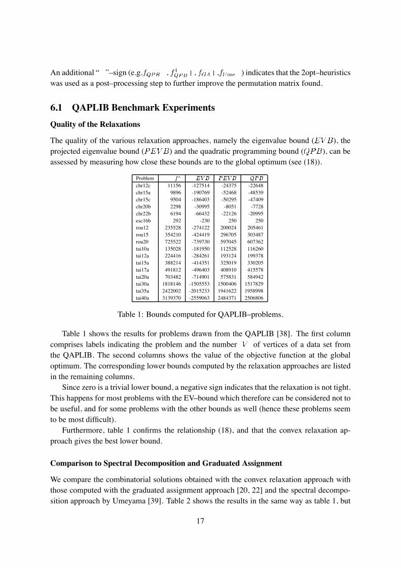
Problem ��

chr12c 11156 -127514 -24375 -22648chr15a 9896 -190769 -52468 -48539chr15c 9504 -186403 -50295 -47409chr20b 2298 -30995 -8051 -7728chr22b 6194 -66432 -22126 -20995esc16b 292 -230 250 250rou12 235528 -274122 200024 205461rou15 354210 -424419 296705 303487rou20 725522 -739730 597045 607362tai10a 135028 -181950 112528 116260tai12a 224416 -284261 193124 199378tai15a 388214 -414351 325019 330205tai17a 491812 -496403 408910 415578tai20a 703482 -714901 575831 584942tai30a 1818146 -1505553 1500406 1517829tai35a 2422002 -2015233 1941622 1958998tai40a 3139370 -2559063 2484371 2506806

Table 1: Bounds computed for QAPLIB–problems.

Table 1 shows the results for problems drawn from the QAPLIB [38]. The first columncomprises labels indicating the problem and the number �� of vertices of a data set fromthe QAPLIB. The second columns shows the value of the objective function at the globaloptimum. The corresponding lower bounds computed by the relaxation approaches are listedin the remaining columns.

Since zero is a trivial lower bound, a negative sign indicates that the relaxation is not tight.This happens for most problems with the EV–bound which therefore can be considered not tobe useful, and for some problems with the other bounds as well (hence these problems seemto be most difficult).

Furthermore, table 1 confirms the relationship (18), and that the convex relaxation ap-proach gives the best lower bound.

Comparison to Spectral Decomposition and Graduated Assignment

We compare the combinatorial solutions obtained with the convex relaxation approach withthose computed with the graduated assignment approach [20, 22] and the spectral decompo-sition approach by Umeyama [39]. Table 2 shows the results in the same way as table 1, but

17

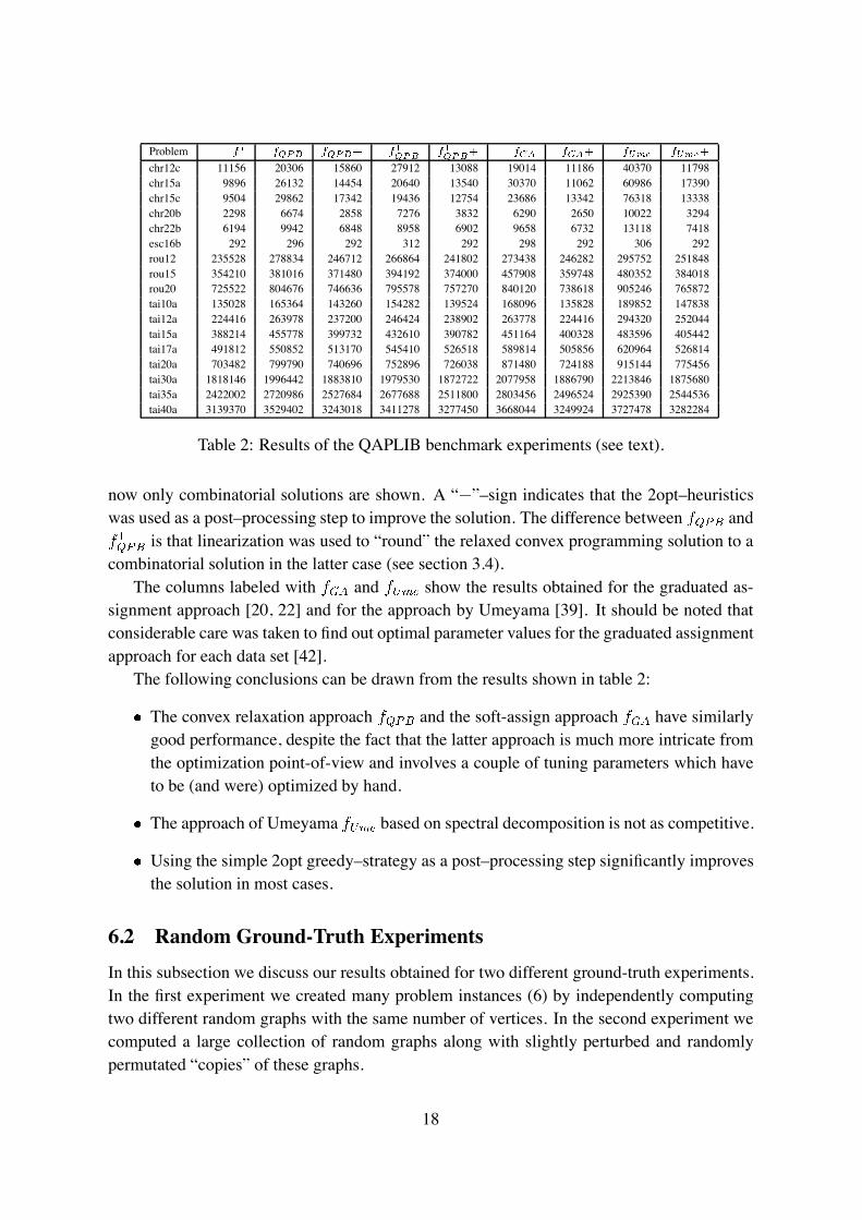
Problem ��

chr12c 11156 20306 15860 27912 13088 19014 11186 40370 11798chr15a 9896 26132 14454 20640 13540 30370 11062 60986 17390chr15c 9504 29862 17342 19436 12754 23686 13342 76318 13338chr20b 2298 6674 2858 7276 3832 6290 2650 10022 3294chr22b 6194 9942 6848 8958 6902 9658 6732 13118 7418esc16b 292 296 292 312 292 298 292 306 292rou12 235528 278834 246712 266864 241802 273438 246282 295752 251848rou15 354210 381016 371480 394192 374000 457908 359748 480352 384018rou20 725522 804676 746636 795578 757270 840120 738618 905246 765872tai10a 135028 165364 143260 154282 139524 168096 135828 189852 147838tai12a 224416 263978 237200 246424 238902 263778 224416 294320 252044tai15a 388214 455778 399732 432610 390782 451164 400328 483596 405442tai17a 491812 550852 513170 545410 526518 589814 505856 620964 526814tai20a 703482 799790 740696 752896 726038 871480 724188 915144 775456tai30a 1818146 1996442 1883810 1979530 1872722 2077958 1886790 2213846 1875680tai35a 2422002 2720986 2527684 2677688 2511800 2803456 2496524 2925390 2544536tai40a 3139370 3529402 3243018 3411278 3277450 3668044 3249924 3727478 3282284

Table 2: Results of the QAPLIB benchmark experiments (see text).

now only combinatorial solutions are shown. A “�”–sign indicates that the 2opt–heuristicswas used as a post–processing step to improve the solution. The difference between �� and� �� is that linearization was used to “round” the relaxed convex programming solution to acombinatorial solution in the latter case (see section 3.4).

The columns labeled with �� and �� show the results obtained for the graduated as-signment approach [20, 22] and for the approach by Umeyama [39]. It should be noted thatconsiderable care was taken to find out optimal parameter values for the graduated assignmentapproach for each data set [42].

The following conclusions can be drawn from the results shown in table 2:

� The convex relaxation approach �� and the soft-assign approach �� have similarlygood performance, despite the fact that the latter approach is much more intricate fromthe optimization point-of-view and involves a couple of tuning parameters which haveto be (and were) optimized by hand.

� The approach of Umeyama �� based on spectral decomposition is not as competitive.

� Using the simple 2opt greedy–strategy as a post–processing step significantly improvesthe solution in most cases.

6.2 Random Ground-Truth Experiments

In this subsection we discuss our results obtained for two different ground-truth experiments.In the first experiment we created many problem instances (6) by independently computingtwo different random graphs with the same number of vertices. In the second experiment wecomputed a large collection of random graphs along with slightly perturbed and randomlypermutated “copies” of these graphs.

18

Random Graphs

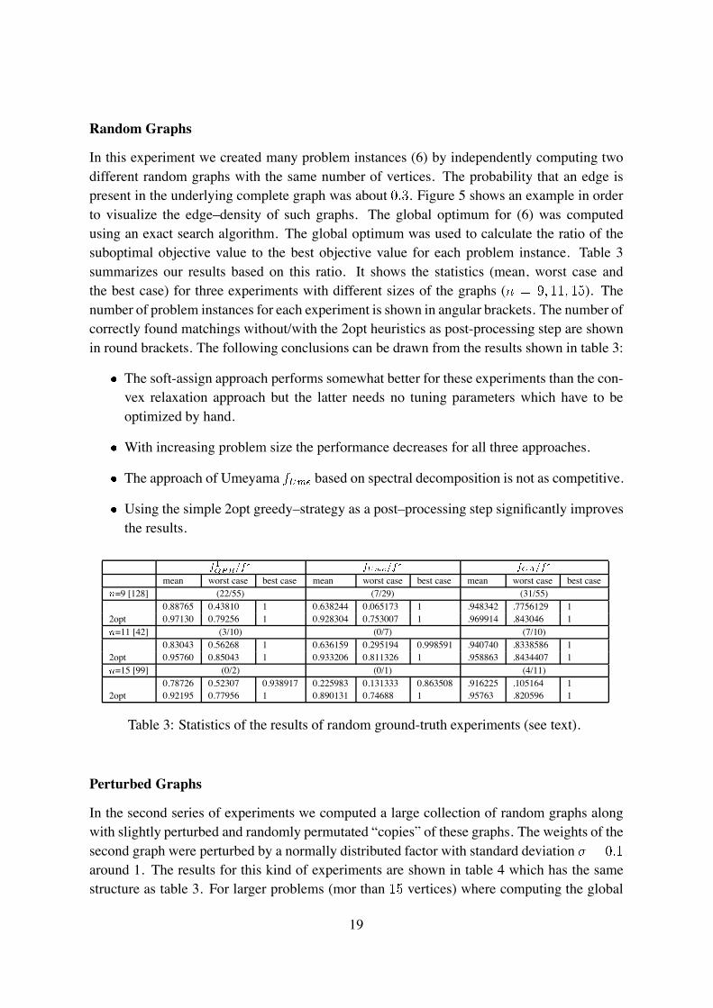
In this experiment we created many problem instances (6) by independently computing twodifferent random graphs with the same number of vertices. The probability that an edge ispresent in the underlying complete graph was about ��. Figure 5 shows an example in orderto visualize the edge–density of such graphs. The global optimum for (6) was computedusing an exact search algorithm. The global optimum was used to calculate the ratio of thesuboptimal objective value to the best objective value for each problem instance. Table 3summarizes our results based on this ratio. It shows the statistics (mean, worst case andthe best case) for three experiments with different sizes of the graphs (� � �� ). Thenumber of problem instances for each experiment is shown in angular brackets. The number ofcorrectly found matchings without/with the 2opt heuristics as post-processing step are shownin round brackets. The following conclusions can be drawn from the results shown in table 3:

� The soft-assign approach performs somewhat better for these experiments than the con-vex relaxation approach but the latter needs no tuning parameters which have to beoptimized by hand.

� With increasing problem size the performance decreases for all three approaches.

� The approach of Umeyama �� based on spectral decomposition is not as competitive.

� Using the simple 2opt greedy–strategy as a post–processing step significantly improvesthe results.

��

� ��

mean worst case best case mean worst case best case mean worst case best case�=9 [128] (22/55) (7/29) (31/55)

0.88765 0.43810 1 0.638244 0.065173 1 .948342 .7756129 12opt 0.97130 0.79256 1 0.928304 0.753007 1 .969914 .843046 1�=11 [42] (3/10) (0/7) (7/10)

0.83043 0.56268 1 0.636159 0.295194 0.998591 .940740 .8338586 12opt 0.95760 0.85043 1 0.933206 0.811326 1 .958863 .8434407 1�=15 [99] (0/2) (0/1) (4/11)

0.78726 0.52307 0.938917 0.225983 0.131333 0.863508 .916225 .105164 12opt 0.92195 0.77956 1 0.890131 0.74688 1 .95763 .820596 1

Table 3: Statistics of the results of random ground-truth experiments (see text).

Perturbed Graphs

In the second series of experiments we computed a large collection of random graphs alongwith slightly perturbed and randomly permutated “copies” of these graphs. The weights of thesecond graph were perturbed by a normally distributed factor with standard deviation & � ��

around 1. The results for this kind of experiments are shown in table 4 which has the samestructure as table 3. For larger problems (mor than �� vertices) where computing the global

19

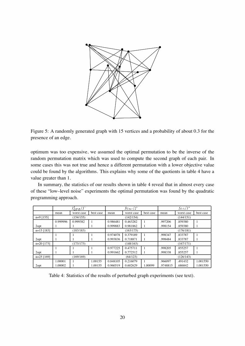
Figure 5: A randomly generated graph with 15 vertices and a probability of about 0.3 for thepresence of an edge.

optimum was too expensive, we assumed the optimal permutation to be the inverse of therandom permutation matrix which was used to compute the second graph of each pair. Insome cases this was not true and hence a different permutation with a lower objective valuecould be found by the algorithms. This explains why some of the quotients in table 4 have avalue greater than 1.

In summary, the statistics of our results shown in table 4 reveal that in almost every caseof these “low–level noise” experiments the optimal permutation was found by the quadraticprogramming approach.

��

��

�

mean worst case best case mean worst case best case mean worst case best casen=9 [155] (154/155) (142/154) (144/151)

0.999996 0.999382 1 0.986481 0.463282 1 .997206 .859380 12opt 1 1 1 0.999883 0.981862 1 .998154 .859380 1n=15 [183] (183/183) (163/175) (176/181)

1 1 1 0.974078 0.379189 1 .998347 .833787 12opt 1 1 1 0.993836 0.718871 1 .998484 .833787 1n=20 [173] (173/173) (148/163) (167/171)

1 1 1 0.977225 0.475711 1 .998205 .855257 12opt 1 1 1 0.991662 0.772512 1 .998338 .855257 1n=25 [169] (169/169) (64/123) (126/143)

1.00001 1 1.00155 0.848105 0.216079 1 .966097 .491432 1.0015502opt 1.00002 1 1.00155 0.960519 0.602629 1.00099 .9748815 .686842 1.001550

Table 4: Statistics of the results of perturbed graph experiments (see text).

20

7 Conclusion and Further Work

We showed that the convex programming approach is a competitive approach for findingsuboptimal solutions to the weighted graph-matching problem. We compared the convexapproach with both a recent deterministic annealing approach and an approach based on theeigenvalue decomposition. The performance of the latter approach is worse whereas the deter-ministic annealing approach performs similarly or slightly better, but uses parameters valueswhich were optimized by hand. The advantage of the convex approach is that no “tuning”parameters have to be determined at all. Furthermore, in contrast with the deterministic an-nealing approach, the convex approach provides a lower bound and thus can be used as asubroutine within an exact search strategy like branch-and-bound. Our results show that it isan attractive direction of research for solving relational matching problems in the context ofview-based object recognition.

Our further work will focus on the case of graphs with an unequal number of vertices:�� . If this difference is small, our approach can be applied by filling up the smallergraph with “virtual nodes”. In general, of course, this is not a satisfying way. The conse-quence of different numbers of vertices is that the unknown permutation matrix � becomesa matching matrix, and that either of the two constants �� in the objective function (5)changes to a term which depends on � , too. In our further work we will extend the approachpresented here to this more general case.

Acknowledgement

The authors are grateful to Jens Keuchel and Daniel Cremers for scrutinizing the manuscriptand many suggestions.

References

[1] M. Herbert, J. Ponce, T. Boult, and A. Gross, editors. Object Representation in ComputerVision, volume 994 of Lect. Not. Comp. Sci. Springer-Verlag, 1995.

[2] H.H. Bulthoff and S. Edelman. Psychophysical support for a two-dimensional viewinterpolation theory of object recognition. Proc. Nat. Acad. Science,, 92:60–64, 1992.

[3] W. Forstner. A framework for low level feature extraction. In J.O. Eklundh, editor, Com-puter Vision - ECCV ’94, volume 801 of Lect. Not. Comp. Sci., pages 61–70. Springer-Verlag, 1994.

[4] S. Sahni and T. Gonzalez. P-complete approximation problems. J. ACM, 23:555–565,1976.

21

[5] R.E. Burkard, E. Cela, P.M. Pardalos, and L.S Pitsoulis. The quadratic assignment prob-lem. In P.M. Pardalos and D.-Z. Du, editors, Handbook of Combinatorial Optimization,pages 241–338. Kluwer Acad. Publishers, 1998.

[6] E.L. Lawler. The quadratic assignment problem. Management Science, 9:586–599,1963.

[7] H.A. Almohamad and S.O. Duffuaa. A linear programming approach for the weightedgraph matching problem. IEEE Trans. Patt. Anal. Mach. Intell., 15(5):522–525, 1993.

[8] M.S. Bazaraa and H.D. Sherali. On the use of exact and heuristic cutting plane methodsfor the quadratic assignment problem. J. Operations Res. Soc., 33:991–1003, 1982.

[9] P.M. Pardalos, K.G. Ramakrishnan, M.G.C. Resende, and Y. Li. Implementation of avariable reduction based lower bound in a branch and bound algorithm fir the quadraticassignment problem. SIAM J. Optimiz., 7:280–294, 1997.

[10] P. Gilmore. Optimal and suboptimal algorithms for the quadratic assignment problem.SIAM J. Applied Math., 10:305–313, 1962.

[11] E. Aarts and J.K. Lenstra, editors. Local Search in Combinatorial Optimization, Chich-ester, 1997. Wiley & Sons.

[12] G. Finke, R.E. Burkard, and F. Rendl. Quadratic assignment problems. Annals of Dis-crete Mathematics, 31:61–82, 1987.

[13] S.W. Hadley, F. Rendl, and H. Wolkowicz. A new lower bound via projection for thequadratic assignment problem. Math. of Operations Research,, 17:727–739, 1992.

[14] N. Brixius and K. Anstreicher. Solving quadratic assignment problems using convexquadratic programing relaxations. Optimization Methods and Software, 16(1–4):49–68,2001.

[15] R. Kree and A. Zippelius. Recognition of topological features of graphs and images inneural networks. J. Phys. A, 21:L813–L818, 1988.

[16] C. Peterson and B. Soderberg. A new method for mapping optimization problems ontoneural networks. Int. J. of Neural Systems, 1:3–22, 1989.

[17] A.L. Yuille. Generalized deformable models, statistical physics, and matching problems.Neural Comp., 2:1–24, 1990.

[18] P. Simic. Constrained nets for graph matching and other quadratic assignment problems.Neural Computation, 3(2):268–281, 1991.

22

[19] J.J. Kosowsky and A.L. Yuille. The invisible hand algorithm: Solving the assignmentproblem with statistical pyhysics. Neural Networks, 7(3):477–490, 1994.

[20] S. Gold and A. Rangarajan. A graduated assignment algorithm for graph matching.IEEE Trans. Patt. Anal. Mach. Intell., 18(4):377–388, 1996.

[21] A. Rangarajan, A. Yuille, and E. Mjolsness. Convergence properties of the softassignquadratic assignment algorithm. Neural Computation, 11(6):1455–1474, 1999.

[22] S. Ishii and M. Sato. Doubly constrained network for combinatorial optimization. Neu-rocomputing, 43, 239-257 (2002).

[23] A. Blake and A. Zisserman. Visual Reconstruction. MIT Press, 1987.

[24] Y.G. Leclerc. Constructing simple stable descriptions for image partitioning. Int. J. ofComp. Vision, 3(1):73–102, 1989.

[25] D. Geiger and F. Girosi. Parallel and deterministic algorithms from mrf’s: Surface re-construction. IEEE Trans. Patt. Anal. Mach. Intell., 13(5):401–412, 1991.

[26] D. Geiger and A. Yuille. A common framework for image segmentation. Int. J. ofComp. Vision, 6(3):227–243, 1991.

[27] T. Hofmann and J. Buhmann. Pairwise data clustering by deterministic annealing. IEEETrans. Patt. Anal. Mach. Intell., 19(1):1–14, 1997.

[28] A.V. Rao, D.J. Miller, K. Rose, and A. Gersho. A deterministic annealing approach forparsimonious design of piecewise regression models. IEEE Trans. Patt. Anal. Mach. In-tell., 21(2):159–173, 1999.

[29] M. Sato and S. Ishii. Bifurcations in mean-field-theory annealing. Physical Review E,53(5):5153–5168, 1996.

[30] W.J. Christmas, J. Kittler, and M. Petrou. Structural matching in computer vision usingprobabilistic relaxation. IEEE Trans. Patt. Anal. Mach. Intell., 17(8):749–764, 1995.

[31] A.D.J. Cross, R.C. Wilson, and E.R. Hancock. Inexact graph matching using geneticsearch. Pattern Recog., 30(6):953–970, 1997.

[32] B.T. Messmer and H. Bunke. A new algorithm for error-tolerant subgraph isomorphismdetection. IEEE Trans. Patt. Anal. Mach. Intell., 20(5):493–504, 1998.

[33] B. Luo and E.R. Hancock. Structural graph matching using the em algorithm and sin-gular value decomposition. IEEE Trans. Patt. Anal. Mach. Intell., 23(10):1120–1136,2001.

23

[34] A.D.J. Cross and E.R. Hancock. Graph-matching with a dual-step em algorithm. IEEETrans. Patt. Anal. Mach. Intell., 20(11):1236–1253, 1998.

[35] M. Pelillo, K. Siddiqi, and S.W. Zucker. Matching hierarchical structures using associa-tion graphs. IEEE Trans. Patt. Anal. Mach. Intell., 21(11):1105–1120, 1999.

[36] H. Bunke. Error correcting graph matching: On the influence of the underlying costfunction. IEEE Trans. Patt. Anal. Mach. Intell., 21(9):917–922, 1999.

[37] Y. Nesterov and A. Nemirovskii. Interior Point Polynomial Methods in Convex Pro-gramming. SIAM, 1994.

[38] R.E. Burkard, S. Karisch, and F. Rendl. Qaplib – a quadratic assignment problem library.J. Global Optimization, 10:391–403, 1997.

[39] S. Umeyama. An eigendecomposition approach to weighted graph matching problems.IEEE Trans. Patt. Anal. Mach. Intell., 10(5):695–703, 1988.

[40] K. Anstreicher and H. Wolkowicz. On langrangian relaxation of quadratic matrix con-straints. SIAM J. Matrix Anal. Appl., 22(1):41-55, 2000

[41] K.M. Anstreicher and N.W. Brixius. A new bound for the quadratic assignment prob-lem based on convex quadratic programming. Technical report, Dept. of ManagementSciences, University of Iowa, 1999.

[42] S. Roth. Analysis of a deterministic annealing method for graph matching and quadraticassignment problems in computer vision. Master’s thesis, CVGPR–group, University ofMannheim, May 2001.

24

performance evaluation of a convex relaxation approach to the quadratic assignment of relational...

Documents