adding time dimension to relational model and extending relational algebra

inform. Sysrems Vol. 11, No. 4, pp. 343-355. 1986 03~*4379/86 $3.00 + 0.00 Printed in Great Britain Pergamon Journals Ltd

ADDING TIME DIMENSION TO RELATIONAL MODEL AND EXTENDING RELATIONAL ALGEBRA

ABDULLAH Uz TANSEL

Department of Statistics and Computer Information Systems, Baruch College-CUNY, 17 Lexington Avenue, New York, NY 10010, U.S.A.

(Received 26 August 1985; in revised form 8 April 1986)

Abstract-A methodology for adding the time dimension to the relational model is proposed and reiational algebra is extended for this purpose. We propose time-stamping attributes instead of adding time to tuples. Each attribute value is stored along with a time interval over which it is valid. Non-first normal form realations are used. A relation can have atomic, set-valued, triplet-valued, or set triplet- valued attributes. The last two types of attributes preserve the time (history). Furthe~ore, new algebraic operations are defined to extract information from historical relations. These operations convert one attribute type to another and do selection over the time dimension. Algebraic rules and identities for the new operations are also included.

Keywords: Historical databases, non-first normal form relations, relational algebra, relational model, time.

1. ENTRODUCTION

A relational database is defined as a set of time- varying relations [l]. So far, research in relational database theory concentrated on static relations which are the snapshots of the real world. As the real world changes states, the snapshot is updated to form the most recent one. The previous values are dis- carded and no past data is maintahled in the database. Yet, many applications require both the current and the past data. This apparent need forms the rationale for historical relational databases.

The attributes of an object (i.e. an entity or a relationship) assume different values over time. The set of these values form the history of that object. A database which maintains object histories is called a historical database (HDB) or a temporal database (TDB).

In this paper, we extend the methodology, we developed in a previous study [2], for adding the time dimension to the relational model. Time is added at the attribute level unlike other previous proposals which time-stamp the tuples and cause data duplication. Time-dependent attributes receive their values from complex domains whose elements represent values and time intervals over which they are valid. This, requires using non-first normal form relations which form a logical, and non-redundant approxi- mation of the real world since historical data is modelled without any duplication. Furthermore, simple and set-valued attributes are also allowed in each relation. We also develop a historical relational alge-

The material in this paper is the revised and extended version of a paper which appeared in the proceedings of the ACM SIGMOD Conference on the Management of Darn, 1985.

bra (HRA) which includes new operations in addition to the traditional algebraic operations. These operations convert one attribute type to another and do selection on the time dimension.

2. PREVIOUS WORK

Bolour er al. gives a comprehensive survey of the literature on the role of time in information pro- cessing [3]. A taxonomy of temporal data models has been developed by Snodgrass and Ahn [21]. There are recent attempts for incorporating the time dimension to different data models 15-71. Extensions to relational model and some relational query languages to include time dimension are proposed by several researchers [2,4,8-121.

Historical relations can be visualized as three- dimensional structures (cubesj. Time comprises the third dimension in addition to the attribute and object (tuple) dimensions. The three-dimensional structure is converted to two-dimensional tables by some kind of tuple time-stamping [4,8-101 or by extracting static relations from the cube [12].

Clifford and Warren [lo] gives a complete the- oretical treatment of time in relational model based on Intensional logic. State and existence attributes are added to each tuple. In his Time Relational Model, Ben-Zvi adds five different time domains to each tuple and extracts static relations which are manipulated by traditional relational algebra operations [9]. An extension to SQL for handling time is proposed by Ariav [8]. Snodgrass develops a new language TQuel which is a derivative of QUEL of INGRES database management system [4,13]. TQuel follows QUEL syntax and has additional clauses for manipulating historical data.

343

344 ABDULLAH Uz TANSEL

Lum et al. proposes keeping the current tuples in a relation and chaining the history tuples to current tuples in reverse time order [14]. Implementation strategies for this approach are further explored in

]15]. There are three recent studies which attach time-

stamps to attributes and use non-first normal form relations. Clifford uses time points as time-stamps [1 11. He also discusses various semantic issues and gives examples for the operations of a possible historical relational algebra. Gadia proposes the use of time intervals as time-stamps and defines a temporal domain out of the intervals [ 12, 161. He develops algebra and calculus languages and shows their equivalence. He also extends QUEL of INGRES for handling time [16]. We also use time intervals as time-stamps and give historical relational algebra operations. This is the case in our previous work too [2]. Gadia and we both have the same view of the three-dimensional structure. The approaches however differ in the way historical information is referred to. Gadia extracts static relations from the cube, which limit the reference capability to other time points outside of the time of derived relation, while we use operators to normalize the cube and then, apply relational algebra operations.

In Section 3, we incorporate the time dimension into the relational model. New operations of the historical relational algebra are introduced in Section 4. Section 5 gives example queries for illustrating HRA operations. Algebraic identities and the rules for HRA operations are included in Sections 6 and 7. Section 8 is the conclusion.

3. TIME IN RELATIONAL DATABASES

3.1 Time

Time is a continuous variable and can be repre- sented by real numbers. However, in a database environment approximating time as discrete points, isomorphic to natural numbers, is more practical. We will consider time as the set of consecutive, equally- distanced points. Figure 1 shows the time axis illustrating to, t,, tz, . . . , now as the discrete time points. T is the set of time points which is a total order under less than-equal-to (6). The points are identified relative to an origin toa

Where

T = {t,,, t, , . . . , ti, . . . ,now>

to<t,c++-<ti<.-+< now

ti=ti_l+l and t,=t,-t-i

Fig. 1. Time axis.

now is the marking symbol for the current time. As time advances the value of now also changes accord- ingly. The time unit is not specified and left to the user. It may be days, hours, minutes, etc. Between two consecutive points, there is a time duration which is equivalent to one time unit. Any moment in this duration is not visible unless a smaller time unit is used.

The interval [f, u) is the set of consecutive time points between f and u. I is the beginning (lower bound) of the interval and u is its end ( upper bound).

The interval [I, u) is closed at the beginning and it is open at the end. Similarly, the interval [/, u] is closed at both ends; it includes I, u, and the points between them. Consider two intervals [l, u) and [1’, u’). They are disjoint if they do not have any points in common. Two intervals overlap if they have time points in common, i.e. their intersection is not null. In the case of adjacent intervals, one follows the other. In other words, I’ = u or f = u’. The interval [I, u) is a subset of the interval [I’, u’) if the latter includes all the time points which belong to the former. The set operations, like union, intersection, difference, can be defined on intervals. These definitions are straightforward and are not included here. However, the set of intervals is not closed under the set theoretic operations.

3.2 Events

Events are the transactions, operations, or actions causing the assignment of new values to the attributes of the objects involved in a database. Withdrawing money from a bank account, paying an invoice, and hiring an employee are examples of events. Many of these events affect only a few attributes while the remaining attributes retain their existing values. These are the update transactions and make up a considerable portion of the activities in many applications. This observation forms the rationale for time- stamping the attributes. A deletion transaction causes removal of the tuples of deleted objects from the database. These tuples are usually archived. How- ever, a HDB should keep the deleted tuples, otherwise the database would contain incomplete data. In our proposal the deleted tuples are kept in the data base. Unlike the attribute time, deletion time belongs to an entire tuple. So, it would be appropriate to add a deletion time attribute to each relation whose values will be the deletion time of the tuples. A deleted tuple participates in database operations only when the queries refer to the period during which it exists. On the other hand, an insertion transaction introduces a new object (or a previously deleted object) to the database. In this case, all the attributes acquire their initial values and have the insertion time as initial time reference.

In Fig. 1, e,, e,, and e3 are events. They assign the

Adding time dimension to relational model 345

values, say, a,, az, and a, to attribute A of an object u, respectively. a, is assigned at time t, and is valid for the time interval [tz, 15). In other words, the object o has a, as its A attribute value over the time points f2, t3 and r, and the time duration between these points. Similarly, o acquired a2 at time t, and retains it until t6. At t6 it acquires a3 which is valid over the interval

[f6, now]. Each attribute value is recorded as a {time, value)

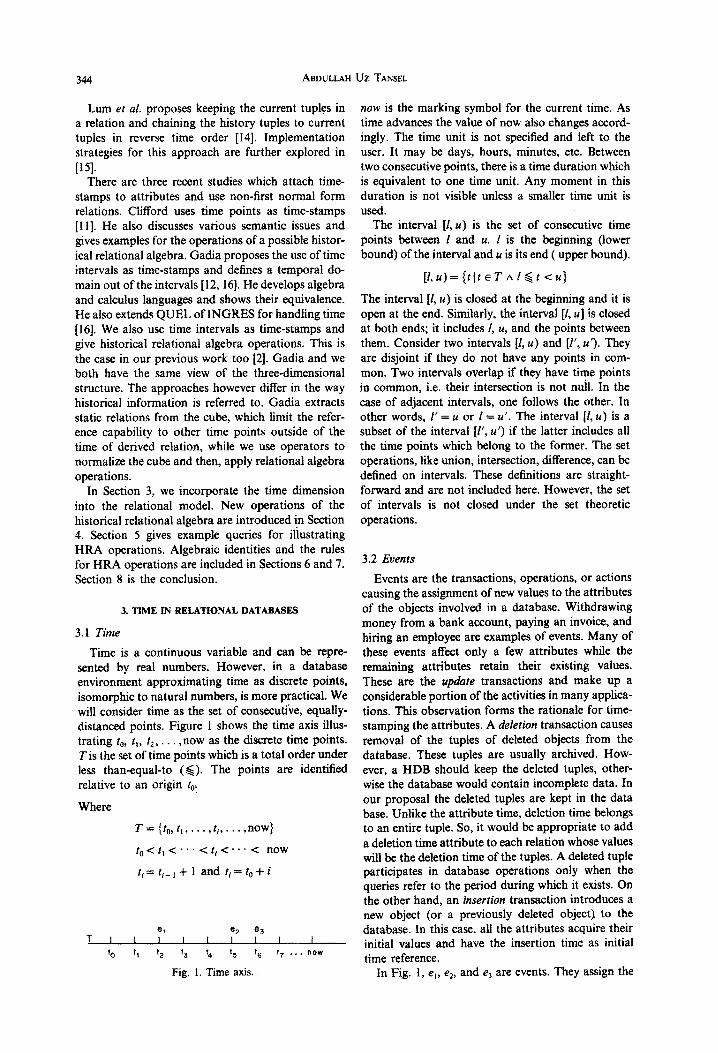
pair. The time part of this pair can be taken as the time point at which the attribute value is acquired or the interval in which the value is valid. In the former case, the pair becomes (ti, v} and it becomes ([t, u), v > in the latter case. Figure 2 shows these two alternatives for a relation, EMP (NAME, SALARY). Representing the time as point (Fig. 2a) is simple and looks logical. However, this approach splits the time interval between two successive pairs. Hence, to determine the time duration over which a value is valid, the successor pair has to be examined. This creates complications in expressing and interpreting the relational algebra operations. Because of this reason, we choose the second alternative which represents the attribute values as triplets. A triplet has the form ([I, u), u} where I and u are the lower and upper bounds of an interval in which the value v is valid. [l, u) is interval (time) component of the triplet and functions as the time-stamp. v is its data component. Figure 2b show this representation method. Note that % stands for now in Fig. 2b.

Any interval which includes now as its upper bound is an expanding interval. As time advances, the interval [I, now] expands. Unlike the other intervals it is closed at both ends. When an event occurs this interval is split into two intervals, [I, u) and [I,, now] such that 1, = u. Assume s is a tuple of a relation, one of whose attribute is A and event e assigns a new value a, to A. $[A] contains ([l, now), a) before e occurs. afterwards, s[A] contains two triplets ([f, u),

a> and (If,, now), 0 th is the time when an object, o, is introduced to the

database. All of its attributes has tb as the initial time-stamp. Each of o’s attributes have either a non-null value or the value null or a combination of these in the interval [tb, now]. Value null is denoted by ‘-’ and indicates that the attribute value is unknown.

3.3 The model

Let W be the set of all values regarded as atomic such as integers, reals, and character strings and the value null. Let D,, , . . . , D, be subsets of U and D s,, . . . , D+, be subsets of P(U) where P(U) is the power set of U. TI is the set of intervals defined over the time points in T. It is a subset of T x T where x denotes the Cartesian product:

At,,<ug now A c&u> ETxT)

D 1,) * * 1, D, are the subsets of TI x U and

PG4,),..., P(L),*) are their co~esponding power sets.

Consider a collection of sets E,, E2,, . . ,E, where E, is one of the above defined sets D,,, . . . ,D.,, D s, 9 * ’ ’ f D fn’ Dfr,...,Dx_, PW,,), ..-, P(D,,) for f =: 1 , . . . ,n. A h~~t~rjc~~ relation (HR), defined on the sets E,, E,, . . . , E,, is a subset of the Cartesian product E, x E2 x . , . x E,. As is clear from the definition a HR is a non-first normal form relation whose nesting depth is at most one, that is, the attribute values can only be sets, not sets of sets and so on. Also, time dependent attribute values are functions from time intervals to the elements of U.

&4, . . . ,A,) is a historical relation scheme. n is called the degree of R. Atr(R) is the set of the attributes of R. r is the historical relation instance (occurrence) for the historical relation scheme R. Let R, S, . . . be HR schemes, then the historical relational database schema DB is (R, S, . . .> and

( r, s, . . . > its one instance. From now on, we will use the term relation to include historical relations too. We will also use relations and relation schemes interchangeably. The meaning will be clear from the context.

A historical relation may have four types of attributes. Atomic attributes contain atomic values, that is, they receive values from the domains which are subsets of U. Triplet-valued attributes contain triplets as atomic values where an atom is a 3-tuple in our context. These attributes quite often correspond to the primary, or foreign key attributes whose values are expected not to change over time. Values of a set-valued attribute are sets of atomic values. These

I NAME SALARY 1

<[lo, nl, BOB) (I25 nl, 18 K)

([12.18), 15K)

<[12, nl. BILL) (118, nl, 20 K)

Fig. 2. Example EMP relation. (a) Point representation. (b) Interval representation.


FOREIGN E# ENAME SALARY MANAGER LANGUAGES

{([15.19), RON), {<[lb, 25), 14 I(>, ([19,22), GARY),

133 TOM

<[25,nl, 19 K>] (122, nl, AL)] (French, Spanish)

140 ANN {(lO,nJ, 12 K)} {<PO. nl. LIZ)} I’-‘1

(a)

FOREIGN E# ENAME SALARY MANAGER LANGUAGES

(<E20,25), 14 K), {([20,22), GARY), 133

TOM <[25,@), 18 IO} <[22,40), AL)] {French, Spanish)

140 ANN f<[20.40), 12 K>] {([SO, 40), LIZ)} { ‘-7

(b)

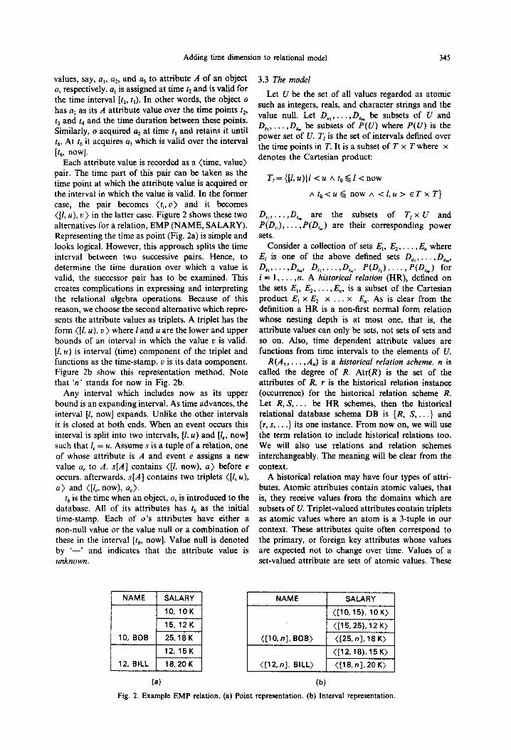
Fig. 3. An example historical relation and its instance in the interval [20,40). (a) An example historical relation (EMP). (b) Instance of EMP relation over the inten& [20,40).

values are considered to be independent of time. Set-triplet-valued attributes contain sets of triplets as values. Each set is a collection of one or more triplets, defined over the interval f&, now] and represents the attribute’s history. The interval component of a triplet is a subset of [t6, now] and its value component corresponds to a value which the attribute has acquired. Figure 3a shows an example HR. It is also possible to define an attribute whose domain is time, e.g. birth-date. The values of such attributes can be compared with the time-stamps of other attributes for various type of data extraction.

In the case of attributes which contain a single value at any instance of time, the time components of triplets are disjoint. However, there are other attributes which do not invalidate their previous values when a new value is acquired. For example, prizes

won or skills acquired by an employee are such attributes. In this case, each prize won at time fp has a validity interval [t,, now] and time intervals of triplets overlap.? Another example is the foreign languages spoken by an employee. Such cases are modeled as event relations in [13].

We use the following notation in naming the attributes of a relation. Let A, B, . . . be attributes of a relation. Atomic attributes are referred to by their names, like A, B, etc. Set-valued attributes are prefixed with an asterisk, e.g. *A, *B, etc. We denote triplet-valued attributes by a bar over the attribute name, e.g. 2, R, etc. Simiiarly, an asterisk and a bar are used for the set-triplet-valued attributes, e.g. *A, *R, etc. It is possible to refer to the components of a triplet-valued attribute. A,, &, and 2, represent the lower bound, the upper bound and the data (value) components, respectively of the triplet-valued attribute 2. Similarly, for a triplet X, X,, E,, and X, represent the lower bound, the upper bound and the data (value) components, respectively. 55, denotes the

tNote that the upper limit is not necessarily now, i.e. a skill may be outdated and may no longer be valid at present.

set corresponding to the time interval of P. 2, denotes the set which represents the time inerval of 2. Similar definitions can also be given for the set triplet-valued attributes. For instance, 5, represents the set con- taining the time intervals of the triplets in *.?.

Let min(r& be the minimum time-stamp in a historical relation. Then, this relation has tuples in the interval [min(&), now].

3.4 Defining relations over a time interval

In this section we will define instances of a relation, say R, over the interval [I, U) and at the time point t. Let rt,,“) and r, denote these instances, respectively. We will also define tuple components and tuples over [&u) and at time t. Let s be a tuple of r. s[AII,,,, is the tuple component which corresponds to attribute A. If A is an atomic attribute s[A&,,,, is the same as s[A]. Similarly, s[+A]t,,,, is the same as s[*A], because these attribute types are independent of time. On the other hand, for the triplet-valued attribute 2,

m[t,u) is equal to a triplet ([f’, u’), a) where [I’, u’) = [I, u)n[l”, u”), where p”, u”) is the time of s[A]. Of course, when the intersection of intervals is nuli, s[&,,, is also null. For the set triplet-valued attribute *A:

s[*Al~,,,,j= {W,u’),a)lx Ed*4 A

[I’, 24’) = [I, u)n[x,, x,) #(b A a =x,1

The tuple s#,) is then, defined as:

st/,u) = (~[A,l~,,,)o~[AZl[,,u)o. . .4%Id

where Ai E Atr(R), 1 6 i Q deg(R) and o denotes con- catenation. Then,

Time point r can be visualized as the interval [t, t + 1). So, r, is equivalent to rI,,r+ Ij. Tuple components and tupies at time t can analogously be defined. Figure 3b. shows EMP relation over the interval [20,40).


4. AN ALGEBRA OF HISTORICAL RELATIONS

In this section we define standard relational algebra operations as well as the new operations introduced for historical relations. Before proceeding with the definitions, some notation will be introduced.

In the remainder of the paper we will use the following notation. Let R and S be two relations and X and Y be attribute lists, IX]= ]Y] =n 2 1, X c Atr(R) and Y c Atr(S). XBY denotes X,8Y,AX#Y*A... A X,eY,. Type (Xi) denotes the type of attribute Xi, i.e. atomic, set-valued, etc., and the underlying domain. Type (Xi) = Type ( Yi) indicates that types of attributes Xi and Y,, and their underlying domains are the same. In other words, Xi and Y, are union compatible. Similarly, Type (X) = Type (Y) is the shortened version of Type (X,)=Type (Y,) A . . . A Type (X) = Type (Y,).

A, denotes the set of atomic attributes in R. A, denotes the set of set-valued attributes in R. Similarly A, and A,, denote the sets of triplet-valued and set-triplet-valued attributes, respectively.

0, contains the relational comparison operators, {=, #, >, 2, <, g}. 0, contains the set comparison operators, { =, c, E, 2, 2 } and f7,,, is the set membership operator, {E}.

If A is an attribute of relation R, C, denotes the remaining attributes of R, i.e. Atr(R) - {A}.

4.1 Standard relational algebra operations

Standard relational algebra operations can directly be applied to HR’s with minor modifications. Modifications are needed to accomodate new attribute types when attributes are used as operands in formulas. Project (H), and Cartesian product (x) operations do not require any modifications. It has been observed that projecting temporal attributes of a relation out produces a relation which does not have time dimension [1 11. However, this problem can be solved by storing, in the deletion time attribute, the time interval in which the tuple is valid, instead of the deletion time. Set union (U) and Set difference ( - ) operations require minor modifications to ac- commodate overlapping, adjacent, and contained intervals when the corresponding tuple values agree. This may cause an attribute to change its type from triplet-valued to set triplet-valued (see Section 4.8.1). On the other hand, selection (a) has to be modified to handle different attributes types. It can be defined as:

a,(R)={tlt~R AF} whereFisaformulaofthe terms X0 Y and X8u connected by A, v , and T. u is a constant. It should be consistent with the type of X. The attributes X and Y and the comparison operator, 0, may take the following forms:

(a) BE0,whenX,YoA,orX,YeA,orXaA,, Y E A,. However, when triplet-valued attributes are referenced, their components should be used. i.e. Y,, X,, or X,. For example,

X, < Y, A X, > Y, A X, = Y, specifies the con- dition that the interval part of X includes the interval part of Y and their values are equal.

(b) 0 E 8, when X, YE A, or X, YE A,,. (c) 0e&when(XaA,orXeA,)and YEA,,or

X E A, and YE A,,. However, in the former case, if X is a triplet-valued attribute, its components, X,, X,, or X, should be used.

Join @) can be similarly defined. The possible forms the formula takes are the same as selection. A new type of join operation, natural join by intersection has been defined for the set-valued attributes

by PJI.

4.2 Aggregate formation operation

Let R be a relation and X E Atr(R) with IX I = k. For the atomic or triplet-valued attribute A of relation R and aggregate function f, aggregate formation operation is defined as:

W’d,)={tWloyIt~T~y

=fA({t’lt’ E R A t[x] = t’[X]})

and produces a relation of degree k + 1. Aggregate formation operation partitions the tuples of R according to the values of X. Each partition contains the same X-value. Then, it applies function f to A-value of the tuples in each partition. X-value and the result of aggregate function forms a tuple of the result relation. Naturally, aggregation can be applied to the components of a triplet-valued attribute K too. Aggregate formation operation is defined for 1NF relations by Klug [17] and is extended to non-first normal form relations with one level of nesting by Ozsoyoglu and Ozsoyoglu [ 18, 191.

4.3 New and revised operations

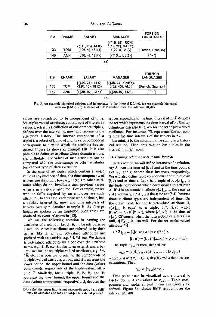
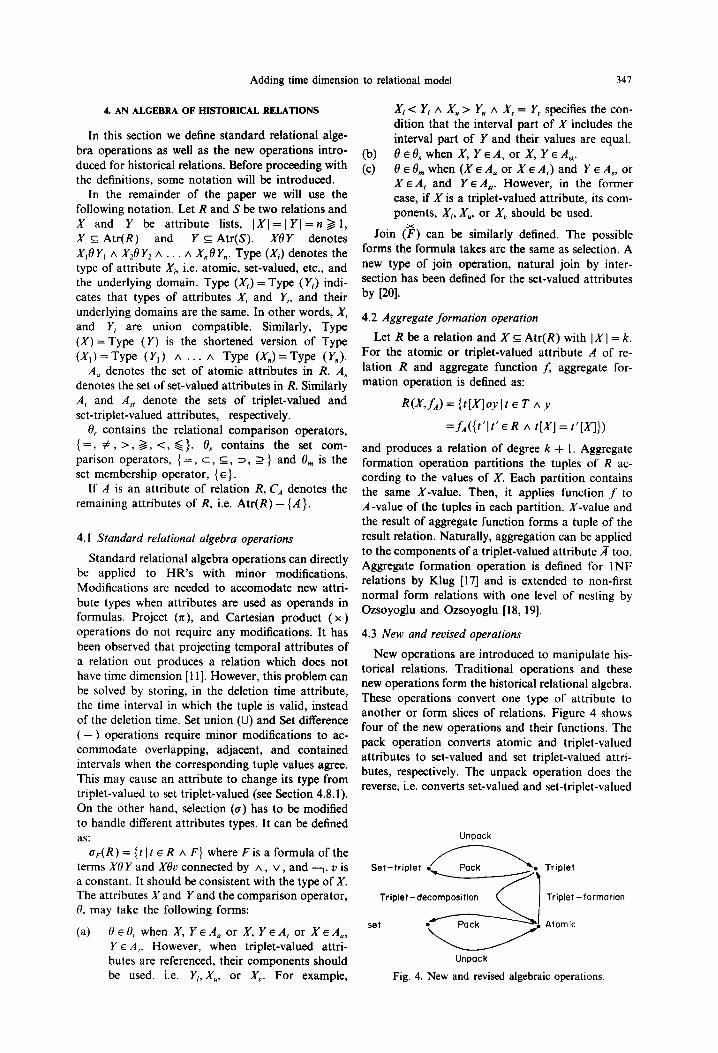
New operations are introduced to manipulate historical relations. Traditional operations and these new operations form the historical relational algebra. These operations convert one type of attribute to another or form slices of relations. Figure 4 shows four of the new operations and their functions. The pack operation converts atomic and triplet-valued attributes to set-valued and set triplet-valued attributes, respectively. The unpack operation does the reverse, i.e. converts set-valued and set-triplet-valued

Unpack

Pack . Triplet

~Lze:e5& Triplet -formation

Pack . Atomic

Unpack

Fig. 4. New and revised algebraic operations.

348 Aanm.t+a~ Uz TANSEL

attributes to atomic and triplet-valued attributes. Triplet-decomposition operation breaks a triplet- valued attribute into its components, lower bound of interval, upper bound of interval, and the value. Triplet-formation operation converts three attributes, corresponding to lower and upper bounds of an interval, and a value, into a triplet-valued attribute. The slice operation restricts the time of an attribute according to the time of another attribute. The drop-time operation discards the time component of triplet-valued and set-triplet-valued attributes.

4.4 Pack operation (P)

The pack operation, when applied to attribute A of the relation R, collects the values in attribute A into a single tuple component for tuples whose remaining attributes agree f 18,191. Let R be a relation of degree n and A be one of its att~butes. For each (n - 1) tuple in x,-, (R), an n-tuple I%‘, is defined as follows:

W&“l =g

WJAI =

{@IIt ER A t[C,l=g) if A is an atomic or triplet-valued attribute

Ix It3 t) (t E R ‘-x WA] =g AXE~[A])~

if A is a set-valued or a set-triplet-valued attribute

P,(R) = {ulglg ER[CAI>

Note that the pack operation takes the union of the tuple components for the set-valued or set-triplet- valued attributes, instead of creating another level of nesting.

4.5. Unpack operation (U)

The unpack operation, creates a family of tuples for each tuple of the relation .R when it is applied on one of R’s set-valued attributes [18-201. One tuple is created for each element of the set in the attribute value. It is the inverse of the pack operation. Let t be a tuple of R.

:

(t) if A is an atomic or a triplet-valued attribute

UJI) = ft’l t’[A] E z[A] A t’[C,J = t[C,]) if A is a set-valued or a set-triplet-valued attribute.

Then:

U,(R)= u U.&f) 1sR

trample 2. Applying the unpack operation on the SALARY attribute of EMP, of Example 1 produces the original relation EMP,:

lJ .~xKw(EMPJ

Successive application of the unpack operation to the attributes in Atr(R) of the relation R converts R into first normal form. The order of operations is not significant.

Unpacking a tuple according to the attribute *A, produces a family of tuples which differ only in their A-values. The rest of the resulting tuples are the same. A-value of each tuple is a triplet whereas the other set-triplet-valued attributes still contain the entire history of the original unpacked tuple. Thus, redundant data is created. Successive application of the unpack operation on different set-triplet-valued attributes increases this redundancy. Considering the large size of the historical relations, successive application of the unpack operation may create pro-

--

Ex~p~e 1. Consider the following relation, EMP,.

EMP, : ENAME SALARY *MANAGER

{<[15.19), RON), ([lg. 22), GARY),

TOM <[15,25), 14 K) (122. nl,AL)}

{<[I 5,19), ROW ([19,22), GARY),

TOM <[25,n], 18 K) (122. hl, AL>}

ANN <[IO, nl, 12 K> {<lo, nl, LIZ)}

G4LARY (EMP,) produces the result relation EMP,:

EMP,: ENAME ‘SALARY ‘MANAGER

{<[15,19). RON). {<[15,25),14K), ([lg. 22). GARY).

TOM <[25, n], 18 K)} (E22, nl. AL>)

ANN f<[lO,nl, 12 K>j {<[IO, nl, LIZ)]


hibitively large relations. The other attributes may be sliced according to the time of unpacked attribute to avoid this data redundancy. For this purpose, the slice operation (defined later) can be used.

It is shown in [20] that applying the pack operation, followed by the unpack operation on the same attribute produces the original relation. That is, U,(P,(R) = R provided that A is simple or triplet- valued. However, the reverse, that is, PA [U,(R)] 7 R holds only if A is a set or set triplet-valued attribute and R includes a key attribute in addition to A.

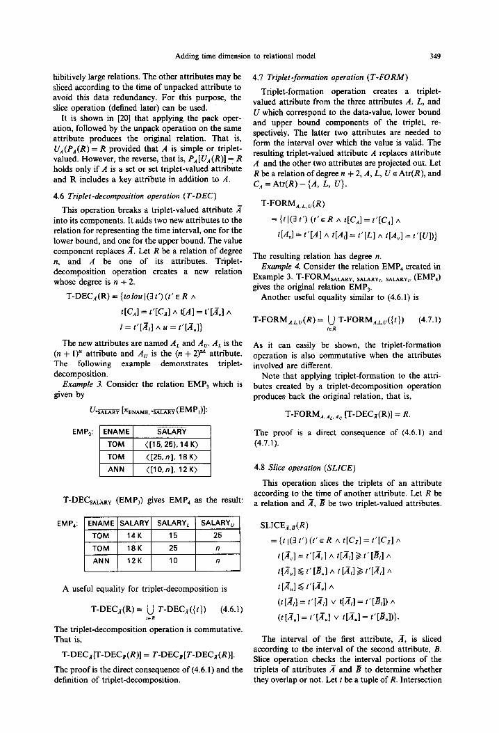
4.6 Triplet-decomposition operation (T-DEC)

This operation breaks a triplet-valued attribute ,? into its components. It adds two new attributes to the relation for representing the time interval, one for the lower bound, and one for the upper bound. The value component replaces A. Let R be a relation of degree n, and A be one of its attributes. Triplet- decomposition operation creates a new relation whose degree is n + 2.

T-DEC,(R)={to[ou((3t’)(t’oR A

t[CJ = t’[Cz] A t[A] = t’[A,] A

I= t’[A,] A 24 = t’[A,]}

The new attributes are named A, and A,. AL is the (n + l),, attribute and A, is the (n + 2)nd attribute. The following example demonstrates triplet- decomposition.

Example 3. Consider the relation EMP, which is given by

u-- *SALARY bENAME, l xicdEMP~)I:

EMP,: ENAME SALARY

TOM ([IS, 25). 14 K)

TOM ([25.n]. 18K)

ANN ([fO.nl. 12 K)

T-DWmiw (EMP,) gives EMP, as the result:

gMP,: 61

A useful equality for triplet-decomposition is

T-DECr(R) = u T-DECr({t}) (4.6.1) IER

The triplet-decomposition operation is commutative. That is,

T-DECnp-DE&(R)] = T-DECx[T-DECn(R)].

The proof is the direct consequence of (4.6.1) and the definition of triplet-decomposition.

4.1 Triplet-formation operation (T-FORM)

Triplet-formation operation creates a triplet- valued attribute from the three attributes A, L, and U which correspond to the data-value, lower bound and upper bound components of the triplet, respectively. The latter two attributes are needed to form the interval over which the value is valid. The resulting triplet-valued attribute A replaces attribute A and the other two attributes are projected out. Let R be a relation of degree n + 2, A, L, U E Atr(R), and C, = Atr(R) - {A, L, U}.

T-FORM,,,, u(R)

= {t1(3 t’) (t’E R A t[CA] = t’[c,] A

tM,l= t’[Al A +I,] = t’[L] A t[A,] = t’[U])}

The resulting relation has degree n. Example 4. Consider the relation EMP, created in

Example 3. T-FORM SALARY, SALARY‘, SALARY” (EMP,)

gives the original relation EMP,. Another useful equality similar to (4.6.1) is

T-FORM A.&Q = u T-FORM,,,,,({t)) (4.7.1) &R

As it can easily be shown, the triplet-formation operation is also commutative when the attributes involved are different.

Note that applying triplet-formation to the attributes created by a triplet-decomposition operation produces back the original relation, that is,

T-FORM,, AL. Ag [T-DECr(R)] = R.

The proof is a direct consequence of (4.6.1) and (4.7.1).

4.8 Slice operation (SLICE)

This operation slices the triplets of an attribute according to the time of another attribute. Let R be a relation and 3, B be two triplet-valued attributes.

= {t1(3 t’)(t’E R A t[Cn] = t’[c,] A

t [iT,] = t’[&.] A t[A,] 3 t’ [B,] A

t[/T,] 6 t’ [B,] A t [A,] 2 t’[& A

t[&] g t’[&] A

(t[&] = t’[&] V t[&] = t’[&]) A

(t [A,] = t’[ii.] v t[A.] = t’[B.l)}.

The interval of the first attribute, A, is sliced according to the interval of the second attribute, B. Slice operation checks the interval portions of the triplets of attributes 2 and B to determine whether they overlap or not. Let t be a tuple of R. Intersection


of the time intervals of t[A] and r[g] is assigned to the interval component of the new triplet for 2. The new triplet receives its data-value from attribute A. If the two intervals do not overlap, the tuple is not considered. The slice operation can be extended for any combination of triplet-valued and set-triplet- valued attributes, e.g. SLICEn, *s(R), SLICE.;(, s(R), or SLICE,,-..s(R). These versions can be defined analogously. The last three versions of the slice operation can also be done by first unpacking the set-triplet-valued attributes and then applying its first version. However, among these, only SLICE.&R) has the following property.

SLICE.,&R) = P,[SLICEn,s[U.;I(R)]].

Applying the slice operation on a relation R can also be expressed as:

SLICEn, s(R) = u SLICEJ, ,({ t }). 1ER

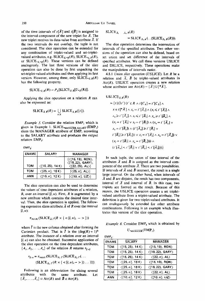
Example 5. Consider the relation EMP, which is given in Example 1. SLICE.m,m (EMP,) slices the MANAGER attribute of EMP, according to the SALARY attribute and produces the output relation EMP,:

EMP,:

ENAME SALARY MANAGER

1 {<[15.19). RON). I .-

([19,22); GARY). TOM ([15,25), 14K) (122,251, AL)}

TOM (125,nl. 18K) {(25,nl. AL)} I ANN 1 (IlO.nl.12K) 1 {([lO,n], LIZ)} 1

The slice operation can also be used to determine the values of time dependent attributes of a relation, R, over an interval [I, a). First, R is augmented by a new attribute which contains the desired time interval. Then, the slice operation is applied. The following expression slices attribute A of R over the interval

V, a):

71Atr(R) WI’=Z,I (R X { < [h u)v - ’ },,

where 7 is the new column obtained after forming the Cartesian product. That is f is the (deg(R) + l)th attribute. The instance of a relation over an interval [I, u) can also be obtained. Successive application of the slice operation on the time dependent attributes, {A,, A,, . . . , A,} of the relation R returns rt,,+

q/, u) = 71Alr(R) (SLICE,,,r (SLICE,,, (. . .

W1CEnn.r (R x { < 14 u),- > 1) . . NN.

Following is an abbreviation for slicing several attributes with the same attribute. Let {A,, . . ,A,} c Atr(R) and B E Atr(R).

SL1CE.q.. ..n,.dR)

= SLICEz,, B (. . (SLICE,, B(R))).

The slice operation determines the intersection of intervals of the specified attributes. Two other versions of the operation can also be defined, based on set union and set difference of the intervals of specified attributes. We call these versions USLICE and DSLICE, respectively. These operations make the manipulation of intervals easier.

4.8. I Union slice operation (USLZCE). Let R be a relation and A, fi be triplet-valued attributes in Atr(R). USLICE operation creates a new relation whose attributes are Atr(R) - {A } U {*d }.

={tl@t’)(t’~R ~t[C~]=t’[C~]r\

x E t [*A I A X” = t’[PQ,] A (x, < t’ [I,] A

x,2t’[K,]Ax,<t’[B,]Ax,>t’[B”]A

(x, = t’ [K,] v x,= t’ [I?,]) A (x, = t’ [A”] v

X” = t’[B,]) A (t’[A,] 2 t’[B,] v

t’[B,] 2 t’[x,])) v x,= t’[‘T,] A X” = t’[&]) v

(x, = t’[B,] A x, = t’[B,]))) A

(W”l < tV,l v t’[Rl < t’mN)

In each tuple, the union of time interval of the attributes K and B is assigned as the interval component of the attribute K. There are two possibilities. If intervals of A and R intersect, the result is a single large interval. On the other hand, when intervals of d and R are disjoint, the result has two components, interval of K and interval of B. In this case, two triplets are formed as the result. Because of this reason, the USLICE operation creates a set triplet- valued attribute from a triplet-valued attribute. The definition is given for two triplet-valued attributes. It can analoguously be extended for other attribute combinations. Following is an example which illustrates this version of the slice operation.

Example 6. Consider EMP, which is obtained by

u*nAm (EMPi ).

EMP,:

1 ENAME 1 SALARY MANAGER I

TOM ([25,nl. 18 K) ([22. nl. AL>

ANN <[lO.n], 12K) <[lo. nl, LIZ)


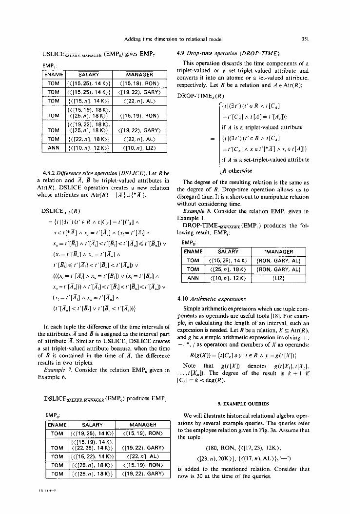
USLICEsALARY,MAN~~~~ (EMP,) gives EMP,

EMP,:

4.8.2 Difference slice operation (DSLICE). Let R be a relation and 2, B be triplet-valued attributes in Atr(R). DSLICE operation creates a new relation whose attributes are Atr(R) - {A} U {*x}.

DSLICE,,,(R)

={t1(3t’)(r’~R A~[C,]=~‘[C,]A

xEt[*K]Ax,.=t’[A,]A(X,=t’[A,]A

X, = t’[&] A t’[&]<t’[&]<t’[&] < t’[&]) V

(x, = r’[B,] A x, = t’[K,] A

t’[B,] < r’[A,] < t’[B,] < t’[K,]) v

(((X, = ?‘[.&I A X, = t’[&]) V (X, = t’[i?,] A

X,=t’[&]))A t’[&]<t’[&]<t’[&]<t’[J,])V

(X, = t’[A,] A X, = t’[z,] A

(t’[K,] < t’[B,] v t’[B, < t’[K,))}

In each tuple the difference of the time intervals of the attributes 2 and B is assigned as the interval part of attribute 2. Similar to USLICE, DSLICE creates a set triplet-valued attribute because, when the time of B is contained in the time of A, the difference results in two triplets.

Example 7. Consider the relation EMP, given in Example 6.

DSLICE,,,,, makes (EMP,) produces EMP,.

EMP,:

ENAME SALARY MANAGER

TOM {([19.25). 14K)} ([I 5,191, RON)

TOM {([15.19), 14 K). ([22,25), 14 K)} ([19,22), GARY)

TOM {([15,22), 14K)) <[22, nl, AL)

TOM {([25.n]. 18 K)} ([15.19). RON)

TOM {([25.n]. 18K)J <[19,22). GARY)

4.9 Drop-time operation (DROP-TIME)

This operation discards the time components of a triplet-valued or a set-triplet-valued attribute and converts it into an atomic or a set-valued attribute, respectively. Let R be a relation and A E Atr(R):

DROP-TIME,(R)

=

{tl@t’)(t’ER A t[Cz]

=t’[C,] A t [A] = t’[&]))

if A is a triplet-valued attribute

(tl(lt’)(t’ER A t[C,]

=t’[C,]AXEt’[*A]AX,Et[A])}

if A is a set-triplet-valued attribute

R otherwise

The degree of the resulting relation is the same as the degree of R. Drop-time operation allows us to disregard time. It is a short-cut to manipulate relation without considering time.

Example 8. Consider the relation EMP, given in Example 1.

DROP-TIME .m(EMPI) produces the following result, EMP,:

EMP,:

1 ENAME 1 SALARY *MANAGER

4.10 Arithmetic expressions

Simple arithmetic expressions which use tuple components as operands are useful tools [18]. For example, in calculating the length of an interval, such an expression is needed. Let R be a relation, X c Atr(R), and g be a simple arithmetic expression involving + , -9 *, / as operators and members of X as operands:

NgO’N = {t[Cxlo~ It 6 R A Y = g(t P’l);~ Note that g(t [Xl) denotes g(t[X,], t[XJ, . , t [X,,,]). The degree of the result is k + 1 if

/i”l = k < deg(R).

5. EXAMPLE QUERIES

We will illustrate historical relational algebra operations by several example queries. The queries refer to the employee relation given in Fig. 3a. Assume that the tuple

(180, RON, {([17,23), 12K),

([23, n), 20K)}, {<[17, n), AL)}, ‘--‘)

is added to the mentioned relation. Consider that now is 30 at the time of the queries.


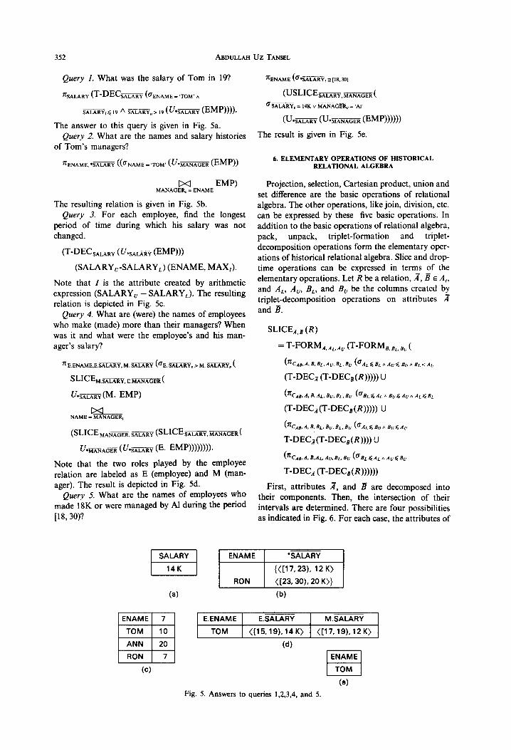
Query 1. What was the salary of Tom in 19?

FSALARY (T-DECSALARY (QENAME = ‘TOM’ n

SALARY,& 19 * mAmu > 19 (hxiniv WfP)))).

The answer to this query is given in Fig. Sa. Query 2. What are the names and salary histories

of Tom’s managers?

KENAME. l sLm ((ONAME -‘TOM’ c”*m (EMP))

Da EMP) MANAGER, = ENAME

The resulting relation is given in Fig. 5b. Query 3. For each employee, find the longest

period of time during which his salary was not changed.

(T-DEC,,, (u.m (EMP)))

(SALARY,-SALARY,) (ENAME, MAX,).

Note that I is the attribute created by arithmetic expression (SALARY, - SALARY,). The resulting relation is depicted in Fig. 5c.

Query 4. What are (were) the names of employees who make (made) more than their managers? When was it and what were the employee’s and his manager’s salary?

=E.ENAME,E.~,M.~(bE,~,>M.~.(

SLICE __ -_( M.SALARY, EMANAGER

u l sxixicv@f. EW

Da NAME = MANAGER,

(SLICE ~,~(SLICE~.~(

u SMANACER (U.m (E. EMP)))))))).

Note that the two roles played by the employee relation are labeled as E (employee) and M (manager). The result is depicted in Fig. Sd.

Query 5. What are the names of employees who made 18K or were managed by Al during the period [18,30)?

nENAME (Q~ALARY, 2 [IS. 30)

B-, = 14K v MANAGER, = ‘Al

&hxin (“*&fiii 0-W)))))

The result is given in Fig. 5e.

6. ELEMENTARY OPERATIONS OF HISTORICAL RELATIONAL ALGEBRA

Projection, selection, Cartesian product, union and set difference are the basic operations of relational algebra. The other operations, like join, division, etc. can be expressed by these five basic operations. In addition to the basic operations of relational algebra,

pack, unpack, triplet-formation and triplet- decomposition operations form the elementary operations of historical relational algebra. Slice and drop- time operations can be expressed in terms of the elementary operations. Let R be a relation, A, B E A,, and A,, A,, BL, and B, be the columns created by triplet-decomposition operations on attributes 2 and B.

SLICEA, B (R )

= T-FORM,,,,,, (T-FORMa Br. BU (

(n: CAB.A,B,BL.AU,BL,BU @AL~B~AA~QE~~B~<A~

(T-DECn (T-DECs(R))))) U

(%AB. A, 8. AL 80 81. Bu @B, Q AL n B” S A” A AL 4 BL . . .

(T-DECz(T-DECs(R))))) U

SCAB, A, B, BL, Bo, Br, B” @AL 6 Bu A B. 6 AU

T-DECz(T-DEC,(R)))) U

(‘CA+, &AL, Au, BL. Br, @BL 4 AL . A”6 8”

T-D& V-DEWRNNN

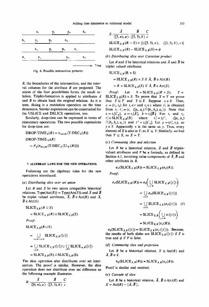
First, attributes 2, and B are decomposed into their components. Then, the intersection of their intervals are determined. There are four possibilities as indicated in Fig. 6. For each case, the attributes of

(4 (b)

E.ENAME ESALARY M.SALARY

TOM ([15,19),14K) ([17,19),12K)

(d)

Fig. 5. Answers to queries 1,2,3,4, and 5.


AL BL AU BU

AL BU Au

AL BL 4J AU

AL AU BU

- Time

Fig. 6. Possible intersection patterns.

R, the boundaries of the interesection, and the interval columns for the attribute R are projected. The union of the four possibilities forms the result relation. Triplet-formation is applied to attributes A and 3 to obtain back the original relation. As it is seen, slicing is a restriction operation on the time dimension. Similar expressions can be constructed for the USLICE and DSLICE operations, too.

Similarly, drop-time can be expressed in terms of elementary operations. The two possible expressions for drop-time are:

DROP-TIMEz(R) = xAlrcR) (T-DECn(R))

DROP-TIME.z(R)

= P.4 (%U(Rf (T-DECz (U., (R))))

7. ALGEBRAIC LAWS FOR THE NEW OPERATIONS

Following are the algebraic rules for the new operations introduced.

(a) Distributing slice over set union

Let R and S be two union compatible historical relations, Ty~(Atr(R)) = Ty~(Atr(~)) and 2 and B be triplet valued attributes, 2, B E Atr(R~ and 2, B E Atr(S).

SLICEz,s (R U S)

= SLICE,rs(R) U SLICE;IqB(S)

Proof

SLICEJ.s(R US)

= U SLICEa,B(It3> fCR”fES

= U SLICEZ,B (ftf, U ,~SSLICE~,~(~f~) IER

= SLICEz. s(R) U SLICEz, B (S).

The slice operation also distributes over set intersection. The proof is similar. However, the slice operation does not distribute over set difference as the following example illustrates.

2 B c

R: GO, n), a> <P, 5), b) c

A B c ” W, n), a> ([3,5), b) c

SLICEx, B (R - 9 = {(([3,5), a >, ([3,5), b >, c)}

SLICEK,B (R) - SLICE;I,B(S) = 4

(b) Distributing slice over Cartesian product

Let R and S be historical relations and 2 and B be triplet valued attributes.

SLICEI,a (R x S)

= SLICEz,s(R) x S if A, B E Atr(R)

= R x SLICEns(S) if A, R E Atr(S).

Proof: Let X = SLICEn,B (R x S), Y= SLICE,rs(R) x S. To prove that X = Y we prove that X c Y and YE X. Suppose x E X. Then, x = (t;, tz) for t, E r and tz ES where t; is obtained from t, ‘ t; = (z, ([a,, a,) fl [b,, b,), a,)). Note that z = r,[C”], a = t, [A], b = t,[BB]. For t, and t,, t; E SLICEn,s(R) where t; = (z”, ([% a,) II [b,, b,), a,)) and z” = t,[CAJ. Let y = (t;, t2), so y E Y. Apparently x is the same as y. Thus, every element of X is also in Y, so X c Y. Similarly, we find that Y E X, so X = Y.

(c) Commuting slice and selection

Let R be a historical relation, A and B triplet- valued attributes and F be a formula, as defined in -- Section 4.1, involving value components of A, I3 and other attributes in R.

o,(=ICEz B(R)) = SLICE;I,E @AR)).

Proof:

(‘F(SLICE~,B (RI) = OF (

,li, SLICE,, d(t})

>

= ,; ~FWICEX.B (If 1))

= ,; S~ICEn,s(~4tDl (1)

= SLICEn, B (oF(R)).

er(SL1CEx,~({t)) = SLIcE;~,s(cr,((tf)). Because, the results of both slides are SLICE,,B (fr)) if F is true and (p if F is false.

(d) commuting slice and projection

Let R be a historical relation, X c Atr(R) and A,BEX.

G(SLICE;I,B(R)) = SLICE,r.&,(R)).

Proof is similar and omitted.

(e) Cascade of slice

Let R be a historical relation, 2, B E Atr(R) and X = Atr(R) - (A, 3 ).


SLICE,-,B(SLICEs.n (R)

= SLICEs.,- (SLICE,,,(R)).

Proof: Let t be a tuple of R and x = t [Xl.

(i) SLICE,-s (SL1CEs.a ({t},

= SL1CEz.s (SL1CEs.a ({(x, ([U), a>,

([m, n), b )))))

= SLICE.r,s({(x, ([U), a>,

([m’, n’), b))))

where [m’, n’) = [i,j) n [m, n)

= {(x7 ([i’J’)> a>, ([m’, n’), b))}

where

[i’,j’) = [i,j) f-l [m’, n’)

= I&j) f-l Lj) f-l [m, n)

=[i,j)n[m,n)

(ii) SLICEB,,(SLICE,_rs({r}) = SLICEs,n

(SLICE;I.B(((X, U), a>, ([m, n), b))]))

= SLICEs,,- ((~7 <[i’J’), a>, (1~ n), b))))

where [i’,j’) = [i,j) fl [m, n)

= {(x, (VJ’), a>, <[m’, n’), b))}

where

[m’, n’) = [i’,j’) n p71, TI)

= [i,j) n h 4 n h 4

= [id n b, 4

The result of (i) is equal to the result of (ii). Hence,

SLICE,r,s (SLICEa,a(R))

= SLICEn, s (

u SLICEB,A({~)) IER >

= U SLICEA.B(SLICE~,A((~)))

IER

= U SLICE,,(SLICEA.B((~}))

IER

= SLICEB,n u SLICEA,s({f}) ( rcR >

= SLICEs,z (SLICE As (R)).

As is seen, slicing two attributes by each other aligns their interval components. That is, in each tuple, the two attributes have the same time value. Another useful equality is the following. Let A, B, and c E Atr(R).

SLICE,-,s(SLICE;l,c (R))

= SLICE;l,c (SLICE,,,(R)).

The proof is similar and omitted. The cumulative affect of the attributes i? and c on the attribute K can also be obtained by first slicing B by 2; and then A by B or c by B and then 2 by c. However, in this case the resulting relations are not equal even though

their K attributes are the same. This is because of the fact that the attributes B and 2; also change. That is,

SLICE,-, s (SLICE s, c (R))

# SLICE,~.~(SLICE~.B (RI)

but, Qt E R,

‘12 (SLICEA, E (=ICE~.c(ftl)))

= n;l (SL1CEa.c WC&, E (It}))).

(f) Distributing triplet-decomposition over set union

Let R and S be historical relations, Type

(Atr(R) = Type(Atr(S)) and 2 E Atr(R), Atr(S).

T-DEC,-(R U S) = T-DECn(R) U T-DECn(S).

Triplet-decomposition also distributes over set difference. The proof is omitted. We give other rules

for triplet-decomposition without proof since they are straightforward.

(g) Commuting triplet-decomposition with selection

Let R be a historical relation, 2 E Atr(R) and F be a formula involving attributes of R,

T-DECn(a,(R)) = a,(T-DECa(R))

where F’ is the same as F except references to A in F is changed to A,, 6,, and 2, in F’.

(h) Commuting triplet-decomposition with projection

Let R be a historical relation, X E Atr(R), and A E X. X’ is X - {A} U {AL, A,, A,,}.

T-DECJ(rr,(R)) = z&T-DECA(R)).

(i) Distributing triplet-decomposition with Cartesian

product

Let R and S be historical relations and 2 be a

triplet-valued attribute.

T-DECJ (R x S) = T-DECz(R) x S

if 1 E Atr(R)

= R x T-DEC, (S) if 2 E Atr(S).

The rules for triplet-formation are similar to the rules for triplet-decomposition and they are not included here.

8. CONCLUSION

In this paper, we introduced a methodology for incorporating time dimension into the relational model. We believe that our approach has the desired properties of historical relational databases proposed by Clifford [ll]. It is a natural extension of the

Adding time dimension to relational model 35.5

classical relational model and relational algebra. It maintains the three-dimensional relations view at the external user level.

The proposed approach has several advantages. First, it is a closer abstraction of the real world. Second, it eliminates data redundancy resulting from duplication of unchanged attributes which is inherent in the case of tuple time-stamping. Third, it is possible to obtain past relation instances which allow a user to extract information for any time point or time interval since the beginning of the database. Further- more, the proposed methodology is flexible and provides convenience to the user since it allows different types of attributes to coexist in the same relation.

Further research is needed in several directions. Currently, we are working on proving that the extended relational algebra has the same expressive power as the relational calculus for the historical relations and designing a graphical query language for HRDB’s. We are also planning to explore the strategies for a prototype implementation of the proposed model and language.

Acknowledgements-The author would like to express his gratitude to Dr E. Arkun of Baruch College, and Dr G. &soyogh~ and Dr M. Z. &soyoglu of Case Western Reserve University for their valuable contributions.

REFERENCES

[l] E. F. Codd. A relational model of data for large shared data banks. Commun. ACM 13 (6) 377-387 (1970).

[2] A. U. Tansel and J Clifford. On an algebra for historical relational databases: Two views. Proc. ACM SZG- MOD Inter~at~onffl Conference on M~agement of Data, pp. 247265 (1985).

[3] A. Bolour, T. L. Anderson, L. J. Deketser and H. K. T. Worm. The role of time in information nrocessina: A survey. ACM SZGMOD Record 12 (3), 2838 (1982T.

[4] R. Snodgrass. A temporal query language. To appear in TODS.

[5] T. L. Anderson. Database semantics of time. Ph.D. Dissertation, Computer Science Department, Univer- sity of Washington (1981).

[6] S. Ginsberg and K. Tanaka. Interval queries on object histories. Proc. 10th International Conference on Very Large Dafu Bases, pp. 208217 (1984).

[7] M. R. Klopproge and P. C. Lockemann. Modelling information preserving databases: Consequences of the concept of time. Proc. 9th International Conference on Very Large Databases, pp. 399-416 (1983).

[8] G. Ariav. Preserving the time dimension in information systems. Ph.D. Dissertation, Decision Sciences Department, University of Pennsylvania (1983).

[9] J. Ben-Zvi. The time relational model. Ph.D. Dis- sertation, Computer Science Department, University of California. Los Aneeles (1982).

[lOI

WI

1131

t141

USI

1161

1171

WI

[I91

PO1

I211

J. Clifford and D.-S. Warren. Formal semantics for time in databases. ACM Trans. Database Systems 6 (2), 214-264 (1983). J. Clifford and A. U. Tansel. On an algebra for historical relational databases: Two views. Proc. ACM SZG~OD Znternat~onal Conference on ~anagemeni of Data pp. 247-265 (May 1985). S. K. Gadia. A homogeneous relational model and query languages for temporal databases. Submitted for publication. R. Snodgrass. The temporal query language TQuel. Proc. 3rd ACM SIGACT-SZGMOD Symposium on PrincipZes of Database Systems, pp. 204-213 (April 1984). V. Lum et al. Designing DBMS support for the temporal dimension. Proc. ACM SZGMOD International Conference on Management of Data, pp. 115-l 26 (June 1984). P. Dadan, V. Lum and H. D. Werner. Integration of time versions in relational database systems. Proc. 10th Znternafional Conference on Very Large Databases, pp. 5099521 (1984). S. K. Gadia and J. H. Vaishnav. A query language for a homogeneous temporal database. Proc. 4th ACM SZGACT-SIGMOD Symposium on Principles of Data- base Systems, pp. 51-56 (April 1985). A. Klug. Equivalence of relational algebra and relational calculus languages having aggregate functions. J. ACM 29 (3), 699-717 (1982). G. &soyo~lu, M. Z. &soyoglu and V. Matos. Extend- ing relational algebra and relational calculus with set-valued attributes and aggregate functions. Submit- ted for

8 ublication.

M. Z. noyoglu and G. ~zsoyoglu. An extension of relational algebra for summary tables. Proc. 2nd Znter- national Workshop on SDB Management (1983). G. Jaeschke and H. J. Schek. Remarks on the algebra of non-first-normal form relations. Proc. 1st ACM SZGMOD Symposjum on Frinriples of Database Sys- tems, pp. 124-138 (1982). R. Snodgrass and I. Ahn. A taxonomy of time in databases. Proc. ACM SZGMOD International Confer- ence on Management of Data, pp. 236-246 (May 1985).

adding time dimension to relational model and extending relational algebra

Documents