arX

iv:0

806.

2274

v2 [

cs.D

M]

9 D

ec 2

009

Exposing Multi-Relational Networks to

Single-Relational Network Analysis Algorithms1

Marko A. Rodrigueza, Joshua Shinavierb

aT-5 Center for Nonlinear Studies, Los Alamos National Laboratory, Los Alamos, New

Mexico 87545bTetherless World Constellation, Rensselaer Polytechnic Institute, Troy, New York,

12180

Abstract

Many, if not most network analysis algorithms have been designed specifi-cally for single-relational networks; that is, networks in which all edges areof the same type. For example, edges may either represent “friendship,”“kinship,” or “collaboration,” but not all of them together. In contrast, amulti-relational network is a network with a heterogeneous set of edge labelswhich can represent relationships of various types in a single data structure.While multi-relational networks are more expressive in terms of the varietyof relationships they can capture, there is a need for a general framework fortransferring the many single-relational network analysis algorithms to themulti-relational domain. It is not sufficient to execute a single-relational net-work analysis algorithm on a multi-relational network by simply ignoring edgelabels. This article presents an algebra for mapping multi-relational networksto single-relational networks, thereby exposing them to single-relational net-work analysis algorithms.

Key words: multi-relational networks, path algebra, network analysis

1Rodriguez M.A., Shinavier, J., Exposing Multi-Relational Networks to Single-Relational Network Analysis Algorithms, Journal of Informetrics, volume 4, number 1,pages 29-41, ISSN:1751-1577, Elsevier, doi:10.1016/j.joi.2009.06.004, LA-UR-08-03931,December 2009.

Preprint submitted to Journal of Informetrics and published December 9, 2009

1. Introduction

Much of graph and network theory is devoted to understanding and an-alyzing single-relational networks (also known as directed or undirected un-labeled graphs). A single-relational network is composed of a set of vertices(i.e. nodes) connected by a set of edges (i.e. links) which represent relation-ships of a single type. Such networks are generally defined as G = (V, E),where V is the set of vertices in the network, E is the set of edges in the net-work, and E ⊆ (V × V ). For example, if i ∈ V and j ∈ V , then the orderedpair (i, j) ∈ E represents an edge from vertex i to vertex j.2 Ignoring thedifferences in the vertices that edges connect, all edges in E share a singlenominal, or categorical, meaning. For example, the meaning of the edges ina single-relational social network may be kinship, friendship, or collabora-tion, but not all of them together in the same representation as there is noway distinguish what the edges denote. Moreover, single-relational networksmay be weighted, where w : E → R is a function that maps each edge inE to a real value. Weighted forms are still considered single-relational as allthe edges in E have the same meaning; the only difference is the “degree ofmeaning” defined by w.

The network, as a data structure, can be used to model many real andartificial systems. However, because a network representation of a systemcan be too complicated to understand directly, many algorithms have beendeveloped to map the network to a lower dimensional space. For a fine reviewof the many popular network analysis algorithms in use today, refer to [1, 2].Examples of such algorithms, to name a few of the more popularly usedalgorithms, include the the family of geodesic [3, 4, 5, 6], spectral [7, 8, 9],and community detection algorithms [10, 11, 12].

Most network analysis algorithms have been developed for single-relationalnetworks as opposed to multi-relational networks. A multi-relational networkis composed of two or more sets of edges between a set of vertices. A multi-relational network can be defined as M = (V, E), where V is the set of verticesin the network, E = E1, E2, . . . , Em is a family of edge sets in the network,and any Ek ⊆ (V ×V ) : 1 ≤ k ≤ m. Each edge set in E has a particular nom-inal, or categorical, interpretation. For example, within the same network

2This article is primarily concerned with directed networks, as opposed to undirectednetworks, in which an edge is an unordered set of two vertices (e.g. i,j). However, theformalisms presented work with undirected networks.

2

M , E1, E2 ∈ E may denote “kinship” and “coauthorship,” respectively.The multi-relational network is not new. These structures have been used

in various disciplines ranging from cognitive science and artificial intelligence[13] (e.g. semantic networks for knowledge representation and reasoning) tosocial [1] and scholarly [14, 15] modeling. Furthermore, the multi-relationalnetwork is the foundational data structure of the emerging Web of Data[16, 17]. While a multi-relational network can be used to represent morecomplicated systems than a single-relational network, unfortunately, thereare many fewer multi-relational algorithms than single-relational algorithms.Moreover, there are many more software packages and toolkits to analyzesingle-relational networks. Multi-relational network analysis algorithms thatdo exist include random walk [18], unique path discovery [19], communityidentification [20], vertex ranking [21], and path ranking algorithms [22].

The inclusion of multiple relationship types between vertices complicatesthe design of network algorithms. In the single-relational world, with alledges being “equal,” the executing algorithm need not be concerned withthe meaning of the edge, but only with the existence of an edge. Multi-relational network algorithms, on the other hand, must take this informationinto account in order to obtain meaningful results. For example, if a multi-relational network contains two edge sets, one denoting kinship (E1 ∈ E)and the other denoting coauthorship (E2 ∈ E), then for the purposes of ascholarly centrality algorithm, kinship edges should be ignored. In this sim-ple case, the centrality algorithm can be executed on the single-relationalnetwork defined by G = (V, E2). However, there may exist more complicatedsemantics that can only be expressed through path combinations and otheroperations. Thus, isolating single-relational network components of M is notsufficient. As a remedy to this situation, this article presents an algebra fordefining abstract paths through a multi-relational network in order to de-rive a single-relational network representing vertex connectivity according tosuch path descriptions. From this single-relational representation, all of theknown single-relational network algorithms can be applied to yield mean-ingful results. Thus, the presented algebra provides a means of exposingmulti-relational networks to single-relational network analysis algorithms.

2. Path Algebra Overview

This section provides and overview of the various constructs of the pathalgebra and primarily serves as a consolidated reference. The following sec-

3

tions articulate the use of the constructs summarized here.The purpose of the presented algebra is to transform a multi-relational

network into a “semantically-rich” single-relational network. This is ac-complished by manipulating a three-way tensor representation of a multi-relational network. The result of the three-way tensor manipulation yieldsan adjacency matrix (i.e. a two-way tensor).3 The resultant adjacency matrixrepresents a “semantically-rich” single-relational network. The “semantically-rich” aspect of the resultant adjacency matrix (i.e. the single-relational net-work) is determined by the algebraic path description used to manipulate theoriginal three-way tensor (i.e. the multi-relational network). More formally,the multi-relational path algebra is an algebraic structure that operates onn×n adjacency matrix “slices” of a n×n×m three-way tensor representationof a multi-relational network in order to generate a n × n path matrix. Thegenerated n×n path matrix represents a “semantically-rich” single-relationalnetwork that can be subjected to any of the known single-relational net-work analysis algorithms. The path algebra is a matrix formulation of thegrammar-based random walker framework originally presented in [18]. How-ever, the algebra generates “semantically-rich” single-relational networks, asopposed to only executing random walk algorithms in a “semantically-rich”manner. In other words, the algebra is cleanly separated from the analysisalgorithms that are ultimately applied to it. This aspect of the algebra makesit generally useful in many network analysis situations.

The following list itemizes the various elements of the algebra to be dis-cussed in §3.

• A ∈ 0, 1n×n×m: a three-way tensor representation of a multi-relationalnetwork.4

• Z ∈ Rn×n+ : a path matrix derived by means of operations applied to A.

• Ri ∈ 0, 1n×n: a row “from” path filter.

• Ci ∈ 0, 1n×n: a column “to” path filter.

3The term tensor has various meanings in mathematics, physics, and computer science.In general, a tensor is a structure which includes and extends the notion of scalar, vector,and matrix. A zero-way tensor is a scalar, a one-way tensor is a vector, a two-way tensoris a matrix, and a three-way tensor is considered a “cube” of scalars. For a three-waytensor, there are three indices used to denote a particular scalar value in the tensor.

4This article is primarily concerned with boolean tensors. However, note that thepresented algebra works with tensors in R

n×n×m

+ .

4

• Ei,j ∈ 0, 1n×n: an entry path filter.

• I ∈ 0, 1n×n: the identity matrix as a self-loop filter.

• 1 ∈ 1n×n: a matrix in which all entries are 1.

• 0 ∈ 0n×n: a matrix in which all entries are 0.

The following list itemizes the various operations of the algebra to be dis-cussed in §4.

• A·B: ordinary matrix multiplication determines the number of (A,B)-paths between vertices.

• A⊤: matrix transpose inverts path directionality.

• A B: Hadamard, entry-wise multiplication applies a filter to selec-tively exclude paths.

• n(A): not generates the complement of a 0, 1n×n matrix.

• c(A): clip generates a 0, 1n×n matrix from a Rn×n+ matrix.

• v±(A): vertex generates a 0, 1n×n matrix from a Rn×n+ matrix, where

only certain rows or columns contain non-zero values.

• λA: scalar multiplication weights the entries of a matrix.

• A + B: matrix addition merges paths.

In short, any abstract path σ is a series of operations on A that can begenerally defined as

σ : 0, 1n×n×m → Rn×n+ .

The resultant Rn×n+ matrix is an adjacency matrix. Thus, the resultant ma-

trix is a single-relational network. This resultant single-relational networkcan be subjected to single-relational network analysis algorithms while stillpreserving the semantics of the original multi-relational network.

Throughout the remainder of this article, scholarly examples are providedin order to illustrate the application of the various elements and operationsof the path algebra. All of the examples refer to a single scholarly tensordenoted A. The following list itemizes the tensor “slices” and their domainsand ranges, where H ⊂ V is the set of all humans, A ⊂ V is the set of allarticles, J ⊂ V is the set of all journals, S ⊂ V is the set of all subjectcategories, and P ⊂ V is the set of all software programs:

• A1: authored : H → A

5

• A2: authoredBy : A → H

• A3: cites : A → A

• A4: contains : J → A

• A5: category : J → S

• A6: developed : H → P .

3. Path Algebra Elements

This section introduces the elements of the algebra and the next sectionarticulates their use in the various operations of the algebra. The elementsof the path algebra are structures that are repeatedly used when mapping amulti-relational tensor to a single-relational path matrix.

3.1. Three-way Tensor Representation of a Multi-Relational Network

A single-relational network defined as

G = (V, E ⊆ (V × V ))

can be represented as the adjacency matrix A, where

Ai,j =

1 if (i, j) ∈ E

0 otherwise

without loss of information. This adjacency matrix is also known as a two-way tensor because it has two dimensions, each with an order of n, wheren = |V |. Stated another way, A ∈ 0, 1n×n.

A three-way tensor can be used to represent a multi-relational network[23]. If

M = (V, E = E1, E2, . . . , Em ⊆ (V × V ))is a multi-relational network, then

Aki,j =

1 if (i, j) ∈ Ek : 1 ≤ k ≤ m

0 otherwise.

In this formulation, two dimensions have an order of n while the third hasan order of m, where m = |E|. Thus, A ∈ 0, 1n×n×m and any adjacencymatrix “slice” Ak ∈ 0, 1n×n : 1 ≤ k ≤ m. A represents the primarystructure by which individual adjacency matrices are indexed and composedin order to derive a resultant single-relational path matrix.

6

3.2. Path Matrices

The path algebra operates on n × n adjacency matrix elements of A toconstruct a “semantically-rich” path matrix. The simplest path is made upof a single edge type. Thus, Ak is a path matrix for vertex-to-vertex pathsof length 1. The meaning of that path is simply defined by the meaning ofEk. When constructing complex paths through A (when utilizing multipleedge types in A), the resulting matrix may have entries with values greaterthan 1. Furthermore, in conjunction with the use of R+ scalar multiplica-tion (described in §4.3), entries of a path matrix may be non-negative realnumbers. Therefore, in general, all path matrices discussed throughout theremainder of this article are matrices in R

n×n+ and are denoted Z. In short,

the resultant Z matrix can be seen as a positively weighted single-relationalnetwork. In other words, Z denotes a single-relational network of the formG = (V, E, w), where w : E → R+.

3.3. Filter Matrices

Filters are used to ensure that particular paths through A are either in-cluded or excluded from a path composition. Generally, a filter is a 0, 1n×n

matrix. Filters may be derived from intermediate path matrices (describedin §4.2) or may target a specific vertex that is known a prior. A vertex-specific filter is either a row Ri ∈ 0, 1n×n, column Ci ∈ 0, 1n×n, or entryEi,j ∈ 0, 1n×n filter.

1. A row filter is denoted Ri, where all entries in row i are equal to 1 andall other entries are equal to 0. Row filters are useful for allowing onlythose paths that have an origin of i.

2. A column filter is denoted Ci, where all entries in column i are equal to1 and other entries are equal to 0. Column filters are useful for allowingonly those paths that have a destination of i.

3. Entry filters are denoted Ei,j and have a 1 at the (i, j)-entry and 0elsewhere. Entry filters allow only those paths that have an origin of i

or a destination of j.

Useful properties of the vertex-specific filters include:

• Ri = C⊤i

• Ci = R⊤i

• Ei,j = E⊤j,i.

7

The identity matrix I is useful for allowing or excluding self-loops. Finally,the filter 1 ∈ 1n×n is a matrix in which all entries are equal to 1, and 0 ∈ 0n×n

is a matrix in which all entries are equal to 0.

4. Path Algebra Operations

The previous section defined the common elements of the path algebra.These elements are composed with one another to create a path composition.This section discusses the various operations that are used when composingthe aforementioned elements.

4.1. The Traverse Operation

A useful property of the single-relational adjacency matrix A ∈ 0, 1n×n

is that when it is raised to the tth power, the entry A(t)i,j is equal to the number

of paths of length t that connect vertex i ∈ V to vertex j ∈ V [24]. This

is simple to prove using induction. Given, by definition, that A(1)i,j (i.e. Ai,j)

represents the number of paths that go from i to j of length 1 (i.e. a singleedge) and by the rules of ordinary matrix multiplication,

A(t)i,j =

∑

l∈V

A(t−1)i,l · Al,j : t ≥ 2.

The same mechanism for finding the number of paths of length t in asingle-relational network can be used to find the number of semanticallymeaningful paths through a multi-relational network. For example, supposeA1 has the label authored, A2 has the label authoredBy, A3 has the labelcites, and

Z = A1 · A3 · A2.

Semantically, Zi,j is the number of paths from vertex i to vertex j such thata path goes from author i to one the articles he or she has authored, fromthat article to one of the articles it cites, and finally, from that cited articleto its author j.5 The meaning of Z is hasCited : H → H and represents anedge if some author has cited some other author by means of their respectivearticles (i.e. an author citation network). This method is analogous to raising

5If vertex i is not an author, then such a path composition would yield 0 paths from i

to any j. A path composition must respect the domains and ranges of the edge types if ameaningful path matrix is to be generated.

8

an adjacency matrix to the tth power, except that, in place of multiplying thesame adjacency matrix with itself, a sequence of different adjacency matrix“slices” in A are used to represent typed paths with a compositionally definedmeaning.

It is worth noting that ordinary matrix multiplication is not commutative.Thus, for the most part, when A 6= B, A ·B 6= B ·A. Given paths through amulti-relational network, this makes intuitive sense. The path from authored

to cites is different than the path from cites to authored. In the firstcase, if the resultant path is seen as a mapping, then authored : H → A

(i.e. human to article) and cites : A → A (i.e. article to article). Thus,through composition cites authored : H → A.6 However, in the lattercase, composition is not possible as cites has a range of an article andauthored has a domain of human.

Finally, any n × n adjacency matrix element of A can be transposed inorder to traverse paths in the opposite direction. For example, given A1 andA2 identified as authored and authoredBy, respectively, where A1⊤ = A2,

then Z = A1 ·A3 ·A2 = A1 ·A3 ·A1⊤. Thus, inverse edge types can be createdusing matrix transpose.

4.2. The Filter Operation

In many cases, it is important to exclude particular paths when traversingthrough A. Various path filters can be defined and applied using the entry-wise Hadamard matrix product denoted [25], where

A B =

A1,1 · B1,1 · · · A1,m · B1,m

.... . .

...An,1 · Bn,1 · · · An,m · Bn,m

.

The following list itemizes various properties of the Hadamard product:

• A 1 = A

• A 0 = 0

• A B = B A

• A (B + C) = (A B) + (A C)

6The symbol is overloaded in this article meaning both function composition and theHadamard matrix product. The context of the symbol indicates its meaning.

9

• A λB = λ(A B)

• A⊤ B⊤ = (A B)⊤.

If A is a 0, 1n×n matrix, then A A = A. For the row, column, and entryfilters,

• Ri Rj = 0 : i 6= j

• Ci Cj = 0 : i 6= j

• Ri Cj = Ei,j.

Finally, if Z ∈ Rn×n+ and Z has a trace of 0 (i.e. no self-loops), then ZI = 0.

The Hadarmard product is used in the path algebra to apply a filter. Asstated previously, a typical filter is a 0, 1n×n matrix, where 0 entries setthe corresponding path counts in Z to 0. The following subsections defineand illustrate some useful functions to generate filters.

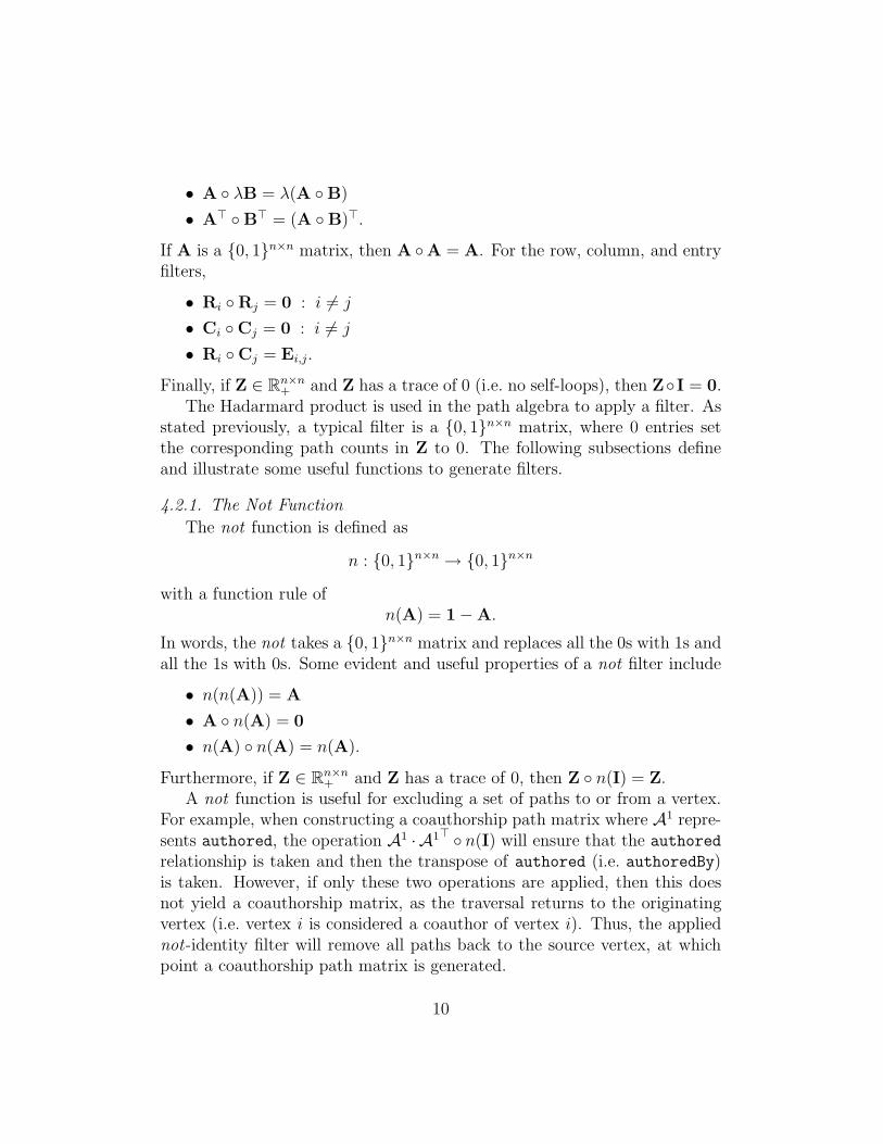
4.2.1. The Not Function

The not function is defined as

n : 0, 1n×n → 0, 1n×n

with a function rule ofn(A) = 1 − A.

In words, the not takes a 0, 1n×n matrix and replaces all the 0s with 1s andall the 1s with 0s. Some evident and useful properties of a not filter include

• n(n(A)) = A

• A n(A) = 0

• n(A) n(A) = n(A).

Furthermore, if Z ∈ Rn×n+ and Z has a trace of 0, then Z n(I) = Z.

A not function is useful for excluding a set of paths to or from a vertex.For example, when constructing a coauthorship path matrix where A1 repre-sents authored, the operation A1 · A1⊤ n(I) will ensure that the authored

relationship is taken and then the transpose of authored (i.e. authoredBy)is taken. However, if only these two operations are applied, then this doesnot yield a coauthorship matrix, as the traversal returns to the originatingvertex (i.e. vertex i is considered a coauthor of vertex i). Thus, the appliednot-identity filter will remove all paths back to the source vertex, at whichpoint a coauthorship path matrix is generated.

10

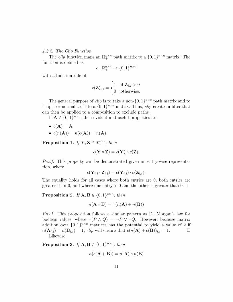
4.2.2. The Clip Function

The clip function maps an Rn×n+ path matrix to a 0, 1n×n matrix. The

function is defined asc : R

n×n+ → 0, 1n×n

with a function rule of

c(Z)i,j =

1 if Zi,j > 0

0 otherwise.

The general purpose of clip is to take a non-0, 1n×n path matrix and to“clip,” or normalize, it to a 0, 1n×n matrix. Thus, clip creates a filter thatcan then be applied to a composition to exclude paths.

If A ∈ 0, 1n×n, then evident and useful properties are

• c(A) = A

• c(n(A)) = n(c(A)) = n(A).

Proposition 1. If Y,Z ∈ Rn×n+ , then

c(Y Z) = c(Y) c(Z).

Proof. This property can be demonstrated given an entry-wise representa-tion, where

c(Yi,j · Zi,j) = c(Yi,j) · c(Zi,j).

The equality holds for all cases where both entries are 0, both entries aregreater than 0, and where one entry is 0 and the other is greater than 0.

Proposition 2. If A,B ∈ 0, 1n×n, then

n(A B) = c (n(A) + n(B))

Proof. This proposition follows a similar pattern as De Morgan’s law forboolean values, where ¬(P ∧ Q) = ¬P ∨ ¬Q. However, because matrixaddition over 0, 1n×n matrices has the potential to yield a value of 2 ifn(Ai,j) = n(Bi,j) = 1, clip will ensure that c(n(A) + c(B))i,j = 1.

Likewise,

Proposition 3. If A,B ∈ 0, 1n×n, then

n(c(A + B)) = n(A) n(B)

11

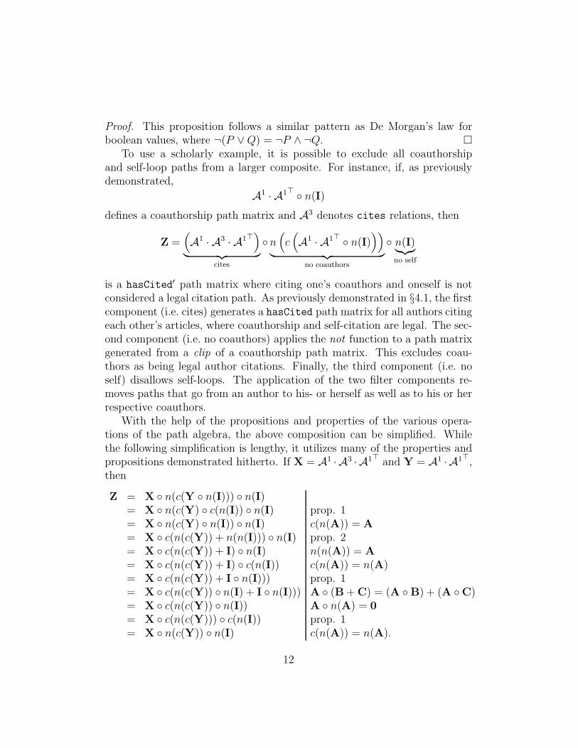
Proof. This proposition follows a similar pattern as De Morgan’s law forboolean values, where ¬(P ∨ Q) = ¬P ∧ ¬Q.

To use a scholarly example, it is possible to exclude all coauthorshipand self-loop paths from a larger composite. For instance, if, as previouslydemonstrated,

A1 · A1⊤ n(I)

defines a coauthorship path matrix and A3 denotes cites relations, then

Z =(

A1 · A3 · A1⊤)

︸ ︷︷ ︸

cites

n(

c(

A1 · A1⊤ n(I)))

︸ ︷︷ ︸

no coauthors

n(I)︸︷︷︸

no self

is a hasCited′ path matrix where citing one’s coauthors and oneself is notconsidered a legal citation path. As previously demonstrated in §4.1, the firstcomponent (i.e. cites) generates a hasCited path matrix for all authors citingeach other’s articles, where coauthorship and self-citation are legal. The sec-ond component (i.e. no coauthors) applies the not function to a path matrixgenerated from a clip of a coauthorship path matrix. This excludes coau-thors as being legal author citations. Finally, the third component (i.e. noself) disallows self-loops. The application of the two filter components re-moves paths that go from an author to his- or herself as well as to his or herrespective coauthors.

With the help of the propositions and properties of the various opera-tions of the path algebra, the above composition can be simplified. Whilethe following simplification is lengthy, it utilizes many of the properties andpropositions demonstrated hitherto. If X = A1 · A3 · A1⊤ and Y = A1 · A1⊤,then

Z = X n(c(Y n(I))) n(I)= X n(c(Y) c(n(I)) n(I) prop. 1= X n(c(Y) n(I)) n(I) c(n(A)) = A

= X c(n(c(Y)) + n(n(I))) n(I) prop. 2= X c(n(c(Y)) + I) n(I) n(n(A)) = A

= X c(n(c(Y)) + I) c(n(I)) c(n(A)) = n(A)= X c(n(c(Y)) + I n(I))) prop. 1= X c(n(c(Y)) n(I) + I n(I))) A (B + C) = (A B) + (A C)= X c(n(c(Y)) n(I)) A n(A) = 0

= X c(n(c(Y))) c(n(I)) prop. 1= X n(c(Y)) n(I) c(n(A)) = n(A).

12

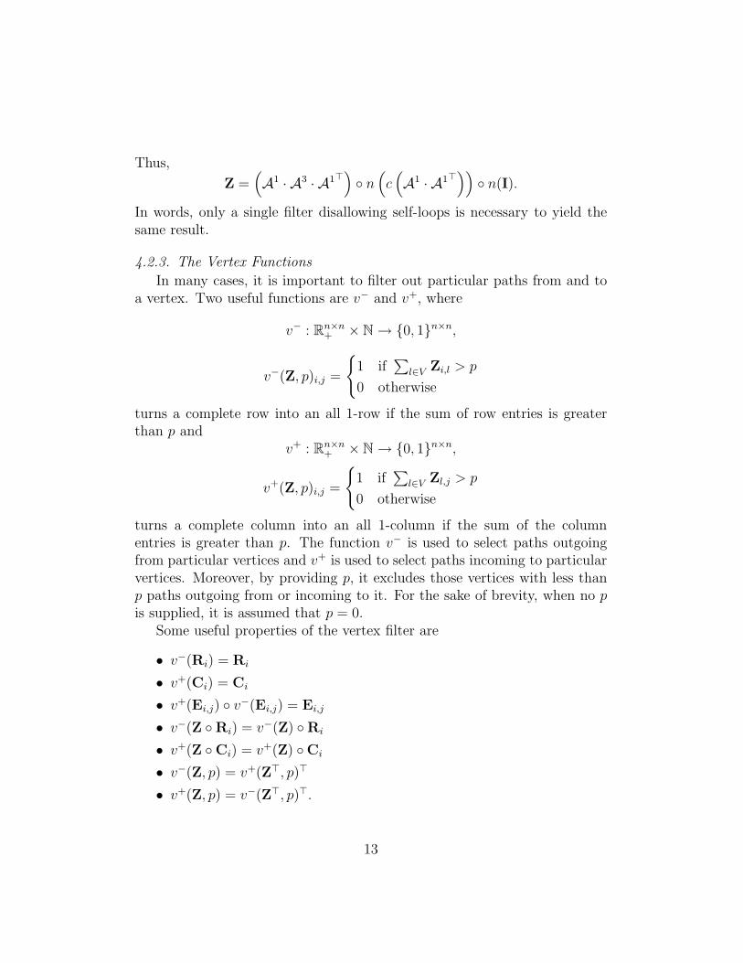
Thus,

Z =(

A1 · A3 · A1⊤)

n(

c(

A1 · A1⊤))

n(I).

In words, only a single filter disallowing self-loops is necessary to yield thesame result.

4.2.3. The Vertex Functions

In many cases, it is important to filter out particular paths from and toa vertex. Two useful functions are v− and v+, where

v− : Rn×n+ × N → 0, 1n×n,

v−(Z, p)i,j =

1 if∑

l∈VZi,l > p

0 otherwise

turns a complete row into an all 1-row if the sum of row entries is greaterthan p and

v+ : Rn×n+ × N → 0, 1n×n,

v+(Z, p)i,j =

1 if∑

l∈V Zl,j > p

0 otherwise

turns a complete column into an all 1-column if the sum of the columnentries is greater than p. The function v− is used to select paths outgoingfrom particular vertices and v+ is used to select paths incoming to particularvertices. Moreover, by providing p, it excludes those vertices with less thanp paths outgoing from or incoming to it. For the sake of brevity, when no p

is supplied, it is assumed that p = 0.Some useful properties of the vertex filter are

• v−(Ri) = Ri

• v+(Ci) = Ci

• v+(Ei,j) v−(Ei,j) = Ei,j

• v−(Z Ri) = v−(Z) Ri

• v+(Z Ci) = v+(Z) Ci

• v−(Z, p) = v+(Z⊤, p)⊤

• v+(Z, p) = v−(Z⊤, p)⊤.

13

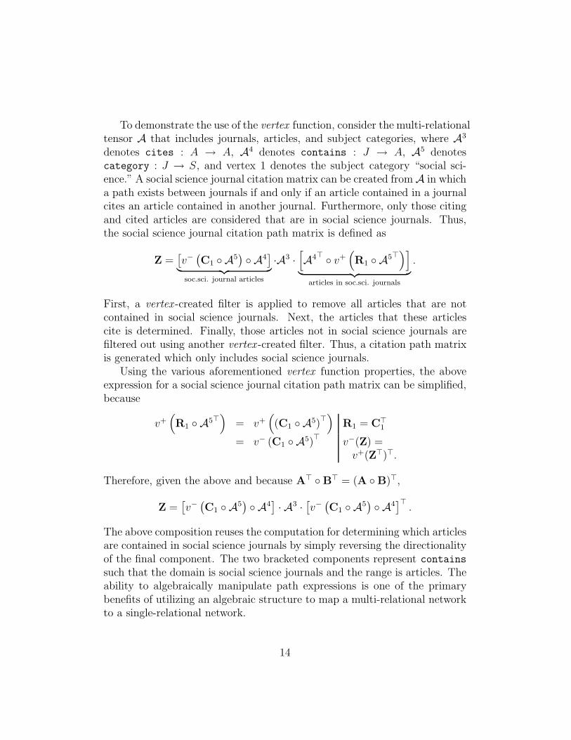
To demonstrate the use of the vertex function, consider the multi-relationaltensor A that includes journals, articles, and subject categories, where A3

denotes cites : A → A, A4 denotes contains : J → A, A5 denotescategory : J → S, and vertex 1 denotes the subject category “social sci-ence.” A social science journal citation matrix can be created from A in whicha path exists between journals if and only if an article contained in a journalcites an article contained in another journal. Furthermore, only those citingand cited articles are considered that are in social science journals. Thus,the social science journal citation path matrix is defined as

Z =[v−

(C1 A5

) A4

]

︸ ︷︷ ︸

soc.sci. journal articles

·A3 ·[

A4⊤ v+(

R1 A5⊤)]

︸ ︷︷ ︸

articles in soc.sci. journals

.

First, a vertex -created filter is applied to remove all articles that are notcontained in social science journals. Next, the articles that these articlescite is determined. Finally, those articles not in social science journals arefiltered out using another vertex -created filter. Thus, a citation path matrixis generated which only includes social science journals.

Using the various aforementioned vertex function properties, the aboveexpression for a social science journal citation path matrix can be simplified,because

v+(

R1 A5⊤)

= v+(

(C1 A5)⊤)

R1 = C⊤1

= v− (C1 A5)⊤

v−(Z) =v+(Z⊤)⊤.

Therefore, given the above and because A⊤ B⊤ = (A B)⊤,

Z =[v−

(C1 A5

) A4

]· A3 ·

[v−

(C1 A5

) A4

]⊤.

The above composition reuses the computation for determining which articlesare contained in social science journals by simply reversing the directionalityof the final component. The two bracketed components represent contains

such that the domain is social science journals and the range is articles. Theability to algebraically manipulate path expressions is one of the primarybenefits of utilizing an algebraic structure to map a multi-relational networkto a single-relational network.

14

4.3. The Weight Operation

Composed paths can be weighted using ordinary matrix scalar multipli-cation. Given a scalar value of λ ∈ R, λZ will weight all the paths in Z byλ. This operation is useful when merging path matrices in such a way as tomake one path matrix more or less significant than another path matrix. Thenext subsection, §4.4, discusses the operation of merging two path matricesand presents an example that includes the weight operation.

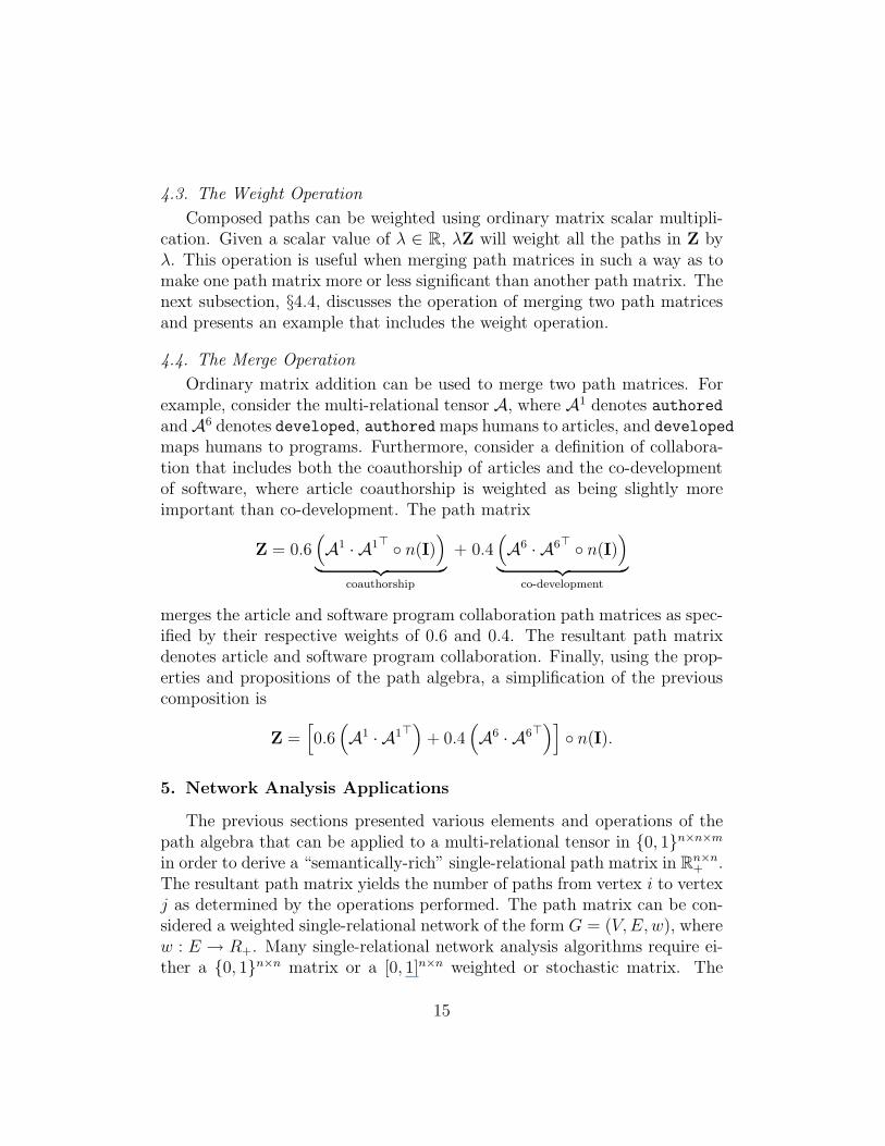
4.4. The Merge Operation

Ordinary matrix addition can be used to merge two path matrices. Forexample, consider the multi-relational tensor A, where A1 denotes authoredand A6 denotes developed, authored maps humans to articles, and developed

maps humans to programs. Furthermore, consider a definition of collabora-tion that includes both the coauthorship of articles and the co-developmentof software, where article coauthorship is weighted as being slightly moreimportant than co-development. The path matrix

Z = 0.6(

A1 · A1⊤ n(I))

︸ ︷︷ ︸

coauthorship

+ 0.4(

A6 · A6⊤ n(I))

︸ ︷︷ ︸

co-development

merges the article and software program collaboration path matrices as spec-ified by their respective weights of 0.6 and 0.4. The resultant path matrixdenotes article and software program collaboration. Finally, using the prop-erties and propositions of the path algebra, a simplification of the previouscomposition is

Z =[

0.6(

A1 · A1⊤)

+ 0.4(

A6 · A6⊤)]

n(I).

5. Network Analysis Applications

The previous sections presented various elements and operations of thepath algebra that can be applied to a multi-relational tensor in 0, 1n×n×m

in order to derive a “semantically-rich” single-relational path matrix in Rn×n+ .

The resultant path matrix yields the number of paths from vertex i to vertexj as determined by the operations performed. The path matrix can be con-sidered a weighted single-relational network of the form G = (V, E, w), wherew : E → R+. Many single-relational network analysis algorithms require ei-ther a 0, 1n×n matrix or a [0, 1]n×n weighted or stochastic matrix. The

15

resultant path matrix can be manipulated in various ways (e.g. normalizedout going weight distribution) to yield a matrix that can be appropriatelyused with the known single-relational network analysis algorithms. This sec-tion discusses the connection of a path matrix to a few of the more popularsingle-relational network analysis algorithms. However, before discussing thesingle-relational network analysis algorithms, the next subsection discussesthe relationship between the path algebra and multi-relational graph querylanguages.

5.1. Relationship to Multi-Relational Graph Query Languages

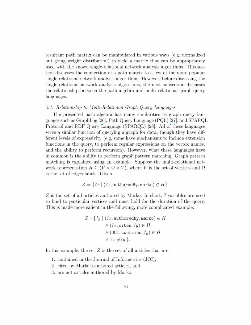
The presented path algebra has many similarities to graph query lan-guages such as GraphLog [26], Path Query Language (PQL) [27], and SPARQLProtocol and RDF Query Language (SPARQL) [28]. All of these languagesserve a similar function of querying a graph for data, though they have dif-ferent levels of expressivity (e.g. some have mechanisms to include extensionfunctions in the query, to perform regular expressions on the vertex names,and the ability to perform recursion). However, what these languages havein common is the ability to perform graph pattern matching. Graph patternmatching is explained using an example. Suppose the multi-relational net-work representation H ⊆ (V × Ω × V ), where V is the set of vertices and Ωis the set of edges labels. Given

Z = ?x | (?x, authoredBy, marko) ∈ H,

Z is the set of all articles authored by Marko. In short, ?-variables are usedto bind to particular vertices and must hold for the duration of the query.This is made more salient in the following, more complicated example:

Z =?y | (?x, authoredBy, marko) ∈ H

∧ (?x, cites, ?y) ∈ H

∧ (JOI, contains, ?y) ∈ H

∧ ?x 6=?y .

In this example, the set Z is the set of all articles that are

1. contained in the Journal of Informetrics (JOI),

2. cited by Marko’s authored articles, and

3. are not articles authored by Marko.

16

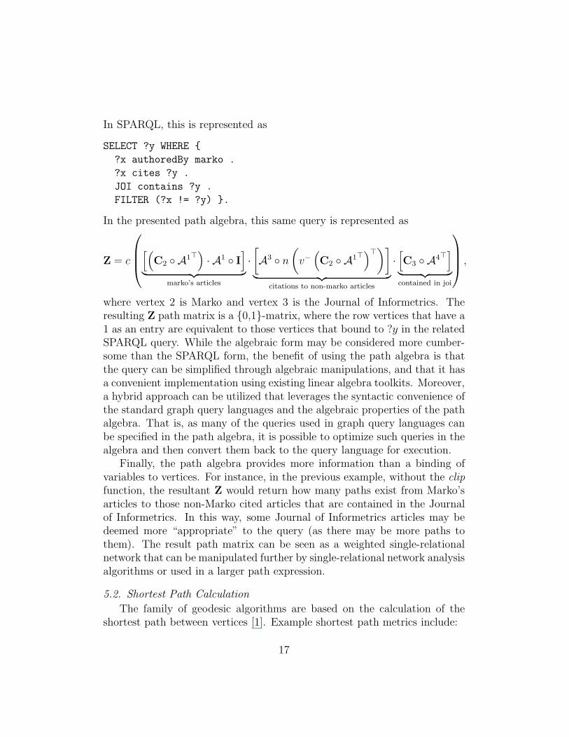
In SPARQL, this is represented as

SELECT ?y WHERE

?x authoredBy marko .

?x cites ?y .

JOI contains ?y .

FILTER (?x != ?y) .

In the presented path algebra, this same query is represented as

Z = c

[(

C2 A1⊤)

· A1 I]

︸ ︷︷ ︸

marko’s articles

·[

A3 n

(

v−

(

C2 A1⊤)⊤

)]

︸ ︷︷ ︸

citations to non-marko articles

·[

C3 A4⊤]

︸ ︷︷ ︸

contained in joi

,

where vertex 2 is Marko and vertex 3 is the Journal of Informetrics. Theresulting Z path matrix is a 0,1-matrix, where the row vertices that have a1 as an entry are equivalent to those vertices that bound to ?y in the relatedSPARQL query. While the algebraic form may be considered more cumber-some than the SPARQL form, the benefit of using the path algebra is thatthe query can be simplified through algebraic manipulations, and that it hasa convenient implementation using existing linear algebra toolkits. Moreover,a hybrid approach can be utilized that leverages the syntactic convenience ofthe standard graph query languages and the algebraic properties of the pathalgebra. That is, as many of the queries used in graph query languages canbe specified in the path algebra, it is possible to optimize such queries in thealgebra and then convert them back to the query language for execution.

Finally, the path algebra provides more information than a binding ofvariables to vertices. For instance, in the previous example, without the clip

function, the resultant Z would return how many paths exist from Marko’sarticles to those non-Marko cited articles that are contained in the Journalof Informetrics. In this way, some Journal of Informetrics articles may bedeemed more “appropriate” to the query (as there may be more paths tothem). The result path matrix can be seen as a weighted single-relationalnetwork that can be manipulated further by single-relational network analysisalgorithms or used in a larger path expression.

5.2. Shortest Path Calculation

The family of geodesic algorithms are based on the calculation of theshortest path between vertices [1]. Example shortest path metrics include:

17

• eccentricity : defined for a vertex as the longest shortest path to allother vertices [6],

• radius: defined for the network as the smallest eccentricity value for allvertices,

• diameter : defined for the network as the largest eccentricity value forall vertices,

• closeness : defined for a vertex as the mean shortest path of a vertexto all other vertices [3],

• betweenness : defined for a vertex as the number of shortest paths thata vertex is a part of [5].

A straightforward (though computationally expensive) way to calculatethe shortest path between any two vertices i and j in an adjacency matrixA is to continue to raise the adjacency matrix by a power until A

(t)i,j > 0.

The first t where A(t)i,j > 0 denotes the length of the shortest path between

vertex i and j as t. This same principle holds for calculating the shortestpath in a path matrix Z and thus, the resulting path matrix generated froma path composition can be used to determine “semantically-rich” shortestpaths between vertices.

5.3. Diffusing an Energy Vector through AMany network analysis algorithms can be represented as an energy diffu-

sion, wheref : R

n+ × R

n×n+ → R

n+

maps a row-vector of size n (i.e. “energy vector”) and a matrix of size n ×n to a resultant energy vector of size n. Algorithms of this form includeeigenvector centrality [7], PageRank [8], and spreading activation [29, 30] toname but a few.

With respect to eigenvector centrality and PageRank, the general formof the algorithm can be represented as a problem in finding the primaryeigenvector of an adjacency matrix such that πA = λπ, where π ∈ R

n andπ is the energy vector being diffused. Both algorithms can be solved usingthe “power method.” In one form of the power method, the solution is foundby iteratively multiplying π by A until π converges to a stable set of valuesas defined by ||π(t−1) − π(t)||2 < ǫ for some small ǫ ∈ R+. In another form,the problem is framed as finding which t-power of A will yield a π such that

18

πA(t) = λπ. With respect to spreading activation, the same power methodcan be used; however, the purpose of the algorithm is not to find the primaryeigenvector, but instead to propagate an energy vector some finite numberof steps. Moreover, the total energy flow through each vertex at the end ofa spreading activation algorithm is usually what is determined.

5.3.1. The PageRank Path Matrix

The PageRank algorithm was developed to determine the centrality ofweb pages in a web citation network [8] and since, has been used as a generalnetwork centrality algorithm for various other types of networks includingbibliographic [31, 32], social [33], and word networks [34]. The web citationnetwork can be defined as G = (V, E), where V is a set of web pages andE ⊆ (V × V ) is the set of directed citations between web pages (i.e. href).The interesting aspect of the PageRank algorithm is that it “distorts” theoriginal network G by overlaying a “teleportation” network in which everyvertex is connected to every other vertex by some weight defined by δ ∈ (0, 1].The inclusion of the teleportation network ensures that the resulting hybridnetwork is strongly connected7 and thus, the resultant primary eigenvectorof the network is a positive real-valued vector.

In the matrix form of PageRank, there exist two adjacency matrices in[0, 1]n×n denoted

P1i,j =

1

Γ(i)if (i, j) ∈ E

0 otherwise.

and

P2i,j =

1

|V | ,

where Γ(i) is the out degree of vertex i. P1 is a row-stochastic adjacencymatrix and P2 is a fully connected adjacency matrix known as the teleporta-tion matrix. The purpose of PageRank is to identify the primary eigenvectorof a merged, weighted path matrix of the form

Z = δP1 + (1 − δ)P2.

Z is guaranteed to be a strongly connected single-relational path matrix

7Strongly connected means that there exists a path from every vertex to every othervertex. In the language of Markov chains, the network is irreducible and recurrent.

19

because there is some probability (defined by 1 − δ) that every vertex isreachable by every other vertex.

5.3.2. Constrained Spreading Activation

The concept of spreading activation was made popular by cognitive sci-entists and the connectionist approach to artificial intelligence [29, 35, 36],where the application scenario involves diffusing an energy vector through anartificial neural network in order to simulate the neural process of a spreadingactivation potential in the brain. Spreading activation can be computed in amanner analogous to the power method of determining the primary eigenvec-tor of an adjacency matrix. However, spreading activation does not attemptto find a stationary energy distribution in the network and moreover, usuallyincludes a decay function or activation/threshold function that can yield aresultant energy vector whose sum is different than the initial energy vector.

The neural network models of connectionism deal with weighted, single-relational networks. Spreading activation was later generalized to supportmulti-relational networks [30]. While there are many forms of spreadingactivation on single-relational networks and likewise, many forms on multi-relational networks, in general, a spreading activation algorithm on a multi-relational network is called constrained spreading activation as not all edgesto and from a vertex are respected equally. Constrained spreading activationhas been used for information retrieval on the web [30, 37, 38], semanticvertex ranking [18, 39], and collaborative filtering [40]. The path algebraprovides a means by which to separate the spreading activation algorithmfrom the data structure being computed on. That is, the constrained aspectof the algorithm is defined by the path algebra and the spreading activation

aspect of the algorithm is defined by standard, single-relational spreadingactivation.

5.4. Mixing Patterns

Given a network and a scalar or categorical property value for each vertexin the network, it is possible to determine whether the network is assorta-tive or disassortative with respect to that property [41]. Example scalarproperties for journal vertices in a scholarly network include impact factorranking, years in press, cost for subscription, etc. Example categorical prop-erties include subject category, editor in chief, publisher, etc. A network isassortative with respect to a particular vertex property when vertices of like

20

property values tend to be connected to one another. Colloquially, assorta-tivity can be understood by the phrase “birds of a feather flock together,”where the “feather” is the property binding individuals [42]. On the otherhand, a network is disassortative with respect to a particular vertex propertywhen vertices of unlike property values tend to be connected to one another.Colloquially, disassortativity can be understood by the phrase “oppositesattract.”

There are two primary components needed when calculating the assor-tativity of a network. The first component is the network and the secondcomponent is a set of property values for each vertex in the network. A pop-ular publication defining the assortative mixing for scalar properties uses theparametric Pearson correlation of two vectors [43].8 One vector is the scalarvalue of the vertex property for the vertices on the tail of all edges. Theother vector is the scalar value of the vertex property for the vertices on thehead of all the edges. Thus, the length of both vectors is |E| (i.e. the totalnumber of edges in the single-relational network). Formally, the correlationis defined as

r =|E|

∑

i jiki −∑

i ji

∑

i ki√

[|E|

∑

i j2i − (

∑

i ji)2] [

|E|∑

i k2i − (

∑

i ki)2]

,

where ji is the scalar value of the vertex on the tail of edge i, and ki is thescalar value of the vertex on the head of edge i. The correlation coefficient r

is in [−1, 1], where −1 represents a fully disassortative network, 0 representsan uncorrelated network, and 1 represents a fully assortative network. Onthe other hand, for categorical properties, the equation

r =

∑

a eaa −∑

a iaja

1 −∑

a iaja

yields a value in [−1, 1] as well, where eaa is the number of edges in thenetwork that have property value a on both ends, ia is the number of edgesin the network that have property value a on their tail vertex, and ja is thenumber of edges that have property value a on their head vertex [41].

8Note that scalar value distributions may not be normally distributed and thus, insuch cases, a non-parametric correlation such as the Spearman ρ may be the more usefulcorrelation coefficient.

21

Given a path matrix, assortativity is calculated on paths, not on edges,where there may be many paths (possibly weighted) between any two ver-tices.9 Thus, a weighted correlation is required [44]. Let ji denote the scalarproperty value of the vertex on the tail of path i and ki denote the scalarproperty value of the vertex on the head of path i. The previous scalar as-sortativity equation can be generalized such that if zi is the fraction of pathweight in Z for path i, then

r =covj,k√

covj,jcovk,k

,

where

covj,k =1

∑

i zi

[∑

i

zi

(

ji −∑

i ziji∑

i zi

)(

ki −∑

i ziki∑

i zi

)]

.

Similarly, for categorical vertex properties,

r =

∑

a eaa −∑

a iaja

1 −∑

a iaja

where eaa is the total path weight of paths that have tail and head verticeswith a property value of a, ia is the total path weight of all paths that havea tail vertex with a property value of a, and ja is the total path weight of allpaths that have a head vertex with a property value of a.

6. Conclusion

The number of algorithms and toolkits for single-relational networks farexceeds those currently available for multi-relational networks. However,with the rising popularity of the multi-relational network, as made evident bythe Web of Data initiative and the multi-relational RDF data structure [45],there is a need for methods that port the known single-relational networkanalysis algorithms over to these multi-relational domains. A convenient

9It is important to note that with multi-relational networks, vertex property valuescan be encoded in the network itself. For instance, given the scholarly network exampleof previous, the subject category “social science” is a vertex adjacent to a set of journalvertices according to the relation category : J → S. More generally, vertex propertyvalues may be determined through path composition.

22

method to do so is a path algebra. Path algebras have been used extensivelyfor analyzing paths in single-relational networks [46, 47] and the applica-tion to multi-relational networks can prove useful. The multi-relational pathalgebra presented in this article operates on an n × n × m tensor represen-tation of a multi-relational network. By means of a series of operations ontwo-way “slices” of this tensor, a “semantically-rich” n × n single-relationalpath matrix can be derived. The resulting path matrix represents a single-relational network. This single-relational network may then be subjected toany of the known single-relational network analysis algorithms. Thus, thepresented path algebra can be used to expose multi-relational networks tosingle-relational network analysis algorithms.

References

[1] S. Wasserman, K. Faust, Social Network Analysis: Methods and Appli-cations, Cambridge University Press, Cambridge, UK, 1994.

[2] U. Brandes, T. Erlebach (Eds.), Network Analysis: Methodolgical Foun-dations, Springer, Berling, DE, 2005.

[3] A. Bavelas, Communication patterns in task oriented groups, The Jour-nal of the Acoustical Society of America 22 (1950) 271–282.

[4] E. W. Dijkstra, A note on two problems in connexion with graphs,Numerische Mathematik 1 (1959) 269–271.

[5] L. C. Freeman, A set of measures of centrality based on betweenness,Sociometry 40 (35–41).

[6] F. Harary, P. Hage, Eccentricity and centrality in networks, Social Net-works 17 (1995) 57–63.

[7] P. Bonacich, Power and centrality: A family of measures., AmericanJournal of Sociology 92 (5) (1987) 1170–1182.

[8] S. Brin, L. Page, The anatomy of a large-scale hypertextual web searchengine, Computer Networks and ISDN Systems 30 (1–7) (1998) 107–117.

[9] F. R. K. Chung, Spectral Graph Theory, American Mathematical Soci-ety, 1997.

23

[10] M. E. J. Newman, M. Girvan, Finding and evaluating community struc-ture in networks, Physical Review E 69 (2004) 026113.URL http://arxiv.org/abs/cond-mat/0308217

[11] M. Girvan, M. E. J. Newman, Community structure in social and bio-logical networks, Proceedings of the National Academy of Sciences 99(2002) 7821–7826.URL http://arxiv.org/abs/cond-mat/0112110

[12] M. E. J. Newman, Finding community structure in networks using theeigenvectors of matrices, Physical Review E 74. arXiv:physics/0605087.URL http://arxiv.org/abs/physics/0605087

[13] J. F. Sowa, Principles of Semantic Networks: Explorations in the Rep-resentation of Knowledge, Morgan Kaufmann, San Mateo, CA, 1991.

[14] M. A. Rodriguez, A multi-relational network to support the scholarlycommunication process, International Journal of Public InformationSystems 2007 (1) (2007) 13–29.URL http://arxiv.org/abs/cs/0601121

[15] J. Bollen, M. A. Rodriguez, H. Van de Sompel, L. L. Balakireva, A. Hag-berg, The largest scholarly semantic network...ever., in: Proceedings ofthe World Wide Web Conference, ACM Press, New York, NY, 2007, pp.1247–1248. doi:10.1145/1242572.1242789.

[16] T. Berners-Lee, J. A. Hendler, Publishing on the Semantic Web, Nature410 (6832) (2001) 1023–1024. doi:10.1038/35074206.

[17] M. A. Rodriguez, Data Management in the Semantic Web, Nova Pub-lishing, 2009, Ch. Interpretations of the Web of Data.URL http://arxiv.org/abs/0905.3378

[18] M. A. Rodriguez, Grammar-based random walkers in seman-tic networks, Knowledge-Based Systems 21 (7) (2008) 727–739.doi:10.1016/j.knosys.2008.03.030.URL http://arxiv.org/abs/0803.4355

[19] S. Lin, Interesting instance discovery in multi-relational data, in: D. L.McGuinness, G. Ferguson (Eds.), Proceedings of the Conference on In-novative Applications of Artificial Intelligence, MIT Press, 2004, pp.991–992.

24

[20] D. Cai, Z. Shao, X. He, X. Yan, J. Han, Community mining from multi-relational networks, in: Proceedings of the 2005 European Conferenceon Principles and Practice of Knowledge Discovery in Databases, Vol.3721 of Lecture Notes in Computer Science, Springer, Porto, Portugal,2005, pp. 445–452. doi:10.1007/11564126.

[21] H. Zhuge, L. Zheng, Ranking semantic-linked network, in: Proceedingsof the International World Wide Web Conference, Budapest, Hungary,2003.

[22] B. Aleman-Meza, C. Halaschek-Wiener, I. B. Arpinar, C. Ra-makrishnan, A. P. Sheth, Ranking complex relationships on thesemantic web, IEEE Internet Computing 9 (3) (2005) 37–44.doi:http://doi.ieeecomputersociety.org/10.1109/MIC.2005.63.

[23] T. G. Kolda, B. W. Bader, J. P. Kenny, Higher-order web link analysisusing multilinear algebra, in: Proceedings of the International Confer-ence on Data Mining ICDM’05, IEEE, 2005, pp. 242–249.

[24] G. Chartrand, Introductory Graph Theory, Dover, 1977.

[25] R. Horn, C. Johnson, Topics in Matrix Analysis, Cambridge UniversityPress, 1994.

[26] M. P. Consens, A. O. Mendelzon, Graphlog: a visual formalism forreal life recursion, in: Proceedings of the Symposium on Princi-ples of Database Systems, ACM, New York, NY, 1990, pp. 404–416.doi:10.1145/298514.298591.

[27] U. Leser, A query language for biological networks, Bioinformatics 21 (2)(2005) 33–39. doi:10.1093/bioinformatics/bti1105.

[28] E. Prud’hommeaux, A. Seaborne, SPARQL query language for RDF,Tech. rep., World Wide Web Consortium (October 2004).URL http://www.w3.org/TR/2004/WD-rdf-sparql-query-20041012/

[29] J. R. Anderson, A spreading activation theory of memory, Journal ofVerbal Learning and Verbal Behaviour 22 (1983) 261–295.

[30] P. R. Cohen, R. Kjeldsen, Information retrieval by constrained spreadingactivation in semantic networks, Information Processing and Manage-ment 23 (4) (1987) 255–268.

25

[31] J. Bollen, M. A. Rodriguez, H. Van de Sompel, Journal status, Sciento-metrics 69 (3) (2006) 669–687. doi:10.1007/s11192-006-0176-z.URL http://arxiv.org/abs/cs/0601030

[32] P. Chen, H. Xie, S. Maslov, S. Redner, Finding scientific gems withGoogle, Journal of Informetrics 1 (1) (2007) 8–15.URL http://arxiv.org/abs/physics/0604130

[33] X. Liu, J. Bollen, M. L. Nelson, H. Van de Sompel, Co-authorship net-works in the digital library research community, Information Processingand Management 41 (6) (2006) 1462–1480.URL http://arxiv.org/abs/cs.DL/0502056

[34] R. Mihalcea, P. Tarau, E. Figa, Pagerank on semantic networks,with application to word sense disambiguation, in: Proceedings ofthe International Conference on Computational Linguistics, Associa-tion for Computational Linguistics, Morristown, NJ, 2004, p. 1126.doi:10.3115/1220355.1220517.

[35] A. M. Collins, E. F. Loftus, A spreading activation theory of semanticprocessing, Psychological Review 82 (1975) 407–428.

[36] D. E. Rumelhart, J. L. McClelland, Parallel Distributed Processing:Explorations in the Microstructure of Cognition, MIT Press, 1993.

[37] F. Crestani, Application of spreading activation techniques in informa-tion retrieval, Artificial Intelligence Review 11 (6) (1997) 453–582.

[38] F. Crestani, P. L. Lee, Searching the web by constrained spreading acti-vation, Information Processing and Management 36 (4) (2000) 585–605.

[39] M. A. Rodriguez, Social decision making with multi-relational networksand grammar-based particle swarms, in: Proceedings of the Hawaii In-ternational Conference on Systems Science, IEEE Computer Society,Waikoloa, Hawaii, 2007, pp. 39–49. doi:10.1109/HICSS.2007.487.URL http://arxiv.org/abs/cs.CY/0609034

[40] J. Griffith, C. O’Riordan, H. Sorensen, Knowledge-Based IntelligentInformation and Engineering Systems, Vol. 4253 of Lecture Notesin Artificial Intelligence, Springer-Verlag, 2006, Ch. A Constrained

26

Spreading Activation Approach to Collaborative Filtering, pp. 766–773.doi:10.1007/11893011.

[41] M. E. J. Newman, Mixing patterns in networks, Physical Review E67 (2) (2003) 026126. doi:10.1103/PhysRevE.67.026126.URL http://arxiv.org/abs/cond-mat/0209450

[42] M. McPherson, L. Smith-Lovin, J. Cook, Birds of a feather: Homophilyin social networks, Annual Review of Sociology 27 (2001) 415–444.

[43] M. E. J. Newman, Assortative mixing in networks, Physical ReviewLetters 89 (20) (2002) 208701.URL http://arxiv.org/abs/cond-mat/0205405/

[44] J. M. Bland, D. G. Altman, Calculating correlation coefficients with re-peated observations: Part 2–correlation between subjects, British Med-ical Journal 310 (6980) (1995) 633.

[45] E. Miller, An introduction to the Resource Description Framework, Bul-letin of the American Society for Information Science and Technology25 (1) (1998) 15–19. doi:10.1002/bult.105.

[46] B. Carre, Graphs and Networks, Oxford University Press, 1979.

[47] R. Manger, A new path algebra for finding paths in graphs, in: Pro-ceedings of the International Conference on Information Technology In-terfaces, Vol. 1, 2004, pp. 657–662. doi:10.1109/ITI.2004.242700.

27