performance calculations of gas turbine engine ... - mdpi

applied sciences

Article

Performance Calculations of Gas Turbine Engine ComponentsBased on Particular Instrumentation Methods

Răzvan Marius Catană *, Gabriel Dediu, Cornel Mihai Tărăbîc and Horat,iu Mihai S, erbescu

��

Citation: Catana, R.M.; Dediu, G.;

Tarabîc, C.M.; S, erbescu, H.M.

Performance Calculations of Gas

Turbine Engine Components Based

on Particular Instrumentation

Methods. Appl. Sci. 2021, 11, 4492.

https://doi.org/10.3390/app11104492

Academic Editor: Adrian Irimescu

Received: 16 March 2021

Accepted: 11 May 2021

Published: 14 May 2021

Publisher’s Note: MDPI stays neutral

with regard to jurisdictional claims in

published maps and institutional affil-

iations.

Copyright: © 2021 by the authors.

Licensee MDPI, Basel, Switzerland.

This article is an open access article

distributed under the terms and

conditions of the Creative Commons

Attribution (CC BY) license (https://

creativecommons.org/licenses/by/

4.0/).

National Research and Development Institute for Gas Turbines COMOTI, 061126 Bucharest, Romania;[email protected] (G.D.); [email protected] (C.M.T.); [email protected] (H.M.S, .)* Correspondence: [email protected]; Tel.: +40-0763181775

Abstract: This paper presents an analytical method to determine various main parameters or per-formances of engine components when those parameters cannot be directly measured and it isnecessary to determine them. Additionally, some variants of instrumentation methods are presented,for example: engine inlet, compressor, turbine or jet nozzle instrumentation. The purpose of theinstrumentation methods is to directly measure the possible parameters, which are then used asinputs in a model to determine other parameters or performance metrics. This model is basedon gasodynamic process equations, and it is used to compute the air and gas parameters, such asenthalpy and entropy, which are described in polynomial form, thus leading to a more realisticcalculation. At the end, this paper presents a practical example of instrumentation applied on aKlimov TV2-117A turboshaft, with a series of experimental results, following the engine testing onthe test bench.

Keywords: measured parameters; performances; calculation model

1. Introduction

Generally, most of the gas turbine engines that are in service, or are going to enterinto service, have a standard minimal instrumentation [1,2], through which the engine canbe monitored. In the case of a new engine project that has been developed in the designphase, and if an engine prototype based on the previous phases has been developed, aseries of tests at any condition are required. For the first engine tests, it is necessary tohave additional dedicated instrumentation ports and probes in the main engine sections.Therefore, the measurement of possible parameters which can be used to compute othermain engine parameters is allowed. Furthermore, the area where the parameters aremonitored during the engine tests on the test bench can be extended [3,4]. In many cases,when the engine is ready to enter into service, due to intellectual property reasons, theengine manufacturer does not equip the engine with all the instrumentation ports [5] as itwas equipped in the testing phase. Some engine manufacturers keep the supplementaryports and install plugs on them, or they equip the engine with several inspection ports. Thisis a useful solution, from the testing and maintenance accessibility point of view, because itgives the possibility to install different instrumentation probes. The instrumentation of anengine depends on what experimentation is planned, or it depends on what type of practicalresearch is used or involved [6]. If the engine will be involved in an experimental project,additional instrumentation will be needed. There are various situations when, technically,it is not possible to measure the diverse main parameters or engine performance directly [7],which also applies to the mass air flow, the overall pressure ratio, the compressor andturbine efficiency or the engine power and thrust. However, these main parameters canbe indirectly determined by models (algorithms) that use different measured parameters.If the performance of a gas turbine engine is required, it is necessary to study the engineconfiguration, in order to analyze where instrumentation probes can be inserted andwhat type of probe is suitable to be mounted in the engine station. Therefore, the inlet

Appl. Sci. 2021, 11, 4492. https://doi.org/10.3390/app11104492 https://www.mdpi.com/journal/applsci

https://www.mdpi.com/journal/applsci

https://www.mdpi.com

https://www.mdpi.com/article/10.3390/app11104492?type=check_update&version=1



https://creativecommons.org/

https://creativecommons.org/licenses/by/4.0/

https://creativecommons.org/licenses/by/4.0/


https://www.mdpi.com/journal/applsci

Appl. Sci. 2021, 11, 4492 2 of 17

and outlet of the engine components are defined. The level of engine instrumentation isdetermined in accordance with the test results, parameters that are requested and the levelof experimentation. The instrumentation level is furthermore correlated with the enginecomponents’ accessibility which allows for the instrumentation probes to be mounted.

In the case of our application, the instrumentation was divided for the gas turbineengine components, based on the availability of ports and the necessary measure pointsfor the algorithm. For a particular industrial application, similar to our application, it isaimed for every engine component to display multiple parameters in every engine sector.The purpose of our study is to determine these parameters, and to decrease the errors inthe calculation method.

Generally, in gasodynamic calculation theory, constant values of entropy and enthalpyare used in order to create an easier algorithm. In reality, the entropy and enthalpy arefunctions of temperature. Each method can be used in the application, but the methodwhere the entropy and enthalpy depend on the temperature offers a higher precision. Eachcase has advantages and disadvantages regarding the number of instrumentation parame-ters. This means that the temperature-dependent enthalpy and entropy require a highernumber of instrumentation parameters in determining the general engine performance orkey parameters.

The method will be used for a specific case (such as an industrial application) thatincludes used engines that are at the end of their lifespan, not for a newly designed engine.

2. Instrumentation Methods

In this chapter, different instrumentation methods for engine components are pre-sented, which are useful for determining some of the main parameters that cannot bemeasured directly and which are required for a more in-depth study [8].

The instrumentation project starts from what main parameters or performances arerequested to be determined. Then, according to the type of parameters or performances re-quired by the mathematical definition and equations, the parameters of interest are studied.In the next step, a technical study is conducted to analyze the available instrumentationports on the engine. An analysis is also performed to determine if the available ports onthe engine can be adapted as needed. As a result, the parameters that can be measuredare established.

2.1. Engine Inlet Instrumentation

The engine inlet (bellmouth) is instrumented to measure the engine air flow. The massair flow (Ma f ) is defined as the multiplication of density (ρs), velocity (V) and cross-section(A) [9], where the density and velocity are functions which depend on multiple variables,such as: temperature, pressure and the Mach number.

Ma f = ρs(p, T) ·V(M, T) · A; Ma f =ps

Ra · Ts· M√

k · Ra · Ts· A (1)

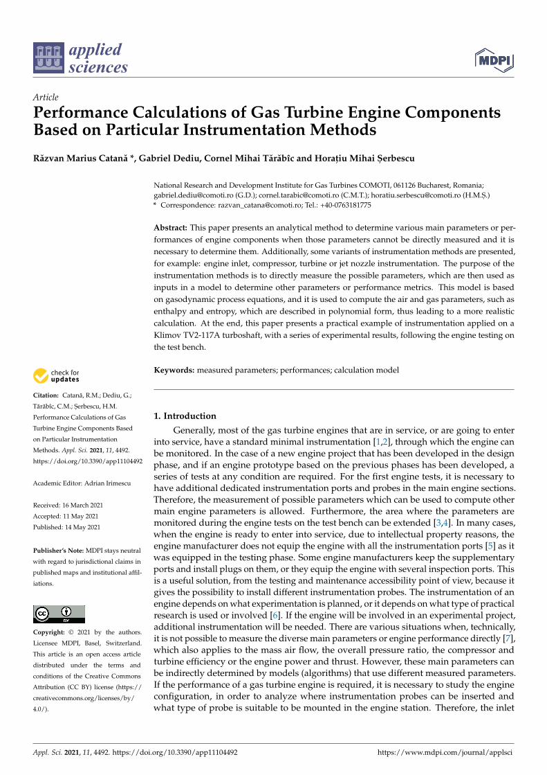
According to the density (ρs) and velocity (V) mathematical definitions [9], the pa-rameters that are possible to be measured are established, which are used in the densityand velocity computation. One method, as presented in Figure 1a, is to instrument thebellmouth only for static pressure measurement (ps), in order to measure the differentialpressure (DP), to use the test cell air pressure (p0), in order to determine the air velocity(V), and then to measure the test cell air temperature (T0) which is used to determine theair density (ρs). The cross-section (A) is determined using the bellmouth diameter (D).

Another method, which is more accurate, as presented in Figure 1b, is to instrument thebellmouth for static pressure measurement (ps), for total pressure (pt) and total temperaturemeasurement (Tt), with approximately the same cross-section.

The method presented in Figure 1a requires fewer parameters on the inlet and, basedon the approximation of the pressure loss coefficient on the bellmouth, it results in ahigher error. The method presented in Figure 1b uses the measured parameters directly

Appl. Sci. 2021, 11, 4492 3 of 17

and eliminates the error that is introduced by the approximation of the pressure losscoefficients, and, as a result, it has a lower error. It is to be mentioned that any methodpresents an error of measurement that is introduced by the instrumentation probes.

Appl. Sci. 2021, 11, x FOR PEER REVIEW 3 of 19

the air density ( s ). The cross-section ( A ) is determined using the bellmouth diameter (

D ).

(a) (b)

Figure 1. Bellmouth instrumentation method scheme, model (a), bellmouth instrumentation method scheme, model (b).

Another method, which is more accurate, as presented in Figure 1b, is to instrument

the bellmouth for static pressure measurement ( sp ), for total pressure ( tp ) and total tem-

perature measurement ( tT ), with approximately the same cross-section.

The method presented in Figure 1a requires fewer parameters on the inlet and, based

on the approximation of the pressure loss coefficient on the bellmouth, it results in a

higher error. The method presented in Figure 1b uses the measured parameters directly

and eliminates the error that is introduced by the approximation of the pressure loss co-

efficients, and, as a result, it has a lower error. It is to be mentioned that any method pre-

sents an error of measurement that is introduced by the instrumentation probes.

2.2. Compressor Instrumentation

The compressor is instrumented to determine the total adiabatic efficiency and, by

default, the total overall pressure ratio. The total overall pressure ratio [9] is defined as the

ratio between the outlet total pressure ( 2.tp ) and inlet total pressure ( 1.tp ).

The first method, presented in Figure 2a, through which the total overall pressure ratio

can be determined, is to measure only the outlet total pressure ( 2.tp ) because the inlet total

pressure ( 1.tp ) can be determined from the cell air pressure ( 0p ). Compressor total adia-

batic efficiency [9] is the ratio between the total specific ideal work ( . .C t idl ) and the total spe-

cific actual work ( .C tl ). The total specific actual work [9] ( .C tl ) is the difference between the

outlet total specific enthalpy ( 2.th ) and the inlet total specific enthalpy ( 1.th ).

. . . . 2. . 1. 2. 1.C t C t id C t t id t t tl l h T h T h T h T (2)

(a) (b)

Figure 2. Compressor instrumentation method scheme, model (a); compressor instrumentation method scheme, model (b).



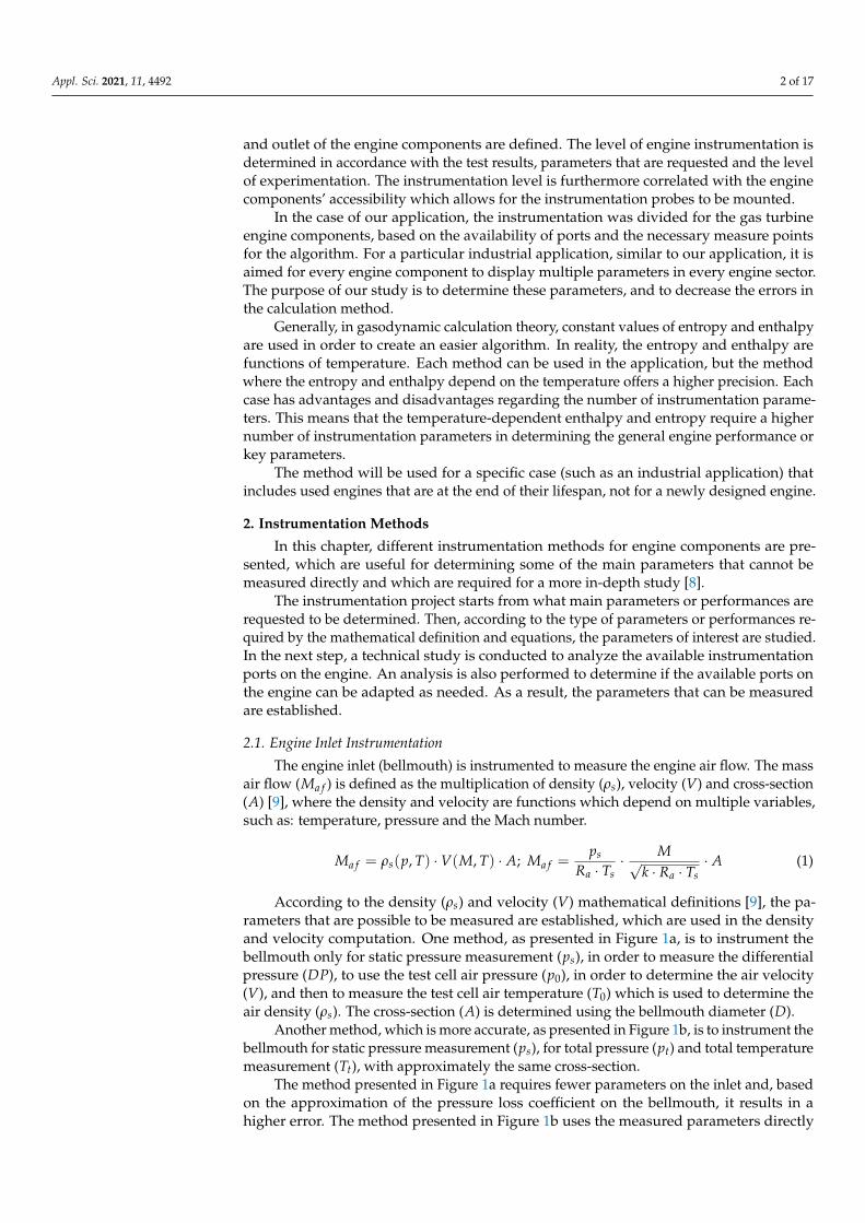
The compressor is instrumented to determine the total adiabatic efficiency and, bydefault, the total overall pressure ratio. The total overall pressure ratio [9] is defined as theratio between the outlet total pressure (p2.t) and inlet total pressure (p1.t).

The first method, presented in Figure 2a, through which the total overall pressureratio can be determined, is to measure only the outlet total pressure (p2.t) because the inlettotal pressure (p1.t) can be determined from the cell air pressure (p0). Compressor totaladiabatic efficiency [9] is the ratio between the total specific ideal work (lC.t.id) and the totalspecific actual work (lC.t). The total specific actual work [9] (lC.t) is the difference betweenthe outlet total specific enthalpy (h2.t) and the inlet total specific enthalpy (h1.t).

ηC.t = lC.t.id/lC.t = (h2.t.id(T)− h1.t(T))/(h2.t(T)− h1.t(T)) (2)


the air density ( s ). The cross-section ( A ) is determined using the bellmouth diameter (

D ).

(a) (b)


Another method, which is more accurate, as presented in Figure 1b, is to instrument

the bellmouth for static pressure measurement ( sp ), for total pressure ( tp ) and total tem-

perature measurement ( tT ), with approximately the same cross-section.

The method presented in Figure 1a requires fewer parameters on the inlet and, based

on the approximation of the pressure loss coefficient on the bellmouth, it results in a

higher error. The method presented in Figure 1b uses the measured parameters directly

and eliminates the error that is introduced by the approximation of the pressure loss co-

efficients, and, as a result, it has a lower error. It is to be mentioned that any method pre-

sents an error of measurement that is introduced by the instrumentation probes.


The compressor is instrumented to determine the total adiabatic efficiency and, by

default, the total overall pressure ratio. The total overall pressure ratio [9] is defined as the

ratio between the outlet total pressure ( 2.tp ) and inlet total pressure ( 1.tp ).

The first method, presented in Figure 2a, through which the total overall pressure ratio

can be determined, is to measure only the outlet total pressure ( 2.tp ) because the inlet total

pressure ( 1.tp ) can be determined from the cell air pressure ( 0p ). Compressor total adia-

batic efficiency [9] is the ratio between the total specific ideal work ( . .C t idl ) and the total spe-

cific actual work ( .C tl ). The total specific actual work [9] ( .C tl ) is the difference between the

outlet total specific enthalpy ( 2.th ) and the inlet total specific enthalpy ( 1.th ).

. . . . 2. . 1. 2. 1.C t C t id C t t id t t tl l h T h T h T h T (2)

(a) (b)

Figure 2. Compressor instrumentation method scheme, model (a); compressor instrumentation method scheme, model (b). Figure 2. Compressor instrumentation method scheme, model (a); compressor instrumentation method scheme, model (b).

In this case, in order to determine the total adiabatic efficiency, only the outlet totaltemperature (T2.t) must be determined because the inlet total temperature (T1.t) is similarto the cell air temperature.

The second method, as shown in Figure 2b, shows that because of how the engine isconstructed, there are situations when it is not allowed to install an outlet total pressureprobe (p2.t). In this case, it is mandatory to install an outlet static pressure probe (p2.S) andit is necessary to know the cross-section (A2) where it will be installed.

2.3. Turbine Instrumentation

The turbine is instrumented to determine the total adiabatic efficiency, the total degreeof expansion or a certain inlet or outlet turbine temperature, depending on the type of test

Appl. Sci. 2021, 11, 4492 4 of 17

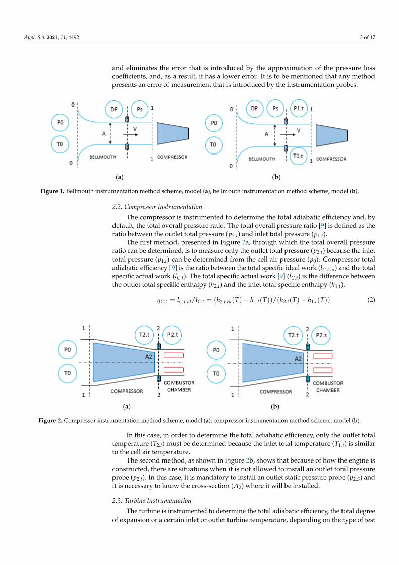
requested. Turbine total adiabatic efficiency [9] is the ratio between the total specific actualwork (lT.t) and the total specific ideal work (lT.t.id). The total specific actual work [9] (lT.t)is the difference between the inlet total specific enthalpy (h3.t) and the outlet total specificenthalpy (h4.t).

ηT.t = lT.t/lT.t.id = (h3.t(T)− h4.t(T))/(h3.t(T)− h4.t.id(T)) (3)

According to the engine instrumentation, in the vicinity of the turbine gas temperatureprobe location, an accessible instrumentation method, as presented in Figure 3, is used todetermine the total adiabatic efficiency. The outlet total pressure (p4.t) must be measured,and it is also necessary to measure the total outlet temperature (T4.t), since the total inlettemperature (T3.t) can be determined from the energy equation applied on the combustionchamber. This happens if the total inlet temperature (T3.t) is not measured.


In this case, in order to determine the total adiabatic efficiency, only the outlet total

temperature ( 2.tT ) must be determined because the inlet total temperature ( 1.tT ) is similar

to the cell air temperature.

The second method, as shown in Figure 2b, shows that because of how the engine is

constructed, there are situations when it is not allowed to install an outlet total pressure

probe ( 2.tp ). In this case, it is mandatory to install an outlet static pressure probe ( 2.sp )

and it is necessary to know the cross-section ( 2A ) where it will be installed.

2.3. Turbine Instrumentation

The turbine is instrumented to determine the total adiabatic efficiency, the total de-

gree of expansion or a certain inlet or outlet turbine temperature, depending on the type

of test requested. Turbine total adiabatic efficiency [9] is the ratio between the total specific

actual work ( .T tl ) and the total specific ideal work ( . .T t idl ). The total specific actual work

[9] ( .T tl ) is the difference between the inlet total specific enthalpy ( 3.th ) and the outlet

total specific enthalpy ( 4.th ).

. . . . 3. 4. 3. 4. .T t T t T t id t t t t idl l h T h T h T h T (3)

According to the engine instrumentation, in the vicinity of the turbine gas tempera-

ture probe location, an accessible instrumentation method, as presented in Figure 3, is

used to determine the total adiabatic efficiency. The outlet total pressure ( 4.tp ) must be

measured, and it is also necessary to measure the total outlet temperature ( 4.tT ), since

the total inlet temperature ( 3.tT ) can be determined from the energy equation applied on

the combustion chamber. This happens if the total inlet temperature ( 3.tT ) is not meas-

ured.

(a) (b)

Figure 3. Turbine instrumentation method scheme, model (a); turbine instrumentation method

scheme, model (b).

The method presented in Figure 3a requires only the total outlet turbine pressure and

temperature parameters, and it is not necessary to know the outlet turbine cross-section

in the calculation algorithm. The method presented in Figure 3b requires for the static

outlet turbine pressure to be measured. It is mandatory to know the outlet turbine cross-

section, used in the calculation algorithm.

2.4. Jet Nozzle Instrumentation

Figure 3. Turbine instrumentation method scheme, model (a); turbine instrumentation methodscheme, model (b).

The method presented in Figure 3a requires only the total outlet turbine pressure andtemperature parameters, and it is not necessary to know the outlet turbine cross-section inthe calculation algorithm. The method presented in Figure 3b requires for the static outletturbine pressure to be measured. It is mandatory to know the outlet turbine cross-section,used in the calculation algorithm.

2.4. Jet Nozzle Instrumentation

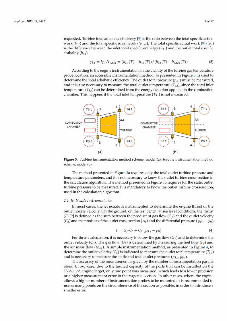
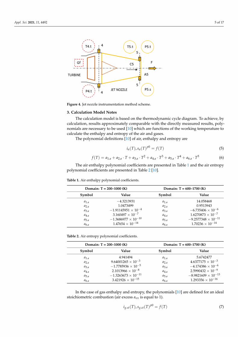
In most cases, the jet nozzle is instrumented to determine the engine thrust or theoutlet nozzle velocity. On the ground, on the test bench, at sea level conditions, the thrust(F) [9] is defined as the sum between the product of gas flow (G f ) and the outlet velocity(C5) and the product of the outlet cross-section (A5) and the differential pressure ( p5.t − p0).

F = G f ·C5 + C5·(p5.S − p0) (4)

For thrust calculation, it is necessary to know the gas flow (G f ) and to determine theoutlet velocity (C5). The gas flow (G f ) is determined by measuring the fuel flow (Ff ) andthe air mass flow (Ma f ). A simple instrumentation method, as presented in Figure 4, todetermine the outlet velocity (C5) is indicated to measure the outlet total temperature (T5.t)and is necessary to measure the static and total outlet pressures (p5.s, p5.t).

The accuracy of the measurement is given by the number of instrumentation param-eters. In our case, due to the limited capacity of the ports that can be installed on theTV2-117A engine target, only one point was measured, which leads to a lower precisionor a higher measurement error in the targeted section. In other cases, where the engineallows a higher number of instrumentation probes to be mounted, it is recommended touse as many points on the circumference of the section as possible, in order to introduce asmaller error.

Appl. Sci. 2021, 11, 4492 5 of 17


In most cases, the jet nozzle is instrumented to determine the engine thrust or the

outlet nozzle velocity. On the ground, on the test bench, at sea level conditions, the thrust

( F ) [9] is defined as the sum between the product of gas flow ( fG ) and the outlet ve-

locity ( 5C ) and the product of the outlet cross-section ( 5A ) and the differential pressure (

5. 0sp p ).

5 5 5. 0f sF G C A p p (4)

For thrust calculation, it is necessary to know the gas flow ( fG ) and to determine

the outlet velocity ( 5C ). The gas flow ( fG ) is determined by measuring the fuel flow (

fF ) and the air mass flow ( afM ). A simple instrumentation method, as presented in Fig-

ure 4, to determine the outlet velocity ( 5C ) is indicated to measure the outlet total tem-

perature ( 5.tT ) and is necessary to measure the static and total outlet pressures ( 5.sp ,

5.tp ).

Figure 4. Jet nozzle instrumentation method scheme.

The accuracy of the measurement is given by the number of instrumentation param-

eters. In our case, due to the limited capacity of the ports that can be installed on the TV2-

117A engine target, only one point was measured, which leads to a lower precision or a

higher measurement error in the targeted section. In other cases, where the engine allows

a higher number of instrumentation probes to be mounted, it is recommended to use as

many points on the circumference of the section as possible, in order to introduce a smaller

error.

3. Calculation Model Notes

The calculation model is based on the thermodynamic cycle diagram. To achieve, by

calculation, results approximately comparable with the directly measured results, poly-

nomials are necessary to be used [10] which are functions of the working temperature to

calculate the enthalpy and entropy of the air and gases.

The polynomial definitions [10] of air, enthalpy and entropy are

0

, ( )p

a ai T s T f T (5)

2 3 4 5

1. 2. 3. 4. 5. 6.( ) a a a a a af T a a T a T a T a T a T (6)

Figure 4. Jet nozzle instrumentation method scheme.

3. Calculation Model Notes

The calculation model is based on the thermodynamic cycle diagram. To achieve, bycalculation, results approximately comparable with the directly measured results, poly-nomials are necessary to be used [10] which are functions of the working temperature tocalculate the enthalpy and entropy of the air and gases.

The polynomial definitions [10] of air, enthalpy and entropy are

ia(T), sa(T)p0 = f (T) (5)

f (T) = a1.a + a2.a · T + a3.a · T2 + a4.a · T3 + a5.a · T4 + a6.a · T5 (6)

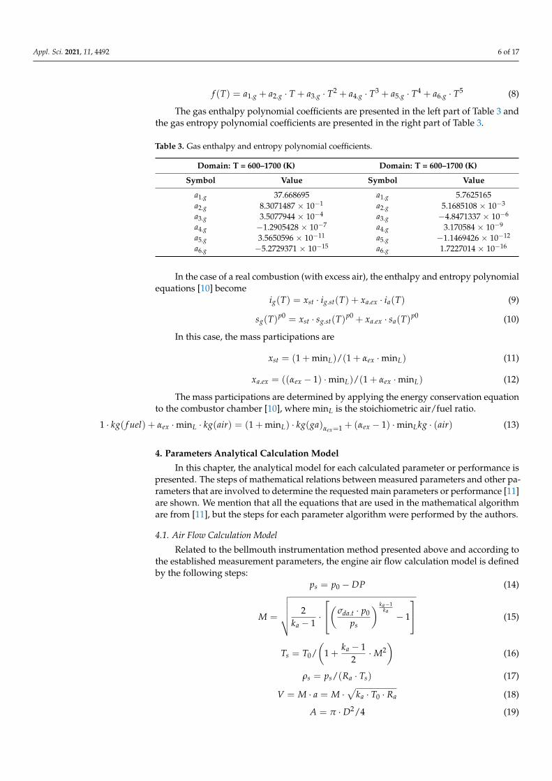
The air enthalpy polynomial coefficients are presented in Table 1 and the air entropypolynomial coefficients are presented in Table 2 [10].

Table 1. Air enthalpy polynomial coefficients.

Domain: T = 200–1000 (K) Domain: T = 600–1700 (K)

Symbol Value Symbol Value

a1.a −4.3213931 a1.a 14.058468a2.a 1.0473499 a2.a 0.9513943a3.a −1.91145951 × 10−4 a3.a −6.735406 × 10−6

a4.a 3.160497 × 10−7 a4.a 1.6270873 × 10−7

a5.a −1.3686977 × 10−10 a5.a −9.2577348 × 10−11

a6.a 1.47654 × 10−14 a6.a 1.70236 × 10−14

Table 2. Air entropy polynomial coefficients.



a1.a 4.941494 a1.a 5.6742477a2.a 9.64001265 × 10−3 a2.a 4.6377175 × 10−3

a3.a −1.7785936 × 10−5 a3.a −4.174386 × 10−6

a4.a 2.1013966 × 10−8 a4.a 2.5990432 × 10−9

a5.a −1.3263673 × 10−11 a5.a −8.9821609 × 10−13

a6.a 3.421926 × 10−15 a6.a 1.293356 × 10−16

In the case of gas enthalpy and entropy, the polynomials [10] are defined for an idealstoichiometric combustion (air excess αex is equal to 1).

ig.st(T), sg.st(T)p0 = f (T) (7)

Appl. Sci. 2021, 11, 4492 6 of 17

f (T) = a1.g + a2.g · T + a3.g · T2 + a4.g · T3 + a5.g · T4 + a6.g · T5 (8)

The gas enthalpy polynomial coefficients are presented in the left part of Table 3 andthe gas entropy polynomial coefficients are presented in the right part of Table 3.

Table 3. Gas enthalpy and entropy polynomial coefficients.



a1.g 37.668695 a1.g 5.7625165a2.g 8.3071487 × 10−1 a2.g 5.1685108 × 10−3

a3.g 3.5077944 × 10−4 a3.g −4.8471337 × 10−6

a4.g −1.2905428 × 10−7 a4.g 3.170584 × 10−9

a5.g 3.5650596 × 10−11 a5.g −1.1469426 × 10−12

a6.g −5.2729371 × 10−15 a6.g 1.7227014 × 10−16

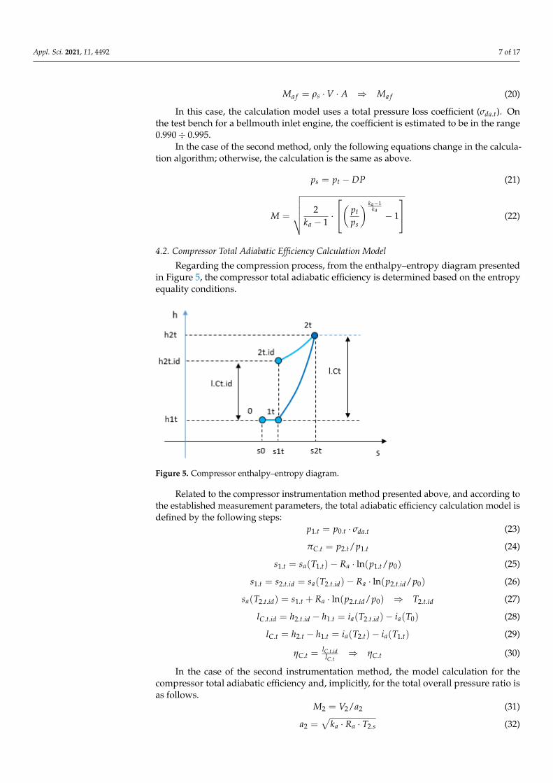
In the case of a real combustion (with excess air), the enthalpy and entropy polynomialequations [10] become

ig(T) = xst · ig.st(T) + xa.ex · ia(T) (9)

sg(T)p0 = xst · sg.st(T)

p0 + xa.ex · sa(T)p0 (10)

In this case, the mass participations are

xst = (1 + minL)/(1 + αex ·minL) (11)

xa.ex = ((αex − 1) ·minL)/(1 + αex ·minL) (12)

The mass participations are determined by applying the energy conservation equationto the combustor chamber [10], where minL is the stoichiometric air/fuel ratio.

1 · kg( f uel) + αex ·minL · kg(air) = (1 + minL) · kg(ga)αex=1 + (αex − 1) ·minLkg · (air) (13)

4. Parameters Analytical Calculation Model

In this chapter, the analytical model for each calculated parameter or performance ispresented. The steps of mathematical relations between measured parameters and other pa-rameters that are involved to determine the requested main parameters or performance [11]are shown. We mention that all the equations that are used in the mathematical algorithmare from [11], but the steps for each parameter algorithm were performed by the authors.

4.1. Air Flow Calculation Model

Related to the bellmouth instrumentation method presented above and according tothe established measurement parameters, the engine air flow calculation model is definedby the following steps:

ps = p0 − DP (14)

M =

√√√√√ 2ka − 1

·

(σda.t · p0

ps

) ka−1ka− 1

(15)

Ts = T0/(

1 +ka − 1

2·M2

)(16)

ρs = ps/(Ra · Ts) (17)

V = M · a = M ·√

ka · T0 · Ra (18)

A = π · D2/4 (19)

Appl. Sci. 2021, 11, 4492 7 of 17

Ma f = ρs ·V · A ⇒ Ma f (20)

In this case, the calculation model uses a total pressure loss coefficient (σda.t). Onthe test bench for a bellmouth inlet engine, the coefficient is estimated to be in the range0.990÷ 0.995.

In the case of the second method, only the following equations change in the calcula-tion algorithm; otherwise, the calculation is the same as above.

ps = pt − DP (21)

M =

√√√√√ 2ka − 1

·

( pt

ps

) ka−1ka− 1

(22)

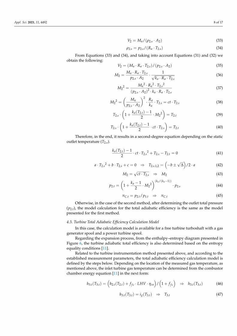
4.2. Compressor Total Adiabatic Efficiency Calculation Model

Regarding the compression process, from the enthalpy–entropy diagram presentedin Figure 5, the compressor total adiabatic efficiency is determined based on the entropyequality conditions.


In this case, the calculation model uses a total pressure loss coefficient ( .da t ). On the

test bench for a bellmouth inlet engine, the coefficient is estimated to be in the range

0.990 0.995 .

In the case of the second method, only the following equations change in the calcu-

lation algorithm; otherwise, the calculation is the same as above.

s tp p DP (21)

1

21

1

a

a

k

kt

a s

pM

k p

(22)

4.2. Compressor Total Adiabatic Efficiency Calculation Model

Regarding the compression process, from the enthalpy–entropy diagram presented

in Figure 5, the compressor total adiabatic efficiency is determined based on the entropy

equality conditions.

Figure 5. Compressor enthalpy–entropy diagram.

Related to the compressor instrumentation method presented above, and according

to the established measurement parameters, the total adiabatic efficiency calculation

model is defined by the following steps:

1. 0. .t t da tp p (23)

. 2. 1.C t t tp p (24)

1. 1. 1. 0lnt a t a ts s T R p p (25)

1. 2. . 2. . 2. . 0lnt t id a t id a t ids s s T R p p (26)

2. . 1. 2. . 0 2. .lna t id t a t id t ids T s R p p T (27)

. . 2. . 1. 2. . 0C t id t id t a t id al h h i T i T (28)

. 2. 1. 2. 1.C t t t a t a tl h h i T i T (29)

Figure 5. Compressor enthalpy–entropy diagram.

Related to the compressor instrumentation method presented above, and according tothe established measurement parameters, the total adiabatic efficiency calculation model isdefined by the following steps:

p1.t = p0.t · σda.t (23)

πC.t = p2.t/p1.t (24)

s1.t = sa(T1.t)− Ra · ln(p1.t/p0) (25)

s1.t = s2.t.id = sa(T2.t.id)− Ra · ln(p2.t.id/p0) (26)

sa(T2.t.id) = s1.t + Ra · ln(p2.t.id/p0) ⇒ T2.t.id (27)

lC.t.id = h2.t.id − h1.t = ia(T2.t.id)− ia(T0) (28)

lC.t = h2.t − h1.t = ia(T2.t)− ia(T1.t) (29)

ηC.t =lC.t.idlC.t

⇒ ηC.t (30)

In the case of the second instrumentation method, the model calculation for thecompressor total adiabatic efficiency and, implicitly, for the total overall pressure ratio isas follows.

M2 = V2/a2 (31)

a2 =√

ka · Ra · T2.s (32)

Appl. Sci. 2021, 11, 4492 8 of 17

V2 = Ma/(ρ2.s · A2) (33)

ρ2.s = p2.s/(Ra · T2.s) (34)

From Equations (33) and (34), and taking into account Equations (31) and (32) weobtain the following:

V2 = (Ma · Ra · T2.s)/(p2.s · A2) (35)

M2 =Ma · Ra · T2.s

p2.s · A2· 1√

ka · Ra · T2.s(36)

M22 =

Ma2 · Ra

2 · T2.s2

(p2.s · A2)2 · ka · Ra · T2.s

(37)

M22 =

(Ma

p2.s · A2

)2· Ra

ka· T2.s = ct · T2.s (38)

T2.s ·(

1 +ka(T2.t)− 1

2·M2

2)= T2.t (39)

T2.s ·(

1 +ka(T2.t)− 1

2· ct · T2.s

)= T2.t (40)

Therefore, in the end, it results in a second-degree equation depending on the staticoutlet temperature (T2.s).

ka(T2.t)− 12

· ct · T2.s2 + T2.s − T2.t = 0 (41)

a · T2.s2 + b · T2.s + c = 0 ⇒ T2.s.1,2 =

(−b±

√∆)

/2 · a (42)

M2 =√

ct · T2.s ⇒ M2 (43)

p2.t =

(1 +

ka − 12·M2

2)(ka/(ka−1))

· p2.s (44)

πC.t = p2.t/p1.t ⇒ πC.t (45)

Otherwise, in the case of the second method, after determining the outlet total pressure(p2.t), the model calculation for the total adiabatic efficiency is the same as the modelpresented for the first method.

4.3. Turbine Total Adiabatic Efficiency Calculation Model

In this case, the calculation model is available for a free turbine turboshaft with a gasgenerator spool and a power turbine spool.

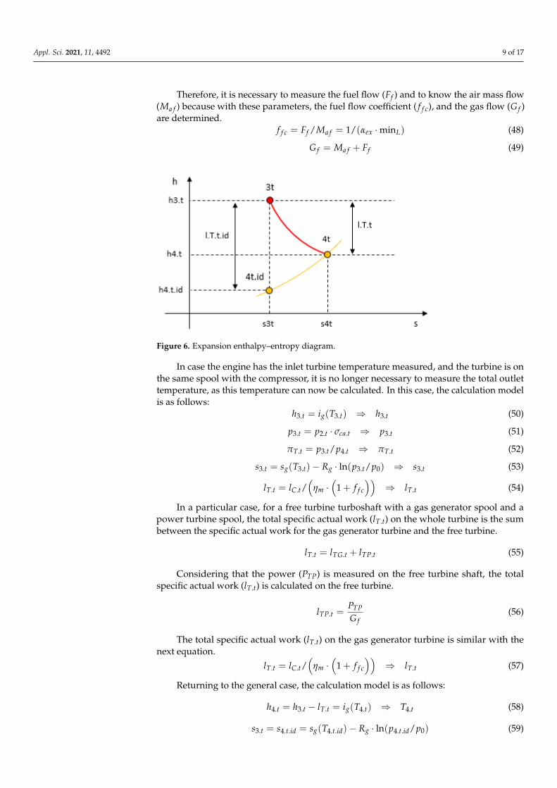
Regarding the expansion process, from the enthalpy–entropy diagram presented inFigure 6, the turbine adiabatic total efficiency is also determined based on the entropyequality conditions [11].

Related to the turbine instrumentation method presented above, and according to theestablished measurement parameters, the total adiabatic efficiency calculation model isdefined by the steps below. Depending on the location of the measured gas temperature, asmentioned above, the inlet turbine gas temperature can be determined from the combustorchamber energy equation [11] in the next form:

h3.t(T3.t) =(

h2.t(T2.t) + f f c · LHV · ηca

)/(

1 + f f c

)⇒ h3.t(T3.t) (46)

h3.t(T3.t) = ig(T3.t) ⇒ T3.t (47)

Appl. Sci. 2021, 11, 4492 9 of 17

Therefore, it is necessary to measure the fuel flow (Ff ) and to know the air mass flow(Ma f ) because with these parameters, the fuel flow coefficient ( f f c), and the gas flow (G f )are determined.

f f c = Ff /Ma f = 1/(αex ·minL) (48)

G f = Ma f + Ff (49)


Otherwise, in the case of the second method, after determining the outlet total pres-

sure ( 2.tp ), the model calculation for the total adiabatic efficiency is the same as the model

presented for the first method.

4.3. Turbine Total Adiabatic Efficiency Calculation Model

In this case, the calculation model is available for a free turbine turboshaft with a gas

generator spool and a power turbine spool.

Regarding the expansion process, from the enthalpy–entropy diagram presented in

Figure 6, the turbine adiabatic total efficiency is also determined based on the entropy

equality conditions [11].

Figure 6. Expansion enthalpy–entropy diagram.

Related to the turbine instrumentation method presented above, and according to the

established measurement parameters, the total adiabatic efficiency calculation model is

defined by the steps below. Depending on the location of the measured gas temperature,

as mentioned above, the inlet turbine gas temperature can be determined from the com-

bustor chamber energy equation [11] in the next form:

3. 3. 2. 2. 3. 3.( ) ( ) 1 ( )t t t t fc ca fc t th T h T f LHV f h T (46)

3. 3. 3. 3.( )t t g t th T i T T (47)

Therefore, it is necessary to measure the fuel flow ( fF ) and to know the air mass flow

( afM ) because with these parameters, the fuel flow coefficient ( fcf ), and the gas flow ( fG

) are determined.

1 minfc f af ex Lf F M (48)

f af fG M F (49)

In case the engine has the inlet turbine temperature measured, and the turbine is on

the same spool with the compressor, it is no longer necessary to measure the total outlet

temperature, as this temperature can now be calculated. In this case, the calculation model

is as follows:

3. 3. 3.t g t th i T h (50)

3. 2. . 3.t t ca t tp p p (51)

Figure 6. Expansion enthalpy–entropy diagram.

In case the engine has the inlet turbine temperature measured, and the turbine is onthe same spool with the compressor, it is no longer necessary to measure the total outlettemperature, as this temperature can now be calculated. In this case, the calculation modelis as follows:

h3.t = ig(T3.t) ⇒ h3.t (50)

p3.t = p2.t · σca.t ⇒ p3.t (51)

πT.t = p3.t/p4.t ⇒ πT.t (52)

s3.t = sg(T3.t)− Rg · ln(p3.t/p0) ⇒ s3.t (53)

lT.t = lC.t/(

ηm ·(

1 + f f c

))⇒ lT.t (54)

In a particular case, for a free turbine turboshaft with a gas generator spool and apower turbine spool, the total specific actual work (lT.t) on the whole turbine is the sumbetween the specific actual work for the gas generator turbine and the free turbine.

lT.t = lTG.t + lTP.t (55)

Considering that the power (PTP) is measured on the free turbine shaft, the totalspecific actual work (lT.t) is calculated on the free turbine.

lTP.t =PTPG f

(56)

The total specific actual work (lT.t) on the gas generator turbine is similar with thenext equation.

lT.t = lC.t/(

ηm ·(

1 + f f c

))⇒ lT.t (57)

Returning to the general case, the calculation model is as follows:

h4.t = h3.t − lT.t = ig(T4.t) ⇒ T4.t (58)

s3.t = s4.t.id = sg(T4.t.id)− Rg · ln(p4.t.id/p0) (59)

Appl. Sci. 2021, 11, 4492 10 of 17

sg(T4.t.id) = s3.t + Rg · ln(p4.t/p0) ⇒ T4.t.id (60)

lT.t.id = h3.t − h4.t.id = h3.t − ig(T4.t.id) (61)

ηT.t = lT.t/lT.t.id ⇒ ηT.t (62)

In the case of the second instrumentation method, the model calculation for the turbinetotal adiabatic efficiency is similar to the compressor model and follows the same steps,but it uses the parameters from the outlet and inlet turbine stations.

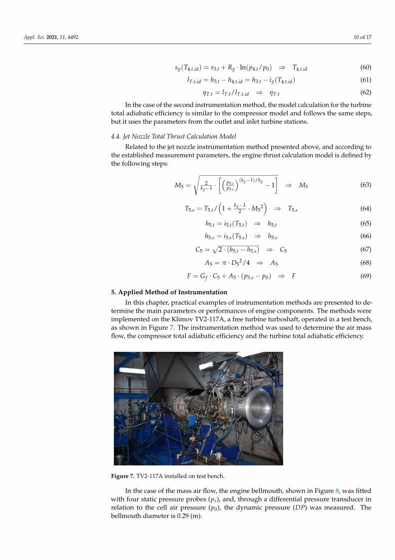
4.4. Jet Nozzle Total Thrust Calculation Model

Related to the jet nozzle instrumentation method presented above, and according tothe established measurement parameters, the engine thrust calculation model is defined bythe following steps:

M5 =

√2

kg−1 ·[(

p5.tp5.s

)(kg−1)/kg− 1]⇒ M5 (63)

T5.s = T5.t/(

1 + kg−12 ·M5

2)⇒ T5.s (64)

h5.t = i5.t(T5.t) ⇒ h5.t (65)

h5.s = i5.s(T5.s) ⇒ h5.s (66)

C5 =√

2 · (h5.t − h5.s) ⇒ C5 (67)

A5 = π · D52/4 ⇒ A5 (68)

F = G f · C5 + A5 · (p5.s − p0) ⇒ F (69)

5. Applied Method of Instrumentation

In this chapter, practical examples of instrumentation methods are presented to de-termine the main parameters or performances of engine components. The methods wereimplemented on the Klimov TV2-117A, a free turbine turboshaft, operated in a test bench,as shown in Figure 7. The instrumentation method was used to determine the air massflow, the compressor total adiabatic efficiency and the turbine total adiabatic efficiency.


5. 5. 5. 5. s s s sh i T h (66)

5 5. 5. 52 t sC h h C (67)

2

5 5 54A D A (68)

5 5 5. 0f sF G C A p p F (69)


In this chapter, practical examples of instrumentation methods are presented to de-

termine the main parameters or performances of engine components. The methods were

implemented on the Klimov TV2-117A, a free turbine turboshaft, operated in a test bench,

as shown in Figure 7. The instrumentation method was used to determine the air mass

flow, the compressor total adiabatic efficiency and the turbine total adiabatic efficiency.

Figure 7. TV2-117A installed on test bench.

In the case of the mass air flow, the engine bellmouth, shown in Figure 8, was fitted

with four static pressure probes ( sp ), and, through a differential pressure transducer in

relation to the cell air pressure ( 0p ), the dynamic pressure ( DP ) was measured. The

bellmouth diameter is 0.29 (m).

Figure 8. TV2-117A bellmouth instrumentation.


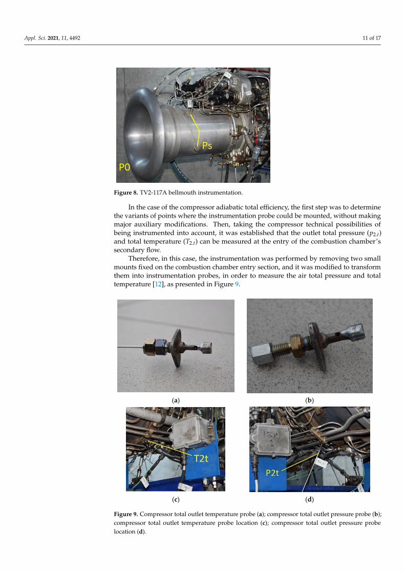
In the case of the mass air flow, the engine bellmouth, shown in Figure 8, was fittedwith four static pressure probes (ps), and, through a differential pressure transducer inrelation to the cell air pressure (p0), the dynamic pressure (DP) was measured. Thebellmouth diameter is 0.29 (m).

Appl. Sci. 2021, 11, 4492 11 of 17


5. 5. 5. 5. s s s sh i T h (66)

5 5. 5. 52 t sC h h C (67)

2

5 5 54A D A (68)

5 5 5. 0f sF G C A p p F (69)


In this chapter, practical examples of instrumentation methods are presented to de-

termine the main parameters or performances of engine components. The methods were

implemented on the Klimov TV2-117A, a free turbine turboshaft, operated in a test bench,

as shown in Figure 7. The instrumentation method was used to determine the air mass

flow, the compressor total adiabatic efficiency and the turbine total adiabatic efficiency.


In the case of the mass air flow, the engine bellmouth, shown in Figure 8, was fitted

with four static pressure probes ( sp ), and, through a differential pressure transducer in

relation to the cell air pressure ( 0p ), the dynamic pressure ( DP ) was measured. The

bellmouth diameter is 0.29 (m).

Figure 8. TV2-117A bellmouth instrumentation. Figure 8. TV2-117A bellmouth instrumentation.

In the case of the compressor adiabatic total efficiency, the first step was to determinethe variants of points where the instrumentation probe could be mounted, without makingmajor auxiliary modifications. Then, taking the compressor technical possibilities ofbeing instrumented into account, it was established that the outlet total pressure (p2.t)and total temperature (T2.t) can be measured at the entry of the combustion chamber’ssecondary flow.

Therefore, in this case, the instrumentation was performed by removing two smallmounts fixed on the combustion chamber entry section, and it was modified to transformthem into instrumentation probes, in order to measure the air total pressure and totaltemperature [12], as presented in Figure 9.


In the case of the compressor adiabatic total efficiency, the first step was to determine the variants of points where the instrumentation probe could be mounted, without making major auxiliary modifications. Then, taking the compressor technical possibilities

of being instrumented into account, it was established that the outlet total pressure ( 2.tp) and total temperature ( 2.tT ) can be measured at the entry of the combustion chamber’s secondary flow.

Therefore, in this case, the instrumentation was performed by removing two small mounts fixed on the combustion chamber entry section, and it was modified to transform them into instrumentation probes, in order to measure the air total pressure and total temperature [12], as presented in Figure 9.

(a) (b)

(c) (d)

Figure 9. Compressor total outlet temperature probe (a); compressor total outlet pressure probe (b); compressor total outlet temperature probe location (c); compressor total outlet pressure probe location (d).

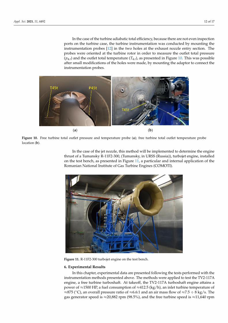
In the case of the turbine adiabatic total efficiency, because there are not even inspection ports on the turbine case, the turbine instrumentation was conducted by mounting the instrumentation probes [12] in the two holes at the exhaust nozzle entry section. The probes were oriented at the turbine rotor in order to measure the outlet total

pressure ( 4.tp ) and the outlet total temperature ( 4.tT ), as presented in Figure 10. This was possible after small modifications of the holes were made, by mounting the adaptor to connect the instrumentation probes.

Figure 9. Compressor total outlet temperature probe (a); compressor total outlet pressure probe (b);compressor total outlet temperature probe location (c); compressor total outlet pressure probelocation (d).

Appl. Sci. 2021, 11, 4492 12 of 17

In the case of the turbine adiabatic total efficiency, because there are not even inspectionports on the turbine case, the turbine instrumentation was conducted by mounting theinstrumentation probes [12] in the two holes at the exhaust nozzle entry section. Theprobes were oriented at the turbine rotor in order to measure the outlet total pressure(p4.t) and the outlet total temperature (T4.t), as presented in Figure 10. This was possibleafter small modifications of the holes were made, by mounting the adaptor to connect theinstrumentation probes.


(a) (b)

Figure 10. Free turbine total outlet pressure and temperature probe (a); free turbine total outlet temperature probe location (b).

In the case of the jet nozzle, this method will be implemented to determine the engine thrust of a Tumansky R-11F2-300, (Tumansky, in URSS (Russia)), turbojet engine, installed on the test bench, as presented in Figure 11, a particular and internal application of the Romanian National Institute of Gas Turbine Engines (COMOTI).

Figure 11. R-11F2-300 turbojet engine on the test bench.

6. Experimental Results In this chapter, experimental data are presented following the tests performed with

the instrumentation methods presented above. The methods were applied to test the TV2-117A engine, a free turbine turboshaft. At takeoff, the TV2-117A turboshaft engine attains a power of ≈ 1500 HP, a fuel consumption of ≈ 412.5 (kg/h), an inlet turbine temperature of ≈ 875 (°C), an overall pressure ratio of ≈ 6.6:1 and an air mass flow of ≈ 7.5÷8 kg/s. The gas generator speed is ≈ 20,882 rpm (98.5%), and the free turbine speed is ≈ 11,640 rpm (97%). The engine was tested on various working regimes, defined by the gas generator

shaft speed ( GGN ), from idle (64.80%) to a maximum regime (99.11%), so the measured parameters were acquired at each working regime. The experimental values were used in the calculation model presented above in order to determine the mass air flow and the compressor and turbine total adiabatic efficiency. The calculated values are presented in the tables below.

In our case, due to the limited information from the description manual which is provided by the engine manufacturer, the takeoff regime is defined only by the values of

Figure 10. Free turbine total outlet pressure and temperature probe (a); free turbine total outlet temperature probelocation (b).

In the case of the jet nozzle, this method will be implemented to determine the enginethrust of a Tumansky R-11F2-300, (Tumansky, in URSS (Russia)), turbojet engine, installedon the test bench, as presented in Figure 11, a particular and internal application of theRomanian National Institute of Gas Turbine Engines (COMOTI).


(a) (b)

Figure 10. Free turbine total outlet pressure and temperature probe (a); free turbine total outlet

temperature probe location (b).

In the case of the jet nozzle, this method will be implemented to determine the engine

thrust of a Tumansky R-11F2-300, (Tumansky, in URSS (Russia)), turbojet engine, installed

on the test bench, as presented in Figure 11, a particular and internal application of the

Romanian National Institute of Gas Turbine Engines (COMOTI).


6. Experimental Results

In this chapter, experimental data are presented following the tests performed with

the instrumentation methods presented above. The methods were applied to test the TV2-

117A engine, a free turbine turboshaft. At takeoff, the TV2-117A turboshaft engine attains

a power of ≈ 1500 HP, a fuel consumption of ≈ 412.5 (kg/h), an inlet turbine temperature

of ≈ 875 (°C), an overall pressure ratio of ≈ 6.6:1 and an air mass flow of ≈ 7.5÷8 kg/s. The

gas generator speed is ≈ 20,882 rpm (98.5%), and the free turbine speed is ≈ 11,640 rpm

(97%). The engine was tested on various working regimes, defined by the gas generator

shaft speed ( GGN ), from idle (64.80%) to a maximum regime (99.11%), so the measured

parameters were acquired at each working regime. The experimental values were used in

the calculation model presented above in order to determine the mass air flow and the

compressor and turbine total adiabatic efficiency. The calculated values are presented in

the tables below.

In our case, due to the limited information from the description manual which is pro-

vided by the engine manufacturer, the takeoff regime is defined only by the values of shaft


6. Experimental Results

In this chapter, experimental data are presented following the tests performed with theinstrumentation methods presented above. The methods were applied to test the TV2-117Aengine, a free turbine turboshaft. At takeoff, the TV2-117A turboshaft engine attains apower of ≈1500 HP, a fuel consumption of ≈412.5 (kg/h), an inlet turbine temperature of≈875 (◦C), an overall pressure ratio of ≈6.6:1 and an air mass flow of ≈7.5 ÷ 8 kg/s. Thegas generator speed is ≈20,882 rpm (98.5%), and the free turbine speed is ≈11,640 rpm

Appl. Sci. 2021, 11, 4492 13 of 17

(97%). The engine was tested on various working regimes, defined by the gas generatorshaft speed (NGG), from idle (64.80%) to a maximum regime (99.11%), so the measuredparameters were acquired at each working regime. The experimental values were usedin the calculation model presented above in order to determine the mass air flow and thecompressor and turbine total adiabatic efficiency. The calculated values are presented inthe tables below.

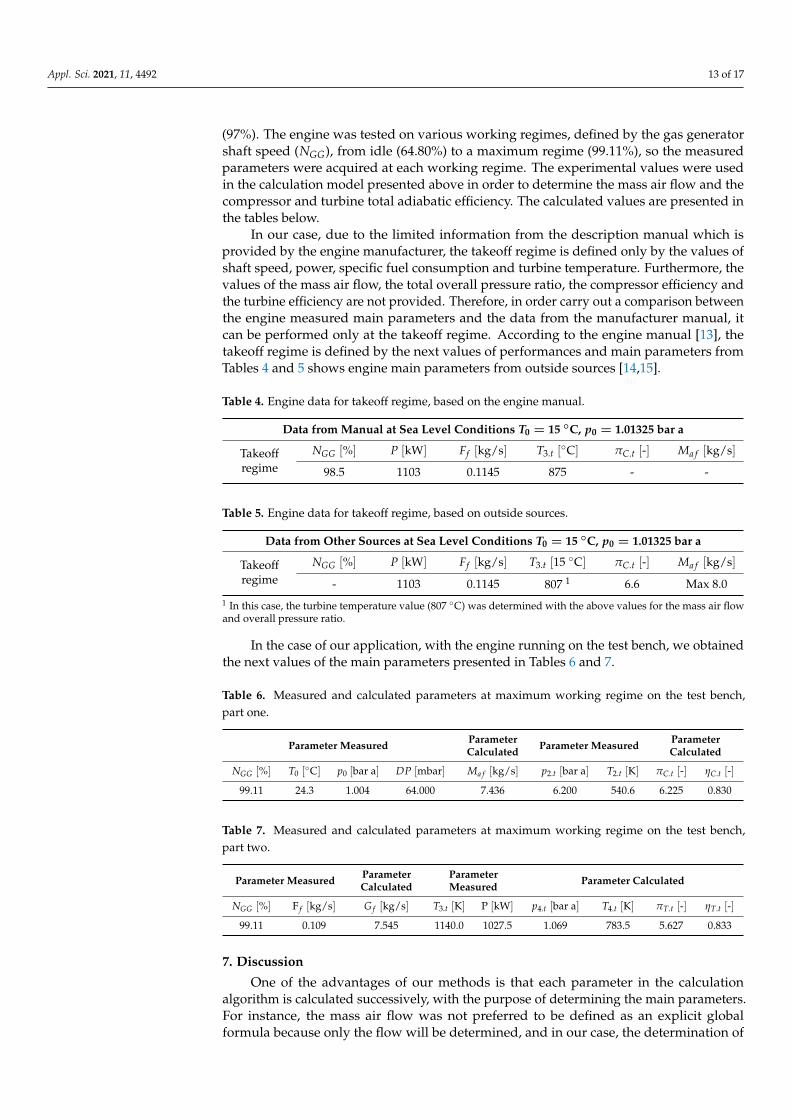
In our case, due to the limited information from the description manual which isprovided by the engine manufacturer, the takeoff regime is defined only by the values ofshaft speed, power, specific fuel consumption and turbine temperature. Furthermore, thevalues of the mass air flow, the total overall pressure ratio, the compressor efficiency andthe turbine efficiency are not provided. Therefore, in order carry out a comparison betweenthe engine measured main parameters and the data from the manufacturer manual, itcan be performed only at the takeoff regime. According to the engine manual [13], thetakeoff regime is defined by the next values of performances and main parameters fromTables 4 and 5 shows engine main parameters from outside sources [14,15].

Table 4. Engine data for takeoff regime, based on the engine manual.

Data from Manual at Sea Level Conditions T0 = 15 ◦C, p0 = 1.01325 bar a

Takeoffregime

NGG [%] P [kW] Ff [kg/s] T3.t [◦C] πC.t [-] Ma f [kg/s]

98.5 1103 0.1145 875 - -

Table 5. Engine data for takeoff regime, based on outside sources.

Data from Other Sources at Sea Level Conditions T0 = 15 ◦C, p0 = 1.01325 bar a

Takeoffregime

NGG [%] P [kW] Ff [kg/s] T3.t [15 ◦C] πC.t [-] Ma f [kg/s]

- 1103 0.1145 807 1 6.6 Max 8.01 In this case, the turbine temperature value (807 ◦C) was determined with the above values for the mass air flowand overall pressure ratio.

In the case of our application, with the engine running on the test bench, we obtainedthe next values of the main parameters presented in Tables 6 and 7.

Table 6. Measured and calculated parameters at maximum working regime on the test bench,part one.

Parameter Measured ParameterCalculated Parameter Measured Parameter

Calculated

NGG [%] T0 [◦C] p0 [bar a] DP [mbar] Ma f [kg/s] p2.t [bar a] T2.t [K] πC.t [-] ηC.t [-]

99.11 24.3 1.004 64.000 7.436 6.200 540.6 6.225 0.830

Table 7. Measured and calculated parameters at maximum working regime on the test bench,part two.

Parameter Measured ParameterCalculated

ParameterMeasured Parameter Calculated

NGG [%] F f [kg/s] G f [kg/s] T3.t [K] P [kW] p4.t [bar a] T4.t [K] πT.t [-] ηT.t [-]

99.11 0.109 7.545 1140.0 1027.5 1.069 783.5 5.627 0.833

7. Discussion

One of the advantages of our methods is that each parameter in the calculationalgorithm is calculated successively, with the purpose of determining the main parameters.For instance, the mass air flow was not preferred to be defined as an explicit globalformula because only the flow will be determined, and in our case, the determination of

Appl. Sci. 2021, 11, 4492 14 of 17

all parameters was aimed at. For the same reason, it was applied on most of the enginemain parameters.

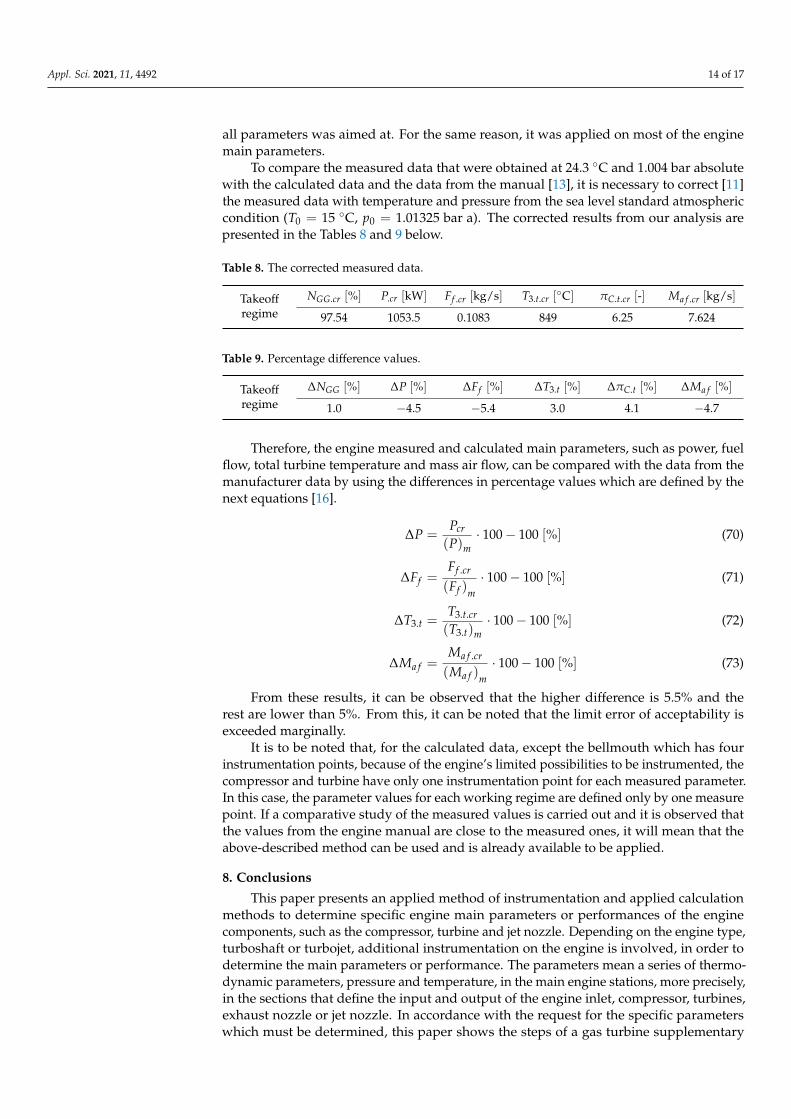
To compare the measured data that were obtained at 24.3 ◦C and 1.004 bar absolutewith the calculated data and the data from the manual [13], it is necessary to correct [11]the measured data with temperature and pressure from the sea level standard atmosphericcondition (T0 = 15 ◦C, p0 = 1.01325 bar a). The corrected results from our analysis arepresented in the Tables 8 and 9 below.

Table 8. The corrected measured data.

Takeoffregime

NGG.cr [%] P.cr [kW] Ff .cr [kg/s] T3.t.cr [◦C] πC.t.cr [-] Ma f .cr [kg/s]

97.54 1053.5 0.1083 849 6.25 7.624

Table 9. Percentage difference values.

Takeoffregime

∆NGG [%] ∆P [%] ∆Ff [%] ∆T3.t [%] ∆πC.t [%] ∆Ma f [%]

1.0 −4.5 −5.4 3.0 4.1 −4.7

Therefore, the engine measured and calculated main parameters, such as power, fuelflow, total turbine temperature and mass air flow, can be compared with the data from themanufacturer data by using the differences in percentage values which are defined by thenext equations [16].

∆P =Pcr

(P)m· 100− 100 [%] (70)

∆Ff =Ff .cr

(Ff )m· 100− 100 [%] (71)

∆T3.t =T3.t.cr

(T3.t)m· 100− 100 [%] (72)

∆Ma f =Ma f .cr

(Ma f )m· 100− 100 [%] (73)

From these results, it can be observed that the higher difference is 5.5% and therest are lower than 5%. From this, it can be noted that the limit error of acceptability isexceeded marginally.

It is to be noted that, for the calculated data, except the bellmouth which has fourinstrumentation points, because of the engine’s limited possibilities to be instrumented, thecompressor and turbine have only one instrumentation point for each measured parameter.In this case, the parameter values for each working regime are defined only by one measurepoint. If a comparative study of the measured values is carried out and it is observed thatthe values from the engine manual are close to the measured ones, it will mean that theabove-described method can be used and is already available to be applied.

8. Conclusions

This paper presents an applied method of instrumentation and applied calculationmethods to determine specific engine main parameters or performances of the enginecomponents, such as the compressor, turbine and jet nozzle. Depending on the engine type,turboshaft or turbojet, additional instrumentation on the engine is involved, in order todetermine the main parameters or performance. The parameters mean a series of thermo-dynamic parameters, pressure and temperature, in the main engine stations, more precisely,in the sections that define the input and output of the engine inlet, compressor, turbines,exhaust nozzle or jet nozzle. In accordance with the request for the specific parameterswhich must be determined, this paper shows the steps of a gas turbine supplementary

Appl. Sci. 2021, 11, 4492 15 of 17

instrumentation, starting from the study on how accessible is the engine to be instru-mented, the study of what parameters can be measured and the possibility of installing theinstrumentation probes, and ending with the main parameters and performance modelcalculation for each applied instrumentation method, based on the various measureddata. By testing the engine on a test bench, a series of experimental results were obtained,which were analyzed and compared with reference values from the engine manual. Itwas determined that the values from the test and from the manual are very similar, whichmeans that instrumentation methods and model calculations are available to be appliedand implemented on other engines as well.

Author Contributions: Conceptualization, R.M.C. and C.M.T.; methodology, R.M.C.; software, G.D.;validation, H.M.S, ., C.M.T. and G.D.; formal analysis, H.M.S, .; investigation, H.M.S, .; resources, R.M.C.;data curation, C.M.T.; writing—original draft preparation, R.M.C.; writing—review and editing,C.M.T.; visualization, H.M.S, .; supervision, G.D. Moreover, preparing the engines, instrumentation,the acquisition of parameters and testing were conducted by all authors. All authors have read andagreed to the published version of the manuscript.

Funding: This research was funded by the National Research and Development Institute for GasTurbines COMOTI, Romania.

Institutional Review Board Statement: Not applicable.

Informed Consent Statement: Not applicable.

Data Availability Statement: Experimental data were obtained following the engine tests that wereinternally conducted at the National Research and Development Institute for Gas Turbines COMOTI,in the gas turbine engine research-development stand for aeronautical (civil and military) andindustrial applications department, and the data presented in this study are available in this article.

Conflicts of Interest: The authors declare no conflict of interest.

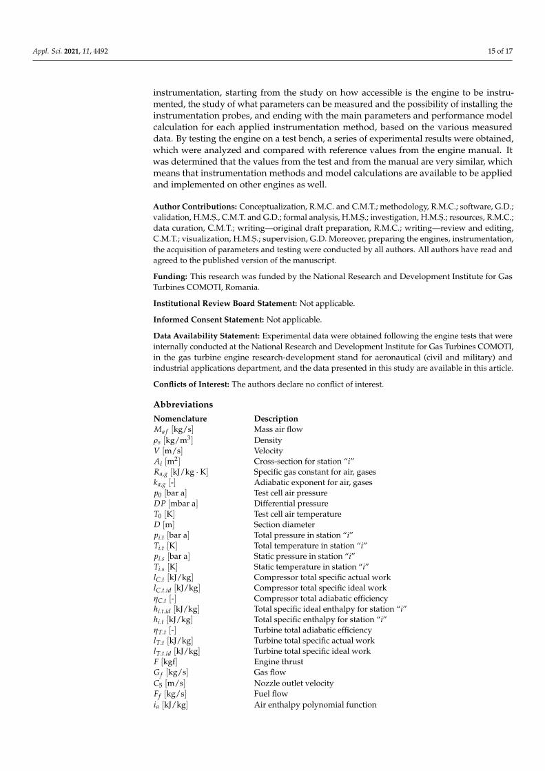
AbbreviationsNomenclature DescriptionMa f [kg/s] Mass air flowρs [kg/m3] DensityV [m/s] VelocityAi [m2] Cross-section for station “i”Ra,g [kJ/kg ·K] Specific gas constant for air, gaseska,g [-] Adiabatic exponent for air, gasesp0 [bar a] Test cell air pressureDP [mbar a] Differential pressureT0 [K] Test cell air temperatureD [m] Section diameterpi.t [bar a] Total pressure in station “i”Ti.t [K] Total temperature in station “i”pi.s [bar a] Static pressure in station “i”Ti.s [K] Static temperature in station “i”lC.t [kJ/kg] Compressor total specific actual worklC.t.id [kJ/kg] Compressor total specific ideal workηC.t [-] Compressor total adiabatic efficiencyhi.t.id [kJ/kg] Total specific ideal enthalpy for station “i”hi.t [kJ/kg] Total specific enthalpy for station “i”ηT.t [-] Turbine total adiabatic efficiencylT.t [kJ/kg] Turbine total specific actual worklT.t.id [kJ/kg] Turbine total specific ideal workF [kgf] Engine thrustG f [kg/s] Gas flowC5 [m/s] Nozzle outlet velocityFf [kg/s] Fuel flowia [kJ/kg] Air enthalpy polynomial function

Appl. Sci. 2021, 11, 4492 16 of 17

sa [kJ/kg ·K] Air entropy polynomial functionai.a [-] Air enthalpy and entropy polynomial coefficientsig.st [kJ/kg] Gases enthalpy polynomial function for stoichiometric combustionsg.st [kJ/kg ·K] Gas entropy polynomial function for stoichiometric combustionai.g [-] Gas enthalpy and entropy polynomial coefficientsαex [-] Excess airxa.ex [-] Mass air participationsxst [-] Mass gases participationsig [kJ/kg] Gas enthalpy polynomial functionsg [kJ/kg ·K] Gas entropy polynomial functionminL [kg air/kg fuel] Stoichiometric air/fuel ratioMi [-] Mach number for station “i”σda.t [-] Total pressure loss coefficientπC.t [-] Total overall pressure ratioai [m/s] Sound velocity for station “i”f f c [-] Fuel flow coefficientLHV [kJ/kg ·K] Low heating valueηca [-] Combustion chamber efficiencyπT.t [-] Turbine total expansion degreeηm [-] Mechanic efficiencylTG.t [kJ] Gas generator turbine total specific actual worklTP.t [kJ] Free power turbine total specific actual workPTP [kW] Free turbine shaft powerNGG.cr [%] Corrected speedP.cr [kW] Corrected powerFf .cr [kg/s] Corrected fuel flowT3.t.cr [

◦C] Corrected total turbine temperatureπC.t.cr [-] Corrected total overall pressure ratioMa f .cr [kg/s] Corrected mass air flow∆P [%] Difference percentages of power∆Ff [%] Difference percentages of fuel flow∆T3.t [%] Difference percentages of total turbine temperature∆Ma f [%] Difference percentages of mass air flow

References1. SAE ARP 1217A. Instrumentation Requirements for Turboshaft Engine Performance Measurements; Aviation Standards; SAE Interna-

tional: Warrendale, PA, USA, 1 May 1997.2. SAE ARP 1587. Aircraft Gas Turbine Engine Monitoring System Guide; Aerospace Recommended Practice; SAE International:

Warrendale, PA, USA, April 1981.3. Available online: https://www.vzlu.cz/en/engineering-for-gas-turbine-engines-c272.html#prettyPhoto (accessed on

11 May 2021).4. Available online: https://www.ciam.ru/en/experimental-bases/ (accessed on 11 May 2021).5. SAE AIR 1873. Guide to Limited Engine Monitoring Systems for Aircraft Gas Turbine Engines; Aerospace Information Report; SAE

International: Warrendale, PA, USA, May 1988.6. Purvis, J.T. Industrial Gas Turbine Performance Measurement, International Congress on Combustion Engines; Texas A&M University:

College Station, TX, USA, 1974.7. Available online: https://www.bkvibro.com/fileadmin/mediapool/Internet/Application_Notes/Gas_Turbines_BAN0010EN12.

pdf (accessed on 11 May 2021).8. Saravanamuttoo, H.I.H. Recommended Practices for Measurement of Gas Path Pressures and Temperatures for Performance Assessment of

Aircraft Turbine Engines and Components; Theory of Gas Turbine, AGARD Advisory Report Number 245; Advisory Group forAerospace Research and Development (AGARD): Neuilly sur Seine, France, 1990.

9. Cohen, H.; Rogers, G.F.C.; Saravanamuttoo, H.I.H.; Mayhew, Y.R. Gas Turbine Theory, 4th ed.; Longman Group Limited: London,UK, 1996.

10. Stanciu, V. Jet Engines Preliminary Design Guide, Polytechnic Institute of Bucharest, Aircraft Faculty, Gas Turbine Theory, Course Notes;Polytechnic Institute of Bucharest: Bucharest, Romania, 1991. (Translation from Romanian)

11. Bathie, W.W. Fundamentals of Gas Turbines; Iowa State University of Science and Technology: Ames, IA, USA, 1984.12. Anthoine, J.; Arts, T.; Boerrigter, H.L. Measurement Techniques. In Fluid Dynamics, 3rd ed.; Von Karman Institute for Fluid

Dynamics: Genesius-Rode, Belgium, 2009; ISBN 978-2-930389-96-6.

https://www.vzlu.cz/en/engineering-for-gas-turbine-engines-c272.html#prettyPhoto

https://www.ciam.ru/en/experimental-bases/

https://www.bkvibro.com/fileadmin/mediapool/Internet/Application_Notes/Gas_Turbines_BAN0010EN12.pdf

https://www.bkvibro.com/fileadmin/mediapool/Internet/Application_Notes/Gas_Turbines_BAN0010EN12.pdf

Appl. Sci. 2021, 11, 4492 17 of 17

13. Zambfirescu, V. TV2-117A Free Turbine Turboshaft Engine Description and Maintenance Manual, Engine Maintenance; Documentationand Technical Publications Center: Bucharest, Romania, 1973. (Translation from Romanian)

14. Available online: http://all-aero.com/index.php/64-engines-power/13152-klimov-tv2-117-isotov-tv2-117 (accessed on11 May 2021).

15. Available online: http://etexportbg.com/en/catalog/aviation/engines.html (accessed on 11 May 2021).16. Available online: https://www.onlinemathlearning.com/relative-error-formula.html (accessed on 11 May 2021).

http://all-aero.com/index.php/64-engines-power/13152-klimov-tv2-117-isotov-tv2-117

http://etexportbg.com/en/catalog/aviation/engines.html

https://www.onlinemathlearning.com/relative-error-formula.html

performance calculations of gas turbine engine ... - mdpi

Documents