patterns of resource distribution and exploitation by the red fox
TRANSCRIPT
Patterns of resource distribution and exploitation
by the red fox (Vulpes vulpes) and the
Eurasian badger (Melee meles); a comparative study.
Heribert Hofer
A thesis submitted for the Degree of
Doctor of Philosophy at the University
of Oxford
Queen's College, June 1986
PATTERNS OP RESOURCE DISPERSION AND EXPLOITATION BY THE RED POX (VUlpea VUlpes) AND THE EURASIAN BADGER (Me168 meles)t A COMPARATIVE STUDY.
HerlDert Hofer Queen's College, oxford
Doctor of Philosophy Trinity 1986
Thirteen badgers and 20 foxes were radio-tracked in the Wytham Estate, Oxfordshire, between 1981 and 1983. Thirteen badger and 10 fox groups were identified from radio-tracking and bait marking. Badger groups (mean size 1982: 4.45, 1983t 5.82) occupied contiguous territories (sizet 22-75 ha) with boundaries marked by latrines. Seasonal variation in marking intensity and choice of marking sites presumably were responses to changing intrusion pressure. Fox groups (mean size? 2.6) occupied stable territories (sizet 22- 104 ha) with little overlap. Faeces deposition by foxes facilitated territory marking.
Earthworms^ Lumbricus terrestris) dominated the diet of badgers (63 % estimated dry weight EDW, faeces), followed by cereals, fruits and other Invertebrates. Diet was highly variable between groups and seasons. For foxes, lagomorphs (20 % EDW) and earthworms (33 % EDW) were the most important prey, followed by scavenge and fruits. Variation in diet between groups and seasons was marked in lagomorphs but not earthworms.
Multlvarlate analyses of habitat parameters revealed a low-dimensional 'resource space' that could be divided into conventional habitat categories. Censuses of prey species indicated that resource presence varied consistently between habitat categories.
Key habitats occurred at fairly constant proportions in territories of both species) their dispersion partly determined the configuration of territory boundaries. The proportions of specific habitats per territory were correlated with the proportions of certain prey items in diets.
space use by individuals was analysed by spatial autocorrelation methods, variation in space use by foxes was attributed to variation in resource dispersion. In contrast, individual badgers were similar in their use of space. Here, small-scale heterogeneity in intensity of use may reflect local earthworm availability, in one studied fox group, males and females differed in range use. Individuals in one studied badger group coordinated their use of space probably to minimize foraging interference.
It is suggested that group living in Wytham badgers is a response to defending resources, and a model is proposed to explain how the spatial and social organisation of male and female badgers relate to the characteristics of the resources they require.
To Marion
If you want to get the plain truth
Be not concerned with right and wrong
The conflict between right and wrong
Is the sickness of the mind.
Zen Master Seng-Ts'an
[Raymond M. Smullyani The tao is silent,
Harper & Row, New York 1977.]
CONTENTS
Abstract Contents Acknowledgements
1. INTRODUCTION............................................ 1
2. HABITAT................................................. 8
2.1. Introduction.................................... 92.2. The habitat map................................232.3. The habitat records............................ 322.4. Discussion.....................................48
3. RESOURCES................................................53
3.1. Introduction...................................543.2. Earthworms (Lumbricldae).......................563.3. Pheasant (Phasianus colchicua)................. 813.4. wood pigeon (Columba palumbus).................873.5. Rabbits (OrvctolaouB cuniculus)............... .833.6. Rodents.......................................1OO3.7. Discussion....................................103
4. DIET....................................................111
4.1 Introduction..................................1124.2 Pox diet......................................1144.3 Badger diet...................................1344.4 Comparison of fox and badger diet............. 153
5. FOX AND BADGER HOME RANGES..............................159
5.1. Introductioni review of home range concepts...1615.2. Methods of data collection....................1625.3. Methods of analysis...........................1685.4. Badger group ranges........................... 1755.5. Pox group ranges..............................1965.6. Habitat composition of and resource use in
group ranges.................................. 211
6. PATTERNS OP RANGE UTILIZATION...........................217
6.1. Methods.......................................2186.2. Patterns of space use......................... 2226.3. Simultaneous movements within the Upper
Follies badger group.......................... 2546.4. Habitat utilization...........................264
7. SPATIAL ORGANISATION AND REPRODUCTIVE STRATEGIES INBADGERS................................................. 274
7.1. Introduction..................................2757.2. Energetics of female reproductive effort......2767.3. Spatial and social strategies of females...... 2867.4. Male competition and female choice............3017.5. Discussioni resource characteristics, group
size and territoriality.......................3O9
APPENDICES
A.I.
A.2.
A. 3.
A.4.
A.5.
A.6.
A.7.
A.8.
A.9.
Statistical considerations for sampling designStatistical considerations for data analysis of habitat dataData selection procedures and statistical techniques for diet analysis statistical analysis of telemetry datat the problem of temporal independence Spatial independence of datat the concept of spatial autocorrelationA sequence of citations from the geographical and anthropological literature on the impor tance of spatially related data Computation procedure and test on significance of Koran's I and Geary's cAsymmetries of transition frequencies between patches as investigated by the Bradley-Terry Model of paired comparisons Estimate of dally energy expenditure of lac- tat ing female badgers
REFERENCES
A detailed table of contents Is listed at the beginning of each chapter.
ACKNOWLEDGEMENTS
It la a real pleasure to express my gratitude (at least once) to the
many people that have so unfailingly supported this project. I owe the
greatest debt to my supervisor, David Macdonald, whose constant and
unwavering support and infectious enthusiasm for the project has kept me
going through many bad patches. I shall never forget the unique way by which
he introduced me to my study area, my fellow Foxlot colleagues and the
mysteries of barn dancing within 24 hours after my arrival in Britain.
I than* Professor Sir Richard Southwood for use of the Zoology
Department and Dr David McFarland for space in the Animal Behaviour Research
Group. I am very grateful to the organisations that provided studentships
and financial supporti the Studienstiftung des deutschen Volkes (German
National scholarship Foundation) and the Deutscher Akademischer
Austauschdienst (German Academic Exchange Service) in Germany and Queen's
College for an EPA Florey studentship. Many thanks go to the great people
from intake, and in particular the workshops: Dave Palmer, Tony Price and
Dick Cheney have always listened to my requests and constructed all kinds of
ingenious equipment. I am also grateful for the support from the electronics
people, Mike Dolan and Terry Barker. Many people within the University, and
in particular the Computer Centre, were very cooperative and greatly helped
the progress of the study. Here, it is a special pleasure to mention Dr.
F.H.C. Marriott, university Lecturer in Biomathematics, who combines a
unique talent to explain statistical matters to non-initiated biologists
with a special enthusiasm for untidy, real field data. In the field, two
persons deserve a special award. Without Mrs. Gardiner, The Dewe House,
Wytham, the project could never have started. She allowed us access to her
garden at all day and night times, provided scavenge for the foxes and had a
deep, unparalleled concern for their well-being. Dennis Woods, the game
keeper from Wytham has been an active supporter of the project throughout
the studyi I got on very well with him. Back to the writing desk, I am very
grateful to Madeline Mltchell for typing most of the thesist without her
help it would have been Impossible to produce anything at all! In Germany, I
received much support from Angelika Jahner and Christine Zehren during
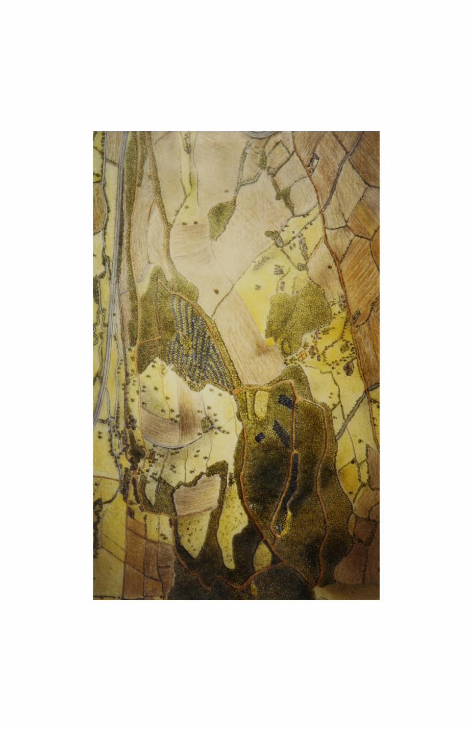
various stages of writing up. Angelika also is responsible for the beautiful
frontispiece.
Despite its peripheral locality in the department, the Poxlot room and
its inhabitants have played a central role during my stay in Oxford and have
been (by any standards) an incredible source of surprises, ideas and
laughters I am very grateful to Gill Kerby, Malcolm Newdick, Pat Doncaster,
Pall Hersteinsson, Emllio A. Herrera, Andy Taber, lan Llndsay and Geoff
Carr. Emllio Herrera not only shared the burden of celebrating our birthdays
together, but has put up with me for inumerable times (in all sorts of ways)
and been a source of Inspiration ranging from the secrets of the Epson
computer to fox faeces collection methods and the South American approach to
downhill skiing. Malcolm Newdick and Patrick Doncaster shared my enthusiasm
for fox-tracking and their enthusiasm for computer programming with me.
Without either of them, foxwork would have meant less success and much less
fun (re Caribbean).
Amongst the many friends that were part of the 'midnight community' in
the computer room I would like to single out Stephan Harding who is, amongst
other memorable events, responsible for me investigating the geographical
literature and discovering the subtleties of spatial dependence. I am also
grateful to Alan Grafen whose speed of thinking usually surpasses the
constraints of the human larynx as much as did the condensed thoughtfulness
of his brief statements overwhelm my capacities of comprehension
(conversations were therefore interspersed at half-year intervals).
Much-needed deflection from work was provided throughout most of the
time by the valuable members of the 'Bolywell zoo'. I thank Blythe Maraton,
Allson Sa^ovlc, Peter Paulsen, Anne Caubel, Said Rabbanl and Stacy Boffhaus

for their friendship.
Finally, I was very lucky to receive personal support from two sides.
My parents have always been on my side, no matter what happened - they
deserve a special honour. To Marion East I am deeply grateful for the
friendship she has granted me and the practical and intellectual support in
inumerable situations - not the least for getting my car out of snow drifts
or getting petrol at 4.30 in the morning!
1. Introduction.
Every animal faces four major tasksi
- avoid being killed or dying
- find something to eat
- find a place to live
- reproduce
The last three tasks deal with resources, ie. the acquisition and
exploitation of food, space, and mates. Ever since Crook's (1964) classical
study of weaver birds (Ploceinae), ethologlsts have come to appreciate that
three characteristics of resources,
- their occurrence in time and space,
- the predictability of their occurrence,
- their quality,
have a major influence on the way animals organise their lives. Broad
interspecific comparisons within major taxa have indicated important trends
in the relationship between the social organisation of a species and its
feeding ecology, morphological parameters (e.g. body size) and the habitats
occupied by that species (Jarman 1974 for antelopes, Glutton-Brock & Harvey
1977 for primates and Bekoff et al 1984 for carnivores). Although the
methodology used in these interspecific comparisons are not devoid of
criticism (Krebs fi Oavies 1981, Harvey & Mace 1962), they have been a
valuable source of stimulation for many behavioural ecology studies.
Within the carnivores, recent studies have revealed an Impressive
diversity of
- foraging strategies, ranging from solitary hunting (red
fox, Vulpes vulpes, Macdonald 1977a) to highly
organised cooperative ventures (e.g. in wild dogs,
Lvcaon pictus. Frame et al 1979)
- spatial and social systems, ranging from solitary
individuals (e.g. bears, Ursus arctos, Craighead
1979) to groups of SO animals on a territory (spotted
hyenas, Crocuta crocuta, Kruuk 1972),
- mating systems, ranging from strict monogamy (golden
jackals, Canis aureus, Moehlman 1983), to polygy-
nandry (lions, Panthera leo, Bertram 1975).
A focus of attention has been the relationship between social
organisation, in particular the occurrence of group living, foraging
strategies, and the dispersion of resources in space and time (Kruuk 1975,
Lamprecht 1981, Macdonald 1983a). To date, three classes of benefits derived
from group living have been identified for carnivorest
- cooperation in huntingt extension of the dietary spec
trum or increase in the efficiency of exploiting resour
ces (e.g. wolf,Canis lupus, Mech 1970)
- cooperation in anti-predator defensei reduction in
required vigilance and chance of capture, Improvement of
foraging rates and chances of escape from a predator
(e.g. banded mongoose, Rood 1974)
- cooperation In reproductioni Improvement of survival
a. of cubs due to helpers (e.g. brown hyena, Hyaena
brunnea. Owens & Owens 1984)
These benefits explain the occurrence of group living in some, but not all
carnivore species. Several species, amongst them the red fox, Vulpes vulpes,
the Eurasian badger, Meles roeles, and the giant otter, Pteronura
bras i liens is, do not fit these explanations, yet have been observed to live
in groups (Macdonald 1977a, Kruuk 1978a, Duplaix 1980). Here other
explanations are required. Bradbury & Vehrencamp (1976) and Carr & Macdonald
(in press) are amongst those who have developed a model, called the Resource
Dispersion Hypothesis (RDH), by which specific patterns of the dispersion of
resources in time and space may permit the formation of groups, ie. the
presence of additional individuals in the range of primary occupants (e.g. a
pair), with little or no cost to the primary occupant. Red foxes in the city
of Oxford (Macdonald 1981a, Newdicx 1983) and badgers in Britain (Kruuk &
Parish 1982) have been suggested as candidates for RDH.
Despite the importance of resources, few studies exist that have
monitored both the social and spatial organisation of a carnivore population
and the dispersion of resources (examples are Herstelnsson £ Macdonald 1982
for arctic foxes, Alopex lagopus; Mills 1982 for brown hyaenas, Hyaena
brunneai Doncaster 1985 for urban red foxes). However, this is an essential
prerequisite if we want to get beyond broad generalisations, since inter-
population comparisons indicate a tremendous variation in the spatial and
social organisation within the same species. In red foxes, for Instance,
range size may vary between 10 hectares (Macdonald, Ball fi Hough 198O) in an
urban population and 2OOO ha in rural populations in Ontario, Canada (Voigt
& Macdonald 1985).
This study is an exercise in explaining the spatial and social
organisation of carnivores by the dispersion and availability of resources.
Two species, the red fox and the Eurasian badger, were selected as study
animals. They were chosen because
- both evade the usual explanations for group living in
carnivores,
- previous studies indicate that resources play a vital
part in the organisation of their lives,
- both are medium-sized and live in relatively small
groups (foxes up to 6, Macdonald 1977aj badgers up to 15
individuals, results of the Annual Badger Census in
Wytham, Animal Ecology Research Group, Oxford, unpubl),
- both entertain ranges of a size suitable for a detailed
investigation of resource presence,
- both are medium-sized solitary foragers exploiting
roughly the same range of prey items.
This thesis is divided into three parts. The first part, Chapters 2 and
3, is dedicated to a detailed description of the characteristics of
resources. Here I am concerned with food, and discuss in detail the patterns
of dispersion and abundance of different prey items. I considered prey items
that were either identified as important in earlier studies of foxes and
badgers, or turned up in the analysis of scats of the Wytham populations of
both species (see Chapter 4). In the introduction to Chapter 3, the
selection of investigated prey items is discussed in more detail. Besides
absolute patterns of dispersion and occurrence I was Interested in the
distribution of prey in relationship to habitats. In Chapter 2, I discuss in
detail the definition and relationship between habitats and resources. Here
It suffices to mention briefly the reasons that prompted me to Include
habitats in an investigation of the relationship between resources and the
social and spatial organisation of the predator speciest
- previous studies have compared the social organisation
of foxes and badgers in relation to habitat types. If
different prey show habitat preferences, then habitats
may be used as indicators of resource presence. Provided
that preferences are consistent between study sites,
results of previous studies may be compared with the
present study.
- discrete habitat types are a convenient means to struc
ture the range of an individual or a group for large-
scale purposes (e.g. in connection with investigations
on bovine tuberculosis in badgers or rabies in foxes).
- even within such a small area as my study area, it proved
impossible to record quantitatively resource presence
over the entire area. Hence, resource presence was in
vestigated in relation to habitat types at specific
sampling sites and the results generalized.
The multivariate analyses of records of habitat variables in Chapter 2 show
that a carefully designed system of discrete habitat types is sufficient to
satisfactorily describe the general (vegetation and prey) structure of the
study area as seen from the point of view of foxes and badgers. Hence, the
system of discrete habitat types, as recorded in a computerized habitat map,
was the reference system with which resource use was compared.
In the second part, Chapters 4 to 6, resource use is described and
compared with resource presence (as usually indicated by the habitat map).
First, the diet of foxes and badgers in Wytham is analysed in Chapter 4.
6
Changes over seasons, variation between different group ranges and
differences between foxes and badgers are described and discussed. In
Chapter 5, I first describe the spatial and social organisation of both
species in Wytham and discuss some of their properties, e.g. long-term
stability of group ranges and the way ranges are maintained by scent-
marking. The spatial system of the predators is then projected onto the
habitat map and the relationship between the two levels are discussed. Here
my main purpose is to discover the rules along which the considerable intra-
population variation in resource use and presence is organised. Chapter 6
complements this discussion by considering the processes that lead from
resource presence to resource uset the movements and space utilization by
individual foxes and badgers. After a description of the patterns of space
utilization, two major aspects are discussed i (1) to what extent can space
utilization be explained by resource presence, and (11) how do members of a
group structure their use of space and resources in relation to other
members of the group ?
In the third part, Chapter 7, I use the results of the preceding parts
to discuss the life history and the observed inter-population variation in
the social organisation of badgers. Energetic costs of pregnancy and
lactation are shown to be considerable, since females provide most of the
parental investment. This places some pressure on the correct timing of
major reproductive events in relation to the availability and dispersion of
resources. An optimal exploitation of economically deferrable resources
requires exclusive access to high density resource areas. Under certain
circumstances, the presence of several females in a range can be explained
as the formation of a coalition to defend the exclusivity of access to high
density resource areas. Uncertainty of paternity due to repeated emulations
and delayed implantation in females has profound Implications for the way
males can hope to maximize reproductive success. Territorlality and ttve

formation of male groups are discussed as possibilities by which males may
attempt to limit other males* access to females and ensure their own
reproductive success.
The presence of several males and females in a badger group
('intrasexual coalitions') is subjected to a cost-benefit analysis. The
costs and benefits of defending exclusive access to a resource (for males i
females, for females» protein-rich food) are analysed as a function of the
qualities of the resource (density, availability, renewal, and dispersion)
and the population density (intrusion pressure). This yields a model of the
social organisation of badgers that accommodates the diverging results of
previous studies.

8
2. Habitat
2.1. Introduction
2.1.1. some definitions
2.1.2. Habitat-resources-niche
.1. Identification of resources in different
habitats
.2. Identification of niche parameters as
habitat variables
.3. Habitat selection and 'bionomic' strategies
2.1.3. Suggestions
2.1.4. The approach
2.2. The habitat map
2.2.1. Habitat classification
2.2.2. Construction of the map
2.2.3. Results
2.3. The habitat records
2.3.1. Methods« Forestry data
2.3.2. Methods: Fox and badger habitats
2.3.3. Results
2.4. Discussion

2.1 Introduction
Foxes and badgers are surrounded by varying sets of resources as well
as other components of the environment. Their activities, ie. their
movement patterns, feeding and life histories, are expressions of their
relationship with their environment. This relationship is moulded by four
main factorsi
1. The potential capabilities of the organism as a
consequence of its morphological, physiological and
behavioural traits
2. The distribution and availability of various
resources
3. The influence of other animals (predators,
competitors)
4. Environmental (abiotic) factors
In this, and the following chapter, I want to concentrate on the second
factor, the distribution and availability of various resources. In the
following sections I will define the related concepts of habitat, resources,
and niche. I will show that the concept of habitat is useful in a variety
of contexts including niche and competition theory and behavioural ecology.
Measurement of habitats can indicate the distribution of resources although
the relationship between habitats and resources may not necessarily be
straightforward. Emphasis is placed on a distinction between various sets
of resources as defined by the ability of the animal to use them.
Habitats can be treated as either discrete natural units or as a
continuum, a concept related to the gradient concept In plant community
ecology (Whlttaxer 1975). The data sets of sections 2.2 and 2.3 accoomodate
10
both conceptst the habitat map (section 2.2) is an example of discrete
habitat types. Its correspondance with the distribution of resources is the
subject of Chapter 3. The habitat records (section 2.3) quantify habitat
variables and permit the investigation of continuous variation in habitat
features. They are analysed by using linear and non-linear methods of
multivariate analyses. The analysis demonstrates how habitat parameters can
be used in conjunction with indicators of fox and badger presence, and
Indicates the way habitat parameters can vary in the study area between
sites chosen for detailed habitat recording. It also shows the value of
habitat characteristics in predicting some of the prey-predator
relationships that are the subject of the next chapter.
2.1.1. Some definitions
HABITAT. A survey of the literature dealing with habitat reveals that
authors often prefer not to define it at all. A very general definition was
provided by Baker (1978) who simply defined habitat as the area that can be
used by an animal. Southwood (1981131) defined habitat as 'the area
accessible to the trivial movements of the food harvesting stages' [of any
particular animal]. A useful definition of habitat should recognize that
habitats contain resources that are important to an animal. Habitats not
only contain sets of resources but also competitors, predators, and other
elements. However the definition of habitats used in this study centres on
the consideration of the resources they contain i
habitatt a spatial unit containing a particular set of
resources
Different habitat types can contain the same resources but in different
11
proportions. The recognition of different spatial units as habitats, ie.
the classification of habitats into habitat types depends on the resources
considered, but not necessarily on that alone. If habitat is viewed as a
continuum of features, any division into types will be arbitrary. Even with
continuous variation of habitat parameters, however, it might be sensible to
describe discrete types, for at least two reasons. The animal might itself
not classify the variation as continuous but as discrete, using a threshold
function. Also, two habitat types that show continuous variation of
resources with respect to the animal might be very different by some other
criterion, e.g. human land use. Thus, there might be some other criteria,
perhaps related to the purpose of the study, that make a distinction of
habitat types useful even with continuous variation of habitat features. It
is Important to recognise that definition of habitat and classification of
habitats are closely related but not entirely identical processesj the
former proceeds in relation to the animal while the latter is a trade-off
between the characteristics important to the animal and the purpose of the
Investigation.
RESOURCES. There are many types of resources and certainly just as
many ways of classifying them. Among the conmonly recognised types of
resources are food (quality, size etc.), space (height in vegetation or
other Euclidean distances), physico-chemical characteristics (substrate
type) and time (seasonal, diel). Andrewartha & Browning (1961), Andrewartha
(197O) and Schoener (1974a) provide good summaries. Classification of an
entity as a resource is an essentially animal-oriented process. The
reference system Is the animal's set of abilities that determine whether It
can at least potentially exploit it. The value of the resource might lie
anywhere along a gradient between favourable and unfavourable. I
distinguish three functional sets of resources (hereafter referred to as SET
12
1, SET 2, and SET 3)i
SET It The set of factors out of all those present
that constitutes resources as defined by the
organism's ability to use them (Hutchinson's
fundamental niche).
SET 2: The subset of SET 1 that occurs at the place
(habitat) Where the organism lives. This might
be called the 'local' niche. This subset may
or may not include all elements of SET 1.
SET 31 The subset of SET 2 that the organism can
actually utilize (Hutchinson s realized
niche). This may or may not Include all
elements of SET 2.
SET 1 resources refer to those resources that are accessible over the
entire range of a species. For instance, a fox in Australia will have
access to many prey species that do not occur in Europe and a badger living
in Finland has a different choice of berries than one in Britain. Any
particular individual's range usually covers only part of the species'
entire range and therefore has potential access to only a selection of the
resources that are part of SET It this is the 'local window' to the
treasuries of SET 1 and constitutes SET 2. For opportunists, this
difference between SET 1 and SET 2 is likely to be great. Now, in a given
place (the range of an individual) other factors have an influence on
utilization of SET 2 resources. An example is the effect of Interference
between two conspeclflcs when they try to hunt the same prey. This is a
well Known phenomenon in waders (Sutherland £ Koene 1982). The first badger
might come to a feeding ground with many earthworms accessible on the
surface on a mild, humid night in early September. It feeds in the area for
about one hour and then leaves. A second badger arrives shortly afterwards
13
and goes to the same place Where earthworms are usually available. On this
occasion, however, it will not find a single worm as they have either been
caught or disturbed by the first badger. The worms in this particular patch
are part of the SET 3 resources of the first, but not of the second badger.
Similarly, females might be a resource of value only to sexually mature
males, and certain types of food might only be taken if the animal reaches a
certain size. Animals might be prevented from exploiting a resource through
a lack of training or experience or their state of health t a fox cub has to
learn how to catch earthworms (Macdonald (198O)). SET 3 contains all those
resources that are accessible and important at a particular moment in time.
The relationship between prey abundance and prey availability will be
discussed in greater detail In chapter 3.
NICHE. When the concept of the niche was Introduced (Grinnell 1917,
Elton 1927) it almost immediately came to mean two different things.
Grinnell viewed niche as a subdivision of the habitat (Qdvardy 1959) and
used it to describe the range of environments where a species occurred.
This Is basically a distributional concept (Whittaker et al. 1973).
According to Elton, the niche represented the species' 'role' in the
community. Hutchinson (1958) defined niche more formally as a^n-dimensional
hypervolume where each dimension was equivalent to a natural gradient over
which the species can survive and reproduce. Therefore Hutchinson's
definition emphasized the concept of fitness while Elton had paid more
attention to the trophic relationships within the community. Hutchinson-s
definition made the application of the niche concept exceedingly difficult
In practice but la easy to visualize and thus of great heuristic value.
Since then, niche dimensions have been increasingly Identified as resource
gradients, while the species' tolerance to changes In the physico-chemical
environment which dominated early investigations of competition has been
14
neglected, at least In zoological investigations. The niche of a species is
then the combination of the resource utilization patterns over all resource
gradients of relevance (Pianka 1981).
2.1.2. Habitat - resources - niche
As can be seen from the previous section, habitat, resources and niche
are closely related concepts. I shall now discuss their relationships and
then formulate a set of suggestions of how to embark on a habitat
description once the purpose of the habitat description has been determined.
2.1.2.1. Identification of resources in different habitats.
Classification of an entity as a resource may not be straightforward as
the resource can only be defined with reference to the animal. As Green
(1971i543) states in the context of resource dimensions related to the niche
of species,
" One can in theory demonstrate that two species do
not occupy the same niche, but one can never
demonstrate that they do occupy the same niche
as there is always a practical limit to the
number of environmental parameters which can be
measured."
As one approach to this problem, habitats are classified Instead of
resources and habitat parameters are recorded to find out how changes in
habitat will reflect changes In resource distribution. The great advantage
of measuring habitat is that all possible factors relevant to the animal can
be included if they have a direct or indirect relationship to the habitat
classification criteria. However, as it is an indirect method It will
15
Introduce additional 'noise' because irrelevant factors are entered in the
habitat description together with relevant factors. Also, the amount of
resource at a particular location will change in time, either because of its
own intrinsic dynamics (e.g. cyclicity in the abundance of prey populations)
or because the resource is depleted by the organism, competitors, or
unfavourable environmental factors such as climate. Thus, habitat can
provide only an indication of resource abundance, accounting for some types
of variation, but not for others. Note that by measuring habitats as
proposed here, only the variation in SET 2 is tackled and that variations in
SET 3 are not considered.
We therefore do not necessarily expect a straightforward relationship
between habitats and resource distribution and abundance, but an appropriate
habitat classification may, nevertheless, mimic important changes from one
place to another, if averaged over a period of time.
This approach can be applied for at least three different purposes i
1. When studying animals on a high trophic level such as carnivores or
raptors, the number of different resources to be taken into account is
considerable and food abundance is difficult to measure. Thus the coarser
but more managable approach of measuring habitat might be favoured.
2. To develop a set of parameters that summarises the animal's
relationship to its environment in a convenient manner. Here, in contrast
to the first point, emphasis is put on parameters that can be conveniently
determined but have not necessarily any causal relationship with the animal.
For Instance, Newton et al. (1977) describe a correlation between
eparrowhawk breeding density and soil productivity. If little is known of a
species, this approach might be the first step to produce a basis from whlcli
the search for the real causes begins.
3. studies concerned with the assessment of management policies and
similar activities ('environmental impact evaluation*) have emphasized the
16
need for classification systems that make It possible to predict changes In
the wildlife communities (Macdonald et al. 1981). Here the assumption Is
that there are relatively few resource gradients for food and breeding
requirements on which species can be grouped. The resources vary from
habitat to habitat In a manner that Is satisfactorily described by
presenting different habitat types. Changes in habitat then lead to changes
in resource distributions which in turn lead to predictable changes in guild
composition and presence (Severinghaus (1981, Short & Burnham 1982). The
advantage here is that it might be easier and quicker to agree upon and
evaluate habitat types rather than Investigate resource distributions in
each case.
2.1.2.2. Identification of niche parameters from habitat variables
Although it is acknowledged in the ecological literature that an
ultimately satisfactory niche concept has to Incorporate reproductive
parameters (Pianka 1976, 1981), most present work is concerned with niches
as defined by resource utilization patterns. However, due to the above
mentioned difficulties of identifying resources as appropriate niche
dimensions, habitat variables are measured and possibly combined to
construct new axes so that they define the niche of species. This is an
important although very practical modification of the Hutchinsonian niche
concept. According to MacArthur & Levins (1967) and Levins (1968148), niche
axes with an unambiguous biological meaning Which could not be properly
measured are replaced by axes that can be measured but have no intrinsic
biological meaning. MacArthur and Levins' ideas heralded the use of
sophisticated statistical methods to transform biological data to niche
axes, if more than one or two factors are to be identified. As subsequent
studies showed (e.g. Green 1971, Rotenberry & Wlens 198O), the practical
17
resolution of MacArthur and Levins' concept has its limitations defined by
the way the statistical methods operate. For instance, some techniques tend
to separate, others to aggregate species along the new niche axes (see e.g.
Williams 1981). An investigator has to be careful as to Whether the choice
of analytical method is not biased by his view of the species and the
community he investigates. The MacArthur-Levins model however has the great
advantage that it permits the concept of a habitat continuum, ie. of
continuous variation of resources similar to the gradient model of plant
communities (Whittaker 1975).
2.1.2.3. Habitat use and blonomlc strategies
The two sections that follow both employ habitat rather than the
resource as the unit of operation to be considered by the organism. It is
assumed that resource spectra are summarized and expressed by habitats and
that differences between habitats are indicators of resource changes.
HABITAT SELECTION. This approach views habitats as spatial units each
representing different portions of environmental' gradients. Animals that
occur over a range of habitats in different densities or distribute their
activities unevenly between habitats are said to exercise habitat selection.
According to Meadows & Campbell (19721145) this can be defined ast
"the repertoire of behavioural responses to environmental
stimuli by means of which an animal locates its preferred
habitat.** (Meadows & Campbell 19721145)v
These environmental stimuli comprise resources, lethal conditions etc.
Here, spatial units naturally fall into qualitatively different, discrete
types called habitats. An individual has to consider the relative pay-offs
of each habitat. By choosing to live in one habitat or by allocating time
18
to different habitats, the individual will also be exposed to the factors
influencing the composition of SET 3, the utilizable resources. The spatial
distribution of the individuals over the habitats will thus be a result of a
trade-off between factors influencing the composition of SET 3 and the
payoff each habitat can offer by the sum of the resources it contains.
Interest in habitat selection has increased in recent years as its
effects on a variety of population parameters were considered. Schoener
(1974b) proposed a series of multiple regression models for competition
between species incorporating non-linear relationships, based on the
assumption that habitats are merely the 'arena 1 where competition takes
place. His models allowed for varying carrying capacities between habitats.
If, however, species evolutionarlly diverge in habitat preferences and items
in habitats correspond to resource types, instantaneous competition may be
quickly reduced and his models inapplicable. Templeton and Rothman (1981)
investigated this possibility in a model of genotype specific habitat
selection for organisms that are subjected to within-lifetime environmental
fluctuations. They demonstrated that the relationship between selection of
habitat preference and the genotype's fitness in the particular habitat is
complex and sometimes counterintuitive. Hallett and Pimm (1979) developed a
method for direct estimation of competition that makes no assumptions about
the nature of competition or the amount of resource overlap between species.
They noted that structural components of habitats are often found to be
correlated with the abundance of species (e.g. Anderson & Shugart 1974,
Crowell & Pimm 1976) and suggested a multiple regression model that
Incorporated habitat variables so that the calculated competition
coefficients reflect the effect of each species after the effects of habitat
selection have been taken into account. Rosenzwelg and co-jworkers
(Rosenzwelg 1979, 1981, PUnm & Rosenzwelg 1981) investigated the effects of
differential habitat use on the fitness of habitat selection strategies
19
(e.g. habitat specialists vs. generalists) when various costs (e.g.
searching cost) are taken into account. Their theory is conceptually
related to optimal foraging models with the difference that they consider
maximising fitness instead of energy or other foraging units. Finally,
Shigesada and Roughgarden (1982) present a model in which they investigate
the role of dispersal in relation to population growth and regional
population dynamics and show that if they regard the niche axes as habitat
axes in space, they can link theories of habitat selection with the theory
of local niche partitioning due to MacArthur and Levins (1967) that has been
described in section 2.1.2.2.
In essence, habitat selection looks at the whole complex of habitat-
resource-niche from a slightly different angle. Habitat is the starting
point and the species' response to it, and one species' relation to another,
are investigated. Habitats can be arranged along a few dimensions that
represent 'quality' gradients. The common use, as a shorthand description,
of 'good' and 'bad 1 habitats is derived from this.
2. BIONOMIC STRATEGIES. Southwood (1977, 1981) suggested a different
way of looking at the relationship between habitat and the organisms that
live in it. Each organism follows a 'bionomic' strategy that combines
reproductive parameters (fecundity etc.) with other life-history traits
(longevity, size, range, migration habits). The strategy will evolve to
maximise the fitness of the organism in the environment, hence different
strategies should suit different environments. Environments or habitats
are classified according to the way they have an impact on the bionomic
strategy. This is a functional classification that relates
temporal characteristics to temporal characteristics
of habitatsi of organismsi

20
duratlonal stability, to
variation In resource states
longevity, generation
time
as expressed through
variations in carrying capacity
(SET 2)
spatial characteristics to
of habitats»
spatial heterogeneity to
(continuity or patchlness)
spatial characteristics
of organisms!
range size and migration
habits
Here the emphasis is on evolutionary consequences! habitat selection by
the organism will occur as a consequence of Its particular bionomic strategy
and differential survival in a habitat will select for a certain kind of
bionomic strategy in that habitat.
2.1.3. Suggestions
As a summary, habitat description can be designed to satisfy a variety
of purposes (cf. Rotenberry 1981). Classification of habitats could
a) reflect changes in resource distribution and abundance;
b) minimize within-guild variation of species present
within the same habitat and maximize between-guild
variation for different habitatsi
c) correlate with or provide niche dimensionsi
d) reflect habitat preferences of the organismsi
e) correspond to characteristics of bionomic strategies.
I conclude that it is both interesting and worthwile to do habitat

21
recording. With regard to the questions of the present study, habitat
recording is important for the determination of resource distribution and
abundance which can illustrate the niche dimensions of foxes and badgers and
provide an explanation for the habitat preferences exhibited by the two
species.
I suggest two principles that can aid in the design of habitat
recording schemes.
1. The Principle of Adequacy i Describe the habitat by
selecting parameters so that you list the habitat
factors you think are most relevant to the animal.
2. The Principle of Convenience! Describe the habitat
by selecting parameters that most conveniently
summarize the patterns of the organism's ecology and
behaviour you are interested in.
While it is desirable to record parameters that are of relevance to the
animal (adequacy) this is not always feasible, either because it is not
clear what is of relevance, or because the relevant parameters are difficult
to measure. Selecting parameters that are easy to measure (convenience)
offers a solution to this problem. Parameters are then used as indicators
of the animal's activities, even though the causal relationships remain
open.
Selection of habitat parameters of Interest to foxes and badgers is
difficult (see section 2.3)t some of the factors might be missed altogether,
while others cannot be measured although It is known that they are
potentially Ijnportant. For example, determination of the distribution and
abundance of small mammals Is so draining on manpower and time as to be
Impractical for many studies of habitat.
22
2.1.4. The approach
As I wanted to use habitat data for a variety of purposes (listed in
sections 2.2 and 2.3) I decided to record habitat data in two different ways
(cf. Howard 1981)i
1. A habitat map was constructed containing polygonal patches. Each
patch was assigned to a particular habitat type. The habitat types were
defined after the whole study area had been thoroughly visitedf the final
classification incorporated the habitat types defined by NewdlcX (1983).
The habitat map corresponds to the concept of recognizable, 'discrete'
habitat types and Illustrates the application of the Principle of
Convenience.
2. A variety of habitat variables were recorded in selected parts of
the study area using quadrats with a size of 0.25 ha. The habitat records
correspond to the 'continuum* concept: it allows the investigation of
continuous variation of habitat parameters and their quantitative
relationships. This is particularly useful if habitat parameters are to be
employed as niche dimensions. The habitat records are an example of an
application of the Principle of Adequacy t it was attempted to record as many
relevant parameters as possible while bearing in mind that a compromise had
to be found between the desire to record everything of interest and the
problems of measurement and the time and manpower available.
In addition, the distribution and abundance of a variety of resources
were recorded over large parts of the study area (described in Chapter 3).
This was done in an attempt to illuminate how well habitat types (as defined
in the habitat map) indicate the distribution of resources.
Details of the construction and layout of the habitat map are described
In section 2.2, the habitat records in section 2.3, and the data on resource
distribution and abundance are the subject of the next chapter.
23
2.2. The habitat map
A map of the study area was designed and constructed for six purposes t
1. As a base map to facilitate field work
2. To assess the habitat components of the study area
3. To examine the habitat components of individual and
group ranges of foxes and badgers
4. To label all radlotracking data with habitat informa-
ion to facilitate the examination of habitat use by
foxes and badgers
5. To label all other data with any spatial information
to facilitate the examination of the distribution and
abundance of the respective entities over habitats s
- fox faeces
- badger latrines
- pheasant sightings
- fox dens, badger setts and rabbit warrens
- remains of badger interactions (hairs)
- fox and badger sight Ings
- bird remains
6. To facilitate comparisons with the results of NewdlOc
(1983) and Doncaster (1985) on fox movements in Oxford
city.
2.2.1. Habitat classification
During summer 1981 the entire study area was thoroughly visited and
preliminary habitat information recorded. Land use was then classified into
47 habitat types (Box 1) by expanding NewdlcX's (1983) classification of fox
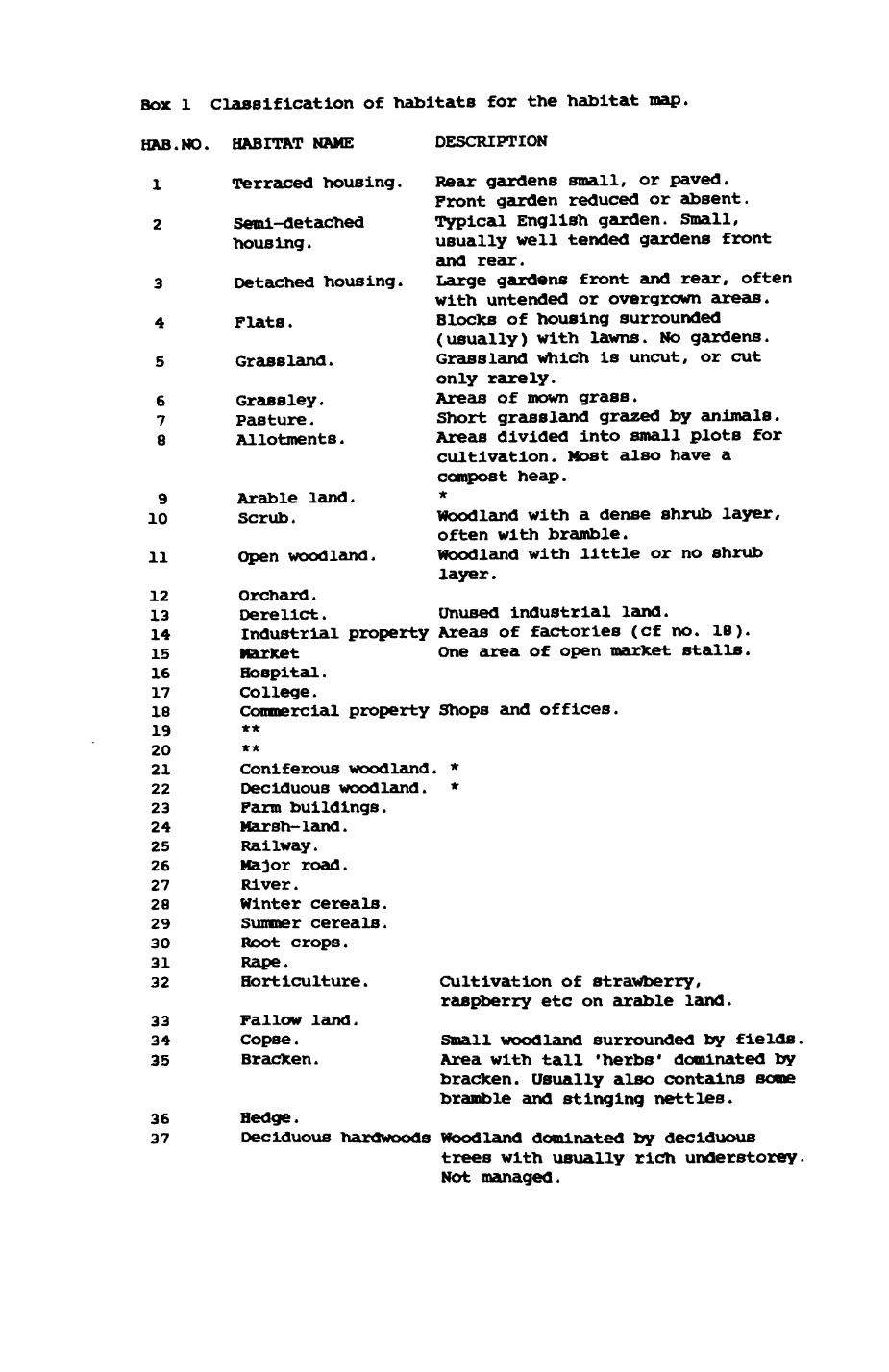
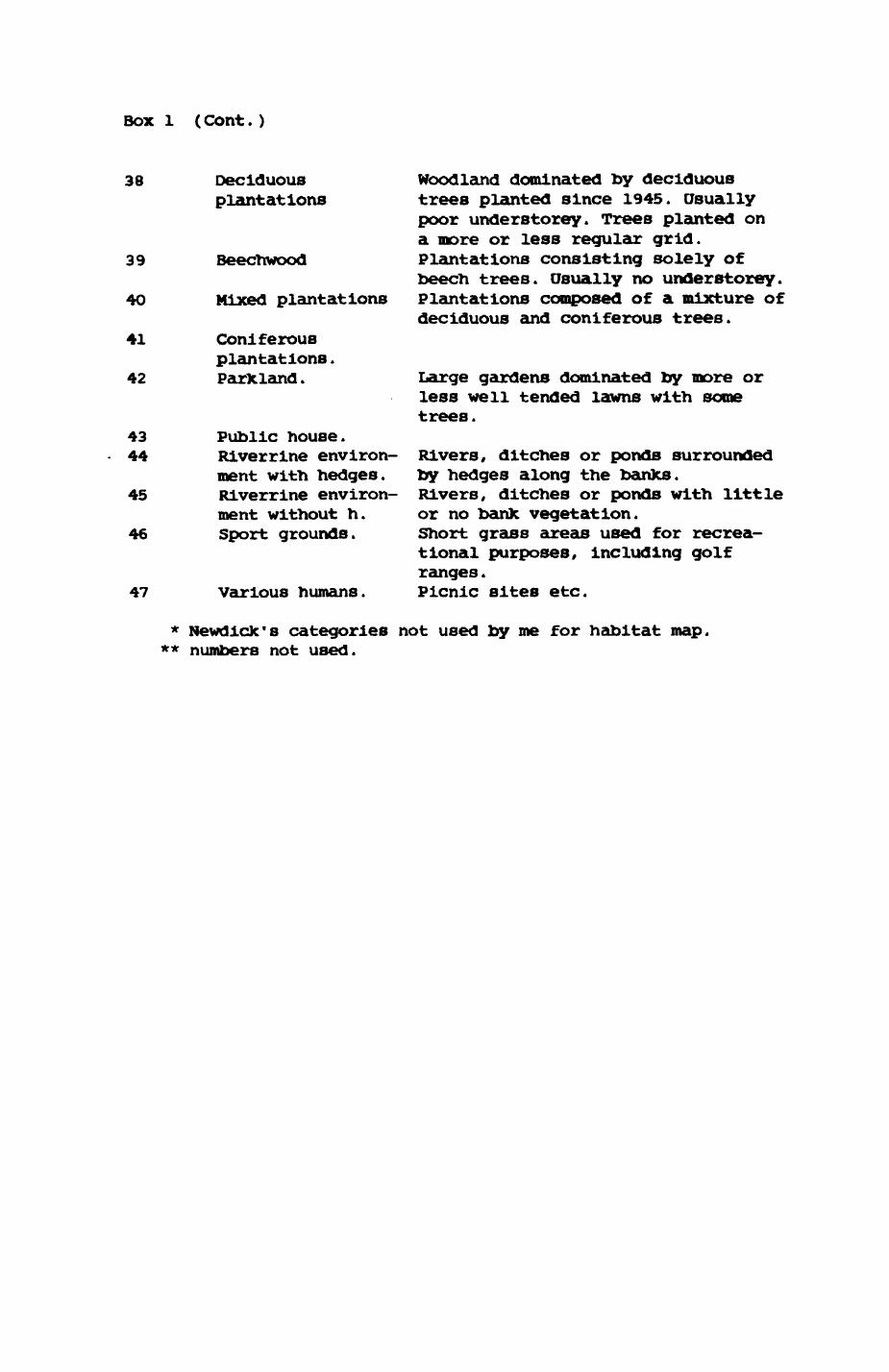
Box 1 Classification of habitats for the habitat map.
HAB.NO. HABITAT NAME DESCRIPTION
1 Terraced housing. Rear gardens small, or paved.Front garden reduced or absent.
2 Semi-detached Typical English garden. Small,housing. usually well tended gardens front
and rear.3 Detached housing. Targe gardens front and rear, often
with untended or overgrown areas.4 Flats. Blocks of housing surrounded
(usually) with lawns. No gardens.5 Grassland. Grassland which is uncut, or cut
only rarely.6 Grassley. Areas of mown grass.7 Pasture. Short grassland grazed by animals.8 Allotments. Areas divided into small plots for
cultivation. Most also have a compost heap.
9 Arable land. *10 scrub. Woodland with a dense shrub layer,
often with bramble.11 Open woodland. Woodland with little or no shrub
layer.12 Orchard.13 Derelict. Unused industrial land.14 Industrial property Areas of factories (cf no. 18).15 Market One area of open market stalls.16 Hospital.17 College.18 Commercial property Shops and offices.19 **20 **21 Coniferous woodland. *22 Deciduous woodland. *23 Farm buildings.24 Marsh-land.25 Railway.26 Major road.27 River.28 Winter cereals.29 Summer cereals.30 Root crops.31 Rape.32 Horticulture. Cultivation of strawberry,
raspberry etc on arable land.33 Fallow land.34 copse. small woodland surrounded by fields.35 Bracken. Area with tall 'herbs' dominated by
bracken. Usually also contains some bramble and stinging nettles.
36 Hedge.37 Deciduous hardwoods Woodland dominated by deciduous
trees with usually rich under storey. Not managed.
Box 1 (Cont. )
38
39
40
41
42
4344
45
46
47
Deciduous plantations
Beechwood
Mixed plantations
Coniferous plantations. Parkland.
Public house. Rlverrine environ ment with hedges. Rlverrine environ ment without h. Sport grounds.
Various humans.
Woodland dominated by deciduous trees planted since 1945. Usually poor understorey. Trees planted on a more or less regular grid. Plantations consisting solely of beech trees. Usually no understorey. Plantations composed of a mixture of deciduous and coniferous trees.
Large gardens dominated by more or less well tended lawns with some trees.
Rivers, ditches or ponds surrounded by hedges along the banks. Rivers, ditches or ponds with little or no bank vegetation. Short grass areas used for recrea tional purposes, including golf ranges. Picnic sites etc.
* Newdlck's categories not used by me for habitat map. ** numbers not used.
24
habitats, which is used by all members of the Oxford Foxlot (Newdick 1983,
Ooncaster 1985). The first 27 habitat types are identical with this
classification. Some of the habitat categories are not important to my
study area, e.g. colleges, or hospitals, but some of the housing types, for
Instance, occur at the fringe of the study area (Table 2.1). So, while
retaining comparability with analyses based on this classification, I
elaborated it for use in Wytham. Arable land was split into several
categories to permit a more fine-grained analysis of land-use. Rape was
Included as an arable land category. Woodlands were split into several types
based on the type of management corresponding to the plantation types
recognized by the Department of Forestry, Oxford (see below). Beechwood was
distinguished from other deciduous woodlands in recognition of associated
marked vegetational changes and changes in prey abundance, particularly
earthworms (see Chapter 3). In contrast to the city, a number of public
houses occur at isolated sites within the study area. It was decided that
they warranted a separate category as they are potentially good sites for
food scraps. On similar grounds, category 46 (sports grounds) was
distinguished from category 6 (grass ley) as differential human presence
might be of importance in an area that is not as dominated by human presence
as is the case with the city. However, the last two criteria had little
effect on the overall composition of habitats as can be seen from Table 2.1.
Also, for these cases the definition of patch boundaries (see below) would
have been unaffected by the assignment to a particular habitat type. For a
discussion, and other classification systems, see e.g. Elton and Miller
(1954), Short and Burnham (1980), Brown (1980), Armstrong et al. (1981) and
Ogle (1981).
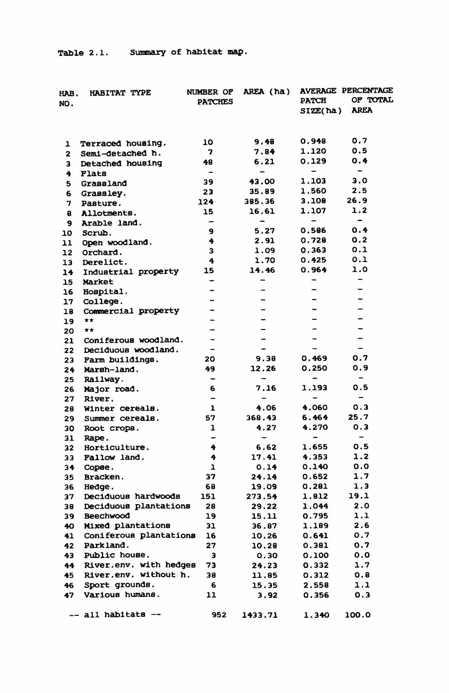
Table 2.1. Summary of habitat map.
HAB. NO.
HABITAT TYPE NUMBER OF AREA (ha) AVERAGE PERCENTAGE PATCHES PATCH OF TOTAL
SIZE(ha) AREA
123456789
1011121314151617181920212223242526272829303132333435363738394O41424344454647
Terraced housing.Semi-detached h.Detached housingFlatsGrasslandGrass ley.Pasture .Allotments .Arable land.Scrub.Open woodland.Orchard .Derelict .Industrial propertyMarketHospital .College .Commercial property****Coniferous woodland.Deciduous woodland.Farm buildings.Marsh-land .Railway.Major road.River.Winter cereals.Summer cereals.Root crops.Rape.Horticulture .Fallow land.Copse .Bracken .Hedge .Deciduous hardwoodsDeciduous plantationsBeechwoodMixed plantationsConiferous plantationsParkland .Public house.River. env. with hedgesRiver. env. without h.Sport grounds.Various humans.
107
48—
3923
12415—9434
15————————
2049—6—
1571—
441
3768
15128193116273
73386
11
9.487.846.21—
43.0035.89385.3616.61
—5.272.911.O91.7014.46
————————
9.3812.26
—7.16—
4.O6368.43
4.27—
6.6217.410.1424.1419.09273.5429.2215.1136.8710.2610.28O.3024.2311.8515.353.92
0.9481.1200.129
—1.1031.5603.1O81.107
—0.5860.7280.3630.4250.964
————————
0.4690.250
—1.193
—4.06O6.4644.27O
—1.6554.3530.14O0.6520.2811.8121.0440.7951.1890.6410.3810.100O.3320.3122.5580.356
0.70.5O.4—
3.02.5
26.91.2-
0.4O.20.10.11.0————————
0.70.9—
0.5—
0.325.70.3—
0.51.2O.O1.71.3
19.12.01.12.60.70.7O.O1.70.81.10.3
— all habitats — 952 1433.71 1.34O 1OO.0
25
2.2.2. Construction of the map
In autumn 1981 and winter 1981/1982 the entire study area was
systematically visited using Ordnance Survey maps (scale ItlOOOO) and the
Wytham Woods Atlas (January 1981 version by R.L.Hockin, Department of
Forestry, Oxford; scale ItBOOO). Location in the study area was facilitated
by numerous landmarks and particularly by the orange 10O m grid poles in the
woodlands.
A map (scale ItSOOO) was constructed by using the Wytham Woods Atlas as
a base. The parts of the study area not covered by the Atlas were entered
on the map using aerial photographs taken on September 22, 1978 by Hunting
Surveys Ltd., Elstree Way, Boreham Wood, Hertfordshire on a scale ItlOOOO.
Slides were used to project the aerial photographs straight onto the map in
line with suggestions by Kllford (1979) and Marcot et al. (1981) (see also
Puller (1983). The map was updated with Ordnance Survey maps and field
records. Special emphasis was laid on accurate positioning of conspicuous
landmarks within large homogeneous areas (e.g. single trees on arable land).
Knowledge of their exact coordinates facilitated and improved data recording
from such areas. The map was then divided into non-overlapping components
called patches. They were marked out using the following criteria.
1. Each patch forms a distinct plot of land and habitat type. Fences,
boundary roads or tracks constituted well defined borders. This was usually
straightforward and most patch boundaries were thus defined.
2. All boundaries of the compartments recognized by the Forestry
Service of Wytham Woods were incorporated. Ifost compartment boundaries were
already 'covered 1 by the first criterion, but in some cases this meant
inclusion of some additional borders. Thus, one compartment might consist
of several patches, but one patch would not Include sections of more than
one compartment.
26
3. The resulting map was checked against the plantation map of the
Department of Forestry, Oxford, to make sure that the boundaries of the
areas occupied by the plantation types recognized by the Department of
Forestry were included.
4. Minimum size of patches was 30 m by 3O m, to match approximately the
accuracy of radio-tracking data.
5. Each patch was delineated with a mininum number of straight lines in
order to minimise the memory space required for computer storage.
Criteria 1, 4 and 5 are identical with those of Newdlck's (1983)
habitat map. The other two criteria were specified to facilitate
comparisons with other maps of Wytham Woods. Recognition of compartment
boundaries and plantation types is also useful as the management of the
woodland and thus potential habitat changes occur in accordance with
compartment and plantation boundaries. The map was thus designed to
minimize the probability that major habitat changes could occur across patch
boundaries during the time of the study. It is easier because of
computational considerations to change habitat types or lump patches than it
is to modify patch boundaries. During the period of my field work few
habitat changes occurred and those were within and not across patch
boundaries.
The entire map was then photographically reduced at the photographic
laboratory of the Department of Nuclear Physics, Oxford, with a camera that
eliminates any distortions resulting from reduction. The map was then
digitized and entered into the computer using the same procedure as
described by Newdick (1983). The map was checked and corrected using
program BODGE and finally assembled with program BUILD (written by M.T.
Newdick).
27
2.2.3. Results
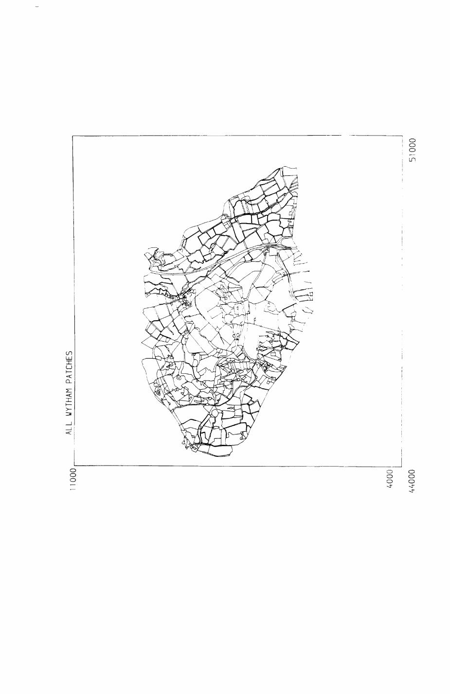
The final map covered the following area (Fig. 2.1)t the centre of the
map constituted Wytham Woods with Wytham village. To the east, the area
covered includes the Western Bypass, and the entire Binsey area between the
River Thames, Wolvercote (Godstow Road) and Botley Road. To the south, the
Eynsham Road from Botley to the Toll Bridge constituted a very convenient
border. To the west and north, the River Thames and the agricultural fields
between Wytham Wood and the university Field Station completed the border
line. Hereafter, the entire area covered by the map is referred to as the
study area. Sections of It are called study sites (e.g. for habitat
records).
The map covers altogether 14.3 square Kilometres in 952 patches over 34
different habitat types. Program HTOT (written by M.T. NewdicX) was used to
summarize the components of the habitat map. Results are presented in Table
2.1. Three habitat types dominate the landscapet pasture (124 patches,
26.9% of the area), fields with summer cereals (57 patches, 25.7%) and
deciduous hardwoods (151 patches, 19.1%). On average, patches with summer
cereals are largest (average size 6.464 ha) and approximately twice the size
of pasture patches (average size 3.108 ha) and more than three times the
size of deciduous hardwoods patches (average size 1.812 ha). Most other
habitat types occur in far smaller patches. Looking at the habitat map in
more detail, I tried to gain an impression of • local* habitat composition.
Program NEIGHBOUR was used to create a 'map' containing information on the
neighbours of each patch and program PATSUM compiled this information by
habitat categories. Each patch was used as a 'window' to the local habitat
composition by evaluating the number of neighbouring patches and their
habitat types, and an attempt was made to summarize this Information in an
expression of habitat diversity. Note that habitat diversity refers here to

Pig. 2.1. The computerized habitat map of the study area, with National Grid References (map SP); scale 7 by 7 km. Each area unit represents a habitat patch. The map was produced by program MAPITH, using the GHOST-80 Graphics system.
000
ALL
WYTHAh PA
TCHE
S
4000
4400
051
000
28
the presence or absence of habitat types amongst the neighbours of a
particular patch, not to any variation within a patch or within a
neighbouring patch.
There have been many suggestions of how to measure ecological diversity
and a variety of diversity indices have been proposed (e.g. Hill 1973, Help
1974, & Pielou 1977). Comparison of their performance (Hurlbert 1971, Help
& Engels 1974, May 1975, Pielou 1979, Alatalo 1981, & Kobayashi 1981) has
shown that there is no general 'best' index. I decided to use the Dominance
Index proposed by Berger and Parker (197O) as it is easy to visualize and
calculate, and has been shown to be very robust in many cases (May 1975).
The Dominance Index for a given patcTi is
the number of patches of the most frequent habitat type
amongst the neighbours of the patch divided by the total
number of neighbouring patches of the patch
The Dominance Index assumes values in the range between O and 1. A
small number indicates low dominance of the most frequent habitat type while
a value close to 1 indicates high dominance of the most frequent habitat
type. A value of 1 indicates perfect dominancet all neighbouring patches
are of the same habitat type. In terms of diversity, a high value (high
dominance) would indicate good homogeneity or low diversity, and a low value
(low dominance diversity) would indicate low homogeneity or high diversity.
Results are shown in Table 2.2 and Fig. 2.2. The grand mean of the
Dominance Index over all habitats is O.537. There is, however,
considerable, significant scatter between different habitats (Kruskal-Wallls
one-way analysis of variance, H(adjusted) - 93.28, p< O.OO1, df - 24). Pig.
2.2a shows that indeed the dominance index decreases and thus diversity
Increases with the number of different habitat types represented amongst the
neighbours (Spearman rank correlation, rho - -O.717, p < O.OO1). The number
of neighbouring habitats is correlated with the average patch size (Pig
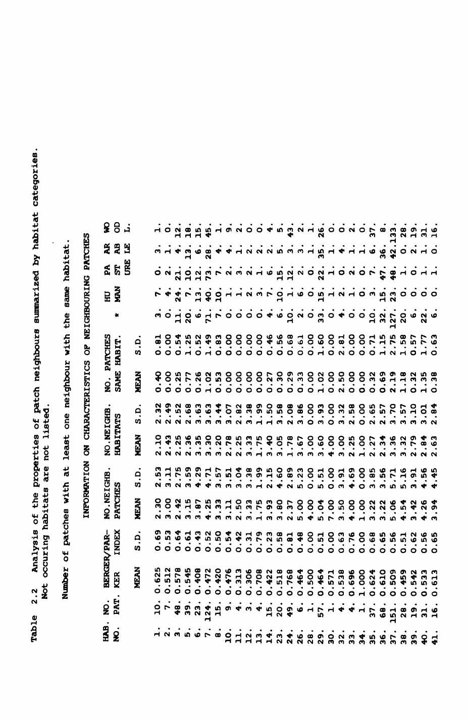
Table
2.2
Analysis o
f the
proper
ties
of
patc
h ne
ighb
ours s
ummarized by hab
itat
cat
egorie
s Not
occuring
hab
itat
s ar
e not
list
ed.
Number o
f patches wi
th a
t le
ast
one
neig
hbou
r wi
th t
he s
ame habitat.
INFORMATION ON CHARACTERISTICS OF NEIGHBOURING PATCHES
HAB. NO.
BERGER/PAR-
NO.NEIGHB.
NO.NEIGHB.
NO.
PATCHES
HU
PA AR WO
NO.
PAT. KER
INDEX
PATCHES
HABITATS
SAME HABIT.
* MAN
ST AB OD
URE LE
L.
1. 2. 3. 5. 6. 7. 8.10.
11.
12.
13.
14.
23.
24.
26.
28.
29.
30.
32.
33.
34.
35.
36.
37.
38.
39.
40.
41.
10. 7.
48.
39.
23.
124.
15. 9. 4. 3. 4.
15.
20.
49. 6. 1.
57. 1. 4. 4. 1.
37.
68.
151. 28.
19.
31.
16.
MEAN
0.625
0.512
O.578
0.545
O.4O8
0.472
0.420
0.476
0.313
0.306
0.708
0.422
O.518
0.768
O.464
0.500
O.464
0.571
0.538
0.696
l.OOO
0.624
O.610
0.509
0.459
O.542
O.533
0.613
S.D.
O.69
0.53
0.64
0.61
O.43
O.52
0.50
0.54
O.42
O.31
O.79
0.23
0.58
0.81
O.48
O.OO
O.51
O.OO
0.63
O.76
O.OO
O.68
O.65
O.56
O.51
O.62
0.56
O.65
MEAN
2.30
3.OO
2.42
3.15
3.87
4.25
3.33
3.11
2.50
3.33
1.75
3.93
3.80
2.37
5.OO
4.OO
5.04
7.00
3.50
4.00
l.OO
3.22
3.22
5.06
4.54
3.42
4.26
3.94
S.D.
2.53
3.11
2.75
3.59
4.29
4.71
3.57
3.51
3.04
3.38
1.99
2.15
4.60
2.89
5.23
O.OO
5.51
0.00
3.91
4.69
O.OO
3.85
3.56
5.71
5.16
3.91
4.56
4.45
MEAN
2.10
2.43
2.25
2.36
3.35
3.30
3.20
2.78
2.25
3.33
1.75
3.40
3.05
1.78
3.67
3.00
3.6O
4.00
3.00
2.25
l.OO
2.27
2.34
3.36
3.32
2.79
2.84
2.63
S.D.
2.32
2.49
2.52
2.68
3.63
3.63
3.44
3.O7
2.82
3.38
1.99
1.50
3.58
2.08
3.86
0.00
3.93
0.00
3.32
2.58
O.OO
2.65
2.57
3.7O
3.57
3.10
3.01
2.84
MEAN
O.4O
O.OO
O.25
O.77
O.26
1.02
0.53
O.OO
0.00
O.OO
O.OO
0.27
0.30
0.29
O.33
O.OO
1.O2
O.OO
2.50
0.00
O.OO
O.32
O.69
2.19
1.18
0.32
1.35
0.38
S.D.
0.81
0.00
O.54
1.25
O.52
1.49
O.83
0.00
0.00
O.OO
O.OO
0.46
0.56
0.68
0.61
O.OO
1.60
O.OO
2.81
O.OO
0.00
O.71
1.15
2.75
1.58
O.57
1.77
0.63
3. 0.11
.20
. 6.71
. 7. O. 0. 0. 0. 4. 6.10
. 2. 0. 33. O. 4. O. 0.
10.
32.
127. 20. 6.
22. 6.
7. 4.24. 7.
13.
40.
10. 1. 1. 2. 3. 7.
10. 1. 6. 0.
15. 1. 2. 1. 0. 3.
15.
23. 0. 0. 0. 0.
O. 2.21
.1O.
12.
73. 7. 2. 3. 2. 1. 6.
15.
12. 2. 0.
22. 1. 0. 2. O. 7.
47.
48. 1. 0. 1. 1.
3. 1. 4.13
. 6.28
. 4. 4. 1. 2. 2. 2. 5. 3. 3. 1. 35. 1. 4. 1. 1. 6. 36.
42. 0. 2. 1. 0.
1. O.12.
18.
15.
45. 1. 9. 2. O. 0. 4. 5.
43. 2. 1.
26. 0. 0. 2. 0. 37. 8.
133. 28.
19.
31.
16.
Tab
le 2.2
(C
en
t.)
41 .
16 .
42 .
27 .
43.
3.44.
73.
45.
38.
46.
6.47 .
11 .
grand
means
O.613
0.40
10.583
0.543
0.587
O.421
0.529
O.537
0.65
O.44
0.70
O.59
O.64
O.45
0.25
O.13
3.94
3.52
2.33
4.26
3.76
4.5O
3.73
3.60
4.45
3.77
2.79
4.95
4.50
4.87
1.27
1.11
2.63
3.19
2.33
2.97
2.68
3.50
3.09
2.80
2.84
3.36
2.79
3.35
3.O3
3.76
0.94
O.64
0.38
O.44
0.00
O.95
O.26
O.OO
0.00
O.63
0.73
0.00
1.45
O.57
O.OO
O.OO
6.11. O.
43. 9. O. O.
0. 4. 2.16
. 6. 3. 6.
1.16. 1.
58.
26. 3. 4.
O. 4. O.33. 8. 1. 2.
16. 7. 1.
14.
18. O. 5.

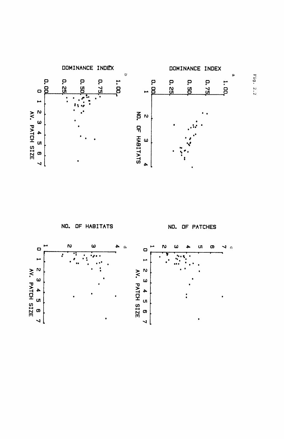
Pig. 2.2. Characteristics of the habitat map, as analysed on a local scale. Each point represents the average value for one habitat.
a. The Berger-ParXer Dominance Index (see text) vs.the number of different neighbouring habitats perpatch.
b. Dominance Index vs. average patch size, c. Number of neighbouring patches per patch vs.
average patch size, d. number of different neighbouring habitats vs.
average patch size.
DOMINANCE INDEX DOMINANCE INDEXcr & "3
oooo^ oooo«- f2*•••• «>>••
0
> ro
U) TJH *•n
Ul(^l-l N °>m
DIMUl^JO OWUIvlO M DU1OUIO i-OUlOUIO
• * . *
p ro
0TI • • > u)
CDH- 1H H
• ' ' * *
V* t
1 •
NO. OF HABITATS NO. OF PATCHES
0)
uin
U)N o m
IN) U) o. »- l\) U) *. Ul O)
> ro
0)-o> ^n
Nm
Ul
29
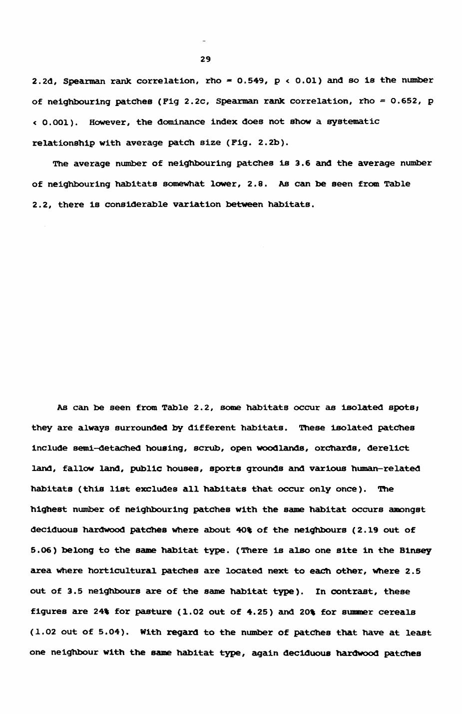
2.2d, Spearman rank correlation, rho » 0.549, p < O.O1) and so is the number
of neighbouring patches (Pig 2.2c, Spearman rank correlation, rho - 0.652, p
< O.OOl). However, the dominance index does not show a systematic
relationship with average patch size (Pig. 2.2b).
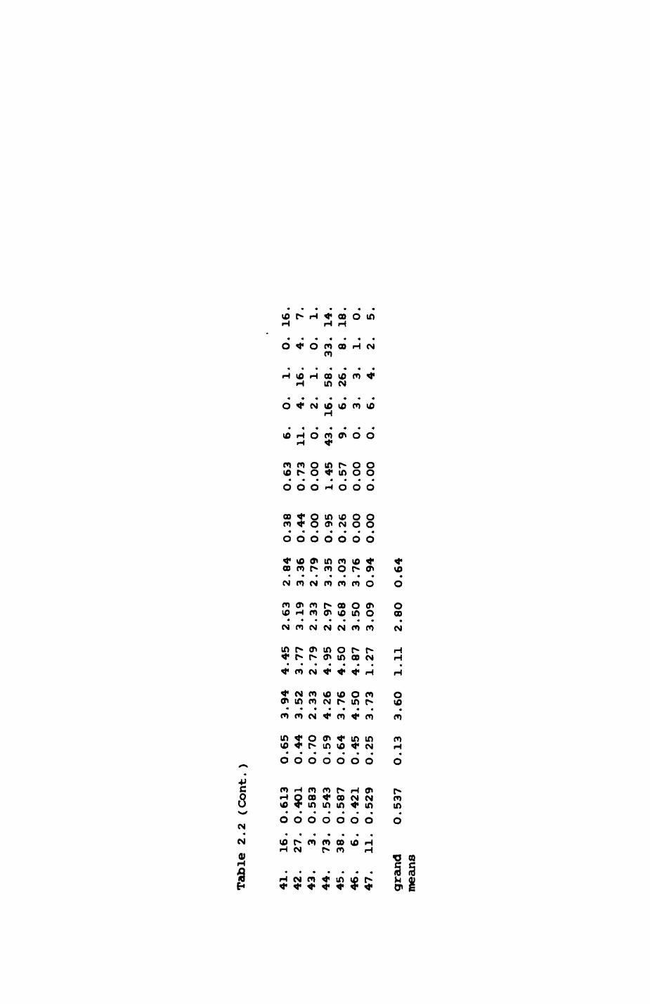
The average number of neighbouring patches is 3.6 and the average number
of neighbouring habitats somewhat lower, 2.8. As can be seen from Table
2.2, there is considerable variation between habitats.
As can be seen from Table 2.2, some habitats occur as isolated spots;
they are always surrounded by different habitats. These isolated patches
include semi-detached housing, scrub, open woodlands, orchards, derelict
land, fallow land, public houses, sports grounds and various human-related
habitats (this list excludes all habitats that occur only once). The
highest number of neighbouring patches with the same habitat occurs amongst
deciduous hardwood patches Where about 4O% of the neighbours (2.19 out of
5.O6) belong to the same habitat type. (There is also one site in the Blnsey
area where horticultural patches are located next to each other, where 2.5
out of 3.5 neighbours are of the same habitat type). In contrast, these
figures are 24% for pasture (1.02 out of 4.25) and 20% for summer cereals
(1.O2 out of 5.O4). With regard to the number of patches that have at least
one neighbour with the same habitat type, again deciduous hardwood patches
30
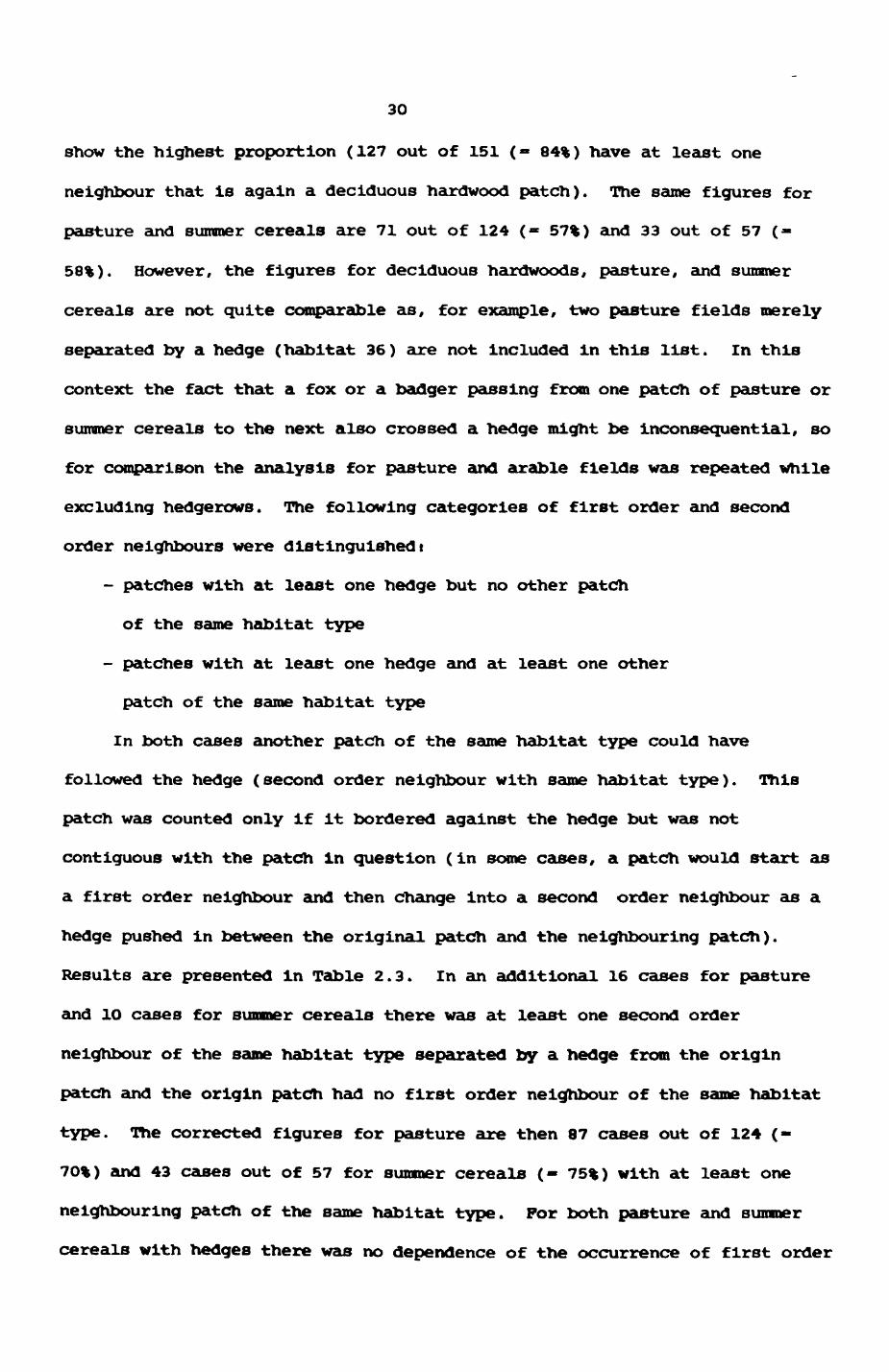
show the highest proportion (127 out of 151 ( = 84%) have at least one
neighbour that is again a deciduous hardwood patch). The same figures for
pasture and summer cereals are 71 out of 124 (« 57%) and 33 out of 57 (-
58%). However, the figures for deciduous hardwoods, pasture, and summer
cereals are not quite comparable as, for example, two pasture fields merely
separated by a hedge (habitat 36) are not included in this list. In this
context the fact that a fox or a badger passing from one patch of pasture or
summer cereals to the next also crossed a hedge might be inconsequential, so
for comparison the analysis for pasture and arable fields was repeated while
excluding hedgerows. The following categories of first order and second
order neighbours were distinguished!
- patches with at least one hedge but no other patch
of the same habitat type
- patches with at least one hedge and at least one other
patch of the same habitat type
In both cases another patch of the same habitat type could have
followed the hedge (second order neighbour with same habitat type). This
patch was counted only if it bordered against the hedge but was not
contiguous with the patch in question (in some cases, a patch would start as
a first order neighbour and then change into a second order neighbour as a
hedge pushed in between the original patch and the neighbouring patch).
Results are presented in Table 2.3. In an additional 16 cases for pasture
and 10 cases for summer cereals there was at least one second order
neighbour of the same habitat type separated by a hedge from the origin
patch and the origin patch had no first order neighbour of the same habitat
type. The corrected figures for pasture are then 87 cases out of 124 (-
70%) and 43 cases out of 57 for summer cereals (- 75%) with at least one
neighbouring patch of the same habitat type. For both pasture and summer
cereals with hedges there was no dependence of the occurrence of first order
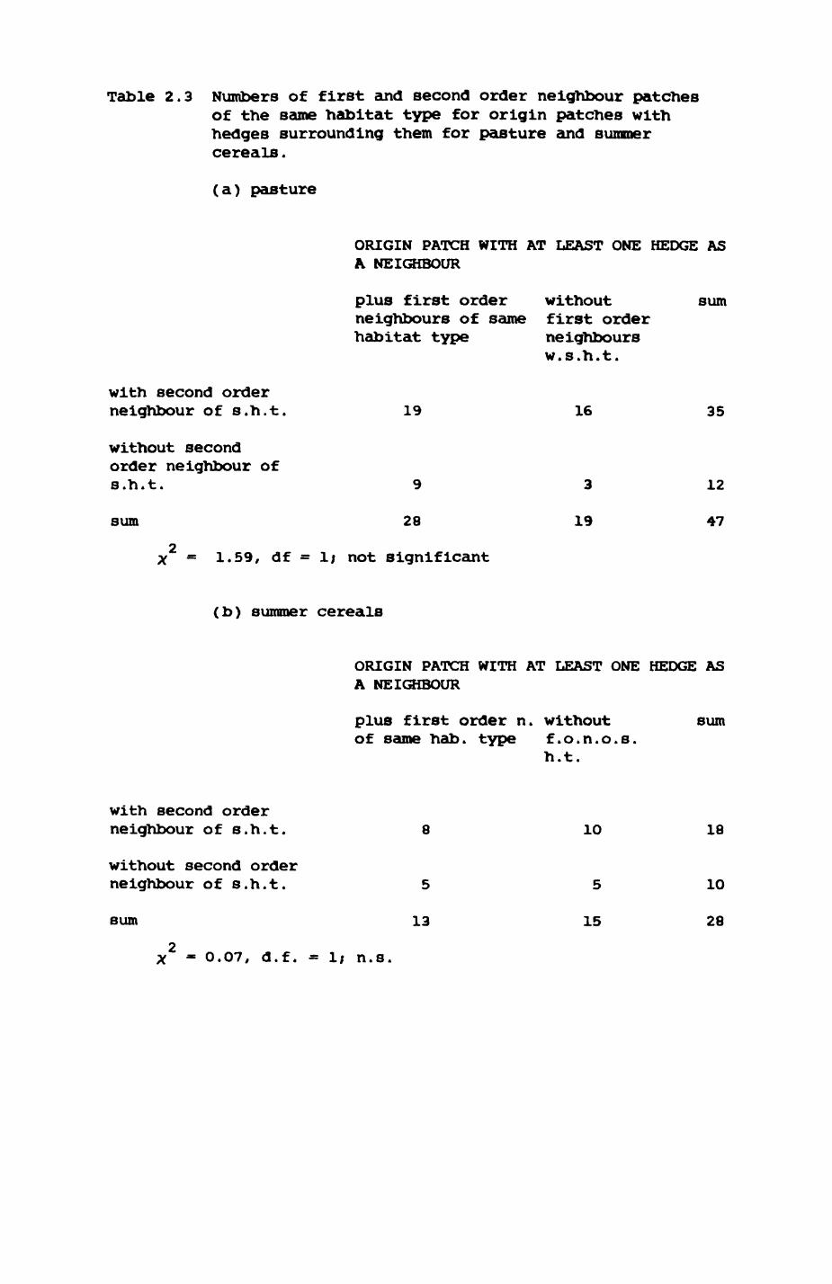
Table 2.3 Numbers of first and second order neighbour patches of the same habitat type for origin patches with hedges surrounding them for pasture and summer cereals.
(a) pasture
ORIGIN PATCH WITH AT LEAST ONE HEDGE AS A NEIGHBOUR
plus first order without neighbours of same first order habitat type neighbours
w.s.h.t.
sum
with second order neighbour of s.h.t,
without second order neighbour of s.h.t.
sum
19
28
1.59, df - Ij not significant
(b) summer cereals
16 35
3
19
12
47
ORIGIN PATCH WITH AT LEAST ONE HEDGE AS A NEIGHBOUR
plus first order n. without of same hab. type f.o.n.o.s.
h.t.
sum
with second order neighbour of s.h.t.
without second order neighbour of s.h.t.
sum
8
13
1O
5
15
18
10
28
O.O7, d.f. - 1; n.S.
31
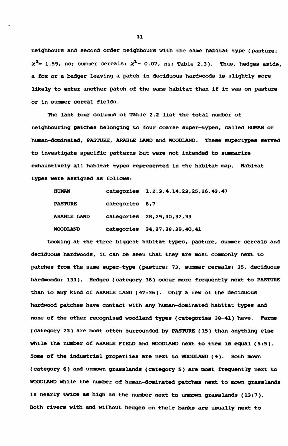
neighbours and second order neighbours with the same habitat type (pasture:
Xx- 1.59, ns; summer cereals: x1** 0.07, ns; Table 2.3). Thus, hedges aside,
a fox or a badger leaving a patch in deciduous hardwoods is slightly more
likely to enter another patch of the same habitat than if it was on pasture
or in summer cereal fields.
The last four columns of Table 2.2 list the total number of
neighbouring patches belonging to four coarse super-types, called HUMAN or
human-dominated, PASTURE, ARABLE LAND and WOODLAND. These supertypes served
to investigate specific patterns but were not Intended to summarize
exhaustively all habitat types represented in the habitat map. Habitat
types were assigned as follows t
HUMAN categories 1,2,3,4,14,23,25,26,43,47
PASTURE categories 6,7
ARABLE LAND categories 28,29,30,32,33
WOODLAND categories 34,37,38,39,40,41
Looking at the three biggest habitat types, pasture, summer cereals and
deciduous hardwoods, it can be seen that they are most commonly next to
patches from the same super-type (pasture: 73, summer cerealst 35, deciduous
hardwoodst 133). Hedges (category 36) occur more frequently next to PASTURE
than to any kind of ARABLE LAND (47i36). Only a few of the deciduous
hardwood patches have contact with any human-dominated habitat types and
none of the other recognised woodland types (categories 38-41) have. Farms
(category 23) are most often surrounded by PASTURE (15) than anything else
while the number of ARABLE FIELD and WOODLAND next to them is equal (5i5).
Some of the Industrial properties are next to WOODLAND (4). Both mown
(category 6) and unmown grasslands (category 5) are most frequently next to
WOODLAND while the number of human-dominated patches next to mown grasslands
is nearly twice as high as the number next to unmown grasslands (13i7).
Both rivers with and without hedges on their banks are usually next to
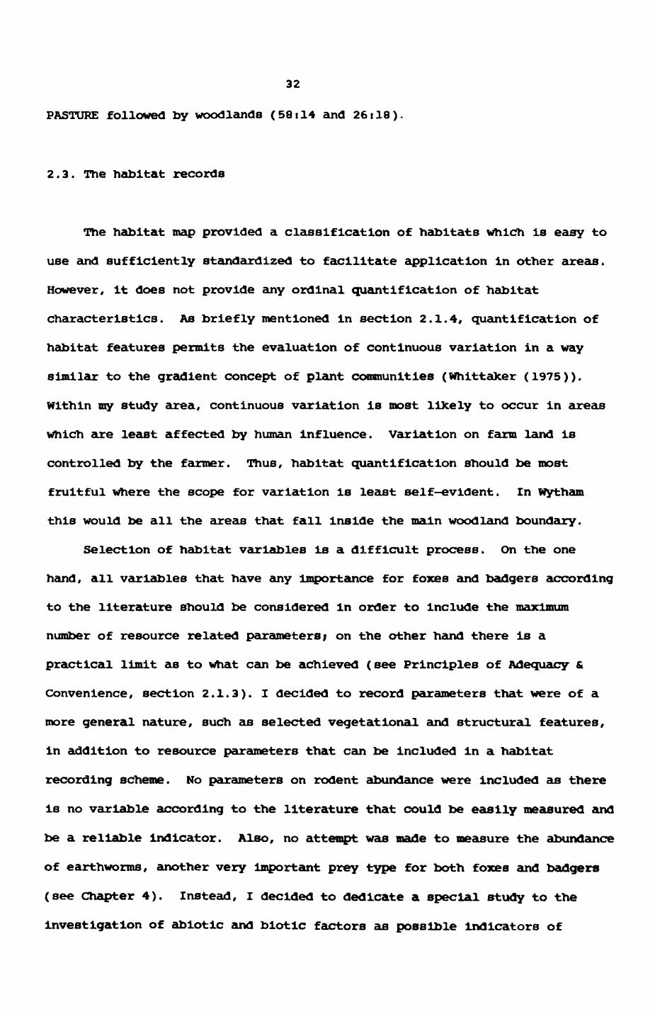
32
PASTURE followed by woodlands (58il4 and 26il8)
2.3. The habitat records
The habitat map provided a classification of habitats which is easy to
use and sufficiently standardized to facilitate application in other areas.
However, it does not provide any ordinal quantification of habitat
characteristics. As briefly mentioned in section 2.1.4, quantification of
habitat features permits the evaluation of continuous variation in a way
similar to the gradient concept of plant communities (Whittaker (1975)).
Within my study area, continuous variation is most likely to occur in areas
which are least affected by human influence. Variation on farm land is
controlled by the farmer. Thus, habitat quantification should be most
fruitful where the scope for variation is least self-evident. In Nytham
this would be all the areas that fall inside the main woodland boundary.
Selection of habitat variables is a difficult process. On the one
hand, all variables that have any importance for foxes and badgers according
to the literature should be considered in order to Include the maximum
number of resource related parameters i on the other hand there is a
practical limit as to what can be achieved (see Principles of Adequacy &
Convenience, section 2.1.3). I decided to record parameters that were of a
more general nature, such as selected vegetational and structural features,
in addition to resource parameters that can be included in a habitat
recording scheme. No parameters on rodent abundance were included as there
is no variable according to the literature that could be easily measured and
be a reliable indicator. Also, no attempt was made to measure the abundance
of earthworms, another very important prey type for both foxes and badgers
(see Chapter 4). Instead, I decided to dedicate a special study to the
investigation of abiotic and blotlc factors as possible indicators of
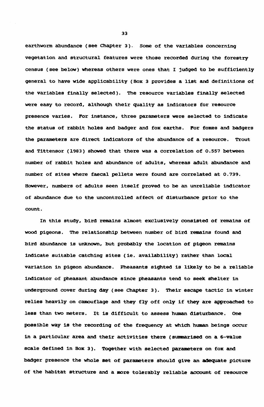
33
earthworm abundance (see Chapter 3). Some of the variables concerning
vegetation and structural features were those recorded during the forestry
census (see below) whereas others were ones that I judged to be sufficiently
general to have wide applicability (Box 3 provides a list and definitions of
the variables finally selected). The resource variables finally selected
were easy to record, although their quality as indicators for resource
presence varies. For instance, three parameters were selected to indicate
the status of rabbit holes and badger and fox earths. For foxes and badgers
the parameters are direct indicators of the abundance of a resource. Trout
and Tittensor (1983) showed that there was a correlation of O.557 between
number of rabbit holes and abundance of adults, whereas adult abundance and
number of sites where faecal pellets were found are correlated at 0.739.
However, numbers of adults seen itself proved to be an unreliable indicator
of abundance due to the uncontrolled affect of disturbance prior to the
count.
In this study, bird remains almost exclusively consisted of remains of
wood pigeons. The relationship between number of bird remains found and
bird abundance is unknown, but probably the location of pigeon remains
indicate suitable catching sites (le. availability) rather than local
variation in pigeon abundance. Pheasants sighted is likely to be a reliable
Indicator of pheasant abundance since pheasants tend to seek shelter in
underground cover during day (see Chapter 3). Their escape tactic In winter
relies heavily on camouflage and they fly off only if they are approached to
less than two meters. It is difficult to assess human disturbance. One
possible way is the recording of the frequency at which human beings occur
in a particular area and their activities there (summarised on a 6-value
scale defined in Box 3). Together with selected parameters on fox and
badger presence the Whole set of parameters should give an adequate picture
of the habitat structure and a more tolerably reliable account of resource

BOX 2 Variables and scoring methods for habitat census 1974.
VEGETATION Cover (1) Top coven above 2.5 meters(2) Middle cover: 0.5 - 2.5 meters(3) Bottom cover t 0-0.5 meters
measured on a percent scale and entered to the nearest 5 percent.
* Ecoslgs (4) Rubus fruticosus bramble
(5) Pterldium aqulllnum bracken(6) Chamaenerlon angustlfolium fireweed (7 ) Endymlon non-scrlptus bluebell(8) Urtlca dlolca stinging nettle(9) Mercurlalls perennls dog's mercury
*the aggregate
measured on a 0 to 5 scale (see text).
OTHER DATA (10) Slope(11) Water presence(12) mean pH
see text for quantification procedures.
34
presence.
Two data sets are used to evaluate habitat patterns. The first was
kindly provided by Dr. B.C. Dawkins, Department of Forestry, Oxford (see Box
2). The second constitutes my own records. The two data sets were recorded
for different purposes. Dr. Dawklns designed his sampling scheme as a part
of a long-term surveillance system for British woodlands (Dawkins & Field
1977, 1978). His records are exclusively from woodland areas and
concentrate on aspects relevant to trees. They are, however, so
comprehensive that they can be easily used for other purposes. Dr. Dawkins*
data (hereafter referred to as forestry data) do not cover potential fox and
badger resources or signs of fox and badger presence, so I had to do
additional habitat recording that would provide such information.
2.3.1. Methods! Forestry Data.
Statistical considerations for the two habitat sampling schemes are
discussed in detail in Appendix 1. Collection of the forestry data is
described by Dawkins and Field (1977, 1978). The following section
summarises the procedure they adopted, emphasising those data I extracted
from their set (Box 21).
The forestry data from Wytham were collected throughout summer 1974,
the soil samples taken mostly in summer 1976. A quadrat of 10 by 1O meters
was placed at a distance of 14.142 meter at an angle of 45° northeast from
the nearest 100 m intersection point. The position of quadrats of two rows
were alternating) in the same row, the distance from one quadrat to the next
was 200 m. 164 quadrats were recorded, placed over the entire wood but
excluding Bean Wood (Fig 2.3). Variables measured Included structural
features, e.g. coverage at different height classes, monitoring of Important
species (ecoslgs), number* species and various measurements of trees, all

Pig. 2.3. The central area of the study area with the locations of the sample plots of the Forestry habitat data (re gularly dispersed on a 200 m lattice). Woodland stippled, agricultural areas blank, human settlements black, woodland segmented into the compartments recog nized by the Dept of Forestry, Oxford.
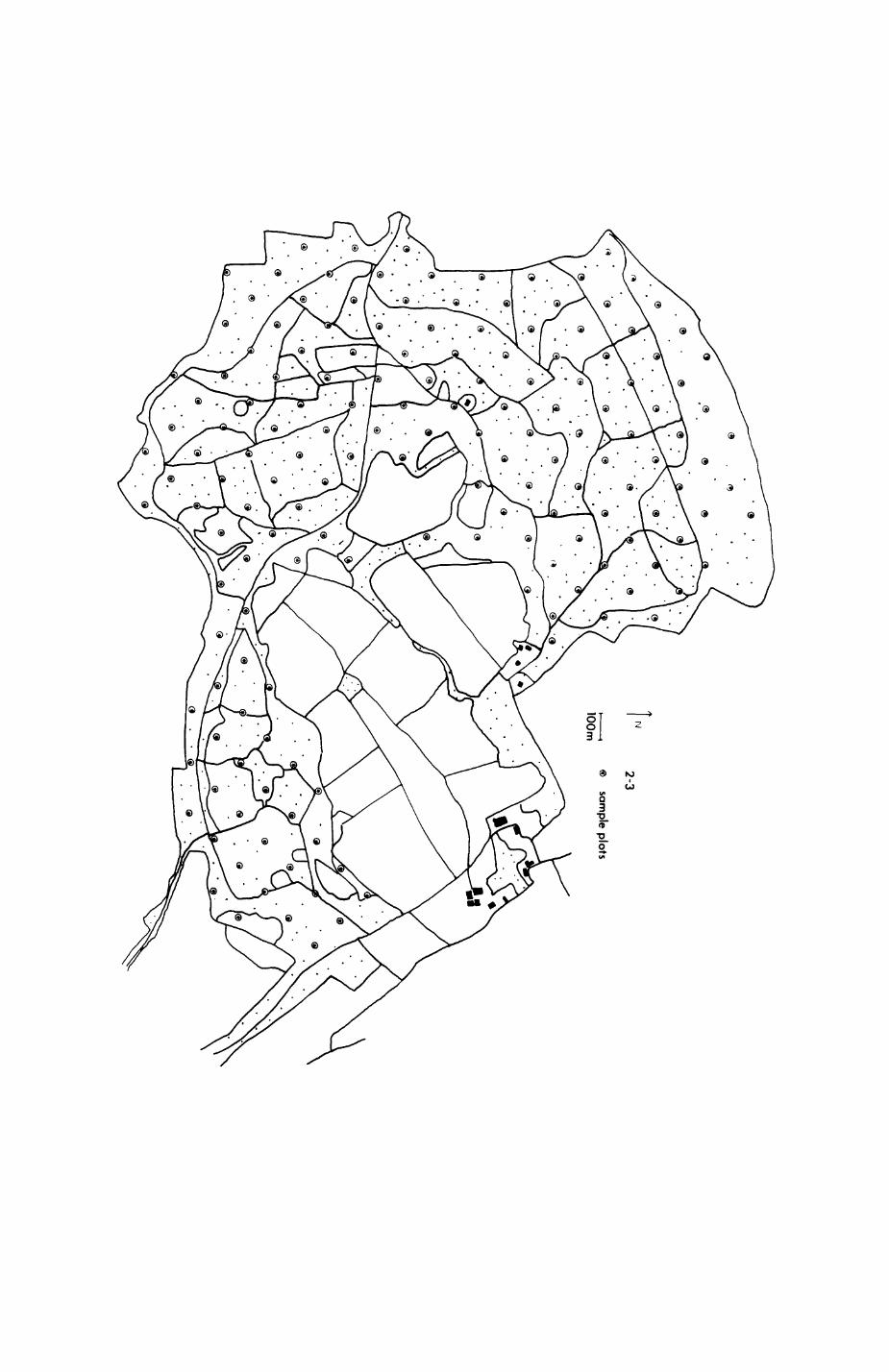
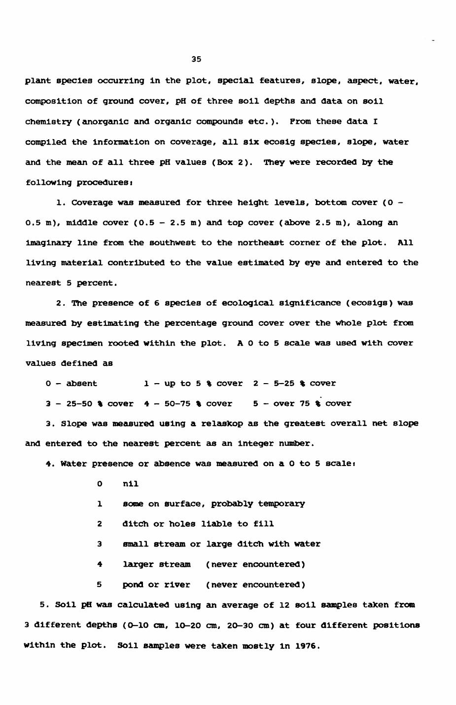
35
plant species occurring in the plot, special features, slope, aspect, water,
composition of ground cover, pH of three soil depths and data on soil
chemistry (anorganic and organic compounds etc.). From these data I
compiled the information on coverage, all six ecoslg species, slope, water
and the mean of all three pH values (Box 2). They were recorded by the
following procedures!
1. Coverage was measured for three height levels, bottom cover (0 -
0.5 m), middle cover (0.5 - 2.5 m) and top cover (above 2.5 m), along an
imaginary line from the southwest to the northeast corner of the plot. All
living material contributed to the value estimated by eye and entered to the
nearest 5 percent.
2. The presence of 6 species of ecological significance (ecosigs) was
measured by estimating the percentage ground cover over the whole plot from
living specimen rooted within the plot. A 0 to 5 scale was used with cover
values defined as
0 - absent 1 - up to 5 % cover 2 - 5-25 % cover
3 - 25-50 % cover 4 - 5O-75 % cover 5 - over 75 % cover
3. Slope was measured using a relaslcop as the greatest overall net slope
and entered to the nearest percent as an Integer number.
4. Water presence or absence was measured on a 0 to 5 scale t
0 nil
1 some on surface, probably temporary
2 ditch or holes liable to fill
3 small stream or large ditch with water
4 larger stream (never encountered)
5 pond or river (never encountered)
5. Soil pH was calculated using an average of 12 soil samples taken from
3 different depths (O-10 cm, 10-20 cm, 20-30 cm) at four different positions
within the plot. Soil samples were taken mostly In 1976.
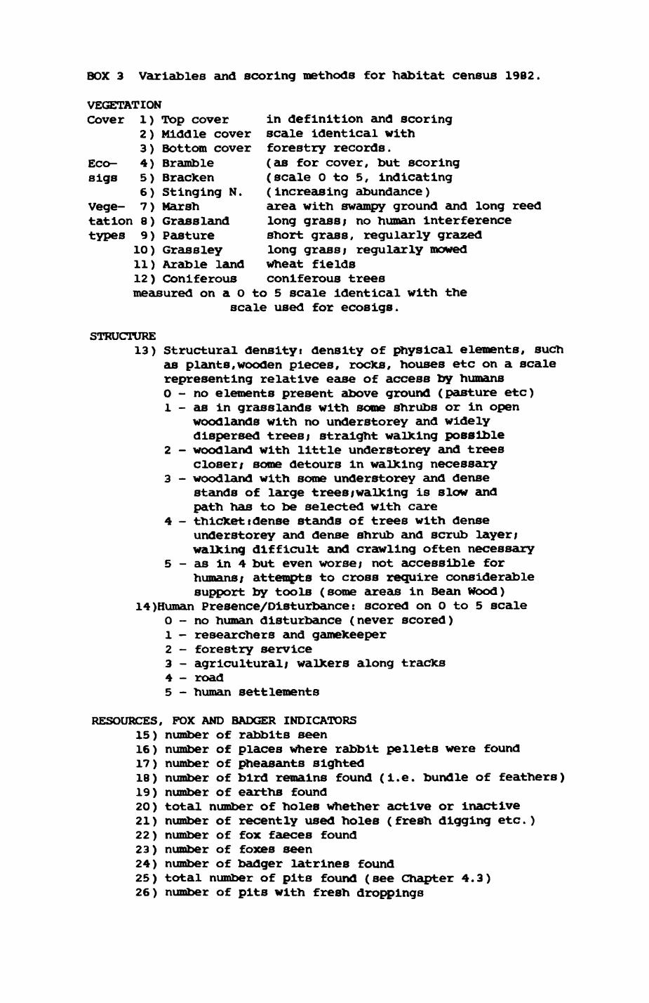
BOX 3 Variables and scoring methods for habitat census 1982.
VEGETATIONCover 1) Top cover in definition and scoring
2) Middle cover scale identical with3) Bottom cover forestry records.
Eco- 4) Bramble (as for cover, but scoring sigs 5) Bracken (scale 0 to 5, indicating
6) Stinging N. (increasing abundance)Vege- 7) Marsh area with swampy ground and long reed tation 8) Grassland long grass/ no human interference types 9) Pasture short grass, regularly grazed
10) Grassley long grass; regularly mowed11) Arable land wheat fields12) Coniferous coniferous trees measured on a 0 to 5 scale identical with the
scale used for ecosigs.
STRUCTURE13) Structural densityt density of physical elements, such
as plants,wooden pieces, rocks, houses etc on a scale representing relative ease of access by humans O - no elements present above ground (pasture etc)1 - as in grasslands with some shrubs or in open
woodlands with no understorey and widely dispersed treesi straight walking possible
2 - woodland with little understorey and trees closer/ some detours in walking necessary
3 - woodland with some understorey and dense stands of large trees/walking is slow and path has to be selected with care
4 - thickettdense stands of trees with denseunderstorey and dense shrub and scrub layeri walking difficult and crawling often necessary
5 - as in 4 but even worse; not accessible forhumans/ attempts to cross require considerable support by tools (some areas in Bean Mood)
14)Human Presence/Disturbance: scored on O to 5 scale O - no human disturbance (never scored)1 - researchers and gamekeeper2 - forestry service3 - agricultural/ walkers along tracks4 - road5 - human settlements
RESOURCES, FOX AND BADGER INDICATORS15) number of rabbits seen16) number of places where rabbit pellets were found17) number of pheasants sighted18) number of bird remains found (I.e. bundle of feathers)19) number of earths found20) total number of holes whether active or inactive21) number of recently used holes (fresh digging etc.)22) number of fox faeces found23) number of foxes seen24) number of badger latrines found25) total number of pits found (see Chapter 4.3)26) number of pits with fresh droppings
36
2.3.2. Methodsi fox and badger habitats
Data were recorded on variables of four different classes (Box 3)i
vegetation data, structural data, data on resource presence and data related
to fox and badger presence. Altogether 26 variables were measured. Data
were recorded by a two-man team (myself and a visiting biologist, Jose
Colon) between January 26th and February 16th 1982. Two areas were coveredi
the Mar ley Wood/Pastlcks area and the Bean Wood/Hill End Camp area. The
exact location of the plots Is presented in Fig. 2.4. A total of 232 and
209 plots were visited in Mar ley and HEC area respectively. In practice, we
went to a 1OO m intersection of the National Grid System marked by an orange
pole and recorded the four plots next to it (le. northeast, southeast,
southwest and northwest)i the 'central area' was located within the 'base
area' by walking a fixed number of steps from the 'pole' corner of the base
area (point of origin) using a compass to keep the direction constant.
Before commencing the habitat recording we had determined our step size
(average length per step) in trial runs and found it highly constant for
both of us. Results for such runs are shown for one of us in Table 2.4. We
also trained our ability to follow a straight line through woodland in
several trials. During the habitat recording the person standing at the
point of origin continuously checked the progress of the person walking,
correcting if necessary. Under extreme conditions (thickets, marshland)
this had to be repeated until we were sure that the central area was
satisfactorily located. As a result of our training prior to the actual
recording we feel confident about our method but do not recommend it for
applications involving distances much larger than those which we used (ca.
4O m). Within the central area, cover values, structural density, and
ecoslgs were assessed. First, a score for each of the tno halves of the

Fig. 2.4. central and southern parts of the study area(computerized habitat map)/ with the two habitat record areas represented by dotted linest top area is MARLEY, bottom area is HILL END CAMP.
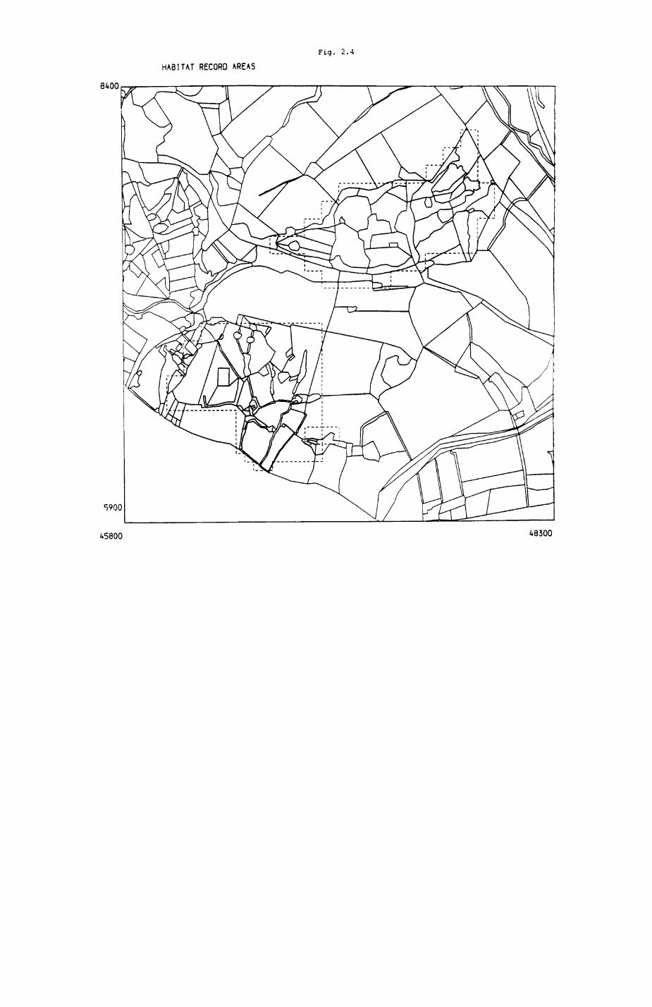
Fig. 2.4
HABITAT RECORD AREAS
8400
5900
45800 48300
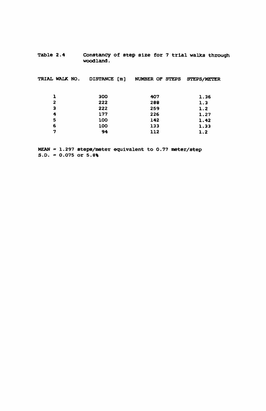
Table 2.4 Constancy of step size for 7 trial wanes throughwoodland.
TRIAL WALK NO. DISTANCE [m] NUMBER OP STEPS STEPS/METER
1 300 407 1.362 222 288 1.33 222 259 1.24 177 226 1.275 100 142 1.426 100 133 1.337 94 112 1.2
MEAN = 1.297 steps/meter equivalent to 0.77 meter/step S.D. = O.O75 or 5.8%
37
quadrat was estimated and from that the final score for the total central
area determined. Next, a zigzag course was walked on a circle approximately
half way between the border of the base area and the central area. This was
done with one person standing in the central area and checking the progress
of the person walking the zigzag course. We attempted to cover the entire
area between the central area and the border of the base area as
comprehensively as possible and much time was spent to achieve this. Thus,
the remaining variables (vegetation types, resource and fox & badger
indicators) were assessed for the entire base area.
2.3.3. Results
I shall first present a short summary of the raw habitat data and then
proceed with their analysis.
Table 2.5 presents a summary of the forestry data with the number of
plots that had scores greater than zero. Host of the 162 plots considered
had top, middle and bottom canopies greater than zero indicating a varied
and complex structure. Amongst the six ecoslg species, bramble was most
widely spread and occurred in ca 85% of all plots. Flreweed was nearly as
widespread as bramble, while stinging nettles and bluebells occurred less
frequently. Most plots did not have any indication of water on the surface
(only 8 plots) and are situated on some kind of slope, corresponding to the
two-hill layout of Wytham Woods.
Table 2.6 lists the results for the 1982 habitat census for each of the
two study sites separately and combined. Mar ley Area is mostly dominated by
woodlandi 212 out of 232 plots are situated Inside the woodland boundary.
Hill End camp/Bean Wood Area however includes both woodland (Bean Wood) and
the pastures and grasslands around the camp. This is reflected by the high
number of plots with some proportion of pasture and grass ley. other main
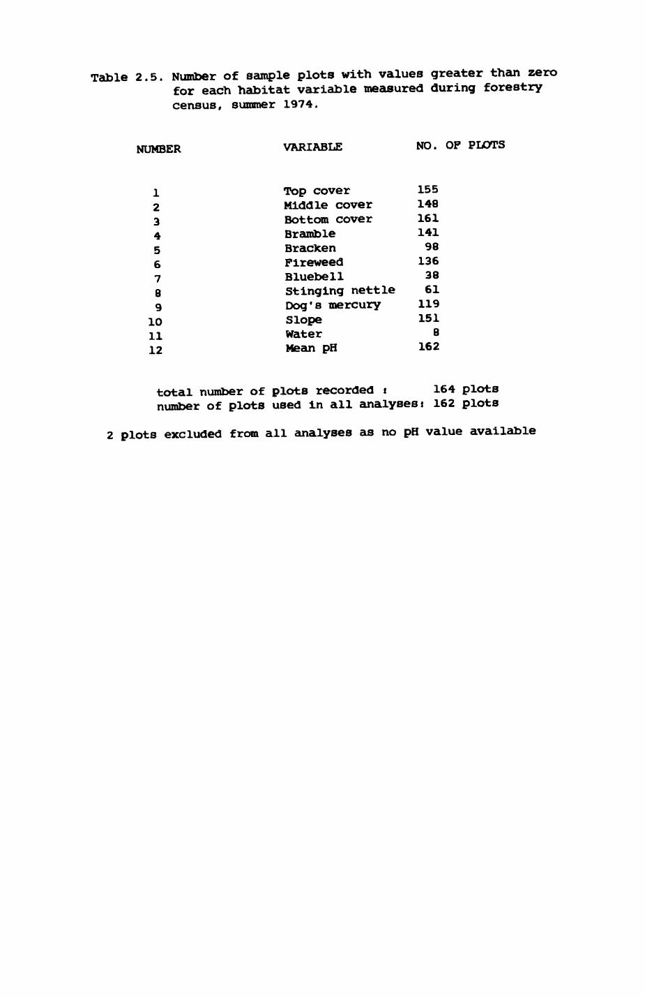
Table 2.5. Number of sample plots with values greater than zero for each habitat variable measured during forestry census, summer 1974.
NUMBER VARIABLE NO. OF PLOTS
1 Top cover 1552 Middle cover 1483 Bottom cover 1614 Bramble 1415 Bracken 986 Fireweed 1367 Bluebell 388 Stinging nettle 619 Dog's mercury 11910 Slope 15111 Water 812 Mean pH 162
total number of plots recorded t 164 plots number of plots used in all analyses! 162 plots
2 plots excluded from all analyses as no pH value available
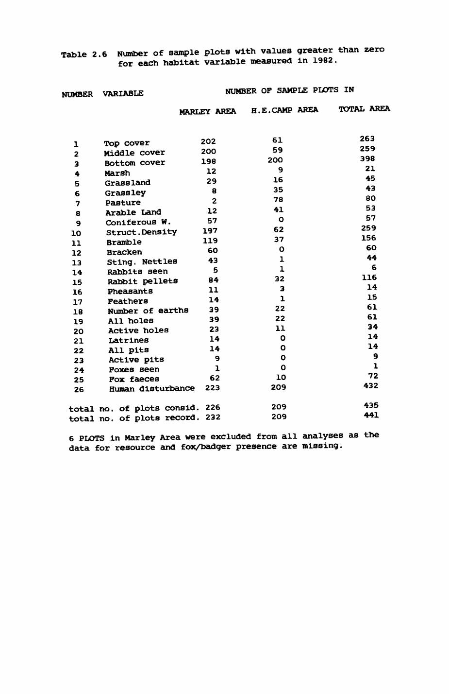
Table 2.6 Number of sample plots with values greater than zero for each habitat variable measured in 1982.
NUMBER VARIABLE NUMBER OF SAMPLE PLOTS IN
MARLEY AREA H.E.CAMP AREA TOTAL AREA
1 Top cover 202 61 2632 Middle cover 200 59 2593 Bottom cover 198 2OO 3984 Marsh 12 9 21
5 Grassland 29 16 456 Grassley 8 35 437 Pasture 2 78 80
8 Arable Land 12 41 53
9 Coniferous W. 57 0 57
10 Struct. Density 197 62 25911 Bramble 119 37 15612 Bracken 60 0 6013 Sting. Nettles 43 1 4414 Rabbits seen 51 615 Rabbit pellets 84 32 11616 Pheasants 11 3 1417 Feathers 14 1 1518 Number of earths 39 22 6119 All holes 39 22 61
20 Active holes 23 11 3421 Latrines 14 0 1422 All pits 14 0 14
23 Active pits 90 924 Foxes seen 1 O 125 Fox faeces 62 10 7226 Human disturbance 223 209 432
total no. of plots consid. 226 209 435
total no. of plots record. 232 209 441
6 PLOTS in Mar ley Area were excluded from all analyses as the data for resource and fox/badger presence are missing.
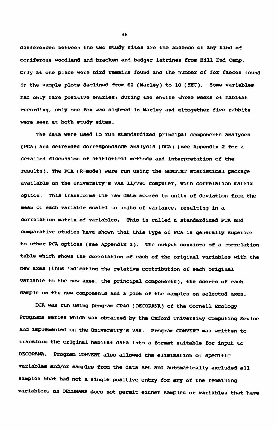
38
differences between the two study sites are the absence of any kind of
coniferous woodland and bracken and badger latrines from Hill End Camp.
Only at one place were bird remains found and the number of fox faeces found
in the sample plots declined from 62 (Marley) to 1O (HEC). Some variables
had only rare positive entriest during the entire three weeks of habitat
recording, only one fox was sighted in Mar ley and altogether five rabbits
were seen at both study sites.
The data were used to run standardized principal components analyses
(PCA) and detrended correspondance analysis (DCA) (see Appendix 2 for a
detailed discussion of statistical methods and interpretation of the
results). The PCA (R-mode) were run using the GENSTAT statistical package
available on the University's VAX 11/780 computer, with correlation matrix
option. This transforms the raw data scores to units of deviation from the
mean of each variable scaled to units of variance, resulting in a
correlation matrix of variables. This is called a standardized PCA and
comparative studies have shown that this type of PCA is generally superior
to other PCA options (see Appendix 2). The output consists of a correlation
table which shows the correlation of each of the original variables with the
new axes (thus indicating the relative contribution of each original
variable to the new axes, the principal components), the scores of each
sample on the new components and a plot of the samples on selected axes.
DCA was run using program CP4O (DECORANA) of the Cornell Ecology
Programs series which was obtained by the Oxford University Computing Sevlce
and Implemented on the University's VAX. Program CONVERT was written to
transform the original habitat data Into a format suitable for input to
DECORANA. Program CONVERT also allowed the elimination of specific
variables and/or samples from the data set and automatically excluded all
samples that had not a single positive entry for any of the remaining
variables, as DECORANA does not permit either samples or variables that have
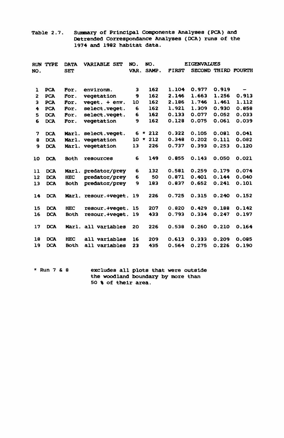
Table 2.7. Summary of Principal Components Analyses (PC A) and Detrended Correspondance Analyses (OCA) runs of the 1974 and 1982 habitat data.
RUN TYPE DATA VARIABLE SET NO. NO. NO. SET VAR. SAMP.
EIGENVALUES FIRST SECOND THIRD FOURTH
123456
789
10
111213
14
1516
17
1819
PCAPCAPCAPCADCADCA
DCADCADCA
DCA
DCADCADCA
DCA
DCADCA
DCA
DCADCA
For.For.For.For.For.For.
Marl.Marl.Marl.
Both
Marl.HECBoth
Marl.
HECBoth
Marl.
HECBoth
environm.vegetationveget. -I- env.select. veget.select. veget.vegetation
select. veget.vegetationvegetation
resources
predator/preypredator/preypredator/prey
resour . -l-veget .
resour . -l-veget .resour . -l-veget .
all variables
all variablesall variables
39
10669
61013
6
669
19
1519
20
1623
162162162162162162
* 212* 212
226
149
13250
183
226
207433
226
209435
122100
000
0
000
o
00
0
00
.104
.146
.186
.921
.133
.128
.322
.348
.737
.855
.581
.871
.837
.725
.820
.793
.538
.613
.564
011100
000
0
000
0
00
0
00
.977
.663
.746
.309
.077
.075
.105
.202
.393
.143
.259
.401
.652
.315
.429
.334
.260
.333
.275
0.9191.2561.4610.9300.0520.061
O.O810.1110.253
0.050
0.1790.1440.241
0.240
0.1880.247
0.210
0.2090.226
—0.9131.1120.8580.0330.039
0.0410.0820.120
0.021
O.O740.0400.101
0.152
0.1420.197
0.164
O.O850.19O
* Run 7 & 8 excludes all plots that were outside the woodland boundary by more than 50 % of their area.
39
not a single positive entry. As a result, different DCA runs operated on a
different number of samples. Only in Runs 7 and 8 were plots excluded
specifically, in all other cases the number of samples for each run is
simply the number of samples that had at least one positive entry for the
variables considered.
Altogether 19 ordinations were run (Table 2.7). 4 PCA and 2 DCA were
run on forestry data and the remaining 13 on my own data set. Table 2.7
indicates in a shortlist the types of variables selected for each run, the
actual number of variables considered, the number of samples considered (le.
with positive entries) and the first four eigenvalues of each analysis. In
PCA, eigenvalues are produced by the eigenanalysis of the transformed
samples-by-variables matrix (into either a variance-covariance or
correlation matrix) and indicate the variance accounted for by the relevant
principal component. In recipropcal averaging and DCA, the eigenvalues
indicate the amount of contraction in the variable scores achieved by the
ordination. The axes are then ordered according to their eigenvalues so
that the first component or the first DCA axis has the highest eigenvalue,
le accounting for the highest amount of variance. Thus, a high value
indicates a lot of variation accounted for. The eigenvalues of PCA and DCA
are not directly compatible in their absolute values (cf. RUN 4 (PCA) and 5
(DCA) and RUN 2 (PCA) and RUN 6 (DCA) on identical data sets for both
ordination methods), but what is of Interest are the differences in
eigenvalues of the first few axest if the first axis has a high eigenvalue
and the following axes very low values in relation to the first (see e.g.
RUN 10), most of the variation in the data is summarized in one dimension by
the first axis while the following dimensions contribute relatively little.
However, if the converse is true, the second, third etc. axis might be
Important for the understanding of the variation in the data.
Results of the 19 runs are presented in Table 2.8 (PCA correlation
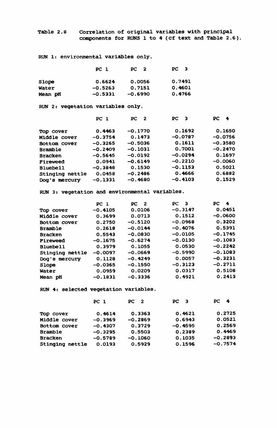
Table 2.8 Correlation of original variables with principalto 4 (cf text and Table 2.6)
RUN Is environmental variables only.
PC 1
Slope 0.6624Water -0.5263Mean pH -0.5331
RUN 2t vegetation variables
PC 1
Top cover 0.4463Middle cover -0.3754Bottom cover -0.3265Bramble -0 . 24O9Bracken -0 . 5645Fireweed 0 . 0941Bluebell -0.3848Stinging nettle O.O458Dog's mercury -0.1331
PC 2
0.00560.7151
-0.699O
only.
PC 2
-0.17700 . 1473
-O.5036-0.1031-O.O192-O.61490.1530
-O . 2486-0.4680
RUN 3: vegetation and environmental
PC 1Top cover -0.4105Middle cover 0.3699Bottom cover 0.2750Bramble 0 . 2618Bracken 0 . 5543Pireweed -0 . 1675Bluebell 0 . 3979Stinging nettle -O.O097Dog's mercury 0.1128Slope -O.O365water O.O959Mean pH -0.1831
PC 20.0106O.O713
-0.5120-0.0144-0.0830-0.62740 . 1055
-0.0669-0.4249-0 . 155OO.O209
-0.3336
PC 3
0.74910.46010 . 4766
PC 3
0.1692-0.07870.16110.70O1
-O.0294-0.221O-0 . 11530.4666
-0 . 4103
variables .
PC 3-0.31470.1512
-0.0968-0 . 4076-O.O105-0.013O0.0530
-0.59900 . 0057
-0.31230.03170.4921
RUN 4 i selected vegetation variables.
PC 1
Top cover 0.4614Middle cover -0.3969Bottom cover -0.4307Bramble -0.3295Bracken -0.5789Stinging nettle O.O193
PC 2
0.3363-0.28690.37290.5503
-0 . 10600.5929
PC 3
0.46210.6943
-0 . 45950.23890.10350 . 1596
PC 4
0.1650-0.0756-0.3580-0.2470 0.1697
-0.0060 0.5021 0.6882 0.1529
PC 4 0.0451
-O.O60O 0.3202 0.5391
-0.1745-0.1083-O.2242-0.1083-O.3231-0.2711 0.5108 0.2413
PC 4
0.27250.05210.25690.4469
-0.2893-O.7574
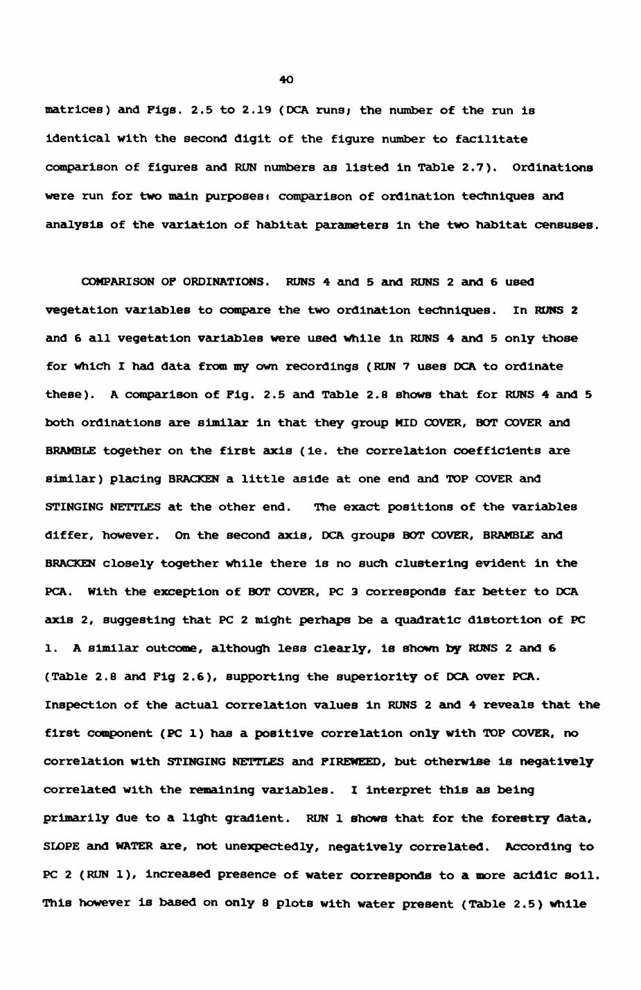
4O
matrices) and Figs. 2.5 to 2.19 (DCA runs; the number of the run is
identical with the second digit of the figure number to facilitate
comparison of figures and RUN numbers as listed in Table 2.7). Ordinations
were run for two main purposest comparison of ordination techniques and
analysis of the variation of habitat parameters in the two habitat censuses.
COMPARISON OF ORDINATIONS. RUNS 4 and 5 and RUNS 2 and 6 used
vegetation variables to compare the two ordination techniques. In RUNS 2
and 6 all vegetation variables were used while In RUNS 4 and 5 only those
for which I had data from my own recordings (RUN 7 uses DCA to ordinate
these). A comparison of Fig. 2.5 and Table 2.8 shows that for RUNS 4 and 5
both ordinations are similar in that they group MID COVER, BOT COVER and
BRAMBLE together on the first axis (ie. the correlation coefficients are
similar) placing BRACKEN a little aside at one end and TOP COVER and
STINGING NETTLES at the other end. The exact positions of the variables
differ, however. On the second axis, DCA groups BOT COVER, BRAMBLE and
BRACKEN closely together while there is no such clustering evident in the
PCA. With the exception of BOT COVER, PC 3 corresponds far better to DCA
axis 2, suggesting that PC 2 might perhaps be a quadratic distortion of PC
1. A similar outcome, although less clearly, is shown by RUNS 2 and 6
(Table 2.8 and Fig 2.6), supporting the superiority of DCA over PCA.
Inspection of the actual correlation values In RUNS 2 and 4 reveals that the
first component (PC 1) has a positive correlation only with TOP COVER, no
correlation with STINGING NETTLES and FIREWEED, but otherwise Is negatively
correlated with the remaining variables. I interpret this as being
primarily due to a light gradient. RUN 1 shows that for the forestry data,
SLOPE and WATER are, not unexpectedly, negatively correlated. According to
PC 2 (RUN 1), Increased presence of water corresponds to a more acidic soil.
This however is based on only 8 plots with water present (Table 2.5) while
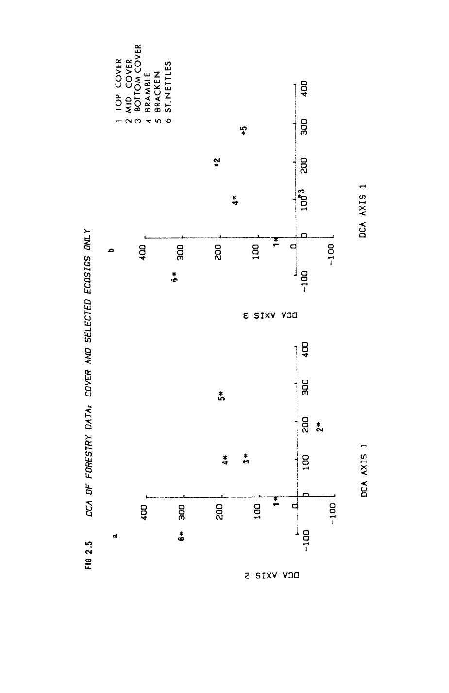
FIG 2
.5
DC
A
OF
F
OR
ES
TR
Y
DA
TA
t C
OV
ER
A
ND
S
ELE
CT
ED
E
CO
SIG
S
ON
LY
O) *- X CJ
Q
40
0
6*
300
.
200
.
100 n
-100
-100
4* 3*
D 10
02
00
300
2*
40
0
CO en i—i x <
6*
40
0
,.
300
200
100
-100
-100
4*
*2
1 T
OP
C
OV
ER
2 M
ID
CO
VE
R3
BO
TT
OM
CO
VE
R4
BR
AM
BLE
5 B
RA
CK
EN
6
ST.
NE
TT
LE
S
D 10
0*3
200
300
400
OC
A
AX
IS
1OC
A A
XIS
1
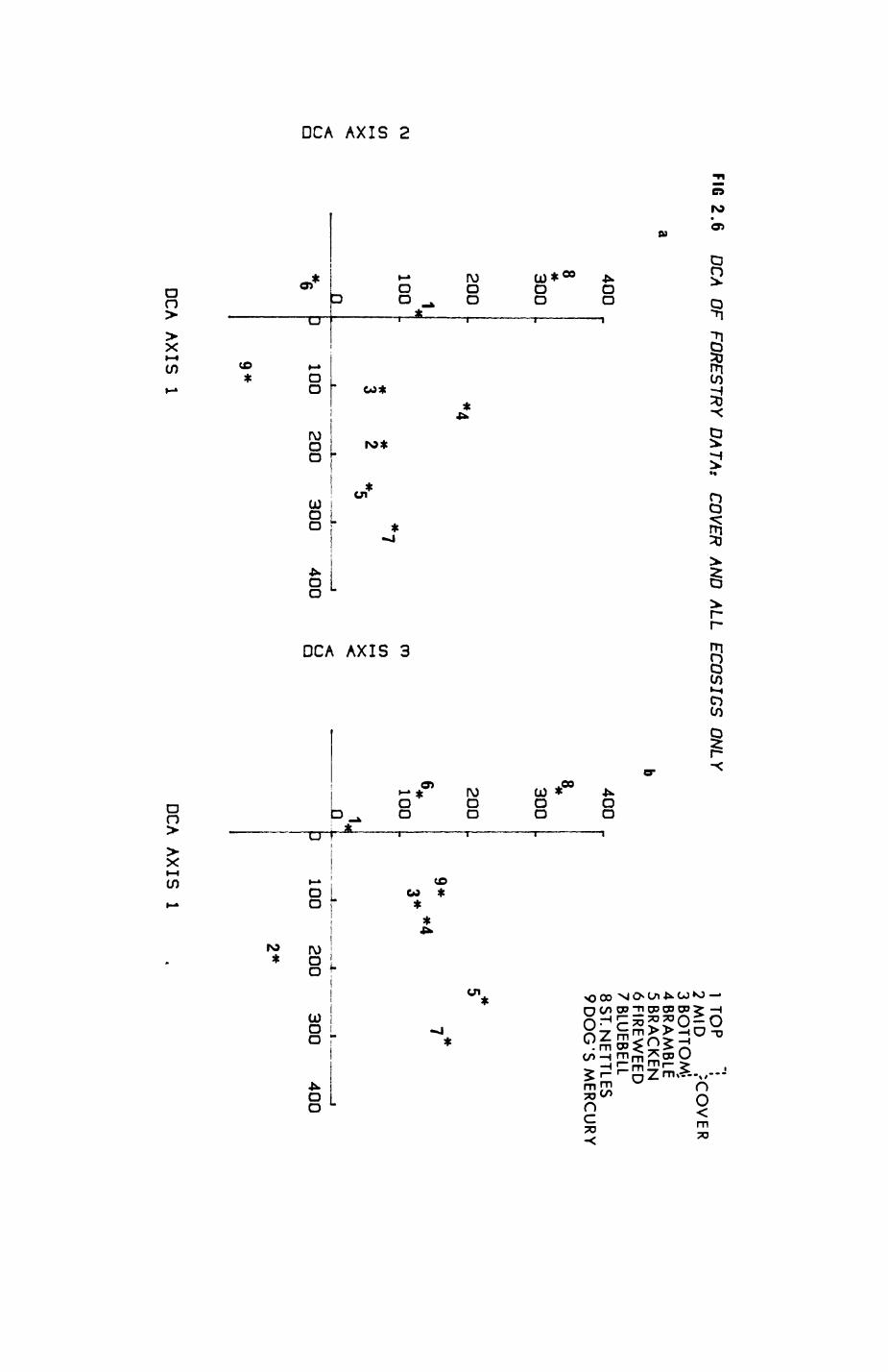
FIG 2.6 O
CA
O
F
FO
RE
ST
RY
D
AT
As C
OV
ER
A
ND
A
LL
EC
OS
ICS
O
NLY
400400
1 TOP
2 MID
.-C
OV
ER
3 BOTTO
M^
4 BRAM
BLE5 B
RA
CK
EN
6FIR
EW
EE
D
/BLU
EB
ELL
830
0
20
0'*CM
10
0
1— 1 X
Q0
*>. a
6
8*300
*4 20
°
«*L.
CD 1
00
* *
7 <n
3 2
* £
5 ><
1 <
'•«
k •
i i
j 0
D 100
20
0
30
0
400 ^
9-
O O
1. INC
1 1 L
LO
9DO
G'S
MER
C
•
*5^
9
7
*4 -i*
i- '
i i
i3
100 2
00
30
0
40
0
2*
OCA AXIS
1DCA
AXIS 1
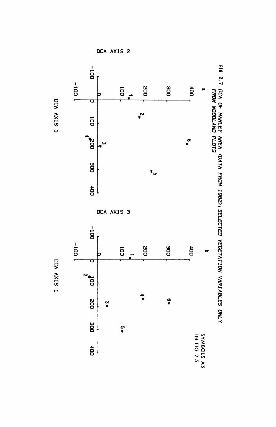
FIG 2.7
OC
A
OF
M
AR
LEY
A
RE
A
<DA
TA
FRO
M
1982), S
ELE
CT
ED
V
EG
ET
AT
ION
V
AR
IAB
LE
S
ON
LY
FRO
M
WO
OD
LAN
D
PLO
TS
b
400 ..
SY
MB
OLS
AS
IN
FIG
2.5400
.TW*^
300
200
CM 1*
en 100
^•4^^^
X£j .
n-100
-100
r* C
TWW
** 4t
300
5
. 200
^*
1-en
100X
3 <
i *
i j
n
u Q
3 100
.200 300
400 -100
4
-100
6*
• A A&
^L ^^
• **
• •
• •
D ^00
200 300
400 2
»
OCA
AX
IS
1O
CA A
XIS
1
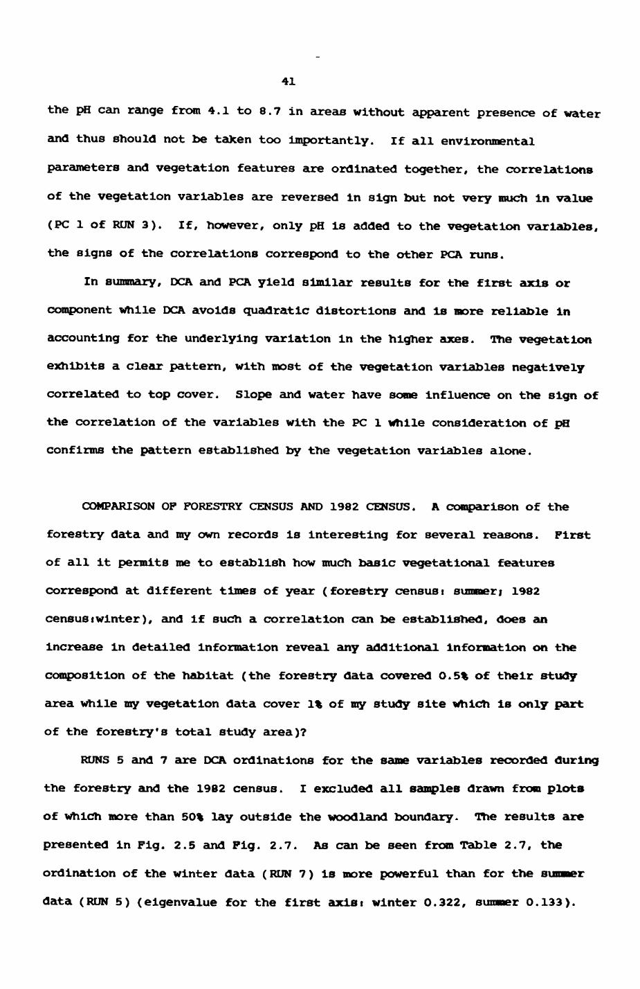
41
the pH can range from 4.1 to 8.7 in areas without apparent presence of water
and thus should not be taken too importantly, if all environmental
parameters and vegetation features are ordinated together, the correlations
of the vegetation variables are reversed in sign but not very much in value
(PC 1 of RUN 3). If, however, only pH is added to the vegetation variables,
the signs of the correlations correspond to the other PCA runs.
In summary, DCA and PCA yield similar results for the first axis or
component while DCA avoids quadratic distortions and is more reliable in
accounting for the underlying variation in the higher axes. The vegetation
exhibits a clear pattern, with most of the vegetation variables negatively
correlated to top cover. Slope and water have some Influence on the sign of
the correlation of the variables with the PC 1 while consideration of pH
confirms the pattern established by the vegetation variables alone.
COMPARISON OF FORESTRY CENSUS AND 1982 CENSUS. A Comparison Of the
forestry data and my own records is interesting for several reasons. First
of all it permits me to establish how much basic vegetational features
correspond at different times of year (forestry censusi summeri 1982
censustwinter), and if such a correlation can be established, does an
Increase in detailed information reveal any additional information on the
composition of the habitat (the forestry data covered O.5% of their study
area while my vegetation data cover 1% of my study site which is only part
of the forestry's total study area)?
RUNS 5 and 7 are DCA ordinations for the same variables recorded during
the forestry and the 1982 census. I excluded all samples drawn from plots
of which more than 50% lay outside the woodland boundary. The results are
presented in Fig. 2.5 and Fig. 2.7. As can be seen from Table 2.7, the
ordination of the winter data (RUN 7) is more powerful than for the summer
data (RUN 5) (eigenvalue for the first axisi winter 0.322, summer O.133).
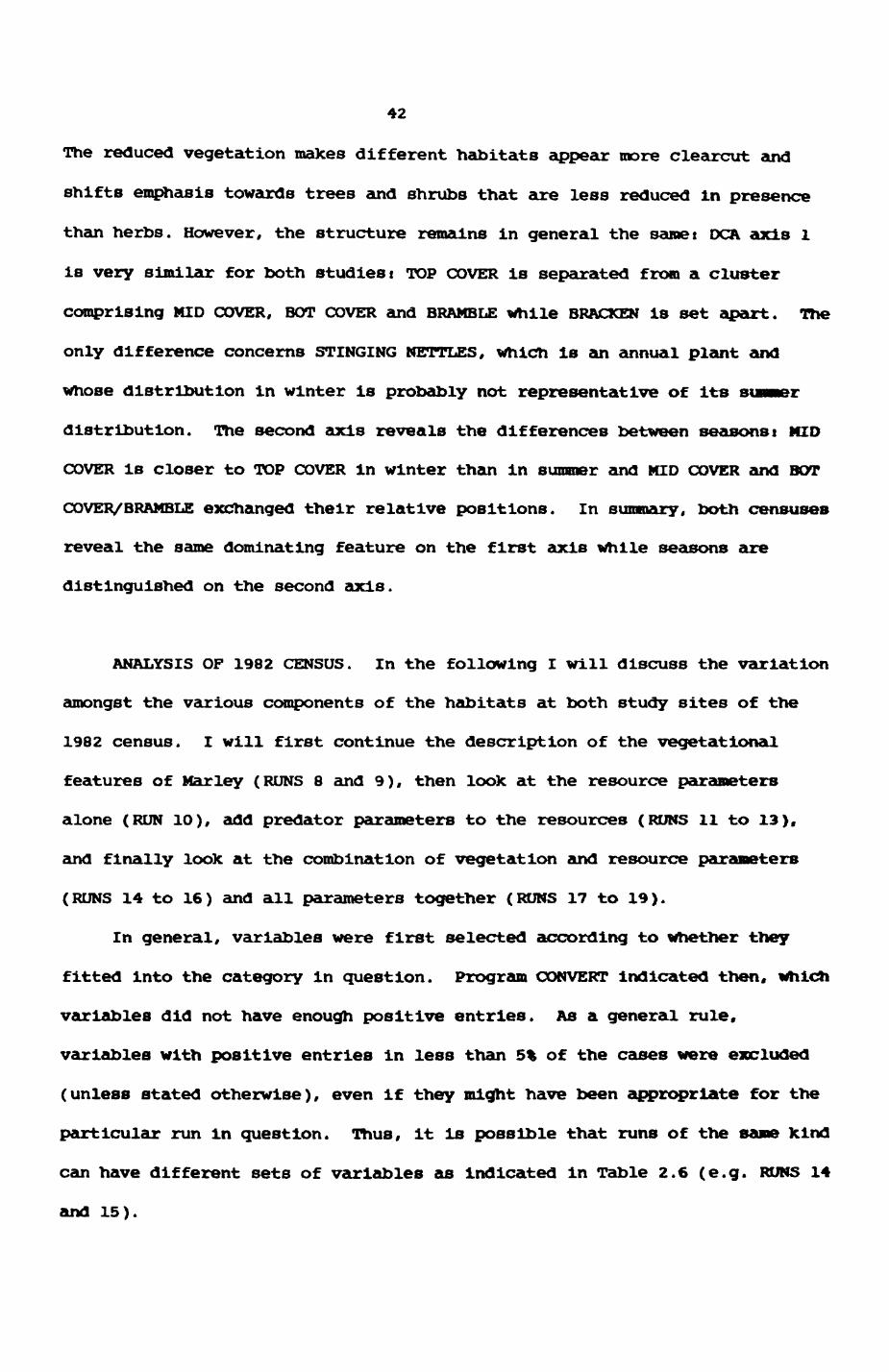
42
The reduced vegetation makes different habitats appear more clearcut and
shifts emphasis towards trees and shrubs that are less reduced in presence
than herbs. However, the structure remains in general the saroet OCA axis 1
is very similar for both studies i TOP COVER is separated from a cluster
comprising MID COVER, BOT COVER and BRAMBLE while BRACKEN is set apart. The
only difference concerns STINGING NETTLES, which is an annual plant and
whose distribution in winter is probably not representative of its sunaer
distribution. The second axis reveals the differences between seasons i MID
COVER is closer to TOP COVER in winter than in summer and MID COVER and BOT
COVER/BRAMBLE exchanged their relative positions. In summary, both censuses
reveal the same dominating feature on the first axis while seasons are
distinguished on the second axis.
ANALYSIS OF 1982 CENSUS. In the following I will discuss the variation
amongst the various components of the habitats at both study sites of the
1982 census. I will first continue the description of the vegetational
features of Marley (RUNS 8 and 9), then look at the resource parameters
alone (RUN 10), add predator parameters to the resources (RUNS 11 to 13),
and finally look at the combination of vegetation and resource parameters
(RUNS 14 to 16) and all parameters together (RUNS 17 to 19).
In general, variables were first selected according to Whether they
fitted Into the category in question. Program CONVERT indicated then, Which
variables did not have enough positive entries. As a general rule,
variables with positive entries In less than 5% of the cases were excluded
(unless stated otherwise), even if they might have been appropriate for the
particular run In question. Thus, it is possible that runs of the same kind
can have different sets of variables as Indicated in Table 2.6 (e.g. RUNS 14
and 15).
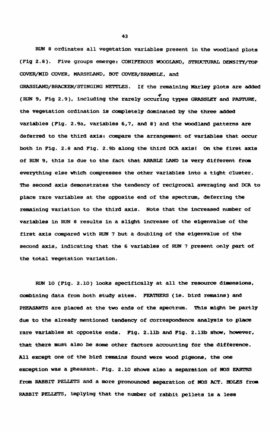
43
RUN 8 ordinates all vegetation variables present in the woodland plots
(Pig 2.8). Five groups emerget CONIFEROUS WOODLAND, STRUCTURAL DENSITY/TOP
COVER/MID COVER, MARSHLAND, BOT COVER/BRAMBLE, and
GRASSLAND/BRACKEN/STINGING NETTLES. If the remaining Mar ley plots are added
(RUN 9, Fig 2.9), including the rarely occuring types GRASSLCY and PASTURE,
the vegetation ordination is completely dominated by the three added
variables (Fig. 2.9a, variables 6,7, and 8) and the woodland patterns are
deferred to the third axisi compare the arrangement of variables that occur
both in Fig. 2.8 and Fig. 2.9b along the third DCA axisi On the first axis
of RUN 9, this is due to the fact that ARABLE LAND is very different from
everything else which compresses the other variables into a tight cluster.
The second axis demonstrates the tendency of reciprocal averaging and DCA to
place rare variables at the opposite end of the spectrum, deferring the
remaining variation to the third axis. Note that the increased number of
variables in RUN 8 results in a slight increase of the eigenvalue of the
first axis compared with RUN 7 but a doubling of the eigenvalue of the
second axis, indicating that the 6 variables of RUN 7 present only part of
the total vegetation variation.
RUN 1O (Fig. 2.1O) IOOKS specifically at all the resource dimensions,
combining data from both study sites. FEATHERS (ie. bird remains) and
PHEASANTS are placed at the two ends of the spectrum. This might be partly
due to the already mentioned tendency of correspondence analysis to place
rare variables at opposite ends. Fig. 2.lib and Fig. 2.13b show, however,
that there must also be some other factors accounting for the difference.
All except one of the bird remains found were wood pigeons, the one
exception was a pheasant. Fig. 2.10 shows also a separation of NOS EARTHS
from RABBIT PELLETS and a more pronounced separation of NOS ACT. BOLES from
RABBIT PELLETS, implying that the number of rabbit pellets is a less
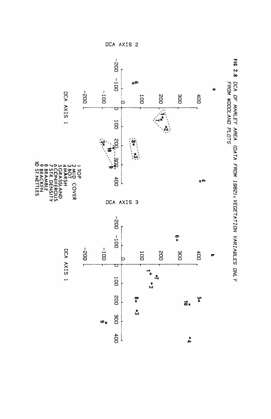
FIG 2.8
OC
A O
F M
AR
LEY
AR
EA (D
ATA
FR
OM
1982): V
EG
ETA
TION
V
AR
IAB
LES
O
NLY
FR
OM
W
OO
DLAN
D
PLO
TS
a b
400
30
0
20
0
100c\J
6* ent— ix
, ——
——
_ R
_<
-2
00
-1
00
u°
-100
-200
4* 400
6*
30°
%;-'
100,-""" *3'«
mi— i,
, .
x
, ,
n3
100 2
00...3JQ
Q;
400 ^
-200
-10
0
/10 ..-''*
§
/5*. - ' '
- 1 00
L -2
00
5*10 *
4-
*71*
*2
.8*
*3
fill
D 100
200 300
400
•if 9
DC
A A
XIS
1
1 TOP
2 MID
C
OV
ER
3B
OT
4M
AR
SH
5G
RA
SS
LAN
D
6 CO
NIFE
RO
US
7S
TR
.DE
NS
ITY
8 BRAM
BLE9 B
RA
CK
EN
10 ST.N
ETTLES
DC
A A
XIS
1
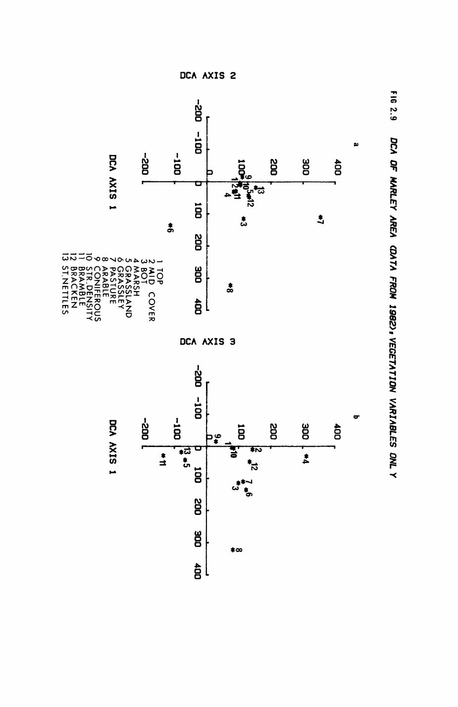
FIG 2.9 O
CA
O
F M
AR
LEY
AR
EA
(D
ATA
FR
OM
19B
2)i V
EG
ET
AT
ION
V
AR
IAB
LE
S
ON
L Y
400
CMCO1-4^^
^%
^£
(Ja
^w
^^^^^
300
200
100»n-2
00
-1
00-1
00
-20
0
*7
•J3105*12
.3M
W
J
2*4
^8 (nO
)»H
*
J
I
f
^^
^^
) 100
200 300
400 <0a
•
1 TO
P2 M
ID
CO
VE
RL
3 BOT
^v^^^*
300
200
100 19«n
-20
0
-100-1
00
-20
0
.•4
2 1?
* *
7 »6*
0•„.
«o 8
»10 o
«
t *
t *
) 100
200 300
400•n **i10 4
0•«T1
B
OCA AX
IS
1
4 MA
RS
H5 G
RA
SS
LAN
D6 G
RA
SS
LEY
7 PASTU
RE
8 ARABLE
9 CO
NIFE
RO
US
10 S
IR.D
EN
SITY
11 B
RA
MB
LE12
BR
AC
KE
N13 S
T.NE
TTLES
OCA AX
IS
1
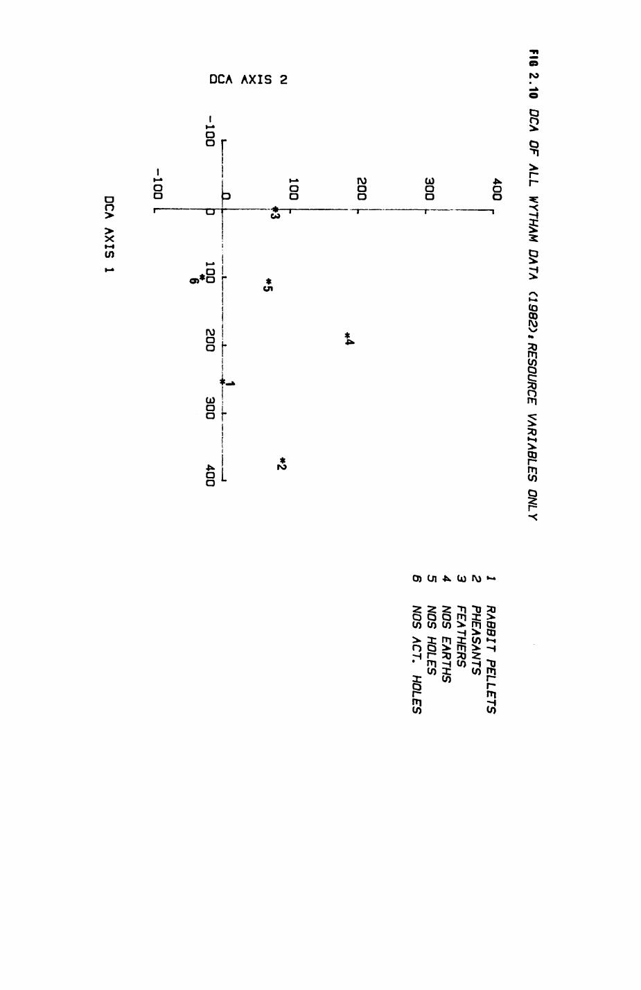
FIG 2.10 O
CA O
F ALL
WYTHAM
DATA
<1982)• R
ESOU
RC
E V
AR
IAB
LES
ON
LY
(MXCJa-100
400
300
200
100n
-100 L
*4
100200
300400
1 R
AB
BIT
PE
LLET
S2
PH
EA
SA
NTS
3 FE
ATH
ER
S4
NO
S EA
RTH
S5
NO
S HO
LES
6
NO
S AC
T. H
OLE
S
DCA A
XIS
1
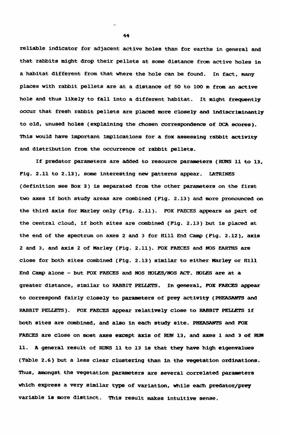
44
reliable indicator for adjacent active holes than for earths in general and
that rabbits might drop their pellets at some distance from active holes in
a habitat different from that where the hole can be found. In fact, many
places with rabbit pellets are at a distance of 5O to 1OO m from an active
hole and thus likely to fall into a different habitat. It might frequently
occur that fresh rabbit pellets are placed more closely and indlscrlminantly
to old, unused holes (explaining the chosen correspondence of DCA scores).
This would have important implications for a fox assessing rabbit activity
and distribution from the occurrence of rabbit pellets.
If predator parameters are added to resource parameters (RUNS 11 to 13,
Fig. 2.11 to 2.13), some interesting new patterns appear. LATRINES
(definition see Box 3) is separated from the other parameters on the first
two axes if both study areas are combined (Fig. 2.13) and more pronounced on
the third axis for Mar ley only (Fig. 2.11). FOX FAECES appears as part of
the central cloud, if both sites are combined (Fig. 2.13) but is placed at
the end of the spectrum on axes 2 and 3 for Hill End Camp (Fig. 2.12), axis
2 and 3, and axis 2 of Marley (Fig. 2.11). FOX FAECES and NOS EARTHS are
close for both sites combined (Fig. 2.13) similar to either Marley or Hill
End Camp alone - but FOX FAECES and NOS HOLES/NOS ACT. HOLES are at a
greater distance, similar to RABBIT PELLETS. In general, FOX FAECES appear
to correspond fairly closely to parameters of prey activity (PHEASANTS and
RABBIT PELLETS). FOX FAECES appear relatively close to RABBIT PELLETS if
both sites are combined, and also In each study site. PHEASANTS and FOX
FAECES are close on most axes except axis of RUN 13, and axes 1 and 3 of RUN
11. A general result of RUNS 11 to 13 Is that they have high eigenvalues
(Table 2.6) but a less clear clustering than in the vegetation ordinations.
Thus, amongst the vegetation parameters are several correlated parameters
which express a very similar type of variation, while each predator/prey
variable is more distinct. This result makes Intuitive sense.
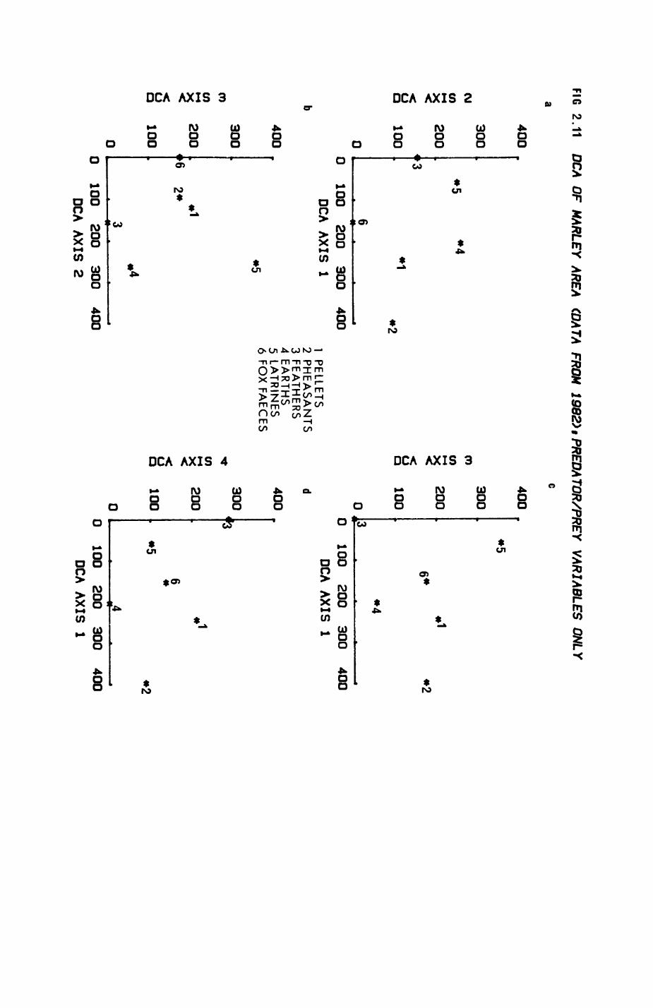
FIG 2.11
OC
A
OF M
AR
LEY
AR
EA
(DA
TA
FRO
M
1982)iPR
ED
AT
OR
/PR
EY
V
AR
IAB
LES
ON
LY
a
CMcn^^^^^W<^o a
b
cnH4
5Ua
400 400
300
200<
100o
300cn
*5 (/ix
200<
>3 <
*1 *2
°
10°
. §
. n .
«5
«16*
*5
*41
&
A
A
&
0 100
200 300
400 0
100 200
300 400
DCA AXIS
1 } PELLETS
DCA AXIS 1
2 PHEASANTS
d3 FEATHERS
.„_ 4 E
ARTHS
.__ 400
. 5 LATRINES
400
300
200<
1000
^5 6 FOX FAECES
300 4"*
«1 X
200^6
2*
<a
100
3
6« »5
^j
M4 .
100 200
300 DCA
AX
IS
2400
100 200
300 400
DCA AXIS 1
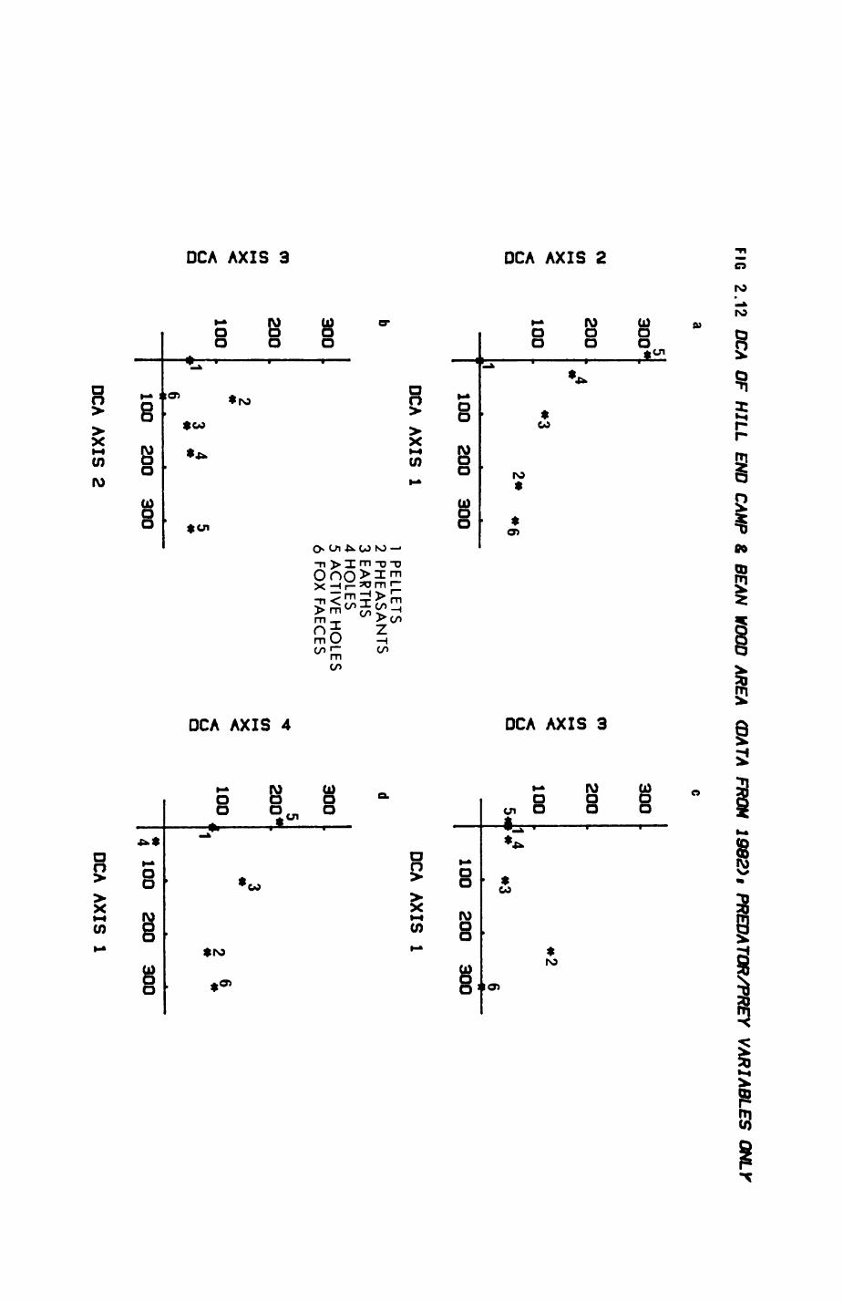
FIG 2.12
OCA
OF H
ILL
E
ND
C
AM
P &
BEA
N
WOOD A
REA
(D
ATA
FR
OM
1962)t
PR
ED
ATO
R/P
RE
Y
VA
RIA
BLE
S O
NLY
5 300*
1-4
X<
1000a
• — i
300
: «
* 1-1x
*3 <
1002*
«6 8
5.3 —— . —— , ————
100 200
300
•
*2
?» «3
0
100 200
300
OCA AXIS
1 OCA
AXIS 1
b 300
"
200
X<
100aa
•
1 PELLETS
2 PHEASANTS
d3 EARTHS 4 H
OLES
5 ACTIVE HOLES
ann
6 FOX FAECES 3UU
«
200-k^
2 x^
100 ,1
3.4
5 g
6———— H — i —————— • —————— • ———
———
100 200
300
1 5
4
4 100
200 300
OCA AX
IS 2
DCA AX
IS
1
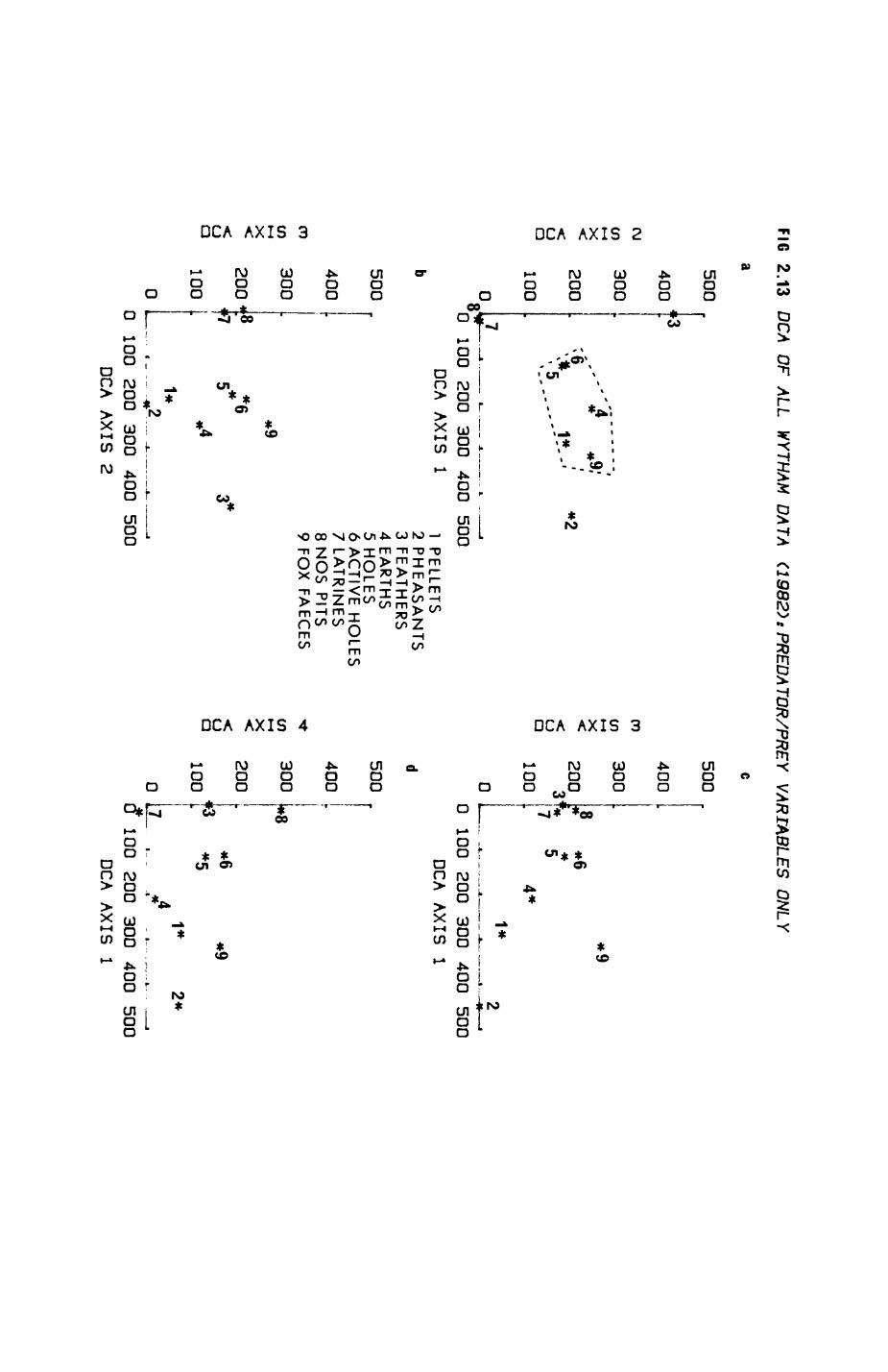
FIG 2.13
OCA OF ALL
WYTHAM DATA
(1982)t PREDATOR/PREY VARIABLES ONLY
C\Jt_X<
£uaCD|-
i
X<•
«£Ua
a500
400 °3
300 .
.-*''?
*9.'
200 \6.
... '
*2,*
J---'<
D . -- '
* _
- "
100 .
0 K#—
~+ «-
- -
_ i
0 100
200 300
400 500
OCA
AX
IS
1 !
PELLETSb
2 PH
EA
SA
NTS
3 FEATHER
S4 EAR
THS
500 r
5 HO
LES
1 6 AC
TIVE HO
LES4Q
O
7 LATRIN
ES r
8NO
S PITS
9 FOX FAEC
ES300
.*
200 *.8 *6
^7 5
3*
100 .
*4
0 _
,
^2 ^_ _.__J_ _
_ ,
c
500
400 .
CD(n 300
.t-t
*L
Q
X
R
c200
* *6
<
THh* *
u
J ^J 5
°
100 .
4*
1* 2
0 -^
._. _1—0
100 200
300 400
500O
CA A
XIS
1
d5001
400 .
•<frco 300
*8X<
200
.^
*6 o
(J ,
*"°
100 3
*51*
2*o ll_
,__ *4
.._..._...... _0
100 200
300 400
500 OCA
AXIS 2
0* 100
200 300
400 500
OCA AXIS
1
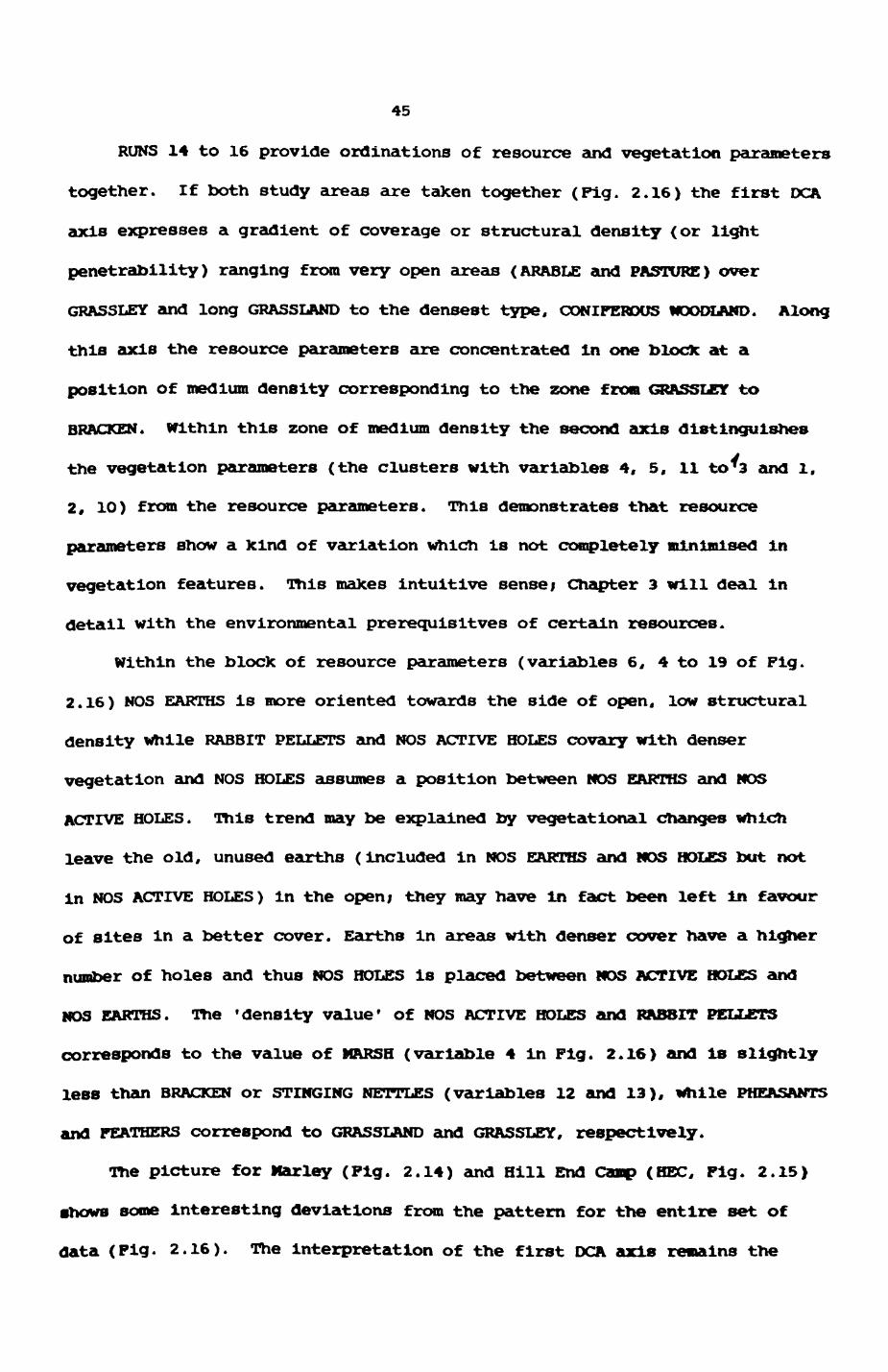
45
RUNS 14 to 16 provide ordinations of resource and vegetation parameters
together. If both study areas are taken together (Fig. 2.16) the first DCA
axis expresses a gradient of coverage or structural density (or light
penetrability) ranging from very open areas (ARABLE and PASTURE) over
GRASSLEY and long GRASSLAND to the densest type, CONIFEROUS WOODLAND. Along
this axis the resource parameters are concentrated in one block at a
position of medium density corresponding to the zone from GRASSLEY to
BRACKEN. Within this zone of medium density the second axis distinguishes
the vegetation parameters (the clusters with variables 4, 5, 11 to^3 and 1.
2, 10) from the resource parameters. This demonstrates that resource
parameters show a kind of variation Which is not completely minimised in
vegetation features. This makes intuitive sense; Chapter 3 will deal in
detail with the environmental prerequlsitves of certain resources.
Within the block of resource parameters (variables 6, 4 to 19 of Pig.
2.16) NOS EARTHS is more oriented towards the side of open, low structural
density while RABBIT PELLETS and NOS ACTIVE HOLES covary with denser
vegetation and NOS HOLES assumes a position between NOS EARTHS and NOS
ACTIVE HOLES. This trend may be explained by vegetational changes which
leave the old, unused earths (included in NOS EARTHS and NOS HOLES but not
in NOS ACTIVE HOLES) in the open; they may have in fact been left in favour
of sites in a better cover. Earths in areas with denser cover have a higher
number of holes and thus NOS HOLES is placed between NOS ACTIVE HOLES and
NOS EARTHS. The 'density value' Of NOS ACTIVE HOLES and RABBIT PELLETS
corresponds to the value of MARSH (variable 4 in Fig. 2.16) and is slightly
less than BRACKEN or STINGING NETTLES (variables 12 and 13), while PHEASANTS
and FEATHERS correspond to GRASSLAND and GRASSLEY, respectively.
The picture for Marley (Fig. 2.14) and Hill End Camp (HEC, Fig. 2.15)
ghows some interesting deviations from the pattern for the entire set of
data (Fig. 2.16). The interpretation of the first DCA axis remains the
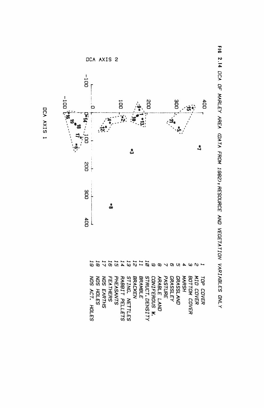
FIG
2.14 O
CA
OF
MA
RLE
Y
AREA
(DA
TA
FRO
M
19
82
): RESO
UR
CE
AND
V
EG
ETA
TION
V
AR
IAB
LES
O
NLY
400r$t30
0
20
0
''•*/
100C\JO
)t—i x
'
-1002
00
30
0400
-10019
16..-
1 TOP COVER
2
MID
C
OVER
3
BOTTOM COVER
4 M
ARSH
5
GR
AS
SLA
ND
6
GR
AS
SLE
Y7
PA
STU
RE
8 A
RA
BLE
LA
ND
9
CONIFEROUS W.
10 STRUCT. D
ENSITY
11 BRAMBLE
12 BRACKEN
13 STING.
NETTLES
14 RABBIT PELLETS
15 PHEASANTS
16 FEATHERS
17
NOS EARTHS
18 NOS HOLES
19 NOS ACT.
HOLES
OCA AXIS
1
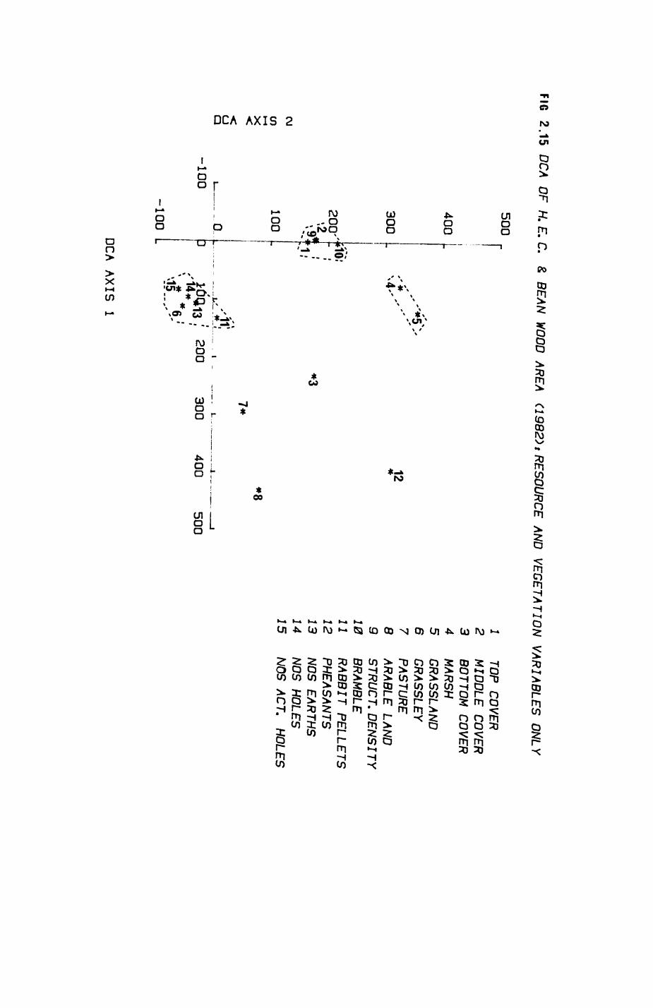
FIG 2.15
DC
A O
F H. E. C. &
BE
AN
W
OOD AREA
(19
82
) t RESO
UR
CE AN
D
VE
GE
TATIO
N
VA
RIA
BLE
S O
NLY
500
400 L.
300 .
200'
•2tttCJX(Ja
100 .
\4-'12*
Id:
1„ • I
*8
-100
-100 .
^{gta; 200
300400
500
i5
1 TO
P C
OVER
2 M
IDD
LE
CO
VER3
BOTTO
M C
OVER
4 MARSH
5
GRASSLAND
6
GRASSLEY
7 PASTURE
8 ARABLE LAND
9
STRUCT. DENSITY
10 BRAMBLE
11 RABBIT PELLETS
12 PHEASANTS
13 NOS EARTHS
14 NOS HOLES
15 NOS ACT.
HOLES
DCA AXIS
1
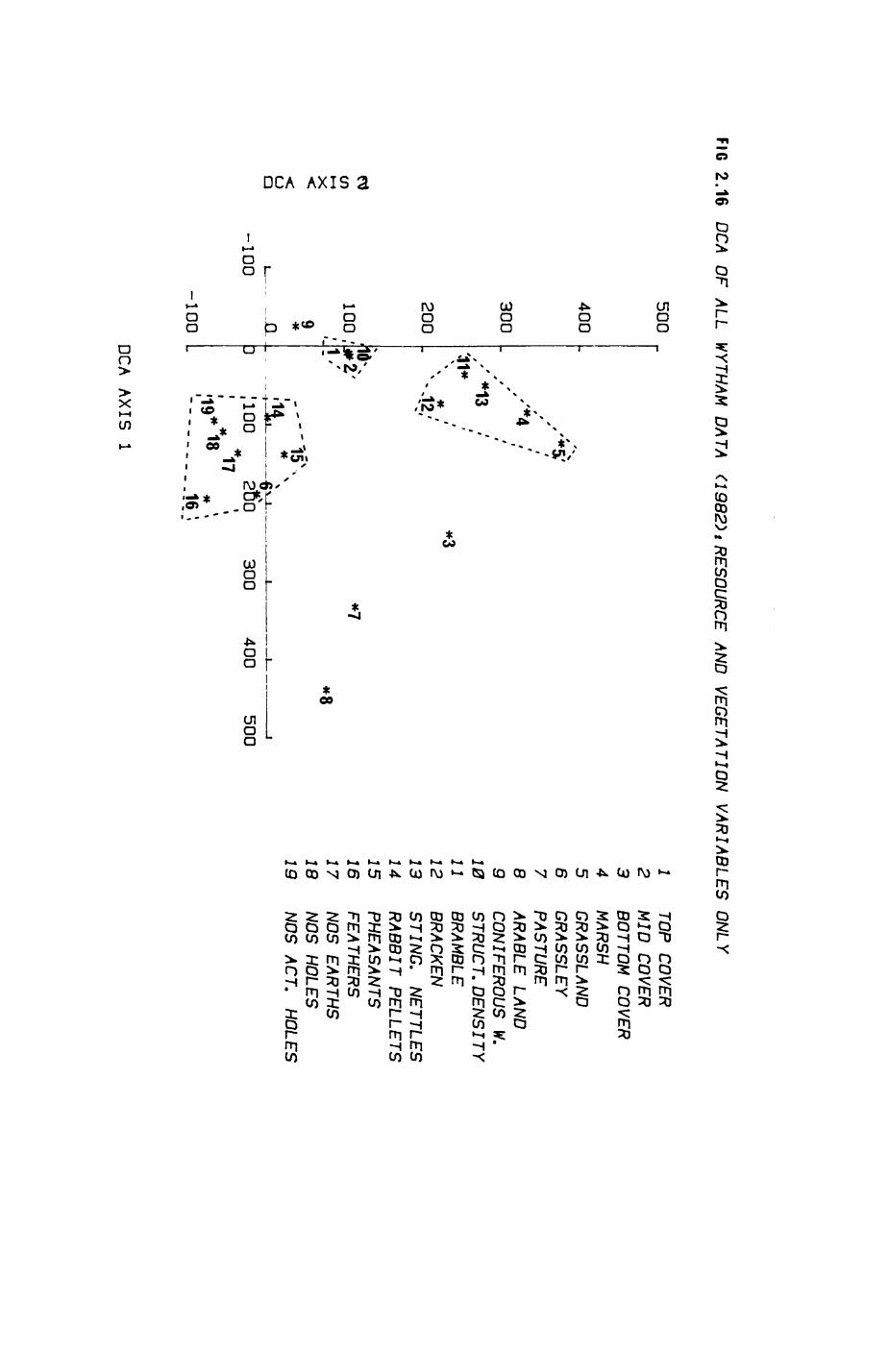
FIG 2.16
DCA OF ALL WYTHAM DATA (1982)
« RESOURCE AND VEGETATION VARIABLES ONLY
500 „
400
300
200
IDi—iX
ioo;i i_
9*
-100...
_JD_... 3
-100 .
,'*&'*
i/
/~4
/,
«t
i
' *13 / «
'' - 42/
I/- - - ' "15\
1002fio
300400
50017
-------- .16 j
1 TOP COVER
2 MID COVER
3
BOTTOM COVER
4 MARSH
5 GRASSLAND
6
GRASSLEY
7 PASTURE
8 ARABLE LAND
9
CONIFEROUS W.
10 STRUCT. D
ENSITY
11 BRAMBLE
12 BRACKEN
13 STING.
NETTLES
14 RABBIT PELLETS
15 PHEASANTS
16 FEATHERS
17 NOS EARTHS
18 NOS HOLES
19 NOS ACT.
HOLES
DCA AXIS
1
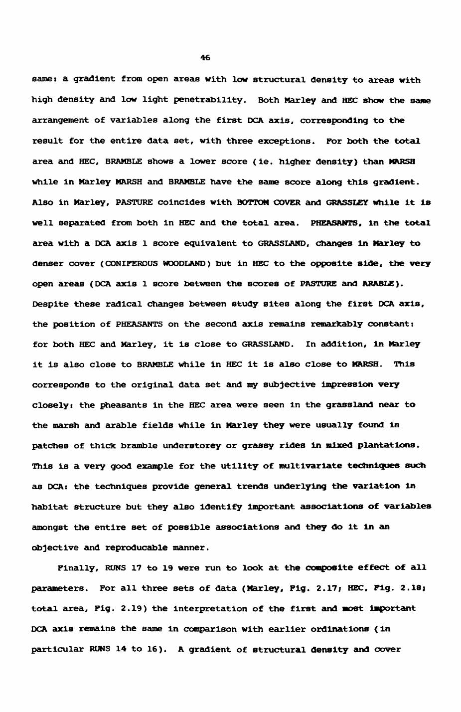
46
same i a gradient from open areas with low structural density to areas with
high density and low light penetrability. Both Mar ley and HEC show the same
arrangement of variables along the first DCA axis, corresponding to the
result for the entire data set, with three exceptions. For both the total
area and HEC, BRAMBLE shows a lower score (ie. higher density) than MARSH
while in Mar ley MARSH and BRAMBLE have the same score along this gradient.
Also in Mar ley, PASTURE coincides with BOTTOM COVER and GRASSLEY while it Is
well separated from both in HEC and the total area. PHEASANTS, in the total
area with a DCA axis 1 score equivalent to GRASSLAND, changes In Marley to
denser cover (CONIFEROUS WOODLAND) but in HEC to the opposite side, the very
open areas (DCA axis 1 score between the scores of PASTURE and ARABLE).
Despite these radical changes between study sites along the first DCA axis,
the position of PHEASANTS on the second axis remains remarkably constant:
for both HEC and Marley, it is close to GRASSLAND. In addition, in Marley
it is also close to BRAMBLE while in HEC it is also close to MARSH. This
corresponds to the original data set and my subjective impression very
closelyi the pheasants in the HEC area were seen in the grassland near to
the marsh and arable fields while in Marley they were usually found in
patches of thick bramble understorey or grassy rides In mixed plantations.
This is a very good example for the utility of multivarlate techniques such
as DCAt the techniques provide general trends underlying the variation In
habitat structure but they also identify Important associations of variables
amongst the entire set of possible associations and they do it in an
objective and reproducable manner.
Finally, RUNS 17 to 19 were run to look at the composite effect of all
parameters. For all three sets of data (Marley, Fig. 2.17j HEC, Pig. 2.18j
total area, Fig. 2.19) the interpretation of the first and Most Important
DCA axis remains the same in comparison with earlier ordinations (In
particular RUNS 14 to 16). A gradient of structural density and cover
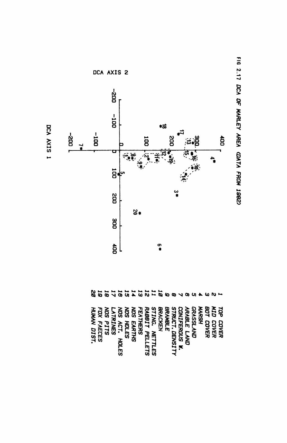
FIG 2.17
OCA O
F MAR
LEY AREA (D
ATA FRO
M 1982)
400
18
CMXu0
200
100n-200
-100
-100
-20
0
"1Q1
12,'
20
-'
100200
300400
1 TO
P COVER
2 M
ID CO
VER3
BOT CO
VER4
MARSH
5 G
RASSLAND6
ARABLE LAN
D7
CONIFEROUS W.
8 STRUCT. DENSITY
9
BRAMBLE
10 BRACKEN
11 STING.
NETTLES12
RABBIT PELLETS13
FEATHERS
14 NOS EARTHS
15 NOS HOLES
18 NOS ACT.
HOLES
17 LATRINES
18 NOS PITS
19 FOX FAECES
20 HUMAN DIST.
OCA AXIS 1
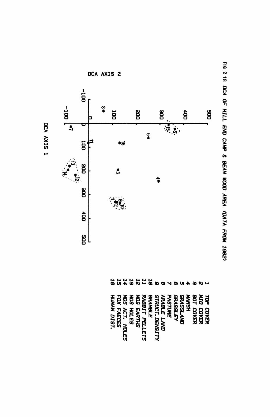
FIG 2.18 O
CA OF H
ILL END CAM
P ft BEAN W
OOD AREA (D
ATA FRO
M 1992)
500 ..
CM0) »-iX8
400
*
300
200
100 8«
D-100
-100
M5/
16»
J TOP COVER
2 M
ID COVER3
SDT CDVER4
MAftSH
5 G
RASSLAN
D6
G
RA
SS
LEY
7
PA
STU
RE
9 AR
ABLE LAND
9
STR
UC
T. DE
NS
ITY
10
BR
AM
BLE
11 RABBIT PELLETS
12 NOS EARTHS
13 NOS HOLES
14 NOS ACT.
HOLES15
FOX FAECES
16 HUMAN DIST.
JL100200
----•12'.*
300400
500
»7
OCA AXIS 1
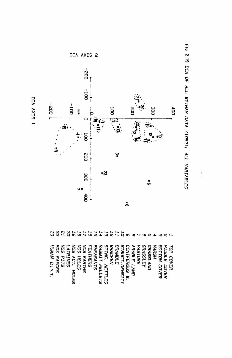
FIG 2.19
OCA
OF A
LL W
YTHAM D
ATA (1
98
2)*
ALL
VA
RIA
BLE
S
400
300
.-'20',#-
en »-« xu
a
-200 -100
200
100
__Q_
9*-100
-20
0
*6
14'.
100200
23*300400
* 7
1 TO
P C
OVER
2
MID
DLE
CO
VER3
BOTTO
M
CO
VER4
MAR
SH5
GR
ASSLAND
6 G
RA
SS
LEY
7 P
AS
TUR
E8
AR
AB
LE LA
ND
9
CO
NIFE
RO
US
W.
10 S
TRU
CT. D
EN
SIT
Y11
BRAM
BLE12
BRAC
KEN13
ST
ING
. N
ETTLE
S14
RA
BB
IT P
ELLE
TS
15 P
HE
AS
AN
TS16
FEA
THE
RS
17 N
OS
EA
RTH
S18
NO
S H
OLES
19 N
OS A
CT.
HO
LES
20
LAT
RIN
ES
21 N
OS P
ITS
22
FOX FA
EC
ES
23
HU
MAN
D
IST
,
OCA A
XIS
1
47
ranges from open areas with little cove and high light penetrability to
areas with dense cover and low light penetrability. The second DCA axis
separates the three groups of variables (vegetation, resource, predators).
In Marley and in the whole area, the inclusion of fox, badger, and human
presence (variables 17 to 20) separates RABBIT PELLETS from the other
resource variables and increases the distance between HOS EARTHS and NDS
HOLES/NOS ACTIVE HOLES. Badger LATRINES and NDS PITS (definitions in Box 3)
are grouped together with FOX FAECES and RABBIT PELLETS. LATRINES and NOS
PITS are associated with densest coven they surpass even CONIFEROUS
WOODLAND, in HEC, POX FAECES is placed between GRASSLAND and PASTURE and
therefore in more open cover than in Marley (here between MARSH and MID
COVER). For all three data sets HUMAN DISTURBANCE assumes a position in
fairly open ground.
The inclusion of the additional 'predator' variables results in a
considerable stretching of the first DCA axis for Marley, a moderate
stretching for the total area and a contraction for HEC relative to the
corresponding RUNS 14 to 16 with only vegetation and resource variables.
All eigenvalues of the first DCA axis of RUNS 17 to 19 decreased relative to
RUNS 14 to 16, ie. DCA axis 1 of RUNS 17 to 19 accounted for less of the
variance than did the DCA axis 1 for RUNS 14 to 16. Thus, the effect of the
inclusion seems to be an increase in variation space and the result a less
clear cut, higher dimensional structure. This impression is enhanced by a
comparison of the eigenvalues of RUN 10 (resource variables only for the
total area) and RUN 13 (resources and predator variables for the total
area). In RUN 1O, the first DCA axis accounts for most of the variance
since the eigenvalues of the higher axes are very low (Table 2.7). In
contrast in RUN 13, the second and the third eigenvalues are much higher
than the second eigenvalue of RUN 10 (0.652 and O.241 against O.143). The
ordinations Including vegetation and resource parameters only (RUNS 14 to
48
16) seem to me the most successful and useful ordinations indicating a low-
dimensional habitat structure and a clear and straightforward interpretation
of the ordination axes. Despite the field impression of apparent complexity
and seemingly endless changes in vegetation patterns it is reassuring and
interesting to note that most of this variation can be arranged In a low-
dimensional structure. This is also remarkable from another point of views
with a low-dimensional structure, habitat selection by foxes and badgers and
related adaptation processes can more easily be envisaged and analysed.
2.4 Discussion
In the following section I want to discuss the relationship of the two
approaches to habitat recording and classification, namely the discrete
habitat types of the habitat map (section 2.2) and the continuous habitat
structure as revealed by the habitat records (section 2.3), and relate this
to the overall alms of this study.
The identification and classification of areas as discrete habitats is
based on the personal decision of the researcher and thus neither
necessarily undisputed nor entirely reproducable, but of great utility for
further analysis under a broad perspective. A summary of the environment in
a certain area as a discrete habitat has a filtering effect on continous
small scale variations which are neglected ('flocked out'); only the broad
lines of structural variation permit. An appropriate system of discrete
habitats is equivalent to an efficient filter that is arranged on the right
scale of variation, considers the correct habitat parameters (ie. the
parameters responsible for the Important variation) and yields habitat types
that are actually different from each other 1 Since habitat was defined in
relation to the animal's requirements and potential resources (section 2.1).
there is the posslbllty (and the hope) that foxes and badgers might view
49
their environment through a filter corresponding In Its effects to my
habitat categorization. Obviously, If the habitat categories do not
correspond to the categories as seen through the animal's filter, little can
be said about 'habitat' utilization by animals, as the results would be
based on an artificial and inadequate system. Thus it should be a central
point in any investigation of carnivore behavioural ecology based on
habitats to find a procedure which describes how well the chosen habitat
categorization corresponds to the habitat structure as perceived by the
animals. As far as I am aware, this is the first study in carnivore ecology
to combine two different approaches to habitat description and show how a
system of discrete habitat types can be compared with the continuous
variation of 'actual' habitat structure as represented by a sample of
continuously varying habitat parameters, so that an estimate of the adequacy
and efficiency of the habitat categorization is possible.
For this comparison the following procedure was adoptedi Program
HABCOORD placed a systematic grid of five equidistant points over each
recording unit of the habitat records (the 'basal area' or by SO by SO m
cell). Programe SRCH2HAB then evaluated the patch number and habitat type
(from the habitat map) for each grid point. Program HABSEL compared the
habitat types of all five grid points in each cell and selected only those
cells with all gridpoints having the same habitat type. Thus, only
homogeneous cells as defined by the system of the habitat map were admitted
for further analysis. Program HABDECO took each of these homogeneous cells
and tagged it with its scores on the four DCA axes of the RUNS 17 to 19. In
Marley, only three habitat types, bracken, deciduous hardwoods, and mixed
plantations had big enough sample sizes (ie. a sufficient number of
homogeneous cells) to be useful for a statistical analysis (Table 2.9). In
Hill End Camp (HEC) five variables satisfied this condition (grassley.
pasture, summer cereals, deciduous hardwoods, sportsgrounds. Table 2.1O) and
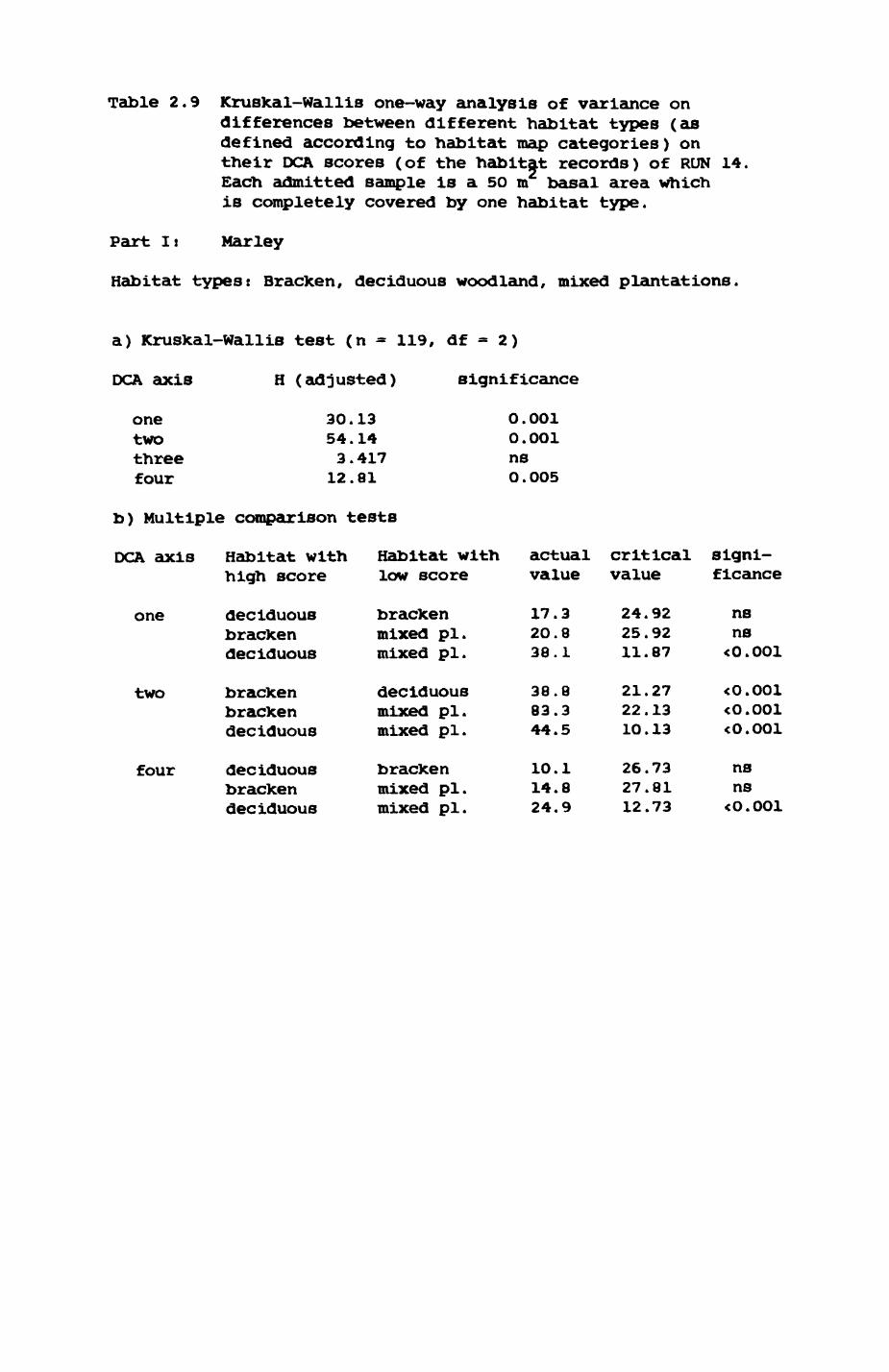
Table 2.9
Part Is
Kruskal-Wallis one-way analysis of variance on differences between different habitat types (as defined according to habitat map categories) on their DCA scores (of the habitat records) of RUN 14 Each admitted sample is a 50 m basal area which is completely covered by one habitat type.
Marley
Habitat types: Bracken, deciduous woodland, mixed plantations
a) Kruskal-Wallis test (n = 119, df = 2)
DCA axis
one two three four
H (adjusted)
30.1354.143,41712.81
significance
O.O01 O.O01 ns 0.005
b) Multiple comparison tests
DCA axis
one
two
four
Habitat with high score
deciduousbrackendeciduous
bracken bracken deciduous
deciduousbrackendeciduous
Habitat with low score
bracken mixed pi. mixed pi.
deciduous mixed pi. mixed pi.
bracken mixed pi. mixed pi.
actual critical signi- value value ficance
17.320.838.1
10.114.824.9
24.9225.9211.87
26.7327.8112.73
ns ns <0.001
38.8 83.3 44.5
21.27 22.13 10.13
< 0.001 <0.001 <O.O01
ns ns <0.001
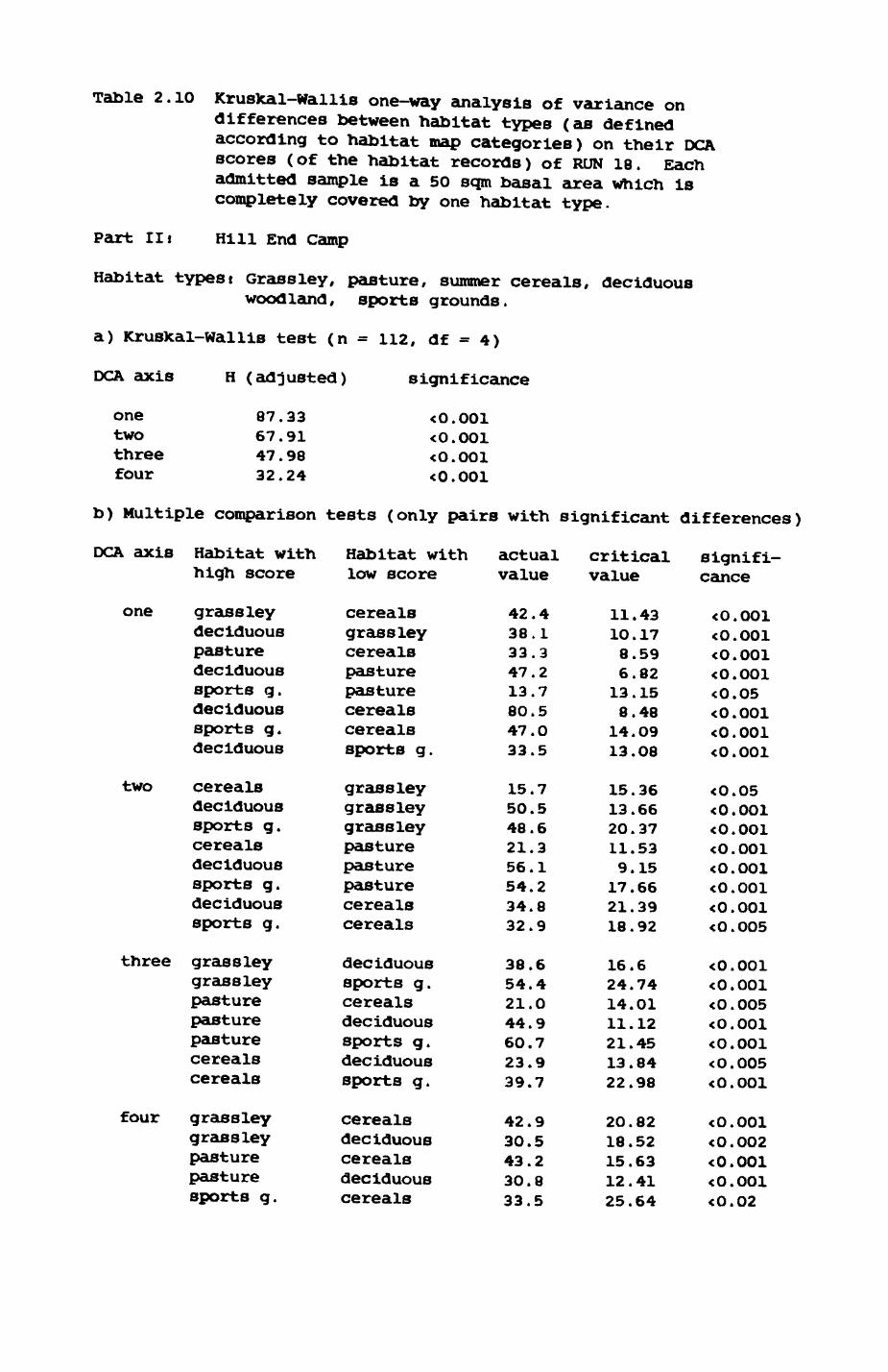
Table 2.10
Part Hi
Kruskal-Wallis one-way analysis of variance on differences between habitat types (as defined according to habitat map categories) on their DCA scores (of the habitat records) of RUN 18. Each admitted sample is a 50 sqm basal area which is completely covered by one habitat type.
Hill End Camp
Habitat typest Grassley, pasture, summer cereals, deciduouswoodland, sports grounds.
a) Kruskal-Wallis test (n = 112, df = 4)
OCA axis
one two three four
H (adjusted)
87.3367.9147.9832.24
significance
<0.001 <O.O01 <0.001 <O.O01
b) Multiple comparison tests (only pairs with significant differences)
DCA axis
one
two
three
four
Habitat with high score
grassley deciduous pasture deciduous sports g. deciduous sports g. deciduous
cereals deciduous sports g. cereals deciduous sports g. deciduous sports g.
grassleygrassleypasturepasturepasturecerealscereals
grassley grassley pasture pasture sports g.
Habitat with low score
cereals grassley cereals pasture pasture cereals cereals sports g.
grassleygrassleygrassleypasturepasturepasturecerealscereals
deciduous sports g. cereals deciduous sports g. deciduous sports g.
cerealsdeciduouscerealsdeciduouscereals
actual value
42.438.133.347.213.780.547.033.5
15.750.548.621.356.154.234.832.9
38.654.421.044.960.723.939.7
42.930.543.230.833.5
critical value
11.4310.178.596.8213.158.48
14.0913.08
signifi cance
<0.001<O.O01<0.001<O.O01<0.05<O.OO1<0.001<0.001
15.3613.6620.3711.539.15
17.6621.3918.92
<O.05<0.001<O.OO1<0.001<0.001<O.O01<0.001<0.005
16.624.7414.0111.1221.4513.8422.98
20.8218.5215.6312.4125.64
<0.001 <0.001 <0.005 <0.001 <O.OO1 <0.005 <0.001
<O.O01 <0.002 <0.001 <0.001 <0.02
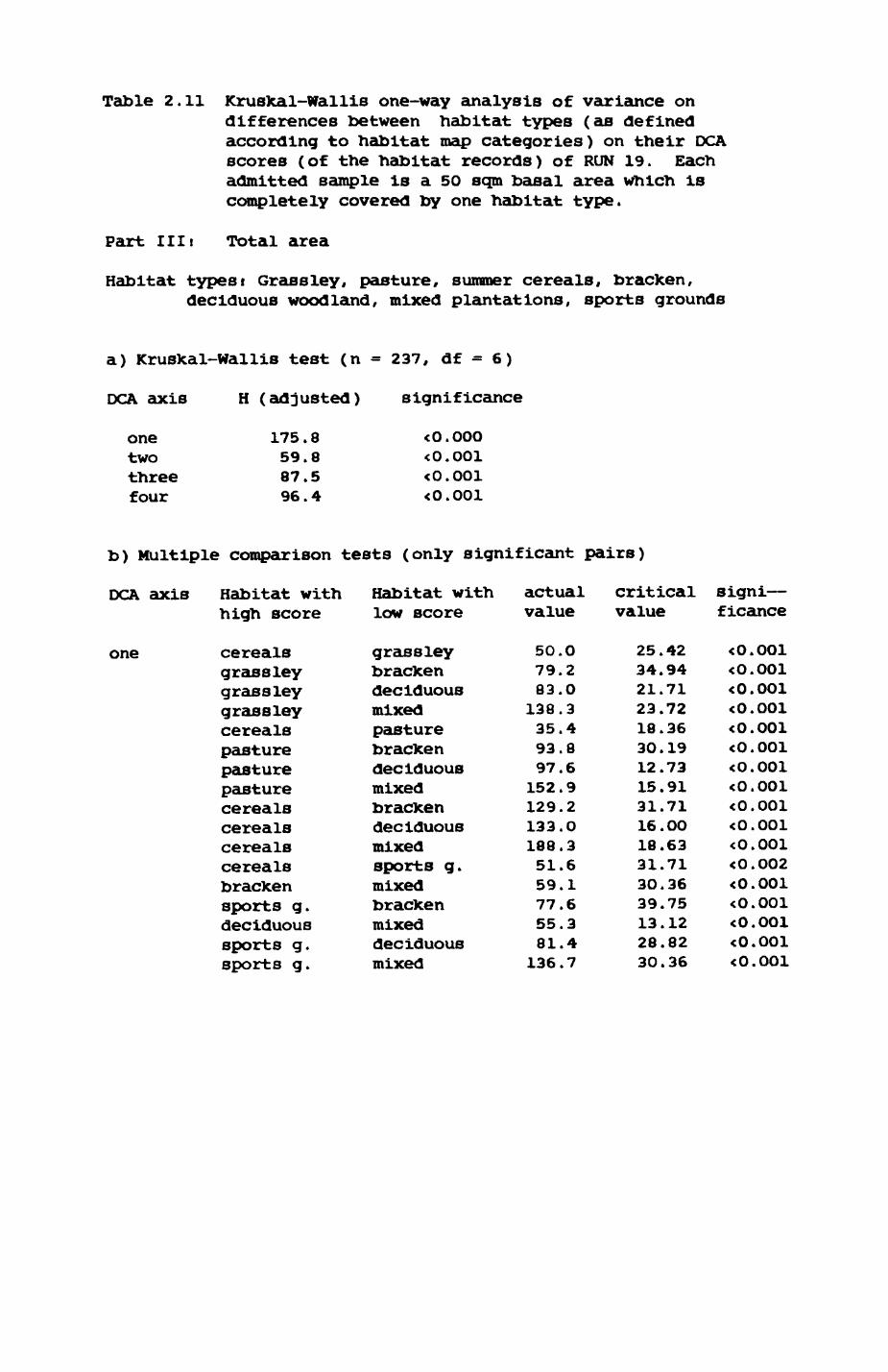
Table 2.11 Kruskal-Wallis one-way analysis of variance on differences between habitat types (as defined according to habitat map categories) on their DCA scores (of the habitat records) of RUN 19. Each admitted sample is a 50 sqm basal area which is completely covered by one habitat type.
Part IIIi Total area
Habitat typesi Grassley, pasture, summer cereals, bracken,deciduous woodland, mixed plantations, sports grounds
a) Kruskal-Wallis test (n = 237, df = 6)
DCA axis
one two three four
H (adjusted)
175.859.887.596.4
significance
<O.OOO <0.001 <O.O01 <O.O01
b) Multiple comparison tests (only significant pairs)
DCA axis
one
Habitat with high score
cerealsgrassleygrassleygrassleycerealspasturepasturepasturecerealscerealscerealscerealsbrackensports g.deciduoussports g.sports g.
Habitat with low score
grassleybrackendeciduousmixedpasturebrackendeciduousmixedbrackendeciduousmixedsports g.mixedbrackenmixeddeciduousmixed
actual value
50.079.283.0
138.335.493.897.6
152.9129.2133.0188.351.659.177.655.381.4
136.7
critical signi— value ficance
25.4234.9421.7123.7218.3630.1912.7315.9131.7116.0018.6331.7130.3639.7513.1228.8230.36
<O.O01<O.O01<O.O01<0.001<O.O01<0.001<O.O01<O.O01<0.001<O.O01<0.001<0.002<0.001<O.001<0.001<0.001<0.001
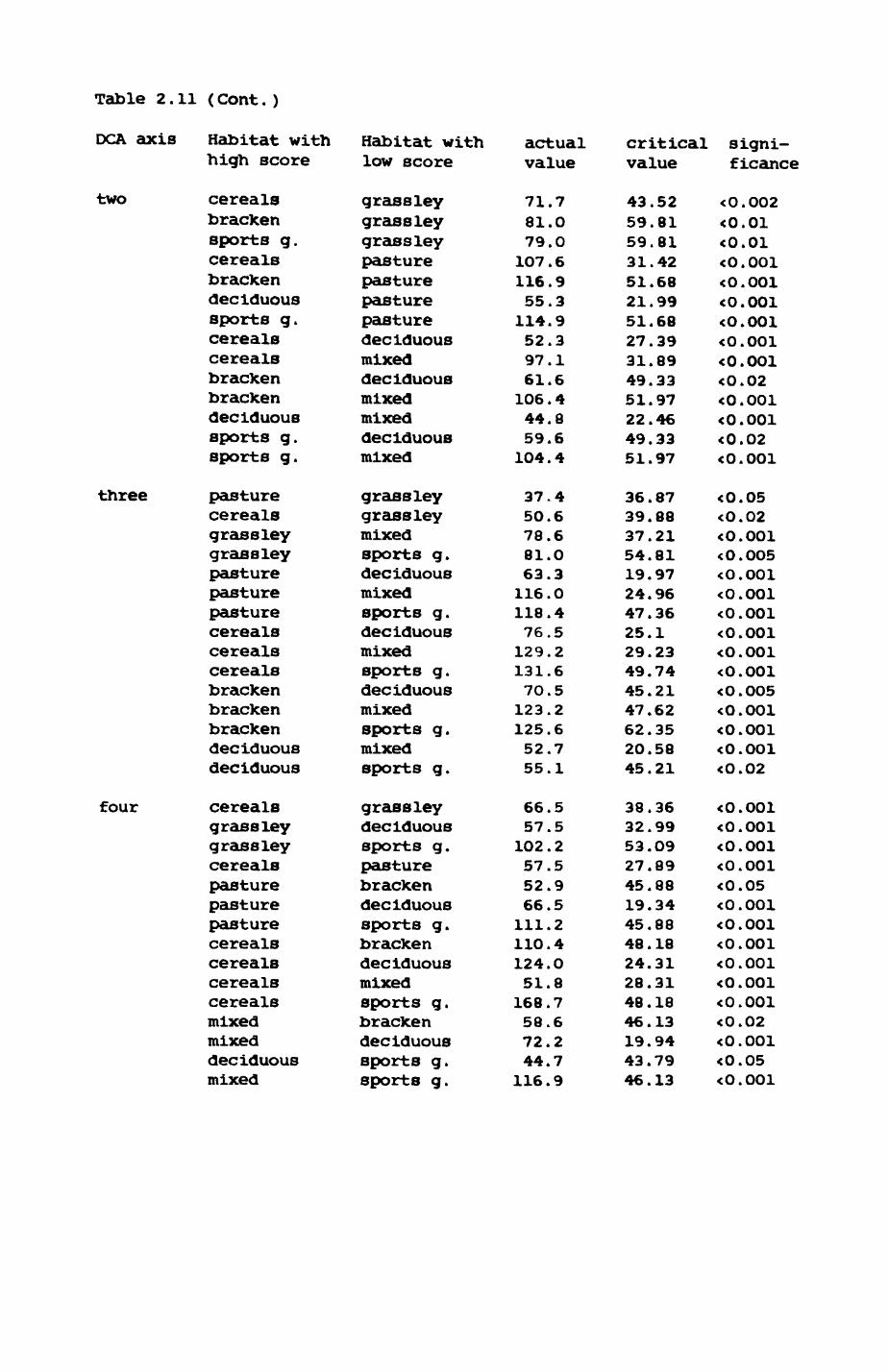
Table 2.11 (Cont. )
DCA axis Habitat with Habitat with actual critical signi-high score low score value value ficance
two cereals grassley 71.7 43.52 <0.002bracken grassley 81.0 59.81 <0.01sports g. grassley 79.0 59.81 <0.01cereals pasture 1O7.6 31.42 <0.001bracken pasture 116.9 51.68 <O.O01deciduous pasture 55.3 21.99 <0.001sports g. pasture 114.9 51.68 <0.001cereals deciduous 52.3 27.39 <0.00lcereals mixed 97.1 31.89 <0.001bracken deciduous 61.6 49.33 <0.02bracken mixed 106.4 51.97 <0.001deciduous mixed 44.8 22.46 <0.001sports g. deciduous 59.6 49.33 <0.02sports g. mixed 104.4 51.97 <0.001
three pasture grassley 37.4 36.87 <0.05cereals grassley 50.6 39.88 <0.02grassley mixed 78.6 37.21 <O.O01grassley sports g. 81.0 54.81 <O.O05pasture deciduous 63.3 19.97 <O.OO1pasture mixed 116.0 24.96 <O.O01pasture sports g. 118.4 47.36 <O.O01cereals deciduous 76.5 25.1 <O.O01cereals mixed 129.2 29.23 <O.O01cereals sports g. 131.6 49.74 <O.O01bracken deciduous 7O.5 45.21 <O.OO5bracken mixed 123.2 47.62 <O.O01bracken sports g. 125.6 62.35 <O.O01deciduous mixed 52.7 20.58 <O.O01deciduous sports g. 55.1 45.21 <O.02
four cereals grassley 66.5 38.36 <O.OO1grassley deciduous 57.5 32.99 <O.O01grassley sports g. 102.2 53.O9 <O.O01cereals pasture 57.5 27.89 <O.OO1pasture bracken 52.9 45.88 <0.05pasture deciduous 66.5 19.34 <O.O01pasture sports g. 111.2 45.88 <O.O01cereals bracken 110.4 48.18 <0.001cereals deciduous 124.O 24.31 <0.001cereals mixed 51.8 28.31 <O.OO1cereals sports g. 168.7 48.18 <0.001mixed bracken 58.6 46.13 <0.02mixed deciduous 72.2 19.94 <O.OO1deciduous sports g. 44.7 43.79 <0.05mixed sports g. 116.9 46.13 <O.O01
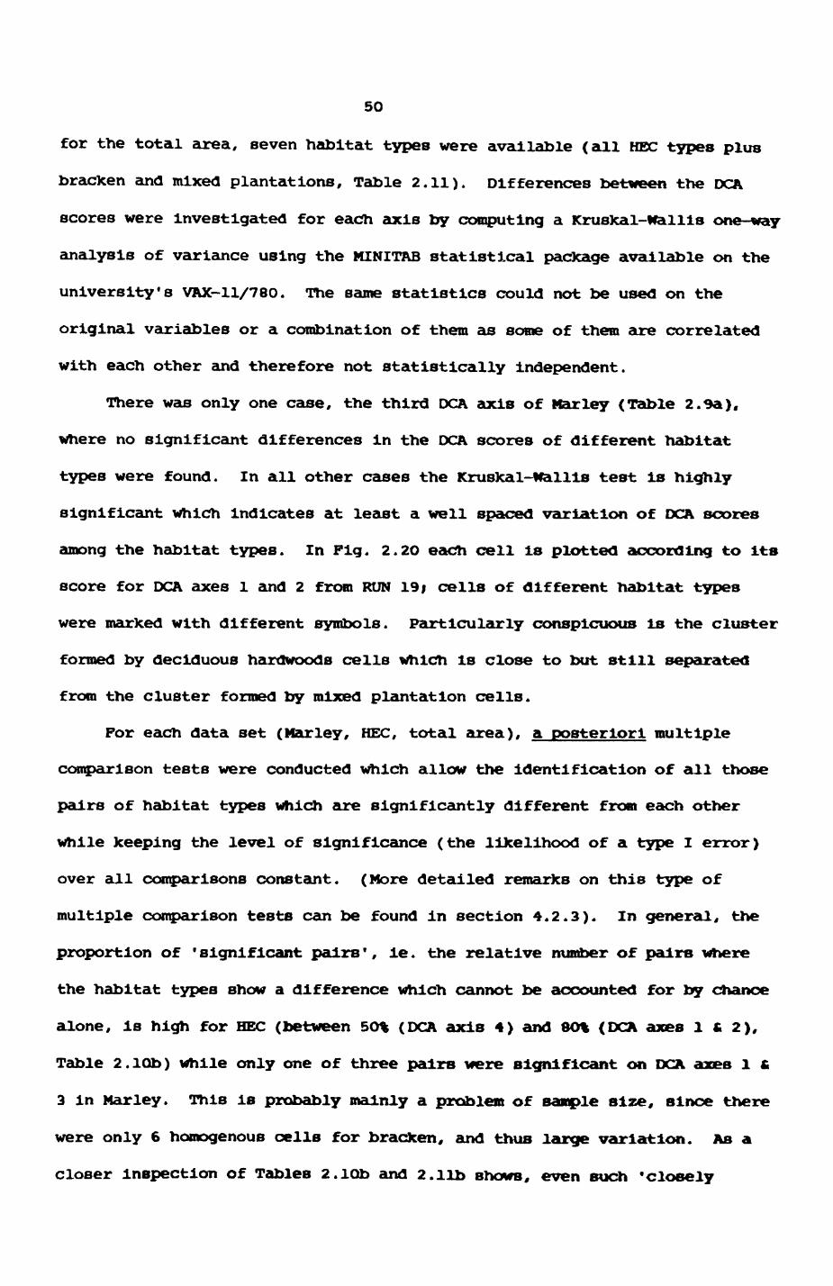
50
for the total area, seven habitat types were available (all HEC types plus
bracken and mixed plantations. Table 2.11). Differences between the DCA
scores were investigated for each axis by computing a Kruskal-lfallis one-way
analysis of variance using the MINITAB statistical package available on the
university's VAX-11/780. The same statistics could not be used on the
original variables or a combination of them as some of them are correlated
with each other and therefore not statistically independent.
There was only one case, the third OCA axis of Mar ley (Table 2.9a),
where no significant differences in the DCA scores of different habitat
types were found. In all other cases the Kruskal-Wallis test is highly
significant which indicates at least a well spaced variation of DCA scores
among the habitat types. In Fig. 2.2O each cell is plotted according to its
score for DCA axes 1 and 2 from RUN 19j cells of different habitat types
were marked with different symbols. Particularly conspicuous is the cluster
formed by deciduous hardwoods cells which is close to but still separated
from the cluster formed by mixed plantation cells.
For each data set (Marley, HEC, total area), a posteriori multiple
comparison tests were conducted which allow the identification of all those
pairs of habitat types which are significantly different from each other
while keeping the level of significance (the likelihood of a type I error)
over all comparisons constant. (More detailed remarks on this type of
multiple comparison tests can be found in section 4.2.3). In general, the
proportion of ' significant pairs', le. the relative number of pairs where
the habitat types show a difference which cannot be accounted for by chance
alone, is high for HEC (between 5O% (DCA axis 4) and 8O% (DCA axes 142),
Table 2.1Ob) while only one of three pairs were significant on DCA axes 1 £
2 In Mar ley. This is probably mainly a problem of sample size, since there
were only 6 homogenous cells for bracken, and thus large variation. As a
closer inspection of Tables 2.lQb and 2.lib shows, even such 'closely

Pig. 2.20 Distinction of conventional habitat categories, as de fined by the computerized habitat map, by the habitat records, as represented by the OCA axes 1 and 2. Each symbol represents one 50 by 50 m cell exclusively covered by one conventional habitat category.
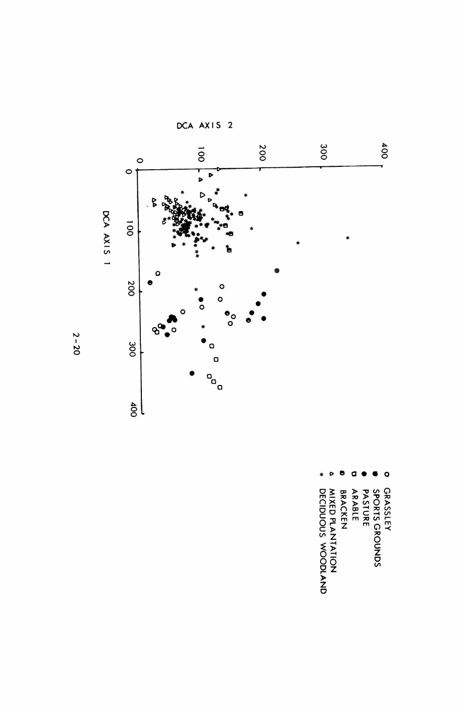
400
300
200
CNX
<1000
O
* •
0100
200300
400
o G
RASSLEY
• SPO
RTS G
RO
UN
DS
• PASTU
RE
0 A
RA
BLE
o B
RA
CK
EN
A M
IXE
D P
LAN
TATIO
N•*
DE
CID
UO
US
W
OO
DLA
ND
DC
A A
XIS
1
2-2
0
51
related' habitats as grassley, pasture and sports grounds are significantly
different on many DCA axes.
As may be recalled from section 2.3.5., the first axis of the DCA
ordinations was interpreted as a gradient of structural density and light
penetrability ranging from open areas with high penetrability to areas
packed with dense vegetation and low light penetrability while the second
axis distinguished resource variables from predator and vegetation
variables. While some of the closely related habitats (e.g. bracken and
deciduous woodlandi grassley, pasture and sports grounds) are
indistinguishable on the first DCA axis in all three data sets, most of thew
are separated on the second, the resource axis, although the habitat
parameters chosen certainly did not consider all important resources
(section 2.3.1). This most encouraging result is further corroborated by
the detailed Investigations reported in Chapter 3, where, for instance, a
significant difference in earthworm abundance and biomass could be shown
between deciduous hardwoods and mixed plantations, or where bracken showed a
higher index of rabbit activity than decidlous woodland. Other studies
Indicate that a distinction of habitat types might be justified even if the
resource presence is similar as for grass ley and pasture but the resource
availability changes due to differential hunting success of the predator
changes. A case in point is the reduced hunting success of badgers foraging
for earthworms in long grass habitat (grassland, Kruuk et al. (1979)).
In summary, the apparent complexity of Vfytham Hoods' blotic structure
can be summarised as a low—dimensional habitat space and is adequately
represented by the system of discrete habitat types developed in section
2.2. The foregoing analysis demonstrates that a definition of habitats as
units of resources is not only useful in theory but also feasible in
practice. In the following chapter the abundance of selected resources is
investigated in more detail and the present discussion of resources that are

52
part of SET 2 (the local window to the fundamental niche, section 2.1.1.)
extended to a detailed consideration of the relationship of resource
abundance, resource availability, and the foraging techniques of foxes and
badgers which together determine the composition of SET 3.
53
3. Resources
3.1. I introduction
3.2. Earthworms (Lumbricidae)
3.2.1. Introduction
3.2.2. Methods
3.2.3. Results of present study
3.2.4. Discussion
3.3. Pheasant (Phaaianua colchlcus)
3.3.1. Introduction
3.3.2. Pheasant census and observations
3.4. Wood pigeon (Columba palumbus)
3.4.1. Introduction
3.4.2. Observations on wood pigeons and pigeon remains
3.5. Lagoroorphs
3.5.1. Introduction
3.5.2. The rabbit population in Wytham Woods
.1. Methods
.2. Results
.3. Discussion
3.6. Rodents
3.6.1. Ecology of voles and mice
3.6.2. Antipredator tactics and defense
3.6.3. Predator foraging
3.6.4. The rodent populations in Wytham
3.7. Discussion
3.7.1. Comparison of prey characteristics
3.7.2. Foraging tactics of predators in relation to
the energy obtained from different prey.
54
3. Resources.
3.1. Introduction.
In this Chapter I shall present Information on the abundance of resources
and relate them to the foraging techniques of foxes and badgers. There are
two main almst
1. to explore further the extent to Which habitats can
be predictors of resource abundancej
2. to Investigate the conditions by Which a resource that
Is present (and thus an element of SET 2, the local
niche (section 2.1.1.)) also becomes available to the
predators (and thus an element of SET 3, the realized
niche).
The results should answer the question of what food availability a badger or
a fox might 'expect' in given habitats and thus may explain patterns of use
in habitat and prey selection by foxes and badgers. The aim is to Interpret
the predator's movements through different habitats.
In the previous chapter it was shown that the discrete habitat types of
the habitat map correspond well to the actual, continuous habitat variation.
It is therefore legitimate to restrict the following discussion of resource
abundance and availability to habitats as defined by the habitat nap.
The difference between food abundance and availability is critical (section
2.1.2). Natural selection could favour traits that minimize the time a prey
individual spends in states where it is available to predators. This in turn
would require the predators to be efficient in the detection of available
prey and favour the development of searching strategies designed to optimize
a resource yield function such as maximization of net energy intake or
minimization of time spent foraging resulting in a selection of prey types
55
by the predators. In sections 3.2. to 3.6. I shall discuss the mechanisms
and factors that determine the likely foraging success of foxes and badgers
for a given prey in a given area, While section 3.7. will discuss the
decision of what a predator should do in order to maximize fitness, ie. e.g.
how much time it should spend foraging for a particular type of prey.
Fig. 3.1. depicts a general model for the factors that influence the capture
success of a predator. The model was designed with reference to carnivore
behaviour and ecology. These factors will be shown to be of importance for
certain prey but they do not represent an exhaustive list. For instance, a
model for predators in lacustrine ecosystems would place more emphasis on
the sensory limitations of the predator and the effects of prey body size
(e.g. gape-limited predators) and reduce the importance of small scale
habitat heterogeneity and prey experience (Zaret (198O)). in the model,
ecological circumstances are underrepresented on the understanding that the
Importance of various factors may change if ecological circumstances
(habitat, weather) change. Factors 14 and 15 are examples of such an
influence.
In the following accounts of five selected prey I will list the aspects
of prey biology and behaviour along with the predators' foraging techniques
pertinent to the proposed scheme. Earthworms, rabbits, rodents, pheasants,
and wood pigeons were selected for detailed accounts because
- they are important elements of the diet of one or both
predator species as shown In Chapter 4 (earthworms,
rabbits, rodents);
- there is a strong scientific and public interest In
the corresponding predator/prey relationship (phea
sants ) i
- previous accounts of prey and predator biology do not
satisfactorily explain how foxes in Wytham Moods are
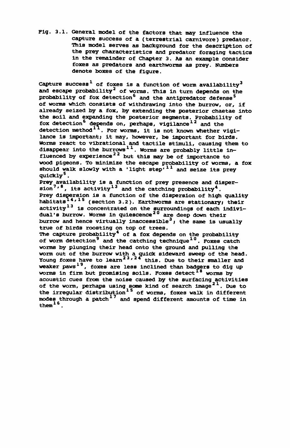
Pig. 3.1. General model of the factors that may influence thecapture success of a (terrestrial carnivore) predator. This model serves as background for the description of the prey characteristics and predator foraging tactics in the remainder of Chapter 3. As an example consider foxes as predators and earthworms as prey. Numbers denote boxes of the figure.
Capture success 1 of foxes is a function of worm availability3 and escape probability2 of worms. This in turn depends on the probability of fox detection 6 and the antlpredator defense 5 of worms which consists of withdrawing into the burrow, or, if already seized by a fox, by extending the posterior chaetae into the soil and expanding the posterior segments. Probability of fox detection 6 depends on, perhaps, vigilance 12 and the detection method 11 . For worms, it is not known whether vigi lance is important; it may, however, be important for birds. Worms react to vlbrational and tactile stimuli, causing them to disappear into the burrows 11 . Worms are probably little in fluenced by experience 22 but this may be of importance to wood pigeons. To minimize the escape probability of worms, a fox should walk slowly with a 'light step' 11 and seize its prey quickly 5 .Prey availability is a function of prey presence and disper sion 7 ' 8 , its activity13 and the catching probability4 . Prey dispersion is a function of the dispersion of high quality habitats14 ' 15 (section 3.2). Earthworms are stationaryi their activity 13 is concentrated on the surroundings of each indivi dual's burrow. Worms In quiescence 20 are deep down their burrow and hence virtually Inaccessible 3 ; the same is usually true of birds roosting on top of trees.The capture probability4 of a fox depends on the probability of worm detection 9 and the catching technique 10 . Foxes catch worms by plunging their head onto the ground and pulling the worm out of the burrow with a quick sideward sweep of the head. Young foxes have to learn 23 ' 24 this. Due to their smaller and weaker paws 19 , foxes are less inclined than badgers to dig up worms in firm but promising soils. Foxes detect 18 worms by acoustic cues from the noise caused by the surfacing activities of the worm, perhaps using some kind of search image 21 . Due to the irregular distribution 15 of worms, foxes walk in different modes through a patch and spend different amounts of time in them 16 .
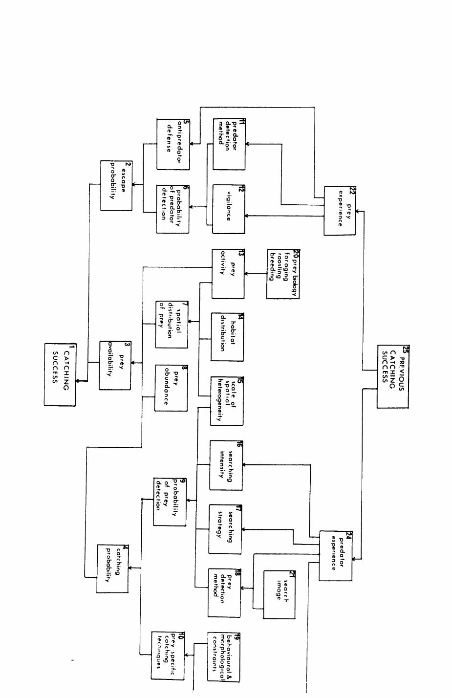
25P
RE
VIO
US
CA
TC
HIN
G
SU
CC
ES
S
22pre
y
exp
erie
nce
ftlpre
dato
rde
tectio
n
method
154p
redato
r experience
cOprey biology
fora
gin
g
roosting bre
edin
g
/igila
nce
L
pre
y
activ
ity
1antip
redato
r
de
fense
pro
bability
of p
redato
r de
tectio
n
114habita
t
distrib
utio
n
15sea I e of
spatia
lheterogeneity
16se
arch
ing
inte
nsity
21searc h im
age
search
ing
strate
gy
preyde
tectio
nm
eth
od
be
havio
ura
l &m
orp
ho
logic
al
constra
ints
spatia
l distrib
utio
n
of
pre
y
pre
y
abundance
esca
pe
pro
bability
pro
bability
of
pre
y de
tectio
n
pre
y
ava
ilability1
pre
y
sp
ecific
catc
hin
gte
chniq
ue
s
catch
ing
pro
bability
CA
TC
HIN
G
SU
CC
ES
S
56
successful predators on this prey.
3.1. EARTHWORMS (LUMjiRJCIDAE)
Among the 27 lumbricid species recorded for Britain (Gerard (1964))
only two, Lumbricus terrestris and Lumbricus rubellus, are shown to be
utilized by badgers and foxes, according to scat analyses and feeding
observations (Kruuk (I978a), Kruuk & Parish (1981, 1982), Macdonald (1980,
1984)). L. terrestris far outweighs L. rubellus In Importance so that L.
rubellus is only exploited In the absence of L. terrestris as demonstrated
In wetlands and moorlands In Scotland (Kruuk et al* references above). I
therefore restrict my discussion to L. terrestris. All future references to
earthworms, or worms, unless otherwise stated, are Intended to refer to L.
terrestris only.
3.2.1. INTRODUCTION.
ACTIVITIES. Earthworms live In burrows, often descending to a depth of one
to two meters (Edwards & Lofty (1977)). They have a natural life expectancy
of one to two years but have been observed to live for several years In the
laboratory. They primarily feed on leaf litter, but also consume
considerable quantities of other organic matter and soil. They forage by
surfacing from their burrow, searching the surrounding area for leaves,
which they collect and return to their burrows. Their burrows are sealed
with a leaf or small piles of stones ('worm cairns'). They do not feed on
the surface but hoard leaves down their burrows.
L. terrestris shows preference for certain types of litter. Pood
selection experiments (e.g. Satchell & Lowe (1967)) demonstrated that leaves
of different plant species, particularly trees, differ in their palatablllty
57
to worms. Palatability is Important as it determines the food supply
actually available to earthworms which in turn influences worm densities and
blomass (Edwards & Lofty (1977)). Palatabllity seems to be Influenced by a
variety of factors Including the chemical compositlion of the leaves,
particularly the presence of secondary compounds such as phenols and
condensed tannins. These are found for example in the leaves of larch,
spruce, oak and beech (comparatively unpalatable to earthworms) and are
absent in dog's mercury, nettles, elderberry ash and wych elm (Brown et al.
(1963)). Reynolds and Jordan (1975) suggested a leaf palatability scale
(with particular reference to North American earthworms) with
Robinia » Alnue « Populus > Prunus = Sallx - Ulmus =*
Acer * Llriodendron > Fraxlnus « Tllla - Gleditsia *
Betula > Quercus - Fagus > conifers
These results suggest that worms show both relative preference (for
e.g. sycamore (Acer) and ash (Fraxlnus)) and relative avoidance (conifers,
oak (Quercus), beech (Fagus)) of certain species (Satchell & Lowe (1967)).
L. terrestrls has a clear seasonal pattern of activity mainly
influenced by climatic factors (Rundgren (1977 ), Satchell (1967)). For
southern Sweden, Nordstrom (1975) and Rundgren (1977) reported that worm
activity is greatest from late March to mid-December, as long as soil
temperatures are higher than 0° C. In Britain, the same activity pattern
can be observed (Satchell (1967)). During periods of adverse conditions
such as frost or prolonged periods of drought, worms can enter a latent
phase (diapause) and are then found at greater depths In the soil.
L. terrestrls shows a negative phototaxle to strong light and a
positive phototaxls to dim light (Satchell (1967), Edwards & Lofty (1977)),
restricting surface feeding to the hours of dusk and darkness.
58
Consequently, most surfacing activity has been found to occur between 6 pm
and midnight (Baldwin (1917)), and extending to 6 am (Edwards & Lofty
(1977i138)). Otherwise, L. terrestrls is known to be able to tolerate a
wide range of environmental conditionsi it survives a wide range of pH
values ( pH 3.7 to 7.5, Edwards & Lofty (1977)), can survive severe
desiccation (up to 70 % loss of water) and live submerged under water for
many days (Roots (1956)). However, L. terrestrls generally Increases in
abundance with increasing pH value, is never actually found in flooded soils
or in soils with a pH of less than 4.1 and after prolonged rains surfaces
frequently and for extended periods of time (Edwards & Lofty (1977)).
General motor activity and particularly surfacing has been shown to be
influenced by a variety of factors. Kollmannsperger (1955) reported an
optimum soil temperature of 10.5° C. Satchell (1967), in experiments
conducted at Rothamsted Field Station, found surfacing to be positively
correlated with rainfall in the previous four days, soil temperature and air
temperature. Nights most suitable for earthworm activity were those with
grass-air temperatures above 2° C, soil temperatures around 1O.5° C and when
there had been some rain In the previous four days. Gerard (1967)
investigated the effects of soil moisture and temperature on the activity
and depth distribution of several species of earthworms in pasture. He
found that L. terrestris was never quiescent, but occurred significantly
deeper in experimental dry soils than in experimental wet soils, thereby
suggesting increased surfacing activity under wet conditions. On a lawn
Kruuk (I978a) found a significant correlation of the number of worms with*-.
the amount of rainfall during the previous 24 hours. Macdonald (1980) in a
study of fox predation on L. terrestris obtained a best fit of earthworm
activity with climatic factors in a multiple regression equation that
Included relative humidity, amount of rainfall, time since last rainfall and
departure from the optimal temperature. He and Kruuk (1978a) also
59
emphasized the Importance of wind as a negative Influence on surfacing
activity promoting an exponential decrease of relative air humidity with
increasing wlndspeed (see Kruuk (1978a)). The possibility remains that if
food supply for worms is low or it is dry for some time, worms might surface
more frequently than expected (Satchell (1967)).
Worms show habitat preferences related to food preferences and soil
conditions. Abundance figures have been reported from a variety of
countries for different habitat types and soils (see e.g. summary in Edwards
fi Lofty (1977)). They show that L. terrestris varies considerably in
abundance and biomass both between and within habitats. Amongst the factors
that Influence worm abundance within habitats are soil moisture (Vernon et
al.(1981)), soil type (Cuendet (1984)), soil depth (Phllllpson et al.
(1976)), and management history (Edwards & Lofty (1982a, 1982b), Andersen
(1980), Edwards & Lofty (1977)). When comparing the suitability of
different habitats for earthworms, important additional factors include
plant composition and pH (bearing an influence on light Intensity, humidity,
and evaporation), soil temperature and food supply (Bocock et al. (1977),
BococX & Adamson (1982), Nicholson & Owen (1982), Standen (1979)). In an
attempt to evaluate these factors and their interrelations, Reynolds fi
Jordan (1975) proposed a general model of earthworm activity and abundance.
Data on the distribution, abundance and biomass of L. terrestris in
different habitats in Wytham Woods are available from 4 studies t
1971 - 1973 beechwood at Brogden's Belt; Phillipson et
al. (1976, 1978)
1974 - 1975 a variety of habitats, mostly in the Mar ley -
Jew's Harp area; Kruuk (1978a)
1981 three different types of woodland, around
Healing's Copse and The Chaleti Cuendet (1984)
60
1982 a variety of habitats (Pig. 3.9), along the
Singing Way and at Rough Commoni this study.
Table 3.1 presents summaries of the densities and biomass obtained by
the four studies. The results of Phllllpson et al. (1978) are the value for
beechwood on rendzlna listed under Cuendet (1984) in Table 3.1. Note that
my data differ from those of the other studies (but see discussion below )
in that I explicitly identified only adult LumbricuB and large immatures (>
70 mm) that are easily distinguished from the closely related L. rubellus
(Gerard (1964), G. Cuendet, pers. comm. ), but did not make an attempt to
identify smaller juveniles as this is a difficult and time consuming task
(all smaller juveniles were assigned to the category OTHER JUVENILES). This
is not likely to have caused any serious error in the estimation of worm
biomass, although the number of L. terrestris will certainly be smaller than
expected from the results of other studies. As Table 3.3 confirms, OTHER
JUVENILES represent only 20.35 % of the total blomass while constituting the
bulk (64.67%) of the number of individuals collected. Adult and large
juvenile L. terrestris are few in number (together 18.1 %) but contribute
most to the overall biomass (71.2 %). With these restrictions in mind,
Table 3.1 shows that worms were most abundant in deciduous woodlands and
pasture, less in arable land and least in plantations. For other habitats,
Standen (1979) and Kruuk and Parish (1981, 1982) showed that L. terrestris
occurs rarely or not all in wetlands and moorlands while Raw (1962) and Raw
and Lofty (1959) found high populations in orchards.
ANTIPREDATOR DEFENSE AND TACTICS. L. terrestris possesses senses for
chemical, visual, vibratlonal, tactile and other types of stimuli. Strong
vibrations e.g. caused by somebody walking quickly over the ground will
cause the worms to disappear. When touched, worms will retract back Into
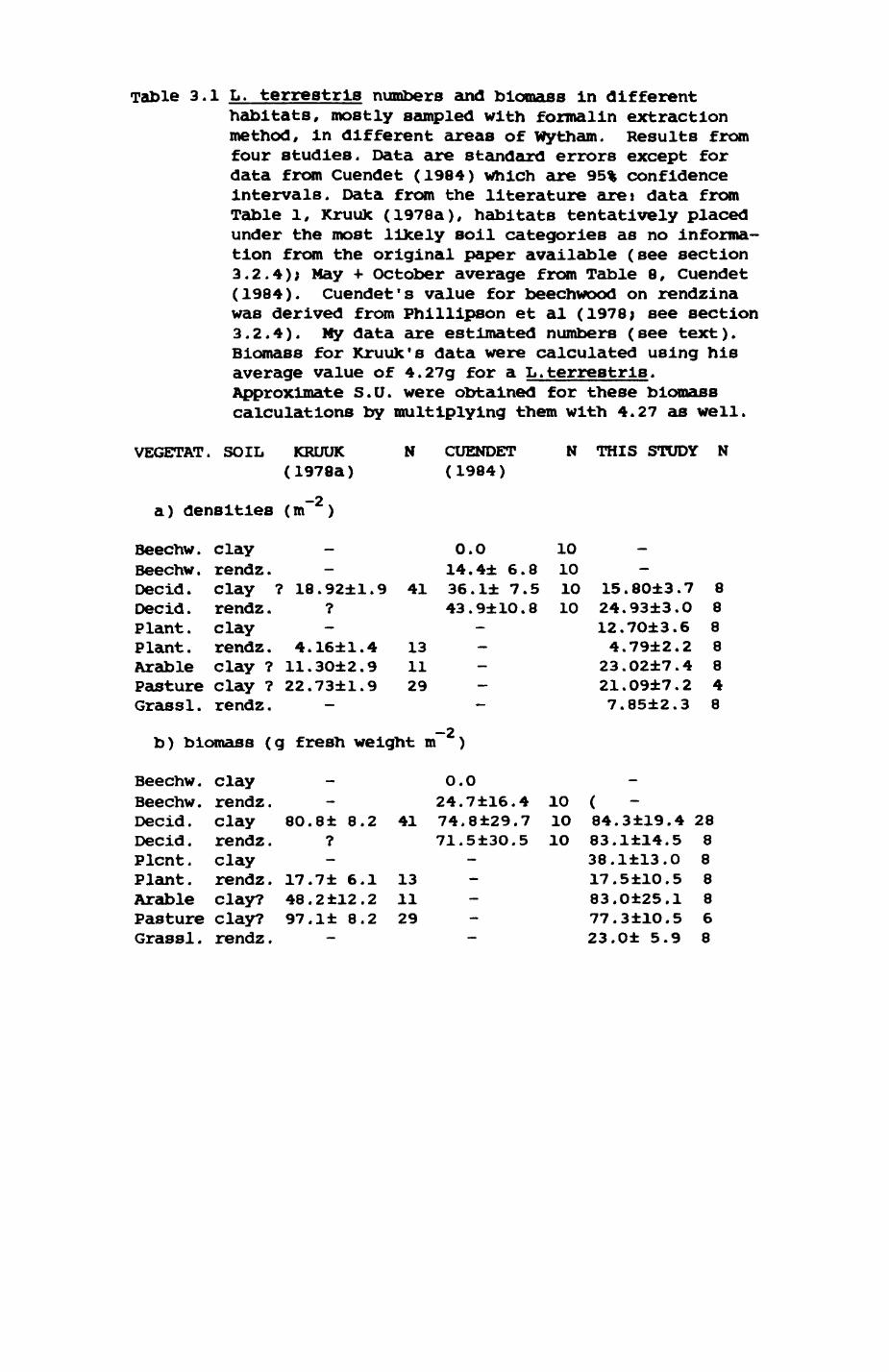
Table 3.1 L. terrestrls numbers and biomass in differenthabitats, mostly sampled with formalin extraction method, in different areas of Wytham. Results from four studies. Data are standard errors except for data from Cuendet (1984) which are 95% confidence intervals. Data from the literature arej data from Table 1, KruuJc (1978a), habitats tentatively placed under the most likely soil categories as no informa tion from the original paper available (see section 3.2.4); May -I- October average from Table 8, Cuendet (1984). Cuendet's value for beechwood on rendzina was derived from Phillipson et al (1978; see section 3.2.4). My data are estimated numbers (see text). Biomass for Kruuk's data were calculated using his average value of 4.27g for a L.terrestris. Approximate S.U. were obtained for these biomass calculations by multiplying them with 4.27 as well.
VEGETAT. SOIL KRUUK N CUENDET N THIS STUDY N(1978a) (1984)
_2a) densities (m )
Beechw. clay - 0.0 10 -Beechw. rendz. - 14.4± 6.8 10Decid. Clay ? 18.92±1.9 41 36.1± 7.5 1O 15.80±3.7 8Decid. rendz. ? 43.9±1O.8 1O 24.93±3.O 8Plant, clay - - 12.7O±3.6 8Plant, rendz. 4.16±1.4 13 - 4.79±2.2 8Arable clay ? 11.3O±2.9 11 - 23.02±7.4 8Pasture clay ? 22.73±1.9 29 - 21.09±7.2 4Grassl. rendz. - - 7.85±2.3 8
-2b) biomass (g fresh weight m )
Beechw. clay - 0.0Beechw. rendz. - 24.7±16.4 1O (Decid. Clay 80.8± 8.2 41 74.8±29.7 10 84.3±19.4 28Decid. rendz. ? 71.5±3O.5 10 83.1±14.5 8Plcnt. clay - - 38.1±13.0 8Plant, rendz. 17.7± 6.1 13 - 17.5±10.5 8Arable clay? 48.2±12.2 11 - 83.o±25.l 8Pasture clay? 97.l± 8.2 29 - 77.3±10.5 6Grassl. rendz. - - 23.0± 5.9 8
61
their burrows. The strength of their reaction depends on how much they are
protruding from their burrow. If most of the body Is below the soil
surface, the worm will withdraw only slightly, away from the Immediate
vicinity of the stimulus (Edwards & Lofty (1977)). However, If the worm has
partly left the burrow It will actively resist any attempt to pull It out by
extending their posterior chatae Into the soil and expanding their posterior
segments. It Is then virtually Impossible to pull them out, and if grasped
strongly enough, the worms frequently break into two parts (Edwards & Lofty
(1977), pers. obs.). if worms have been subjected to adverse stimuli or
treatment, they will withdraw deeply into their burrow and not reappear for
some time.
PREDATOR FORAGING. Earthworms are a comparatively stationary prey and thus
an excellent subject for the study of predator foraging tactics. Kruuk
(1978a), and Kruuk et al. (1979) have published detailed accounts on the
foraging behaviour and efficiency of badgers and Macdonald (198O) described
the foraging behaviour of foxes in relation to earthworms. Studies on
earthworm foraging by other species are available, e.g. the pioneering
studies of Smith (I974a, 1974b) on European blackbirds (Turdus merula), and
studies on the black-headed gull (Larus rldlbundus, Cuendet (1983)).
In a patch of high worm densities, both badgers and foxes wander slowly
In a highly convoluted path, head close to the ground. Under conditions of
intermediate or low worm densities, foxes tend to follow a less convoluted*..
path and visit a larger area over the same time (Macdonald (1980)). The
badger seems to locate the worms primarily by olfactory clues, keeping its
head close to the ground. When a worm is located, it lowers its head to the
ground, and pulls the worm out of its burrow by a quick upward movement of
its head while holding the worm between Its incisors. Poxes While foraging
for worms listen for any audible sign of worm surfacing activity.
62
When a worm is located the fox pauses, apparently to determine its precise
position, and then plunges its head onto the ground pulling the worm out of
its burrow with a quick sideways sweep of its head. Capture rates appear to
be similar for both species under the same conditions (Macdonald (1977ft,
1980)). Foxes might, however, use badgers as a clue to sites with high worma.
densities, particularly under bad 'worming' conditions (Macdonald (198O)).
There is some evidence that badgers forage 'optimally' (at least if defined
by the marginal value theorem (Charnov (1976)), leaving a particular site if
the capture rate drops below an average rate for several sites (KruuX
(1978a)). Some foxes, however, If living in groups with more than 2
members, tend to leave a patch too late with respect to optimalltya.,
considerations. As Macdonald (1980) suggests this should be seen in
connection with the social organization of the foxes with subdomlnant
animals deliberately • overfishing • the worm patches as they are prevented
from access to preferred feeding sites by the dominant animals in the group.
3.2.2. METHODS.
I have collected data with a view to answering three questions about
worm ecology!
(1) how do worm densities and blomasses vary between
habitats ?
(2) what factors could be used by foxes and badgers to
locate patches with high worm densities and/or
blomasses ?
(3) could an animal familiar with its range predict
mlcroclimatlc patterns Important in determining
worm surfacing activity ?
Earthworm samples were collected in July 1982 by the formalin
63
extraction method (Raw (1959)). The relative merits of different sampling
methods have been discussed by several authors (e.g. Satchell (1969, 1971))
and the formalin extraction method has been found to yield similar or
slightly worse results in comparison with other methods for most worm
species but superior results for deep burrowing species such as L.
. The efficiency of formalin sampling has been shown to be
closely related to the factors affecting motor activity of earthworms.
Lakhanl and Satchell (1970) determined that soil temperature and soil
moisture are the two main factors affecting the efficiency of formalin
sampling and they developed an equation for deriving corrected population
estimates from samples with conditions deviating from optimal conditions aso
determined in experiments (soil temperature of 10.6 and soil moisture of 1O
%). Optimal condltons are most likely to be encountered in spring or in
autumn. Using Lakhani and Satchell 's correction equation (equation (1); see
below) it should be possible, however, to obtain results comparable to other
studies from other times of the year. The advantage of a summer sample
extracted with formalin lies in the fact that only the active part of the
population is collected which is the only one of interest to foxes and
badgersl Thus, summer sampling can provide two measures of earthworm
populations i using the correction factor, the 'true' population density can
be estimated while the actual numbers collected provide an index of the
density of the active and, for foxes and badgers, potentially accessible
population. Results from summer should be of particular Interest as this
must be a 'bottleneck' period of worm availability to foxes and badgers.
Samples were collected from 5 different habitats (as recognized by the
habitat map classification, section 2.2 and Box l)i deciduous woodland,
mixed coniferous/deciduous plantations, summer cereals (arable land),
pasture, and long grassland. I also attempted to sample different soil
types and selected within two habitats (deciduous woodland and mixed
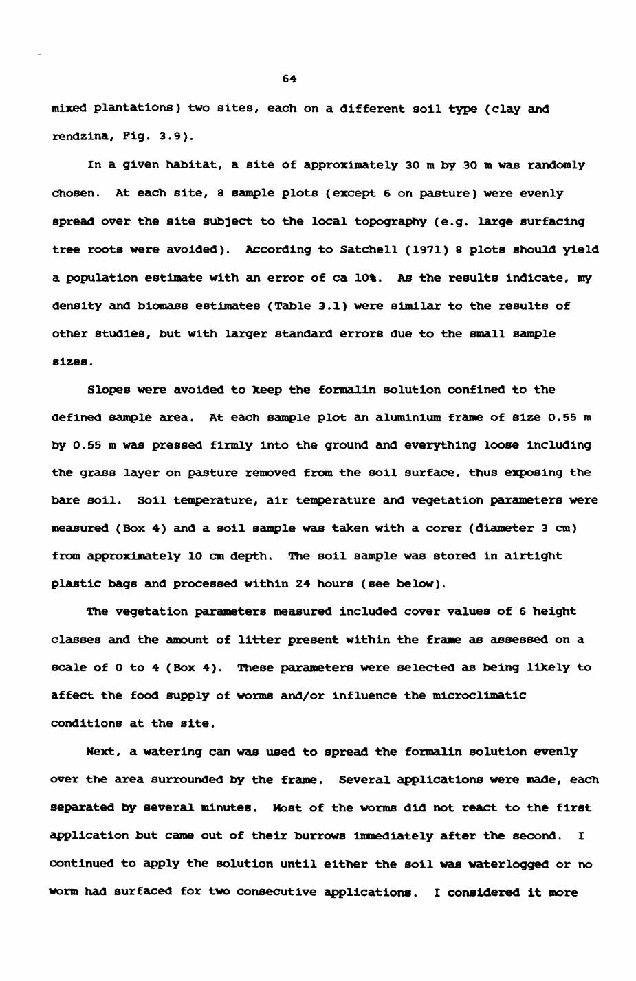
64
mixed plantations) two sites, each on a different soil type (clay and
rendzina, Pig. 3.9).
In a given habitat, a site of approximately 3O m by 3O m was randomly
chosen. At each site, 8 sample plots (except 6 on pasture) were evenly
spread over the site subject to the local topography (e.g. large surfacing
tree roots were avoided). According to Satchell (1971) 8 plots should yield
a population estimate with an error of ca 10%. As the results Indicate, my
density and biomass estimates (Table 3.1) were similar to the results of
other studies, but with larger standard errors due to the small sample
sizes.
Slopes were avoided to keep the formalin solution confined to the
defined sample area. At each sample plot an aluminium frame of size O.55 m
by O.55 m was pressed firmly into the ground and everything loose Including
the grass layer on pasture removed from the soil surface, thus exposing the
bare soil. Soil temperature, air temperature and vegetation parameters were
measured (Box 4) and a soil sample was taken with a corer (diameter 3 cm)
from approximately 10 cm depth. The soil sample was stored in airtight
plastic bags and processed within 24 hours (see below).
The vegetation parameters measured included cover values of 6 height
classes and the amount of litter present within the frame as assessed on a
scale of O to 4 (Box 4). These parameters were selected as being likely to
affect the food supply of worms and/or influence the microcllmatic
conditions at the site.
Next, a watering can was used to spread the formalin solution evenly
over the area surrounded by the frame. Several applications were made, each
separated by several minutes. Host of the worms did not react to the first
application but came out of their burrows immediately after the second. I
continued to apply the solution until either the soil was waterlogged or no
worm had surfaced for two consecutive applications. I considered it more
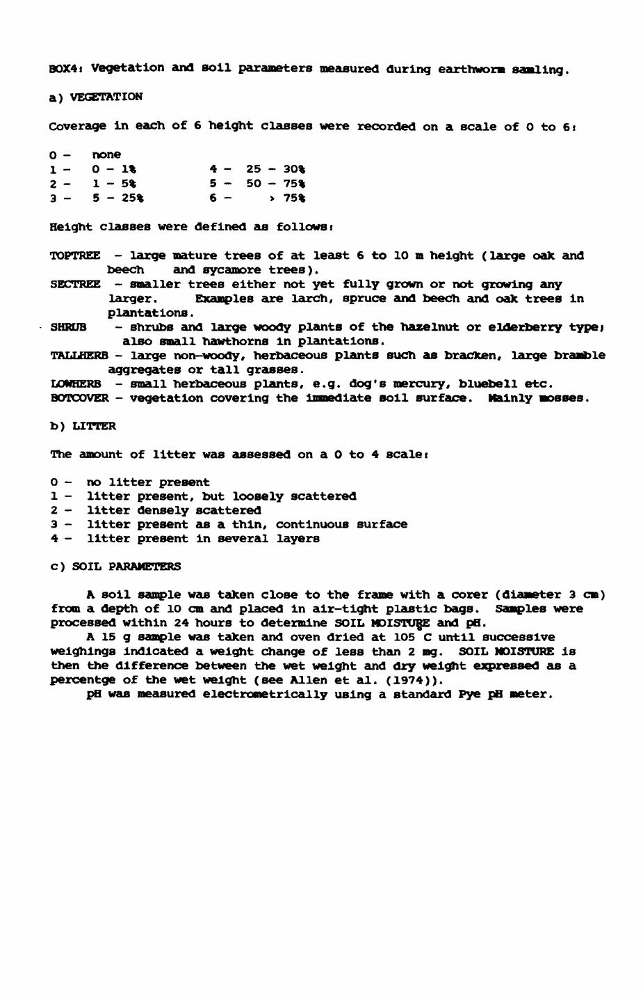
BOX4t Vegetation and soil parameters measured during earthworm samling.
a) VEGETATION
Coverage in each of 6 height classes were recorded on a scale of O to 6t
0 - none1- 0-1% 4-25- 30%2 - 1-5% 5-50- 75%3 - 5 - 25% 6 - > 75%
Height classes were defined as followst
TOPTREE - large mature trees of at least 6 to 10 m height (large oak andbeech and sycamore trees).
SECTREE - smaller trees either not yet fully grown or not growing anylarger. Examples are larch, spruce and beech and oak trees inplantations.
SHRUB - shrubs and large woody plants of the hazelnut or elderberry type;also small hawthorns in plantations.
TALLHERB - large non-woody, herbaceous plants such as bracken, large brambleaggregates or tall grasses.
LONHERB - small herbaceous plants, e.g. dog's mercury, bluebell etc. BOTCOVER - vegetation covering the immediate soil surface. Mainly mosses.
b) LITTER
The amount of litter was assessed on a 0 to 4 scalei
0 - no litter present1 - litter present, but loosely scattered2 - litter densely scattered3 - litter present as a thin, continuous surface4 - litter present in several layers
C) SOIL PARAMETERS
A soil sample was taken close to the frame with a corer (diameter 3 cm) from a depth of 10 cm and placed in air-tight plastic bags. Samples were processed within 24 hours to determine SOIL MOISTURE and pH.
A 15 g sample was taken and oven dried at 105 c until successive weighings indicated a weight change of less than 2 mg. SOIL MOISTURE Is then the difference between the wet weight and dry weight expressed as a percentge of the wet weight (see Alien et al. (1974)).
pfl was measured electrometrlcally using a standard Pye pH meter.
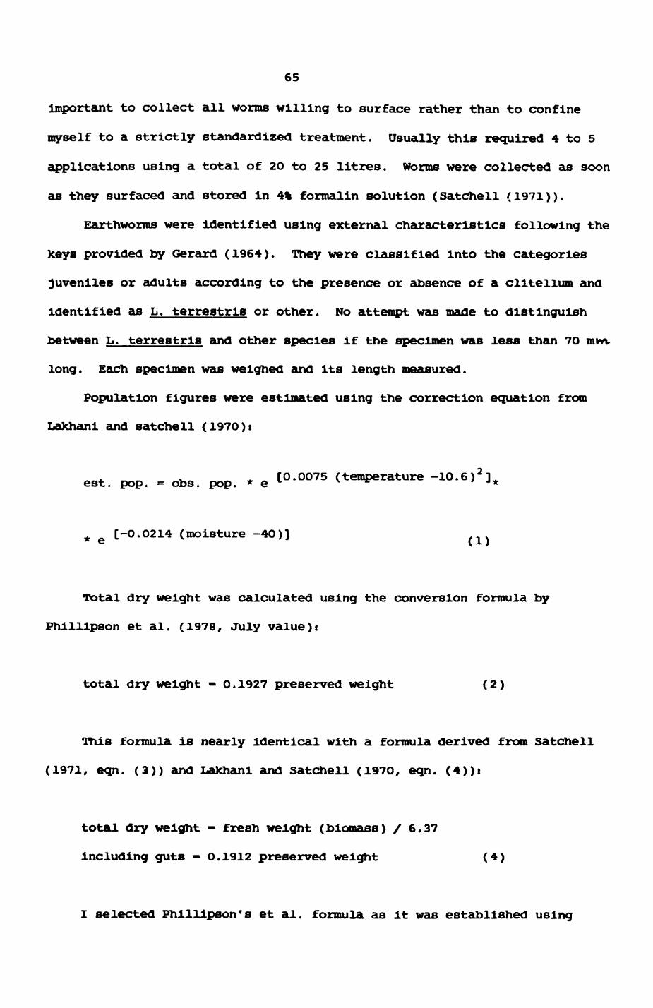
65
Important to collect all worms willing to surface rather than to confine
myself to a strictly standardized treatment. Usually this required 4 to 5
applications using a total of 2O to 25 litres. Worms were collected as soon
as they surfaced and stored in 4% formalin solution (Satchell (1971)).
Earthworms were identified using external characteristics following the
keys provided by Gerard (1964). They were classified into the categories
juveniles or adults according to the presence or absence of a clltellum and
identified as L. terrestris or other. No attempt was made to distinguish
between L. terrestris and other species if the specimen was less than 7O mm.
long. Each specimen was weighed and its length measured.
Population figures were estimated using the correction equation from
LaXhanl and satchell (1970)t
est. pop. = obs. pop. • e tO ' O°75
[-0.0214 (moisture -4O)]
Total dry weight was calculated using the conversion formula by
Fhillipson et al. (1978, July value)t
total dry weight - 0.1927 preserved weight (2)
This formula is nearly identical with a formula derived from Satchell
(1971, eqn. (3)) and Lafchani and Satchell (1970, eqn. (4))t
total dry weight - fresh weight (biomass) / 6.37
including guts - 0.1912 preserved weight (4)
I selected Phillipson'e et al. formula as it was established using
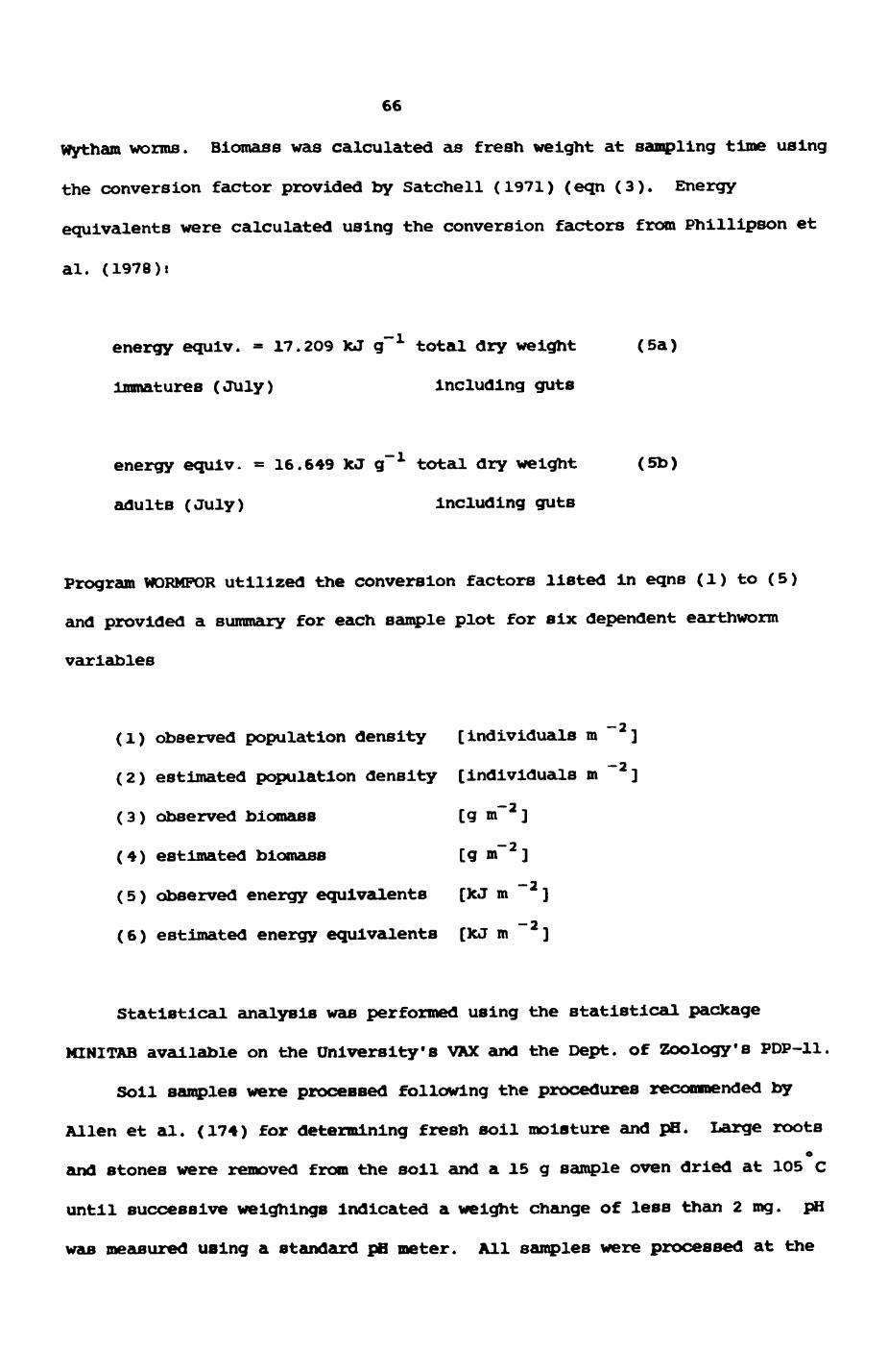
66
Wytham worms. Bloroass was calculated as fresh weight at sampling time using
the conversion factor provided by Satchell (1971) (eqn (3). Energy
equivalents were calculated using the conversion factors from Philllpson et
al. (1978)i
energy equiv. = 17.2O9 XJ g" 1 total dry weight (5a)
Immatures (July) Including guts
energy equiv. = 16.649 XJ g" 1 total dry weight (5b)
adults (July) Including guts
Program WORMFOR utilized the conversion factors listed in eqns (1) to (5)
and provided a summary for each sample plot for six dependent earthworm
variables
(1) observed population density [individuals m ~ 2 ]
(2) estimated population density [individuals m ~ 2 ]
(3) observed blomass [g m~ 2 ]
(4) estimated blomass [g m~ 2 ]
(5) observed energy equivalents [kJ m ~2 ]
(6) estimated energy equivalents [fcJ m ~2 ]
Statistical analysis was performed using the statistical package
MINITAB available on the University's VAX and the Dept. of Zoology's PDP-11.
Soil samples were processed following the procedures recommended by
Alien et al. (174) for determining fresh soil moisture and pH. Large rootso
and stones were removed from the soil and a 15 g sample oven dried at 105 C
until successive weighings Indicated a weight change of less than 2 mg. pH
was measured using a standard pH meter. All samples were processed at the
67
University Field Station in Wytham.
The western half of Wytham Park was selected as an area of pasture
suitable for microclimatic measurements. The area consists of three fields
separated by fences and is regularly grazed by cattle. It is shaped like a
shallow valley and surrounded on three sides by woodland and bordered on the
fourth side by pastures, arable fields and a small piece of woodland known
as Wormstall Duck Fond. A spring originates in the southwestern upper half
and runs northeast towards Wormstall Duck Pond along the bottom of the
valley between moderate to steep slopes.
Measurement of microclimatic variables and obsevatlons on earthworm
activity were conducted by N. Wadham (1984). Data were collected in spring
on 9 mights between 29th March 1983 and 9th April 1983 and in autumn on 6
nights between 15th September 1983 and 21st September 1983. Measurement
points for the microclimatic measurements were selected to gather
information about changes in wind exposure and soil temperature. Points
3,4,5 and 1,9,8 were symmetrically arranged about the valley midline to
accommodate changes in exposure as predicted by the prevailing wind
direction (Fig. 3.2)t points 1 and 3 lie in the shadow of the wood, points 4
and 9 lie on exposed areas in the centre of two fields and points 5 and 8
lie on the North east boundary directly exposed to the wind. Points 2,6,
and 7 lie along the base of the valley with predicted reduced wind exposure.
At dusk, each point was visited sequentially from 1 to 9. At each
measurement point, soil temperature was recorded using two thermistor
probes. The data value for the point was taken as the mean of both
observations. Wind speed was recorded using a hand held anemometer as the
average speed over one minute.
In addition, the entire area was split into sections (strata) which
were thought to reflect possible changes in worm abundance (Pig. 3.3)
according to changes In water content, slope and litter presence. Sections
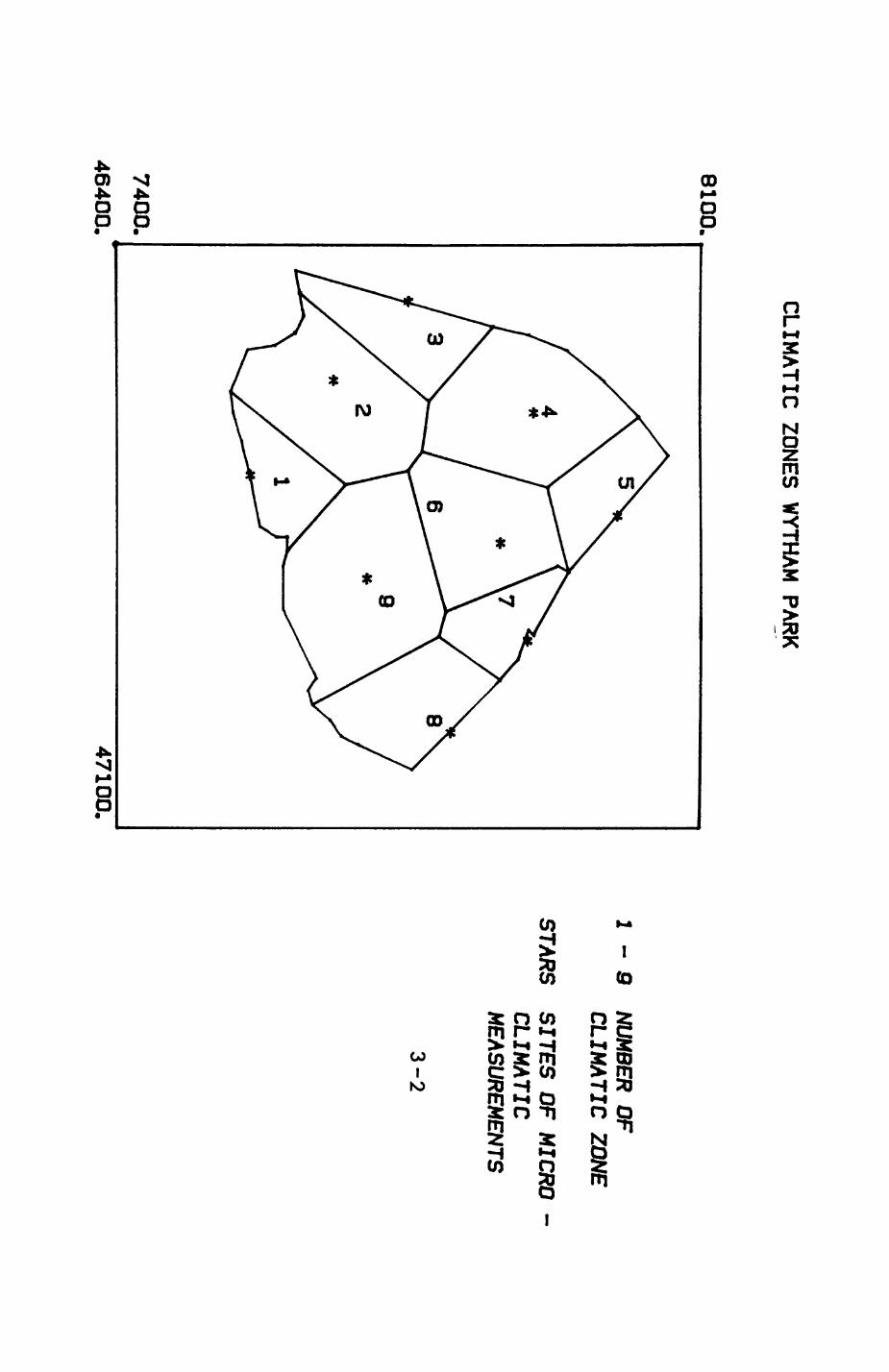
CLIMATIC ZONES WYTHAM PARK
8100.
7400.
46400.47100,
2 - 9
NUMBER OF
CLIMATIC ZONE
STARS SITES O
F MICRO
CLIMATIC MEASUREMENTS
3-2
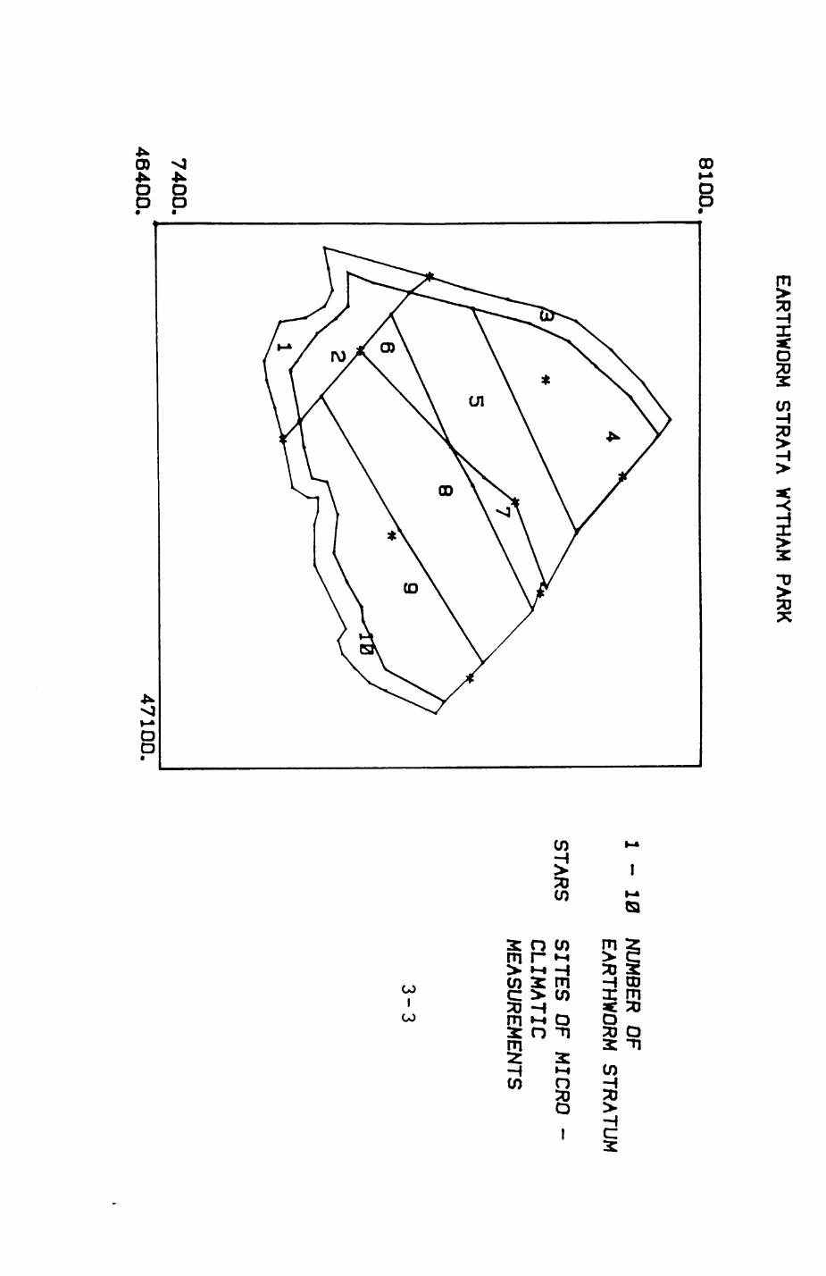
EARTHWORM STRATA
WYTHAM PARK
8100.
7400.
46400.
1-10
NUMBER OF
EARTHWORM STRATUM
STARS SITES OF MICRO
- CLIMATIC MEASUREMENTS
3-3
47100.
68
1,3, and 10 run parallel to the woodland boundary reflecting increased
litter presence and reduced wind. Sections 6 and 7 are at the bottom of the
valley with 7 being considerably wetter than 6 due to the flooding of the
area next to the ditch. Sections 2,4,5,8, and 9 reflected different degrees
of slope with its possible consequences for water levels, humidity etc.
(Reynolds & Jordan (1975)) and take into account possible differences
between fields due to differential grazing by the cattle. Section 2 had the
steepest slope, followed by 5 and 8 while 4 and 9 had only a slight slope.
Several fixed transects were walked through each section to record worm
surfacing activity, using a torch fitted with a red light. Worms were
counted on several occasions, but only on the first night was an appreciable
amount of surfacing observed. Thus we confirmed that earthworms occurred
but were not able to obtain reliable quantitative results. Data were
analysed using MINITAB statistical package.
3.2.3. RESULTS OP PRESENT STUDY.
Altogether 684 worms were collected from 54 plots. Table 3.2 shows the
distribution of numbers and average weights over different habitats and
Table 3.3 summarizes data on length and weights. Other juveniles comprised
the bulk of the earthworms sampled in terms of numbers (64.67 %) but
constituted only 20.35 % of the total preserved weight biomass. L.
terrestris constituted only a small fraction of the numbers (18.1 %) but the
bulk of the weight (70.18 %). On average, an adult L. terrestris weighed
6.75 g (preserved weight (PW)j n-38) while the large immature L. terreatrla
weighed 2.48 g PW (n-86) yielding an overall average figure of 3.79 g PW.
Adults of other species weighed on average 0.438 g PW (n-117) and juveniles
0.252 g PW (n-443), with an overall average of 0.291 g PW (n-560).
The average weight of L. terrestris adults and juveniles varies
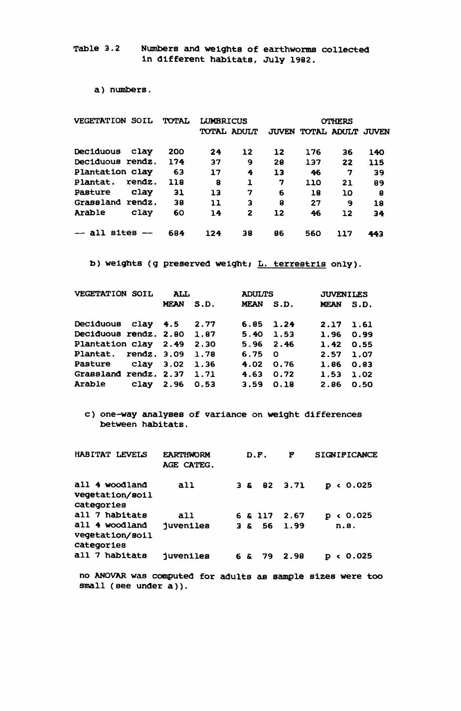
Table 3.2 Numbers and weights of earthworms collected in different habitats, July 1982.
a) numbers.
VEGETATION SOIL TOTAL LCJMBRICUS OTHERSTOTAL ADULT JUVEN TOTAL ADULT JUVEN
Deciduous clay 20O 24 12 12 176 36 140Deciduous rendz. 174 37 9 28 137 22 115Plantation clay 63 17 4 13 46 7 39Plantat. rendz. 118 817 110 21 89Pasture clay 31 13 7 6 18 10 8Grassland rendz. 38 ll 3 8 27 9 18Arable clay 60 14 2 12 46 12 34
— all Sites — 684 124 38 86 560 117 443
b) weights (g preserved weightj L. terrestrls only).
VEGETATION SOIL ALL ADULTS JUVENILESMEAN S.D. MEAN S.D. MEAN S.D.
Deciduous Clay 4.5 2.77 6.85 1.24 2.17 1.61Deciduous rendz. 2.8O 1.87 5.40 1.53 1.96 0.99Plantation clay 2.49 2.3O 5.96 2.46 1.42 O.55Plantat. rendz. 3.09 1.78 6.75 0 2.57 1.07Pasture clay 3.02 1.36 4.02 O.76 1.86 O.83Grassland rendz. 2.37 1.71 4.63 0.72 1.53 1.02Arable clay 2.96 0.53 3.59 0.18 2.86 O.5O
c) one-way analyses of variance on weight differences between habitats.
HABITAT LEVELS EARTHWORM D.P. P SIGNIFICANCEAGE CATEG.
all 4 woodland all 3 & 82 3.71 p < O.O25vegetation/soilcategoriesall 7 habitats all 6 & 117 2.67 p < 0.025all 4 woodland juveniles 3 & 56 1.99 n.s.vegetat ion/sol1categoriesall 7 habitats juveniles 6 & 79 2.98 p < 0.025
no ANOVAR was computed for adults as sample sizes were too small (see under a)).
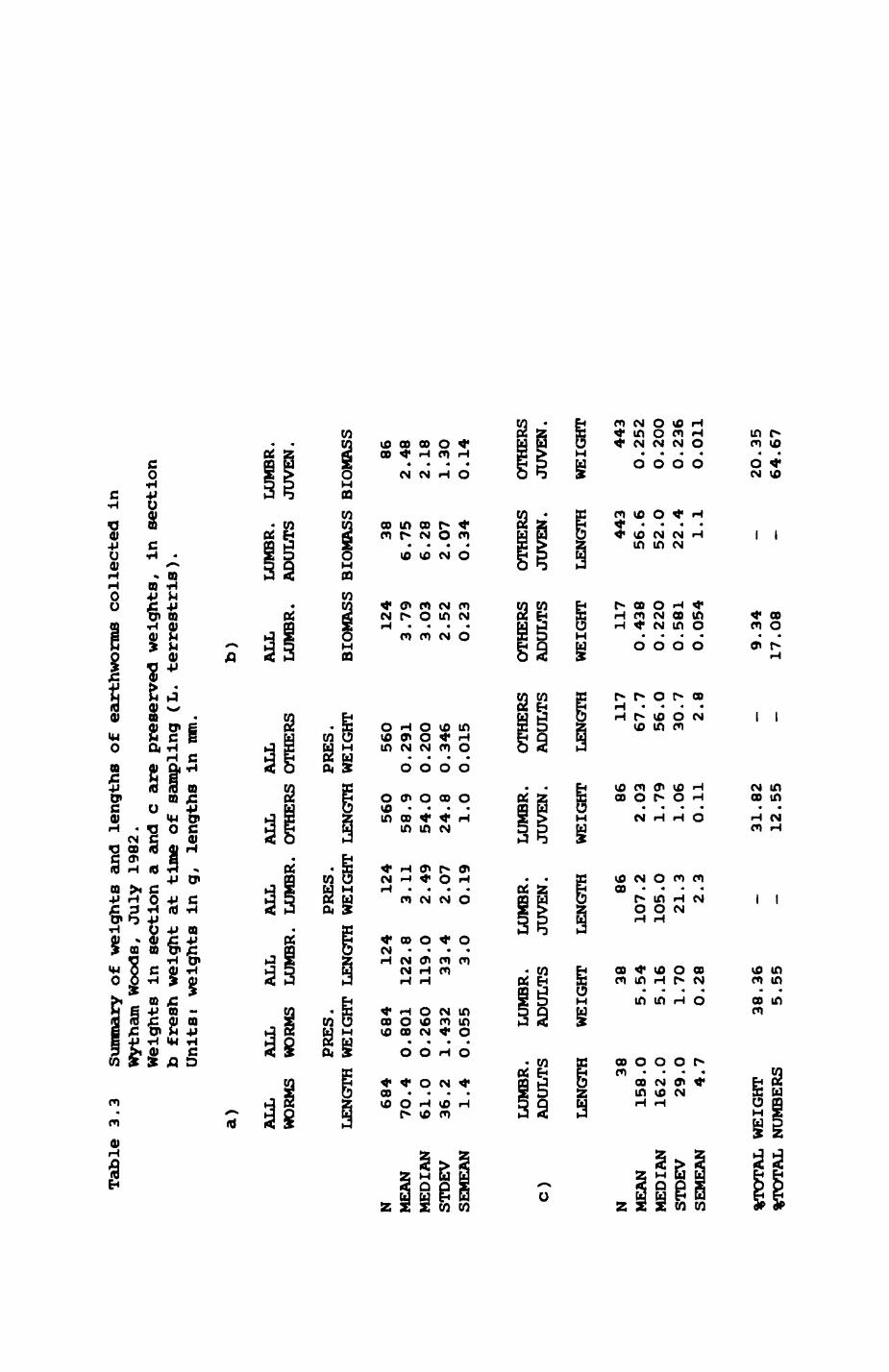
Table
3.3
Summ
ary of weigh
ts a
nd le
ngth
s of e
arthworms
collected
inwy
tham
Woods
, July 1
982.
Weig
hts
in s
ection a
and
c a
re p
reserved weights,
in s
ecti
onb
fresh we
ight
at
time
of
samp
ling
(L. te
rres
tris
).Unit
s I weights
in g
, lengths
in m
m.
ALL
ALL
ALL
ALL
ALL
ALL
WORMS
WORMS
LUMB
R. LUMBR. OTHERS OTHERS
ALL
LUMB
R.
LUMB
R.
LUMBR.
ADULTS
JUVEN.
PRES.
PRES.
PRES
. LENGTH WEIGHT LENGTH WEIGHT LENGTH WEIGHT
BIOMASS BIOMASS BIOMASS
N MEAN
MEDIAN
STDEV
SEMEAN
c)
684
7O.4
61.0
36.2
1.4
LUMBR.
ADULTS
0 0 1 O
684
.801
.260
.432
.055
124
122.8
119.0
33.4
3.0
124
3.11
2.49
2.O7
0.19
LUMBR.
LUMBR.
ADULTS
JUVEN.
560
58.9
54.0
24.8
1.0
LUMBR.
JUVEN.
O 0 0 0
560
.291
.200
.346
.015
OTHERS
ADULTS
124
3.79
3.03
2.52
O.23
OTHERS
ADULTS
386.75
6.28
2.O7
O.34
OTHERS
JUVEN.
862.48
2.18
1.3O
O.14
OTHERS
JUVEN.
LENGTH
WEIGHT
LENGTH
WEIGHT
LENGTH
WEIGHT
LENGTH
WEIGHT
N MEAN
MEDIAN
STDEV
SEMEAN
%TOTAL
%TOTAL
38158.0
162. 0
29.0
4.7
WEIGHT
NUMBERS
5 5 1 O 385
38 .54
.16
.70
.28
.36
.55
86107.2
105. 0
21.3
2.3
«•> —
2 1 1 0 31 12
86 .03
.79
.06
.11
.82
.55
117
67.7
56.0
30.7
2.8
_ —
0 0 O 0 917
117
.438
.220
.581
.054
.34
.08
443
56.6
52.0
22.4
1.1
_ —
443
0.252
0.200
O.236
0.011
2O.35
64.67
69
considerably between habitats (Table 3.2). The mean weight of adults over
all four woodland sites is significantly larger than the mean of the exposed
habitats (arable, pasture and grasslandi t-test, two-tailed, t - 5.53,
p=O.OOO). Several one-way analyses of variance show significant differences
of mean weights for different habitats and worm categories (Table 3.2c).
Table 3.4 presents the results of the calculations performed by program
WORMFOR. As a comparison of the 'observed' against 'estimated' columns
shows, LaXhani & Satchell's (1970) formula (eqn (1)) yields estimated
population densities of up to four times higher than the observed density.
However, the correction factor varies considerably between habitats and is
far higher in exposed habitats (pasture and arable land) than in woodland.
Statistical analyses were then performed to obtain answers to the
following questionsi
1. Are there differences between habitats of L. terrestris
densities, biomass and energy equivalents ?
2. Which habitats differ significantly ?
3. Are there differences between soil types in L. terrestris densities?
4. How do soil type and habitat type affect worm densities,
biomass and energy equivalents ?
5. Do L. terrestris densities, biomass and energy
equivalents show any relationship to vegetation and
soil parameters ?
6. What is the relationship between these parameters
and the earthworm variables ?
7. What is the pattern of microclimate over one habitat ?
How could this pattern affect the foraging efforts of
badgers and foxes. ?
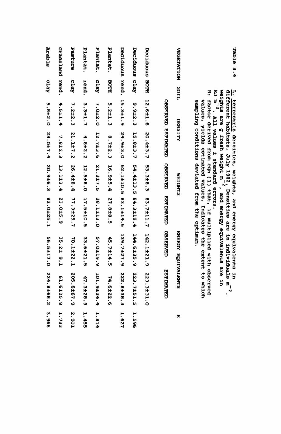
Table 3.4 L.
terrestrls densities, weights,
and energy equivalents in
different habitats, July 1982.
Densities are in individuals m~2
, weights are g fresh weight m~
2, and energy equivalents are
infcJ m
.All values ± standard errors.
RJ factor derived
from eqn (1) that, if multiplied with observed
values, yields estimated values.
Indicates the extent to whichsampling conditions deviated
from the optimum.
VEGETATION
SOIL
DENSITY
WEIGHTS
ENERGY EQUIVALENTS
R
OBSERVED ESTIMATED OBSERVED
ESTIMATED OBSERVED
ESTIMATED
Deciduous BOTH
12.6±1.6
20.4±3.7
53.3±8.3
83.7±11.7
142.1±21.9
223.3±31.O
Deciduous Clay
9.9±2.3
15.8±3.7
54.4±13.5 84.3±19.4
144.6±35.9
223.7±51.5
1.596
DecidUOUS rend. 15.3±1.9
24.9±3.O
52.1±10.5 83.1±14.5
139.7±27.9
222.8±38.3
1.627
Plantat.
BOTH
5.2±1.3
8.7±2.3
16.9±5.4
27.8±8.5
45.7±14.5
74.6±22.6
Plantat.
Clay
7.0±2.O
12.7±3.6
21.3±7.5
38.1±13.O
57.O±19.9
1O1.9±34.4
1.814
Plantat.
rend.
3.3±1.7
4.8±2.2
12.5±8.O
17.5±10.5
33.6±21.5
47.3±28.3
1.455
Pasture
Clay
7.2±2.3
21.1±7.2
26.4±8.4
77.3±25.7
7O.1±22.1
2O5.6±67.9
2.931
Grassland rend.
4.5±1.4
7.8±2.3
13.1±3.4
23.0±5.9
35.2± 9,1
61.6±15.8
1.733
Arable
Clay
5.8±2.O
23.0±7.4
2O.9±6.3
83.0±25.1
56.5±17.O
224.8±68.2
3.966
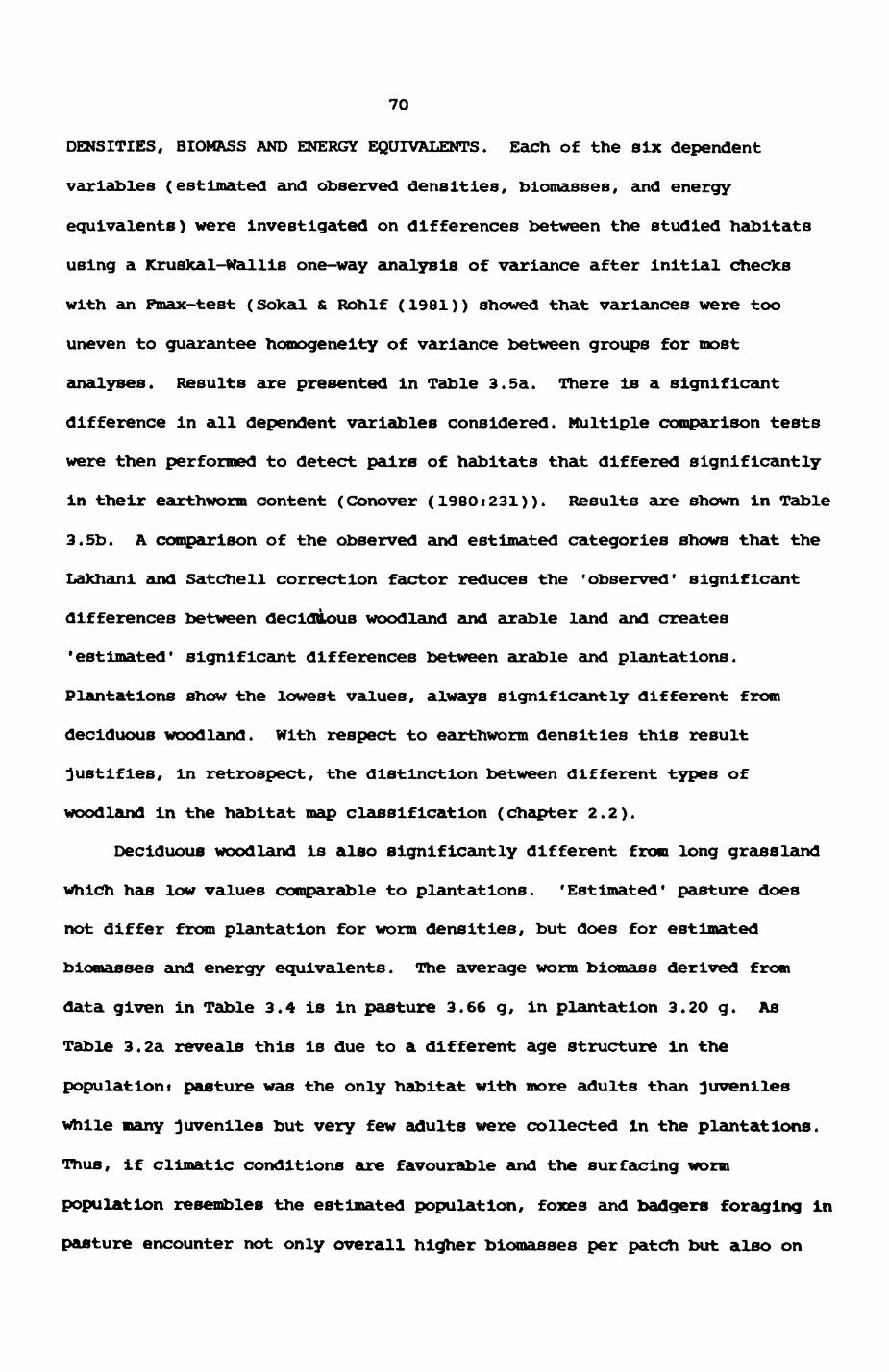
70
DENSITIES, BIOMASS AND ENERGY EQUIVALENTS. Each of the Six dependent
variables (estimated and observed densities, blomasses, and energy
equivalents) were Investigated on differences between the studied habitats
using a Kruslcal-Wallis one-way analysis of variance after initial Checks
with an Pmax-test (Sokal & Rohlf (1981)) showed that variances were too
uneven to guarantee homogeneity of variance between groups for most
analyses. Results are presented in Table 3.5a. There is a significant
difference in all dependent variables considered. Multiple comparison tests
were then performed to detect pairs of habitats that differed significantly
in their earthworm content (Conover (1980t231)). Results are shown in Table
3.5b. A comparison of the observed and estimated categories shows that the
LaKhani and Satchell correction factor reduces the 'observed' significant
differences between deciduous woodland and arable land and creates
'estimated' significant differences between arable and plantations.
Plantations show the lowest values, always significantly different from
deciduous woodland. With respect to earthworm densities this result
justifies, in retrospect, the distinction between different types of
woodland in the habitat map classification (chapter 2.2).
Deciduous woodland is also significantly different from long grassland
which has low values comparable to plantations. 'Estimated' pasture does
not differ from plantation for worm densities, but does for estimated
bioraasses and energy equivalents. The average worm biomass derived from
data given in Table 3.4 is in pasture 3.66 g, in plantation 3.20 g. As
Table 3.2a reveals this is due to a different age structure in the
population! pasture was the only habitat with more adults than juveniles
while many juveniles but very few adults were collected in the plantations.
Thus, if climatic conditions are favourable and the surfacing worm
population resembles the estimated population, foxes and badgers foraging In
pasture encounter not only overall higher blomasses per patch but also on
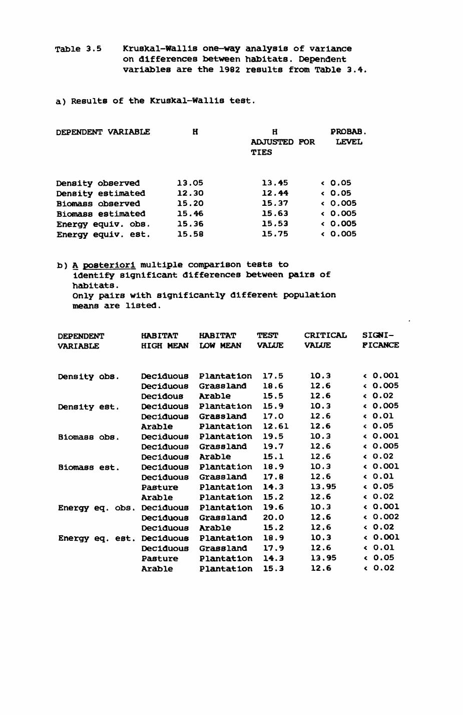
Table 3.5 Krusfcal-Wallls one-way analysis of variance on differences between habitats. Dependent variables are the 1982 results from Table 3.4.
a) Results of the KrusKal-wallls test.
DEPENDENT VARIABLE H PROBAB. ADJUSTED FOR LEVEL TIES
Density observed Density estimated Biomass observed Biomass estimated Energy equiv. obs. Energy equiv. est.
13.0512. 3O15.2015.4615.3615.58
13.4512.4415.3715.6315.5315.75
< 0.05< 0.05< 0.005< O.O05< O.O05< O.005
b) A posteriori multiple comparison tests toidentify significant differences between pairs of habitats.Only pairs with significantly different population means are listed.
DEPENDENT VARIABLE
Density obs.
Density est.
Biomass obs.
Biomass est.
Energy eq. obs.
Energy eq. est.
HABITAT HABITAT HIGH MEAN LOW MEAN
DeciduousDeciduousDecidousDeciduousDeciduousArableDeciduousDeciduousDeciduousDeciduousDeciduousPastureArableDeciduousDeciduousDeciduousDeciduousDeciduousPastureArable
PlantationGrasslandArablePlantationGrasslandPlantationPlantationGrasslandArablePlantationGrasslandPlantationPlantationPlantationGrasslandArablePlantationGrasslandPlantationPlantation
TESTVALUE
17.518.615.515.917.012.6119.519.715.118.917.814.315.219.620.015.218.917.914.315.3
CRITICALVALUE
10.312.612.610.312.612.610.312.612.610.312.613.9512.610.312.612.610.312.613.9512.6
SIGNIFICANCE
< 0.001< 0.005< 0.02< 0.005< 0.01< 0.05< 0.001< 0.005< 0.02< O.OO1< 0.01< 0.05< 0.02< 0.001< O.O02< O.O2< O.OO1< O.O1< O.O5< O.O2
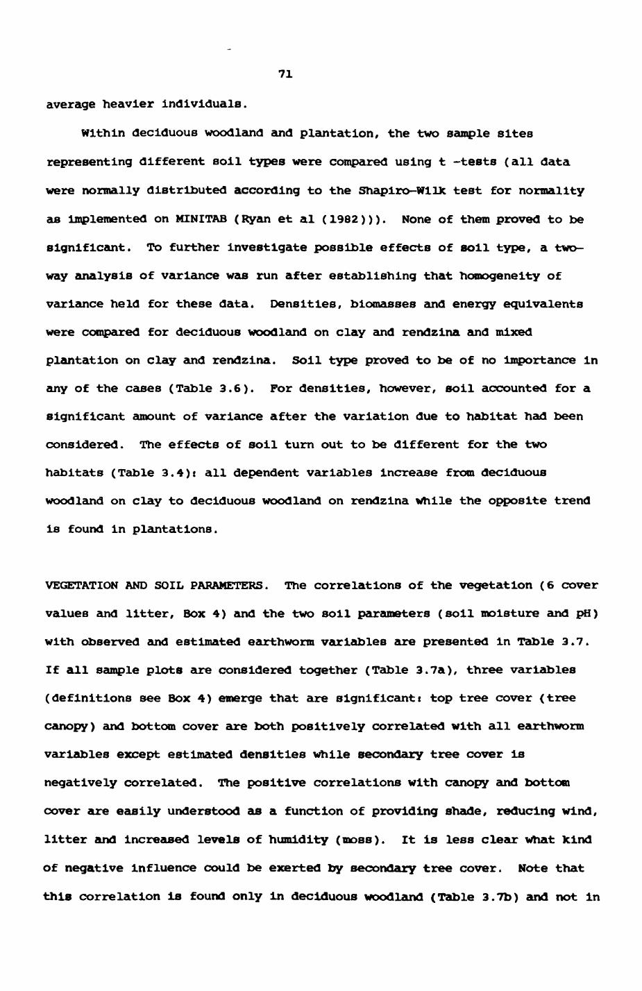
71
average heavier Individuals.
Within deciduous woodland and plantation, the two sample sites
representing different soil types were compared using t -tests (all data
were normally distributed according to the Shaplro-WllX test for normality
as implemented on KINITAB (Ryan et al (1982))). None of them proved to be
significant. To further investigate possible effects of soil type, a two-
way analysis of variance was run after establishing that homogeneity of
variance held for these data. Densities, blomasses and energy equivalents
were compared for deciduous woodland on clay and rendzina and mixed
plantation on clay and rendzina. Soil type proved to be of no importance in
any of the cases (Table 3.6). For densities, however, soil accounted for a
significant amount of variance after the variation due to habitat had been
considered. The effects of soil turn out to be different for the two
habitats (Table 3.4)t all dependent variables increase from deciduous
woodland on clay to deciduous woodland on rendzina while the opposite trend
is found in plantations.
VEGETATION AND SOIL PARAMETERS. The correlations of the vegetation (6 cover
values and litter, Box 4) and the two soil parameters (soil moisture and pH)
with observed and estimated earthworm variables are presented in Table 3.7.
If all sample plots are considered together (Table 3.7a), three variables
(definitions see Box 4) emerge that are significant! top tree cover (tree
canopy) and bottom cover are both positively correlated with all earthworm
variables except estimated densities while secondary tree cover Is
negatively correlated. The positive correlations with canopy and bottom
cover are easily understood as a function of providing shade, reducing wind,
litter and Increased levels of humidity (moss). It is less clear what Kind
of negative influence could be exerted by secondary tree cover. Note that
this correlation is found only in deciduous woodland (Table 3.7b) and not In
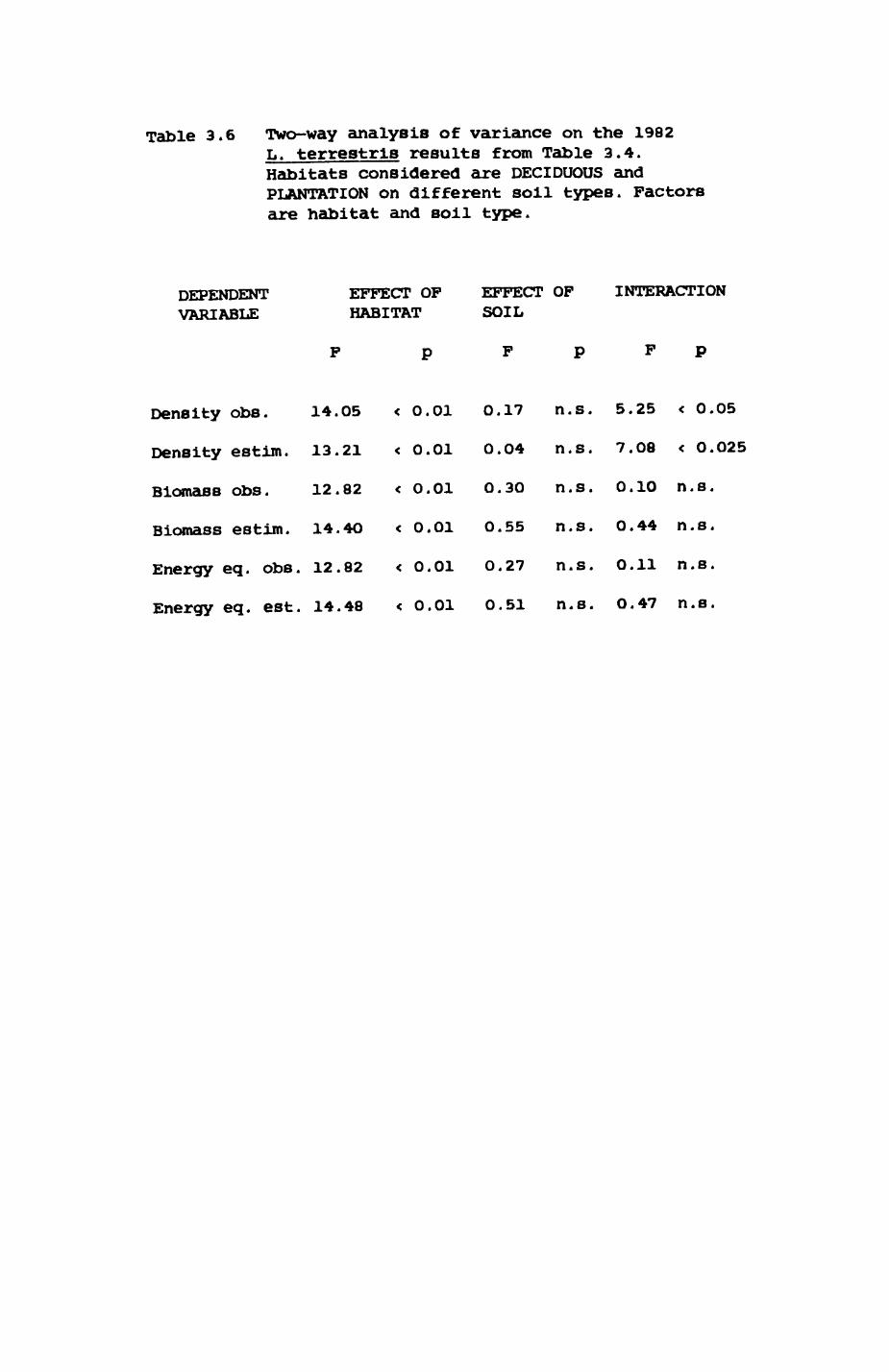
Table 3.6 Two-way analysis of variance on the 1982 L. terrestris results from Table 3.4. Habitats considered are DECIDUOUS and PLANTATION on different soil types. Factors are habitat and soil type.
EFFECT OF EFFECT OF INTERACTION VARIABLE HABITAT SOIL
Density obs. 14.05 < 0.01 O.17 n.s. 5.25 < 0.05
Density estim. 13.21 < 0.01 0.04 n.s. 7.08 < 0.025
Biomass obs. 12.82 < 0.01 O.30 n.s. 0.1O n.s.
Biomass estim. 14.4O < 0.01 0.55 n.s. O.44 n.s.
Energy eq. obs. 12.82 < 0.01 0.27 n.s. O.ll n.s.
Energy eq. est. 14.48 < 0.01 0.51 n.s. O.47 n.s.
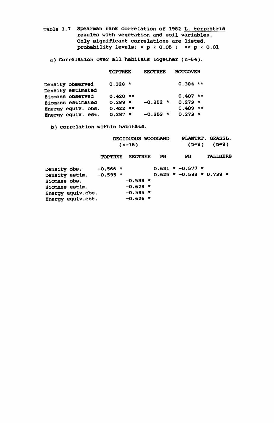
Table 3.7 Spearman rank correlation of 1982 L. terrestris results with vegetation and soil variables. Only significant correlations are listed, probability levels: * p < 0.05 ; ** p < 0.01
a) Correlation over all habitats together (n=54).
Density observed Density estimated Biomass observed Blomasa estimated Energy equlv. obs. Energy equiv. est.
b) correlation within habitats.
TOPTREE SECTREE BOTCOVER
0.328 * 0.384 **
0.420 ** 0.289 * 0.422 ** 0.287 *
-0.352 *
-0.353 *
0.407 ** 0.273 * 0.409 ** 0.273 *
DECIDUOUS WOODLAND PLANTAT. GRASSL.
TOPTREE SECTREE PH PH TALLHERB
Density Obs. -0.566 * 0.631 * -O.577 * Density estim. -0.595 * 0.625 * -0.583 * O.739 Biomass obs. -0.588 * Biomass estim. -O.628 * Energy equiv.obs. -0.585 * Energy equiv.est. -O.626 *
72
plantations.
In no case does litter show a correlation with earthworm variables.
This is presumably due to the fact that the litter available at this time of
the year is dominated by less palatable species (oaX, beech etc.). As Table
3.7b also indicates, pH could be responsible for the opposing tendencies
observed earlier for deciduous woodland and plantations! presence of
earthworms increases with pH In deciduous woodland (from clay to rendzlna)
and decreases for plantations (from rendzlna to clay).
In grassland, tall herb cover shows a strong correlation to earthworm
presence. This might be due to the fact that dense long grass reduces wind
and thus increases humidity while also providing more organic material.
This, however, could only be partially exploited by badgers or foxes as the
capture success of badgers decreases with sward length (Kruuk et al. (1979))
and a similar effect could be expected for foxes. Macdonald (1980)
suggested that foxes skirted the edge of long grass patches to get the best
compromise.
All factors were then combined in a multiple regression equation to
detect possible interaction effects between variables. The first multiple
regression considered all 54 plots and all parameters. The results were
unsatisfactoryi Table 3.8 demonstrates that only a small fraction of the
variation is accounted for; in two cases the regression is not significant
and none of the multiple regression coefficients is significantly different
from zero except soil moisture for observed biomasses and energy
equivalents, if anything, this again emphasises the paramount importance of
water relations to earthworms. I then decided to investigate whether any
relationship between earthworm abundance parameters and environmental
variables existed within given habitats. Due to small sample sizes,
regressions were only run on the deciduous woodland and plantation plots
(both n-16). None of the regressions for plantations, nor for deciduous
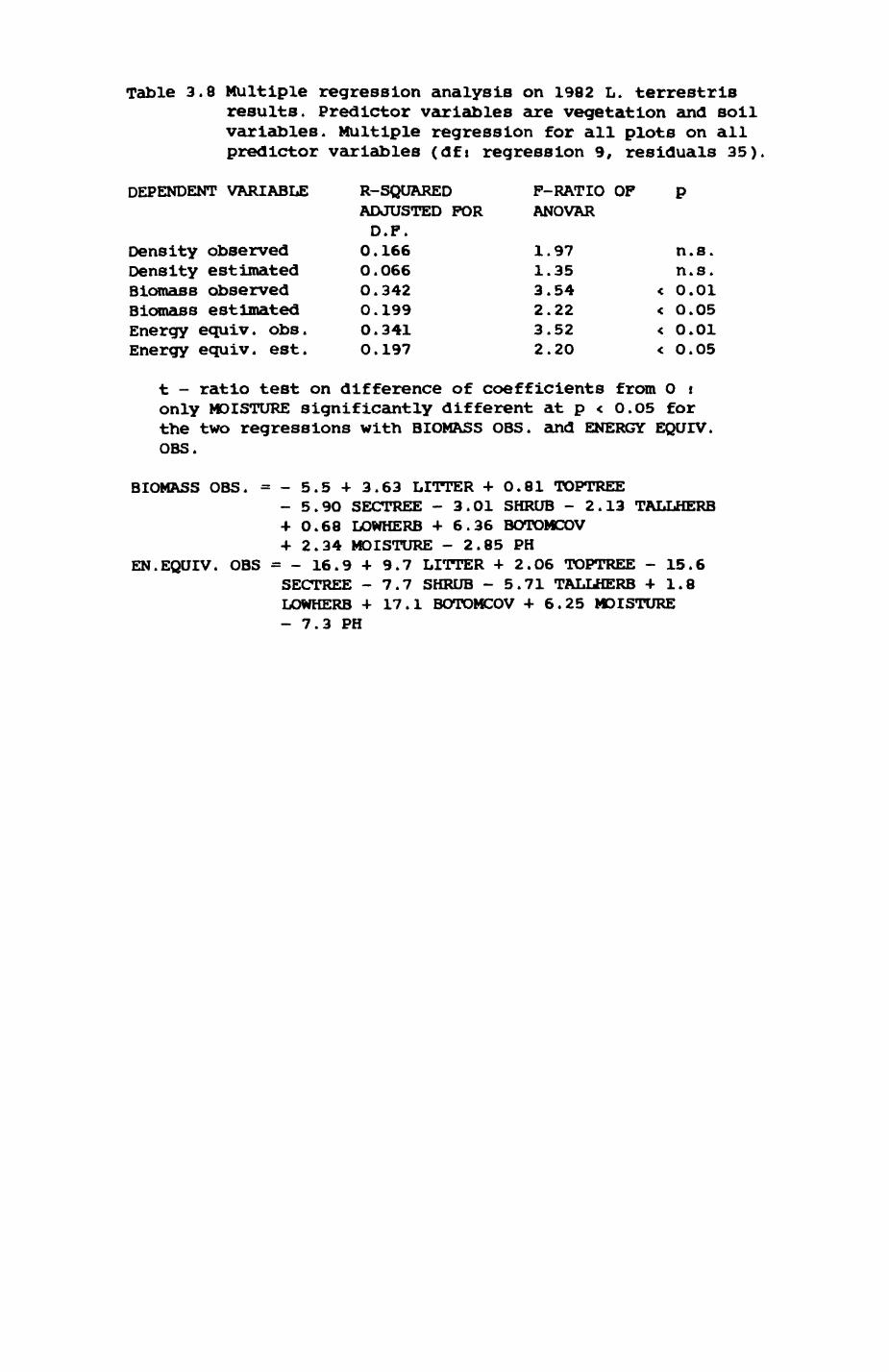
Table 3.8 Multiple regression analysis on 1982 L. terrestrisresults. Predictor variables are vegetation and soil variables. Multiple regression for all plots on all predictor variables (dfi regression 9, residuals 35).
DEPENDENT VARIABLE R-SQUARED P-RATIO OP pADJUSTED FOR ANOVARD.F.
Density observed 0.166 1.97 n.s.Density estimated 0.066 1.35 n.s.Biomass observed 0.342 3.54 < 0.01Biomass estimated 0.199 2.22 < 0.05Energy equiv. obs. 0.341 3.52 < 0.01Energy equiv. est. 0.197 2.2O < O.05
t - ratio test on difference of coefficients from 0 t only MOISTURE significantly different at p < O.O5 for the two regressions with BIOMASS OBS. and ENERGY EQUIV. OBS.
BIOMASS OBS. = - 5.5 -I- 3.63 LITTER +0.81 TOPTREE- 5.9O SECTREE - 3.01 SHRUB -2.13 TALLHERB + 0.68 LOWHERB +6.36 BOTOMCOV +2.34 MOISTURE - 2.85 PH
EN.EQUIV. OBS = - 16.9 + 9.7 LITTER + 2.O6 TOPTREE - 15.6SECTREE - 7.7 SHRUB - 5.71 TALLHERB +1.8 LOWHERB +17.1 BOTOMCOV +6.25 MOISTURE- 7.3 PH
73
woodland showed any significant results. I therefore decided to select only
those vegetation parameters that had previously shown a significant
correlation with the dependent variables (Table 3.7b). The resulting
multiple regression was significant for the two measures of density (Table
3.9) which were the only ones with non-significant regressions when all
habitats were pooled (Table 3.8). The two regressions for observed and
estimated densities showed different sets of coefficients to be significant
and thus perhaps distinguish between seasonal effects (effects on motor
activity) and long term effects (general level of population density). This
still does not explain why secondary tree cover should have a negative
effect on earthworm presence.
To summarize the results of this section, there seems to be little
gained from using cover or litter as an indicator of earthworm presence at
this time of the year (summer). Highest 'active* (observed) densities are
found in deciduous woodland while few worms were present in exposed
habitats. Higher 'active' blomasses are generally found in wetter soils.
Sites with large trees or well developed bottom cover (moss) which again are
dependent on a wet soil are favourable for worms. The results emphasize the
dominating role of humidity and soil water content for earthworm numbers at
a time when their food supply is restricted.
MICROCLIMATE. The third question concerns earthworm surfacing activity in
relation to microclimatic pattern. The Investigation was designed to see
whether microclimatic conditions over a relatively uniform habitat shoved
any kind of consistency that could be useful in predicting surfacing
activity.
During both periods of recording little precipitation fell and most
nights were dry. Soil temperatures in spring were well below, and In autumn
well above the optimum temperature of 10*5° C. There were persistent
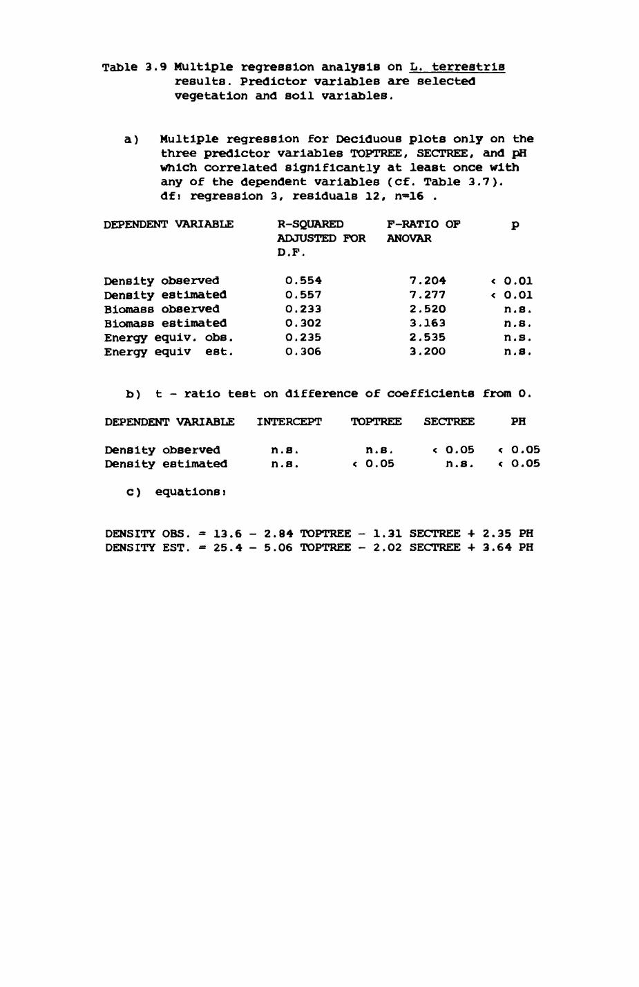
Table 3.9 Multiple regression analysis on L. terrestrls results. Predictor variables are selected vegetation and soil variables.
a) Multiple regression for Deciduous plots only on the three predictor variables TOPTREE, SECTREE, and pH which correlated significantly at least once with any of the dependent variables (cf. Table 3.7). dfi regression 3, residuals 12, n=16 .
VARIABLE R-SQUARED ADJUSTED FOR D.F.
F-RATIO OF ANOVAR
Density observed Density estimated Biomass observed Biomass estimated Energy equiv. obs. Energy equiv est.
0.554 0.557 0.233 0.3O2 0.235 0.306
7.2047.2772.5203.1632.5353.200
< 0.01< 0.01
n.s.n.s.n.s.n.s.
b) t - ratio test on difference of coefficients from O.
DEPENDENT VARIABLE INTERCEPT TOPTREE SECTREE PH
Density observed Density estimated
c) equationsi
n.s. n.s.
n.s. < O.O5 < O.O5 < 0.05 n.s. < 0.05
DENSITY OBS. - 13.6 - 2.84 TOPTREE - 1.31 SECTREE -I- 2.35 PH DENSITY EST. = 25.4 - 5.06 TOPTREE - 2.O2 SECTREE + 3.64 PH
74
differences in soil temperature between 6.4° C and 8.1° c for spring and
12.7° C and 14.5° c in autumn. A one-way analysis of variance yielded
significant differences between sites for soil temperature in spring
(F«3.53, n=81, df.= B and 72, p<O.OO5) but not in autumn and not for wind
speed in either recording period. However, the pattern of variation between
sites compared between the two seasons is the same (x =0.83 for soil
temperature and 1.92 for wind speed, n. a. ), as Illustrated by Fig. 3.4.
Table 3.10 presents a matrix of Spearman ran* correlations between the
sites for both variables for each period. Position 5 does not correlate in
wind speed (spring) with any of the points on the same side, nor with any of
the points in the bottom of the valley, but it correlates with positions 8
and 9 on the other side. The exposed positions 5, 8, and 9 correlate well
with each other but poorly with other positions. Position 4 is a unique
place which correlates well with both the group of positions 5, 9, 9 and
with the positions 1, 2, and 3. An exception to this is the non-correlation
with position 6 which, although geographically close. Is placed In a
different topographical situation. Soil temperature In spring demonstrates
a strong group of positions on the side of the Wormstall Ducx Pond (5-9)
while there Is no correlation between 1 to 3. This situation changes in
autumn where there Is little correlation in soil temperature between sites 5
to 9 and the fewer sites correlate than in spring. However, position 2 is
still correlated with position 6 for wind speed.
Figure 3.5 shows how the territorial boundary between the Jew's Harp
badger Clan and the Sunday's Hill badger Clan (based on radlotradclng
results) partitions the valley. Thus it may be of little Importance that
conditions on one side of the valley (e.g. position 5) can be predicted from
the other side (e.g. position 9) while it is more relevant for the local
badgers that there is some correlation within the sites at the southwest end
of the valley (positions 1 to 3) but less correlation with the wore distant
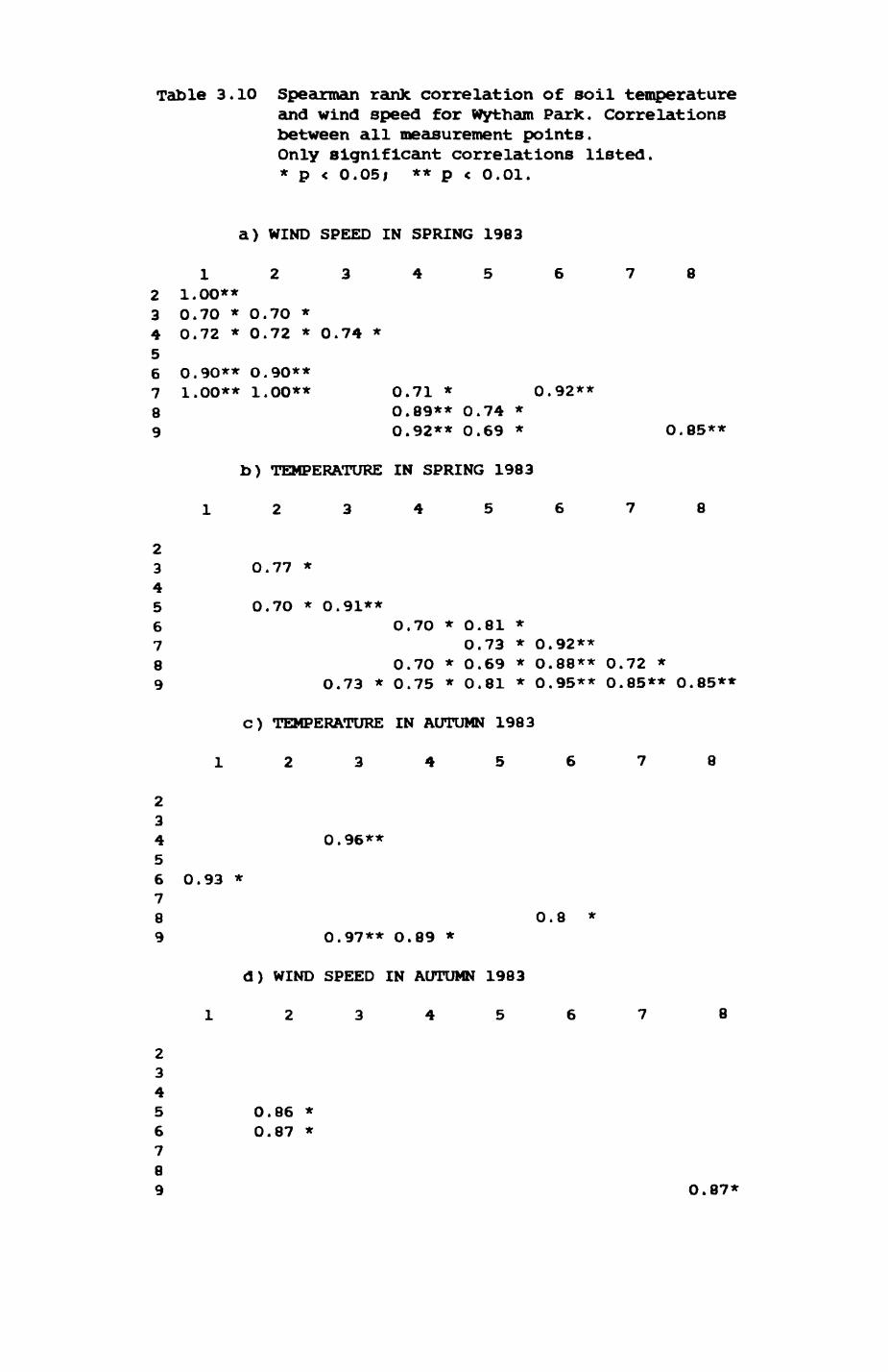
Table 3.10 Spearman rank correlation of soil temperature and wind speed for Wytham Park. Correlations between all measurement points. Only significant correlations listed. * p < 0.05i ** p < 0.01.
a) WIND SPEED IN SPRING 1983
123456782 1.00**3 0.70 * 0.70 *4 0.72 * 0.72 * 0.74 *56 0.90** 0.90**7 1.00** 1.00** 0.71 * 0.92**8 0.89** 0.74 *9 0.92** 0.69 * 0.85**
b) TEMPERATURE IN SPRING 1983
12345678
23 0.77 *45 0.70 * 0.91**6 O.70 * 0.81 *7 O.73 * 0.92**8 0.70 * 0.69 * O.88** 0.72 *9 O.73 * 0.75 * 0.81 * 0.95** 0.85** 0.85**
C) TEMPERATURE IN AUTUMN 1983
12345678
234 0.96**56 0.93 *78 0.8 *9 0.97** O.89 *
d) WIND SPEED IN AUTUMN 1983
1 234567 8
2345 0.86 *6 0.87 *789 0.87*
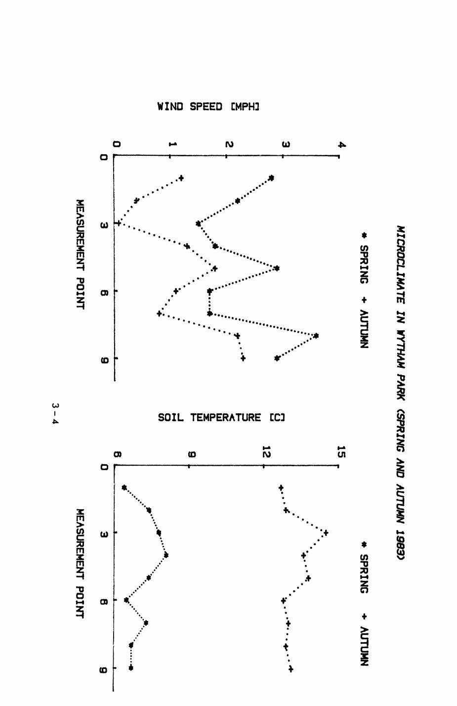
MICROCLIMATE IN WYTHAM PARK (SPRING AND AUTUMN 19B3)
SPRINGAUTUMN
* SPRINGAUTUMN
X
Q.Q
UJ UJ Q. (/)
4 „
69
15 ..
12 *&6
"V"*.
...••*
69
MEASUREMENT POINTMEASUREMENT POINT
3-4
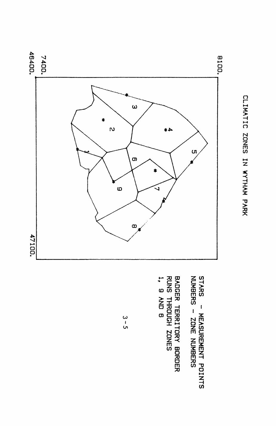
CLIMATIC ZONES
IN WYTHAM
PARK
8100.
7400.
46400.47100,
STARS -
MEASUREMENT POINTS
NUMBERS -
ZONE NUMBERS
BADGER TERRITORY
BORDER RUNS
THROUGH ZONES
lf 9
AND 63-5
75
sites towards Wormstall Duck Pond. The observed differences in soil
temperature and wind speed between sites were similar in their distribution,
indicating an element of temporal stability while on the other hand the
degree of correlation between sites changed between the seasons. There are
at least two simple, and even complementary strategies which could
efficiently exploit these correlations. The first strategy would utilize
the correlations between the type of weather and the status of the earthworm
populations found at a particular site while a second strategy would use the
correlation amongst several sites. Thus, a badger (or a fox) would make a
decision according to the rule
At if humidity and wind is such and such then go to site(s) X/Y/Zi
Bt if site X is fruitful then try also sites Y and Z but avoid
sites A and B etc.
The two rules could also be combinedt
Ci If humidity and wind is such and such try first site X, not Yf and
depending on the result, continue either to sites A,B, .. or to
sites C,D, .. but not to both.
It is difficult to decide which one of the rules promises to be most
successful, as this depends on the number of different climatic conditions
recognised by the animal (rule A) or the number of patches that are used as
'first* patch (rule B), le. patches that serve as Indicators for the
profitability of other patches. However, it seems likely that the
utilization of all the information available (rule C) may improve the
foraging success relative to rules A and B. Whether certain patches are
constantly visited as 'first' patches and how an Individual moves through a
76
given night is the subject of Chapter 6.
3.2.4. DISCUSSION.
EARTHWORM SAMPLING DESIGN AND IDENTIFICATION PROCEDURE. A comparison Of my
results with Kruuk (1978a) and Cuendet (1984) shows general agreement (Table
3.1). Kruuk (1978) showed significant differences between woodland and
plantation and no differences between deciduous woodland and pasture. His
results for arable land correspond to my observed populations while they
differ for the estimated populations by a factor of two. However, some
caution is needed when comparing his results with those of other studies.
UnliJce Cuendet (1984), Phllllpson et al. (1978) or the present study, he did
not distinguish between different soil types and as he did not give a
precise reference for the locations of his sampling plots they can only be
tentatively placed (as in Table 3.1) according to the dominating soil
characteristics of the area he mentioned ('Marley-Jews Harp* area). It is
likely that he sampled from sites on both soil types since his density
estimate for deciduous woodland lies between my density estimates for clay
and rendzina (Table 2.4).
Kruuk (1978a) does not describe in detail how he identified the wormsKt
in his samples but essentially followed a procedure similar to mine (Kruuk,
pers. comm. 13.10.1984). Cuendet (1984) used a different sampling design
(systematic placement of sample points along a linear transecti handsorting
of the top 25 cm of the soil plus formalin sampling), and identified all
specimens down to species level, resulting in similar biomass estimates but
different density estimates, up to twice as high as the results presented
here or those of Kruuk (Table 3.1). His value for beechwood on rendzina was
derived from Phllllpson's et al. (1978) original data (where sample sites
were distributed on a stratified random basis) by placing a linear transect
77
over their sampling area and selecting the 10 nearest plots from their
original May/June and October/November samples. The average of Phillipson's
et al. (1978) original results for the two periods is 11.27 L. terrestris m~
2 as compared to 14.4 m~ 2 as derived by Cuendet. This shows that even
different sampling regimes yield approximately similar results.
VARIATIONS IN BODY WEIGHT. Kruuk's worm biomasses were calculated using an
average weight of 4.27 g for all habitats. This value is slightly less than
Cuendet's (1984) mean fresh body weight for adults, ranging from 4.291 g in
beech/rendzina woodland to 4.545 g in non-beech/rendzina and 4.665 g in non-
beech/clay, and more than my mean fresh weight value of 3.79 g for adults
and juveniles combined (adults separately! 6.75 gj juvenilesi 2.48 g; Table
3.3). Unfortunately, Kruuk does not indicate how many juveniles and adults
were represented in the sample of 41 L. terrestris from which he derived his
mean value, so any interpretations of the differences have to remain
speculative. Whatever the explanation, these differences obviously affect
the biomass calculations, as can be seen in Table 3.1. While Kruuk's and my
density estimates for pasture are very close (22.73 ind m~ 2 vs. 21.09 ind m~
, a difference of 7.7 %), his biomass estimate (97.1 g m~2 ) is 25.6% larger
than mine (77.3 g m~ 2 ).
Kruuk (I978a) did not examine whether body weight varied between
habitats. Cuendet (1984) did not find significant differences of adult mean
fresh body weights for L. terreatrls between the woodland types he
considered. In the present study, differences in juvenile mean body weight
were not significant for the woodland sites, but became significant when all
habitats were considered. Although small sample sizes prevent any firm
conclusions for adults, inspection of Table 3.2b reveals differences between
the woodland sites, but more pronounced differences between woodland and
open habitats, resulting in overall significant differences for both the 4
78
woodland sites and all 7 habitats If both juveniles and adults are
considered together. Table 12 of Cuendet (1984) Indicates a noticable
decline of mean adult fresh body weight from May (non-beech/clayt 6.05 gj
non-beech/rendzinaj 5.095 g) to October (n-b/c«4.288 gi n-b/n 4.380 g). A
possible explanation for this result could be a change in the age structure
of the populations with the majority of adults in autumn being freshly
matured ex-juveniles. If this change takes place during summer, habitat
differences in mean adult and overall body weight between habitats could
reflect differential progress in the transformation of the populations, in
which case Cuendet's findings and the results of the present study would not
be incompatible.
EFFECTS OF SOIL AND LITTER. Both Cuendet (1984) and the present study found
differences between habitats to be more important than between soil
categories. However, there were some important effects of soil type, once
the variance due to habitat differences was considered. Thus, the results
of these two studies urge any future investigations to consider both habitat
and soil type and to account for this in sampling design and subsequent
analysis.
Rendzina contains a high content of carbonate which provides a pH near
neutrality independent of the type of litter. This allows soil
microorganisms to break down the polyphenollc substances of the beech
leaves, thus improving the palatability of beech litter. In the clay,
without the buffering effect of carbonates, the soil is acidic and induces
reduced mlcroblal activity which leaves the litter unpalatable for a long
time, severely restricting the amount of food available (Cuendet (1984)).
The results of the present study do not show any significant
relationship between the amount of litter present and L. terrestrls
populations. Litter was assessed on a 0 to 4 scale and this might have been
79
too crude to give reliable results. Furthermore, the litter that was still
present in July could be litter of less or not preferred species and thus
was of little or no importance to the worms. To investigate this
possiblity, Cuendet (1984) recorded quantitatively the species composition
and the total amount of the litter present at his study sites. The input of
litter at the beginning of the litter 'year* in November was comparable for
the two non-beech woodlands (44O g m~2 on clay; 4OO g m~2 on rendzina) and
beech on rendzina ( 411 g m~ 2 ). Beechwood on clay had 1597 g m~2 (factor of
4). By June, non-beech on rendzina was reduced to 82 g m~2 , non-beech/clay
to 137 g m~ 2 and beechwood on rendzina to 220 g m~ 2 while beechwcod on clay
had 1443 g ra~ 2 of litter present (factor of approximately 10).
The Importance of litter as food for earthworms is mainly expressed by
the litter species composition as indicated by the type of habitat. This
determines how much food is available, no matter what amount of overall
litter is present. Preferred litter vanishes rapidly while less preferred
litter declines only slowly and seems to be accumulating from year to year
as expressed by the high values of beechwood on clay at both sampling
occasions.
HABITAT DIFFERENCES AND FORAGING STRATEGIES OF FOXES AND BADGERS. The
results of the present study reveal differences in earthworm populations
between habitats with consequences for the foraging activity of foxes and
badgers. As the large differences between estimated and observed population
levels (Table 3.4) Indicate, only a fraction of the earthworm population Is
active in July and this fraction declines from open (exposed) habitats such
as arable land and pasture or grassland to woodland. While it is true that
plantations contain only low densities, they might be of Increased Interest
to foxes or badgers, if for some reason they are not able to use the much
more preferable deciduous woodland. This could be especially the case for
80
young and subordinate animals that might be prevented from access to more
profitable sites by dominant individuals or for a range which does not
happen to encompass any deciduous patches. If climatic conditions are
unfavourable (e.g. in periods of dryness), plantations would still be more
humid and thus favour the surfacing activity of worms. An additional source
of attraction at all times of the year may be the grassy rides that often
separate patches of woodland from each other, as they probably contain a
locally more abundant population of worms.
Nothing is Known of whether profitability of worms is similar for
different worm weight or length categories. Thompson and Barnard (1984)
have shown that the profitability of earthworms eaten by plovers and
lapwings decreases sharply with increasing worm length. Such a drastic
effect might not necessarily be expected for badgers or foxes. However,
badgers sometimes manage to secure only parts of a large worm (Kruuk
(I978a), pers. obs.)/ indicating that the optimal size as expressed by the
profitability might not necessarily correspond to the maximum size
available. A habitat such as plantation on rendzina, while generally
unfavourable because of the low worm densities, might be of increasing
interest as it contains larger than average juveniles (which might be close
to the optimal size; Table 3.2b) if unsuitable weather conditions or other
reasons prevent successful foraging in more exposed habitats. This,
together with the aforementioned reasons, could explain, why Kruuk (1978a)
found that badgers in Wytham spent a large amount of their time (27 %) in
plantations. Kruuk does not Indicate from which season his activity
estimates were compiled, but the Increased use of plantations by the badgers
of his study during dry spells of weather seems to support the view
expressed above.
MICROCLIMATE. As Kruuk (I978a) noted, large microcllmatlc differences exist
81
between different sites within the same habitat, even if they are quite
close to each other. In the present study, an attempt was made to see how
much microcllmatic variables vary and whether this variation had any
predictable spatial or temporal components. Patterns of spatial stability
were found while changes occurred between seasons. Thus, an animal with
memory should be able to predict climatic conditions over its range (at
least within certain habitats) but it would also need to occasionally update
its knowledge of the climatic conditions at different Bites. As described
in section 3.2.3., there are at least three simple strategies conceivable
that can efficiently exploit these regularities of micro-climatic
conditions.
3.3 PHEASANT (Phasianus colchicus).
Three game bird species occur in Wytham, the pheasant (Phasianus
colchlcus) . the partridge (Perdlx perdlx) and the woodcock (Scolopax
rustlcola). There are comparatively few woodcocks in Wythami during the
habitat census In January and February 1982 only three Individuals were
encountered. Partridges can be regularly seen on the grassy rides and major
tracks. Middle ton (1935) and others have described the Impact of fox
predatlon on partridge populations, particularly during the breeding season.
However, I did not find a single partridge remain killed by foxes in Wytham
and no attempt was made to sample systematic information on their
distribution. Thus, the rest of this section is restricted to a description
of the predator/prey relationship between foxes and badgers and pheasants.
3.3.1 INTRODUCTION
ACTIVITIES. Pheasants are gamebirds with a complex mating system,
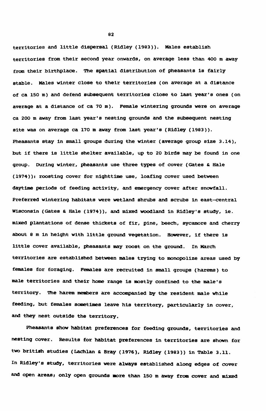
82
territories and little dispersal (Ridley (1983)). Males establish
territories from their second year onwards, on average less than 4OO m away
from their birthplace. The spatial distribution of pheasants is fairly
stable. Males winter close to their territories (on average at a distance
of ca 150 m) and defend subsequent territories close to last year's ones (on
average at a distance of ca 70 m). Female wintering grounds were on average
ca 200 m away from last year's nesting grounds and the subsequent nesting
site was on average ca 170 m away from last year's (Ridley (1983)).
Pheasants stay in small groups during the winter (average group size 3.14),
but if there is little shelter available, up to 20 birds may be found in one
group. During winter, pheasants use three types of cover (Gates & Hale
(1974))i roosting cover for nighttime use, loafing cover used between
daytime periods of feeding activity, and emergency cover after snowfall.
Preferred wintering habitats were wetland shrubs and scrubs in east-central
Wisconsin (Gates & Hale (1974)), and mixed woodland in Ridley's study, ie.
mixed plantations of dense thickets of fir, pine, beech, sycamore and cherry
about 8 m in height with little ground vegetation. However, if there is
little cover available, pheasants may roost on the ground. In March
territories are established between males trying to monopolize areas used by
females for foraging. Females are recruited in small groups (harems) to
male territories and their home range is mostly confined to the male's
territory. The harem members are accompanied by the resident male while
feeding, but females sometimes leave his territory, particularly in cover,
and they nest outside the territory.
Pheasants show habitat preferences for feeding grounds, territories and
nesting cover. Results for habitat preferences in territories are shown for
two british studies (Lachlan & Bray (1976), Ridley (1983)) in Table 3.11.
In Ridley's study, territories were always established along edges of cover
and open areas i only open grounds more than 15O m away from cover and mixed
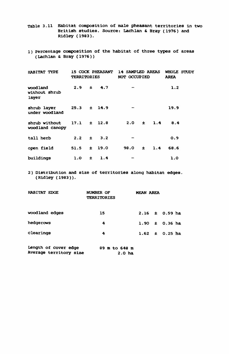
Table 3.11 Habitat composition of male pheasant territories in two British studies. Source: Lachlan & Bray (1976) and Ridley (1983).
1) percentage composition of the habitat of three types of areas (Lachlan & Bray (1976))
HABITAT TYPE 15 COCK PHEASANT 14 SAMPLED AREAS WHOLE STUDYTERRITORIES NOT OCCUPIED AREA
woodland without shrub layer
2.9 ± 4.7 1.2
shrub layer 25.3 ± 14.9 under woodland
19.9
shrub without 17.1 ± 12.8 woodland canopy
2.0 ± 1.4 8.4
tall herb 2.2 ± 3.2 0.9
open field
buildings
51.5 ± 19.0
1.0 ± 1.4
98.0 ± 1.4 68.6
1.0
2) Distribution and size of territories along habitat edges. (Ridley (1983)).
HABITAT EDGE NUMBER OF TERRITORIES
MEAN AREA
woodland edges
hedgerows
clearings
15 2.16 ± 0.59 ha
1.90 ± 0.36 ha
1.62 ± O.25 ha
Length of cover edge Average territory size
89 m to 648 m 2.0 ha
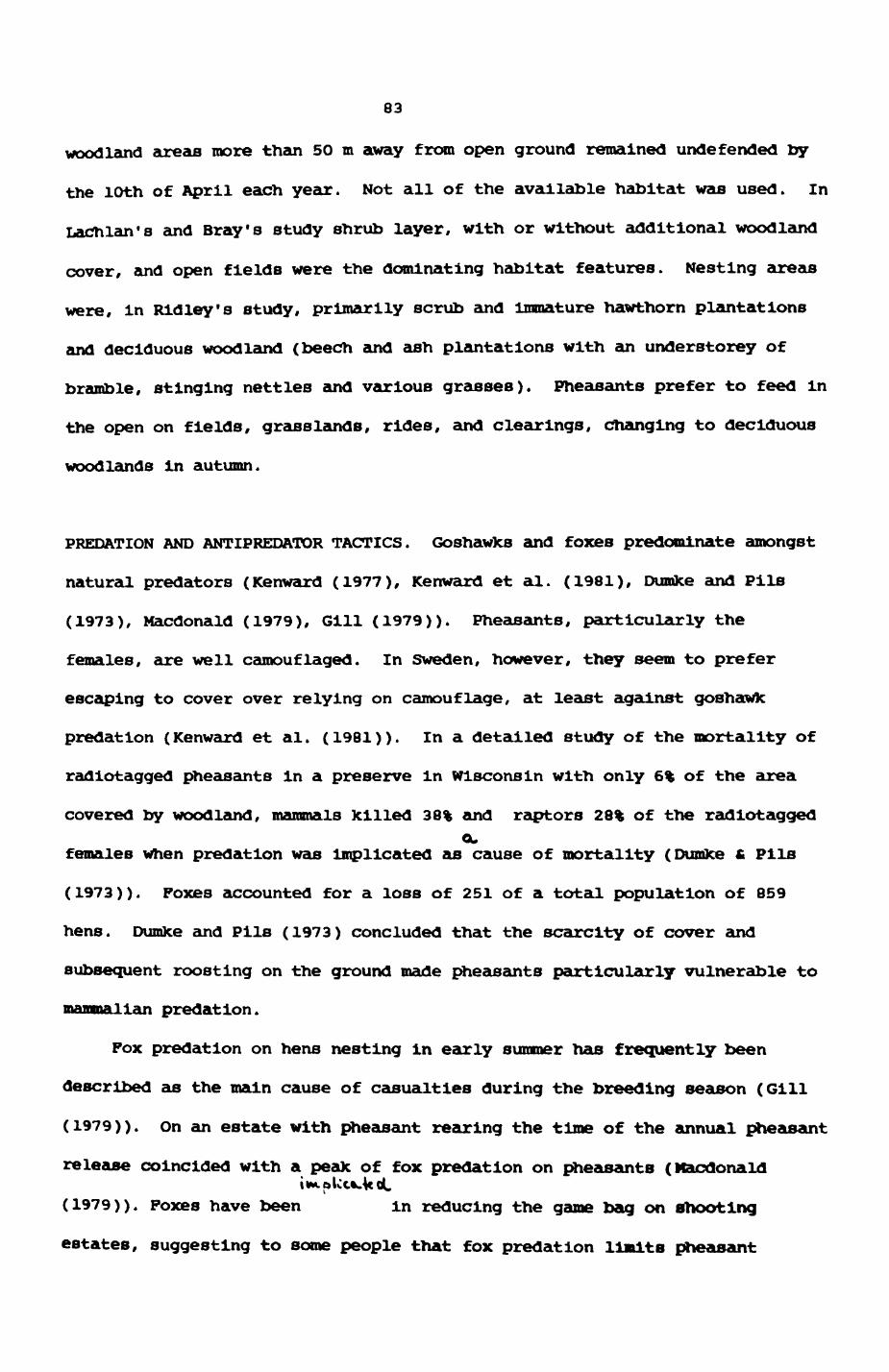
83
woodland areas more than 50 tn away from open ground remained undefended by
the 10th of April each year. Not all of the available habitat was used. In
Lachlan's and Bray's study shrub layer, with or without additional woodland
cover, and open fields were the dominating habitat features. Nesting areas
were, In Rldley's study, primarily scrub and Immature hawthorn plantations
and deciduous woodland (beech and ash plantations with an understorey of
bramble, stinging nettles and various grasses). Pheasants prefer to feed In
the open on fields, grasslands, rides, and clearings, changing to deciduous
woodlands in autumn.
PREDATION AND ANTIPREDATOR TACTICS. Goshawks and foxes predominate amongst
natural predators (Kenward (1977), Kenward et al. (1981), Dundee and Pils
(1973), Macdonald (1979), Gill (1979)). Pheasants, particularly the
females, are well camouflaged. In Sweden, however, they seem to prefer
escaping to cover over relying on camouflage, at least against goshawk
predatlon (Kenward et al. (1981)). In a detailed study of the mortality of
radlotagged pheasants in a preserve in Wisconsin with only 6% of the area
covered by woodland, mammals killed 38% and raptors 28% of the radlotaggedGU
females when predatlon was implicated as cause of mortality (Dumke & Pi Is
(1973)). Foxes accounted for a loss of 251 of a total population of 859
hens. Dumke and Pils (1973) concluded that the scarcity of cover and
subsequent roosting on the ground made pheasants particularly vulnerable to
mammalian predation.
Fox predation on hens nesting in early summer has frequently been
described as the main cause of casualties during the breeding season (Gill
(1979)). on an estate with pheasant rearing the time of the annual pheasant
release coincided with a peak of fox predation on pheasants (KaodonaldtlM.aUtMcoL
(1979)). Poxes have been in reducing the game bag on shooting
estates, suggesting to some people that fox predatlon limits pheasant
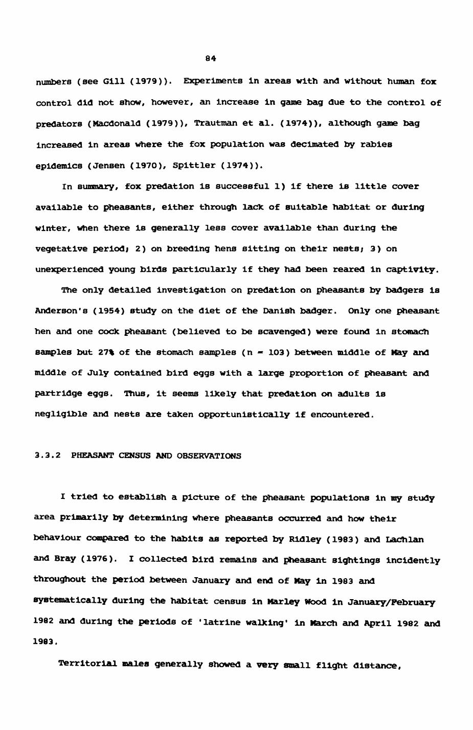
84
numbers (see Gill (1979)). Experiments in areas with and without human fox
control did not show, however, an increase in game bag due to the control of
predators (Macdonald (1979)), Trautman et al. (1974)), although game bag
increased in areas where the fox population was decimated by rabies
epidemics (Jensen (1970), Spittler (1974)).
In summary, fox predation is successful 1) if there is little cover
available to pheasants, either through lack of suitable habitat or during
winter, when there is generally less cover available than during the
vegetative periodi 2) on breeding hens sitting on their nestsi 3) on
unexperienced young birds particularly if they had been reared in captivity.
The only detailed investigation on predation on pheasants by badgers is
Anderson's (1954) study on the diet of the Danish badger. Only one pheasant
hen and one code pheasant (believed to be scavenged) were found in stomach
samples but 27% of the stomach samples (n - 1O3) between middle of May and
middle of July contained bird eggs with a large proportion of pheasant and
partridge eggs. Thus, it seems lUcely that predation on adults is
negligible and nests are taken opportunistically if encountered.
3.3.2 PHEASANT CENSUS AND OBSERVATIONS
I tried to establish a picture of the pheasant populations in my study
area primarily by determining where pheasants occurred and how their
behaviour compared to the habits as reported by Rid ley (1983) and Lachlan
and Bray (1976). I collected bird remains and pheasant sight ings incident ly
throughout the period between January and end of May in 1983 and
systematically during the habitat census in Marley Wood in January/February
1982 and during the periods of 'latrine walking' in March and April 1982 and
1983.
Territorial males generally showed a very small flight distance.
85
particularly When approached by car. In January and February, pheasants were sometimes observed to settle on their roosts in big groups, usually in old, well grown hawthorn thickets. On one occasion (12th February 1983), I counted at least 24 pheasants roosting together at a height of 4 m In a hawthorn thiclcet at the very northeastern tip of Mar ley Plantation, a place LIO (male fox from Mar ley) used to visit regularly at dawn and dusk.
On 107 occasions altogether 140 pheasants were counted in both years. In the majority of cases (9O out of 107) only one pheasant was observed, on 14 occasions two pheasants were seen, on two occasions four pheasants and once, already mentioned, 24 individuals were counted. Of the 1O7 sigh tings 89 were defined as unique observations, ie. the sight ings were at least 1OO meters apart from each other within the same year. Particularly during spring, male pheasants were repeatedly seen at exactly the same location (see Fig. 3.6). These unique sightings were investigated for possible habitat preferences related to their cover value. Due to small sample sizes, habitats were summarized under seven categoriesi
HUMAN Habitats 1,2,3,4,14,23,25,26,43,47 (definition BOX 1)
GRASSLAND Habitats 5,6,7,46
ARABLE Habitats 9,28,29,30,31,32,33
SPECIAL AGRICULTURE 8,12,13,42
OTHER Habitats 24,27,45
WOODLAND Habitats 11,21,22,34,37,38,39,40,41
SHRUB Habitats 10,35,36,44
These categories were then classified as 'open* (HUMAN, GRASSLAND, ARABLE, SPECIAL AGRICULTURE, OTHER) and 'cover* habitats (WOODLAND, SHRUB). Program SRCH2P was run to identify patch and habitat number for each
pheasant sighting. The modified data were then submitted to program BORDER.
Pig. 3.6. Census data of bird populations projected onto the computerized habitat map. Habitats plotted are habi tats 7, pasture, and 37, deciduous woodland.
Red trianglesi pheasant slghtings; results combinedfrom 1982 and 1983. A red number indi cates more than one sighting at a site.
Green diamondsi feather remains (24 wood pigeons, 4other birds); data combined from 1982 and 1983.
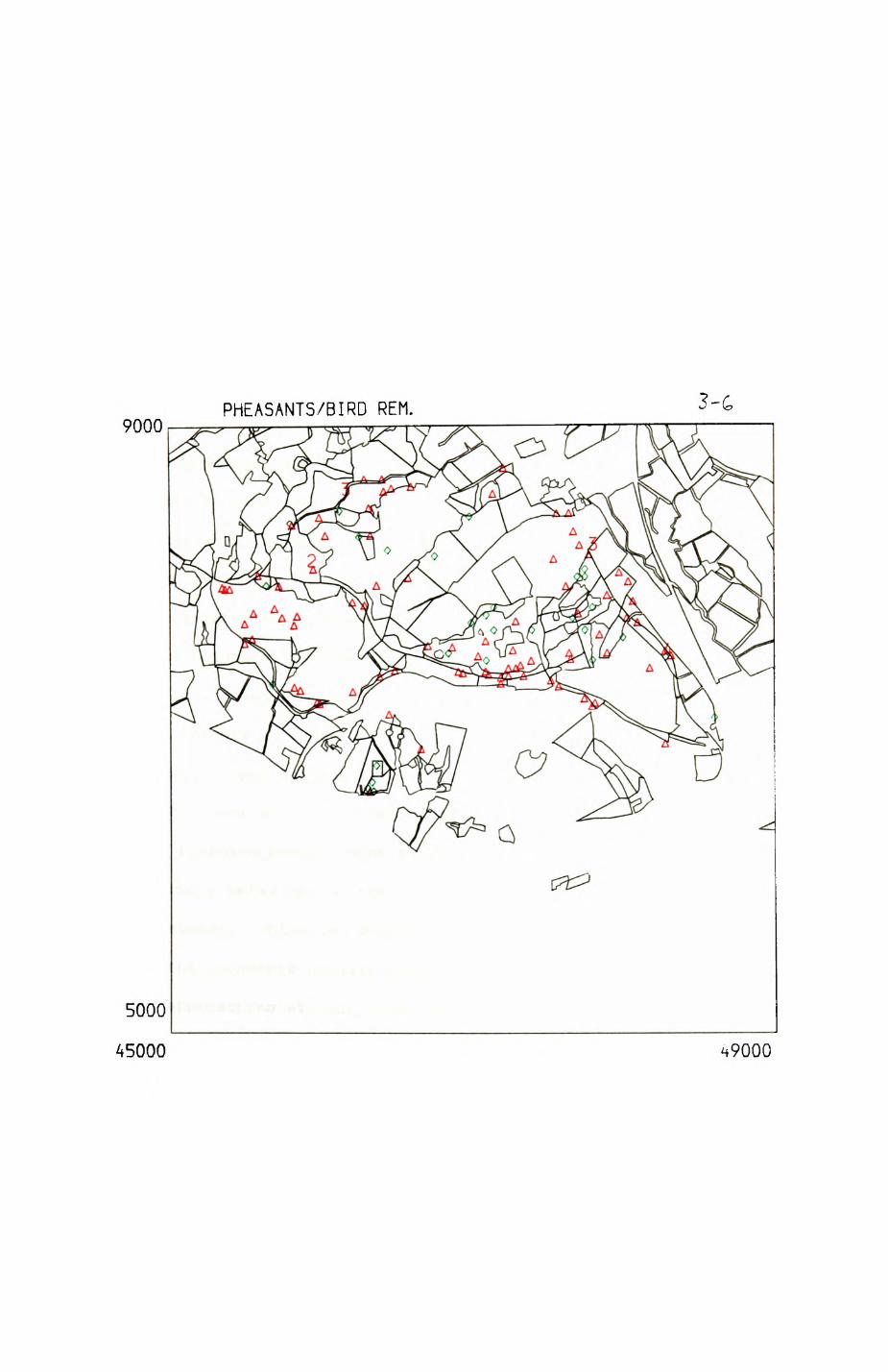
9000PHEASANTS/BIRD REM.
<&> oc3^
5000
45000 ^9000
86
This program calculates for a given point the shortest distance to the
border of its patch, the coordinate of the Intersection of the shortest
distance with the patch border and identifies the number and habitat type of
the neighbouring patch at the point of intersection. Thus, program BORDER
identifies the nearest neighbouring patch for any given coordinate within a
patch. The P-STAT statistical package, available on the university's VAX-
11/780, was used to evaluate the association of the habitat type of each
patch with a pheasant sighting with the habitat type of the nearest
neighbouring patch. Table 3.12a presents the results. Pheasants were
mostly seen in cover (66 out of 89 cases) and were also most likely next to
another habitat with cover (53 cases). Only in 12.4% of the cases (11 out
of 89) were pheasants seen in open habitats next to open habitats. The
selection of habitats by pheasants is independent from the cover value of
the nearest neighbouring habitat (p = O.4, n.s.). Looking at the distances
(Table 3.l2b), pheasants are at a similar actual and proportional distance
from patch borders in three out of four cases. Only pheasants in open
habitat next to open habitat are further away from the patch border.
The characteristics of pheasant ecology and behaviour, particularly
during the breeding season, seem to facilitate their detection; especially
the conspicuous behaviour of the cocks patrolling their territory in spring
and early summer. While the detection probability may be very high in open
habitats, the pheasants usually place themselves so that there is little
chance of approaching without them taking notice. Due to the small tendency
of pheasants to disperse within and between years foxes could certainly
assess the current status of the population within their range and predict
future developments to some extent.
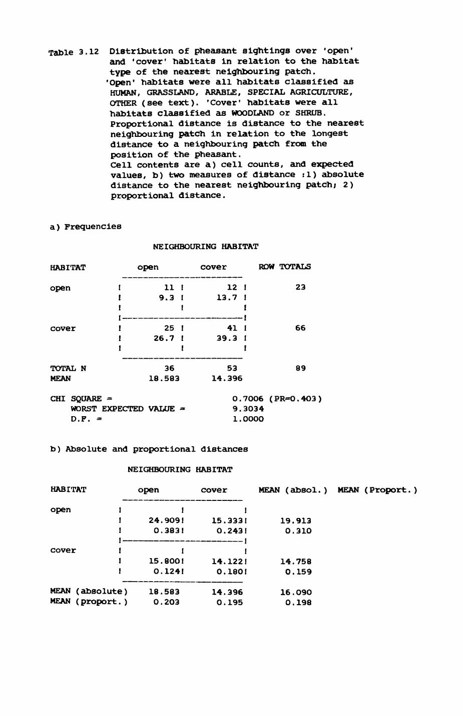
Table 3.12 Distribution of pheasant sightings over 'open' and 'cover' habitats in relation to the habitat type of the nearest neighbouring patch. 'Open' habitats were all habitats classified as HUMAN, GRASSLAND, ARABLE, SPECIAL AGRICULTURE, OTHER (see text). 'Cover* habitats were all habitats classified as WOODLAND or SHRUB. Proportional distance is distance to the nearest neighbouring patch in relation to the longest distance to a neighbouring patch from the position of the pheasant.Cell contents are a) cell counts, and expected values, b) two measures of distance :1) absolute distance to the nearest neighbouring patch; 2) proportional distance.
a) Frequencies
NEIGHBOURING HABITAT
HABITAT
open
open cover
cover
TOTAL N MEAN
119.3
25 26.7
36 18.583
12 13.7
41 39.3
53 14.396
ROW TOTALS
23
66
89
CHI SQUARE =WORST EXPECTED VALUE D.P. =
0.7006 (PR=0.4O3)9.30341.OOOO
b) Absolute and proportional distances
NEIGHBOURING HABITAT
HABITAT
open
cover
open cover
I24.9O9! 0.383!
I15.800! O.124!
MEAN (absolute) IB.583 MEAN (proport.) 0.2O3
!15.333! 0.2431
I14.122! 0.180!
14.3960.195
MEAN (absol.) MEAN (Proport.)
19.9130.310
14.7580.159
16.O90 0.198
87
WOODPIGEON. (COLUMBA PALUMBUS )
3.4.1 Introduction
ACTIVITIES. Wood pigeons are gregarious throughout the winter, feeding in
compact flocks, often with up to 1OO individuals, on fields on various crops
and seeds (Hurt on (1965)). Roosting is nocturnal and communal, though
gregarious tendencies are much less pronounced in breeding birds. Wood
pigeons roost mainly in tall trees, particularly conifers and deciduous
trees using firm leafy branches at a height of 6 to 15 m ( M.Wilson, in
press). In February and March territory formation takes place with males
moving to the middle tree canopy from which they give territorial calls
before roosting with the other birds, slowly extending their territorial
activities until they roost in their own territories. The midday period
spent on feeding decreases until July when nearly all time is spent in the
territory (Murton & isaacson (1962)). Breeding taxes places throughout the
summer until September. The most preferred breeding habitats are coniferous
woodland (Murton (I958)t on average 5.6 nests/acre), hedgerows (4.4
nests/acre) and deciduous woodland (1.5 nests/acre). Wood pigeons have
several feeding grounds that are used very regularly. Both entire flocks
and individual pigeons revisit the same places again and again.
PREDATION AND ANTIPREOATOR TACTICS. Wood pigeons fall prey to a variety of
predators. Tomialojc (1979) listed more than 2O predator species and
concluded that nest-site selection and other aspects of wood pigeon biology
evolved under p red at ion pressure. Goshawks and crows are important avlan
predators while martens and cats are Important mammalian predators. Kenward
(197Ba, I978b) investigated the reaction of wood pigeons to human
disturbance and goshawk p reflation. Goshawk attacks on pigeons feeding on
88
brassica fields were more successful in the hour before sunset than in the
previous four hours, and single birds and small flocks suffered a higher
predation rate than flocks with more than 10 wood pigeons. He suggested
that increased group size resulted in an increased vigilance and attributed
the higher capture success before sunset to Increased vulnerability of
pigeons because of pre-roost crop-filling. Wood pigeons quickly resettled
on the fields whether they were disturbed by humans, traffic, or goshawks.
Neither badgers nor foxes are mentioned as predators in Murton's (1965)
monograph on the wood pigeon. Tomialojc (1979) and Rzebik-Kowalska (1972)
list the fox as a predator on adults. Badgers are not mentioned in either
of the sources. There seem to be few opportunities for foxes to catch
pigeons if their roosting, breeding or flock feeding habits are considered.
However, remains of wood pigeons eaten by foxes can be regularly found in
Wytham. How is this possible?
3.4.2. OBSERVATIONS ON WOOD PIGEONS AND MOOD PIGEON REMAINS
Almost all of 28 collected bird remains were wood pigeons, except one
black bird, one marsh tit, and two pheasants. Fig. 3.6 shows the spatial
distribution of 28 bird remains that were left by foxes (birds taken by
foxes can be easily distinguished from birds taken by sparrowhawks as
sparrowhawks pluck the feathers neatly, while foxes simply bite them off).
A more detailed analysis of the habitats where remains of wood pigeons were
found is presented in Table 3.13. Results were obtained by running programs
SRCH2P and BORDER and submitting the data to P-STAT in a way similar to the
analysis of the pheasant data. The results are not straightforward to
interpret as the places where the prey remains were found may not be
identical with the place of capture. Remains were found well Inside patches
within mixed plantations but close to the patch border of pasture and Burner
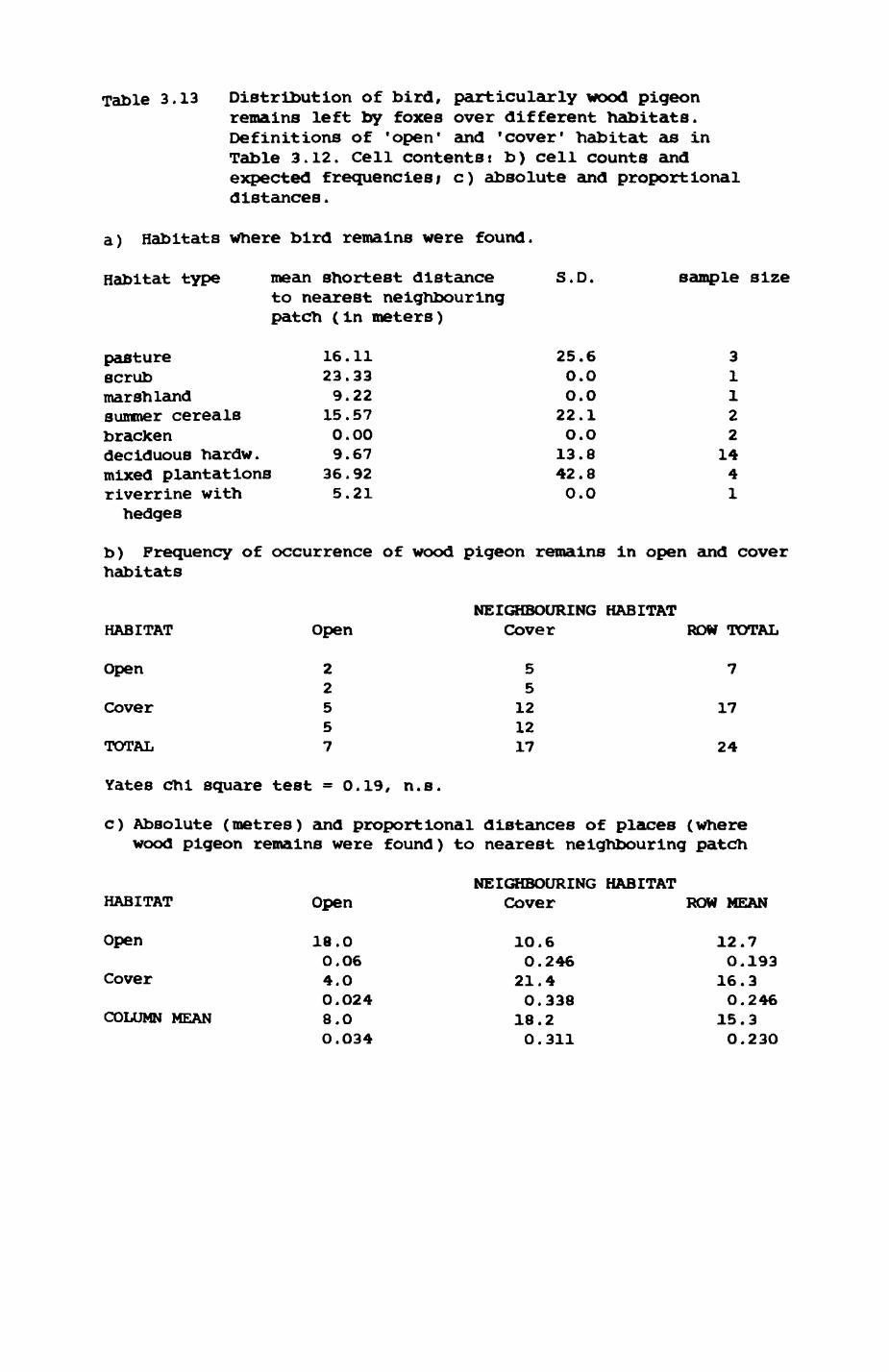
Table 3.13 Distribution of bird, particularly wood pigeon remains left by foxes over different habitats. Definitions of 'open 1 and 'cover' habitat as in Table 3.12. Cell contentst b) cell counts and expected frequencies; c) absolute and proportional distances.
a) Habitats Where bird remains were found.
Habitat type mean shortest distance to nearest neighbouring patch (in meters)
S.D. sample size
pasture 16.11scrub 23.33marshland 9.22summer cereals 15.57bracken 0.00deciduous hardw. 9.67mixed plantations 36.92riverrine with 5.21 hedges
25.6 0.0 O.O22.1 O.O13.842.8 0.0
31122
1441
b) Frequency of occurrence of wood pigeon remains in open and cover habitats
HABITAT
Open
Cover
TOTAL
Open
22557
NEIGHBOURING HABITAT Cover
55
121217
ROW TOTAL
7
17
24
Yates chi square test - 0.19 f n.s.
c) Absolute (metres) and proportional distances of places (where wood pigeon remains were found) to nearest neighbouring patch
HABITAT
Open
Cover
COLUMN MEAN
Open
18.0 0.06 4.0 0.024 8.0 O.034
NEIGHBOURING HABITAT Cover
1O.6O.246 21.4O.338
18.20.311
ROW MEAN
12.70.193
16.30.246
15.30.230
89
cereals. As Pig. 3.6 indicates, the remains found in open habitats are
close to woody habitats and roost of the prey remains found in deciduous
woodland are fairly close to areas with open habitats; in particular, those
that were found in cover next to open habitats are nearly on the border of
the patch (Table 3.13c). This is an interesting contrast to the sightings
of pheasants (Table 3.12b) where sightings in cover habitat were at an equal
distance from open and from cover habitat. No dependence was found for the
type of habitat where remains were found and the habitat of the nearest
neighbouring patch (Table 3.13b).
Poxes might be able to opportunistically catch some pigeons while they
feed on fields. Kenward (1978bt282) showed in an analysis of the spatial
distribution of pigeons feeding on a brasslca field that some pigeons were
quite close to the surrounding hedges that could provide the necessary cover
for a stalking fox. However, I believe that the majority of the pigeons are
actually caught by foxes in the woodland (Table 3.13a). Many wood pigeons
are shot on the farms that are next to the study area. Not all of these may
be killed. David Macdonald and I once found a pigeon injured with gunshot
which would have been an easy victim for foxes. Also, wood pigeons can be
observed regularly in the woodland. Table 3.14 presents a list of wood
pigeon sightings in Harley Wood and Mar ley Plantation for a lO-day period in
April 1984 (data Kindly provided by Marion East). The pigeons were not
specifically searched for and most of the data were collected by approaching
the pigeons by car. Regular visits to bathing, drinking or feeding sites
seem to be common and thus should be predictable for foxes as well.
3.5. LAGOMDRPHS
As there are practically no brown hares (Lepus europaeus) present in
Wytham, I restrict my account of lagomorpha to a description of rabbit
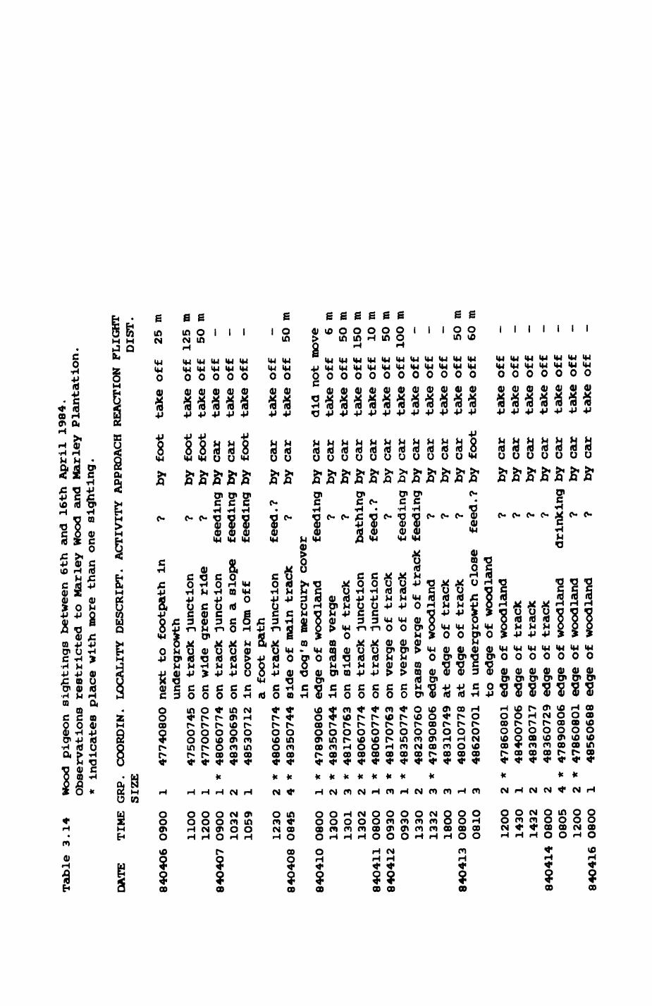
Table
3.14
Wood p
igeon
sightings between
6th
and
16th April 19
84.
Observations restricted t
o Marley Wood
and Marley P
lantation.
* indicates
place with more
than o
ne sighting.
DATE
TIME GRP. COORDIN. LOCALITY DESCRIPT. ACTIVITY APPROACH REACTION PLIGHT
SIZE
DIST.
84O4O6 O9OO
14774O8OO
84O4O7
84O4O8
84O410
840411
84O412
84O413
84O414
84O416
11OO
1200
O900
1032
1059
123O
0845
080O
130O
1301
1302
O800
093O
0930
1330
1332
180O
O8OO
O81O
120O
1430
1432
08OO
O8O5
120O
080O
1 1 1 2 1 2 4 1 2 3 2 1 3 1 2 3 3 1 3 2 1 2 2 4 2 1
47500745
477OO77O
* 48060774
48390695
4853O712
* 48060774
* 4835O744
* 47890806
* 4835O744
* 48170763
* 4806O774
* 48060774
* 48170763
* 48350774
48230760
* 47890806
48310749
48010778
4862O701
* 478608O1
4840O706
48380717
4836O729
* 4789O8O6
* 47860801
48560688
next to footpath In
undergrowth
on t
rack j
unction
on wide
green
ride
on track j
unction
on t
rack o
n a
slope
in c
over lOm off
a foot path
on t
rack j
unction
side o
f main t
rack
In dog's mercury cover
edge o
f woodland
in g
rass v
erge
on side o
f track
on t
rack junction
on t
rack junction
on v
erge o
f track
on v
erge o
f track
grass
verge
of t
raedge o
f woodland
at edge o
f track
at e
dge of t
rack
in u
ndergrowth c
lose
to e
dge of woodland
edge of woodland
edge o
f track
edge o
f track
edge o
f track
edge o
f woodland
edge o
f woodland
edge o
f woodland
by foot
take o
ff
25 m
? ?feeding
feeding
feeding
feed.?
er feeding
? ?bathing
feed.? ?
feeding
: feeding
? ? ?'
feed . ?
? ? ? ?drinking
? ?
by by by by toy
by by by by by by by by by by by by by by by by by by by by by
foot
foot
car
car
foot
car
car
car
car
car
car
car
car
car
car
car
car
car
foot
car
car
car
car
car
car
car
take
take
take
take
take
take
take
off
off
off
off
off
off
off
12550 — — — — 50
m m m
did
not move
take
take
take
take
take
take
take
take
take
take
take
take
take
take
take
take
take
take
off
off
off
off
off
off
off
off
off
off
off
off
off
off
off
off
off
off
65O
15O 10 5O
1OO — — —5O
60 — — — — — — —
m m m m m m m m
90
presence (orvctolacrus cuniculus). My account of rabbit ecology and
behaviour follows Lloyd (1977) unless other sources are cited. A general
monograph on rabbits was written by Thompson and Worden (1956).
3.5.1. Introduction
ACTIVITIES. Rabbits are small herbivores, reaching a size of up to 4O cm
(length) and an adult weight between 1.2 and 2 Kg with pregnant females
reaching up to 2.2 leg. Rabbits are usually crepuscular and nocturnal but
may also become diurnal if undisturbed. Rabbits occupy special burrows
called warrens (systems of interconnecting tunnels with multiple entrances)
which are necessary for breeding (Garson (1981), Cowan, pers. comm.).
warrens may also be used as a daytime refuge, although in a study using
radiotracked individuals. Wheeler et al. (1981) showed that most rabbits
prefer to stay above ground in cover during the day. Severe adverse weather
causes only a slight increase in the proportion of rabbits talcing refuge in
a warren while an increase in population density reduces the proportion of
rabbits staying in warrens considerably (relegation effect; Gibb (1981)).
Dominant individuals keep their offspring in the main warren but subordinate
and satellite females may have to dig special breeding stops or occasionally
keep nests above ground in dense cover. Times of "emergence" at dusk or at
night can be variable, even if ground predators are absent. Activity
depends on intensity of moonlight and cloud coven rabbits tend to be more
timid in strong moonlight.
Rabbits use runs to and from feeding areas. Erect grasses are most
preferred but rabbits are also attracted by cereal fields, pastures and
roots. Host preferred habitats are therefore areas of relatively short
grass which are in close proximity to some kind of refuge (warrens or cover
vegetation). At high population densities rabbits Increase the amount of
91
time spent on feeding during night and day and eventually sacrifice their
morning rest period. The amount of available feed in the vicinity of the
warren is quickly reduced and they have to go further away in order to
obtain sufficient food.
ANTIPREDATOR TACTICS. Rabbits play a major role as a keystone prey species
in temperate, particularly meditterranean-type ecosystems (Dellbes & Hiraldo
(1981), Wagner (1981)). An efficient communal alarm system serves to warn
all group members of the approaching danger. Alarm is signalled visually by
an erect posture and flashing of the tall during nigh speed running, and
acoustically by thumping with the hind legs above and below ground. Rabbits
are fast runners that change flight direction rapidly several times In an
escape sequence. They usually move less than 200 metres away from cover and
prefer to be active when visibility is low. There is the suggestion that
synchrony of estrus and births may be an adaptation to "swamp" predators
with a flood of young (Garson (1981)). Diseases, particularly coccidiosis
and myxomatosis, reduce the rabbits' alertness (pers. obs.). As a result,
some predators like the imperial eagle (Aguila adalberti) showed an increase
in rabbit consumption (Dellbes & Hidalgo (1981)), after myxomatosis was
Introduced.
PREDATOR FORAGING. Both foxes and badgers are known to take rabbits.
European badgers nave been characterized as 'croppers* rather than hunters
since they mostly dig out nests with young rabbits but seldom attempt to
hunt adults (Neal (1977), Delibes & Hidalgo(1981)), in contrast to the North
American badger (Taxldea taxus) where rabbits may be a staple part of the
diet (Neal (1977), Lindxey (1971), Long & Klllingley (1983)). Nests are
located by scent or hearing and dug out vertically rather than by opening up
a tunnel (Neal (1977)).
92
Foxes hunt adults and young, usually above ground although they might
endeavour to try and sneak into a rabbit warren if the entrance is large
enough. There is some evidence that fox predation on rabbit nests is
related to edaphic conditions! in an Australian study, predation was heavy
or\ stony soils (Myers & Parker (1965)). Foxes use a variety of tactics to
catch rabbits above ground. They usually stalk them if the habitat is
suitable, or they hide and wait close to warrens, or they chase them in the
open. In the latter case they are only successful if the rabbit is sonehow
not capable of maintaining full escape speed (in case of disease etc.) or if
it detected the fox too late. Similarly, North amerlcan red foxes stalk
cottontail rabbits (Sylvilagus spec.) but are outrun by them in the open,
even in snow (Scott (1943 )).
3.5.2. The rabbit population in Wytham Woods
3.5.2.1. Methods
The following methods were usedi
1. Identification of rabbit warrens.
2. Notes of rabbit signs. During the 1982 habitat census the number of
sites with rabbit pellets in each 'basal' area (see section 2.3) was
recorded. This parameter is a reliable indicator of rabbit distribution and
abundance and has been used for some time (Taylor (1956), Lloyd (1977),
Ooaterveld (1983), Trout & Tlttensor (1983)). During the habitat census,
patches with rabbit hair were also frequently noted. According to Trout and
Tlttenaor (1983) the correlation of adult abundance and number of hair Bites
along habitat boundaries IB moderate (0.425). Since such sites were
93
recorded regularly only during part of the habitat census, it was not
possible to evaluate them quantitatively. However, the results gave the
distinct qualitative impression that rabbits occurred regularly in dense
woodland areas, perhaps to a greater extent than would be expected from the
literature.
3. Records of rabbit sightings. Wherever a rabbit was seen, the place,
habitat, number, time and special conditions were recorded. This
information was used to compile Fig. 3.7 where the major areas of rabbit
occurrence together with a coarse habitat map are presented.
4. Transect walks. After some exploratory attempts in autumn 1982, several
transects along habitat boundaries were designed according to the system
introduced by Trout and Tittensor (1983) for the MAPF rabbit survey and
adapted to the local circumstances. In principle their results should be
comparable with my study.
Six transects were designed along habitat boundaries, ie. usually
boundaries between so-called open and cover habitats (e.g. woodland and
pasture). Transects were walxed between March 24 and March 31, 1983, by
Christa Heliner. Three parameters were recorded! number of rabbits seen,
number of rabbit warrens encountered, and number of places with rabbit
pellets. If possible, a strip of 10 meter width was searched for any signs
of rabbits. Only rabbits that stayed in the vicinity of the transect route
were counted. In practice this turned out to be no problem, since the
rabbits seen were close to the habitat boundary. All six transects were
walxed at least twicei the first time only rabbits were counted, while on
the second round the number of rabbit pellet places and the number ofl^wSttVft
warrens were counted.were walxed at dusX as initial trials showed a much
reduced number to be present at dawn. Since all transects were walxed

Pig. 3.7. Map of the central part of the study area, with the distribution of main habitat categories, buildings (black) and track roads. Areas with high rabbit abun dance shaded. Dotted lines represent rabbit transectsj number of transect and direction of walking Indicated.
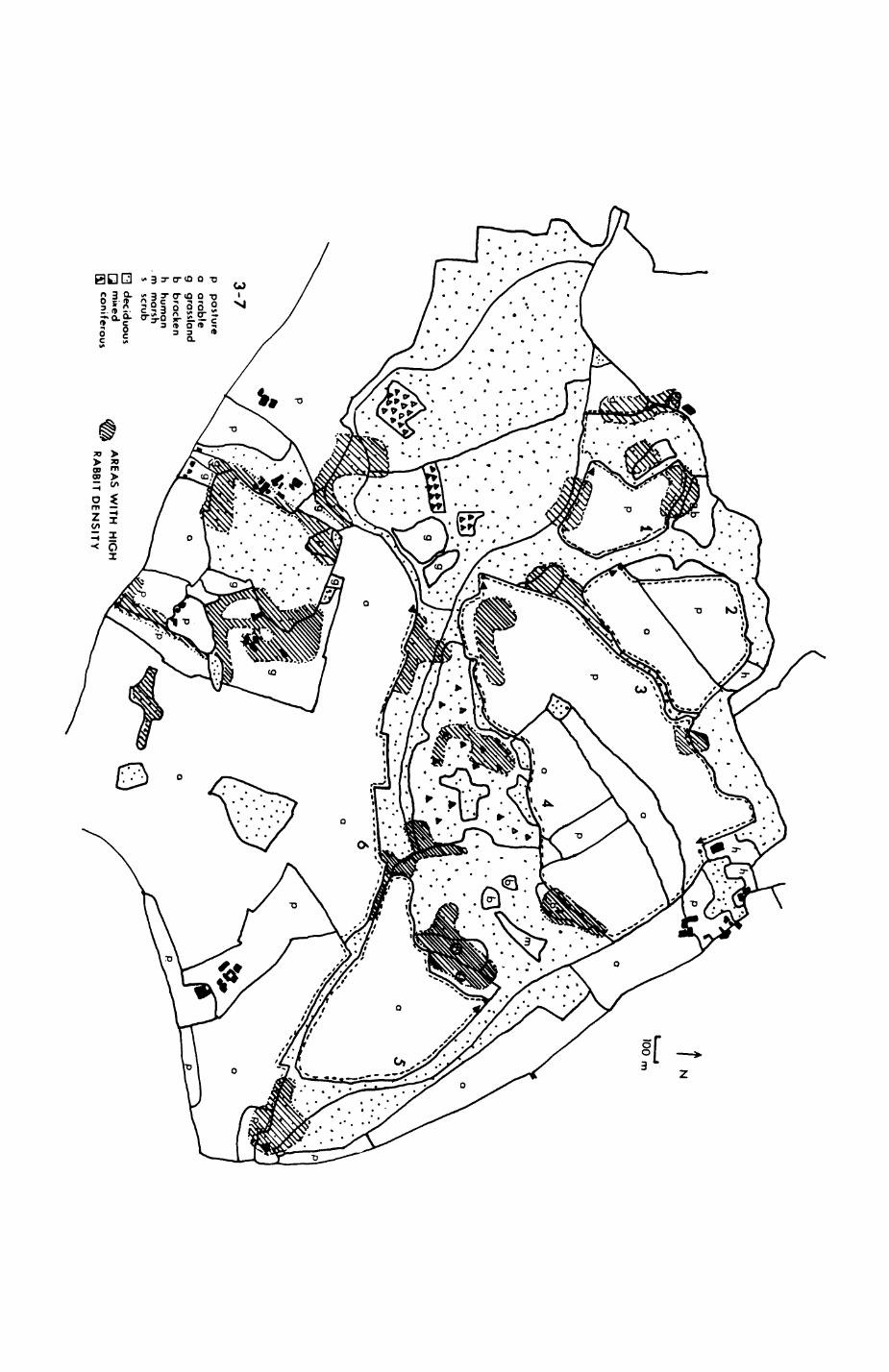
3-7p
pasturea
arable
g grassland
b bracken
h hum
an. m
m
arshs
scrub
03 deciduous
Q m
ixedconiferous
AR
EA
S W
ITH
H
IGH
R
AB
BIT D
EN
SIT
Y
94
within a week, time differences between different subpopulations are
probably negligible.
3.5.2.2. Results
A qualitative summary on the distribution of rabbits in Wytham is
presented in Pig. 3.7. Hajor habitats are illustrated together with areas
of high rabbit density. Emphasis was placed on a correct outline of habitat
boundaries close to the major rabbit areas while such a detailed split up of
habitats was not done in areas where rabbits occurred only at low densities
(e.g. Radbrook Common Area). Also shown are the routes of the six transects
(numbered 1 to 6) and the direction of transect walking. Although rabbits
occur at low densities more or less everywhere in Vfytham Woods, there are
areas of peak abundance with a corresponding Increase in warren density
(Pig. 3.8). Many areas of peak abundance combine open and cover habitats
but some are almost exclusively restricted to woody areas (e.g. one area
close to the Pasticks). This may be partly due to traditioni before I960
the areas around the Pasticks (which are today mixed plantations) consisted
of arable land and pasture fields, surrounded by small strips of woodland,
ideal for rabbits. Although there is little known about rabbit dispersal,
it seems that a warren is passed from one female group to the next
generation female group (probably close kin) (Gareon (1981)). Rabbits nay
simply have stayed there, despite the habitat changes. It is likely that
the grassy rides in this area are very important to the rabbits i they were
seen to feed there at any time of the night or day.
In Pig. 3.8 all rabbit warrens in the area, whether active or Inactive,
are plotted on a habitat map showing pasture (habitat 7), long grassland
(habitat 5), grass ley (habitat 6), marsh (habitat 24) and bracken (habitat
35), facilitating a comparison with the areas of rabbit peak abundance in

Pig. 3*8. Rabbit warrens (red stars) projected onto the compu terized habitat map. Habitats plotted are habitats 7, pasture, 36, hedge, and 44, rlverrine environment with hedge.
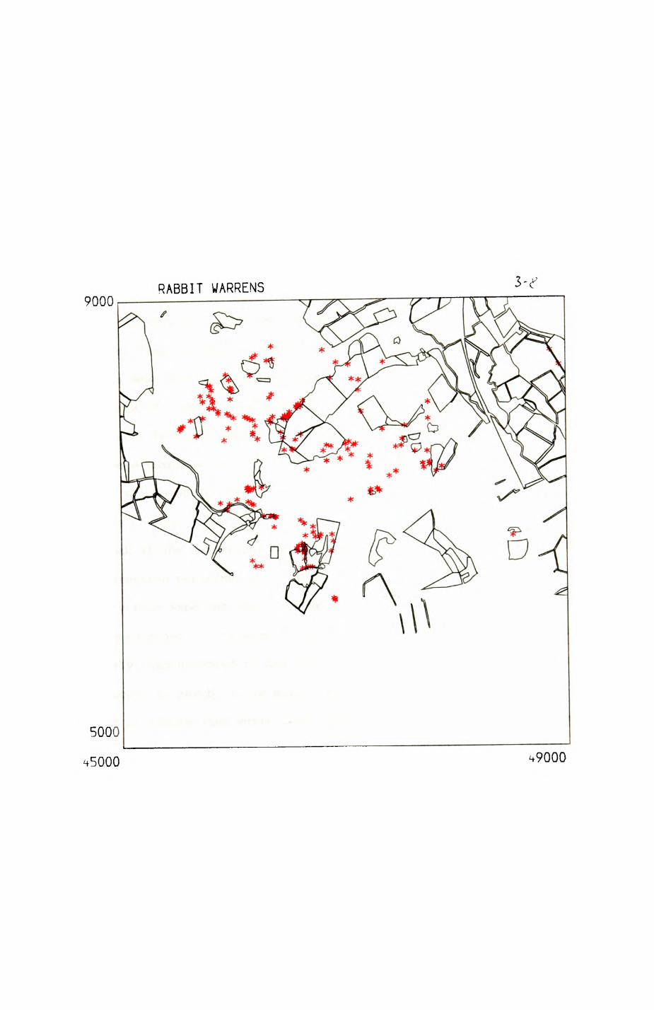
9000RABBIT WARRENS
49000
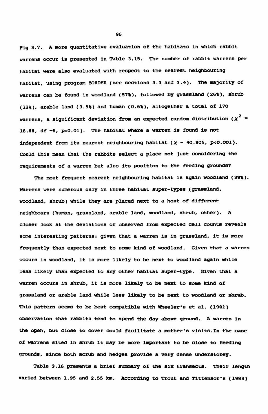
95
Pig 3.7. A more quantitative evaluation of the habitats in which rabbit
warrens occur is presented in Table 3.15. The number of rabbit warrens per
habitat were also evaluated with respect to the nearest neighbouring
habitat, using program BORDER (see sections 3.3 and 3.4). The majority of
warrens can be found in woodland (57%), followed by grassland (26%), shrub
(13%), arable land (3.5%) and human (0.6%), altogether a total of 17O
warrens, a significant deviation from an expected random distribution (x -
16.88, df «6, p<O.Ol). The habitat where a warren is found Is not*
independent from its nearest neighbouring habitat (x » 4O.8O5, p<O.OOl).
Could this mean that the rabbits select a place not just considering the
requirements of a warren but also its position to the feeding grounds?
The most frequent nearest neighbouring habitat is again woodland (38%).
Warrens were numerous only in three habitat super-types (grassland,
woodland, shrub) while they are placed next to a host of different
neighbours (human, grassland, arable land, woodland, shrub, other). A
closer look at the deviations of observed from expected cell counts reveals
some interesting patterns i given that a warren is in grassland, it is more
frequently than expected next to some kind of woodland. Given that a warren
occurs in woodland, it is more likely to be next to woodland again while
less likely than expected to any other habitat super-type. Given that a
warren occurs in shrub, it is more likely to be next to some kind of
grassland or arable land while less likely to be next to woodland or shrub.
This pattern seems to be best compatible with Wheeler's et al. (1981)
observation that rabbits tend to spend the day above ground. A warren in
the open, but close to cover could facilitate a mother's visits.In the case
of warrens sited in shrub It may be more Important to be close to feeding
grounds, since both scrub and hedges provide a very dense understorey.
Table 3.16 presents a brief summary of the six transects. Their length
varied between 1.95 and 2.55 km. According to Trout and Tlttensor f B (1983)
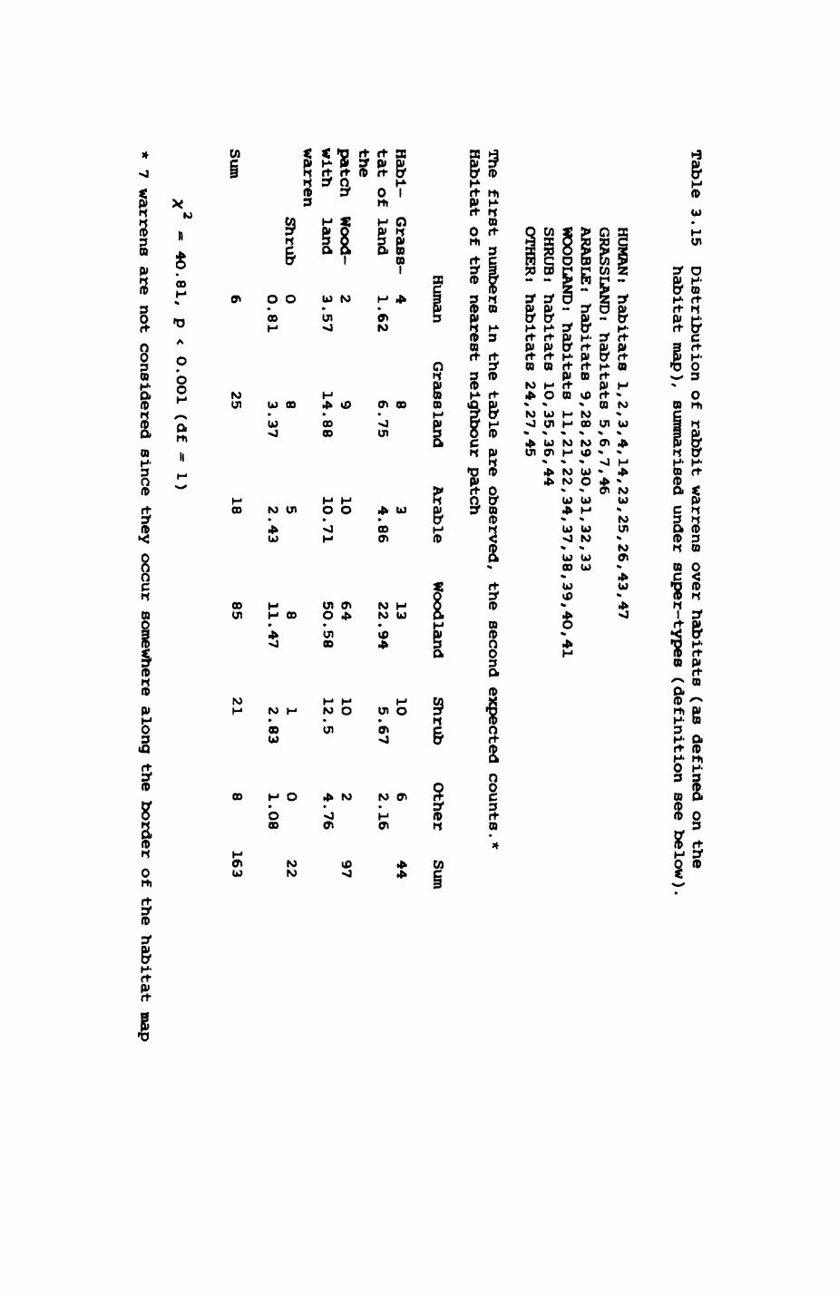
Table 3.15 Distribution of rabbit warrens over habitats (as defined on thehabitat map),
summarised under super-types (definition see below)
HUMAN! habitats 1,2,3,4,14,23,25,26,43,47
GRASSLANDi habitats 5,6,7,46
ARABLEt habitats 9,28,29,30,31,32,33
WOODLANDi habitats 11,21,22,34,37,38,39,40,41
SHRUBi habitats 10,35,36,44
OTHER! habitats 24,27,45
The first numbers
in the table are observed, the second expected counts.*
Habitat of the nearest neighbour patch
HumanGrassland
ArableWoodland
Shrub
Habi- Grass-
tat of land
thepatch
Wood- with
land warren
Shrub
Sum
Other
41.62
23.57
00.81
86.75
914.88
83.37
34.86
1010.71
52.43
1322.94
64
SO. 58
811.47
105.67
1O12.5
12.83
62.16
24.76
01.08
2518
8521
8
Sum
44
9722
163
X
- 40.81,
p < O.001
(df - 1)
* 7 warrens
are not
considered since
they occur somewhere
along the border of the habitat map
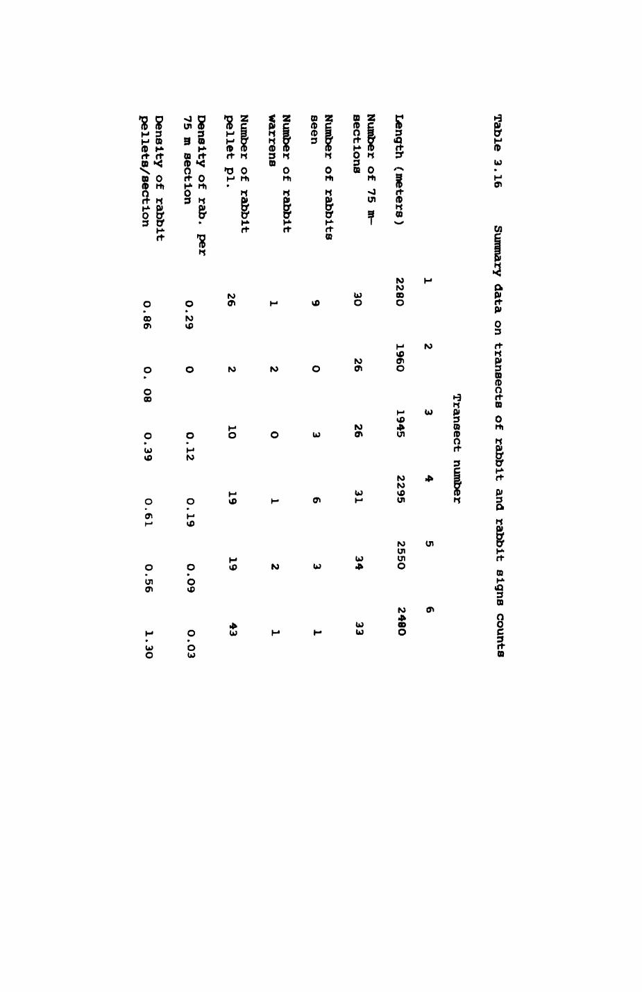
Table 3.16
Summary data on transects of rabbit and rabbit signs counts
Transect number
Length (meters)
Number of 75 in sect Ions
2280
1960
1945
2295
255O
248O
30
2626
3134
33
Number of rabbits seen
Number of rabbit warrens
Number of rabbit pellet pi.
Density of rab. per
75 m section
Density of rabbit pellets/section
260.29
0.86
1019
19
0. OS
O.39
O.61
O.56
43
0.12
0.19
O.O9
0.03
1.30
96
design, each transect was subdivided into 75 m sections and all subsequent
densities refer to a unit length of 75 m. The number of rabbits seen was
small on most transects, and it was highly variable. For instance, a second
walk along Transect 1 yielded only two sightings.
The number of rabbit pellet places was judged to be the most reliable
indicator of rabbit presence. As Table 3.15 shows, densities of rabbits
seen and densities of pellet places do not covary very well (Spearman's rank
correlation, rho - 0.37, n.s. ). In Table 3.17 a more detailed compilation
of pellet place densities in relation to the habitat types along the
transect is pesented. I distinguished between the habitat type, on which
side the transect was walked ("inside" habitat) and the habitat on the other
side of the boundary ("outside" habitat). Along each transect, one element
represented a distance over which the inside and outside habitat do not
change. The length of each habitat type was computed by adding the length
of all elements where the given habitat type was present, independent of
possible habitat changes on the other side of the habitat boundary. The
densities are the mean of the counts of all elements with a given habitat
present.
In general, pellet places were clumped along the transect, not
regularly distributed over the entire length. The highest densities were
found on transect sections with bracken as outside habitat (densities of 3
and 5 pellet places per 75 m), also one section with pasture on the inside
(5 pellet places per 75 m). This section is a short section and was
immediately next to Botley Lodge at the very southeast of the wood. Since
high density sections seemed to be very short, I investigated the
possibility that the length of a section belonging to the same habitat type
(either as inside or as outside habitat) exerts an Influence on pellet place
densities. There is a weak negative correlation (Spearman rank correlation.
- -O.29, n.e.)/ If all elements (defined as sharing the sane Inside and
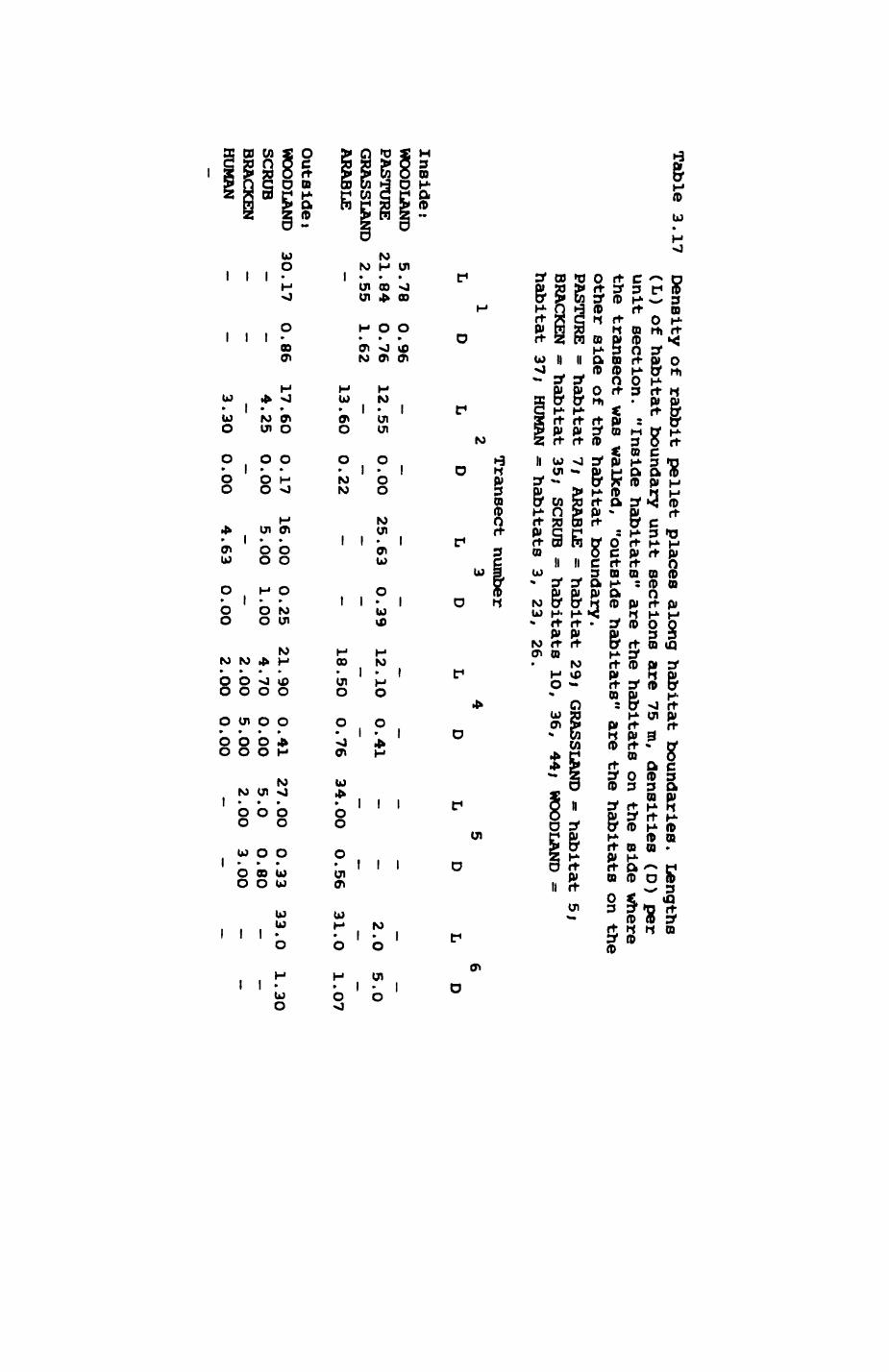
Table 3.17
Density of rabbit pellet places along habitat boundaries. Lengths
(L) of habitat boundary unit sections are 75 m, densities (D) per
unit section.
"Inside habitats" are the habitats on the
side Where the transect was walked,
"outside habitats" are the habitats on the
other side of the habitat boundary.PASTURE = habitat 7;
ARABLE = habitat 29;
GRASSLAND - habitat 5i
BRACKEN - habitat 35;
SCRUB = habitats 10,
36, 44;
WOODLAND =
habitat 37; HUMAN - habitats 3,
23, 26.
Transect number
2 3
L D
L D
4
L
D6
L
D
Inside:WOODLAND
5.78 0.96-
-
-
-
-
-
-
-
__
PASTURE
21.84
O.76
12.55
O.OO
25.63
0.39
12.10
O.41
-
-
2.O
5.0
GRASSLAND
2.55 1.62-
-
-
-
-
-
-
-
--
ARABLE
-
13.60
0.22
-
-
18.5O
O.76
34.OO
0.56
31.0
1.O7
Outside iWOODLAND
30 . 17
SCRUB
BRACKEN
O.86
17.4.—
—
6025
O.17
O.OO
—
165.00.00—
0.25
1.00
—
21.90
4.70
2.0O
0.41
0.00
5.0O
2752
.00.O.OO
0.33
0.80
3.OO
HUMAN
3.3O
O.OO
4.63
O.OO
2.00
0.00
33.0
1.30
97
outside habitat, not listed In Table 3.16) are considered. Looking at the
relationship of element length and pellet place density within an Inside or
outside habitat type, I found a highly significant positive correlation of
element length for "outside- woodland and pellet place density (Spearman
rank correlation, rho = 0.886, p<0.01), ie. the longer a strip of woodland
as outside habitat the higher the density of pellets.
If different habitats are compared, the following results were
obtainedi no significant differences in pellet place densities were found
between pasture and arable as inside habitats (Mann-Whitney U-test, n = 4
(le. excluding the high density element of pasture of Transect 6). M - 4. O
- 15, n.s.i n - 5 (Including .. ), m - 4, U - 24, n.s.), nor was there a
difference between outside habitats (exact KrusXal-wailis one-way analysis
of variance on woodland, scrub, and bracken, n = 12 (n = 16, n2 = 4, n3 =
2), H (adjusted) « 4.921, df » 2, n.s.). However, the sample sizes are very
small and thus the results should be interpreted with caution. To
Investigate the relationship of woodland as outside habitat with
neighbouring outside habitats and Inside habitats more closely, the two
following comparisons were madet
1. Mann-Whitney U-test on differences between sections with bracken and
woodland as outside habitat, with inside habitat only arable landi this
difference was significant (U - 19, n - 2, m - 8, p<O.025). Although again
based on a small sample size, this result is particularly valuable, since It
justifies the differentiation of bracken and deciduous woodland as separate
habitats. We shall later see that at least one radiotracked fox spent a lot
of time in one of the bracken areas close to the boundary to arable land.
2. Mann-Whltney U-test on differences between section with pasture and
arable land as inside habitat, with woodland as outside habitat In all
cases i there were no significant differences (U - 48, n - 6, m - 8, n.s.).
98
Thus It seems that rabbits tend to visit pasture and arable land to similar
extents, at least those sections which are close to woodland.
To summarize, the results from the transects, the density of pellet
places (and thus presumably the amount of rabbit activity and the number of
rabbits) varies between different types of "cover" habitat (such as bracken
and woodland) but does not seem to vary significantly between different
types of open habitats (such as pasture and summer cereals). If a fox can
Include long strips of woodland next to some open habitat In Its hone range
it can expect a higher activity (expressed as higher density of pellet
places) of rabbits along the habitat boundary. The majority of rabbit
warrens lies Inside woodland.
Signs of fox predation on rabbits were occasionally found but
successful captures were observed only twice. On the first occasion, a
radiotracked vixen (PINTOOTH) was observed through an image intensifier from
the Eynsham road on November 1st, 1981, between 4.32 and 4.4O a.m. She came
out of a hedge onto a pasture and started to move slowly as if foraging for
earthworms. At the same time several rabbits sat or foraged approximately
150 m away on the same field of pasture. After several minutes of similar,
slow movements in the direction of the rabbits, Plntooth suddenly started a
high-speed sprint and covered at least 50 metres within 2 or 3 seconds.
Most rabbits saw the fox in time and vanished into the nearby hedge except
one, apparently younger individual which sat closest to the fox and was
caught. On another occasion (25.11.83, 11.3O a.m.), Marion East watched an
untagged fox moving Into dense scrub at the south west of Marley plantation
where she shortly before had also seen several rabbits. Within a minute,
several loud screams could be heard and the fox left the scrub again, this
time an obviously freshly killed rabbit In its mouth.
99
3.5.2.3. Discussion
Although ray data on rabbit occurrence in Wytham are limited, some
interesting results were found in comparison with the literature. Lloyd
(1977) described the ideal habitat of rabbits as a fairly small area of
short grass close to some cover. While this kind of habitat is certainly
also favoured by Wytham rabbits, their flexibility and perhaps their ability
to utilize a wide range of resources allow them to occur in other kinds of
habitats where short grass may be a minor elementi even areas of mixed
plantations seem to support a viable population. Moreover, the majority of
warrens were found in woodland (mostly deciduous woodland) and most warrens
were again next to some kind of woodland habitat. The important
implications for a fox or badger searching for rabbits or rabbit nests are
to spend some time looking at woodland, at habitat boundaries from open to
cover habitat and at typical feeding grounds such as short or long grass
areas. Surprisingly, bracken was identified as a habitat with high rabbit
presence (expressed as a high density of rabbit pellet places). Another
interesting result was the Increase of pellet place density (and thus
presumably rabbit activity) with the length of the woodland strip along a
habitat boundary with woodland and some type of open habitat. I judged my
own data to be Insufficient to explore how well the density of pellet places
reflects actual rabbit activity or rabbit abundance. However, Trout and
Tlttensor (1983) found a high correlation of the number of adults counted
with the number of dropping places and urine patches (O.729) in a study
designed similar as mine and other studies, particularly Taylor (1956) and
Oosterveld (1983), identified pellet place densities as a reliable Indicator
of rabbit abundance.
100
3.6. Rodents
Seven species of rodents were found in food remains left by foxes and
badgers in Wytham Woods (section 4.2)i
field vole Microtus ag rest is
bank vole Clethrionomys qlareolus
wood mouse Apodemus sylvaticus
house mouse Mus musculus
common doormouse Muscardinus avellanarius
common rat Rattus norveqicus
grey squirrel Sciurus carolinensis
Of these species, I am going to look at the first three, which have
been subjects of many studies in Wytham (and elsewhere) since the late
194O's (e.g Miller (1955, 1958), Klkxawa (1964), Watts (1968, 1969, 197O),
Evans (1973), Flowerdew (1972), Southern (1970, 1979a), Southern & Lowe
(1968, 1982)) which are still continued (the project of the Animal Ecology
Research Group of the Department of Zoology, Oxford) Fenn (unpubl.)). The
following sections summarize these and other studies and are updated by the
most recent unpublished results.
3.6.1. Ecology of voles and wood mice
All three species are of small size, with a length of approximately 10
cm (excluding the tall) and weights of between 15 and 4O grams. The wood
mouse Is clearly distinguished from the two voles by its large ears and the
long tall and Its smaller size. Table 3.18 surveys the main ecological
features of the three species. Although any of the three species may
101
overlap with others in habitat use, different habitat selection criteria and
food requirements usually cause them to be well separated from each other.
In all three species reproduction starts in spring and continues throughout
scanner until it ceases in autumn unless food supply and mild weather permit
the animals to breed through the winter. Populations develop in a cyclic or
non-cyclic manner, with occasional outbreaks of plagues, particularly in the
field vole, and subsequent breakdowns of the populations (Southern (1979b)).
3.6.2. Antlpredator tactics and defence
All three species of rodents are prey to many predators (see Flowerdew
(1979a, 1979b), Evans (1979)), both avian and mammalian species. As a
result, the antipredator strategies may be general. It is not known whether
any of these species have a communal alarm system. Their escape probability
may more depend on the chance of the predator locating them rather than
their active escape efforts (e.g. Dickman & Doncaster (1984)). For
instance, Skoog (197O) suggested that the preference Swedish badgers showed
for Mlcrotus relative to Clethrionomys or Apodemus may simply be related to
the fact that the badgers spend most of their time in fields where the
runways of the field vole are superficial and clearly exposed and where
nests can be dug out easily while in the woodland, mice paths may not be
found so easily and digging may be hampered by tree roots. Also, Southern
and Lowe (1968) found tawny owls (Strlx aluco)) to prefer wood mice to bank
voles and could relate this to the Increased presence of wood mice In open
parts of the woodland.
3.6.3. Predator foraging
Both badgers and foxes are known to take all three species of rodents
102
(Neal (1977), Macdonald (1977)). Badgers tend to dig up the runways until
they reach a rodent nest and take the adults and young. They usually do not
attempt the capture of free-running adults j wood mice are too agile for them
(Neal (1977)).
Poxes prefer field voles relative to bank voles and wood mice
(Macdonald (1977)). Foxes usually use a hunting technique described as a
pounce (Smith (1944), Dekker (1983)). Burrows or actively used runways are
identified by scent. The fox then typically pauses until it locates the
prey by acoustic cues followed by a big jump which may cover up to 4.5
meters. The fox then quickly seizes the prey and chews it a couple of times
to kill it. Sometimes foxes simply stamp on mice or voles without leaving
the ground with their hindpaws. If a fox missed its prey it starts to dig
with quickly alternating front feet until it captures its prey. Despite the
frequent observations of these hunting techniques, no systematic study
exists which shows whether catching success may be influenced by vegetation
height, soil type or similar factors. It is conceivable that dense
grassland makes it more difficult for foxes to dig out their prey quickly
enough if they missed it and it may increase the probability of missing the
prey altogether.
3.6.4. The rodent populations in Wytham
Information from several other studies relating to minimum and maximum
densities is summarized in Table 3.19. The highest density was calculated
for Microtus with 49.5 individuals per hectare or 1 individual per ZOO m2 .
Godfrey's study (1955) shows that local variation in the development of
different subpopulationa can be considerable. The most recent trapping
efforts at Rough Common and Sunday's Hill also show variation between study
sites (S. Fenn, pers. comm.).
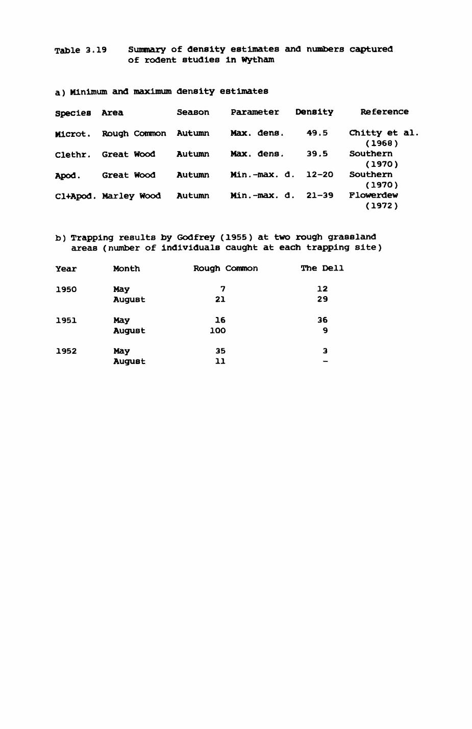
Table 3.19 Summary of density estimates and numbers capturedof rodent studies In wytham
a) Minimum and maximum density estimates
Species Area Season
Mlcrot. Rough Common Autumn
Clethr. Great Wood Autumn
Apod. Great Wood Autumn
Parameter Density
Max. dens. 49.5
Max. dens. 39.5
Min.-max. d. 12-20
Cl+Apod. Mar ley Wood Autumn Min.-max. d. 21-39
Reference
Chitty et al(1968)
Southern(1970)
Southern(1970)
Flowerdew(1972)
b) Trapping results by Godfrey (1955) at two rough grassland areas (number of individuals caught at each trapping site)
Year
1950
1951
1952
Month
May August
May August
May August
Rough Common
721
16 1OO
3511
The Dell
1229
369
103
In spring 1982, I put out longworth traps on five grids on rough
grasslands at various parts of the Wood in order to compare these grassland
areas with each other and with woodland areas trapped elsewhere in Wytham
Woods (Southern's study). Pig. 3.9 indicates the places of the five grids
while Table 3.20 summarizes the characteristics of the grid and the trapping
results. Very few voles were caught (Table 3.2O). The extension of the
trapping session to six rounds (one round every morning and afternoon) did
not yield any improvements in numbers. Presumably the severe winter 1981/82
had catastrophic effects on the vole populations. The results of my
trapping are consistent with Susan Fenn's trapping at Rough Common and
Sundays Hill and the trapping in woodland (by Ken Mars land, continuation of
H.N. Southern's study). Since the maintenance of five grids with a total of
238 traps meant too much effort in the long run, I decided to abandon
trapping and took Ken Marsland's data as a crude approximation to the recent
development of all three species in wytham Woods.
Fig. 3.10 presents the last 11 years of these data together with the
results up to December 1983. Of particular interest is the development
between 1981 and 1983. Population levels break down completely after the
very severe winter 1981/82. Both Apodemus and Clethrionomys populations
quickly recover towards winter 1982 reaching long-term average values.
Apodemus numbers Increase even further but also drop quickly towards the
end of 1983 while Clethrionomys seems to be then very stable. The Microtus
populations recovered similarly to average values (S. Perm, pers. comm.).
3.7 Discussion
In my discussion of resources I shall concentrate on two related
aspectsi a comparison of prey characteristics and the expected foraging
tactics of a predator in relation to the energy obtained from different
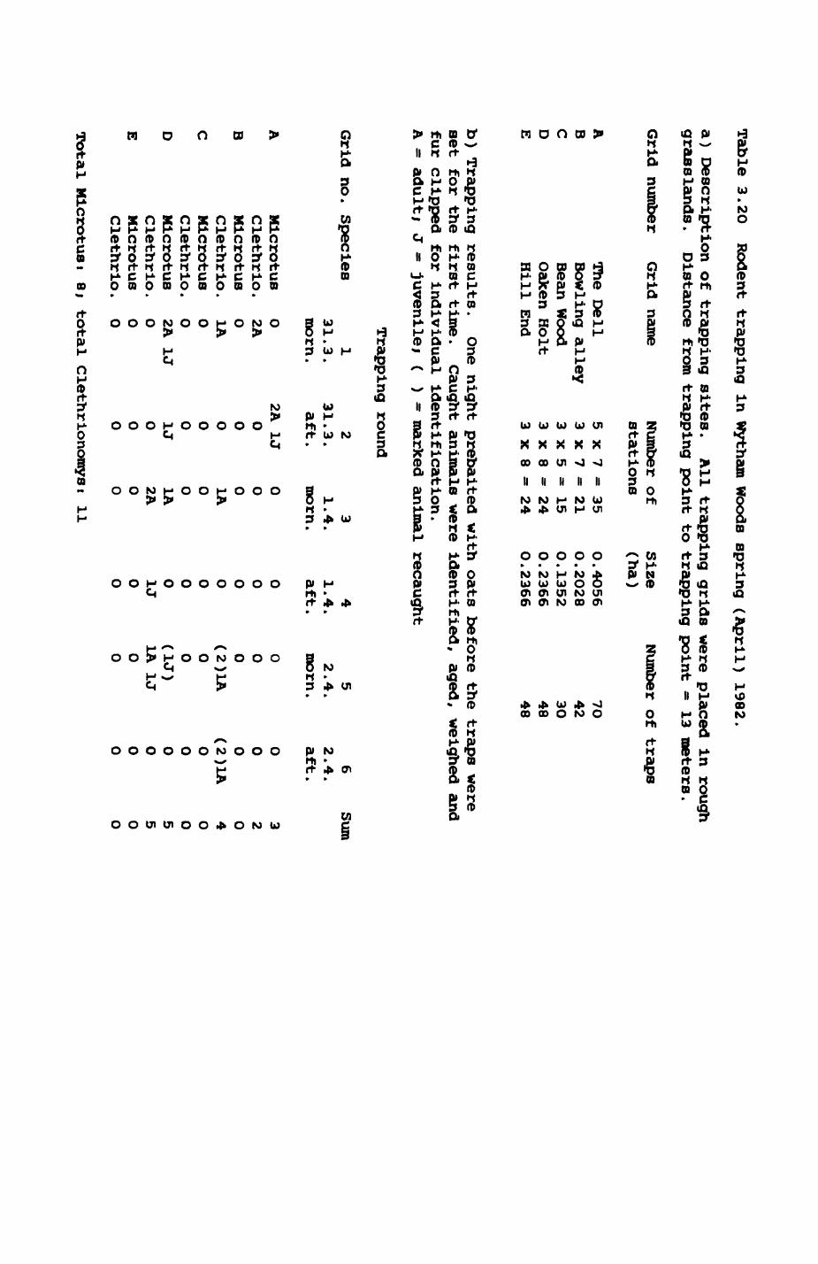
Table 3.2O Rodent trapping in Wytham woods spring (April)
1982.
a) Description of trapping sites.
All trapping grids were placed in rough
grasslands. Distance
from trapping point to trapping point = 13 meters.
Grid number Grid name
A B C DE
The Dell Bowling alley Bean Wood Oaken Holt Hill End
Number of Size
stations (ha)
53333
XXXXX
77588
=•====
3521152424
O000O
.4O56
.2028.1352
.2366.2366
Number of traps
7O 42 30 48 48
b) Trapping results. One night prebaited with oats before the traps were
set for the
first time. Caught animals were identified,
aged, weighed and
fur clipped for individual identification.
A = adult; J - juvenile;
( ) - marked animal recaught
Grid no. Species
Trapping round
131.3. morn.
231.3
aft
31.4,
morn,
41
.4.
aft.
52
.4.
morn.
62
.4.
aft.
Sum
A
B
C
D
E
MicrotusClethrlo.MicrotusClethrio.MicrotusClethrio.MicrotusClethrio.MicrotusClethrio.
O2A01A002A
1J
OO0
2A
1J
O00001J
O0O
0O01AO01A2AOO
00O00001J00
0OO(2
)LA
O0(1J)1A
1J
O0
000(2
)1A
00000O
32040055OO
Total Microtusi 8j
total Clethrionomyst 11

Pig. 3.9' Map of the central part of the study area. Main wood land and field boundaries as in Fig. 3.7. Human buildings black, sampling sites for rodent trapping and earthworm sampling indicated.
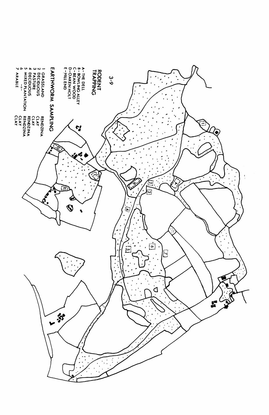
3-9
RO
DEN
T TR
APPIN
G
A-T
HE
DELLB
-BO
WL IN
G ALLEY
C-B
EA
N W
OO
D
D-O
AK
EN
HO
LT
E
-HILL E
ND
EAR
THW
OR
M SA
MPLIN
G
1 G
RA
SS
LAN
D
RE
ND
ZINA
2 D
EC
IDU
OU
S
CLA
Y3
PASTURE CLAY
4 D
EC
IDU
OU
S
RE
ND
ZINA
5 M
IXE
D PLA
NTA
TION
R
EN
DZIN
A6
-"-
CLA
Y7
AR
AB
LE
CLA
Y
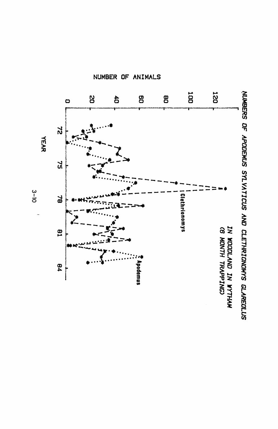
NUMBER OF ANIMALS
m
CJi
en
a>
CD
GO
l\>o O)o GO o o o ro o
oCO
e 3
~"7'*--.... »•-{••••••••-:CD
gm
f- ^
§i
S 5 D
m
104
prey. The discussion not only considers resources as presented in the
previous sections 3.2 to 3.6 but also includes other resources such a
invertebrates (excluding earthworms), scavenge, fruits, and cereals. For
convenience, these items are all included in the term 'prey*.
3.7.1. Comparison of prey Characteristics
Table 3.21 summarizes some of the features of different prey types
relevant to movement and foraging decisions of predators. Obviously, for a
predator to utilize the full spectrum of prey types necessitates Keeping
track of many different things I In Table 3.21, prey were allocated to four
classes, arranged according to ascending size. As prey items increase in
size from tiny to medium-sized (class I to IV), they not only increase in
energy contents but also in effort required to capture them, and difficulty
in monitoring their abundance, while at the same time decreasing in density.
Common to all prey items is a fairly stable and predictable
distribution across habitats, usually both on a long-term as well as short-
term basis. A fox will find pheasants in the same copse year after year,
earthworms are invariable at higher densities in deciduous woodlands than in
plantations and the locations of rabbit warrens are longstanding and
conspicuous. However, the predator's knowledge of resource distribution and
availability patterns will never be perfect, lagging behind recent changes
and bedevilled by chance events.
3.7.2. Foraging tactics of predators In relation to the
energy obtained from different prey.
As Illustrated in Table 3.21, different kinds of prey pose different
problems to the predator, but also promise different yields. While the
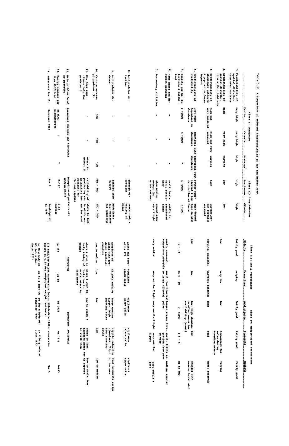
Table 3.21
A comparison of selected
characteristic* of
fox and badger
prey.
Class I:
Inanimate Class
II: Invertebrates
Others
I Predictability of
very high spatial
diatribu<- tion
over habitats
. predictability
of high
spatial dlstrlbu-
very high
very high
high high
varying low
high
low
tion within
habitats
3. predictability of
high but high
but very
varying abundance
patterns very
seasonal seasonal
t population deve
lopment
highvarying, of »• ten
strongly seasonal
4. predictability
of availability
very much identical with
identical dependent on
abundance abundance
abundance
5. Density
per ha
(11- >
1OOOO terature
• estima
tes)
6. Home
Range and
Mo- -
vement patterns
7. Locomotory
abilities
> 1OOOO
6. Antlpredator
de tection
rlth rather comp-
such dependHeated «
low dent on
abun(microclimate)
dance
> 10000
> 1OOO
small; basl-
small; in
colly static-
restrictednary
areas
slow moving ground:!low
except for
ain flight
quick retreat
through vi brations
restricted; variety
of means
Class III;
Small vertebrates
_Rodents
Class IV,
Medium-sized vertebrates
fairly good varying
very low
fairly good fairly good
fairly good
lowlowrexcept
for varying
•ales during
breeding season
varying; seasonal
varying) seasonal
goodgood
lowlow
ca 5
- SO
lowt high
abundan- low
ce often means low
availability (roost)
7 (low)
< 1
- 5
good; seasonal
changes with
season (cover
etc)
up to
1OO
small; seasonal
small (territories)larger areas;
irre--small; little ml- medium;
regular migrations
possible to
large (flocks)
gular gratjon
from yearto year
very mobile very mobile;
scent and
acou- vigilance
sties (?)
alarm calls
it very mobile if light very mobile; flight
vigilance vigilance
alarm calls alarm calls
very mobile t
fast
vigilance alarm
calls
9. Antlpredator
de fense
10. Capture
success 1OO
1OO of
predator («)
11. Bow does
expe rience
help the
predator ?
12. Main
problem faced
(seasonal changes
In) A HINDANCE
by predator
13. Energy content
per ca O.O2
7 item
(kJ/ltn») blackberries
14. Reference
for 13.
Sorensen 1981
retreat into
burrow
?8O - 1OO
move fast;
fly; distaste
ful (mimicry)
75O - 1OO
where to
reliability of where to
lock expect
It predicting
av- In
which sea-
ailabillty In-
son for what
creases; ef
ficient capture
(complicated patterns of)
AVAILA HLITY
1O.1373.53 beetles
Randolph et
al 1976
'
avoidance of flight;
mobbing large groups;
areas with pre- flight;
high dator
scent;lo- roosting
sites comotlon
low to medlunlow
low
where t when
to where
» when to
how to stalk
7 look;
timing of look;
how to pounce
stalk; where
to find nests
cryptic colouring
fast movements;ascap»
(females); flight
to burrows
high roosting
sites
lowlow
to medium
where to
find how
to stalk;
how breeding
hens; how
to capture
to stalk
them
ca 117
ca 88
DETECTION AVOIDANCE
ca 292«
ca 7315
5.6 kcal/dry weight conversion
factor (Slobodkin
1962); conversion
factor of O.2S dry weight/wet weight (estimate)
ca 2O g body wt
ca 15
g body wt
ca Soo g body wt
ca 125O g
body wt (Corbet
I Sou-
Schemer 198O
Glut* 1973
them 1977)
1O693
B>x 5
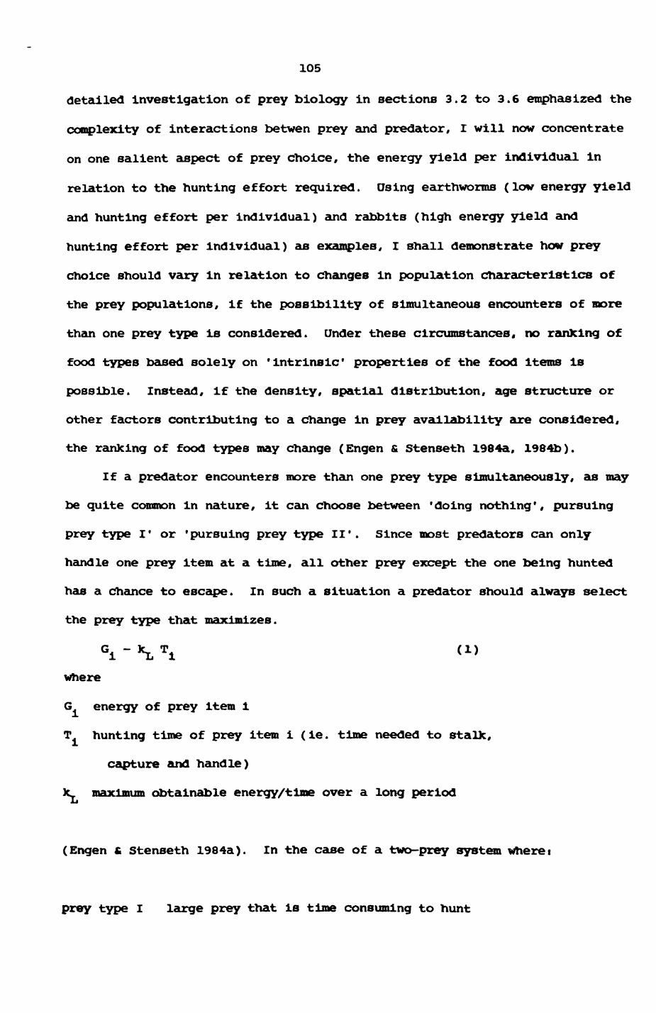
105
detailed investigation of prey biology in sections 3.2 to 3.6 emphasized the
complexity of interactions betwen prey and predator, I will now concentrate
on one salient aspect of prey choice, the energy yield per individual in
relation to the hunting effort required. Using earthworms (low energy yield
and hunting effort per individual) and rabbits (high energy yield and
hunting effort per Individual) as examples, I shall demonstrate how prey
choice should vary in relation to changes in population characteristics of
the prey populations, if the possibility of simultaneous encounters of more
than one prey type is considered. Under these circumstances, no ranking of
food types based solely on 'intrinsic' properties of the food Items is
possible. Instead, if the density, spatial distribution, age structure or
other factors contributing to a change in prey availability are considered,
the ranking of food types may change (Engen £ Stenseth 1984a, 1984b).
If a predator encounters more than one prey type simultaneously, as may
be quite common in nature, it can choose between 'doing nothing', pursuing
prey type I' or 'pursuing prey type II*. Since most predators can only
handle one prey item at a time, all other prey except the one being hunted
has a chance to escape. In such a situation a predator should always select
the prey type that maximizes.
Gl - *L Ti (1>
where
G energy of prey item 1
T hunting time of prey item i (ie. time needed to stalk,
capture and handle)
x_ mairimiini obtainable energy/time over a long period
(Engen £ Stenseth 198 4a). In the case of a two-prey system where i
prey type I large prey that is time consuming to hunt
106
prey type II smaller prey that is quickly hunted
a predator should always choose prey type I, the large prey, if
with
and type II, if
(Engen & Stenseth 1984a). Obviously, the long-term expected maximum
energy/time is a function of the density and thus the encounter rate of the
different Kinds of prey. For instance, if density of prey type I increases
greatly (the large prey), then the long-term expected maximum energy/time
would rise. If, as a result, k_ becomes larger than k we would expect theLi O
predator to switch from prey type I to prey type II (see eqn (3)). Thus, an
increase in the abundance or density of a prey type could mean a reduction
in its proportion of the predators diet! This surprising prediction has
been termed • self -reduction • by Engen & Stenseth (1984a / I984b) and
demonstrates that the right prey choice may be far from obvious.
Using rabbits as an example for prey type I, earthworms as an example
for prey type II, I shall show how the fox's choice (le. ranking of food
types) may be expected to vary as a result of the variation in energy per
time unit obtained from the prey types. Since the value for energy Includes
both successful and unsuccessful hunts, energy gain will be a function of
capture success (itself a complex function of prey and predator biology).
Hunting time can similarly be expected to vary considerably, depending on
the method of hunting (stalking or ambush predatlon) and environmental
features (vegetation etc. ). Population dynamics are also Important, since a
change in age ratio during the reproductive season will reduce the average
weight and thus energy obtained from an average prey individual, all else
107
being equal. In a simple model, capture success (of rabbits), hunting time
and changes in age ratio in the rabbit population have been considered as
variables, to answer three questions!
1. Are there conditions under which the energy per unit hunting time
obtained from rabbits drops below a threshold so that foxes should prefer
earthworms?
2. When should we expect a change in food preferences to occur in relation
to the population development of rabbits?
3. Can we find any evidence from the Vfytham population that changes in
food preferences occur, as for instance described by the phenomen of 'self-
reduction'?
The precise conditions for self-reduction to be possible aret
1. Energy G obtained from rabbits is higher than the energy G obtained
from earthworms.
2. Hunting time T for rabbits is higher than for earthworms (T ), so that
yield per unit time (G/T) is less for rabbits than for worms ( G-./T,<G /T ).
In Box 5 I have summarized the parameter values and the equations
incorporating the effects of capture probability and hunting time on energy
yield per unit hunting time; Pig. 3.11 is a plot of the results. Energy
contents per individual show a thousand fold difference between rabbit and
earthworm. However, differences in energy yield per unit hunting time are
smaller, since earthworms are caught at a high rate and eaten qulcXly, the
potential for ingestion of earthworms is considerable. For rabbit hunting,
neither a reduction in capture success from intermediate to low levels nor
an increase in hunting time from intermediate to high values have drastic
effect. With the parameter values used, improvements in hunting time are
rewarded more than improvements in capture success. This favours a predator
that stalks rather than sits and waits for the rabbit to approach its hiding
place. On this basis the observed tactic of rabbits disturbed by a fox
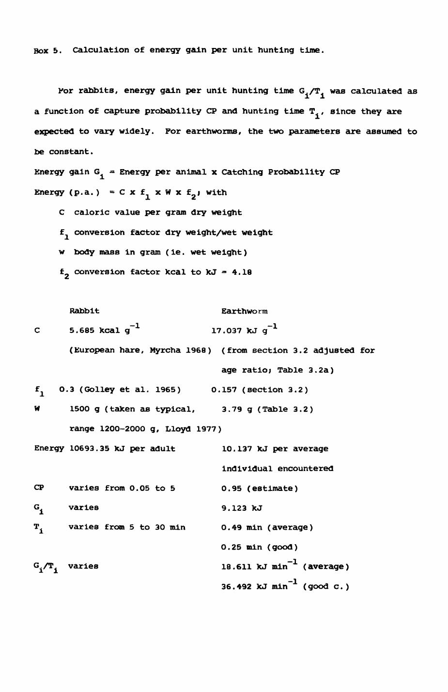
Box 5. Calculation of energy gain per unit hunting time.
For rabbits, energy gain per unit hunting time G /T was calculated as
a function of capture probability CP and hunting time T , since they are
expected to vary widely. For earthworms, the two parameters are assumed to
be constant.
Energy gain G = Energy per animal x Catching Probability CP
Energy (p.a.) «Cx£xWxfj with
C caloric value per gram dry weight
f conversion factor dry weight/wet weight
w body mass in gram (ie. wet weight)
f conversion factor kcal to kJ - 4.18
W
Rabbit Earthworm
5.685 kcal g-1
17.037 kJ g-1
(European hare, Myrcha 1968) (from section 3.2 adjusted for
age ratio; Table 3.2a)
f 0.3 (Golley et al. 1965) 0.157 (section 3.2)
1500 g (taken as typical, 3.79 g (Table 3.2)
range 1200-2000 g, Lloyd 1977)
Energy 10693.35 kJ per adult
CP varies from 0.05 to 5
G varies
varies from 5 to 30 min
G /T varies
10.137 kJ per average
individual encountered
0.95 (estimate)
9.123 kJ
0.49 min (average)
0.25 min (good)
18.611 kJ min"1 (average)
36.492 kJ min"1 (good c. )
108
vanishing into their warrens for half an hour (Macdonald, 1977) appears to
be an efficient one.
In Fig. 3.11, the dotted line numbered 1 indicates the level of
expected earthworm energy gain (36.492 kJ min~ ) under good hunting
conditions. If a fox hunts rabbits in circumstances below this line,
conditions 1 and 2 are fulfilled, and - from the theory - a change in food
preferences becomes likely. Note, however, that a switch In prey choice is
only likely to occur, if k_ becomes larger than k (eqn (2) and (3», ie.Li O
the abundance of rabbits Increases. We shall therefore examine the changes
that are likely to hojppen during the reproductive season of the rabbits, le.
a time when population density of rabbits Increases and the age ratio in the
population changes.
During the breeding season from January to June, more and more juvenile
rabbits join the adult population so that the expected energy gain from an
average individual captured will become reduced. Generally,
energy = pE+pE (4)
with
P «P.i proportions of adults and juveniles in the diet a J
E ,E. energy from adults and juveniles, respectively
Assuming that the energy content of juveniles does not differ from that of
adults per gram body mass, and setting g as the ratio of average gain
expected at time t (rabbit population consisting of adults and juveniles,
le. during breeding season) in relation to previous gain at tine t (adults
only, le. during winter before breeding season),
9 * (P^ E + b p. Ea)/Ea (5) a a j
with E - b Ea and b - ratio of juvelle to adult body weight
or
g-Pa + b Pj (6 )If juveniles are assigned a quarter of the body weight of adults (b - O.25)

Pig. 3.11. Model of energy gain per unit hunting time for foxes hunting rabbits as a function of hunting time and capture probability. Calculations according to the formulae presented In Box 5.Lines 1-3t Lines of equal energy gain for foxes hun
ting rabbits or hunting earthworms.
Line It foxes hunting adult rabbits only.2i foxes hunting adults and juveniles in
proportion It2. 3t foxes hunting adults and juveniles In
proportion It9.
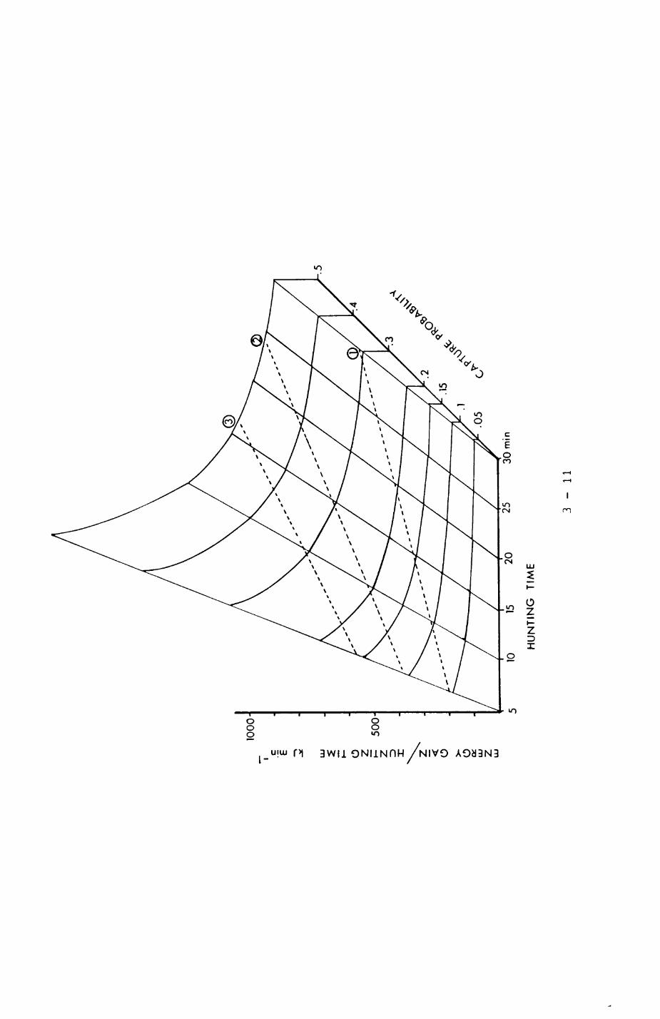
ENERGY GAIN/HUNTING TIMEkJ min
UJ
I

109
g = pa 4- 0.25 p
Thus g will be 1 If only adults are present; g will decrease to 0.5 at an
age ratio of 1 adultt2 juveniles, further decrease to 0.325 at a ratio of
Ii9 and reach its minimum value of 0.25 if only juveniles are present.
Reducing the energy gain by the factor g is equivalent to increasing the
threshold level where condition 2 begins to hold, ie. multiplying the
expected energy gain from earthworms by 1/g. For the age ratios It2 and
the corresponding threshold values are 77.042 XJ min~ and 118.526 fcJ min
These are represented in Fig. 3.11 by the dotted lines 2 and 3. With an
Increase in the ratio of juvenilesiadults (corresponding to an Increase In
overall population density) a fox is therefore more llXely to find Itself In
a situation when It should switch from rabbits to earthworms, provided it
has the chance to encounter both prey types simultaneously.
There are two factors that may modify the true energy yield per unit
hunting time to make it different from the average expected yield, ie. the
yield as expected from the change in age ratio as described above. Both
factors derive from juvenile stupidity) they are Improved capture success
(relative to capture success of adults), leading to a higher energy gain per
gram body mass from juveniles than the energy gain obtained from adults, and
reduced hunting time and effort that should tempt foxes to take
disproportionately many young and so create a ratio of juveniles to adults
in the diet of the predator that is higher than the population ratio, in
the latter case, a reduced uneixjy gain (relative to the average expected
gain) would result. Both factors may In the end cancel each other out, but
data are not available to test this.
The probability of switching from rabbits to earthworms Increases
towards the end of the breeding season, when the age ratio changes In favour
of juveniles and the overall population density of rabbits Increases. This
is a time (April and May) when conditions for foraging for earthworms have
110
Improved and are at their optimum, suggesting that the figures for energy
yield from earthworms per unit hunting time calculated in Box 5 are
conservative estimates. Under these simple, but not implausible conditions,
I would therefore expect fox home ranges with high rabbit densities to be
likely to exhibit self-reduction in their diet from winter (beginning of
rabbit breeding season) to spring (end of breeding season), despite an
Increase in the simple abundance of rabbits if rabbits and earthworms occur
in the same habitats. Two confounding conditions may render it difficult to
show self-reduction in practice. Social hierarchies within fox groups can
have an Influence on the range of prey a subordinate fox is able to use
(Macdonald 1980), and large differences in experience and traditions between
individuals and/or groups may further modify the actual thresholds for prey
switching. Profound differences in hunting traditions between groups have
been shown e.g. in wolves (Mech 1970, Mech pers. comm.). Nevertheless*
anticipating the results of the analysis of the diet (Chater 4) and fox home
ranges (Chapter 5), there is some evidence that self-reduction occurs in
some ranges in Wythami in two fox ranges with high rabbit densities (ranges
6 and 7), a significant reduction in the proportion of rabbit in the diet
was found from winter to spring, when rabbit numbers were nevertheless known
to increase. In contrast, neighbouring range 5, with lower rabbit densities
than range 6 or 7, Increased the proportion of rabbits in its diet - in that
case rabbit population densities may not have been sufficiently high to
force the foxes of range 5 to reduce their amount of rabbit hunting! An
alternative explanation would be that in range 5 the possibility of
simultaneous encounters of rabbits and earthworms is reduced, since the
rabbits seem to occur more In wooded areas While earthworms are present on
pasture, in ranges 6 and 7, both rabbits and earthworms are present on
pasture and also deciduous woodland.
Ill
4. Diet
4.1 Introduction
4.2 Fox diet
4.2.1 Methods of sampling
4.2.2. Methods of analysis
4.2.3. Results
.1. General composition of the diet
.2. Temporal variation in the diet
.3. Variation in the diet of different ranges
.1. General diet composition of ranges
.2. Seasonal variation in the diet or ranges
4.2.4. Fox diett summary
4.2.5 Comparison with other studies
4.3 Badger diet
4.3.1 Methods of sampling
4.3.2. Methods of analysis
4.3.3. Results
.1. General composition of the diet
.2. Temporal variation in the diet
.3. Variation in the diet of different ranges
.1. General composition of the diet
.2. Temporal variation in the diet
.4. Comparison of border and non-border latrines
4.3.4. Badger dleti summary
4.3.5. Comparison with other studies
4.4 Comparison of fox and badger diet
112
4.1 Introduction
In this chapter I turn my attention to one aspect of resource
utilization! the diets of the fox and badger populations in Wytham. In the
previous chapters, the analyses of the habitat composition, the prey
populations and the foraging techniques of foxes and badgers indicated Where
the prey can be found and how its availability varies. The processes
underlying prey selection together with the predator's foraging efficiency
determine the portion of the available prey Which is used. The diets of the
two predator species are the result of this process.
The diets of foxes and badgers have been widely studied, partly because
this is one of the few aspects of their behavioual ecology that can be
studied easily. However, as Macdonald (1977ft) stressed, many studies have
only limited usefulness since the diversity of methods used precludes
detailed comparisons. A comprehensive list of European studies of the diet
of the red fox is provided by Jensen & Sequiera (1978) while information on
the diet of European badgers is presented by Andersen (1954), Skoog (1970),
and Kruuk and Parish (1981).
In this study it was important to adopt a method of analysis that
disclosed the details of each species' diet, and did so in a way which
thereafter facilitated comparison between them. Ideally, the method should
also maximise the opportunities for comparison with other studies. The
analysis of dried remains of undigested food items in faeces proved to be
such a method. Several measures of the Importance of each prey type in the
diet were investigated and simultaneous use of estimated dry weight and
frequency of occurrence were found - in line with other Oxford studies*,*»
(Macdonald (1977), Newdldc (1983), Doncaster (1985)) - to provide the best
compromise between a maximum of quantitative information, a minimum of
113
cumulative systematic error and the potential comparability between species
and reproducability in other studies. Estimated dry weight of each digested
food type was used as a measure of its contribution to the diet, annually
and seasonally for each species (sections 4.2 and 4.3). In addition, the
diets of animals within ranges for which there were sufficient sample sizes
were investigated.
A computer program incorporating a filtering procedure (Appendix 3) was used
to avoid ambiguities when each faeces was assigned to a range. The
different patterns of faeces deposition by foxes and badgers necessitated
different filtering procedures for each species. In the case of badgers,
samples collected from sites on the border of neighbouring badger ranges
("border-latrines") were excluded from analyses of the diet within
individual ranges. For foxes, there was some overlap between neigbouring
ranges, so that all droppings collected in the overlap zones were excluded
from analyses of the diet within each range. These filtering procedures
reduced some sample sizes, but enhanced the value of the results by reducing
"noise" in the data. My analyses of the diet composition of badgers and
foxes in group ranges involved both spatial and temporal trends, and thus
yielded a very detailed picture of variation of the diet of the two predator
populations.
Several methods have been used to study the diet of foxes and badgers
(see Newdick (1983))i
1. Collection of food items around dens
2. Following trades
3. Analysis of stomach contents
4. Analysis of droppings
5. Direct observation
In this study several methods were tried, the principal one being the
114
analysis of undigested food remains in faeces. In addition, prey remains
(mainly those of birds) were collected whenever encountered (see Chapter 3).
This proved to be very unsatisfactory since the sample size was small (28
bird remains collected between 1981 and 1983). Direct observations on
feeding habits of marked and unmarked foxes and badgers were made whenever
possible. They were also used to evaluate predation techniques (Chapter 3)
and to analyse patterns of activity and habitat use (Chapter 6). For
Instance, chance observations confirmed that foxes were hunting during the
dayi on one occasion an adult fox was seen to take a rabbit at 11 a.m. in
Mar ley Plantation (at the southeast corner of the wood). On another
occasion a male fox was seen to return to its den with a freshly killed male
pheasant at 11.30 a.m. and feed the prey to its vixen and the cubs.
I decided to concentrate upon collecting and analysing droppings
because this
- was easy, quick and therefore efficient!
- disturbs the study populations comparatively little,
with the possible exception of disrupting scent-markingL
(Macdonald, 1980)i
- allows repeated sampling of the output of the same
individuals (in contrast to the analysis of stomach
contents);
- provides a standardized approach to allow a comparison of
the diet of both species.
4.2. Fox diet
4.2.1. Methods of sampling
A total of 2030 fox droppings were collected over the entire study area
115
between April 1981 and October 1983; (data for April, May and June 1981 were
kindly provided by D.W. Macdonald). As It was Impossible to search all
parts of the study area with the same Intensity, a 'core 1 area was defined
which was visited regularly (sometimes daily, but at least once every 14
days, Fig. 3.9).
Table 4.1 records the sample sizes for each month, summarized over the
three years, for each season over the entire study area, together with the
grand totals for all recognized fox ranges and seasonal totals for ranges
with a reasonable sample size (ie. the five ranges which were later
investigated in detail and SURPRISE'S range (No. 8, Swinford Lodge)). The
uneven temporal distribution of sampling effort is partly due to reduced
sampling effort due to restrictive weather conditions e.g. snowfall in
December, and partly due to restrictions on my daylight activities imposed
by the necessity of tracking by night.
Identification of fox droppings in the field proved to be easy (see
Newdlck (1983)). Badger droppings could also readily be identified (Kruufc
(1978b))t they are usually much larger than fox faeces, have a
characteristic texture and odour and are usually deposited at specially
prepared sites (latrines). In the three field seasons of the study I found
badger faeces outside latrines on only two occasions but both droppings were
readily identifiable as badger faeces because of their size, and texture.
On collection, each fox dropping was placed in an envelope and the
following details recorded!
1. Date
2. Map coordinates
3. Information on the details of locationt
.1. Presence or absence of a path
.2. Presence or absence of a junction of paths
.3. Presence or absence of a conspicuous object
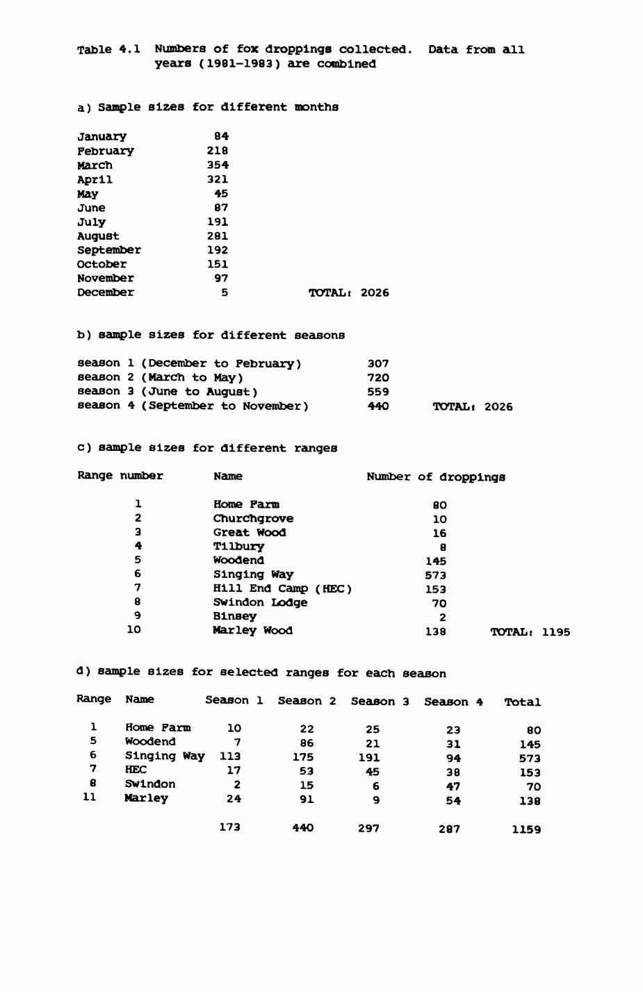
Table 4.1 Numbers of fox droppings collected, years (1981-1983) are combined
Data from all
a) Sample sizes for different months
JanuaryFebruaryMarchAprilMayJuneJulyAugustSeptemberOctoberNovemberDecember
842183543214587
191281192151975 TOTAL t 2O26
b) sample sizes for different seasons
season 1 (December to February) 307season 2 (March to May) 72Oseason 3 (June to August) 559season 4 (September to November) 44O TOTALt 2026
c) sample sizes for different ranges
Range number
123456789
10
Name
Home FarmChurchgroveGreat WoodTilburyWoodendSinging wayHill End Camp (HEC)Swindon LodgeBinseyMarley Wood
Number of droppings
SO 10 168
145573153702
138 TOTALt 1195
d) sample sizes for selected ranges for each season
Range Name Season 1 Season 2 Season 3 Season 4 Total
1 Home Farm 105 Woodend 76 Singing Way 1137 HEC 178 Swindon 2
11 Mar ley 24
2286
175531591
2521
1914569
233194384754
8014557315370138
173 44O 297 287 1159
116
.4. Nature of the conspicuous object, if present
4. Smell (codest O - nonei 1 - weakj 2 - medium* 3 - strong)
5. Age (codesi 1 - within the last two nightsi 2 - older than
the last two nights but within the last week; 3 - older than
a week)
A path was defined as a visible break in the vegetation with signs of
animal tracks. Any man-made track was also regarded as a path. Age was
estimated on the basis of appearance and accounting for prevailing weather
conditions. For experienced field workers the coding was straightforward in
the field. In trials, two independent collectors were highly consistent in
assigning the same age and odour classes to given droppings. The envelopese
were oven dried at SO and stored prior to analysis.
4.2.2 Methods of analysis
In principle, the analysis of the faecal contents followed thea
procedure described by Macdonald (1977) and Newdlck (1983)t
Each fresh dropping was weighed and then crumbled into a petri disho
where its compsltlon was examined under a binocular microscope. The prey
remains were separated into categories and the percentage of the total
volume comprised of each category was estimated by eye. As most faeces
consisted of only two or three types of prey remains, the error associated
with the estimation by eye is probably low. Also, Macdonald & Dickman
(unpubl.) have recently shown that results from this relatively quick method
do not differ from those of tedious wet sieve techniques. The analysis of
the faeces was performed by David Macdonald In order to keep the systematic
error of faeces analysis constant and reduce error variation between
different Poxlot studies to a minimum.
117
The major prey types were categorized as follows (definitions from
Newdick (1983))i
1. small mammals (e.g. rodents, Insectivores) Tightly packed tufts of
brown hairs which can be distinguished from the longer brindled guard hairs
of lagomorphs or their pale, woolly under fur. The size of bone chips and
presence of teeth also aided diagnosis. The species were identified by
examining the hairs microscopically according to the keys provided by Day
(1966) and Debrot (1982).
2. Invertebrates Fragments of exoskeleton of, for example, beetle elytra
or caterpillar remains, were easily identifiable, as were fragments of snail
shell. Chaetae of earthworms were recorded separately.
3. Fruits Pips of soft fruit, plum stones and pieces of integument could
be identified, often associated with a characteristically hard, dark, and
often aerated matrix. Whenever possible the fruit type was identified and
recorded using an extensive collection of samples of different types of
fruits and berries.
4. Birds Traces of feathers, especially quills, usually accompanied by a
grey flaky matrix. They were identified to the level of order under
microscopic examination of the splcule patterns.
5. Laqomorph see small mammals
6. Scavenge This faecal material consisted of a homogeneous matrix and was
often accompanied by non-food items such as plastic, string, or elastic
bands. Newdlck (1983) performed baiting experiments which showed that food
of human origin Invariably appeared as this type of uniform matrix.
7. Soil Soil was almost invariably accompanied by chaetae of earthworms
and is taken as an indicator of their representation in the diet. Kacdonalda.
(1977a, 1980) showed that this is a justifiable assumption.
8. Grass indigestable grass fragments could be clearly Identified.
118
9. Domestic shock Pur tufts of the unusual colours of 'exotic* breeds.
10. Others Any items that could not be placed in the other categories.
This Included e.g. the remains of deer, cow pats and various other prey
types the precise identity of Which were recorded separtely under a section
"curiosities".
11. cereals These were barely digested and clearly identifiable.
12. Tree fruits Readily distinguishable from all other types.
All data were allotted codes and subsequently transferred to the
university's VAX-11/780 computer. Several programs were written in order to
check the data for inconsistencies and errors and to add necessary
information! Program WYFPRDG checked double and erroneous labelling of
faeces, program TINPUT inserted dates, program WINPUT inserted weights and
program CINPUT inserted coordinates of the location of the dropping into the
file with the results of the scat analysis. Each weight, date and map
coordinate was labelled with its dropping reference number. Program HAIR
finally Inserted the identity of small mammal, fruit and bird species,
checked the data for detectable typing errors and reformatted the data for
further analysis. Statistical analysis was performed with procedures
('macros') which I wrote for the KENITAB statistical package available on
the VAX.
Prom the raw data, five measures of diet were computed using a variety
of techniques and correction factors. These arei
1. Frequency of occurrence t This Is the number of occurrences of a prey
category found In the droppings and usually expressed as a percentage of the
total number of droppings. As it disregards any quantitative Information on
the bulk of the remains in the dropping. It Is Inadequate alone as a measure
of the relative Importance of prey categories. Rather it Indicates the
119
degree of regularity with which each prey category is consumed.
2. Estimated volume This is the percent volume of each prey category in
each dropping, as estimated by eye. Prey items that are many times larger
than the average size of a dropping, e.g. rabbits, occupy most of a faeces
While prey items such as beetles occupy only a fraction of the dropping.
Together, the frequency of occurrence of the prey items and its estimated
volume provide information on the relative contribution of each prey
category to the total diet (see Fig. 4.3).
3. Estimated dry weight Here, each percent volume is multiplied by the dry
weight of each dropping. This gives a measure where the estimated volume
(measure 2) is corrected by the dry weight of each dropping. This
estimation of dry weight of undigested food remains assumes equal density of
each food category in the faeces.ci
4. Estimated fresh weight Using Lockie's (1959) and Macdonald's (1977)
correction factors for different digestibilities of different prey items,
the fresh weight of prey eaten can be derived from the estimated dry weight
of undigested remains in the faeces. This measure seems to come close to an
ecologically useful quantification of diet. However, the undoubted errors
associated with the correction factors are not precisely known.
5. Calorific value By applying another set of correction factors (fromOk.
Macdonald (1977)) the calorific intake from each food types can be
calculated from the estimated fresh weight.
Each of the measures suffer from some bias; the ecologically most
useful measures also suffer from the most multiplicative effects of several
potential sources of errors. As a compromise I decided, in line with«,
previous studies (Kacdonald (1977), Newdlck (1983)), to use estimated dry
weight as a basis for most of my analyses. This measure is easy to compute
and well suited for comparisons between populations or with other species.
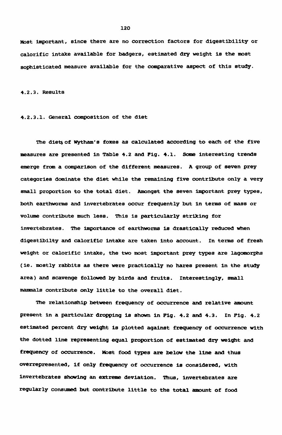
120
Most important, since there are no correction factors for digestibility or
calorific intake available for badgers, estimated dry weight is the most
sophisticated measure available for the comparative aspect of this study.
4.2.3. Results
4.2.3.1. General composition of the diet
The diets of Wytham's foxes as calculated according to each of the five
measures are presented in Table 4.2 and Fig. 4.1. Some interesting trends
emerge from a comparison of the different measures. A group of seven prey
categories dominate the diet While the remaining five contribute only a very
small proportion to the total diet. Amongst the seven Important prey types,
both earthworms and invertebrates occur frequently but In terms of mass or
volume contribute much less. This is particularly striking for
invertebrates. The importance of earthworms is drastically reduced when
digestlbilty and calorific intake are taken into account. In terms of fresh
weight or calorific intake, the two most important prey types are lagomorphs
(ie. mostly rabbits as there were practically no hares present in the study
area) and scavenge followed by birds and fruits. Interestingly, small
mammals contribute only little to the overall diet.
The relationship between frequency of occurrence and relative amount
present in a particular dropping is shown in Fig. 4.2 and 4.3. In Fig. 4.2
estimated percent dry weight is plotted against frequency of occurrence with
the dotted line representing equal proportion of estimated dry weight and
frequency of occurrence. Most food types are below the line and thus
overrepresented, if only frequency of occurrence is considered, with
Invertebrates showing an extreme deviation. Thus, invertebrates are
regularly consumed but contribute little to the total amount of food
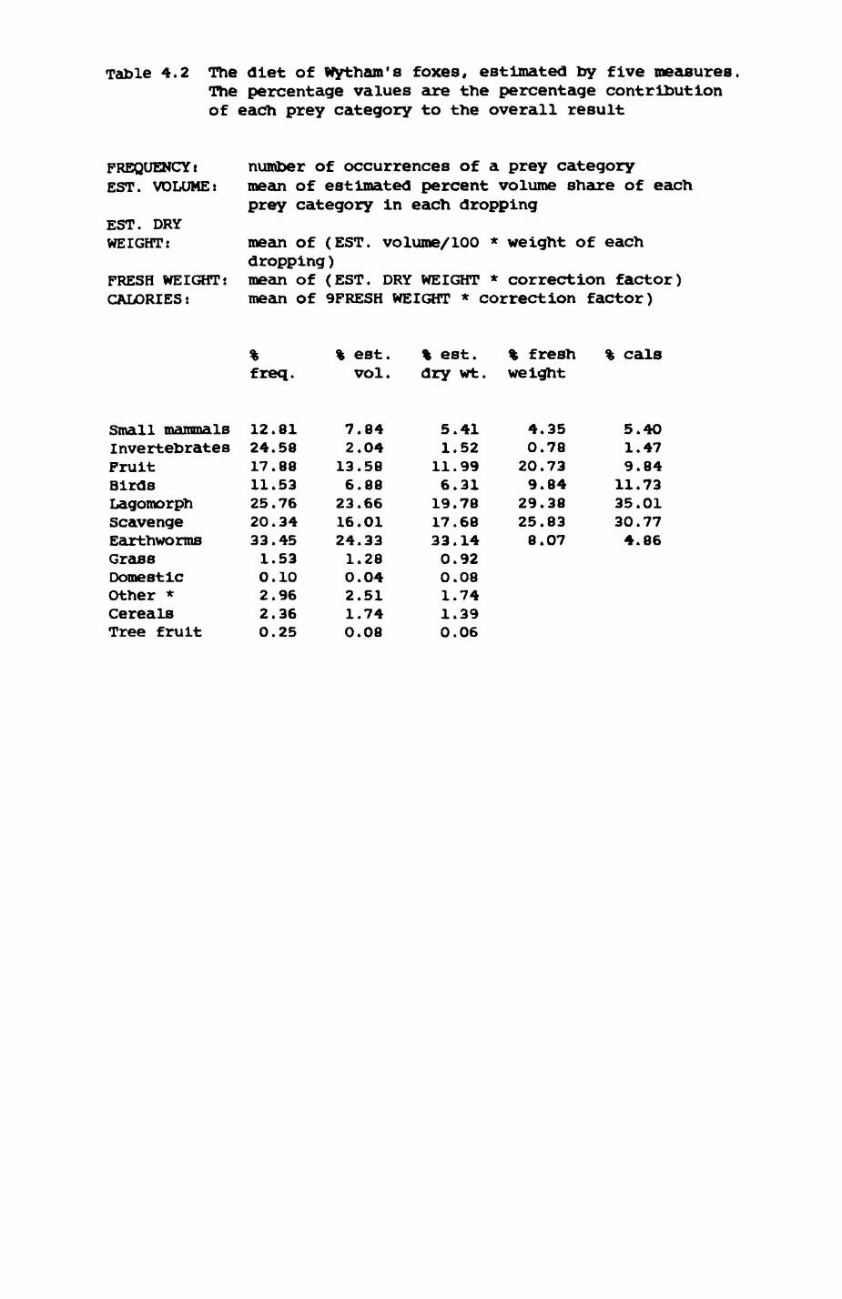
Table 4.2 The diet of Wytham's foxes, estimated by five measures. The percentage values are the percentage contribution of each prey category to the overall result
FREQUENCY! EST. VOLUMEt
EST. DRY WEIGHT:
FRESH WEIGHT: CALORIES:
number of occurrences of a prey categorymean of estimated percent volume share of eachprey category in each dropping
mean of (EST. volume/100 * weight of each dropping)mean of (EST. DRY WEIGHT * correction factor) mean of 9FRESH WEIGHT * correction factor)
Small mammalsInvertebratesFruitBirdsLagomorphScavengeEarthwormsGrassDomesticOther *CerealsTree fruit
%freq.
12.8124.5817.8811.5325.7620.3433.451.530.102.962.360.25
% est.vol.
7.842.04
13.586.8823.6616.0124.331.280.042.511.740.08
% est.dry wt.
5.411.52
11.996.3119.7817.6833.140.920.081.741.390.06
% freshweight
4.350.7820.739.84
29.3825.838.07
% cals
5.401.479.84
11.7335.0130.774.86

Pig. 4.1. The diet of wytham's foxes, as measured by four different categories!
a. per cent frequencyb. per cent fresh weightc. per cent dry weightd. per cent calories
Measures are explained in more detail in the text and in Table 4.2. Food categories are (in brackets typical abbreviations in the following figures)!
1 - small mammals SM2 - other invertebrates INV3 - fruits PR4 - birds BD5 - lagomorphs LAG6 - scavenge SCA7 - earthworms EW
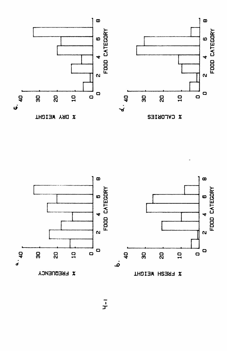
4040
u UJ a
iii
a:
u.
30 20 10
I- o
>-« UJ a:
a
30 20 10
H-l
H-
UJ O)
UJ a:
u.
40
S
30 20 10
24
68
FO
OD
CAT
EGO
RY
246
8
FOO
D C
ATEG
OR
Y
UJ o H
40 30 10
24
68
FO
OD
C
ATEG
OR
Y
246
8
FOO
D CA
TEG
ORY
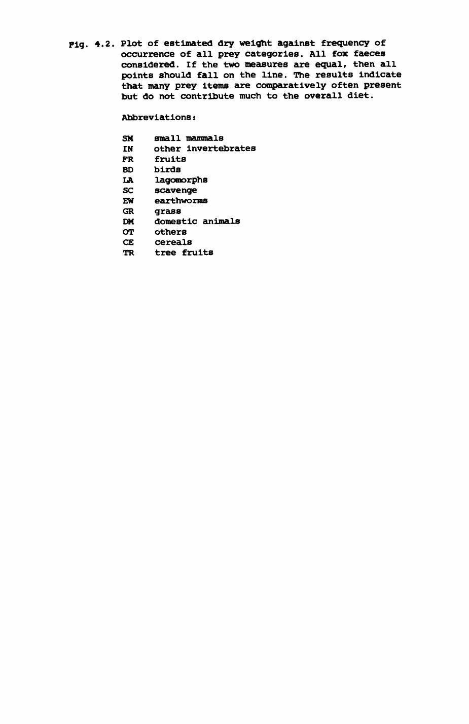
Pig. 4.2. Plot of estimated dry weight against frequency of occurrence of all prey categories. All fox faeces considered. If the two measures are equal, then all points should fall on the line. The results indicate that many prey items are comparatively often present but do not contribute much to the overall diet.
Abbreviationsi
SM small mammalsIN other invertebratesFR fruitsBO birdsLA lagomorphsSC scavengeEW earthwormsGR grassDM domestic animalsOT othersCE cerealsTR tree fruits
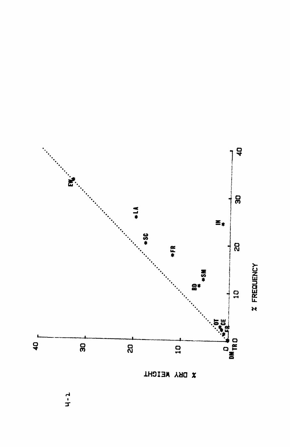
T**
30 20
i- o LU * ft?
10Q H
0 <
«.
*
*LA
..•'*
*sc
*
.*
*FR
« • * *
.••'
BD * *S
M
XOT
IN.%
CE
*
1^, J
fO
t t
tDM
TRO
1020
3040
FREQ
UENC
Y
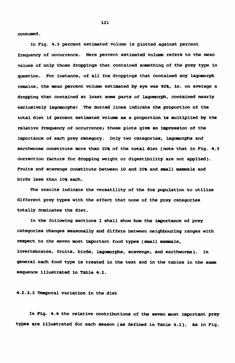
121
consumed.
In Fig. 4.3 percent estimated volume is plotted against percent
frequency of occurrence. Here percent estimated volume refers to the mean
values of only those droppings that contained something of the prey type in
question. For instance, of all fox droppings that contained any lagomorph
remains, the mean percent volume estimated by eye was 92%, ie. on average a
dropping that contained at least some parts of lagomorph, contained nearly
exclusively lagomorphs! The dotted lines indicate the proportion of the
total diet if percent estimated volume as a proportion is multiplied by the
relative frequency of occurrence j these plots give an impression of the
importance of each prey category. Only two categories, lagomorphs and
earthworms constitute more than 20% of the total diet (note that in Fig. 4.3
correction factors for dropping weight or digestibility are not applied).
Fruits and scavenge constitute between 10 and 20% and small mammals and
birds less than 10% each.
The results indicate the versatility of the fox population to utilize
different prey types with the effect that none of the prey categories
totally dominates the diet.
In the following sections I shall show how the importance of prey
categories changes seasonally and differs between neighbouring ranges with
respect to the seven most important food types (small mammals.
Invertebrates, fruits, birds, lagomorphs, scavenge, and earthworms). In
general each food type is treated in the text and in the tables in the same
sequence illustrated in Table 4.2.
4.2.3.2 Temporal variation In the diet
In Fig. 4.4 the relative contributions of the seven most important prey
types are illustrated for each season (as defined in Table 4.1). As in Fig.

Pig. 4.3. Average percent volume per faeces of each preycategory vs. frequency of occurrence, a so-called •KruuX-plof . All fox faeces.
Fig. 4.4. Similar plots (and identical symbols) as in Fig. 4.3., but each season plotted separately.
a. springb. summerc. autumnd. winter
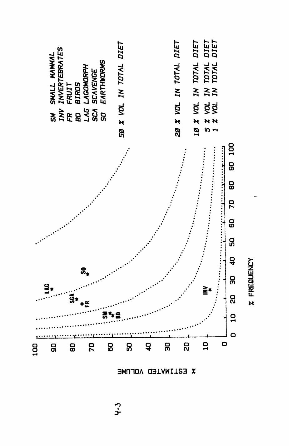
H•n*j m ocmzn•<
co •
0 '
r\) 0 '
0) o •
o •
(Jl 0
O) o •
•sja
a>O '
CDoi-*0o l
«o»
X ESTIMATED VOLUME
i- ro a) *• en a>D O O O O O O
^ • *
..•••• "t^^*
» * • * • *
• ^^_ • •• ^^ * • * • *• * - •
: *' :^ •
• p • • . *
* • •
* •* • "
• * • ^ • *
* • * * • •*• • *
• • * • *• * •• • ^* • • *
.* ^
• • •
• *
• • •
• * t** * •• • •• • •
; .• .*
• • f°• *
*"-* r\j Ui
^ < s 8 CD o o o or- ^
5S z z 5 *3333 3 1 22 2 2 2 | r* r- r- r- r- Sw)tDCD C3 C3 g
rn rn rn rn rnH H "H H H
•sJ (Do o
..;...... J. .
3**o
, . •...••**'
*a»w
..'"
*
#*
.•""""
§gS3FRUIT BIRDS
LAGOMORPH SCAVENGE
CO Oo o
9 m • *
• • * * ^
e»
.•*• ..•*
|$
SM/LL MAMl INVERTEBR*
5 rn r*~CO
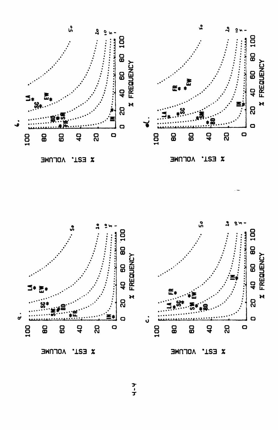
UJ 3E -J O
•
(/> UJ X UJ ID -J 0
•
(/)
UJ X
100 80 60 40 20 0
1 c10
0 80 60 40 20 0
r •
• •
LA
••»
• «
. hn
. .
. .
. J*
•^V
»
* '
*•
• •
• vfc
AJ
•
:: :
SC'.
EW
:::*
*.
*•
I SM"
«: :*
: : B
D.
. .
. •,
,<f ...
••
CA• C
D
*.
'.
*°
.TIL
• .
*.••
.
. .
...
•»....
.•.
•• .
•••.
•••..
••-.
. -•
••
»•
*..
* •• ..
. •..
•••...
•••
•••...
. »«
IN '
••....
— —
— ..
....
. f
*.-,
_
•. . .
. .'J J
..V 1
.' .'.'.
.r .V
.?,.r
,£.».
. au-
a f ,
u *
• I
D 20
40
60
80
10
0%
FREQ
UENC
Y
* 0
> •
•
»
»ft
*
•
•
•
•
•
*
•
*
'••••*
: : :
LA -.
PR
• • •
* •
it: :
. s
c '• *
. .
.»*{
*:
: .
"•; U
'n EV
. .
* cw
* *.
: '.*
\
'. •••
5o
: W
-.
...
.>.
. .
....
*. . .
•-..
.:.
••-.
•--.
..
••-•
• u
'••-.JJ
! •-
--..
...
,../"
•_••
>•••
-••-
••*-
••-•
*»*»
•*-•
-*••
-•-•
'
0 20
40
60
80 10
0 %
FREQUENCY
UJ O en UJ UJ o en UJ x
100 80 60 40 20
'. EW
•. *
•'*'
• to
. 1
0••
5"
^»
I
0 20
40
60
80
10
0 % FR
EQUE
NCY
100 80 60 40 20 0
•C.
> •
• >
» •
• •
E -.LA
*.:
v '.
. .
• p
n
" •
• •
rn
• •*
•
*fcfsc
\ *
i :
\ EW
••-
.• :
'» *.
•CM
* •
S.
^bm»
. •.
a:*
•• •.
*:BD\
\
: \
'•-.
« .
.. ...
•• '••.
•-..
• •*•
''•••...
•''''•••
•••'•'•
'•V/.V
.V.v.v
: •?
0 20
40
60
80
100
% FR
EQUE
NCY
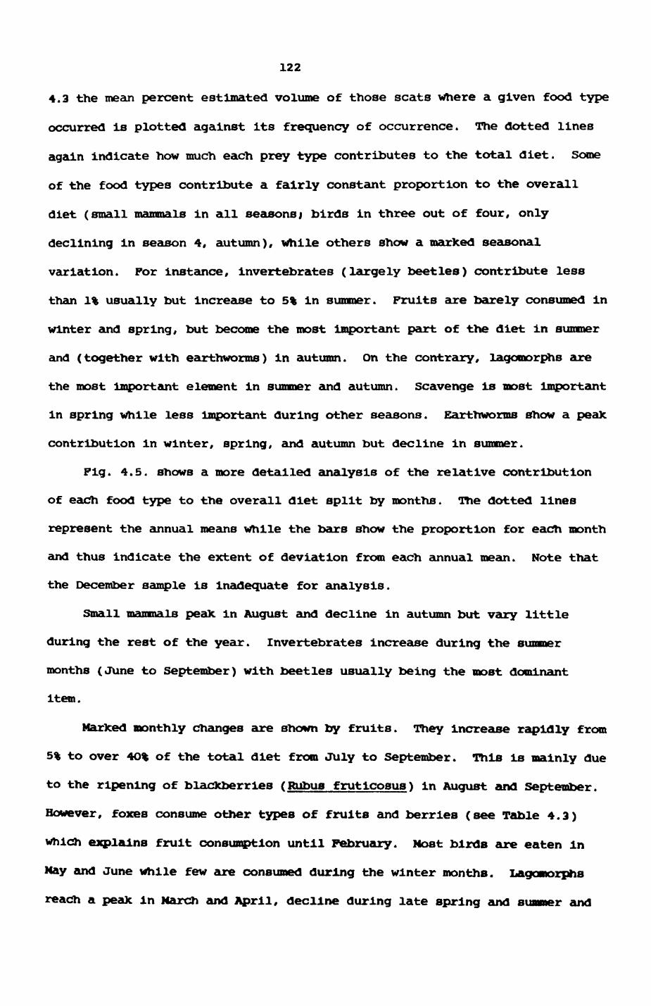
122
4.3 the mean percent estimated volume of those scats Where a given food type
occurred Is plotted against Its frequency of occurrence. The dotted lines
again indicate how much each prey type contributes to the total diet. Some
of the food types contribute a fairly constant proportion to the overall
diet (small mammals in all seasons/ birds in three out of four, only
declining in season 4, autumn), While others show a marked seasonal
variation. For instance, invertebrates (largely beetles) contribute less
than 1% usually but increase to 5% in summer. Fruits are barely consumed in
winter and spring, but become the most important part of the diet in summer
and (together with earthworms) in autumn. On the contrary, lagomorphs are
the most important element in summer and autumn. Scavenge is most important
In spring while less Important during other seasons. Earthworms show a peak
contribution in winter, spring, and autumn but decline In summer.
Fig. 4.5. shows a more detailed analysis of the relative contribution
of each food type to the overall diet split by months. The dotted lines
represent the annual means while the bars show the proportion for each month
and thus indicate the extent of deviation from each annual mean. Note that
the December sample is inadequate for analysis.
Small mammals peak in August and decline in autumn but vary little
during the rest of the year. Invertebrates increase during the summer
months (June to September) with beetles usually being the most dominant
Item.
Marked monthly changes are shown by fruits. They increase rapidly from
5% to over 4O% of the total diet from July to September. This is mainly due
to the ripening of blackberries (Rubus frutlcosus) in August and September.
However, foxes consume other types of fruits and berries (see Table 4,3)
which explains fruit consumption until February. Most birds are eaten In
Nay and June while few are consumed during the winter months. Lagomorphs
reach a peak In March and April, decline during late spring and summer and
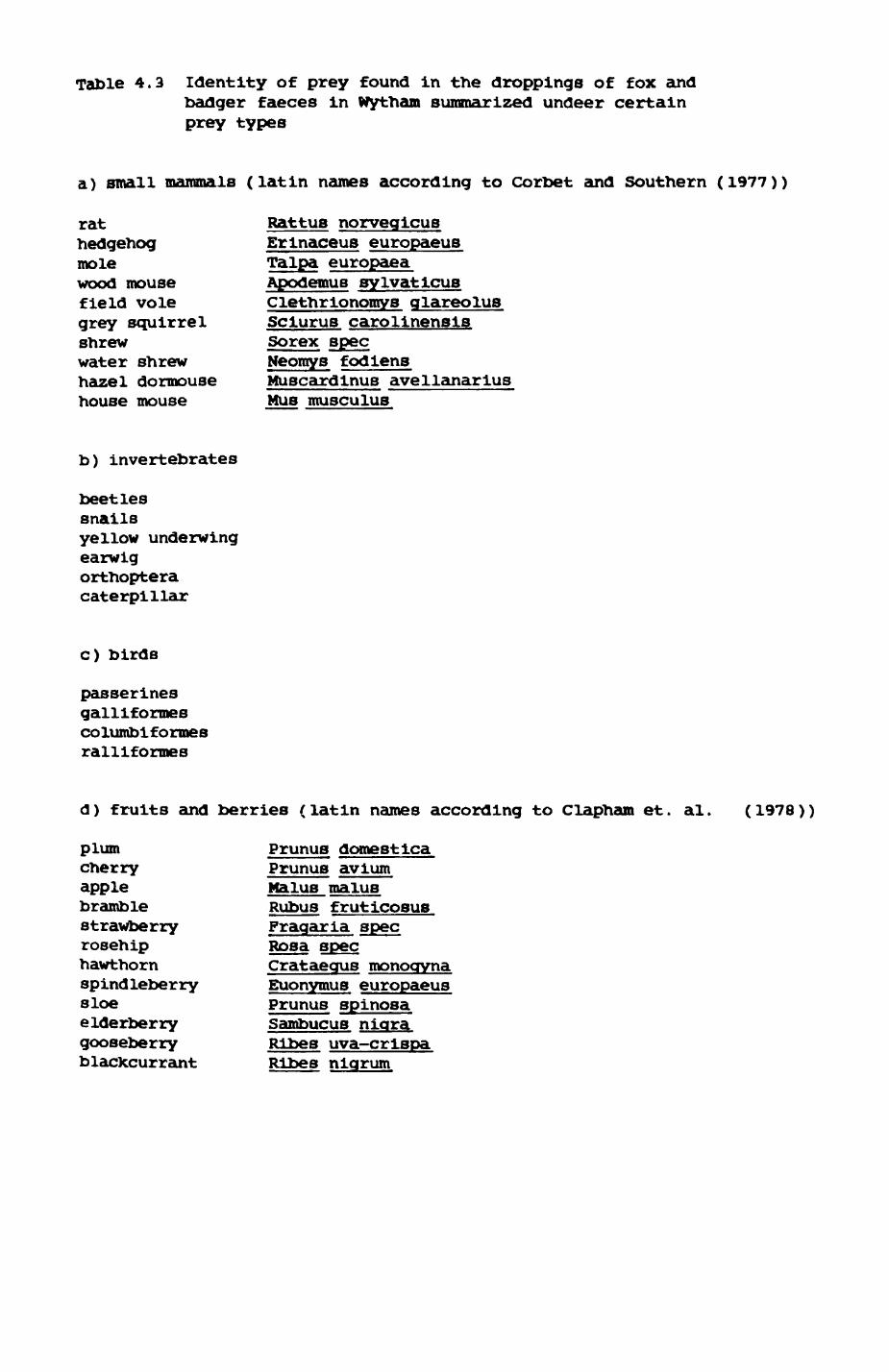
Table 4.3 Identity of prey found in the droppings of fox and badger faeces in Wytham summarized undeer certain prey types
a) small mammals (latin names according to Corbet and Southern (1977))
rat Rattus norveqicushedgehog Erinaceus europaeusmole Talpa europaeawood mouse Apodemus sylvaticusfield vole Clethrionomys glareolusgrey squirrel Sciurus carolinensisshrew Sorex specwater shrew Neomys fodienshazel dormouse Kuscardinus avellanariushouse mouse Mus musculus
b) invertebrates
beetlessnailsyellow underwingearwigorthopteracaterpillar
c) birds
passerines galliformes columbiformes ralliformes
d) fruits and berries (latin names according to Clapham et. al. (1978))
plum Prunus domesticacherry Prunus aviumapple Malus malusbramble Rubus fruticosusstrawberry Fraqaria specrosehip Rosa spechawthorn Crataequs monoqynaspindleberry Euonymus europaeussloe Prunus spinosaelderberry Sambucus niqragooseberry Ribes uva-crispablackcurrant Ribes niqrum

pig. 4.5. Monthly changes in the diet of Wytham's foxes as determined by estimated dry weight.
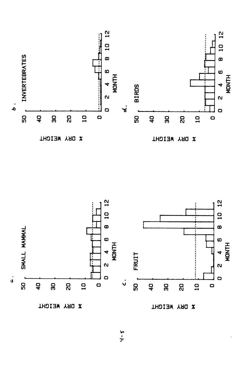
X DRY WEIGHTX DRY WEIGHT
o
!
O
IN)
0)
CD
O
fN)
i-" D C
1 '
h
IN) 0) ^ cn ) O O O O
-nC
_l
i- ro O Oen o
0)
CD
oII
> r
X DRY WEIGHTX DRY WEIGHT
o
ro
o . 2 *•
O)
CD
O
fN)
i-* ro u) *. cn o o o o o o (j : • • ' >L tJ
M ru, „ S n 1 «> 2*
X0)
37 °ro
^ PJ a) *. tn D a o o o o
2mrn^^r
4 m \ 03T] 5 tj zj
1
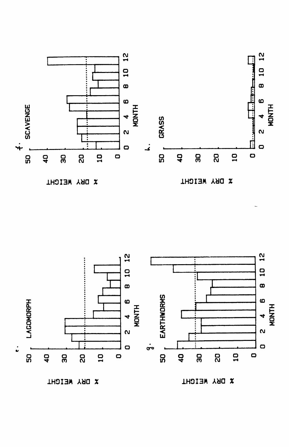
X DRY WEIGHTX DRY WEIGHT
0
roz:2 *
XO)
GO
O
M %
H* ro o) o o o o
i|
i
*. en o o• | » eA o
J 5*^ >• ro
— , 1 °^ * z ^I —— 9 i i ^1 i «A»
2 0) 0)
GO
11
o o
—-j;1i t
ro CD ^ ui 0000
~l rOo01^HK
X
Z DRY WEIGHTX DRY WEIGHT
or ro
0)
GO
ttD
ro oCOo
4*» Ocn o
o37 0)(/)
ro
1o
ro
*
0)
GO
O
•-* M %
D O'1
.
i1,i
1
ro co 4^ ( 0 0 0 (
3-, i ^^ <«4
, ——— I•
—— i
i2m
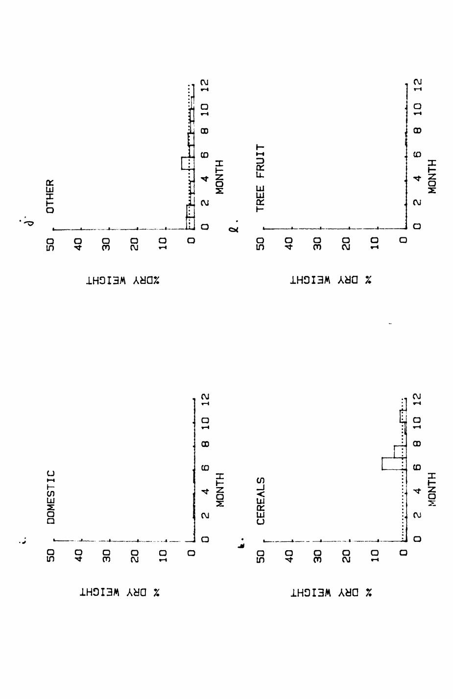
50
f DO
MEST
IC
40
<T50
, OTHER
40X CD E
30
•^ a
20
ia *«
10
i
0 .,
. 0
I
k .50
.
CEI i
h-
40
•X CD u
30
..
a
20
.a *
10
[
0 ••••-,
J- X CD
»— 1
Ul 36 fy^ Q 5s?
> 4
6 8
10
12MONTH
E:REALS
X CD K-l UJ > a ^t
~1 __
T-F
1 \
20
[ i10
L i
_..-
0 2
4 6
8 10
12MONTH
e.50
TREE FRUIT
40
.
30
. i
20
..
10
.
n .
t , _
. ,
0 2
4 6
8 10
12
MO
NTH
0 2
4 6
8 10
12
MONTH
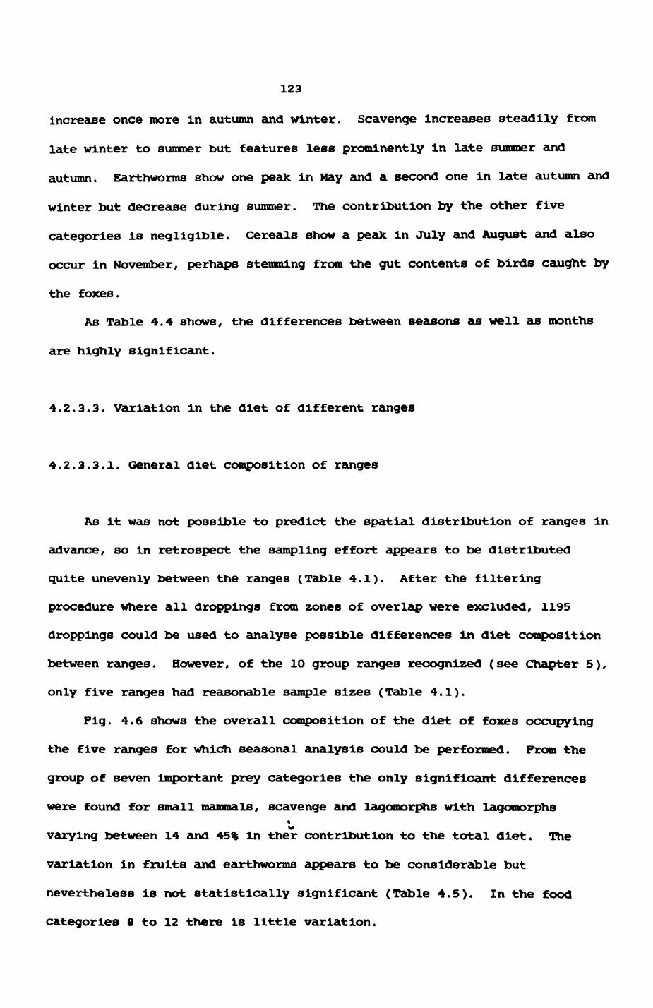
123
increase once more in autumn and winter. Scavenge increases steadily from
late winter to summer but features less prominently in late summer and
autumn. Earthworms show one peak in Hay and a second one in late autumn and
winter but decrease during summer. The contribution by the other five
categories is negligible. Cereals show a peak in July and August and also
occur in November, perhaps stemming from the gut contents of birds caught by
the foxes.
As Table 4.4 shows, the differences between seasons as well as months
are highly significant.
4.2.3.3. Variation in the diet of different ranges
4.2.3.3.1. General diet composition of ranges
As it was not possible to predict the spatial distribution of ranges in
advance, so in retrospect the sampling effort appears to be distributed
quite unevenly between the ranges (Table 4.1). After the filtering
procedure where all droppings from zones of overlap were excluded, 1195
droppings could be used to analyse possible differences in diet composition
between ranges. However, of the 10 group ranges recognized (see Chapter 5),
only five ranges had reasonable sample sizes (Table 4.1).
Fig. 4.6 shows the overall composition of the diet of foxes occupying
the five ranges for which seasonal analysis could be performed. Prom the
group of seven important prey categories the only significant differences
were found for small mammals, scavenge and lagomorphs with lagomorphs•
varying between 14 and 45% In ther contribution to the total diet. The
variation in fruits and earthworms appears to be considerable but
nevertheless is not statistically significant (Table 4.5). In the food
categories 8 to 12 there is little variation.
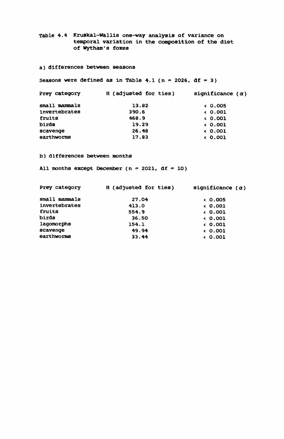
Table 4.4 KrusXal-Wallis one-way analysis of variance ontemporal variation in the composition of the diet of Wytham's foxes
a) differences between seasons
Seasons were defined as in Table 4.1 (n = 2026, df = 3)
Prey category H (adjusted for ties) significance (a)
small mammals 13.82 < O.O05invertebrates 390.6 < 0.001fruits 468.9 < 0.001birds 19.29 < o.OOlscavenge 26.48 < O.OOlearthworms 17.83 < 0.001
b) differences between months
All months except December (n = 2O21, df = 10)
Prey category H (adjusted for ties) significance (a)
small mammals 27.04 < O.O05invertebrates 413.0 < O.OOlfruits 554.9 < O.OOlbirds 36.5O < o.OOllagomorphs 154.1 < O.OOlscavenge 49.94 < O.OOlearthworms 33.44 < O.OOl
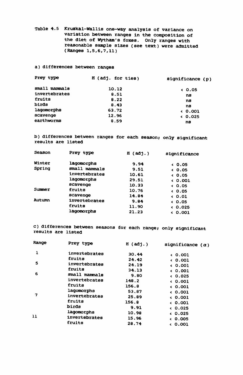
Table 4.5 Krusfcal-wallis one-way analysis of variance on variation between ranges in the composition of the diet of Wytham's foxes. Only ranges with reasonable sample sizes (see text) were admitted (Ranges 1,5,6,7,11)
a) differences between ranges
Prey type
small mammalsinvertebratesfruitsbirdslagomorphsscavengeearthworms
H (adj. for ties)
10.128.518.228.43
63.7212.968.59
significance (p)
< 0.05nsnsns
< O.O01 < 0.025ns
b) differences between ranges for each season; only significant results are listed
Season
Winter Spring
Summer
Autumn
Prey type
lagomorphssmall mammalsinvertebrateslagomorphsscavengefruitsscavengeinvertebratesfruitslagomorphs
H (adj.)
9.949.5110.6129.5110.3310.7614.849.84
11.9021.23
significance
0.050.050.05O.O010.050.05O.01O.050.0250.001
c) differences between seasons for each range; only significant results are listed
Range
1
5
6
11
Prey type
invertebratesfruitsinvertebratesfruitssmall mammalsinvertebratesfruitslagomorphsinvertebratesfruitsbirdslagomorphsinvertebratesfruits
H (adj.)
3O.4424.4224.1934.13 9.80
148.2 156.853.8725.89
156.8 9.91
10.9815.9628.74
significance (a)
0.001 0.001 0.001 0.001 0.025 0.001 O.O01 0.001 0.001 O.O01 0.025 0.025 0.005 O.OO1

Pig. 4.6. Differences in the diet of five fox groups asdetermined by estimated dry weight. Food categories plotted in identical sequence to Fig. 4.5. and Table 4.2
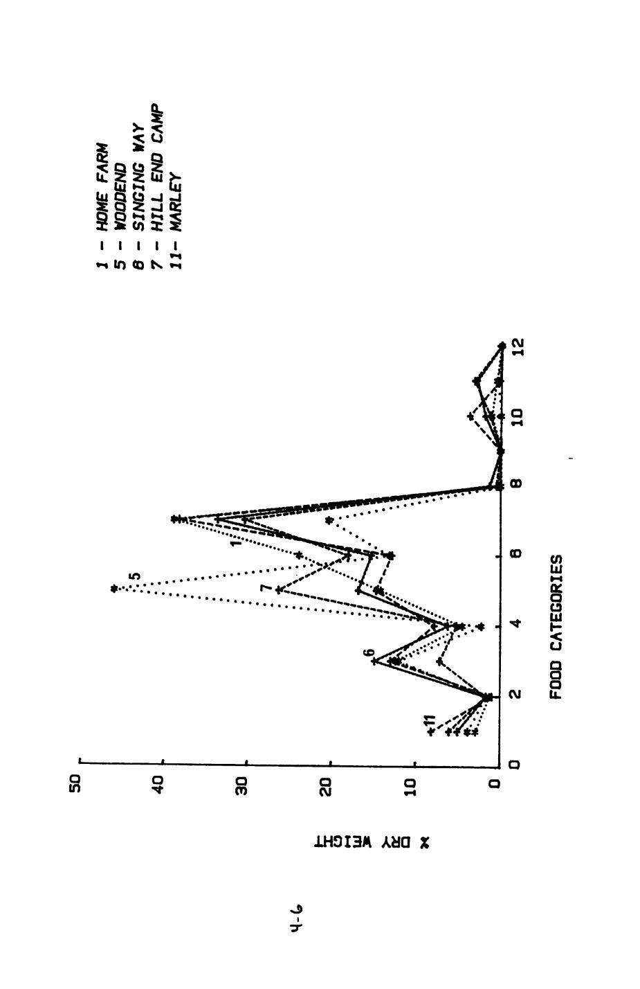
50 „
40
.
30
.
M-C,
20o UJ Q
H10
1 5 8 7
- HOME FARM
- WOODEND
- SINGING
WAY
- HJLL END CAMP
" MARLEY
68
FOOD C
ATEGORIES
124
A posteriori multiple comparison tests were carried out for the three
food types with significant variation to investigate which ranges differed
from which others. The results are summarized in Table 4.6.
From small mammals, only three pairs of ranges showed significant
differencesi Range 11 (Marley Wood) consumed more small mammals than Ranges
1 (Home Farm) and 5 (Woodend Farm) and Range 6 (Singing Way) consumed more
than 5 (Woodend Farm). Looking at the results for scavenge, Range 1 (Home
Farm) had by far the highest intake of scavenge, significantly higher than
any of the other ranges while none of the other ranges were different from
each other.
Lagomorphs showed the most consistent variation between ranges. Range
5 (Woodend Farm) had a higher proportion of lagomorphs in its diet than all
other ranges except the neighbouring Range 7 (Hill End Camp) which was
different from the other three ranges as well. These three ranges (No.l
(Home Farm), No. 6 (Singing Way), and No. 11 (Marley Wood)) were similar in
lagomorph consumption.
The results of the multiple comparison tests indicate some interesting
differences for prey categoriesi for two food categories (scavenge and
lagomorphs), one and two ranges respectively had a much higher proportion of
the prey type in question and thus dominated the others. For the third prey
category (small mammals) variation was generally little and only sufficient
for three pairs to yield significant differences. Two ranges emerge that
are dominated by one prey itemt Range 5 (Woodend Farm) and Range 1 (Home
Farm) while the other three ranges seem to have a more even share of the
various prey types.
Differences in the diet of the five ranges are graphically illustrated
In Fig. 4.7 for four prey types which also shows their spatial relationship
to each other (Fig. 4.7a). For both lagomorphs and earthworms there exist
spatial gradients running In opposite directions to each other. The peak of
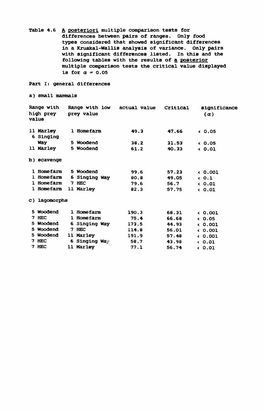
Table 4.6 A posteriori multiple comparison tests fordifferences between pairs of ranges. Only food types considered that showed significant differences in a KrusJcal-Wallis analysis of variance. Only pairs with significant differences listed. In this and the following tables with the results of a posterior multiple comparison tests the critical value displayed is for a = 0.05
Part It general differences
a) small mammals
Range with Range with low actual value Critical significance high prey prey value (a) value
11 Marley 1 Homefarm 49.3 47.66 < 0.05 6 SingingWay 5 Woodend 38.2 31.53 < 0.05
11 Marley 5 Woodend 61.2 4O.33 < 0.01
b) scavenge
1 Homefarm 5 Woodend 99.6 57.23 < O.O011 Homefarm 6 Singing Way 80.8 49.05 < 0.11 Homefarm 7 HEC 79.6 56.7 < O.011 Homefarm 11 Marley 82.3 57.75 < O.01
c) lagomorphs
5 Woodend 1 Homefarm 19O.3 68.31 < O.O017 HEC 1 Homefarm 75.4 66.68 < O.055 Woodend 6 Singing Way 173.5 44.93 < 0.0015 Woodend 7 HEC 114.8 56.01 < O.O015 Woodend 11 Marley 191.9 57.48 < 0.0017 HEC 6 Singing way 58.7 43.98 < O.017 HEC 11 Marley 77.1 56.74 < 0.01
Fig. 4.7. Differences in the diet of five fox groups, as determined by estimated dry weight.
a. Map with main woodland and field boundaries and approximate range boundaries of fox groups.
b. Differences in consumption of main prey items. Numbers are group numbers, arrows indicate an increase in the consumption of a particular item. Arrows drawn to scale.
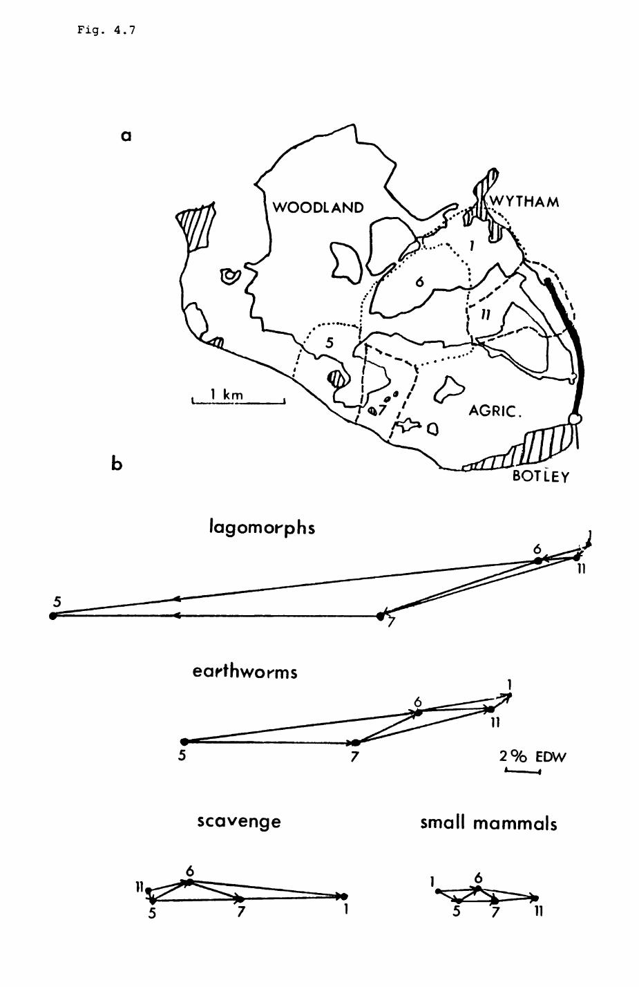
Fig. 4.7
WYTHAMWOODLAND
BOTLEY
lagomorphs
n
earthworms
n
2% EDW
scavenge small mammals
125
earthworm consumption is in Range 1 (north east) corresponding to the lowest
consumption of lagomorphs which reaches its peak in the southwest. Both
scavenge and small mammal consumption show a non-uniform spatial trend t the
three Ranges 5,6, and 7 have an intermediate consumption while Ranges 1 and
11 show an extreme high or low consumption. A high proportion of scavenging
in Range 1 corresponds to the lowest proportion in small mammals; the
opposite is true for Range 11.
4.2.3.3.2. Seasonal variation in the diet of ranges
There are at least three different ways of looking at seasonal effects
on the composition of the diet of foxes in different ranges. One way is to
follow each individual range through the various seasons and investigate
changes in the diet composition. This Is depicted for Ranges 1,5,6,7, and
11 in Fig. 4.8 to 4.12 and the corresponding statistical analysis can be
found in Table 4.5c. The second way is to look at each season in turn and
to compare the diet of all ranges within that season. This approach
indicates how much variation there is between single ranges for one season
and gives an impression of how well the seasonal trends found for the entire
study area (section 4.2.4.2) correspond to those in individual ranges. For
this second presentation, the relevant statistics are listed in Table 4.5b
and 4.7. The third way is to look at the degree of synchrony In the
composition of the diet of ranges in their temporal fluctuations. The
results of this analysis can be found In Table 4.12a.
Changes within individual territories Fig 4.8 to 4.12 show the seasonal
distribution of prey categories for each of the five ranges. The results
are presented first for each range and then summarized for each food type in
turn. Significant differences indicate that the means of estimated dry
weight of a given food category vary more than can be explained by chance

Pig. 4.8-4.12. Seasonal changes in the diet of five fox groups.Diet items plotted in sequence identical to Fig. 4.5 and Table 4.2.
Fig. 4.8i group 1 HOMEFARM4.9i group 5 WOODEND4.10i group 6 SINGING WAY4.1l! group 7 HILL END CAMP4.12! group 11 MARLEY
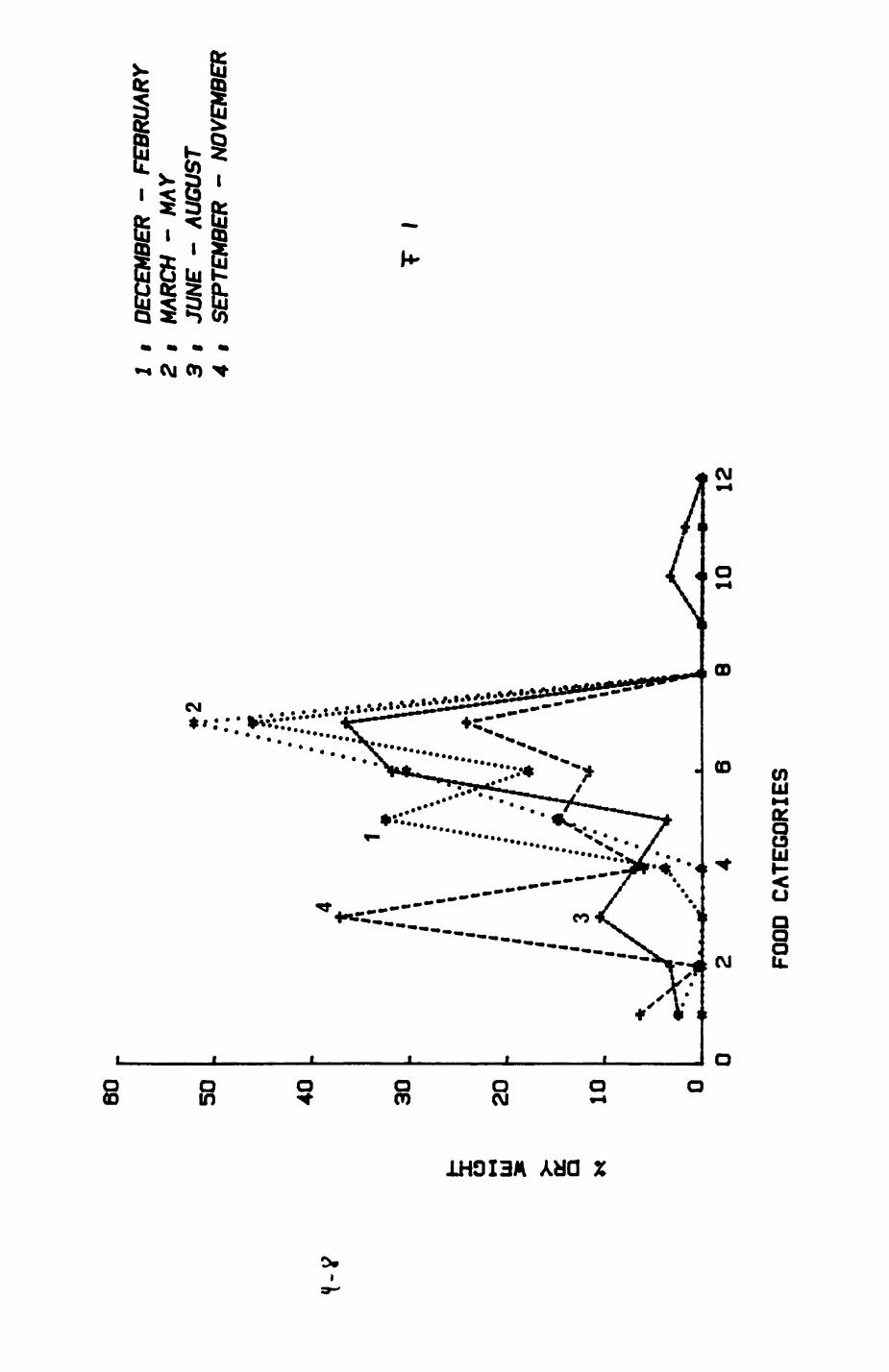
60 50 40 30
tu a: Q H
20 10
1 i DECEMBER - FEBRUARY
2 i
MARCH -
AMV
3 t JUNE -
AUGUST
4 t SEPTEMBER - NOVEMBER
T
I
68
FOOD CATEGORIES
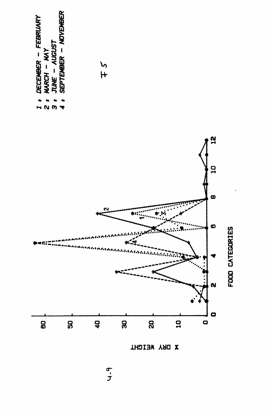
60 50 40 30
UJ >• Q
20 10
J t DECEMBER - FEBRUARY
2 i
MARCH - AMY
3 t JUNE - AUGUST
4 i
SEPTEMBER - NOVEMBER
FOOD C
ATEGORIES
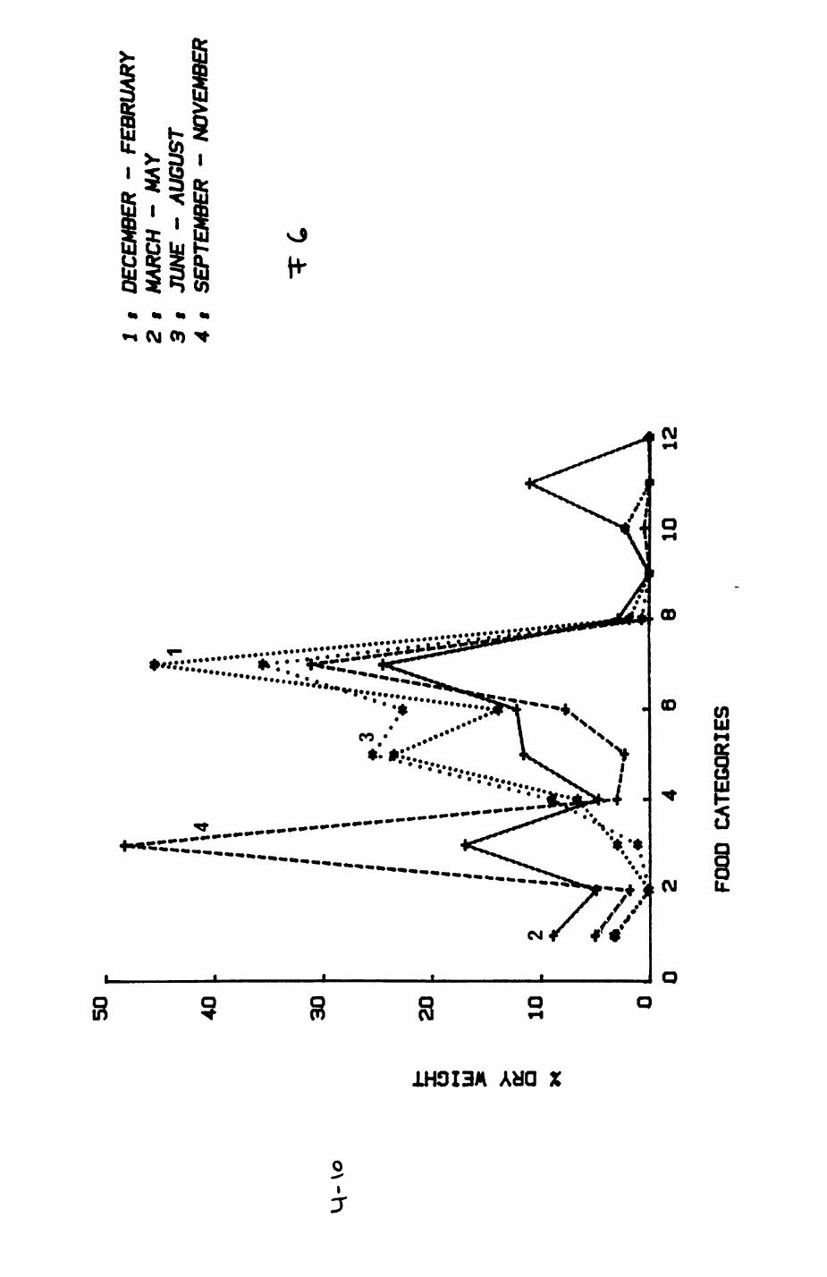
50 40 30M-Vo
20
K
Q10
1 t DECEMBER - FEBRUARY
2 i
MARCH - MAY
3 t JU
NE - AUGUST
4 i
SEPTEMBER - NOVEMBER
C
FOOD C
ATEGORIES

40 30
M-H
20
o
•-« UJ i10
1 i DECEMBER - FEBRUARY
2 t
MARCH - MAY
3 i
JUNE - AUGUST
4 i
SEPTEMBER - NOVEMBER
FOOD C
ATEGORIES
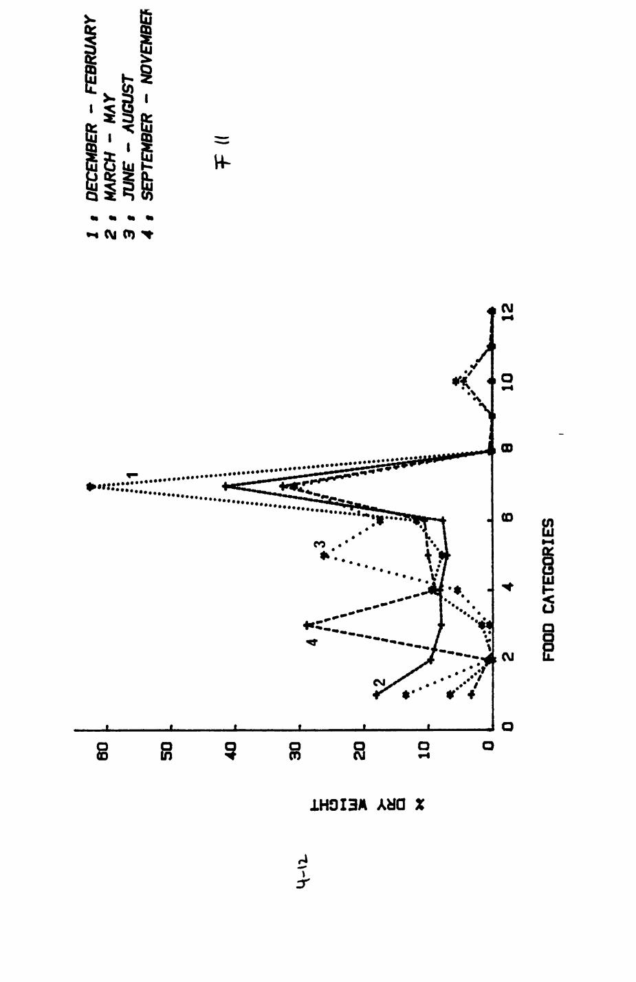
60 50 40 30
a: Q
X10
1 i DECEMBER - FEBRUARY
2 i
MARCH - MAY
3 i
JUNE - AUGUST
4 i SEPTEMBER - NOVEMBER
FOOD C
ATEGORIES
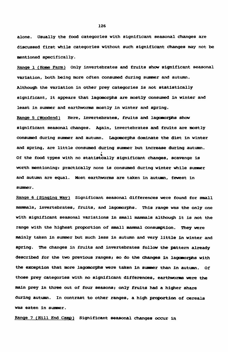
126
alone. Usually the food categories with significant seasonal changes are
discussed first While categories without such significant changes may not be
mentioned specifically.
Range 1 (Home Farm) Only invertebrates and fruits show significant seasonal
variation, both being more often consumed during summer and autumn.
Although the variation in other prey categories Is not statistically
significant, it appears that lagomorphs are mostly consumed In winter and
least In summer and earthworms mostly In winter and spring.
Range 5 (Woodend) Here, Invertebrates, fruits and lagomorphs show
significant seasonal changes. Again, invertebrates and fruits are mostly
consumed during summer and autumn. Lagomorphs dominate the diet in winter
and spring, are little consumed during summer but Increase during autumn.»t
Of the food types with no statlstcally significant changes, scavenge is
worth mentioningt practically none is consumed during winter while summer
and autumn are equal. Host earthworms are talcen in autumn, fewest in
summer.
Range 6 (Singing Way) Significant seasonal differences were found for small
mammals. Invertebrates, fruits, and lagomorphs. This range was the only one
with significant seasonal variations in small mammals although It Is not the
range with the highest proportion of small mammal consumption. They were
mainly talcen In summer but much less In autumn and very little In winter and
spring. The changes in fruits and Invertebrates follow the pattern already
described for the two previous ranges j so do the changes In lagomorphs with
the exception that more lagomorphs were taken In summer than In autumn. Of
those prey categories with no significant differences, earthworms were the
main prey in three out of four seasons) only fruits had a higher share
during autumn. In contrast to other ranges, a high proportion of cereals
was eaten In summer.
Range 7 (Hill End Camp) Significant seasonal changes occur in
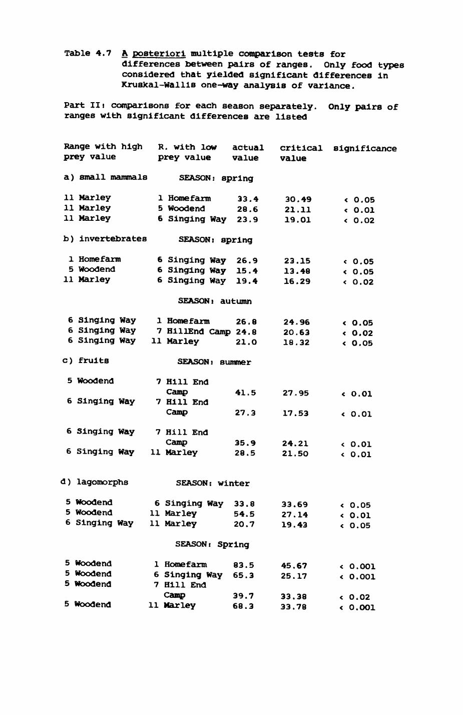
Table 4.7 A posteriori multiple comparison tests fordifferences between pairs of ranges. Only food types considered that yielded significant differences in KrusXal-Wallls one-way analysis of variance.
Part Hi comparisons for each season separately. ranges with significant differences are listed
Only pairs of
Range with high R. with low actual prey value prey value value
a) small mammals
11 Marley 11 Marley 11 Marley
b) invertebrates
1 Homefarm 5 Woodend
11 Marley
6 Singing Way 6 Singing Way 6 Singing Way
c) fruits
5 Woodend
6 Singing Way
6 Singing Way
SEASON: spring
1 Homefarm 33.45 Woodend 28.66 Singing Way 23.9
SEASON: spring
6 Singing Way 26.96 Singing Way 15.46 Singing Way 19.4
SEASON} autumn
1 Homefarm 26.87 HlllEnd Camp 24.8
11 Marley 21.O
SEASONi summer
7 Hill EndCamp
7 Hill EndCamp
7 Hill EndCamp
6 Singing Way 11 Marley
41.5
27.3
35.928.5
critical value
significance
30.4921.1119.01
23.1513.4816.29
24.9620.6318.32
27.95
17.53
24.21 21.5O
< O.05< 0.01< 0.02
< 0.05< 0.05< 0.02
< O.05< 0.02< O.O5
< 0.01
< 0.01
< 0.01 < 0.01
d) lagomorphs
5 Woodend5 Woodend6 Singing Way
5 Woodend 5 Woodend 5 Woodend
5 Woodend
SEASON: winter
6 Singing Way 33.8 33.6911 Marley 54.5 27.1411 Marley 20.7 19.43
SEASON t Spring
1 Home farm 83.5 45.676 Singing Way 65.3 25.177 Hill EndCamp 39.7 33.38
11 Marley 68.3 33.78
< 0.05< 0.01< 0.05
< O.OO1< O.O01
< 0.02< 0.001

Table 4.7 (Cont. )
SEASONi autumn
5 Woodend 6 Singing Way 38.4 16.22 < 0.0015 Woodend 11 Mar ley 28.1 17.65 < 0.017 Hill End Camp 6 Singing Way 19.9 15.06 < 0.01
e) scavenge SEASON: spring
1 Home farm 5 Woodend 47.8 36.15 < 0.01 1 Homefarm 7 Hill End
Camp 4O.8 38.37 < 0.05 6 Singing Way 5 Woodend 23.9 19.93 < 0.02
SEASON: summer1 Homefarm 5 Woodend 37.9 33.37 < O.05 1 Homefarm 6 Singing Way 45.3 23.98 < 0.001
127
invertebrates, fruits, birds and lagomorphs. This is tne only range that
showed significant differences for birds. This was due to intensive
consumption during summer. Again lagomorphs were mainly taken during winter
and spring and less so in summer and autumn. Earthworms constituted the
major food type in winter and autumn and were consumed less in summer.
There were big changes in the amount of scavenge taken (although not
significant)! most of it was taken during summer and least taken in autumn.
Range 11 (Marley wood) Only invertebrates and fruits showed significant
seasonal changes. This is the range with the fewest significant changes,
together with the neighbouring Homefarm range (no.l). Invertebrates and
fruits were eaten more In summer and autumn. There seemed to be some
seasonal differences in the amount of small mammals consumed. Earthworms
dominated the diet In all four seasons.
The following paragraphs summarize the preceding results for each food
categoryi
Small mammals Only one range showed a significant seasonal variation (Range
6). In all five ranges, small mammals usually constituted less than 1O% of
the seasonal diet with the exception of Range 11 (Marley) where the
proportion Increased significantly from 6.6% In winter to 13.5% in spring
and 18% in summer.
Invertebrates and fruits In all ranges they were mostly consumed during
summer and autumn and far less during the remaining seasons. Invertebrates
comprised up to 1O% of the seasonal diet while fruits reached close to 5O%
(Range 6).
Birds Only Range 7 (Hill End Camp) showed significant seasonal variation
for birds. In all five ranges, birds never exceeded 10% of the seasonal
diet except for summer In Range 7.
Laqoroorphs Significant seasonal changes were found In Ranges 5, 6 and 7.
128
In four ranges the greatest seasonal Incidence of lagomorphs was during
winter and spring. In four ranges they were taken least in summer, only
Range 6 during autumn.
Scavenge Despite apparently considerable variation, no significant seasonal
variation was found) no consistent seasonal pattern of consumption appears
either. In two ranges most scavenge was taken in spring, in three in
summer.
Earthworms None of the ranges showed seasonal changes in the consumption of
earthworms, which constituted a very important prey category (at least If
measured by dry weight). Generally, fewer worms were eaten In summer than
in any other season. There was at least one range where In each of winter,
spring or autumn earthworms had the highest share of all food categories in
the seasonal diet.
Differences between ranges within single seasons Table 4.5b and 4.7
summarize the results of the statistical analyses performed to discern the
spatial variation within a season. Within each season, there is at least
one prey item for which significant differences exist between ranges.
However, the number of prey categories that show significant differences
varies from season to seasont
Winter 1 prey category
Spring 4 prey categories
Summer 2 prey categories
Autumn 3 prey categories
Thus, seasons with high spatial diversity of diet are followed by
seasons with a spatially more uniform consumption of prey types.
Winter Lagomorphs are the only prey type with significant spatial
variation. This la a time of peak consumption of lagomorphs.
Spring Pour prey categories (snail mammals, invertebrates, lagouorphs, and
129
scavenge) vary In their consumption by different ranges. This is the season
with the highest spatial diversificationi it is also the season when the
cubs are brought up.
Sumner Fruits and scavenge show significant spatial variation.
Autumn Invertebrates, fruits, and lagomorphs vary significantly between
ranges.
Of the seven prey categories considered, five show significant spatial
variation in at least one season, only birds and earthworms are consumed at
more or less constant proportions in all ranges throughout the year.
Small mammals The only significant spatial variation was found for spring,
not a time of peak consumption of small mammals.
Invertebrates They vary significantly between ranges In spring and autumn,
but not during the time of peak consumption (summer).
Fruits They vary between ranges in summer and autumn which are peak seasons
of consumption.
Laqomorphs They show the most consistent spatial variation (three seasons
out of four), excluding only summer which is a time of low consumption of
lagomorphs.
Scavenge Significant spatial variation was found for spring and summer
which are times of peak consumption. Here we have the interesting situation
that In none of the ranges does the level of scavenging change seasonally
(see preceding sections), yet the differences between various ranges change
seasonally such that the spatial variation is significant In peak
consumption times (spring and summer) but not for the remaining seasons.
Comparing the two most Important elements (If measured by dry weight)
of the fox diet In tfytnam, earthworms and lagomorphs, there are obvious and
Interesting differences. Considering earthworms, no significant spatial or
130
temporal variation in the amount consumed could be detected, whether on a
general level or for either different temporal or spatial units; in short,
earthwoms form a consistently Important part of the diet. On the other
hand, there is a lot of variation in lagomorphst in general between seasons
and ranges, within seasons between ranges and within ranges between seasons.
A posteriori multiple comparison tests were performed to investigate
differences between ranges within single seasons (Table 4.7). In five out
of ten cases one range with a particularly high score on one prey type
dominates all other ranges and is responsible for the significant spatial
variation within the particular season and food type. This is on two
occasions Range 6 (invertebrates and fruits in autumn) and once each Range 1
(scavenge in summer), Range 5 (lagomorphs in spring) and Range 11 (small
mammals in spring). Thus, the results of Table 4.6 where differences between
ranges were noted over the entire year are corroborated.
Synchrony of the direction of temporal fluctuations between ranges In
addition to asking whether there is spatial variation for a given time unit,
one may ask whether the direction of temporal fluctuations is synchronized
between ranges. This was tested using Kendall's coefficient of concordance.
Results are presented in Table 4.12a. Fox ranges show a significant
synchronization for invertebrates, fruits, and lagomorphs. This means that
even though significant differences may have been found between ranges at a
given time the change in consumption from one season to the next follows the
same direction for all ranges.
4.2.4. Fox dlett summary
1. 2030 fox droppings were collected between April 1981 and October 1983
Including samples from every month of the year.
131
2. Lagomorphs and earthworms were the most Important consltuents of the diet
(as measured by dry weight). Lagomorphs occurred less often than earthworms
and contributed one half as much estimated dry weight to the total diet as
earthworms, but far more If corrected for digestibility and calorific
Intake. Scavenge and fruits ranked next in Importance (scavengei 20%
frequency of occurrence (FO), 18% estimated dry weight (EDW)/ fruitst 18% PO
and 13% EDW), followed by birds (11% FO and 6% EDW), small mammals (13% FO
and 5% EDW) and invertebrates (25% FO and 2% EDW).
3. Of the twelve major prey types, five occurred in less than 1O% of the
samples and constituted only small proportions of the diet.
4. There is marked temporal variation in the proportion of most food types
as measured by EDW. Invertebrates, fruits and small mammals show peaks in
July, August and July respectively. Birds are consumed preferentially in
May and June, lagomorphs in late winter and spring (January until April) and
far less during the remaining months. Earthworms show peaks in the diet
twice in the yeart first, during late spring (May) and second during autumn
and winter (November until January) with lower consumption at the end of
winter/beginning of spring and in summer. Scavenge is more or less equally
consumed between February and April and June and July but far less during
autumn. All these changes are highly significant.
5. There is some variation in the composition of the diet of different fox
ranges with significant spatial variation in small mammals, lagomorphs, and
scavenge. For scavenge and lagomorphs one and two ranges respectively had a
much higher share of these prey types than the other ranges. Usually, the
number of significantly different pairs of ranges were small in comparison
132
with the total number of pairs. Only for lagomorphs were more pairs
significantly different than not. Variation in the diet is spread widely
but quite unequally amongst ranges.
6. Within each range, some prey types usually varied greatly between seasons
while others did not. Fruits and invertebrates were the only prey
categories that showed significant temporal variation in all ranges while
scavenge and earthworms did not show any at all. The variation in the three
other main prey categories was for most of the ranges significant
(lagomorphs) or insignificant (small mammals, birds). Fruits, invertebrates
and lagomorphs invariably showed the same pattern of peak consumption in
different ranges (summer and late winter/spring, respectively), ie. the
ranges were synchronized. No pattern emerged for scavenge. Although
changes were not significant for earthworms, there was some variation with*
winter, sping and autumn having at least one range with its peak in that
particular season. Summer was the season when fewer worms were eaten than
at any other time of the year. Thus variation was similar in direction in
some prey categories but highly different in magnitude for different ranges.
7. There is considerable variation between seasons in the amount of
variation between ranges. No seasonal differences were found between ranges
for the consumption of birds and earthworms. A season with high spatial
diversification in diet is followed by a season with a low one
(spring/summer, autumn/winter). Lagomorphs show the most consistent spatial
variation in three out of four seasons. Scavenge varies in spring and
summer, fruits in summer and autumn and invertebrates in spring and autumn,
small mamma IB in spring only. Looking at pairs of ranges for each prey type
with significant spatial variation It turns out that In five out of ten
cases one range with a disproportionate prey value dominates all other
133
ranges and IB responsible for the significant spatial variation. In all
cases the number of pairs that differ significantly is less than the number
of pairs that does not.
4.2.5. Comparison with other studies
The results of the preceding section will initially be contrasted with
three other studies from Oxford areas before a comparison is made with
studies from areas outside Oxford.
Newdick (1983) Investigated the diet of foxes In the City of Oxford.
Scavenge was the most important diet component with 47% frequency of
occurrence and 37% estimated dry weight, followed by earthworms (38% and
25%). other Important food categories were small mammals (16% and 7%),
birds (17% and 7%) amd lagomorphs (9% and 6%). Thus the most notable
difference is the importance of scavenge in town and the reduced presence of
lagomorphs. Two neighbouring areas, the "Shoot", an agricultural area with
shooting interests and the Boars Hill area were Investigated by D.w.&
Macdonald (1977 and unpubl.). The shoot area is a rural area where much the
same food was taken as in wytham. Lagomorphs were the principal diet, at a
proportion higher than in Wytham If measured by estimated dry weight (3O%),
followed by earthworms and scavenge (22% and 20%). In the adjacent Boars
Hill area, a suburban area of detached housing with lawns and orchards among
farmland, earthworms accounted for 50% estimated dry weight, followed by
scavenge (28%) while all other items were much below 10%. Preliminary
results from another study area, the Cumnor area adjacent to wytham,
Indicate that earthworms are the principal diet as well, followed by fruits
and then by lagomorphs and scavenge (Macdonald, unpubl. ).
Results from other studies emphasise one overriding aspecti the fox's
versatility in adapting to the spectrum of locally available prey. Mulder
134
(1982) in a study of red foxes in a Dutch coastal dune reserve with a high
rabbit population found that 91% of the bulk diet consisted of rabbits. The
next significant items were birds, fruits and small mammals. In a study of
foxes in southern Sweden, von schantz (1980) found that foxes ate mostly
rabbits (86%) while other prey categories contributed only minute amounts.
In another study of suburban fox habits, Harris (1981) found earthworms and
scavenge to be Important parts of the diet, but emphasised the high
diversity of prey types consumed at any time of the year. In the camargue,
Reynolds (1979) found rabbit to be predominant in the diet amongst a highly
diverse assemblage of other prey categories. Matejka et al. (1977) found
field voles and other rodents dominating the diet of foxes in a German rural
area. Many other studies could be cited (for a review see Sequlera (1980))
which indicate how the main components of the diet change according to the
local conditions of the study site. Most of these studies have the
limitation, however, of presenting data only on the frequency of occurrence
of prey categories, indicating only qualitatively which items constitute the
bulk of the diet. In most studies seasonal changes are marked for most«. important prey items. Aside from Macdonald (1977), who found similar
patterns of spatial and temporal variation, this is the only study that
compares the diet between ranges and its possible seasonal variation within
ranges.
4.3. Badger diet
4.3.1. Methods of sampling
A total of 1053 badger droppings were collected over the 'core* area
(see section 4.2.1.) between May 1982 and October 1983. in contrast to
foxes which deposit their faeces everywhere in their ranges, badgers
135
generally defaecate at certain specially prepared sites called latrines
(Neal (1977)). These are sites where the badgers dig little holes or pits
of 5 to 30 cm diameter, with a depth of between a couple of cm up to 50 cm.
These deeper pits are often blind entries to badger setts. A latrine may
consist of 1 to 8O pits and cover an area between 1O by 1O cm up to 15 m
maximum length and 1O m mavinmm width.
Latrines are often found at transitions of microhabitats and at
conspicuous landmarks such as fence posts, trades, ditches and setts. In
wytham, badgers usually defaecate into latrines. It is also Known that they
defaecate underground (Kruuk & Parish (1982)).
After emerging from their winter break at the beginning of March,
badgers usually dig a whole set of new latrines and enlarge some old ones.
Therefore I searched from the end of March onwards for latrines. Detailed
searching involved walking transects through the entire study area, but
concentrating on the 'core area' as defined in section 4.2.1. These
transects were walked at a slow pace and spaced at variable distances so
that the field of view overlapped slightly with that of neighbouring
transects. In dense vegetation this usually meant a width of five to ten
meters or less, while in vegetation with less undergrowth (e.g. beechwood
plantations) transect widths were larger. To cover the entire area in a
relatively short time I usually spent nine hours every day on transect
walking from the end of March until the end of April. In spring 1982 I was
greatly helped by Nick Styles and in spring 1983 by Christa He liner. Their
assistance enabled me to cover almost every square meter of the core area so
that I could be sure to find most of the latrines. This was a very
Important requirement to ensure that my samples of faeces and the data on
the activity of latrines were representative for the entire population of
latrines. During the remainder of the year no further systematic search was
undertaken but whenever a new latrine was encountered, the details were
136
taken down and this latrine included in future check rounds. As I checked
each latrine at least once a month I still covered quite a large area and
probably discovered the majority of new latrines created as the year
progressed. In addition I was aided by members of the Edward Grey Institute
of Field Ornithology who told me if they found any new latrines. As a
result I found altogether 70 latrines in spring 1982 and 119 new latrines in
spring 1983 (while some of the 1982 latrines were still going), and
altogether 274 latrines in the core area between March 1982 and October
1983. By comparison, Kruuk (1978, pers. comm.) found in 1974 a total of 89
latrines in wytham, but searched a larger area which included the Great Wood
and the areas around the reservoir In the west.
The deposition of faeces at particular sites by the badgers facilitated
the collection of samples enormously. This made the design of a sampling
scheme necessary. Amongst the various sampling designs conceivable I shall
evaluate the adequacy of two.
Sampling Design it Collection of a fixed number of samples
from each latrine. Sampling more or less
unrelated to the activity of the badgers.
Sampling Design 2t Collection of samples proportionate to
the activity of badgers. Possibility of
unequal sample sizes for different latrines
within one monthly check round and for the
same latrine between different check rounds.
Sampling design 1 (SD l) has the advantage of being simple, resulting
in fixed sample sizes for different latrine check rounds which may be
advantageous for statistical analysis. However, as the badgers distribute
their attention unequally among latrines (In each check round there are at
least some latrines without any fresh droppings) some samples would either
have to contain old droppings or some latrines would have to be omitted.
137
Reduction of the number of samples taken from each latrine (fixed under SD
1) would minimize the necessity to collect old droppings, but also reduce
overall sample sizes and would result in a strong underrepresentation of
very active latrines. Selection of only a few samples from a very active
latrine is likely to Introduce some bias.
Under SO 2 the number of samples collected from a latrine Is
proportionate to the activity of badgers at that latrine. If there are no
fresh droppings, no samples are taken. If there are fresh droppings in
several pits, a sample from each pit is taken, but no more than 10 samples
from any latrine. Thus, the droppings (and therefore the diet) are
adequately sampled, although there is an element of subjectivity in the
decision of how many samples to take from each latrine. As I considered
proportionate sampling and thus a representative sample as the most
important criterion, I decided to apply sampling design 2, the proportionate
sampling scheme.
While mapping latrines during March and April, no samples of droppings
were collected. Although I realized the potential use of such data,
collection was impossible for several reasons. During March, each badger
sett was baited for at least two weeks with a mixture of peanuts, syrup and
plastic pellets of different colurs. In consequence the diet samples would
have been distorted by my baiting activities. During the period from end of
March to the end of April all my effort was devoted to locating badger
latrines, trapping and radlotracking foxes. As several setts were baited
during this time for trapping purposes, diet samples would again have been
affected.
Prom May until November latrines were visited at least once a month but
in June only a few samples were taken. Usually each latrine was visited and
its state of activity checked. If fresh droppings were present, a sample
was collected. If the number of fresh droppings was very small, then It was
138
sometimes necessary to collect all droppings. However, if the number of
fresh droppings exceeded ten, a selection of droppings was taken. Droppings
were selected so that all pits with fresh droppings were represented at
least once in the sample for that latrine. The dropping was gently
separated from its substrate (either another dropping or bare ground) and
placed in a plastic bag on which the number of the sample, the number of the
latrine and the date were noted. The plastic bag was closed with rubber
band and first stored in the deep freeze before being dried in an oven at 50 c
C.
4.3.2. Methods of analysis
The analysis of the scats basically followed the scheme adopted for the
analysis of fox droppings. This has the advantage of analysing the diet of
the two species with comparable methods. A "wet" analysis as was performed
by Kruuk (e.g. 1978b) would have taken far too long and had little advantage
except to disclose more of the infrequent, small, softbodied prey. The
categorization of prey types was the same as described for fox faeces (see
section 4.2.2.). Data were typed into a paper-tape machine and then
transferred to the university's ICL-2988 computer where the paper-tape was
read in and the files edited. Statistical analysis was performed on the
university's VAX-11/7BO computer with procedures which I wrote for the
statistical package MINITAB, analogous to the procedures used for the
analysis of the fox diet.
The analysis of the baiting actions in 1982 and 1983 plus the results
of radlotracking permitted the determination of badger hone range borders
(Chapter 5). Each latrine was assigned the status of being either a
"border" or a "non-border" latrine. If a latrine was assigned the status of
a border latrine, at least two, sometimes three neighbouring ranges shared
139
the latrine and could be responsible for faeces there. Program BORIAT
inserted the status of the latrine number together with its range number(s)
into the file containing the results of the scat analysis. All analyses
performed on ranges only considered non-border latrines, ie. those that lay
inside one range and away from any borders (section 4.3.3.3. ). A comparison
of the contents of border and non-border latrines can be found in section
4.3.3.4.
4.3.3. Results
4.3.3.1. General composition of the diet
In 1982 and 1983, 1O53 badger droppings were collected between May and
November. The distribution of sample sizes for various subsets of the data
are shown in Table 4.8.
Although no samples were collected during March and April, there is
nevertheless information available to suggest what badgers ate during these
two months. First, most fresh droppings had the darkish brown colour and
liquid texture typical for faeces dominated by earthworms. In addition,
detailed observations at the Jews Harp sett (Range B4) in April showed that
badgers caught and ate mostly earthworms at the surface and ate hardly
anything else around the sett. Of course these observations are of limited
value as the badgers could not be observed away from the sett but the
incidental observations available (from the work of Nlclcie Wadham, see
Chapter 3/ and observations during radiotraclclng) it became clear that
earthworms were a big part of the diet.
Table 4.9 lists the diet of Wytham's badgers as calculated by the three
available measures (frequency of occurrence, estimated volume and estimated
dry weight). Earthworms constitute by far the most Important component of
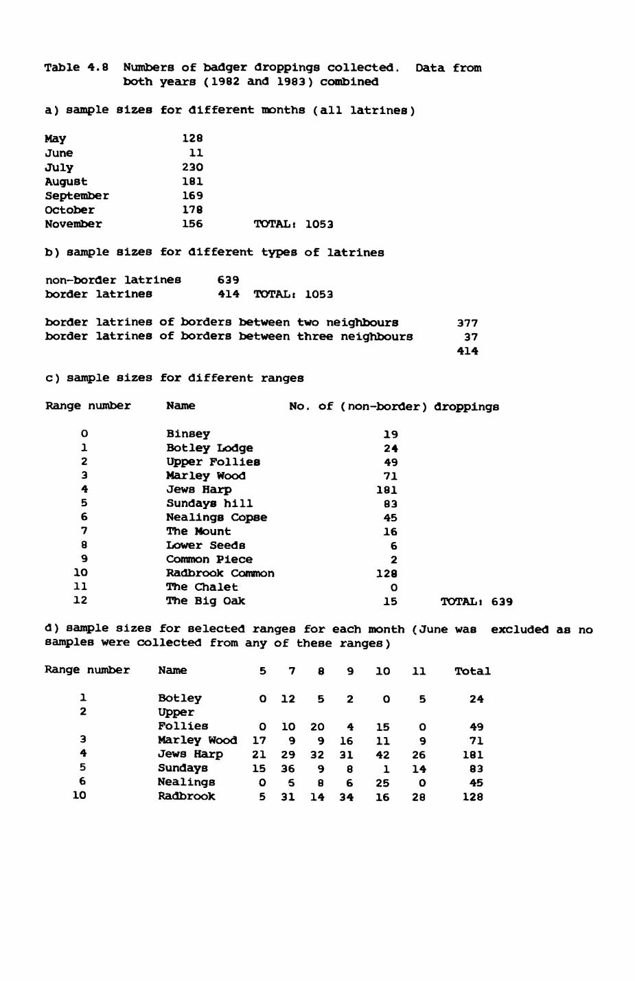
Table 4.8 Numbers of badger droppings collected. Data from both years (1982 and 1983) combined
a) sample sizes for different months (all latrines)
MayJuneJulyAugustSeptemberOctoberNovember
12811
230181169178156 TOTAL! 1053
b) sample sizes for different types of latrines
non-border latrines border latrines
639414 TOTALi 1053
border latrines of borders between two neighbours border latrines of borders between three neighbours
c) sample sizes for different ranges
37737
414
Range number
0123456789
101112
Name
Binsey Botley Lodge Upper Follies Marley Wood Jews Harp Sundays hill Nealings Copse The Mount Lower Seeds Common Piece Radbrook Common The Chalet The Big Oak
No. of (non-border) droppings
19244971
18183451662
1280
15 TOTALi 639
d) sample sizes for selected ranges for each month (June was samples were collected from any of these ranges)
excluded as no
Range number Name 8 10 11
12
345610
Botley O 12
Total
24UpperFolliesMarley WoodJews HarpSundaysNealingsRadbrook
017211505
109
2936S
31
209
3298
14
416318634
1511421
2516
09
26140
28
49711818345
128
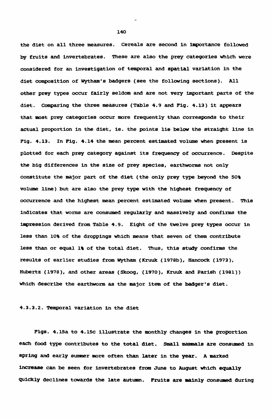
140
the diet on all three measures. Cereals are second in importance followed
by fruits and invertebrates. These are also the prey categories which were
considered for an investigation of temporal and spatial variation in the
diet composition of wytham's badgers (see the following sections). All
other prey types occur fairly seldom and are not very important parts of the
diet. Comparing the three measures (Table 4.9 and Fig. 4.13) it appears
that most prey categories occur more frequently than corresponds to their
actual proportion in the diet, ie. the points lie below the straight line in
Fig. 4.13. In Fig. 4.14 the mean percent estimated volume when present is
plotted for each prey category against its frequency of occurrence. Despite
the big differences in the size of prey species, earthworms not only
constitute the major part of the diet (the only prey type beyond the 50%
volume line) but are also the prey type with the highest frequency of
occurrence and the highest mean percent estimated volume when present. This
indicates that worms are consumed regularly and massively and confirms the
Impression derived from Table 4.9. Eight of the twelve prey types occur in
less than 10% of the droppings which means that seven of them contribute
less than or equal 1% of the total diet. Thus, this study confirms the
results of earlier studies from Hytham (Kruuk (1978b), Hancock (1973),
Hubertz (1978), and other areas (Sfcoog, (1970), Kruufc and Parish (1981))
which describe the earthworm as the major item of the badger's diet.
4.3.3.2. Temporal variation in the diet
Figs. 4.15a to 4.15C illustrate the monthly changes in the proportion
each food type contributes to the total diet. Small mammalB are consumed in
spring and early summer more often than later in the year. A marked
Increase can be seen for invertebrates from June to August which equally
quickly declines towards the late autumn. Fruits are mainly consumed during
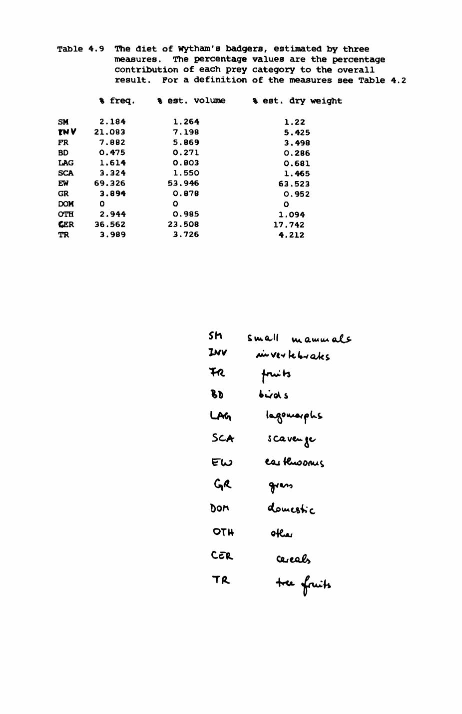
Table 4.9 The diet of wytham's badgers, estimated by threemeasures. The percentage values are the percentage contribution of each prey category to the overall result. For a definition of the measures see Table 4.2
% freq. % est. volume % est. dry weight
SM 2.184 1.264 1.22tNV 21.083 7.198 5.425PR 7.882 5.869 3.498BD 0.475 0.271 0.286LAG 1.614 0.803 0.681SCA 3.324 1.550 1.465CW 69.326 53.946 63.523GR 3.894 0.878 0.952DOM 00 0OTH 2.944 0.985 1.094CER 36.562 23.508 17.742TR 3.989 3.726 4.212
0

Pig. 4.13. Plot of estimated dry weight of prey items in thediet of wytham's badgers against frequency of occur rence. Interpretation of plot identical to Pig. 4.2. Abbreviations as before and in Table 4.9. Some poorly represented diet items have not been specifically labelled; precise data for these as well as the labelled prey types are listed in Table 4.9.
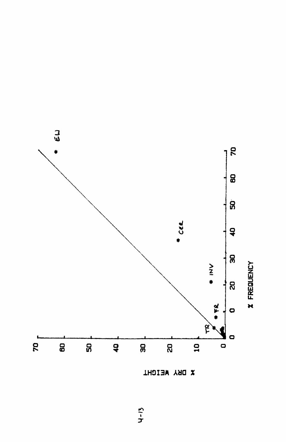
X DRY WEIGHT
ooro o8o01 0)0 0 (
M
38O

Pig. 4.14. 'Kruidc-plot' (see Pig. 4.3.) of the badger diet, as determined by percent volume per faeces.
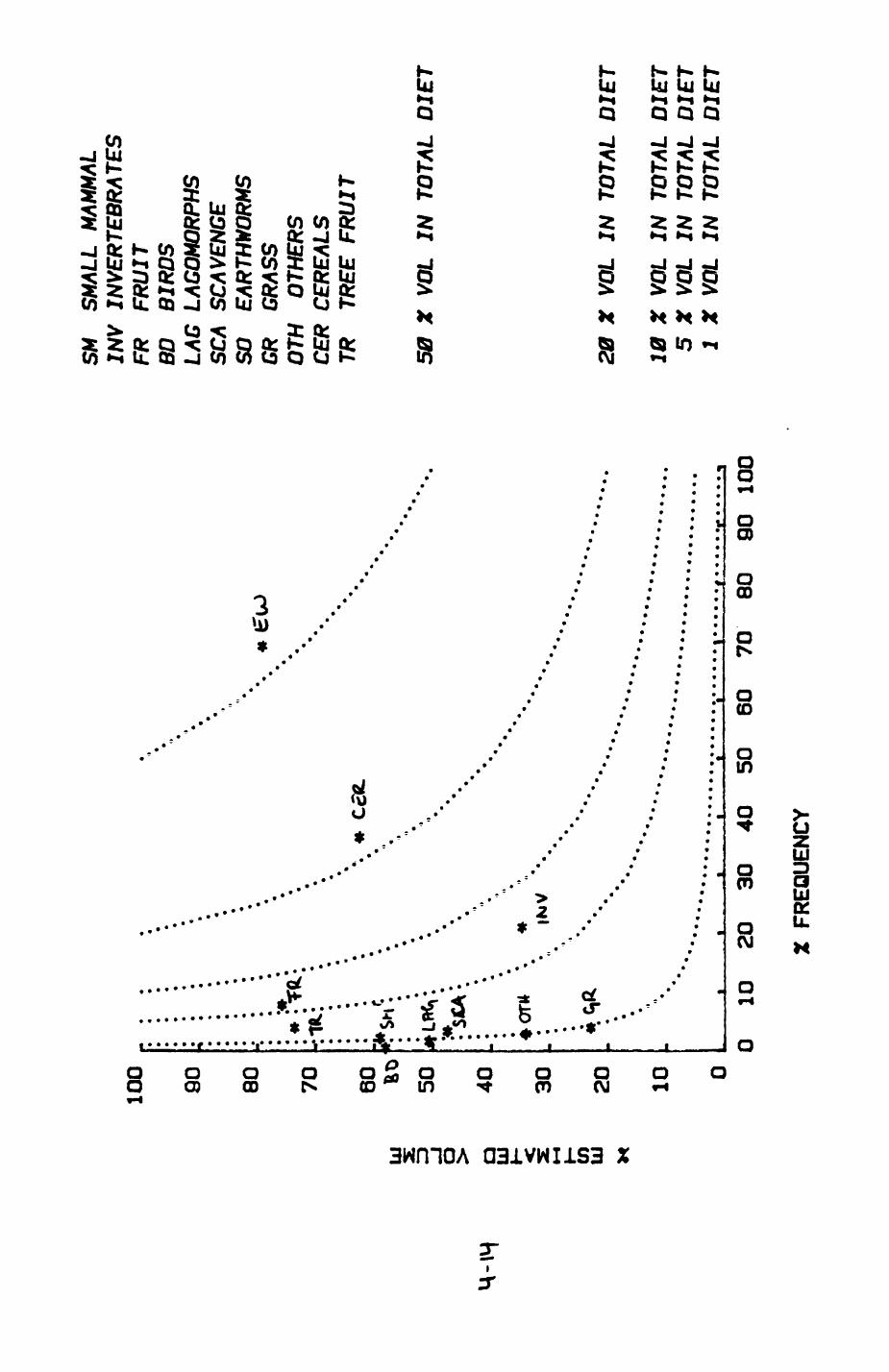
X ESTIMATED VOLUME
i-» ro o oa) oen ooCD 0<D 0a 0
m o
r\> o
0)o
Qen o
CD o
CDo
CDo
a o
*o
•' *n\ t
*- tn
§§§§
H "H H3 S 3r- r-D C3 M Mrn rrj
5r- DMrnH
co toH ^ rn r- co

Pig. 4.15. Monthly changes in the diet of wytham's badgers, as determined by estimated dry weight, sequence of prey types Identical as in Pig. 4.5 for foxes.
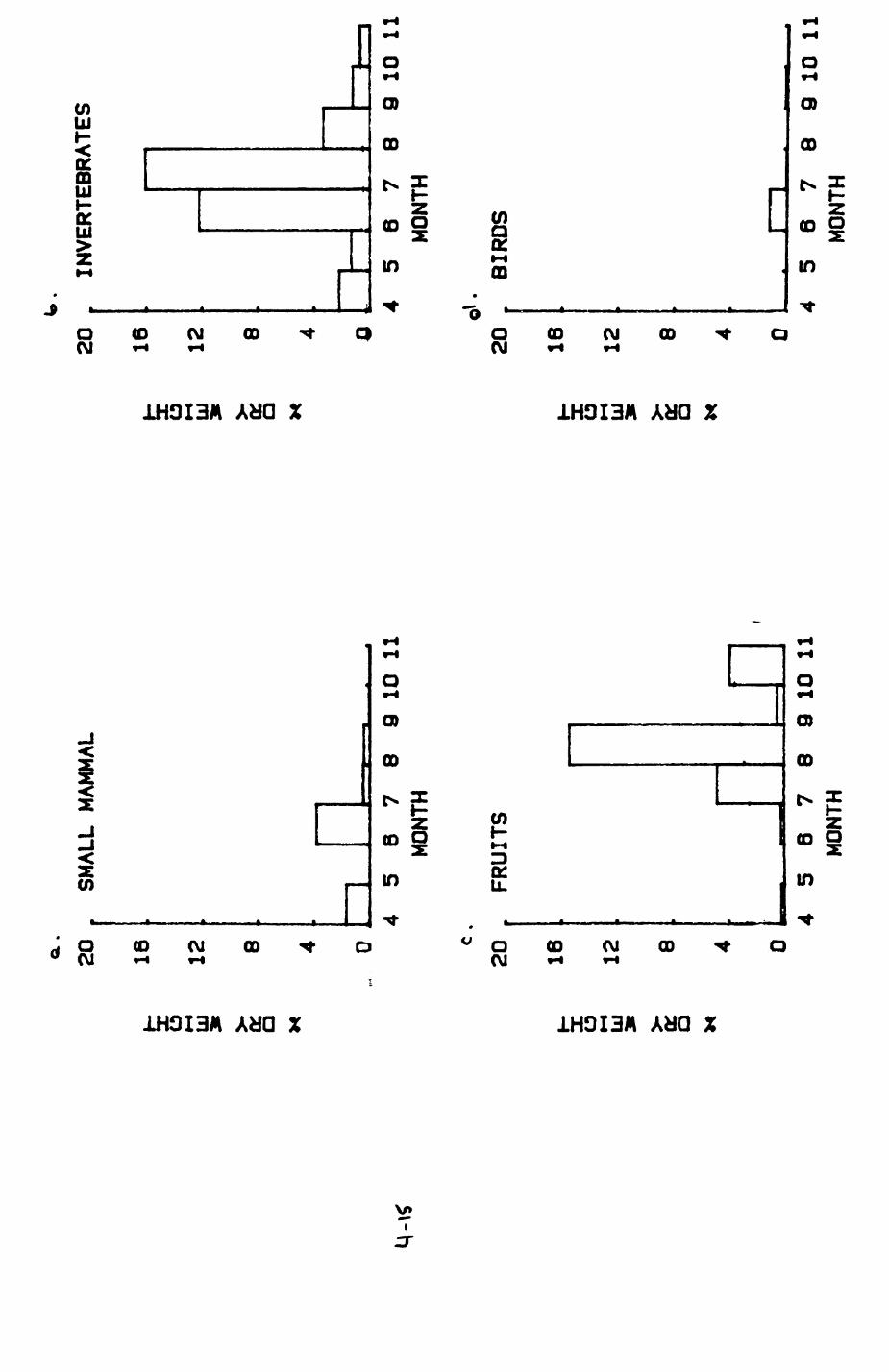
X DRY WEIGHTX DRY WEIGHT
•-• i-» IN) O 4** CD IN) O) O
en
O)
CD
(Ol-» O
en
CD
CDK* O
»-»»-» IN) 0 <D IN) O) O P
X DRY WEIGHTX DRY WEIGHT
Ul
u>
CD
(0
O
•-*•-* IN) O *. OD IN) O> O I
•
t-4 W
1 S § ^
CD
(0>-* 0»-*
k- K- |\)t) 4^ QD IN) 0) Of » 4 U 4 "^
iN ———————— —— . m
CDro
m
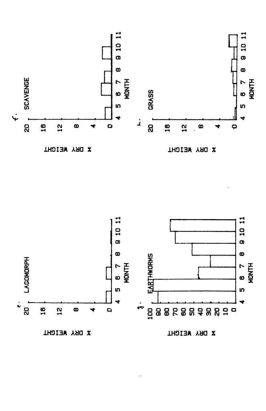
X DRY WEIGHTX DRY WEIGHT
ena: o o> -i , X >l
00
<O
0 I-*K*
i
en 3: — O 0)
GO
CO
o
DOOOOOOOOOO^
>» Ul
i X ° ^———— , — o d xj
30 3= ^ —————— 1 ———— 0) Q)
"" "' (O
—————————— i. o
% DRY WEIGHT
*-» •-» i\)b *• GO 10 CO O r (.......
1 § <"gj |o>
-4J x ^
1 ^ •J to
J -
•-*»-» f\) t) *h. GO !\> O) O
j
Cl
p IX
X DRY WEIGHT
»-*•-» i\)D * GO IN) CO O
J „Om om
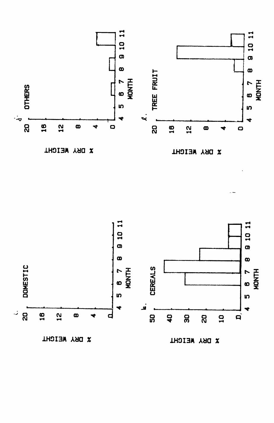
X DRY WEIGHTX DRY WEIGHT
i- IN) Cl) * 01 1X
O1
O CDz
CD
CD
O
3 O O O O O
0 Wm _ ———— $ |°>to x ^
" ——— ' CD
—— —— (O
—— : °
D *> CO IN) CD O
aom0)
n
X DRY WEIGHTX DRY WEIGHT
01
O CD
CD
CO
O »-• . .
D^CDIN)CDO O^.COIN)CDO
» WS a: m 0 CD
3 |^ i~«— j H co
J "
o
](n 3
141
September and to nearly the same extent In August and November. In August
and September the ripening of blackberries (Rubus fruticosus) is responsible
for the big contribution of fruits While the November peak is due to some
cultivated fruits (apple, etc.)* Birds are only eaten in July, lagomorphs
in May and July (this is in common with small mammals). Scavenge is taken
to some extent in each of the three seasons represented, as is grass.
Earthworms, however, show a marked decline from spring to a minimum in July
and August and an Increase during autumn. Tree fruits are mainly consumed
In October (due to the sweet chestnut mast). Cereals peak In August but are
still heavily consumed during September and to some extent In October and
November. This is most likely due to the fact that cereals remain available
at the edges of fields even after they have been harvested (September) while
the consumption In middle and late autumn is probably due to the collection
of newly sown grain.
Table 4.10a shows the results of a Kruskal-Wallis one-way analysis of
variance on differences between months. Here, only the six most important
food types were investigated. All prey types show significant differences
between months.
4.3.3.3. Variation in the diet of different ranges
The following analysis is based on latrines of non-border status only.
4.3.3.3.1. General composition of the diet
Of the thirteen ranges that could be recognized (Chapter 5) some had to
be excluded because of insufficient sample sizes (Ranges B8, B9 and Bll,
Table 4.8) while for others there was not enough information available to
determine the range borders reliably (Ranges BO, B7 and B12, Chapter 5).
142
Pig. 4.16a and 4.16b depict the diet composition for the seven remaining
ranges. It emphasises the importance of earthworms for all seven ranges but
indicates that there was some variation between ranges, particularly in
earthworms but also in cereals, invertebrates and tree fruits. The Kruskal-
Wallis test confirms that these variations were significant (Table 4.1Ob).
Spatial variation in fruits and small mammals, however, were not
significant.
A posteriori multiple comparison tests (Table 4.11) were used to
examine differences between range pairs. In three out of four prey
categories two ranges with high prey values dominate all other ranges. With
the exception of Ranges Bl and B5 that do not occur In any of the
significant pairs when examining earthworms, each range appears at least
once in each of the prey categories considered. The high proportion of
pairs with significant differences indicate that variation is wide and well
spread amongst ranges for each prey type.
4.3.3.3.2. Temporal variation in the diet
Following the approach used in the analysis of the fox diet I shall
first discuss seasonal changes within each range before I look at the
spatial variation within a temporal unit and the degree of synchrony between
ranges in the direction of temporal fluctuations.
Changes within individual ranges Pig. 4.17 depicts the temporal variation
in the composition of the diet of two ranges, Jews Harp (Range B4) and
Radbrook (Range BIO) for the four major prey categories. The graphs
exemplify how different the proportions can be between ranges and how
radically the proportions of any particular food type might change from
month to month. Consider for instance the rapid decline of Invertebrates in
Range Bio from a peak in August to almost nothing in September and the

Fig. 4.16. Differences in the diet of seven badger groups, as determined by estimated dry weight.
a. Ranges Bl, B2, B3.
b. Ranges 84, B5, B6, BIO.
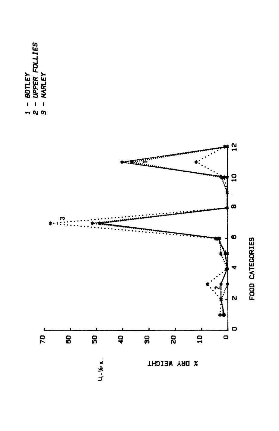
X DRY WEIGHT
0oro oU)o0
Ulo
CD O <
a o
m
§1-4mCfl
^—*»*****!ah*v* ••••••«•* rrrrrrrrr^-------^ *
(0 IN) ^ I I I
S8m
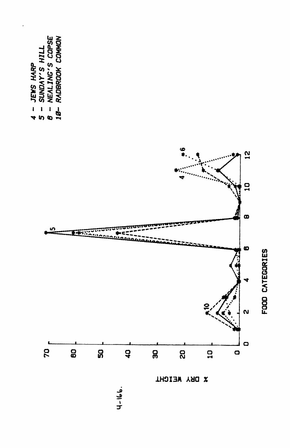
1tf-
X DRY WEIGHT
ooo0)oo
Ul 0
0> O (
Tl o8O
m
§!-• m
»-* CD en <u i i i i
</> 5o
5 o r- f^ O u>

Pig. 4.17. Monthly changes in the consumption of the four major prey types by badger groups B4 (JEWS HARP) and BIO (RADBRDOK COMMON).
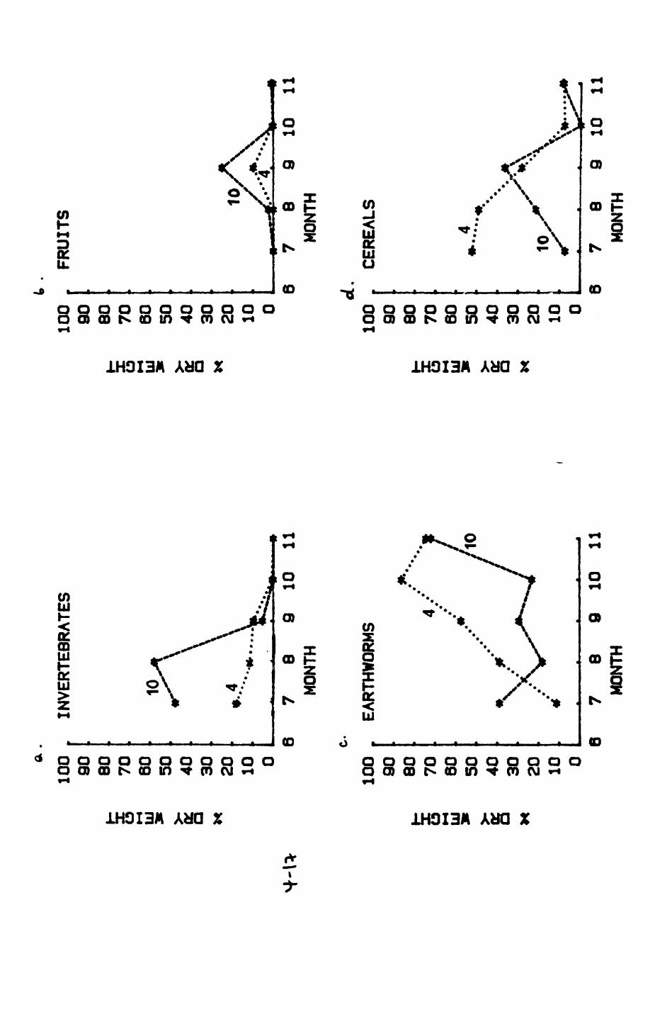
-cV
X DRY WEIGHTX DRY WEIGHT
oooooooooooO) r—,—i—i—,—,—,—,—,—,—i o
OOOOOOOOOOO p
<D
<o
o
m
o ;o0)
X DRY WEIGHT% DRY WEIGHT
•-» l\) (A) *. OI00000033888
O)
(D
(O
'\s.*
n m
(0
ooooooooooo
•n D
(0
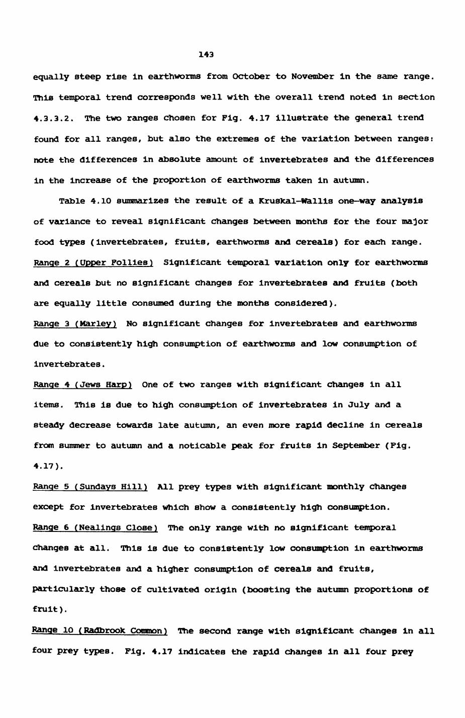
143
equally steep rise in earthworms from October to November in the same range.
This temporal trend corresponds well with the overall trend noted in section
4.3.3.2. The two ranges chosen for Pig. 4.17 illustrate the general trend
found for all ranges, but also the extremes of the variation between ranges i
note the differences in absolute amount of invertebrates and the differences
in the increase of the proportion of earthworms taken in autumn.
Table 4.10 summarizes the result of a Kruskal-Wallis one-way analysis
of variance to reveal significant changes between months for the four major
food types (invertebrates, fruits, earthworms and cereals) for each range.
Range 2 (Upper Follies) Significant temporal variation only for earthworms
and cereals but no significant changes for Invertebrates and fruits (both
are equally little consumed during the months considered).
Range 3 (Marley) No significant changes for invertebrates and earthworms
due to consistently high consumption of earthworms and low consumption of
Invertebrates.
Range 4 (Jews Harp) One of two ranges with significant changes in all
items. This is due to high consumption of invertebrates in July and a
steady decrease towards late autumn, an even more rapid decline in cereals
from summer to autumn and a noticable peak for fruits in September (Pig.
4.17).
Range 5 (Sundays Hill) All prey types with significant monthly changes
except for invertebrates which show a consistently high consumption.
Range 6 (Nealinqa Close) The only range with no significant temporal
changes at all. This is due to consistently low consumption in earthworms
and Invertebrates and a higher consumption of cereals and fruits,
particularly those of cultivated origin (boosting the autumn proportions of
fruit).
Range 10 (Radbrook Common) The second range with significant changes in all
four prey types. Pig. 4.17 indicates the rapid changes in all four prey
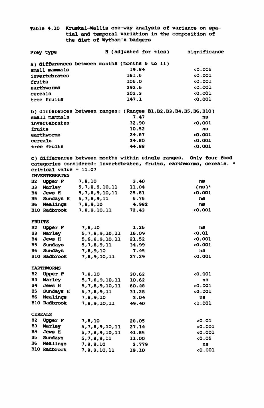
Table 4.10 Kruskal-Wallis one-way analysis of variance on spa tial and temporal variation in the composition of the diet of Wytham's badgers
Prey type H (adjusted for ties) significance
a) differences between months (months 5 to 11)small mammals 19.84 <0.005invertebrates 161.5 <0.001fruits 105.0 < 0.001earthworms 292.6 < 0.001cereals 202.3 <0.001tree fruits 147.1 <0.001
b) differences between rangesi (Ranges 81,82,83,84,85,86,810)small mammals 7.47 nsInvertebrates 32.90 <0.001fruits 10.52 nsearthworms 24.87 <0.001cereals 34.80 <0.001tree fruits 44.88 <0.001
c) differences between months within single ranges. Only four food categories considered! invertebrates, fruits, earthworms, cereals. * critical value = 11.07 INVERTEBRATES82 Upper F 7,8,10 3.4O ns83 Marley 5,7,8,9,10,11 11.04 (ns)*84 Jews H 5,7,8,9,10,11 25.81 <0.00185 Sundays H 5,7,8,9,11 5.75 ns86 Nealings 7,8,9,10 4.982 ns 810 Radbrook 7,8,9,10,11 72.43 <0.001
FRUITS82 Upper F 7,8,10 1.25 ns83 Marley 5,7,8,9,10,11 16.09 <0.0184 Jews H 5,6,8,9,10,11 21.52 <0.00185 Sundays 5,7,8,9,11 34.99 <0.00186 Sundays 7,8,9,10 7.45 ns810 Radbrook 7,8,9,10,11 27.29 <0.001
EARTHWORMS82 Upper F 7,8,10 30.62 <0.00183 Marley 5,7,8,9,10,11 10.62 ns84 Jews H 5,7,8,9,10,11 60.48 <0.00185 Sundays H 5,7,8,9,11 31.28 <0.00186 Nealings 7,8,9,10 3.04 ns810 Radbrook 7,8,9,10,11 49.4O <0.001
CEREALS82 Upper F 7,8,10 28.05 <0.0183 Marley 5,7,8,9,10,11 27.14 <0.00184 Jews H 5,7,8,9,10,11 41.85 <0.00185 Sundays 5,7,8,9,11 11.00 <0.0586 Nealings 7,8,9,10 3.779 ns810 Radbrook 7,8,9,10,11 19.10 <0.001
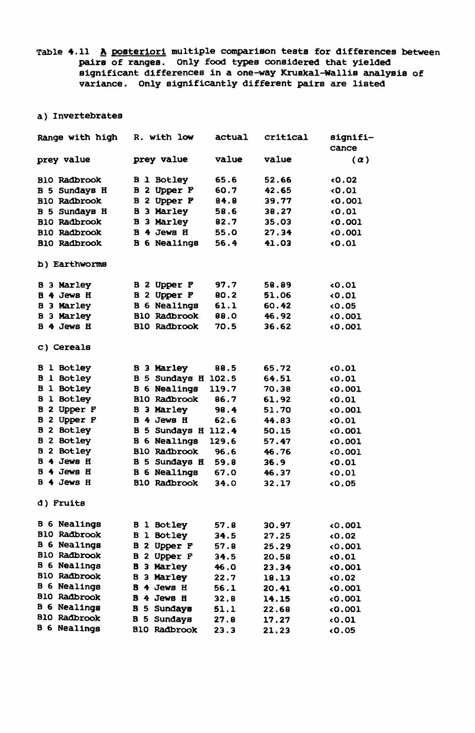
Table 4.11 A posteriori multiple comparison tests for differences between pairs of ranges. Only food types considered that yielded significant differences in a one-way Kruskal-wallis analysis of variance. Only significantly different pairs are listed
a) Invertebrates
Range with high R. with low
prey value
BIO Radbrook B 5 Sundays H BIO Radbrook B 5 Sundays H BIO Radbrook BlO Radbrook BIO Radbrook
b) Earthworms
B 3 MarleyB 4 Jews HB 3 MarleyB 3 MarleyB 4 Jews H
c) cereals
B 1 BotleyB 1 BotleyB 1 BotleyB 1 BotleyB 2 Upper FB 2 Upper FB 2 BotleyB 2 BotleyB 2 BotleyB 4 Jews HB 4 Jews HB 4 Jews H
d) Fruits
B 6 Nealings BIO Radbrook B 6 Nealings Bio Radbrook B 6 Nealings BlO Radbrook B 6 Nealings Bio Radbrook B 6 Nealings Bio Radbrook B 6 Nealings
prey value
B 1 Botley B 2 Upper F B 2 Upper F B 3 Marley B 3 Marley B 4 Jews H B 6 Nealings
B 2 Upper F B 2 Upper F B 6 Nealings BIO Radbrook BIO Radbrook
B 3 Marley B 5 Sundays H B 6 Nealings BIO Radbrook B 3 Marley B 4 Jews H B 5 Sundays H B 6 Nealings BIO Radbrook B 5 Sundays H B 6 Nealings BlO Radbrook
B 1 Botley B 1 Botley B 2 Upper F B 2 Upper F B 3 Marley B 3 Marley B 4 Jews H B 4 Jews H B 5 Sundays B 5 Sundays BIO Radbrook
actual
value
65.660.784.858.682.755.056.4
97.780.261.188.070.5
88.5102.5119.786.798.462.6112.4129.696.659.867.034.0
57.834.557.834.546.022.756.132.851.127.823.3
critical
value
52.6642.6539.7738.2735.0327.3441.03
58.8951.0660.4246.9236.62
65.7264.5170.3861.9251.7044.8350.1557.4746.7636.946.3732.17
30.9727.2525.2920.5823.3418.1320.4114.1522.6817.2721.23
signifi cance
(a)
<0.02<0.01<0.001<0.01<0,001<0.001<0.01
<0.01<0.01<O.05<0.001<0.001
<0.01<0.01<0.001<0.01<0.001<0.01<0.001<0.001<0.001<0.01<0.01<0.05
<0.001<0.02<0.001<0.01<0.001<0.02<0.001<0.001<0.001<0.01<0.05
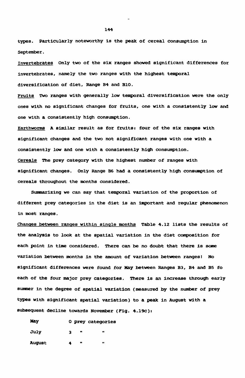
144
types. Particularly noteworthy is the peak of cereal consumption in
September.
Invertebrates Only two of the six ranges showed significant differences for
invertebrates, namely the two ranges with the highest temporal
diversification of diet, Range B4 and BIO.
Fruits Two ranges with generally low temporal diversification were the only
ones with no significant changes for fruits, one with a consistently low and
one with a consistently high consumption.
Earthworms A similar result as for fruits t four of the six ranges with
significant changes and the two not significant ranges with one with a
consistently low and one with a consistently high consumption.
Cereals The prey category with the highest number of ranges with
significant changes. Only Range B6 had a consistently high consumption of
cereals throughout the months considered.
Summarizing we can say that temporal variation of the proportion of
different prey categories in the diet is an important and regular phenomenon
in most ranges.
Changes between ranges within single months Table 4.12 lists the results of
the analysis to look at the spatial variation in the diet composition for
each point in time considered. There can be no doubt that there is some
variation between months in the amount of variation between ranges! No
significant differences were found for May between Ranges B3, B4 and B5 fo
each of the four major prey categories. There is an Increase through early
summer in the degree of spatial variation (measured by the number of prey
types with significant spatial variation) to a peak in August with a
subsequent decline towards November (Pig. 4.19c)i
May 0 prey categories
July 3 " n
August 4 "
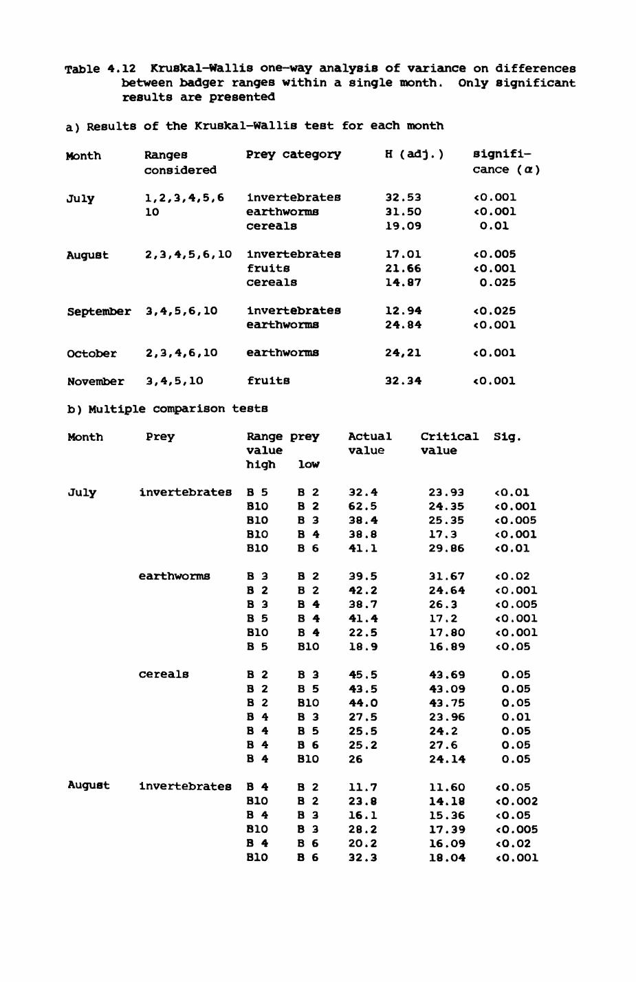
Table 4.12 Kruskal-Wallis one-way analysis of variance on differences between badger ranges within a single month. Only significant results are presented
a) Results of the Kruskal-Wallis test for each month
Month Ranges Prey category H (ad j. )
July
August
Ranges considered
1,2,3,4,5,6 10
signifi cance (a)
invertebratesearthwormscereals
2,3,4,5,6,10 invertebratesfruits cereals
September 3,4,5,6,10
October 2,3,4,6,10
November 3,4,5,10
invertebrates earthworms
earthworms
fruits
b) Multiple comparison tests
Month
July
Prey
invertebrates
earthworms
cereals
August invertebrates
32.5331.5019.09
17.0121.6614.87
12.9424.84
<0.001<0.0010.01
<0.005<0.0010.025
<0.025<0.001
24,21
32.34
<0.001
<0.001
Rangevaluehigh
B 5BIOBIOBIOBIO
B 3B 2B 3B 5BIOB 5
B 2B 2B 2B 4B 4B 4B 4
B 4BIOB 4BIOB 4BIO
prey
low
B 2B 2B 3B 4B 6
B 2B 2B 4B 4B 4BIO
B 3B 5BIOB 3B 5B 6BIO
B 2B 2B 3B 3B 6B 6
Actualvalue
32.462.538.438.841.1
39.542.238.741.422.518.9
45.543.544.027.525.525.226
11.723.816.128.220.232.3
Criticalvalue
23.9324.3525.3517.329.86
31.6724.6426.317.217.8016.89
43.6943.0943.7523.9624.227.624.14
11.6014.1815.3617.3916.0918.04
Sig.
<0.01<0.001<0.005<0.001<0.01
<0.02<0.001<0.005<0.001<0.001<0.05
0.050.050.050.010.050.050.05
<0.05<0.002<0.05<0.005<O.02<0.001
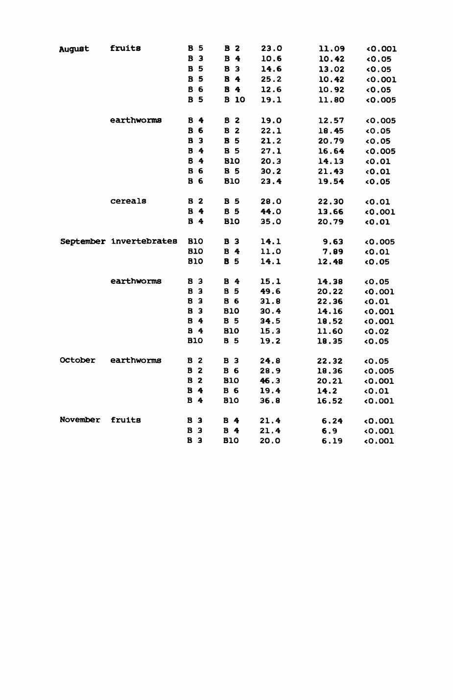
August fruits
earthworms
cereals
September invertebrates
earthworms
October earthworms
November fruits
B 5B 3B 5B 5B 6B 5
B 4B 6B 3B 4B 4B 6B 6
B 2B 4B 4
BIOBIOBIO
B 3B 3B 3B 3B 4B 4BIO
B 2B 2B 2B 4B 4
B 3B 3B 3
B 2B 4B 3B 4B 4B 10
B 2B 2B 5B 5BIOB 5BIO
B 5B 5BIO
B 3B 4B 5
B 4B 5B 6BIOB 5BIOB 5
B 3B 6BIOB 6BIO
B 4B 4BIO
23.010.614.625.212.619.1
19.022.121.227.120.330.223.4
28.044.035.0
14.111.014.1
15.149.631.830.434.515.319.2
24.828.946.319.436.8
21.421.420.0
11.0910.4213.0210.4210.9211.80
12.5718.4520.7916.6414.1321.4319.54
22.3013.6620.79
9.637.8912.48
14.3820.2222.3614.1618.5211.6018.35
22.3218.3620.2114.216.52
6.246.96.19
<0.001<0.05<0.05<0.001<0.05<0.005
<0.005<0.05<O.05<0.005<0.01<0.01<0.05
<0.01<O.OO1<0.01
< 0.00 5<0.01<0.05
<O.05<0.001<0.01<0.001<0.001<0.02<0.05
<0.05<0.005<0.001<0.01<0.001
<0.001<O.001<0.001
145
September 2 " "
October 1
November 1
Invertebrates There is significant spatial variation during peak
consumption times (July and August) and during a general decline in
consumption (September).
Fruits significant spatial variation occurs before peak consumption time in
August and after peak consumption time in late autumn (November).
Earthworms Earthworms Is the prey category with the highest spatial
diversificationi there is significant variation for all months except May
and November, Which are times of peak consumption While the other months
form the mid-year "trough".
Cereals Significant spatial changes occur in times of peak consumption
(July and August).
Thus there is considerable variation for all food types, but the
spatial variation may occur either at times of peak or low consumption.
Synchronization in the changes of the diet between ranges As Pig. 4.17
indicated, ranges might show similarities in the way a diet component
changes in its proportion from month to month (e.g. fruits) but also
differences (marked differences In cereals, also some variation in
earthworms). In Table 4.13b the results of the statistical analysis using
Kendall's coefficient of concordance are presented. As could have been
guessed from Fig. 4.17, the similarities between ranges In the direction of
changes in the proportions of prey types are significant only for fruits and
Invertebrates, but not for cereals or earthworms.
4.3.3.4 comparison of border and non-border latrines
So far the analysis of the badger diet in Wytham largely Involved
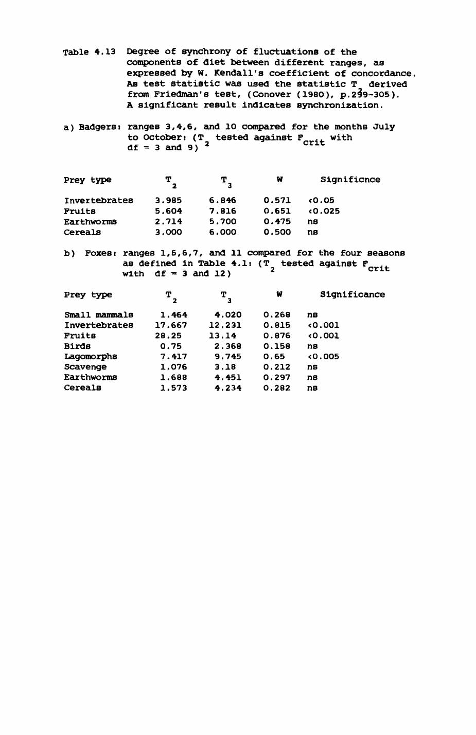
Table 4.13 Degree of synchrony of fluctuations of thecomponents of diet between different ranges, as expressed by W. Kendall's coefficient of concordance. As test statistic was used the statistic T derived from Friedman's test, (Conover (1980), p. 29*9-305). A significant result indicates synchronization.
a) Badgersi ranges 3,4,6, and 10 compared for the months July to Octoben (T tested against P .. with df = 3 and 9) 2 crit
Prey type T T w Significnce
Invertebrates 3.985 6.846 0.571 <0.05Fruits 5.604 7.816 0.651 <0.025Earthworms 2.714 5.700 0.475 nsCereals 3.000 6.000 0.500 ns
b) Foxesi ranges 1,5,6,7, and 11 compared for the four seasons as defined in Table 4.1i (T tested against Fwith df = 3 and 12) 2
Prey type T T W Significance
Small mammals 1.464 4.020 0.268 nsInvertebrates 17.667 12.231 0.815 <0.001Fruits 28.25 13.14 0.876 <0.001Birds 0.75 2.368 0.158 nsLagomorphs 7.417 9.745 0.65 <0.005Scavenge 1.076 3.18 0.212 nsEarthworms 1.688 4.451 0.297 nsCereals 1.573 4.234 0.282 ns
146
latrines that could be associated with one range only. I now want to
Investigate whether faeces collected from latrines on the border between
ranges differ In their composition from those collected from latrines that
lay Inside the neighbouring ranges. If for Instance two neighbours had a
radically different diet and utilized the border latrines to equal amounts,
differences should occur between border latrines (which comprise a sort of
compromise of the diets of the two ranges) and the latrines lying inside the
range of each neighbour.
There is no published evidence so far that badgers can detect the
components of faeces. However, it is reasonable to assume that they can do
so both by appearance and odour. It is known that badgers smell their prey,
particularly earthworms (Kruuk, 1978b, pers. obs.) and that they are also
able to distinguish individual badgers from their own group from badgers
from another group by smell (KruuX et al., 1984, Gorman et al., 1984).
Beauchamp (1976) showed that guinea pigs (Cavla)can distinguish different
metabolites In the urine of conspeclfics. Badgers may therefore have some
information about the diet of their neighbours. This may not bee particularly usful during favourable times (e.g. In spring when all badgers
eat a plentiful supply of earthworms). But at times when conditions are
generally unfavourable (e.g. summer with Its short, dry nights reducing the
available earthworm populations) it would be of great value for badgers to
assess what food resources the neighbouring ranges were exploiting. If
badgers in one range have a disproportionate amount of a desirable resource
It would seem to be beneficial to conceal this fact.
I Investigated possible differences between border and non-border
latrines In three stepsi
1. For each range, border and non-border latrines were compared for
possible differences In diet composition (always only the four major prey
147
types considered).
2. All border latrines were split according to the neighbouring range and
for each possible differences between border latrines shared with different
neighbours were investigated. For instance, Range B4 (Jews Harp) shared
border latrines with neighbouring Ranges B 3 (Marley), B5 (Sunday Hills) and
B6.
Results can be summarized briefly. No differences were found for any
comparisons with two interesting exceptions! there were significant
differences between border and non-border latrines in the amount of
invertebrates consumed in July (Kruskal-Wallls test, H (adjusted) - 8.1O2,
df - 2, n = 230, p<O.O25) and there were differences in the amount of
earthworms consumed in August (t-test, t = 1.99, df = 174, p = O.O49). In
both cases the non-border latrines had a higher proportion of the food type
in question than the border latrines. As these are results when the border
latrines and non-border latrines are lumped over all ranges it is not
possible to say whether these effects are restricted to particular borders
accounting for the significant variation or whether this is actually the
case for all borders. As Table 4.12 shows, there is significant spatial
variation both for Invertebrates in July and earthworms in August. If the
composition of samples from the borders are a compromise of the diet of the
neighbours, then there should be no significant differences between border
and non-border latrines unless there is an active selection process by the
badgers. Whether this is the case or not has to be determined by
experimental procedures but the decision to distinguish between border and
non-border latrines is certainly justified in the light of these results.
An alternative explanation would be that males and females had different
diets (at least for this period) and also different tendencies to use border
latrines and non-border latrines. Although nothing is known about possible
148
sex differences, the results of the radiotracking seem to indicate that
female badgers at least visit border latrines regularly. This of course
does not exclude the possibility that males visit the border latrines even
more frequently, but the proportion of 'active* latrines is lower during
summer than in spring or autumn. Previous studies (e.g. by Kruuk and
others) never indicated whether they distinguished between border and non-
border latrines for their sampling scheme or during analysis. However,
Kruuk (pers. comm.) states that he usually excluded border latrines from his
sampling scheme.
4.3.4. Badger diett summary
1. 1O53 badger droppings were collected between May 1982 and October 1983
with samples in each month from May until November each year.
2. Earthworms were the most important component of the diet with 69% of
samples containing earthworms and 61% of the estimated dry weight (EDW).
Cereals are the second most Important component with 36.5% frequency of
occurrence (PO) and 17.7% EOW, followed by Invertebrates (21.1% PO and 5.4%
EDW), fruits (7.9% PO and 3.5% EDW) and tree fruits (4% PO and 4.2% EDW).
3. Of the twelve prey categories considered, eight occurred in less than 10%
of the samples and seven of them contributed less than 1.5% EDW each.
4. There is marked temporal variation in some food types but not in others.
The main components of the diet (earthworms, cereals, fruits, invertebrates)
show a marked variation. Invertebrates, fruits, and cereals are mostly
consumed during July and August, while earthworms are mostly consumed in
spring and autumn with a trough in consumption in July and August. These
149
changes are highly significant.
5. There is a highly significant variation in the diet composition of
different badger ranges for four prey types (invertebrates, earthworms,
cereals, tree fruits). Only small mammals and fruits are equally consumed
in different ranges. Each range appears in at least one pair of
significantly different ranges for each food type that showed an overall
significant spatial variation. The only exceptions are Ranges Bl and B5 for
earthworms. Variation in the diet composition is highly and equally well
spread amongst ranges.
6. within each range, there is marked temporal variation in the amount of
each of the four major prey types consumed (invertebrates, fruits,
earthworms, cereals), with the exception of invertebrates where only two out
of six ranges varied significantly. Variation is similar in direction but
partly different in magnitude between different ranges.
7. There is some variation between months in the amount of variation between
ranges. Significant spatial variation in invertebrates occurs from July to
September and in fruits in August (time of peak consumption) and November
(time of low consumption). Earthworms showed significant spatial variation
from July to October at a time when all ranges generally increased their
consumption of earthworms but at different rates of change, converging in
November. Ranges show also significant differences in the amount of cereal
consumption in July and August (peak consumption time). Ranges were
synchronized in the direction of temporal fluctuations of prey consumption
only for invertebrates and fruits but not in their changes of cereal or
earthworm consumption.
150
8. Comparisons of border and non-border latrines for each range did not
yield significant differences, nor did a comparison of border latrines
shared with different neighbours, if all months are lumped. However, if
data are lumped over all ranges, there was a significantly higher proportion
of Invertebrates represented in non-border latrines than in border latrines
in July and the same was valid for earthworms in August.
4.3.5. Comparison with other studies
Fortunately, the diet of Wytham f s badgers has been studied several
times before (Hancox (1973), Hubertz (1978) and Kruuk (1978b)). Despite
apparent differences between the studies in sampling design, purpose and
duration, a broad consensus emerges. Hancox (1973) found that earthworms
occurred in 91% of over 2OOO badger faeces he collected from Wytham Woods,
making up a total volume of 61%, a figure that comes very close to my result
of 63.5% (estimated dry weight (EDW)) and 54% (estimated percent volume, ie.
not corrected for the weight of the dropping). Kruuk (I978b) found in a
sample of 39 droppings from September/October 1974 earthworms the most
important element, followed by cereals, Insects, bird remains and acorns.
Hubertz (1978) found from a sample of two periods during summer (beginning
and end of July) similar results as my study for July. Together with my
study there is unequivocal evidence for the consistently important role
earthworms play for the badger population at Wytham. Other studies from
Britain (Kruuk et al., (1979), Kruuk and Parish (1981), Meal (1977)) support
this Impression and serve to confirm the notion of the badger as an
'earthworm specialist' (Kruuk and Parish (1981)). An interesting exception
was found by Harris (1982, 1984). He investigated the social structure and
the diet of a suburban population of badgers around Bristol and found
scavenged items to be the generally most important element of the diet, only
151
surpassed by fruits in late summer and early autumn. Earthworms generally
constituted between 20% and 3O% of the diet (estimated by percent volume)
with less marked seasonal variation as in this study. From other European
countries there are the notable studies of Andersen (1954) from Denmark,
Skoog (1970) from Sweden, Wlertz (1976) from Holland and a brief study by
Kruuk and De Koclc (1981) on the diet of badgers in northern Italy.
Earthworms were again the most or one of the most important elements of the
diet with the interesting exception of the Italian badgers which almost
exclusively ate olives. However, there are also local variations. Wlertz
(1976) emphasised the regularity by which small mammals and birds are
consumed all year around by Dutch badgers (measured by PO). Skoog (1970)
distinguished between a group of primary foods (most importantly earthworms)
also insects, plant foods and mammals) and secondary foods (birds, molluscs,
amphibians, reptiles and garbage plus carrion) in the diet of the Swedish
badger. He also found a seasonal decline in earthworm consumption during
summer and related this to the suboptimal soil temperatures with their
detrimental effects on the activity and size of earthworm populations.
Andersen's (1954) results on the diet of the Danish badgers showed
similarities to SXoog'8 (1970) results both for the general composition and
the seasonal variations. The large number of Insectivores, especially
shrews, that were eaten by Danish badgers was notable.
Excluding the two atypical studies of Harris (1982, 1984) and Kruuk and
De Kock (1981), the seasonal trends found at different study sites emerge as
remarkably similar for the prey types considered. However, there is only
one study available with a full investigation of spatial trends t Kruuk and
Parish's study (1981) on the diet of the Scottish badger (differences
between several sites were also partly evaluated by Skoog (1970) and inertz
(1976)). They compared the results of six study areas, ie. six different
populations of badgers. So far, my study is the only one to have
152
investigated spatial variation within one study population. Comparing the
results of the different study populations in Scotland with the results of
the different ranges within the Wytham populations, some similar spatial and
temporal trends appear. Invertebrates and fruits peak at the same times for
both studies (if measured by percent volume)i also the spatial units in both
studies are synchronized for both prey items. Cereals peak at the same
times in both studies j In Scotland the study areas were synchronized in
their temporal fluctuations of cereal consumption while in my study the
badger ranges were not. No synchronization between spatial units were found
in either of the studies for earthworms. Interestingly, the Scottish
badgers did not consume more earthworms in autumn than in summer (measured
by percent volume) but decreased in their consumption slightly, while the PO
of earthworms in samples was much higher in Scotland than in Wytham.
So far, no study except this one has distinguished between border and
non-border latrines explicitly; in actual fact, hardly any study reports on
the sampling scheme applied (most authors simply referred to the 'collection
of droppings from latrines at setts and in the vegetation'). Therefore it
is not possible to estimate the errors associated with the results of each
study except in very general terms (e.g. sample size). From the results of
my study some conclusions can be drawn on an appropriate sampling scheme.
For instance, the sharp changes that can occur from month to month as
detailed in previous sections (and also found to some extent by Skoog (197O)
and others) are not adequately brought out by sampling latrines every two
months (examples are Kruuk's and co-worker's studies). Most studies used
only frequency of occurrence as a measure of diet and thus ignored most of
the Information that can be extracted from an analyis of the food remains.
Whether the amount of underground defaecation follows temporal fluctuations
of some kind is not known. Presumably the droppings placed underground are
a similar, representative sample of the total diet as the droppings above
153
ground, so that ignoring them does not Introduce a systematic bias but
merely reduces the number of droppings available for sampling.
4.4. Comparison of fox and badger diet
The following comparison of the results of the analyses of the diet of
Wytham's foxes and badgers emphasises patterns that emerged in sections 4.2
and 4.3. It was not possible to sample the faeces of both species in a
directly comparable manner, since the patterns of deposition are different.
This does not impede comparison of the diets of the two species since the
collection resulted in a representative sample of faeces for both. Due to
the reduced activity of the badgers in winter and the priorities of the
study in spring, it was not possible to sample all seasons for the analysis
of the badger diet. As a result concise information on the badger diet
exists only for part of the year, although there is some indication as to
what they consume during winter and spring. This of course reduces a
quantitative comparison of the diet of the two species to the time from Hay
until November.
Prom the results of the overall diet a measure of proportional overlap
in resource utilization was computed (Colwell & Futuyma (1971), Southwood
(1978)i
11
resource overlap - 1 - 0.5 £ |
with p± t the proportion of estimated dry weight for
a given prey category for a given species
The proportion of each prey category was recalculated after ••others'*
154
had been extracted. "Others" were excluded because It was not a taxonomlc
unit but an assemblage of various 'curiosities', and each type of curiosity
occurred only once or twice. Resource overlap for the general diet as
calculated by equation (1) was 0.46 for Wytham's foxes and badgers/ this
value is half-way between perfect separation (overlap - 0) and perfect
overlap (overlap =1).
Of the twelve major prey types considered, four items turned out to be
Important for badgers (earthworms, cereals, invertebrates, fruits) while
there was a group of seven items important to foxes (earthworms, lagomorphs,
scavange, fruits, birds, small mammals, invertebrates). Even though the
badger diet was sampled only for late spring, summer, and autumn, this
conclusion would presumably still hold for the entire year, as the cereals
and fruits proved to be such an Important part of the diet during summer.
In general, food types show the same marked, temporal variation in
magnitude and direction for both speciesi invertebrates and fruits peak
during summer (so do small mammals for foxes and cereals for badgers and
foxes). There are peaks of earthworm consumption in late spring and autumn
for badgers (presumably also In early spring) and in late spring, autumn and
winter for foxes. In addition, foxes ate lagomorphs mainly in late winter
and spring and birds in May and June (badgers in July).
There is some variation in the diet composition of animals in different
ranges for both foxes and badgers. The picture here is a little bit more
complicated! fruits and small mammals are consumed equally in all badger
ranges considered, but all other prey types (invertebrates, cereals,
earthworms, tree fruits) vary significantly between ranges. In contrast,
the three types of prey that showed significant spatial variation in foxes
were small mammals, scavenge and lagomorphs. Variation between badger
ranges is generally large and well spread as Indicated by the high number of
pairs of ranges with significant differences between the ranges of that pair

Pig. 4.18. Pie charts of the diet of wytham's foxes and badgers as determined by estimated dry weight. Abbreviations for prey items as before.
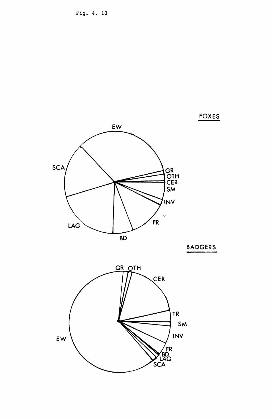
Fig. 4. 18
FOXES
EW
SCA
INV
LAG FR
BADGERS
GR OTH
CER
EW
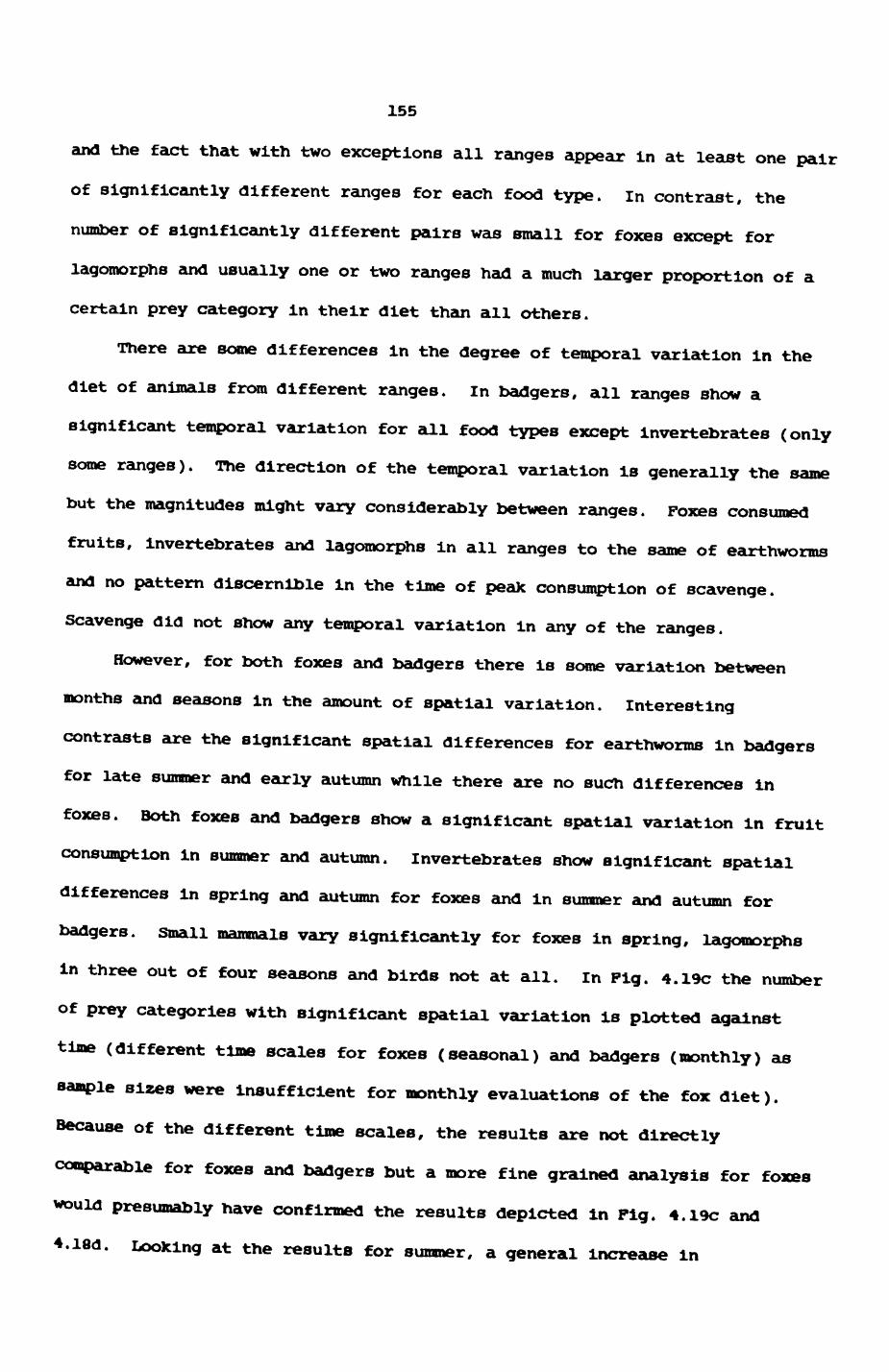
155
and the fact that with two exceptions all ranges appear in at least one pair
of significantly different ranges for each food type. In contrast, the
number of significantly different pairs was small for foxes except for
lagomorphs and usually one or two ranges had a much larger proportion of a
certain prey category in their diet than all others.
There are some differences in the degree of temporal variation in the
diet of animals from different ranges. In badgers, all ranges show a
significant temporal variation for all food types except invertebrates (only
some ranges). The direction of the temporal variation is generally the same but the magnitudes might vary considerably between ranges. Foxes consumed
fruits, invertebrates and lagomorphs in all ranges to the same of earthworms and no pattern discernible in the time of peak consumption of scavenge.
Scavenge did not show any temporal variation in any of the ranges.
However, for both foxes and badgers there is some variation between months and seasons in the amount of spatial variation. Interesting
contrasts are the significant spatial differences for earthworms in badgers for late summer and early autumn while there are no such differences in
foxes. Both foxes and badgers show a significant spatial variation in fruit consumption in summer and autumn. Invertebrates show significant spatial
differences in spring and autumn for foxes and in summer and autumn for
badgers. Small mammals vary significantly for foxes in spring, lagomorphs in three out of four seasons and birds not at all. In Pig. 4.19c the number of prey categories with significant spatial variation is plotted against
time (different time scales for foxes (seasonal) and badgers (monthly) as
sample sizes were insufficient for monthly evaluations of the fox diet).
Because of the different time scales, the results are not directly
comparable for foxes and badgers but a more fine grained analysis for foxes
would presumably have confirmed the results depicted In Pig. 4.19c and
4.l8d. Looking at the results for summer, a general increase in

Pig. 4.19. Comparison of seasonal changes in the diet of Wytham's foxes and badgers In
a. number of prey types present In the diet per month, for entire populations.
b* resource overlap between foxes and badgers as computed by Col we11 & Futuyma's (1971) formula (see text); data from entire populations.
c. spatial diversity of diet, ie. the number of prey items with significant differences in consumption between groups; for badgers evaluated per month, excluding June; for foxes evaluated per season and plotted for the central month of each season.
d. proportional spatial diversity of diet, ie.spatial diversity in relation to total number of different prey types consumed per time unit.
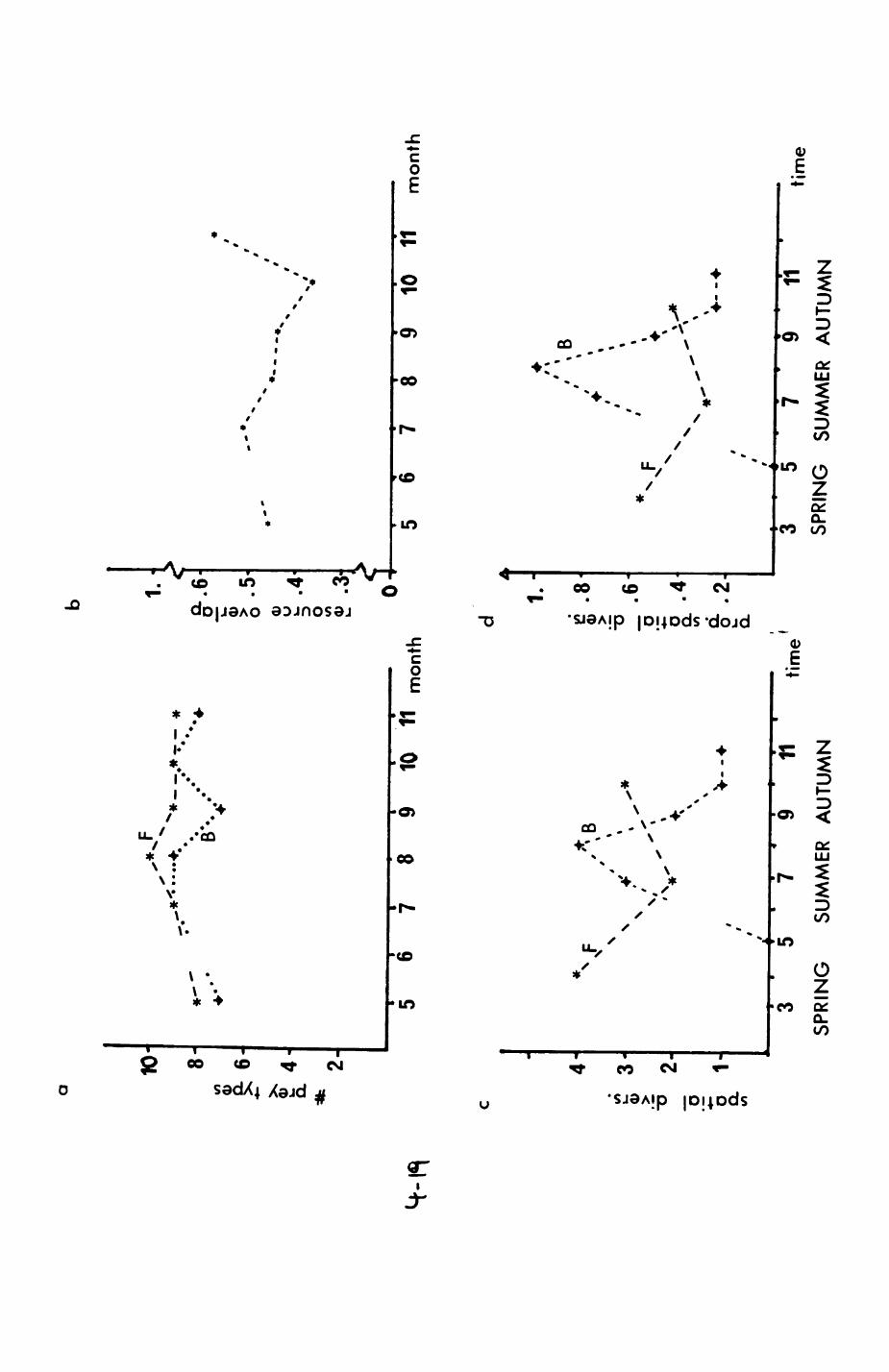
spatial divers. -» ro co
prey typesroa>co 8
co-oxO CO.
ZO
Cn-
COC£ ^'m
C— I
^Z — '
•
_^
tn.
/' a>-"» x X
x' "^J"\ ^NX-'-'ci4
-f''' *' O" •f
^'
O
t 1 *. \
•\**A: \: \
y i• i\ * •. §
V
/iV *
3' 2. a> 3~prop, spatial divers. Q- resource overlap
* • * * ViA ^B^ • • ^pJt
ro £t ar> oo • ° _ £^ ^ tn OT> _ • 1 . « A • Ik.
CO CO
?D
Z O en
COc^ -JmxO
^x (O<c-H
i*•
/ 0><*«» *in
«/ -^1- '
^ * ^ \ ..%-:* \ * " * * no V4"" ^^
t* * _^' O'
^'
3
^^ — "^~ * * 1 ^\ • J~* v* V
<
«i/
/*i i
J*/
//
*«,* >
*
f i (D -*•
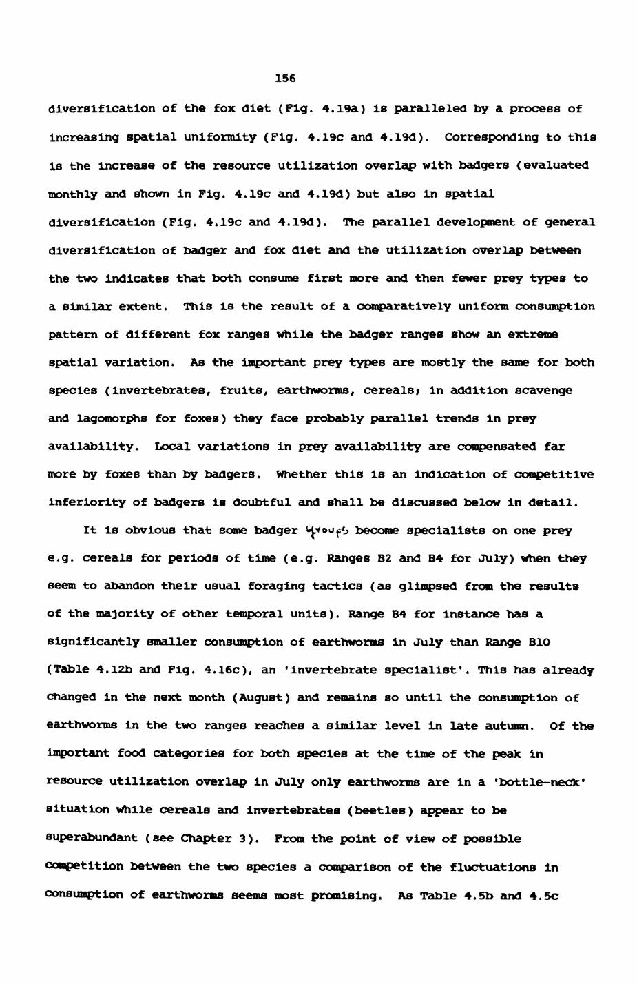
156
diversification of the fox diet (Fig. 4.19a) Is paralleled by a process of
increasing spatial uniformity (Pig. 4.19c and 4.19d). Corresponding to this
is the Increase of the resource utilization overlap with badgers (evaluated
monthly and shown in Fig. 4.19c and 4.19d) but also In spatial
diversification (Fig. 4.19c and 4.19d). The parallel development of general
diversification of badger and fox diet and the utilization overlap between
the two Indicates that both consume first more and then fewer prey types to
a similar extent. This is the result of a comparatively uniform consumption
pattern of different fox ranges while the badger ranges show an extreme
spatial variation. As the important prey types are mostly the same for both
species (invertebrates, fruits, earthworms, cerealsj in addition scavenge
and lagomorphs for foxes) they face probably parallel trends in prey
availability. Local variations in prey availability are compensated far
more by foxes than by badgers. Whether this is an indication of competitive
inferiority of badgers is doubtful and shall be discussed below In detail.
It is obvious that some badger t^foufO become specialists on one prey
e.g. cereals for periods of time (e.g. Ranges B2 and B4 for July) when they
seem to abandon their usual foraging tactics (as glimpsed from the results
of the majority of other temporal units). Range B4 for instance has a
significantly smaller consumption of earthworms in July than Range Bio
(Table 4.l2b and Fig. 4.16c), an 'invertebrate specialist*. This has already
changed in the next month (August) and remains so until the consumption of
earthworms in the two ranges reaches a similar level In late autumn. Of the
important food categories for both species at the time of the peak in
resource utilization overlap in July only earthworms are in a 'bottle-neclc'
situation while cereals and invertebrates (beetles) appear to be
superabundant (see Chapter 3). From the point of view of possible
competition between the two species a comparison of the fluctuations in
consumption of earthworms seems most promising. As Table 4.5b and 4.5c
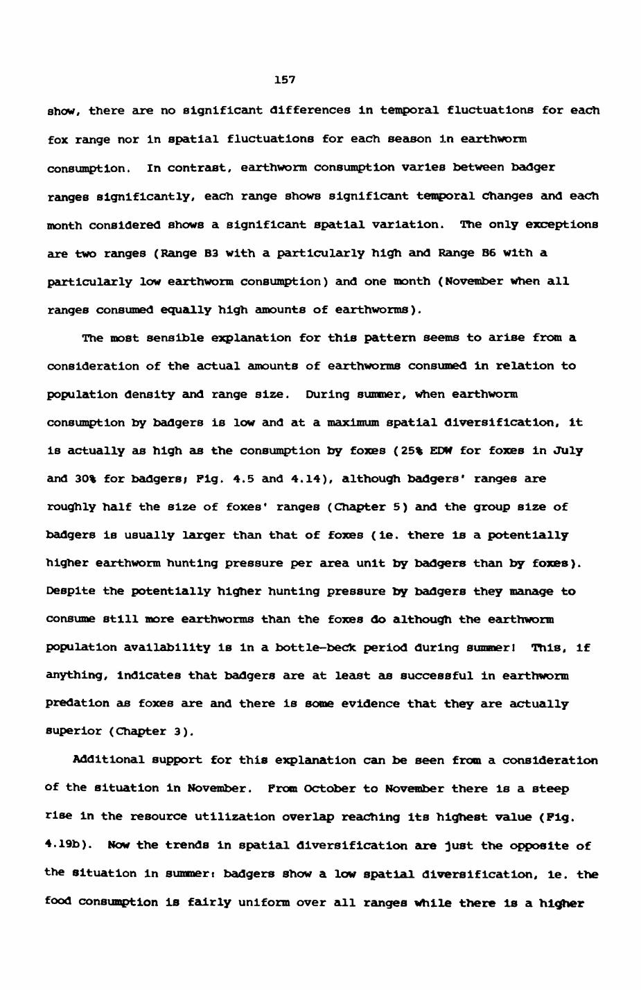
157
show, there axe no significant differences in temporal fluctuations for each
fox range nor in spatial fluctuations for each season in earthworm
consumption. In contrast, earthworm consumption varies between badger
ranges significantly, each range shows significant temporal changes and each
month considered shows a significant spatial variation. The only exceptions
are two ranges (Range B3 with a particularly high and Range B6 with a
particularly low earthworm consumption) and one month (November when all
ranges consumed equally high amounts of earthworms).
The most sensible explanation for this pattern seems to arise from a
consideration of the actual amounts of earthworms consumed in relation to
population density and range size. During summer, when earthworm
consumption by badgers is low and at a ma-giimm spatial diversification, it
Is actually as high as the consumption by foxes (25% EDW for foxes in July
and 30% for badgers; Fig. 4.5 and 4.14), although badgers' ranges are
roughly half the size of foxes' ranges (Chapter 5) and the group size of
badgers is usually larger than that of foxes (le. there is a potentially
higher earthworm hunting pressure per area unit by badgers than by foxes).
Despite the potentially higher hunting pressure by badgers they manage to
consume still more earthworms than the foxes do although the earthworm
population availability is in a bottle-beck period during summer I This, if
anything, indicates that badgers are at least as successful in earthworm
predation as foxes are and there is some evidence that they are actually
superior (Chapter 3).
Additional support for this explanation can be seen from a consideration
of the situation in November. Prom October to November there is a steep
rise in the resource utilization overlap reaching its highest value (Pig.
4.l9b). NOW the trends in spatial diversification are }ust the opposite of
the situation in summeri badgers show a low spatial diversification, le. the
food consumption is fairly uniform over all ranges while there Is a higher
158
spatial diversification in foxes. However, foxes have a very high
consumption of earthworms (45% EDW, badgers 79% EDW). This is a large
difference but it is smaller than those of previous months. At the same
time, earthworms are plentifully abundant and thus there is the opposite of
the bottle-neck situation in summer. Considering the super-availability of
earthworms in November, it is not surprising that both foxes and badgers
consume lots of them and there is little indication of competition between
the predators.
Summarizing we can say that there are two peaks in the resource
utilization overlap between the diet of foxes and badgers, one coinciding
with a trough of earthworm availability in summer when badgers reduce their
earthworm consumption to the level of consumption by foxes (as measured by
percent contribution to the diet of the range) and the other peak coinciding
with a peak of earthworm availability. In the first case, competition is
possible between foxes and badgers, while for the peak in November
competition seems unlikely when a high utilization overlap coincides with
high prey availability. This indicates how resource utilization overlap may
vary independently of the degree of competition and that one cannot
necessarily be deduced from the other. The analysis shows furthermore how a
detailed understanding of the temporal and spatial variation in resource
utilization is absolutely necessary to gain an adequate understanding of the
relationship of two species (this is perhaps even more important if k-
selected species are involved in the comparison). In the light of these
results, much of the current discussion on competition and resource
utilization based on relatively coarse-grained data, such as one value for
resource overlap for the whole year, may look like scratching only the tip
of the Iceberg.

159
5. Fox and badger home ranges
5.1. Introductions review of home range concepts
5.2. Methods of data collection
5.2.1. Telemetry
5.2.2. Bait marking and badger latrine checks
5.2.3. Observations
5.3. Methods of analysis
5.3.1. Processing procedures for telemetric data
5.3.2. Habitat and diet description of ranges
5.4. Badger group ranges
5.4.1. Description of badger group ranges
5.4.2. Relationships between ranges and long-term
developments
5.4.3. Patterns of latrine distribution and utilization
.1. Distribution of latrines
.2. Utilization of latrines
.3. Function and evolution of latrines
5.5. Fox group ranges
5.5.1. Description of fox group ranges
5.5.2. Characteristics of fox group ranges
5.5.3. Distribution of fox faeces
.1. Patterns of distribution
.2. Discussion
5.6. Habitat composition of and resource use in group ranges
5.6.1. Observed and expected proportions of habitats per
group range
5.6.2. Dispersion of habitat composition between ranges
5.6.3. Habitat composition and range size

160
5.6.4. Habitat composition of individual ranges within the
same group
5.6.5. Habitat composition and resource use of group ranges
5.6.6. Discussion.

161
5. Fox and badger home ranges
In this chapter I consider how foxes and badgers partition the resource
space into home ranges for individual use. After a description of group
ranges and scent-marking patterns which may be relevant to the maintenance
of the ranges, I will deal with the resource distribution and abundance
within home ranges, as evidenced by their habitat composition. In
particular, I will explore how home range features relate to habitat and
resource use, as indicated by the diet of the groups. Finally, models are
discussed that describe how individual and group ranges should be dispersed
in space given a certain set of conditions of resource dispersion and
availability.
5.1. Review of home range concepts
Burt (1943) defined home range as the area over which an animal
normally travels during activities associated with feeding, resting,
reproduction, and shelter-seeking. This excluded 'occasional sallies'
outside this area as well as dispersal by adolescent animals. This concept
has been recognized as extremely useful, even if some authors differ in
their opinion as to how excursions should be defined (Wilson 1975, Southwood
1978, Harestad & Bunnell 1979 and others). Home ranges discussed in this
chapter exclude outside sallies.
Despite general agreement in principle, as to what constitutes a home
range, there is a wealth of methods for determining range configuration and
size, several of them constitute models in that they assume a certain
utilization distribution and construct range borders from an assumed
utilization distribution rather than taking into account the distribution of
the original data points. A survey of these and other methods is presented
162
in Table 5.1, together with examples for applications from the literature.
As I shall show in Chapter 6, utilization distributions of fox and
badger ranges are extremely variable and do not fit any of the proposed
distributions (e.g. bivariate normal). Furthermore, many of the non-
parametric probabilistic models assume independent data points, which are
extremely difficult to obtain (see Appendix 4), and therefore are of limited
usefulness. This leaves methods that do not make assumptions about
utilization distributions and other qualities of ranges, ie. the hand-drawn
method, the minimum convex polygon and the grid method. Since hand-drawn
home ranges suffer from observer bias and absence of rigorous rules, I
prefer the grid method and under some circumstances, the minimum convex
polygon (MCP).
5.2. Methods of data collection
Information on home ranges of foxes was derived from radio-tracking of
animals that had previously been captured and fitted with a transmitter.
Capturing and tagging followed the standard techniques employed by members
of the Oxford Foxlot for many years and have been described in detail
elsewhere (Macdonald 1978, Newdick 1983, Doncaster 1985).
Information on home ranges of badgers was combined from radio-tracking
of animals and the results of the non-invasive bait marking technique
developed by Kruuk (I978a) and described in more detail in Section 5.2.2.
Badgers were caught in large steel cage traps that were placed close to
setts and prebalted with peanuts for at least a week. Trap doors were
either released by the badger's weight on a tredle or operated from a hide
by a long cord (see Cheeseman & Mallinson 1980). Traps were checked once
dally early in the morning. The trapping was in accordance with an NCC
licence issued to Dr. D.W. Macdonald. Captured invldiduals were
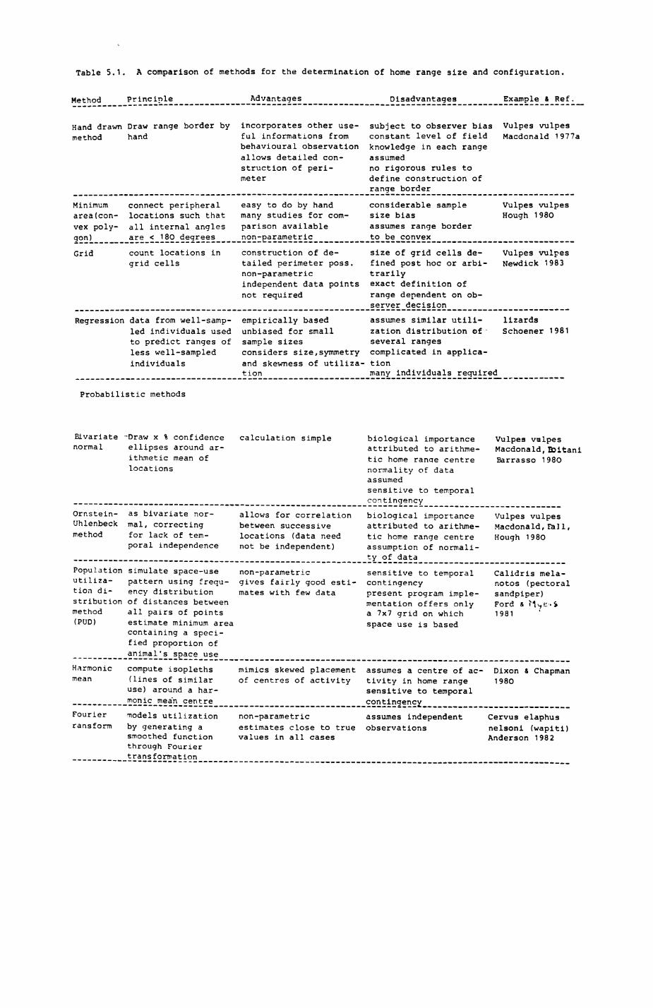
Table 5.1. A comparison of methods for the determination of home range size and configuration.
Method Principle Advantages Disadvantages Example & Ref.
Hand drawn Draw range border by method hand
incorporates other use ful informations from behavioural observation allows detailed con struction of peri meter
subject to observer biasconstant level of fieldknowledge in each rangeassumedno rigorous rules todefine construction ofrange border
Vulpes vulpes Macdonald 1977a
Minimum connect peripheral easy to do by hand area(con- locations such that many studies for corn- vex poly- all internal angles parison available gon) are < 180 degrees non-parametric
considerable sample size biasassumes range border to be convex
Vulpes vulpes Hough 198O
Grid count locations in grid cells
construction of de tailed perimeter poss. non-parametric independent data points not required
size of grid cells de fined post hoc or arbi trarilyexact definition of range dependent on ob server decision
Vulpes vulpes Newdick 1983
Regression data from well-samp- empirically based led individuals used unbiased for small to predict ranges of sample sizes less well-sampled considers size,symmetry individuals and skewness of utiliza
tion
assumes similar utili zation distribution of several ranges complicated in applica tion many individuals required
lizards Schoener 1981
Probabilistic methods
Bivariate -Draw x % confidence normal ellipses around ar
ithmetic mean of locations
calculation simple biological importance attributed to arithme tic home ranae centre normality of data assumedsensitive to temporal contingency
Vulpes vmlpes Macdonald,Eoltani Barrasso 1980
Ornstein- as bivariate nor- Uhlenbeck mal, correcting method for lack of tem
poral independence
allows for correlation between successive locations (data need not be independent)
biological importance attributed to arithme tic home range centre assumption of normali ty of data
Vulpes vulpes Macdonald,rail, Hough 1980
Population simulate space-use non-parametric utiliza- pattern using frequ- gives fairly good esti- tion di- ency distribution mates with few data stribution of distances between method all pairs of points (PUD) estimate minimum area
containing a speci fied proportion of animal's space use
sensitive to temporal contingency present program imple mentation offers only a 7x7 grid on which space use is based
Calidris mela- notos (pectoral sandpiper) Ford s ^ v e. $ 1981
Harmonic compute isopleths mean (lines of similar
use) around a har monic mea'n centre
mimics skewed placement of centres of activity
assumes a centre of ac tivity in home range sensitive to temporal contingency
Dlxon & Chapman 1980
Fourier models utilization ransform by generating a
smoothed function through Fourier transformation
non-parametric estimates close to true values in all cases
assumes independent observations
Cervus elaphus nelsoni (wapiti) Anderson 1982
163
anaesthetized with ketamine hydrochloride, a safe and widely used
immobilization drug (see Beck 1976, Ramsden et al. 1976), before they were
taken out of the trap. Each individual was measured, weighed and fitted
with eartags made by Dalton Supplies Ltd, Nettlebed, Oxon. Eartags were
numbered and an attempt was made to mark members of the same group with
different colours. Adult badgers were then fitted with radio-transmitters
around their neck. The transmitter collar was made of first-class saddle
leather which proved to be ideal for balancing the need of firm attachment
to the body while at the same time not impeding its movements. A beta-light,
manufactured by Saunders & Roe Ltd and embedded in translucient acrylic was
fixed to the upper side of the collar to facilitate observations in the
dark. Animals were then placed close to the sett entrance from which they
had emerged, to facilitate their orientation after rewakenlng. I stayed
with the animals for at least half an hour to check that they were well and
safe after regaining consciousness.
5.2.1. Radio-tracking
Radio-tracking was principally carried out from a car, since home
ranges were generally too large to be covered effectively on foot. Some
attempts were made to follow foxes through woodland on foot; invariably, the
foxes were lost within two hours. Following badgers on foot was more
successful and I could follow individuals even through dense plantations for
several hours, largely due to the betallght which could be seen for up to
two hundred metres. Intensive radio-tracking on foot was done in Autumn
1982 for fourteen days in the Jews Harp Range (see below), not only to
register the movements of individuals but also observe their activities and
monitor their emergence patterns from setts.
On the roof of the car a three element yagl antenna was mounted and
164
connected to an AVM LA12 receiver (AVM Instrument Co. Ltd., 2368 Research
Drive, Livermore, CA 94550). The antenna could be rotated by a handle from
the inside of the car. A direction indicator and a protractor fitted to the
rotating handle completed the tracking device and enabled me to monitor
signal strength and direction while driving. Benefits of such a design
include rapid recording of locations, minimizing errors by always stopping
at sites with optimal signal strength and reduced waste of time, since
driving in the wrong direction was quickly noticed. With an experienced
operator, this design made it possible to record locations every minute.
Recording of locations followed one of two schemes t either several
animals were tracked, or one individual was followed continuously. With the
first approach, data on several individuals were collected quickly. This is
especially important if several animals have been equipped with radios
within a few days, since it was our experience that transmitters either stop
functioning after four or five days, or go on for a long time. With growing
experience, and following preliminary data analysis, it became clear that
the greatest benefit was derived from intensive monitoring lasting for
several days, so in the last radio-tracking season an attempt was made to
follow particular indidivuals for consecutive nights. Since foxes were
infrequently, but regularly seen active during the daylight, I also followed
the movements of indldivual foxes continuously for 60 hours on three
occasions (here I am Indebted to Chris Bowden, Helen DoIk, Marion East,
Gillian Kerby, David Macdonald and Colin Pringle who followed the animals
during the hours I was asleep).
If an animal was followed continuously, a location was recorded if it
moved its position from the previous location. This could mean that a
location was taken every minute, if the animal moved quickly through an
area, but often an animal would stay within the same area of ca 20 by 30
metres for up to an hour. In this case, the same location was recorded
165
every 15 minutes, to indicate that the animal was still there and I still
awake. As a result, time intervals between recording times of successive
locations were very variable, but the record of movements was complete.
Locations were determined by triangulation (see Macdonald & Amlaner
1980, Deat et al. 1980). This was straight foward with animals that were
either inactive, or moving slowly. With rapidly moving animals,
triangulation demanded successive bearings that were only a few seconds
apart and this sometimes necessitated taking fixes from otherwise suboptimal
sites. The vast majority of locations were obtained from rather slow moving
animals, so larger errors possibly associated with fast moving animals will
have little influence.
Accuracy of radio fixes was estimated to average about 3O metres. This
estimate is based on experiments with hidden transmitters, chance
observations, and years of experience in the Oxford Poxlot. The accuracy of
much of the data is better than the 30 metre error margin since my tracking
often resembled what Macdonald (1978) has called 'predictive tracking'. For
example, while tracking members of the Botley Lodge badger clan in Mar ley
Plantation, I would see the individual at least a dozen times during the
night and stay as close as 50 metres sometimes for several hours in a row.
The positions of my favourite triangulation places were determined during
the day by reference to the Wytham Forestry grid system and the Wytham Atlas
(see Chapter 2) and marked on the tracking maps. These were sites where
radio signal reception was especially strong. By confining myself mostly to
such sites, I sought to reduce errors by building up a mental picture of the
transmitting qualities which differed greatly between individual radio-
collars .
In summary, there are many possible sources of error in radio-tracking
(see Amlaner & Macdonald 1980 for reviews). In this study I was fortunate
to overcome most of them and to generate data to a much greater level of
166
accuracy than is customary in radio-tracking studies.
5.2.2. Bait marking and badger latrine checks
Bait marking is a non-invasive technique that was developed by Hans
Kruuk (1978a) and first successfully applied in his earlier study on Wytham
badgers in 1974. Each badger sett is supplied with a mixture of peanuts and
small plastic pellets (length ca 2-3 mm) coated in golden syrup. Each sett
was supplied with a different colour of plastic pellets. Small mounds of
the bait were placed in several holes and covered with soil or sand so that
birds, particularly crows, did not take them. As some fox faeces indicated,
this was not entirely successful with respect to other animal groups.
Badgers ate the mixture and passed the pellets to their faeces in latrines,
where the origins of the individuals using a latrine could then be traced
due to the different colour codings. Baiting continued every day for two or
three weeks in March, July, October 1982 and March 1983. Setts were baited
in July 1982 since the decision was taken to enlarge the area of interest,
thus including the setts of the Radbrook Common area and the first line of
setts west of the Chalet (Fig. 5.4). However, due to reduced utilization of
latrines in summer, delineation of range borders remained doubtful and a
third baiting period was chosen for the same year. I am indebted to Adrian
Barnett and Rory Hewlett for supplying the badger setts with peanuts and
beads in July and October respectively. Setts were selected for baiting (1)
if badgers had been active there in previous weeks, (il) because setts were
included in the Annual Badger Census (ABC) of the Animal Ecology Research
Group in May, or (iii) because they had been used by badgers in Kruuk's
(I978a) study. A detailed list of setts baited is presented in Table 5.4,
sett locations are indicated in Pig. 5.1 - 5.6
Latrines were classified as 'border 1 or 'non-border' latrine. A latrine
167
was assigned border status of It was snared by neighbouring ranges, usually
indicated by the recovery of plastic beads originating from different setts.
In ranges at the fringe of the core study area, existence of neighbours was
occasionally uncertain. In these cases, some of the latrines that were used
to delineate the range border (e.g. SW-corner of Range Bl, BOTLEY LODGE,
Fig. 5.5) were excluded from analysis of range diet (Chapter 4) and latrine
activity (section 5.4.2).
Latrine utilization was gauged by three kinds of parameterst
(a) number of new latrines founded and total number of latrines
available (ie. total of recently and previously found
latrines);
(b) proportion of latrines with at least one recent dropping
("active" latrines) of all latrines available and checked
in a given monthj
(c) measures of intensity of use per latrine:
2 (1) AREAi the area of a rectangle (in m ) with side
lengths equivalent to the maximum length and
maximum width of a latrine measured at right
angles;
(ii) TOTALs the total number of pits per latrine, ie.
shallow excavations either empty or filled with
anal sac secretion and/or dung;
(ill) PlLLEDi number of pits per latrine that contained at
least one badger dropping or anal sac secretion;
(iv) FRESHi number of pits per latrine with at least one
recent dropping (deposited within the last 48
hours) or anal sac secretion.
168
5.2.3. Observations
Observations of the behaviour of foxes and badgers were of three kinds
(Section 4.2.1.): observing radio-tracked foxes and badgers, watching from
hides as badgers emerged from their setts (and returned to them)/ and chance
observations of animals. Observations during the night were made either
using an image-intensifier or infrared binoculars, and notes were spoken
into a dictaphone. Monthly checks of badger setts, fox earths and rabbit
warrens were used to locate fox litters. Earths with fox litters are
characterised by a large area of cleanly swept bare soil in front of the
entrances, flies, fox tracks, scats and prey remains (Lloyd 198O). If a
litter was located in a den, observations were occasionally undertaken at
dusk to confirm the presence of fox cubs and determine litter size.
5.3. Methods of analysis
5.3.1. Processing procedures for telemetric data
Tracking locations were recorded as pairs of x,y coordinates to the
nearest 10 metres on the National Grid System. These coordinates, together
with date, time, an estimate of the confidence (error) for the location,
activity of the animal, observation, weather conditions (air temperature,
wind direction and wind speed according to the Beaufort scale, degree of
precipitation, relative humidity, cloud cover) were typed into computer
files, one each for each individual. Program SRCH2H (written by Ken Royall
and Malcolm Newdlck) tagged each location with its appropriate patch and
habitat number with reference to the computerized habitat map (see Chapter
2). Program ICELLH, a modified version of program ICELL (written by Malcolm
Newdlck) was used to plot all radio-tracking fixes on a grid based map, so
169
typing errors could be checked (e.g. Indicated by anomalous position). All
data files were checked line by line and compared with the original data
sheets. Later, program VELOCITY fitted polynomials to calculate movement
speeds. All very fast speeds were checked again and the last typing errors
eradicated. These procedures took a very long time, but as a result I feel
that at least 99% of all locations typed in have their correct coordinates
attached to them.
Home range sizes of individual animals and of fox group ranges were
analysed by evaluating tracking data on a grid of 50 by SO metre cells. This
size was considered a satisfactory compromise between the estimated tracking
error, sample size considerations, the desired spatial resolution of space
use patterns and the average habitat heterogeneity per cell. A cell size of
25 metres is not particularly useful, since the suggested maximum error of
radio tracking, 30 metres, exceeds the cell size. Larger cells, e.g. 100
metre cells, decrease sample size considerably and represent quite a
heterogeneous assemblage of different habitats, thereby increasing the
difficulties of interpreting movements with reference to habitat types.
Also, larger sizes do not permit a fine spatial resolution of the exact
delineation of the range border and range utilization patterns (see Chapter
6).
Selection of tracking data poses a problem for most applications,
including the determination of range sizes and the habitat composition of
ranges, since a common assumption is independence of data points. However,
this condition is rarely fulfilled by tracking data. The problem is
discussed in Appendix 4 in detail, and procedures are suggested to overcome
it. it was concluded that selecting data at an interval of 15 minutes
("independence interval") results in approximate and, for our purposes,
sufficient independence of data points. Therefore, tracking data were
selected by this criterion, unless data from intensive tracking periods with
170
'time-tabling' of movements could be used.
Individual home range sizes were usually based on the grid method
(Voigt & Tinline 1980), where the number of cells with radio locations
multiplied by the cell size yields the range size. The effect of data
selection procedures on estimates of range size was explored by adopting the
following measures!
(1) "15 MIN RADIO": fixes selected according to the 15 min independence
intervali only cells with radio locations.
(2) "15 KIN OCCUPIED"! as (1), plus cells immediately surrounding a radio
cell ("Influence cells"), unless they are at the border of the range. Every
Individual must have passed through at least one of the eight influence
cells surrounding a radio cell to reach the point of radio location. With
discontinuous tracking schemes, the record of the movement path of an
Individual is incomplete and the correct neighbouring cell may have been
missed by the researcher. Hence, Newdick (1983) suggested to correct this
deficiency by including influence cells in range calculations. Delineation
of range border remains unchanged, but the inner area of the range is
•filled up 1 .
(3) "15 MIN TOTAL": as (2), plus cells that are completely enclosed by
radio and/or influence cells but do not belong to either of the categories
(empty spaces, so-called "lakes"). While inside the border of the range,
these cells do not belong to the actively used sections of the range.
(4) "0 KIN OCCUPIED"! as (2), but no independence interval, all fixes
admitted.
(5) "0 KIN TOTAL"i as (3), but no independence Interval, all fixes
admitted.
(6) "MCP"(Minimum Convex Polygon)! all fixes admitted, range border
delineated according to the minimum convex polygon method (Table 5.1).
Measures (1) to (3) and (4) to (5) are distinguished by the time
171
interval of data selection while within both groups measures are
distinguished according to procedures intended to correct for deficiencies
in recording procedures. Estimates of range sizes according to measures (1)
to (5) were produced by program ICELLH (modified from Newdick 1983),
estimates according to measure (6) were produced by program CV written by
Malcolm Newdick. Results for individual lifetime ranges are presented in
Table 5.2. Size estimates show differences up to 900 %. Obviously, the
choice of data selection and method of computation is not a trivial one, if
absolute range size is important, e.g. if range size is considered in
relation to body size, metabolic needs etc (Harestad & Bunnell 1979,
Gittleman & Harvey 1982).
Do the six measures produce a similar trend for estimates of range size
for foxes and badgers ? The results of calculations of Kendall's coefficient
of concordance (see Appendix 3) listed in Table 5.3 show that this Is the
case. According to multiple comparisons between different measures (Conover
198O), measures are ranked as follows (listed from producing small to large
estimates):
Foxes: 15 MIN RADIO < 15 MIN OCCUPIED < 0 WIN OCCUPIED =
15 MIN TOTAL < O MIN TOTAL = MCP
Badgers: 15 MIN RADIO < 15 MIN OCCUPIED < 15 MIN TOTAL
O MIN OCCUPIED < 0 MIN TOTAL = MCP
For both species, 15 MIN RADIO yields on average the smallest range size
estimate and MCP the largest. Differences between species in ranking of the
measures concerns the positions of o MIN OCCUPIED and 15 MIN TOTAL. This is
probably an effect of different recording schemes (Chapter 6). In contrast
to foxes, badgers were very intensively tracked (fixes often only a few
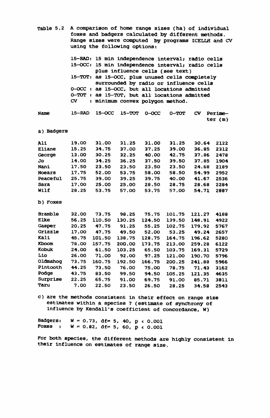
Table 5.2 A comparison of home range sizes (ha) of individual foxes and badgers calculated by different methods. Range sizes were computed by programs ICELLH and CV using the following options:
15-RADs 15 min independence interval; radio cells 15-OCCi 15 min independence interval; radio cells
plus influence cells (see text) 15-TOT: as 15-OCC, plus unused cells completely
surrounded by radio or influence cells 0-OCC i as 15-OCC, but all locations admitted o-TOT t as 15-TOT, but all locations admitted
Name
a) Badgers
AllElianeGeorgeJoNaniNoearsPeacefulSaraWilf
b) Foxes
BrambleElkeGasperGrizzleKaliKboomKobukLloOldmahogPintoothPodgeSurpriseTaru
c) are the
CV : minimum convex polygon method.
15-RAD 15-OCC 15-TOT O-OCC O-TOT CV
19.0015.2513.0014.0017.5017.7525.7517.0028.25
32.0056.2520.2517.0045.7578. OO24.0026.0073.7544.2543.7522.257.00
313430342352392553
731104747101157617116073836522
.00
.75
.25
.25
.50
.00
.00
.00
.75
.75
.50
.75
.75
.50
.75
.50
.00
.75
.50
.50
.75
.50
31.2537.0032.2536.2523.5053.7539.2525.0057.00
98.25130.2591.2549.50138.75200.00103 . 2592.00
192. 5O76.0099.5091. OO23.50
methods consistent inestimates within a species ? (Influence by Kendall's
Badgers iFoxes i
W « 0.w * o.
73, df= 582, df= 5
31.37.40.37.23.58.39.28.53.
75.124.55.52.
128.173.65.97.
166.75.94.69.26.
002500505OOO755075
755025007575502575005O7550
313942392358402857
10113910253
.25
.00
.75
.50
.50
.50
.OO
.75
.OO
.75
.50
.75
.25164.7521310312120078
1059128
their effectestimate
coefficient
, 4O, p < 0., 60, pi < 0.
Of
O01O01
Of
.OO
.75
.OO
.25
.75
.25
.00
.25
on
3O3637372454412854
12114817949196259169190241711218534
Perime ter (m)
.64
.85
.86
.85
.68
.99
.67
.68
.71
.27
.91
.92
.24
.62
.28
.31
.70
.88
.43
.35
.71
.58
212223122478190421892952253622842887
4188492257672657528061225729579659663162463538112543
range sizesynchrony of
concordance, W)
For both species, the different methods are highly consistent in their influence on estimates of range size.
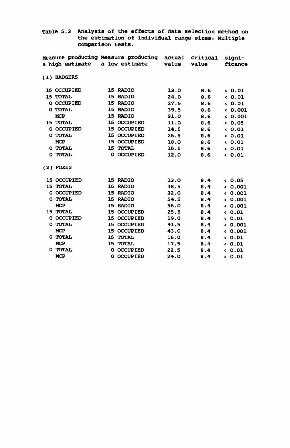
Table 5.3 Analysis of the effects of data selection method on the estimation of individual range sizest Multiple comparison tests.
Measure producing Measure producing a high estimate a low estimate
(1) BADGERS
15 OCCUPIED 15 TOTAL0 OCCUPIED0 TOTALMCP
15 TOTAL0 OCCUPIED0 TOTAL MCP
0 TOTAL0 TOTAL
(2) POXES
15 OCCUPIED 15 TOTAL 0 OCCUPIED 0 TOTALMCP
15 TOTAL 0 OCCUPIED 0 TOTALMCP
0 TOTALMCP
0 TOTAL MCP
15 RADIO 15 RADIO 15 RADIO 15 RADIO 15 RADIO 15 OCCUPIED 15 OCCUPIED 15 OCCUPIED 15 OCCUPIED 15 TOTAL 0 OCCUPIED
15 RADIO15 RADIO15 RADIO15 RADIO15 RADIO15 OCCUPIED15 OCCUPIED15 OCCUPIED15 OCCUPIED15 TOTAL15 TOTAL 0 OCCUPIED 0 OCCUPIED
actual value
13.024.027.539.531. 011.014.526.518.015.512.0
13. 038.532.054.556. 025.519.041.543.016.017.522.524.0
critical value
8.68.68.68.68.68.68.68.68.68.68.6
8.48.48.48.48.48.48.48.48.48.48.48.48.4
signi ficance
< 0.01< 0.01< 0.01< O.O01< 0.001< 0.05< O.01< 0.01< 0.01< 0.01< 0.01
< O.05< O.O01< O.O01< O.OO1< 0.001< 0.01< 0.01< 0.001< 0.001< 0.01< 0.01< 0.01< 0.01
172
minutes apart), hence a relatively high proportion of data is excluded by
the application of a time interval and therefore the difference between 15
KIN OCCUPIED and 0 MIN OCCUPIED is larger than for foxes. The often
discontinuous tracking scheme for foxes produced smaller homogeneous areas
completely covered by radio cells, hence more "lakes" are produced and
therefore the difference between 15 MIN OCCUPIED and 15 KIN TOTAL larger.
To exclude these effects of different recording regimes and facilitate
intra- and interspecific comparisons, I decided to use estimates of range
sizes as determined by the most conservative measure, 15 MIN RADIO, both for
the establishment and the determination of the habitat composition of fox
group ranges.
Fox group ranges were established by combining all cells visited by the
members of a fox group. Table 5.23, section 5.5., lists the radio-tracked
members of each group. Membership of an Individual to a group was identified
by a large proportion of overlap of an Individual's range with those of
other foxes in the same area. This posed no problems at all, since ranges
were clearly separated from each other (Fig. 5.3O-5.33). In three groups
(Ranges 5, 6, and 7), males of the group (OLDSABRE, BOOTS, RABBITS) were
only tracked for brief periods; their ranges showed complete overlap with
those of their respective females (KBOOM, OLDMAHOG, PINTOOTH). In most other
groups, only one group member was caught and radio-tracked, despite
extensive trapping efforts. Only in the HOMEFARM group, several, probably
all group members were caught and tracked. Group range size, delineation of
range border, habitat composition and diet (Chapter 4) were based on a range
that was cleansed from overlap zones with neighbouring ranges. Overlap zones
were determined by the procedures described in Appendix 3, le. cells visited
by individuals of both neighbouring ranges in the border ones were excluded
from both ranges. Not considered in this pruning procedure were occasional
excursions by individuals into neighbouring ranges or even further away.
173
Examples of such excursions are (i) an excursion by the vixen PODGE
(HOMEFARM Range) of more than 2 km outside her usual range during the mating
season (26-27.1.1982), (ii) several day-time visits by the dog-foxes GASPER
and KOBUK (HOMEFARM Range) to an area approximately 3 km outside their usual
range, and (iii) several excursions of KBOOM (WOODEND Range) into the
neighbouring range of PINTOOTH (HILL END CAMP Range). Excursions show a
pattern of movement distinct from the usual ranging behaviour (e.g. Hough
1980): usually, the individual starts quite late (ca 2 to 3 a.m.) and moves
rapidly into a specific direction over a long distance. Movements in border
zones are not distinguished from movements well inside a group range, as far
as radio-tracking can tell.
By restricting myself to the pruned sections of fox group ranges I hope
to have minimized the uncertainty regarding the ownership of a particular
area and Included only those sections of a range that are exclusively used
by a group. Any remaining errors due to misidentlficatlon of the ownership
of a particular area will, however, work against any conclusions to the
effect that a given characteristic differs between groups.
5.3.2. Habitat and diet description of ranges
Each grid cell that was (by previous procedures) identified as part of
a home range served as the base area for extracting 9 equidistant points
(program HABCOR2), that were subsequently tagged with their respective
habitat and patch numbers according to the computerized habitat map (Chapter
2i program SRCH2HAB). Programs HABSEL2 and HABLUMP summarized the output of
SRCH2HAB by habitat and by cell respectively. Thus, an estimate of the
proportion of habitats represented in a range (in absolute as well as
relative values) was derived, and the habitat composition of each cell
Identified.
174
Variability of the absolute and relative proportion of a habitat in
group ranges was assessed by Levene's test (Van Valen 1978, Schultz 1983).
Since the mean values of the area (in % or ha) occupied by different
habitats differed widely, it seemed sensible to assess relative rather than
absolute variability, as expressed by the coefficient of variation. For each
habitat category, the median over all group ranges was identified and new
variables calculated according to
^med,! ' / xmed,i
with y the new variables
x the area in % or ha of the i-th habitat
category in the 3-th group
x the median for the i-th habitat category med, i
There has been much debate recently as to what kind of measure(s) of
variation perform best for biological problems, especially in systematics
(Van Valen 1978, Sokal & Rohlf 1981, Schultz 1983). Several authors cited by
these studies agree that Levene's test is the most robust, yet simplest test
presently available. On Schultz f s (1983) recommendation I used the median
instead of the mean as an estimate of central location. The new variables
y were then tested on differences between habitat categories with the
Kruskal-Wallis one-way analysis of variance because of its usual advantages
(Appendix 3).
A stepwise discriminant analysis was run using the BMDP package, in
order to prove whether, despite considerable inter-group variability in
habitat composition of ranges, species were consistent In their choices
relative to each other. Program BMDP7M was run with option FORCE-0. Then,
only habitat types are included In the classification function, if they are
175
above a certain limit (P-to-enter was set as 4.0). The resulting
classification indicates which habitat variables are best suited to
distinguish fox and badger home ranges.
The procedures used to determine the diet of groups have been explained
in sections 4.2.2. and 4.3.2.
5.4. Badger group ranges.
The results of the sett baiting actions in 1982 and 1983 are presented
in Table 5.5 and Pig 5.1-5.4 (only those latrines from which beads were
recovered are plotted). The proportion of active latrines from which beads
were recovered varied between 32.2 and 58.6 %. The small number of active
latrines in spring 1982 made an unambiguous identification of some sections
of range borders difficult. Since the proportion of bead recoveries in 1982
was similar for latrines later assigned border or non-border status
(binomial test, summed probabilities, one-tailed, p~O.435, 0.601 and O.7O5),
additional information on the movements of individuals was used for the
determination of range boundaries. Spring 1983, however, saw a threefold
increase in the number of active latrines (Table 5.5) with more border
latrines than expected containing beads (binomial test, summed probability,
one-tailed, p - 0.006). Since the level of latrine activity during the
remainder of 1983 fell back to and partly below 1982 levels (section
5.4.3.), spring 1983 should be interpreted as a time of intense marking
activity leading to (i) well-defined range borders and (ii) high efficiency
in deduction of range borders by bead recovery.
I shall now discuss each range in detail, starting in the south-east
corner of the study area.
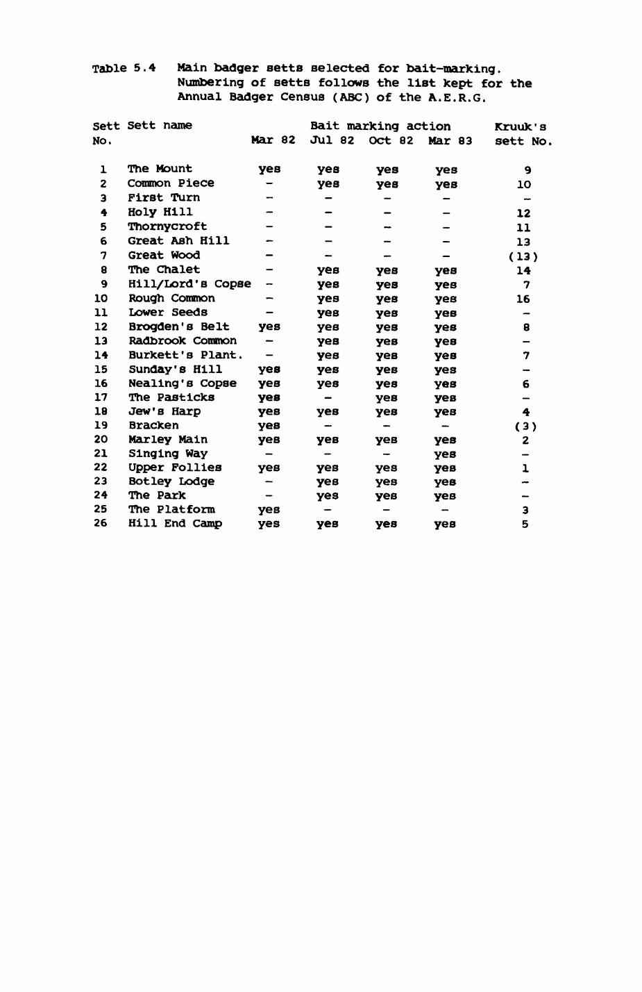
Table 5.4 Main badger setts selected for bait-marking.Numbering of setts follows the list kept for the Annual Badger Census (ABC) of the A.E.R.G.
Sett Sett name Bait marking action Kruuk'sNo. Mar 82 Jul 82 Oct 82 Mar 83 sett No,
1 The Mount yes yes yes yes 92 Common Piece - yes yes yes 103 First Turn - - -4 Holy Hill - 125 Thornycroft - 116 Great Ash Hill - 137 Great Wood - - - - (13)8 The Chalet - yes yes yes 149 Hill/Lord's Copse - yes yes yes 7
10 Rough Common - yes yes yes 1611 Lower Seeds - yes yes yes -12 Brogden's Belt yes yes yes yes 813 Radbrook Common - yes yes yes -14 Burkett's Plant. - yes yes yes 715 Sunday's Hill yes yes yes yes -16 Nealing's Copse yes yes yes yes 617 The Pasticks yes - yes yes -18 Jew's Harp yes yes yes yes 419 Bracken yes - - - (3)20 Mar ley Main yes yes yes yes 221 Singing Way - yes22 Upper Follies yes yes yes yes 123 Botley Lodge - yes yes yes -24 The Park - yes yes yes -25 The Platform yes - - - 326 Hill End Camp yes yes yes yes 5
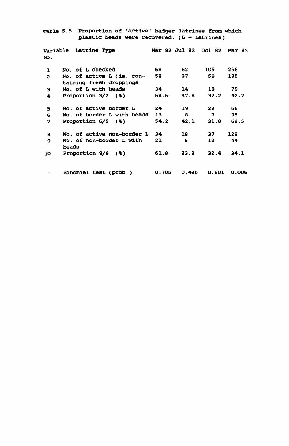
Table 5.5 Proportion of 'active' badger latrines from Which plastic beads were recovered. (L = Latrines)
Variable Latrine Type Mar 82 Jul 82 Oct 82 Mar 83 No.
1 No. of L checked 68 62 105 2562 No. of active L (ie. con- 58 37 59 185
taining fresh droppings3 No. of L with beads 34 14 19 794 Proportion 3/2 (%) 58.6 37.8 32.2 42.7
5 No. of active border L 24 19 22 566 No. of border L with beads 13 8 7 357 Proportion 6/5 (%) 54.2 42.1 31.8 62.5
8 No. of active non-border L 34 18 37 1299 No. of non-border L with 21 6 12 44
beads10 Proportion 9/8 (%) 61.8 33.3 32.4 34.1
Binomial test (prob.) 0.705 0.435 0.6O1 0.006

Pig. 5.1-5.4
Results of baiting actions of badger setts, for spring 1982, summer 1982,
autumn 1982 and spring 1983, respectively.
The thin lines delineate the ma^or woodland borders, and the western bypass
(eastmost line) and the Eynsham Road (southern line). Encircled numbers
indicate identity of setts according to Table 5.4. Latrines from Which
beads were recovered are indicated as filled circles; the lines connecting
latrines with setts indicate the origins of beads recovered from the
latrines.
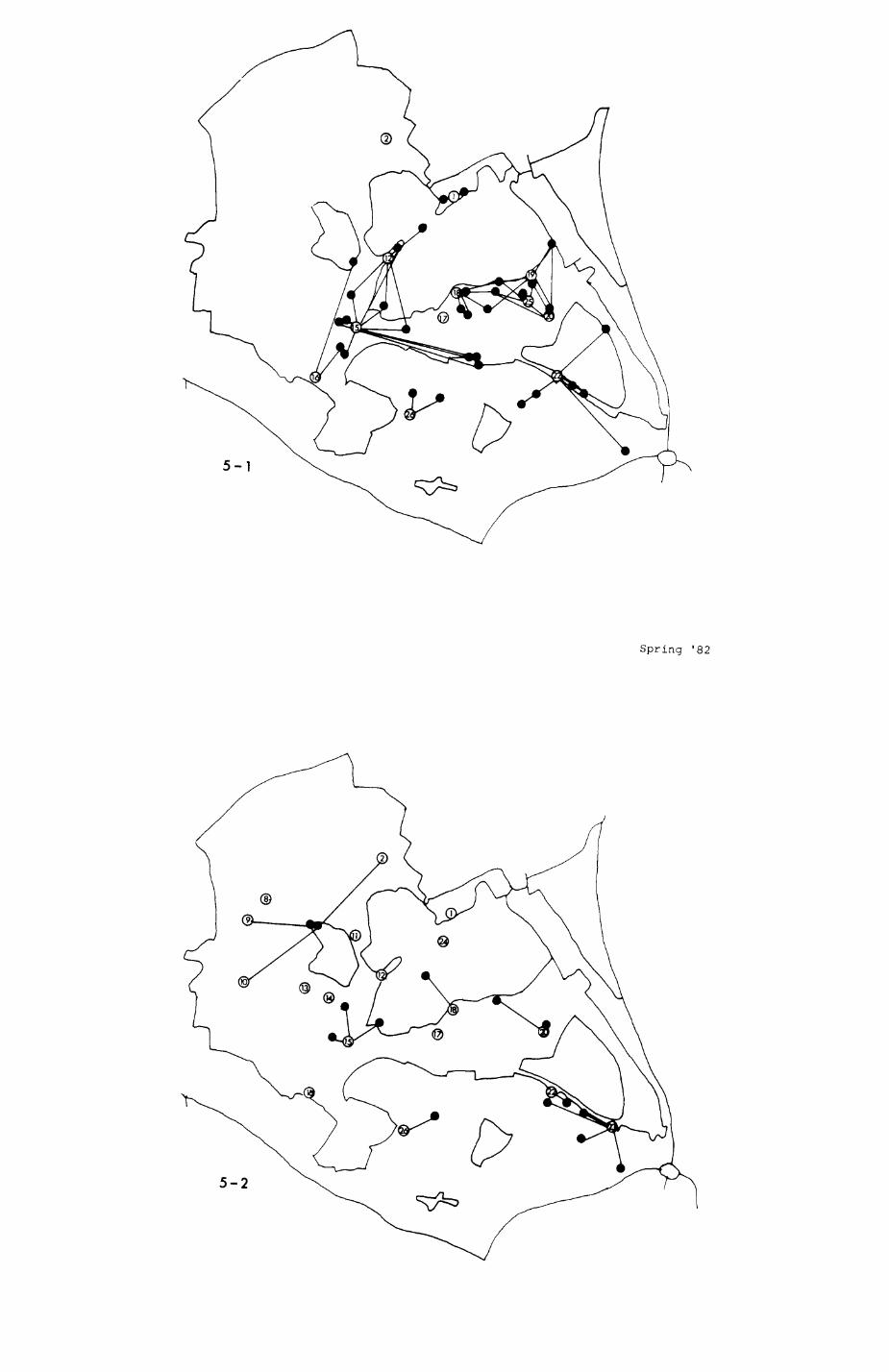
5-1
Spring '82
5-2
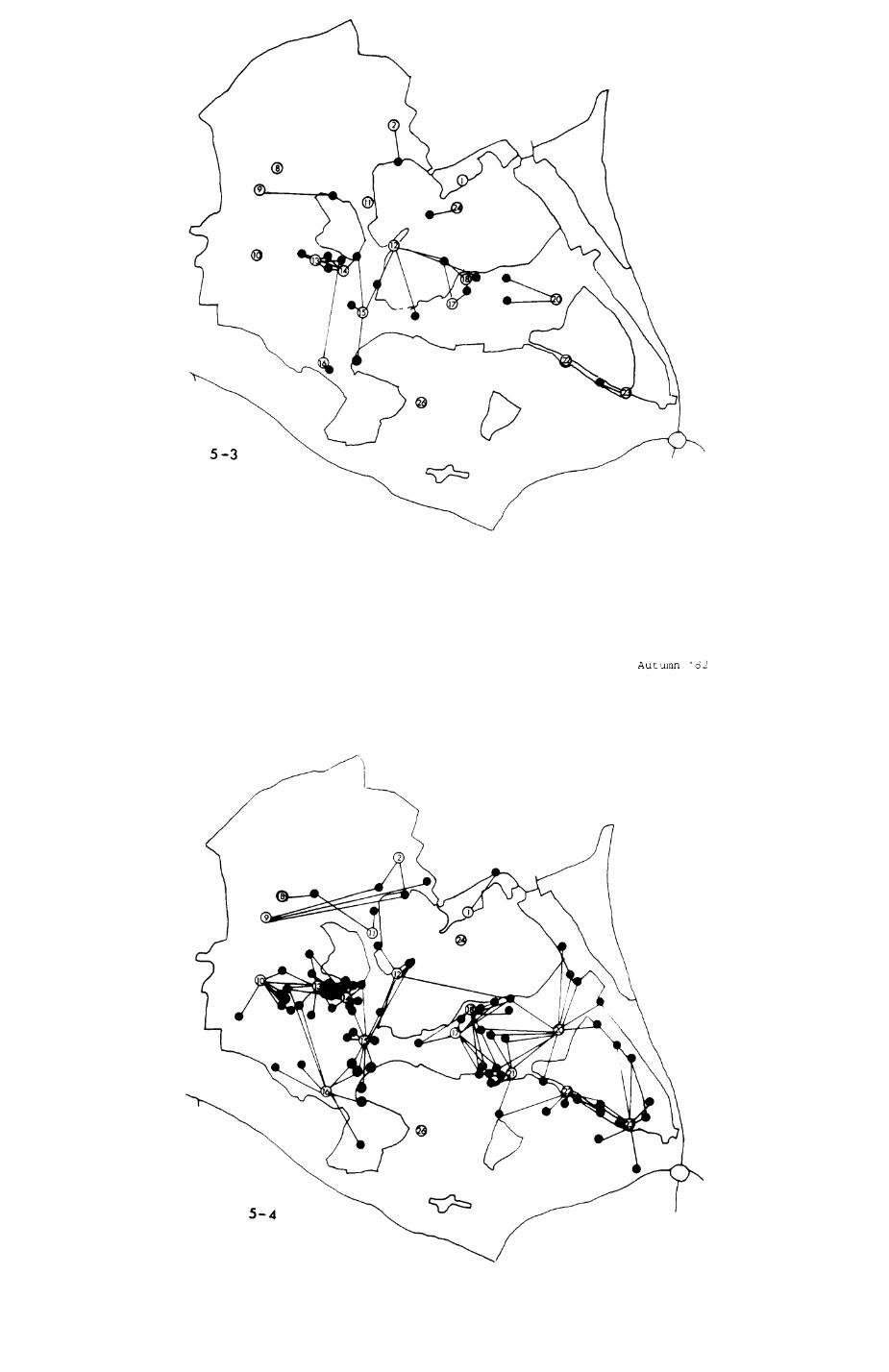
5-3
Autumn '62
5-4
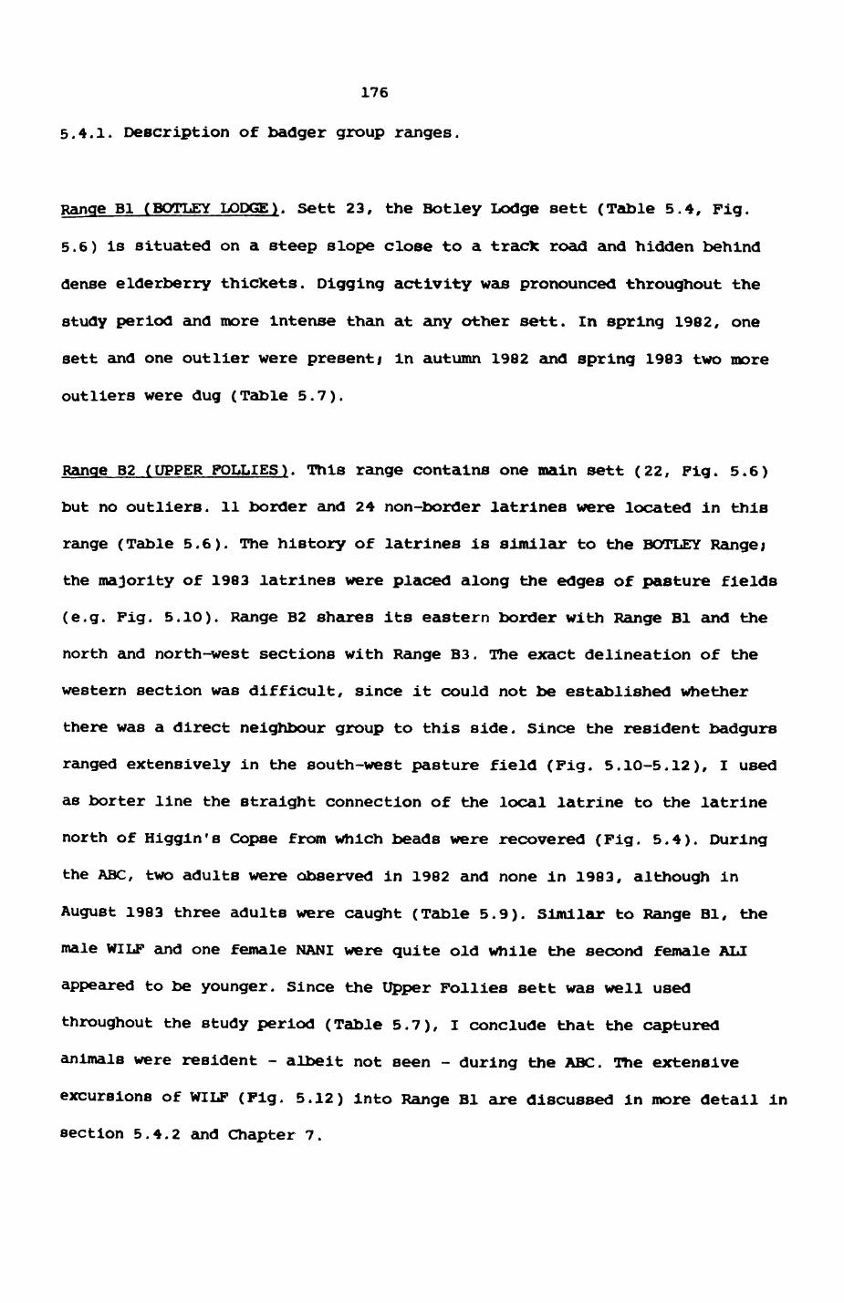
176
5.4.1. Description of badger group ranges.
Range Bl (BOTLEY LODGE), sett 23, the Botley Lodge sett (Table 5.4, Fig.
5.6) is situated on a steep slope close to a trade road and hidden behind
dense elderberry thickets. Digging activity was pronounced throughout the
study period and more intense than at any other sett. In spring 1982, one
sett and one outlier were present; in autumn 1982 and spring 1983 two more
outliers were dug (Table 5.7).
Range B2 (UPPER FOLLIES). This range contains one main sett (22, Fig. 5.6)
but no outliers. 11 border and 24 non-border latrines were located in this
range (Table 5.6). The history of latrines is similar to the BOTLEY Range;
the majority of 1983 latrines were placed along the edges of pasture fields
(e.g. Fig. 5.10). Range B2 shares its eastern border with Range Bl and the
north and north-west sections with Range B3. The exact delineation of the
western section was difficult, since it could not be established whether
there was a direct neighbour group to this side. Since the resident badgurs
ranged extensively in the south-west pasture field (Fig. 5.1O-5.12), I used
as borter line the straight connection of the local latrine to the latrine
north of Biggin's Copse from which beads were recovered (Fig. 5.4). During
the ABC, two adults were observed in 1982 and none in 1983, although in
August 1983 three adults were caught (Table 5.9). Similar to Range Bl, the
male WILF and one female NAN I were quite old while the second female ALI
appeared to be younger. Since the Upper Follies sett was well used
throughout the study period (Table 5.7), I conclude that the captured
animals were resident - albeit not seen - during the ABC. The extensive
excursions of WILF (Fig. 5.12) into Range Bl are discussed in more detail in
section 5.4.2 and Chapter 7.
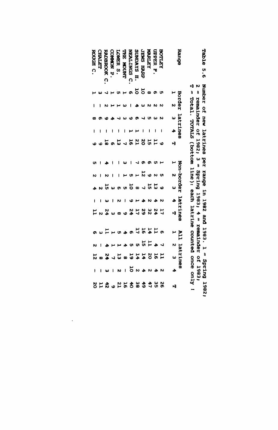
Table 5.6 Number of new latrines per range
in 1982 and 1983.
1 = Spring 1982;
2 = remainder of
1982) 3
= Spring 1983;
4 = remainder of 1983;
T = Total. TOTALS
(bottom line): each
latrine counted once only !
RangeBorder
latrines 1
2 3
4 T
Non-border latrines
1 2
3 4
TAll
latrines1234
BOTLEY
UPPER F.
MARLEY
JEWS HARP
SUNDAYS H.
HEALINGS C
THE MOUNT
LOWER S.
COMMON P.
RADBROOK C
CHALET
ROUGH C.
56810
1O6151731
22234—3112——
235769374968
_._ Q
~
11
-
15-
201
211
167-
136-
189__
Q
15667—3——4—5
52912151——2—2
9131578105631524
242419—2—3——
1724
3229
172498324211
61114161764511136
741115554114—2
1116201414
198137248
12
2424210—2—3——
26354749384O16219
421120

Table 5.7
Number of setts and outliers per badger range. 1 ~ Spring
1982; 2 = Autumn
1982; 3 = Spring
1983; S = number of active setts;
SH = number of used holes, summed over all setts per range/
O - num ber of active outliers;
OH - number of used holes summed over all active outliers per range;
TOTAL = numbers of setts and outliers present,
but not necessarily used per range; x) does not consider
setts or outliers outside the study area.
TOTAL
Range
BOTLEY
UPPER P.
MARLEY
JEWS HARP
SUNDAYS H.
NEALINGS C.
THE MOUNT
LOWER SEEDS
RADBROOK C.
ROUGH C.
Total
setts
S11322—1221
15
1SH25
1165—57
152
58
2S1122212121
15
SH2788738192
55
S1152212121
19
3SH210
2313192
20
11142
116
Outliers1
O_—14——441—14
OH——16——661—2O
2O1—15——————7
OH1—27——————1O
3O2—222———118
OH2—335———11
13
1152212221
3 O 516 9O
x)
4891 X)
20 55
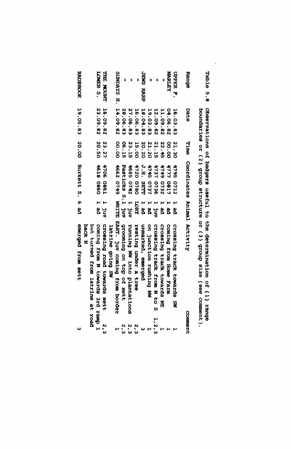
Table 5.8 Observations of badgers useful to the determination of (1)
range boundaries or (2) group structure or (3) group size
(see comment).
RangeDate
UPPER PMARLEY
16.O3.83
04.06.82
11.09.82
12.O9.82
19.03.83
18.04.83
16.O6.83
27.06.83
28.06.83
SUNDAYS H.
14.O9.82
JEWS HARP
it
THE MOUNT
LOWER S.
RADBROOK
16.09.82
23.09.82
Time Coordinates Animal Activity
comment
21.30 oo.oo2
2.4
5
21
.15
21
.20
2
0.2
0
15.0
0
23.1
5
06.1
5
OO
.OO
23.27
20.50
4795 O712
4777 OS17
4749 O732
4737 O736
4745 O737
J.H. SETT
4720 O780
4685 0742
Pas ticks s4662 O749
4706 O861
4618 0860
1 ad 1 ad 1 ad 1
juv 1 ad 1 ad LORY 1 juv .1 }uvWHITE
1 juv
1 ad
19.O5.83
20.OO
Burkett S.
6 ad
crossing track towards SW 1
coming from Home Farm 1
crossing track towards NE 1
crossing track from N to S 1,2,3
on junction rushing NW 1
unmarked, emerged
3 resting under a tree
2,3 running NW into plantations
2,3 grooming on top of sett
2,3 EART.
juv coming from border 1
latrine going SWcrossing road
towards sett 2,3
coming from N towards
3rd ramp 1 but
turned from latrine at road
back N emerged
from sett 3
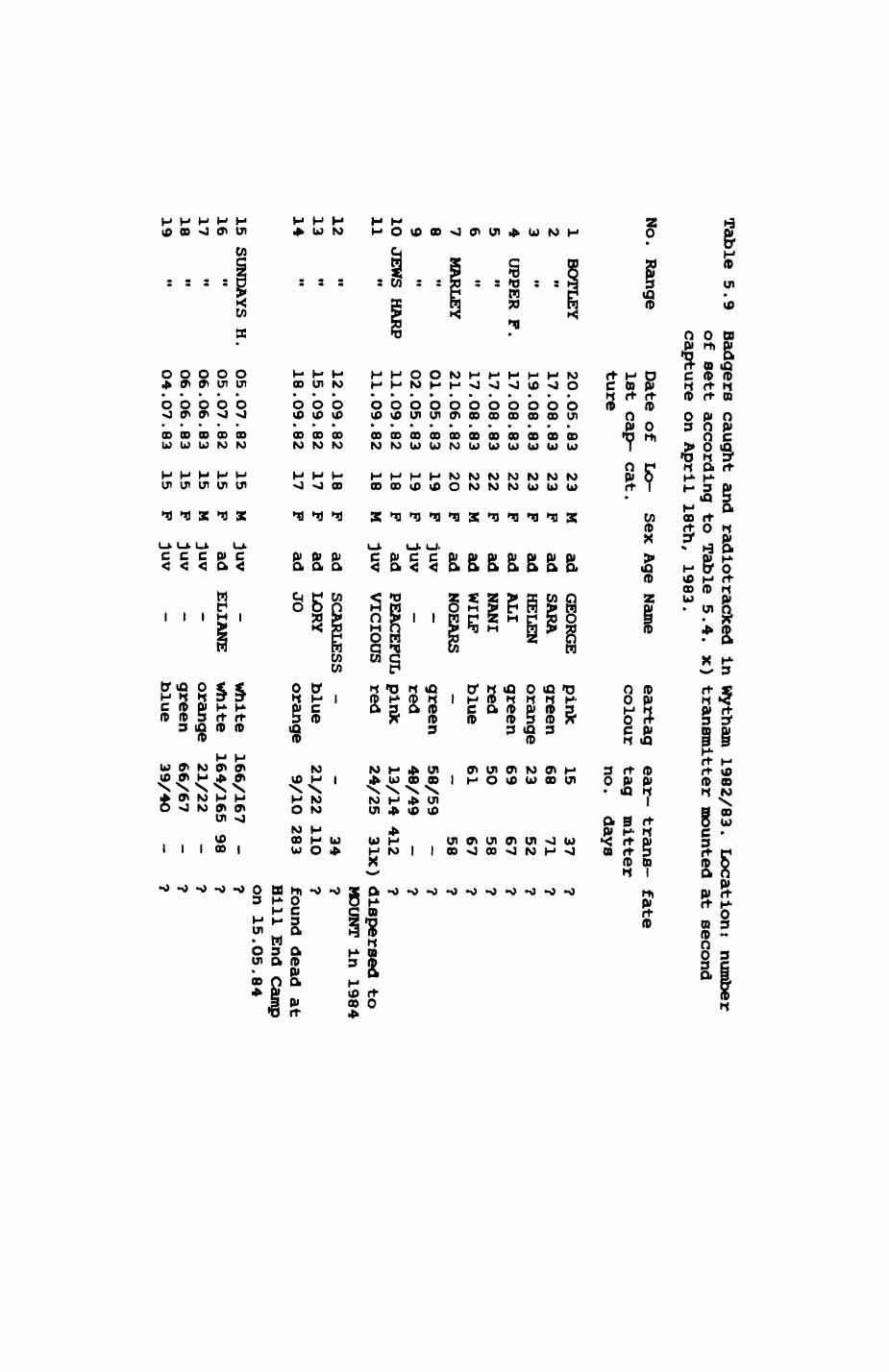
Table 5.9Badgers caught and radlotracked
in Wytham 1982/83. Location!
number of sett according to Table 5.4.
x) transmitter mounted at second capture on April 18th,
1983.
No. Range
Date of Lo-
sex Age Name1st cap- cat.ture
eartag ear- trans- fate
colour tag
mitter no.
days
1 BOTLEY
234 UPPER F.
567 MARLEY
8910
JEWS HARP
11
121314
15 SUNDAYS H.
1617
••
1819
20.17.19.17.17.17.21.01.02.11.11.
12.15.18.
05.O5.O6.O6.O4.
05
08
08O8
08
08O6
05
050909
090909
O7O706
O6O7
.83.83.83.83.83.83.82.83.83.82.82
.82.82.82
.82.82.83.83.83
2323232222222O19191818
18
1717
15
15
151515
MFPPPMFFFPMFFFMFMFF
adadadadadadadjuvjuvad}uvadadad
juvadjuvjuvJuv
GEORGE
SARA
HELEN
ALI
NANI
WILF
NOEARS
——
PEACEFUL
VICIOUS
SCARLESS
LORY
JO
—ELIANE
———
pinkgreenorangegreenredblue—greenredpinkred—blueorange
whitewhiteorangegreenblue
1568236950
61—58/59
48/49
13/14
24/25
—21/22
9/10
166/167
164/165
21/22
66/67
39/4O
3771
52
67586758—-
4123 IX)
34
110
283-
98———
??????????dispersed toHDUNT in 1984
??found dead atHill End campon 15.O5.84?????
Fig. 5.5
core study area with latrines and badger range borders.
Thin linesi major woodland border
Dotted linesi range borders
Stippled lines t major tracks and foot paths
Encircled numberst setts according to Table 5.4
Filled circlest latrines
Some latrines were not shown, if they are very close to others and a main
sett
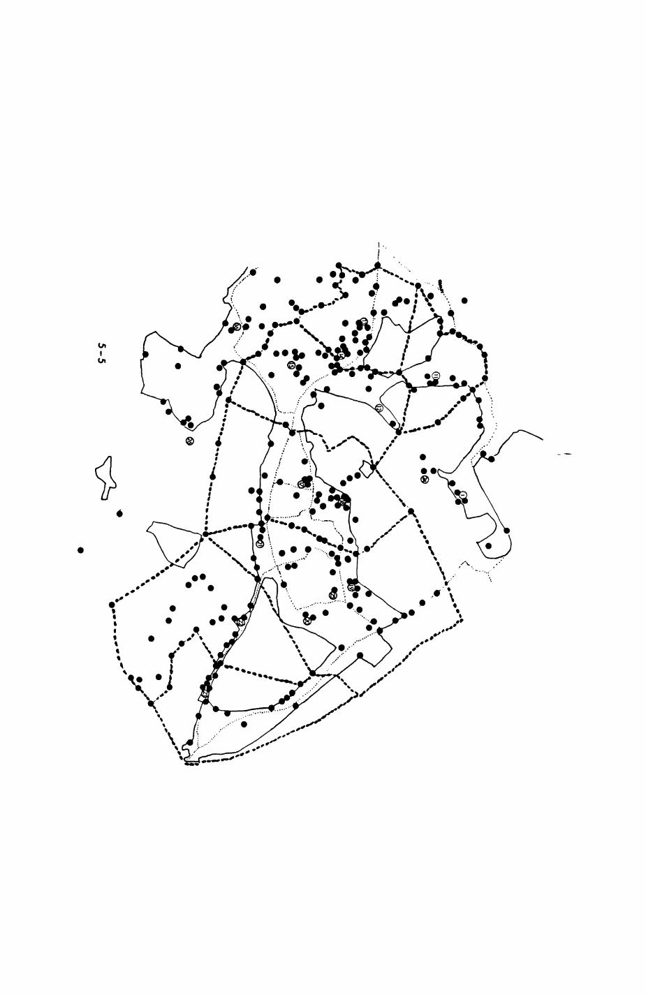

Pig. 5.6
Map with Known outliers and major setts.
Thin linest major woodland boundaries
Dotted linesi range borders
Encircled numbersi setts according to Table 5.4
Pilled circlest outliers
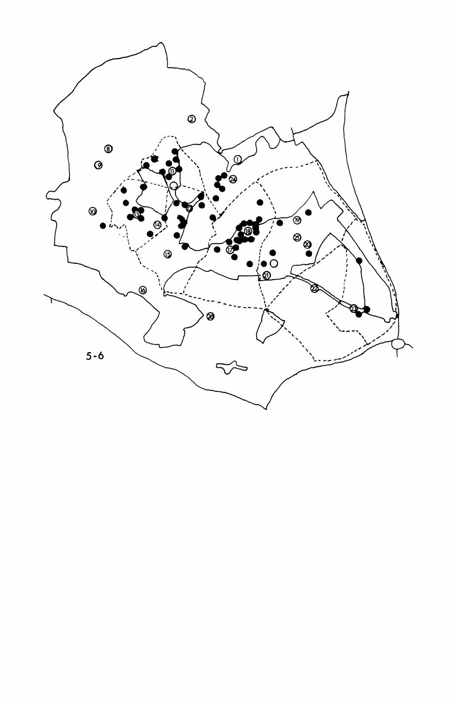
5-6
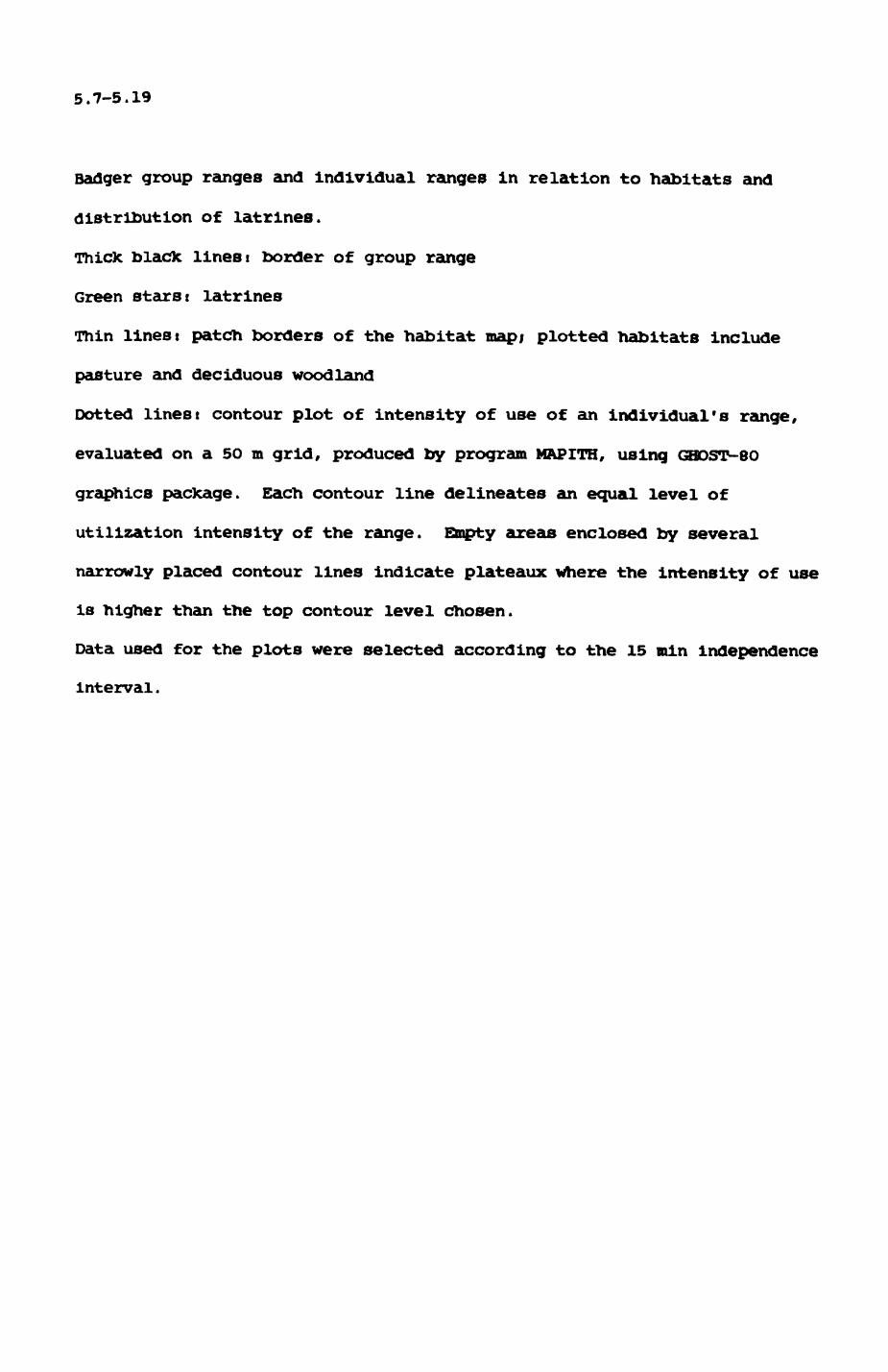
5.7-5.19
Badger group ranges and individual ranges in relation to habitats and
distribution of latrines.
Thick blade lines i border of group range
Green stars» latrines
Thin lines t patch borders of the habitat map; plotted habitats include
pasture and deciduous woodland
Dotted lines t contour plot of intensity of use of an individual's range,
evaluated on a 50 m grid, produced by program MAPITH, using GHOST-80
graphics package. Each contour line delineates an equal level of
utilization intensity of the range. Empty areas enclosed by several
narrowly placed contour lines indicate plateaux Where the intensity of use
is higher than the top contour level chosen.
Data used for the plots were selected according to the 15 min independence
Interval.
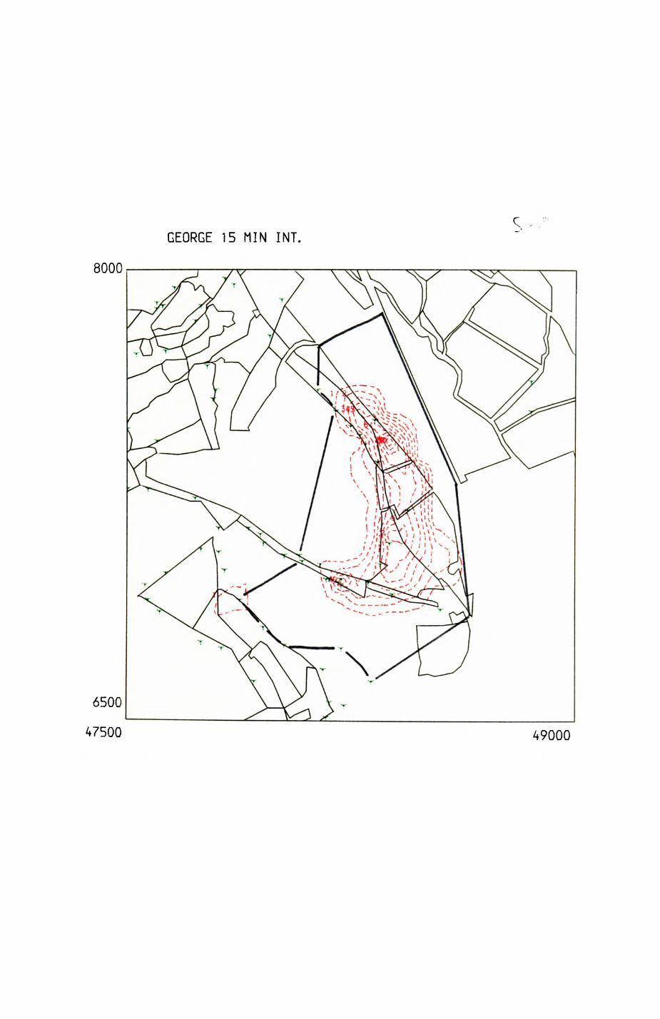
inUJ
C3
a: oU
J C
3
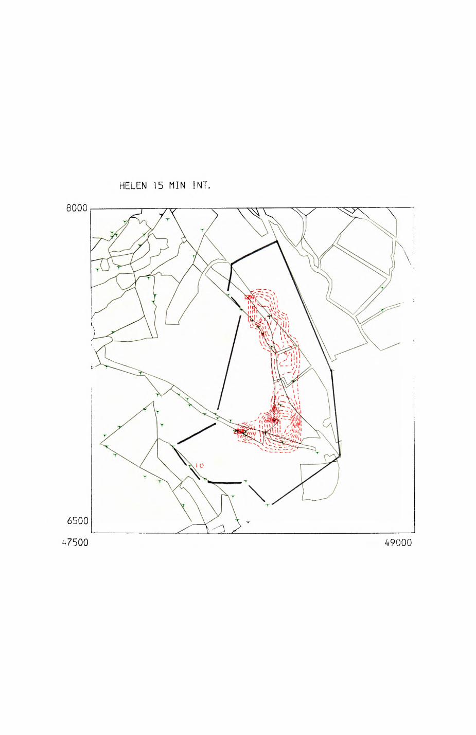
HELEN 15 MIN INT.
8000
49000
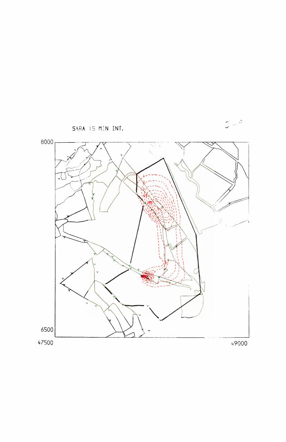
S^RA 15 MIN INT.
8000
^9000
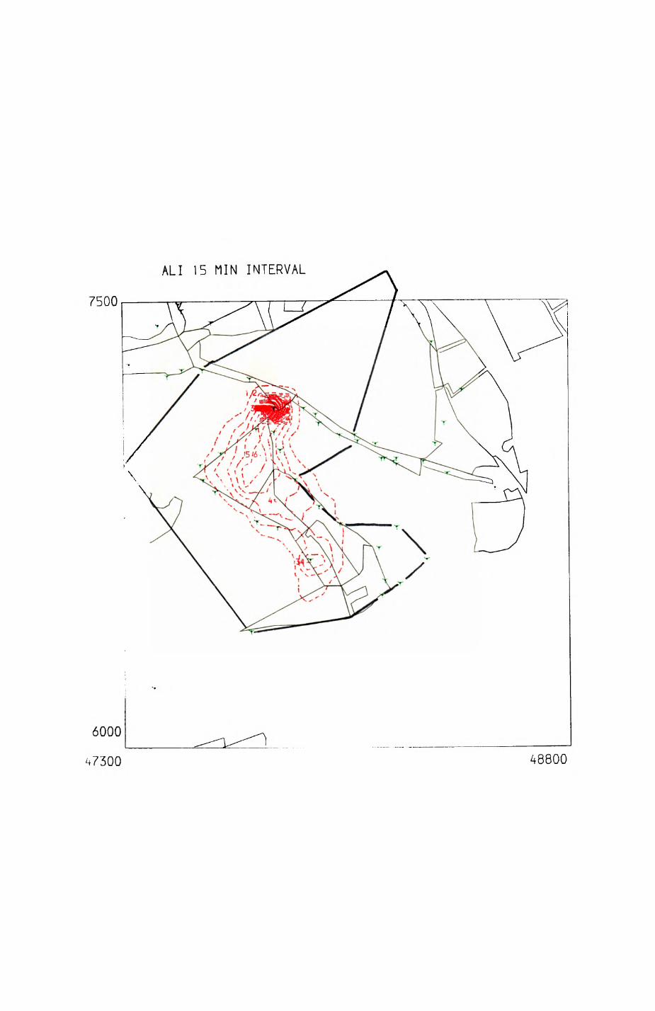
0088*7
0009
OOSZ
lVAd31NI NIW 51 I1V
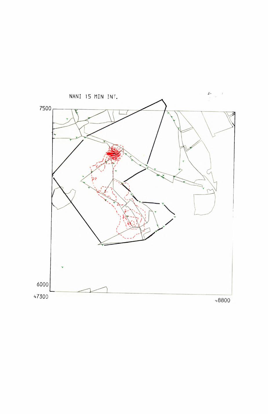
NANI 15 MIN INT.
7500
8800
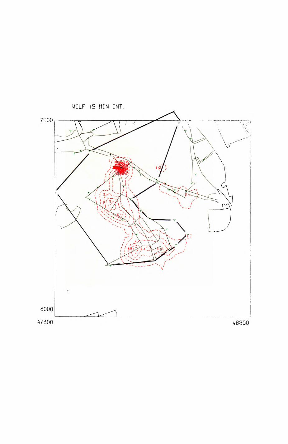
0088^
0009
OOSZ
LPtn o: <cLU
O
PEACEFUL 15 MIN INT.
3^00
6900
46200 47700
CN
(V)
o
o 4--
O
O
o LJ1 H rn
LORY 15 M!N INTERVAL
7700
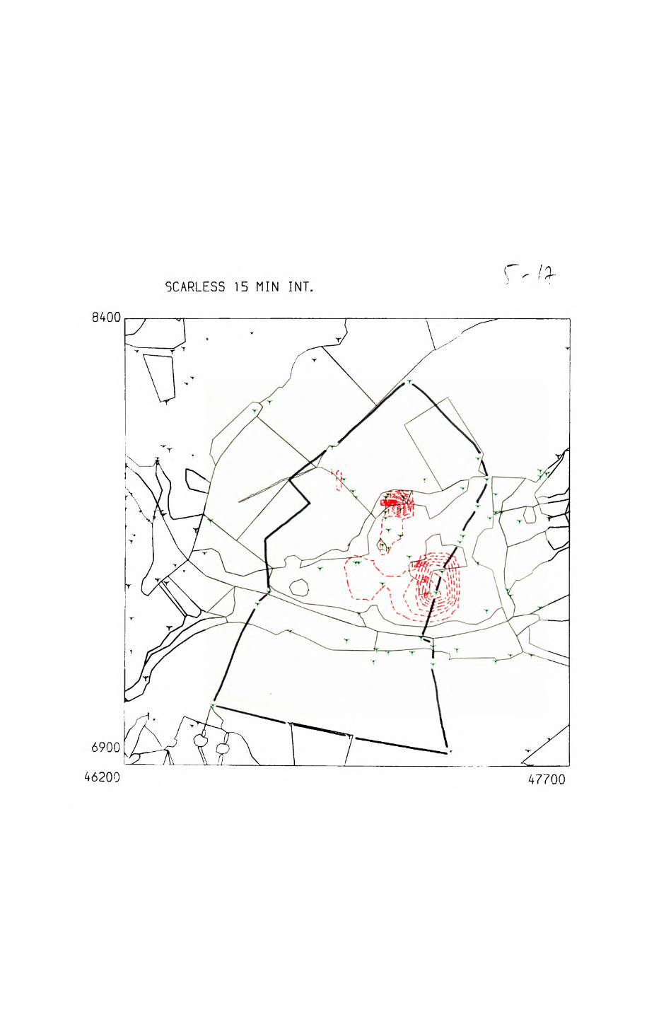
SCARLESS 15 MIN INT.
8400
47700
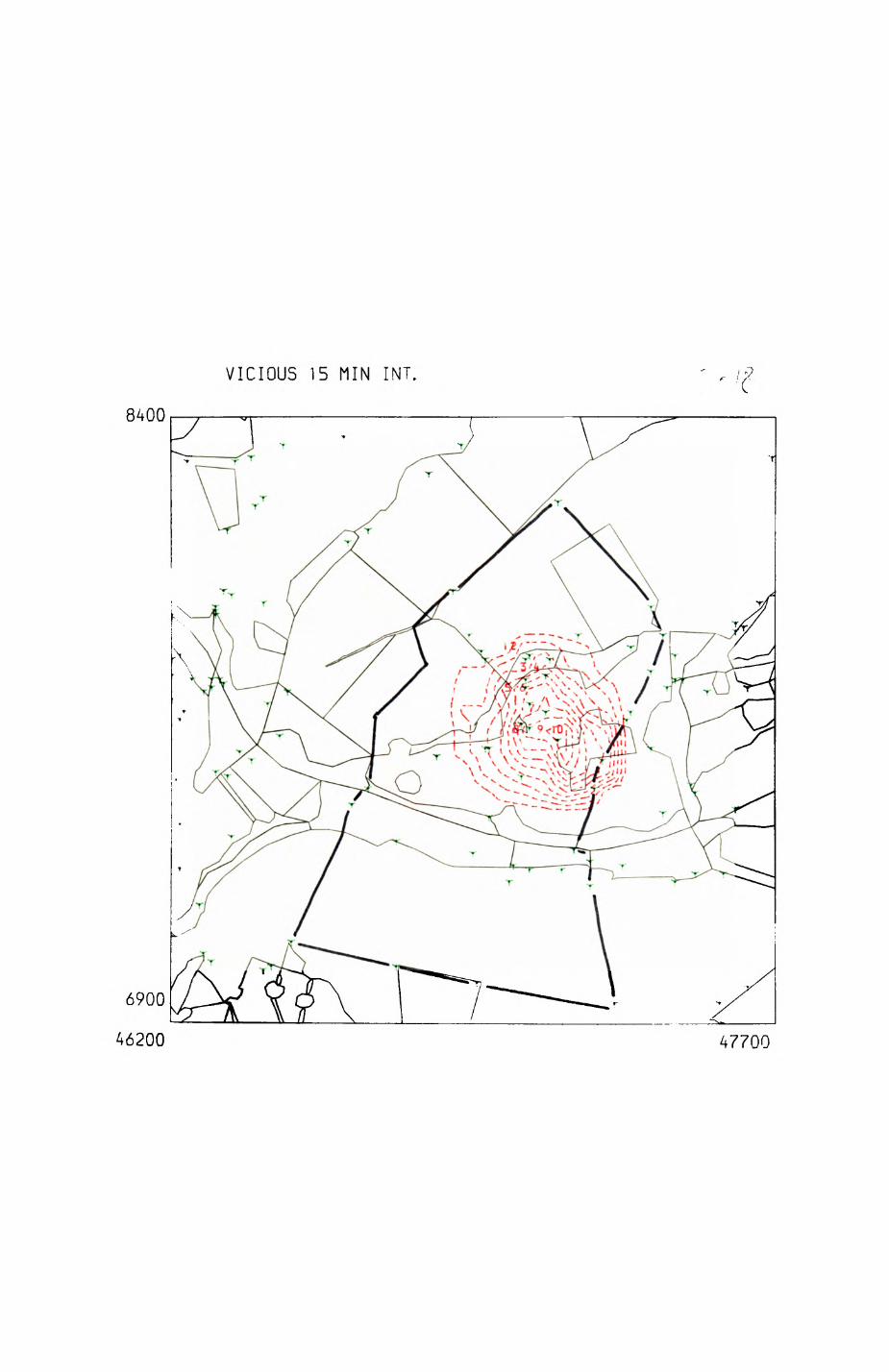
VICIOUS 15 MIN INT. 'C
8400
47700
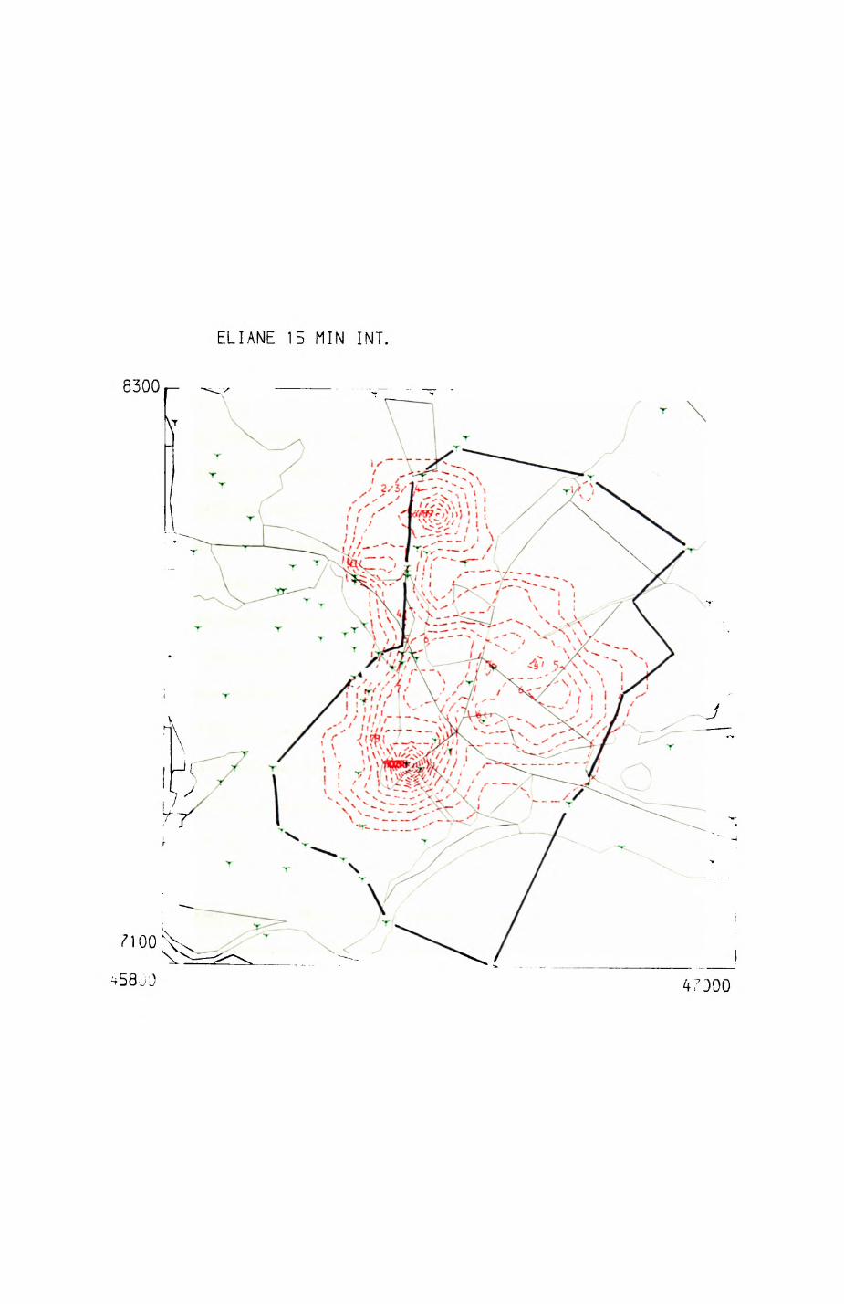
LTI
LU
177
Range B3 (MARLEY). This is the largest known range in wytham (Table 5.10).
At least 5 excavations qualify as setts (Fig. 5.6), three of which are
checked during the ABC (19, 20, 21, Pig. 5.6). One sett (25, Fig. 5.6),a. formerly the centre of Hans Kruuk's (1978a) bachelor clan,0is now mostly
occupied by foxes and rabbits, and another hole (unnumbered. Fig. 5.6) is
occasionally used by badgers. 15 border latrines and 32 non-border latrines
were found. One of the best documented range boundaries is shared by the
MARLEY Range with its western neighbour, the JEWS HARP Range. This border
section runs from north to south through the Pastick's Plantation and is
clearly defined by a heavily trotten badger track and 1O latrines (Fig. 5.5
and 5.13). Several observations of unmarked badgers in the south-west corner
of the range and the observation of a badger returning from Home Farm in the
north-west (Table 5.8) besides the movements of the female NOEARS (Fig.
5.13) and the bead recovery record emphasize the extension of the range of
this group. During the ABC 3 adults in 1982 and 2 adults in 1983 were
observed. More badgers were observed, but since they emerged from different
setts at different dates, the total number is unknown. In June 1982, one old
female without pinnae was caught (Tabe 5.9, Fig. 5.13). Despite intense
trapping efforts at setts 19 and 20, only two cubs were caught in spring
1983 (Table 5.9).
Range B4 (JEWS HARP). This range contains two main setts (17 & 18, Fig.
5.6), both intensively used throughout the study period, and 16 outliers,
some of which were used in 1982 (Table 5.7). The observed increase in use of
outliers in autumn 1982 could indicate dispersal pressure since juveniles
and subdominants ready to disperse tend to stay in outliers in autumn (Kruuk
(I978a), Neal (1977), Long & Killingley 1983). JEWS HARP is the only range
with information on dispersal. JO, an old female occasionally located
outside the group range (Fig. 5.15), was found dead in Range B6 at Hill End
178
Camp. VICIOUS, a male cub recaught as a young adult dispersed in its second
year to range B7 (ABC, 1984). Both animals dispersed to neighbouring ranges,
less than 1 tan apart. 20 border and 29 non-border latrines were identified
(Table 5.6). Eastern, northern, and western sections of the range border
were well-defined (Pig. 5.1-5.4, 5.14-5.18). Although I did not recover
beads from the southern border I believe the extension of the range beyond
the wood is justified, since two radio-tracked animals were located in the
midst of the arable fields south of the woodland. According to the ABC and
my own observations group size varied between 5 and 7 adults (Table 5.8,
5.10). Four females were caught, two old ones (PEACEFUL and JO) and two in
their prime (LORY and SCARLESS) and one male cub later recaught as a young
adult (VICIOUS). Contour plots of their movements are shown in Fig. 5.14-
5.18.
Range 85 (SUNDAYS HILL). This includes two setts (12 and 15, Fig. 5.6) and 9
outliers, sett no. 12 was included in this range since bead recoveries from
both setts overlapped (Fig. 5.1-5.4) and during each baiting period several
faeces were found that contained beads from both setts, implying that at
least one individual has been eating beads at both setts. In this range 21
border latrines were found, the highest score of all ranges. Also, the
highest number of border latrine foundations outside spring occurred here
(Table 5.6). The border to range BIO, its western neighbour, is littered
with border latrines and non-border latrines nearby (Fig. 5.5, 5.19). The
south-east corner of the Lower Seeds field seemed to be attractive to both
ranges, as indicated by ELIANE's excursions in autumn 1982 (Fig. 5.19) and a
series of latrine foundations along the track leading to the south-east
corner in spring 1983, mostly claimed by Range BIO (Fig. 5.4). All other
border sections were well defined except for the south-east corner. Any of
the latrines 254, 255 or 59 was a likely candidate as a cornerstone of the
179
border to the eastern neighbour, the JEWS HARP Range. Here I decided to take
the medium line between the two extremes, following in principle Kruuk's
(I978a) procedure. In 1982 a male cub and a small old female called ELIANE
and in 1983 three juveniles were caught. Despite one chance observation
(Table 5.8) none of the marked cubs has been observed since its capture.
Range B6 (NEALINGS COPSE). This is a range with one main sett within the
Wytham Wood area and no outliers and extending over Denman's Farm to Cumnor
Hill, south of the study area (Fig. 5.20). A male badger caught by D.W.
Macdonald at Cumnor was radio-tracked throughout the Cumnor area, Denman's
Farm and the Radbrook Common area in Wytham (D.W. Macdonald pers. comm. ).
Badgers were also repeatedly observed to cross the Eynsham road from Hill
End camp to Denman's Farm; one female was killed by a car while crossing.
Beads placed at the Nealing's Copse sett (16, Fig. 5.6) were recovered from
latrines at Cumnor Hill (Fig. 5.2O). Close inspection of the latrines at the
Nealing's Copse sett in autumn 1982 and 1983 revealed the presence of
cultivated fruits in badger faeces that are unknown from Wytham but grown in
the orchards at Denman's Farm. This considerable body of evidence implies
regular exchange of badgers between areas on both sides of the Eynsham road
and supports the idea that both areas are part of one range. Thus, absence
of badgers from Nealing's Copse during the ABC does not Indicate an empty
range; rather group size estimates are incomplete. Within the study area 16
border and 24 non-border latrines were located. The position of the Hill End
Camp sett (26, Fig. 5.6) is uncertain) the bead recoveries do not present
conclusive evidence to establish it as the centre of a separate range next
to B6.
Range 87 (THE MOUNT). This range includes two setts (1,24, Fig. 5.6). 16
latrines were located in parts of the study area that could be unequivocally
180
assigned to this range. Its extension to the north and the east (towards the
village) remains unknown (Pig. 5.20). In autumn 1981 and 1982 I repeatedly
observed badgers in the village and once saw a large adult cross the parking
area of the local pub at 22.00 hours while radiotracking a fox nearby. The
relationship of B7 to its western neighbour B9 is unknown. In spring 1982
and 1983 excavation activity was very pronounced (Table 5.7) but thereafter
sett 1 showed little signs of use. 2 adults and 1 cub were seen in 1982, 5
adults and 2 cubs in 1983 and 3 adults and 4 cubs in 1984 (Table 5.10).
Range 88 (LOWER SEEDS). The smallest of all known ranges in wytham includes
one main sett and another old and infrequently used excavation at its
southern border. This range had no access to pasture fields except some
fallow land slowly converting to grassland. The asphalt road from the
village to the Chalet was determined as its north-western border, since few
of the many badgers seen close to the road actually crossed but usually
turned back in the direction from which they came, and the track was
littered with latrines (Fig. 5.5). Animals were observed in 1982 and 1984,
but not in 1983.
Range B9 (COMMON PIECE). This range covers the north-eastern part of the
Great Wood around sett 2 (Fig. 5.20). 9 latrines could be associated with
It. Animals were observed at the main sett in 1982 and 1984 (Table 5.10).
Range BIO (RADBRQQK COMMON). Similar as Range B8, this is a range without
access to pasture fields and includes two main setts (13, 14, Fig. 5.6)
surrounded by a host of outliers (Table 5.7, Fig. 5.6). 18 border and 24
non-border latrines were identified (Table 5.6). The baiting periods in
autumn 1982 and spring 1983 showed conclusively that the two setts belong
together and are apparently used inter-changeably by the resident badgers
181
(Pig. 5.3, 5.4). Faeces with beads from both setts were recovered several
times. Although the second smallest of all known ranges, group sizes can
compete with or exceed those of larger ranges (e.g. B3 and B4, Table 5.10),
and reproductive output was consistently high (Table 5.10). Range borders
were well defined except for the northern section across the Lower Seeds
field. As with the border between Ranges B4 and B5 I took the middle line
and assigned the northern half of the Lower Seeds field to Range B8 and the
southern half to Range BIO. Despite intensive search on the Lower Seeds
field no latrines were located suggesting that this was not an important
border section.
Range Bll (THE CHALET). This range covers some parts of the north-west of
the Great Wood and Includes setts 8 and 9 (Fig. 5.6). 11 latrines could be
assigned to this range within my study area (Table 5.6). Group sizes were
amongst the highest encountered (Table 5.10).
Range B12 (ROUGH COMMON). This range is probably the southern neighbour of
Range Bll and the western neighbour of Range BIO. One sett is found in the
study area (Fig. 5.6) but it is likely that a second sett at the Reservoir
belongs to this range as well (Kruuk 1978a). Activity increased greatly in
spring 1983 when 8 new border latrines were founded (Table 5.6), separating
this range more clearly from the east (Range BIO) and the southeast (Range
86). Group size appeared to be small (Table 5.10) but was probably
underestimated since the second sett at the Reservoir was not included in
the ABC.
Summary. Altogether 12 ranges could be identified in Wytham from bead
recovery, radio-tracking and chance observations. 7 ranges could be
completely delineated. Both bead recovery records and radio tracking were
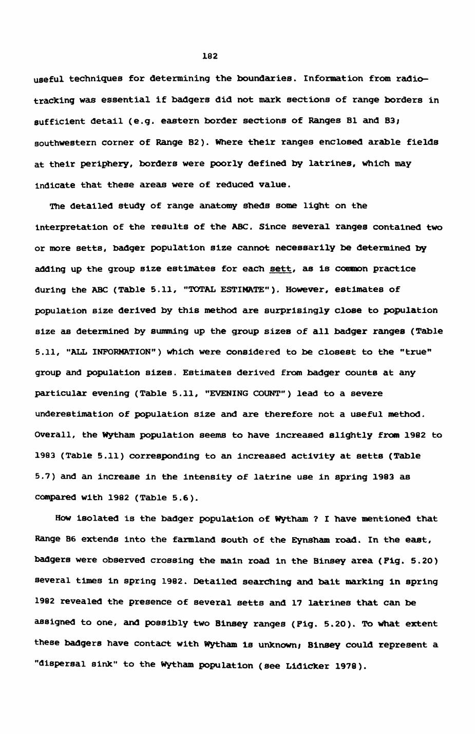
182
useful techniques for determining the boundaries. Information from radio-
tracking was essential if badgers did not marie sections of range borders in
sufficient detail (e.g. eastern border sections of Ranges Bl and 83;
southwestern corner of Range B2). Where their ranges enclosed arable fields
at their periphery, borders were poorly defined by latrines, which may
indicate that these areas were of reduced value.
The detailed study of range anatomy sheds some light on the
interpretation of the results of the ABC. Since several ranges contained two
or more setts, badger population size cannot necessarily be determined by
adding up the group size estimates for each sett, as is common practice
during the ABC (Table 5.11, "TOTAL ESTIMATE"). However, estimates of
population size derived by this method are surprisingly close to population
size as determined by summing up the group sizes of all badger ranges (Table
5.11, "ALL INFORMATION") which were considered to be closest to the "true"
group and population sizes. Estimates derived from badger counts at any
particular evening (Table 5.11, "EVENING COUNT") lead to a severe
underestimation of population size and are therefore not a useful method.
Overall, the Wytham population seems to have increased slightly from 1982 to
1983 (Table 5.11) corresponding to an increased activity at setts (Table
5.7) and an increase in the intensity of latrine use in spring 1983 as
compared with 1982 (Table 5.6).
How isolated is the badger population of Wytham ? I have mentioned that
Range B6 extends into the farmland south of the Eynsham road. In the east,
badgers were observed crossing the main road in the Blnsey area (Pig. 5.20)
several times in spring 1982. Detailed searching and bait markIng in spring
1982 revealed the presence of several setts and 17 latrines that can be
assigned to one, and possibly two Binsey ranges (Pig. 5.20). To what extent
these badgers have contact with Wytham Is unknown; Blnsey could represent a
"dispersal sink" to the Wytham population (see Lidicker 1978).
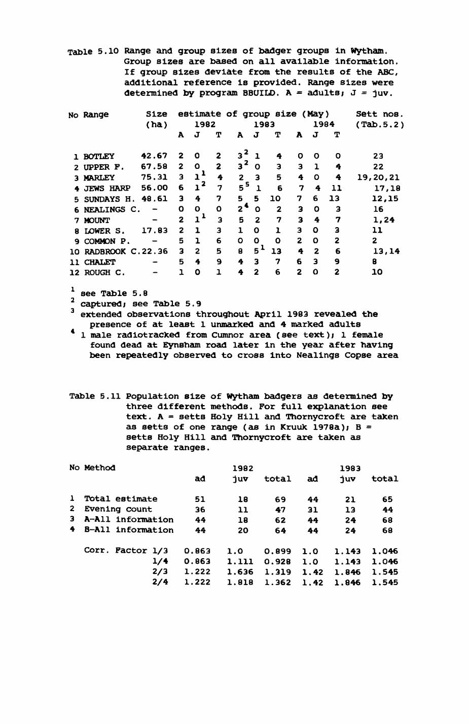
Table 5.10 Range and group sizes of badger groups in wytham.Group sizes are based on all available information. If group sizes deviate from the results of the ABC, additional reference is provided. Range sizes were determined by program BBUTLD. A = adults; J = juv.
No Range Size estimate of group size (May) (ha) 1982 1983 1984
AJTAJTAJT
1 BOTLEY2 UPPER P.3 NARLEY4 JEWS HARP5 SUNDAYS H6 NEALINGS C. -7 MOUNT8 LOWER S.9 COMMON P.
10 RADBROOK11 CHALET12 ROUGH C.
123
Sett nos. (Tab.5.2)
4267755648
17
22
.67
.58
.31
.00
.61——.83_.36
—_
223630225351
00I 1I 2
4OI 1
11240
224770336591
3 23 2
25 5
52 4
510844
1031
502005 1
32
4356
102710
1376
034773332462
010460400230
044
1113
3732692
2322
19,20,2117,1812,15161,2411213,14810
see Table 5.8captured; see Table 5.9extended observations throughout April 1983 revealed the presence of at least 1 unmarked and 4 marked adults
1 male r ad lot racked from Cumnor area (see text); 1 female found dead at Eynsham road later in the year after having been repeatedly observed to cross into Neallngs Copse area
Table 5.11 Population size of Wytham badgers as determined by three different methods. For full explanation see text. A = setts Holy Hill and Thornycroft are taken as setts of one range (as in Kruuk 1978a); B = setts Holy Hill and Thornycroft are taken as separate ranges.
No Methodad
1 Total estimate 512 Evening count 363 A-A11 information 444 B-A11 information 44
Corr. Factor 1/3 1/4 2/3 2/4
1982juv total ad
1983juv total
18111820
69476264
44314444
21132424
65446868
0.8630.8631.2221.222
1.01.1111.6361.818
0.8990.9281.3191.362
1.01.01.421.42
1.1431.1431.8461.846
1.0461.0461.5451.545

Pig. 5.20
Map of the study area with all known badger ranges.
Thin lines t major woodland boundaries and roads
Thin parallel linesi rivers
Numbers! number of badger range
Empty circles i major setts of range
Pilled circlesi latrines in the Binsey area; lines indicate bead recovery
and origin of beads
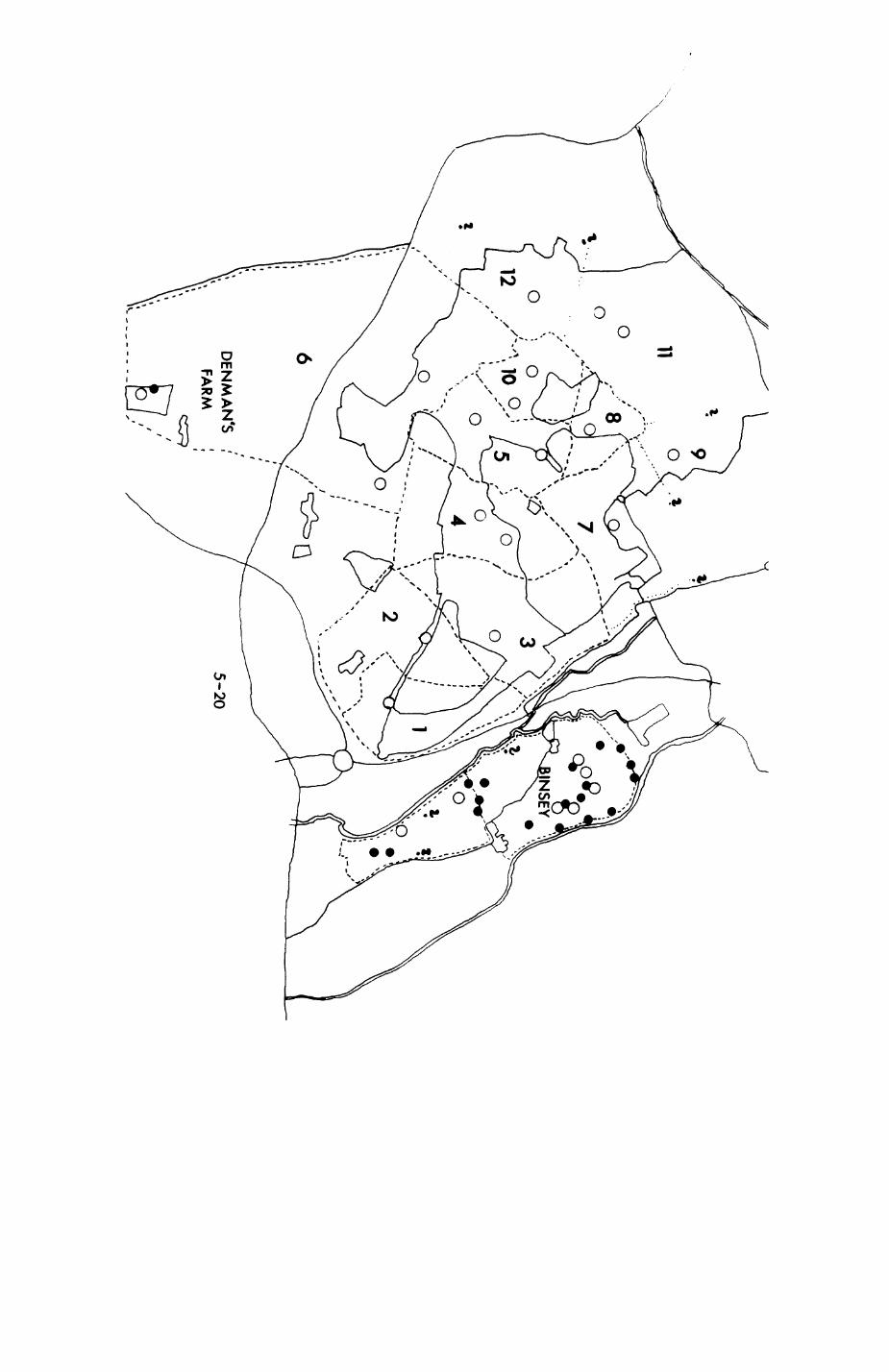
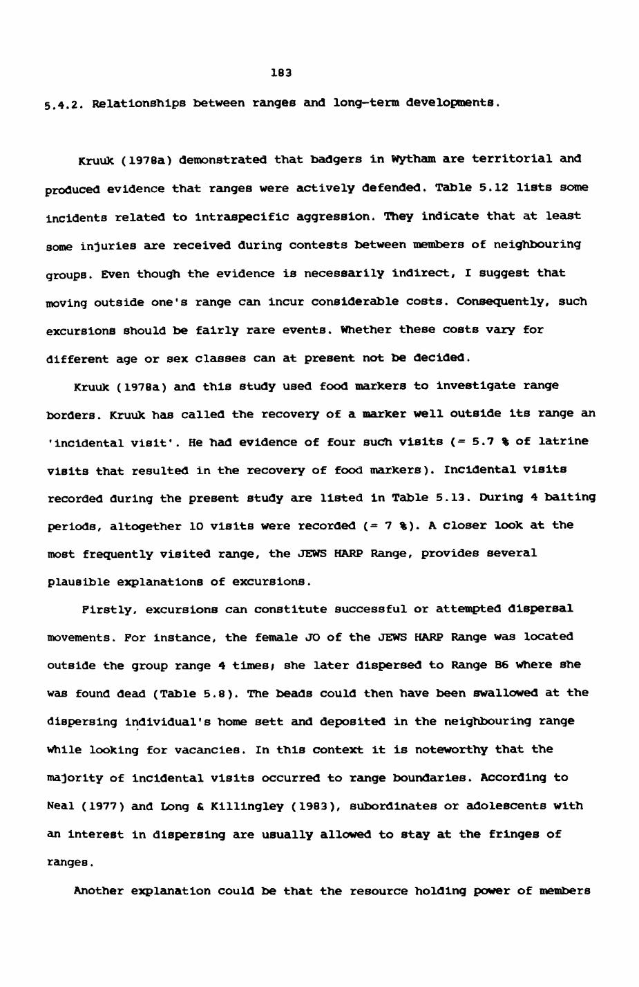
183
5.4.2. Relationships between ranges and long-term developments.
Kruuk (I978a) demonstrated that badgers in wytham are territorial and
produced evidence that ranges were actively defended. Table 5.12 lists some
incidents related to intraspecific aggression. They indicate that at least
some injuries are received during contests between members of neighbouring
groups. Even though the evidence is necessarily indirect, I suggest that
moving outside one's range can incur considerable costs. Consequently, such
excursions should be fairly rare events. Whether these costs vary for
different age or sex classes can at present not be decided.
Kruuk (I978a) and this study used food markers to investigate range
borders. Kruuk has called the recovery of a marker well outside its range an
'incidental visit'. He had evidence of four such visits (= 5.7 % of latrine
visits that resulted in the recovery of food markers). Incidental visits
recorded during the present study are listed in Table 5.13. During 4 baiting
periods, altogether 1O visits were recorded (= 7 %). A closer look at the
most frequently visited range, the JEWS HARP Range, provides several
plausible explanations of excursions.
Firstly, excursions can constitute successful or attempted dispersal
movements. For instance, the female JO of the JEWS HARP Range was located
outside the group range 4 times; she later dispersed to Range B6 where she
was found dead (Table 5.8). The beads could then have been swallowed at the
dispersing individual's home sett and deposited in the neighbouring range
while looking for vacancies. In this context it is noteworthy that the
majority of incidental visits occurred to range boundaries. According to
Neal (1977) and Long & Kllllngley (1983), subordinates or adolescents with
an interest in dispersing are usually allowed to stay at the fringes of
ranges.
Another explanation could be that the resource holding power of members
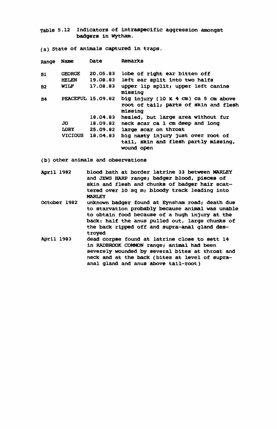
Table 5.12 Indicators of intraspecific aggression amongst badgers in Wytham.
(a) State of animals captured in traps.
Range Name Date Remarks
Bi GEORGE 20.05.83 lobe of right ear bitten off HELEN 19.08.83 left ear split into two halfs
B2 WILP 17.08.83 upper lip split; upper left caninemissing
B4 PEACEFUL 15.09.82 big injury (10 x 4 cm) ca 5 cm aboveroot of tail; parts of skin and flesh missing
18.04.83 healed, but large area without fur JO 18.09.82 neck scar ca 1 cm deep and long LORY 25.09.82 large scar on throat VICIOUS 18.04.83 big nasty injury just over root of
tail, skin and flesh partly missing, wound open
(b) other animals and observations
April 1982 blood bath at border latrine 33 between MARLEYand JEWS HARP range; badger blood, pieces of skin and flesh and chunks of badger hair scat tered over 10 sq m; bloody track leading into MARLEY
October 1982 unknown badger found at Eynsham road; death dueto starvation probably because animal was unable to obtain food because of a hugh injury at the back: half the anus pulled out, large chunks of the back ripped off and supra-anal gland des troyed
April 1983 dead corpse found at latrine close to sett 14In RADBROOK COMMON range; animal had been severely wounded by several bites at throat and neck and at the back (bites at level of supra- anal gland and anus above tail-root)
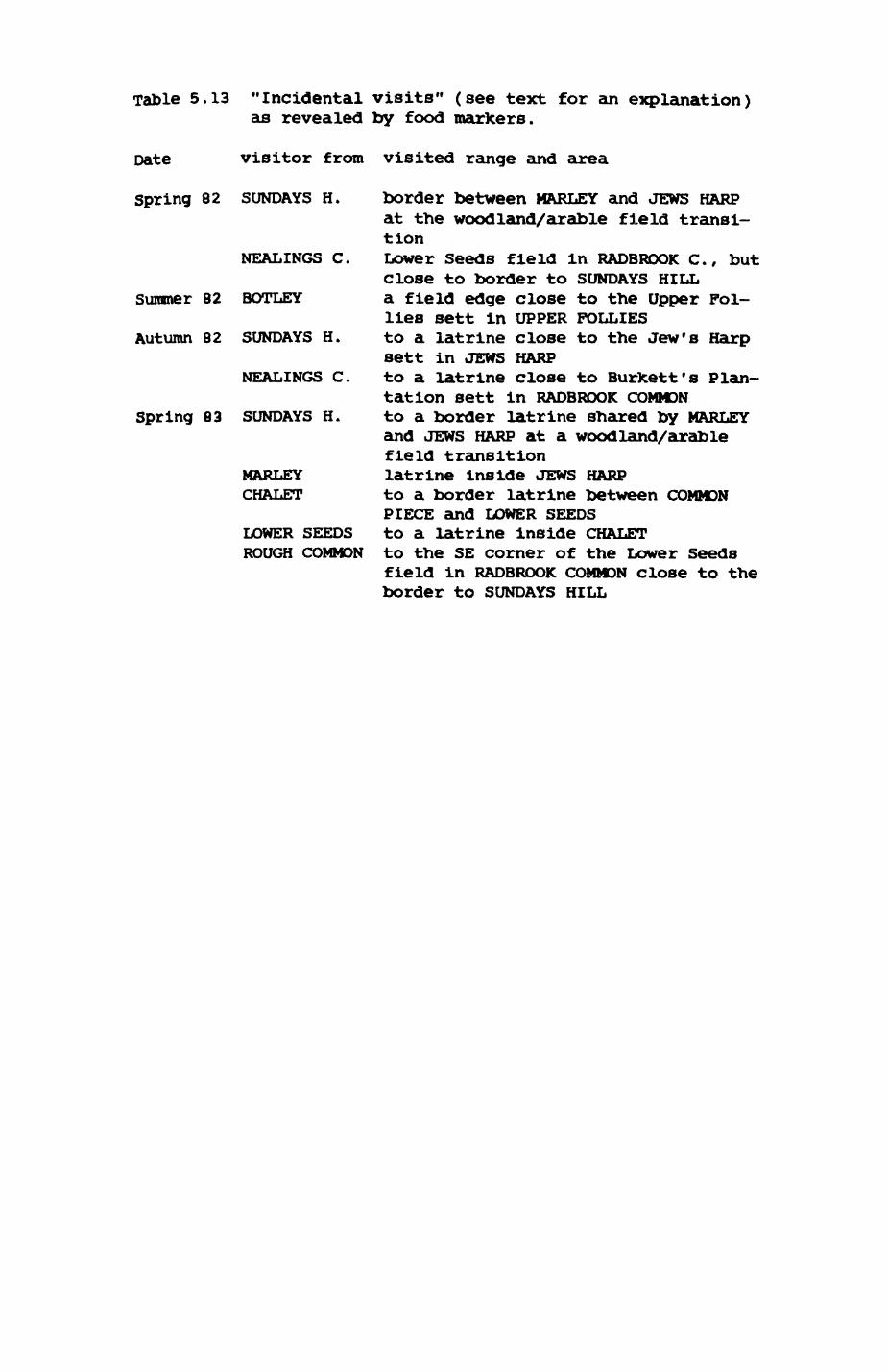
Table 5.13
Date
"Incidental visits" (see text for an explanation) as revealed by food markers.
visitor from visited range and area
Spring 82 SUNDAYS H,
NEALINGS C.
Summer 82 BOTLEY
Autumn 82 SUNDAYS H.
NEALINGS C.
Spring 83 SUNDAYS H.
MARLEY CHALET
LOWER SEEDS ROUGH COMMON
border between MARLEY and JEWS HARP at the woodland/arable field transi tionLower seeds field in RADBROOK C., but close to border to SUNDAYS HILL a field edge close to the Upper Fol lies sett in UPPER FOLLIES to a latrine close to the Jew's Harp sett in JEWS HARPto a latrine close to Burkett's Plan tation sett in RADBROOK COMMON to a border latrine shared by MARLEY and JEWS HARP at a woodland/arable field transition latrine inside JEWS HARP to a border latrine between COMMON PIECE and LOWER SEEDS to a latrine inside CHALET to the SE corner of the Lower Seeds field in RADBROOK COMMON close to the border to SUNDAYS HILL
184
of the JEWS HARP group was lower than usual and insufficient to make their
neighbours readily accept a settlement based on roles. Then contests would
have escalated and could have resulted in the injuries noticed on several
group members (Table 5.12 ).
A third explanation concerns the identity of visitors. The food markers
do not indicate the sex-age class of the visitor. According to intensive
observations at both main setts of the JEWS HARP Range in autumn 1982 and
April 1983, it is almost certain that the sex-ratio was female-biased, since
apart from the four trapped females only two other animals were observed
that could have been males; one of them, however, seemed to be too small for
an adult male. Thus, the high proportion of visits to the JEWS HARP Range
may be due to males from surrounding ranges visiting the resident females.
In a similar vein, the excursion of the old male WILF from Range B2 (Fig.
5.12) into the neighbouring range Bl was probably undertaken to visit the
local females. WILF was actually located once in Range Bl in an outlier
together with SARA, one of the resident females (see also Chapter 7).
If excursions are rare and territoriality a constant feature of the
local system, then long-term changes of the spatial arrangements of groups
should be modest. The results of Kruuk's study provide an ideal opportunity
to record the changes over a 8-year period (1974/75 to 1982/83). Fig 5.21
shows a plot of Kruuk's and my range boundaries.
The most conspicuous change is the amalgamation of the bachelor clan at
The Platform sett with the MARLEY Range. The western border of the then
bachelor clan still serves as boundary between the JEWS HARP Range and its
eastern neighbour - a fine example of continuity ! The fusion of the
bachelor clan with its eastern neighbour lead to considerable modifications
in the east of the study area. A comparison of Kruuk's plots of the ranges
of his females with Fig. 5.7-5.13 shows that the ranges of the local females
changed less than the delineation of group range borders (Fig. 5.22). The
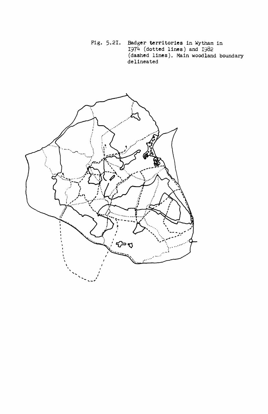
Fig. 5.21. Badger territories in Wytham in I9Jk (dotted lines) and 1982 (dashed lines). Main woodland boundary delineated
Pig. 5.22
Changes in range configuration from Kruuk's study 1974/75 to this study
1982/83, in the Harley-Botley area.
Thin linest major woodland boundaries
Stippled linest male ranges 1974/75
Dotted lines: female ranges 1974/75, hatched area: overlap between
neighbouring females
Stippled and dotted combined! group ranges 1982/83
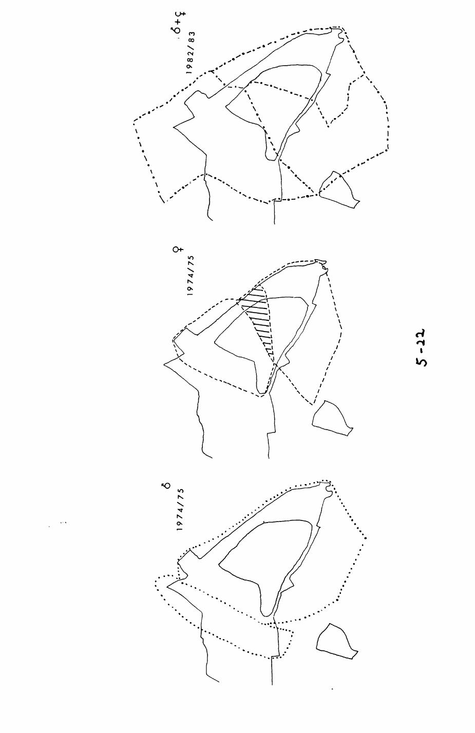
\. "
185
border between Kruuk's "Marley" and "Botley" females is now formalized as a
boundary between the MARLEY Range and its southern two neighbours. This
suggests that, at least in this case, the driving force behind the
rearrangement of groups was the negotiation of spheres of influence of
males. (A more detailed discussion of the reasons and consequences for this
is deferred to Chapter 7). The south-east area, formerly just occupied by
Kruuk's "Botley" females, now supports two ranges. These two ranges (Bl &
82) extend further to the south-east and the south-west than the "Botley"
females used to, and there is some evidence (e.g. the digging activity in
Bl) to suggest that Bl is a split from the UPPER FOLLIES Range.
The JEWS HARP Range has changed little since 1974; it lost a small area
in the west and gained a similar sized area In the north-east. Further west,
Kruuk's old Brogden Belt's range has moved south, leaving space for the new
and small LOWER SEEDS Range still contained within large portions of the old
Brogden Belt's border. By pushing south, the SUNDAYS HILL range reduced the
western JEWS HARP extension and the northern NEALINGS COPSE extension.
STEALINGS COPSE, however, compensated by talcing chunks off the southern
section of the RADBROOK COMMON Range.
5.4.3. Patterns of latrine distribution and utilization.
Following Kruuk's (1978a) results, badger latrines were identified and
used as markers of group range boundaries (section 5.4.1). An analysis of
latrine distribution and utilization may therefore contribute to an
understanding of the procedures by which badgers establish ranges, how
groups react to pressures applied by their neighbours, and how ranges are
maintained. Thus, we need to know in more detail where badgers place
latrines, how they use them and how the usage varies with time, space and in
relation to environmental features. Since at present very little is known
186
about the various functions that latrines may fulfil as one possible source
of information in badger societies, I also want to explore other possible
functions besides territory maintenance. Therefore, my analysis is centred
around the following questions:
1. Do badgers show preferences for particular sites when establishing new
latrines ? For instance, efficient advertisement of range boundaries would
imply a distribution of latrines that (i) conveys claims of ownership of an
area and intention of defense with a minimum of effort, and (ii) is highly
predictable for other badgers. Then, badgers would expect latrines to be
located at such sites and this is why latrines could (in evolutionary time)
have evolved into information centres.
2. Many latrines are founded inside the group range (non-border latrines).
What message do they convey ?
3. Can variation of latrine distribution and utilization be explained by
variation in local environmental features ? For Instance, latrines could be
distributed and utilized so that areas important to the range inhabitants
are well marked. If high quality food patches receive increased marking
attention, then variation in habitat quality (which is related to resource
presence, Chapter 2 and 3) should correspond to variation in marking
intensity. Such a pattern could arise directly ('intentional 1 placement and
utilization of latrines) or indirectly (increased marking activity could be
the incidental consequence of increased frequency of visits to such areas,
Indicating to trespassers that the risk of encountering resident badgers
Increases).
5.4.3.1. Distribution of latrines.
Thirteen latrines were located in large, homogeneous areas without any
discernible characteristics (e.g. a ploughed field, Table 5.14). 137
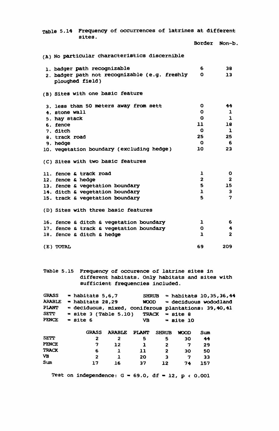
Table 5.14 Frequency of occurrences of latrines at different sites.
Border Non-b.
(A) No particular characteristics discernible
1. badger path recognizable 62. badger path not recognizable (e.g. freshly 0
ploughed field)
(B) Sites with one basic feature
3. less tham 50 meters away from sett 04. stone wall 05. hay stack O6. fence 117. ditch 08. track road 259. hedge o
10. vegetation boundary (excluding hedge) 10
(C) Sites with two basic features
11. fence & track road 112. fence & hedge 213. fence & vegetation boundary 514. ditch & vegetation boundary 115. track & vegetation boundary 5
(D) Sites with three basic features
16. fence & ditch & vegetation boundary 117. fence & track & vegetation boundary 018. fence & ditch & hedge 1
(E) TOTAL 69
3813
4411
181
256
23
02
1537
642
209
Table 5.15 Frequency of occurence of latrine sites in different habitats. Only habitats and sites with sufficient frequencies included.
GRASS - habitats 5,6,7 SHRUB = habitats 10,35,36,44ARABLE - habitats 28,29 WOOD = deciduous wododlandPLANT « deciduous, mixed, coniferous plantations! 39,40,41SETT - site 3 (Table 5.1O) TRACK = site 8FENCE - site 6 VB - site 10
SETTFENCETRACKVBSum
2762
17
212
11
16
ANT51
112037
SHRUB5223
12
WOOD307
3O7
74
Sum44295033
157
Teat on independence: G - 69.0, df - 12, p < 0.001
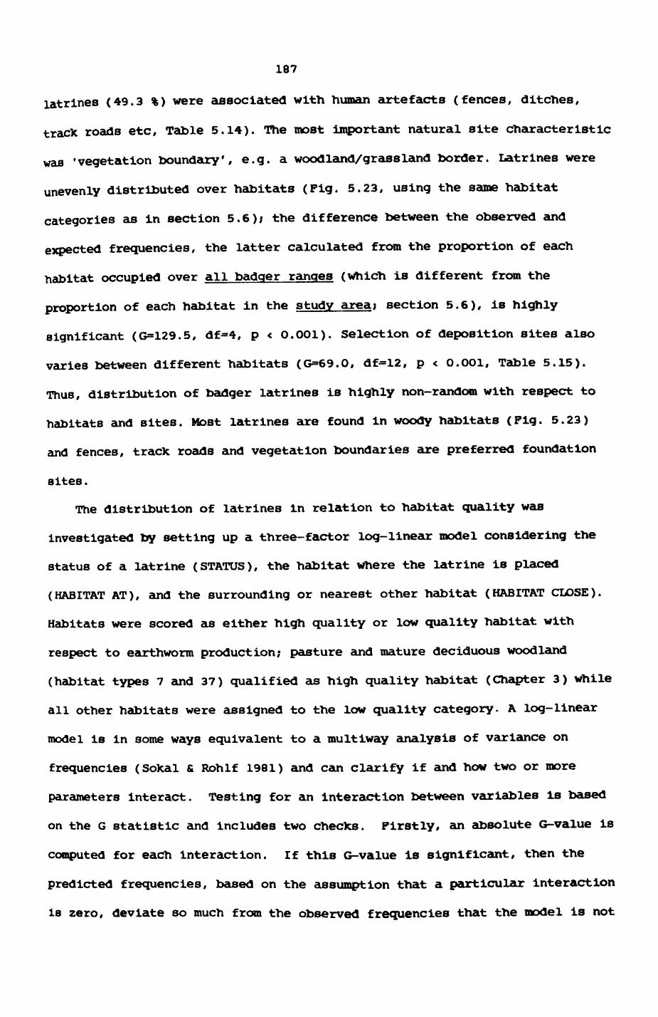
187
latrines (49.3 %) were associated with human artefacts (fences, ditches,
track roads etc, Table 5.14). The most Important natural site characteristic
was 'vegetation boundary', e.g. a woodland/grassland border. Latrines were
unevenly distributed over habitats (Pig. 5.23, using the same habitat
categories as in section 5.6); the difference between the observed and
expected frequencies, the latter calculated from the proportion of each
habitat occupied over all badger ranges (which is different from the
proportion of each habitat in the study area; section 5.6), is highly
significant (G=129.5, df=4, p < O.OOl). Selection of deposition sites also
varies between different habitats (G=69.0, df=12, p < O.OOl, Table 5.15).
Thus, distribution of badger latrines is highly non-random with respect to
habitats and sites. Most latrines are found in woody habitats (Fig. 5.23)
and fences, trade roads and vegetation boundaries are preferred foundation
sites.
The distribution of latrines in relation to habitat quality was
Investigated by setting up a three-factor log-linear model considering the
status of a latrine (STATUS), the habitat where the latrine is placed
(HABITAT AT), and the surrounding or nearest other habitat (HABITAT CLOSE).
Habitats were scored as either high quality or low quality habitat with
respect to earthworm production; pasture and mature deciduous woodland
(habitat types 7 and 37) qualified as high quality habitat (Chapter 3) while
all other habitats were assigned to the low quality category. A log-linear
model is in some ways equivalent to a multiway analysis of variance on
frequencies (SoXal & Rohlf 1981) and can clarify if and how two or more
parameters interact. Testing for an interaction between variables is based
on the G statistic and includes two checks. Firstly, an absolute G-value is
computed for each interaction, if this G-value is significant, then the
predicted frequencies, based on the assumption that a particular interaction
ia zero, deviate so much from the observed frequencies that the model is not
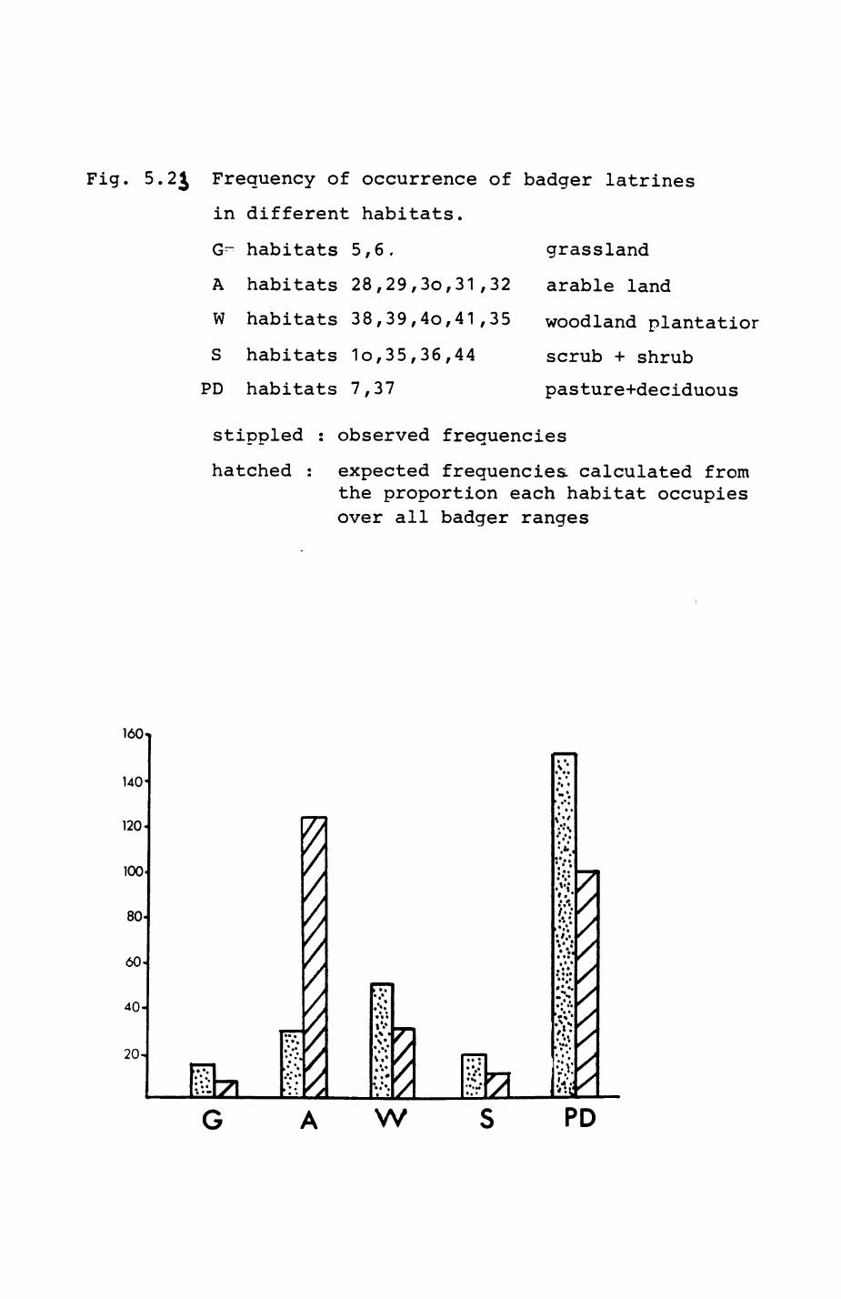
Fig. 5.2J Frequency of occurrence of badger latrines
in different habitats.
G^- habitats 5,6,
A habitats 28,29,30,31,32
grassland
arable land
W habitats 38,39,4o,41,35 woodland plantatior
S habitats 1o,35,36,44 scrub + shrub
PD habitats 7,37 pasture+deciduous
stippled :
hatched :
observed frequencies
expected frequencies, calculated from the proportion each habitat occupies over all badger ranges
140'
120-
100
80-
60-
40-
20-rri['••I _hv.rn
m^^
•'•'.i*^**• • *• * •
!X^ryyr .S' (
i •••*«r• • «»v•*.'%'!•
^»• j*• •X^
1 • • • 1
1 *^ * t^^^Tl***»^i S\
•^•i
^ •:-vt.*«*?• *'."•*"'• f-*% ** i s'•.«*''•'•iVV&
7
'^^^*
sy
X
w PD

188
in accordance with the data. Thus, that interaction has to be included in
the model. Even if this absolute G-value is not significant, the
interaction may still be Included in the model, if the increase in the G-
value from the highest-order interaction is significant, since then the
difference is too large to be ignored. The final model then specifies the
simplest combination of parameters and interactions between them with the
best fit to the original data.
Table 5.16 lists the data and the generation of the model, and Table
5.17 presents an interpretation of the model. Two highly significant
interactions exist: for a given level of HABITAT CLOSE, quality of HABITAT
AT and STATUS are interrelated, and for a given STATUS, HABITAT AT and
HABITAT CLOSE are interdependent (Table 5.16). Since there was no
interrelation of HABITAT CLOSE and STATUS for a given level of HABITAT AT, I
excluded the three-factor interaction from the model, even though it was -
if only barely - significant (Table 5.16).
How can this model be interpreted in terms of communicative function of
latrine characteristics ? More border latrines than expected occurred at
habitat transitions with a change in habitat quality. This could be due to a
variety of reasons. For instance, badgers may be more inclined to check
habitat transitions carefully for signs of other badgers, since a major
proportion of heavily used badger paths run along or across transitions
(section 6.2.6). Resident badgers should then place border latrines at such
sites to increase the probability of information transmission.
Alternatively, residents may put an increased effort in marking quality
transitions as a response to increased intrusion pressure from badgers in
search of high quality areas (see Chapter 7). A third possibility is that
density of latrine presence is an indicator of the importance residents
attach to a particular area, ie. how willing (or rather how unwilling)
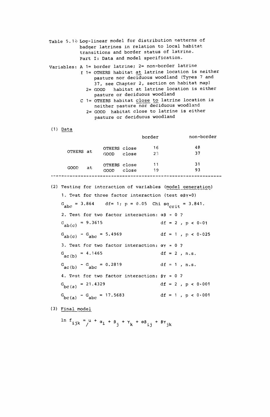
Table 5. 1 c Log-linear model for distribution natterns of badger latrines in relation to local habitat transitions and border status of latrine. Part I: Data and model specification.
Variables: A 1= border latrine; 2= non-border latrineE 1= OTHERS habitat at latrine location is neither
pasture nor deciduous woodland (Types 7 and 37, see Chapter 2, section on habitat map)
2= GOOD habitat at latrine location is eitherpasture or deciduous woodland
C 1= OTHERS habitat close to latrine location isneither pasture nor deciduous woodland
2= GOOD habitat close to latrine is either pasture or deciduous woodland
(1) Data
border non-border
OTHERS
GOOD
at
at
OTHERSGOOD
OTHERS GOOD
closeclose
close close
1623
11 19
4837
31 93
(2) Testing for interaction of variables (model generation)
1 . Test for three factor interaction (test a3Y=0)
G . = 3.864 df= 1; p = 0.05 Chi sq = 3.841. abc ^ Mcrit
2. Test for two factor interaction: a3 = 0 ?
G . , . = 9.3615 df = 2 , p < 0-01 ab(c)
Gab(c) - Gabc = 5 ' 4969 df = ] ' P < °' 025
3. Test for two factor interaction: ay = 0 ?
G ,. = 4. 1465 df = 2 , n.s. ac(b)
G .. . - G = 0.2819 df = 1 , n.s. ac(b) abc
4. Test for two factor interaction: 3y = 0 ?
G. , . = 21.4329 df = 2 , p < 0-001 be (a) ^
G, , . - G , = 17.5683 df = 1 , p < 0-001 be (a) abc
(3) Final model
In f. ., = u- — i- a i •ij ' MI jk
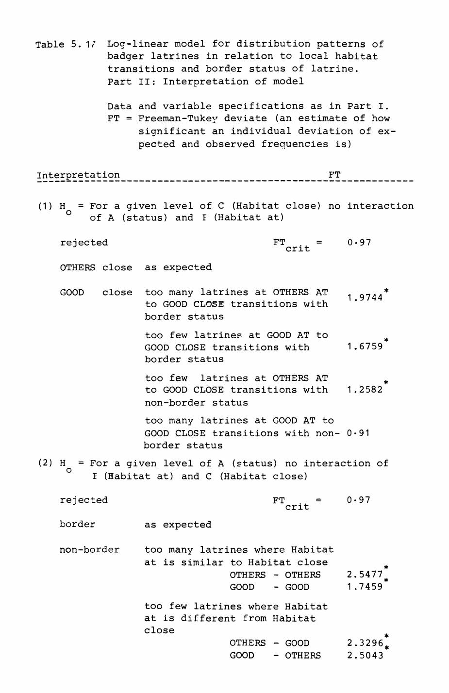
Table 5. 17 Log-linear model for distribution patterns ofbadger latrines in relation to local habitat transitions and border status of latrine. Part II: Interpretation of model
Data and variable specifications as in Part I.FT = Freeman-Tukey deviate (an estimate of how
significant an individual deviation of ex pected and observed frequencies is)
Interpretation FT
(1) H = For a given level of C (Habitat close) no interaction ° of A (status) and I (Habitat at)
rejected FT . = 0-97crit
OTHERS close as expected
GOOD close too many latrines at OTHERS AT 9744*to GOOD CLOSE transitions with border status
too few latrines at GOOD AT to ^ GOOD CLOSE transitions with 1.6759 border status
too few latrines at OTHERS AT ^ to GOOD CLOSE transitions with 1.2582 non-border status
too many latrines at GOOD AT toGOOD CLOSE transitions with non- 0-91border status
(2) H = For a given level of A (status) no interaction of oI (Habitat at) and C (Habitat close)
rejected FT = 0-97crit
border as expected
non-border too many latrines where Habitatat is similar to Habitat close
OTHERS - OTHERS 2.5477^ GOOD - GOOD 1 .7459
too few latrines where Habitatat is different from Habitatclose
OTHERS - GOOD 2.3296^ GOOD - OTHERS 2.5043

189
residents are to "negotiate" ownership of this area with their neighbours.
Here, border latrines nay not only advertise range boundaries but also
reinforce ownership claims on high quality habitat. Indirect evidence for
this suggestion is the poor presence of latrines at border sections that run
through arable land, a habitat of supposedly low value to badgers.
Fewer border latrines than expected were placed at high quality to high
quality habitat transitions. If significance to badgers is a function of
presence or absence of habitat transitions per se, then this should be
distinguishable (in terms of latrine presence) from transitions in quality,
since some habitat transitions occur where there is no change in habitat
quality (e.g. from pasture to deciduous woodland). It is arguable (Chapter
7) that areas of high quality to high quality transitions are less subject
to high intrusion pressure than areas with transitions with a quality
change, perhaps because such adjacent areas are treated as a single
functional patch. If density of latrines is a function of pressure from
Intruders, then presence of latrines at such transitions should be reduced,
as is the case. If border latrines serve to reinforce ownership claims on
high quality habitats, then latrine presence should be independent from the
quality of neighbouring habitatj a reduced presence is Inconsistent with
this expectation. However, it may well be that badgers do not react to
transitions between areas of similar quality as transitions at alii
consequently there would be no need to maintain a marking intensity on a
level comparable with that at transitions associated with a quality change.
According to the two significant two-factor interactions, non-border
latrines occur more often than expected at transitions with no quality
change while fewer than expected occur at transitions with a quality change.
High quality habitats are frequently and intensively visited by residents
(Chapter 6). Increased latrine usage may just be an incidental consequence
of badgers staying in such areas for a long time, so that the need for
190
defaecation arises more frequently. However, if defaecation inside the range
is an incidental affair, then there is no need to maintain special sites for
defaecation. Alternatively, marking at non-border latrines could remind an
individual whether it has already visited this particular area on a given
night and how much time has elapsed since its last visit or that of a group
member. (This assumes that badgers can tell from the condition of a marking
how much time has elapsed since it was deposited). Foraging success (e.g.
rate of energy intake) in high quality habitats is a function of the time
since the area was last visited (see Chapter 7): with more time elapsed
without any badger presence, more worms are likely to have returned to the
surface and thus become available, provided the weather has not
deteriorated. In areas of high intrinsic value, revisiting intervals are
shorter than in other areas (Chapter 6), increasing the likelihood that
badgers may return to an area before it has fully 'recovered', and thus
depress their feeding rate, unless their movements are somehow coordinated
(details see Chapter 6). Since badgers can distinguish the scent of
different individuals (Kruuk et al. 1984, German et al. 1984), marking as an
indicator of previous usage of a patch could facilitate intra-group
communication and help avoid (i) over-exploitation of patches and (ii) waste
of time on fruitless searches of patches already 'harvested'. This is
important, if group members want to minimize interference (Chapter 7).
The log-linear model shows that it is important to distinguish between
border and non-border latrines, since the model identified patterns of
latrine characteristics opposite in trend for latrines of different status.
5.4.3.2. Utilization of latrines
Data on latrine utilization are available from each month for the
periods April to November 1982 and March to October 1983. 39.7 % of latrines
191
checked contained at least one recent dropping ("active" latrines). The
majority of latrines without a recent dropping had obviously not been
visited for some time and showed clear signs of decay. The following
analysis only deals with "active" latrines.
The majority of latrines were founded in spring (Table 5.6, Fig. 5.24).
In spring 1983, three times more new latrines were founded and active than
in spring 1982. However, since the number of active latrines during the
remainder of the year was similar for both years (Mann-Whitney U-test,
normalized, n=7, m=7, U (border latrines)= -0.771, nsj U (non-border
latrines)= -0.832, ns), data from both years were analysed together.
The size distribution of latrines as measured by numbers of TOTAL,
FILLED, and FRESH pits per latrine is shown in Fig. 5.25. Four size classes
were distinguished! small (1-2 pits), medium (3-9), large (1O-19), and
extra-large latrines (> 19 pits). 7.9 % of all checks encountered latrines
with more than 19 TOTAL pits, but only 1.3 % had similarly many FRESH pits.
55.8 % of the cases concerned latrines with 1-2 FRESH pits. The size
distributions differ between the three measures (G=129.8, df=6, p < O.OO1).
The pattern of utilization varied between latrines of different status.
Binomial tests (Table 5.18) were used to investigate whether observed
numbers of active latrines of a given status matched expected ones. In 11
out of 16 months, observed and expected numbers corresponded. In 4 months of
1983, more border latrines were active and in June 1982, fewer border
latrines were active than expected. Measures of intensity of use per latrine
were significantly different for latrines of different status (Table 5.19);
in all cases, border latrines were larger or contained more pits than non-
border latrines.
Latrine utilization also varied greatly between different times of the
year (Fig. 5.26, Table 5.19). Table 5.20 analyses differences in intensity
of use of border latrines In more detail. Differences occurred both within
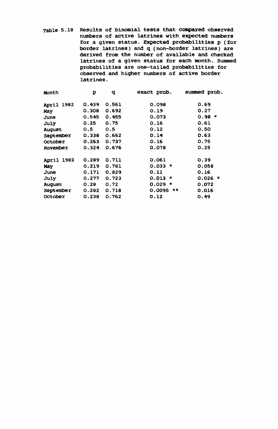
Table 5.18
Month
April 1982MayJuneJulyAugustSeptemberOctoberNovember
April 1983MayJuneJulyAugustSeptemberOctober
Results of binomial tests that compared observed numbers of active latrines with expected numbers for a given status. Expected probabilities p (for border latrines) and q (non-border latrines) are derived from the number of available and checked latrines of a given status for each month. Summed probabilities are one-tailed probabilities for observed and higher numbers of active border latrines.
exact prob, summed prob.
0.4390.3080.5450.250.50.3380.2630.324
0.2890.2190.1710.2770.280.2820.238
0.5610.6920.4550.750.50.6620.7370.676
0.7110.7810.8290.7230.720.7180.762
0.0980.190.0730.16O.120.140.160.078
O.O610.033 *0.110.013 *0.029 *O.0095 **0.12
0.690.270.98 *0.610.500.63O.750.25
0.390.0580.16O.026 *O.O720.0160.49

Table 5.19 Comparison of intensity of use of latrines of different status and during different seasons. H = Krusfcal-Wallis analysis of variance, adjusted for ties.
(a) Comparison of latrines of different statust non-border latrines, border latrines shared by two neighbour ranges, border latrines shared by three neighbour ranges.
variable df H significance
AREA 2 54.5 < 0.001TOTAL number of pits 2 70.7 < 0.001FILLED " " " 2 65.6 < O.O01FRESH " » .1 2 3O.3 < O.OO1
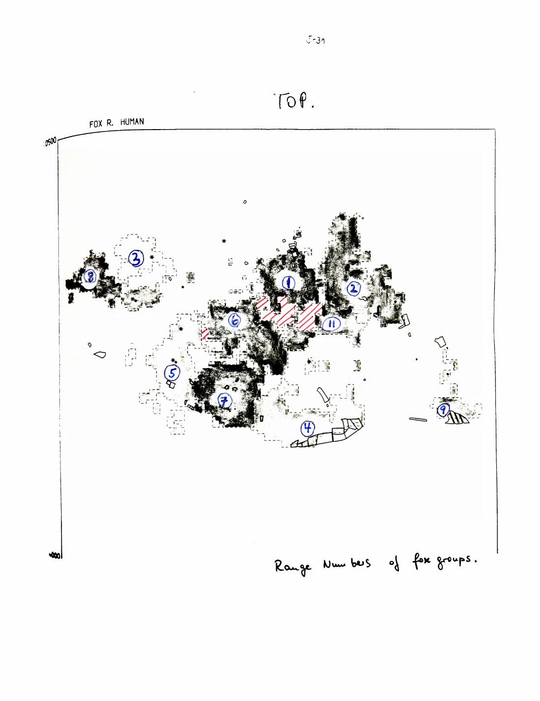
t/1
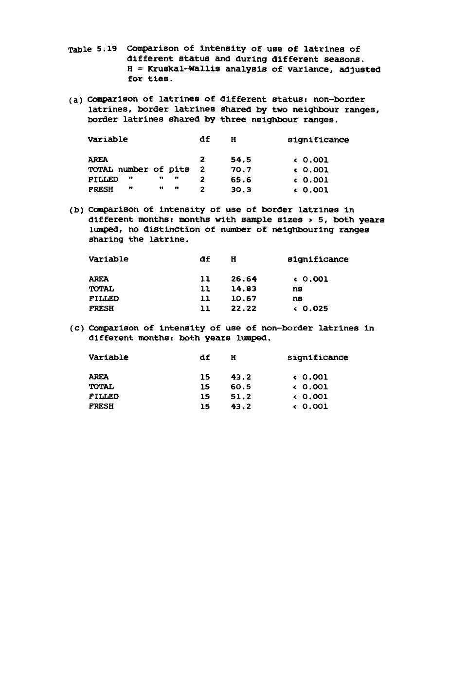
Table 5.19 Comparison of intensity of use of latrines of different status and during different seasons. H = Krusfcal-Wallis analysis of variance, adjusted for ties.
(a) Comparison of latrines of different statusi non-border latrines, border latrines shared by two neighbour ranges, border latrines shared by three neighbour ranges.
variable df H significance
AREA 2 54.5 < O.O01TOTAL number of pits 2 70.7 < O.O01PILLED " " " 2 65.6 < 0.001FRESH " .... 2 30.3 < O.O01
(b) Comparison of intensity of use of border latrines indifferent months i months with sample sizes > 5, both years lumped, no distinction of number of neighbouring ranges sharing the latrine.
Variable df H significance
AREA 11 26.64 < 0.001TOTAL 11 14.83 nsFILLED 11 10.67 nsFRESH 11 22.22 < 0.025
(c) Comparison of intensity of use of non-border latrines in different months i both years lumped.
Variable df H significance
AREA 15 43.2 < 0.001TOTAL 15 60.5 < 0.001FILLED 15 51.2 < 0.001FRESH 15 43.2 < O.OO1
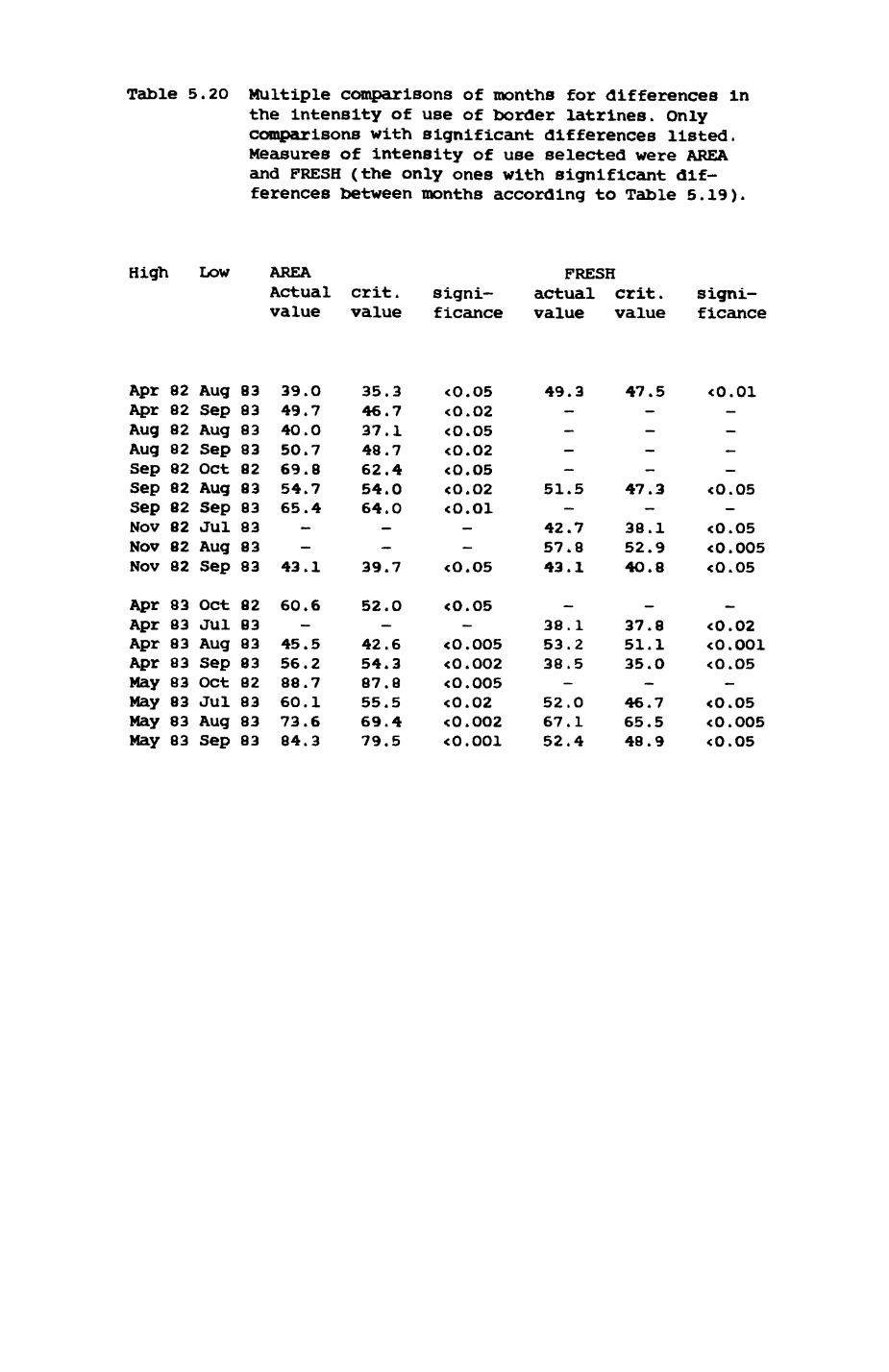
Table 5.20 Multiple comparisons of months for differences in the intensity of use of border latrines. Only comparisons with significant differences listed. Measures of intensity of use selected were AREA and FRESH (the only ones with significant dif ferences between months according to Table 5.19).
High Low AREAActualvalue
Apr 82Apr 82Aug 82Aug 82sep 82sep 82sep 82NOV 82NOV 82NOV 82
Apr 83Apr 83Apr 83Apr 83May 83May 83May 83May 83
AugsepAugSepOctAugSepJulAugSep
octJulAugSepoctJulAugSep
83838383828383838383
8283838382838383
39.049.740.050.769.854.765.4——
43.1
60.6—
45.556.288.760.173.684.3
crit •
value
35.46.37.48.62.54.64.
——
39.
52.—
42.54.87.55.69.79.
3717400
7
O
638545
significance
<O.O5<0.02<O.O5<0.02<O.O5<0.02<0.01——
<O.O5
<0.05—
<O.OO5<0.002<O.005<0.02<0.002<O.OO1
FRESH actual critvalue
49.————
51.—
42.57.43.
—38.53.38.
—
52.67.52.
3
5
781
125
014
»
value
47.————
47.—
38.52.4O.
—37.51.35.
—46.65.48.
5
3
198
810
759
significance
<0.01————
<0.05—
<0.05<0.005<0.05
—<0.02<0.001<0.05—
<0.05<O.O05<0.05

Fig. 5.24
Changes of number of (a) new (b) total available and (c) proportion of
active latrines over time (from April 1982 to October 1983)
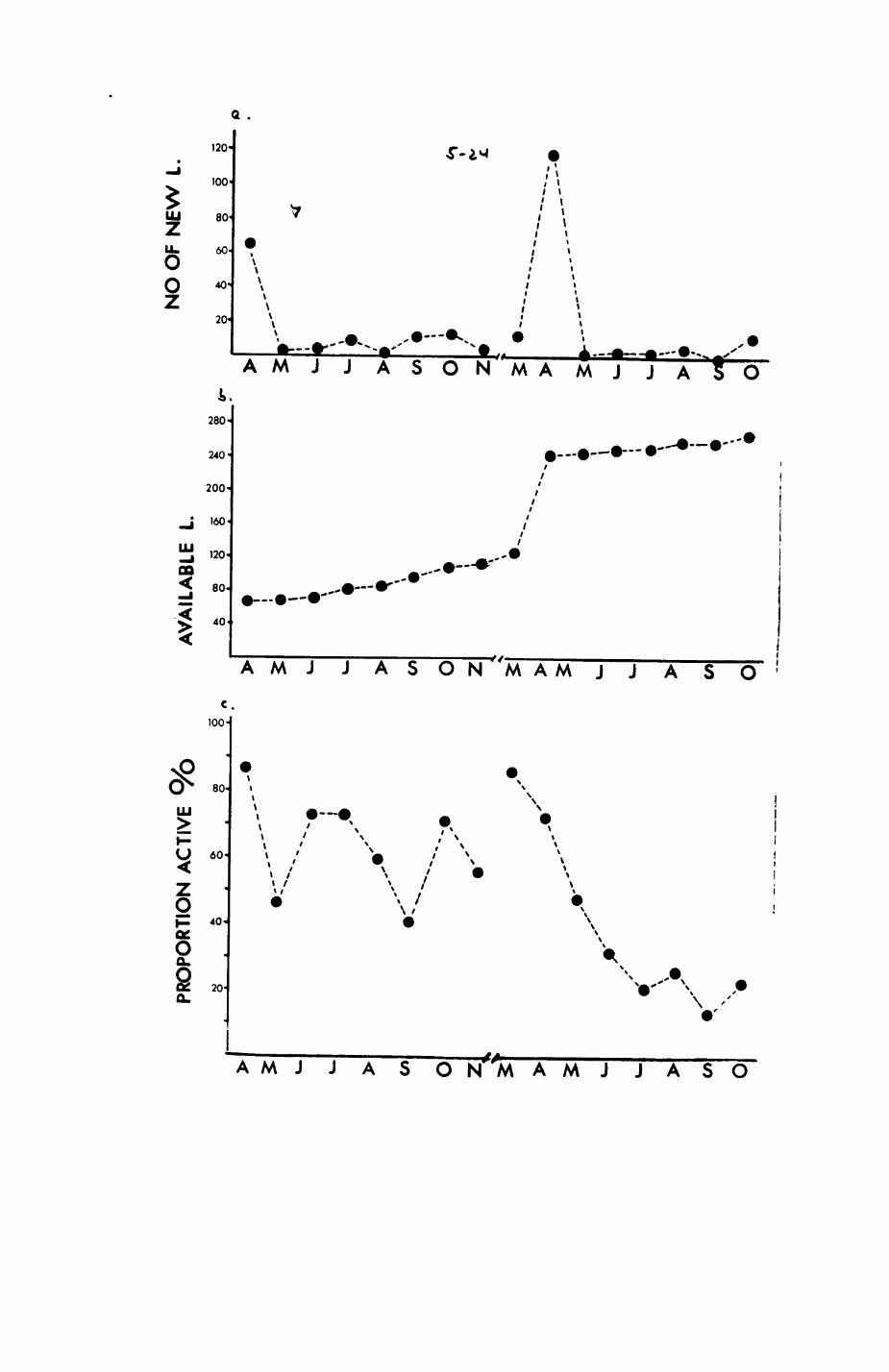
PRO
PORT
ION
AC
TIVE
%AV
AILA
BLE
L.o
§A
!**
o 2,i
(/> > c/>l
O
\ \
NO
OF
NE
W L
.
g S
8 g
8
en
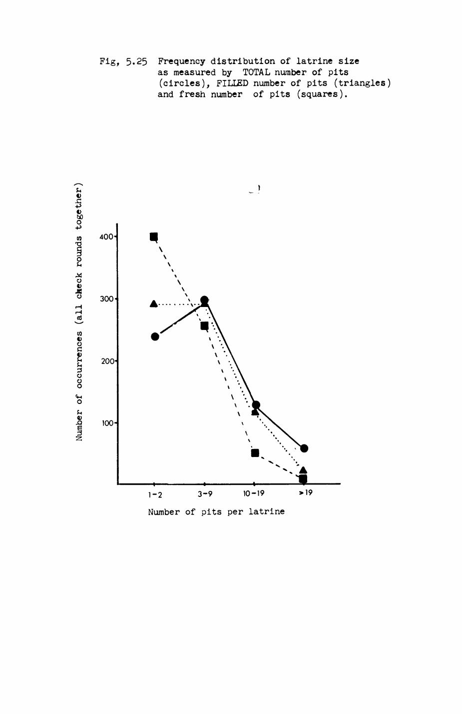
Fig, 5.25 Frequency distribution of latrine size as measured by TOTAL number of pits (circles), FILLED number of pits (triangles) and fresh number of pits (squares).
bO O -P
CO
8O4;•S
cti
w4) OC
3 O O O
CM O
V
400
300
200'
100'
1-2 3-9 10-19 >19
Number of pits per latrine

Pig. 5.26
Proportion of utilized latrines of latrines available and checked in a given
month versus time (April 1982 to October 1983)
Circlest non-border latrines
Trianglesi border latrines
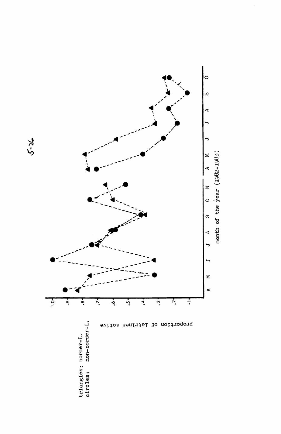
proportion of latrines active
O r»-H- "-Jt-J H-O P
CD 0)
CO
i?? a s?
3 O Dff
O03
r»<<- o
HH VD 00ro i >
00
03
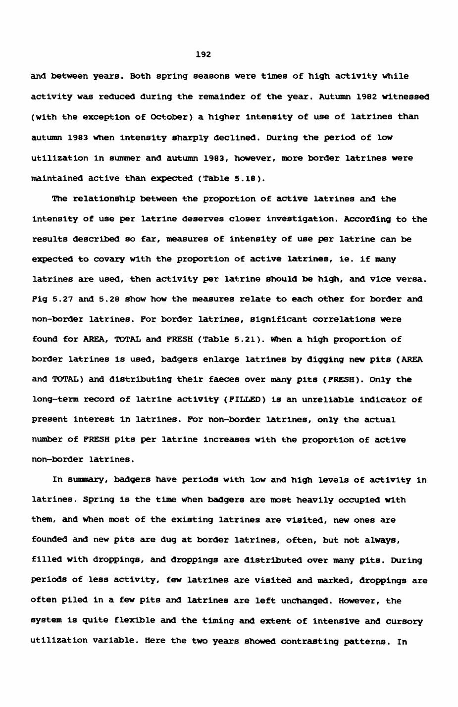
192
and between years. Both spring seasons were times of high activity while
activity was reduced during the remainder of the year. Autumn 1982 witnessed
(with the exception of October) a higher Intensity of use of latrines than
autumn 1983 when Intensity sharply declined. During the period of low
utilization in summer and autumn 1983, however, more border latrines were
maintained active than expected (Table 5.18).
The relationship between the proportion of active latrines and the
intensity of use per latrine deserves closer investigation. According to the
results described so far, measures of intensity of use per latrine can be
expected to covary with the proportion of active latrines, ie. if many
latrines are used, then activity per latrine should be high, and vice versa.
Pig 5.27 and 5.28 show how the measures relate to each other for border and
non-border latrines. For border latrines, significant correlations were
found for AREA, TOTAL and FRESH (Table 5.21). When a high proportion of
border latrines is used, badgers enlarge latrines by digging new pits (AREA
and TOTAL) and distributing their faeces over many pits (FRESH). Only the
long-term record of latrine activity (FILLED) is an unreliable Indicator of
present interest in latrines. For non-border latrines, only the actual
number of FRESH pits per latrine increases with the proportion of active
non-border latrines.
In summary, badgers have periods with low and high levels of activity in
latrines. Spring is the time when badgers are most heavily occupied with
them, and when most of the existing latrines are visited, new ones are
founded and new pits are dug at border latrines, often, but not always,
filled with droppings, and droppings are distributed over many pits. During
periods of less activity, few latrines are visited and marked, droppings are
often piled in a few pits and latrines are left unchanged. However, the
system is quite flexible and the timing and extent of intensive and cursory
utilization variable. Here the two years showed contrasting patterns. In
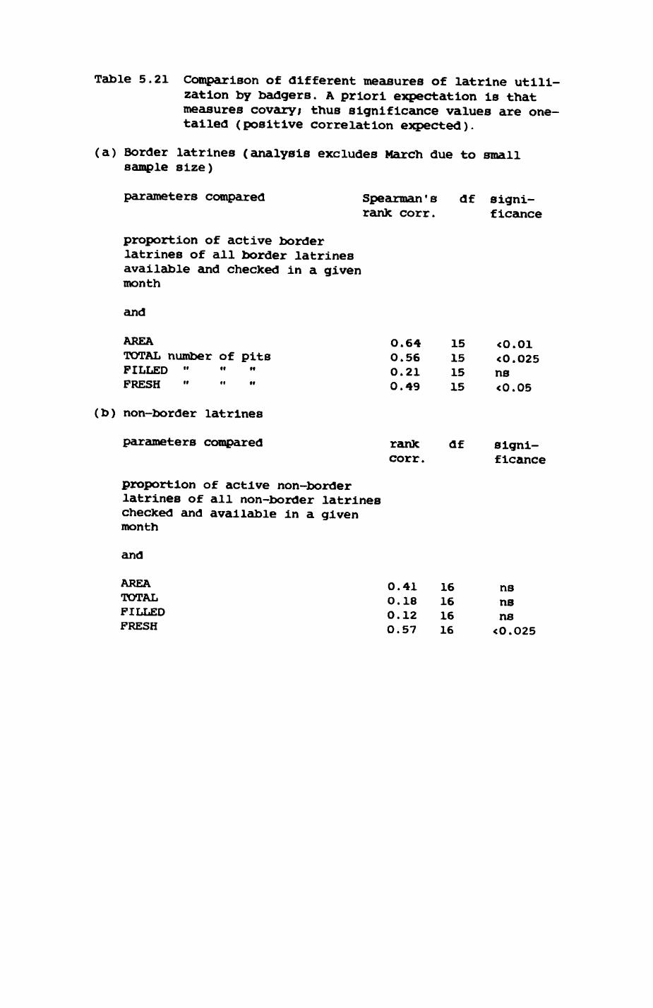
Table 5.21 Comparison of different measures of latrine utili zation by badgers. A priori expectation is that measures covary; thus significance values are one- tailed (positive correlation expected).
(a) Border latrines (analysis excludes March due to small sample size)
parameters compared Spearman's rank corr.
df signi ficance
proportion of active border latrines of all border latrines available and checked in a given month
and
AREATOTAL number of pitsFILLED " " "FRESH
O.64 O.56 0.21 0.49
15151515
<0.01 <O.O25 ns <0.05
(b) non-border latrines
parameters compared
proportion of active non-border latrines of all non-border latrines checked and available in a given month
and
rank corr.
df signi ficance
AREA TOTAL FILLED FRESH
0.410.180.120.57
16161616
ns ns ns <0.025

Pig. 5.27-5.28
Relationship between different measures of intensity of use per latrine and
the proportion of latrines active of a given category (border and non-border
latrines, respectively)
a. AREA (ha) versus proportion of active border-L
b. TOTAL " " " " "
C. FILLED
d. FRESH " "
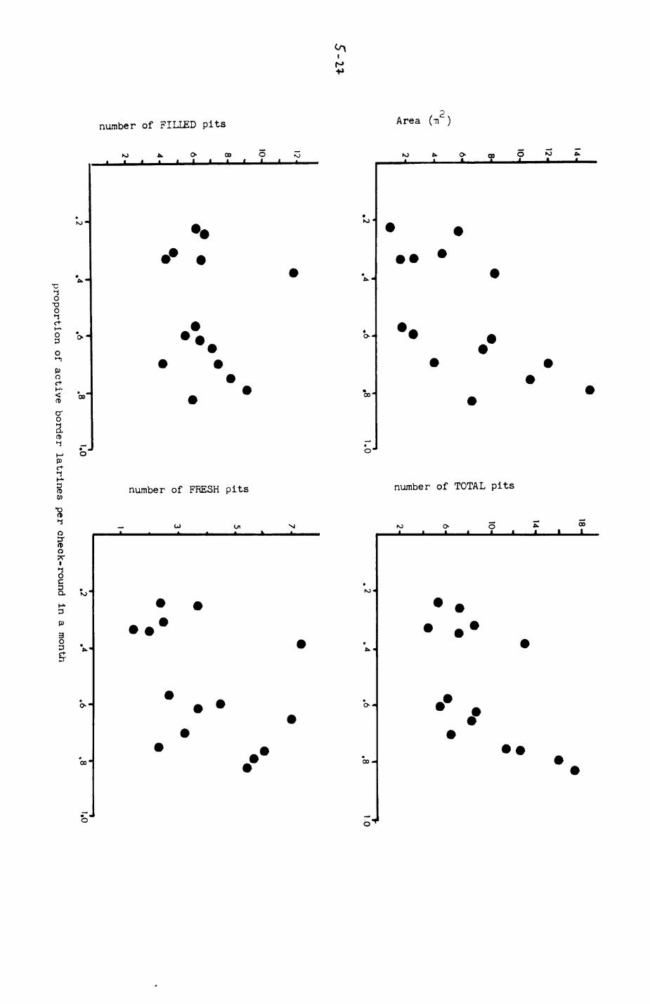
14-
12-
10-U]•P•Ha
18-
14-
10-
OJtd<U
<Mo
.2.6
1.0.2
.4.6
.810
12-
10-*
«
8-
-P•H
. Q
,
Q
6-
Mfc 4-
<«H0^ %
2.
d
•
7-«
• 3
5•
-g, 5<
A •
x
A
™
CO .
A
A
^
[i]
•
•
• •
•
1
••
°
3•
•
h%
£1C
!•
•
\
•
•
•
•
• • *
.••
/2 .4
.6
.'s 'Jo
.2 .4
.6
.8
'.0
proportion of
active border
latrines per
check-round in
a month
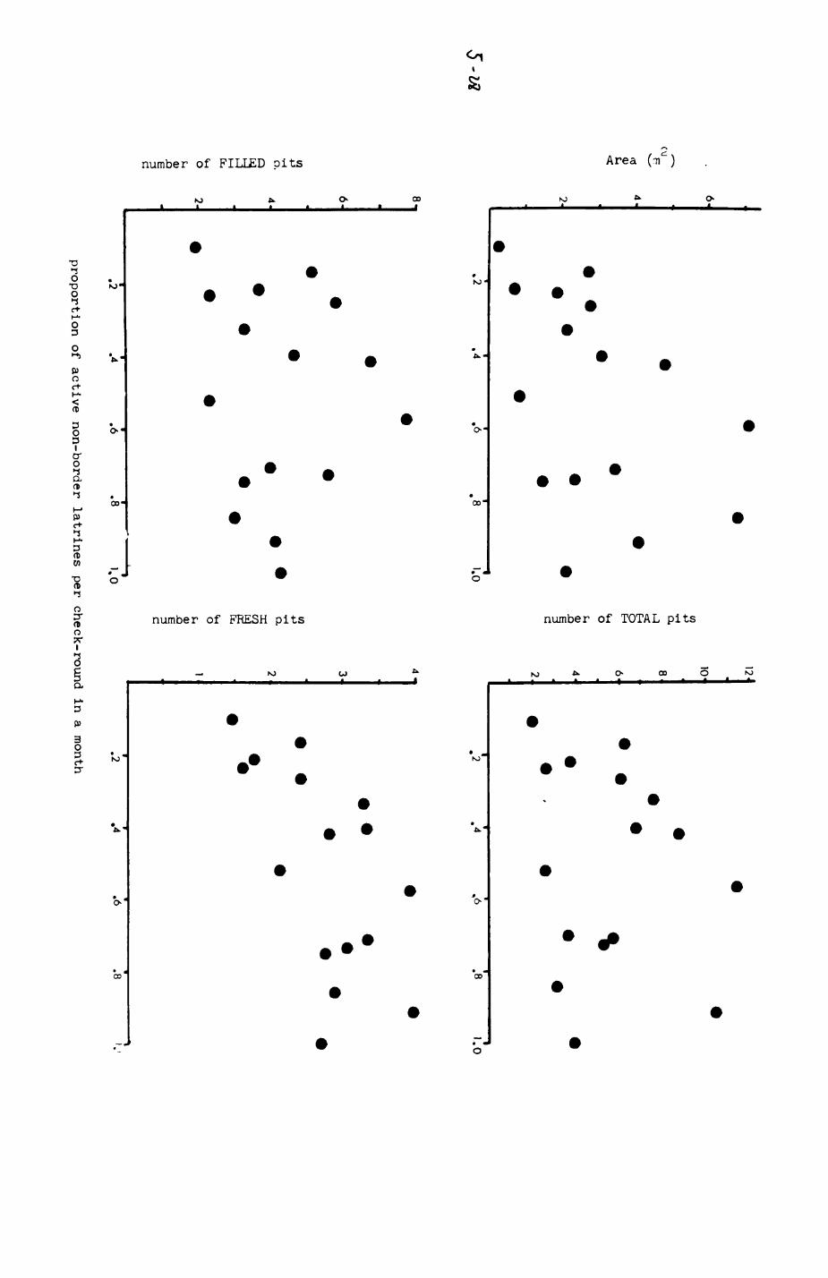
(VIai
g
w -pa>.0
10'
.41.0
.81.0
3•H O,
Q(UXI c:
.2.4
.6.8
1.0
(0-PaCO0) J36C
.2.6
.8
proportion of
active non-border
latrines per
check-round in a
month
193
1982, a moderate number of latrines was available, a high proportion was
maintained active throughout the year and active latrines were intensively
used. In 1983, foundation activity and numbers available were extremely high
in spring, but intensity of use declined strongly according to all measures
employed during the remainder of the year.
5.4.3.3. Function and evolution of badger latrines.
Due to their solitary movements (Chapter 6) and foraging habits
(Chapter 3), badgers face the problem of transmitting information indirectly
to a heterogenous group of potential receivers, some of which they know
(neighbours) and some they do not (e.g. dispersing adolescents). The use of
latrines, constituting a formalized marking system by which special sites
are agreed upon as Information centres, increases the likelihood that (i)
information will be received and (ii) that it is received by the appropriate
individuals. Further characteristics of the latrine marking system are (i)
marking is continued throughout the year (Harris 1982, pers. obs.), le.
information flow is permanent! (11) marking Intensity never drops below a
threshold i (ill) marking Intensity varies and can be adjusted by the
resident animals.
Fine tuning of marking Intensity can best be understood as an adaptation
to changing pressures, particularly intrusion pressure. Fig. 5.29 depicts a
graphical model relating marking intensity, as observed in latrine
utilization, to pressure. Two elements characterise the model. At low levels
of pressure, marking intensity never drops below a threshold. Here, the
message includes the statement "I am/we are still about and continue to
occupy this range". If, as in Wytham (Kruuk 1978a, section 5.4.2.), ranges
are defended territories, the message extends to Mand I/we shall continue
to defend it". At low levels of utilization, border latrines were more
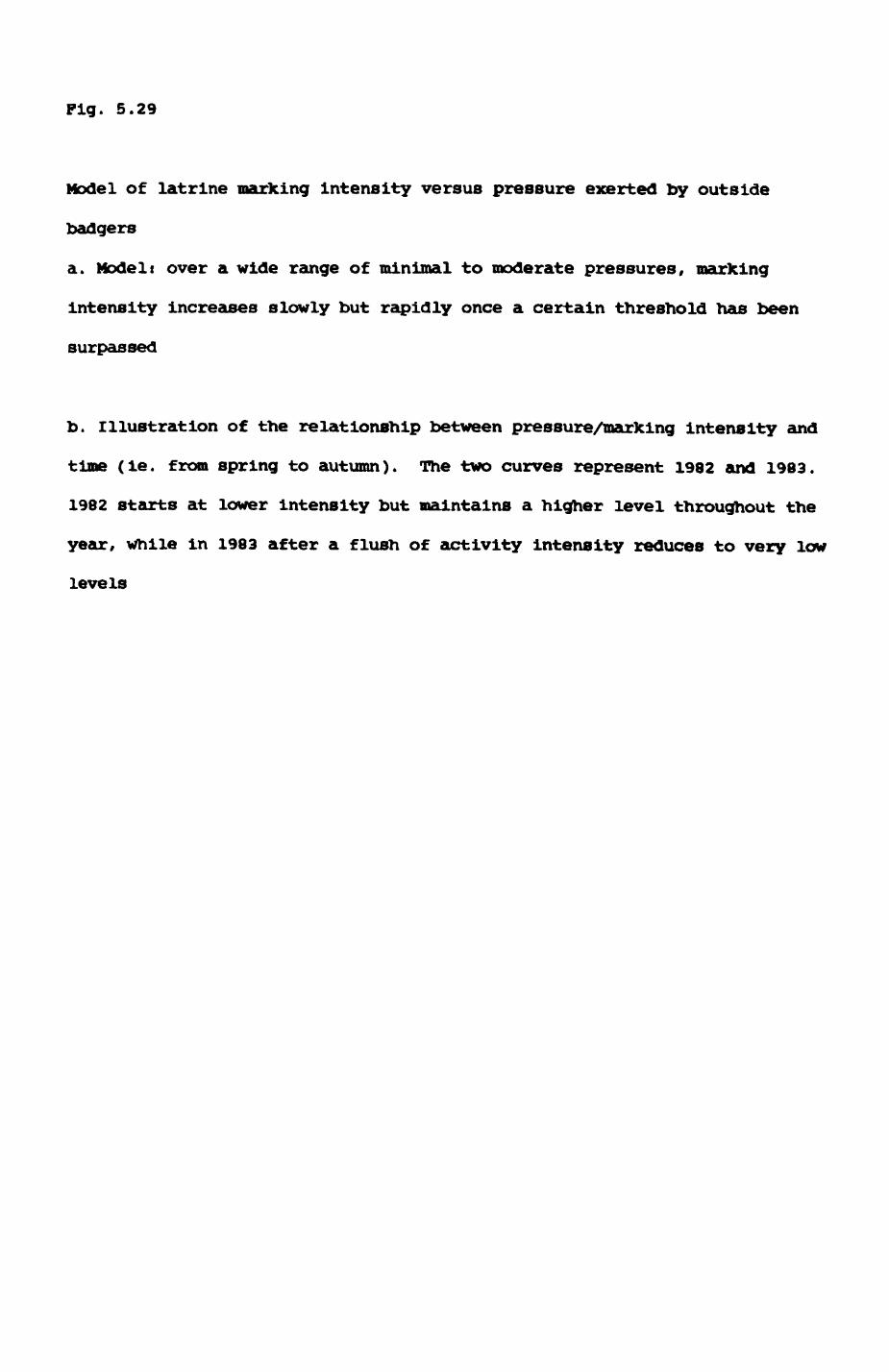
Pig. 5.29
Model of latrine marking intensity versus pressure exerted by outside
badgers
a. Nodelt over a wide range of minimal to moderate pressures, marking
intensity increases slowly but rapidly once a certain threshold has been
surpassed
b. Illustration of the relationship between pressure/marking intensity and
time (ie. from spring to autumn). The two curves represent 1982 and 1983.
1982 starts at lower intensity but maintains a higher level throughout the
year, while in 1983 after a flush of activity intensity reduces to very low
levels
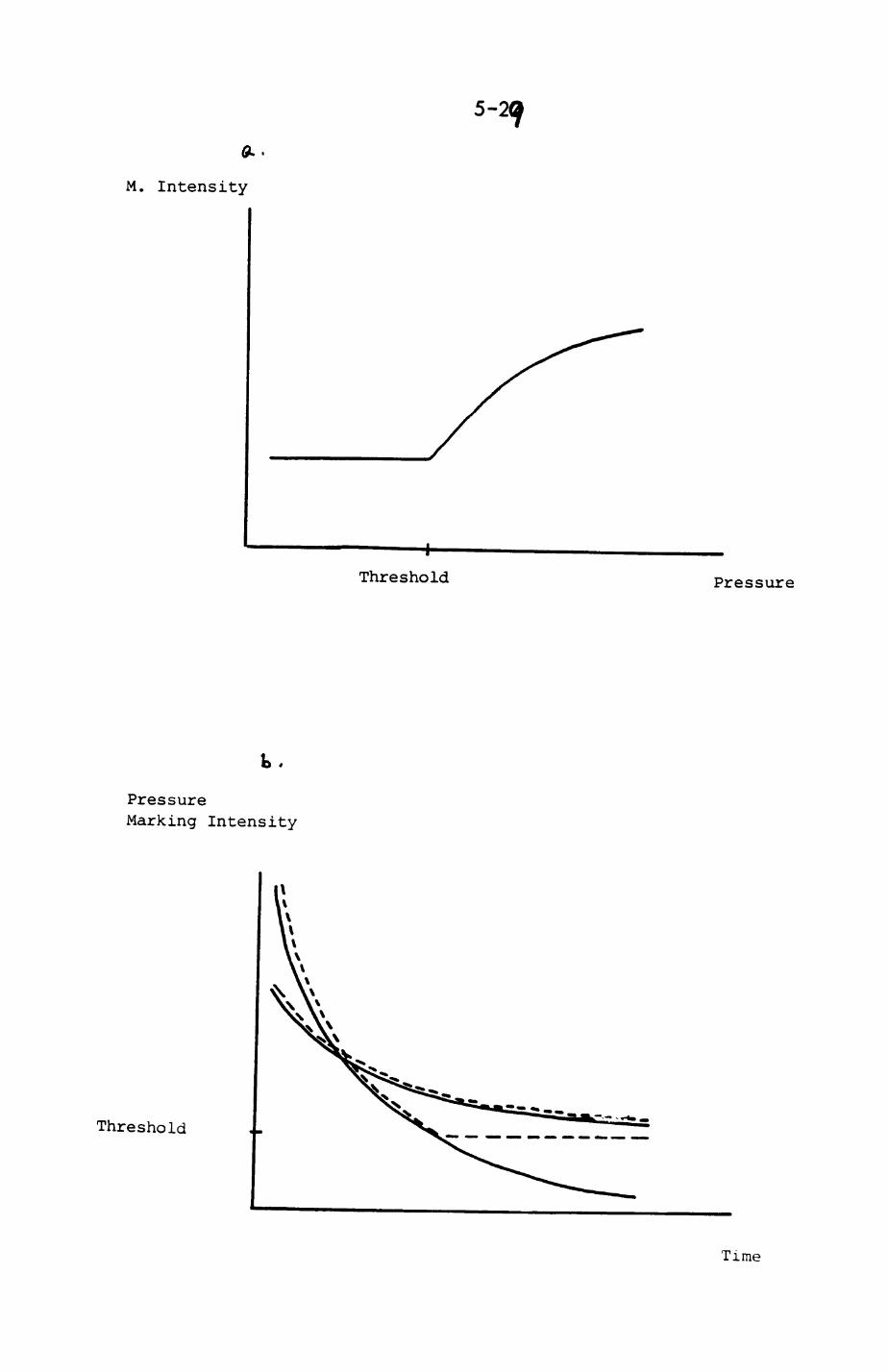
5-
M. Intensity
Threshold Pressure
I,
PressureMarking Intensity
Threshold
Time
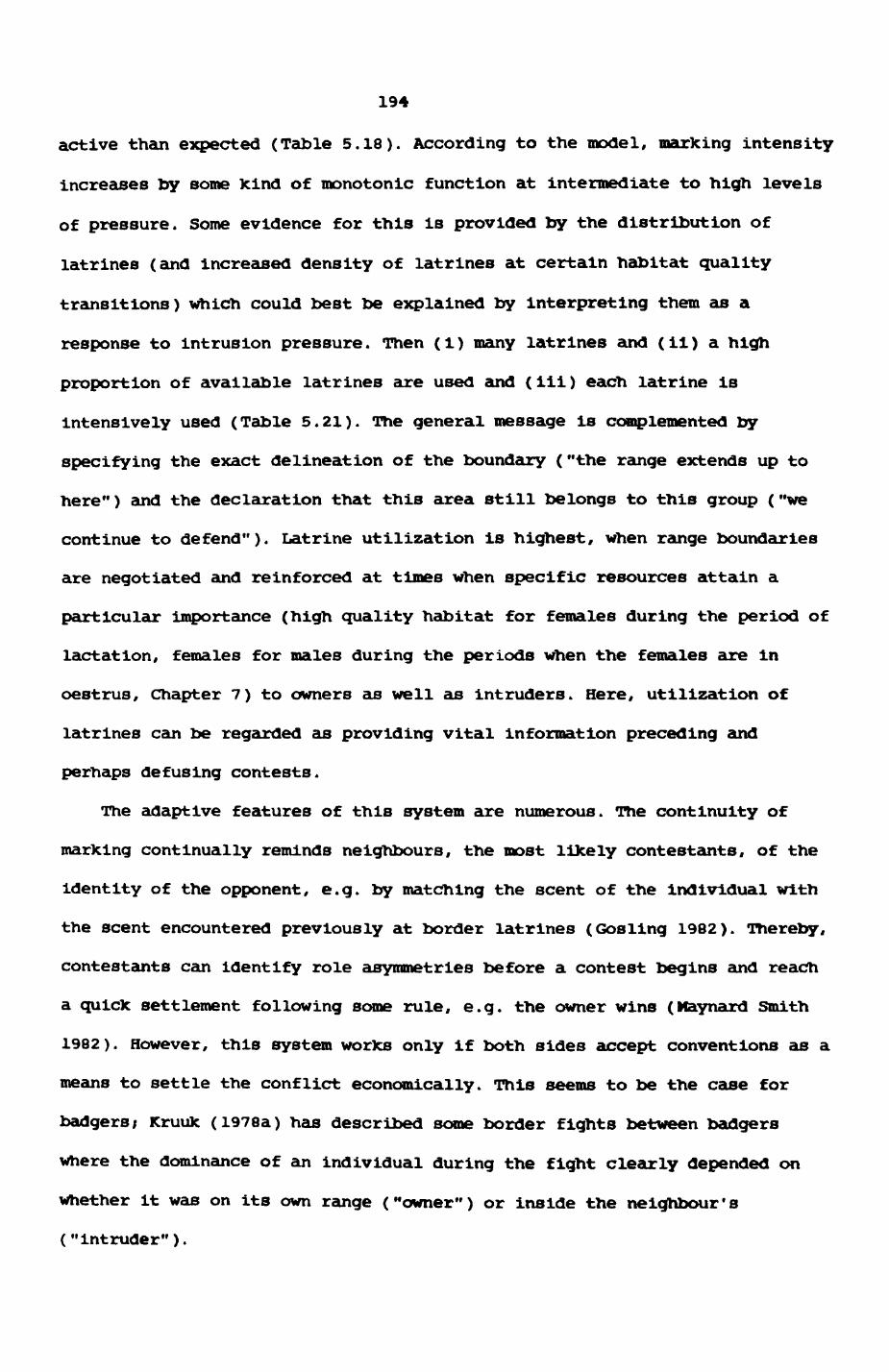
194
active than expected (Table 5.18). According to the model, marking intensity
increases by some kind of monotonic function at intermediate to high levels
of pressure. Some evidence for this is provided by the distribution of
latrines (and increased density of latrines at certain habitat quality
transitions) Which could best be explained by interpreting them as a
response to intrusion pressure. Then (i) many latrines and (11) a high
proportion of available latrines are used and (ill) each latrine is
intensively used (Table 5.21). The general message is complemented by
specifying the exact delineation of the boundary ("the range extends up to
here") and the declaration that this area still belongs to this group ("we
continue to defend"). Latrine utilization is highest, when range boundaries
are negotiated and reinforced at times when specific resources attain a
particular importance (high quality habitat for females during the period of
lactation, females for males during the periods when the females are in
oestrus, Chapter 7) to owners as well as intruders. Here, utilization of
latrines can be regarded as providing vital information preceding and
perhaps defusing contests.
The adaptive features of this system are numerous. The continuity of
marking continually reminds neighbours, the most likely contestants, of the
identity of the opponent, e.g. by matching the scent of the individual with
the scent encountered previously at border latrines (Gosling 1982). Thereby,
contestants can identify role asymmetries before a contest begins and reach
a quick settlement following some rule, e.g. the owner wins (Maynard Smith
1982). However, this system works only if both sides accept conventions as a
means to settle the conflict economically. This seems to be the case for
badgers; Kruuk (I978a) has described some border fights between badgers
where the dominance of an individual during the fight clearly depended on
whether it was on its own range ("owner") or inside the neighbour's
("intruder").
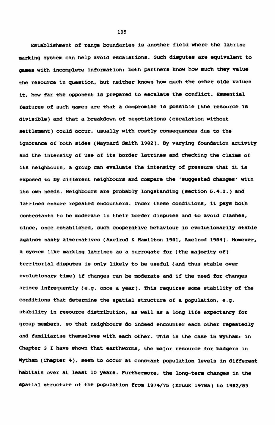
195
Establishment of range boundaries is another field where the latrine
marking system can help avoid escalations. Such disputes are equivalent to
games with incomplete information t both partners Know how much they value
the resource in question, but neither Knows how much the other side values
it, how far the opponent is prepared to escalate the conflict. Essential
features of such games are that a compromise is possible (the resource is
divisible) and that a breakdown of negotiations (escalation without
settlement) could occur, usually with costly consequences due to the
Ignorance of both sides (Maynard Smith 1982). By varying foundation activity
and the intensity of use of its border latrines and checking the claims of
its neighbours, a group can evaluate the intensity of pressure that it is
exposed to by different neighbours and compare the 'suggested changes' with
its own needs. Neighbours are probably longstanding (section 5.4.2.) and
latrines ensure repeated encounters, under these conditions, it pays both
contestants to be moderate in their border disputes and to avoid clashes,
since, once established, such cooperative behaviour is evolutionarily stable
against nasty alternatives (Axelrod & Hamilton 1981, Axelrod 1984). However,
a system like marking latrines as a surrogate for (the majority of)
territorial disputes is only likely to be useful (and thus stable over
evolutionary time) if changes can be moderate and if the need for changes
arises Infrequently (e.g. once a year). This requires some stability of the
conditions that determine the spatial structure of a population, e.g.
stability in resource distribution, as well as a long life expectancy for
group members, so that neighbours do indeed encounter each other repeatedly
and familiarise themselves with each other. This is the case in Wythamt in
Chapter 3 I have shown that earthworms, the major resource for badgers in
wytham (Chapter 4), seem to occur at constant population levels in different
habitats over at least 10 years. Furthermore, the long-term changes in the
spatial structure of the population from 1974/75 (Kruuk 1978a) to 1982/83
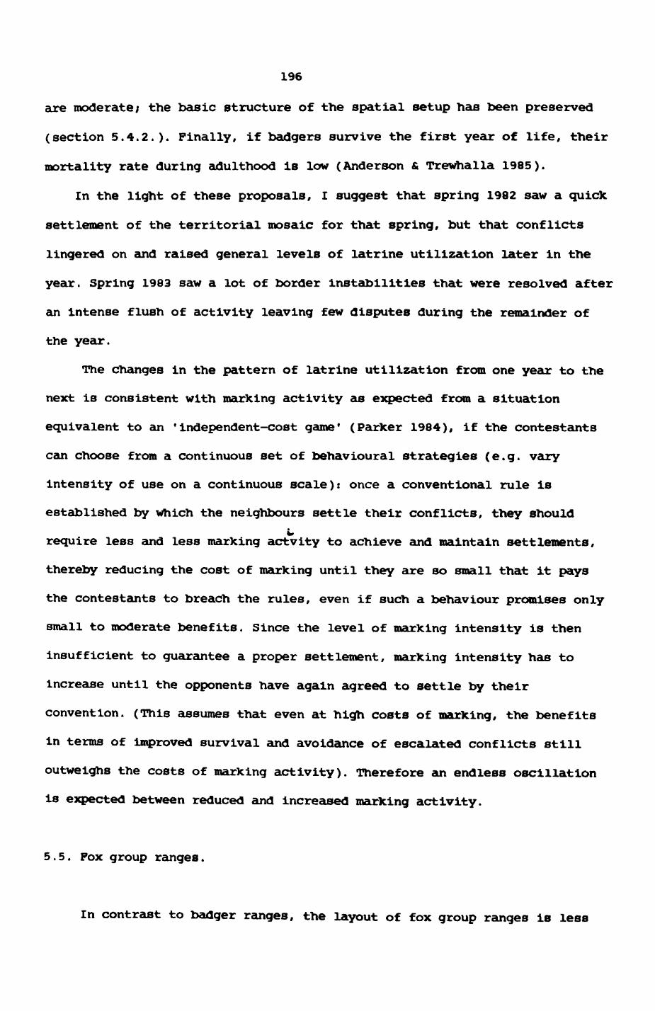
196
are moderate; the basic structure of the spatial setup has been preserved
(section 5.4.2.)- Finally, if badgers survive the first year of life, their
mortality rate during adulthood is low (Anderson & Trewhalla 1985).
In the light of these proposals, I suggest that spring 1982 saw a quick
settlement of the territorial mosaic for that spring, but that conflicts
lingered on and raised general levels of latrine utilization later in the
year. Spring 1983 saw a lot of border instabilities that were resolved after
an Intense flush of activity leaving few disputes during the remainder of
the year.
The changes in the pattern of latrine utilization from one year to the
next is consistent with marking activity as expected from a situation
equivalent to an 'independent-cost game' (Parker 1984), if the contestants
can choose from a continuous set of behavioural strategies (e.g. vary
intensity of use on a continuous scale): once a conventional rule is
established by which the neighbours settle their conflicts, they shouldw
require less and less marking actvity to achieve and maintain settlements,
thereby reducing the cost of marking until they are so small that it pays
the contestants to breach the rules, even if such a behaviour promises only
small to moderate benefits. Since the level of marking intensity is then
insufficient to guarantee a proper settlement, marking intensity has to
increase until the opponents have again agreed to settle by their
convention. (This assumes that even at high costs of marking, the benefits
in terms of Improved survival and avoidance of escalated conflicts still
outweighs the costs of marking activity). Therefore an endless oscillation
is expected between reduced and increased marking activity.
5.5. Fox group ranges.
In contrast to badger ranges, the layout of fox group ranges is less
197
neat and tidy, and some - although not substantial - overlap between
neighbouring ranges may occur, exceptional cases notwithstanding (Kacdonald
1977a). Poxes are also distinguished from badgers in that the den does not
assume the same importance to the fox as the sett does to the badger. Pox
dens seem to be essential only as a hide for small cubs in spring, and, in
unsuitable landscapes and geological formations, may then limit the breeding
density of foxes (Weber 1985). According to monthly checks of earths of all
kinds and the habits of radio-tracked individuals, use of earths, badger
setts or extended rabbit warrens was erratic or absent in other seasons.
Poxes show great flexibility in their choice of day-time resting places. In
Range 7, for instance, the two radio-tracked foxes RABBITS and PINTOOTH
often slept in a large blackberry bush that stood isolated in the midst of
pastures and long grassland and was surrounded by buildings, or they went to
a small thicket next to the swimming pool at Hill End Camp. During summer,
wheat fields were a favourite resting site. This behaviour is used by the
local farmers who successfully hunt foxes from reaping machines during
harvest.
Information on range characteristics was derived from radio-tracking of
20 foxes (Tables 5.22 and 5.23). Hence, the available information,
particularly for group size and reproductive success per group, is not as
extensive as for badger groups, where the radio-tracking supplemented the
results of the baiting action and the Annual Badger Census. This information
is summarized in the following section.
5.5.1. Description of fox group ranges.
Pig. 5.30-5.33 illustrate the distribution of fox group ranges in the
study area in relation to four major habitat categories (HUMAN t habitat
types 1, 2, 3, 23, 471 DECIDUOUS WOODLANDi habitat type 37; PASTURE! habitat
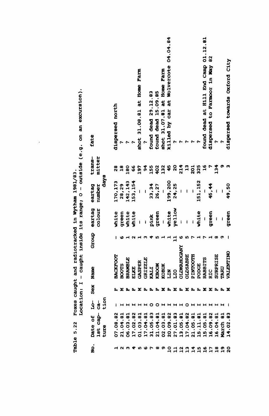
Table
5.22
Foxes
caug
ht a
nd r
adiotracked
in Wyt
ham
1981/83.
Loca
tion
t I -
caught in
side
it
s ra
nge;
O
- ou
tsid
e (e.g
. on a
n excursion)
NO.
Date o
f 1st
cap-
ture
1 2 3 4 5 6 7 8 91O 11 12 13 14
15 16 17 18 19 20
O7 21
06 17 01 17 31
21
02 20 27 13 17 21 15 15 16 16
.08.
.04.
.03.
.02.
.03.
.04.
.05.
.04.
.03.
.09.
.01.
.05.
.04.
.05.
.11.
.05.
.09.
.04.
March
14.02.
82 81 81 82 81 81 83 81 81 82 83 81 82 81 81 81 82 81 81 83
Lo
ca
sex
Name
Gi:o
u]
tion _ I I I I I O O I I I I O I I I I I I —
F M F F M F F F M F M F M F F M M F F M
BACKFOOT
BOOTS
BRAMBLE
ELKE
GASPER
GRIZZLE
KALI
KBOOM
KOBUK
LIN
LIO
OLDMAHOGANY
OLDSABRE
PINTOOTH
PODGE
RABBITS
RIC
SURPRISE
TARU
VALENTINO
_ 6 1 2 1 3 4 5 1 1116 5 7 1 7 1 8 9 —
Group
eartag
eart
ag
trans-
fate
colo
ur
numb
er
mitt
er
days
— 6 1 2 1 3 4 5 1 1116 5 7 1 7 1 8 9 —
white
green
white
white
— — pink
green
— white
yell
ow— — — white
—gree
n— —
green
170,173
28,29
142,143
153,154
— —33,34
26,27
—199,200
24,25
— — —151,152
—45,44
— —49
, 5O
28 18ISO
66
197 94
155
4O2
132 45 2O
214 13
2O1
325 16 7
134 9 3
disp
erse
d north
? ? ?shot 31.O8.8l a
t Home F
arm
?fo
und de
ad 2
9.12
.83
found de
ad 15.O9.85
shot 31.O7.81 a
t Home F
arm
killed by
car
at W
olvercote
O4.O4.84
? ? ? ? ?fo
und de
ad a
t Hill E
nd C
amp
Ol.1
2.81
dispersed
to F
armoor i
n Ma
y 82
? ?dispersed to
ward
s Ox
ford
City
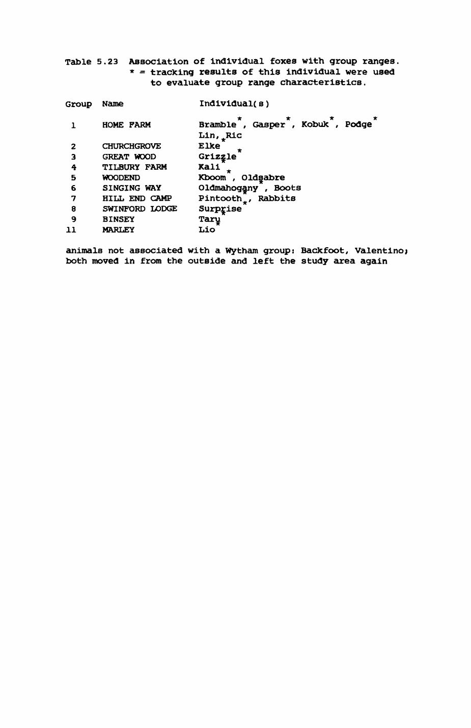
Table 5.23 Association of individual foxes with group ranges. * = tracking results of this individual were used
to evaluate group range characteristics.
Group Name Individual( s)
1 HOME FARM Bramble , Gasper , KobuX , PodgeLin,^Ric
2 CHURCHGROVE EUce ^3 GREAT WOOD Grizzle4 TILBURY FARM Kali #5 WOODEND Kboom , Oldgabre6 SINGING WAY Oldmahogany , Boots7 HILL END CAMP Pintooth^, Rabbits8 SWINFORD LODGE Surprise9 BINSEY Taru.
11 MARLEY LiO
animals not associated with a Wytham group: Back foot/ Valentino; both moved in from the outside and left the study area again
198
type 7; ARABLE: habitat type 28, 29, 30).
Range Fl (HOMEFARM). This is the best known fox range in this study. It
covers the southern half of Wytham village, extends to the Wytham road in
the east, covers the northern half of Mar ley Wood in the south and includes
the eastern fields of the Wytham Park in the West. Pour adults, the dog
foxes GASPER and KOBUK and the vixens BRAMBLE and PODGE, were tracked in
1981 and 1982 (Table 5.22). There is some evidence that PODGE, the vixen
caught in November 1981, was a resident throughout 1981. In summer 1981,
unmarked fox(es) could be frequently observed at the back of Mrs. Gardiner's
garden, and at the date of capture, PODGE was quite old and hence unlikely
to be a recent immigrant (Lloyd 1980). In spring 1981, BRAMBLE had a litter
in a den under a tree in the backyard of Mrs. Gardiner's garden (see Fig.
5.30-5.33), but moved the cubs to the wood later in the year. In spring
1982, PODGE had cubs in the same den as BRAMBLE in 1981 in the woodland at
the southern fringe of the range, but moved them probably temporarily to the
backyard of Mrs. Gardiner's garden at some stage (for a detailed description
of her movements during the breeding season see Chapter 6). Both males were
shot by the owner of Home Farm in late summer 1981; the fate of both females
remains unknown. Observed litter size in both years was two cubs. Two young
individuals, the vixen LIN and the dog-fox RIC, were caught in autumn 1982,
but due to premature transmitter failure a satisfactory record of their
dispersal movements could not be obtained. In May 1984, LIN was run over by
a car at a distance of 2 km from her natal range in Wolvercote at the age of
nearly 3 years. RIC moved in autumn 1982 from the village area to Mar ley
Wood into the transition zone between Ranges Fl and Fll and dispersed to
Farmoor at the southern edge of the study area in spring 1983, where he was
sighted several times (straight dispersal distance from the natal range of
4.3 km). The HOMEFARM Range is dominated by pasture and deciduous woodland;
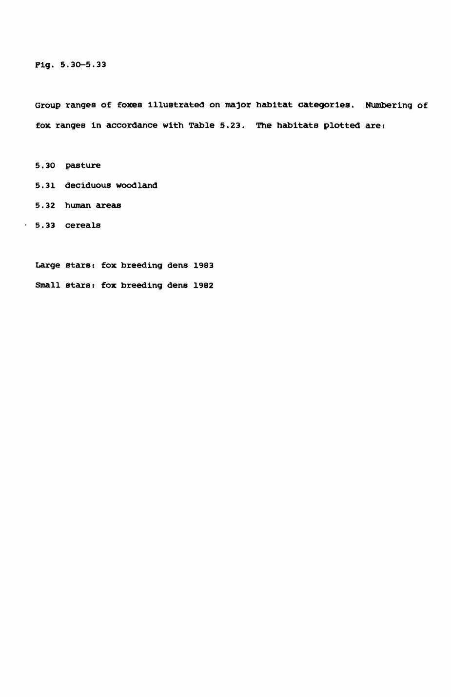
Pig. 5.30-5.33
Group ranges of foxes illustrated on major habitat categories. Numbering of
fox ranges in accordance with Table 5.23. The habitats plotted arei
5.30 pasture
5.31 deciduous woodland
5.32 human areas
5.33 cereals
Large stars: fox breeding dens 1983
Small starst fox breeding dens 1982
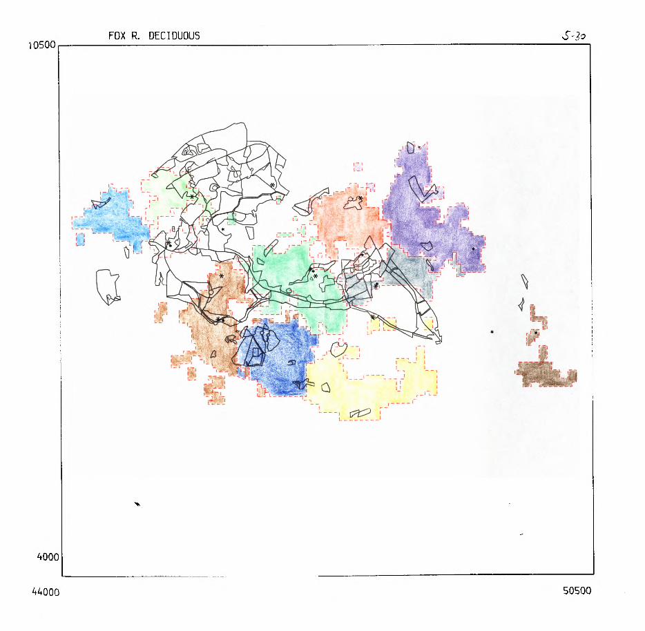
10500FOX R. DECIDUOUS
4000
44000 50500
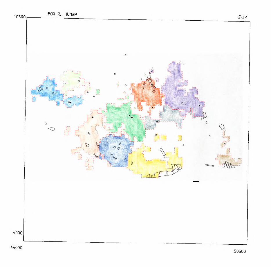
00505000*7*7
000*7
11i i
NVWOH -'oosot
o:•=> \— to-cQ
-
Xo
o
o
in o
o
oLA
O
O
OO
O
O
O^j-
-a-
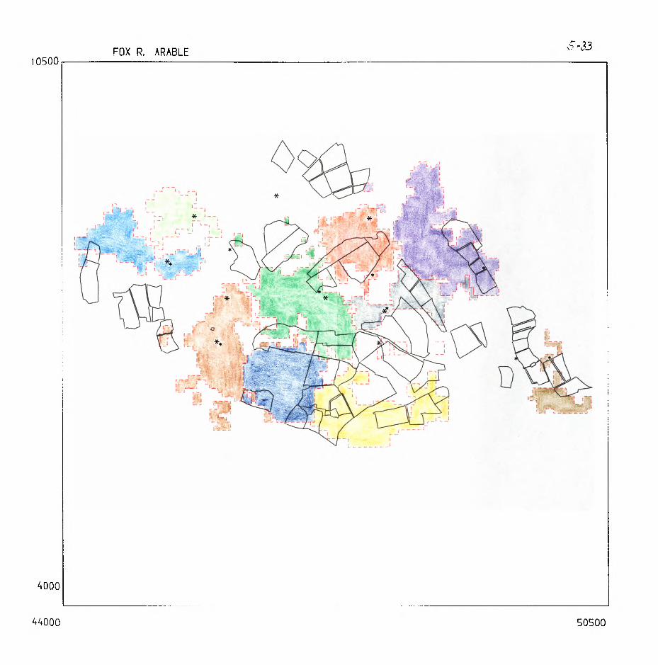
10500FOX R. ARABLE
S-33
wisrii
4000
44000 50500
199
third in area are wheat fields and root crops. Access to human-originated
resources is manifold and varied (compost heaps, farms etc).
Range P2 (CHURCHGROVE). This range covers the northern half of the Binsey
area. One fox, the vixen ELKE, was tracked here in 1982. Her range
approximately coincides with the range of a vixen tracked several years
earlier by Newdick (1983), Indicating that the spatial setup of the fox
ranges includes some stability. This vixen was barren when caught
(17.2.1982), suggesting a group size of 3 if a breeding vixen was also
present. In 1982, a breeding den was located In a hedge north of the Binsey
Farm. According to the local farmer, that breeding den was regularly used.
Accordingly, minimum estimate of group size Is 3. Litter size could not be
determined.
Range F3 (GREAT WOOD). This is a little known range where the vixen GRIZZLE
was tracked in 1981. In 1983, 4 fox cubs were sighted in the Chalet badger
sett in this area. The range is broadly partitioned into two sections: a
short-grass pasture area in the west, and dense, heterogeneous woodland in
the east.
Range F4 (TILBURY FARM). This range extends from southeastern sections of
the woodland to the suburbs of Botley, Including large fields, grass ley and
pastures, but especially human-dominated areas (farms, allotments, detached,
and semi-detached housing). Here, another barren vixen, KALI, was caught and
radio-tracked in 1983. Simultaneous observation of 3 foxes during radio-
tracking on 2.6./3.6.1983 lends additional support to the suggested minimum
group size of 3. A fox litter was regularly observed at the Upper Follies
badger sett, but since it is outside the range used by KALI, It is probably
not associated with the TILBURY range. It Is possible that cubs were reared
200
in the southern part of the range which was not included in any of the usual
checks in spring time.
Range P5 (WOODEND). This range extends from the Eynsham road and Farnraoor in
the south to the Singing Way and Radbrook Common in the north. The male
OLDSABRE and the vixen KBOOM were tracked in this area in 1981 and 1982.
Minimum estimate of group size is 2) information on possible additional
group members is lacking. Close to the Nealing's Copse badger sett, a fox
litter was observed with two cubs in all three years 1981-1983. Besides
large areas of pasture and various kinds of woodlands, the range contains
the Woodend Farm, the Buddhist Centre and other private housing.
Range F6 (SINGING WAY). The central range in Wytham covers The Pastlcks
Plantations in the east, most of Wytham Park in the north, part of the
Radbrook Common area in the west and part of the wheat fields between the
Singing Way and Hill End Camp in the south. The dog-fox BOOTS and the vixen
OLDMAHOG were tracked in 1981; up to 4 foxes were observed simultaneously
(DW Macdonald, pers. comm.). Breeding dens were located at varying sites
every year. Litter size was 2 in both 1982 and 1983. Habitat heterogeneity
is considerable, ranging from fields over pasture fields to mixed
plantations, but no human habitation is present.
Range P7 (HILL END CAMP). This range covers some of Bean Wood in the west,
but mostly the pastures and grasslands around the Hill End Camp Farm and the
local natural history school. The dog-fox RABBITS and the vixen PINTOOTH
were radio-tracked here In 1981. At dusk, other, unmarked fox(ee) could
occasionally be observed in the area. Presence of fox cubs could not be
directly confirmed, although an earth was found at the edge of the wheat
fields with signs typical for the presence of cubs In 1982 and 1983.
201
Range P8 (5WINFORD LODGE). This range extends from Swinford Lodge at the
toll bridge to Eynsham in the west to the woodlands south of The Chalet and
around the Reservoir in the east. It is again known from only one fox, the
vixen SURPRISE tracked in 1981. A breeding den was found in 1982 and 1983 in
a fox den in the neighbourhood of The Great Oak badger sett (Rough Common
badger range).
Range F9 (BINSEY). This range covers agricultural and human-dominated area,
mainly grass ley, wheat fields, allotments and terraced housing. Here, the
vixen TARU was tracked in autumn 1981. Her range is nearly identical with
that of previous members of Newdick's (1983) Blnsey group radio-tracked
several years earlier, again suggesting that long-term stability may be
important.
Range Fll (MARLEY). This range is the southern neighbour of Range PI. It
covers areas on both sides of the western by-pass and consists mostly of
arable fields, pasture and deciduous woodland. In the east, it borders onto
Range F2. Here, the dog-fox LIO was radio-tracked in 1983. A fox litter was
located in the bracken area at the southwestern corner of Marley Wood both
in 1982 and 1983. Litter size, could not be determined.
5.5.2. Characteristics of fox group ranges.
Several features of the range system as described in the previous
section deserve special consideration.
(1) Long-term stability of range boundaries beyond the life-time of an
individual seems to be common in Wytham. Evidence for this comes from at
least four ranges. ELKE (Range F2) and TARU (Range F9) occupied ranges very
similar to those occupied by foxes tracked several years earlier by Newdlck
202
(1983). Furthermore, range boundaries of the HOMEFARM range as determined
from the radio-tracking of PODGE in 1982 are consistent with the boundaries
determined from the radio-tracking of BRAMBLE, GASPER, and KOBUK in 1981.
Finally, the western edge of KALI'S range (Range F4) in 1983 coincides with
the eastern boundary of PINTOOTH's range (Range F7) in 1981, and the eastern
edge of LIO's range (Range Fll) in 1983 corresponds to the southwestern
border of ELKE's range (Range F2) in 1982. Therefore I believe it is
justified to consider all ranges from all three years together as one system
in my subsequent analyses.
(2) Are Wytham foxes territorial ? Although there are many different
views as to what constitutes territoriality (for a review see Kaufmann
1983), two commonly agreed criteria are (i) exclusive use of an area and
(ii) active maintenance and defence of the area. I shall first deal with
exclusive use and then turn to the maintenance and defense of ranges.
Several group ranges overlap slightly or moderately (Fig. 5.3O-5.33).
However, most part of the ranges are exclusively used by group members {Fig.
5.30-5.33). overlap may be due to three causesi
(i) overlap is an artefact! assume, for instance that a river
constitutes a perfect border between two neighbouring ranges but runs at an
oblique angle through a cell. Foxes from different groups walking along both
sides of the river would never touch the same ground, yet due to the
analysis based on 50 m grid cells they would seem to share one or several
cells. This artefact accounts for narrow bands of overlap (Fig. 5.3O-5.33).
(ii) overlap is the result of slight seasonal or long-term changes
in range use: this is again an artefact of the chosen method of analysis.
Real separation of ranges may be perfect at each point in tine, yet slight
shifts of range boundaries from year to year may cause records of range use
of neighbouring ranges from different years to produce sowe overlap. This
effect may account for some of the overlap between Ranges Fl and Fll in
203
Mar ley Wood, since all individuals of Range Fl were tracked either in 1981
or 1982, while LIO from Range Fll was tracked in 1983. Slight seasonal
shifts may have contributed to range overlap between OLDMAHOG (Range F6) and
KBOOM (Range F7) who were tracked at the same time.
(iii) overlap is the result of common use by different individuals
of the same area at the same time: this constitutes 'true' overlap. Commonly
used areas, ie. areas of which members of both groups treat the common areas
as their own, are expected to occur in high quality habitat. Overlap between
ranges of OLDMAHOG and KBOOM do occur in high quality habitats, while areas
of little use may result in empty spaces between ranges (PINTOOTH and
OLDMAHOG).
Several lines of evidence suggest that foxes actively defend their
ranges. Foxes token-urinate to mark the border of their ranges (Macdonald
1979b)i they also defend ranges in the suburbs and the city of Oxford
(Newdick 1983, Doncaster 1985). I was fortunate to witness a fight between
KBOOM (Range F5) and an unmarked fox close to her range border. In Chapter
6, the fine-grained analysis of movements will reveal the extent to which
foxes spend time and energy on marking and patrolling of the range border.
Finally, the next section will investigate how the patterns of feaces
deposition contribute to the advertisement of range ownership and hence the
defense and maintenance of the ranges.
(3) Brief observations of fox litters at breeding dens are notoriously
unreliable for the determination of litter size (Lloyd 198O). It is rarely
the case that all cubs are present and observable at the den at the same
time. Hence, observations of cubs were used to confirm the presence of a
litter, but not as an indicator of reproductive success. Surprisingly, there
may have been no breeding activities in Ranges 4 and Range 7, but fox cubs
were also discovered in areas where foxes were not caught (Pig. 5.3O-5.33).
204
(4) Host ranges nave access to resources of human origin. These are
usually located at the fringe of the range (Ranges 1, 2, 4, 5, 9). Food from
human origins is an important part of the diet. It seems therefore plausible
that the dispersion of these human 'patches' determine to some extent the
delineation of the range boundary/ as suggested by the Resource Dispersion
Hypothesis of Bradbury & vehrencamp (1976) and elaborated by carr &
Macdonald (in press). However, since proximity to easily accessible, human-
derived food may increase the danger to cubs, breeding dens are usually
placed far away from housing. In the context of range utilization and
movement patterns (Chapter 6), evidence for the need to balance the desire
for easy access to food with the need to protect the young will be discussed
in detail.
5.5.3. Distribution of fox faeces
Red foxes are known to use a variety of odours for scent-marking, and
these are both of glandular, e.g. anal and supracaudal gland, and non-
glandular origin, e.g. urine (Macdonald 1985). However, little is Known
about patterns of faeces deposition and its possible role in scent-marking.
In this section I analyse the position of fox faeces in relation to the
local topography of deposition sites to investigate whether their
distribution suggests a possible role in scent-marking.
The task of testing patterns of faeces distribution for a communicative
function raises some difficulties in the absence of olfactory information.
Faeces may differ in their communicative significance (e.g. with or
without anal sac secretion), and some may have no communicative function at
all. The social significance may be affected by the circumstances at the
time of defaecatlon and by the locality (e.g. core versus periphery of the
territory), and also by the individual's status (e.g. dominant versus
205
subordinate). Furthermore, foxes nay place faeces randomly with respect to
their tracks, but their trades may be highly nonrandom, and anyway difficult
for the observer to identify. These are only some of the many difficulties
hindering analysis of patterns of scent marking, as researched extensively
in Brown and Macdonald (1985). In the light of these difficulties, I will
restrict myself to one fundamental question: does the pattern of faeces
deposition comply with conditions likely to maximize the transmission of a
message? This question can be paraphrased by asking whether the deposition
of fox faeces matches the criteria proposed by Kleiman (1966) and elaborated
by Macdonald (1985) for diagnosing a scent mark. Clearly, the development
of scent marks will be affected by the functional context, movement
patterns, spatial and social organization etc., but nonetheless they should
Invariably include two elements!
(1) Maximize probability of faeces being encountered.
(2) Maximize probability of faeces being detected.
5.5.3.1. Patterns of distribution
Fox faeces were collected methodically throughout the study area during
each month from April 1981 to October 1983, and the location and
circumstances of each were recorded. Details of sampling procedures and
data recording have been presented in sections 4.2.1. and 2.3.3. In
addition two or more faeces were scored as "closely together", if each of
them was at least within one metre of any of the other faeces present. In
practice if several faeces were present, they were usually almost touching.
Also, faeces found on fox dens and badger setts were habitually scored as on
a path, since dens are regularly associated with trails leading to and away
from them. Two samples of faeces were distinguished!
(1) those collected while habitat recording (Chapter 2) - a highly
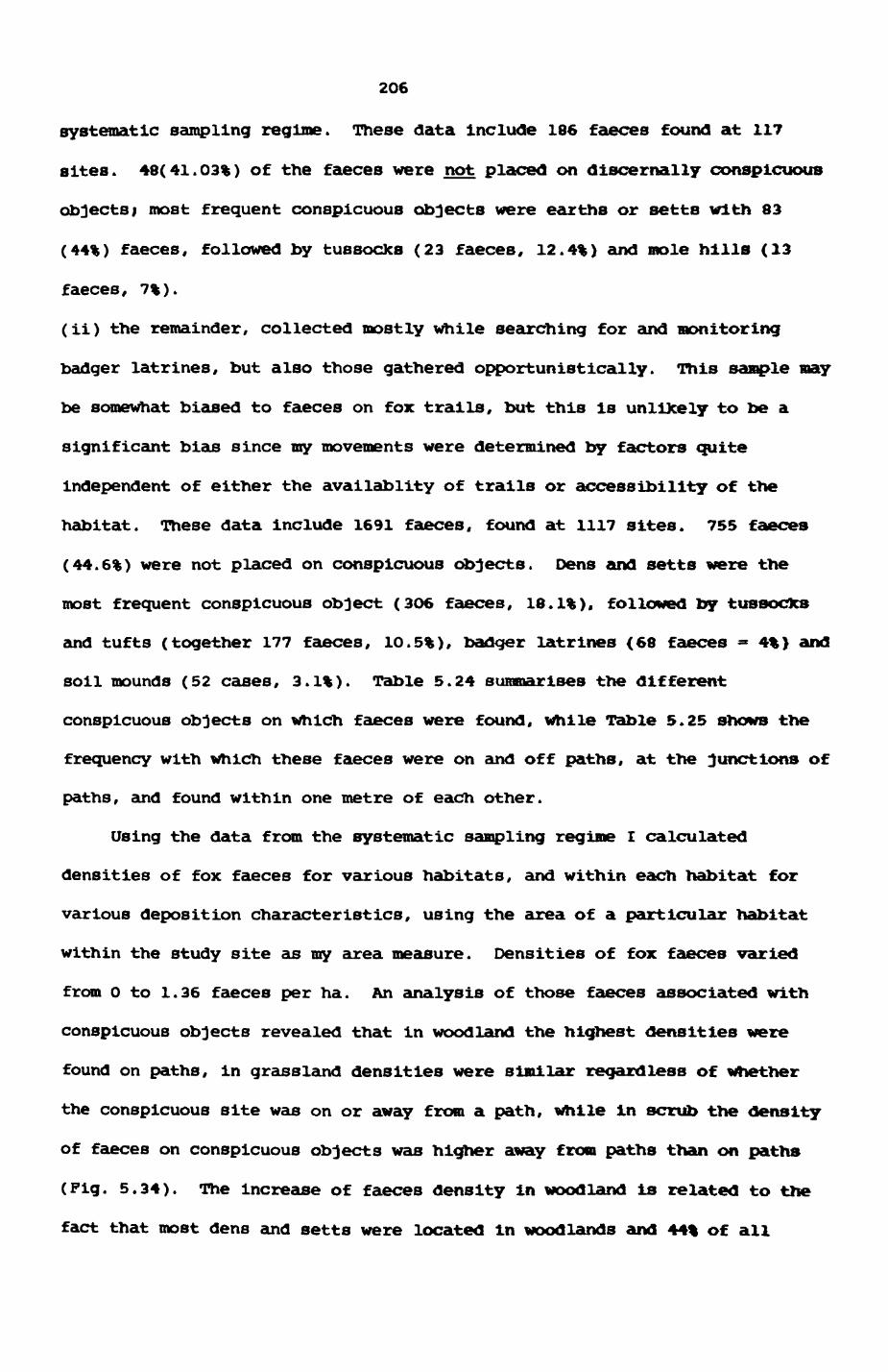
206
systematic sampling regime. These data include 186 faeces found at 117
sites. 48(41.03%) of the faeces were not placed on discernally conspicuous
objects; most frequent conspicuous objects were earths or setts with 83
(44%) faeces, followed by tussocks (23 faeces, 12.4%) and mole hills (13
faeces, 7%).
(ii) the remainder, collected mostly while searching for and monitoring
badger latrines, but also those gathered opportunistically. This sample may
be somewhat biased to faeces on fox trails, but this is unlikely to be a
significant bias since my movements were determined by factors quite
independent of either the availablity of trails or accessibility of the
habitat. These data include 1691 faeces, found at 1117 sites. 755 faeces
(44.6%) were not placed on conspicuous objects. Dens and setts were the
most frequent conspicuous object (3O6 faeces, 18.1%), followed by tussocks
and tufts (together 177 faeces, 1O.5%), badger latrines (68 faeces =4%) and
soil mounds (52 cases, 3.1%). Table 5.24 summarises the different
conspicuous objects on which faeces were found, while Table 5.25 shows the
frequency with which these faeces were on and off paths, at the junctions of
paths, and found within one metre of each other.
Using the data from the systematic sampling regime I calculated
densities of fox faeces for various habitats, and within each habitat for
various deposition characteristics, using the area of a particular habitat
within the study site as my area measure. Densities of fox faeces varied
from 0 to 1.36 faeces per ha. An analysis of those faeces associated with
conspicuous objects revealed that in woodland the highest densities were
found on paths, in grassland densities were similar regardless of whether
the conspicuous site was on or away from a path, while in scrub the density
of faeces on conspicuous objects was higher away from paths than on paths
(Pig. 5.34). The Increase of faeces density in woodland Is related to the
fact that most dens and setts were located in woodlands and 44% of all
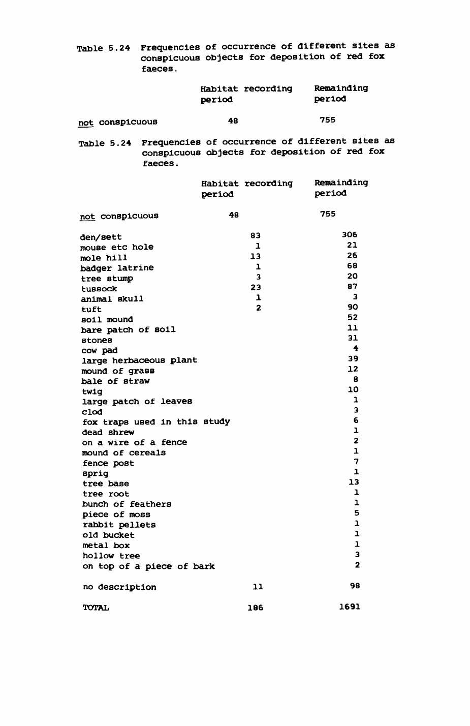
Table 5.24 Frequencies of occurrence of different sites as conspicuous objects for deposition of red fox faeces.
Habitat recording Remaindingperiod period
not conspicuous 48 755
Table 5.24 Frequencies of occurrence of different sites as conspicuous objects for deposition of red fox faeces.
Habitat recording Remaindingperiod period
not conspicuous 48 755
den/sett 83 3O6mouse etc hole 1 21mole hill 13 26badger latrine 1 68tree stump 3 20tussock 23 87animal skull 1 3tuft 2 90soil mound 52bare patch of soil 11stones 31cow pad 4large herbaceous plant 39mound of grass 12bale of straw 8twig 10large patch of leaves 1clod 3fox traps used in this study 6dead shrew 1on a wire of a fence 2mound of cereals 1fence post 7sprig 1tree base 13tree root 1bunch of feathers 1piece of moss 5rabbit pellets 1old bucket 1metal box 1hollow tree 3on top of a piece of bark 2
no description 11 98
TOTAL 186 1691

Pig. 5.34
Deposition of fox faeces in relation to conspicuousness and habitat
a. faeces not on conspicuous objects
b. faeces on conspicuous objects
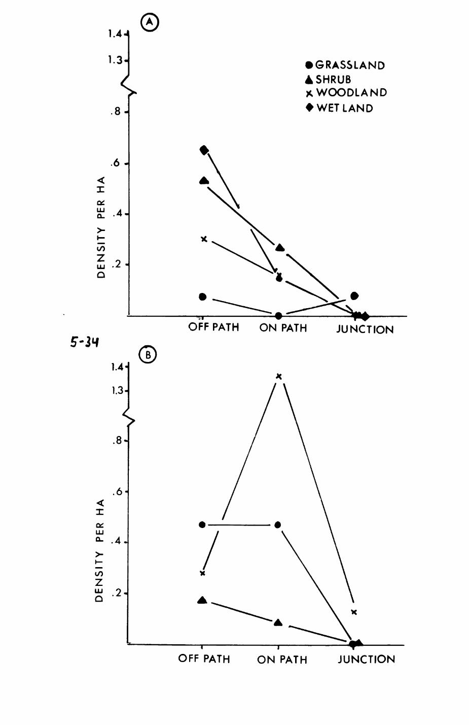
• GRASSLANDASHRUBX WOODLAND* WET LAND
OFF PATH ON PATH JUNCTION
OFF PATH ON PATH JUNCTION
207
faeces found In woodland were in association with dens. In wet lands (marsh,
riverrine environment etc.) faeces were not found associated with
conspicuous objects.
To summarise, fox faeces were found throughout all habitats, and off
fox trails, and the majority of them are found on conspicuous objects on
trails.
To explore the relationships of the characteristics of a deposition
site, I generated log-linear models (see section 5.4.3) that took into
account presence or absence of conspicuous objects (CONSP OBJECT) and paths
(PATH) and how many faeces were found at a site (NOS PRESENT).
A priori, one might expect faeces at earths to differ from those
elsewhere a) because of the social significance of dens and b) because an
accumulation of faeces at a den may simply be a consequence of the fox's
tendency to defecate soon after awalcening. Therefore I analysed two data
sets, one including faeces found on dens (data from systematic sampling
during habitat recording), and the second excluding them* Data for the
latter analysis were extracted from the data Including all faeces found
during the remainder of the study period. In Table 5.25 data and the model
generation are presented for both data sets. Note that each datum is a
deposition site, not a single faeces.
The final models for both data sets include two of three possible two-
way interactions, one of them common to both: there is a significant mutual
influence of Numbers Present and Path for a given level of Conspicuous
Object. As Table 5.26 reveals (section (3)), this significant interaction
Is based on contrasting events. For data set I (including dens etc.), too
many faeces on conspicuous objects found off-path were single faeces, while
on-path too many faeces occurred as two or even larger accumulations -
obviously an effect of accumulajtlons at dens. If dens are excluded (data
set II), too many groups of faeces are found off path, while too few two or
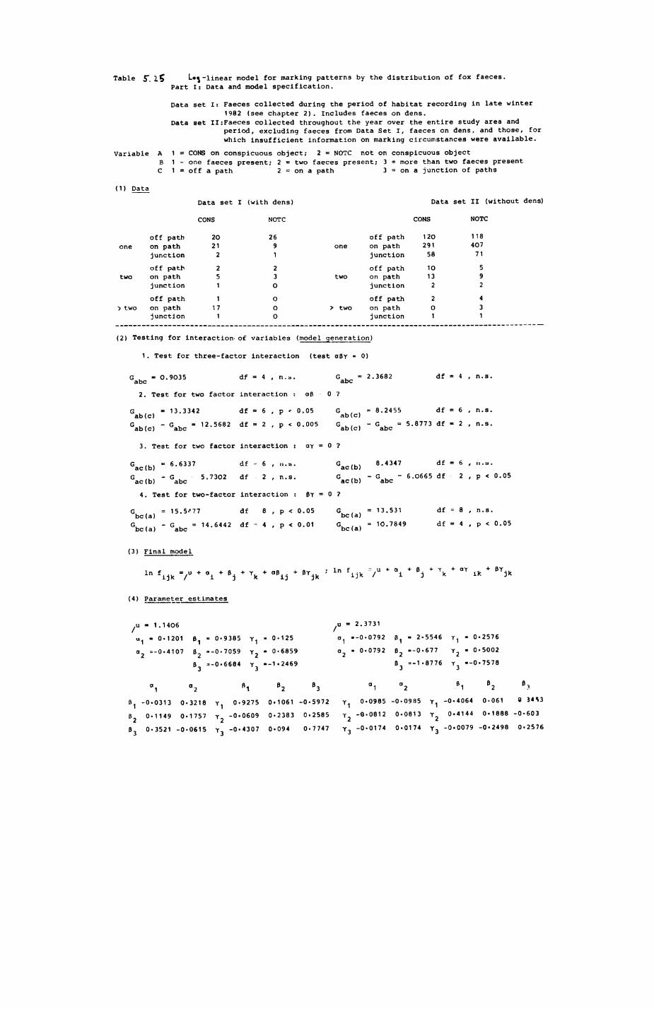
Table £". l5 L«^-linear model for marking patterns by the distribution of fox faeces. Part I: Data and model specification.
Data set I: Faeces collected during the period of habitat recording in late winter 1982 (see chapter 2). Includes faeces on dens.
Data set II:Faeces collected throughout the year over the entire study area andperiod, excluding faeces from Data Set I, faeces on dens, and those, for which insufficient information on marking circumstances were available.
Variable A 1 = CONS on conspicuous object; 2 = NOTC not on conspicuous objectB 1 =• one faeces present; 2 = two faeces present; 3 = more than two faeces presentC 1 « off a path 2 = on a path 3 = on a junction of paths
(1) Data
Data set I (with dens) Data set II (without dens)
CONS NOTC CONS NOTC
one
two
off path on path junction
off path on path junction
off path > two on path
junction
2O 21 2
25 1
1 17
1
(2) Testing for interaction^ of
1 . Test for three-factor
Gabc ' °' 9035
2. Test for
df
26 9 1
23 0
O O 0
variables
off path one on path
junction
off path two on path
junction
off path > two on path
junction
(model generation)
12O 291 58
10 13 2
2 O 1
118 407 71
5 92
4 31
interaction (test aBY - 0)
=4 , n.s
two factor interaction
G % = 13.3342 df able)
= 6 , p »
G . = 2.3682 abc
: aB 0 ?
0.05 G , = 8.2455 ab(c)
df = 4
df = 6
, n.s.
, n.s.
G . . . - G . = 12.5682 df = 2 , p < 0.005 G . , . - G ,_ = 5.8773 df = 2 , n.s. ab(c) abc r ab(c) abc
3. Test for two factor interaction : <rr = 0 ?
df --• 6 , n.s. GGac(b) = 6 ' 6337
Gac(b) - Gabc 5 ' 7302 dfac(b) 8.4347 df = 6 , ii. a .
G ... - G ,_ - 6.0665 df 2 , p < 0.05 ac(b) abc
4. Test for two-factor interaction : BT = 0 ?
= 15.5*77 df 8 , p < 0.05w / , be (a)Gbc(a) * Gabc - 14 ' 6442
G. , = 13.531 be (a)
Gbc,a) • 10 ' 7849
df = 8 , n.s.
df = 4 , p < 0.05
(3) Final model
in B. BY . k B.
(4) Parameter estimates
« 1.1406
- 0-1201
=-0-4107
0-9385 Y 0-125
--0-7059 Y, • 0-6859
B =--0-6684 Y^ --1.2469
u - 2.3731
a 1 --0-0792
a. « 0-0792
' 2-5546
--0-677
=-1-8776
• 0-2576
• 0-5002
•0-7578
B 1 -0-0313 0-3218
B, 0-1149 0-1757
B, 0-3521 -0-0615 Y,
Y 1 0-9275 0-1061 -0-5972
Y -0-0609 0-2383 0-2585
-4307 0-094 0-7747
B B
Y. 0-0985 -0-0985 Y.. -0-4064 0-061
Y -0-0812 0-0813
1 "2
0 J4S3
0.4144 0-1888 -0-603
-0-0174 0-0174 Y 3 -0.0079 -0-2498 0-2576
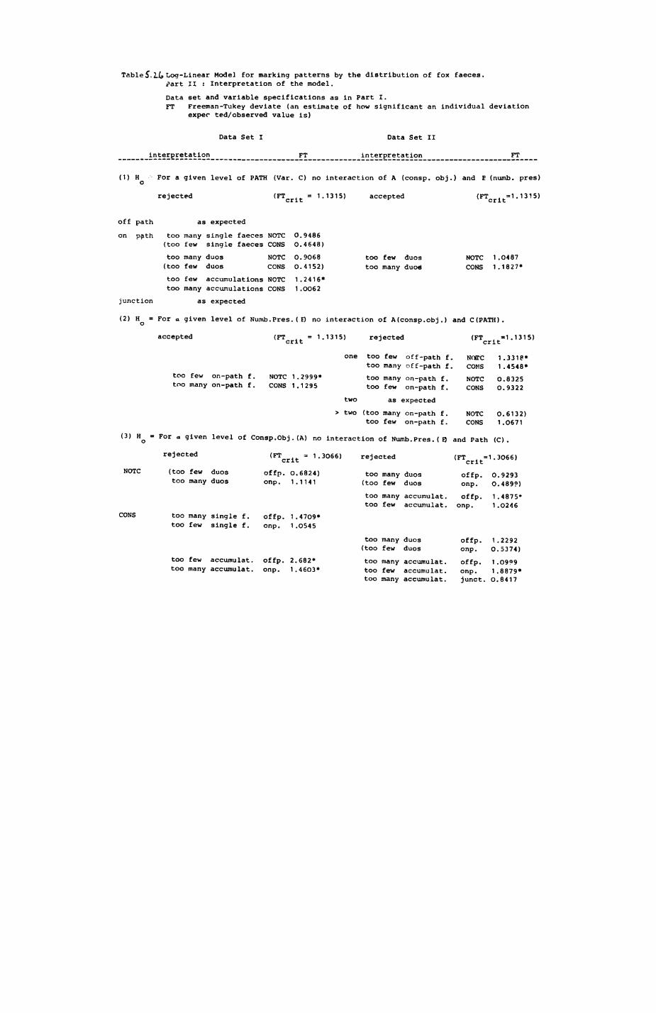
Table5.lt Log-Linear Model for marking patterns by the distribution of fox faeces. Part II : Interpretation of the model.
Data set and variable specifications as in Part I.FT Freeman-Tukey deviate (an estimate of how significant an individual deviation
expec ted/observed value is)
Data Set I
interpretation FT
Data Set II
interpretation FT
(1) H For a given level of PATH (Var. C) no interaction of A (consp. obj.) and E (numb, pres) o
rejected = 1.1315) accepted <FTcrlt-1.1315)
off path
on path
junction
as expected
too many single faeces NOTC (too few single faeces CONS
too many duos (too few duos
NOTC CONS
too few accumulations NOTC too many accumulations CONS
as expected
O.9486 O.4648)
0.9068 0.4152)
1.2416*
1 . OO62
too few duos too many duoti
NOTC 1.0487 CONS 1.1827*
(2) H = For a given level of Numb.Pres. ( E) no interaction of Afconsp.obj.) and C(PATH).
accepted (FT = 1.1315) rejected
too few on-path f. too many on-path f.
NOTC 1.2999* CONS 1.1295
one too few off-path f. too many off-path f.
too many on-path f. too few on-path f.
,FTcrlt=1.1315)
NOffC 1.3318* CONS 1.4548*
two as expected
> two (too many on-path f. too few on-path f.
NOTC CONS
NOTC CONS
0.8325 O.9322
0.6132) 1.O671
(3) H = For a. given level of Consp.Obj . (A) no interaction of Numb.Pres. ( Q and Path (C) .
rejected (FT
NOTC
CONS
-j--~ — *«•* r 4*. ~ i.juooi tejectea \t r =i.JUoo;
(too too
few many
duos duos
offp. onp.
0.6824) 1.1141
too (too
too too
many few
many few
duos duos
accumulat. accumulat.
offp. onp.
offp. onp.
0 O
1 1
.9293
.489?)
.4875*
.0246too many single f. too few single f.
offp. 1.4709* onp. 1.O545
too few accumulat. offp. 2.682* too many accumulat. onp. 1.46O3*
too many duos (too few duos
too many accumulat. too few accumulat. too many accumulat.
offp. onp.
1.2292 O.5374)
offp. 1.0999onp. 1.8879*junct. 0.8417
208
more faeces can be found on path. This holds both for conspicuous and not
conspicuous objects. The same effect of faeces accumulations at dens bears
on the interaction of Conspicuous Object and Number present for a given
level of Path (significant only for data set I). Too many accumulations
were found on conspicuous objects on paths.
Based on the analyses of data set II (excluding dens), I suggest that
foxes follow two kinds of rules, which I term locational and functional
strategies. A locational strategy tells the fox where exactly to drop the
faeces, given its current position. A functional strategy governs the fox's
over-riding goals, irrespective of its current position. Prom the results
of the log linear model I hypothesise two locational strategies (Figure
5.35)!
(1) If the animal is off a fox trail, probability of detection is low.
Thus, to Improve detection probability, the first action rule is 'select a
conspicuous object'. An occasional alternative is "select another faeces'* -
two faeces together would represent a formidable conspicuous object itself!
(2) If the animal is on a fox trail, probability of detection is high, thus
it is more important to maximize the encounter rate, and so the action rule
is 'select a site with no other faeces present'.
Two basic functional strategies reflect the conditions for maximizing
information transmission. Foxes should position their faeces to increasei
(1) Probability of encounter by an appropriate recipient (the majority of
faeces are on trails and are spread along them, but some are also sited off
paths).
(2) Probability of detection (less of a problem if faeces are on trails,
but off trails, careful placement improves odour diffusion and visual
detection).
In summary, then, foxes seem to place their faeces more often than
expected by chance in such a fashion that Information transmission Is
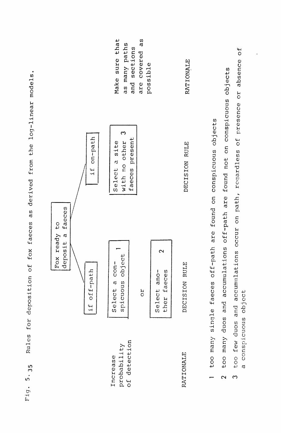
Fig.
5. 2
5 Rules
for
deposition of fox
faeces as derived
from the
log-linear models.
Fox
ready
to
deposit
a faeces
Increase
probability
of detection
RATIONALE
if off-path
Select a
con
spicuous object
or
DECISION RULE
Select ano
ther faeces
1
if on-path
Select a
site
with no other
3 faeces present
DECISION RULE
Make sure that
as many paths
and
sections
are
covered as
possible
RATIONALE
1 too
many single faeces off-path are
found
on conspicuous objects
2 too
many duos and
accumulations off-path are
found
not
on conspicuous objects
3 too
few
duos and
accumulations occur
on path,
regardless of presence or absence of
a conspicuous object
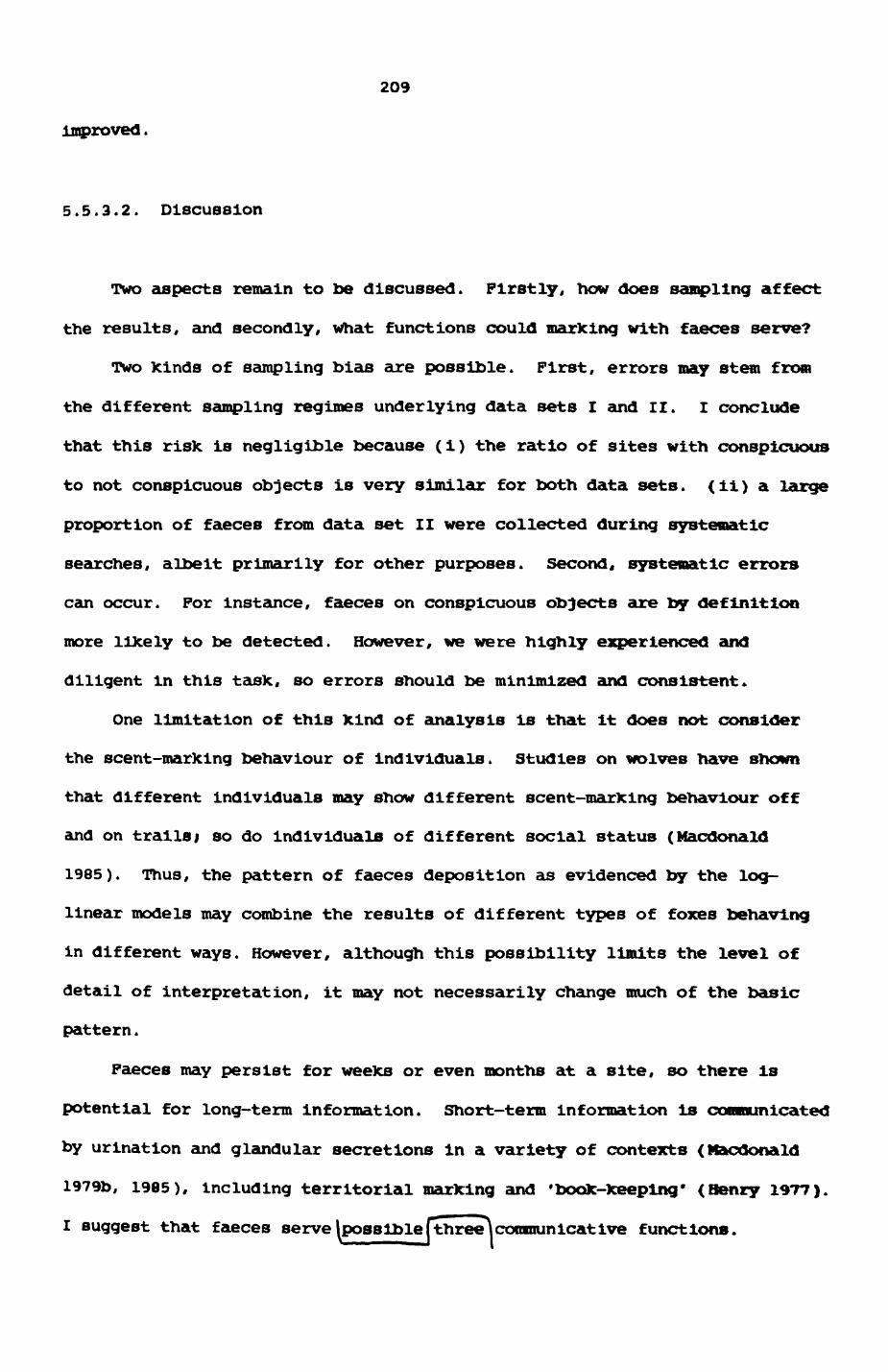
2O9
improved.
5.5.3.2. Discussion
Two aspects remain to be discussed. Firstly, how does sampling affect
the results, and secondly, what functions could marking with faeces serve?
Two kinds of sampling bias are possible. First, errors may stem from
the different sampling regimes underlying data sets I and II. I conclude
that this risk is negligible because (i) the ratio of sites with conspicuous
to not conspicuous objects is very similar for both data sets, (ii) a large
proportion of faeces from data set II were collected during systematic
searches, albeit primarily for other purposes. Second, systematic errors
can occur. For instance, faeces on conspicuous objects are by definition
more likely to be detected. However, we were highly experienced and
diligent in this task, so errors should be minimized and consistent.
One limitation of this kind of analysis is that it does not consider
the scent-marking behaviour of Individuals. Studies on wolves have shown
that different individuals may show different scent-marking behaviour off
and on trailsi so do individuals of different social status (Macdonald
1985). Thus, the pattern of faeces deposition as evidenced by the log-
linear models may combine the results of different types of foxes behaving
in different ways. However, although this possibility limits the level of
detail of interpretation, it may not necessarily change much of the basic
pattern.
Faeces may persist for weeks or even months at a site, so there is
potential for long-term information. Short-term information is comunicated
by urination and glandular secretions in a variety of contexts (Katcdonald
I979b, 1985), including territorial marking and 'book-keeping* (Henry 1977).
I suggest that faeces serve possible three^communicative functions*
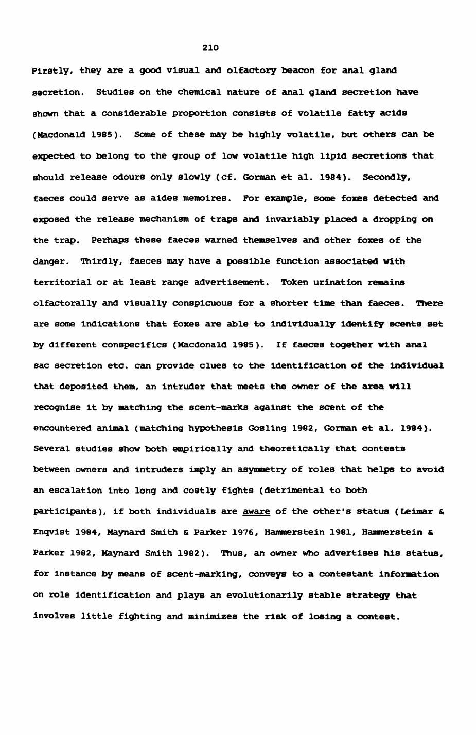
210
Firstly, they are a good visual and olfactory beacon for anal gland
secretion. Studies on the chemical nature of anal gland secretion have
shown that a considerable proportion consists of volatile fatty acids
(Macdonald 1985). Some of these may be highly volatile, but others can be
expected to belong to the group of low volatile high lipid secretions that
should release odours only slowly (cf. Gorraan et al. 1984). Secondly,
faeces could serve as aides memoires. For example, some foxes detected and
exposed the release mechanism of traps and invariably placed a dropping on
the trap. Perhaps these faeces warned themselves and other foxes of the
danger. Thirdly, faeces may have a possible function associated with
territorial or at least range advertisement. Token urination remains
olfactorally and visually conspicuous for a shorter time than faeces. There
are some indications that foxes are able to individually identify scents set
by different conspecifics (Macdonald 1985). If faeces together with anal
sac secretion etc. can provide clues to the identification of the individual
that deposited them, an Intruder that meets the owner of the area will
recognise it by matching the scent-marks against the scent of the
encountered animal (matching hypothesis Gosling 1982, German et al. 1984).
Several studies show both empirically and theoretically that contests
between owners and intruders imply an asymmetry of roles that helps to avoid
an escalation into long and costly fights (detrimental to both
participants), if both individuals are aware of the other's status (Leimar &
Enqvist 1984, Maynard Smith & Parker 1976, Hammerstein 1981, Hammerstein &
Parker 1982, Maynard Smith 1982). Thus, an owner who advertises his status,
for Instance by means of scent-marking, conveys to a contestant information
on role Identification and plays an evolutionarlly stable strategy that
Involves little fighting and minimizes the risk of losing a contest.
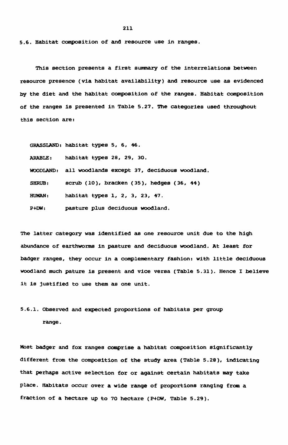
211
5.6. Habitat composition of and resource use in ranges.
This section presents a first summary of the interrelations between
resource presence (via habitat availability) and resource use as evidenced
by the diet and the habitat composition of the ranges. Habitat composition
of the ranges is presented in Table 5.27. The categories used throughout
this section arei
GRASSLANDi habitat types 5, 6, 46.
ARABLE! habitat types 28, 29, 30.
WOODLAND! all woodlands except 37, deciduous woodland.
SHRUB: scrub (10), bracken (35), hedges (36, 44)
HUMAN) habitat types 1, 2, 3, 23, 47.
P+DW: pasture plus deciduous woodland.
The latter category was identified as one resource unit due to the high
abundance of earthworms in pasture and deciduous woodland. At least for
badger ranges, they occur in a complementary fashions with little deciduous
woodland much pature is present and vice versa (Table 5.31). Hence I believe
it is justified to use them as one unit.
5.6.1. Observed and expected proportions of habitats per group
range.
Most badger and fox ranges comprise a habitat composition significantly
different from the composition of the study area (Table 5.28), indicating
that perhaps active selection for or against certain habitats may take
place. Habitats occur over a wide range of proportions ranging from a
fraction of a hectare up to 70 hectare (P+DW, Table 5.29).
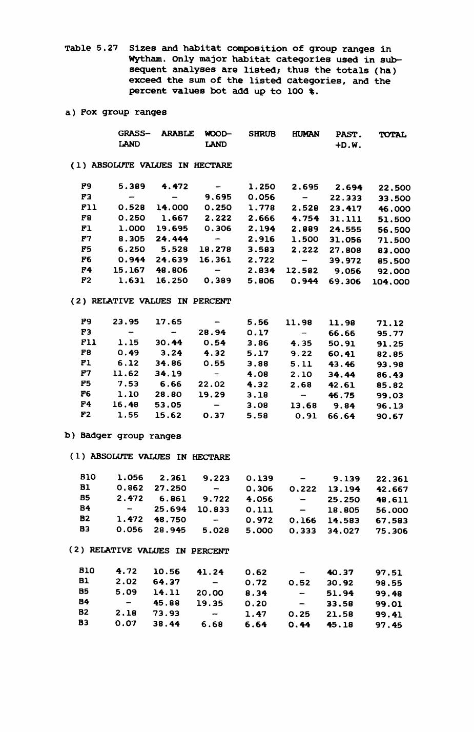
Table 5.27 Sizes and habitat composition of group ranges in Wytham. Only major habitat categories used in sub sequent analyses are listed; thus the totals (ha) exceed the sum of the listed categories, and the percent values bot add up to 10O %.
a) Fox group ranges
GRASS- ARABLE WOOD LAND LAND
(1) ABSOLUTE VALUES IN
P9 5.389P3Pll 0.528P8 0.250PI 1.000P7 8 . 305P5 6 . 25OP6 0 . 944P4 15 . 167F2 1.631
4.472—
14.0001.667
19.69524.4445.52824.63948 . 80616.250
(2) RELATIVE VALUES IN
F9 23.95F3Pll 1 . 15F8 0 . 49Fl 6 . 12P7 11.62F5 7.53F6 1 . 10F4 16 . 48F2 1.55
b) Badger group
17.65—
30.443.24
34.8634.196.6628.8053.0515.62
ranges
(1) ABSOLUTE VALUES IN
BIO 1.056Bl 0.86285 2.47284B2 1.47283 0.056
2.36127.2506.86125.69448.75028.945
(2) RELATIVE VALUES IN
810 4.7281 2.0285 5 . 098482 2 . 1883 0.07
10.5664.3714.1145.8873.9338.44
SHRUB HUMAN PAST. 4D.W.
TOTAL
HECTARE
9020
1816
0
—
.695
.250
.222
.306—
.278
.361—.389
1012223225
.250
.056
.778
.666
.194
.916
.583
.722
.834
.806
2.
2.4.2.1.2.
12.0.
695—52875488950O222—582944
2.22.23.31.24.31.27.39.9.
69.
694333417111555056808972056306
223346515671838592104
.500
.500
.OOO
.500
.500
.500
.OOO
.500
.OOO
.OOO
PERCENT
28040
2219
O
—
.94
.54
.32
.55—.02.29—
.37
5O35344335
.56
.17
.86
.17
.88
.08
.32
.18
.08
.58
11.
4.9.5.2.2.
13
98—3522111O68—.68
O.91
11.66.50.60.43.34.42.46.9.
66.
98669141464461758464
7195918293868599969O
.12
.77
.25
.85
.98
.43
.82
.03
.13
.67
HECTARE
9
910
5
.223—
.722
.833—.028
004O05
.139
.306
.056
.111
.972
.OOO
O.
0.0.
_
222——166333
9.13.25.18.14.34.
139194250805583027
224248566775
.361
.667
.611
.OOO
.583
.306
PERCENT
41
2019
6
.24—.00.35—.68
0O8016
.62
.72
.34
.20
.47
.64
O.
O.0.
_52——2544
4O.30.51.33.21.45.
379294585818
979899999997
.51
.55
.48
.01
.41
.45
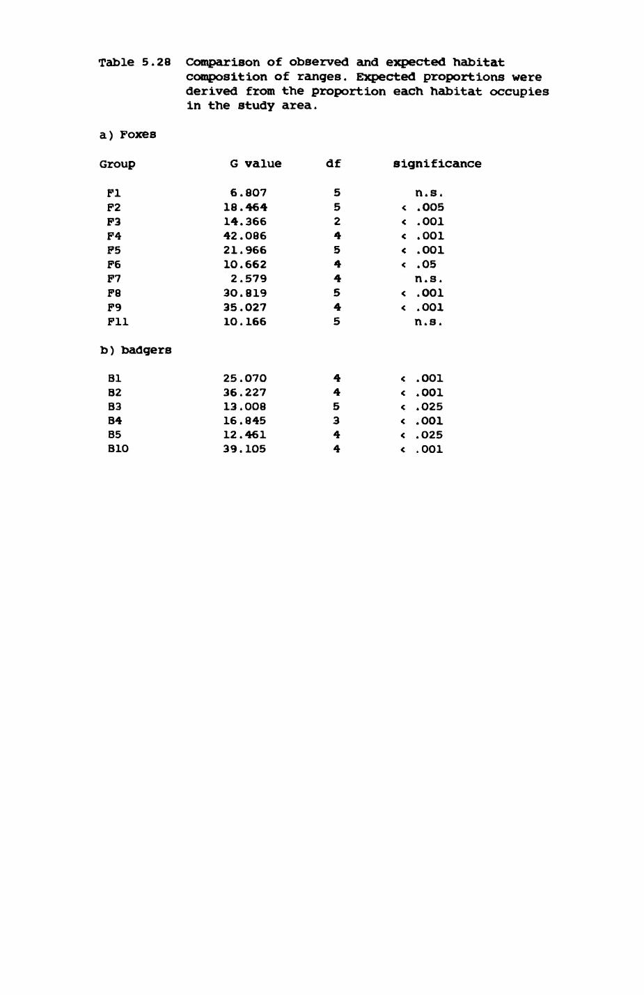
Table 5.28 Comparison of observed and expected habitatcomposition of ranges. Expected proportions were derived from the proportion each habitat occupies in the study area.
a) Foxes
Group G value df significance
Fl F2 F3 F4 F5 F6 F7 F8 F9 Fll
b) badgers
81 B2 B3 84 B5 BIO
6.80718.46414.36642.08621.96610.6622.579
30.81935.02710 . 166
5524544545
n.s.< .005< .001< .001< .001< .05
n.s.< .001< .001n.s.
25.07036.22713.00816 . 84512.46139.105
445344
< .OO1< .001< .025< .001< .025< .001
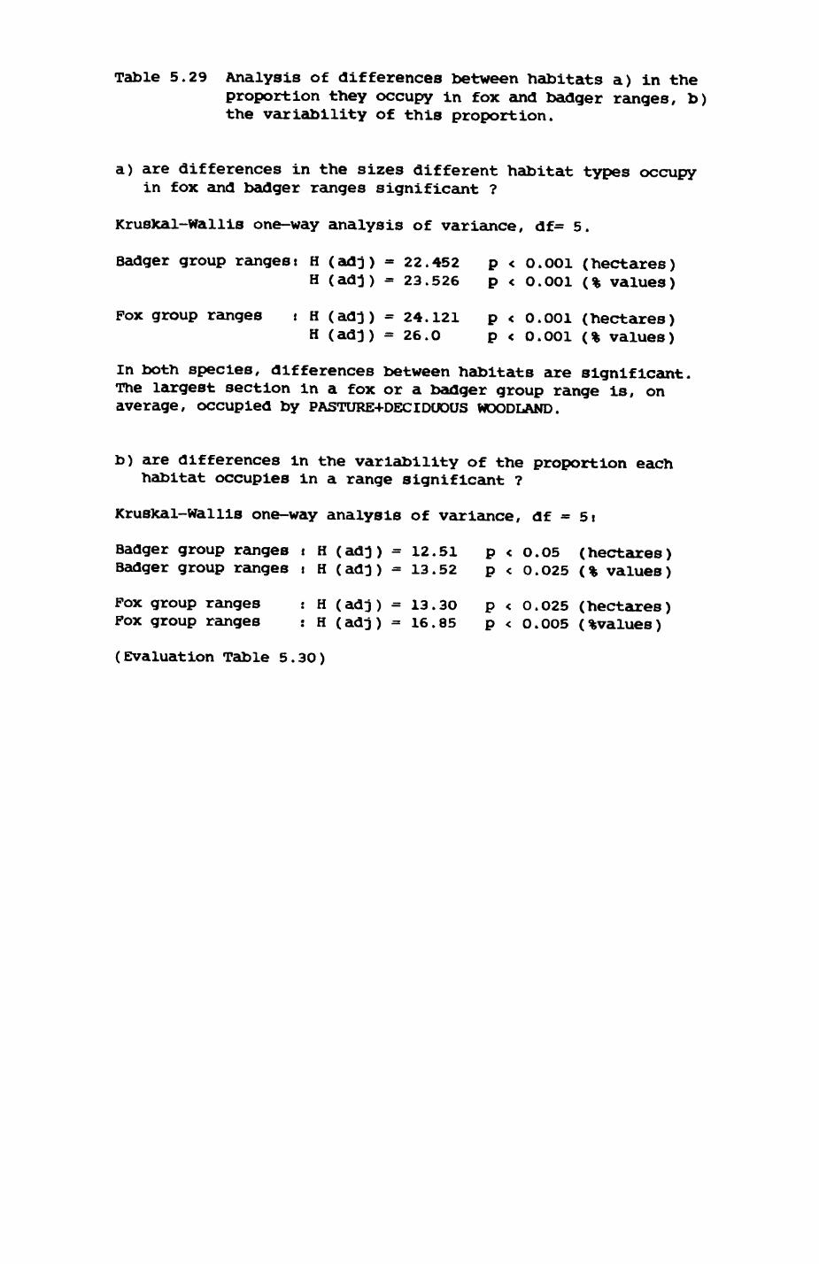
Table 5.29 Analysis of differences between habitats a) in the proportion they occupy in fox and badger ranges, b) the variability of this proportion.
a) are differences in the sizes different habitat types occupy in fox and badger ranges significant ?
Kruskal-Wallis one-way analysis of variance, df= 5.
Badger group ranges: H (adj) = 22.452 p < O.OOl (hectares)H (ad}) = 23.526 p < O.OOl (% values)
Pox group ranges t H (adj) = 24.121 p < O.OOl (hectares)H (ad}) = 26.0 p < O.OOl (% values)
In both species, differences between habitats are significant. The largest section in a fox or a badger group range is, on average, occupied by PASTURE-1-DECIDUOUS WOODLAND.
b) are differences in the variability of the proportion each habitat occupies in a range significant ?
Kruskal-Wallls one-way analysis of variance, df = 5f
Badger group ranges t H (ad}) = 12.51 p < O.O5 (hectares) Badger group ranges i H (ad}) =13.52 p < O.O25 (% values)
Fox group ranges : H (ad}) =13.30 p < 0.025 (hectares) Pox group ranges : H (ad}) =16.85 p < O.OO5 (%values)
(Evaluation Table 5.30)
212
5.6.2. Dispersion of habitats composition between ranges.
Not only are absolute or relative proportions of habitats different from
each other but habitats also vary significantly in the degree of which their
contribution to a range changes from one range to another (Table 5.29). For
badgers, habitats that are present in relative constant proportions (ie.
little inter-group variability) are especially P+DW (% values, Table 5.3O),
but also several of the other habitat types, if ha values are considered
(Table 5.30). These however, occur with more variability in relative
proportions. In foxes, little variability occurs mainly for P+DW but also
for shrub. As Table 5.31 shows, this is due to the steady increase of the
proportion of shrub and D+PW with range size (see also Fig. 5.36-37). Human
habitations vary considerably in their contribution to the range, but
nevertheless seem to be partly responsible for the delineation of range
boundaries I This difference in variability perhaps reflects the different
relationships of the productivity of habitats in relation to their size.
While a large field of pasture contains more earthworms, and a longer hedge
more birds, a compost heap may be equally 'productive' whether it occurs in
a large or a small garden.
5.6.3. Habitat composition and range size.
The relationship between the key habitats identified in the preceding
section and range size is illustrated in Fig. 5.36 and Fig. 5.37 (also Table
5.31). While it is no surprise that habitats constituting the bulk of the
landscape (such as arable fields) will increase in contribution with range
size, small habitats , e.g. shrub, cannot necessarily be expected to grow in
the same proportions. P4-DW grows with range size in absolute terms, but
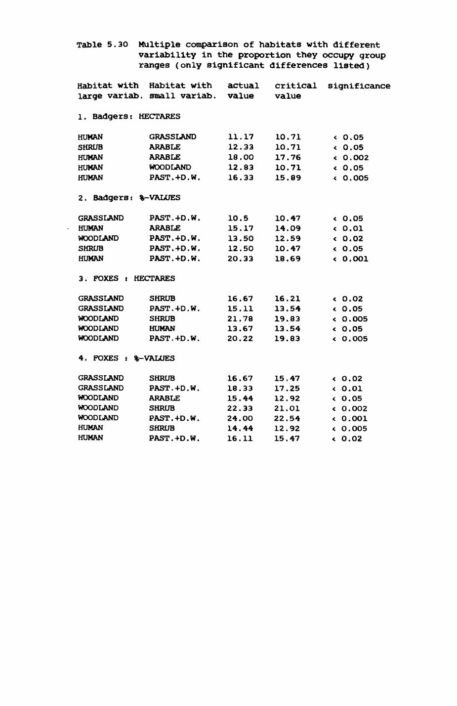
Table 5.30 Multiple comparison of habitats with different variability in the proportion they occupy group ranges (only significant differences listed)
Habitat with Habitat with large variab. small variab,
1. Badgers: HECTARES
HUMAN SHRUB HUMAN HUMAN HUMAN
GRASSLANDARABLEARABLEWOODLANDPAST.+D.W.
2. Badgers: %-VALUES
GRASSLANDHUMANWOODLANDSHRUBHUMAN
PAST.+D.W.ARABLEPAST.+D.W.PAST.+D.W.PAST.+D.W.
3. POXES t HECTARES
GRASSLANDGRASSLANDWOODLANDWOODLANDWOODLAND
SHRUBPAST.+D.W.SHRUBHUMANPAST.+D.W.
4. POXES { %-VALUES
GRASSLANDGRASSLANDWOODLANDWOODLANDWOODLANDHUMANHUMAN
SHRUBPAST.+D.W.ARABLESHRUBPAST.+D.W.SHRUBPAST.+D.W.
actualvalue
11.1712.3318.0012.8316.33
10.515.1713.5012.502O.33
16.6715.1121.7813.6720.22
16.6718.3315.4422.3324. OO14.4416.11
criticalvalue
10.7110.7117.761O.7115.89
10.4714.0912.5910.4718.69
16.2113.5419.8313.5419.83
15.4717.2512.9221.O122.5412.9215.47
significance
0.050.05O.OO20.05O.OO5
< O.05< 0.01< 0.02< O.05< O.OO1
< 0.02< 0.05< 0.005< O.05< O.OO5
0.020.010.050.002O.OO1O.OO50.02
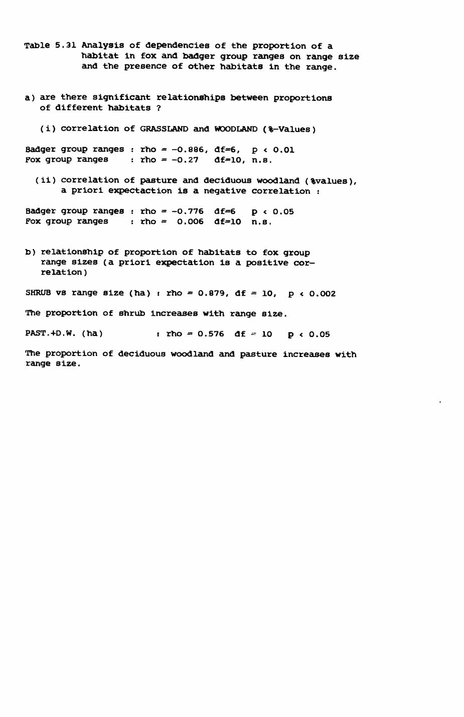
Table 5.31 Analysis of dependencies of the proportion of ahabitat in fox and badger group ranges on range size and the presence of other habitats in the range.
a) are there significant relationships between proportions of different habitats ?
(i) correlation of GRASSLAND and WOODLAND (%-Values)
Badger group ranges : rho = -0.886, df=6, p < O.Ol Pox group ranges : rho = -O.27 df=10, n.s.
(ii) correlation of pasture and deciduous woodland (%values), a priori expectaction is a negative correlation t
Badger group ranges j rho = -O.776 df=6 p < O.05 Pox group ranges t rho = O.OO6 df=lO n.s.
b) relationship of proportion of habitats to fox group range sizes (a priori expectation is a positive cor relation )
SHRUB vs range size (ha) t rho = 0.879, df = 10, p < O.O02
The proportion of shrub increases with range size.
PAST.+D.W. (ha) i rho = 0.576 df - 10 p < 0.05
The proportion of deciduous woodland and pasture increases with range size.

Pig. 5.36-5.37
Area and proportion of habitats in relation to (5.36) badger and (5.37) fox
group ranges
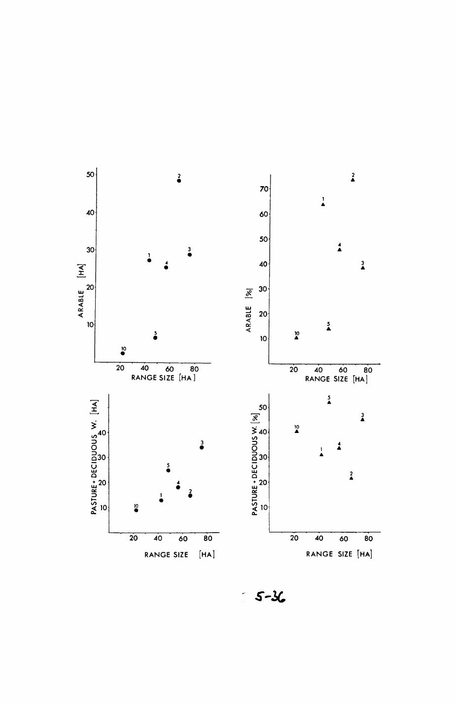
AR
AB
LEKJ
O
[HA
]C*
> O
o1IM
OIU
KC
' L/C
V-I
U'L
IWW
O
TT
.
II1
MI
_
KJ
t*>
*»
•0
0
0
0
K>
O
77 I
°m M
0;
m
O
* _~
"*
?
00>
O
KJ O
•5
> Z
*•>
0°
rn
• •-
" M
^
m O
• *•
-^
_ •>
. •
M
^0
0 o• u
•o
.^
• *
.
• K
>
• "
KJ
O
70
> I °
-
3:
M
O 00 o
PAST
UR
E +
DE
CID
UO
US
W.
[%]
_(O
W^
J0«
ooooo
KJ
O
70 Z g M
m >
ARAB
LE
\%\
-.K
iC
.J
ooo
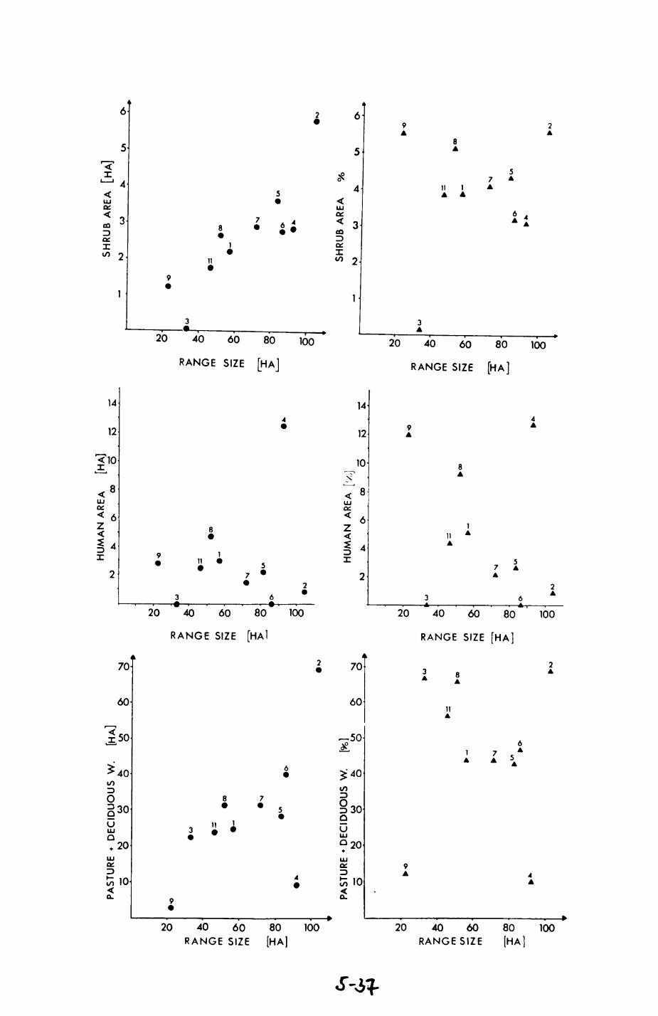
PAST
UR
E *
DE
CID
UO
US
W
. [H
A]
oK
J C
J ik
. U
> O
o
o
p
p
o
K> .
O
zSl
O
m
oo
O
• •0
•o
PAST
URE
» D
ECID
UO
US
W.
[%}
O~""
o
o
o
o
^r _
__
_ _ _
_ *_
____
____
i___
____
__i_
m
oo 8
>•=
KJH
UM
AN
AR
EA
[H
A]
tk.
O
00
O(O
10 o
0
m M
8m >
§ 8
• o
• oo
HU
MA
N
AREA
[<
/u]10
^
O
00
O
KJ
KJ
O
!•«-»
§ S
S 8 oo
o O
O
I >»
to
o
2
oM
o
m 5
oo
>
o to
oTO I
°m M
g
m
°
>
§ 8
SH
RU
B A
RE
A
[HA
]K
> C
J £k
• •
0
• NI
•M
SHR
UB
AREA
%
M
CO
.U
O»
*•«
213
occupies a relative constant proportion,
5.6.4. Habitat composition of individual ranges within the same
group.
The results presented so far constitute mean values per group range.
Consideration of individual ranges within broadly the same framework should
Indicate to what extent group range composition mirrors individual choice.
While the distinction between members of badger groups is not tidy (Table
5.32), and the ranges of individual badgers sometimes do and sometimes do
not show a similar composition, it is clear that there are large differences
in fox groups. These differences may be partly an artefact of sample size
(well tracked females vs. little tracked males in Ranges P6 and P7). The
results from the HOMEFARM group show, however, some consistent, intersexual
differences in habitat composition of ranges. Reasons for sex-specific
differences will be discussed in Chapter 6.
5.6.5. Habitat composition and resource use of group ranges.
Group ranges of foxes and badgers are easily, and reliably
distinguished by their habitat composition. The Stepwise Discriminant
Function Analysis (SDFA) whose results are reported in Table 5.34, indicates
that the proportion of P+DW and HUMAN are the key habitats that suffice to
distinguish the species. Foxes have on average a much higher proportion of
human habitation than badgers while their proportion of P+CTf is similar)
here again foxes occupy more P+DW. This apparent contradiction with the
finding that the badgers, not the foxes specialize in earthworms, can easily
be resolved, if Individual ranges are consideredt badger group ranges
contain large areas of wheat fields that are underrepresented In use by
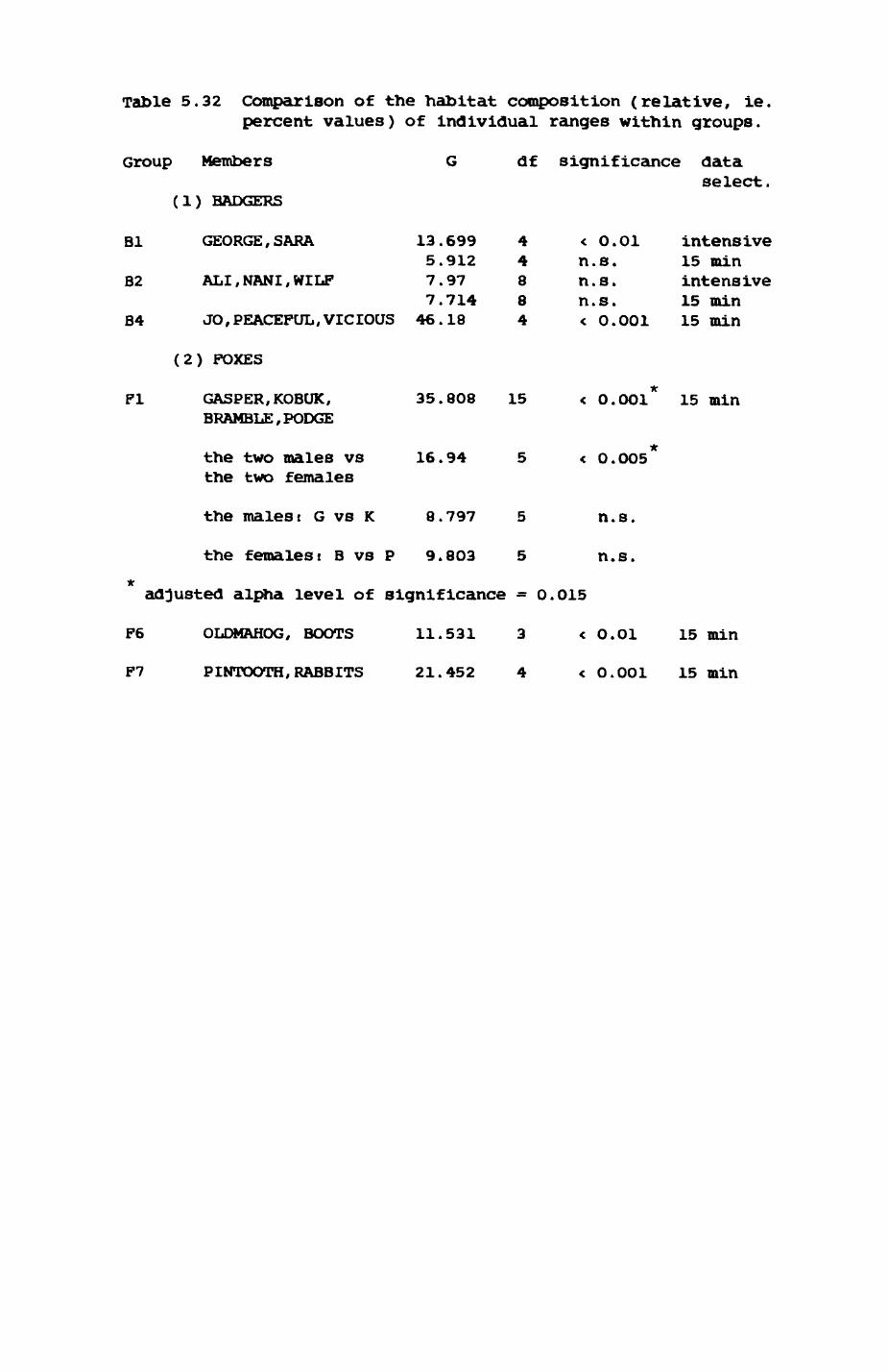
Table 5.32 Comparison of the habitat composition (relative, ie. percent values) of individual ranges within groups.
Group Members
(1) BADGERS
Bl
82
B4
GEORGE, SARA
ALI,NANI,WILF
JO, PEACEFUL, VICIOUS
13.6995.9127.977.71446.18
44884
< O.01n.s.n.s.n.s.< 0.001
df significance dataselect.
intensive 15 min intensive 15 min 15 min
(2) FOXES
Fl GASPER,KOBUK, 35.808 BRAMBLE,PODGE
the two males vs 16.94 the two females
15 < o.OOl 15 min
< O.OO5
the malest G vs K 8.797 n.s.
the females! B vs P 9.8O3
adjusted alpha level of significance = O.O15
n.s.
F6 OLDMAHOG, BOOTS 11.531 < 0.01 15 min
F7 PINTOOTH,RABBITS 21.452 < O.OOl 15 min
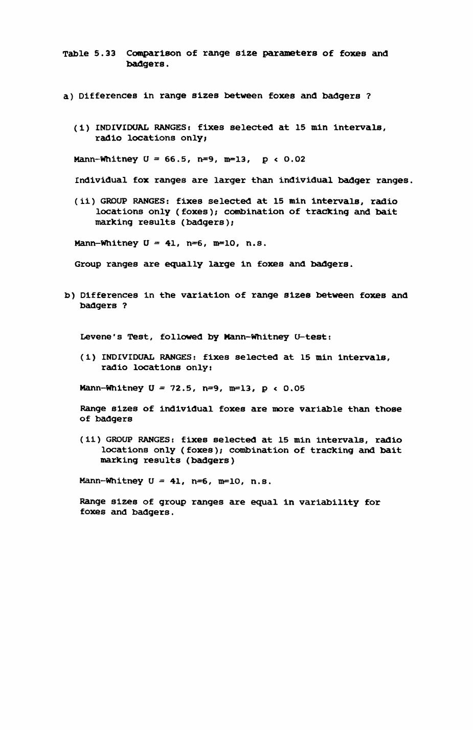
Table 5.33 Comparison of range size parameters of foxes and badgers.
a) Differences in range sizes between foxes and badgers ?
(1) INDIVIDUAL RANGES: fixes selected at 15 min intervals, radio locations only;
Mann-Whitney U = 66.5, n=9, m=13, p < 0.02
Individual fox ranges are larger than individual badger ranges.
(ii) GROUP RANGES: fixes selected at 15 min intervals, radio locations only (foxes); combination of tracking and bait marking results (badgers);
Mann-Whitney U = 41, n=6, m=lO, n.s.
Group ranges are equally large in foxes and badgers.
b) Differences in the variation of range sizes between foxes and badgers ?
Levene's Test, followed by Mann-Whitney u-test:
(i) INDIVIDUAL RANGES: fixes selected at 15 min intervals, radio locations only:
Mann-Whitney U = 72.5, n=9, m=13, p < O.O5
Range sizes of individual foxes are more variable than those of badgers
(ii) GROUP RANGES: fixes selected at 15 min intervals, radio locations only (foxes); combination of tracking and bait marking results (badgers)
Mann-Whitney u - 41, n=6, m=lO, n.s.
Range sizes of group ranges are equal in variability for foxes and badgers.
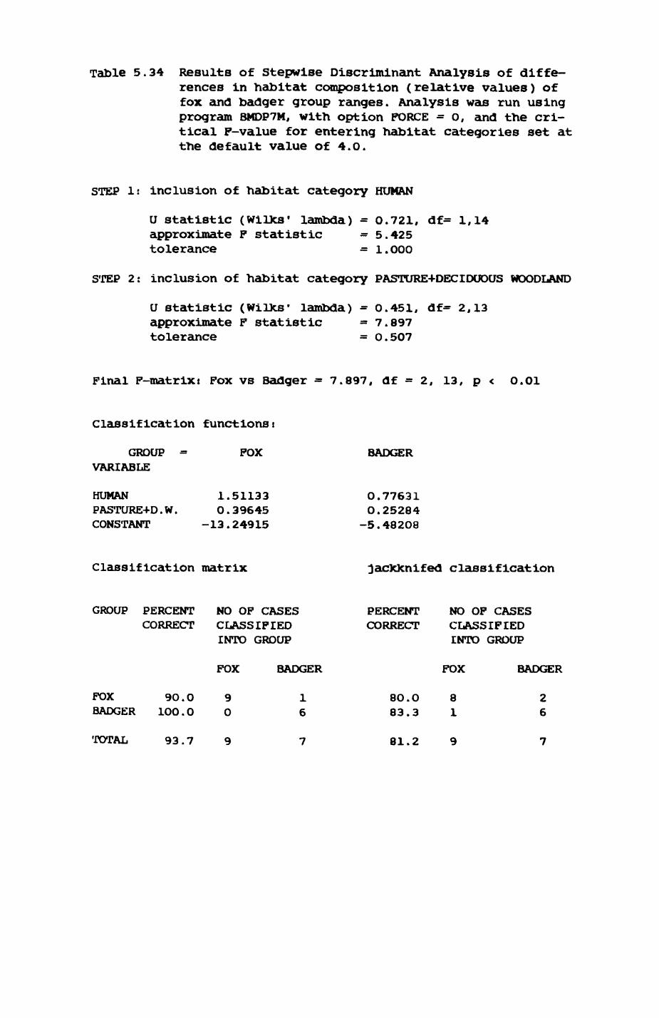
Table 5.34 Results of Stepwise Discriminant Analysis of diffe rences in habitat composition (relative values) of fox and badger group ranges. Analysis was run using program BMDP7M, with option FORCE = 0, and the cri tical F-value for entering habitat categories set at the default value of 4.0.
STEP Is inclusion of habitat category HUMAN
U statistic (WiUcs' lambda) = 0.721, df= 1,14 approximate F statistic = 5.425 tolerance = l.OOO
STEP 2: inclusion of habitat category PASTURE+DECIDUOUS WOODLAND
a statistic (WilXs f lambda) = 0.451, df= 2,13 approximate F statistic = 7.897 tolerance = O.507
Final F-matrixt Fox vs Badger - 7.897, df = 2, 13, p < O.01
Classification functions!
GROUP VARIABLE
FOX BADGER
HUMANPASTURE-HD.W.CONSTANT
1.511330.3964513.24915
0.77631O.25284-5.48208
Classification matrix jacklcnifed classification
GROUP PERCENT NO OF CASES CORRECT CLASSIFIED
INTO GROUP
PERCENT CORRECT
NO OF CASES CLASSIFIED INTO GROUP
FOX BADGER
FOX 90.0 9 1BADGER 1OO.O 0 6
8O.O 83.3
FOX
81
BADGER
26
TOTAL 93.7 81.2
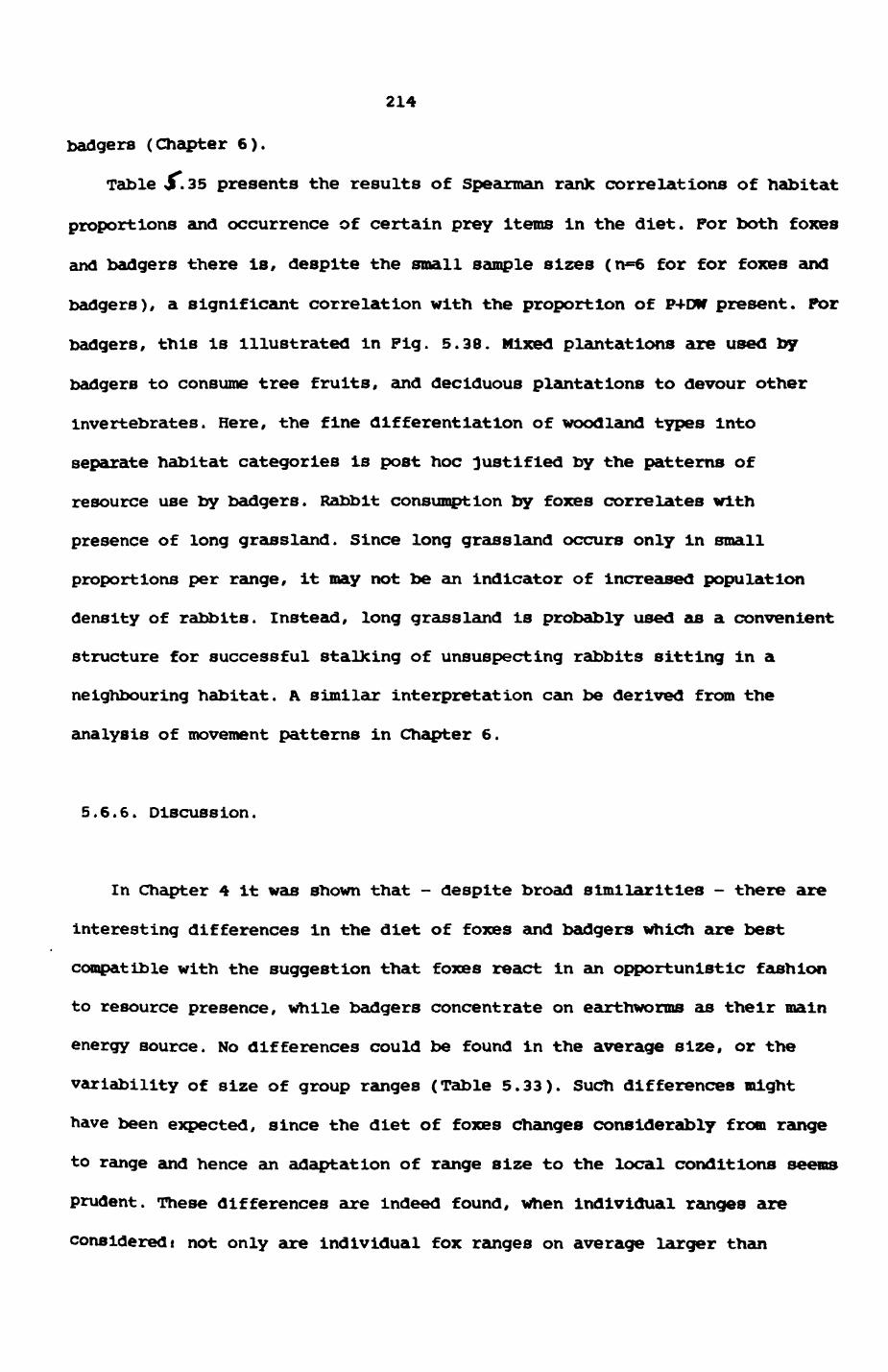
214
badgers (Chapter 6).
Table J.35 presents the results of Spearman rank correlations of habitat
proportions and occurrence of certain prey items in the diet. For both foxes
and badgers there is, despite the small sample sizes (tv=6 for for foxes and
badgers), a significant correlation with the proportion of P+DW present. For
badgers, this is illustrated in Fig. 5.38. Mixed plantations are used by
badgers to consume tree fruits, and deciduous plantations to devour other
Invertebrates. Here, the fine differentiation of woodland types into
separate habitat categories is post hoc justified by the patterns of
resource use by badgers. Rabbit consumption by foxes correlates with
presence of long grassland. Since long grassland occurs only in small
proportions per range, it may not be an indicator of increased population
density of rabbits. Instead, long grassland is probably used as a convenient
structure for successful stalking of unsuspecting rabbits sitting in a
neighbouring habitat. A similar interpretation can be derived from the
analysis of movement patterns in Chapter 6.
5.6.6. Discussion.
In Chapter 4 it was shown that - despite broad similarities - there are
interesting differences in the diet of foxes and badgers which are best
compatible with the suggestion that foxes react in an opportunistic fashion
to resource presence, while badgers concentrate on earthworms as their main
energy source. No differences could be found in the average size, or the
variability of size of group ranges (Table 5.33). Such differences might
have been expected, since the diet of foxes changes considerably from range
to range and hence an adaptation of range size to the local conditions seems
prudent. These differences are Indeed found, when individual ranges are
considered t not only are individual fox ranges on average larger than
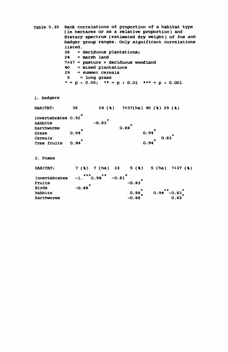
Table 5.35 Rank correlations of proportion of a habitat type (in hectares or as a relative proportion) and dietary spectrum (estimated dry weight) of fox and badger group ranges. Only significant correlations listed.38 = deciduous plantations; 24 = marsh land7+37 = pasture 4- deciduous woodland 4O = mixed plantations 29 - summer cereals 5 = long grass
* = p < O.O5; ** = p < O.O1 *** = p < O.OO1
1. Badgers
HABITAT: 38 24 (%) 7+37(ha) 4O (%) 29 (%)
* Invertebrates O.92 ^Kabbits -0.83 ^Earthworms # 0.88 ^Grass O.94 O.94Cereals ^ ^ O.83Tree fruits 0.94 0.94
2. Foxes
HABITAT! 7 (%) 7 (ha) 23 5 (%) 5 (ha) 7+37 (%)
*** ** *Invertebrates -1. O.94 -O.81 #Fruits ^ -O.83Birds -O.88 # ** *Rabbits °- 88 * °- 94 ~°* 83 *Earthworms -O.88 0.83
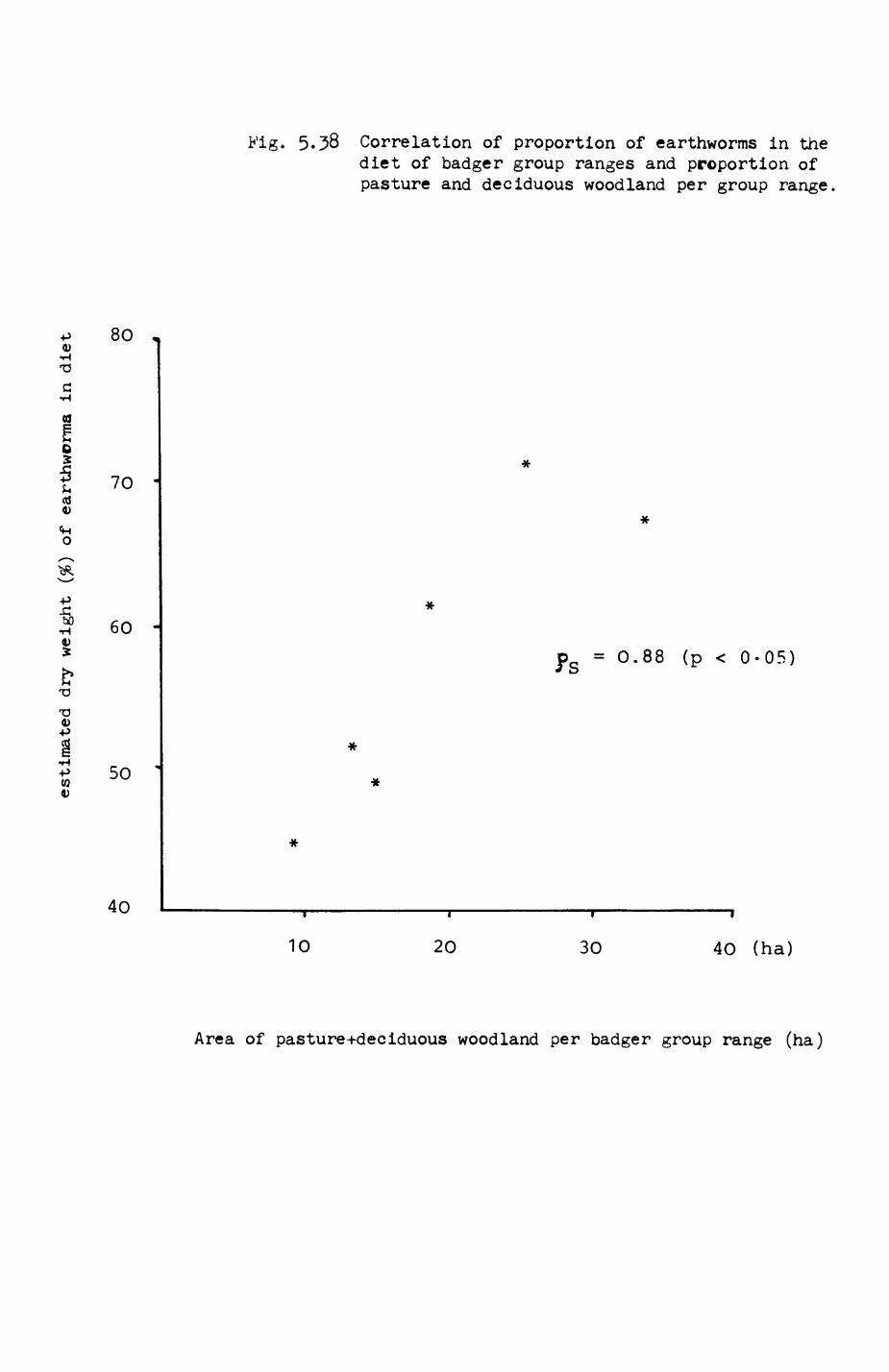
5O8 Correlation of proportion of earthworms in the diet of badger group ranges and proportion of pasture and deciduous woodland per group range.
•H TD
fi•H
00
oI<Ho
-•aI
TD
4)-P
-PCO
80
70 •
60 -
50
40
= 0.88 (p < 0-05)
10 20 30 40 (ha)
Area of pasture-i-deciduous woodland per badger group range (ha)
215
individual badger ranges (Table 5.33), but size also varies to a greater
extent. This is due to the fact that the ranges actually utilized by an
individual badger may constitute only a proportion of the total range
(Chapter 6). One possible interpretation of this difference between range
sizes of individuals and groups In badgers may be a 'fall-safe' mechanism
for most of the time only a fraction of the group range is required to feed
a badger. However, under bad conditions, additional areas may be required to
satisfy the range inhabitants. Therefore, group ranges should contain a
safety margin and hence be larger than Individual ranges. Then range
maintenance will also be cheaper and more efficient than with large changes
- modest changes of range boundaries are more efficient and less likely to
lead to escalated conflicts between neighbours (Section 5.4).
The investigation of habitat composition in relation to resource use and
range configuration permits to draw some conclusions about 'Key' habitats.
Pasture and deciduous woodland together are essential habitats for badgers.
Further evidence for this is presented in the analysis of movements in
Chapter 6. Range configuration can, in some cases at least, be explained as
a result of the dispersion of pasture areas (Fig 5.3O-33). These are results
entirely compatible with the resource dispersion hypothesis, which predicts
that range size should be determined by the dispersion of food patches. In
Chapter 7, I shall discuss this problem again and conclude that RDH is
certainly consistent with the resource setup in wytham, while an additional
factor, defense of resources, is likely to play a decisive role in the
formation of groups.
Due to their more varied feeding habits, foxes present a more
complicated picture. Human housing constitutes one Key habitat, since the
dispersion of human housing influences the delineation of range boundaries.
Pasture + Deciduous Woodland form a second key resource unit evidenced by
their constant representation In the group ranges. A third group of

216
important habitats is summarized by SHRUB; these are small, but very diverse
habitats (bracken, hedges, scrubs with grass layers) Known to harbour a
large variety of interesting prey items.
217
6. Patterns of range utilization
6.1. Methods
6.2. Patterns of space use
6.2.1. One week with PODGE in the breeding season
6.2.2. Range use by OLDMAHOG
6.2.3. Range use by other foxes
6.2.4. Range use within the HOMEFARM fox group
6.2.5. Range use by badgers
6.2.6. Direction preferences In local movements
6.2.7. Conclusions
6.3. Simultaneous movements within the UPPER FOLLIES badger
group
6.3.1. Coordination of movements
6.3.2. Renewal periods and Interference pressure
6.4. Habitat utilization
6.4.1. Habitat preferences
6.4.2. Habitat characteristics and resource levels in
visited cells
6.4.3. intensity of use in relation to resource density
6.4.4. Patterns of visits to different habitats
218
6. Patterns of range utilization
In the previous chapter I looked at the spatial configuration and the
size of badger and fox home ranges and correlated them with the presence of
habitats and resources. These analyses provide preliminary insights of the
importance of certain areas to the animals. To gain a deeper understanding
of these results we have to explore in detail the utilization of the
animals' ranges. In this chapter I first look at the picture of range usage
that emerges from the accumulation of many nights' data. I shall then
investigate what kind of movement patterns in a given night are responsible
for the overall picture of range utilization.
6.1. Methods
Data from radio tracking were used to analyse movement patterns. For
foxes, complete nights of intensive tracking were available only for a
minority of individuals. Therefore the number of locations ('fixes') per
area unit was used as a measure of the Intensity of use of the area. Fixes
were selected by program ICELLH according to the 15 minutes Independence
Interval criterion (Chapter 5, Appendix 4), and summed over each area unit.
For some foxes, and most of the badgers, two measures of the intensity of
use were derived from nights of intensive radio tracking: (i) number of
visits (NOV) and (ii) duration of stay (DOS) per area unit. For complete
nights of radio-tracking, program TRANSIT (adapted from Doncaster (1985))
calculated arrival and departure times for each area unit, by splitting the
elapsed time between two successive locations in different areas and
assigning half to each area. The error of this approximation is likely to
be small, since - due to the intensive tracking efforts - locations were
219
ly nore than 5 minutes apart. Therefore, the maximum possible error,
the difference between the actual and calculated time of 'crossing the
border', was reduced to 2-3 minutes which turns out to be unimportant in the
context of this analysis. Program CELT IM used the calculated arrival and
departure times and compiled the number of visits and the total duration of
stay (in hours) per area unit. Output from program CELTIM was then used for
a variety of analyses described below.
Two Kinds of area units were used: (i) 'Natura' patches delineated on
the habitat map and (ii) a systematic 50 by 5O metre quadratic grid which
eliminated effects due to varying sizes of habitat patches (see 6.4. ).
Where analyses relied heavily on actual departure times and time intervals
between successive visits to the same cell, cell size was varied (25, 5O and
100 m) to explore the effects of choice of cell size on the patterns of use.
Scaling of space use, patterns of space use and the effects of the
spatial location of a site on its intensity of use by an animal ( 'spatial
dependence') were investigated by spatial autocorrelation functions.
Appendices 5, 6 and 7 describe the problem of spatial dependence and
solutions to it, explain the parameters important for the investigation of
scaling in space, introduce two measures of spatial autocorrelation (Koran's
I and Geary's c), and finally explain how to interpret spatial cor re log rams
and spatial models and the results of fitting models to the data.
Computation of spatial autocorrelations were performed by program AUTCOR
using the algorithms listed in Appendix 7. For foxes, the number of fixes
per 50 m cell, selected according to the 15 min independence interval
criterion, was employed as a measure of the intensity of use. For badgers,
I used the measures derived from records of intensive radio- tracking as
described above.
Possible interference between the movements of group members was
investigated for one badger group, the UPPER FOLLIES range B2. Here, I was
220
reasonably certain that all group members had been tagged (Chapter 5).
Locations of all three tagged animals, the females ALI and NAN I and the male
WILF, were recorded simultaneously. This was possible since all individuals
spent almost all of their time in one small valley. I recorded simultaneous
locations at fixed intervals of 15 minutes from the beginning to the end of
the night for a period of seven consecutive nights in October 1983. In the
middle of October, foraging activities are expected to soar since badgers
have to accumulate reserves for the inactive periods in winter and for
lactation in spring. Therefore I assumed that the majority of movements
Involved foraging. Activity at the sett mainly involves cleaning nest
chambers and decorating them with fresh hay and leaves, and was consequently
excluded from the analysis as were periods of rest or Inactivity. Programs
were written to process the data through the following stages of analysist
(1) Program PRAEP associated each location with the appropriate cell
number, depending on the chosen size (25, 50 or 1OO m).
(2) Program HAUPT computed distances between pairs of animals at successive
locations and compiled times of visits and identity of visitor for each
cell.
(3) Program ZAEHL identified whether given pairs of animals moved closer or
further to each other between successive locations, and compiled a summary
for all three possible pairs (ALI-NANI, NANI-WILF, ALI-WILF). Distance
changes were tested for random arrangement with the runs test for trends
(Sofcal & Ronif (1981)) by considering increases (withdrawals) and decreases
(approaches) in distance and excluding instances when separations did not
change (= 12% of all cases).
(4) Program VISIT calculated (i) the number of visits by each individual to
each cell, (ii) the total number of visits by all three badgers to each
cell, (ill) the mean duration of visit of each individual per cell, and (iv>
the average revisit interval of each individual per cell. Several
221
successive locations of an Individual In the same cell were treated as one
visit.
(5) Program ZELLE3 used the output of programs HAUPT and VISIT to calculate
single and average revisit intervals (renewal periods) per cell by pooling
the movements of all three Individuals. Renewal periods were computed
separately for (a) cases In which a cell was visited twice In succession by
the same individual, and (b) cases in which successive visitors were
'different individuals. Revisit intervals were calculated as 'mean'
estimates. For each location, the individual was assumed to start its visit
at the time of talcing the fix and finish the visit just before the next
location. For example, an individual located in cell A at 21.OO hours, in
cell B at 21.15 and in cell A again at 21.3O would be accorded a revisit
Interval of 15 minutes. However, reality could substantially vary around
this estimate i the animal might have left cell A at 21.14, arrived at cell B
at 21.15 and re-entered cell A at 21.16 yielding the minimum revisit
Interval of 2 minutes, or it could have left cell A at 21.01, stayed in cell
B until 21.29 to return to cell A at 21.30, yielding the maximum revisit
Interval of 28 minutes. Given a sufficient sample size, the 'true' revisit
intervals would be expected to be normally distributed between the two
possible extremes.
The analysis of habitat preferences was based on 50 m grid cells. The
habitat composition of grid cells was identified by applying the same
procedure as described in Chapter 2 and 5 and Appendix 3. An estimate of
habitat diversity per grid cell was taken simply as the number of different
habitats represented in a cell (program TRACKHAB). Earthworm biomass per
cell was estimated by multiplying the proportion that each habitat occupied
in a cell with a factor as listed in Table 6.1 (program TCHANGE). Those
cells within the aea of habitat recording (Chapter 2) were also tagged with
the scores of the first four axes of the detrended correspondence analysis
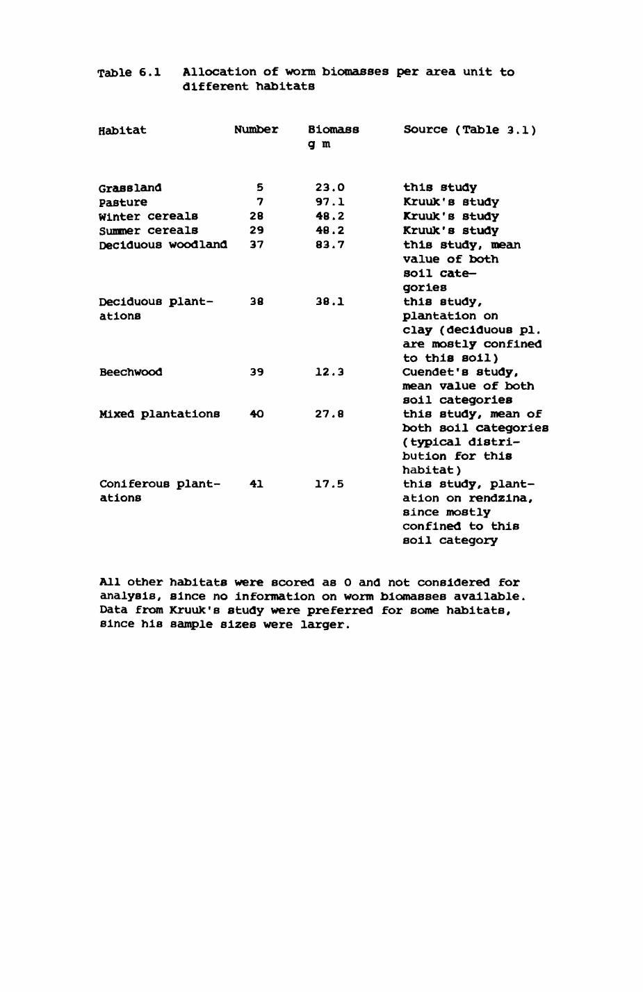
Table 6.1 Allocation of worm biomasses per area unit to different habitats
Habitat Number Biomass g m
Source (Table 3.1)
Grassland PastureWinter cereals Summer cereals Deciduous woodland
57
282937
Deciduous plant ations
38
Beechwood
Mixed plantations
39
40
Coniferous plant ations
41
23.097.148.248.283.7
38.1
12.3
27.8
17.5
this study KruuX's study Kruuk's study KruuX's study this study, mean value of both soil cate gories this study, plantation on clay (deciduous pi. are mostly confined to this soil) Cuendet's study, mean value of both soil categories this study, mean of both soil categories (typical distri bution for this habitat)this study, plant ation on rendzina, since mostly confined to this soil category
All other habitats were scored as 0 and not considered for analysis, since no Information on worm blomasses available. Data from KruuK's study were preferred for some habitats, since his sample sizes were larger.
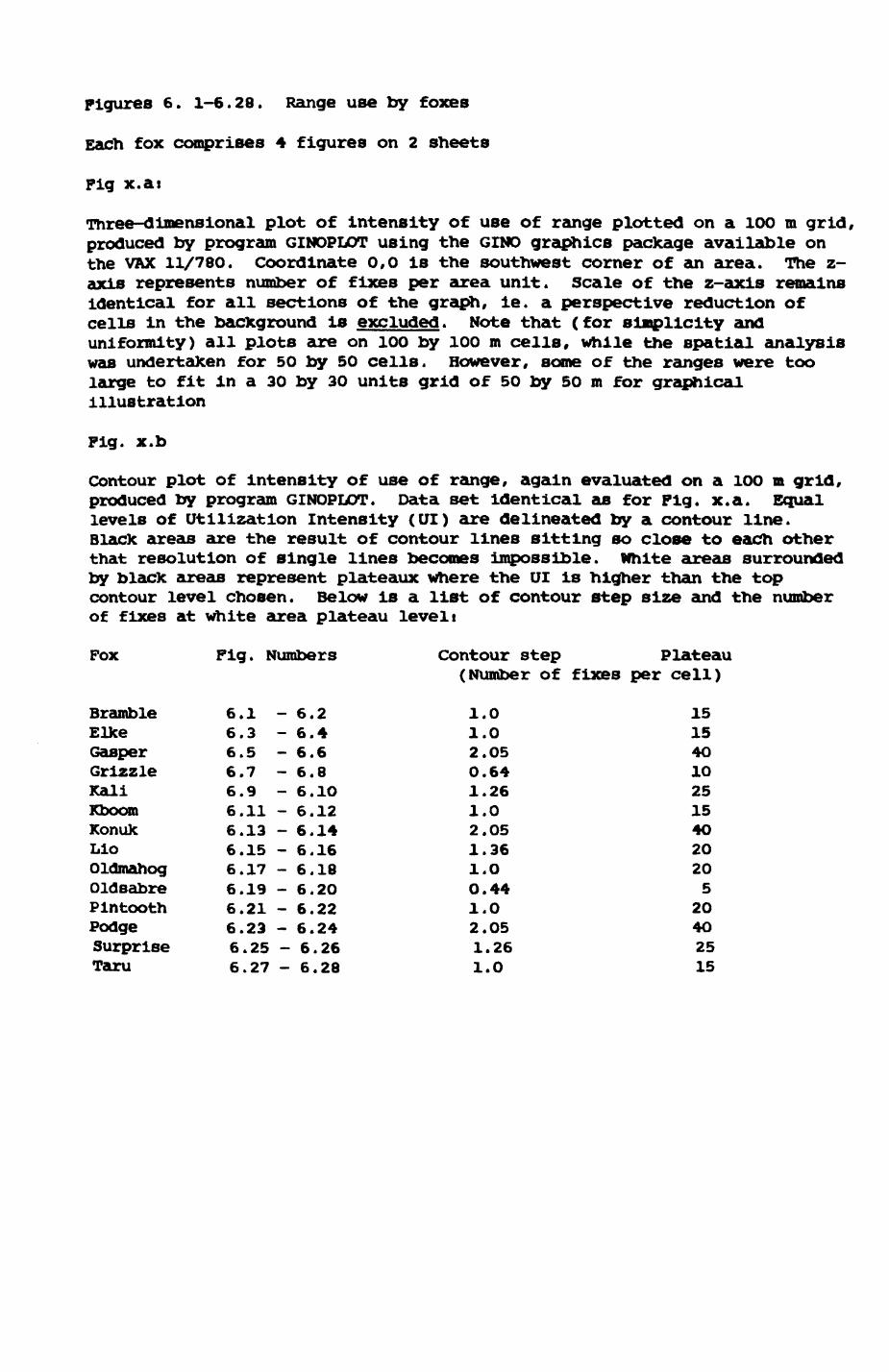
Figures 6. 1-6.28. Range use by foxes
Each fox comprises 4 figures on 2 sheets
Fig x.at
Three-dimensional plot of intensity of use of range plotted on a 10O m grid, produced by program GINOPLOT using the GINO graphics package available on the VAX 11/780. Coordinate 0,0 is the southwest corner of an area. The z- axis represents number of fixes per area unit. Scale of the z-axls remains Identical for all sections of the graph, ie. a perspective reduction of cells in the background is excluded. Note that (for simplicity and uniformity) all plots are on 10O by 100 m cells. While the spatial analysis was undertaken for 50 by 50 cells. However, some of the ranges were too large to fit in a 30 by 30 units grid of 50 by 50 m for graphical illustration
Fig. x.b
Contour plot of Intensity of use of range, again evaluated on a 1OO m grid, produced by program GINOPLOT. Data set identical as for Pig. x.a. Equal levels of Utilization Intensity (UI) are delineated by a contour line. Black areas are the result of contour lines sitting so close to each other that resolution of single lines becomes impossible. White areas surrounded by black areas represent plateaux where the UI is higher than the top contour level chosen. Below is a list of contour step size and the number of fixes at white area plateau leveli
Fox
BrambleElkeGasperGrizzleKaliKboomKonukLloOldmahogOldsabrePintoothPodgeSurpriseTaru
Fig. Numbers Contour step Plateau (Number of fixes per cell)
6.16.36.56.76.96.116.136.156.176.196.216.236.256.27
- 6.2- 6.4- 6.6- 6.8- 6.1O- 6.12- 6.14- 6.16-6.18-6.20-6.22- 6.24- 6.26-6.28
1, 1
00
2.05 0.64 1.26 1.0 2.05 1.36 1.0 O.44 1.0 2.05 1.26 1.0
15 15 40 10 25 15 4O 20 20 5
20402515
Figures 6. 1-6.28 (Cont. )
Pig. x+l.a:
Results of fitting the spatial models 1 to 5 (see 6.2.2. and Appendices 5-7) to UI data. The weighing function along the x-axis represents the number of the model; the higher the number, the more weight is attached to pairs of cells at a large distance. The y-axis represents the results, plotted as spatial autocorrelation coefficients (SACs), Koran's I and Geary's c. Plotting symbols for the SAC are
SAC
Moran's I Geary's c
Pig. x+l.bi
SAC significantly different from expected mean (null hypothesis rejected)
filled circles filled squares
SAC corresponding to expected mean value (null hypothesis confirmed)
starszeros with a dot
Spatial correlograms of UI data, using Koran's I as SAC. For a detailedexplanation, see text or Appendix 5.Pilled circles! SAC significantly different from the expected mean (nullhypothesis rejected)Starsi SAC cannot be distinguished from the expected mean (null hypothesisconfirmed)
All "significant" results refer to a probability of O.05
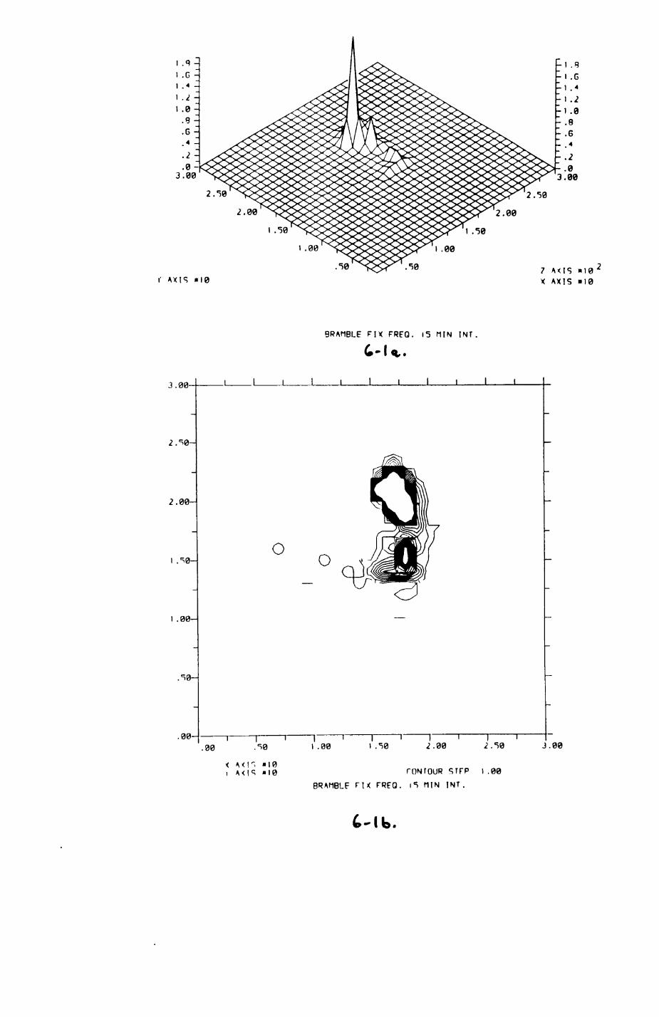
Jl ?IS
IS
Jl ISCO
IS
Nj Jl
is <s
IS <s Jl ISes
s
\ r
CO
XI CD •n JO J, =
2 5
IS
IS J\ IS IS
IS
IS
ISJl CO
o o
IS <s
i w ft
CD •n x -n ui z
z
X
.«.
LO
,/)
en c
oIS
CO
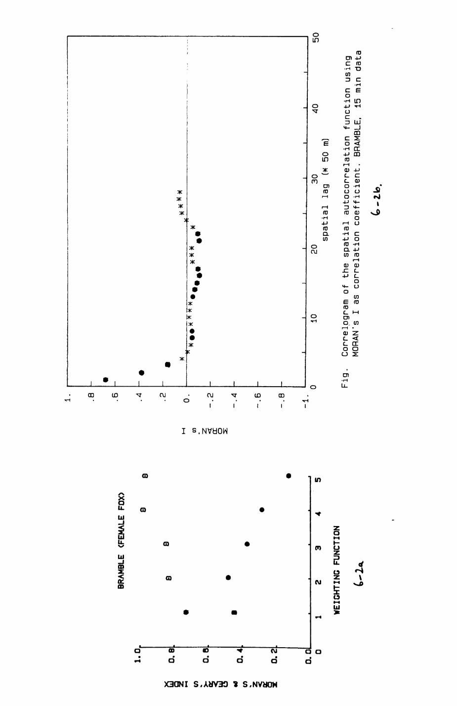
1 . .8 .6
BRAM
BLE
(FEM
ALE
FOX)
1.0
|
°-8
</> £
0. B
-
0.4
z 1
0.2
0.0
0
r •
•0
• - 2
•
0.
en <
-.2
O
. •
*
-.4
•
-'
6
-.8
•
-1.
——
——
— • —
——
——
• ——
——
— • —
——
——
• ——
——
— •
C 1
2345
L- - -*
X
*****
*x»
«**
**«
M^xxx^x
- - -
. ——
1 ——
....
. _
.J.
.!...!_
1
1 1
1 1
) 10
20
30
40
5(
WEIGHTING
FUNC
TION
Fig.
Correlpgram
of th
e spatial
auto
corr
elat
ion
function using
MORAN'
s I
as corr
elatio
n co
effi
cien
t. BRAMBLE.
15 min
data
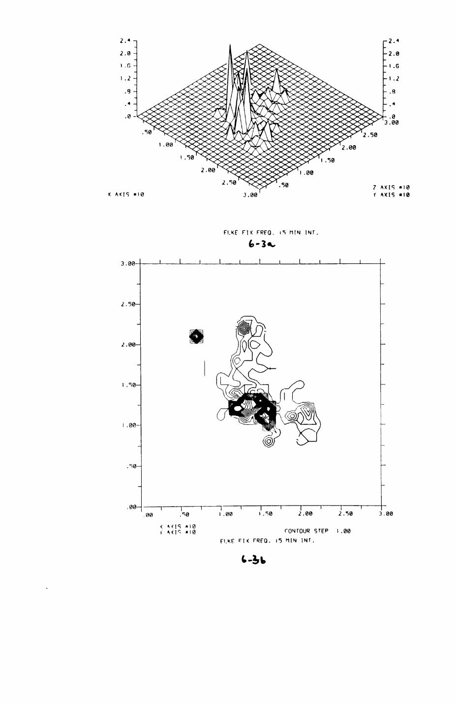
00 'C
00' I d3ib
0S,'?00'?i I
N1U £.1 '03&J Xld 3X"I3
0^' I 00' 1 I i I
0 I » b I > V .' 01* b!>V >
I I
00'
-I————— -00 '
-00' I
-00V
-0C,'?
-00-
N1WXld
ei» bixv A01* blXV L
,00'C01* blXV X05,'
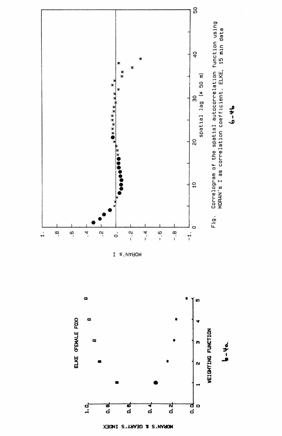
tn
1. .8 .6
ELKE
(F
EMAL
E FO
X)
1.0
0.8
0.6
0.4
0.2
0.0
0 .4
B
Q •
.2
• M
0.
en <
-.2
cr
o 2:-.
A»
-.6
-1.
——
——
——
i ——
——
——
i ——
——
——
i ——
——
——
i ——
——
——
J r- -
• **
K *********
**
**
^^•••••***^
X^
K **
x
»«
- -
J_
. ..
.. .
L.
1 1
1 1
1 i
i^
4 /"»
O
rt
rsrv
>i/
-»
r— /
1234
WEI
GH
TIN
G F
UNCT
ION
-V*.
50sp
atia
l la
g (*
50 m)
Fig.
Correlogram
of the
spatial
auto
corr
elat
ion
function using
MORAN's
I as corr
elat
ion
coef
fici
ent.
EL
KE.
15 min
data
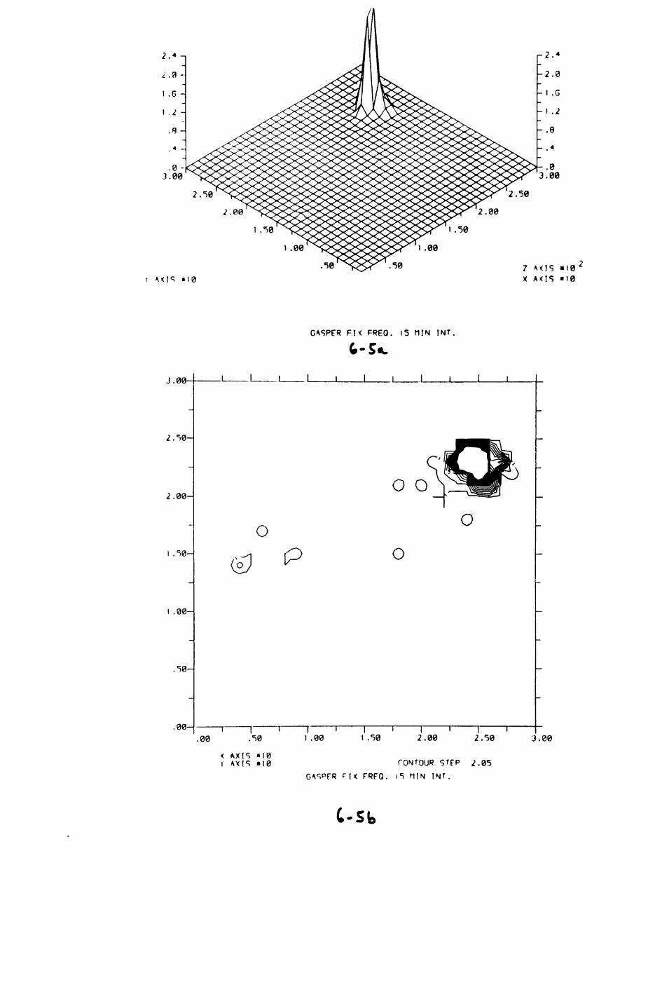
.0 -3.00
1 .00
.50
.50
00
50t MIS «I0
7 MIS «I0 X AXIS *10
GASPER FIX F-REQ. 15 MIN INT.
J.00- i I i I
2.50-
2.00-
I .50-
I .00-
.50-
.00-
o
I I ' I.00 .50 1 .00
< AXIS »I0 I AXIS «I0
o o
o
I ' I 1.50 2.00
I I 2.50
CONTOUR STEP 2.05 ri< FRFO. 15 MIN INT.
3.00
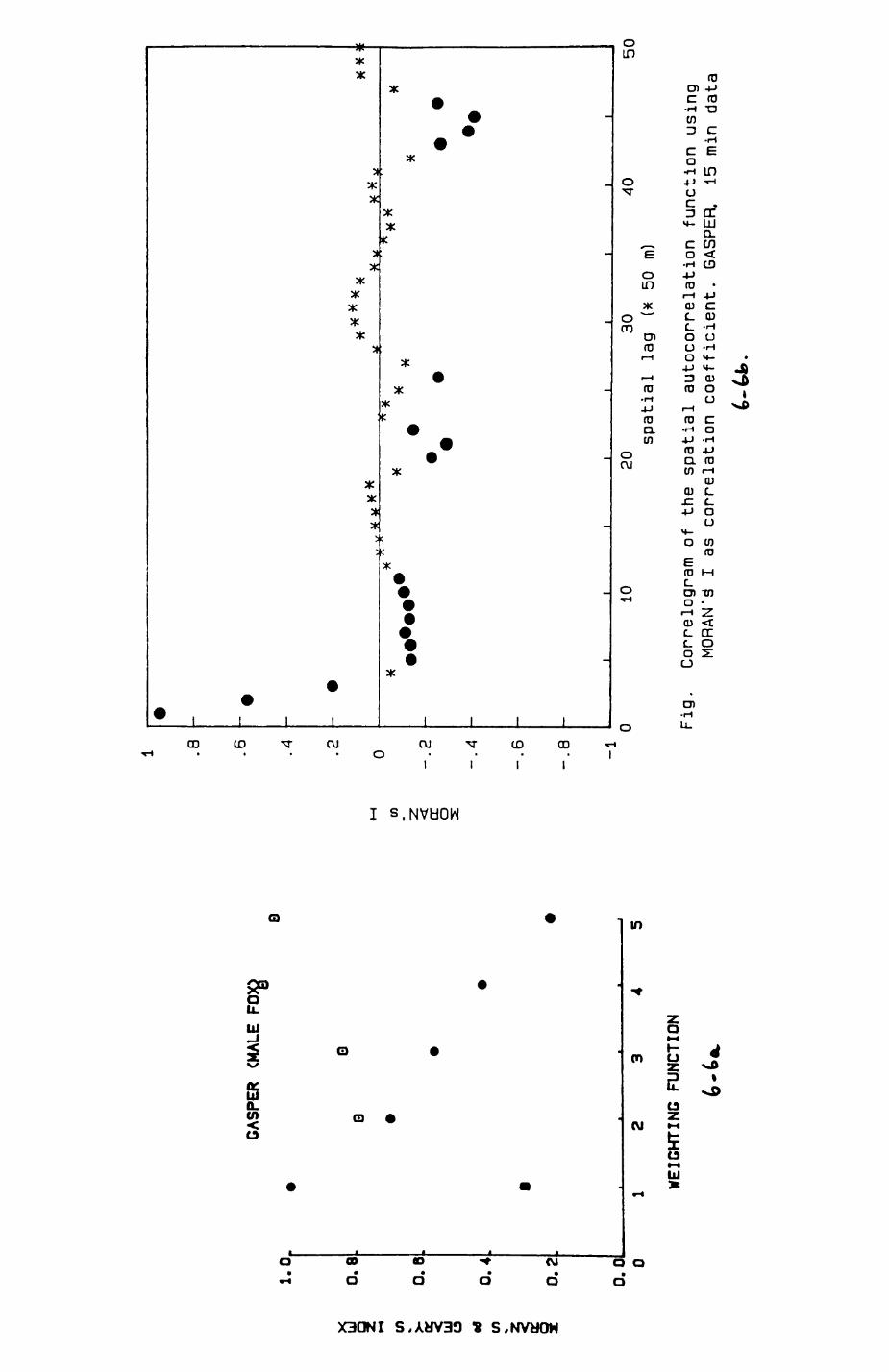
a
a. .8
1.0
0.0
0.4
0.2
0.0
0
.6
GASP
ER
(MAL
E F0
)g0
• -4
a - 2
00
•
CO z•
cr
~ o
•
-.8
/i—
——
——
, ——
——
— • —
——
——
• ——
——
— ' —
——
——
• C
12
34
5
* "•
*•
^^
^C
^^
i
x x
wx
* *
*H*
••••••*
X •
* *
x
%
•*
——
_
._
...!_
._
1
1 1
1 1
I |
i
) 10
20
30
40
5(
WEI
GH
TIN
G
FUNC
TIO
N
G-U
Fig.
Correlognam
of the
spatial
autocorrelation
func
tion
us
ing
MORA
N's1
I as co
rrel
atio
n coefficient. GA
SPER
. 15 min
data
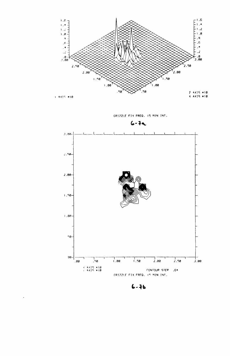
1 .00
-50
"107 AXIS «I0 X AXIS «10
CRI7ZI.F FIX FREQ. 15 HIM INT
I
2.00-
I .50-
I .00-
S0-
.00 i .00 i .50 2.00 2.50 J.00
CONTOUR
ORI77IF FIX FRFQ. is MIN INT.
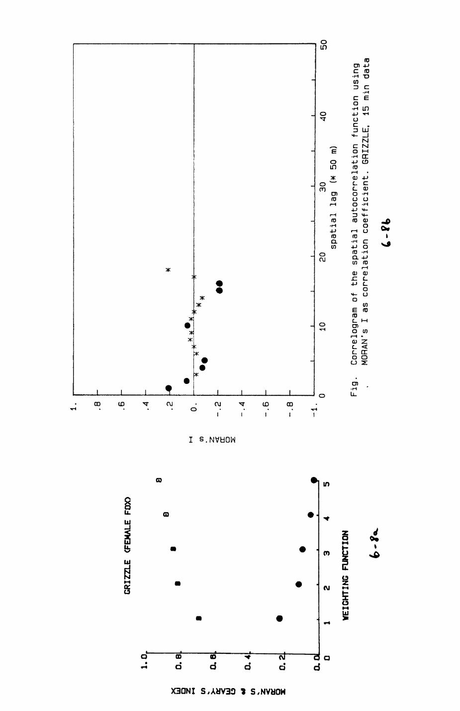
1 . .8
GR
IZZL
E
(FEM
ALE
FOX
> ' 6
1.0
&
0. 8
^j
C/) >
ae
**
0.4
en z o:
§
0.2 an
.48
• Q
' 2
• °"
1
-'2
o-.
4
~ . 6
-.8
• •
•
•
^r
"
- - - -•
^
•
X v
*^
****
x MX
*< ••—
11
1 ...!
._..
1 1
1 1
I
1020
30
40
spat
ial
lag
(* 50 m)
WEIGHTING
FUNCTION
50
Fig.
Correlogra
m of th
e spatial
autocorrelation
func
tion
using
MORAN's
I as correlation
coefficient. GR
IZZL
E,
15 mi
n da
ta
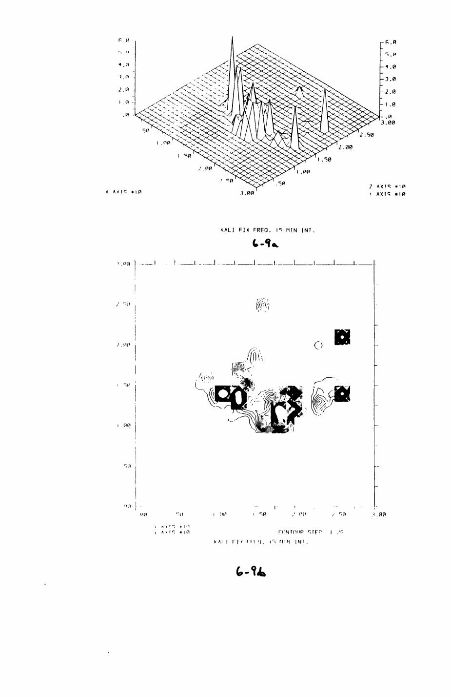
' INI NlU Li ' (i M i * 1.1 ] IV 1
-jS I dJJb dllOJNUJ
Hl.Ok) .'rfk'i
"INI NIUxid
0I« SIXV » dl« biXV Z
biXV
11' J
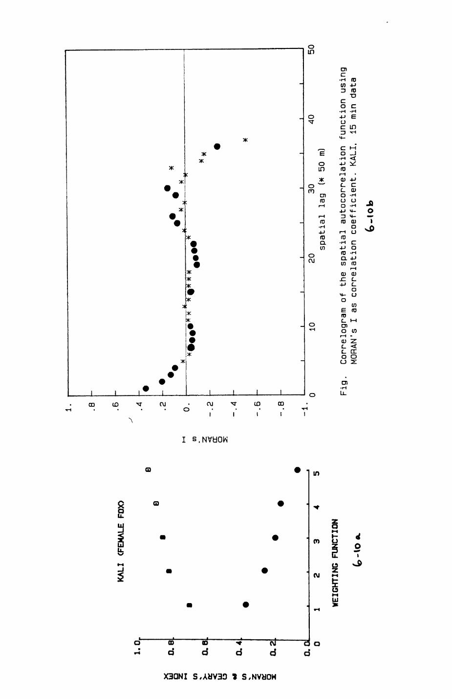
1 . .8
KA
LI
(FEM
ALE
FOX)
'6
1.0
a z (/) % >-
0. G
K UJ
O ^ °-
4U
)N z o: i
0.2 o. n 0
r .4
88
• M
o.CO • Z <
- 2
or
o
2:-.
4
-.6
^•
-.8
•
1
- - _
•
%
.
•
*•
X
*
K^
^^
A
^ X
X A
X X
X
X^
A
A^
9^^
^^
^X
^—
•-
X_ —
1 1
1 II
J 1
1 1
, P
o A
^ 0
10
20
30
40
5(A
C
O
^
3
WEIGHTING
FUNCTION
spatial
lag
(x 50
m)
Fig.
Correlogram
of th
e spatial
autocorrelation
function using
MORAN's
I as correlation
coefficient. KA
LI,
15 m
in data
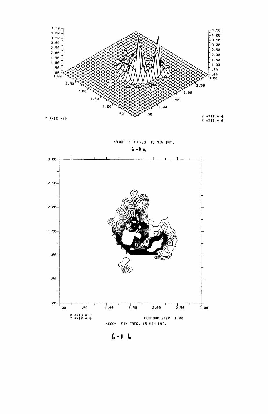
00
I .50 I .50
I .00 .00
.50 50
.00
f AXIS «I0Z AXIS X AXIS
»0 H0
KBOOn FIX FREQ. 15 NIN INT.
tt-ll*.
3.00- .1. _L
2.50-
2.00-
1 .50-
.00-
.50-
.00-
.00 .50
X AXIS "10 1 AXIS »I0
I .00 I .50 2.00 2.50 3.00
CONTOUR STEP I.00 KBOOM FIX FREO. 15 MIN INT.
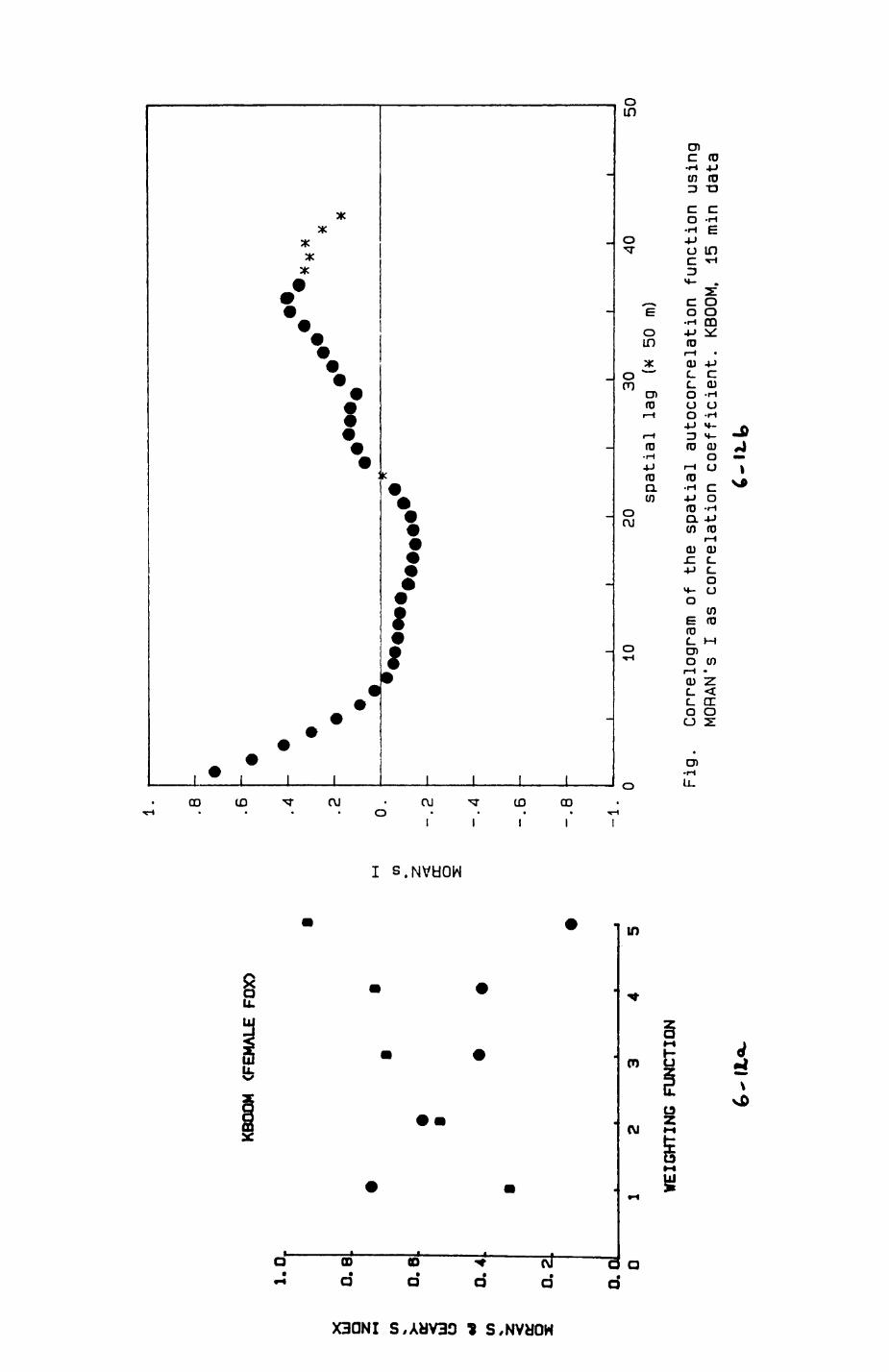
1.0
en0.6.
13
•0
0. Ol 0
KBOO
M
(FEM
ALE
FOX>
WEIGHTING
FUNC
TION
-(to
-
OJ
1. .8
.6
.4
.2
0.
-.2
~ . 6
_ ,
4
Fig
-*-
1020
30sp
atia
l la
g (* 50 m)
Corr
elog
ram
of th
e sp
atia
l autocorrelation
function using
MORAN's
I as co
rrel
atio
n co
effi
cien
t. KBOOM.
15 m
in data
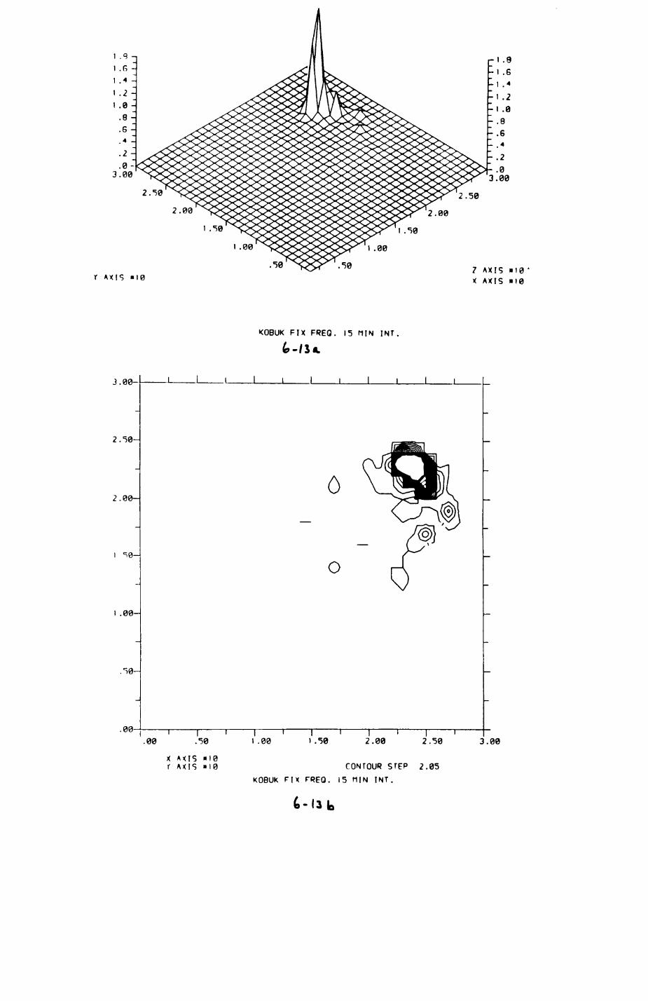
.0 -3.00
2.50
2.00
1 .50
I .00
."50
r AXIS «i07 AXIS »I0 X AXIS »I0
KOBUK FIX FREQ. 15 HIN INT.
J.00-
2.50-
2.00-
I =10-
I .00-
.50-
.00-
.1____L
6
o
.00-i——i——
.50
X AXIS «I0r AXIS »i0
i .00n——r
I .50 2.00 2.50
CONTOUR STEP 2.05 KOBUK FIX FREQ. 15 MIN INT.
3.00
6-13
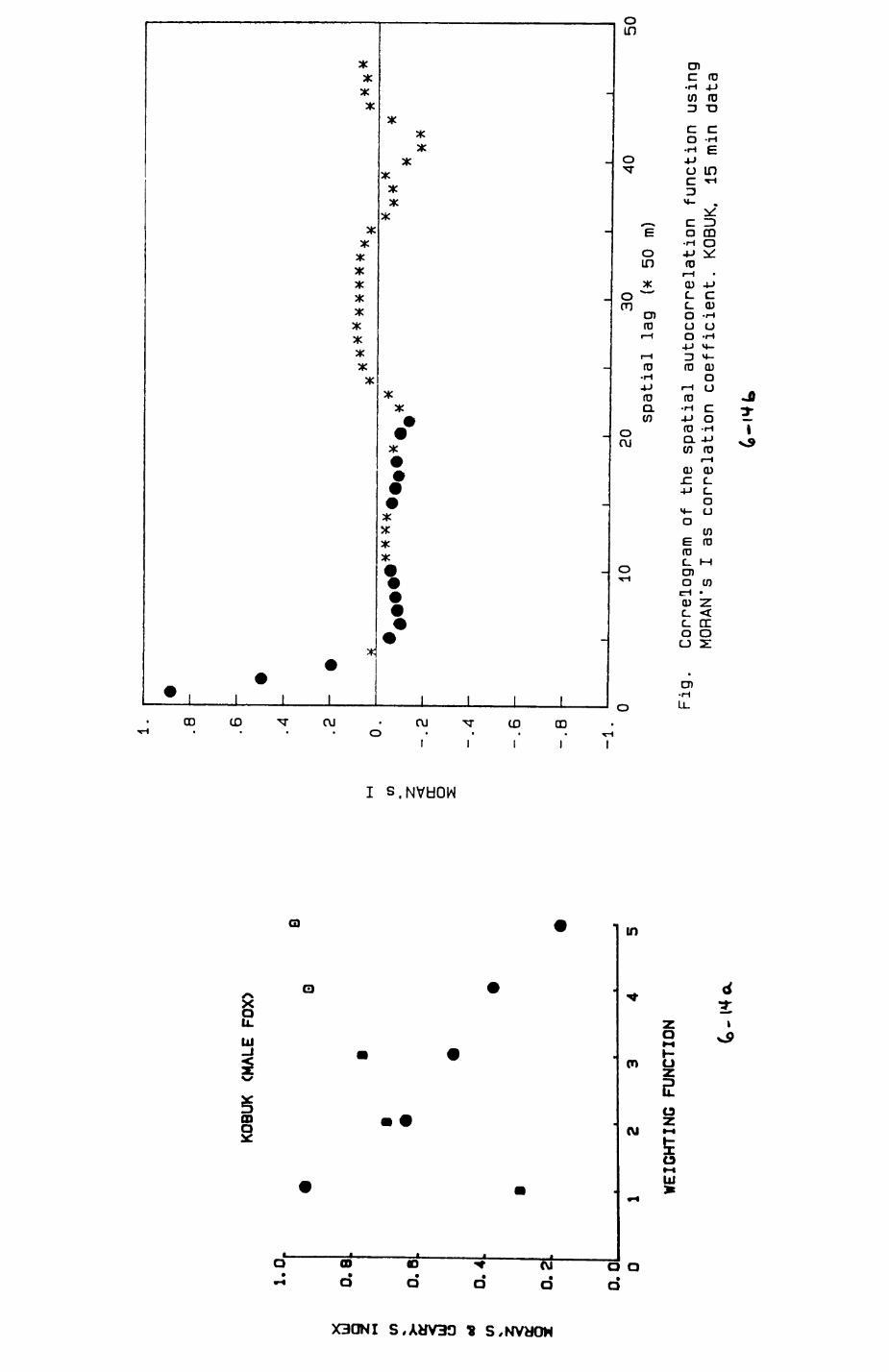
O)
1.0,
.
0.6
0.4
0.2.
0.0
KOBUK
(MAL
E FOX)
0
01234
5
WEI
GHTI
NG F
UNCT
ION
(0 z
< o
1.
.8
.6
.4
.2
0.
-.A .8
1.10
20
30spatial
lag
(x
50
m)40
50
Fig
.Co
rrel
ogra
m of th
e spatial
autocorrelation
func
tion
using
MORAN's
I as
co
rrel
atio
n co
effi
cien
t. KO
BUK.
15 min
data
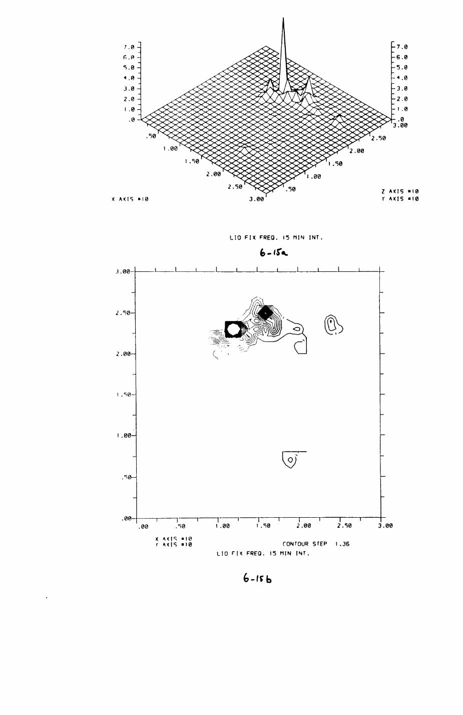
1.00I ."50
2.00
2.50
.50
.00
.50X AXIS »I0 3.00
Z AXIS "10r AXIS >i0
LIO FIX FREO. 15 niN INT,
. 00-
2.50-
2.00-
1 .S0-
1.00-
.50-
.00--
.00 .50
X AXIS «I0r AXIS *i0
i .00 I .50
~l——I——I—2.00 2.50 3.00
CONTOUR STEP 1.36 LIO fix FREO. 15 MIN INT.
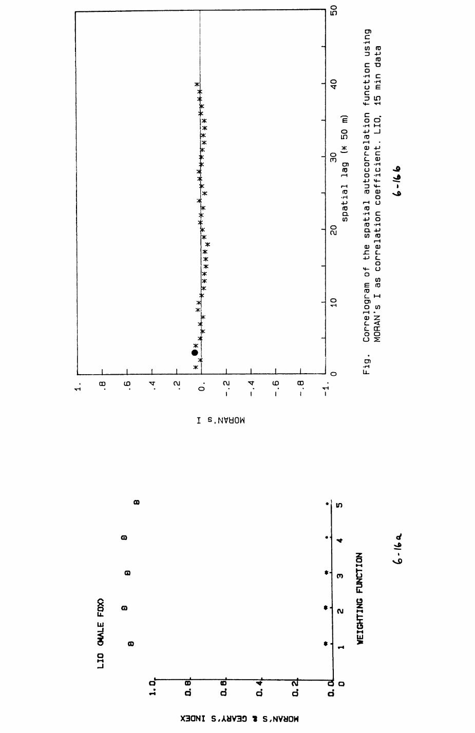
LIO
04
ALE
FOX>
1.0,
a8
08
* •
w
a
°'8
(0 >
0.6
-
0.4
V) z 1
a2
0.0
» •
• •
» *
*
01
234
5
WEI
GHTI
NG F
UNCT
ION
1 . .8 .6 .2 0.
CO 2 <
-2
cr o
-.4
-.6
-.8
-1.
- - — * • *
* *
*******£
*****
* *
*********
- - -
__j_
._..
.....i
.. i
i .1
i i
i i
0 Fig
.
1020
30
sp
atia
l la
g (*
50
m)
4050
Cor
relo
gram
o
f th
e sp
atia
l a
uto
corr
ela
tion
fu
nct
ion
usi
ng
MO
RAN'
s I
as co
rre
latio
n co
effic
ien
t.
LIO
, 15
m
in
data
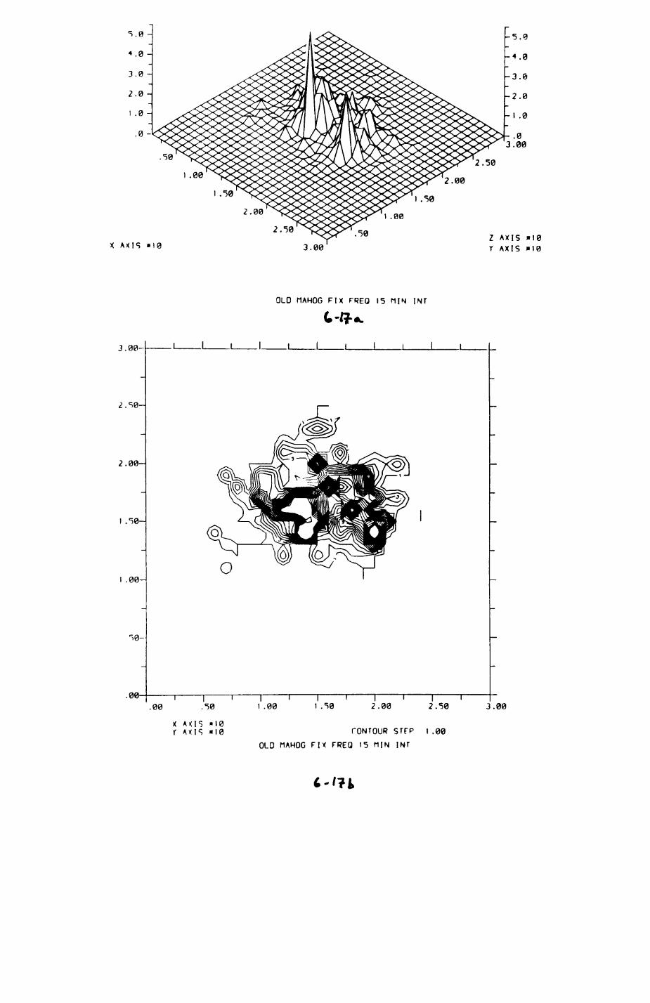
00' i
00'C 0S-3I I
INI NIU SI 03MJ Xld 90HVU 010
00' I I I00'? 0S' I
I I I
0i» bi>v ; 01* SIXV X
0C," 00'
•00-
-00' I
-0L" I
-00'
I I1 1-00'C
iNl NIU SI 03J1J Xld 90HVW OHO
0l« SIXV X 0t» SIXV Z
00'C0I« SIXV X

1 .
.8 .6
OLD
MAH
OGAN
Y (F
EMAL
E FO
X)
1.0
|
°-8
»-i in |
0.6
UJ 10 -
0.4
W Z a: 3
0.2
0. O
——
——
——
——
——
——
——
——
L
r •
- 4
•
'
0.
• .m 1
--
2
fo
: i
•
~' A
•
•
-.6
_
Q
•
-1
.
01
234
5
- \
•
••K
)<
*_
A0***0*0*
•
••
^••••^••••••^
- _ i
i i
i i
i i
i i
) 10
20
30
40
5(
on
= 4
-n=
1
Tan
(*t
RH
m
^
WEIG
HTIN
G FUNCTION
Fig.
Cornelogram
of the
spat
ial
auto
corr
elat
ion
function using
MORAN's
I as correlation
coef
fici
ent.
OL
DMAH
06AN
Y.
15 m
in data
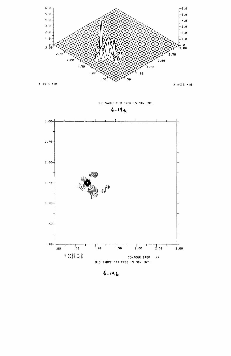
1 .50
1 .00
.50( AXIS *10 X AXIS »10
OLD SABRE FIX FREQ 15 ttlN INT,
3.00-
2.S0-
2.00-
1 .50-
I .00-
50-
.00.00 .50
X A<IS «10 r MIS "10
I .00 1.50 2.00I |
2.50 3.00
CONTOUR STEP OLD SABRF FIX FRFQ 15 HIN INT.
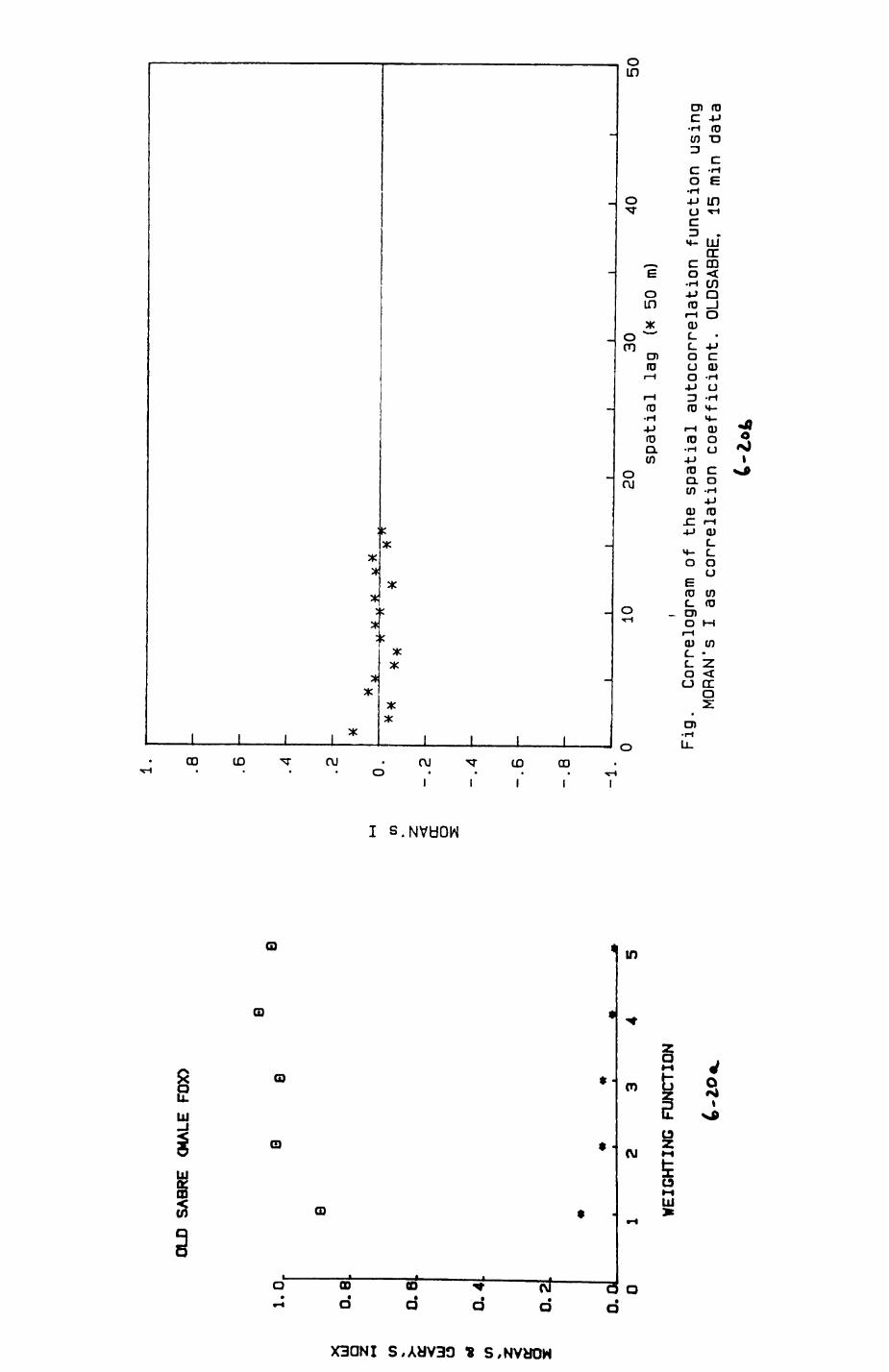
OLD
SABRE
(MAL
E FOX>
1.0,
00
eA
•
*rf
*•« |
0.6
o **
0.4
V) z i
0.2
0.0
8
.
01
2345
WEIGHTING
FUNCTION
0)
1. .8
.6 .2 0. -.4
-.6
-.8
0
J*
**.
1020
30sp
atia
l la
g (* 5
0 m)
50
Fig.
Conr
elogram
of the
spatial
autocorrelation
function using
MORA
N's
I as
correlation
coef
fici
ent.
OLDSABRE.
15 m
in data
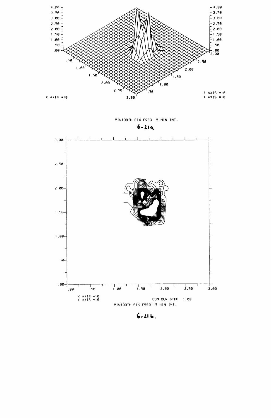
00'C
'INI NIU £.1 03dJ XU HUOOlNId
00'I d3iS
00' I
01* S1>V Jl 0I» SIXV X
00'?00'
t-00'
-00' t
-00'?
-00'
'INI NIU SI 03«J Xld HiOOlNId
01- S1XV Jl 01* SIXV Z
00-C0l» biXV X
00-c 00-
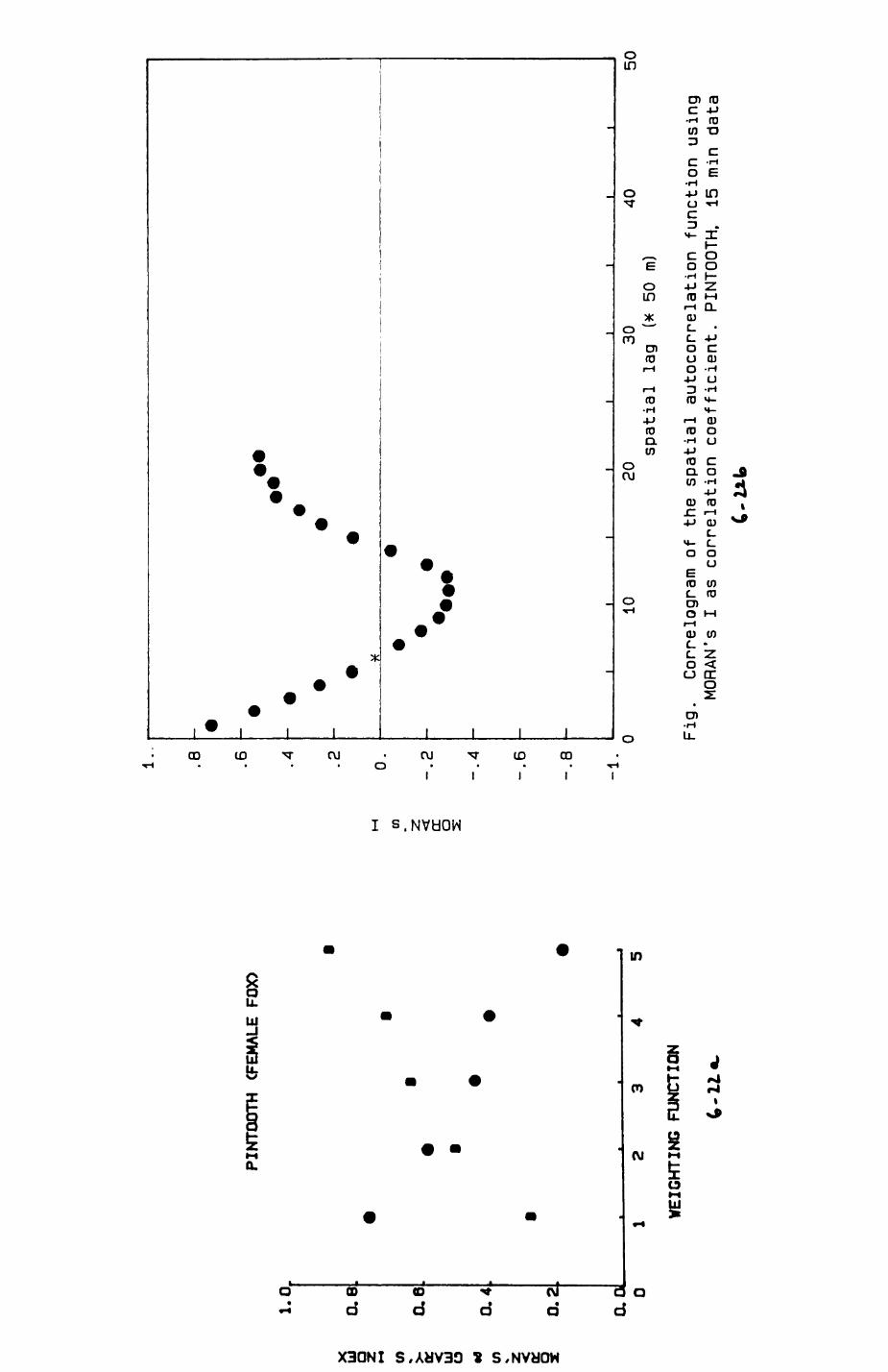
1.0
PINT
OOTH
(FEMALE
FOX>
A •
W
2
0.6
a •-H to b
ae
£ 0 - a4
(/) % a:
§
0.2 an
I
••
• • •
••
a •
01
234
5
WEIG
HTIN
G FU
NCTI
ON
cn tr
o
.8
.6
.4
.2
0. -.2
-.4
_ e
-.8
1020
30
40
spatial
lag
(* 50 m)
50
Fig.
Corr
elog
ram
of the
spatial
autocorrelation
func
tion
using
MORAN's
I as co
rrel
atio
n co
effi
cien
t. PI
NTOO
TH.
15 mi
n data
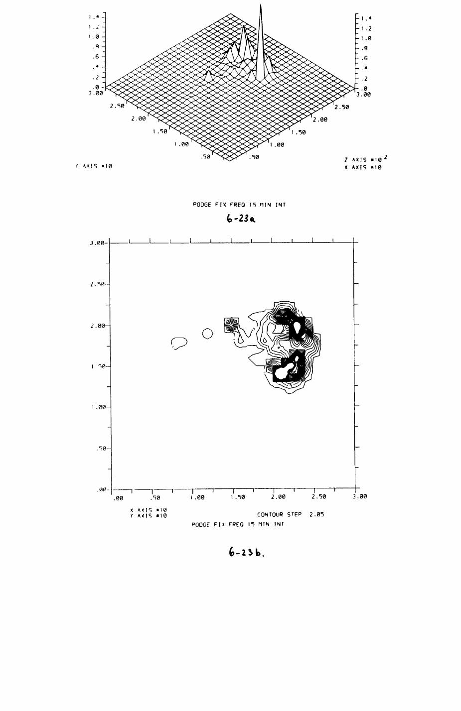
2.00
r AXIS «i0
I .50 1 .50
I .00 1 .00
.50 50 7 AXIS *I0 2 X AXIS «M0
PODGE FIX FREQ 15 MIN INT
3.00-
2.50-
2.00-
I .00-
.50-
I I I
.00 .50
X AXIS »I0r AXIS *I0
I I i I I I
O
I .00
1———r———|———i———|———i——1.50 2.00 2.50 3.00
CONTOUR STEP 2.05
PODGE FIX FREO 15 MIN INT
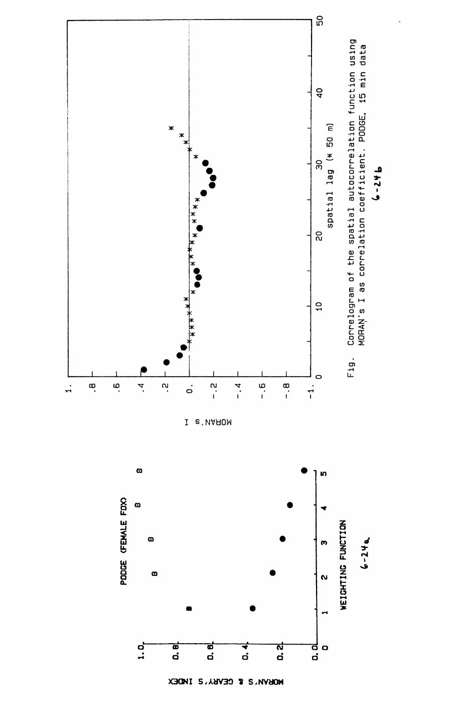
1 .
.8 .6
PODG
E (F
EMAL
E FO
X)
1.0
2
0.8
1-4 >-
0.6
"*
0.4
I 1
0.2
0.0
0 0
.A
0.2
• 0.
in z
<
-2
cr 0 2:
-.4
-.6
* .
. .
. *
- - -^
X
*•
vx
XX
•
m*
— -
i.i
i i
i i.i
i i
L A
r\
^* f\
*•> ^«
* ^
««
^_ .
1234
WEI
GH
TIN
G F
UNCT
ION
spatial
lag
(*
50
m)40
50
Fig.
Correlogram
of the
spatial
autocorrelation
func
tion
us
ing
MORAY'S
I as
co
rrel
atio
n co
effi
cien
t. PO
DGE.
15 min
data
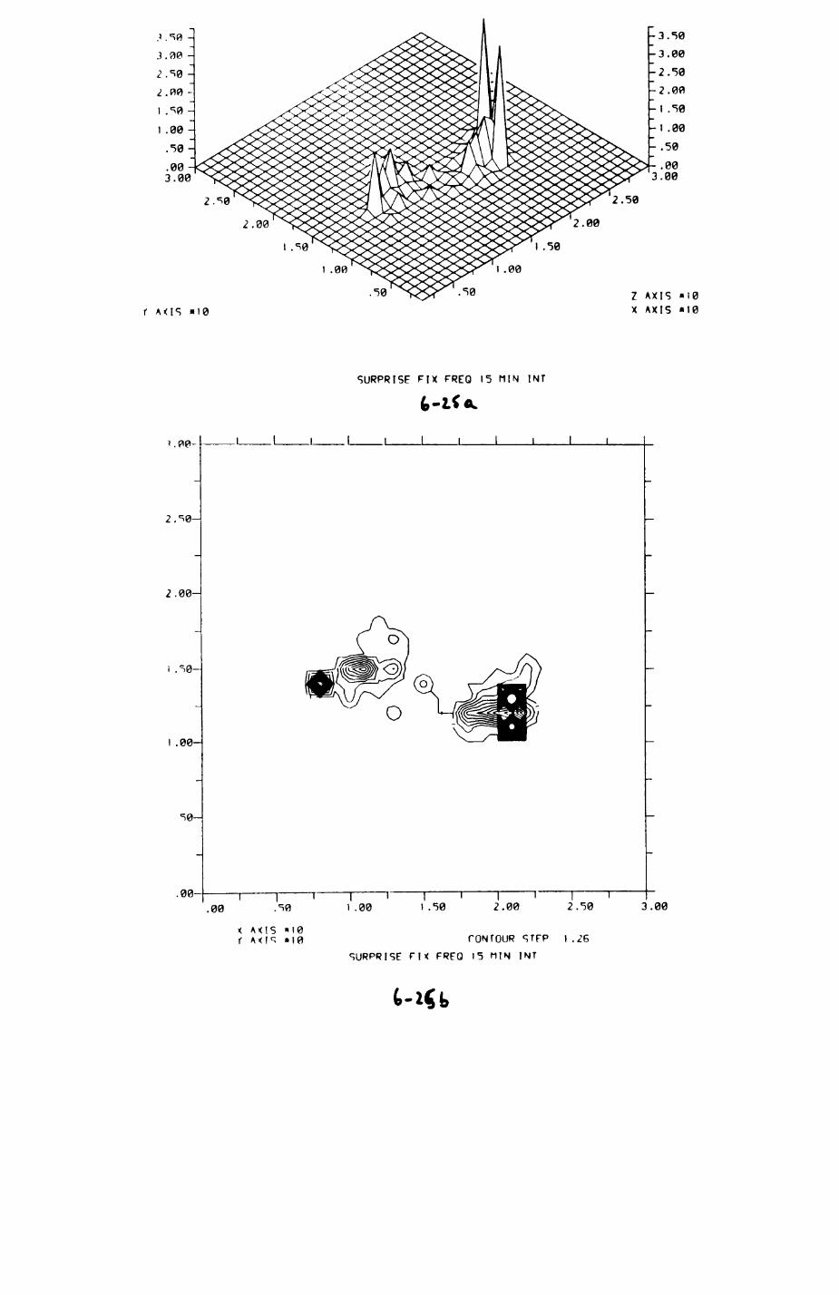
.003.00
2.50
r MIS »i0
2.00
I .50
1 .00
."50
.00 3.00
2.50
2.00
I .50
00
Z AXIS "10 X AXIS "10
SURPRISE FIX FREQ 15 MIN I NT
2.^0-
2.00-
I .50-
I .00-J
.00-
.1___I___I___L
.00 .50
< A<IS •10r
j___I
1.001———I———I———I———I———I—— 1.50 2.00 2.50 3.00
fONfOUR STFP I.26
SURPRISE fix PREQ 15 MIN I NT
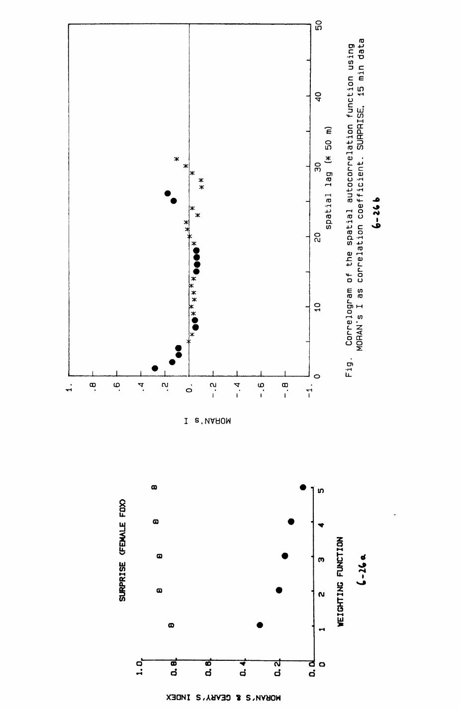
1 . .8
SUR
PRIS
E (F
EMAL
E FO
X>
" 6
1.0
g
0.8
z
en >
0.6
5 i7l CD •0 w
°*4
z 1 a2 0.0
r - A
R
88
82
•
La
8»
0.
en <
-.2
cr o s:-.
4
•
-.6
^•
-.8
T -i.
- - - • < — ^^ •
«^••
^^^••
••^""^
,/
7\
^\
— - ~"
i i
i .
\ ...
...
i i
i ..
.. i
i
1234
WEIG
HTIN
G FU
NCTI
ON
C-zc
20
30
40
spat
ial
lag
(x 50 m)
Fig.
Conr
ejog
ram
of the
spat
ial
autocorrelation
func
tion
using
MORAN's
I as
correl
atio
n coefficient. SU
RPRI
SE.
15 mi
n da
ta
50
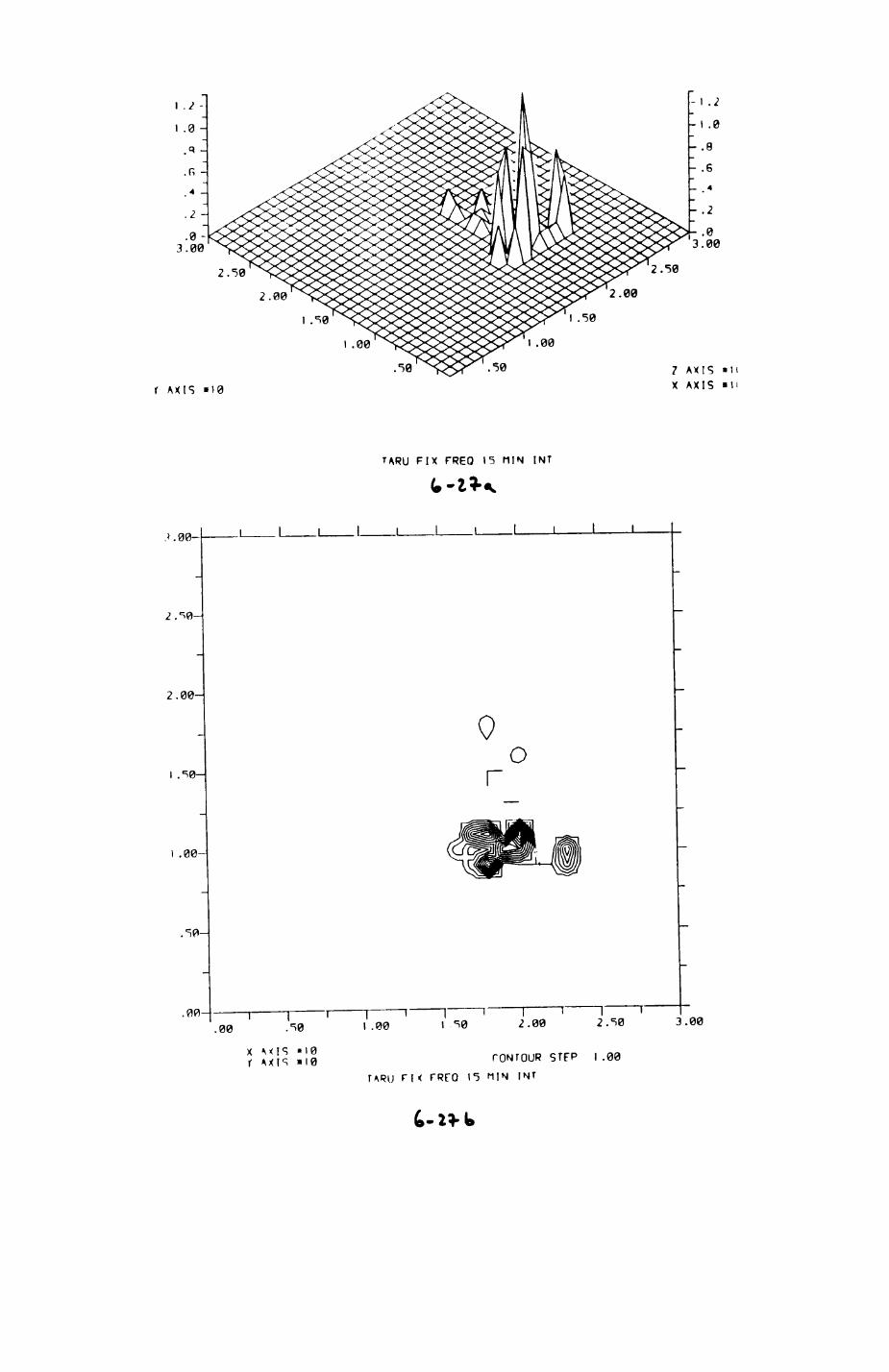
Jl
•s<s (S I.
is CS
Nj Jl
(S is
» "
<S<3
IS
I |S»
•f
Jl
<S (S
(SLO —
* T
! TJ IS
ISJl IS <s
<s
<s
oo
JO c -n X
X
X
t/> l
/l
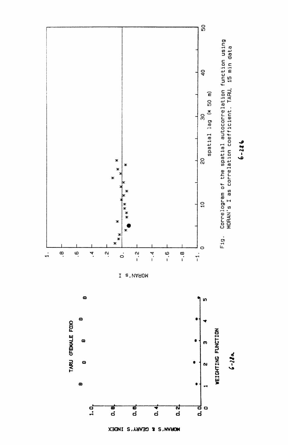
1.0
0.8
>-
0.6
0.4
0.2
.
0.
TARU
CF
EMAL
E FO
X>
9 0
ea
3
12
345
WEI
GH
TIN
G
FUN
CTI
ON
CO
1.
.8
.6 .2 0. .6
,8
** *
0 Fig
.
10
**
* 20
30sp
atia
l la
g
(x
50
m)40
50
Corr
elog
ram
of th
e spatial
autocorrelation
function using
MORAN's
I as correlation
coefficient. TA
RU.
15 m
in data
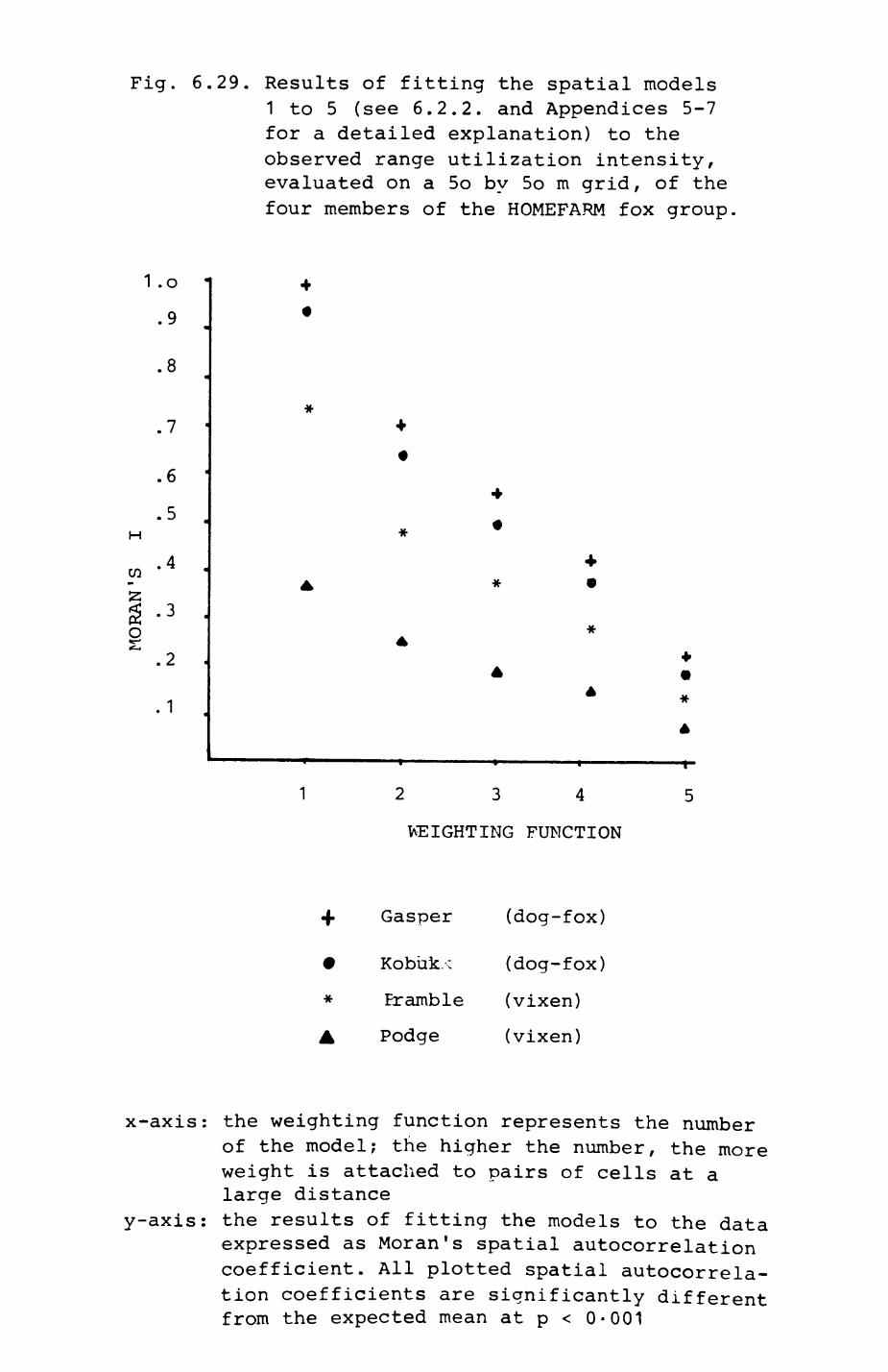
Fig. 6.29. Results of fitting the spatial models 1 to 5 (see 6.2.2. and Appendices 5-7 for a detailed explanation) to the observed range utilization intensity, evaluated on a 5o by 5o m grid, of the four members of the HOMEFARM fox group,
H
1 .0
.9
.8
.7
.6
.5
.4
.3
.2
.1
WEIGHTING FUNCTION
Gasper
Kobuk.:
Er amble
Podge
(dog-fox)
(dog-fox)
(vixen)
(vixen)
x-axis: the weighting function represents the number of the model; the higher the number, the more weight is attached to pairs of cells at a large distance
y-axis: the results of fitting the models to the data expressed as Moran's spatial autocorrelation coefficient. All plotted spatial autocorrela tion coefficients are significantly different from the expected mean at p < 0-001
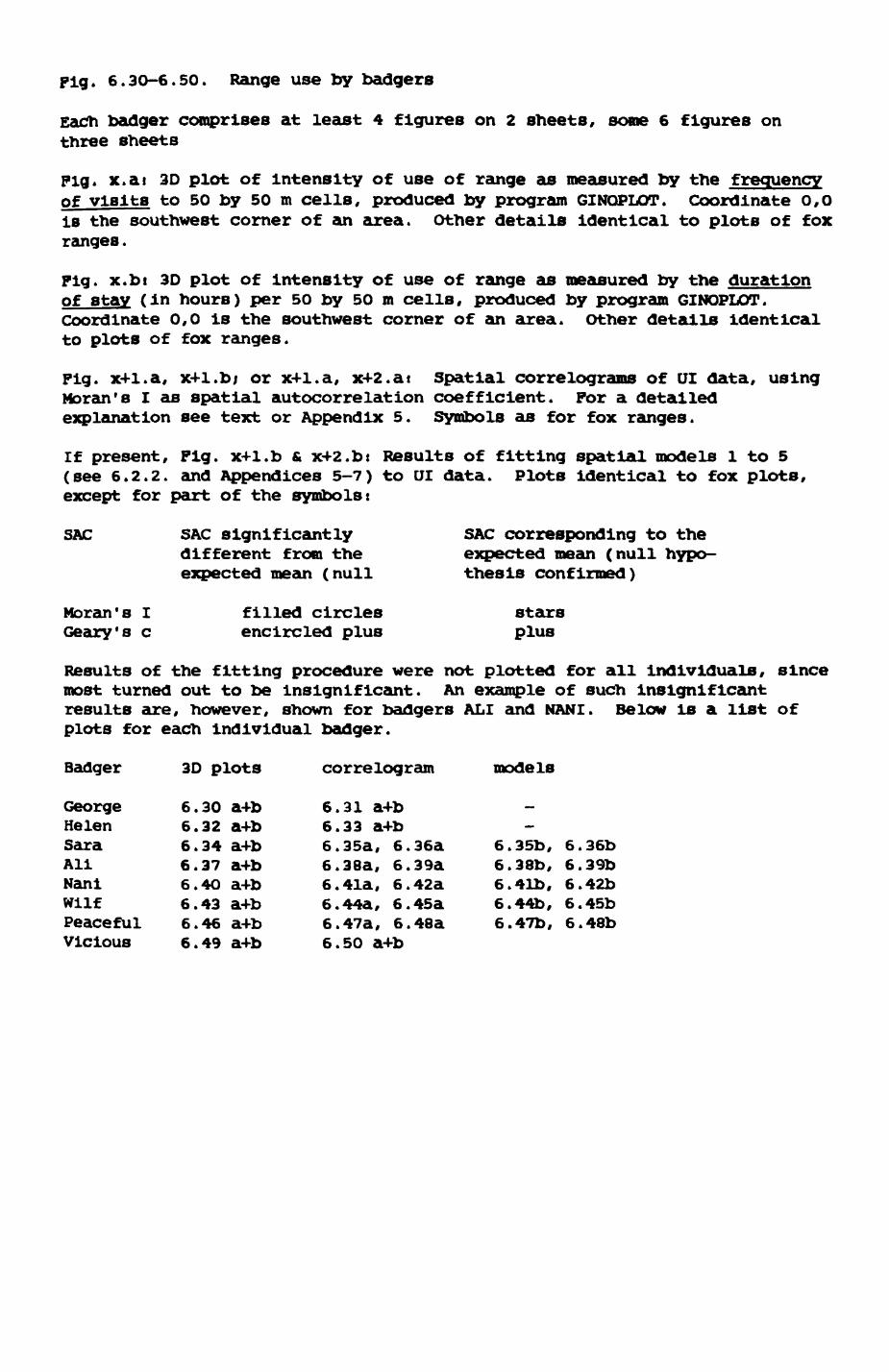
pig. 6.30-6.50. Range use by badgers
Each badger comprises at least 4 figures on 2 sheets, some 6 figures on three sheets
Pig. x.ai 3D plot of intensity of use of range as measured by the frequency of visits to 50 by 50 m cells, produced by program GINOPLOT. Coordinate 0,0 is the southwest corner of an area. Other details Identical to plots of fox ranges.
Pig. x.bi 3D plot of intensity of use of range as measured by the duration of stay (In hours) per 50 by 50 m cells, produced by program GINOPLOT. Coordinate 0,0 is the southwest corner of an area. Other details identical to plots of fox ranges.
Fig. x+l.a, x+l.bj or x+l.a, x+2.at spatial correlograms of UI data, using Moran's I as spatial autocorrelation coefficient. Por a detailed explanation see text or Appendix 5. Symbols as for fox ranges.
If present, Pig. x-H.b & x+2.bt Results of fitting spatial models 1 to 5 (see 6.2.2. and Appendices 5-7) to UI data. Plots identical to fox plots, except for part of the symbols!
SAC SAC significantly SAC corresponding to the different from the expected mean (null hypo- expected mean (null thesis confirmed)
Moran's I filled circles stars Geary's c encircled plus plus
Results of the fitting procedure were not plotted for all individuals, since most turned out to be insignificant. An example of such insignificant results are, however, shown for badgers ALI and NANI. Below is a list of plots for each individual badger.
Badger 3D plots correlogram models
George 6.30 a+b 6.31 a+b -Helen 6.32 a+b 6.33 a+bSara 6.34 a+b 6.35a, 6.36a 6.35b, 6.36bAll 6.37 a+b 6.38a, 6.39a 6.38b, 6.39bNanl 6.40 a+b 6.4la, 6.42a 6.41b, 6.42bWllf 6.43 a+b 6.44a, 6.45a 6.44b, 6.45bPeaceful 6.46 a+b 6.47a, 6.48a 6.47b, 6.48bVicious 6.49 a+b 6.50 a+b
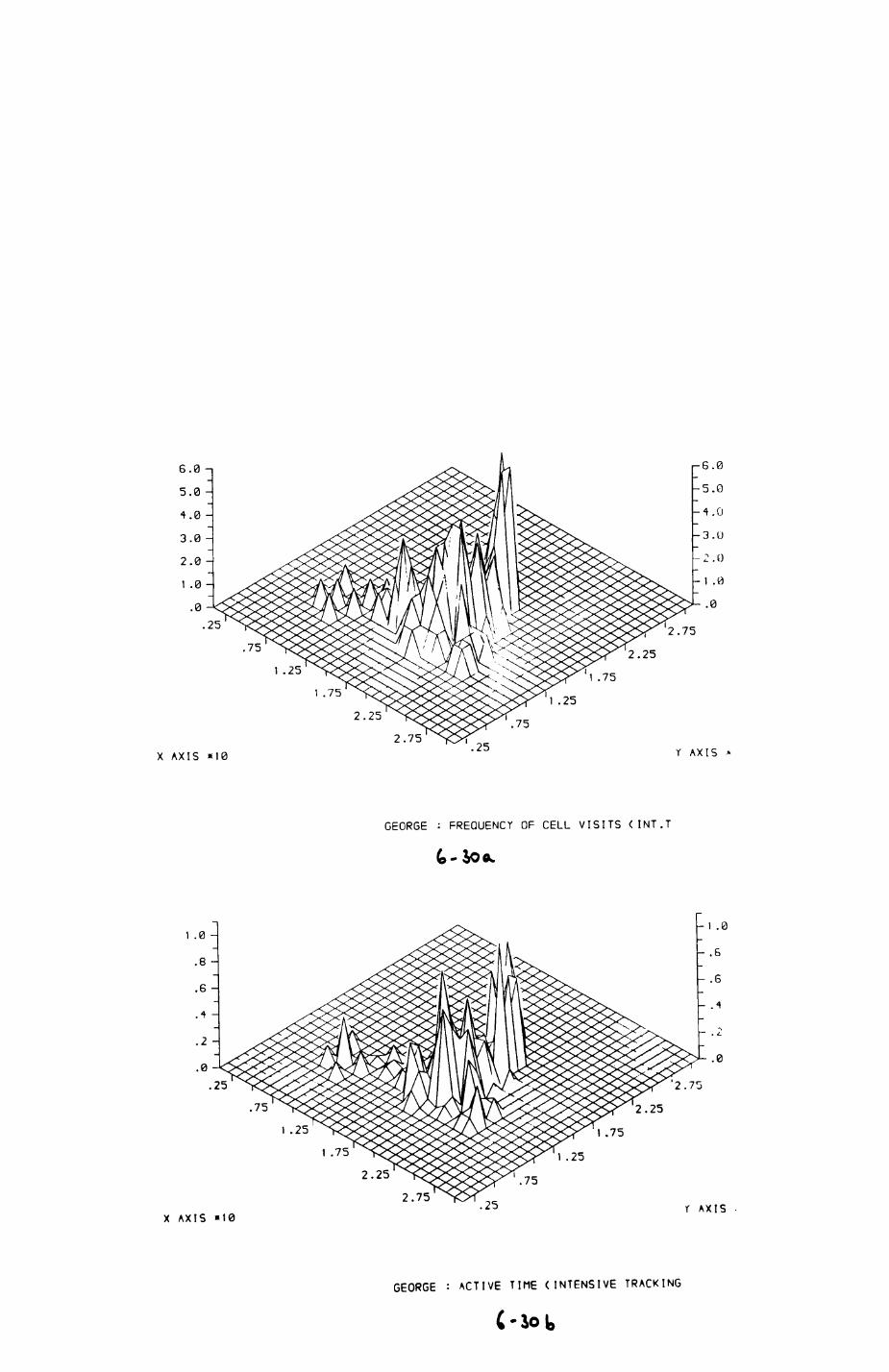
1 .75
2.25
2.75
2.25
1 .75
1 .25
2.75X AXIS *10 Y AXIS *
GEORGE : FREQUENCY OF CELL VISITS (INT.T
.02.75
25
75
2.25
2.75
X AXIS «10r AXIS
GEORGE : ACTIVE TIHE (INTENSIVE TRACKING
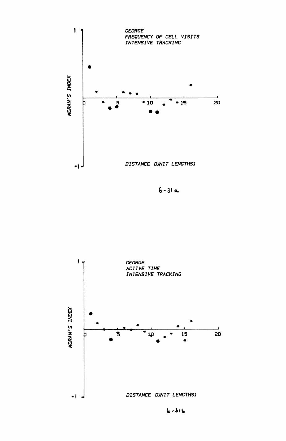
(n\ *
-I
GEORGEFREQUENCY OF CELL VISITSINTENSIVE TRACKING
10 20
DISTANCE [UNIT LENGTHS!
fe-31
0)s
GEORGE ACTIVE TIME INTENSIVE TRACKING
15 20
DISTANCE [UNIT LENGTHS!
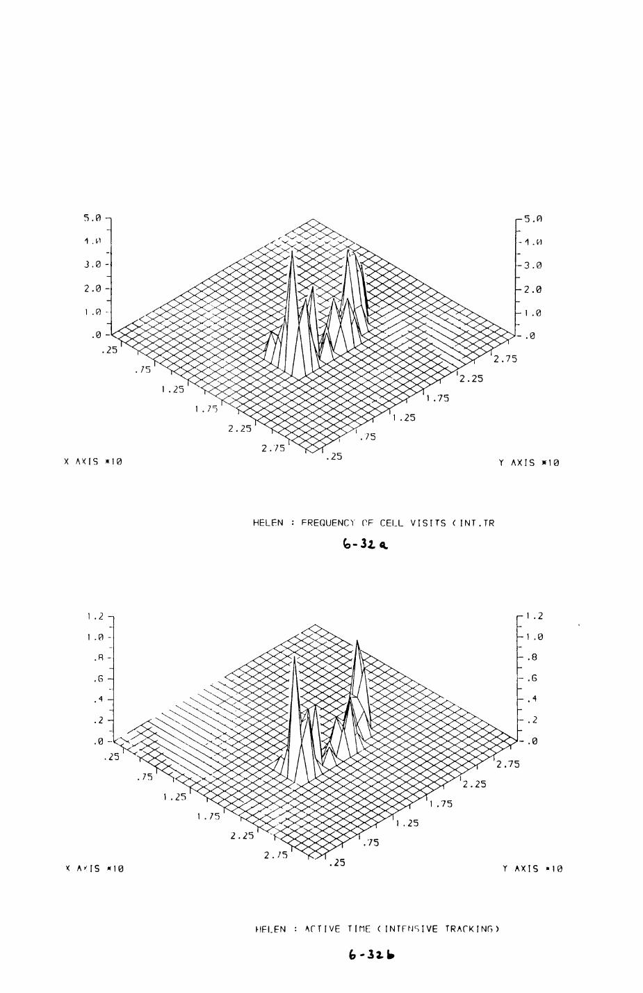
1 . 7=5
2.75
2.25
2.75X AXIS *I0 Y AXIS *10
HELEN : FREQUENCY OF CELL VISITS (INT.TR
1 .75
2.25
2.75
2.25
.75
25
2.75X AXIS "10 Y AXIS »I0
HELEN : ACTIVE TIME (INTENSIVE TRACKING)
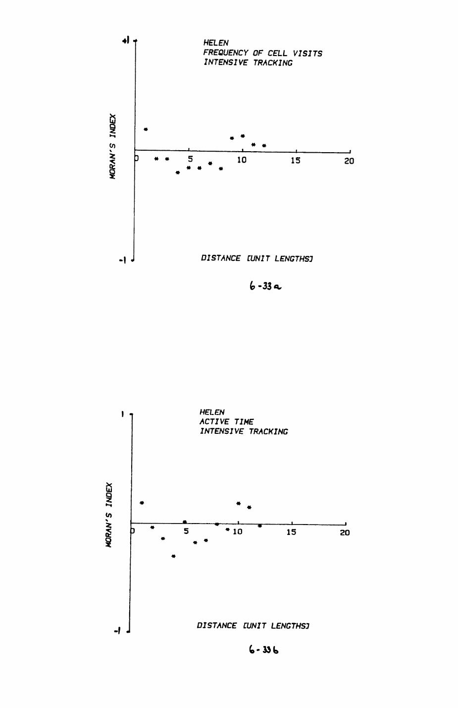
•»!
(n
-I
0)X
HELENFREQUENCY OF CELL VISITSINTENSIVE TRACKING
» • 5 10 15 20
DISTANCE [UNIT LENGTHS!
HELENACTIVE TIME INTENSIVE TRACKING
10 15 20
DISTANCE [UNIT LENGTHS]
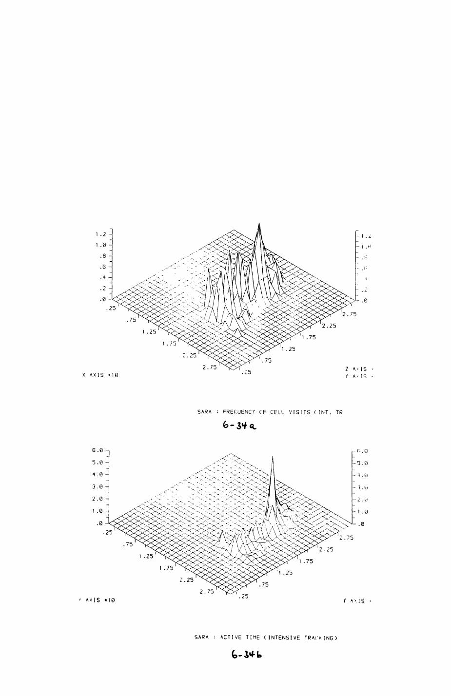
2.75
2.25
1 .75
1 .25
2.75X AXIS *10
Z A' ISr A- is
SARA : FRECUENCY TF CELL VISITS MNT. TR
.75
1 .252.25
.752.75
* AXIS «I0 .25 r AXIS
SARA : ACTIVE TIME (INTENSIVE TRACKING)
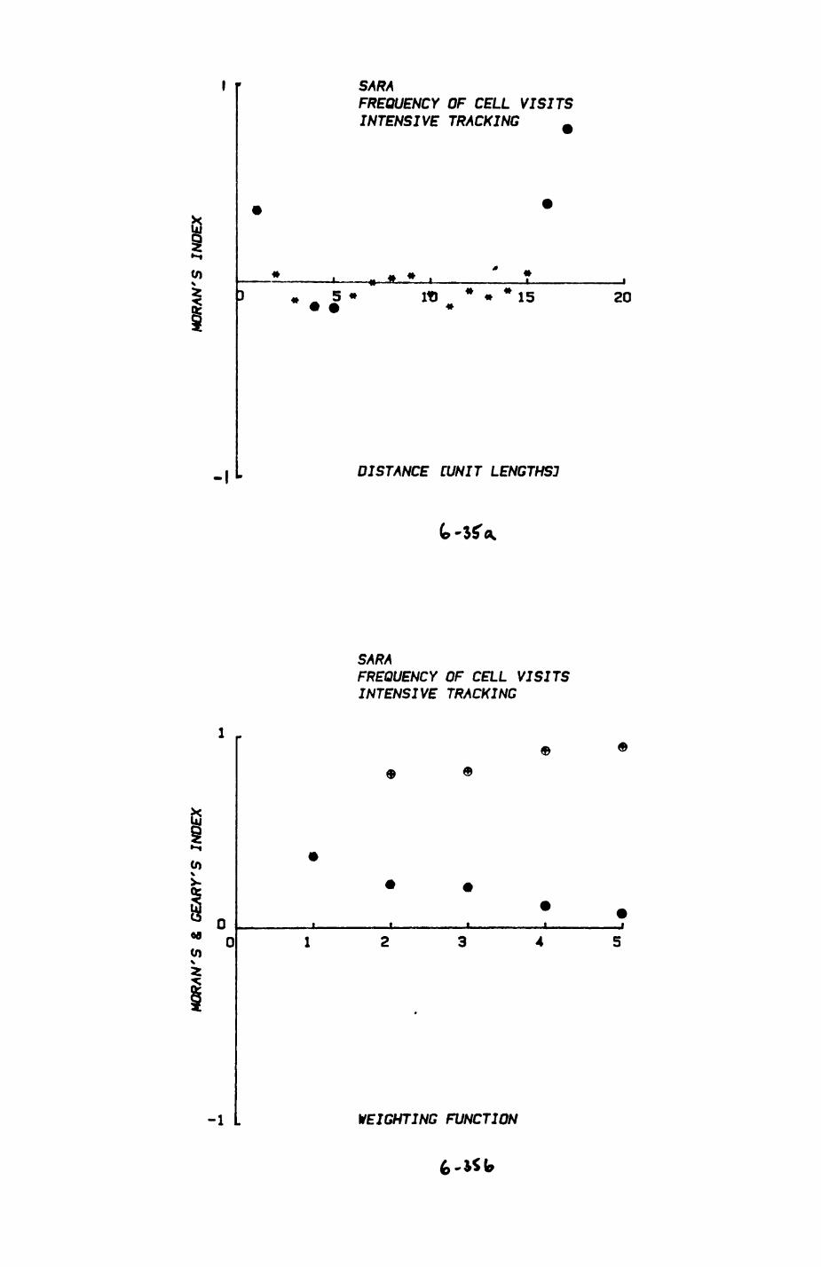
u 0I* o0)
SARAFREQUENCY OF CELL VISITSINTENSIVE TRACKING
5 • It) * • * 15 20
DISTANCE [UNIT LENGTHS]
SARAFREQUENCY OF CELL VISITSINTENSIVE TRACKING
9 ••
-1 . WEIGHTING FUNCTION
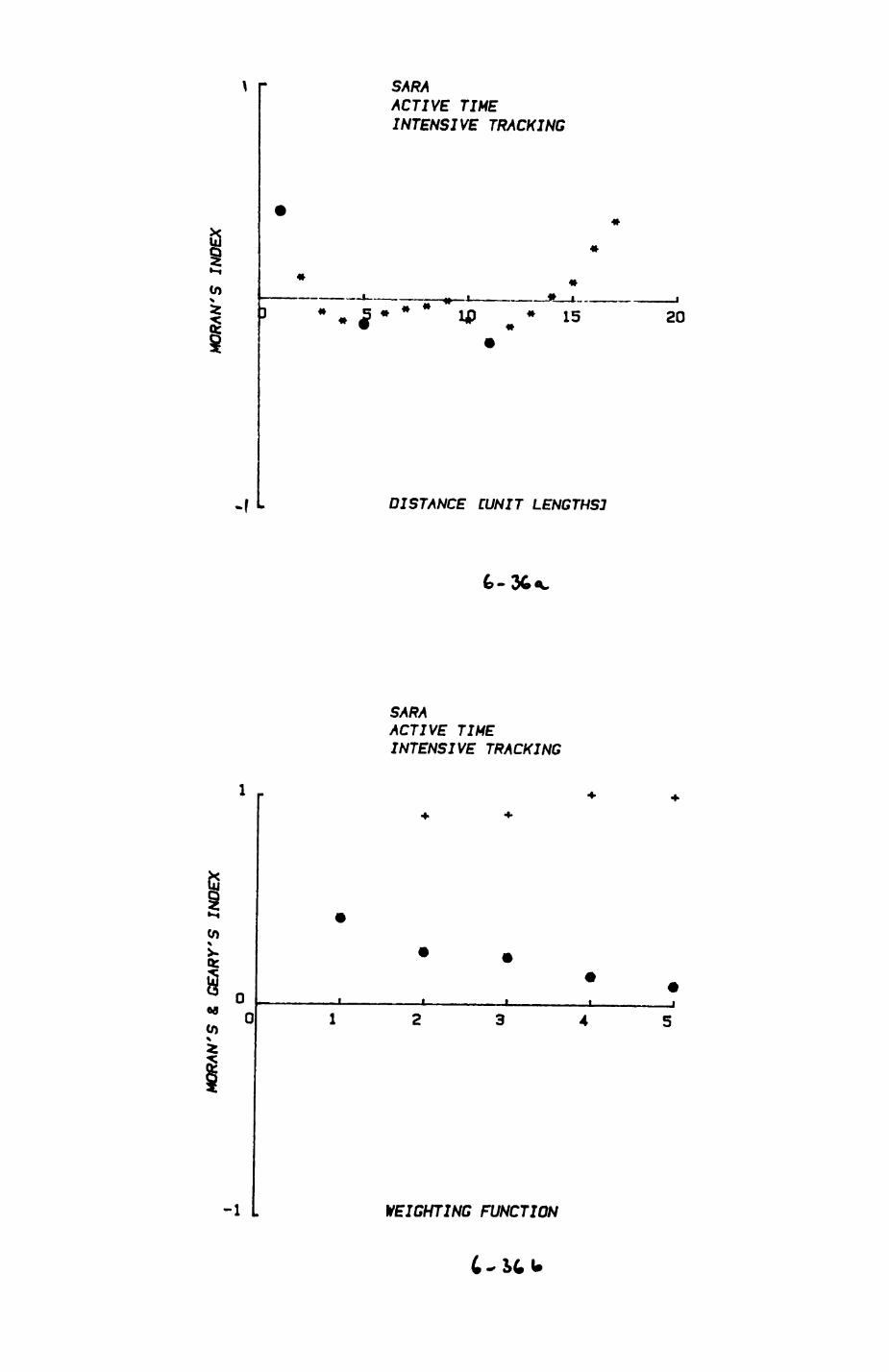
\ r SARAACTIVE TIME INTENSIVE TRACKING
f <* UP 15 20
DISTANCE CUNIT LENGTHS]
SARAACTIVE TIME INTENSIVE TRACKING
\ Z.
-I WEIGHT INC FUNCTION
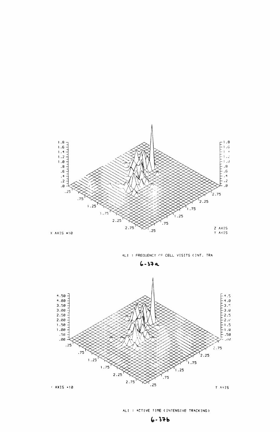
.0
2.75
2.25
1 .751 .75
1 .252.25
2.75X AXIS *10
Z AXIS Y AX IS
ALI : FREQUENCY TF CELL VISITS (INT. TRA
2.25
2.75AXIS -10 Y AXIS
ALI : ACTIVE TIME (INTENSIVE TRACKING)
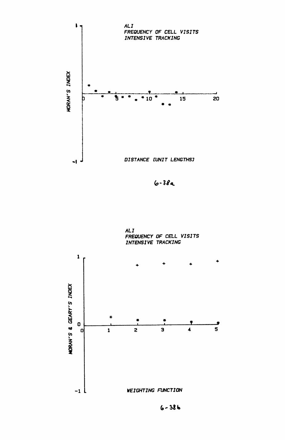
ALIFREQUENCY OF CELL VISITSINTENSIVE TRACKING
10 * 15 20
DISTANCE [UNIT LENGTHS:
ALIFREQUENCY OF CELL VISITSINTENSIVE TRACKING
(os
WEIGHTING FUNCTION
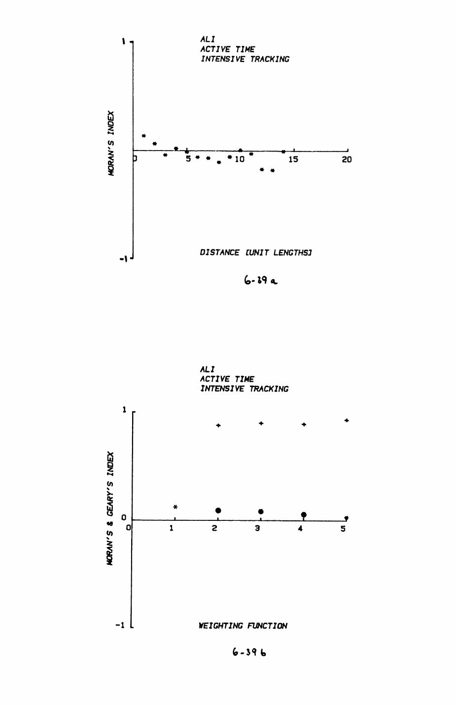
I -, ALIACTIVE TIME INTENSIVE TRACKING
5 » » ^ * 10 15 20* »
DISTANCE [UNIT LENGTHS]
ALIACTIVE TIMEINTENSIVE TRACKING
00
-1 . WEIGHTING FUNCTION
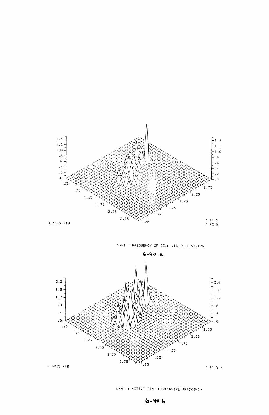
.0.25
X AXIS »I0
2.75.75
2.251 .25
1 .751 .75
2.25
2.75 Z AXIS r AXIS
NANI : FREQUENCY CF CELL VISITS (INT.TRA
1 .25
1 .75
2.25
2.75
.75
2.25
I .75
.25
.75
AXIS "10 .25 r AXIS
NANI : ACTIVE TIME (INTENSIVE TRACKING)
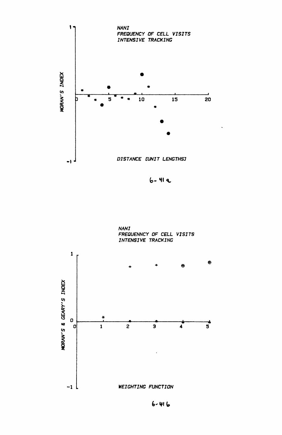
\ *
NANIFREQUENCY OF CELL VISITSINTENSIVE TRACKING
10 15
DISTANCE [UNIT LENGTHS]
NANIFREQUENNCY OF CELL VISITSINTENSIVE TRACKING
X-a:
00
0)
-1 WEIGHTING FUNCTION
e
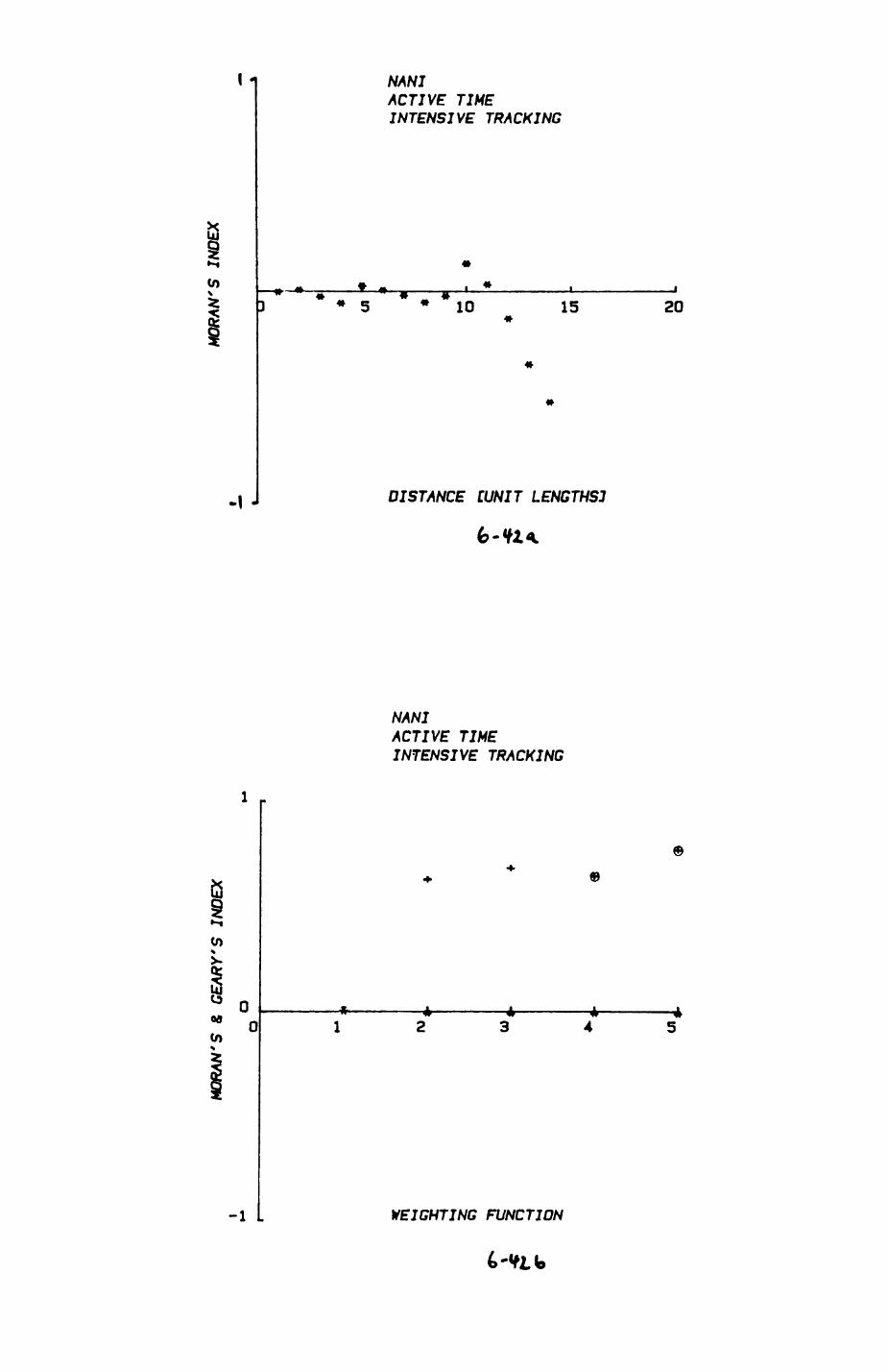
I1
CO\
-I J
NANIACTIVE TIME INTENSIVE TRACKING
10 15 20
DISTANCE [UNIT LENGTHS]
NANIACTIVE TIME INTENSIVE TRACKING
-1 WEIGHTING FUNCTION
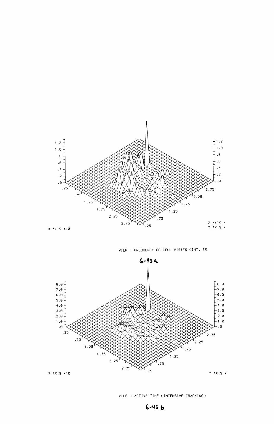
-1 .2
2.75
2.25
751 .75 1 .25
2.25
2.75
X AXIS *10
Z AXIS Y AXIS
WILF : FREQUENCY OF CELL VISITS (INT. TR
75
2.25
75I .75
252.25
2.75X AXIS «10 Y AXIS *
WILF : ACTIVE TIME (INTENSIVE TRACKING)
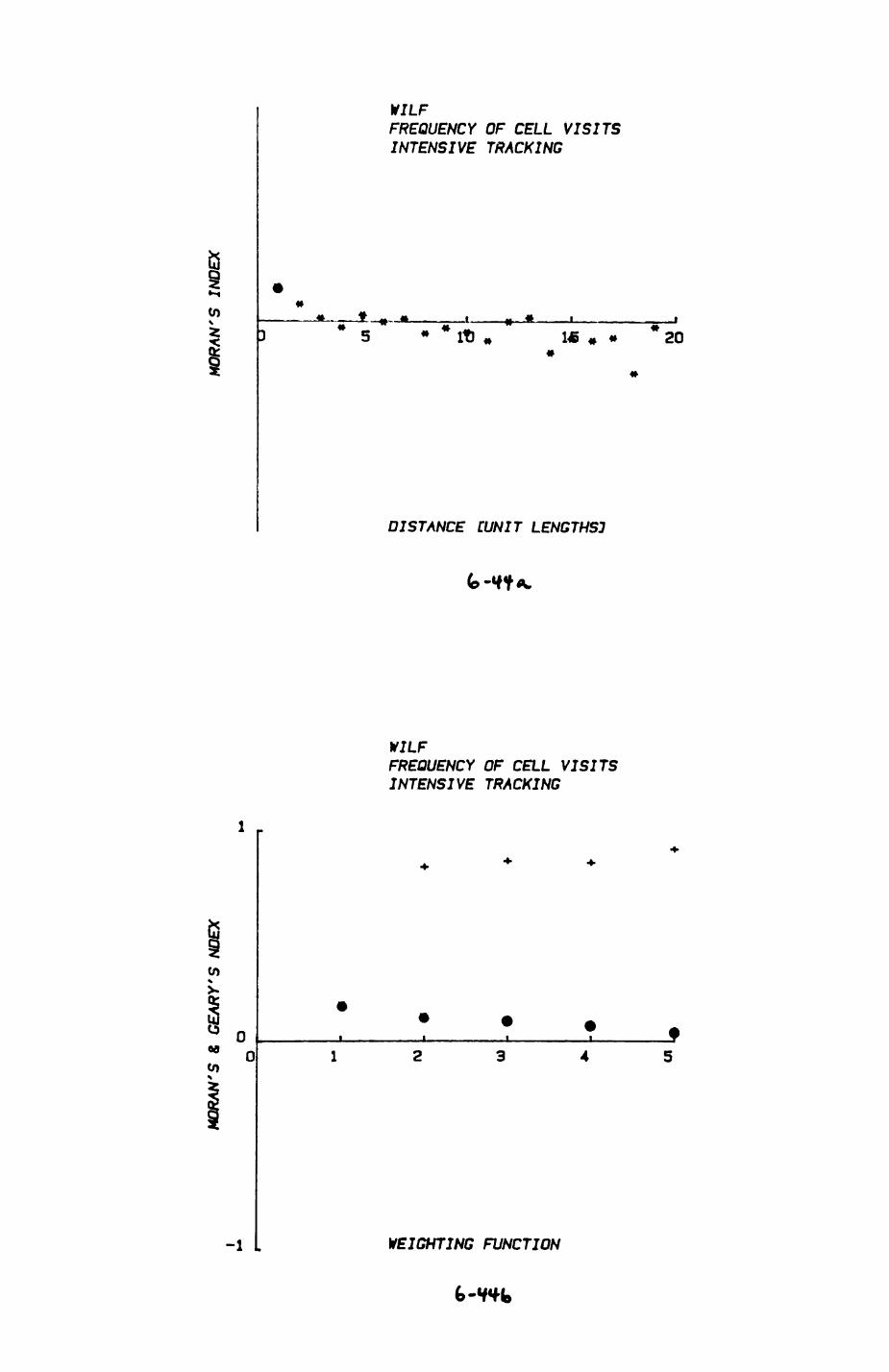
VILFFREQUENCY OF CELL VISITSINTENSIVE TRACKING
* _ ________5 ~ * * It) » ~ 1* » « * 20
DISTANCE WNIT LENGTHS]
WILFFREQUENCY OF CELL VISITSINTENSIVE TRACKING
w 008 0 en
-1 WEIGHTING FUNCTION
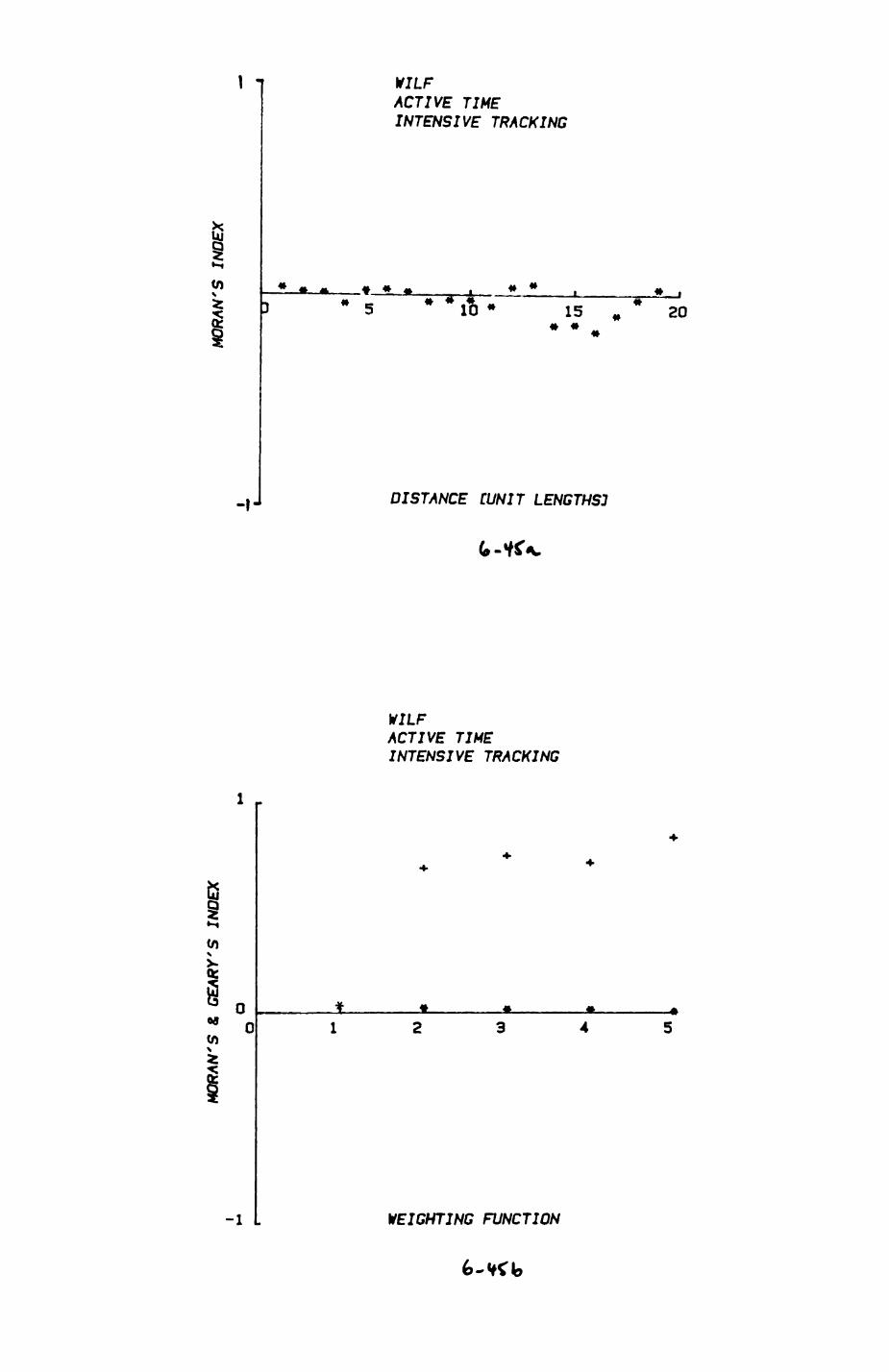
0)V
1
VILFACTIVE TIME INTENSIVE TRACKING
1*015 20
DISTANCE [UNIT LENGTHS!
VILF/CTJVE TIME" INTENSIVE TRACKING
(A\Q:
0)\z.
-1 WEIGHTING FUNCTION
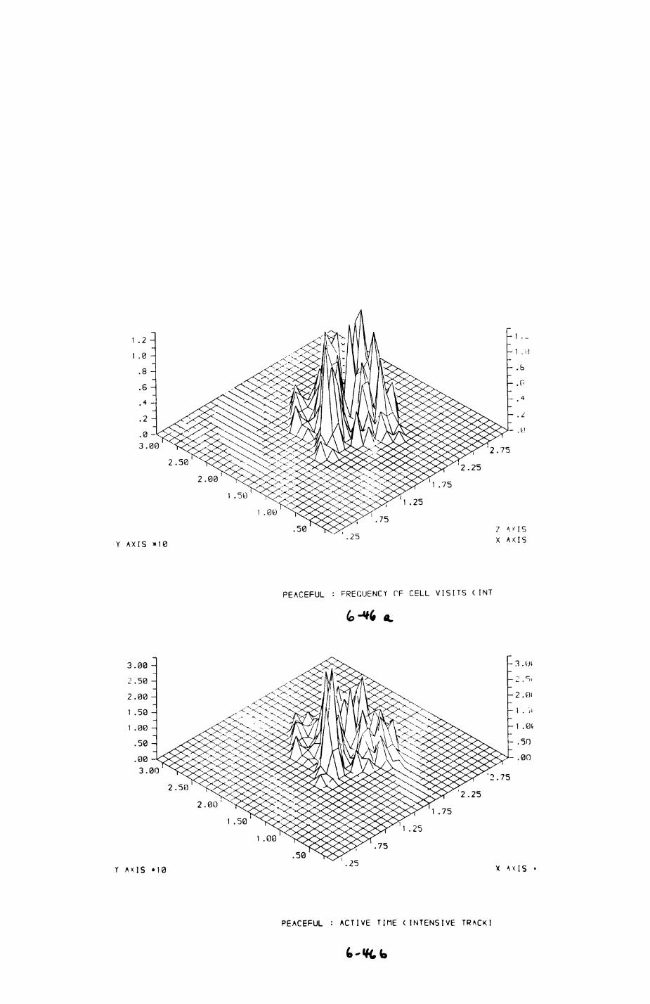
2.75
'2.25
1 .751 .50
1 .251 .00
.50
Y AXIS *10
7 AMS X AXIS
PEACEFUL : FREQUENCY OF CELL VISITS (INT
.00 ->
3.00'
2.50
2.00
1 .50
1 .00
.50
2.75
2.25
75
1 .25
75
Y AXIS »10.25 X ^XIS
PEACEFUL : ACTIVE TIHE (INTENSIVE TRACKI
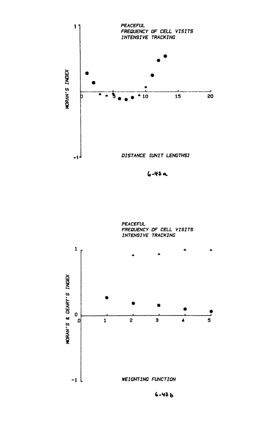
\ 1
to% *
PEACEFULFREQUENCY OF CELL VISITSINTENSIVE TRACKING
10 15 20
DISTANCE CUNIT LENGTHS]
PEACEFULFREQUENCY OF CELL VISITSINTENSIVE TRACKING
00
-1 WEIGHTING FUNCTION
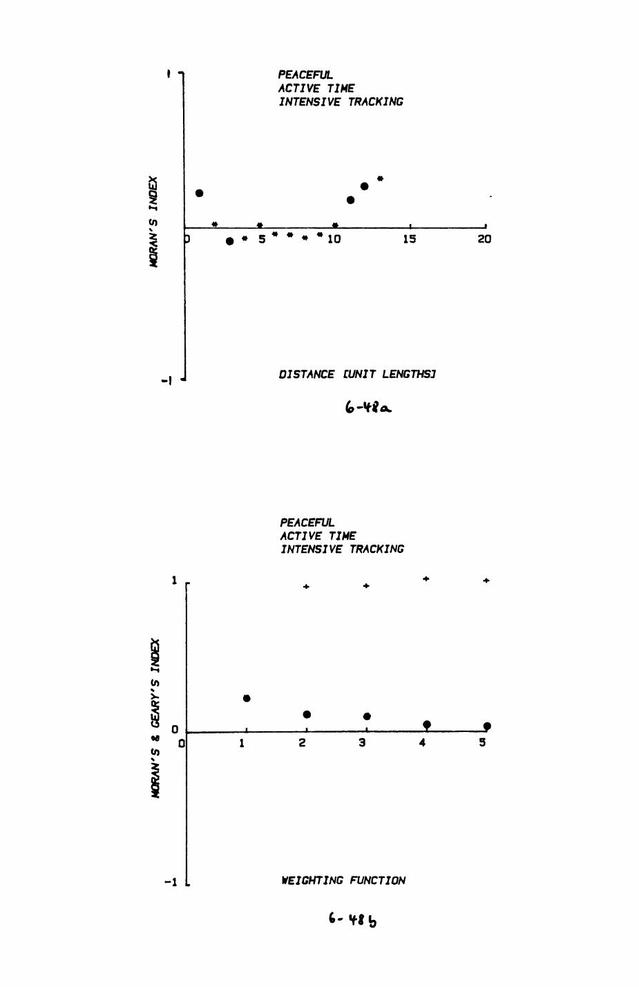
PEACEFUL ACTIVE TIME INTENSIVE TRACKING
10 15 20
DISTANCE [UNIT LENGTHS]
PEACEFUL ACTIVE TIME INTENSIVE TRACKING
1 „
00
-1 . WEIGHTING FUNCTION
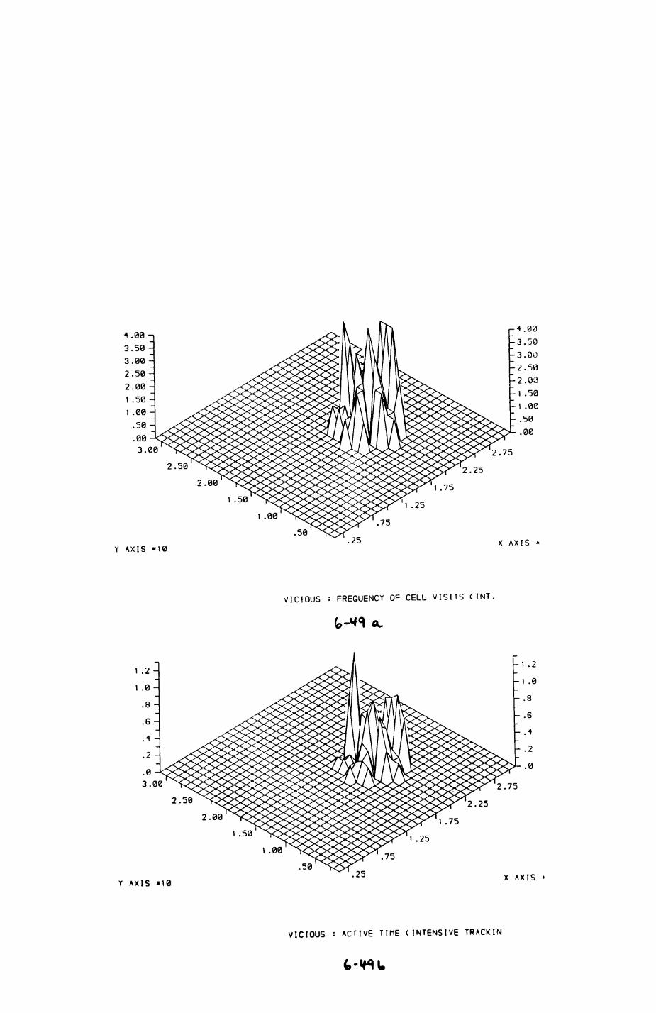
2.
2.75
2.25
1 .00
.50
Y AXIS »10X AXIS *
VICIOUS : FREQUENCY OF CELL VISITS (INT.
2.75
2.25
1 .75
251 .00
.50
Y AXIS "10X AXIS •
VICIOUS : ACTIVE TIME (INTENSIVE TRACKIN
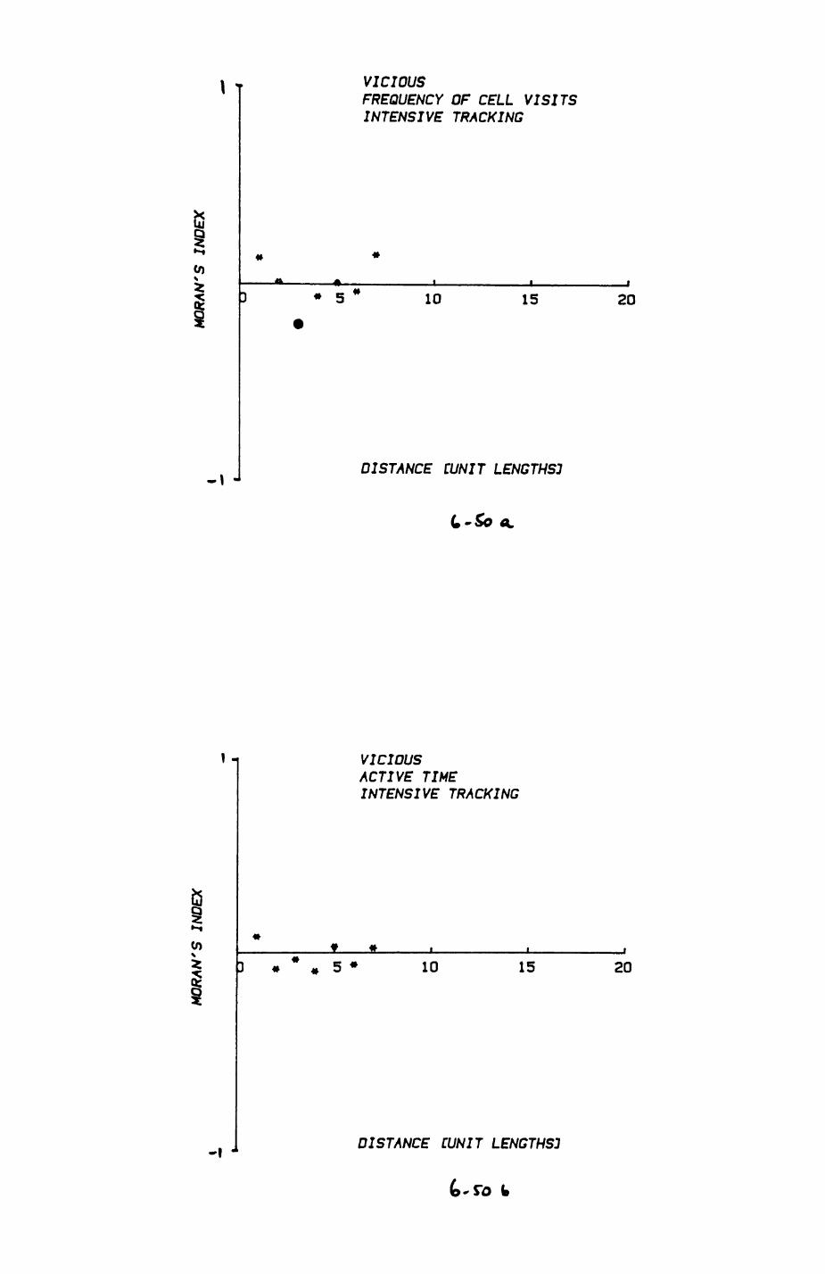
i 7 VICIOUSFREQUENCY OF CELL VISITS INTENSIVE TRACKING
en\
-»
• 5 * 10 15 20
en
DISTANCE [UNIT LENGTHS]
VICIOUS ACTIVE TIME INTENSIVE TRACKING
5 • 10 15 20
DISTANCE [UNIT LENGTHS]
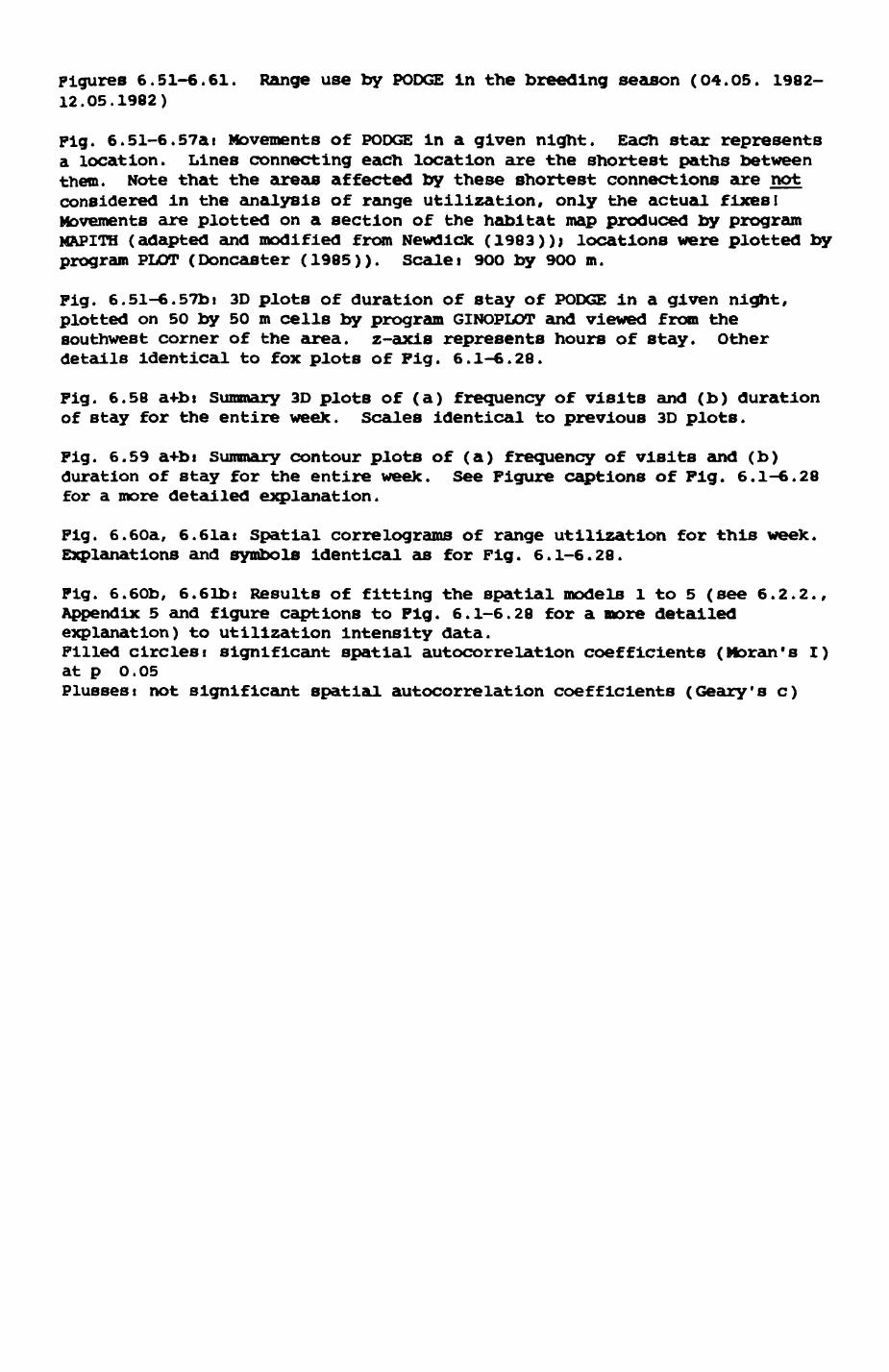
Figures 6.51-6.61. Range use by PODGE in the breeding season (04.05. 1982- 12.05.1982)
Fig. 6.5l-6.57ai Movements of PODGE in a given night. Each star represents a location. Lines connecting each location are the shortest paths between them. Note that the areas affected by these shortest connections are not considered in the analysis of range utilization, only the actual fixes I Movements are plotted on a section of the habitat map produced by program MAPITH (adapted and modified from Newdlck (1983))) locations were plotted by program PLOT (Doncaster (1985)). Scalei 900 by 9OO m.
Fig. 6.51-6.57b« 3D plots of duration of stay of PODGE in a given night, plotted on 50 by 50 m cells by program GINOPLOT and viewed from the southwest corner of the area, z-axis represents hours of stay. Other details identical to fox plots of Fig. 6.1-6.28.
Fig. 6.58 a+bi Summary 3D plots of (a) frequency of visits and (b) duration of stay for the entire weeJc. Scales identical to previous 3D plots.
Fig. 6.59 a+bs Summary contour plots of (a) frequency of visits and (b) duration of stay for the entire week. See Figure captions of Fig. 6.1-6.28 for a more detailed explanation.
Fig. 6.60a, 6.6lat Spatial correlograms of range utilization for this week. Explanations and symbols identical as for Fig. 6.1-6.28.
Fig. 6.60b, 6.6Lbi Results of fitting the spatial models 1 to 5 (see 6.2.2.,Appendix 5 and figure captions to Fig. 6.1-6.28 for a more detailedexplanation) to utilization Intensity data.Filled circlesi significant spatial autocorrelation coefficients (Koran's I)at p 0.05Plussest not significant spatial autocorrelation coefficients (Geary's c)
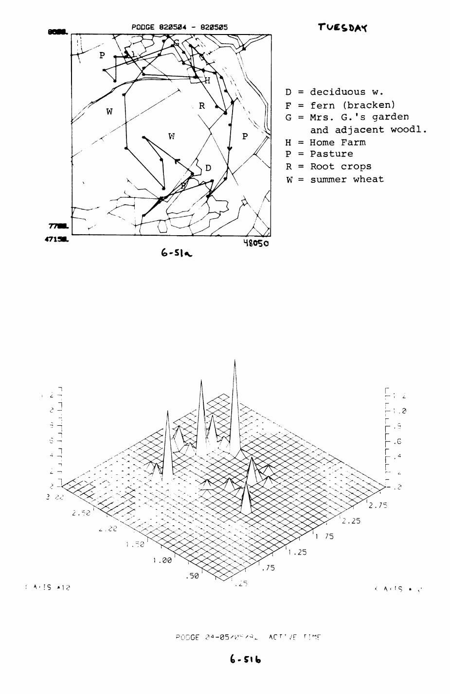
PODGE 820504 - 820505
D = deciduous w. F = fern (bracken) G = Mrs. G.'s garden
and adjacent woodl H = Home Farm P = Pasture R = Root crops W = summer wheat
471
r
2.75
2.25
.50IS < A «' ' S *
PODGE AC ri .'F r ' M.f
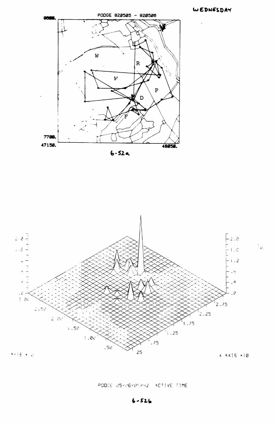
Ill pU)3
Y////^^Y
Y\/
\ , / / v /yyVV
Vy
en
LULJ'Nl
T1
VVUDjiIPLJ
L)
oo
a
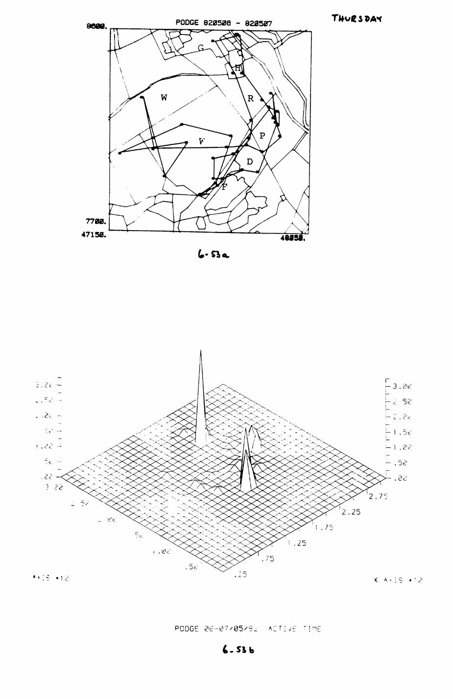
5A
a
UJ
L J
xin'UUJ
ID
Q
Oa
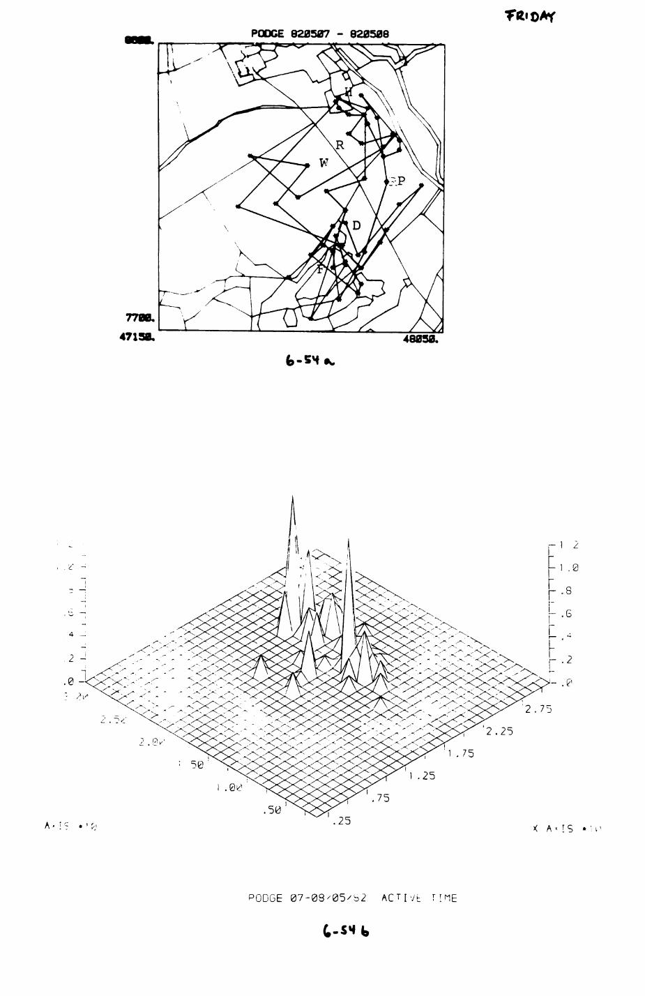
PODGE 820507 - 820508
48090.
2.75
2.25
'1 .75
1 .25
75.50
.25X A « ! S *
PODGE 07-08/05/S2 ACTjVt TIME
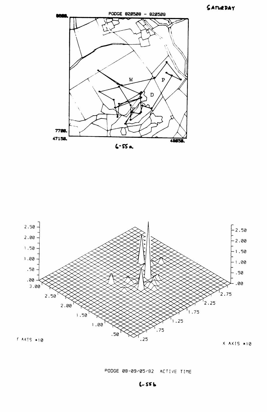
PODGE 820508 - 820509
c-ss
2.00
1 .50
-2.50
L .00
2.75
2.25
75
1 .251 .00
.50r AXIS *i0
X AXIS »10
PODGE 08-09/05/82 ACTIVE TIME
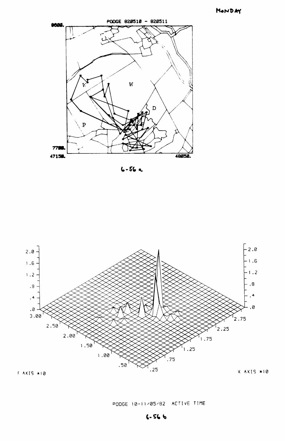
PODGE 820510 - 820511
4713* 48050.
2.00
1 .50
1 .00
2.75
2.25
1 .75
1 .25
.50
AXIS «I0 X AXIS *10
PODGE 10-11/05/82 ACTIVE TIHE
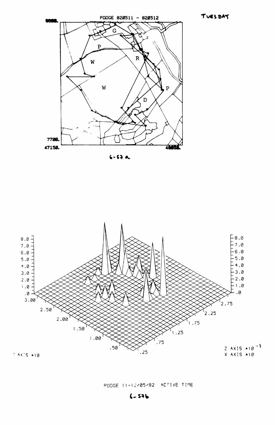
3AIi3V39QOd
\-01* SIXV X 01* SIXV Z
01* SiXV ;
ZTS0Z8 - IIS038 3000d
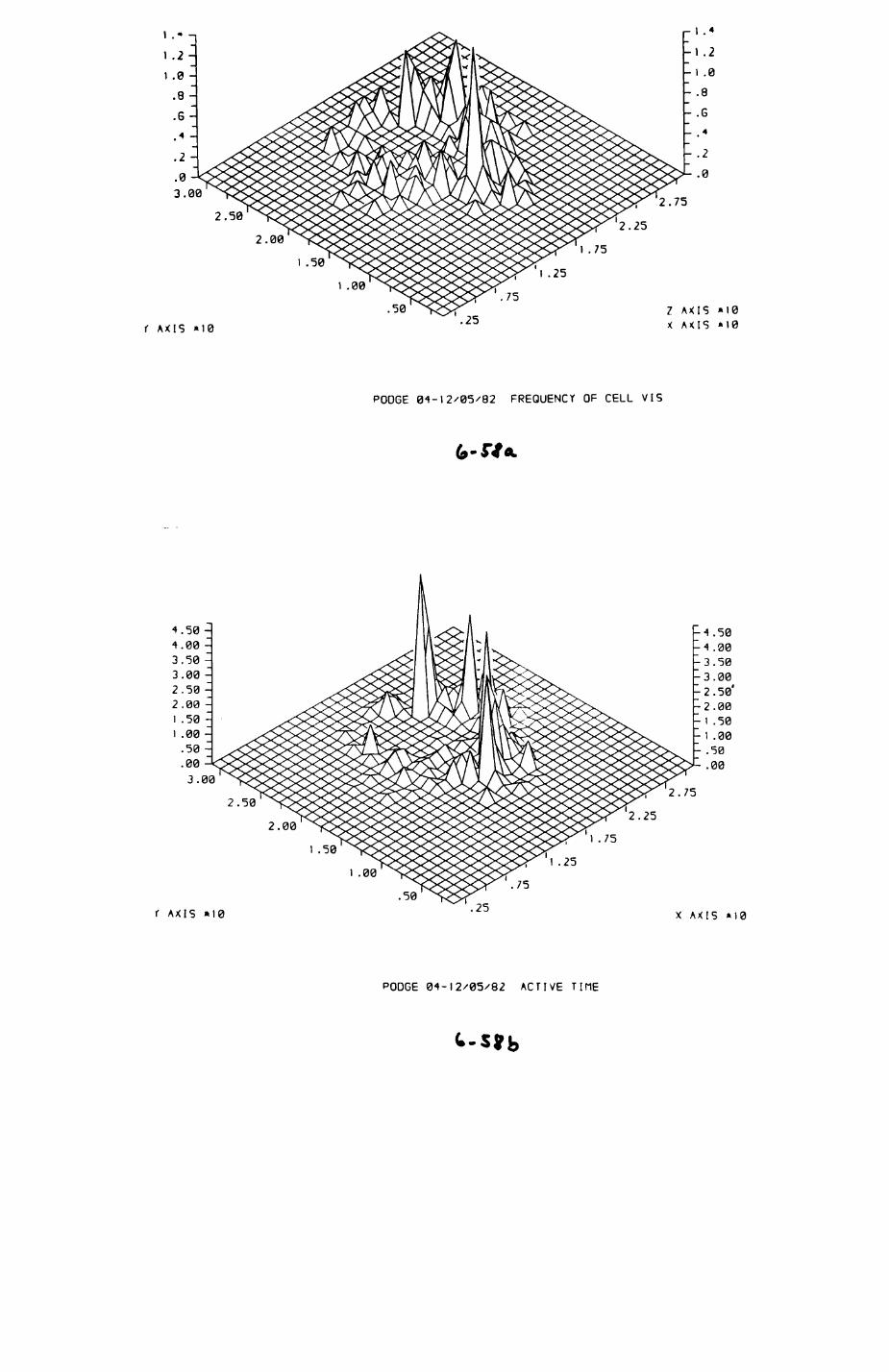
3.002.75
2.5025
2.00
r AXIS *10
751 .50
1 .00
.50 Z AXIS »I0 X AXIS *I0
PODGE 01-12/05/82 FREQUENCY OF CELL VIS
75
1 .00
r AXIS »i0 X AXIS »10
PODGE 01-12/05/82 ACTIVE TIHE
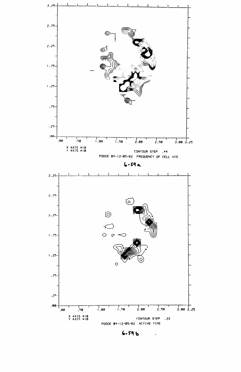
3.25- -
2.75-
2.25
I .75-
.25-
.75-
.25-
.50
X AXIS "10r AXIS »i0
I——i——|——i——|——i——i——1-50 2.00 2.50 3.00 3.25
CONTOUR STEP .11PODGE 01-12/05/82 FREQUENCY OF CELL vis
3.25-
1 .75-
I .25-
.75-
.00-
I___i I I I___i I I I
X AXIS "10 Y AXIS «I0
I I.•S0 1.00 I .S0 2.00 2.50 3.00 3.25
CONTOUR STEP .33 PODGE 01-12/05/82 ACTIVE TIME
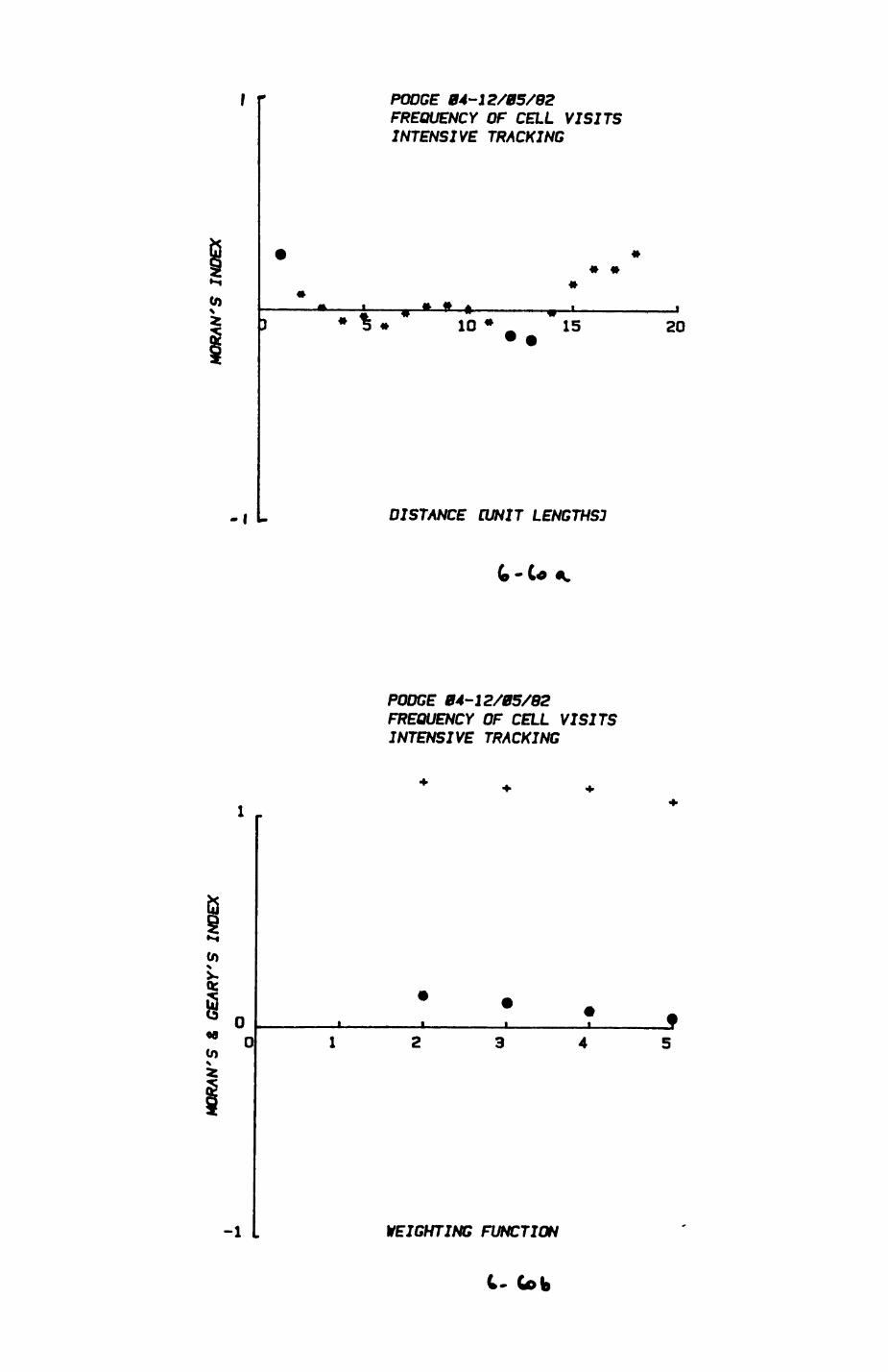
PODGE 04-12/05/82 FREQUENCY OF CELL VISITS INTENSIVE TRACKING
% • 10 * 15 20
DISTANCE [UNIT LENGTHS]
PODGE 04-12/05/82 FREQUENCY OF CELL VISITS INTENSIVE TRACKING
00
WEIGHTING FUNCTION
t- Cob
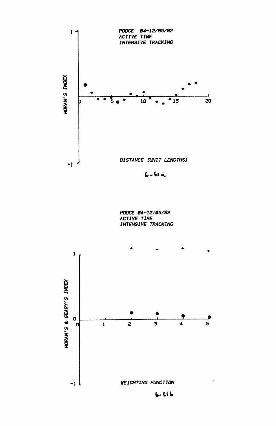
PODGE 04-J2/05/82 ACTIVE TIME INTENSIVE TRACKING
* 5 • * 10 « M * 15 20
DISTANCE CUNIT LENGTHS]
PODGE 04-1 2/05/82 dCriVE TIME INTENSIVE TRACKING
\ It
00
-1 WEIGHTING FUNCTION
(,-ClU
222
(DCA) of DCA run 19 (Chapter 2, program TCHANGE).
Programs DETSUM and DETPLOT complied for each area unit times,
frequencies and durations of visits. For patches, frequencies and durations
of visits. For patches, durations of visits were classified by 5 minute
intervals in 7 classest less than 5 minutes, 5-10 min, 11-15 min, 16-2O min,
21-25 min, 26-30 min, more than 30 min. Program TRANSFORM compiled
proportional and cumulative proportional frequencies. Program NEGEXP
(adapted from a program written by A. Hart) used the original data of visit
lengths to patches and compared them with expected visit lengths as derived
from the function-x/t 1 - e ^ t: parameters estimated as sample mean,
xt visit length (min).
This function describes the probability of occurrence of a certain visit
length for a random process of movement, le. equal probabilities to leave a
patch independent of the visit length elapsed until a given moment.
Differences between observed and expected distributions were tested with the
Lllllefors test for the exponential distribution (Conover (l98Oi 362)), a
test from the family of Kolmogorov-Smirnov goodness-of-fit tests.
The effect of the size of an area on its intensity of use and the
relations between the two measures of intensity of use were investigated by
linear regression analysis using the MINITAB statistical package available
on both the departmental PDP-11 computer and the university's VAX 11/78O.
6.2. Patterns of space use
The majority of studies considering the patterns of space use restrict
their attention to the problem of reconciling a favourite model of home
range usage with their data In order to calculate (hone range size (section
5.1)). However, home range models make certain assumptions about the

223
utilization distribution (UD, Van Winkle 1975). These include an expected
number of sites with a peak in activity (1 or several), the position of
these sites within the range and the configuration of the range. Empirical
justification of these assumptions is often lacking, for foxes at least
(Macdonald, Ball & Hough 1980). Alternative non-parametric methods (Ford &
Krurame 1979) can generate UD without a priori assumptions but, in their
present formulation, still suffer from several drawbacks. They are based on
an evaluation of activity summarized on a very coarse grid (7x7 points)
and they do not indicate the location of activity relative to the real
plane. Furthermore, they are most valuable for analysing data with little
information per individual gathered for many individuals/ consequently UDs
are often generated by averaging oVsr several individuals (the population
UD or PUD). In view of these restrictions, application of either of these
approaches seemed inappropriate.
In the following sections I shall concenrate on the following aspects
of space use:
(1) Sites with peaks of activities!
- how many centres of activity are present?
- where are they located within a range?
- does the number of these sites and their distribution within a range
vary between individuals?
- how useful is the concept of a centre of activity?
- do centres of activity coincide with peaks of resources?
(2) Scaling of space use:
- do regions of similar use exist?
- how large are they?
- in what fashion are they distributed?
(3) Predictability of space user
- how well can use of a given area be predicted from the use of other
224
areas?
- how does predictability vary with distance between predicted and
predictor areas?
(4) Variation within groupsi
- how do space use patterns (point 1 to 3) vary between members of the
same group?
- are there sex-specific differences?
Range use was investigated by evaluating measures of the intensity of
use on a grid with cell size 50 by 50 metres, as described in section 6.1.
Pig. 6.1-6.29 (foxes), 6.3O-6.50 (badgers) and 6.51-6.61 (foxes) illustrate
range use patterns and present the results of the computations of spatial
autocorrelation functions. I shall start with an analysis of range use by
foxes. A detailed description of one week of intensive tracking of a
breeding vixen Introduces the subject and conveys an idea of how to
Interpret the measures of Intensity of use. A second detailed description
of range use (by OLDMAHOG, section 6.2.2.) explains the interpretation of
the Figures and precedes a condensed account of the remaining individuals.
6.2.1. One week with PODGE in the breeding season
Pig. 6.51-6.57 (at the end of section 6.2) describe the movements of
the vixen PODGE in seven nights in early May 1982 (note that the last digit
of the figure numbers corresponds to the appropriate number of each tracking
night). The top picture of each figure shows the sequence of movements in
relation to the structure and the habitats of the area while the bottom
picture (viewed from the southwest) plots the duration of stay in each area
on a grid of 50 by 50 m cells.
Signals were recorded automatically at the den every 15 min during the
225
daytime throughout this week, and confirmed that PODGE spent all day with
her cubs in the den.
NIGHT 1: at 22.12 hours, PODGE leaves the area around the den with the
cubs behind and proceeds rapidly zig-zagging over two large fields in the
west of the range towards the back of Mrs. Gardiner's garden (22.25 hours),
where food scraps are frequently provided for the foxes. PODGE then (22.30)
moves towards HOME FARM where she spends 46 minutes around the barns,
probably hunting rats, mice and collecting scavenge. She then visits the
field south of Home Farm and moves quickly to the pasture field where she
remains until 00.37, foraging for earthworms. She then moves back to the
field south of the farm (root crops). Observations suggest that she is
hunting for both mice and earthworms. She then passes the farm, moves onto
the pasture fields southwest of Wytham Abbey at 1.13 (a good area for
earthworms), before she moves back, passing the farm at 3.42 and returning
to the den at 4.55 via the east side of the range.
Several interesting features emerge from PODGE'S movements. Firstly,
she spends hours at sites of special interest but moves quickly between them
(Fig. 6.5lb). Secondly, during her movements she visits, briefly, most of
the range borders. As subsequent nights show (e.g. Fig 6.53b) these were
not the most direct routes open to her. Finally, PODGE does not return to
her cubs until early morning. This could put them a£ risk (Klenk 1971),
unless the other group members are contributing to their well-being (e.g.
Macdonald I979b).
NIGHT 2: PODGE tracks again a portion of the western range border, at
00.30 and 2.12, spends 6 minutes at the farm (at 21.50) and ignores the
northern range section. Instead, she concentrates on the field with root
crops and the neighbouring pasture field in the south east. As in the
previous night, she does not travel in direct route to her den, but visits
the south east corner of the range, returning to the cubs at 5.40.
226
NIGHT 3j western border sections are visited again briefly. PODGE
spends more than 3 hours around the farm and the farm house, visits briefly
the site of intensive use of the previous night and visits for one and a
half hours the area along the bracken-woodland-field border, where rabbits
occur at high densities (Chapter 3). The eastern section of the border is
visited again.
NIGHT 4t western and eastern sections of the range border receive a
cursory visit. PODGE commutes between the area around the farm and the
field with root crops, and an area of mixed marshland, bracken and deciduous
woodland, where earthworms and rabbits are abundant. Again, cubs are not
visited before 6.08 in the morning.
NIGHT 51 a Saturday, PODGE keeps away from the heightened human
activity in the village, and spends 6 hours in the bracken and field area
north west of the den. Brief excursions to the western and eastern border
sections occur at 00.25 and 22.30, respectively. She probably revisited her
cubs at 01.30 and, possibly at 4.00.
NIGHT 6: PODGE concentrates again on the southern areas of the range
and stays within the woodland boundary except for an extensive excursion to
the western range border.
NIGHT 7: PODGE starts another round-trip along the border of her range,
this time commuting frequently between the area of her den and a spinney at
the southeastern tip of Mrs. Gardlner's garden. Each time PODGE follows a
different route and she finishes with a brief patrol along the western
border of the range. During these trips PODGE moved her cubs to an earth in
Mrs. Gardiner's spinney.
The similarity of movements on nights 1 and 7, round-trips along most
sections of the range border, may indicate some long-term cycllclty in
PODGE'S ranging behaviour. Doncaster (1985) found cyclical regularities in
the activity of Oxford's urban foxes.
227
A striking fact was the regularity with which PODGE visited the border
of her range, sometimes via large detours. PODGE presumably faced the
"travelling salesman" problem: how to visit a number of places with a
minimum of effort in time or energy expenditure, so that a maximum of effort
can be dedicated to the activities at a site. The solution of this problem
is complicated by the fact that visiting a site may only be useful if she
arrived at a particular time (e.g. before other foxes have eaten the scraps
at Mrs. Gardlner's garden) or under certain climatic conditions
(earthworms). Given these constraints there will be no general optimal
solution, but a variety of alternatives equally applicable. In such a
situation, rules of thumb are expected to be a simple and efficient device
(Janetos & Cole 1981, Houston & McNamara 1984). One rule of thumb seems to
be "visit stretches of the range border distant from foraging places either
on the way to these places or on the way back" (all sections, Nights 1 and
7; eastern section Night 2 and 3; western section, Night 4). Several visits
to range borders are, however, not covered by this rule (all sections Night
5; western section, Nights 2,3,6). These constitute true detours where
PODGE 'goes out of her way' to visit the range border.
Fig. 6.58-6.59 summarize the entire week and show 3D and contour plots
for the number of visits (NOV) and the duration of stay (DOS) per 50 by 5O m
cell, in the contour plots, black areas are the result of contour lines
sitting so close to each other that resolution of single lines becomes
Impossible, indicating steep slopes and dramatic changes In CJI of
neighbouring cells. The white areas surrounded by the black areas represent
plateaux where the UI is higher than the top contour level chosen. The two
plots complement each other in yielding a detailed visual impression of
changes in CJI. The contour plot presents a more detailed picture of the
positions of areas of high and low UI, while the 3D plot gives a better
indication of the magnitude of these changes.
228
There seem to be areas of high and low UI of similar activity. I will
call these areas "activity patches" (to distinguish them from habitat
patches of the habitat map). It is reassuring to find that PODGE seems to
confirm the basic idea of the habitat map (a patch arrangement in contrast
to a continuous gradient). However/ the decline in the UI from these
patches is uneven, different patches have different Uls and the
determination of the size of these patches looks at best ambiguous. Is
there a method that permits us to decide whether these patterns are 'real'?
This is the problem of scaling space use. On a local level, how can we
decide whether a given change in UI from one cell to another is sufficiently
small to assign both cells to an area of 'similar' use (an activity patch),
or sufficiently large to indicate that they are separate? On a general
level, can we Interpret changes in Uls on a large scale as 'patterns'! are
there regularities (symmetries) in the distribution of Uls?
To answer these questions, and to reveal the patterns of spatial
dependence between different sites, I computed the spatial autocorrelation
function for classes of sites with increasing distance between each other
(Appendices 5-7) and plotted them in Fig. 6.60a and 6.6la. Such a plot is
called a spatial correlogram. Each point indicates how similar the Uls are
of pairs of grid cells at a given distance, called the spatial lag. For
instance, at spatial lag 1, where each cell is taken in turn and its UI
compared with those of all cells that are immediate neighbours and have been
visited at least once by the animal, the correlation has a value of 0. 26
for NOV and 0.17 for DOS (significant at p<O.OOl and p<0.0l). Positive
autocorrelation indicates that cells exhibit similar Uls. In both Fig.
e.eoa and 6.6la, significant positive spatial autocorrelation coefficients
(SAC) are restricted to immediate neighbourhood (lag 1) for both measures of
intensity of use. Pairs of cells at a distance of already two lags show
Independence of ui. what can we conclude from this?
229
The compilation of UIs as shown in Pig. 6.58 and 6.59 has indicated that
there are preferred (activity patches) and neglected areas within the range.
The computation of SACs provides us with a quantitative measure to indicate
that (i) areas of similar use are small and restricted to a size of 50-100
m; (ii) UI of a site only depends on its immediate neighbours, the influence
of the spatial location of a cell on its UI is a highly local affair.
The computation of SACs also helps us to investigate another visual
Impression from Fig. 6.58 and 6.59. The two measures of intensity of use,
NOV and DOS, differ in one intriguing aspectt variation between cells in MOV
is small as compared with the variation In DOS (Pig. 6.58a vs. Pig. 6.58b).
DOS seems to be a better indicator of the status of a cell, ie. whether a
certain area is merely used as a transition area between centres of activity
or constitutes a centre of activity itself. There is a significant negative
SAC for DOS for lag 6 (250 m), indicating a contrast of UI at this distance,
but not for NOV!
The interpretation of the results of fitting spatial models to the
tracking data (Pig. 6.60b and 6.61b) will be discussed in detail in the next
three sections.
In summary, intensive tracking over a period of a week revealed the
kind of activity that contributes to the formation of activity patches as ^H s the development of areas of low utilization intensity. These are
areas which may be regularly visited but only for a short duration.
Activity patches are not an artificial phenomenon/ they are real as
evidenced by the amount of time
the individual invests in them. PODGE is quite flexible in choosing
different routes to reach the same site or connect different pairs of sites.
Despite the heavy energetic demands on PODGE due to the cubs, she puts
considerable effort into maintaining range borders. However, it may well be
that such dedication to the range border is an essential prerequisite for
230
maintaining exclusive access to the resources within the range.
6.2.2. Range use by OLDMAHOG
OLDMAHOG represents Range 6, the Singing Way Range. Fig. 6.17a is a 3D
plot of the UI of her range, based on fixes selected according to the 15 min
independence interval criterion, on a grid of 100 by 10O metres, viewed from
the southeast. Fig. 6.17b depicts a contour plot of these data (equal
levels of UI are delineated by contour lines, separated by increments of 1
location per cell, the top contour line enclosing areas with more than 20
locations per cell).
It is obvious that not all cells are used in a similar manner. Several
peaks can be identified, but there are also regions of medium height, and
consequently medium UI, and little used areas. The major peaks occur in the
south of the range while the arithmetic mean (centre) of the range seems
rather devoid of intensive use. The most intensively used area is a site
towards the southwest where a peak emerges from a plateau of high UI. This
is favourite daytime lying-up site in mature deciduous woodland, but also
intensively used at night, and close to the breeding territories of several
cock pheasants and a number of rabbit warrens. (Note that there is no fox
den). The extension of the range towards the northwest covers the pasture
fields of the Wytham Park where earthworms are abundant. A trough of low
UI, running from the southwest to the northeast, separates these areas from
a second area of high UI in the southeast where abundant sweet chestnut
trees attract many grey squirrels (Sciurus carolinensis). and several rabbit
warrens and pheasant territories are present as well.
Spatial autocorrelation coefficients (SAC) were computed to analyse the
scaling of space use in a quantitative manner (see previous section and
Appendix 5). The results are plotted as a spatial correlogram in Fig.
231
6.18b.
For OLDMAHOG, positive correlations were identified for the first six
lags. This means that up to a distance of 250 m there were more pairs of
cells with similar UI than expected from a random arrangement of the
observed in UIs in space.
At spatial lags of medium order (8 to 20, or 350 to 960 m) significant
negative correlations were found. Thus, in a broad range of mediumo
distances, tvo many pairs of cells of a given distance had dissimilar UIs as
compared with a random arrangement of the same values in space. We
therefore have to conclude that ups and downs in CJIs are distributed in
space in such a fashion that similar values stick together, but do so only
over a limited range - with increasing distance, the proportion of
dissimilar values increases, indicating a real change in CJIs. At larger
distances, correlations become positive again. As the contour plot (Pig.
6.l7b) indicates, this is due to the similar level of comparatively low
activity in the border zones of the range.
Pig. 6.18a shows the results of fitting several spatial models to the
data. Two different SACS, Koran's I (circles if significant, stars if not
significant) and Geary's c (zeros if not significant, filled zeros if
significant) are plotted against the model number ("weighing function"). In
contrast to the correlogram, where only pairs of cells of a given distance
were considered per spatial lag, the spatial model includes all pairs of
cells (except for Model 1 which is identical to spatial lag 1). Each model
constitutes a proposal concerning how the UI of cells of a given distance
exert an influence on the QI of a given cell. The Influence of cells
declines with distance according to a specific function!
232
Model 1: weight of influence = 1; 0 < distance < 0.99 lags
Model 2i weight of influence - exp -(distance)
Model 3: weight of influence = I/(distance) 2
Model 4s weight of influence = exp -0.5 (distance)
Model 5s weight of influence = I/distance
Models 2 to 5 are distinguished by an increased consideration of pairs
of cells with large distances. Thus, with increasing model number, along
the x axis in Fig. 6.l8a, spatial effects over a large distance attain more
importance. For our considerations, the exact function describing the
influence of cells at varying distances from a given cell is not so
important as a comparison between the results of the different models, ie.
the question of how does an increasing consideration of cells at large
distances change the degree of spatial dependence exhibited by the data?
The value of the SAC indicates the degree of spatial dependence while the
slope connecting the SACs from different models reveals the importance of
cells at larger distances. Together, they point to the major structure of
the range:
233
High SAC values
(Koran's I)
Moderate SAC values
(Koran's I)
Shallow
slope
(1)
range contains a
fairly large propor-
(2)
range contains a mixture
of areas of high and low
(Koran's I) tion of land used in a UI/ some are large and
uniform way; changes in have similar CJIs or are
UI to the periphery are small and arranged in a
gradual and moderate regular fashion
Medium
slope
(3) (4)
range contains a fairly range contains a mixture
large proportion of land of areas of high and low
(Koran's I) used in a uniform way; UI of varying size
changes in UI towards
the periphery are radical
Several activity patches and larger areas with comparatively little use
yield medium SAC values for OLDMAHOG and result in a medium slope (ie. the
disturbance caused by considering cells at larger distances is moderate). I
would therefore place her in category 4 of the above list.
What does the application of spatial models and correlograms tell us
that we cannot deduce from visual inspection of 3D or contour plots?
(1) Ups and downs in Uls from cell to cell can of course be Identified from
graphs but mere visual impression cannot indicate whether changes in UI are
arranged in space in a random fashion. Why is this important. Because we
do not want to be misguided in our inerpretation of the background of high
or low uis - we do not want to confound spatial inevitabilities with a
234
preference due to the intrinsic attractivity of a habitat. Specifically, if
we want to test habitat preferences or other aspects of range use we have to
make sure that the UI of area units are independent from each other.
However, if we find spatial dependence - as described for OLDMAHOG - we have
to adjust the test statistic (see Appendix 5).
(2) We can compare range use on a quantitative basis. A comparison of
spatial models provides us with a mean*to compare range use patterns of
different individuals. Of course, we can compare range use without
computing SACS, but by using SACs we can attach a precise meaning to our
comparison.
(3) The results of fitting spatial models gives us a compressed summary of
the predictability of space use of an area unit by other area units. This
Is not only Interesting per se, and important for statistical tests.
Predictability of space use may be important for other individuals, whether
they coinhabit the same range or are merely interested in the activities of
their neighbours. Simply looking at 3D plots does not reveal
predictability. Compare, for instance, the 3D plots of GRIZZLE
(predictable) and OLDSABRE and TARU (unpredictable), or the two essentially
linear ranges of SURPRISE (predictable) and LIO (unpredictable). The
graphical presentation is here insufficient to provide the required•
Information. Certainly the UI of a site related to its intrinsic
characteristics (e.g. section 6.2.1.). However, the presence of resources,
for Instance, is Insufficient to 'guarantee 1 a certain level of UI. A good
example is variation in range use within badger groups in section 6.2.5. or
in the HOMEFARM fox group (section 6.2.4.). Take the range use by the two
vixens, BRAMBLE and PODGE (Pig. 6.1-6.2, 6.23-6.24). Superficially they are
similar. However, the analysis reveals that predictability of UI is high
for BRAMBLE and moderate for PODGE. The extensive areas in the west of
PODGE'S range contribute to the disturbance caused by cells of dissimilar
235
values at larger distances and the greater heterogeneity of UIs near the
peaks of activity depress the overall level of predictabilty. Consequently,
both individuals are assigned to different categories of range use patterns
(BRAMBLE: 3; PODGE: 2).
In summary, there are clear spatial dependencies in the way OLDMAHOG
uses her range. Several preferred areas could be identified (activity
patches) with an estimated diameter of between 50 and 250 metres. Activity
patches were separated from each other by areas of low use. Changes in UI
are rather pronounced as evidence by the broad range of spatial lags when
pairs of cells show dissimilair values. These patterns of range use can be
predicted from the UI of other cells to a significant and reasonable degree,
if the influence exerted by cells at larger distances is reduced.
6.2.3. Range use by other foxes
The following summaries present for each individual results to the
following aspects:
(1) Number of activity patches
(2) Habitat and resource presence in activity patches
(3) UI of the arithmetic mean (important for potential
application of probabilistic home range models)
(4) Scaling of space use
(5) Predictability of UI as evidenced by the results of spatial
methods
(6) Category of range use patterns
For three foxes, space used could not be distinguished from a random
arrangement, it is therija difficult if not impossible to speak of 'patterns*
of range use; then a categorization of range use pattern seemed
236
inappropriate.
BRAMBLE (vixen, Pig. 6.1-6.2; note the scale of the z-axis in Pig. 6.la).
(1) There are three activity patches present.
(2) The northern activity patches centre around Home Farm and Mrs.
Gardiner's garden and backyard (earthworms and scraps), the southern patch
is a strip of pasture plus the border region of deciduous woodland-bracXen-
arable land (earthworms, rabbits).
(3) The arithmetic mean is not a centre of activity.
(4) Sizes of activity patches are small (lag 1-3), and there are definite
troughs at several places (lags 7-8, 13-17). The overall range use is
asymmetric and biased towards the northern part (no positive correlations at
high lags).
(5) Increased consideration of cells at a larger distance result in a large
reduction in the accuracy of prediction of the UI.
(6) All spatial models describe significant spatial dependence; but
predictability decreases rapidly from a high level; therefore category 3.
ELKE (vixen, Fig. 6.3-6.4).
(1) Several small activity patches present.
(2) Activities centre around the Churchgrove Farm and the Binsey Farm and
adjacent pastures (scraps, earthworms). The activity patch in the north is
a preferred earthworm hunting ground (pasture).
(3) The arithmetic mean is not a centre of activity; the range is banana-
shaped.
(4) Large proportions of the range are either intensively or comparatively
little used. Activity patches are medium-sized (lags 1-4). They are
clearly distinguished from other areas (negative SACs at lags 8-16).
Overall range use is asymmetric.
237
(5) Spatial models do not reveal significant dependencies, except for Model
1.
(6) The separation in two areas with different base levels of CJI results in
a shallow slope; therefore category 2.
GASPER (dog-fox, Pig. 6.5-6.6).
(1) One large centre of activity present.
(2) This includes Home Farm and the pasture around wytham Abbey (scrape,
mice, earthworms) and Mrs. Gardiner's garden and backyard (scraps and
earthworms).
(3) The arithmetic mean coincides with the peak in activity.
(4) Size of centre of activity is small (lag 1-3), decline of CJI towards the
periphery rapid (no positive SACs at medium lags). Occasionally visited
sites outside the group range are responsible for some significant negative
SACs at large lags.
(5) Models indicate a high degree of predictability, declining rapidly with
increased influence of distant cells.
(6) The observed pattern is assigned category 3.
GRIZZLE (vixen Fig. 6.7-6.8).
(1) Two activity patches of small size (lags 1-2) and a complex of small
peaks (a "plateau") in the southwest.
(2) Both peaks occur in areas of high earthworm abundance, one in pasture,
the other in deciduous woodland.
(3) The arithmetic mean does not coincide with a peak in activity.
(4) uis between the two activity patches are rather variable, one trough
separating the northern patch from the "plateau" and the southern patch.
The impression of a regular arrangement of the peaks is supported by a
algnifleant positive SAC at lag 10, but the decline towards the periphery Is
238
asymmetric (lags 15-16).
(5) Overall predictability of space use is low, but the spatial dependence
exhibited is significant.
(6) The regular arrangement of peaks produces a shallow slope in the decline
of predictability (category 2).
KALI (vixen, Pig. 6.9-6.10).
(1) Several major areas are arranged in a roughly linear fashion from west
to east.
(2) The westernmost patch covers a small woodland surrounded by fields and a
small farm, Slmpson's cottagej the next patch to the east lies in a field
with long grass where I could frequently observe her catching mice) the
complex in the east covers a residential areas with some allotments at the
back and the easternmost area includes a small local school with a sports
ground (scraps and earthworms).
(3) The range is banana-shaped, the arithmetic mean lies outside centres of
activity.
(4) Patches are medium-sized (lags 1-4) and separated by several troughs)
areas which are quickly crossed and that only serve as a connection from one
major area to another (see section 6.2.6). The positive SACs at large lags
indicate symmetrical UI, due to the position of activity patches at extreme
positions, but an assymetric decline towards the west results in a last
negative SAC.
(5) All spatial models describe significant spatial dependencies and have
moderate success in predicting CJls.
(6) The regular linear arrangement produces a shallow slope in the decline
of predictability if distant cells are progressively more considered)
therefore category 2.
239
KBOQM (vixen, Pig. 6.11-6.12).
(1) Usage patterns are similar to OLDMAHOG. Two major areas separated by a
trough.
(2) Peak areas include: Woodend Farm and Bean Wood, areas north of Bean Wood
and particularly the backyards and parkland of the Buddhist centre and the
long grass fields and gardens of the three houses east of the Buddhist
centre where I frequently observed her hunting for rodents.
(3) The arithmetic mean is near a centre of activity.
(4) Patterns of use are very regular, e.g. the symmetrical decline of UI
towards north, northwest and northeast, resulting In a perfect spatial
correlogram.
(5) Spatial dependencies revealed by the models are pronounced and highly
predictable, which is not surprising in view of the regularities exhibited
in Fig. 6.lib.
(6)1 pto-<* KBOOM in category 1 with a tendency towards category 3.
KOBUK (dog-fox, Fig. 6.13-6.14).
(1) One major activity patch and two smaller peaks are present.
(2) The major patch is identical with the area preferred by GASPER while the
smaller peaks are close to the areas preferred by BRAMBLE.
(3) The arithmetic mean Is close to the centre of activity.
(4) Patch size is medium, and UI decline asymmetrically towards the
southeast (negative SACs at medium, and non-significant SACs at large lags).
(5) Spatial models reveal a high degree of predictability of UI from nearby
cells.
(6) This leads to a similarly steep slope as in GASPER/ therefore category
3.
24O
LIO (dog-fox; Fig. 6.15-6.16).
(1) The major peak is situated in deciduous woodland close to a fox den and
several rabbit warrens; a second smaller peak at a wood land/fie Id border
with a major pheasant roost.
(2) The arithmetic mean is close to the small peak of activity.
(3) The spatial arrangement of Uls corresponds to a random arrangement,
except for lag 3.
(4) No spatial dependencies could be identified.
(5) Since no clear spatial pattern present, categorization seems
inappropriate.
QLDSABRE (dog-fox, Pig. 6.19-6.20).
(1) One peak is evident.
(2) The peak lies in dense deciduous woodland; possibly rich in earthworms.
(3) The arithmetic mean is not at the centre of activity.
(4) No clear patterns are discernible; the spatial arrangement could be due
to a random process, since there are no spatial dependencies.
(5) UI are not predictable and none of the models produce significant SACs.
(6) Therefore, no category provided.
OLDSABRE occupied the woodlands in the southern part of the Radbrook
Common area. His range is exceptionally uniform in terms of habitat
diversity. However, OLDSABRE was tracked for only a short time, and the
number of fixes may be insufficient to reveal significant contrasts in UI.
PINTOQTH (vixen, Pig. 6.21-6.22).
(1) Several major peaks and a large plateau in the southeast are
characteristic for this range.
(2) Peaks coincide with the sites of several farm houses and large rabbit
warrens in the pasture/ long grass area northeast and west of the Hill End
241
camp Natural History school. The southeastern plateau covers a complex of
pastures and hedges where PINTOOTH frequently foraged for earthworms and
rabbits, and two school buildings (scraps).
(3) The arithmetic mean coincides with the centre of activity.
(4) The range is fairly symmetrically used, and peaks are separated by
pronounced troughs, both contributing to a perfect spatial correlogram.
(5) High predictability of ui.
(6) Therefore category 1, with a tendency to 3.
PODGE (vixen, Pig. 6.23-6.24).
(1) Three major activity patches are present, in nearly identical location
to those used by BRAMBLE.
(2) PODGE'S range extends further south west and covers more ground towards
the west (mainly agricultural land and, in the northwest, pastures).
(3) The arithmetic mean is not the centre of the range.
(4) Patch sizes are medium (lags 1-4). Extended areas of little UI between
the major peaks contribute to the significant negative SACs at medium lags.
(5) The predictability of UI by the models is significantly lower than in
BRAMBLE (section 6.2.4.). This is due to the extensive disturbance caused
by cells of dissimilar value at large distances, and to the greater
heterogeneity of uis near the peaks of activity as compared with BRAMBLE.
(6) This usage pattern corresponds to category 2.
SURPISE (vixen, Fig. 6.25-6.26).
(1) Three major activity patches can be identified.
(2) Two patches are very close together in the east, and one, an area around
a farm, in the west. This is an extremely one-dimensional range.
(3) The arithmetic mean is at the largest possible distance from any centre
of activity.
242
(4) Patches are of medium size (lags 1-4). The symmetric appearance is
reinforced by the positive SAC at large lags and the negative SACs at medium
lags.
(5) Predictability is only moderate, but little affected by large weights of
cells at larger distances.
(6) This corresponds to category 2.
TARU (vixen, Pig. 6.27-6.28).
(1) several peaks are Interspersed with areas of little UI.
(2) The western peaks correspond to an area completely covered by the Binsey
allotments, Whereas to the east TARU frequently foraged for rodents and
earthworms on pasture and In a field of grass ley.
(3) The arithmetic mean is close to a centre of activity.
(4) The spatial correlogram shows systematically changing, but insignificant
SACs.
(5) The predictability of UIs from other cells is low, since range use
cannot be distinguished from a random arrangement of UI.
(6) For this reason, a categorization seems inappropriate.
In summary, the patterns of range use were analysed for 14 foxes. They
were associated with usage categories as followst
category 1 i 2 individuals
2 : 5
3 i 3
4 i 1
no pattern i 3
This small list Indicates that the most notable feature of space use in
foxes is enormous variability, even within the same population, covering a
243
wide range from simple to complex patterns:
(i) two ranges were symmetrically used throughout the majority of the area
(category 1).
(ii) three ranges had a large centre of activity but UI declined rapidly
towards the periphery (category 3).
(iii) five ranges exhibit regularities that were of two Kinds. Activity
patches were regularly distributed, or ranges consisted of a well-used and a
neglected section, within each of which UI may vary again (category 2).
(iv) one range showed a truly impressive array of activity patches
interspersed with troughs of low activity (category 4).
(v) Three ranges were used in a way that could not be distinguished from a
random arrangement of UIs in space (no pattern).
Most activity patches were clearly associated with specific resources.
Most ranges were asymmetrically used or approached linearity (banana form).
The arithmetic mean rarely coincided with a peak in activity. Both results
underline the proposition that probabilistic home range models with a priori
expectations of UD are inappropriate, at least for foxes.
6.2.4. Range use within the HOMEFARM fox group
In the HOMEFARM group range four foxes were tracked with sufficient
Intensity to facilitate exploration of intra-group variation in space use.
Two adult males, GASPER and KOBUK and two females, BRAMBLE and PODGE,
occupied the range. In section 6.2.3. it was shown that both males
exhibited a fairly simple pattern of space use, highly predictable from the
surrounding cells, and concentrated on one centre of activity. The two
females exhibited a more complex pattern. They both used the same three
activity patches; one of these patches coincided with the area most
intensively used by the males. For the vixens, space use patterns were not
244
so predictable as for the males. The results of fitting the five different
models, the SAC, were regressed against the number of the model, where
models were arranged so that high model numbers indicated improved influence
of cells that were at a large distance from a given cell. The steep slope
of the regression lines of the two males (Table 6.2, Pig. 6.29) indicates a
rapid decline of reliability of predicting UI if cells at larger distances
attain more influence. For females, however, reliability of prediction,
although generally lower, is less sensitive to changes in the weighting
procedure. BRAMBLE has a considerably shallower slope than the two males,
although the differences are not significant, whereas PODGE'S slope is
shallower than any of the others.
There are several possible explanations of the differences in patterns
between males and females. First, if males dominate females, then females
might be expected to move away from the centre of activity of the males
whenever possible. Second, energetic considerations may encourage females
to look for large, profitable prey, such as rabbits, during the breeding
season. Such prey occurs only in the southeast and south of the HOMEFARM
range. However, utilization patterns before, during and after the cub
rearing season remained similar. Third, safety of cubs away from human
disturbance is an important factor to consider. In 1981, BRAMBLE probably
had cubs in Mrs Gardiner's garden close to prime food sources but then moved
them after a week or so to the wood, where PODGE kept her cubs a year later.
Obviously, females have to find a compromise between proximity to food and
the protection of the cubs from danger.
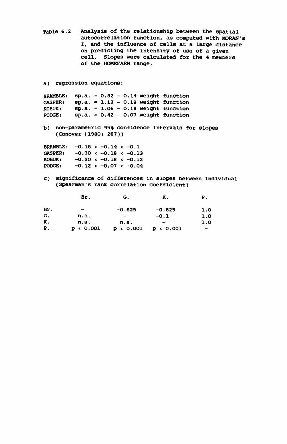
Table 6.2 Analysis of the relationship between the spatial autocorrelation function, as computed with MDRAN's I, and the influence of cells at a large distance on predicting the intensity of use of a given cell. Slopes were calculated for the 4 members of the HOMEFARM range.
a) regression equations:
BRAMBLE t sp.a. = 0.82 - 0.14 weight functionGASPERi sp.a. = 1.13 - 0.18 weight functionKOBUKi sp.a. - 1.06 - O.18 weight functionPODGE t sp.a. = 0.42 - O.07 weight function
b) non-parametric 95% confidence intervals for slopes (Conover (1980i 267))
BRAMBLEt -0.18 < -0.14 < -0.1GASPERi -0.30 < -0.18 < -O.13KOBUKi -0.30 < -0.18 < -O.12PODGE! -0.12 < -0.07 < -O.04
c) significance of differences in slopes between individual (Spearman's rank correlation coefficient)
Br. G. K. P.
Br. G. K. P.
n.s. n.s.
p < O.O01
-0.625
n.s. p < 0.001
-0.625-0.1
p < O.OO1
1.0 1.0 1.0
245
6.2.5. Range use by badgers.
The analysis of range use in badgers differs from that of foxes in that
only results from intensive tracking nights were selected for the analysis.
Since contour plots have already been presented in Chapter 5, the figures of
this section are restricted to 3D plots and the results of the computations
of SACs (correlograms and models) for both measures. To enable intra-group
comparisons, individuals of a group are presented together. Otherwise the
description follows in style the summaries for the foxes.
Range Bl (Botley Lodge). Pig. 6.30-6.31 depict the results for GEORGE,
6.32-6.33 for HELEN and 6.34-6.36 for SARA.
(1) All three individuals concentrate their efforts in the same area. In
addition, GEORGE ranges extensively towards the southwest. Both GEORGE and
HELEN have two, identical centres of activity at opposite ends of the range.
SARA'S only activity patch (according to duration of stay, DOS) coincides
with the northern activity patch of GEORGE and HELEN.
(2) The activity patch in the north is a small area of deciduous woodland
(sycamore/oak) with an understory of dog's mercury which is probably a good
indicator of high earthworm abundance (Chapter 3). The activity patch in
the south is partly woodland of the same type but also partly covered by
dense thickets. Here tree stumps and fallen tree trunks provide a good
medium for a rich invertebrate fauna. In this area I could frequently
observe the gradual decay of fallen trees pulled apart by badgers over
periods of several weeks, both in spring and autumn.
(3) The arithmetic mean falls into little used areas for all three group
members.
(4) Cell visits by HELEN could not be distinguished from a random
arrangement (Fig. 6.33). GEORGE produced significant negative SACs at
246
several medium lags, indicating a coarse partitioning of his range into two
activity patches. This partitioning is especially pronounced for NOVj
obviously the trough between the activity patches is wider for NOV than for
DOS. GEORGE visits the area between the activity centres less regularly
than the activity centres, but occasionally stays at the edge of the
activity patches for quite a while.
At medium lags, SARA, exhibits the same habits as GEORGE does for NOV.
However, the symmetric distribution of CJI over her range leads to high
positive SACs at extreme distances. This is in contrast to the gradient
shown by GEORGE due to his large extension towards the southwest, a little
used area. Similar to PODGE, DOS is a clear indicator of the centre of
activity in SARA'S range. Although SARA visits many cells at relatively
high frequencies, she spends only little time in them except for her
preferred foraging area in the north.
For both SARA and GEORGE, variability of CJI at a small scale is
sufficient to reduce areas of similar use to a small size (only lag 1
significant).
(5) Predictability of CJI is low for SARA but significant, while
Insignificant for both GEORGE and HELEN.
(6) All three grup members correspond to the situation typical for category
21 the simple structure of partionIng the range in coarse sections makes
predictability insensitive to changes in influence of cells at large
distances. Small scale heterogeneity of CJI is sufficient, however, to
depress the reliability of prediction.
Range B2 (Upper Follies). Fig. 6.37-6.39 depict the results for ALI, 6.40-
6.42 for NANI and 6.43-6.45 for WILF.
(l) Range use, as illustrated by the 3D plots is very similar for the two
females. WILF includes an additional occasionally visited eastern section
247
in his range. No special sites of high activity could be identified, except
the sett in the north of the range.
(2) Most of the utilized areas cover pasture/ a prime earthworm habitat
(Chapter 3). Small-scale variability of availability of earthworms in space
and time seems to prohibit the formation of highly preferred, uniformly used
areas.
(3) The arithmetic mean of the ranges is not characterized by activity
peaks.
(4) ALl's pattern of range use is characterized by considerable
heterogeneity in UI at such a small scale that the formation of uniformly
used areas is prohibited; consequently the SACs are Insignificant and
fluctuate round zero. The small-scale heterogeneity is evident also in
NANI's range use but overshadowed by medium-sized trends producing
significant SACs at medium and high lags. The contrasting UI in the north
(where the main sett is situated, an area heavily used by all three
individuals) and the southwest create a gradient as evidenced by the
strongly SAC at extreme distances. WlLP's range use reveals heterogeneity
of UI at a larger scale (lag 1 significantly positive) but otherwise similar
to ALL
(5) Reliability of prediction of UIs by the models is very low and
dependencies are insignificant except for NOV of WILP and DOS of ALI,
leaving the overall impression that the use of a given cell is basically
independent from the use of other cells. UI may be find-tuned at a scale of
the size or smaller than the selected cell size.
(6) since it is difficult to speak of activity patches a categorization
seems inappropriate.
Range B4 (Jew's Harp). Pig. 6.46-6.48 depict the results for PEACEFUL and
Pig. 6.49-6.50 the results for VICIOUS.
248
(1) Three small peaks of activity are recognizable in VICIOUS 1 range. Pour
major activity patches occur in PEACEFUL's range.
(2) The westernmost activity patch in PEACEFUL f s range is situated at the
southeastern border of the pasture fields of Wytham Park (the area Where
microclimatlc measurements were undertaken as described In Chapter 3).
Another activity patch occurs around Wormstall Duck Pond, a small spinney at
the bottom of the Park and surrounded by pastures. Two activity patches,
one in the centre, and one in the east of the range. Both cover small areas
of deciduous woodland, a mixture of sycamore and oak wood with an understory
of dog's mercury, areas supposedly rich in earthworms. They border onto the
mixed plantations further south which are also well used. These two
activity patches are also frequently visited by VTCIOUS, but he spends
relatively more time in the plantations than PEACEFUL.
(3) The arithmetic mean falls close to highly used areas in both ranges.
(4) Peaceful's activity patches are relatively small (positive SACs for lag
1 and 2, NOV). These peaks are separated by a system of less visited
troughs (lag 6-8). The activity patches are distributed in a regular
fashion over the entire range and range use declines symmetrically towards
the periphery. Both factors produce positive SACs at large lags again.
Medium-scaled heterogeneity in UI is sufficiently large to create a less
clear although, in trend, similar picture for DOS in PEACEFUL's range. The
considerable small-scale heterogeneity of UI in VTCIOUS 1 range prohibits the
formation of larger patches. Little used areas, however, can be clearly
recognized and lead to negative SACs at lag 3.
(5) Predictability of UI is only moderate for PEACEFUL and non-existent for
VICIOUS.
(6) PEACEFUL corresponds to category 2.
in contrast to foxes, the badgers studied are very similar in their
249
basic pattern of range use. This pattern is characterized by a considerable
small-scale heterogneity, preventing in many cases the formation of large/
uniformly used areas. Then, the distribution of UI within a range can often
not be distinguished from a random arrangement, at least not at the chosen
scale of spatial resolution. In two groups, one high quality habitat type
covers a large proportion of the actuallv utilized part of the group range,
pasture for individuals of group 2 and deciduous woodland for individuals
from group 1. Obviously, these badgers restricted their visits to areas of
special interest to them and thus utilized only part of the group range.
Where ranges span a variety of different habitats, UI proliferates and
yields a more complicated picture. This is especially evident for PEACEFUL,
but also applicable on ELIANE and NOEARS, two individuals not considered
here before. Contour plots of their range use were presented in Chapter 5
(data selected according to the 15 min Independence interval criterion).
Both NOEARS and ELIANE displayed ranges with many areas of high UI
Interspersed with areas of low UI, qualifying for category 2. For both
individuals, all spatial models were significant, but reliability of
prediction of UI generally low (highest correlation coefficients for ELIANEi
0.22, and for NOEARSt 0.13).
6.2.6. Direction preferences in local movements
In this section I will investigate whether foxes and badgers show
preferences for certain routes. One way of examining this question is to
select a particular patch, hereafter called the 'origin patch', and
investigate an individual's movements towards and away from it. The origin
patch forms the base of a network of patches called the 'local window*.
This window includes all patches Immediately bordering onto the origin
patch, if an individual visited during periods of intensive tracking, say
250
15 patches, then 15 local windows can be created, one for each patch. A
•link 1 was defined as the connection that an animal has travelled between
two patches within one local window. For each link, the number of crossings
la counted. Usually, the sum of Arrivals to a specific patch from all
neighbouring patches equals the sum of Departures from that specific patch
to all neighbouring patches (except for the first and the last patch of a
given tracking sequence). However, the links leading to and from a given
patch may be used to different extents. Three questions can be explored
within this frameworkj
1. The frequency with which different links are crossed can give some
indication of the existence of preferred paths. Do foxes and badgers have
frequently used 'highways' and rarely used 'by-tracks'?
2. Do foxes and badgers have directional preferences in the way that they
travel their home ranges?
3. If direction preferences occurred in several links associated with an
origin patch, are the differences between the asymmetries significant? To
Investigate this, a procedure was devised that ranked all patches of a local
window on a continuous scale according to the difference of Departures and
Arrivals along each link (Appendix 8). The distances betwen the ranks of
all patches were then simultaneously assessed to determine whether direction
preferences varied significantly between links (evaluated per match).
In Pig. 6.62, transition frequencies of KBOOM are shown for all links
between an origin patch and its neighbours. Frequent transitions occur
between patches Y and X and between X and Z (patch preference), and in 77.8%
of all transitions between X and Y KBOOM left Y and arrived in X (direction
preference). The figure illustrates the difficulties of such an analysis
that deals with natural and therefore unevenly shaped area units. For
instance, the whole eastern surface of Y borders X (and the majority of
crossings between Y and X start from Y to X), while only a fraction of the
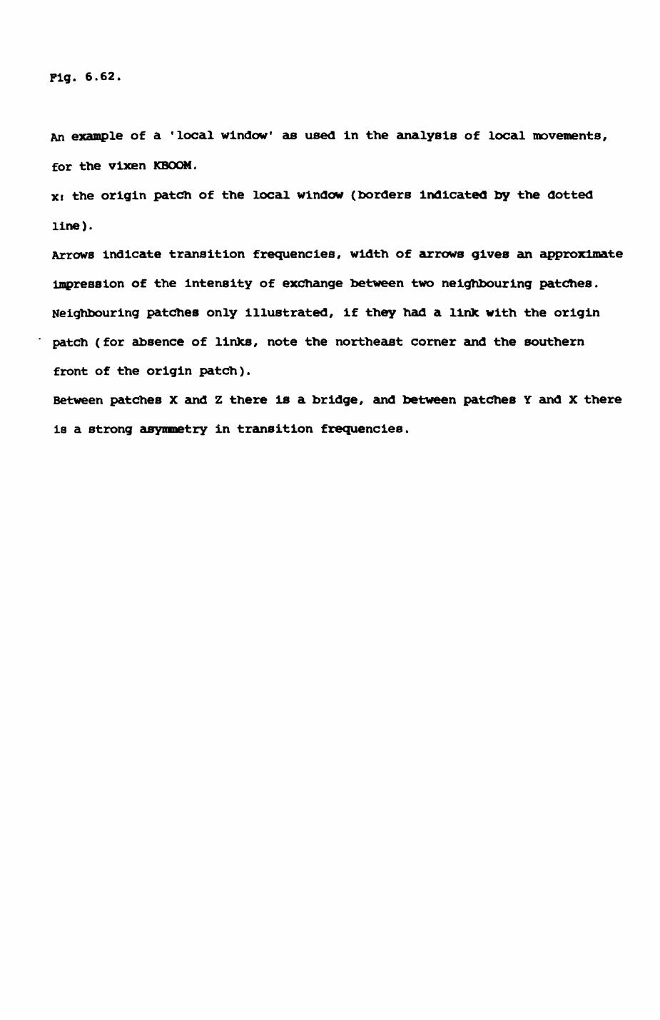
Pig. 6.62.
An example of a 'local window' as used in the analysis of local movements,
for the vixen KBOOM.
xi the origin patch of the local window (borders indicated by the dotted
line).
Arrows Indicate transition frequencies, width of arrows gives an approximate
impression of the Intensity of exchange between two neighbouring patches.
Neighbouring patches only illustrated, if they had a link with the origin
patch (for absence of linJcs, note the northeast corner and the southern
front of the origin patch).
Between patches X and Z there is a bridge, and between patches Y and X there
is a strong asymmetry in transition frequencies.
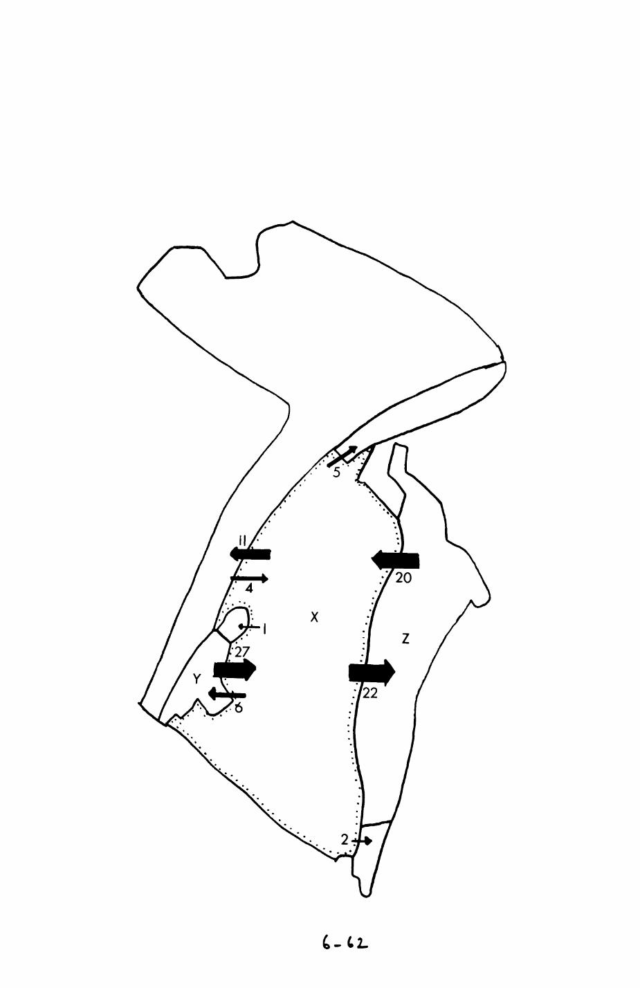
UC2.
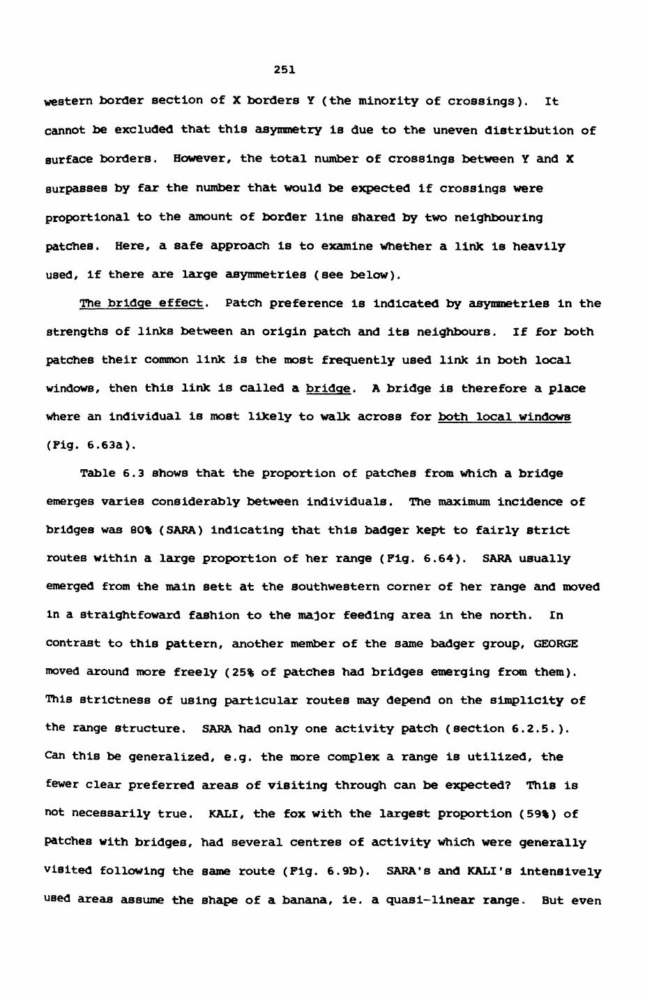
251
western border section of X borders Y (the minority of crossings). It
cannot be excluded that this asymmetry is due to the uneven distribution of
surface borders. However, the total number of crossings between Y and X
surpasses by far the number that would be expected if crossings were
proportional to the amount of border line shared by two neighbouring
patches. Here, a safe approach is to examine whether a link is heavily
used, if there are large asymmetries (see below).
The bridge effect. Patch preference is indicated by asymmetries in the
strengths of links between an origin patch and its neighbours. If for both
patches their common link is the most frequently used link in both local
windows, then this link is called a bridge. A bridge is therefore a place
where an individual is most likely to walk across for both local windows
(Fig. 6.63a).
Table 6.3 shows that the proportion of patches from which a bridge
emerges varies considerably between individuals. The maximum incidence of
bridges was 80% (SARA) indicating that this badger kept to fairly strict
routes within a large proportion of her range (Pig. 6.64). SARA usually
emerged from the main sett at the southwestern corner of her range and moved
in a straight toward fashion to the major feeding area in the north. In
contrast to this pattern, another member of the same badger group, GEORGE
moved around more freely (25% of patches had bridges emerging from them).
This strictness of using particular routes may depend on the simplicity of
the range structure. SARA had only one activity patch (section 6.2.5.).
Can this be generalized, e.g. the more complex a range is utilized, the
fewer clear preferred areas of visiting through can be expected? This is
not necessarily true. KALI, the fox with the largest proportion (59%) of
patches with bridges, had several centres of activity which were generally
visited following the same route (Pig. 6.9b). SARA'S and KALI'S Intensively
used areas assume the shape of a banana, ie. a quasi-linear range. But even
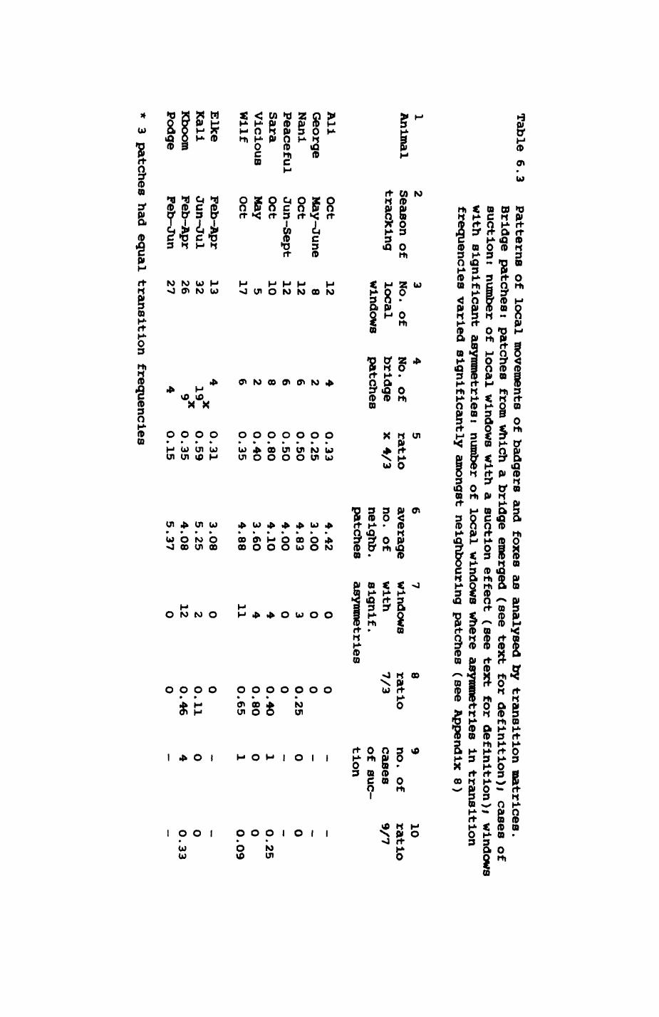
Table 6.3Patterns of
local movements of badgers and foxes as analysed by transition matrices. Bridge patchesi
patches from Which a bridge emerged (see text
for definition)/ cases of
suctiont number of local windows with a suction effect
(see text for definition);
windows with significant asymmetriest
number of local windows where asymmetries in transition
frequencies varied significantly amongst neighbouring patches (see Appendix 8)
1Animal
AliGeorgeNaniPeacefulSaraViciousWilf
ElkeKaliKboomPodge
2Season oftracking
OctMay-JuneoctJun-SeptOctMayOct
Feb-AprJun-JulFeb-AprFeb-Jun
3No. of
localwindows
12a12
12105
17
1332
2627
4NO. Of
bridgepatches
42668264 x
199X
4
5ratiox 4/3
0.33
0.25
0.50
0.50
O.80
0.40
0.35
0.31
O.59
O.35
0.15
6averageno.
ofneighb .patches
4.42
3.00
4.83
4.00
4.1O
3.6O
4.88
3.O8
5.25
4.08
5.37
7windowswithslgnif .asymmetries
O03O4411O2120
8ratio7/3O00.25
O0.40
0.80
0.65
OO.ll
0.46
O
9no. of
casesof suction
_—0—1O1—O4—
10ratio9/7
_—O—0.25
0O.O9
—O0.33
—
* 3 patches had equal transition frequencies
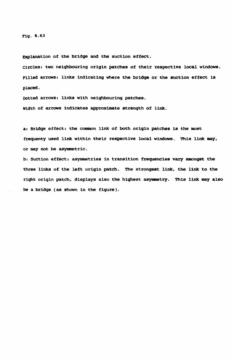
pig. 6.63
Explanation of the bridge and the suction effect.
Circlest two neighbouring origin patches of their respective local windows.
Filled arrows i links indicating where the bridge or the suction effect Is
placed.
Dotted arrows i links with neighbouring patches.
Width of arrows Indicates approximate strength of link.
at Bridge effect: the common link of both origin patches is the most
frequenty used link within their respective local windows. This link may,
or may not be asymmetric.
b: Suction effect: asymmetries in transition frequencies vary amongst the
three links of the left origin patch. The strongest link, the link to the
right origin patch, displays also the highest asymmetry. This link may also
be a bridge (as shown in the figure).
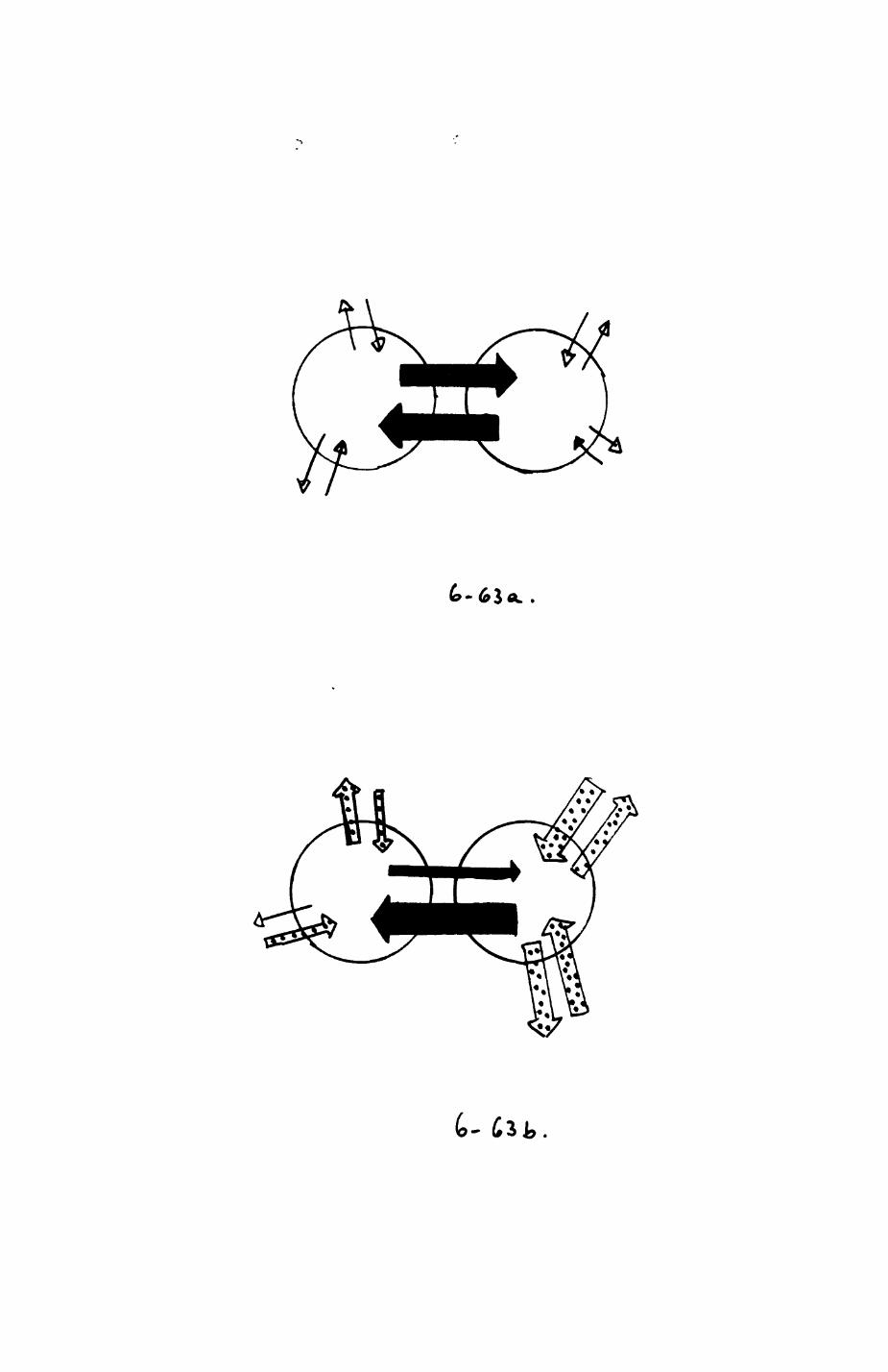

Pig. 6.64
Movements of the badger SARA in one night, illustrating the directionality
of local movements.
Radio locations were plotted with program PLOT, and the section of the
habitat map by program MAPITH (see Fig. 6.51 for details). Scalet 80O by
800 metres. Sara moves from the southeasternmost fix, the sett, to the
ma}or feeding areas in the north along a very strict route, at the edge of
the woodland to the neighbouring wheat fields.
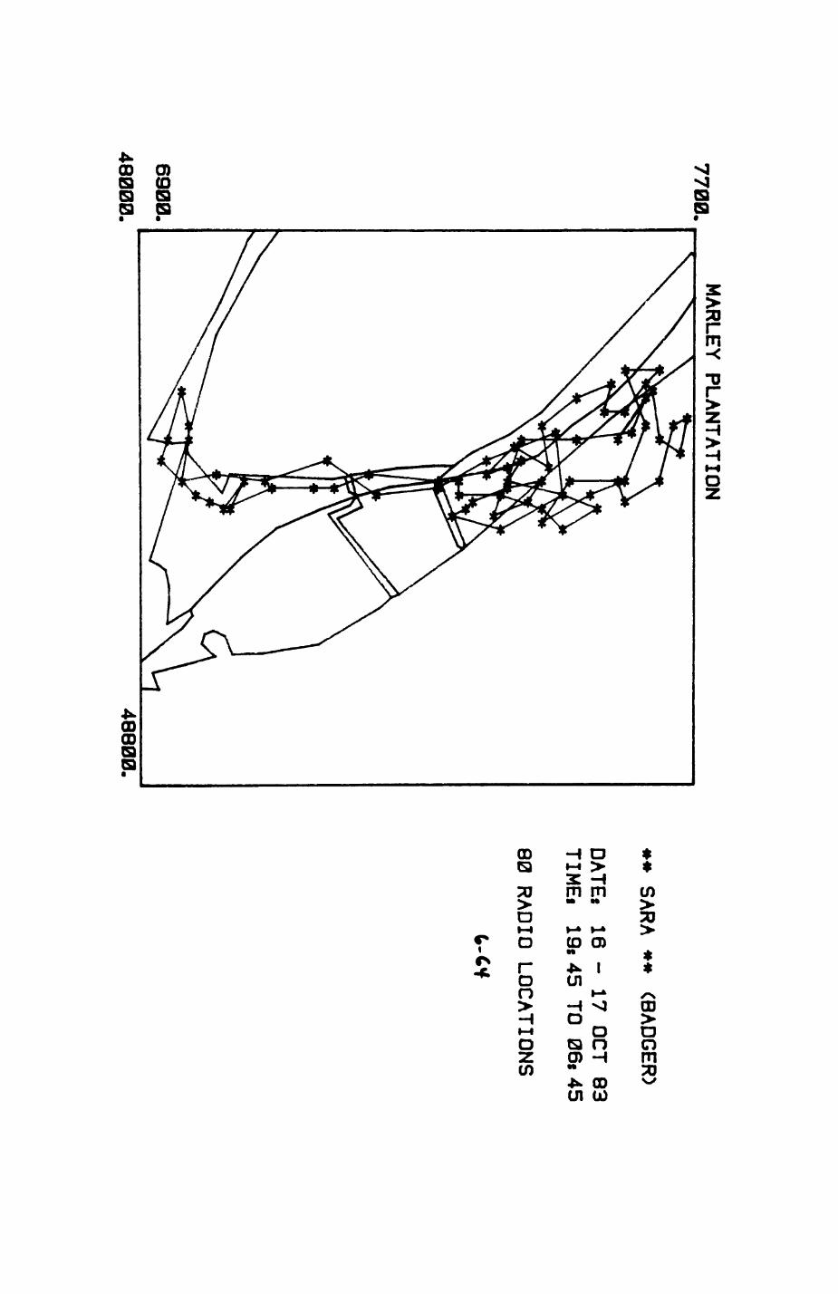
7700.MARLEY
PLANTATION
6900.
48000.
** SARA
** (BADGER)
DATE*
16
-17
OCT
83 T
IME
i 19i 45
TO
06i 45
80 RADIO
LOCATIONS
48800.
252
for animals with several centres of activity spread evenly (PEACEFUL,
KBOOM), some links are clearly more attractive than others.
A detailed list of habitats associated with bridges is presented in
Table 6.4a. In 73% of the cases for badgers, bridges Involved transitions
between habitats of low and high quality as defined for the log-linear
models of latrine use (section 5.4). For PODGE, one bridge occurred along
the route where she patrolled the eastern sections of her range border,
while the second bridge lied in the area where she was likely to hunt for
rabbits (section 6.2.1.; cf. also Chapter 3).
The suction effect. Although many links differed in the frequency
distribution of transition frequencies, few of these asymmetries were
significant within each local window (column 7, Table 6.3). Asymmetries
were most pronounced when the neighbouring patch with the strongest link to
an origin patch was also the most 'dominant' patch (see Appendix 8). In
this case, the Ratio
Number of Departures from Origin Patch divided by the
Number of Arrivals at Origin Patch
usually drops below 0.5 (Table 6.4b). I call this the 'suction effect': if
the animal enters the origin patch, it is most likely to do so from the
'dominant' neighbouring patch (fig. 6.63b). In 4 of the 6 cases of suction
(column 9, Table 6.3), the link to the neighbouring patch also constituted a
bridge. Then, an animal that has arrived in a neighbouring patch with a
link to a "sucking" origin patch is also most likely to depart to the origin
patch. However, such a direction preference seems rare as compared with the
frequency of occurrence of bridges.
In summary, both foxes and badgers do not move indiscriminately within
a local network of habitat patches but often restrict their "degrees of
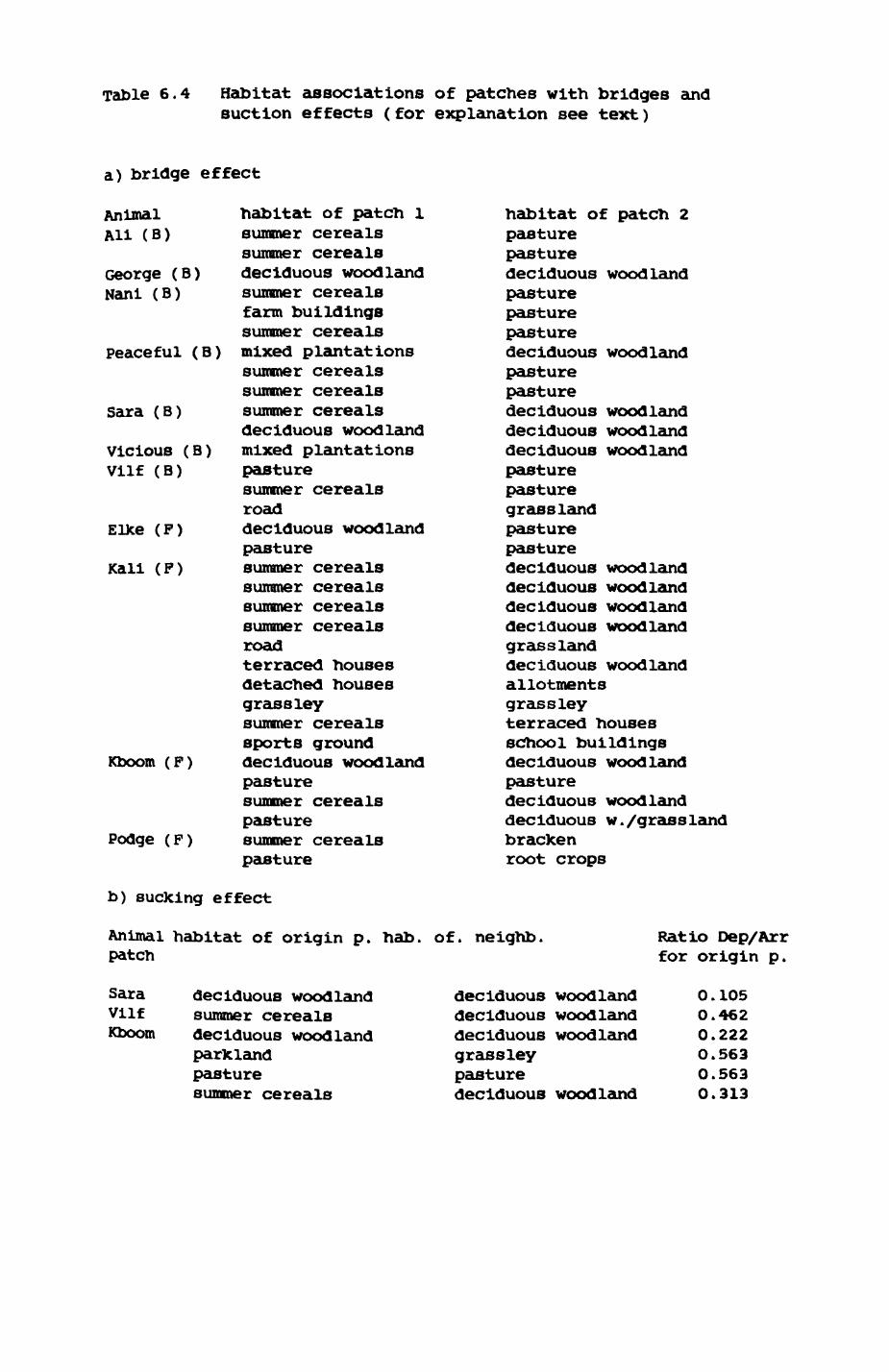
Table 6.4 Habitat associations of patches with bridges and suction effects (for explanation see text)
a) bridge effect
Animal Ali (B)
George (B) Nani (B)
Peaceful (B)
Sara (B)
Vicious (B) Vilf (B)
Elke (P)
Kali (P)
Kboom (P)
Podge (P)
habitat of patch 1summer cerealssummer cerealsdeciduous woodlandsummer cerealsfarm buildingssummer cerealsmixed plantationssummer cerealssummer cerealssummer cerealsdeciduous woodlandmixed plantationspasturesummer cerealsroaddeciduous woodlandpasturesummer cerealssummer cerealssummer cerealssummer cerealsroadterraced housesdetached housesgrassleysummer cerealssports grounddeciduous woodlandpasturesummer cerealspasturesummer cerealspasture
b) sucking effect
habitat of patch 2pasturepasturedeciduous woodlandpasturepasturepasturedeciduous woodlandpasturepasturedeciduous woodlanddeciduous woodlanddeciduous woodlandpasturepasturegrasslandpasturepasturedeciduous woodlanddeciduous woodlanddeciduous woodlanddeciduous woodlandgrasslanddeciduous woodlandallotmentsgrassleyterraced housesschool buildingsdeciduous woodlandpasturedeciduous woodlanddeciduous w./grasslandbrackenroot crops
Animal habitat of origin p. hab. of. neighb. patch
Sara deciduous woodland Vllf summer cereals Kboom deciduous woodland
parklandpasturesummer cereals
deciduous woodland deciduous woodland deciduous woodland grassley pasture deciduous woodland
Ratio Dep/Arr for origin p.
0.105 0.462 0.222 O.563 0.563 0.313
253
freedom" of movements. Some links are strongly used, mostly in both
directions (bridges). Even though transition frequencies often vary between
directions of movement per link, they rarely vary significantly within a
local network. In a few cases, movement patterns exhibit strong blasses in
favour of one direction (suction effect).
6.2.7. Cone lus ions
I have already discussed at length the advantages of using spatial
autocorrelation functions in addition to a visual inspection of 3D and
contour plots. In section 6.4 I shall use some of the results to correct
test statistics used to evaluate habitat utilization. Application of SACs
has quantified the scale of changes in range use. Here a remarkable
difference between the two species appeared. Range use by foxes was very
variable between individuals but relatively coarse-grained. Range use by
badgers was quite similar between individuals and fine-grained.
I hope to have shown that this is the result of differences in prey
preferences and perhaps techniques of range maintenance. Several badgers
used the group range only partly, most of which corresponded to preferred
habitats. Heterogeneity of range use is compatible with observed spatial
and temporal variation in availability of earthworms (Chapter 3).
Differences between NOV and DOS in badgers are slight, except for SARA. In
foxes, however, maintenance of range not only requires considerable detours
but also frequent visits by the range inhabitant to the range borders. In
contrast, range edges of badgers are very little visited, in foxes,
activity patches coincide with areas of abundance of a large variety of
different prey types, ranging from human scraps over earthworms to rabbits.
Poxes adapt their movements to the different kinds of locally available prey
- consequently scale and pattern of space use vary considerably from range
254
to range.
6.3. Simultaneous movements within the UPPER FOLLIES badger group
Simultaneous radio-tracking of all members of a badger group is
essential for an estimate of the likelihood of Interference and the level of
competition within a group. This bears on a variety of problems related to
the development of groups, group sizes, structure and maintenance (Chapter
7). In my analysis I will consider two aspects»
1. Do group members somehow 'adjust' their movements in order to minimize
interference, ie. do individuals coordinate their movements?
2. Given the patterns of movements, what levels of interference pressure
(signs of possible competition) do occur?
6.3.1. Coordination of movements
The analysis of spatial dependencies of the movements of an individual
per se (section 6.2) has shown that there are basically no spatial effects.
We can therefore Investigate patterns of visits without having to fear
influences due to the absolute location of a cell. The question of
coordination of movements between individuals is particularly difficult to
tackle, it is a problem that I shall treat in several steps.
1. Individuals do not move randomly in space as expected from a truely
random process (e.g. section 6.4). What is the appropriate null hypothesis
for independence of movements of two individuals in relation to each other?
2. Coordination of movements between two individuals is ambiguous to
interpret, since such coordination may be intentional (as exemplified by a
situation of social attraction) or unintentional (if the movements of both
255
individuals are independently governed by an external factor, e.g. climate).
Can we resolve this problem with reference to the distances between
individuals involved?
3. if coordination of movements was intentional, what evidence do we have to
identify simple rules that could govern coordinate movements?
Pig 6.65-6.67 show how the distance between all three pairs of individuals
(ALI-NANI, NANI-WILF, ALI-WILP) varies during seven nights. Distances
between ALI and NANI are on average slightly less than those between NANI
and WILP and ALI and WILF. If the frequency distributions of all pairs are
compared with each other, significant differences emerge (Table 6.5a). ALI
and NANI are closest, but similar to NANI and WILF, while ALI and WILF are
farthest away. However, differences in the frequency distribution of
absolute distances could result from different sized ranges and ranges with
different degrees of overlap. Although all three ranges overlap to a large
extent (cf. contour plots in Chapter 5 and 3D figures in section 6.2.),
overlaps are not perfect and range sizes are different. Therefore a
comparison of distances per se is insufficient. Furthermore, we require an
expected frequency distribution under the null hypothesis of independence of
movements of two individuals in relation to each other.
Doncaster (1985) has developed a method by which the effects of partial
range overlap and synchrony of movements can be teased apart. He refers to
range overlap of two animals as "static interaction" (see also Macdonald,
Ball and Hough 1980). This overlap yields an estimate of the expected
frequency distribution of distances between two individuals under the
assumption of no coordination of movement of each other ("dynamic
interaction"). All possible permutations of distances of each fix of badger
A from all fixes of badger B are computed, without reference to the actual
time of the fixes. Thus, the static Interaction measures the displacement
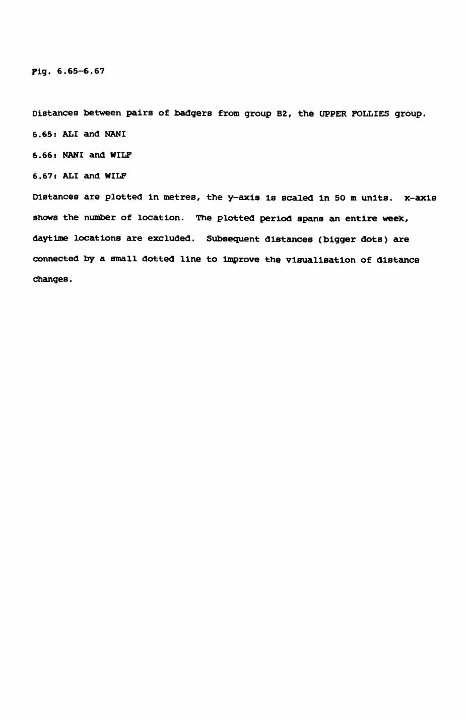
Fig. 6.65-6.67
Distances between pairs of badgers from group B2, the UPPER FOLLIES group.
6.65t ALI and NANI
6.66t NANI and WILF
6.67t ALI and WILF
Distances are plotted in metres, the y-axis is scaled in 5O m units, x-axis
shows the number of location. The plotted period spans an entire weeK,
daytime locations are excluded. Subsequent distances (bigger dots) are
connected by a small dotted line to improve the visualisation of distance
changes.
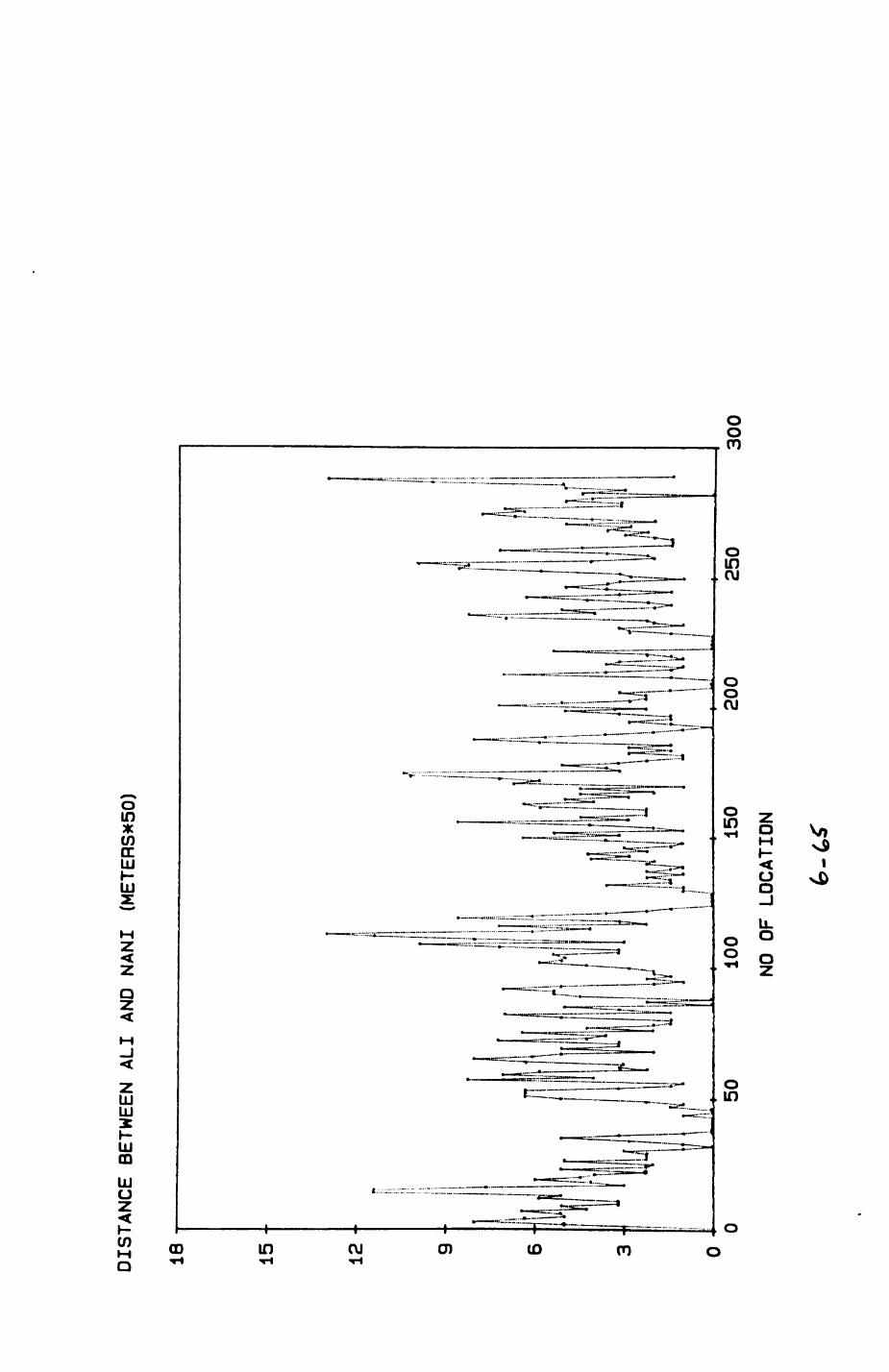
DISTANCE BETWEEN
ALI
AND
NANI (METERS*50)
iO 15 •
12 • 9
•
6 3 -
n .
1 l!, Ill ">l
\ i i
1 \\ y
' J 1 !1 i \t Mi
r i i \i i ! .1 * i rfII i! it 1 » i i
I ii
I || !i ii j! M
I 1 1 i i 1,
i[^
4 |
I *(
r
i I
1 '
1
fi !
V [
' T ^ i ^
i
H
!1 \
!
1! 1
111 II!
1 II
* 1
it
IS!ii
l ! f
h i ju
'1
w/lh
1 1 I'llll
; 4
i**J
»f
•
if"
si
i, —
——
——
— kM
i ——
——
——
——
——
_»
__
f| i 1
(I Ii P I
^ ii ii !: ' i i f 1
-• R it i'i IP •A
I fi i i i 1j i
if f
i i r i II 1 H IIt 1 1 1 I j if 1 !
ti
ll1 *
\t
1 f
[ ii i i| ii I liil MM If1! Il | !
I
——
— 4-
1 1!
t|
j
'
'
,
J
I '' r U
'
! 1 1
i I i
i i
I r!
ti
i Jl
il f
I!\m
- i/ 1i I i i ii 1|
5010
0 15
0
NO OF LOCATION
200
250
300
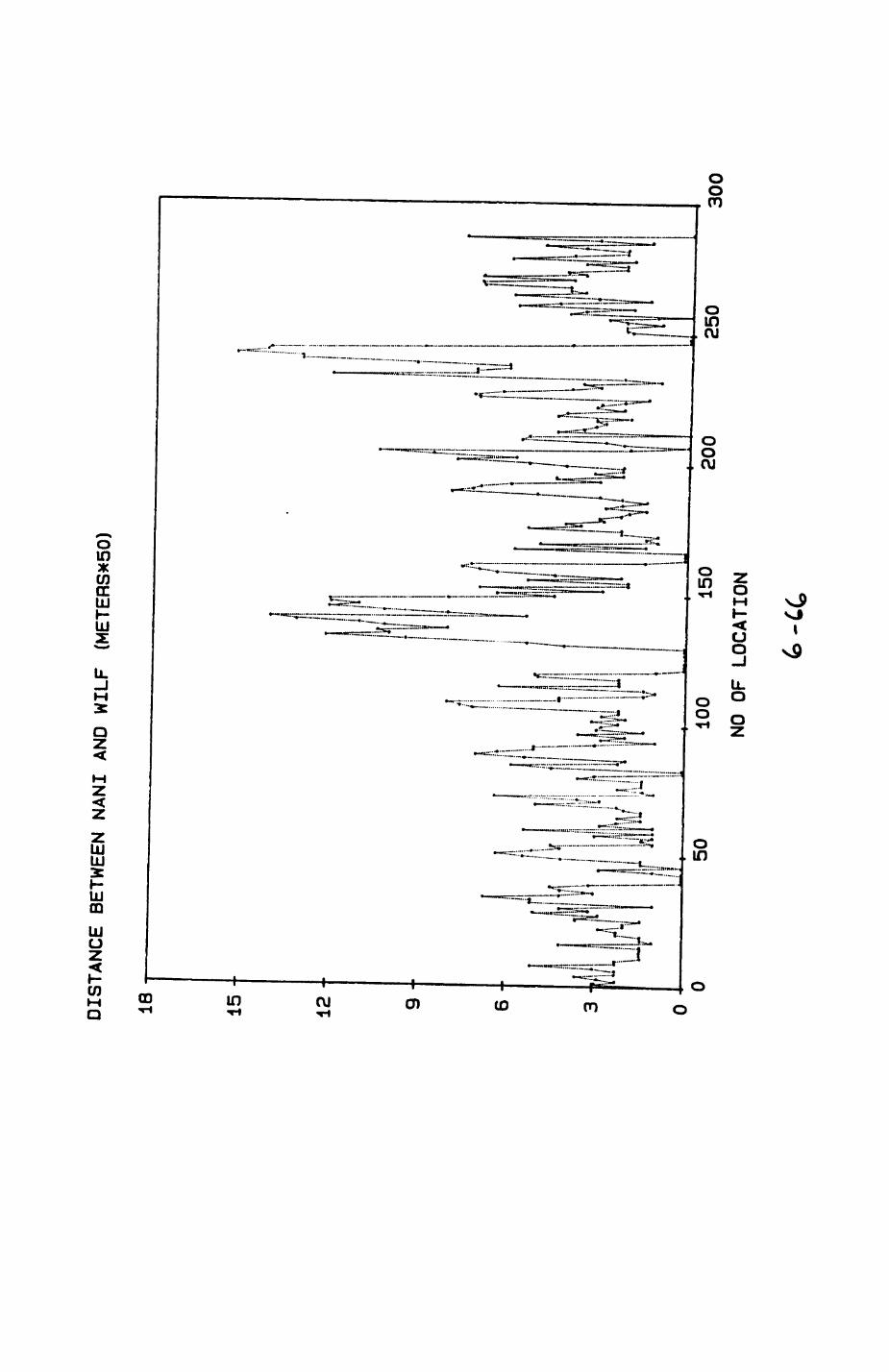
DISTANCE BETWEEN
NANI AND
WILF (METERS*50)
10
•
15 •
12 9 - H ', n
J
• .
1 ,il r/k'1 i! »M*i ?{ f {] i f i 1 i ! i !
! /i fl1
! V
41
i ••
\l\ i
i .
'• i
! i
M
l ,!
1 1
i !
i I
i i
si ill
jl1
Ml
lie
i <ir
iii i
i t
il *u
IB j/l _
I !
II |
III! ,
1l!H
S
j,
It!
Mi
ij. i
i !
liill
MiJ
h pup. ( : 1 ii
f «i
! ti
I !i
It li
r1!
Ill11
ills
U 1
li
i mil
4 «r
i
i lii
!ti|i*
S«I
II
1
iivija
n
!iI 1
V|| i
i
I 4 1 i !!
| |j
jit
•IJ
i1^
1
• ! i i ! i ! f i 1
•^••^1
^
in fi/i 1* i t ? i 1 j i f |
i j
i 1 ! i li li
• — »—
s /' / J 1 1 II !l t* ^•A
^^M
! | i iJM
.'/ [A
•
\ ji n I
1. w Vf•••••^••iM
MV
i 1 n B II II! I! i i IIr
! I! iii — i —
f •1 i II i _
t \ \ |
! \
\M
^^ n
•^••^^K
^to
^
| t i
| *
i
1 || II F
] f. l>
i i
! i
! 1
•>
!
! |
i i
i i
! i
! ! ! i i i i i
I i
!1
f 1
! !
!i
I !
' ' i i i
ii.i
i
II.
l i
4 1j
t
i ri, i
^l^
H^H
H
\l
«1
•••^•IB
I
I 1 li i^•^^
^• i i ! i ——
50100
150
200
250
300
NO O
F LOCATION
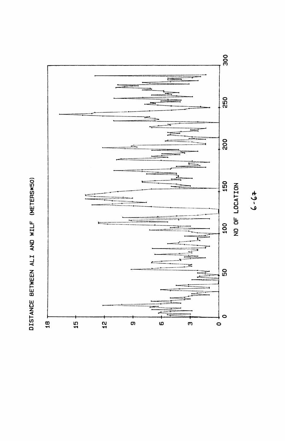
DISTANCE BETWEEN
ALI
AND
WILF (MET
ERS*
50)
6 -
100
150
NO OF LOCATION
200
250
300
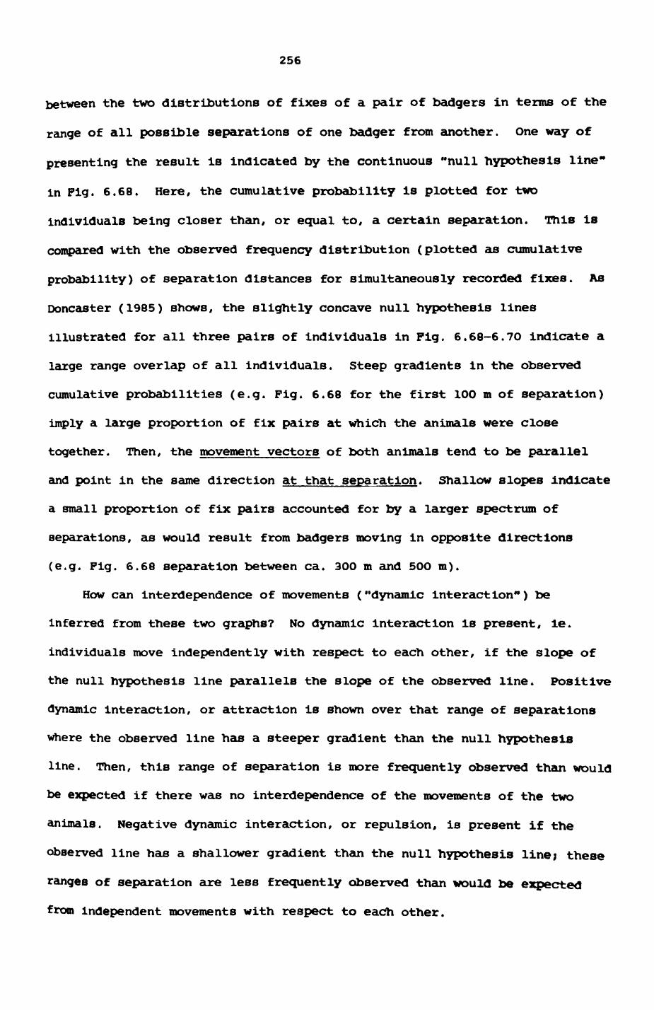
256
between the two distributions of fixes of a pair of badgers in terms of the
range of all possible separations of one badger from another. One way of
presenting the result is indicated by the continuous "null hypothesis line-
in Pig. 6.68. Here, the cumulative probability is plotted for two
individuals being closer than, or equal to, a certain separation. This is
compared with the observed frequency distribution (plotted as cumulative
probability) of separation distances for simultaneously recorded fixes. As
Doncaster (1985) shows, the slightly concave null hypothesis lines
illustrated for all three pairs of individuals in Pig. 6.68-6.70 indicate a
large range overlap of all individuals. Steep gradients in the observed
cumulative probabilities (e.g. Pig. 6.68 for the first 1OO m of separation)
imply a large proportion of fix pairs at which the animals were close
together. Then, the movement vectors of both animals tend to be parallel
and point in the same direction at that separation. Shallow slopes indicate
a small proportion of fix pairs accounted for by a larger spectrum of
separations, as would result from badgers moving in opposite directions
(e.g. Fig. 6.68 separation between ca. 300 m and 500 m).
How can interdependence of movements ("dynamic interaction") be
inferred from these two graphs? No dynamic Interaction is present, ie.
individuals move independently with respect to each other, if the slope of
the null hypothesis line parallels the slope of the observed line. Positive
dynamic interaction, or attraction is shown over that range of separations
where the observed line has a steeper gradient than the null hypothesis
line. Then, this range of separation is more frequently observed than would
be expected if there was no interdependence of the movements of the two
animals. Negative dynamic interaction, or repulsion, is present if the
observed line has a shallower gradient than the null hypothesis line; these
ranges of separation are less frequently observed than would be expected
from Independent movements with respect to each other.
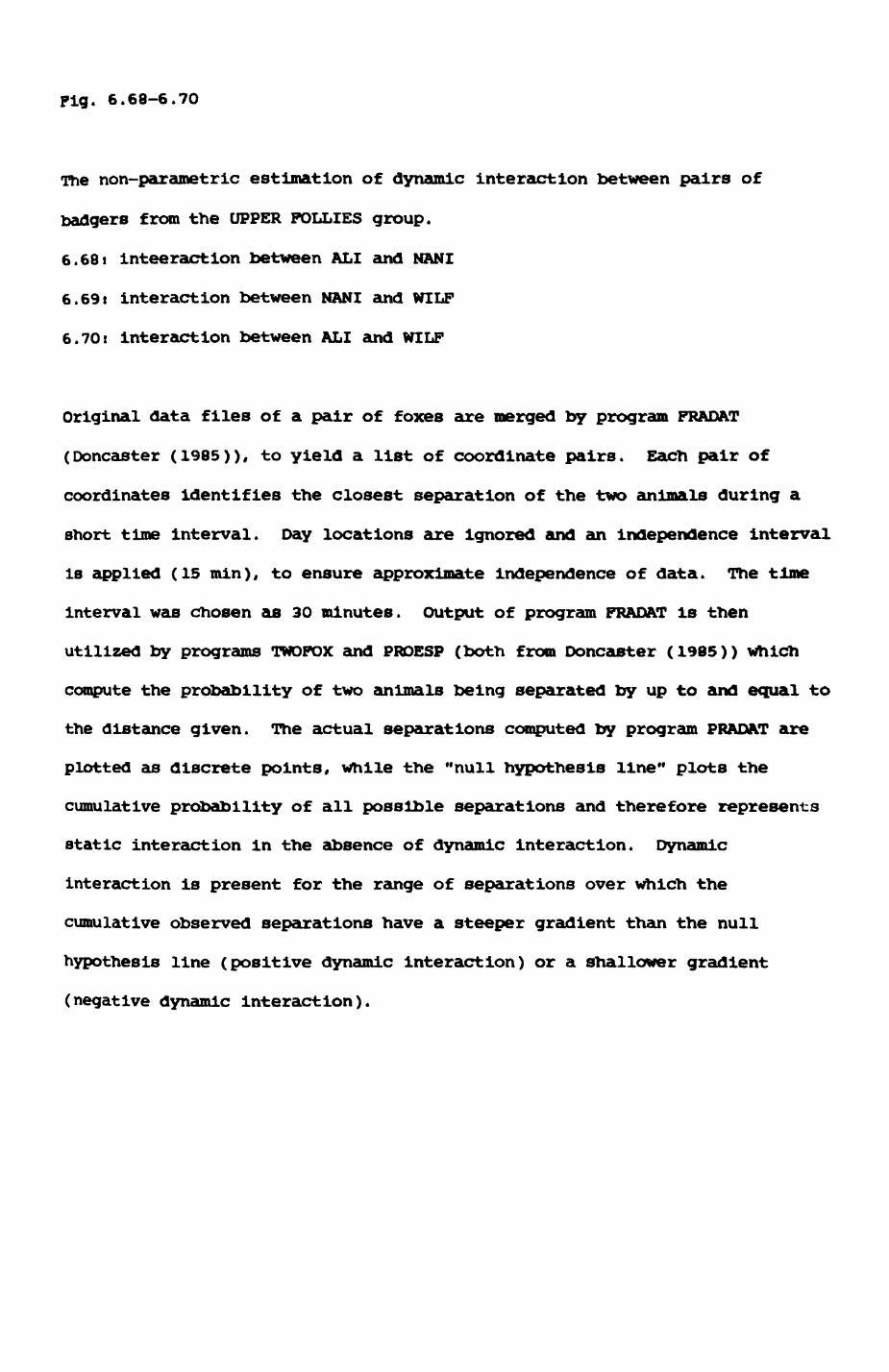
Pig. 6.68-6.70
The non-parametric estimation of dynamic interaction between pairs of
badgers from the UPPER FOLLIES group.
6.681 inteeraction between ALI and NANI
6.69i interaction between NANI and VflLF
6.70: interaction between ALI and WILP
Original data files of a pair of foxes are merged by program FRADAT
(Doncaster (1985)), to yield a list of coordinate pairs. Each pair of
coordinates identifies the closest separation of the two animals during a
short time interval. Day locations are ignored and an independence interval
is applied (15 min), to ensure approximate independence of data. The time
interval was chosen as 30 minutes. Output of program FRADAT is then
utilized by programs TWOPOX and PRDESP (both from Doncaster (1985)) which
compute the probability of two animals being separated by up to and equal to
the distance given. The actual separations computed by program PRADAT are
plotted as discrete points, while the "null hypothesis line" plots the
cumulative probability of all possible separations and therefore represents
static interaction in the absence of dynamic interaction. Dynamic
interaction is present for the range of separations over which the
cumulative observed separations have a steeper gradient than the null
hypothesis line (positive dynamic interaction) or a shallower gradient
(negative dynamic Interaction).
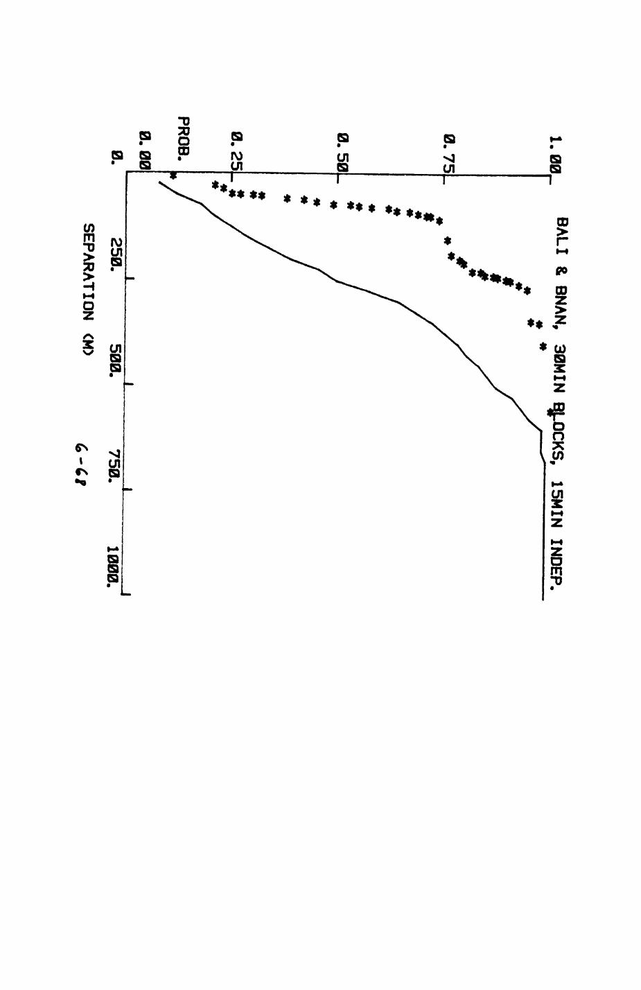
1.00 BALI
& BNAN' 30MIN
0.75
0.50
0.25
PROB.
0.00
0.
, 15MIN
INDEP.
_LJ
250. 500.
SEPARATION <M>
750.1000.
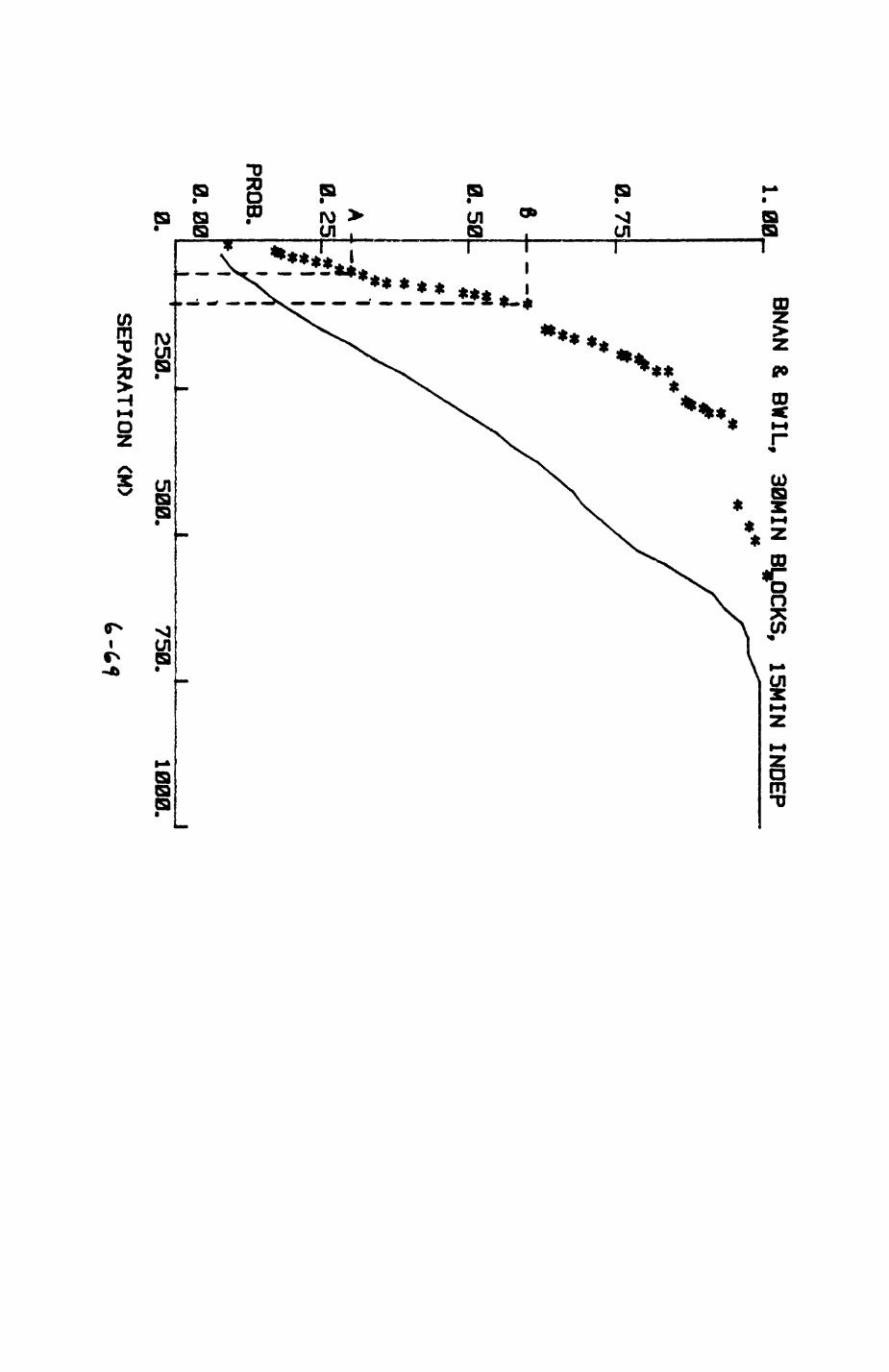
1.00 BNAN
& BWIL' 30MIN
, 15MIN
INDEP
0.75_
PROS.
250.500.
750.1000.
SEPARATION CM>
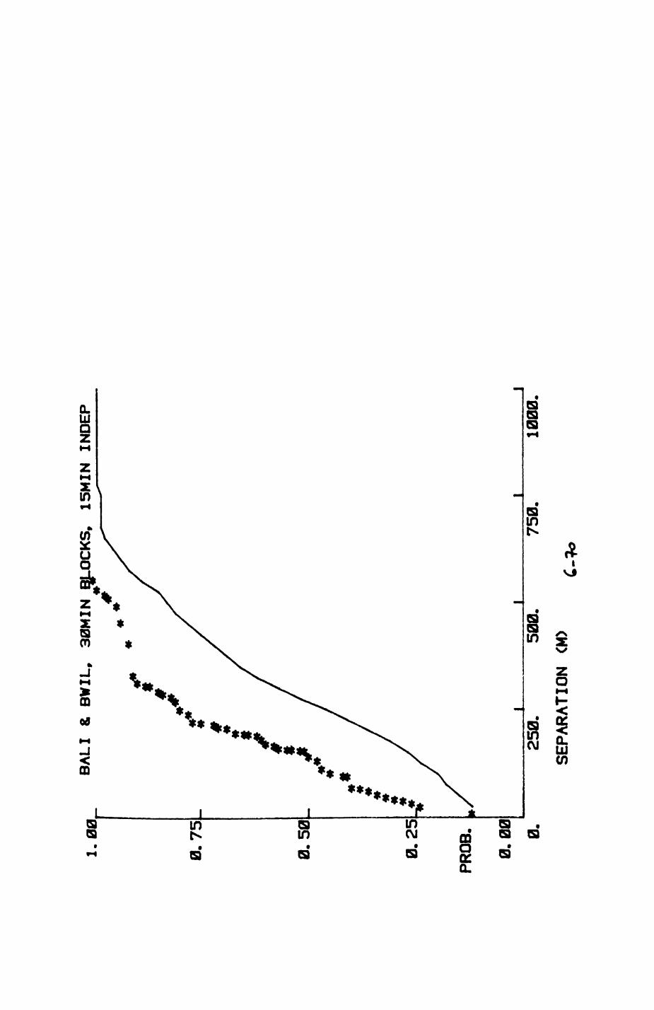
1.00
BALI
&
BWIL,
0. 75 _
0.50
0.25
PROB.
0.00
0.
15MIN INDEP
II
I250.
500.
SEPARATION <M
>
750.
1000
.
257
In Pig. 6.68-6.70, all three pairs show dynamic positive interaction at
low separation distances. The positive dynamic interaction is particularly
strong for the two females, ALI and NANI, ie. those two individuals that are
expected to suffer most from intragroup competition (Chapter 7). At larger
distances all pairs exhibit negative dynamic Interactions.
Doncaster (1985) has simulated a large number of possible cases and
suggests the following interpretationt positive dynamic interactions at
small separation distances are typical of stable social coordination, e.g.
In order to realize some mutually shared goal, with parallel movement
vectors in the same direction. Both animals appear to be "bound together"
and move in synchrony, apparently under the influence of a shared stimulus.
He calls this type of interaction "intentionally synchronous time-tabling".
A typical case is the common pressure of a similar resource need.
To what extent may the observed synchrony of movements be simply a by
product of two individuals following the same schedule, but independent (or
unaware) of each other ? This interpretation cannot be excluded on
statistical grounds; intentionality cannot be derived from or rejected by
the computations illustrated in Fig. 6.68-70. One likely possibility is the
effect of an external factor - e.g. the weather induces all group members to
proceed to the same area where worms are available in a given night.
Coordination at medium separation distances may be to some extent due to
such unintentional coordination - individuals moving towards roughly the
same area - but at closer distances, less than 50 or 1OO m, the probability
of noticing each other and thus the scope for intentional coordination
increases rapidly. The graphs in Pig. 6.68-6.70 do not support the
suggestion that Interference between individuals and consequent agonistic
encounters occurred at small separations. If two badgers were close
together, they were peacefully close.
I suggest that, for badgers at least, synchronous time-tabling helps
individuals to organize their foraging activities so that each individuals
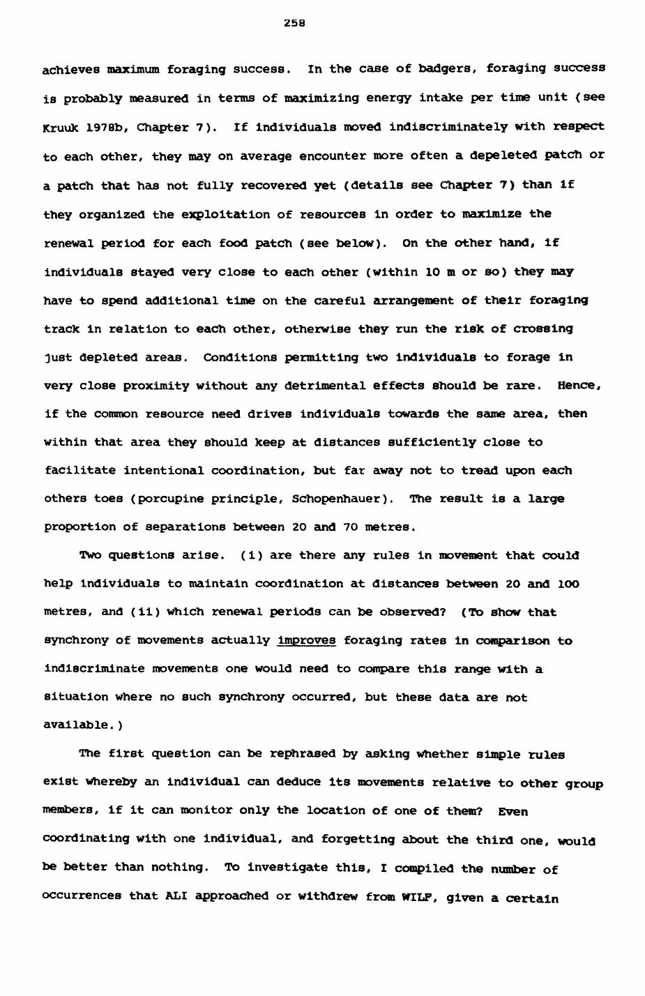
258
achieves maximum foraging success. In the case of badgers, foraging success
is probably measured in terms of maximizing energy intake per time unit (see
Kruuk 1978b, Chapter 7). If individuals moved indiscriminately with respect
to each other, they may on average encounter more often a depeleted patch or
a patch that has not fully recovered yet (details see Chapter 7) than if
they organized the exploitation of resources in order to maximize the
renewal period for each food patch (see below). On the other hand, if
individuals stayed very close to each other (within 10 m or so) they may
have to spend additional time on the careful arrangement of their foraging
track in relation to each other, otherwise they run the risk of crossing
just depleted areas. Conditions permitting two individuals to forage in
very close proximity without any detrimental effects should be rare. Hence,
if the common resource need drives individuals towards the same area, then
within that area they should keep at distances sufficiently close to
facilitate intentional coordination, but far away not to tread upon each
others toes (porcupine principle, Schopenhauer). The result is a large
proportion of separations between 20 and 70 metres.
Two questions arise, (i) are there any rules in movement that could
help individuals to maintain coordination at distances between 2O and 1OO
metres, and (11) which renewal periods can be observed? (To show that
synchrony of movements actually improves foraging rates in comparison to
indiscriminate movements one would need to compare this range with a
situation where no such synchrony occurred, but these data are not
available. )
The first question can be rephrased by asking whether simple rules
exist whereby an individual can deduce its movements relative to other group
members, if it can monitor only the location of one of them? Even
coordinating with one individual, and forgetting about the third one, would
be better than nothing. To investigate this, I compiled the number of
occurrences that ALI approached or withdrew from WILF, given a certain
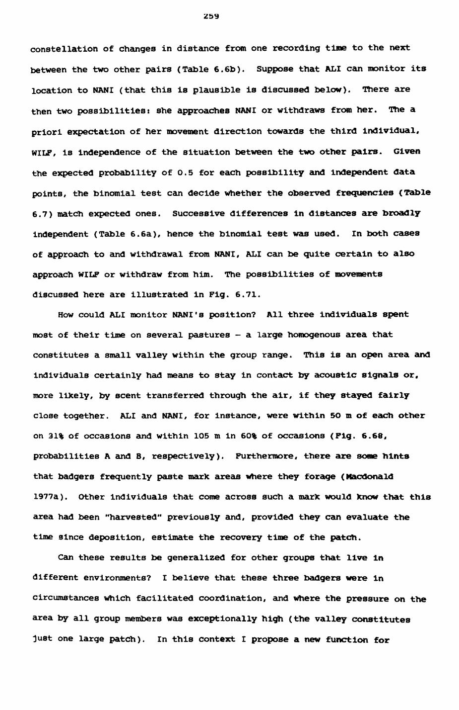
Z59
constellation of changes in distance from one recording time to the next
between the two other pairs (Table 6.6b). Suppose that ALI can monitor its
location to NANI (that this is plausible is discussed below). There are
then two possibilities! she approaches NANI or withdraws from her. The a
priori expectation of her movement direction towards the third individual,
WILF, is independence of the situation between the two other pairs. Given
the expected probability of 0.5 for each possibility and independent data
points, the binomial test can decide whether the observed frequencies (Table
6.7) match expected ones. Successive differences in distances are broadly
independent (Table 6.6a), hence the binomial test was used. In both cases
of approach to and withdrawal from NANI, ALI can be quite certain to also
approach WTLF or withdraw from him. The possibilities of movements
discussed here are illustrated in Fig. 6.71.
How could ALI monitor NANI's position? All three individuals spent
most of their time on several pastures - a large homogenous area that
constitutes a small valley within the group range. This is an open area and
individuals certainly had means to stay in contact by acoustic signals or,
more likely, by scent transferred through the air, if they stayed fairly
close together. ALI and NANI, for instance, were within SO m of each other
on 31% of occasions and within 105 m In 6O% of occasions (Pig. 6.68,
probabilities A and B, respectively). Furthermore, there are sone hints
that badgers frequently paste mark areas where they forage (Macdonald
1977a). other individuals that come across such a mark would know that this
area had been "harvested" previously and, provided they can evaluate the
time since deposition, estimate the recovery time of the patch.
Can these results be generalized for other groups that live in
different environments? I believe that these three badgers were in
circumstances which facilitated coordination, and where the pressure on the
area by all group members was exceptionally high (the valley constitutes
just one large patch). In this context I propose a new function for
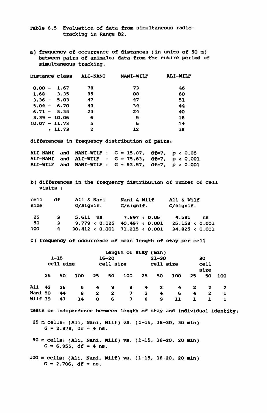
0.00 -1.68 -3.36 -5.04 -6.71 -8.39 -10.07 -
>
1.673.355.036.708.38
10.0611.7311.73
7885474323652
Table 6.5 Evaluation of data from simultaneous radio- tracking in Range B2.
a) frequency of occurrence of distances (in units of 5O m) between pairs of animals; data from the entire period of simultaneous tracking.
Distance class ALI-NANI NANT-WILF ALI-WTLF
73 4688 6047 5134 4424 405 166 14
12 18
differences in frequency distribution of pairst
ALI-NANI and NANI-WILF : G = 15.87, df-7, p < O.05ALI-NANI and ALI-WILF : G = 75.63, df=7, p < O.O01ALI-WILP and NANI-WILF t G = 53.57, df=7, p < O.O01
b) differences in the frequency distribution of number of cell visits «
cell df Ali & Nani Nani & Wilf All & Wilf size G/signif. G/signif. G/signif.
25 3 5.611 ns 7.897 < O.O5 4.581 ns50 3 9.779 < 0.025 4O.497 < O.O01 25.153 < O.OO1100 4 30.412 < 0.001 71.215 < O.OO1 34.825 < O.OO1
c) frequency of occurrence of mean length of stay per cell
Length of stay (min)1-15 16-20 21-3O 30
cell size cell size cell size cellsize
25 50 100 25 50 100 25 50 100 25 5O 1OO
Ali 43Nani 5OWilf 39
364447
58
14
420
926
877
438
249
46
11
241
221
211
tests on independence between length of stay and individual identity:
25 m cells: (Ali, Nani, Wilf) vs. (1-15, 16-3O, 3O min) G - 2.978, df - 4 ns.
50 m cellsj (Ali, Nani, Wilf) vs. (1-15, 16-20, 20 min) G - 6.955, df - 4 ns.
100 m cells: (Ali, Nani, Wilf) vs. (1-15, 16-20, 20 min) G - 2.706, df - ns.

Table 6.6 Patterns of changes of distances between pairs of individuals at successive locations
a) runs test to check whether successive differences in distances between pairs of animals are randomly arranged (independent from each other)i test procedures follow Sofcal & Rohlf (1981).
NightNo. N runs
Ali-Nani Nani-Wilfsig. No. N
runssig.
Ali-WilfNo. N
runs s sig.
1234567
20242027221522
33 -O.71 ns35 0.41 ns37 -1.73 ns34 1.95 ns36 -O.68 ns
19 30 -O.3 ns24 35 0.41 ns20 33 -O.71 ns18 33 1.56 ns24 37 -0.13 ns
21 39 -1.82 ns22 37 -0.93 ns17 37 -2.93 <0.00513 37 -4.53 <0.00122 36 -0.68 ns
33 -2.83 <0.005 18 36 -2.30 <O.OO5 20 41 -2.65 <0.0136 -O.68 ns 24 34 0.7 ns 26 38 0.39 ns
In 16 out of 21 cases (76%) are distance changes randomly arranged In 5 out of 21 cases (24%) distance changes are not Independent from each other.
b) frequency of change of distance between Ali and Wilf at two successive locations, given a certain change of distance between Ali and Nani and Nani and Wilf (data pooled from all nights)
group change of distance between
Ali/Nani Nani/Wilf
change of distance between
Ali and Wilf a) Ali b) Ali
approaches withdraws Wilf from Wilf
approach stay equal approach
stay equalwithdrawwithdraw
stay equalapproachapproach
withdraw stay equal withdraw
58 17
23 61
3
4
approach
withdraw
withdraw
approach
29
31
22
23
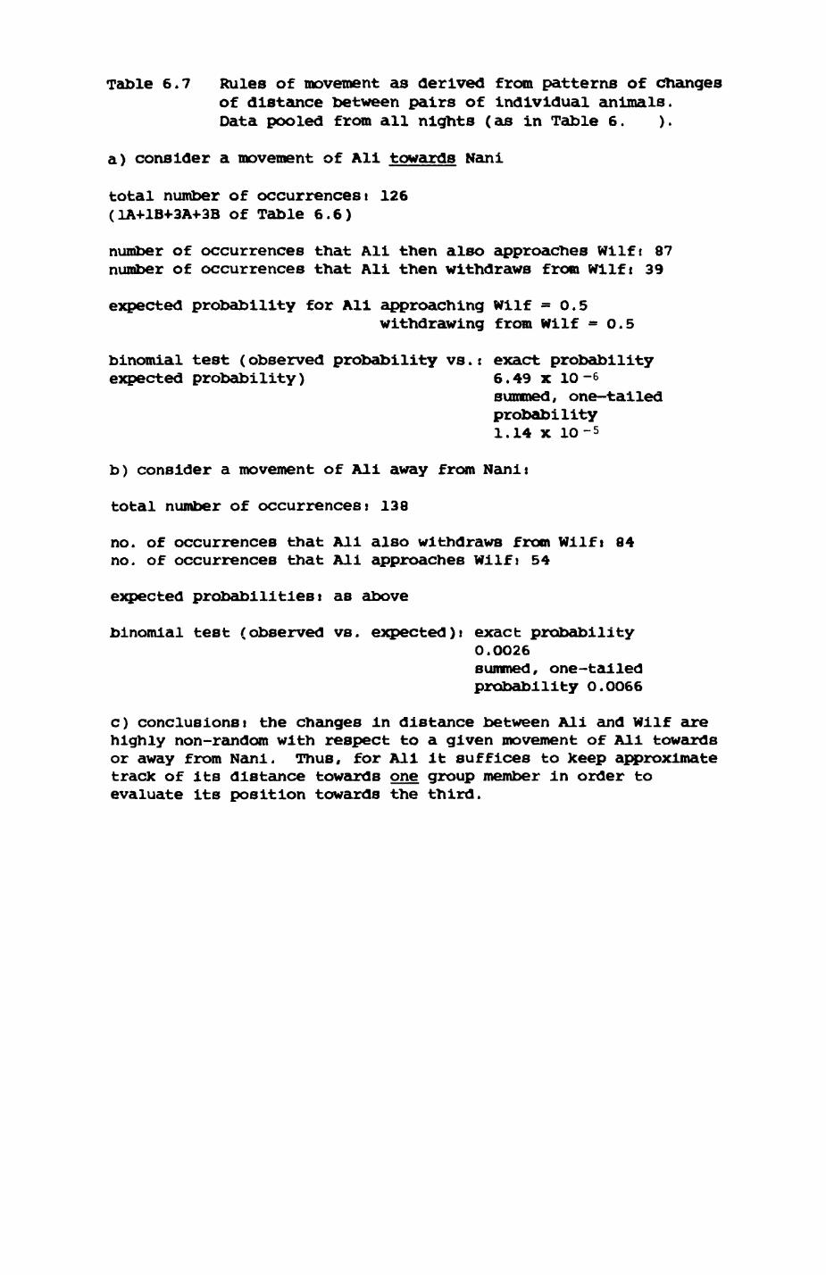
Table 6.7 Rules of movement as derived from patterns of changes of distance between pairs of Individual animals. Data pooled from all nights (as in Table 6. ).
a) consider a movement of Ali towards Nani
total number of occurrencesi 126 (1A4-1B+3A4-3B Of Table 6.6)
number of occurrences that Ali then also approaches Wilft 87 number of occurrences that Ali then withdraws from Wllft 39
expected probability for Ali approaching Wilf =0.5withdrawing from Wilf = 0.5
binomial test (observed probability vs.: exact probability expected probability) 6.49 x 10⁻⁶
summed, one-tailed probability 1.14 x 10 ~ 5
b) consider a movement of Ali away from Nanii
total number of occurrences! 138
no. of occurrences that Ali also withdraws from Wilf j 84 no. of occurrences that Ali approaches Wilfj 54
expected probabilitiesi as above
binomial test (observed vs. expected)! exact probabilityO.OO26summed, one-tailedprobability O.OO66
c) conclusionsi the changes in distance between All and Wllf are highly non-random with respect to a given movement of All towards or away from Nani. Thus, for All it suffices to keep approximate track of its distance towards one group member In order to evaluate its position towards the third.
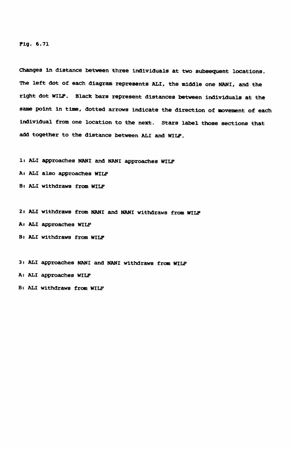
Pig. 6.71
Changes in distance between three individuals at two subsequent locations.
The left dot of each diagram represents ALI, the middle one NANI, and the
right dot WILF. Black bars represent distances between individuals at the
same point in time, dotted arrows indicate the direction of movement of each
individual from one location to the next. Stars label those sections that
add together to the distance between ALI and WILF.
It ALI approaches NANI and NANI approaches WILF
At ALI also approaches WILF
Bt ALI withdraws from WILF
2t ALI withdraws from NANI and NANI withdraws from WILF
At ALI approaches WILF
Bt ALI withdraws from WILF
31 ALI approaches NANI and NANI withdraws from WILF
A: ALI approaches WILF
Bt ALI withdraws from WILF
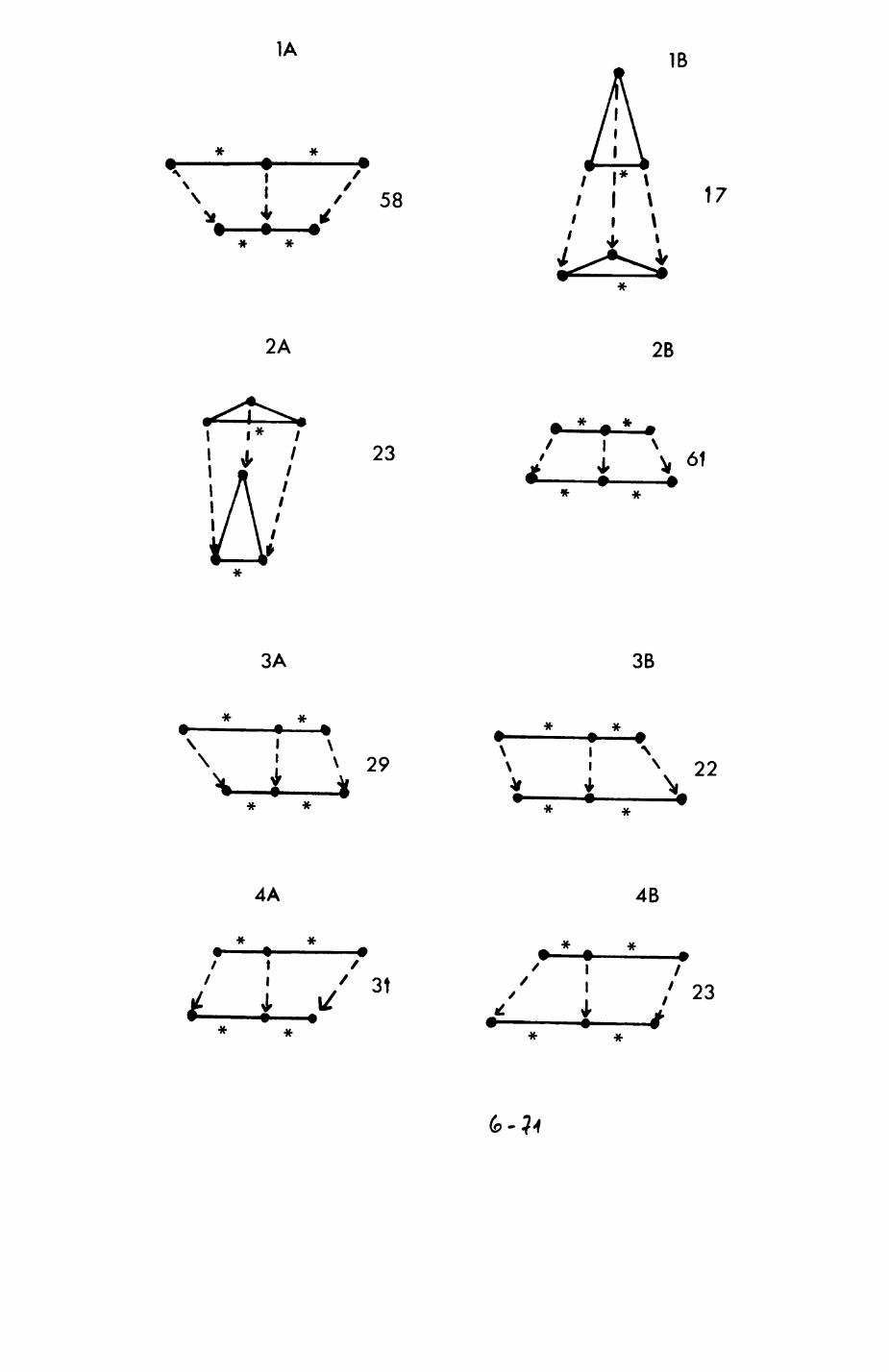
tO
SD
— 4
10
COCn
CO
I -vo
-]• CD
to
GJ
CA)
to 03
10

Pig. 6.72
Movements of NANI (red) and WILF (green) In night 1 from 20.00 hours to
00.50 hours.
Scalei 800 by BOO metres. Each location Is separated from the next one by
15 mln. If labels of subsequent locations differ by more than 1, then the
animal stayed at the previous location for several locations.
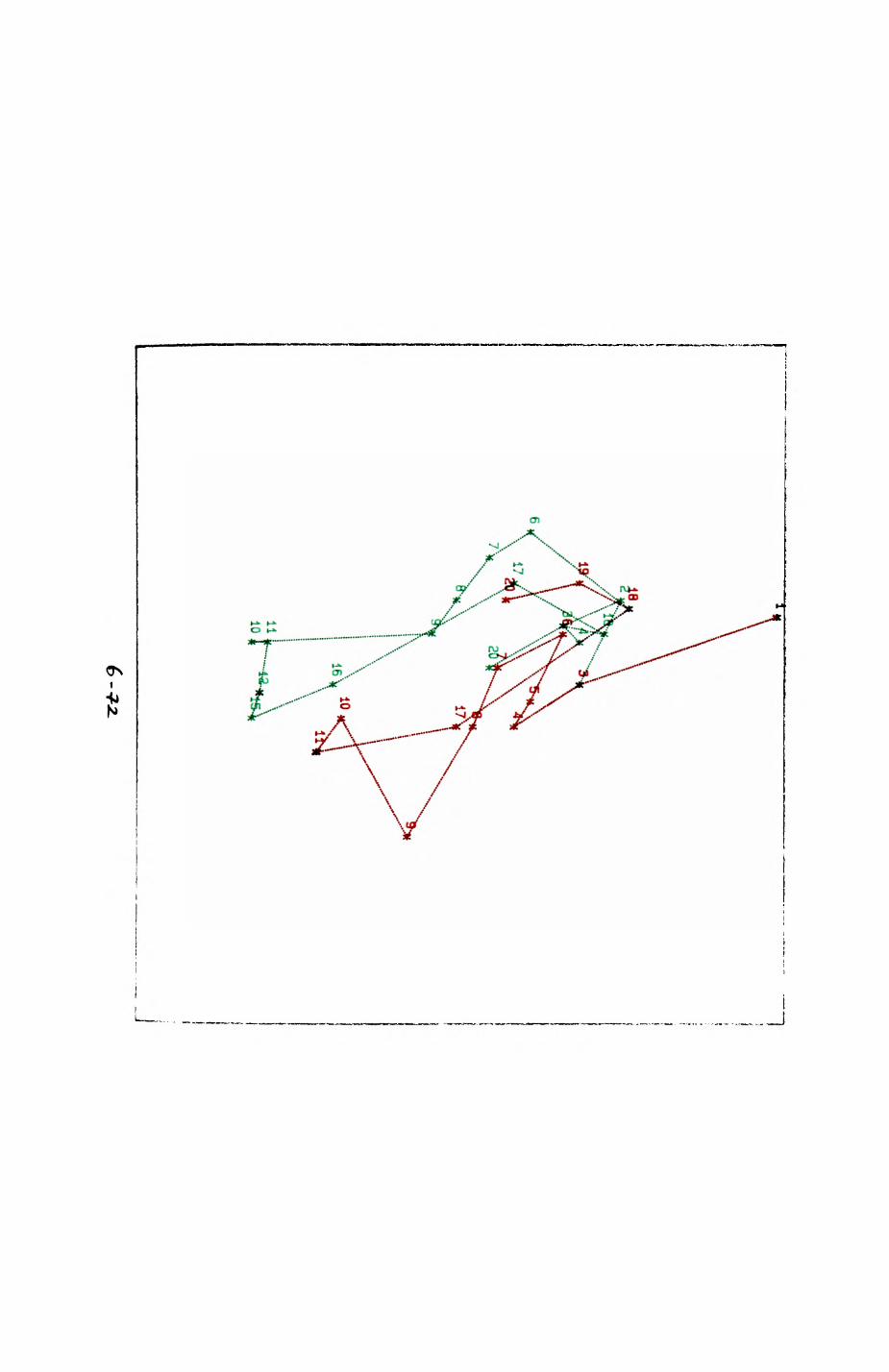
r L
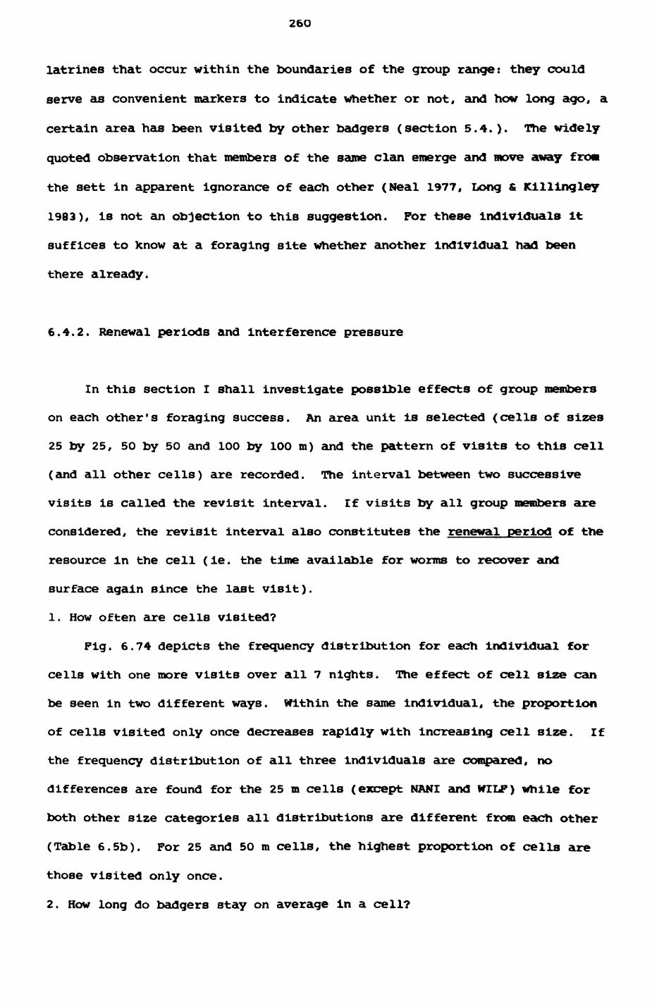
26O
latrines that occur within the boundaries of the group range: they could
serve as convenient markers to indicate whether or not, and how long ago, a
certain area has been visited by other badgers (section 5.4.). The widely
quoted observation that members of the same clan emerge and move away frow
the sett in apparent ignorance of each other (Meal 1977, Long & Killingley
1983), is not an objection to this suggestion. For these individuals it
suffices to know at a foraging site whether another individual had been
there already.
6.4.2. Renewal periods and interference pressure
In this section I shall investigate possible effects of group members
on each other's foraging success. An area unit is selected (cells of sizes
25 by 25, 50 by 50 and 100 by 100 m) and the pattern of visits to this cell
(and all other cells) are recorded. The interval between two successive
visits is called the revisit interval. If visits by all group members are
considered, the revisit interval also constitutes the renewal period of the
resource in the cell (ie. the time available for worms to recover and
surface again since the last visit).
1. How often are cells visited?
Pig. 6.74 depicts the frequency distribution for each individual for
cells with one more visits over all 7 nights. The effect of cell size can
be seen in two different ways. Within the same individual, the proportion
of cells visited only once decreases rapidly with increasing cell size. If
the frequency distribution of all three individuals are compared, no
differences are found for the 25 m cells (except NANI and WILF) while for
both other size categories all distributions are different from each other
(Table 6.5b). For 25 and 50 m cells, the highest proportion of cells are
those visited only once.
2. How long do badgers stay on average in a cell?
Pig. 6.74
Proportion of cells that are visited for a certain number of tiroes by the
UPPER FOLLIES badgers.
G.D.Ai cells of size 25 m
H,E,Bt cells of size 50 m
l,F,Ci cells of size 100 m
ALIt diagrams A,B,C
NANIi diagrams D,E,F
wiLFi diagrams G,H,I
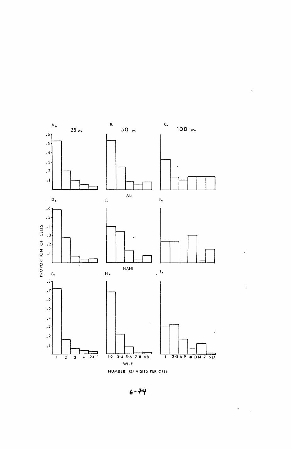
PR
OP
OR
TIO
N
OF
CE
LLS
O—
KJ
CO
*»
• <•/
> O
_J—
——
——
——
1——
——
——
I——
——
——
1——
——
——
I——
——
—pi
Q
ro Ul
i I m
_
I"O
5
CO —4
</>
•D m 77 n
XI • CD V
CO
z > Z
ICn
O
n
Ln
OO
O 7
V SJ
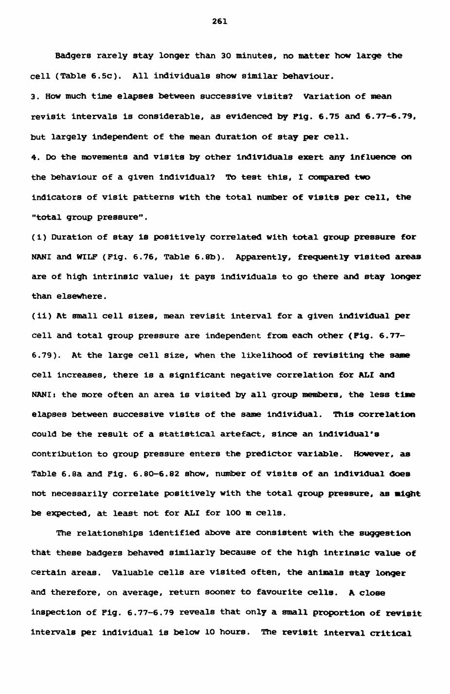
261
Badgers rarely stay longer than 30 minutes, no matter how large the
cell (Table 6.5c). All individuals show similar behaviour*
3. How much time elapses between successive visits? Variation of mean
revisit intervals is considerable, as evidenced by Pig. 6.75 and 6.77-6.79,
but largely independent of the mean duration of stay per cell.
4. Do the movements and visits by other individuals exert any influence on
the behaviour of a given individual? To test this, I compared two
indicators of visit patterns with the total number of visits per cell, the
"total group pressure".
(1) Duration of stay is positively correlated with total group pressure for
NANI and WILF (Fig. 6.76, Table 6.8b). Apparently, frequently visited areas
are of high intrinsic value; it pays individuals to go there and stay longer
than elsewhere.
(ii) At small cell sizes, mean revisit interval for a given individual per
cell and total group pressure are independent from each other (Pig. 6.77-
6.79). At the large cell size, when the likelihood of revisiting the sane
cell increases, there is a significant negative correlation for ALI and
NANIs the more often an area is visited by all group members, the less tine
elapses between successive visits of the same individual. This correlation
could be the result of a statistical artefact, since an Individual's
contribution to group pressure enters the predictor variable. However, as
Table 6.8a and Pig. 6.8O-6.82 show, number of visits of an individual does
not necessarily correlate positively with the total group pressure, as might
be expected, at least not for ALI for 1OO m cells.
The relationships identified above are consistent with the suggestion
that these badgers behaved similarly because of the high intrinsic value of
certain areas. Valuable cells are visited often, the animals stay longer
and therefore, on average, return sooner to favourite cells. A close
inspection of Fig. 6.77-6.79 reveals that only a small proportion of revisit
Intervals per individual is below 10 hours. The revisit Interval critical
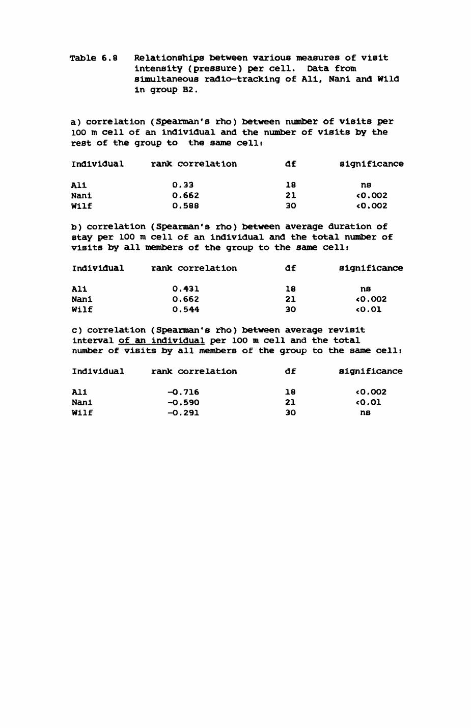
Table 6.8 Relationships between various measures of visit Intensity (pressure) per cell. Data from simultaneous radio-tracfcing of Ali, Nani and Wild in group B2.
a) correlation (Spearman's rho) between number of visits per 100 m cell of an individual and the number of visits by the rest of the group to the same celli
Individual
AliNaniWilf
ran* correlation
0.330.6620.588
df
182130
significance
ns<O.O02 <O.O02
b) correlation (Spearman's rho) between average duration of stay per 100 m cell of an individual and the total number of visits by all members of the group to the same celli
Individual
AliNaniWilf
rank correlation
0.431 O.662 0.544
df
18 21 3O
significance
ns<O.O02 <0.01
c) correlation (Spearman's rho) between average revisitinterval of an individual per 1OO m cell and the totalnumber of visits by all members of the group to the same cell:
Individual
AliNaniWilf
rank correlation
-O.716-O.590-O.291
df
182130
significance
<0.002 <0.01 ns
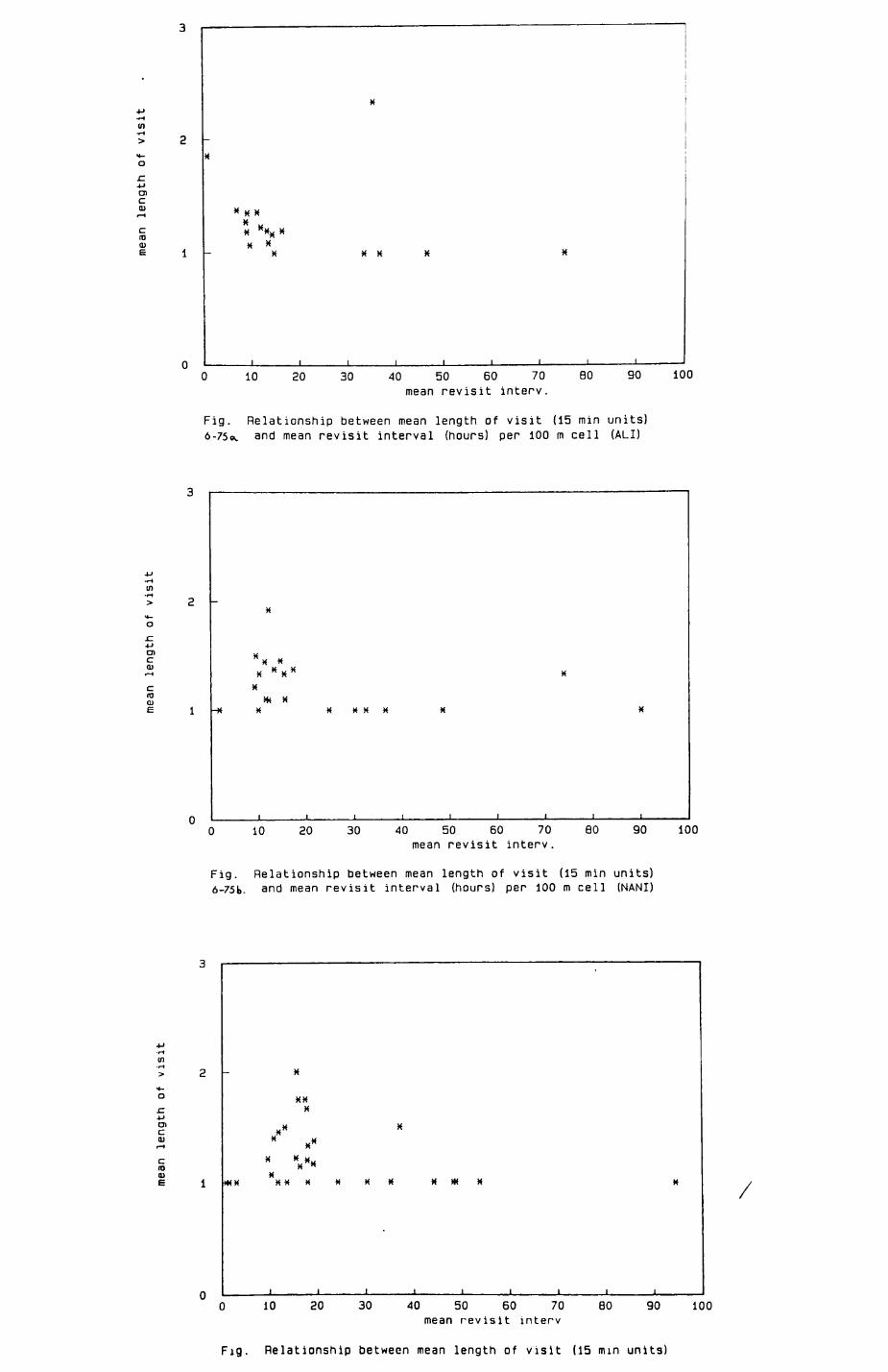
4-1-*H
in
c. -p 01 c tu
cID QJE
*xx *x*
X
10 20 30 40 50 60 70mean revisit interv.
80 90 100
Fig. Relationship between mean length of visit (15 min units) 6-75«. and mean revisit interval (hours) per 100 m cell (ALI)
oc. J-l enc<D
c co(De X X
10 20 30 40 50 60 70mean revisit interv.
80 90 100
Fig. Relationship between mean length of visit (15 min units) 6-75k. and mean revisit interval (hours) per 100 m cell (NANI)
-M•r-t
in
01c0)
c(O 0)e
X*'
xx x
x ***
X X
10 20 30 40 50 60 70mean revisit interv
80 90 100
Fig. Relationship between mean length of visit (15 mm units)
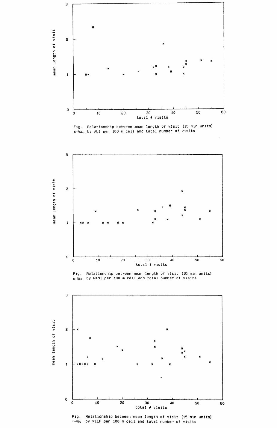
Olc0]
c10<u
XX
10 20 30total # visits
40 50 60
Fig. Relationship between mean length of visit (15 min units) 6-76*.. by ALI per 100 m cell and total number of visits
c.-Uenc tu
c inOJ
- XK X XX
10 20 30 40 total # visits
50 60
Fig. Relationship between mean length of visit (15 min units) 6-76b. by NANI per 100 m cell and total number of visits
O)c01
c10 0)
X
X
-XXXXX X
10 20 30 total *
50 60visits
Fig. Relationship between mean length of visit (15 min units) '-76c by WILF per 100 m cell and total number of visits
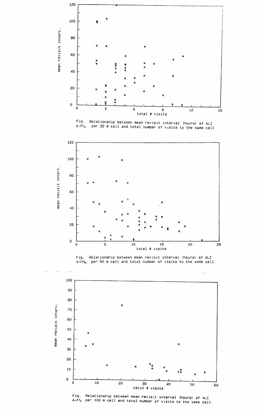
c01
c-f-1*J.201C-
cIDO)E
CO)JJc•«H
-U
Ul-iH
CDc.croO)E
-
•c.O)4J
C
-M••H
-rH
Olc_cIDOlE
120
100
80
60
40
20
i
XIf
XX X
X *XX
* j| M * *./ U ^* XX
X XX "
X* X. *
* X *X *X
Xi*?iiiiii*¥iii
0 3 6 9 12 15total # visits
Fig. Relationship between mean revisit interval (hours) of ALI6-77u,. pen 25 m cell and total number of visits to the same cell
120 — '
100
80
60
40
20
Xx x
-
Xx x *
-
Xx x x" vt *rt ^ •
-
* X * " X * *
X X *x x**xx, *
XX *
* x ¥ _______ i _________ J ——— S ————— 1° 0 5 10 15 20 2total # visits
Fig Relationship between mean revisit interval (hours) of ALI 6-77t. pen 50 m cell and total number of visits to the same cell
100 -• -- ——— ————————————————————————————————————————
90
80
70
60
50
40
30
20
10
n
-
X-
-
-X
_UX *
—
_
* * *xx xX XX X
1 1 I 1 1 1 1 X 1 I l I10 20 30 40
total # visits50 60
Fig. Relationship between mean revisit interval (hours) of ALI 6-77c . per 100 m cell and total number of visits to the same cell
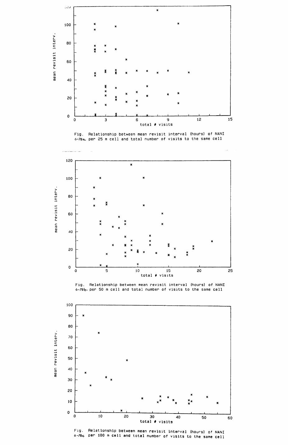
""
100
c.2 80c
-fH
in > 60<uccm0)e 40
20
x
x *X
X ^
8 x *X
x * 2 x " * x *
* X *u w
x H « M HX "** u X»* „ H xx x
i M i % i * x i _ _ _ i ___ i ___ i ___ i ___ i ___ u ——0 3 6 9 12 If
total # visits
Fig. Relationship between mean revisit interval (hours) of NANI6-78ou per 25 m cell and total number of visits to the same cell
120 ——————————————————————————————————————————————————
100
C-<u" 80c•r-1
4J
in> 60OJc-cID0)e 40
20
X
X X
X
—X
x * x
XX
X X"XX X
* X-
* X *xx x
X X X X ^ „
«X X
„ .. x H xX * N ^ X
* X 1 1 10 ———————————————————————————————————————————————————————0 5 10 15 20 25
total # visits
Fig. Relationship between mean revisit interval (hours) of NANI6-78b- per 50 m cell and total number of visits to the same cell
100
90
80>-£ 70Cf-l 60in> 500)c_<= 40100)E
30
20
10
0 — ______________________ ,
- X
-
X-
-
-
_
XX
X
X-
X * * * *¥ M K
——— 1 ——— 1 ——— I — _*_ 1 I , I I , , ,0 10 20 30 40 50 Kr
Fig. Relationship between mean revisit interval (hours) of NANI 6-78c per 100 m cell and total number of visits to the same cell
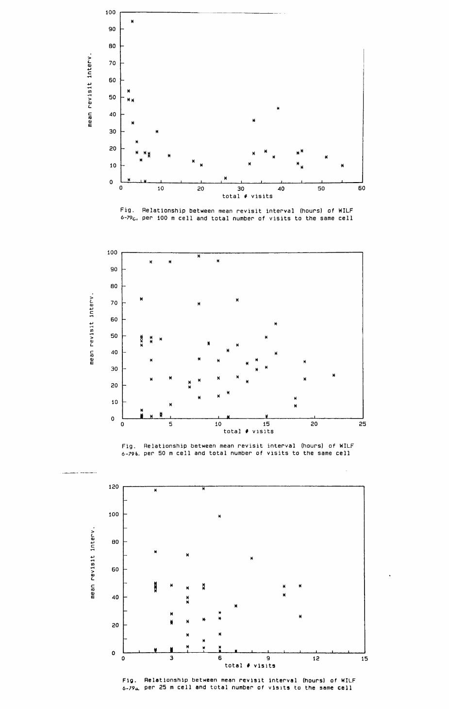
<_
c
4J-rH
cnrevi
cO)e
1UU
go
BO
70
60
50
40
30
20
10
0
x-
-
-
-
x~ *x
-
X *
X
X
x x« x * x* x * x * *
* * *x *
— S —— LS —— i ———— i ———— i _____ i ____ i ____ i ____ i ____ i ———— i _____ i _____10 20 30 40
total # visits50 60
Fig. Relationship between mean revisit interval (hours) of WILF 6-79c, per 100 m cell and total number of visits to the same cell
>C- 01
c
_,_,en
••H
>
C.
cCO01E
100 ———————————————————————————————————————————————————————
90
80
70
60
50
40
30
20
10
n
XXX X
-
-
M X
x
8 X * *H " X
* X
* xX *
x x ^ x x „ »«X
x x ^X K
M x * , , M ¥10 15
total # visits20 25
Fig. Relationship between mean revisit interval (hours) of WILF 6-79b. per 50 m cell and total number of visits to the same cell
120
100 -
80 -
01c.c ia 01
60 -
40 -
20 -
6 9 total # visits
12 15
Fig. Relationship between mean revisit interval (hours) of WILF 6-79a. Per 25 m cell and total number of visits to the same cell
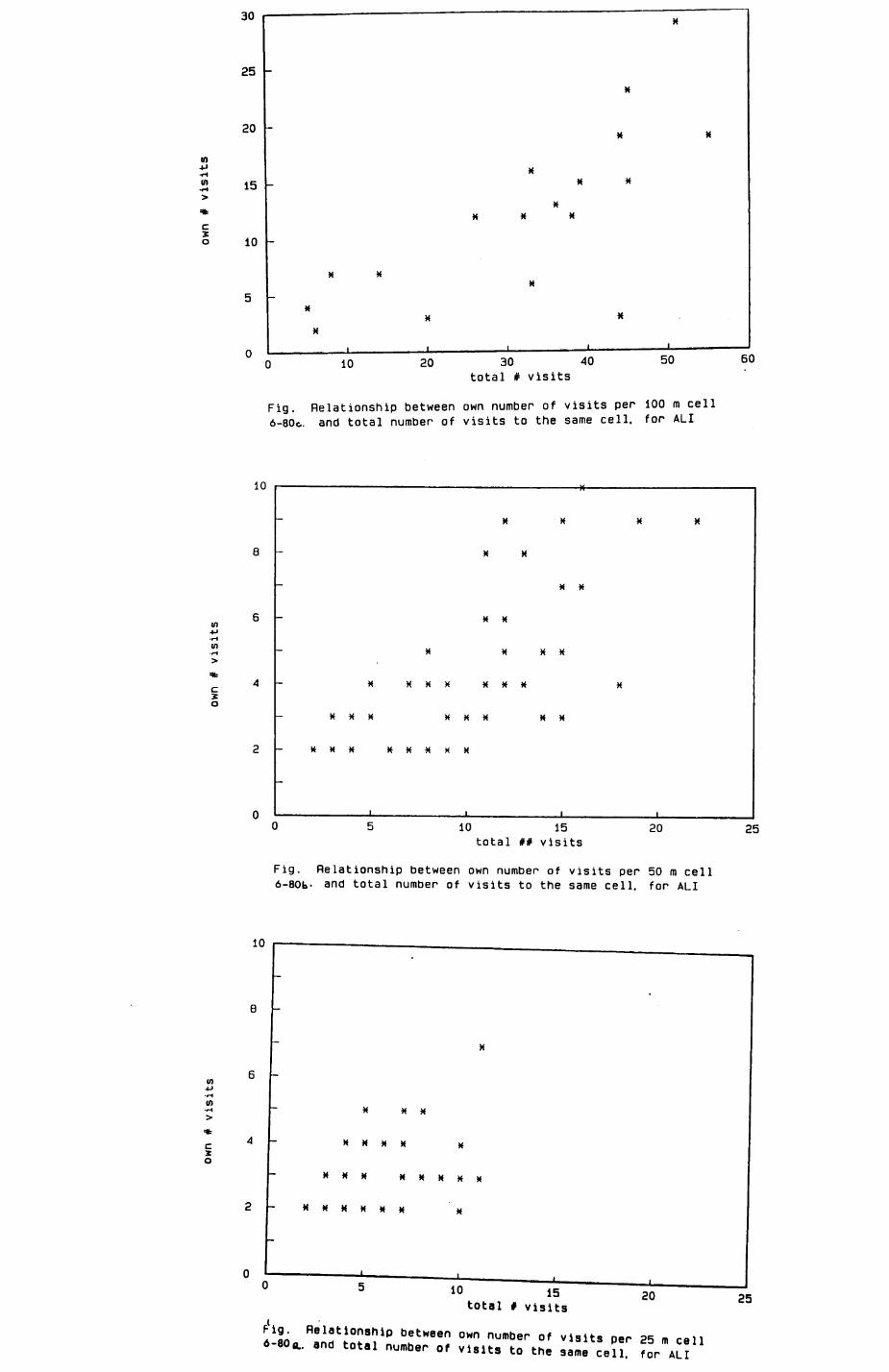
30
25
20
m-P•r* in
c. z o
15
10
x *
c3.o
10_l_________i _._______J_ 20 30 40
total # visits50
Fig. Relationship between own number of visits per 100 m cell 6-80c. and total number of visits to the same cell, for ALI
10
* x
XXX
X X
XXX XXX
XXX
X X
X X
XXX XKXKX
10 15 total ## visits
20
Fig. Relationship between own number of visits pen 50 m cell 6-80b- and total number of visits to the same cell, for ALI
60
25
10
C
o
X XX
X H X X X
*** xxxxx
« X X X X X x
™ between own number of visits per 25 m cell -80a.. and total number of visits to the same cell, for ALI
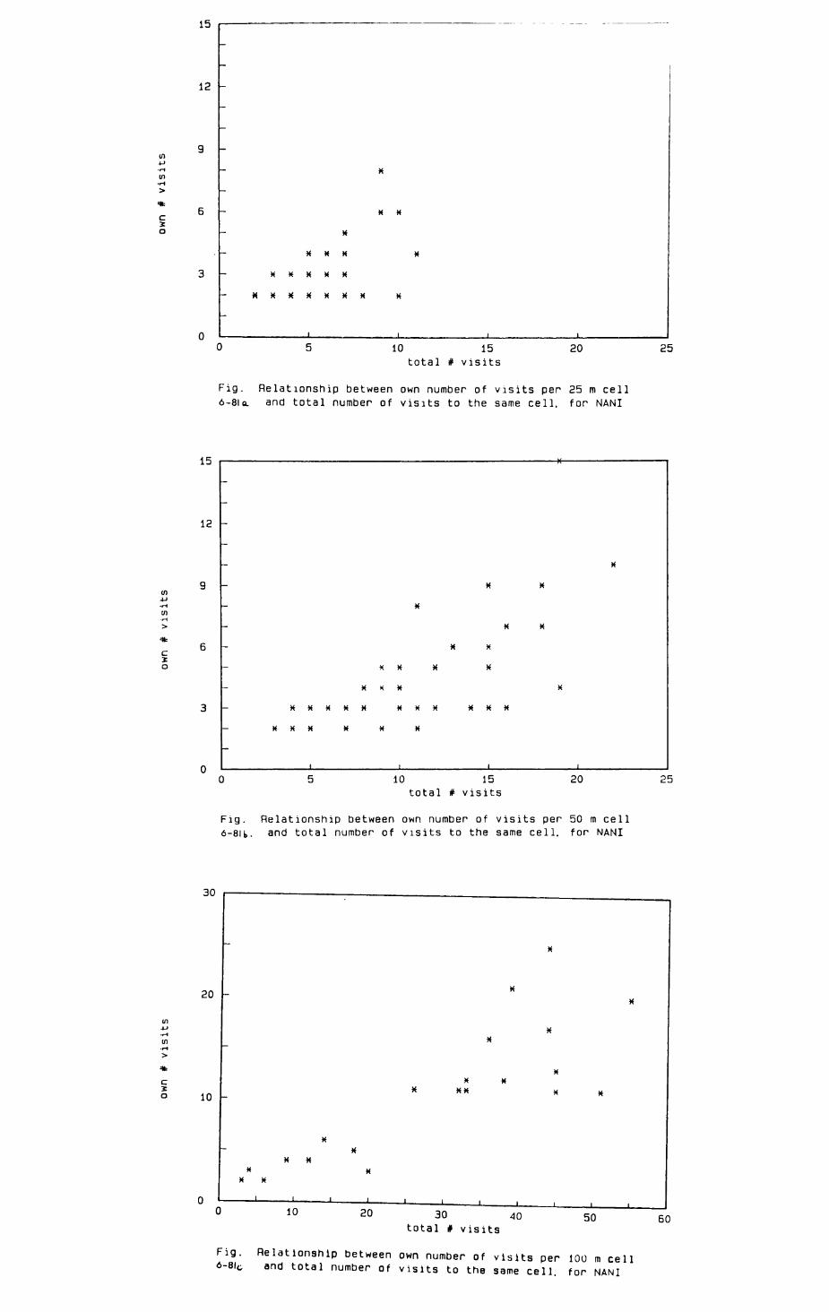
c o
15
12
X X
K
XXX
X X X K X
X X X X X X
10 15
total # visits20
Fig. Relationship between own number of visits per 25 m cell 6-8lo. and total number of visits to the same cell, for NANI
10 15 total # visits
20
Fig. Relationship between own number of visits per 50 m cell 6-8lt. and total number of visits to the same cell, for NANI
25
10
12
9in-U-r-tin-|H
>
*
6
2O
3
n
- X
- XX
i- X
XX
xx
x x x x
X K X X
XXXXX XXX XXX
XXX X X X
1 1 1 1
25
_JU
20
in•rH
in
*c
o 10
0
x
X
X
XX
xx x
X XX * *
XX
X X* X
X X
—— I —— 1 —— 1 —— ••••.,..10 20 30 40
total # visits50
Fig. Relationship between own number of visits per 100 m cell 6-8lc and total number of visits to the same cell, for NANI
60
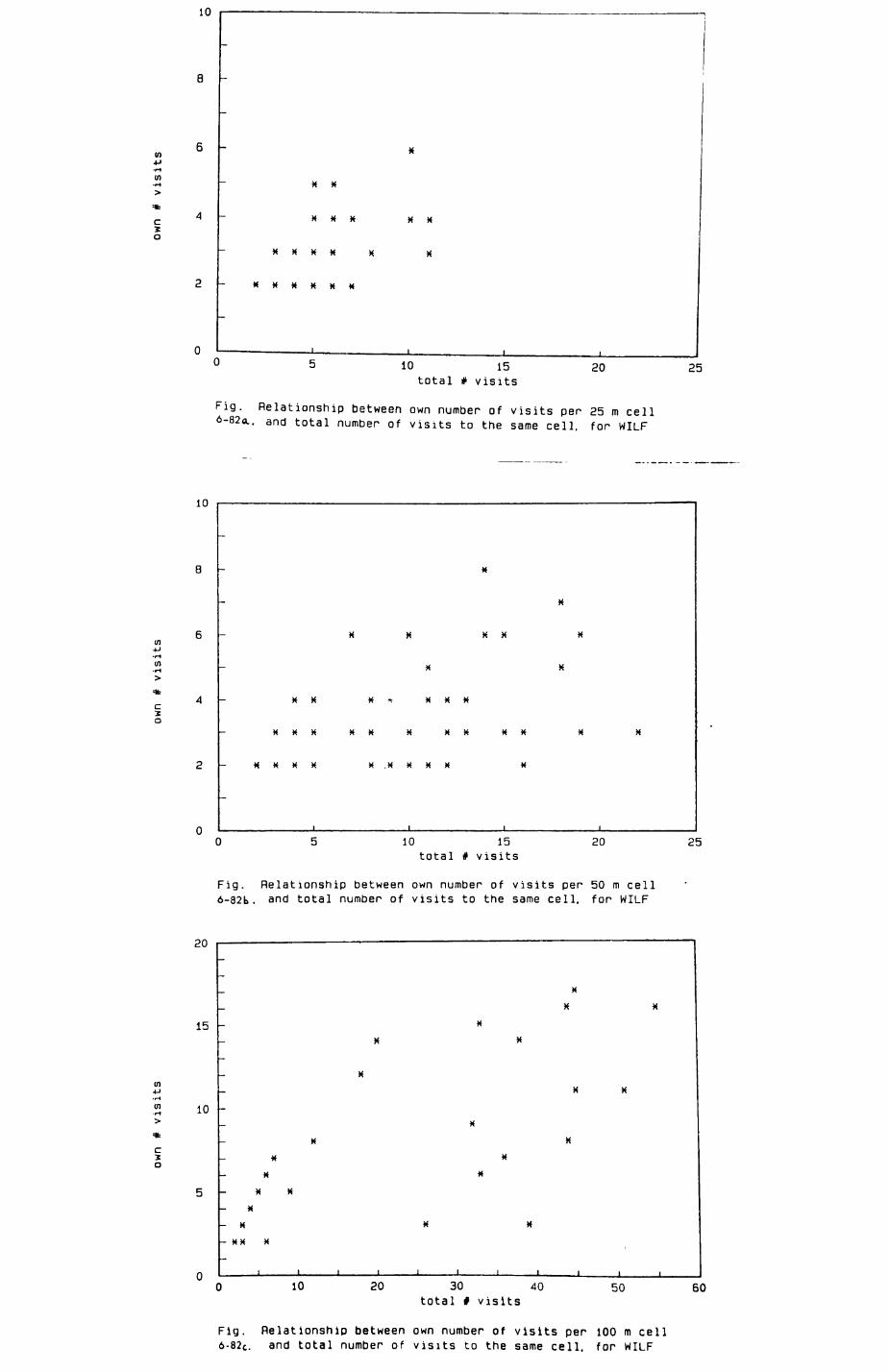
10
CO 4J -r4
tn X X
c2 O
XXX
X X X X
2 - X H
10total
15 # visits
20 25
Fig. Relationship between own number of visits pen 25 m cell 6-82o.. and total number of visits to the same cell, for WILF
10
a
6in4J •rHin
•«-l
>
*4ci
O
2
n
X
X
i- XX XX X
XX
XX Xt XXX
XXX XX X XX XX X X
X X X X X.XXXX X
1 1 1 1
10 15 total # visits
20 25
Fig. Relationship between own number of visits per 50 m cell 6-82b. and total number of visits to the same cell, for WILF
20
15
en
S 10>*cX O
5
n
XXX
X
— . 7% *
XXX
X
— n "
x *— K "-XX
X
- X XX
-XXX
1 1 1 I I 1 1 1 1 1 1
10 20 30 40 total * visits
50 60
Fig. Relationship between own number of visits per 100 m cell 6-82 c . and total number of visits to the same cell, for WILF
262
for a depression in foraging rate, ie. the interval that a patch takes to
recover to an equilibrium density of surfacing worms, is much below that
(Chapter 7). The significance of the relationships reported above cannot be
taken at face value, since independence of data points cannot be assumed.
However, all that is required is to yield a general impression that prepares
us for the following discussion.
In Table 6.9 results are presented of the computation of frequencies of
renewal periods. Here, in contrast to the previous analyses, all visits to
a cell, regardless of the individual responsible for it, have been pooled.
Frequencies are listed as mean renewal periods per cell. In BLOCK A.
frequencies are listed for six-hour-blocks while in BLOCK B the first Block
is listed in detail. Renewal periods were calculated for two casest (i) the
previous visitor is identical with the present visitor; <ii) the two are two
different individuals.
If individuals coordinated their movement, I would expect them to be
cautious about entering an area that has recently been visited by another
individual. No such precaution applies if the animal visits an area again
Where it was the previous visitor, provided it has the sensory capacties to
remember the state of the art at its last visit. Therefore, in case 1 I
expect individuals to return to cells earlier than case 2 individuals. This
expectation hinges crucially on the proposed size of a foraging patch as
perceived by the badgers. The spatial analysis of section 6.2 indicates
independence of utilization intensities for cells of size SO by SO m,
proposing a small patch size as perceived by badgers. Furthermore, the raean
length of visits did not increase when cell sizes were enlarged from SO to
100 m (Table 6.5). One interpretation of this result is that an individual
foraged in an area of 50 by 50 metres (or less), and, once finished,
vanished to another site at a medium distance. If the true patch size was
100 m, or even larger, slowly meandering "worming" badgers should have spent
more time per 100 m cell. Therefore I conclude that the cell size most
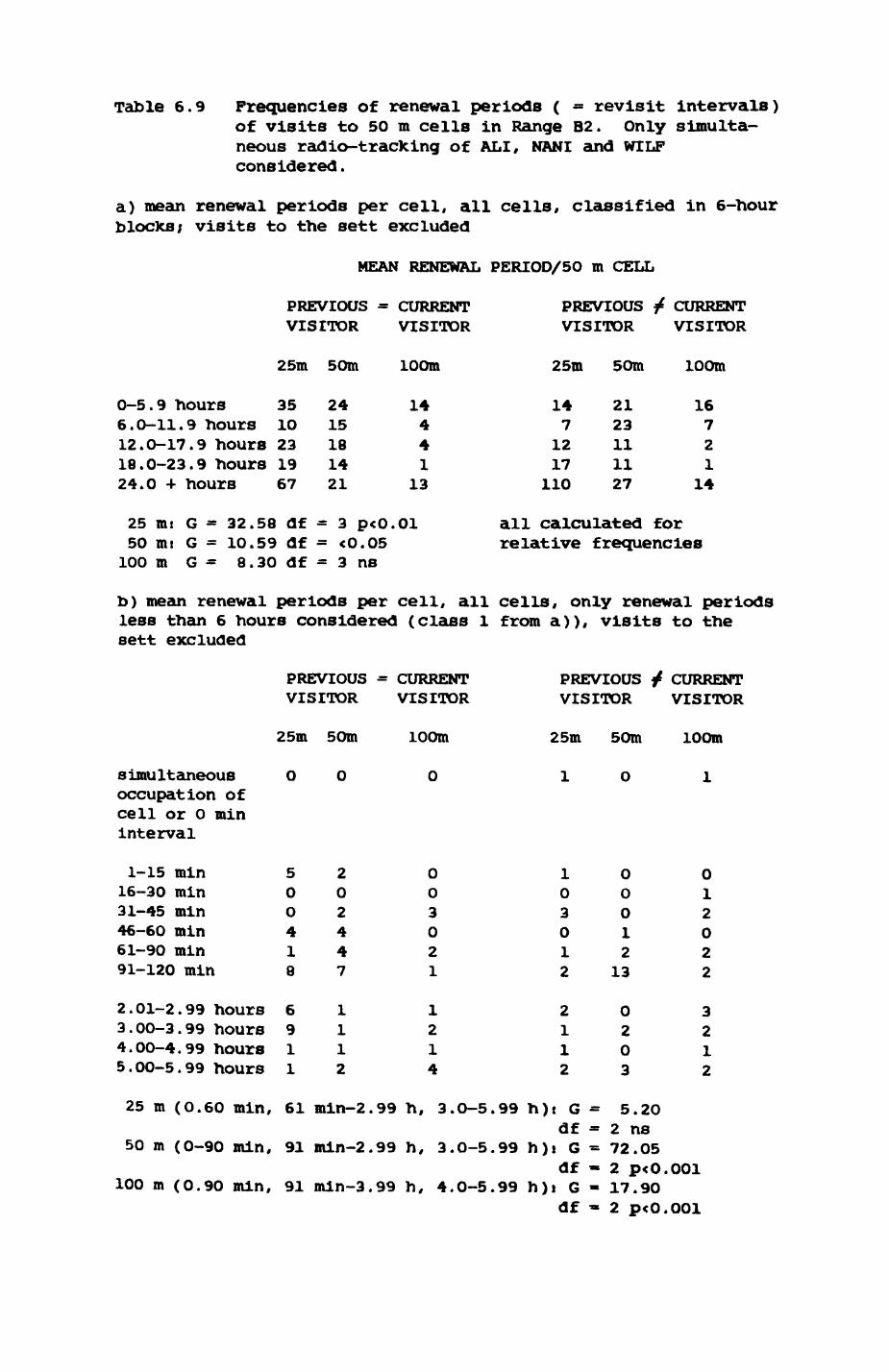
Table 6.9 Frequencies of renewal periods ( = revisit intervals) of visits to 50 m cells in Range B2. Only simulta neous radio-tracking of ALI, NANI and WILF considered.
a) mean renewal periods per cell, all cells, classified in 6-hour blocks* visits to the sett excluded
MEAN RENEWAL PERIOD/SO m CELL
PREVIOUS VISITOR
CURRENT VISITOR
PREVIOUS VISITOR
CURRENT VISITOR
25m 5Om loom 25m 5Om loom
0-5.9 hours 35 246.0-11.9 hours 1O 1512.0-17.9 hours 23 1818.0-23.9 hours 19 1424.0 -»• hours 67 21
14441
13
25 mi G =50 mi G =100 m G =
32.58 df = 3 p<0.01 10.59 df = <0.05 8.3O df = 3 ns
147
1217
110
2123111127
16721
14
all calculated for relative frequencies
b) mean renewal periods per cell, all cells, only renewal periods less than 6 hours considered (class 1 from a)), visits to the sett excluded
PREVIOUS = CURRENT VISITOR VISITOR
PREVIOUS VISITOR
CURRENT VISITOR
simultaneous occupation of cell or 0 min interval
25m 5Om
O 0
lOOm
0
25m 5Om loom
10 1
1-15 min 16-30 min 31-45 min 46-60 min 61-90 min 91-120 min
2.01-2.99 hours 3.0O-3.99 hours4.00-4.99 hours 5.00-5.99 hours
50O418
6911
202447
1112
0 O 3021
1214
103012
2112
25 m (0.60 min, 61 min-2.99 h, 3.0-5.99 h)t Gdf
50 m (0-90 min, 91 min-2.99 h, 3.0-5.99 h)i Gdf
100 m (0.90 min, 91 mln-3.99 h, 4.0-5.99 h)i Gdf
O 0O 10 21 02 2
13 2
0 32 20 13 2
5.20 2 ns 72.05 2 p<O.001 17.90 2 p<0.001
263
suitable for this kind of investigation is 5O by 5O m (cf. Chapter 5).
However, for completeness I have also included the results for the two other
cell sizes (Table 6.9).
No differences between the two cases (previous visitor - current
visitor and previous visitor^ current visitor) were found for 1OO » cells
for BLOCK A data (coarse 6 hour blocks), and the 25 m cells for the detailed
analysis of renewal periods of less than 6 hours (BLOCK B data). In 3 out
of 4 situations with significant differences, case 1 visitors returned
sooner to the same cell than case 2 visitors} only 1OO m cells in BLOCK B
showed the reverse. Noteworthy is the sudden increase of frequency of
renewal periods after ca 1.5 hours, in all cases. In general, short renewal
periods constitute only a small fraction of all renewal periods (Table
6.9a). Even from the point of view of worst possible case, the 1OO m cell
records, interference is limited, since in those 4 cells Where the current
visitor may experience a reduced foraging rate (cells with renewal periods
of 0 - 45 min), the probability of hitting the spot depreciated by the
previous visitor is on average only one fourth of the probability of hitting
the same spot ink 50 by 50 m cell.
In summary, badgers within the same group seem to coordinate their
movements relative to each other. Simple rules were identified that aid in
maintaining the coordination. It could not conclusively show to what extent
the coordination is solely due to intent tonality or a by-product of similar
pressures by an external factor* Interference between individuals as
evidenced by agonistic encounters could not be found* Actual levels of
Interference as evidenced by the pattern of distribution of renewal periods
are small.
264
6.4. Habitat utilization
In sections 6.2. I have already indicated that areas of intensive use
often coincide with the presence of specific resources. In this section I
will investigate in more detail how the intensity of use of a specific area
within an animal's range relates to the presence (or absence) of resources
therein. As already discussed in Chapter 2, I will use habitats as defined
by the habitat map as an indicator of resource presence, although the
relationship between resource abundance and habitat type may not necessarily
be straightforward. The analysis is centred around the following questions i
1. Which habitats are visited?
2. Does intensity of use, as measured by the number of visits (MOV) and
duration of stay (DOS), vary between habitats? Which habitats are
preferred?
3. What are the habitat and resource characteristics of those area units
within a group range actually utilized by individuals?
4. How does intensity of use relate to resource presence?
5. What are the effects of the size of a patch or a habitat on its use by
resident animals?
6. How do patterns of visits to uniform areas compare with simple randan
movements?
Before I present the results, two notes of caution are appropriate*
The first relates to the problem of spatial dependence, as discussed In
Appendices 5-7. This concerned the influence of the location of a given
unit area could exert on the probability of being visited. In section 6.2
spatial correlograms indicated the scale at which this effect operates.
Spatial dependence influences the error probability (type 1 error) of a test
statistic. Positive spatial dependence leads to an undesirable increase of
the actual alpha level, while negative spatial dependence decreases the
alpha-level and produces a conservative estimate (Appendix 5, Cliff & Ord
265
1981). Therefore, the average overall individuals of a species of
the number of the highest lag with a significant positive spatial
autocorrelation before the first insignificant or negative
autocorrelation value
of the correlograms of section 6.2 was computed as an index of the scale of
spatial dependence. This index is 3.2 for foxes (n=!4, Fig. 6.1-6.28) and
0.5 for badgers (n=8, Fig. 6.30-6.50), indicating a significant spatial
Interdependence for foxes but none for badgers at the chosen level of
spatial resolution. Thus, the test statistics computed in sections 6.5.1. -
6.5.3. were modified according to the following rulest
- for foxes i (1) a test statistic is distributed according to
the chi square distribution! divide the test
statistic by 3, but leave the degrees of
freedom unchanged.
(ii) all other test statistics t divide the degrees
of freedom by three.
- for badgerst no corrections required.
The second note of caution relates to the degree by which a measure of
the intensity of use of an area does actually reflect this area's
"importance" to an individual. For instance, PODGE stayed in the western
and eastern peripheral areas of her range only for brief periods, but the
regularity of visits and the fact that they must have caused some
Inconvenience to her can be interpreted in the sense that these were
Important visits necessary to maintain and defend the range. Here, the
intensity of use in relation to habitat type does not capture the essence of
these visits. Another example is the backyard (garden) of houses in suburbs
(e.g. in KALI'S range), where, say, watchdogs are present during most of the
266
night. These gardens may represent valuable resources to the fox, yet it
may have to wait in the neighbouring fields for a long time until a suitable; i
moment when it can nip in for 10 minutes and take everything previous from
the compost heap before vanishing into the neighbouring fields again. Yet
in my compilation of events, the short period of visiting the garden may be
underrated in comparison with the waiting time in the neighbouring field.
This is not meant to Imply that a consideration of Intensity of use is
totally use less i It just serves to remind us of the limits of this approach.
In section 6.5.4 I will describe an alternative approach that goes beyond a
simple compilation of NOV and DOS.
6.4.1. Habitat preferences
Habitat utilization was analysed for seven foxes (ELKE, KALI, KBOOM,
OLDMAHOG, PODGE, TARU, LIO) and seven badgers (ALI, GEORGE, NANI, PEACEFUL,
SARA, VICIOUS, WILF) with sufficient intensive tracking data. MOV and DOS
were analysed for 50 by 5O m cells. Variation in utilization intensity (UI>
was significant between habitats for which sufficient cells were present
that were completely covered by that habitat (n=478 for foxes and n=256 for
badgers) (Table 6.10)). If the correction for spatial dependence is
considered in foxes, the variation is still significant for NOV but not for
DOS. However, for this particular sample, spatial dependence may be
relatively weak, since cells covered with only one habitat must be separated
from cells covered by another habitat by at least one cell where the
transition occurs.
Table 6.11 and 6.12 present the results of multiple comparison tests
between habitats of high and low UI for badgers and foxes, respectively.
Not surprisingly, high quality habitats with respect to earthworms
experience on average a higher UI than low quality habitats in badgers < for
definitions see section 5.4.). There may be a bias due to the fact that
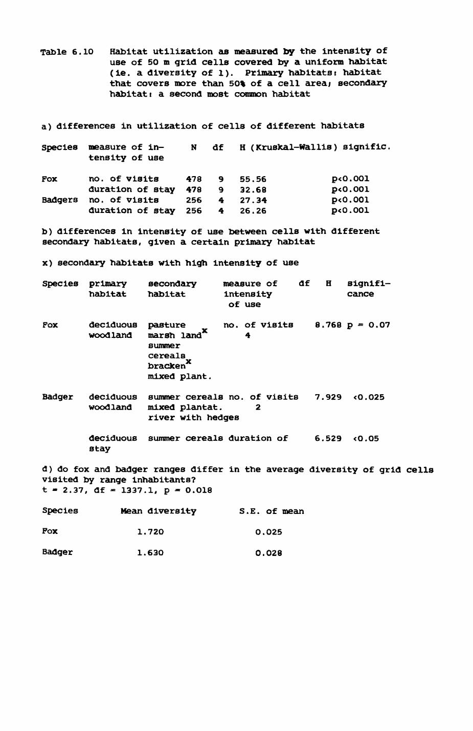
Table 6.10 Habitat utilization as measured by the intensity of use of 50 m grid cells covered by a uniform habitat (ie. a diversity of 1). Primary habitatst habitat that covers more than 50% of a cell area; secondary habitatt a second most common habitat
a) differences in utilization of cells of different habitats
Species measure of in- N df H (Krusfcal-Wallis) signific. tensity of use
Pox no. Of Visits 478 9 55.56 p<O.O01duration of stay 478 9 32.68 p<O.OOl
Badgers no. of visits 256 4 27.34 p<0.001duration of stay 256 4 26.26 p<O.O01
b) differences in intensity of use between cells with different secondary habitats, given a certain primary habitat
x) secondary habitats with high intensity of use
Species primary secondary measure of df H signifi- habitat habitat intensity cance
of use
Fox deciduous pasture no. of visits 8.768 p - 0.07 woodland marsh land 4
summer cereals brackenx mixed plant.
Badger deciduous summer cereals no. of visits 7.929 <O.025 woodland mixed plantat. 2
river with hedges
deciduous summer cereals duration of 6.529 <O.05 stay
d) do fox and badger ranges differ in the average diversity of grid cellsvisited by range inhabitants?t - 2.37, df - 1337.1, p - O.O18
Species Mean diversity S.E. of mean
Pox 1.720 O.025
Badger 1.630 0.028
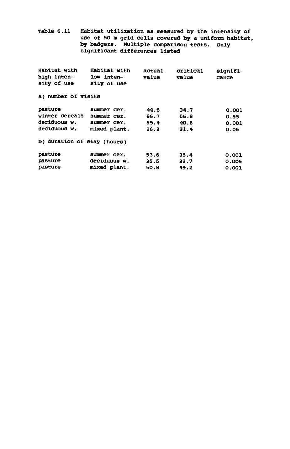
Table 6.11 Habitat utilization as measured by the intensity of use of 50 m grid cells covered by a uniform habitat, by badgers. Multiple comparison tests. Only significant differences listed
Habitat with Habitat with actual critical signifi-high inten- low inten- value value cancesity of use sity of use
a) number of visits
pasture summer cer. 44.6 34.7 0.001winter cereals summer cer. 66.7 56.8 O.55deciduous w. summer cer. 59.4 4O.6 0.001deciduous w. mixed plant. 36.3 31.4 0.05
b) duration of stay (hours)
pasture summer cer. 53.6 35.4 0.001pasture deciduous w. 35.5 33.7 O.O05pasture mixed plant. 50.8 49.2 O.O01
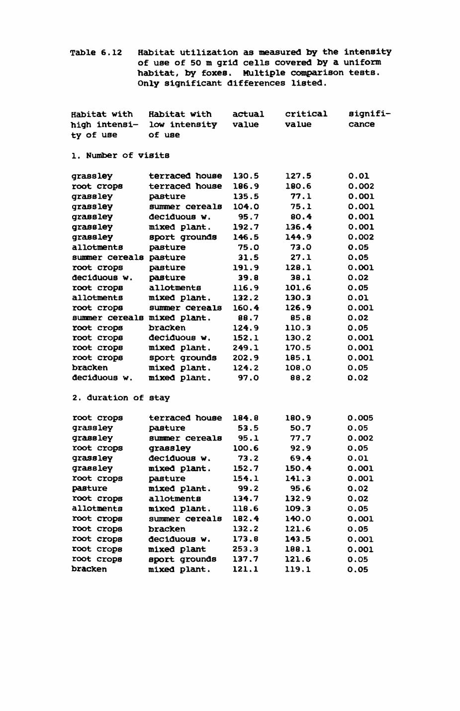
Table 6.12 Habitat utilization as measured by the intensity of use of 50 m grid cells covered by a uniform habitat, by foxes. Multiple comparison tests. Only significant differences listed.
Habitat with high intensi- ty of use
Habitat with low intensity of use
1. Number of visits
actual value
critical value
signifi- cance
grassleyroot cropsgrassleygrassleygrassleygrassleygrassleyallotmentssummer cereals pastureroot crops pasturedeciduous w.root cropsallotmentsroot crops
terraced house terraced house pasture summer cereals deciduous w. mixed plant. sport grounds pasture
pasture allotments mixed plant. summer cereals
summer cereals mixed plant.root crops root crops root crops root crops bracken deciduous w.
bracken deciduous w. mixed plant. sport grounds mixed plant. mixed plant.
2. duration of stay
root crops grassley grassley root crops grassley grassley root crops pasture root crops allotments root crops root crops root crops root crops root crops bracken
terraced house pasture summer cereals grassley deciduous w. mixed plant. pasture mixed plant. allotments mixed plant. summer cereals bracken deciduous w. mixed plant sport grounds mixed plant.
130.5186.9135.5104.095.7
192.7146.575.031.5
191.939.8
116.9132.2160.488.7
124.9152.1249.1202.9124.297. 0
127.5180.677.175.1SO. 4
136.4144.973.027.1
128.138.1
101.6130.3126.985.8
110.3130.2170.5185.1108.088.2
0.010.0020.0010.0010.0010.0010.0020.050.050.0010.020.050.010.0010.020.05O.OOlO.OOlO.OOl0.05O.02
184.853.595.1100.673.2152.7154.199.2134.7118.6182.4132.2173.8253.3137.7121.1
180.9SO. 777.792.969.4150.4141.395.6
132.9109.314O.O121.6143.5188.1121.6119.1
O.O05O.050.002O.05O.OlO.OOl0.001O.020.02O.05O.OOlO.05O.OOl0.0010.050.05
267
most intensive tracking data were obtained during periods of good earthworm
availability (April-May and September-November); it can be expected that
utilization of arable fields increases during the summer months (Chapter 4).
For foxes, the picture is more complicated. Highly valued areas are
grassley and root crops (rabbits/earthworms) and deciduous woodland f but
also summer cereals. However, if the correction for spatial dependence is
considered, the significant pairs of Table 6.l2il with a probability level
of more than 0.001 would turn insignificant while the comparisons under IIi
would be inadmissible. Even then, pasture, sports grounds and terraced
houses remain little visited in comparison with other habitats»
If cells are considered where several habitats occur (Table 6.1Ob>, the
effect of neighbouring habitats can be considered. For this purpose the
habitat with the highest proportion of area per cell was designated as
"primary habitat", and the habitat with the second highest proportion as
"secondary habitat". Cells were excluded, if primary habitats occupied less
than 50% of the cell area (to ensure "dominance" of primary habitat). In
foxes, no significant effects on UI due to secondary habitats could be
Identified, while In badgers UI of deciduous woodland in zones of transition
depended on the secondary habitat, both for NOV and DOS. UI of the primary
habitat (deciduous woodland) was high if the secondary habitat Is nixed
plantations, but low If consisting of cereals, rivers or even pasture. This
Is consistent with Kruuk's (1978a) observations of frequent use of mixed
plantations by his badgers in the Jews Harp group.
6.4.2. Habitat characteristics and resource levels in visited cells
Here, the following parameters were considered t habitat diversity, ie.
the number of different habitats that occur per cell, the DCA-scorea
(badgers only, since only here did an appreciable proportion of range occur
in the area of habitat recording) and the worm biomasa index ( for
268
computation procedures see section 6.1).
Fox ranges had a higher habitat diversity than badger ranges (Table
6.10C). Diversity was also significantly variable between fox ranges (table
6.13c), but not significant, if the modified test statistic is used.
Similarly, badger ranges had equivalent levels of habitat diversity (Table
6.14C). Habitat diversity was closely, and inversely, related to the wora
biomass index per cell, both for foxes and badgers (Table 6.13b, 6.14b).
This dependence is linear, for foxes at least (Table 6.13b).
Mean worm biomass per cell varies significantly between ranges, both
for foxes and badgers. In foxes, this variation does not contribute to an
overall difference in earthworm consumption between ranges (Chapter 4).
Similarly, in badgers, the differences listed here do not produce
significant differences in earthworm consumption for the ranges concerned
(Table 4.12b, September to November). However, the reasons are different
for the two species (see below).
DCA scores in range 84 correlate significantly with worm biomass on the
first three axis (Table 6.l4d). This supports Shute and West's (1982)
proposal that general habitat inventories are also very useful for special
applications. During habitat recording, no specific variable was selected as
earthworm indicator, yet the resulting ordination yields a structure that is
correlated with earthworm abundance.
6.4.3. Intensity of use in relation to resource density.
Here I considered the relationship between UI and the worm biomass index per
cell as an example. Table 6.15 presents the results of correlating UI with
worm biomass for individual badgers and for foxes. In foxes, despite wide
variation in mean worm content per cell between ranges (see previous
section), no significant differences could be found in earthworm consumption
between ranges (Chapter 4). Consequently, ui should be independent of the
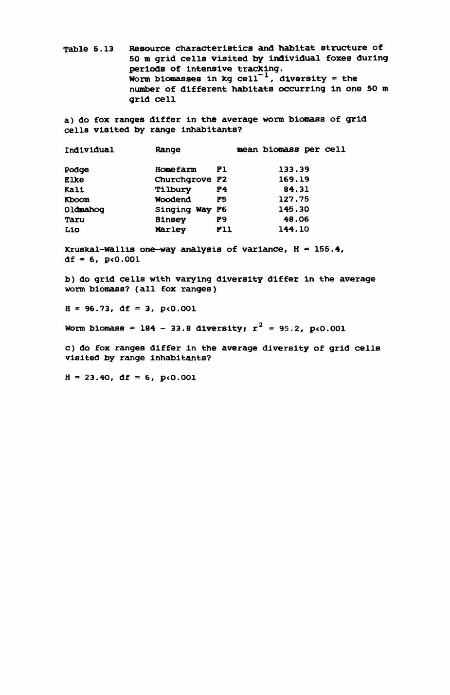
Table 6.13 Resource character1stics and habitat structure of 50 m grid cells visited by individual foxes during periods of intensive tracking. Worm biomasses in leg cell" 1 , diversity = the number of different habitats occurring in one 50 m grid cell
a) do fox ranges differ in the average worm biomass of grid cells visited by range inhabitants?
Individual Range mean biomass per cell
Podge Home farm Fl 133.39EIXe Churchgrove F2 169.19Kali Tilbury F4 84.31Kboom Woodend F5 127.75Oldmahog Singing Way F6 145.30Taru Binsey F9 48.06Lio Mar ley Fll 144.10
Kruskal-Wallis one-way analysis of variance, H = 155.4, df - 6, p<0.00l
b) do grid cells with varying diversity differ in the average worm biomass? (all fox ranges)
H * 96.73, df - 3, p<0.001
worm biomass = 184 - 33.8 diversity/ r 2 = 95.2, p<O.OOl
c) do fox ranges differ in the average diversity of grid cells visited by range inhabitants?
H - 23.40, df = 6, p<0.001
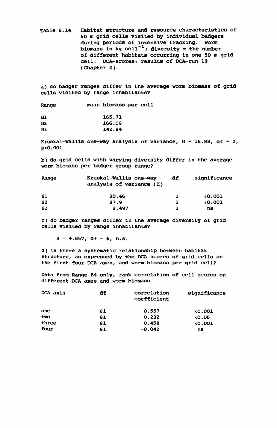
Table 6.14 Habitat structure and resource characteristics of 50 m grid cells visited by individual badgers during periods of intensive tracking. Worm biomass in Xg cell" 1 ; diversity - the number of different habitats occurring in one 50 m grid cell. DCA-scorest results of DCA-run 19 (Chapter 2).
a) do badger ranges differ in the average worm biomass of grid cells visited by range inhabitants?
Range mean biomass per cell
Bl 165.71B2 166.09B3 142.84
Krusfcal-Wallis one-way analysis of variance, H - 16.88, df = 2, p<0.001
b) do grid cells with varying diversity differ in the average worm biomass per badger group range?
Range Krusfcal-Wallis one-way df significanceanalysis of variance (H)
Bl 30.46 2 <0.001B2 37.9 2 <0.001B2 3.497 2 ns
c) do badger ranges differ in the average diversity of grid cells visited by range Inhabitants?
H * 4.857, df = 6, n.s.
d) is there a systematic relationship between habitat structure, as expressed by the OCA scores of grid cells on the first four OCA axes, and worm biomass per grid cell?
Data from Range B4 only, rank correlation of cell scores on different DCA axes and worm biomass
DCA axis df correlation significancecoefficient
one 81 0.557 <0.001two 81 0.232 <0.05three 81 O.458 <O.001four 81 -0.042 ns
269
worm biomass per cell. This is the case if the modified test statistic is
considered for DOS, while there are in fact slightly negative, although
significant correlations between UI and worm biomass for NOV (Table 6.15C).
In Chapter 5, however, earthworm consumption per group range was positively
correlated with the proportion of pasture and deciduous woodland per group
range. How can these differences be resolved?
In one sense, the two results cannot be compared directly. The
correlation between pasture and deciduous woodland and earthworm consumption
was restricted to the proportion of high quality earthworm habitat per group
range. The above, negative correlation is a result of indexing all cells.
ie. also cells with low quality habitat, (we shall see below that this is a
difference that matters also for badgers). Such cells, however, may be
visited by foxes in order to hunt rabbits or mice, which are time consuming
activities. For a wide range of worm biomasses, the worm biomass may simply
be irrelevant to a fox - only areas with high worm abundance may be of
interest and guarantee an energy intake comparable with that achieved by
hunting for rabbits (Chapter 3). An additional complication is the fact that
earthworm availability may be quite different from earthworm abundance, and
certainly more so in open areas such as pastures or grass ley (if cut) than
in deciduous woodland (Chapter 3).
In badgers, UI Is either positively correlated or independent fro* the
worm biomass index per cell (Table 6.15a and b). For the two individuals
from Range B4, PEACEFUL and VICIOUS, a relatively low average worm biomass
per cell was previously computed (Table 6.14); consequently the UI is
independent of worm biomass, due to a high level of UI in mixed plantations.
Some reasons for this were discussed in Chapter 3. UI of cells by PEACEFUL
la, however, correlated with the DCA cell scores on DCA axis 1 (Spearman's
rho-0.293, n-45, p<0.05). Mean DCA scores on axes 1 to 4 of cells visited by
PEACEFUL are 97.33, 112.20, 112.76, and 143.37. No differences were found on
the DCA scores of cells between PEACEFUL and VTCIOUS on any of the DCA axes.
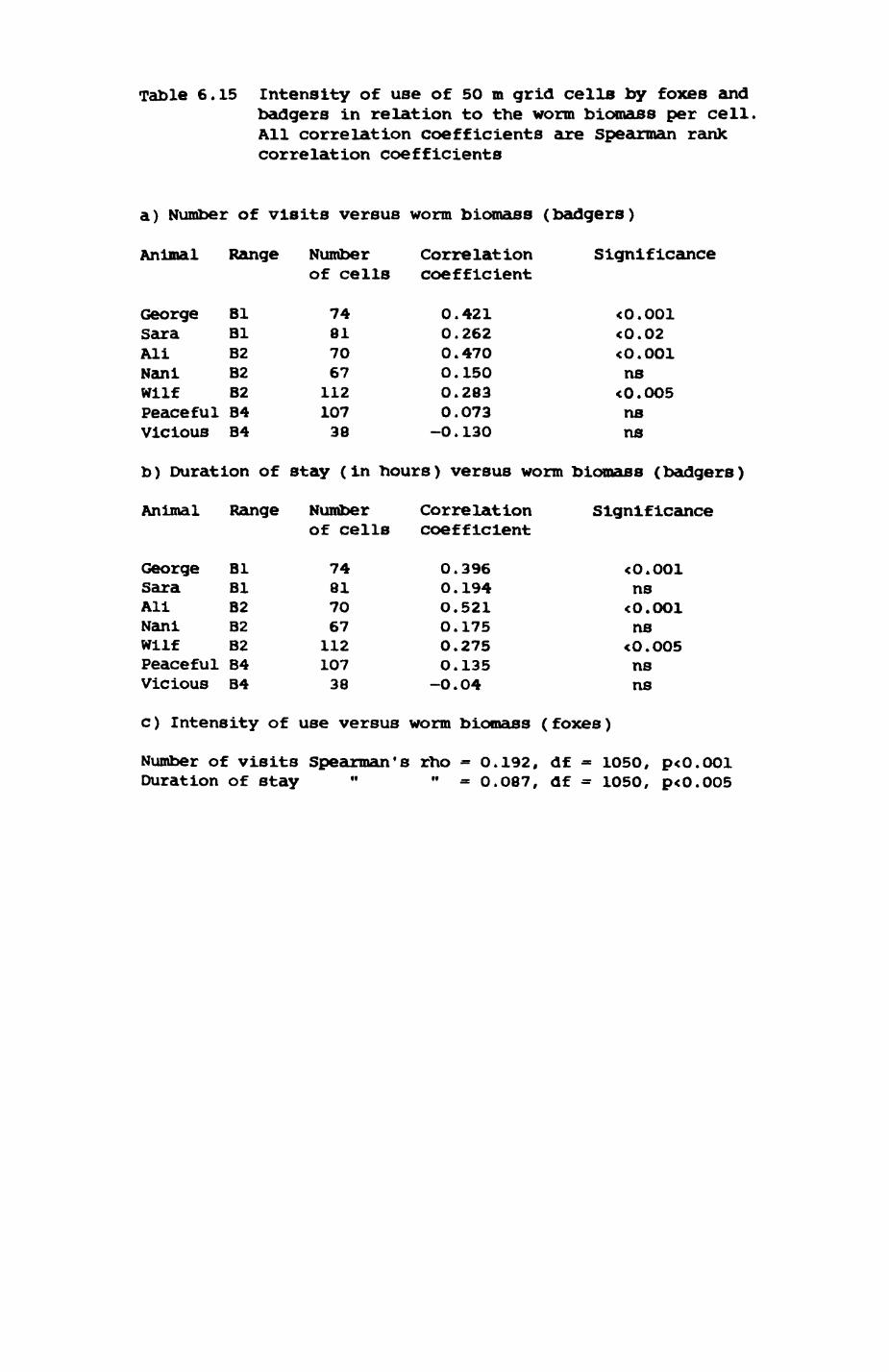
Table 6.15 Intensity of use of 50 m grid cells by foxes and badgers in relation to the worm biomass per cell, All correlation coefficients are Spearman rank correlation coefficients
a) Number of visits versus worm biomass (badgers)
Animal Range Number Correlation Significanceof cells coefficient
George Bl 74 0.421 <0.001Sara Bl 81 0.262 <0.02Ali B2 70 0.470 cO.OOlNani B2 67 O.150 nsWllf B2 112 0.283 <O.OO5Peaceful B4 107 O.O73 nsViCiOUS B4 38 -0.130 ns
b) Duration of stay (in hours) versus worm biomass (badgers)
Animal Range Number Correlation Significanceof cells coefficient
George Bl 74 0.396 <O.OO1Sara Bl 81 0.194 nsAli B2 7O 0.521 <O.OO1Nani B2 67 0.175 nsWilf B2 112 0.275 <O.O05Peaceful 84 1O7 O.135 nsVicious B4 38 -O.O4 ns
c) Intensity of use versus worm biomass (foxes)
Number of visits Spearman's rho - O.192, df - 1050, p<O.OOlDuration of stay " " - 0.087, df = 1050, p<0.005
270
For other individuals, the majority of correlations of UI with the worm
bioroass index per cell is significantly positive. These are individuals
with, on average, high worm biomass indices per cell.
In summary, the index of worm biomass chosen here is not a wholly
satisfying predictor of small-scale range use. For foxes, this may be due
to the fact that worm biomass may be irrelevant for many cells that they
visit. In badgers, it is a reliable predictor, if the overall bionass level
is high. Obviously, an indicator of earthworm availability would be a much
more satisfying parameter - but this was impossible to measure in this
study.
6.4.4. Patterns of visits to different habitats
In this section, patches from the habitat map are the basic units of
investigation. The effects of the size of a patch and a habitat <ie. the
sum of all patches per range that belong to the same habitat) are
illustrated in Fig. 6.83 (badgers) and 6.84 (foxes). Corresponding
correlation and regression analyses can be found in Table 6.16. The results
are similar for both species. The larger the area of a particular habitat
per range, the more often and the longer it is visited. However, there is
no linear dependency between area of single patches and UI (cf. Fig. 6.83C.
d, 6.84c, d, Table 6.16). A small patch may often be visited despite its
sizej similarly, large patches may rarely be visited, if they are of no
interest.
Both measures of UI are highly correlated (Fig. 6.85-6.86, badgers}
Fig. 6.87-6.88, foxes* Table 6.16). For both single patches and habitats,
often visited areas are visited for a long time and rarely vlslsted areas
are inspected only briefly . In Fig. 6.86 and 6.88, the relationship
between NOV and DOS is investigated in more detail. Two classes of
durations of visits were compared with MOVt very short visits (less than 5
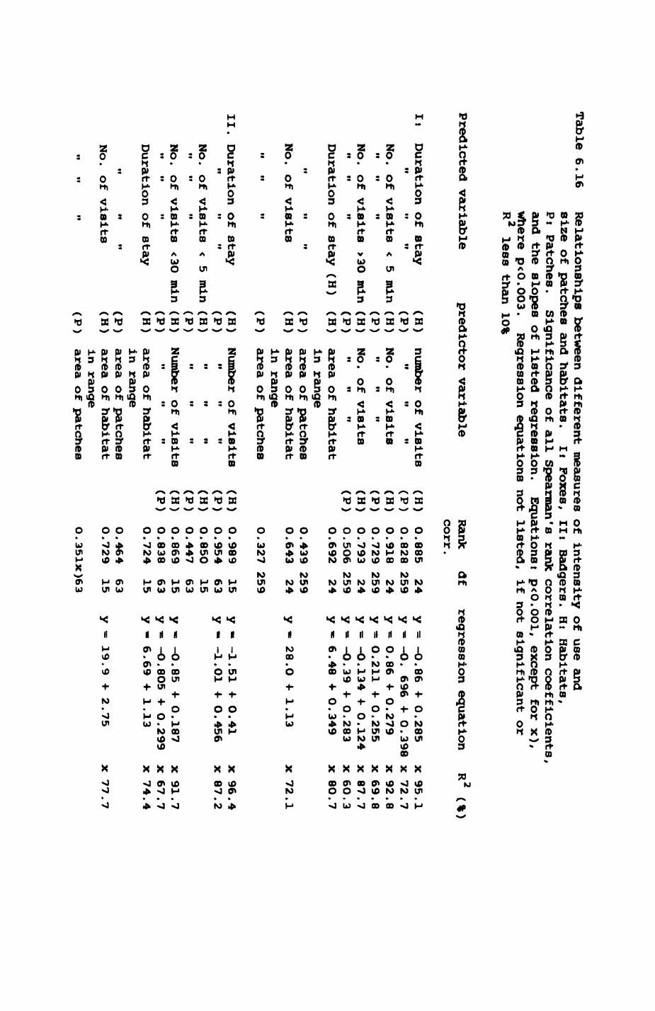
Table 6.16Relationships between different measures of intensity of use andsize of patches and habitats.
It Foxes,
lit Badgers.
Hi Habitats,
Pi Patches.
Significance of all Spearman's rank correlation coefficients,and the slopes of
listed regression. Equations!
p<O.OOl, except
for x),where p<O.OO3.
Regression equations not listed,
if not significant or
R2
less than 10%
Predicted variable
Duration of stay
predictor variable
(H) number of visits
(P) No.
of visits <
5 min (H) No.
of visits
No. of visits
>3O min (H)
No. of visits
„ „
„ (P)
,, .,
„Duration of stay (H)
(H) area of habitatin range
" M
M
(pj
area of patches N
o. of v
isits (H
) area of h
abitat
in range M
M
•• (p
j area of patches
II. Duration of stay
II M
MII
M
II
II If
II
II II
II
(H) Number of visits
(P) No.
of visits <
5 min (H)•I
if it
/ p \No.
of visits <3O min (H)
Number of visitsM
M ?•
(P) "
" "
Duration of stay (H)
area of habitatin range
•• M
M
^ p) area of patches
No.
of v
isits (H
) area of h
abitat
In range••M
M (p)
area of patches
Rankdf
regression equation R
(%corr.
(H)(P)(H)(P)(H)(P)
(H)(P)(H)
(P)(H)
(P)
000O0O000000O0O00
.885.828.918.729.793.506.692
.439.643
.327
.989.954.850.447.869.838.724
24
25924
25924
25924
25924
259156315
6315
63
15
y -y -y -y =y -y -y -
y -
y -y -
y -y -y -
-o-o0.0.-0
-o6.28-i-i-o-o6.
.864-
0
. 696
4-86
4-211
.134
.3948
4-
.O 4-
.51.01
.85.80569
4-
0.4-
04-
4- O
0.1.
.2850.398
279
.2550.124
.283349
13
4- O.41
4- O.456
4- 0.187
4-1.O.299
13
XXXXXXXXXXXXX
95
72926987
6O8O
729687916774
.1.7.8.8.7.3.7.1.4.2.7.7.4
O.464
63
O.729
15
O.351X)63
19.9
4- 2.75
X 77.7
Pig. 6.83-6.84
Utilization intensity of habitats (ie. all habitat nap patches belonging to
the same habitat type summarized) and patches (as delineated by the habitat
map) in relation to the size of the area of the respective area unit.
Measures of utilization intensity are duration of stay (TIME) and number of
visits (NO. OF VISITS). In Fig. 6.83, results are presented for all
badgers, in fig. 6.84, for all foxes. Intensively tracked nights only.
Fig. 6.85-6.87
Relationship between the two measures of intensity of use. 6.85t badgers,
6.87i foxes.
Fig. 6.86-6.88
Utilization intensity of habitats and patches (as defined for Fig. 6.83-
6.84) as expressed by the number of short (5 min) and long (30 mln) visits
in relation to the total number of visits to the same area. 6.86t badgers,
6.881 foxes.
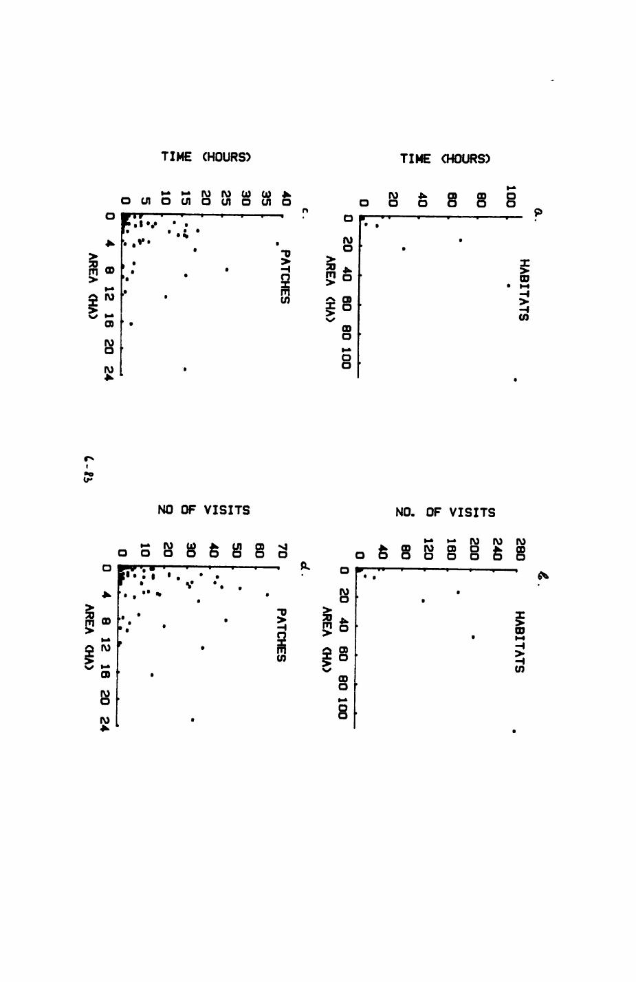
GL.
10080604020
HABITATS
ena:1NX
$l-f
40
35
30
25
20151050 1 0
20 40
60 80 100
AREA (HA)
PATCHES
••*4
8 12
16 20
24 AREA
CHA)
COHco>u. odCOCOfei
280 HABITATS
240
200
160
12080400 1
•
-D 20
40 60
80 100AREA
(HA)d.
70 PATCHES
605040302010 0
*
•
•/•
*
*•
••
C-fi4
8 12
16 20
24 AREA
CHA)
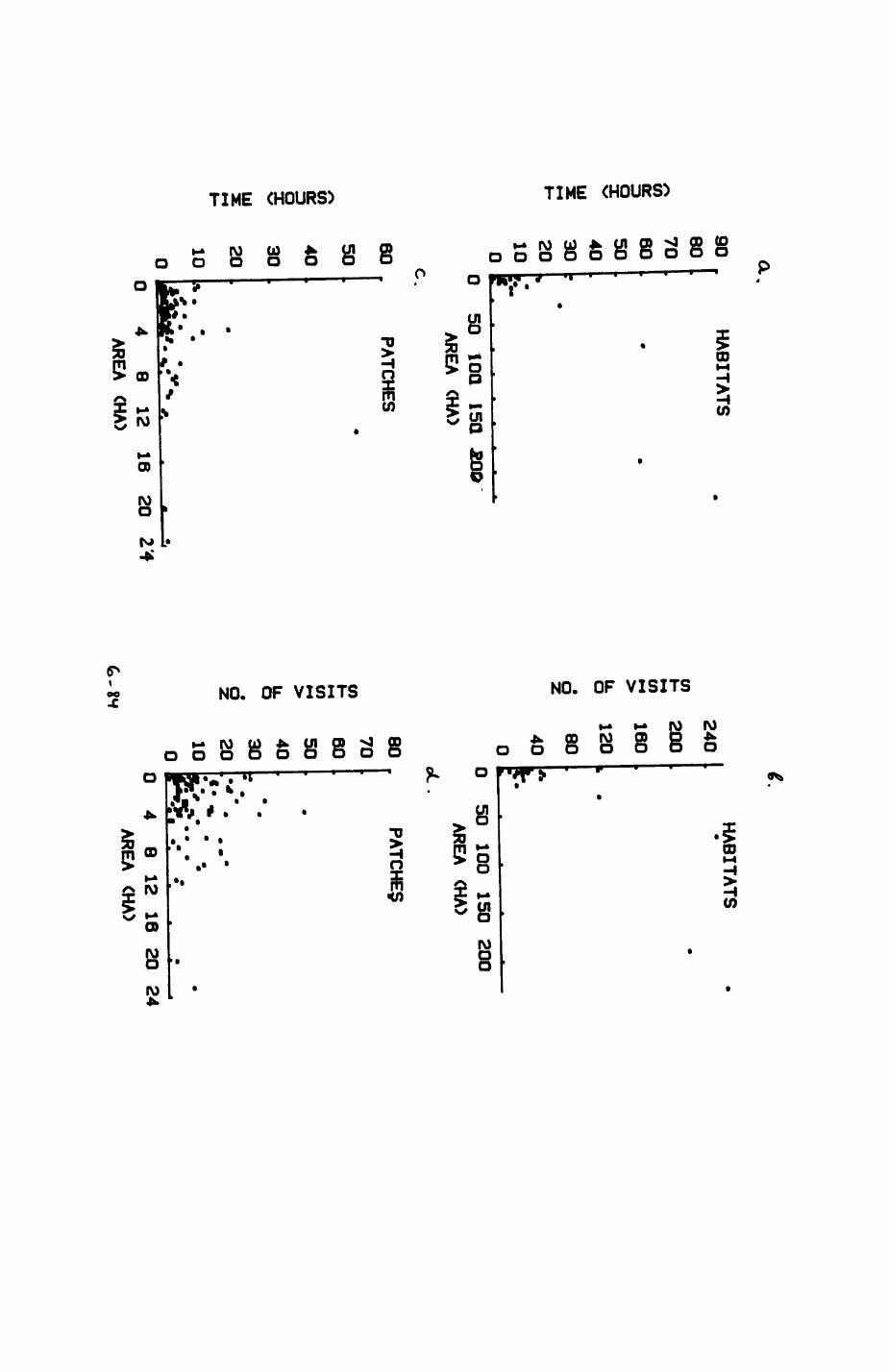
^cna:oXX
UlPcn§UlXp
90 HABITATS
80706050403020100
.
fk•J-0 50
10Q I5Q
£0*
AREA (HA)
c.
6050403020100
PATCHES•
,,*' . "•£&£.'• *rv
*»- A
HA
BITA
TS
cncnu. od
240
200
160
12080
.•
,b •
0 50
100 150
200
£cn1-4u.0d
AREA <HA>
oC.
80 PATCHES
70605040302010 0
.1 •
,
•
• •
1 6
m m
m +
• *
4 8
12 AREA
<HA>16
20 2'4
4 8
12 16
20 24
AREA (HA>
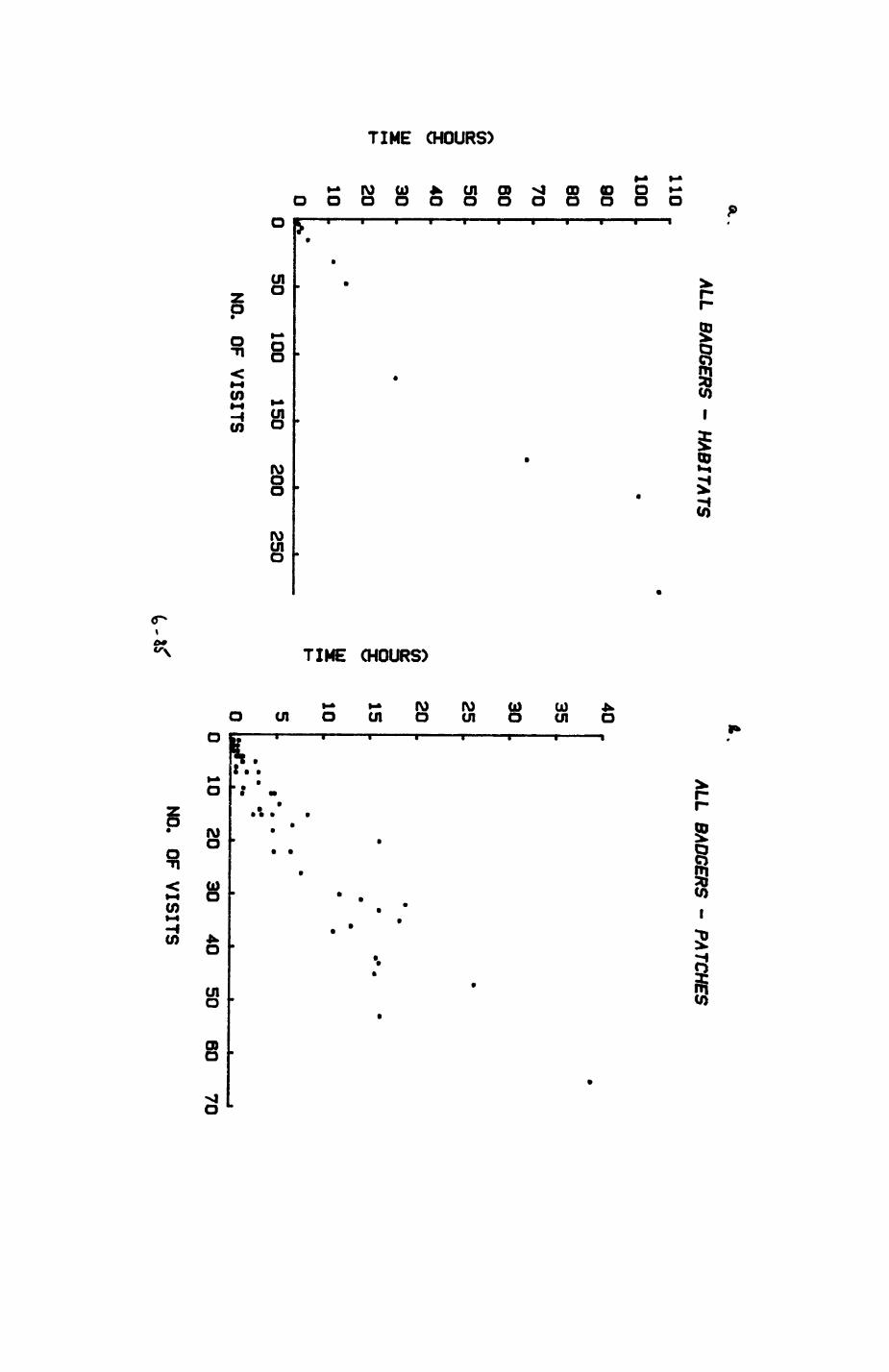
OL.
tu
ALL BADGERS - HABITATSALL
BADGERS - PATCHES110
1009080706050403020100
•»
4035»
30%^**
25
~
201i
15•
" I?
10H-
^m
• •
t •
•
0 50
100 150
200 250
5
NO. OF VISITS
0
•>(•
•
'
» — *
_
rf-' :• "" .
10 20
30 40
50 60
70
NO. OF VISITS
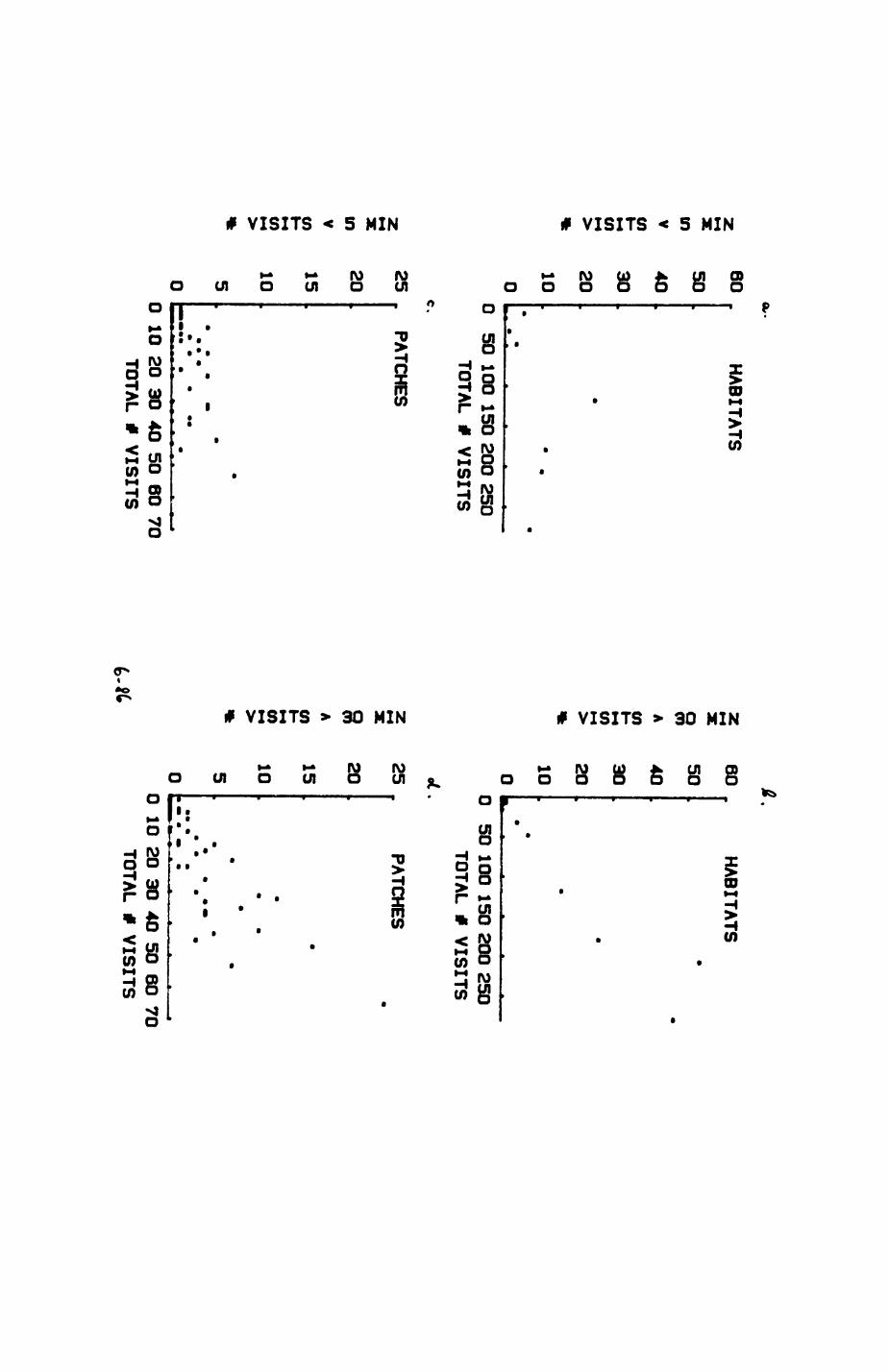
605040in v ent
30en*-i>
20*
10
HABITATS
0 50 100 150 200 250
TOTAL * VISITS
c.
25PATCHES
inVcncn*
c-w
20151050
••
• "
_..*.
. .
0 10 20 30 40 50 60 70
TOTAL * VISITS
58 »
A 40
cnt
30cn>
2010
HABITATS
0 50 100 150 200 250
TOTAL * VISITS
cn
2520151050 t
PATCHES
0 10 20 30 40 50 60 70
TOTAL * VISITS
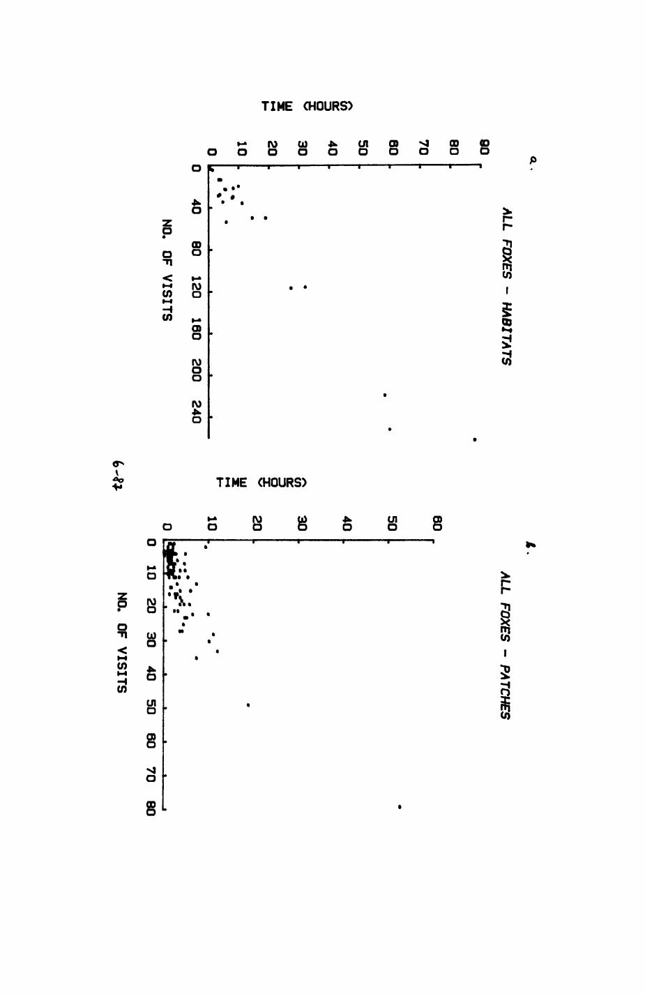
FOXES - HABITATS
ALL FOXES -
PATCHES
oUJ
908070605040302010•
%40 80
120 160
200 240
NO. OF VISITS
605040
w
30 a:5
2010
0 10
20 30
40 50
60 70
80
NO. OF VISITS
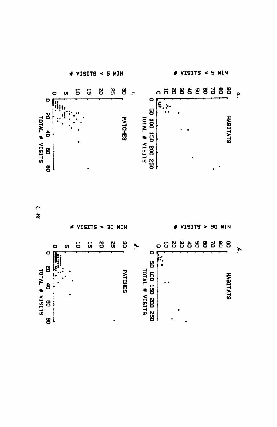
z*-«inVtntn••H*t-4
inVin1-4
tn>
a.
90 HABITATS
80706050403020100
.•
i •
,,-:: :.*-•0
50 100
150 200 250TOTAL # VISITS
c.302520151050
PATCHES
m.
I •
" "
«•""£•szrl
""20
40 60
60 TOTAL
# VISITS
zx0
COAtntn>*z
1-1z0Atni- 1-1tnit
90 HABITATS
80706050403020100
,,,,1 •
t •
. *
•»*%& ....»*
0 50
100 150 200 250
TOTAL # VISITS«*.
302520151050
PATCHES
•
i •
£JE.: ::j "... -,.-,..-.._.,.._.
20 40
60 60
TOTAL *
VISITS
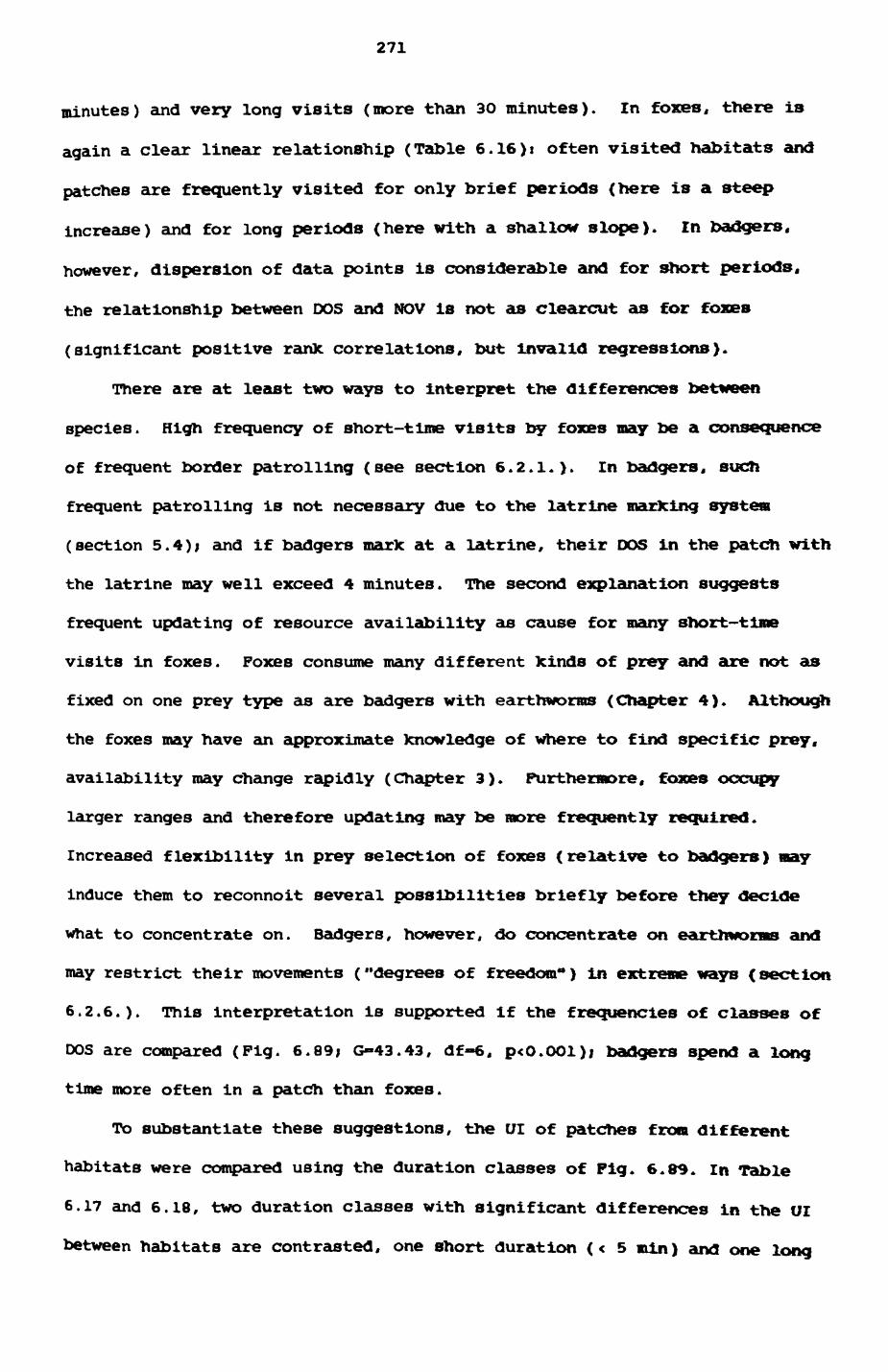
271
minutes) and very long visits (more than 30 minutes). In foxes, there is
again a clear linear relationship (Table 6.16)i often visited habitats and
patches are frequently visited for only brief periods (here is a steep
increase) and for long periods (here with a shallow slope)* In badgers,
however, dispersion of data points is considerable and for short periods,
the relationship between DOS and NOV is not as clearcut as for foxes
(significant positive rank correlations, but invalid regressions)*
There are at least two ways to interpret the differences between
species. High frequency of short-time visits by foxes may be a consequence
of frequent border patrolling (see section 6*2.1*). In badgers, such
frequent patrolling is not necessary due to the latrine marking system
(section 5.4); and if badgers mark at a latrine, their DOS in the patch with
the latrine may well exceed 4 minutes. The second explanation suggests
frequent updating of resource availability as cause for many short-time
visits in foxes. Poxes consume many different kinds of prey and are not as
fixed on one prey type as are badgers with earthworms (Chapter 4). Although
the foxes may have an approximate knowledge of where to find specific prey,
availability may change rapidly (Chapter 3)* Furthermore, foxes occupy
larger ranges and therefore updating may be more frequently required.
Increased flexibility in prey selection of foxes (relative to badgers) nay
induce them to reconnoit several possibilities briefly before they decide
What to concentrate on. Badgers, however, do concentrate on earthworms and
may restrict their movements ("degrees of freedom") in extreme ways (section
6.2.6.). This interpretation is supported if the frequencies of classes of
DOS are compared (Pig. 6.89; G-43.43, df-6, p<o*OOl)j badgers spend a long
time more often in a patch than foxes.
To substantiate these suggestions, the UI of patches from different
habitats were compared using the duration classes of Pig. 6*89. in Table
6.17 and 6.18, two duration classes with significant differences in the UI
between habitats are contrasted, one short duration (< 5 min) and one long
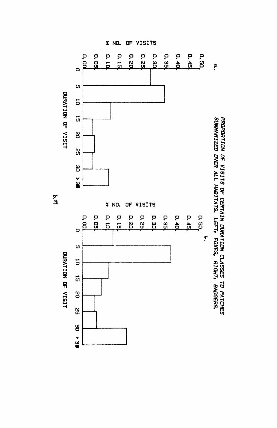
PROPORTION OF VISITS OF CERTAIN DURATION CLASSES TO PATCHES
0.
0.5
0
0.4
5
0.4
0
0.3
5
en 0
.30
2
0.2
5>u.
0.2
0
od
0. 15zx
0. 10
0.0
5
0.0
0
••k•
SU
MM
AK
lttD
OV
ER
A
LL
HA
BIT
AT
S.
LEF1
0.5
0
0.4
5
0.4
0
0.3
5
(n 0
.30
2
0-2
5>u.
0.2
00d
0- 15z«
0. 10
0.0
5
n_nn
r§ FO)t.
• • •»• »••
<ES, fH
GH
Tt
BA
DG
ER
S.
1015
20 25
30 >31
10 15
20 25
30 >39
DURATION OF
VISITDURATION
OF VISIT
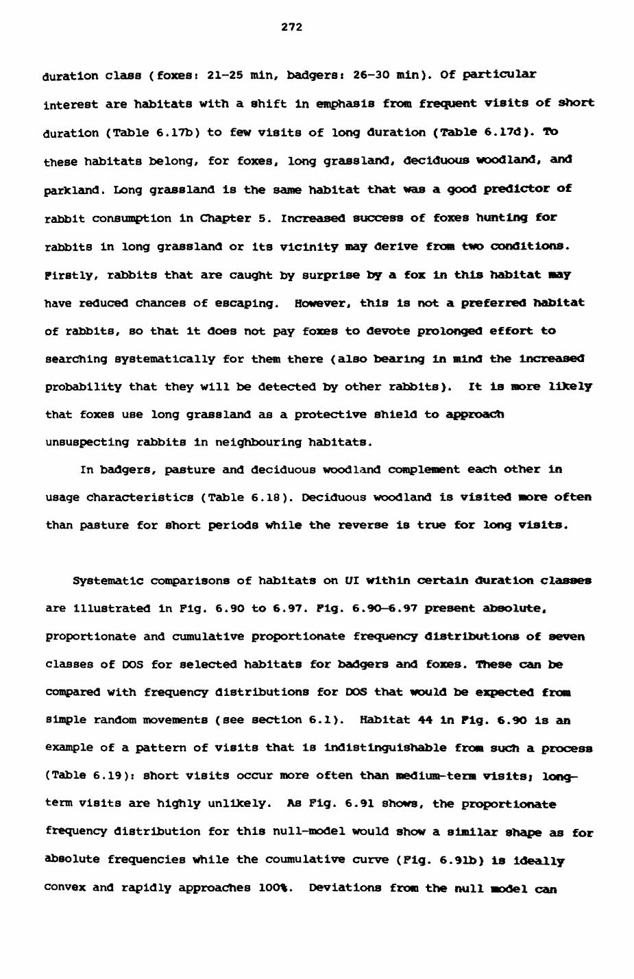
272
duration class (foxest 21-25 min, badgerst 26-30 min). of particular
interest are habitats with a shift in emphasis from frequent visits of short
duration (Table 6.17b) to few visits of long duration (Table 6.17d). To
these habitats belong, for foxes, long grassland, deciduous woodland, and
parkland. Long grassland is the same habitat that was a good predictor of
rabbit consumption in Chapter 5. Increased success of foxes hunting for
rabbits in long grassland or its vicinity may derive from two conditions.
Firstly, rabbits that are caught by surprise by a fox in this habitat may
have reduced chances of escaping. However, this is not a preferred habitat
of rabbits, so that It does not pay foxes to devote prolonged effort to
searching systematically for them there (also bearing in mind the increased
probability that they will be detected by other rabbits)* It is more liXely
that foxes use long grassland as a protective shield to approach
unsuspecting rabbits in neighbouring habitats.
In badgers, pasture and deciduous woodland complement each other in
usage characteristics (Table 6.18). Deciduous woodland is visited more often
than pasture for short periods while the reverse is true for long visits.
Systematic comparisons of habitats on I/I within certain duration classes
are Illustrated In Fig. 6.90 to 6.97. Fig. 6.9O-6.97 present absolute,
proportionate and cumulative proportionate frequency distributions of seven
classes of DOS for selected habitats for badgers and foxes. These can be
compared with frequency distributions for DOS that would be expected from
simple random movements (see section 6.1). Habitat 44 In Fig. 6.9O is an
example of a pattern of visits that is indistinguishable from such a process
(Table 6.19): short visits occur more often than medium-term visitsj long-
term visits are highly unlikely. As Fig. 6.91 shows, the proportionate
frequency distribution for this null-model would show a similar shape as for
absolute frequencies while the coumulative curve (Fig. 6.9lb) is ideally
convex and rapidly approaches 100%. Deviations from the null model can
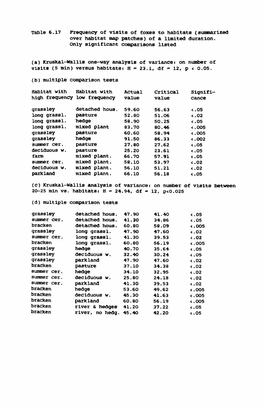
Table 6.17 Frequency of visits of foxes to habitats (summarized over habitat map patches) of a limited duration. Only significant comparisons listed
(a) Kruskal-Wallis one-way analysis of variance: on number of visits (5 min) versus habitatsi H = 23.1, df = 12, p < 0.05.
(b) multiple comparison tests
Habitat with Habitat withhigh frequency low frequency
grass leylong grass 1.long grass 1.long grass 1.grass leygrass leysummer cer.deciduous w.farmsummer cer.deciduous w.parkland
detached hous.pasturehedgemixed plantpasturehedgepasturepasturemixed plant.mixed plant.mixed plant.mixed plant.
(c) Kruskal-wallis analysis of20-25 min vs
(d) multiple
grass leysummer cer.brackengrass leysummer cer.brackengrass leygrass leygrass leybrackensummer cer.summer cer.summer cer.brackenbrackenbrackenbrackenbracken
. habitats t H - 24
comparison tests
detached hous.detached hous.detached hous.long grass 1.long grass 1.long grass 1.hedgedeciduous w.parklandpasturehedgedeciduous w.parklandhedgedeciduous w.parklandriver & hedgesriver, no hedg.
Actualvalue
59.6052.8058.9083.7060.6091.5027.8025.2066.7058.1056.1066.10
variance t.94, df =
47.9041.3060.8047. 9O41.306O.8040.7032.4047. 9O37.1034.1025.8041.3053.6045.3060. 8O41.2045.40
Criticalvalue
56.6351.0650.2580.4658.9486.3327.6223.6157.9153.9751.2156.18
on number12, p<0.025
41.4034.8658.0947. 6O39.5356.1935.6430.2447.6034.3832.9524.1839.5349.6241.6356.1937.2242.20
Significance
<.05<.02<.05<.O05<.OO5<.002<.05<.05<.05<.02<.02<.O5
of visits between
<.05<.05<.O05<.02<.02<.OO5<.05<.O5<.02<.02<.02<.02<.02<.O05<.OO5<.OO5<.05<.05
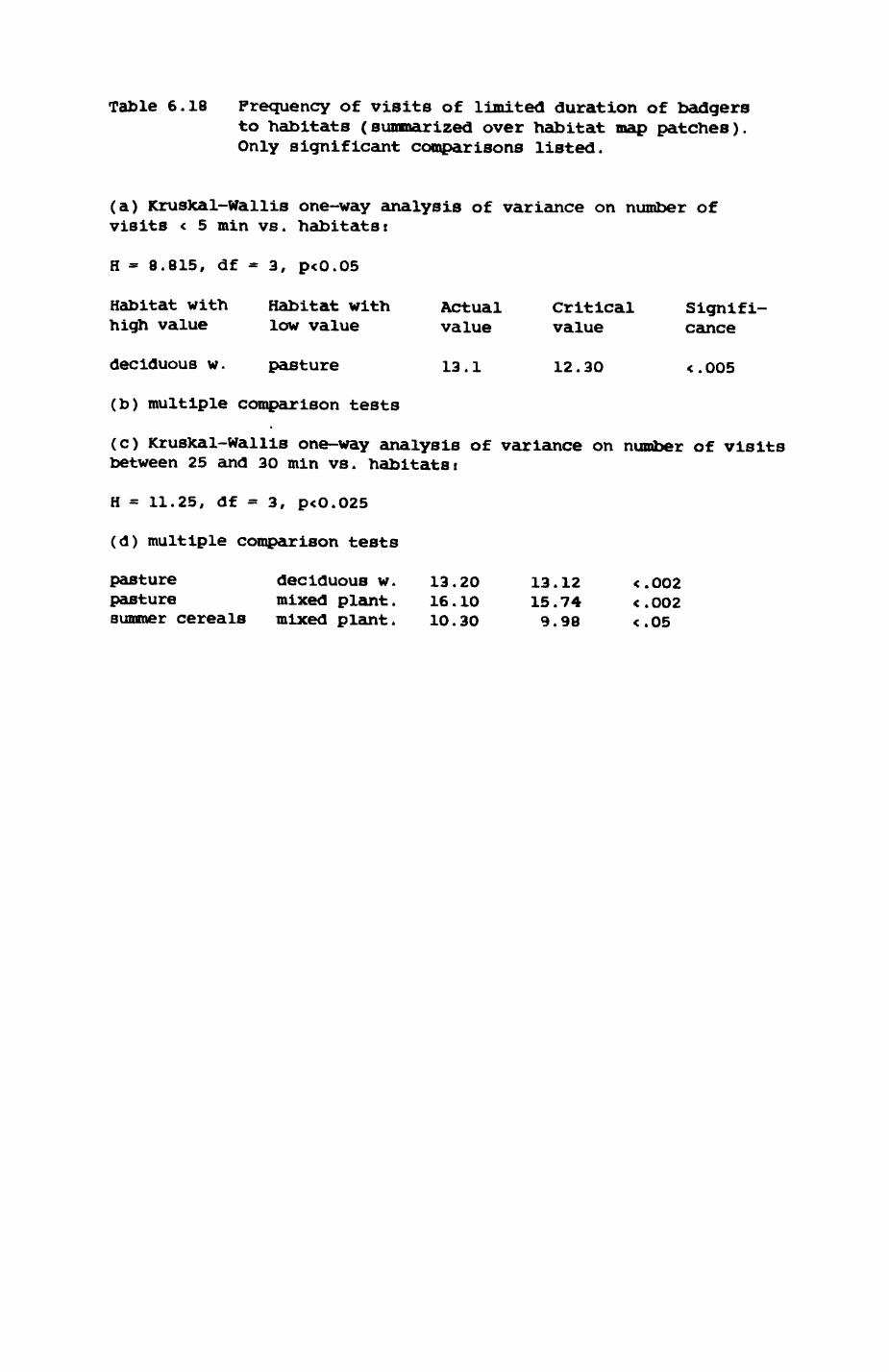
Table 6.18 Frequency of visits of limited duration of badgers to habitats (summarized over habitat map patches). Only significant comparisons listed.
(a) Kruslcal-Wallis one-way analysis of variance on number of visits < 5 min vs. habitatst
H » 8.815, df = 3, p<0.05
Habitat with Habitat with Actual Critical Signifi- high value low value value value cance
deciduous w - pasture 13.1 12.30 < . 005
(b) multiple comparison tests
(c) Kruslcal-Wallis one-way analysis of variance on number of visits between 25 and 30 min vs. habitats t
H = 11.25, df = 3, p<O.025
(d) multiple comparison tests
pasture deciduous w. 13.20 13.12 <.002pasture mixed plant. 16.10 15.74 <.O02simmer cereals mixed plant. 10.30 9.98 <.05
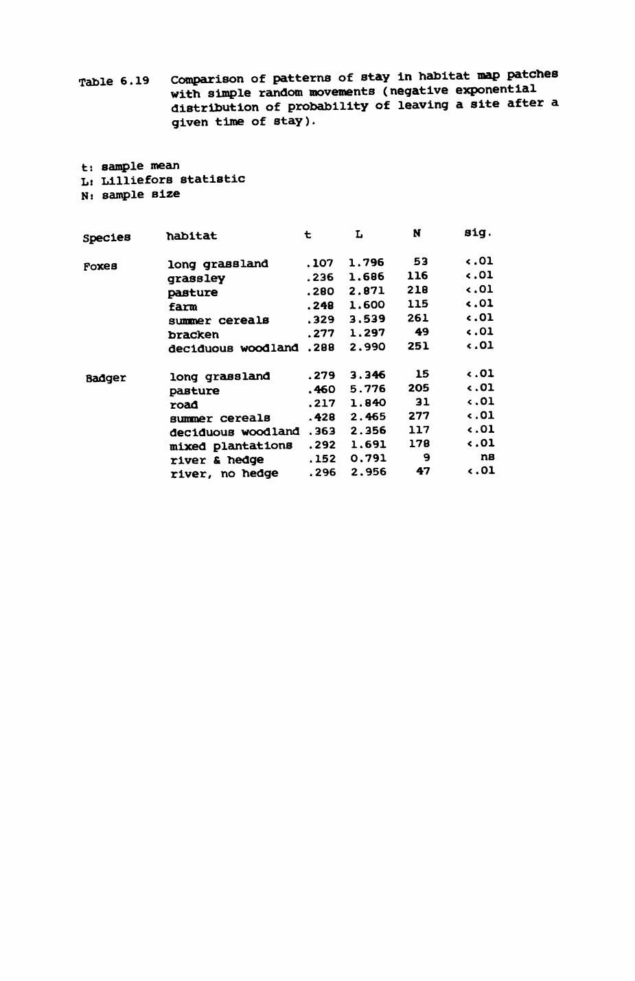
Table 6.19 Comparison of patterns of stay in habitat map patches with simple random movements (negative exponential distribution of probability of leaving a site after a given time of stay).
t: sample meanL« Lilliefors statisticNi sample size
Species habitat t L N sig.
Foxes
Badger
long grasslandgrassleypasturefarmsummer cerealsbracfcendeciduous woodland
long grasslandpastureroadsummer cerealsdeciduous woodlandmixed plantationsriver & hedgeriver, no hedge
.107
.236
.280
.248
.329
.277
.288
.279
.460
.217
.428
.363
.292
.152
.296
1.7961.6862.8711.6003.5391.2972.990
3.3465.7761.8402.4652.3561.6910.7912.956
5311621811526149251
152O531
277117178
947
<*01 ns
273
easily be picked out by looking at the cumulative frequencies i concave or
sigmoid curves indicate a larger proportion of visits of long duration
classes than expected. Pasture (habitat 7) in Pig. 6.93b is a conspicuous
example. Habitats with reduced resource presence, such as long grass and
riverrine environments (Pig. 6.9O-6.91) show patterns that resemble the
results of random movements. An interesting exception is habitat 26, road.
I have frequently observed badgers strolling slowly along the periphery of a
track or an asphalt road where they search for beetles and particularly for
snails in the long grass. All habitats of Pig. 6.93 deviate significantly
from the suggested null model. (Note that the comparison with the expected
dlstsibution is Independent from the class sizes chosen for illustration, as
described in section 6.1). Furthermore, the three individuals ALI, KAMI and
WILF were excluded from these analyses, since the way they were tracked (cf.
section 6.4) would have biased the frequency distribution towards the 11-15
min class).
Pig. 6.94-6.97 illustrate frequency distributions of visit durations
for selected habitats in foxes. Again, visit patterns of the habitats
illustrated deviate from the null model. An interesting exception provides
long grassland (habitat 5}, which, unlike all other habitats, experiences
too few long duration visits to comply with the simple randan process.
Reasons for this have been discussed above.
In summary, patterns of visits to habitats as expressed by the
frequency of visits of certain duration classes reflect prey preferences (as
indicated before) and indicate movement and foraging 'styles* of the two
species. Despite these differences, movements of individuals of both species
are not compatible with simple random movements.
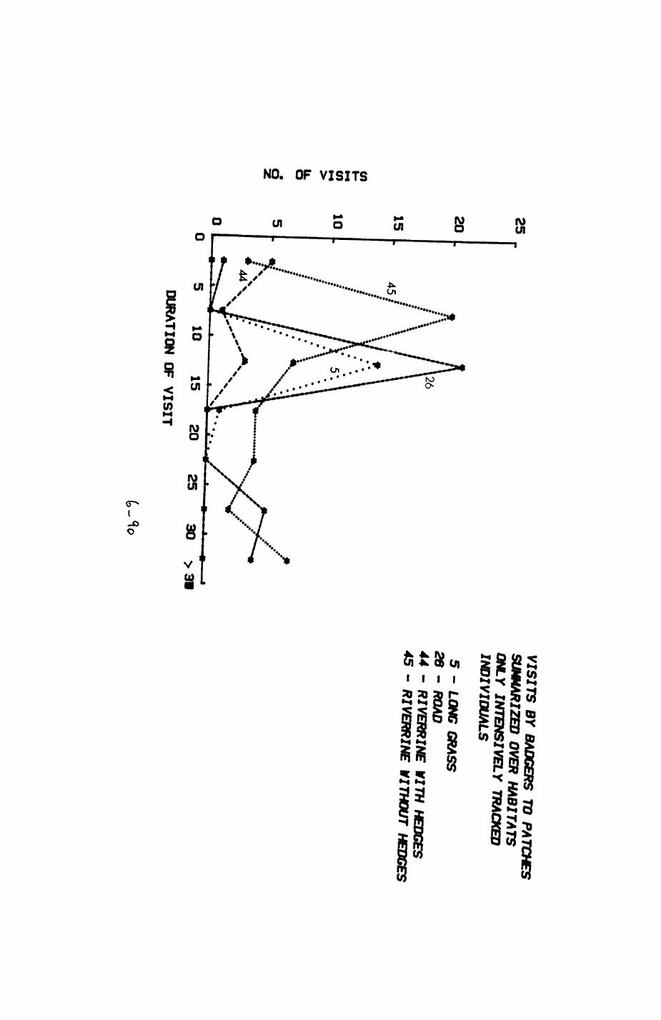
25 ..
COI-1-4CO
2015
5 10
15 20
25 30
>3I
DURATION OF VISIT
VISITS BY BADGERS TO P
ATCHES
SUMMARIZED OVER HABITATS
ONLY INTENSIVELY TRACKED
INDIVIDUALS
5 - L
ONG GRASS
26 - R
OAD
44 - RIVERRINE WITH HEDGES
45 - R
IVERRINE WITHOUT HEDGES
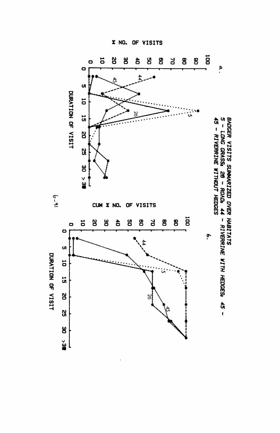
en1-4 (ft
u. od
BADGER VISITS SUMMARIZED O
VER HABITATS
5 -
LONG GRASSi
26 - ROADt 44 - RIVERRINE
WITH HEDGESt 45 -
45 - R
IVERRINE WITHOUT HEDGES
5 10
15 20
25
DURATION OF VISIT
30 >
3f
enMI
25 30
>3i
DU
RATIO
N O
F V
ISIT
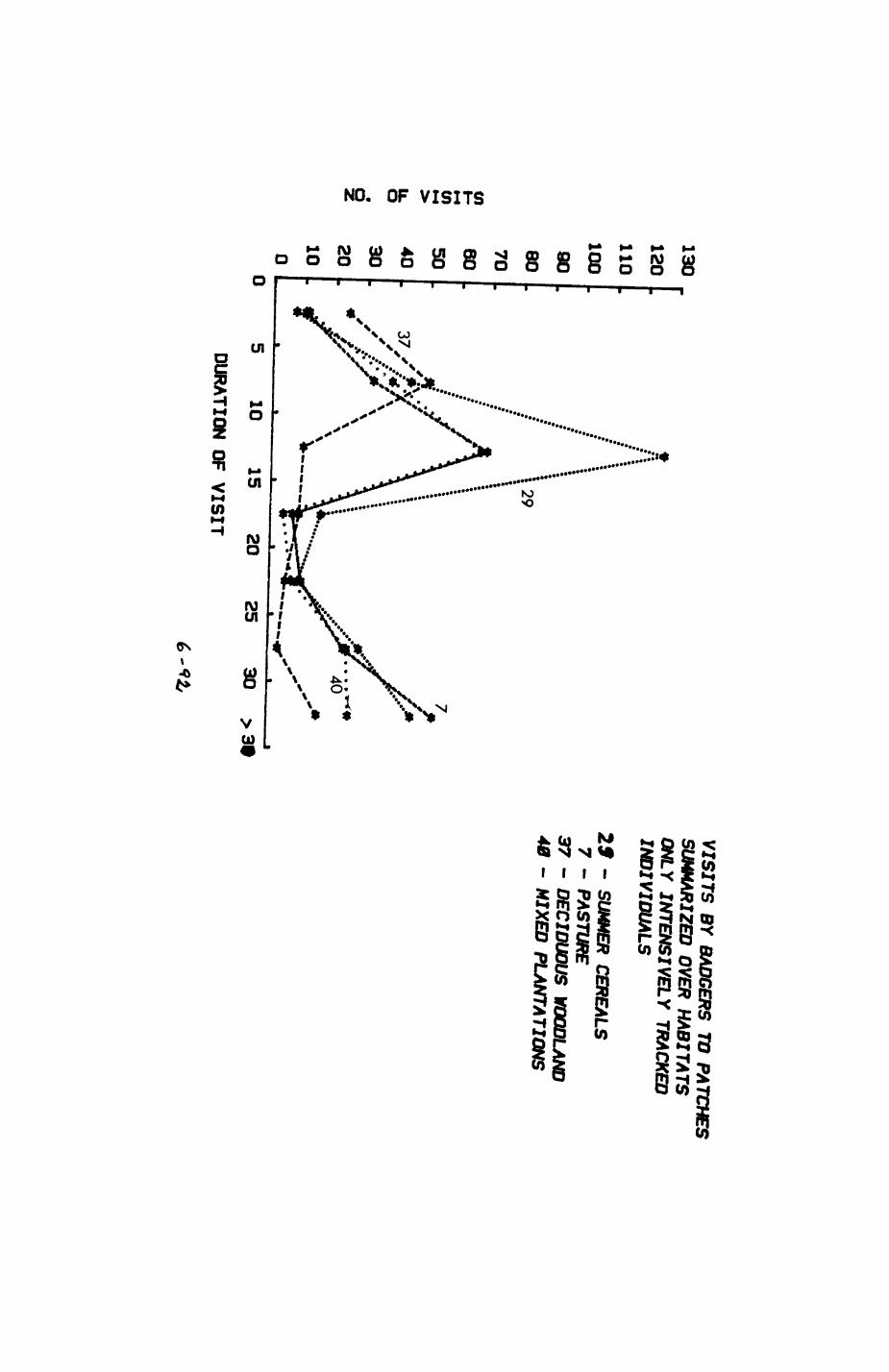
CO
u.O
1301201101000080706050403020100
\29
VIS
ITS
BY BADGERS TO PATCHES SUM
MARIZED O
VER HA
BITA
TS O
NLY INTE
NS
IVE
LY TRACKED
IND
IVID
UA
LS
29 - SUM
MER CEREALS
7 - PASTURE37 - DECIDUO
US WOODLAND
40 - MIXED
PLAN
TATIO
NS
5 10
15 20
DURATION OF VISIT
2530
> 3f

CO1-1 COu. ooz
504030
2010
A .
BADGER VISITS SUMMARIZED OVER HABITATS
7 - PASTUREt 29 - SUMMER CEREALSt
37 - DECIDUOUS WOODL.,
40
40 - MIXED P
LANTATIONS
1015
20 25
30 >3i
DURATION OF VISIT
CO•-•(OU.oiMU
100908070605040302010010
15 20
25 30
DURATION OF VISIT
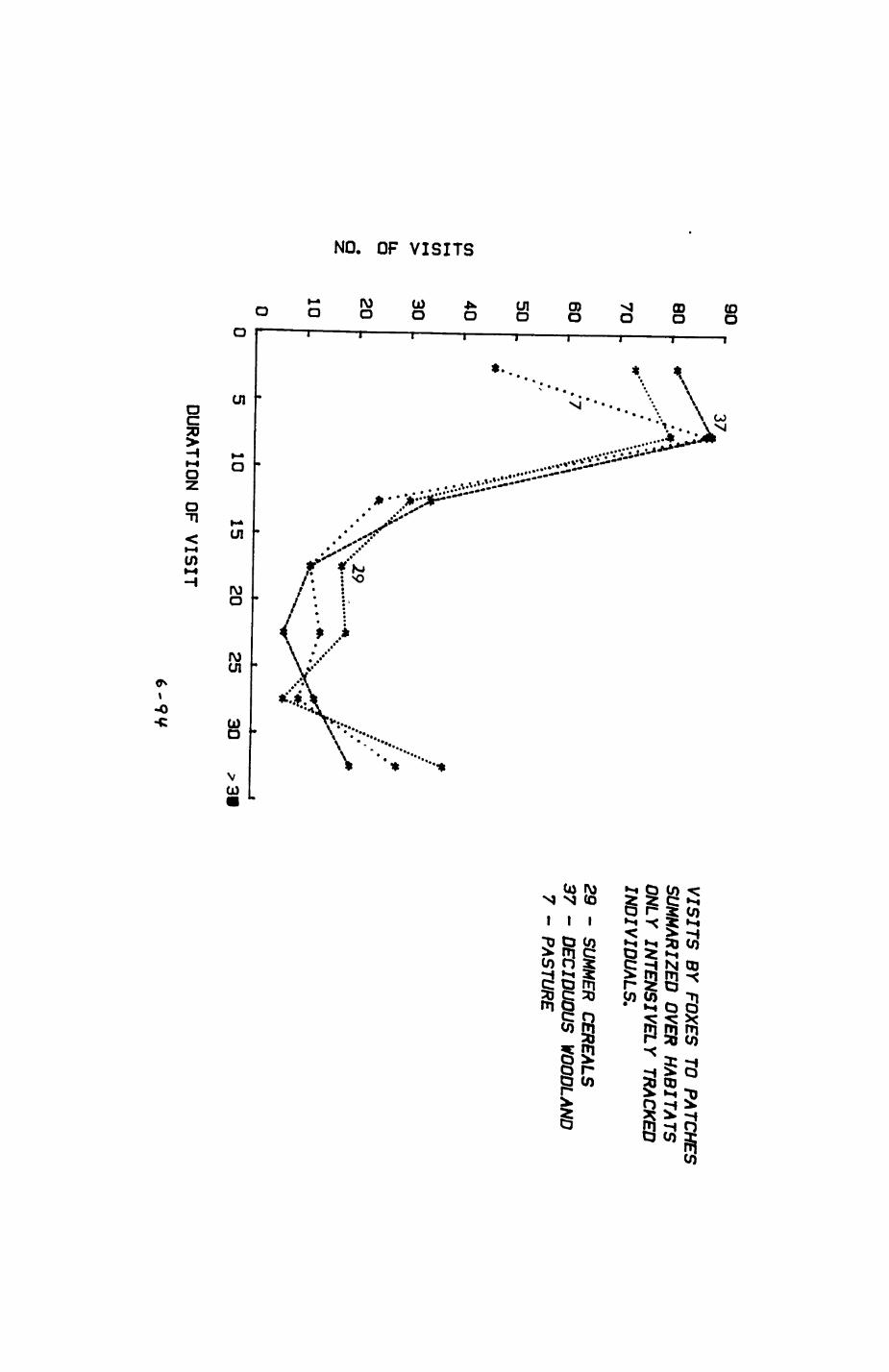
enH i-<cnu. a
9080706050403020100
37,
1015
2025
30
VISITS BY FOXES TO PATCHES
SUMMARIZED OVER HABITATS ONLY INTENSIVELY
TRACKED INDIVIDUALS.
29 - SUMMER CEREALS 37 - DECIDUOUS WOODLAND 7 - PASTURE
DURATION OF VISIT
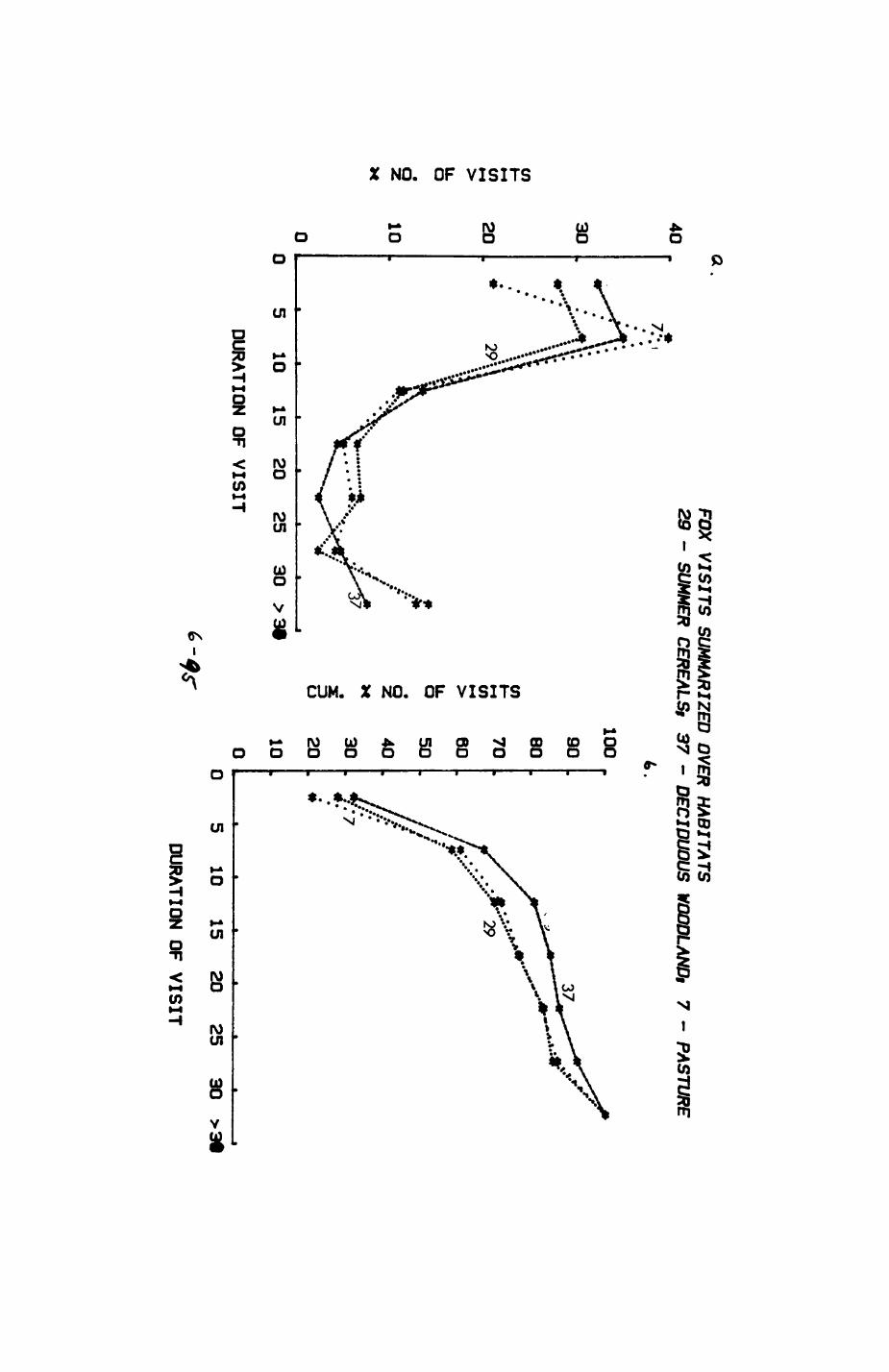
a.
40FOX VISITS SUMMARIZED OVER HABITATS29 - SUMMER CEREALSt
37 - DECIDUOUS WOODLANDi
7 - PASTURE
u. ad
30
2
2010
5 10
15 20
25 30
>3f
DURATION OF VISIT
eni- »-ienU- QU
100 ,
908070605040302010
10 15
20 25
30 >3t
DURATION OF VISIT
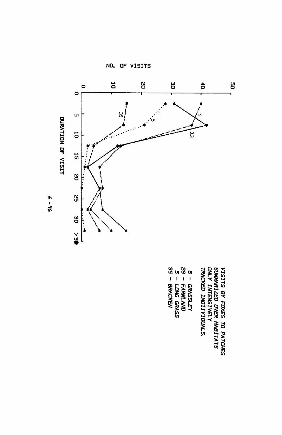
50 ,.
enU_o
40
30
2010
•^..x>"SB-"
1015
2025
30 >
3t
VIS
ITS
BY
FOXES
TO PATC
HES
SUM
MAR
IZED O
VER H
AB
ITATS
O
NLY
INT
EN
SIV
ELY
TR
ACKED
IN
DIV
IDU
AL
S.
6 -
GR
ASSLEY 2
3 - FAR
MLAN
D5
- LON
G G
RASS
35
- BRAC
KEN
DURATION OF VISIT
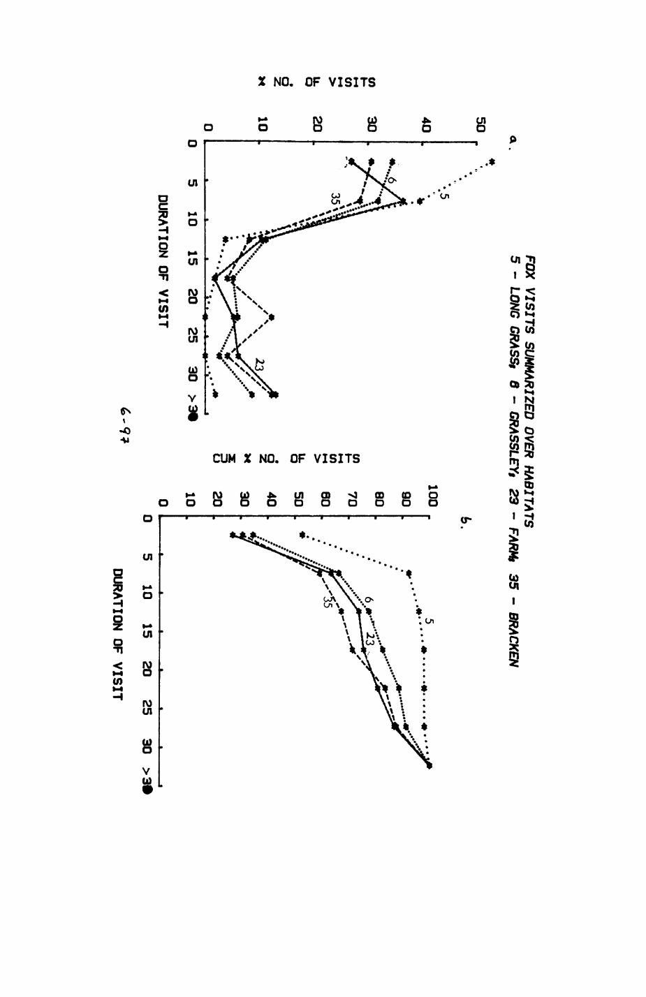
FOX VISITS SUMMARIZED OVER HABITATS
5 -
LONG GRASSt
6 - GRASSLEYt
23 -
FARMt 35 - B
RACKEN
COI- 1-1cnu. ad
5O f
40
302010
10 15
20 25
30 >3»
DURATION OF VISIT
cn1-4cnd
100go so70605040302010
10 15
20 25
30
DURATION OF VISIT

274
7. Spatial organisation and reproductive strategies in badgers.
7.1. Introduction
7.2. Energetics of female reproductive effort
7.2.1. Energetics of maternal Investment
7.2.2. Development of the young
7.2.3. Factors Influencing the future reproductive success
of the young
7.2.4. Summaryi direction of selection pressures
7.3. Spatial and social strategies of females
7.3.1. Why should a territory owner do better ?
7.3.2. What are the costs of owning a territory ?
7.3.3. Factors affecting intrusion pressure
7.3.4. Responses of territory owners to high intrusion
pressure
7.3.5. Costs and benefits of satellites
7.3.6. Social organisation in relation to resource
characteristics! other studies
7.3.7. Discussion
7.4. Male competition and female choice
7.4.1. Mating seasons and mating success
7.4.2. Mating behaviourt opportunities for female choice
7.4.3. The costs and benefits of multiple matIngs for
males
7.4.4. The costs and benefits of multiple matings for
females
7.5. Conelus ions.
275
7. Spatial organisation and reproductive strategies of badgers.
7.1. Introduce ion.
The previous chapters nave illustrated how the intricate relationship
between the movements of individuals, the resulting spatial utilization
patterns and the characteristics of habitats and resources shape the
badger's social system in Wytham. A variety of recent field studies (KruuX
I978a, KruuX & parish 1979, I982aj Harris 1982, 1984; Cheeseman et al 1985]
Martin-Franquelo & Delibes 1985) suggest that there is considerable
variation in the spatial and social organisation in badgers. I hope to
reconcile these diverging descriptions of badger social organisation by
considering the relationship between resources and social and spatial
organisation in the wider context of life history and reproductive patterns.
I shall start with an examination of the reproductive biology of the
female badger. Energetic costs of pregnancy and lactation are considerable
(section 7.2), since females provide most of the parental investment, nils.
together with additional factors concerning post-weaning development.
survival prospects for the first harsh period, and the potential future
reproductive success of the young, places considerable selection pressures
on the timing of birth, favouring a date early in spring (section 7.2). If
the main food resource is economically defendable, females can Improve their
breeding success by striving for exclusive access to areas containing these
resources for themselves and their offspring. If intrusion pressure from
other females and resource density on the defended areas is high, then
females could form coalitions with other females to share defense costs.
Since females carry the main burden of parental investment, standard
socloblological theory predicts that they should exhibit mate choice
(Trlvers 1972, 1985). The sexual dimorphism shown by badgers (Andersen t
276
TreWhella 1985) is an indication that sexual selection may nave been
operating on males competing with each other for females. If females can
Improve their fitness by choosing their mates carefully, then they should
come into oestrus when the prospects for mate choice are good. For badgers*
this is the time shortly after parturition, since the males reach their peaJc
in body size in February. Since there is powerful selection pressure for
birth early in the year, the evolution of delayed implantation is a possible
solution to the problem of timing mate choice, since It allows the mating
season to vary Independently from the time of parturition (Sandell 1985}.
The evolution of seasonal delay has far-reaching Implications for the
reproductive behaviour and the spatial distribution of males. Uncertainty of
paternity caused by repeated ovulatlons of females and their abilities to
eel«et-between different blastocysts (Ahnlund 1S8O) requires males to
maximise mating attempts and defend exclusive access to females.
Territorially and the formation of male coalitions are two strategies by
Which males can attempt to limit other males' access to females.
The formation of intrasexual coalitions are submitted to a cost-benefit
analysis (sections 7.3. and 7-4 ). The costs and benefits of defending
exclusive access to a resource (for malest females, for femalesi protein-
rich food) are analysed as a function of the qualities of the resource
(density, availability, renewal and dispersion) and the population density
(Intrusion pressure). A model of the social organisation of the badgers
based on the results of this analysis (section 7.5} can be shown to
accommodate the diverging results of previous studies.
7.2. Energetics of female reproductive effort
In the seasonal environment that occurs throughout the range of the
European badger, resource availability changes considerably over time
(Chapter 3). Thus, the timing and intensity of reproductive activities are
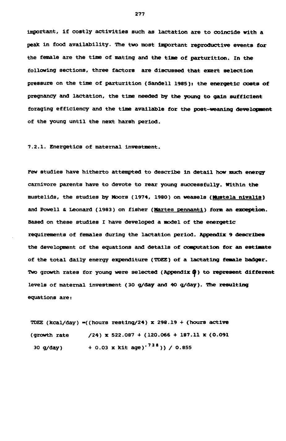
277
important, if costly activities such as lactation are to coincide with a
peaX in food availability. The two most important reproductive events for
the female are the time of mating and the time of parturition. In the
following sections, three factors are discussed that exert selection
pressure on the time of parturition (Sandell 19*5 )s the energetic costs of
pregnancy and lactation, the time needed by the young to gain sufficient
foraging efficiency and the time available for the post-weaning development
of the young until the next harsh period,
7.2.1. Energetics of maternal investment.
Few studies have hitherto attempted to describe in detail how much energy
carnivore parents have to devote to rear young successfully. Within the
mustelids, the studies by Moors (1974, 198O) on weasels (Mustela nivalis)
and Powell & Leonard (1983) on fisher (Martes pennantl) form an exception.
Based on these studies I have developed a model of the energetic
requirements of females during the lactation period. Appendix 9 describes
the development of the equations and details of computation for an estimate
of the total dally energy expenditure (TDEE) of a lactating female badger.
Two growth rates for young were selected (Appendix ft > to represent different
levels of maternal investment (3O g/day and 4O g/day). The resulting
equations are:
TDEE (kcal/day) -((hours resting/24) x 298.19 -»• (hours active
(growth rate /24) x 522.087 -I- (120.066 + 187.11 x (O.O91
30 g/day) + 0.03 x kit age)' 738 )) / O.855

278
TDEE (kcal/day) -((hours resting/24) x 298.19 + (hours active
(growth rate /24) X 522.087 + (16O.O8* + 187.11 x (O.O91
40 g/day) + 0.04 x kit age)' 738 )) / O.855
Pig. 7.1 shows a plot of TDEE from the time of birth of the young (day 1) to
the approximate time of weaning (day 9O) for hi#i (graph A) and low growth
rates (graph B). Also shown is lactation energy expenditure for both growth
rates (graph C and D). Final energy expenditure is almost twice as hi#i as
at the beginning. A comparison of energy expenditure with and without
lactation is provided in Fig. 7.2. Here the quotient
R = Maintenance Energy -I- Activity Energy + Lactation
Maintenance Energy -I- Activity Energy
is plotted against time. Towards the end of the lactation period, energy
expenditure is 2.5 (low) to 3.2 times (high growth rate) higher than energy
expenditure without lactation, or lactation comprises up to 67 % of TDEE I
This result corresponds closely to estimates for small mustelids (Moors
1980) where energy needs during lactation are estimated to be 2 to 3 times
above average values.
How does this additional energy expenditure translate into additional
foraging effort ? Since badgers in Nytham eat mainly earthworms during
spring (Chapter 4), I considered the time females need to devote to hunting
for additional earthworms in order to obtain a balanced energy budget. Since
it can be safely assumed that badgers catch worms as efficiently as foxes, I
computed the additional foraging time using (for comparative purposes) the
two capture rates determined by Macdonald (198Oi see section 3.7) for foxes
worming on average nights (2.06 worms/min) and good nights (4.O4 worms/mln).
If energy Intake is set equal to energy expenditure, ie digestive efficiency
set to 100 %, then total foraging time for a non-lactatlng female comprises
Pig. 7.1. Daily energy expenditure (fccal day ) by lact at ingfemale badgers in relation to age of young (= days of lactation).
A, Bi total daily energy expenditure)C, Dt lactation energy expenditure per day.
A, C) high maternal investment (growth rate40 g day );
B, D: low maternal investment (growth rate30 g day ).
Fig. 7.2. Factor R vs. age of young. R indicates the degree to which a lactating female badger's daily energy expen diture surpasses that of a non-lactating female (R=l).
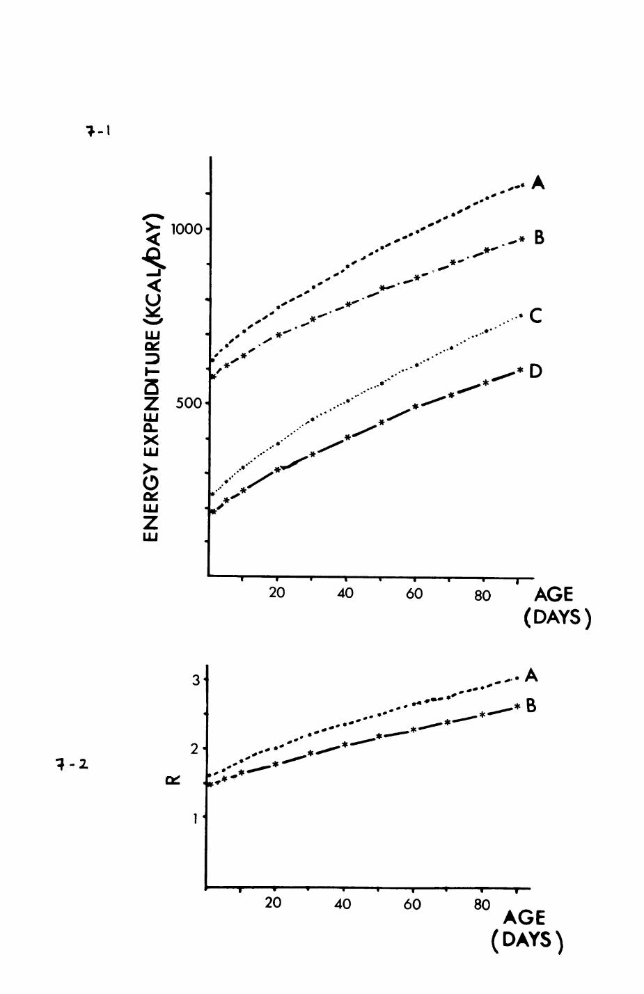
KJ
O '
o -
61 00 .
o 1
R v\ * • \\ * * % \ TT \» %
•W
*
% * t « t % * » \ * * \ \ * • \
ENER
GY
EXPE
NDIT
URE
(KC
ALyf
cAY)
o"
o •
0s
-o
1 §1CP
>
o
en 0 0
A \ *
*. \ \ V\ *
\ %
* «
»
n \ •*
\ \
\
n
* \\ •
\\ i
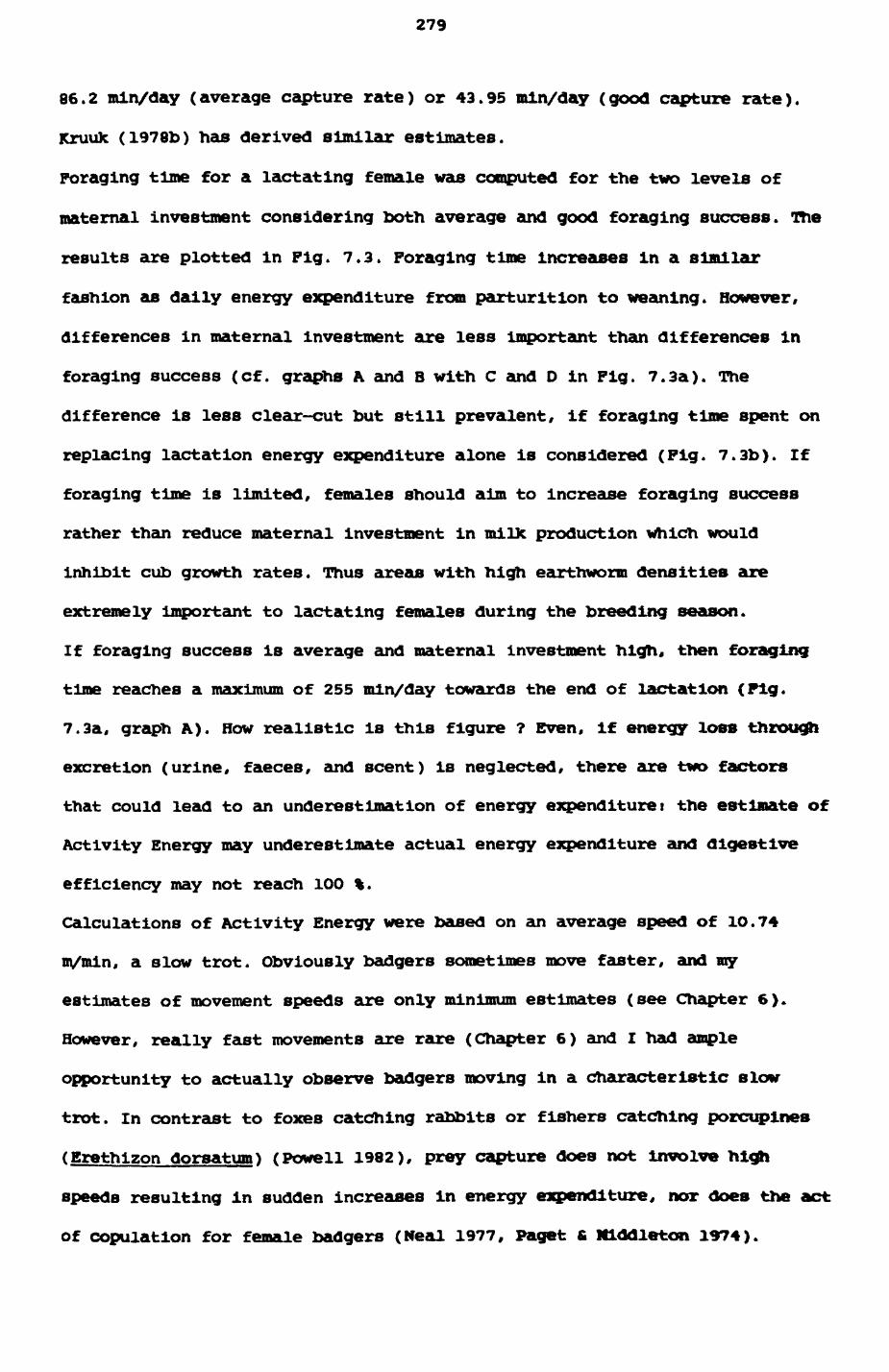
279
86.2 mln/day (average capture rate) or 43.95 mln/day (good capture rate).
Kruuk (1978b) has derived similar estimates.
Foraging time for a lactating female was computed for the two levels of
maternal investment considering both average and good foraging success. The
results are plotted in Fig. 7.3. Foraging time increases in a similar
fashion as daily energy expenditure from parturition to weaning. However,
differences in maternal investment are less Important than differences in
foraging success (cf. graphs A and B with C and D in Fig. 7.3a). The
difference is less clear-cut but still prevalent, if foraging time spent on
replacing lactation energy expenditure alone is considered (Fig. 7.3b). If
foraging time is limited, females should aim to Increase foraging success
rather than reduce maternal Investment in milk production which would
Inhibit cub growth rates. Thus areas with high earthworm densities are
extremely important to lactating females during the breeding season.
If foraging success is average and maternal investment high, then foraging
time reaches a maximum of 255 mln/day towards the end of lactation (Fig.
7.3a, graph A). How realistic is this figure ? Even, if energy loss through
excretion (urine, faeces, and scent) is neglected, there are two factors
that could lead to an underestimation of energy expendituret the estimate of
Activity Energy may underestimate actual energy expenditure and digestive
efficiency may not reach 100 %.
Calculations of Activity Energy were based on an average speed of 1O.74
m/min, a slow trot. Obviously badgers sometimes move faster, and my
estimates of movement speeds are only minimum estimates (see Chapter 6).
However, really fast movements are rare (Chapter 6) and I had ample
opportunity to actually observe badgers moving in a characteristic slow
trot. In contrast to foxes catching rabbits or fishers catching porcupines
(Erethizon dorsatum) (Powell 1982), prey capture does not involve high
speeds resulting in sudden increases in energy expenditure, nor does the act
of copulation for female badgers (Neal 1977, Paget & Middleton 1974).

Pig. 7.3. Foraging time of lactating females foraging for earth worms necessary to balance
a. total dally energy expenditureb. lactation energy expenditure per day
vs. age of young.
Ai high maternal Investment & low foraging rateB: low maternal Investment & low foraging rate
C: high maternal investment & high foraging rateD: low maternal investment & high foraging rate
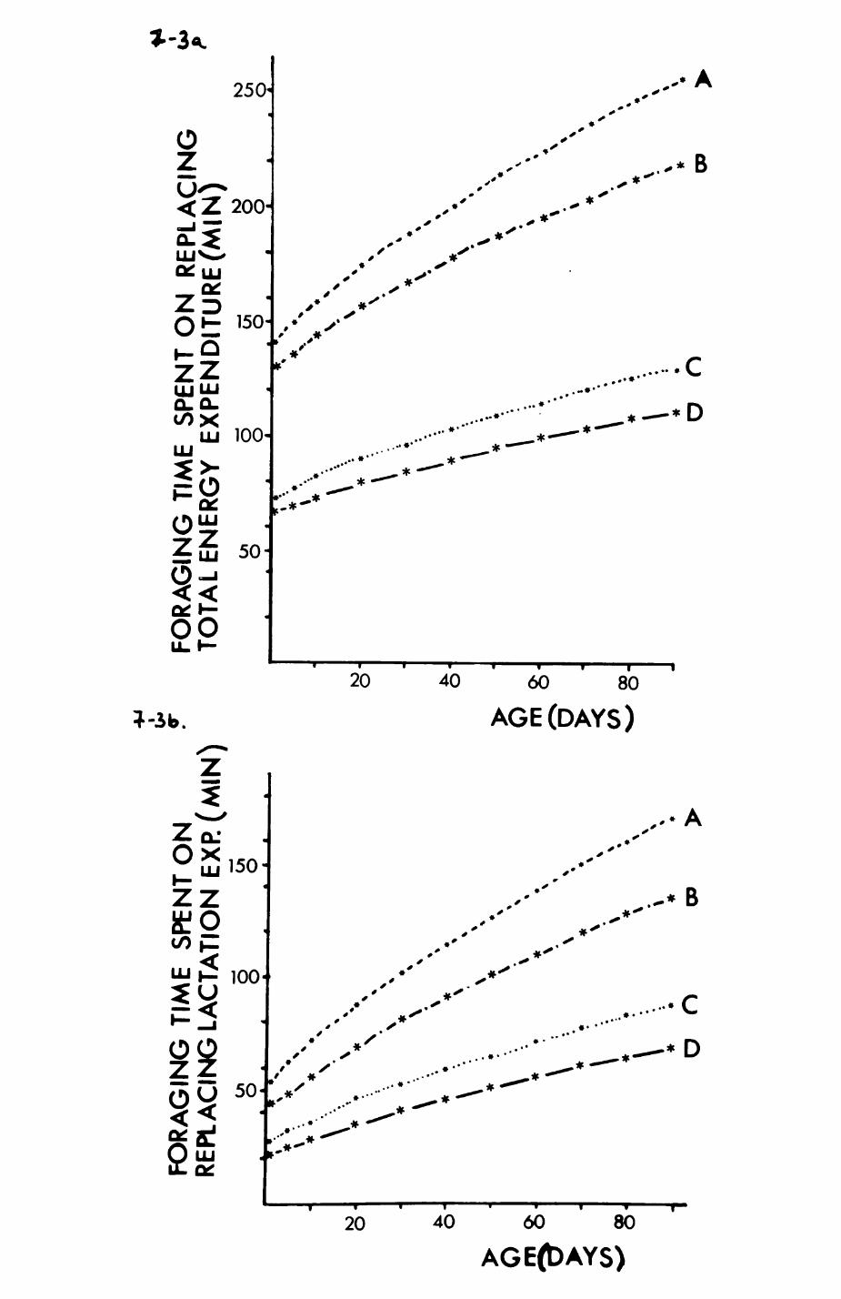
o8
FOR
AG
ING
TIM
E SP
ENT
ON
RE
PLAC
ING
LAC
TATI
ON
EXR
(MIN
)FO
RA
GIN
G T
IME
SPEN
T O
N R
EPLA
CIN
G
TOTA
L EN
ERG
Y EX
PEN
DIT
UR
E (M
lN)
c*
—
—
" _
_
»o
ro
Cn
o
*•"
OiO
Cn
Otn
O
Q°
OO
OO
Oa
ft
4 *
4 A
m
ft i
ft ft
ft *
I fl
ft A
« ft
i ft
i i
ft •
*V
* v
• "
"""""
-" '
* \
*
%*
• *
*\
. \
\*
* *
*V
\ \
\ '••••
'* \
* *
* 0'
\ N
*\
. \
\*
* *
*
V v
'-^
'^ '*
^*
* *
o-
\ y
\ °
\ .
\*
* *
* "V
w
\ \
\ \
s»
\ ™
8-\
\ \
'\ P
* *
* *
^\
* \
<\
\ \
</>
a,
* *
* *
x-x
S
-
\\
\ ^^
o
\
* *
* *
J
* i
* *%
« *•
» *
»*
* *^
**
\"
V
%
v
V*
* *
*
\ \
s N
\ '..
v v
» \
^*
* *
*\
''•• N-
N\
\ v
\*
* *
*
\ x
%v\
: \
*
* *v
\
\ '-
X
\ ^
^*
* *
*
\ '
X«
\ :
* \
*
- *
*
*\
^ X
\ \
• v
*
* *
*
\ ''"•
x»
V *
* %
* *
* *
\ '-'
•'
: %
\*
* *
%«Q
OO
O>
Q
O
CD
l^
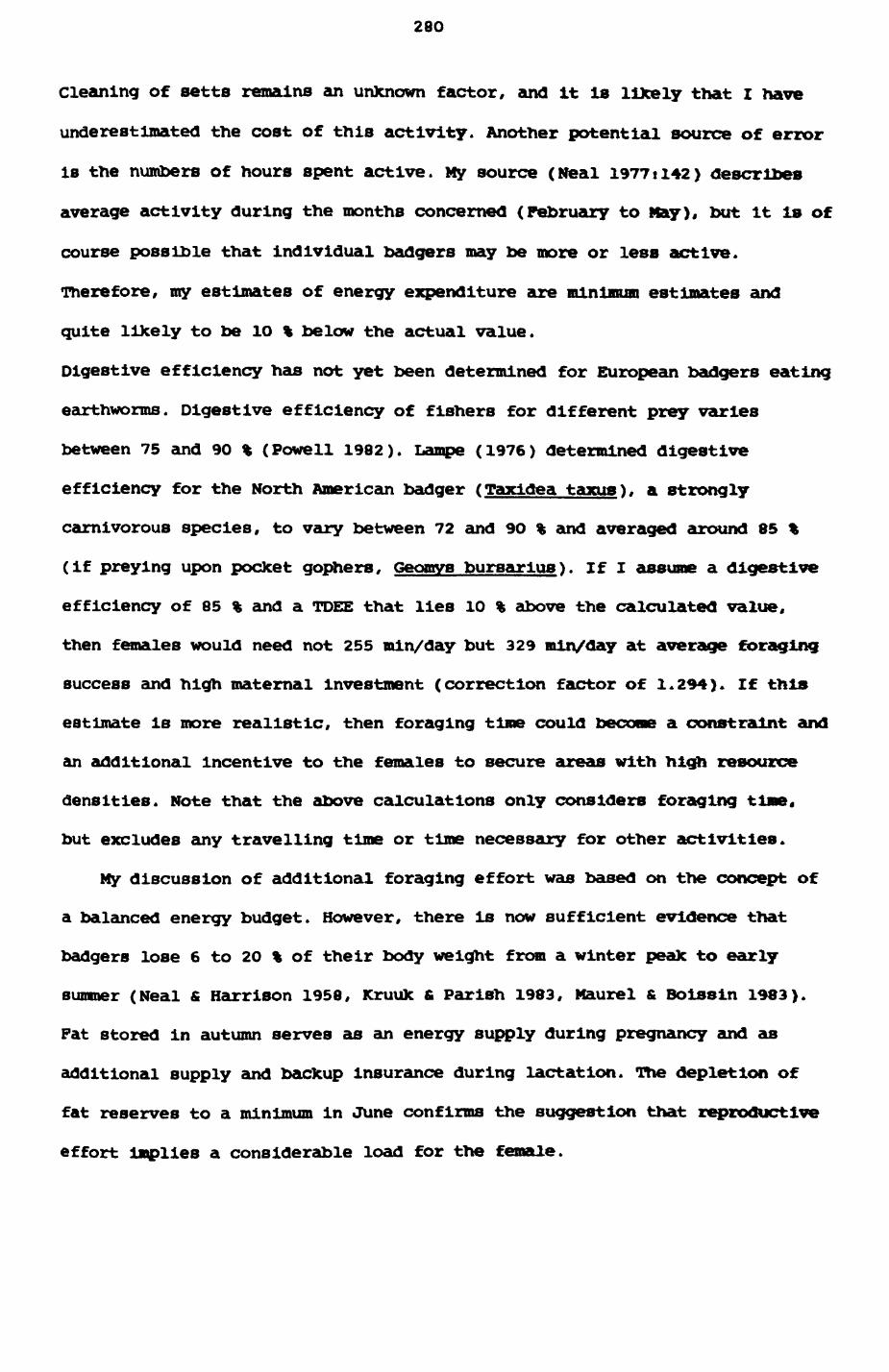
280
Cleaning of setts remains an unknown factor, and It Is likely that I nave
underestimated the cost of this activity. Another potential source of error
is the numbers of hours spent active. My source (Neal 1977t142) describes
average activity during the months concerned (February to Nay), but It Is of
course possible that Individual badgers may be more or less active.
Therefore, my estimates of energy expenditure are minimum estimates and
quite likely to be 10 % below the actual value.
Digestive efficiency has not yet been determined for European badgers eating
earthworms. Digestive efficiency of fishers for different prey varies
between 75 and 90 % (Powell 1982). Lampe (1976) determined digestive
efficiency for the North American badger (Taxidea taxus). a strongly
carnivorous species, to vary between 72 and 9O % and averaged around 85 %
(if preying upon pocket gophers, Geomvs bursar iue). if I assume a digestive
efficiency of 85 % and a TDEE that lies 10 % above the calculated value*
then females would need not 255 min/day but 329 min/day at average foraging
success and high maternal investment (correction factor of 1.294). If this
estimate is more realistic, then foraging time could becone a constraint and
an additional Incentive to the females to secure areas with high resource
densities. Note that the above calculations only considers foraging tine,
but excludes any travelling time or time necessary for other activities.
My discussion of additional foraging effort was based on the concept of
a balanced energy budget. However, there is now sufficient evidence that
badgers lose 6 to 20 % of their body weight from a winter peak to early
simmer (Neal & Harrison 1958, Kruuk fi Parish 1983, Maurel £ Boissin 1983).
Fat stored in autumn serves as an energy supply during pregnancy and as
additional supply and backup Insurance during lactation. The depletion of
fat reserves to a minimum in June confirms the suggestion that reproductive
effort implies a considerable load for the female.
281
7.2.2. Development of the young.
Several studies (summarized In Anderson £ Trewhalla 1985) point out that
mortality during the Initial stages of cub development may be considerable.
A comparison of prenatal litter sizes and litter sizes at a cub age of 12
weeks have shown a reduction of 25 % Which was attributed to respiratory
disease, aggressive behaviour by adult badgers and starvation (Stubbe 197O,
Anderson & Trewhalla 1985). Thus, at least some females are unable to
provide sufficient food either because of Insufficient fat reserves or
because of poor food availability. Average time of birth Is early In the
year (at the end of January/beginning of February) and generally coincides
with poor food availability, since the soil temperature Is too low, and the
ground Is often covered In snow, so that very few worms are active.
Selection should favour females either to give birth later in the year (when
food availability is Increased) or accumulate sufficient fat reserves in
autumn.
An indication of female investment during the lactation period is the
average growth rate of cubs. According to Neal (1977), birth dates in South
England occur around the beginning of February, and lactation lasts for 9O
days. Assuming a birth date of 1st February, I calculated average growth
rates for badger cubs caught in Wytham (Table 7.1). Average growth rates of
the two cubs caught at the end of lactation are around 4O g day" 1 ,
corresponding to the high investment growth rate of section 7.2.1., and
decline considerably in the period after weaning, in accordance with other
mammals (Koenig 1985). Although the paucity of studies on this aspect of
juvenile development precludes any generalizations, the few studies that are
available indicate that the period after weaning can be critical for
survival, as young animals need to develop predatory skills. Tan &
Counsilman (1985) have shown that kittens (Fells catua) require several
weeks to become proficient hunters, while plpistrelle bats {Pipjetrellus
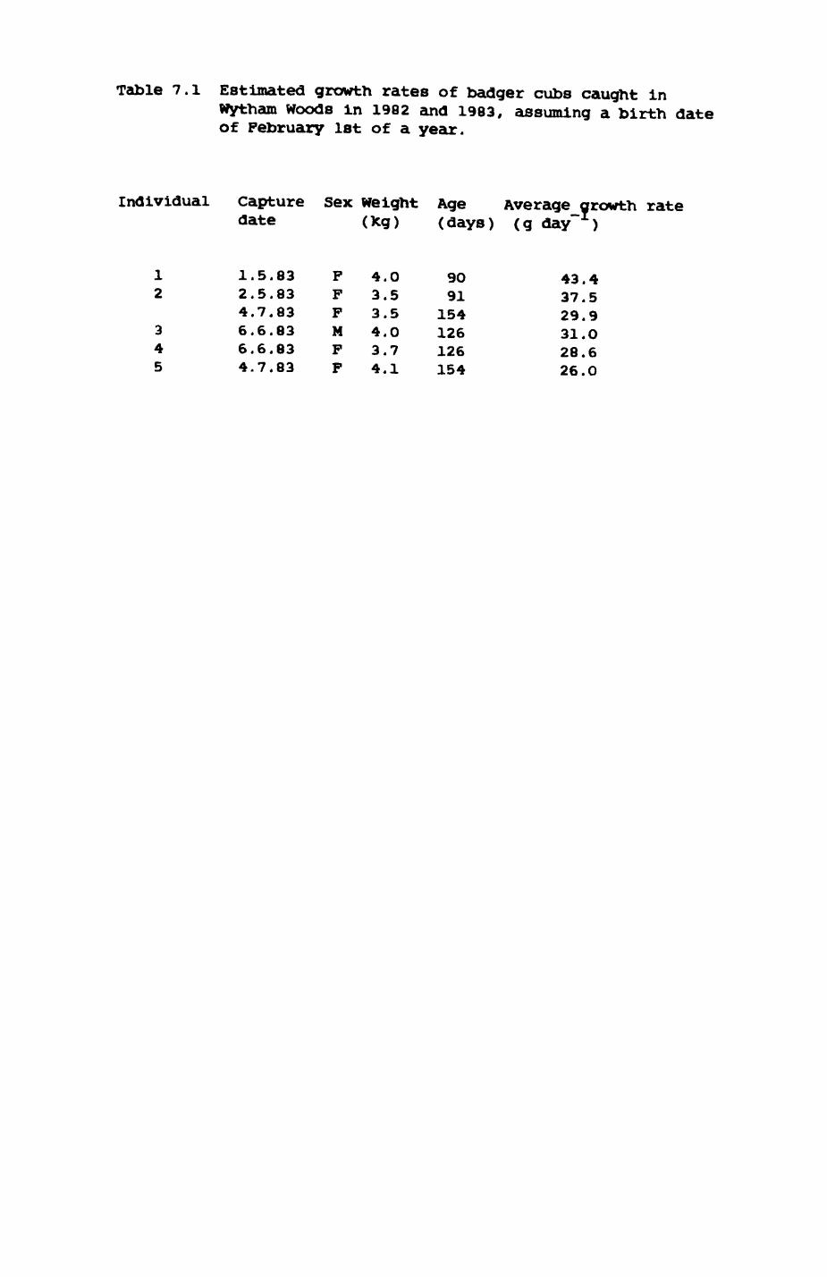
Table 7.1 Estimated growth rates of badger cubs caught InWytham Woods In 1982 and 1983, assuming a birth date of February 1st of a year.
Individual capture Sex Weight Age Average_growth rate date (leg) (days) (g day )
12
345
1.5.832.5.834.7.836.6.836.6.834.7.83
FFFNFF
4.03.53.54.03.74.1
9091
154126126154
43.437.529.931.028.626.0
282
plDlatrellue) take at least three weeks to reach a hunting efficiency
comparable with that of adults (Racey & Swift 1985). Young badgers (as other
carnivorous vertebrates) should have the best chance of developing foraging
skills while food Is reasonably abundant. However, the weather from Kiddle
of Nay (le from the time of lactation) onwards is dominated by dry, warm
spells of weather detrimental to Intense surfacing activity of worms,
resulting In a reduction of earthworm consumption by badgers during summer
(Chapter 4) and a reduction in the abundance of leaf litter fauna in general
(Manns 1967). The young with the highest probability of surviving such lean
periods in summer are those that have attained sufficient foraging
proficiency before the dry spells are likely to start, since they may
otherwise find it difficult to obtain enough food. A comparison of spring
versus autumn samples Indicates that this Is indeed a difficult time/
between 48 and 68 % of the cubs of a year may die during this period
(Anderson & Trewhalla 1985). Thus, selection should favour a sufficiently
early date of weaning and, consequently, an early date of birth which
ensures that young badgers achieve a degree of competence In foraging before
any extended periods of reduced food availability start. The direction of
this selection pressure is opposite to the one favouring a late birth (to
avoid a bottleneck In energy supply for the mother), since this implies a
date of weaning between middle and the end of April and consequently a date
of birth between middle and end of January.
Even if cubs born late survive they may show a greatly reduced
development , experience a higher mortality over the winter and not reach
adult body size until well into their second spring. In tfytham, one 'late*
cub (the male VICIOUS) caught In the JENS HARP clan on September llth, 1982,
had a body weight of 4.75 kg, implying a birth date in April or May, Be was
recaught on April 18th, 1983 still weighing only 7.7 kg (average adult body
weight in Wytham is around 9 kg, Kruuk & Parish 1983, and my own data). In
September, VICIOUS was probably still suckling, since a female of the mm*
283
group, JO, was caught one week after him, showing well developed nipples and
a belly devoid of hair, signs typical of a lactating female. Thus, if JO was
suckling VICIOUS in September, she was incurring a considerable energetic
burden at a time when female badgers typically build up fat stores in
preparation for winter and to provide reserves for early lactation in the
following breeding season.
Thus, if females followed the first option and gave birth later in the
year at a time with high food availability (e.g. April), their young may not
starve in the early stages of development, but face a reduced rate of
development in the summer and perhaps reduced probability of survival over
the winter. Females would then follow a high-risk strategy in the sense that
they place the time of peak energy expenditure, ie. towards the end of
lactation, in June/July, a period with reduced availability of high quality
food. Furthermore, opportunities for accumulation of fat reserves in autumn
for their own survival may be missed. On the other hand, giving birth early
in the year implies the probability of loss of young, since mothers may not
have sufficient energy energy supplies at their disposal to suckle the
young. The present evidence indicates that the balance is tipped in favour
of selection for an early time of birth. Yet the present compromise between
the opposing selection forces is not completely satisfactory, since 48-6* %
mortality occurs in the summer, presumably due to late weaning, while
Insufficient food reserves, favouring a late time of birth, account for only
less than 25 % mortality.
7.2.3. Factors influencing the future reproductive success of
the young.
One positive effect of heavy female investment may simply be an increase in
body size of the young. If differences in body size amongst cube are
preserved in adult badgers (Gosling fi Petrle 1981) and body size is related
284
to mating success via dominance (e.g. red deer, cervus elaphus. Glutton-
BroOc et al 1982), then the growth rate and development of the young will
Influence a female's fitness. Selection should favour an early date of
parturition, thus providing the young with sufficient tine to grow and
develop foraging skills before the winter inhibits these pi
A second effect of heavy female investment could be an improved
capacity of the young to store fat. Storage capacity of fat is limited by
the number of fat cells which seems to be fixed during juvenile development
(Pond & Mattacks 1984, Pond 1986). I confirmed for badgers that
intraspecific and interindividual variation in obesity must be attributed to
variation in cell size, not cell numbers. With the help of Dr. Caroline Pond
(Open University) I extracted all fat reserves in 1« different anatomical
sites (details of method see Pond & Matacks 1985) of badgers collected frost
the Oxfordshire/Milton Keynes area. Results are presented In Fig. 7.4. Ttie
correlation of average cell volume and obesity expressed as percent fat
tissue of total body weight is highly significant (Spearman's rho - o.«27,
df-io, p < o.Ol). Fat storage Is important to females for survival through
the winter, and for the lactation of cubs in spring (as Shown before). Pat
storage in males may be beneficial because of increased body size (up to 2O-
30 % of body mass can be made up of fat) and as energy reserve for the main
mating season in February when males range widely and feed little (see
below).
Therefore, I suggest that selection should favour female badgers that
have sufficient fat reserves to start lactation early in the year and
females that have access to high density protein rich food areas permitting
a high investment in lactation to enable rapid development of young.

Pig. 7.4. Mean cell volume of fat cells averaged over 18anatomical sites per animal vs. total obesity per animal. Data from badgers collected in the Oxford shire/Milton Keynes area. All adipose tissue was quantitatively extracted by dissection.
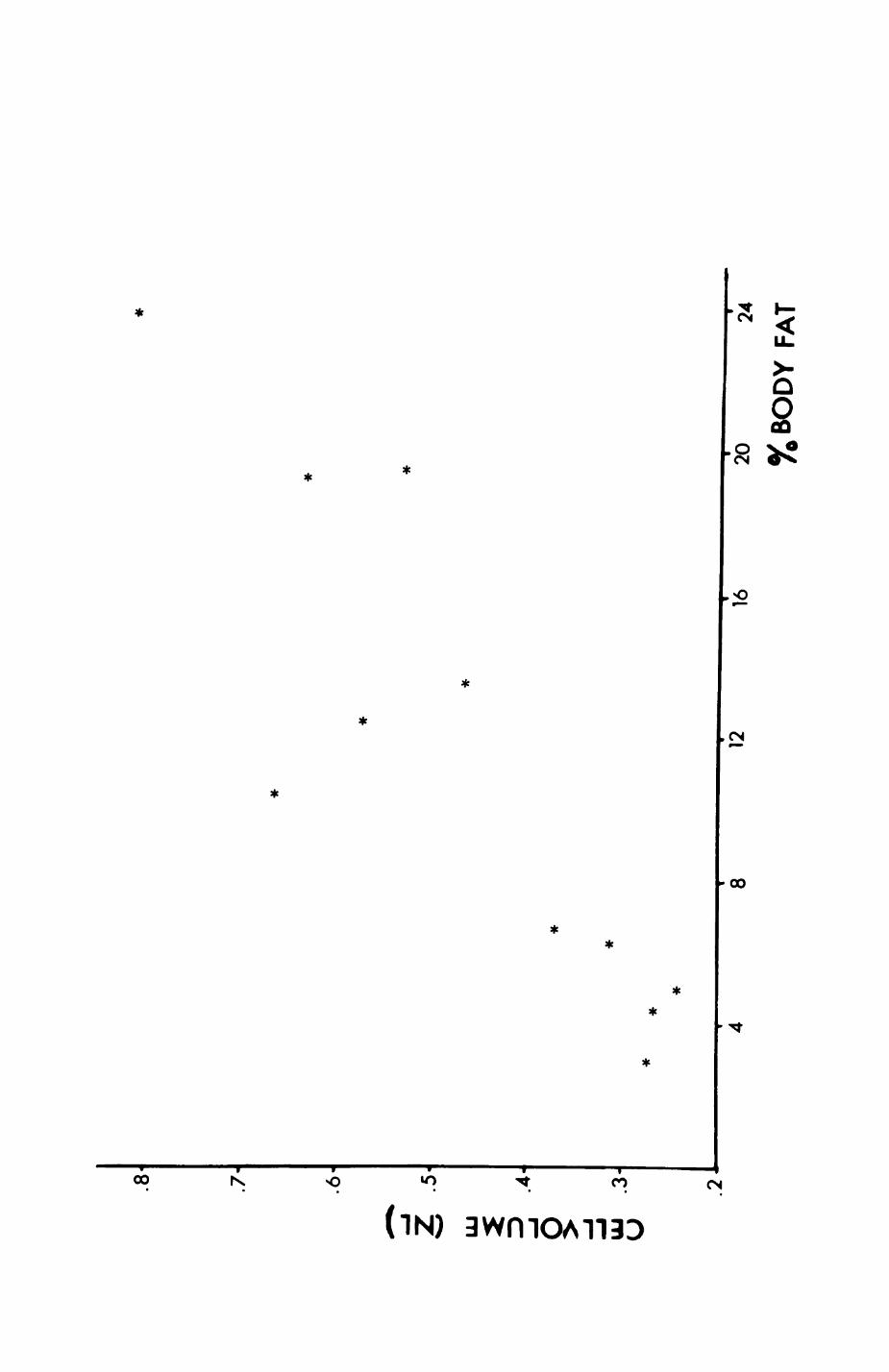
.8
Z
5 •* § .2.3*
*
8 12
16
20
24
BOD
Y FA
T

285
7.2.4. Summary! direction of selection pressures.
1. Maternal costs of rearing young are considerable. Up to 66 % of the
dally energy expenditure of a female may consist of mil* provided for the
young.
2. Mothers need sufficient high density resource areas at their
disposal to cope with the increased energy expenditure during the breeding
season. Attaining high density resource areas is more profitable than
reducing energy expenditure, e.g. by reducing maternal investment.
3. Mothers need stored fat for their own maintenance during winter when
they are largely inactive, as energy supply during pregnancy and as backup
during the breeding period. This requires good foraging areas for protein-
rich food in autumn when badgers store fat.
4. Cub mortality during the period of lactation indicates that
selection should favour a birth date later in the year (March or April) When
earthworm availability is high and less unpredictable.
5. Cub mortality after weaning suggests that selection should favour a
birth date very early in the year in order to have more time available for
the cubs to gain sufficient foraging experience before extended spells of
dry, unfavourable weather and associated reduced food availability can lead
to high cub mortality.
6. Selection should favour mothers that invest heavily. Higher growth
rates of young could lead to a large adult body size, better fat storage
capabilities and an increased chance of survival. Large body size and
appropriate fat storage capabilities may imply increased reproductive
success of the young and thus enhance the mother's fitness.
286
7.3. Spatial and social strategies of females.
In this section I will examine the kind of spatial and social organization
Which should be favoured by females in order to achieve maximal reproductive
success. Breeding success in badgers seems mainly to be related to maternal
care after birth and to the factors promoting it, since Ahnlund (198O) has
shown, at least for badgers in Sweden, that there is rather little variation
in litter size or regularity of breeding between different adult age-
classes. In the previous section I showed that the energetic burden during
lactation is considerable and that females should obtain access to high
density protein-rich food areas. Before I discuss in detail, how females
should go about to obtain such access, I shall investigate constraints on
possible forms of spatial distributions of females.
One necessary prerequisite for reproduction is the availability of
setts. If suitable sites are rare, then availability of setts is a ma^or
factor limiting the local reproductive rate. In one study of badgers in the
Bavarian Alps, for Instance, females reproduced only If they occupied
natural rock cavities on the mountain slopes that could be sufficiently
enlarged to provide space for the mother and the young {W. Bode, pers.
conm.). Such rock cavities are rare In comparison with other, low quality
sites. Males and females without suitable sleeping sites did not maintain
stable home ranges but instead drifted through a variety of neighbouring
areas. In Wytham availability of setts is high. More than 7O setts and
outliers were located in the study area (see also Table 5.7) and many more
fox dens and rabbit warrens could be extended to a size suitable for
badgers. Due to the distribution of the 'sand-belt* (Kruuk 1978a), the
preferred and easy-to-dig soil throughout the area (Killingley 1972, Heal
1977, Long £ Kllllngley 1983), all group ranges have suitable sites at their
disposal.
Setts are probably indispensable for effective protection of the young.
287
Interspecific predatlon on cubs by large raptors and possibly large
carnivores may have been Important in evolutionary tines and has been
occasionally documented In the present day (eagle owl. Bubo bubo.
Uttendoerfer 1952j golden eagle, Aqulla chrvsaetos, Klotz 19O3). Probably
more Important is Intraspeclflc predatlon, especially by adult males (Stubbe
1970). Females defend sett entrances leading to nesting chambers with their
young against males and scent-mark the entrances (Meal fi Harrlson 1958). The
black and White coloration of the badger's face already shown by very young
cubs has also been Interpreted as mimicry to protect cubs against predators
(see Neal 1977).
Setts are also important resting sites during the winter quiescence.
Badgers do not hibernate (Johannson 1956) but show much reduced activity and
spend most of their time in setts (Neal 1977). Efficient thexmoregulation is
achieved by selecting nesting chambers away from the surface and providing
them with ample bedding consisting of dry hay and litter. It is Important to
minimize energy losses due to temperature differences between body and the
air, since badgers have no specific metabolic adaptations to the cold. The
continuous occupation of specific setts by many generations of badgers may
indicate that this condition is not necessarily fulfilled, and setts with
good thermoregulatory properties may be rare.
The second constraint concerns the presence of sufficient food
resources within the reach of a female. Female body condition, intensity of
lactation and the survival and reproductive prospects of the young are all
dependent on fat reserves in the female and the presence of high resource
density areas. Here, the following questions appear to be relevantt
1. when does It pay a female to maintain exclusive access
to a resource (or a habitat), ie. why should a territory
owner do better ?
2. What are the costs of holding a territory ?
3. How should, and how do, females cope with
288
tit ion from other females, ie. What are the coats and
benefits of sharing one's range with other females ?
These questions are discussed in detail with reference to the wythaa
badgers. In section 7.3.6 I will then show how differences between
populations in the setup of the resource system leads to different types of
spatial and social organisation of female badgers.
7.3.1. Why should a territory owner do better ?
Here, a territory owner is defined as an animal with exclusive access to a
resource which is actively defended. Territoriality is possible, if the
characteristics of the resource, ie. its spatial and temporal occurrence
(and in the case of food) productivity permit an economic defense (Brown
1964). Although this is a necessary condition, it is not sufficient to
account for territorially, since a territory owner must do better than If
it was without a territory.
Earthworms are the main food resource of badgers in wytham (Chapter 4)
and are a stationary prey with little variation In abundance throughout the
year (Fhllllpson et at 1978) or over longer periods (cf blomass estimates in
similar habitats from Kruuk's and my study, Table 3.11). This makes an
economic defense plausible. In principle, the status of a badger (whether
territory owner or intruder) should, all else being equal, be independent of
•earthworm intake' per time unit. Availability of earthworms is, beyond
broad generalizations, essentially unpredictable (Chapter 3). This Is
mirrored by the fine-scaled utilization distribution of the home ranges
(Chapter 6). Good patches are temporarily depleted, if badgers forage there
for a long time, since the disturbance and vibrations caused by the badgers
on their foraging path will induce the worms to retreat into their burrows
and not surface again for some time (at least for ca. 1/2 hour, but may be
even longer, Edwards £ Lofty 1977). Thus, even though badgers are not likely
289
to affect earthworm population densities substantially (Macdonald
the proportion of the available worm population at the surface will be
considerably affected by their activities. The number of worms that return
to the surface feeding is a function of time (and microclimatic
circumstances, Chapter 3). Although the precise shape of the recovery
function is not Known, it seems plausible to assume that It follows an
exponential curve (Davies £ Houston 1981), ie. after a threshold time, there
is a non-linear increase of worms surfacing until the numbers approach an
asymptotic density value which may or may not be equal to the previous
level, depending, for instance, on the current microclimatic conditions
which may or may not have changed since the worms retreated into their
burrows (Fig. 7.5). Hence, the foraging success depends on the time that
has elapsed since the last visit of a badger (the renewal period of a given
area). Thus, a badger feeding in an area with a short renewal period suffers
a depressed feeding rate compared with an animal that enters a patch without
any previous depletion; therefore, knowledge of good patches and the renewal
time of a given patch is important to achieve a good feeding rate. Due to
their energy requirements, badgers are probably energy maximteers (Krutdt
1978b, Krebs et al 1983), thus feeding rate is important. Here territory
owners do better, for at least three reasons.
1. Owners can minimize search effort for good patches and
travelling time.
As shown in Chapter 3, microclimatic conditions as indicators of possible
worm surfacing activity vary considerably within the same habitat, but can
be partially predicted for a given location from other sites, provided the
knowledge of correlations between different sites is available and
occasionally updated. Here, a territory owner with an intimate knowledge of
its area is favoured over intruders who cannot usually be expected to have
such knowledge.
2. By evicting Intruders, a territory owner can enjoy a
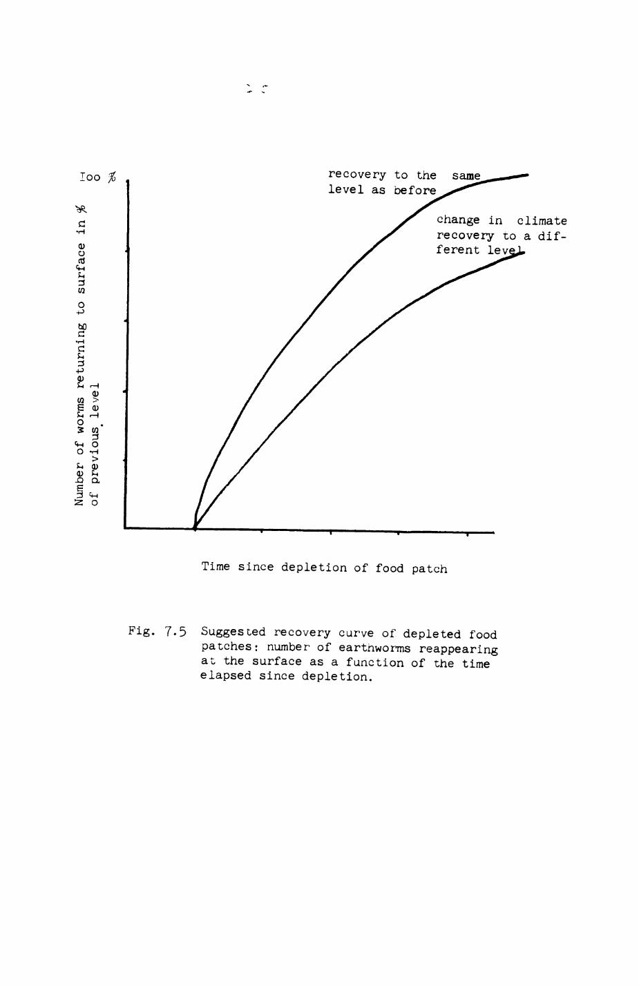
loo %
o«JCM k 3 W
O-p bO
-P
0)w >E 0SU rHo
£-1 0)0) SH-Q a
recovery to the level as before
same
change in climate recovery to a dif-
Time since depletion of food patch
Fig. 7-5 Suggested recovery curve of depleted food patches: number of earthworms reappearing at the surface as a function of the time elapsed since depletion.
290
higher feeding rate, since the number of patches deple
ted and the degree of depletion caused by the foraging
activities of other badgers is reduced.
Since It pays females to exploit high density resource areas (section 7.2),
Intruders should concentrate on foraging In patches predicted to be 'rich'
for a given night. Even within the sane habitat type, variation In
microcllmatlc conditions implies that only a fraction of potentially good
sites are actually full of surfacing worms at any Instant. Since It pays the
owner to forage In the same areas as potential intruders, the probability is
high that a resident will come across a depleted patch which has not yet
recovered, if only a limited number of sites is available in a given moment.
The consequence is a depressed feeding rate; hence, residents should evict
intruders to achieve high feeding rates.
3. By exploiting a territory systematically, a resident may
benefit itself by increasing the return time to a deple
ted patch, le. the time between two successive visits.
and simultaneously render it unprofitable to an intruder
to come in.
Here, systematic search is defined as any behaviour that maximizes renewal
rates of food areas. Systematic search has been observed both on a
microscopic scale (within a small food patch. Roper 1983) as well as on a
larger scale (Chapter 6). By utilizing patches in a systematic fashion,
renewal periods can be increased allowing depleted patches to recover.
Examples of renewal periods (Chapter 6) show that residents usually revisit
a patch after it is likely to have recovered. The most profitable site,
amongst those with high worm availability in a given night, is presumably
the site where the time since the last depletion is greatest. If residents
search in a systematic fashion, then the most profitable patch Should be the
one they are about to enter. This, however, is also the place most
profitable to an Intruder, a place where an Intruder could do a •»*-!••» of
291
damage, and Where an Intruder Is most iDcely to be evicted. If an intruder
arrives at other places it can be expected to do worse on average than the
owner, since it may not know Where the patches with the nicest renewal
periods are on the territory.
Some observations suggest that foraging badgers frequently scent-*arX
with their anal glands (Macdonald I977a, Neal 1977). This could both remind
an owner that it has already visited this area, minimizing time spent in
recently utilized areas (sections 5.4.3 and 6.3.), and deter an intruder by
advertising that the area has already been used. An intruder would then
either go somewhere else or start foraging. In the first case, its search
time increases, while in the second case it is likely to experience a
reduced feeding rate, because the depleted patch may not have recovered yet.
It is conceivable that the use of non-border latrines serves as a convention
to advertise recent exploitation of a food resource (section 5.4.3., Davles
1981), indicating to a prospective user the unprofltablllty of the area.
Davles £ Houston (1981) call this type of territorial defense 'defence by
depletion'.
7.3.2. What are the costs of owning a territory ?
Territory owners incur costs prior to any Intrusion through activities
Intended to deter intruders and costs associated with eviction if an
Intruder has arrived.
Marking of territories is one conventional way of advertisement of
territory ownership (Chapter 5). In badgers, it is achieved by scent-marking
at latrines (section 5.4.3., Kruuk 1978a, Kruuk et al 1984). The number of
latrines maintained is high, if necessary (in spring up to 5O within a
range, section 5.4.3), and is apparently adapted to the outside pressure
experienced by the range Inhabitants (section 5.4.3). Maintenance Incurs
costs due to the additional distances that have to be covered, digging
292
activities, and secretion production in the anal and subcaudal glands.
Although it is not possible to quantify these costs at present, it
likely that they are a significant additional burden <cf. Kruuk et al 1984)
Additional costs may arise through the need for intruder detection t e.g.
patrolling the territory boundary.
Once an Intruder has been detected, the owner has to evict hisu
Intraspeclflc aggression, has been invoiced as one of the ajo causes of
mortality in badgers (Stubbe 1970, Andersen & Trewhella 1985). Although the
proportion of Injuries or deaths due to territorial fights is unknown,
fights observed by Kruuk (1978a) indicate that they can result in severe
injuries (cf also Table 5.12). Even if a fight does not result in an injury,
chasing an Intruder costs time and energy.
After the eviction of an intruder an owner nay be displaced from its
original site, and may return to a place different from its last place prior
to the contest. If the owner had been feeding prior to the contest,
returning to an already depleted area will cause a depression in the owner's
feeding rate. Finally, an owner also suffers if an intruder tpmntrm
undetected while feeding, since this reduces the renewal period of the patch
which could result In a subsequent depression in the feeding rate of the
owner (see above).
7.3.3. Factors affecting intrusion pressure.
Females are most likely to compete with each other at tines of peak
energetic requirements. As discussed before (section 7.2) these are the
lactation period in spring and, to a lesser extent, the feeding periods in
autumn when females accumulate fat for the winter and the next reproductive
season. In these periods, females should marl mire their energy intake
(section 7.2). Itoxlmlzlng energy Intake should induce fenal*s to strive for
access to high density resource areas. *nuis. Intrusion pressure is expected
293
to Increase with resource density and availability per patch during these
periods. Competition (and Intrusion pressure) is also likely to Increase
with population density and Is related to the number of females requiring
high quality areas and the number of dispersing animals.
Pig. 7.6 illustrates how these factors are expected to relate to
intrusion pressure. Evidence for the proposed functional relationships is
largely circumstantial. The increased maintenance and marking activities,
particularly at border latrines, in spring can be explained as a response to
increased intrusion pressure (section 5.4.2). Similarly, latrine activity is
low in summer, when energy requirements of females are at their •JJJ»<«M» J and
when badgers partly switch to other, superabundant foods such as cereals.
High resource density areas are preferred by females and visited for long
periods (Chapter 6), suggesting that an intruder should also prefer such an
area. In a study on the economics of territory ownership on feeding
territories of pied wagtails (Motacilla alba), Davies £ Houston (1981) also
found an increase in intrusion pressure with increased food availability.
The high population density in Wytham, the intensive narXlng activity,
and the occurrence of aggressive encounters suggest that intrusion pressurecc
may be high at certain times of the year. How can territory owner cope with
this ?
7.3.4. Responses of territory owners to high intrusion pressure
In reviews on recent studies of terrltoriality in relation to resource
levels and defense costs, Schoener (1983) and Stamps fi Buechner (1995)
identified four common responses of owners to elevated intrusion pressuress
1. change territory sizej
2. increase the degree of overlap with adjacent territories)
3. accept subordinates In the terrltoryi
4. abandon territorial defense altogether.

Pig. 7.6. Relationships between resource and social parametersand intrusion and interference pressure. Curves do not represent real data, but are hypothetical (although derived from estimates of the literature for other species).
a. defense costs or intrusion pressure on a territory in relation to the productivity or availability of resources. Two thresholds are indicated. Below a lower threshold, a food resource is probably unattractive to intruders as compared with other resources. Beyond a higher threshold, defense costs are so high that territory owners may abandon defense altogether.
b. Interference costs within a group are likely to decrease with total resource availability.
c. Interference costs within a group are likely to increase with group size.
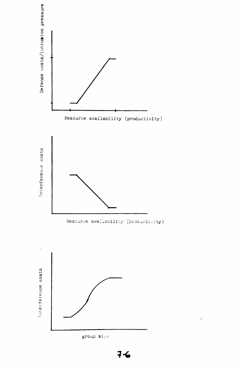
CO (0<vf-, ac o
W•t->
COo
0)wc0)
-p w o o
0)
Resource availability (productivity)
Resource avaiiacility (prodjctivity)
w o c;0)o
0)
groap si/e
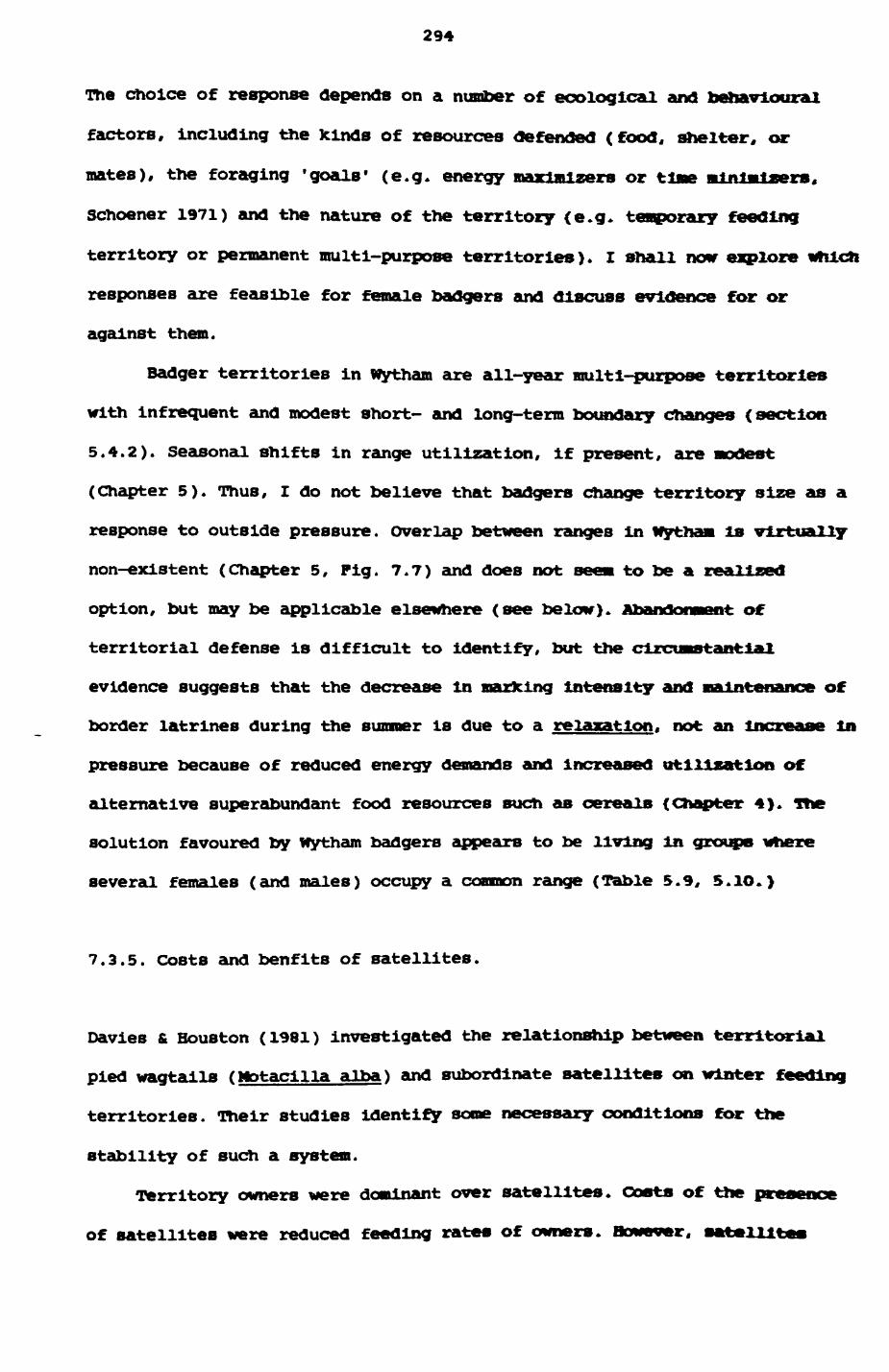
294
The choice of response depends on a number of ecological and behavioural
factors. Including the kinds of resources defended (food, shelter, or
nates), the foraging 'goals' (e.g. energy maxlmlzers or tine minlmisers,
Schooner 1971) and the nature of the territory (e.g. temporary feeding
territory or permanent multi-purpose territories). I shall now explore which
responses are feasible for female badgers and discuss evidence for or
against them.
Badger territories in Wytham are all-year multi-purpose territories
with infrequent and modest short- and long-term boundary changes (section
5.4.2). Seasonal shifts in range utilization, if present, are modest
(Chapter 5). Thus, I do not believe that badgers change territory size as a
response to outside pressure. Overlap between ranges in Nytham is virtually
non-existent (Chapter 5, Pig. 7.7) and does not seem to be a realized
option, but may be applicable elsewhere (see below)* Abandonment o£
territorial defense is difficult to identify, but the circumstantial
evidence suggests that the decrease in marking intensity and maintenance of
border latrines during the summer is due to a relaxation, not an Increase in
pressure because of reduced energy demands and increased utilization o£
alternative superabundant food resources such as cereals (Chapter 4). The
solution favoured by wytham badgers appears to be living in groups where
several females (and males) occupy a common range (Table 5.9, S.1O.)
7.3.5. Costs and benfits of satellites.
Davies & Houston (1981) investigated the relationship between territorial
pied wagtails (Motacilla alba) and subordinate satellites on winter feeding
territories. Their studies identify some necessary conditions for the
stability of such a system.
Territory owners were dominant over satellites. Costs of the
of satellites were reduced feeding rates of owners. Bowever. Mkt*llll

Pig. 7.7. Plot of the ranges of five female badgers,representing five adjacent group territories, on the computerized habitat map. Habitat categories plotted are habitats 7, pasture, and 37, deciduous woodland. Green stars Indicate position of latrines.
REDi bottom right - ALI group B2 (UPPER FOLLIES)upper right - NOEARS group B3 (MARLEY)left - ELIANE group B5 (SUNDAYS HILL)
BLUEt right - SARA group Bl (BOTLEY)left - PEACEFUL group B4 (JEWS HARP)
All ranges are plotted as contour plots using 15 min independence interval data. Plots created by program MAPITH, using the GHOST-80 graphics system.
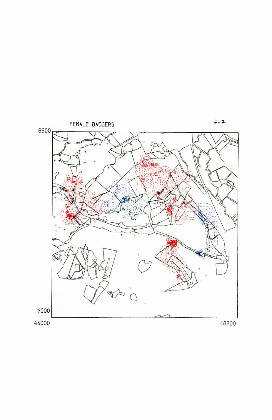
FEMALE BADGERS8800
6000
46000 48800
295
foraged In such a fashion that the depression In owner's feeding rate
less than that caused by undetected, feeding intruders. Benefits of presence
of satellites to the owner were a ma^or reduction In defense costs against
Intruders (1/3 to 1/2 of defense costs). Owners admitted satellites only
When intrusion pressure and defense costs were high, and evicted them when
the costs of the satellite's presence outweighed the benefits. However, If
an owner left Its territory leaving a satellite behind and did not return
for some time, the satellite sometimes took over and successfully expelled
the former owner when it returned. Individuals from flocks joined territory
owners only if feeding rates in territories exceeded feeding rates in non-
territorial flocks. Thus, a satellite may receive both short-tern, and. If
it persists, also long-term benefits by inheriting a territory. By a similar
argument, Gaston (1978) has proposed the 'payment principle', according to
which a satellite should take on a share of the defense costs }ust
sufficiently large to make a territory owner accept its presence, ie. the
subordinate satellite pays for being tolerated.
The data on group living of badgers in ifytham suggest that badger
groups could be modelled on the territory owner/satellite system.
Accordingly, groups should form in territories. When defense costs are hlgft.
A comparison of group sizes for the period 1982-1984 (Table 5.1O) shows that
group range sizes remained constant while group sizes varied greatly from
one year to the next. Badgers seem to prefer to change group size rather
than range size. However, no data are available to show that changes In
group size are a response to changes in defense costs. Such changes could be
induced by high-ranking females ('owners') that expel subordinates
('satellites'), since studies on captive badgers in Sweden revealed a
dominance hierarchy amongst females (H. Oestborn, pers. com*.).
To minimize interference costs for members of the same group, as would
be required if satellites are less costly than intruders, group members
should somehow coordinate their foraging activities. One possibility is a
296
dissection of the group range Into several areas, each of Which Is
exclusively utilized by one group member. Occasionally, utilization patterns
of the group range by several group members seem to fit this pattern
(Chapter 5), although there does not seem to be a fixed division in Vfythan*
However, group members in a study area on the Downs in Sussex are reported
to permanently utilize different parts of a group's territory (T. Roper,
pers. coran.). A second possibility is the coordinated movements of group
members over the group's entire range. Simultaneous radio—tracking of
individuals of one group confirmed that group members move in a somewhat
coordinated fashion, minimizing disturbance and maximizing renewal periods
of food patches (Chapter 6). Interference costs between group members, ie.
costs of presence of satellites, therefore appear to be small, at least in
the range studied. 'Payment* for residential rights of satellites appears to
occur as well, since all group members participate in marking activities and
defense (cf Table 5.12, unpublished observations on movements of members of
the Jews Harp group to latrines), although dominant individuals carry the
main burden (Kruuk et al 1984).
In summary, the formation of female groups in tfytham can be interpreted
as formations of defense coalitions as a response to elevated defense costs*
Benefits to territory owners (high-ranking females) Include the reduction of
defense costs. Benefits to satellites (low ranking females) include a place
to live, and the prospects of possibly inheriting the territory or acme part
of it. This is compatible with the developments observed over a period of 9
years (section 5.4.2). All foundations of new ranges can be interpreted as
offshoots from existing ranges.
297
7.3.6. Social organisation In relation to resource
characteristicsi other studies
Here I present the results of other studies and discuss the differences
to wytham emerging from these studies In relation to changes In the resource
system.
Two studies In Britain report an essentially similar situation as In
Wytham. Kruuk and colleagues (Kruuk 1978a, Kruuk fi Parish 1981, 1982)
studied badgers at several study sites In Scotland. Groups occupied
exclusive territories, badgers were shown to behave as feeding specialists
on earthworms, and group sizes varied between 2 and 11. Territory sizes in
Scotland varied between 120 and 309 ha. In Staffordshire, Cheeseman et al.
(1985) studied five ranges with group sizes (adults only) ranging from 4 to
11 and territory sizes from 54 to 131 ha. Territories were exclusively used
by the residents only.
Two other studies report different results.
In Bristol, Harris (1982) tracked members of 7 group ranges. Here, no
distinct territories could be identified. Several radio-tracked females used
setts and foraging areas of different groups. Harris therefore defined a
'group-foraging range' as the area in which each individual member of the
'group' spent the majority of its time. Animals were ascribed to a social
•group* according to the setts they •normally' used as a daytime resting
site, but these are not the only setts they may use for this purpose. If he
group ranges from his Fig. 1 are taken to calculate the area occupied by the
badgers (ca 3.5 km2 ), and the number of badgers caught and radio-tracked
(31) as a minimum estimate of population density, we arrlv« at a density of
ca 8.9 individuals/km2 . This density is one of the highest recorded (Kruuk
1978a gives a figure for Wytham of 8.4 lnd/km2 , Chmsmiin et al. I9«s report
a density of 6.2 ind/km2 ). This is probably an underestimate sine*^<r-P
presumably not all Individuals In the were caught. Be concluded that the
298
social and spatial setup of this population is remarkably different fi
those observed in other studies.
Difficulties in Interpreting his results arises from the procedure by
Which he defines group existance and membership, especially since he does
not provide any information on latrine distribution or results of bait
recoveries. If I had defined my groups solely on the association with
certain setts, similar problems as reported by Harris would have arisen.
Without any information on marking activity or agonistic encounters. It is
difficult to assess to What extent the loose organisation of ranges is
'real' or merely an artefact of the methodology chosen* Assuming that indeed
the Bristol badgers show some range overlap I suggest two explanations for
the deviation from the normal patternj
(a) the population reached such a high density that only a core area of
the territory can be defended and overlap with neighbouring groups at the
periphery cannot be avoided
(b) territory defense is abandoned altogether*
What evidence do we have for either of these suggestions ? This depends
to a large extent on the characteristics of resources and the way
Individuals use them. The results reported by Harris (1982) suggest that
resources are probably superabundant and distinct, in their characteristics.
from the situation encountered in previous studies. Except for December,
when Bristol badgers eat almost exclusively earthworms), they do not appear
to exhibit habitat selection. Then, food diversity is high, the food is more
scattered, food patches are visited for only short periods (except for
periods with high fruit availability) and earthworms, other invertebrates,
scavenged items and fruits contribute similar proportions to the overall
diet.
This pattern of resource use is distinctly different frosi that of the
studies cited previously. The differences concern <l) abundance of food.
299
(11) the Importance of renewal rates for foraging rate and (11) the pattern
of resource availability. The Bristol badgers do not suffer fro* a shortage
of food. In contrast to Wytham, for Instance, there seem to be a lot of
potential scavenge available during the critical periods In sprlngi they
constitute the bulk of the diet from January until Hay* If the conventional
'bottleneck' In food supply at the end of winter is not present, Inter-group
food competition can be expected to be much relaxed and hence Intrusion
pressure Is expected to drop considerably. The major prey types are
distinguished from earthworms in that their renewal rate Is independent of
the foraging activities of the badgers. Hence, the likelihood of
interference and the benefits gained from a defense are reduced.
Why, then, do Bristol badgers live in groups ? it is not clear to what
extent the units identified by Harris actually constitute badger groups in
the conventional sense. If it is typical for the population that setts axe
used in quite a flexible manner, as Harris (1982) described for several
females, it may not be justified to call them groups, bat rather a system of
loosely connected individual ranges, where sometimes several IntUvHHials
occupy the same resting site. In this respect it is interesting that Baxrls
once observed in one of his 'groups' two breeding units emeitje in early 198O
and subsequently split the 'group range 1 into two separate sections..
In summary, the situation in the urban population in Bristol is quite
different from that usually encountered in studies in more natural habitats,
but as far as the data permit conclusions, still consistent with the
expectations derived from the discussion of territoriallty in the preceding
sections.
One final study remains to be mentioned. Martin-Pranquelo 4 Dellbes
(1985) studied the behavioural ecology of badgers in a mediterranean region
in Spain. Despite the preliminary nature of the results, nrmf interesting
snippets emerge. The main food item are rabbit nests and young rabbitsi
earthworms are very low in abundance. The dispersion of rabbit
300
to large ranges (on average 422 ha) with only one male and one female
present per group. Rabbit nests are relatively scarce, but predictable in
occurrencei hence the Spanish badgers defend territories. The nature of the
main resource and the low densdlty of badgers leads to a low level of
intruder pressure, hence group sizes are expected to drop to the minimum*
7.3.7. Discussion.
The Resource Dispersion Hypothesis (RDH) put forward by Bradbury £
Vehrencamp (1976) and Carr & Macdonald (In press) shows that at very little
or no cost to a primary occupant (In foxes and badgers usually a pair)
additional individuals may be sustained on a territory under certain
circumstances. Given a certain level of heterogeneity in resource
availability, a primary occupant has to defend an area larger than it would
if food availability was 1OO % homogeneous ( ie. all food present on a
territory is also available). How large the defended area is depends on the
chosen level of security, (e.g. in 95 % of all nights there should toe a
satisfactory energy IntaKe). Then, in a large proportion of nights, resource
availability will be higher than what is required to satisfy the primary
occupant and other individuals can harvest the 'superfluous crop*. The
characteristics of earthworms as main prey fit very snugly to the conditions
presupposed by RDH. However, while RDH in principle is certainly applicable
to badgers in Wytham, I believe that the foregoing results show that there
is at least one additional factor contributing to group formations under
conditions of (a) high energy demands and (b) critical resource
availability, intrusion pressure may increase, if suitable high density
resource areas are present within a territory, and necessitate the
acceptance of additional individuals (satellites) In order to Maintain the
territory. RDH makes it plausible that presence of a satellite say be
costly than may otherwise be assumed. The 'defense coalition hypothesis*
301
described in the previous sections shows that presence of additional
individuals may not only be tolerated but actively solicited by a primary
occupant. To What extent other processes (e.g. Kin selection) play a role In
furthering group stability can at present not be decided.
7.4. Hale competition and female choice.
In this section I shall first describe some basic features of the
reproductive biology of males and females, before I turn to a discussion of
the possible Incidence of sperm competition, female choice and the evolution
of delayed Implantation.
7.4.1. Mating seasons and mating success.
In Eurasian badgers, the majority of matlngs take place In spring, le.
between February and April (Neal & Harrlson 1958, Meal 1977); a sizable
proportion constitute post-partum oestrus. Ovulatlon frequency reaches
almost 100 % by June (Ahnlund 1980 for Swedish badgers). Not all animals
appear to conceive after ovulatlon, since the ovulatlon rate increases
faster during spring than the Incidence of blastocyst formation (Ahnlund
1980). However, renewed ovulatlon Is not restricted to females that failed
to conceive but occurs also In pregnant females. This Is Indicated by the
relatively large proportion of females that contain on average 3 blastocysts
and 5 corpora lutea I According to Ahnlund f s (1980) detailed analyses, very
old and very young (first year or second year breeders) show a higher
incidence of renewed ovulatlons than middle-aged females. Renewed ovulatlons
may usually reoccur until autumni this explains why males produce fertile
sperm from January until autumn, unllXe the males of many other species with
delayed Implantation. Renewed ovulatlon may occasionally lead to an increase
in the total number of blastocysts and hence litter sice. This is because
302
about 15 % of the blastocysts already present survive the second mating
period, at least In mlnX Mustela vlson (Johannson & Venge 1951).
Superfecundatlon (several males fertilize eggs during the same oestrus)
occurs In the mlnK (Enders & Enders 1963), and may be possible In badgers,
since several males have been observed to mate with the same female (e.g.
paget & Mlddleton 1974). It Is undecided whether female badgers are
spontaneous or Induced ovulators. The extended periods of copulation
frequently observed (Neal 1977), sometimes up to several hours, suggest,
however, that badgers similar to other mustellds may belong to the Induced
ovulators.
In summary, there is a well defined mating season (spring) but females
may ovulate at additional times of the year. In the majority of females,
formation of blastocysts and pregnancy occur after the first ovulatlon.
Males produce fertile sperm throughout most of the year and may secure
additional pregnancies during secondary ovulatlons. Some of these
circumstances of the reproductive biology of badgers are exceptionali
(1) Why do pregnant females come into oestrous repeatedly ?
(2) Why do females exhibit post-partum oestrous, le. spend
a considerable proportion of time on mating while they
could spend it on rearing the newly born young ?
(3) Why do females exhibit delayed implantation ?
(4) How do males cope with uncertain paternity that may
arise from repeated ovulations ?
7.4.2. Mating behaviour t opportunities for female choice.
Field observations have shown that (1) males may mate with several
females and (11) females may mate with several males. According to
observations by Paget £ Nlddleton (1974) and Neal (1977), females do not
seem to actively solicit males. In February, the pea* mating period In
303
Britain, the boar calls the sow softly after emergence and patrols around
the sett. At this time, females are quite aggressive towards males and
decline males access to entrances to the nest chamber of their young.
Consequently, mating taxes place outside the sett. The male then mounts in
typical mustelid fashion gripping the sow by her neck or her ear. The mating
pair may stay together for a variable period, between 10 seconds and several
hours, but usually matings are of short (less than 5-10 min) or long
duration (from half an hour onwards). The female usually finishes the
copulation by going down a sett entrance, so that the male is forced to let
her go. Oestrous lasts for 4-7 days (Neal & Harrison 1958) and during this
time mating may occur on and off for hours throughout the period. Mating
sites and the female(s) are often scent-marked by the boar after mating.
Despite her apparent passivity, a female has a variety of possibilities
to influence the procedure!
(i) termination of copulation can be decided by the femalej hence she
can decide whether a mating leads to ovulation and possibly conception!
(ii) many males are attracted to a female in oestrous (Meal 1977),
since she may advertise her reproductive condition through the latrine
system.
(iii) the possibility of repeated ovulatlons presents her with the
opportunity to receive sperm more than once a year, either to exercise
positive mate choice or to use it as a 'fail-safe' system (a very high
proportion of old females showed renewed ovulations in Sweden, Ahnlund
1980).
I shall now examine costs and benefits of multiple mating from first
the male's and then the female's point of view.
7.4.3. Costs and benefits of multiple mating in males.
Males contribute little (KruuK, pers. co»n., observed males in
304
captivity to provision young with food) or nothing to the rearing of the
cubs. Hence, they should, in line with other polygynous and sexually
dimorphic males (e.g. Glutton-Brock et al. 1982) strive to achieve maximum
reproductive success by maximizing mating success. Mating success is
characterized by two aspectsi
(i) secure mating success (ie. conception) by monopolizing females and
prohibiting other males from access to females;
(ii) maximize the number of mat ings by mating with as many females as
possible.
As Parker (1984) has pointed out, the first aspect poses an
evolutionary arms race problem, where adaptations of males to prevent
subsequent mat ings by other males are counteracted by adaptations to produce
armament (in a wide sense) to overcome the paternity assurance adaptation.
Monopolizing females may be achieved in several ways. Precopulatory and
postcopulatory guarding may be an ESS under certain conditions (Grafen £
Ridley 1983, Parker 1984). Postcopulatory guarding may not be sensible, if
several females in a group come into oestrous simultaneously. Efficiency of
postcopulatory guarding is also limited, because it would require the male
to guard the female during all oestrous periods. This may be worth only for
subdominant males that have little chance to secure other mat ings (e.g.
stoats, Mustela erminea, Sandell 1985). For other males, however,
opportunity to mate with other females may represent a higher payoff than
guarding (Sandell & Llberg, in prep). Hence, guarding is predicted to be
observed occasionally, but not invariably (see Paget & Middle ton 1974, Neal
1977). Parker (1984i44) presents a model of sperm competition where he
Investigates possible ESS solutions to contests between males over mating
opportunities with females. If a male has already mated ('resident') and
comes across another male without mating ('interloper*) then the resident
may lose the contest, and hence the interloper gain access to the female, if
there is the possibility that more than 2 ejaculates compete for
305
fertilization.
Males may also restrict other males' access to females by defending a
territory encompassing the range of one or several females. Hence, males
should defend territories most vigorously in spring during the main mating
season, a time When females have a special Interest in territory defense due
to their increased energy requirements. Work by Kruuk (1978a, Kruuk et al
1984) has shown that males (i) defend territories and sometimes carry the
main burden, and (11) exclude other males from access to females (Kruuk*s
1978a 'bachelor clan 1 ). In section 5.4.2. it was shown that the
restructuring of the group range arrangements between 1974 and 1982 could
best be interpreted as a reorganisation of males' influence spheres. If
population density and correspondingly intrusion pressure by other males is
high (e.g. Drabble 1970), a single male may not be able to defend his range
effectively. Then it is conceivable that a male may tolerate another male in
order to share defense costs, in the same way as it pays females to accept
other females as satellites, even If this lowers his reproductive success,
(By sharing mating opportunities with another male he may still have a
higher reproductive success than if he had to give up the territory
altogether, or be swamped by intruders I).
Under certain conditions, a male may find himself In the situation of the
Prisoner's Dilemma. Consider two neighbours who initially defend territories
with their respective females. Their choice is to play cooperative (be
'peaceful' ), or form a coalition with another male, because they suspect an
increase in pressure from the other territory owner, or because they would
like to extend their sphere of influence. This is a 'defection' and makes
the second male defect as well, le. admit an additional male in his area, to
redress the 'balance of power*. With additional males on their homeground
they are now worse off on average than they would have otherwise been.
Hence, the presence of more than one male In a range may not necessarily be
beneficial. If the males are related, benefits would accrue to the original
306
occupant through Inclusive fitness, but kin relationships between badgers
are not known at present.
The second avenue open to a male is to secure a mM-immn lumber of
matlngs. A male should try to maximize the number of mat ings in his own
group and, if possible, also mate with other females. Although the latter
may be dangerous (see the results of intraspecific aggression. Table 5.12).
there is evidence from tracking in wytham that this may take place. In Pig.
7.8 and 7.9, contour plots of ranges of neighbouring males and females are
plotted on the habitat map. The UPPER FOLLIES male WILF went twice for an
excursion into the BOTLEY LODGE Range (Fig. 7.8), where I tracked him once
in the same outlier as a female of the local range, SARA. Some overlap is
also indicated by GEORGE'S movements relative to ALl's range use (Pig. 7.9),
but their movements were followed at different times. The occurrence of such
excursions emphasizes the necessity of a good and effective territory
defense, and confirms that even holding a territory does not suffice to
assume perfect paternity for the offspring of your own group.
In summary, males can maximize mating opportunities by restricting
access of other males to their own females while at the same time strive to
mate with as many females as possible, both inside and outside the group. As
a result of specific conditions, males may be required to accept other males
in their territory if they want to secure any matings at all.
7.4.4. Costs and benefits of multiple matings in females.
Several authors discussed the costs and benefits of multiple mat ings for
females (Thomhill £ AlcocJc 1983, schwagmeyer 1984). There are at least four
possible kinds of costst
(1) additional time and energy devoted to courtship and copulation. Por
Instance, female badgers could spend the time used for courtship and Mating
to concentrate on the rearing of the young.
Pig. 7.8. Ranges of the male WILF (red) from group B2 (UPPER FOLLIES) and the female SARA (blue) from group Bl (BOTLEY) plotted on the computerized habitat map. Lay-out of map and data types identical with Fig. 7.7,
Note that both animals were tracked at the approxima tely same time. Some of the overlap between SARA and WILF is due to simultaneous presence of both indi viduals at the same site (an outlier in Range Bl).
Fig. 7.9. Ranges of the male GEORGE (red) from group Bl (BOTLEY) and the female ALI (blue) from group B2 (UPPER FOLLIES)/ plotted on the computerized habitat map. Lay-out and data types identical with Fig. 7.7.
Animals were tracked at different seasons of the year.
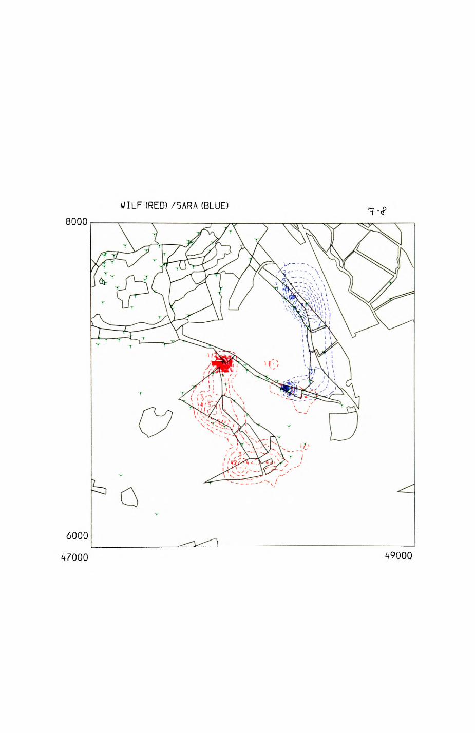
WILF(RED) /SARA (BLUE)
8000
49000
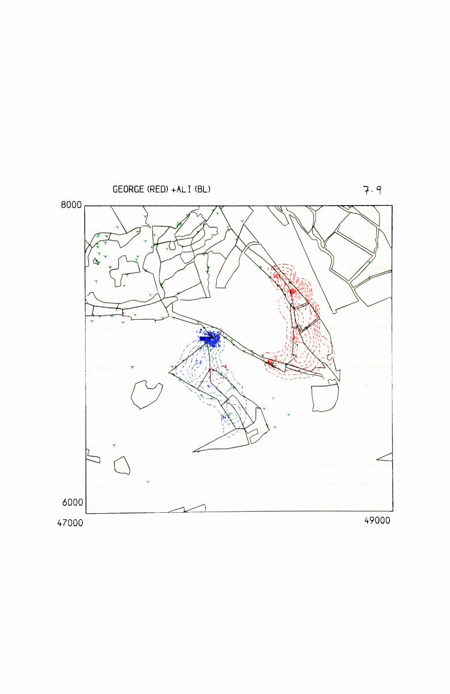
GEORGE (RED) +ALI (BL)
8000
49000
307
(11) time required to repel unwanted suitors, if in Intermediate stages
of receptivity. This seems to be a negligible problem for female badgers -
all they have to do is to vanish into the sett and emerge from a different
entrance, if necessary.
(ill) loss of paternal investment by the male. Acceding to the present
evidence unllXely to play an Important role In badgers.
(iv) increased vulnerability to predators - this is probably a
negligible aspect for badgers.
Altogether 11 benefits have been put forward to explain multiple mat ings
in females:
(i) add to depleted or inadequate sperm supplies - of no importance to
badgers.
(11) sperm storage places cost too much - of no importance to badgers.
(ill) the male provides nutritional benefits or other material resources
- of no Importance to badgers.
(Iv) the male helps reduce the risk: of predatlon or helps her reduce
competition for a resource. This is something male badgers could do. but is
unlikely to be important on a general level. One counterexample is the
situation of males and females in Mar ley in Kruuk's study (see section
5.4.2)t there, males defended the territory against other males, but
Included the ranges of several females occupying nearly separate ranges and
hence were unllJcely to be of any efficient help in intra-group struggles.
This argument does of course not apply to mat ings with extra-group males.
(v) the male provides protection from other sexually active males. Since
copulating pairs have been observed to be harrassed by other males, this
does not seem a very lUcely possibility.
(vi) replace sperm from a genetically inferior male by that of a
genetically superior male. This requires an Identification procedure
according to which genetically Inferior males can be detected. Following
308
this rule, females should mate at tines When maximum distinction between
males is possible, e.g. at times When males are in their best condition
(Sandell 1985). This seems to be the case for badgers t males reach the
highest body weight in February When the mating season starts and are then
in prime condition. Sandell (1985) described the conditions that facilitate
the evolution of delayed implantation, ie. the decoupling of the time of
mating from the time of parturition. Evolution of delayed implantation is
then an advantageous development, if opportunities for mate choice are to be
maximized, and yet the specific circumstances, e.g. prey availability,
prohibit a change in the timing of parturition (section 7.2.4)*
(vii) increase genetic diversity of offspring. This is a largely
unproven hypothesis Which poses all kinds of theoretical problems (William
1975).
(viil) avoid the costs of trying to prevent superfluous copulations.
This may occasionally be a problem boars have been observed to drag a
female out of a sett to mate with her. One possibility for her is to mate
briefly (< 10 min) and then terminate copulation.
(Ix) reduce aggression of males. This is especially Important, If a new
male or a new group of males take over a range. Hales would gain from
killing young cubs, since females may be able to produce a late litter (see
section 7.2). Females should copulate with the new males in order to prevent
them from killing next year's litter (Which they may already have
conceived). The difficulty with evidence for this hypothesis is that, so
far, a 'take-over' of a territory by outside males has not been observed.
However, infanticide may be a real threat to the young, since females are
known to actively defend sett entries to nesting chambers with their young
from approaching males.
(x) Increase average degree of relatedness of the offspring of all
females within a group (Davles fi Boersma 1984). This is a suggestion put
forward to explain some of the features of lion Panthera leo society. Too
309
little is known about degrees of relatedness amongst and between badger
groups, as that a serious evaluation of this suggestion can be attempted.
(xi) facilitate Immigration Into a group. The problem with this argument
la that even If males will tolerate the new female, it nay depend on the
female members of the group whether she is accepted. Their 'decision'
probably has nothing to do with the Incidence of multiple mating.
In summary, with the present data available, three benefits are
possible candidates: avoidance of infanticide, mate choice and avoidance of
costs of superfluous copulations.
7.5. Conclusions.
In the previous sections, I described how the characteristics of a
resource influence the spatial and social organisation of the two sexes.
These are summarized in Pig 7.1O. Three dependent variables characterise the
social and spatial organisation! home range size, terrItorlallty or non-
territorial ity, and group formation. Resource characteristics determine
directly or indirectly all three parameters in a decisive manner. They may
exert their Influence via the defense coalition path, and/or along the
resource dispersion path. For instance, the dispersion of earthworms and the
form of recovery of depleted patches determine home range size,
defendability of the range and the costs and benefits of group formation.
The model applies also for males defending females as a resource. In
summary, it points to the success of using resources as an approach for
explaining the details of the spatial and social organisation of badgers in
Wytham.
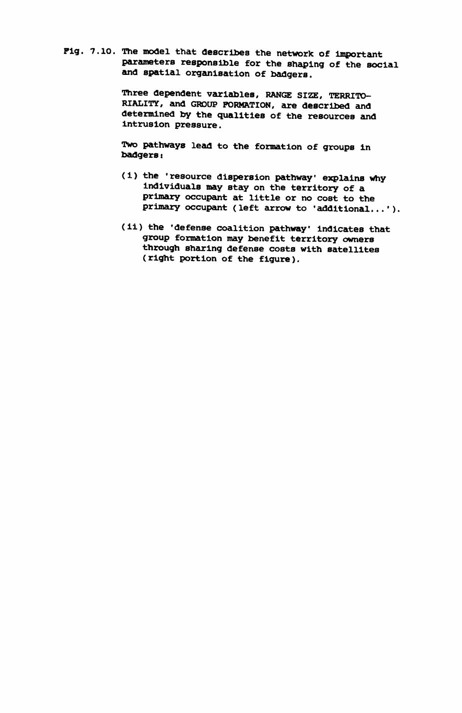
Pig. 7.10. The model that describes the network of importantparameters responsible for the shaping of the social and spatial organisation of badgers.
Three dependent variables, RANGE SIZE, TERRITO- RIALITY, and GROUP FORMATION, are described and determined by the qualities of the resources and intrusion pressure.
Two pathways lead to the formation of groups in badgers j
(i) the 'resource dispersion pathway' explains why individuals may stay on the territory of a primary occupant at little or no cost to the primary occupant (left arrow to 'additional...').
(ii) the 'defense coalition pathway' indicates that group formation may benefit territory owners through sharing defense costs with satellites (right portion of the figure).
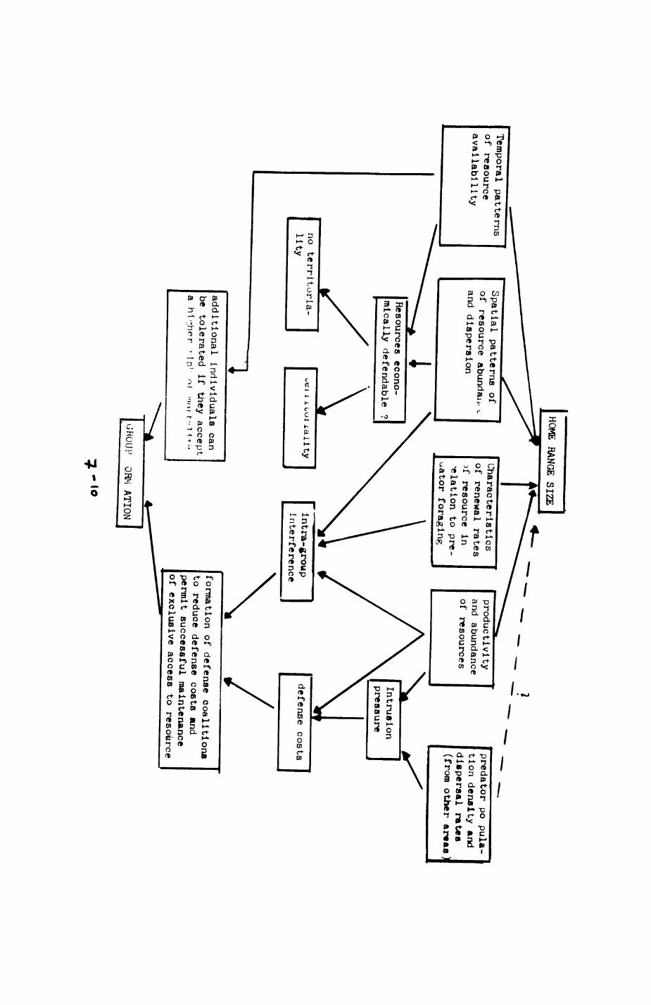
Temporal patterns
of resource
availability
Spatial patterns
of of
resource abundan
and dispersion
Resources econo
mically defendable
?
no territoria-
lity
Characteristics of
renewal rates
if resource
in "elation
to pre-
uator foraging
productivity and
abundance of
resources
predator po pula-
tion density and
dispersal rat*s
(from other areas)
Intrusion pressure
lality
rin
tra-gro
up
interferen
cedefense
costs
additio
nal
indiv
iduals
can be
tolerated
if
they accept a ht^hor
vlr>! ^f
""it t"1 ^f"
formation of defense coalitions
to reduce
defense costs
and permit successful maintenance of exclusive
access to
resource
iJHOUP OHM
ATION
-10

APPENDIX It statistical considerations for sampling design
The accuracy and the results of habitat records depend on the sampling
design. Hence, emphasis was placed on a careful sampling scheme. There is
a considerable body of literature dealing with sampling problems. There are
both general introductions (notably Cochran 1977, Payandeh & Beilhartz 1978,
and Green 1979) and studies dealing specifically with problems encountered
in vegetation, land use or habitat classification (e.g. Kuechler 1967,
Mueller-Oombois & Ellenberg 1974, Howard 1981, Johnson 198la, Karr 1981,
Gauch 1982a, and Greig-Smith 1983). Gauch (1982a), amongst others, lists
the following criteria for the development of an appropriate sampling
designt
1. APPROPRIATENESS. The type, intensity and breadth of information
collected should be adapted to the research purposes and the kind of
statistical analysis Intended (see also point 3).
2. HOMOGENEITY. Samples should be placed so that the possibility of
environmental discontinuity is minimized. The sampling design and the scale
on which data are measured should be adjusted to the scale of variation
expected for each parameter. Preliminary field observations aid in
estimating this. It might not always be possible to develop statistical
estimates (Noon (1981)).
3. OBJECTIVITY and STANDARDIZATION. Each parameter should be measured
in the same way over all sampling units to make data points comparable.
Scoring of data points should be on compatible levels, ie. a variation from
continuous data (e.g. a percentage scale from 0 to 100%) to binary data
(presence/absence) should be avoided, If possible.
4. EFFICIENCY. There is a trade-off between the number of sampling
units that can be recorded and the number of variables and the precision by
which they are recorded due to the limited amount of manpower and time
available. A successful compromise preserves sufficient accuracy in scoring
While providing for a large number of sampling units.
Particular sampling requirements to consider arei
1. TYPE OF SAMPLING UNIT. The two possible alternatives are transects
and plots. The decision of Which one to choose will depend on the kind of
variables, their expected variation and the expected error, accessibility of
the study area, intended statistical analyses and purpose of study.
Syntheses of analytical methods and sampling designs are provided for plots
by Greig-Smith (1983) and for transects by Caughley (1977) and Burriham et
al. (1980). Both my data and those from Forestry were recorded using plots.
Transects were discarded because in woodlands transects are less economical
than plots in terms of area of sample that must be obtained for a given
sampling error and efficiency of detection (Dawkins 1952). Also, most of my
other data (e.g. radiotraclcing data) are effectively summarized using area
units. Compatibility of such data with habitat transects would be low. In
addition, initial field trials with transects through woodland showed
enormous problems with the location of transect lines and accurate transect
walking.
2. DISTRIBUTION OF SAMPLING UNITS. The most common schemes are
random, stratified random and systematic (regular) sampling (Cochran 1977).
Statistical considerations demonstrate both advantages and disadvantages for
all three methods. Systematic sampling was selected for the forestry data
because the sampling units were intended as the first stage of a long-term
Continuous Forestry Inventory System. For such a scheme, regular spacing
forms an efficient grid within which future samples, possibly random, can be
placed. As Dawkins and Field (1978, their Appendix 1) showed, the
probability of detection of rare and unusual events is higher for systematic
than for random sampling. The most likely alternative, stratified random
sampling, has the disadvantage that the bases of stratification (statistical
and ecological considerations) might change with time and therefore render

the initial stratification procedure inefficient or meaningless. I adopted
systematic sampling to comply with the Forestry data and to ease comparison
with possible future work. It also facilitated accurate location of plots
In the field and reduced the time needed to complete field worfc, thereby
increasing sample size.
3. SHAPE OP SAMPLING UNITS. Either square plots or circular plots are
usually used. Squares were used in both studies as their perimeter is
easier to determine and potential subsampling facilitated.
4. SIZE OP SAMPLING UNITS. Generally the plot size should correspond
to the scale of variation expected. However, this is often difficult to
predict. Depending on the size of the sampling units, a positive, negative
or no correlation can be detected for the association of e.g. two plant
species (Greig-Smith 1983). As possible solutions to this problem, a
variety of measures have been suggested, e.g. sampling with different plot
sizes (Greig-Smith 1983), sampling in concentric plots with expanding
aureoles (Bunce & Shaw 1973) etc. A summary can be found in Greig-Smith
(1983). Statistical advice on how to deal with results from differently
sized plots can be found in Mead (1974). Forestry data were recorded on a
10 by 1O meter square to comply with the unit of area basic to European
forest site-quality assessment. I adopted two plot sizest a 5 by 5 meter
square ('central area'), which I judged to be the maximum plot size for
which I could record reliable vegetation scores, was located in the centre
of the 'base area' of 50 by 50 meters where information on resources, badger
and fox presence was recorded.
5. FREQUENCY OF SAMPLING UNITS. Theoretical considerations made it
necessary to sample at least 100 plots for the forestry records (DawXins &
Field 1978i11). The final forestry data set comprised 164 plots spread over
326 ha of woodland and covered 0.5 % of their study area. I sampled
altogether 441 plots at two sites that covered together 110.25 ha. The data
on vegetation covered 1 % of the study area while I tried to sample as much
of the study sites as possible (at least 75%) for data on resources and fox
and badger presence.
The number of possible sampling schemes Is Infinite. There are many
different investigative purposes; a researcher interested in bird habitats
will emphasise different aspects than a mammalog1st or a forest scientist.
Also, schemes need to be adapted to the local situation. However, there is
enough scope for more general surveys. "General" variables might reveal the
patterns for a specific purpose just as well as variables dealing
specifically with it, at least for plant communities (Shute & West 1982).
Suggestions for alternative recording procedures can be found in Bunce and
Shaw (1973), James and Shugart (1970), Cody (1968), Wiens (1969), Noon
(1981), Hirst (1975), Burnham et al. (1980), Sabo (1980), and Kling (198O).

APPENDIX 2i statistical considerations for data analysis of
habitat data
The habitat records are a typical case of multivarlate datai many
variables (also called parameters, variates or attributes) were recorded for
many samples (also called sample units or cases). Multivarlate methods are
particularly suited for these kind of data (see discussion by Gauch
1982a:12, Johnson 1981b, and Shugart 1981). A first task is to summarize
the raw data efficiently and reduce the number of dimensions (each variable
can be viewed as one dimension) from many to few, revealing the systematic
patterns of variation while losing little of the detailed information
contained in the raw data. This is necessary because raw data are bulJcy,
difficult to access and contain a lot of redundant informationi the number
of samples is usually far greater than the number of 'pattern units' (e.g.
communities or habitat types) to be discovered. Another task is reduction of
'noise' in the data, le. the random variation from one sample to another.
The class of techniques that are commonly used for this is called
ordination. Many of them have been developed, particularly in the fields of
psychology and plant community ecology. A suitable ordination technique is
a technique with underlying assumptions that are not violated by the data or
are at least robust against slight to moderate deviations. In recent years,
a number of studies have been published that provide comparisons of the
performance of several ordination techniques using either real data or
artificial data sets with exactly known properties (Gauch et al. 1977,
Pimentel 1981, Gauch 1982a, 1982b, and Shute & West 1982). In my discussion
of the techniques and performance criteria I will draw mainly on these
studies and then justify the methods chosen for the analysis.
In principle, ordination techniques work as followst the data set is
canvassed and a series of ordination axes extracted that represent the 'new*
variables, along which the variation inherent in the data set is sunmarized.
Usually these new axes are extracted in a hierarchial fashion with the first
axis summarizing most of the variance, the second axis then summarizing roost
of the variance remaining, and so on. Ordination techniques differ in the
ways in which they extract these axes, how they combine the original
variables to create new axes, and how they define the relationship between
new axes. This is particularly effective if most of the original variables
are somewhat correlated: if they were perfectly uncorrelated, an ordination
of the data would lead to no significant reduction in the dimensionality of
the data set as defined by the number of new axes created. The new axes are
called the principal components in Principal Components Analysis, factors in
Factor Analysis, and so on. Their virtue lies in the fact that not only do
they help to reduce the number of original dimensions but can also be
uncorrrelated with each other and thus useful for further analysis.
However, the new axes have only a precise mathematical, but no intrinsic
biological definition. Therefore it is important to Know the limitations of
the technique employed in order to decide Whether an axis has a biological
meaning or not.
The ordination techniques can be characterized by the assumptions they
make about the distribution functions of the variables and the relationship
between variables. Most of the ordination techniques assume a normal
distribution of the variable values (e.g. Principal Components Analysis,
Principal Coordinate Analysis, Factor Analysis), if tests for significance
of relationships are to be made, but some do not (e.g. the group of
multidimensional scaling techniques; cf. Colgan & Smith 1978, Prey &
Pimentel 1978, Spence 1978, Pimentel & Prey 1978, Bhattacharyya 1981, and
Williams 1981). Also, all ordination techniques make assumptions about the
relationships between variables; most of them assume a linear relationship
between all variables. There are thus two main questions to consider when a
choice of an ordination technique is to be madet
1. How realistic are the assumptions of the distribution functions of
variables and the relationship between variables for the data set in
question ?
2. Given a data set that is appropriate for the ordination techniques under
consideration, how well do the techniques reduce the noise in the data and
reveal the systematic patterns of variation ?
DISTRIBUTION FUNCTION OP VARIABLES. Ecological data, such as data on plant
communities or habitat data, are likely to have skewed distributions. It
has however been shown that multivariate techniques are quite robust against
this kind of violation (Gauch 1982a), usually more robust than common
univariate and bivariate parametric methods.
RELATIONSHIP BETWEEN VARIABLES. A more severe problem is the kind of
relationship between variables. Most ordination methods assume linearity,
e.g. the commonly used Principal Components Analysis. This, however, may be
Inappropriate, if variables have any kind of non-linear relationship. There
are many kinds of non-linear relationships possible, e.g. quadratic,
negative quadratic, Gausslan, cubic, etc. A whole school of plant community
ecologists work with the premise that plant species show a Gausslan response
to environmental factors and to each other (Whittaker 1975). In general,
the possibility of ecological data exhibiting Gaussian or other non-linear
behaviour has not been sufficiently recognized (for an appraisal see e.g.
Westman 1980), and zoological studies investigating nonlinear responses are
few (Meents et al. 1983, Phillips 1978). Ordination techniques permitting
nonlinear relationships are Principal Components Analysis on suitably
transformed data (see Gnanadesikan 1977), parametric mapping (Noy-Meir
1974), Gaussian ordination (Gauch et al. 1974), multidimensional scaling
(Anderson 1971) and correspondance analysis or reciprocal averaging
including detrended correspondance analysis (Hill 1973b, 1979, Hill & Gauch
1980).
PERFORMANCE OF ORDINATION TECHNIQUES. Gauch et al. (1977) and Gauch (1982b)
developed a set of criteria by which to judge the performance of ordination
techniques. i
1. Noise reduction.
2. Recoverage of underlying gradients (e.g. coenoclines).
3. Response to random sampling errors.
4. Behaviour in case of outliers.
5. Reaction to partially disjunct data sets.
Gauch et al.'s (1977) results with simulated data demonstrated superior
performance of reciprocal averaging over another technique commonly used in
plant ecology, Bray-Curtis polar ordination (Bray & Curtis 1957), and
various kinds of principal components analyses. They used a data set with
'plant species' responding in a Gaussian fashion to underlying one- and two-
dimensional gradients. Reciprocal averaging recovered much of the original
gradients, but principal components analysis involuted the gradient ends at
high levels of 'species' diversity, resulting in a sequence reversal. In
all cases, the expected outcome was a straight line.
Plmentel (1981) used a set of nonlinear taxonomlc data to compare
principal components analysis, principal coordinate analysis, nonlinear
mapping and nonmetrlc multidimensional scaling. He found that non-linear
mapping showed consistently poor results. Good results were achieved using
nonmetric multidimensional scaling based on Gower's general similarity
coefficient (Gower 1971). Principal components analysis on a correlation
matrix showed best, but still inaccurate results. A consultation of these
studies shows that reciprocal averaging and standardized principal
components analysis (ie. performed on a correlation matrix) show superior
performance to other techniques, but are still Inadequate for data
exhibiting a strong nonlinear tendency.
The two main problems of reciprocal averaging and principal components
analysis are the 'arch effect' and the compression of axis ends. These
problems result from a discrepancy In the underlying models and the
mathematical properties of non-linear data (Gauch I982atl50, I982b). Their
effect can be demonstrated using simple data sets of simulated data. If a
data set Is arranged so that the variation is along one gradient only, the
perfect ordination technique would plot all points along a straight line,
ie. all points should have the same value on the second axis. Both
reciprocal averaging (RA) and principal components analysis (PCA) show an
arch distortion (see Gauch I982atl51, his Pig 4.11) with the points in the
centre of the first axis separated from the points at both ends. This is
due to a quadratic distortion which results from the condition that two
successive axes should merely be uncorrelated (a stronger condition would be
that axes should exhibit no systematic relation of any kind with each
other). This can lead to ambiguous results when strongly non-linear data
are ordinatedt the second axis, being merely a quadratic distortion of the
first axis, accounts for more of the 'variance 1 (ie. has a higher
eigenvalue) than the third axis with proper representation of the 'real'
biological variation deferred to the third axis. The second problem Involves
compression of the first axis ends in RA relative to the axis middle, so
that a given distance of separation in the ordination does not carry the
same meaning in terms of implied differences between samples or variables.
As a consequence of these undesirable effects, Hill (1979, Hill & Gauch
198O) introduced a modified version of reciprocal averaging called detrended
correspondance analysis (DCA). OCA was specifically designed to correct the
two main faults of RA and PCA described above. Tests with simulated and
real data show that it actually does what it is meant to and indicate a far
superior performance over any other ordination technique (Gauch 1982b).
As a conclusion I decided to use detrended correspondence analysis
(DCA) as my main ordination technique. In summary, DCA avoids the main
problems of PCA and RA, permits handling of non-linear data and ordinates
variables and samples simultaneously on axes that have a meaningful
dimension.
APPENDIX 3: Data selection procedures and statistical
techniques for diet analysis.
For the analysis of the diet of fox ranges, droppings had to be
assigned to each range. As the vast majority of droppings could not be
assigned reliably to known individuals, I had to use the information on the
location of each dropping and compare this with the information available on
the spatial configuration of the ranges. There are at least two potential
errors that can lead to a wrong association of dropping and range based on
spatial Information!
1. Overlap of ranges (see detailed discussion in Chapter 5) prohibits a
reliable assignment of droppings collected within overlap zones. Inclusion
of droppings from a neighbouring range may introduce a bias.
2. Itinerant and migrating individuals traversing a range might leave
scats which distort the results. This problem is intractable and probably
has equal effect on each range.
Both these sources of noise will tend to work against any conclusions
to the effect that diets differ between the foxes in different ranges.
Probably the more influential error is the possible bias introduced by an
inclusion of droppings from neighbouring individuals. I therefore developed
a procedure to exclude droppings from zones of overlap.
In program SCATCELL a reference map with a 50 meter base grid was
established. The program tagged each cell according to which of 14 selected
foxes were located at least once therein. In this way a list of all
observed combinations of individuals which shared cells was prepared. For
each group range a list of 'admissible' combinations of foxes was drawn up
(see Table 5.22). For each range program CODESEL compared the list of
admissible combinations of foxes with the observed combination in each cell
of the base map; the program selected only grid cells with an admissible
combination. Finally, program TURSEL tagged each dropping in this heavily
filtered subsample with the appropriate range number by comparing the map
coordinates of the dropping with the list of grid cells of each range as
determined by program CODESEL.
This procedure is a very strict one in that it excludes all cells where
individuals from different groups were located, without regard to the
frequency of such events. However, I feel that this is necessary in order
to have confidence in the analyses of correlations between habitat and diet
characteristics of fox ranges (Chapter 5). The possibility remains that
other, not radiotracked, members of each group may have trespassed into
neighbouring ranges even further than the radiotraclced animals.
The test statistic generally used for comparisons of different temporal
and spatial units (months, seasons, ranges) was the Kruskal-wallls test, a
non-parametric equivalent of the one-way analysis of variance. Initial
checks with the P -test (Sokal & Rohlf 1981) Indicated that the variances
were too heterogeneous for a normal analysis of variance. Where the
Kruskal-Wallis test statistic was significant, ie. differences between the
means could not be accounted for by chance alone, a multiple comparison
procedure was possible (Conover 1980, p.23) in which each mean was compared
with each other mean to test whether the means differed. Thus it was
possible to work out which range differed from which others without altering
the overall level of significance (ie. without an increase in type I
errors).
Another non-parametric test-statistic was used to investigate whether
the directions of temporal fluctuations were synchronized between ranges.
For example, this procedure was used to test the significance area of an
apparent decrease of the proportion of rabbits taken by foxes from a peak in
winter to a trough in summer. Irrespective of the possibility that the
representation of rabbits in the diet may vary between different ranges at
any time, the test answers the question of whether the changes from one
temporal unit to another follow the same pattern for all ranges over all
temporal units considered. The test statistic used is Kendall's coefficient
of concordance. Kendall's coefficient of concordance can assume values
between 0 (perfect asynchrony) and 1 (perfect synchrony). Computation
procedures and hypothesis testing followed Conover (1980) who suggested that
the test statistic should be compared with critical values based on a
different distribution (the P-distribution) rather than the usual Chi-square
approximation. Results of an earlier investigation of the badger's diet
(Kruuk & Parish 1981) with published concordance values were used to
Investigate the effect of Conover's suggestion. The results of the modified
tests showed a greatly improved level of significance for all significant
effects (ie. synchrony between study areas) and changed one test value from
insignificance to significance at a level of alpha = O.05.
APPENDIX 4t Statistical analysis of telemetric datai the
problem of temporal independence
A basic property of telemetric data is the frequent lack of
independence of successive data points. By this we mean that within a short
time interval a fox or a badger is not equally liXely to reach all other
locations in its range from a given starting point, hence its subsequent
location is partly dependent on its previous location. Hore formally,
statisticians call two events A and B 'independent* from each other if
p(AB) = p(A) p(B) (1)
with
p(AB) the probability of event A and B occurring together
(the }oint probability of A and B)
p(A) the probability of event A occurring
p(B) the probability of event B occurring
(Conover 1980t16). The definition implies symmetry, that is if point A is
independent from point B, B is also independent from A. The definition is
directly derived from the concept of conditional probability. Consider the
relationship of the probability of event A and the conditional probability
of A given B, p(A/B). This conditional probability is
p(VB) - P (AB)/p(B) (2)
Now, if the probability of A, given that B occurs, is the same as the
probability of A without any information on the occurrence or non-occurrence
of B, one could say that the occurrence of A is independent of whether or
not B occursi the two probabilities would be equal, or p(A/B) - p(A). If
p(A/B) is replaced by p(A) in eqn (2), ie. we set A as independent from B,
we get eqn (1).
The definition of independence of two events A and B as in eqn (1)
implies that the idea of A and B being independent from each other is not an

absolute nor an unconditional statement. The judgement, independence or
not, depends on the probability function for events A and B. Naturally, we
can not describe the probability function for locations visited by a fox or
a badger in advance. However, we know that the probability function depends
on the time interval at which we choose to look at events A and B. To
demonstrate this by an extreme example, we could choose one second as a
suitable time interval for considering two successive events A and B. We
know that the highest recorded speeds of foxes are ca 40 km/h (Lloyd 1980)
which is equivalent to 11.1 m/sec. The probability that a location B at a
distance of more than 12 metres from the present location A would be visited
(ie. event B occurs) is practically equal to zero. If you take the same
locations but increase the time interval to three days, there is a high
probability of event B occurring given a location A - at least with
reference to the constraint imposed by the maximum speed of foxes 1
Lack of independence of successive data points is Important, since a
variety of probabilistic home range concepts, whether parametric or non-
parametric, assume independence of events. Furthermore, many classical
statistical tests require independent data points. Estimates of home range
size based on the grid method (Voigt & Tin line 1980) benefit from
independent data points, since then the data points are more likely to
constitute a representative sample of the animals' movements. There are
three ways to cope with this problem:
(1) modify the test statistic to cope with the special
qualities of the data
(2) modify the data to create independent data pointsj
(3) Ignore the problem.
As Cliff and Ord (1981) point out (see also Appendix 5), the formally
correct procedure is always to modify the test statistic. Since such
modified procedures are not yet available, or only for certain problems
(e.g. within the context of spatial autocorrelation, Appendix 5), I shall
discuss the second suggestion in more detail.
To date, four procedures have been suggested to look at temporal
independence in a data sett
(1) Dunn and Gipson (1977) developed a probabilistic model of home ranges
based on the multivariate Ornstein-Uhlenbeck diffusion process. This is a
special stationary process based on normally distributed data assuming that
a location depends only on its immediate predecessor. With these
assumptions, lack of independence decreases exponentially with increased
time interval between two locations. This approach is of limited use
because of the assumption of bivariate normally distributed data.
(2) Schoener (1981) showed that the ratio of the mean square distance
between successive observations to the mean squared distance to the
geometric centre should be 2 for independent observations, if the successive
observations are identically distributed. However, Schoener did not make
any suggestions as to what to do if the observed ratio deviates from his
expected value, ie. if the data exhibit dependence (as can be safely assumed
for telemetry data).
(3) Newdick (1983), in a study on the ranging behaviour of red foxes in
urban Oxford, selected an 'independence interval' by calculating the largest
distance across the home range, if defined by all data points, and dividing
it by the maximum speed observed for foxes (4O km/h or 667 m/min). One
disadvantage of this method is that it produces varying independence
intervals if range sizes and configurations vary (in his study he calculated
independence intervals of 10 to 30 min for different ranges), so different
proportions of the original data set are discarded. The method may also be
sensitive to sample size. Doncaster (1985) therefore opted for a consistent
Independence interval of 15 minutes.
(4) In an extension to Schoener's preliminary analysis, Swihart and Slade
(1985) provided empirical evidence that a test statistic can be based on
Schoener's ratio and developed an objective, albeit arbitrary criterion to
determine the independence interval. Using data on movements of a female
cotton rat (Sigmodon hispidus). they calculated a time interval of 270
minutes, an estimate close to the results Newdick (1983) obtained when he
used simpler correlation coefficients in his fox study.
Even though Swihart's and Slade's (1985) procedure may be objective, I
doubt whether it is of much use. If only data were admitted for analysis
that are at least 4 or 5 hours apart, the bulk of the data would have to be
discarded. This renders most problems typical in studies of animal
movements totally, and absurdly, beyond analysis.
Newdick's (1983) method of relating the top speed to the largest
distance seems most appealing. The resulting Interval provides an estimate
of the minimum time an animal would require to reach any other point In Its
range. Since most points in a range are more towards the centre than the
periphery of the range, the actual time Interval may usually be shorten
thus Newdick's rule provides conservative estimates. Since my ranges were
comparable in size with his results, I decided to adopt a standard
independence interval of 15 minutes (the mean of the independence intervals
for 17 fox home ranges (excluding transient foxes), calculated according to
Newdick's procedure, was 15.35 min - S.D. 6.25). The majority of the data
points of all foxes will be independent according to this criteria, and
comparisons with other studies will be easy.
A second approach considers actual times spent by the animal in an
area. If an animal is followed continuously throughout the night, the actual
time spent in a patch (or in a grid cell) can be calculated. Home range
measures based on actual times spent in area units do not suffer from
problems of temporal independence as do measures based on frequencies of
visits, if there is still dependence In the data, It mimics non-random
behaviour in space (a process we are interested in), but not side-effects
derived from the vagaries of a particular sampling regime.
This distinction between unfavourable statistical side-effects of a

particular recording scheme (leading to possible dependencies between
successive observations) and the correlations due to the non-random movement
patterns of the Individual in question has largely been overlooked, but is a
vital one» we want to minimize the chance for distortions arising from the
sampling procedure while in contrast we are interested in the correlations
exhibited by non-random behaviour. Recording of actual times spent in an
area unit provides an acceptable solution to this problem. If we record
actual times spent in an area, the probability of visiting an area by an
individual may also depend on the probability of visiting another area. This
is the problem of 'spatial dependence' which will be dealt with in Appendix
5.
APPENDIX 5: Spatial independence of datat the concept of
spatial autocorrelation
Consider a habitat which is of no interest to a badger. Let a clump of
beech trees be such a habitat. All else being equal, the intensity of usage
of this clump of beech trees would be low. Consider a second clump of beech
trees which, unlike the first, is situated on a patch leading from one very
attractive habitat to another one. As the badgers would pass along the path
many times they would naturally also traverse the clump of beech trees
(which in a sense is nothing but an obstacle to them). In such a case the
Intensity of use of this clump of trees can be said to depend on the
Intensity of use of the two attractive areas. That is to say, the intensity
of usage of a habitat (e.g. the clump of beech trees) may solely be a
function of its spatial location (e.g. between two attractive sites).
A5.1 Spatial autocorrelation
If the intensity of usage of point A (or, formally speaking, the
probability of an animal visiting point A) depends on its spatial location,
e.g. on the probability of visits to neighbouring points B,C,..., then the
two events A and B, A and C,... are not independent. What is the practical
importance of this? If I want to compare the intensity of usage of patches
belonging to a selection of different habitats, I cannot be sure that the
differences (or similarities) found can solely be attributed to the habitats
(e.g. their intrinsic attractivity); it may rather be the case that the
result is influenced considerable by the spatial location of the patches
considered relative to each other and perhaps to other patches not
consideredI Unravelling the Interplay between habitat selection and spatial
inevitabilities might prove interesting per se, but it also means that
conventional statistics can be used only in a restricted way - a chi square
test on differences between habitats in the intensity of use would only be
admissible under certain conditions (section A5.2). The principle of
spatial dependence in radio-tracking data is obvious, but its statistical
implications have never hitherto been acknowledged in the vast literature on
animal movements.
If a set of data points display interdependence over space, they are
said to be spatially autocorrelated. spatial, because the interdependence
is over space, and autocorrelated, because data points of only one variable
(e.g. intensity of use) are correlated with each other. The formal
definition of spatial autocorrelation is, according to Cliff and Ord
(198118)!
If for every pair of spatial units 1 and } in the study area the
drawings which yield x. and x. are uncorrelated, then there is no spatial
autocorrelation in this system of spatial units on X;
with X being a random variable (intensity of use) and x., x. the values of X
for spatial units i and j. Data with this property are common in
disciplines where the analysis of data on their spatial information is
required (anthropology, geography, or ecology), in fact, they can be the
kind of data that are of special interest to the researcher (Appendix 6).
However, the tools for a correct appreciation of the properties of spatially
autocorrelated data have only recently become available (Cliff and Ord 1973,
1981). This study is the first to apply them to telemetric data. I shall
therefore discuss the properties of spatial autocorrelation in some detail.
The relationship of temporal and spatial independence deserves to be
discussed further. We might have achieved temporal independence for the
data selected to determine the configuration of the range, but quite apart,
there might still be spatial interdependence and thus spatial
autocorrelation in the intensity of usagei for the question of spatial
autocorrelation the only aspect of interest is whether the intensity of
usage of a given part of the range is due to its location near to or distant
from other areas. It is important to realize that temporal and spaial
interdependence are different problems and that the solution of one of them
does not necessarily imply anything about the state of solution of the
other! Should therefore the data be cleansed of temporal interdependence
before they are subjected to an analysis of spatial interdependence ? The
answer 1st there is no need, since there is no requirement for the data to
be independent data points in order to calculate the spatial autocorrelation
function. In fact, the object of this study is to explore, rather than
eliminate, the spatial interdependence that may exist in the data. What is
Important is not possible temporal independence of data points but their
represent at ivity of the true events. Consider the example of the beech
trees once more. If the animals take a short time, say 5 minutes, to pass
through the beech trees situated between the two attractive sites at which
they linger for much longer, and if the decision was taken to collect data
every 15 minutes, the badgers might be missed on some or even on all
occasions when they walked through this patch of beech trees during the
period of data sampling. My sample might then not record their movements
through the beech trees and I could therefore not consider this patch of
trees in an investigation of spatial use, since in this case the sample
would not be representative.
This problem can be generalized by considering the average speed of
movement M in relation to the average size of the spatial unit S and relate
this to the sample time interval. Four extreme conditions are possible (t -
time interval for sampling):
Speed of movement (M)
Slow movements Past movements
S small (1) S < M*t for some (2) S < M*t for almost all
Intervals intervals
S large (3) S < M*t for most (4) S < M*t for some
intervals intervals
The probability of missing a patch visited by the animal would be low
under condition (3), moderate under condition (1) and (4) and high under
condition (2). If the probability of missing a patch is fairly high, the
results of the spatial autocorrelation analysis would be suspect. This
would not only affect procedures to investigate spatial interdependence but
also bias the picture of range usage I The simplest and best sampling design
not affected by this is the continuous recording of the movements of the
animal. It is then possible to consider actual durations in a given spatial
unit and the spatial units can then be designed independently from
considerations of how to sample movements.
As the spatial autocorrelation is defined as the correlation of pairs
of values of a random variable mapped onto the study area divided into a
system of spatial units, the autocorrelation will depend on the mapping
procedure, ie. on the division of the study area into units. For instance,
spatial units could be patches of irregular shape (as defined In the habitat
map) or cells of a systematic grid placed over the study area. What kind of
unit to choose and the effects on the autocorrelation will be discussed in
more detail in section AS.3.
A further point to note is that spatial autocorrelation is defined as
the outcome of comparisons of many pairs of spatial units. The rules for
building the pairs allow the consideration of points in all directions.
This is a fundamental difference to autocorrelation functions found in
residuals of regression analysis or the temporal autocorrelation in time
series analysis where the pair formation is restricted to one direction.
Spatial autocorrelation can be generated by multilateral interactions
because of at least two dimensions in space (for the analysis of fox and
badger units the third dimension is neglected, but would be important for
arboreal species). The direction of interaction is not defined a priori; in
fact, the number of possibilities for interaction directions is infinite.
As a consequence, a multitude of different kinds of spatial
interdependences occur. For instance, a gradient (trend) may influence the
overall pattern; the correlation may depend on the direction (e.g. relative
to the earth's magnetic field) of the link between two sites, or the
relative strength of the link, e.g. the amount of border line shared by two
sites. The scale of dependence can vary as wellt on a very local level, as
in the example with the clump of beech trees, only immediate neighbours are
affected. Effects over large distances are equally conceivable as in
animals with symmetrically shaped ranges (e.g. the hexagonal territories of
some fishes) visiting the range borders regularly.
These examples show how varied spatial processes can be. Thus,
'spatial interdependence' reveals itself not as a closely defined process
but as a summary of a multitude of diverse phenomena - there is not -Just one
kind of spatial dependence but there are many. 'Testing directly for
spatial dependence' is rarely possible, or even useful and effective; in
most cases this should be read as 'testing for a particular kind of spatial
dependence'. We can answer the question 'do the data display spatial
interdependence 1 ?' only via the question 'what kind of spatial
interdependence is shown by the data?•.
Thus, investigating spatial interdependence fulfills more than purely
statistical considerations, in addition, by setting up and testing spatial
models with specified properties (i.e. the hypothesized way spatial location
exerts an influence on the dependent variable) we gain an alternative method
to complement the usual analytical tools that require independent data
points.
A5.2. Effects of spatial autocorrelation on statistical inference
There is general agreement that spatial autocorrelation will affect the
outcome of statistical tests (Haggett et al. 1977 p. 336, Cliff & Ord 1981).
The following discussion is mainly drawn from Cliff and Ord (1981t 184-196).
Conventional methods of hypothesis testing employing statistical inference
are based on the assumption that the data points are assumed to be
independent. However, the important feature of spatially located data is
that the data points cannot necessarily be assumed to be independent. For
instance, in the case of positive autocorrelation (values of pairs of
spatial units are of similar magnitude), an observation contains less
information than an Independent observation, since it is partly predictable
from other observations located nearby.
So far few studies are available that consider this effect of
autocorrelation or that make suggestions of how to modify the conventional
procedures to account for the autocorrelation. In principle, there are
three possibilities to cope with autocorrelated datai
1. Modify the conventional test statistic to account for the
interdependence of observations.
2. Modify the data and filter the autocorrelation out.
3. Ignore the fact that the data contain spatial auto-
correlation.
The formally correct procedure is always to modify the test statistic
(Cliff & Ord 1975). This was quite burdensome in all cases investigated so
far. There is, on the other hand, only one study that considers the effect
of filtering procedures (Martin 1974). Thus I shall concentrate on the
modified test statistics.
Studies have been published for the following test proceduresi
(1) t-testi (Cliff & Ord 1975)
(2) one-way analysis of variancei (Griffith 1978)
(3) Pearson's product-moment correlation coefficient; (Blvand 1980)
(4) Regression. (Cliff & Ord 1981).
The general message from the results of these studies is quite cleart
if autocorrelation is not considered, severe Inferential errors are
possible. As a rule of thumb, however, it is reasonable to say that if low
to moderate levels of positive autocorelation are present and the actual
value exceeds by far the critical one (at least the critical one at the 5
percent level) then this result should be significant even if compared with
critical values obtained from a modified procedure. If data exhibit negative
autocorrelation, the opposite is true - then normal test statistics may be
conservative for a given alpha level.
A5.3. Models of spatial autocorrelation
As the previous sections showed, there can be different kinds of
spatial Interdependence. For the following sections I shall define a model
of spatial autocorrelation as a specific scheme of interactions of sites due
to their spatial location, ie. a scheme that proposes what specific
properties the spatial process in question shows. I emphasize the
importance of specificity of models of spatial autocorrelation since the
power of the autocorrelation measures is highest, when the factual
autocorrelation pattern corresponds to the hypothesized one (the type II
error of accepting a null hypothesis while it is in fact false is then
minimized; Cliff and Ord 1981). The power of the various autocorrelation
measures is also related to the 'degree of specificity* of the modelj if
many interactions between sites are considered then the power is potentially
lower than if there are few and very specific interactions postulated. In
other words, there has to be a compromise between the desire to include as
many connections and types of interactions as possible (thus maximizing the
chance that the factual autocorrelation pattern is amongst the multitude of
Included ones) and the loss of power of distinction incurred by the
Increased generality of possible patterns. These properties of spatial
autocorrelation measures have to be considered for a correct appreciation of
the results. They also Illustrate the importance of a careful decision on
how pairs of spatial units (to be compared) are formed, which connections
should be of interest and how they are considered. There are then three
steps in the procedure of setting up the basic properties of a model:
1. Define the size and shape of area units, ie. the admission to pair
formation (how should the areas be defined that are compared?).
2. Determine the admissible connections between area units, ie. the links
by which the units are supposed to interact (the formal, or structural
pattern).
3. Decide, what influence each connection should exert (the functional
pattern of interactions).
Area units are sometimes predetermined by the study in guest ion. If,
for Instance, the gene freguencies of different populations of a species
should be compared and a model is suggested what kind of spatial process is
responsible for the pattern found (e.g. panmixis, migration, fission etc. ),
then the sites, the area units, are already givent they are the places where
the different populations are present at the time of the study. On the
other hand situations exist where there is a choice amongst competing
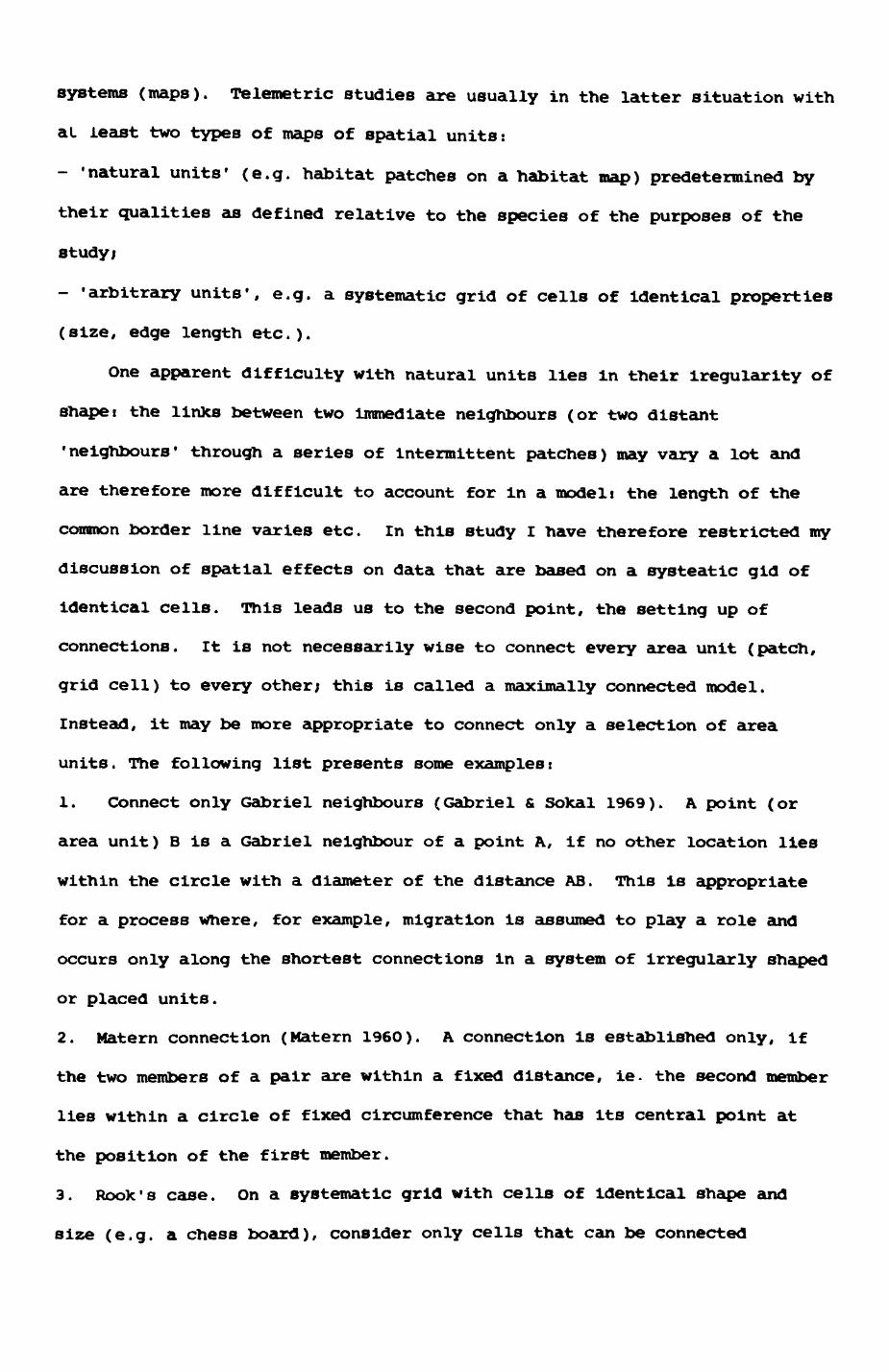
systems (maps). Telemetric studies are usually in the latter situation with
at least two types of maps of spatial units:
- 'natural units' (e.g. habitat patches on a habitat map) predetermined by
their qualities as defined relative to the species of the purposes of the
study;
- 'arbitrary units', e.g. a systematic grid of cells of identical properties
(size, edge length etc.).
One apparent difficulty with natural units lies in their iregularity of
shapei the links between two immediate neighbours (or two distant
'neighbours' through a series of intermittent patches) may vary a lot and
are therefore more difficult to account for in a modeli the length of the
common border line varies etc. In this study I have therefore restricted my
discussion of spatial effects on data that are based on a systeatic gid of
identical cells. This leads us to the second point, the setting up of
connections. It is not necessarily wise to connect every area unit (patch,
grid cell) to every other; this is called a maximally connected model.
Instead, it may be more appropriate to connect only a selection of area
units. The following list presents some examples:
1. Connect only Gabriel neighbours (Gabriel & Sokal 1969). A point (or
area unit) B is a Gabriel neighbour of a point A, if no other location lies
within the circle with a diameter of the distance AB. This is appropriate
for a process where, for example, migration is assumed to play a role and
occurs only along the shortest connections in a system of Irregularly shaped
or placed units.
2. Matern connection (Matern 1960). A connection is established only, if
the two members of a pair are within a fixed distance, ie. the second member
lies within a circle of fixed circumference that has its central point at
the position of the first member.
3. Rook's case. On a systematic grid with cells of Identical shape and
size (e.g. a chess board), consider only cells that can be connected
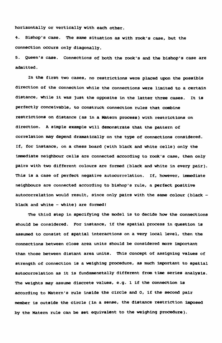
horizontally or vertically with each other.
4. Bishop's case. The same situation as with rook's case, but the
connection occurs only diagonally.
5. Queen's case. Connections of both the rook's and the bishop's case are
admitted.
In the first two cases, no restrictions were placed upon the possible
direction of the connection while the connections were limited to a certain
distance, while it was }ust the opposite in the latter three cases. It is
perfectly conceivable, to construct connection rules that combine
restrictions on distance (as in a Matern process) with restrictions on
direction. A simple example will demonstrate that the pattern of
correlation may depend dramatically on the type of connections considered.
If, for instance, on a chess board (with black and white cells) only the
immediate neighbour cells are connected according to rook's case, then only
pairs with two different colours are formed (black and white in every pair).
This is a case of perfect negative autocorrelation. If, however, immediate
neighbours are connected according to bishop's rule, a perfect positive
autocorrelation would result, since only pairs with the same colour (black -
black and white - white) are formed I
The third step in specifying the model is to decide how the connections
should be considered. For instance, if the spatial process in question Is
assumed to consist of spatial interactions on a very local level, then the
connections between close area units should be considered more important
than those between distant area units. This concept of assigning values of
strength of connection is a weighing procedure, as much Important to spatial
autocorrelation as it is fundamenetally different from time series analysis.
The weights may assume discrete values, e.g. 1 if the connection is
according to Matern*s rule inside the circle and 0, if the second pair
member is outside the circle (In a sense, the distance restriction imposed
by the Matern rule can be set equivalent to the weighing procedure).
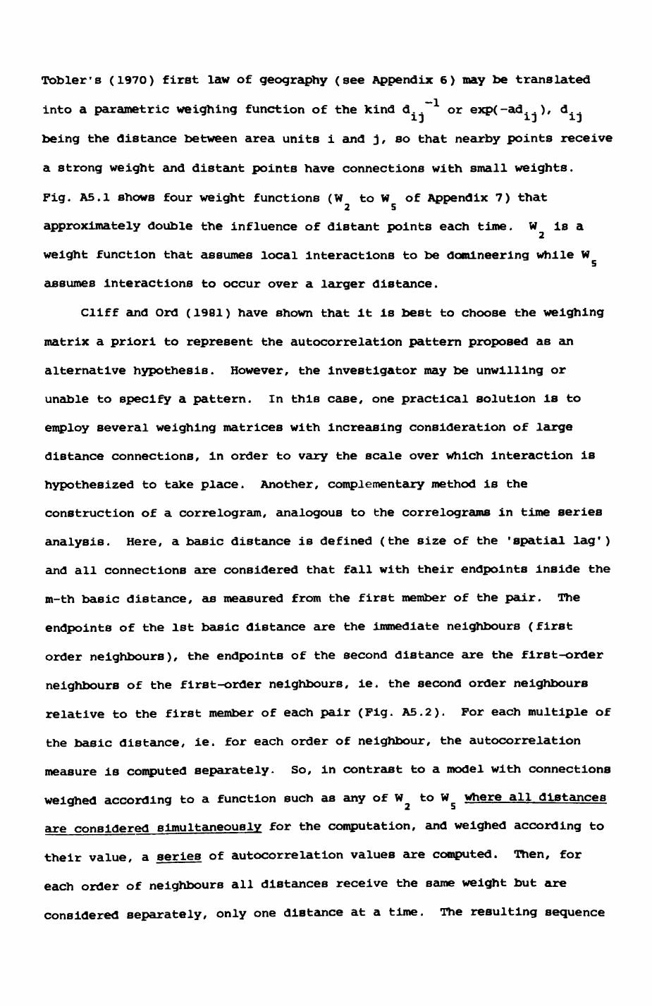
Tobler's (1970) first law of geography (see Appendix 6) may be translated
into a parametric weighing function of the kind d..-1 or exp(-ad..), d..
being the distance between area units i and j, so that nearby points receive
a strong weight and distant points have connections with small weights.
Pig. A5.1 shows four weight functions (W to W of Appendix 7) that
approximately double the influence of distant points each time. W is a2
weight function that assumes local Interactions to be domineering while W
assumes interactions to occur over a larger distance.
Cliff and Ord (1981) have shown that it is best to choose the weighing
matrix a priori to represent the autocorrelation pattern proposed as an
alternative hypothesis. However, the investigator may be unwilling or
unable to specify a pattern. In this case, one practical solution is to
employ several weighing matrices with increasing consideration of large
distance connections, in order to vary the scale over which interaction is
hypothesized to take place. Another, complementary method is the
construction of a correlogram, analogous to the correlograms in time series
analysis. Here, a basic distance is defined (the size of the 'spatial lag')
and all connections are considered that fall with their endpoints inside the
m-th basic distance, as measured from the first member of the pair. The
endpoints of the 1st basic distance are the immediate neighbours (first
order neighbours), the endpoints of the second distance are the first-order
neighbours of the first-order neighbours, le. the second order neighbours
relative to the first member of each pair (Pig. A5.2). For each multiple of
the basic distance, ie. for each order of neighbour, the autocorrelation
measure is computed separately. So, in contrast to a model with connections
weighed according to a function such as any of W to W where all distances
are considered simultaneously for the computation, and weighed according to
their value, a series of autocorrelation values are computed. Then, for
each order of neighbours all distances receive the same weight but are
considered separately, only one distance at a time. The resulting sequence

Fig. A5.1. Shape of weighting functions 2 to 5 used in the fitting of spatial models to radio-tracking data. Wi weight, scaled between 0 and 1, for a given pair
of cells, as a function of Lt distance, le. the spatial lag, in cell size units.
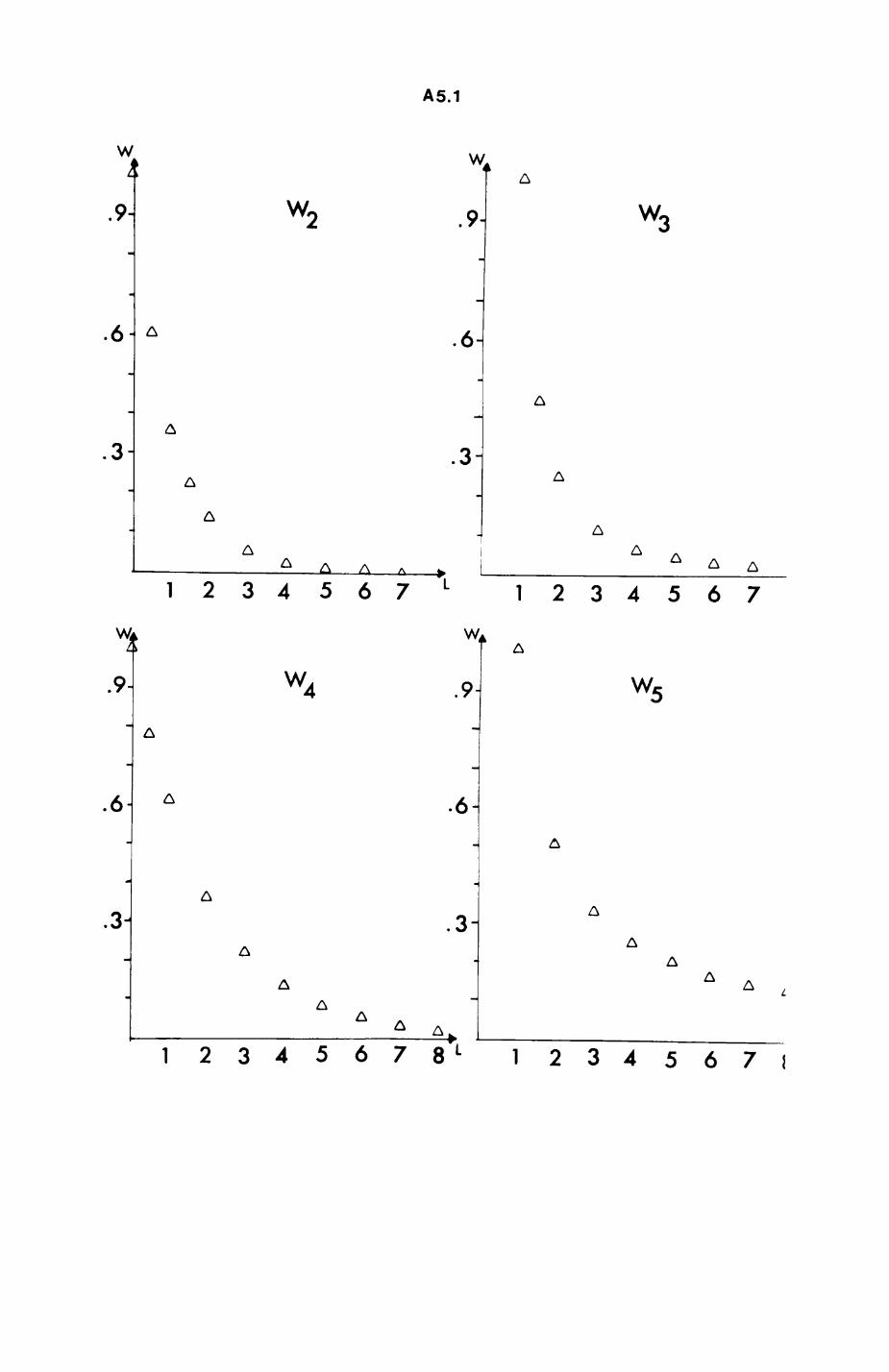
A5.1
W
,9- W,
W
.9-
6- .6-
3- .3-
A A
1234567 1 234567WA
.9-
w
9-
6- 6-
,3- .3- A
12345678 1 1234567J
Pig. AS.2. Definition of spatial lags and Illustration of spatial autocorrelation functions.
a. Definition of spatial lag.cell indexed 1ji cell in question, in the i-th
column and the j-th row. other indexed cellst some of the first order
neighbours of cell ij.
b. Autocorrelation functions are plotted as spatial autocorrelation coefficients versus the spatial lag.
AF represents a function decaying only slowly wi£h increasing lags, ie. similarity of use of cells at higher lags in comparison with the cell in question is on average high.
AF represents a function decaying quickly with increasing lags, le. similarity of use of cells at higher lags in comparison with the cell in question is on average low.
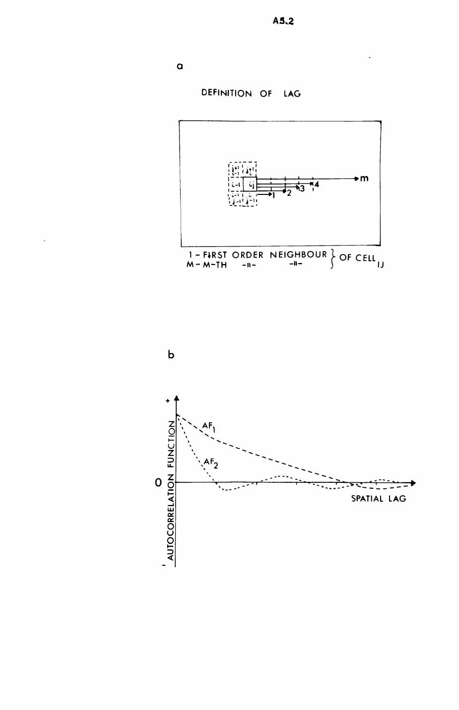
AS.2
DEFINITION OF LAG
•k* ™
1 - FIRST ORDER NEIGHBOUR I OF CEU M-M-TH -n- -"- J IJ
ZoI—uZ
\ x s AF,
AF,
Q£ QiOUO
SPATIAL LAG
of autocorrelation values is called an autocorrelation function and is
usually plotted against the order of the spatial lags (Pig. A5.2). The
slope of the autocorrelation function curve indicates on which scale (at
which distance levels) the spatial process under question operates. Steep
declining slopes at low lags (ie. looking at the neighbours nearby) indicate
that spatial interactions are very locally restricted and that influence
fades quickly away, while a shallow slope at low lags Indicate a well
expressed local interaction that fades away only slowly over larger
distances.
Thus, a correlogram can indicate to us some properties, e.g. the scale,
of the spatial process under consideration. It does not replace a proper
model of spatial autocorrelation, since it does not specify parameters of
the model, but it gives a hint which class of models may perform better and
which do not.
Since this is the first telemetric study to employ spatial
autocorrelation, I used both methods (correlogram and different weighing
matrices) to establish a picture of spatial dependence of animal locations.
AS. 4. Measures of spatial autocorrelation
Several measures of autocorrelation have been proposed (see Cliff & Ord
1981). Of these, two indices, Koran's I and Geary's contiguity ratio c are
the most appropriate for the analysis of telemetric datat they permit the
weighing of distances or other measures of connection between two area units
and they have been shown to be far superior to other measures (see Chapter 6
of Cliff & Ord 1981). Computation procedures are Illustrated for both in
Appendix 7.
Although particularly Koran's I bears some resemblance to normal
correlation coefficients, it is worth pointing out that the two measures
depart from 'normal' correlation coefficients in several aspects. In
Koran's I the expected value is not 0 (as for a normal correlation
coefficient) but changes with sample size, and always lies below zero, if
only slightly for large samples sizes, while the expected value of Geary's c
is 1. Although Koran's I ranges approximately from -1 (perfect negative
autocorrelation to 41 (positive autocorrelation), extreme cases are
conceivable where these values may not be reached or even surpassed. In the
case oL Geary's c, perLed positive autocorrelation is at a value of 0 while
there is no definite limit for negative autocorrelation (for details see
Cliff and Ord 1981). These deviations from the pattern of normal
correlation coefficients can also mean that the level of significance may
decrease to values as low as 0.1 (for Koran's I) which is not directly
comparable to a value of 0.1 of, say, Pearson's coefficient. Tests of
significance for both measures are described in Appendix 7 as well. While
for Koran's I the test is usually applied in its two-tailed version, Geary's
c can be tested only for positive autocorrelation.
The two measures are sensitive to slightly different behaviours of the
data (Jumars et al 1977). Koran's I is most sensitive to large deviations
from the mean (x -x) weighed strongly, while c is most sensitive to the
difference (x -x ) independent from the overall mean. In other words, I is
most sensitive to a proximity of extreme x values, while c is most
sensitive to a proximity of similar or dissimilar x values, independent
from their departure from the overall mean, x.
APPENDIX 6. A sequence of citations from the geographical and
anthropological literature on the importance of
spatially related data.
(1) Francis Galton (1889) remarked on a paper by Tylor on the historical
links between societies through migration and cultural dlffusioni
It was extremely desirable for the sake of those who may wish to study
the evidence for Mr. Tylor's conclusions, that full information should be
given as to the degree in which the customs of the tribes and races which
are compared together are independent. It might be, that some of the tribes
had derived them from a common source, so that they were duplicate copies of
the same original. Certainly, in such an investigation as this, each of the
observations ought, in the language of statisticians, to be carefully
'weighted*.
(2) W.R. Tobler (1970) defined the 'first law of geography'!
Everything is related to everything else, but near things are more
related than distant things.
(3) P.R. Gould (1970) discussed the Interest geographers should show for
spatially related datai
Why we should expect Independence in spatial observations which are of
the slightest intellectual interest or importance in geographic research I
cannot imagine. All our efforts to understand spatial pattern structure and
process have indicated that it is precisely the lack of independence - the
interdependence - of spatial phenomena that allows us to substitute pattern,
and therefore predictability and order, for chaos and apparent lack of
interdependence - of things in space and time.
(4) P.P. Stephan (1934) discussed the nature of geographic datai
Data of geographic units are tied together like bunches of grapes not
separate like balls In an urn.
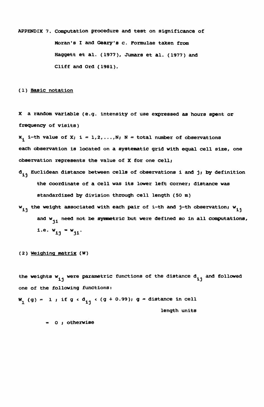
APPENDIX 7. computation procedure and test on significance of
Koran's I and Geary's c. Formulae taken from
Haggett et al. (1977), JUmars et al. (1977) and
Cliff and Ord (1981).
(1) Basic notation
X a random variable (e.g. intensity of use expressed as hours spent or
frequency of visits)
x i-th value of X; i = 1,2,...,N; N = total number of observations
each observation is located on a systematic grid with equal cell size, one
observation represents the value of X for one cell;
d Euclidean distance between cells of observations i and j; by definition
the coordinate of a cell was its lower left corner/ distance was
standardized by division through cell length (50 m)
w the weight associated with each pair of i-th and j-th observation; w
and w need not be symmetric but were defined so in all computations,
i » C « * <4 ™* H < *
(2) Weighing matrix (W)
the weights w were parametric functions of the distance d and followed
one of the following functions!
W (g) = 1 i i£ g < d < (g + 0.99); g = distance in cell
length units
= O ; otherwise
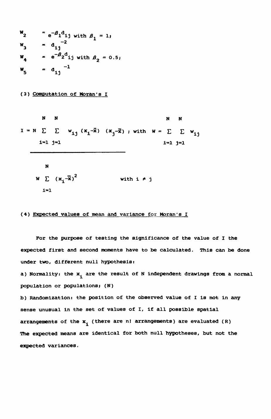
W2 e~*idij with
e~*2dij with B2 = 0.5;
W5
(3) Computation of Koran's I
N N N N
I - N E E w± (x±-x) (x -x) ; with W = E I
N
W E (xx)2 with i
(4) Expected values of mean and variance for Moran's I
For the purpose of testing the significance of the value of I the
expected first and second moments have to be calculated. This can be done
under two, different null hypothesisi
a) Normality! the x are the result of N independent drawings from a normal
population or populations; (N)
b) Randomization! the position of the observed value of I is not in any
sense unusual in the set of values of I, if all possible spatial
arrangements of the x. (there are nl arrangements) are evaluated (R)
The expected means are identical for both null hypotheses, but not the
expected variances.
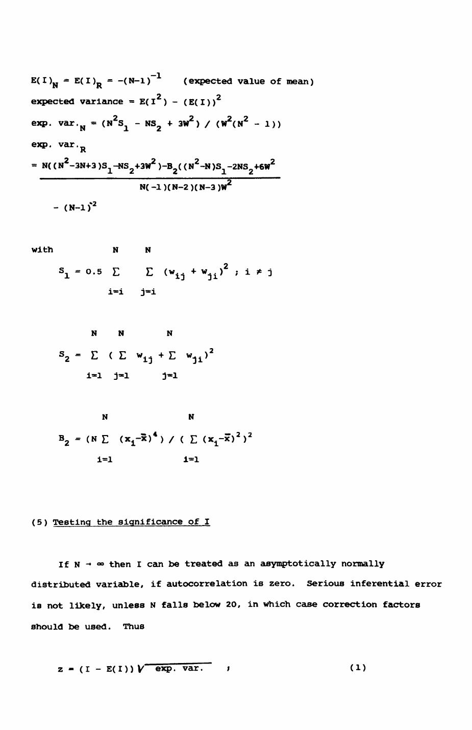
E( I )N = E( I )R = -( N-l ) ( expected value of mean )
expected variance = E(I2 ) - (E(I))2
exp. var. N = (N^ - NS2 + 3W2 ) / (W2(N2 - 1))
exp. var. R
= N( ( N2-3N+3 )S-NS-I-3W2 )-B< ( N2-N
N(-1)(N-2)(N-3)W2
with N
S! - 0-5 E
N
E 0'« + wn )2 ;
N N N
S2 - E ( E wi:J + E w.Ji ) 2
i-i j-1 3-1
N N
B2 - <N E (X^x) 4 ) / ( E (X±-X) 2 ) 2
i=l 1=1
(5) Testing the Biqnificance of I
If N -. oo then I can be treated as an asymptotically normally
distributed variable, if autocorrelation is zero. Serious inferential error
is not llXely, unless N falls below 20, in which case correction factors
should be used. Thus
2 - (I - E(I)) V exp. var. i (1)
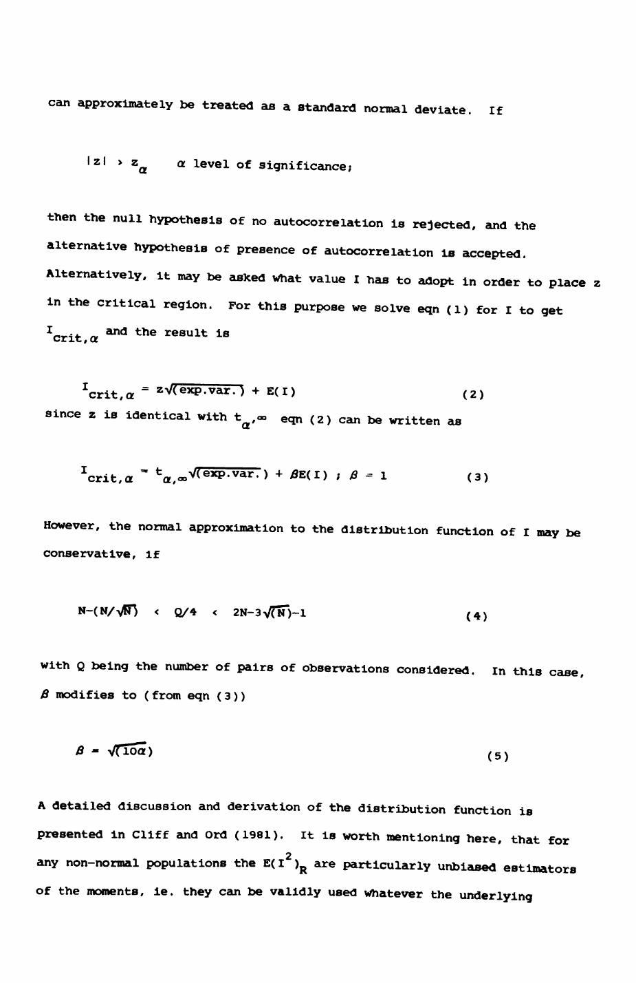
can approximately be treated as a standard normal deviate. If
Izl > z a. level of significance;
then the null hypothesis of no autocorrelation is rejected, and the alternative hypothesis of presence of autocorrelation is accepted. Alternatively, it may be asked what value I has to adopt in order to place z in the critical region. For this purpose we solve eqn (1) for I to getI .. and the result is crit, a
Zcrit,a = zV(exp.var. ) + E(I) (2) since z is identical with t ,« eqn (2) can be written as
fca..V(exp.var.) + *E(I) , * - 1 (3)
However, the normal approximation to the distribution function of I may be conservat ive , 1 f
Q/4 < 2N-3N)-1 (4)
with Q being the number of pairs of observations considered. In this case,
B modifies to (from eqn (3))
0 - VTloa) (5)
A detailed discussion and derivation of the distribution function ispresented in Cliff and Ord (1981). It is worth mentioning here, that for
2 any non-normal populations the E(I )R are particularly unbiased estimatorsof the moments, ie. they can be validly used whatever the underlying
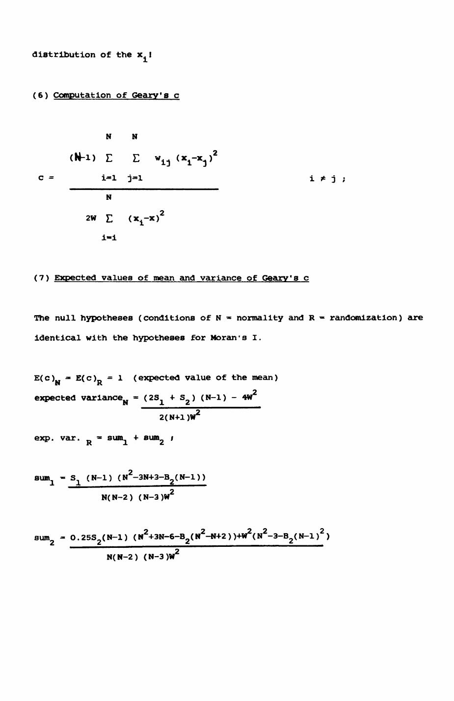
distribution of the x I
(6) Computation of Geary'a c
N N
E E w±j (x^x.j)2
i-l 3=1 i * j ;
N
2W E (X±-X)2
i-i
(7) Expected values of mean and variance of Gearv's c
The null hypotheses (conditions of N * normality and R - randomization) are
identical with the hypotheses for Noran•s I.
E(c)._ - E(c)_ = 1 (expected value of the mean)N K.
expected variance = (25 4- s ) (N-l) - 4W2
2(N4-l)W2
exp. var. = sum + sum i
sum - S (N-l) (N2-3N+3-B2(N-l))
N(N-2) (N-3 )W2
0.25S2(N-1)
N(N-2) (N-3)W2

(8) Testing the significance of c
Principles and conditions for conservativity of the normal approximation are
identical with Koran's I (see above). The equation for the critical c Is
Ccrit,« = X ~ ta/ «vexp.var. + ^(N-l) (D
& - 1; for the normal approximation
B - VlOd ; if the conservativety criterium is valid
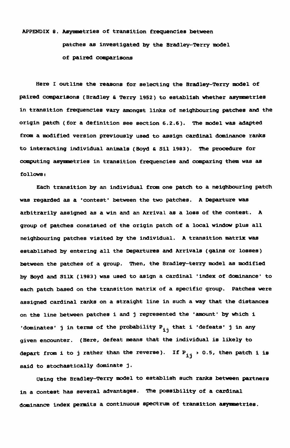
APPENDIX 8. Asymmetries of transition frequencies between
patches as investigated by the Bradley-Terry model
of paired comparisons
Here I outline the reasons for selecting the Bradley-Terry model of
paired comparisons (Bradley & Terry 1952) to establish whether asymmetries
in transition frequencies vary amongst links of neighbouring patches and the
origin patch (for a definition see section 6.2.6). The model was adapted
from a modified version previously used to assign cardinal dominance ranks
to interacting individual animals (Boyd & Sil 1983). The procedure for
computing asymmetries in transition frequencies and comparing them was as
follows t
Each transition by an individual from one patch to a neighbouring patch
was regarded as a 'contest' between the two patches. A Departure was
arbitrarily assigned as a win and an Arrival as a loss of the contest. A
group of patches consisted of the origin patch of a local window plus all
neighbouring patches visited by the individual. A transition matrix was
established by entering all the Departures and Arrivals (gains or losses)
between the patches of a group. Then, the Bradley-terry model as modified
by Boyd and SiUc (1983) was used to asign a cardinal 'index of dominance' to
each patch based on the transition matrix of a specific group. Patches were
assigned cardinal ranks on a straight line in such a way that the distances
on the line between patches i and j represented the 'amount' by which i
'dominates' j in terms of the probability P.. that i 'defeats' j in any
given encounter. (Here, defeat means that the individual is likely to
depart from i to j rather than the reverse). If P > 0.5, then patch i is
said to stochastically dominate j.
Using the Bradley-Terry model to establish such ranks between partners
in a contest has several advantages. The possibility of a cardinal
dominance index permits a continuous spectrum of transition asymmetries.
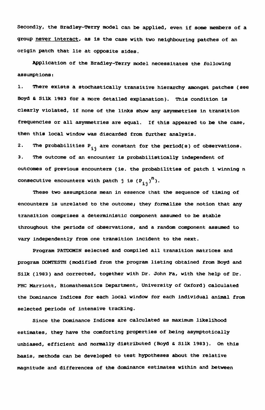
Secondly, the Bradley-Terry model can be applied, even if some members of a
group never interact, as is the case with two neighbouring patches of an
origin patch that lie at opposite sides.
Application of the Bradley-Terry model necessitates the following
assumptionsi
1. There exists a stochastically transitive hierarchy amongst patches (see
Boyd & Silk 1983 for a more detailed explanation). This condition is
clearly violated, if none of the links show any asymmetries in transition
frequencies or all asymmetries are equal. If this appeared to be the case,
then this local window was discarded from further analysis.
2. The probabilities P.. are constant for the period(s) of observations.
3. The outcome of an encounter is probabilistically independent of
outcomes of previous encounters (ie. the probabilities of patch i winning n
consecutive encounters with patch j is (P..)n ).
These two assumptions mean in essence that the sequence of timing of
encounters is unrelated to the outcome; they formalize the notion that any
transition comprises a deterministic component assumed to be stable
throughout the periods of observations, and a random component assumed to
vary independently from one transition incident to the next.
Program PATDOMIN selected and compiled all transition matrices and
program DOMTESTH (modified from the program listing obtained from Boyd and
Silk (1983) and corrected, together with Dr. John Fa, with the help of Dr.
FHC Marriott, Biomathematics Department, University of Oxford) calculated
the Dominance Indices for each local window for each individual animal from
selected periods of intensive tracking.
Since the Dominance Indices are calculated as maximum likelihood
estimates, they have the comforting properties of being asymptotically
unbiased, efficient and normally distributed (Boyd & Silk 1983). On this
basis, methods can be developed to test hypotheses about the relative
magnitude and differences of the dominance estimates within and between
groups (Boyd & SilJc 1983). The null hypothesis of interest in our case
states thatt
the patches belonging to the subset S of a specific
local window have the same cardinal dominance rank) where
s is the subset of all neighbouring patches except the
origin patch.
The alternative hypothesis states that
at least two patches within the subset S have significantly different
dominance indices.
To test the null hypothesis, the generalized likelihood ratio statistic is
used which, after suitable modification, is approximately distributed as a
chi square random variable with t degrees of freedom, t being the number of
neighbouring patches per local window. A significant result would indicate
that asymmetries in transition frequencies for different transition
directions vary significantly amongst neighbouring patches. Program
DCMfTESTH was used to calculate the test statistic.

Appendix 9. Estimate of daily energy expenditure of lactating
female badgers.
Total energy = (1) Maintenance energy *
expenditure (2) Energy for hunting and searching prey +
(kcal day"1 ) (3) Energy for prey capture +
(4) Energy for copulation +
(5) Energy for lactation +
(6) Energy spent on cleaning and preparing the
sett +
(7) Energy for thermoregulation
(Powell 1982:176). Thermoregulation is probably negligible during lactation
(Powell 1982). Copulation, activities concerning the preparation of the
sett, activities related to foraging, and lactation are mutually exclusive
activities. Since female badgers do not seem to spend much time to search
for a mate and are fairly passive during copulation (see text), the energy
expenditure for copulation probably does not exceed that for hunting. Energy
spent on cleaning the sett is difficult to estimate and is provisionally
assumed similar to hunting energy per time unit. However, since this
activity is not very important, if considered over the entire period of
lactation (90 days), the error is probably not very important. Since the
main item of the badger diet in Wytham is earthworms (Chapter 4), energy
spent on capturing prey should be similar to energy spent on searching for
and detecting prey ("hunting"). Thus, hunting energy, energy for prey
capture, energy for copulation and energy spent on activities concerning the
sett are assumed equal per time unit and summarized as "Activity Energy".
The modified equation is them
total energy - (1) Maintenance Energy during sleep and rest +
expenditure (2) Activity Energy during active periods +
(3) Lactation Energy
Aft.l Maintenance Energy during sleeping and rest
This is assumed to be equivalent to the energy expenditure known as Basal
Metabolic Rate (BMR).
BMR (ml O2 g"1 hr"1 ) = 0.3 (for Taxidea taxus, the
American badger, Harlow, 1981)
Assuming that the European badger has a very similar BMR, this correpsonds
to 34.56 kcal kg" day" . using Hayssen & Lacy's (1985) empirical
relationship of body weight and BMR for Carnivores (exp 0.738) and their
conversion factors, we get the characteristic equation_1 *73fl
BMR (kcal day ) - 61.459 W (1)
The average body weight of female badgers caught in early autumn (ie. at a
time when they show a similar body weight as during the period of lactation)
is 8.5 kg. This gives
298.19 kcal day"1
Using Weal's (1977i142) data, badgers are active on average for
10 hours at February, 1st set as Day 1 of lactation
9.5 " " March, 2nd " " " 30 "
9 " " April, 1st " " " 60 "
8 " " May, 1st " " " 9O "
The remainder is spent as rest or sleep. From this the energy spent during
sleep can be calculated. Maintenance Energy is then
(hours of rest/24) * 298.19 kcal day"1 .
AA. 2 Activity Energy
Energy spent during the active period can be expressed as specific metabolic
rate (SNR) while running (Powell 1982, Peters 1983). This is linearly
dependent on running speed. From Peters ( 1983 1 81) we obtain i
SMR = specific basal metabolism (BMR) * postural
(kcal correction + net transport costsT>
day ) =73.75 W 4 196.55 W V
with W body weight (kg), V running speed (m min" ),
using the BMR from eqn (1) times 1.2, the postural
correction ( Peters ( 1983 ) )
Using 8.5 kg as the average body weight for a female badger in Wytham, we
obtain
SMR (kcal day"1 ) = 357.83 4 15.294 V
Using 1O.74 m min~ as the average running speed from a typical night of
PEACEFUL, we get
522. O87 kcal day"1
Lactation energy
From Moors (1974)
lactation - (litter size * (kit growth energy + kit maintenance
energy energy)) / (lactation efficiency * milk assimilation
efficiency)
Litter size is set as 2.43, the average litter size from several published
studies (Anderson & Trewhalla 1985). From Powell (1982)
kit growth - kit growth rate (g day ) * energy content per
energy unit weight (kcal g~ )
(kcal day"1 )
Kit growth rate is difficult to determine. Peters (1983) suggests to use
Case's (1978) empirically determined relationship of the growth rate for the
time when the kit grows from 10 % to about 90 % of adult body weight
G10-90 < watts > = °- 445 w
which yields for an adult badger of 8.5 kg body weight 2.0775 Watts or
O.O4 kg day" (1 kg wet mass equals 7 * 106 Joules,
Peters (1983))
or 40 g day
Successive weightings of two young badgers reared in a Polish zoo yields
an average linearized growth rate of 30 g day" (data from Gucwinska &
Gucwinski 1968) and a rate of 39 g day" for later stages of development,
for a reported adult weight of 9 kg which is fairly close to the value
Case's. The average linearized growth rate for several badgers reared in
captivity by Frank (194O) is ca 56 g day" . For a reported mean adult body
weight 12.5 kg as again closely to the by Case's eqn predicted growth rate
of 53 g day" , i the rate 30 g day" from the Polish zoo study as 'normal*
Investment and the (predicted) rate of 40 g day as 'heavy' investment.
According to Powell (1982)
energy content per unit weight = 1.647 kcal g
so that
kit growth energy (rate 1) = 49.41 kcal day"
(rate 2) - 65.88 kcal day"1
Following again Powell (1982)
kit maintenance - K * (birth weight + (kit age * kit-1 B energy (kcal day growth rate))
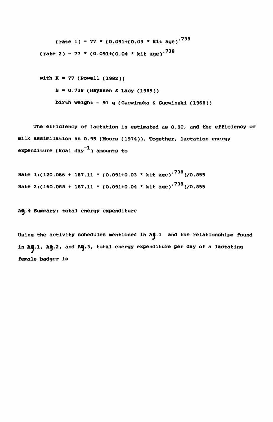
73S(rate 1) = 77 * (O.091+(0.03 * kit age)700
(rate 2) = 77 * (0.09l+(0.04 * kit age)
with K = 77 (Powell (1982))
B = O.738 (Hayssen & Lacy (1985))
birth weight = 91 g (Gucwinska & Gucwinski (1968))
The efficiency of lactation is estimated as 0.9O, and the efficiency of
milk assimilation as 0.95 (Moors (1974)). Together, lactation energy
expenditure (kcal day" ) amounts to
738 Rate It(120.066 + 187.11 * (0.091+0.03 * kit age) )/O.855
73flRate 2»(160.088 •*- 187.11 * (0.091+0.04 * kit age) )/o.855
Summary! total energy expenditure
Using the activity schedules mentioned in Afl.l and the relationships found
in Att.l, Ag.2, and A^.3, total energy expenditure per day of a lactatlng
female badger is
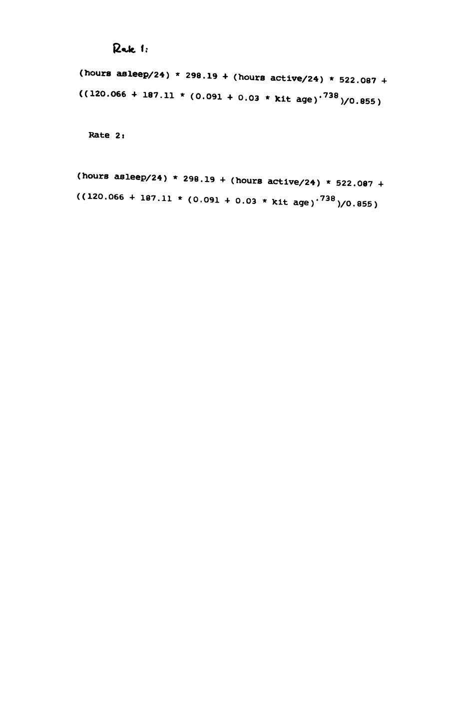
<:
(hours asleep/24) * 298.19 + (hours active/24) * 522.087 -f ((120.066 -I- 187.11 * (0.091 4 0.03 * kit age ) * 738 )/0.855 )
Rate 2i
(hours asleep/24) * 298.19 + (hours active/24) * 522.087 -I-•700 ((120.066 -I- 187.11 * (0.091 4 0.03 * kit age) )/0.855)

REFERENCES
Ahnlund H 1980. Sexual maturity and breeding season of thebadger. Melee melee in Sweden. J Zool Lond 190, 77-95.
Alatalo RV 1981. Problems in the measurement of evenness In ecology. Olkos 37, 199-204.
Alien SE 1974. Chemical analyses of ecological materials. Blackwell Sclent Publ, Oxford.
Amlaner CJ Macdonald DW 1980. A handbook on biotelemetry and radiotracking. Pergamon Press, Oxford, 8O4 pp.
Andersen C 1980. The influence of farmyard manure and slurry on the earthworm population (Lumbricidae) in arable soil. Proc VII Internat Soil Zool Colloquium ISSS, 325-335.
Andersen J 1954. The food of the Danish badger (Meles meles danica) with special reference to the summer months. Dan Rev Game Biol 3, 1-52.
Anderson AJB 1971. Ordination methods in ecology. J Ecol 59, 713-726.
Anderson OJ 1982. The home rangei a new nonparametric estimation technique. Ecology 63, 103-112.
Anderson RM Trewhella W 1985. Population dynamics of the badger (Meles meles) and the epidemiology of bovine tuber culosis (Mycobacterlum bovis). Phllos Trans Roy Soc Lond B 310, 327-382.
Anderson SH Shugart HH 1974. Habitat selection of breedingbirds in an east Tennessee deciduous forest. Ecology 55,828-837.
Andrewartha HG 1970. Introduction to the study of animal popula tions. Chapman & Hall, London, Zed.
Andrewartha HG Browning TO 1961. An analysis of the idea of •resources' in animal ecology. J Theor Biol 1, 83-97.
Armstrong P Park GN Molloy BPJ 1981. Towards a national classi fication of New Zealand vegetation and landforms. New Zeal J Ecol 4, 129-130.
Aumann GO 1965. Microtine abundance and soil sodium levels. J Mammal 46, 594-6O4.
Axelrod R 1984. The evolution of cooperation. Basic Books, New York, 241 pp.
Axelrod R Hamilton WD 1981. The evolution of cooperation. Science 211, 1390-1396.
Baker RR 1978. The evolutionary ecology of animal migration. Hooder & Stoughton, London, 1012 pp.
Baldwin PM 1917. Diurnal activity of the earthworm. J Anim Behav 7, 187-190.
Beauchamp GK 1976. Diet influences attractiveness of urine in guinea pigs. Nature 263, 587-588.
Beck CC 1976. Vetalar (ketamine hydrochloride). A unique cata- leptoid anesthetic agent for multispecies usage. J Zoo Anim Med 7, 11-38.
Bekoff M Daniels TJ Gittleman JL 1984. Life history patterns and the comparative social ecology of carnivores. Ann Rev ECOl Syst 15, 191-232.
Berger WH Parker PL 1970. Diversity of planktonic Foraminifera in deep sea sediments. Science 168, 1345-1347.
Bertram BCR 1975. Social factors influencing reproduction in wild lions. J Zool Lond 177, 463-482.
Bhattacharyya H 1981. Theory and methods of factor analysis and principal components. In : Capen 1981, pp 72-79.
Bivand R 1980. A Monte Carlo study of correlation coefficient estimation with spatially autocorrelated observations. Quaest Geogr
Bocock KL Adamson JK 1982. Soil temperature in a deciduous wood land in north-west England. Merlewood R & D Paper 87, 23 pp.
Bocock KL Jeffers JNR Lindley DK Adamson JK Gill CA 1977. Esti mating woodland soil temperature from air temperature and other climatic variables. Agricult Meteor 18, 351- 372.
Boyd R Silk JB 1983. A method for assigning cardinal dominance ranks. Anim Behav 31, 45-58.
Bradbury JW vehrencamp SL 1976. Social organisation and foraging in emballonurid bats. I-t-II. Behav Ecol Sociobiol 1, 337-4O4.
Bradley RA Terry ME 1952. Rank analysis of incomplete block designs. I. The method of paired comnparisons. Biometrika 39, 324-335.
Bray JR Curtis JT 1957. An ordination of the upland forest com munities of southern Wisconsin. Ecol Monogr 27, 325-349.
Brown BR Love CW Handley WRC 1963. Protein-fixing constituents of plants. Rep For Res Lond III, 9O-93.
Brown DE 1980. A system for classifying cultivated and cultured lands within a systematic classification of natural eco systems. J Ariz Nev Acad Scl 15, 2, 48-53.
Brown JL 1964. The evolution of diversity in avian territorial
systems. Wilson Bull 76, 160-169.
Brown RE Macdonald DW 1985. Social odours in mammals. Oxford UP, Oxford, 2 vols, 882 pp.
Bunce RGH Shaw MA 1973. A standardized procedure for ecological survey. J Environm Mgmt l, 239-258.
Burnham KP Anderson DR Laake JL 1980. Estimation of density from line transect sampling of biological populations. Wildl Monogr 72, 202 pp.
Burt WH 1943. Territoriality and home-range concepts as applied to mammals. J Mammal 24, 346-352.
Capen DE (ed) 1981. The use of multivariate statistics instudies of wildlife habitats. CJniv Vermont Publ & USDA For Serv Gen Techn Rep RM-87, 249 pp.
Carr CM Macdonald DW in press. The sociality of solitary fora gers t a model based on resource dispersion. Anim Behav
Case TJ 1978. On the evolution and adaptive significance ofpostnatal growth rates in the terrestrial vertebrates. Quart Rev Biol 53, 243-282.
Caughley G 1977. Analysis of vertebrate populations. John Wlley, New York, 234 pp.
Charnov EL 1976. Optimal foraging: the marginal value theorem. Theor Pop Biol 9, 129-136.
Cheeseman CL Little TWA Mallinson PJ Page RJC Wile smith JWPritchard DG 1985. Population ecology and prevalence of tuberculosis in badgers in an area of Staffordshire. Mammal Rev 15, 125-135.
Cheeseman CL Mallinson PJ 1980. Radiotracking in the study ofbovine tuberculosis in badgers. In: Amlaner & Macdonald1980, pp 649-656.
Chitty D Pimentel D Krebs CJ 1968. Food supply of overwintered voles. J Anim Ecol 37, 113-120.
Clapman AR Tutin TG Warburg EF 1978. Excursion flora of theBritish Isles. Cambridge UP, Cambridge, 2nd ed, 586 pp.
Cliff AD Ord JK 1973. Spatial autocorrelation. Pion, London, 175 pp.
Cliff AD Ord JK 1975. The comparison of means when samples consist of spatially autocorrelated observations. Environm & Plan 7A, 725-734.
Cliff AD & Ord JK 1981. Spatial processes. Models and appli cations. Plon, London, 266 pp.
Clutton-BrocX TH Guinness FE Albon SD 1982. Red Deer. The ecology of two sexes. Chicago UP, Chicago, 348 pp.
Clutton-Broc)c TH Harvey PH 1977. Primate ecology and social organisation. J Zool Lond 183, 1-39.
Cochran WG 1977. Sampling techniques. John Wiley, New York, 3rd ed f 428 pp.
Cody ML 1968. On methods of resource division in grassland bird communities. Am Nat 102, 107-147.
Colgan PW Smith JT 1978. Multidimensional contingency table analysis. In: PW Colgan (ed) - Quantitative ethology. John Wiley, New York, 145-174.
Colwell RK Futuyma DJ 1971. On the measurement of niche breadth and overlap. Ecology 52, 567-576.
Conover WJ 1980. Practical nonparametric statistics. John Wiley, New York, 2nd ed., 493 pp.
Corbet GB Southern HN 1977. The handbook of British mammals. Blackwell Sclent Publ, Oxford, 520 pp.
Cralghead F 1979. On the track of the grizzly. Sierra Club Books, San Francisco.
Crook JH 1964. The evolution of social organisation and visual communication in weaver birds (Ploceinae). Behaviour, Suppl 10.
Crowell KL Pimm SL 1976. Competition and niche shifts of mice introduced onto islands. Olkos 27, 251-258.
Cuendet G 1983. Predation on earthworms by the black-headed gull (Larus ridlbundus). In: JE Satchell (ed) - Earthworm ecology. Chapman & Hall, London, 415-424.
Cuendet G 1984. A comparative study of the earthworm populations of four different woodland types in Wytham Woods, Oxford. Pedobiol 26, 421-439.
Davies NB 1961. calling as an ownership convention on pied wag tail territories. Anim Behav 29, 529-534.
Davies NB Houston AJ 1981. Owners and satellites: the economics of territory defence in the pied wagtail, Motacllla alba. J Anlm Ecol 50, 157-180.
Dawklns HC 1952. Expereiments with low percentage enumerations in tropical high forest. Emp For Rev 31, 131-145.
Dawkins HC Field DRB 1977. A long-term surveillance system for British woodland vegetation. NERC Project Report, Dept of Forestry, Oxford, 124 pp.
Dawkina HC Field DRB 1978. A long-term surveillance system forBritish woodland vegetation. Occ Pap Dep For Commonw For Inst For Oxf No. 1, 1O6 pp.
Day MG 1966. identification of hair and feather remains in the gut and faeces of stoats and weasels. J Zool Lond 148, 201-217.
Oeat 1980. The automatic/ continuous and fixed radiotracking system of the Chize Forest: theoretical and practical analysis. In Amlaner & Macdonald 1980, 439- 451.
Debrot S Pivaz G Mermod C Weber JM 1982. Atlas des polls de Mammiferes d'Europe. Ed Inst Zool, Univ. Neufchatel, 208 pp.
DeXker D 1983. Denning and foraging of red fox, VUlpes vul- pes, and their interaction with coyotes, Canls la- trans. in central Alberta, 1972-1981.
Delibes M Hidalgo F 1981. The rabbit as prey in the Iberian Mediterranean ecosystem. Proc World Lagom Conf, Univ Guelph, 614-622.
Dlckman CR Doncaster CP 1984. Responses of small mammals to red fox (Vulpes vulpes). J Zool Lond 204, 521-531.
Dixon KR Chapman JA 1980. Harmonic mean measure of animal activity. Ecology 61, 104O-1044.
Doncaster CP 1985. The spatial organisation of Urban foxes (VUlpes vulpes) in Oxford. DPhil thesis, Oxford, 2 vols, 497 pp.
Dundee RT Pils CM 1973. Mortality of radio-tagged pheasants onthe Waterloo wildlife area. Wisconsin Dept Nat Res Techn Bull 72, 52 pp.
Dunn JE Gipson PS 1977. Analysis of radio telemetry data in studies of home range. Biometrics 33, 85-101.
Duplaix N 1980. Observations on the ecology and behaviour of the giant river otter Pteronura brasiliensis in Suriname. Terre et Vie 34, 495-620.
Edwards CA Lofty JR 1977. Biology of earthworms. Chapman & Hall, London, 2nd ed, 283 pp.
Edwards CA Lofty JR 1982a. The effect of direct drilling and minimal cultivation on earthworm populations. J appl ECOl 19, 723-734
Edwards CA Lofty JR 1982b. Nitrogenous fertilizers and earthworm populations in agricultural soil. Soil Biolog Bochum 14, 515-521.
Elton CS 1927. Animal Ecology. Chapman & Hall, London, 207 pp.
Elton CS 1966 The pattern of animal communities. Chapmann & Hall, London, 430 pp.
Elton CS Miller RS 1954. The ecological survey of animal commu-
nities: with a practical system of classifying habitats by structural characterisitcs. J Ecol 42, 46O-496 .
Engen S stenseth NC 1984a. An ecological paradox: a food type may become more rare in the diet as a consequence of being more abundant. Am Nat 124, 352-359
Engen S Stenseth NC I984b. A general version of optimal foraging theory: the effect of simultaneous encounters. Theor Pop Biol.
ErJcinaro E 1961. The seasonal change of activity of Microtus agrestis. Oikos 12, 157-163.
Evans DM 1973. Seasonal variations in the body composition and nutrition of the vole Microtus aqrestis. J Anim Ecol 42, 1-18.
Evans DM 1977. The field vole, Microtus aqreals, ini Corbet & Southern 1977, pp 185-193.
Flowerdew JR 1972. The effect of supplementing food on a popula tion of wood mice (Apodemus sylvaticus). J Anim Ecol 41, 553-566.
Flowerdew JR 1977a. The bank vole, Clethrionomvs qlareolus. In: Corbet & Southern 1977, pp 173-184.
Flowerdew JR 1977b. The wood mouse, Apodemus sylvaticus. In: Corbet & Southern 1977, pp 206-217.
Ford RG Krumme DW 1979. The analysis of space use patterns. J Theor Biol 76, 125-155.
Ford RG Myers JP 1981. An evaluation and comparison of tech niques for estimating home range and territory size. Studies Avian Biol 6, 461-465.
Frame LH Malcolm JR Frame GW van Lawick H 1979. Social organi sation of African wild dogs (Lycaon pictus) on the Serengeti Plains, Tanzania, 1967-1978. Z Tierpsychol 50, 225-249.
Frank HR 194O. Die Biologie des Dachs. Z Jagdk 2, 1-25.
Frey DP Pimentel RA 1978. Principal component analysis and factor analysis. In: PW Colgan (ed) - Quantitative ethology. John Wiley, New York, 219-245.
Fuller RM (ed) 1983. Ecological mapping from ground, air and space. NERC/ITE Symp 10, Monks Wood, 142 pp.
Gabriel KR Sokal RR 1969. A new statistical approach to geo graphic variation analysis. Syst Zool 18, 259-270.
Galton F 1889. Comments. J Roy Anthrop Inst Great Brit Irel 18, 245-272.
Carson PJ 1981. Social organisation and reproduction In the
rabbits a review. Proc World Lagom Conf Uhiv Guelph, 256-270.
Gaston AJ 1978. The evolution of group territorial behaviour and cooperative breeding. Am Nat 112, 1091-1100.
Gates JM Hale JB 1974. Seasonal movement, winter habitat use,and population distribution of an east central Wisconsin pheasant population. Wisconsin Dept Nat Res Techn Bull 76, 55 pp.
Gauch HG 1982a. Multivariate analysis in community ecology. Cambridge UP, Cambridge, 320 pp.
Gauch HG 1982b. Noise reduction by eigenvector ordinations. Ecology 63, 1643-1649.
Gauch HG Chase GB Whittaker RH 1974. Ordination of vegetation samples by Gaussian species distributions. Ecology 55, 1382-1390.
Gauch HG Whittaker RH Wentworth TR 1977. A comparative study ofreciprocal averaging and other ordination techniques.J ECOl 65, 157-174.
Gerard BM 1964. Lumbricidae (Annelidae). Synop Brit Fauna 6, 1-58.
Gibb JA 1981. What determines the numbers of small herbivorous animals ? New Zeal J Ecol 4, 73-77.
Gill M 1979. Foxes and pheasants. Ann Rev Game Cons 11, 42-43.
Gittleman JL Harvey PH 1982. Carnivore home-range size, meta bolic needs and ecology. Behav Ecol Sociobiol 10, 57-63.
Glutz von Blotzheim UN 1973. Phasianus colchicus Linne 1758, Fasan. Im UN Glutz von Blotzheim (ed) - Handbuch der Voegel Mitteleuropae 5. Akademische Verlagsgesellschaft, Wiesbaden, 322-37O.
Gnanadesikan R 1977. Methods for statistical data analysis of multivariate observations. John Wiley, New York.
Godfrey GK 1955. Observations on the nature of decline in num bers of two MlcrotusI populations. J Mammal 36, 209-214.
Go1ley FB Petrides GA Rauber EL Jenkins JH 1965. Food intake and assimilation by bobcats under laboratory conditions. J Wildl Mgmt 29, 442-447.
German ML Kruuk H Leitch A 1984. Social function of the sub- caudal scent gland secretion of the European badger Meles meles (Carnivorai Mustelidae). J Zool Lond 203, 549-560.
Gosling LM 1982. A reassessment of the functions of scent-mar king in territories. Z Tierpsychol 60, 89-118.
Gosling LM Petrie M 1981. Economics of social organisation. Ini CR Townsend & P Calow (eds) - Physiological ecology. Blaclcwell Scient Publ, Oxford, 315-345.
Gould PR 1970. is 'Statistix inferenns' the geographical name for a wild goose ? Econ Geogr 46, 439-448.
Gower jc 1971. A general coefficient of similarity and some of its properties. Biometrics 27, 857-871.
Grafen A Ridley M 1983. A model of mate guarding. J theor Biol 102, 549-567.
Green RH 1971. A multivariate statistical approach to the Hut- chinsonlan nichet bivalve molluscs of central Canada. Ecology 52, 543-556.
Green RH 1979. Sampling design and statistical methods for envi ronmental biologists. John Wiley, New York, 257 pp.
Grelg-Smith P 1983. Quantitative plant ecology. Blackwell Sclent Publ, Oxford, 3rd ed, 359 pp.
Griffith DA 1978. A spatially adjusted ANOVA model. Geogr Anal 1O, 296-301.
Grinnell J 1917. The niche-relationships of the California thrasher. Auk 34, 427-433.
Gucwinska H Gucwinski A 1968. A note on the development and growth of European badgers, Males meles, born at Wroclaw Zoo. Int Zoo Yearb 8, 133.
Haggett P Cliff AD Frey A 1977. Locational methods. Edward Arnold, London, 6O5 pp.
Hallett JG Pimm SL 1979. Direct estimation of competition. Am Nat 113, 593-600.
Hammerstein P 1981. The role of asymmetries in animal contests. Anim Behav 29, 193-205.
Hammerstein P Parker GA 1982. The asymmetric war of attrition. J Theor Biol 96, 647-682.
Hancock M 1980. studies on the ecology of the Eurasian badger Melea meles. Unpubl DPhll thesis, Oxford (Elton Library).
Hansson L 1971. Habitat, food and population dynamics of the field vole Microtus aqrestis in South Sweden. Viltrevy 8, 267-378.
Hansson L 1977. Spatial dynamics of field vole Microtus aqrestie in heterogeneous landscapes. Oikos 29, 539-544.
Hansson L 1978. Small mammal abundance in relation to environ mental variables in three Swedish forest phases. Stud
For Suecica 147, 40 pp.
Rarestad AS Bunnell PL 1979. Home range and body weight - a reevaluation. Ecology 60, 389-402.
Harlow HJ 1981. Torpor and other physiological adaptations of the badger (Taxidea taxus) to cold environments. Physiol Zool 54, 267-275.
Harris s 1981. The food of suburban foxes (Vulpes vulpes)with special reference to London. Mammal Rev 11, 151- 168.
Harris S 1982. Activity patterns and habitat utilization of badgers (Males meles) in suburban Bristol! a radio tracking study. Symp Zool Soc Lond 49, 3O1-323.
Harris S 1984. Ecology of urban badgers Meles melesi distri bution in Britain and habitat selection, persecution and damage in the city of Bristol. Biol Conserv 28, 349-375.
Harvey PH Mace GM 1982. Comparisons between taxa and adaptive trendst problems of methodology. Int King's College Sociobiology Group (ed) - Current problems in Sociobio- logy. Cambridge UP, Cambridge, 269-289.
Hayssen V Lacy RC 1985. Basal metabolic rates in Mammalsi taxo- nomic differences in the allometry of BMR and body mass. Comp Biochem Physiol 81A, 741-754.
Help c 1974. A new index measuring evenness. J mar biol Ass UK 54, 555-557.
Heip C Engels P 1974. Comparing species diversity and evenness indices. J mar biol Ass UK 54, 559-563.
Henry JD 1977. The use of urine marking in the scavenging beha viour of the red fox (vulpes vulpes). Behaviour 61,82-106.
Hersteinsson P Macdonald DW 1982. Some comparisons between red and arctic foxes,Vulpes vulpes and Alopex laqopua, as revealed by radio-tracking. Symp Zool Soc Lond 49, 259-289.
Hill MO I973a. Diversity and evennesst a unifying notation and its consequences. Ecology 54, 427-432.
Hill MO I973b. Reciprocal averaging! an eigenvector method of ordination. J Ecol 61, 237-249.
Hill MO 1979. DECORANA - a Fortran program for detrended corres pondence analysis and reciprocal averaging. Ecology & Systemat, Cornell Univ, Ithaca, New York 52 pp.
Hill MO Gauch HG 1980. Detrended correpsondance analysis! an improved ordination technique. Vegetatio 42, 47-58.
Hirst SM 1975. Ungulate-habitat relationships in a south African
woodland/savannah ecosystem. Wildl Monogr 44, 1-60.
Hough NG 1980. The ranging behaviour of a maturing female red fox, Vulpes vulpes. In: Amlaner & Kascdonald 1983, pp 691-696.
Houston AI McNamarra JM 1984. Imperfectly optimal animals. A correction. Behav Ecol Sociobiol 15, 61-64.
Howard P 1981. Statistical considerations in island and habitat classification. Merlewood R & D Paper, ITE.
Huebertz H 1978. A general study of the summer diet of the badger (Meles meles)in Wytham Woods, England. Ms., Elton Library, Oxford.
Hurlbert SH 1971. The non-concpet of species diversity! a cri tique and alternative parameters.
Hutchinson GE 1978. Concluding remarks. Cold Spring Harb Symp Quant BlOl 22, 415-427.
James FC Shugart HH 1970. A quantitative method of habitat des cription. Audubon Field Notes 24, 727-736.
JanetOB AC Cole BJ 1981. Imperfectly optimal animals. Behav Ecol Sociobiol 9, 203-209.
Jarman PJ 1974. The social organisation of antelope in relation to their ecology. Behaviour 58, 215-267.
Jensen B 197O. Effect of fox control programs on the bag of some other game species. Proc 9th Int Cong Game Biol, Moscow, 480.
Jensen B Sequeira DM 1978. The diet of the red fox (Vulpes vulpes) in Denmark. Dan Rev Game Biol 10,8,1-16.
Johannson B 1957. Some biochemical and electrocardiographical data on badgers. Acta Zool Stockholm 38, 205-218.
Johnson DH 198la. How to measure habitat - a statistical per spective. In Capen (ed) 1981, 53-58.
Johnson DH 198Ib. The use and misuse of statistics in wildlife habitat sudles. Im Capen (ed) 1981, 11-19.
Jumars PA Thistle D Jones ML 1977. Detecting two dimensional spatial structure in biological data. Oecologia 28, 109-123.
Karr JR 1981. Rationale and techniques for sampling avian habi tats i introduction. Im Capen (ed) 1981, 26-28.
Kaufmann JH 1983. On definitions and functions of dominance and territoriality. Biol Rev 58, 1-20.
Kenward RE 1977. Predation on released pheasants (Phasianuscolchlcua) by goshawks (Accipiter gentilis) in central Sweden. Viltrevy 10, 79-112.
Kenward RE I978a. Hawks and dovest factors effecting success and selection in goshawks attacks on wood pigeons. J Anim ECOl 47, 449-460.
Kenward RE I978b. The influence of human and goshawk activity on wood pigeons Columbus palumbus) at brassica fee ding sites. Ann appl Biol 89, 277-286.
Kenward RE Marcstroem V Karlbom M 1981. Goshawk winter ecology in Swedish pheasant habitats. J Wildl Mgmt 45, 397-4O8.
Kikkawa J 1964. Movement, activity and distribution of the small rodents Clethrionomys qlareolus and Apodemus sylva- ticicus in woodland.
Kilford VOC 1979. Elementary air survey. Pitman, London, 4th ed, 345 pp.
Killingley CA 1972. Badgers Iran buckinghamshire. Records Bucks 19, 199-211.
Kleiman DG 1966. Scent-marking in the canidae. Symp Zool Soc Lond 18, 167-177
Klenk K 1971. Das Aktlvitaetsmuster des Rotfuchses VUlpesvulpes in einem Frellandgehege mit kuenstllchem Bau. Z Saeugetierk 36, 257-279.
Kling CL 1980. Pattern recognition for habitat evaluation. KSc thesis, Colorado State Univ, 244 pp.
Klotz R 19O3. Der Dachs. Koethen, Hermannstadt.
Kobayashi S 1981. Diversity indices: relations to sample size and spatial distribution. Jap J Ecol 31, 231-236.
Koenig B 1985. Die Brutpflegestrategie der Maeusemutter (Mus musculus). PhD thesis, University Konstanz.
Kollmannsperger F 1955. Ueber Rhythmen bei Lumbriciden. Decheniana 1O8, 81-92.
Krebs JR Davies NB 1981. An introduction to behavioural ecology. Blackwell Scient Publ, Oxford. 292 pp
Krebs JR Stephens DW Sutherland WJ 1983. Perspectives in optimal foraging. Im Perspectives in Ornithology, 165-216.
Kruuk H 1972. The spotted hyaena: a study of predation and social behaviour. UP Chicago, Chicago. 335 pp
Kruuk H 1975. Functional aspects of social hunting bycarnivores. Ini G Baerends C Beer A Manning (eds) - Function and evolution in behaviour. Clarendon Press, Oxford, 119-141.
Kruuk H I978a. Spatial organisation and territorial behaviour of the European badger Meles roeles. J Zool Lond 184, 1-19.
Kruuk H I978b. Foraging and spatial organisation of the European badger, Meles meles L. Behav Ecol Sociobiol 4, 75-89.
Kruuk H De Kock L 1981. Food and habitat of badgers (Melesmeles) on Monte Baldo, northern Italy. Z Saeugetierk 46, 295-300.
Kruuk H Gorman ML Leitch A 1984. Scent-marking with the sub- caudal gland by the European badger, Meles meles. Anim Behav 32, 899-907.
Kruuk H Parish T 1981. Feeding specialisation of the European badger Meles meles in Scotland. J Anim Ecol 50, 773-788.
Kruuk H Parish T 1982. Factors affecting population density, group size and territory size of the European badger, Meles meles. j zool bond 196, 31-39.
Kruuk H Parish T 1983. Seasonal and local differences in the weight of European badgers (Meles meles) in relation to food supply. Z Saeugetierk 48, 45-50.
Kruuk H Parish T Brown CAJ Carrera J 1979. The use of pasture by the European badger (Meles meles). J Appl Ecol 16,453-459.
Kuechler AW 1967. Vegetation mapping. Ronald, New York 472 pp.
Lachlan C Bray RP 1976. Habitat selection by cock pheasants in spring. J Appl Ecol 13, 691-704.
Lakhani KH Satchell JE 197O. Production by Lumbricus terrestris. J Anim ECOl 39, 473-492.
Lampe RP 1976. Aspects of the predatory strategy of the North Amercican badger, Taxidea taxus. PhD thesis, Univ Minnesota, 1O6 pp. Diss Abatr int 37, 12, 1977.
Lamprecht J 1981. The function of social hunting in larger terrestrial carnivores. Mammal Rev 11, 169-179.
Leimar D Enqulst M 1984. Effects of asymmetries in owner- intruder conflicts. J theor Biol 111, 475-492.
Levins R 1968. Evolution in changing environments. Prlnceton UP, New Jersey.
Lidlcker WZ 1978. Regulation of numbers In small mammal popu lations - historical reflections and a synthesis. Ini DP Snyder (ed) - Populations of small mammals under natural conditions. Pymatuning Lab of Ecology, Pitts burgh, 122-166.
Lindzey FG 1971. Ecology of badgers In Curlew valley, Utah and Idaho with emphasis on movement and activity patterns. MSc thesis, Utah State University. 50 pp
Lloyd HG 1977. The rabbit, OrvctolaQus cunlculus. Im Corbet
& Southern (1977), 130-139.
Lloyd HG 1980. The red fox. Batsford, London. 257 pp
Lockie JD 1959. The estimation of the food of foxes. J Wildl Mgmt 23, 224-227.
Long CA Killing ley CA 1983. The badgers of the world. Charles C. Thomas Publ, Springfield, Illinois. 4O4 pp.
Macarthur RH Levins R 1967. The limiting similarity, convergence and divergence of coexisting species. Am Nat 101, 377- 385.
Macdonald DW I977a. The behavioural ecology of the red fox, Vulpes vulpest a study of social organisation and resource exploitation. DPhil thesis. University Oxford.
Macdonald DW I977b. On food preference In the red fox. Mammal Rev 7, 7-23.
Macdonald DW 1978. Radio trackingt some applications and limi tations. Ini B Stonehouse (ed) - Animal markingi recog nition marking of animals in research. Macmlllan Press, London, 192-204.
Macdonald DW 1979a. Foxes and pheasants on a small syndicate shoot. Ann Rev Game Cons 11, 44-47.
Macdonald DW I979b. Some observations and field experiments on the urine marking behaviour of the red fox,Vulpes vulpes. Z Tierpsychol 51, 1-22.
Macdonald DW 1979C. 'Helpers' in fox societies. Nature 282, 69-71.
Macdonald DW I980a. The red fox,vulpes vulpes, as a predator upon earthworms . Lumbricus terreetris. Z Tierpsychol 52, 171-2OO.
Macdonald DW 1980b. Patterns of scent-marking with urine andfaeces amongst carnivore communities. Symp Zool Soc Lond45, 1O7-139.
Macdonald DW 1981. Resource dispersion and the socialorganization of the red fox, VUlpes vulpes. Ini JA Chapman D Pursely (eds) - Proc Worldw Furb Conf 2, 918- 949.
Macdonald DW I983a. The ecology of carnivore social behaviour. Nature 301, 379-394.
Macdonald DW 1983b. Predatloon on earthworms by terrestrialvertebrates. Im JE Satchell (ed) - Earthworm ecology. Chapman & Hall, London, 393-414.
Macdonald DW 1985. The carnivores i order Carnivora. Im RE Brown & DW Macdonald (eds) - Social odours in mammals. Oxford UP, Oxford, 619-722.
Macdonald DW Amlaner CJ 1980. A practical guide to radiotracking. In: Amlaner & Macdonald (1980), 143-159.
Macdonald DW Ball FG Hough NG 1980. The evaluation of home range size and configuration using radio tracking data. In: Amlaner & Macdonald (1980), 4O5-424.
Macdonald DW Boitani L Barrasso p 1980. Foxes, wolves and con servation in the Abruzzo mountains. Int E Zimen (ed) - The red fox. Biogeographica 15, 223-236.
Macdonald DW Bunce RGB Bacon PJ 1981. Fox populations, habitat characterization and rabies control. J Biogeogr 8, 145-151.
Manns L 1967. Leaf litter fauna in ecology of ground-dwelling birds. Lond Nat 46, 116-125.
Manzlni T 1983. DPhil thesis, Oxford.
Marcot BG Mayer K Fox L Gutterrez Rj 1981. Application of remote sensing to wildlife habitat inventory workshop. Wildl Soc Bull 9, 328.
Martin DL 1974. On spatial dependence, bias and the use of first spatial differences in regression analysis. Area 6, 185-194.
Martin-Franquelo R Delibes M 1985. Ecology of the badger in Donana, mediterranean Spain. Poster presented at the Internat Theriolog Congr IV, Edmonton, Alberta.
Matejka H Roeben P Schroeder E 1977. Zur Ernaehrung des Rot- fuchses,Vulpes vulpes (Linne 1758) im offenen Kulturland. z Saeugetierk 42, 347-357.
Matern B I960, spatial variation. Meddl Fran Stat Skogsforskn 49, 1-144.
Maurel D Boissin J 1983. Relationships between thyroid hormones and the annual body weight cycle in the male European badger, Meles meles. Comptes Rendus Acad Sci Ser IIISCi Vie 296, 651-654.
May RM 1975. Patterns of species abundance and diversity. Im ML Cody & JM Diamond (eds) - Ecology and evolution of communities. Harvard UP, Cambridge, Mass.
Maynard Smith J 1982. Evolution and the theory of games. Cambridge UP, Cambridge. 224 pp
Maynard Smith J Parker GA 1976. The logic of asymmetric contests. Anim Behav 24, 159-175.
Mead R 1974. A test for spatial pattern at several scales using data from a grid of contiguous quadrats. Biometrics 30, 295-307.
Meadows PS Campbell JJ 1972. Habitat selection and animaldistribution in the seat the evolution of a concept. Proc Roy Soc Edinb B 73, 145-157.
Mech LD 1970. The wolf: the ecology and behaviour of anendangered species. Natural History Press, New York.384 pp.
Meents JK Rice J Anderson BW Ohmart RD 1983. Nonlinear rela tionships between birds and vegetation. Ecology 64, 1022-1O27.
Middleton AD 1935. Factors controlling the population of the partridge (Perdix perdix) in Great Britain. Proc Zool SOC Lond 1935, 795-815.
Miller RS 1954. Food habits of the wood mouse,Apodemussylvatlcus (Llnne 1758) and the bank vole, Cleth- rionomys qlareolus (Schreber 1780), In Wytham Woods Berkshire. Saeugetierk Mitt 2, 109-114.
Miller RS 1958. A study of a wood mouse population in wytham Woods, Berkshire. J Mammal 39, 477-495.
Mills MGL 1982. Factors affecting group size and territory size of the brown hyaena, Hyaena brunnea. J Zool Lond198, 39-51.
Moehlman P 1983. Socioecology of silverbacked and golden jackals Canis mesomelas and C. aureus. Int JF Eisenberg& DG Kleiman (eds) - Recent advances in the study of
mammalian behaviour. Spec Publ Am Soc Mammal 7.
Moors PJ 1974. The annual energy budget of a weasel (Mustela nivalis L. ) population in farmland. PhD thesis, University of Aberdeen.
Moors PJ 1980. Sexual dimorphism in the body size of mustelids. The roles of food habits and breeding systems. Oikos 34, 147-158.
Mueller-Dombois D Ellenberg H 1974. Aims and methods of vegetation ecology. John Wlley, New York. 547 pp
Mulder JL 1982. Home ranges, population density, reproductionand diet of red foxes in a Dutch coastal dune reserve - a preliminary report. Poster presented at the Intern Theriolog Congr III, Helsinki 1982.
Murton RK 1958. The breeding of wood pigeon populations. Bird Study 5, 157-183.
Murton RK 1965. The wood pigeon. New Naturalist Series, Collins, London.
Murton RK Isaacson AJ 1962. The functional basis of some behaviour in the wood pigeon. Ibis 104, 503-521.
Myers K Parker BS 1965. A study of the biology of the wild
rabbit in climatically different regions in eastern Australia. It Patterns of distribution. CSIRD Wildl Res 10, 1-32.
Myrcha A 1968. Caloric value and chemical composition of the body of the European hare. Acta Theriol 13, 65-70.
Neal E 1977. Badgers. Blandford Press, Poole. 321 pp
Neal EG Harrison RJ 1958. Reproduction in the European badger (Melee meles L.). Trans Zool Soc Lond 29, 67-131.
Newdick MT 1983. The behavioural ecologyof urban foxes, VUlpes vulpes, in Oxford. DPhil thesis, Oxford. 264 pp
Newton I Marquise M Weir ON Moss O 1977. Spacing of sparrowhawk nesting territories. J Anim Ecol 46, 425-441.
Nicholson CP Owen RB 1982. Earthworm abundance in selected forest habitats in Miami. Megadrilogica 4, 78-80.
Noon BR 1981. Techniques for sampling avian habitats. Int Capen (1981), 42-52.
Noy-Meir I 1974. Catenation! quantification methods for defini tion of coenoclines. Vegetatio 29, 89-99.
Ogle CC 1981. The ranking of wildlife habitats. New Zeal J Ecol 4, 115-123.
Oosterveld P 1982. Monitoring of rabbits and vegetation (1973- 81). Paper presented at the Intern Theriol Congr III, Helsinki 1982.
Owens DO Owens MJ 1984. Helping behaviour in brown hyenas. Nature 308, 843-845.
Paget RJ Middleton ALV 1974. Some observations on the sexualactivities of badgers (Meles meles) in Yorkshire inthe months December to April. J Zool Lond 173, 256-26O.
Parker GA 1984. Sperm competition and the evolution of animalmating strategies. Ini RL Smith (ed) - Sperm competition and the evolution of animal mating systems. Academic Press, New York, 1-6O.
Payandeh B Beilhartz DW 1978. Sample size estimation made easy. Can For Serv Sault Ste Marie Ont Rep O-X-275, 19 pp.
Peters RH 1983. The ecological implications of body size. Cambridge UP, Cambridge. 329 pp
Phillips DL 1978. Polynomial ordinationi field and computer tes ting of a new method. Vegetatio 37, 129-14O.
Phllllpson J Abel R Steel J Woodell J 1976. Earthworms and the factors governing their distribution In an English beechwood. Pedoblol 16, 258-285.
Fhillipson J Abel R Steel J Woodell j 1978. Earthworm numbers,blomass and respiratory metabolism in a beech woodland - Wytham Woods, Oxford. Oecologia 33, 291-309.
Pianka ER 1976. Evolutionary ecology. Harper & Row, New York. 356 pp
Pianka ER 1981. Competition and niche theory. In» RM May (ed) - Theoretical Ecology. Blackwell Scient Publ, Oxford.
Pielou EC 1975. Ecological diversity. John Wiley, New York. 165 pp.
Pielou EC 1977. Mathematical ecology. John Wiley, New York.
Pimentel RA Prey DP 1978. Multivariate analysis of variance and discriminant analysis. In PW Colgan (ed) - Quantitative ethology. John Wiley, New York, 247-274.
Pimentel RA 1981. A comparative study of data and ordination techniques based on a hybrid swarm of sand verbenas (Abronia Juss). Syst Zool 30, 250-267.
Pimm SL Rosenzweig ML 1981. Competitors and habitat use. Oikos 37, 1-6.
Pond CM 1986. The natural history of adipocytes. Science Progr 70, 45-71.
Pond CM Mattacks CA 1985. Body mass and natural diet as deter minants of the number and volume of adipocytes in eu- therian mammals. J Morphol 185, 183-193.
Powell RA 1982. The fisher. Minnesota UP, 217 pp.
Powell RA Leonard RD 1983. Sexual dimorphism and energyexpenditure for reproduction in female fisher Martes pennant!. Oikos 4O, 166-174.
Racey PA Swift SM 1985. Feeding ecology of Pipistrelluspipistrellus (Chiropterai Vespertilionidae) during pregnancy and lactation. I. Foraging behaviour. J Anim ECOl 54, 2O5-215.
Ramsden RD Coppin PF Johnston OH 1976. Clinical observations on the use of ketamine hydrochloride in wild carnivores. J Wildl Dis 12, 221-225.
Randolph JC Randolph PA Barlow CA 1976. Variations in energycontent of some carabid beetles in eastern Canada. Can J Zool 54, 10-18.
Raw P 1959. Estimating earthworm populations by using formalin. Nature 184, 1661-1662.
Raw F 1962. Studies of earthworm populations in orchards. I Leaf burials in apple orchards. Ann appl Biol 50, 389-4O4.
Raw F Lofty JR 1959. Earthworm populations in orchards. Rep
Rothamsted exp Stat 1958, 134-135.
Reynolds JW Jordan GA 1975. A preliminary conceptual model ofmegadrile activity and abundance in the Hallburton High lands. Megadrilogica 2, 2, 1-9.
Reynolds P 1979. Preliminary observations on the food of the fox (Vulpes vulpes) in the Camargue, with special reference to rabbit predation. Mammalia 43, 295-307.
Rldley MW 1983. The mating system of the pheasant Phasianus colchicus. DPhll thesis, Oxford.
Rood JP 1974. Banded mongoose males guard young. Nature 248, 176.
Roots BI 1956. The water relations of earthworms. II. Resistance to desiccation and immersion and behaviour when submerged and when allowed choice of environment. J exp Biol 33, 29-44.
Roper T 1983. Search paths of badgers in artificial foodpatches. Paper held at ASAB spring meeting, University of Nottingham.
Rosenzweig ML 1979. Optimal habitat selection in two-species competitive systems. Portschr Zool 25, 2/3, 283-293.
Rosenzweig ML 1981. A theory of habitat selection. Ecology 62, 327-335.
Rotenberry JT 1981. Why measure bird habitat ? Im Capen (1981), 29-32.
Rotenberry JT Wlens JA 1980. Habitat structure, patchiness and avian communities in North American steppe vegetation - multlvarlate analysis. Ecology 61, 1228-1250.
Rundgren S 1977. Vertical distribution of lumbricids in southern Sweden. OiXos 26, 299-3O6.
Ryan TA Joiner BL Ryan BP 1982. Minitab Reference manual. Penn sylvania State University, Duxbury Press, Boston. 144 pp
RzebUc-Kowalska B 1972. [Studies on the diet of carnivores in Poland]. Acta zool Cracov 17, 415-506 (polish).
Sabo SR 1980. Niche and habitat relations in subalpine bird communities of the white mountains of New Hampshire. Ecol Monogr 5O, 241-259.
Sandell M 1985. Ecology and behaviour of the stoat Mustela erminea and a theory on delayed implantation. PhD thesis, University of Lund. 115 pp
Satchell JE 1967. Lumbricidae. Im A Surges P Raw (eds) - Soil biology. Academic Press, London, 259-322.
Satchell JE 1969. Methods of sampling earthworm populations. Pedobiologia 9, 20-25.
Satchell JE 1971. Earthworms. Im J Fhillipson (ed) - Methods of study in quantitative soil ecology. Blaclcwell Sclent Publ, Oxford.
Satchell JE Lowe DG 1966. Selection of leaf litter by Lumbricus terrestrls. Ini O Graff JE Satchell (eds) - Progress in soil biology. North-Holland, Amsterdam, 102-118.
Schantz T von 1980. Prey consumption of a red fox populationin southern Sweden. Ini E Zimen (ed) - The red fox. Blo- geographica 15, 53-64.
Schemer E 1980. Columba palumbus (Ringeltaube). Ini UNGlutz von Blotzheim (ed) - Handbuch der Voegel Mltteleu- ropas 9. Akad verlagsges, Wiesbaden, 64-97.
Schoener TW 1971. Theory of feeding strategies. Ann Rev Ecol Syst 2, 369-4O4.
Schoener TW 1974a. Resource partitioning in ecological communities. Science 185, 27-39.
Schoener TW 1974b. Competition and the form of habitat shift. Theor Pop Biol 6, 265-3O7.
Schoener TW 1981. An empirically based estimate of home range. Theor Pop Biol 2O, 281-315.
Schoener TW 1983. Simple models of optimal feeding-territory size: a reconciliation. Am Nat 121, 6O8-629.
Schultz B 1983. On Levene's test and other statistics of variation. Evolut Theory 6, 197-204.
Schwagmeyer PL 1984. Multiple mating and intersexual selection in thirteen-lined ground squirrels. Im JO Murie GR Michener (eds) - The Biology of ground squirrels. Nebraska UP, Lincoln, 275-293.
Scott TG 1943. Some food coactions of the northern plains red fox. Ecol Monogr 1943, 427-479.
Sequelra DM 198O. Comparison of the diet of the red fox(VUlpes vulpes) in Gelderland, Holland, Denmark and Finnish Lapland. Im E Zimen (ed) - The red fox. Bio- geographica 15, 35-52.
Severinghaus wo 1981. Guild theory development as amechanism for assessing environmental impact. Environm Mgmt 5, 187-19O.
Shigesada N Roughgarden J 1982. The role of rapid dispersal in the population dynamics of competition. Theor Pop Biol 21, 353-372.
Short HL Burnham KP 1982. Technique for structuring wildlife
guilds to evaluate impacts on wildlife communities, us Dept Int Pish Wildl Serv SpecSci Publ Wildl 244, 34pp.
Shugart HH 1981. An overview of multivariate methods and their application to studies of wildlife habitat. Int Capen 1981, 4-10.
Shute DA West ME 1982. Two basic methodological choices in wild- land vegetation inventories! their consequences and implications. J Appl Ecol 19, 249-262.
Sfcoog P 1970. The food of the Swedish badger, Melee meles. Vlltrevy 7, 1-20.
Slobodkin L 1962. Energy in animal ecology. Adv Ecol Res 1, 69- 101.
Smith JNM 1974a,b. The food searching behaviour of two European thrushes. I-I-II. Behaviour 48, 276-302 & 49, 1-61.
Smith WP 1944. Red fox's method of hunting field mice. J Mammal 25, 9O-91.
Sofcal RR Rohlf PJ 1981. Biometry. Freeman, San Francisco, 2nd ed. 859 pp.
Sorensen AE 1981. Interaction between birds and fruit in a temperate woodland. Oecologia 50, 242-249.
Southern HN 1970. The natural control of a population of tawny owl (Strix aluco). J Zool Lond 162, 197-285.
Southern HN 1979a. Population processes in small mammals. Int DM St odd art (ed) - Ecology of small mammals. Chapman £ Hall London, 63-1O1.
Southern HN 1979b. The stability and instability of small mammal populations. Int DM Stoddart (ed) - Ecology of small mammals. Chapman & Hall, London, 103-134.
Southern HN Lowe VPW 1968. The pattern of distribution of prey and predation in tawny owl territories. J Anim Ecol 37, 75-97.
Southern HN Lowe VPW 1982. Predation by tawny owls (Strix aluco) on bank voles(Clethrionomys qlareolus) and wood mice (Apodemus sylvaticus). J Zool Lond 198, 83-1O2.
Southwood TRE 1977. Habitat, the templet for ecological strategies ? J Anim Ecol 46, 337-365.
Southwood TRE 1978. Ecological methods. Chapman & Hall, London 2nd ed. 524 pp
Southwood TRE 1981. Single populations. Int RM May (ed) - Theoretical ecology. BlaOcwell Sclent Publ, Oxford.
Spence I 1979. Multidimensional scaling. In: PW Colgan (ed) - Quantitative ethology. John Wiley, New York, 175-217.
Spittler H 1974. zur Populationsdynamik des Puchses (Vulpes vulpee) in Nordrhein-Westfalen. llth Int Congr Game Biol Stockholm, 167-174.
Stamps JA Buechner M 1985. The territorial hypothesis and the ecology of insular vertebrates. Quart Rev Blol 60, 155-181.
Standen V 1979. Factors affecting the distribution of Lumbricids (Oligochaeta) in associations at peat and mineral sites in northern England. Oecologia 42, 359-374.
Stephan PP 1934. Sampling errors and the Interpretation ofsocial data ordered in time and space. J Am Stat Ass 29, 165-166.
Stubbe M 1970. Population biology of the badger (Melea melee). Trans ixth Int Congr Game Biol Moscow, 544.
Sutherland WJ Koene p 1982. Field estimates of the strength of interference between oystercatchers Haematopus ostralogus. Oecologia 55, 108-109.
Swihart RK Slade NA 1985. Testing for independence of observa tions. Ecology 66, 1176-1184.
Tan PL Counsilman JJ 1985. The influence of weaning on prey- catching behaviour in kittens. Z Tierpsychol 70, 148-164
Taylor RH 1956. The use of pellet counts for estimating the den sity of populations of the wild rabbit, Oryetplague cuniculus. N Zeal J Sci Techn 38, 236-256.
Templeton AR Rothman ED 1981. Evolution in fine-grained environ ments. II Habitat selection as a homeostatic mechanism. Theor Pop Biol 19, 326-340.
Thompson HV Worden A 1956. The rabbit. Collins, London.
Thornhill J Alcock J. 1983. The evolution of insect mating systems.
Tobler WR 1970. A computer movie simulating urban growth in the Detroit Region. Econ Geogr Suppl 46, 234-240.
Tomialojc L 1979. The impact of predation on urban and rural woodpigeon (Columba palumbus) populations. Pol Ecol Stud 5, 4, 141-220.
Trautman CG Frederickson LF Carter AV 1974. Relationship of red foxes and other predators to populations of ring-necked pheasants and other prey in South Dakota. Trans N Am Wildl Nat Res Conf 39, 241-252.
Trlvers RL 1972. Parental investment and sexual selection. Int B Campbell (ed) - Sexual selection and the descent of man,
1871-1971. UP Chicago, Chicago, 136-179.
Trivers RL 1985. Social evolution. Benjamin Cummings, Menlo Park 462 pp.
Trout RC Tittensor AM 1982. Rabbit census. Paper presented at the 3rd Int Theriol Congr, Helsinki 1982.
Udvardy MDS 1959. Notes on the ecological concepts of habitat, biotope, and niche. Ecology 40, 725-728.
Uttendoerfer o 1952. Neue Ergebnisse ueber die Ernaehrung der Grelfvoegel und Eulen. Ulmer, Stuttgart. 230 pp
Van Valen L 1978. The statistics of variation. Evolut Theory 4, 33-43 & 2O2.
Van winkle W 1975. Comparison of several probabilistic home- range models. J Wlldl Ngmt 39, 118-123.
Vernon JDR Findlay DC Lyons CH 1981. Some observations on earthworm populations in grassland soils. Pedobiol 21, 446-449.
Voigt OR & Macdonald DW 1985. Variation in the spatial and social behaviour of the red fox, Vulpes vulpes. Acta Zool Fenn.
Voigt OR Tinline RR 1980. Strategies for analysing radio- tracking data. In: Amlaner & Macdonald 1980, 387-4O4.
Wadham N 1984. (Badger foraging in relation to microclimate). Undergrad Project, Oept of Zoology, Oxford, 56 pp.
Wagner FH 1981. Role of lagomorphs in ecosystems. Proc World Lagom Conf CJniv Guelph, 668-694.
Watts CHS 1968. The foods eaten by woodmice (Apodemus svlvati- cuS) and bank voles (Clethrionomys qlareolus) in in Wytham Woods, Berkshire.
Watts CHS 1969. The regulation of wood mouse Apodemus sylvati- cus numbers in Wytham Woods, Berkshire. J Anim Ecol 38, 285-3O4. J Anim Ecol 38, 285-304.
Watts CHS 197O. Effect of supplementary food on breeding in woodland rodents. J Mammal 51, 169-171.
Weber D 1985. Zur Baubenutzung und ihrer Punktion be1m Fuchs (Vulpes vulpes). z saeugetlerk 50, 356-368.
Westman WE 198O. Gaussian analysis: identifying environmental factors influencing bell-shaped species distributions. Ecology 61, 733-739.
Wheeler SH King DR Robinson MH 1981. Habitat and warren utiliza tion by the European rabbit Orvctolagus cuniculus. as determined by radio-tracking. Austr Wildl Res 8, 581-588.
WhittaXer RH (ed) - Ordination and classification of communities Part 5. Handbook of vegetation sciences. Dr W JUnk Publ
WhittaXer RH. Communities and ecosystems. Kacmillan, New York, 2nd ed.
Wiens JA 1969. An approach to the study of ecological relation ships among grassland birds. Ornithol Monogr 8, 1-93.
Wiertz J 1976. De voedsel-ecologie van de das (Melee meles Wetherland. Eljks inst voor Naturbeh Rep 79/9.
Williams BK 1981. Discriminant analysis in wildlife researchi theory and applications, ini Capen (1981), 59-71.
Williams GC 1975. Sex and evolution. Prlnceton Press.
Wilson EO 1975. Sociobiology. The new synthesis. Harvard UP, Cambridge, Mass. 697 pp.
Zaret TN 1980. Predation and freshwater communities. 187 pp.