parallel o(n) tight-binding molecular dynamics of polyethylene and compressed methane

Journal of Computer-Aided Materials Design, 5: 295–316, 1998.KLUWER/ESCOM© 1998Kluwer Academic Publishers. Printed in the Netherlands.

Parallel O(N) tight-binding molecular dynamics of polyethyleneand compressed methane

J.D. KRESSa,∗, S. GOEDECKERb, A. HOISIEc, H. WASSERMANc, O. LUBECKc,L.A. COLLINSa and B.L. HOLIANa

aTheoretical Division, Los Alamos National Laboratory, Los Alamos, NM 87545, U.S.A.bMax-Planck Institute for Solid State Research, Stuttgart, GermanycComputer, Information and Communications Division, Los Alamos National Laboratory, Los Alamos,NM 87545, U.S.A.

Received 27 March 1998; accepted 3 April 1998

Abstract. A molecular dynamics program has been written that is based on a quantum mechanical (tight-binding)treatment of the valence electrons. A new algorithmic approach to the solution of the tight-binding equations hasbeen employed that (i) naturally leads to a very efficient parallel implementation; and (ii) is O(N), where the com-putational effort scales linearly with respect to the number of atomsN . Both very high single node performanceas well as significant parallel speedup are obtained on the Silicon Graphics Origin 2000, IBM RS/6000 SP, andIntel TFLOPS parallel computers. Polymer simulations of size up to C3072H6250(18 538 valence electrons) wereincluded in the benchmark calculations. A parallel speedup of 400, relative to a single processor, was obtainedusing 768 processors on the TFLOPS computer. Sustained molecular dynamics simulations of the dissociation of adense methane fluid and of stress–strain in a large hydrocarbon polymer are presented. The dissociation of methaneinto elemental carbon and molecular hydrogen is studied for fixed volume and eight different temperatures usinga 128-molecule (1024 valence electrons) simulation cell and trajectories of length up to 6.6 ps (13 200 time steps).The nature and structure of the final dissociation products are probed with pair correlation function, cluster, andnearest-neighbor analyses. These results are compared with shock-compression experiments, chemical equilibriacalculations, and an ab initio molecular dynamics simulation. In the second application, a calculation of the stress–strain curve for an amorphous simulation cell of polyethylene (single-chain C1000H2002, 6002 valence electrons)is described, where a trajectory of length 12 ps (12 000 timesteps) was generated.

Keywords: High pressure, Linear scaling, Methane, Molecular dynamics, Polyethylene, Tight-binding

1. Introduction

The understanding of molecular systems and bulk materials on an atomistic level is one of thefundamental tasks of contemporary physics and chemistry. The role of computational methodsin this challenging task is steadily increasing as a result of both the rapid progress in computerperformance and the algorithmic advances in the field. A long-term goal of this work is tostudy the dynamics of polymer systems under both realistic and extreme conditions, such asthat encountered in the aging of polymer components in nuclear weapons [1] and that en-countered by plastic components in gas-gun and laser-driven shock-compression experiments[2].

∗To whom correspondence should be addressed.The U.S. Government’s right to retain a non-exclusive, royalty free licence in and to any copyright isacknowledged.

296 J.D. Kress et al.

The equations governing the behavior of matter are well known. The time-dependentSchrödinger equation governs the interactions and evolution of such a system. In princi-ple, all questions in chemistry and materials science are therefore problems in computa-tional science. If it were possible to solve these equations for any molecular system, allpossible characteristics of this system such as mechanical, electronic, and optical proper-ties would be accessible. However, to perform such calculations on reasonable size sampleswould require immense computational resources. To obtain a more tractable problem, theBorn–Oppenheimer approximation is made, and the atomic and electronic motion decouple.

Three classes of methods are available today that allow modeling at the atomic scale. Thesemethods approximate the quantum mechanical equations with different levels of accuracy. Notsurprisingly, less accurate methods are less demanding in their computational requirements.The least accurate method is the classical molecular dynamics (MD), using classical forcefields to describe interactions, thus ignoring the quantum mechanical origin of the forcesacting among the atoms. These forces are replaced with classical potentials that are fittedto reproduce the geometries of a set of molecules. Therefore, by definition, classical forcefields cannot describe electronic and optical properties. However, with these limitations inmind, useful simulations of trajectories for thousands of atoms can be routinely generated formany nanoseconds.

At the other end of the spectrum in complexity are the very accurate density functional andquantum chemistry methods. Unfortunately they are computationally so expensive that onlysystems with at most a few hundred atoms can be treated. For example, ab initio moleculardynamics (AIMD) was used to simulate [3] dense methane (CH4) for 16 molecules (128valence electrons) up to about 1 ps. Solid-state polymerization of acetylene (C2H2), with up to32 molecules (320 valence electrons), was simulated [4] by AIMD for less than 1 ps. Finally,dense hydrogen, with typically 100 atoms (100 valence electrons), can be simulated [5,6] byAIMD for up to 1 ps.

Tight-binding (TB) methods fall in between classical and ab initio MD. TB is based onquantum mechanics and can therefore capture many of the features that are inaccessible toforce field methods. At the same time, TB is much less costly computationally compared withAIMD. For certain classes of materials, such as hydrocarbons, very reliable TB parametershave recently been developed [7], which give accuracies that are very close to those obtainedfrom density functional calculations. In contrast to previous TB methods, this new schemeincorporates self-consistency corrections, which possibly explains its higher accuracy.

However, using a TB scheme alone does not yet allow one to simulate very large atomicsystems. Traditional methods solving for quantum mechanical equations scale as the cubeof the number of atoms. Therefore, in this framework, it is not possible to treat systemscontaining more than 500 atoms for more than 1 ps of simulation time, even when usingTB schemes.

So-called O(N) algorithms for TB that scale linearly with respect to the number of atomshave recently been developed [8] to overcome these limitations. In this work, we describe twoO(N) algorithms [9,10] that have the very important additional property of being intrinsicallyparallel. This means that this algorithm allows us to split up the big computational probleminto loosely coupled subproblems based on our understanding of molecular systems at thephysical level. This approach ensures extremely good scalability, since the communicationrequirements are very modest. On machines of teraflop (1× 1012 floating point operationsper second) capabilities, we anticipate doing both static and tight-binding molecular dynamic

ParallelO(N) tight-binding molecular dynamics of polyethylene and compressed methane297

(TBMD) quantum mechanical calculations for systems containing up to 100 000 atoms. Thesesystems are then 2 orders of magnitude larger in size than what was previously possible.

This paper is organized as follows. First, the formalism for the O(N) algorithms is re-viewed. Then, benchmark timings on parallel architectures are presented. Next, two appli-cations are described. The first application is a study of the dissociation of dense methanefluid, where 128 molecules (1024 valence electrons) have been simulated for up to 6.6 pswith an MD time step of 0.5 fs (13 200 time steps). In the second application, a calculation ofthe stress–strain curve for amorphous polyethylene (a single-chain C1000H2002, 6002 valenceelectrons) is described, where a 12 000 time step MD trajectory of length 12 ps was generated.

2. Formalism

2.1. MOLECULAR DYNAMICS

We consider as a model a collection ofN atoms andNel electrons in a cubic reference cellof dimensionsLx × Ly × Lz. The evolution of the system is divided into two stages. For afixed atomic configuration, a quantum mechanical treatment applies to the electrons. From anelectronic structure calculation, we determine the forceEfα on each atom. The atoms are thenadvanced temporally by solving the classical equations of motion

mα Erα = Efα (1)

wheremα is the mass of theαth atom andErα is its acceleration. We solve these equations by astandard velocity Verlet technique [11]. Repeating the two-step process of quantum mechani-cal evaluation of the forces for a fixed atomic configuration and of moving the atoms accordingto classical MD, we evolve the system in time by determining positions and velocities at eachstep. The collection of these coordinates and velocities forms a trajectory from which variousbulk and thermodynamical equilibrium properties can be extracted.

All of our simulations employ periodic boundary conditions, whereby a particle exiting thecell through one side is reintroduced on the opposite side with the same velocity, preservingconstant density within the cell. We consider both microcanonical and isokinetic ensembles.In the former, the system remains free to adjust to an average equilibrium temperatureT ,and the total energy is conserved to O(1t2), where1t is the computational time step. Thedegree to which energy and momentum are conserved provides excellent diagnostics for theMD simulation. For the isokinetic ensemble, we fix the temperature at a prescribed valueT

and maintain this balance through a simple velocity scaling procedure [11].

2.2. TOTAL ENERGY TIGHT-BINDING METHOD

We first briefly review the orthogonal tight-binding (TB) method [12] as it is currently used inatomistic simulations. Given a system ofN atoms at a specified geometry, one constructs theone-electron Hamiltonian matrixH . The columns and rows ofH are labeled by the doubleindexlα, whereα denotes a particular atom andl denotes the quantum numbers of the valencebasis (Löwdin) orbitalϕlα centered on theαth atom.H is of dimensionm × m, wherem =N × norb andnorb = number of basis orbitals per atom. (This assumes for now a single-component system.) The off-site matrix elements ofH generally have a simple, two-centerform. For the TB schemes implemented in the present work, the Löwdin basis is orthogonalby assumption; therefore, the overlap matrix between basis functions isSlα,l′α′ = δlα,l′α′.


Within the TBMD scheme the total energyEtot of a given system is expressed as

Etot = Ebs+ Urep=∑i

εif

(εi − µkBT

)+ Urep (2)

whereEbs is the band structure energy,εi are the single–particle energies (eigenvalues) ob-tained from the TB HamiltonianH , f ((εi−µ)/kBT ) is the Fermi–Dirac distribution function,kB is the Boltzmann constant, andµ is the chemical potential (or, equivalently, the FermienergyEF). Urep is a suitable potential that represents core–core repulsion and neglectedcontributions to the true electronic energy, such as double-counting terms. During a conven-tional TBMD simulation most of the computational work is spent calculating the eigenvalues{εi} and the eigenvectors{9i} of H . The computational work for solving (diagonalizing) theeigenvalue problem scales as N3 and thus becomes excessive for simulations ofN > 500 andlong MD trajectories (1000’s of time steps).

For the methane and polyethylene simulations, the Oxford [7] tight-binding scheme forhydrocarbons is employed. One s-orbital per hydrogen atom and one s-orbital and three p-orbitals per carbon atom are used. The repulsive energy is given by a pair functional ratherthan a simple pair potential. The scheme is employed self-consistently by enforcing localcharge neutrality (LCN); see Section 4.1.3 for details. The off-site (interatomic) matrix ele-ments ofH are given by a product of angular factors and two-center (hopping) integrals. Theangular factors are determined using the Slater–Koster table [13], and the hopping integralsare parametrized with a radial shape for each possible angular momentum combination (e.g.,hssσ(r), hspσ (r), hppσ (r), andhppπ(r), for an sp3 basis).

The Oxford scheme uses a combination of TB parameters. The C-C parameters, from Xuet al. [14], give reasonable energy versus volume curves for many carbon polytypes, a gooddescription of the phonons and elastic constants for the diamond and graphite structures, andgood agreement with ab initio calculations for small carbon microclusters. The H-H and C-Hparameters are based on those from Davidson and Pickett [15]. None of the H-H parametersare changed, nor are the C-H hopping integrals. The H-H parameters are based on the repul-sive interaction between two CH4 molecules; therefore, the description of the H2 molecule isonly fair compared to experiment (the binding energy= 7 and 4.7 eV/molecule, respectively,for TB and experiment, and the bond length= 0.66 and 0.74 Å, respectively, for TB andexperiment). In preliminary work not presented here [16], the H-H parameters have beenmodified such that the binding energy for H2 agrees well with experiment. The C-H repulsiveenergy and the radial scalings in both the repulsive energy and hopping integrals in the Oxfordscheme are refitted relative to Ref. 15. Experimental bond lengths are within 0.03 Å or betterfor CH4, C2H2, C3H6, C3H8 and experimental total atomization energies are within 0.3 eV/C-atom or better for small alkanes (up to C5H12), small alkenes (up to C4H8), small alkynes(up to C3H4), and benzene. The Oxford TB scheme has been used, with conventional N3-scaling TBMD, to simulate the synthesis of hydrogenated amorphous carbon from molecularprecursors [17] (for example, 30 ethylene molecules,∼5000 time steps) and to simulate freeradical polymerization reactions [18] for polyethylene (eight ethylene molecules,∼4000 timesteps), polypropylene (eight propylene molecules, 5000 time steps), and polystyrene (sevenstyrene (C8H8) molecules, 4000 time steps).


2.3. O(N ) ELECTRONIC STRUCTURE METHODS

There are four basic approaches to achieve linear scaling (see Ref. 8 for a detailed review).In the divide and conquer method for the electronic density matrix [19], the relevant partsof the density matrix are patched together from pieces which were calculated for smallersubsystems. In the density matrix minimization approach [20,21], one finds the density matrixby a constrained minimization of an energy expression based on the density matrix. In theorbital minimization approach [22,23], one finds only the space spanned by the occupiedelectronic states. The fourth approach is the Fermi operator expansion (FOE) and the closelyrelated kernel polynomial method (KPM). The basic quantity in the FOE algorithm is thefinite-temperature density matrixF . The basic quantity in the KPM algorithm is the electronicdensity of states (DOS). From either the FO or from the DOS, all quantities of interest such asthe total energy and the atomic forces can be obtained. Next we briefly describe the FOE andthe KPM, and then discuss features common to each. The molecular dynamics code we havedeveloped based on the FOE and the KPM is called TBON (for tight-binding O(N)). Appli-cation to the generalized eigenvalue problem (nonorthogonal basis set) has been discussed forthe FOE [24,25] and for the KPM [26].

2.4. FERMI OPERATOR EXPANSION

The central object in the Fermi operator expansion (FOE) algorithm is the finite-temperaturedensity or Fermi matrix given by

Fµ,T = f(H − µkBT

)(3)

which is expressed as a matrix polynomial inH :

Fµ,T = pµ,T (H) (4)

In the present implementation, the matrix polynomialpµ,T (H) is expanded in ChebyshevpolynomialsTj up to ordernpl,

pµ,T (H) = c0

2+

npl∑j=1

cjTj (H) (5)

The Chebyshev matrix polynomials satisfy the recursion relationsT0(H) = I , T1(H) =H , andTj+1(H) = 2HTj(H) − Tj−1(H), whereI is the identity matrix. Since Chebyshevpolynomials are defined on the interval[−1,1], an estimate of the lower (evlo) and upper(evhi) end of the eigenvalue spectrum needs to be specified. With these parameters, the energy(H matrix) is shifted and scaled to obtain eigenvalues in the range[−1,1]. In what follows forboth the FOE and KPM algorithm, the shifting and scaling will be suppressed in the notation(see Ref. 10 for details).

A column of the Fermi matrix|flα > can be written as

|flα〉 = F |ϕlα〉 ≈ pµ,T (H)|ϕl,α〉 = c0

2|t0lα〉 +

npl∑j=1

cj |tjα 〉 (6)


|tjlα〉 can be calculated with the Chebyshev polynomial recursion as|t0lα〉 = ϕlα〉, |t1lα〉, and|tj+1lα 〉 = 2H |tjlα〉 − |tj−1

lα 〉.Using this polynomial expansion for the Fermi matrix, the band structure energy can be

expressed as

Ebs= Trace[HF ] =∑lα

〈ϕlα|HF |ϕlα〉 =∑lα

〈Hϕlα|flα〉 (7)

With this form, the energy can be decomposed in a physically intuitive way into the con-tributions from each atomα that depends only on the localized orbitals centered on atomα.

In analogy to the band structure energy, the total number of electrons is given by

Nel = Trace[F ] =∑lα

〈ϕlα|F |ϕlα〉 =∑lα

〈ϕlα|flα〉 (8)

One diagonal element of the Fermi matrix〈ϕlα|flα〉 gives the occupancy of the orbitalϕlα.The sumqα = ∑l〈ϕlα|flα〉 gives the charge associated with atomα. Again it is only the setof orbitals centered on atomα which determines its charge. This is then used to determine thelocal charge neutrality (LCN).

The force acting on an atom is again a sum of a contribution arising from a classicalrepulsive energy, which is trivial, and the band structure energy. The second contribution isalso called the Hellman–Feynman forceEfβ , which is the derivative ofEbs with respect to theatomic displacementsERβ :

Efβ = Trace

[(pµ,T (H)+Hp′µ,T (H))

∂H

∂ ERβ

]

=∑lα

∑l′α′〈ϕlα| (pµ,T (H)+Hp′µ,T (H))|ϕl′α′ 〉 × 〈ϕl′α′ |

∂H

∂ ERβ|ϕlα〉 (9)

wherep′µ,T is the derivative ofpµ,T .The time-consuming part of the calculation is the repeated matrix-vector multiplies to cal-

culate the Chebyshev vectors{|tjlα〉}. To calculate one column of the Fermi matrix, a sequenceof npl matrix times vector multiplications must be performed. In the tight-binding context,the Hamiltonian matrix is a sparse matrix whose number of off-diagonal elementsnoff isequal to the number of interacting orbitals on the neighboring atoms. The calculation of onesequence of columns|tjlα(H)〉, j = 0, . . . , npl, is completely independent from the calcu-lation of another sequence|tjl′α′(H)〉, j = 0, . . . , npl. This is the reason why the algorithmis intrinsically parallel, and therefore well suited for parallel computers. The computationaleffort is proportional tom2 · npl · noff.

As described to this point, the algorithm scales quadratically (m2 ∝ N2) with the numberof atoms in the system. By taking advantage of the decay properties of the Fermi matrix, onecan however obtain a linearly scaling scheme. Wannier functions decay exponentially inr forinsulators [27], wherer is the distance from the atom that the Wannier function is centered.Numerical testing [28] of the current procedure showed that for an insulator the off-diagonalelements decay exponentially.


Because of this decay property, a column of the Fermi matrix|flα> is called a localizedorbital. In the original FOE work, [9,28] a cut-off radiusrcut was defined outside of which theamplitude of the localized orbital is zero. This has been called [10] physical truncation. In theKPM work [10], a ‘logical’ truncation region was investigated based on the atom connectivitydefined in the Hamiltonian. Two atoms are defined as H-linked if they have a nonzeroH

matrix element between them, in which case one can retain all atoms within a given number(nhop) of H-links (or hops) from atomα. For example, truncation withnhop = 1 retains allatoms withinrcut of atomα, wherercut is the cut-off distance for theH matrix element. Trun-cation withnhop = 2 retains all H-linked neighbors ofα and all the H-linked neighbors ofthose neighbors. In a study [10] of the cohesive energy for silicon, logical truncation provideda monotonic convergence with respect to increasingnhop, whereas the physical truncationshowed a less satisfactory, nonmonotonic behavior. Therefore, in the present work, the logicaltruncation is implemented.

This means that we can consider the Fermi matrix to be sparse withmloc off-diagonalelements, wheremloc is the number of orbitals in the localization region. The numericaleffort to calculate the Fermi matrix is therefore proportional tom ·mloc · npl · noff . Insteadof carrying out the polynomial recursions over the whole volume of the system, they are donein the localization region only. Absorbing boundary conditions are used at the surface of thelocalization sphere. If the volume of the system is larger than the localization volume, onlym

increases with the number of atoms in the system and the method is therefore linear.

2.5. KERNEL POLYNOMIAL METHOD

Next is an introduction to the kernel polynominal method (KPM) [29]; the method has beenpresented in more formal detail elsewhere [30, 10]. The basic quantity in the KPM algorithmis the electronic density of states (DOS),

n(ε) =m∑i

δ(ε − εi) (10)

expressed in the eigenfunction representation. The band structure energy is defined as theenergy integral over the occupied states of this DOS,

Ebs= 2

∞∫−∞

εθ(ε − EF)n(ε) dε (11)

whereθ(ε) is a zero-temperature Fermi function and the factor of 2 accounts for the closed-shell spin state (two electrons per orbital). The Fermi level (EF) is either prespecified or isdetermined by requiring that the system have the correct number of valence electrons,

Nel = 2

∞∫−∞

θ(ε − EF)n(ε) dε (12)

The KPM, implemented with Chebyshev polynomials, offers a controlled approximation tothe band structure energy (Eq. 11) while retaining facile differentiability for computing forces.

The DOS projected onto|ϕlα> can be expressed as an expansion in Chebyshev polynomi-als:


nlα(ε) ∼=npl∑j=0

µj,lα

qjgjw(ε)Tj(ε) (13)

wherew(ε) is a weight function andqj is a normalization. (The shifting and scaling of theHmatrix is suppressed in the notation as discussed above.){µj,lα} are the Chebyshev momentsof H ,

µj,lα = 〈ϕlα|Tj (H)|ϕlα〉 = 〈ϕlα|tjlα〉 (14)

where|tjlα〉 is defined above. (Do not confuse the moments with the chemical potentialµ.)The Gibbs factors{gj } in Eq. 14 are designed to reduce the Gibbs oscillations in the DOS[30] resulting from the finite truncation of the expansion (Eq. 13). The Gibbs factor formderived by Jackson [30] is used, which maintains the desired positive-definite nature of theDOS, while optimizing the energy resolution.

Once the Chebyshev moments have been computed, the Fermi energy is determined bysubstituting Eq. 13 into Eq. 12,

Nel = µ0g0

(1− φF

π

)−

npl∑j=1

2gjµj sin(jφF)

jπ(15)

whereµj = ∑lα µj,lα. Because the choice for the Gibbs damping factorsgj guarantees thatn(ε) is nonnegative, Eq. 15 defines a unique solution for the Fermi energyEF = a cos(φF)+b,wherea and b are determined from theH matrix shift and scaling.EF can be found, forexample, by bisection.

Taking a similar approach, the band structure energy can be calculated with two differentapproximations [10]. The smeared-DOS approximation yields

ESDbs = −

µ0g0 sin(φF)

π− µ1g1

(φF

π− 1+ sin(2πF)

2π

)

−npl+1∑j=1

µj−1gj−1

(sin(jφF)

jπ+ sin((j − 2)φF)

(j − 2)π

)(16)

while the smeared-Fermi function approximation yields

ESFbs = µ1g0

(1− φF

π

)−

npl∑j=1

(µj−1+ µj+1)gjsin(jφF)

jπ(17)

The average ofESDbs andESF

bs can offer a better approximation [10] to the true energy thaneither one alone.

Equations 15 and 17 can be mapped onto the equivalent FOE expressions if the coefficientsin Eq. 5 are assigned asc0 = 2g0(1− φF/π) andcj = −2gj (sin(jφF)/jπ). In this manner,the KPM smeared-Fermi approximation was implemented in the existing FOE code [31].

The band structure force calculation Eq. 9, which is implemented in the present code, isstrictly exact only if the Fermi vectors|tjlα〉 arenot truncated. In the case of local truncation


0

20

40

60

80

100

120

0 2000 4000 6000 8000 10000

s iliconpolyet hylene

CP

U

tim

e (s

ec/p

roce

ssor

)

Number of atoms

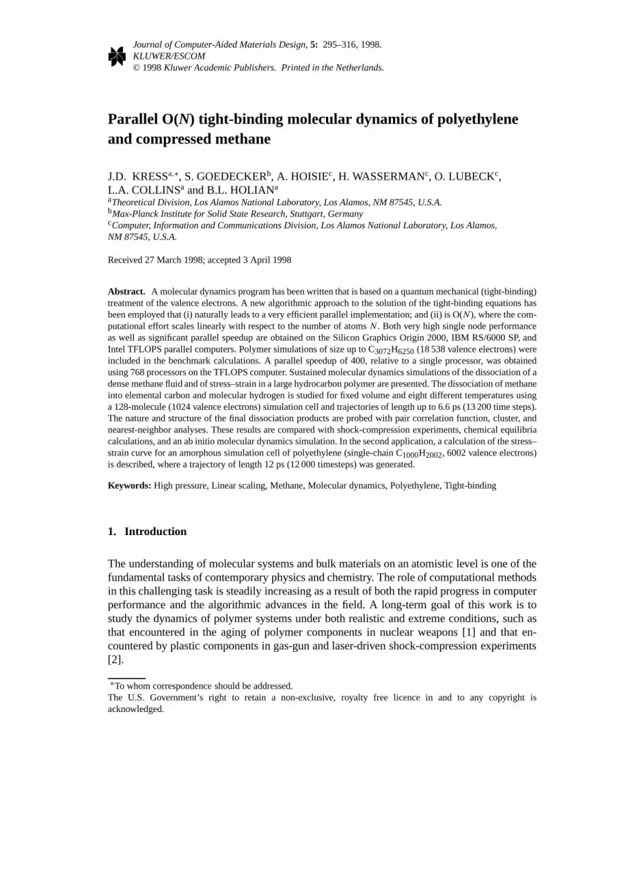
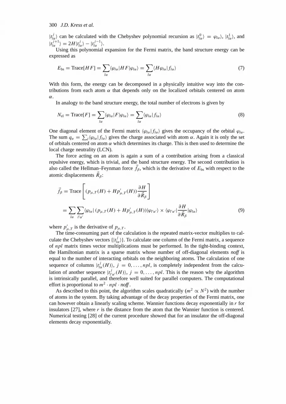
Figure 1. CPU time per processor on an SGI Origin 2000 computer (solid circles) as a function of the number ofatoms. Each line is a least-squares fit to the silicon and polyethylene data, respectively.

(or local charge neutrality enforced via a local Fermi energy on each atom), the trace in Eq.9 is broken [10], and therefore the forces are in theory only approximate. To obtain formallyexact forces requires a full matrix treatment of the polynomial expansion [10], which can beaccomplished in a fashion that retainsN scaling (albeit with a larger prefactor in front ofNcompared to implementing Eq. 9). In practice, however, the approximation improves asnhop

is increased (the forces are formally exact fornhop = ∞).The potential energy (Eq. 2) contribution to the pressure is calculated using a finite-differ-

ence volume approachPpot= −1Etot/1V , where1V = (Lx+δL)×(Ly+δL)×(Lz+δL)−V andV = Lx ×Ly ×Lz. The total pressureP must include the ion dynamical contribution,which has a simple ideal gas form, given byP = Ppot+ (N/V )kBT . The potential energycontribution to the stress is calculated in a similar fashion asσxx = 1Etot/1V , where1V =(Lx + δL)× Ly × Lz − V .

3. Benchmark timings on parallel architectures

In this section, benchmark calculations [32] on linear scaling and on CPU speed versus thenumber of processors are presented. Both silicon (a three-dimensional (3D) diamond struc-ture) and polyethylene (one-dimensional (1D) chains) are considered. For silicon, the TBparameters of Goodwin et al. [33] are used. The basis set consists of one s-orbital and three p-orbitals per atom, thus, theH matrix for the system is of orderm = 4N. For polyethylene, theOxford TB parameters for hydrocarbons are used. The basis set consists of one s-orbital perhydrogen atom and of one s-orbital and three p-orbitals per carbon atom. Thus, theH matrixis of orderm = 4NC+NH, whereNC andNH are the number of carbon and hydrogen atoms,respectively. For the polyethylene timing benchmarks, the LCN self-consistency is disabled(unless specified otherwise). The CPU times reported are for one MD time step (one energyand force calculation).

Linear scaling (O(N)) for the Fermi Operator Expansion [9,28] and the kernel polynomialmethod [10] algorithms has been shown previously. Linear scaling for the present code isdemonstrated for two processors in Fig. 1 for silicon and polyethylene. (Note that linearscaling is independent of parallelism.) The three polyethylene data points correspond to 32,


0

10

20

30

40

50

60

0 10 20 30 40 50 60

4608 atomsideal

Spee

du

p

Number of processors

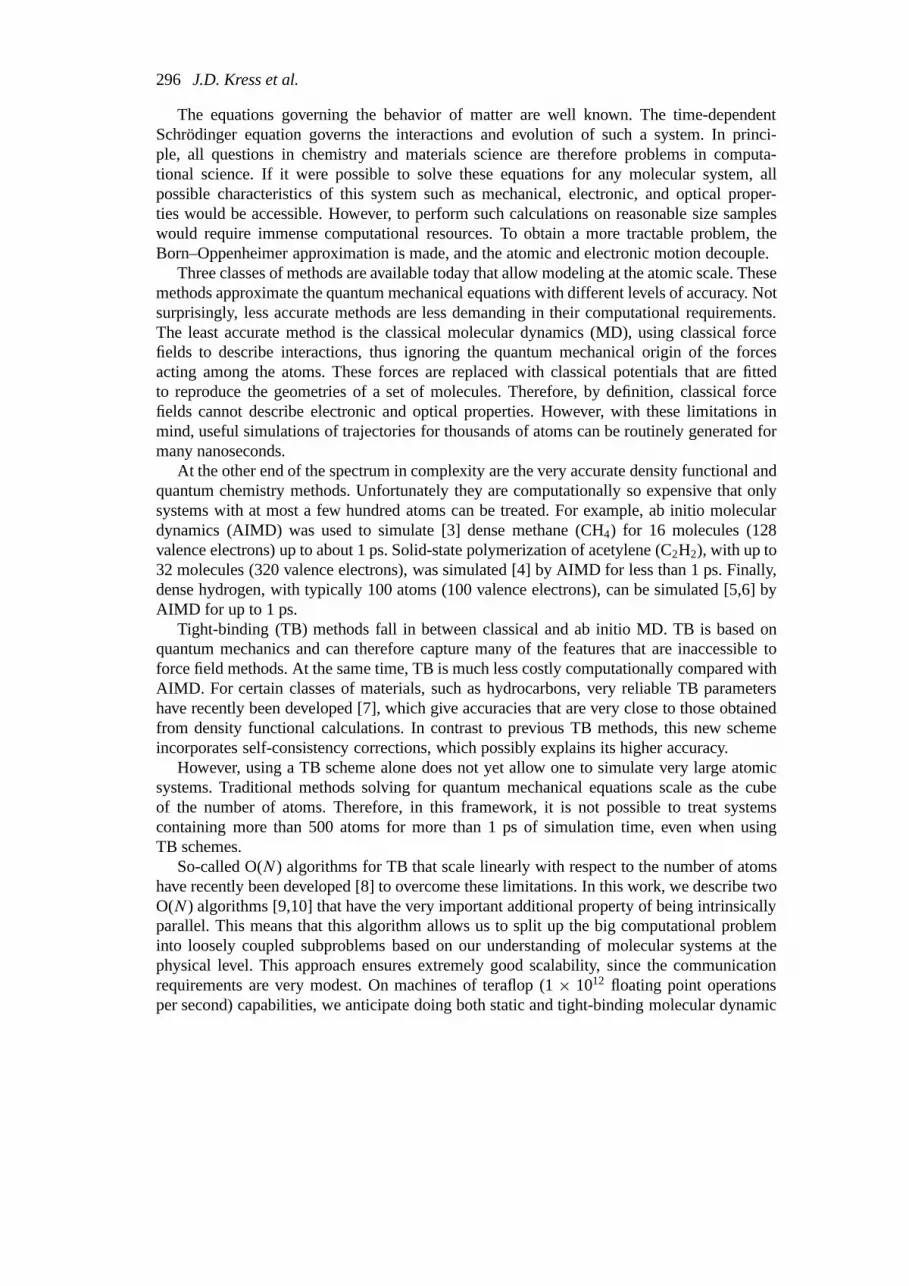
Figure 2. Speedup on the ASCI Blue Mountain computer as a function of the number of processors. Solid circles:TBON calculation on a single 4608-atom chain of polyethylene C1536H3072; straight line: ideal speedup.

64, and 128 chains of C24H50. The slope of the line in Fig. 1 for silicon is larger than that forpolyethylene mainly because there are more atoms in the localization region for a 3D diamondstructure withnhop = 3 compared to 1D C24H50 chains withnhop = 4. Also,npl = 128 forsilicon andnpl = 96 for polyethylene.

The parallel performance of the TBON code has been benchmarked on three differentASCI computers: (i) a Silicon Graphics Inc. Origin 2000 (‘Blue Mountain’) at Los AlamosNational Laboratory; (ii) an IBM RS/6000 SP (‘Blue Pacific’) at Lawrence Livermore Na-tional Laboratory; and (iii) the Intel TFLOPS (‘Red’) at Sandia National Laboratory. Forthese benchmarks, we have not run on more than 50 processors on Blue Mountain and notmore than 128 processors on Blue Pacific. Since we felt that demonstrating weak scalability(i.e., proportionally increasing both the problem size and the number of processors) on thissmall number of processors would not be very convincing, we choose to demonstrate themore difficult strong scalability (i.e., constant problem size solved on increasing number ofprocessors) on all three computers.

The results for Blue Mountain (SGI Origin 2000) are shown in Fig. 2. The single-chainpolymer C1536H3072 was used for this test run. The size of this polymer was chosen such that,from a memory requirement point of view, the sequential computation was still feasible on asingle node. Forty-five LCN iterations took roughly 15 min in serial mode, and about 20 s onthe 50-processor configuration.

In a realistic physical system, it is practically impossible to have perfect load balancing.Since a polymer has a nonregular structure, not all of the localization regions have the samesize. For instance, the localization region for an atom at the end of a polymer chain is just halfas big as the localization region of an atom in the middle of the chain. But even for atomsfarther from the end of the chain, the localization regions can vary in size due to the thermalmotion of the chain. Since the number of operations needed to calculate a localized orbitalis proportional to the size of the localization region, the numerical task involved varies inmagnitude as well. In addition, the number of carbon and hydrogen atoms assigned to eachprocessor is not exactly equal unless the total number of both carbon and hydrogen atoms is amultiple of the number of processors, which is not possible in most cases. These two factorslead to a load imbalance which causes deviation from linear speedup. In the case of the 50-


0

20

40

60

80

100

120

140

0 20 40 60 80 100 120 140

128-chain ideal

Spee

du

p


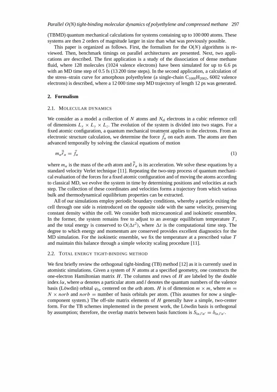
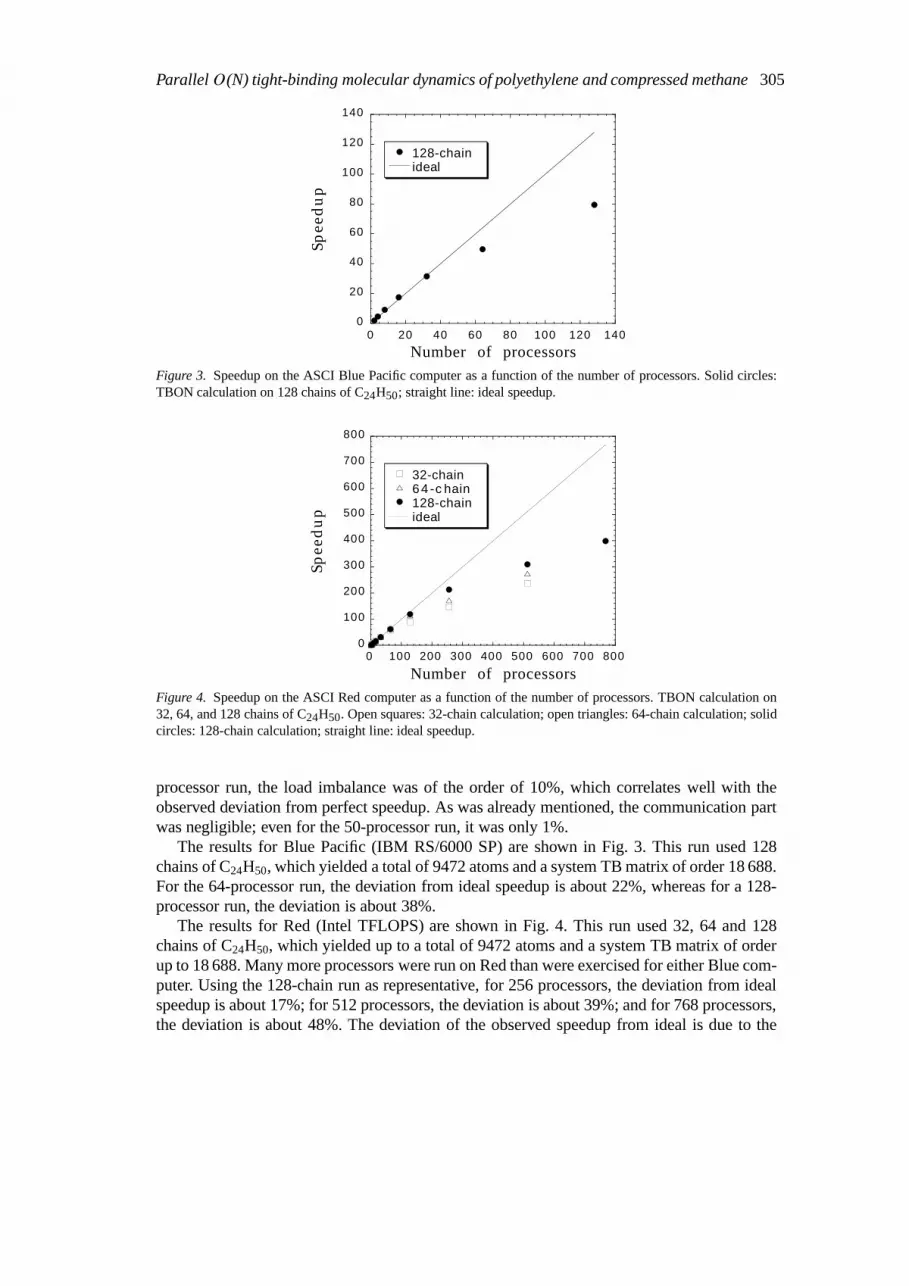
Figure 3. Speedup on the ASCI Blue Pacific computer as a function of the number of processors. Solid circles:TBON calculation on 128 chains of C24H50; straight line: ideal speedup.

0

100

200

300

400

500

600

700

800

0 100 200 300 400 500 600 700 800

32-chain 6 4 -c hain128-chain ideal

Spee

du

p


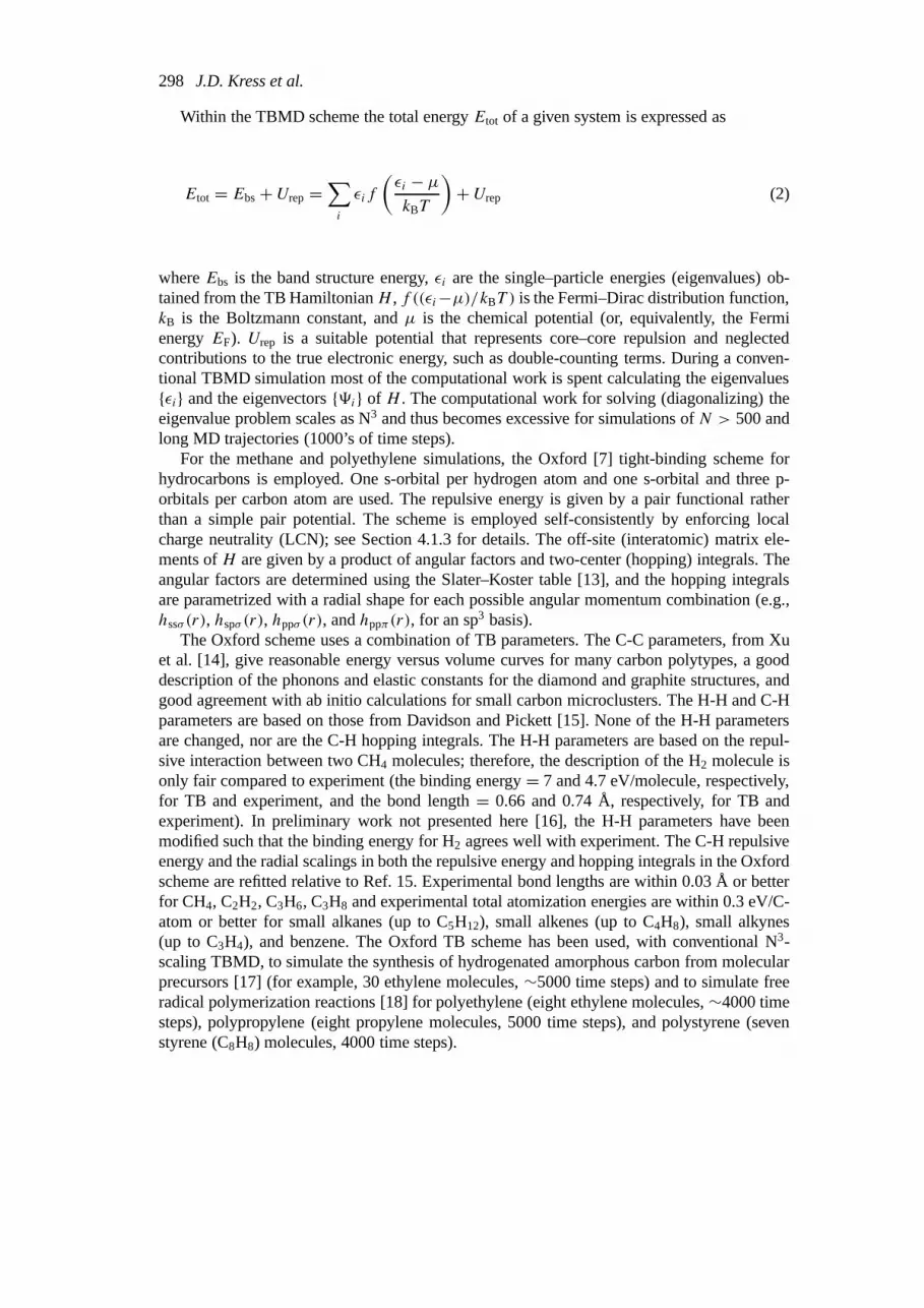
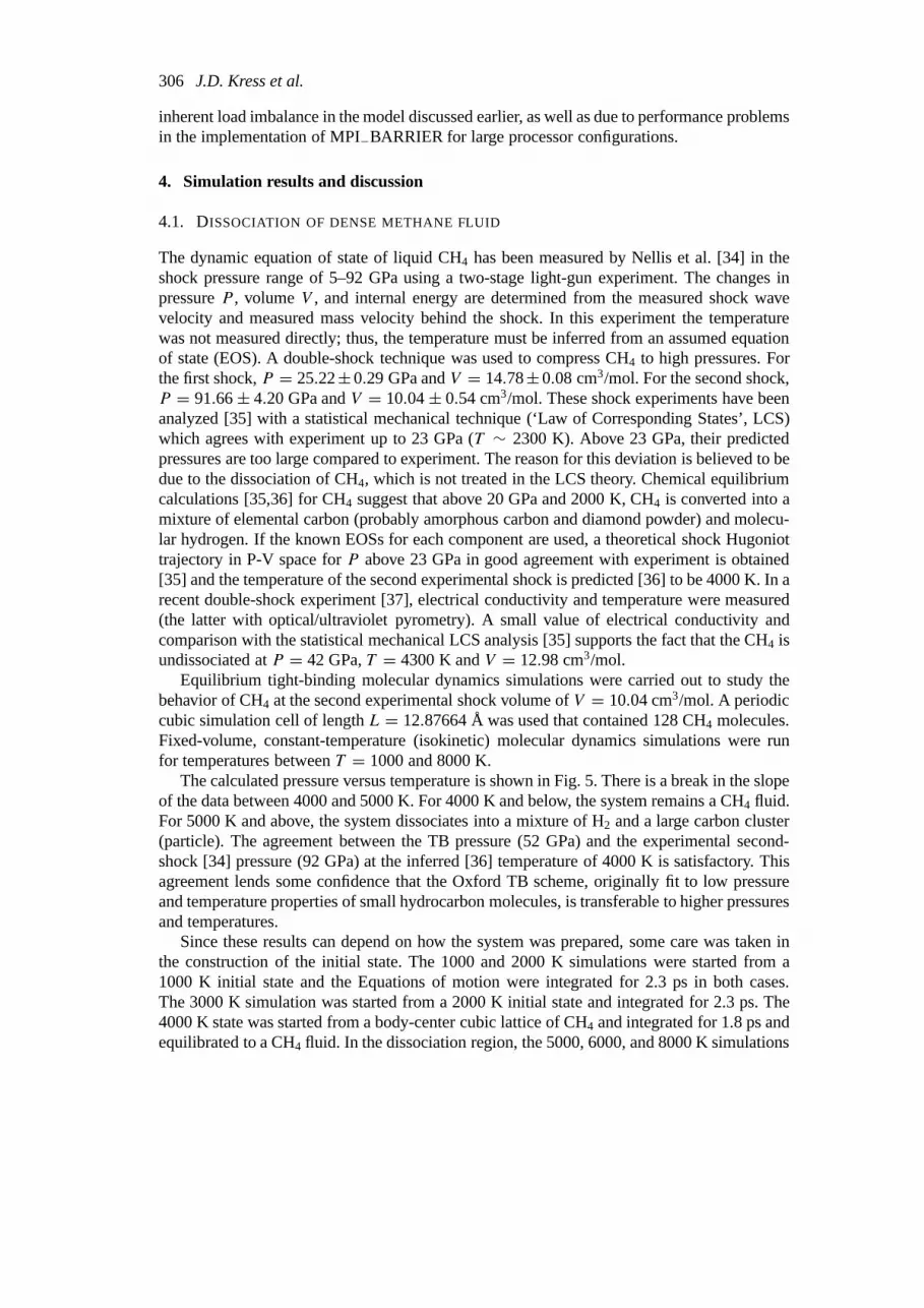
Figure 4. Speedup on the ASCI Red computer as a function of the number of processors. TBON calculation on32, 64, and 128 chains of C24H50. Open squares: 32-chain calculation; open triangles: 64-chain calculation; solidcircles: 128-chain calculation; straight line: ideal speedup.

processor run, the load imbalance was of the order of 10%, which correlates well with theobserved deviation from perfect speedup. As was already mentioned, the communication partwas negligible; even for the 50-processor run, it was only 1%.

The results for Blue Pacific (IBM RS/6000 SP) are shown in Fig. 3. This run used 128chains of C24H50, which yielded a total of 9472 atoms and a system TB matrix of order 18 688.For the 64-processor run, the deviation from ideal speedup is about 22%, whereas for a 128-processor run, the deviation is about 38%.

The results for Red (Intel TFLOPS) are shown in Fig. 4. This run used 32, 64 and 128chains of C24H50, which yielded up to a total of 9472 atoms and a system TB matrix of orderup to 18 688. Many more processors were run on Red than were exercised for either Blue com-puter. Using the 128-chain run as representative, for 256 processors, the deviation from idealspeedup is about 17%; for 512 processors, the deviation is about 39%; and for 768 processors,the deviation is about 48%. The deviation of the observed speedup from ideal is due to the


inherent load imbalance in the model discussed earlier, as well as due to performance problemsin the implementation of MPI−BARRIER for large processor configurations.

4. Simulation results and discussion

4.1. DISSOCIATION OF DENSE METHANE FLUID

The dynamic equation of state of liquid CH4 has been measured by Nellis et al. [34] in theshock pressure range of 5–92 GPa using a two-stage light-gun experiment. The changes inpressureP , volumeV , and internal energy are determined from the measured shock wavevelocity and measured mass velocity behind the shock. In this experiment the temperaturewas not measured directly; thus, the temperature must be inferred from an assumed equationof state (EOS). A double-shock technique was used to compress CH4 to high pressures. Forthe first shock,P = 25.22±0.29 GPa andV = 14.78±0.08 cm3/mol. For the second shock,P = 91.66± 4.20 GPa andV = 10.04± 0.54 cm3/mol. These shock experiments have beenanalyzed [35] with a statistical mechanical technique (‘Law of Corresponding States’, LCS)which agrees with experiment up to 23 GPa (T ∼ 2300 K). Above 23 GPa, their predictedpressures are too large compared to experiment. The reason for this deviation is believed to bedue to the dissociation of CH4, which is not treated in the LCS theory. Chemical equilibriumcalculations [35,36] for CH4 suggest that above 20 GPa and 2000 K, CH4 is converted into amixture of elemental carbon (probably amorphous carbon and diamond powder) and molecu-lar hydrogen. If the known EOSs for each component are used, a theoretical shock Hugoniottrajectory in P-V space forP above 23 GPa in good agreement with experiment is obtained[35] and the temperature of the second experimental shock is predicted [36] to be 4000 K. In arecent double-shock experiment [37], electrical conductivity and temperature were measured(the latter with optical/ultraviolet pyrometry). A small value of electrical conductivity andcomparison with the statistical mechanical LCS analysis [35] supports the fact that the CH4 isundissociated atP = 42 GPa,T = 4300 K andV = 12.98 cm3/mol.

Equilibrium tight-binding molecular dynamics simulations were carried out to study thebehavior of CH4 at the second experimental shock volume ofV = 10.04 cm3/mol. A periodiccubic simulation cell of lengthL = 12.87664 Å was used that contained 128 CH4 molecules.Fixed-volume, constant-temperature (isokinetic) molecular dynamics simulations were runfor temperatures betweenT = 1000 and 8000 K.

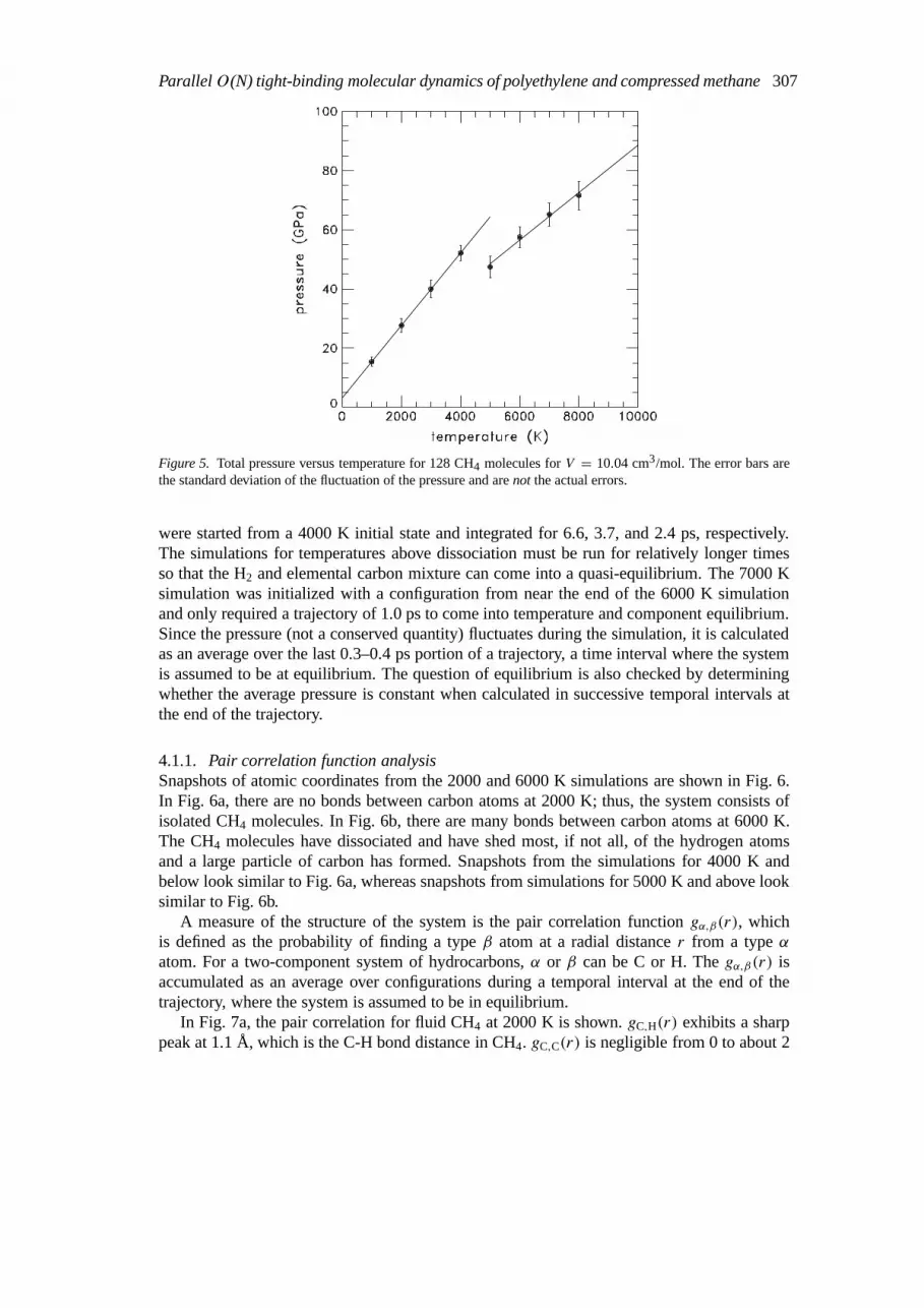
The calculated pressure versus temperature is shown in Fig. 5. There is a break in the slopeof the data between 4000 and 5000 K. For 4000 K and below, the system remains a CH4 fluid.For 5000 K and above, the system dissociates into a mixture of H2 and a large carbon cluster(particle). The agreement between the TB pressure (52 GPa) and the experimental second-shock [34] pressure (92 GPa) at the inferred [36] temperature of 4000 K is satisfactory. Thisagreement lends some confidence that the Oxford TB scheme, originally fit to low pressureand temperature properties of small hydrocarbon molecules, is transferable to higher pressuresand temperatures.

Since these results can depend on how the system was prepared, some care was taken inthe construction of the initial state. The 1000 and 2000 K simulations were started from a1000 K initial state and the Equations of motion were integrated for 2.3 ps in both cases.The 3000 K simulation was started from a 2000 K initial state and integrated for 2.3 ps. The4000 K state was started from a body-center cubic lattice of CH4 and integrated for 1.8 ps andequilibrated to a CH4 fluid. In the dissociation region, the 5000, 6000, and 8000 K simulations


Figure 5. Total pressure versus temperature for 128 CH4 molecules forV = 10.04 cm3/mol. The error bars arethe standard deviation of the fluctuation of the pressure and arenot the actual errors.

were started from a 4000 K initial state and integrated for 6.6, 3.7, and 2.4 ps, respectively.The simulations for temperatures above dissociation must be run for relatively longer timesso that the H2 and elemental carbon mixture can come into a quasi-equilibrium. The 7000 Ksimulation was initialized with a configuration from near the end of the 6000 K simulationand only required a trajectory of 1.0 ps to come into temperature and component equilibrium.Since the pressure (not a conserved quantity) fluctuates during the simulation, it is calculatedas an average over the last 0.3–0.4 ps portion of a trajectory, a time interval where the systemis assumed to be at equilibrium. The question of equilibrium is also checked by determiningwhether the average pressure is constant when calculated in successive temporal intervals atthe end of the trajectory.

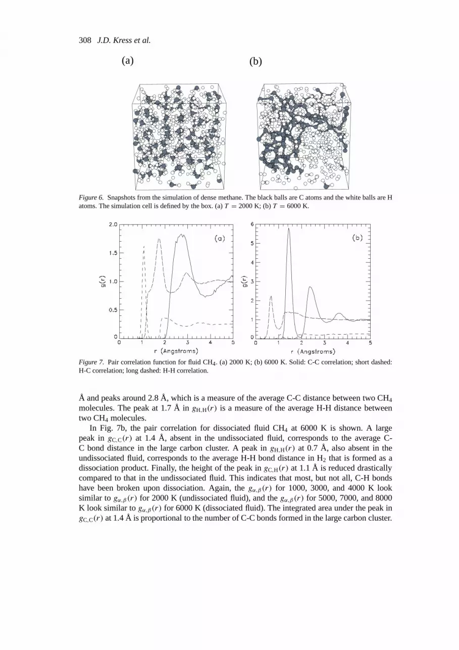
4.1.1. Pair correlation function analysisSnapshots of atomic coordinates from the 2000 and 6000 K simulations are shown in Fig. 6.In Fig. 6a, there are no bonds between carbon atoms at 2000 K; thus, the system consists ofisolated CH4 molecules. In Fig. 6b, there are many bonds between carbon atoms at 6000 K.The CH4 molecules have dissociated and have shed most, if not all, of the hydrogen atomsand a large particle of carbon has formed. Snapshots from the simulations for 4000 K andbelow look similar to Fig. 6a, whereas snapshots from simulations for 5000 K and above looksimilar to Fig. 6b.

A measure of the structure of the system is the pair correlation functiongα,β(r), whichis defined as the probability of finding a typeβ atom at a radial distancer from a typeαatom. For a two-component system of hydrocarbons,α or β can be C or H. Thegα,β(r) isaccumulated as an average over configurations during a temporal interval at the end of thetrajectory, where the system is assumed to be in equilibrium.

In Fig. 7a, the pair correlation for fluid CH4 at 2000 K is shown.gC,H(r) exhibits a sharppeak at 1.1 Å, which is the C-H bond distance in CH4. gC,C(r) is negligible from 0 to about 2


(a) (b)

Figure 6. Snapshots from the simulation of dense methane. The black balls are C atoms and the white balls are Hatoms. The simulation cell is defined by the box. (a)T = 2000 K; (b)T = 6000 K.

Figure 7. Pair correlation function for fluid CH4. (a) 2000 K; (b) 6000 K. Solid: C-C correlation; short dashed:H-C correlation; long dashed: H-H correlation.

Å and peaks around 2.8 Å, which is a measure of the average C-C distance between two CH4

molecules. The peak at 1.7 Å ingH,H(r) is a measure of the average H-H distance betweentwo CH4 molecules.

In Fig. 7b, the pair correlation for dissociated fluid CH4 at 6000 K is shown. A largepeak ingC,C(r) at 1.4 Å, absent in the undissociated fluid, corresponds to the average C-C bond distance in the large carbon cluster. A peak ingH,H(r) at 0.7 Å, also absent in theundissociated fluid, corresponds to the average H-H bond distance in H2 that is formed as adissociation product. Finally, the height of the peak ingC,H(r) at 1.1 Å is reduced drasticallycompared to that in the undissociated fluid. This indicates that most, but not all, C-H bondshave been broken upon dissociation. Again, thegα,β(r) for 1000, 3000, and 4000 K looksimilar togα,β(r) for 2000 K (undissociated fluid), and thegα,β(r) for 5000, 7000, and 8000K look similar togα,β(r) for 6000 K (dissociated fluid). The integrated area under the peak ingC,C(r) at 1.4 Å is proportional to the number of C-C bonds formed in the large carbon cluster.


0

1 0

2 0

3 0

4 0

5 0

6 0

1 2 3 4 5 6 7P

erc

en

t

N

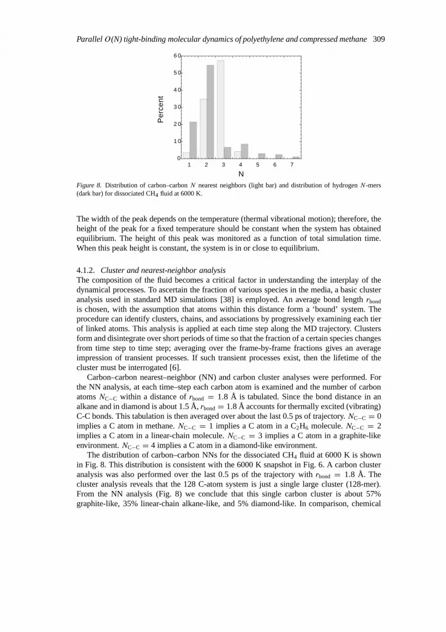
Figure 8. Distribution of carbon–carbonN nearest neighbors (light bar) and distribution of hydrogenN-mers(dark bar) for dissociated CH4 fluid at 6000 K.

The width of the peak depends on the temperature (thermal vibrational motion); therefore, theheight of the peak for a fixed temperature should be constant when the system has obtainedequilibrium. The height of this peak was monitored as a function of total simulation time.When this peak height is constant, the system is in or close to equilibrium.

4.1.2. Cluster and nearest-neighbor analysisThe composition of the fluid becomes a critical factor in understanding the interplay of thedynamical processes. To ascertain the fraction of various species in the media, a basic clusteranalysis used in standard MD simulations [38] is employed. An average bond lengthrbond

is chosen, with the assumption that atoms within this distance form a ‘bound’ system. Theprocedure can identify clusters, chains, and associations by progressively examining each tierof linked atoms. This analysis is applied at each time step along the MD trajectory. Clustersform and disintegrate over short periods of time so that the fraction of a certain species changesfrom time step to time step; averaging over the frame-by-frame fractions gives an averageimpression of transient processes. If such transient processes exist, then the lifetime of thecluster must be interrogated [6].

Carbon–carbon nearest–neighbor (NN) and carbon cluster analyses were performed. Forthe NN analysis, at each time–step each carbon atom is examined and the number of carbonatomsNC−C within a distance ofrbond = 1.8 Å is tabulated. Since the bond distance in analkane and in diamond is about 1.5 Å,rbond= 1.8 Å accounts for thermally excited (vibrating)C-C bonds. This tabulation is then averaged over about the last 0.5 ps of trajectory.NC−C = 0implies a C atom in methane.NC−C = 1 implies a C atom in a C2H6 molecule.NC−C = 2implies a C atom in a linear-chain molecule.NC−C = 3 implies a C atom in a graphite-likeenvironment.NC−C = 4 implies a C atom in a diamond-like environment.

The distribution of carbon–carbon NNs for the dissociated CH4 fluid at 6000 K is shownin Fig. 8. This distribution is consistent with the 6000 K snapshot in Fig. 6. A carbon clusteranalysis was also performed over the last 0.5 ps of the trajectory withrbond = 1.8 Å. Thecluster analysis reveals that the 128 C-atom system is just a single large cluster (128-mer).From the NN analysis (Fig. 8) we conclude that this single carbon cluster is about 57%graphite-like, 35% linear-chain alkane-like, and 5% diamond-like. In comparison, chemical


equilibria analyses of shock-compression experiments for methane [35] and hydrocarbonpolymers [39] suggest dissociation into elemental carbon (diamond) and molecular hydrogenabove pressures of 20 GPa and temperatures of 2000 K.

A constant-pressure ab initio molecular dynamics (AIMD) simulation [3] for 100 GPaand 4000 K, corresponding to the experimental second-shock [34], finds that the 16 CH4

molecules in the simulation cell break down to form two CH4, four C2H6, and two C3H8

molecules (‘although the small number of particles (atoms). . . does not allow a reliablestoichiometric analysis. . .’). Due to the small sample size of 16 C atoms and, perhaps, theshort trajectory length, the AIMD simulation cannot give a statistically meaningful descriptionof the formation of elemental carbon but predicts ‘the tendency of CH4 to dissociate (underthese conditions)’. In comparison, an instantaneous cluster analysis near the beginning (at0.24 ps) of the present 6000 K trajectory yielded a carbon-containing molecule distribution ofeleven C2, two C3 and the rest C1. At 0.48 ps, the distribution was 11 C2, two C3, four C4, twoC7, one C8, one C9 and the rest C1. A distribution of elemental carbon (C128) and molecularhydrogen at quasi-equilibrium is eventually reached by 3.7 ps.

For 4000 K and below in the present simulations, the methane fluid is not dissociated. Thus,the distribution is 100%NC−C = 0 carbon-carbon NNs (all of the carbon exists as methane)for 4000 K and below. Also, the carbon–carbon NN distributions and carbon cluster analysesfor 5000, 7000, and 8000 K (not shown) look very similar to that for 6000 K.

Hydrogen cluster analyses were also performed usingrbond = 1.0Å, which accounts forthermally excited H-H bonds as the equilibrium bond distance in H2 is about 0.7 Å. Thedistribution of hydrogen clusters for the dissociated CH4 fluid at 6000 K is shown in Fig. 8.A monomer (1-mer) is a bare H atom or an H atom bonded to a C atom. A dimer (2-mer) isa hydrogen molecule. The higherNH-mers are most likely transient hydrogen polymers. Thelow populations in Fig. 8 forNH ≥ 3 are consistent with this picture. Since a lifetime analysis[6] was not performed, we cannot discriminate between, for example, a trimer or a monomercolliding with a dimer in the fluid. The hydrogen cluster distribution in Fig. 8 is also consistentwith the 6000 K snapshot in Fig. 6. The hydrogen cluster distributions for 5000, 7000, and8000 K (not shown) look very similar to that for 6000 K.

For temperatures of 4000 K and below, the methane fluid is not dissociated. Thus, thedistribution is 100% hydrogen ‘monomers’ as the hydrogen atoms are NNs to only the carbonatom in a methane molecule and are not NNs to any other H atom.

4.1.3. Some computational detailsThe Oxford TB scheme [7] was used. Local charge neutrality (LCN) was imposed by shiftingthe on-site energies (εlα = Hlα,lα) of the formεlα → ε

′lα = εlα+vα, wherevα = Xα(qα−q0

α)

andXα is a response function. The shifts depend on the atomα and not on the orbitalsl.The on-site energies are iterated until maxα |qα − q0

α| ≤ tollcn. LCN is achieved when thenumber of electronsqα equals the number of valence electronsq0

α, atom by atom, to within atolerancetollcn. Converged on-site shifts from the previous MD time step are used as initialguesses for the next time step. A Chebychev polynomial of degreenpl = 200 was used withthe smeared-Fermi approximation (Eq. 17). The other TBON parameters werenhop = 7,evlo = −75 eV, andevhi = 75 eV. The MD time step1t = 0.5 fs.

For simulations of temperatures of 4000 K and below, a CPU time of about 0.1 min/timestep on 32 processors on the Blue Mountain computer (SGI Origin 2000) was required. Fortemperatures of 5000 K and above, the CPU time increased to about 1 min/time step. Atthese higher temperatures more LCN iterations per time step are required to capture the


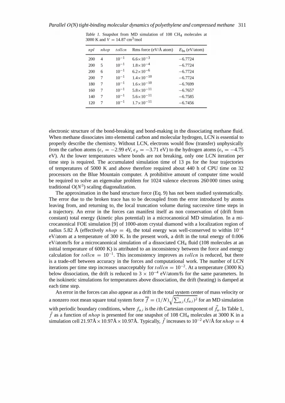
Table 1. Snapshot from MD simulation of 108 CH4 molecules at3000 K andV = 14.87 cm3/mol

npl nhop tollcn Rms force (eV/Å atom) Ebs (eV/atom)

200 4 10−1 6.6×10−3 −6.7724

200 5 10−1 1.8×10−4 −6.7724

200 6 10−1 6.2×10−6 −6.7724

200 7 10−1 1.4×10−10 −6.7724

180 7 10−1 1.6×10−10 −6.7699

160 7 10−1 5.8×10−11 −6.7657

140 7 10−1 5.6×10−11 −6.7585

120 7 10−1 1.7×10−11 −6.7456

electronic structure of the bond-breaking and bond-making in the dissociating methane fluid.When methane dissociates into elemental carbon and molecular hydrogen, LCN is essential toproperly describe the chemistry. Without LCN, electrons would flow (transfer) unphysicallyfrom the carbon atoms (εs = −2.99 eV,εp = −3.71 eV) to the hydrogen atoms (εs = −4.75eV). At the lower temperatures where bonds are not breaking, only one LCN iteration pertime step is required. The accumulated simulation time of 13 ps for the four trajectoriesof temperatures of 5000 K and above therefore required about 440 h of CPU time on 32processors on the Blue Mountain computer. A prohibitive amount of computer time wouldbe required to solve an eigenvalue problem for 1024 valence electrons 260 000 times usingtraditional O(N3) scaling diagonalization.

The approximation in the band structure force (Eq. 9) has not been studied systematically.The error due to the broken trace has to be decoupled from the error introduced by atomsleaving from, and returning to, the local truncation volume during successive time steps ina trajectory. An error in the forces can manifest itself as non conservation of (drift fromconstant) total energy (kinetic plus potential) in a microcanonical MD simulation. In a mi-crocanonical FOE simulation [9] of 1000-atom crystal diamond with a localization region ofradius 5.82 Å (effectivelynhop = 4), the total energy was well-conserved to within 10−4

eV/atom at a temperature of 300 K. In the present work, a drift in the total energy of 0.006eV/atom/fs for a microcanonical simulation of a dissociated CH4 fluid (108 molecules at aninitial temperature of 6000 K) is attributed to an inconsistency between the force and energycalculation fortollcn = 10−1. This inconsistency improves astollcn is reduced, but thereis a trade-off between accuracy in the forces and computational work. The number of LCNiterations per time step increases unacceptably fortollcn = 10−2. At a temperature (3000 K)below dissociation, the drift is reduced to 3× 10−4 eV/atom/fs for the same parameters. Inthe isokinetic simulations for temperatures above dissociation, the drift (heating) is damped ateach time step.

An error in the forces can also appear as a drift in the total system center of mass velocity or

a nonzero root mean square total system forcef = (1/N)√∑

α,i(fα,i)2 for an MD simulation

with periodic boundary conditions, wherefα,i is theith Cartesian component ofEfα. In Table 1,f as a function ofnhop is presented for one snapshot of 108 CH4 molecules at 3000 K in asimulation cell 21.97Å×10.97Å×10.97Å. Typically,f increases to 10−2 eV/Å for nhop = 4


when the fluid dissociates (the insulator band gap begins to close due to unpaired electrons).Therefore,nhop = 7 is used in the simulations of a dissociating CH4 fluid. Also in Table 1, theband structure energyEbs as a function ofnpl is presented.npl = 200 givesEbs convergedto within 0.003 eV/atom with respect tonpl. For comparison,npl = 100 andnhop = 3yielded acceptable convergence for the vacancy formation energy in an Si diamond lattice[10]. In general, the larger the value fornpl, the more energy resolution in the Fermi operatoror density of states.

4.2. STRESS–STRAIN OF POLYETHYLENE

Exploratory TBON nonequilibrium MD calculations for the tensile strain of amorphous poly-ethylene are described next. The stress–strain curve for a uniaxial strain rate ofε = 2×1010/sis compared indirectly to classical MD simulations with strain rates 2–3 orders of magnitudeslower. This TBON simulation tests the description of the intrachain potential energy for bond-breaking, where TB is more accurate than a classical potential. The classical simulations,at the slower strain rates, basically only exercise the interchain and elastic potential energy.In future work, we will address shock-compression Hugoniot experiments of hydrocarbonpolymers [39], where the higher strain rates are relevant.

An amorphous sample consisting of one chain of polyethylene C1000H2002 was generated.First, a single chain of C1000H2002 was constructed using Insight II [40]. Then, the method ofTheodorou and Suter [41], as implemented in Insight II with the CVFF classical force field,was used to pack the chain into a cubic box with periodic boundary conditions (Lx = Ly =Lz = 28.95 Å) at a density of 0.96 g/cm3. The structure obtained from this process is shown inFig. 9. This configuration was then equilibrated with TBON using the Oxford TB parameters[7] with isokinetic MD atT = 1 K. This relaxes the system to essentially zero pressure andto one of a myriad of local minima available. The initial state for the stress–strain calculationswas taken from the last equilibration snapshot.

For tensile strain MD simulations of polymers, uniaxial, homogeneously expanding pe-riodic boundary conditions are employed [42]. The side length of the simulation cell in thex-direction increases with time asLx(t) = Lx(0)[1+ ε(0)t], while the cross-sectional lengthsLy andLz are held fixed. A constant Lagrangian strain rate in thex-direction is imposed byadding to thex-component of the initial thermal velocity, for each atom, a term proportionalto the atomicx coordinate,vx → vx + ε(0)x. Define the left-hand and right-hand sides ofthe x-period asx = −Lx(t)/2 andLx(t)/2. When an atom crosses the left-hand boundaryand is replaced at the right-hand end of the cell, thex-velocity component must be adjustedas vx(t) → vx(t) + ε(0)Lx(0), so to preserve the sense of expansion. Conversely, whenan atom crosses the right-hand boundary and is replaced at the left-hand end of the cell,vx(t)→ vx(t)− ε(0)Lx(0).

A uniaxial strain rate ofε = 2× 1010/s was applied in thex-direction. Adiabatic initialvelocity conditions were applied as described above. Due to an oversight in the implementa-tion, periodic boundary conditions werenot imposed for the velocities; therefore, the presentresults should be viewed as preliminary. The non-equilibrium MD simulation was run withno temperature control, thereby approximating isentropic, rather than isothermal, strain. AChebychev polynomial of degreenpl = 200 was used with the smeared-Fermi approximation(Eq. 17). The other TBON parameters werenhop = 4 andtollcn = 1×10−1. The simulationwas run for 12 000 time steps with1t = 1 fs, for a total simulation time of 12 ps. Since, onthe average, about one LCN iteration per time step was needed, this simulation of C1000H2002


Figure 9. Polyethylene C1000H2002. The black balls are C atoms and the white balls are H atoms. Left panel:unfolded; right panel: folded. Each panel is a different scale: the chain in the left panel is bounded roughly by acube of volume (120 Å)3, whereas the simulation cell in the right panel is of volume(28.95 Å)3.

Figure 10. Tensile stress in the direction of the strain as a function of strainεx for amorphous polyethyleneC1000H2002at a strain rate ofε = 2× 1010/s.

would require a prohibitive amount of computer time using traditional O(N3) scaling diago-nalization to solve an eigenvalue problem for 6002 valence electrons over 12 000 times. Onesegment (2000 time steps) of the TBON trajectory ran for 145 min CPU time on 64 processorsof the SGI Origin 2000 Blue Mountain parallel computer.

The resulting stress versus strain is shown in Fig. 10. Only the internal stress (potentialenergy contribution) along the direction of the strainσxx is plotted; the thermal contributionto σxx is negligible under these conditions. The stress increases slowly fromε = 0 until aboutε = 0.1. Fluctuations in the stress resulting from the MD simulation are clearly apparent.From there, the stress increases steadily until the simulation was terminated (at aboutε =


0.26). Presumably, if the simulation was continued, the stress would increase until the singlelinear-chain yield strength of about 20–25 GPa was reached (see below).

Previously, molecular dynamics simulations have been performed [43, 44] for amorphousC1000H2002 using classical potentials and a united atom description for the –CH2– unit. Theclassical descriptions, although less accurate in describing the making and breaking of bonds,are much more computationally efficient and therefore much lower strain rates can be simu-lated. Using a Brown–Clarke constant-pressure MD simulation withε ∼ 3× 107s, a plateauin the stress versus strain curve at a stress of about 0.15 GPa was found [43]. Using a moresophisticated isothermal, constant perpendicular stress MD simulation withε ∼ 4× 108/s,a rough plateau in the stress versus strain curve at a stress of about 0.15 GPa was also found[44]. The TBON simulation atε = 2× 1010/s cannot be directly compared to these classicalsimulations due to the disparity in the strain rates.

The theoretical yield strength for polyethylene described by the Oxford TB scheme was in-vestigated by running similar stress–strain simulations on a single infinite linear polyethylenechain at high strain rates. If the chain is oriented along thex-axis, an effective infinite chainwas prepared by applying periodic boundary conditions in thex-direction such that the C atomat one end of thex-period is bound to the C atom at the other end of thex-period with theappropriate C-C bond length. Periodic chains ranging in size from C24H48 to C768H1536 wereused. A theoretical yield strength of about 20–25 GPa was found for these chains of varyingsize. Specifically for C768H1536 at ε = 3× 1012/s, the strain versus stress is essentially linear(elastic) untilε = 0.5, with stress = 21 GPa. Forε > 0.5, the stress rapidly decreases.

Finally, TBON simulations have also been performed on an amorphous sample consistingof 80 short-chain polyethylene molecules C36H74. This 8800-atom system results in a systemTB matrix of order 17 440. The smeared-Fermi approximation (Eq. 17) was used withnhop =4, npl = 200, andtollcn = 1× 10−1. A trajectory of 300 time steps, with an average of1.3 LCN iterations per time step, used 127 min of CPU time on 24 processors of the SGIOrigin 2000 Blue Mountain parallel computer. This 8800-atom simulation has an equivalentserial CPU speed of 3 min/1t=(127 min×24 processors)/(3001t × 1.3), comparable to theequivalent serial speed for the 3002-atom simulation described above. The equation of stateof polystyrene under extreme conditions was recently examined experimentally [2], using alaser-shock technique; in the future we hope to simulate various aspects of this experiment.

We note also that (in work [45] not described here) an amorphous cell of silicon containing4096 atoms (16 384 valence electrons) has been simulated for 100 fs (100 timesteps) forvarious temperatures.

Acknowledgements

Large parts of this program were developed by S.G. during a stay at Los Alamos NationalLaboratory. Interesting discussions with A. Voter, R. Silver, H. Roeder, A. Redondo, and D.Drabold are acknowledged. We thank A. Horsfield for providing us with a detailed data baseof the new tight-binding scheme before its publication. Special thanks to Mark Dalton withSGI in Los Alamos for his support during the benchmarks.

The authors wish to acknowledge the Advanced Computing Laboratory of Los AlamosNational Laboratory, Los Alamos, NM. This work was performed on computing resourceslocated at this facility.


This work was performed under the auspices of the U.S. Department of Energy by LosAlamos National Laboratory under contract W-7405-ENG-36. J.D.K. and L.A.C. were sup-ported by the Advanced Strategic Computing Initiative (ASCI). B.L.H. was supported by theMultiscale LDRD (Laboratory Directed Research and Development) Competency Develop-ment Thrust. S.G. thanks Los Alamos for its hospitality.

References

1. Redondo, A., private communication.2. Cauble, R., Perry, T.S., Bach, D.R., Budil, K.S., Hammel, B.A., Collins, G.W., Gold, D.M., Dunn, J., Cel-

liers, P., Da Silva, L.B., Foord, M.E., Wallace, R.J., Stewart, R.E. and Woolsey, N.C., Phys. Rev. Lett., 80(1998) 1248.

3. Ancilotto, F., Chiarotti, G.L., Scandolo, S. and Tosati, E., Science, 275 (1997) 1288.4. Bernasconi, M., Chiarotti, G.L., Focher, P., Parrinello, M. and Tosati, E., Phys. Rev. Lett., 78 (1997) 2008.5. a. Collins, L., Kwon, I., Kress, J. and Troullier, N., Phys. Rev., E52 (1995) 6202.

b. Kwon, I., Collins, L., Kress, J., Troullier, N. and Lynch, D., Phys. Rev., E49 (1994) R4771.c. Collins, L., Kress, J., Kwon, I., Lynch, D. and Troullier, N., AIP Conf. Proc., 322 (1995) 187.d. Collins, L.A., Kress, J.D., Lynch, D.L. and Troullier, N., J. Quant. Spec. Rad. Trans., 51 (1994) 65.

6. Collins, L., Kress, J., Kwon, I., Windl, W., Lenosky, T., Troullier, N. and Bauer, R., J. Comput.-Aided Mater.Design, 5 (1998) 173 (this issue).

7. Horsfield, A.P., Godwin, P.D., Pettifor, D.G. and Sutton, A.P., Phys. Rev., B54 (1996) 15773.8. a. Goringe, C., Bowler, D. and Hernandez, E., Rep. Prog. Phys., 60 (1997) 1447.

b. Ordejon, P., Drabold, D.A., Martin, R.M. and Grumbach, M.P., Phys. Rev., B51 (1995) 1456.c. Goedecker, S., Rev. Mod. Phys., in press.

9. Goedecker, S. and Colombo, L., Phys. Rev. Lett., 73 (1994) 122.10. Voter, A.F., Kress, J.D. and Silver, R.N., Phys. Rev., B53 (1996) 12733.11. Allen, M.P. and Tildesley, D.J., Computer Simulation of Liquids, Oxford Science, Oxford, 1987.12. Sutton, A.P., Finnis, M.W., Pettifor, D.G. and Ohta, Y., J. Phys., C21 (1988) 35.13. Harrison, W.A., Electronic Structure and the Properties of Solids, Freeman, San Francisco, CA, 1980.14. Xu, C.H., Wang, C.Z., Chan, C.T. and Ho, K.M., J. Phys.: Condens. Matter, 4 (1992) 6047.15. Davidson, B.N. and Pickett, W.E., Phys. Rev., B49 (1994) 11253.16. Kress, J.D., unpublished.17. Godwin, P.D., Horsfield, A.P., Pettifor, D.G. and Sutton, A.P., Phys. Rev., B54 (1996) 15776.18. Godwin, P.D., Horsfield, A.P., Stoneham, A.M., Bull, S.J., Ford, I.J., Harker, A.H., Pettifor, D.G. and Sutton,

A.P., Phys. Rev., B54 (1996) 15785.19. Yang, W., Phys. Rev. Lett., 66 (1991) 1438.20. Li, X.P., Nunes, R. and Vanderbilt, D., Phys. Rev., B47 (1993) 10891.21. Daw, M.S., Phys. Rev., B47 (1993) 10895.22. Mauri, F., Galli, G. and Car, R., Phys. Rev., B47 (1993) 9973.23. Kim, J., Mauri, F. and Galli, G., Phys. Rev., B52 (1995) 1640.24. Goedecker, S., J. Comput. Phys., 118 (1995) 261.25. Stephan, U. and Drabold, D.A., Phys. Rev., B57 (1998) 6391.26. Goedecker, S. and Teter, M., Phys. Rev., B51 (1995) 9455.27. Roeder, H., Silver, R.N., Drabold, D.A. and Dong, J.J., Phys. Rev., B55 (1997) 15382.28. a. Kohn, W., Phys. Rev., 115 (1959) 809.

b. des Cloizeaux, J., Phys. Rev., 135 (1964) A698.29. Silver, R.N. and Roeder, H., Int. J. Mod. Phys., C5 (1994) 735.30. Silver, R.N., Roeder, H., Voter, A.F. and Kress, J.D., J. Comput. Phys., 124 (1996) 115.31. Goedecker, S. and Colombo, L., Tight Binding Molecular Dynamics on Parallel Computers, Technical Re-

port CTC94TR183, Cornell Theory Center, June 1994; Proceedings of the Supercomputing Conference,Washington, DC, 1994.

32. Goedecker, S., Hoisie, A., Kress, J., Lubeck, O. and Wasserman, H., Scalable Quantum MechanicalSimulation of Large Polymer Systems, Los Alamos Unclassified Report No. LA-UR-97-1504, 1997.

33. Goodwin, L., Skinner, A.J. and Pettifor, D.G., Europhys. Lett., 9 (1989) 701.


34. Nellis, W.J., Ree, F.H., van Thiel, M. and Mitchell, A.C., J. Chem. Phys., 75 (1981) 3055.35. Ross, M. and Ree, F.H., J. Chem. Phys., 73 (1980) 6146.36. Ross, M., Nature, 292 (1981) 435.37. Radousky, H.B., Mitchell, A.C. and Nellis, W.J., J. Chem. Phys., 93 (1990) 8235.38. Rapaport, D.C., The Art of Molecular Dynamics Simulations, Cambridge University Press, Cambridge,

1995.39. Ree, F.H., J. Chem. Phys., 70 (1979) 974.40. Polymer User Guide, Molecular Simulations Inc., San Diego, CA, September 1996; Insight II User Guide,

v. 2.3.0, Molecular Simulations Inc., San Diego, CA, 1993.41. Theodorou, D.N. and Suter, U.W., Macromolecules, 18 (1985) 1467.42. Holian, B.L. and Ravelo, R., Phys. Rev., B51 (1995) 11275.43. McKechnie, J.I., Haward, R.N., Brown, D. and Clarke, J.H.R., Macromolecules, 26 (1993) 198.44. Yang, L., Srolovitz, D.J. and Yee, A.F., J. Chem. Phys., 107 (1997) 4396.45. Dong, J.J., Kress, J.D. and Drabold, D.A., unpublished.

parallel o(n) tight-binding molecular dynamics of polyethylene and compressed methane

Documents