oracle® retail apc-ro user guide
TRANSCRIPT
Oracle® Retail Analytic Parameter Calculator for Replenishment OptimizationUser Guide
Release 13.3
E26375-01
January 2012
Oracle® Retail Analytic Parameter Calculator for Replenishment Optimization User Guide, Release 13.3
E26375-01
Copyright © 2012, Oracle and/or its affiliates. All rights reserved.
Primary Author: Judith Meskill
This software and related documentation are provided under a license agreement containing restrictions on use and disclosure and are protected by intellectual property laws. Except as expressly permitted in your license agreement or allowed by law, you may not use, copy, reproduce, translate, broadcast, modify, license, transmit, distribute, exhibit, perform, publish, or display any part, in any form, or by any means. Reverse engineering, disassembly, or decompilation of this software, unless required by law for interoperability, is prohibited.
The information contained herein is subject to change without notice and is not warranted to be error-free. If you find any errors, please report them to us in writing.
If this software or related documentation is delivered to the U.S. Government or anyone licensing it on behalf of the U.S. Government, the following notice is applicable:
U.S. GOVERNMENT RIGHTS Programs, software, databases, and related documentation and technical data delivered to U.S. Government customers are "commercial computer software" or "commercial technical data" pursuant to the applicable Federal Acquisition Regulation and agency-specific supplemental regulations. As such, the use, duplication, disclosure, modification, and adaptation shall be subject to the restrictions and license terms set forth in the applicable Government contract, and, to the extent applicable by the terms of the Government contract, the additional rights set forth in FAR 52.227-19, Commercial Computer Software License (December 2007). Oracle USA, Inc., 500 Oracle Parkway, Redwood City, CA 94065.
This software is developed for general use in a variety of information management applications. It is not developed or intended for use in any inherently dangerous applications, including applications which may create a risk of personal injury. If you use this software in dangerous applications, then you shall be responsible to take all appropriate fail-safe, backup, redundancy, and other measures to ensure the safe use of this software. Oracle Corporation and its affiliates disclaim any liability for any damages caused by use of this software in dangerous applications.
Oracle is a registered trademark of Oracle Corporation and/or its affiliates. Other names may be trademarks of their respective owners.
This software and documentation may provide access to or information on content, products, and services from third parties. Oracle Corporation and its affiliates are not responsible for and expressly disclaim all warranties of any kind with respect to third-party content, products, and services. Oracle Corporation and its affiliates will not be responsible for any loss, costs, or damages incurred due to your access to or use of third-party content, products, or services.
Value-Added Reseller (VAR) Language
Oracle Retail VAR Applications
The following restrictions and provisions only apply to the programs referred to in this section and licensed to you. You acknowledge that the programs may contain third party software (VAR applications) licensed to Oracle. Depending upon your product and its version number, the VAR applications may include:
(i) the MicroStrategy Components developed and licensed by MicroStrategy Services Corporation (MicroStrategy) of McLean, Virginia to Oracle and imbedded in the MicroStrategy for Oracle Retail Data Warehouse and MicroStrategy for Oracle Retail Planning & Optimization applications.
(ii) the Wavelink component developed and licensed by Wavelink Corporation (Wavelink) of Kirkland, Washington, to Oracle and imbedded in Oracle Retail Mobile Store Inventory Management.
(iii) the software component known as Access Via™ licensed by Access Via of Seattle, Washington, and imbedded in Oracle Retail Signs and Oracle Retail Labels and Tags.
(iv) the software component known as Adobe Flex™ licensed by Adobe Systems Incorporated of San Jose, California, and imbedded in Oracle Retail Promotion Planning & Optimization application.
You acknowledge and confirm that Oracle grants you use of only the object code of the VAR Applications. Oracle will not deliver source code to the VAR Applications to you. Notwithstanding any other term or condition of the agreement and this ordering document, you shall not cause or permit alteration of any VAR Applications. For purposes of this section, "alteration" refers to all alterations, translations, upgrades, enhancements, customizations or modifications of all or any portion of the VAR Applications including all reconfigurations, reassembly or reverse assembly, re-engineering or reverse engineering and recompilations or reverse compilations of the VAR Applications or any derivatives of the VAR Applications. You acknowledge that it shall be a breach of the agreement to utilize the relationship, and/or confidential information of the VAR Applications for purposes of competitive discovery.
The VAR Applications contain trade secrets of Oracle and Oracle's licensors and Customer shall not attempt, cause, or permit the alteration, decompilation, reverse engineering, disassembly or other reduction of the

VAR Applications to a human perceivable form. Oracle reserves the right to replace, with functional equivalent software, any of the VAR Applications in future releases of the applicable program.

v
Contents
Preface ................................................................................................................................................................. ix
Audience....................................................................................................................................................... ixDocumentation Accessibility ..................................................................................................................... ixRelated Documents ..................................................................................................................................... xCustomer Support ....................................................................................................................................... xReview Patch Documentation ................................................................................................................... xOracle Retail Documentation on the Oracle Technology Network ..................................................... xConventions ................................................................................................................................................. xi
Send Us Your Comments ....................................................................................................................... xiii
1 Getting Started
Introduction............................................................................................................................................... 1-1Data Requirements .................................................................................................................................. 1-2User Requirements................................................................................................................................... 1-2Overview of Interface .............................................................................................................................. 1-2Features of the Stage Screens ................................................................................................................. 1-5
Common Buttons ............................................................................................................................... 1-6Checking Your Browser Settings........................................................................................................... 1-7
Setting Up Internet Explorer 7 ......................................................................................................... 1-7Configuring Internet Explorer’s Security Settings ................................................................. 1-7Adjusting Internet Explorer’s Language Settings ............................................................... 1-10Reviewing Internet Explorer’s Cache Settings .................................................................... 1-10
Setting Up Internet Explorer 8 ...................................................................................................... 1-10Login ........................................................................................................................................................ 1-11Email Notification ................................................................................................................................. 1-12
2 Data Validation
Introduction............................................................................................................................................... 2-1Data Aggregation...................................................................................................................................... 2-2Data Validation Sub-Stages.................................................................................................................... 2-2Filters Not Available in the UI............................................................................................................... 2-2Parameters.................................................................................................................................................. 2-3Time Divisions.......................................................................................................................................... 2-5Grid Filters................................................................................................................................................. 2-5
vi
Replenishment Parameters Threshold Override ........................................................................... 2-5Minimum Total Item/Location Sales per Period .......................................................................... 2-6Minimum Total Item Sales per Period ............................................................................................ 2-7Allowable % of Total Item/Location Sales per Period ................................................................. 2-7Maximum Allowable Week % of Total Item Sales ........................................................................ 2-8
Data Validation Reports .......................................................................................................................... 2-9Report Descriptions ........................................................................................................................... 2-9
Data Validation Charts ......................................................................................................................... 2-10Chart Descriptions .......................................................................................................................... 2-10
Data Validation Reports and Charts Terminology.......................................................................... 2-11Period Level Filter Summary Report ................................................................................................. 2-12Output Tables ......................................................................................................................................... 2-12
3 Preprocessing
Introduction ............................................................................................................................................... 3-1Data Requirements and Restrictions.................................................................................................... 3-2Preprocessing Filters................................................................................................................................ 3-3Main Sample Setup.................................................................................................................................. 3-3
Accuracy Calculation......................................................................................................................... 3-4Acceptable Weeks-on-Hand Filtering .................................................................................................. 3-4Sales Units Filtering................................................................................................................................. 3-5Sales Pattern Filtering ............................................................................................................................. 3-5Stock-out Filtering.................................................................................................................................... 3-7Filter Reports ............................................................................................................................................. 3-7
Filter Summary Report ...................................................................................................................... 3-7Period Level Filter Summary Report .............................................................................................. 3-8
Output Tables ............................................................................................................................................ 3-9
4 Baseline Estimation
Introduction ............................................................................................................................................... 4-1Baseline Estimation Calculation ........................................................................................................... 4-2Show Iteration Histogram ...................................................................................................................... 4-5Output Tables ............................................................................................................................................ 4-6
5 Demand Series Generation
Introduction ............................................................................................................................................... 5-1Parameters.................................................................................................................................................. 5-2Advanced Settings.................................................................................................................................... 5-3Lost Sales Draws Scaling Factor ............................................................................................................ 5-3Output Tables ............................................................................................................................................ 5-4
6 Statistical Adjustment
Introduction ............................................................................................................................................... 6-1Configuration ............................................................................................................................................ 6-1Approach .................................................................................................................................................... 6-2Parameters.................................................................................................................................................. 6-2
vii
Output Tables............................................................................................................................................ 6-4
7 Simulation
Introduction............................................................................................................................................... 7-1The Simulation Stage .............................................................................................................................. 7-2
Sampling.............................................................................................................................................. 7-2Test Sample Setup .............................................................................................................................. 7-3Other Parameters ............................................................................................................................... 7-3Allocation Subroutine........................................................................................................................ 7-4Forecast Data and Simulation Window .......................................................................................... 7-4
Examples ...................................................................................................................................... 7-5Scenarios .............................................................................................................................................. 7-5
Reports........................................................................................................................................................ 7-7Simulator Status Report .................................................................................................................... 7-7Service Level Histogram ................................................................................................................... 7-8
Review Times ............................................................................................................................................ 7-8Killing a Simulation Run........................................................................................................................ 7-9Simulation Output Script ....................................................................................................................... 7-9
8 Statistical Grouping
Introduction............................................................................................................................................... 8-1Process ........................................................................................................................................................ 8-1Example ...................................................................................................................................................... 8-3Output Tables............................................................................................................................................ 8-5
9 Optimization
Introduction............................................................................................................................................... 9-1Optimization UI........................................................................................................................................ 9-2
Process ................................................................................................................................................. 9-3Frontier Curves ......................................................................................................................................... 9-3Configuring the Sales Measure and the Inventory Measure........................................................... 9-5Output......................................................................................................................................................... 9-5
10 Output
Store Output Process ............................................................................................................................ 10-1Warehouse Output Process .................................................................................................................. 10-2
Glossary
Index

viii
ix
Preface
Analytic Parameter Calculator for Replenishment Optimization (APC-RO) is an analytical tool used to calculate replenishment simulations for the Replenishment Optimization (RO) application.
AudienceAPC-RO is designed to be used by a scientist or analyst who is familiar with data analysis, statistical analysis, and the replenishment process.
Documentation AccessibilityOur goal is to make Oracle products, services, and supporting documentation accessible to all users, including users that are disabled. To that end, our documentation includes features that make information available to users of assistive technology. This documentation is available in HTML format, and contains markup to facilitate access by the disabled community. Accessibility standards will continue to evolve over time, and Oracle is actively engaged with other market-leading technology vendors to address technical obstacles so that our documentation can be accessible to all of our customers. For more information, visit the Oracle Accessibility Program Web site at http://www.oracle.com/accessibility/.
Accessibility of Code Examples in DocumentationScreen readers may not always correctly read the code examples in this document. The conventions for writing code require that closing braces should appear on an otherwise empty line; however, some screen readers may not always read a line of text that consists solely of a bracket or brace.
Accessibility of Links to External Web Sites in DocumentationThis documentation may contain links to Web sites of other companies or organizations that Oracle does not own or control. Oracle neither evaluates nor makes any representations regarding the accessibility of these Web sites.
Access to Oracle SupportOracle customers have access to electronic support through My Oracle Support. For information, visit http://www.oracle.com/support/contact.html or visit http://www.oracle.com/accessibility/support.html if you are hearing impaired.
x
Related DocumentsFor more information about APC-RO, see the following documents in the Oracle Retail Analytic Parameter Calculator for Replenishment Optimization documentation set:
■ Oracle Retail Analytic Parameter Calculator for Replenishment Optimization Implementation Guide
■ Oracle Retail Analytic Parameter Calculator for Replenishment Optimization Installation Guide
■ Oracle Retail Analytic Parameter Calculator for Replenishment Optimization Release Notes
■ Oracle Retail Analytic Parameter Calculator for Replenishment Optimization Security Guide
For more information about RO, see the following documents in the Oracle Retail Replenishment Optimization documentation set:
■ Oracle Retail Replenishment Optimization Implementation Guide
■ Oracle Retail Replenishment Optimization Installation Guide
■ Oracle Retail Replenishment Optimization Release Notes
■ Oracle Retail Replenishment Optimization User Guide
Customer SupportTo contact Oracle Customer Support, access My Oracle Support at the following URL:
https://support.oracle.com
When contacting Customer Support, please provide the following:
■ Product version and program/module name
■ Functional and technical description of the problem (include business impact)
■ Detailed step-by-step instructions to re-create
■ Exact error message received
■ Screen shots of each step you take
Review Patch DocumentationWhen you install the application for the first time, you install either a base release (for example, 13.3) or a later patch release (for example, 13.3.1). If you are installing the base release, additional patch, and bundled hot fix releases, read the documentation for all releases that have occurred since the base release before you begin installation. Documentation for patch and bundled hot fix releases can contain critical information related to the base release, as well as information about code changes since the base release.
Oracle Retail Documentation on the Oracle Technology NetworkDocumentation is packaged with each Oracle Retail product release. Oracle Retail product documentation is also available on the following Web site:
http://www.oracle.com/technology/documentation/oracle_retail.html
xi
(Data Model documents are not available through Oracle Technology Network. These documents are packaged with released code, or you can obtain them through My Oracle Support.)
Documentation should be available on this Web site within a month after a product release.
ConventionsThe following text conventions are used in this document:
Convention Meaning
boldface Boldface type indicates graphical user interface elements associated with an action, or terms defined in text or the glossary.
italic Italic type indicates book titles, emphasis, or placeholder variables for which you supply particular values.
monospace Monospace type indicates commands within a paragraph, URLs, code in examples, text that appears on the screen, or text that you enter.

xii
xiii
Send Us Your Comments
Oracle® Retail Analytic Parameter Calculator for Replenishment Optimization User Guide, Release 13.3
Oracle welcomes customers' comments and suggestions on the quality and usefulness of this document.
Your feedback is important, and helps us to best meet your needs as a user of our products. For example:
■ Are the implementation steps correct and complete?
■ Did you understand the context of the procedures?
■ Did you find any errors in the information?
■ Does the structure of the information help you with your tasks?
■ Do you need different information or graphics? If so, where, and in what format?
■ Are the examples correct? Do you need more examples?
If you find any errors or have any other suggestions for improvement, then please tell us your name, the name of the company who has licensed our products, the title and part number of the documentation and the chapter, section, and page number (if available).
Send your comments to us using the electronic mail address: [email protected]
Please give your name, address, electronic mail address, and telephone number (optional).
If you need assistance with Oracle software, then please contact your support representative or Oracle Support Services.
If you require training or instruction in using Oracle software, then please contact your Oracle local office and inquire about our Oracle University offerings. A list of Oracle offices is available on our Web site at http://www.oracle.com.
Note: Before sending us your comments, you might like to check that you have the latest version of the document and if any concerns are already addressed. To do this, access the new Applications Release Online Documentation CD available on My Oracle Support and www.oracle.com. It contains the most current Documentation Library plus all documents revised or released recently.

xiv
1
Getting Started 1-1
1Getting Started
This chapter provides details about using the APC-RO user interface. It contains the following sections:
■ Introduction
■ Data Requirements
■ User Requirements
■ Overview of Interface
■ Features of the Stage Screens
■ Checking Your Browser Settings
■ Login
■ Email Notification
IntroductionAnalytic Parameter Calculator for Replenishment Optimization (APC-RO) is an analytical application that uses a client’s historical sales patterns to perform replenishment simulations and to calculate statistics that can be used to fine-tune the simulations. Replenishment Optimization (RO) uses the APC-RO simulation results to make optimal replenishment recommendations based on specific business goals and retail constraints.
The replenishment process starts when inventory drops below a certain level (the order point) and the store places an order. After the lead (transit) time, the order arrives at the Store or DC.
The goal of a replenishment system is to balance the costs of inventory and lost sales by maintaining enough inventory on the store floor to meet most demand, but not so much inventory that excess costs are incurred.
The APC-RO application is organized into stages. Each stage occupies a separate screen or screens in the UI, and each stage contains parameters that are configurable. The stages are used to process the input data that the Simulation stage uses to simulate the replenishment process and produce outputs for RO.
An optional Optimization stage provides functionality to generate frontier curves that can be used to analyze simulation and statistical grouping results and prune inefficient scenarios that are not performing well prior to sending the simulation results to RO.
This chapter provides a general overview of the features and functionality of the APC-RO application. Each stage is described in detail in the subsequent chapters.

Data Requirements
1-2 Oracle® Retail Analytic Parameter Calculator for Replenishment Optimization User Guide
Data RequirementsAPC-RO requires at least 52 weeks of historical data; however, 104 weeks of data is preferable. The historical data for APC-RO can be at either weekly or daily level. Note that you cannot provide a mixture of daily data and weekly data. For more information on the details of the standard interface data specifications, see the Oracle Retail Analytical Parameter Calculator for Replenishment Optimization Implementation Guide.
User RequirementsAPC-RO is designed to be used by a scientist or analyst who is familiar with data analysis, statistical analysis, and the replenishment process.
Data analysis experience is needed in order to:
■ Validate that data has been loaded correctly
■ Interpret results
■ Summarize results
Replenishment experience includes:
■ Familiarity with how the RO software works together with a forecasting system and an ordering system to create orders
■ Familiarity with key factors that affect replenishment performance such as lead times, pack sizes, and review cycles
■ Experience interpreting key RO metrics, including weeks-on-hand, service level, and in-stock rates
An understanding of the RO approach includes:
■ Insights into how RO balances inventory carrying costs and lost sales costs
■ An understanding of how year-to-year demand variability affects RO
■ Insights into how and why item/locations are grouped for optimization
Overview of InterfaceThe user interface for the APC-RO application consists of a series of screens and scripts representing the nine stages of the application that you must complete in order to generate the results required by RO.
Overview of Interface
Getting Started 1-3
Each of the following nine stages is described in a separate chapter of this guide:
■ Data Validation – sets the end date for the data window and filters out unreliable data such as missing data, missing replenishment parameters, and noisy data.
■ Preprocessing – allows further filtering to generate the Main sample dataset. For example, items with stockouts due to vendor shortages are filtered.
■ Baseline Estimation – uses sales history to calculate lost sales, including average demand and inventory levels for the Main sample dataset.
■ Demand Series Generation – used with the Main sample dataset to specify the demand distribution of lost sales in order to take into account the variability in demand.
■ Statistical Adjustment – calculates the mean and standard deviation of historical sales values for the Main sample dataset. If only one year of sales data is available, then the mean and standard deviation for the second year are calculated using year-one data and the UI parameters.
■ Simulation – simulates the replenishment process for each user-defined replenishment scenario using the Main sample dataset or the Test sample dataset.
■ Statistical Grouping – calculates weights and defines groups for all item/locations that will be used by RO.
■ Optimization – an optional stage that generates frontier curves that can be used to identify the best replenishment scenarios.
■ Output – consists of two parts. To initiate the output process, the user clicks the Output button that is located in the Optimization stage screen. This populates the output tables. Then, the user must run the output scripts in order to extract the data to flat files. Note that the contents of the Simulation stage are cleared when the Output stage is run.
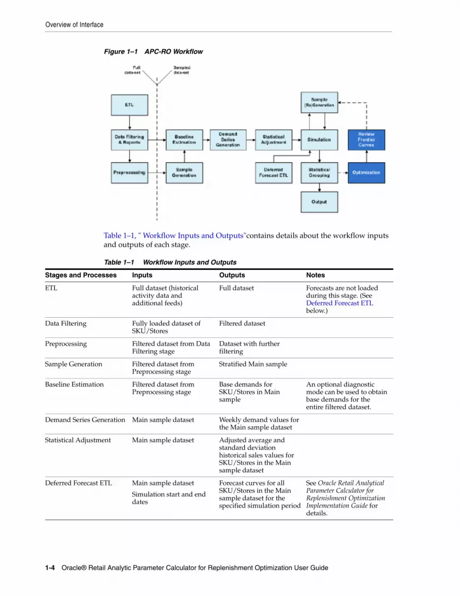
Figure 1–1, "APC-RO Workflow" provides a representation of the APC-RO workflow.
Note: With the exception of the optional Optimization stage, it is mandatory that you run each stage of APC-RO in the order indicated in the process train of the UI.
No stage can be run until the previous stage has completed. Stages cannot be run in parallel.
APC-RO state management enforces a strict workflow that prevents the user from skipping stages or initializing downstream stages when stages are re-run. If the database tables are directly modified, incorrect results or exceptions may occur.
When any stage of APC-RO is to be re-run, the user is informed that all the current data input, output, and temporary results will be deleted from all subsequent stages that had been part of the previous run. Once the user clicks OK, all the downstream data is deleted and the status of each of these subsequent stages is changed to Uninitialized. These stages will then need to be re-run as well.
Overview of Interface
1-4 Oracle® Retail Analytic Parameter Calculator for Replenishment Optimization User Guide
Figure 1–1 APC-RO Workflow
Table 1–1, " Workflow Inputs and Outputs"contains details about the workflow inputs and outputs of each stage.
Table 1–1 Workflow Inputs and Outputs
Stages and Processes Inputs Outputs Notes
ETL Full dataset (historical activity data and additional feeds)
Full dataset Forecasts are not loaded during this stage. (See Deferred Forecast ETL below.)
Data Filtering Fully loaded dataset of SKU/Stores
Filtered dataset
Preprocessing Filtered dataset from Data Filtering stage
Dataset with further filtering
Sample Generation Filtered dataset from Preprocessing stage
Stratified Main sample
Baseline Estimation Filtered dataset from Preprocessing stage
Base demands for SKU/Stores in Main sample
An optional diagnostic mode can be used to obtain base demands for the entire filtered dataset.
Demand Series Generation Main sample dataset Weekly demand values for the Main sample dataset
Statistical Adjustment Main sample dataset Adjusted average and standard deviation historical sales values for SKU/Stores in the Main sample dataset
Deferred Forecast ETL Main sample dataset
Simulation start and end dates
Forecast curves for all SKU/Stores in the Main sample dataset for the specified simulation period
See Oracle Retail Analytical Parameter Calculator for Replenishment Optimization Implementation Guide for details.
Features of the Stage Screens
Getting Started 1-5
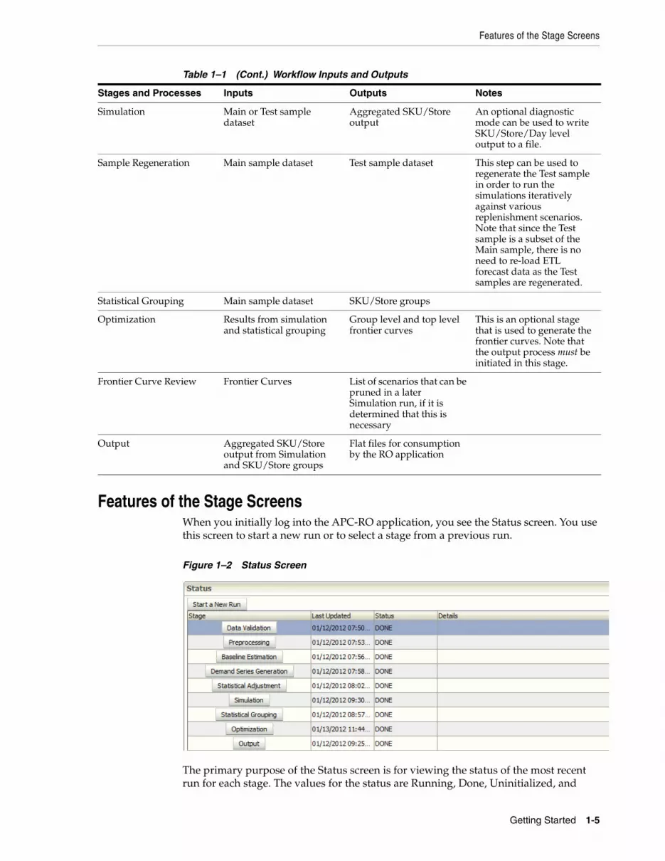
Features of the Stage ScreensWhen you initially log into the APC-RO application, you see the Status screen. You use this screen to start a new run or to select a stage from a previous run.
Figure 1–2 Status Screen
The primary purpose of the Status screen is for viewing the status of the most recent run for each stage. The values for the status are Running, Done, Uninitialized, and
Simulation Main or Test sample dataset
Aggregated SKU/Store output
An optional diagnostic mode can be used to write SKU/Store/Day level output to a file.
Sample Regeneration Main sample dataset Test sample dataset This step can be used to regenerate the Test sample in order to run the simulations iteratively against various replenishment scenarios. Note that since the Test sample is a subset of the Main sample, there is no need to re-load ETL forecast data as the Test samples are regenerated.
Statistical Grouping Main sample dataset SKU/Store groups
Optimization Results from simulation and statistical grouping
Group level and top level frontier curves
This is an optional stage that is used to generate the frontier curves. Note that the output process must be initiated in this stage.
Frontier Curve Review Frontier Curves List of scenarios that can be pruned in a later Simulation run, if it is determined that this is necessary
Output Aggregated SKU/Store output from Simulation and SKU/Store groups
Flat files for consumption by the RO application
Table 1–1 (Cont.) Workflow Inputs and Outputs
Stages and Processes Inputs Outputs Notes
Features of the Stage Screens
1-6 Oracle® Retail Analytic Parameter Calculator for Replenishment Optimization User Guide
Failed. Note that a status of Invalid indicates that the data for that stage has been deleted because an earlier stage has been re-run. (Whenever a stage is re-run, the data from all downstream stages is deleted and so the stages then need to be re-run.)
Once you click the Start a New Run button you see the Data Validation stage screen. The process names are displayed in the process train at the top of each stage screen.You can access any of the stages by clicking the name for that stage.
The Start a New Run button loads a set of default parameters from the application and deletes the current set of parameters as well as any customizations or previous changes. Because of this you should only use this button to start a new run. To continue an existing run you should use the stage buttons. When you select a stage button, the last set of parameters run by the application for the entire set of eight stages will be loaded.
The basic functionality of each stage screen is the same. Each stage provides parameters that can be configured. The default values for each parameter are listed and space is provided for user-supplied data. Many of the stages also contain grids that are used to define ranges of values for certain parameters.
Common ButtonsThe following buttons are used in the UI for actions such as navigation and application actions.
■ Add/Remove rows and columns – used in the grid configuration areas to add or remove rows and columns that are used to establish ranges of values to run the stage against.
■ Back – navigates back to the Data Validation stage screen from either the Data Validation Reports or the Data Validation Charts.
■ Buckets – used to enter values for the ranges.
■ Cleanup Intermediate Tables – if this box is checked, the information stored in the intermediate tables during the previous stage is discarded before each new stage is run. Only the information in the output tables is saved.
■ Draw Chart – renders the chart selected from the list of charts in the Data Validation Chart display.
■ Run – initiates the processing for the specific stage that a user is accessing. In the case of Data Validation, Baseline Estimation, Demand Series Generation, Preprocessing, Statistical Adjustment, Statistical Grouping, and Optimization, previously generated outputs are overwritten by re-running a stage. In the case of the Simulation stage, the output is appended to previous results.
■ Start a New Run – initiates the APC-RO process.
■ Status – navigates to the status chart in the initial screen.
■ View Data Validation Reports – provides access to reports.
■ View Data Validation Charts – provides access to charts.
■ View Filter Summary Reports – provides access to reports.
■ View Period Level Filter Summary Reports – provides access to period-level filter summaries for Data Validation and Preprocessing results.
■ View Iteration Histogram – provides access to the Baseline Estimation chart.
■ Show Service Level Histogram – provides access to the Simulation results chart.
Checking Your Browser Settings
Getting Started 1-7
■ Frontier Curve – plots inventory measure against sales measure for designated groups and scenarios.
■ Simulator Status Report – provides access to a report showing the status of the current Simulation run.
■ XML Load – re-loads a previously saved configuration.
■ XML Save – saves a configuration.
■ Logout
■ Help Link
Checking Your Browser SettingsAPC-RO is a Web-based application that is supported on Microsoft Internet Explorer version 7 and 8. Before using APC-RO, it is important to check your browser settings. This section describes the browser settings for both versions of Microsoft Internet Explorer.
Setting Up Internet Explorer 7Complete the following steps:
■ Configure Internet Explorer’s Security Settings—add the APC-RO URL to the appropriate zone (Local intranet or Trusted sites) to ensure that the APC-RO application will use the appropriate security settings. For more information, see Configuring Internet Explorer’s Security Settings.
Important: Do not use the Internet zone to configure browser settings for APC-RO. Use only the Local intranet zone or the Trusted sites zone, as explained in Adjusting Internet Explorer’s Language Settings.
■ Adjust Internet Explorer’s Language Settings—if you are using a different language on your computer, you can adjust Internet Explorer to also use the same language. For more information, see Adjusting Internet Explorer’s Language Settings.
■ Review Cache Settings—the default cache setting for Internet Explorer is Automatic, and normally these settings do not need to be adjusted. However, if you do want to check your cache settings, refer to Reviewing Internet Explorer’s Cache Settings.
Configuring Internet Explorer’s Security SettingsTo configure Internet Explorer for APC-RO:
1. Open Internet Explorer.
2. From the Tools menu, select Internet Options.
3. From the Internet Options dialog box, click the Security tab.
4. From the Security tab, click Local intranet, or, if you have been instructed to do so by your Systems Administrator, Trusted sites, and then click the Sites button.

Checking Your Browser Settings
1-8 Oracle® Retail Analytic Parameter Calculator for Replenishment Optimization User Guide
Figure 1–3 Internet Options Dialog Box
Important: Do not select Internet unless you have been instructed to do so by the administrator. In most cases, the APC-RO application will be available on your company’s intranet or on a Oracle Retail trusted site.
If you selected Local intranet, go to step 5. If you selected Trusted sites, go to step 6.
5. On the Local Intranet dialog box, click the Advanced button, as in the following example:
Figure 1–4 Local Intranet Dialog Box
6. On the resulting Local intranet or Trusted sites dialog box, add the APC-RO URL if it is not already listed.
Figure 1–5 Internet Explorer Trusted Sites
To do so, type the APC-RO URL in the Add this Web site to the zone text box. Click Add. When the URL appears in the Web sites list, click OK.
Checking Your Browser Settings
Getting Started 1-9
7. If the Local Intranet dialog box from step 5 is still open, click OK to close it.
8. Based on the selection your made in step 4, from the Security Tab of the Internet Options dialog box, select either Local intranet or Trusted sites. Click the Custom Level button.
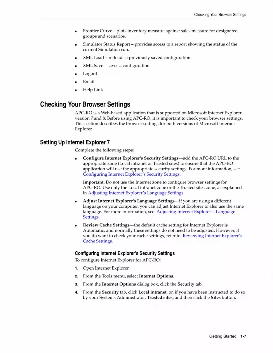
9. The Security Settings dialog box opens.
Figure 1–6 Internet Explorer Security Settings
10. Make sure the following commands are set to Prompt or Enable:
■ Download signed ActiveX controls
■ Run ActiveX controls and plug-ins
■ Script ActiveX controls marked safe for scripting
■ File download
■ Active scripting
■ Allow script–initiated windows without size or position constraints
■ Initialize and script ActiveX controls not marked as safe—a Microsoft ActiveX® control is required each time you export to Excel. While this ActiveX control is signed, it is not marked as safe (meaning that it could potentially be used to do unsafe things).
■ Click OK.
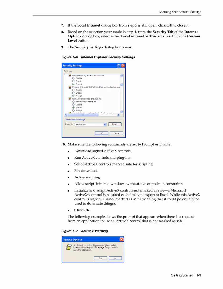
The following example shows the prompt that appears when there is a request from an application to use an ActiveX control that is not marked as safe.
Figure 1–7 Active X Warning
Checking Your Browser Settings
1-10 Oracle® Retail Analytic Parameter Calculator for Replenishment Optimization User Guide
11. On the Internet Options dialog box, click OK to return to the browser.
Adjusting Internet Explorer’s Language SettingsTo adjust the language settings for Internet Explorer, do the following:
1. From Internet Explorer, select Tools - Internet Options.
2. Click the Languages button located across the bottom of the window.
3. Click the Add button to add another language. Select your desired language from the list, and click OK.
4. To remove a language, click once onto a language from the list of existing languages, and click Remove.
5. Click OK to exit the Languages dialog box.
6. From the Internet Options window, click Apply to apply your changes. Click OK to exit.
Reviewing Internet Explorer’s Cache SettingsTo review Internet Explorer’s cache settings:
1. From the Tools menu, select Internet Options.
2. From the Internet Options dialog box, select the General tab.
3. From the Temporary Internet Files section of the screen., click the Settings button.
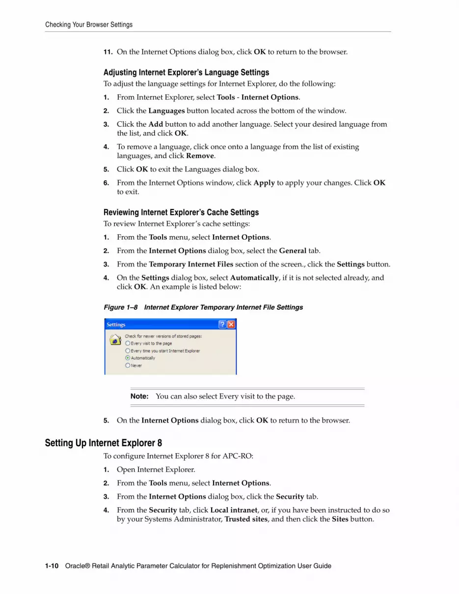
4. On the Settings dialog box, select Automatically, if it is not selected already, and click OK. An example is listed below:
Figure 1–8 Internet Explorer Temporary Internet File Settings
5. On the Internet Options dialog box, click OK to return to the browser.
Setting Up Internet Explorer 8To configure Internet Explorer 8 for APC-RO:
1. Open Internet Explorer.
2. From the Tools menu, select Internet Options.
3. From the Internet Options dialog box, click the Security tab.
4. From the Security tab, click Local intranet, or, if you have been instructed to do so by your Systems Administrator, Trusted sites, and then click the Sites button.
Note: You can also select Every visit to the page.
Login
Getting Started 1-11
If you selected Local intranet, go to step 5. If you selected Trusted sites, go to step 6.
5. On the Local Intranet dialog box, click the Advanced button.
6. On the resulting Local intranet or Trusted sites dialog box, add the APC-RO URL if it is not already listed.
To do so, type the APC-RO URL in the Add this Web site to the zone text box. Click Add. When the URL appears in the Web sites list, click OK.
7. If the Local Intranet dialog box from step 5 is still open, click OK to close it.
8. Based on the selection your made in step 4, from the Security Tab of the Internet Options dialog box, select either Local intranet or Trusted sites. Click the Custom Level button.
9. The Security Settings dialog box opens.
10. From the default Internet Explorer settings, ensure that the following options are set to Prompt or Enable:
■ Automatic prompting for ActiveX controls
■ Allow previously unused ActiveX controls to run without prompt
■ Allow script–initiated windows without size or position constraints
11. Ensure that the Only allow approved domains to use ActiveX without prompt option is set to Disable.
12. Click OK.
13. In case you have Pop-up Blocker enabled, add the host name from the APC-RO URL as an exception using the following steps:
a. On the Internet Options dialog box, click the Privacy tab.
b. On the Privacy tab, in the Pop-up Blocker section, click Settings.
c. On the Pop-up Blocker Settings dialog box, enter the host name in the Address of website to allow field, and click Add.
d. Click Close.
14. On the Internet Options dialog box, click OK to return to the browser.
LoginOnce APC-RO is installed, you can access the application using the following URL:
http://<SERVER>:<PORT>/apcro/faces/User/Status.jspx
To log into APC-RO, enter the user name and password assigned to you during the installation procedure. See the Oracle Retail Analytic Parameter Calculator for Replenishment Optimization Installation Guide for details.
Note: Do not select Internet unless you have been instructed to do so by the administrator. In most cases, the APC-RO application will be available on your company’s intranet or on a Oracle Retail trusted site.
Email Notification
1-12 Oracle® Retail Analytic Parameter Calculator for Replenishment Optimization User Guide
Email NotificationEmail notification can be accessed from a global link located in the header and footer of each page. The link triggers a pop-up that can be used to enter a comma-separated list of recipients to email.
After you have entered the list, click Okay to confirm the new list of email recipients. Click Cancel to undo any changes and preserve the old list.
Email notification should be configured once. The configuration persists in the database unless it is modified again.
Email addresses included in the list of recipients receive a status email when an APC-RO stage run completes or fails to complete. The status message includes a list of tasks successfully completed or the error message if the stage fails to complete.
2
Data Validation 2-1
2Data Validation
This chapter provides details about using the Data Validation stage of APC-RO. It contains the following sections:
■ Introduction
■ Data Aggregation
■ Data Validation Sub-Stages
■ Filters Not Available in the UI
■ Parameters
■ Time Divisions
■ Grid Filters
■ Data Validation Reports
■ Data Validation Charts
■ Data Validation Reports and Charts Terminology
■ Period Level Filter Summary Report
■ Output Tables
IntroductionThe Data Validation stage is used to:
■ Process SKU/Store-level item data or SKU/DC-level item data (indicated in the Current Location Level parameter).
■ Set the end date for the data window. The data window, as determined by the system, is either 52 weeks long or 104 weeks long and must be contained within the range of the historical data. The user is responsible for setting the end date only.
■ Filter out the items and locations for which the historical data in the data window is too unreliable to be used in the other APC-RO stages. For example, some historical data may contain weeks for which no information is available.
■ Provide summaries of the item and location data in a selection of tables and charts. This information can be used to adjust the data validation parameters.
The Data Validation stage removes the entire item/location, not just certain weeks for the item/location. The Preprocessing stage also filters data.
Data Aggregation
2-2 Oracle® Retail Analytic Parameter Calculator for Replenishment Optimization User Guide
Data AggregationThe historical data provided to APC-RO can be at either the daily or the weekly level. If the data is at daily level, it will be aggregated to weekly, according to the following criteria:
1. The value for the weekly sales is produced by summing the daily sales.
2. The end-of-week inventory is defined as the end-of-day inventory of the last day of data in the week.
3. The stock-out flag for the week is 1 if the last day of data in the week has a stock-out flag = 1. That is, any stock-outs that occurred earlier in the week for the aggregation are ignored.
Data Validation Sub-StagesThe Data Validation process consists of an ordered series of steps.
1. High-level summaries are generated for display. These include Data Validation Reports, Data Validation Charts, and a Period Level Summary Report. The summaries provided in this stage can be used to set parameters in some of the other sub-stages within the Data Validation stage.
2. The data is filtered based on the unit sales.
3. The data is filtered to account for sudden changes in inventory.
4. The data is filtered based on the maximum acceptable stock-out rate.
5. The item/locations that do not have inventory are filtered out. Then the item/locations that do not have weeks-on-hand falling within a defined range of values are filtered out.
6. The item/locations that do not meet the defined criteria for lead time, review frequencies, pack size, and presentation stock are filtered. Histogram displays are available for the frequencies values for these. Item/locations that have a value of 0/null for the unit price are also filtered out. Perishable item/locations with a value of 0 for the shelf life are filtered out.
7. Once this series of steps is complete,
■ The total number of active item/locations are provided as reports.
■ The distribution of various metrics are displayed as either grids or histograms.
■ A summary that shows how many item/locations have been filtered out is displayed as a grid.
■ The number of sales and inventory units removed during each period for each Data Validation filter is provided in a report.
Filters Not Available in the UIThe following table contains details for filters that cannot be adjusted using the parameters in the Data Validation stage. You can review the Filter Summary Report
Note: When any stage of APC-RO is re-run, the current data input, output, and temporary results will be deleted from all subsequent stages that were part of the previous run.
Parameters
Data Validation 2-3
and examine the number of item/locations that remain after each filter is applied. If too many items are removed by these filters, it may indicate that your input data should be modified.
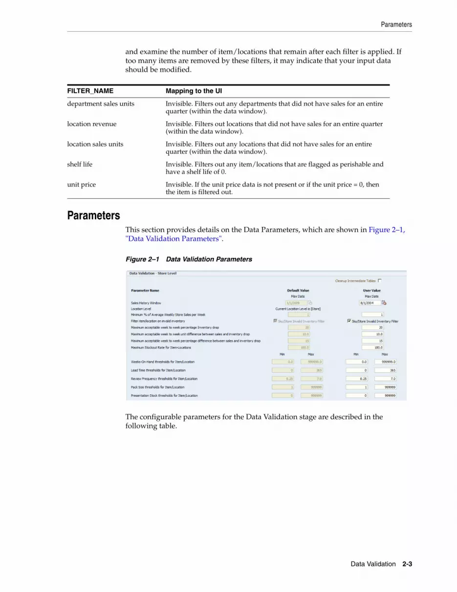
ParametersThis section provides details on the Data Parameters, which are shown in Figure 2–1, "Data Validation Parameters".
Figure 2–1 Data Validation Parameters
The configurable parameters for the Data Validation stage are described in the following table.
FILTER_NAME Mapping to the UI
department sales units Invisible. Filters out any departments that did not have sales for an entire quarter (within the data window).
location revenue Invisible. Filters out locations that did not have sales for an entire quarter (within the data window).
location sales units Invisible. Filters out any locations that did not have sales for an entire quarter (within the data window).
shelf life Invisible. Filters out any item/locations that are flagged as perishable and have a shelf life of 0.
unit price Invisible. If the unit price data is not present or if the unit price = 0, then the item is filtered out.
Parameters
2-4 Oracle® Retail Analytic Parameter Calculator for Replenishment Optimization User Guide
Table 2–1 Data Validation Parameters
Parameter Name Configuration Details
Sales History Window Use to set the end date of the Data Window. The Data Window is either 52 weeks long or 104 weeks long and must be contained within historical data. You can only set the end date. The system determines whether the window is 52 weeks long or 104 weeks long by taking the largest range completely contained by the historical data window, using the user-provided end date.
Location Level Used to indicate whether you are using APC-RO with Store data or with DC data. APC-RO has two schemas, one for store data and one for DC data. When you initially log in to the application, you log in with a Store ID or with a DC ID. The Stage title at the top of the screen indicates which of the two options you are using.
Minimum % of Average Weekly Store Sales per Week
Calculates the average weekly sales (total sales units over 52 or 104 weeks). Then, for each week, calculate sales units/average weekly sales units (expressed as a fraction). Every week must have sales units that are at least (value specified for parameter)% of average sales units.
Filter Item/Location on Invalid Inventory
Use this check box to enable the three filters that appear after this in the UI. If the box is not checked, then the three filters are bypassed. The filters are Maximum acceptable week-to-week percentage inventory drop, Maximum acceptable week-to-week unit difference between sales and inventory drop, and Maximum acceptable week-to-week percentage difference between sales and inventory drop. The item/location must pass all three filters.
Maximum acceptable week-to-week percentage inventory drop
Use this parameter to define a threshold filter for sudden decreases in inventory because of shrinkage (loss of inventory due to theft, loss, or expiration for perishable goods).
Maximum acceptable week-to-week unit difference between sales and inventory drop
Use this parameter to define a threshold filter for sudden decreases in inventory because of shrinkage (loss of inventory due to theft, loss, or expiration for perishable goods).
Maximum acceptable week-to-week percentage difference between sales and inventory drop
Use this parameter to define a threshold filter for sudden decreases in inventory because of shrinkage (loss of inventory due to theft, loss, or expiration for perishable goods).
Maximum Stock-out Rate of Item/Locations
Each week is associated with a stock-out flag. A stock-out flag with a value of 1 indicates that the last day of the week had a stock-out. The stock-out rate is calculated as Total # weeks with stock-out/Total # weeks (either 52 or 104). Each item/location must have a stock-out rate less than or equal to the user-defined parameter.
Weeks-On-Hand thresholds for Item/Location
A replenishment parameter whose filters specify a low and a high threshold for the weeks-on-hand value for the item/location.
Lead Time Thresholds for Item/Location
A replenishment parameter whose filters specify a low and a high value for the lead time threshold for the item/location.
Review Frequency Thresholds for Item/Location
A replenishment parameter whose filters specify a low and a high threshold for the review frequency value for the item/location.
Pack Size Thresholds for Item/Location
A replenishment parameter whose filters specify a low and a high threshold for the pack size value for the item/location.
Presentation Stock Thresholds for Item/Location
A replenishment parameter whose filters specify a low and a high threshold for the presentation stock value for the item/location. Note that Presentation Stock thresholds for the item/location filter are not applicable when the user has specified "DC" as the location level.
Grid Filters
Data Validation 2-5
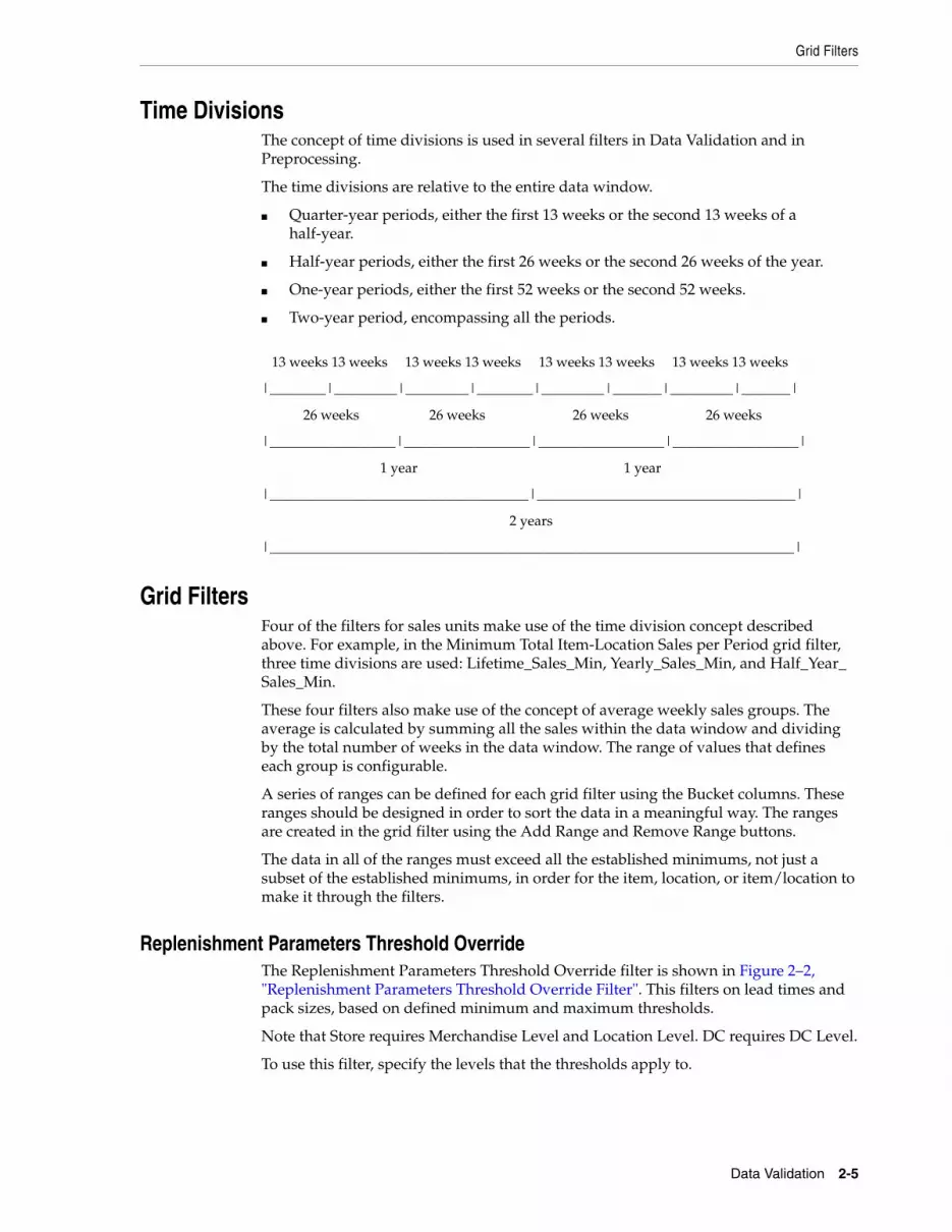
Time DivisionsThe concept of time divisions is used in several filters in Data Validation and in Preprocessing.
The time divisions are relative to the entire data window.
■ Quarter-year periods, either the first 13 weeks or the second 13 weeks of a half-year.
■ Half-year periods, either the first 26 weeks or the second 26 weeks of the year.
■ One-year periods, either the first 52 weeks or the second 52 weeks.
■ Two-year period, encompassing all the periods.
Grid FiltersFour of the filters for sales units make use of the time division concept described above. For example, in the Minimum Total Item-Location Sales per Period grid filter, three time divisions are used: Lifetime_Sales_Min, Yearly_Sales_Min, and Half_Year_Sales_Min.
These four filters also make use of the concept of average weekly sales groups. The average is calculated by summing all the sales within the data window and dividing by the total number of weeks in the data window. The range of values that defines each group is configurable.
A series of ranges can be defined for each grid filter using the Bucket columns. These ranges should be designed in order to sort the data in a meaningful way. The ranges are created in the grid filter using the Add Range and Remove Range buttons.
The data in all of the ranges must exceed all the established minimums, not just a subset of the established minimums, in order for the item, location, or item/location to make it through the filters.
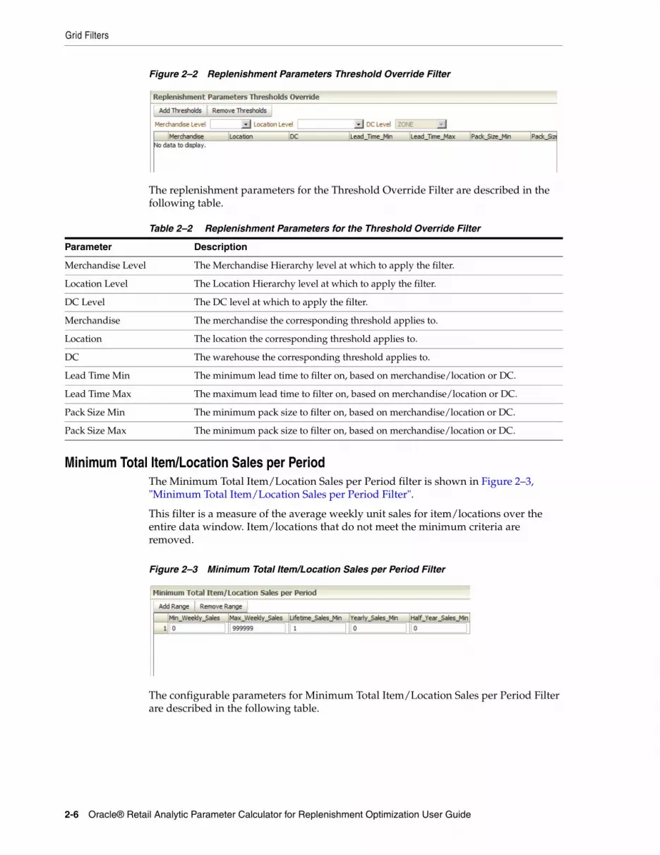
Replenishment Parameters Threshold OverrideThe Replenishment Parameters Threshold Override filter is shown in Figure 2–2, "Replenishment Parameters Threshold Override Filter". This filters on lead times and pack sizes, based on defined minimum and maximum thresholds.
Note that Store requires Merchandise Level and Location Level. DC requires DC Level.
To use this filter, specify the levels that the thresholds apply to.
13 weeks 13 weeks 13 weeks 13 weeks 13 weeks 13 weeks 13 weeks 13 weeks
|________|_________|_________|________|_________|_______|_________|_______|
26 weeks 26 weeks 26 weeks 26 weeks
|__________________|__________________|__________________|__________________|
1 year 1 year
|_____________________________________|_____________________________________|
2 years
|___________________________________________________________________________|
Grid Filters
2-6 Oracle® Retail Analytic Parameter Calculator for Replenishment Optimization User Guide
Figure 2–2 Replenishment Parameters Threshold Override Filter
The replenishment parameters for the Threshold Override Filter are described in the following table.
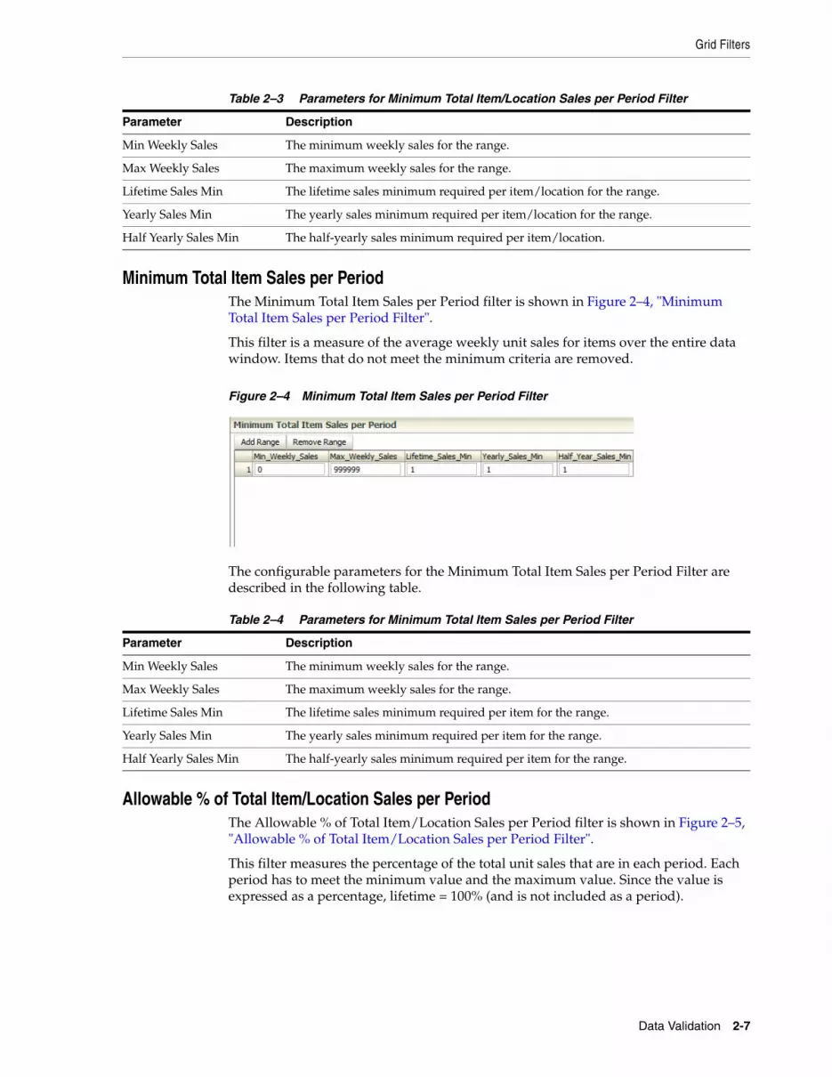
Minimum Total Item/Location Sales per PeriodThe Minimum Total Item/Location Sales per Period filter is shown in Figure 2–3, "Minimum Total Item/Location Sales per Period Filter".
This filter is a measure of the average weekly unit sales for item/locations over the entire data window. Item/locations that do not meet the minimum criteria are removed.
Figure 2–3 Minimum Total Item/Location Sales per Period Filter
The configurable parameters for Minimum Total Item/Location Sales per Period Filter are described in the following table.
Table 2–2 Replenishment Parameters for the Threshold Override Filter
Parameter Description
Merchandise Level The Merchandise Hierarchy level at which to apply the filter.
Location Level The Location Hierarchy level at which to apply the filter.
DC Level The DC level at which to apply the filter.
Merchandise The merchandise the corresponding threshold applies to.
Location The location the corresponding threshold applies to.
DC The warehouse the corresponding threshold applies to.
Lead Time Min The minimum lead time to filter on, based on merchandise/location or DC.
Lead Time Max The maximum lead time to filter on, based on merchandise/location or DC.
Pack Size Min The minimum pack size to filter on, based on merchandise/location or DC.
Pack Size Max The minimum pack size to filter on, based on merchandise/location or DC.
Grid Filters
Data Validation 2-7
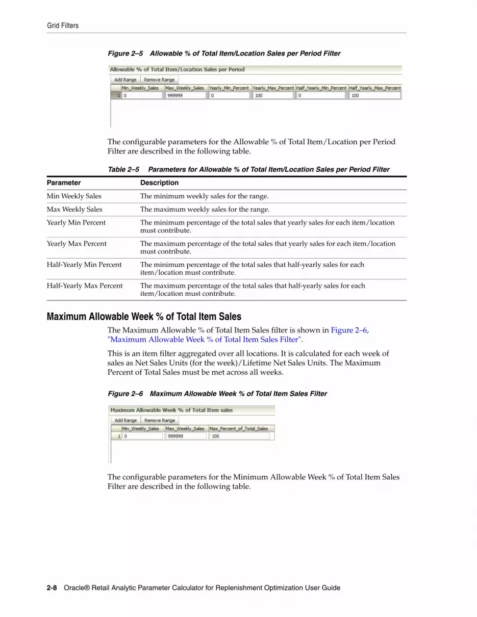
Minimum Total Item Sales per PeriodThe Minimum Total Item Sales per Period filter is shown in Figure 2–4, "Minimum Total Item Sales per Period Filter".
This filter is a measure of the average weekly unit sales for items over the entire data window. Items that do not meet the minimum criteria are removed.
Figure 2–4 Minimum Total Item Sales per Period Filter
The configurable parameters for the Minimum Total Item Sales per Period Filter are described in the following table.
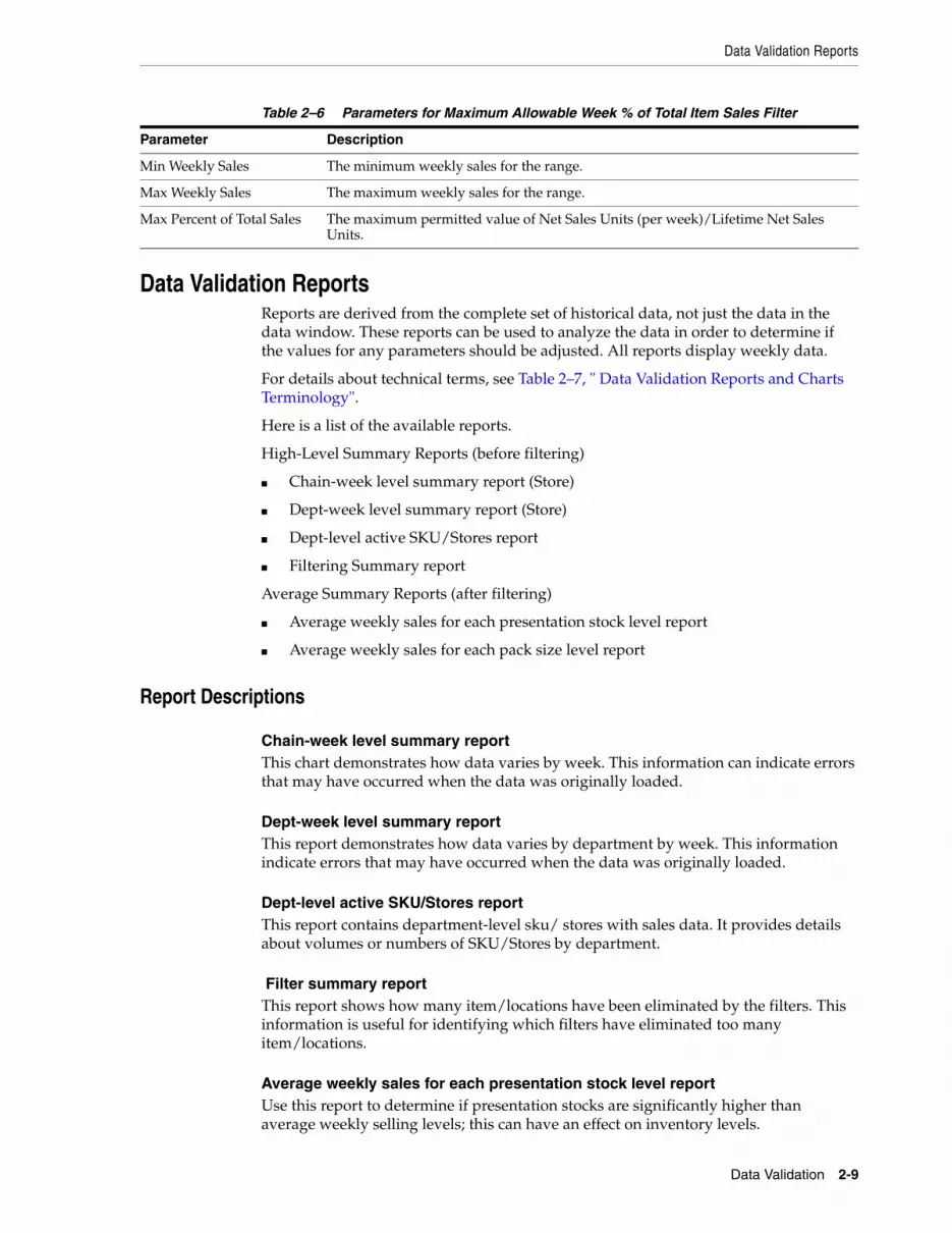
Allowable % of Total Item/Location Sales per PeriodThe Allowable % of Total Item/Location Sales per Period filter is shown in Figure 2–5, "Allowable % of Total Item/Location Sales per Period Filter".
This filter measures the percentage of the total unit sales that are in each period. Each period has to meet the minimum value and the maximum value. Since the value is expressed as a percentage, lifetime = 100% (and is not included as a period).
Table 2–3 Parameters for Minimum Total Item/Location Sales per Period Filter
Parameter Description
Min Weekly Sales The minimum weekly sales for the range.
Max Weekly Sales The maximum weekly sales for the range.
Lifetime Sales Min The lifetime sales minimum required per item/location for the range.
Yearly Sales Min The yearly sales minimum required per item/location for the range.
Half Yearly Sales Min The half-yearly sales minimum required per item/location.
Table 2–4 Parameters for Minimum Total Item Sales per Period Filter
Parameter Description
Min Weekly Sales The minimum weekly sales for the range.
Max Weekly Sales The maximum weekly sales for the range.
Lifetime Sales Min The lifetime sales minimum required per item for the range.
Yearly Sales Min The yearly sales minimum required per item for the range.
Half Yearly Sales Min The half-yearly sales minimum required per item for the range.
Grid Filters
2-8 Oracle® Retail Analytic Parameter Calculator for Replenishment Optimization User Guide
Figure 2–5 Allowable % of Total Item/Location Sales per Period Filter
The configurable parameters for the Allowable % of Total Item/Location per Period Filter are described in the following table.
Maximum Allowable Week % of Total Item SalesThe Maximum Allowable % of Total Item Sales filter is shown in Figure 2–6, "Maximum Allowable Week % of Total Item Sales Filter".
This is an item filter aggregated over all locations. It is calculated for each week of sales as Net Sales Units (for the week)/Lifetime Net Sales Units. The Maximum Percent of Total Sales must be met across all weeks.
Figure 2–6 Maximum Allowable Week % of Total Item Sales Filter
The configurable parameters for the Minimum Allowable Week % of Total Item Sales Filter are described in the following table.
Table 2–5 Parameters for Allowable % of Total Item/Location Sales per Period Filter
Parameter Description
Min Weekly Sales The minimum weekly sales for the range.
Max Weekly Sales The maximum weekly sales for the range.
Yearly Min Percent The minimum percentage of the total sales that yearly sales for each item/location must contribute.
Yearly Max Percent The maximum percentage of the total sales that yearly sales for each item/location must contribute.
Half-Yearly Min Percent The minimum percentage of the total sales that half-yearly sales for each item/location must contribute.
Half-Yearly Max Percent The maximum percentage of the total sales that half-yearly sales for each item/location must contribute.
Data Validation Reports
Data Validation 2-9
Data Validation ReportsReports are derived from the complete set of historical data, not just the data in the data window. These reports can be used to analyze the data in order to determine if the values for any parameters should be adjusted. All reports display weekly data.
For details about technical terms, see Table 2–7, " Data Validation Reports and Charts Terminology".
Here is a list of the available reports.
High-Level Summary Reports (before filtering)
■ Chain-week level summary report (Store)
■ Dept-week level summary report (Store)
■ Dept-level active SKU/Stores report
■ Filtering Summary report
Average Summary Reports (after filtering)
■ Average weekly sales for each presentation stock level report
■ Average weekly sales for each pack size level report
Report Descriptions
Chain-week level summary reportThis chart demonstrates how data varies by week. This information can indicate errors that may have occurred when the data was originally loaded.
Dept-week level summary reportThis report demonstrates how data varies by department by week. This information indicate errors that may have occurred when the data was originally loaded.
Dept-level active SKU/Stores reportThis report contains department-level sku/ stores with sales data. It provides details about volumes or numbers of SKU/Stores by department.
Filter summary reportThis report shows how many item/locations have been eliminated by the filters. This information is useful for identifying which filters have eliminated too many item/locations.
Average weekly sales for each presentation stock level reportUse this report to determine if presentation stocks are significantly higher than average weekly selling levels; this can have an effect on inventory levels.
Table 2–6 Parameters for Maximum Allowable Week % of Total Item Sales Filter
Parameter Description
Min Weekly Sales The minimum weekly sales for the range.
Max Weekly Sales The maximum weekly sales for the range.
Max Percent of Total Sales The maximum permitted value of Net Sales Units (per week)/Lifetime Net Sales Units.

Data Validation Charts
2-10 Oracle® Retail Analytic Parameter Calculator for Replenishment Optimization User Guide
Average weekly sales for each pack size level reportUse this to determine if pack sizes are significantly higher than average weekly selling levels; this can have an effect on inventory levels.
Data Validation ChartsCharts are derived from the complete set of historical data, not just the data in the data window. All the charts display weekly data.
For details about technical terms, see Table 2–7, " Data Validation Reports and Charts Terminology".
Here is a list of the available charts. Each chart displays a histogram of the frequency distribution for the indicated parameter.
Frequency Distributions (before filtering)
■ Frequency distribution of average weekly sales chart
■ Frequency distribution of lead times chart
■ Frequency distribution of review frequencies chart
■ Frequency distribution of pack sizes chart
■ Frequency distribution of presentation stocks chart
■ Frequency distribution of stock-out rates chart
■ Frequency distribution of weeks on hand chart
Frequency Distributions (after filtering)
■ Frequency distribution of average weekly sales chart
■ Frequency distribution of ratio of year 1/2 sales chart
Bucket widths are used to define the size of the groups used to calculate the chart metrics. For example, a bucket width of 1 results in chart buckets of 0, 1, 2, 3..., while a bucket width of 5 results in buckets of 0, 5, 10, 15....
In addition, note these details about the following computations:
The average weekly sales for each item/location is computed for data within the data window, and then a frequency distribution of the averages is produced. (Count the number of item/locations that fall into each bucket. The size of the bucket is configurable in the UI.)
The ratio of total item/location year-one sales to year-two sales is computed for each item/location. A frequency distribution of the ratios is produced. (Count the number of item/locations that have a ratio within a particular range. If the data window is only 52 weeks, then this histogram is not available.)
Chart Descriptions
Frequency distribution of average weekly sales chartThis information can help determine the distribution of demand, which can be used to set thresholds in the Data Validation and Preprocessing stages.
Frequency distribution of lead times chartThis information can be used to set thresholds in the Data Validation and Preprocessing stages. It can also be used to analyze the data.
Data Validation Reports and Charts Terminology
Data Validation 2-11
Frequency distribution of review frequencies chartThis information can be used to set thresholds in the Data Validation and Preprocessing stages. It can also be used to analyze the data.
Frequency distribution of pack sizes chartThis information can be used to set thresholds in the Data Validation and Preprocessing stages. It can also be used to analyze the data.
Frequency distribution of presentation stocks chartThis information can be used to set thresholds in the Data Validation and Preprocessing stages. It can also be used to analyze the data.
Frequency distribution of stock-out rates chartThe item/location stock-out rate is defined as the number of weeks with stock-outs/total number of weeks for the item/location.
Frequency distribution of weeks on hand chartThis chart shows the frequency after filtering the ratio of the item/location year-one sales to the year-two sales for each item/location.
Frequency distribution of average weekly sales chartThis chart shows the frequency distribution after filtering the item/location average weekly sales.
Frequency distribution of ratio of year 1/2 sales chartThis chart is only used for data windows larger than 52 weeks. It shows the frequency distribution after filtering the ratio of the total item/location year-one sales to year- two sales computed for each item/location.
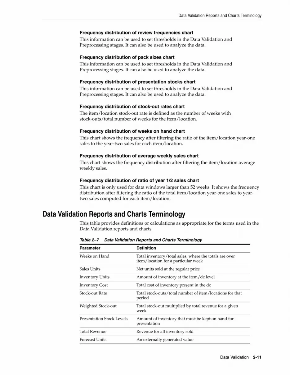
Data Validation Reports and Charts TerminologyThis table provides definitions or calculations as appropriate for the terms used in the Data Validation reports and charts.
Table 2–7 Data Validation Reports and Charts Terminology
Parameter Definition
Weeks on Hand Total inventory/total sales, where the totals are over item/location for a particular week
Sales Units Net units sold at the regular price
Inventory Units Amount of inventory at the item/dc level
Inventory Cost Total cost of inventory present in the dc
Stock-out Rate Total stock-outs/total number of item/locations for that period
Weighted Stock-out Total stock-out multiplied by total revenue for a given week
Presentation Stock Levels Amount of inventory that must be kept on hand for presentation
Total Revenue Revenue for all inventory sold
Forecast Units An externally generated value

Period Level Filter Summary Report
2-12 Oracle® Retail Analytic Parameter Calculator for Replenishment Optimization User Guide
Period Level Filter Summary ReportThis report, accessed via the View Period-Level Filter Summary button, shows how many sales and inventory units have been removed during each period for each filter that was run in the Data Validation stage. To control which filters are displayed in the graph, select the appropriate check boxes in the table to the right and then click Redraw Filter Summary. This report is shown in Figure 2–7, "Data Validation Period Level Filter Summary".
Figure 2–7 Data Validation Period Level Filter Summary
Output TablesThe following are the key output tables for the Data Validation stage. Use these tables to review the results of this stage.
■ RO_DF_WINDOW_SUBDIVIDED
■ RO_FILTERED_WEEKLY_DATA
■ RO_FILTERED_ITEM_LOC_FACT
Note that these output tables are not created during installation. Instead, they are created once the Data Validation stage has been run to completion at least once. So the output tables do not exist in the database schema until after the Data Validation stage has been run once.
Average Weekly Sales Total weekly sales divided by either 52 or 104
Pack Size Level The bucketing of pack sizes
Active Item SKU/store that has any positive non-zero sales
Table 2–7 (Cont.) Data Validation Reports and Charts Terminology
Parameter Definition
3
Preprocessing 3-1
3Preprocessing
This chapter provides details about using the Preprocessing stage of APC-RO. It contains the following sections:
■ Introduction
■ Data Requirements and Restrictions
■ Preprocessing Filters
■ Main Sample Setup
■ Acceptable Weeks-on-Hand Filtering
■ Sales Units Filtering
■ Sales Pattern Filtering
■ Stock-out Filtering
■ Filter Reports
■ Output Tables
IntroductionData is initially filtered during the Data Validation stage. Additional filtering then occurs during the Preprocessing stage. This filtering is used to define the acceptable range of data, based on configurable criteria. Optional criteria for stock-out levels and the weeks-on-hand range can be applied.
The preprocessing filters are:
■ Invalid sales units
■ Invalid sales patterns
■ Invalid stock-out patterns
■ Invalid weeks-on-hand levels
The Main sample dataset, which is used in the Simulation stage, is generated.
All stages after the Preprocessing stage use only the item/locations of the Main sample dataset.
The input data for the Preprocessing stage must be weekly. If daily input data is provided, it will be aggregated.
Data Requirements and Restrictions
3-2 Oracle® Retail Analytic Parameter Calculator for Replenishment Optimization User Guide
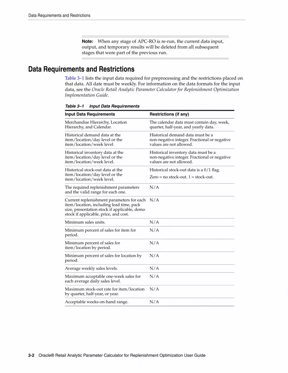
Data Requirements and RestrictionsTable 3–1 lists the input data required for preprocessing and the restrictions placed on that data. All date must be weekly. For information on the data formats for the input data, see the Oracle Retail Analytic Parameter Calculator for Replenishment Optimization Implementation Guide.
Note: When any stage of APC-RO is re-run, the current data input, output, and temporary results will be deleted from all subsequent stages that were part of the previous run.
Table 3–1 Input Data Requirements
Input Data Requirements Restrictions (if any)
Merchandise Hierarchy, Location Hierarchy, and Calendar.
The calendar data must contain day, week, quarter, half-year, and yearly data.
Historical demand data at the item/location/day level or the item/location/week level.
Historical demand data must be a non-negative integer. Fractional or negative values are not allowed.
Historical inventory data at the item/location/day level or the item/location/week level.
Historical inventory data must be a non-negative integer. Fractional or negative values are not allowed.
Historical stock-out data at the item/location/day level or the item/location/week level.
Historical stock-out data is a 0/1 flag.
Zero = no stock-out. 1 = stock-out.
The required replenishment parameters and the valid range for each one.
N/A
Current replenishment parameters for each item/location, including lead time, pack size, presentation stock if applicable, demo stock if applicable, price, and cost.
N/A
Minimum sales units. N/A
Minimum percent of sales for item for period.
N/A
Minimum percent of sales for item/location by period.
N/A
Minimum percent of sales for location by period.
N/A
Average weekly sales levels. N/A
Maximum acceptable one-week sales for each average daily sales level.
N/A
Maximum stock-out rate for item/location by quarter, half-year, or year.
N/A
Acceptable weeks-on-hand range. N/A
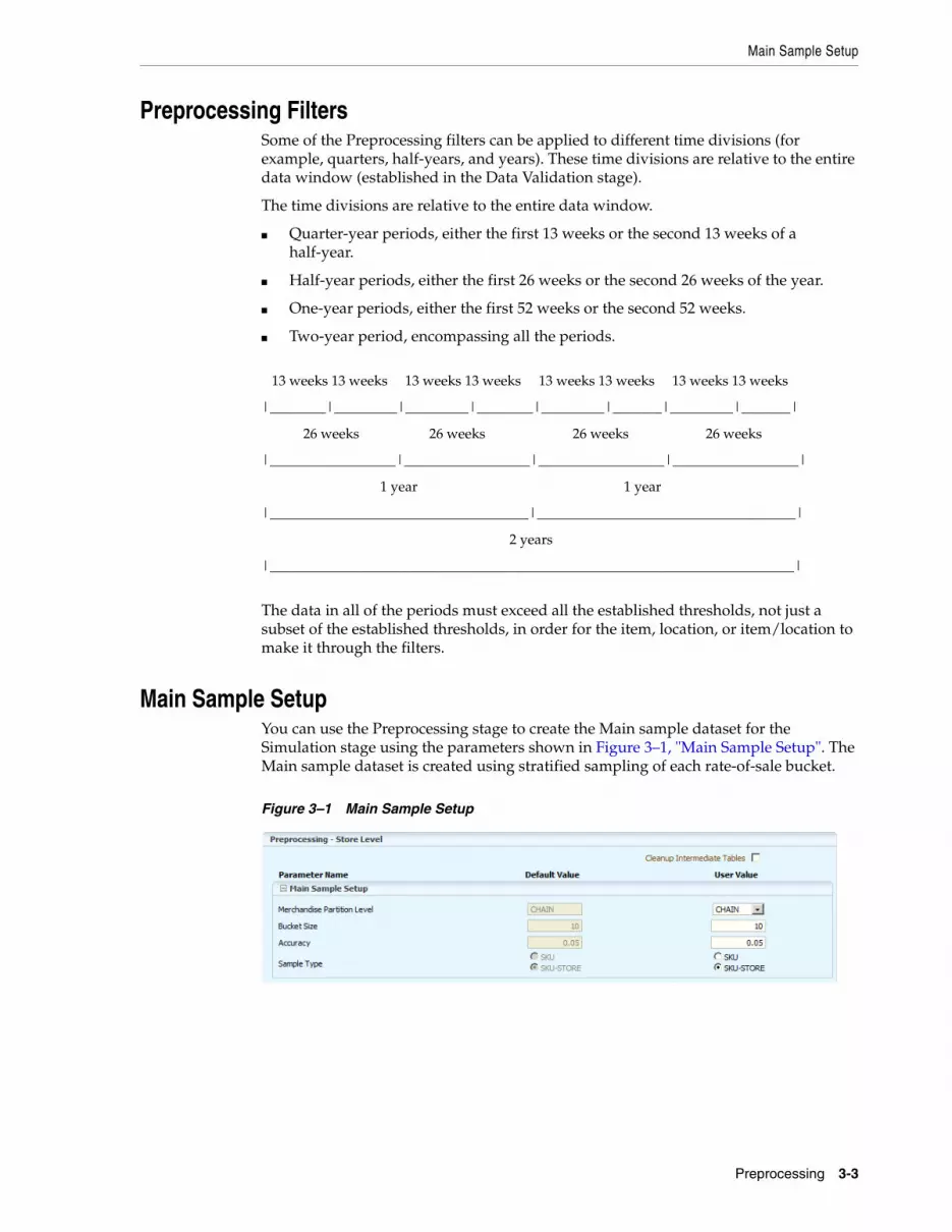
Main Sample Setup
Preprocessing 3-3
Preprocessing FiltersSome of the Preprocessing filters can be applied to different time divisions (for example, quarters, half-years, and years). These time divisions are relative to the entire data window (established in the Data Validation stage).
The time divisions are relative to the entire data window.
■ Quarter-year periods, either the first 13 weeks or the second 13 weeks of a half-year.
■ Half-year periods, either the first 26 weeks or the second 26 weeks of the year.
■ One-year periods, either the first 52 weeks or the second 52 weeks.
■ Two-year period, encompassing all the periods.
The data in all of the periods must exceed all the established thresholds, not just a subset of the established thresholds, in order for the item, location, or item/location to make it through the filters.
Main Sample SetupYou can use the Preprocessing stage to create the Main sample dataset for the Simulation stage using the parameters shown in Figure 3–1, "Main Sample Setup". The Main sample dataset is created using stratified sampling of each rate-of-sale bucket.
Figure 3–1 Main Sample Setup
13 weeks 13 weeks 13 weeks 13 weeks 13 weeks 13 weeks 13 weeks 13 weeks
|________|_________|_________|________|_________|_______|_________|_______|
26 weeks 26 weeks 26 weeks 26 weeks
|__________________|__________________|__________________|__________________|
1 year 1 year
|_____________________________________|_____________________________________|
2 years
|___________________________________________________________________________|
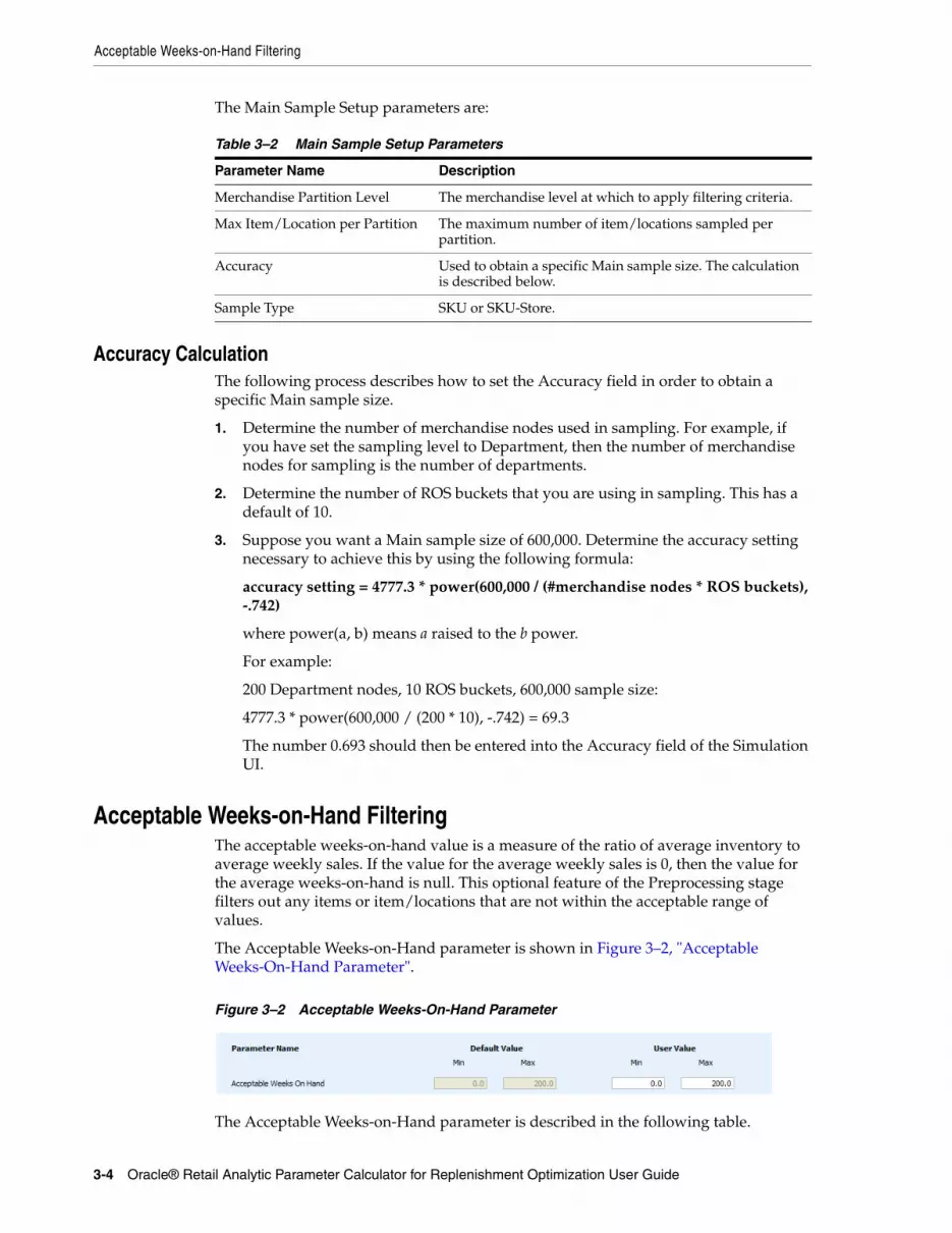
Acceptable Weeks-on-Hand Filtering
3-4 Oracle® Retail Analytic Parameter Calculator for Replenishment Optimization User Guide
The Main Sample Setup parameters are:
Accuracy CalculationThe following process describes how to set the Accuracy field in order to obtain a specific Main sample size.
1. Determine the number of merchandise nodes used in sampling. For example, if you have set the sampling level to Department, then the number of merchandise nodes for sampling is the number of departments.
2. Determine the number of ROS buckets that you are using in sampling. This has a default of 10.
3. Suppose you want a Main sample size of 600,000. Determine the accuracy setting necessary to achieve this by using the following formula:
accuracy setting = 4777.3 * power(600,000 / (#merchandise nodes * ROS buckets), -.742)
where power(a, b) means a raised to the b power.
For example:
200 Department nodes, 10 ROS buckets, 600,000 sample size:
4777.3 * power(600,000 / (200 * 10), -.742) = 69.3
The number 0.693 should then be entered into the Accuracy field of the Simulation UI.
Acceptable Weeks-on-Hand FilteringThe acceptable weeks-on-hand value is a measure of the ratio of average inventory to average weekly sales. If the value for the average weekly sales is 0, then the value for the average weeks-on-hand is null. This optional feature of the Preprocessing stage filters out any items or item/locations that are not within the acceptable range of values.
The Acceptable Weeks-on-Hand parameter is shown in Figure 3–2, "Acceptable Weeks-On-Hand Parameter".
Figure 3–2 Acceptable Weeks-On-Hand Parameter
The Acceptable Weeks-on-Hand parameter is described in the following table.
Table 3–2 Main Sample Setup Parameters
Parameter Name Description
Merchandise Partition Level The merchandise level at which to apply filtering criteria.
Max Item/Location per Partition The maximum number of item/locations sampled per partition.
Accuracy Used to obtain a specific Main sample size. The calculation is described below.
Sample Type SKU or SKU-Store.

Sales Pattern Filtering
Preprocessing 3-5
Sales Units FilteringThe Preprocessing stage filters the sales units that do not meet the defined values for minimum sales units in any quarter, half-year, of year. This filtering eliminates outlier data and data with limited or uneven history. This filter operates at the item level.
The Minimum Sales Units per Period filter, shown in Figure 3–3, "Minimum Sales Units per Period Filter", eliminates sales units that do not meet the minimum requirements for sales units in any quarter year, half year, or full year in the window you define here. The upper bound is two years.
Figure 3–3 Minimum Sales Units per Period Filter
The Minimum Sales Units per Period Filter parameters are described in the following table.
Sales Pattern FilteringThe Preprocessing stage filters the percentage share of sales for quarter, half-year, and yearly period that fall between the defined minimum and maximum values of a range. Separate filters are used for items, shown in Figure 3–4, "Percent Range of Item Sales per Period Filter", item/locations, shown in Figure 3–5, "Percent Range of
Table 3–3 Weeks-on-Hand Parameter
Parameter Description
Acceptable Weeks on Hand Min
A measure of the ratio of average inventory to average weekly sales. If the value for the average weekly sales is 0, then the value for the average weeks-on-hand is null. Item/locations below the minimum will be filtered out.
Acceptable Weeks on Hand Max
A measure of the ratio of average inventory to average weekly sales. If the value for the average weekly sales is 0, then the value for the average weeks-on-hand is null. Item/locations above the maximum will be filtered out.
Table 3–4 Minimum Sales Units per Period Parameters
Parameter Description
Annual Minimum Sales Units for First Year, Second Year (Full Years, Half Years, Quarters)
These parameters filter out items whose sales units do not meet defined minimums for the year, half-year, and quarter. The upper bound is two years. They remove outlier data and data with limited or uneven history.
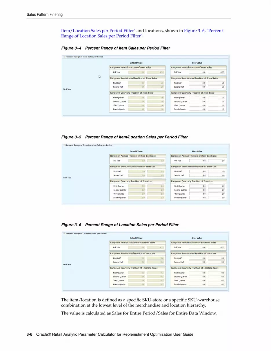
Sales Pattern Filtering
3-6 Oracle® Retail Analytic Parameter Calculator for Replenishment Optimization User Guide
Item/Location Sales per Period Filter" and locations, shown in Figure 3–6, "Percent Range of Location Sales per Period Filter".
Figure 3–4 Percent Range of Item Sales per Period Filter
Figure 3–5 Percent Range of Item/Location Sales per Period Filter
Figure 3–6 Percent Range of Location Sales per Period Filter
The item/location is defined as a specific SKU-store or a specific SKU-warehouse combination at the lowest level of the merchandise and location hierarchy.
The value is calculated as Sales for Entire Period/Sales for Entire Data Window.
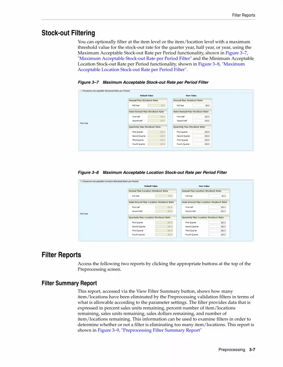
Filter Reports
Preprocessing 3-7
Stock-out FilteringYou can optionally filter at the item level or the item/location level with a maximum threshold value for the stock-out rate for the quarter year, half year, or year, using the Maximum Acceptable Stock-out Rate per Period functionality, shown in Figure 3–7, "Maximum Acceptable Stock-out Rate per Period Filter" and the Minimum Acceptable Location Stock-out Rate per Period functionality, shown in Figure 3–8, "Maximum Acceptable Location Stock-out Rate per Period Filter".
Figure 3–7 Maximum Acceptable Stock-out Rate per Period Filter
Figure 3–8 Maximum Acceptable Location Stock-out Rate per Period Filter
Filter ReportsAccess the following two reports by clicking the appropriate buttons at the top of the Preprocessing screen.
Filter Summary ReportThis report, accessed via the View Filter Summary button, shows how many item/locations have been eliminated by the Preprocessing validation filters in terms of what is allowable according to the parameter settings. The filter provides data that is expressed in percent sales units remaining, percent number of item/locations remaining, sales units remaining, sales dollars remaining, and number of item/locations remaining. This information can be used to examine filters in order to determine whether or not a filter is eliminating too many item/locations. This report is shown in Figure 3–9, "Preprocessing Filter Summary Report"
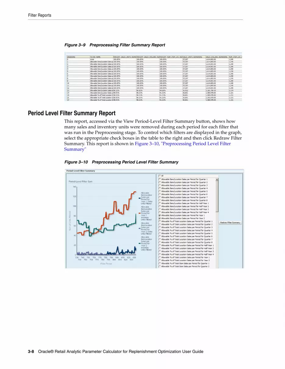
Filter Reports
3-8 Oracle® Retail Analytic Parameter Calculator for Replenishment Optimization User Guide
Figure 3–9 Preprocessing Filter Summary Report
Period Level Filter Summary ReportThis report, accessed via the View Period-Level Filter Summary button, shows how many sales and inventory units were removed during each period for each filter that was run in the Preprocessing stage. To control which filters are displayed in the graph, select the appropriate check boxes in the table to the right and then click Redraw Filter Summary. This report is shown in Figure 3–10, "Preprocessing Period Level Filter Summary"
Figure 3–10 Preprocessing Period Level Filter Summary
Output Tables
Preprocessing 3-9
Output TablesThe following are the key output tables for the Preprocessing stage. Use these tables to review the results of this stage.
■ RO_FILTER_FINAL
■ RO_SAMPLES
Note that these output tables are not created during installation. Instead, they are created once the Preprocessing stage has been run to completion at least once. So the output tables do not exist in the database schema until after the Preprocessing stage has been run once.

Output Tables
3-10 Oracle® Retail Analytic Parameter Calculator for Replenishment Optimization User Guide
4
Baseline Estimation 4-1
4Baseline Estimation
This chapter provides details about using the Baseline Estimation stage of APC-RO. It contains the following sections:
■ Introduction
■ Baseline Estimation Calculation
■ Baseline Estimation Histogram
■ Output Tables
IntroductionBaseline sales are defined as sales that would have occurred historically if there had been sufficient inventory to prevent stock-outs, since stock-outs decrease sales. In addition to stock-outs, the baseline estimation also removes increases in sales resulting from a price cut or a promotion.
The Baseline Estimation stage can take as input either daily-level data or weekly-level data. Unlike Data Filtering, if the data is at daily level, Baseline Estimation does not aggregate it to weekly. If the data is at daily level, Baseline Estimation uses it directly.
Because Baseline Estimation can work with either daily or weekly data, the word "period" in what follows will be used to denote "day or week as dictated by the input data."
When there are stock-outs, the sales units are less than the demand. If the application did not correct for the stock-outs, simulation on the item/location would be simulating replenishment for the case in which sales are less than they should have been. The replenishment parameters might perpetuate stock-outs in the future.
Lost sales are sales lost at the item/location level during a given period as a result of a stock-out. Since replenishment occurs at the item/location level and the simulation is also done at the same level, the Baseline Estimation stage corrects for stock-outs at the item/location level. It first calculates a seasonality curve at a configurable higher level in the merchandise/location hierarchy. It then iteratively uses the seasonality curve and the average sales to obtain a better estimate of the lost sales, which in turn changes the average sales. In this manner, it continues to improve the estimate of the lost sales until it achieves convergence.
For the calculation of seasonality curves, Baseline Estimation uses all data that passed the Data Filtering stage. However, Baseline Estimation only calculates lost sales for those item/locations that are in the Main sample set, because only the item/locations in the Main sample set will go through the simulator.
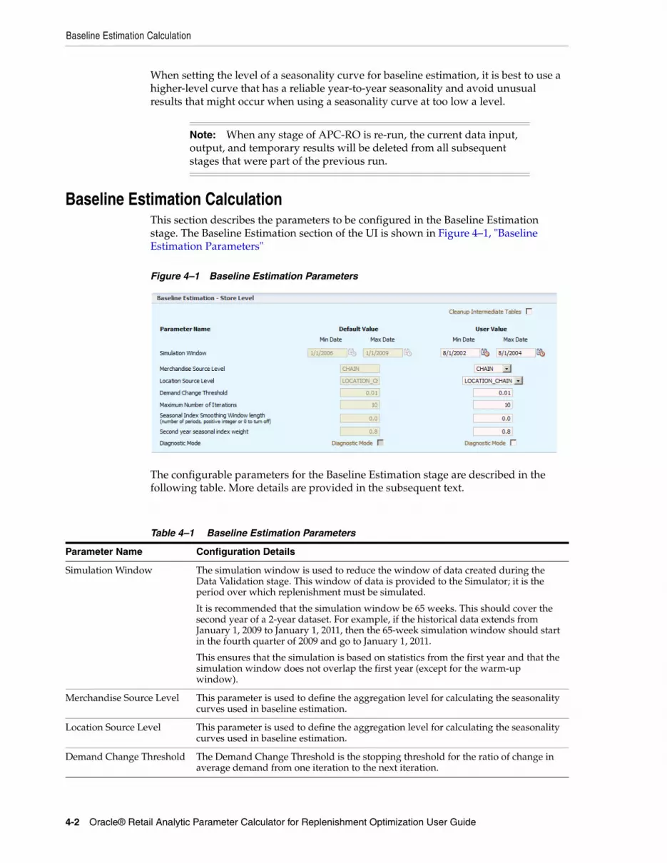
Baseline Estimation Calculation
4-2 Oracle® Retail Analytic Parameter Calculator for Replenishment Optimization User Guide
When setting the level of a seasonality curve for baseline estimation, it is best to use a higher-level curve that has a reliable year-to-year seasonality and avoid unusual results that might occur when using a seasonality curve at too low a level.
Baseline Estimation CalculationThis section describes the parameters to be configured in the Baseline Estimation stage. The Baseline Estimation section of the UI is shown in Figure 4–1, "Baseline Estimation Parameters"
Figure 4–1 Baseline Estimation Parameters
The configurable parameters for the Baseline Estimation stage are described in the following table. More details are provided in the subsequent text.
Note: When any stage of APC-RO is re-run, the current data input, output, and temporary results will be deleted from all subsequent stages that were part of the previous run.
Table 4–1 Baseline Estimation Parameters
Parameter Name Configuration Details
Simulation Window The simulation window is used to reduce the window of data created during the Data Validation stage. This window of data is provided to the Simulator; it is the period over which replenishment must be simulated.
It is recommended that the simulation window be 65 weeks. This should cover the second year of a 2-year dataset. For example, if the historical data extends from January 1, 2009 to January 1, 2011, then the 65-week simulation window should start in the fourth quarter of 2009 and go to January 1, 2011.
This ensures that the simulation is based on statistics from the first year and that the simulation window does not overlap the first year (except for the warm-up window).
Merchandise Source Level This parameter is used to define the aggregation level for calculating the seasonality curves used in baseline estimation.
Location Source Level This parameter is used to define the aggregation level for calculating the seasonality curves used in baseline estimation.
Demand Change Threshold The Demand Change Threshold is the stopping threshold for the ratio of change in average demand from one iteration to the next iteration.
Baseline Estimation Calculation
Baseline Estimation 4-3
Simulation WindowThe simulation window is used to reduce the window of data created during the Data Validation stage. This window of data is provided to the Simulator; it is the interval of time over which replenishment must be simulated. The simulation window must be a single uninterrupted interval of time and must lie within the Data Window produced in the Data Validation stage. Baseline Estimation corrects for stock-outs only in the simulation window because other periods are not used in the simulation.
It is recommended that the simulation window be 65 weeks. This should cover the second year of a 2-year dataset. For example, if the historical data extends from January 1, 2009 to January 1, 2011, then the 65-week simulation window should start in the fourth quarter of 2009 and go to January 1, 2011.
This ensures that the simulation is based on statistics from the first year and that the simulation window does not overlap the first year (except for the warm-up window).
Merchandise Source Level and Location Source LevelThese parameters are used to define the aggregation level for calculating the seasonality curves used in Baseline Estimation. The aggregation level of input data must be above the item/location level. In determining these aggregation levels, a level should be chosen that is high enough to determine a reliable seasonality pattern and low enough to be representative of the specified item's behavior.
The aggregation level selected should be a higher level and that has reliable year-to-year seasonality.
Seasonality Curve Calculation (Seasonal Index Smoothing Window Length and Second Year Seasonal Index Weight)A preliminary seasonality curve is first calculated at the chosen Merchandise Hierarchy and Location Hierarchy level by aggregating the sales to that level and dividing the sales for each week by the average sales in the corresponding year for each period. For two years of data, the preliminary seasonality curve is two years long. The curve is normalized to an average of one unit of sales per period. A normalized curve retains its shape but does not reflect the sales volume. So, for a given Merchandise Hierarchy/Location Hierarchy level, sales may be high, but this will not be reflected in the normalized seasonality curve. Note that the values in a seasonality curve are called the seasonality indices.
The Second Year Seasonal Index Weight is used to create the final seasonal indices by computing a weighted average of the preliminary seasonality curves for the two years. The Second Year Seasonal Index Weight is given to the preliminary seasonality index
Maximum Number of Iterations
The value for the Maximum Number Of Iterations is used to limit the number of iterations used to calculate lost sales.
Seasonal Index Smoothing Window Length
The Seasonal Index Smoothing Window is the length of the smoothing window. This value defines the number of neighbor weeks that are averaged together in order to obtain a smoother curve.
Second Year Seasonal Index Weight
The Second Year Seasonal Index Weight is used to create the final seasonal indices by computing a weighted average of the preliminary seasonality curves for the two years. If the input data is at the daily level, the smoothing window is still given in weeks.
Diagnostic Mode The Diagnostic Mode is used to indicate whether or not to calculate lost sales for all item/locations instead of only the item/locations in the Main sample.
Table 4–1 (Cont.) Baseline Estimation Parameters
Parameter Name Configuration Details
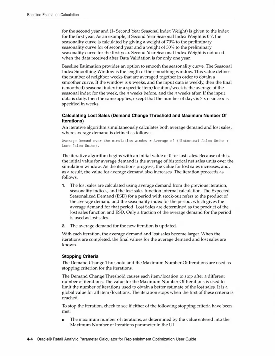
Baseline Estimation Calculation
4-4 Oracle® Retail Analytic Parameter Calculator for Replenishment Optimization User Guide
for the second year and (1- Second Year Seasonal Index Weight) is given to the index for the first year. As an example, if Second Year Seasonal Index Weight is 0.7, the seasonality curve is calculated by giving a weight of 70% to the preliminary seasonality curve for of second year and a weight of 30% to the preliminary seasonality curve for the first year. Second Year Seasonal Index Weight is not used when the data received after Data Validation is for only one year.
Baseline Estimation provides an option to smooth the seasonality curve. The Seasonal Index Smoothing Window is the length of the smoothing window. This value defines the number of neighbor weeks that are averaged together in order to obtain a smoother curve. If the window is n weeks, and the input data is weekly, then the final (smoothed) seasonal index for a specific item/location/week is the average of the seasonal index for the week, the n weeks before, and the n weeks after. If the input data is daily, then the same applies, except that the number of days is 7 x n since n is specified in weeks.
Calculating Lost Sales (Demand Change Threshold and Maximum Number Of Iterations)An iterative algorithm simultaneously calculates both average demand and lost sales, where average demand is defined as follows:
Average Demand over the simulation window = Average of (Historical Sales Units + Lost Sales Units).
The iterative algorithm begins with an initial value of 0 for lost sales. Because of this, the initial value for average demand is the average of historical net sales units over the simulation window. As the iterations progress, the value for lost sales increases, and, as a result, the value for average demand also increases. The iteration proceeds as follows.
1. The lost sales are calculated using average demand from the previous iteration, seasonality indices, and the lost sales function internal calculation. The Expected Seasonalized Demand (ESD) for a period with stock-out refers to the product of the average demand and the seasonality index for the period, which gives the average demand for that period. Lost Sales are determined as the product of the lost sales function and ESD. Only a fraction of the average demand for the period is used as lost sales.
2. The average demand for the new iteration is updated.
With each iteration, the average demand and lost sales become larger. When the iterations are completed, the final values for the average demand and lost sales are known.
Stopping CriteriaThe Demand Change Threshold and the Maximum Number Of Iterations are used as stopping criterion for the iterations.
The Demand Change Threshold causes each item/location to stop after a different number of iterations. The value for the Maximum Number Of Iterations is used to limit the number of iterations used to obtain a better estimate of the lost sales. It is a global value for all item/locations. The iteration stops when the first of these criteria is reached.
To stop the iteration, check to see if either of the following stopping criteria have been met:
■ The maximum number of iterations, as determined by the value entered into the Maximum Number of Iterations parameter in the UI.
Show Iteration Histogram
Baseline Estimation 4-5
■ The quantity abs(total_lost_sales(i) - total_lost_sales(i-1))/(total_lost_sales(i-1) + total_sales) is less than or equal to the demand-change threshold. The quantity within the absolute value is the total change in lost sales from the previous iteration to the current one. If that change, relative to total current demand, is small, then stop. That is, if the lost sales have not changed much from one iteration to the next, then the lost sales calculation has converged, so the calculation can stop. (Stopping an iterative algorithm when the answer does not change much is a standard stopping criterion for such algorithms.)
Diagnostic ModeThe Diagnostic Mode is an optional feature. The default value is Off.
If The Off option is selected, then the full historical dataset is used to calculate seasonality. The Sample dataset is used to calculate the source levels. If Off is selected, then lost sales are calculated only for item/locations in the Main sample.
If the On option is selected, then the full historical dataset is used to calculate both the seasonality and the source levels. If On is selected, then the lost sales calculation is performed for every item/location that was not filtered out during Data Filtering, not just the ones in the Main sample.
Show Iteration HistogramThe Show Iteration Histogram, shown in Figure 4–2, "Baseline Estimation Histogram", displays the distribution of the number of times the lost sales calculation was performed for each item. Items without lost sales do not appear in this chart.
This histogram shows the distribution of the iteration counts used for baseline estimation. Items with very low iteration counts may have unreliable lost sales calculations.
Typically, you will execute baseline estimation and then examine the iteration histogram and other metrics and optionally re-execute the stage.
Figure 4–2 Baseline Estimation Histogram

Output Tables
4-6 Oracle® Retail Analytic Parameter Calculator for Replenishment Optimization User Guide
Output TablesThe following are the key output tables for the Baseline Estimation stage. Use these tables to review the results of this stage.
■ RO_BE_FINAL_LOST_SALES
■ RO_BASELINE_DEMAND
■ RO_BASELINE_DEMAND_FULL (Diagnostic Mode)
Note that these output tables are not created during installation. Instead, they are created once the Baseline Estimation stage has been run to completion at least once. So the output tables do not exist in the database schema until after the Baseline Estimation stage has been run once.
5
Demand Series Generation 5-1
5Demand Series Generation
This chapter provides details about using the Demand Series Generation stage of APC-RO. It contains the following sections:
■ Introduction
■ Parameters
■ Advanced Settings
■ Lost Sales Draws Scaling Factor
■ Output Tables
IntroductionThe Demand Series Generation stage is used to generate the demand distribution of lost sales for item/locations in order to take into account the variability in demand. This stage introduces an element of randomness to the estimated lost sales in the previous baseline estimation stage to account for real-life demand variability.
This stage performs the following tasks:
■ It maps each item/location into one of three probability distributions: Poisson, Normal, or Gamma, based on user-specified thresholds for the average demand.
■ It calculates the demand time-series data for each item/location based on the previously determined probability distribution.
■ It spreads down the weekly demand values to the day level.
The Demand Series Generation stage can use either daily data or weekly data as input. The type of data is determined by the output of the Baseline Estimation stage.
Note: When any stage of APC-RO is re-run, the current data input, output, and temporary results that were part of the previous run will be deleted from all subsequent stages.
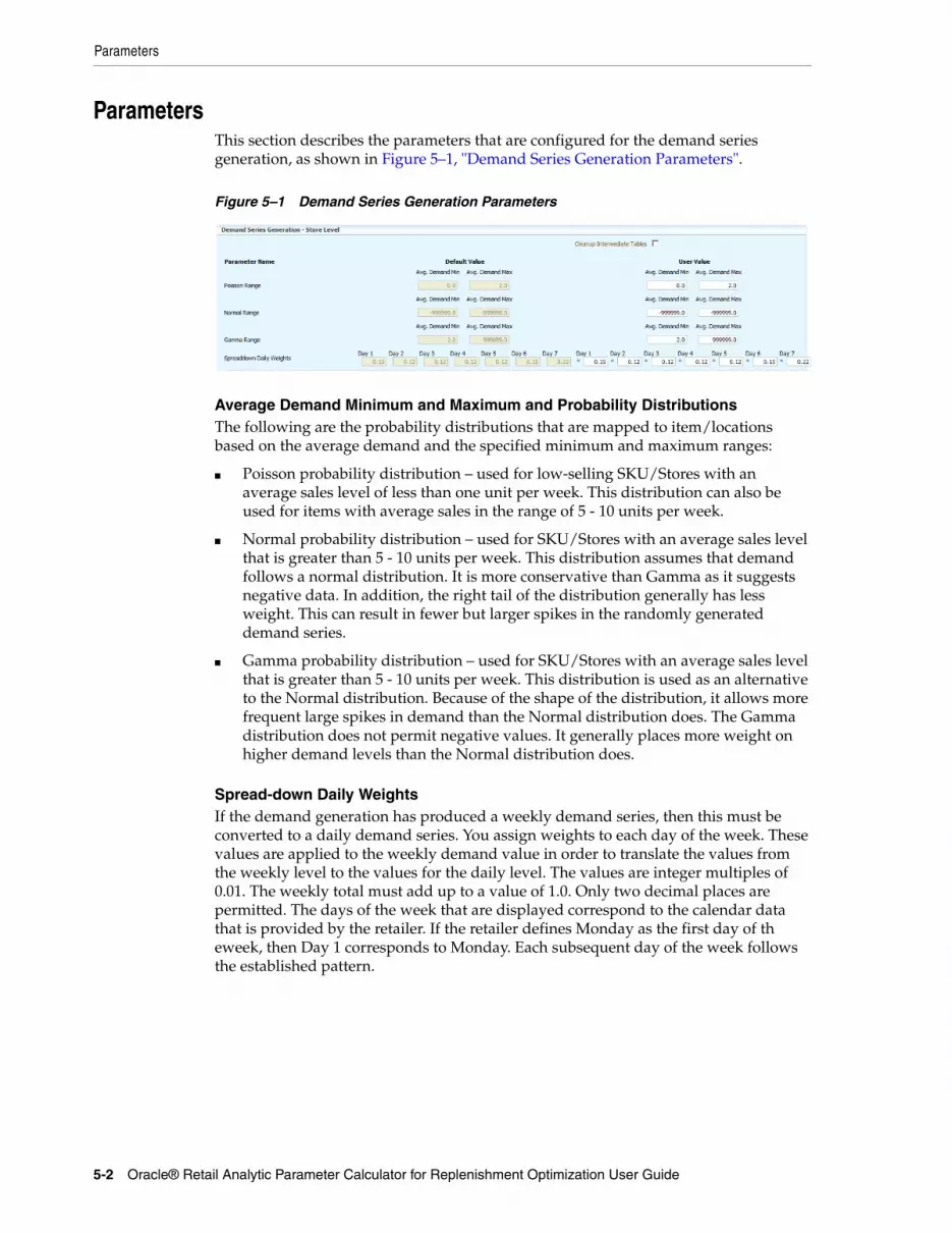
Parameters
5-2 Oracle® Retail Analytic Parameter Calculator for Replenishment Optimization User Guide
ParametersThis section describes the parameters that are configured for the demand series generation, as shown in Figure 5–1, "Demand Series Generation Parameters".
Figure 5–1 Demand Series Generation Parameters
Average Demand Minimum and Maximum and Probability DistributionsThe following are the probability distributions that are mapped to item/locations based on the average demand and the specified minimum and maximum ranges:
■ Poisson probability distribution – used for low-selling SKU/Stores with an average sales level of less than one unit per week. This distribution can also be used for items with average sales in the range of 5 - 10 units per week.
■ Normal probability distribution – used for SKU/Stores with an average sales level that is greater than 5 - 10 units per week. This distribution assumes that demand follows a normal distribution. It is more conservative than Gamma as it suggests negative data. In addition, the right tail of the distribution generally has less weight. This can result in fewer but larger spikes in the randomly generated demand series.
■ Gamma probability distribution – used for SKU/Stores with an average sales level that is greater than 5 - 10 units per week. This distribution is used as an alternative to the Normal distribution. Because of the shape of the distribution, it allows more frequent large spikes in demand than the Normal distribution does. The Gamma distribution does not permit negative values. It generally places more weight on higher demand levels than the Normal distribution does.
Spread-down Daily WeightsIf the demand generation has produced a weekly demand series, then this must be converted to a daily demand series. You assign weights to each day of the week. These values are applied to the weekly demand value in order to translate the values from the weekly level to the values for the daily level. The values are integer multiples of 0.01. The weekly total must add up to a value of 1.0. Only two decimal places are permitted. The days of the week that are displayed correspond to the calendar data that is provided by the retailer. If the retailer defines Monday as the first day of th eweek, then Day 1 corresponds to Monday. Each subsequent day of the week follows the established pattern.
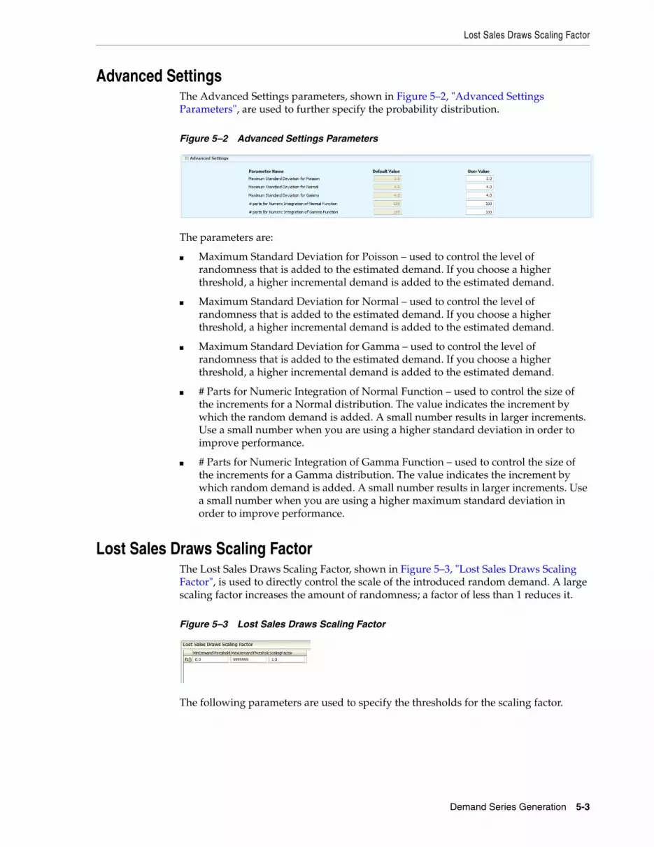
Lost Sales Draws Scaling Factor
Demand Series Generation 5-3
Advanced SettingsThe Advanced Settings parameters, shown in Figure 5–2, "Advanced Settings Parameters", are used to further specify the probability distribution.
Figure 5–2 Advanced Settings Parameters
The parameters are:
■ Maximum Standard Deviation for Poisson – used to control the level of randomness that is added to the estimated demand. If you choose a higher threshold, a higher incremental demand is added to the estimated demand.
■ Maximum Standard Deviation for Normal – used to control the level of randomness that is added to the estimated demand. If you choose a higher threshold, a higher incremental demand is added to the estimated demand.
■ Maximum Standard Deviation for Gamma – used to control the level of randomness that is added to the estimated demand. If you choose a higher threshold, a higher incremental demand is added to the estimated demand.
■ # Parts for Numeric Integration of Normal Function – used to control the size of the increments for a Normal distribution. The value indicates the increment by which the random demand is added. A small number results in larger increments. Use a small number when you are using a higher standard deviation in order to improve performance.
■ # Parts for Numeric Integration of Gamma Function – used to control the size of the increments for a Gamma distribution. The value indicates the increment by which random demand is added. A small number results in larger increments. Use a small number when you are using a higher maximum standard deviation in order to improve performance.
Lost Sales Draws Scaling FactorThe Lost Sales Draws Scaling Factor, shown in Figure 5–3, "Lost Sales Draws Scaling Factor", is used to directly control the scale of the introduced random demand. A large scaling factor increases the amount of randomness; a factor of less than 1 reduces it.
Figure 5–3 Lost Sales Draws Scaling Factor
The following parameters are used to specify the thresholds for the scaling factor.
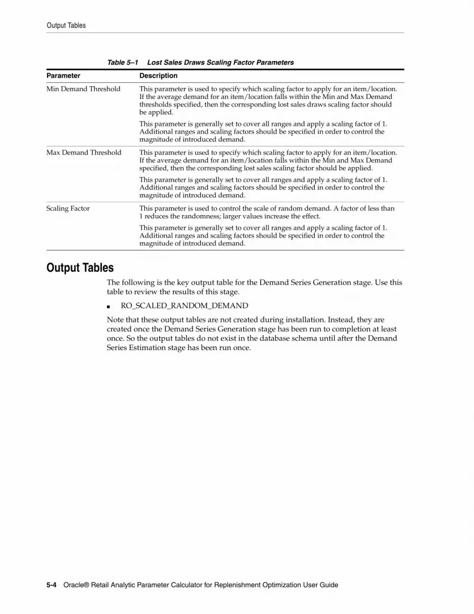
Output Tables
5-4 Oracle® Retail Analytic Parameter Calculator for Replenishment Optimization User Guide
Output TablesThe following is the key output table for the Demand Series Generation stage. Use this table to review the results of this stage.
■ RO_SCALED_RANDOM_DEMAND
Note that these output tables are not created during installation. Instead, they are created once the Demand Series Generation stage has been run to completion at least once. So the output tables do not exist in the database schema until after the Demand Series Estimation stage has been run once.
Table 5–1 Lost Sales Draws Scaling Factor Parameters
Parameter Description
Min Demand Threshold This parameter is used to specify which scaling factor to apply for an item/location. If the average demand for an item/location falls within the Min and Max Demand thresholds specified, then the corresponding lost sales draws scaling factor should be applied.
This parameter is generally set to cover all ranges and apply a scaling factor of 1. Additional ranges and scaling factors should be specified in order to control the magnitude of introduced demand.
Max Demand Threshold This parameter is used to specify which scaling factor to apply for an item/location. If the average demand for an item/location falls within the Min and Max Demand specified, then the corresponding lost sales scaling factor should be applied.
This parameter is generally set to cover all ranges and apply a scaling factor of 1. Additional ranges and scaling factors should be specified in order to control the magnitude of introduced demand.
Scaling Factor This parameter is used to control the scale of random demand. A factor of less than 1 reduces the randomness; larger values increase the effect.
This parameter is generally set to cover all ranges and apply a scaling factor of 1. Additional ranges and scaling factors should be specified in order to control the magnitude of introduced demand.

6
Statistical Adjustment 6-1
6Statistical Adjustment
This chapter provides details about using the Statistical Adjustment stage of APC-RO. It contains the following sections:
■ Introduction
■ Configuration
■ Approach
■ Parameters
■ Output Tables
IntroductionThe Statistical Adjustment stage provides values for the mean and standard deviations for historical sales, which are required inputs for both the Simulation stage and the Statistical Grouping stage. Statistical Adjustment also prepares data for the Simulator (table partitioning). This may have a performance impact.
ConfigurationThe Statistical Adjustment stage is mandatory. The function of this stage depends on the number of years of data that have been loaded. When only one year of data is available, the Statistical Adjustment stage calculates the mean and standard deviation of sales for that year ("year one") and infers what the mean and standard deviation would have been in the previous year ("year two") using year one data and the UI parameters. This is done to make simulation and frontier curve results more realistic; if it is not done, then simulation and frontier curve results will be unrealistically optimistic. When two years of data are available, this stage calculates the mean and standard deviation for both years ("year one" and "year two") of sales for each item/location. The UI input parameters are ignored; they are only required when one year of data is loaded.
Note: When any stage of APC-RO is re-run, the current data input, output, and temporary results will be deleted from all subsequent stages that were part of the previous run.
Note: The remainder of this chapter is not relevant if two years of sales data have been loaded.
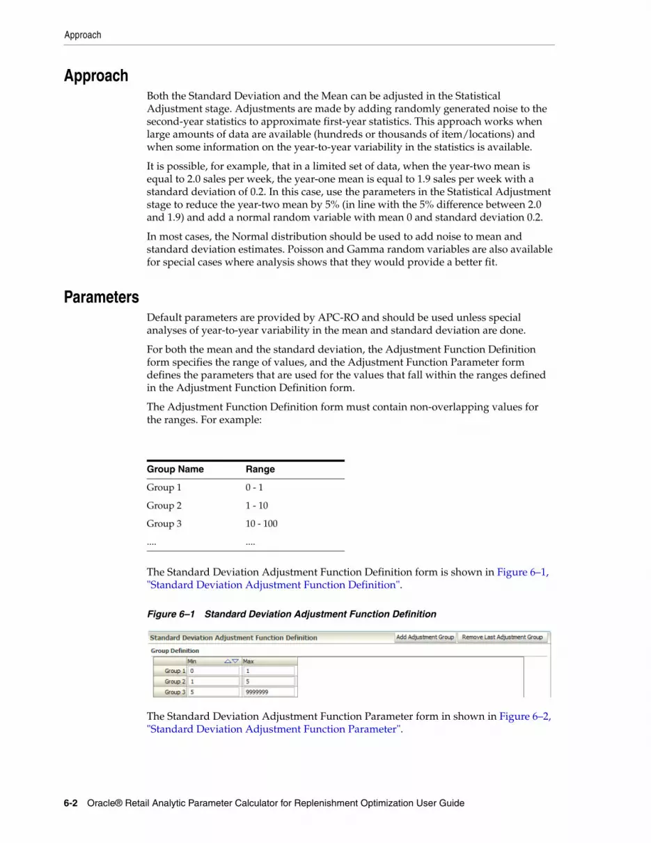
Approach
6-2 Oracle® Retail Analytic Parameter Calculator for Replenishment Optimization User Guide
ApproachBoth the Standard Deviation and the Mean can be adjusted in the Statistical Adjustment stage. Adjustments are made by adding randomly generated noise to the second-year statistics to approximate first-year statistics. This approach works when large amounts of data are available (hundreds or thousands of item/locations) and when some information on the year-to-year variability in the statistics is available.
It is possible, for example, that in a limited set of data, when the year-two mean is equal to 2.0 sales per week, the year-one mean is equal to 1.9 sales per week with a standard deviation of 0.2. In this case, use the parameters in the Statistical Adjustment stage to reduce the year-two mean by 5% (in line with the 5% difference between 2.0 and 1.9) and add a normal random variable with mean 0 and standard deviation 0.2.
In most cases, the Normal distribution should be used to add noise to mean and standard deviation estimates. Poisson and Gamma random variables are also available for special cases where analysis shows that they would provide a better fit.
ParametersDefault parameters are provided by APC-RO and should be used unless special analyses of year-to-year variability in the mean and standard deviation are done.
For both the mean and the standard deviation, the Adjustment Function Definition form specifies the range of values, and the Adjustment Function Parameter form defines the parameters that are used for the values that fall within the ranges defined in the Adjustment Function Definition form.
The Adjustment Function Definition form must contain non-overlapping values for the ranges. For example:
The Standard Deviation Adjustment Function Definition form is shown in Figure 6–1, "Standard Deviation Adjustment Function Definition".
Figure 6–1 Standard Deviation Adjustment Function Definition
The Standard Deviation Adjustment Function Parameter form in shown in Figure 6–2, "Standard Deviation Adjustment Function Parameter".
Group Name Range
Group 1 0 - 1
Group 2 1 - 10
Group 3 10 - 100
.... ....
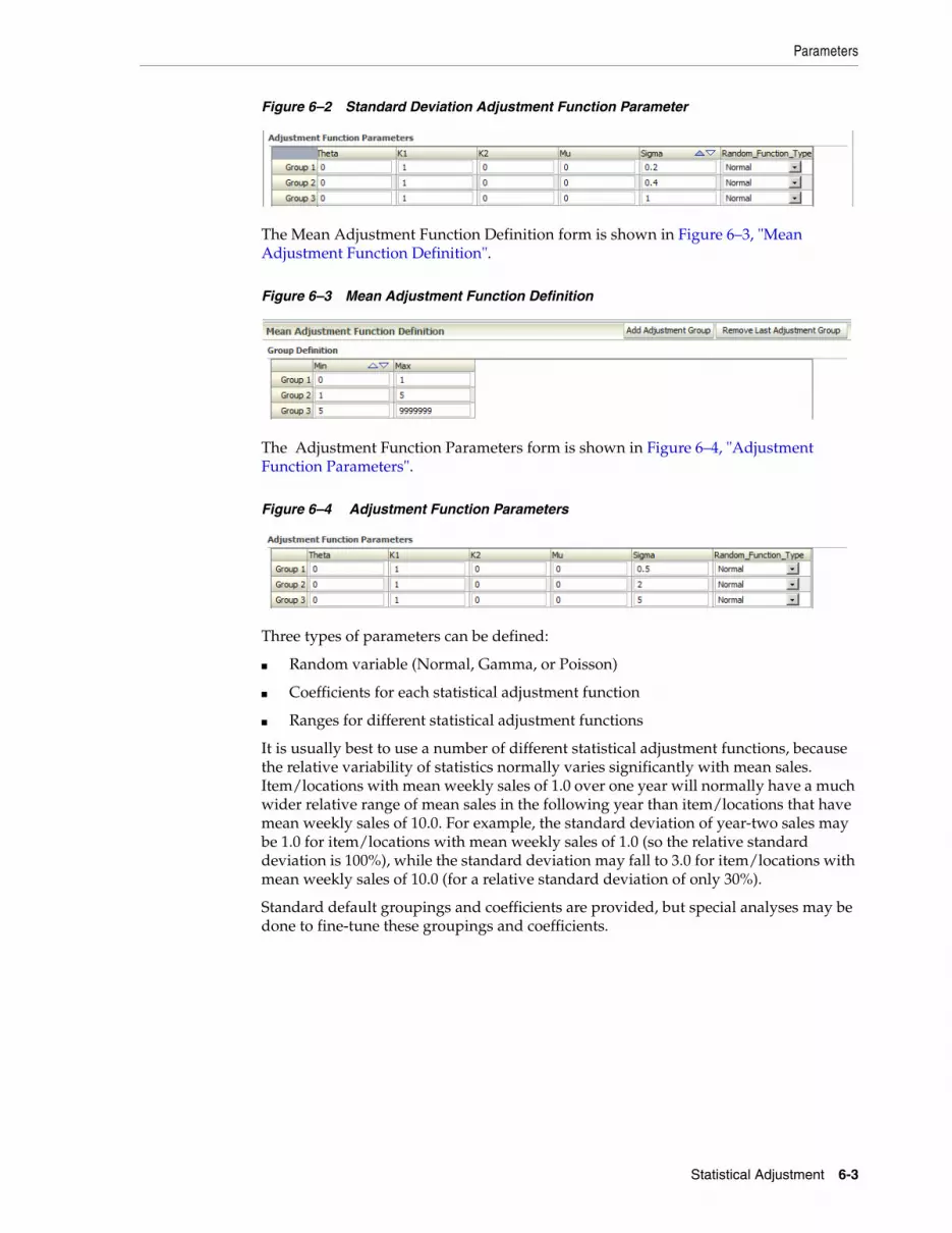
Parameters
Statistical Adjustment 6-3
Figure 6–2 Standard Deviation Adjustment Function Parameter
The Mean Adjustment Function Definition form is shown in Figure 6–3, "Mean Adjustment Function Definition".
Figure 6–3 Mean Adjustment Function Definition
The Adjustment Function Parameters form is shown in Figure 6–4, "Adjustment Function Parameters".
Figure 6–4 Adjustment Function Parameters
Three types of parameters can be defined:
■ Random variable (Normal, Gamma, or Poisson)
■ Coefficients for each statistical adjustment function
■ Ranges for different statistical adjustment functions
It is usually best to use a number of different statistical adjustment functions, because the relative variability of statistics normally varies significantly with mean sales. Item/locations with mean weekly sales of 1.0 over one year will normally have a much wider relative range of mean sales in the following year than item/locations that have mean weekly sales of 10.0. For example, the standard deviation of year-two sales may be 1.0 for item/locations with mean weekly sales of 1.0 (so the relative standard deviation is 100%), while the standard deviation may fall to 3.0 for item/locations with mean weekly sales of 10.0 (for a relative standard deviation of only 30%).
Standard default groupings and coefficients are provided, but special analyses may be done to fine-tune these groupings and coefficients.
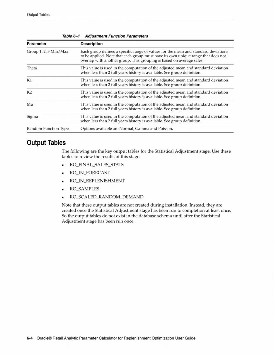
Output Tables
6-4 Oracle® Retail Analytic Parameter Calculator for Replenishment Optimization User Guide
Output TablesThe following are the key output tables for the Statistical Adjustment stage. Use these tables to review the results of this stage.
■ RO_FINAL_SALES_STATS
■ RO_IN_FORECAST
■ RO_IN_REPLENISHMENT
■ RO_SAMPLES
■ RO_SCALED_RANDOM_DEMAND
Note that these output tables are not created during installation. Instead, they are created once the Statistical Adjustment stage has been run to completion at least once. So the output tables do not exist in the database schema until after the Statistical Adjustment stage has been run once.
Table 6–1 Adjustment Function Parameters
Parameter Description
Group 1, 2, 3 Min/Max Each group defines a specific range of values for the mean and standard deviations to be applied. Note that each group must have its own unique range that does not overlap with another group. This grouping is based on average sales
Theta This value is used in the computation of the adjusted mean and standard deviation when less than 2 full years history is available. See group definition.
K1 This value is used in the computation of the adjusted mean and standard deviation when less than 2 full years history is available. See group definition.
K2 This value is used in the computation of the adjusted mean and standard deviation when less than 2 full years history is available. See group definition.
Mu This value is used in the computation of the adjusted mean and standard deviation when less than 2 full years history is available. See group definition.
Sigma This value is used in the computation of the adjusted mean and standard deviation when less than 2 full years history is available. See group definition.
Random Function Type Options available are Normal, Gamma and Poisson.
7
Simulation 7-1
7Simulation
This chapter provides details about using the Simulation stage of APC-RO. It contains the following sections:
■ Introduction
■ The Simulation Stage
■ Reports
■ Review Times
■ Killing a Simulation Run
■ Simulation Output Script
IntroductionThe Simulation stage is the core component of APC-RO. Users can try different replenishment policies and compare the effects on revenue. The user defines scenario settings in terms of item/location and replenishment settings through the UI parameters and then initiates the simulation. When the simulation of all items is complete, the status is displayed in the UI.
The Simulation stage is used to simulate the replenishment process day-to-day and to track various metrics such as beginning-of-day inventory, end-of-day inventory, sales, wastage, and order information. RO then uses this information to measure the financial impact of a particular replenishment policy in order to choose the best policy.
APC-RO provides an optional Optimization stage. This stage uses the results of the Simulation stage and the Statistical Grouping stage to produce frontier curves, which can be used to determine optimal replenishment policies. The Simulator can then be run using a pruned subset of the scenarios displayed in the frontier curves, and these pruned results can be sent to RO. For more information on the Optimization stage, see Chapter 9, "Optimization".
The results of a simulation will not be ready for export to RO until after Statistical Grouping has been run. The output process requires the user to click the Output button located in the Optimization screen and to then run the output scripts in order to extract the data to flat files. Once the Output stage is run, the simulation output tables are cleared. For more information on the output scripts, see Chapter 10, "Output".
Note: When any stage of APC-RO is re-run, the current data input, output, and temporary results will be deleted from all subsequent stages that were part of the previous run.
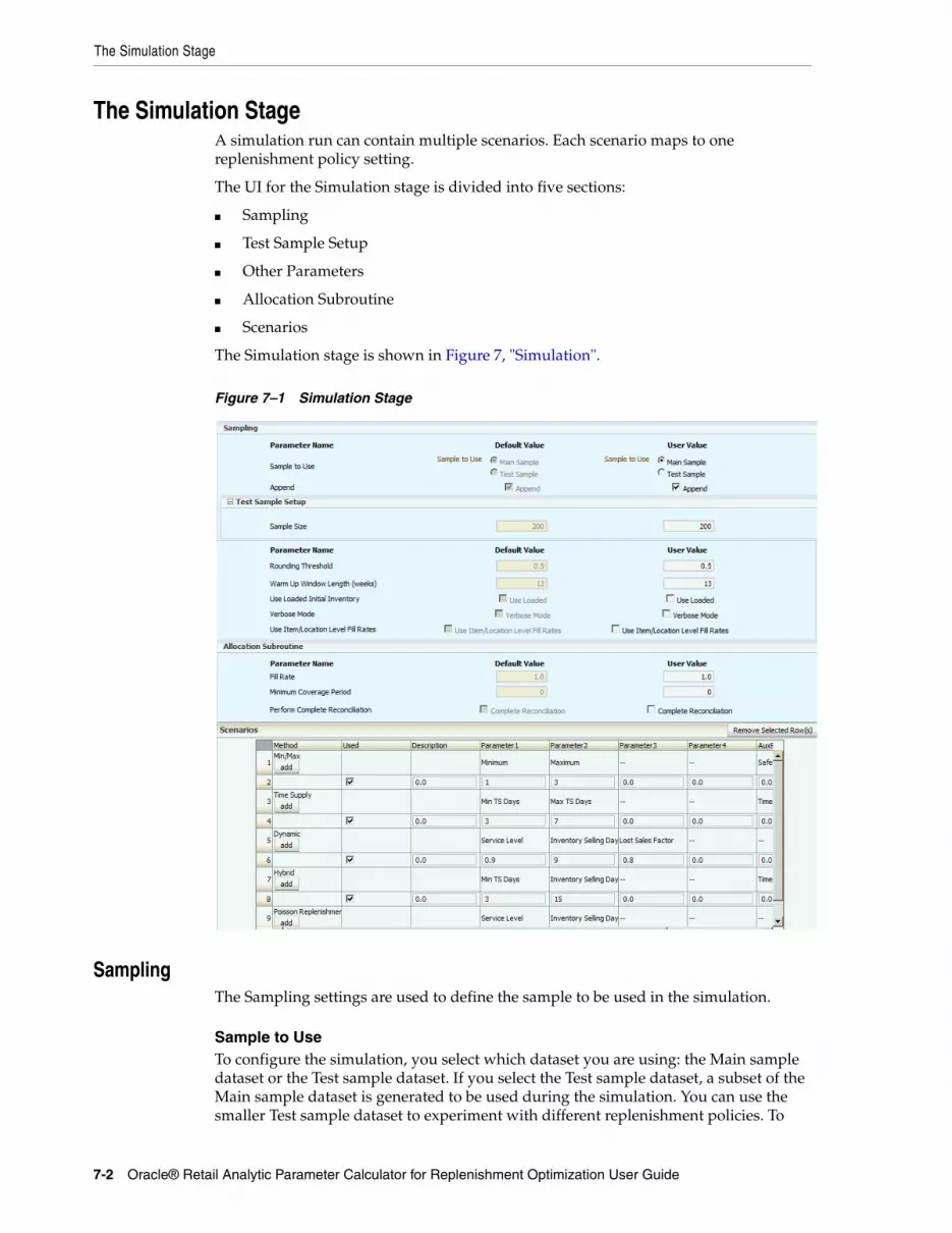
The Simulation Stage
7-2 Oracle® Retail Analytic Parameter Calculator for Replenishment Optimization User Guide
The Simulation StageA simulation run can contain multiple scenarios. Each scenario maps to one replenishment policy setting.
The UI for the Simulation stage is divided into five sections:
■ Sampling
■ Test Sample Setup
■ Other Parameters
■ Allocation Subroutine
■ Scenarios
The Simulation stage is shown in Figure 7, "Simulation".
Figure 7–1 Simulation Stage
SamplingThe Sampling settings are used to define the sample to be used in the simulation.
Sample to UseTo configure the simulation, you select which dataset you are using: the Main sample dataset or the Test sample dataset. If you select the Test sample dataset, a subset of the Main sample dataset is generated to be used during the simulation. You can use the smaller Test sample dataset to experiment with different replenishment policies. To
The Simulation Stage
Simulation 7-3
regenerate the Test sample, change the Test sample size and re-run the Simulation stage.
AppendUse the Append flag to indicate whether or not the output from a simulation will be appended to output from previous runs. Note the following:
■ If you do not select Append, the output from the previous Simulation will be deleted.
■ If you regenerate the Test sample, all the output from the simulation will be deleted.
■ Every time you run the Preprocessing stage, the Main sample is regenerated and the previous Simulation results are deleted.
■ The Simulation results are deleted after the Output stage is run.
Test Sample SetupDefine the size of the test sample you want to use in order to explore different replenishment scenarios.
Other ParametersSet the following general parameters:
Rounding ThresholdOrders must be placed in terms of packs that may contain one or more units. For a pack with 5 SKUs in it, 10 units is equivalent to 2 packs. Rounding occurs when a location’s need is not a multiple of the pack size (for example, when the need is 12 and the pack size is 5).
The rounding threshold is 0 - 1. In the case where the threshold is zero with no pack remainder, rounding does not round up to the next number of packs.
Warm-Up Window LengthThis length is the portion of the simulation window before inventory has reached a steady state. It is used for the simulation but it is not included in the final simulation statistics calculation.
Use Loaded Initial InventoryIf this option is not checked, then the value for the initial inventory is 1. If this option is checked, then the value for the initial inventory is provided in the optional initial inventory data feed.
Verbose ModeThis flag indicates whether or not to save the SKU/Loc/Day level simulation outputs.
Use Item/Location Level Fill RatesIf this option is selected, the global fill rate is overridden with the fill rate for the specific item/location. For item/locations that are not overridden through the schema's table interface, the global fill rate is still used.
The Simulation Stage
7-4 Oracle® Retail Analytic Parameter Calculator for Replenishment Optimization User Guide
Allocation SubroutineFor purposes of allocation, the available inventory is calculated as the total outstanding orders multiplied by the fill rate. If the fill rate = 1, then no push or shortage occurs. If the fill rate > 1, then a push occurs because the availability inventory is greater than the total outstanding orders. If the fill rate < 1, then a shortage occurs because the available inventory is less the total outstanding orders.
Use these parameters to define how inventory is distributed to stores.
Fill RateA double value > 0.0 that indicates how much inventory is available for the simulator to use in fulfilling the orders from the stores. For example, if the fill rate is 0.6, then the simulation is performed with the assumption that the amount of inventory at the DC available to fulfill store orders each day is 0.6 times the sum of the order quantities from the stores for that day. If the fill rate is above 1.0, then the simulation is performed with the DC having more quantity than the stores need for orders. A fill rate of exactly 1.0 means the simulation is run with each store receiving exactly the quantity that it orders. For fill rates other than 1.0, during the simulation, the stores may or may not receive the quantities that they ordered. The exact amount that the stores receive is determined by the reconciliation algorithm. If the fill rate is exactly 1.0, then reconciliation does not run, and stores receive exactly the order quantity they asked for.
The fill rate is defined in the Replenishment Parameters interface. If not present, it is defined using the fill rate provided in the UI.
Minimum Coverage Period for ShortagesMinimum coverage period for shortages is expressed in # days.
Perform Complete ReconciliationThis check box controls whether reconciliation considers all stores or only stores with active orders when performing allocation. When order frequency is an important concern, it may be desirable that only stores with active orders are reconciled. If complete reconciliation is checked, then stores that are not ordering may still receive an allocation, if the reconciliation algorithm determines that even though they are not ordering, they will order soon. If complete reconciliation is checked, and the fill rate is less than 1.0, it is possible for a store that is ordering to receive no allocation.
Forecast Data and Simulation WindowFor the forecast-based simulations to produce meaningful results, there must be complete forecast data for the item/locations being simulated. Complete means that there must be a forecast curve for every week within the Simulation Window. Forecast curves are indexed on three pieces of information:
■ Merchandise key
■ Location key
■ Forecast start date
TerminologyHere are some relevant terms.
Forecast curve. A group of week-level forecasts for an item/location/forecast start date.
The Simulation Stage
Simulation 7-5
Rolling forecast periods. The length of each forecast curve in weeks.
Forecasted Weeks. The total number of weeks for which forecast data is available (that is, the number of forecast curves + rolling forecast periods).
ExamplesHere are two examples, one correct and one incorrect, that demonstrate how forecast-based simulations can produce meaningful results.
CorrectIn this example there is a Simulation Window of 65 weeks and 65 Forecast Curves. The Simulation should be able to find forecast data for every week.
IncorrectIn this example there is a Simulation Window of 65 weeks but only 52 Forecast Curves. The Simulation will not be able to find forecast data for weeks 53 through 65.
ScenariosThe following replenishment policies are used by the Simulator:
■ Min/Max – The Min/Max method is a safe method that generally works well across many types of item/locations. This method makes use of the Minimum and Maximum UI parameters.
■ Calculated Min/Max – This method is similar to the Min/Max but uses a different algorithm and different UI parameters.
■ Time Supply – The Time Supply method is the simplest forecast-based replenishment method. It works well when item/locations are not highly seasonal.
Note: Though the second example has 65 forecasted weeks, this is not the same as having the required 65 forecast curves.
Simulation Window 10/6/2007 through 1/3/2009 (65 weeks)
Rolling Forecast Periods 13
Forecast Curve 65 (78 forecasted weeks)
Simulation Window 10/6/2007 through 1/3/2009 (65 weeks)
Rolling Forecast Periods 13
Forecast Curve 52 (65 forecasted weeks)
Note: Because demo stock cannot be sold or replenished, APC-RO does not account for it in its simulations. In order to compare your existing WOS (which may include demo stock) against APC-RO simulations, you must make adjustments in order to achieve commensurable results. In addition, note that the frontier points in RO ignore demo stock.
The Simulation Stage
7-6 Oracle® Retail Analytic Parameter Calculator for Replenishment Optimization User Guide
■ Dynamic – The Dynamic method allows a specific service level to be targeted. It works well for moderate or high-selling item/locations, especially when forecast error (cumint) measures are accurate.
■ Hybrid – The Hybrid method is a combination of Dynamic and Time Supply replenishment methods. The main difference between the Hybrid and Dynamic methods is the calculation of safety stock.
■ Poisson Replenishment – The Poisson Replenishment method is a version of the Dynamic method that is designed to work well for low-selling item/locations (below an average of approximately 0.5 sales per week).
For each replenishment policy scenario that is checked in the Used column of the scenarios table, the Simulation stage generates an independent output set with its own group of performance metrics and characteristics. This is used to determine the relative and absolute performance of each replenishment policy configuration.
Non-forecasted item/stores in SimulationNon-forecasted item/stores are item/stores that do not have forecast data loaded. As a result, these item/stores are unsuitable for any of the forecast-based replenishment policies. The flag indicating whether or not an item/store has forecast data loaded along with other replenishment input data.
There are two types of replenishment policies. Replenishment policies that use forecast data include Time Supply, Dynamic, Hybrid and Poisson Replenishment. Replenishment policies that do not use forecast data include Min/Max and Calc Min/Max.
The item/stores that do not have forecast data will not be processed by the Simulator for forecast-based Replenishment Policies such as Time Supply. They will however be processed by the Simulator for non forecast-based Replenishment Policies such as Min/Max.
Suggested Parameter Ranges for Replenishment PoliciesThe following ranges are typical ranges. All period-related values are expressed in days.
Replenishment Policy Suggested Range
Fixed Min/Max Min >= 1
Max >= Min
Time Supply Min Time Supply = 3 - 30 days
Max Time Supply = Min Time Supply + x (1 <= x <= 20)
Time Supply Horizon {none, 35, 70}
Dynamic 0.8 <= Service Level <= 1.0
0 <= Inventory Selling Days <= 21
0.5 <= Lost Sales Factor <= 1.0
Hybrid Min Time Supply = 3 - 30 days
0 <= Inventory Selling Days <= 21
Time Supply Horizon {none, 35, 70}
Poisson 0.8 <= Service Level <= 1.0
0 <= Inventory Selling Days <= 21
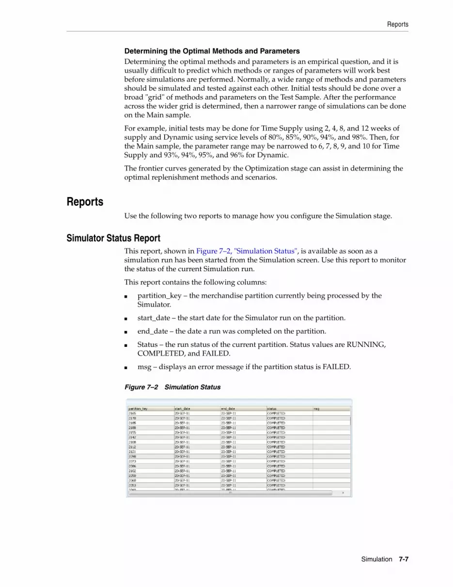
Reports
Simulation 7-7
Determining the Optimal Methods and ParametersDetermining the optimal methods and parameters is an empirical question, and it is usually difficult to predict which methods or ranges of parameters will work best before simulations are performed. Normally, a wide range of methods and parameters should be simulated and tested against each other. Initial tests should be done over a broad "grid" of methods and parameters on the Test Sample. After the performance across the wider grid is determined, then a narrower range of simulations can be done on the Main sample.
For example, initial tests may be done for Time Supply using 2, 4, 8, and 12 weeks of supply and Dynamic using service levels of 80%, 85%, 90%, 94%, and 98%. Then, for the Main sample, the parameter range may be narrowed to 6, 7, 8, 9, and 10 for Time Supply and 93%, 94%, 95%, and 96% for Dynamic.
The frontier curves generated by the Optimization stage can assist in determining the optimal replenishment methods and scenarios.
ReportsUse the following two reports to manage how you configure the Simulation stage.
Simulator Status ReportThis report, shown in Figure 7–2, "Simulation Status", is available as soon as a simulation run has been started from the Simulation screen. Use this report to monitor the status of the current Simulation run.
This report contains the following columns:
■ partition_key – the merchandise partition currently being processed by the Simulator.
■ start_date – the start date for the Simulator run on the partition.
■ end_date – the date a run was completed on the partition.
■ Status – the run status of the current partition. Status values are RUNNING, COMPLETED, and FAILED.
■ msg – displays an error message if the partition status is FAILED.
Figure 7–2 Simulation Status
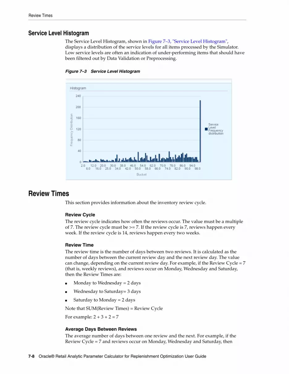
Review Times
7-8 Oracle® Retail Analytic Parameter Calculator for Replenishment Optimization User Guide
Service Level HistogramThe Service Level Histogram, shown in Figure 7–3, "Service Level Histogram", displays a distribution of the service levels for all items processed by the Simulator. Low service levels are often an indication of under-performing items that should have been filtered out by Data Validation or Preprocessing.
Figure 7–3 Service Level Histogram
Review TimesThis section provides information about the inventory review cycle.
Review CycleThe review cycle indicates how often the reviews occur. The value must be a multiple of 7. The review cycle must be >= 7. If the review cycle is 7, reviews happen every week. If the review cycle is 14, reviews happen every two weeks.
Review TimeThe review time is the number of days between two reviews. It is calculated as the number of days between the current review day and the next review day. The value can change, depending on the current review day. For example, if the Review Cycle = 7 (that is, weekly reviews), and reviews occur on Monday, Wednesday and Saturday, then the Review Times are:
■ Monday to Wednesday = 2 days
■ Wednesday to Saturday= 3 days
■ Saturday to Monday = 2 days
Note that SUM(Review Times) = Review Cycle
For example: 2 + 3 + 2 = 7
Average Days Between ReviewsThe average number of days between one review and the next. For example, if the Review Cycle = 7 and reviews occur on Monday, Wednesday and Saturday, then
Simulation Output Script
Simulation 7-9
Review Times are 2, 3 and 2 (see “Review Time” above). Average Days Between Reviews (2 + 3 + 2) / 3 = 2.33 days.
Average Review FrequencyThe average number of reviews in a week. This is used to ensure that the review time information is valid. For example, using the Average Days Between Reviews from above:
Average number of reviews in a week = 1/(Average Days Between Reviews) * 7
= 1 / 2.33 * 7
= 3
This is easily verified. Reviews occur every week on Monday, Wednesday, and Saturday (that is, 3 reviews per week).
ExampleReview Cycle = 14
Review Days = Monday, Wednesday and Saturday
Review Times:
Monday to Wednesday = 2 days
Wednesday to Saturday= 3 days
Saturday to Monday = 9 days (because reviews only occur every other week)
Average Days Between Reviews = (2 + 3 + 9) / 3 = 4.67 days
Average Review Frequency = 1 / Average Days Between Reviews * 7 = 1 / 4.67 * 7 = 1.5
Killing a Simulation RunIt may be necessary to kill a simulation run (for example, if settings need to be modified or the simulation run is taking longer than expected).
To kill a simulation run, complete the following steps:
1. Stop the simulation run by closing the browser where APC-RO is loaded.
2. Call this shell script to kill any scheduled or running job related to the simulator:
apcro_kill_sim_jobs.sh <apcro_st_wallet_alias or apcro_dc_wallet_alias>
Simulation Output ScriptThe Simulation output script generates output from the results of the simulation and saves those results in simulation output tables. It then archives the results of the simulation to archiving tables differently, depending on whether or not the Verbose Mode check box has been selected.
The following are the key simulation output tables. Use these tables to review the output results. Note that RO_INVENTORY and RO_ORDER are only available if you select the Verbose Mode flag.
■ AGGREGATE_SIM_RESULTS
■ RO_SCENARIO_PARAMS
Simulation Output Script
7-10 Oracle® Retail Analytic Parameter Calculator for Replenishment Optimization User Guide
■ RO_SIMULATION_PARAMS
■ RO_INVENTORY
■ RO_ORDER
A summary of the data for each output table is available. Once the Simulation run is complete, click View Simulator Status to generate the output results for the stage. For detailed information about the results, refer to these output tables in the database schema.
Note that these output tables are not created during installation. Instead, they are created once the Simulation stage has been run to completion at least once. So the output tables do not exist in the database schema until after the Simulation stage has been run once.
The RO_INVENTORY and RO_ORDER tables only contain data if you selected Complete Clusters.
If the Verbose Mode check box has been selected:
■ The simulation parameter results and calculation results are archived to the AGGREGATE_SIM_RESULTS table.
■ All simulation parameter results and simulation calculation results are truncated.
■ Determines whether day-level data is output to RO_ORDER and RO_INVENTORY.
8
Statistical Grouping 8-1
8Statistical Grouping
This chapter provides details about using the Statistical Grouping stage of APC-RO. It contains the following sections:
■ Introduction
■ Process
■ Example
■ Output Tables
IntroductionThe Statistical Grouping stage uses the Mean and Standard Deviation of historic sales (calculated in the Statistical Adjustment stage) to calculate weights for all item/locations. These weights are then used in conjunction with user-specified grouping factors to bucket the item/locations into a set of groups. APC-RO exports these groups to the RO application for use with its Optimization component.
You should not have too many groups for a selected sample set. Note that empty groups may cause problems loading output into RO.
ProcessThis section outlines the statistical grouping process. The Statistical Grouping Definition form, used for this task, is shown in Figure 8–1, "Statistical Grouping Definition Form".
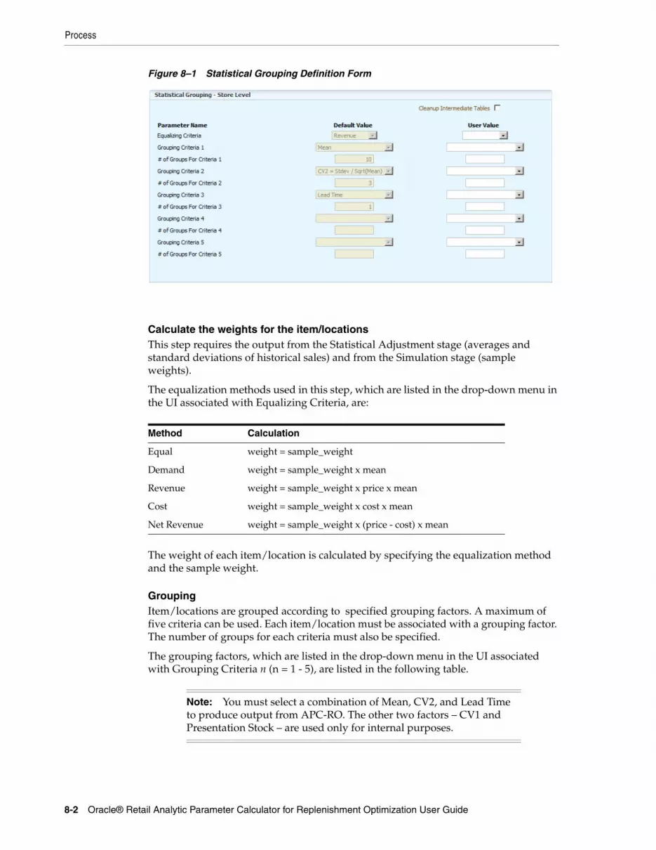
Process
8-2 Oracle® Retail Analytic Parameter Calculator for Replenishment Optimization User Guide
Figure 8–1 Statistical Grouping Definition Form
Calculate the weights for the item/locationsThis step requires the output from the Statistical Adjustment stage (averages and standard deviations of historical sales) and from the Simulation stage (sample weights).
The equalization methods used in this step, which are listed in the drop-down menu in the UI associated with Equalizing Criteria, are:
The weight of each item/location is calculated by specifying the equalization method and the sample weight.
GroupingItem/locations are grouped according to specified grouping factors. A maximum of five criteria can be used. Each item/location must be associated with a grouping factor. The number of groups for each criteria must also be specified.
The grouping factors, which are listed in the drop-down menu in the UI associated with Grouping Criteria n (n = 1 - 5), are listed in the following table.
Method Calculation
Equal weight = sample_weight
Demand weight = sample_weight x mean
Revenue weight = sample_weight x price x mean
Cost weight = sample_weight x cost x mean
Net Revenue weight = sample_weight x (price - cost) x mean
Note: You must select a combination of Mean, CV2, and Lead Time to produce output from APC-RO. The other two factors – CV1 and Presentation Stock – are used only for internal purposes.
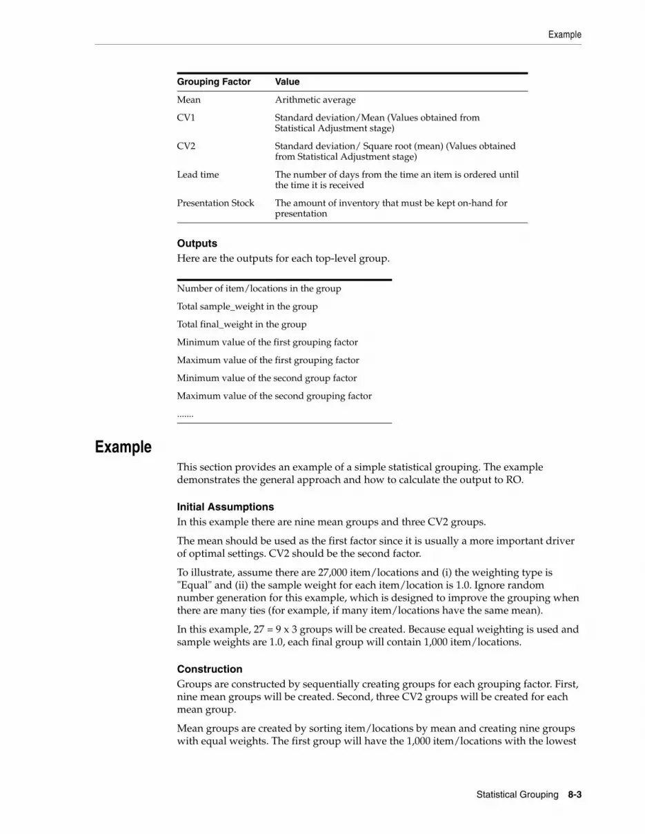
Example
Statistical Grouping 8-3
OutputsHere are the outputs for each top-level group.
ExampleThis section provides an example of a simple statistical grouping. The example demonstrates the general approach and how to calculate the output to RO.
Initial AssumptionsIn this example there are nine mean groups and three CV2 groups.
The mean should be used as the first factor since it is usually a more important driver of optimal settings. CV2 should be the second factor.
To illustrate, assume there are 27,000 item/locations and (i) the weighting type is "Equal" and (ii) the sample weight for each item/location is 1.0. Ignore random number generation for this example, which is designed to improve the grouping when there are many ties (for example, if many item/locations have the same mean).
In this example, 27 = 9 x 3 groups will be created. Because equal weighting is used and sample weights are 1.0, each final group will contain 1,000 item/locations.
ConstructionGroups are constructed by sequentially creating groups for each grouping factor. First, nine mean groups will be created. Second, three CV2 groups will be created for each mean group.
Mean groups are created by sorting item/locations by mean and creating nine groups with equal weights. The first group will have the 1,000 item/locations with the lowest
Grouping Factor Value
Mean Arithmetic average
CV1 Standard deviation/Mean (Values obtained from Statistical Adjustment stage)
CV2 Standard deviation/ Square root (mean) (Values obtained from Statistical Adjustment stage)
Lead time The number of days from the time an item is ordered until the time it is received
Presentation Stock The amount of inventory that must be kept on-hand for presentation
Number of item/locations in the group
Total sample_weight in the group
Total final_weight in the group
Minimum value of the first grouping factor
Maximum value of the first grouping factor
Minimum value of the second group factor
Maximum value of the second grouping factor
.......
Example
8-4 Oracle® Retail Analytic Parameter Calculator for Replenishment Optimization User Guide
means, the second group will have the 1,000 item/locations with the next lowest means, and so on.
After the mean groups are created, the CV2 groups are created. Note that the CV2 grouping is done independently for each mean group, so there will usually be different CV2 cutoffs for each mean group. For example, for the first mean group, the maximum CV2 in the first CV2 group might be 2, but for the second mean group 2, the maximum value for the first CV2 group might be 3.
Group NamesGroup names are created so that the first (left-most) digits are determined by the first grouping factor, the second digits by the second grouping factor, and so on.
In the example, there will be 27 groups with numbers from 101 to 903. The numbers in the tens and ones place determine the CV2 group, and the numbers in the hundreds and thousands places determine the mean group. For example, group 101 is for the first mean group and first CV2 group, while 201 is for the second mean group and first CV2 group, and 903 is for the ninth mean group and the third CV2 group.
Statistical Grouping OutputThe output needs to be available providing the min mean and max mean for each of the nine mean groups. These should be calculated as follows.
Mean Calculations - Group 1:
Min Mean = Min{All Item/Locs in groups starting with a 1}
Max Mean = Max{All Item/Locs in groups starting with a 1}
Mean Calculations - Group 2:
Min Mean = Max Mean for Group 1
Max Mean = Max{All Item/Locs in groups starting with a 2}
...
Mean Calculations - Group 9:
Min Mean = Max Mean for Group 8
Max Mean = Max{All Item/Locs in groups starting with a 9}
For CVs, the Min and Max CV2 must be output for each of the 27 CV2 groups. It is not possible to just output 3 Min and Max CV2 groups because these values will vary across mean groups.
CV2 Calculations - Group 101:
Min CV2 = Min{All Item/Locs in groups starting with 101}
Max CV2 = Max{All Item/Locs in groups starting with a 101}
CV2 Calculations - Group 102:
Min CV2 = Max CV2 for Group 101
Max CV2 = Max{All Item/Locs in groups starting with a 102}
CV2 Calculations - Group 103:
Min CV2 = Max CV2 for Group 102
Max CV2 = Max{All Item/Locs in groups starting with a 103}
CV2 Calculations - Group 201:
Output Tables
Statistical Grouping 8-5
Min CV2 = Min{All Item/Locs in groups starting with 201}
Max CV2 = Max{All Item/Locs in groups starting with a 201}
....
CV2 Calculations - Group 903:
Min CV2 = Max CV2 for Group 902
Max CV2 = Max{All Item/Locs in groups starting with a 903}
Output TablesThe following are the key output tables for the Statistical Grouping stage. Use these tables to review the results of this stage.
■ RO_TOP_GROUPING_ASSIGNMENT
■ RO_TOP_GROUPING_STATISTICS
Note that these output tables are not created during installation. Instead, they are created once the Statistical Grouping stage has been run to completion at least once. So the output tables do not exist in the database schema until after the Statistical Grouping stage has been run once.

Output Tables
8-6 Oracle® Retail Analytic Parameter Calculator for Replenishment Optimization User Guide
9
Optimization 9-1
9Optimization
This chapter provides details about using the Optimization stage of APC-RO. It contains the following sections:
■ Introduction
■ Optimization UI
■ Frontier Curves
■ Configuring the Sales Measure and the Inventory Measure
■ Output
IntroductionThe Optimization stage is an optional stage that can be used to generate a frontier curve within APC-RO, evaluate the results, and make any adjustments if necessary, prior to outputting results for RO. This can simplify the overall workflow since APC-RO itself (instead of RO) can be used to validate the replenishment rules and grouping statistics. The process within APC-RO can be repeated as necessary by regenerating samples, modifying replenishment scenarios, and then re-running the Simulation and Optimization stages before exporting the results.
The Optimization stage processes the output of the Simulation stage in combination with the statistical grouping of the item/locations in order to generate a frontier curve. The frontier curve displays the relationship between a given inventory measure and a given sales measure for a given group of replenished item/locations.
An inefficient sales/inventory combination indicates a situation in which too much is being spent on inventory to generate a specific sales goal. An unachievable sales/inventory combination indicates a situation in which it is not possible to achieve a specific sales goal by spending any less on inventory.
You can use the frontier curve to analyze simulation and statistical grouping results and prune inefficient scenarios that are not performing well.
The Optimization stage also contains the Run Output button, which you must use to produce output for RO.
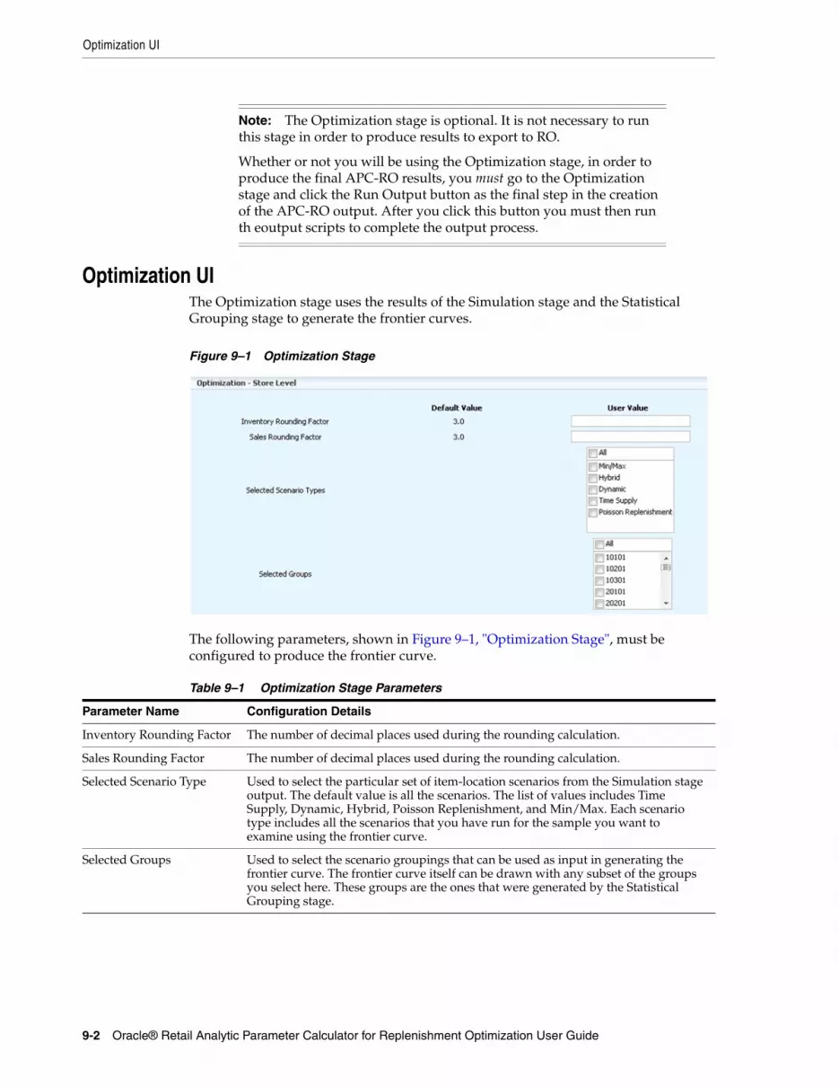
Optimization UI
9-2 Oracle® Retail Analytic Parameter Calculator for Replenishment Optimization User Guide
Optimization UIThe Optimization stage uses the results of the Simulation stage and the Statistical Grouping stage to generate the frontier curves.
Figure 9–1 Optimization Stage
The following parameters, shown in Figure 9–1, "Optimization Stage", must be configured to produce the frontier curve.
Note: The Optimization stage is optional. It is not necessary to run this stage in order to produce results to export to RO.
Whether or not you will be using the Optimization stage, in order to produce the final APC-RO results, you must go to the Optimization stage and click the Run Output button as the final step in the creation of the APC-RO output. After you click this button you must then run th eoutput scripts to complete the output process.
Table 9–1 Optimization Stage Parameters
Parameter Name Configuration Details
Inventory Rounding Factor The number of decimal places used during the rounding calculation.
Sales Rounding Factor The number of decimal places used during the rounding calculation.
Selected Scenario Type Used to select the particular set of item-location scenarios from the Simulation stage output. The default value is all the scenarios. The list of values includes Time Supply, Dynamic, Hybrid, Poisson Replenishment, and Min/Max. Each scenario type includes all the scenarios that you have run for the sample you want to examine using the frontier curve.
Selected Groups Used to select the scenario groupings that can be used as input in generating the frontier curve. The frontier curve itself can be drawn with any subset of the groups you select here. These groups are the ones that were generated by the Statistical Grouping stage.
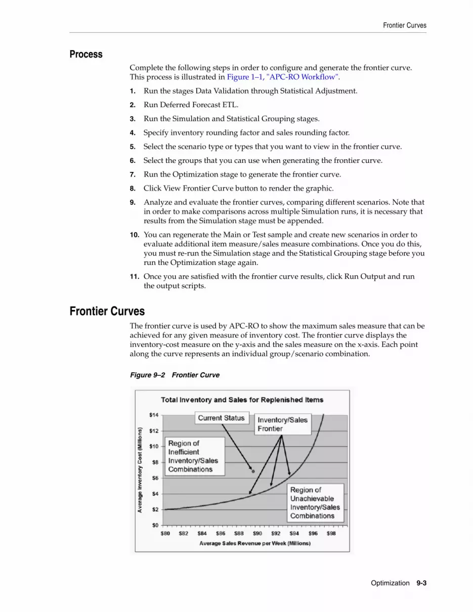
Frontier Curves
Optimization 9-3
ProcessComplete the following steps in order to configure and generate the frontier curve. This process is illustrated in Figure 1–1, "APC-RO Workflow".
1. Run the stages Data Validation through Statistical Adjustment.
2. Run Deferred Forecast ETL.
3. Run the Simulation and Statistical Grouping stages.
4. Specify inventory rounding factor and sales rounding factor.
5. Select the scenario type or types that you want to view in the frontier curve.
6. Select the groups that you can use when generating the frontier curve.
7. Run the Optimization stage to generate the frontier curve.
8. Click View Frontier Curve button to render the graphic.
9. Analyze and evaluate the frontier curves, comparing different scenarios. Note that in order to make comparisons across multiple Simulation runs, it is necessary that results from the Simulation stage must be appended.
10. You can regenerate the Main or Test sample and create new scenarios in order to evaluate additional item measure/sales measure combinations. Once you do this, you must re-run the Simulation stage and the Statistical Grouping stage before you run the Optimization stage again.
11. Once you are satisfied with the frontier curve results, click Run Output and run the output scripts.
Frontier CurvesThe frontier curve is used by APC-RO to show the maximum sales measure that can be achieved for any given measure of inventory cost. The frontier curve displays the inventory-cost measure on the y-axis and the sales measure on the x-axis. Each point along the curve represents an individual group/scenario combination.
Figure 9–2 Frontier Curve
Frontier Curves
9-4 Oracle® Retail Analytic Parameter Calculator for Replenishment Optimization User Guide
Points along the curve represent the optimal combination of inventory and sales. The combination provides the best service level for the associated inventory level. Those above the curve are not feasible. Those below the curve are not optimal.
The frontier curve actually consists of discrete points, so it does not necessarily appear as a curve. The number of points produced is a function of the number of scenarios run in the Simulation stage, so a large number of scenarios can potentially result in an actual curve.
The sales measure is a measure of sales performance such as service level, sale units, or sales revenue. By default, it is defined to be service level, which is total sales divided by total demand, both taken over the simulation horizon.
The inventory measure is a measure of inventory performance such as weeks of sales, average inventory level, or average spoilage. By default, it is weeks of sales, which is the sum over the simulation horizon of end-of-week inventory divided by total sales over the simulation horizon.
The recommended approach is to calculate the sales measure and the inventory measure for all scenario-group combinations. The sales measures and inventory measures for all scenarios of a particular group are then used to calculate the frontier for that group. The top-level frontier is then derived from the group-level frontiers.
Group Level Curves The frontier curve for one specific group of item-locations.
Top Level CurvesThe aggregate frontier curve across all item-locations being optimized. The top-level curve is a display of almost all of the points of the group-level curves together. It shows the envelope of performance across all of the groups. For a given service level, it is possible that different groups require different inventory levels to achieve that service level. The top-level curve will show the difference in inventory levels by plotting all of the group-level points.

Output
Optimization 9-5
Figure 9–3 Frontier Curve Graphs
Configuring the Sales Measure and the Inventory MeasureThe frontier curve is configured in the following three views. The sales measure and the inventory measure can be configured by updating RO_FC_VIEW.
CREATE TABLE RO_FC_PARAMS ( RUN_ID NUMBER(7) NOT NULL, INV_ROUNDING_FACTOR NUMBER(7) NOT NULL, SALES_ROUNDING_FACTOR NUMBER(7) NOT NULL ) PCTFREE 0 NOLOGGING ;
CREATE TABLE RO_FC_SCN_TYPES ( RUN_ID NUMBER(7) NOT NULL, METHOD_NAME VARCHAR2(50) NULL )
CREATE TABLE RO_FC_GROUPS ( RUN_ID NUMBER(12) NOT NULL, GROUP_NUMBER NUMBER(12) NOT NULL ) PCTFREE 0 NOLOGGING ;
OutputTo generate the final output for APC-RO, click Run Output in the Optimization stage.
The APC-RO UI Output button clears all Simulation and post-Simulation data from the main APC-RO schema and populates the output database tables for export to the
Output
9-6 Oracle® Retail Analytic Parameter Calculator for Replenishment Optimization User Guide
RO schema. After this, the output scripts must be run in order th generate the data flat files.
The results of the Output stage are appending to the output tables. If the sample version number has not changed, the output is appended to the output table for that sample version number. If the sample version number has changed, then the output is appended to a table for the new sample version number.
The following output tables are used:
■ Scenarios are appended to the RO_OUT_STORE_SCENARIO/RO_OUT_DC_SCENARIO tables.
■ Groups are appended to the RO_OUT_STORE_GROUP/RO_OUT_DC_GROUP tables.
■ Scenario/Item statistics are appended to the RO_OUT_STORE_ITEM_STATS/RO_OUT_DC_ITEM_STATS tables.
■ Scenario/Group statistics are appended to the RO_OUT_GROUP_STATS/RO_OUT_DC_GROUP_STATS tables.
This output consists of a set of flat files that have been TAR'd and GZIP'd into the fixed filename: apcro_out_store.tar.gz for Stores data and apcro_out_dc.tar.gz for Warehouse data, as described in Chapter 10, "Output".
These flat files will ultimately be imported by the RO (RPAS) application.
10
Output 10-1
10Output
This chapter provides details about the output of data from APC-RO to RO. It contains the following sections:
■ Store Output Process
■ Warehouse Output Process
For information about the output files themselves, see the Oracle Retail Analytic Parameter Calculator for Replenishment Optimization Implementation Guide.
Store Output ProcessThis section describes the output process for the Store data.
Note that all RO_OUT_ tables are truncated after the Output script has been run. The Output data is accumulated into the RO_OUT_FINAL tables.
The final output of the APC-RO application is a set of flat files that have been TAR'd and GZIP'd into the fixed filename: apcro_out_store.tar.gz. These flat files will ultimately be imported by the RO (RPAS) application. The 'apcro_out_store.tar.gz' file is generated via a UNIX shell script:
$ ./extract_output_store.sh
Usage: ./extract_output_store.sh {APCRO_ST_ALIAS}
For example:
./extract_output_store.sh apcro_st_alias
The above script requires that the ORACLE_HOME environment variable be set to a valid ORACLE client installation >= 10g. This should be the same ORACLE_HOME used to create your Oracle password stores during the APC-RO installation process. The TNS_ADMIN environment variable should also be set to the location of your tnsnames.ora file containing the aliases created during installation setup.
Note that the TAR'd and GZIP'd output file contains all the Store flat files and all the Warehouse flat files. When you use the extract_output_store.sh script, only the Store flat files contain data. When you use the extract_output_dc.sh script, only the Warehouse flat files contain data.
Note: The output stage scripts will export the Main sample result or Test sample result. This is determined by the running mode that is selected in the Simulation stage.
Warehouse Output Process
10-2 Oracle® Retail Analytic Parameter Calculator for Replenishment Optimization User Guide
Warehouse Output ProcessThis section describes the output process for the Warehouse data.
Note that all RO_OUT_ tables are truncated after the Output script has been run. The Output data is accumulated into the RO_OUT_FINAL tables.
The final output of the APC-RO application is a set of flat files that have been TAR'd and GZIP'd into the fixed filename: apcro_out_dc.tar.gz. These flat files will ultimately be imported by the RO (RPAS) application. The 'apcro_out_dc.tar.gz' file is generated via a UNIX shell script:
$ ./extract_output_dc.sh
Usage: ./extract_output_dc.sh {APCRO_DC_ALIAS}
For example:
./extract_output_dc.sh apcro_dc_alias
The above script requires that the ORACLE_HOME environment variable be set to a valid ORACLE client installation >= 10g. This should be the same ORACLE_HOME used to create your Oracle password stores during the APC-RO installation process. The TNS_ADMIN environment variable should also be set to the location of your tnsnames.ora file containing the aliases created during installation setup.
Note that the TAR'd and GZIP'd output file contains all the Store flat files and all the Warehouse flat files. When you use the extract_output_store.sh script, only the Store flat files contain data. When you use the extract_output_dc.sh script, only the Warehouse flat files contain data.
Glossary -1
Glossary
Average Demand Level
The average daily demand over the demand window.
Baseline Sales
The level of historical sales if no stock-outs had occurred (that is, if sufficient inventory had been available). In addition, the effects of promotions or sales are also factored in.
Cumulative Daily Demand Profile
For a given day, the average share of the weekly demand.
Daily Demand Profile
For a given day, the average share of daily demand.
Days-On-Hand
Total inventory divided by total sales, where the totals are over all item-locations for a given day.
Demand Series
The weekly SKU-location level demand. Demand refers to historical sales corrected for expected lost sales. It is the demand that was historically present and, if not for a stock-out, would have been fulfilled.
Demand Window
The period of time over which the demand series must be generated.
Expected Lost Sales
The estimate of the sales that were lost because of a stock-out for a given SKU-location-week. For weeks that did not have a stock-out, it is defined as zero.
Expected Seasonalized Demand Estimation
The expected demand for any item-location period that determined during the Baseline Estimation stage.
Forecast Data
Information provided by an external application such as RDF. Forecast data is used by the following replenishment policies: Time Supply, Dynamic, Hybrid, and Poisson Replenishment. The only replenishment policies that do not use forecast data are Min/Max and Calculated Min/Max.
Forecast Start Date
-2 Oracle® Retail Analytic Parameter Calculator for Replenishment Optimization User Guide
Forecast Start Date
The day the forecast is created. Forecasts are weekly only. The forecast horizon is the weeks for which a forecast exists, starting with the week immediately after the forecast start date and continuing for as many weeks as are in the horizon.
Frontier
Displays the maximum sales measure that can be achieved for any given measure of inventory cost. The frontier is a curve with the inventory-cost measure on the y axis and the sales measure on the x axis. Individual points on the curve represent individual group/scenario combinations. That is, each individual group/scenario combination contributes one point (x,y) = (sales measurement, inventory measurement) to the curve. The graphical interpretation of sub-optimal is the following: If there are two points (x,y) and (x,z), where z > y, then (x,z) represents a scenario in which inventory is higher while still only providing the same service level x as the point (x,y). This, the point (x,z) is suboptimal.
Gamma Distribution
The demand distribution that can be used as an alternative to the Normal distribution for SKU-stores that have an average sales level of more than 5 to 10 items per week
Group-Level Frontier
The frontier for one specific group of item-locations.
Half Year
A time division that is either the first 26 weeks or the second 26 weeks of a year of the data window.
Inventory Cost Measure
The measurement of inventory performance that is used to build the frontier. This measurement can be weeks of sales, average inventory level, average spoilage, or retailer-defined (for example, 12% of inventory at cost). It should give the inventory performance of each simulated itme-location-scenario. By default, it is defined as seeks of sales (the sum over the simulation horizon of end-of-week inventory divided by total sales over the simulation horizon). Before it is used to construct group-level frontiers, the inventory measure at the item-location-scenario level must be aggregated to the group-scenario level, since a group-level inventory measure is required for a group-level curve.
Inventory Series
The weekly SKU-locationlevel inventory.
Item-Location
A specific SKU-store or SKU-warehouse combination. Note that an item-location is always the lowest level of the merchandise hierarchy and the location hierarchy.
Key Performance Measures
The key performance measures for simulation data are total sales, demand, lost sales, average end-of-week inventory on hand, average inventory on order, total orders, total days out of stock, and total wastage. These values are at the item-location-scenario level. The key performance measures are not used in the drawing of the frontier curves, but simply provide additional information to the user.
Required Replenishment Parameters
Glossary -3
Lost Sales Function
The function that specifies how to calculate lost sales during the iteration performed by the Baseline Estimation stage. Lost sales are those that occur for a particular SKU-location-week as a result of a stock-out.
Main Sample
The set of data that contains a selection of SKUs or SKU-stores. The Main sample is configured using a group of parameters that includes merchandise level, number of item-locations, and accuracy.
Maximum Acceptable One-Week Demand
The maximum share of demand that can occur within any one week of the demand window.
Maximum Acceptable Stock-out Rate by Period
The maximum share of stock-outs that can occur within a period.
Minimum Demand Units
The minimum number of acceptable demand units.
Minimum Percent of Sales by Period
The minimum acceptable share of demand units that can occur in any period. for example, consider a situation in which the minimum acceptable share of demand for a store in the first quarter of the demand window is 5%. If total demand in the first quarter was less than 5% of total demand over the demand window, then the store woruld be filtered out.
Normal Distribution
The demand distribution that is useful for SKU-stores that have an average sales level of more than 5 to 10 items per week.
Number of Steps for Numeric Intergration
The number of steps used for the numeric intergration of the Normal and Gamma distributions.
Optimization Window
The period over which an optimization occurs.
Poisson Distribution
The demand distribution that is useful for low-selling SKU-stores (typically with an average sales level of less than one item per week).
Presentation Stock
The level of inventory needed in a store to support Promotion activities.
Quarter Year
A time division that is either the first 13 weeks or the second 13 weeks of a half year of the data window.
Required Replenishment Parameters
Any of the standard replenishment parameters required for analysis.
Sales Measure
-4 Oracle® Retail Analytic Parameter Calculator for Replenishment Optimization User Guide
Sales Measure
The measurement of sales performance that is used to build the frontier. This measurement can be sevice level, sales units, sales revenue, or retailer-defined. It should give the sales performance of each simulated item-location-scenario. By default, it is defined as service level (the total sales divided by total demand, taken over the simulation horizon). Before it is used to construct group-level frontiers, the sales measure at the item-location-scenario level must be aggregated to the group-scenario level, since a group-level sales measure is required for a group-level curve.
Sales Series
The series of item-location-week or item-location-day level sales.
Scaling Factor
A parameter that is used to control the scale of random demand.
Scenario
A specific replenishment method and setting (for example, a Dynamic scenario with a 97% service level target nad 21 inventory supply days).
Schemas
APC-RO uses three different schemas to store data. The Stage schema is used for flat files from external sources. The Core schema is used for common data, including the Merchandise Hierarchy, Location Hierarchy, Calendar, and Sales. The RO schema is used for the APC-RO data used for each calculation stage.
Seasonality Curve
Provides what the shape of sales in history should have been if no stockouts had occurred.
Simulation Window
A UI parameter used for the time window over which the Simulation stage simulates replenishment. It must be within the Data Window (from the Data Validation stage).
SKU-Location
A specific SKU-store or SKU-warehouse combination(depending on the mode that APC-RO is running in - Store or DC).
Spread-Down
The process by which values from one level, such as SKU-store-week, are translated into values at a lower level, such as SKU-store-day.
Source Hierarchy Level
The source hierarchy levels are UI parameters that define the aggregation level that the Baseline Estimation stage uses to construct the seasonality curves.
Standard Replenishment Parameters
The following are standard: lead time, time between reviews, pack size, unit price, unit cost, and shelf life.
Statistical Group
A group of item-locations that are determined by the statistical grouping component of APC-RO.
Year
Glossary -5
Stock-Out Rate
For Chain-Week, the stock-out rate for a specific week is the total stockouts divided by the total item-location, where the totals are over item-locations. "Revenue weighted" means that the stock-out flag is multiplied by the revenue for the item-location for the specific week. That value is is divided by the total revenue, where the totla is taken over all item-locations for the specific week.
Stock-Out Series
A flag (0/1) that indicates whether or not a stock-out has occured for an item-location-day.
Stock-Out Window
The period for which stock0out data must be available.
Test Sample
The set of data that is a subset of the Main sample data.
Top-Level Frontier
The aggregated frontier across all item-locations being optimized.
Weeks-On-Hand
Total inventory divided by total sales, where the totals are over all item-locations for a given week.
Weight
A relative weight that is placed on each item-location. It is used when forming aggregations of the key performance measures and when forming aggregations of the inventory cost measure and sales measure at the group level.
Year
A time division that is either the first 52 weeks or the second 52 week of the data window. A data window that is only 52 weeks long, then it only has 1 year.

Year
-6 Oracle® Retail Analytic Parameter Calculator for Replenishment Optimization User Guide
Index-1
Index
AAcceptable Weeks-on-Hand parameter, 3-4acceptable weeks-on-hand range, 3-2accuracy calculation, 3-4Add Range button, 2-5Add/Remove rows and columns button, 1-6AGGREGATE_SIM_RESULTS, 7-9Allowable % of Total Item/Location Sales per Period
filter, 2-7append flag, 7-3average demand, 4-4average demand calculation, 5-1Average demand maximum parameter, 5-2Average demand minimum parameter, 5-2average demand probability distribution
parameter, 5-2average sales, 4-1average weekly sales, 2-4Average weekly sales for each pack size level
report, 2-10Average weekly sales for each presentation stock level
report, 2-9average weekly sales groups, 2-5average weekly sales level, 3-2average weekly unit sales for item/locations, 2-6average weekly unit sales for items, 2-7
BBack button, 1-6baseline estimation key output tables, 4-6Baseline Estimation stage, 1-3beginning-of-day inventory, 7-1bucket width, 2-10buckets, 1-6
Ccalendar data, 3-2Chain-week level summary report, 2-9Cleanup Intermediate Tables check box, 1-6cost, 3-2curve, normalized, 4-3CV1 grouping factor, 8-3CV2 grouping factor, 8-3
Ddaily sales, 2-2data filtering, additional in preprocessing stage, 3-1data range, acceptable, 3-1data requirements, 1-2data requirements, input, 3-2data validation charts, 2-2, 2-10data validation key output tables, 2-12data validation reports, 2-9Data Validation stage, 1-3, 2-1Data Validation stage, re-running, 2-1data validation tables, 2-2data window, 2-1, 2-5data window, end date, 2-4days-on-hand range, 3-1DC data, 2-4deferred forecast ETL, 1-4demand change threshold, 4-4demand series generation key output tables, 5-4Demand Series Generation stage, 1-3, 5-1demand time series data, 5-1demand variability, 5-1demo, 3-2demo stock, 7-5Dept-level active SKU/Stores report, 2-9Dept-week level summary report, 2-9Done, status, 1-5Draw Chart button, 1-6Dynamic replenishment method, 7-6
Eemail, 1-7email notification, 1-12end date, 2-1end-of-day inventory, 7-1end-of-week inventory, 2-2equalization methods, 8-2ETL, 1-4expected seasonalized demand, 4-4
FFailed, status, 1-6Fill rate parameter, 7-4

Index-2
Filter Item/Location on Invalid Inventory parameter, 2-4
Filter Summary Report, 3-7Filter summary report, 2-9forecast-based simulation, 7-5Frequency distribution of average weekly sales
chart, 2-10, 2-11Frequency distribution of lead times chart, 2-10Frequency distribution of pack sizes chart, 2-11Frequency distribution of presentation stocks
chart, 2-11Frequency distribution of ratio of year 1/2 sales
chart, 2-11Frequency distribution of review frequencies
chart, 2-11Frequency distribution of stock-out rates chart, 2-11Frequency distribution of weeks on hand chart, 2-11frontier curve, 7-1, 9-4Frontier Curve button, 1-7
GGamma probability distribution, 5-1, 5-2Gamma random variable, 6-3Gamma statistical distribution, 6-2grid filter ranges, 2-5grid filters, 2-5grouping factor, 8-2group-level curve, 9-4
HHelp, 1-7histogram data, 2-2historical data, 2-1, 2-10historical data aggregation, 1-2historical demand data, 3-2historical inventory data, 3-2historical net sales units, 4-4historical sales, 8-1historical sales mean, 6-1historical sales standard deviation, 6-1historical stock-out data, 3-2Hybrid replenishment method, 7-6
Iinput data requirements, 3-2Internet Explorer settings, 1-7
adjusting language settings, 1-10cache settings, 1-10
inventory measure, 9-4inventory review cycle, 7-8
Llead, 3-2lead time, 1-1, 2-2, 2-5lead time grouping factor, 8-3Lead Time Thresholds for Item/Location
parameter, 2-4
location hierarchy, 3-2Location Level, 2-5Location Level parameter, 2-4Location Level parameter, changing, 2-1location source level, 4-3login screen, 1-11Logout, 1-7lost sales, 4-4lost sales calculation, 4-4lost sales demand distribution, 5-1Lost Sales Draws Scaling Factor, 5-3lost sales, definition, 4-1
MMain sample dataset, 7-2maximum acceptable one-week sales, 3-2Maximum Acceptable Stock-out Rate per Period
filter, 3-7Maximum acceptable week-to-week percentage
difference between sales and inventory drop parameter, 2-4
Maximum acceptable week-to-week percentage inventory drop parameter, 2-4
Maximum acceptance week-to-week unit difference between sales and inventory drop parameter, 2-4
Maximum Allowable % of Total Item Sales filter, 2-8Maximum Number of Iterations, 4-4maximum stock-out rate, 3-2Maximum Stock-out Rate of Item/Location
parameter, 2-4Mean adjustment function definition form, 6-3Mean adjustment function parameter, 6-3mean grouping factor, 8-3merchandise hierarchy, 3-2Merchandise Level, 2-5merchandise source level, 4-3Minimum % of Average Weekly Store Sales per Week
parameter, 2-4Minimum Acceptable Location Stock-out Rate per
Period filter, 3-7Minimum coverage period for shortages
parameter, 7-4minimum percent of sales, 3-2minimum sales units, 3-2Minimum Sales Units per Period filter, 3-5Minimum Total Item Sales per Period filter, 2-7Minimum Total Item/Location Sales per Period
filter, 2-6Min/Max replenishment method, 7-5
NNormal probability distribution, 5-1, 5-2Normal random variable, 6-3Normal statistical distribution, 6-2
OOptimization stage, 1-3
Index-3
order point, 1-1Output stage, 1-3
Ppack, 3-2pack size, 2-2, 2-5Pack Size Thresholds for Item/Location
parameter, 2-4Percent Range of Item Sales per Period filter, 3-5Percent Range of Item-Location Sales per Period
filter, 3-5Percent Range of Location Sales per Period filter, 3-6percentage of the total unit sales per period, 2-7Perform complete reconciliation parameter, 7-4Period Level Filter Summary Report, 2-12, 3-8Poisson probability distribution, 5-1, 5-2Poisson random variable, 6-3Poisson replenishment method, 7-6Poisson statistical distribution, 6-2preprocessing key output tables, 3-9Preprocessing stage, 1-3, 3-1presentation, 3-2presentation stock, 2-2presentation stock grouping factor, 8-3Presentation Stock Thresholds for Item/Location
parameter, 2-4price, 3-2process train, 1-3push, 7-4
Rrandom variable parameter, 6-3Remove Range button, 2-5replenishment, 1-1replenishment parameter, 3-2, 4-1Replenishment Parameters Threshold Override
filter, 2-5replenishment policy, 7-1replenishment policy ranges, 7-6replenishment policy, simulator, 7-5replenishment, optimal methods, 7-7replenishment, optimal parameters, 7-7replenishment, simulation window, 4-3review frequencies, 2-2Review Frequency Thresholds for Item/Location
parameter, 2-4RO_BASELINE_DEMAND, 4-6RO_BASELINE_DEMAND_FULL, 4-6RO_BE_FINAL_LOST_SALES, 4-6RO_DF_WINDOW_SUBDIVIDED, 2-12RO_FC_GROUPS, 9-5RO_FC_PARAMS, 9-5RO_FC_SCN_TYPES, 9-5RO_FC_VIEW, 9-5RO_FILTER_FINAL, 3-9RO_FILTERED_ITEM_LOC_FACT, 2-12RO_FILTERED_WEEKLY_DATA, 2-12RO_FINAL_SALES_STATS, 6-4
RO_IN_FORECAST, 6-4RO_IN_REPLENISHMENT, 6-4RO_INVENTORY, 7-10RO_ORDER, 7-10RO_OUT_DC_GROUP, 9-6RO_OUT_DC_GROUP_STATS, 9-6RO_OUT_DC_ITEM_STATS, 9-6RO_OUT_DC_SCENARIO, 9-6RO_OUT_GROUP_STATS, 9-6RO_OUT_STORE_GROUP, 9-6RO_OUT_STORE_ITEM_STATS, 9-6RO_OUT_STORE_SCENARIO, 9-6RO_SAMPLES, 3-9, 6-4RO_SCALED_RANDOM_DEMAND, 6-4RO_SCENARIO_PARAMS, 7-9RO_SD_FINAL, 5-4RO_SIMULATION_PARAMS, 7-10RO_TOP_GROUPING_ASSIGNMENT, 8-5RO_TOP_GROUPING_STATISTICS, 8-5Rounding threshold parameter, 7-3Run button, 1-6Run Output button, 9-2Running, status, 1-5
SSales History Window parameter, 2-4sales measure, 9-4sales unit filtering, 2-5scenario settings, 7-1scenario, mapping to replenishment policy, 7-2seasonality curve, 4-2seasonality curve calculation, 4-3seasonality curve smoothing, 4-4seasonality index smoothing window length, 4-3second year seasonal index weight, 4-3service level, 9-4Service Level Histogram, 7-8shortage, 7-4Show Iteration Histogram, 4-5Show Service Level Histogram button, 1-6shrinkage, 2-4simulation, 7-1simulation input, 6-1simulation key output tables, 7-9Simulation stage, 1-3, 7-1Simulation stage output, 8-2simulation window, 4-3, 7-4Simulator Status Report, 7-7Simulator Status Report button, 1-7SKU/DC-level item data, 2-1SKU/Store-level item data, 2-1SKU/Stores, low-selling, 5-2Standard deviation adjustment function definition
form, 6-2Standard deviation adjustment function parameter
form, 6-2Start a New Run button, 1-6Start a new Run button, 1-6state management, 1-3

Index-4
statistical adjustment function coefficient, 6-3statistical adjustment function range, 6-3statistical adjustment key output table, 6-4Statistical adjustment output, 8-2statistical adjustment output, 8-1Statistical Adjustment stage, 1-3, 6-1Statistical grouping definition form, 8-1statistical grouping example, 8-3statistical grouping input, 6-1, 8-1statistical grouping key output tables, 8-5statistical grouping output, 8-3statistical grouping process, 8-1Statistical Grouping stage, 1-3, 8-1statistical variability, 6-3status, 1-3Status button, 1-6status email, 1-12status screen, 1-5status, Done, 1-5status, Failed, 1-6status, Running, 1-5stock-out, 4-1stock-out flag, 2-2stock-out level, 3-1stock-out rate, maximum acceptable, 2-2stock-out, simulation window, 4-3stopping criteria, 4-4Store data, 2-4summary data, data validation, 2-2
TTest sample dataset, 7-2time division, 3-3time division, data validation, 2-5time period, 3-3Time Supply replenishment method, 7-5top-level curve, 9-4transit time, 1-1
UUse loaded initial inventory parameter, 7-3user interface, 1-2user requirements, 1-2
VVerbose Mode parameter, 7-3View Data Validation Charts button, 1-6View Data Validation Reports button, 1-6View Filter Summary Report button, 1-6View Iteration Histogram button, 1-6
WWarm-up window length parameter, 7-3weekly sales, 2-2Weeks-on-Hand thresholds for Item/Location
parameter, 2-4workflow, 1-4
XXML Load button, 1-7XML Save button, 1-7