1

OPTIMIZATION AND ANALYSIS OF VARIABILITY IN INJECTION MOLDING

Carlos E. Castro1, Mauricio Cabrera Ríos2, Blaine Lilly1, and José M. Castro1 1Dept. of Industrial, Welding & Systems Engineering

The Ohio State University Columbus, Ohio, USA 43202

2Graduate Program in Systems Engineering

Universidad Autónoma de Nuevo León Sn. Nicolás de los Garza, Nuevo León, México 66450

Abstract:

Injection Molding (IM) is the most important process for mass-producing plastic products. The

difficulty of optimizing an IM process is that the performance measures (PMs), usually show conflicting

behavior. The aim of this work is to demonstrate a method utilizing CAE, statistical testing, artificial

neural networks (ANNs), and data envelopment analysis (DEA) to find the best compromises between

multiple PMs and their variability. Two case studies are presented. A case study based on a virtual part

is discussed in detail in order to illustrate this method. The second case study is experimentally based,

using the American Society of Testing Materials (ASTM) mold, to illustrate how this approach applies

when only experimental results are available.

Introduction:

The U.S. industry is under increasing pressure to develop technology to mass-produce high-end

goods with tight tolerances. It is critical that the industry meets these goals to maintain an edge over

countries that, by keeping a low labor cost scheme, have been the recipients of a large amount of

off-shored manufacturing operations. Injection molding (IM) is a process that is particularly well suited

to the demands of extreme precision at high production rates. One of the biggest challenges facing

injection molders is to determine the best settings for the controllable process variables (CPVs). The

difficulty of optimizing an IM process is that the performance measures (PMs), such as surface quality

2

or cycle time, that characterize the adequacy of the part for its intended purpose usually show conflicting

behavior. Furthermore, in actual molding, the CPVs will vary over some range during molding. This

inconsistency of the process variables will lead to variability in the PMs. In high precision

manufacturing, in particular for micro scale components and devices, or parts with micro features, this

variability needs to be minimized and if possible, eliminated. Thus, the variability in the CPVs needs to

be included in the optimization problem.

The aim of this work is to demonstrate a method utilizing CAE, statistical testing, artificial

neural networks (ANNs), and data envelopment analysis (DEA) to find the best compromises between

multiple PMs and their variability to prescribe the values for the CPVs in IM. Two different approaches

for analyzing variability and their merits for different IM applications are investigated. Two case studies

are presented. A case study based on a virtual part is presented in detail in order to illustrate this

method. The optimization is separated into two phases. Phase 1 uses PMs which are only dependent on

the location of the injection gate (as found by statistical testing) to identify candidate injection gates.

Phase 2 of the optimization considers the variability of two new PMs in order to select between the

candidate injection gates. The second case study is experimentally based, using the American Society of

Testing Materials (ASTM) mold, to illustrate how this approach applies when only experimental results

are available.

The Optimization Strategy:

Proposed by Cabrera-Rios, et al [1,2] the general strategy to find the best compromises between

several PMs consists of five steps:

3

Step 1) Define the physical system. Determine the performance measures, the phenomena of interest, the

controllable and non-controllable variables, the experimental region, and the responses that will be

included in the study.

Step 2) Build physics-based models to represent the phenomena of interest in the system. Define models

that relate the controllable variables to the responses of interest. If this is not feasible, skip this step.

Step 3) Run experimental designs. Create data sets by either systematically running the models from the

previous step, or by performing an actual experiment in the physical system when a mathematical model

is not possible.

Step 4) Fit metamodels to the results of the experiments. Create empirical expressions (metamodels) to

mimic the functionality in the data sets.

Step 5) Optimize the physical system. Use the metamodels to obtain predictions of the phenomena of

interest, and to find the best compromises among the PMs for the original system. The best

compromises are identified here through DEA.

One step that was added to the general strategy is the introduction of variability into the

optimization problem. This work studies two different forms of introducing variability into the IM

process optimization. First, for experimentally-based data, the variability is inherent. Running several

repeats in a physical system at given conditions in step 3 of the optimization strategy will automatically

introduce the variability. Secondly, in a case where physics-based models are the basis of the

optimization process, the variability is not inherent. Running a model simulation at a given set point

will always result in the same outputs for the PMs of interest. Therefore, some other means of

introducing the variability of the PMs must be pursued. In order to introduce variability into the

optimization problem we can take advantage of the capability of the metamodels to generate data

quickly. In order to simulate the action of running experimental repeats in a physical system, the

metamodel is run several times at process settings that are slightly perturbed from the original set point.

4

This allows us to illustrate what the effect of this variation of controllable process variables is on the

PMs of interest. The next step is to incorporate this measure of variability into the optimization problem.

Toward that end, the simplest way is to take the measure of variability and designate it as a separate PM.

Then this separate PM is included in the traditional DEA model as a PM which should be minimized.

Data Envelopment Analysis (DEA):

On previous publications [3-5] we have demonstrated that if a set of candidate solutions

evaluated by multiple PMs (criteria) is available, it is possible to determine the best compromises

between all criteria through DEA. The idea behind DEA is to use an optimization model to compute a

relative efficiency score for each particular solution with respect to the rest of the candidate solutions.

The resulting best compromises, identified through their efficiency score, form the envelope of the

solution set. These solutions are also called Pareto-efficient or simply efficient.

The DEA linear programming formulations proposed by Banks, Charnes and Cooper [7] are

shown below:

0 ,

1 Subject to

Maximize

to,,, Find

00

00minmax

min0

00max0

00

≥

⋅≥

⋅≥

=≤++−

=

++

−+

−+

−+

−+

µµ

ε

ε

µµ

µµ

µµ

1ν1µ

YνYµ

Yν

Yµ

µν

T

T

jT

jT

T

T

1,...,nj1

(1)

5

0,

1 Subject to

Minimize

to ,,, Find

00

00maxmin

max0

00min0

00

≥

⋅≥

⋅≥

=≥++−

=

++

−+

−+

−+

−+

νν

ε

ε

νν

νν

νν

1ν1µ

YµYν

Yµ

Yν

µν

T

T

jT

jT

T

T

1,...,nj1

(2)

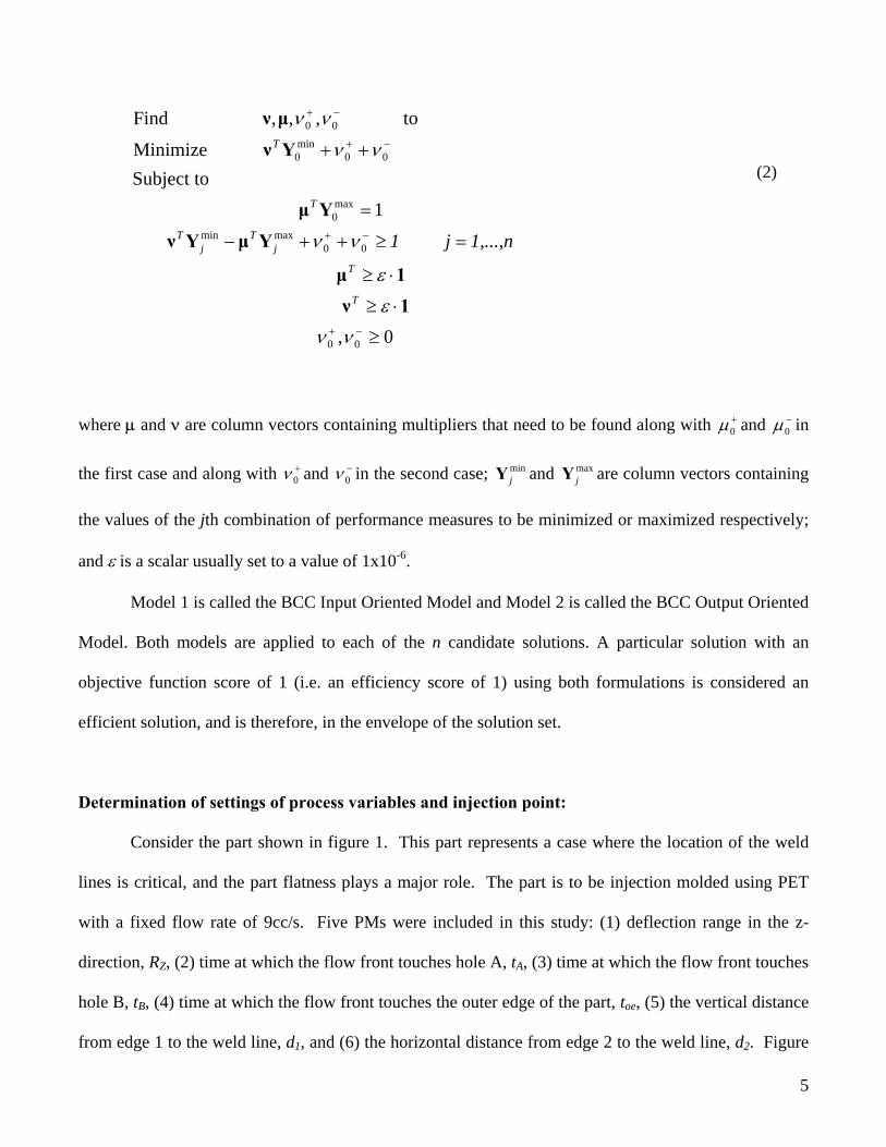
where µ and ν are column vectors containing multipliers that need to be found along with +0µ and −

0µ in

the first case and along with +0ν and −

0ν in the second case; minjY and max

jY are column vectors containing

the values of the jth combination of performance measures to be minimized or maximized respectively;

and ε is a scalar usually set to a value of 1x10-6.

Model 1 is called the BCC Input Oriented Model and Model 2 is called the BCC Output Oriented

Model. Both models are applied to each of the n candidate solutions. A particular solution with an

objective function score of 1 (i.e. an efficiency score of 1) using both formulations is considered an

efficient solution, and is therefore, in the envelope of the solution set.

Determination of settings of process variables and injection point:

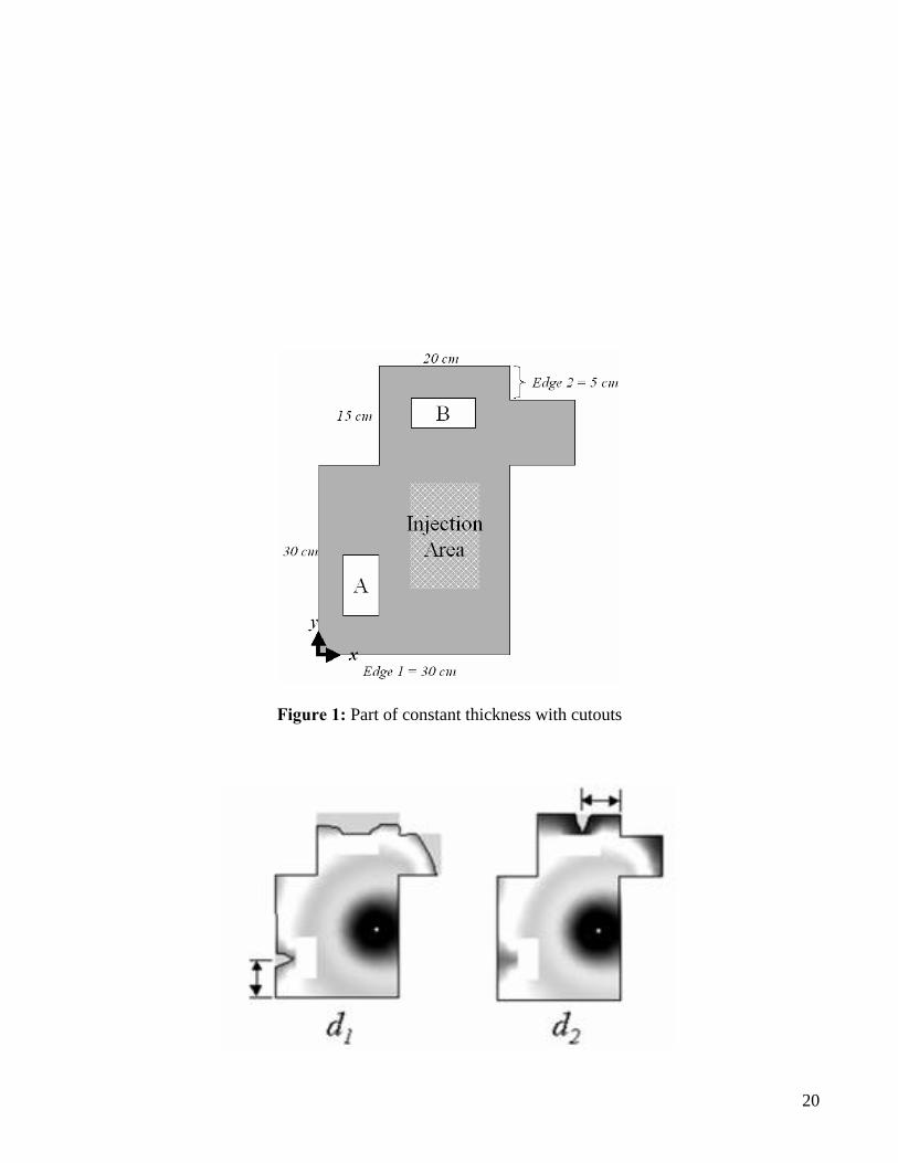
Consider the part shown in figure 1. This part represents a case where the location of the weld

lines is critical, and the part flatness plays a major role. The part is to be injection molded using PET

with a fixed flow rate of 9cc/s. Five PMs were included in this study: (1) deflection range in the z-

direction, RZ, (2) time at which the flow front touches hole A, tA, (3) time at which the flow front touches

hole B, tB, (4) time at which the flow front touches the outer edge of the part, toe, (5) the vertical distance

from edge 1 to the weld line, d1, and (6) the horizontal distance from edge 2 to the weld line, d2. Figure

6

2 shows how the weld line locations were measured. These particular performance measures were

chosen because they are good indicators of process efficiency (i.e. cycle time) and resulting part

performance for the intended application. For production purposes it is desirable to minimize RZ to

control the part dimensions in the critical direction. It is desirable to maximize tA, tB, toe, d1, and d2. tA,

tB, and toe should be maximized in order to provide a balanced flow and a uniform pressure distribution

along the edges of the part. Uniform pressure along the edges will minimize the potential for flash. d1

and d2 should be maximized to keep the weld lines away from the corners. It was assumed that the top

right and bottom left corners of the part would be subjected to the highest stress during the intended

application.

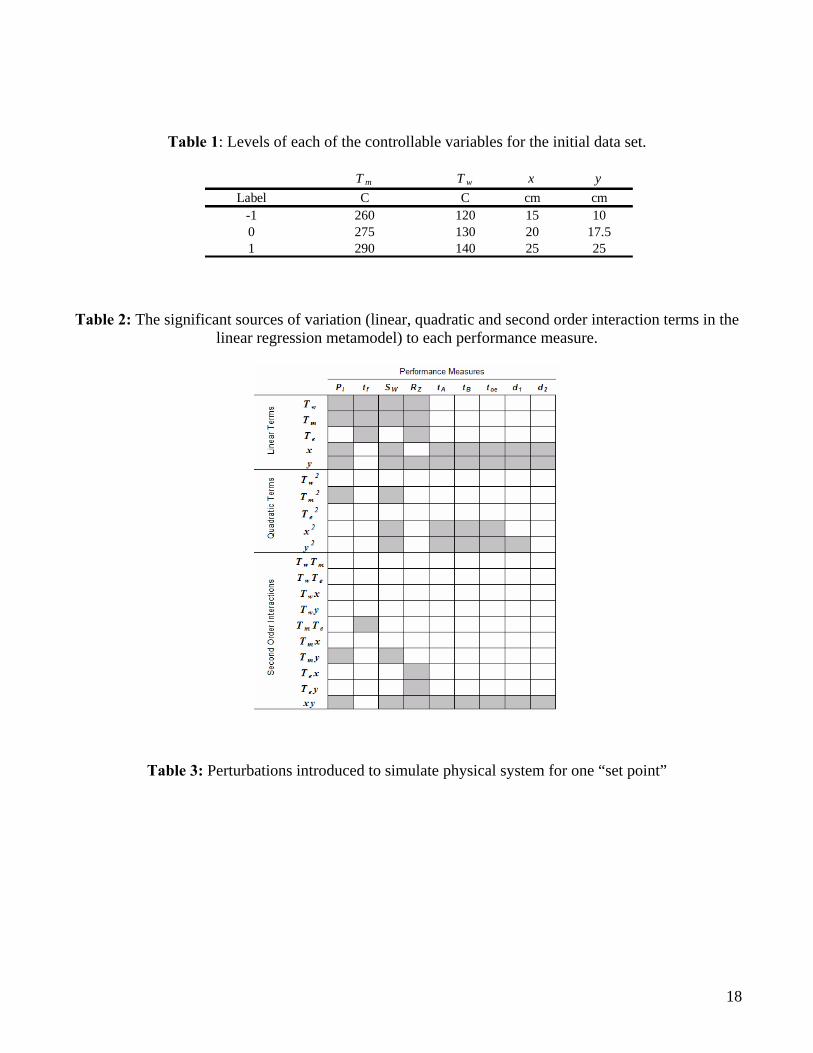
Four controllable variables were varied at the levels shown in table 1 in a full factorial design.

These variables include: (a) the melt temperature, Tm, (b) the mold temperature, Tw, (c) the horizontal

coordinate of the injection point, x, and (d) the vertical coordinate of the injection point, y. The injection

point location is constrained to be in the region shown in figure 1, due to some limitation of the IM

machine. This point will be characterized by the variables x and y in a Cartesian coordinate system with

its origin at the lower left corner of the part.

A finite element mesh of the part was created in MoldflowTM in order to obtain estimates for the

performance measures. Following with the general optimization strategy, this initial dataset was used to

create metamodels to mimic the behavior of each performance measure. In general, it is favorable to fit

a simple model to the data. In this study, second order linear regressions were initially considered as

models for the performance measures. When simple models do not suffice, then more complicated ones,

in this case artificial neural networks (ANNs), become necessary. In order to measure the prediction

capability of the metamodels, a validation set was used. The ANNs provided accurate models for each

of the PMs, so they were used to generate the larger dataset necessary for the multiple criteria

7

optimization problem. Further details of the performance of the ANNs are available in any of the

references 3 thru 6.

In order to extract useful information about the dependence of the PMs on the controllable

variables, an analysis of variance (ANOVA) was carried out. The results of the ANOVA are shown in

table 2. Notice that several PMs (tA, tB, toe, d1, and d2) are only dependent on the location of the injection

gate (x and y). With this knowledge, we were able to divide the optimization problem into two phases.

The first phase incorporates those PMs that are exclusively dependent on x and y in a multiple criteria

optimization problem to determine candidate injection gate locations. Since these PMs are not

influenced by the controllable temperatures, the ANNs were used to create a new dataset by varying x

and y at nine levels each within the experimental region (see table 1) resulting in a second data set with

81 data points. This multiple criteria optimization problem was solved both by DEA and a weighted

objective function, resulting in two candidate gate locations. In the second phase, the two candidate gate

locations from phase one are compared by incorporating the part warpage in the z-direction and

considering variability of the part warpage due the variation of Tm and Tw about their set values.

First Phase of the Optimization Procedure:

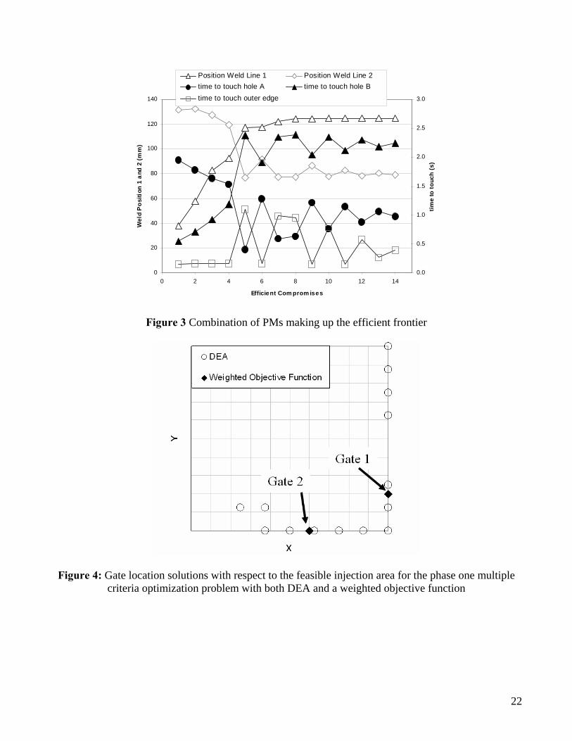
DEA was applied to the experimental dataset of 81 points to identify the efficient frontier. The

results of the DEA showed that 14 points were efficient. The combinations of PMs that were identified

as efficient are shown in figure 3. These efficient solutions were then traced back to the corresponding

injection locations. The resulting injection locations are shown in figure 4. It would be possible to run

the following analysis for all fourteen candidate locations, but this would be rather time consuming.

Therefore it was decided to reduce the number of candidate gate locations from fourteen to two

locations. This still allows for effective illustration of our methodology.

8

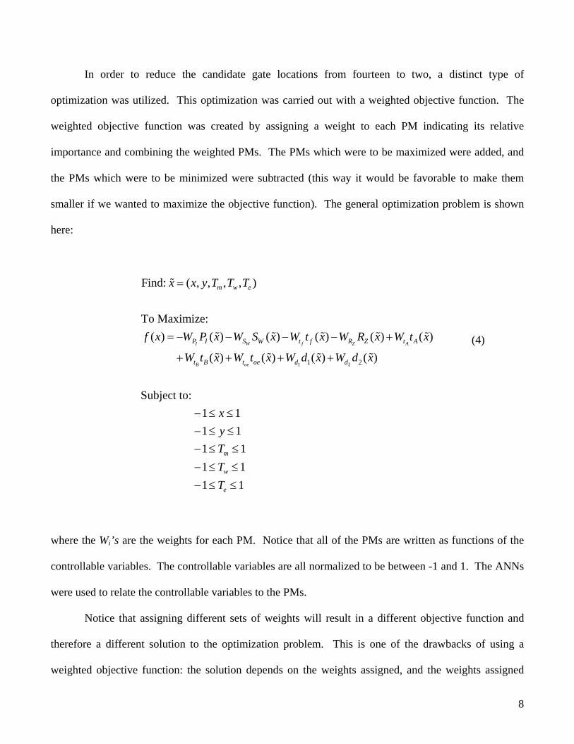
In order to reduce the candidate gate locations from fourteen to two, a distinct type of

optimization was utilized. This optimization was carried out with a weighted objective function. The

weighted objective function was created by assigning a weight to each PM indicating its relative

importance and combining the weighted PMs. The PMs which were to be maximized were added, and

the PMs which were to be minimized were subtracted (this way it would be favorable to make them

smaller if we wanted to maximize the objective function). The general optimization problem is shown

here:

1 21 2

Find: ( , , , , )

To Maximize: ( ) ( ) ( ) ( ) ( ) ( )

( ) ( ) ( ) ( )

Subject to:1 11 11 11 11 1

I W f Z A

B oe

m w e

P I S W t f R Z t A

t B t oe d d

m

w

e

x x y T T T

f x W P x W S x W t x W R x W t x

W t x W t x W d x W d x

xyTTT

=

= − − − − +

+ + + +

− ≤ ≤− ≤ ≤− ≤ ≤

− ≤ ≤− ≤ ≤

%

% % % % %

% % % %

where the Wi’s are the weights for each PM. Notice that all of the PMs are written as functions of the

controllable variables. The controllable variables are all normalized to be between -1 and 1. The ANNs

were used to relate the controllable variables to the PMs.

Notice that assigning different sets of weights will result in a different objective function and

therefore a different solution to the optimization problem. This is one of the drawbacks of using a

weighted objective function: the solution depends on the weights assigned, and the weights assigned

(4)

9

depend on the bias of the assigner. Also, even when a solution is found, it is still necessary to verify that

the solution is indeed optimal. This can be done analytically by showing that the Hessian matrix is

positive definite which indicates that the function is convex and has one optimum which is the global

optimum, or by verifying that the Kuhn-Tucker optimality conditions are satisfied [8].

These reasons are why using a weighted objective function by itself can be dangerous. In our

case, since the objective function is very complicated due to the inclusion of the ANNs, either of these

two options becomes difficult and time consuming. However, combining the use of a weighted

objective function with our DEA results alleviates the need of proving optimality. This is also beneficial

in extracting information about the optimization solutions and illustrating the relationship between the

DEA and a weighted objective function.

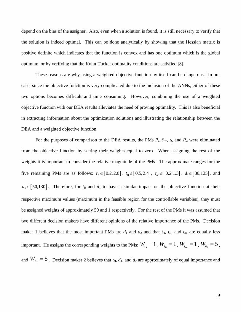
For the purposes of comparison to the DEA results, the PMs PI, SW, tf, and RZ were eliminated

from the objective function by setting their weights equal to zero. When assigning the rest of the

weights it is important to consider the relative magnitude of the PMs. The approximate ranges for the

five remaining PMs are as follows: [ ]0.2, 2.0At ∈ , [ ]0.5, 2.4Bt ∈ , [ ]0.2,1.3oet ∈ , [ ]1 30,125d ∈ , and

[ ]2 50,130d ∈ . Therefore, for tB and d1 to have a similar impact on the objective function at their

respective maximum values (maximum in the feasible region for the controllable variables), they must

be assigned weights of approximately 50 and 1 respectively. For the rest of the PMs it was assumed that

two different decision makers have different opinions of the relative importance of the PMs. Decision

maker 1 believes that the most important PMs are d1 and d2 and that tA, tB, and toe are equally less

important. He assigns the corresponding weights to the PMs: 1At

W = , 1Bt

W = , 1oetW = ,

15dW = ,

and 2

5dW = . Decision maker 2 believes that tB, d1, and d2 are approximately of equal importance and

10

tA and toe are of less importance. He assigns the weights: 1At

W = , 50Bt

W = , 1oetW = ,

11dW = ,

and 2

1dW = .

The optimization problem was solved for both sets of weights using the Hooke and Jeeve’s

method [9]. The first set of weights results in an optimal solution for the injection gate of x=1.0 and y=-

0.6. The second set of weights resulted in an optimal injection gate of x=0.2 and y=-1.0. At this stage

some test for optimality should be done; however, as mentioned earlier, the use of ANNs in the

objective functions makes either optimality test very difficult. Comparing the results of the weighted

objective function solutions to the efficient frontier found by DEA shows that the two solutions lie on

the efficient frontier. This indicates that they are in fact optimal solutions. Figure 4 shows the solutions

for both types of optimization with respect to the feasible injection region. The injection gate located at

x=1.0 and y=-0.6 will be referred to as gate 1, and the gate located at x=0.2 and y=-1.0 will be referred to

as gate 2 from this point forward.

The two optimal solutions determined by the Hooke and Jeeves method using a weighted

objective function very closely match the solutions determined by DEA. If more cases with different

weights were considered, it is likely that points would have been found that could represent the rest of

the DEA efficient frontier. The solutions don’t exactly match because DEA uses discrete points, and the

weighted objective function is continuous.

Second Phase of the Optimization Procedure:

In the second phase the part deflection in the critical direction (z-direction) was incorporated. In

high precision manufacturing applications it is necessary to obtain very tight dimensional tolerances. In

injection molding, this may be achieved by decreasing the part deflection. In addition, it is also crucial to

achieve a repeatable process that results in a consistent product. With this in mind, it is necessary to

11

incorporate the variability of the PMs in the optimization problem when considering a high precision

application.

In a physical IM setup, it is impossible to control certain variables with absolute accuracy. The

process variables will vary over some finite range resulting in some variability of the PMs.

Traditionally, the variability of a PM is evaluated by running several experimental repeats and then

estimating the standard deviation. In our case, this was not feasible since the model of our system is a

numerical one. In order to simulate a physical experiment, perturbations of the process variables were

introduced. It was assumed that the mold and melt temperatures could be controlled with accuracies of

±5 and ±10 oC respectively.

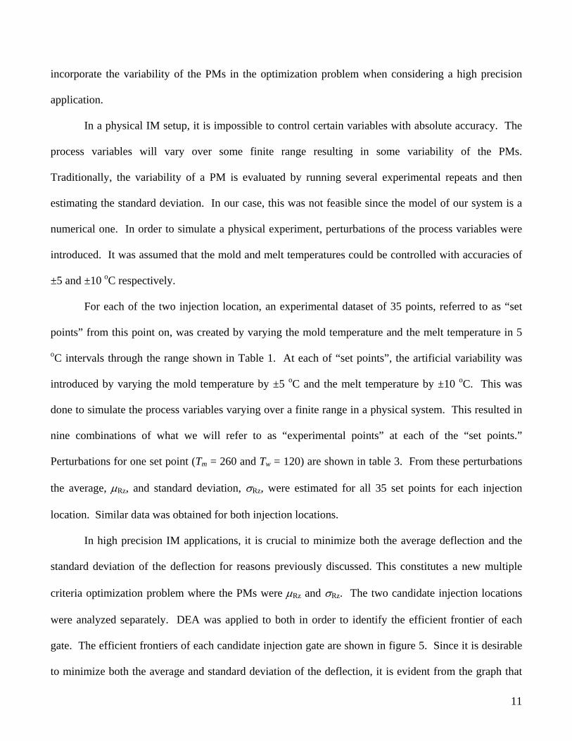
For each of the two injection location, an experimental dataset of 35 points, referred to as “set

points” from this point on, was created by varying the mold temperature and the melt temperature in 5

oC intervals through the range shown in Table 1. At each of “set points”, the artificial variability was

introduced by varying the mold temperature by ±5 oC and the melt temperature by ±10 oC. This was

done to simulate the process variables varying over a finite range in a physical system. This resulted in

nine combinations of what we will refer to as “experimental points” at each of the “set points.”

Perturbations for one set point (Tm = 260 and Tw = 120) are shown in table 3. From these perturbations

the average, µRz, and standard deviation, σRz, were estimated for all 35 set points for each injection

location. Similar data was obtained for both injection locations.

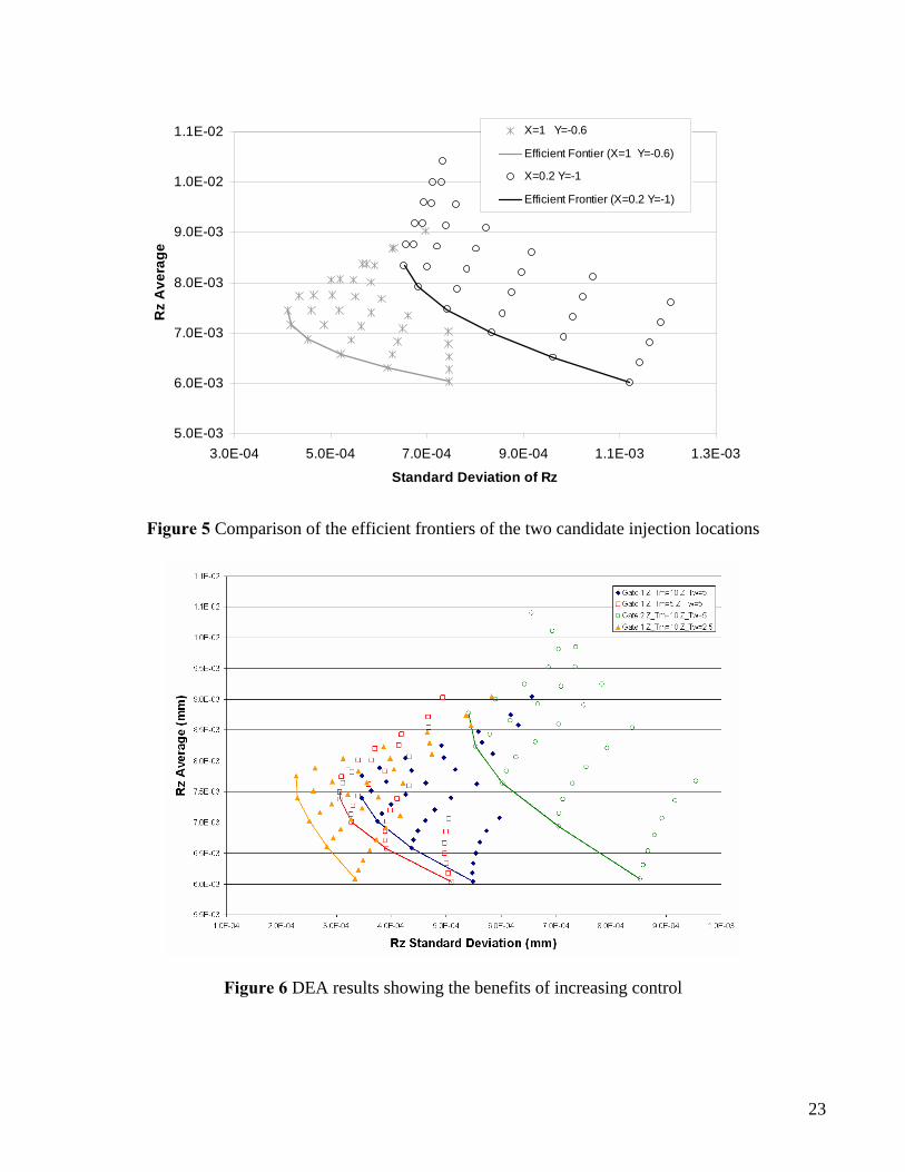
In high precision IM applications, it is crucial to minimize both the average deflection and the

standard deviation of the deflection for reasons previously discussed. This constitutes a new multiple

criteria optimization problem where the PMs were µRz and σRz. The two candidate injection locations

were analyzed separately. DEA was applied to both in order to identify the efficient frontier of each

gate. The efficient frontiers of each candidate injection gate are shown in figure 5. Since it is desirable

to minimize both the average and standard deviation of the deflection, it is evident from the graph that

12

the injection location of (1.0, -0.6) results in a more favorable efficient frontier. If a decision was to be

made based on the average deflection alone, neither injection gate would hold a distinct advantage over

the other, because the minimum deflection of both gates is essentially the same. However, when the

variability is introduced in the form of the standard deviation, there is a clear advantage to locating the

injection gate at (1.0, -0.6). Choosing this gate would result in a more effective process for high

precision IM applications.

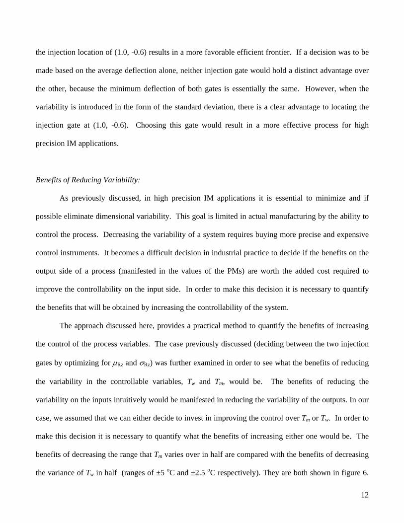
Benefits of Reducing Variability:

As previously discussed, in high precision IM applications it is essential to minimize and if

possible eliminate dimensional variability. This goal is limited in actual manufacturing by the ability to

control the process. Decreasing the variability of a system requires buying more precise and expensive

control instruments. It becomes a difficult decision in industrial practice to decide if the benefits on the

output side of a process (manifested in the values of the PMs) are worth the added cost required to

improve the controllability on the input side. In order to make this decision it is necessary to quantify

the benefits that will be obtained by increasing the controllability of the system.

The approach discussed here, provides a practical method to quantify the benefits of increasing

the control of the process variables. The case previously discussed (deciding between the two injection

gates by optimizing for µRz and σRz) was further examined in order to see what the benefits of reducing

the variability in the controllable variables, Tw and Tm, would be. The benefits of reducing the

variability on the inputs intuitively would be manifested in reducing the variability of the outputs. In our

case, we assumed that we can either decide to invest in improving the control over Tm or Tw. In order to

make this decision it is necessary to quantify what the benefits of increasing either one would be. The

benefits of decreasing the range that Tm varies over in half are compared with the benefits of decreasing

the variance of Tw in half (ranges of ±5 oC and ±2.5 oC respectively). They are both shown in figure 6.

13

From these results we can see that decreasing the variance of Tw in half has a greater effect than

decreasing the variance of Tm in half. This provides a justification for investing in improving the control

of Tw instead of Tm assuming both cost the same.

American Society of Testing and Materials (ASTM) Mold:

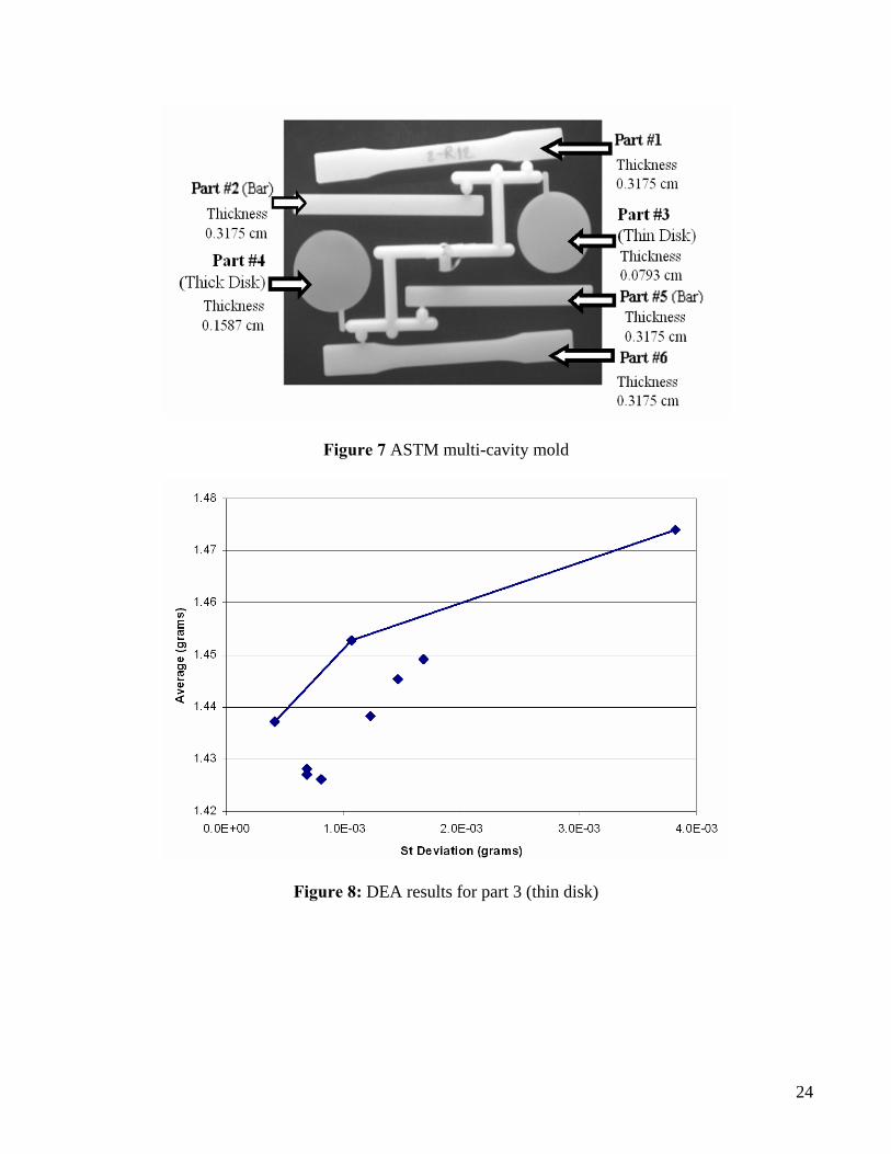
The second case involves the analysis of a multicavity mold to produce a set of dissimilar parts

used for standard ASTM destructive tests. The molding is shown in figure 7 along with the thicknesses

of the parts. From this figure, it is easy to identify that the identical parts 1 and 6 are the specimens used

in tension tests; identical parts 2 and 5 are used in flexure tests; and the disks 3 and 4 (which have

different thickness between them and to the rest of the parts) are used in hardness tests. The material

used in this case was High Density Polyethylene (HDPE). The commercial name is HID-9035 from

Chevron Phillips.

The same general optimization strategy was applied to this experimental case. In this case, since

we did not use a physics based model step 2 was skipped. Also, step 4 was removed from the analysis

for simplicity, and the study was limited to the use of experimental data points. In order to complete this

analysis, it will be necessary to fit metamodels to the experimental data and use these metamodels to

generate a larger dataset. The process variables used were the injection speed and the packing pressure.

They were varied as percentages of the total machine capacity for each. The machine has a maximum

injection speed of 160 mm/s and a maximum packing pressure of 2,230 kgf/cm2. The process variables

were varied at the levels shown in table 4.

A full factorial design of experiments was used resulting in a total of nine set points. The central

values for these variables were based on the recommended values from the Moldflow materials database.

Five experimental repeats were run at each of the set points, resulting in a total of 45 experimental runs.

The weight was measured for each individual part and also for the all the parts together with the runners.

14

The weight is relatively easy to measure and gives a good indication of the repeatability of the process.

From the five repeats, the average weight, iW , and standard deviation of the weight, iσ , were calculated

for each of the parts.

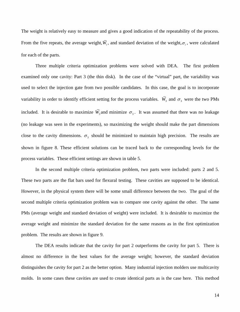
Three multiple criteria optimization problems were solved with DEA. The first problem

examined only one cavity: Part 3 (the thin disk). In the case of the “virtual” part, the variability was

used to select the injection gate from two possible candidates. In this case, the goal is to incorporate

variability in order to identify efficient setting for the process variables. 3W and 3σ were the two PMs

included. It is desirable to maximize 3W and minimize 3σ . It was assumed that there was no leakage

(no leakage was seen in the experiments), so maximizing the weight should make the part dimensions

close to the cavity dimensions. 3σ should be minimized to maintain high precision. The results are

shown in figure 8. These efficient solutions can be traced back to the corresponding levels for the

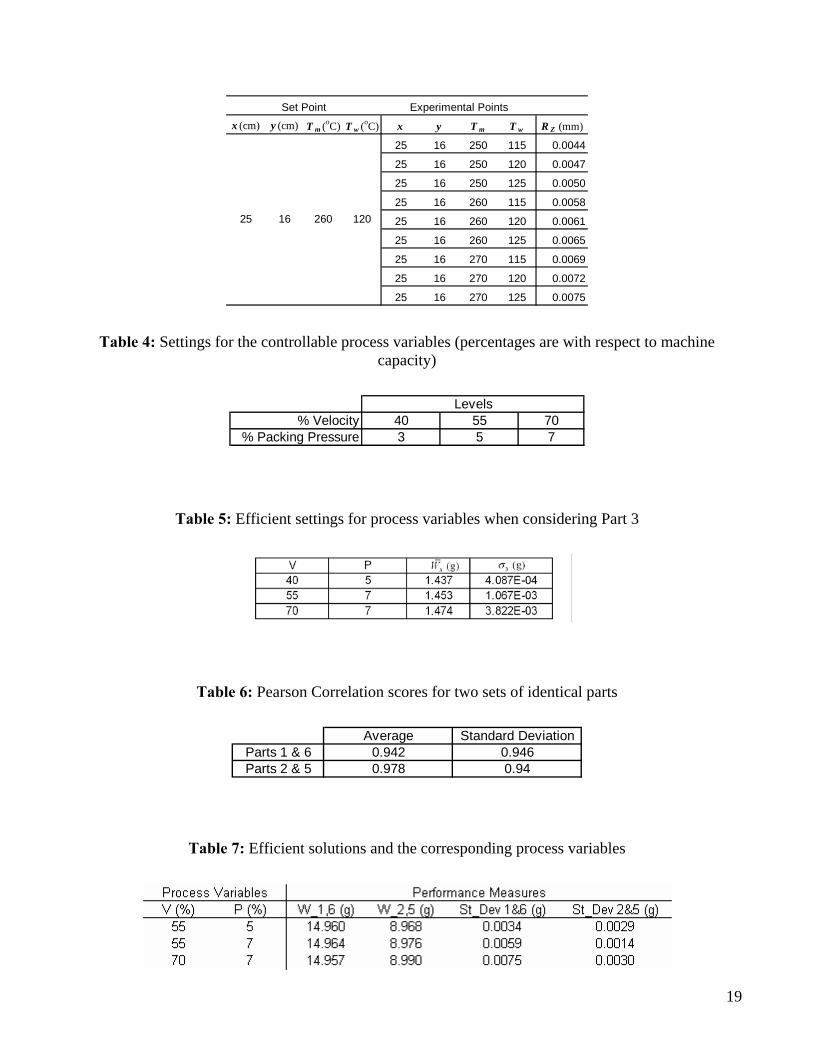
process variables. These efficient settings are shown in table 5.

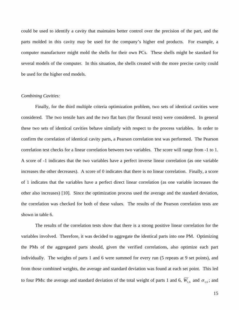
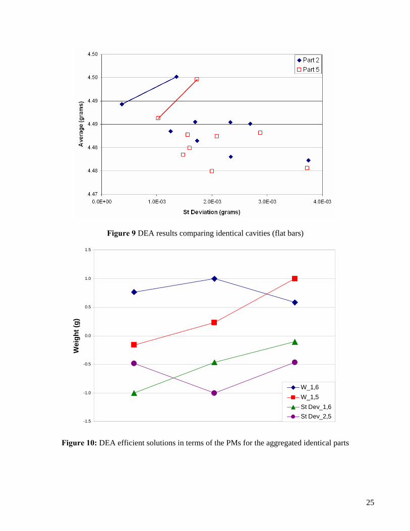
In the second multiple criteria optimization problem, two parts were included: parts 2 and 5.

These two parts are the flat bars used for flexural testing. These cavities are supposed to be identical.

However, in the physical system there will be some small difference between the two. The goal of the

second multiple criteria optimization problem was to compare one cavity against the other. The same

PMs (average weight and standard deviation of weight) were included. It is desirable to maximize the

average weight and minimize the standard deviation for the same reasons as in the first optimization

problem. The results are shown in figure 9.

The DEA results indicate that the cavity for part 2 outperforms the cavity for part 5. There is

almost no difference in the best values for the average weight; however, the standard deviation

distinguishes the cavity for part 2 as the better option. Many industrial injection molders use multicavity

molds. In some cases these cavities are used to create identical parts as is the case here. This method

15

could be used to identify a cavity that maintains better control over the precision of the part, and the

parts molded in this cavity may be used for the company’s higher end products. For example, a

computer manufacturer might mold the shells for their own PCs. These shells might be standard for

several models of the computer. In this situation, the shells created with the more precise cavity could

be used for the higher end models.

Combining Cavities:

Finally, for the third multiple criteria optimization problem, two sets of identical cavities were

considered. The two tensile bars and the two flat bars (for flexural tests) were considered. In general

these two sets of identical cavities behave similarly with respect to the process variables. In order to

confirm the correlation of identical cavity parts, a Pearson correlation test was performed. The Pearson

correlation test checks for a linear correlation between two variables. The score will range from -1 to 1.

A score of -1 indicates that the two variables have a perfect inverse linear correlation (as one variable

increases the other decreases). A score of 0 indicates that there is no linear correlation. Finally, a score

of 1 indicates that the variables have a perfect direct linear correlation (as one variable increases the

other also increases) [10]. Since the optimization process used the average and the standard deviation,

the correlation was checked for both of these values. The results of the Pearson correlation tests are

shown in table 6.

The results of the correlation tests show that there is a strong positive linear correlation for the

variables involved. Therefore, it was decided to aggregate the identical parts into one PM. Optimizing

the PMs of the aggregated parts should, given the verified correlations, also optimize each part

individually. The weights of parts 1 and 6 were summed for every run (5 repeats at 9 set points), and

from those combined weights, the average and standard deviation was found at each set point. This led

to four PMs: the average and standard deviation of the total weight of parts 1 and 6, 6,1W and 6,1σ ; and

16

the average and standard deviation of the total weight of parts 2 and 5, 5,2W and 5,2σ . These four PMs

were included in a multiple criteria optimization problem which was solved with DEA. Three efficient

solutions were found. They are shown in figure 10 in terms of the levels of the PMs (all PMs were

normalized to fall between -1 and 1). These three solutions can be traced back to the corresponding

process settings shown in table 7.

Conclusions:

High precision injection molding will be possible and marketable only if the process can deliver

parts at high production rates with tight tolerances in a consistent manner. This poses a multiple criteria

optimization problem in which variability must be considered explicitly as a performance measure. In

this work, we demonstrated the coordinated use of CAE, statistics, neural networks, and data

envelopment analysis to find the best compromises among the process controllable variables, including

variability as one of the performance measures. When experimental data is used, variability is inherent,

however, when only mathematical models are used, as in the first case presented here, the variability can

be generated by assuming a given variability in the controllable variables. Here we assumed a uniform

distribution for the variability of the performance measures, future work will involve analysis of the

effect of using different statistical distributions of variability of the process variables on the efficient

frontier. Statistical analysis can help determine the dependency of the performance measures on the

controllable process variables. If the analyses can be decoupled, then an optimization in several stages is

appropriate as demonstrated in this application.

References

1. Cabrera-Rios, M., Zuyev, K., Chen, X., Castro, J.M., and Straus, E.J. Polymer Composites, 23:5

(2002)

17

2. Cabrera-Rios, M., Mount-Campbell, C.A., and Castro J. M., Journal of Polymer Engineering, 22:5

(2002)

3. Castro, C.E., Cabrera-Rios, M., Lilly, B., Castro, J.M., and Mount-Campbell, C.A. Journal of

Integrated Design & Process Science, 7:1 (2003)

4. Castro, C.E., Bhagavatula, N., Cabrera-Rios, M., Lilly, B., and Castro, J.M., ANTEC Proceedings

(2003)

5. Castro, C.E., Cabrera-Rios, M., Lilly, B., and Castro, J. M., Journal of Polymer Engineering,

accepted for publication (2005)

6. Castro, C.E. “Optimization and Analysis of Engineering in High Precision Injection Molding.” M.S.

Thesis, The Ohio State University, OH, 2005.

7. Charnes, A., W.W., and Rhodes, E. European Journal of Operational Research, 2:6 (1978)

8. Arora, J.S., Introduction to Optimum Design. McGraw-Hill (2001)

9. Hooke, R., Jeeves, T.A., Journal of Association of Computing Machinery, (1961)

10. Devore, J., Applied Statistics for Engineering and the Sciences, International Thomson Publishing

Company (2000)

Key Words

Injection Molding, Artificial Neural Networks, Data Envelopment Analysis, Robust Solutions

18

Table 1: Levels of each of the controllable variables for the initial data set.

T m T w x yLabel C C cm cm

-1 260 120 15 100 275 130 20 17.51 290 140 25 25

Table 2: The significant sources of variation (linear, quadratic and second order interaction terms in the linear regression metamodel) to each performance measure.

Table 3: Perturbations introduced to simulate physical system for one “set point”

19

x (cm) y (cm) T m (oC) T w (oC) x y T m T w R Z (mm)

25 16 250 115 0.0044

25 16 250 120 0.0047

25 16 250 125 0.0050

25 16 260 115 0.0058

25 16 260 120 0.0061

25 16 260 125 0.0065

25 16 270 115 0.0069

25 16 270 120 0.0072

25 16 270 125 0.0075

Set Point Experimental Points

25 16 260 120

Table 4: Settings for the controllable process variables (percentages are with respect to machine capacity)

% Velocity 40 55 70% Packing Pressure 3 5 7

Levels

Table 5: Efficient settings for process variables when considering Part 3

Table 6: Pearson Correlation scores for two sets of identical parts

Average Standard Deviation

Parts 1 & 6 0.942 0.946Parts 2 & 5 0.978 0.94

Table 7: Efficient solutions and the corresponding process variables

20

Figure 1: Part of constant thickness with cutouts

21

Figure 2: Measuring the locations of the weld lines

22

0

20

40

60

80

100

120

140

0 2 4 6 8 10 12 14

Efficient Com prom ises

Wel

d P

ositi

on 1

and

2 (m

m)

0.0

0.5

1.0

1.5

2.0

2.5

3.0

time

to to

uch

(s)

Position Weld Line 1 Position Weld Line 2time to touch hole A time to touch hole Btime to touch outer edge

Figure 3 Combination of PMs making up the efficient frontier

Figure 4: Gate location solutions with respect to the feasible injection area for the phase one multiple criteria optimization problem with both DEA and a weighted objective function

23

5.0E-03

6.0E-03

7.0E-03

8.0E-03

9.0E-03

1.0E-02

1.1E-02

3.0E-04 5.0E-04 7.0E-04 9.0E-04 1.1E-03 1.3E-03

Standard Deviation of Rz

Rz

Ave

rage

X=1 Y=-0.6

Efficient Fontier (X=1 Y=-0.6)

X=0.2 Y=-1

Efficient Frontier (X=0.2 Y=-1)

Figure 5 Comparison of the efficient frontiers of the two candidate injection locations

Figure 6 DEA results showing the benefits of increasing control

24

Figure 7 ASTM multi-cavity mold

Figure 8: DEA results for part 3 (thin disk)

25

Figure 9 DEA results comparing identical cavities (flat bars)

-1.5

-1.0

-0.5

0.0

0.5

1.0

1.5

Wei

ght (

g)

W_1,6W_1,5St Dev_1,6St Dev_2,5

Figure 10: DEA efficient solutions in terms of the PMs for the aggregated identical parts