improving the predictions of injection molding simulation software

THIS IS THE PEER REVIEWED VERSION OF

THE FOLLOWING ARTICLE:

U. Vietri, A. Sorrentino, V.Speranza, R.Pantani “IMPROVING THE PREDICTIONS OF INJECTION MOLDING SIMULATION SOFTWARE“

Polymer Engineering & Science; 51 (12); 2542-2551

DOI 10.1002/pen.22035

WHICH HAS BEEN PUBLISHED IN FINAL FORM AT

http://onlinelibrary.wiley.com/doi/10.1002/pen.22035/abstract

THIS ARTICLE MAY BE USED ONLY FOR NON-COMMERCIAL

PURPOSES

IMPROVING THE PREDICTIONS OF INJECTION MOLDING

SIMULATION SOFTWARE

U. Vietri , A. Sorrentino, V. Speranza*, R. Pantani

AUTHOR AFFILIATION: Polymer Technology Group - www.PolymerTechnology.it

Department of Industrial Engineering, University of Salerno

Via Ponte don Melillo – Fisciano (SA) – I 84084 – Italy

AUTHOR EMAIL ADDRESS: [email protected], [email protected], [email protected],

[email protected]

*To whom correspondence should be addressed.

Postal address: University of Salerno – Department of Industrial Engineering –

Via Ponte don Melillo, I-84084, Fisciano (SA), ITALY

E-mail address: [email protected]

Telephone number: (direct) (+39) 08996 4145 or 4013 (mobile) (+39) 320 7979017

Fax number: (+39) 08996 4057

Abstract

Injection molding is one of the most widespread processes for plastic manufacturing. Software

packages are often used in several steps of the production cycle, from mold design to the

determination of processing conditions. In this work a method is reported to improve the predictions of

the description of pressure profiles made by injection molding simulation software. The method is

applied to two polymeric materials (a PolyStyrene and a PolyCarbonate) injection molded into line-

gated rectangular cavities adopting different molding conditions and cavity thickness. The method,

that is independent of the software adopted, in this paper is illustrated adopting the commercial code

Moldflow®. It is shown that the predictions of the description of pressure curves inside the cavity can

be significantly improved by introducing the effect of pressure on viscosity and the effect of cavity

deformation during molding. The former effect is taken into account by finding an appropriate value

for the parameter which takes into account the effect of pressure in the equation which describes

material rheology. The latter effect can be introduced by defining and implementing an apparent

material compressibility.

Introduction

The injection molding process is widely applied for polymer engineering materials. The process

itself is a complex mix of time, temperature and pressure variables [1] with a multitude of

manufacturing defects that can occur without the right combination of processing parameters and

design components [2]. Because of these complexities, both mold-makers and producers of plastic

parts are increasingly interested in more precise and specific results from simulation codes, in order to

reduce development time, improve quality of molded products, and basically save money. Traditional

goals for simulations (mainly limited to predictions of flow front advancement, hot points and weld

line positions and pressure history) have been recently enlarged to include also predictions of final

product morphology and properties [3]. This makes the demand of accurate predictions even more

stringent. Currently, also thanks to the powerful hardware available, injection moling simulation

packages are able to solve the relevant equations for a Newtonian fluid flowing in a cold cavity, even

in three dimensions. The numerical routines are powerful enough to take into account all the terms in

the energy and momentum balance equations [4]. Pressure and temperature evolutions are normally

considered to be reasonably well predicted by and the majority of the commercial software packages

currently available; nevertheless several aspects of interest to post-filling steps still must be examined

or more deeply investigated, like the pressure effect on polymer viscosity [5], and the relevance to

process variables evolution of mold deformation [6]. Despite of the fact that these two phenomena

require a careful characterization of material properties and an analysis of the interactions between

pressure distributions and mold compliance, a simplified approach can be adopted to take into account

rather easily both of them. This approach is shown in this work and applied to the simulations made by

means of Moldflow® of the injection molding tests carried out with two different amorphous

materials: an atactic Polystyrene, and a Polycarbonate.

Experimental Techniques and Results

Materials

Two different thermoplastic amorphous polymers were used: a general purpose Polystyrene (PS

678E) supplied by Dow Chemicals with a molecular weight distribution characterized by

Mn = 87x103, Mw = 250x10

3 and Mz = 490x10

3 and a Polycarbonate (PC Lexan 141R) supplied by

GE Plastics (Europe) with a density equal to 1.20 g/cm! and a Melt Volume-Flow Rate (MVR

300°C/1.2 kg) equal to 12.0 cm!/10min.

Rheology description

The Cross-WLF model is the most commonly adopted way for the description of the viscosity of

polymers, and is therefore widely used also in injection molding simulation software both commercial

and non-commercial. According to that model, the viscosity of the material, ", is described as a

function of temperature, T, pressure, P, and shear rate

!

".

by the following equation:

!

"(#.

,T,P ) ="0(T,P )

1+"0 T,P( )#

.

$

%

&

' ' '

(

)

* * *

1+n (1)

where !0 is the zero shear rate viscosity which is given by a modified form of the WLF equation:

!

"0(T,P ) = D1 #exp$A1 # T $D2 $D3P( )

A2 +T $D2

%

&

' '

(

)

* * (2)

The parameters ", n, D1, D2, D3, A1, A2 are typically data-fitted coefficients, even though each of them

has a physical meaning [7].

If eq. 2 is adopted, the parameters # and $ which describe the effects of temperature and pressure on

zero shear rate viscosity, respectively, are given by the following equations:

!

" =1

#0

$#0

$T

%

& '

(

) *

P

= +A

1, A

2+ D

3P( )

A2

+T +D2( )

2 (3)

!

" =1

#0

$#0

$P

%

& '

(

) * T

=A

1+D

3

A2

+T ,D2

(4)

Eq. 4 clarifies the fact that the effect of pressure on viscosity can be described by adopting a suitable

value for the parameter D3. For most of the materials, including those adopted in this work, injection

molding simulation are normally conducted setting the parameter D3 equal to zero. The effect of

pressure on viscosity is quite commonly neglected in polymer processing modeling, even though it is

well known that during injection molding the phenomenon is quite relevant due to the high pressure

levels.

The values of the Cross-WLF model constants, as reported in the Moldflow® database, are given in

table 1.

The polymer PVT behavior in the numerical simulations is very often described by a modified

form of the Tait equation, which is a quite successful equation, despite of the fact that it is an equation

of state, and thus inadequate for a correct description of the volume of polymers which depend on the

cooling history [8]. The Tait equation is expressed as:

!

v(T,P ) = v0(T ) 1"C ln 1+P

B(T )

#

$ %

&

' (

#

$ %

&

' ( + v

r(T,P ) (5)

where v(T,P) is the specific volume at a given temperature and pressure, v0 is the specific volume at

zero pressure, C is a universal constant 0.0894. The function vr(T,P) allows to describe the effect of

crystallization on specific volume (clearly, vr(T,P) is zero for amorphous resins). The parameters of the

model are defined in table 2.

The constants B1 to B9 are data-fitted coefficients. The subscripts “m” or “s” refer to the values in

the high and low temperature range (namely the melt and the solid), respectively. By adopting the Tait

equation, the parameters $V and #V, respectively the compressibility and the thermal expansion

coefficient of the polymer, are expressed, for an amorphous material, by the following equations

!

"V(T,P ) = #

1

v 0(T )

$v

$P

%

& '

(

) * T

=C

B(T ) + P (6)

!

"V(T,P ) =

1

v0(T )

#v

#T

$

% &

'

( )

P

=B2

v 0(T )1*C ln 1+

P

B(T )

$

% &

'

( )

$

% &

'

( ) *

C B4 P

B(T ) + P (7)

The values of the parameters of the Tait model, as reported in the Moldflow® database, are given

in table 3.

Molding Equipment and conditions

A 70-ton Negri-Bossi reciprocating screw, injection molding machine was used for the

experiments. The materials were injected into line gated rectangular cavities having length L=120

[mm], width W=30 [mm] and two different thicknesses: S=2 [mm] (for PS), and S=4 [mm] (for PS

and PC).

Special dies containing different gates could be assembled in the mold, in particular use was made

of two gates both having the same width of the cavity, length h=6 [mm] and thickness b=1.5 [mm] for

PS, and b=2 [mm] for PC, because its higher viscosity.

Five Kistler® piezoelectric pressure transducers were mounted along the flow path. In particular

one transducer was located in the injection chamber, one in the runner the others in the cavity 15, 60

and 105 mm downstream to the gate. These positions will be referred to as P0, P1, P2, P3 and P4,

respectively. The transducers signals were recorded by a fast data acquisition system. A complete

description of the geometry of the cavities adopted is given in Figure 1.

The injection molding PS experiments were carried out by adopting two holding pressures: 600 and

to 1100[bar]. For this material, injection temperature was held at 220 [°C], the mold was conditioned

at 25 [°C], holding time was 12 [s], and injection time was set at about 0.5 [s]. As far as Polycarbonate

is concerned, the holding pressure was changed over a range of values from 360 to 800 [bar]. Injection

temperature was 310 [°C], the mold was conditioned at 70 [°C], holding time was 12 [s], and injection

time was about 2.5 [s]. The time after holding (cooling time) was kept at about 20 [s]. The processing

conditions are summarized in table 4.

Experimental

In figure 2 and figure 3 the experimental pressure curves at the five transducer positions are

reported for the molding tests considered in this work, respectively for PS and PC.

As far as the pressure curves recoded during the injection molding of PS (figure 2) it can be noticed

that a residual pressure after 30 s is always present for the highest applied holding pressures (figure 2b

and 2d). The phenomenon is also present for the lowest applied holding pressure if the thinner cavity

is adopted (figure 2a). It is also interesting to notice that, for the same cavity, the pressure drops

between position P0 (nozzle) and P1 (runner), during the packing phase i.e. after 0.6 s, increase on

increasing holding pressure. This is mainly due to the effect of pressure on viscosity.

Similar observations hold true also for the pressure curves recoded during the injection molding of

PC (Figure 3).

Simulations.

Molding tests have been simulated using Moldflow® Plastic Insight ver 5.3. Each experimental test

was simulated by imposing the geometry of nozzle, channels and cavity. Basically, the molded part

geometry was reproduced and adopted as calculus domain by means of finite element meshing. The

mesh provides the basis for a Moldflow® analysis, where molding properties are calculated at every

node. It was necessary to use two different meshing type for calculus domain. For nozzle and sprue

geometries a beam element meshing was considered, which consists of a cylindrical shaped element

included among two-nodes, with longitudinal straight axis, so that when modeling curved beams, they

provide a "faceted" approximation to the true geometry. Hot runner channels were chosen for the

nozzle geometry mesh, and cold runner channels for meshing the sprue. To mesh the remaining

molded part we have chosen the mid-plane mesh element type which consists of tri-node triangular

elements that form a one dimensional representation of the part, through its centre. This mesh type is

suited in the case of thin-walled parts.

Each test was simulated by setting the injection and mold temperature, the filling time and the

experimental packing pressure profile at the nozzle node location. The filling time used in the

simulation was determined directly by experimental pressure curves: it was chosen as the time taken

by the polymer to reach position P4 (cavity tip). As a first attempt, pressure curves were simulated by

adopting the parameters for Cross WLF equation and Tait equation already present in the standard

Moldflow® database .

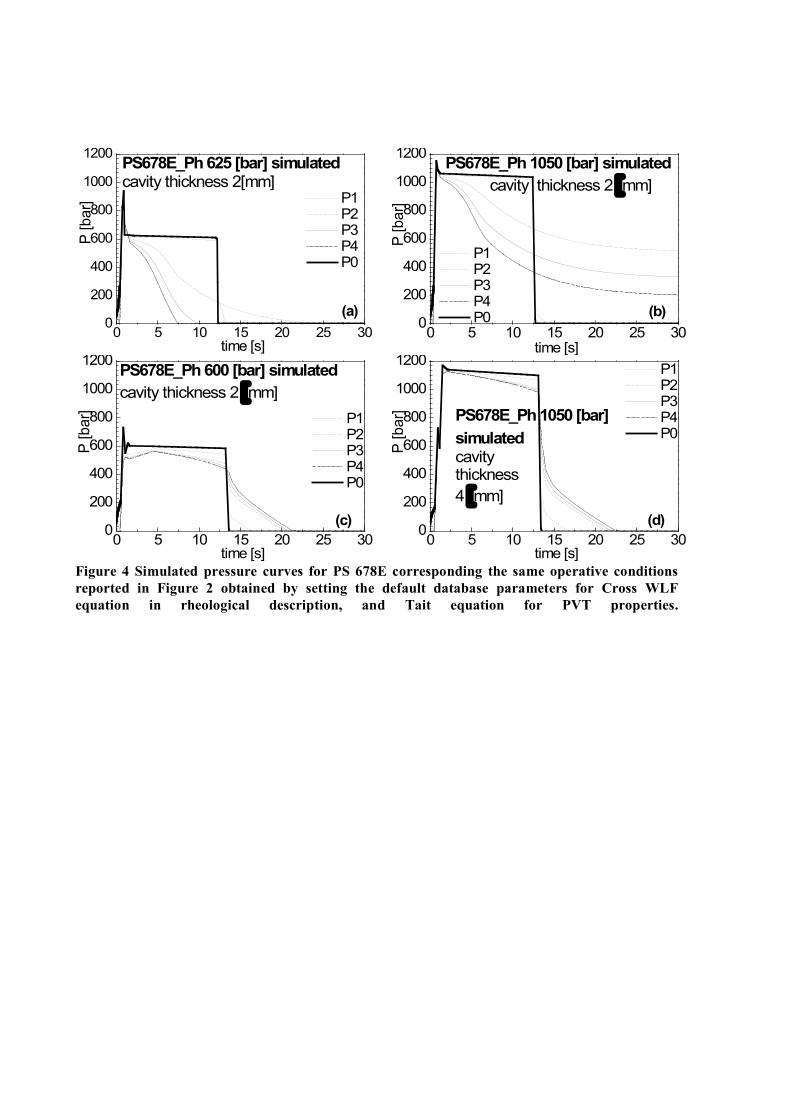
Simulated pressure evolutions corresponding to the same operative conditions considered in figure

2 (for PS) and figure 3 (for PC) are reported in figure 4 and 5, respectively.

With regard to the tests conducted with PS, the comparison of the simulations reported in figure 4

with the experimental plots of figure 2 shows that the predicted pressure drops among all transducer

positions are much smaller than experimental ones and thus pressures at each cavity transducer

position are larger than experimental ones. Furthermore, the pressure decrease is much faster. Similar

comments can be made also on the comparison of the experimental pressures measured for PC (Figure

3) and the simulated ones reported in figure 5.

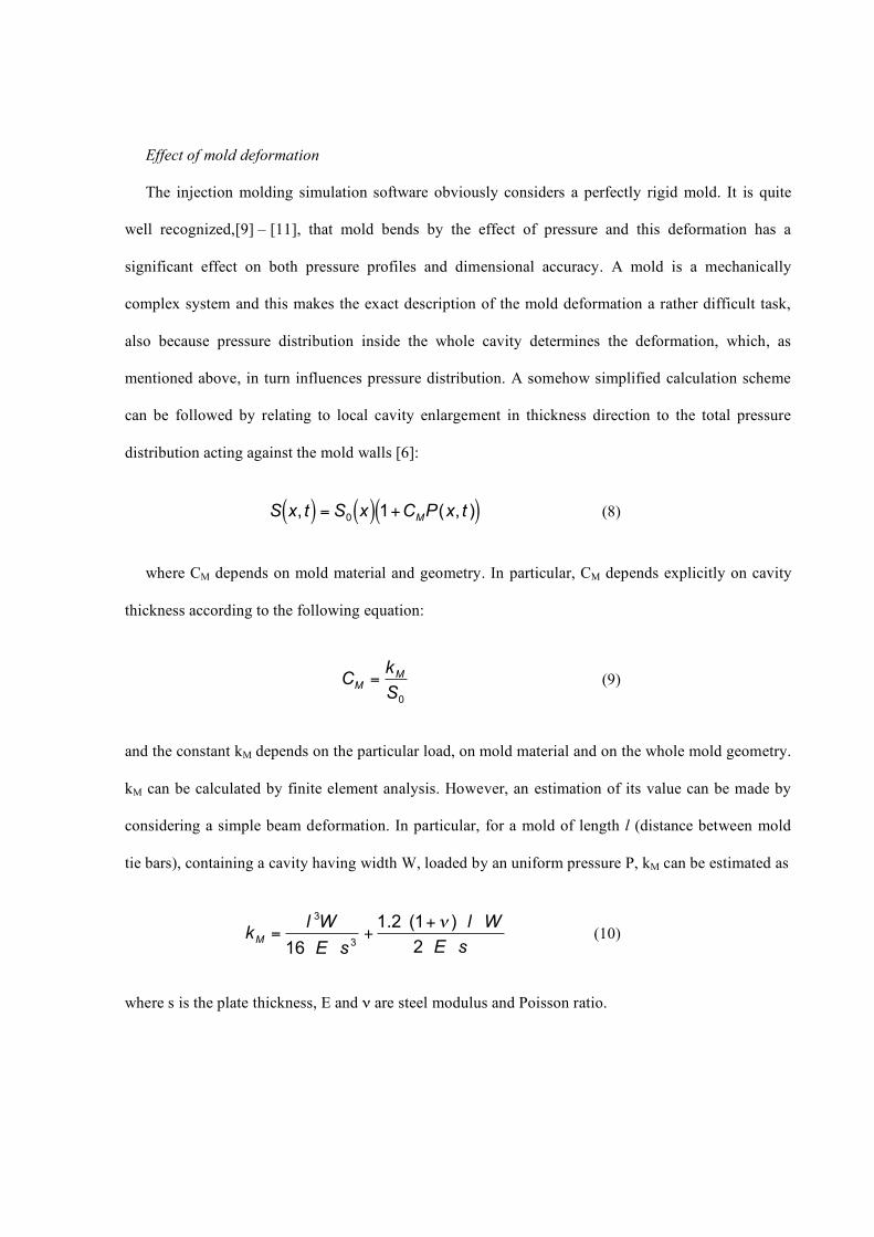
Effect of mold deformation

The injection molding simulation software obviously considers a perfectly rigid mold. It is quite

well recognized,[9] – [11], that mold bends by the effect of pressure and this deformation has a

significant effect on both pressure profiles and dimensional accuracy. A mold is a mechanically

complex system and this makes the exact description of the mold deformation a rather difficult task,

also because pressure distribution inside the whole cavity determines the deformation, which, as

mentioned above, in turn influences pressure distribution. A somehow simplified calculation scheme

can be followed by relating to local cavity enlargement in thickness direction to the total pressure

distribution acting against the mold walls [6]:

!

S x, t( ) = S0 x( ) 1+CMP(x, t )( ) (8)

where CM depends on mold material and geometry. In particular, CM depends explicitly on cavity

thickness according to the following equation:

!

CM

=k

M

S0

(9)

and the constant kM depends on the particular load, on mold material and on the whole mold geometry.

kM can be calculated by finite element analysis. However, an estimation of its value can be made by

considering a simple beam deformation. In particular, for a mold of length l (distance between mold

tie bars), containing a cavity having width W, loaded by an uniform pressure P, kM can be estimated as

!

kM

=l

3W

16 E s3

+1.2 (1+ " ) l W

2 E s (10)

where s is the plate thickness, E and $ are steel modulus and Poisson ratio.

Depending on mold geometry and material, kM typically assumes values in the range 10-5

÷10-4

[mm/bar] [6]. For this work it was found, by means of eq. 10, that kM was about 10-4

[mm/bar].

In order to introduce the effect of cavity deformation in software simulation, it is necessary to convert

it into a parameter which is present in the software. To do this, we consider the cooling step, namely

the stage of injection molding which starts from the gate sealing time, and represents the longest part

of the molding cycle. During the cooling stage, although the cavity volume decreases because of mold

deformation release, the mass per unit cavity length remains essentially constant with time; thus:

!

v x, z, t( )0

S ( x,t )

" dz = const (11)

Differentiating both terms of (eq.11) and making use of (eq.8), one simply obtains:

!

dv x, z, t( )dt

"

#

$ $

%

&

' '

0

S ( x,t )

( dz + v x,S x, t( ), t( )CMS0

)P x, t( ))t

= 0 (12)

which can be easily rearranged assuming that pressure does not depend on z

!

v 0"v

#T x, z, t( )#t

$ v0 %v

+v x,S x, t( ), t( )

v 0

CM

S0

S(x, t )

&

'

( (

)

*

+ +

#P x, t( )#t

dz

0

S ( x,t )

, = 0 (13)

Eq. 13 can be also written as

!

v 0"v

#T x, z, t( )#t

$ v0%v,a

#P x, t( )#t

dz

0

S ( x,t )

& = 0 (14)

in which $v,a is an apparent material compressibility given by;

!

"v,a = "

v+

v x,S x, t( ), t( )v0

CM

S0

S(x, t )# "

v+C

M (15)

It is clear that mold deformation can be taken into account by increasing material compressibility,

and thus it can be described by changing the material volumetric parameters in such way to keep

unchanged the values of #V and increase the values of $V by adding the mold compliance CM. We

assume that this method to describe mold deformation, obtained considering just the cooling stage, can

be adopted during the whole molding cycle. It can be demonstrated, that if the gate is the first section

to solidify (as it should normally happen) the same analysis can be done also on the packing/holding

stage, leading to the conclusion that also in this stage the mold deformation can be described by means

of $v,a.

If Tait equation is adopted for the description of material properties, it is possible to change #V and

$V nearly independently on acting on the parameters B3 and B4. In this work, we changed these two

parameters for the solid and the melt, as reported in Table 3 in order to satisfy eq. 15. It can be noticed

that the values adopted for the thicker cavity are different from those adopted for the thinner one. The

differences are obviously due to the mold geometry that directly affect the resulting mold compliance.

In figure 6 and figure 7, respectively for PS 678 and PC, are shown, for a fixed pressure of 200 bar, #V

and $V evaluated using with and without taking account the effect of mold deformation and $V,a

evaluated with eq. 15.

Effect of pressure on viscosity

As mentioned above, the parameter D3 describing the pressure influence on viscosity is set to zero

in the Moldflow® standard database. The correct value of the parameter can be determined on the

basis of experimental data of viscosity under high pressure, which however are quite difficult to obtain

[12].

A simple expression can be found in Van Krevelen [13], relating the effect of temperature and

pressure on zero shear rate viscosity to the volumetric properties. This equation can be written as:

!

" # $%"

V

%V

(16)

in which # and $ are the temperature and pressure dependence of viscosity, $V and #V are the

compressibility and the thermal expansion coefficient polymer. Equation (16), although very simple,

was found to be a good approximation of the experimental data of the effect of pressure on viscosity

[14].

The right hand side of (eq. 16) can be calculated as a function of temperature by adopting equations

3, 6 and 7, whose parameters are known for both materials. The value of $ was expressed in (eq. 4) as

depending on the parameter D3. A suitable choice for the value of the parameter D3 can be made in

order to obtain the best possible description of the RHS of (eq. 16) by means of (eq. 4), as shown in

figure 8. The values of the parameter D3 for both materials are reported in table 1. The values found

for the parameter D3 is about the same for both materials. It should be noticed, however, than the same

value of D3 does not give raise to the same effect of pressure on viscosity, being the latter related to all

the other parameters for viscosity description.

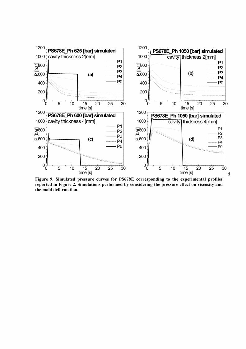
Improved simulations of pressure profiles

In figure 9 and figure 10, the predicted pressure profiles referred to simulations performed by setting

the chosen D3 parameter in Cross WLF equation, and setting the new values for the parameters B3 and

B4 in Tait equation, are reported for the same operative conditions considered in figure 2 (for PS) and

Figure 3 (for PC). The plots highlight that a sensitive improvement in predicting the experimental

pressure profile by simulation, has been achieved. In fact the effect produced by setting a non zero

value for D3 (see table 1) in simulating the injection molding tests, leads to a satisfactorily pressure

drop prediction (between P0 and P1) in comparison to the experimental cases. Also the fact that the

pressure drop increases on increasing the holding pressure is captured. A remarkable improvement,

involves also the pressure profiles evolution during the cooling stage. The correction of the material

compressibility in simulation obtained by modifying the values of the parameters B3 and B4 of the Tait

equation, slows down the pressure decrease and allows to describe the residual pressure for PS.

Obviously, the simulations are not perfect. In particular, for PC no residual pressure is predicted. This

can be due to the simplicity of the model describing mold deformation and to the fact that this effect

can be only introduced indirectly in the simulation program by modifying the material parameters. It is

worth mentioning, however, that no optimization has been carried out on material parameters, since

the aim of this paper is to present a method for improving the simulations without relying on data from

material characterization.

Conclusions

In this work, a method is presented to take into account, on first approximation, the effect of pressure

on viscosity and of cavity deformation on the predictions of pressure profiles carried out by means of

an injection molding simulation software. In particular, two amorphous materials, a PS and a PC, were

injection molded into rectangular cavities of two different thickness, by changing the holding pressure.

Pressure evolution at different positions along the flowpath were measured. The same tests were

simulated by means of Moldflow® Plastics Insight ver. 5.3. It was found that the pressure drops

between consecutive transducer positions were largely underestimated if the parameters taken from the

standard software database were adopted. Furthermore, for both materials and all molding conditions,

the predicted cavity pressure decreased too quickly during the cooling step. In order to obtain more

accurate predictions, the effect of pressure on viscosity was introduced by estimating the value of the

corresponding parameter in the WLF equation by means of a combination of other material properties.

Eventually, a method was suggested to keep into account the effect of cavity enlargement on pressure

profiles. It was shown that a sensitive improvement could be achieved in spite of the simplicity of the

method adopted.

References

1 R. Pantani, and G. Titomanlio, “The simulation of post–filling steps in injection molding” -

Injection Molding – Fundamentals and Applications, M. R. Kamal, A. I. Isayev and S.–J. Liu

editors, Carl Hanser Publisher (2009).

2 T. A. Osswald, L.-S. Turng, and P. Gramann, Injection molding handbook – Chap. 10-12,

Carl Hanser Publishers (2008).

3 R. Pantani, I. Coccorullo, V. Speranza, and G. Titomanlio, Prog. Polym. Sci. , 30 (12), 1185

(2005).

4 P. Kennedy, Practical and Scientific Aspects of Injection Molding Simulation, PhD. Thesis,

Eindhoven University of Technology (2008).

5 R. Pantani, and A. Sorrentino, Polym. Bull. , 54, 365 (2005).

6 R. Pantani, V. Speranza, and G. Titomanlio, Polym. Eng. Sci. , 41 (11), 2022 (2001).

7 J. D. Ferry, Viscoelastic properties of polymers., Wiley (1980).

8 R. Y. Chang, C. H.Chen, and K. S. Su, Polym. Eng. Sci. , 36 (13), 1789 (1996).

9 B. Carpenter, S. Patil, R. Hoffman, B. Lilly, and J. Castro, Polym. Eng. Sci. , 46 (7), 844

(2006).

10 D. Delaunay, P. Le Bot, R. Fulchiron, J. F. Luye, and G. Regnier, Polym. Eng. Sci. , 40 (7),

1692 (2000).

11 W. Cheng-Hsien, and H. Yu-Jen, Int. J. Adv. Manuf. Tech. , 32 (11-12), 1144 (2007).

12 R. Cardinaels, P. Van Puyvelde, and P. Moldenaers, Rheol. Acta , 46 (4), 495 (2007).

13 D.W. Van Krevelen, Properties of Polymers: their correlation with chemical structure, their

numerical estimation and prediction from additive group contributions, Elsevier (1997).

14 A. Sorrentino, and R. Pantani, Rheol. Acta , 48 (4), 467 (2009).

Table 1. Values of the Cross-WLF model constants reported in the Moldflow® database. The

value of the parameter D3 was modified in this work to consider the effect of pressure on

viscosity.

Parameters PS 678E PC Lexan 141R Unit

n 0.252 0.17 [-]

" 30.8 936.3 kPa

D1 47.6 7.75 GPa s

D2 373.15 417.15 K

D3 0.51* 0.5

* K MPa

-1

A1 25.7 31.67 [-]

A2 61.06 51.6 K

* This value was determined in this work. The original value was 0

Table 2 Definition of the parameters for Tait equation.

Upper temperature region

(T > Tr(P))

Lower temperature region

(T < Tr(P))

vo(T)= B1m+B2m Tc B1s+B2s Tc

B(T)= B3m exp(-B4m Tc) B3s exp(-B4s Tc)

vr(T,P)= 0 B7 exp(B8 TC – B9 P)

Tc = T – B5

Tr(P)= B5 + B6 P

Table 3 Values of the parameters for the Tait model reported in Moldflow® database. The

parameters B3 and B4 were modified in this work with respect to the original ones to describe the

effect of mold deformation.

Parameters PS 678E PC Lexan 141R Unit

B5 377.23 408.15 K

B6 0.3495 0.423 K MPa-1

B1m 0.972 10-3

0.859 10-3

m3 kg

-1

B2m 6.044 10-7

5.86 10-7

m3 kg

-1 K

-1

B3m 185 (original value)

42.8 (modified for S=2mm)


179 (original value)


MPa

B4m 4.93 10-3

(original value)

2.48 10-3

(modified for S=2mm)

3.14 10-3


4.887 10-3 3

(original value)

3.19 10-3


K-1

B1s 0.972 10-3

0.86 10-3

m3 kg

-1

B2s 2.248 10-7

1.95 10-7

m3 kg

-1 K

-1

B3s 264 (original value)



278 (original value)


MPa

B4s 3.51 10-3

(original value)

9.86 10-4


1.43 10-3


1.75 10-3

7.75 10-4


K-1

B7, B8, B9 0 0 m3 kg

-1, K

-1, MPa

-

1

Table 4 Summary of Injection Molding processing condition for PS678E and PC Lexan 141R.

Polymer Holding

Pressure,

Ph [MPa]

Holding

time,

th [s]

Injection

time tinj [s]

Melt

temp.,

Tinj [°C]

Mold

temp,

Tmold [°C]

Gate

thickness b

[mm]

Cavity

thickness

S [mm]

PS

678E

60 and 110 12 0.5 220 25 1.5 2 and 4

PC

Lexan

141R

from 36 to 80 12 2.5 310 70 2 4

Figure Captions.

Figure 1. Geometry of the cavities adopted in this work.

Figure 2. Experimental pressure curves for PS under several operative condition. Fig. 2a-2b: cavity

thickness=2mm. Fig. 2c-2d: cavity thickness=4mm. Gate thickness=1.5mm.

Figure 3. Experimental pressure curves for PC under several operative condition Cavity

thickness=4mm. Gate thickness=2mm.

Figure 4. Simulated pressure curves for PS 678E corresponding the same operative conditions

reported in Figure 2 obtained by setting the default database parameters for Cross WLF

equation in rheological description, and Tait equation for PVT properties.

Figure 5. Simulated pressure curves for PC Lexan 141R corresponding the same operative conditions

reported in Figure 3 obtained setting the default database parameters for Cross WLF


Figure 6. Apparent compressibility and thermal expansion of PC Lexan 141R with and without

taking into account the mold deformation evaluated using eq. 6 and 7 with the parameters

reported in Table 3. The material compressibility is compared with the apparent material

compressibility obtained with eq. 15.

Figure 7. Apparent ccompressibility and thermal expansion of PS678E with and without taking into

account the mold deformation evaluated using eq. 6 and 7 with the parameters for the solid

and the melt, as reported in Table 3. The material compressibility is compared with the

apparent material compressibility obtained with eq. 15.

Figure 8. Comparison, for a fixed pressure of 200 [bar], between the description of the effect of

pressure on viscosity (describedevaluated, with a suitable value for D3, by eq. 4, with a

suitable value for D3) and by the RHS of eq. 16 calculated by adopting the parameters

present in the standard Moldflow® database.

Figure 9. Simulated pressure curves for PS678E corresponding to the experimental profiles reported

in Figure 2. Simulations performed by considering the pressure effect on viscosity and the

mold deformation.

Figure 10. Simulated pressure curves for PC Lexan 141R corresponding to the experimental profiles

reported in Figure 3. Simulations performed by considering the pressure effect on viscosity

and the mold deformation.

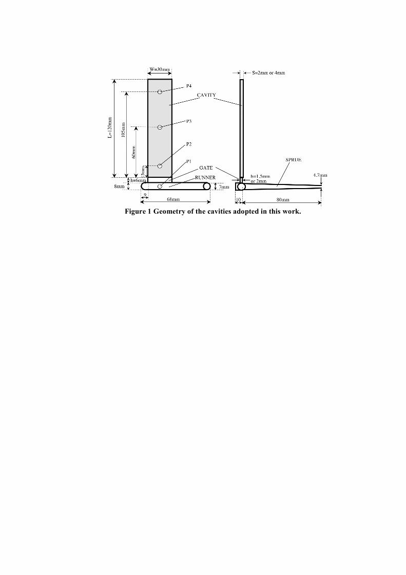
Figure 1 Geometry of the cavities adopted in this work.

0 5 10 15 20 25 300

200

400

600

800

1000

1200PS678E_Ph 625 [bar]

cavity thickness 2[mm]

Experimental

P [bar]

time [s]

P1 P2 P3 P4 P0

(a)

0 5 10 15 20 25 300

200

400

600

800

1000

1200PS678E_Ph 1050 [bar]


Experimental

P [bar]

time [s]

P1 P2 P3 P4 P0

(b)

0 5 10 15 20 25 300

200

400

600

800

1000

1200PS678E_Ph 600 [bar]


Experimental

P [bar]

time [s]

P1 P2 P3 P4 P0

(c)

0 5 10 15 20 25 300

200

400

600

800

1000

1200PS678E_Ph 1050 [bar]


Experimental

P

[bar]

time [s]

P1 P2 P3 P4 P0

(d)

Figure 2 Experimental pressure curves for PS under several operative condition. Fig. 2a-2b:

cavity thickness=2mm. Fig. 2c-2d: cavity thickness=4mm. Gate thickness=1.5mm.

0 5 10 15 20 25 300

200

400

600

800

1000

1200PCLexan 141R_Ph 800 [bar]

Experimental

(a)

P [

ba

r]

time [s]

P1 P2 P3 P4 P0

0 5 10 15 20 25 300

200

400

600

800

1000


Experimental

(b)

P [

ba

r]

time [s]

P1 P2 P3 P4 P0

0 5 10 15 20 25 300

200

400

600

800

1000


Experimental

(c)

P [

ba

r]

time [s]

P1 P2 P3 P4 P0

0 5 10 15 20 25 300

200

400

600

800

1000


Experimental

(d)

P [

ba

r]

time [s]

P1 P2 P3 P4 P0

Figure 3 Experimental pressure curves for PC under several operative condition Cavity

thickness=4mm. Gate thickness=2mm

0 5 10 15 20 25 300

200

400

600

800

1000

1200PS678E_Ph 625 [bar] simulatedcavity thickness 2[mm]

P [

ba

r]

time [s]

P1 P2 P3 P4 P0

(a)

0 5 10 15 20 25 300

200

400

600

800

1000

1200

(b)

PS678E_Ph 1050 [bar] simulated

cavity thickness 2 [mm]

P [

ba

r]

time [s]

P1 P2 P3 P4 P0

0 5 10 15 20 25 300

200

400

600

800

1000

1200

(c)

PS678E_Ph 600 [bar] simulated

cavity thickness 2 [mm]

P [

ba

r]

time [s]

P1 P2 P3 P4 P0

0 5 10 15 20 25 300

200

400

600

800

1000

1200

(d)

PS678E_Ph 1050 [bar]

simulatedcavitythickness

4 [mm]

P [

ba

r]

time [s]

P1 P2 P3 P4 P0

Figure 4 Simulated pressure curves for PS 678E corresponding the same operative conditions

reported in Figure 2 obtained by setting the default database parameters for Cross WLF


0 5 10 15 20 25 300

200

400

600

800

1000

1200

(a)

PCLexan 141R_Ph 800 [bar]

simulated

P [

ba

r]

time [s]

P1 P2 P3 P4 P0

0 5 10 15 20 25 300

200

400

600

800

1000

1200

(b)


simulated

P [

ba

r]

time [s]

P1 P2 P3 P4 P0

0 5 10 15 20 25 300

200

400

600

800

1000

1200

(a)


simulated

P [

ba

r]

time [s]

P1 P2 P3 P4 P0

0 5 10 15 20 25 300

200

400

600

800

1000

1200

(a)


simulated

P [

ba

r]

time [s]

P1 P2 P3 P4 P0

Figure 5 Simulated pressure curves for PC Lexan 141R corresponding the same operative

conditions reported in Figure 3 obtained setting the default database parameters for Cross WLF


Figure 6 Apparent compressibility and thermal expansion of PC Lexan 141R with and without

taking into account the mold deformation evaluated using eq. 6 and 7 with the parameters

reported in Table 3. The material compressibility is compared with the apparent material

compressibility obtained with eq. 15.

Figure 7 Apparent ccompressibility and thermal expansion of PS678E with and without taking

into account the mold deformation evaluated using eq. 6 and 7 with the parameters for the solid

and the melt, as reported in Table 3. The material compressibility is compared with the

apparent material compressibility obtained with eq. 15.

Figure 8. Comparison, for a fixed pressure of 200 [bar], between the description of the effect of

pressure on viscosity (describedevaluated, with a suitable value for D3, by eq. 4, with a suitable

value for D3) and by the RHS of eq. 16 calculated by adopting the parameters present in the

standard Moldflow® database.

0 5 10 15 20 25 300

200

400

600

800

1000


P [

ba

r]

time [s]

P1 P2 P3 P4 P0

(a)

0 5 10 15 20 25 300

200

400

600

800

1000

1200PS678E_Ph 1050 [bar] simulated cavity thickness 2[mm]

P [

ba

r]

time [s]

P1 P2 P3 P4 P0

(b)

0 5 10 15 20 25 300

200

400

600

800

1000


P [

ba

r]

time [s]

P1 P2 P3 P4 P0

(c)

0 5 10 15 20 25 300

200

400

600

800

1000

1200PS678E_Ph 1050 [bar] simulated cavity thickness 4[mm]

P [

ba

r]

time [s]

P1 P2 P3 P4 P0

(d)

d

Figure 9. Simulated pressure curves for PS678E corresponding to the experimental profiles

reported in Figure 2. Simulations performed by considering the pressure effect on viscosity and

the mold deformation.

0 5 10 15 20 25 300

200

400

600

800

1000

1200

(a)


simulated

P [

ba

r]

time [s]

P1 P2 P3 P4 P0

0 5 10 15 20 25 300

200

400

600

800

1000

1200

(a)


simulated

P [

ba

r]

time [s]

P1 P2 P3 P4 P0

0 5 10 15 20 25 300

200

400

600

800

1000

1200

(c)


simulated

P [

ba

r]

time [s]

P1 P2 P3 P4 P0

0 5 10 15 20 25 300

200

400

600

800

1000

1200

(d)


simulated

P [

ba

r]

time [s]

P1 P2 P3 P4 P0

Figure 10. Simulated pressure curves for PC Lexan 141R corresponding to the experimental

profiles reported in Figure 3. Simulations performed by considering the pressure effect on

viscosity and the mold deformation.

improving the predictions of injection molding simulation software

Documents