optimal multilevel redundancy allocation in series and series–parallel systems

Computers & Industrial Engineering 57 (2009) 169–180

Contents lists available at ScienceDirect

Computers & Industrial Engineering

journal homepage: www.elsevier .com/ locate/caie

Optimal multilevel redundancy allocation in series and series–parallel systems q

Ranjan Kumar *, Kazuhiro Izui, Masataka Yoshimura, Shinji NishiwakiDepartment of Aeronautics and Astronautics, Kyoto University, Yoshida-honmachi, Sakyo-ku, Kyoto 606-8501, Japan

a r t i c l e i n f o

Article history:Received 21 November 2007Received in revised form 11 June 2008Accepted 4 November 2008Available online 18 November 2008

Keywords:Redundancy allocationMultilevel series systemMultilevel series–parallelModular redundancyComponent redundancyGenetic algorithms

0360-8352/$ - see front matter � 2008 Elsevier Ltd. Adoi:10.1016/j.cie.2008.11.008

q This manuscript was processed by Area Editor E.A* Corresponding author. Tel.: +81 75 753 5198; fax

E-mail addresses: [email protected] (Rac.jp (K. Izui), [email protected] (M. Yoshac.jp (S. Nishiwaki).

a b s t r a c t

To achieve truly optimal system reliability, the design of a complex system must address multilevel reli-ability configuration concerns at the earliest possible design stage, to ensure that appropriate degrees ofreliability are allocated to every unit at all levels. However, the current practice of allocating reliability ata single level leads to inferior optimal solutions, particularly in the class of multilevel redundancy allo-cation problems. Multilevel redundancy allocation optimization problems frequently occur in optimizingthe system reliability of multilevel systems. It has been found that a modular scheme of redundancy allo-cation in multilevel systems not only enhances system reliability but also provides fault tolerance to theoptimum design. Therefore, to increase the efficiency, reliability and maintainability of a multilevel reli-ability system, the design engineer has to shift away from the traditional focus on component redun-dancy, and deal more effectively with issues pertaining to modular redundancy. This paper proposes amethod for optimizing modular redundancy allocation in two types of multilevel reliability configura-tions, series and series–parallel. A modular design variable is defined to handle modular redundancyin these two types of multilevel redundancy allocation problem. A customized genetic algorithm, namely,a hierarchical genetic algorithm (HGA), is applied to solve the modular redundancy allocation optimiza-tion problems, in which the design variables are coded as hierarchical genotypes. These hierarchicalgenotypes are represented by two nodal genotypes, ordinal and terminal. Using these two genotypes isextremely effective, since this allows representation of all possible modular configurations. The numer-ical examples solved in this paper demonstrate the efficacy of a customized HGA in optimizing the mul-tilevel system reliability. Additionally, the results obtained in this paper indicate that achieving modularredundancy in series and series–parallel systems provides significant advantages when compared withcomponent redundancy. The demonstrated methodology also indicates that future research may yieldsignificantly better solutions to the technological challenges of designing more fault-tolerant systemsthat provide improved reliability and lower lifecycle cost.

� 2008 Elsevier Ltd. All rights reserved.

1. Introduction

Modularity in product design is a crucial topic when developinghighly reliable product architectures. It is a key strategy for achiev-ing better serviceability and reliability, particularly when design-ing products whose lifetime operational costs exceed the initialacquisition cost, such as for airplanes, locomotives, power generat-ing plants, and major manufacturing equipment (Molina, Kusiak, &Sanchez, 1999). Most complex engineering systems of this kindcontain thousands of different components that function interde-pendently, while certain components are used only for a specificset of subtasks within the system. Such sets of components havingindependent functions can be accommodated within a simple sub-

ll rights reserved.

. Elsayed.: +81 75 753 5857.. Kumar), [email protected]), [email protected].

system, or sub-unit. Here, such a subsystem is called a module, asshown in Fig. 1. In system reliability theory, a module indicates agroup of components that has a single input from, and a single out-put to, the rest of the system (Kuo & Zuo, 2003). The contribution ofall components in a module to the performance of the whole sys-tem can be represented by the state of the module. Once the stateof the module is known, one does not need to know the states ofthe components within the module to determine the states ofthe system.

Systems that have modular subsystems usually have superiorfault tolerance, ease of maintenance, and allow modules to berecovered for possible further use when the system as a wholehas reached the end of its useful life (Rasmussen & Niles, 2005).Furthermore, a modular system is often simpler than a complexsystem built from single components. In essence, the modulararchitecture of reliability design reduces the number of parts inan optimal configuration by providing a modular redundancy. De-spite these subtle and profound benefits of a modular redundancythat enhances fault tolerance and reduces lifecycle costs, optimiz-

mailto:[email protected]

mailto:[email protected]. ac.jp


mailto:[email protected]



http://www.sciencedirect.com/science/journal/03608352

http://www.elsevier.com/locate/caie

Nomenclature

Us system level unitUi ith unit; a common name for system, subsystem, and

componentRi reliability of Ui

xi number of components used in Ui

x set of design variables xi

f(x) reliability functionC(x) cost functionni number of sub-units in Ui

Ui;ninith sub-unit of Ui

Uji;m jth redundant unit of mth sub-unit of Ui

Rji;m reliability of Uj

i;m

xji;m number of sub-units of unit Uj

i;m; a nonnegative integer

Cji;m cost of unit Uj

i;mCi cost of ith unitCs system costC0 threshold costki additional costs of ith unit when adding a redundant

unit to a unitNi ordinal genotype node of ith unitNt terminal genotype node of ith unit

170 R. Kumar et al. / Computers & Industrial Engineering 57 (2009) 169–180

ing modular-level allocation under resource constraints is a chal-lenging task for design engineers.

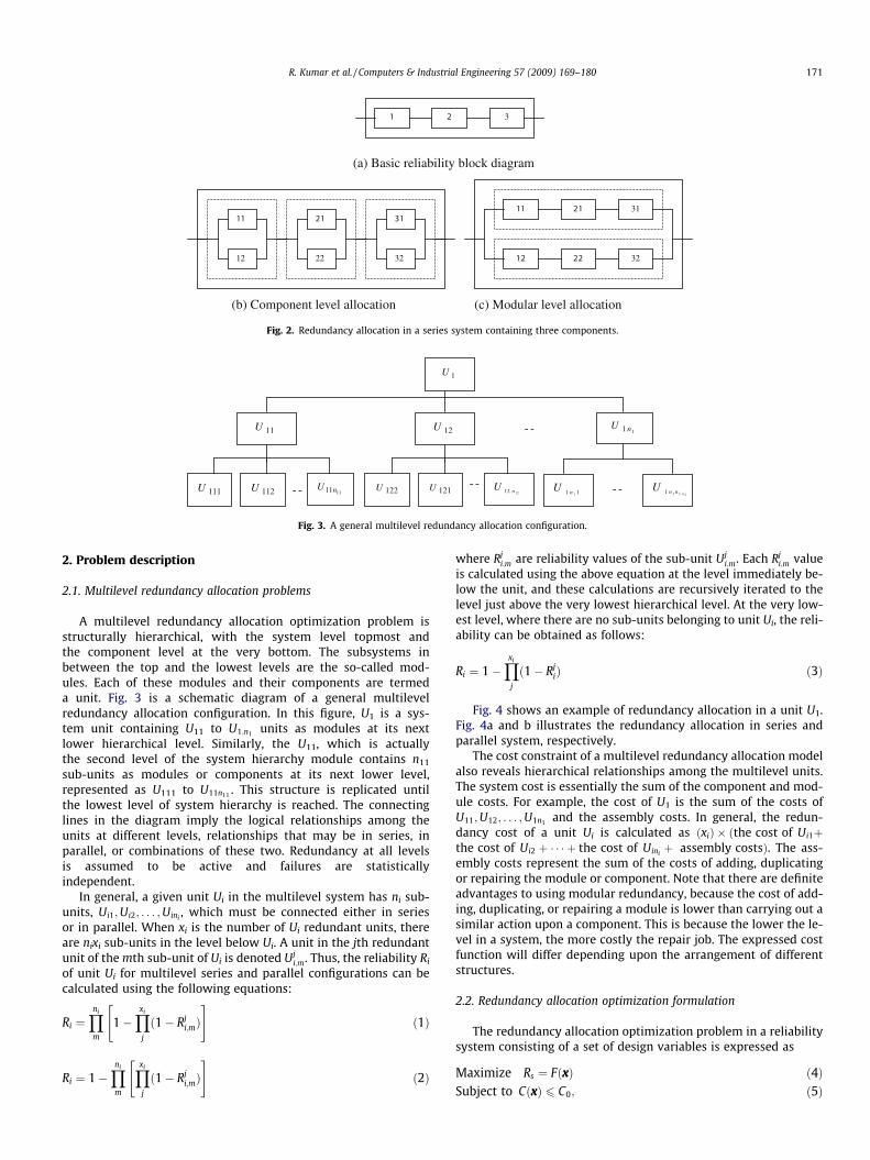
Conventionally, redundancy is added either to a component le-vel or to a subsystem level, when optimizing system reliability. Theredundancy added at the component level is termed componentredundancy, and redundancy added at the modular level is termedmodular redundancy. Specifically, a redundant module is a similarmodule added in parallel to the existing module to increase its reli-ability without altering its internal structure. Fig. 2 illustrates thesetwo redundancy schemes in a series system containing threecomponents.

In other words, we preserve a module’s internal structure, suchas the arrangement of its sub-modules and components, while pro-viding modular redundancy. Thus, to know the status of the sys-tem, we need not know the status of its components. Modularredundancy therefore simplifies the complexity of the systemand makes it easier to isolate faults in case of failure.

In the literature, we find that several models for several sys-tem configurations have been proposed, such as series, parallel,series–parallel, network, and k-out-of-n systems, and others. Tomaximize the system reliability of these models, a large numberof techniques have been proposed for optimal redundancy allo-cation problems. Most techniques for redundancy optimization,however, have been limited to single levels (Kuo & Prasad,2000). Boland and EL-Neweihi (1995) demonstrated that redun-dancy at the component level is not always more effective thanredundancy at the system level in cases of redundancy usingnon-identical parts. In addition, modular redundancy can helpa system become truly fault tolerant. For example, a modularsystem can shift operation from failed modules to healthy ones,allowing repairs to be carried out without downtime (Rasmussen& Niles, 2005). The design transition from component to modu-lar redundancy actually reduces costs and enhances efficiency,flexibility, and reliability. Despite the various benefits that mod-ularity offers, multilevel modular redundancy allocation optimi-zation has seldom been discussed in detail, or an appropriate

Product

Module 1

Module 2

Module 3

System Modules Components

Fig. 1. Multilevel configuration of system reliability.

methodology provided. To leverage the merits of modular redun-dancy allocation, this paper presents a methodology for optimiz-ing the system reliability of a multilevel class of problems usinga modular redundancy allocation scheme.

In a similar direction, Yun and Kim (2004) proposed a multi-level series redundancy allocation optimization model in whichthey considered that each unit of a three level series system issubjected to redundancy, and they optimized system reliabilityby using conventional genetic algorithms (GAs). Their methodcan solve certain problems based on the assumption where onlyone unit is allowed to have redundancy in a direct line. Thisassumption reduces the feasible design space and fails to yielda globally optimal solution, because conventional GAs requireone dimensional vector representation of the design variables.Later, Yun, Song, and Kim (2007) presented a formulation ofmultiple multilevel redundancy allocation problems in seriessystem and applied a GA with a sequential recording methodwithout reflecting the solution positions are used. However,the design variables in a multilevel system have hierarchicalrelationships, and the artificial transformation into vector codingleads to a reduced feasible design space and suboptimalsolutions.

Therefore, this paper proposes a modular redundancy allocationoptimization methodology in which hierarchical design variablesare represented by hierarchical genotypes in the optimization. Thiscustomized methodology is based on a type of genetic algorithmproposed by Yoshimura and Izui (2002), in which the hierarchicalgenotype coding representation is used to exactly express theinternal structure and related hierarchical details, a techniqueusing so-called hierarchical genetic algorithms (HGAs). In orderto handle general multilevel redundancy allocation problems suchas series and series–parallel problems, this paper redefines a math-ematical expression of system reliability for series and series–par-allel and proposes a design-variable coding method usinghierarchical genotypes. This paper demonstrates that HGA canhandle both modular and component schemes of redundancy allo-cation easily by using two newly defined genotypes, nodal andterminal.

This paper is organized as follows. Section 2 describes the de-tailed mathematical formulation for the multilevel redundancyallocation optimization problems. In Section 3, HGA conceptsare explained, and a HGA coding method for modular redun-dancy allocation optimization problems is proposed. In Section4, we solve two multilevel redundancy optimization problems,one series and one series–parallel, each having four hierarchicallevels. In this section, the input data used and the results aresummarized. The results obtained in Section 4 are explainedand discussed in Section 5. Finally, Section 6 concludes thepaper.

(a) Basic reliability block diagram

(b) Component level allocation (c) Modular level allocation

1 2 3

11

12

21

22

31

32

11 21 31

12 22 32

Fig. 2. Redundancy allocation in a series system containing three components.

1U

11 nU11U

111U 112U 1111nU

12U

121U122U1212 nU

11 1nU1111 nnnU

Fig. 3. A general multilevel redundancy allocation configuration.

R. Kumar et al. / Computers & Industrial Engineering 57 (2009) 169–180 171

2. Problem description

2.1. Multilevel redundancy allocation problems

A multilevel redundancy allocation optimization problem isstructurally hierarchical, with the system level topmost andthe component level at the very bottom. The subsystems inbetween the top and the lowest levels are the so-called mod-ules. Each of these modules and their components are termeda unit. Fig. 3 is a schematic diagram of a general multilevelredundancy allocation configuration. In this figure, U1 is a sys-tem unit containing U11 to U1;n1 units as modules at its nextlower hierarchical level. Similarly, the U11, which is actuallythe second level of the system hierarchy module contains n11

sub-units as modules or components at its next lower level,represented as U111 to U11n11 . This structure is replicated untilthe lowest level of system hierarchy is reached. The connectinglines in the diagram imply the logical relationships among theunits at different levels, relationships that may be in series, inparallel, or combinations of these two. Redundancy at all levelsis assumed to be active and failures are statisticallyindependent.

In general, a given unit Ui in the multilevel system has ni sub-units, Ui1;Ui2; . . . ;Uini

, which must be connected either in seriesor in parallel. When xi is the number of Ui redundant units, thereare nixi sub-units in the level below Ui. A unit in the jth redundantunit of the mth sub-unit of Ui is denoted Uj

i;m. Thus, the reliability Ri

of unit Ui for multilevel series and parallel configurations can becalculated using the following equations:

Ri ¼Yni

m

1�Yxi

j

ð1� Rji;mÞ

" #ð1Þ

Ri ¼ 1�Yni

m

Yxi

j

ð1� Rji;mÞ

" #ð2Þ

where Rji;m are reliability values of the sub-unit Uj

i;m. Each Rji;m value

is calculated using the above equation at the level immediately be-low the unit, and these calculations are recursively iterated to thelevel just above the very lowest hierarchical level. At the very low-est level, where there are no sub-units belonging to unit Ui, the reli-ability can be obtained as follows:

Ri ¼ 1�Yxi

j

ð1� RjiÞ ð3Þ

Fig. 4 shows an example of redundancy allocation in a unit U1.Fig. 4a and b illustrates the redundancy allocation in series andparallel system, respectively.

The cost constraint of a multilevel redundancy allocation modelalso reveals hierarchical relationships among the multilevel units.The system cost is essentially the sum of the component and mod-ule costs. For example, the cost of U1 is the sum of the costs ofU11;U12; . . . ;U1n1 and the assembly costs. In general, the redun-dancy cost of a unit Ui is calculated as ðxiÞ � ðthe cost of Ui1þthe cost of Ui2 þ � � � þ the cost of Uini

þ assembly costsÞ. The ass-embly costs represent the sum of the costs of adding, duplicatingor repairing the module or component. Note that there are definiteadvantages to using modular redundancy, because the cost of add-ing, duplicating, or repairing a module is lower than carrying out asimilar action upon a component. This is because the lower the le-vel in a system, the more costly the repair job. The expressed costfunction will differ depending upon the arrangement of differentstructures.

2.2. Redundancy allocation optimization formulation

The redundancy allocation optimization problem in a reliabilitysystem consisting of a set of design variables is expressed as

Maximize Rs ¼ FðxÞ ð4ÞSubject to CðxÞ 6 C0; ð5Þ

111U

1U

11

11

xU 1

12U 12

12

xU

11U 12U

1U

1

11U

1U

11

11

xU 112U 12

12

xU

11U 12U

1U

(a) Series configuration

(b) Parallel configuration

Using Eq. (1), system reliability is ])1(1[])1(1[ 1211

12111

xx RRR −−×−−=

Using Eq. (2), system reliability is ])1()1(1[ 1211

12111

xx RRR −−−=

11U 12U

11U 12U

Fig. 4. Series and parallel redundancy allocation in a unit U1.


where Rs, F(x), C(x), and x are the system reliability, reliability func-tion, cost function, and a set of design variables, respectively. C0 is agiven fixed positive value for the cost constraint.

For example, the problem of optimizing a 2-level series redun-dancy allocation, as shown in Fig. 5, can be stated mathematicallyas follows:

Rs ¼ ½1� ð1� f1� ð1� R11Þx11g � f1� ð1� R12Þx12 Þgx1 � ð6Þ

where x1, x11, and x12 are the number of redundancy of units U1, U11,and U12, respectively. The values of the design variables, x11, and x12

depend on the value of x1, the design variable at the parent unit. Ifthe number of redundancies represented by x1 is two, then theredundancies of x11, and x12 should be at least two, however, the

1

11U

1

1U

1111

xU 112U 12

12

xU

System

11U 11U

Fig. 5. An example of series redun

values of design variables x11, and x12 are independent of eachother.

In this paper, the following cost functions have been applied tocalculate the costs for modules and components:

Ci ¼Xni

m¼1

Xxi

j¼1

Cji;m ð7Þ

Ci ¼ cixi þ kxii ð8Þ

where Cji;m are modular cost of the sub-unit Uj

i;m. The symbols xi, ci,and ki, respectively represent the number of redundancy, the unitcost, and the assembly cost for ith unit. Each Cj

i;m value is calculatedusing Eq. (7) at the level immediately below the unit, and these cal-

1

11U

1

1

xU

1111

xU 112U 12

12

xU

11U 11U

dancy allocation in a unit U1.

Original Structure

Mutated offspring

1 3 1 2

4 3 1 2

Parent 1 Parent 2

Offspring 1 Offspring 2

21 3 1 2

1 1 4 3

1 4 3

2 3 1 2

(b) Mutation operation (a) Crossover operation

Fig. 6. Crossover and mutation operators for hierarchical genotype.

Table 1Hierarchical genotype representation.

Ordinal genotype node Ni Terminal genotypenode Nti

Designvariable

xji;m: the number of subordinate modules for

the mth module

Parameter T: unit type k: the redundancyfor component Ui

k: the redundancy for unit Ui ri: unit reliabilityn: the number of sub-modules ci: unit cost


culations are recursively iterated to the level just above the verylowest hierarchical level. At the very lowest level, where there are

(a) An example of a multileve

(b) Design variables and parameters at ea

U11

U12U1

U

U

U

U111

U112

U112

U11

U111

U111

U112

111,11

=Ux

212,11

=Ux

U11

221,11

=Ux

122,11

=Ux

111,12

=Ux

212,12

=Ux

U12

211,1

=Ux

112,1

=Ux

U1

System

111, =sysx

n = 1

k = 1

n = 2

k = 1

n = 2

k = 2

k = 1 k = 2

U112 U111

k = 2 k = 1

U112

U1211

k = 1 k = 2

U

T = S

T = S

111,121

=Ux

212,121

=Ux

U121

Fig. 7. Hierarchical genotype re

no sub-units belonging to unit Ui, the cost is calculated by Eq. (8).Eq. (8) has been taken from the paper by Yun and Kim (2004). Thus,the total cost for a multilevel structure is calculated by using Eqs.(7) and (8).

3. Hierarchical genetic algorithms

Hierarchical genetic algorithms (Yoshimura & Izui, 2002) arecustomized and applied to solve the multilevel redundancy allo-

l reliability system U1

ch ordinal and terminal node

U1211

U1212

U1212

121

122

U1222U1221

122

U1221

U1222

U1222

n = 2

k = 1

1212

T = P

n = 2

k = 1

T = S11

1,122=Ux

112,122

=Ux

U122

121,122

=Ux

222,122

=Uxn = 2

k = 2

T = S

U1221

k = 1 k = 1

U1222 U1221

k = 1 k = 2

U1222

presentation in system U1.

U1

1121U

U11

1122U1112U

U112U111

1221U

U12

1222U1211U

U12U12

1111U 1212U

Fig. 9. Four-level hierarchical series configuration of U1.

U1 U4U3

U2

U1 U4U3

U2Uα

Fig. 8. Interpretation of mixed series and parallel configurations.

U1

U11 U12

1121U 1122U1112U

U111

1221U 1222U1211U1111U 1212U

U112 U121 U122

Fig. 10. Four-level hierarchical series–parallel configuration of U1.


cation optimization problems here. HGAs are advanced geneticalgorithms that can represent hierarchical relationships among

Table 2Input data.

Level Unit Parent unit Redundancy

1 U1 x1

2 U11 U1 x2

U12 U1 x3

3 U111 U11 x4

U112 U11 x5

U121 U12 x6

U122 U12 x7

4 U1111 U111 x8

U1112 U111 x9

U1121 U112 x10

U1122 U112 x11

U1211 U121 x12

U1212 U121 x13

U1221 U122 x14

U1222 U122 x15

design variables using hierarchical genotypes, and can optimizehierarchical problems in a single optimization process. Whileconventional genetic algorithms (Goldberg, 1989) use vectorgenotype structures, HGAs employ hierarchical genotypestructures.

The multilevel redundancy allocation optimization problemshere involve hierarchical relationships among design variables,which represent redundant modules or component selections, asshown in Fig. 5, and hierarchical genotype representation is partic-ularly suited to handling such hierarchical relationships. SinceHGAs have special types of genotype structures, new crossoverand mutation operators have to be applied. The HGAs allowbranches of the hierarchical structure to be exchanged, in additionto the exchange of genes. Fig. 6 illustrates the crossover and muta-tion operators for hierarchical genotypes. Using such genetic oper-ations, new individuals are produced and optimal hierarchicalstructures can then be obtained.

3.1. Solution encoding

A hierarchical genotype is represented using two types ofnode, ordinal and terminal, as shown in Table 1. Ordinal nodeNi corresponds to redundancy unit Ui, and is characterized byseveral parameters and design variables. Parameter T 2 {S,P} rep-resents the type of unit where S means that the sub-units have aseries reliability relationship, while P means a parallel configura-tion. When T equals S, this node is called a series node, andwhen T equals P, the node is called a parallel node. Parametersk and n stand for the redundancy number of unit Ui, and thenumber of sub-units, respectively. Here, k is given by a designvariable at an upper node, while the parameter n is a fixed valuethat depends on the optimization problem to be solved. xj

i;m is adesign variable denoting the redundancy number for the mthsub-unit of the jth redundancy unit, where j varies from 1 tok. Therefore, there are nik design variables in unit Ui. A terminalnode Nti

corresponds to one of the lowest units, and incorporatesdesign variable k, unit reliability ri, and the unit cost ci. Sincethere are no sub-units at the terminal node, it does not containparameter n or design variable xj

i;m. Using these two genotypes,all possible redundancy allocation solutions for both the seriesand series–parallel reliability allocation problems can berepresented.

Fig. 7 illustrates an example of the genotype encoding. Fig. 7ashows a redundancy configuration for a system U1 consisting twomodules, U11 and U12, at the second level. This redundancy struc-ture can be represented using hierarchical genotype nodes asshown in Fig. 7b. The ordinal and terminal nodes are assigned to

Basic reliability Cost k

Series system Series–parallel

0.2198 0.6268 102 20.5130 0.7110 48 20.4284 0.8816 50 20.7200 0.7200 21 30.7125 0.9875 21 30.6300 0.6300 23 30.6800 0.6800 21 30.9000 0.9000 7 40.8000 0.8000 6 40.7500 0.7500 8 40.9500 0.9500 5 40.7000 0.7000 9 40.9000 0.9000 6 40.8500 0.8500 5 40.8000 0.8000 8 4

Generation

Fit

ness

Worst

Best

Average

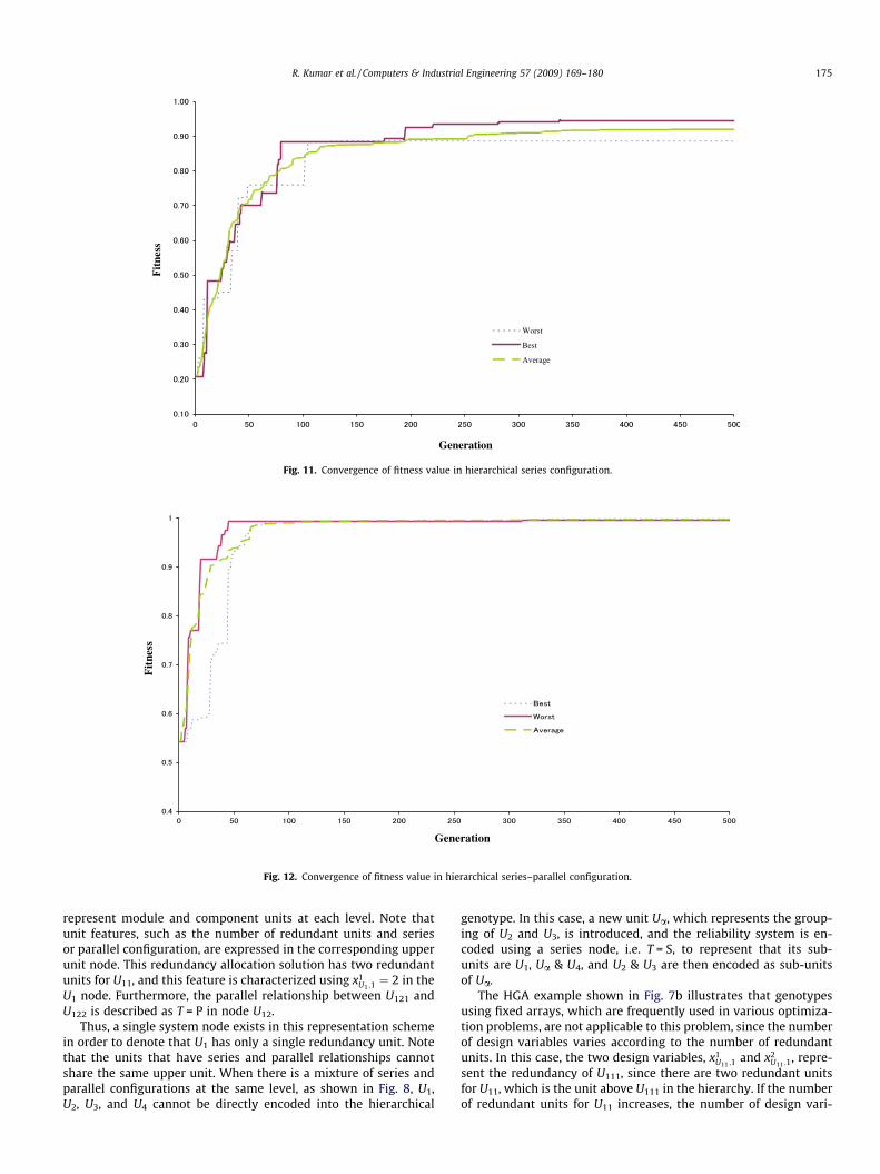
Fig. 11. Convergence of fitness value in hierarchical series configuration.

Generation

Fit

ness

Fig. 12. Convergence of fitness value in hierarchical series–parallel configuration.


represent module and component units at each level. Note thatunit features, such as the number of redundant units and seriesor parallel configuration, are expressed in the corresponding upperunit node. This redundancy allocation solution has two redundantunits for U11, and this feature is characterized using x1

U1 ;1¼ 2 in the

U1 node. Furthermore, the parallel relationship between U121 andU122 is described as T = P in node U12.

Thus, a single system node exists in this representation schemein order to denote that U1 has only a single redundancy unit. Notethat the units that have series and parallel relationships cannotshare the same upper unit. When there is a mixture of series andparallel configurations at the same level, as shown in Fig. 8, U1,U2, U3, and U4 cannot be directly encoded into the hierarchical

genotype. In this case, a new unit Ua, which represents the group-ing of U2 and U3, is introduced, and the reliability system is en-coded using a series node, i.e. T = S, to represent that its sub-units are U1, Ua & U4, and U2 & U3 are then encoded as sub-unitsof Ua.

The HGA example shown in Fig. 7b illustrates that genotypesusing fixed arrays, which are frequently used in various optimiza-tion problems, are not applicable to this problem, since the numberof design variables varies according to the number of redundantunits. In this case, the two design variables, x1

U11 ;1and x2

U11 ;1, repre-

sent the redundancy of U111, since there are two redundant unitsfor U11, which is the unit above U111 in the hierarchy. If the numberof redundant units for U11 increases, the number of design vari-

Table 3Optimal redundancy allocation in series system.

Basic reliability Modular redundancy Component redundancy

Optimal configuration x1-x2x3-x4x5-x8x9-x10x11 x6x7-x12x13-x14x15

Optimalreliability

Optimal configuration x1-x2x3-x4x5-x8x9-x10x11 x6x7-x12x13-x14x15

Optimalreliability

0.3202 1-22-11-1222-2222-21-32-33 0.9775 1-11-11-23-32-11-32-23 0.94600.1050 1-11-21-2212-33-12-23-2222 0.8677 1-11-11-33-23-11-22-32 0.76580.3202 1-11-22-2212-2122-12-33-2222 0.9777 1-11-11-32-23-11-23-32 0.94600.1201 1-11-12-32-2223-12-22-2222 0.8870 1-11-11-22-33-11-22-33 0.78570.1587 1-11-12-32-2223-12-22-2222 0.9368 1-11-11-33-32-11-32-22 0.84270.1805 1-11-32-112222-2123-21-2211-32 0.9508 1-11-11-23-23-11-23-32 0.85780.2318 1-11-12-23-1212-22-2132-2222 0.9538 1-11-11-23-22-11-32-23 0.90940.2938 1-11-12-23-2122-22-2232-32212 0.9742 1-11-11-32-32-11-23-32 0.93760.2179 1-11-22-2222-2222-21-2222-32 0.9502 1-11-11-32-32-11-23-32 0.89450.2085 1-11-23-2122-112112-22-2222-2132 0.9645 1-11-11-33-32-11-22-32 0.8928

Table 4Optimal redundancy allocation in series–parallel system.

Basicreliability

Modular redundancy Component redundancy

Optimal configuration x1-x2x3-x4x5-x8x9-x10x11x6x7-x12x13-x14x15

Optimalreliability

Optimal configuration x1-x2x3-x4x5-x8x9-x10x11x6x7-x12x13-x14x15

Optimalreliability

0.3202 1-11-21-2323-22-11-32-22 0.9991 1-11-11-23-32-11-32-23 0.94220.1050 1-11-31-221223-22-31-222221-22 0.9956 1-11-11-33-23-11-22-32 0.76580.3202 1-11-22-2332-2211-21-2222-22 0.9993 1-11-11-32-23-11-23-32 0.94600.1020 1-11-22-3232-2211-21-2122-22 0.9986 1-11-11-31-33-11-22-33 0.78570.1587 1-11-31-222322-22-21-1122-23 0.9967 1-11-11-33-22-11-32-22 0.84270.1805 1-11-41-22232212-23-11-22-22 0.9975 1-11-11-23-23-11-23-32 0.85780.2318 1-11-31-222221-32-12-21-2322 0.9995 1-11-11-23-23-11-32-23 0.90940.2938 1-11-31-221322-21-31-112223-12 0.9995 1-11-11-23-22-11-33-23 0.93770.2179 1-11-21-3232-22-21-2312-22 0.9980 1-11-11-32-32-11-23-32 0.89450.2085 1-11-31-222222-13-11-33-22 0.9986 1-11-11-33-32-11-22-32 0.8928


ables for U111 will also increase. The solution encoding scheme pro-posed in this paper can successfully represent different numbers ofdesign variables at every hierarchical level.

The ordinal and the terminal genotypes each have two func-tions, namely, reliability and cost, and the difference between ser-ies and parallel nodes only pertains to reliability calculations.When the reliability function in the series node is called, the unitreliability is calculated using Eq. (1), while Eq. (2) is used for theparallel node. When calculating either of these equations, the reli-ability values of the lower units, Rk

i;m, are required, and these areobtained by calling the reliability function of the lower units. Final-ly, the reliability function of the terminal node returns its unit reli-ability ri. Thus, the reliability functions are recursively called, andthe total system reliability can be effectively obtained. Similarly,the system cost can be obtained by calling the cost functionembedded in each node.

3.2. Objective function

A penalty function method has been applied to transform theconstrained problem into an unconstrained problem, by penalizinginfeasible solutions via a penalty term added to the objective func-tion for any violation of the constraints. In this paper, we used Genand Cheng’s method, which applies a severe penalty to infeasiblesolutions (Gen & Cheng, 1996, 1997). The fitness function, eval(x),is calculated using the following equation:

evalðxÞ ¼ f ðxÞ � pðxÞ ð9Þ

where f(x), p(x) and x are the reliability function, penalty functionand a set of design variables, respectively. We calculate the valueof p(x) using Gen and Cheng’s penalty function for each individual,and for highly constrained optimization problems, the infeasible

solutions occupy relatively large portions of the population at eachgeneration. The penalty approach here adjusts the ratio of penaltiesadaptively at each generation to achieve a balance between thepreservation of information, the selective pressure for infeasibility,and the avoidance of excessive penalization.

3.3. Crossover operators

Crossover operations between individuals are conducted amongeach corresponding set of genes, using a two-step procedure. Forthe initial step, any other individual is first selected as the cross-over partner and crossover operators then exchange the corre-sponding genes of the two individuals. Here, when a gene of analternative for a substructure is exchanged with the correspondinggene of another alternative, all corresponding lower substructuresare also exchanged, to preserve consistency in the selection ofalternatives. If this operation were not conducted in this way,meaningless lower structures might be generated in the lowerpositions of the exchanged substructures. The algorithmic proce-dures are follows:

Step (1) Select two individuals for crossover operations, thenfind the set of genes at the highest level of the mul-tilevel structural system for each of the two individ-uals, and start the crossover operation withprobability pc1

.

Step (2.1) If the gene xji;m of individual 1 and that of individual 2

are different; conduct a crossover operation for xji;m

with probability pc2. This operation is the same as a

uniform crossover of simple genetic algorithms with

U 1121

U 1211

U1212

U121

U11

U1

U12

U1111 U1112

U111

U1111 U1112

U1111 U1112

U111

U1111 U1112

U1111 U1112

U111

U1111 U1112

U 1122

U 1122

U 1122

U 112

U 1211

U 1211

U1212

U1212

U 1221 U1222

U 1221 U1222

U122

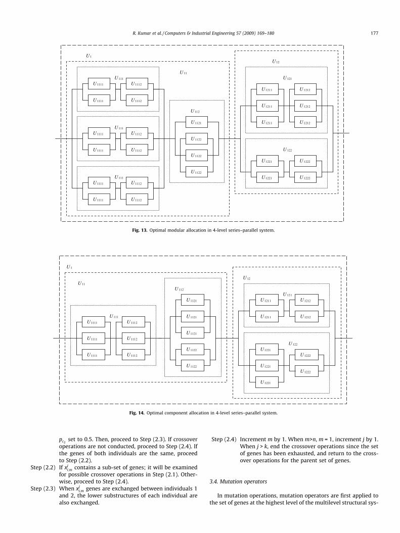
Fig. 13. Optimal modular allocation in 4-level series–parallel system.

U1121

U1211

U121

U11

U 12

U1

U1111 U1112

U111

U1111 U1112

U1122

U1122

U112

U1211

U1212

U1221

U1222

U1221

U1222

U 122

U1111 U1112

U1121

U1121

U1221

U1212

Fig. 14. Optimal component allocation in 4-level series–parallel system.


pc2set to 0.5. Then, proceed to Step (2.3). If crossover

operations are not conducted, proceed to Step (2.4). Ifthe genes of both individuals are the same, proceedto Step (2.2).

Step (2.2) If xji;m contains a sub-set of genes; it will be examined

for possible crossover operations in Step (2.1). Other-wise, proceed to Step (2.4).

Step (2.3) When xji;m genes are exchanged between individuals 1

and 2, the lower substructures of each individual arealso exchanged.

Step (2.4) Increment m by 1. When m>n, m = 1, increment j by 1.When j > k, end the crossover operations since the setof genes has been exhausted, and return to the cross-over operations for the parent set of genes.

3.4. Mutation operators

In mutation operations, mutation operators are first applied tothe set of genes at the highest level of the multilevel structural sys-


tem, and mutation operators are recursively applied to their childsets of genes in the same way as for crossover operators. The algo-rithmic procedures are as follows:

Step (1) Examine the substructure at the highest level.

Step (2.1) Determine whether or not a mutation operationshould be conducted, with mutation probability pm

for the gene xji;m. If the mutation is conducted, proceed

to Step (2.3) otherwise proceed to Step (2.2).Step (2.2) If xj

i;m contains a child set of genes, proceed to Step(2.1) and examine the child set of genes. If not, proceedto Step (2.5).

Step (2.3) Randomly generate xji;m.

Step (2.4) Randomly reconstruct the genes of all sub-unit’s nodefor the selected alternative.

Step (2.5) Increment m by 1. When m > n, m = 1, increment j by 1.When j > k, end the crossover operations since the setof genes has been exhausted, and return to the cross-over operations for the parent set of genes.

4. Numerical examples

4.1. Four-level series and series–parallel problems

In this section, we solve two multilevel redundancy allocationoptimization problems. Figs. 9 and 10 show the two 4-level multi-level systems that have series and series–parallel configurations.We applied HGA to optimize the system reliability of these twoproblems. For example, U1 is a unit at the system level, (U11,U12)and (U111,U112,U121,U122) are units at the module levels, and(U1111 & U1112, U1121 & U1122, U1211 & U1212, U1221 & U1222) are unitsat the component level.

Fig. 9 shows a series system in which all the units are arrangedin series at every level, while Fig. 10 shows a series–parallel systemin which U121 & U122 and U1121 & U1122 are in parallel and the restof units are in series either at the same level or at different levels.We see in Fig. 10 that U12 & U112 consists of parallel units, U121 &U122 and U1121 & U1122 at their immediate lower levels.

4.2. Input data

Suitable parameters for optimizing the two allocation problemswere selected based on several experimental runs using the pro-posed HGA. The crossover rates pc1

and pc2when solving these

problems were set to 0.8 and 0.5 and the mutation rate pm wasset to 0.05. An initial population of 100 individuals was generated,and 500 generations were processed in each case. Table 2 summa-rizes the basic reliability and corresponding cost for each unit inboth problems. The unit reliability and the unit cost at the verylowest level in the multilevel redundancy allocation problemswere used when calculating the unit reliability and the unit costof upper level units, up to the system level. In each of these tables,x’s represent the integer value of the optimal redundancy to be ob-tained during the optimization process.

4.3. Computational results

The HGA was applied to solve the series and series–parallelproblems using separate modular and component redundancyschemes, under the same HGA parameters. In the modular redun-dancy scheme, we allowed redundancy to units at all levels,whereas in the component scheme, we only allowed redundancyat the component level. We applied these two schemes to explorewhat the differences in the optimal solutions would be under the

same cost constraint. Ten cases that used varying unit reliabilityvalues in basic configurations were considered when solving thetwo problems, and ten 500-generation trials were performed ineach case. Figs. 11 and 12 show the convergence of objective func-tion values in ten 500-generation trials for both problems. The costconstraint was always kept constant at a value of 500. Finally, thebest solution among the 10 trials is summarized for the two prob-lems in Tables 3 and 4.

Optimal redundancy allocations and solutions are given inboth tables. Table 3 provides the best solutions for the seriesredundancy allocation problems and Table 4 the best solutionsfor the series–parallel problem, and the reliability settings arethe same in each row of the tables. Here, reliability settings referto the number of units, the hierarchical levels, and the reliabilityof the units. Tables 3 and 4 indicate that the optimal componentredundancy allocation is the same in each case, implying that theachieved values represent optimal system reliability. However,the optimal modular redundancy allocation and the correspond-ing system reliability for the series and series–parallel systemsare different.

For example, in the 10th case of Table 4, the optimal modularredundancy configuration for U1 at the system level, [U1], is [1],at the second level, [U11 U12], is [11], at the third level, [U111U112-U121U122], is [31-11], and at the lowest level, [U1111U1112-U1211U1212-U1211U1212-U1221U1222], is [222222-13-33-22]. Fig. 13shows an optimal redundancy arrangement for the modularschemes.

For the same case in Table 4, the optimal component redun-dancy configuration for U1 at the system level, [U1], is [1], at thesecond level, [U11U12], is [11], at the third level, [U111U112-U121U122], is [11-11], and at the lowest level, [U1111U1112-U1211U1212-U1211U1212-U1221U1222], is [33-32-22-32]. Fig. 14 showsan optimal redundancy arrangement for the component scheme.All the optimal solutions summarized in Tables 3 and 4 can beillustrated by pictorial representations in a similar way.

Next, we solved the two allocation optimization problems byvarying the cost constraints. Ten cases using various cost con-straints while maintaining constant values of unit reliabilitywere carried out when solving the series and series–parallelproblems, and ten 500-generation trials were performed in eachcase. Finally, the best solution among the 10 trials was selectedas the optimal solution. Figs. 15 and 16 graphically show thetrends of the optimal solutions for different cost constraint. Inboth problems, the cost constraint was varied in increments of50, from 200 to 650.

In both figures, we compare the optimal solutions obtainedusing the modular redundancy scheme with those obtained usingthe component redundancy scheme. The x- and y-axes, respec-tively, represent the system cost constraints and the optimal sys-tem reliability.

5. Discussion

The numerical examples for the multilevel series and series–parallel redundancy allocation problems clearly demonstrate thatthe modular scheme of redundancy allocation has certain distinctadvantages over the component scheme of redundancy allocation.The obtained results shown in Tables 3 and 4 clearly support theclaim that a modular redundancy approach yields superior systemreliability compared with the component redundancy scheme. Wesee in Table 4 that the average improvement in optimal solutionsusing a modular redundancy scheme for a multilevel series systemis 7.6%, and the maximum improvement is 13.3% better than thebest result obtained with the component scheme of redundancyallocation. Similarly, for the series–parallel system, the modularredundancy approach yielded an average improvement of 13.8%


and a maximum improvement of 30.0% compared with the compo-nent scheme of redundancy allocation. Although the percentageimprovement can vary according to the parameters used, we inferthat modular redundancy yields better optimal solutions thancomponent redundancy scheme in multilevel redundancy alloca-tion optimization problems.

The average computation time for single run in the modularallocation optimization problems varies between 149.0 and153.1 s. On the other hand, the average calculation time in compo-nent allocation problems lies between 19.6 and 20.2. Thus, thecomputational cost of solving modular redundancy allocation opti-mization problems is significantly higher due to the larger searchspace than that of component allocation problems. However, Figs.15 and 16 indicate that the optimal reliability achieved for each ofthe 10 cost constraint cases again demonstrates the superiority ofthe modular redundancy scheme over the component scheme.Although, the difference in the optimal solutions between thetwo schemes is not very significant at a system cost of 200, highersystem cost values increasingly show the superiority of a modularallocation approach.

0.3500

0.4000

0.4500

0.5000

0.5500

0.6000

0.6500

0.7000

0.7500

0.8000

0.8500

0.9000

0.9500

1.0000

100 150 200 250 300 350 400 450

Cost

Syst

em r

elia

bilit

y

Fig. 15. Modular and component redun

0.9

0.91

0.92

0.93

0.94

0.95

0.96

0.97

0.98

0.99

1

200 250 300 350 400

Cost

Syst

em r

elia

bilit

y

Fig. 16. Modular and component redundanc

Thus, it appears advantageous to allocate redundancy withoutaffecting the internal hierarchical relationships of a multilevel reli-ability system. It is recognized that using conventional GAs to rep-resent design variables having hierarchical relationships isproblematic, and we overcame this difficulty by applying HGA inwhich the modular design variables are encoded using an innova-tive hierarchical genotype representation. We observe that thehierarchical genotype representation of modular design variablesis highly appropriate for solving hierarchical reliability optimiza-tion problems, since such representation allows sufficient flexibil-ity for every possible redundancy combination to be addressed.

As described in the introduction, the particular benefit of usinga modular approach to redundancy allocation in a multilevel sys-tem, and hierarchical genotypes, is that both fault tolerance andsystem reliability are improved. Modularity reduces the numberof parts and thus simplifies the system design. The fewer partsand subsystems there are, the more reliable a system will be in ser-vice. Thus, well-implemented modular redundancy offers a kind ofsynergistic benefit in terms of reducing complexity while increas-ing the fault tolerance of a system design, and the computational

500 550 600 650 700 750 800 850 900

Component

Modular

dancy allocations in series system.

450 500 550 600 650

Component

Modular

y allocations in series–parallel system.


results presented confirm that modular redundancy allocationoptimizations lead to improved optimal system reliability. This isbecause a hierarchical genotype representation not only preservesthe hierarchical relationship of the modular design variables butalso allows simultaneous redundancy allocation at more thanone level during the optimization process.

6. Conclusion

This paper discussed the importance of modular redundancyallocation applied to multilevel system reliability problems. Weproposed a methodology to solve series and series–parallel redun-dancy allocation problems considering the hierarchical relation-ships among design variables. Modular design variables wereencoded using hierarchical genotypes in hierarchical genetic algo-rithms, and the multilevel redundancy allocation optimizationproblems were efficiently solved. The optimization of numericalexamples in this paper indicates that the modular scheme ofredundancy allocation yields superior system reliability for multi-level configurations, in contrast to the conventional notion thatcomponent level redundancy allocation yields better optimal solu-tions. The application of a HGA proved to be flexible and efficientwhen solving large-scale multilevel redundancy allocation optimi-zation problems. We believe that future research will extend the

method presented here to encompass other multilevel classes ofredundancy allocation optimization problems.

References

Boland, P., & EL-Neweihi, E. (1995). Component redundancy vs systemredundancy in the hazard rate ordering. IEEE Transactions on Reliability,44(4), 614–619.

Gen, M., & Cheng, R. (1996). A survey of penalty technique in genetic algorithms. InProceedings of the 1996 international conference on evolutionary computation,804-809, Nagoya University, Japan.

Gen, M., & Cheng, R. (1997). Genetic algorithms and engineering design. NY: Wiley.Goldberg, D. E. (1989). Genetic algorithms in search, optimization and machine

learning. MA: Addison-Wesley.Kuo, W., & Prasad, V. R. (2000). An annotated overview of system-reliability

optimization. IEEE Transactions on Reliability, 49(2), 176–187.Kuo, W., & Zuo, M. J. (2003). Optimal reliability modeling: Principles and applications.

NJ: Wiley.Molina, A., Kusiak, A., & Sanchez, J. (1999). Handbook of life cycle engineering:

Concepts, models and technologies. Boston: Kluwer Academic Publishers.Rasmussen, N., & Niles, S. (2005). Modular systems: The evolution of reliability. White

paper, 76, American Power Corporation.Yoshimura, M., & Izui, K. (2002). Smart optimization of machine systems using

hierarchical genotype representations. ASME Journal of Mechanical Design,124(3), 375–384.

Yun, W. Y., & Kim, J. W. (2004). Multi-level redundancy optimization in seriessystems. Computers and Industrial Engineering, 46, 337–346.

Yun, W. Y., Song, Y. M., & Kim, H. G. (2007). Multiple multi-level redundancyallocation in series systems. Reliability Engineering and Systems Safety, 92,308–313.

optimal multilevel redundancy allocation in series and series–parallel systems

Documents