optimal learning - castle labs
TRANSCRIPT

OPTIMAL LEARNING

OPTIMAL LEARNING2nd Edition (Draft)
Warren B. PowellOperations Research and Financial EngineeringPrinceton University
Ilya O. RyzhovRobert H. Smith School of BusinessUniversity of Maryland
March 11, 2018
A JOHN WILEY & SONS, INC., PUBLICATION

Copyright c©2017 by John Wiley & Sons, Inc. All rights reserved.
Published by John Wiley & Sons, Inc., Hoboken, New Jersey.Published simultaneously in Canada.
No part of this publication may be reproduced, stored in a retrieval system, or transmitted in any formor by any means, electronic, mechanical, photocopying, recording, scanning, or otherwise, except aspermitted under Section 107 or 108 of the 1976 United States Copyright Act, without either the priorwritten permission of the Publisher, or authorization through payment of the appropriate per-copy fee tothe Copyright Clearance Center, Inc., 222 Rosewood Drive, Danvers, MA 01923, (978) 750-8400,fax (978) 646-8600, or on the web at www.copyright.com. Requests to the Publisher for permission shouldbe addressed to the Permissions Department, John Wiley & Sons, Inc., 111 River Street, Hoboken, NJ07030, (201) 748-6011, fax (201) 748-6008.
Limit of Liability/Disclaimer of Warranty: While the publisher and author have used their best efforts inpreparing this book, they make no representations or warranties with respect to the accuracy orcompleteness of the contents of this book and specifically disclaim any implied warranties ofmerchantability or fitness for a particular purpose. No warranty may be created ore extended by salesrepresentatives or written sales materials. The advice and strategies contained herin may not besuitable for your situation. You should consult with a professional where appropriate. Neither thepublisher nor author shall be liable for any loss of profit or any other commercial damages, includingbut not limited to special, incidental, consequential, or other damages.
For general information on our other products and services please contact our Customer CareDepartment with the U.S. at 877-762-2974, outside the U.S. at 317-572-3993 or fax 317-572-4002.
Wiley also publishes its books in a variety of electronic formats. Some content that appears in print,however, may not be available in electronic format.
Library of Congress Cataloging-in-Publication Data:
Optimal Learning / Warren B. Powell and Ilya O. Ryzhovp. cm.—(Wiley series in survey methodology)
“Wiley-Interscience."Includes bibliographical references and index.ISBN 0-471-48348-6 (pbk.)1. Surveys—Methodology. 2. Social
sciences—Research—Statistical methods. I. Groves, Robert M. II. Series.
HA31.2.S873 2007001.4’33—dc22 2004044064Printed in the United States of America.
10 9 8 7 6 5 4 3 2 1

To our families


CONTENTS
Preface xv
Acknowledgments xix
1 The challenges of learning 1
1.1 From optimization to learning 21.2 Areas of application 31.3 Major problem classes 101.4 Two applications 12
1.4.1 The newsvendor problem 131.4.2 Learning the best path 14
1.5 Learning from different communities 161.6 Information collection using decision trees 18
1.6.1 A basic decision tree 181.6.2 Decision tree for offline learning 191.6.3 Decision tree for online learning 211.6.4 Discussion 23
1.7 Website and downloadable software 241.8 Goals of this book 25
Problems 26
2 Adaptive learning 31
vii

viii CONTENTS
2.1 Belief models 322.2 The frequentist view 332.3 The Bayesian view 34
2.3.1 The updating equations for independent beliefs 352.3.2 Updating for correlated normal priors 372.3.3 Bayesian updating with an uninformative prior 40
2.4 Bayesian updating for sampled nonlinear models 412.5 The expected value of information 432.6 Updating for non-Gaussian priors 45
2.6.1 The gamma-exponential model 462.6.2 The gamma-Poisson model 482.6.3 The Pareto-uniform model 482.6.4 Models for learning probabilities* 492.6.5 Learning an unknown variance* 522.6.6 The normal as an approximation 54
2.7 Monte Carlo simulation 542.8 Why does it work?* 57
2.8.1 Derivation of σ 572.8.2 Derivation of Bayesian updating equations for independent
beliefs 582.9 Bibliographic notes 60
Problems 60
3 Offline learning 63
3.1 The model 643.2 Learning policies 66
3.2.1 Deterministic vs. sequential policies 663.2.2 Optimal learning policies 673.2.3 Heuristic policies 69
3.3 Simulating outcomes 733.3.1 Policy-independent representations 733.3.2 Policy-dependent representation 753.3.3 Discussion 75
3.4 Evaluating policies 763.5 Handling complex dynamics 773.6 Equivalence of using true means and sample estimates* 783.7 Tuning policies 793.8 Extensions of the ranking and selection problem 803.9 Bibliographic notes 83
Problems 83
4 Value of information policies 87
CONTENTS ix
4.1 The value of information 884.2 The knowledge gradient for independent beliefs 90
4.2.1 Computation 914.2.2 Some properties of the knowledge gradient 93
4.3 The value of information and the S-curve effect 944.3.1 The S-curve 944.3.2 The KG(*) policy 964.3.3 A tunable lookahead policy 964.3.4 The problem of too many choices 97
4.4 The four distributions of learning 984.5 Knowledge gradient for correlated beliefs 98
4.5.1 Updating with correlated beliefs 994.5.2 Computing the knowledge gradient 1014.5.3 The value of a KG policy with correlated beliefs 102
4.6 Anticipatory vs. experiential learning 1044.7 The knowledge gradient for some non-Gaussian distributions 105
4.7.1 The beta-Bernoulli model 1064.7.2 The gamma-exponential model 1084.7.3 The gamma-Poisson model 1114.7.4 The Pareto-uniform model 1124.7.5 The normal distribution as an approximation 1134.7.6 Discussion 114
4.8 Expected improvement 1144.9 The problem of priors 1154.10 Value of information with unknown variance* 1174.11 Discussion 1204.12 Why does it work?* 121
4.12.1 Derivation of the knowledge gradient formula 1214.13 Bibliographic notes 125
Problems 126
5 Online learning 137
5.1 An excitation policy 1405.2 Upper confidence bounding 1415.3 Gittins indices 143
5.3.1 Gittins indices in the beta-Bernoulli model 1445.3.2 Gittins indices in the normal-normal model 1465.3.3 Approximating Gittins indices 149
5.4 The knowledge gradient for online learning 1495.4.1 The basic idea 1505.4.2 Tunable variations 1525.4.3 Some experimental comparisons 153

x CONTENTS
5.4.4 Non-normal models 1555.5 Variations of bandit problems 1565.6 Evaluating policies 1575.7 Bibliographic notes 160
Problems 160
6 Elements of a learning problem 165
6.1 The states of our system 1666.2 Types of decisions 1696.3 Exogenous information 1706.4 Transition functions 1716.5 Objective functions 172
6.5.1 Terminal vs. cumulative reward 1726.5.2 Experimental costs 1746.5.3 Objectives 175
6.6 Designing policies 1816.6.1 Policy search 1826.6.2 Lookahead policies 1836.6.3 Classifying policies 183
6.7 The role of priors in policy evaluation 1856.8 Policy search and the MOLTE testing environment 1886.9 Discussion 1916.10 Bibliographic notes 192
Problems 193
7 Linear belief models 195
7.1 Applications 1967.1.1 Maximizing ad clicks 1977.1.2 Dynamic pricing 1987.1.3 Housing loans 1987.1.4 Optimizing dose response 199
7.2 A brief review of linear regression 2007.2.1 The normal equations 2007.2.2 Recursive least squares 2017.2.3 A Bayesian interpretation 2027.2.4 Generating a prior 203
7.3 The knowledge gradient for a linear model 2057.3.1 Calculations 2057.3.2 Behavior 206
7.4 Application to drug discovery 2087.5 Application to dynamic pricing 212

CONTENTS xi
7.6 Bibliographic notes 216Problems 216
8 Nonlinear belief models 219
8.1 An optimal bidding problem 2208.1.1 Modeling customer demand 2218.1.2 Some valuation models 2228.1.3 The logit model 2238.1.4 Bayesian modeling for dynamic pricing 2258.1.5 An approximation for the logit model 2308.1.6 Bidding strategies 2328.1.7 Numerical illustrations 235
8.2 A sampled representation 2388.2.1 The belief model 2398.2.2 The experimental model 2408.2.3 Sampling policies 2408.2.4 Resampling 241
8.3 The knowledge gradient for sampled belief model 2418.4 Locally quadratic approximations 2438.5 Bibliographic notes 243
Problems 243
9 Large choice sets 245
9.1 Sampled experiments 2469.2 Subset selection 247
9.2.1 Choosing a subset 2499.2.2 Setting prior means and variances 2499.2.3 Two strategies for setting prior covariances 2509.2.4 Managing large sets 2529.2.5 Using simulation to reduce the problem size 2529.2.6 Computational issues 2549.2.7 Experiments 255
9.3 Hierarchical learning for multiattribute choices 2579.3.1 Laying the foundations 2589.3.2 Combining multiple levels of aggregation 2619.3.3 Hierarchical knowledge gradient 263
9.4 Why does it work? 2679.4.1 Computing bias and variance 267
9.5 Bibliographic notes 269Problems 269

xii CONTENTS
10 Optimizing a scalar function 271
10.1 Deterministic experiments 27110.1.1 Differentiable functions 27210.1.2 Nondifferentiable functions, finite budget 27210.1.3 Nondifferentiable functions, infinite budget 274
10.2 Noisy experiments 27510.2.1 The model 27610.2.2 Finding the posterior distribution 27610.2.3 Choosing the experiment 27910.2.4 Discussion 281
10.3 Bibliographic notes 281Problems 282
11 Stopping problems 283
11.1 Sequential probability ratio test 28411.2 The secretary problem 288
11.2.1 Setup 28911.2.2 Solution 290
11.3 Bibliographic notes 293Problems 294
12 Active learning in statistics 297
12.1 Deterministic policies 29812.2 Sequential policies for classification 301
12.2.1 Uncertainty sampling 30212.2.2 Query by committee 30312.2.3 Expected error reduction 304
12.3 A variance minimizing policy 30512.4 Mixtures of Gaussians 307
12.4.1 Estimating parameters 30712.4.2 Active learning 309
12.5 Bibliographic notes 31012.5.1 Optimal computing budget allocation 311
13 Learning in mathematical programming 313
13.1 Applications 31513.1.1 Piloting a hot air balloon 31513.1.2 Optimizing a portfolio 32013.1.3 Network problems 32113.1.4 Discussion 325
13.2 Learning on graphs 325

CONTENTS xiii
13.3 Alternative edge selection policies 32813.4 Learning costs for linear programs* 32913.5 Bibliographic notes 335
14 Optimizing over continuous alternatives* 337
14.1 The belief model 33914.1.1 Updating equations 34014.1.2 Parameter estimation 342
14.2 Sequential kriging optimization 34314.3 Efficient global optimization 34514.4 Experiments 34614.5 Extension to higher dimensional problems 34714.6 Bibliographic notes 348
15 Learning with a physical state 351
15.1 Introduction to dynamic programming 35315.1.1 Approximate dynamic programming 35415.1.2 The exploration vs. exploitation problem 35615.1.3 Discussion 357
15.2 Some heuristic learning policies 35815.3 The local bandit approximation 35815.4 The knowledge gradient in dynamic programming 361
15.4.1 Generalized learning using basis functions 36115.4.2 The knowledge gradient 36415.4.3 Experiments 366
15.5 An expected improvement policy 36815.6 Bibliographic notes 369


PREFACE
This book emerged from a stream of research conducted in CASTLE Laboratory at Prince-ton University in 2006-2011. Initially, the work was motivated by the “exploration vs.exploitation” problem that arises in the design of algorithms for approximate dynamicprogramming, where it may be necessary to visit a state to learn the value of being in thestate. However, we quickly became aware that this basic question had many applicationsoutside of dynamic programming.
The results of this research were made possible by the efforts and contributions ofnumerous colleagues. The work was conducted under the guidance and supervision ofWarren Powell, founder and director of CASTLE Lab. Key contributors include PeterFrazier, Ilya Ryzhov, Warren Scott, and Emre Barut, all graduate students at the time;Martijn Mes, a post-doctoral associate from University Twente in the Netherlands; DianaNegoescu, Gerald van den Berg and Will Manning, then undergraduate students. Theearliest work by Peter Frazier recognized the power of a one-step look-ahead policy, whichhe named the knowledge gradient, in offline (ranking and selection) problems. The truepotential of this idea, however, was realized later with two developments. The first, byPeter Frazier, adapted the knowledge gradient concept to an offline problem with correlatedbeliefs about different alternatives. This result made it possible to learn about thousands ofdiscrete alternatives with very small measurement budgets.
The second development, by Ilya Ryzhov, made a connection between the knowledgegradient for offline problems and the knowledge gradient for online problems. This rela-tionship links two distinct communities: ranking and selection in statistics and simulation,and the multi-armed bandit problem in applied probability and computer science. Thislink provides a tractable approach to multi-armed bandit problems with correlated beliefs,a relatively new extension of the well-known bandit model.
xv
xvi PREFACE
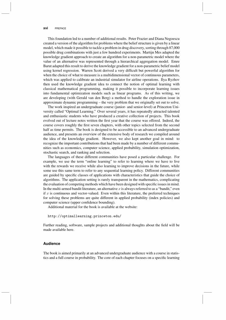
This foundation led to a number of additional results. Peter Frazier and Diana Negoescucreated a version of the algorithm for problems where the belief structure is given by a linearmodel, which made it possible to tackle a problem in drug discovery, sorting through 87,000possible drug combinations with just a few hundred experiments. Martijn Mes adapted theknowledge gradient approach to create an algorithm for a non-parametric model where thevalue of an alternative was represented through a hierarchical aggregation model. EmreBarut adapted this result to derive the knowledge gradient for a non-parametric belief modelusing kernel regression. Warren Scott derived a very difficult but powerful algorithm forwhen the choice of what to measure is a multidimensional vector of continuous parameters,which was applied to calibrate an industrial simulator for airline operations. Ilya Ryzhovthen used the knowledge gradient idea to connect the notion of optimal learning withclassical mathematical programming, making it possible to incorporate learning issuesinto fundamental optimization models such as linear programs. As of this writing, weare developing (with Gerald van den Berg) a method to handle the exploration issue inapproximate dynamic programming – the very problem that we originally set out to solve.
The work inspired an undergraduate course (junior- and senior-level) at Princeton Uni-versity called “Optimal Learning.” Over several years, it has repeatedly attracted talentedand enthusiastic students who have produced a creative collection of projects. This bookevolved out of lecture notes written the first year that the course was offered. Indeed, thecourse covers roughly the first seven chapters, with other topics selected from the secondhalf as time permits. The book is designed to be accessible to an advanced undergraduateaudience, and presents an overview of the extensive body of research we compiled aroundthe idea of the knowledge gradient. However, we also kept another goal in mind: torecognize the important contributions that had been made by a number of different commu-nities such as economics, computer science, applied probability, simulation optimization,stochastic search, and ranking and selection.
The languages of these different communities have posed a particular challenge. Forexample, we use the term “online learning” to refer to learning where we have to livewith the rewards we receive while also learning to improve decisions in the future, whilesome use this same term to refer to any sequential learning policy. Different communitiesare guided by specific classes of applications with characteristics that guide the choice ofalgorithms. The application setting is rarely transparent in the mathematics, complicatingthe evaluation of competing methods which have been designed with specific issues in mind.In the multi-armed bandit literature, an alternative x is always referred to as a “bandit,” evenif x is continuous and vector-valued. Even within this literature, the preferred techniquesfor solving these problems are quite different in applied probability (index policies) andcomputer science (upper confidence bounding).
Additional material for the book is available at the website:
http://optimallearning.princeton.edu/
Further reading, software, sample projects and additional thoughts about the field will bemade available here.
Audience
The book is aimed primarily at an advanced undergraduate audience with a course in statis-tics and a full course in probability. The core of each chapter focuses on a specific learning

PREFACE xvii
problem, and presents practical, implementable algorithms. Downloadable software isprovided for several of the most important algorithms, and a fairly elaborate implemen-tation, the Optimal Learning Calculator, is available as a spreadsheet interface calling asophisticated Java library.
The later chapters cover material that is more advanced, including learning on graphsand linear programs, and learning where the alternatives are continuous (and possiblyvector-valued). We have provided chapters designed to bridge with communities such assimulation optimization and machine learning. This material is designed to help Ph.D.students and researchers to understand the many communities that have contributed to thegeneral area of optimal learning.
While every effort has been made to make this material as accessible as possible, thetheory supporting this field can be quite subtle. Material that is more suitable to a graduatelevel audience is indicated with an * in the section title.
Organization of the book
The book is roughly organized into three parts:
Part I: Fundamentals
Chapter 1 - The challenges of learning
Chapter 2 - Adaptive learning
Chapter 3 - The economics of information
Chapter 4 - Ranking and selection
Chapter 5 - The knowledge gradient
Chapter 6 - Bandit problems
Chapter 7 - Elements of a learning problem
Part II: Extensions and Applications
Chapter 8 - Linear belief models
Chapter 9 - Subset selection models
Chapter 10 - Optimizing a scalar function
Chapter 11 - Optimal bidding
Chapter 12 - Stopping problems
Part III: Advanced topics
Chapter 13 - Active learning in statistics
Chapter 14 - Simulation optimization
Chapter 15 - Learning in mathematical programming
Chapter 16 - Optimizing over continuous measurements
Chapter 17 - Learning with a physical state
The book is used as a textbook for an undergraduate course at Princeton. In this setting,Part I covers the foundations of the course. This material is supplemented with traditional

xviii PREFACE
weekly problem sets and a midterm exam (two hourly exams would also work well here).Each of these chapters have a relatively large number of exercises to help students developtheir understanding of the material.
After this foundational material is covered, students have to come up with a projectwhich involves the efficient collection of information. Students are encouraged to work inteams of two, and the project progresses in three stages: initial problem definition, designof the belief model and learning algorithms, and then submission of the final report whichinvolves the testing of different policies in the context of their application. In the initialproblem definition, it is important for students to clearly identify the information that isbeing collected, the implementation decision (which may be different, but not always), andthe metric used to evaluate the quality of the implementation decision.
While the students work on their projects, the course continues to work through most ofthe topics in Part II. The material on linear belief models is particularly useful in many ofthe student projects, as is the subset selection chapter. Sometimes it is useful to prioritizethe material being presented based on the topics that the students have chosen. The chaptersin part II have a small number of exercises, many of which require the use of downloadableMatlab software to help with the implementation of these more difficult algorithms.
Part III of the book is advanced material, and is intended primarily for researchers andprofessionals interested in using the book as a reference volume. These chapters are notaccompanied by exercises, since the material here is more difficult and would require theuse of fairly sophisticated software packages.
WARREN B. POWELL
ILYA O. RYZHOV
Princeton University, University of Maryland
October, 2011

ACKNOWLEDGMENTS
This book reflects the contributions of a number of students at Princeton University. Specialthanks go to Peter Frazier, who developed the initial framework that shaped our research inthis area. Warren Scott, Diana Negoescu, Martijn Mes and Emre Barut all made importantcontributions, and their enthusiastic participation in all stages of this research is gratefullyacknowledged.
The Optimal Learning Calculator was co-written by Gerald van den Berg and WillManning, working as undergraduate interns. The spreadsheet-based interface has providedvaluable insights into the behavior of different learning policies.
We are very grateful to the students of ORF 418, Optimal Learning, who put up withthe formative development of these ideas, and who provided an extensive list of creativeprojects to highlight potential applications of information collection.
The research was supported primarily by the Air Force Office of Scientific Researchfrom the discrete mathematics program headed by Don Hearn, with additional support fromthe Department of Homeland Security through the CICCADA Center at Rutgers under theleadership of Fred Roberts, and the National Science Foundation. Special thanks also goesto SAP and the enthusiastic support of Bill McDermott and Paul Hofmann, and the manycorporate partners of CASTLE Laboratory and PENSA who have provided the challengingproblems which motivated this research.
W. B. P. and I. O. R.
xix


CHAPTER 1
THE CHALLENGES OF LEARNING
We are surrounded by situations where we need to make a decision or solve a problem, butwhere we do not know some or all of the relevant information for the problem perfectly.Will the path recommended by my navigation system get me to my appointment on time?Am I charging the right price for my product, and do I have the best set of features? Will anew material make batteries last longer? Will a drug cocktail help reduce a cancer tumor?If I turn my retirement fund over to this investment manager, will I be able to outperformthe market?
Sometimes the decisions have a simple structure (what is the best drug to treat mydiabetes), while others require complex planning (how do I deploy a team to assess theoutbreak of a disease). There are settings where we have to learn while we are doing (thesales of a book at a particular price), while in other cases we may have a budget to collectinformation before making a final decision that is implemented in the field. In fact, learningproblems come in a range of major problem classes that reflect the nature of choices beingmade (e.g. which drug), what we learn (success/failure, or estimates of varying accuracy),the size of our learning budget, and whether we are learning online (in the field) or offline(in the laboratory).
There are some decision problems that are hard even if we have access to perfectly accu-rate information about our environment: planning routes for aircraft and pilots, optimizingthe movements of vehicles to pick up and deliver goods, or scheduling machines to finisha set of jobs on time. This is known as deterministic optimization. Then there are othersituations where we have to make decisions under uncertainty, but where we assume weknow the probability distributions of the uncertain quantities: how do I allocate investments
Optimal Learning. By Warren B. Powell and Ilya O. RyzhovCopyright c© 2018 John Wiley & Sons, Inc.
1
2 THE CHALLENGES OF LEARNING
Alternative Value
1 7592 7223 6984 6535 616
Alternative Mean Std. dev.
1 759 1202 722 1423 698 1334 653 905 616 102
(a) The best of five known alternatives (b) The best of five uncertain alternatives
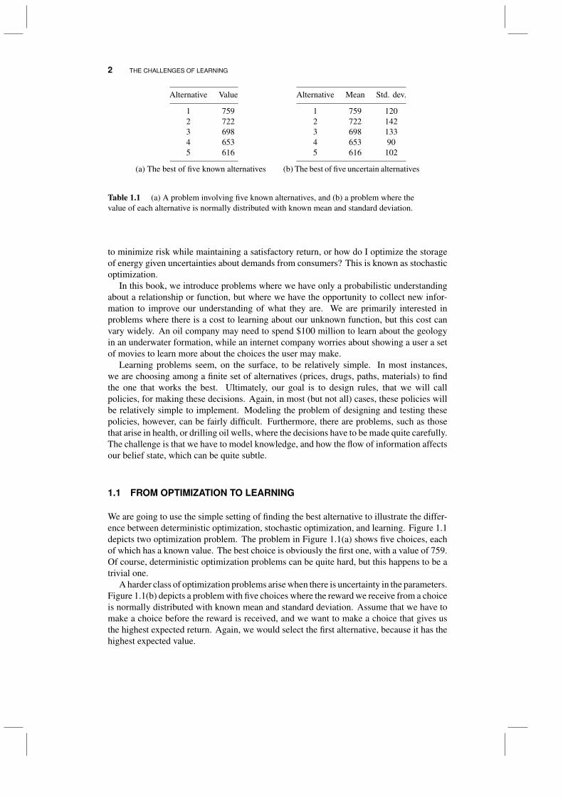
Table 1.1 (a) A problem involving five known alternatives, and (b) a problem where thevalue of each alternative is normally distributed with known mean and standard deviation.
to minimize risk while maintaining a satisfactory return, or how do I optimize the storageof energy given uncertainties about demands from consumers? This is known as stochasticoptimization.
In this book, we introduce problems where we have only a probabilistic understandingabout a relationship or function, but where we have the opportunity to collect new infor-mation to improve our understanding of what they are. We are primarily interested inproblems where there is a cost to learning about our unknown function, but this cost canvary widely. An oil company may need to spend $100 million to learn about the geologyin an underwater formation, while an internet company worries about showing a user a setof movies to learn more about the choices the user may make.
Learning problems seem, on the surface, to be relatively simple. In most instances,we are choosing among a finite set of alternatives (prices, drugs, paths, materials) to findthe one that works the best. Ultimately, our goal is to design rules, that we will callpolicies, for making these decisions. Again, in most (but not all) cases, these policies willbe relatively simple to implement. Modeling the problem of designing and testing thesepolicies, however, can be fairly difficult. Furthermore, there are problems, such as thosethat arise in health, or drilling oil wells, where the decisions have to be made quite carefully.The challenge is that we have to model knowledge, and how the flow of information affectsour belief state, which can be quite subtle.
1.1 FROM OPTIMIZATION TO LEARNING
We are going to use the simple setting of finding the best alternative to illustrate the differ-ence between deterministic optimization, stochastic optimization, and learning. Figure 1.1depicts two optimization problem. The problem in Figure 1.1(a) shows five choices, eachof which has a known value. The best choice is obviously the first one, with a value of 759.Of course, deterministic optimization problems can be quite hard, but this happens to be atrivial one.
A harder class of optimization problems arise when there is uncertainty in the parameters.Figure 1.1(b) depicts a problem with five choices where the reward we receive from a choiceis normally distributed with known mean and standard deviation. Assume that we have tomake a choice before the reward is received, and we want to make a choice that gives usthe highest expected return. Again, we would select the first alternative, because it has thehighest expected value.
AREAS OF APPLICATION 3
Initial mean and std. dev. First Updated mean and std. dev. SecondAlternative Mean Std dev obs. Mean Std dev obs.
1 759 102 702 712 922 722 133 722 133 7343 698 78 698 784 653 90 653 905 616 102 616 102
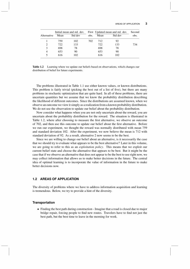
Table 1.2 Learning where we update our beliefs based on observations, which changes ourdistribution of belief for future experiments.
The problems illustrated in Table 1.1 use either known values, or known distributions.This problem is fairly trivial (picking the best out of a list of five), but there are manyproblems in stochastic optimization that are quite hard. In all of these problems, there areuncertain quantities but we assume that we know the probability distribution describingthe likelihood of different outcomes. Since the distributions are assumed known, when weobserve an outcome we view it simply as a realization from a known probability distribution.We do not use the observation to update our belief about the probability distribution.
Now consider what happens when you are not only uncertain about the reward, you areuncertain about the probability distribution for the reward. The situation is illustrated inTable 1.2, where after choosing to measure the first alternative, we observe an outcomeof 702, and then use this outcome to update our belief about the first alternative. Beforewe run our experiment, we thought the reward was normally distributed with mean 759and standard deviation 102. After the experiment, we now believe the mean is 712 withstandard deviation of 92. As a result, alternative 2 now seems to be the best.
Since we are willing to change our belief about an alternative, is it necessarily the casethat we should try to evaluate what appears to be the best alternative? Later in this volume,we are going to refer to this as an exploitation policy. This means that we exploit ourcurrent belief state and choose the alternative that appears to be best. But it might be thecase that if we observe an alternative that does not appear to be the best to use right now, wemay collect information that allows us to make better decisions in the future. The centralidea of optimal learning is to incorporate the value of information in the future to makebetter decisions now.
1.2 AREAS OF APPLICATION
The diversity of problems where we have to address information acquisition and learningis tremendous. Below, we try to provide a hint of the diversity.
Transportation
• Finding the best path during construction - Imagine that a road is closed due to majorbridge repair, forcing people to find new routes. Travelers have to find not just thebest path, but the best time to leave in the morning for work.
4 THE CHALLENGES OF LEARNING
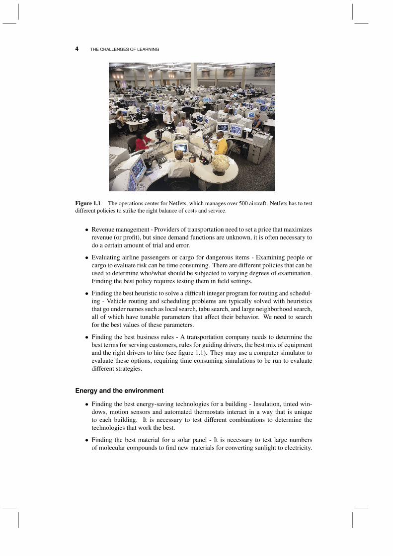
Figure 1.1 The operations center for NetJets, which manages over 500 aircraft. NetJets has to testdifferent policies to strike the right balance of costs and service.
• Revenue management - Providers of transportation need to set a price that maximizesrevenue (or profit), but since demand functions are unknown, it is often necessary todo a certain amount of trial and error.
• Evaluating airline passengers or cargo for dangerous items - Examining people orcargo to evaluate risk can be time consuming. There are different policies that can beused to determine who/what should be subjected to varying degrees of examination.Finding the best policy requires testing them in field settings.
• Finding the best heuristic to solve a difficult integer program for routing and schedul-ing - Vehicle routing and scheduling problems are typically solved with heuristicsthat go under names such as local search, tabu search, and large neighborhood search,all of which have tunable parameters that affect their behavior. We need to searchfor the best values of these parameters.
• Finding the best business rules - A transportation company needs to determine thebest terms for serving customers, rules for guiding drivers, the best mix of equipmentand the right drivers to hire (see figure 1.1). They may use a computer simulator toevaluate these options, requiring time consuming simulations to be run to evaluatedifferent strategies.
Energy and the environment
• Finding the best energy-saving technologies for a building - Insulation, tinted win-dows, motion sensors and automated thermostats interact in a way that is uniqueto each building. It is necessary to test different combinations to determine thetechnologies that work the best.
• Finding the best material for a solar panel - It is necessary to test large numbersof molecular compounds to find new materials for converting sunlight to electricity.

AREAS OF APPLICATION 5
Figure 1.2 Wind turbines are one form of alternative energy resources (fromhttp://www.nrel.gov/data/pix/searchpix.cgi ).
Testing and evaluating materials is time consuming and very expensive, and thereare large numbers of molecular combinations that can be tested.
• Optimizing the best policy for storing energy in a battery - A policy is defined byone or more parameters that determine how much energy is stored and in what typeof storage device. One example might be, “charge the battery when the spot price ofenergy drops below x1, discharge when it goes above x2.” We can collect informationin the field or a computer simulation that evaluates the performance of a policy overa period of time.
• Learning how lake pollution due to fertilizer run-off responds to farm policies - Wecan introduce new policies that encourage or discourage the use of fertilizer, but wedo not fully understand the relationship between these policies and lake pollution,and these policies impose different costs on the farmers. We need to test differentpolicies to learn their impact, but each test requires a year to run and there is someuncertainty in evaluating the results.
• On a larger scale, we need to identify the best policies for controlling CO2 emissions,striking a balance between the cost of these policies (tax incentives on renewables,a carbon tax, research and development costs in new technologies) and the impacton global warming, but we do not know the exact relationship between atmosphericCO2 and global temperatures.
Homeland security
• You would like to minimize the time to respond to an emergency over a congestedurban network. You can run experiments to improve your understanding of the time
6 THE CHALLENGES OF LEARNING
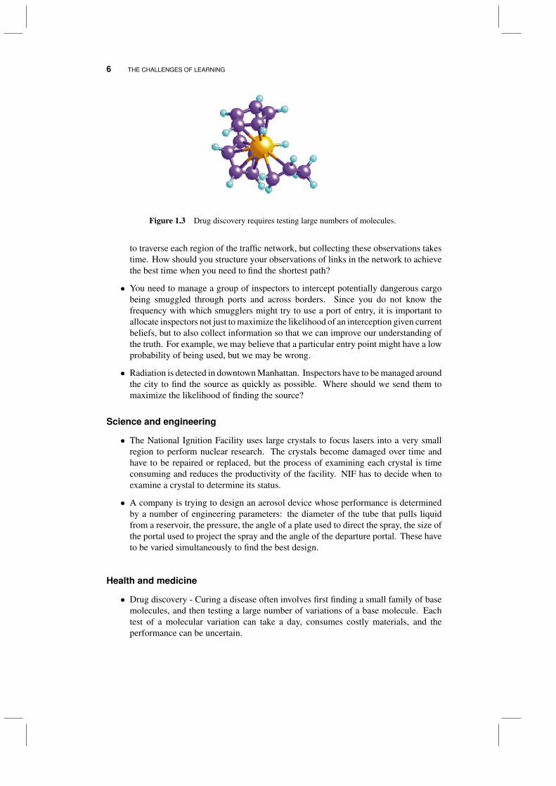
Figure 1.3 Drug discovery requires testing large numbers of molecules.
to traverse each region of the traffic network, but collecting these observations takestime. How should you structure your observations of links in the network to achievethe best time when you need to find the shortest path?
• You need to manage a group of inspectors to intercept potentially dangerous cargobeing smuggled through ports and across borders. Since you do not know thefrequency with which smugglers might try to use a port of entry, it is important toallocate inspectors not just to maximize the likelihood of an interception given currentbeliefs, but to also collect information so that we can improve our understanding ofthe truth. For example, we may believe that a particular entry point might have a lowprobability of being used, but we may be wrong.
• Radiation is detected in downtown Manhattan. Inspectors have to be managed aroundthe city to find the source as quickly as possible. Where should we send them tomaximize the likelihood of finding the source?
Science and engineering
• The National Ignition Facility uses large crystals to focus lasers into a very smallregion to perform nuclear research. The crystals become damaged over time andhave to be repaired or replaced, but the process of examining each crystal is timeconsuming and reduces the productivity of the facility. NIF has to decide when toexamine a crystal to determine its status.
• A company is trying to design an aerosol device whose performance is determinedby a number of engineering parameters: the diameter of the tube that pulls liquidfrom a reservoir, the pressure, the angle of a plate used to direct the spray, the size ofthe portal used to project the spray and the angle of the departure portal. These haveto be varied simultaneously to find the best design.
Health and medicine
• Drug discovery - Curing a disease often involves first finding a small family of basemolecules, and then testing a large number of variations of a base molecule. Eachtest of a molecular variation can take a day, consumes costly materials, and theperformance can be uncertain.

AREAS OF APPLICATION 7
• Drug dosage - Each person responds to medication in a different way. It is oftennecessary to test different dosages of a medication to find the level that produces thebest mix of effectiveness against a condition with minimum side effects.
• How should a doctor test different medications to treat diabetes, given that he willnot know in advance how a particular patient might respond to each possible courseof treatment?
• What is the best way to test a population for an emerging disease so that we can plana response strategy?
Sports
• How do you find the best set of five basketball players to use as your starting lineup?Basketball players require complementary skills in defense, passing and shooting,and it is necessary to try different combinations of players to see which group worksthe best.
• What is the best combination of rowers for a four person rowing shell? Rowersrequire a certain synergy to work well together, making it necessary to try differentcombinations of rowers to see who turns in the best time.
• Who are the best hitters that you should choose for your baseball team? It isnecessary to see how a player hits in game situations, and of course these are verynoisy observations.
• What plays work the best for your football team? Specific plays draw on differentcombinations of talents, and a coach has to find out what works best for his team.
Business
• What are the best labor rules or terms in a customer contract to maximize profits?These can be tested in a computer simulation program, but it may require severalhours (in some cases, several days) to run. How do we sequence our experiments tofind the best rules as quickly as possible?
• What is the best price to charge for a product being sold over the Internet? It isnecessary to use a certain amount of trial and error to find the price that maximizesrevenue.
• We would like to find the best supplier for a component part. We know the price ofthe component, but we do not know about the reliability of the service or the qualityof the product. We can collect information on service and product quality by placingsmall orders.
• We need to identify the best set of features to include in a new laptop we aremanufacturing. We can estimate consumer response by running market tests, butthese are time consuming and delay the product launch.
• A company needs to identify the best person to lead a division that is selling a newproduct. The company does not have time to interview all the candidates. Howshould a company identify a subset of potential candidates?

8 THE CHALLENGES OF LEARNING
• Advertising for a new release of a movie - We can choose between TV ads, billboards,trailers on movies already showing, the Internet and promotions through restaurantchains. What works best? Does it help to do TV ads if you are also doing Internetadvertising? How do different outlets interact? You have to try different combina-tions, evaluate their performance and use what you learn to guide future advertisingstrategies.
• Conference call or airline trip? Business people have to decide when to try to landa sale using teleconferencing, or when a personal visit is necessary. For companiesthat depend on numerous contacts, it is possible to experiment with different methodsof landing a sale, but these experiments are potentially expensive, involving the timeand expense of a personal trip, or the risk of not landing a sale.
E-commerce
• Which ads will produce the best consumer response when posted on a website? Youneed to test different ads, and then identify the ads that are the most promising basedon the attributes of each ad.
• Netflix can display a small number of movies to you when you log into your account.The challenge is identifying the movies that are likely to be most interesting to aparticular user. As new users sign up, Netflix has to learn as quickly as possiblewhich types of movies are most likely to attract the attention of an individual user.
• You need to choose keywords to bid on to get Google to display your ad. What bidshould you make for a particular keyword? You measure your performance by thenumber of clicks that you receive.
• YouTube has to decide which videos to feature on its website to maximize the numberof times a video is viewed. The decision is the choice of video, and the information(and reward) is the number of times people click on the video.
• Amazon uses your past history of book purchases to make suggestions for potentialnew purchases. Which products should be suggested? How can Amazon use yourresponse to past suggestions to guide new suggestions?
The service sector
• A university has to make specific offers of admission, after which it then observeswhich types of students actually matriculate. The university has to actually makean offer of admission to learn whether a student is willing to accept the offer. Thisinformation can be used to guide future offers in subsequent years. There is a hardconstraint on total admissions.
• A political candidate has to decide in which states to invest his remaining time forcampaigning. He decides which states would benefit the most through telephonepolls, but has to allocate a fixed budget for polling. How should he allocate hispolling budget?
• The Federal government would like to understand the risks associated with issuingsmall business loans based on the attributes of an applicant. A particular applicant

AREAS OF APPLICATION 9
Figure 1.4 The air force has to design new technologies, and determine the best policies foroperating them.
might not look attractive, but it is possible that the government’s estimate of risk isinflated. The only way to learn more is to try granting some higher risk loans.
• The Internal Revenue Service has to decide which companies to subject to a taxaudit. Should it be smaller companies or larger ones? Are some industries moreaggressive than others (for example, due to the presence of lucrative tax write-offs)?The government’s estimates of the likelihood of tax cheating may be incorrect, andthe only way to improve its estimates is to conduct audits.
The military
• The military has to collect information on risks faced in a region using UAVs (un-manned aerial vehicles). The UAV collects information about a section of road, andthen command determines how to deploy troops and equipment. How should theUAVs be deployed to produce the best deployment strategy?
• A fighter has to decide at what range to launch a missile. After firing a missile, welearn whether the missile hit its target or not, which can be related to factors suchas range, weather, altitude and angle-of-attack. With each firing, the fighter learnsmore about the probability of success.
• The Air Force has to deploy tankers for mid-air refueling. There are different policiesfor handling the tankers, which include options such as shuttling tankers back andforth between locations, using one tanker to refuel another tanker, and trying differentlocations for tankers. A deployment policy can be evaluated by measuring how muchtime fighters spend waiting for refueling, and the number of times a fighter has toabort a mission from lack of fuel.
• The military has to decide how to equip a soldier. There is always a tradeoff betweencost and the weight of the equipment, versus the likelihood that the soldier willsurvive. The military can experiment with different combinations of equipment toassess its effectiveness in terms of keeping a soldier alive.
10 THE CHALLENGES OF LEARNING
Tuning models and algorithms
• There is a large community that models physical problems such as manufacturingsystems using Monte Carlo simulation. For example, we may wish to simulate themanufacture of integrated circuits which have to progress through a series of stations.The progression from one station to another may be limited by the size of bufferswhich hold circuit boards waiting for a particular machine. We wish to determinethe best size of these buffers, but we have to do this by sequential simulations whichare time consuming and noisy.
• There are many problems in discrete optimization where we have to route people andequipment, or scheduling jobs to be served by a machine. These are exceptionallyhard optimization problems that are typically solved using heuristic algorithms suchas tabu search or genetic algorithms. These algorithms are controlled by a seriesof parameters which have to be tuned for specific problem classes. One run of analgorithm on a large problem can require several minutes to several hours (or more),and we have to find the best setting for perhaps five or ten parameters.
• Engineering models often have to be calibrated to replicate a physical process suchas weather or the spread of a chemical through groundwater. These models can beespecially expensive to run, often requiring the use of fast supercomputers to simulatethe process in continuous space or time. At the same time, it is necessary to calibratethese models to produce the best possible prediction.
1.3 MAJOR PROBLEM CLASSES
Given the diversity of learning problems, it is useful to organize these problems into majorproblem classes. A brief summary of some of the major dimensions of learning problemsis given below.
• Online vs. offline - Online problems involve learning from experiences as they occur.For example, we might observe the time on a path through a network by travelingthe path, or adjust the price of a product on the Internet and observe the revenue. Wecan try a decision that looks bad in the hopes of learning something, but we have toincur the cost of the decision, and balance this cost against future benefits. In offlineproblems, we might be working in a lab with a budget for running experiments, orwe might set aside several weeks to run computer simulations. If we experimentwith a chemical or process that does not appear promising, all we care about is theinformation learned from the experiment; we do not incur any cost from running anunsuccessful experiment. When our budget has been exhausted, we have to use ourobservations to choose a design or a process that will then be put into production.
• Objectives - Problems differ in terms of what we are trying to achieve. Most ofthe time we will focus on minimizing the expected cost or maximizing the expectedreward from some system. However, we may be simply interested in finding the bestdesign, or ensuring that we find a design that is within five percent of the best.
• The experimental decision - In some settings, we have a small number of choices suchas drilling test wells to learn about the potential for oil or natural gas. The numberof choices may be small, but each test can cost millions of dollars. Alternatively, we
MAJOR PROBLEM CLASSES 11
might have to find the best set of 30 proposals out of 100 that have been submitted,which means that we have to choose from 3 × 1025 possible portfolios. Or wemay have to choose the best price, temperature or pressure (a scalar, continuousparameter). We might have to set a combination of 16 parameters to produce thebest results for a business simulator. Each of these problems introduce differentcomputational challenges because of the size of the search space.
• The implementation decision - Collecting the best information depends on what youare going to do with the information once you have it. Often, the choices of what toobserve (the experimental decision) are the same as what you are going to implement(finding the choice with the best value). But you might measure a link in a graphin order to choose the best path. Or we might want to learn something about a newmaterial to make a decision about new solar panels or batteries. In these problems,the implementation decision (the choice of path or technology) is different from thechoice of what to measure.
• What we believe - We may start by knowing nothing about the best system. Typically,we know something (or at least we will know something after we make our firstexperiment). What assumptions can we reasonably make about different choices?Can we put a normal distribution of belief on an unknown quantity? Are the beliefscorrelated (if a laptop with one set of features has higher sales than we expected,does this change our belief about other sets of features)? Are the beliefs stored as alookup table (that is, a belief for each design), or are the beliefs expressed as somesort of statistical model?
• The cost of an observation or experiment - One of the most important distinguishingfeatures of different problem classes is the cost of running an experiment. There aretwo important problem classes:
Inexpensive experiments A popular source of problems arise in internet settingssuch as finding the best ad to maximize ad-clicks, or finding the best moviesor products to advertise on a retail site. This problem class tends to involve avery large number of choices (there can be thousands of ads or movies), butdifferent choices can be tested relatively easily. An important issue here is thatthe logic for deciding what to test needs to be easy to compute.
Expensive experiments There are many settings where a single experiment can bequite expensive, whether it is a day in a laboratory, hours to run a simulationon a computer, or weeks of testing in the field. Here, experiments need to becarefully designed, taking advantage of any prior information.
• The nature of an observation - Closely related to what we believe is what we learnwhen we run an experiment. Is the observation normally distributed? Is it a binaryrandom variable (success/failure)? Are experiments run with perfect accuracy? Ifnot, do we know the distribution of the error from running an experiment?
• Switching costs - The simplest problems assume that you can switch from one choiceto another without penalty, but this is not always the case. We may have equipmentset up to run a particular set of experiments; switching incurs a cost.
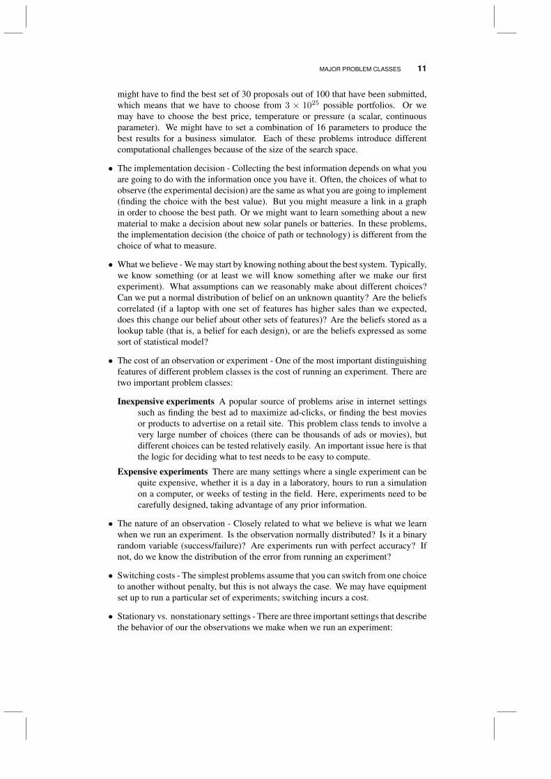
• Stationary vs. nonstationary settings - There are three important settings that describethe behavior of our the observations we make when we run an experiment:
12 THE CHALLENGES OF LEARNING
Stationary distributions - Observations come from an unknown distribution whichis not changing over time.
Nonstationary distributions - Observations are coming from distributions that areevolving over time (we hope that they are not changing too quickly). Forexample, sales of a product at a certain price depends on other exogenousfactors that may change over time.
Learning problems - The more we try something, the better it may get.
• The experimental budget - Primarily relevant in offline settings, experimental budgetsmay be quite small (we can only run 20 laboratory experiments in a summer), ormuch larger (I might have a robotic scientist that can run hundreds of experiments).
• Planning constraints - There are fast-paced settings where we may have 50 mil-liseconds to make a decision, to problems where a single experiment is both timeconsuming and expensive, justifying significant computation before making the nextexperiment.
• Sequential vs. parallel (or batch) experimentation - We may have to run eachexperiment in sequence, which means we know the results of one experiment beforedeciding the next, but there are many settings where experiments can be run inparallel or batch. For example, we may try out a new drug on a group of patients atthe same time.
• Belief states and physical/information states - All learning problems include a beliefstate which captures what we believe about the system. There are many learningproblems where the belief state is the only information we have available. However,there are problems where we have access to additional information that changesthe behavior of our problem (we call this the “information state”), or we may bemanaging a physical system that changes the decisions we can make (we call this the“physical state”). For example
Information state - We may learn about the pricing decisions of our competitorsbefore choosing the price we charge for our product, or we might obtain thecharacteristics of a patient before prescribing medication.
Physical state - We may be managing a technical team that is collecting informationabout the spread of a disease. The decision of where to send the team nextdepends on where it is located now.
Given the richness of these problems, it should perhaps not be surprising that they havearisen in different communities who have devised strategies that are suited to differentenvironments. In fact, it is important to understand the problem setting to appreciate thediversity of solution strategies that have evolved.
1.4 TWO APPLICATIONS
In this section, we provide a little more detail using two very classic problems: thenewsvendor problem and the shortest path problem.
TWO APPLICATIONS 13
1.4.1 The newsvendor problem
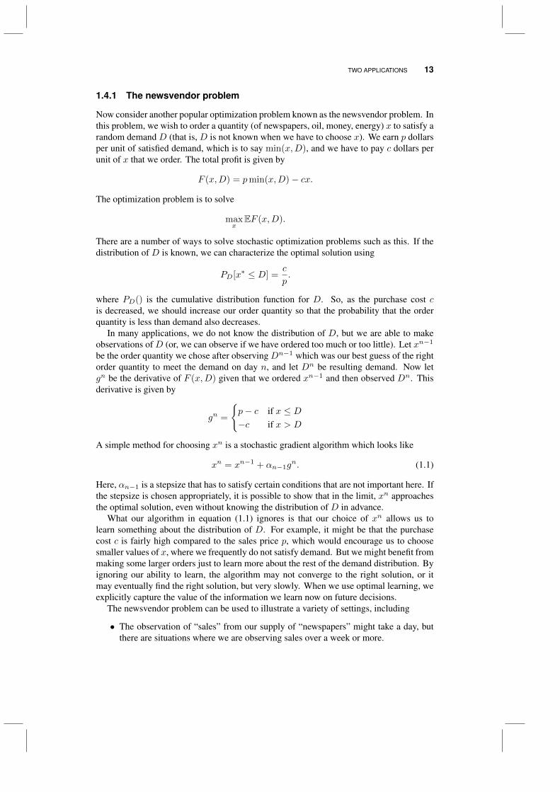
Now consider another popular optimization problem known as the newsvendor problem. Inthis problem, we wish to order a quantity (of newspapers, oil, money, energy) x to satisfy arandom demand D (that is, D is not known when we have to choose x). We earn p dollarsper unit of satisfied demand, which is to say min(x,D), and we have to pay c dollars perunit of x that we order. The total profit is given by
F (x,D) = pmin(x,D)− cx.
The optimization problem is to solve
maxx
EF (x,D).
There are a number of ways to solve stochastic optimization problems such as this. If thedistribution of D is known, we can characterize the optimal solution using
PD[x∗ ≤ D] =c
p.
where PD() is the cumulative distribution function for D. So, as the purchase cost cis decreased, we should increase our order quantity so that the probability that the orderquantity is less than demand also decreases.
In many applications, we do not know the distribution of D, but we are able to makeobservations of D (or, we can observe if we have ordered too much or too little). Let xn−1
be the order quantity we chose after observing Dn−1 which was our best guess of the rightorder quantity to meet the demand on day n, and let Dn be resulting demand. Now letgn be the derivative of F (x,D) given that we ordered xn−1 and then observed Dn. Thisderivative is given by
gn =
p− c if x ≤ D−c if x > D
A simple method for choosing xn is a stochastic gradient algorithm which looks like
xn = xn−1 + αn−1gn. (1.1)
Here, αn−1 is a stepsize that has to satisfy certain conditions that are not important here. Ifthe stepsize is chosen appropriately, it is possible to show that in the limit, xn approachesthe optimal solution, even without knowing the distribution of D in advance.
What our algorithm in equation (1.1) ignores is that our choice of xn allows us tolearn something about the distribution of D. For example, it might be that the purchasecost c is fairly high compared to the sales price p, which would encourage us to choosesmaller values of x, where we frequently do not satisfy demand. But we might benefit frommaking some larger orders just to learn more about the rest of the demand distribution. Byignoring our ability to learn, the algorithm may not converge to the right solution, or itmay eventually find the right solution, but very slowly. When we use optimal learning, weexplicitly capture the value of the information we learn now on future decisions.
The newsvendor problem can be used to illustrate a variety of settings, including
• The observation of “sales” from our supply of “newspapers” might take a day, butthere are situations where we are observing sales over a week or more.
14 THE CHALLENGES OF LEARNING
( , )μ σ
(22,4)(24,6)
(26,2)(28,10)
(30,12)
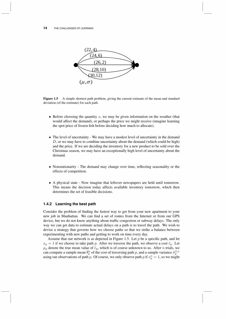
Figure 1.5 A simple shortest path problem, giving the current estimate of the mean and standarddeviation (of the estimate) for each path.
• Before choosing the quantity x, we may be given information on the weather (thatwould affect the demand), or perhaps the price we might receive (imagine learningthe spot price of frozen fish before deciding how much to allocate).
• The level of uncertainty - We may have a modest level of uncertainty in the demandD, or we may have to combine uncertainty about the demand (which could be high)and the price. If we are deciding the inventory for a new product to be sold over theChristmas season, we may have an exceptionally high level of uncertainty about thedemand.
• Nonstationarity - The demand may change over time, reflecting seasonality or theeffects of competition.
• A physical state - Now imagine that leftover newspapers are held until tomorrow.This means the decision today affects available inventory tomorrow, which thendetermines the set of feasible decisions.
1.4.2 Learning the best path
Consider the problem of finding the fastest way to get from your new apartment to yournew job in Manhattan. We can find a set of routes from the Internet or from our GPSdevice, but we do not know anything about traffic congestion or subway delays. The onlyway we can get data to estimate actual delays on a path is to travel the path. We wish todevise a strategy that governs how we choose paths so that we strike a balance betweenexperimenting with new paths and getting to work on time every day.
Assume that our network is as depicted in Figure 1.5. Let p be a specific path, and letxp = 1 if we choose to take path p. After we traverse the path, we observe a cost cp. Letµp denote the true mean value of cp, which is of course unknown to us. After n trials, wecan compute a sample mean θnp of the cost of traversing path p, and a sample variance σ2,n
p
using our observations of path p. Of course, we only observe path p if xnp = 1, so we might
TWO APPLICATIONS 15
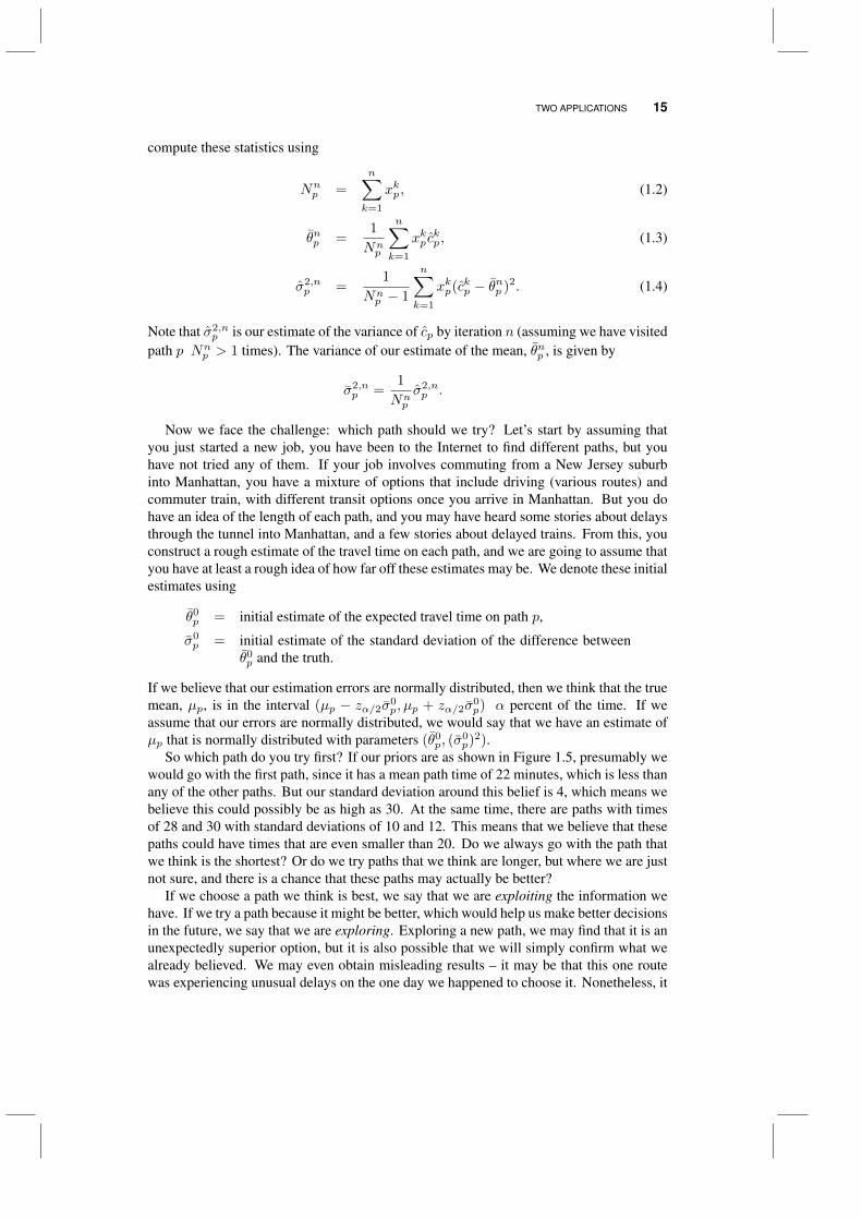
compute these statistics using
Nnp =
n∑k=1
xkp, (1.2)
θnp =1
Nnp
n∑k=1
xkp ckp, (1.3)
σ2,np =
1
Nnp − 1
n∑k=1
xkp(ckp − θnp )2. (1.4)
Note that σ2,np is our estimate of the variance of cp by iteration n (assuming we have visited
path p Nnp > 1 times). The variance of our estimate of the mean, θnp , is given by
σ2,np =
1
Nnp
σ2,np .
Now we face the challenge: which path should we try? Let’s start by assuming thatyou just started a new job, you have been to the Internet to find different paths, but youhave not tried any of them. If your job involves commuting from a New Jersey suburbinto Manhattan, you have a mixture of options that include driving (various routes) andcommuter train, with different transit options once you arrive in Manhattan. But you dohave an idea of the length of each path, and you may have heard some stories about delaysthrough the tunnel into Manhattan, and a few stories about delayed trains. From this, youconstruct a rough estimate of the travel time on each path, and we are going to assume thatyou have at least a rough idea of how far off these estimates may be. We denote these initialestimates using
θ0p = initial estimate of the expected travel time on path p,
σ0p = initial estimate of the standard deviation of the difference between
θ0p and the truth.
If we believe that our estimation errors are normally distributed, then we think that the truemean, µp, is in the interval (µp − zα/2σ0
p, µp + zα/2σ0p) α percent of the time. If we
assume that our errors are normally distributed, we would say that we have an estimate ofµp that is normally distributed with parameters (θ0
p, (σ0p)2).
So which path do you try first? If our priors are as shown in Figure 1.5, presumably wewould go with the first path, since it has a mean path time of 22 minutes, which is less thanany of the other paths. But our standard deviation around this belief is 4, which means webelieve this could possibly be as high as 30. At the same time, there are paths with timesof 28 and 30 with standard deviations of 10 and 12. This means that we believe that thesepaths could have times that are even smaller than 20. Do we always go with the path thatwe think is the shortest? Or do we try paths that we think are longer, but where we are justnot sure, and there is a chance that these paths may actually be better?
If we choose a path we think is best, we say that we are exploiting the information wehave. If we try a path because it might be better, which would help us make better decisionsin the future, we say that we are exploring. Exploring a new path, we may find that it is anunexpectedly superior option, but it is also possible that we will simply confirm what wealready believed. We may even obtain misleading results – it may be that this one routewas experiencing unusual delays on the one day we happened to choose it. Nonetheless, it
16 THE CHALLENGES OF LEARNING
is often desirable to try something new to avoid becoming stuck on a suboptimal solutionjust because it “seems” good. Balancing the desire to explore versus exploit is referred toin some communities as the exploration vs. exploitation problem. Another name is thelearn vs. earn problem. Regardless of the name, the point is the lack of information whenwe make a decision, and the value of new information in improving future decisions.
1.5 LEARNING FROM DIFFERENT COMMUNITIES
The challenge of efficiently collecting information is one that arises in a number of com-munities. The result is a lot of parallel discovery, although the questions and computationalchallenges posed by different communities can be quite different, and this has produceddiversity in the strategies proposed for solving these problems. Below we provide a roughlist of some of the communities that have become involved in this area.
• Simulation optimization - The simulation community often faces the problem oftuning parameters that influence the performance of a system that we are analyzingusing Monte Carlo simulation. These parameters might be the size of a buffer for amanufacturing simulator, the location of ambulances and fire trucks, or the number ofadvance bookings for a fare class for an airline. Simulations can be time consuming,so the challenge is deciding how long to analyze a particular configuration or policybefore switching to another one.
• The ranking and selection problem - This is a statistical problem that arises inmany settings, including the simulation optimization community. It is most oftenapproached using the language of classical frequentist statistics (but not always), andtends to be very practical in its orientation. In ranking and selection, we assumethat for each experiment, we can choose from a set of alternatives (there is no costfor switching from one alternative to another). Although the ranking and selectionframework is widely used in simulation optimization, the simulation communityrecognizes that it is easier to run the simulation for one configuration a little longerthan it is to switch to the simulation of a new configuration.
• The bandit community - There are two subcommunities that work on learning prob-lems known as the multiarmed bandit problem. It evolved originally within appliedprobability in the 1950’s, which led to a breakthrough known as Gittins indicesthat represented the first computable, optimal policy for a particular learning prob-lem. This work spawned the search for what became known as “index policies” forsolving variations of learning problems. The difficulty was that while these werecomputable in principle, they were difficult to compute. In the 1980’s, a new lineof research emerged within computer science with the discovery that some simplepolicies, known as “upper confidence bounds,” exhibited attractive bounds on theirperformance that suggested that they would work well.
• Global optimization of expensive functions - The engineering community often findsa need to optimize complex functions of continuous variables. The function issometimes a complex piece of computer software that takes a long time to run, butthe roots of the field come from geospatial applications. The function might bedeterministic (but not always), and a single evaluation can take an hour to a week ormore.
LEARNING FROM DIFFERENT COMMUNITIES 17
• Learning in economics - Economists have long studied the value of information ina variety of idealized settings. This community tends to focus on insights into theeconomic value of information, rather than the derivation of specific procedures forsolving information collection problems.
• Active learning in computer science - A popular problem in computer science isclassification: Is a news article fake? Does a patient have cancer? Will a customerpurchase a product or movie? Whereas most machine learning is performed with astatic (batch) dataset, we may be able to control our inputs (for example, by choosingwhich movies to show a user, or choosing a treatment regime for a patient). Havingthe ability to choose our data is known as active learning, and the goal is often tomaximize classification success.
• Statistical design of experiments - A classical problem in statistics is deciding whatexperiments to run. For certain objective functions, it has long been known thatexperiments can be designed deterministically, in advance, rather than sequentially.Our focus is primarily on sequential information collection, but there are importantproblem classes where this is not necessary.
• Frequentist versus Bayesian communities - It is difficult to discuss research in optimallearning without addressing the sometimes contentious differences in styles andattitudes between frequentist and Bayesian statisticians. Frequentists look for thetruth using nothing more than the data that we collect, while Bayesians would liketo allow us to integrate expert judgment.
• Optimal stopping - There is a special problem class where we have the ability toobserve a single stream of information such as the price of an asset. As long as wehold the asset, we get to observe the price. At some point, we have to make a decisionwhether we should sell the asset or continue to observe prices (a form of learning).Another variant is famously known as the “secretary problem” where we interviewcandidates for a position (or offers for an asset); after each candidate (or offer) wehave to decide if we should accept and stop or reject and continue observing.
• Approximate dynamic programming/reinforcement learning - Approximate dynamicprogramming, widely known as reinforcement learning in the computer sciencecommunity, addresses the problem of choosing an action given a state which generatesa reward and takes us to a new state. We do not know the exact value of thedownstream state, but we might decide to visit a state just to learn more about it.This is generally known as the “exploration vs. exploitation” problem, and thissetting has motivated a considerable amount of research in optimal learning.
• Psychology - Not surprisingly, the tradeoff between exploration and exploitationis a problem that has to be solved by people (as well as other animals rangingfrom chimpanzees to ants) for problems ranging from finding foot to finding mates.Psychologists have been attracted to the problem of understanding how people makethese decisions.
• Learning in the plant and animal sciences - Both plants and animals have to findfood and mates, which requires that they also solve the exploration vs. exploitationproblem. Two-armed slime molds have to decide which arm to extend; vines have todecide in which direction to grow along the ground to find a tree; predators on landand sea have to devise strategies for searching for food.
18 THE CHALLENGES OF LEARNING
Hold
Sell
Decision Outcome Decision Outcome
Hold
$1P
$1 w/p 0.3 $0 w/p 0.5$1 w/p 0.2
PPP
$1 w/p 0.3 $0 w/p 0.5$1 w/p 0.2
PPP
$1 w/p 0.3 $0 w/p 0.5$1 w/p 0.2
PPP
w/p 0.3
w/p 0.5
w/p 0.2
$0P
$1P
Sell
Hold
Sell
Hold
Sell
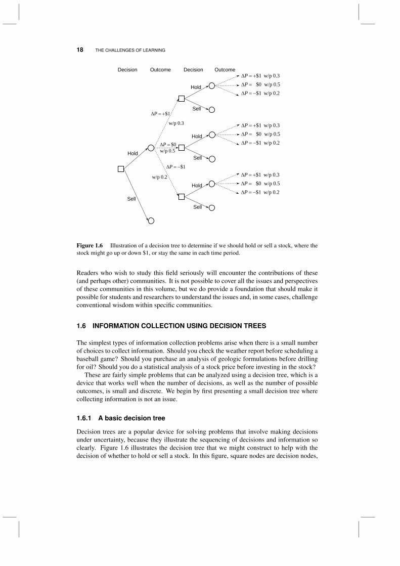
Figure 1.6 Illustration of a decision tree to determine if we should hold or sell a stock, where thestock might go up or down $1, or stay the same in each time period.
Readers who wish to study this field seriously will encounter the contributions of these(and perhaps other) communities. It is not possible to cover all the issues and perspectivesof these communities in this volume, but we do provide a foundation that should make itpossible for students and researchers to understand the issues and, in some cases, challengeconventional wisdom within specific communities.
1.6 INFORMATION COLLECTION USING DECISION TREES
The simplest types of information collection problems arise when there is a small numberof choices to collect information. Should you check the weather report before scheduling abaseball game? Should you purchase an analysis of geologic formulations before drillingfor oil? Should you do a statistical analysis of a stock price before investing in the stock?
These are fairly simple problems that can be analyzed using a decision tree, which is adevice that works well when the number of decisions, as well as the number of possibleoutcomes, is small and discrete. We begin by first presenting a small decision tree wherecollecting information is not an issue.
1.6.1 A basic decision tree
Decision trees are a popular device for solving problems that involve making decisionsunder uncertainty, because they illustrate the sequencing of decisions and information soclearly. Figure 1.6 illustrates the decision tree that we might construct to help with thedecision of whether to hold or sell a stock. In this figure, square nodes are decision nodes,
INFORMATION COLLECTION USING DECISION TREES 19
Hold
Sell
Hold
$1P
w/p 0.3
w/p 0.5
w/p 0.2
$0P
$1P
Sell
Hold
Sell
Hold
Sell
$51.10
$50P
$51.00
$50.10
$50.00
$49.10
$49.00
Hold
Sell
$1P
w/p 0.3
w/p 0.5
w/p 0.2
$0P
$1P
$51.10
$50P
$50.10
$49.10
Hold
Sell
$50P
$50.20
$50.00
1.7(a) 1.7(b) 1.7(c)
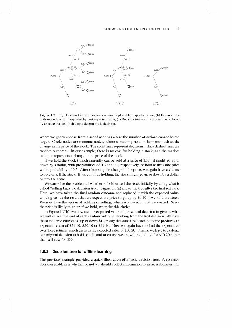
Figure 1.7 (a) Decision tree with second outcome replaced by expected value; (b) Decision treewith second decision replaced by best expected value; (c) Decision tree with first outcome replacedby expected value, producing a deterministic decision.
where we get to choose from a set of actions (where the number of actions cannot be toolarge). Circle nodes are outcome nodes, where something random happens, such as thechange in the price of the stock. The solid lines represent decisions, while dashed lines arerandom outcomes. In our example, there is no cost for holding a stock, and the randomoutcome represents a change in the price of the stock.
If we hold the stock (which currently can be sold at a price of $50), it might go up ordown by a dollar, with probabilities of 0.3 and 0.2, respectively, or hold at the same pricewith a probability of 0.5. After observing the change in the price, we again have a chanceto hold or sell the stock. If we continue holding, the stock might go up or down by a dollar,or stay the same.
We can solve the problem of whether to hold or sell the stock initially by doing what iscalled “rolling back the decision tree.” Figure 1.7(a) shows the tree after the first rollback.Here, we have taken the final random outcome and replaced it with the expected value,which gives us the result that we expect the price to go up by $0.10 if we hold the stock.We now have the option of holding or selling, which is a decision that we control. Sincethe price is likely to go up if we hold, we make this choice.
In Figure 1.7(b), we now use the expected value of the second decision to give us whatwe will earn at the end of each random outcome resulting from the first decision. We havethe same three outcomes (up or down $1, or stay the same), but each outcome produces anexpected return of $51.10, $50.10 or $49.10. Now we again have to find the expectationover these returns, which gives us the expected value of $50.20. Finally, we have to evaluateour original decision to hold or sell, and of course we are willing to hold for $50.20 ratherthan sell now for $50.
1.6.2 Decision tree for offline learning
The previous example provided a quick illustration of a basic decision tree. A commondecision problem is whether or not we should collect information to make a decision. For

20 THE CHALLENGES OF LEARNING
example, consider a bank that is considering whether it should grant a short term creditloan of $100,000. The bank expects to make $10,000 if the loan is paid off on time. If theloan is defaulted, the bank loses the amount of the loan.
From history, the bank knows that 95 percent of loans are repaid in full, while 5 percentdefault. If the bank purchases the credit report, this information will allow the bank toclassify the customer into one of three groups: 52 percent fall into the top A rating, 30percent fall into the middle B rating, while 18 percent fall into the lower C rating with thehighest risk of default. The company selling the credit report provides the joint distributionP (Credit,Default) that a customer will receive each credit rating, and whether it defaultedor not. This data is summarized in Table 1.3.
We need to understand how the information from the credit report changes our beliefabout the probability of a default. For this, we use a simple application of Bayes’ theorem,which states
P (Default | Credit) =P (Credit | Default)P (Default)
P (Credit)
=P (Credit,Default)
P (Credit).
Bayes’ theorem allows us to start with our initial estimate of the probability of a default,P (Default), then use the information “Credit” from the credit history and turn it into aposterior distribution P (Default | Credit). The results of this calculation are shown in thefinal two columns of Table 1.3.
P(Credit,Default) P(Default | Credit)
Credit rating P(Credit) No Yes No Yes
A 0.52 0.51 0.01 0.981 0.019B 0.30 0.28 0.02 0.933 0.067C 0.18 0.16 0.02 0.889 0.111
P(Default)= 0.95 0.05
Table 1.3 The marginal probability of each credit rating; the joint probability of a creditrating and whether someone defaults on a loan, and the conditional probability of a defaultgiven a credit rating.
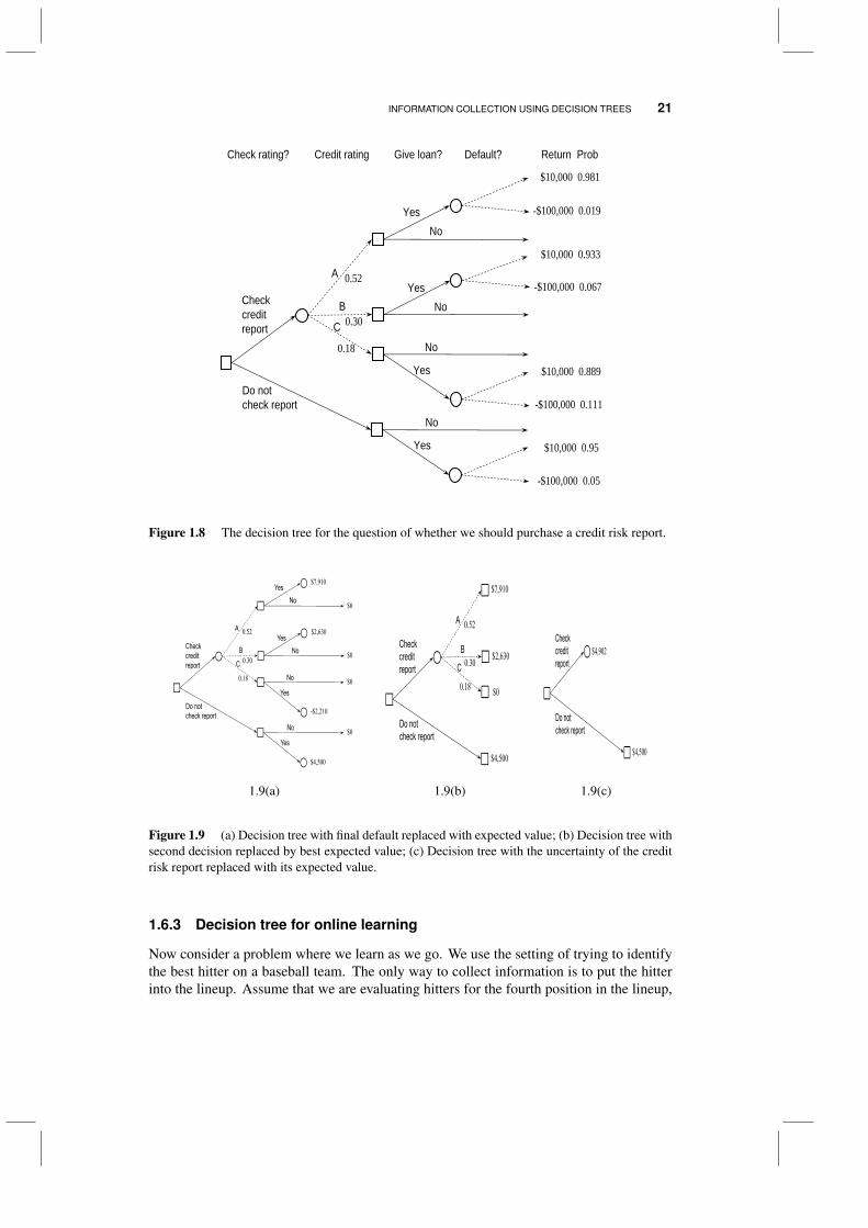
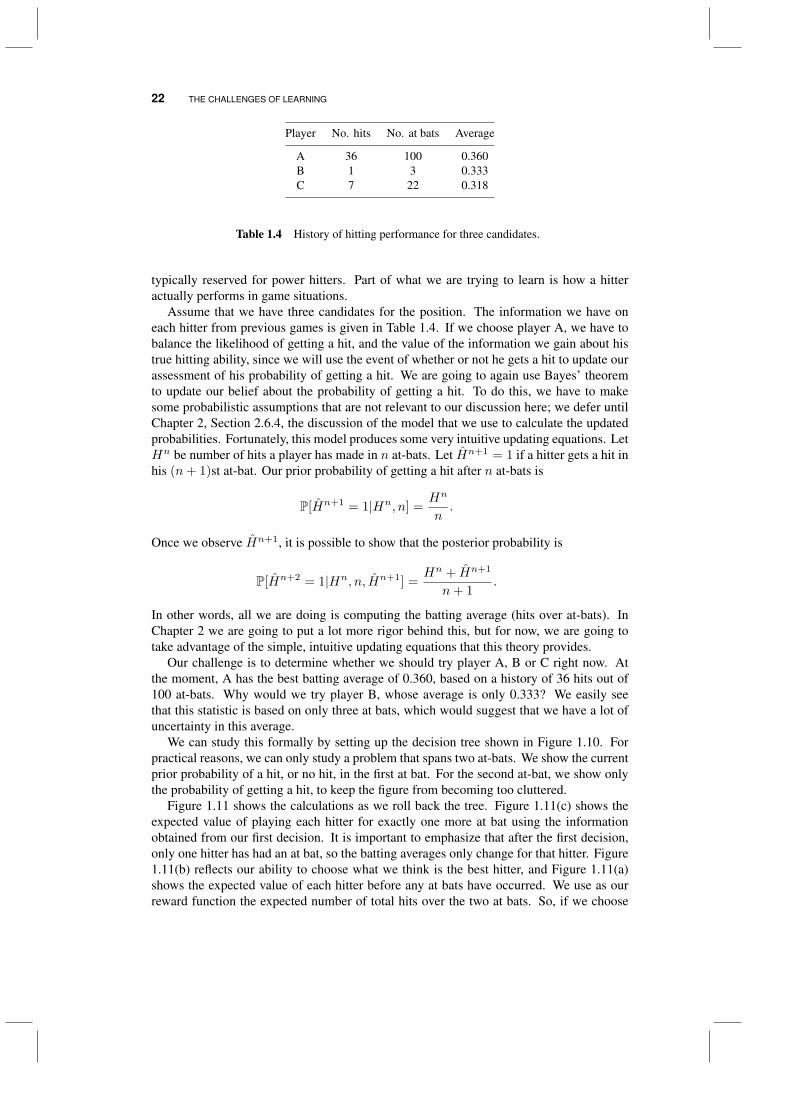
Using this information, we can construct a new decision tree, shown in Figure 1.8. Unlikeour first decision tree in Figure 1.7, we now see that the decision to collect informationchanges the downstream probabilities.
We repeat the exercise of rolling back the decision tree in Figure 1.9. Figure 1.9(a)shows the expected value of the decision to grant the loan given the information about thecredit history. We see that if the grantee has an A or B credit rating, it makes sense to grantthe loan, but not if the rating is C. Thus, the information from the credit report has the effectof changing the decision of whether or not to grant the loan. After we roll the tree back tothe original decision of whether to purchase the credit report, we find that the credit reportproduces an expected value of $4,900, compared to $4,500 that we would expect to receivewithout the credit report. This means that we would be willing to pay up to $400 for thecredit report.
INFORMATION COLLECTION USING DECISION TREES 21
A
Check rating? Credit rating Give loan? Default? Return Prob
B
C
Checkcreditreport
Do notcheck report
YesNo
YesNo
Yes
No
Yes
No
0.52
0.30
0.18
$10,000 0.981
-$100,000 0.019
$10,000 0.933
-$100,000 0.067
$10,000 0.889
-$100,000 0.111
$10,000 0.95
-$100,000 0.05
Figure 1.8 The decision tree for the question of whether we should purchase a credit risk report.
A
B
C
Checkcreditreport
Do notcheck report
YesNo
YesNo
Yes
No
Yes
No
0.52
0.30
0.18
$7,910
$2,630
-$2,210
$4,500
$0
$0
$0
$0
A
B
C
Checkcreditreport
Do notcheck report
0.52
0.30
0.18
$7,910
$2,630
$4,500
$0
Checkcreditreport
Do notcheck report
$4,500
$4,902
1.9(a) 1.9(b) 1.9(c)
Figure 1.9 (a) Decision tree with final default replaced with expected value; (b) Decision tree withsecond decision replaced by best expected value; (c) Decision tree with the uncertainty of the creditrisk report replaced with its expected value.
1.6.3 Decision tree for online learning
Now consider a problem where we learn as we go. We use the setting of trying to identifythe best hitter on a baseball team. The only way to collect information is to put the hitterinto the lineup. Assume that we are evaluating hitters for the fourth position in the lineup,
22 THE CHALLENGES OF LEARNING
Player No. hits No. at bats Average
A 36 100 0.360B 1 3 0.333C 7 22 0.318
Table 1.4 History of hitting performance for three candidates.
typically reserved for power hitters. Part of what we are trying to learn is how a hitteractually performs in game situations.
Assume that we have three candidates for the position. The information we have oneach hitter from previous games is given in Table 1.4. If we choose player A, we have tobalance the likelihood of getting a hit, and the value of the information we gain about histrue hitting ability, since we will use the event of whether or not he gets a hit to update ourassessment of his probability of getting a hit. We are going to again use Bayes’ theoremto update our belief about the probability of getting a hit. To do this, we have to makesome probabilistic assumptions that are not relevant to our discussion here; we defer untilChapter 2, Section 2.6.4, the discussion of the model that we use to calculate the updatedprobabilities. Fortunately, this model produces some very intuitive updating equations. LetHn be number of hits a player has made in n at-bats. Let Hn+1 = 1 if a hitter gets a hit inhis (n+ 1)st at-bat. Our prior probability of getting a hit after n at-bats is
P[Hn+1 = 1|Hn, n] =Hn
n.
Once we observe Hn+1, it is possible to show that the posterior probability is
P[Hn+2 = 1|Hn, n, Hn+1] =Hn + Hn+1
n+ 1.
In other words, all we are doing is computing the batting average (hits over at-bats). InChapter 2 we are going to put a lot more rigor behind this, but for now, we are going totake advantage of the simple, intuitive updating equations that this theory provides.
Our challenge is to determine whether we should try player A, B or C right now. Atthe moment, A has the best batting average of 0.360, based on a history of 36 hits out of100 at-bats. Why would we try player B, whose average is only 0.333? We easily seethat this statistic is based on only three at bats, which would suggest that we have a lot ofuncertainty in this average.
We can study this formally by setting up the decision tree shown in Figure 1.10. Forpractical reasons, we can only study a problem that spans two at-bats. We show the currentprior probability of a hit, or no hit, in the first at bat. For the second at-bat, we show onlythe probability of getting a hit, to keep the figure from becoming too cluttered.
Figure 1.11 shows the calculations as we roll back the tree. Figure 1.11(c) shows theexpected value of playing each hitter for exactly one more at bat using the informationobtained from our first decision. It is important to emphasize that after the first decision,only one hitter has had an at bat, so the batting averages only change for that hitter. Figure1.11(b) reflects our ability to choose what we think is the best hitter, and Figure 1.11(a)shows the expected value of each hitter before any at bats have occurred. We use as ourreward function the expected number of total hits over the two at bats. So, if we choose
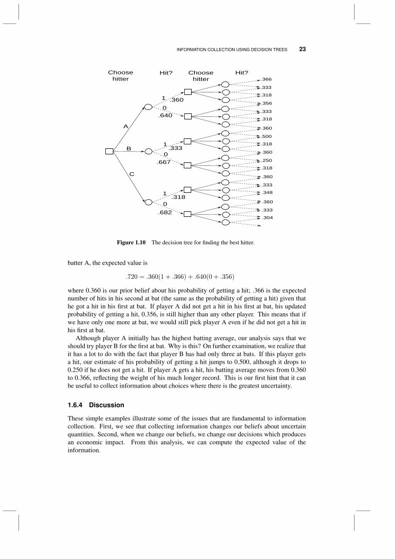
INFORMATION COLLECTION USING DECISION TREES 23
Choose hitter
A
B
C
Hit?
1
0
1
0
1
0
Choose hitter
Hit?
.360
.640
.333
.667
.318
.682
.366
.333
.318
.356
.333
.318
.360
.500
.318
.360
.250
.318
.360
.333
.348
.360
.333
.304
Figure 1.10 The decision tree for finding the best hitter.
batter A, the expected value is
.720 = .360(1 + .366) + .640(0 + .356)
where 0.360 is our prior belief about his probability of getting a hit; .366 is the expectednumber of hits in his second at bat (the same as the probability of getting a hit) given thathe got a hit in his first at bat. If player A did not get a hit in his first at bat, his updatedprobability of getting a hit, 0.356, is still higher than any other player. This means that ifwe have only one more at bat, we would still pick player A even if he did not get a hit inhis first at bat.
Although player A initially has the highest batting average, our analysis says that weshould try player B for the first at bat. Why is this? On further examination, we realize thatit has a lot to do with the fact that player B has had only three at bats. If this player getsa hit, our estimate of his probability of getting a hit jumps to 0.500, although it drops to0.250 if he does not get a hit. If player A gets a hit, his batting average moves from 0.360to 0.366, reflecting the weight of his much longer record. This is our first hint that it canbe useful to collect information about choices where there is the greatest uncertainty.
1.6.4 Discussion
These simple examples illustrate some of the issues that are fundamental to informationcollection. First, we see that collecting information changes our beliefs about uncertainquantities. Second, when we change our beliefs, we change our decisions which producesan economic impact. From this analysis, we can compute the expected value of theinformation.
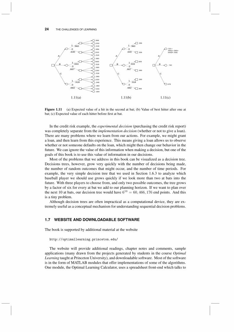
24 THE CHALLENGES OF LEARNING
A
B
C
1
0
1
0
1
0
.366
.333
.318
.356
.333
.318
.360
.500
.318
.360
.250
.318
.360
.333
.348
.360
.333
.304
.360
.640
.333
.667
.318
.682
A
B
C
1
0
1
0
1
0
.366
.356
.500
.360
.360
.360
.360
.640
.333
.667
.318
.682
A
B
C
.720 =
.360(1+.366)+
.640(0+.356)
.740
.678
1.11(a) 1.11(b) 1.11(c)
Figure 1.11 (a) Expected value of a hit in the second at bat; (b) Value of best hitter after one atbat; (c) Expected value of each hitter before first at bat.
In the credit risk example, the experimental decision (purchasing the credit risk report)was completely separate from the implementation decision (whether or not to give a loan).There are many problems where we learn from our actions. For example, we might granta loan, and then learn from this experience. This means giving a loan allows us to observewhether or not someone defaults on the loan, which might then change our behavior in thefuture. We can ignore the value of this information when making a decision, but one of thegoals of this book is to use this value of information in our decisions.
Most of the problems that we address in this book can be visualized as a decision tree.Decisions trees, however, grow very quickly with the number of decisions being made,the number of random outcomes that might occur, and the number of time periods. Forexample, the very simple decision tree that we used in Section 1.6.3 to analyze whichbaseball player we should use grows quickly if we look more than two at bats into thefuture. With three players to choose from, and only two possible outcomes, the tree growsby a factor of six for every at bat we add to our planning horizon. If we want to plan overthe next 10 at bats, our decision tree would have 610 = 60, 466, 176 end points. And thisis a tiny problem.
Although decision trees are often impractical as a computational device, they are ex-tremely useful as a conceptual mechanism for understanding sequential decision problems.
1.7 WEBSITE AND DOWNLOADABLE SOFTWARE
The book is supported by additional material at the website
http://optimallearning.princeton.edu/
The website will provide additional readings, chapter notes and comments, sampleapplications (many drawn from the projects generated by students in the course OptimalLearning taught at Princeton University), and downloadable software. Most of the softwareis in the form of MATLAB modules that offer implementations of some of the algorithms.One module, the Optimal Learning Calculator, uses a spreadsheet front-end which talks to
GOALS OF THIS BOOK 25
a series of Java-based modules which implement some of the algorithms. The spreadsheetoffers an interactive environment which makes it possible to experiment with a variety oflearning policies. You can solve a learning problem manually, or simulate any of a seriesof policies on problems. These problems can be randomly generated, or entered manuallyby hand.
1.8 GOALS OF THIS BOOK
There are a number of communities that address the general problem of collecting infor-mation. These communities span economics, computer science, statistics, and operationsresearch (which in turn includes subcommunities such as decision analysis, applied prob-ability, and simulation). One of our goals is to bring these communities together under acommon vocabulary and notation.
Given the diversity of problems where learning arises, it is not surprising that a multitudeof techniques have evolved to address these problems. Our presentation reviews a numberof these techniques, but considerable emphasis is put on a concept called the knowledgegradient which guides experiments based on the marginal value of a single experiment. Theknowledge gradient is comparable to the gradient in classical optimization, but focuses onthe value of information. The power of the knowledge gradient is that it is a simple conceptthat can be applied to a wide range of problems. In fact, this technique opens up newproblems, and allows us to consider learning in settings where it has previously not beenconsidered. Our empirical work to date suggests that it is a surprisingly robust strategy, inthat it is usually competitive with competing techniques, while often outperforming othermethods without the need for tunable parameters.
The book is aimed at students and professionals with a basic course in statistics and afull course in probability. The presentation emphasizes concepts and practical tools overheavy mathematical development.

26 THE CHALLENGES OF LEARNING
PROBLEMS
1.1 Pick a problem that involves sequential information and decision processes. Ideally,the problem is one of special interest to you. Give a short description of the problemin plain English. Then describe the following components listed below. In each case,a candidate answer is provided using the setting of finding a new compound for storingenergy in a battery (this is a fairly complicated example - there are many settings which aremuch simpler).
a) What decision are you making that determines the information you collect? [Exam-ple: Testing a particular molecule.]
b) Precisely what information is being observed as a result of your choice? [Example:The amount of energy stored per pound.]
c) What decision are you going to make with this information? [Example: We will usethis information to decide which type of battery is the most economical, which inturn will impact our decision of whether to use batteries, flywheels or hydroelectricreservoirs as our major form of storage.]
d) What is the economic impact of the decision? [Example: The information will allowthe Department of Energy to determine if it should invest in rooftop solar panels,where batteries are needed to smooth out variations in solar energy, or more distantwind turbines, which can be used in conjunction with water reservoirs.]
1.2 For each of the situations below, identify whether it is an on-line or off-line learningproblem. Then, identify the experimental decision (what is being measured), and how youevaluate the quality of the experiments (that is, what is the value of the information you arecollecting).
a) The adventurer Steve Fossett was lost somewhere in Nevada. The problem is todesign a search process that might identify the location of the plane he was flying.
b) You would like to find the best price for a downloadable song by adjusting the price.
c) You are using a computer simulator of an airline to test the effect of different levelsof schedule slack to achieve a given level of reliability.
d) A bank evaluates loans based on a set of attributes determined from a loan application.Some loans are turned down, others are approved. For the loans that are approved,the bank can observe if the loan is repaid or defaults. The bank can then later use thisdata to correlate the default rate to the attributes of the loan. Since the bank is notable to observe defaults on loans which are not approved, it occasionally may decideto grant a loan which its policy suggests should be turned down, just to observe theinformation.
e) A scientist is testing different molecular compounds to find a drug that is the mosteffective at killing cancer cells.
f) A doctor administers drugs to control the blood pressure in a patient. The doctor willadjust both the type of medication as well as the dosage, observing the effect on thepatient’s blood pressure.
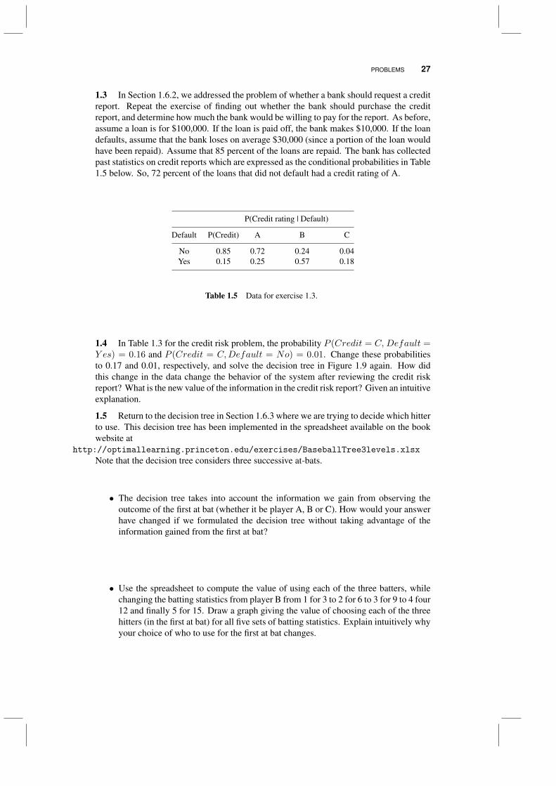
PROBLEMS 27
1.3 In Section 1.6.2, we addressed the problem of whether a bank should request a creditreport. Repeat the exercise of finding out whether the bank should purchase the creditreport, and determine how much the bank would be willing to pay for the report. As before,assume a loan is for $100,000. If the loan is paid off, the bank makes $10,000. If the loandefaults, assume that the bank loses on average $30,000 (since a portion of the loan wouldhave been repaid). Assume that 85 percent of the loans are repaid. The bank has collectedpast statistics on credit reports which are expressed as the conditional probabilities in Table1.5 below. So, 72 percent of the loans that did not default had a credit rating of A.
P(Credit rating | Default)
Default P(Credit) A B C
No 0.85 0.72 0.24 0.04Yes 0.15 0.25 0.57 0.18
Table 1.5 Data for exercise 1.3.
1.4 In Table 1.3 for the credit risk problem, the probability P (Credit = C, Default =Y es) = 0.16 and P (Credit = C,Default = No) = 0.01. Change these probabilitiesto 0.17 and 0.01, respectively, and solve the decision tree in Figure 1.9 again. How didthis change in the data change the behavior of the system after reviewing the credit riskreport? What is the new value of the information in the credit risk report? Given an intuitiveexplanation.
1.5 Return to the decision tree in Section 1.6.3 where we are trying to decide which hitterto use. This decision tree has been implemented in the spreadsheet available on the bookwebsite at
http://optimallearning.princeton.edu/exercises/BaseballTree3levels.xlsx
Note that the decision tree considers three successive at-bats.
• The decision tree takes into account the information we gain from observing theoutcome of the first at bat (whether it be player A, B or C). How would your answerhave changed if we formulated the decision tree without taking advantage of theinformation gained from the first at bat?
• Use the spreadsheet to compute the value of using each of the three batters, whilechanging the batting statistics from player B from 1 for 3 to 2 for 6 to 3 for 9 to 4 four12 and finally 5 for 15. Draw a graph giving the value of choosing each of the threehitters (in the first at bat) for all five sets of batting statistics. Explain intuitively whyyour choice of who to use for the first at bat changes.
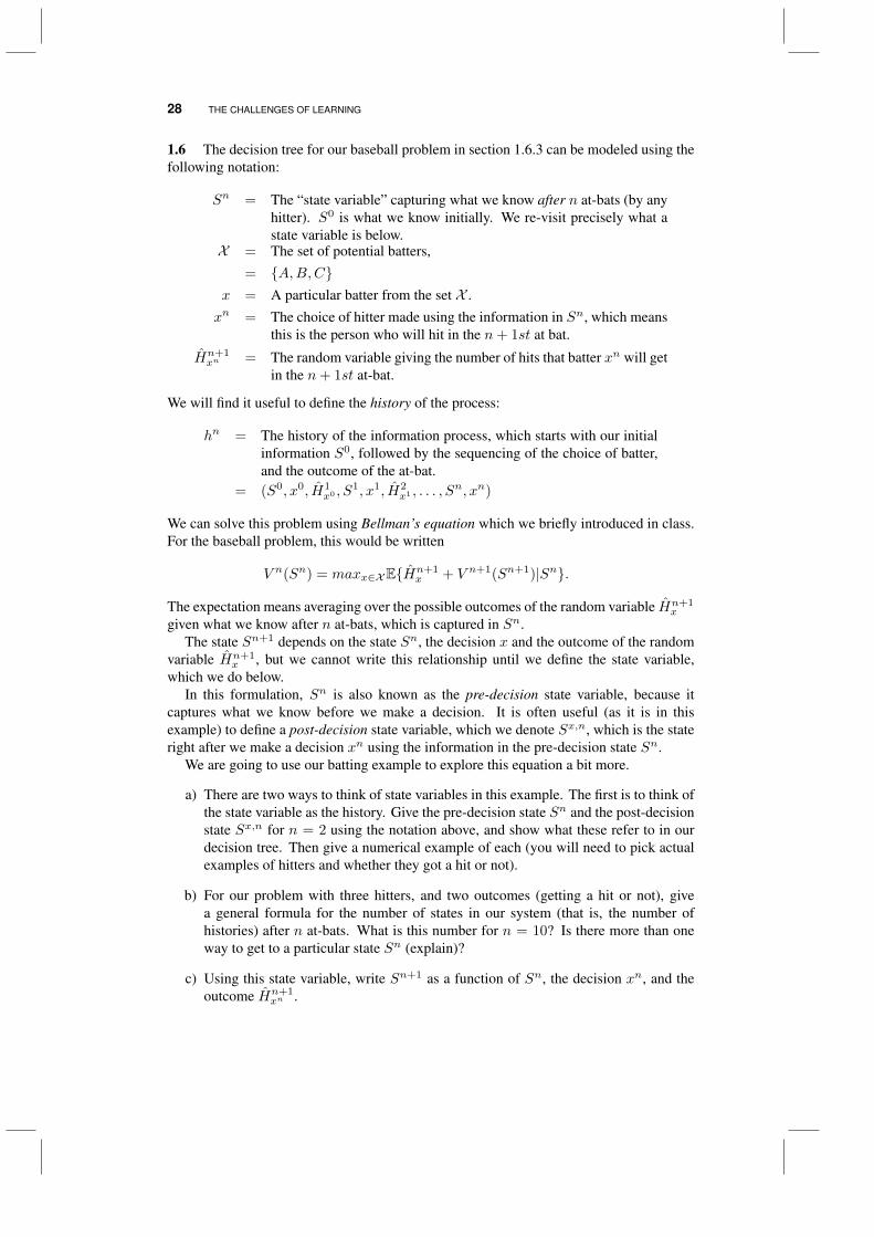
28 THE CHALLENGES OF LEARNING
1.6 The decision tree for our baseball problem in section 1.6.3 can be modeled using thefollowing notation:
Sn = The “state variable” capturing what we know after n at-bats (by anyhitter). S0 is what we know initially. We re-visit precisely what astate variable is below.
X = The set of potential batters,= A,B,C
x = A particular batter from the set X .xn = The choice of hitter made using the information in Sn, which means
this is the person who will hit in the n+ 1st at bat.
Hn+1xn = The random variable giving the number of hits that batter xn will get
in the n+ 1st at-bat.
We will find it useful to define the history of the process:
hn = The history of the information process, which starts with our initialinformation S0, followed by the sequencing of the choice of batter,and the outcome of the at-bat.
= (S0, x0, H1x0 , S1, x1, H2
x1 , . . . , Sn, xn)
We can solve this problem using Bellman’s equation which we briefly introduced in class.For the baseball problem, this would be written
V n(Sn) = maxx∈XEHn+1x + V n+1(Sn+1)|Sn.
The expectation means averaging over the possible outcomes of the random variable Hn+1x
given what we know after n at-bats, which is captured in Sn.The state Sn+1 depends on the state Sn, the decision x and the outcome of the random
variable Hn+1x , but we cannot write this relationship until we define the state variable,
which we do below.In this formulation, Sn is also known as the pre-decision state variable, because it
captures what we know before we make a decision. It is often useful (as it is in thisexample) to define a post-decision state variable, which we denote Sx,n, which is the stateright after we make a decision xn using the information in the pre-decision state Sn.
We are going to use our batting example to explore this equation a bit more.
a) There are two ways to think of state variables in this example. The first is to think ofthe state variable as the history. Give the pre-decision state Sn and the post-decisionstate Sx,n for n = 2 using the notation above, and show what these refer to in ourdecision tree. Then give a numerical example of each (you will need to pick actualexamples of hitters and whether they got a hit or not).
b) For our problem with three hitters, and two outcomes (getting a hit or not), givea general formula for the number of states in our system (that is, the number ofhistories) after n at-bats. What is this number for n = 10? Is there more than oneway to get to a particular state Sn (explain)?
c) Using this state variable, write Sn+1 as a function of Sn, the decision xn, and theoutcome Hn+1
xn .

PROBLEMS 29
d) A more compact way of describing our system is to define:
Hnx = The total number of hits made by batter x after n at-bats. Note that
we are given values for H0x before we start solving our problem.
Using this notation, give a different formulation of the state variable Sn (keep inmind that the state Sn has to capture what we know for all three batters). Show thatwe can calculate the probability that Hn+1
x equals 0 or 1 given just the informationin Sn.
e) Using this representation of the state variable, write Sn+1 as a function of Sn, thedecision xn, and the outcome Hn+1
xn .
f) Using this new state representation, give the size of the state space after n iterations.Is there more than one way to get to a state Sn? If so, give an example for n = 3 bygiving an example of a state, and different trajectories for getting to that state.

CHAPTER 2
ADAPTIVE LEARNING
At the heart of any learning problem is a belief model, which is some type of statisticalmodel that characterizes what we know about the behavior of our system. However, unlikethe usual statistical model which is just a point estimate, our belief models will alwaysinclude an explicit representation of the uncertainty in our model. Thus, if we have anestimate that driving a particular route is likely to take 25 minutes, our belief model willinclude a distribution about what the true mean might be. These beliefs will evolve as newinformation arrives, and our goal in this book is to acquire information that has the biggestimpact on the quality of our decisions.
There are two perspectives that we can take when forming a belief, known as thefrequentist view and the Bayesian view. In the frequentist view, we begin with no knowledgeat all about our parameters, and our beliefs are formed entirely by the results of experimentsthat we run. Since experiments are inherently noisy, we can repeat a series of experimentsand obtain different estimates of the parameters. If we repeat the experiments oftenenough, we can form a frequency distribution of any parameter that we estimate using theexperiments.
In the Bayesian view, we start with initial beliefs about parameters, known as the priordistribution, which is formed before we make any observations. After an experiment, wecombine the prior distribution with an experiment to form a posterior distribution. Thisthen becomes the next prior distribution. This distribution is our distribution of belief aboutthe true values of a set of parameters, formed from a combination of our initial beliefand subsequent observations. By contrast, in the frequentist view, we form a probabilitydistribution of estimates of parameters that reflect the variation in the observations.
Optimal Learning. By Warren B. Powell and Ilya O. RyzhovCopyright c© 2018 John Wiley & Sons, Inc.
31
32 ADAPTIVE LEARNING
We begin with an overview of major classes of belief models, including lookup table,parametric and nonparametric models.
2.1 BELIEF MODELS
At the heart of any learning problem is some sort of statistical model we refer to as thebelief model, which captures not only our estimate of how a function or system will respondto a controllable input x, but also the uncertainty in our estimate of the function.
We can represent our function or system as f(x). Often, this is a function of a controllableinput x (drug dosages, price of a product, concentration of a chemical), and a randomvariable W which covers any uncontrollable (we sometimes refer to these as exogenous)inputs. In principle, we might write
f(x) = EF (x,W ),
where the expectation E averages over all possible outcomes W .Most of the time in this book we are going to treat x as being a discrete choice. We can
write the set of choices as X = x1, x2, . . . , xM. These might be discrete choices (color,choice of material, choice of drug), or discretized values of a continuous parameter (price,length, dosage). If x is multidimensional, we might view X as a sample of possible valuesof x. However, we will occasionally address situations where x is continuous, either scalar,or a continuous vector.
Belief models can be described as coming in one of three flavors:
Lookup tables Assume that we have a discrete set of choices x ∈ X = x1, . . . , xMand let
µx = f(x) = EWF (x,W ).
A lookup table representation refers to an estimate µnx ≈ µx for each x ∈ X . So, ifM = 100, then we need to estimate 100 different parameters.
Parametric models There are settings where the set X can become quite large, as occurswhen x is multidimensional, or continuous. In such a setting, we might want to writeour belief model as
f(x|θ) ≈ EF (x,W )
=∑f∈F
θfφf (x), (2.1)
where φf (x), f ∈ F is a set of features. For example, x might be a choice of amovie, while φf (x) captures features such as genre. Now, instead of having a beliefµx for every movie x, we just have to estimate a vector of parameters (θf ), f ∈ Ffor a presumably small set of features. Equation (2.1) illustrates a linear model,which means it is linear in θ (the features φf (x) may be highly nonlinear in x). Wemay also need to use a nonlinear model such as
f(x|θ) =
1 If x < θmin
0 If θmin < x < θmax
-1 If x > θmax
THE FREQUENTIST VIEW 33
Another example might be a logistic function
f(x|θ) =eθ0+θ1x
1 + eθ0+θ1x.
Nonparametric models Nonparametric models allow us to create estimates without hav-ing to assume a functional form such as our linear model above, but the price ishigh. Imagine we have a set of observations (xn, fn), n = 1, . . . , N . We can createan approximation f(x) by using a local average around x, consisting of an averageof points fn with weights that are inversely proportional to the distance ‖x − xn‖.Nonparametric models are quite flexible, but can be hard to use, and as a result willnot play a major role in our treatment.
The remainder of this chapter will focus on methods for updating lookup table beliefmodels. For this setting, we are going to use Wn
x as the observation of our function f(x),which means that if we choose to evaluate the function at x = xn, then we are going toobserve
Wn+1xn = f(xn) + εn+1
= µxn + εn+1.
Below, we describe how to use frequentist and Bayesian statistics to produce estimates ofµx for each x.
2.2 THE FREQUENTIST VIEW
The frequentist view is arguably the approach that is most familiar to people with anintroductory course in statistics. Assume we are trying to estimate the mean µ of a randomvariable W which might be the performance of a device or policy. Let Wn be the nthsample observation. Also let µn be our estimate of µ, and σ2,n be our estimate of thevariance of W . We know from elementary statistics that we can write µn and σ2,n using
µn =1
n
n∑m=1
Wm (2.2)
σ2,n =1
n− 1
n∑m=1
(fm − µn)2. (2.3)
The estimate µn is a random variable (in the frequentist view) because it is computed fromother random variables, namely W 1,W 2, . . . ,Wn. Imagine if we had 100 people eachchoose a sample of n observations of W . We would obtain 100 different estimates of µn,reflecting the variation in our observations of W . The best estimate of the variance of theestimator µn is easily found to be
σ2,n =1
nσ2,n.
Note that as n→∞, σ2,n → 0, but σ2,n → σ2 where σ2 is the true variance of W . If σ2
is known, there would be no need to compute σ2,n and σ2,n would be given as above withσ2,n = σ2.
34 ADAPTIVE LEARNING
We can write these expressions recursively using
µn =
(1− 1
n
)µn−1 +
1
nWn, (2.4)
σ2,n =
1n (Wn − µn−1)2 n = 2,n−2n−1 σ
2,n−1 + 1n (Wn − µn−1)2 n > 2.
(2.5)
We will often speak of our belief state which captures what we know about the parameterswe are trying to estimate. Given our observations, we would write our belief state as
Bfreq,n = (µn, σ2,n, n).
Equations (2.4) and (2.5) describe how our belief state evolves over time.The belief state is supposed to communicate a probability distribution as opposed to
statistics such as mean and variance. When we are forming an average, we can applythe law of large numbers and assume that our estimate µn is approximately normallydistributed. This is true exactly ifW is normally distributed, but it is generally a very goodapproximation even when W is described by other distributions.
2.3 THE BAYESIAN VIEW
The Bayesian perspective casts a different interpretation on the statistics we compute whichis particularly useful in certain problem settings in optimal learning. While the frequentistperspective starts with no knowledge about a function or response (which is the case inmany settings), the Bayesian perspective leverages prior knowledge that comes from pastexperience or an understanding of the dynamics of a problem.
For example, let x be the price of a product, and let µx be the sales when we offer theproduct at a price x. With frequentist learning, we start knowing nothing about µx, but aswe collect data to construct estimates µnx ofmux, we may find that µnx does not necessarilydecline with x. In a Bayesian model, we would at least start with a prior µ0
x where this isthe case.
The biggest difference between Bayesian and frequentist learning is the Bayesian prior,which is the initial distribution of belief about the truth. The prior is how we are able tocommunicate domain knowledge, if this is available. A prior is critical in the context ofvirtually any problem where experiments are really expensive (such as laboratory or fieldexperiments), or when there is significant risk, as in health decisions.
The second difference between the two perspectives is the view of the truth. In theBayesian view, the truth µx is handled as a random variable. For example, we mightmodel µx as being normally distributed with mean µ0
x and variance σ2,0x . As we collect
information, this distribution changes, where we can guarantee that the variance will steadilyshrink. In the frequentist perspective, the truth is an unknown number, and our estimateof this number is a random variable that reflects the variation in our observations. Weunderstand, for example, that if 100 people all collected data to produce an estimate, eachof these 100 estimates would be different, and could be described by some distribution(often normal).
The Bayesian perspective is well suited to information collection in settings whereinformation is expensive (or where there is a significant risk involved if we make the wrongdecision). It is in these settings where there is the incentive to bring in prior knowledge, but
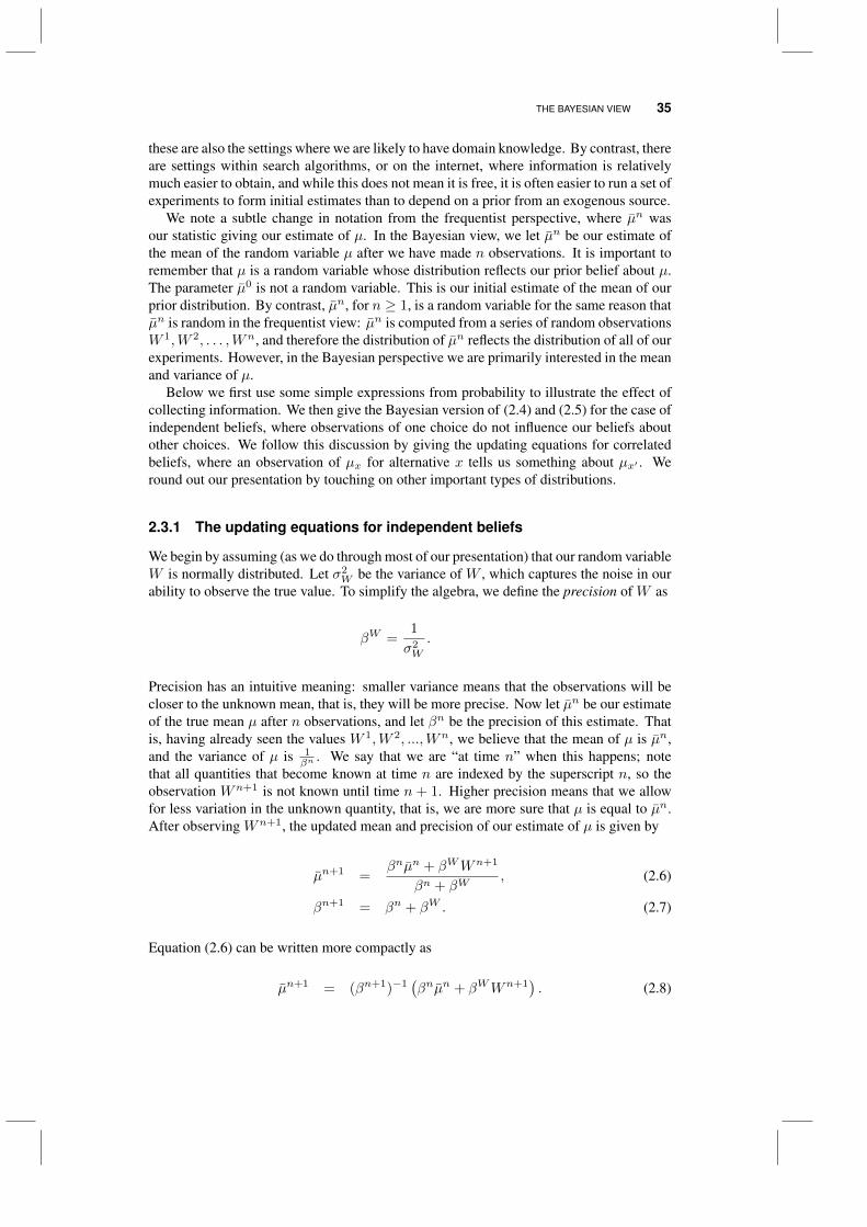
THE BAYESIAN VIEW 35
these are also the settings where we are likely to have domain knowledge. By contrast, thereare settings within search algorithms, or on the internet, where information is relativelymuch easier to obtain, and while this does not mean it is free, it is often easier to run a set ofexperiments to form initial estimates than to depend on a prior from an exogenous source.
We note a subtle change in notation from the frequentist perspective, where µn wasour statistic giving our estimate of µ. In the Bayesian view, we let µn be our estimate ofthe mean of the random variable µ after we have made n observations. It is important toremember that µ is a random variable whose distribution reflects our prior belief about µ.The parameter µ0 is not a random variable. This is our initial estimate of the mean of ourprior distribution. By contrast, µn, for n ≥ 1, is a random variable for the same reason thatµn is random in the frequentist view: µn is computed from a series of random observationsW 1,W 2, . . . ,Wn, and therefore the distribution of µn reflects the distribution of all of ourexperiments. However, in the Bayesian perspective we are primarily interested in the meanand variance of µ.
Below we first use some simple expressions from probability to illustrate the effect ofcollecting information. We then give the Bayesian version of (2.4) and (2.5) for the case ofindependent beliefs, where observations of one choice do not influence our beliefs aboutother choices. We follow this discussion by giving the updating equations for correlatedbeliefs, where an observation of µx for alternative x tells us something about µx′ . Weround out our presentation by touching on other important types of distributions.
2.3.1 The updating equations for independent beliefs
We begin by assuming (as we do through most of our presentation) that our random variableW is normally distributed. Let σ2
W be the variance of W , which captures the noise in ourability to observe the true value. To simplify the algebra, we define the precision of W as
βW =1
σ2W
.
Precision has an intuitive meaning: smaller variance means that the observations will becloser to the unknown mean, that is, they will be more precise. Now let µn be our estimateof the true mean µ after n observations, and let βn be the precision of this estimate. Thatis, having already seen the values W 1,W 2, ...,Wn, we believe that the mean of µ is µn,and the variance of µ is 1
βn . We say that we are “at time n” when this happens; notethat all quantities that become known at time n are indexed by the superscript n, so theobservation Wn+1 is not known until time n + 1. Higher precision means that we allowfor less variation in the unknown quantity, that is, we are more sure that µ is equal to µn.After observing Wn+1, the updated mean and precision of our estimate of µ is given by
µn+1 =βnµn + βWWn+1
βn + βW, (2.6)
βn+1 = βn + βW . (2.7)
Equation (2.6) can be written more compactly as
µn+1 = (βn+1)−1(βnµn + βWWn+1
). (2.8)
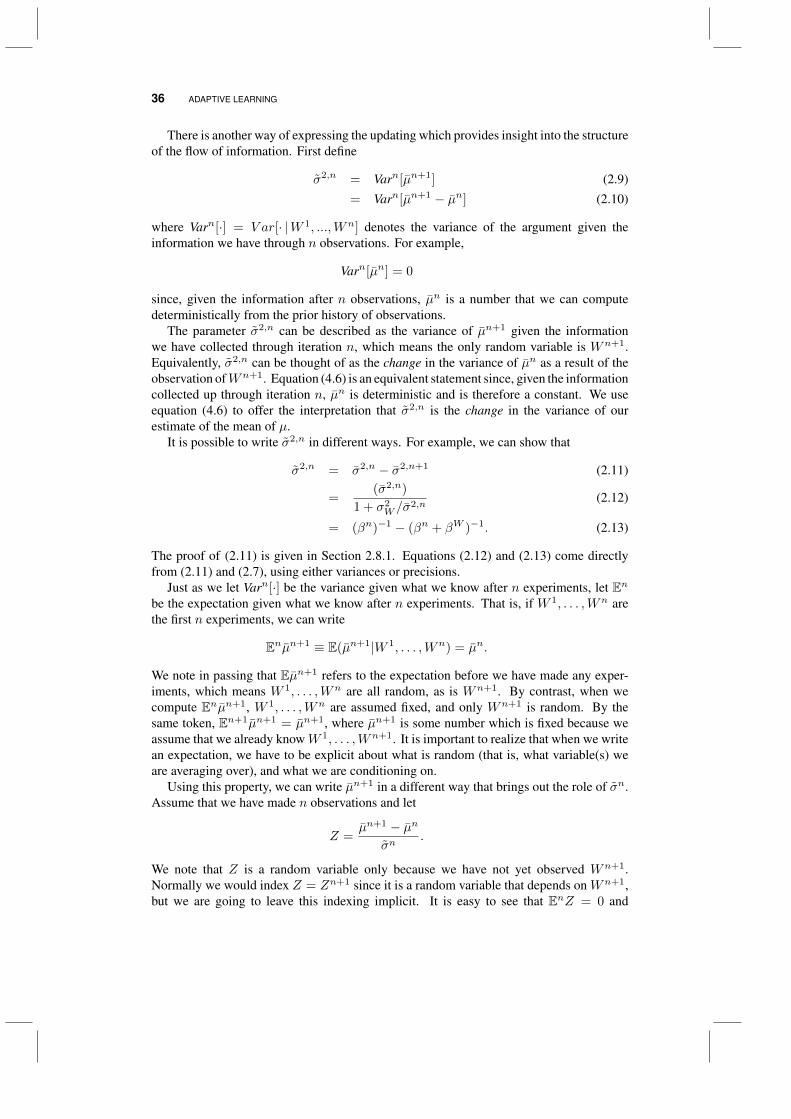
36 ADAPTIVE LEARNING
There is another way of expressing the updating which provides insight into the structureof the flow of information. First define
σ2,n = Varn[µn+1] (2.9)= Varn[µn+1 − µn] (2.10)
where Varn[·] = V ar[· |W 1, ...,Wn] denotes the variance of the argument given theinformation we have through n observations. For example,
Varn[µn] = 0
since, given the information after n observations, µn is a number that we can computedeterministically from the prior history of observations.
The parameter σ2,n can be described as the variance of µn+1 given the informationwe have collected through iteration n, which means the only random variable is Wn+1.Equivalently, σ2,n can be thought of as the change in the variance of µn as a result of theobservation ofWn+1. Equation (4.6) is an equivalent statement since, given the informationcollected up through iteration n, µn is deterministic and is therefore a constant. We useequation (4.6) to offer the interpretation that σ2,n is the change in the variance of ourestimate of the mean of µ.
It is possible to write σ2,n in different ways. For example, we can show that
σ2,n = σ2,n − σ2,n+1 (2.11)
=(σ2,n)
1 + σ2W /σ
2,n(2.12)
= (βn)−1 − (βn + βW )−1. (2.13)
The proof of (2.11) is given in Section 2.8.1. Equations (2.12) and (2.13) come directlyfrom (2.11) and (2.7), using either variances or precisions.
Just as we let Varn[·] be the variance given what we know after n experiments, let Enbe the expectation given what we know after n experiments. That is, if W 1, . . . ,Wn arethe first n experiments, we can write
Enµn+1 ≡ E(µn+1|W 1, . . . ,Wn) = µn.
We note in passing that Eµn+1 refers to the expectation before we have made any exper-iments, which means W 1, . . . ,Wn are all random, as is Wn+1. By contrast, when wecompute Enµn+1, W 1, . . . ,Wn are assumed fixed, and only Wn+1 is random. By thesame token, En+1µn+1 = µn+1, where µn+1 is some number which is fixed because weassume that we already knowW 1, . . . ,Wn+1. It is important to realize that when we writean expectation, we have to be explicit about what is random (that is, what variable(s) weare averaging over), and what we are conditioning on.
Using this property, we can write µn+1 in a different way that brings out the role of σn.Assume that we have made n observations and let
Z =µn+1 − µn
σn.
We note that Z is a random variable only because we have not yet observed Wn+1.Normally we would index Z = Zn+1 since it is a random variable that depends on Wn+1,but we are going to leave this indexing implicit. It is easy to see that EnZ = 0 and
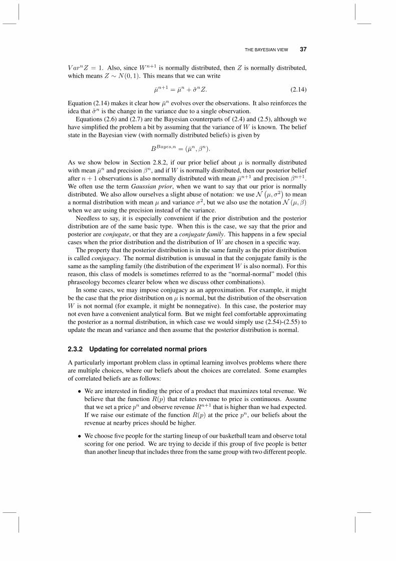
THE BAYESIAN VIEW 37
V arnZ = 1. Also, since Wn+1 is normally distributed, then Z is normally distributed,which means Z ∼ N(0, 1). This means that we can write
µn+1 = µn + σnZ. (2.14)
Equation (2.14) makes it clear how µn evolves over the observations. It also reinforces theidea that σn is the change in the variance due to a single observation.
Equations (2.6) and (2.7) are the Bayesian counterparts of (2.4) and (2.5), although wehave simplified the problem a bit by assuming that the variance of W is known. The beliefstate in the Bayesian view (with normally distributed beliefs) is given by
BBayes,n = (µn, βn).
As we show below in Section 2.8.2, if our prior belief about µ is normally distributedwith mean µn and precision βn, and if W is normally distributed, then our posterior beliefafter n+ 1 observations is also normally distributed with mean µn+1 and precision βn+1.We often use the term Gaussian prior, when we want to say that our prior is normallydistributed. We also allow ourselves a slight abuse of notation: we use N
(µ, σ2
)to mean
a normal distribution with mean µ and variance σ2, but we also use the notation N (µ, β)when we are using the precision instead of the variance.
Needless to say, it is especially convenient if the prior distribution and the posteriordistribution are of the same basic type. When this is the case, we say that the prior andposterior are conjugate, or that they are a conjugate family. This happens in a few specialcases when the prior distribution and the distribution of W are chosen in a specific way.
The property that the posterior distribution is in the same family as the prior distributionis called conjugacy. The normal distribution is unusual in that the conjugate family is thesame as the sampling family (the distribution of the experimentW is also normal). For thisreason, this class of models is sometimes referred to as the “normal-normal” model (thisphraseology becomes clearer below when we discuss other combinations).
In some cases, we may impose conjugacy as an approximation. For example, it mightbe the case that the prior distribution on µ is normal, but the distribution of the observationW is not normal (for example, it might be nonnegative). In this case, the posterior maynot even have a convenient analytical form. But we might feel comfortable approximatingthe posterior as a normal distribution, in which case we would simply use (2.54)-(2.55) toupdate the mean and variance and then assume that the posterior distribution is normal.
2.3.2 Updating for correlated normal priors
A particularly important problem class in optimal learning involves problems where thereare multiple choices, where our beliefs about the choices are correlated. Some examplesof correlated beliefs are as follows:
• We are interested in finding the price of a product that maximizes total revenue. Webelieve that the function R(p) that relates revenue to price is continuous. Assumethat we set a price pn and observe revenueRn+1 that is higher than we had expected.If we raise our estimate of the function R(p) at the price pn, our beliefs about therevenue at nearby prices should be higher.
• We choose five people for the starting lineup of our basketball team and observe totalscoring for one period. We are trying to decide if this group of five people is betterthan another lineup that includes three from the same group with two different people.
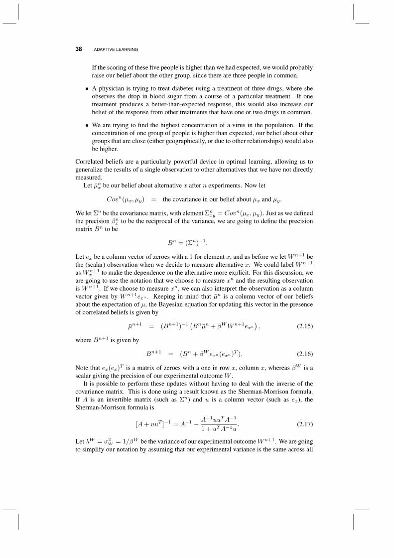
38 ADAPTIVE LEARNING
If the scoring of these five people is higher than we had expected, we would probablyraise our belief about the other group, since there are three people in common.
• A physician is trying to treat diabetes using a treatment of three drugs, where sheobserves the drop in blood sugar from a course of a particular treatment. If onetreatment produces a better-than-expected response, this would also increase ourbelief of the response from other treatments that have one or two drugs in common.
• We are trying to find the highest concentration of a virus in the population. If theconcentration of one group of people is higher than expected, our belief about othergroups that are close (either geographically, or due to other relationships) would alsobe higher.
Correlated beliefs are a particularly powerful device in optimal learning, allowing us togeneralize the results of a single observation to other alternatives that we have not directlymeasured.
Let µnx be our belief about alternative x after n experiments. Now let
Covn(µx, µy) = the covariance in our belief about µx and µy .
We let Σn be the covariance matrix, with element Σnxy = Covn(µx, µy). Just as we definedthe precision βnx to be the reciprocal of the variance, we are going to define the precisionmatrix Bn to be
Bn = (Σn)−1.
Let ex be a column vector of zeroes with a 1 for element x, and as before we let Wn+1 bethe (scalar) observation when we decide to measure alternative x. We could label Wn+1
as Wn+1x to make the dependence on the alternative more explicit. For this discussion, we
are going to use the notation that we choose to measure xn and the resulting observationis Wn+1. If we choose to measure xn, we can also interpret the observation as a columnvector given by Wn+1exn . Keeping in mind that µn is a column vector of our beliefsabout the expectation of µ, the Bayesian equation for updating this vector in the presenceof correlated beliefs is given by
µn+1 = (Bn+1)−1(Bnµn + βWWn+1exn
), (2.15)
where Bn+1 is given by
Bn+1 = (Bn + βW exn(exn)T ). (2.16)
Note that ex(ex)T is a matrix of zeroes with a one in row x, column x, whereas βW is ascalar giving the precision of our experimental outcome W .
It is possible to perform these updates without having to deal with the inverse of thecovariance matrix. This is done using a result known as the Sherman-Morrison formula.If A is an invertible matrix (such as Σn) and u is a column vector (such as ex), theSherman-Morrison formula is
[A+ uuT ]−1 = A−1 − A−1uuTA−1
1 + uTA−1u. (2.17)
Let λW = σ2W = 1/βW be the variance of our experimental outcomeWn+1. We are going
to simplify our notation by assuming that our experimental variance is the same across all
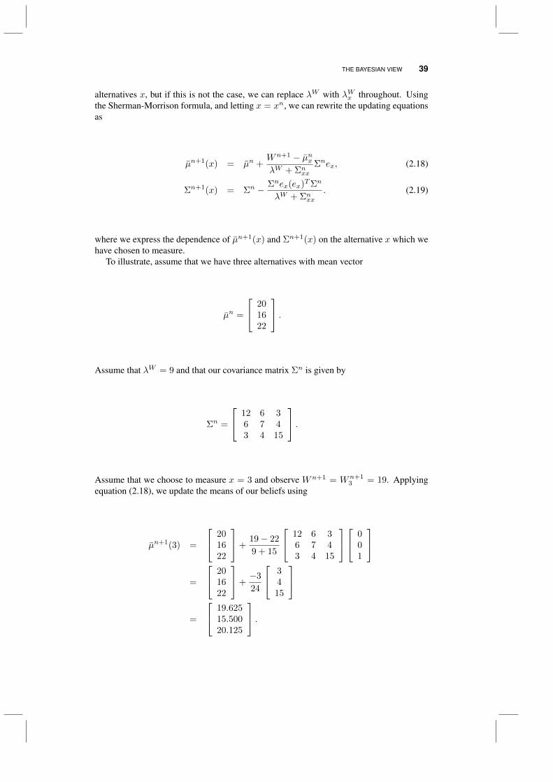
THE BAYESIAN VIEW 39
alternatives x, but if this is not the case, we can replace λW with λWx throughout. Usingthe Sherman-Morrison formula, and letting x = xn, we can rewrite the updating equationsas
µn+1(x) = µn +Wn+1 − µnxλW + Σnxx
Σnex, (2.18)
Σn+1(x) = Σn − Σnex(ex)TΣn
λW + Σnxx. (2.19)
where we express the dependence of µn+1(x) and Σn+1(x) on the alternative x which wehave chosen to measure.
To illustrate, assume that we have three alternatives with mean vector
µn =
201622
.
Assume that λW = 9 and that our covariance matrix Σn is given by
Σn =
12 6 36 7 43 4 15
.
Assume that we choose to measure x = 3 and observe Wn+1 = Wn+13 = 19. Applying
equation (2.18), we update the means of our beliefs using
µn+1(3) =
201622
+19− 22
9 + 15
12 6 36 7 43 4 15
001
=
201622
+−3
24
3415
=
19.62515.50020.125
.
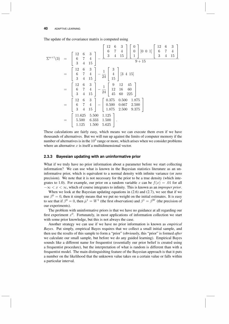
40 ADAPTIVE LEARNING
The update of the covariance matrix is computed using
Σn+1(3) =
12 6 36 7 43 4 15
− 12 6 3
6 7 43 4 15
001
[0 0 1]
12 6 36 7 43 4 15
9 + 15
=
12 6 36 7 43 4 15
− 1
24
3415
[3 4 15]
=
12 6 36 7 43 4 15
− 1
24
9 12 4512 16 6045 60 225
=
12 6 36 7 43 4 15
− 0.375 0.500 1.875
0.500 0.667 2.5001.875 2.500 9.375
=
11.625 5.500 1.1255.500 6.333 1.5001.125 1.500 5.625
.These calculations are fairly easy, which means we can execute them even if we havethousands of alternatives. But we will run up against the limits of computer memory if thenumber of alternatives is in the 105 range or more, which arises when we consider problemswhere an alternative x is itself a multidimensional vector.
2.3.3 Bayesian updating with an uninformative prior
What if we truly have no prior information about a parameter before we start collectinginformation? We can use what is known in the Bayesian statistics literature as an un-informative prior, which is equivalent to a normal density with infinite variance (or zeroprecision). We note that it is not necessary for the prior to be a true density (which inte-grates to 1.0). For example, our prior on a random variable x can be f(x) = .01 for all−∞ < x <∞, which of course integrates to infinity. This is known as an improper prior.
When we look at the Bayesian updating equations in (2.6) and (2.7), we see that if weuse β0 = 0, then it simply means that we put no weight on the initial estimates. It is easyto see that if β0 = 0, then µ1 = W 1 (the first observation) and β1 = βW (the precision ofour experiments).
The problem with uninformative priors is that we have no guidance at all regarding ourfirst experiment x0. Fortunately, in most applications of information collection we startwith some prior knowledge, but this is not always the case.
Another strategy we can use if we have no prior information is known as empiricalBayes. Put simply, empirical Bayes requires that we collect a small initial sample, andthen use the results of this sample to form a “prior” (obviously, this “prior” is formed afterwe calculate our small sample, but before we do any guided learning). Empirical Bayessounds like a different name for frequentist (essentially our prior belief is created usinga frequentist procedure), but the interpretation of what is random is different than with afrequentist model. The main distinguishing feature of the Bayesian approach is that it putsa number on the likelihood that the unknown value takes on a certain value or falls withina particular interval.
BAYESIAN UPDATING FOR SAMPLED NONLINEAR MODELS 41
2.4 BAYESIAN UPDATING FOR SAMPLED NONLINEAR MODELS
There will be many instances where we need to work with models that are nonlinear in theparameter vector θ. Some examples are
EXAMPLE 2.1
Pricing a product on the internet - Imagine that we set a price xn for day n and thenobserve total revenue Yt. We might model the demand for the product using
D(x|θ) = θ1e−θ2(x−θ3).
The revenue would then be given by f(x|θ) = xD(x|θ). We might set a pricexn for day x and then observe revenue Y n. After N days, we have a dataset(Y n, xn), n = 1, . . . , N .
EXAMPLE 2.2
Assume a physical has to choose from a set of treatments X = x1, . . . , xM forreducing blood sugar. We are interested in estimating the probability that a treatmentx will be judged a success.
We might begin by constructing a utility function that captures the attractiveness ofthe product as a function of price p, which we might write as
U(x|θ) = θ0 +
M∑m=1
θm1x=xm .
where
1x=xm =
1 If x = xm
0 Otherwise.
Now assume that we model the probability of the treatment x being effective is givenby
P (x) =eU(x|θ)
1 + eU(x|θ) .
Normally the estimation of nonlinear models can become quite complex, but we aregoing to use a technique known as a sampled belief model. We assume that we aregiven a nonlinear function f(x|θ) where x is the input (in our examples this was eithera price or medical treatment), and then we observe a response Y . We then assumethat θ is one of the set Θ = θ1, . . . , θK, initially with probability P [θ = θk] = p0
k.We refer to p0 = (p0
k), k = 1, . . . ,K as the prior.
The next step is to design the updating equations for the probability vector pn afterrunning an experiment with x = xn and observing a response yn+1. We start withBayes theorem
P(A|B) =P(B|A)P(A)
P(B).

42 ADAPTIVE LEARNING
Now interpret the event A as the event that θ = θk, and B as the new informationyn+1. We are going to let Hn be the history of our experiments where
Hn = (S0, x0, y1, x1, y2, . . . , xn−1, yn).
We can write our belief probabilities as
pnk = P[θ = θk|Hn].
We note that we can write Bayes’ theorem where all of the probabilities are condi-tioned on a third event C, as in
P(A|B,C) =P(B|A,C)P(A|C)
P(B|C).
In our setting, the new event C is our history Hn. Adapting this to our setting givesus
P[θ = θk|yn+1 = y,Hn] =P[yn+1 = y|θk, Hn]P[θ = θk|Hn]
P[yn+1 = y|Hn]. (2.20)
Let fy(y = y|θ) be the distribution of the random observation y given θ, or
fy(y = y|θ) = P[y = y|θ].
The conditioning on the historyHn affects the probability that θ takes on a particularvalue. We can rewrite equation (2.20) as
pn+1k =
fy(yn+1 = y|θk)pnkfy(yn+1 = y)
(2.21)
where
fy(yn+1 = y) =
K∑k=1
fy(yn+1 = y|θk)pnk . (2.22)
We are exploiting the fact that the distribution of yn+1 depends only on θ, so we candrop the dependence on Hn when we are also conditioning on θ, since the historyonly affects the probabilities pnk .
We again note that we assume that fy(yn+1|θk) is a known distribution that can beeasily computed from the structure of the problem. For example, it might be a normaldensity, a Poisson distribution, or a logistic regression.
Equation 2.21 is quite easy to compute (given fy(yn+1|θk)) when we use a sampledbelief model. Without the sampled belief model, the expectation in equation (2.22)can become quite complex (imagine what happens when θ is a vector). By contrast,this equation is easy to compute for the sampled belief model, even if θ is a high-dimensional vector.
The process is illustrated in figure 2.1 for a problem where we are trying to showthe market response to the price using a logistics curve. The figure shows (a) theinitial, uniform prior of a sampled belief model with four possible values of θ, (b) thepossible outcomes from an experiment x, (c) the actual result of an experiment, and(d) the posterior distribution which are indicated by the thickness of the lines.
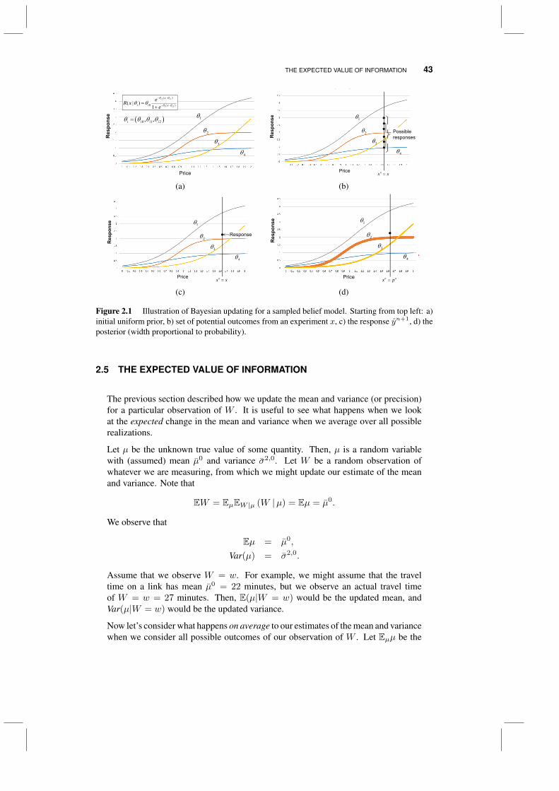
THE EXPECTED VALUE OF INFORMATION 43
1
2
3
4
Price
Res
pons
e
1 2
1 2
( )
0 ( )( | )1
i i
i
x
i i x
eR xe
0 1 2, ,i i i i
nx x
1
2
3
4
PossibleresponsesR
espo
nse
Price
(a) (b)
1
2
3
4
Response
Res
pons
e
nx xPrice n nx p
1
2
3
4
Res
pons
e
Price
(c) (d)
Figure 2.1 Illustration of Bayesian updating for a sampled belief model. Starting from top left: a)initial uniform prior, b) set of potential outcomes from an experiment x, c) the response yn+1, d) theposterior (width proportional to probability).
2.5 THE EXPECTED VALUE OF INFORMATION
The previous section described how we update the mean and variance (or precision)for a particular observation of W . It is useful to see what happens when we lookat the expected change in the mean and variance when we average over all possiblerealizations.
Let µ be the unknown true value of some quantity. Then, µ is a random variablewith (assumed) mean µ0 and variance σ2,0. Let W be a random observation ofwhatever we are measuring, from which we might update our estimate of the meanand variance. Note that
EW = EµEW |µ (W |µ) = Eµ = µ0.
We observe that
Eµ = µ0,
Var(µ) = σ2,0.
Assume that we observe W = w. For example, we might assume that the traveltime on a link has mean µ0 = 22 minutes, but we observe an actual travel timeof W = w = 27 minutes. Then, E(µ|W = w) would be the updated mean, andVar(µ|W = w) would be the updated variance.
Now let’s consider what happens on average to our estimates of the mean and variancewhen we consider all possible outcomes of our observation of W . Let Eµµ be the
44 ADAPTIVE LEARNING
expected value of µ (over our density function for µ), which is equal to µ0. Nowlet Eµ(µ|W ) be the expected value of µ given a particular observation of W . Theexpectation Eµ(µ|W ) is a random variable (since it depends on W ), but we areinterested in its expectation over all possible values of W , which we can write asEWEµ(µ|W ). We can compute this by taking expectations of equation (2.8) givenwhat we know at iteration n (which means that only Wn+1 is random). We start byobserving that
Eµ(µ|W ) = µ1 = (β1)−1(β0µn + βWW
),
where β1 = β0 + βW . We then take expectations of both sides over the randomobservation W to obtain
EW µ1 = EW((β1)−1
(β0µ0 + βWW
))= (β1)−1
(β0µ0 + βWEW
)= (β1)−1
(β0µ0 + βW µ0
)= (β1)−1
(β0 + βW
)µ0
= µ0.
This result seems to be saying that collecting an observation of W does not changeour belief of the true mean µ. This is not the case. As we saw in the previous section,a particular observation of W will, in fact, change our belief about the mean of µ.But if we look at all possible realizations of W , before the observation occurs, onaverage our estimate of the mean does not change.
This simple equation provides an insight into priors and learning. Imagine if
Eµ = EWEµ(µ|W ) = µ0 + a.
That is, observing W will, on average, shift our belief about the true mean from µ0
to µ0 + a, where a is a constant which would have to be known before we run ourexperiment. If this were true (for a other than zero), then this would mean that ourinitial estimate µ0 is not a true prior. That is, we could shift our prior by a so that itbecomes an unbiased estimate of the mean.
Now consider what happens to the variance after an experiment. We use some basicrelationships from probability to obtain
Var(µ) = Eµ(µ2)− (Eµ(µ))2 (2.23)
= Eµ(µ2)− (Eµ(µ))2 + (Eµ(µ))2 − (Eµ(µ))2 (2.24)
= EW [(Eµ(µ2|W ))]− EW [(Eµ(µ|W ))2] + EW [(Eµ(µ|W ))2]− (EW [Eµ(µ|W )])2
(2.25)
= EW [(Eµ(µ2|W ))− (Eµ(µ|W ))2] + EW [(Eµ(µ|W ))2]− (EW [Eµ(µ|W )])2
(2.26)
= EW [Var(µ|W )] + Var[Eµ(µ|W )]. (2.27)
Equation (2.23) is the definition of the variance. In (2.24), we add and subtract(Eµ(µ|W ))2. In (2.25), we then condition throughout on W and then take theexpectation overW . In (2.26), we pull the EW out front of the first two terms, settingup the final (and classic) result given by equation (2.28). Our interest is primarily in

UPDATING FOR NON-GAUSSIAN PRIORS 45
equation (2.26). Above, we pointed out that EWEµ(µ|W ) = Eµµ. This is not thecase with the variance, where equation (2.28) tells us that
EW [Var(µ|W )] = Var(µ)− Var[Eµ(µ|W )]. (2.28)
This means that the variance after an experiment will, on average, always be smallerthan the original variance. Of course, it might be the case that Var[Eµ(µ|W )] = 0.This would happen if W were an irrelevant piece of information. For example,assume that µ is our estimate of the travel time on a path in a network, and W isan observation of the change in the S&P stock index yesterday. The S&P stockindex does not tell us anything about the travel time on the path, which means thatEµ(µ|W ) is a constant (in our example, it would be µ0). Clearly, Var(µ0) = 0, sinceµ0 is not a random variable (it is just a number).
We collect observations one at a time. So, the above discussion continues to applyafter we observe W 1,W 2, ...,Wn. Since the posterior mean µn is a known, fixedquantity at time n, we can simply view it as a new prior. Our problem essentiallyrestarts after each observation, just with different parameters for our distribution ofbelief. The advantage of recursive updating is that it allows us to turn a problemwith a long-time horizon into a sequence of small problems – a concept that will alsoinform our solution techniques in later chapters.
2.6 UPDATING FOR NON-GAUSSIAN PRIORS
So far, we have considered a setting where the random observationsWn are assumedto come from a normal distribution, whose mean is the true value that we wish toestimate. We have also used a normal distribution to describe our prior belief aboutthe unknown value. These are two very different normal distributions, and it isimportant to distinguish between them. We use the term “sampling distribution” torefer to the distribution of the observationsWn. This distribution depends on certainunknown parameters, like the value µ in the preceding section. Although we do notknow this distribution, we have a way of obtaining samples from it.
By contrast, the term “prior distribution” describes the distribution of our own beliefsabout the unknown parameters of the sampling distribution. Unlike the samplingdistribution, which is determined by nature and unknown to us, the prior distributionis something that we construct to encode our own uncertainty about the truth. Theprior distribution changes as we accumulate observations, reflecting the changesin our beliefs and the reduction in our uncertainty that result from collecting newinformation.
In the preceding section, both the sampling distribution and the prior distribution areassumed to be normal. This model is particularly intuitive and versatile because theunknown parameter in the sampling distribution is precisely the mean of the sampledobservations. The mean µ0 of the prior distribution can easily be interpreted as our“best guess” as to the unknown value, with σ0 representing our uncertainty. Thus,whenever we have a rough idea of what the unknown mean might be, a normaldistribution provides a very intuitive and understandable way to encode that idea ina mathematical model.
46 ADAPTIVE LEARNING
Unfortunately, the normal-normal model (normal prior, normal samples) is not alwayssuitable. For one thing, a normal sampling distribution assumes that our randomobservations can take on any real value. In reality, this might not be the case: forinstance, we might be observing the waiting times of customers in a service center,where we are trying to estimate the service rate. Waiting times are always positive,so an exponential distribution would seem to be a more appropriate choice than anormal distribution. Even more troubling is a situation where our observations areobviously discrete. For instance, we might be observing the success or failure of amedical test, where the outcome is 0 or 1. A normal distribution is certainly a poorchoice for a sampling model in this setting.
The normal distribution is not always the best choice for a prior, either. For example,if we are observing exponentially distributed service times, the service rate is neces-sarily a strictly positive number. If we were to put a normal prior on the service rate,then even with a positive prior mean, we would essentially be allowing the possibilitythat our exponential sampling distribution has a negative rate, which is impossible.Our uncertainty about the service rate should be encoded using a different kind ofdistribution that accounts for the fact that the rate must be positive. In the case of0/1 observations (success or failure of a test), the sample mean is the probability ofsuccess. We know that this number must be between 0 and 1, so a normal distributionis again not the best choice to represent our beliefs.
In this section, we discuss several other possible learning models where the samplingand prior distributions are not normal. However, all the distributions that we considerwill retain the conjugacy property, which means that the posterior distribution is ofthe same type as the prior distribution.
2.6.1 The gamma-exponential model
The gamma-exponential model is one possible choice for a situation where theobservations are continuous and positive. Suppose that we are trying to estimatethe service time distribution at a car repair shop by combining our prior belief withobservations of actual service times. We feel comfortable assuming that the samplingdistribution governing the service times is exponential with parameter λ. The servicerate is the unknown value that we wish to estimate.
Sinceλ is itself unknown, we view it as a random variable. Clearly it is not appropriateto assume that it follows a normal distribution, since this would mean that we believethat λ might be negative. Assume instead that λ comes from a gamma distributionwith parameters a and b. This distribution is given by
f(x|a, b) = b(bx)a−1 e−bx
Γ(a)
where a is typically an integer (as it will be for our applications) and Γ(a) = (a−1)!.Figure 2.2 illustrates several examples of the gamma density. If a = 1, the gamma isan exponential distribution. For a > 1, it takes on a skewed shape which approachesa normal distribution for larger values of a.
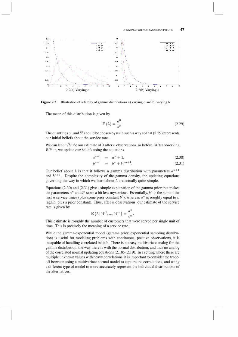
UPDATING FOR NON-GAUSSIAN PRIORS 47
2.2(a) Varying a 2.2(b) Varying b
Figure 2.2 Illustration of a family of gamma distributions a) varying a and b) varying b.
The mean of this distribution is given by
E (λ) =a0
b0. (2.29)
The quantities a0 and b0 should be chosen by us in such a way so that (2.29) representsour initial beliefs about the service rate.
We can let an/bn be our estimate of λ after n observations, as before. After observingWn+1, we update our beliefs using the equations
an+1 = an + 1, (2.30)bn+1 = bn +Wn+1. (2.31)
Our belief about λ is that it follows a gamma distribution with parameters an+1
and bn+1. Despite the complexity of the gamma density, the updating equationsgoverning the way in which we learn about λ are actually quite simple.
Equations (2.30) and (2.31) give a simple explanation of the gamma prior that makesthe parameters an and bn seem a bit less mysterious. Essentially, bn is the sum of thefirst n service times (plus some prior constant b0), whereas an is roughly equal to n(again, plus a prior constant). Thus, after n observations, our estimate of the servicerate is given by
E(λ |W 1, ...,Wn
)=an
bn.
This estimate is roughly the number of customers that were served per single unit oftime. This is precisely the meaning of a service rate.
While the gamma-exponential model (gamma prior, exponential sampling distribu-tion) is useful for modeling problems with continuous, positive observations, it isincapable of handling correlated beliefs. There is no easy multivariate analog for thegamma distribution, the way there is with the normal distribution, and thus no analogof the correlated normal updating equations (2.18)-(2.19). In a setting where there aremultiple unknown values with heavy correlations, it is important to consider the trade-off between using a multivariate normal model to capture the correlations, and usinga different type of model to more accurately represent the individual distributions ofthe alternatives.
48 ADAPTIVE LEARNING
2.6.2 The gamma-Poisson model
The gamma-Poisson model is similar to the gamma-exponential model, but the ob-servations are now assumed to be discrete. For example, we may now be interestedin the arrival rate of customers to the car repair shop, rather than the service time.Suppose that the total number of customers N that visit the shop in a single dayfollows a Poisson distribution with rate λ customers per day. Our observations arenow the actual numbers of customers that arrive on different days. If the arrival rateis λ, the distribution of N follows the Poisson distribution given by
P[N = x] =λxe−λ
x!,
where x = 0, 1, . . .. The problem is that we do not know λ, and we wish to estimateit from observationsNn whereNn is the observed number of arrivals on the nth day.
Once again, we assume that λ comes from a gamma distribution with parametersa0 and b0. The prior distribution changes after each observation according to theequations
an+1 = an +Nn+1, (2.32)bn+1 = bn + 1. (2.33)
After n observations, our estimate of the Poisson rate,
E(λ |W 1, ...,Wn
)=an
bn,
is roughly equal to the average number of customers that arrived per day. This is inline with the meaning of the Poisson rate.
The gamma-Poisson case highlights the distinction between the sampling distributionand the prior. While the individual Poisson observations are discrete, the Poissonrate itself can be any positive real number, and thus can be modeled using the gammadistribution.
2.6.3 The Pareto-uniform model
Suppose thatW is uniform on the interval [0, B], whereB is unknown. Our problemis thus to estimate the maximum of a uniform distribution. This problem is thecontinuous version of a production estimation problem, in which we can observea sequence of serial numbers, and the goal is to guess the highest serial numberproduced. We can also use this model to estimate the maximum possible demand fora product or other extreme values.
We assume thatB comes from a Pareto distribution with parameters b > 0 andα > 1.The density of this distribution is given by
f (x|α, b) =
αbα
xα+1 if x > b0 otherwise.
UPDATING FOR NON-GAUSSIAN PRIORS 49
Thus, our prior estimate of B using priors α = α0 and b = b0 is given by
E (B) =α0b0
α0 − 1.
The parameter b0 estimates the α0−1α0 -quantile of the uniform distribution, and α0
gives us the multiplier used to obtain the estimate of the maximum.
Although this model looks somewhat peculiar, it also has the conjugacy property.Our beliefs continue to have a Pareto distribution as we make observations, and theparameters of the distribution evolve according to the equations
bn+1 = max(bn,Wn+1
), (2.34)
αn+1 = αn + 1. (2.35)
Thus, bn is roughly the maximum of the first n uniform observations. Our beliefstell us that the true maximum of the distribution must be larger than bn. However, ifwe have made many observations, it is likely that bn is fairly close to the maximum.The degree of this “closeness” is represented by αn.
2.6.4 Models for learning probabilities*
In many problems, our objective is to learn the probability that a certain event willoccur, rather than the economic value of the event. For example, in a medicalsetting, our observations might simply be whether or not a certain medical treatmentis successful. Such an observation can be modeled as a Bernoulli random variable,which is equal to 1 (success) with probability ρ, and 0 (failure) with probability 1−ρ.The success probability ρ is the unknown true value in this case.
We assume that ρ comes from a beta distribution with parameters α and β. Recallthat the beta density is given by
f (x|α, β) =
Γ(α+β)
Γ(α)Γ(β)xα−1 (1− x)
β−1 if 0 < x < 1
0 otherwise.
As before, Γ(y) = y! when y is integer. In this setting, α and β are always integer.Figure 2.3 illustrates the beta distribution for different values of α and β.
Our prior estimate of ρ using α = α0 and β = β0 is given by
E (ρ) =α0
α0 + β0. (2.36)
Thus, α0 and β0 are weights that, when normalized, give us the probabilities ofsuccess and failure, respectively. If α0 is large relative to β0, this means that webelieve success to be more likely than failure.
A common trait of all the learning models we have discussed thus far is that, whilethe prior or sampling distributions can have fairly complicated densities, the resultingupdating equations are simple and often have an intuitive meaning. This is also the
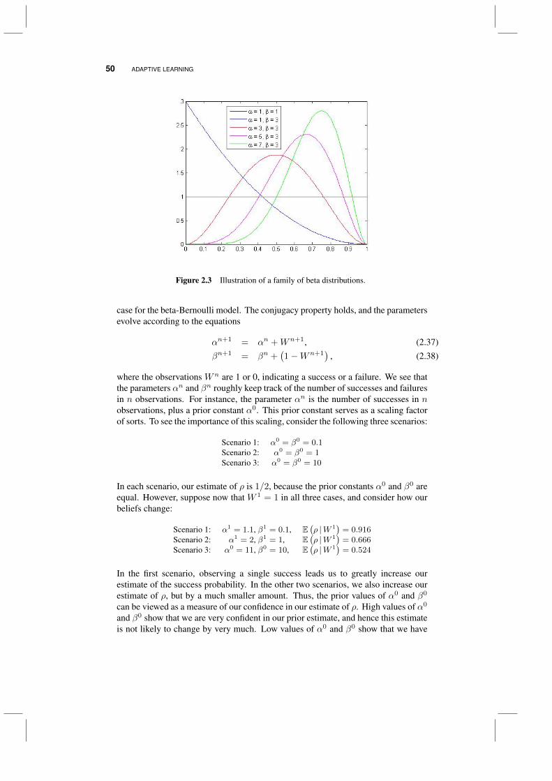
50 ADAPTIVE LEARNING
Figure 2.3 Illustration of a family of beta distributions.
case for the beta-Bernoulli model. The conjugacy property holds, and the parametersevolve according to the equations
αn+1 = αn +Wn+1, (2.37)βn+1 = βn +
(1−Wn+1
), (2.38)
where the observations Wn are 1 or 0, indicating a success or a failure. We see thatthe parameters αn and βn roughly keep track of the number of successes and failuresin n observations. For instance, the parameter αn is the number of successes in nobservations, plus a prior constant α0. This prior constant serves as a scaling factorof sorts. To see the importance of this scaling, consider the following three scenarios:
Scenario 1: α0 = β0 = 0.1Scenario 2: α0 = β0 = 1Scenario 3: α0 = β0 = 10
In each scenario, our estimate of ρ is 1/2, because the prior constants α0 and β0 areequal. However, suppose now that W 1 = 1 in all three cases, and consider how ourbeliefs change:
Scenario 1: α1 = 1.1, β1 = 0.1, E(ρ |W 1
)= 0.916
Scenario 2: α1 = 2, β1 = 1, E(ρ |W 1
)= 0.666
Scenario 3: α0 = 11, β0 = 10, E(ρ |W 1
)= 0.524
In the first scenario, observing a single success leads us to greatly increase ourestimate of the success probability. In the other two scenarios, we also increase ourestimate of ρ, but by a much smaller amount. Thus, the prior values of α0 and β0
can be viewed as a measure of our confidence in our estimate of ρ. High values of α0
and β0 show that we are very confident in our prior estimate, and hence this estimateis not likely to change by very much. Low values of α0 and β0 show that we have
UPDATING FOR NON-GAUSSIAN PRIORS 51
little prior knowledge about ρ, and our prior estimate can easily be changed by onlya few observations.
The beta-Bernoulli model can be easily generalized to a multivariate setting. Supposethat, instead of a simple 0/1 value, each observation can be classified as belongingto one of K different categories. For example, instead of merely measuring thesuccess or failure of a medical treatment, we also consider cases where the treatmentis generally effective, but causes certain side effects. This result should be vieweddifferently from either total failure or unqualified success. Consequently, we nowhave more than two possible outcomes.
We model our observations as individual trials from a multinomial distribution withK categories. The probability that an observation belongs to category k = 1, ...,Kis P (Wn = k) = ρk, with each ρk ∈ [0, 1] and
∑Kk=1 ρk = 1. The unknown true
values are now the probabilities ρk. Let us use ρ = (ρ1, ..., ρK) to denote the vectorcontaining all these probabilities.
Our prior is the multivariate generalization of the beta distribution, called the Dirichletdistribution. This distribution has a vector of parameters α = (α1, ..., αK), with oneparameter for each category, satisfying αk ≥ 0 for all k. The Dirichlet density isgiven by
f (x) =
Γ(α1+...+αK)∏K
k=1 Γ(αk)
∏Kk=1 x
αk−1k if xk ≥ 0 for all k and
∑Kk=1 xk = 1
0 otherwise.(2.39)
Essentially, the Dirichlet density is a probability distribution for the probability thatan observation belongs in a particular category. The density can only be non-zeroon the set of points x (the probabilities) in a k-dimensional space such that everycomponent of x is positive, and the sum of the components is 1 (since the sum ofthe probabilities of being in each category has to sum to 1). For example, in twodimensions, this set is the part of the line x1 + x2 = 1 that lies in the non-negativequadrant.
By computing the marginal densities of (2.39), it can be shown that our estimate ofthe probability of observing an outcome in category k given a prior α = α0 is
E (ρk) =α0k
α01 + ...+ α0
K
,
a straightforward generalization of (2.36). Just as with the beta-Bernoulli model, theprior values α0
k represent the weight that we want to assign to the kth category. Largevalues of α0
k relative to α0k′ indicate that we are more likely to observe category k
than category k′. Our earlier discussion of scaling applies here as well.
To update our beliefs, we apply the equation
αn+1k =
αnk + 1 if Wn+1 belongs to category kαn otherwise. (2.40)
We can write this more concisely if we model W as taking values of the form ek,where ek is a K-vector of zeroes, with only the kth component equal to 1. Then,the probability mass function of W is given by P (W = ek) = ρk, and (2.40) can berewritten as
αn+1 = αn +Wn+1. (2.41)
52 ADAPTIVE LEARNING
It is important to remember that (2.41) is a vector equation, where only one componentof Wn+1 is equal to 1, and the other components are equal to zero. Simply put, ifobservation n + 1 belongs to category k, we increment αnk by 1 and leave the othercomponents of αn unchanged.
2.6.5 Learning an unknown variance*
Our last learning model takes us back to the basic setting of one-dimensionalGaussian priors from Section 2.3.1. As before, we assume that the observationW ∼ N
(µ, βW
), where βW = 1/σ2
W is the precision. However, we will nowsuppose that both the true mean µ and the precision βW are unknown. We will haveto learn both of these quantities at the same time.
It is easy to imagine applications where βW is unknown. In fact, the precision of anobservation is often more difficult to estimate than the mean. For example, in finance,the return of a stock can be directly observed from market data, but the volatilityhas to be indirectly inferred from the returns. We often assume that βW is knownbecause it makes our model cleaner, but even then, in practice the value that we plugin for this quantity will be some sort of statistical estimate.
Because the mean and precision are both estimated using the same data, our be-liefs about these two quantities are correlated. We create a joint prior distribu-tion on
(µ, βW
)in the following way. First, the marginal distribution of βW is
Gamma (a, b), where a, b > 0 are prior parameters of our choosing. Next, giventhat βW = r, the conditional distribution of µ is N (θ, τr), where −∞ < θ < ∞and τ > 0 are also prior parameters. Note that τr denotes the conditional precisionof µ, not the conditional variance. We can write the joint density of
(µ, βW
)as
f (x, r | θ, τ, a, b) =1√
2πτ−1r−1
b (br)a−1
e−br
Γ (a)e−
(x−θ)2
2τ−1r−1 .
This is widely known as a “normal-gamma” distribution. It is closely related toStudent’s t-distribution (often simply called the t-distribution), used in statistics toestimate the mean of a sample under unknown variance. In fact, if
(µ, βW
)is normal-
gamma with parameters θ, τ , a and b, the marginal distribution of µ can be connectedback to the t distribution. The random variable
√τab (µ− θ) follows the standard t
distribution with 2a degrees of freedom, analogous to expressing a Gaussian randomvariable in terms of the standard Gaussian distribution.
The estimates of the unknown quantities that we obtain from the normal-gammadistribution are given by
Eµ = θ, EβW =a
b.
The parameter τ only affects the amount of uncertainty in our beliefs, with
V ar (µ) =b
τ (a− 1), V ar
(βW)
=a
b2.
Recall that τ affects the precision, so lower τ leads to more uncertainty and higherprior variance.
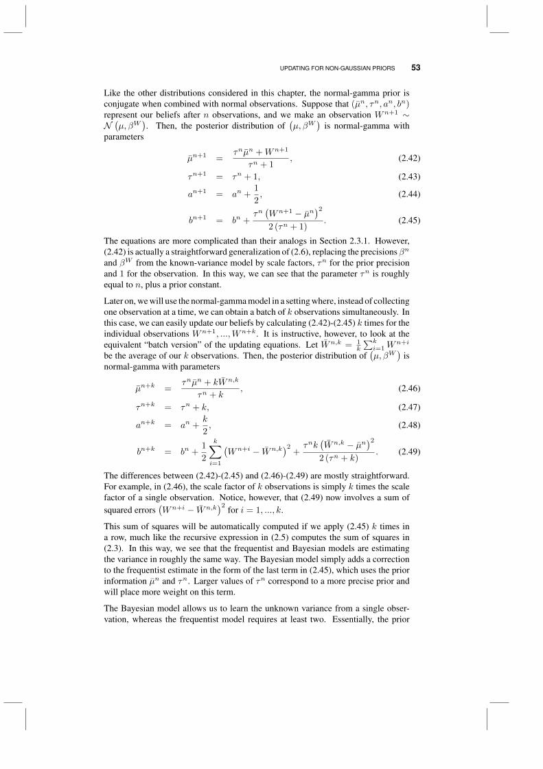
UPDATING FOR NON-GAUSSIAN PRIORS 53
Like the other distributions considered in this chapter, the normal-gamma prior isconjugate when combined with normal observations. Suppose that (µn, τn, an, bn)represent our beliefs after n observations, and we make an observation Wn+1 ∼N(µ, βW
). Then, the posterior distribution of
(µ, βW
)is normal-gamma with
parameters
µn+1 =τnµn +Wn+1
τn + 1, (2.42)
τn+1 = τn + 1, (2.43)
an+1 = an +1
2, (2.44)
bn+1 = bn +τn(Wn+1 − µn
)22 (τn + 1)
. (2.45)
The equations are more complicated than their analogs in Section 2.3.1. However,(2.42) is actually a straightforward generalization of (2.6), replacing the precisions βn
and βW from the known-variance model by scale factors, τn for the prior precisionand 1 for the observation. In this way, we can see that the parameter τn is roughlyequal to n, plus a prior constant.
Later on, we will use the normal-gamma model in a setting where, instead of collectingone observation at a time, we can obtain a batch of k observations simultaneously. Inthis case, we can easily update our beliefs by calculating (2.42)-(2.45) k times for theindividual observations Wn+1, ...,Wn+k. It is instructive, however, to look at theequivalent “batch version” of the updating equations. Let Wn,k = 1
k
∑ki=1W
n+i
be the average of our k observations. Then, the posterior distribution of(µ, βW
)is
normal-gamma with parameters
µn+k =τnµn + kWn,k
τn + k, (2.46)
τn+k = τn + k, (2.47)
an+k = an +k
2, (2.48)
bn+k = bn +1
2
k∑i=1
(Wn+i − Wn,k
)2+τnk
(Wn,k − µn
)22 (τn + k)
. (2.49)
The differences between (2.42)-(2.45) and (2.46)-(2.49) are mostly straightforward.For example, in (2.46), the scale factor of k observations is simply k times the scalefactor of a single observation. Notice, however, that (2.49) now involves a sum ofsquared errors
(Wn+i − Wn,k
)2for i = 1, ..., k.
This sum of squares will be automatically computed if we apply (2.45) k times ina row, much like the recursive expression in (2.5) computes the sum of squares in(2.3). In this way, we see that the frequentist and Bayesian models are estimatingthe variance in roughly the same way. The Bayesian model simply adds a correctionto the frequentist estimate in the form of the last term in (2.45), which uses the priorinformation µn and τn. Larger values of τn correspond to a more precise prior andwill place more weight on this term.
The Bayesian model allows us to learn the unknown variance from a single obser-vation, whereas the frequentist model requires at least two. Essentially, the prior
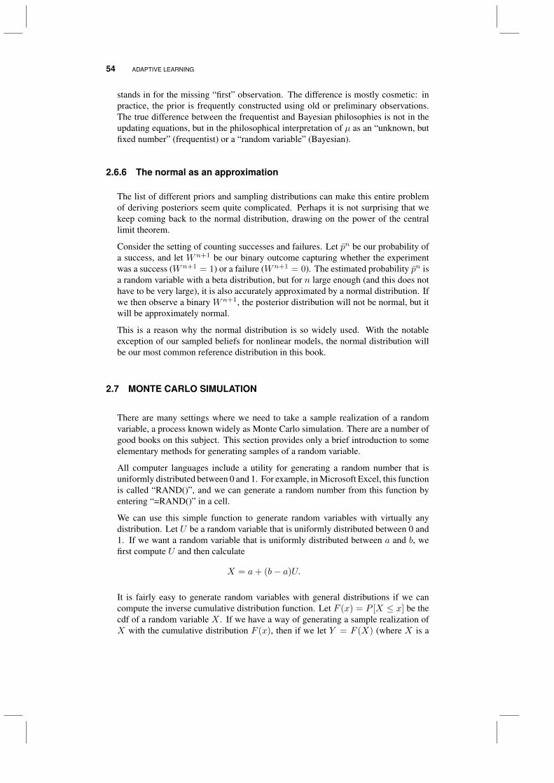
54 ADAPTIVE LEARNING
stands in for the missing “first” observation. The difference is mostly cosmetic: inpractice, the prior is frequently constructed using old or preliminary observations.The true difference between the frequentist and Bayesian philosophies is not in theupdating equations, but in the philosophical interpretation of µ as an “unknown, butfixed number” (frequentist) or a “random variable” (Bayesian).
2.6.6 The normal as an approximation
The list of different priors and sampling distributions can make this entire problemof deriving posteriors seem quite complicated. Perhaps it is not surprising that wekeep coming back to the normal distribution, drawing on the power of the centrallimit theorem.
Consider the setting of counting successes and failures. Let pn be our probability ofa success, and let Wn+1 be our binary outcome capturing whether the experimentwas a success (Wn+1 = 1) or a failure (Wn+1 = 0). The estimated probability pn isa random variable with a beta distribution, but for n large enough (and this does nothave to be very large), it is also accurately approximated by a normal distribution. Ifwe then observe a binary Wn+1, the posterior distribution will not be normal, but itwill be approximately normal.
This is a reason why the normal distribution is so widely used. With the notableexception of our sampled beliefs for nonlinear models, the normal distribution willbe our most common reference distribution in this book.
2.7 MONTE CARLO SIMULATION
There are many settings where we need to take a sample realization of a randomvariable, a process known widely as Monte Carlo simulation. There are a number ofgood books on this subject. This section provides only a brief introduction to someelementary methods for generating samples of a random variable.
All computer languages include a utility for generating a random number that isuniformly distributed between 0 and 1. For example, in Microsoft Excel, this functionis called “RAND()”, and we can generate a random number from this function byentering “=RAND()” in a cell.
We can use this simple function to generate random variables with virtually anydistribution. Let U be a random variable that is uniformly distributed between 0 and1. If we want a random variable that is uniformly distributed between a and b, wefirst compute U and then calculate
X = a+ (b− a)U.
It is fairly easy to generate random variables with general distributions if we cancompute the inverse cumulative distribution function. Let F (x) = P [X ≤ x] be thecdf of a random variable X . If we have a way of generating a sample realization ofX with the cumulative distribution F (x), then if we let Y = F (X) (where X is a
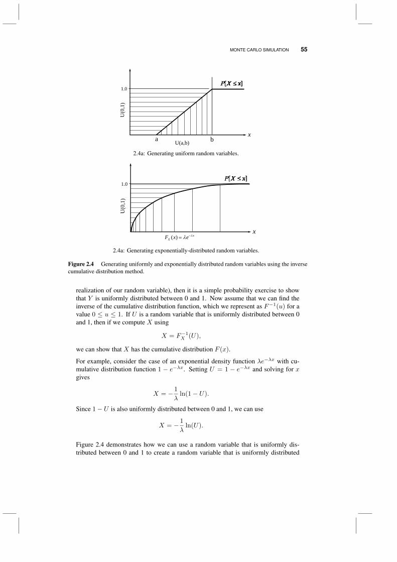
MONTE CARLO SIMULATION 55
a b
1.0
x
U(0
,1)
U(a,b)
2.4a: Generating uniform random variables.
1.0
x
U(0
,1)
( ) xXF x e λλ −=
2.4a: Generating exponentially-distributed random variables.
Figure 2.4 Generating uniformly and exponentially distributed random variables using the inversecumulative distribution method.
realization of our random variable), then it is a simple probability exercise to showthat Y is uniformly distributed between 0 and 1. Now assume that we can find theinverse of the cumulative distribution function, which we represent as F−1(u) for avalue 0 ≤ u ≤ 1. If U is a random variable that is uniformly distributed between 0and 1, then if we compute X using
X = F−1X (U),
we can show that X has the cumulative distribution F (x).
For example, consider the case of an exponential density function λe−λx with cu-mulative distribution function 1 − e−λx. Setting U = 1 − e−λx and solving for xgives
X = − 1
λln(1− U).
Since 1− U is also uniformly distributed between 0 and 1, we can use
X = − 1
λln(U).
Figure 2.4 demonstrates how we can use a random variable that is uniformly dis-tributed between 0 and 1 to create a random variable that is uniformly distributed
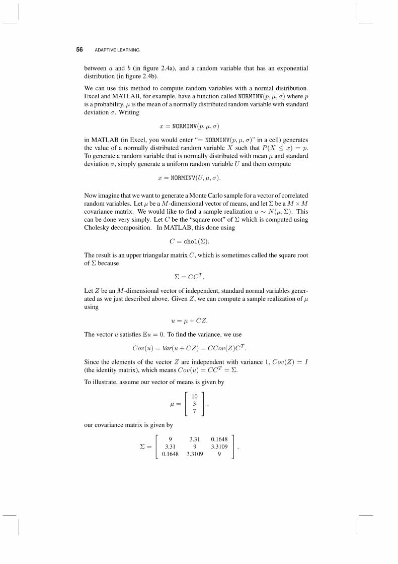
56 ADAPTIVE LEARNING
between a and b (in figure 2.4a), and a random variable that has an exponentialdistribution (in figure 2.4b).
We can use this method to compute random variables with a normal distribution.Excel and MATLAB, for example, have a function called NORMINV(p, µ, σ) where pis a probability, µ is the mean of a normally distributed random variable with standarddeviation σ. Writing
x = NORMINV(p, µ, σ)
in MATLAB (in Excel, you would enter “= NORMINV(p, µ, σ)” in a cell) generatesthe value of a normally distributed random variable X such that P (X ≤ x) = p.To generate a random variable that is normally distributed with mean µ and standarddeviation σ, simply generate a uniform random variable U and them compute
x = NORMINV(U, µ, σ).
Now imagine that we want to generate a Monte Carlo sample for a vector of correlatedrandom variables. Let µ be aM -dimensional vector of means, and let Σ be aM×Mcovariance matrix. We would like to find a sample realization u ∼ N(µ,Σ). Thiscan be done very simply. Let C be the “square root” of Σ which is computed usingCholesky decomposition. In MATLAB, this done using
C = chol(Σ).
The result is an upper triangular matrix C, which is sometimes called the square rootof Σ because
Σ = CCT .
Let Z be an M -dimensional vector of independent, standard normal variables gener-ated as we just described above. Given Z, we can compute a sample realization of µusing
u = µ+ CZ.
The vector u satisfies Eu = 0. To find the variance, we use
Cov(u) = Var(u+ CZ) = CCov(Z)CT .
Since the elements of the vector Z are independent with variance 1, Cov(Z) = I(the identity matrix), which means Cov(u) = CCT = Σ.
To illustrate, assume our vector of means is given by
µ =
1037
.our covariance matrix is given by
Σ =
9 3.31 0.16483.31 9 3.3109
0.1648 3.3109 9
.
WHY DOES IT WORK?* 57
The Cholesky decomposition computed by MATLAB using C = chol(Σ) is
C =
3 1.1033 0.05490 3 1.16510 0 3
.Imagine that we generate a vector Z of independent standard normal deviates
Z =
1.1-0.570.98
.Using this set of sample realizations of Z, a sample realization u would be
u =
10.72492.43187.9400
.Using computers to generate random numbers has proven to be an exceptionallypowerful tool in the analysis of stochastic systems. Not surprisingly, then, the fieldhas matured into a rich and deep area of study. This presentation is little more thana hint at the many tools available to help with the process of generating randomnumbers.
2.8 WHY DOES IT WORK?*
2.8.1 Derivation of σ
An important quantity in optimal learning is the variance σnx of µn+1x given what we
know after n experiments.
Proposition 2.8.1 The variance of µn+1, defined as
σn = Varn[µn+1]
= Varn[µn+1 − µn],
is given by (σnx )2 = (σnx )2 − (σn+1x )2.
Proof: Keep in mind that after n experiments, µnx is deterministic. We are dealingwith two random variables: the truth µx, and the estimate µn+1
x after we have maden experiments (the n + 1st experiment, Wn+1, is unknown). We begin with therelation
(µn+1x − µx) = (µn+1
x − µnx) + (µnx − µx). (2.50)
Recall that (σn+1x )2 = En+1
[(µn+1x − µx)2
]. Squaring both sides of (2.50) and
taking the conditional expectation En+1(·) = E(·|W 1, . . . ,Wn+1) gives
(σn+1x )2 = En+1
[(µnx − µx)2
]+ 2En+1
[(µnx − µx)(µn+1
x − µnx)]
+ En+1[(µn+1x − µnx)2
]= En+1
[(µnx − µx)2
]+ 2(µnx − µn+1
x )(µn+1x − µnx) + (µn+1
x − µnx)2
= En+1[(µnx − µx)2
]− (µn+1
x − µnx)2.
58 ADAPTIVE LEARNING
Keep in mind that En+1µn+1x = µn+1
x and En+1µx = µn+1x . We then observe that
while µn+1x is random given the first n observations, σn+1
x is deterministic, becauseσn+1x does not depend onWn+1 - it only depends on our decision of what to measurexn. Using this property, we can take the expectation given W 1, . . . ,Wn to obtain
En(σn+1x )2 = (σn+1
x )2 = En[En+1
[(µnx − µx)2
]]− En
[(µn+1x − µnx)2
]= En
[(µnx − µx)2
]− En
[(µn+1x − µnx)2
]= (σnx )2 − (σnx )2.
2.8.2 Derivation of Bayesian updating equations for independent beliefs
Bayesian analysis begins with a simple formula that everyone learns in their firstprobability course. Given the events A and B, the basic properties of conditionalprobability imply
P (A,B) = P (A|B)P (B) = P (B|A)P (A)
which implies
P (B|A) =P (A|B)P (B)
P (A).
This expression is famously known as Bayes’ theorem. In a learning setting, theevent A refers to an experiment (or some type of new information), while B refersto the event that a parameter (say, the mean of a distribution) takes on a particularvalue. P (B) refers to our initial (or prior) distribution of belief about the unknownparameter before we run an experiment, and P (B|A) is the distribution of beliefabout the parameter after the experiment has been run. For this reason, P (B|A) isknown as the posterior distribution.
We can apply the same idea for continuous variables. We replace B with the eventthat µ = u (to be more precise, we replace B with the event that u ≤ µ ≤ u+ du),and A with the event that we observed W = w. Let g(u) be our prior distribution ofbelief about the mean µ, and let g(u|w) be the posterior distribution of belief aboutµ given that we observed W = w. We then let f(w|u) be the distribution of therandom variable W if µ = u. We can now write our posterior g(u|w), which is thedensity of µ given that we observe W = w, as
g(u|w) =f(w|u)g(u)
f(w),
where f(w) is the unconditional density of the random variableW which we computeusing
f(w) =
∫u
f(w|u)g(u).
Equation (2.51) gives us the density of µ given that we have observed W = w.
WHY DOES IT WORK?* 59
We illustrate these calculations by assuming that our prior g(u) follows the normaldistribution with mean µ0 and variance σ2,0, given by
g(u) =1√
2πσ0exp
(−1
2
(u− µ0)2
σ2,0
).
We further assume that the observation W is also normally distributed with mean µand variance σ2
ε , which is sometimes referred to as the experimental or observationerror. The conditional distribution f(w|u) is
f(w|u) =1√2πσ
exp
(−1
2
(w − u)2
σ2ε
).
We can compute f(w) from f(w|u) and g(u), but it is only really necessary to findthe density g(u|w) up to a normalization constant (f(w) is part of this normalizationconstant). For this reason, we can write
g(u|w) ∝ f(w|u)g(u). (2.51)
Using this reasoning, we can drop coefficients such as 1√2πσ0
, and write
g(u|w) ∝[exp
(−1
2
(w − u)2
σ2
)]·[exp
(−1
2
(u− µ0)2
σ2,0
)],
∝ exp
[−1
2
((w − u)2
σ2+
(u− µ0)2
σ2,0
)]. (2.52)
After some algebra, we find that
g(u|w) ∝ exp−1
2β1(u− µ1)2 (2.53)
where
µ1 =(βWw + β0µ0)
α+ β0, (2.54)
β1 = βW + β0. (2.55)
The next step is to find the normalization constant (call itK) which we do by solving
K
∫u
g(u|w)du = 1.
We could find the normalization constant by solving the integral and picking K sothat g(u|w) integrates to 1, but there is an easier way. What we are going to do is lookaround for a known probability density function with the same structure as (2.53),and then simply use its normalization constant. It is fairly easy to see that (2.53)corresponds to a normal distribution, which means that the normalization constant
K =√
β1
2π . This means that our posterior density is given by
g(u|w) =
√β1
2πexp−1
2β1(u− µ1)2. (2.56)

60 ADAPTIVE LEARNING
From equation (2.56), we see that the posterior density g(u|w) is also normallydistributed with mean µ1 given by (2.54), and precision β1 given by (2.55) (it isonly now that we see our choice of notation µ1 and β1 in equations (2.54) and(2.55) was not an accident). This means that as long as we are willing to stay withour assumption of normality, then we need only to carry the mean and variance (orprecision). The implication is that we can write our belief state as Bn = (µn, βn)(or Bn = (µn, σ2,n)), and that (2.54)-(2.55) is our belief transition function.
Our derivation above was conducted in the context of the normal distribution, but wefollowed certain steps that can be applied to other distributions. These include:
1) We have to be given the prior g(u) and the conditional density f(w|u) of the experimentaloutcome.
2) We use equation (2.51) to find the posterior up to the constant of proportionality, as wedid in (2.52) for the normal distribution.
3) We then manipulate the result in the hope of finding a posterior distribution, recognizingthat we can discard terms that do not depend on u (these are absorbed into thenormalization constant). If we are lucky, we will find that we have a conjugatefamily, and that we end up with the same class of distribution we started with for theprior. Otherwise, we are looking for a familiar distribution so that we do not have tocompute the normalization constant ourselves.
4) We identify the transition equations that relate the parameters of the posterior to theparameters of the prior and the distribution of the experimental outcome, as we didwith equations (2.54)-(2.55).
2.9 BIBLIOGRAPHIC NOTES
Sections 2.2-2.3 - There are numerous books on both frequentist and Bayesian statistics.An excellent reference for frequentist statistics is Hastie et al. (2009), which isavailable as of this writing as a free download in PDF form. An excellent referencefor Bayesian statistics is Gelman et al. (2004). Another classical reference, with afocus on using Bayesian statistics to solve decision problems, is DeGroot (1970).
Section 2.6 - See Gelman et al. (2004) for a thorough treatment of Bayesian models.
Section 2.7 - There are a number of outstanding references on Monte Carlo simulation,including Banks et al. (1996), Roberts & Casella (2004), Glasserman (2004) andRubinstein & Kroese (2008), to name a few.
PROBLEMS
2.1 In a spreadsheet, implement both the batch and recursive formulas for the fre-quentist estimates mean and variance of a set of random numbers (just use RAND() toproduce random numbers between 0 and 1). Use a sequence of 20 random numbers.Note that Excel has functions to produce the batch estimates (AVERAGE and VAR) of

PROBLEMS 61
the mean and variance. Compare your results to Bayesian estimates of the mean andvariance assuming that your prior is a mean of .5 and a variance of .2 (the prior estimateof the mean is correct, while the variance is incorrect).
2.2 Download the spreadsheet from the book website:
http://optimallearning.princeton.edu/exercises/FiveAlternative.xls
On day 0, the spreadsheet shows your initial estimate of the travel time on each path. Inthe column painted yellow, enter the path that you wish to follow the next day. You willsee an observed time, and in the column to the right, we record the time you experiencethe next day when you follow your chosen path. To the right there is a work areawhere you can code your own calculations. Assume all random variables are normallydistributed.
a) In the work area, use the Bayesian updating formulas to compute updated estimatesof the mean and variance. Assume that the standard deviation of the observed traveltime for any path is 5 minutes.
b) Using your estimates from part a, simulate a policy where you always choose thepath that you thought was fastest. Record your total travel time, and the path thatyou thought was best.
c) You should find that you are getting stuck on one path, and that you do not “discover”the best path (you can quickly find that this is path 1). Suggest a policy that could beapplied to any dataset (there can not be any hint that you are using your knowledgeof the best path). Report your total travel time and the final path you choose.
2.3 You are trying to determine the distribution of how much people weigh in apopulation. Your prior distribution of belief about the mean µ is that it is normallydistributed with mean 180 and standard deviation 40. You then observe the weights ofn students drawn from this population. The average weight in the sample is y = 150pounds. Assume that the weights are normally distributed with unknown mean µ and aknown standard deviation of 20 pounds.
a) Give your posterior distribution for µ given the sample you have observed. Note thatyour answer will be a function of n.
b) A new observation is made and has a weight of y pounds. Give the posteriordistribution for y (again, your answer will be a function of n).
c) Give a 95 percent posterior confidence intervals for µ and y if n = 10.
d) Repeat (c) with n = 100.
2.4 Show that, for a fixed k > 1, equation (2.49) is equivalent to applying (2.45) ktimes in a row. Use the equivalence of (2.3) and (2.5). Now implement both the recursiveand batch formulas in a spreadsheet and verify that they produce the same numbers.

62 ADAPTIVE LEARNING
2.5 In this problem, you will derive the Bayesian updating equations (2.30) and (2.31)for the gamma-exponential model. Suppose that W is a continuous random variablethat follows an exponential distribution with parameter λ. The parameter λ is alsorandom, reflecting our distribution of belief. We say that λ has a gamma prior by writingλ ∼ Gamma(a, b), meaning that our distribution of belief is gamma. Each time weobserve W , we use this observation to update our belief about the true distribution ofW , reflecting our uncertainty about λ.
a) Write down the prior density f(u). What does u refer to?
b) Write down the conditional density g(w|u) of the observation.
c) Write down the unconditional density g(w) of the observation. (Hint: Start withg(w|u) and take an expectation over the prior. Remember that the gamma functionhas the property that Γ(a) = (a− 1)Γ(a− 1).)
d) Apply Bayes’ rule to get f(u|w), the posterior density after the observation. Whatdistribution does this density correspond to? How does this verify equations (2.30)and (2.31)?
2.6 In this problem, you will see how the updating equations you derived in exercise2.5 works in practice. Suppose that the customer service time at a certain store isexponentially distributed, and we are using the gamma-exponential model to learn theservice rate as we observe the service times of individual customers.
a) Let U be a random variable that is uniformly distributed between 0 and 1. LetR = − 1
λ logU . Show that R follows an exponential distribution with parameterλ. This gives us a way to create samples from any exponential distribution bytransforming samples from a uniform distribution (see section 2.4).
b) In a spreadsheet, use the above method to simulate 10 observations from an expo-nential distribution with parameter λ = 3. Now suppose that we do not know that λhas this value, and model our beliefs using a gamma prior with parameters α0 = 1and β0 = 0.2. What is our best initial estimate of λ? In your spreadsheet, recordthe values of αn and βn, as well as the resulting estimate of λ, for each n. Copy theresults into a table and hand in a paper copy.

CHAPTER 3
OFFLINE LEARNING
Offline learning represents the set of problems where we have a budget to run Nexperiments, after which we have to use the information we gained to make the bestdecision possible based on what we learned about the function. One of the earliestversions of this problem arose in statistics under the name ranking and selection. Thetwo defining characteristics of this problem class are:
• The possible decisions x fall in a finite set X = x1, . . . , xM, where xm may be acategorical choice (type of drug or material, type of color), a discretized value of acontinuous parameter, or a possibly sampled value of a multidmensional vector.
• We have a finite budget N , and we only care about the quality of the final decisionrather than how well we do while we are learning. We refer to the performance atthe end as the terminal reward.
Offline learning problems arise in many settings. We may have to choose a type ofcholesterol drug, the parameters of a chemical process (e.g. temperature, relative mixof certain inputs), or the design of a manufacturing process (choice of equipment,size of buffers, routing of jobs). Testing an alternative might involve running atime-consuming computer simulation, or it might require a physical experiment. Weassume that in either case, the experiment involves some noise, which means we mayneed to repeat the experiment several times. We assume that we have a budget that
Optimal Learning. By Warren B. Powell and Ilya O. RyzhovCopyright c© 2018 John Wiley & Sons, Inc.
63
64 OFFLINE LEARNING
determines how many times we can perform these experiments, after which we haveto take the best design and live with it.
We need to pause and comment on different interpretations of the terms “offline” and“online” (a class of problems we turn to in chapter 5). In this book, we interpretoffline problems as having two distinct phases:
The information collection phase This is when we are running experiments to learn aboutthe properties of a function or process, without regard to how well we are doing.
The implementation phase This is when we use what we have learned to design a systemor process, and then we have to live with the performance of the resulting design.
By contrast, online problems represent problems that are running in the field, wherewe learn and implement at the same time. For example, testing medication on apatient would be an online problem; if we misdiagnose the condition, the patient willsuffer. Similarly, trying to find the best price for a product requires setting a price andthen receiving the associated revenue stream which may be lower than it could be,but we learn from this. This chapter focuses on offline learning. We turn to onlinelearning, which has a separate but very rich history, in chapter 5.
This is not the only interpretation of offline vs. online. The machine learningcommunity (to name one) uses offline learning to refer to using a batch dataset toestimate a function. By contrast, “online” refers to procedures that are sequentialin nature. Implementing a process in the field is inherently sequential, hence theassociation of “online” with “sequential.” But, learning in the lab or a simulation(offline) can also be sequential, and hence the machine learning community willinterpret this setting as online as well, while recognizing that we do not care abouthow well we do.
In this chapter, we are going to show how to model offline learning problems. Wethen illustrate how to design and evaluate different learning policies for choosingthe next experiment to run. The policies we introduce in this chapter are not themost sophisticated, although they can work quite well if properly tuned. Further, weare going to introduce new policies in chapter 5 for online learning that can also beapplied to offline problems.
3.1 THE MODEL
The learning process proceeds as follows. Let Sn be our belief state, which capturesthe statistics we have collected from our first n observations using the methods weintroduced in chapter 2. We assume we have some policy Xπ(Sn) that returns adecision xn given our belief state that is given by Sn. We start at time n = 0, andmake decision x0 = Xπ(S0) using our initial state S0 (that is, our prior). Using thelookup table model we introduced in chapter 2, assume we choose xn = Xπ(Sn)and then observe
Wn+1xn = µxn + εn+1. (3.1)
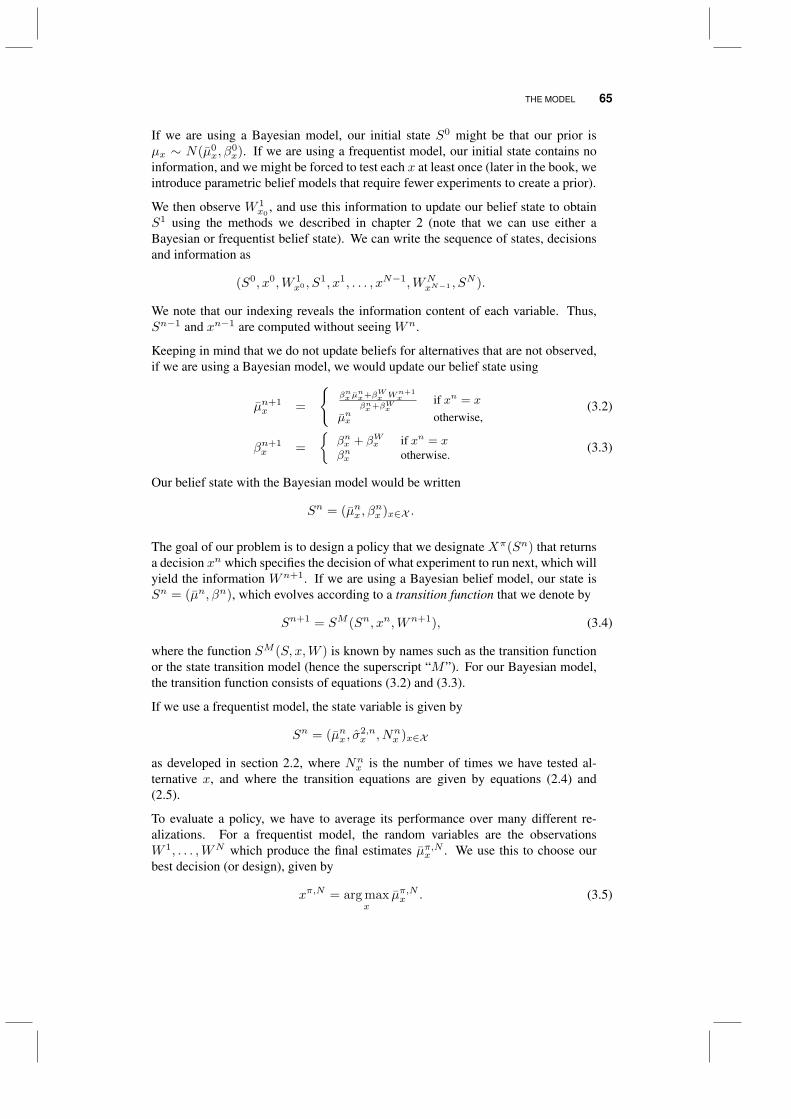
THE MODEL 65
If we are using a Bayesian model, our initial state S0 might be that our prior isµx ∼ N(µ0
x, β0x). If we are using a frequentist model, our initial state contains no
information, and we might be forced to test each x at least once (later in the book, weintroduce parametric belief models that require fewer experiments to create a prior).
We then observe W 1x0
, and use this information to update our belief state to obtainS1 using the methods we described in chapter 2 (note that we can use either aBayesian or frequentist belief state). We can write the sequence of states, decisionsand information as
(S0, x0,W 1x0 , S1, x1, . . . , xN−1,WN
xN−1 , SN ).
We note that our indexing reveals the information content of each variable. Thus,Sn−1 and xn−1 are computed without seeing Wn.
Keeping in mind that we do not update beliefs for alternatives that are not observed,if we are using a Bayesian model, we would update our belief state using
µn+1x =
βnx µ
nx+βWx Wn+1
x
βnx+βWxif xn = x
µnx otherwise,(3.2)
βn+1x =
βnx + βWx if xn = xβnx otherwise.
(3.3)
Our belief state with the Bayesian model would be written
Sn = (µnx , βnx )x∈X .
The goal of our problem is to design a policy that we designate Xπ(Sn) that returnsa decision xn which specifies the decision of what experiment to run next, which willyield the information Wn+1. If we are using a Bayesian belief model, our state isSn = (µn, βn), which evolves according to a transition function that we denote by
Sn+1 = SM (Sn, xn,Wn+1), (3.4)
where the function SM (S, x,W ) is known by names such as the transition functionor the state transition model (hence the superscript “M”). For our Bayesian model,the transition function consists of equations (3.2) and (3.3).
If we use a frequentist model, the state variable is given by
Sn = (µnx , σ2,nx , Nn
x )x∈X
as developed in section 2.2, where Nnx is the number of times we have tested al-
ternative x, and where the transition equations are given by equations (2.4) and(2.5).
To evaluate a policy, we have to average its performance over many different re-alizations. For a frequentist model, the random variables are the observationsW 1, . . . ,WN which produce the final estimates µπ,Nx . We use this to choose ourbest decision (or design), given by
xπ,N = arg maxx
µπ,Nx . (3.5)
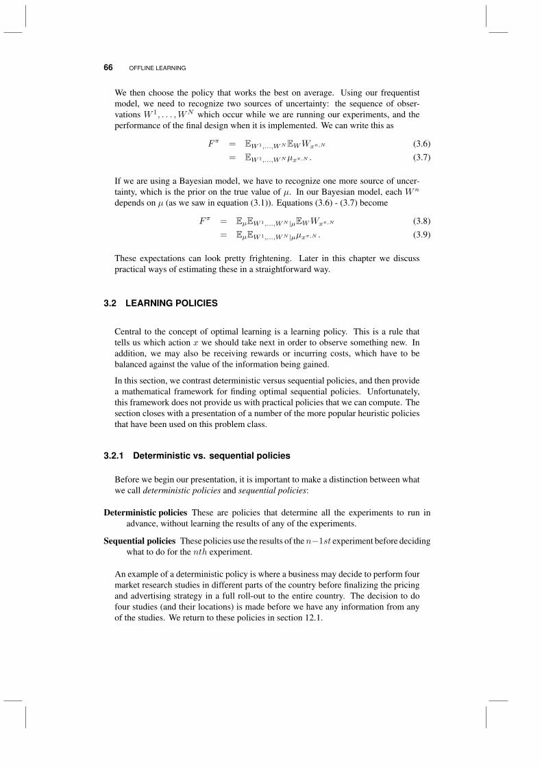
66 OFFLINE LEARNING
We then choose the policy that works the best on average. Using our frequentistmodel, we need to recognize two sources of uncertainty: the sequence of obser-vations W 1, . . . ,WN which occur while we are running our experiments, and theperformance of the final design when it is implemented. We can write this as
Fπ = EW 1,...,WNEWWxπ,N (3.6)= EW 1,...,WNµxπ,N . (3.7)
If we are using a Bayesian model, we have to recognize one more source of uncer-tainty, which is the prior on the true value of µ. In our Bayesian model, each Wn
depends on µ (as we saw in equation (3.1)). Equations (3.6) - (3.7) become
Fπ = EµEW 1,...,WN |µEWWxπ,N (3.8)= EµEW 1,...,WN |µµxπ,N . (3.9)
These expectations can look pretty frightening. Later in this chapter we discusspractical ways of estimating these in a straightforward way.
3.2 LEARNING POLICIES
Central to the concept of optimal learning is a learning policy. This is a rule thattells us which action x we should take next in order to observe something new. Inaddition, we may also be receiving rewards or incurring costs, which have to bebalanced against the value of the information being gained.
In this section, we contrast deterministic versus sequential policies, and then providea mathematical framework for finding optimal sequential policies. Unfortunately,this framework does not provide us with practical policies that we can compute. Thesection closes with a presentation of a number of the more popular heuristic policiesthat have been used on this problem class.
3.2.1 Deterministic vs. sequential policies
Before we begin our presentation, it is important to make a distinction between whatwe call deterministic policies and sequential policies:
Deterministic policies These are policies that determine all the experiments to run inadvance, without learning the results of any of the experiments.
Sequential policies These policies use the results of then−1st experiment before decidingwhat to do for the nth experiment.
An example of a deterministic policy is where a business may decide to perform fourmarket research studies in different parts of the country before finalizing the pricingand advertising strategy in a full roll-out to the entire country. The decision to dofour studies (and their locations) is made before we have any information from anyof the studies. We return to these policies in section 12.1.
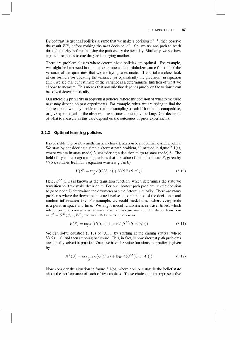
LEARNING POLICIES 67
By contrast, sequential policies assume that we make a decision xn−1, then observethe result Wn, before making the next decision xn. So, we try one path to workthrough the city before choosing the path we try the next day. Similarly, we see howa patient responds to one drug before trying another.
There are problem classes where deterministic policies are optimal. For example,we might be interested in running experiments that minimizes some function of thevariance of the quantities that we are trying to estimate. If you take a close lookat our formula for updating the variance (or equivalently the precision) in equation(3.3), we see that our estimate of the variance is a deterministic function of what wechoose to measure. This means that any rule that depends purely on the variance canbe solved deterministically.
Our interest is primarily in sequential policies, where the decision of what to measurenext may depend on past experiments. For example, when we are trying to find theshortest path, we may decide to continue sampling a path if it remains competitive,or give up on a path if the observed travel times are simply too long. Our decisionsof what to measure in this case depend on the outcomes of prior experiments.
3.2.2 Optimal learning policies
It is possible to provide a mathematical characterization of an optimal learning policy.We start by considering a simple shortest path problem, illustrated in figure 3.1(a),where we are in state (node) 2, considering a decision to go to state (node) 5. Thefield of dynamic programming tells us that the value of being in a state S, given byV (S), satisfies Bellman’s equation which is given by
V (S) = maxx
(C(S, x) + V (SM (S, x))
). (3.10)
Here, SM (S, x) is known as the transition function, which determines the state wetransition to if we make decision x. For our shortest path problem, x (the decisionto go to node 5) determines the downstream state deterministically. There are manyproblems where the downstream state involves a combination of the decision x andrandom information W . For example, we could model time, where every nodeis a point in space and time. We might model randomness in travel times, whichintroduces randomness in when we arrive. In this case, we would write our transitionas S′ = SM (S, x,W ), and write Bellman’s equation as
V (S) = maxx
(C(S, x) + EWV (SM (S, x,W ))
). (3.11)
We can solve equation (3.10) or (3.11) by starting at the ending state(s) whereV (S) = 0, and then stepping backward. This, in fact, is how shortest path problemsare actually solved in practice. Once we have the value functions, our policy is givenby
X∗(S) = arg maxx
(C(S, x) + EWV (SM (S, x,W ))
). (3.12)
Now consider the situation in figure 3.1(b), where now our state is the belief stateabout the performance of each of five choices. These choices might represent five
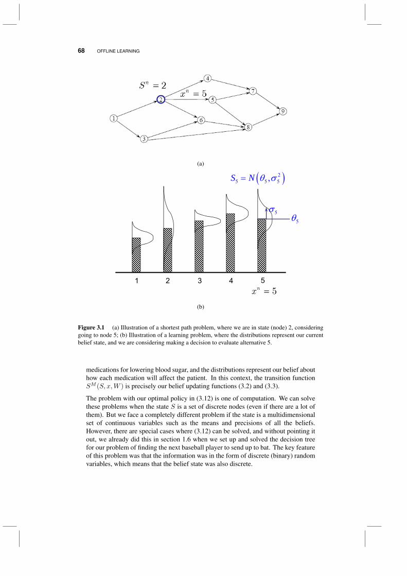
68 OFFLINE LEARNING
(a)
10
10
1 2 3 4 5
1 1( ) max ( , ) ( ) |n n n n n nxV S C S x E V S S
Current state of knowledgeDecision to make a measurementNew state of knowledge
55
25 5 5,S N
5nx
(b)
Figure 3.1 (a) Illustration of a shortest path problem, where we are in state (node) 2, consideringgoing to node 5; (b) Illustration of a learning problem, where the distributions represent our currentbelief state, and we are considering making a decision to evaluate alternative 5.
medications for lowering blood sugar, and the distributions represent our belief abouthow each medication will affect the patient. In this context, the transition functionSM (S, x,W ) is precisely our belief updating functions (3.2) and (3.3).
The problem with our optimal policy in (3.12) is one of computation. We can solvethese problems when the state S is a set of discrete nodes (even if there are a lot ofthem). But we face a completely different problem if the state is a multidimensionalset of continuous variables such as the means and precisions of all the beliefs.However, there are special cases where (3.12) can be solved, and without pointing itout, we already did this in section 1.6 when we set up and solved the decision treefor our problem of finding the next baseball player to send up to bat. The key featureof this problem was that the information was in the form of discrete (binary) randomvariables, which means that the belief state was also discrete.
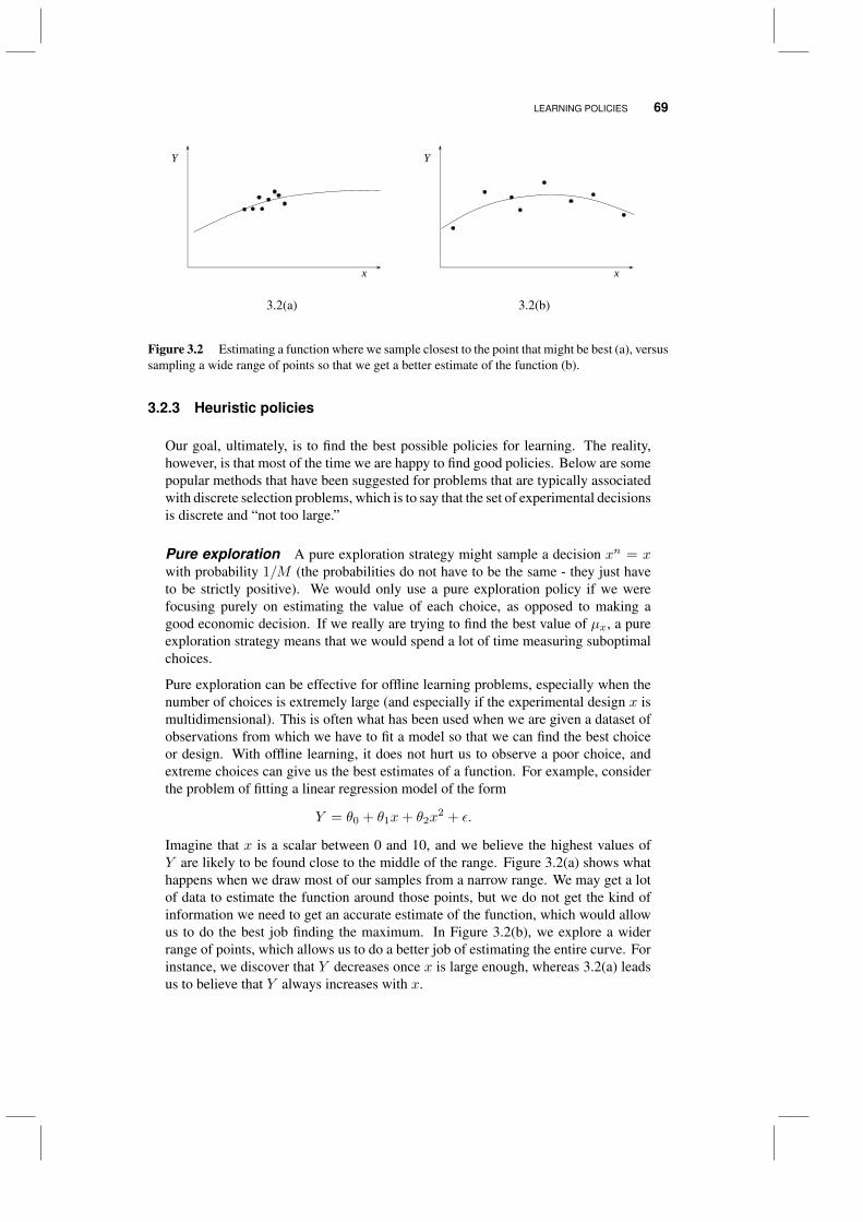
LEARNING POLICIES 69
x
Y
x
Y
3.2(a) 3.2(b)
Figure 3.2 Estimating a function where we sample closest to the point that might be best (a), versussampling a wide range of points so that we get a better estimate of the function (b).
3.2.3 Heuristic policies
Our goal, ultimately, is to find the best possible policies for learning. The reality,however, is that most of the time we are happy to find good policies. Below are somepopular methods that have been suggested for problems that are typically associatedwith discrete selection problems, which is to say that the set of experimental decisionsis discrete and “not too large.”
Pure exploration A pure exploration strategy might sample a decision xn = xwith probability 1/M (the probabilities do not have to be the same - they just haveto be strictly positive). We would only use a pure exploration policy if we werefocusing purely on estimating the value of each choice, as opposed to making agood economic decision. If we really are trying to find the best value of µx, a pureexploration strategy means that we would spend a lot of time measuring suboptimalchoices.
Pure exploration can be effective for offline learning problems, especially when thenumber of choices is extremely large (and especially if the experimental design x ismultidimensional). This is often what has been used when we are given a dataset ofobservations from which we have to fit a model so that we can find the best choiceor design. With offline learning, it does not hurt us to observe a poor choice, andextreme choices can give us the best estimates of a function. For example, considerthe problem of fitting a linear regression model of the form
Y = θ0 + θ1x+ θ2x2 + ε.
Imagine that x is a scalar between 0 and 10, and we believe the highest values ofY are likely to be found close to the middle of the range. Figure 3.2(a) shows whathappens when we draw most of our samples from a narrow range. We may get a lotof data to estimate the function around those points, but we do not get the kind ofinformation we need to get an accurate estimate of the function, which would allowus to do the best job finding the maximum. In Figure 3.2(b), we explore a widerrange of points, which allows us to do a better job of estimating the entire curve. Forinstance, we discover that Y decreases once x is large enough, whereas 3.2(a) leadsus to believe that Y always increases with x.
70 OFFLINE LEARNING
Pure exploitation Exploitation means making the best decision given our currentset of estimates (we are “exploiting” our knowledge). So, after iteration n, we wouldnext measure
xn = arg maxx∈X
µnx .
This strategy would seem to focus our energy on the options that appear to be thebest. However, it is very easy to get stuck measuring choices that seem to be the best,especially when we simply had some bad luck measuring the better choices.
Pure exploitation is a common strategy in online problems, where we have to livewith the results of each experiment. With pure exploitation, we can always defendour choice because we are doing what we believe is the best, but we may be ignoringerrors in our own beliefs.
Excitation policies A popular policy in the control of engineering systems withcontinuous controls is to assume we have some policy that specifies the action wethink is best and then adds a random noise term. For example, we might specify therate at which gasoline flows into a combustion chamber as a function of the speedSt of a vehicle. Assume that we use the following policy (known as a control law inengineering):
Xπ(St|θ) = θ0 + θ1St + θ2S2t .
Presumably we think this is the policy that produces the best gas mileage whilemaintaining the speed of the vehicle, so we would call this a pure exploitation policy.We can introduce a random noise term to induce exploration using
Xπ(St|θ) = θ0 + θ1St + θ2S2t + ε.
The noise ε is known in engineering as excitation, and it helps to learn new behaviors.
Epsilon-greedy exploration A simple strategy that avoids the limitations ofpure exploration and pure exploitation is to use a mixed strategy, where we explorewith probability ε (known as the exploration rate) and we exploit with probability1− ε. The value of ε has to be tuned for each application.
Mixing exploration and exploitation is appealing because it allows you to spendmore time evaluating the choices that appear to be best (to make sure this is thecase) while still doing a certain amount of exploration. As our experimentationbudget goes to infinity, we can still provide guarantees that we will find the bestalternative because of the exploration component. But this policy still suffers fromthe significant limitation that when we do choose to explore, we sample from theentire population of alternatives, which may be extremely large, including choicesthat are clearly suboptimal.
The problem with a mixed exploration/exploitation strategy with fixed ε is thatthe correct balancing of exploration and exploitation changes with the number ofiterations. In the beginning, it is better to explore. As we build confidence in ourestimates, we would prefer to exploit more. We can do this by using an exploration
LEARNING POLICIES 71
probability εn at iteration n that declines with n. We have to make sure it does notdecline too quickly. We do this by setting
εn = c/n
for 0 < c < 1. If we explore, we would choose experimental design x withprobability 1/|X |. This means that in the limit, the number of times we will measurex is given by
∞∑n=1
c
n|X |=∞.
This assures us that we will estimate each experiment x perfectly, but as the ex-periments progress, we will spend more time measuring what we think are the bestchoices.
Boltzmann exploration A different strategy for balancing exploration and ex-ploitation is known as Boltzmann exploration. With this strategy, we run experimentx with probability pnx given by
pnx(θB) =eθB µnx∑
x′∈X eθB µn
x′. (3.13)
This policy is also known as the soft max policy. If θB = 0, we are going to run eachexperiment x with equal probability (pure exploration). As θB → ∞, we will runthe experiment with the highest value of µn with probability 1 (pure exploitation). Inbetween, we explore the better options with higher probability. Furthermore, we canmake θB increase with n (which is typical), so that we explore more in the beginning,converging to a pure exploitation strategy. Tuning such policies, however, can betricky; we return to this below in section 3.7.
Care should be used when computing the probabilities using a Boltzmann distribution,especially if you are increasing θB as you progress to focus attention on the bestalternatives. The problem is that the exponent θBµnx can become so large as to makeit impossible to evaluate eθ
B µnx . A better way is to first compute
µn = maxx∈X
µnx ,
and then compute the probabilities using
pnx(θB) =eθB(µnx−µ
n)∑x′∈X e
θB(µnx′−µ
n).
This calculation can be further streamlined by excluding any choices x where µnx issufficiently far from µn (for example, where θB |µn − µnx | > 10).
We write the Boltzmann policy by first generating a random variableU that is uniformon [0, 1]. To simplify notation, assume that xm = m. Next, create a cumulativedistribution Pnx (θB) =
∑xx′=1 p
nx′(θ
B). Finally, we can write our policy using
XBoltz(Sn|θB) = arg maxxx|Pnx (θB) ≤ U. (3.14)
72 OFFLINE LEARNING
Boltzmann exploration is more effective than epsilon-greedy which either choosesthe very best, or chooses among the rest purely at random. Boltzmann focuses itsefforts more on the choices that are at least somewhat attractive. However, it ismissing an important feature that is enjoyed by the policies which follow.
Upper confidence bounding UCB policies (as they are known) were developedprimarily for the setting of online learning, so we are going to cover these in moredepth in chapter 5. However, they represent an important class of policy, and theycan be used in offline settings if they are properly tuned (the same can be said of allof the heuristic policies described in this section).
A basic version of a UCB policy (known as “UCB1” in the research literature) isgiven by
XUCB1,n(Sn|θUCB) = arg maxx
(µnx + θUCB
√2 log n
Nnx
.
)(3.15)
The parameter θUCB is one that we have introduced, and we will have to tune it foran offline setting (this is discussed below).
Thompson sampling Thompson sampling is a simple policy based on the ideaof created a sampled estimate of what might happen in the next experiment for eachpossible design. We illustrate using a Bayesian belief model, although a frequentistmodel could be used as well.
Assume that aftern experiments, we characterize our belief aboutµx ∼ N(µnx , σ2,nx ).
Now, randomly sample µn+1x from the belief N(µnx , σ
2,nx ), where Eµn+1
x = µnx .However, µn+1
x may be higher or lower than µnx . The Thompson sampling policy isthen given simply by
XTS(Sn) = arg maxx
µn+1x . (3.16)
The randomization in choosing µn+1x is the mechanism by which Thompson sampling
explores different alternatives, with a bias toward the choices that appear to be better.
Interval estimation Imagine that instead of running the experiment that we thinkis best, we choose an alternative that we think might learn is the best if we were totake enough observations. With this idea, we might construct a confidence intervaland then value an option based on the upper limit of, say, a 95% confidence interval.Letting α be our confidence level and denoting by zα the standard normal deviateleaving α in the upper tail, our upper limit would be
νIE,nx = µnx + zασnx (3.17)
where σnx =√
1βnx
is the standard deviation of the distribution of our belief at timen. When we use an interval exploration policy, we choose the experiment xn withthe highest value of νIE,nx .
Although the interpretation as the upper limit of a confidence interval is appealing,the confidence level α carries no particular meaning. In fact, the policy we would
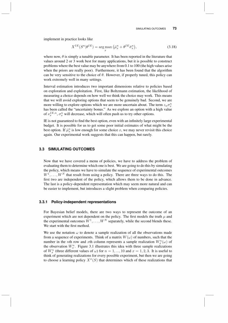
SIMULATING OUTCOMES 73
implement in practice looks like
XIE(Sn|θIE) = arg maxx
(µnx + θIE σnx
), (3.18)
where now, θ is simply a tunable parameter. It has been reported in the literature thatvalues around 2 or 3 work best for many applications, but it is possible to constructproblems where the best value may be anywhere from 0.1 to 100 (the high values arisewhen the priors are really poor). Furthermore, it has been found that the algorithmcan be very sensitive to the choice of θ. However, if properly tuned, this policy canwork extremely well in many settings.
Interval estimation introduces two important dimensions relative to policies basedon exploration and exploitation. First, like Boltzmann estimation, the likelihood ofmeasuring a choice depends on how well we think the choice may work. This meansthat we will avoid exploring options that seem to be genuinely bad. Second, we aremore willing to explore options which we are more uncertain about. The term zασ
nx
has been called the “uncertainty bonus.” As we explore an option with a high valueof νIE,nx , σnx will decrease, which will often push us to try other options.
IE is not guaranteed to find the best option, even with an infinitely large experimentalbudget. It is possible for us to get some poor initial estimates of what might be thebest option. If µnx is low enough for some choice x, we may never revisit this choiceagain. Our experimental work suggests that this can happen, but rarely.
3.3 SIMULATING OUTCOMES
Now that we have covered a menu of policies, we have to address the problem ofevaluating them to determine which one is best. We are going to do this by simulatingthe policy, which means we have to simulate the sequence of experimental outcomesW 1, . . . ,WN that result from using a policy. There are three ways to do this. Thefirst two are independent of the policy, which allows them to be done in advance.The last is a policy-dependent representation which may seem more natural and canbe easier to implement, but introduces a slight problem when comparing policies.
3.3.1 Policy-independent representations
For Bayesian belief models, there are two ways to represent the outcome of anexperiment which are not dependent on the policy. The first models the truth µ andthe experimental outcomes W 1, . . . ,WN separately, while the second blends these.We start with the first method.
We use the notation ω to denote a sample realization of all the observations madefrom a sequence of experiments. Think of a matrix W (ω) of numbers, such that thenumber in the nth row and xth column represents a sample realization Wn
x (ω) ofthe observation Wn
x . Figure 3.1 illustrates this idea with three sample realizationsof Wn
x (three different values of ω) for n = 1, ..., 10 and x = 1, 2, 3. It is useful tothink of generating realizations for every possible experiment, but then we are goingto choose a learning policy Xπ(S) that determines which of these realizations that
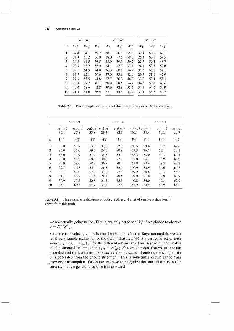
74 OFFLINE LEARNING
ω = ω1
n Wn1 Wn
2 Wn3
1 37.4 64.1 59.22 24.3 65.2 56.03 30.5 64.5 56.54 20.5 63.2 55.95 29.1 64.5 44.86 36.7 62.1 59.67 27.3 53.5 44.88 26.8 57.7 48.19 40.0 58.6 42.8
10 21.4 51.6 56.4
ω = ω2
Wn1 Wn
2 Wn3
38.1 66.9 55.728.0 57.6 59.338.9 59.3 50.234.1 57.7 57.136.3 60.1 56.437.0 53.6 42.927.7 60.9 48.928.8 68.6 54.439.6 52.8 53.533.1 54.5 42.7
ω = ω3
Wn1 Wn
2 Wn3
33.4 66.5 40.125.4 60.1 59.522.7 59.5 48.724.1 59.8 58.837.3 65.1 57.120.7 51.8 42.932.0 53.4 53.334.3 53.0 48.631.1 64.0 59.933.4 56.7 42.7
Table 3.1 Three sample realizations of three alternatives over 10 observations.
ω = ω1
µ1(ω1) µ2(ω1) µ3(ω1)32.1 57.8 55.8
n Wn1 Wn
2 Wn3
1 33.8 57.7 53.32 37.0 55.0 59.73 36.0 54.9 51.94 30.8 53.3 58.65 30.9 58.6 58.36 29.7 56.3 55.67 32.1 57.0 57.98 31.1 53.9 54.49 35.9 55.5 50.8
10 35.4 60.5 54.7
ω = ω2
µ1(ω2) µ2(ω2) µ3(ω2)29.5 62.3 60.1
Wn1 Wn
2 Wn3
32.6 62.7 60.526.0 60.8 55.334.3 65.0 58.330.0 57.7 57.830.7 59.4 61.026.3 62.4 60.931.6 57.8 59.929.1 59.6 59.031.5 65.9 60.833.7 62.4 55.9
ω = ω3
µ1(ω3) µ2(ω3) µ3(ω3)34.4 59.2 59.7
Wn1 Wn
2 Wn3
29.6 55.7 62.636.8 62.1 59.138.0 60.3 60.436.1 59.9 63.238.6 58.3 63.233.9 54.6 64.530.8 63.3 55.331.6 58.9 60.836.0 62.3 62.938.9 54.9 64.2
Table 3.2 Three sample realizations of both a truth µ and a set of sample realizations Wdrawn from this truth.
we are actually going to see. That is, we only get to see Wnx if we choose to observe
x = Xπ(Sn).
Since the true values µx are also random variables (in our Bayesian model), we canlet ψ be a sample realization of the truth. That is, µ(ψ) is a particular set of truthvalues µx1(ψ), ..., µxM (ψ) for the different alternatives. Our Bayesian model makesthe fundamental assumption that µx ∼ N (µ0
x, β0x), which means that we assume our
prior distribution is assumed to be accurate on average. Therefore, the sample pathψ is generated from the prior distribution. This is sometimes known as the truthfrom prior assumption. Of course, we have to recognize that our prior may not beaccurate, but we generally assume it is unbiased.
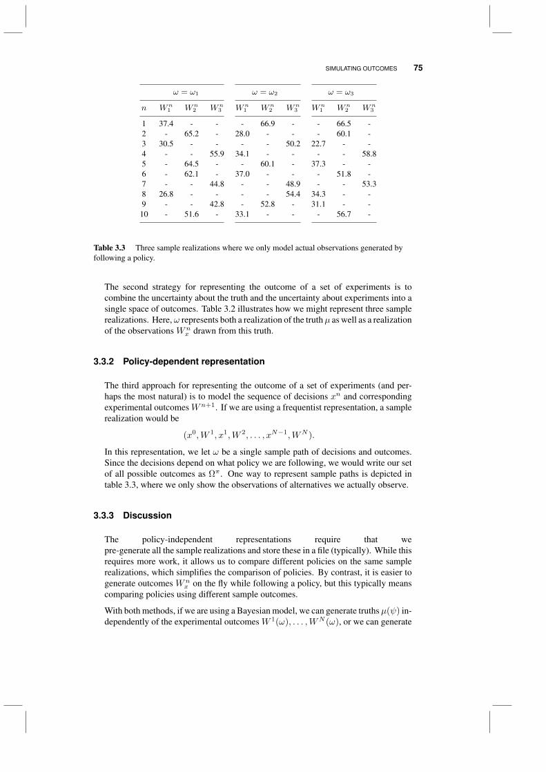
SIMULATING OUTCOMES 75
ω = ω1
n Wn1 Wn
2 Wn3
1 37.4 - -2 - 65.2 -3 30.5 - -4 - - 55.95 - 64.5 -6 - 62.1 -7 - - 44.88 26.8 - -9 - - 42.810 - 51.6 -
ω = ω2
Wn1 Wn
2 Wn3
- 66.9 -28.0 - -
- - 50.234.1 - -
- 60.1 -37.0 - -
- - 48.9- - 54.4- 52.8 -
33.1 - -
ω = ω3
Wn1 Wn
2 Wn3
- 66.5 -- 60.1 -
22.7 - -- - 58.8
37.3 - -- 51.8 -- - 53.3
34.3 - -31.1 - -
- 56.7 -
Table 3.3 Three sample realizations where we only model actual observations generated byfollowing a policy.
The second strategy for representing the outcome of a set of experiments is tocombine the uncertainty about the truth and the uncertainty about experiments into asingle space of outcomes. Table 3.2 illustrates how we might represent three samplerealizations. Here, ω represents both a realization of the truthµ as well as a realizationof the observations Wn
x drawn from this truth.
3.3.2 Policy-dependent representation
The third approach for representing the outcome of a set of experiments (and per-haps the most natural) is to model the sequence of decisions xn and correspondingexperimental outcomesWn+1. If we are using a frequentist representation, a samplerealization would be
(x0,W 1, x1,W 2, . . . , xN−1,WN ).
In this representation, we let ω be a single sample path of decisions and outcomes.Since the decisions depend on what policy we are following, we would write our setof all possible outcomes as Ωπ . One way to represent sample paths is depicted intable 3.3, where we only show the observations of alternatives we actually observe.
3.3.3 Discussion
The policy-independent representations require that wepre-generate all the sample realizations and store these in a file (typically). While thisrequires more work, it allows us to compare different policies on the same samplerealizations, which simplifies the comparison of policies. By contrast, it is easier togenerate outcomes Wn
x on the fly while following a policy, but this typically meanscomparing policies using different sample outcomes.
With both methods, if we are using a Bayesian model, we can generate truths µ(ψ) in-dependently of the experimental outcomes W 1(ω), . . . ,WN (ω), or we can generate
76 OFFLINE LEARNING
them simultaneously, creating a single sample realization (µ(ω),W 1(ω), . . . ,WN (ω).For the same number of simulations, the latter approach will produce a better mixtureof truths and experimental outcomes.
If we are using a frequentist belief model, we skip the sampling of a truth. Instead,we have to sample the experimental outcomes W from an assumed distribution.
3.4 EVALUATING POLICIES
We now want to estimate the performance of policy Xπ(S). Our challenge is toevaluate a policy which we might do using our Bayesian objective (equation (3.9))given by
Fπ = EµEW 1,...,WN |µµxπ,N .
The problem is that we cannot actually compute these expectations. For this reason,we have to use Monte Carlo simulation to approximate the value of a policy.
Recall that xπ,N is the best decision based on our final estimates µπ,Nx computedwhen we follow policyπwith an experimental budget ofN observations (see equation(3.5)). We refine this notation by indexing it by the sample truth and the sample ofobservations, which gives us
xπ,Nx (ψ, ω) = The optimal decision based on the estimates µπ,Nx for each al-ternative x when the truth is µ(ψ) and the observations areW 1(ω), . . . ,WN (ω).
There are two ways we can evaluate the performance of a policy. The first is basedpurely on the actual estimates of the value of each alternative. Let
µπ,Nx (ψ, ω) = The estimate of µx if µx(ψ) is the true value of µ, we observeW (ω)while following policy Xπ(S) with a budget N .
Remember that each observation Wnx (ω) is generated using
Wn+1xn (ω) = µxn(ψ) + εn+1(ω)
for a given truth µx(ω). With this, we finally can compute a sample realization ofthe value of a policy using
Fπ(µ(ψ),W (ω)) = maxx∈X
µπ,Nx (ψ, ω)
= µπ,Nxπ,N (ψ,ω)
(ψ, ω). (3.19)
Equation (3.19) is simply using our final estimate of each µx to evaluate how wellthe policy has performed. Naturally, we need to average over different truths µ(ψ)and sample observations W 1(ω), . . . ,WN (ω). If we sample L truths µ(ψ`) andK experiments W 1(ωk), . . . ,WN (ωk), then we can compute an estimate of theperformance of the policy using
Fπ
=1
L
L∑`=1
(1
K
K∑k=1
Fπ(µ(ψ`),W (ωk))
). (3.20)
HANDLING COMPLEX DYNAMICS 77
We can also use the representation illustrated in table 3.2 where we sample the truthµ and the outcomes W 1, . . . ,WN simultaneously, rather than in the nested fashionthat we use in our estimate in equation (3.20). In this case, we let µπ,Nx (ω) be theestimate of µx when we sample the combination of truth and experimental outcomes(µ(ω),W 1(ω), . . . ,WN (ω)). We also let xπ,N (ω) be the optimal solution given by
xπ,N (ω) = arg maxx
µπ,Nx (ω).
Using this representation, our estimate of the value of a policy would be written
Fπ
=1
K
K∑k=1
Fπ(µ(ωk),W (ωk)). (3.21)
An important feature of equation (3.20) is that it requires nothing more than sampledobservations that could come from any field source. However, it is often the case thatwe are using simulations to evaluate and compare policies that would then be used inthe field. When we are simulating a policy, we do this using a simulated truth µ(ψ).When this is the case, then we can evaluate the policy using the actual truth, equation(3.19) becomes
Fπ(µ(ψ),W (ω)) = maxx∈X
µx(ψ, ω)
= µxπ,N (ψ,ω)(ψ, ω). (3.22)
We then use this method for computing Fπ(µ(ψ),W (ω)) in equation (3.20). Equa-tion (3.22) avoids the noise inherent when using the estimates µπ,N
xπ,N (ψ,ω)(ψ, ω).
A particularly powerful idea is to compute what is known variously as the opportunitycost or the regret which calculates how much worse we are doing than the optimalsolution. Using our ability to use the known truth (because we are simulating it), wecan find the difference between how well we do using our estimates to find the best,and what is truly the best. This is given by
Rπ =1
L
L∑`=1
(1
K
K∑k=1
(µx∗(ψ)− µxπ(µ(ψ`),W (ωk)) (ψ)
)). (3.23)
where µx∗(ψ) = maxx µx(ψ) is the best we can do for a particular truth. The regrethas a lower bound of zero, which provides a nice reference point.
There are other ways to evaluate a policy which we discuss in greater depth in chapter6. However, most of the time we will use either the expected performance or, quitefrequently, the opportunity cost (or regret).
We suggest that the best environment for identifying good learning policies is insidethe computer, where you can assume a truth and then try to discover the truth. Onceyou have decided on a good learning policy, you can go to the field where the truthis unknown, and you only have access to the estimates µπ,Nx .
3.5 HANDLING COMPLEX DYNAMICS
It is useful to note that the process of evaluating policies is quite robust to theunderlying dynamics or choice of belief model. For example, in chapter 2 we
78 OFFLINE LEARNING
introduced updating equations if we have correlated beliefs. Our process of simulatingpolicies is quite robust to the introduction of correlated beliefs, or more complexinformation processes.
To see this, imagine that we have a current belief state Sn = (µn,Σn) where µn is avector with element µnx (as we have assumed above), and where Σn is our estimateof the covariance matrix in our beliefs, with element
Σxx′ = Covn(µx, µx′).
This is the covariance in our belief about the truths µx and µx′ after we have observedW 1, . . . ,Wn. After choosing xn and observingWn+1, we can then use the updatingequations for correlated beliefs (see section 2.3.2) to produce updated estimates µn+1
and Σn+1.
Similarly, our information process W may have its own complex dynamics. Forexample, we might use a time series equation of the form
Wn+1 = θ0Wn + θ1W
n−1 + θ2Wn−2.
Incorporating more complex time series models that depend on trailing observationsdoes not affect our process of testing and comparing policies.
3.6 EQUIVALENCE OF USING TRUE MEANS AND SAMPLE ESTIMATES*
It turns out that our evaluation of the policy using sampled estimates, given in equation(3.19), is the same (on average) as that computed using the real truth, given in equation(3.22). This result means that
EµEW 1,...,WN |µµxπ = EµEW 1,...,WN |µ maxx
µπ,Nx . (3.24)
Below, we are going to use E instead of the nested EµEW 1,...,WN |µ. When usingthe single expectation operator, it is easiest to think of this as using the combinedsampling of both the truth and the outcomes as we illustrated in table 3.2.
To demonstrate equation (3.24), recall that ENµx = µπ,Nx for any fixed x. We usethe tower property of conditional expectation, which simply means that we can nestexpectations. For example, imagine that we have random variablesA andB, Assumethat the expectation E refers to taking the expectation over the combination of A andB, which we might write as EA,B . The tower property can be written
EX = EA,BX = EAEB|AX.
For our problem, we can think of the truth µ as the random variable A, and then letthe sequence W 1, . . . ,WN be the random variable B. The tower property allows usto write
Eµxπ = EµEW 1,...,WN |µµxπ = Eµπ,Nxπ ,
because xπ = arg maxx µπ,Nx is known at time N (that is, it is fixed from the point
of view of our time-N beliefs). However, µπ,Nxπ = maxx µπ,Nx by definition of xπ .
TUNING POLICIES 79
There is an interesting corollary to this result. Denote by χ an “implementationpolicy” for selecting an alternative at time N . We can think of χ as a functionmapping the belief state SN to an alternative χ(Sn) ∈ x1, ..., xM. Then,
maxχ
Eµχ(SN ) = maxx
µπ,Nx .
In other words, the optimal decision at time N is always to select µπ,Nx . If we haveno more opportunities to learn, the best possible decision we can make is to go withour final set of beliefs. This result addresses the issue of why most of our policiesseek to maximize maxx µ
π,Nx in some way, even though what we really want to learn
is the unknown true value maxx µx.
3.7 TUNING POLICIES
Most heuristic policies have a tunable parameter. Perhaps the simplest illustration isthe interval estimation policy, which we restate for easy reference as
XIE(Sn|θIE) = arg maxx
(µnx + θIEσnx
).
We now have the problem of tuning θIE so that the policy performs at its best. Whenworking with a specific policy such as interval estimation, the problem of searchingover policies π becomes one of searching over values of θIE .
We generally assume that we are tuning a policy using a simulator, which means thatwe can evaluate our policy using the actual (simulated) truth as we did in equation(3.22). Instead of writing the performance of the policy as F
π, we can write it as
F (θIE). Now we can write our tuning problem as
maxθIE
F (θIE).
It should not be lost on us that the problem of designing a good policy for learning isitself a learning problem. An important difference between our tuning problem andthe learning problem that we really want to solve is that we assume that we are usinga fairly fast simulator to evaluate a policy.
If we do very accurate simulations, we can treat F (θIE) as if it were deterministicand unimodular (which means it has a single maximum), which makes it fairly easyto search. In chapter 10, we review a number of methods for efficiently searching forthe maximum of a scalar function, even when the simulations are noisy.
Often, the problem of tuning a policy involves performing a one-dimensional searchto find the best value of a single parameter such as θIE . In some settings (intervalestimation is one of them) we have a rough idea of the magnitude of the tunableparameter. In the case of interval estimation, θIE is unitless, so we know it is on theorder of 1, but might be 0.1 or perhaps as large as 10. However, the tunable parameterfor the Boltzmann policy has units, and as a result might be anywhere from 10−5 to105. For this reason, it is a good idea to first search across orders of magnitude, andthen refine the search over smaller ranges.

80 OFFLINE LEARNING
To appreciate the importance of tuning, we tuned two policies on a library of nineproblems. The first policy was interval estimation, while the second is a class ofupper confidence bounding policy called UCB-E, which is given by
XUCBE,n(θUCBE) = arg maxx
(µnx +
√θUCBE
Nnx
). (3.25)
whereNnx is the number of times we have observed alternative x. We note that while
the tunable parameter θIE is unitless, the parameter for the UCBE policy, θUCBE , isnot.
Table 3.4 shows the tuned values of these parameters for each of nine test problems.We see that the variation in θIE , which ranges from 10 to 10−2, is much narrower thanthe variation of θUCBE , which ranges from 103 to 10−4. We also note that tuningmatters; the performance of a policy can vary quite a bit as the tunable parameter isadjusted.
Problem class IE UCBE
P1 0.0994 2571P2 0.0150 0.319P3 0.0187 1.591P4 0.0109 6.835P5 0.2694 .00036P6 1.1970 1.329P7 0.8991 21.21P8 0.9989 0.00016P9 0.2086 0.001476
Table 3.4 Illustration of tuned parameters for interval estimation (IE) and the UCB policyUCB-E over nine different problems.
We are going to assume that we always have access to a simulator for the purpose oftuning our policy. However, this presumes that our simulator captures the behaviorof the real environment in which we are doing learning. Needless to say, this willintroduce errors.
There are settings where simulators are simply not available. This means that wehave to do tuning in the field, in the same expensive environment where we also haveto do learning. As of this writing, policy tuning in the field remains an open researchquestion.
3.8 EXTENSIONS OF THE RANKING AND SELECTION PROBLEM
Our basic ranking and selection problem, characterized by a discrete set of alternativesX = x1, . . . , xM and a lookup table belief model, can be extended in a number ofways to produce an almost unlimited number of problem variations. Below we listsome of the more popular variations.
EXTENSIONS OF THE RANKING AND SELECTION PROBLEM 81
Decisions There are a number of different characterizations of decisions:
• Binary X = 0, 1, which arises in A/B testing of websites (old versus new),or stopping problems (continue/stop).
• Finite set, where X = x1, . . . , xM, which is the setting we have focused onabove.
• Subsets, where we haveK items (such as members of a basketball team), wherewe have to choose 5 players. If K = 10, some elements of our set might looklike:
(0, 1, 1, 0, 0, 1, 0, 1, 1, 0)
(0, 1, 0, 0, 0, 1, 1, 0, 1, 0)
(1, 0, 1, 0, 0, 1, 0, 1, 0, 1)
(0, 0, 1, 1, 0, 0, 1, 1, 1, 0)
(1, 0, 1, 0, 1, 1, 0, 0, 1, 0)
The distinguishing feature of subset selection problems is that the number ofalternatives may be extremely large.
• Continuous scalar, as in X = [a, b]. This might describe the price of a product,concentration of an additive or dosage of a drug.
• Vector-valued continuous, which we might write as x = (x1, . . . , xK) whereeach xk is a continuous scalar.
• Vector valued discrete, where each xk has to be 0 or 1. This is similar tothe subset selection problem, except that it may be limited by more complexconstraints.
• Multiattribute. We might be choosing among people, who are each charac-terized by a number of attributes (gender, age, weight, ethnicity, education).Alternative, we might need to choose to target a particular population for anad campaign, where a population group might be characterized by country orregion, the device they are using (laptop or smartphone), their gender and age.The number of attributes can be quite large, but we might be able to exploit ahierarchical structure.
Types of noise Above we assumed that our random noiseW was normally distributed, butwe have a library of distributions to choose from, including
Unknown distribution - We may start with the realization that we simply do notknow the distribution. For example, we may not even know if the proper dosageis .01mg, .1, mg, 1 mg, 10 mg.
Binomial - This might describe settings where the outcome is a success or failure,or whether a drug is judged to be a success (allowing us to go to market) or not.
Exponential family - This includes a number of distributions such as normal, ex-ponential, log-normal, gamma, chi-squared, beta, Bernoulli, Poisson, and geo-metric.
Uniform distributions - We may know that a random variable is bounded. Forexample, the energy generated by a 2mw wind turbine may be reasonablyapproximated as a uniform distribution between 0 and 2mw.

82 OFFLINE LEARNING
Heavy-tailed distributions - This might include the Cauchy distribution (which hasinfinite variance) or spikes, as occurs with electricity prices, which can jumpfrom $20 per megawatt-hour to $300 per mwh in a matter of minutes, and thendrop back.
Mixture distributions - We randomly choose an observation from one of two dis-tributions, one with a relatively smaller variance, and one with an extremelyhigh variance.
Bursts - Bursts can arise when the wind rises during a storm, a product brieflybecomes popular through word of mouth, or a disease pops up and spreadsbefore it is contained.
Rare events - These are events that may occur and which we have to prepare for,even though it is quite rare. Examples include major floods, a tree falling onyour house, or being robbed.
Offline vs. online learning In this chapter we have considered only offline learning, wherewe are only interested in the performance of the decision after all experiments havebeen conducted. In chapter 5 we make the transition to online learning, where wewish to maximize the cumulative rewards that arise while we are learning. Thesetwo problem classes have evolved since the 1950’s in very distinct communities, butare actually quite closely related.
Experimentation costs and budgets There are settings in the internet where we can trydifferent alternatives quite quickly, often making it possible to consider very highdimensional choice problems (such as which movies to display on a users account).There are many other settings where experiments are quite expensive, sharply limitingthe number of experiments. For example, a scientist may be able to test 20 or 30compounds over the course of a summer before his budget runs out. A businessmight want to test market features of a product, but it may require several months toobserve sales. A patient may require a month before we know how she responds toa new diabetes medication.
Switching cost It may be easy to switch from one design x to another x′, as an internetretailer might do when testing different prices for a product. There are many settings,however, where there is a switching cost. For example, we may be taking samplesfrom people to test for the presence of a disease in a location. Moving to anotherlocation involves a switching cost.
Transient performance We have assumed that the underlying truth µ is unknown butconstant. However, the market response to a price may change as a result of decisionsmade by competitors; the performance of an athlete may improve as he gets moreplaying time; and the impact of a drug may drop as a disease acquires immunity.
Transient alternatives A standard assumption is that the set of alternatives X is static,but even this is not always the case. We can only try a restaurant if we can get areservation; we can only learn about the performance of a storm sensor if there is astorm; and we can only test the efficacy of a drug for a particular medical conditionif we can find a patient that meets our criteria.
Belief models We have illustrated our learning with a lookup table belief model, but thesebecome clumsy when the number of alternatives is very large (or continuous). Laterwe are going to consider other classes of linear and nonlinear models.
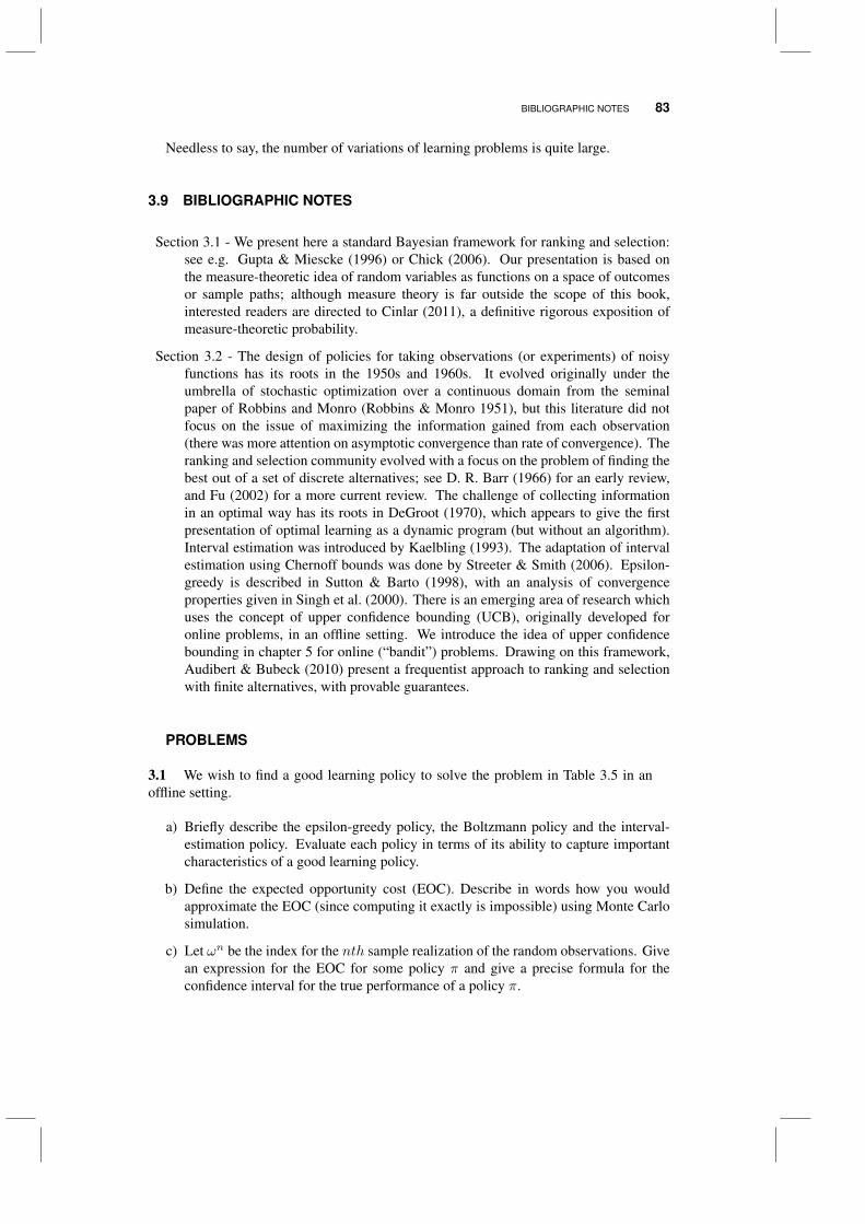
BIBLIOGRAPHIC NOTES 83
Needless to say, the number of variations of learning problems is quite large.
3.9 BIBLIOGRAPHIC NOTES
Section 3.1 - We present here a standard Bayesian framework for ranking and selection:see e.g. Gupta & Miescke (1996) or Chick (2006). Our presentation is based onthe measure-theoretic idea of random variables as functions on a space of outcomesor sample paths; although measure theory is far outside the scope of this book,interested readers are directed to Cinlar (2011), a definitive rigorous exposition ofmeasure-theoretic probability.
Section 3.2 - The design of policies for taking observations (or experiments) of noisyfunctions has its roots in the 1950s and 1960s. It evolved originally under theumbrella of stochastic optimization over a continuous domain from the seminalpaper of Robbins and Monro (Robbins & Monro 1951), but this literature did notfocus on the issue of maximizing the information gained from each observation(there was more attention on asymptotic convergence than rate of convergence). Theranking and selection community evolved with a focus on the problem of finding thebest out of a set of discrete alternatives; see D. R. Barr (1966) for an early review,and Fu (2002) for a more current review. The challenge of collecting informationin an optimal way has its roots in DeGroot (1970), which appears to give the firstpresentation of optimal learning as a dynamic program (but without an algorithm).Interval estimation was introduced by Kaelbling (1993). The adaptation of intervalestimation using Chernoff bounds was done by Streeter & Smith (2006). Epsilon-greedy is described in Sutton & Barto (1998), with an analysis of convergenceproperties given in Singh et al. (2000). There is an emerging area of research whichuses the concept of upper confidence bounding (UCB), originally developed foronline problems, in an offline setting. We introduce the idea of upper confidencebounding in chapter 5 for online (“bandit”) problems. Drawing on this framework,Audibert & Bubeck (2010) present a frequentist approach to ranking and selectionwith finite alternatives, with provable guarantees.
PROBLEMS
3.1 We wish to find a good learning policy to solve the problem in Table 3.5 in anoffline setting.
a) Briefly describe the epsilon-greedy policy, the Boltzmann policy and the interval-estimation policy. Evaluate each policy in terms of its ability to capture importantcharacteristics of a good learning policy.
b) Define the expected opportunity cost (EOC). Describe in words how you wouldapproximate the EOC (since computing it exactly is impossible) using Monte Carlosimulation.
c) Let ωn be the index for the nth sample realization of the random observations. Givean expression for the EOC for some policy π and give a precise formula for theconfidence interval for the true performance of a policy π.
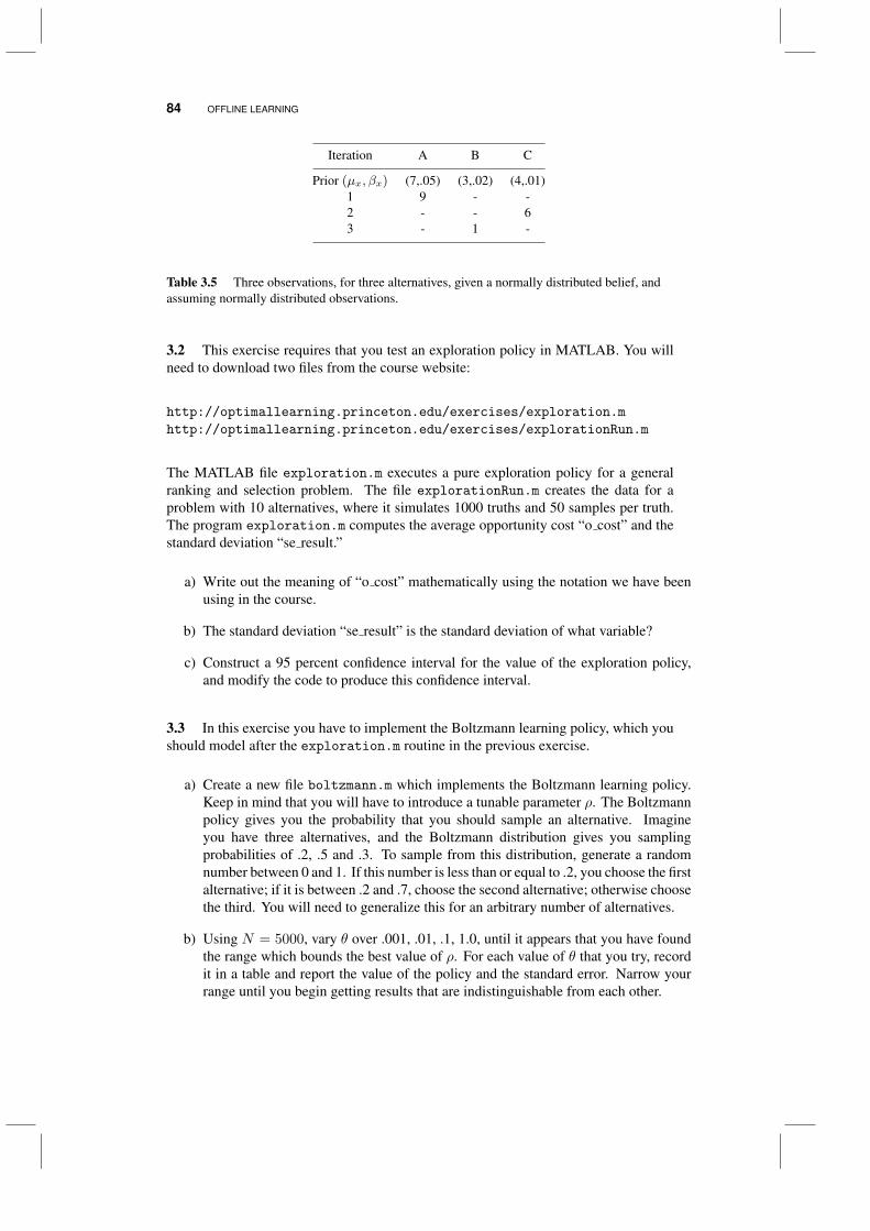
84 OFFLINE LEARNING
Iteration A B C
Prior (µx, βx) (7,.05) (3,.02) (4,.01)1 9 - -2 - - 63 - 1 -
Table 3.5 Three observations, for three alternatives, given a normally distributed belief, andassuming normally distributed observations.
3.2 This exercise requires that you test an exploration policy in MATLAB. You willneed to download two files from the course website:
http://optimallearning.princeton.edu/exercises/exploration.m
http://optimallearning.princeton.edu/exercises/explorationRun.m
The MATLAB file exploration.m executes a pure exploration policy for a generalranking and selection problem. The file explorationRun.m creates the data for aproblem with 10 alternatives, where it simulates 1000 truths and 50 samples per truth.The program exploration.m computes the average opportunity cost “o cost” and thestandard deviation “se result.”
a) Write out the meaning of “o cost” mathematically using the notation we have beenusing in the course.
b) The standard deviation “se result” is the standard deviation of what variable?
c) Construct a 95 percent confidence interval for the value of the exploration policy,and modify the code to produce this confidence interval.
3.3 In this exercise you have to implement the Boltzmann learning policy, which youshould model after the exploration.m routine in the previous exercise.
a) Create a new file boltzmann.m which implements the Boltzmann learning policy.Keep in mind that you will have to introduce a tunable parameter ρ. The Boltzmannpolicy gives you the probability that you should sample an alternative. Imagineyou have three alternatives, and the Boltzmann distribution gives you samplingprobabilities of .2, .5 and .3. To sample from this distribution, generate a randomnumber between 0 and 1. If this number is less than or equal to .2, you choose the firstalternative; if it is between .2 and .7, choose the second alternative; otherwise choosethe third. You will need to generalize this for an arbitrary number of alternatives.
b) Using N = 5000, vary θ over .001, .01, .1, 1.0, until it appears that you have foundthe range which bounds the best value of ρ. For each value of θ that you try, recordit in a table and report the value of the policy and the standard error. Narrow yourrange until you begin getting results that are indistinguishable from each other.
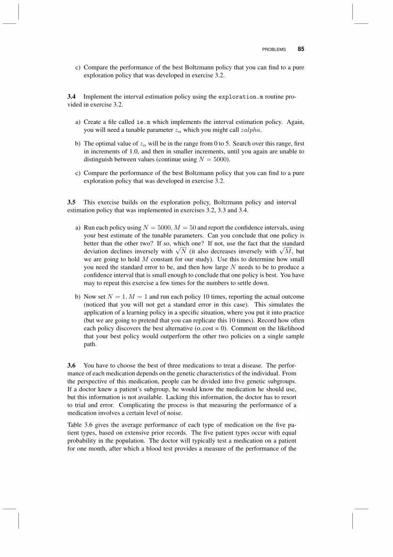
PROBLEMS 85
c) Compare the performance of the best Boltzmann policy that you can find to a pureexploration policy that was developed in exercise 3.2.
3.4 Implement the interval estimation policy using the exploration.m routine pro-vided in exercise 3.2.
a) Create a file called ie.m which implements the interval estimation policy. Again,you will need a tunable parameter zα which you might call zalpha.
b) The optimal value of zα will be in the range from 0 to 5. Search over this range, firstin increments of 1.0, and then in smaller increments, until you again are unable todistinguish between values (continue using N = 5000).
c) Compare the performance of the best Boltzmann policy that you can find to a pureexploration policy that was developed in exercise 3.2.
3.5 This exercise builds on the exploration policy, Boltzmann policy and intervalestimation policy that was implemented in exercises 3.2, 3.3 and 3.4.
a) Run each policy usingN = 5000,M = 50 and report the confidence intervals, usingyour best estimate of the tunable parameters. Can you conclude that one policy isbetter than the other two? If so, which one? If not, use the fact that the standarddeviation declines inversely with
√N (it also decreases inversely with
√M , but
we are going to hold M constant for our study). Use this to determine how smallyou need the standard error to be, and then how large N needs to be to produce aconfidence interval that is small enough to conclude that one policy is best. You havemay to repeat this exercise a few times for the numbers to settle down.
b) Now set N = 1,M = 1 and run each policy 10 times, reporting the actual outcome(noticed that you will not get a standard error in this case). This simulates theapplication of a learning policy in a specific situation, where you put it into practice(but we are going to pretend that you can replicate this 10 times). Record how ofteneach policy discovers the best alternative (o cost = 0). Comment on the likelihoodthat your best policy would outperform the other two policies on a single samplepath.
3.6 You have to choose the best of three medications to treat a disease. The perfor-mance of each medication depends on the genetic characteristics of the individual. Fromthe perspective of this medication, people can be divided into five genetic subgroups.If a doctor knew a patient’s subgroup, he would know the medication he should use,but this information is not available. Lacking this information, the doctor has to resortto trial and error. Complicating the process is that measuring the performance of amedication involves a certain level of noise.
Table 3.6 gives the average performance of each type of medication on the five pa-tient types, based on extensive prior records. The five patient types occur with equalprobability in the population. The doctor will typically test a medication on a patientfor one month, after which a blood test provides a measure of the performance of the

86 OFFLINE LEARNING
medication. But these experiments are not precise; the error between the experimentand the actual impact of the medication is normally distributed with a standard deviationof 2.2 (we assume this is constant for all medications and patient types).
Patient type
Medication A B C D E
M1 6.2 7.3 5.4 7.2 5.4M2 8.4 6.9 6.8 6.6 4.2M3 5.2 5.8 6.3 5.5 3.7
Table 3.6 The performance of each type of medication for each type of patient.
a) What is the prior vector µ0 that you would use for this problem, given the data in thetable?
b) What is your prior probability distribution for the performance of medication M1?Note: It is not normally distributed.
c) Test each of the following policies below. You may use the MATLAB routinesdeveloped in the previous exercises, or perform the exercise manually with a budgetof N = 10 observations. If you are using the MATLAB routines, use a budget ofN = 50 observations.
1) Pure exploitation.
2) Boltzmann exploration, using scaling factor ρ = 1.
3) Epsilon-greedy exploration, where the exploration probability is given by 1/n.
4) Interval estimation. Test the performance of zα = 1.0, 2.0, 3.0 and 4.0 andselect the one that performs the best.
For each policy, report the average performance based on 100 trials, and compute a95 percent confidence interval.

CHAPTER 4
VALUE OF INFORMATION POLICIES
An important class of problems are those where experiments are expensive, and as aresult the budget for the number of experiments is relatively small. For now, we aregoing to stay with the same types of problems we addressed in chapter 3, which isto say that we have a not-too-large set of discrete alternatives, described by a lookuptable belief model. However, now we are going to assume that are experimentsare expensive, which translates to relatively small budgets, which may be smaller(sometimes much smaller) than the number of alternatives.
At the same time, we are going to relax what are sometimes strict conditions onhow much time we have to determine what to do next. In internet applications, wemay have 50 milliseconds to determine what to do next. In the context of expensivedecisions, we are not going to object to decision rules that might take seconds orminutes (or more) to compute.
Examples of expensive experiments include
• We may drill a well to evaluate the potential of the underground geology for producingoil or gas.
• We may need to observe a patient taking a new drug for several weeks to see howher body responds to the medication.
• A business may need to observe the sales of a product over a period of several weeksto evaluate the market response to a price.
Optimal Learning. By Warren B. Powell and Ilya O. RyzhovCopyright c© 2018 John Wiley & Sons, Inc.
87
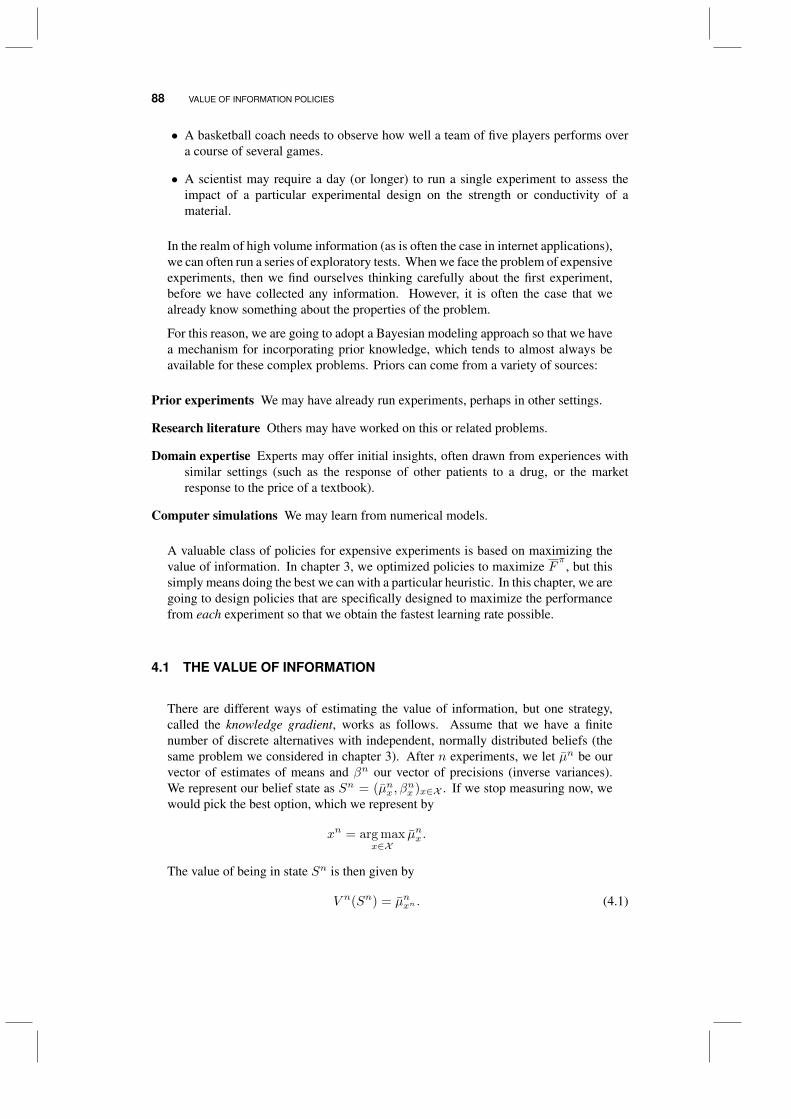
88 VALUE OF INFORMATION POLICIES
• A basketball coach needs to observe how well a team of five players performs overa course of several games.
• A scientist may require a day (or longer) to run a single experiment to assess theimpact of a particular experimental design on the strength or conductivity of amaterial.
In the realm of high volume information (as is often the case in internet applications),we can often run a series of exploratory tests. When we face the problem of expensiveexperiments, then we find ourselves thinking carefully about the first experiment,before we have collected any information. However, it is often the case that wealready know something about the properties of the problem.
For this reason, we are going to adopt a Bayesian modeling approach so that we havea mechanism for incorporating prior knowledge, which tends to almost always beavailable for these complex problems. Priors can come from a variety of sources:
Prior experiments We may have already run experiments, perhaps in other settings.
Research literature Others may have worked on this or related problems.
Domain expertise Experts may offer initial insights, often drawn from experiences withsimilar settings (such as the response of other patients to a drug, or the marketresponse to the price of a textbook).
Computer simulations We may learn from numerical models.
A valuable class of policies for expensive experiments is based on maximizing thevalue of information. In chapter 3, we optimized policies to maximize F
π, but this
simply means doing the best we can with a particular heuristic. In this chapter, we aregoing to design policies that are specifically designed to maximize the performancefrom each experiment so that we obtain the fastest learning rate possible.
4.1 THE VALUE OF INFORMATION
There are different ways of estimating the value of information, but one strategy,called the knowledge gradient, works as follows. Assume that we have a finitenumber of discrete alternatives with independent, normally distributed beliefs (thesame problem we considered in chapter 3). After n experiments, we let µn be ourvector of estimates of means and βn our vector of precisions (inverse variances).We represent our belief state as Sn = (µnx , β
nx )x∈X . If we stop measuring now, we
would pick the best option, which we represent by
xn = arg maxx∈X
µnx .
The value of being in state Sn is then given by
V n(Sn) = µnxn . (4.1)
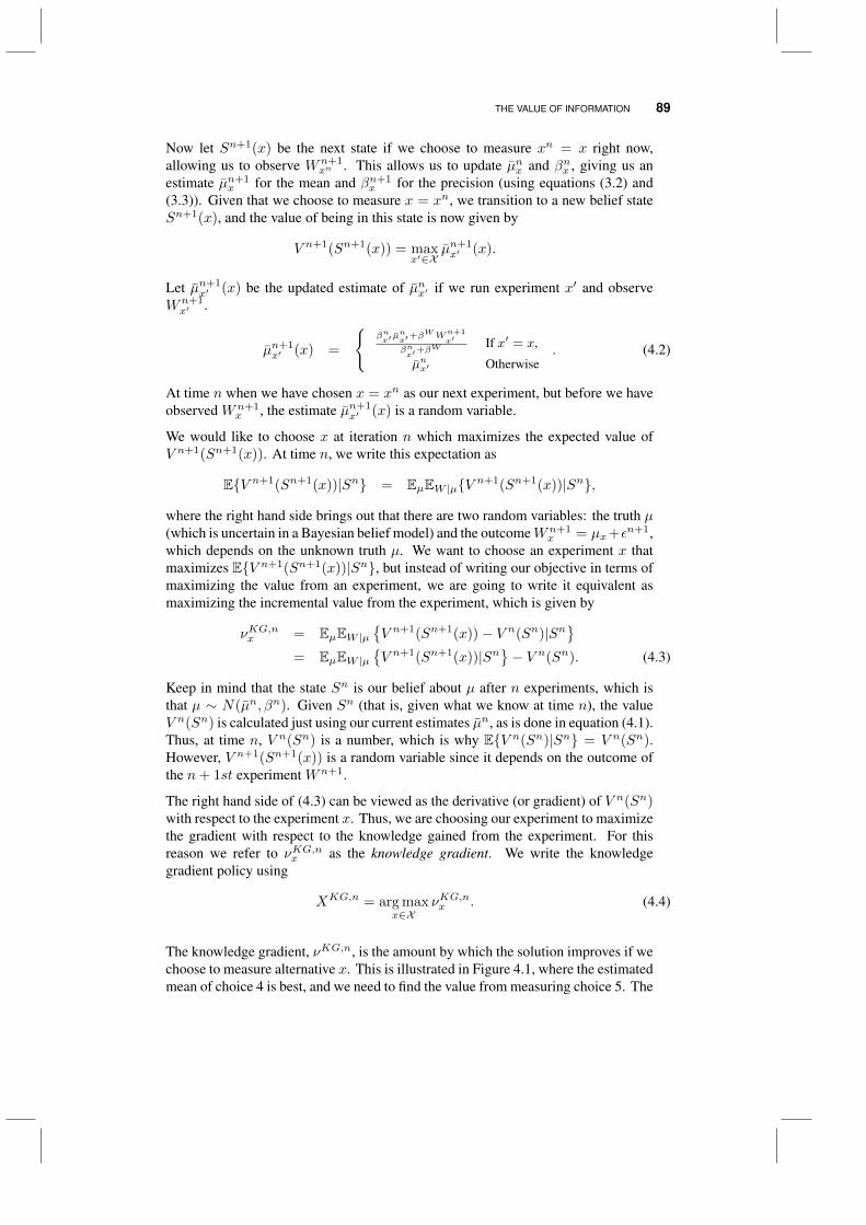
THE VALUE OF INFORMATION 89
Now let Sn+1(x) be the next state if we choose to measure xn = x right now,allowing us to observe Wn+1
xn . This allows us to update µnx and βnx , giving us anestimate µn+1
x for the mean and βn+1x for the precision (using equations (3.2) and
(3.3)). Given that we choose to measure x = xn, we transition to a new belief stateSn+1(x), and the value of being in this state is now given by
V n+1(Sn+1(x)) = maxx′∈X
µn+1x′ (x).
Let µn+1x′ (x) be the updated estimate of µnx′ if we run experiment x′ and observe
Wn+1x′ .
µn+1x′ (x) =
βnx′ µ
nx′+β
WWn+1x′
βnx′+β
W If x′ = x,
µnx′ Otherwise. (4.2)
At time n when we have chosen x = xn as our next experiment, but before we haveobserved Wn+1
x , the estimate µn+1x′ (x) is a random variable.
We would like to choose x at iteration n which maximizes the expected value ofV n+1(Sn+1(x)). At time n, we write this expectation as
EV n+1(Sn+1(x))|Sn = EµEW |µV n+1(Sn+1(x))|Sn,
where the right hand side brings out that there are two random variables: the truth µ(which is uncertain in a Bayesian belief model) and the outcomeWn+1
x = µx+εn+1,which depends on the unknown truth µ. We want to choose an experiment x thatmaximizes EV n+1(Sn+1(x))|Sn, but instead of writing our objective in terms ofmaximizing the value from an experiment, we are going to write it equivalent asmaximizing the incremental value from the experiment, which is given by
νKG,nx = EµEW |µV n+1(Sn+1(x))− V n(Sn)|Sn
= EµEW |µ
V n+1(Sn+1(x))|Sn
− V n(Sn). (4.3)
Keep in mind that the state Sn is our belief about µ after n experiments, which isthat µ ∼ N(µn, βn). Given Sn (that is, given what we know at time n), the valueV n(Sn) is calculated just using our current estimates µn, as is done in equation (4.1).Thus, at time n, V n(Sn) is a number, which is why EV n(Sn)|Sn = V n(Sn).However, V n+1(Sn+1(x)) is a random variable since it depends on the outcome ofthe n+ 1st experiment Wn+1.
The right hand side of (4.3) can be viewed as the derivative (or gradient) of V n(Sn)with respect to the experiment x. Thus, we are choosing our experiment to maximizethe gradient with respect to the knowledge gained from the experiment. For thisreason we refer to νKG,nx as the knowledge gradient. We write the knowledgegradient policy using
XKG,n = arg maxx∈X
νKG,nx . (4.4)
The knowledge gradient, νKG,n, is the amount by which the solution improves if wechoose to measure alternative x. This is illustrated in Figure 4.1, where the estimatedmean of choice 4 is best, and we need to find the value from measuring choice 5. The
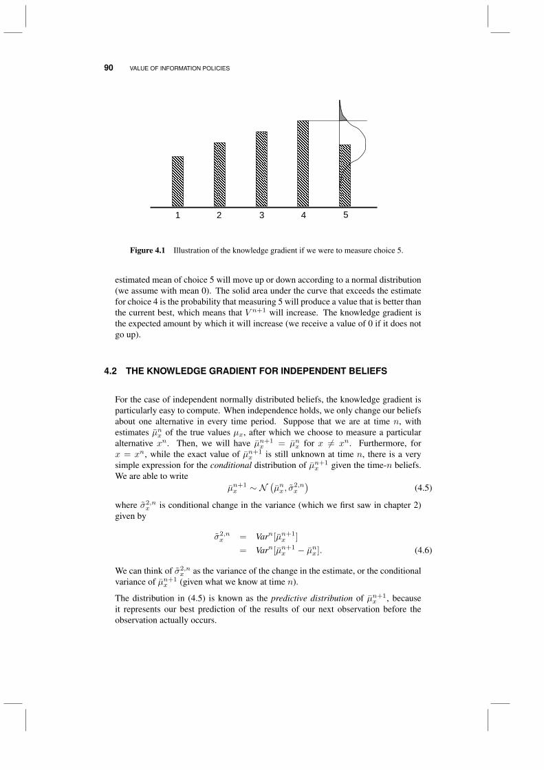
90 VALUE OF INFORMATION POLICIES
1 2 3 4 5
Figure 4.1 Illustration of the knowledge gradient if we were to measure choice 5.
estimated mean of choice 5 will move up or down according to a normal distribution(we assume with mean 0). The solid area under the curve that exceeds the estimatefor choice 4 is the probability that measuring 5 will produce a value that is better thanthe current best, which means that V n+1 will increase. The knowledge gradient isthe expected amount by which it will increase (we receive a value of 0 if it does notgo up).
4.2 THE KNOWLEDGE GRADIENT FOR INDEPENDENT BELIEFS
For the case of independent normally distributed beliefs, the knowledge gradient isparticularly easy to compute. When independence holds, we only change our beliefsabout one alternative in every time period. Suppose that we are at time n, withestimates µnx of the true values µx, after which we choose to measure a particularalternative xn. Then, we will have µn+1
x = µnx for x 6= xn. Furthermore, forx = xn, while the exact value of µn+1
x is still unknown at time n, there is a verysimple expression for the conditional distribution of µn+1
x given the time-n beliefs.We are able to write
µn+1x ∼ N
(µnx , σ
2,nx
)(4.5)
where σ2,nx is conditional change in the variance (which we first saw in chapter 2)
given by
σ2,nx = Varn[µn+1
x ]
= Varn[µn+1x − µnx ]. (4.6)
We can think of σ2,nx as the variance of the change in the estimate, or the conditional
variance of µn+1x (given what we know at time n).
The distribution in (4.5) is known as the predictive distribution of µn+1x , because
it represents our best prediction of the results of our next observation before theobservation actually occurs.
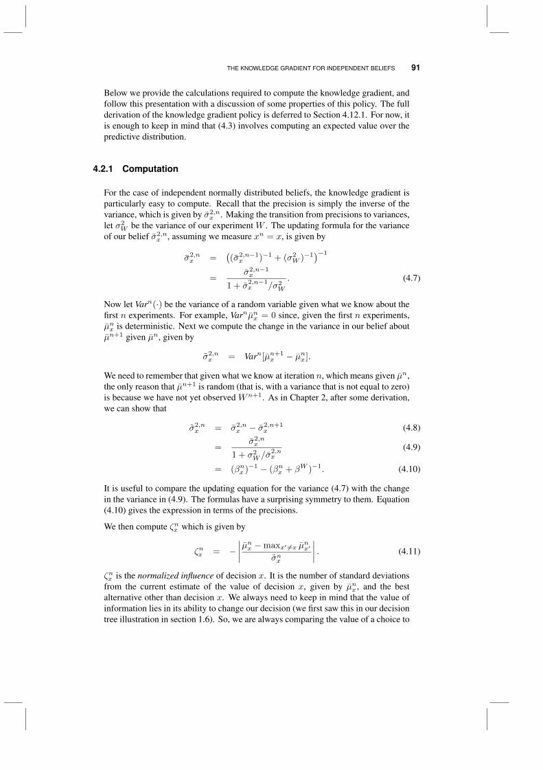
THE KNOWLEDGE GRADIENT FOR INDEPENDENT BELIEFS 91
Below we provide the calculations required to compute the knowledge gradient, andfollow this presentation with a discussion of some properties of this policy. The fullderivation of the knowledge gradient policy is deferred to Section 4.12.1. For now, itis enough to keep in mind that (4.3) involves computing an expected value over thepredictive distribution.
4.2.1 Computation
For the case of independent normally distributed beliefs, the knowledge gradient isparticularly easy to compute. Recall that the precision is simply the inverse of thevariance, which is given by σ2,n
x . Making the transition from precisions to variances,let σ2
W be the variance of our experiment W . The updating formula for the varianceof our belief σ2,n
x , assuming we measure xn = x, is given by
σ2,nx =
((σ2,n−1x )−1 + (σ2
W )−1)−1
=σ2,n−1x
1 + σ2,n−1x /σ2
W
. (4.7)
Now let Varn(·) be the variance of a random variable given what we know about thefirst n experiments. For example, Varnµnx = 0 since, given the first n experiments,µnx is deterministic. Next we compute the change in the variance in our belief aboutµn+1 given µn, given by
σ2,nx = Varn[µn+1
x − µnx ].
We need to remember that given what we know at iteration n, which means given µn,the only reason that µn+1 is random (that is, with a variance that is not equal to zero)is because we have not yet observed Wn+1. As in Chapter 2, after some derivation,we can show that
σ2,nx = σ2,n
x − σ2,n+1x (4.8)
=σ2,nx
1 + σ2W /σ
2,nx
(4.9)
= (βnx )−1 − (βnx + βW )−1. (4.10)
It is useful to compare the updating equation for the variance (4.7) with the changein the variance in (4.9). The formulas have a surprising symmetry to them. Equation(4.10) gives the expression in terms of the precisions.
We then compute ζnx which is given by
ζnx = −∣∣∣∣ µnx −maxx′ 6=x µ
nx′
σnx
∣∣∣∣ . (4.11)
ζnx is the normalized influence of decision x. It is the number of standard deviationsfrom the current estimate of the value of decision x, given by µnx , and the bestalternative other than decision x. We always need to keep in mind that the value ofinformation lies in its ability to change our decision (we first saw this in our decisiontree illustration in section 1.6). So, we are always comparing the value of a choice to
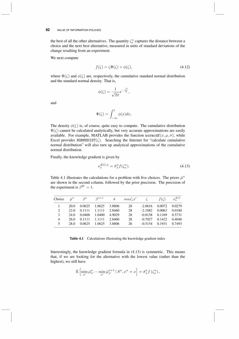
92 VALUE OF INFORMATION POLICIES
the best of all the other alternatives. The quantity ζnx captures the distance between achoice and the next best alternative, measured in units of standard deviations of thechange resulting from an experiment.
We next compute
f(ζ) = ζΦ(ζ) + φ(ζ), (4.12)
where Φ(ζ) and φ(ζ) are, respectively, the cumulative standard normal distributionand the standard normal density. That is,
φ(ζ) =1√2πe−
ζ2
2 ,
and
Φ(ζ) =
∫ ζ
−∞φ(x)dx.
The density φ(ζ) is, of course, quite easy to compute. The cumulative distributionΦ(ζ) cannot be calculated analytically, but very accurate approximations are easilyavailable. For example, MATLAB provides the function normcdf(x, µ, σ), whileExcel provides NORMSDIST(ζ). Searching the Internet for “calculate cumulativenormal distribution” will also turn up analytical approximations of the cumulativenormal distribution.
Finally, the knowledge gradient is given by
νKG,nx = σnxf(ζnx ). (4.13)
Table 4.1 illustrates the calculations for a problem with five choices. The priors µn
are shown in the second column, followed by the prior precision. The precision ofthe experiment is βW = 1.
Choice µn βn βn+1 σ max′xx′ ζ f(ζ) νKGx
1 20.0 0.0625 1.0625 3.8806 28 -2.0616 0.0072 0.02792 22.0 0.1111 1.1111 2.8460 28 -2.1082 0.0063 0.01803 24.0 0.0400 1.0400 4.9029 28 -0.8158 0.1169 0.57314 26.0 0.1111 1.1111 2.8460 28 -0.7027 0.1422 0.40485 28.0 0.0625 1.0625 3.8806 26 -0.5154 0.1931 0.7493
Table 4.1 Calculations illustrating the knowledge gradient index
Interestingly, the knowledge gradient formula in (4.13) is symmetric. This meansthat, if we are looking for the alternative with the lowest value (rather than thehighest), we still have
E[minx′
µnx′ −minx′
µn+1x′ |S
n, xn = x]
= σnxf (ζnx ) ,
THE KNOWLEDGE GRADIENT FOR INDEPENDENT BELIEFS 93
with the only difference being that maxx′ 6=x µnx′ is replaced by minx′ 6=x µ
nx′ in the
definition of ζnx . This symmetry is a consequence of our choice of a Gaussian learningmodel with Gaussian observations. Intuitively, the normal density is symmetricabout its mean, and thus, whether we are looking for the largest or the smallestnormal value, the computation consists of integrating over the tail probability ofsome normal distribution. This does not mean that alternative x has the exact sameKG factor in both cases (we are changing the definition of ζnx ), but it does mean thatthe KG formula retains the same basic form and intuitive interpretation. Later on,we show that this does not hold when the learning model is not Gaussian.
4.2.2 Some properties of the knowledge gradient
Recall that we provided a mathematical framework for an optimal learning policy inSection 3.2.2. It is important to keep in mind that the knowledge gradient policy isnot optimal, in that it is not guaranteed to be the best possible policy for collectinginformation for any budgetN . But for ranking and selection problems, the knowledgegradient policy has some nice properties. These include
• Property 1: The knowledge gradient is always positive, νKG,nx ≥ 0 for all x. Thus,if the knowledge gradient of an alternative is zero, that means we won’t measure it.
• Property 2: The knowledge gradient policy is optimal (by construction) if we aregoing to make exactly one experiment.
• Property 3: If there are only two choices, the knowledge gradient policy is optimalfor any experiment budget N .
• Property 4: If N is our experimental budget, the knowledge gradient policy isguaranteed to find the best alternative as N is allowed to be big enough. That is, ifxN is the solution we obtain after N experiments, and
x∗ = arg maxµx
is the true best alternative, then xN → x∗ as N → ∞. This property is known asasymptotic optimality.
• Property 5: There are many heuristic policies that are asymptotically optimal (for ex-ample, pure exploration, mixed exploration-exploitation, epsilon-greedy explorationand Boltzmann exploration). But none of these heuristic policies is myopically opti-mal. The knowledge gradient policy is the only pure policy (an alternative term wouldbe to say it is the only stationary policy) that is both myopically and asymptoticallyoptimal.
• Property 6: The knowledge gradient has no tunable algorithmic parameters. Heuris-tics such as the Boltzmann policy (θB in equation (3.13)) and interval estimation (θIE
in equation (3.17)) have tunable algorithmic parameters. The knowledge gradienthas no such parameters, but as with all Bayesian methods, assumes we have a prior.Later, we demonstrate settings where we do have to introduce tunable parameters.
The knowledge gradient is not an optimal policy for collecting information, butthese properties suggest that it is generally going to work well. There are situations
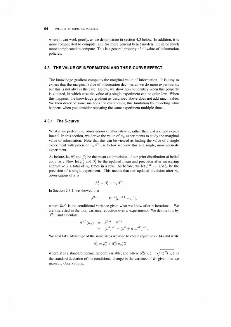
94 VALUE OF INFORMATION POLICIES
where it can work poorly, as we demonstrate in section 4.3 below. In addition, it ismore complicated to compute, and for more general belief models, it can be muchmore complicated to compute. This is a general property of all value-of-informationpolicies.
4.3 THE VALUE OF INFORMATION AND THE S-CURVE EFFECT
The knowledge gradient computes the marginal value of information. It is easy toexpect that the marginal value of information declines as we do more experiments,but this is not always the case. Below, we show how to identify when this propertyis violated, in which case the value of a single experiment can be quite low. Whenthis happens, the knowledge gradient as described above does not add much value.We then describe some methods for overcoming this limitation by modeling whathappens when you consider repeating the same experiment multiple times.
4.3.1 The S-curve
What if we perform nx observations of alternative x, rather than just a single exper-iment? In this section, we derive the value of nx experiments to study the marginalvalue of information. Note that this can be viewed as finding the value of a singleexperiment with precision nxβW , so below we view this as a single, more accurateexperiment.
As before, let µ0x and β0
x be the mean and precision of our prior distribution of beliefabout µx. Now let µ1
x and β1x be the updated mean and precision after measuring
alternative x a total of nx times in a row. As before, we let βW = 1/σ2W be the
precision of a single experiment. This means that our updated precision after nxobservations of x is
β1x = β0
x + nxβW .
In Section 2.3.1, we showed that
σ2,n = Varn[µn+1 − µn],
where Varn is the conditional variance given what we know after n iterations. Weare interested in the total variance reduction over n experiments. We denote this byσ2,0, and calculate
σ2,0(nx) = σ2,0 − σ2,1
= (β0)−1 − (β0 + nxβW )−1.
We next take advantage of the same steps we used to create equation (2.14) and write
µ1x = µ0
x + σ0x(nx)Z
where Z is a standard normal random variable, and where σ0x(nx) =
√σ2,0x (nx) is
the standard deviation of the conditional change in the variance of µ1 given that wemake nx observations.
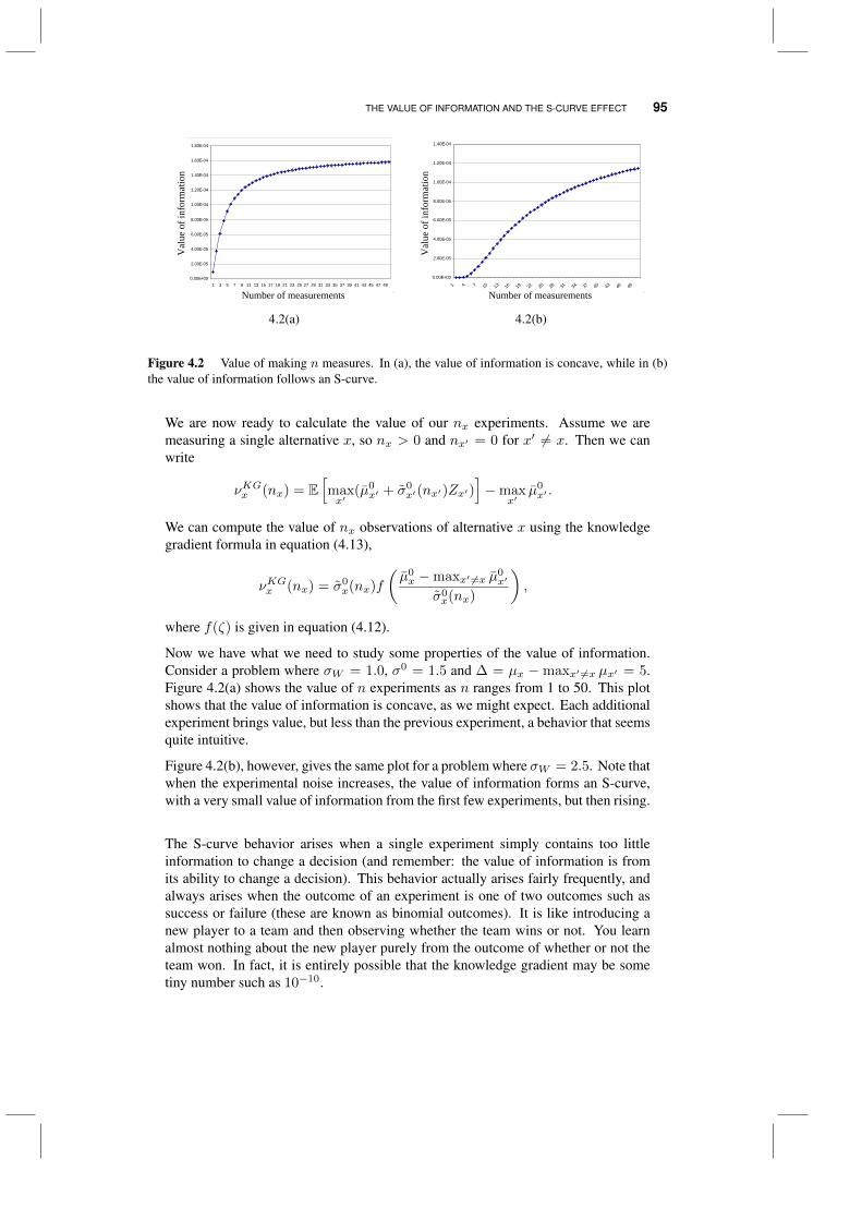
THE VALUE OF INFORMATION AND THE S-CURVE EFFECT 95
0.00E+00
2.00E-05
4.00E-05
6.00E-05
8.00E-05
1.00E-04
1.20E-04
1.40E-04
1.60E-04
1.80E-04
1 3 5 7 9 11 13 15 17 19 21 23 25 27 29 31 33 35 37 39 41 43 45 47 49
Number of measurements
Val
ue o
f inf
orm
atio
n
0.00E+00
2.00E-05
4.00E-05
6.00E-05
8.00E-05
1.00E-04
1.20E-04
1.40E-04
1 4 7 10 13 16 19 22 25 28 31 34 37 40 43 46 49
Number of measurements
Val
ue o
f inf
orm
atio
n
4.2(a) 4.2(b)
Figure 4.2 Value of making n measures. In (a), the value of information is concave, while in (b)the value of information follows an S-curve.
We are now ready to calculate the value of our nx experiments. Assume we aremeasuring a single alternative x, so nx > 0 and nx′ = 0 for x′ 6= x. Then we canwrite
νKGx (nx) = E[maxx′
(µ0x′ + σ0
x′(nx′)Zx′)]−max
x′µ0x′ .
We can compute the value of nx observations of alternative x using the knowledgegradient formula in equation (4.13),
νKGx (nx) = σ0x(nx)f
(µ0x −maxx′ 6=x µ
0x′
σ0x(nx)
),
where f(ζ) is given in equation (4.12).
Now we have what we need to study some properties of the value of information.Consider a problem where σW = 1.0, σ0 = 1.5 and ∆ = µx −maxx′ 6=x µx′ = 5.Figure 4.2(a) shows the value of n experiments as n ranges from 1 to 50. This plotshows that the value of information is concave, as we might expect. Each additionalexperiment brings value, but less than the previous experiment, a behavior that seemsquite intuitive.
Figure 4.2(b), however, gives the same plot for a problem where σW = 2.5. Note thatwhen the experimental noise increases, the value of information forms an S-curve,with a very small value of information from the first few experiments, but then rising.
The S-curve behavior arises when a single experiment simply contains too littleinformation to change a decision (and remember: the value of information is fromits ability to change a decision). This behavior actually arises fairly frequently, andalways arises when the outcome of an experiment is one of two outcomes such assuccess or failure (these are known as binomial outcomes). It is like introducing anew player to a team and then observing whether the team wins or not. You learnalmost nothing about the new player purely from the outcome of whether or not theteam won. In fact, it is entirely possible that the knowledge gradient may be sometiny number such as 10−10.
96 VALUE OF INFORMATION POLICIES
0.00E+00
2.00E-05
4.00E-05
6.00E-05
8.00E-05
1.00E-04
1.20E-04
1.40E-04
1 4 7 10 13 16 19 22 25 28 31 34 37 40 43 46 49
Number of measurements
Val
ue o
f inf
orm
atio
n
*xn
*
*x x
x
v nn
Figure 4.3 The KG(*) policy, which maximizes the average value of a series of experiments of asingle alternative.
4.3.2 The KG(*) policy
A variant of the KG policy is called the KG(*) policy, which finds the numberof experiments n∗x which produces the highest average value of each observation,computed using
n∗x = arg maxnx>0
νKGx (nx)
nx. (4.14)
Figure 4.3 illustrates this policy. If the value of information is concave, then n∗x = 1.If the function is non-concave, then it is very easy to find the value of n∗x that solvesequation (4.14).
4.3.3 A tunable lookahead policy
The KG(*) policy implicitly assumes that our experimental budget is large enoughto sample alternative x roughly n∗x times. There are many applications where this isjust not going to be true. We can mimic the basic idea of KG(*), but replace n∗x witha tunable parameter. Begin by defining
νKG,n(θKG) = The knowledge gradient computed using a precision β1 = β0 + θKGβW .
We then define our tunable KG policy as
XKG(θKG) = arg maxx
νKG,nx (θKG)
We now have to tune our policy to find the best value of θKG (see section 3.7 forour discussion on tuning). Here is where our policy adapts to our learning budget, aswell as other problem characteristics that we choose to model.
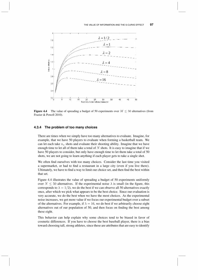
THE VALUE OF INFORMATION AND THE S-CURVE EFFECT 97
1/ 2
1
2
4
8
16
Figure 4.4 The value of spreading a budget of 50 experiments over M ≤ 50 alternatives (fromFrazier & Powell 2010).
4.3.4 The problem of too many choices
There are times when we simply have too many alternatives to evaluate. Imagine, forexample, that we have 50 players to evaluate when forming a basketball team. Wecan let each take nx shots and evaluate their shooting ability. Imagine that we haveenough time to let all of them take a total of N shots. It is easy to imagine that if wehave 50 players to consider, but only have enough time to let them take a total of 50shots, we are not going to learn anything if each player gets to take a single shot.
We often find ourselves with too many choices. Consider the last time you visiteda supermarket, or had to find a restaurant in a large city (even if you live there).Ultimately, we have to find a way to limit our choice set, and then find the best withinthat set.
Figure 4.4 illustrates the value of spreading a budget of 50 experiments uniformlyover N ≤ 50 alternatives. If the experimental noise λ is small (in the figure, thiscorresponds to λ = 1/2), we do the best if we can observe all 50 alternatives exactlyonce, after which we pick what appears to be the best choice. Since our evaluation isvery accurate, we do the best when we have the most choices. As the experimentalnoise increases, we get more value if we focus our experimental budget over a subsetof the alternatives. For example, if λ = 16, we do best if we arbitrarily choose eightalternatives out of our population of 50, and then focus on finding the best amongthese eight.
This behavior can help explain why some choices tend to be biased in favor ofcosmetic differences. If you have to choose the best baseball player, there is a biastoward choosing tall, strong athletes, since these are attributes that are easy to identify
98 VALUE OF INFORMATION POLICIES
and help to narrow the field. People are biased toward brands that are well known,and companies tend to work with established vendors. Simply landing near the topof an Internet search can also be a way of pruning a set of choices. However it isdone, there are many examples where there is a need to use an initial filter to reducethe set of choices to one that can be evaluated using a fixed experimental budget.
4.4 THE FOUR DISTRIBUTIONS OF LEARNING
Perhaps one of the most subtle aspects of learning is understanding the different typesof uncertainty, which depend on when you are asking the question. There are fourdifferent distributions that arise in the learning process. We illustrate these in thecontext of learning problems where all random variables are represented by normaldistributions.
1) The prior distributionN(µ0x, σ
2,0x ), which gives our initial distribution of belief about
the mean.
2) The sampling distribution of the random variable W , which is given byN(µ, σ2
W ), where µ is the true mean and σ2W is the sample variance.
3) The posterior distribution (aftern experiments), given byN(µnx , σ2,nx ), which reflects
the noise in the experimental outcome W . Here, we are modeling the distribution ofµ after n experiments, but when we are at time n = 0 (that is, we have not run anyexperiments yet).
4) The conditional distribution of µn+1x given our beliefs at time n. This is also known
as the predictive distribution. If we have seen W 1, ...,Wn, then µn+1x is random
before we have observed Wn+1, which means that µn+1x ∼ N (µnx , σ
2,nx ).
An understanding of these distributions is useful because it helps to highlight thedifferent types of uncertainties we are trying to resolve by collecting information.
4.5 KNOWLEDGE GRADIENT FOR CORRELATED BELIEFS
There are many problems where updating our belief about one alternative tells ussomething about other alternatives. Some examples include
• We are trying to find the best set of features for a laptop. We try one laptop with12G of RAM, a 2.8 Ghz processor, a 14” screen and weighing 3.2 pounds. We thenoffer a second laptop with 8G of RAM, but everything else the same. A third laptophas 10G of RAM, a 3.2 Ghz processor, a solid state internal disk drive, a 13” screenand weighs 2.5 lbs (with a much higher price). We start by selling the first laptop,and find that we are getting sales higher than expected. Given the similarities withthe second laptop, it is reasonable to assume that the sales of this laptop will also behigher than expected.
KNOWLEDGE GRADIENT FOR CORRELATED BELIEFS 99
• Now we are trying to find the best price for our laptop. We start with an initial guessof the sales volume we anticipate for prices in $100 increments from $800 to $1500.We start at $1100, and sales are much lower than we expected. This would lower ourbeliefs about sales at $1000 and $1200.
• We are trying to find the best of several paths to use for routing a bus. Each time thebus finishes a trip, we record the start and end times, but not the times for individualcomponents of the trip (the bus driver does not have the time for this). If the traveltime for one path is higher than expected, this would increase our estimates for otherpaths that have shared links.
• We are estimating who has a disease. If a concentration of a disease is higher thanexpected in one part of the population, then we would expect that people who arenearby, or otherwise have a reason to interact, will also have a higher likelihood ofhaving the disease.
Correlations are particularly important when the number of possible experimentsis much larger than the experimental budget. The experiment design might becontinuous (where in the United States should we test birds for bird flu), or there maysimply be a very large number of choices (such as websites relevant to a particularissue). The number of choices to measure may be far larger than our budget tomeasure them in a reliable way.
We begin our discussion by reviewing the updated formulas for correlated beliefs,first presented in section 2.3.2. We then describe how to compute the knowledgegradient using correlated beliefs, and close with a discussion of the benefits.
4.5.1 Updating with correlated beliefs
As we pointed out in section 3.5, we can handle correlations with any policy if weuse this structure to update beliefs after we have decided which experiment to make.However, the knowledge gradient is able to imbed our knowledge of correlated beliefswhen we compute the value of information.
We assume that we have a covariance matrix (or function) that tells us how experi-ments of x and x′ are correlated. If x is a scalar, we might assume that the covarianceof µx and µx′ is given by
Cov(x, x′) = σxσx′e−β|x−x′|,
whereσx andσx′ is the standard deviation of our belief aboutµx andµx′ , respectively.Here, β controls the relationship between µx and µx′ as the distance between x andx′ changes. Or, we just assume that there is a known covariance matrix Σ withelement σxx′ . For now, we continue to assume that the alternatives x are discrete, anassumption we relax later.
There is a way of updating our estimate of µn which gives us a more convenientanalytical form than what is given in Section 2.3.2. To simplify the algebra a bit,we let λW = σ2
W = 1/βW . As we did in Section 4.2, we need the change in thevariance of our belief due to the results of an experiment. Following the development
100 VALUE OF INFORMATION POLICIES
in Chapter 2, let Σn+1(x) be the updated covariance matrix given that we have chosento measure alternative x, and let Σn(x) be the change in the covariance matrix dueto evaluating x, which is given by
Σn(x) = Σn − Σn+1 (4.15)
=Σnex(ex)TΣn
Σnxx + λW, (4.16)
where ex is a column vector of 0’s with a 1 in the position corresponding to x. Wenote that (4.15) closely parallels (4.8) for the case of independent beliefs. Now definethe column vector σn(x), which gives the change in our belief about each alternativex′ resulting from measuring alternative x. This is calculated using
σn(x) =Σnex√
Σnxx + λW. (4.17)
Keep in mind that σn(x) is a vector with element σni (x) for a given experimentx = xn.
Also let σi(x) be the component (ei)T σ(x) of the vector σ(x). Let Varn(·) be the
variance given what we know after n experiments. We note that if we measurealternative xn, then
Varn[Wn+1xn − µnxn
]= Varn
[µxn + εn+1 − µnxn
](4.18)
= Varn[µxn + εn+1
](4.19)
= Σnxnxn + λW . (4.20)
We obtain equation (4.18) using Wn+1xn = µxn + εn+1, since Wn+1
xn is a noisyobservation of the truth µxn (which is random because of our Bayesian belief model).We drop µnxn to obtain (4.18) because we are conditioning on what we know after nexperiments, which means that µnxn is deterministic (that is, it is just a number).
Next define the random variable Zn+1
Zn+1 =(Wn+1
x − µnx)√Varn
[Wn+1x − µnx
] ,where x = xn. The random variableWn+1
x is normally distributed with mean µnx andvariance Varn
[Wn+1x − µnx
]= Varn
[Wn+1x
], which means that Zn+1 is normally
distributed with mean 0 and variance 1.
We use the notation µn+1(xn) to represent the updated vector of estimates of the meanµn, with element µn+1
i (xn) after running experiment xn. The updating equation forcorrelated beliefs (first presented in section 2.3.2) is given by
µn+1(xn) = µn +Wn+1xn − µnxn
λW + ΣnxnxnΣnexn . (4.21)
We can rewrite (4.21) as
µn+1(xn) = µnxn + σn(xn)Zn+1, (4.22)
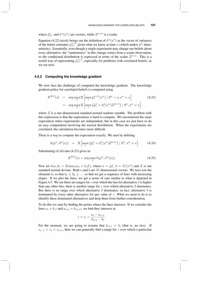
KNOWLEDGE GRADIENT FOR CORRELATED BELIEFS 101
where µnxn and σn(xn) are vectors, while Zn+1 is a scalar.
Equation (4.22) nicely brings out the definition of σn(xn) as the vector of variancesof the future estimates µn+1
xn given what we know at time n (which makes µn deter-ministic). Essentially, even though a single experiment may change our beliefs aboutevery alternative, the “randomness” in this change comes from a scalar observation,so the conditional distribution is expressed in terms of the scalar Zn+1. This is auseful way of representing µn+1
xn , especially for problems with correlated beliefs, aswe see next.
4.5.2 Computing the knowledge gradient
We now face the challenge of computed the knowledge gradient. The knowledgegradient policy for correlated beliefs is computed using
XKG(s) = arg maxx
E[maxiµn+1i (xn) | Sn = s, xn = x
](4.23)
= arg maxx
E[maxi
(µni + σni (xn)Zn+1
)| Sn, xn = x
].
where Z is a one-dimensional standard normal random variable. The problem withthis expression is that the expectation is hard to compute. We encountered the sameexpectation when experiments are independent, but in this case we just have to doan easy computation involving the normal distribution. When the experiments arecorrelated, the calculation becomes more difficult.
There is a way to compute the expectation exactly. We start by defining
h(µn, σn(x)) = E[maxi
(µni + σni (xn)Zn+1
)| Sn, xn = x
]. (4.24)
Substituting (4.24) into (4.23) gives us
XKG(s) = arg maxx
h(µn, σn(x)). (4.25)
Now let h(a, b) = Emaxi(ai + biZ), where a = µni , b = σni (xn) and Z is ourstandard normal deviate. Both a and b are M -dimensional vectors. We next sort theelements bi so that b1 ≤ b2 ≤ . . . so that we get a sequence of lines with increasingslopes. If we plot the lines, we get a series of cuts similar to what is depicted inFigure 4.5. We see there are ranges for z over which the line for alternative 1 is higherthan any other line; there is another range for z over which alternative 2 dominates.But there is no range over which alternative 3 dominates; in fact, alternative 3 isdominated by every other alternative for any value of z. What we need to do is toidentify these dominated alternatives and drop them from further consideration.
To do this we start by finding the points where the lines intersect. If we consider thelines ai + biz and ai+1 + bi+1z, we find they intersect at
z = ci =ai − ai+1
bi+1 − bi.
For the moment, we are going to assume that bi+1 > bi (that is, no ties). Ifci−1 < ci < ci+1, then we can generally find a range for z over which a particular
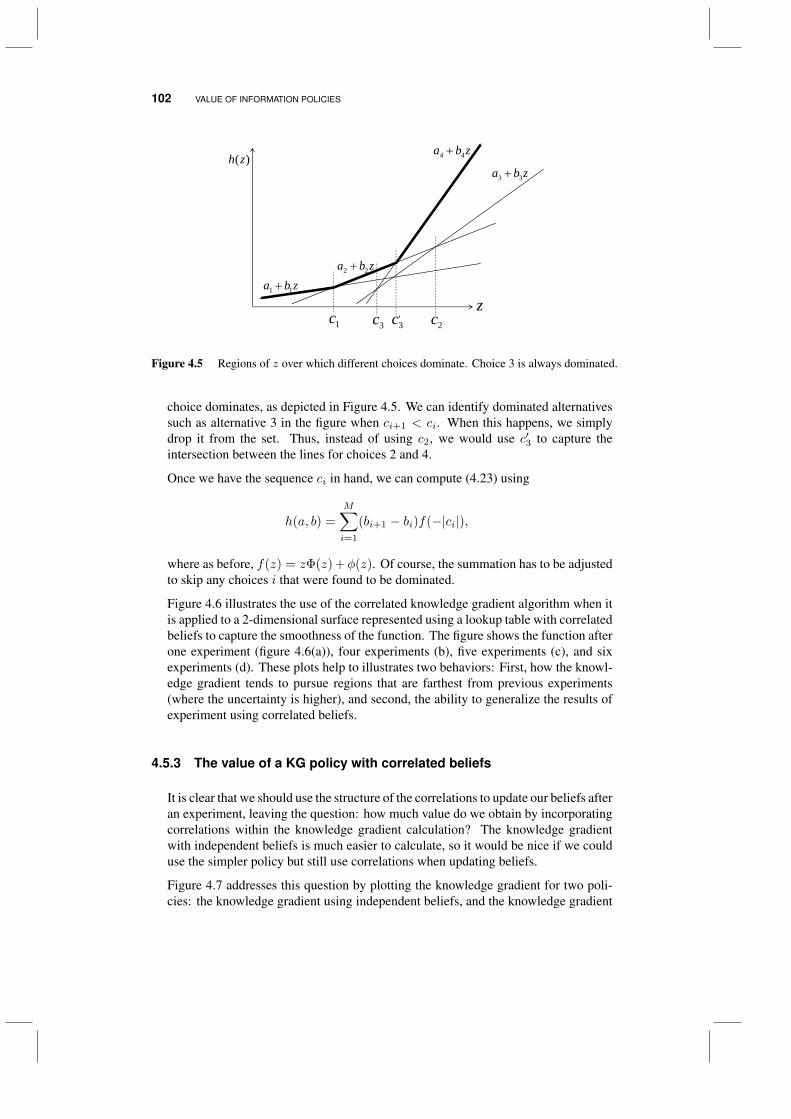
102 VALUE OF INFORMATION POLICIES
1 1a b z2 2a b z
3 3a b z
4 4a b z
z
( )h z
1c 2c3c 3c'
Figure 4.5 Regions of z over which different choices dominate. Choice 3 is always dominated.
choice dominates, as depicted in Figure 4.5. We can identify dominated alternativessuch as alternative 3 in the figure when ci+1 < ci. When this happens, we simplydrop it from the set. Thus, instead of using c2, we would use c′3 to capture theintersection between the lines for choices 2 and 4.
Once we have the sequence ci in hand, we can compute (4.23) using
h(a, b) =
M∑i=1
(bi+1 − bi)f(−|ci|),
where as before, f(z) = zΦ(z) +φ(z). Of course, the summation has to be adjustedto skip any choices i that were found to be dominated.
Figure 4.6 illustrates the use of the correlated knowledge gradient algorithm when itis applied to a 2-dimensional surface represented using a lookup table with correlatedbeliefs to capture the smoothness of the function. The figure shows the function afterone experiment (figure 4.6(a)), four experiments (b), five experiments (c), and sixexperiments (d). These plots help to illustrates two behaviors: First, how the knowl-edge gradient tends to pursue regions that are farthest from previous experiments(where the uncertainty is higher), and second, the ability to generalize the results ofexperiment using correlated beliefs.
4.5.3 The value of a KG policy with correlated beliefs
It is clear that we should use the structure of the correlations to update our beliefs afteran experiment, leaving the question: how much value do we obtain by incorporatingcorrelations within the knowledge gradient calculation? The knowledge gradientwith independent beliefs is much easier to calculate, so it would be nice if we coulduse the simpler policy but still use correlations when updating beliefs.
Figure 4.7 addresses this question by plotting the knowledge gradient for two poli-cies: the knowledge gradient using independent beliefs, and the knowledge gradient
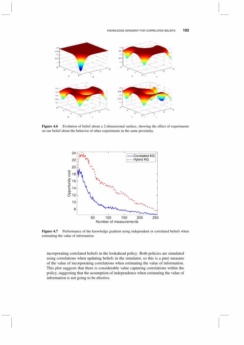
KNOWLEDGE GRADIENT FOR CORRELATED BELIEFS 103
87
Initially we think the concentration is the same everywhere:
» We want to measure the value where the knowledge gradient is the highest. This is the measurement that teaches us the most.
Estimated concentration Knowledge gradient
89
After four measurements:
» Whenever we measure at a point, the value of another measurement at the same point goes down. The knowledge gradient guides us to measuring areas of high uncertainty.
Measurement
Estimated concentration Knowledge gradient
90
After five measurements:
Estimated concentration Knowledge gradient
91
After six samples
Estimated concentration Knowledge gradient
Figure 4.6 Evolution of belief about a 2-dimensional surface, showing the effect of experimentson our belief about the behavior of other experiments in the same proximity.
Figure 4.7 Performance of the knowledge gradient using independent or correlated beliefs whenestimating the value of information.
incorporating correlated beliefs in the lookahead policy. Both policies are simulatedusing correlations when updating beliefs in the simulator, so this is a pure measureof the value of incorporating correlations when estimating the value of information.This plot suggests that there is considerable value capturing correlations within thepolicy, suggesting that the assumption of independence when estimating the value ofinformation is not going to be efective.
104 VALUE OF INFORMATION POLICIES
Handling correlations between experiments has tremendous practical value. Whenwe assumed independent experiments, it was necessary to measure each option atleast once. There are applications where the number of potential experiments isfar greater than the number of experiments that we can actually make. If we haveinformation about correlations, we can find good designs even when the experimentalbudget is much smaller than the number of alternatives.
4.6 ANTICIPATORY VS. EXPERIENTIAL LEARNING
In section 3.5, we made the point that no matter what the policy does, we can capturecomplex belief models, along with complex dynamics of the information process,when we step forward from experiment n to n+ 1. Thus, all of the heuristic policiesintroduced in section 3.2 can capture correlated beliefs as part of the learning process.
Then, we just saw that we could include correlated beliefs in our model of the futureas part of the process of deciding what experiment to run.
These are two very different ways of incorporating correlated beliefs (or, for thatmatter, any type of belief model). We distinguish these two modes using the followingterms:
Anticipatory learning - This is the learning that we anticipate doing as part of our decisionrule, when we are simulating decisions in the future.
Experiential learning - This is learning that we would do as we experience data from realobservations from the field.
Anticipatory learning occurs within the decision function Xπ(St) when decisionsrequire calculations that approximate in some way how new information may changeour underlying belief. In our discussion of decision trees in Section 1.6, Section1.6.1 presented a basic decision tree where outcomes did not change downstreamprobabilities. This is a case of a policy that does not use anticipatory learning.Sections 1.6.2 and 1.6.3 provided examples where observations of information wereused to change downstream distributions within the decision tree used to make thedecision. These sections provide examples of policies that use anticipatory learning.
Experiential learning is what happens after a decision has been made, and we thenobserve an actual outcome. Section 3.2.2 introduced the transition function St+1 =SM (St, xt,Wt+1) which describes the updated belief state given an observationWt+1. In some cases, Wt+1 comes from a real physical system where the newinformation might be observed sales, or an observed response to a drug treatment. Itis entirely possible that the distribution generating observed values of Wt+1 is quitedifferent than a distribution fW (w) that we are assuming for Wt+1 within our policyXπ(St). If this is the case, then it is natural to use observations of Wt+1 to updateour estimate of the density fW (w). This is experiential learning, and it is assumedto be part of the transition function SM (·).
There are, however, many applications where SM (·) represents a computer simu-lation, and Wt+1 is generated from an assumed probability distribution fW (w). If

THE KNOWLEDGE GRADIENT FOR SOME NON-GAUSSIAN DISTRIBUTIONS 105
fW (w) is the distribution we use within our policy Xπ(St), then we are not actuallylearning anything from an observation Wt+1 that comes from fW (w). This is quitecommon in many stochastic simulations, where the focus is on the uncertainty in W ,and not in the uncertainty about the distribution fW (w) of W . An exception wouldbe a simulation that is focusing explicitly on policies for collecting information. Insuch simulations, it is natural to make observations of Wt+1 as we step forwardusing St+1 = SM (St, xt,Wt+1) which are drawn from a truth that is unknown tothe policy Xπ(St).
With these concepts in mind, we can describe three modeling strategies based on hownew information is used.
1) No anticipatory or experiential learning. This is the default strategy in both deter-ministic and stochastic optimization, where we assume that observations of randomvariables are realizations from a known distribution, and as a result would not changeour belief about the distribution. This situation is analogous to the “independentKG” curve in Figure 4.7.
2) Experiential learning without anticipatory learning. Here we use actual observationsof random variables to update our beliefs, but we ignore the fact that we are going todo this when we make a decision. Learning is thus reduced to a statistical problem,with no optimization component. This is exactly the “hybrid KG” situation in Figure4.7.
3) Experiential learning with anticipatory learning. This is where we use learningwithin the policy, as in equation (4.25), and in the transition function, as in equations(2.18)-(2.19). Such a situation corresponds to the “correlated KG” curve in Figure4.7.
We ignore the combination of using anticipatory learning without experiential learn-ing, because it does not make sense to anticipate the effect of observations on beliefs,but then not use real observations to update beliefs.
Anticipatory learning spans any policy (optimal or heuristic) which uses some rep-resentation of the uncertainty in our belief about the value of each choice. We didthis heuristically in Chapter 3 with policies such as mixed exploitation-exploration,epsilon-greedy exploration, and Boltzmann exploration. In this chapter, the knowl-edge gradient, expected improvement and linear loss policies all represent methodswhich use some form of explicit learning within the learning policy.
4.7 THE KNOWLEDGE GRADIENT FOR SOME NON-GAUSSIANDISTRIBUTIONS
It is important to remember that, while the definition of the knowledge gradient givenin (4.3) is general, and can be written down for almost any learning problem, theKG formula given in (4.13) is geared specifically to the ranking and selection prob-lem with independent alternatives and a normal-normal learning model (normallydistributed prior, normally distributed experimental outcomes). This is not particu-larly surprising, because the formula uses the functions φ and Φ that characterize a
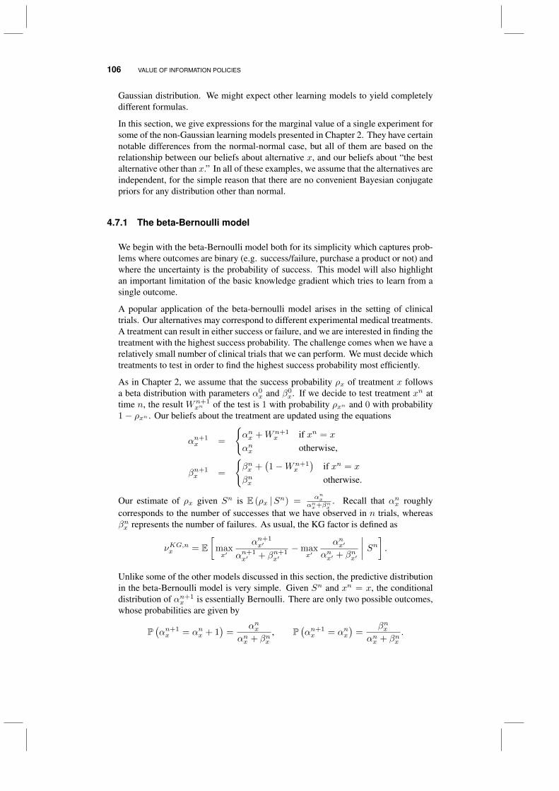
106 VALUE OF INFORMATION POLICIES
Gaussian distribution. We might expect other learning models to yield completelydifferent formulas.
In this section, we give expressions for the marginal value of a single experiment forsome of the non-Gaussian learning models presented in Chapter 2. They have certainnotable differences from the normal-normal case, but all of them are based on therelationship between our beliefs about alternative x, and our beliefs about “the bestalternative other than x.” In all of these examples, we assume that the alternatives areindependent, for the simple reason that there are no convenient Bayesian conjugatepriors for any distribution other than normal.
4.7.1 The beta-Bernoulli model
We begin with the beta-Bernoulli model both for its simplicity which captures prob-lems where outcomes are binary (e.g. success/failure, purchase a product or not) andwhere the uncertainty is the probability of success. This model will also highlightan important limitation of the basic knowledge gradient which tries to learn from asingle outcome.
A popular application of the beta-bernoulli model arises in the setting of clinicaltrials. Our alternatives may correspond to different experimental medical treatments.A treatment can result in either success or failure, and we are interested in finding thetreatment with the highest success probability. The challenge comes when we have arelatively small number of clinical trials that we can perform. We must decide whichtreatments to test in order to find the highest success probability most efficiently.
As in Chapter 2, we assume that the success probability ρx of treatment x followsa beta distribution with parameters α0
x and β0x. If we decide to test treatment xn at
time n, the result Wn+1xn of the test is 1 with probability ρxn and 0 with probability
1− ρxn . Our beliefs about the treatment are updated using the equations
αn+1x =
αnx +Wn+1
x if xn = x
αnx otherwise,
βn+1x =
βnx +
(1−Wn+1
x
)if xn = x
βnx otherwise.
Our estimate of ρx given Sn is E (ρx |Sn) =αnx
αnx+βnx. Recall that αnx roughly
corresponds to the number of successes that we have observed in n trials, whereasβnx represents the number of failures. As usual, the KG factor is defined as
νKG,nx = E[
maxx′
αn+1x′
αn+1x′ + βn+1
x′−max
x′
αnx′
αnx′ + βnx′
∣∣∣∣ Sn] .
Unlike some of the other models discussed in this section, the predictive distributionin the beta-Bernoulli model is very simple. Given Sn and xn = x, the conditionaldistribution of αn+1
x is essentially Bernoulli. There are only two possible outcomes,whose probabilities are given by
P(αn+1x = αnx + 1
)=
αnxαnx + βnx
, P(αn+1x = αnx
)=
βnxαnx + βnx
.
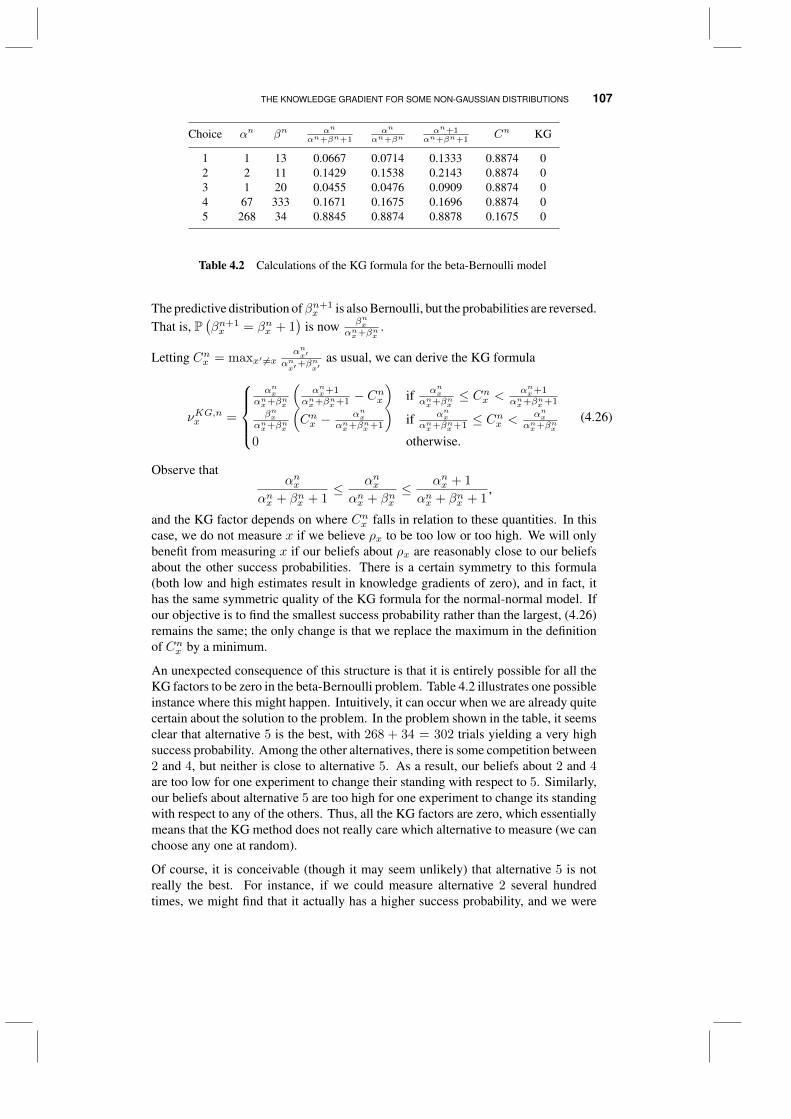
THE KNOWLEDGE GRADIENT FOR SOME NON-GAUSSIAN DISTRIBUTIONS 107
Choice αn βn αn
αn+βn+1αn
αn+βnαn+1
αn+βn+1Cn KG
1 1 13 0.0667 0.0714 0.1333 0.8874 02 2 11 0.1429 0.1538 0.2143 0.8874 03 1 20 0.0455 0.0476 0.0909 0.8874 04 67 333 0.1671 0.1675 0.1696 0.8874 05 268 34 0.8845 0.8874 0.8878 0.1675 0
Table 4.2 Calculations of the KG formula for the beta-Bernoulli model
The predictive distribution ofβn+1x is also Bernoulli, but the probabilities are reversed.
That is, P(βn+1x = βnx + 1
)is now βnx
αnx+βnx.
Letting Cnx = maxx′ 6=xαnx′
αnx′+β
nx′
as usual, we can derive the KG formula
νKG,nx =
αnx
αnx+βnx
(αnx+1
αnx+βnx+1 − Cnx
)if αnxαnx+βnx
≤ Cnx <αnx+1
αnx+βnx+1
βnxαnx+βnx
(Cnx −
αnxαnx+βnx+1
)if αnxαnx+βnx+1 ≤ C
nx <
αnxαnx+βnx
0 otherwise.
(4.26)
Observe thatαnx
αnx + βnx + 1≤ αnxαnx + βnx
≤ αnx + 1
αnx + βnx + 1,
and the KG factor depends on where Cnx falls in relation to these quantities. In thiscase, we do not measure x if we believe ρx to be too low or too high. We will onlybenefit from measuring x if our beliefs about ρx are reasonably close to our beliefsabout the other success probabilities. There is a certain symmetry to this formula(both low and high estimates result in knowledge gradients of zero), and in fact, ithas the same symmetric quality of the KG formula for the normal-normal model. Ifour objective is to find the smallest success probability rather than the largest, (4.26)remains the same; the only change is that we replace the maximum in the definitionof Cnx by a minimum.
An unexpected consequence of this structure is that it is entirely possible for all theKG factors to be zero in the beta-Bernoulli problem. Table 4.2 illustrates one possibleinstance where this might happen. Intuitively, it can occur when we are already quitecertain about the solution to the problem. In the problem shown in the table, it seemsclear that alternative 5 is the best, with 268 + 34 = 302 trials yielding a very highsuccess probability. Among the other alternatives, there is some competition between2 and 4, but neither is close to alternative 5. As a result, our beliefs about 2 and 4are too low for one experiment to change their standing with respect to 5. Similarly,our beliefs about alternative 5 are too high for one experiment to change its standingwith respect to any of the others. Thus, all the KG factors are zero, which essentiallymeans that the KG method does not really care which alternative to measure (we canchoose any one at random).
Of course, it is conceivable (though it may seem unlikely) that alternative 5 is notreally the best. For instance, if we could measure alternative 2 several hundredtimes, we might find that it actually has a higher success probability, and we were
108 VALUE OF INFORMATION POLICIES
simply unlucky enough to observe 11 failures in the beginning. Unfortunately, theKG method only looks ahead one time step into the future, and thus is unable toconsider this possibility. This hints at possible limitations of the knowledge gradientapproach in a situation where the observations are discrete, similar to the S-curveeffect we saw in Section 4.3.
4.7.2 The gamma-exponential model
Suppose that we have M exponentially distributed random variables with meansλ1, ..., λM , and we wish to find the one with the largest rate. For instance, we mightbe looking at a number of servers, with the goal of finding the one with the highest(fastest) service rate. Alternately, we might have a number of products, each with anexponential daily demand. In this setting, we might want to discover which producthas the lowest demand (corresponding to the largest exponential rate), so that wemight take this product out of production. A final example is the problem of networkrouting, where we have a number of possible routes for sending packets, and theobjective is to find the route with the lowest ping time. In all of these problems,the observations (service time, daily demand, network latency) are positive, whichmeans that the normal-normal model is not a good fit.
Instead, we use the gamma-exponential model (which we first saw in Section 2.6.1).We start by assuming that the rate λx of each alternative is uncertain and followsa gamma distribution with parameters a0
x and b0x. When we choose to measurealternative xn at time n, we make a random observation Wn+1
xn ∼ Exp (λxn), andupdate our beliefs according to the equations
an+1x =
anx + 1 if xn = x
anx otherwise,
bn+1x =
bnx +Wn+1
x if xn = x
bnx otherwise.
We still have an independent ranking and selection problem, as in (3.2) and (3.3),but the specific updating mechanism for the alternative we measure is taken from thegamma-exponential model in Chapter 2.
Recall that, given the beliefs anx and bnx , our estimate of λx is anx/bnx , the mean of the
gamma distribution. The KG factor of alternative x at time n is now given by
νKG,nx = E[maxx′
an+1x′
bn+1x′−max
x′
anx′
bnx′|Sn
]. (4.27)
We omit the steps in the computation of this expectation; interested readers can followthe procedure in Section 4.12.1 and compute the formula for themselves. However,we point out one interesting detail. As in the normal-normal case, the computationof νKG,nx requires us to find the conditional distribution, given Sn and xn = x, ofthe parameter bn+1
x . This is known as the predictive distribution of bnx . It is easy to
THE KNOWLEDGE GRADIENT FOR SOME NON-GAUSSIAN DISTRIBUTIONS 109
see that
P(bn+1x > y |Sn, xn = x
)= P
(Wn+1 > y − bnx |Sn, xn = x
)= E
[P(Wn+1 > y − bnx |λx
)|Sn, xn = x
]= E
[e−λx(y−bnx ) |Sn, xn = x
]=
(bnxy
)anx.
We get from the second line to the third line by using the cumulative distribution(cdf) of the exponential distribution, since Wn+1
x is exponential given λx. The lastline uses the moment-generating function of the gamma distribution. From thiscalculation, it follows that the density of bn+1
x is given by
f (y) =anx (bnx)
anx
yanx+1
,
which is precisely the Pareto density with parameters anx and bnx .
Once we have this fact, computing (4.27) is a matter of taking an expectation ofa certain function over the Pareto density. Define Cnx = maxx′ 6=x
anxbnx
. As before,this quantity represents the “best of the rest” of our estimates of the rates. We thencompute
νnx =(bnx)
anx (Cnx )anx+1
(anx + 1)anx+1 (4.28)
which is a sort of baseline knowledge gradient. However, depending on certain con-ditions, we may subtract an additional penalty from this quantity when we computethe final KG formula.
It can be shown that the KG formula is given by
νKG,nx =
νnx if x = arg maxx′
anx′bnx′
νnx −(Cnx −
anxbnx
)if a
nx+1bnx
> maxx′anx′bnx′
0 otherwise.
(4.29)
This particular formula is skewed towards exploitation. If x 6= arg maxx′anx′bnx′
, we
subtract an additional value Cnx −anxbnx
from the KG factor of alternative x. However,
if x = arg maxx′anx′bnx′
, there is no additional penalty. Furthermore, if our estimate
of λx is low enough that anx+1bnx≤ maxx′
anx′bnx′
, the KG factor is automatically zero.
Since νKG,nx ≥ 0 for all x, just like in the normal-normal case, this means that wewon’t even consider an alternative if our beliefs about it are too low. So, there is amore pronounced slant in favor of alternatives with high estimates than we saw in thenormal-normal setting.
Table 4.3 illustrates this issue for a problem with five alternatives. Based on ourbeliefs, it seems that alternative 5 is the best. This alternative also has the highest KGfactor. Although our estimate of λ3 is very close to our estimate of λ5 (they differ
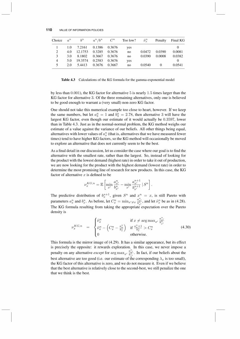
110 VALUE OF INFORMATION POLICIES
Choice an bn an/bn Cn Too low? νnx Penalty Final KG
1 1.0 7.2161 0.1386 0.3676 yes 02 4.0 12.1753 0.3285 0.3676 no 0.0472 0.0390 0.00813 3.0 8.1802 0.3667 0.3676 no 0.0390 0.0008 0.03824 5.0 19.3574 0.2583 0.3676 yes 05 2.0 5.4413 0.3676 0.3667 no 0.0540 0 0.0541
Table 4.3 Calculations of the KG formula for the gamma-exponential model
by less than 0.001), the KG factor for alternative 5 is nearly 1.5 times larger than theKG factor for alternative 3. Of the three remaining alternatives, only one is believedto be good enough to warrant a (very small) non-zero KG factor.
One should not take this numerical example too close to heart, however. If we keepthe same numbers, but let an3 = 1 and bn3 = 2.78, then alternative 3 will have thelargest KG factor, even though our estimate of it would actually be 0.3597, lowerthan in Table 4.3. Just as in the normal-normal problem, the KG method weighs ourestimate of a value against the variance of our beliefs. All other things being equal,alternatives with lower values of anx (that is, alternatives that we have measured fewertimes) tend to have higher KG factors, so the KG method will occasionally be movedto explore an alternative that does not currently seem to be the best.
As a final detail in our discussion, let us consider the case where our goal is to find thealternative with the smallest rate, rather than the largest. So, instead of looking forthe product with the lowest demand (highest rate) in order to take it out of production,we are now looking for the product with the highest demand (lowest rate) in order todetermine the most promising line of research for new products. In this case, the KGfactor of alternative x is defined to be
νKG,nx = E[minx′
anx′
bnx′−min
x′
an+1x′
bn+1x′|Sn
].
The predictive distribution of bn+1x , given Sn and xn = x, is still Pareto with
parameters anx and bnx . As before, let Cnx = minx′ 6=xanx′bnx′
, and let νnx be as in (4.28).The KG formula resulting from taking the appropriate expectation over the Paretodensity is
νKG,nx =
νnx if x 6= arg maxx′
anx′bnx′
νnx −(Cnx −
anxbnx
)if a
nx+1bnx
> Cnx
0 otherwise.
(4.30)
This formula is the mirror image of (4.29). It has a similar appearance, but its effectis precisely the opposite: it rewards exploration. In this case, we never impose apenalty on any alternative except for arg maxx′
anx′bnx′
. In fact, if our beliefs about thebest alternative are too good (i.e. our estimate of the corresponding λx is too small),the KG factor of this alternative is zero, and we do not measure it. Even if we believethat the best alternative is relatively close to the second-best, we still penalize the onethat we think is the best.
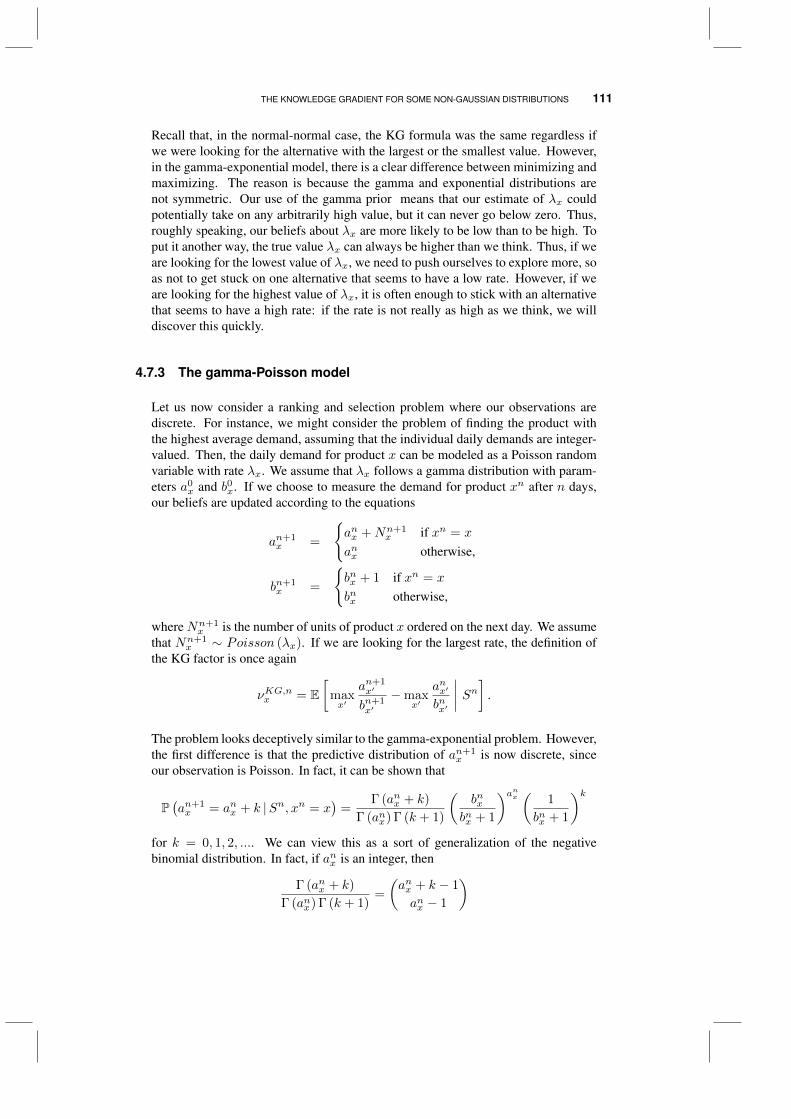
THE KNOWLEDGE GRADIENT FOR SOME NON-GAUSSIAN DISTRIBUTIONS 111
Recall that, in the normal-normal case, the KG formula was the same regardless ifwe were looking for the alternative with the largest or the smallest value. However,in the gamma-exponential model, there is a clear difference between minimizing andmaximizing. The reason is because the gamma and exponential distributions arenot symmetric. Our use of the gamma prior means that our estimate of λx couldpotentially take on any arbitrarily high value, but it can never go below zero. Thus,roughly speaking, our beliefs about λx are more likely to be low than to be high. Toput it another way, the true value λx can always be higher than we think. Thus, if weare looking for the lowest value of λx, we need to push ourselves to explore more, soas not to get stuck on one alternative that seems to have a low rate. However, if weare looking for the highest value of λx, it is often enough to stick with an alternativethat seems to have a high rate: if the rate is not really as high as we think, we willdiscover this quickly.
4.7.3 The gamma-Poisson model
Let us now consider a ranking and selection problem where our observations arediscrete. For instance, we might consider the problem of finding the product withthe highest average demand, assuming that the individual daily demands are integer-valued. Then, the daily demand for product x can be modeled as a Poisson randomvariable with rate λx. We assume that λx follows a gamma distribution with param-eters a0
x and b0x. If we choose to measure the demand for product xn after n days,our beliefs are updated according to the equations
an+1x =
anx +Nn+1
x if xn = x
anx otherwise,
bn+1x =
bnx + 1 if xn = x
bnx otherwise,
whereNn+1x is the number of units of product x ordered on the next day. We assume
that Nn+1x ∼ Poisson (λx). If we are looking for the largest rate, the definition of
the KG factor is once again
νKG,nx = E[
maxx′
an+1x′
bn+1x′−max
x′
anx′
bnx′
∣∣∣∣ Sn] .
The problem looks deceptively similar to the gamma-exponential problem. However,the first difference is that the predictive distribution of an+1
x is now discrete, sinceour observation is Poisson. In fact, it can be shown that
P(an+1x = anx + k |Sn, xn = x
)=
Γ (anx + k)
Γ (anx) Γ (k + 1)
(bnx
bnx + 1
)anx ( 1
bnx + 1
)kfor k = 0, 1, 2, .... We can view this as a sort of generalization of the negativebinomial distribution. In fact, if anx is an integer, then
Γ (anx + k)
Γ (anx) Γ (k + 1)=
(anx + k − 1
anx − 1
)
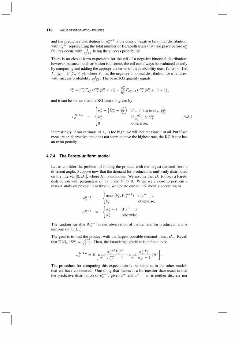
112 VALUE OF INFORMATION POLICIES
and the predictive distribution of an+1x is the classic negative binomial distribution,
with an+1x representing the total number of Bernoulli trials that take place before anx
failures occur, with 1bnx+1 being the success probability.
There is no closed-form expression for the cdf of a negative binomial distribution;however, because the distribution is discrete, the cdf can always be evaluated exactlyby computing and adding the appropriate terms of the probability mass function. LetFa (y) = P (Ya ≤ y), where Ya has the negative binomial distribution for a failures,with success probability 1
bnx+1 . The basic KG quantity equals
νnx = CnxFanx (Cnx (bnx + 1))− anxbnxFanx+1 (Cnx (bnx + 1) + 1) ,
and it can be shown that the KG factor is given by
νKG,nx =
νnx −
(Cnx −
anxbnx
)if x 6= arg maxx′
anx′bnx′
νnx if anxbnx+1 ≤ C
nx
0 otherwise.
(4.31)
Interestingly, if our estimate of λx is too high, we will not measure x at all, but if wemeasure an alternative that does not seem to have the highest rate, the KG factor hasan extra penalty.
4.7.4 The Pareto-uniform model
Let us consider the problem of finding the product with the largest demand from adifferent angle. Suppose now that the demand for product x is uniformly distributedon the interval [0, Bx], where Bx is unknown. We assume that Bx follows a Paretodistribution with parameters α0 > 1 and b0 > 0. When we choose to perform amarket study on product x at time n, we update our beliefs about x according to
bn+1x =
max
(bnx ,W
n+1x
)if xn = x
bnx otherwise,
αn+1x =
αnx + 1 if xn = x
αnx otherwise.
The random variable Wn+1x is our observation of the demand for product x, and is
uniform on [0, Bx].
The goal is to find the product with the largest possible demand maxxBx. Recallthat E [Bx |Sn] =
αnxbnx
αnx−1 . Then, the knowledge gradient is defined to be
νKG,nx = E[maxx′
αn+1x′ bn+1
x′
αn+1x′ − 1
−maxx′
αnx′bnx′
αnx′ − 1|Sn
].
The procedure for computing this expectation is the same as in the other modelsthat we have considered. One thing that makes it a bit messier than usual is thatthe predictive distribution of bn+1
x , given Sn and xn = x, is neither discrete nor
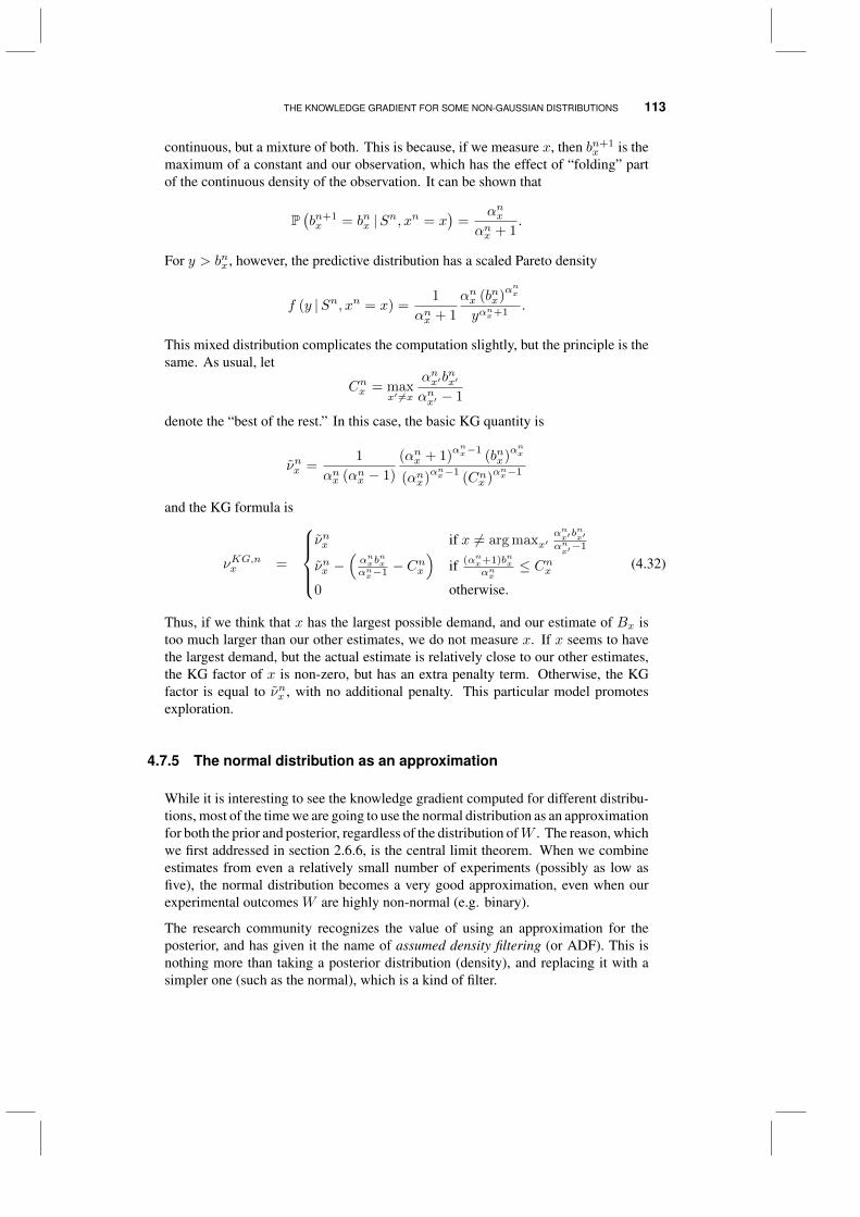
THE KNOWLEDGE GRADIENT FOR SOME NON-GAUSSIAN DISTRIBUTIONS 113
continuous, but a mixture of both. This is because, if we measure x, then bn+1x is the
maximum of a constant and our observation, which has the effect of “folding” partof the continuous density of the observation. It can be shown that
P(bn+1x = bnx |Sn, xn = x
)=
αnxαnx + 1
.
For y > bnx , however, the predictive distribution has a scaled Pareto density
f (y |Sn, xn = x) =1
αnx + 1
αnx (bnx)αnx
yαnx+1
.
This mixed distribution complicates the computation slightly, but the principle is thesame. As usual, let
Cnx = maxx′ 6=x
αnx′bnx′
αnx′ − 1
denote the “best of the rest.” In this case, the basic KG quantity is
νnx =1
αnx (αnx − 1)
(αnx + 1)αnx−1
(bnx)αnx
(αnx)αnx−1
(Cnx )αnx−1
and the KG formula is
νKG,nx =
νnx if x 6= arg maxx′
αnx′b
nx′
αnx′−1
νnx −(αnxb
nx
αnx−1 − Cnx
)if (αnx+1)bnx
αnx≤ Cnx
0 otherwise.
(4.32)
Thus, if we think that x has the largest possible demand, and our estimate of Bx istoo much larger than our other estimates, we do not measure x. If x seems to havethe largest demand, but the actual estimate is relatively close to our other estimates,the KG factor of x is non-zero, but has an extra penalty term. Otherwise, the KGfactor is equal to νnx , with no additional penalty. This particular model promotesexploration.
4.7.5 The normal distribution as an approximation
While it is interesting to see the knowledge gradient computed for different distribu-tions, most of the time we are going to use the normal distribution as an approximationfor both the prior and posterior, regardless of the distribution ofW . The reason, whichwe first addressed in section 2.6.6, is the central limit theorem. When we combineestimates from even a relatively small number of experiments (possibly as low asfive), the normal distribution becomes a very good approximation, even when ourexperimental outcomes W are highly non-normal (e.g. binary).
The research community recognizes the value of using an approximation for theposterior, and has given it the name of assumed density filtering (or ADF). This isnothing more than taking a posterior distribution (density), and replacing it with asimpler one (such as the normal), which is a kind of filter.
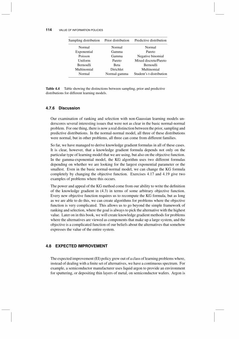
114 VALUE OF INFORMATION POLICIES
Sampling distribution Prior distribution Predictive distribution
Normal Normal NormalExponential Gamma Pareto
Poisson Gamma Negative binomialUniform Pareto Mixed discrete/ParetoBernoulli Beta Bernoulli
Multinomial Dirichlet MultinomialNormal Normal-gamma Student’s t-distribution
Table 4.4 Table showing the distinctions between sampling, prior and predictivedistributions for different learning models.
4.7.6 Discussion
Our examination of ranking and selection with non-Gaussian learning models un-derscores several interesting issues that were not as clear in the basic normal-normalproblem. For one thing, there is now a real distinction between the prior, sampling andpredictive distributions. In the normal-normal model, all three of these distributionswere normal, but in other problems, all three can come from different families.
So far, we have managed to derive knowledge gradient formulas in all of these cases.It is clear, however, that a knowledge gradient formula depends not only on theparticular type of learning model that we are using, but also on the objective function.In the gamma-exponential model, the KG algorithm uses two different formulasdepending on whether we are looking for the largest exponential parameter or thesmallest. Even in the basic normal-normal model, we can change the KG formulacompletely by changing the objective function. Exercises 4.17 and 4.19 give twoexamples of problems where this occurs.
The power and appeal of the KG method come from our ability to write the definitionof the knowledge gradient in (4.3) in terms of some arbitrary objective function.Every new objective function requires us to recompute the KG formula, but as longas we are able to do this, we can create algorithms for problems where the objectivefunction is very complicated. This allows us to go beyond the simple framework ofranking and selection, where the goal is always to pick the alternative with the highestvalue. Later on in this book, we will create knowledge gradient methods for problemswhere the alternatives are viewed as components that make up a large system, and theobjective is a complicated function of our beliefs about the alternatives that somehowexpresses the value of the entire system.
4.8 EXPECTED IMPROVEMENT
The expected improvement (EI) policy grew out of a class of learning problems where,instead of dealing with a finite set of alternatives, we have a continuous spectrum. Forexample, a semiconductor manufacturer uses liquid argon to provide an environmentfor sputtering, or depositing thin layers of metal, on semiconductor wafers. Argon is
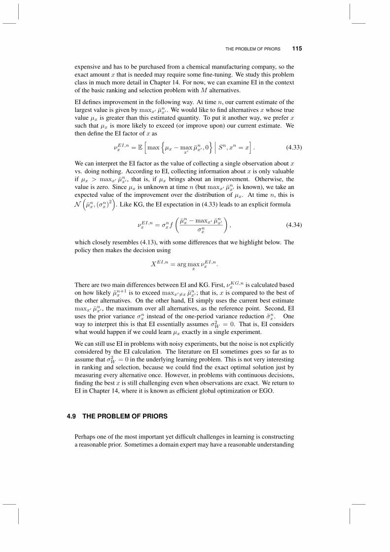
THE PROBLEM OF PRIORS 115
expensive and has to be purchased from a chemical manufacturing company, so theexact amount x that is needed may require some fine-tuning. We study this problemclass in much more detail in Chapter 14. For now, we can examine EI in the contextof the basic ranking and selection problem with M alternatives.
EI defines improvement in the following way. At time n, our current estimate of thelargest value is given by maxx′ µ
nx′ . We would like to find alternatives x whose true
value µx is greater than this estimated quantity. To put it another way, we prefer xsuch that µx is more likely to exceed (or improve upon) our current estimate. Wethen define the EI factor of x as
νEI,nx = E[
maxµx −max
x′µnx′ , 0
∣∣∣ Sn, xn = x]. (4.33)
We can interpret the EI factor as the value of collecting a single observation about xvs. doing nothing. According to EI, collecting information about x is only valuableif µx > maxx′ µ
nx′ , that is, if µx brings about an improvement. Otherwise, the
value is zero. Since µx is unknown at time n (but maxx′ µnx′ is known), we take an
expected value of the improvement over the distribution of µx. At time n, this isN(µnx , (σ
nx )
2)
. Like KG, the EI expectation in (4.33) leads to an explicit formula
νEI,nx = σnxf
(µnx −maxx′ µ
nx′
σnx
), (4.34)
which closely resembles (4.13), with some differences that we highlight below. Thepolicy then makes the decision using
XEI,n = arg maxx
νEI,nx .
There are two main differences between EI and KG. First, νKG,nx is calculated basedon how likely µn+1
x is to exceed maxx′ 6=x µnx′ ; that is, x is compared to the best of
the other alternatives. On the other hand, EI simply uses the current best estimatemaxx′ µ
nx′ , the maximum over all alternatives, as the reference point. Second, EI
uses the prior variance σnx instead of the one-period variance reduction σnx . Oneway to interpret this is that EI essentially assumes σ2
W = 0. That is, EI considerswhat would happen if we could learn µx exactly in a single experiment.
We can still use EI in problems with noisy experiments, but the noise is not explicitlyconsidered by the EI calculation. The literature on EI sometimes goes so far as toassume that σ2
W = 0 in the underlying learning problem. This is not very interestingin ranking and selection, because we could find the exact optimal solution just bymeasuring every alternative once. However, in problems with continuous decisions,finding the best x is still challenging even when observations are exact. We return toEI in Chapter 14, where it is known as efficient global optimization or EGO.
4.9 THE PROBLEM OF PRIORS
Perhaps one of the most important yet difficult challenges in learning is constructinga reasonable prior. Sometimes a domain expert may have a reasonable understanding
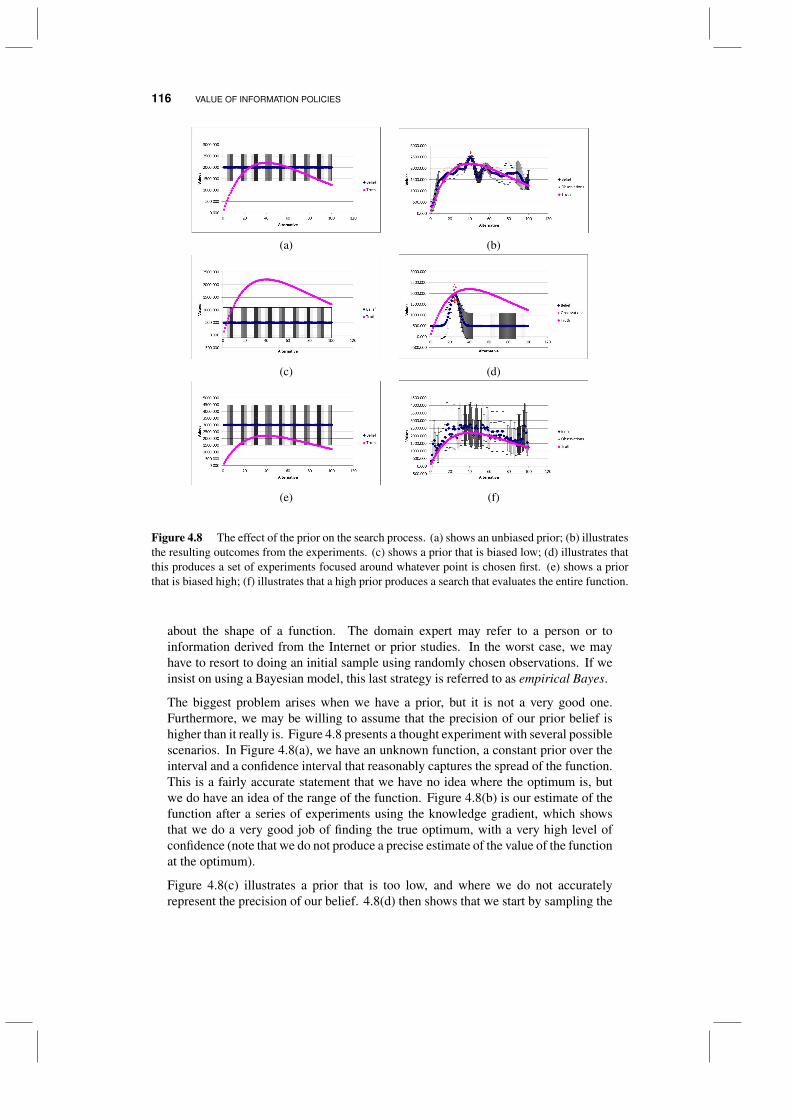
116 VALUE OF INFORMATION POLICIES
(a) (b)
(c) (d)
(e) (f)
Figure 4.8 The effect of the prior on the search process. (a) shows an unbiased prior; (b) illustratesthe resulting outcomes from the experiments. (c) shows a prior that is biased low; (d) illustrates thatthis produces a set of experiments focused around whatever point is chosen first. (e) shows a priorthat is biased high; (f) illustrates that a high prior produces a search that evaluates the entire function.
about the shape of a function. The domain expert may refer to a person or toinformation derived from the Internet or prior studies. In the worst case, we mayhave to resort to doing an initial sample using randomly chosen observations. If weinsist on using a Bayesian model, this last strategy is referred to as empirical Bayes.
The biggest problem arises when we have a prior, but it is not a very good one.Furthermore, we may be willing to assume that the precision of our prior belief ishigher than it really is. Figure 4.8 presents a thought experiment with several possiblescenarios. In Figure 4.8(a), we have an unknown function, a constant prior over theinterval and a confidence interval that reasonably captures the spread of the function.This is a fairly accurate statement that we have no idea where the optimum is, butwe do have an idea of the range of the function. Figure 4.8(b) is our estimate of thefunction after a series of experiments using the knowledge gradient, which showsthat we do a very good job of finding the true optimum, with a very high level ofconfidence (note that we do not produce a precise estimate of the value of the functionat the optimum).
Figure 4.8(c) illustrates a prior that is too low, and where we do not accuratelyrepresent the precision of our belief. 4.8(d) then shows that we start by sampling the

VALUE OF INFORMATION WITH UNKNOWN VARIANCE* 117
function at a random point, and not surprisingly the observed value is much higherthan our prior. As a result, we tend to focus our search near this point, since ourprior suggests that there is no value in sampling points far from the initial sample. Ifwe were to repeat the exercise with a different random starting point, we would havefocused our entire search close to that point. The result is an unreliable estimate ofthe optimum.
Figure 4.8(e) then depicts a prior that is too high. When this is the case, Figure 4.8(f)shows that we end up sampling the entire function, since every observation producesan estimate that is very low relative to our prior estimate for the rest of the function.We then proceed to sample any point that has not been sampled before (and which isnot close to a previously sampled point). This works if our budget is large enough tosample the entire function, but it would work poorly if this were not the case.
Perhaps the most visible lesson from this illustration is that it is important to be honestabout the uncertainty in the prior. Figures 4.8(c) and 4.8(e) both display confidenceintervals that do not cover the function. A narrow confidence bound is particularlyproblematic if the prior is biased low, because we tend to focus all of our energyaround any point that we sample.
Of course, from the Bayesian point of view, there is no one fixed function. Rather,our prior encodes our beliefs about a wide range of possible true functions. Themessage of the preceding example can be taken to mean that we should make surethat this range is in some way “wide enough.”
Care should be used to ensure that the prior does not exclude portions of the functionthat may be quite good. For this reason, it is better to be biased high, and to use carenot to overstate the precision of your prior (that is, where your confidence interval istoo narrow). However, using a prior that is too high, and/or a confidence interval thatis too large, may simply result in a lot of unnecessary exploration. In other words,the better your prior is, the better your search will be. This may be a way of sayingthat there is no free lunch in information collection.
4.10 VALUE OF INFORMATION WITH UNKNOWN VARIANCE*
An important simplifying assumption that we made for the knowledge gradient isthat we know the variance (or precision) of an experimental outcome. In this sectionwe consider the more difficult case of unknown variance, which was developed underthe name “linear loss.” Not surprisingly, this is a more difficult problem, with acorresponding increase in complexity.
Two policies have been proposed in the literature under the names LL(1) and LL1,which might leave the impression that they are the same policy. Despite having verysimilar names, LL(1) andLL1 are actually two different policies. Both are examplesof “linear-loss” or LL methods, close analogs to KG that were developed for rankingand selection with unknown means and variances. We discussed learning in thissetting in Section 2.6.5.
Supposing that alternative x has value µx, and our observations of µx also have anunknown precision βWx , we can represent our beliefs about the mean and precision
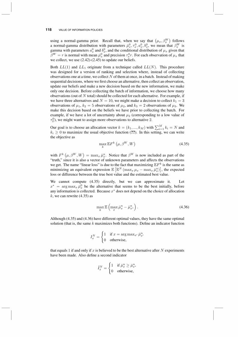
118 VALUE OF INFORMATION POLICIES
using a normal-gamma prior. Recall that, when we say that(µx, β
Wx
)follows
a normal-gamma distribution with parameters µ0x, τ
0x , a
0x, b
0x, we mean that βWx is
gamma with parameters a0x and b0x, and the conditional distribution of µx given that
βW = r is normal with mean µ0x and precision τ0
xr. For each observation of µx thatwe collect, we use (2.42)-(2.45) to update our beliefs.
Both LL(1) and LL1 originate from a technique called LL(N). This procedurewas designed for a version of ranking and selection where, instead of collectingobservations one at a time, we collectN of them at once, in a batch. Instead of makingsequential decisions, where we first choose an alternative, then collect an observation,update our beliefs and make a new decision based on the new information, we makeonly one decision. Before collecting the batch of information, we choose how manyobservations (out ofN total) should be collected for each alternative. For example, ifwe have three alternatives and N = 10, we might make a decision to collect k1 = 3observations of µ1, k2 = 5 observations of µ2, and k3 = 2 observations of µ3. Wemake this decision based on the beliefs we have prior to collecting the batch. Forexample, if we have a lot of uncertainty about µ2 (corresponding to a low value ofτ02 ), we might want to assign more observations to alternative 2.
Our goal is to choose an allocation vector k = (k1, ..., kM ) with∑Mi=1 ki = N and
ki ≥ 0 to maximize the usual objective function (??). In this setting, we can writethe objective as
maxk
EF k(µ, βW ,W
)(4.35)
with F k(µ, βW ,W
)= maxx µ
nx . Notice that βW is now included as part of the
“truth,” since it is also a vector of unknown parameters and affects the observationswe get. The name “linear loss” is due to the fact that maximizing EF k is the same asminimizing an equivalent expression E
[EN (maxx µx −maxx µ
nx)], the expected
loss or difference between the true best value and the estimated best value.
We cannot compute (4.35) directly, but we can approximate it. Letx∗ = arg maxx µ
0x be the alternative that seems to be the best initially, before
any information is collected. Because x∗ does not depend on the choice of allocationk, we can rewrite (4.35) as
maxk
E(
maxx
µnx − µnx∗). (4.36)
Although (4.35) and (4.36) have different optimal values, they have the same optimalsolution (that is, the same k maximizes both functions). Define an indicator function
INx =
1 if x = arg maxx′ µ
nx′
0 otherwise,
that equals 1 if and only if x is believed to be the best alternative afterN experimentshave been made. Also define a second indicator
INx =
1 if µnx ≥ µnx∗0 otherwise,
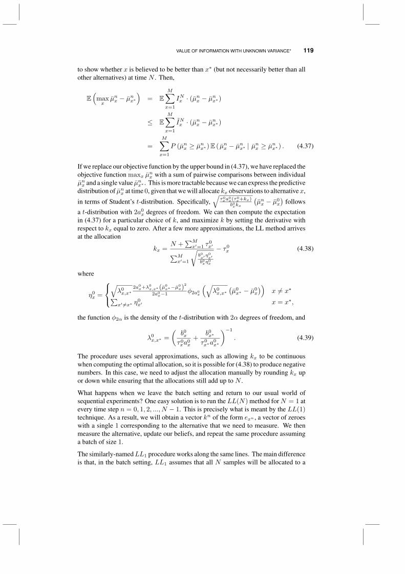
VALUE OF INFORMATION WITH UNKNOWN VARIANCE* 119
to show whether x is believed to be better than x∗ (but not necessarily better than allother alternatives) at time N . Then,
E(
maxx
µnx − µnx∗)
= EM∑x=1
INx · (µnx − µnx∗)
≤ EM∑x=1
INx · (µnx − µnx∗)
=
M∑x=1
P (µnx ≥ µnx∗)E ( µnx − µnx∗ | µnx ≥ µnx∗) . (4.37)
If we replace our objective function by the upper bound in (4.37), we have replaced theobjective function maxx µ
nx with a sum of pairwise comparisons between individual
µnx and a single value µnx∗ . This is more tractable because we can express the predictivedistribution of µnx at time 0, given that we will allocate kx observations to alternativex,
in terms of Student’s t-distribution. Specifically,√
τ0xa
0x(τ0
x+kx)b0xkx
(µnx − µ0
x
)follows
a t-distribution with 2a0x degrees of freedom. We can then compute the expectation
in (4.37) for a particular choice of k, and maximize k by setting the derivative withrespect to kx equal to zero. After a few more approximations, the LL method arrivesat the allocation
kx =N +
∑Mx′=1 τ
0x′∑M
x′=1
√b0x′η
0x′
b0xη0x
− τ0x (4.38)
where
η0x =
√λ0x,x∗
2a0x+λ0
x,x∗(µ0x∗−µ
0x)
2
2a0x−1 φ2a0
x
(√λ0x,x∗
(µ0x∗ − µ0
x
))x 6= x∗∑
x′ 6=x∗ η0x′ x = x∗,
the function φ2α is the density of the t-distribution with 2α degrees of freedom, and
λ0x,x∗ =
(b0xτ0xa
0x
+b0x∗
τ0x∗a
0x∗
)−1
. (4.39)
The procedure uses several approximations, such as allowing kx to be continuouswhen computing the optimal allocation, so it is possible for (4.38) to produce negativenumbers. In this case, we need to adjust the allocation manually by rounding kx upor down while ensuring that the allocations still add up to N .
What happens when we leave the batch setting and return to our usual world ofsequential experiments? One easy solution is to run the LL(N) method forN = 1 atevery time step n = 0, 1, 2, ..., N − 1. This is precisely what is meant by the LL(1)technique. As a result, we will obtain a vector kn of the form exn , a vector of zeroeswith a single 1 corresponding to the alternative that we need to measure. We thenmeasure the alternative, update our beliefs, and repeat the same procedure assuminga batch of size 1.
The similarly-namedLL1 procedure works along the same lines. The main differenceis that, in the batch setting, LL1 assumes that all N samples will be allocated to a
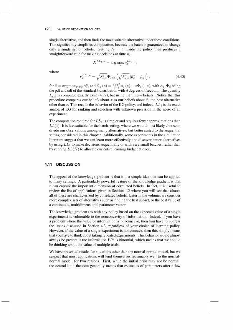
120 VALUE OF INFORMATION POLICIES
single alternative, and then finds the most suitable alternative under these conditions.This significantly simplifies computation, because the batch is guaranteed to changeonly a single set of beliefs. Setting N = 1 inside the policy then produces astraightforward rule for making decisions at time n,
XLL1,n = arg maxx
νLL1,nx ,
whereνLL1,nx =
√λnx,xΨ2anx
(√λnx,x |µ
nx − µnx |
), (4.40)
for x = arg maxx′ 6=x µnx , and Ψd (z) = d+z2
d−1 φd (z)− zΦd (−z), with φd,Φd beingthe pdf and cdf of the standard t-distribution with d degrees of freedom. The quantityλnx,x is computed exactly as in (4.39), but using the time-n beliefs. Notice that thisprocedure compares our beliefs about x to our beliefs about x, the best alternativeother than x. This recalls the behavior of the KG policy, and indeed, LL1 is the exactanalog of KG for ranking and selection with unknown precision in the noise of anexperiment.
The computation required forLL1 is simpler and requires fewer approximations thanLL(1). It is less suitable for the batch setting, where we would most likely choose todivide our observations among many alternatives, but better suited to the sequentialsetting considered in this chapter. Additionally, some experiments in the simulationliterature suggest that we can learn more effectively and discover better alternativesby using LL1 to make decisions sequentially or with very small batches, rather thanby running LL(N) to allocate our entire learning budget at once.
4.11 DISCUSSION
The appeal of the knowledge gradient is that it is a simple idea that can be appliedto many settings. A particularly powerful feature of the knowledge gradient is thatit can capture the important dimension of correlated beliefs. In fact, it is useful toreview the list of applications given in Section 1.2 where you will see that almostall of these are characterized by correlated beliefs. Later in the volume, we considermore complex sets of alternatives such as finding the best subset, or the best value ofa continuous, multidimensional parameter vector.
The knowledge gradient (as with any policy based on the expected value of a singleexperiment) is vulnerable to the nonconcavity of information. Indeed, if you havea problem where the value of information is nonconcave, then you have to addressthe issues discussed in Section 4.3, regardless of your choice of learning policy.However, if the value of a single experiment is nonconcave, then this simply meansthat you have to think about taking repeated experiments. This behavior would almostalways be present if the information Wn is binomial, which means that we shouldbe thinking about the value of multiple trials.
We have presented results for situations other than the normal-normal model, but wesuspect that most applications will lend themselves reasonably well to the normal-normal model, for two reasons. First, while the initial prior may not be normal,the central limit theorem generally means that estimates of parameters after a few
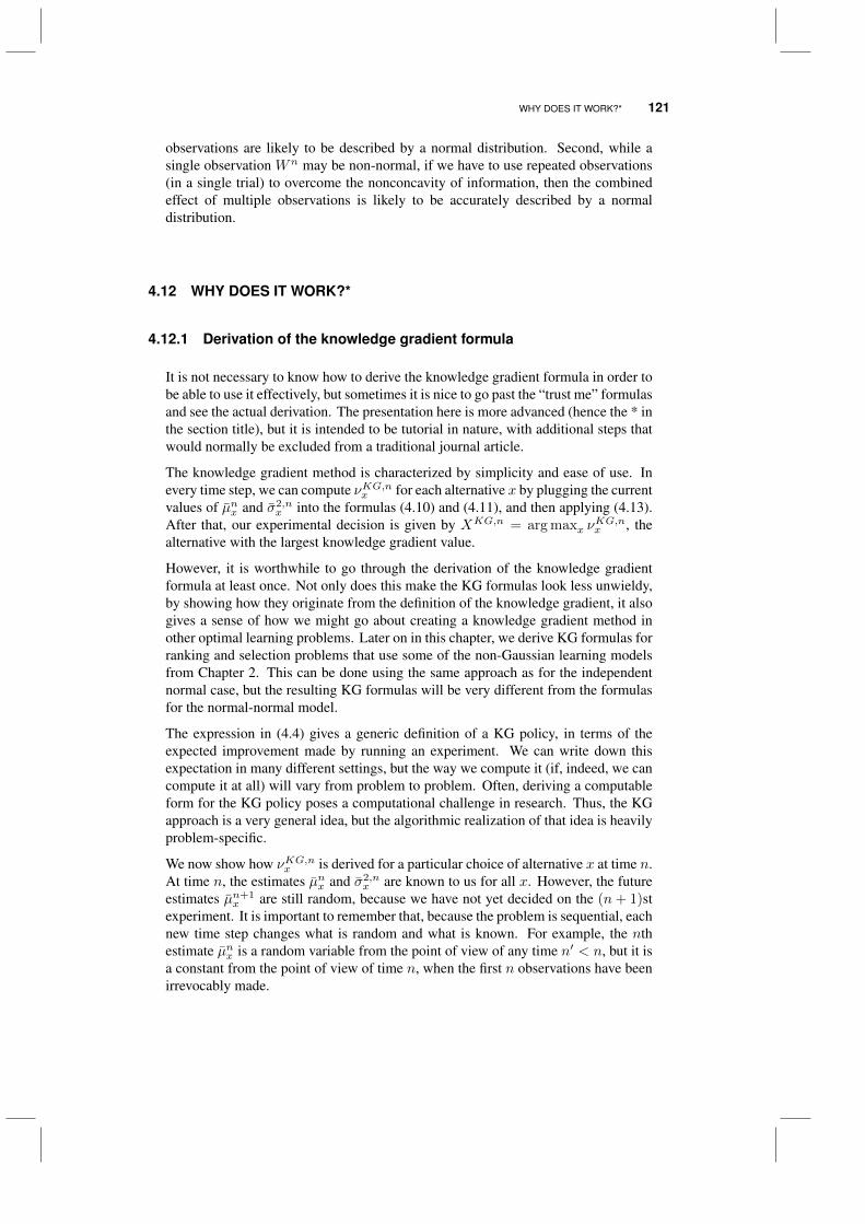
WHY DOES IT WORK?* 121
observations are likely to be described by a normal distribution. Second, while asingle observation Wn may be non-normal, if we have to use repeated observations(in a single trial) to overcome the nonconcavity of information, then the combinedeffect of multiple observations is likely to be accurately described by a normaldistribution.
4.12 WHY DOES IT WORK?*
4.12.1 Derivation of the knowledge gradient formula
It is not necessary to know how to derive the knowledge gradient formula in order tobe able to use it effectively, but sometimes it is nice to go past the “trust me” formulasand see the actual derivation. The presentation here is more advanced (hence the * inthe section title), but it is intended to be tutorial in nature, with additional steps thatwould normally be excluded from a traditional journal article.
The knowledge gradient method is characterized by simplicity and ease of use. Inevery time step, we can compute νKG,nx for each alternative x by plugging the currentvalues of µnx and σ2,n
x into the formulas (4.10) and (4.11), and then applying (4.13).After that, our experimental decision is given by XKG,n = arg maxx ν
KG,nx , the
alternative with the largest knowledge gradient value.
However, it is worthwhile to go through the derivation of the knowledge gradientformula at least once. Not only does this make the KG formulas look less unwieldy,by showing how they originate from the definition of the knowledge gradient, it alsogives a sense of how we might go about creating a knowledge gradient method inother optimal learning problems. Later on in this chapter, we derive KG formulas forranking and selection problems that use some of the non-Gaussian learning modelsfrom Chapter 2. This can be done using the same approach as for the independentnormal case, but the resulting KG formulas will be very different from the formulasfor the normal-normal model.
The expression in (4.4) gives a generic definition of a KG policy, in terms of theexpected improvement made by running an experiment. We can write down thisexpectation in many different settings, but the way we compute it (if, indeed, we cancompute it at all) will vary from problem to problem. Often, deriving a computableform for the KG policy poses a computational challenge in research. Thus, the KGapproach is a very general idea, but the algorithmic realization of that idea is heavilyproblem-specific.
We now show how νKG,nx is derived for a particular choice of alternative x at time n.At time n, the estimates µnx and σ2,n
x are known to us for all x. However, the futureestimates µn+1
x are still random, because we have not yet decided on the (n+ 1)stexperiment. It is important to remember that, because the problem is sequential, eachnew time step changes what is random and what is known. For example, the nthestimate µnx is a random variable from the point of view of any time n′ < n, but it isa constant from the point of view of time n, when the first n observations have beenirrevocably made.
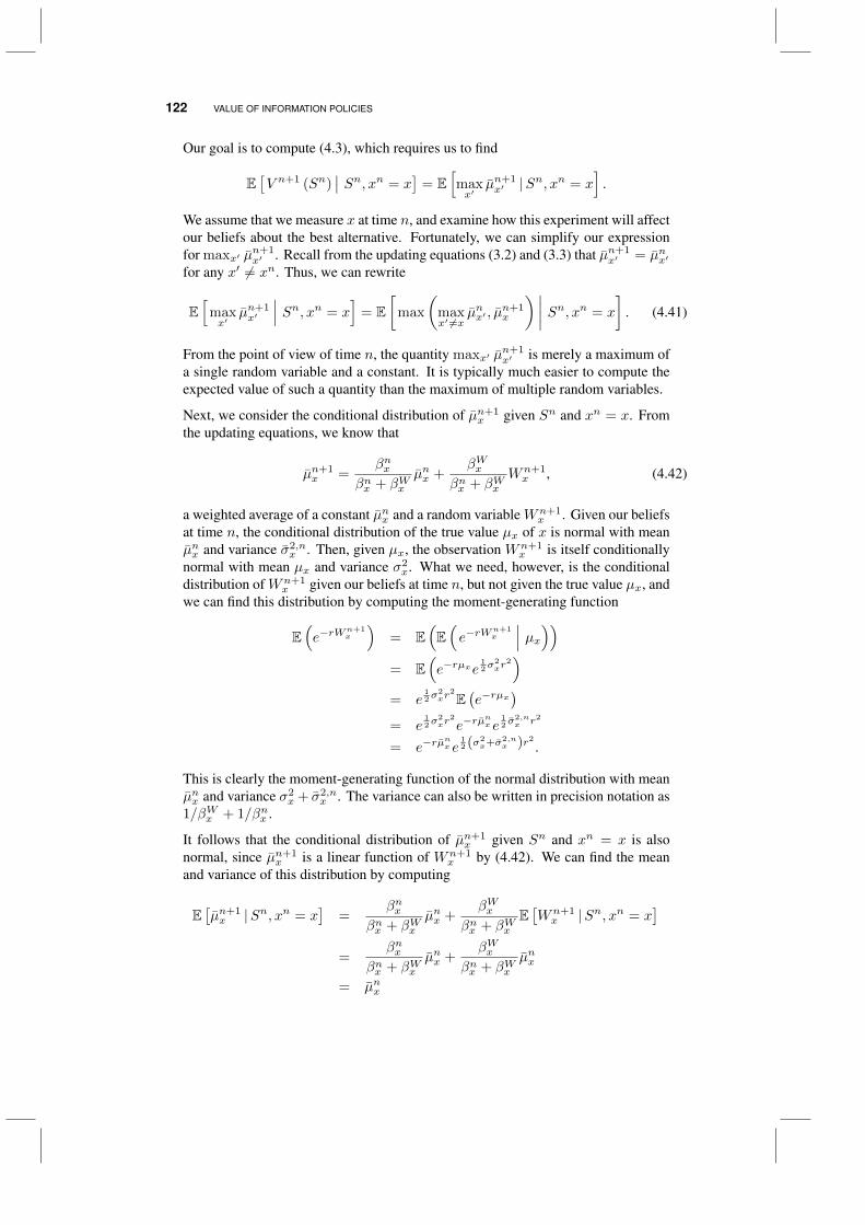
122 VALUE OF INFORMATION POLICIES
Our goal is to compute (4.3), which requires us to find
E[V n+1 (Sn)
∣∣ Sn, xn = x]
= E[maxx′
µn+1x′ |S
n, xn = x]
.
We assume that we measure x at time n, and examine how this experiment will affectour beliefs about the best alternative. Fortunately, we can simplify our expressionfor maxx′ µ
n+1x′ . Recall from the updating equations (3.2) and (3.3) that µn+1
x′ = µnx′for any x′ 6= xn. Thus, we can rewrite
E[
maxx′
µn+1x′
∣∣∣ Sn, xn = x]
= E[
max
(maxx′ 6=x
µnx′ , µn+1x
) ∣∣∣∣ Sn, xn = x
]. (4.41)
From the point of view of time n, the quantity maxx′ µn+1x′ is merely a maximum of
a single random variable and a constant. It is typically much easier to compute theexpected value of such a quantity than the maximum of multiple random variables.
Next, we consider the conditional distribution of µn+1x given Sn and xn = x. From
the updating equations, we know that
µn+1x =
βnxβnx + βWx
µnx +βWx
βnx + βWxWn+1x , (4.42)
a weighted average of a constant µnx and a random variableWn+1x . Given our beliefs
at time n, the conditional distribution of the true value µx of x is normal with meanµnx and variance σ2,n
x . Then, given µx, the observation Wn+1x is itself conditionally
normal with mean µx and variance σ2x. What we need, however, is the conditional
distribution ofWn+1x given our beliefs at time n, but not given the true value µx, and
we can find this distribution by computing the moment-generating function
E(e−rW
n+1x
)= E
(E(e−rW
n+1x
∣∣∣ µx))= E
(e−rµxe
12σ
2xr
2)
= e12σ
2xr
2
E(e−rµx
)= e
12σ
2xr
2
e−rµnx e
12 σ
2,nx r2
= e−rµnx e
12 (σ2
x+σ2,nx )r2
.
This is clearly the moment-generating function of the normal distribution with meanµnx and variance σ2
x + σ2,nx . The variance can also be written in precision notation as
1/βWx + 1/βnx .
It follows that the conditional distribution of µn+1x given Sn and xn = x is also
normal, since µn+1x is a linear function of Wn+1
x by (4.42). We can find the meanand variance of this distribution by computing
E[µn+1x |Sn, xn = x
]=
βnxβnx + βWx
µnx +βWx
βnx + βWxE[Wn+1x |Sn, xn = x
]=
βnxβnx + βWx
µnx +βWx
βnx + βWxµnx
= µnx

WHY DOES IT WORK?* 123
and
V ar[µn+1x |Sn, xn = x
]=
(βWx
βnx + βWx
)2
V ar[Wn+1x |Sn, xn = x
]=
(βWx
βnx + βWx
)2(1
βWx+
1
βnx
)=
βWxβnx (βWx + βnx )
.
Using the definition of the precision again, we can write
βWxβnx (βWx + βnx )
=σ2,nx
σ2x
(1σ2x
+ 1σ2,nx
)=
σ2,nx
1 + σ2x/σ
2,nx
which is precisely σ2,nx by (4.9).
We have found that the conditional distribution of µn+1x , given Sn and xn = x, is
normal with mean µnx and variance σ2,nx . In words, when we measure x at time n,
we expect that the next observation will be equal to µnx , that is, our beliefs µnx areaccurate on average. As a consequence of this experiment, the variance of our beliefsabout µx will decrease by an amount equal to the variance of the next observation.
Now, we can return to (4.41) and rewrite the right-hand side as
E[
max
(maxx′ 6=x
µnx′ , µn+1x
) ∣∣∣∣ Sn, xn = x
]= E
[max
(maxx′ 6=x
µnx′ , µnx + σnxZ
)]where Z is a standard normal (mean 0, variance 1) random variable. Our goal is nowto compute an expectation of a function of Z, which looks far more tractable than theexpression we started out with.
Let Cnx = maxx′ 6=x µnx′ , and observe that
max (Cnx , µnx + σnxZ) =
Cnx if Z ≤ C−µnx
σnx
µnx + σnx otherwise.
Thus,
E [max (Cnx , µnx + σnxZ)] =
∫ Cnx−µnx
σnx
−∞Cnxφ (z) dz
+
∫ ∞Cnx−µ
nx
σnx
(µnx + σnxz)φ (z) dz
where ∫ Cnx−µnx
σnx
−∞Cnxφ (z) dz = CnxΦ
(Cnx − µnxσnx
)

124 VALUE OF INFORMATION POLICIES
and ∫ ∞Cnx−µ
nx
σnx
(µnx + σnxz)φ (z) dz = µnxΦ
(−C
nx − µnxσnx
)+ σnxφ
(Cnx − µnxσnx
).
The first term in the second equation uses the symmetry of the normal distribution,and the second term is due to the fact that∫ ∞
y
zφ (z) dz = φ (y) ,
which can be verified by a back-of-the-envelope calculation.
Observe now that, due to the symmetry of the normal density,
φ
(Cnx − µnxσnx
)= φ
(−C
nx − µnxσnx
)= φ (ζnx ) ,
which gives us one of the terms that make up the KG formula. To obtain the otherterm, we consider two cases. If Cnx ≤ µnx , then µnx = maxx′ µ
nx′ and
CnxΦ
(Cnx − µnxσnx
)+ µnxΦ
(−C
nx − µnxσnx
)= CnxΦ (ζnx ) + µnx − µnxΦ (ζnx )
= µnx + σnx
(Cnx − µnxσnx
)Φ (ζnx )
= µnx + σnxζnxΦ (ζnx ) .
However, if µnx < Cnx , then Cnx = maxx′ µnx′ and
CnxΦ
(Cnx − µnxσnx
)+ µnxΦ
(−C
nx − µnxσnx
)= Cnx − CnxΦ (ζnx ) + µnxΦ (ζn)x)
= Cnx + σnxζnxΦ (ζnx ) .
Either way,
CnxΦ
(Cnx − µnxσnx
)+ µnxΦ
(−C
nx − µnxσnx
)= max
x′µnx′ + σnxζ
nxΦ (ζnx ) .
Putting all the terms together,
E [max (Cnx , µnx + σnxZ)] = max
x′µnx′ + σnx (ζnxΦ (ζnx ) + φ (ζnx ))
= maxx′
µnx′ + σnxf (ζnx ) ,
whence
νKG,nx = E[
maxx′
µn+1x′ −max
x′µnx′∣∣∣ Sn, xn = x
]= E
[max
(maxx′ 6=x
µnx′ , µn+1x
) ∣∣∣∣ Sn, xn = x
]−max
x′µnx′
= σnxf (ζnx ) ,
which is precisely the KG formula that we introduced earlier.
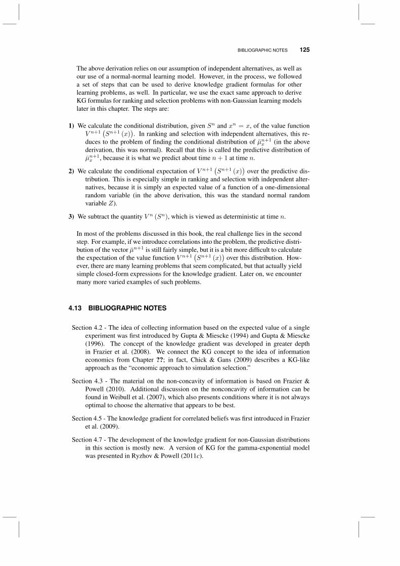
BIBLIOGRAPHIC NOTES 125
The above derivation relies on our assumption of independent alternatives, as well asour use of a normal-normal learning model. However, in the process, we followeda set of steps that can be used to derive knowledge gradient formulas for otherlearning problems, as well. In particular, we use the exact same approach to deriveKG formulas for ranking and selection problems with non-Gaussian learning modelslater in this chapter. The steps are:
1) We calculate the conditional distribution, given Sn and xn = x, of the value functionV n+1
(Sn+1 (x)
). In ranking and selection with independent alternatives, this re-
duces to the problem of finding the conditional distribution of µn+1x (in the above
derivation, this was normal). Recall that this is called the predictive distribution ofµn+1x , because it is what we predict about time n+ 1 at time n.
2) We calculate the conditional expectation of V n+1(Sn+1 (x)
)over the predictive dis-
tribution. This is especially simple in ranking and selection with independent alter-natives, because it is simply an expected value of a function of a one-dimensionalrandom variable (in the above derivation, this was the standard normal randomvariable Z).
3) We subtract the quantity V n (Sn), which is viewed as deterministic at time n.
In most of the problems discussed in this book, the real challenge lies in the secondstep. For example, if we introduce correlations into the problem, the predictive distri-bution of the vector µn+1 is still fairly simple, but it is a bit more difficult to calculatethe expectation of the value function V n+1
(Sn+1 (x)
)over this distribution. How-
ever, there are many learning problems that seem complicated, but that actually yieldsimple closed-form expressions for the knowledge gradient. Later on, we encountermany more varied examples of such problems.
4.13 BIBLIOGRAPHIC NOTES
Section 4.2 - The idea of collecting information based on the expected value of a singleexperiment was first introduced by Gupta & Miescke (1994) and Gupta & Miescke(1996). The concept of the knowledge gradient was developed in greater depthin Frazier et al. (2008). We connect the KG concept to the idea of informationeconomics from Chapter ??; in fact, Chick & Gans (2009) describes a KG-likeapproach as the “economic approach to simulation selection.”
Section 4.3 - The material on the non-concavity of information is based on Frazier &Powell (2010). Additional discussion on the nonconcavity of information can befound in Weibull et al. (2007), which also presents conditions where it is not alwaysoptimal to choose the alternative that appears to be best.
Section 4.5 - The knowledge gradient for correlated beliefs was first introduced in Frazieret al. (2009).
Section 4.7 - The development of the knowledge gradient for non-Gaussian distributionsin this section is mostly new. A version of KG for the gamma-exponential modelwas presented in Ryzhov & Powell (2011c).
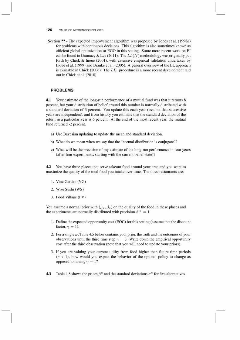
126 VALUE OF INFORMATION POLICIES
Section ?? - The expected improvement algorithm was proposed by Jones et al. (1998a)for problems with continuous decisions. This algorithm is also sometimes known asefficient global optimization or EGO in this setting. Some more recent work on EIcan be found in Gramacy & Lee (2011). TheLL(N) methodology was originally putforth by Chick & Inoue (2001), with extensive empirical validation undertaken byInoue et al. (1999) and Branke et al. (2005). A general overview of the LL approachis available in Chick (2006). The LL1 procedure is a more recent development laidout in Chick et al. (2010).
PROBLEMS
4.1 Your estimate of the long-run performance of a mutual fund was that it returns 8percent, but your distribution of belief around this number is normally distributed witha standard deviation of 3 percent. You update this each year (assume that successiveyears are independent), and from history you estimate that the standard deviation of thereturn in a particular year is 6 percent. At the end of the most recent year, the mutualfund returned -2 percent.
a) Use Bayesian updating to update the mean and standard deviation.
b) What do we mean when we say that the “normal distribution is conjugate”?
c) What will be the precision of my estimate of the long-run performance in four years(after four experiments, starting with the current belief state)?
4.2 You have three places that serve takeout food around your area and you want tomaximize the quality of the total food you intake over time. The three restaurants are:
1. Vine Garden (VG)
2. Wise Sushi (WS)
3. Food Village (FV)
You assume a normal prior with (µx, βx) on the quality of the food in these places andthe experiments are normally distributed with precision βW = 1.
1. Define the expected opportunity cost (EOC) for this setting (assume that the discountfactor, γ = 1).
2. For a singleω, Table 4.5 below contains your prior, the truth and the outcomes of yourobservations until the third time step n = 3. Write down the empirical opportunitycost after the third observation (note that you will need to update your priors).
3. If you are valuing your current utility from food higher than future time periods(γ < 1), how would you expect the behavior of the optimal policy to change asopposed to having γ = 1?
4.3 Table 4.8 shows the priors µn and the standard deviations σn for five alternatives.
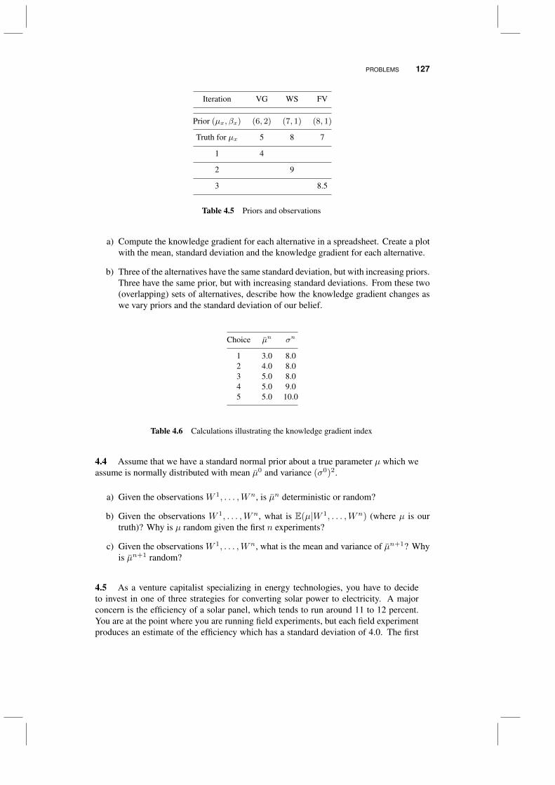
PROBLEMS 127
Iteration VG WS FV
Prior (µx, βx) (6, 2) (7, 1) (8, 1)
Truth for µx 5 8 7
1 4
2 9
3 8.5
Table 4.5 Priors and observations
a) Compute the knowledge gradient for each alternative in a spreadsheet. Create a plotwith the mean, standard deviation and the knowledge gradient for each alternative.
b) Three of the alternatives have the same standard deviation, but with increasing priors.Three have the same prior, but with increasing standard deviations. From these two(overlapping) sets of alternatives, describe how the knowledge gradient changes aswe vary priors and the standard deviation of our belief.
Choice µn σn
1 3.0 8.02 4.0 8.03 5.0 8.04 5.0 9.05 5.0 10.0
Table 4.6 Calculations illustrating the knowledge gradient index
4.4 Assume that we have a standard normal prior about a true parameter µ which weassume is normally distributed with mean µ0 and variance (σ0)2.
a) Given the observations W 1, . . . ,Wn, is µn deterministic or random?
b) Given the observations W 1, . . . ,Wn, what is E(µ|W 1, . . . ,Wn) (where µ is ourtruth)? Why is µ random given the first n experiments?
c) Given the observations W 1, . . . ,Wn, what is the mean and variance of µn+1? Whyis µn+1 random?
4.5 As a venture capitalist specializing in energy technologies, you have to decideto invest in one of three strategies for converting solar power to electricity. A majorconcern is the efficiency of a solar panel, which tends to run around 11 to 12 percent.You are at the point where you are running field experiments, but each field experimentproduces an estimate of the efficiency which has a standard deviation of 4.0. The first
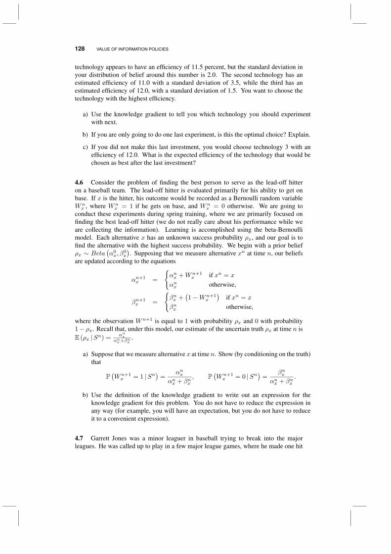
128 VALUE OF INFORMATION POLICIES
technology appears to have an efficiency of 11.5 percent, but the standard deviation inyour distribution of belief around this number is 2.0. The second technology has anestimated efficiency of 11.0 with a standard deviation of 3.5, while the third has anestimated efficiency of 12.0, with a standard deviation of 1.5. You want to choose thetechnology with the highest efficiency.
a) Use the knowledge gradient to tell you which technology you should experimentwith next.
b) If you are only going to do one last experiment, is this the optimal choice? Explain.
c) If you did not make this last investment, you would choose technology 3 with anefficiency of 12.0. What is the expected efficiency of the technology that would bechosen as best after the last investment?
4.6 Consider the problem of finding the best person to serve as the lead-off hitteron a baseball team. The lead-off hitter is evaluated primarily for his ability to get onbase. If x is the hitter, his outcome would be recorded as a Bernoulli random variableWnx , where Wn
x = 1 if he gets on base, and Wnx = 0 otherwise. We are going to
conduct these experiments during spring training, where we are primarily focused onfinding the best lead-off hitter (we do not really care about his performance while weare collecting the information). Learning is accomplished using the beta-Bernoullimodel. Each alternative x has an unknown success probability ρx, and our goal is tofind the alternative with the highest success probability. We begin with a prior beliefρx ∼ Beta
(α0x, β
0x
). Supposing that we measure alternative xn at time n, our beliefs
are updated according to the equations
αn+1x =
αnx +Wn+1
x if xn = x
αnx otherwise,
βn+1x =
βnx +
(1−Wn+1
x
)if xn = x
βnx otherwise,
where the observation Wn+1 is equal to 1 with probability ρx and 0 with probability1− ρx. Recall that, under this model, our estimate of the uncertain truth ρx at time n isE (ρx |Sn) =
αnxαnx+βnx
.
a) Suppose that we measure alternative x at time n. Show (by conditioning on the truth)that
P(Wn+1x = 1 |Sn
)=
αnxαnx + βnx
, P(Wn+1x = 0 |Sn
)=
βnxαnx + βnx
.
b) Use the definition of the knowledge gradient to write out an expression for theknowledge gradient for this problem. You do not have to reduce the expression inany way (for example, you will have an expectation, but you do not have to reduceit to a convenient expression).
4.7 Garrett Jones was a minor leaguer in baseball trying to break into the majorleagues. He was called up to play in a few major league games, where he made one hit
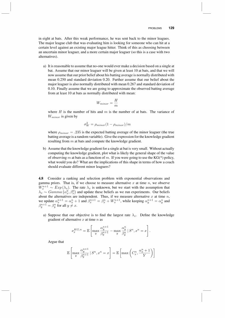
PROBLEMS 129
in eight at bats. After this weak performance, he was sent back to the minor leagues.The major league club that was evaluating him is looking for someone who can hit at acertain level against an existing major league hitter. Think of this as choosing betweenan uncertain minor leaguer, and a more certain major leaguer (so this is a case with twoalternatives).
a) It is reasonable to assume that no-one would ever make a decision based on a single atbat. Assume that our minor leaguer will be given at least 10 at bats, and that we willnow assume that our prior belief about his batting average is normally distributed withmean 0.250 and standard deviation 0.20. Further assume that our belief about themajor leaguer is also normally distributed with mean 0.267 and standard deviation of0.10. Finally assume that we are going to approximate the observed batting averagefrom at least 10 at bats as normally distributed with mean:
Wminor =H
m
where H is the number of hits and m is the number of at bats. The variance ofWminor is given by
σ2W = ρminor(1− ρminor)/m
where ρminor = .235 is the expected batting average of the minor leaguer (the truebatting average is a random variable). Give the expression for the knowledge gradientresulting from m at bats and compute the knowledge gradient.
b) Assume that the knowledge gradient for a single at bat is very small. Without actuallycomputing the knowledge gradient, plot what is likely the general shape of the valueof observingm at bats as a function ofm. If you were going to use the KG(*) policy,what would you do? What are the implications of this shape in terms of how a coachshould evaluate different minor leaguers?
4.8 Consider a ranking and selection problem with exponential observations andgamma priors. That is, if we choose to measure alternative x at time n, we observeWn+1x ∼ Exp (λx). The rate λx is unknown, but we start with the assumption that
λx ∼ Gamma(α0x, β
0x
)and update these beliefs as we run experiments. Our beliefs
about the alternatives are independent. Thus, if we measure alternative x at time n,we update αn+1
x = αnx + 1 and βn+1x = βnx + Wn+1
x , while keeping αn+1y = αny and
βn+1y = βny for all y 6= x.
a) Suppose that our objective is to find the largest rate λx. Define the knowledgegradient of alternative x at time n as
νKG,nx = E
[maxy
αn+1y
βn+1y
−maxy
αnyβny|Sn, xn = x
].
Argue that
E
[maxy
αn+1y
βn+1y
|Sn, xn = x
]= E
[max
(Cnx ,
αnx + 1
Y
)]

130 VALUE OF INFORMATION POLICIES
where Cnx = maxy 6=xαnyβny
and Y ∼ Pareto (αnx , βnx ).
(Remember that the Pareto (a, b) density is g (t) = aba
ta+1 for t > b and zeroelsewhere.)
b) Suppose that αnx+1βnx≤ Cnx . Show that
E[max
(Cnx ,
αnx + 1
Y
)]= Cnx .
c) Suppose that αnx+1βnx
> Cnx . Show that
E[max
(Cnx ,
αnx + 1
Y
)]=αnxβnx
+(βnx )
αnx (Cnx )αnx+1
(αnx + 1)αnx+1 .
d) Based on parts b) and c), show that
νKG,nx =
(βnx )αnx (Cnx )α
nx+1
(αnx+1)αnx+1 if x = arg maxy
αnyβny
(βnx )αnx (Cnx )α
nx+1
(αnx+1)αnx+1 −
(maxy
αnyβny− αnx
βnx
)if x 6= arg maxy
αnyβny,
αnx+1βnx
> maxyαnyβny
0 otherwise.
4.9 We again consider a ranking and selection problem with exponential observationsand gamma priors. There are five alternatives, and the belief state for a certain time stepn is given in table 4.7. The objective is to find the largest rate.
x αnx βnx
1 2 182 3 173 1 74 2 155 3 14
Table 4.7 Priors for exercise 4.9
4.10 Consider a ranking and selection problem with independent alternatives, expo-nential observations and gamma priors.
a) Suppose that we want to find the alternative with the highest rate. Derive the KGformula given in (4.29). (Hint: Consider the three cases given in the formulaseparately before trying to take integrals.)
b) Repeat your analysis for the case where our goal is to find the lowest rate. Show thatthe KG formula is given by (4.30).
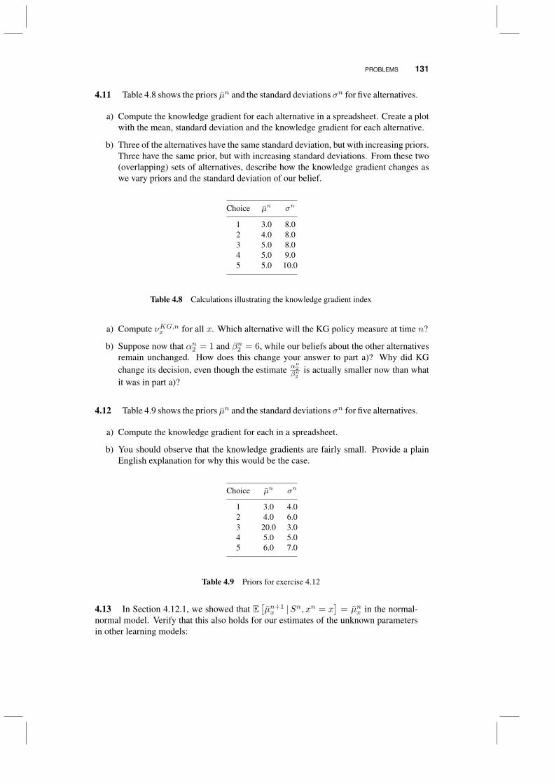
PROBLEMS 131
4.11 Table 4.8 shows the priors µn and the standard deviations σn for five alternatives.
a) Compute the knowledge gradient for each alternative in a spreadsheet. Create a plotwith the mean, standard deviation and the knowledge gradient for each alternative.
b) Three of the alternatives have the same standard deviation, but with increasing priors.Three have the same prior, but with increasing standard deviations. From these two(overlapping) sets of alternatives, describe how the knowledge gradient changes aswe vary priors and the standard deviation of our belief.
Choice µn σn
1 3.0 8.02 4.0 8.03 5.0 8.04 5.0 9.05 5.0 10.0
Table 4.8 Calculations illustrating the knowledge gradient index
a) Compute νKG,nx for all x. Which alternative will the KG policy measure at time n?
b) Suppose now that αn2 = 1 and βn2 = 6, while our beliefs about the other alternativesremain unchanged. How does this change your answer to part a)? Why did KGchange its decision, even though the estimate αn2
βn2is actually smaller now than what
it was in part a)?
4.12 Table 4.9 shows the priors µn and the standard deviations σn for five alternatives.
a) Compute the knowledge gradient for each in a spreadsheet.
b) You should observe that the knowledge gradients are fairly small. Provide a plainEnglish explanation for why this would be the case.
Choice µn σn
1 3.0 4.02 4.0 6.03 20.0 3.04 5.0 5.05 6.0 7.0
Table 4.9 Priors for exercise 4.12
4.13 In Section 4.12.1, we showed that E[µn+1x |Sn, xn = x
]= µnx in the normal-
normal model. Verify that this also holds for our estimates of the unknown parametersin other learning models:
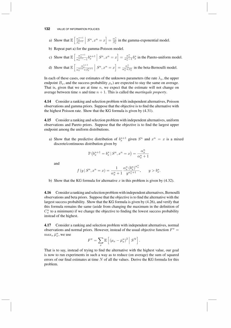
132 VALUE OF INFORMATION POLICIES
a) Show that E[αn+1x
βn+1x
∣∣∣ Sn, xn = x]
=αnxβnx
in the gamma-exponential model.
b) Repeat part a) for the gamma-Poisson model.
c) Show that E[
αn+1x
αn+1x −1
bn+1x
∣∣∣ Sn, xn = x]
=αnxαnx−1b
nx in the Pareto-uniform model.
d) Show that E[
αn+1x
αn+1x +βn+1
x
∣∣∣ Sn, xn = x]
=αnx
αnx+βnxin the beta-Bernoulli model.
In each of these cases, our estimates of the unknown parameters (the rate λx, the upperendpoint Bx, and the success probability ρx) are expected to stay the same on average.That is, given that we are at time n, we expect that the estimate will not change onaverage between time n and time n+ 1. This is called the martingale property.
4.14 Consider a ranking and selection problem with independent alternatives, Poissonobservations and gamma priors. Suppose that the objective is to find the alternative withthe highest Poisson rate. Show that the KG formula is given by (4.31).
4.15 Consider a ranking and selection problem with independent alternatives, uniformobservations and Pareto priors. Suppose that the objective is to find the largest upperendpoint among the uniform distributions.
a) Show that the predictive distribution of bn+1x given Sn and xn = x is a mixed
discrete/continuous distribution given by
P(bn+1x = bnx |Sn, xn = x
)=
αnxαnx + 1
and
f (y |Sn, xn = x) =1
αnx + 1
αnx (bnx)αnx
yαnx+1
, y > bnx .
b) Show that the KG formula for alternative x in this problem is given by (4.32).
4.16 Consider a ranking and selection problem with independent alternatives, Bernoulliobservations and beta priors. Suppose that the objective is to find the alternative with thelargest success probability. Show that the KG formula is given by (4.26), and verify thatthis formula remains the same (aside from changing the maximum in the definition ofCnx to a minimum) if we change the objective to finding the lowest success probabilityinstead of the highest.
4.17 Consider a ranking and selection problem with independent alternatives, normalobservations and normal priors. However, instead of the usual objective function Fπ =maxx µ
nx , we use
Fπ =∑x
E[
(µx − µnx)2∣∣∣ SN] .
That is to say, instead of trying to find the alternative with the highest value, our goalis now to run experiments in such a way as to reduce (on average) the sum of squarederrors of our final estimates at time N of all the values. Derive the KG formula for thisproblem.

PROBLEMS 133
4.18 Suppose that we have four different products. The profit margin of product x,x = 1, 2, 3, 4 is represented by µx. We can choose to perform a market study on productx to get an observation Wx of its profit margin. The observation is normally distributedwith mean µx and variance (σWx )2. Table 4.10 below gives the true values of µx and(σWx )2:
x µx(σWx)2
1 15 42 10 33 12 54 11 2
Table 4.10 Priors for exercise 4.18.
However, we do not know the true values of µx. We describe our beliefs about themusing a multivariate Gaussian prior with the following mean vector and covariancematrix:
µ0 =
12141310
, Σ0 =
12 0 6 30 7 4 26 4 9 03 2 0 8
.
Assume that we choose to observe product 3 and we observe W 13 = 15. Show how our
beliefs would change using the updating equations
µ1 = µ0 +W 1x − µ0
x
(σWx )2
+ Σ0xx
Σ0ex, Σ1 = Σ0 − Σ0exeTxΣ0
(σWx )2
+ Σnxx(4.43)
where x = 3 is the particular product that you are considering, and ex is a column vectorof zeroes with a single 1 in the xth coordinate. Report the resulting values of µ1 andΣ1. (Equation (4.43) gives the “convenient” version of the updating equations, whereyou don’t have to compute an inverse. You do not have to derive these equations.)
4.19 Consider a ranking and selection problem with independent alternatives, normalobservations and normal priors. However, instead of the usual objective function Fπ =maxx µ
nx , we use
Fπ = maxx|µnx | .
That is, we want to find the alternative with the largest absolute value. Show that theKG factor of alternative x is given by
νKG,nx = σnx (f (ζnx ) + f (δnx )) ,
where
ζnx = −∣∣∣∣ µnx −maxx′ 6=x |µnx′ |
σnx
∣∣∣∣ , δnx = − µnx + maxx′ 6=x |µnx′ |
σnx .
4.20 The revenue generated by an online advertisement has an exponential distributionwith parameter λ (thus the mean revenue is 1
λ ). We do not know λ, so we use a gamma
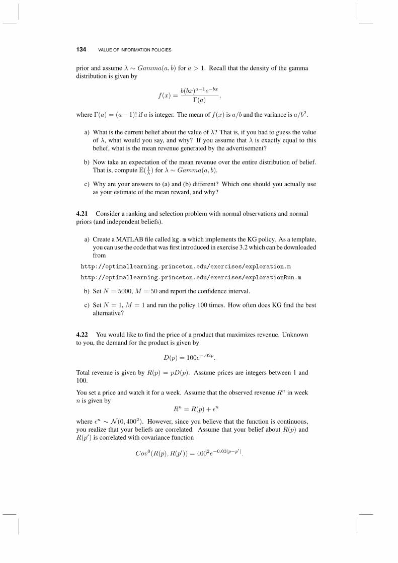
134 VALUE OF INFORMATION POLICIES
prior and assume λ ∼ Gamma(a, b) for a > 1. Recall that the density of the gammadistribution is given by
f(x) =b(bx)a−1e−bx
Γ(a),
where Γ(a) = (a− 1)! if a is integer. The mean of f(x) is a/b and the variance is a/b2.
a) What is the current belief about the value of λ? That is, if you had to guess the valueof λ, what would you say, and why? If you assume that λ is exactly equal to thisbelief, what is the mean revenue generated by the advertisement?
b) Now take an expectation of the mean revenue over the entire distribution of belief.That is, compute E( 1
λ ) for λ ∼ Gamma(a, b).
c) Why are your answers to (a) and (b) different? Which one should you actually useas your estimate of the mean reward, and why?
4.21 Consider a ranking and selection problem with normal observations and normalpriors (and independent beliefs).
a) Create a MATLAB file called kg.m which implements the KG policy. As a template,you can use the code that was first introduced in exercise 3.2 which can be downloadedfrom
http://optimallearning.princeton.edu/exercises/exploration.m
http://optimallearning.princeton.edu/exercises/explorationRun.m
b) Set N = 5000, M = 50 and report the confidence interval.
c) Set N = 1, M = 1 and run the policy 100 times. How often does KG find the bestalternative?
4.22 You would like to find the price of a product that maximizes revenue. Unknownto you, the demand for the product is given by
D(p) = 100e−.02p.
Total revenue is given by R(p) = pD(p). Assume prices are integers between 1 and100.
You set a price and watch it for a week. Assume that the observed revenue Rn in weekn is given by
Rn = R(p) + εn
where εn ∼ N (0, 4002). However, since you believe that the function is continuous,you realize that your beliefs are correlated. Assume that your belief about R(p) andR(p′) is correlated with covariance function
Cov0(R(p), R(p′)) = 4002e−0.03|p−p′|.

PROBLEMS 135
So, Cov0(R(p), R(p)) = V ar0(R(p)) = 4002, and Cov0(R(20), R(30)) = 4002 ×0.7408. Use this to create your prior covariance matrix Σ0. Assume that your initialestimate of R(p) is µ0
p = 2000 for each p (this is known as a “uniform prior,” andrepresents a situation where you have no idea which price is the best.) Note that we areusing online learning for this exercise.
a) Write out the updating formulas for updating your estimate µnp giving the estimatedrevenue when you charge price p, and the updating formula for the covariance matrixΣn.
b) Implement the algorithm for computing the knowledge gradient in the presence ofcorrelated beliefs (call this algorithm KGCB), using as a starting point
http://optimallearning.princeton.edu/exercises/KGCorrBeliefs.m
An example illustration of the KGCB algorithm is given in
http://optimallearning.princeton.edu/exercises/KGCorrBeliefsEx.m
Verify your algorithm first by running it with a diagonal covariance matrix, andshowing that the independent and correlated KG algorithms give you the samenumbers. Note that you may find that for some prices, the knowledge gradient is toosmall to compute (for example, you get a very negative exponent).
c) Next use the initial covariance matrix described above. Plot the log of the knowl-edge gradient for prices between 1 and 100 (again, be careful with large negativeexponents), and compare your results to the log of the knowledge gradient assumingindependent beliefs. How do they compare?
d) Now we are going to compare policies. Please do the following:
i) Run your KGCB algorithm for 10 experiments, and plot after each experimentthe opportunity cost, which means you take what you think is the best pricebased on your current set of estimates, and compare it to the revenue you wouldget if you knew the best price (hint: it is $50). Repeat this exercise 20 times,and report the average opportunity cost, averaged over the 20 iterations. Thegoal here is to get a sense of the variability of the performance of a learningpolicy.
ii) We want to compare KGCB against pure exploration, pure exploitation andinterval estimation using zα = 1.96 (a standard default). For each policy,perform 20 sample paths and plot the average opportunity cost over all 20sample paths. Compare all three policies. [Please make sure that you areresetting the covariance matrix to its initial structure after you are done with asample path (once you have gone over a single truth). If you skip this part, theKG algorithm will assume it has very precise priors for the second run, whichof course is not true.]
e) The knowledge gradient policy can be quite sensitive to the prior. Instead of an initialprior of 2000, now assume that we start with a uniform prior of 500 (same standarddeviation). If you edit the prior (column B), the package regenerates the truth. Youare going to have to re-enter the formula for the truth after changing the prior. Afterdoing this, perform 3 repetitions of KG, pure exploration and pure exploitation, andcontrast their performance.


CHAPTER 5
ONLINE LEARNING
In this chapter we turn to the problem where we have to learn as we go. Thismeans that we no longer have the luxury of making mistakes within our experimentalbudget before we have to decide which design to implement. Now, every decisionis an implementation decision where we have to live with the consequences, butsimultaneously learning as we go.
On the surface, the difference between the offline learning problem we introduced inchapter 3, and the online learning problem we address in this chapter, is the objectivefunction. With the offline problem, our objective could be stated as
maxπ
EµEW 1,...,WN |µµxπ,N , (5.1)
where xπ,N is the alternative we think is best given our estimates µNx , given by
xπ,N = arg maxx
µNx .
This means we are only interested in the performance µxπ,N of the final design xπ,N
that we learned by following learning policy π after exhausting our experimentalbudget N .
For an online learning problem, we have to learn as we go. So, ifXπ(S) is our policythat returns a decision xn = Xπ(Sn) when our belief state is Sn. We then receive a
Optimal Learning. By Warren B. Powell and Ilya O. RyzhovCopyright c© 2018 John Wiley & Sons, Inc.
137
138 ONLINE LEARNING
reward Wn+1. This means we have to find the policy that solves
maxπ
EµEW 1,...,WN |µ
N−1∑n=0
Wn+1xn , (5.2)
where xn = Xπ(Sn). If we assume that we have access to the true mean µx for thepurpose of testing policies (as we did in equation (5.1)), we could write our objectiveas
maxπ
EµEW 1,...,WN |µ
N−1∑n=0
µXπ(Sn). (5.3)
However we calculate the objective, we see that our offline problem focuses on thefinal (or terminal) reward or performance, while our online problem focuses on thecumulative reward.
Viewed this way, the difference between offline (terminal reward) and online (cu-mulative reward) seems modest, and for some classes of policies, it is. However,online learning problems have a long and rich history where it has evolved as themultiarmed bandit problem.
The multi-armed bandit problem (or MAB, as it is often known) is a venerable topicin optimal learning, and has inspired some of the pioneering work in the field. Thestory that was originally used to motivate the problem (and gave the problem itsname) is not really an important application, but is useful for understanding the basicidea behind the problem. The term “one-armed bandit” refers to a slot machineoperated by pulling a lever (or “arm”) on its side. A multi-armed bandit, then, is acollection of slot machines, each with a different winning probability (or differentaverage winnings).
Suppose that we have M slot machines each with a different but unknown rewarddistribution (yes, that is the story). If we play slot machine x at time n, we receiverandom winnings Wn+1
x . Suppose that the expected value of these winnings, givenby µx, is unknown. We would like to estimate µx, but the only way to do this isby putting money into the machine and collecting a random observation. For thisreason, we must balance our desire to find the slot machine with the highest valuewith our desire to achieve good results on every play.
There are numerous examples of online learning problems. Some examples are
EXAMPLE 5.1
You need to find the best path to work, but the only way to evaluate a path is toactually try it.
EXAMPLE 5.2
A physician has to find the best diabetes medication for a patient, but the only wayto see how the patient responds is to try the medication on the patient.
139
EXAMPLE 5.3
A company needs to place bids to have its ad appear on Google. The company hasto try different bids to find the one that strikes the best balance between cost andresponse.
EXAMPLE 5.4
An internet movie provider has to decide which movies to show to maximize thelikelihood that a user logging into her account will pick one of the movies to watch.
EXAMPLE 5.5
An internet retailer has to experiment with different prices for a product to find theprice that maximizes revenue.
Both offline and online learning problems require balancing exploration and exploita-tion, but the tradeoff is more apparent with online problems.
As early as 1970, we have known that we could characterize an optimal policy bysetting up Bellman’s equation
V n(Sn) = maxx
(µnx + EWV n+1(Sn+1)
), n = 0, . . . , N − 1 (5.4)
V N (SN ) = maxx
µNx , (5.5)
where Sn+1 = SM (Sn, x,Wn+1x ). Here, Sn = (µnx , β
nx )x∈X is the belief state,
x is a decision of which “arm” to try, Wn+1x is what we learn, and SM (S, x,W )
captures the equations for updating the belief model. The problem is that if we havea normally distributed belief model and M alternatives, then S has 2M continuousdimensions. As a result, solving equation (5.5) is completely intractable.
Given this, it was quite a breakthrough when J.C. Gittins found, in 1974, that insteadof solving a 2M dimensional problem across all M alternatives, it was possible tofind an optimal policy by solving M individual dynamic programs. Each of thesedynamic programs returned an index, later known as the Gittins index, which requiredthat we simply find the alternative with the highest index. This became known asan index policy. This spawned a steady stream of papers looking for optimal indexpolicies for variations of the basic bandit problem.
The development of Gittins indices generated considerable enthusiasm in the appliedprobability community, although they still remained a computational challenge inthat while they were computable, they were not easy to compute. We illustrate thebasic idea of Gittins indices, which also serves to highlight the relative complexity,especially compared to the policies we have seen so far for the offline problem.
A completely different approach was developed by Lai and Robbins in 1985, whofound that a very simple idea called upper confidence bounding (which we first sawin chapter 3) produced a policy where it is possible to bound how often it chose thewrong arm. While this does not mean that UCB policies (as they are known) are

140 ONLINE LEARNING
optimal, it provided evidence that they might be quite good. In addition, they aretrivial to compute, which makes them attractive for high-speed internet applications.
Reflecting the combined contributions of these two communities, the multi-armedbandit problem has attracted a substantial following that has grown past the core nichecommunities that developed these ideas. In fact, these communities have collectivelyspawned the study of a wide range of “bandit problems” that has introduced novelproblem variations that have been overlooked by other communities working onstochastic optimization problems.
We are ultimately going to see that there are many policies that were designedoriginally for online learning problems, but which still need to be tuned, and whichcan be tuned for either online or offline applications. We are going to cover threemajor classes of policies:
Excitation policy Excitation policies use a simple rule, such as a decision that appears tobe best, and introduces some noise to encourage exploration.
Upper confidence bounding UCB policies are trivial to compute and enjoy bounds thatsuggest that they should work well, although they still have to be tuned in practice.
Gittins indices Gittins indices determine the best decision based on the value of informa-tion from the decision over the entire horizon, computed using dynamic program-ming. These are more difficult to compute, but provide a rare example of an optimalpolicy when certain assumptions are satisfied.
Lookahead policies While Gittins indices using dynamic programming to compute thevalue of being in a belief state, another approach is to try to model decisions andlearning in the future to help make a decision now. We have already seen this insection 1.6 when we used decision trees to model decisions and information oversome horizon. In this chapter we are going to illustrate some different strategies forapproximating the future.
5.1 AN EXCITATION POLICY
Consider the problem of pricing a product where we have to set a price x in the hopeof maximizing revenue. We might assume that we can approximate the demandD(p)as a function of price p over a reasonable range of prices using a linear function
D(p|θ) = θ1 − θ2p.
We would like to maximize the revenue R(p) = pD(p). If we knew θ = (θ1, θ2) wewould just take the derivative of R(p), set it equal to zero and solve for the optimalprice, giving us
p∗ =θ1
2θ2.
UPPER CONFIDENCE BOUNDING 141
The problem is that we do not know θ. Let θn be our estimate of θ after n samples.This means that we would compute our price pn using
pn =θn12θn2
.
Further assume that after setting a price pn we observe a revenue Rn+1. The revenueRn+1 presumably comes from
Rn+1 = θ1 − θ2pn + εn+1,
where θ1 and θ2 are the true (but unknown) parameters, and εn+1 represents noise inthe process of generating revenue.
Since we only have an estimate θn, we would expect to use the data (Rn+1, pn) toobtain an updated estimate θn+1 (we learn how to do this with a linear belief modelin chapter 7).
This seems reasonable, except that this method will tend to test prices in a fairlynarrow range. If we think θn is a good estimate of the true θ, this is fine. But whatif we do not have a lot of confidence in this estimate? Sampling points in a narrowrange is not a good way of generating data to estimate a model.
A simple strategy that is widely used in some communities is to simply add a noiseterm, εp, to induce exploration. Assume that εp ∼ N(0, σ2
ε ), where the standarddeviation σε is a tunable parameter. We refer to the resulting policy as an excitationpolicy which is written as
P exc(Sn|σε) =θn12θn2
+ εp,n+1. (5.6)
We can think of the rule in equation (5.6) as a type of policy where we use someformula for making a decision, such as choosing the decision that appears to be best,and then adding noise (of course, this only works if the decision is continuous). Thevariance σ2
ε is a tunable parameter, where larger values encourage more exploration.
5.2 UPPER CONFIDENCE BOUNDING
A class of policies that has received considerable interest is known as upper confidencebounding or UCB policies. These policies are quite simple to implement, anddifferent variants have been developed using this approach for many types of rewarddistributions. For example, imagine we have a problem where all the rewards are inthe interval [0, 1], e.g. if we are using a beta-Bernoulli model. In this setting, onepossible UCB policy defines the index of alternative x to be
νUCB1,nx = µnx +
√2 log n
Nnx
, (5.7)
where Nnx is the number of times we have played arm x up to and including time
n. The policy is somewhat analogous to interval estimation: we take our current
142 ONLINE LEARNING
estimate of µx and add an uncertainty bonus. Just as in interval estimation, thisparticular uncertainty bonus represents the half-width of a confidence interval. Ina sense, (5.7) represents a probabilistic guess of the largest possible value that µxcould realistically take on. We choose to measure, not the alternative with the highestestimated value, but rather the alternative that could potentially have the largest value.
The policy in (5.7) is geared toward the specific case where the rewards are in [0, 1].A UCB policy designed for the normal-normal model defines the index of x as
νUCB1−Normal,nx = µnx + 4σW
√log n
Nnx
. (5.8)
There are also many other versions in the literature for both beta-Bernoulli andnormal-normal problems, but (5.7) and (5.8) are two of the most prominent. Problemswith bounded rewards turn out to be particularly attractive for the UCB approachbecause, in these settings, a particular proof technique can be applied to create UCBpolicies with provable bounds on the regret.
There is also a UCB policy for the gamma-exponential model, where Wx follows anexponential distribution with parameter λx, and our beliefs about λx are representedby a gamma distribution with parameters anx and bnx . In this case, we compute
νUCB−Exp,nx =bnx
anx − 1+ θmin
(√2
log n+ 2 log log n
Nnx
, 1
), (5.9)
with θ being a tunable parameter.
The reasons why UCB policies have attracted attention is a) they are easy to computeand b) because they have an optimality property of sorts. If we are able to make Nexperiments, and we make them by following a UCB-type policy, then the averagenumber of times we will play a sub-optimal alternative (an alternative with µx <maxx′ µx′ ) can be bounded above by C logN , where C is some constant. This isknown as a regret bound. Thus, the number of times that we choose any particularsub-optimal alternative is on the order of logN . It has been proven that this is thebest possible bound (up to the choice of C) on the number of times a sub-optimalmachine is played. Each of the UCB policies given above have this property.
The structure of the policies (5.7), (5.8) and (5.9) all have the general form
XUCB(Sn|θ) = arg maxx
(µnx + θBunc,nx ) , (5.10)
where Bunc,nx is often referred to as the uncertainty bonus. The trick is in the designof this bonus. We are looking for a function that starts large (which encourages thelogic to try an alternative) and shrinks as the number of times we test an alternativegrows. The trick is in designing this bonus. For example, we could use
Bunc,nx = 4σW
√log n
Nnx
, (5.11)
or
Bunc,nx = 4σWlog n
Nnx
. (5.12)
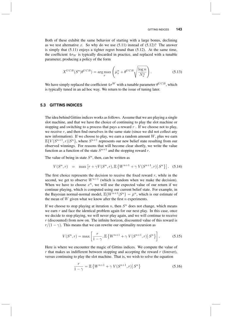
GITTINS INDICES 143
Both of these exhibit the same behavior of starting with a large bonus, decliningas we test alternative x. So why do we use (5.11) instead of (5.12)? The answeris simply that (5.11) enjoys a tighter regret bound than (5.12). At the same time,the coefficient 4σW is typically discarded in practice, and replaced with a tunableparameter, producing a policy of the form
XUCB(Sn|θUCB) = arg maxx
(µnx + θUCB
√log n
Nnx
). (5.13)
We have simply replaced the coefficient 4σW with a tunable parameter θUCB , whichis typically tuned in an ad hoc way. We return to the issue of tuning later.
5.3 GITTINS INDICES
The idea behind Gittins indices works as follows. Assume that we are playing a singleslot machine, and that we have the choice of continuing to play the slot machine orstopping and switching to a process that pays a reward r . If we choose not to play,we receive r, and then find ourselves in the same state (since we did not collect anynew information). If we choose to play, we earn a random amount W , plus we earnEV (Sn+1, r)|Sn, where Sn+1 represents our new belief state resulting from ourobserved winnings. For reasons that will become clear shortly, we write the valuefunction as a function of the state Sn+1 and the stopping reward r.
The value of being in state Sn, then, can be written as
V (Sn, r) = max[r + γV (Sn, r),E
Wn+1 + γ V (Sn+1, r)
∣∣Sn] . (5.14)
The first choice represents the decision to receive the fixed reward r, while in thesecond, we get to observe Wn+1 (which is random when we make the decision).When we have to choose xn, we will use the expected value of our return if wecontinue playing, which is computed using our current belief state. For example, inthe Bayesian normal-normal model, EWn+1|Sn = µn, which is our estimate ofthe mean of W given what we know after the first n experiments.
If we choose to stop playing at iteration n, then Sn does not change, which meanswe earn r and face the identical problem again for our next play. In this case, oncewe decide to stop playing, we will never play again, and we will continue to receiver (discounted) from now on. The infinite horizon, discounted value of this reward isr/(1− γ). This means that we can rewrite our optimality recursion as
V (Sn, r) = max
[r
1− γ,EWn+1 + γ V (Sn+1, r)
∣∣Sn] , (5.15)
Here is where we encounter the magic of Gittins indices. We compute the value ofr that makes us indifferent between stopping and accepting the reward r (forever),versus continuing to play the slot machine. That is, we wish to solve the equation
r
1− γ= E
Wn+1 + γ V (Sn+1, r)
∣∣Sn (5.16)
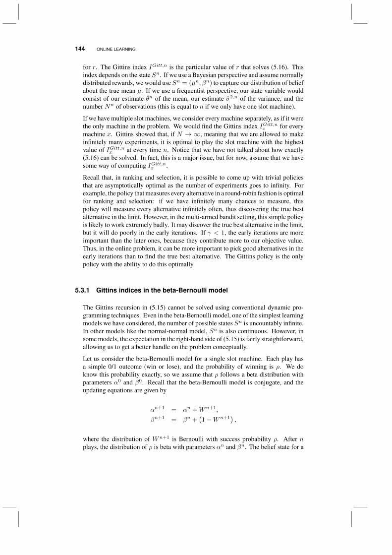
144 ONLINE LEARNING
for r. The Gittins index IGitt,n is the particular value of r that solves (5.16). Thisindex depends on the state Sn. If we use a Bayesian perspective and assume normallydistributed rewards, we would use Sn = (µn, βn) to capture our distribution of beliefabout the true mean µ. If we use a frequentist perspective, our state variable wouldconsist of our estimate θn of the mean, our estimate σ2,n of the variance, and thenumber Nn of observations (this is equal to n if we only have one slot machine).
If we have multiple slot machines, we consider every machine separately, as if it werethe only machine in the problem. We would find the Gittins index IGitt,nx for everymachine x. Gittins showed that, if N → ∞, meaning that we are allowed to makeinfinitely many experiments, it is optimal to play the slot machine with the highestvalue of IGitt,nx at every time n. Notice that we have not talked about how exactly(5.16) can be solved. In fact, this is a major issue, but for now, assume that we havesome way of computing IGitt,nx .
Recall that, in ranking and selection, it is possible to come up with trivial policiesthat are asymptotically optimal as the number of experiments goes to infinity. Forexample, the policy that measures every alternative in a round-robin fashion is optimalfor ranking and selection: if we have infinitely many chances to measure, thispolicy will measure every alternative infinitely often, thus discovering the true bestalternative in the limit. However, in the multi-armed bandit setting, this simple policyis likely to work extremely badly. It may discover the true best alternative in the limit,but it will do poorly in the early iterations. If γ < 1, the early iterations are moreimportant than the later ones, because they contribute more to our objective value.Thus, in the online problem, it can be more important to pick good alternatives in theearly iterations than to find the true best alternative. The Gittins policy is the onlypolicy with the ability to do this optimally.
5.3.1 Gittins indices in the beta-Bernoulli model
The Gittins recursion in (5.15) cannot be solved using conventional dynamic pro-gramming techniques. Even in the beta-Bernoulli model, one of the simplest learningmodels we have considered, the number of possible states Sn is uncountably infinite.In other models like the normal-normal model, Sn is also continuous. However, insome models, the expectation in the right-hand side of (5.15) is fairly straightforward,allowing us to get a better handle on the problem conceptually.
Let us consider the beta-Bernoulli model for a single slot machine. Each play hasa simple 0/1 outcome (win or lose), and the probability of winning is ρ. We doknow this probability exactly, so we assume that ρ follows a beta distribution withparameters α0 and β0. Recall that the beta-Bernoulli model is conjugate, and theupdating equations are given by
αn+1 = αn +Wn+1,
βn+1 = βn +(1−Wn+1
),
where the distribution of Wn+1 is Bernoulli with success probability ρ. After nplays, the distribution of ρ is beta with parameters αn and βn. The belief state for a
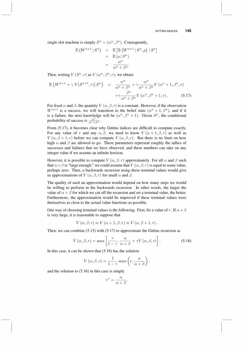
GITTINS INDICES 145
single slot machine is simply Sn = (αn, βn). Consequently,
E(Wn+1 |Sn
)= E
[E(Wn+1 |Sn, ρ
)|Sn
]= E (ρ |Sn)
=αn
αn + βn.
Then, writing V (Sn, r) as V (αn, βn, r), we obtain
EWn+1 + γ V (Sn+1, r)
∣∣Sn =αn
αn + βn+ γ
αn
αn + βnV (αn + 1, βn, r)
+γβn
αn + βnV (αn, βn + 1, r) . (5.17)
For fixed α and β, the quantity V (α, β, r) is a constant. However, if the observationWn+1 is a success, we will transition to the belief state (αn + 1, βn), and if itis a failure, the next knowledge will be (αn, βn + 1). Given Sn, the conditionalprobability of success is αn
αn+βn .
From (5.17), it becomes clear why Gittins indices are difficult to compute exactly.For any value of r and any α, β, we need to know V (α+ 1, β, r) as well asV (α, β + 1, r) before we can compute V (α, β, r). But there is no limit on howhigh α and β are allowed to go. These parameters represent roughly the tallies ofsuccesses and failures that we have observed, and these numbers can take on anyinteger value if we assume an infinite horizon.
However, it is possible to compute V (α, β, r) approximately. For all α and β suchthat α+β is “large enough,” we could assume that V (α, β, r) is equal to some value,perhaps zero. Then, a backwards recursion using these terminal values would giveus approximations of V (α, β, r) for small α and β.
The quality of such an approximation would depend on how many steps we wouldbe willing to perform in the backwards recursion. In other words, the larger thevalue of α+ β for which we cut off the recursion and set a terminal value, the better.Furthermore, the approximation would be improved if these terminal values werethemselves as close to the actual value functions as possible.
One way of choosing terminal values is the following. First, fix a value of r. If α+βis very large, it is reasonable to suppose that
V (α, β, r) ≈ V (α+ 1, β, r) ≈ V (α, β + 1, r) .
Then, we can combine (5.15) with (5.17) to approximate the Gittins recursion as
V (α, β, r) = max
[r
1− γ,
α
α+ β+ γV (α, β, r)
]. (5.18)
In this case, it can be shown that (5.18) has the solution
V (α, β, r) =1
1− γmax
(r,
α
α+ β
),
and the solution to (5.16) in this case is simply
r∗ =α
α+ β.

146 ONLINE LEARNING
α 1 2 3 4 5 6 7β
1 0.7029 0.8001 0.8452 0.8723 0.8905 0.9039 0.9141
2 0.5001 0.6346 0.7072 0.7539 0.7869 0.8115 0.8307
3 0.3796 0.5163 0.6010 0.6579 0.6996 0.7318 0.7573
4 0.3021 0.4342 0.5184 0.5809 0.6276 0.6642 0.6940
5 0.2488 0.3720 0.4561 0.5179 0.5676 0.6071 0.6395
6 0.2103 0.3245 0.4058 0.4677 0.5168 0.5581 0.5923
7 0.1815 0.2871 0.3647 0.4257 0.4748 0.5156 0.5510
Table 5.1 Gittins indices for the beta-Bernoulli model with α, β = 1, ..., 7 for γ = 0.9.
We can use this result to approximate Gittins indices for a desiredαn andβn. First, wechoose some large numberN . If α+β ≥ N , we assume that V (α, β, r) = 1
1−γα
α+βfor all r. Then, we can use (5.15) and (5.17) to work backwards and computeV (αn, βn, r) for a particular value of r. Finally, we can use a search algorithm tofind the particular value r∗ that makes the two components of the maximum in theexpression for V (αn, βn, r) equal.
The computational cost of this method is high. IfN is large, the backwards recursionbecomes more expensive for each value of r, and we have to repeat it many times tofind the value r∗. However, the recursion (for fixed r) is simple enough to be codedin a spreadsheet, and r can then be varied through trial and error (see Exercise 5.3).Such an exercise allows one to get a sense of the complexity of the problem.
When all else fails, the monograph by Gittins (1989) provides tables of Gittins indicesfor several values of γ and α, β = 1, 2, ..., 40. A few of these values are given inTables 5.1 and 5.2 for γ = 0.9, 0.95. The tables allow us to make several interestingobservations. First, the Gittins indices are all numbers in the interval [0, 1]. Infact, this is always true in the beta-Bernoulli model (but not for other models, as weshall see in the next section). Second, the indices are increasing in the number ofsuccesses, and decreasing in the number of failures. This is logical; if the numberof successes is low, and the number of trials is high, we can be fairly sure that thesuccess probability of the slot machine is low, and therefore the fixed-reward processshould give us smaller rewards.
5.3.2 Gittins indices in the normal-normal model
Let us now switch to the normal-normal model. Instead of winning probabilities, wedeal with average winnings, and we assume that the winnings in each play follow anormal distribution. The quantity µx represents the unknown average winnings ofslot machine x. Every observationWn
x is normal with mean µx and known precisionβW , and every unknown mean µx is normally distributed with prior mean µ0
x and
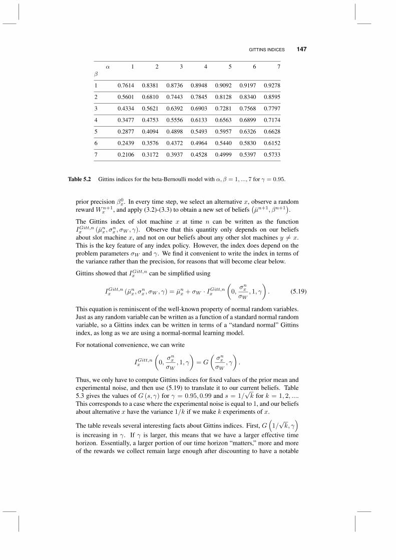
GITTINS INDICES 147
α 1 2 3 4 5 6 7β
1 0.7614 0.8381 0.8736 0.8948 0.9092 0.9197 0.9278
2 0.5601 0.6810 0.7443 0.7845 0.8128 0.8340 0.8595
3 0.4334 0.5621 0.6392 0.6903 0.7281 0.7568 0.7797
4 0.3477 0.4753 0.5556 0.6133 0.6563 0.6899 0.7174
5 0.2877 0.4094 0.4898 0.5493 0.5957 0.6326 0.6628
6 0.2439 0.3576 0.4372 0.4964 0.5440 0.5830 0.6152
7 0.2106 0.3172 0.3937 0.4528 0.4999 0.5397 0.5733
Table 5.2 Gittins indices for the beta-Bernoulli model with α, β = 1, ..., 7 for γ = 0.95.
prior precision β0x. In every time step, we select an alternative x, observe a random
reward Wn+1x , and apply (3.2)-(3.3) to obtain a new set of beliefs
(µn+1, βn+1
).
The Gittins index of slot machine x at time n can be written as the functionIGitt,nx (µnx , σ
nx , σW , γ). Observe that this quantity only depends on our beliefs
about slot machine x, and not on our beliefs about any other slot machines y 6= x.This is the key feature of any index policy. However, the index does depend on theproblem parameters σW and γ. We find it convenient to write the index in terms ofthe variance rather than the precision, for reasons that will become clear below.
Gittins showed that IGitt,nx can be simplified using
IGitt,nx (µnx , σnx , σW , γ) = µnx + σW · IGitt,nx
(0,σnxσW
, 1, γ
). (5.19)
This equation is reminiscent of the well-known property of normal random variables.Just as any random variable can be written as a function of a standard normal randomvariable, so a Gittins index can be written in terms of a “standard normal” Gittinsindex, as long as we are using a normal-normal learning model.
For notational convenience, we can write
IGitt,nx
(0,σnxσW
, 1, γ
)= G
(σnxσW
, γ
).
Thus, we only have to compute Gittins indices for fixed values of the prior mean andexperimental noise, and then use (5.19) to translate it to our current beliefs. Table5.3 gives the values of G (s, γ) for γ = 0.95, 0.99 and s = 1/
√k for k = 1, 2, ....
This corresponds to a case where the experimental noise is equal to 1, and our beliefsabout alternative x have the variance 1/k if we make k experiments of x.
The table reveals several interesting facts about Gittins indices. First, G(
1/√k, γ)
is increasing in γ. If γ is larger, this means that we have a larger effective timehorizon. Essentially, a larger portion of our time horizon “matters,” more and moreof the rewards we collect remain large enough after discounting to have a notable

148 ONLINE LEARNING
Discount factork 0.5 0.7 0.9 0.95 0.99 0.995
1 0.2057 0.3691 0.7466 0.9956 1.5758 1.8175
2 0.1217 0.2224 0.4662 0.6343 1.0415 1.2157
3 0.0873 0.1614 0.3465 0.4781 0.8061 0.9493
4 0.0683 0.1272 0.2781 0.3878 0.6677 0.7919
5 0.0562 0.1052 0.2332 0.3281 0.5747 0.6857
6 0.0477 0.0898 0.2013 0.2852 0.5072 0.6082
7 0.0415 0.0784 0.1774 0.2528 0.4554 0.5487
8 0.0367 0.0696 0.1587 0.2274 0.4144 0.5013
9 0.0329 0.0626 0.1437 0.2069 0.3608 0.4624
10 0.0299 0.0569 0.1313 0.1899 0.3529 0.4299
20 0.0155 0.0298 0.0712 0.1058 0.2094 0.2615
30 0.0104 0.0202 0.0491 0.0739 0.1520 0.1927
40 0.0079 0.0153 0.0375 0.0570 0.1202 0.1542
50 0.0063 0.0123 0.0304 0.0464 0.0998 0.1292
60 0.0053 0.0103 0.0255 0.0392 0.0855 0.1115
70 0.0045 0.0089 0.0220 0.0339 0.0749 0.0983
80 0.0040 0.0078 0.0193 0.0299 0.0667 0.0881
90 0.0035 0.0069 0.0173 0.0267 0.0602 0.0798
100 0.0032 0.0062 0.0156 0.0242 0.0549 0.0730
Table 5.3 Gittins indices G (s, γ) for the case where s = 1/√k, from Gittins (1989).
effect on our objective value. This means that we can afford to do more exploration,because one low reward early on will not harm our objective value as much. Hence,the Gittins indices are higher, encouraging us to explore more.
Second, G(
1/√k, γ)
is decreasing in k. This is fairly intuitive. The standardGittins index G (s, γ) represents the uncertainty bonus, and does not depend on ourestimate of the value of an alternative. As the variance of our beliefs goes down, theuncertainty bonus should go down as well, and we should only continue to measurethe alternative if it provides a high reward.
Unfortunately, even the seminal work by Gittins does not give the values of G (s, γ)for all possible s and γ. In general, computing these values is a difficult problem inand of itself. For this reason, a minor literature on Gittins approximation has arisenin the past ten years. To obtain a practical algorithm, it is necessary to examine thisliterature in more depth.
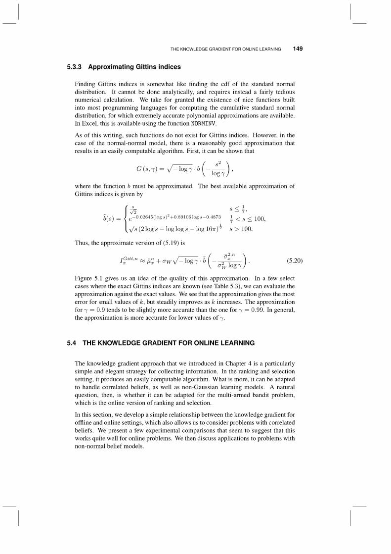
THE KNOWLEDGE GRADIENT FOR ONLINE LEARNING 149
5.3.3 Approximating Gittins indices
Finding Gittins indices is somewhat like finding the cdf of the standard normaldistribution. It cannot be done analytically, and requires instead a fairly tediousnumerical calculation. We take for granted the existence of nice functions builtinto most programming languages for computing the cumulative standard normaldistribution, for which extremely accurate polynomial approximations are available.In Excel, this is available using the function NORMINV.
As of this writing, such functions do not exist for Gittins indices. However, in thecase of the normal-normal model, there is a reasonably good approximation thatresults in an easily computable algorithm. First, it can be shown that
G (s, γ) =√− log γ · b
(− s2
log γ
),
where the function b must be approximated. The best available approximation ofGittins indices is given by
b(s) =
s√2
s ≤ 17 ,
e−0.02645(log s)2+0.89106 log s−0.4873 17 < s ≤ 100,
√s (2 log s− log log s− log 16π)
12 s > 100.
Thus, the approximate version of (5.19) is
IGitt,nx ≈ µnx + σW√− log γ · b
(− σ2,n
x
σ2W log γ
). (5.20)
Figure 5.1 gives us an idea of the quality of this approximation. In a few selectcases where the exact Gittins indices are known (see Table 5.3), we can evaluate theapproximation against the exact values. We see that the approximation gives the mosterror for small values of k, but steadily improves as k increases. The approximationfor γ = 0.9 tends to be slightly more accurate than the one for γ = 0.99. In general,the approximation is more accurate for lower values of γ.
5.4 THE KNOWLEDGE GRADIENT FOR ONLINE LEARNING
The knowledge gradient approach that we introduced in Chapter 4 is a particularlysimple and elegant strategy for collecting information. In the ranking and selectionsetting, it produces an easily computable algorithm. What is more, it can be adaptedto handle correlated beliefs, as well as non-Gaussian learning models. A naturalquestion, then, is whether it can be adapted for the multi-armed bandit problem,which is the online version of ranking and selection.
In this section, we develop a simple relationship between the knowledge gradient foroffline and online settings, which also allows us to consider problems with correlatedbeliefs. We present a few experimental comparisons that seem to suggest that thisworks quite well for online problems. We then discuss applications to problems withnon-normal belief models.
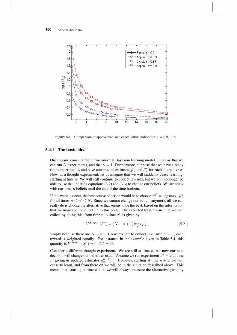
150 ONLINE LEARNING
Figure 5.1 Comparison of approximate and exact Gittins indices for γ = 0.9, 0.99.
5.4.1 The basic idea
Once again, consider the normal-normal Bayesian learning model. Suppose that wecan run N experiments, and that γ = 1. Furthermore, suppose that we have alreadyrun n experiments, and have constructed estimates µnx and βnx for each alternative x.Now, as a thought experiment, let us imagine that we will suddenly cease learning,starting at time n. We will still continue to collect rewards, but we will no longer beable to use the updating equations (3.2) and (3.3) to change our beliefs. We are stuckwith our time-n beliefs until the end of the time horizon.
If this were to occur, the best course of action would be to choose xn′
= arg maxx µnx
for all times n ≤ n′ ≤ N . Since we cannot change our beliefs anymore, all we canreally do is choose the alternative that seems to be the best, based on the informationthat we managed to collect up to this point. The expected total reward that we willcollect by doing this, from time n to time N , is given by
V Stop,n (Sn) = (N − n+ 1) maxx
µnx , (5.21)
simply because there are N − n + 1 rewards left to collect. Because γ = 1, eachreward is weighted equally. For instance, in the example given in Table 5.4, thisquantity is V Stop,n (Sn) = 6 · 5.5 = 33.
Consider a different thought experiment. We are still at time n, but now our nextdecision will change our beliefs as usual. Assume we run experiment xn = x at timen, giving us updated estimates µn+1
x′ (x). However, starting at time n + 1, we willcease to learn, and from there on we will be in the situation described above. Thismeans that, starting at time n + 1, we will always measure the alternative given by
THE KNOWLEDGE GRADIENT FOR ONLINE LEARNING 151
arg maxx′ µn+1x′ (x). The problem thus reduces to choosing one single decision xn
to maximize the expected total reward we collect, starting at time n.
This idea is essentially the knowledge gradient concept from a slightly differentpoint of view. In ranking and selection, we chose each decision to maximize theincremental improvement (obtained from a single experiment) in our estimate of thebest value. Essentially, we treated each decision as if it were the last time we wereallowed to learn. We made each decision in such a way as to get the most benefit outof that single experiment. In the online setting, we do the same thing, only “benefit”is now expressed in terms of the total reward that we can collect from time n to theend of the time horizon.
The KG decision for the bandit problem is given by
XKG,n = arg maxx
E[µx + V Stop,n+1
(Sn+1
)|Sn, xn = x
](5.22)
= arg maxx
µnx + (N − n)E[maxx′
µn+1x′ (x) |Sn, xn = x
](5.23)
= arg maxx
µnx + (N − n)E[maxx′
µn+1x′ (x)−max
x′µnx′ |Sn, xn = x
](5.24)
= arg maxx
µnx + (N − n) νKG,nx , (5.25)
where νKG,nx is simply the knowledge gradient for ranking and selection, given by(4.13). We start with the basic Bellman equation in (5.22). The downstream valueis given by V Stop,n+1 because we assume that we will cease to learn starting at timen + 1. Next, we use the fact that E (µx |Sn) = µnx , together with the definition ofV Stop,n+1 from (5.21) to obtain (5.23). Because the quantity maxx′ µ
nx′ is constant
given Sn, and does not depend on x, we can put it into the expression withoutchanging the arg max, thus arriving at (5.24). Finally, we apply the definition of theknowledge gradient from (4.3) to obtain (5.25).
This line of reasoning has given us a simple and easily computable algorithm for themulti-armed bandit problem. At first, the expression µnx + (N − n) νKG,nx that wecompute for alternative x may look very similar to the index policies we discussedearlier. Like interval estimation, Gittins indices, and other methods, KG takes µnxand adds an uncertainty bonus (N − n) νKG,nx . Just as in the other index policies,the uncertainty bonus gets smaller as σnx gets smaller: thus, if the level of uncertaintyis zero, the uncertainty bonus is zero as well. Furthermore, all other things beingequal, the uncertainty bonus is larger if n is smaller, reflecting the fact that it is moreimportant to learn in the early stages of the problem, while we have more remainingtime steps in which we can potentially use the information we collect.
However, the KG policy is not an index policy. Crucially, the knowledge gradientνKG,nx depends not only on µnx , but also on maxx′ 6=x µ
nx′ . This cannot happen in an
index policy, where the index of x is only allowed to depend on our beliefs about x.The knowledge gradient policy does not decompose the multi-armed bandit probleminto many one-armed bandit problems. It considers each alternative relative to theothers.
Table 5.4 shows the computations performed by the online KG policy for a particularproblem with five alternatives and N − n = 5 experiments remaining in the timehorizon. This example illustrates the distinction between the online KG policy and
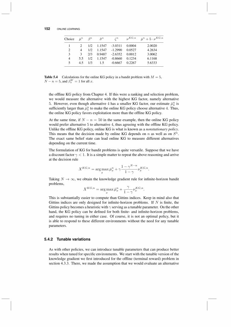
152 ONLINE LEARNING
Choice µn βn σn ζn νKG,n µn + 5 · νKG,n
1 2 1/2 1.1547 -3.0311 0.0004 2.00202 4 1/2 1.1547 -1.2990 0.0527 4.26343 3 2/3 0.9487 -2.6352 0.0012 3.00624 5.5 1/2 1.1547 -0.8660 0.1234 6.11685 4.5 1/3 1.5 -0.6667 0.2267 5.6333
Table 5.4 Calculations for the online KG policy in a bandit problem with M = 5,N − n = 5, and βWx = 1 for all x.
the offline KG policy from Chapter 4. If this were a ranking and selection problem,we would measure the alternative with the highest KG factor, namely alternative5. However, even though alternative 4 has a smaller KG factor, our estimate µn4 issufficiently larger than µn5 to make the online KG policy choose alternative 4. Thus,the online KG policy favors exploitation more than the offline KG policy.
At the same time, if N − n = 50 in the same example, then the online KG policywould prefer alternative 5 to alternative 4, thus agreeing with the offline KG policy.Unlike the offline KG policy, online KG is what is known as a nonstationary policy.This means that the decision made by online KG depends on n as well as on Sn.The exact same belief state can lead online KG to measure different alternativesdepending on the current time.
The formulation of KG for bandit problems is quite versatile. Suppose that we havea discount factor γ < 1. It is a simple matter to repeat the above reasoning and arriveat the decision rule
XKG,n = arg maxx
µnx + γ1− γN−n
1− γνKG,nx .
Taking N → ∞, we obtain the knowledge gradient rule for infinite-horizon banditproblems,
XKG,n = arg maxx
µnx +γ
1− γνKG,nx .
This is substantially easier to compute than Gittins indices. Keep in mind also thatGittins indices are only designed for infinite-horizon problems. If N is finite, theGittins policy becomes a heuristic with γ serving as a tunable parameter. On the otherhand, the KG policy can be defined for both finite- and infinite-horizon problems,and requires no tuning in either case. Of course, it is not an optimal policy, but itis able to respond to these different environments without the need for any tunableparameters.
5.4.2 Tunable variations
As with other policies, we can introduce tunable parameters that can produce betterresults when tuned for specific environments. We start with the tunable version of theknowledge gradient we first introduced for the offline (terminal reward) problem insection 4.3.3. There, we made the assumption that we would evaluate an alternative
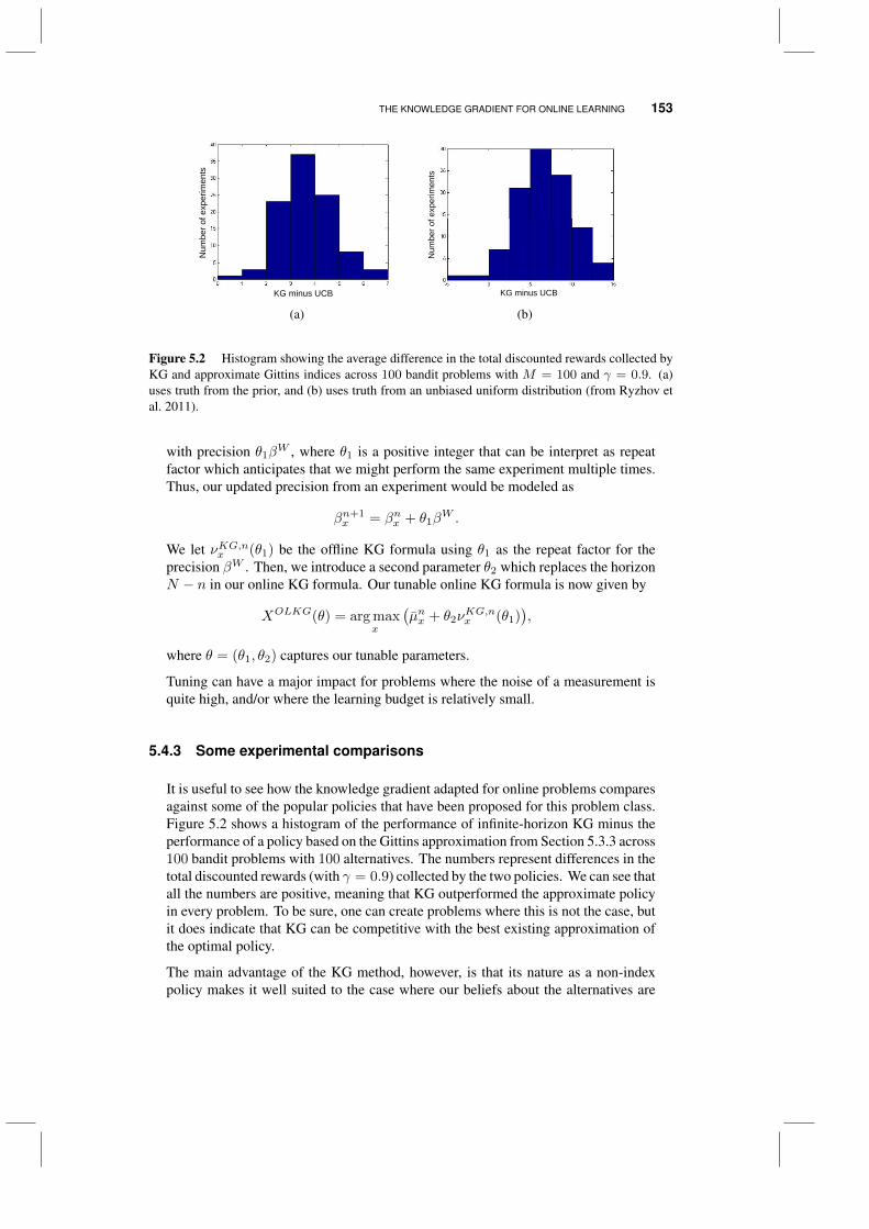
THE KNOWLEDGE GRADIENT FOR ONLINE LEARNING 153
KG minus UCB
Num
ber o
f exp
erim
ents
KG minus UCB
Num
ber o
f exp
erim
ents
(a) (b)
Figure 5.2 Histogram showing the average difference in the total discounted rewards collected byKG and approximate Gittins indices across 100 bandit problems with M = 100 and γ = 0.9. (a)uses truth from the prior, and (b) uses truth from an unbiased uniform distribution (from Ryzhov etal. 2011).
with precision θ1βW , where θ1 is a positive integer that can be interpret as repeat
factor which anticipates that we might perform the same experiment multiple times.Thus, our updated precision from an experiment would be modeled as
βn+1x = βnx + θ1β
W .
We let νKG,nx (θ1) be the offline KG formula using θ1 as the repeat factor for theprecision βW . Then, we introduce a second parameter θ2 which replaces the horizonN − n in our online KG formula. Our tunable online KG formula is now given by
XOLKG(θ) = arg maxx
(µnx + θ2ν
KG,nx (θ1)
),
where θ = (θ1, θ2) captures our tunable parameters.
Tuning can have a major impact for problems where the noise of a measurement isquite high, and/or where the learning budget is relatively small.
5.4.3 Some experimental comparisons
It is useful to see how the knowledge gradient adapted for online problems comparesagainst some of the popular policies that have been proposed for this problem class.Figure 5.2 shows a histogram of the performance of infinite-horizon KG minus theperformance of a policy based on the Gittins approximation from Section 5.3.3 across100 bandit problems with 100 alternatives. The numbers represent differences in thetotal discounted rewards (with γ = 0.9) collected by the two policies. We can see thatall the numbers are positive, meaning that KG outperformed the approximate policyin every problem. To be sure, one can create problems where this is not the case, butit does indicate that KG can be competitive with the best existing approximation ofthe optimal policy.
The main advantage of the KG method, however, is that its nature as a non-indexpolicy makes it well suited to the case where our beliefs about the alternatives are
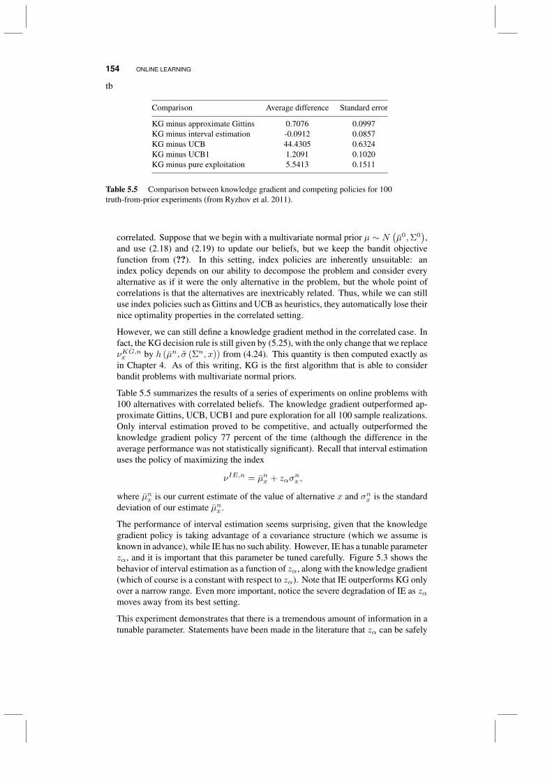
154 ONLINE LEARNING
tb
Comparison Average difference Standard error
KG minus approximate Gittins 0.7076 0.0997KG minus interval estimation -0.0912 0.0857KG minus UCB 44.4305 0.6324KG minus UCB1 1.2091 0.1020KG minus pure exploitation 5.5413 0.1511
Table 5.5 Comparison between knowledge gradient and competing policies for 100truth-from-prior experiments (from Ryzhov et al. 2011).
correlated. Suppose that we begin with a multivariate normal prior µ ∼ N(µ0,Σ0
),
and use (2.18) and (2.19) to update our beliefs, but we keep the bandit objectivefunction from (??). In this setting, index policies are inherently unsuitable: anindex policy depends on our ability to decompose the problem and consider everyalternative as if it were the only alternative in the problem, but the whole point ofcorrelations is that the alternatives are inextricably related. Thus, while we can stilluse index policies such as Gittins and UCB as heuristics, they automatically lose theirnice optimality properties in the correlated setting.
However, we can still define a knowledge gradient method in the correlated case. Infact, the KG decision rule is still given by (5.25), with the only change that we replaceνKG,nx by h (µn, σ (Σn, x)) from (4.24). This quantity is then computed exactly asin Chapter 4. As of this writing, KG is the first algorithm that is able to considerbandit problems with multivariate normal priors.
Table 5.5 summarizes the results of a series of experiments on online problems with100 alternatives with correlated beliefs. The knowledge gradient outperformed ap-proximate Gittins, UCB, UCB1 and pure exploration for all 100 sample realizations.Only interval estimation proved to be competitive, and actually outperformed theknowledge gradient policy 77 percent of the time (although the difference in theaverage performance was not statistically significant). Recall that interval estimationuses the policy of maximizing the index
νIE,n = µnx + zασnx ,
where µnx is our current estimate of the value of alternative x and σnx is the standarddeviation of our estimate µnx .
The performance of interval estimation seems surprising, given that the knowledgegradient policy is taking advantage of a covariance structure (which we assume isknown in advance), while IE has no such ability. However, IE has a tunable parameterzα, and it is important that this parameter be tuned carefully. Figure 5.3 shows thebehavior of interval estimation as a function of zα, along with the knowledge gradient(which of course is a constant with respect to zα). Note that IE outperforms KG onlyover a narrow range. Even more important, notice the severe degradation of IE as zαmoves away from its best setting.
This experiment demonstrates that there is a tremendous amount of information in atunable parameter. Statements have been made in the literature that zα can be safely
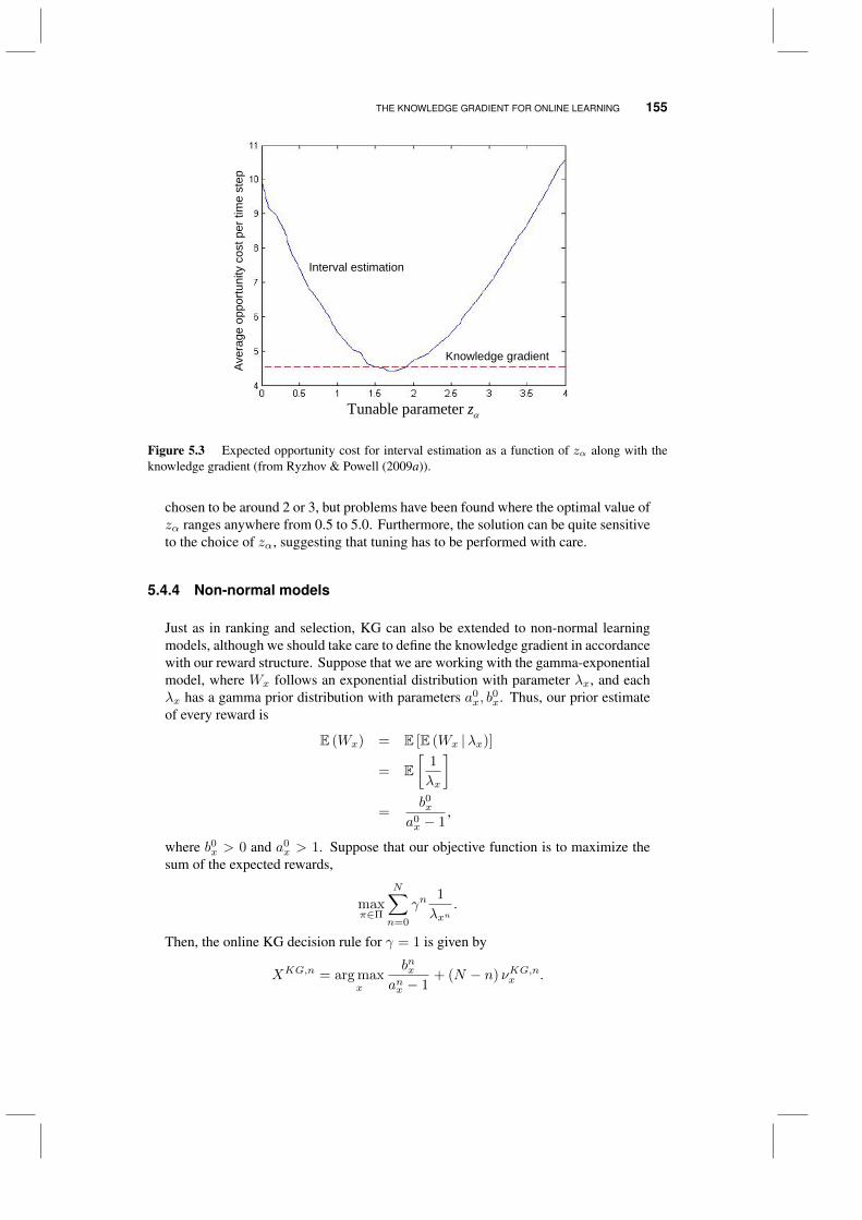
THE KNOWLEDGE GRADIENT FOR ONLINE LEARNING 155
Aver
age
oppo
rtuni
ty c
ost p
er ti
me
step
Tunable parameter z
Interval estimation
Knowledge gradient
Figure 5.3 Expected opportunity cost for interval estimation as a function of zα along with theknowledge gradient (from Ryzhov & Powell (2009a)).
chosen to be around 2 or 3, but problems have been found where the optimal value ofzα ranges anywhere from 0.5 to 5.0. Furthermore, the solution can be quite sensitiveto the choice of zα, suggesting that tuning has to be performed with care.
5.4.4 Non-normal models
Just as in ranking and selection, KG can also be extended to non-normal learningmodels, although we should take care to define the knowledge gradient in accordancewith our reward structure. Suppose that we are working with the gamma-exponentialmodel, where Wx follows an exponential distribution with parameter λx, and eachλx has a gamma prior distribution with parameters a0
x, b0x. Thus, our prior estimate
of every reward is
E (Wx) = E [E (Wx |λx)]
= E[
1
λx
]=
b0xa0x − 1
,
where b0x > 0 and a0x > 1. Suppose that our objective function is to maximize the
sum of the expected rewards,
maxπ∈Π
N∑n=0
γn1
λxn.
Then, the online KG decision rule for γ = 1 is given by
XKG,n = arg maxx
bnxanx − 1
+ (N − n) νKG,nx .

156 ONLINE LEARNING
To write the knowledge gradient νKG,nx , let Cnx = maxx′ 6=xbnx′
anx′−1 and define the
baseline KG quantity
νnx =(bnx)
anx
(anxCnx )anx−1
(1
anx − 1− 1
anx
).
Then,
νKG,nx =
νnx if x 6= arg maxx′
bnx′
anx′−1
νnx −(
bnxanx−1 − C
nx
)if Cnx ≥
bnxanx
0 otherwise.
(5.26)
Once again, we have an easily computable KG algorithm, for a problem where Gittinsapproximations are not easily available. Note the presence of a penalty term in (5.26),much like in the expression for gamma-exponential KG in ranking and selection thatwas presented in Section 4.7.
5.5 VARIATIONS OF BANDIT PROBLEMS
One of the notable features of the bandit literature has been the introduction of awide range of variations. The style of this community is to provide names of theform “XXX bandits” where XXX describes some variation, typically in the natureof the arms (choices), the exogenous information process, and/or the belief model.This style has produced a colorful literature full of creative adjectives, as illustratedin table 5.6. Below we provide more detailed descriptions on a few of the examples.
Restless bandits - The standard bandit model assumes that the truth µx for arm x remainsthe same over time. Restless bandits describe a model where the means are allowedto vary over time.
Arm acquiring bandits - These are problems where the number of alternatives growsover time.
Intermittent bandits - In this setting, not all the arms are available to be tested. A relatedvariation is known as “sleeping bandits.”
Continuous armed bandits - While the standard bandit problem involves discrete alter-natives x ∈ X = x1, . . . , xM, some authors have considered the case where thechoices are continuous.
Response-surface bandits - This is an instance of a bandit problem where the adjectiveis describing the belief model. While the most standard belief model is a lookuptable, some authors have considered parametric models (“response surface”). Theterm linear bandit has also been used for this purpose.
Finite horizon bandits - While the classic problem assumes an infinite horizon, someauthors have worked on finite-horizon problems.
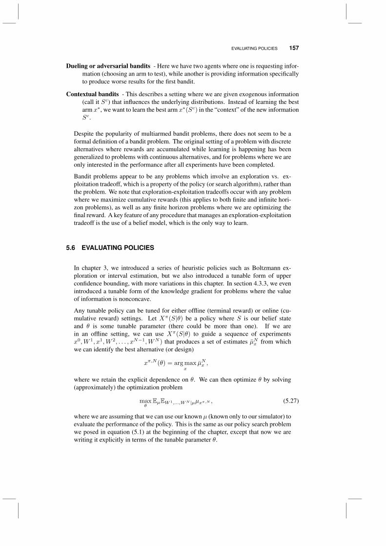
EVALUATING POLICIES 157
Dueling or adversarial bandits - Here we have two agents where one is requesting infor-mation (choosing an arm to test), while another is providing information specificallyto produce worse results for the first bandit.
Contextual bandits - This describes a setting where we are given exogenous information(call it Sc) that influences the underlying distributions. Instead of learning the bestarm x∗, we want to learn the best arm x∗(Sc) in the “context” of the new informationSc.
Despite the popularity of multiarmed bandit problems, there does not seem to be aformal definition of a bandit problem. The original setting of a problem with discretealternatives where rewards are accumulated while learning is happening has beengeneralized to problems with continuous alternatives, and for problems where we areonly interested in the performance after all experiments have been completed.
Bandit problems appear to be any problems which involve an exploration vs. ex-ploitation tradeoff, which is a property of the policy (or search algorithm), rather thanthe problem. We note that exploration-exploitation tradeoffs occur with any problemwhere we maximize cumulative rewards (this applies to both finite and infinite hori-zon problems), as well as any finite horizon problems where we are optimizing thefinal reward. A key feature of any procedure that manages an exploration-exploitationtradeoff is the use of a belief model, which is the only way to learn.
5.6 EVALUATING POLICIES
In chapter 3, we introduced a series of heuristic policies such as Boltzmann ex-ploration or interval estimation, but we also introduced a tunable form of upperconfidence bounding, with more variations in this chapter. In section 4.3.3, we evenintroduced a tunable form of the knowledge gradient for problems where the valueof information is nonconcave.
Any tunable policy can be tuned for either offline (terminal reward) or online (cu-mulative reward) settings. Let Xπ(S|θ) be a policy where S is our belief stateand θ is some tunable parameter (there could be more than one). If we arein an offline setting, we can use Xπ(S|θ) to guide a sequence of experimentsx0,W 1, x1,W 2, . . . , xN−1,WN ) that produces a set of estimates µNx from whichwe can identify the best alternative (or design)
xπ,N (θ) = arg maxx
µNx ,
where we retain the explicit dependence on θ. We can then optimize θ by solving(approximately) the optimization problem
maxθ
EµEW 1,...,WN |µµxπ,N , (5.27)
where we are assuming that we can use our known µ (known only to our simulator) toevaluate the performance of the policy. This is the same as our policy search problemwe posed in equation (5.1) at the beginning of the chapter, except that now we arewriting it explicitly in terms of the tunable parameter θ.
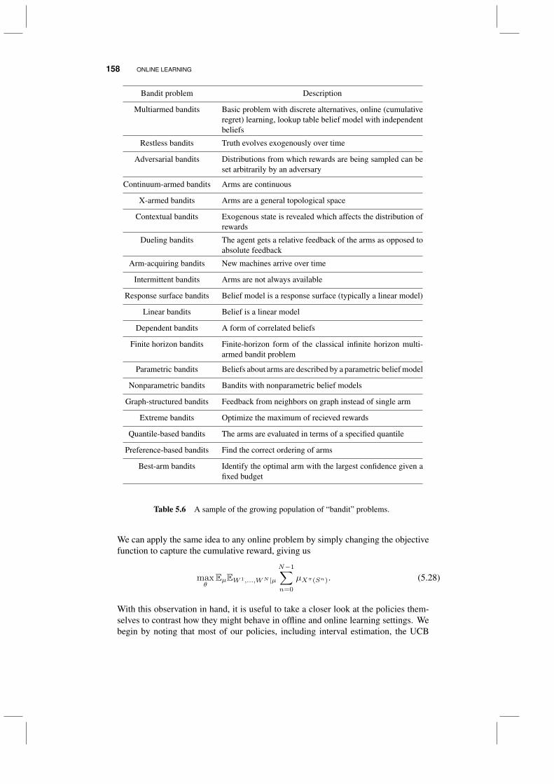
158 ONLINE LEARNING
Bandit problem Description
Multiarmed bandits Basic problem with discrete alternatives, online (cumulativeregret) learning, lookup table belief model with independentbeliefs
Restless bandits Truth evolves exogenously over time
Adversarial bandits Distributions from which rewards are being sampled can beset arbitrarily by an adversary
Continuum-armed bandits Arms are continuous
X-armed bandits Arms are a general topological space
Contextual bandits Exogenous state is revealed which affects the distribution ofrewards
Dueling bandits The agent gets a relative feedback of the arms as opposed toabsolute feedback
Arm-acquiring bandits New machines arrive over time
Intermittent bandits Arms are not always available
Response surface bandits Belief model is a response surface (typically a linear model)
Linear bandits Belief is a linear model
Dependent bandits A form of correlated beliefs
Finite horizon bandits Finite-horizon form of the classical infinite horizon multi-armed bandit problem
Parametric bandits Beliefs about arms are described by a parametric belief model
Nonparametric bandits Bandits with nonparametric belief models
Graph-structured bandits Feedback from neighbors on graph instead of single arm
Extreme bandits Optimize the maximum of recieved rewards
Quantile-based bandits The arms are evaluated in terms of a specified quantile
Preference-based bandits Find the correct ordering of arms
Best-arm bandits Identify the optimal arm with the largest confidence given afixed budget
Table 5.6 A sample of the growing population of “bandit” problems.
We can apply the same idea to any online problem by simply changing the objectivefunction to capture the cumulative reward, giving us
maxθ
EµEW 1,...,WN |µ
N−1∑n=0
µXπ(Sn). (5.28)
With this observation in hand, it is useful to take a closer look at the policies them-selves to contrast how they might behave in offline and online learning settings. Webegin by noting that most of our policies, including interval estimation, the UCB
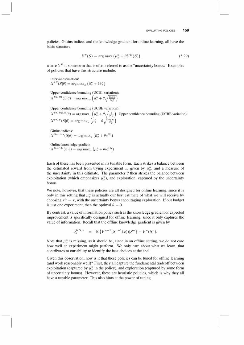
EVALUATING POLICIES 159
policies, Gittins indices and the knowledge gradient for online learning, all have thebasic structure
Xπ(S) = arg max(µnx + θUB(S)
), (5.29)
whereUB is some term that is often referred to as the “uncertainty bonus.” Examplesof policies that have this structure include:
Interval estimation:XIE(S|θ) = arg maxx
(µnx + θσnx
)Upper confidence bounding (UCB1 variation):
XUCB1(S|θ) = arg maxx
(µnx + θ
√lognNnx
)Upper confidence bounding (UCBE variation):
XUCBE,n(θ) = arg maxx
(µnx + θ
√1Nnx
). Upper confidence bounding (UCBE variation):
XUCB(S|θ) = arg maxx
(µnx + θ
√lognNnx
)Gittins indices:XGittins(S|θ) = arg maxx
(µnx + θσW
)Online knowledge gradient:XOLKG(S|θ) = arg maxx
(µnx + θνKGx
)
Each of these has been presented in its tunable form. Each strikes a balance betweenthe estimated reward from trying experiment x, given by µnx , and a measure ofthe uncertainty in this estimate. The parameter θ then strikes the balance betweenexploitation (which emphasizes µnx), and exploration, captured by the uncertaintybonus.
We note, however, that these policies are all designed for online learning, since it isonly in this setting that µnx is actually our best estimate of what we will receive bychoosing xn = x, with the uncertainty bonus encouraging exploration. If our budgetis just one experiment, then the optimal θ = 0.
By contrast, a value of information policy such as the knowledge gradient or expectedimprovement is specifically designed for offline learning, since it only captures thevalue of information. Recall that the offline knowledge gradient is given by
νKG,nx = EV n+1(Sn+1(x))|Sn
− V n(Sn).
Note that µnx is missing, as it should be, since in an offline setting, we do not carehow well an experiment might perform. We only care about what we learn, thatcontributes to our ability to identify the best choices at the end.
Given this observation, how is it that these policies can be tuned for offline learning(and work reasonably well)? First, they all capture the fundamental tradeoff betweenexploitation (captured by µnx in the policy), and exploration (captured by some formof uncertainty bonus). However, these are heuristic policies, which is why they allhave a tunable parameter. This also hints at the power of tuning.

160 ONLINE LEARNING
5.7 BIBLIOGRAPHIC NOTES
Section 5.3 - Gittins index theory is due to Gittins & Jones (1974), Gittins (1979) andGittins (1989). Berry & Fristedt (1985) also provides a rigorous analysis of banditproblems. This research has launched an entire field of research into the searchfor index policies for variations on the basic bandit problems. Glazebrook (1982)analyzes policies for variations of the basic bandit model. Glazebrook & Minty(2009) presents a generalized index for bandit problems with general constraintson information collection resources. Bertsimas & Nino-Mora (2000) show how anindex policy can be computed using linear programming for a certain class of banditproblems. See the updated version of Gittins’ 1989 book, Gittins et al. (2011), fora modern treatment of bandit problems and a much more thorough treatment of thisextensive literature. The approximation of Gittins indices is due to Chick & Gans(2009), building on the diffusion approximation of Brezzi & Lai (2002).
Section 5.2 - Lai & Robbins (1985) and Lai (1987) provide the seminal research that showsthat the number of times an upper confidence bound policy chooses a particular sub-optimal machine is on the order of logN , and that this is the best possible bound.Auer et al. (2002) derives finite-time regret bounds on the UCB1 and UCB1-Normalpolicies and reports on comparisons against variations of UCB policies and epsilon-greedy on some small problems (up to 10 arms). The UCB policy for exponentialrewards comes from Agrawal (1995).
Section 5.4 - The online adaptation of the knowledge gradient is due to Ryzhov et al.(2011). Some additional experimental comparisons can be found in Ryzhov &Powell (2009b). Ryzhov & Powell (2011c) presents the KG policy for the gamma-exponential model. Rates of convergence for KG-type policies are still an openquestion, but Bull (2011) is an interesting first step in this direction.
PROBLEMS
5.1 You have three materials, A, B and C that you want to test for their abilityto convert solar energy to electricity, and you wish to find which one produces thehighest efficiency, which you have to do by learning from field implementations (inother words, online learning). Table 5.7 shows your initial beliefs (which we assumeare independent) summarized as the mean and precision. Your prior belief is normal,and testing alternative x produces an observationWx which is normally distributed withprecision βW = 1.
a) You follow some learning policy that has you first evaluating A, then B and finallyC, obtaining the observations Wn
x shown in Table 5.7 (for example, W 1A = 3). Give
the updated belief (mean and precision) for µ1A given the observation W 1
A = 3. Alsocompute the updated means only (not the precisions) for µ2
B and µ3C .
b) Give the objective function (algebraically) to find the best policy afterN experimentsif this is an off-line learning problem. Compute a sample realization of the objectivefunction for this example.
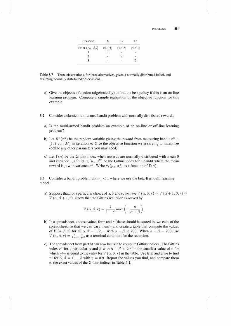
PROBLEMS 161
Iteration A B C
Prior (µx, βx) (5,.05) (3,.02) (4,.01)1 3 - -2 - 2 -3 - - 6
Table 5.7 Three observations, for three alternatives, given a normally distributed belief, andassuming normally distributed observations.
c) Give the objective function (algebraically) to find the best policy if this is an on-linelearning problem. Compute a sample realization of the objective function for thisexample.
5.2 Consider a classic multi-armed bandit problem with normally distributed rewards.
a) Is the multi-armed bandit problem an example of an on-line or off-line learningproblem?
b) Let Rn(xn) be the random variable giving the reward from measuring bandit xn ∈(1, 2, . . . ,M) in iteration n. Give the objective function we are trying to maximize(define any other parameters you may need).
c) Let Γ(n) be the Gittins index when rewards are normally distributed with mean 0and variance 1, and let νx(µx, σ
2x) be the Gittins index for a bandit where the mean
reward is µ with variance σ2. Write νx(µx, σ2x) as a function of Γ(n).
5.3 Consider a bandit problem with γ < 1 where we use the beta-Bernoulli learningmodel.
a) Suppose that, for a particular choice ofα, β and r, we haveV (α, β, r) ≈ V (α+ 1, β, r) ≈V (α, β + 1, r). Show that the Gittins recursion is solved by
V (α, β, r) =1
1− γmax
(r,
α
α+ β
).
b) In a spreadsheet, choose values for r and γ (these should be stored in two cells of thespreadsheet, so that we can vary them), and create a table that compute the valuesof V (α, β, r) for all α, β = 1, 2, ... with α + β < 200. When α + β = 200, useV (α, β, r) = 1
1−γα
α+β as a terminal condition for the recursion.
c) The spreadsheet from part b) can now be used to compute Gittins indices. The Gittinsindex r∗ for a particular α and β with α + β < 200 is the smallest value of r forwhich r
1−γ is equal to the entry for V (α, β, r) in the table. Use trial and error to findr∗ for α, β = 1, ..., 5 with γ = 0.9. Report the values you find, and compare themto the exact values of the Gittins indices in Table 5.1.
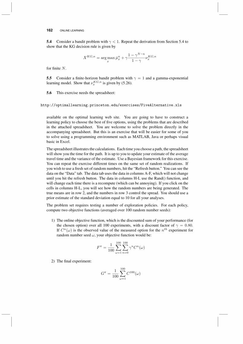
162 ONLINE LEARNING
5.4 Consider a bandit problem with γ < 1. Repeat the derivation from Section 5.4 toshow that the KG decision rule is given by
XKG,n = arg maxx
µnx + γ1− γN−n
1− γνKG,nx
for finite N .
5.5 Consider a finite-horizon bandit problem with γ = 1 and a gamma-exponentiallearning model. Show that νKG,nx is given by (5.26).
5.6 This exercise needs the spreadsheet:
http://optimallearning.princeton.edu/exercises/FiveAlternative.xls
available on the optimal learning web site. You are going to have to construct alearning policy to choose the best of five options, using the problems that are describedin the attached spreadsheet. You are welcome to solve the problem directly in theaccompanying spreadsheet. But this is an exercise that will be easier for some of youto solve using a programming environment such as MATLAB, Java or perhaps visualbasic in Excel.
The spreadsheet illustrates the calculations. Each time you choose a path, the spreadsheetwill show you the time for the path. It is up to you to update your estimate of the averagetravel time and the variance of the estimate. Use a Bayesian framework for this exercise.You can repeat the exercise different times on the same set of random realizations. Ifyou wish to use a fresh set of random numbers, hit the “Refresh button.” You can see thedata on the “Data” tab. The data tab uses the data in columns A-F, which will not changeuntil you hit the refresh button. The data in columns H-L use the Rand() function, andwill change each time there is a recompute (which can be annoying). If you click on thecells in columns H-L, you will see how the random numbers are being generated. Thetrue means are in row 2, and the numbers in row 3 control the spread. You should use aprior estimate of the standard deviation equal to 10 for all your analyses.
The problem set requires testing a number of exploration policies. For each policy,compute two objective functions (averaged over 100 random number seeds):
1) The online objective function, which is the discounted sum of your performance (forthe chosen option) over all 100 experiments, with a discount factor of γ = 0.80.If Cn(ω) is the observed value of the measured option for the nth experiment forrandom number seed ω, your objective function would be:
Fπ =1
100
100∑ω=1
100∑n=0
γnCn(ω)
2) The final experiment:
Gπ =1
100
100∑ω=1
C100(ω)
PROBLEMS 163
Fπ is our online objective function, while Gπ is our offline objective function. Also let
F =
100∑n=0
γnµ∗
G = µ∗
where µ∗ is the true mean for the best choice, if we knew the true means. Wherenecessary, you may assume that the standard deviation of an experiment is 10. You haveto test the following policies:
1) Pure exploitation.
2) Boltzmann exploration, using scaling factor θ = 1.
3) Epsilon-greedy exploration, where the exploration probability is given by 1/n.
4) Interval estimation. Test the performance of zα = 1.0, 2.0, 3.0 and 4.0 and select theone that performs the best.
5) Gittins indices (use the numerical approximation of Gittins indices given in Section5.3.3.
Do the following
a) In a graph, report Fπ and Gπ for each of the policies below. Also show F and G toprovide a measure of how well we are doing.
b) Discuss your results. Compare the performance of each policy in terms of the twodifferent objective functions.
5.7 Consider a multi-armed bandit problem with independent normal rewards. In thisexercise, you will implement a few online policies.
a) How should the opportunity cost be expressed in the online problem?
b) In exercise 3.4 you implemented the interval estimation policy in an offline setting.Now take your code from before, and adapt it to online problems by changing theobjective function appropriately. The parameters of the problem should be the sameas before (use the same priors and assume γ = 1), but now you need to computeopportunity cost differently. How does the best value of the tunable parameter zαchange when the problem becomes online? After you tune zα, report the confidenceinterval for the opportunity cost using 200 simulations.
c) Now implement the Gittins index approximation for the independent normal-normalmodel. You cannot solve the Gittins recursion – just use the approximation functionb. Our problem has a finite horizon, so you can treat the parameter γ in the Gittinsindex calculation as another tunable parameter. What value of γ gives you the bestresults?
d) Now implement the online KG policy. Compare the confidence intervals for KG,Gittins, and interval estimation.

CHAPTER 6
ELEMENTS OF A LEARNING PROBLEM
By now we have covered some elementary classes of learning problems. Fortunately,these describe a very broad class of applications. But there are some importantproblem classes that we have not yet discussed, and which we cannot solve usingthe tools presented so far. However, before we launch into what can seem to be alist of scattered applications, it is useful to lay out a more comprehensive modelingframework that at least hints at how we might deal with the major classes of unsolvedproblems. This presentation will motivate the problems we consider in the remainderof the volume, but will also serve potentially as areas for further research.
The dimensions of any stochastic, dynamic problem can be organized along five coredimensions:
1) States variables - For learning problems, these capture our belief about unknownparameters.
2) Actions (or decisions or controls) - These are the experimental choices we can make.
3) Exogenous information - This is the new information we obtain as the result of anexperiment.
4) The transition function - For learning problems, these are the equations that updateour beliefs given the results of an experiment.
Optimal Learning. By Warren B. Powell and Ilya O. RyzhovCopyright c© 2018 John Wiley & Sons, Inc.
165

166 ELEMENTS OF A LEARNING PROBLEM
5) The objective function - This captures our performance metric, and is the basis forhow we evaluate a learning policy.
This presentation will provide a general framework that allows us to approach virtu-ally any sequential decision problem, and certainly any learning problem. This willlay the foundation for the more complex settings we are going to address later in thisbook.
6.1 THE STATES OF OUR SYSTEM
The state St (or Sn) of a system can be described as consisting of all the informationneeded from history to model the system from time t (or experiment n) onward. Thismeans it has the information we need to make a decision, compute our performancemetrics, and compute the transition to the next state. For example, the transitionequations for updating beliefs
make a decision, compute the objective (contributions and rewards), and computethe transition to the next state. Elements of a state variable can include the followingtypes of information:
• The physical state - These are variables that describe the locations, quantities andstatus of people, equipment and goods. In most applications, decisions directlyimpact the physical state.
• The information state - The information state captures other information needed tomodel the problem. In most applications, this information arrives exogenously to thesystem, such as weather, prices, customer demands or changes in technology.
• The belief state - This captures our distribution of belief about quantities that wedo not know perfectly. For example, if we are using an independent normal-normalmodel, the belief state consists of a vector of means and a vector of variances (orprecisions). For pure learning problems, the belief state is the only state variable, butlater we consider more general problems.
We might designate the state as St if it is the information available before we make adecision xt at time t after which we learnWt+1 between t and t+1. Or we might useSn as the state after the nth experiment which is used to make decision xn, whichare the choices needed to run the n+ 1st experiment. Either way, St or Sn is knownas the pre-decision state.
There are times when it is useful to define the post-decision state Sxt (or Sx,n), whichis the state immediately after we make a decision, but before any new informationarrives. The key difference is that Sxt no longer includes any information needed tomake the decision xt (or xn). Instead, Sxt only carries the information that is neededat time t+ 1, which would always include our belief state.
Up to now, our problems (ranking and selection and the bandit problem) have beencharacterized by just a belief state, which is used only by the policy. To help withthis distinction, we identify two classes of functions (or problems):
THE STATES OF OUR SYSTEM 167
State-independent functions These are problems where the function we are optimizingdoes not depend on our state variable. For example, imagine that we are trying tooptimize a newsvendor problem:
maxx
EF (x,W ) = E[pmin(x,W )− cx].
Assume that we do not know the distribution of W , but we are allowed to observeactual sales after each iteration. With each iteration, we learn more about the functionµx = EF (x,W ), but this information is used only to make a decision. After day t,we would write our (Bayesian) belief about the function EF (x,W ) as
St = Bt = (µtx, βtx)x∈X .
State-dependent functions Now imagine that the prices change from day to day, and thaton day t, we are first shown the price pt before we have to make our decision wherewe wish to solve
maxx
EF (x,W )|pt = E[pt min(x,W )− cx].
For this version, our state variable includes both pt as well as our beliefs Bt =(µtx, βtx)x∈X about the function EF (x,W )|pt, so we would write our state as
St = (pt, Bt).
Some call this a contextual learning problem (in some communities this is knownas a contextual bandit problem) since we have to learn the belief state Bt in the“context” of the price pt. If pt is independent of pt−1, then the post-decision statewould be
Sxt = Bt,
since the belief state does not change until we have observed the outcome of thenext experiment, and pt is irrelevant at time t+ 1. However, we might have a priceprocess that evolves according to
pt+1 = θ0pt + θ1pt−1 + θ2pt−2 + εt+1.
In this case, our pre-decision state would be
St = ((pt, pt−1, pt−2), Bt).
The post-decision state would then be
Sxt = ((pt, pt−1), Bt),
since we no longer need pt−2 when we advance to time t+ 1.
We could also introduce a physical state by assuming that leftover newspapers areheld until tomorrow. Let Rt be the newspapers on hand at the beginning of day t,where
Rt+1 = Rt + xt −min(xt +Rt,Wt+1).
168 ELEMENTS OF A LEARNING PROBLEM
Returning to the setting where pt does not depend on history, our state variable nowincludes both the physical state Rt, and the price pt, as well as our belief state Btabout the function:
maxx
EF (x,W )|pt = Ept min(x+Rt,W )− cx.
Thus, our (pre-decision) state would be
St = (Rt, pt, Bt),
where Bt is our belief state as it was above.
State-independent functions represent pure learning problems, which is the focus ofthis book. State-dependent functions are inherently more difficult to solve than stan-dard learning problems. For example, consider the easiest state-dependent problem,where we do not have a physical stateRt, and where pt does not depend on history. Inthis setting, the price pt represents the “context,” and it means that we have to designa policyXπ(Bt|pt), whereas in the past we only had to designXπ(Bt). Think of thecontextual problem as having to design a learning policy Xπ(Bt|pt) for each pricept.
If we introduce a physical state Rt where Rt+1 depends on xt, then our policiesneed to capture the impact of a decision xt on the future state. The types of learningpolicies we have seen up to now will not work well in this setting.
Problems with a physical state are quite complex, and generally beyond the scope ofthis book. We only revisit problems with a physical state at the end of the book.
Most of our attention focuses on problems with a pure belief state. There are threeimportant classes of belief states:
Stationary distribution This is the primary focus of this volume, and describes problemswith an unknown parameter characterized by a distribution, where we are trying toreduce the uncertainty by collecting information, typically from noisy experiments.
Nonstationary distribution In this setting, the unknown parameter is changing exoge-nously over time, which means that our distribution of belief about these parameterswill exhibit increasing variance over time. This represents the problems known asrestless bandits that were introduced in section 5.5.
Controllable distribution The most difficult problem class is where the uncertainty iscontrolled (or at least influenced) by decisions. For example, we may be tryingto minimize the blood sugar of a patient through the choice of type of medication(which is a decision) that affects how the patient responds to different types of food(in an uncertain way). Alternatively, an athlete (or team) will improve with practice.
We have already seen problems with correlations in the belief model. This is whereCov(µx, µx′) 6= 0. We have only begun to explore the depth and richness ofcovariance structures for correlated beliefs. Correlated beliefs allow us to addressproblems with large (or infinite) numbers of potential alternatives with relativelysmall experimental budgets. Some examples of correlated beliefs include:
TYPES OF DECISIONS 169
• Evaluations are made of a continuous (and possibly scalar) function. We might besampling disease within a population, the response due to a particular drug dosage,or the demand response to the price of a product. The results of experiments arecorrelated inversely proportional to the distance between two experiments.
• Evaluations of multiattribute entities. We might be predicting the importance of adocument (based on the attributes of the document) or the likelihood that someonewill default on a loan (as a function of an individual’s financial characteristics).
• Estimating the time on a path in a network. The observed travel time over one pathwill be correlated with other paths that share common links.
• Effectiveness of a drug compound. Different drug compounds will share commonatomic subsequences which interact and determine the effectiveness of a drug. Drugcompounds sharing common atoms (typically in specific locations) may exhibitcorrelations in their effectiveness.
The distinction between a physical (or resource) state and a belief (or knowledge) statehas caused confusion in the dynamic programming community since the 1950s. It iscommon for people to equate “state” and “physical state,” which is problematic whenwe only have a belief state. When it became clear that our belief about parameterscould also evolve, Bellman & Kalaba (1959) used the term “hyperstate” to refer tothe combination of physical state (an imperfect term) and belief state. In Chapter 15we address the problem of learning in the presence of a physical state. Rather thanuse terms like hyperstate, we prefer to use terms like physical (or resource) state,information state and belief state.
6.2 TYPES OF DECISIONS
The complexity of a problem depends in large part on the nature of the decision wehave to make in order to make an experiment. Major problem classes include:
• Binary decisions - We can continue to collect information, or stop; we can decide toshow a document to an expert, or not; or we can switch to a new web design, or staywith our existing one (known as A/B testing).
• Discrete choice - Here, we have a set of discrete choices (not too large - dozens,hundreds, perhaps thousands), where at each point in time we have to make adecision to collect information about one of the choices. A discrete choice could bea person to do a job, a technology, a drug compound or a path through a network. Sofar, we have considered only discrete choice problems under the heading of rankingand selection or bandit problems.
• A scalar, continuous variable - We have to choose a quantity, price, location of afacility or concentration of a chemical that we need to optimize.
• A vector, where the elements can come in several flavors:
a) Binary - 0’s and 1’s, which we would use to choose subsets or portfolios ofdiscrete items.
170 ELEMENTS OF A LEARNING PROBLEM
b) Reals - We might have to set a multidimensional set of continuous parameters,such as testing a series of settings on a physical device such as an engine, orparameters governing the performance of a simulator.
c) Integers - Similarly, we may have a vector of discrete variables (but other than0 or 1), such as testing an allocation of ambulances or locomotives, or a mix ofdifferent types of aircraft.
d) Multiattribute - We might choose a complex item (a document, a molecule, aperson) characterized by a vector of categorical attributes.
We let x represent a generic “decision.” We might have x ∈ (0, 1), or x =(1, 2, . . . ,M), or x = (xd)d∈D where d ∈ D is a type of decision (“fly to Chicago,”“try a particular drug compound”) where xd can be binary, discrete or continuous.We let X be the set of feasible decisions. It is very important from a computationalperspective to understand the nature of x, since there are problems where we assumethat we can easily enumerate the elements of X . In the list above, we open the doorto problem classes where the size of X is infinite (if x is continuous) or much toolarge to enumerate.
A different dimension arises when we separate experimental decisions from imple-mentation decisions. Some examples include:
• We may fund research (the experiment) to build a device (the implementation).
• We may observe the performance of links in a network (the experiment) to choose apath (implementation).
• We may wish to visit a company to talk to its management team (the experiment)before deciding to invest in the company (implementation).
For online learning problems, we learn as we go, so the only decisions are imple-mentation decisions, but we can also learn from these. For offline learning problems,we run a series of experiments where x represent experimental design decisions. Wehave assumed up to now that after testing different x ∈ X , that we choose one xas our final design, which means that X is also the set of implementation decisions.However, this is not always the case.
6.3 EXOGENOUS INFORMATION
Exogenous information clearly comes in a wide variety depending on the application.We briefly survey a few common types:
• Stationary, uncorrelated processes - This is the simplest problem, where observationscome from a stationary distribution (with unknown mean, and potentially unknownvariance), and where observations of different alternatives are uncorrelated.
• Nonstationary processes - We may make an observation of the level of disease inthe population, but this can clearly change over time, but it changes in an exogenousway that we do not control.
TRANSITION FUNCTIONS 171
• Correlated beliefs - We might wish to simulate multiple configurations using what areknown as common random variables, which means that we use the same sample real-izations to help control statistical error. It is important to separate correlated beliefs(whereWn
x is correlated withWnx′ ) and correlated beliefs (whereCov(µx, µx′) > 0).
• Learning processes - We might have a nonstationary process, but one that improves(or potentially deteriorates) as we sample it, rather than through some exogenousprocesses. For example, imagine observing how well a baseball player can hit; aswe observe the player, his hitting may actually improve.
• State and/or action dependent processes - We generally view exogenous informationas dependent on an unknown truth, but exogenous information may be a function ofthe state (this happens with learning processes described above) and possibly even theaction (if we decide to sell stock or expensive equipment, this can depress the marketprice for these assets). When this happens, we will replace our conditional expecta-tion EW 1,...,WN |µ . . . with EπW 1,...,WN |µ . . ., since the observations Wn depend onthe policy Xπ(Sn).
All of these generalizations represent interesting extensions of our learning model.
6.4 TRANSITION FUNCTIONS
If there is a physical state Rn, we are going to assume we are given a function thatdescribes how it evolves over time. We write it as
Rn+1 = RM (Rn, xn,Wn+1).
The notation RM (·) represents the “resource transition function.” In traditionaldynamic models (where the belief state is held constant), this would be the transitionfunction, system model or simply “the model.” For our purposes, we do not need toget into the details of this function, which can vary widely.
We assume that with each decision xn, we learn something that allows us to updateour belief state. We represent this generically using
Bn+1 = BM (Bn, xn,Wn+1).
For example, BM (·) could represent the Bayesian updating equations (3.2) and (3.3)in a ranking and selection problem. When we want to be really compact, we writethe state variable as Sn = (Rn, Bn) and represent its transition function using
Sn+1 = SM (Sn, xn,Wn+1).
Elsewhere in this volume, we have been using the function SM (·) to represent theupdating of the belief state when there is no physical state because this notation ismore familiar and there is no ambiguity. We suggest using the notation BM (·) insituations where there is both a physical and a belief state, and when we want to referspecifically to the updating of the belief state.
Most of this volume focuses on problems without a physical state. Chapter 15addresses learning in the presence of a physical state.
172 ELEMENTS OF A LEARNING PROBLEM
6.5 OBJECTIVE FUNCTIONS
There are several dimensions to the design of an objective function:
1) Are we focusing on the best design (terminal reward) or maximizing performance alongthe way (cumulative reward)? Terminal reward problems tend to arise in a laboratoryor test setting (sometimes called offline learning) while cumulative reward problemsarise when we have to learn in the field (also known as online learning).
2) Different types of experimental costs.
3) Performance metrics and policy evaluation.
6.5.1 Terminal vs. cumulative reward
Chapters 3 and 4 started with the types of learning problems that arise in a laboratory,computer simulator or a test environment, where we care only about the quality ofthe final design rather than how well we do while learning this final design. Sincethis objective typically arises in a testing environment, it is often referred to as offlinelearning.
Chapter 5 then shifted to learning in the field, a setting that is sometimes referred toas online learning. Here, we have to pay attention to how well we are doing whilewe are learning, which means we want to maximize the cumulative reward.
Below, we briefly sketch how offline (terminal reward) and online (cumulative reward)objectives might be structured.
Offline learning (terminal reward)
Up to now, we have represented our truth about design x using an unknown µx. Wecan use our learning policy Xπ(S) to generate decisions about what experiment toperform next, giving us the sequence
(S0, x0,W 1x0 , S1, x1,W 2
x1 , . . . , xN−1,WNxN−1 , S
N )
where xn = Xπ(Sn). From the sequence W 1x0 ,W 2
x1 , . . . ,WNxN−1 , we obtain esti-
mates µπ,Nx , from which we find our best design
xπ,N = arg maxx∈X
µπ,Nx .
We can then evaluate the performance of our policy using
Fπ = EµEW 1,...,WN |µµπ,Nxπ,N
.
In a simulator where we simulate µx from the prior N(µ0x, β
0x), we can use our
simulated truth to evaluate the policy with
Fπ = EµEW 1,...,WN |µµxπ,N .
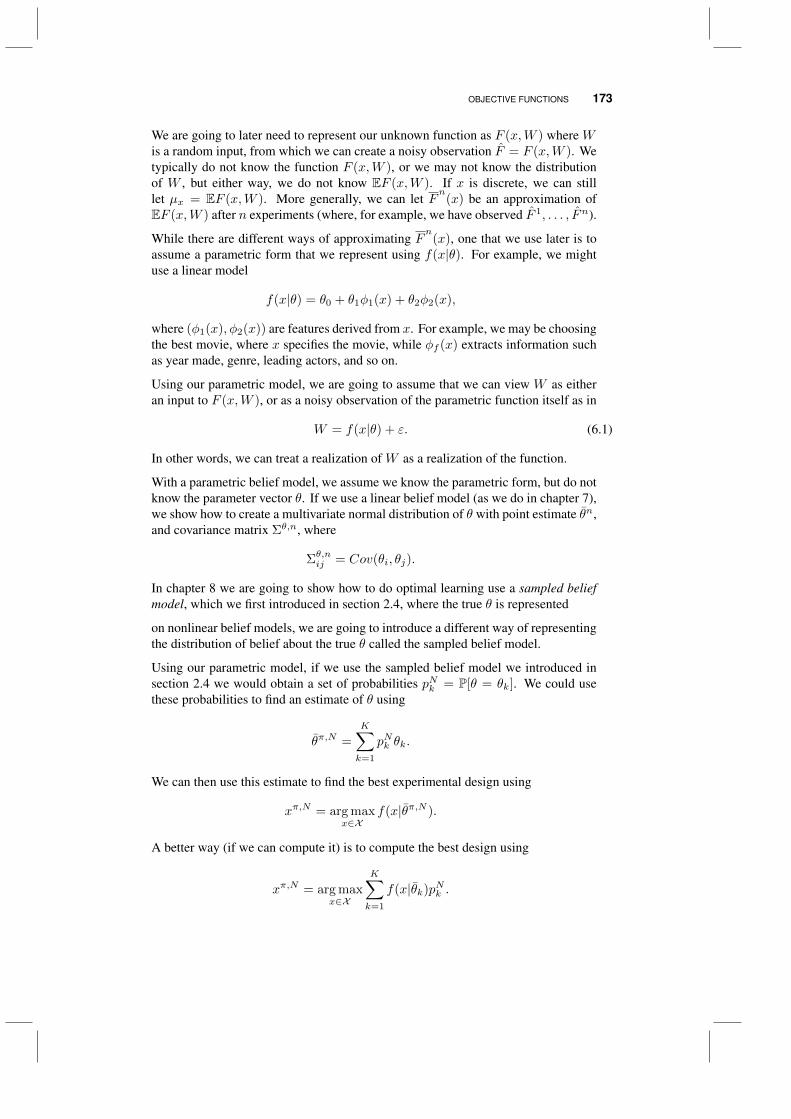
OBJECTIVE FUNCTIONS 173
We are going to later need to represent our unknown function as F (x,W ) where Wis a random input, from which we can create a noisy observation F = F (x,W ). Wetypically do not know the function F (x,W ), or we may not know the distributionof W , but either way, we do not know EF (x,W ). If x is discrete, we can stilllet µx = EF (x,W ). More generally, we can let F
n(x) be an approximation of
EF (x,W ) after n experiments (where, for example, we have observed F 1, . . . , Fn).
While there are different ways of approximating Fn(x), one that we use later is to
assume a parametric form that we represent using f(x|θ). For example, we mightuse a linear model
f(x|θ) = θ0 + θ1φ1(x) + θ2φ2(x),
where (φ1(x), φ2(x)) are features derived from x. For example, we may be choosingthe best movie, where x specifies the movie, while φf (x) extracts information suchas year made, genre, leading actors, and so on.
Using our parametric model, we are going to assume that we can view W as eitheran input to F (x,W ), or as a noisy observation of the parametric function itself as in
W = f(x|θ) + ε. (6.1)
In other words, we can treat a realization of W as a realization of the function.
With a parametric belief model, we assume we know the parametric form, but do notknow the parameter vector θ. If we use a linear belief model (as we do in chapter 7),we show how to create a multivariate normal distribution of θ with point estimate θn,and covariance matrix Σθ,n, where
Σθ,nij = Cov(θi, θj).
In chapter 8 we are going to show how to do optimal learning use a sampled beliefmodel, which we first introduced in section 2.4, where the true θ is represented
on nonlinear belief models, we are going to introduce a different way of representingthe distribution of belief about the true θ called the sampled belief model.
Using our parametric model, if we use the sampled belief model we introduced insection 2.4 we would obtain a set of probabilities pNk = P[θ = θk]. We could usethese probabilities to find an estimate of θ using
θπ,N =
K∑k=1
pNk θk.
We can then use this estimate to find the best experimental design using
xπ,N = arg maxx∈X
f(x|θπ,N ).
A better way (if we can compute it) is to compute the best design using
xπ,N = arg maxx∈X
K∑k=1
f(x|θk)pNk .
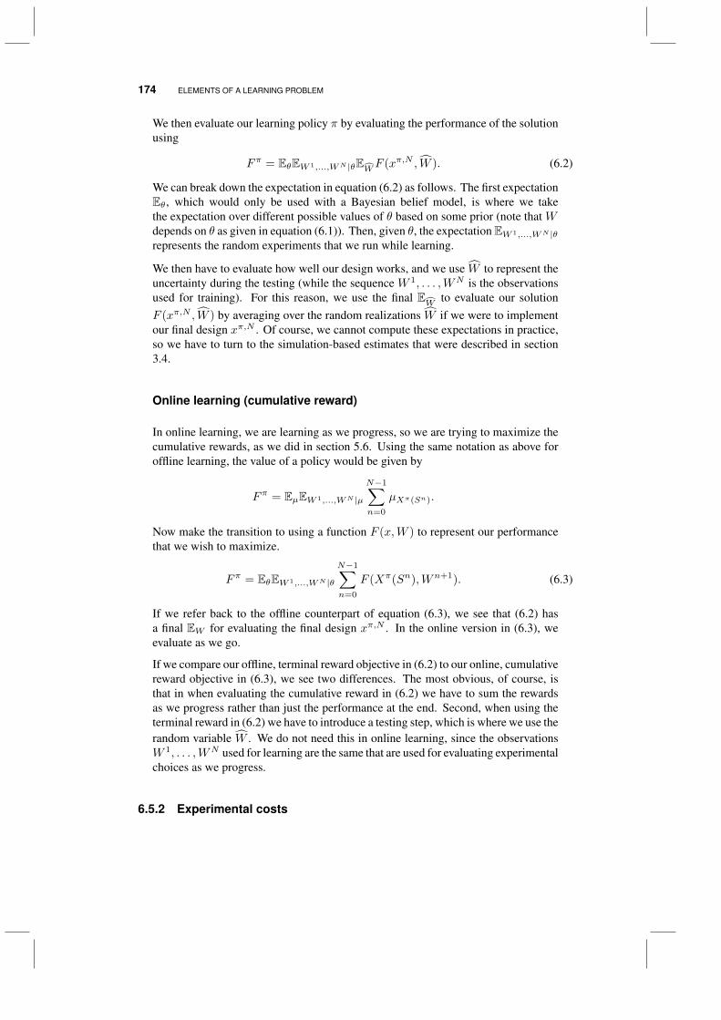
174 ELEMENTS OF A LEARNING PROBLEM
We then evaluate our learning policy π by evaluating the performance of the solutionusing
Fπ = EθEW 1,...,WN |θEWF (xπ,N , W ). (6.2)
We can break down the expectation in equation (6.2) as follows. The first expectationEθ, which would only be used with a Bayesian belief model, is where we takethe expectation over different possible values of θ based on some prior (note that Wdepends on θ as given in equation (6.1)). Then, given θ, the expectation EW 1,...,WN |θrepresents the random experiments that we run while learning.
We then have to evaluate how well our design works, and we use W to represent theuncertainty during the testing (while the sequence W 1, . . . ,WN is the observationsused for training). For this reason, we use the final E
Wto evaluate our solution
F (xπ,N , W ) by averaging over the random realizations W if we were to implementour final design xπ,N . Of course, we cannot compute these expectations in practice,so we have to turn to the simulation-based estimates that were described in section3.4.
Online learning (cumulative reward)
In online learning, we are learning as we progress, so we are trying to maximize thecumulative rewards, as we did in section 5.6. Using the same notation as above foroffline learning, the value of a policy would be given by
Fπ = EµEW 1,...,WN |µ
N−1∑n=0
µXπ(Sn).
Now make the transition to using a function F (x,W ) to represent our performancethat we wish to maximize.
Fπ = EθEW 1,...,WN |θ
N−1∑n=0
F (Xπ(Sn),Wn+1). (6.3)
If we refer back to the offline counterpart of equation (6.3), we see that (6.2) hasa final EW for evaluating the final design xπ,N . In the online version in (6.3), weevaluate as we go.
If we compare our offline, terminal reward objective in (6.2) to our online, cumulativereward objective in (6.3), we see two differences. The most obvious, of course, isthat in when evaluating the cumulative reward in (6.2) we have to sum the rewardsas we progress rather than just the performance at the end. Second, when using theterminal reward in (6.2) we have to introduce a testing step, which is where we use therandom variable W . We do not need this in online learning, since the observationsW 1, . . . ,WN used for learning are the same that are used for evaluating experimentalchoices as we progress.
6.5.2 Experimental costs
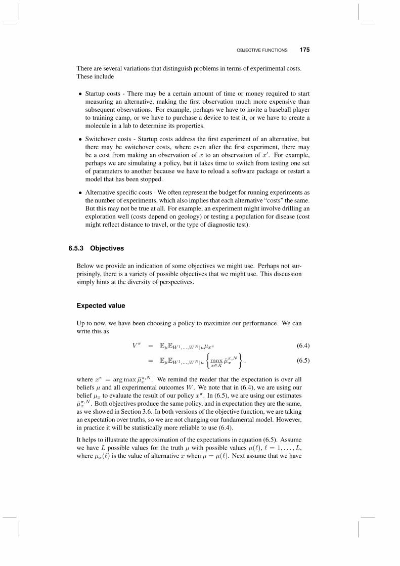
OBJECTIVE FUNCTIONS 175
There are several variations that distinguish problems in terms of experimental costs.These include
• Startup costs - There may be a certain amount of time or money required to startmeasuring an alternative, making the first observation much more expensive thansubsequent observations. For example, perhaps we have to invite a baseball playerto training camp, or we have to purchase a device to test it, or we have to create amolecule in a lab to determine its properties.
• Switchover costs - Startup costs address the first experiment of an alternative, butthere may be switchover costs, where even after the first experiment, there maybe a cost from making an observation of x to an observation of x′. For example,perhaps we are simulating a policy, but it takes time to switch from testing one setof parameters to another because we have to reload a software package or restart amodel that has been stopped.
• Alternative specific costs - We often represent the budget for running experiments asthe number of experiments, which also implies that each alternative “costs” the same.But this may not be true at all. For example, an experiment might involve drilling anexploration well (costs depend on geology) or testing a population for disease (costmight reflect distance to travel, or the type of diagnostic test).
6.5.3 Objectives
Below we provide an indication of some objectives we might use. Perhaps not sur-prisingly, there is a variety of possible objectives that we might use. This discussionsimply hints at the diversity of perspectives.
Expected value
Up to now, we have been choosing a policy to maximize our performance. We canwrite this as
V π = EµEW 1,...,WN |µµxπ (6.4)
= EµEW 1,...,WN |µ
maxx∈X
µπ,Nx
, (6.5)
where xπ = arg max µπ,Nx . We remind the reader that the expectation is over allbeliefs µ and all experimental outcomes W . We note that in (6.4), we are using ourbelief µx to evaluate the result of our policy xπ . In (6.5), we are using our estimatesµπ,Nx . Both objectives produce the same policy, and in expectation they are the same,as we showed in Section 3.6. In both versions of the objective function, we are takingan expectation over truths, so we are not changing our fundamental model. However,in practice it will be statistically more reliable to use (6.4).
It helps to illustrate the approximation of the expectations in equation (6.5). Assumewe have L possible values for the truth µ with possible values µ(`), ` = 1, . . . , L,where µx(`) is the value of alternative x when µ = µ(`). Next assume that we have
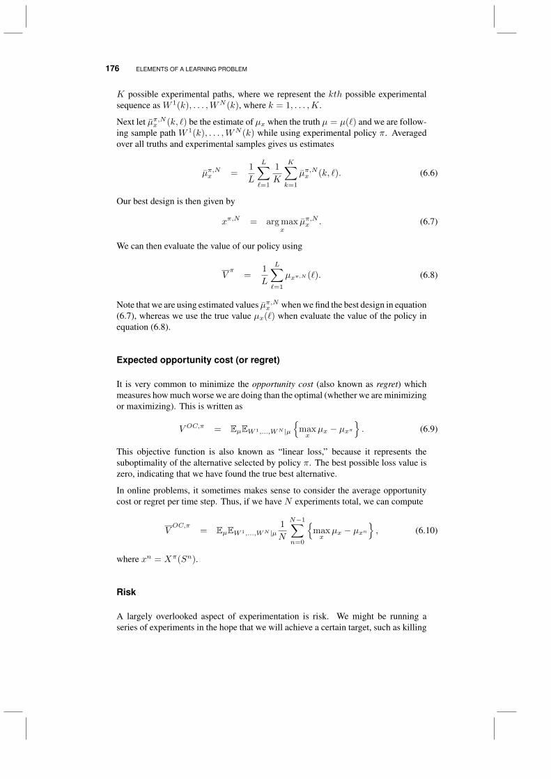
176 ELEMENTS OF A LEARNING PROBLEM
K possible experimental paths, where we represent the kth possible experimentalsequence as W 1(k), . . . ,WN (k), where k = 1, . . . ,K.
Next let µπ,Nx (k, `) be the estimate of µx when the truth µ = µ(`) and we are follow-ing sample path W 1(k), . . . ,WN (k) while using experimental policy π. Averagedover all truths and experimental samples gives us estimates
µπ,Nx =1
L
L∑`=1
1
K
K∑k=1
µπ,Nx (k, `). (6.6)
Our best design is then given by
xπ,N = arg maxx
µπ,Nx . (6.7)
We can then evaluate the value of our policy using
Vπ
=1
L
L∑`=1
µxπ,N (`). (6.8)
Note that we are using estimated values µπ,Nx when we find the best design in equation(6.7), whereas we use the true value µx(`) when evaluate the value of the policy inequation (6.8).
Expected opportunity cost (or regret)
It is very common to minimize the opportunity cost (also known as regret) whichmeasures how much worse we are doing than the optimal (whether we are minimizingor maximizing). This is written as
V OC,π = EµEW 1,...,WN |µ
maxx
µx − µxπ. (6.9)
This objective function is also known as “linear loss,” because it represents thesuboptimality of the alternative selected by policy π. The best possible loss value iszero, indicating that we have found the true best alternative.
In online problems, it sometimes makes sense to consider the average opportunitycost or regret per time step. Thus, if we have N experiments total, we can compute
VOC,π
= EµEW 1,...,WN |µ1
N
N−1∑n=0
maxx
µx − µxn, (6.10)
where xn = Xπ(Sn).
Risk
A largely overlooked aspect of experimentation is risk. We might be running aseries of experiments in the hope that we will achieve a certain target, such as killing
OBJECTIVE FUNCTIONS 177
enough cancer cells, finding the price that produces revenue over a particular target,or designing a material whose strength is over a required level. For such situations,we need to replace the expectation with a risk measure that we designate ρ(Z) whichoperates on a random variable Z (the objective function) in a way that penalizesunacceptable outcomes. For example, imagine we have a threshold zα. Our riskmeasure might be
ρ(Z) = EZ + ηEmax0, Z − zα. (6.11)
This version of ρ(Z) is striking a balance between maximizing the expectation EZand maximizing the expectation of Z when it exceeds a threshold zα. Here, theparameter η puts the weight on outcomes Z > zα, with an implicit penalty onoutcomes Z < zα. Evaluating policies using the risk measure ρ(Z) using simulationis the same as with an expectation, with the single change of including the additionalpenalty term. This said, very little attention has been placed on handling risk inlearning problems.
Robust optimization
In some settings, it makes more sense to focus on the worst case rather than anexpectation. This is becoming known in the optimization community as robustoptimization. We illustrate the calculation of a robust objective using the sampledapproximation we introduced when computing the expected value of a policy above.There, we let µx(`) for ` = 1, . . . , L be a set of truths for µx, and Wn(k) be the nthrealization of W when following sample path k, k = 1, . . . ,K. Let µπ,N calculatedusing equation (6.6), and let xπ,N be the best design computed using equation (6.7).
Above, we computed the expected performance of a policy using
Vπ
=1
L
L∑`=1
µxπ,N (`).
We might be interested in knowing how badly our policy might perform when thetruth is some extreme value. Instead of taking an average, we might instead use thetruth that produces the worst performance, which we can compute using
Vrobust,π
= min`µxπ,N (`). (6.12)
where xπ,N is computed using equation (6.7).
Equation (6.12) recognizes that some truths may be harder to discover than others.We may also want to consider that some experimental sequences may also produceworse designs. Let
µπ,Nx (k, `) = Estimate of µx when µ = µ(`) and we observe experimental se-quence W 1(k), . . . ,WN (k).
Now let the resulting best design be computed using
xπ,N (k) = arg maxx
µπ,Nx (k, `). (6.13)
178 ELEMENTS OF A LEARNING PROBLEM
Finally, we can compute the worst possible performance over truths and sample pathsusing
Vrobust2,π
= min`
minkµxπ,N (k)(`). (6.14)
We can now use Vrobust,π
or Vrobust2,π
as the value of the policy when comparingthe performance of policies. While it is nice to find policies that work best onaverage, there may be considerable interest in policies that mitigate the worst possibleoutcomes.
Yet a further generalization is to use the concept of quantile optimization. If Qα isthe α quantile of a random variable, we may wish to solve
V πα = Qαµxπ . (6.15)
Quantile optimization is related to robust optimization, because we might choose tomaximize the 10th quantile. Quantile optimization is also useful in the presence ofheavy-tailed random variables.
Probability of correct selection
A different perspective is to focus on the probability that we have selected the bestout of a set X alternatives. In this setting, it is typically the case that the number ofalternatives is not too large, say 10 or 20, and certainly not 100,000. Assume that
x∗ = arg maxx∈X
µx
is the best decision (for simplicity, we are going to ignore the presence of ties). Asbefore our we choose as the best design
xπ,N = arg maxx∈X
µπ,Nx .
We have made the correct selection if xπ,N = x∗, but even the best policy cannotguarantee that we will make the best selection every time. Let 1E = 1 if the eventE is true, 0 otherwise. We write the probability of correct selection as
PCS,π = probability we choose the best alternative= Eπ1xπ,N=x∗,
where the underlying probability distribution depends on our learning policy π. Theprobability is computed using the appropriate distribution, depending on whether weare using Bayesian or frequentist perspectives. This may be written in the languageof loss functions. We would define the loss function as
LCS,π = 1xπ,N 6=x∗.
Although we use LCS,π to be consistent with our other notation, this is more com-monly represented as L0−1 for “0-1 loss.”
Note that we write this in terms of the negative outcome so that we wish to minimizethe loss, which means that we have not found the best selection. In this case, wewould write the probability of correct selection as
PCS,π = 1− EπLCS,π.
OBJECTIVE FUNCTIONS 179
Indifference zone selection
A variant of the goal of choosing the best is to maximize the likelihood that we makea choice that is almost as good as the best. Assume we are equally happy with anyoutcome within δ of the best. This is referred to as the indifference zone. Let V n,π bethe value of our solution after n experiments. We require Pπµd∗ = µ∗|µ > 1− αfor all µ where µ[1] − µ[2] > δ, and where µ[1] and µ[2] represent, respectively, thebest and second best choices.
We might like to maximize the likelihood that we fall within the indifference zone,which we can express using
P IZ,π = Pπ(V n,π > µ∗ − δ).
As before, the probability has to be computed with the appropriate Bayesian orfrequentist distribution.
Least squared error
A different form of loss function arises when we want to fit a function to a set of data.In this setting, we think of “x” as a set of independent variables which we choosedirectly or indirectly. For example, we may be able to choose x directly when fittinga linear regression of the form
Y (x) = θ0x0 + θ1x1 + θ2x2 + . . .+ θIxI + ε
= θx+ ε.
where Y is the observed response and ε is the random error explaining differencesbetween the linear model and the responses. We choose it indirectly when ourregression is in the form of basis functions, as in
Y (x) =∑f∈F
θfφf (x) + ε.
Classical linear regression assumes that we are given a set of observations which weuse to fit a model by choosing θ. Let
Y n+1 = θxn + εn+1.
where θ is the true set of parameters. Our indexing reflects our requirement that xn
be chosen before we observe εn+1. Our measure of performance is given by
F (Y (N+1), x(N)|θ) =
N∑n=1
(Y n+1 − θxn)2.
which is the sample sum of squares given experiments x(N) = (x0, . . . , xN ) andobservations Y (N+1) = (Y 1, . . . , Y N+1). Ordinary least squares regression fits amodel by finding
θN+1 = arg minθ
F (Y (N+1), x(N)|θ).
180 ELEMENTS OF A LEARNING PROBLEM
Let F ∗(Y (N+1), x(N)) = F (Y (N+1), x(N)|θN+1) be the optimal solution givenY (N+1) and x(N). Sequential estimation starts with θn, then measures xn, andfinally observes Y n+1 from which we compute θn+1. This can be done easily usingrecursive least mean squares, given by
θn+1 = θn −Hnxn(θnxn − Y n+1)
where Hn is an I × I scaling matrix that is computed recursively (we cover this inSection 7.2.2).
Our focus is on choosing the experiment xn. Classical experimental design assumesthat we choose (xn)Nn=0 first and then fit the model. This is sometimes referred to asbatch design because the entire sample is chosen first. This is equivalent to solving
minx(N)
EF ∗(Y (N+1), x(N))
where the expectation is over the random variables in Y (N+1).
We focus on sequential design, where we choose xn given our state Sn, whichincludes θn and the information we need to update θn. In a sequential learningproblem, we have to use some basis for determining how well we have done. Inour optimization problems, we want to maximize our expected contribution. Thisoptimization problem determines the values of x that are most interesting. In the areaof adaptive estimation, we have to specify the values of x that are most likely to beinteresting to us, which we designate by a density h(x) which has to be specified. Inan off-line learning environment, we want to choose x1, . . . , xn, . . . , xN accordingto a policy π to solve
minπ
E∫x
(Y (x)− θπx
)2h(x)dx
where Y (x) is the random variable we observe given x, and where θπ is the value ofθ produced when we select xn according to π, and when we estimate θ optimally.
This formulation requires that we specify the domain that interests us most throughthe density h(x). An illustration of the density function arises when we are trying tosample nuclear material over a border or in a region. For such cases, h(x) might bethe uniform density over the region in question. When we solve on-line and off-lineoptimization problems, we do not have to specify h(x) explicitly. The optimizationproblem, e.g. equation (5.3), determines the region within X that is of greatestinterest.
Entropy minimization
Entropy is a measure of uncertainty that can be used for numeric and nonnumeric data.Imagine that we are trying to estimate a parameter µ that we know with uncertainty.If our distribution of belief about µ is continuous with density f(u), a measure of theuncertainty with which we know µ is given by the entropy of f(u), given by
H(µ) = −∫u
fu log(fu)du.
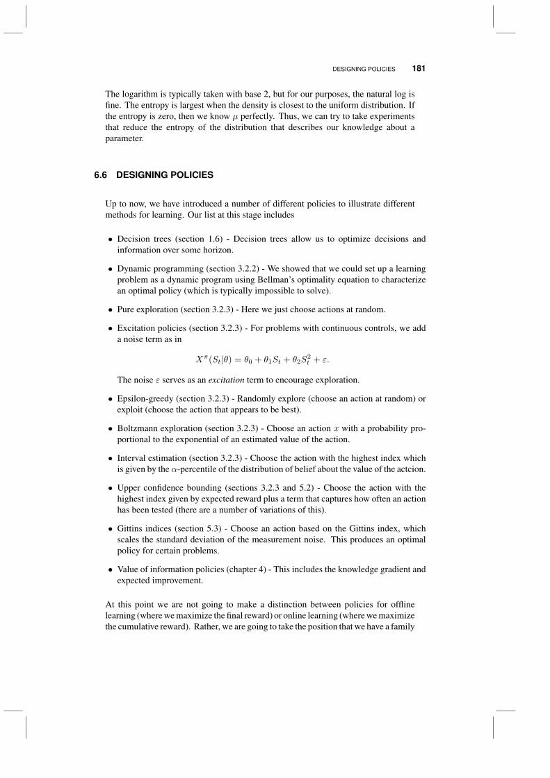
DESIGNING POLICIES 181
The logarithm is typically taken with base 2, but for our purposes, the natural log isfine. The entropy is largest when the density is closest to the uniform distribution. Ifthe entropy is zero, then we know µ perfectly. Thus, we can try to take experimentsthat reduce the entropy of the distribution that describes our knowledge about aparameter.
6.6 DESIGNING POLICIES
Up to now, we have introduced a number of different policies to illustrate differentmethods for learning. Our list at this stage includes
• Decision trees (section 1.6) - Decision trees allow us to optimize decisions andinformation over some horizon.
• Dynamic programming (section 3.2.2) - We showed that we could set up a learningproblem as a dynamic program using Bellman’s optimality equation to characterizean optimal policy (which is typically impossible to solve).
• Pure exploration (section 3.2.3) - Here we just choose actions at random.
• Excitation policies (section 3.2.3) - For problems with continuous controls, we adda noise term as in
Xπ(St|θ) = θ0 + θ1St + θ2S2t + ε.
The noise ε serves as an excitation term to encourage exploration.
• Epsilon-greedy (section 3.2.3) - Randomly explore (choose an action at random) orexploit (choose the action that appears to be best).
• Boltzmann exploration (section 3.2.3) - Choose an action x with a probability pro-portional to the exponential of an estimated value of the action.
• Interval estimation (section 3.2.3) - Choose the action with the highest index whichis given by the α-percentile of the distribution of belief about the value of the actcion.
• Upper confidence bounding (sections 3.2.3 and 5.2) - Choose the action with thehighest index given by expected reward plus a term that captures how often an actionhas been tested (there are a number of variations of this).
• Gittins indices (section 5.3) - Choose an action based on the Gittins index, whichscales the standard deviation of the measurement noise. This produces an optimalpolicy for certain problems.
• Value of information policies (chapter 4) - This includes the knowledge gradient andexpected improvement.
At this point we are not going to make a distinction between policies for offlinelearning (where we maximize the final reward) or online learning (where we maximizethe cumulative reward). Rather, we are going to take the position that we have a family
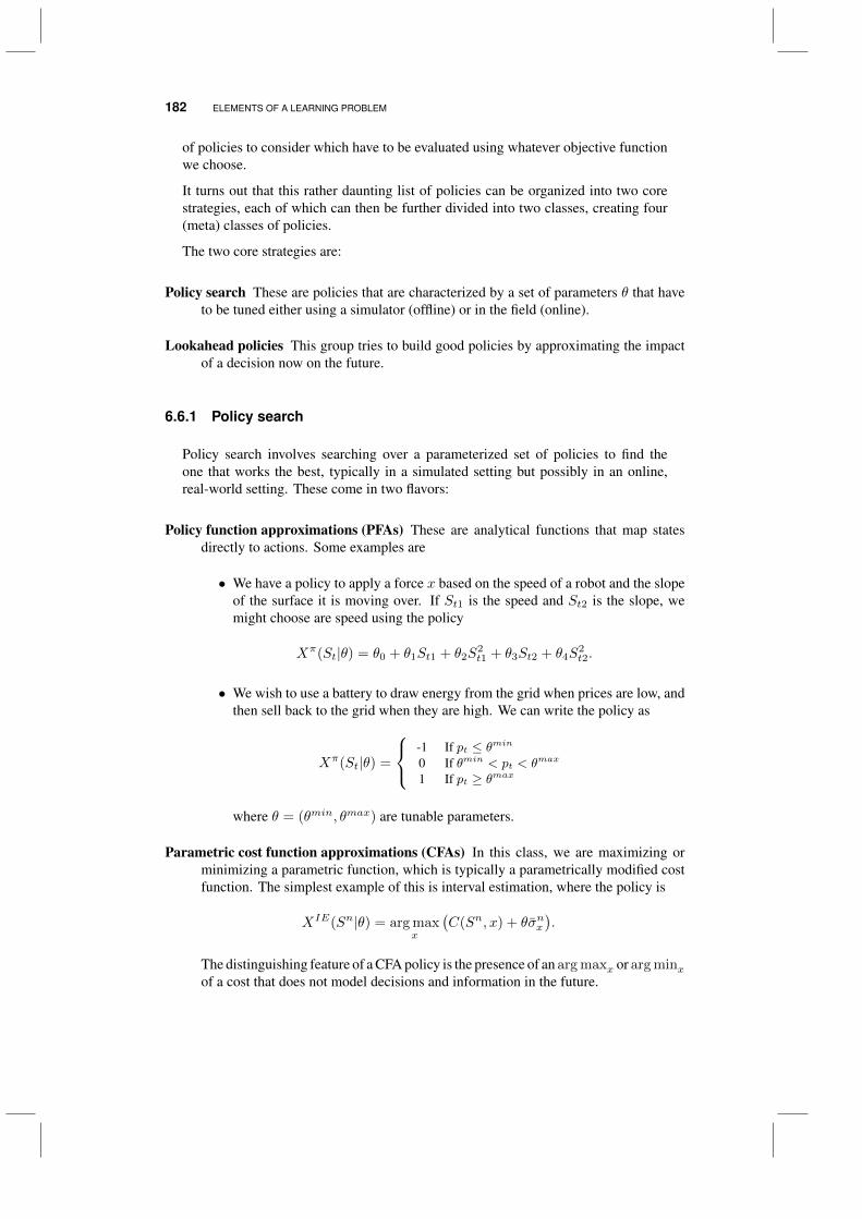
182 ELEMENTS OF A LEARNING PROBLEM
of policies to consider which have to be evaluated using whatever objective functionwe choose.
It turns out that this rather daunting list of policies can be organized into two corestrategies, each of which can then be further divided into two classes, creating four(meta) classes of policies.
The two core strategies are:
Policy search These are policies that are characterized by a set of parameters θ that haveto be tuned either using a simulator (offline) or in the field (online).
Lookahead policies This group tries to build good policies by approximating the impactof a decision now on the future.
6.6.1 Policy search
Policy search involves searching over a parameterized set of policies to find theone that works the best, typically in a simulated setting but possibly in an online,real-world setting. These come in two flavors:
Policy function approximations (PFAs) These are analytical functions that map statesdirectly to actions. Some examples are
• We have a policy to apply a force x based on the speed of a robot and the slopeof the surface it is moving over. If St1 is the speed and St2 is the slope, wemight choose are speed using the policy
Xπ(St|θ) = θ0 + θ1St1 + θ2S2t1 + θ3St2 + θ4S
2t2.
• We wish to use a battery to draw energy from the grid when prices are low, andthen sell back to the grid when they are high. We can write the policy as
Xπ(St|θ) =
-1 If pt ≤ θmin0 If θmin < pt < θmax
1 If pt ≥ θmax
where θ = (θmin, θmax) are tunable parameters.
Parametric cost function approximations (CFAs) In this class, we are maximizing orminimizing a parametric function, which is typically a parametrically modified costfunction. The simplest example of this is interval estimation, where the policy is
XIE(Sn|θ) = arg maxx
(C(Sn, x) + θσnx
).
The distinguishing feature of a CFA policy is the presence of an arg maxx or arg minxof a cost that does not model decisions and information in the future.
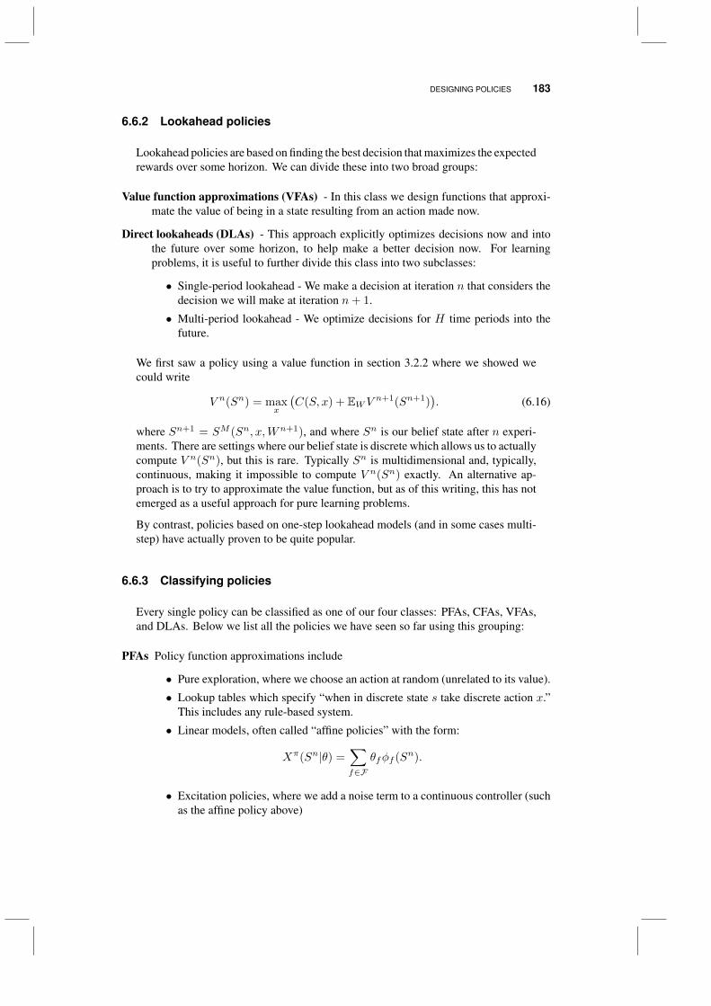
DESIGNING POLICIES 183
6.6.2 Lookahead policies
Lookahead policies are based on finding the best decision that maximizes the expectedrewards over some horizon. We can divide these into two broad groups:
Value function approximations (VFAs) - In this class we design functions that approxi-mate the value of being in a state resulting from an action made now.
Direct lookaheads (DLAs) - This approach explicitly optimizes decisions now and intothe future over some horizon, to help make a better decision now. For learningproblems, it is useful to further divide this class into two subclasses:
• Single-period lookahead - We make a decision at iteration n that considers thedecision we will make at iteration n+ 1.
• Multi-period lookahead - We optimize decisions for H time periods into thefuture.
We first saw a policy using a value function in section 3.2.2 where we showed wecould write
V n(Sn) = maxx
(C(S, x) + EWV n+1(Sn+1)
). (6.16)
where Sn+1 = SM (Sn, x,Wn+1), and where Sn is our belief state after n experi-ments. There are settings where our belief state is discrete which allows us to actuallycompute V n(Sn), but this is rare. Typically Sn is multidimensional and, typically,continuous, making it impossible to compute V n(Sn) exactly. An alternative ap-proach is to try to approximate the value function, but as of this writing, this has notemerged as a useful approach for pure learning problems.
By contrast, policies based on one-step lookahead models (and in some cases multi-step) have actually proven to be quite popular.
6.6.3 Classifying policies
Every single policy can be classified as one of our four classes: PFAs, CFAs, VFAs,and DLAs. Below we list all the policies we have seen so far using this grouping:
PFAs Policy function approximations include
• Pure exploration, where we choose an action at random (unrelated to its value).
• Lookup tables which specify “when in discrete state s take discrete action x.”This includes any rule-based system.
• Linear models, often called “affine policies” with the form:
Xπ(Sn|θ) =∑f∈F
θfφf (Sn).
• Excitation policies, where we add a noise term to a continuous controller (suchas the affine policy above)
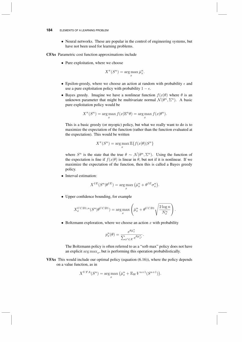
184 ELEMENTS OF A LEARNING PROBLEM
• Neural networks. These are popular in the control of engineering systems, buthave not been used for learning problems.
CFAs Parametric cost function approximations include
• Pure exploitation, where we choose
Xπ(Sn) = arg maxx
µnx .
• Epsilon-greedy, where we choose an action at random with probability ε anduse a pure exploitation policy with probability 1− ε.
• Bayes greedy. Imagine we have a nonlinear function f(x|θ) where θ is anunknown parameter that might be multivariate normal N (θn,Σn). A basicpure exploitation policy would be
Xπ(Sn) = arg maxx
f(x|Enθ) = arg maxx
f(x|θn).
This is a basic greedy (or myopic) policy, but what we really want to do is tomaximize the expectation of the function (rather than the function evaluated atthe expectation). This would be written
Xπ(Sn) = arg maxx
Ef(x|θ)|Sn
where Sn is the state that the true θ ∼ N (θn,Σn). Using the function ofthe expectation is fine if f(x|θ) is linear in θ, but not if it is nonlinear. If wemaximize the expectation of the function, then this is called a Bayes greedypolicy.
• Interval estimation:
XIE(Sn|θIE) = arg maxx
(µnx + θIEσnx
).
• Upper confidence bounding, for example
XUCB1,nx (Sn|θUCB1) = arg max
x
(µnx + θUCB1
√2 log n
Nnx
).
• Boltzmann exploration, where we choose an action x with probability
pnx(θ) =eθµ
nx∑
x′∈X eθµnx′.
The Boltzmann policy is often referred to as a “soft-max” policy does not havean explicit arg maxx, but is performing this operation probabilistically.
VFAs This would include our optimal policy (equation (6.16)), where the policy dependson a value function, as in
XV FA(Sn) = arg maxx
(µnx + EWV n+1(Sn+1)
).
THE ROLE OF PRIORS IN POLICY EVALUATION 185
This is how Gittins indices were computed in section 5.3.
DFAs Direct lookaheads - These come in single-step and multi-step variations:
• Single step - These are very popular in optimal learning applications, andinclude:
– Value of information policies such as the knowledge gradient or expectedimprovement.
XKG,nx = arg max
x
(E
maxx′∈X
µn+1x′ (x)|Sn
− V n(Sn)
).
The maximization over x′ is actually an optimization over possible de-cisions xn+1, after the outcome of the experiment xn = x has beencompleted.
– Thompson sampling:
XTS(Sn) = arg maxx
µn+1x .
Thompson sampling can be thought of a simulation of what might happenin the n+ 1st experiment based on the time n distribution of belief.
• Multistep lookaheads:– Decision trees, which we first introduced in section 1.6.– The KG(*) policy, where we make a decision based on repeating an exper-
iment nx times (this is a restricted lookahead).– Extensions of KG(*) based on tuning the lookahead. We introduced this
in seciton 4.3.3, where the policy is given by
XKG(θKG) = arg maxx
νKG,nx (θKG)
Here, θKG is the parameter governing how many times we plan on repeat-ing each experiment.
As of this writing, CFAs (such as upper confidence bounding) and one-step DLAsare by far the most popular. Randomized exploitation policies (a form of PFA) arepopular with online applications, where it is tempting to do what appears to be best,but with some recognition that we need to introduce exploration.
Almost all of these policies can be tuned, or converted to a tunable version. Value ofinformation policies are generally used without a tunable parameter by exploiting aBayesian prior.
6.7 THE ROLE OF PRIORS IN POLICY EVALUATION
The process of evaluating policies is subtle, because it can bias the identificationof good policies toward problems with specific properties that may not be clearlyidentified. Perhaps one of the most difficult issues arises in the interaction betweenhow problems are generated (that is, the “truth”) and the relationship between thetruth and any prior information that may be used.
186 ELEMENTS OF A LEARNING PROBLEM
Truth from prior
From the Bayesian point of view, arguably the most natural way to evaluate a learningpolicy is to use the method described in Chapter 3, where we:
1) Generate a truth µ(ψ) from a prior.
2) Sample observations W (ω) from the truth µ(ψ).
3) Evaluate how well we discover the truth using one of the objectives listed above.
4) Repeat many times for different truths and different sample observations, to evaluatehow well we discover the truth on average, and how reliably.
This strategy represents a very controlled experiment, which eliminates potentialbiases which a particular policy might be able to exploit. However, this approachmay bias the evaluation process toward policies that work well with good priors.
Truth from an alternative prior
A way of evaluating the robustness of a policy is to generate truths from distributionsother than the prior. For example, our prior may be normally distributed, but wemight generate truths from a uniform or exponential distribution. Such experimentsshould focus on the ability of a policy to work with truths that come from distributionswith potentially heavy tails, but the expected truth should match the expectation ofthe priors, which is to say that the prior should be unbiased.
Truth from a fixed prior
In the global optimization literature, where we collect noisy observations in anattempt to discover the maximum of an unknown continuous function, it is commonto evaluate policies using a few “test functions.” In other words, the truth is set toa fixed value that, for some reason, is believed to be a particularly interesting ordifficult test case. For example, the Branin function
f (x1, x2) =
(x2 −
5.1
4π2x2
1 +5
πx1 − 6
)2
+ 10
(1− 1
8π
)cos (x1) + 10
is a commonly used test function in two dimensions. Test functions may be highlynon-linear with multiple local maxima, and so we may view them as posing anespecial challenge for an optimization algorithm. If we are able to successfully findthe point (x∗1, x
∗2) that maximizes this difficult function, we may reasonably believe
that our policy will be able to learn other functions.
This is a frequentist approach to policy evaluation, where we consider a few fixedtest cases rather than sampling truths from a distribution. However, the strength ofthis approach is that it presents a very clear and well-defined test suite of problems.In Chapter 14, we mention some of these test functions, such as the Branin function,the Ackley function, and others.
THE ROLE OF PRIORS IN POLICY EVALUATION 187
Truth from a biased prior
In any particular learning situation, the sample realization of a specific truth is goingto be higher or lower than the mean of any prior distribution. However, a subtle issuearises if the expected truth is higher or lower than the expectation of the prior, an issuethat we touched on in Section 4.9. In that section, we discussed the problem withthe prior is consistently higher or lower than the truth. But this discussion did notrecognize that it may be possible to identify and correct biases. Even more importantto the discussion here is the fact that if there is a bias, then certain types of policieswill tend to exploit this bias. For example, we might use epsilon-greedy or intervalestimation, each of which has a tunable parameter. In the presence of a bias, we onlyhave to tune the parameters to emphasize more exploration, and we are likely to geta better policy.
Expectations versus risks
Most of our presentation focuses on the expected performance of a learning policy.The probability of correct selection and indifference zone criterion can be viewedas risk-based measures, since they focus on finding alternatives that are within aspecified tolerance with a specified probability.
For many information collection problems, risk is a major issue. Finding a workabledrug that will help to extend lives with a high probability may be much more attractivethan finding the best drug, but with a significant risk of not finding anything. Theworkable drug may not be ideal, but it may be good enough to gain federal approvalwhich can then be marketed.
In real implementations, we are not allowed to run many sample realizations and takean average. We will use a policy on a single sample path. If we are not successful infinding, for example, a workable drug, we may be left asking whether this was justbad luck, or did we have a bad policy. We would like to minimize the possibility thatit was bad luck.
Regret bounds
In Section 5.2, we described a policy known as upper confidence bounding. Forexample, for the case of normally distributed priors and rewards, the UCB policy wasgiven by
νUCB1−Normal,nx = µπ,Nx + 4σW
√log n
Nnx
.
where Nnx is the number of times we have observed alternative x after n trials. UCB
policies have attracted considerable attention in the community that works on multi-armed bandit problems after it was found that it was possible to bound the numberof times that incorrect arms would be tested by C logN , for an appropriately chosenconstantC. In fact, it was shown that this was the best possible bound, which is ofteninterpreted to mean that this may be the best possible policy.
188 ELEMENTS OF A LEARNING PROBLEM
In Section 5.4, comparisons were made between a tuned UCB policy and the knowl-edge gradient policy for problems with normally distributed rewards. Although theknowledge gradient policy outperformed UCB, it is hard to know if this reflects asubtle bias in how the experiments were run. As of this writing, there is insufficientempirical evidence to form any judgments regarding the value of regret bounds interms of predicting the empirical performance of a UCB policy.
6.8 POLICY SEARCH AND THE MOLTE TESTING ENVIRONMENT
We first addressed the problem of evaluating policies in some depth in section 3.3 inthe context of offline (terminal reward) settings. When we are using a simulator, wecan use a policy π to find estimates µπ,Nx and then find the best choice using
xπ,N = arg maxx
µNx ,
We then evaluate our policy using the known truth (which we are simulating), whichwe write as
Fπ,N = EµEW 1,...,WN |µ µxπ,N .
We often use the opportunity cost, or regret, where we compare how well we doagainst the best that could be done (which is possible in our simulated environment).This would be written as
Rπ,N = EµEW 1,...,WN |µ(
maxx
µ− µxπ,N).
Then, in chapter 5, we noted that we could evaluate policies using an online (cumu-lative reward) which we can write as
Fπ,N = EµEW 1,...,WN |µ
N−1∑n=0
µXπ(Sn).
or in terms of its opportunity cost (or regret)
Fπ,N = EµEW 1,...,WN |µ
N−1∑n=0
(maxx
µx − µXπ(Sn)
).
Policy search typically involves searching across different classes of policies (UCB,interval estimation, Gittins indices, knowledge gradient), and then tuning parameterswithin a class (if there are tunable parameters).
We developed a public domain, Matlab-based system called MOLTE (Modular,Optimal Learning Testing Environment) for comparing a variety of policies on alibrary of test problems. Comparisons can be made on either an offline (terminalreward) or online (cumulative reward) basis. Each policy, and each problem, isencoded in its own .m file.
The front end of MOLTE is a spreadsheet, shown in figure 6.1, where you can specifywhich problems you want to use for testing, and which policies you want to apply

POLICY SEARCH AND THE MOLTE TESTING ENVIRONMENT 189
MOLTE Modular, optimal learning
testing environment» Matlab-based environment with
modular library of problems and algorithms, each in its own .m file.
» User specifies in a spreadsheet which algorithms are run on which problems
http://www.castlelab.princeton.edu/software.htmFigure 6.1 Snapshot of the spreadsheet front-end of MOLTE. Each line lists a test problem,along with choices on how to construct a prior (maximum likelihood estimation, pre-specified,uninformative), the measurement budget (as a fraction of the number of alternatives), belief model(independent or correlated), and whether it is offline vs. online evaluation. Then there is a list ofpolicies, where the first policy is used as the reference policy against which the other policies arecompared. Tunable parameters can be specified, or a “*” indicates the package should do the tuning.
to that problem. Each line of the spreadsheet refers to a different test problem inthe library, which is captured by a .m file with the name of the problem (such as“Branin.m”). The user then has to specify
• Prior - This is how to construct a prior. Some choices are
– MLE - Maximum likelihood estimation -– Default - Here we assume that that the prior is encoded within the specification
of the problem.– Uninformative - An uninformative prior means that we have no information at
all about the function (think of infinite variance in the prior).
• Measurement budget - this is specified as a fraction of the number of alternatives.
• Belief model - Independent or correlated beliefs (the system can only handle lookuptable belief models).
• Offline vs. online - Offline means we evaluate a policy based on the terminal reward(after the experimental budget has been exhausted). Online means evaluating a policybased on the total rewards earned during the evaluation (the classic bandit setting).
A partial list of the test problems is given in table 6.1.
Then, for each problem, the user may list any number of pre-coded learning policies,shown in table 6.2. Many (but not all) of these policies have a tunable parameter.When these exist, the user may specify (for interval estimation) “IE(2.2)” if theparameter should be set to 2.2, or “IE(*)” to request that MOLTE do automatedtuning. When automated tuning is requested, MOLTE first searches over the range10−5 to 105, finds the right order of magnitude, and then refines the search.
MOLTE outputs a number of tabular and graphical reports to summarize the perfor-mance of the different policies. Figure 6.2 shows a graphical picture of the samplingpattern for a two-dimensional problem for some policy; these plots provide insightsinto the nature of the different behaviors. Figure 6.3 provides a frequency distributionof the difference between each policy and the reference policy.
MOLTE also produces tabular performance statistics, including both the opportunitycost relative to the reference policy, and the probability a policy outperforms the

190 ELEMENTS OF A LEARNING PROBLEM
Bubeck1 Bubeck7
Asymmetric Unimodular Functions
Rosenbrock function
Pinter’s function
Goldstein function
Griewank function
Braninâ^s function
Axis parallel hyper-ellipsoid function
Rastriginâ^s function
Ackleyâ^s function
Six-hump camel back function
Easom function
Gaussian process regression functions
Payload delivery problem
Nanoparticle design
Table 6.1 A list of some of the test problems in MOLTE.
(a) Sampling distribution (b) Function heatmap
Figure 6.2 Example of the sampling distribution from MOLTE, and the resulting functionapproximation shown as a heatmap.
reference policy over many simulations. An example is shown in figure 6.3. MOLTEoutputs the Latex code for the body of the future.
MOLTE makes it easy to add new problems and new policies by just following thestyle of other problems and policies. The software and a users manual is available at

DISCUSSION 191
Interval Estimation (IE)
Kriging
UCB (independent beliefs)
UCBcb (correlated beliefs)
UCBNormal
UCB-E (independent beliefs)
UCBEcb (correlated beliefs)
UCB-V (independent beliefs)
UCBVcb (correlated beliefs)
Bayes-UCB
KL-UCB
Knowledge gradient policy for offline learning
Knowledge gradient for online learning
Successive rejects
Thompson sampling
Pure exploration
Pure exploitation
Table 6.2 A list of policies that are available in MOLTE.
http://castlelab.princeton.edu/software/.
6.9 DISCUSSION
The purpose of this chapter was to provide a more comprehensive perspective oflearning problems by covering all the major dimensions of any sequential learningproblem. The four classes of policies provides an equally comprehensive roadmapfor designing policies that cuts across the different communities that have contributedto solving this important problem class.
One of the challenges of optimal learning is that important contributions have beenmade in specific subcommunities with a style that reflects both the characteristicsof specific problem classes as well as the culture of different research communities.For example, the bandit community, which has attracted the attention of computerscience, tends to emphasize online problems with relatively small action spaces, noswitchover costs, a Bayesian belief model and a desire to derive provable regretbounds. The simulation optimization community, which tends to focus on findingthe best of a small set of designs using discrete event simulation, also deals with

192 ELEMENTS OF A LEARNING PROBLEM
Figure 6.3 Frequency distribution of difference in performance between each policy and thereference policy.
Problem ClassIE UCBE UCBV Kriging TS EXPL
OC Prob. OC Prob. OC Prob. OC Prob. OC Prob. OC Prob.
Goldstein -0.061 0.81 -0.097 0.92 -0.003 0.45 -0.031 0.73 0.100 0.09 0.041 0.16AUF HNoise 0.058 0.40 0.022 0.43 0.037 0.54 0.031 0.39 0.073 0.22 0.047 0.48AUF MNoise 0.043 0.29 0.027 0.42 0.343 0.21 0.023 0.28 0.173 0.21 -0.057 0.52AUF LNoise -0.043 0.73 -0.013 0.64 0.053 0.51 0.005 0.53 0.038 0.20 0.003 0.62
Branin -0.027 0.76 0.025 0.24 0.026 0.26 0.004 0.54 0.041 0.07 0.123 0.00Ackley 0.007 0.42 0.04 0.41 0.106 0.20 0.037 0.42 0.100 0.23 0.344 0.00
HyperEllipsoid -0.059 0.73 0.064 0.12 0.08 0.07 0.146 0.22 0.011 0.38 0.243 0.03Pinter -0.028 0.56 -0.003 0.51 0.029 0.42 -0.055 0.65 0.122 0.19 0.177 0.04
Rastrigin -0.082 0.70 -0.03 0.56 0.162 0.04 -0.026 0.57 0.136 0.08 0.203 0.01
Table 6.3 Example of table produced by MOLTE. MOLTE outputs the latex code for thebody of the table; headings have to be provided. OC refers to opportunity cost, and Prob. is theprobability the policy outperforms the reference policy specified in the spreadsheet.
small choice sets but uses offline learning of a model with significant switching costs,a frequentist belief model, and a desire to show asymptotic optimality.
6.10 BIBLIOGRAPHIC NOTES
Sections 6.1-6.5 - This representation of learning problems is new, but is based on themodeling framework for dynamic programs presented in Powell (2011). The notionof the “hyperstate” to solve the optimal learning problem was put forth by Bellman& Kalaba (1959); further efforts in this direction were undertaken by Cozzolino etal. (1965), Martin (1967) and Satia & Lave (1973).
Section 6.5 - The different objective functions have been proposed by different authors indifferent communities. Expected opportunity cost lends itself better to the Bayesian

PROBLEMS 193
approach (Chick & Inoue 2001), but can also be analyzed in a frequentist setting(Chick 2003, Chick & Wu 2005). A review of early research on indifference zoneprocedures is given in Bechhofer et al. (1968), with a review of somewhat morerecent papers given by Bechhofer et al. (1995).
Section 6.7 - The truth-from-prior approach is used in Bayesian problems; see e.g. Ryzhovet al. (2011). Vermorel & Mohri (2005) and Chhabra & Das (2011) also make useof other evaluation strategies such sampling from an alternative prior or from anempirical dataset. Lai & Robbins (1985) provides the original paper on regret boundsfor upper confidence bound policies. Regret bounds continue to be popular, usuallyin connection with upper confidence bound methods; see, for example, Agrawal(1995), Auer et al. (2002), Auer et al. (2008), Bartlett et al. (2008), Kleinberg et al.(2010), or Srinivas et al. (2010).
PROBLEMS
In each of the exercises below, you are given a situation that involves learning. Foreach situation, you need to describe the five fundamental dimensions of a learningmodel, including:
• Carefully define the state variable, giving variable names to each component. Clearlydistinguish the belief state (what you think about unknown parameters whose beliefsare evolving over time) and any physical state variables.
• Define the experimental decision (how you are collecting information) and the im-plementation decision (what you are doing with the information). Note that thesemay be the same.
• Define the exogenous information. What are you observing? What is the source ofthe information? Is the information possibly changing your belief about a parameter?
• Describe the equations that make up the transition function. Distinguish betweenthe equations used to update your belief state from those that update any physical orinformational state variables that may be present.
• Define your objective function. Here is where you are going to distinguish be-tween offline and online learning. Be sure to differentiate costs of measuring fromimplementation costs.
Note that in our modeling, we are ignoring the dimension of designing policies. Thisis addressed in all the remaining chapters of this volume. You may feel that you needinformation not specified in the problem description, so you should just highlight anymissing elements, or make up elements to round out your model.
6.1 An entrepreneur would like to market the use of portable solar panels for rechargingcell phones in Africa. The idea is to purchase a number of these solar panels and then tolet individuals try to start businesses in different regions of Africa. Each region will faceits own unique characteristics in terms of need, competition for alternative sources ofenergy and the ability of the local population to pay. For example, the market responds

194 ELEMENTS OF A LEARNING PROBLEM
badly to decisions to raise prices. Focus on the problem faced by a single individualwho has to figure out a pricing strategy as quickly as possible.
6.2 A pharmaceutical company is faced with the problem of performing a series ofmarket research studies to determine the best pricing for a drug. The market can beexpected to respond to recent pricing behavior, and the performance of the drug. Thecompany would like to strike a balance between maximizing revenue and minimizingcosts related to the market research. Market research studies may be run in local regionswhile the drug is still being marketed nationally.
6.3 The Centers for Disease Control wants to collect information so that it can bestunderstand the scope of an outbreak of a virulent new virus in the northeast of the UnitedStates. On a limited budget, the CDC would like to manage a single team of technicianswho will set up a tent to test people as they walk by. The tent will typically be set up for1-3 days before the team moves to another location.
6.4 An analyst is using an expensive computer simulation to model the dynamics ofwind and its effect on generating electricity. It is important to understand the impact ofvery low periods of wind, but obtaining these observations can require simulating years,which can take weeks of time on the computer. The analyst is using the simulator todesign the location of wind farms and investments in the power grid. She might runshorter simulations to do quick evaluations to eliminate poor designs, but much longersimulations are needed to obtain accurate estimates of the likelihood that a particulardesign will be susceptible to blackouts.
CHAPTER 7
LINEAR BELIEF MODELS
In the ranking and selection problem and the multiarmed bandit problem, we assumedwe had a finite set of alternatives x ∈ X = 1, 2, . . . ,M, with a belief µx abouteach of the finite alternatives. Known as a lookup table representation, this model isvery flexible in that it does not require any assumed structure among the alternatives.However, such models become very clumsy when the number of alternatives is large.
In this chapter, we make the transition from a lookup table belief model to onethat uses a parametric model that is linear in the parameters. We assume that anexperiment x can be written as the vector x = (x1, x2, . . . , xK) where xk may bediscrete or continuous. Given x, we observe a value y where we assume a linearrelationship of the form
f(x|θ) =∑f∈F
θfφf (x),
where F is a set of features, x is our input data, and (φf (x))f∈F are features that wedraw from the data in x. For example, x could be a movie, while φ1(x) could be thegenre, φ2(x) could be the year the movie was made, and φ3(x) could be the numberof minutes of high action in the movie. After deciding to display movie x, we thenobserve the response y which might be the number of times the movie is viewed byonline users when it is displayed on their login page.
Instead of observing a sample observation µnx of the unknown truth µx, we are goingto observe yn of the function f(x|θ). As before, if we decide to run experiment
Optimal Learning. By Warren B. Powell and Ilya O. RyzhovCopyright c© 2018 John Wiley & Sons, Inc.
195
196 LINEAR BELIEF MODELS
x = xn, we then observe yn+1, staying with our standard convention of using theiteration counter to tell us which experiments the variable is allowed to see.
We are going to need to manipulate our linear model. For this reason, we are going toadopt the standard notation of statistics and let x1, . . . , xK be the features (instead ofφf (x)). This means that we are going to equate the experiment “x” with the featuresof the experiment (x1, . . . , xK).
yn+1 = θ0 + θ1xn1 + θ2x
n2 + . . .+ θKx
nK + εn+1
where εn+1 is typically assumed to be a normally distributed error term with mean 0and variance σ2.
The most common motivation for using a parametric model is that the number ofalternatives M may be extremely large (say, 100,000 or more), or even infinite (if xis continuous). However, there are applications where we know something about thestructure of the function that we can capture with a parametric model. For example,we may be trying to estimate the maximum of a concave function. A quadraticapproximation may capture this quite nicely, whereas a discretized approximationmay easily lose the natural concavity of the function.
In classical regression model applications, we are given a series of observationsx1, x2, . . . , xn, where for each set of explanatory variables xm there is an observa-tion ym+1. (In traditional batch statistics, we would write ym as the observationcorresponding to experiment xm, but in our sequential setting, it makes more senseto choose xm and then observe ym+1.) This data is then used to find a parametervector θ that minimizes the mean squared error between the predicted model andthe actual observations. We often do not have any choice in how the experimentsx1, x2, . . . , xn are chosen.
The problem of determining how to choose a set of experiments is a popular topic inthe literature on statistical design of experiments. This literature, however, typicallyfocuses on problems where a design (that is, a sequence of experiments) is chosenbefore any observations are made (for more on this topic, see Chapter 2). Thisstrategy reflects the nature of the objective function that is used in this work. If thegoal is to minimize variance, we can exploit the property that the variance of anestimate is a function of the experiments xn and not the observations yn.
In this chapter, we show how the knowledge gradient (for offline or online learning)can be extended to problems where the belief is captured by a model that is linearin the parameters. This result will allow us to tackle problems with thousandsof alternatives, capturing correlations in the beliefs between these alternatives butwithout having to store a covariance matrix with thousands of rows and columns.The complexity of most of the steps in our adaptation of the knowledge gradient willbe determined by the number of parameters rather than the number of alternatives.
7.1 APPLICATIONS
It is useful to start with some real applications to provide context to the discussionthat follows.
APPLICATIONS 197
7.1.1 Maximizing ad clicks
Imagine that you are an Internet company. You might be selling a set of products, orperhaps you are Google selling ad space. Either way, you may have a set of ads (andpossibly thousands of ads) that you could post on the Internet, and you want to findthe ad that generates the most ad clicks (the number of times that someone clicks onan ad, indicating interest).
How do you choose which ads to post? Let Di be the data describing the ith ad.Di might include all the text, along with descriptors of any graphics. The hard partof this project requires identifying important features, which are often representedusing a device called basis functions. We let φf (D) be a particular basis function ina set f ∈ F . Examples of basis functions might include
φ1(D) = The number of words in the ad,φ2(D) = The number of times the word “iphone,” “itouch” or
“ipad” appears,φ3(D) = 1 if the ad involves wireless communication, 0 other-
wise,φ4(D) = 1 if the ad involves food, 0 otherwise,φ5(D) = 1 if the ad has color graphics, 0 otherwise,φ6(D) = 1 if the ad claims to save money, 0 otherwise,φ7(D) = 1 if the ad involves travel or vacations, 0 otherwise.
We first quickly realize that a “basis function” is the same as an independent variablein our linear regression model (different words for the same thing). Also, we cancapture both individual features as well as combinations of features. For example,some people might be attracted to ads that involve food, while others enjoy travel,but what about ads that do both? We can reflect the combined contribution by addingthe marginal effect of each, but we can also introduce a basis function that capturewhether an ad covers food in exotic locations.
Using the notation of basis functions, we would write our linear model as
Y = θ0 +∑f∈F
θfφf (D) + ε.
We can make this a bit more compact by introducing the basis function φ0(D) = 1.Now let φ(D) be a column vector of basis functions, and θ be a column vector of thecoefficients. We can then write
Y = θTφ+ ε.
There are numerous variations of this basic problem which involve identifying web-sites (or documents) that achieve a particular purpose. For example:
• Researching information about a company that might predict a change in the stockprice - The observable information might be an actual change in stock price (whichcan be automated) or it might involve showing the website to a domain expert who

198 LINEAR BELIEF MODELS
can assess its importance. Since the domain expert is a limited resource, we have tobe careful in our selection of websites to be evaluated.
• Finding documents that provide information on terrorist activity - Similar to theprevious item, we can scan millions of websites, but we have to choose which oneswe should show to a domain expert for evaluation. This allows us to build up adataset that can be used to calibrate the importance of different features.
7.1.2 Dynamic pricing
Now consider the same Internet company from the point of view of pricing. Perhapswe are selling textbooks, DVDs, or music downloads. In any case, the Internet offersus a great deal of freedom in setting prices for our product. We can choose a price,wait for a period of time and observe the resulting revenue, then adjust the price inresponse. Of course, this is an example of online learning, because our objective isto maximize total revenue.
To keep the modeling simple, we are going to assume that demand is a linear functionof price which can be written
D(p) = θ0 + θ1p,
where presumably θ1 < 0 to create a downward sloping demand function. We donot know θ0 and θ1, but we assume that we can charge a price p and then make anoisy observation of the demand D(p) = θ0 + θ1p + ε. When we charge a price p,the revenue we earn is given by
R(p) = pD(p).
The pricing problem also arises outside the e-commerce setting. For example, it couldapply to a small business that has a lot of room to change its pricing decisions, butis not prominent enough on the market to be able to change the underlying revenuecurve. The business then has to adapt to an existing, unknown true curve. Aninteresting example of such an enterprise is a recharging station for mobile phonesin a developing country. For example, cell phone use in rural Africa is currentlyexperiencing prodigious growth, because it is much easier to build a single cell phonetower in a rural area than to stretch a land line out to every home. Mobile phonescan serve as versatile and affordable tools even for many who are not connected tothe electric power grid. An entrepreneur with a small power generator, such as a carbattery or a solar panel, can serve many users; the question is how the service shouldbe priced.
7.1.3 Housing loans
The Small Business Administration (SBA) plays the role of granting loans to peoplewhose homes have been destroyed by hurricanes and other natural events. As withany bank, the SBA has to identify people who are good loan prospects. By grantinga loan, the SBA is able to observe which people eventually replay the loan. This
APPLICATIONS 199
information can then be used in a regression model to improve future predictions ofwhether someone might default on a loan. Explanatory variables might include
• The term (length) of the loan.
• The credit score of the applicant.
• Number of months employed.
• Income.
• Did the applicant own the home that was damaged or destroyed?
• Amount of the loan relative to the size of the loss from the storm.
• Amount of collateral.
Normally the SBA would grant loans to people whose probability of repaymentis over some amount. However, it is possible for the SBA to grant some loans toapplicants whose probability of repayment might be lower simply for the informationthat might improve their predictive ability for loan defaults.
7.1.4 Optimizing dose response
It is often the case that people respond differently to a particular dosage of a medi-cation, forcing physicians to experiment with different dosages. It is natural to try topredict a patient’s response (lowering blood sugar, controlling high blood pressure,raising the red blood cell count) using a statistical model. However, sometimes itis necessary to experiment with different dosages to help improve the model (whichmay involve a term unique to an individual patient).
We might envision a statistical model that predicts response as a function of apatient’s body mass index, gender, age, ethnicity and other elements of a patient’shistory. However, it is often the case that we want to fit a nonlinear function thatrelates patient response to a nonlinear function which might look like
Pi =eU(xi|θ)
1 + eU(xi|θ),
where U(x|θ) is a linear function of independent variables with the general form
U(x|θ) = θ0 + θ1x1 + θ2x2 + . . . .
In this model, Pi gives the proportion of people in a group i with a specific set ofattributes xi = (xi1, xi2, . . .) who respond to a particular dosage. This is an exampleof a parametric model that is nonlinear in the parameter vector θ. Belief models thatare nonlinear in the parameters cause problems with methods such as the knowledgegradient because we lose conjugacy (see Chapter ?? for an in depth analysis of thisparticular belief model). However, we can overcome this problem by introducing thetransformation
Pi = ln
(Pi
1− Pi
).
200 LINEAR BELIEF MODELS
Using this transformation, we obtain the linear regression
Pi = θ0 + θ1x1 + θ2x2 + . . . .
Now we have the response relationship expressed as a linear regression. We can usethis model given estimates of θ to optimize a dosage strategy. This strategy, however,depends on estimates of the parameter vector θ. We may wish to attempt dosagessimply to learn more about this relationship.
7.2 A BRIEF REVIEW OF LINEAR REGRESSION
Assume we have n experiments of a vector x = (x1, . . . , xK). If xm is the mthexperiment, using the indexing convention we have used throughout this volume, welet ym+1 be the observation corresponding to xm. Recall that our indexing systemreflects the property that xm depends on the observations y1, . . . , ym, and we observeym+1 after we have chosen xm. Let
xn =
xn1xn2...xnK
be a K-dimensional column vector of observations. Often we will let x1 = 1 torepresent a constant term. Letting θ be the column vector of parameters, we can writeour model as
y = θTx+ ε,
where we assume that the errors (ε1, . . . , εn) are independent and identically dis-tributed. Since θn is our estimate of θ after n observations, our best estimate of y isgiven by
yn = (θn)Txn.
7.2.1 The normal equations
We wish to find a parameter vector θ that solves
minθ
n−1∑m=0
(ym+1 −
K∑k=1
θkxmk
)2
. (7.1)
Let θn be the optimal solution for this problem. We can solve this problem verysimply. Let Xn be the n by K matrix
Xn =
x1
1
x21...xn1
x12
x22...xn2
. . .
x1K
x2K...xnK
.

A BRIEF REVIEW OF LINEAR REGRESSION 201
The vector of observations of the dependent variable is given by
Y n =
y1
y2
...yn
.
The optimal parameter vector θn (after n observations) is then given by
θn = [(Xn)TXn]−1(Xn)T Y n. (7.2)
From the normal equations, we can compute the covariance matrix for θn using asimple matrix identity. If u and w are scalar random variables where u = Aw,then we know that Var(u) = A2Var(w). If u and v are vectors, and A is a suitablydimensioned matrix, then we can write Var(u) (the covariance matrix for the vectoru) as
Cov(u) = ACov(w)AT
where Cov(w) is the covariance matrix of w. Recall that for matrices A and B,ABT = (BAT )T . Also keep in mind that [(Xn)TXn]−1 is symmetric. Applyingthis identity to (12.2), where A = [(Xn)TXn]−1(Xn)T , we obtain
Var(θn) = [(Xn)TXn]−1(Xn)TCov(Y n)([(Xn)TXn]−1(Xn)T
)T= [(Xn)TXn]−1(Xn)TCov(Y n)(Xn)[(Xn)TXn]−1.
Since the elements of Y n are independent, Cov(Y n) = σ2ε I where I is the identity
matrix and σ2ε is the variance of our experimental error . This allows us to write
Σθ,n = [(Xn)TXn]−1(Xn)TXn[(Xn)TXn]−1σ2ε
= [(Xn)TXn]−1σ2ε .
It is important to realize that the matrix Xn is n by K, so computing Σθ,n is not toodifficult.
7.2.2 Recursive least squares
There is a shortcut that we can use to do this recursively. The updating equation forθn can be computed using
θn = θn−1 +1
γnBn−1xnεn, (7.3)
where εn is the error given by
εn = yn − θn−1xn−1. (7.4)
The matrixBn = [(Xn)TXn]−1. This can be updated recursively without computingan explicit inverse using
Bn = Bn−1 − 1
γn(Bn−1xn(xn)TBn−1). (7.5)
202 LINEAR BELIEF MODELS
The scalar γn is computed using
γn = 1 + (xn)TBn−1xn. (7.6)
Note that if we multiply (7.5) through by σ2ε we obtain
Σθ,n = Σθ,n−1 − 1
γn(Σθ,n−1xn(xn)TΣθ,n−1),
where we scale γn by σ2ε , giving us
γn = σ2ε + (xn)TΣθ,n−1xn.
Note that we had to multiply each Bn−1 in the second term on the right of (7.5) byσ2ε so we also divided the second term by σ2
ε , which we did by scaling γn.
Thus, we have compact updating equations dimensioned only by the number ofparameters, rather than the number of alternatives.
The recursive updating formulas, aside from allowing us to avoid an expensive matrixinversion, allows us to handle an issue that we have not yet considered. There areproblems where the observations are nonstationary, which means they are comingfrom a process that is changing over time. In such settings, we may not want to giveall the observations equal weight. We can do this by replacing the objective function(12.1) with
minθ
n−1∑m=0
λn−m
(ym+1 −
K∑k=1
θkxmk
)2
. (7.7)
Here, λ is a discount factor that we use to discount older observations. If we use thisobjective function, our recursive updating equations change only slightly to
γn = λ+ (xn)TBn−1xn, (7.8)
instead of (7.7), while we replace (7.5) with
Bn =1
λ
(Bn−1 − 1
γn(Bn−1xn(xn)TBn−1)
).
Setting λ = 1 gives us the original updating equations. Using smaller values ofλ reduces the weight on older observations, but also increases the variance of theestimates.
7.2.3 A Bayesian interpretation
Classical linear regression is, of course, a frequentist method, but we can put lin-ear regression into our standard Bayesian vocabulary. Let µi be the true value ofalternative i which, in our Bayesian setting, is a random variable given by
µi = θxi.
A BRIEF REVIEW OF LINEAR REGRESSION 203
Just as µ is a random variable (our truth), so is θ, which is the truth about the effectof each feature. We learned that we get tremendous benefits from exploiting thecovariance between two alternatives. The covariance between µi and µj is given by
Cov(µi, µj) = Cov
(∑k
θkXik,∑k
θkXjk
)=
∑k,k′
XikX
jk′Cov(θk, θk′) =
∑k,k′
XikX
jk′Σ
θk,k′
= eTi XΣθXT ej ,
where Σθk,k′ = Cov(θk, θk′) is the covariance between the regression coefficientsθk and θk′ . If Σ is our original covariance matrix between our beliefs of differentalternatives, Σ and Σθ are related by
Σ = XΣθXT .
This means that we can write our vector of truths about the value of each alternativeas
µ ∼ N(θTX,XΣθXT ).
Here, X is a matrix with a row and column for each alternative, which means that ithasM rows (one for every alternative which may be an extremely large number) andK columns (one for every feature, which is generally not too large). We then let
Σn = XΣθ,nXT
be the covariance matrix among allM alternatives (hence Σn isM ×M , while Σθ,n
is K × K). This means that we are getting an estimate of the covariance betweenevery pair of alternatives, including those which we have not tested yet, from themuch more compact matrix Σθ. Our goal is to avoid having to explicitly computeand store the complete matrix Σn.
The important result is that we can compute a covariance matrix among all possiblealternatives, using only the covariance matrix Σθ,n among the parameters, and thematrix X of attributes of each possible alternative. Updating Σθ,n from data isrelatively easy using our recursive formulas. Computing Σn, given the potentiallylarge number of rows, is still quite manageable given that it involves fairly simplecalculations.
7.2.4 Generating a prior
To perform learning in our Bayesian setting, we have to generate a truth, and thenapply a learning algorithm (such as the knowledge gradient) to try to discover thetruth. When we had a discrete set of alternatives with normally distributed beliefs,we could simply sample from the normal distribution we used as a prior.
There are several ways to generate a prior for these more complex settings. One,of course, is to collect a small sample of observations from an initial training set
204 LINEAR BELIEF MODELS
x0, . . . , xL−1, producing observations y1, . . . , yL. If L is larger than the number ofparameters to be estimated, we can create an initial estimate of the parameter vectorθ0 using the normal equations in equation (12.2). We can then use this initial estimateto obtain an estimate of the variance σ2 (if this is not known already). In the contextof Bayesian learning, this becomes the same empirical Bayes strategy that we havealready discussed.
Using an estimate of σ2ε obtained from this model, we can estimate an initial covari-
ance matrix for θ from
Σθ,0 = [(XL)TXL]−1σ2ε (7.9)
where XL is our initial set of observations from the first L observations.
We cannot use equation (7.9) if we have fewer than L observations, and we need atleastL+1 observations if we are going to obtain a valid estimate of σ2
ε . However, wecan still get initial estimates of θ and Σθ with fewer than L observations, as long aswe have some sort of prior. If we have some starting point, we can use the recursiveequations (7.3)-(7.7) for an initial set of training points which may be chosen atrandom.
A useful strategy for generating an initial set of estimates is to write the regressionequation in the form
y = θ0 + θ1(x1 − x1) + θ2(x2 − x2) + . . .+ ε,
where xi is viewed as an average or typical value of the independent variable xi. Inthis model, θ0 should be an average (or typical) value of the observations y, while θicaptures the marginal impact of xi on y. For example, consider our pricing modelabove where the demand D(p) is given by
D(p) ≈ θ0 + θ1(p− p).
Here, we have written the independent variable as the deviation from what we mightcall a typical price give by p. In this model, θ0 would be a prior estimate of thetypical demand, while θ1 captures the effect of changes in the price on demand.
Estimating Σθ,0 is somewhat tricker. An estimate of the diagonal terms can be foundby trying to estimate a confidence interval for each coefficient θi. So, we might thinkthe right coefficient for our demand curve is θ1 ≈ −0.07, and we might then bewilling to say that the right coefficient is probably in the range (-0.03,-0.10). Fromthis, we could infer a standard deviation of, say, 0.015, and use this to create thediagonal elements of Σθ,0.
Estimating the off-diagonal elements of Σθ,0 is inherently more complicated. A firstorder approximation is to just set them to zero, but this can be dangerous. Considerthe set of potential demand functions shown in Figure 7.1. We may be uncertainabout the precise line that describes the demand-price tradeoff, but we may feel thatthey all go through a certain region that might reflect the current demand and currentprice. The implication is that smaller values of θ1 correspond to smaller values ofθ0, so our prior on these coefficients would not be independent.
Once we have an initial estimate of a mean vector θ0 and covariance matrix Σ0, wecan generate a truth µ from a normal distribution using the techniques described inSection 2.7.

THE KNOWLEDGE GRADIENT FOR A LINEAR MODEL 205
Most like demand/pricecombination
Price p
Dem
and
D(p
)
Figure 7.1 Illustration of range of potential demand functions.
7.3 THE KNOWLEDGE GRADIENT FOR A LINEAR MODEL
Now we are ready to derive the knowledge gradient using our linear belief model.We begin with the calculations, which are very similar to the knowledge gradientfor correlated beliefs, except that now the correlations are between the parameters.We then contrast the behavior of the knowledge gradient when using a linear beliefmodel versus when we use a lookup table model.
7.3.1 Calculations
Recall that the calculation of the knowledge gradient requires computing the functionh(a, b(j)) where a is a vector with element ai = θni giving the estimate of the valueof the ith alternative, and b(j) is a vector with element bi(j) = σni (j), which isthe conditional variance of the change in θn+1 from measuring alternative j. Thefunction h(a, b) is given by
h(a, b(j)) =
M−1∑i=1
(bi+1(j)− bi(j))f(−|ci(j)|) (7.10)
where
ci(j) =ai − ai+1
bi+1(j)− bi(j).
Refer to Section 4.5 for the details of computing the knowledge gradient for correlatedbeliefs.
Keeping in mind thatM may be a very large number, we have to use care in how thisis computed. We can use θni = θnxi to compute the expected value, which does notdepend on the alternative j that we are measuring.
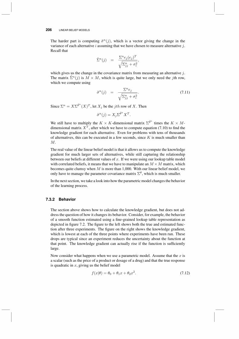
206 LINEAR BELIEF MODELS
The harder part is computing σn(j), which is a vector giving the change in thevariance of each alternative i assuming that we have chosen to measure alternative j.Recall that
Σn(j) =Σnej(ej)
T√Σnjj + σ2
ε
,
which gives us the change in the covariance matrix from measuring an alternative j.The matrix Σn(j) is M ×M , which is quite large, but we only need the jth row,which we compute using
σn(j) =Σnej√
Σnjj + σ2ε
. (7.11)
Since Σn = XΣθn
(X)T , let Xj be the jth row of X . Then
σn(j) = XjΣθnXT .
We still have to multiply the K × K-dimensional matrix Σθn
times the K ×M -dimensional matrix XT , after which we have to compute equation (7.10) to find theknowledge gradient for each alternative. Even for problems with tens of thousandsof alternatives, this can be executed in a few seconds, since K is much smaller thanM .
The real value of the linear belief model is that it allows us to compute the knowledgegradient for much larger sets of alternatives, while still capturing the relationshipbetween our beliefs at different values of x. If we were using our lookup table modelwith correlated beliefs, it means that we have to manipulate anM×M matrix, whichbecomes quite clumsy whenM is more than 1,000. With our linear belief model, weonly have to manage the parameter covariance matrix Σθ, which is much smaller.
In the next section, we take a look into how the parametric model changes the behaviorof the learning process.
7.3.2 Behavior
The section above shows how to calculate the knowledge gradient, but does not ad-dress the question of how it changes its behavior. Consider, for example, the behaviorof a smooth function estimated using a fine-grained lookup table representation asdepicted in figure 7.2. The figure to the left shows both the true and estimated func-tion after three experiments. The figure on the right shows the knowledge gradient,which is lowest at each of the three points where experiments have been run. Thesedrops are typical since an experiment reduces the uncertainty about the function atthat point. The knowledge gradient can actually rise if the function is sufficientlylarge.
Now consider what happens when we use a parametric model. Assume that the x isa scalar (such as the price of a product or dosage of a drug) and that the true responseis quadratic in x, giving us the belief model
f(x|θ) = θ0 + θ1x+ θ2x2. (7.12)
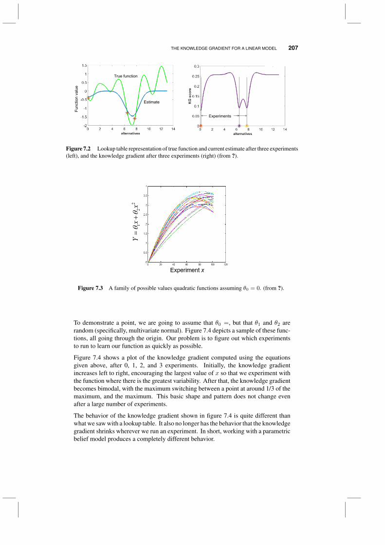
THE KNOWLEDGE GRADIENT FOR A LINEAR MODEL 207
True function
Estimate
Func
tion
valu
e
Experiments
Figure 7.2 Lookup table representation of true function and current estimate after three experiments(left), and the knowledge gradient after three experiments (right) (from ?).
Figure 7.3 A family of possible values quadratic functions assuming θ0 = 0. (from ?).
To demonstrate a point, we are going to assume that θ0 =, but that θ1 and θ2 arerandom (specifically, multivariate normal). Figure 7.4 depicts a sample of these func-tions, all going through the origin. Our problem is to figure out which experimentsto run to learn our function as quickly as possible.
Figure 7.4 shows a plot of the knowledge gradient computed using the equationsgiven above, after 0, 1, 2, and 3 experiments. Initially, the knowledge gradientincreases left to right, encouraging the largest value of x so that we experiment withthe function where there is the greatest variability. After that, the knowledge gradientbecomes bimodal, with the maximum switching between a point at around 1/3 of themaximum, and the maximum. This basic shape and pattern does not change evenafter a large number of experiments.
The behavior of the knowledge gradient shown in figure 7.4 is quite different thanwhat we saw with a lookup table. It also no longer has the behavior that the knowledgegradient shrinks wherever we run an experiment. In short, working with a parametricbelief model produces a completely different behavior.
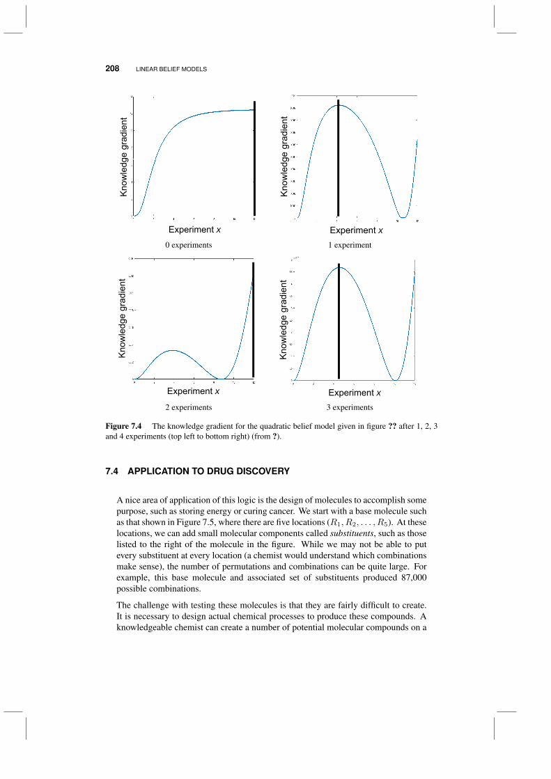
208 LINEAR BELIEF MODELS
Insights
Know
ledg
e gr
adie
nt
Experiment x
Insights
Know
ledg
e gr
adie
nt
Experiment x0 experiments 1 experiment
Insights
Know
ledg
e gr
adie
nt
Experiment x
Insights
Know
ledg
e gr
adie
nt
Experiment x2 experiments 3 experiments
Figure 7.4 The knowledge gradient for the quadratic belief model given in figure ?? after 1, 2, 3and 4 experiments (top left to bottom right) (from ?).
7.4 APPLICATION TO DRUG DISCOVERY
A nice area of application of this logic is the design of molecules to accomplish somepurpose, such as storing energy or curing cancer. We start with a base molecule suchas that shown in Figure 7.5, where there are five locations (R1, R2, . . . , R5). At theselocations, we can add small molecular components called substituents, such as thoselisted to the right of the molecule in the figure. While we may not be able to putevery substituent at every location (a chemist would understand which combinationsmake sense), the number of permutations and combinations can be quite large. Forexample, this base molecule and associated set of substituents produced 87,000possible combinations.
The challenge with testing these molecules is that they are fairly difficult to create.It is necessary to design actual chemical processes to produce these compounds. Aknowledgeable chemist can create a number of potential molecular compounds on a

APPLICATION TO DRUG DISCOVERY 209
R1
R2
R4
R3
R5
18
23
4
5
9
9
74’
3’
2’ 1’
6
3
3
FOHCHOCOCHOCOCH
3OCHCHNOCIOCOCH
Potential substituents:
Figure 7.5 Illustration of base molecule with five substituent locations (from Katz & Ionescu1977).
white board, but once we decide which compound to test next, the actual testing is aproject that can take a day to several days. This is the reason why it is important tosequence the experiments carefully.
The problem of designing molecules arises in many settings. The work in this sectionwas motivated by a problem of finding compounds to cure a form of cancer, but thenumerical work was done using data taken from the literature which was motivated bya variety of applications. All we require is that we are trying to choose a compoundthat maximizes (or perhaps minimizes) some metric, such as killing cancer cells.
In practice, the knowledge gradient can be used to produce a ranked list of potentialmolecules to be tested next. An attraction of this strategy is that it allows a scientist touse expert knowledge to capture dimensions other than the performance of a moleculein terms of a specific metric such as killing cancer cells. For example, a moleculemight be toxic, hard to manufacture or insoluble in water.
To put this problem in the context of our model with linear beliefs, let i = 1, . . . , Ibe the set of sites (five in our example) and let j = 1, . . . , J be the set of potentialsubstituents (10 in our example). Let
Xij =
1 If we put the jth substituent at the ith site,0 Otherwise.
Now letY be an observation of the performance of a particular molecule, which mightbe the percentage of cancer cells that are killed. We might model the performance ofa molecule using
Y = θ0 +
I∑i=1
J∑j=1
θijXij . (7.13)
With this simple model, if we have five sites and 10 substituents, we have 51 param-eters to estimate (including the constant intercept θ0).
To determine the effectiveness of the knowledge gradient, it is necessary to create atruth (following our standard practice) and then try to discover the truth using different
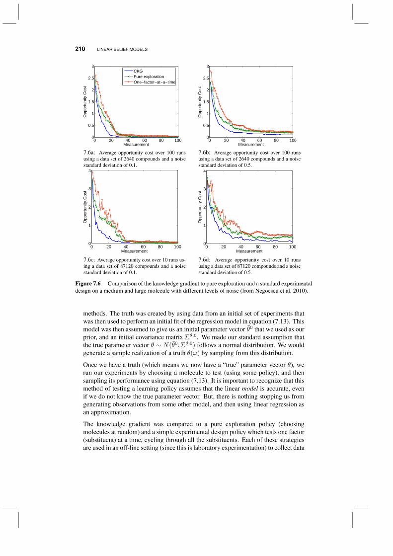
210 LINEAR BELIEF MODELS
0 20 40 60 80 1000
0.5
1
1.5
2
2.5
3
Measurement
Opp
ortu
nity
Cos
t
CKGPure explorationOne−factor−at−a−time
0 20 40 60 80 1000
0.5
1
1.5
2
2.5
3
Measurement
Opp
ortu
nity
Cos
t
7.6a: Average opportunity cost over 100 runsusing a data set of 2640 compounds and a noisestandard deviation of 0.1.
7.6b: Average opportunity cost over 100 runsusing a data set of 2640 compounds and a noisestandard deviation of 0.5.
0 20 40 60 80 1000
1
2
3
4
Measurement
Opp
ortu
nity
Cos
t
0 20 40 60 80 1000
1
2
3
4
Measurement
Opp
ortu
nity
Cos
t
7.6c: Average opportunity cost over 10 runs us-ing a data set of 87120 compounds and a noisestandard deviation of 0.1.
7.6d: Average opportunity cost over 10 runsusing a data set of 87120 compounds and a noisestandard deviation of 0.5.
Figure 7.6 Comparison of the knowledge gradient to pure exploration and a standard experimentaldesign on a medium and large molecule with different levels of noise (from Negoescu et al. 2010).
methods. The truth was created by using data from an initial set of experiments thatwas then used to perform an initial fit of the regression model in equation (7.13). Thismodel was then assumed to give us an initial parameter vector θ0 that we used as ourprior, and an initial covariance matrix Σθ,0. We made our standard assumption thatthe true parameter vector θ ∼ N(θ0,Σθ,0) follows a normal distribution. We wouldgenerate a sample realization of a truth θ(ω) by sampling from this distribution.
Once we have a truth (which means we now have a “true” parameter vector θ), werun our experiments by choosing a molecule to test (using some policy), and thensampling its performance using equation (7.13). It is important to recognize that thismethod of testing a learning policy assumes that the linear model is accurate, evenif we do not know the true parameter vector. But, there is nothing stopping us fromgenerating observations from some other model, and then using linear regression asan approximation.
The knowledge gradient was compared to a pure exploration policy (choosingmolecules at random) and a simple experimental design policy which tests one factor(substituent) at a time, cycling through all the substituents. Each of these strategiesare used in an off-line setting (since this is laboratory experimentation) to collect data
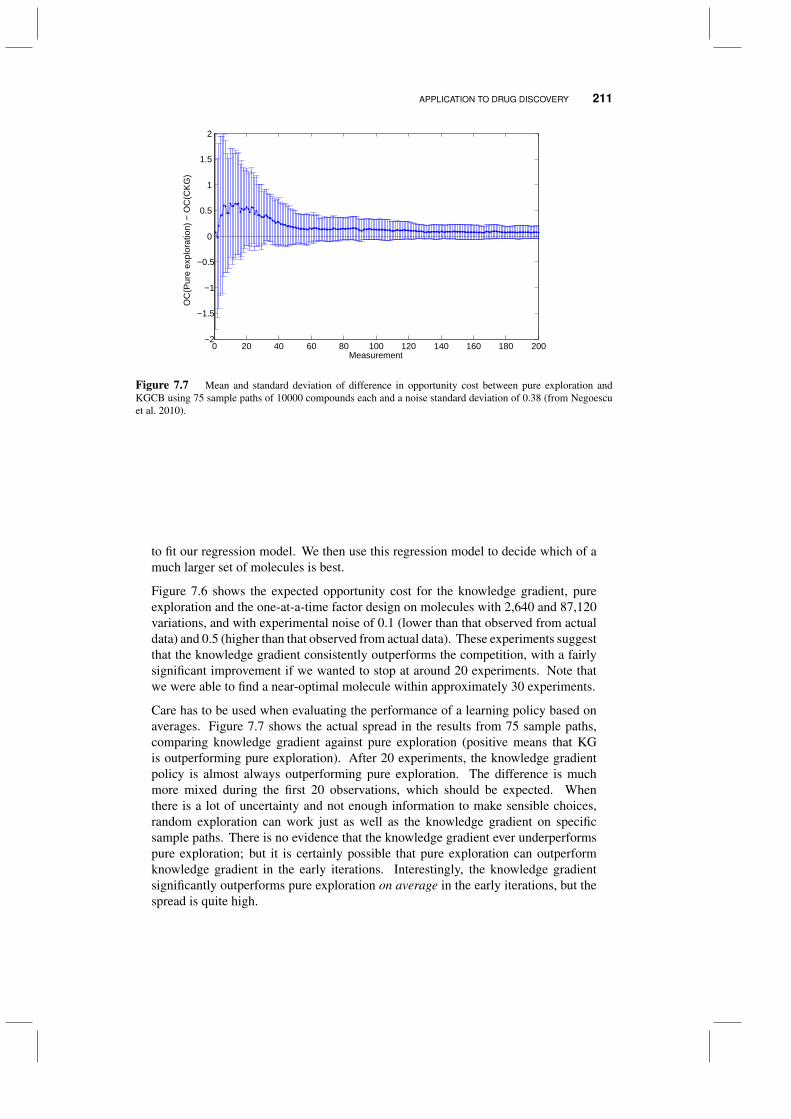
APPLICATION TO DRUG DISCOVERY 211
0 20 40 60 80 100 120 140 160 180 200−2
−1.5
−1
−0.5
0
0.5
1
1.5
2
Measurement
OC
(Pur
e ex
plor
atio
n) −
OC
(CK
G)
Figure 7.7 Mean and standard deviation of difference in opportunity cost between pure exploration andKGCB using 75 sample paths of 10000 compounds each and a noise standard deviation of 0.38 (from Negoescuet al. 2010).
to fit our regression model. We then use this regression model to decide which of amuch larger set of molecules is best.
Figure 7.6 shows the expected opportunity cost for the knowledge gradient, pureexploration and the one-at-a-time factor design on molecules with 2,640 and 87,120variations, and with experimental noise of 0.1 (lower than that observed from actualdata) and 0.5 (higher than that observed from actual data). These experiments suggestthat the knowledge gradient consistently outperforms the competition, with a fairlysignificant improvement if we wanted to stop at around 20 experiments. Note thatwe were able to find a near-optimal molecule within approximately 30 experiments.
Care has to be used when evaluating the performance of a learning policy based onaverages. Figure 7.7 shows the actual spread in the results from 75 sample paths,comparing knowledge gradient against pure exploration (positive means that KGis outperforming pure exploration). After 20 experiments, the knowledge gradientpolicy is almost always outperforming pure exploration. The difference is muchmore mixed during the first 20 observations, which should be expected. Whenthere is a lot of uncertainty and not enough information to make sensible choices,random exploration can work just as well as the knowledge gradient on specificsample paths. There is no evidence that the knowledge gradient ever underperformspure exploration; but it is certainly possible that pure exploration can outperformknowledge gradient in the early iterations. Interestingly, the knowledge gradientsignificantly outperforms pure exploration on average in the early iterations, but thespread is quite high.

212 LINEAR BELIEF MODELS
Prior belief about demand function
Price p
0 0 00 1( )D p p
0 0 00 1( )R p p p
0 maxpnp
Figure 7.8 Prior demand function and revenue curve.
7.5 APPLICATION TO DYNAMIC PRICING
Let us briefly return to the dynamic pricing application in Section 7.1.2. We areinterested in the pricing decision of the African entrepreneur running a cell phonerecharging station. This is a small but profitable operation. For example, theentrepreneur can purchase a car battery, charge it in town, and then travel to avillage to charge phones for a fee that can be anywhere between $0.10 and $0.50.An alternative with a higher startup cost may be to purchase a small solar system(e.g. a set of solar panels) and then sell the generated power. With a good pricingstrategy, the recharging station may see 50–70 customers every day. Assuming thatthe entrepreneur works five days a week, the resulting revenue can be as high as$50–$100 per week.
This problem provides the basic parameters for our example. Every week, the priceper use of the recharging station is chosen from the range [0.10, 0.50]. The weeklyrevenue R (p) can be as high as $50. In this example, we use a simple quadraticbelief model,
R (p) = p(θ0 + θ1p
).
where we capture the fact that R(0) = 0. Our belief about the revenue for the nthweek can be written as Rn (p) = p(θn0 + θn1 p). We would typically start with a priorwhere θ0
1 < 0, because revenue is likely to be concave (we do not expect it to keepincreasing with price forever).
The pricing problem is inherently online: every time we set a price, we collect arevenue. As always, we need to balance the need to maximize revenue with the needto fit a good curve. In this case, we would use the knowledge gradient for onlinelearning, given by
XKG,n (sn) = arg maxp
Rn(p) + (N − n) νKG,np ,
where νKGp is the offline knowledge gradient corresponding to the value of observingdemand at price p.
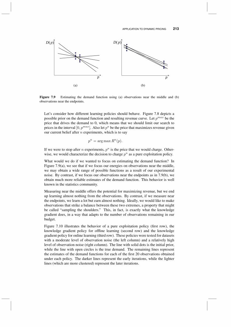
APPLICATION TO DYNAMIC PRICING 213
p
( )D p
p
( )D p
(a) (b)
Figure 7.9 Estimating the demand function using (a) observations near the middle and (b)observations near the endpoints.
Let’s consider how different learning policies should behave. Figure 7.8 depicts apossible prior on the demand function and resulting revenue curve. Let pmax be theprice that drives the demand to 0, which means that we should limit our search toprices in the interval [0, pmax]. Also let pn be the price that maximizes revenue givenour current belief after n experiments, which is to say
pn = arg maxRn(p).
If we were to stop after n experiments, pn is the price that we would charge. Other-wise, we would characterize the decision to charge pn as a pure exploitation policy.
What would we do if we wanted to focus on estimating the demand function? InFigure 7.9(a), we see that if we focus our energies on observations near the middle,we may obtain a wide range of possible functions as a result of our experimentalnoise. By contrast, if we focus our observations near the endpoints as in 7.9(b), weobtain much more reliable estimates of the demand function. This behavior is wellknown in the statistics community.
Measuring near the middle offers the potential for maximizing revenue, but we endup learning almost nothing from the observations. By contrast, if we measure nearthe endpoints, we learn a lot but earn almost nothing. Ideally, we would like to makeobservations that strike a balance between these two extremes, a property that mightbe called “sampling the shoulders.” This, in fact, is exactly what the knowledgegradient does, in a way that adapts to the number of observations remaining in ourbudget.
Figure 7.10 illustrates the behavior of a pure exploitation policy (first row), theknowledge gradient policy for offline learning (second row) and the knowledgegradient policy for online learning (third row). These policies were tested for datasetswith a moderate level of observation noise (the left column) and a relatively highlevel of observation noise (right column). The line with solid dots is the initial prior,while the line with open circles is the true demand. The remaining lines representthe estimates of the demand functions for each of the first 20 observations obtainedunder each policy. The darker lines represent the early iterations, while the lighterlines (which are more clustered) represent the later iterations.
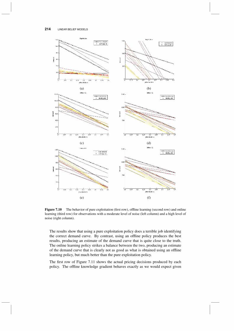
214 LINEAR BELIEF MODELS
(a) (b)
(c) (d)
(e) (f)
Figure 7.10 The behavior of pure exploitation (first row), offline learning (second row) and onlinelearning (third row) for observations with a moderate level of noise (left column) and a high level ofnoise (right column).
The results show that using a pure exploitation policy does a terrible job identifyingthe correct demand curve. By contrast, using an offline policy produces the bestresults, producing an estimate of the demand curve that is quite close to the truth.The online learning policy strikes a balance between the two, producing an estimateof the demand curve that is clearly not as good as what is obtained using an offlinelearning policy, but much better than the pure exploitation policy.
The first row of Figure 7.11 shows the actual pricing decisions produced by eachpolicy. The offline knowledge gradient behaves exactly as we would expect given
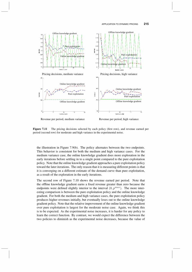
APPLICATION TO DYNAMIC PRICING 215
Offline knowledge gradient
Online knowledge gradient
Pure exploitation
Offline knowledge gradient
Online knowledge gradient
Pure exploitation
Pricing decisions, medium variance Pricing decisions, high variance
Offline knowledge gradient
Online knowledge gradient
Pure exploitation
Offline knowledge gradient
Online knowledge gradient
Pure exploitation
Revenue per period, medium variance Revenue per period, high variance
Figure 7.11 The pricing decisions selected by each policy (first row), and revenue earned perperiod (second row) for moderate and high variance in the experimental noise.
the illustration in Figure 7.9(b). The policy alternates between the two endpoints.This behavior is consistent for both the medium and high variance cases. For themedium variance case, the online knowledge gradient does more exploration in theearly iterations before settling in to a single point compared to the pure exploitationpolicy. Note that the online knowledge gradient approaches a pure exploitation policytoward the later iterations. The only reason that it is measuring different points is thatit is converging on a different estimate of the demand curve than pure exploitation,as a result of the exploration in the early iterations.
The second row of Figure 7.10 shows the revenue earned per period. Note thatthe offline knowledge gradient earns a fixed revenue greater than zero because theendpoints were defined slightly interior to the interval (0, pmax). The more inter-esting comparison is between the pure exploitation policy and the online knowledgegradient. For both the medium and high variance cases, the pure exploitation policyproduces higher revenues initially, but eventually loses out to the online knowledgegradient policy. Note that the relative improvement of the online knowledge gradientover pure exploitation is largest for the moderate noise case. Again, we think thisis to be expected. As the experimental noise increases, it is harder for any policy tolearn the correct function. By contrast, we would expect the difference between thetwo policies to diminish as the experimental noise decreases, because the value of
216 LINEAR BELIEF MODELS
information from learning will be minimal, which again pushes the online knowledgegradient policy toward the pure exploitation policy.
7.6 BIBLIOGRAPHIC NOTES
Section 7.2 - This is classic material that can be found in many statistical textbooks suchas Hastie et al. (2005), which can be downloaded from
https://web.stanford.edu/~hastie/Papers/ESLII.pdf
Section 7.3 - 7.4 - This material is based on Negoescu et al. (2011). The drug discoveryexample is taken from Katz & Ionescu (1977).
Section 7.5 - The experimental results presented here come from work by two under-graduate students at Princeton University. The numerical work was performed byXiaoyang Long as part of her research for the Program in Applied and ComputationalMathematics. The application of pricing cell phone charges was studied by MeganWong as part of her senior thesis.
PROBLEMS
The exercises below require the knowledge gradient algorithm where the belief modelis linear in the parameters. This can be downloaded from
http://optimallearning.princeton.edu/exercises/KGCBLinReg.m
An example implementation of the algorithm is given in
http://optimallearning.princeton.edu/exercises/KGCBLinRegEx.m
7.1 You are going to replicate the experiments in Section 7.5 where we try to learn thedemand as a function of price, while simultaneously trying to maximize revenue. Westart by assuming that the demand as a function of price is given by
D(p) = θ0 + θ1p.
Our revenue is given by R(p) = pD(p), and prices are assumed to range between .1and .5. Assume the true value of θ = (θ0, θ1) = (1233,−2055). Normally we wouldsample this truth from a normal distribution, but we are going to assume a single truthto illustrate how well we discover this truth.
Now assume we start with a high prior θ0 = (1350,−1500), with a starting covariancematrix of
Σθ,0 =
(62500 0
0 2,500,000
)a) Set up and run the knowledge gradient with a linear belief model for N = 20
iterations assuming a low experimental noise of σ2ε = 62, 500, limiting your search
of prices to the range [.1, .5]. Do this for both online and offline learning (recall thatSection 5.4 describes how to compute the online knowledge gradient from the offline

PROBLEMS 217
version). Plot the prices chosen and the updated estimate of the demand curve aftereach iteration.
b) Now sample prices using a pure exploitation policy which maximizes the revenueat each iteration, and compare your results to those obtained using the online andoffline knowledge gradient.
c) Repeat (a) and (b) using σ2ε = 625, 000.
d) Repeat (a) and (b) using σ2ε = 6, 250, 000.
e) Compare the performance of the three algorithmic strategies under the different noiselevels.
7.2 Repeat exercise 7.1, but this time start with a low prior of θ0 = (1350,−4500).
7.3 Repeat exercise 7.1, but now assume that the truth is normally distributed aroundthe prior with mean θ0 = (θ0
0, θ01) = (1233,−2055) and variance
Σθ,0 =
(62500 0
0 2,500,000
)

CHAPTER 8
NONLINEAR BELIEF MODELS
While linear models will always remain an important tool for approximating functions(remember we mean that they are linear in the parameters), there are some problemswhere we cannot avoid models that are nonlinear in the parameters. Some examplesinclude:
EXAMPLE 8.1
We wish to estimate the probability that a customer will purchase an online productwith characterized by price p (which is a decision variable) and other features of theproduct which we denote by a1, . . . , aK . We can then describe our product using
x = (p, a1, . . . , aK).
We think of x as a decision, although the only controllable parameter is p. We mayfeel that we can model the probability of a sale using a logistic model of the form
p(x) =eU(x|θ)
1 + eU(x|θ) ,
where U(x|θ) is a linear function of independent variables with the general form
U(x|θ) = θ0x0 + θ1x1 + θ2x2 + . . . .
Optimal Learning. By Warren B. Powell and Ilya O. RyzhovCopyright c© 2018 John Wiley & Sons, Inc.
219
220 NONLINEAR BELIEF MODELS
We start with an example of a relatively simple nonlinear problem that arises in thecontext of designing bidding policies. We then transition to more general strategiesthat can be applied to a wide range of problems.
8.1 AN OPTIMAL BIDDING PROBLEM
Imagine that industrial customers come to you requesting price quotes on contractsto provide a product of some type. This might be laptops for a large company, acomponent for a product that the customer is building (such as disk drives for thelaptops), or materials used in a manufacturing process. You have to quote a price,recognizing that you have to match or beat competing prices. If you win the contract,you might be left wondering if you could have asked for a little more. If you lose thecontact, you are kicking yourself if you feel that a slightly lower price would havehelped you win the contract.
Figure 8.1 illustrates the economics of different prices. There is a breakeven pricepb, below which you will lose money on the contract. Then there is a price pointpc for each customer c. If you quote a price above this number, you will lose thecontract. The problem, of course, is that you do not know pc. As the figure illustrates,increasing the price above pb produces dramatic increases in profits, especially forcompetitive, commodity products.
We are going to assume that we have several opportunities to quote a price andobserve a buy/not-buy decision from the customer. We are not allowed to observe pcdirectly, even after the fact. After each iteration of quoting a price and observing adecision of whether or not to accept the bid, we have an opportunity to use what wehave learned before deciding on our next bid. We know that we have to bid pricesabove pb, and we know what prices have been accepted in the past. If we discover thatwe can get higher prices, the impact on our profits can be significant. Our challengeis trying to learn pc while balancing the profits we realize against the informationgained while trying higher prices (and potentially losing some contracts).
We can also consider a version of this problem from the customer’s point of view.Suppose that there are now multiple sellers offering a single product. A customermakes a bid for the product at a price of his or her choosing. The bid is successfulif there is a seller willing to accept it, but the customer does not get to observe thesellers’ willingness to sell before making the bid. In this case, higher bids are morelikely to be successful, but the customer can save money by finding the optimalprice. Bidding too low and failing to secure an offer carries an opportunity cost(perhaps we are forced to wait a period of time before bidding again). We might callthis the “Priceline problem,” because of its similarities to the business model of thewell-known online travel agency.
Overall, we can see a clear potential for optimal learning in the bidding problem. Infact, variations of this problem have attracted a great deal of attention in the revenuemanagement community, precisely from an optimal learning perspective. However,it is less clear precisely how learning should be applied. The problem has a number
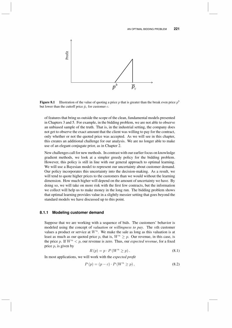
AN OPTIMAL BIDDING PROBLEM 221
Prof
it
bp cp
Figure 8.1 Illustration of the value of quoting a price p that is greater than the break even price pb
but lower than the cuttoff price pc for customer c.
of features that bring us outside the scope of the clean, fundamental models presentedin Chapters 3 and 5. For example, in the bidding problem, we are not able to observean unbiased sample of the truth. That is, in the industrial setting, the company doesnot get to observe the exact amount that the client was willing to pay for the contract,only whether or not the quoted price was accepted. As we will see in this chapter,this creates an additional challenge for our analysis. We are no longer able to makeuse of an elegant conjugate prior, as in Chapter 2.
New challenges call for new methods. In contrast with our earlier focus on knowledgegradient methods, we look at a simpler greedy policy for the bidding problem.However, this policy is still in line with our general approach to optimal learning.We will use a Bayesian model to represent our uncertainty about customer demand.Our policy incorporates this uncertainty into the decision-making. As a result, wewill tend to quote higher prices to the customers than we would without the learningdimension. How much higher will depend on the amount of uncertainty we have. Bydoing so, we will take on more risk with the first few contracts, but the informationwe collect will help us to make money in the long run. The bidding problem showsthat optimal learning provides value in a slightly messier setting that goes beyond thestandard models we have discussed up to this point.
8.1.1 Modeling customer demand
Suppose that we are working with a sequence of bids. The customers’ behavior ismodeled using the concept of valuation or willingness to pay. The nth customervalues a product or service at Wn. We make the sale as long as this valuation is atleast as much as our quoted price p, that is, Wn ≥ p. Our revenue, in this case, isthe price p. If Wn < p, our revenue is zero. Thus, our expected revenue, for a fixedprice p, is given by
R (p) = p · P (Wn ≥ p) . (8.1)
In most applications, we will work with the expected profit
P (p) = (p− c) · P (Wn ≥ p) , (8.2)
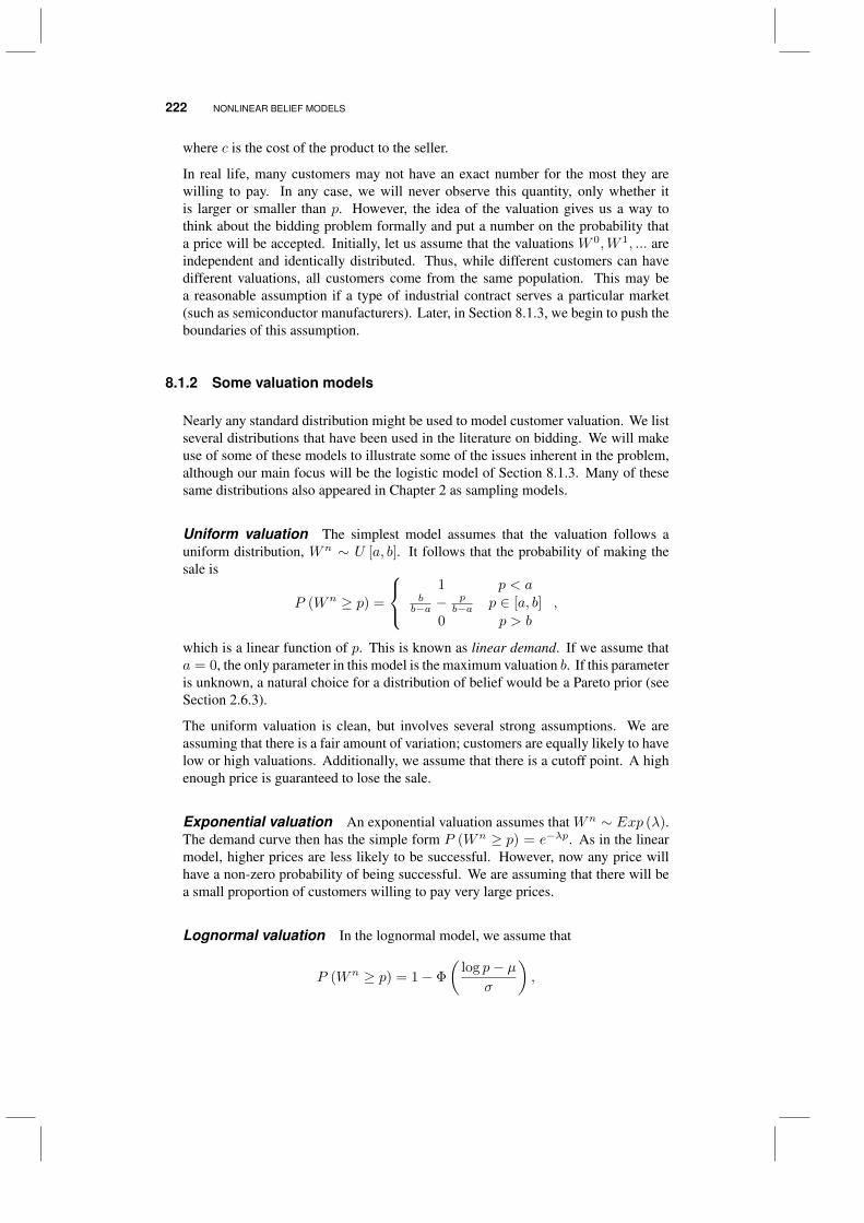
222 NONLINEAR BELIEF MODELS
where c is the cost of the product to the seller.
In real life, many customers may not have an exact number for the most they arewilling to pay. In any case, we will never observe this quantity, only whether itis larger or smaller than p. However, the idea of the valuation gives us a way tothink about the bidding problem formally and put a number on the probability thata price will be accepted. Initially, let us assume that the valuations W 0,W 1, ... areindependent and identically distributed. Thus, while different customers can havedifferent valuations, all customers come from the same population. This may bea reasonable assumption if a type of industrial contract serves a particular market(such as semiconductor manufacturers). Later, in Section 8.1.3, we begin to push theboundaries of this assumption.
8.1.2 Some valuation models
Nearly any standard distribution might be used to model customer valuation. We listseveral distributions that have been used in the literature on bidding. We will makeuse of some of these models to illustrate some of the issues inherent in the problem,although our main focus will be the logistic model of Section 8.1.3. Many of thesesame distributions also appeared in Chapter 2 as sampling models.
Uniform valuation The simplest model assumes that the valuation follows auniform distribution, Wn ∼ U [a, b]. It follows that the probability of making thesale is
P (Wn ≥ p) =
1 p < a
bb−a −
pb−a p ∈ [a, b]
0 p > b,
which is a linear function of p. This is known as linear demand. If we assume thata = 0, the only parameter in this model is the maximum valuation b. If this parameteris unknown, a natural choice for a distribution of belief would be a Pareto prior (seeSection 2.6.3).
The uniform valuation is clean, but involves several strong assumptions. We areassuming that there is a fair amount of variation; customers are equally likely to havelow or high valuations. Additionally, we assume that there is a cutoff point. A highenough price is guaranteed to lose the sale.
Exponential valuation An exponential valuation assumes that Wn ∼ Exp (λ).The demand curve then has the simple form P (Wn ≥ p) = e−λp. As in the linearmodel, higher prices are less likely to be successful. However, now any price willhave a non-zero probability of being successful. We are assuming that there will bea small proportion of customers willing to pay very large prices.
Lognormal valuation In the lognormal model, we assume that
P (Wn ≥ p) = 1− Φ
(log p− µ
σ
),
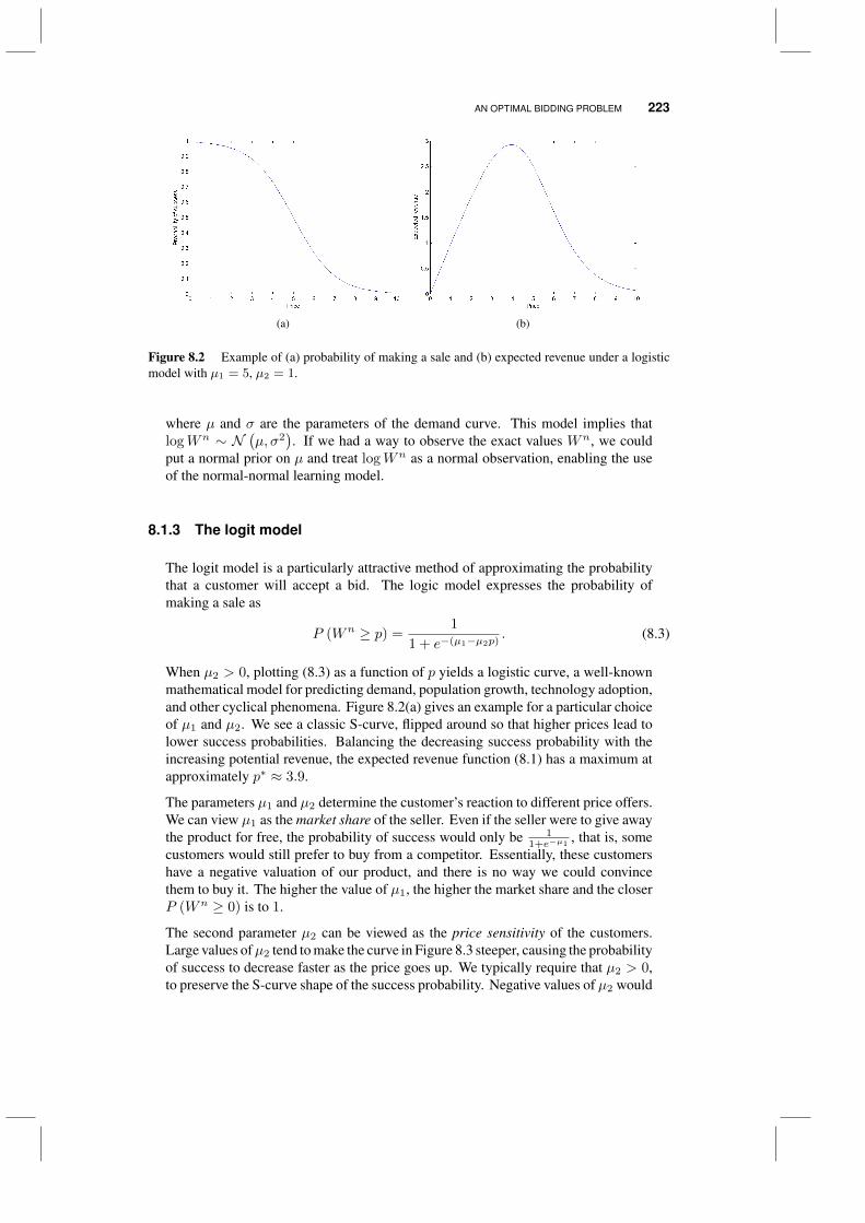
AN OPTIMAL BIDDING PROBLEM 223
(a) (b)
Figure 8.2 Example of (a) probability of making a sale and (b) expected revenue under a logisticmodel with µ1 = 5, µ2 = 1.
where µ and σ are the parameters of the demand curve. This model implies thatlogWn ∼ N
(µ, σ2
). If we had a way to observe the exact values Wn, we could
put a normal prior on µ and treat logWn as a normal observation, enabling the useof the normal-normal learning model.
8.1.3 The logit model
The logit model is a particularly attractive method of approximating the probabilitythat a customer will accept a bid. The logic model expresses the probability ofmaking a sale as
P (Wn ≥ p) =1
1 + e−(µ1−µ2p). (8.3)
When µ2 > 0, plotting (8.3) as a function of p yields a logistic curve, a well-knownmathematical model for predicting demand, population growth, technology adoption,and other cyclical phenomena. Figure 8.2(a) gives an example for a particular choiceof µ1 and µ2. We see a classic S-curve, flipped around so that higher prices lead tolower success probabilities. Balancing the decreasing success probability with theincreasing potential revenue, the expected revenue function (8.1) has a maximum atapproximately p∗ ≈ 3.9.
The parameters µ1 and µ2 determine the customer’s reaction to different price offers.We can view µ1 as the market share of the seller. Even if the seller were to give awaythe product for free, the probability of success would only be 1
1+e−µ1, that is, some
customers would still prefer to buy from a competitor. Essentially, these customershave a negative valuation of our product, and there is no way we could convincethem to buy it. The higher the value of µ1, the higher the market share and the closerP (Wn ≥ 0) is to 1.
The second parameter µ2 can be viewed as the price sensitivity of the customers.Large values ofµ2 tend to make the curve in Figure 8.3 steeper, causing the probabilityof success to decrease faster as the price goes up. We typically require that µ2 > 0,to preserve the S-curve shape of the success probability. Negative values of µ2 would
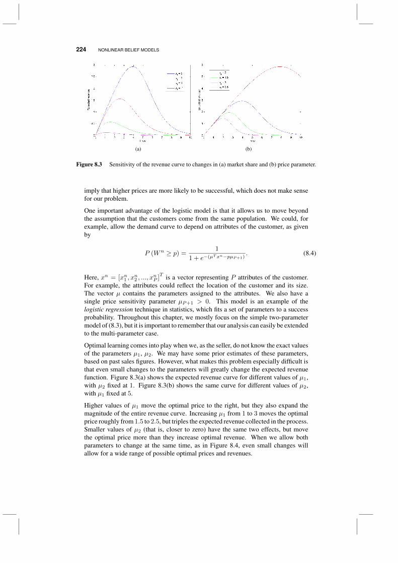
224 NONLINEAR BELIEF MODELS
(a) (b)
Figure 8.3 Sensitivity of the revenue curve to changes in (a) market share and (b) price parameter.
imply that higher prices are more likely to be successful, which does not make sensefor our problem.
One important advantage of the logistic model is that it allows us to move beyondthe assumption that the customers come from the same population. We could, forexample, allow the demand curve to depend on attributes of the customer, as givenby
P (Wn ≥ p) =1
1 + e−(µT xn−pµP+1). (8.4)
Here, xn = [xn1 , xn2 , ..., x
nP ]T is a vector representing P attributes of the customer.
For example, the attributes could reflect the location of the customer and its size.The vector µ contains the parameters assigned to the attributes. We also have asingle price sensitivity parameter µP+1 > 0. This model is an example of thelogistic regression technique in statistics, which fits a set of parameters to a successprobability. Throughout this chapter, we mostly focus on the simple two-parametermodel of (8.3), but it is important to remember that our analysis can easily be extendedto the multi-parameter case.
Optimal learning comes into play when we, as the seller, do not know the exact valuesof the parameters µ1, µ2. We may have some prior estimates of these parameters,based on past sales figures. However, what makes this problem especially difficult isthat even small changes to the parameters will greatly change the expected revenuefunction. Figure 8.3(a) shows the expected revenue curve for different values of µ1,with µ2 fixed at 1. Figure 8.3(b) shows the same curve for different values of µ2,with µ1 fixed at 5.
Higher values of µ1 move the optimal price to the right, but they also expand themagnitude of the entire revenue curve. Increasing µ1 from 1 to 3 moves the optimalprice roughly from 1.5 to 2.5, but triples the expected revenue collected in the process.Smaller values of µ2 (that is, closer to zero) have the same two effects, but movethe optimal price more than they increase optimal revenue. When we allow bothparameters to change at the same time, as in Figure 8.4, even small changes willallow for a wide range of possible optimal prices and revenues.
AN OPTIMAL BIDDING PROBLEM 225
8.1.4 Bayesian modeling for dynamic pricing
We will use a Bayesian model to represent our uncertainty about the parameters. Inthis setting, it becomes especially important to construct our prior in such a way asto realistically cover our range of uncertainty about the optimal price. Furthermore,the nature of the observations in this problem creates additional challenges. We arenot able to observe the customer valuationsWn. Rather, we only observe whether ornot Wn ≥ p. The clean, conjugate Bayesian models introduced in Chapter 2 cannotbe directly applied, and we need to do additional work to be able to use them.
8.1.4.1 A conjugate prior for choosing between two demand curvesBefore we delve into the intricacies of non-conjugate Bayesian learning, let us firstbegin with a simple, stylized model that allows for a conjugate prior. In dynamicpricing, our observations are binary: either the customer accepts the offer (that is,Wn ≥ p), or not. One way to obtain a conjugate prior is if the truth is binary, as well.Suppose that there are only two possible demand curves. Each curve has known,fixed parameters, but we do not know which curve is the right one for describingcustomer valuations. Figure 8.5 gives an example where we are trying to choosebetween a uniform valuation on the interval [3, 7], and an exponential valuation withparameter 0.2.
This model is somewhat stylized, but may be useful in some cases. It may be thatwe, as the seller, have a large amount of historical data on sales figures, enoughto fit any particular type of demand curve. We could conduct a statistical analysisto fit a uniform valuation model, or an exponential model, or perhaps a logisticmodel. For each model, we would fit a different set of parameters. However, weare not sure which type of demand curve is most appropriate. A logistic model maybe fundamentally better-suited to the data than a uniform model. In that case, thebinary-truth problem may help us to distinguish between two competing types ofdemand models.
Figure 8.4 Sensitivity of the revenue curve to changes in both parameters.
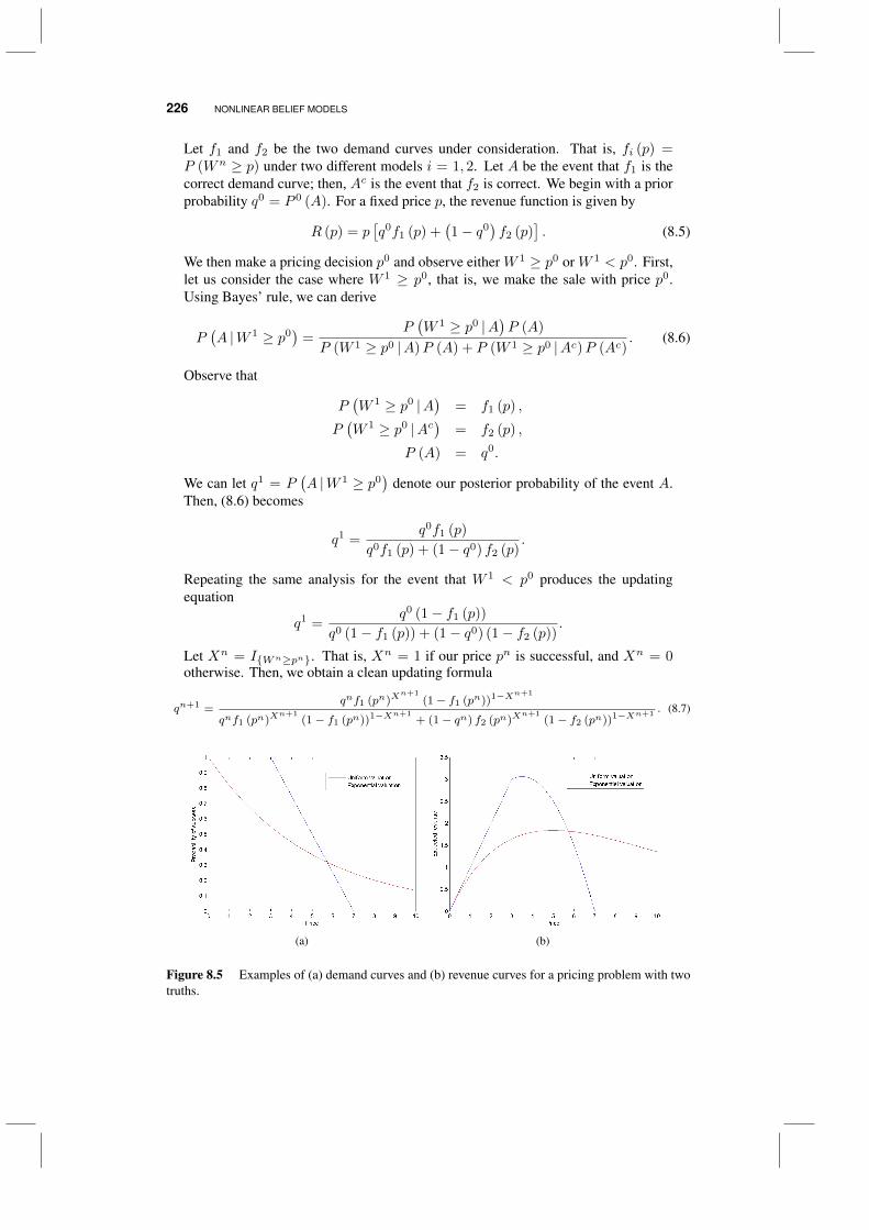
226 NONLINEAR BELIEF MODELS
Let f1 and f2 be the two demand curves under consideration. That is, fi (p) =P (Wn ≥ p) under two different models i = 1, 2. Let A be the event that f1 is thecorrect demand curve; then, Ac is the event that f2 is correct. We begin with a priorprobability q0 = P 0 (A). For a fixed price p, the revenue function is given by
R (p) = p[q0f1 (p) +
(1− q0
)f2 (p)
]. (8.5)
We then make a pricing decision p0 and observe either W 1 ≥ p0 or W 1 < p0. First,let us consider the case where W 1 ≥ p0, that is, we make the sale with price p0.Using Bayes’ rule, we can derive
P(A |W 1 ≥ p0
)=
P(W 1 ≥ p0 |A
)P (A)
P (W 1 ≥ p0 |A)P (A) + P (W 1 ≥ p0 |Ac)P (Ac). (8.6)
Observe that
P(W 1 ≥ p0 |A
)= f1 (p) ,
P(W 1 ≥ p0 |Ac
)= f2 (p) ,
P (A) = q0.
We can let q1 = P(A |W 1 ≥ p0
)denote our posterior probability of the event A.
Then, (8.6) becomes
q1 =q0f1 (p)
q0f1 (p) + (1− q0) f2 (p).
Repeating the same analysis for the event that W 1 < p0 produces the updatingequation
q1 =q0 (1− f1 (p))
q0 (1− f1 (p)) + (1− q0) (1− f2 (p)).
Let Xn = IWn≥pn. That is, Xn = 1 if our price pn is successful, and Xn = 0otherwise. Then, we obtain a clean updating formula
qn+1 =qnf1 (pn)X
n+1(1− f1 (pn))1−Xn+1
qnf1 (pn)Xn+1
(1− f1 (pn))1−Xn+1+ (1− qn) f2 (pn)X
n+1(1− f2 (pn))1−Xn+1
. (8.7)
(a) (b)
Figure 8.5 Examples of (a) demand curves and (b) revenue curves for a pricing problem with twotruths.
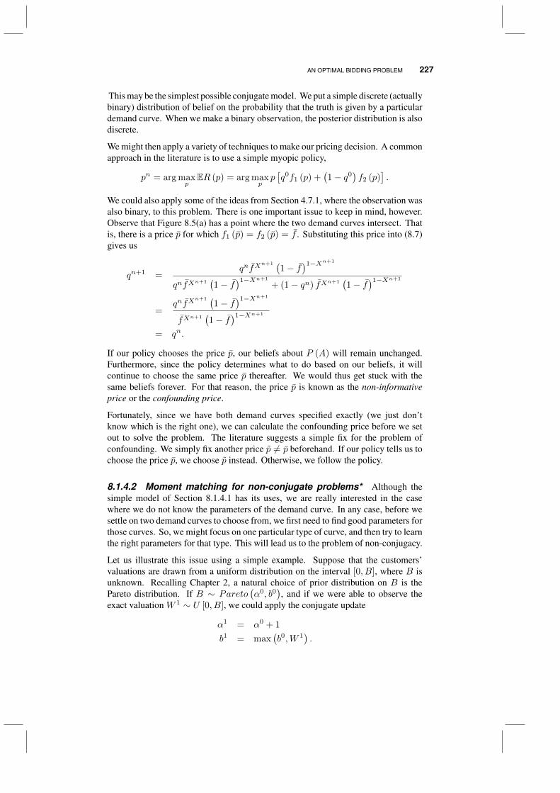
AN OPTIMAL BIDDING PROBLEM 227
This may be the simplest possible conjugate model. We put a simple discrete (actuallybinary) distribution of belief on the probability that the truth is given by a particulardemand curve. When we make a binary observation, the posterior distribution is alsodiscrete.
We might then apply a variety of techniques to make our pricing decision. A commonapproach in the literature is to use a simple myopic policy,
pn = arg maxp
ER (p) = arg maxp
p[q0f1 (p) +
(1− q0
)f2 (p)
].
We could also apply some of the ideas from Section 4.7.1, where the observation wasalso binary, to this problem. There is one important issue to keep in mind, however.Observe that Figure 8.5(a) has a point where the two demand curves intersect. Thatis, there is a price p for which f1 (p) = f2 (p) = f . Substituting this price into (8.7)gives us
qn+1 =qnfX
n+1 (1− f
)1−Xn+1
qnfXn+1(1− f
)1−Xn+1
+ (1− qn) fXn+1(1− f
)1−Xn+1
=qnfX
n+1 (1− f
)1−Xn+1
fXn+1(1− f
)1−Xn+1
= qn.
If our policy chooses the price p, our beliefs about P (A) will remain unchanged.Furthermore, since the policy determines what to do based on our beliefs, it willcontinue to choose the same price p thereafter. We would thus get stuck with thesame beliefs forever. For that reason, the price p is known as the non-informativeprice or the confounding price.
Fortunately, since we have both demand curves specified exactly (we just don’tknow which is the right one), we can calculate the confounding price before we setout to solve the problem. The literature suggests a simple fix for the problem ofconfounding. We simply fix another price p 6= p beforehand. If our policy tells us tochoose the price p, we choose p instead. Otherwise, we follow the policy.
8.1.4.2 Moment matching for non-conjugate problems* Although thesimple model of Section 8.1.4.1 has its uses, we are really interested in the casewhere we do not know the parameters of the demand curve. In any case, before wesettle on two demand curves to choose from, we first need to find good parameters forthose curves. So, we might focus on one particular type of curve, and then try to learnthe right parameters for that type. This will lead us to the problem of non-conjugacy.
Let us illustrate this issue using a simple example. Suppose that the customers’valuations are drawn from a uniform distribution on the interval [0, B], where B isunknown. Recalling Chapter 2, a natural choice of prior distribution on B is thePareto distribution. If B ∼ Pareto
(α0, b0
), and if we were able to observe the
exact valuation W 1 ∼ U [0, B], we could apply the conjugate update
α1 = α0 + 1
b1 = max(b0,W 1
).
228 NONLINEAR BELIEF MODELS
Unfortunately, we are never able to see the exact valuation. However, we can stillderive a posterior distribution of belief, given the incomplete information that we doobserve. For simplicity, let us assume that we set a price p0 < b0. We will firstconsider the case where W 1 < p0, that is, we lost the sale. We apply Bayes’ ruleand write
g(u |W 1 < p0
)=P(W 1 < p0 |B = u
)g (u)
P (W 1 < p0). (8.8)
Conditionally given B = u, the valuation W 1 has a uniform distribution on [0, u].Thus,
P(W 1 < p0 |B = u
)=
p0
u p0 < u1 p0 ≥ u.
Next, the likelihood that B = u is given by the Pareto density,
g (u) =α0(b0)α0
uα0+1for u > b0.
Thus, in our calculations, we are implicitly assuming that u > b0, since B > b0 bythe definition of a Pareto distribution. Since we are also assuming p0 < b0, it followsthat p0 < u for all possible u. The numerator of the right-hand side of (8.8) thusbecomes
P(W 1 < p0 |B = u
)g (u) =
α0p0(b0)α0
uα0+2. (8.9)
Integrating this expression from b0 to infinity, we obtain the denominator of theright-hand side of (8.8),
P(W 1 < p0
)=
∫ ∞b0
α0p0(b0)α0
uα0+2du =
α0
α0 + 1
p0
b0. (8.10)
Dividing (8.9) by (8.10) yields
g(u |W 1 < p0
)=
(α0 + 1
) (b0)α0+1
uα0+2.
This is a Pareto density with parameters α1 = α0 + 1 and b1 = b0. That is, if welose the sale, conjugacy is maintained. The conjugate updating equations hint at this.From (8.8), we see that b1 = max
(b0,W 1
), if we could observe the exact valuation
W 1. However, we are assuming that p0 < b0. Thus, if we observe W 1 < p0, itfollows automatically that max
(b0,W 1
)= b0. We do not really need to know the
exact value of W 1 in this case. For any value of W 1 less than b0, we will not changethe scale parameter of our distribution of belief.
In the other case, however, we run into trouble. Suppose thatW 1 ≥ p0, with p0 < b0
as before. Then,
P(W 1 ≥ p0 |B = u
)=
1− p0
u p0 < u0 p0 ≥ u
and
P(W 1 ≥ p0 |B = u
)g (u) =
α0(b0)α0
uα0+1−α0p0
(b0)α0
uα0+2u > b0.
AN OPTIMAL BIDDING PROBLEM 229
Integrating this quantity from b0 to infinity yields
P(W 1 ≥ p0
)= 1− α0
α0 + 1
p0
b0,
and the posterior density turns out to be
g(u |W 1 < p0
)=
α0(b0)α0
uα0+1− α0p0(b0)
α0
uα0+2
1− α0
α0+1p0
b0
u > b0. (8.11)
What are we to do with this strange expression? It does not correspond to anystandard density. (The difference of two Pareto densities is not the density of thedifference of two Pareto random variables!) It is certainly not a Pareto density.
We get around this problem by using a technique called moment-matching. Definea random variable U that has the density given by (8.11). As long as we have thedensity, we can compute the first two moments of U as follows. First,
EU =
∫ ∞b0
u
α0(b0)α0
uα0+1− α0p0(b0)
α0
uα0+2
1− α0
α0+1p0
b0
=α0b0
α0−1 − p0
1− α0
α0+1p0
b0
. (8.12)
Similarly,
E(U2)
=
∫ ∞b0
u2
α0(b0)α0
uα0+1− α0p0(b0)
α0
uα0+2
1− α0
α0+1p0
b0
=
α0(b0)2
α0−2 −α0b0p0
α0−1
1− α0
α0+1p0
b0
. (8.13)
Let Y be a random variable following a Pareto distribution with parameters α1 andb1. The first and second moments of Y are given by
EY =α1b1
α1 − 1, E
(Y 2)
=α1(b1)2
α1 − 2.
Moment matching works by setting the moments of Y equal to the moments ofU , andsolving for α1 and b1 in terms of α0 and b0. Essentially, we are forcing the posteriordistribution to be Pareto, and choosing α1 and b1 to make this Pareto distributionresemble the actual posterior distribution, at least up to the first two moments. To dothis, we have to solve two sets of nonlinear equations
α1b1
α1 − 1=
α0b0
α0−1 − p0
1− α0
α0+1p0
b0
,
α1(b1)2
α1 − 2=
α0(b0)2
α0−2 −α0b0p0
α0−1
1− α0
α0+1p0
b0
.
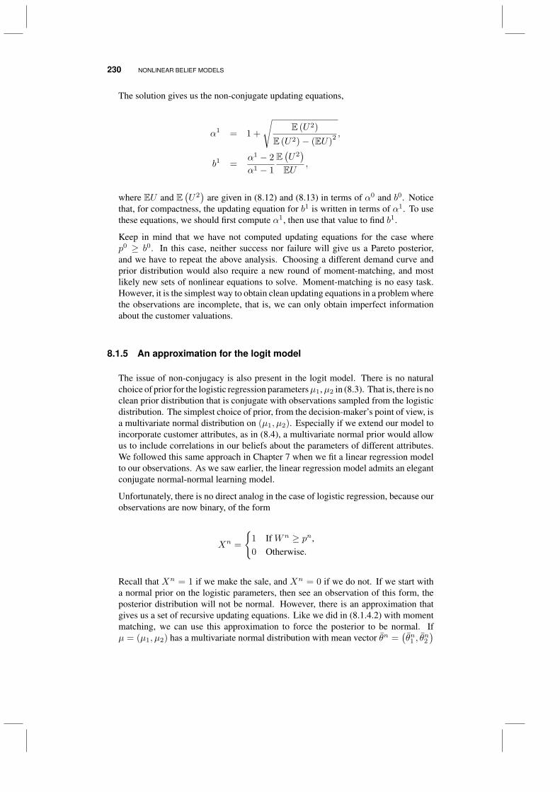
230 NONLINEAR BELIEF MODELS
The solution gives us the non-conjugate updating equations,
α1 = 1 +
√E (U2)
E (U2)− (EU)2 ,
b1 =α1 − 2
α1 − 1
E(U2)
EU,
where EU and E(U2)
are given in (8.12) and (8.13) in terms of α0 and b0. Noticethat, for compactness, the updating equation for b1 is written in terms of α1. To usethese equations, we should first compute α1, then use that value to find b1.
Keep in mind that we have not computed updating equations for the case wherep0 ≥ b0. In this case, neither success nor failure will give us a Pareto posterior,and we have to repeat the above analysis. Choosing a different demand curve andprior distribution would also require a new round of moment-matching, and mostlikely new sets of nonlinear equations to solve. Moment-matching is no easy task.However, it is the simplest way to obtain clean updating equations in a problem wherethe observations are incomplete, that is, we can only obtain imperfect informationabout the customer valuations.
8.1.5 An approximation for the logit model
The issue of non-conjugacy is also present in the logit model. There is no naturalchoice of prior for the logistic regression parametersµ1,µ2 in (8.3). That is, there is noclean prior distribution that is conjugate with observations sampled from the logisticdistribution. The simplest choice of prior, from the decision-maker’s point of view, isa multivariate normal distribution on (µ1, µ2). Especially if we extend our model toincorporate customer attributes, as in (8.4), a multivariate normal prior would allowus to include correlations in our beliefs about the parameters of different attributes.We followed this same approach in Chapter 7 when we fit a linear regression modelto our observations. As we saw earlier, the linear regression model admits an elegantconjugate normal-normal learning model.
Unfortunately, there is no direct analog in the case of logistic regression, because ourobservations are now binary, of the form
Xn =
1 If Wn ≥ pn,0 Otherwise.
Recall that Xn = 1 if we make the sale, and Xn = 0 if we do not. If we start witha normal prior on the logistic parameters, then see an observation of this form, theposterior distribution will not be normal. However, there is an approximation thatgives us a set of recursive updating equations. Like we did in (8.1.4.2) with momentmatching, we can use this approximation to force the posterior to be normal. Ifµ = (µ1, µ2) has a multivariate normal distribution with mean vector θn =
(θn1 , θ
n2
)
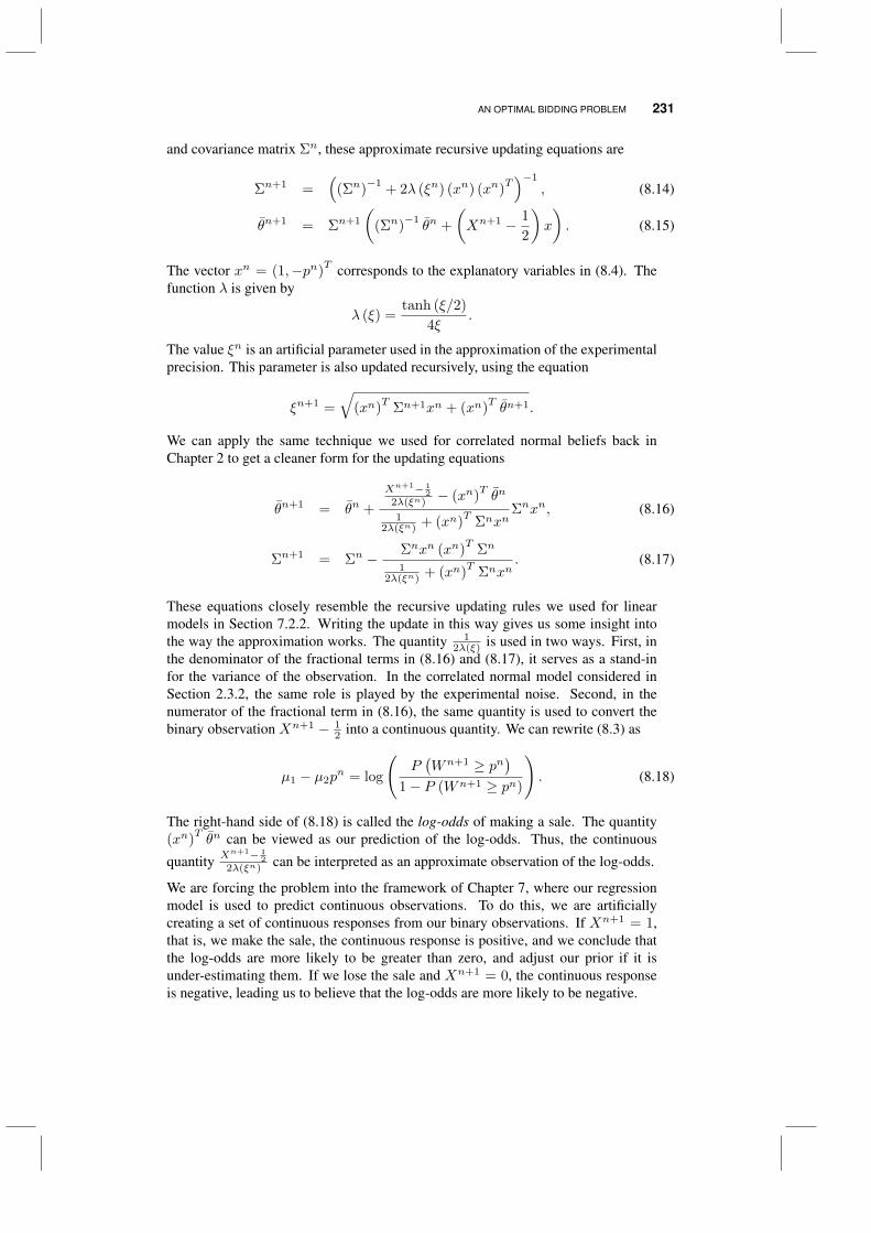
AN OPTIMAL BIDDING PROBLEM 231
and covariance matrix Σn, these approximate recursive updating equations are
Σn+1 =(
(Σn)−1
+ 2λ (ξn) (xn) (xn)T)−1
, (8.14)
θn+1 = Σn+1
((Σn)
−1θn +
(Xn+1 − 1
2
)x
). (8.15)
The vector xn = (1,−pn)T corresponds to the explanatory variables in (8.4). The
function λ is given by
λ (ξ) =tanh (ξ/2)
4ξ.
The value ξn is an artificial parameter used in the approximation of the experimentalprecision. This parameter is also updated recursively, using the equation
ξn+1 =
√(xn)
TΣn+1xn + (xn)
Tθn+1.
We can apply the same technique we used for correlated normal beliefs back inChapter 2 to get a cleaner form for the updating equations
θn+1 = θn +
Xn+1− 12
2λ(ξn) − (xn)Tθn
12λ(ξn) + (xn)
TΣnxn
Σnxn, (8.16)
Σn+1 = Σn − Σnxn (xn)T
Σn
12λ(ξn) + (xn)
TΣnxn
. (8.17)
These equations closely resemble the recursive updating rules we used for linearmodels in Section 7.2.2. Writing the update in this way gives us some insight intothe way the approximation works. The quantity 1
2λ(ξ) is used in two ways. First, inthe denominator of the fractional terms in (8.16) and (8.17), it serves as a stand-infor the variance of the observation. In the correlated normal model considered inSection 2.3.2, the same role is played by the experimental noise. Second, in thenumerator of the fractional term in (8.16), the same quantity is used to convert thebinary observation Xn+1 − 1
2 into a continuous quantity. We can rewrite (8.3) as
µ1 − µ2pn = log
(P(Wn+1 ≥ pn
)1− P (Wn+1 ≥ pn)
). (8.18)
The right-hand side of (8.18) is called the log-odds of making a sale. The quantity(xn)
Tθn can be viewed as our prediction of the log-odds. Thus, the continuous
quantity Xn+1− 12
2λ(ξn) can be interpreted as an approximate observation of the log-odds.
We are forcing the problem into the framework of Chapter 7, where our regressionmodel is used to predict continuous observations. To do this, we are artificiallycreating a set of continuous responses from our binary observations. If Xn+1 = 1,that is, we make the sale, the continuous response is positive, and we conclude thatthe log-odds are more likely to be greater than zero, and adjust our prior if it isunder-estimating them. If we lose the sale and Xn+1 = 0, the continuous responseis negative, leading us to believe that the log-odds are more likely to be negative.
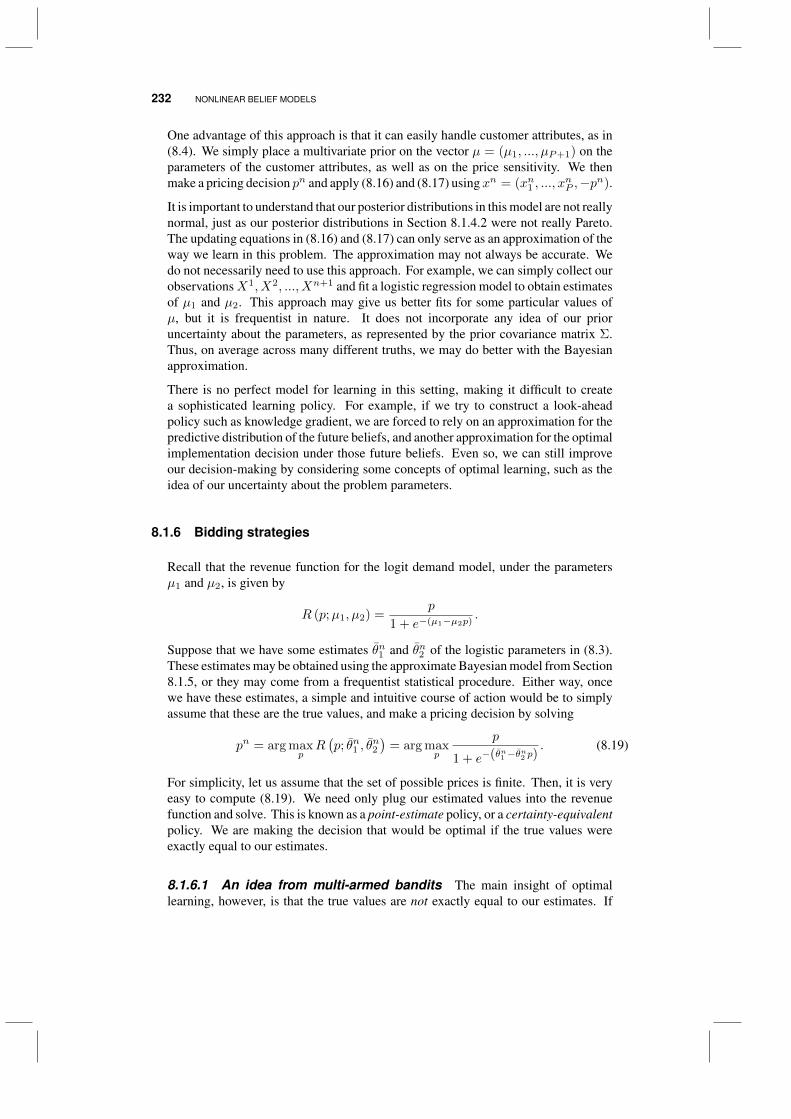
232 NONLINEAR BELIEF MODELS
One advantage of this approach is that it can easily handle customer attributes, as in(8.4). We simply place a multivariate prior on the vector µ = (µ1, ..., µP+1) on theparameters of the customer attributes, as well as on the price sensitivity. We thenmake a pricing decision pn and apply (8.16) and (8.17) usingxn = (xn1 , ..., x
nP ,−pn).
It is important to understand that our posterior distributions in this model are not reallynormal, just as our posterior distributions in Section 8.1.4.2 were not really Pareto.The updating equations in (8.16) and (8.17) can only serve as an approximation of theway we learn in this problem. The approximation may not always be accurate. Wedo not necessarily need to use this approach. For example, we can simply collect ourobservationsX1, X2, ..., Xn+1 and fit a logistic regression model to obtain estimatesof µ1 and µ2. This approach may give us better fits for some particular values ofµ, but it is frequentist in nature. It does not incorporate any idea of our prioruncertainty about the parameters, as represented by the prior covariance matrix Σ.Thus, on average across many different truths, we may do better with the Bayesianapproximation.
There is no perfect model for learning in this setting, making it difficult to createa sophisticated learning policy. For example, if we try to construct a look-aheadpolicy such as knowledge gradient, we are forced to rely on an approximation for thepredictive distribution of the future beliefs, and another approximation for the optimalimplementation decision under those future beliefs. Even so, we can still improveour decision-making by considering some concepts of optimal learning, such as theidea of our uncertainty about the problem parameters.
8.1.6 Bidding strategies
Recall that the revenue function for the logit demand model, under the parametersµ1 and µ2, is given by
R (p;µ1, µ2) =p
1 + e−(µ1−µ2p).
Suppose that we have some estimates θn1 and θn2 of the logistic parameters in (8.3).These estimates may be obtained using the approximate Bayesian model from Section8.1.5, or they may come from a frequentist statistical procedure. Either way, oncewe have these estimates, a simple and intuitive course of action would be to simplyassume that these are the true values, and make a pricing decision by solving
pn = arg maxp
R(p; θn1 , θ
n2
)= arg max
p
p
1 + e−(θn1−θn2 p). (8.19)
For simplicity, let us assume that the set of possible prices is finite. Then, it is veryeasy to compute (8.19). We need only plug our estimated values into the revenuefunction and solve. This is known as a point-estimate policy, or a certainty-equivalentpolicy. We are making the decision that would be optimal if the true values wereexactly equal to our estimates.
8.1.6.1 An idea from multi-armed bandits The main insight of optimallearning, however, is that the true values are not exactly equal to our estimates. If
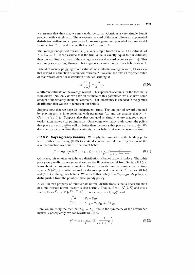
AN OPTIMAL BIDDING PROBLEM 233
we assume that they are, we may under-perform. Consider a very simple banditproblem with a single arm. The one-period reward of the arm follows an exponentialdistribution with unknown parameter λ. We use a gamma-exponential learning modelfrom Section 2.6.1, and assume that λ ∼ Gamma (a, b).
The average one-period reward is 1λ , a very simple function of λ. Our estimate of
λ is Eλ = ab . If we assume that the true value is exactly equal to our estimate,
then our resulting estimate of the average one-period reward becomes 1Eλ = b
a . Thisreasoning seems straightforward, but it ignores the uncertainty in our beliefs about λ.
Instead of merely plugging in our estimate of λ into the average reward, let us viewthat reward as a function of a random variable λ. We can then take an expected valueof that reward over our distribution of belief, arriving at
E(
1
λ
)=
b
a− 1, (8.20)
a different estimate of the average reward. This approach accounts for the fact that λis unknown. Not only do we have an estimate of this parameter, we also have someamount of uncertainty about that estimate. That uncertainty is encoded in the gammadistribution that we use to represent our beliefs.
Suppose now that we have M independent arms. The one-period reward obtainedby playing arm x is exponential with parameter λx, and we assume that λx ∼Gamma (ax, bx). Suppose also that our goal is simply to use a greedy, pure-exploitation strategy for pulling arms. On average over many truth values, the policythat plays arg maxx
bxax−1 will do better than the policy that plays arg maxx
bxax
. Wedo better by incorporating the uncertainty in our beliefs into our decision-making.
8.1.6.2 Bayes-greedy bidding We apply the same idea to the bidding prob-lem. Rather than using (8.19) to make decisions, we take an expectation of therevenue function over our distribution of belief,
pn = arg maxp
ER (p;µ1, µ2) = arg maxp
Ep
1 + e−(µ1−µ2p). (8.21)
Of course, this requires us to have a distribution of belief in the first place. Thus, thispolicy only really makes sense if we use the Bayesian model from Section 8.1.5 tolearn about the unknown parameters. Under this model, we can assume that, at timen, µ ∼ N
(θn,Σn
). After we make a decision pn and observe Xn+1, we use (8.16)
and (8.17) to change our beliefs. We refer to this policy as a Bayes-greedy policy, todistinguish it from the point-estimate greedy policy.
A well-known property of multivariate normal distributions is that a linear functionof a multivariate normal vector is also normal. That is, if µ ∼ N (θ,Σ) and c is avector, then cTx ∼ N
(cT θ, cTΣc
). In our case, c = (1,−p)T and
cT θ = θ1 − θ2p,
cTΣc = Σ11 − 2pΣ12 + p2Σ22.
Here we are using the fact that Σ12 = Σ21 due to the symmetry of the covariancematrix. Consequently, we can rewrite (8.21) as
pn = arg maxp
p · E(
1
1 + e−Y
), (8.22)
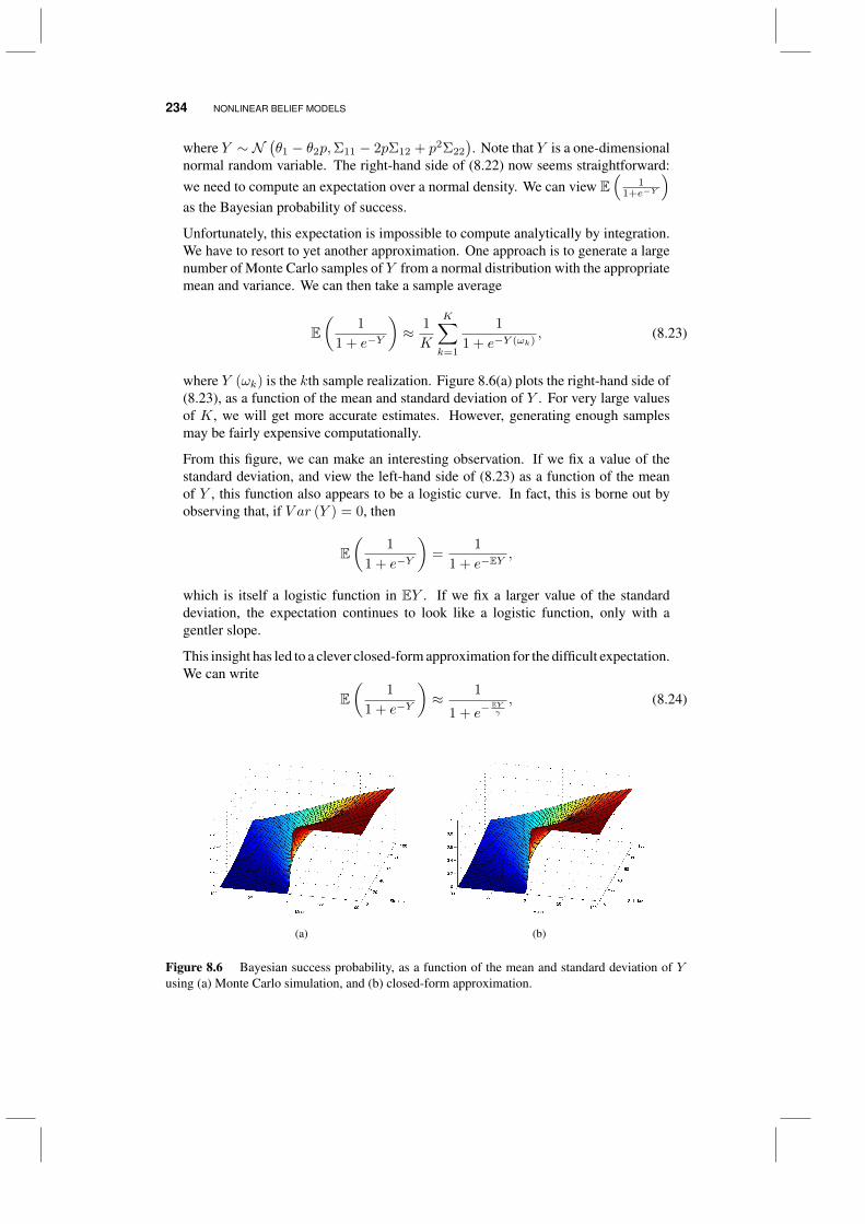
234 NONLINEAR BELIEF MODELS
where Y ∼ N(θ1 − θ2p,Σ11 − 2pΣ12 + p2Σ22
). Note that Y is a one-dimensional
normal random variable. The right-hand side of (8.22) now seems straightforward:we need to compute an expectation over a normal density. We can view E
(1
1+e−Y
)as the Bayesian probability of success.
Unfortunately, this expectation is impossible to compute analytically by integration.We have to resort to yet another approximation. One approach is to generate a largenumber of Monte Carlo samples of Y from a normal distribution with the appropriatemean and variance. We can then take a sample average
E(
1
1 + e−Y
)≈ 1
K
K∑k=1
1
1 + e−Y (ωk), (8.23)
where Y (ωk) is the kth sample realization. Figure 8.6(a) plots the right-hand side of(8.23), as a function of the mean and standard deviation of Y . For very large valuesof K, we will get more accurate estimates. However, generating enough samplesmay be fairly expensive computationally.
From this figure, we can make an interesting observation. If we fix a value of thestandard deviation, and view the left-hand side of (8.23) as a function of the meanof Y , this function also appears to be a logistic curve. In fact, this is borne out byobserving that, if V ar (Y ) = 0, then
E(
1
1 + e−Y
)=
1
1 + e−EY,
which is itself a logistic function in EY . If we fix a larger value of the standarddeviation, the expectation continues to look like a logistic function, only with agentler slope.
This insight has led to a clever closed-form approximation for the difficult expectation.We can write
E(
1
1 + e−Y
)≈ 1
1 + e−EYγ
, (8.24)
(a) (b)
Figure 8.6 Bayesian success probability, as a function of the mean and standard deviation of Yusing (a) Monte Carlo simulation, and (b) closed-form approximation.
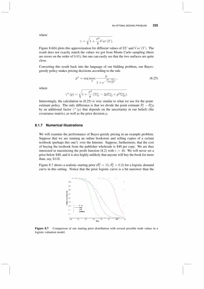
AN OPTIMAL BIDDING PROBLEM 235
where
γ =
√1 +
π2
8V ar (Y ).
Figure 8.6(b) plots this approximation for different values of EY and V ar (Y ). Theresult does not exactly match the values we got from Monte Carlo sampling (thereare errors on the order of 0.01), but one can easily see that the two surfaces are quiteclose.
Converting this result back into the language of our bidding problem, our Bayes-greedy policy makes pricing decisions according to the rule
pn = arg maxp
p
1 + e−θn1 −θ
n2 p
γn(p)
, (8.25)
where
γn (p) =
√1 +
π2
8(Σn11 − 2pΣn12 + p2Σn22).
Interestingly, the calculation in (8.25) is very similar to what we use for the point-estimate policy. The only difference is that we divide the point estimate θn1 − θn2 pby an additional factor γn (p) that depends on the uncertainty in our beliefs (thecovariance matrix), as well as the price decision p.
8.1.7 Numerical illustrations
We will examine the performance of Bayes-greedy pricing in an example problem.Suppose that we are running an online bookstore and selling copies of a certaintextbook (perhaps this one!) over the Internet. Suppose, furthermore, that the costof buying the textbook from the publisher wholesale is $40 per copy. We are thusinterested in maximizing the profit function (8.2) with c = 40. We will never set aprice below $40, and it is also highly unlikely that anyone will buy the book for morethan, say, $110.
Figure 8.7 shows a realistic starting prior (θ01 = 15, θ0
2 = 0.2) for a logistic demandcurve in this setting. Notice that the prior logistic curve is a bit narrower than the
Figure 8.7 Comparison of our starting prior distribution with several possible truth values in alogistic valuation model.
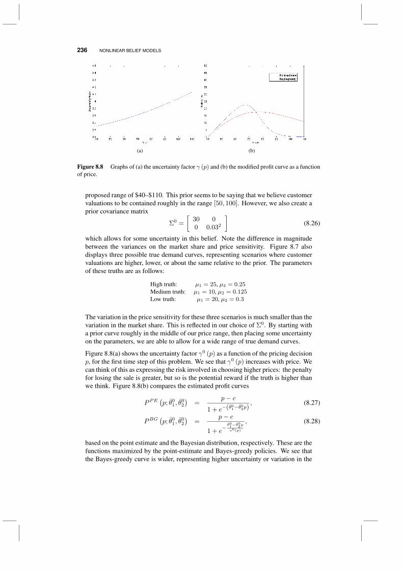
236 NONLINEAR BELIEF MODELS
(a) (b)
Figure 8.8 Graphs of (a) the uncertainty factor γ (p) and (b) the modified profit curve as a functionof price.
proposed range of $40–$110. This prior seems to be saying that we believe customervaluations to be contained roughly in the range [50, 100]. However, we also create aprior covariance matrix
Σ0 =
[30 00 0.032
](8.26)
which allows for some uncertainty in this belief. Note the difference in magnitudebetween the variances on the market share and price sensitivity. Figure 8.7 alsodisplays three possible true demand curves, representing scenarios where customervaluations are higher, lower, or about the same relative to the prior. The parametersof these truths are as follows:
High truth: µ1 = 25, µ2 = 0.25Medium truth: µ1 = 10, µ2 = 0.125Low truth: µ1 = 20, µ2 = 0.3
The variation in the price sensitivity for these three scenarios is much smaller than thevariation in the market share. This is reflected in our choice of Σ0. By starting witha prior curve roughly in the middle of our price range, then placing some uncertaintyon the parameters, we are able to allow for a wide range of true demand curves.
Figure 8.8(a) shows the uncertainty factor γ0 (p) as a function of the pricing decisionp, for the first time step of this problem. We see that γ0 (p) increases with price. Wecan think of this as expressing the risk involved in choosing higher prices: the penaltyfor losing the sale is greater, but so is the potential reward if the truth is higher thanwe think. Figure 8.8(b) compares the estimated profit curves
PPE(p; θ0
1, θ02
)=
p− c1 + e−(θ0
1−θ02p)
, (8.27)
PBG(p; θ0
1, θ02
)=
p− c
1 + e− θ
01−θ
02p
γ0(p)
, (8.28)
based on the point estimate and the Bayesian distribution, respectively. These are thefunctions maximized by the point-estimate and Bayes-greedy policies. We see thatthe Bayes-greedy curve is wider, representing higher uncertainty or variation in the
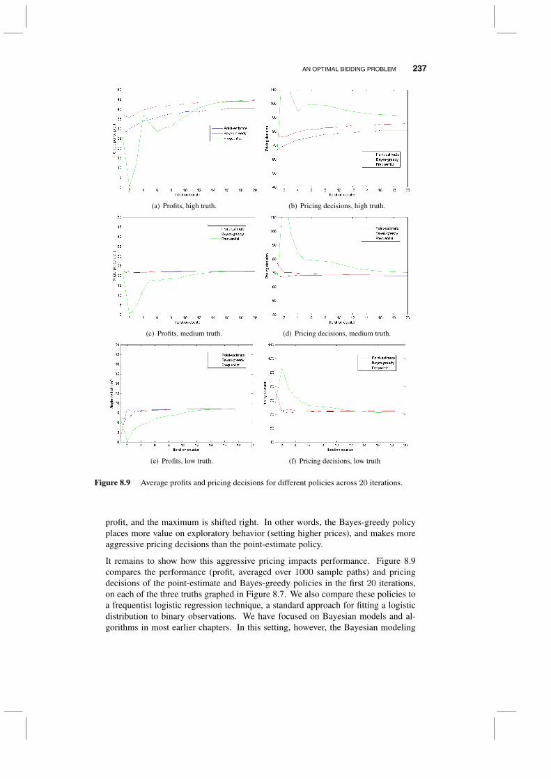
AN OPTIMAL BIDDING PROBLEM 237
(a) Profits, high truth. (b) Pricing decisions, high truth.
(c) Profits, medium truth. (d) Pricing decisions, medium truth.
(e) Profits, low truth. (f) Pricing decisions, low truth
Figure 8.9 Average profits and pricing decisions for different policies across 20 iterations.
profit, and the maximum is shifted right. In other words, the Bayes-greedy policyplaces more value on exploratory behavior (setting higher prices), and makes moreaggressive pricing decisions than the point-estimate policy.
It remains to show how this aggressive pricing impacts performance. Figure 8.9compares the performance (profit, averaged over 1000 sample paths) and pricingdecisions of the point-estimate and Bayes-greedy policies in the first 20 iterations,on each of the three truths graphed in Figure 8.7. We also compare these policies toa frequentist logistic regression technique, a standard approach for fitting a logisticdistribution to binary observations. We have focused on Bayesian models and al-gorithms in most earlier chapters. In this setting, however, the Bayesian modeling
238 NONLINEAR BELIEF MODELS
assumptions do not hold, and our updating equations are approximations. Thus, it isrelevant to compare to a frequentist technique in order to see whether the inaccuracyof the Bayesian model has any negative impact on performance. We deliberately usethe same set of axes for each comparison, to get a better sense of the magnitude ofthe difference between policies.
The graphs reveal several interesting behaviors. First, the Bayes-greedy policyconsistently prices more aggressively than the point-estimate policy, particularly inthe very early iterations. If these aggressive decisions are unsuccessful (for example,if the truth is lower than we believe), the policy quickly corrects its behavior andchooses lower prices. If the optimal price (shown as a dashed line) is higher thanexpected, both point-estimate and Bayes-greedy gradually ramp up their pricingdecisions. However, because Bayes-greedy starts out more aggressively, it is able tomake a bigger profit more quickly. Thus, the Bayes-greedy policy exhibits a kind ofrobustness. If the truth is higher than expected, Bayes-greedy adds considerable value(roughly an extra $10 profit per iteration in Figure 8.9(a)), and if the truth is lower thanexpected, Bayes-greedy tends to lose the first sale, but adjusts almost immediatelyand obtains comparable profits to the point-estimate policy in subsequent iterations.
The frequentist method is able to fit a good model eventually. After around 20iterations, it comes closer to the optimal pricing decision than the two policies usingthe approximate Bayesian model. At the same time, it does not use any priorinformation, and so it requires some time in order to fit a good model. In the firstten iterations, it exhibits volatile behavior and consistently chooses prices that areunreasonably high, even in the case when the truth itself is higher than we think. Itwould seem that Bayes-greedy is able to achieve robust performance in the criticalearly stages of the problem. In some applications, such as the setting of pricingindustrial contracts, ten or twenty iterations may be all we ever get.
8.2 A SAMPLED REPRESENTATION
A powerful approach for handling nonlinear models is to use a sampled representationof the different possible values of the parameter vector θ. When we worked withlookup table representations or linear parametric models, we treated the unknownparameters as following a multivariate normal distribution. While this is a fairlycomplex representation, the linear structure made it possible to derive simple andelegant updating formulas.
With nonlinear models, it is much harder to develop recursive equations if we were tocharacterize the unknown parameter vector θ as multivariate normal. We might alsonote that the multivariate normal distribution can cause difficulties since it allows forvirtually every possible value for θ, which can produce unexpected (and inappropri-ate) behaviors. For example, we might use a quadratic function to approximate aconcave surface, but if a sampled value of the coefficient of the quadratic term comesout positive, the curve flips around to a convex surface.
A SAMPLED REPRESENTATION 239
8.2.1 The belief model
We start by assuming that we have a model f(x|W, θ) that has a known structure,characterized by unknown parameters θ and an exogenous source of experimentalnoise W , that combines to produce a noisy estimate
y = f(x|W, θ),
where both W and θ are random variables, although they behave differently. Therandom variable W changes each time we observe our process. The parameter θ,however, is fixed, but it is fixed at a value that we do not know.
We might think of W as an additive error, as in
y = f(x|θ) +W.
However,W in f(x|W, θ) can represent uncertain parameters in a nonlinear function.
We assume that f(x|W, θ) is nonlinear in θ, which is going to cause us some problemswhen we need to take expectations as we do in the knowledge gradient. There is asimple way to handle a nonlinear model, which is to assume that θ can only take onone of a sampled set Ω = θ1, . . . , θK. We let our belief state about θ be the set ofprobabilities Sn = (pnk )Kk=1 where
pnk = Prob[θ = θk|Hn].
The variable Hn is called the history of the process, which is given by
Hn = (S0,W 1, . . . ,Wn)
A natural way to initialize the probabilities is to start with a uniform prior where
p0k =
1
|Ω|,
for all k. For example, if we have 20 samples in Ω, we would set p0k = .05 for
each k = 1, . . . , 20. We then let the results of experiments quickly update theseprobabilities, giving us our belief state
Sn = (pn1 , . . . , pnK).
Some thought and care has to be put into how the sample θ1, . . . , θK is created sothat we create a reasonable approximation of the distribution of different models thatmight arise. There are three strategies we might use to generate a sample θ1, . . . , θk:
Discretized sample If θ has one to three dimensions, we can simply discretize each di-mension and create a discretized version of the parameter space.
Random sampling We could generate each element of θ from a pre-specified range. Theproblem is that we generally will not know the natural range for each element of θ,especially in the context of a nonlinear, parametric model.
240 NONLINEAR BELIEF MODELS
Fitting with prior data Assume we have a set of inputsx0, x1, . . . , xn with correspondingresponses y1, y2, . . . , yn+1. We can take a series of subsamples (say, half of thedataset), and then fit a model to this data, producing an estimate θk. Repeating thisK times provides an initial set of possible values of θ, which automatically capturesthe correlations between the elements. We suggest using this information to createa multivariate normal distribution, which allows us to scale the covariance matrix ifwe feel there is not enough variability in the sample.
Fitting with synthetic data It will generally be easier to specify the range over whicheach dimension of x might vary, as well as the response y, since these have welldefined units derived from the contextual setting. We can specify a range for eachdimension of x, and then generate random samples (treating each element randomly).We then have to devise a way to generate the responses y, since these are clearlynot independent of x. However, we might assume they are independent, since ouronly goal is to generate a range of θ′s from which to sample. The results of realexperiments will quickly fix this.
8.2.2 The experimental model
The next step is to design the experimental model that determines the probability ofthe response y ∼ fy(y|x, θ). This typically comes from the nature of the problem.Some examples include
• Normal distribution - This is a natural choice when the responses are continuous,and where the noise from an observation of y is due to experimental variability, or arange of complex factors. Keep in mind that the normal allows negative outcomes,which may not be appropriate for many situations. However, it is often the case thata normal approximation of the error is very accurate.
• Poisson distribution - This is appropriate when the response represents a count, suchas the number of sales of a product, or the number of ad-clicks for an online ad.
• Logistic distribution - This would be appropriate when the response is a 0/1 outcomesuch as a success or failure.
• Exponential distribution - Exponential distributions are often a good fit when weare observing a time interval, especially when the interval might be quite small.For example, we might be modeling the time between the arrival of patients with aparticular condition.
For each distribution, θ captures the parameters of the distribution, such as the meanand variance for a normal distribution, the mean λ
The point is that the distribution fy(y|θ) is determined by the characteristics of theproblem, guided by a (presumably) unknown parameter vector θ.
8.2.3 Sampling policies
With our sampled belief model,
THE KNOWLEDGE GRADIENT FOR SAMPLED BELIEF MODEL 241
8.2.4 Resampling
8.3 THE KNOWLEDGE GRADIENT FOR SAMPLED BELIEF MODEL
We are going to demonstrate a powerful method for calculating the knowledge gra-dient that works with very general nonlinear parametric models. We first return tothe knowledge gradient formula, which we repeat here for convenience:
νKG,n(x) = EθEW |θmaxx′
f(x′, θn+1(x))|Sn, x = xn − Eθmaxx′
f(x′, θ)|Sn.
(8.29)
It is useful to break down what is involved in computing the expectations. The first andmost complex expectation is over the unknown parameter vector θ which is typicallymultidimensional, with as few as one or two but perhaps hundreds of dimensions.This same expectation appears in the second term. The second expectation is over theoutcome of the experiment, which is a scalar, and possibly binomial (success/failure).
We are going to demonstrate a powerful and practical way for approximating theknowledge gradient by using the sampled belief model, which we first saw in section2.4. We begin by assuming that the true θ may take on one of a finite (and nottoo large) set θ1, . . . , θK . Let pnk = P[θ = θk] be the probability that θk is thetrue value, given what we know after n experiments. Finally, we let our belief stateSn = (θk, p
nk )Kk=1.
Using the sampled belief model allows us to compute the conditional expectationgiven our belief Sn using
Eθmaxx′
f(x′, θ)|Sn = fn(x′)
=
K∑k=1
pnkf(x′, θk).
Now assume we run an experiment using settings xn = x, and observe the outcomeWn+1 from the n+ 1st experiment. Assume that the distribution of Wn+1 is givenby
fW (w|x, θ) = P[Wn+1 = w|x, θ].
We then use this to update our probabilities using the Bayesian updating logic wepresented in 2.4, which is given by
pn+1k (x = xn|Wn+1 = w) =
1
CwfW (Wn+1 = w|xn, θk)pnk , (8.30)
where Cw is the normalizing constant given Wn+1 = w, which is calculated using
Cw =
K∑k=1
fW (Wn+1 = w|xn, θk)pnk .
Below, we are going to treat CW (with capital W ) as a random variable with realiza-tion Cw.
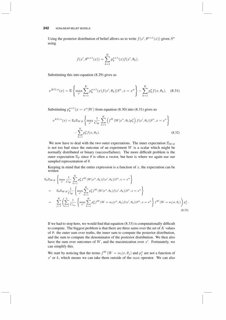
242 NONLINEAR BELIEF MODELS
Using the posterior distribution of belief allows us to write f(x′, θn+1(x)) given Sn
using
f(x′, θn+1(x)) =
K∑k=1
pn+1k (x)f(x′, θk).
Substituting this into equation (8.29) gives us
νKG,n(x) = E
maxx′
K∑k=1
pn+1k (x)f(x′, θk)|Sn, x = xn
−
K∑k=1
pnkf(x, θk). (8.31)
Substituting pn+1k (x = xn|W ) from equation (8.30) into (8.31) gives us
νKG,n(x) = EθEW |θ
maxx′
1
CW
K∑k=1
(fW (W |xn, θk)pnk
)f(x′, θk)|Sn, x = xn
−K∑k=1
pnkf(x, θk). (8.32)
We now have to deal with the two outer expectations. The inner expectation EW |θis not too bad since the outcome of an experiment W is a scalar which might benormally distributed or binary (success/failure). The more difficult problem is theouter expectation Eθ since θ is often a vector, but here is where we again use oursampled representation of θ.
Keeping in mind that the entire expression is a function of x, the expectation can bewritten
EθEW |θ
maxx′
1
CW
K∑k=1
pnkfW (W |xn, θk)f(x′, θk)|Sn, x = xn
= EθEW |θ1
CW
maxx′
K∑k=1
pnkfW (W |xn, θk)f(x′, θk)|Sn, x = xn
=
K∑j=1
(L∑`=1
1
Cw`
maxx′
K∑k=1
pnkfW (W = w`|xn, θk)f(x′, θk)|Sn, x = xn
fW (W = w`|x, θj)
)pnj .
(8.33)
If we had to stop here, we would find that equation (8.33) is computationally difficultto compute. The biggest problem is that there are three sums over the set ofK valuesof θ: the outer sum over truths, the inner sum to compute the posterior distribution,and the sum to compute the denominator of the posterior distribution. We then alsohave the sum over outcomes of W , and the maximization over x′. Fortunately, wecan simplify this.
We start by noticing that the terms fW (W = w`|x, θj) and pnj are not a function ofx′ or k, which means we can take them outside of the max operator. We can also

LOCALLY QUADRATIC APPROXIMATIONS 243
reverse the order of the other sums over k and w`, giving us
EθEW |θ
maxx′
1
CW
K∑k=1
pnkfW (W |xn, θk)f(x′, θk)|Sn, x = xn
=
L∑`=1
K∑j=1
(fW (W = w`|x, θj)pnj
Cw`
)maxx′
K∑k=1
pnkfW (W = w`|xn, θk)f(x′, θk)|Sn, x = xn
.
(8.34)
Using the definition of the normalizing constant Cw we can write
K∑j=1
(fW (W = w`|x, θj)pnj
Cw`
)=
(∑Kj=1 f
W (W = w`|x, θj)pnjCw`
)
=
(∑Kj=1 f
W (W = w`|x, θj)pnj∑Kk=1 f
W (W = w`|x, θk)pnk
)= 1.
We just simplified the problem by cancelling two summations over the K values ofθ. This is a significant simplification, since these sums were nested. This allows usto write (8.34) as
EθEW |θ
maxx′
1
CW
K∑k=1
pnkfW (W |xn, θk)f(x′, θk)|Sn, x = xn
=
L∑`=1
maxx′
K∑k=1
pnkfW (W = w`|xn, θk)f(x′, θk)|Sn, x = xn
.
(8.35)
Equation (8.35) means that we can compute fairly good approximations of the knowl-edge gradient even in the presence of a nonlinear belief model, although some carewould have to be used if θ was high dimensional.
8.4 LOCALLY QUADRATIC APPROXIMATIONS
8.5 BIBLIOGRAPHIC NOTES
Section 7.2 -
PROBLEMS
8.1 Imagine that we are using a logistics curve to model the probability that a customerwill accept a bid, which gives us the revenue function
R(p; θ1, θ2) =p
1 + e−(θ1−θ2p). (8.36)
Assume the prior is θ0 = (4, 2) for prices that are between 0 and 5.

244 NONLINEAR BELIEF MODELS
a) Discretize prices into increments of 0.10 and find the optimal price pExp,1 given thisprior. This represents the choice you would make using a pure exploitation policy.
b) Assume we choose a price p0 = 2 and we observe that the customer accepts the bid(that is, W 1 = 1). Use equations (8.16) and (8.17) to find an updated model. Notethat we did not need to assume a variance for the experimental noise. Why is this?
c) Now use the Bayes-greedy policy in equation (8.25) to compute the price pBG,1. Tryto explain intuitively the difference between pBG,1 and pExp,1.
d) Simulate the Bayes-greedy policy for 20 experiments, using (8.16) and (8.17) toupdate your beliefs. At each iteration, using the beliefs generated by the Bayes-greedy policy, compute pExp,1, and compare the two policies over 20 iterations.
e) Finally, simulate the pure exploitation policy and the Bayes-greedy policy for 20iterations. Repeat this process 100 times and summarize the difference.

CHAPTER 9
LARGE CHOICE SETS
While there are problems where the number of alternative decisions x1, . . . , xMis small enough to be enumerated, it is quite easy to encounter problems where thepotential set is extremely large (tens of thousands to millions). This typically ariseswhen x is a vector, but sometimes there are simply many choices (imagine choosingads or movies to show an online user).
In this chapter, we consider three classes of problems where large choice sets arise:
Subset selection These arise when we have to choose L elements out of a set K, such aschoosing five basketball players from a team of 12. The number of potential subsetsgrows very quickly as K and L increase.
Hierarchical models Imagine having to pick the best person to do a job, or the best adto maximize ad-clicks, where the choice is characterized by a multidimensionalattribute vector, producing an extremely large set of choices.
Continuous vectors There are many problems where x is a multi-dimensional vector(x1, . . . , xK), where xk might be continuous or an integer.
These problems will allow us to illustrate several powerful strategies that shouldprovide a good starting toolbox for a wide range of problem settings.
Optimal Learning. By Warren B. Powell and Ilya O. RyzhovCopyright c© 2018 John Wiley & Sons, Inc.
245
246 LARGE CHOICE SETS
9.1 SAMPLED EXPERIMENTS
A powerful strategy for handling large experimental spaces is to turn a large set ofexperiments into a small one by choosing a smaller sample from the original largeset. If x is multidimensional, we can sample each dimension independently, rejectingany that are not feasible or acceptable. This is a simple but powerful idea that is easyto implement. How well it works depends on the structure of the problem and thenature of the underlying belief model.
Sampling is effective when we use a belief model that allows us to generalize whatwe learn. This is the case if we have correlated beliefs (presented in section 4.5),a linear (or nonlinear) belief model (which we presented in chapters 7 and 8), or ahierarchical belief model (which we present below in section 9.3). The core idea isthat with some form of generalized learning, we do not have to test every experimentin X . Rather, we just need to sample enough to produce a reasonable estimate of ourbelief model, from which we will then find the best value in the set X .
It is easy to overlook that most statistics is done using sampled experiments. Themost standard is when we are given a dataset consisting ofN data points (yn, xn)Nn=1
from which we have to fit a statistical model. We may have no idea how the inputsxn were chosen. Often, they come from a process over which we have no control.For example, xn might be the attributes of a patient and yn is the cost of the medicalprocedure. We typically cannot control which patients walk through the door.
The size of X is much more important for a value of information policy than it isfor the other heuristics. Thus, we might need to draw a relatively smaller sample forthe purpose of computing the knowledge gradient or expected improvement just tosimplify these calculations. Once the experiments are complete, we can use a muchlarger sample to try to find the best design.
There are different strategies for generating and using sampled experiments:
Static samples We can draw a single sample from the set X and then proceed using justthis sampled set for all calculations.
Iterative resampling Since our belief model provides estimates for all x ∈ X , and notjust the sampled experiments, we can draw an entirely new sample each time wewant to find an experiment to run. This reduces the exposure to the vagaries of asingle sample.
Using a sampled subset of experiments from X , combined with a generalized beliefmodel, is an exceptionally powerful strategy. The size of the sample depends on thebehavior of the belief model.
It is possible to approach virtually any problem regardless of the size of the ex-perimental set X , and regardless of the complexity of the underlying belief model,using the idea of a sampled experimental set. You simply have to choose a samplex1, . . . , xM , and then use the tools for discrete alternatives that we have presented indepth. However, even if you can exploit the structure of correlated beliefs, it will stillbe harder to estimate µ1, . . . , µM (where M might be 1000), when you can reducethis to a parametric belief model f(x|θ) where θ = (θ1, . . . , θK).
SUBSET SELECTION 247
9.2 SUBSET SELECTION
Consider the problem where we have to pick the four best rowers to man a four-person shell for rowing competitions. The coach can rank the 15 rowers on histeam based on how they perform on ergonomic machines, but it is well known thatpeople perform differently in a boat, and people interact in ways that affect theirperformance. However, there is over 1,365 ways of choosing four people out of a setof 15, so it is not possible to evaluate every possible team.
Our challenge is to find the best subset of a discrete choice set. This problem, knownas subset selection, arises in numerous settings and has a classical formulation as amathematical program. For example, we might have M items, where xi = 1 if wehave chosen i to be in our subset. Normally we have some sort of budget constraint,so we have to choose the vector x to satisfy this constraint. If we knew that item imade a contribution ci, we could choose our elements by solving
maxx
M∑i=1
cixi
subject to
M∑i=1
aixi ≤ B,
xi ∈ (0, 1).
If ai = 1, then B is simply a limit on how many items we can have (for example,four rowers). The coefficient ai might be the cost of using i, in which case B isa monetary budget constraint. In this case, we have an instance of the well-knownknapsack problem.
Subset selection problems include forming a team, identifying investment portfolios,prescribing a course of treatment for an illness, and choosing tools to solve a problem.In all of these problems, we have to choose a subset of elements that interact witheach other in a relatively complex way. Our specific interest is in problems wherewe do not have a simple deterministic, linear objective function. Because of theinteractions between elements, the problem is harder than simply not knowing thecoefficients ci. However, we may have a learning budget allowing us to experimentwith several subsets before we have to choose one. For example, a basketball coachmay hold some practice games to learn how well different players work together,before committing to a lineup for the season.
We can apply optimal learning concepts to subset selection. In theory, the toolsdeveloped in Chapters 3 and 4 already allow us to handle this problem. We can viewsubset selection as an instance of a ranking and selection problem with correlatedbeliefs. Each alternative in the ranking and selection problem corresponds to onepossible subset. In the problem of choosing four rowers out of 15 possible candidates,we thus have a total of M =
(154
)= 1, 365 alternatives. We model the values of
different subsets separately. If we choose rowers Anne,Mary,Cathy,Tara andAnne,Mary,Susan,Tara, these two subsets would be considered as two distinct
248 LARGE CHOICE SETS
alternatives, each with its own value. However, our beliefs about these two valuesare heavily correlated, because these two subsets have three elements in common.Learning about the effectiveness of one subset should also provide information aboutthe other subset.
As long as we do a good job modeling our prior beliefs (particularly our beliefsabout the correlations between alternatives), we can then apply one of the learningtechniques from Chapter 3, or the knowledge gradient method from Chapter 4, todecide which subset we want to learn about. Conceptually, we can approach theproblem of subset selection entirely within the framework of ranking and selection.For smaller problems such as choosing four rowers out of 15, this approach will workfine.
However, one characteristic specific to subset selection problems is that they tend tobe quite large. Suppose that we need to choose five items from a list of ten. Fiveand ten are small numbers, but the number of possible subsets is
(105
)= 252. If
we slightly increase the size of the problem, and now choose six items from a listof twelve, the number of subsets is
(126
)= 924. The number of alternatives grows
combinatorially as we add more items to our list. Choosing ten items from a list oftwenty results in 184, 756 alternatives!
In Chapter 3, we did not really specify a problem size. Rather, we analyzed a genericproblem withM alternatives. In theory, the techniques we developed can handle anyM , but as a general rule we are limited to M equal to around 1,000. When we arechoosing subsets, the number of subsets can quickly grow much larger than this.
Subset selection problems come in many varieties. We are primarily interested inapplications where there is some relationship between subsets so we can draw on ourtools using correlated beliefs.
• Designing a diabetes treatment - Type 2 diabetes is an illness where the body is unableto properly react to insulin, a hormone used to remove sugar from the bloodstream.Most diabetes drugs fall into one of several categories; for example, sensitizersincrease the body’s sensitivity to insulin, whereas secretagogues stimulate the bodyto secrete more insulin. A course of treatment for a single patient may contain drugsfrom multiple categories, as well as multiple complementary drugs within a singlecategory. Clinical trials can help us learn how well two drugs complement eachother.
• Choosing a starting basketball lineup - The coach wants to find five players whoprovide the best performance over the first quarter of a basketball game. He knowshow many points each player scores from past games, and has other statistics suchas rebounds, assists and blocks, but the simple reality is that there is no easy formulathat predicts how people will interact with each other. Each time he tries out a team,he observes the total score (which might be viewed as a correction to a simplerformula). The coach has 12 players, implying that he has to pick the best set of 5out of a team of 12, which means evaluating 792 different teams. Fortunately, theobservations should be correlated. We would not know the correlations exactly, butwe might start with a covariance matrix that is proportional to the number of playersin common between two teams.

SUBSET SELECTION 249
• Choosing movies to display to a user - We wish to select a sample of movies (perhaps6 or 8) out of a population of thousands to display to a user in the hope that she willselect one to rent or purchase. The value of a set is given by the probability thatshe selects one, which requires guessing whether she is interested in action, drama,comedy, or is more influenced by the lead actor/actress. We have to find the bestsubset of movies to display to maximize the probability of a purchase. It is importantto try a mixture, because if we display all action movies to someone who prefersdrama, we will not be successful.
• Product assortment planning - A retail company has to choose a set of products tooffer at its outlet store, or to display in a storefront window. The profitability of aproduct, or its effectiveness at drawing customers to a store, may also depend on thepresence of other products in the assortment (e.g. accessories for an iPod). It is alsoimportant to display a diverse set of products that may attract buyers from differentdemographic groups. We have a short period of time to experiment with differentassortments at a particular store in an attempt to discover the best one.
• Shortest path problems - Finding a path through a network with uncertain costs (ortravel times) involves finding a subset of links out of the full set of links in thenetwork. Of course, these links have to form a path that joins origin to destination.
9.2.1 Choosing a subset
We show how ranking and selection can be used to find a subset in the context ofdesigning a diabetes treatment. In the latter stages of clinical trials, the search hastypically been narrowed to a relatively small set of the most promising drugs. Wecan create a combination treatment consisting of multiple drugs from this set.
The effectiveness of a diabetes treatment can be measured in terms of blood sugarreduction. Blood sugar level is measured in millimoles per liter, after the patient hasnot eaten for eight hours; this is known as the “fasting plasma glucose” or FPG level.For a healthy person, the FPG level is about 4-6 mmol/L. A diabetic can show FPGlevels of up to 10-15 mmol/L. A single drug can reduce FPG level by an amountbetween 0.5 and 2 mmol/L.
We design a combination treatment for two reasons. First, two drugs yield a biggerFPG reduction than one, and second, combination treatments tend to have lower risksof side effects. Prescribing three drugs instead of one may give us an FPG reductionbetween 2 and 5 mmol/L. Due to interactions between drugs, FPG reduction obtainedfrom the combination is not a straightforward sum of the reductions we might observefrom individual drugs.
9.2.2 Setting prior means and variances
Let us consider an example with six drugs. Our list may include certain basicelements such as conventional treatment (recommending diet and exercise to thepatient), metformin (the first drug of choice in most cases), and insulin injections, aswell as newer compounds such as rosiglitazone, glibenclamide and chlorpropamide.
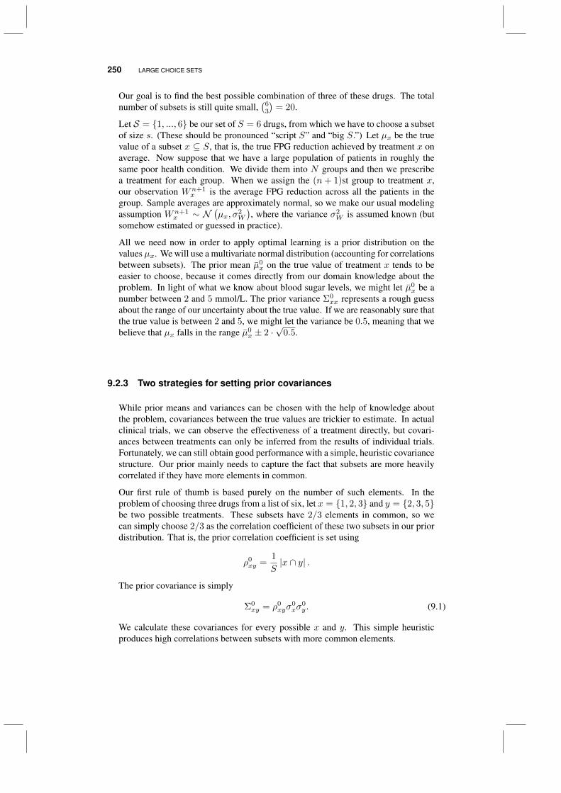
250 LARGE CHOICE SETS
Our goal is to find the best possible combination of three of these drugs. The totalnumber of subsets is still quite small,
(63
)= 20.
Let S = 1, ..., 6 be our set of S = 6 drugs, from which we have to choose a subsetof size s. (These should be pronounced “script S” and “big S.”) Let µx be the truevalue of a subset x ⊆ S, that is, the true FPG reduction achieved by treatment x onaverage. Now suppose that we have a large population of patients in roughly thesame poor health condition. We divide them into N groups and then we prescribea treatment for each group. When we assign the (n+ 1)st group to treatment x,our observation Wn+1
x is the average FPG reduction across all the patients in thegroup. Sample averages are approximately normal, so we make our usual modelingassumption Wn+1
x ∼ N(µx, σ
2W
), where the variance σ2
W is assumed known (butsomehow estimated or guessed in practice).
All we need now in order to apply optimal learning is a prior distribution on thevalues µx. We will use a multivariate normal distribution (accounting for correlationsbetween subsets). The prior mean µ0
x on the true value of treatment x tends to beeasier to choose, because it comes directly from our domain knowledge about theproblem. In light of what we know about blood sugar levels, we might let µ0
x be anumber between 2 and 5 mmol/L. The prior variance Σ0
xx represents a rough guessabout the range of our uncertainty about the true value. If we are reasonably sure thatthe true value is between 2 and 5, we might let the variance be 0.5, meaning that webelieve that µx falls in the range µ0
x ± 2 ·√
0.5.
9.2.3 Two strategies for setting prior covariances
While prior means and variances can be chosen with the help of knowledge aboutthe problem, covariances between the true values are trickier to estimate. In actualclinical trials, we can observe the effectiveness of a treatment directly, but covari-ances between treatments can only be inferred from the results of individual trials.Fortunately, we can still obtain good performance with a simple, heuristic covariancestructure. Our prior mainly needs to capture the fact that subsets are more heavilycorrelated if they have more elements in common.
Our first rule of thumb is based purely on the number of such elements. In theproblem of choosing three drugs from a list of six, let x = 1, 2, 3 and y = 2, 3, 5be two possible treatments. These subsets have 2/3 elements in common, so wecan simply choose 2/3 as the correlation coefficient of these two subsets in our priordistribution. That is, the prior correlation coefficient is set using
ρ0xy =
1
S|x ∩ y| .
The prior covariance is simply
Σ0xy = ρ0
xyσ0xσ
0y. (9.1)
We calculate these covariances for every possible x and y. This simple heuristicproduces high correlations between subsets with more common elements.
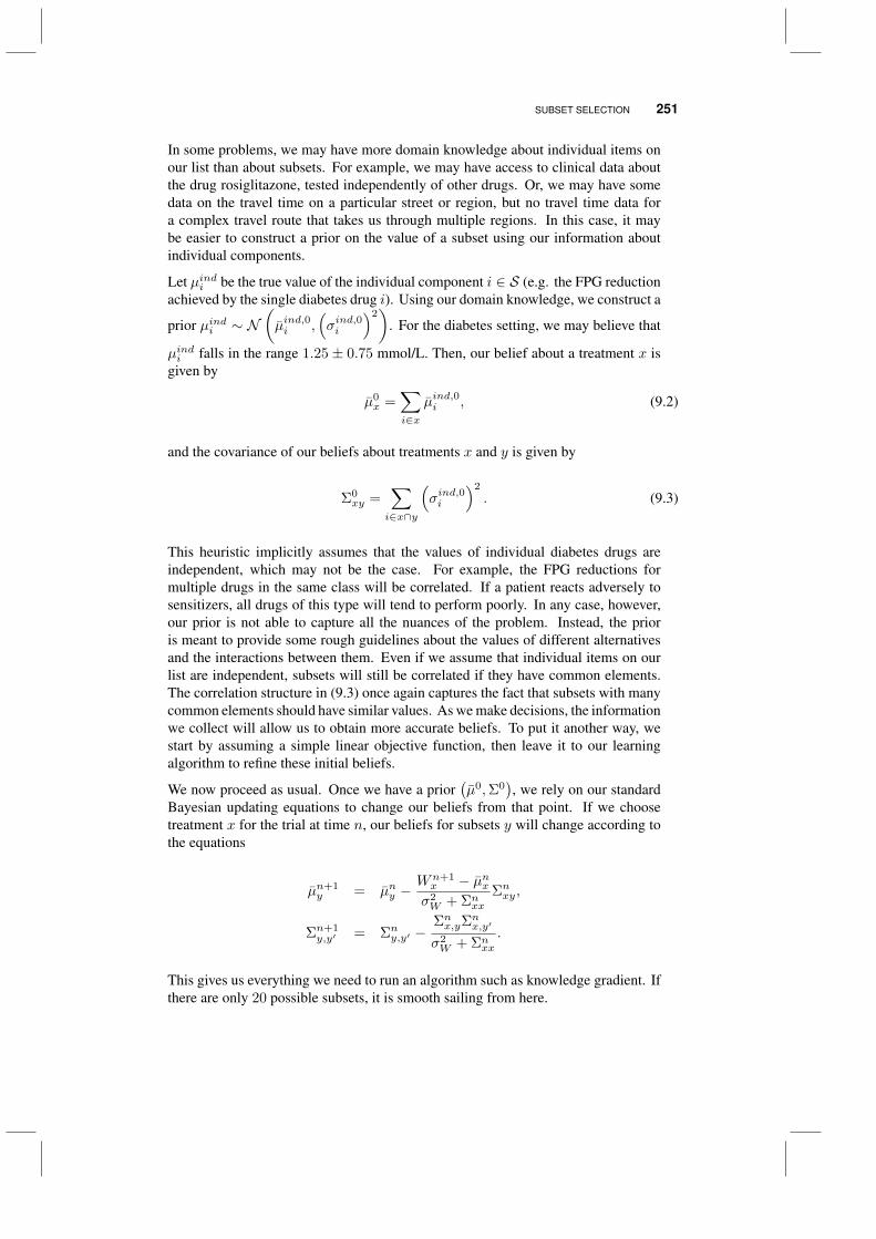
SUBSET SELECTION 251
In some problems, we may have more domain knowledge about individual items onour list than about subsets. For example, we may have access to clinical data aboutthe drug rosiglitazone, tested independently of other drugs. Or, we may have somedata on the travel time on a particular street or region, but no travel time data fora complex travel route that takes us through multiple regions. In this case, it maybe easier to construct a prior on the value of a subset using our information aboutindividual components.
Let µindi be the true value of the individual component i ∈ S (e.g. the FPG reductionachieved by the single diabetes drug i). Using our domain knowledge, we construct a
prior µindi ∼ N(µind,0i ,
(σind,0i
)2)
. For the diabetes setting, we may believe that
µindi falls in the range 1.25 ± 0.75 mmol/L. Then, our belief about a treatment x isgiven by
µ0x =
∑i∈x
µind,0i , (9.2)
and the covariance of our beliefs about treatments x and y is given by
Σ0xy =
∑i∈x∩y
(σind,0i
)2
. (9.3)
This heuristic implicitly assumes that the values of individual diabetes drugs areindependent, which may not be the case. For example, the FPG reductions formultiple drugs in the same class will be correlated. If a patient reacts adversely tosensitizers, all drugs of this type will tend to perform poorly. In any case, however,our prior is not able to capture all the nuances of the problem. Instead, the prioris meant to provide some rough guidelines about the values of different alternativesand the interactions between them. Even if we assume that individual items on ourlist are independent, subsets will still be correlated if they have common elements.The correlation structure in (9.3) once again captures the fact that subsets with manycommon elements should have similar values. As we make decisions, the informationwe collect will allow us to obtain more accurate beliefs. To put it another way, westart by assuming a simple linear objective function, then leave it to our learningalgorithm to refine these initial beliefs.
We now proceed as usual. Once we have a prior(µ0,Σ0
), we rely on our standard
Bayesian updating equations to change our beliefs from that point. If we choosetreatment x for the trial at time n, our beliefs for subsets y will change according tothe equations
µn+1y = µny −
Wn+1x − µnxσ2W + Σnxx
Σnxy,
Σn+1y,y′ = Σny,y′ −
Σnx,yΣnx,y′
σ2W + Σnxx
.
This gives us everything we need to run an algorithm such as knowledge gradient. Ifthere are only 20 possible subsets, it is smooth sailing from here.
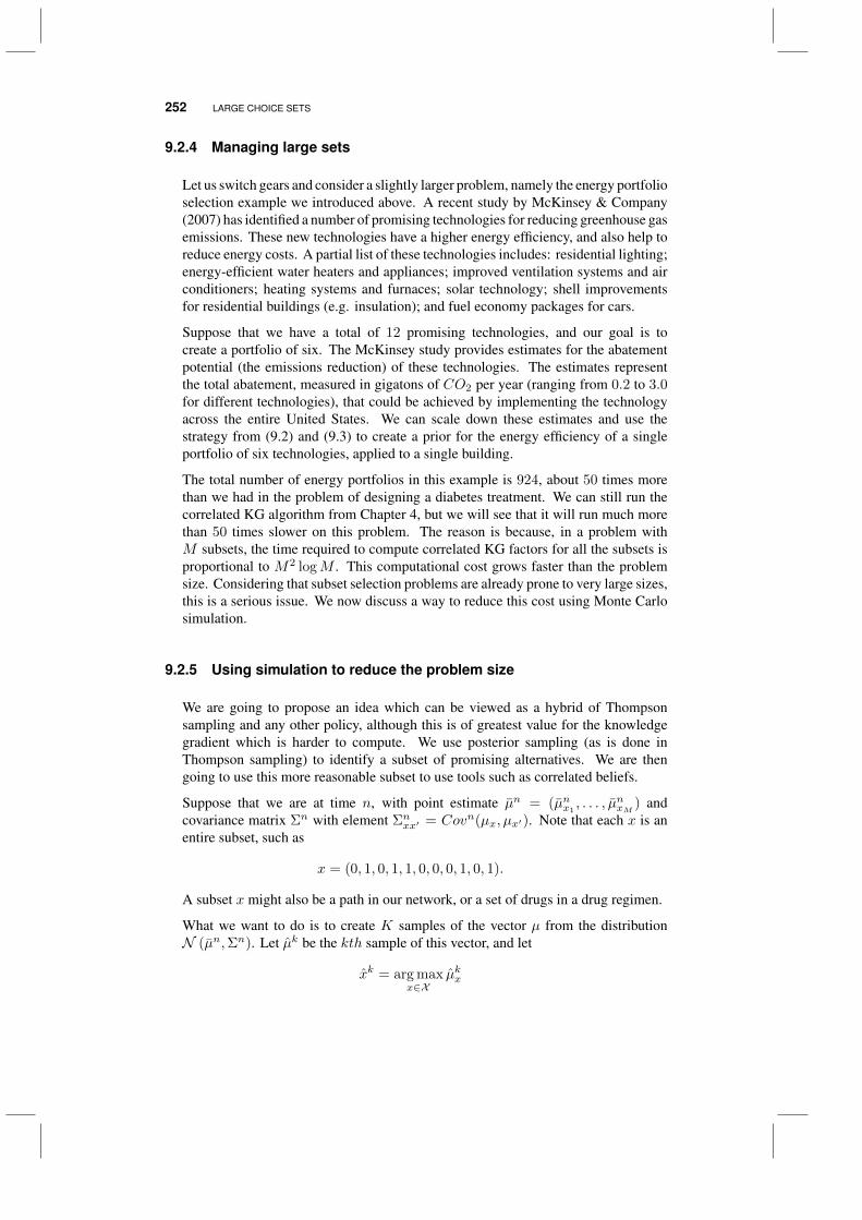
252 LARGE CHOICE SETS
9.2.4 Managing large sets
Let us switch gears and consider a slightly larger problem, namely the energy portfolioselection example we introduced above. A recent study by McKinsey & Company(2007) has identified a number of promising technologies for reducing greenhouse gasemissions. These new technologies have a higher energy efficiency, and also help toreduce energy costs. A partial list of these technologies includes: residential lighting;energy-efficient water heaters and appliances; improved ventilation systems and airconditioners; heating systems and furnaces; solar technology; shell improvementsfor residential buildings (e.g. insulation); and fuel economy packages for cars.
Suppose that we have a total of 12 promising technologies, and our goal is tocreate a portfolio of six. The McKinsey study provides estimates for the abatementpotential (the emissions reduction) of these technologies. The estimates representthe total abatement, measured in gigatons of CO2 per year (ranging from 0.2 to 3.0for different technologies), that could be achieved by implementing the technologyacross the entire United States. We can scale down these estimates and use thestrategy from (9.2) and (9.3) to create a prior for the energy efficiency of a singleportfolio of six technologies, applied to a single building.
The total number of energy portfolios in this example is 924, about 50 times morethan we had in the problem of designing a diabetes treatment. We can still run thecorrelated KG algorithm from Chapter 4, but we will see that it will run much morethan 50 times slower on this problem. The reason is because, in a problem withM subsets, the time required to compute correlated KG factors for all the subsets isproportional to M2 logM . This computational cost grows faster than the problemsize. Considering that subset selection problems are already prone to very large sizes,this is a serious issue. We now discuss a way to reduce this cost using Monte Carlosimulation.
9.2.5 Using simulation to reduce the problem size
We are going to propose an idea which can be viewed as a hybrid of Thompsonsampling and any other policy, although this is of greatest value for the knowledgegradient which is harder to compute. We use posterior sampling (as is done inThompson sampling) to identify a subset of promising alternatives. We are thengoing to use this more reasonable subset to use tools such as correlated beliefs.
Suppose that we are at time n, with point estimate µn = (µnx1, . . . , µnxM ) and
covariance matrix Σn with element Σnxx′ = Covn(µx, µx′). Note that each x is anentire subset, such as
x = (0, 1, 0, 1, 1, 0, 0, 0, 1, 0, 1).
A subset x might also be a path in our network, or a set of drugs in a drug regimen.
What we want to do is to create K samples of the vector µ from the distributionN (µn,Σn). Let µk be the kth sample of this vector, and let
xk = arg maxx∈X
µkx
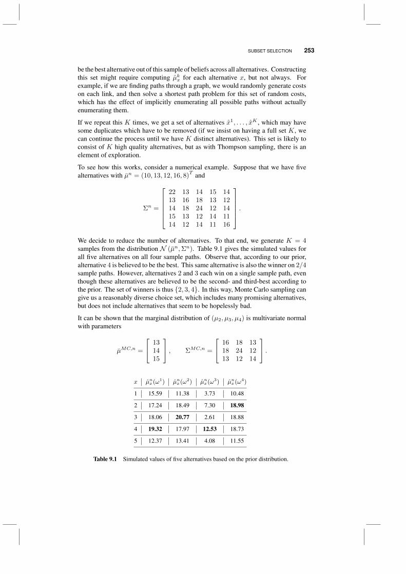
SUBSET SELECTION 253
be the best alternative out of this sample of beliefs across all alternatives. Constructingthis set might require computing µkx for each alternative x, but not always. Forexample, if we are finding paths through a graph, we would randomly generate costson each link, and then solve a shortest path problem for this set of random costs,which has the effect of implicitly enumerating all possible paths without actuallyenumerating them.
If we repeat this K times, we get a set of alternatives x1, . . . , xK , which may havesome duplicates which have to be removed (if we insist on having a full set K, wecan continue the process until we have K distinct alternatives). This set is likely toconsist of K high quality alternatives, but as with Thompson sampling, there is anelement of exploration.
To see how this works, consider a numerical example. Suppose that we have fivealternatives with µn = (10, 13, 12, 16, 8)
T and
Σn =
22 13 14 15 1413 16 18 13 1214 18 24 12 1415 13 12 14 1114 12 14 11 16
.
We decide to reduce the number of alternatives. To that end, we generate K = 4samples from the distribution N (µn,Σn). Table 9.1 gives the simulated values forall five alternatives on all four sample paths. Observe that, according to our prior,alternative 4 is believed to be the best. This same alternative is also the winner on 2/4sample paths. However, alternatives 2 and 3 each win on a single sample path, eventhough these alternatives are believed to be the second- and third-best according tothe prior. The set of winners is thus 2, 3, 4. In this way, Monte Carlo sampling cangive us a reasonably diverse choice set, which includes many promising alternatives,but does not include alternatives that seem to be hopelessly bad.
It can be shown that the marginal distribution of (µ2, µ3, µ4) is multivariate normalwith parameters
µMC,n =
131415
, ΣMC,n =
16 18 1318 24 1213 12 14
.x µnx(ω1) µnx(ω2) µnx(ω3) µnx(ω4)
1 15.59 11.38 3.73 10.48
2 17.24 18.49 7.30 18.98
3 18.06 20.77 2.61 18.88
4 19.32 17.97 12.53 18.73
5 12.37 13.41 4.08 11.55
Table 9.1 Simulated values of five alternatives based on the prior distribution.
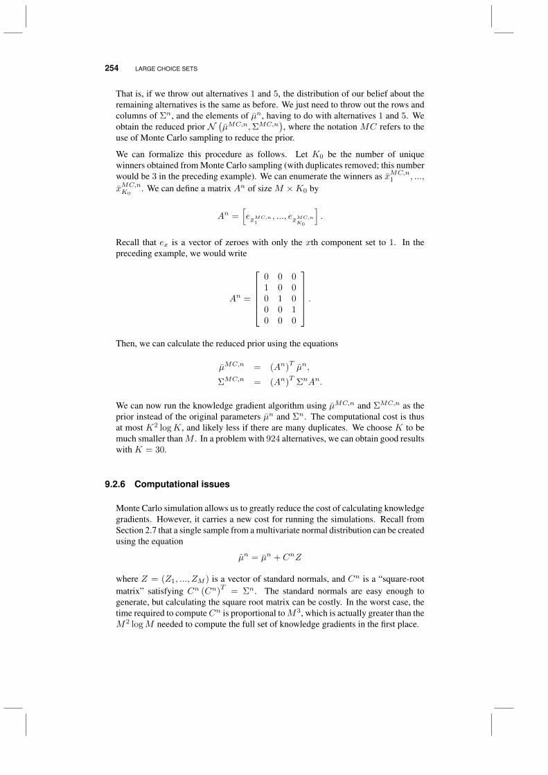
254 LARGE CHOICE SETS
That is, if we throw out alternatives 1 and 5, the distribution of our belief about theremaining alternatives is the same as before. We just need to throw out the rows andcolumns of Σn, and the elements of µn, having to do with alternatives 1 and 5. Weobtain the reduced prior N
(µMC,n,ΣMC,n
), where the notation MC refers to the
use of Monte Carlo sampling to reduce the prior.
We can formalize this procedure as follows. Let K0 be the number of uniquewinners obtained from Monte Carlo sampling (with duplicates removed; this numberwould be 3 in the preceding example). We can enumerate the winners as xMC,n
1 , ...,
xMC,nK0
. We can define a matrix An of size M ×K0 by
An =[exMC,n1
, ..., exMC,nK0
].
Recall that ex is a vector of zeroes with only the xth component set to 1. In thepreceding example, we would write
An =
0 0 01 0 00 1 00 0 10 0 0
.
Then, we can calculate the reduced prior using the equations
µMC,n = (An)Tµn,
ΣMC,n = (An)T
ΣnAn.
We can now run the knowledge gradient algorithm using µMC,n and ΣMC,n as theprior instead of the original parameters µn and Σn. The computational cost is thusat most K2 logK, and likely less if there are many duplicates. We choose K to bemuch smaller thanM . In a problem with 924 alternatives, we can obtain good resultswith K = 30.
9.2.6 Computational issues
Monte Carlo simulation allows us to greatly reduce the cost of calculating knowledgegradients. However, it carries a new cost for running the simulations. Recall fromSection 2.7 that a single sample from a multivariate normal distribution can be createdusing the equation
µn = µn + CnZ
where Z = (Z1, ..., ZM ) is a vector of standard normals, and Cn is a “square-rootmatrix” satisfying Cn (Cn)
T= Σn. The standard normals are easy enough to
generate, but calculating the square root matrix can be costly. In the worst case, thetime required to computeCn is proportional toM3, which is actually greater than theM2 logM needed to compute the full set of knowledge gradients in the first place.
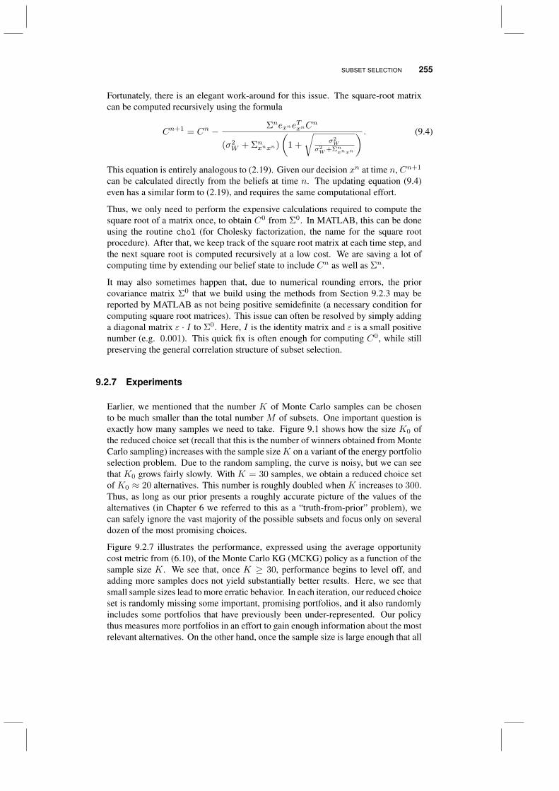
SUBSET SELECTION 255
Fortunately, there is an elegant work-around for this issue. The square-root matrixcan be computed recursively using the formula
Cn+1 = Cn − ΣnexneTxnC
n
(σ2W + Σnxnxn)
(1 +
√σ2W
σ2W+Σn
xnxn
) . (9.4)
This equation is entirely analogous to (2.19). Given our decision xn at time n, Cn+1
can be calculated directly from the beliefs at time n. The updating equation (9.4)even has a similar form to (2.19), and requires the same computational effort.
Thus, we only need to perform the expensive calculations required to compute thesquare root of a matrix once, to obtain C0 from Σ0. In MATLAB, this can be doneusing the routine chol (for Cholesky factorization, the name for the square rootprocedure). After that, we keep track of the square root matrix at each time step, andthe next square root is computed recursively at a low cost. We are saving a lot ofcomputing time by extending our belief state to include Cn as well as Σn.
It may also sometimes happen that, due to numerical rounding errors, the priorcovariance matrix Σ0 that we build using the methods from Section 9.2.3 may bereported by MATLAB as not being positive semidefinite (a necessary condition forcomputing square root matrices). This issue can often be resolved by simply addinga diagonal matrix ε · I to Σ0. Here, I is the identity matrix and ε is a small positivenumber (e.g. 0.001). This quick fix is often enough for computing C0, while stillpreserving the general correlation structure of subset selection.
9.2.7 Experiments
Earlier, we mentioned that the number K of Monte Carlo samples can be chosento be much smaller than the total number M of subsets. One important question isexactly how many samples we need to take. Figure 9.1 shows how the size K0 ofthe reduced choice set (recall that this is the number of winners obtained from MonteCarlo sampling) increases with the sample sizeK on a variant of the energy portfolioselection problem. Due to the random sampling, the curve is noisy, but we can seethat K0 grows fairly slowly. With K = 30 samples, we obtain a reduced choice setof K0 ≈ 20 alternatives. This number is roughly doubled when K increases to 300.Thus, as long as our prior presents a roughly accurate picture of the values of thealternatives (in Chapter 6 we referred to this as a “truth-from-prior” problem), wecan safely ignore the vast majority of the possible subsets and focus only on severaldozen of the most promising choices.
Figure 9.2.7 illustrates the performance, expressed using the average opportunitycost metric from (6.10), of the Monte Carlo KG (MCKG) policy as a function of thesample size K. We see that, once K ≥ 30, performance begins to level off, andadding more samples does not yield substantially better results. Here, we see thatsmall sample sizes lead to more erratic behavior. In each iteration, our reduced choiceset is randomly missing some important, promising portfolios, and it also randomlyincludes some portfolios that have previously been under-represented. Our policythus measures more portfolios in an effort to gain enough information about the mostrelevant alternatives. On the other hand, once the sample size is large enough that all
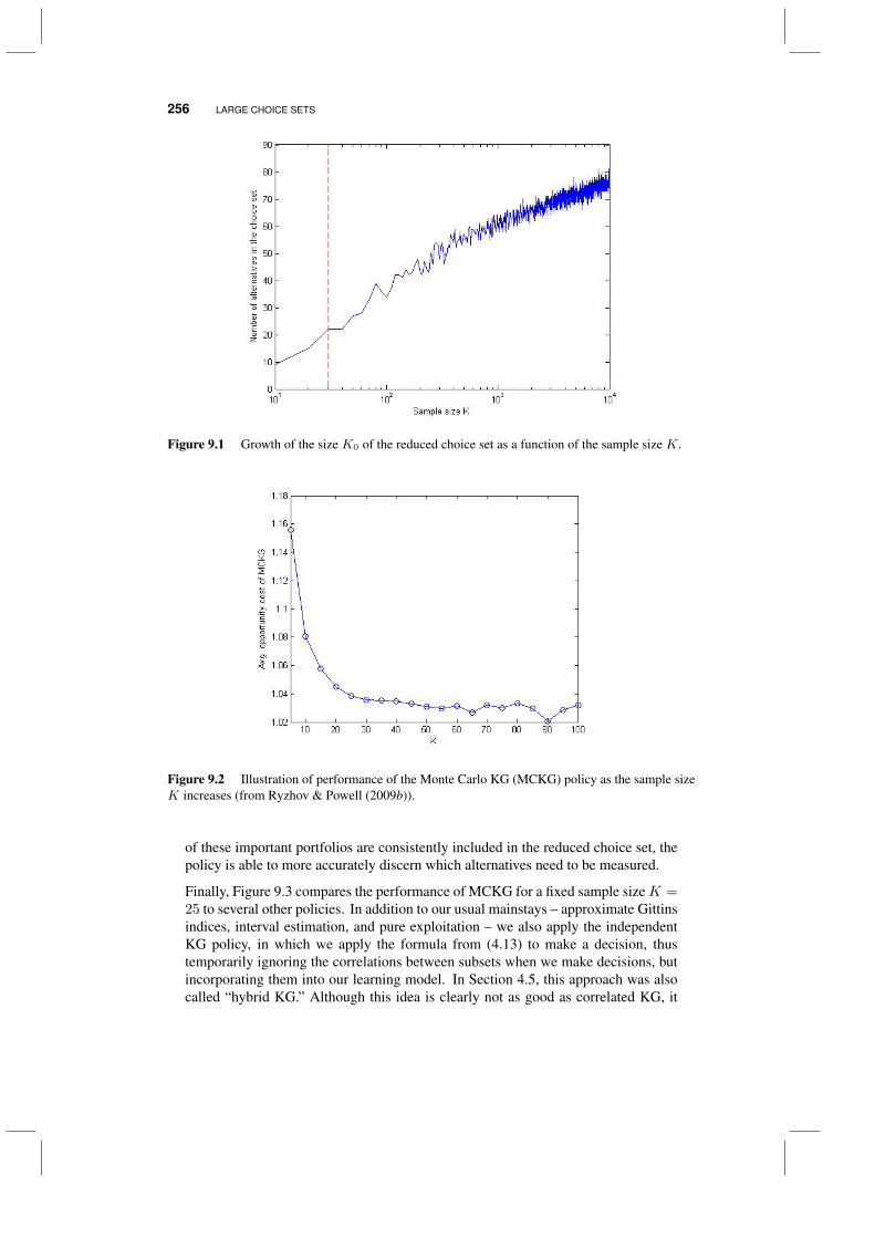
256 LARGE CHOICE SETS
Figure 9.1 Growth of the size K0 of the reduced choice set as a function of the sample size K.
Figure 9.2 Illustration of performance of the Monte Carlo KG (MCKG) policy as the sample sizeK increases (from Ryzhov & Powell (2009b)).
of these important portfolios are consistently included in the reduced choice set, thepolicy is able to more accurately discern which alternatives need to be measured.
Finally, Figure 9.3 compares the performance of MCKG for a fixed sample sizeK =25 to several other policies. In addition to our usual mainstays – approximate Gittinsindices, interval estimation, and pure exploitation – we also apply the independentKG policy, in which we apply the formula from (4.13) to make a decision, thustemporarily ignoring the correlations between subsets when we make decisions, butincorporating them into our learning model. In Section 4.5, this approach was alsocalled “hybrid KG.” Although this idea is clearly not as good as correlated KG, it
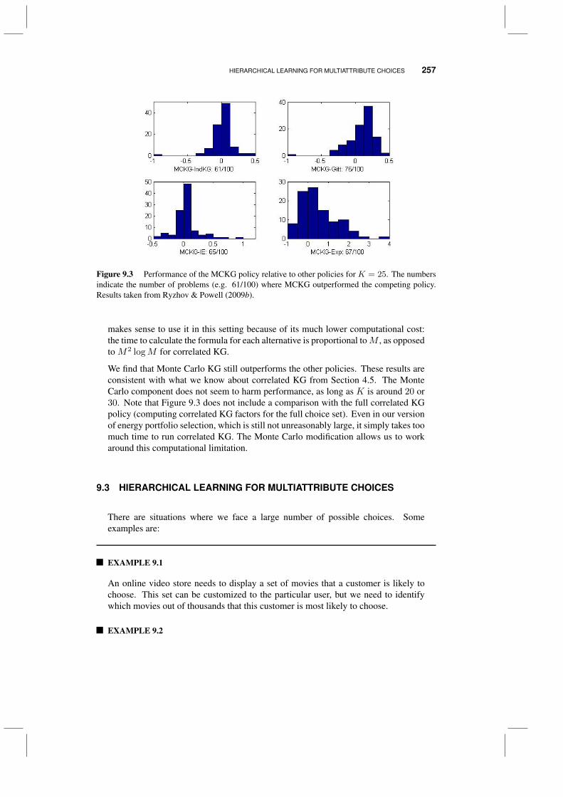
HIERARCHICAL LEARNING FOR MULTIATTRIBUTE CHOICES 257
Figure 9.3 Performance of the MCKG policy relative to other policies for K = 25. The numbersindicate the number of problems (e.g. 61/100) where MCKG outperformed the competing policy.Results taken from Ryzhov & Powell (2009b).
makes sense to use it in this setting because of its much lower computational cost:the time to calculate the formula for each alternative is proportional toM , as opposedto M2 logM for correlated KG.
We find that Monte Carlo KG still outperforms the other policies. These results areconsistent with what we know about correlated KG from Section 4.5. The MonteCarlo component does not seem to harm performance, as long as K is around 20 or30. Note that Figure 9.3 does not include a comparison with the full correlated KGpolicy (computing correlated KG factors for the full choice set). Even in our versionof energy portfolio selection, which is still not unreasonably large, it simply takes toomuch time to run correlated KG. The Monte Carlo modification allows us to workaround this computational limitation.
9.3 HIERARCHICAL LEARNING FOR MULTIATTRIBUTE CHOICES
There are situations where we face a large number of possible choices. Someexamples are:
EXAMPLE 9.1
An online video store needs to display a set of movies that a customer is likely tochoose. This set can be customized to the particular user, but we need to identifywhich movies out of thousands that this customer is most likely to choose.
EXAMPLE 9.2
258 LARGE CHOICE SETS
A company is growing quickly and needs to hire people to fill a variety of newpositions. After posting the job requirements on various internet job boards, thehuman resources director is quickly overwhelmed with thousands of applications.
EXAMPLE 9.3
The Department of Homeland Security needs to identify websites that suggest terroristorigin or intent. Algorithms can process the websites, but it is necessary to showsome of them to experts who can do a better job of assessing risk. Which of the manythousands of websites should we show to the expert?
These are problems with extremely large choice sets, but they lack the nice struc-ture of a subset selection problem. However, each choice is described by a set ofattributes which can be exploited to create a natural hierarchy. For example, whenorganizing movies, we might decide that genre is most important, followed by leadingactor/actress, director, and year it appeared. We can then use this structure to createa series of estimates that balance bias and variance.
We have to begin by describing how to compute estimates of a function at differentlevels of aggregation, since we did not cover this in our first pass through statisticalestimation in chapter 9.5. Fortunately, the equations for doing this are relativelysimple and quite easy to implement. We do this in two stages. Section 9.3.1 laysthe foundation by showing how to estimate bias and variance. Then, section 9.3.2describes how to perform hierarchical estimation using a simple weighting formula.
Once we have this belief model in hand, we can use this with any of our tunablepolicies, just as we could when we first encountered correlated beliefs. Value ofinformation policies such as the knowledge gradient, however, are another matter,since we need to capture the updating of the belief model when we calculate the valueof information. We show how to calculate the knowledge gradient in section 9.3.3.
9.3.1 Laying the foundations
Aggregation can be achieved in different ways. If x is multidimensional, we cansimply ignore dimensions. Example, if estimating the value of posting a movie ona website, we might use genre as the most important attribute, followed by the yearin which it was made, and then the acting lead. But we can also aggregate by usingcoarse representations of a continuous variable, such as the number of words in anad, or by using advanced statistical models to pick out the most important features.
However we handle aggregation, we can represent our procedure as a mapping thatreduces our original set of choices X to a more aggregate set that we write X (g),which write write as
Gg : X → X (g).
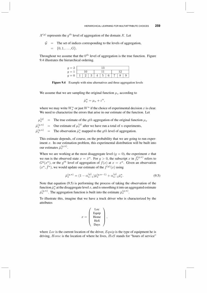
HIERARCHICAL LEARNING FOR MULTIATTRIBUTE CHOICES 259
X (g) represents the gth level of aggregation of the domain X . Let
G = The set of indices corresponding to the levels of aggregation,= 0, 1, . . . , G.
Throughout we assume that the 0th level of aggregation is the true function. Figure9.4 illustrates the hierarchical ordering.
g = 2 13g = 1 10 11 12g = 0 1 2 3 4 5 6 7 8 9
Figure 9.4 Example with nine alternatives and three aggregation levels
We assume that we are sampling the original function µx according to
µnx = µx + εn,
where we may writeWnx or justWn if the choice of experimental decision x is clear.
We need to characterize the errors that arise in our estimate of the function. Let
µ(g)x = The true estimate of the gth aggregation of the original function µx
µ(g,n)x = Our estimate of µ(g)
x after we have run a total of n experiments,µ(g,n)x = The observation µnx mapped to the gth level of aggregation.
This estimate depends, of course, on the probability that we are going to run exper-iment x. In our estimation problem, this experimental distribution will be built intoour estimates µ(g,n)
x .
When we are working at the most disaggregate level (g = 0), the experiment x thatwe run is the observed state x = xn. For g > 0, the subscript x in f (g,n)
x refers toGg(xn), or the gth level of aggregation of f(x) at x = xn. Given an observation(xn, fn), we would update our estimate of the f (g)(x) using
µ(g,n)x = (1− α(g)
n−1)µ(g,n−1)x + α
(g)n−1µ
nx . (9.5)
Note that equation (9.5) is performing the process of taking the observation of thefunction µnx at the disaggregate levelx, and is smoothing it into an aggregated estimateµ
(g,n)x . The aggregation function is built into the estimate µ(g,n)
x .
To illustrate this, imagine that we have a truck driver who is characterized by theattributes
x =
Loc
EquipHomeHoSDays
,
where Loc is the current location of the driver, Equip is the type of equipment he isdriving, Home is the location of where he lives, HoS stands for “hours of service”

260 LARGE CHOICE SETS
which captures how many hours he has worked today, and Days is the number ofdays he has been away from home. Assume we have an observation of the amountof money the driver makes on day n, where we might write
µn
Loc
EquipHome
DOThrsDays
= Money earned on day n .
We can create estimates at three different levels of aggregation using
µ(1,n)
LocEquipHome
= (1− α(1)x,n−1)µ(1,n−1)
LocEquipHome
+ α(1)x,n−1µ
n
Loc
EquipHomeHoSDays
,
µ(2,n)
(Loc
Equip
)= (1− α(2)
x,n−1)µ(2,n−1)
(Loc
Equip
)+ α
(2)x,n−1µ
n
Loc
EquipHomeHoSDays
,
µ(3,n)(
Loc)
= (1− α(3)x,n−1)µ(3,n−1)
(Loc
)+ α
(3)x,n−1µ
n
Loc
EquipHomeHoSDays
.
We need to estimate the variance of our estimate µ(g,n)x . To do this we are going to
need
(s(g,n)x )2 = The bias-corrected sum of squares in the estimate of µ(g,n−1)
x .
(s(g,n)x )2 is the estimate of the variance of the observations µx when we observe the
function at x = xn which aggregates to x(g) (that is, Gg(xn) = x(g)).
To compute (s(g,n)x )2, we have to estimate the total variation in the estimate of
µ(g,n−1)x , and then separate out the bias. We first define
ν(g,n)x = The total variation in the estimate µ(g,n−1)
x .
δ(g,n)x = The estimated bias in µ(g,n−1)
x due to aggregation.
We compute ν(g,n)x using
ν(g,n)x = (1− ηn−1)ν(g,n−1)
x + ηn−1(µ(g,n−1)x − µnx)2,
where ηn−1 follows some stepsize rule (which is typically just a constant such as 0.1).We refer to ν(g,n)
x as the total variation because it captures deviations that arise bothdue to measurement noise (the randomness when we compute µnx) and bias (sinceµ
(g,n−1)x is a biased estimate of the mean of µnx).
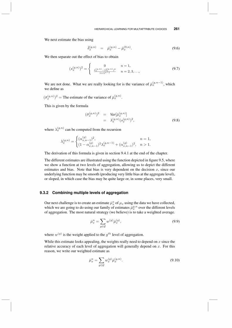
HIERARCHICAL LEARNING FOR MULTIATTRIBUTE CHOICES 261
We next estimate the bias using
δ(g,n)x = µ(g,n)
x − µ(0,n)x . (9.6)
We then separate out the effect of bias to obtain
(s(g,n)x )2 =
0 n = 1,
ν(g,n)x −(δ
(g,n)x )2
1+λn−1 n = 2, 3, . . .,(9.7)
We are not done. What we are really looking for is the variance of µ(g,n−1)x , which
we define as
(σ(g,n)x )2 = The estimate of the variance of µ(g,n)
x .
This is given by the formula
(σ(g,n)x )2 = Var[µ(g,n)
x ]
= λ(g,n)x (s(g,n)
x )2, (9.8)
where λ(g,n)x can be computed from the recursion
λ(g,n)x =
(α
(g)x,n−1)2, n = 1,
(1− α(g)x,n−1)2λ
(g,n−1)x + (α
(g)x,n−1)2, n > 1.
The derivation of this formula is given in section 9.4.1 at the end of the chapter.
The different estimates are illustrated using the function depicted in figure 9.5, wherewe show a function at two levels of aggregation, allowing us to depict the differentestimates and bias. Note that bias is very dependent on the decision x, since ourunderlying function may be smooth (producing very little bias at the aggregate level),or sloped, in which case the bias may be quite large or, in some places, very small.
9.3.2 Combining multiple levels of aggregation
Our next challenge is to create an estimate µnx of µx using the data we have collected,which we are going to do using our family of estimates µg,nx over the different levelsof aggregation. The most natural strategy (we believe) is to take a weighted average.
µnx =∑g∈G
w(g)µ(g)x , (9.9)
where w(g) is the weight applied to the gth level of aggregation.
While this estimate looks appealing, the weights really need to depend on x since therelative accuracy of each level of aggregation will generally depend on x. For thisreason, we write our weighted estimate as
µnx =∑g∈G
w(g)x µ(g,n)
x . (9.10)
262 LARGE CHOICE SETS
f(x)
Aggregated function
Original function
x = point selected
1 Bias x
Errors around disaggregate function
x
Figure 9.5 Illustration of a disaggregate function, an aggregated approximation and a set ofsamples. For a particular state s, we show the estimate and the bias.
If the estimates µ(g,n)x were unbiased, we could show that the best weights are
proportional to the estimates of the variance of µ(g,n)x , which is to say
w(g)x ∝ 1
(σ(g,n)x )2
.
Since the weights should sum to one, we obtain
w(g)x =
(1
(σ(g,n)x )2
)∑g∈G
1
(σ(g,n)x )2
−1
. (9.11)
The problem here is that the estimates µ(g,n)x are clearly not unbiased, but this is easy
to fix using the calculations we presented in the previous section. Instead of usingthe variance, we instead use the variance plus bias squared, where the bias is givenby δ(g,n)
x . This gives us the weighting formula
w(g,n)x ∝ 1(
(σ(g,n)x )2 +
(δ
(g,n)x
)2) (9.12)
Introducing the normalization constant then gives us
w(g,n)x =
1((σ
(g,n)x )2 +
(δ
(g,n)x
)2)∑g′∈G
1((σ
(g′,n)x )2 +
(δ
(g′,n)x
)2)−1
. (9.13)
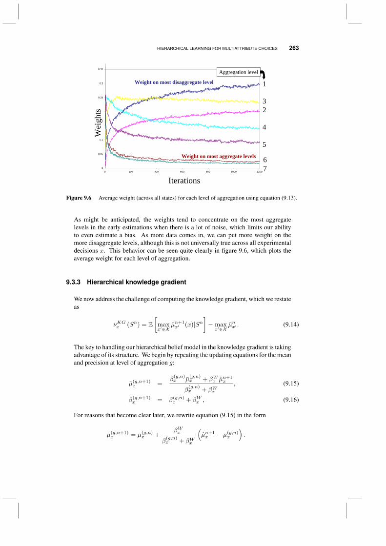
HIERARCHICAL LEARNING FOR MULTIATTRIBUTE CHOICES 263
0
0.05
0.1
0.15
0.2
0.25
0.3
0.35
0 200 400 600 800 1000 1200
Iteration
Wei
ghts
Iterations
Wei
ghts
1
32
4
5
Aggregation level
67
Weight on most disaggregate level
Weight on most aggregate levels
Figure 9.6 Average weight (across all states) for each level of aggregation using equation (9.13).
As might be anticipated, the weights tend to concentrate on the most aggregatelevels in the early estimations when there is a lot of noise, which limits our abilityto even estimate a bias. As more data comes in, we can put more weight on themore disaggregate levels, although this is not universally true across all experimentaldecisions x. This behavior can be seen quite clearly in figure 9.6, which plots theaverage weight for each level of aggregation.
9.3.3 Hierarchical knowledge gradient
We now address the challenge of computing the knowledge gradient, which we restateas
νKGx (Sn) = E[
maxx′∈X
µn+1x′ (x)|Sn
]− maxx′∈X
µnx′ . (9.14)
The key to handling our hierarchical belief model in the knowledge gradient is takingadvantage of its structure. We begin by repeating the updating equations for the meanand precision at level of aggregation g:
µ(g,n+1)x =
β(g,n)x µ
(g,n)x + βWx µn+1
x
β(g,n)x + βWx
, (9.15)
β(g,n+1)x = β(g,n)
x + βWx , (9.16)
For reasons that become clear later, we rewrite equation (9.15) in the form
µ(g,n+1)x = µ(g,n)
x +βWx
β(g,n)x + βWx
(µn+1x − µ(g,n)
x
).

264 LARGE CHOICE SETS
We further rewrite this equation by splitting the second term using
µ(g,n+1)x = µ(g,n)
x +βWx
β(g,n)x + βWx
(µn+1x − µnx
)+
βWx
β(g,n)x + βWx
(µnx − µ(g,n)
x
).
We are next going to rewrite our updating formula as we did in section 4.5 using thestandard normal variable Z,
µ(g,n+1)x = µ(g,n)
x +βWx
β(g,n)x + βWx
(µnx − µ(g,n)
x
)+ σ(g,n)
x Z, (9.17)
where, with some work, we can show that the predictive variance is given by
σ(g,n)x =
βWx√
1
β(g,n)x
+ 1βWx
β(g,n)x + βWx
. (9.18)
We next define the sets
G (x, x′) Set of all aggregation levels that the alternatives x and x′ have in common, withG (x, x′) ⊆ G. In the example in figure 9.4 we have G (2, 3) = 1, 2, since x = 2and x′ = 3 have common points at aggregation levels 1 and 2.
X (g)(x) Set of all alternatives that share the same aggregated alternative G(g)(x) at thegth aggregation level, with X (g)(x) ⊆ X . In the example in figure 9.4 we haveX 1 (4) = 4, 5, 6.
We need to capture the impact of a decision to run experiment x on all the estimatesµx′ for x′ ∈ X . With the hierarchical learning logic, running one experiment x canaffect the estimates of µx′ for all the experiments. This will happen whenever x andx′ share an aggregation level. This might include everything if the highest level ofaggregation is simply a constant baseline over the entire surface. To help with thisprocess, we break our original weighted estimate
µnx =∑g∈G
w(g)x µ(g,n)
x ,
into two parts:
µn+1x′ =
∑g/∈G(x′,x)
w(g,n+1)x′ µ
(g,n+1)x′ +
∑g∈G(x′,x)
w(g,n+1)x′ µ(g,n+1)
x .
After substitution of (9.17) and rearranging gives us
µn+1x′ =
∑g∈G
w(g,n+1)x′ µ
(g,n)x′ +
∑g∈G(x′,x)
w(g,n+1)x′
βWx
β(g,n)x + βWx
(µnx − µ(g,n)
x
)+Z
∑g∈G(x′,x)
w(g,n+1)x′ σ(g,n)
x . (9.19)
HIERARCHICAL LEARNING FOR MULTIATTRIBUTE CHOICES 265
When we run experiment x and observe µnx , we will of course have to update µ(g,n)x
for all aggregation levels g. It is tempting to assume that the weights w(g)x remain
constant, but we found that this did not work, primarily in the early iterations. Forexample, it is natural to initialize w(G)
x = 1 for the highest level of aggregation, butthen we have to understand that an experiment may change this, since otherwise thevalue of information may be zero. For this reason, we have to predict the updatingweights from running experiment x. We approximate the weights using
w(g,n)x′ (x) =
((β
(g,n)x′ + I
(g)x′,xβ
Wx′
)−1
+(β
(g,n)x′
)2)−1
∑g′∈G
((βg′,nx′ + Ig
′
x′,xβWx′
)−1
+(βg′,nx′
)2)−1 , (9.20)
where
I(g)x′,x =
1 if g ∈ G (x′, x)0 otherwise
.
Combining (9.14) with (9.19) and (9.20), gives us the following formula for theknowledge gradient
νKGx (Sn) = E[
maxx′∈X
anx′(x) + bnx′(x)Z|Sn]− maxx′∈X
µnx′ , (9.21)
where
anx′(x) =∑g∈G
w(g,n)
x′ (x)µ(g,n)
x′ +∑
g∈G(x′,x)
w(g,n)
x′ (x)βWx
β(g,n)x + βWx
(µnx − µ(g,n)
x
), (9.22)
bnx′(x) =∑
g∈G(x′,x)
w(g,n)
x′ (x)σ(g,n)x . (9.23)
We now use the procedure described in section 4.5 for the knowledge gradient forcorrelated beliefs, where we have to identify the lines anx′+b
nx′z which are dominated
by the others. We refer to non-dominated lines by anx′ + bnx′z over a reduced set ofalternatives that are now numbered from 1, . . . , M , giving us
νKG,nx =∑
i=1,...,M−1
(bni+1(x)− bni (x)
)f
(−
∣∣∣∣∣ ani (x)− ani+1(x)
bni+1(x)− bni (x)
∣∣∣∣∣), (9.24)
where (as we saw before in chapter 4),
f(ζ) = ζΦ(ζ) + φ(ζ),
where Φ(ζ) is the cumulative normal distribution and φ(ζ) is the standard normaldensity, given respectively by
Φ(ζ) =
∫ ζ
−∞φ(z)dz,
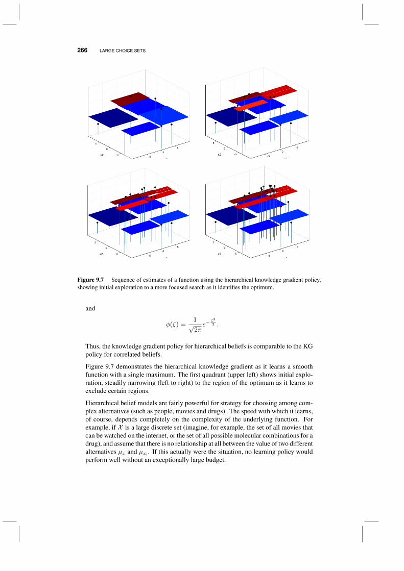
266 LARGE CHOICE SETS
Figure 9.7 Sequence of estimates of a function using the hierarchical knowledge gradient policy,showing initial exploration to a more focused search as it identifies the optimum.
and
φ(ζ) =1√2πe−
ζ2
2 .
Thus, the knowledge gradient policy for hierarchical beliefs is comparable to the KGpolicy for correlated beliefs.
Figure 9.7 demonstrates the hierarchical knowledge gradient as it learns a smoothfunction with a single maximum. The first quadrant (upper left) shows initial explo-ration, steadily narrowing (left to right) to the region of the optimum as it learns toexclude certain regions.
Hierarchical belief models are fairly powerful for strategy for choosing among com-plex alternatives (such as people, movies and drugs). The speed with which it learns,of course, depends completely on the complexity of the underlying function. Forexample, if X is a large discrete set (imagine, for example, the set of all movies thatcan be watched on the internet, or the set of all possible molecular combinations for adrug), and assume that there is no relationship at all between the value of two differentalternatives µx and µx;. If this actually were the situation, no learning policy wouldperform well without an exceptionally large budget.
WHY DOES IT WORK? 267
Fortunately, most real applications (especially large ones) have a lot of structure. Ifthe belief model captures this structure, then a good learning policy can do quite well.The power of the Bayesian knowledge gradient, of course, is that it assumes that westart the process using some prior knowledge, which we want to exploit.
9.4 WHY DOES IT WORK?
From OUU book - needs rewriting
9.4.1 Computing bias and variance
Before we present our methods for hierarchical aggregation, we are going to needsome basic results on bias and variance in statistical estimation. Assume we aretrying to estimate a true but unknown parameter µ which we can observe, but wehave to deal with both bias δ and noise ε, which we write as
µn = µ+ δ + εn. (9.25)
Both the mean µ and bias δ are unknown, but we are going to assume that we havesome way to make a noisy estimate of the bias that we are going to call δn. Later weare going to provide examples of how to get estimates of δ.
Now let µn be our estimate of µ after n observations. We will use the followingrecursive formula for µn
µn = (1− αn−1)µn−1 + αn−1µn.
We are interested in estimating the variance of µn and its bias δn. We start by com-puting the variance of µn. We assume that our observations of µ can be representedusing equation (9.25), where Eεn = 0 and Var[εn] = σ2. With this model, we cancompute the variance of µn using
Var[µn] = λnσ2, (9.26)
where λn can be computed from the simple recursion
λn =
(αn−1)2, n = 1,(1− αn−1)2λn−1 + (αn−1)2, n > 1.
(9.27)
To see this, we start with n = 1. For a given (deterministic) initial estimate µ0, wefirst observe that the variance of µ1 is given by
Var[µ1] = Var[(1− α0)µ0 + α0µ1]
= (α0)2Var[µ1]
= (α0)2σ2.
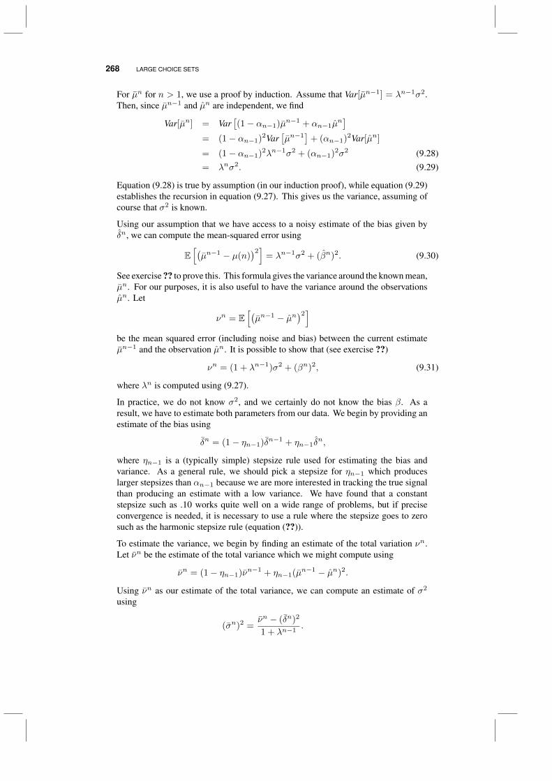
268 LARGE CHOICE SETS
For µn for n > 1, we use a proof by induction. Assume that Var[µn−1] = λn−1σ2.Then, since µn−1 and µn are independent, we find
Var[µn] = Var[(1− αn−1)µn−1 + αn−1µ
n]
= (1− αn−1)2Var[µn−1
]+ (αn−1)2Var[µn]
= (1− αn−1)2λn−1σ2 + (αn−1)2σ2 (9.28)= λnσ2. (9.29)
Equation (9.28) is true by assumption (in our induction proof), while equation (9.29)establishes the recursion in equation (9.27). This gives us the variance, assuming ofcourse that σ2 is known.
Using our assumption that we have access to a noisy estimate of the bias given byδn, we can compute the mean-squared error using
E[(µn−1 − µ(n)
)2]= λn−1σ2 + (βn)2. (9.30)
See exercise ?? to prove this. This formula gives the variance around the known mean,µn. For our purposes, it is also useful to have the variance around the observationsµn. Let
νn = E[(µn−1 − µn
)2]be the mean squared error (including noise and bias) between the current estimateµn−1 and the observation µn. It is possible to show that (see exercise ??)
νn = (1 + λn−1)σ2 + (βn)2, (9.31)
where λn is computed using (9.27).
In practice, we do not know σ2, and we certainly do not know the bias β. As aresult, we have to estimate both parameters from our data. We begin by providing anestimate of the bias using
δn = (1− ηn−1)δn−1 + ηn−1δn,
where ηn−1 is a (typically simple) stepsize rule used for estimating the bias andvariance. As a general rule, we should pick a stepsize for ηn−1 which produceslarger stepsizes than αn−1 because we are more interested in tracking the true signalthan producing an estimate with a low variance. We have found that a constantstepsize such as .10 works quite well on a wide range of problems, but if preciseconvergence is needed, it is necessary to use a rule where the stepsize goes to zerosuch as the harmonic stepsize rule (equation (??)).
To estimate the variance, we begin by finding an estimate of the total variation νn.Let νn be the estimate of the total variance which we might compute using
νn = (1− ηn−1)νn−1 + ηn−1(µn−1 − µn)2.
Using νn as our estimate of the total variance, we can compute an estimate of σ2
using
(σn)2 =νn − (δn)2
1 + λn−1.

BIBLIOGRAPHIC NOTES 269
We can use (σn)2 in equation (9.26) to obtain an estimate of the variance of µn.
If we are doing true averaging (as would occur if we use a stepsize of 1/n), we canget a more precise estimate of the variance for small samples by using the recursiveform of the small sample formula for the variance
(σ2)n =n− 2
n− 1(σ2)n−1 +
1
n(µn−1 − µn)2. (9.32)
The quantity (σ2)n is an estimate of the variance of µn. The variance of our estimateµn is computed using
(σ2)n =1
n(σ2)n.
We are going to draw on these results in two settings, which are both distinguishedby how estimates of the bias δn are computed:
Hierarchical aggregation We are going to estimate a function at different levels of ag-gregation. We can assume that the estimate of the function at the most disaggregatelevel is noisy but unbiased, and then let the difference between the function at somelevel of aggregation and the function at the most disaggregate level as an estimate ofthe bias.
Transient functions Later, we are going to use these results to approximate value func-tions. It is the nature of algorithms for estimating value functions that the underlyingprocess varies over time (see see this most clearly in chapter ??). In this setting, weare making observations from a truth that is changing over time, which introduces abias.
9.5 BIBLIOGRAPHIC NOTES
Section ?? - See also Miller (2002) for additional applications of subset selection instatistics, and Horrace et al. (2008) for applications in economics.
Section 9.2.4 - The energy portfolio application is also considered by Ryzhov & Powell(2009c) and Ryzhov & Powell (2009b). The latter reference also first proposes theMonte Carlo KG policy. The recursive updating equation for the square root matrixcan be found e.g. in Kaminski et al. (1971).
PROBLEMS
9.1 There are six primary drugs that can be used to treat diabetes, and these are oftenprescribed in groups of three at a time. There are 20 ways of choosing three drugsfrom a set of six (known as a “cocktail”), assuming all possible combinations makesense. Enumerate these 20 cocktails, and create a covariance matrix Σ where entryΣij = σ2Nij , where Nij is the number of drugs in common between drug cocktail iand drug cocktail j (so, 0 ≤ Nij ≤ 3). Let σ2 = .352 be the variance in our prior
270 LARGE CHOICE SETS
distribution of belief about the effect of a drug cocktail. Finally, let σ2ε = .552 be the
variance of an observation.
Assume that our prior on the blood sugar level produced by each cocktail is the sameand is equal to 5.0.
a) Randomly generate a truth from this prior for each cocktail. Create the covari-ance matrix and use the knowledge gradient for correlated beliefs to search for thebest cocktail using N = 20 experiments. You may use the MATLAB code (firstintroduced in Chapter 4) that can be downloaded from.
http://optimallearning.princeton.edu/exercises/KGCorrBeliefs.m
An example illustration of the KGCB algorithm is given in
http://optimallearning.princeton.edu/exercises/KGCorrBeliefsEx.m
b) Now repeat (a) for 100 different truths, and summarize how well you discover eachtruth using 20 observations.
c) Next we are going to use the methods described in this chapter to solve a much largerproblem, but we are going to use them on this small test problem. Repeat (a), but thistime you are going to randomly sample 5 out of the 20 combinations, and limit yourcalculation of the KG factor to these three (the easiest way to modify the code is tocompute the knowledge gradient for all 20 as you are doing, but then choose a subsetof 5, and finally choose the drug cocktail with the best knowledge gradient out ofthese five). Perform N = 100 samples and compare the performance to the resultsyou obtained when you computed the knowledge gradient for all the alternatives.
d) Finally, repeat (d) for all 100 truths and report on the average performance.
9.2 Verify that 9.4 produces a valid square root matrix, that is, Cn+1(Cn+1
)T=
Σn+1.
CHAPTER 10
OPTIMIZING A SCALAR FUNCTION
Optimizing scalar functions arises in a variety of settings, such as choosing the priceof a product, the amount of memory in a computer, the temperature of a chemicalprocess or the diameter of the tube in an aerosol gun. It can even be used foroptimizing a tunable parameter in a learning policy! Important special cases arefunctions which are unimodular, as depicted in Figure 10.1, where there is a singlelocal maximum, or concave. In this chapter, we review some specialized algorithmsdesigned for this particular problem class.
We begin our presentation using an unusual problem setting for this volume, whichis an unknown but deterministic function which can be measured perfectly. We thentransition back to our more familiar setting of noisy functions.
10.1 DETERMINISTIC EXPERIMENTS
We are going to consider three settings where we wish to find the best estimate of theoptimum of a deterministic, unimodular function within a given experimental budget.The settings include
• Differentiable functions.
• Nondifferentiable functions, with a finite experimental budget.
Optimal Learning. By Warren B. Powell and Ilya O. RyzhovCopyright c© 2018 John Wiley & Sons, Inc.
271
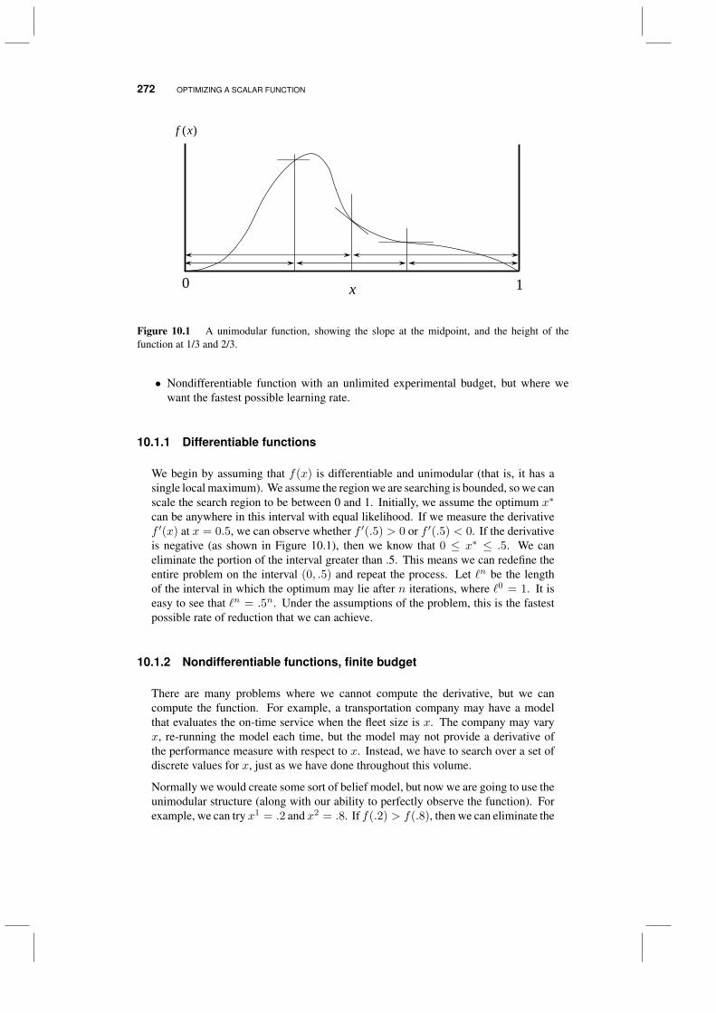
272 OPTIMIZING A SCALAR FUNCTION
x
( )f x
0 1
Figure 10.1 A unimodular function, showing the slope at the midpoint, and the height of thefunction at 1/3 and 2/3.
• Nondifferentiable function with an unlimited experimental budget, but where wewant the fastest possible learning rate.
10.1.1 Differentiable functions
We begin by assuming that f(x) is differentiable and unimodular (that is, it has asingle local maximum). We assume the region we are searching is bounded, so we canscale the search region to be between 0 and 1. Initially, we assume the optimum x∗
can be anywhere in this interval with equal likelihood. If we measure the derivativef ′(x) at x = 0.5, we can observe whether f ′(.5) > 0 or f ′(.5) < 0. If the derivativeis negative (as shown in Figure 10.1), then we know that 0 ≤ x∗ ≤ .5. We caneliminate the portion of the interval greater than .5. This means we can redefine theentire problem on the interval (0, .5) and repeat the process. Let `n be the lengthof the interval in which the optimum may lie after n iterations, where `0 = 1. It iseasy to see that `n = .5n. Under the assumptions of the problem, this is the fastestpossible rate of reduction that we can achieve.
10.1.2 Nondifferentiable functions, finite budget
There are many problems where we cannot compute the derivative, but we cancompute the function. For example, a transportation company may have a modelthat evaluates the on-time service when the fleet size is x. The company may varyx, re-running the model each time, but the model may not provide a derivative ofthe performance measure with respect to x. Instead, we have to search over a set ofdiscrete values for x, just as we have done throughout this volume.
Normally we would create some sort of belief model, but now we are going to use theunimodular structure (along with our ability to perfectly observe the function). Forexample, we can try x1 = .2 and x2 = .8. If f(.2) > f(.8), then we can eliminate the
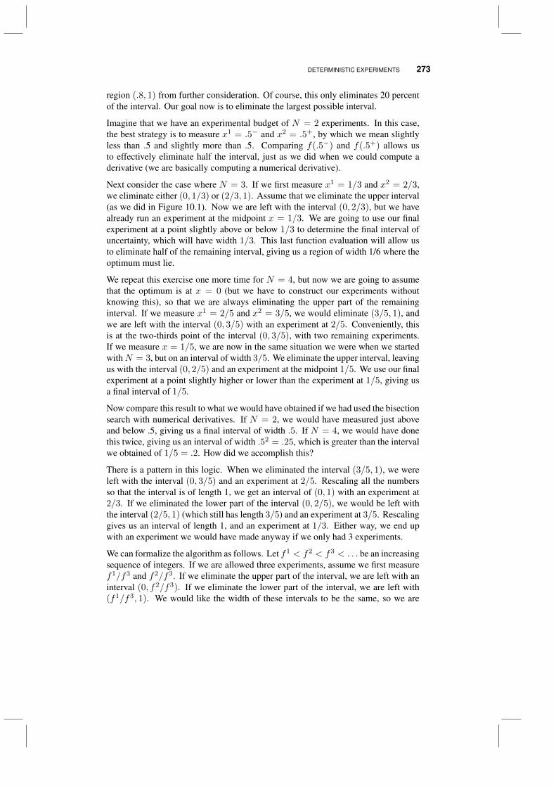
DETERMINISTIC EXPERIMENTS 273
region (.8, 1) from further consideration. Of course, this only eliminates 20 percentof the interval. Our goal now is to eliminate the largest possible interval.
Imagine that we have an experimental budget of N = 2 experiments. In this case,the best strategy is to measure x1 = .5− and x2 = .5+, by which we mean slightlyless than .5 and slightly more than .5. Comparing f(.5−) and f(.5+) allows usto effectively eliminate half the interval, just as we did when we could compute aderivative (we are basically computing a numerical derivative).
Next consider the case where N = 3. If we first measure x1 = 1/3 and x2 = 2/3,we eliminate either (0, 1/3) or (2/3, 1). Assume that we eliminate the upper interval(as we did in Figure 10.1). Now we are left with the interval (0, 2/3), but we havealready run an experiment at the midpoint x = 1/3. We are going to use our finalexperiment at a point slightly above or below 1/3 to determine the final interval ofuncertainty, which will have width 1/3. This last function evaluation will allow usto eliminate half of the remaining interval, giving us a region of width 1/6 where theoptimum must lie.
We repeat this exercise one more time for N = 4, but now we are going to assumethat the optimum is at x = 0 (but we have to construct our experiments withoutknowing this), so that we are always eliminating the upper part of the remaininginterval. If we measure x1 = 2/5 and x2 = 3/5, we would eliminate (3/5, 1), andwe are left with the interval (0, 3/5) with an experiment at 2/5. Conveniently, thisis at the two-thirds point of the interval (0, 3/5), with two remaining experiments.If we measure x = 1/5, we are now in the same situation we were when we startedwithN = 3, but on an interval of width 3/5. We eliminate the upper interval, leavingus with the interval (0, 2/5) and an experiment at the midpoint 1/5. We use our finalexperiment at a point slightly higher or lower than the experiment at 1/5, giving usa final interval of 1/5.
Now compare this result to what we would have obtained if we had used the bisectionsearch with numerical derivatives. If N = 2, we would have measured just aboveand below .5, giving us a final interval of width .5. If N = 4, we would have donethis twice, giving us an interval of width .52 = .25, which is greater than the intervalwe obtained of 1/5 = .2. How did we accomplish this?
There is a pattern in this logic. When we eliminated the interval (3/5, 1), we wereleft with the interval (0, 3/5) and an experiment at 2/5. Rescaling all the numbersso that the interval is of length 1, we get an interval of (0, 1) with an experiment at2/3. If we eliminated the lower part of the interval (0, 2/5), we would be left withthe interval (2/5, 1) (which still has length 3/5) and an experiment at 3/5. Rescalinggives us an interval of length 1, and an experiment at 1/3. Either way, we end upwith an experiment we would have made anyway if we only had 3 experiments.
We can formalize the algorithm as follows. Let f1 < f2 < f3 < . . . be an increasingsequence of integers. If we are allowed three experiments, assume we first measuref1/f3 and f2/f3. If we eliminate the upper part of the interval, we are left with aninterval (0, f2/f3). If we eliminate the lower part of the interval, we are left with(f1/f3, 1). We would like the width of these intervals to be the same, so we are
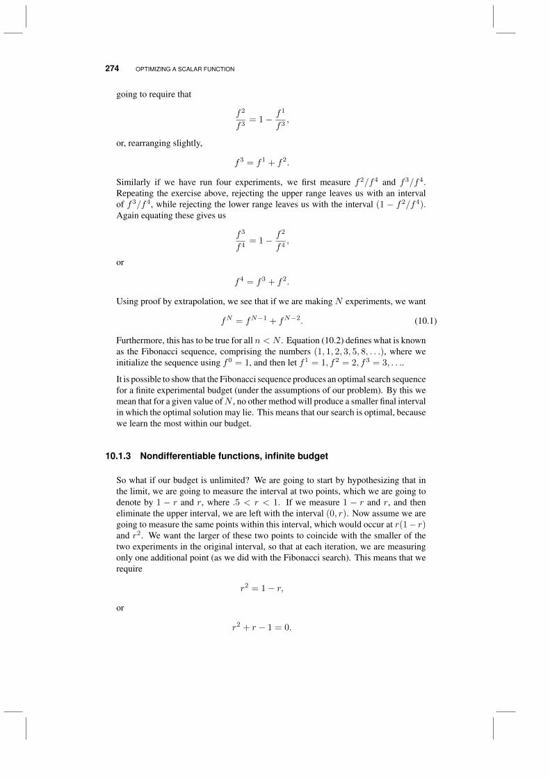
274 OPTIMIZING A SCALAR FUNCTION
going to require that
f2
f3= 1− f1
f3,
or, rearranging slightly,
f3 = f1 + f2.
Similarly if we have run four experiments, we first measure f2/f4 and f3/f4.Repeating the exercise above, rejecting the upper range leaves us with an intervalof f3/f4, while rejecting the lower range leaves us with the interval (1 − f2/f4).Again equating these gives us
f3
f4= 1− f2
f4,
or
f4 = f3 + f2.
Using proof by extrapolation, we see that if we are making N experiments, we want
fN = fN−1 + fN−2. (10.1)
Furthermore, this has to be true for all n < N . Equation (10.2) defines what is knownas the Fibonacci sequence, comprising the numbers (1, 1, 2, 3, 5, 8, . . .), where weinitialize the sequence using f0 = 1, and then let f1 = 1, f2 = 2, f3 = 3, . . ..
It is possible to show that the Fibonacci sequence produces an optimal search sequencefor a finite experimental budget (under the assumptions of our problem). By this wemean that for a given value ofN , no other method will produce a smaller final intervalin which the optimal solution may lie. This means that our search is optimal, becausewe learn the most within our budget.
10.1.3 Nondifferentiable functions, infinite budget
So what if our budget is unlimited? We are going to start by hypothesizing that inthe limit, we are going to measure the interval at two points, which we are going todenote by 1 − r and r, where .5 < r < 1. If we measure 1 − r and r, and theneliminate the upper interval, we are left with the interval (0, r). Now assume we aregoing to measure the same points within this interval, which would occur at r(1− r)and r2. We want the larger of these two points to coincide with the smaller of thetwo experiments in the original interval, so that at each iteration, we are measuringonly one additional point (as we did with the Fibonacci search). This means that werequire
r2 = 1− r,
or
r2 + r − 1 = 0.
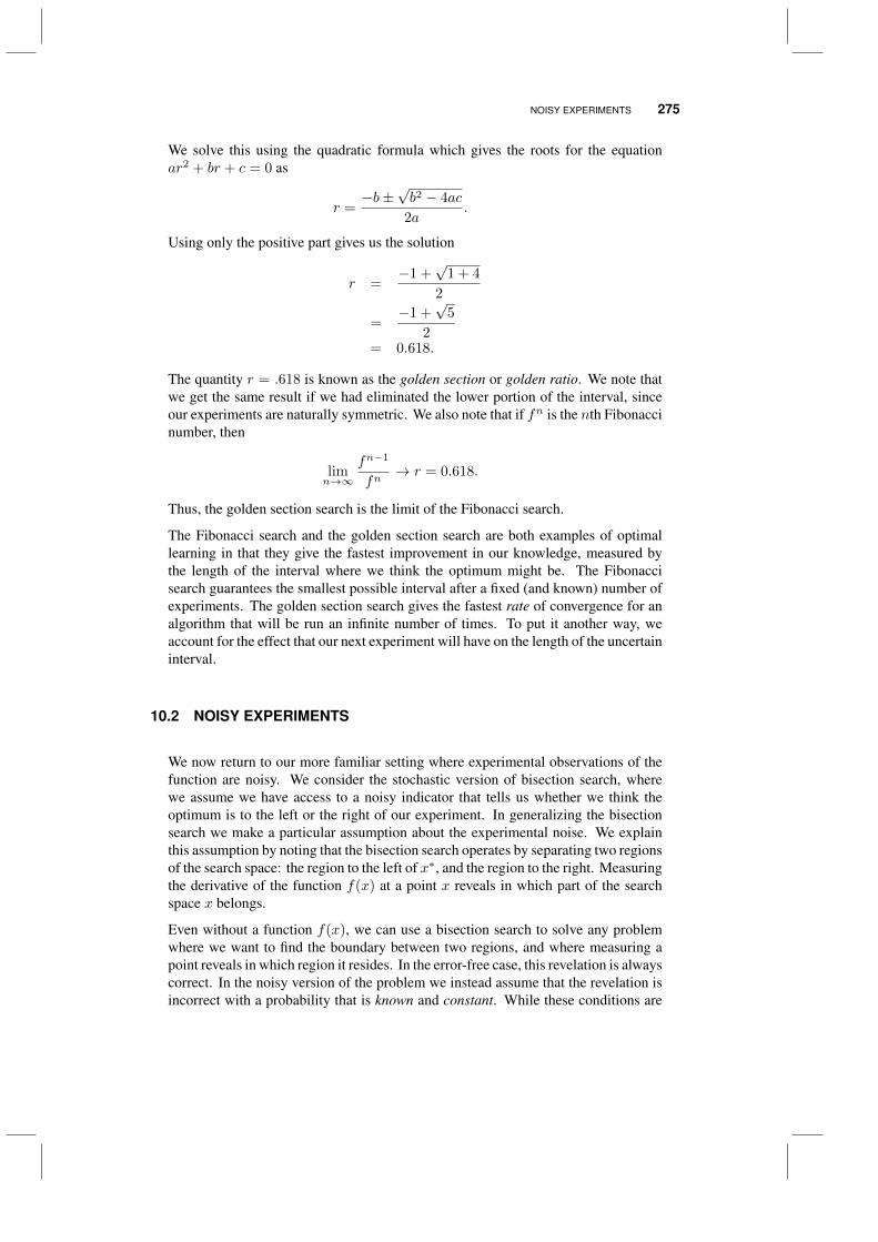
NOISY EXPERIMENTS 275
We solve this using the quadratic formula which gives the roots for the equationar2 + br + c = 0 as
r =−b±
√b2 − 4ac
2a.
Using only the positive part gives us the solution
r =−1 +
√1 + 4
2
=−1 +
√5
2= 0.618.
The quantity r = .618 is known as the golden section or golden ratio. We note thatwe get the same result if we had eliminated the lower portion of the interval, sinceour experiments are naturally symmetric. We also note that if fn is the nth Fibonaccinumber, then
limn→∞
fn−1
fn→ r = 0.618.
Thus, the golden section search is the limit of the Fibonacci search.
The Fibonacci search and the golden section search are both examples of optimallearning in that they give the fastest improvement in our knowledge, measured bythe length of the interval where we think the optimum might be. The Fibonaccisearch guarantees the smallest possible interval after a fixed (and known) number ofexperiments. The golden section search gives the fastest rate of convergence for analgorithm that will be run an infinite number of times. To put it another way, weaccount for the effect that our next experiment will have on the length of the uncertaininterval.
10.2 NOISY EXPERIMENTS
We now return to our more familiar setting where experimental observations of thefunction are noisy. We consider the stochastic version of bisection search, wherewe assume we have access to a noisy indicator that tells us whether we think theoptimum is to the left or the right of our experiment. In generalizing the bisectionsearch we make a particular assumption about the experimental noise. We explainthis assumption by noting that the bisection search operates by separating two regionsof the search space: the region to the left of x∗, and the region to the right. Measuringthe derivative of the function f(x) at a point x reveals in which part of the searchspace x belongs.
Even without a function f(x), we can use a bisection search to solve any problemwhere we want to find the boundary between two regions, and where measuring apoint reveals in which region it resides. In the error-free case, this revelation is alwayscorrect. In the noisy version of the problem we instead assume that the revelation isincorrect with a probability that is known and constant. While these conditions are
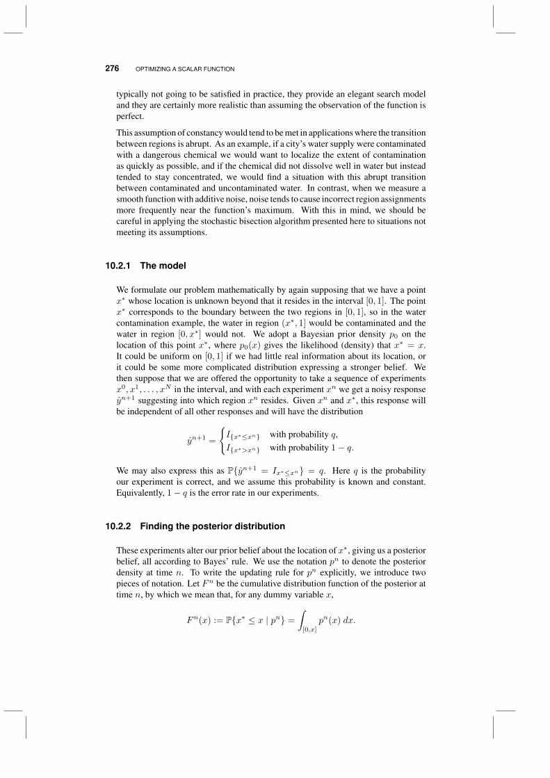
276 OPTIMIZING A SCALAR FUNCTION
typically not going to be satisfied in practice, they provide an elegant search modeland they are certainly more realistic than assuming the observation of the function isperfect.
This assumption of constancy would tend to be met in applications where the transitionbetween regions is abrupt. As an example, if a city’s water supply were contaminatedwith a dangerous chemical we would want to localize the extent of contaminationas quickly as possible, and if the chemical did not dissolve well in water but insteadtended to stay concentrated, we would find a situation with this abrupt transitionbetween contaminated and uncontaminated water. In contrast, when we measure asmooth function with additive noise, noise tends to cause incorrect region assignmentsmore frequently near the function’s maximum. With this in mind, we should becareful in applying the stochastic bisection algorithm presented here to situations notmeeting its assumptions.
10.2.1 The model
We formulate our problem mathematically by again supposing that we have a pointx∗ whose location is unknown beyond that it resides in the interval [0, 1]. The pointx∗ corresponds to the boundary between the two regions in [0, 1], so in the watercontamination example, the water in region (x∗, 1] would be contaminated and thewater in region [0, x∗] would not. We adopt a Bayesian prior density p0 on thelocation of this point x∗, where p0(x) gives the likelihood (density) that x∗ = x.It could be uniform on [0, 1] if we had little real information about its location, orit could be some more complicated distribution expressing a stronger belief. Wethen suppose that we are offered the opportunity to take a sequence of experimentsx0, x1, . . . , xN in the interval, and with each experiment xn we get a noisy responseyn+1 suggesting into which region xn resides. Given xn and x∗, this response willbe independent of all other responses and will have the distribution
yn+1 =
Ix∗≤xn with probability q,Ix∗>xn with probability 1− q.
We may also express this as Pyn+1 = Ix∗≤xn = q. Here q is the probabilityour experiment is correct, and we assume this probability is known and constant.Equivalently, 1− q is the error rate in our experiments.
10.2.2 Finding the posterior distribution
These experiments alter our prior belief about the location of x∗, giving us a posteriorbelief, all according to Bayes’ rule. We use the notation pn to denote the posteriordensity at time n. To write the updating rule for pn explicitly, we introduce twopieces of notation. Let Fn be the cumulative distribution function of the posterior attime n, by which we mean that, for any dummy variable x,
Fn(x) := Px∗ ≤ x | pn =
∫[0,x]
pn(x) dx.

NOISY EXPERIMENTS 277
We may also think of Fn(x) as giving the probability that x is in the region to theleft of x∗, and in our water contamination example as giving the probability that thewater at x is not contaminated. As our second piece of notation, let g be the functiondefined by g(a, 1) = a and g(a, 0) = 1 − a, where a will be a probability (such asthe probability the true value is to the left or the right). Now we are ready to computeour updating rule.
Noting that nature’s correct response to the experiment xn would be Ix∗≤xn, wewrite
Pyn+1 = y | x∗, xn =
q if y = Ix∗≤xn
1− q if y 6= Ix∗≤xn
= g(q, Iy=Ix∗≤xn).
So, g(q, 1) = q corresponds to two cases: either xn < x∗, and we observe yn+1 = 1which correctly indicates that the optimum x∗ is greater than our measured point; orxn > x∗, and yn+1 = 0, which correctly indicates that the optimum x∗ is less thanour measured point. The outcome g(q, 0) = 1 − q corresponds to the opposite ofboth of these cases.
We may also write
Pyn+1 = y | pn = Px∗ ≤ xn | pnPyn+1 = y | x∗ ≤ xn+Px∗ > xn | pnPyn+1 = y | x∗ > xn
= Fn(xn)g(q, y) + (1− Fn(xn))g(1− q, y)
= g(qFn(xn) + (1− q)(1− Fn(xn)), y),
where the last line may be seen by considering the cases y = 0 and y = 1 separately.Fixing some dummy variable y, we may then use Bayes’ rule and these two relationsto write,
pn+1(x) dx = Px∗ ∈ dx | pn, yn+1 = y
=Pyn+1 = y | pn, x∗ = xPx∗ ∈ dx | pn
Pyn+1 = y | pn
=g(q, Iy=Ix≤xn
)g (qFn(xn) + (1− q)(1− Fn(xn)), y)
pn(x) dx.
Substituting yn+1 for y shows that our updating rule is
pn+1(x) =g(q, Iyn+1=Ix≤xn
)g (qFn(xn) + (1− q)(1− Fn(xn)), yn+1)
pn(x). (10.2)
The essential content of this updating rule is as follows. Our observation, if correct,would tell us into what region xn lies and would tell us whether x∗ is to the left orright of the experiment xn. Let us give the name “suggested region" to the regionin which the observation, if correct, would indicate x∗ resides. Since we know thatthe observation is only correct with probability q, we multiply the density in the

278 OPTIMIZING A SCALAR FUNCTION
.6nx
( ) .6nF x 1ˆ 1
,1n
nx xy
g q
.6nx
q
1 q
1
0
nx x
nx x10
(a) (b)
1ˆ 1
,1n
nx xy
g q
.6nx
q
1 q
1
0
nx x
nx x0 1 .6nx
(c) (d)
Figure 10.2 Illustration of the effect of an observation of y for xn = .6, starting with an initialuniform prior (a). (b) and (c) show the new beliefs for y = 1 and y = 0. The updated distributionpn+1(x) is given in (d).
suggested region by q and the density in the other region by 1−q. This leaves us witha density which does not integrate to 1, so we then finish the update by normalizing.
As a numerical example, assume that q = .7, xn = .6, and that we observe yn+1 = 1.Assume that the distribution pn(x) is uniform, as depicted in Figure 10.2(a). Figures10.2(b) and 10.2(c) show the conditional distribution given yn+1 = 1 and yn+1 = 0,respectively. Finally, Figure 10.2(d) shows the updated distribution for pn+1 givenyn+1 = 1, overlaid on top of the original uniform distribution for pn(x). Thisdistribution is computed using
pn+1(x) =
g(.7,1)
g(.7(.6)+.3(.4),0)pn(x) = 0.7
.54pn(x) = 1.296pn(x) x < xn
g(.7,0)g(.7(.6)+.3(.4),0)p
n(x) = 0.3.54p
n(x) = 0.556pn(x) x > xn.
Let us briefly consider the case when our observations are always correct. Thenq = 1 and we are back in the deterministic case. Suppose for the moment that pn isuniform on some interval (an, bn]. Then our updating rule can be simplified to
pn+1(x) =g(
1, Iyn+1=Iu≤xn)
g(Fn(xn)), yn+1)
Ix∈[an,bn]
bn − an=
Ix∈(an,xn]xn−an if yn+1 = 1,
Ix∈(xn,bn]bn−xn if yn+1 = 0..
Thus we see that the posterior is now still uniform but on some smaller interval,where either the points to the left or right of xn have been removed. Thus, if webegin with a uniform prior, i.e., with p0(x) = Ix∈[0,1], then our posterior at eachtime will again be uniform on a smaller interval. Comparing our knowledge in thedeterministic case, where we had an interval in which we knew x∗ resided, to ourknowledge here suggests that a natural way to express knowledge that x∗ lies in aninterval is through a uniform probability distribution on that interval.
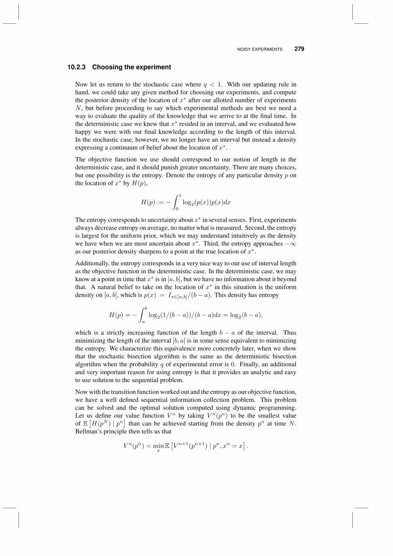
NOISY EXPERIMENTS 279
10.2.3 Choosing the experiment
Now let us return to the stochastic case where q < 1. With our updating rule inhand, we could take any given method for choosing our experiments, and computethe posterior density of the location of x∗ after our allotted number of experimentsN , but before proceeding to say which experimental methods are best we need away to evaluate the quality of the knowledge that we arrive to at the final time. Inthe deterministic case we knew that x∗ resided in an interval, and we evaluated howhappy we were with our final knowledge according to the length of this interval.In the stochastic case, however, we no longer have an interval but instead a densityexpressing a continuum of belief about the location of x∗.
The objective function we use should correspond to our notion of length in thedeterministic case, and it should punish greater uncertainty. There are many choices,but one possibility is the entropy. Denote the entropy of any particular density p onthe location of x∗ by H(p),
H(p) := −∫ 1
0
log2(p(x))p(x)dx
The entropy corresponds to uncertainty about x∗ in several senses. First, experimentsalways decrease entropy on average, no matter what is measured. Second, the entropyis largest for the uniform prior, which we may understand intuitively as the densitywe have when we are most uncertain about x∗. Third, the entropy approaches −∞as our posterior density sharpens to a point at the true location of x∗.
Additionally, the entropy corresponds in a very nice way to our use of interval lengthas the objective function in the deterministic case. In the deterministic case, we mayknow at a point in time that x∗ is in [a, b], but we have no information about it beyondthat. A natural belief to take on the location of x∗ in this situation is the uniformdensity on [a, b], which is p(x) = Ix∈[a,b]/(b− a). This density has entropy
H(p) = −∫ b
a
log2(1/(b− a))/(b− a)dx = log2(b− a),
which is a strictly increasing function of the length b − a of the interval. Thusminimizing the length of the interval [b, a] is in some sense equivalent to minimizingthe entropy. We characterize this equivalence more concretely later, when we showthat the stochastic bisection algorithm is the same as the deterministic bisectionalgorithm when the probability q of experimental error is 0. Finally, an additionaland very important reason for using entropy is that it provides an analytic and easyto use solution to the sequential problem.
Now with the transition function worked out and the entropy as our objective function,we have a well defined sequential information collection problem. This problemcan be solved and the optimal solution computed using dynamic programming.Let us define our value function V n by taking V n(pn) to be the smallest valueof E
[H(pN ) | pn
]than can be achieved starting from the density pn at time N .
Bellman’s principle then tells us that
V n(pn) = minx
E[V n+1(pn+1) | pn, xn = x
].
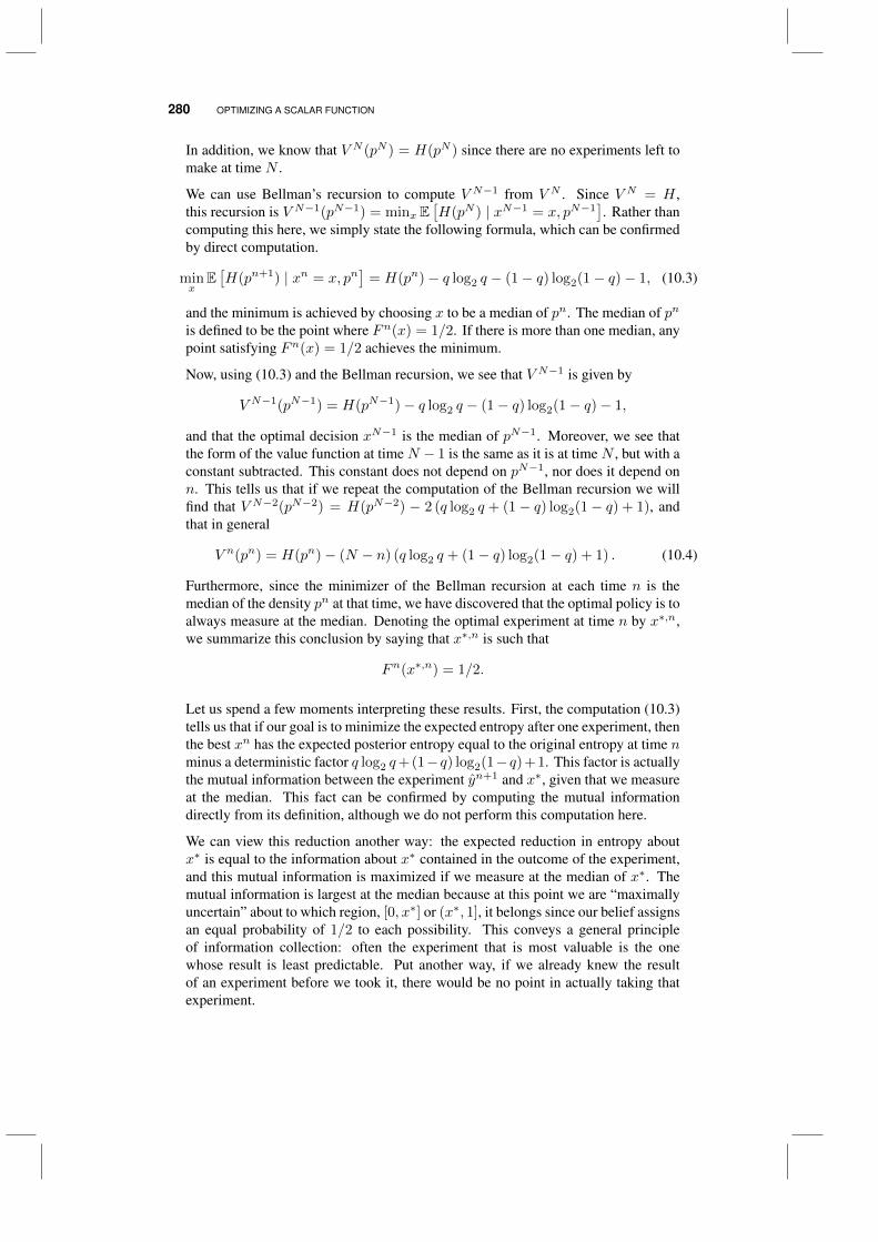
280 OPTIMIZING A SCALAR FUNCTION
In addition, we know that V N (pN ) = H(pN ) since there are no experiments left tomake at time N .
We can use Bellman’s recursion to compute V N−1 from V N . Since V N = H ,this recursion is V N−1(pN−1) = minx E
[H(pN ) | xN−1 = x, pN−1
]. Rather than
computing this here, we simply state the following formula, which can be confirmedby direct computation.
minx
E[H(pn+1) | xn = x, pn
]= H(pn)− q log2 q − (1− q) log2(1− q)− 1, (10.3)
and the minimum is achieved by choosing x to be a median of pn. The median of pn
is defined to be the point where Fn(x) = 1/2. If there is more than one median, anypoint satisfying Fn(x) = 1/2 achieves the minimum.
Now, using (10.3) and the Bellman recursion, we see that V N−1 is given by
V N−1(pN−1) = H(pN−1)− q log2 q − (1− q) log2(1− q)− 1,
and that the optimal decision xN−1 is the median of pN−1. Moreover, we see thatthe form of the value function at time N − 1 is the same as it is at time N , but with aconstant subtracted. This constant does not depend on pN−1, nor does it depend onn. This tells us that if we repeat the computation of the Bellman recursion we willfind that V N−2(pN−2) = H(pN−2) − 2 (q log2 q + (1− q) log2(1− q) + 1), andthat in general
V n(pn) = H(pn)− (N − n) (q log2 q + (1− q) log2(1− q) + 1) . (10.4)
Furthermore, since the minimizer of the Bellman recursion at each time n is themedian of the density pn at that time, we have discovered that the optimal policy is toalways measure at the median. Denoting the optimal experiment at time n by x∗,n,we summarize this conclusion by saying that x∗,n is such that
Fn(x∗,n) = 1/2.
Let us spend a few moments interpreting these results. First, the computation (10.3)tells us that if our goal is to minimize the expected entropy after one experiment, thenthe best xn has the expected posterior entropy equal to the original entropy at time nminus a deterministic factor q log2 q+(1− q) log2(1− q)+1. This factor is actuallythe mutual information between the experiment yn+1 and x∗, given that we measureat the median. This fact can be confirmed by computing the mutual informationdirectly from its definition, although we do not perform this computation here.
We can view this reduction another way: the expected reduction in entropy aboutx∗ is equal to the information about x∗ contained in the outcome of the experiment,and this mutual information is maximized if we measure at the median of x∗. Themutual information is largest at the median because at this point we are “maximallyuncertain” about to which region, [0, x∗] or (x∗, 1], it belongs since our belief assignsan equal probability of 1/2 to each possibility. This conveys a general principleof information collection: often the experiment that is most valuable is the onewhose result is least predictable. Put another way, if we already knew the resultof an experiment before we took it, there would be no point in actually taking thatexperiment.

BIBLIOGRAPHIC NOTES 281
Then, the formula (10.4) shows that this general principle applies not just to singlebut multiple experiments. That is, the best we can do is to measure each time at themedian of our belief, which is the experiment whose outcome is most uncertain, andthe resulting decrease in expected entropy of x∗ is equal to the sum of the mutualinformation in all the experimental outcomes combined. From experiment n onward,this decrease is (N − n) (q log2 q + (1− q) log2(1− q) + 1) since there are N − nexperiments left to make and each contributes q log2 q + (1− q) log2(1− q) + 1.
We may also gain insight by taking the special case q = 1 and comparing to thedeterministic case. As previously noted, when q = 1 and when we begin with auniform prior on [0, 1], the posterior remains uniform on a smaller interval. Then,the median of any such uniform posterior is simply the middle of the interval, and sowe again always measure in the middle of the current interval, just as we did withdeterministic bisection. Thus we see that the stochastic bisection algorithm reducesin the error-free case to exactly the classic bisection algorithm.
10.2.4 Discussion
We make one additional note about the usefulness of the stochastic bisection algorithmwhen our objective function is something different than the entropy objective wehave assumed here. Although we have not shown it here, the decrease in entropy oneobtains from measuring at the median is deterministic, even though the final densitypN itself is certainly random. This is similar to the situation in the deterministic case,where the location of the final interval containing x∗ is unknown a priori, but thelength of that interval is deterministic as long as we use the bisection rule.
This is a very nice property because it means that the optimal policy for the entropyobjective function is also optimal for a broader class of objective functions. Inparticular, if our objective function is E[L(H(pN ))], where L is some concaveincreasing function, then again one can show that the same stochastic bisection ruleis optimal. We can think of L as inducing some kind of risk aversion, in that using itwould indicate we fear uncertainty about x∗more than than we hope for certainty. Forexample, earlier we saw that the length of an interval is equal to the logarithm of theentropy of a uniform distribution on this interval, and so if we wanted to minimizethe length of the final interval in the deterministic case, then perhaps we shouldminimize the logarithm of the entropy rather than just the entropy. But we havealready minimized using this criterion, since the logarithm is concave and increasingand the stochastic bisection algorithm is optimal for this objective function as well.
10.3 BIBLIOGRAPHIC NOTES
Section 10.1 - For a proof of the optimality of the Fibonacci search sequence for unimodularfunctions, see Avriel & Wilde (1966).
Section 10.2 - The development in this section is due to Jedynak et al. (2011).

282 OPTIMIZING A SCALAR FUNCTION
PROBLEMS
10.1 How many iterations of a Fibonacci search sequence are needed to ensure thatwe can find the optimum of a unimodular function within 1 percent?
10.2 Consider the function f(x|α, β) = xα−1(1− x)β−1 for 0 ≤ x ≤ 1.0. Performthe Fibonacci search to find the optimum of this function for the following values of(α, β).
a) α = 8, β = 2.
b) α = 3, β = 12.
c) α = 6, β = 8.
10.3 Repeat exercise 10.2 using the golden section search.
10.4 Assume that we are trying to find the maximum of the function f(x) = x6(1−x)2, but now we are going to assume that we can compute the derivative.
a) Using the derivative to indicate whether the optimum is to the left or the right, performeight iterations of deterministic bisection search and report your best estimate of theoptimal solution. Plot your distribution of belief describing where the optimum liesafter eight observations.
b) Now assume that we can estimate the sign of the derivative correction with probabilityq = .70 (even though we are computing it perfectly). Use the method described inSection 10.2 to find the optimum. Again plot your distribution of belief describingthe location of the optimum.
c) How would your answer to (b) change if q = .5? You should be able to answer thiswithout repeating any of the calculations.

CHAPTER 11
STOPPING PROBLEMS
Stopping problems are a simple but important class of learning problems. In thisproblem class, information arrives over time, and we have to choose whether to viewthe information or stop and make a decision. In this setting, “learning” means tocontinue to continue to receive information. We do not choose which information toobserve, as we have done in the past, but we do have to decide whether to continueobserving or stop and make a decision.
In this chapter we consider two classical stopping problems. The first is the sequentialprobability ratio test, where we have to quickly identify when a signal from somesource is changing. The second is a classic problem known as the secretary problem,where we have to find the best out of a sequence of offers which arrive one at a time.
This chapter will illustrate learning using very different tools than we have seen up tonow. Optimal stopping problems are both a very important problem class, as well asbeing a very special case which offers structure that we can exploit to derive optimalpolicies, rather than the well tuned approximations that have been the focus of thebook until now.
Optimal Learning. By Warren B. Powell and Ilya O. RyzhovCopyright c© 2018 John Wiley & Sons, Inc.
283

284 STOPPING PROBLEMS
11.1 SEQUENTIAL PROBABILITY RATIO TEST
A fundamental problem arises when we need to decide as quickly as possible whensomething is changing. For example, we may think we are observing data beinggenerated by the sequence
Wn = µ0 + εn (11.1)
where we assume that ε is normally distributed with mean 0 and variance σ2. But weare aware that the mean might change to µ1, which means the observations wouldcome from the model
Wn = µ1 + εn. (11.2)
We would like to design a method that allows us to determine when the mean haschanged as quickly as possible.
A more general statement of the problem would be that the observations Wn arecoming from an initial model that we refer to as the null hypothesis H0. We thenwant to determine when the data is coming from a different model that we refer to asthe alternative hypothesis, H1. We start with a prior probability ρ0 = ρ0
0 that H0 istrue. Similarly, ρ0
1 is our prior probability that H1 is true. After we observe W 1, wewould update our prior using Bayes’ rule to obtain
ρ10 = P (H0|W 1)
=P (W 1|H0)P (H0)
P (W 1),
where P (W 1) = ρ0P (W 1|H0) + ρ01P (W 1|H1). The quantity ρ1
1 = P (H1|W 1)would be worked out similarly. For example, if our data is normally distributed, wewould write
P (W 1 = w|H0) =1√2πσ
exp−1
2
((w − µ0)
σ
)2
.
Let p0(wn) = P (Wn = wn|H0). After n observations, we can write the posteriorprobability as
ρn0 =ρ0Πn
k=1p0(wk)
ρ0Πnk=1p0(wk) + ρ0
1Πnk=1p1(wk)
=ρ0λ
n(w1, . . . , wn)
ρ0 + ρ01λn(w1, . . . , wn)
where
λn(w1, . . . , wn) = Πnk=1
p0(wk)
p1(wk).
We can writeSn = (W 1,W 2, . . . ,Wn) as being the set of all experiments, or it couldbe a sufficient statistic (such as the mean and variance of the normal distribution)
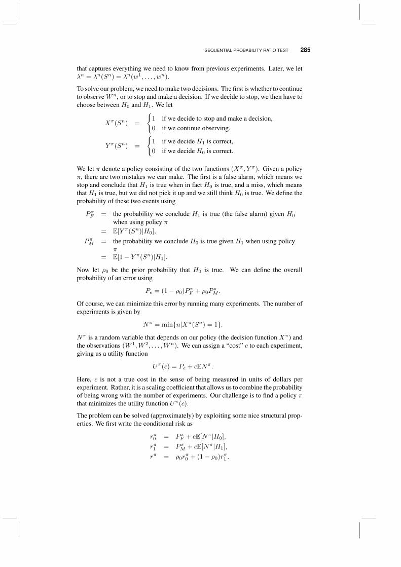
SEQUENTIAL PROBABILITY RATIO TEST 285
that captures everything we need to know from previous experiments. Later, we letλn = λn(Sn) = λn(w1, . . . , wn).
To solve our problem, we need to make two decisions. The first is whether to continueto observe Wn, or to stop and make a decision. If we decide to stop, we then have tochoose between H0 and H1. We let
Xπ(Sn) =
1 if we decide to stop and make a decision,0 if we continue observing.
Y π(Sn) =
1 if we decide H1 is correct,0 if we decide H0 is correct.
We let π denote a policy consisting of the two functions (Xπ, Y π). Given a policyπ, there are two mistakes we can make. The first is a false alarm, which means westop and conclude that H1 is true when in fact H0 is true, and a miss, which meansthat H1 is true, but we did not pick it up and we still think H0 is true. We define theprobability of these two events using
PπF = the probability we conclude H1 is true (the false alarm) given H0
when using policy π= E[Y π(Sn)|H0],
PπM = the probability we conclude H0 is true given H1 when using policyπ
= E[1− Y π(Sn)|H1].
Now let ρ0 be the prior probability that H0 is true. We can define the overallprobability of an error using
Pe = (1− ρ0)PπF + ρ0PπM .
Of course, we can minimize this error by running many experiments. The number ofexperiments is given by
Nπ = minn|Xπ(Sn) = 1.
Nπ is a random variable that depends on our policy (the decision function Xπ) andthe observations (W 1,W 2, . . . ,Wn). We can assign a “cost” c to each experiment,giving us a utility function
Uπ(c) = Pe + cENπ.
Here, c is not a true cost in the sense of being measured in units of dollars perexperiment. Rather, it is a scaling coefficient that allows us to combine the probabilityof being wrong with the number of experiments. Our challenge is to find a policy πthat minimizes the utility function Uπ(c).
The problem can be solved (approximately) by exploiting some nice structural prop-erties. We first write the conditional risk as
rπ0 = PπF + cE[Nπ|H0],
rπ1 = PπM + cE[Nπ|H1],
rπ = ρ0rπ0 + (1− ρ0)rπ1 .
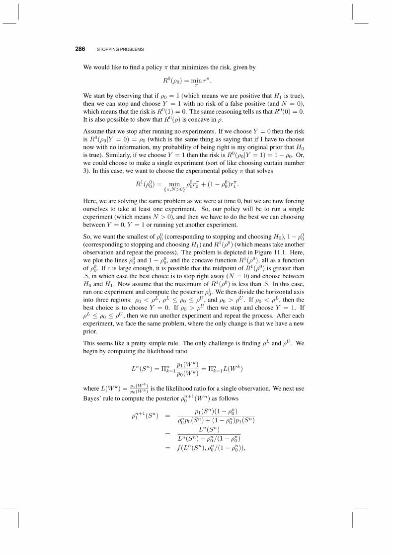
286 STOPPING PROBLEMS
We would like to find a policy π that minimizes the risk, given by
R0(ρ0) = minπrπ.
We start by observing that if ρ0 = 1 (which means we are positive that H1 is true),then we can stop and choose Y = 1 with no risk of a false positive (and N = 0),which means that the risk isR0(1) = 0. The same reasoning tells us thatR0(0) = 0.It is also possible to show that R0(ρ) is concave in ρ.
Assume that we stop after running no experiments. If we choose Y = 0 then the riskis R0(ρ0|Y = 0) = ρ0 (which is the same thing as saying that if I have to choosenow with no information, my probability of being right is my original prior that H0
is true). Similarly, if we choose Y = 1 then the risk is R0(ρ0|Y = 1) = 1− ρ0. Or,we could choose to make a single experiment (sort of like choosing curtain number3). In this case, we want to choose the experimental policy π that solves
R1(ρ00) = min
π,N>0ρ0
0rπ0 + (1− ρ0
0)rπ1 .
Here, we are solving the same problem as we were at time 0, but we are now forcingourselves to take at least one experiment. So, our policy will be to run a singleexperiment (which means N > 0), and then we have to do the best we can choosingbetween Y = 0, Y = 1 or running yet another experiment.
So, we want the smallest of ρ00 (corresponding to stopping and choosing H0), 1− ρ0
0
(corresponding to stopping and choosingH1) andR1(ρ0) (which means take anotherobservation and repeat the process). The problem is depicted in Figure 11.1. Here,we plot the lines ρ0
0 and 1 − ρ00, and the concave function R1(ρ0), all as a function
of ρ00. If c is large enough, it is possible that the midpoint of R1(ρ0) is greater than
.5, in which case the best choice is to stop right away (N = 0) and choose betweenH0 and H1. Now assume that the maximum of R1(ρ0) is less than .5. In this case,run one experiment and compute the posterior ρ1
0. We then divide the horizontal axisinto three regions: ρ0 < ρL, ρL ≤ ρ0 ≤ ρU , and ρ0 > ρU . If ρ0 < ρL, then thebest choice is to choose Y = 0. If ρ0 > ρU then we stop and choose Y = 1. IfρL ≤ ρ0 ≤ ρU , then we run another experiment and repeat the process. After eachexperiment, we face the same problem, where the only change is that we have a newprior.
This seems like a pretty simple rule. The only challenge is finding ρL and ρU . Webegin by computing the likelihood ratio
Ln(Sn) = Πnk=1
p1(W k)
p0(W k)= Πn
k=1L(W k)
where L(W k) = p1(Wk)p0(Wk)
is the likelihood ratio for a single observation. We next use
Bayes’ rule to compute the posterior ρn+10 (Wn) as follows
ρn+11 (Sn) =
p1(Sn)(1− ρn0 )
ρn0p0(Sn) + (1− ρn0 )p1(Sn)
=Ln(Sn)
Ln(Sn) + ρn0/(1− ρn0 )
= f(Ln(Sn), ρn0/(1− ρn0 )),

SEQUENTIAL PROBABILITY RATIO TEST 287
0 1UρLρ0
1
00ρ
00ρ
001 ρ−
1 00( )R ρ
Ris
k
Figure 11.1 The expected risk as a function of the prior probability that H0 is true.
where f(`, β) = `/(` + β). For β ≥ 0, f(`, β) is strictly increasing for ` ≥ 0.This means that if 0 < ρn0 < 1, ρn+1
0 (Sn) is strictly increasing with Ln(Sn). Thismeans that determining if ρn+1
0 (Sn) ≤ ρL or ρn+10 (Sn) ≥ ρU is the same as testing
if Ln(Sn) ≤ A or Ln(Sn) ≥ B, where A and B satisfy
f (A, ρn0/(1− ρn0 )) = ρL,
f (B, ρn0/(1− ρn0 )) = ρU .
We can solve for A and B, which gives us
A =ρn0ρ
L
(1− ρn0 )(1− ρL),
B =ρn0ρ
U
(1− ρn0 )(1− ρU ).
This means that we can write our policy in the form
Ln(Sn) =
≥ B stop and choose Y n = 1
≤ A stop and choose Y n = 0
otherwise take an additional observation.
Hence, it is easy to see why this rule is known as the sequential probability ratio test(SPRT ). The SPRT is controlled by the parameters A and B, and hence we referto the rule as SPRT (A,B).
Finding A and B exactly is difficult, but we can find good estimates using Wald’sapproximation which gives us
PπF ≈ (1−A)
B −A,
PπM ≈ A(B − 1)
B −A.
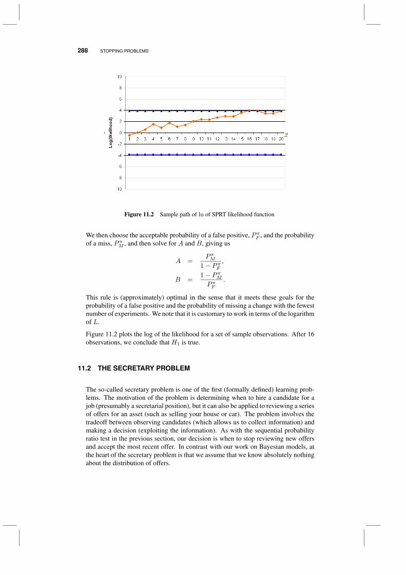
288 STOPPING PROBLEMS
Figure 11.2 Sample path of ln of SPRT likelihood function
We then choose the acceptable probability of a false positive, PπF , and the probabilityof a miss, PπM , and then solve for A and B, giving us
A =PπM
1− PπF,
B =1− PπMPπF
.
This rule is (approximately) optimal in the sense that it meets these goals for theprobability of a false positive and the probability of missing a change with the fewestnumber of experiments. We note that it is customary to work in terms of the logarithmof L.
Figure 11.2 plots the log of the likelihood for a set of sample observations. After 16observations, we conclude that H1 is true.
11.2 THE SECRETARY PROBLEM
The so-called secretary problem is one of the first (formally defined) learning prob-lems. The motivation of the problem is determining when to hire a candidate for ajob (presumably a secretarial position), but it can also be applied to reviewing a seriesof offers for an asset (such as selling your house or car). The problem involves thetradeoff between observing candidates (which allows us to collect information) andmaking a decision (exploiting the information). As with the sequential probabilityratio test in the previous section, our decision is when to stop reviewing new offersand accept the most recent offer. In contrast with our work on Bayesian models, atthe heart of the secretary problem is that we assume that we know absolutely nothingabout the distribution of offers.
THE SECRETARY PROBLEM 289
11.2.1 Setup
Assume that we have N candidates for a secretarial position (you can also think ofthese as offers to purchase an asset). Each candidate is interviewed in sequence andassigned a score that allows us to compare him or her to other candidates (if we aretrying to sell an asset, these scores are the offers to purchase the asset). While itmay be reasonable to try to maximize the expected score that we would receive, inthis case, we want to maximize the probability of accepting the highest score out ofall that have been, or might be, offered. We need to keep in mind that if we stop atcandidate n, then we will not interview candidates n+ 1, . . . , N . Also, we only havethe option of accepting the last candidate or interviewing the next one. Once we haveturned down a candidate, we cannot return to that candidate at a later time.
Let
Wn = Score of the nth candidate.
Sn =
1 If the score of the nth candidate is the best so far0 If the score of the nth candidate is not the best so far∆ If we have stopped already
S = State space, given by (0, 1,∆), where the states 0 and 1 mean thatwe are still searching, and ∆ means we have stopped the process.
X = 0 (continue), 1 (stop), where “stop” means that we hire the lastcandidate interviewed.
Because the decision function uses the most recent piece of information, we defineour history as
hn = W 1, . . . ,Wn.
To describe the system dynamics, it is useful to define an indicator function
In(hn) =
1 if Wn = max1≤m≤nWm0 otherwise.
which tells us if the last observation is the best. Our transition function can now begiven by
Sn+1 =
In(hn) if xn = 0 and Sn 6= ∆
∆ if xn = 1 or Sn = ∆.
To compute the one-step transition matrix, we observe that the event the (n+ 1)stapplicant is the best has nothing to do with whether the nth was the best. As a result,we can write the conditional probability that In+1(hn+1) = 1 using
P[In+1(hn+1) = 1|In(hn)] = P[In+1(hn+1) = 1].
This simplifies the problem of finding the one-step transition probabilities. Bydefinition we have
P[Sn+1 = 1|Sn, xn = 0] = P[In+1(hn+1) = 1].
290 STOPPING PROBLEMS
In+1(hn+1) = 1 if the (n+ 1)st candidate is the best out of the first n + 1, whichclearly occurs with probability 1/(n+ 1). So
P(Sn+1 = 1|Sn, xn = 0) =1
n+ 1,
P(Sn+1 = 0|Sn, xn = 0) =n
n+ 1.
Our goal is to maximize the probability of hiring the best candidate. So, if we do nothire the last candidate, then the probability that we hired the best candidate is zero. Ifwe hire the nth candidate, and the nth candidate is the best so far, then our reward isthe probability that this candidate is the best out of all N . This probability is simplythe probability that the best candidate out of allN is one of the first n, which is n/N .So, the conditional reward function is
Cn(Sn, xn|hn) =
n/N if Sn = 1 and xn = 1,0 otherwise.
With this information, we can now set up the optimality equations
V n(sn) = maxxn∈X
ECn(sn, xn|hn) + V n+1(Sn+1)|sn.
11.2.2 Solution
The solution to the problem is quite elegant, but the technique is unique to thisparticular problem. Readers interested in the elegant answer but not the particularproof (which illustrates dynamic programming but otherwise does not generalize toother problem classes) can skip to the end of the section.
Let V n (s) be the probability of choosing the best candidate out of the entire popu-lation, given that we are in state s after interviewing the nth candidate. Recall thatimplicit in the definition of our value function is that we are behaving optimally fromtime period t onward. The terminal reward is
V N (1) = 1
V N (0) = 0
V N (∆) = 0
Let
Cstop,n =(Cn(1, stop) + V n+1(∆)
),
Ccontinue,n =
Cn(1, continue) +∑
s′∈0,1
p(s′|s)V n+1(s′)
.
The optimality recursion for the problem is given by
V n(1) = maxCstop,n, Ccontinue,n
.

THE SECRETARY PROBLEM 291
Noting that:
Cn(1, continue) = 0,
Cn(1, stop) =n
N,
V n+1(∆) = 0,
p(s′|s) =
1/(n+ 1) s′ = 1
n/(n+ 1) s′ = 0.
We get
V n(1) = max
n
N,
1
n+ 1V n+1(1) +
n
n+ 1V n+1(0)
. (11.3)
Similarly, it is easy to show that
V n(0) = max
0,
1
n+ 1V n+1(1) +
n
n+ 1V n+1(0)
(11.4)
=1
n+ 1V n+1(1) +
n
n+ 1V n+1(0).
Comparing (11.4) and (11.3), we can rewrite (11.3) as
V n(1) = max nN, V n(0)
. (11.5)
From this we obtain the inequality
V n(1) ≥ V n(0) (11.6)
which seems pretty intuitive (you are better off if the last candidate you interviewedwas the best you have seen so far).
At this point, we are going to suggest a policy that seems to be optimal. We are goingto interview the first n candidates, without hiring any of them. Then, we will stopand hire the first candidate who is the best we have seen so far. The decision rule canbe written as
xn(1) =
0 (continue) n ≤ n1 (quit) n > n
.
To prove this, we are going to start by showing that if V m(1) > m/N for somem (oralternatively if V m(1) = m/N = V m(0)), then V m
′(1) > m′/N for m′ < m. If
V m(1) > m/N , then it means that the optimal decision is to continue. We are goingto show that if it was optimal to continue at setm, then it was optimal to continue forall steps m′ < m.
Assume that V m(1) > m/N . This means, from equation (11.5), that it was better tocontinue, which means that V m(1) = V m(0) (or there might be a tie, implying thatV m(1) = m/N = V m(0)). This allows us to write
V m−1(0) =1
mV m(1) +
m− 1
mV m(0)
= V m(1) (11.7)
≥ m
N. (11.8)

292 STOPPING PROBLEMS
Equation (11.7) is true because V m(1) = V m(0), and equation (11.8) is true becauseV m(1) ≥ m/N . Stepping back in time, we get
V m−1(1) = max
m− 1
N,V m−1(0)
≥ m
N(11.9)
>m− 1
N. (11.10)
Equation (11.9) is true because V m−1(0) ≥ m/N . We can keep repeating this form− 1,m− 2, . . ., so it is optimal to continue for m′ < m.
Now we have to show that ifN > 2, then n ≥ 1. If this is not the case, then for all n,V n(1) = n/N (because we would never continue). This means that (from equation(11.4)):
V n(0) =
(1
n+ 1
)(n+ 1
N
)+
(n
n+ 1
)V n+1(0)
=1
N+
(n
n+ 1
)V n+1(0). (11.11)
Using V N (0) = 0, we can solve (11.11) by backward induction:
V N (0) = 0,
V N−1(0) =1
N+
N − 1
N − 1 + 1V N (0)
=1
N,
V N−2(0) =1
N+
N − 2
N − 2 + 1
(1
N
)=
N − 2
N
(1
N − 2+
1
N − 1
).
In general, we get
V m(0) =m
N
[1
m+
1
m+ 1+ · · ·+ 1
N − 1
].
We can easily see that V 1(0) > 1N ; since we were always quitting, we had found
that V 1(1) = 1N . Finally, equation (11.6) tells us that V 1(1) ≥ V 1(0), which means
we have a contradiction.
This structure tells us that for m ≤ n
V m(0) = V m(1),
and for m > n
V m(1) =m
N,
V m(0) =m
N
[1
m+
1
m+ 1+ · · ·+ 1
N − 1
].

BIBLIOGRAPHIC NOTES 293
It is optimal to continue as long as V m(0) > m/N , so we want to find the largestvalue for m such that
m
N
[1
m+
1
m+ 1+ · · ·+ 1
N − 1
]>
m
N,
or [1
m+
1
m+ 1+ · · ·+ 1
N − 1
]> 1.
If N = 5, then we can solve by enumeration:
n = 1 11 + 1
2 + 13 + 1
4 = 2.08n = 2 1
2 + 13 + 1
4 = 1.08n = 3 1
3 + 14 = 0.58
So for N = 5, we would use n = 2. This means interview (and discard) twocandidates, and then take the first candidate that is the best to date.
For large N , we can find a neat approximation. We would like to find m such that:
1 ≈ 1
m+
1
m+ 1+ · · ·+ 1
N − 1
≈∫ N
M
1
xdx
= lnN − lnm
= ln
(N
m
).
Solving for m means finding ln(N/m) = 1 or N/m = e or m/N = e−1 = 0.368.So, for large N , we want to interview 37 percent of the candidates, and then choosethe first candidate that is the best to date.
The secretary problem is a classic, partly because it illustrates an interesting informa-tion collection problem, and partly because it yields such an elegant solution. In realapplications, we can translate the result to a rough rule that says “look at a third ofthe candidates, and then choose the first candidate that is better than all the others.”
11.3 BIBLIOGRAPHIC NOTES
Section 11.1 - The sequential probability ratio test is due to Wald & Wolfowitz (1948).
Section 11.2 - The secretary problem was first introduced in Cayley (1875). Our presen-tation is based on Puterman (1994). Vanderbei (1980) provides an elegant general-ization of the secretary problem to one of finding the best subset. See also Bruss(1984) for extensions.

294 STOPPING PROBLEMS
PROBLEMS
11.1 Download a spreadsheet illustrating the sequential probability ratio test from
http://optimallearning.princeton.edu/exercises/SPRT.xls
In the initial spreadsheet, the standard deviation of an experimental observation has beenset to 5.
a) Translate the cells in row 12 to mathematics. Identify the equation in the bookcorresponding to each cell starting in column D.
b) Change the probability of missing from .02 to .10. How does this change thehypotheses H0 and H1? Now change the probability of a false alarm from .02 to.10? How does this change the hypotheses? When you are done this question, restoreboth probabilities back to .02.
c) The sequential probability ratio test stops with a conclusion that either hypothesisH0 is true or H1 is true when the red line crosses one of the blue lines. If it does notcross either line within the experimental budget, then the test is inconclusive. Hit theF9 key 20 times, and count the number of times the red line crosses one of the bluelines.
d) Now change the standard deviation (cell B9) to 3. Again perform 20 simulationsand count how many times the red line crosses one of the blue lines. You should seethat with a lower standard deviation, SPRT is more effective at declaring that one ofthe two hypotheses is true. Why does a smaller standard deviation make it easier tocome to a conclusion?
11.2 Assume you think you can look at up to 20 bids for the house you are selling.Completely unknown to you, the bids can be modeled as being drawn from a uniformdistribution between $380,000 and $425,000. Use the policy that you are going to rejectthe first seven bids (which is approximately 37 percent of 20), and then accept the firstbid that is better than these seven. If none are better, you have to accept the very lastbid. Start the process by generating all 20 bids in advance, so that when you are done,you can compare the bid you accepted against the best that you might have acceptedwith perfect foresight.
a) Repeat this policy 100 times and report on: i) how many times you accepted the verybest bid out of the 20, and ii) the bid you accepted as a percentage of the very bestbid.
b) Repeat (a), but now reject only the first four bids before you are ready to accept thebid.
c) Finally, repeat (a), but now you decide to reject the first 10 bids before you are readyto accept a bid.
d) Compare the results of the policies you simulated in (a), (b) and (c). Do you seeevidence that one policy outperforms the others?

PROBLEMS 295
11.3 You have to choose the best out of up to 30 bids, where the ith bid, Ri, followsan exponential distribution given by
fR(y) = .02e−.02y.
You can generate random observations from an exponential distribution using
R = −50 lnU
where U is a random variable that is uniformly distributed between 0 and 1.
a) Use the policy where you look at the first 11 bids, and then pick the best bid whichoutperforms all previous bids. Repeat this policy 100 times and report on: i) howmany times you accepted the very best bid out of the 20, and ii) the bid you acceptedas a percentage of the very best bid.
b) Repeat (a), but now reject only the first six bids before you are ready to accept thebid.
c) Finally, repeat (a), but now you decide to reject the first 16 bids before you are readyto accept a bid.
d) Compare the results of the policies you simulated in (a), (b) and (c). Do you seeevidence that one policy outperforms the others?

CHAPTER 12
ACTIVE LEARNING IN STATISTICS
We have focused our attention on problems where we are learning in order to makea better decision in some sort of optimization problem, which gives us an economicvalue of information. It is often the case, however, that we are just trying to fit astatistical model which might be used for a variety of decision problems. We maynot know how the model may be used; we are simply interested in carefully choosingwhat to measure to get the best model.
Most applications of statistics involve problems where we may have to fit a modelfrom a fixed set of observations. This is often referred to as batch statistics. We mayalso have a process where observations arrive over time, but where we do not haveany control over what we observe. This is known as passive learning.
There are many situations where we can control the inputs of a process. For example,we may be able to set the price of a product and then observe sales. We may set userpreferences on Netflix, thus affecting the movies that are displayed to us; we thenchoose a movie to rent, which in turn affects what Netflix observes. After we choosethe inputs (these might be referred to as independent variables or covariates) xn, wethen observe the response yn+1 which is then used to fit the parameters of a model.The machine learning community refers to this process as active learning.
In statistics, active learning refers to the ability to control the choice of independentvariables. In Chapter 1, we made a distinction between the broad umbrella of activelearning, where we make choices with the intent to learn, and the subset of policies
Optimal Learning. By Warren B. Powell and Ilya O. RyzhovCopyright c© 2018 John Wiley & Sons, Inc.
297
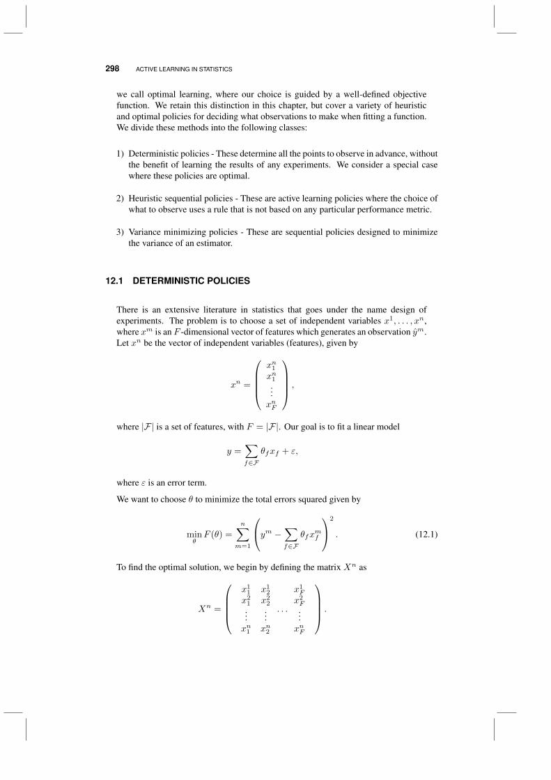
298 ACTIVE LEARNING IN STATISTICS
we call optimal learning, where our choice is guided by a well-defined objectivefunction. We retain this distinction in this chapter, but cover a variety of heuristicand optimal policies for deciding what observations to make when fitting a function.We divide these methods into the following classes:
1) Deterministic policies - These determine all the points to observe in advance, withoutthe benefit of learning the results of any experiments. We consider a special casewhere these policies are optimal.
2) Heuristic sequential policies - These are active learning policies where the choice ofwhat to observe uses a rule that is not based on any particular performance metric.
3) Variance minimizing policies - These are sequential policies designed to minimizethe variance of an estimator.
12.1 DETERMINISTIC POLICIES
There is an extensive literature in statistics that goes under the name design ofexperiments. The problem is to choose a set of independent variables x1, . . . , xn,where xm is an F -dimensional vector of features which generates an observation ym.Let xn be the vector of independent variables (features), given by
xn =
xn1xn1...xnF
,
where |F| is a set of features, with F = |F|. Our goal is to fit a linear model
y =∑f∈F
θfxf + ε,
where ε is an error term.
We want to choose θ to minimize the total errors squared given by
minθF (θ) =
n∑m=1
ym −∑f∈F
θfxmf
2
. (12.1)
To find the optimal solution, we begin by defining the matrix Xn as
Xn =
x1
1
x21...xn1
x12
x22...xn2
. . .
x1F
x2F...xnF
.

DETERMINISTIC POLICIES 299
The vector of observations y1, . . . , yn is represented using
Y n =
y1
y2
...yn
.
As in Chapter 7, the vector θn that solves (12.1) is given by
θn = [(Xn)TXn]−1(Xn)TY n. (12.2)
Equation (12.2) gives us an easy way to find the variance of our estimate θn. Let vbe an n-dimensional random vector, let A be a F × n deterministic matrix, and letu = Av. Let Cov(v) be the covariance matrix of v. Then we can use the identitythat
Cov(u) = ACov(w)AT
where Cov(w) is the covariance matrix of w. Recall that for matrices A and B,ABT = (BAT )T , and that [(Xn)TXn]−1 is a symmetric matrix. We can use theseobservations to find the covariance matrix of θn if we letA = [(Xn)TXn]−1(Xn)T ,giving us
Cov(θn) = [(Xn)TXn]−1(Xn)TCov(Y n)([(Xn)TXn]−1(Xn)T
)T= [(Xn)TXn]−1(Xn)TCov(Y n)(Xn)[(Xn)TXn]−1.
Since the elements of Y n are independent, Cov(Y n) = σ2ε I where I is the identity
matrix and σ2ε is the variance of our experimental error . This allows us to write
Cov(θn) = [(Xn)TXn]−1(Xn)TXn[(Xn)TXn]−1σ2ε
= [(Xn)TXn]−1σ2ε .
The observation error σ2ε is fixed; we cannot change it through our choice of xn.
However, we have direct control over the covariance of θn by our choice of Xn.Furthermore, we quickly see that the matrix Cov(θn) is a deterministic function ofXn, which means we do not gain anything by observing yn. It is for this reason thatwe can determine the precision of θn without making any observations. This is thetheoretical foundation of deterministic policies.
So this leaves the question, what do we want to minimize? θn is a vector, andCov(θn) is a matrix. While we would like to minimize all the elements of Cov(θn),we have to choose a single metric. This issue has created a variety of metrics thathave come to be known as alphabet-optimality, for reasons that will become clearshortly. A sample of these metrics are
A-optimality - Minimize the average (or trace, which is the sum) of the diagonal elementsof [(Xn)TXn]−1. This is the same as minimizing the average of the variances ofeach element of θn.
C-optimality - Given a weighting vector c, minimize cT [(Xn)TXn]c.
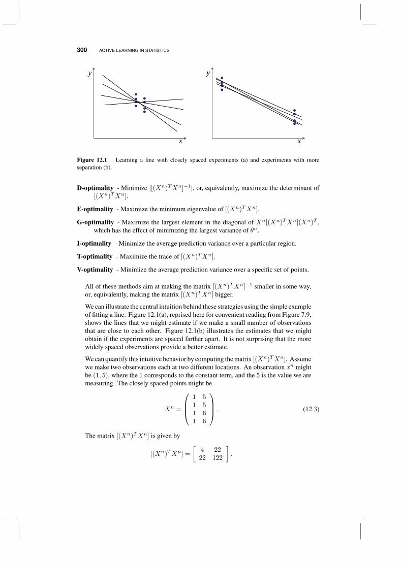
300 ACTIVE LEARNING IN STATISTICS
x
y y
x
Figure 12.1 Learning a line with closely spaced experiments (a) and experiments with moreseparation (b).
D-optimality - Minimize |[(Xn)TXn]−1|, or, equivalently, maximize the determinant of[(Xn)TXn].
E-optimality - Maximize the minimum eigenvalue of [(Xn)TXn].
G-optimality - Maximize the largest element in the diagonal of Xn[(Xn)TXn](Xn)T ,which has the effect of minimizing the largest variance of θn.
I-optimality - Minimize the average prediction variance over a particular region.
T-optimality - Maximize the trace of [(Xn)TXn].
V-optimality - Minimize the average prediction variance over a specific set of points.
All of these methods aim at making the matrix [(Xn)TXn]−1 smaller in some way,or, equivalently, making the matrix [(Xn)TXn] bigger.
We can illustrate the central intuition behind these strategies using the simple exampleof fitting a line. Figure 12.1(a), reprised here for convenient reading from Figure 7.9,shows the lines that we might estimate if we make a small number of observationsthat are close to each other. Figure 12.1(b) illustrates the estimates that we mightobtain if the experiments are spaced farther apart. It is not surprising that the morewidely spaced observations provide a better estimate.
We can quantify this intuitive behavior by computing the matrix [(Xn)TXn]. Assumewe make two observations each at two different locations. An observation xn mightbe (1, 5), where the 1 corresponds to the constant term, and the 5 is the value we aremeasuring. The closely spaced points might be
Xn =
1 51 51 61 6
. (12.3)
The matrix [(Xn)TXn] is given by
[(Xn)TXn] =
[4 2222 122
].
SEQUENTIAL POLICIES FOR CLASSIFICATION 301
Now assume we measure at more extreme points (but where the average is still thesame), given by
Xn =
1 11 11 101 10
.
The matrix [(Xn)TXn] is given by
[(Xn)TXn] =
[4 2222 202
].
The trace of the matrix [(Xn)TXn] for the closely spaced points is 4 + 122 = 126,while the trace for the points that are more spread out is 206. We would say that thesecond matrix has more “information,” and the result is an estimate of θ with lowervariance.
It is important that the data be scaled so that the average value of the measured valuesx remains the same (as we did above). The best way to do this is to simply average theoutcomes of the experiments, and compute a corrected value Xn for each dimension,using
Xni = Xn
i −1
n
n∑m=1
Xmi .
We then compute the matrix using [(Xn)T Xn]. If we do this to the experimentaloutcomes in equation (12.3), we would obtain
Xn =
0 −0.50 −0.50 0.50 0.5
. (12.4)
Regardless of which type of optimality we use, we now have a metric that we canuse to help decide which experiments to run. Given a set of potential experiments,we generally want to choose experiments that are distributed around a center, but asfar from the center as possible.
It is important to realize that we can choose the best set of potential experimentsbefore making any observations. This property is a unique byproduct of the propertythat all statistics relating to the reliability of our estimates of θ are purely a functionof the experiments and not the observations. We have not enjoyed this property inour previous applications.
12.2 SEQUENTIAL POLICIES FOR CLASSIFICATION
An important class of problems in machine learning is known as classification prob-lems. In this problem class, we are given a set of features xm for themth object (this
302 ACTIVE LEARNING IN STATISTICS
might be a document, an email or a website), and we are asked to place this documentinto one of a set of discrete classifications, such as dangerous, threatening, suspi-cious, safe. Often, collecting information about the classification of a document fortraining purposes is expensive. For example, we may need to ask a security expertto assess the threat level of an email or website. However, given the sheer volume ofthese sources, we cannot ask a trained expert to provide this information on a largenumber of documents.
This section describes a series of primarily heuristic search policies for efficientlycollecting information for classification problems.
12.2.1 Uncertainty sampling
Let y be a discrete quantity that indicates the classification of a document withattributes described by x, and let Pθ(y|x) be the probability of the particular classi-fication y if we observe x, given a parameter vector θ. Our goal is to observe thedocument where our prediction has the highest level of uncertainty. If the classifica-tion is binary (for example, dangerous or not), then we want to sample the documentswhere Pθ(y|x) is as close as possible to 0.5.
If there are more than two outcomes, an alternative strategy is to choose to query thedocument whose prediction offers the lowest level of confidence, which we computeusing
xLC = arg maxx
(1− Pθ(y|x)
)where
y = arg maxy
Pθ(y|x)
is the most likely classification. The idea here is that if the most likely classification ina set is small, then this represents a document (more precisely, a class of documents)where we have a lot of uncertainty, and would benefit from more information. We aretrying to mitigate the effect of a worst-case scenario by learning about the documentfor which we are most likely to make an error in prediction.
This strategy focuses on the most probable classification, and as a result ignoresthe probabilities of other classifications. For example, we may be much more cer-tain about one classification, implying that more testing is unlikely to change theclassification. An alternative strategy is to focus on documents whose most likelyclassification is close to the second most likely classification. For fixed θ, let
y1 = arg maxy
Pθ(y|x)
and
y2 = arg maxy 6=y1
Pθ(y|x)
be the most likely and second most likely classification for a document. The marginalsampling policy chooses the document x where the two highest classification proba-
SEQUENTIAL POLICIES FOR CLASSIFICATION 303
bilities are the closest. We state this policy using
xM = arg minx
(Pθ(y1|x)− Pθ(y2|x)
).
The previous two policies look at the level of uncertainty indicated by the mostcertain document or the difference between the two most certain documents. An ideathat takes this thinking a step further uses entropy as a measure of uncertainty. Theentropy maximization policy is computed using
xH = arg maxx
−∑i
Pθ(yi|x) logPθ(yi|x)
where yi represents a single classification. Entropy looks at all the potential classifi-cations, and represents an information-theoretic measure of the information requiredto encode the classification probability distribution.
Empirical research with these policies has produced mixed results. Clearly there willbe differences in behavior as the number of potential classifications changes. Notsurprisingly, performance depends on the true utility function. The margin and levelof confidence policies work better when the goal is to get the classification right,while the entropy maximization policy works if the objective is to minimize the logof the loss from an incorrect classification (“log-loss”).
12.2.2 Query by committee
Imagine that we have several competing models for estimating the classification of adocument. We would refer to this family of models as a “committee,” where c ∈ Cis a particular model in the set C. Let Pθ(c)(yi|x) be the probability that model c(parameterized by θ(c)) returns classification yi given the attributes x of a document.
There are several ways to perform active learning in this setting. One is to let eachmodel vote for a classification. We might record a vote using the indicator function
Ic(yi|x) =
1 if yi = arg maxi Pθ(c)(yi|x)
0 otherwise.
The indicator function Ic(yi|x) simply captures if model c thinks that yi is the mostlikely classification. We can then count the number of votes using
V (yi) =∑c∈C
Ic(yi|x).
Alternatively, we could compute “soft votes” using
V (yi) =∑c∈C
Pθ(c)(yi|x).
We can then choose to sample the document with the highest vote entropy, giving usthe policy
xV E = arg maxx
−∑i
V (yi)
Clog
V (yi)
C.
304 ACTIVE LEARNING IN STATISTICS
Another measure is the Kullback-Leibler divergence metric, which is a way of mea-suring the differences between two distributions. We first compute an average prob-ability of classification across the competing models using
PC(yi|x) =1
|C|∑c∈C
Pθ(c)(yi|x).
The KL divergence is then computed using
D(Pθ(c)‖PC) =∑i
Pθ(c)(yi|x) logPθ(c)(yi|x)
PC(yi|x).
The Kullback-Leibler divergence is a type of distance metric since it is measuring thedegree of similarity between two probability distributions: the distribution (acrosspotential classifications) obtained when we average all the probabilities across thecompeting models, versus the distribution produced by each model. The quantityD(Pθ(c)‖PC) is the KL divergence for a particular model c. Our policy for decidingwhich document to evaluate is obtained by maximizing the average KL divergenceacross all the models, given by
xKL = arg maxx
1
C
∑c∈C
D(Pθ(c)‖PC).
The idea with this policy is to choose to evaluate the document with the greatestdisagreement among the different models. If the competing models largely agree,then it is unlikely that more information will change this consensus. Additionalinformation is likely to have the greatest impact when competing models disagree.
12.2.3 Expected error reduction
An interesting policy uses an estimate of the degree to which information reducesthe likelihood of being incorrect. We are going to assume that we have a set ofunlabeled documents U , which means that we have not solicited a classification froma domain expert. Assume we are considering the possibility of collecting informationon the document x. We do not know its classification, but our current estimate of theprobability that it will be classified as yi is Pθ(yi|x). If we choose document x andobserve the classification yi, we can use this information to update our classificationprobability, which we represent using Pθ+(x,yi)(y|x). This is analogous to a posteriorbelief.
Now, we are going to use this updated probability model on each document u ∈ U ,with feature vector xu. We let
yu = arg maxy
Pθ(y|xu)
be the most likely classification for a particular document xu in our set U .If Pθ+(x,yi)(y
u|xu) is the probability of this most likely classification, then1 − Pθ+(x,yi)(y
u|xu) represents the probability that the document u does not be-long to the class that we think is the most likely. This is analogous to our posterior
A VARIANCE MINIMIZING POLICY 305
belief about how likely we are to make a mistake about document u after observinga result for x. We then choose x to minimize this probability of error in expectationover all possible classifications yi of document x. The policy, then, is given by
xER = arg minx
∑i
Pθ(yi|x)
(∑u∈U
(1− Pθ+(x,yi)(y
u|xu)))
.
12.3 A VARIANCE MINIMIZING POLICY
We are going to describe an information collecting policy with the goal of reducingvariance, but this time we are going to address a richer set of models and issues thanwe encountered in Section 12.1 when the goal was to minimize variance measures ofthe regression vector θ.
We start by assuming that there exists a model y(x) = f(x)+εwhere f(x) is the truemodel and ε is a source of experimental noise over which we have no control. Our goalis to collect a training datasetDn =
(x0, y1), (x1, y2), . . . , (xn−1, yn)
. We group
the choice (x0, . . . , xn−1) of what to measure with the corresponding observations(y1, . . . , yn) into a single training dataset. We note that the standard notation instatistics is to let x1 be the experiment that produces y1, but as the developmentbelow illustrates, it is cleaner to let the superscript capture the information content;when we choose xm, ym+1 is a random variable.
We assume we are using a sequential policy to determine x0, x1, x2, . . . (startingwith x0) which may depend on the outcomes y1, y2, . . .. This means that Dn is arandom set, constructed sequentially. We use this information to fit an approximationyn = fn(x|Dn). Below, we are going to write the prediction as yn(x|Dn) to expressits dependence on the query point x, and the data Dn.
The goal is to design a policy that minimizes the variance in our predictions yn(x|Dn),but this depends on the points x where we might query the function. We did nothave to deal with this issue in Section 12.1, but now we are going to assume that weare given a distribution P (x) that gives the probability that we will want an estimateof the function at x. In practice, P (x) may be chosen to be uniform over someregion, or we may specify a normal distribution with some mean µx and a spreadσx. Alternatively, we may have a sequence of observations x1, . . . , xk from historywhich can serve as a probability distribution. Either way, P (x) serves as a weightingfunction that tells us the region in which we are interested. However, it is importantto recognize that the probability that x is in the random set Dn, which is influencedby our learning policy, may be completely different than P (x).
If we make an observation at x, we are going to observe
y(x) = f(x) + ε,
where f(x) is our true (but unknown) function, and ε is the inherent noise in theobservation. Our approximation is going to give us the estimate yn(x|Dn). Areasonable goal is to design a policy for choosing an experiment x to minimize theprediction error (yn(x|Dn)−y(x))2 for a single realization of y(x) (which is random
306 ACTIVE LEARNING IN STATISTICS
because of ε), and a single estimate yn(x|Dn) from a dataset Dn (which is randombecause Dn is random). To formalize this idea, we need to take expectations. We letET (·) be the total expectation over the observation noise imbedded in y(x) and theobservation of Dn. These are independent, so we can write them as
ET (yn(x|Dn)− y(x))2 = EyED(y(x)− yn(x|Dn))2, (12.5)
where ED is the expectation over all the possible outcomes of Dn, and Ey is theexpectation over all possible realizations of y(x). We can break down the expectedtotal variation (for a given x) in (12.5) using
ET (yn(x|Dn)− y(x))2 = E[(y(x)− E[y(x)])2]
+(ED[y(x|Dn)]− E[y(x)]
)2+ED
[(y(x|Dn)− ED[y(x|Dn)])2
]. (12.6)
The first term reflects the pure noise due to ε, which will not be affected by thelearning policy. The second term captures the bias in the model, which is purelya function of the structural form of the underlying model, as well as the choice ofx. Again, this is not affected by the choice of Dn. The right-hand side of equation(12.6) is also known as a bias-variance decomposition.
The third term is the variance due to the estimation of the model from the training data.This is where we capture the variation in the estimated model (after n observations)due to the different variations in Dn that might be produced by following a specificlearning policy. The variations in Dn arise because of differences in realizations inthe observations y1, . . . , yn that lead to different decisions x2, . . . , xn. This is theterm that we wish to minimize by choosing a good learning policy.
For compactness, we are going to let
σ2,ny (x) = ED
(yn(x|Dn)− ED[yn(x|Dn)]
)2.
Now assume that we are considering the possibility of adding (xn, yn+1) to createan expanded dataset
Dn+1 = Dn ∪ (xn, yn+1).
The choice xn is a deterministic quantity (given Dn) that we are thinking of mea-suring, while yn+1 is the random observation that we have not yet observed whenwe choose xn. Let EnD be the conditional expectation given Dn. The choice ofobservation xn is a deterministic function of Dn. The new information in Dn+1 isyn+1. If we choose xn, let σ2,n
y (x|xn) be the conditional variance (given Dn) of ourestimate if we choose xn, which is given by
σ2,ny (x|xn) = EnD
(yn+1(x|Dn+1)− EnD[yn+1(x|Dn+1)]
)2. (12.7)
The variance σ2,ny (x|xn) is defined in exactly the same way as σ in (2.9). However,
in Chapter 2, we also proved that this quantity coincided with the change in variancebetween two experiments, under a Bayesian learning model. This equivalence doesnot hold in the frequentist model we are considering here. In (12.7), σ2,n representsonly the conditional variance of our estimate given a choice of experiment, and
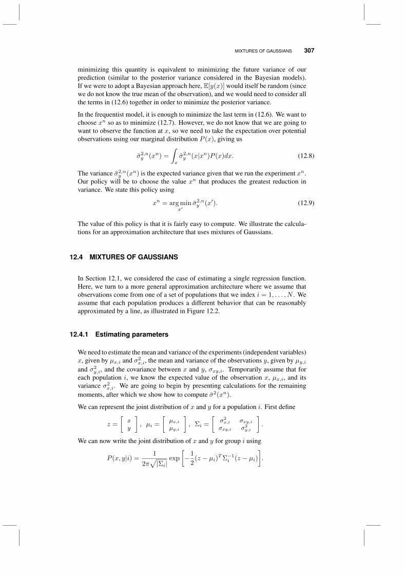
MIXTURES OF GAUSSIANS 307
minimizing this quantity is equivalent to minimizing the future variance of ourprediction (similar to the posterior variance considered in the Bayesian models).If we were to adopt a Bayesian approach here, E[y(x)] would itself be random (sincewe do not know the true mean of the observation), and we would need to consider allthe terms in (12.6) together in order to minimize the posterior variance.
In the frequentist model, it is enough to minimize the last term in (12.6). We want tochoose xn so as to minimize (12.7). However, we do not know that we are going towant to observe the function at x, so we need to take the expectation over potentialobservations using our marginal distribution P (x), giving us
σ2,ny (xn) =
∫x
σ2,ny (x|xn)P (x)dx. (12.8)
The variance σ2,ny (xn) is the expected variance given that we run the experiment xn.
Our policy will be to choose the value xn that produces the greatest reduction invariance. We state this policy using
xn = arg minx′
σ2,ny (x′). (12.9)
The value of this policy is that it is fairly easy to compute. We illustrate the calcula-tions for an approximation architecture that uses mixtures of Gaussians.
12.4 MIXTURES OF GAUSSIANS
In Section 12.1, we considered the case of estimating a single regression function.Here, we turn to a more general approximation architecture where we assume thatobservations come from one of a set of populations that we index i = 1, . . . , N . Weassume that each population produces a different behavior that can be reasonablyapproximated by a line, as illustrated in Figure 12.2.
12.4.1 Estimating parameters
We need to estimate the mean and variance of the experiments (independent variables)x, given by µx,i and σ2
x,i, the mean and variance of the observations y, given by µy,iand σ2
y,i, and the covariance between x and y, σxy,i. Temporarily assume that foreach population i, we know the expected value of the observation x, µx,i, and itsvariance σ2
x,i. We are going to begin by presenting calculations for the remainingmoments, after which we show how to compute σ2(xn).
We can represent the joint distribution of x and y for a population i. First define
z =
[xy
], µi =
[µx,iµy,i
], Σi =
[σ2x,i σxy,i
σxy,i σ2y,i
].
We can now write the joint distribution of x and y for group i using
P (x, y|i) =1
2π√|Σi|
exp
[−1
2(z − µi)TΣ−1
i (z − µi)].

308 ACTIVE LEARNING IN STATISTICS
x
( | )n ny x D1i 2i
3i
Figure 12.2 Illustration of fitting data using mixtures of Gaussians (based on Cohn et al. 1994).
We will not know the true means and variances, but we can estimate them from aninitial sample.
The conditional variance of y given x is given by
σ2y|x,i = σ2
y,i −σxy,iσ2x,i
.
The conditional expectation yni (x|Dn) and variance σ2y,i given x are
yni (x|Dn) = µy,i(x) +σxy,iσ2x,i
(x− µx,i),
σ2y,i =
σ2y|x,i
ni
(1 +
(x− µx,i)2
σ2x,i
).
The scalar ni can be viewed as the weight that group i should be given, calculatedusing
ni =
m∑j=1
P (xj , yj |i)∑Nk=1 P (xj , yj |k)
.
We next compute the probability that population i contributes to the observationcorresponding to x using
hi(x) =P (x|i)∑Nj=1 P (x|j)
,
where
P (x|i) =1√
2πσ2x,i
exp
[− (x− µx,i)2
2σ2x,i
]. (12.10)
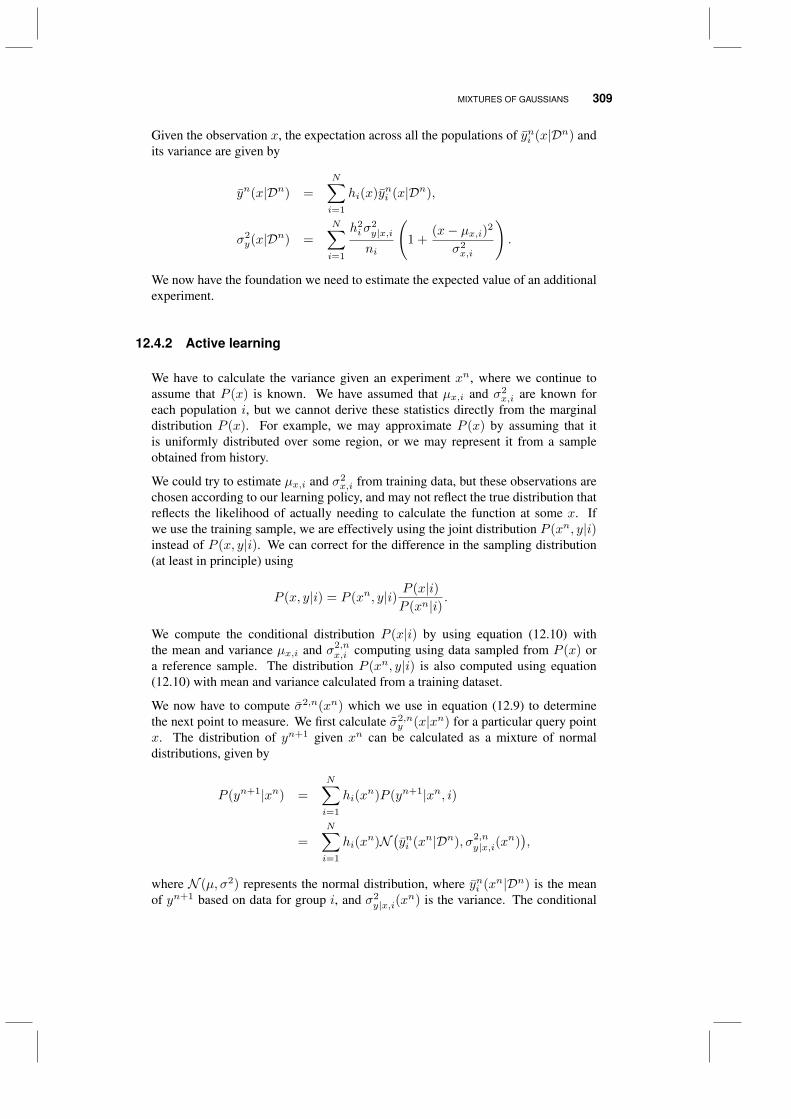
MIXTURES OF GAUSSIANS 309
Given the observation x, the expectation across all the populations of yni (x|Dn) andits variance are given by
yn(x|Dn) =
N∑i=1
hi(x)yni (x|Dn),
σ2y(x|Dn) =
N∑i=1
h2iσ
2y|x,i
ni
(1 +
(x− µx,i)2
σ2x,i
).
We now have the foundation we need to estimate the expected value of an additionalexperiment.
12.4.2 Active learning
We have to calculate the variance given an experiment xn, where we continue toassume that P (x) is known. We have assumed that µx,i and σ2
x,i are known foreach population i, but we cannot derive these statistics directly from the marginaldistribution P (x). For example, we may approximate P (x) by assuming that itis uniformly distributed over some region, or we may represent it from a sampleobtained from history.
We could try to estimate µx,i and σ2x,i from training data, but these observations are
chosen according to our learning policy, and may not reflect the true distribution thatreflects the likelihood of actually needing to calculate the function at some x. Ifwe use the training sample, we are effectively using the joint distribution P (xn, y|i)instead of P (x, y|i). We can correct for the difference in the sampling distribution(at least in principle) using
P (x, y|i) = P (xn, y|i) P (x|i)P (xn|i)
.
We compute the conditional distribution P (x|i) by using equation (12.10) withthe mean and variance µx,i and σ2,n
x,i computing using data sampled from P (x) ora reference sample. The distribution P (xn, y|i) is also computed using equation(12.10) with mean and variance calculated from a training dataset.
We now have to compute σ2,n(xn) which we use in equation (12.9) to determinethe next point to measure. We first calculate σ2,n
y (x|xn) for a particular query pointx. The distribution of yn+1 given xn can be calculated as a mixture of normaldistributions, given by
P (yn+1|xn) =
N∑i=1
hi(xn)P (yn+1|xn, i)
=
N∑i=1
hi(xn)N
(yni (xn|Dn), σ2,n
y|x,i(xn)),
where N (µ, σ2) represents the normal distribution, where yni (xn|Dn) is the meanof yn+1 based on data for group i, and σ2
y|x,i(xn) is the variance. The conditional

310 ACTIVE LEARNING IN STATISTICS
variance of our prediction of x given the choice of xn can be found using
σ2,ny (x|xn) =
n∑i=1
h2i (x)σ2,n
y|x,i(x|xn+1)
ni + hi(x|xn+1)
(1 +
(x− µx,i)σ2x,i
),
where
σ2,ny,i (x|xn+1) =
niσ2,ny,i
ni + hi(x|xn+1)
+ni + hi(x|xn+1)
(σ2y|x,i + (yn+1
i (x|xn+1)− µy,i)2)
(ni + hi(x|xn+1))2,
σ2,ny|x,i(x|x
n+1) = σ2,ny,i (x|xn+1)−
σ2,nxy,i
σ2x,i
,
σxy,i(x|xn+1) =niσxy,i
ni + hi(x|xn+1)
+nihi(x|xn+1)(xn+1 − µx,i)(yn+1
i (x|xn+1)− µy,i)(ni + hi(x|xn+1))2
,
σ2xy,i(x|xn+1) = (σxy,i)
2 +n2i (hi(x|xn+1))2σ2
y|xn+1,i(xn+1 − µx,i)2
.
If we are estimating µx,i and σ2x,i(x|xn+1) from data, we can use the following
equations
µn+1x,i (xn+1) =
niµnx,i + hi(x|xn+1)xn+1
ni + hi(x|xn+1),
σ2,n+1x,i (x|xn+1) =
niσ2,nx,i
ni + hi(x|xn+1)+nihi(x|xn+1)(xn+1 − µnx,i)2
(ni + hi(x|xn+1))2.
With σ2,ny (x|xn) in hand, we use equation (12.8) to integrate over the different query
points x to obtain σ2,ny (xn).
12.5 BIBLIOGRAPHIC NOTES
Section 12.1 - This section covers classic material from experimental design as it is knownwithin the statistics community (see DeGroot 1970, Wetherill & Glazebrook 1986,Montgomery 2008).
Section 12.2 - This section is based on Settles (2009).
Section 12.3 - This section is from Geman et al. (1992), with material from Cohn et al.(1994), Cohn et al. (1996) and Settles (2009). See Hastie et al. (2005) for a nicediscussion of bias-variance decomposition.
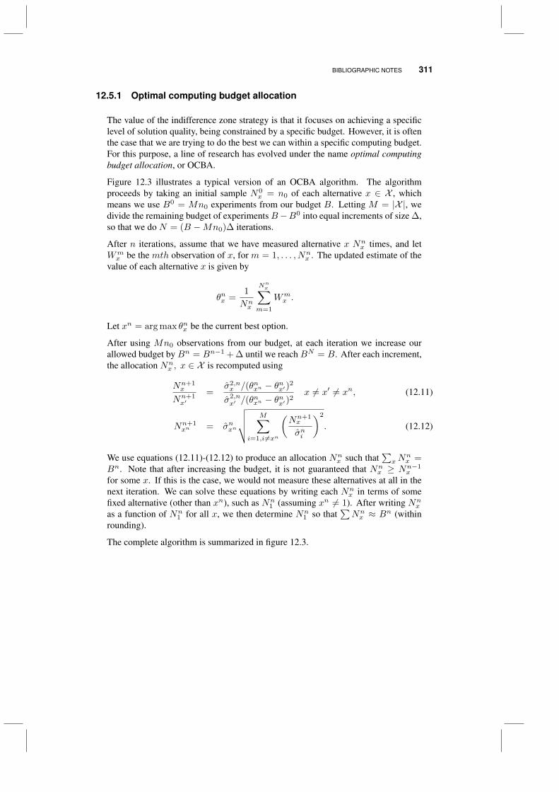
BIBLIOGRAPHIC NOTES 311
12.5.1 Optimal computing budget allocation
The value of the indifference zone strategy is that it focuses on achieving a specificlevel of solution quality, being constrained by a specific budget. However, it is oftenthe case that we are trying to do the best we can within a specific computing budget.For this purpose, a line of research has evolved under the name optimal computingbudget allocation, or OCBA.
Figure 12.3 illustrates a typical version of an OCBA algorithm. The algorithmproceeds by taking an initial sample N0
x = n0 of each alternative x ∈ X , whichmeans we use B0 = Mn0 experiments from our budget B. Letting M = |X |, wedivide the remaining budget of experimentsB−B0 into equal increments of size ∆,so that we do N = (B −Mn0)∆ iterations.
After n iterations, assume that we have measured alternative x Nnx times, and let
Wmx be the mth observation of x, for m = 1, . . . , Nn
x . The updated estimate of thevalue of each alternative x is given by
θnx =1
Nnx
Nnx∑m=1
Wmx .
Let xn = arg max θnx be the current best option.
After using Mn0 observations from our budget, at each iteration we increase ourallowed budget by Bn = Bn−1 + ∆ until we reach BN = B. After each increment,the allocation Nn
x , x ∈ X is recomputed using
Nn+1x
Nn+1x′
=σ2,nx /(θnxn − θnx′)2
σ2,nx′ /(θ
nxn − θnx′)2
x 6= x′ 6= xn, (12.11)
Nn+1xn = σnxn
√√√√ M∑i=1,i6=xn
(Nn+1x
σni
)2
. (12.12)
We use equations (12.11)-(12.12) to produce an allocation Nnx such that
∑xN
nx =
Bn. Note that after increasing the budget, it is not guaranteed that Nnx ≥ Nn−1
x
for some x. If this is the case, we would not measure these alternatives at all in thenext iteration. We can solve these equations by writing each Nn
x in terms of somefixed alternative (other than xn), such as Nn
1 (assuming xn 6= 1). After writing Nnx
as a function of Nn1 for all x, we then determine Nn
1 so that∑Nnx ≈ Bn (within
rounding).
The complete algorithm is summarized in figure 12.3.

312 ACTIVE LEARNING IN STATISTICS
Step 0. Initialization:
Step 0a. Given a computing budget B, let n0 be the initial sample size for each of the M = |X |alternatives. Divide the remaining budget T −Mn0 into increments so that N = (T −Mn0)/δis an integer.
Step 0b. Obtain samples Wmx , m = 1, . . . , n0 samples of each x ∈ X .
Step 0c. Initialize N1x = n0 for all x ∈ X .
Step 0d. Initialize n = 1.
Step 1. Compute
θnx =1
Nnx
Nnx∑m=1
Wmx .
Compute the sample variances for each pair using
σ2,nx =
1
Nnx − 1
Nnx∑m=1
(Wmx − θnx )2 .
Step 2. Let xn = arg maxx∈X θnx .
Step 3. Increase the computing budget by ∆ and calculate the new allocation Nn+11 , . . . , Nn+1
M so that
Nn+1x
Nn+1x′
=σ2,nx /(θnxn − θnx′ )
2
σ2,nx′ /(θ
nxn − θnx′ )2
x 6= x′ 6= xn,
Nn+1xn = σnxn
√√√√√ M∑i=1,i 6=xn
(Nn+1x
σni
)2
.
Step 4. Perform max(Nn+1x −Nn
x , 0)
additional simulations for each alternative x.
Step 5. Set n = n+ 1. If∑x∈X N
nx < B, go to step 1.
Step 6. Return xn arg maxx∈X θnx .
Figure 12.3 Optimal computing budget allocation procedure.

CHAPTER 13
LEARNING IN MATHEMATICALPROGRAMMING
There are applications where we have to collect information to be used in a largeroptimization problem such as a shortest path problem or linear program. Rankingand selection can be viewed as the solution to a simple linear program
vn = maxx
M∑i=1
µixi
subject to
M∑i=1
xi = 1
xi ≥ 0.
The solution to this linear program requires sorting (µi) for all i and choosing theindex i∗ with the largest value of µi, which gives us a solution where xi∗ = 1,and xi = 0, i 6= i∗. Our learning challenge is to choose an element j to measure,producing a value vn+1(j) computed using the vector µi. The goal is to choose theindex j that maximizes the expected value of vn+1. Note for this discussion that weare using indices i and j for our choices, and we are switching (for this chapter) to xas the vector of implementation decisions.
Optimal Learning. By Warren B. Powell and Ilya O. RyzhovCopyright c© 2018 John Wiley & Sons, Inc.
313
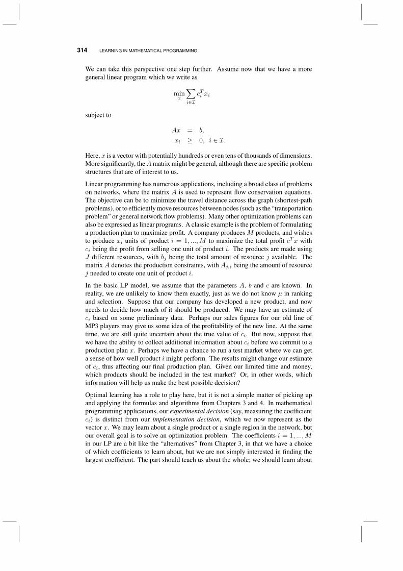
314 LEARNING IN MATHEMATICAL PROGRAMMING
We can take this perspective one step further. Assume now that we have a moregeneral linear program which we write as
minx
∑i∈I
cTi xi
subject to
Ax = b,
xi ≥ 0, i ∈ I.
Here, x is a vector with potentially hundreds or even tens of thousands of dimensions.More significantly, theAmatrix might be general, although there are specific problemstructures that are of interest to us.
Linear programming has numerous applications, including a broad class of problemson networks, where the matrix A is used to represent flow conservation equations.The objective can be to minimize the travel distance across the graph (shortest-pathproblems), or to efficiently move resources between nodes (such as the “transportationproblem” or general network flow problems). Many other optimization problems canalso be expressed as linear programs. A classic example is the problem of formulatinga production plan to maximize profit. A company produces M products, and wishesto produce xi units of product i = 1, ...,M to maximize the total profit cTx withci being the profit from selling one unit of product i. The products are made usingJ different resources, with bj being the total amount of resource j available. Thematrix A denotes the production constraints, with Aj,i being the amount of resourcej needed to create one unit of product i.
In the basic LP model, we assume that the parameters A, b and c are known. Inreality, we are unlikely to know them exactly, just as we do not know µ in rankingand selection. Suppose that our company has developed a new product, and nowneeds to decide how much of it should be produced. We may have an estimate ofci based on some preliminary data. Perhaps our sales figures for our old line ofMP3 players may give us some idea of the profitability of the new line. At the sametime, we are still quite uncertain about the true value of ci. But now, suppose thatwe have the ability to collect additional information about ci before we commit to aproduction plan x. Perhaps we have a chance to run a test market where we can geta sense of how well product i might perform. The results might change our estimateof ci, thus affecting our final production plan. Given our limited time and money,which products should be included in the test market? Or, in other words, whichinformation will help us make the best possible decision?
Optimal learning has a role to play here, but it is not a simple matter of picking upand applying the formulas and algorithms from Chapters 3 and 4. In mathematicalprogramming applications, our experimental decision (say, measuring the coefficientci) is distinct from our implementation decision, which we now represent as thevector x. We may learn about a single product or a single region in the network, butour overall goal is to solve an optimization problem. The coefficients i = 1, ...,Min our LP are a bit like the “alternatives” from Chapter 3, in that we have a choiceof which coefficients to learn about, but we are not simply interested in finding thelargest coefficient. The part should teach us about the whole; we should learn about
APPLICATIONS 315
those coefficients that contribute the most to our ability to optimize. Running a testmarket for product i should lead us to a better production plan.
Although we cannot recycle the knowledge gradient formulas from Chapter 4 in astraightforward way, we can still apply the concept of the knowledge gradient. In thischapter, we show how the value of information can be expressed in problems withuncertain objective functions. After describing several applications, we illustratethe application of the knowledge gradient first in the context of simple shortest pathproblems, and then for more general linear programs.
13.1 APPLICATIONS
In this section, we introduce three models where the implementation decision requiressolving a mathematical program. We begin with a model for piloting a hot air balloon,where the challenge is moving the balloon up and down to find the fastest wind. Givena current set of estimates about the wind, the balloon can solve a linear program tofind the best path to the destination. Then, we describe a common problem in theinvestment community where it is necessary to visit different companies to learn abouttheir potential for future profits. The challenge is determining which companies tovisit (we do not have the time to visit all of them), after which we have to take estimatesof expected returns, variances and covariances to determine the best portfolio. Weclose with a discussion of graph problems.
13.1.1 Piloting a hot air balloon
Consider the problem faced by a balloonist trying to get from one point to anotherin the presence of changing winds that can be different at different altitudes. Herability to make progress depends on finding wind that moves in the right direction.She observes the speed and direction of the wind at her current location, but she maywonder if the conditions are better at a different altitude. Observing the wind at onealtitude provides some information about the wind at other altitudes, as well as thewind at later points in time. But it takes time and (if she has to raise her altitude)energy to make these observations.
The model Optimizing the trajectory of a hot air balloon is a fairly difficult controlproblem, even when we do not include learning as a dimension. For our purposes,we are going to simplify the problem by assuming that our balloon can only movein two dimensions: forward and up or down. Our interest is in finding a path thatbalances distance against changing (and uncertain) wind speeds so that we get to thedestination as quickly as possible.
Our view of the problem is depicted in Figure 13.1, where our balloon is currentlyat horizontal location x, vertical location y, and is faced with one of three decisions:dup takes the balloon on an upward trajectory, dstay holds the balloon at its currentaltitude while ddown takes the balloon on a downward trajectory. Although we wouldlike to model energy expenditure, we are only going to capture the time required
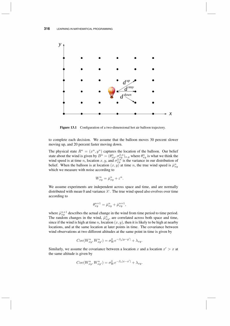
316 LEARNING IN MATHEMATICAL PROGRAMMING
x
y
updstayd
downd
Figure 13.1 Configuration of a two-dimensional hot air balloon trajectory.
to complete each decision. We assume that the balloon moves 30 percent slowermoving up, and 20 percent faster moving down.
The physical state Rn = (xn, yn) captures the location of the balloon. Our beliefstate about the wind is given by Bn = (θnxy, σ
2,nxy )x,y where θnxy is what we think the
wind speed is at time n, location x, y, and σ2,nxy is the variance in our distribution of
belief. When the balloon is at location (x, y) at time n, the true wind speed is µnxywhich we measure with noise according to
Wnxy = µnxy + εn.
We assume experiments are independent across space and time, and are normallydistributed with mean 0 and variance λε. The true wind speed also evolves over timeaccording to
θn+1xy = µnxy + µn+1
xy ,
where µn+1xy describes the actual change in the wind from time period to time period.
The random changes in the wind, µnxy , are correlated across both space and time,since if the wind is high at time n, location (x, y), then it is likely to be high at nearbylocations, and at the same location at later points in time. The covariance betweenwind observations at two different altitudes at the same point in time is given by
Cov(Wnxy,W
nxy′) = σ2
W e−βy|y−y′| + λxy.
Similarly, we assume the covariance between a location x and a location x′ > x atthe same altitude is given by
Cov(Wnxy,W
nxy′) = σ2
W e−βx|x−x′| + λxy.
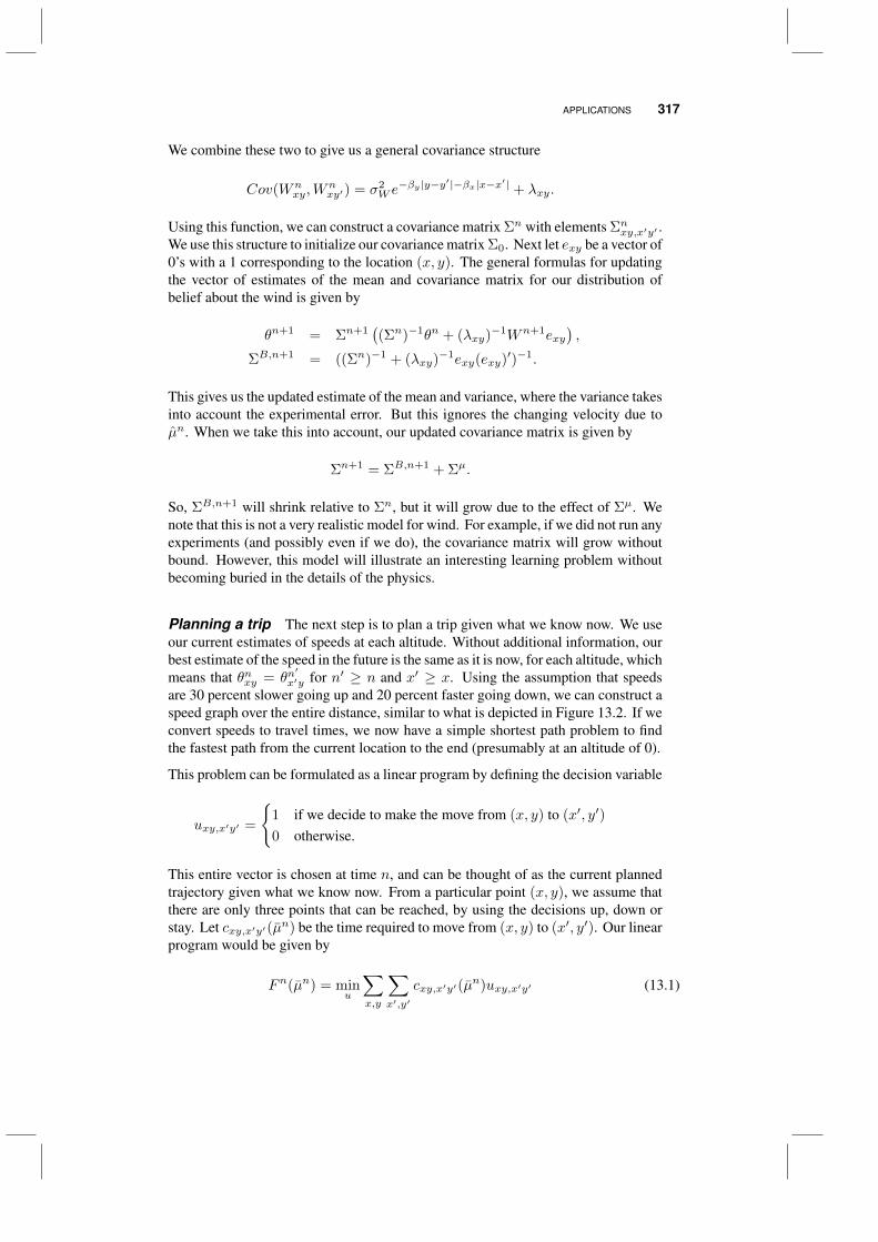
APPLICATIONS 317
We combine these two to give us a general covariance structure
Cov(Wnxy,W
nxy′) = σ2
W e−βy|y−y′|−βx|x−x′| + λxy.
Using this function, we can construct a covariance matrix Σn with elements Σnxy,x′y′ .We use this structure to initialize our covariance matrix Σ0. Next let exy be a vector of0’s with a 1 corresponding to the location (x, y). The general formulas for updatingthe vector of estimates of the mean and covariance matrix for our distribution ofbelief about the wind is given by
θn+1 = Σn+1((Σn)−1θn + (λxy)−1Wn+1exy
),
ΣB,n+1 = ((Σn)−1 + (λxy)−1exy(exy)′)−1.
This gives us the updated estimate of the mean and variance, where the variance takesinto account the experimental error. But this ignores the changing velocity due toµn. When we take this into account, our updated covariance matrix is given by
Σn+1 = ΣB,n+1 + Σµ.
So, ΣB,n+1 will shrink relative to Σn, but it will grow due to the effect of Σµ. Wenote that this is not a very realistic model for wind. For example, if we did not run anyexperiments (and possibly even if we do), the covariance matrix will grow withoutbound. However, this model will illustrate an interesting learning problem withoutbecoming buried in the details of the physics.
Planning a trip The next step is to plan a trip given what we know now. We useour current estimates of speeds at each altitude. Without additional information, ourbest estimate of the speed in the future is the same as it is now, for each altitude, whichmeans that θnxy = θn
′
x′y for n′ ≥ n and x′ ≥ x. Using the assumption that speedsare 30 percent slower going up and 20 percent faster going down, we can construct aspeed graph over the entire distance, similar to what is depicted in Figure 13.2. If weconvert speeds to travel times, we now have a simple shortest path problem to findthe fastest path from the current location to the end (presumably at an altitude of 0).
This problem can be formulated as a linear program by defining the decision variable
uxy,x′y′ =
1 if we decide to make the move from (x, y) to (x′, y′)
0 otherwise.
This entire vector is chosen at time n, and can be thought of as the current plannedtrajectory given what we know now. From a particular point (x, y), we assume thatthere are only three points that can be reached, by using the decisions up, down orstay. Let cxy,x′y′(µn) be the time required to move from (x, y) to (x′, y′). Our linearprogram would be given by
Fn(µn) = minu
∑x,y
∑x′,y′
cxy,x′y′(µn)uxy,x′y′ (13.1)
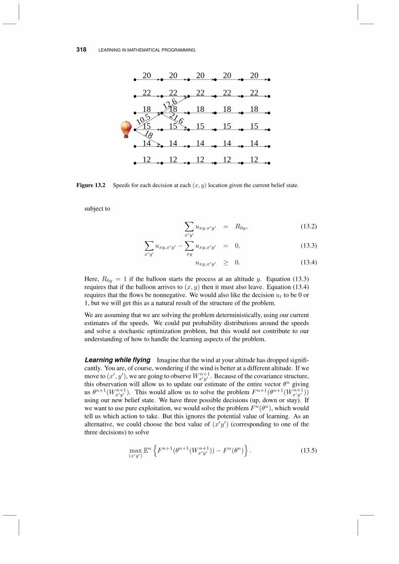
318 LEARNING IN MATHEMATICAL PROGRAMMING
20
22
18
15
14
12
10.5
18
20
22
18
15
14
12
20
22
18
15
14
12
20
22
18
15
14
12
20
22
18
15
14
12
12.621.6
Figure 13.2 Speeds for each decision at each (x, y) location given the current belief state.
subject to ∑x′y′
uxy,x′y′ = R0y, (13.2)
∑x′y′
uxy,x′y′ −∑xy
uxy,x′y′ = 0, (13.3)
uxy,x′y′ ≥ 0. (13.4)
Here, R0y = 1 if the balloon starts the process at an altitude y. Equation (13.3)requires that if the balloon arrives to (x, y) then it must also leave. Equation (13.4)requires that the flows be nonnegative. We would also like the decision ut to be 0 or1, but we will get this as a natural result of the structure of the problem.
We are assuming that we are solving the problem deterministically, using our currentestimates of the speeds. We could put probability distributions around the speedsand solve a stochastic optimization problem, but this would not contribute to ourunderstanding of how to handle the learning aspects of the problem.
Learning while flying Imagine that the wind at your altitude has dropped signifi-cantly. You are, of course, wondering if the wind is better at a different altitude. If wemove to (x′, y′), we are going to observeWn+1
x′y′ . Because of the covariance structure,this observation will allow us to update our estimate of the entire vector θn givingus θn+1(Wn+1
x′y′ ). This would allow us to solve the problem Fn+1(θn+1(Wn+1x′y′ ))
using our new belief state. We have three possible decisions (up, down or stay). Ifwe want to use pure exploitation, we would solve the problem Fn(θn), which wouldtell us which action to take. But this ignores the potential value of learning. As analternative, we could choose the best value of (x′y′) (corresponding to one of thethree decisions) to solve
max(x′y′)
EnFn+1(θn+1(Wn+1
x′y′ ))− Fn(θn). (13.5)
APPLICATIONS 319
We have written this function in the form of the knowledge gradient, recognizingthat Fn(θn) is a constant (given what we know at time n) which does not affect thesolution.
When we first introduced the knowledge gradient, we presented it in the context ofranking and selection where we had to choose from among a small, discrete set ofchoices. Now, we have to solve a linear program for each possible experiment, whichmeans we can no longer compute the expectation exactly. But we can take advantageof the fact that we have a small number of potential experimental decisions (up,down or stay), which means we effectively face a ranking and selection problem. Wecannot compute the expectation exactly, but we can use Monte Carlo methods. LetWn+1x′y′ (ω) be a sample observation of the wind if we were to choose to go to location
(x′y′). This is not a true observation - it is a simulated observation for the purposeof approximating the expectation.
Given this observation, we can update the mean and covariance matrix and solvethe linear program. Note that this observation does not just change the speed outof node (x′y′) (take another look at Figure 13.2); it changes estimates of speedsover the entire network, partly because of the presence of correlations, and partlybecause we solve our linear program by assuming that as we step forward in time, wedo not collect additional information (which means that speeds at the same altitudefor larger values of x′ are the same). Let Fn+1(x′y′|ω) be the resulting “sampleobservation” of EnFn+1(θn+1(Wn+1
x′y′ )). We could then repeat this, say, 100 times,for each possible decision and take an average. We could then make the decision thathas the highest estimated value.
Sound familiar? This is precisely the ranking and selection problem. Solving thelinear program 100 times and taking an average is a bit clumsy (famously knownas the “brute force” solution). A more elegant approach would be to use (drum rollplease) the knowledge gradient algorithm to choose the best decision. This wouldallow us to avoid running 100 experiments of a choice that does not look promising.We can build a prior by initially evaluating each choice assuming that we do not learnanything (the wind does not change from the prior), so that we start with a solutionbuilt around the pure exploitation policy.
Optimal learning versus stochastic optimization It is useful to contrastour learning algorithm versus what we might have done if we were solving this asa stochastic optimization problem. In a stochastic optimization model, we wouldacknowledge that we do not know what wind we will face when we arrive to alocation (x′y′) (above, we solved the problem deterministically). For example, adeterministic solution might take us closer to the ground if the wind seems to befastest there. However, a stochastic solution might recognize that the wind nearthe ground might be much lower than expected, and if we are close to the ground,the only place to go is up (at a high cost). A stochastic solution to this problemis relatively difficult, and probably requires the techniques of approximate dynamicprogramming.
The issue of whether to use a deterministic or stochastic algorithmic strategy did notarise with the simpler problems such as ranking and selection, because the optimalsolution was to pick the index j∗ with the highest expected value of θNj . Ourstochastic shortest path problem, however, is different because it involves finding a
320 LEARNING IN MATHEMATICAL PROGRAMMING
path over a sequence of steps with uncertain costs. Even if we fix our distribution ofbelief, it is still a stochastic optimization problem.
The essential difference between a stochastic optimization algorithm and a learningalgorithm is that with a learning algorithm, we accept that observations of the wind(the external experiment) come from an exogenous distribution that may be differentfrom our true distribution of belief. As a result, we use these observations to updateour distribution of belief. With a classical stochastic optimization formulation, weacknowledge that we do not know the actual wind, but we do know the probabilitydistribution, which means that observations do not change our distribution of beliefabout the distribution.
13.1.2 Optimizing a portfolio
Imagine that you are looking at investing in a group of companies. The companies areorganized by industry segment (retailing, financial services, transportation), so wewill refer to the jth company within the ith industry segment. We start by assumingthat θ0
ij is the expected return (over some period of time) for company j in segmenti. We also let Σ0 be the matrix that captures the covariances in our beliefs about µij ,where the diagonal elements Σij,ij represent the variance.
In general, we assume that the covariance between two companies has the structure
Σij,i′j′ = σ20 + σ2
i 1i=i′.
Thus, σ20 captures the common covariance (e.g. the extent to which companies
respond to the general economy), and σ2i captures the common covariance for com-
panies within industry segment i.
Before we invest in a company, we have the ability to visit the company and learnmore about the management team, marketing plans and facilities. We might assumethat our observation W of each company is independent with variance λij . Letxij = 1 if we visit company (i, j). If we choose to visit company (i, j), we canupdate the mean and variance using our standard formulas, giving us an updatedθ1ij(x). If xij = 0, then θ1
ij(x) = θ0ij , and we let Σ1(x) be the updated covariance
matrix.
Given the vector x of visits (presumably chosen to a constraint on how many visitswe can make), we then have to find an optimal portfolio. Let yij be the amount thatwe are going to invest in company (ij). We do this by solving the standard quadraticprogramming problem
F (x) = EF (x,W ) = miny
(θ1(x)y + θyTΣ1(x)y
)(13.6)
subject to ∑ij
yij = RI , (13.7)
yij ≥ 0. (13.8)
Here, x is our experimental decision, W captures what we observe if we choose torun the experiment, and y is our implementation decision. RI is the amount of money
APPLICATIONS 321
we have to invest. The learning problem is given by
minx
EF (x,W ) (13.9)
subject to ∑ij
cijxij = RM , (13.10)
xij ≥ 0 and integer. (13.11)
Here, RM is our experimental budget. The learning problem is hard to solve, bothbecause it requires integer solutions but primarily because of the problems computingthe expectation in (13.9). We suggest simply finding the marginal value of makingeach visit, and then assigning visits in order of decreasing marginal value until thebudget is exhausted. This is a type of batch ranking and selection problem, whereinstead of finding the best choice, we find the best set of choices.
Even this simple heuristic is hard to implement. Imagine that there are 100 companiesthat we are considering, and we have the budget to make 20 visits. What are the best20 companies to visit? We are not able to compute the expectation EF (x,W ) in(13.6) either. Instead, we can choose a company to visit, then randomly sample whatwe might learn (Wij(ω)). We can perform 100 samples of each company and takean average to obtain an estimate of the value of visiting each company, but this maybe computationally demanding (and 100 samples may not be enough). Or, we canuse the knowledge gradient algorithm to allocate our computational budget acrossthe 100 companies.
13.1.3 Network problems
Optimization on a graph is a well-known class of mathematical programming prob-lems, with applications in transportation, project management, telecommunicationand other areas. A graph is described by a set V of nodes (or “vertices”) and a setE ⊆ V × V of edges, where each edge connects two nodes. Figure 13.3 providesa visual illustration. It is easiest to think of a graph as a map of physical locations:for example, nodes could represent cities and edges could stand for major highwaysconnecting those cities. An edge (i, j) ∈ E between nodes i and j carries a cost (or“length”) cij . The cost can be expressed in terms of money or time. For example,we might focus on the economic cost of transporting a shipment of goods from onecity to another, or on the time needed for the shipment to reach its destination.
Implementation decisions in networks The shipment problem is a well-studied application of minimum-cost flows, a model for optimizing the route ofresources across a network. A number bi represents either the supply or demand for acommodity at node i. If bi > 0, then i is a supply node (perhaps we have a productionfacility in city i, or we purchase from a manufacturer located in this city). If bi < 0,then i is a demand node (perhaps retailers in this city are selling our products). Ifbi = 0, the node is a transit node and our product can be transported through it enroute to a demand node.
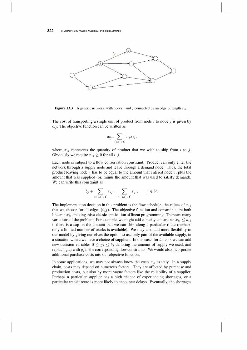
322 LEARNING IN MATHEMATICAL PROGRAMMING
Figure 13.3 A generic network, with nodes i and j connected by an edge of length cij .
The cost of transporting a single unit of product from node i to node j is given bycij . The objective function can be written as
minx
∑(i,j)∈E
cijxij ,
where xij represents the quantity of product that we wish to ship from i to j.Obviously we require xij ≥ 0 for all i, j.
Each node is subject to a flow conservation constraint. Product can only enter thenetwork through a supply node and leave through a demand node. Thus, the totalproduct leaving node j has to be equal to the amount that entered node j, plus theamount that was supplied (or, minus the amount that was used to satisfy demand).We can write this constraint as
bj +∑
i:(i,j)∈E
xij =∑
i:(j,i)∈E
xji, j ∈ V.
The implementation decision in this problem is the flow schedule, the values of xijthat we choose for all edges (i, j). The objective function and constraints are bothlinear in xij , making this a classic application of linear programming. There are manyvariations of the problem. For example, we might add capacity constraints xij ≤ dijif there is a cap on the amount that we can ship along a particular route (perhapsonly a limited number of trucks is available). We may also add more flexibility toour model by giving ourselves the option to use only part of the available supply, ina situation where we have a choice of suppliers. In this case, for bj > 0, we can addnew decision variables 0 ≤ yj ≤ bj denoting the amount of supply we used, andreplacing bj with yj in the corresponding flow constraints. We would also incorporateadditional purchase costs into our objective function.
In some applications, we may not always know the costs cij exactly. In a supplychain, costs may depend on numerous factors. They are affected by purchase andproduction costs, but also by more vague factors like the reliability of a supplier.Perhaps a particular supplier has a high chance of experiencing shortages, or aparticular transit route is more likely to encounter delays. Eventually, the shortages
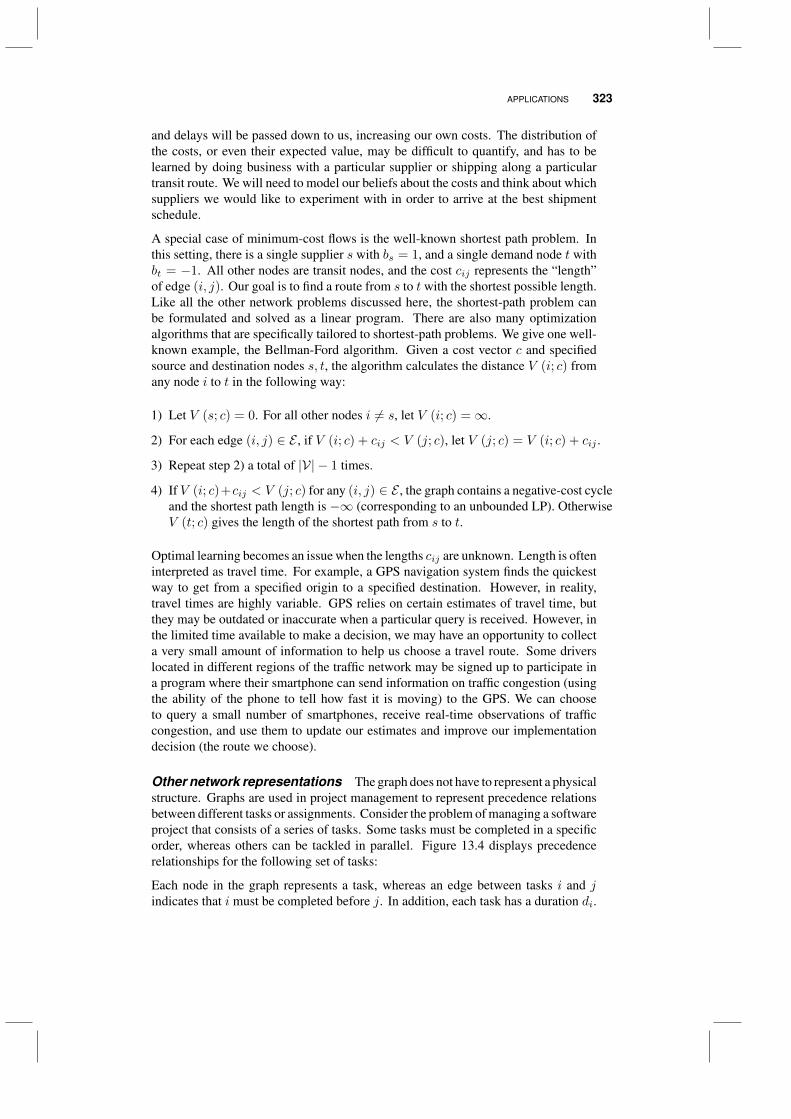
APPLICATIONS 323
and delays will be passed down to us, increasing our own costs. The distribution ofthe costs, or even their expected value, may be difficult to quantify, and has to belearned by doing business with a particular supplier or shipping along a particulartransit route. We will need to model our beliefs about the costs and think about whichsuppliers we would like to experiment with in order to arrive at the best shipmentschedule.
A special case of minimum-cost flows is the well-known shortest path problem. Inthis setting, there is a single supplier s with bs = 1, and a single demand node t withbt = −1. All other nodes are transit nodes, and the cost cij represents the “length”of edge (i, j). Our goal is to find a route from s to t with the shortest possible length.Like all the other network problems discussed here, the shortest-path problem canbe formulated and solved as a linear program. There are also many optimizationalgorithms that are specifically tailored to shortest-path problems. We give one well-known example, the Bellman-Ford algorithm. Given a cost vector c and specifiedsource and destination nodes s, t, the algorithm calculates the distance V (i; c) fromany node i to t in the following way:
1) Let V (s; c) = 0. For all other nodes i 6= s, let V (i; c) =∞.
2) For each edge (i, j) ∈ E , if V (i; c) + cij < V (j; c), let V (j; c) = V (i; c) + cij .
3) Repeat step 2) a total of |V| − 1 times.
4) If V (i; c)+cij < V (j; c) for any (i, j) ∈ E , the graph contains a negative-cost cycleand the shortest path length is −∞ (corresponding to an unbounded LP). OtherwiseV (t; c) gives the length of the shortest path from s to t.
Optimal learning becomes an issue when the lengths cij are unknown. Length is ofteninterpreted as travel time. For example, a GPS navigation system finds the quickestway to get from a specified origin to a specified destination. However, in reality,travel times are highly variable. GPS relies on certain estimates of travel time, butthey may be outdated or inaccurate when a particular query is received. However, inthe limited time available to make a decision, we may have an opportunity to collecta very small amount of information to help us choose a travel route. Some driverslocated in different regions of the traffic network may be signed up to participate ina program where their smartphone can send information on traffic congestion (usingthe ability of the phone to tell how fast it is moving) to the GPS. We can chooseto query a small number of smartphones, receive real-time observations of trafficcongestion, and use them to update our estimates and improve our implementationdecision (the route we choose).
Other network representations The graph does not have to represent a physicalstructure. Graphs are used in project management to represent precedence relationsbetween different tasks or assignments. Consider the problem of managing a softwareproject that consists of a series of tasks. Some tasks must be completed in a specificorder, whereas others can be tackled in parallel. Figure 13.4 displays precedencerelationships for the following set of tasks:
Each node in the graph represents a task, whereas an edge between tasks i and jindicates that i must be completed before j. In addition, each task has a duration di.
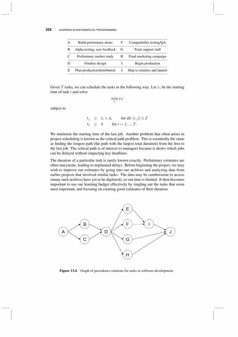
324 LEARNING IN MATHEMATICAL PROGRAMMING
A Build preliminary demo F Compatibility testing/QA
B Alpha testing, user feedback G Train support staff
C Preliminary market study H Final marketing campaign
D Finalize design I Begin production
E Plan production/distribution J Ship to retailers and launch
Given T tasks, we can schedule the tasks in the following way. Let xi be the startingtime of task i and solve
minxxT
subject to
tj ≥ ti + di for all (i, j) ∈ Eti ≥ 0 for i = 1, ..., T.
We minimize the starting time of the last job. Another problem that often arises inproject scheduling is known as the critical path problem. This is essentially the sameas finding the longest path (the path with the largest total duration) from the first tothe last job. The critical path is of interest to managers because it shows which jobscan be delayed without impacting key deadlines.
The duration of a particular task is rarely known exactly. Preliminary estimates areoften inaccurate, leading to unplanned delays. Before beginning the project, we maywish to improve our estimates by going into our archives and analyzing data fromearlier projects that involved similar tasks. The data may be cumbersome to access(many such archives have yet to be digitized), so our time is limited. It then becomesimportant to use our learning budget effectively by singling out the tasks that seemmost important, and focusing on creating good estimates of their duration.
Figure 13.4 Graph of precedence relations for tasks in software development.
LEARNING ON GRAPHS 325
13.1.4 Discussion
We have just seen several problems where the decision problem (we sometimes callthis the implementation problem) is a linear or nonlinear program. Finding theexpected value of an experimental outcome can be computationally difficult. But wehave seen that we can apply our optimal learning ideas within a learning algorithmto help us find a good learning policy.
Both of these problems could be formulated in the general framework of finding anexperimental decision x to minimize EF (x,W ). This is a very classical optimizationproblem with a rich algorithmic history. There are many algorithms which dependon the structure of the problem. An excellent reference for this problem class is Spall(2003) and the references cited there (the literature is extremely large).
13.2 LEARNING ON GRAPHS
We show how optimal learning can be incorporated into network optimization using,the shortest-path problem from Section 13.1.3 as an example. To make our analysiscleaner, we assume that the graph has no cycles, as in Figure 13.3.
Optimal learning begins to play a role when we no longer know the cost vector c. Letus apply our standard modeling assumptions from Chapter 4. Suppose that, for eachedge (i, j) ∈ E , we have cij ∼ N
(θ0ij , β
0ij
), where β0 denotes precision. We put a
Gaussian prior on the length of each edge, and assume that the edges are independent.This is a strong assumption: for example, if the graph represents a traffic network,as in some of the examples discussed in Section 13.1.3, one would expect the traveltimes on neighbouring streets to be heavily correlated. We will allow correlations inSection 13.4. For now, we focus on the insights that can be obtained if we make theindependence assumption.
As in ranking and selection, the belief state in this problem can be written as S =(θ, β), a vector of means and variances. A set of beliefs about the edges induces abelief about the best path. Define V n = V (s; θn) to be the estimated length of theshortest path, given our time-n beliefs about the edge lengths. In other words, wesimply run the Bellman-Ford algorithm using the estimates θn as the costs, and usethe quantity V n as our time-n estimate of the shortest path. Bellman-Ford can alsoprovide us with the path that achieves this estimated length. We refer to this path aspn.
Now suppose that, before we commit to a path through the network, we have Nopportunities to collect information about individual edges. If we choose to learnabout (in, jn) at time n, we collect an observation Wn+1 ∼ N
(cij , β
Wij
)and our
beliefs evolve according to the familiar updating equations
θn+1ij =
βnijθ
nij+β
Wij W
n+1ij
βnij+βWij
if (i, j) = (in, jn)
θnij otherwise,(13.12)
βn+1x =
βnij + βWij if (i, j) = (in, jn)
βnij otherwise.(13.13)
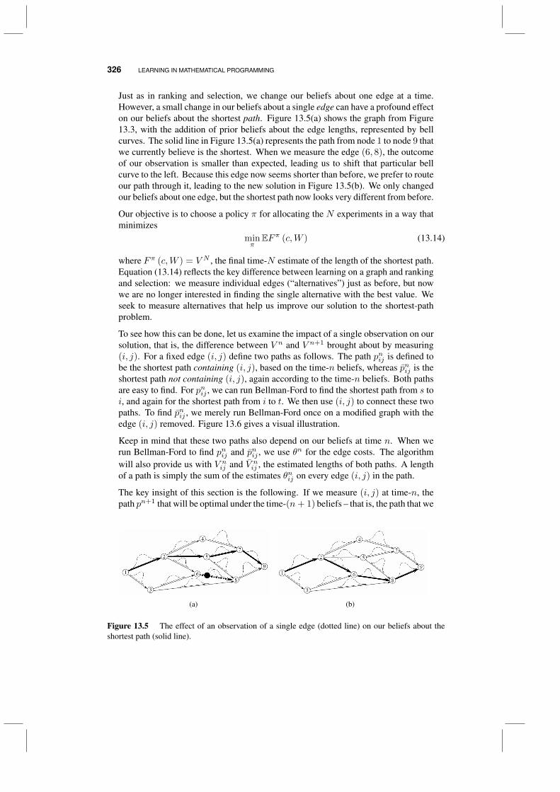
326 LEARNING IN MATHEMATICAL PROGRAMMING
Just as in ranking and selection, we change our beliefs about one edge at a time.However, a small change in our beliefs about a single edge can have a profound effecton our beliefs about the shortest path. Figure 13.5(a) shows the graph from Figure13.3, with the addition of prior beliefs about the edge lengths, represented by bellcurves. The solid line in Figure 13.5(a) represents the path from node 1 to node 9 thatwe currently believe is the shortest. When we measure the edge (6, 8), the outcomeof our observation is smaller than expected, leading us to shift that particular bellcurve to the left. Because this edge now seems shorter than before, we prefer to routeour path through it, leading to the new solution in Figure 13.5(b). We only changedour beliefs about one edge, but the shortest path now looks very different from before.
Our objective is to choose a policy π for allocating the N experiments in a way thatminimizes
minπ
EFπ (c,W ) (13.14)
where Fπ (c,W ) = V N , the final time-N estimate of the length of the shortest path.Equation (13.14) reflects the key difference between learning on a graph and rankingand selection: we measure individual edges (“alternatives”) just as before, but nowwe are no longer interested in finding the single alternative with the best value. Weseek to measure alternatives that help us improve our solution to the shortest-pathproblem.
To see how this can be done, let us examine the impact of a single observation on oursolution, that is, the difference between V n and V n+1 brought about by measuring(i, j). For a fixed edge (i, j) define two paths as follows. The path pnij is defined tobe the shortest path containing (i, j), based on the time-n beliefs, whereas pnij is theshortest path not containing (i, j), again according to the time-n beliefs. Both pathsare easy to find. For pnij , we can run Bellman-Ford to find the shortest path from s toi, and again for the shortest path from i to t. We then use (i, j) to connect these twopaths. To find pnij , we merely run Bellman-Ford once on a modified graph with theedge (i, j) removed. Figure 13.6 gives a visual illustration.
Keep in mind that these two paths also depend on our beliefs at time n. When werun Bellman-Ford to find pnij and pnij , we use θn for the edge costs. The algorithmwill also provide us with V nij and V nij , the estimated lengths of both paths. A lengthof a path is simply the sum of the estimates θnij on every edge (i, j) in the path.
The key insight of this section is the following. If we measure (i, j) at time-n, thepath pn+1 that will be optimal under the time-(n+ 1) beliefs – that is, the path that we
(a) (b)
Figure 13.5 The effect of an observation of a single edge (dotted line) on our beliefs about theshortest path (solid line).
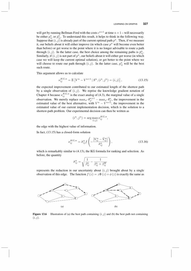
LEARNING ON GRAPHS 327
will get by running Bellman-Ford with the costs cn+1 at time n+1 – will necessarilybe either pnij or pnij . To understand this result, it helps to think in the following way.Suppose that (i, j) is already part of the current optimal path pn. Then, if we measureit, our beliefs about it will either improve (in which case pn will become even betterthan before) or get worse to the point where it is no longer advisable to route a paththrough (i, j). In the latter case, the best choice among the remaining paths is pnij .Similarly, if (i, j) is not part of pn, our beliefs about it will either get worse (in whichcase we will keep the current optimal solution), or get better to the point where wewill choose to route our path through (i, j). In the latter case, pnij will be the bestsuch route.
This argument allows us to calculate
νKG,nij = E[V n − V n+1 |Sn, (in, jn) = (i, j)
], (13.15)
the expected improvement contributed to our estimated length of the shortest pathby a single observation of (i, j). We reprise the knowledge gradient notation ofChapter 4 because νKG,nij is the exact analog of (4.3), the marginal value of a singleobservation. We merely replace maxx′ θ
n+1x′ − maxx′ θ
nx′ , the improvement in the
estimated value of the best alternative, with V n − V n+1, the improvement in theestimated value of our current implementation decision, which is the solution to ashortest-path problem. Our experimental decision can then be written as
(in, jn) = arg max(i,j)
νKG,nij ,
the edge with the highest value of information.
In fact, (13.15) has a closed-form solution
νKG,nij = σnijf
(−∣∣V nij − V nij ∣∣
σnij
), (13.16)
which is remarkably similar to (4.13), the KG formula for ranking and selection. Asbefore, the quantity
σnij =
√1
βnij− 1
βnij + βWij
represents the reduction in our uncertainty about (i, j) brought about by a singleobservation of this edge. The function f (z) = zΦ (z) +φ (z) is exactly the same as
(a) (b)
Figure 13.6 Illustration of (a) the best path containing (i, j) and (b) the best path not containing(i, j).
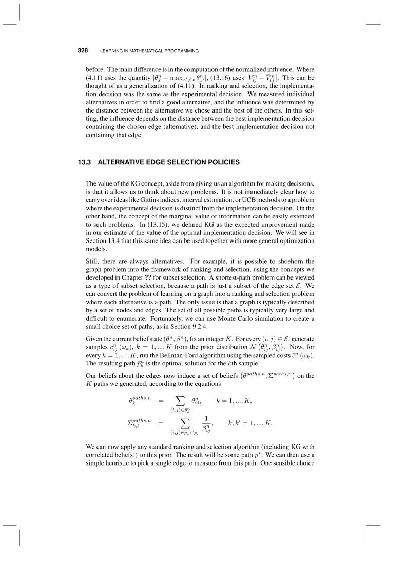
328 LEARNING IN MATHEMATICAL PROGRAMMING
before. The main difference is in the computation of the normalized influence. Where(4.11) uses the quantity |θnx −maxx′ 6=x θ
nx′ |, (13.16) uses
∣∣V nij − V nij ∣∣. This can bethought of as a generalization of (4.11). In ranking and selection, the implementa-tion decision was the same as the experimental decision. We measured individualalternatives in order to find a good alternative, and the influence was determined bythe distance between the alternative we chose and the best of the others. In this set-ting, the influence depends on the distance between the best implementation decisioncontaining the chosen edge (alternative), and the best implementation decision notcontaining that edge.
13.3 ALTERNATIVE EDGE SELECTION POLICIES
The value of the KG concept, aside from giving us an algorithm for making decisions,is that it allows us to think about new problems. It is not immediately clear how tocarry over ideas like Gittins indices, interval estimation, or UCB methods to a problemwhere the experimental decision is distinct from the implementation decision. On theother hand, the concept of the marginal value of information can be easily extendedto such problems. In (13.15), we defined KG as the expected improvement madein our estimate of the value of the optimal implementation decision. We will see inSection 13.4 that this same idea can be used together with more general optimizationmodels.
Still, there are always alternatives. For example, it is possible to shoehorn thegraph problem into the framework of ranking and selection, using the concepts wedeveloped in Chapter ?? for subset selection. A shortest-path problem can be viewedas a type of subset selection, because a path is just a subset of the edge set E . Wecan convert the problem of learning on a graph into a ranking and selection problemwhere each alternative is a path. The only issue is that a graph is typically describedby a set of nodes and edges. The set of all possible paths is typically very large anddifficult to enumerate. Fortunately, we can use Monte Carlo simulation to create asmall choice set of paths, as in Section 9.2.4.
Given the current belief state (θn, βn), fix an integerK. For every (i, j) ∈ E , generatesamples cnij (ωk), k = 1, ...,K from the prior distribution N
(θnij , β
nij
). Now, for
every k = 1, ...,K, run the Bellman-Ford algorithm using the sampled costs cn (ωk).The resulting path pnk is the optimal solution for the kth sample.
Our beliefs about the edges now induce a set of beliefs(θpaths,n,Σpaths,n
)on the
K paths we generated, according to the equations
θpaths,nk =∑
(i,j)∈pnk
θnij , k = 1, ...,K,
Σpaths,nk,l =∑
(i,j)∈pnk∩pnl
1
βnij, k, k′ = 1, ...,K.
We can now apply any standard ranking and selection algorithm (including KG withcorrelated beliefs!) to this prior. The result will be some path p∗. We can then use asimple heuristic to pick a single edge to measure from this path. One sensible choice
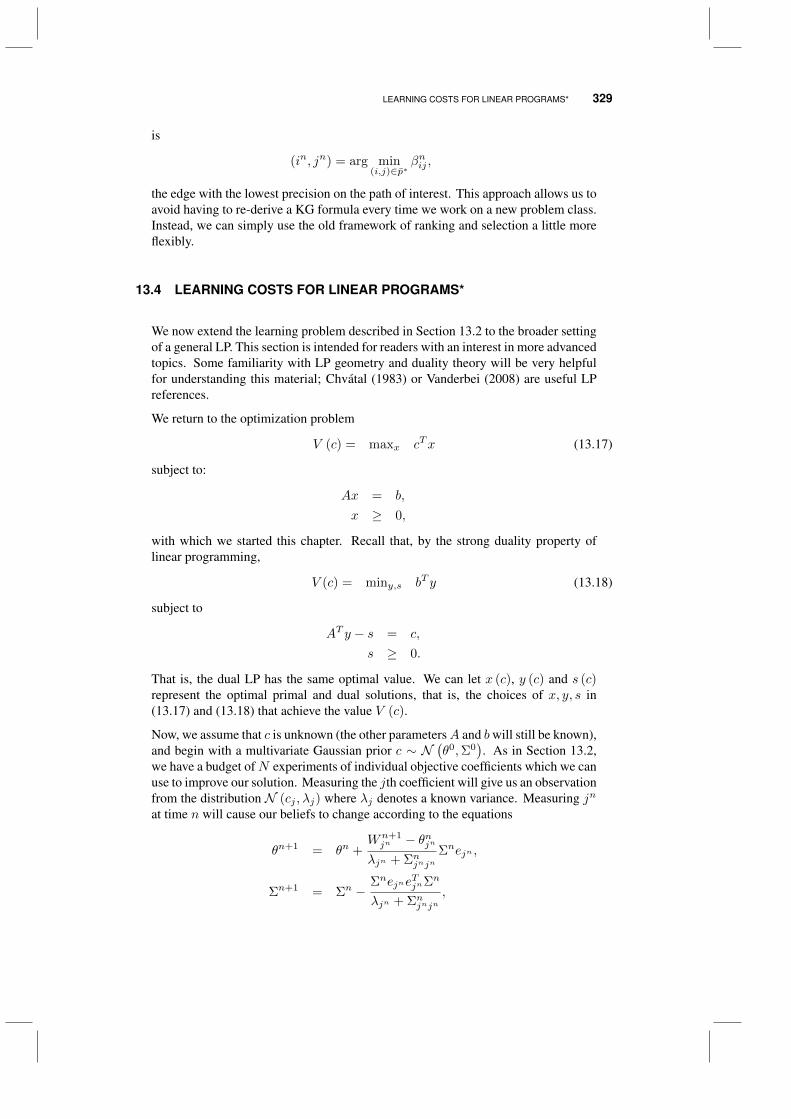
LEARNING COSTS FOR LINEAR PROGRAMS* 329
is
(in, jn) = arg min(i,j)∈p∗
βnij ,
the edge with the lowest precision on the path of interest. This approach allows us toavoid having to re-derive a KG formula every time we work on a new problem class.Instead, we can simply use the old framework of ranking and selection a little moreflexibly.
13.4 LEARNING COSTS FOR LINEAR PROGRAMS*
We now extend the learning problem described in Section 13.2 to the broader settingof a general LP. This section is intended for readers with an interest in more advancedtopics. Some familiarity with LP geometry and duality theory will be very helpfulfor understanding this material; Chvatal (1983) or Vanderbei (2008) are useful LPreferences.
We return to the optimization problem
V (c) = maxx cTx (13.17)
subject to:
Ax = b,
x ≥ 0,
with which we started this chapter. Recall that, by the strong duality property oflinear programming,
V (c) = miny,s bT y (13.18)
subject to
AT y − s = c,
s ≥ 0.
That is, the dual LP has the same optimal value. We can let x (c), y (c) and s (c)represent the optimal primal and dual solutions, that is, the choices of x, y, s in(13.17) and (13.18) that achieve the value V (c).
Now, we assume that c is unknown (the other parametersA and bwill still be known),and begin with a multivariate Gaussian prior c ∼ N
(θ0,Σ0
). As in Section 13.2,
we have a budget ofN experiments of individual objective coefficients which we canuse to improve our solution. Measuring the jth coefficient will give us an observationfrom the distribution N (cj , λj) where λj denotes a known variance. Measuring jn
at time n will cause our beliefs to change according to the equations
θn+1 = θn +Wn+1jn − θnjn
λjn + ΣnjnjnΣnejn ,
Σn+1 = Σn −Σnejne
TjnΣn
λjn + Σnjnjn,
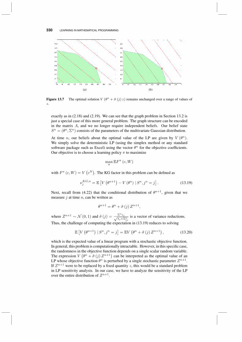
330 LEARNING IN MATHEMATICAL PROGRAMMING
(a) (b)
Figure 13.7 The optimal solution V (θn + σ (j) z) remains unchanged over a range of values ofz.
exactly as in (2.18) and (2.19). We can see that the graph problem in Section 13.2 isjust a special case of this more general problem. The graph structure can be encodedin the matrix A, and we no longer require independent beliefs. Our belief stateSn = (θn,Σn) consists of the parameters of the multivariate Gaussian distribution.
At time n, our beliefs about the optimal value of the LP are given by V (θn).We simply solve the deterministic LP (using the simplex method or any standardsoftware package such as Excel) using the vector θn for the objective coefficients.Our objective is to choose a learning policy π to maximize
maxπ
EFπ (c,W )
with Fπ (c,W ) = V(cN). The KG factor in this problem can be defined as
νKG,nj = E[V(θn+1
)− V (θn) |Sn, jn = j
]. (13.19)
Next, recall from (4.22) that the conditional distribution of θn+1, given that wemeasure j at time n, can be written as
θn+1 = θn + σ (j)Zn+1,
where Zn+1 ∼ N (0, 1) and σ (j) =Σnej√λj+Σnjj
is a vector of variance reductions.
Thus, the challenge of computing the expectation in (13.19) reduces to solving
E[V(θn+1
)|Sn, jn = j
]= EV
(θn + σ (j)Zn+1
), (13.20)
which is the expected value of a linear program with a stochastic objective function.In general, this problem is computationally intractable. However, in this specific case,the randomness in the objective function depends on a single scalar random variable.The expression V
(θn + σ (j)Zn+1
)can be interpreted as the optimal value of an
LP whose objective function θn is perturbed by a single stochastic parameter Zn+1.If Zn+1 were to be replaced by a fixed quantity z, this would be a standard problemin LP sensitivity analysis. In our case, we have to analyze the sensitivity of the LPover the entire distribution of Zn+1.
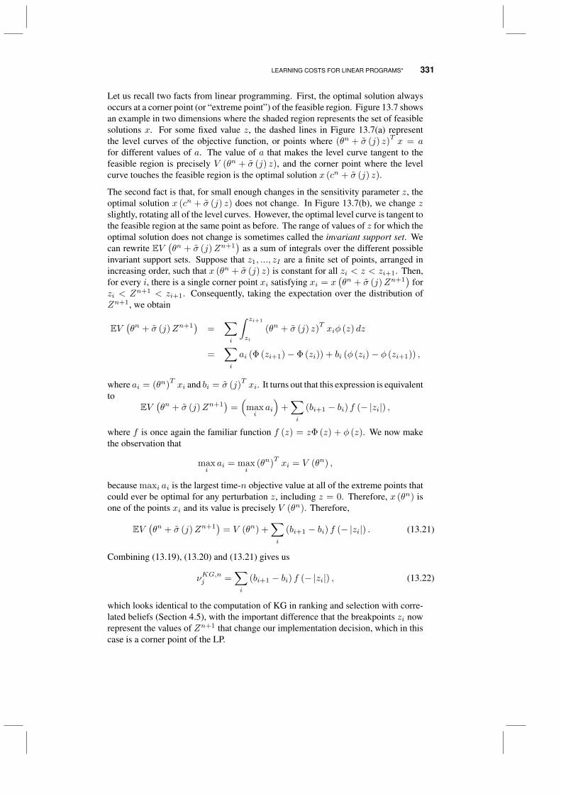
LEARNING COSTS FOR LINEAR PROGRAMS* 331
Let us recall two facts from linear programming. First, the optimal solution alwaysoccurs at a corner point (or “extreme point”) of the feasible region. Figure 13.7 showsan example in two dimensions where the shaded region represents the set of feasiblesolutions x. For some fixed value z, the dashed lines in Figure 13.7(a) representthe level curves of the objective function, or points where (θn + σ (j) z)
Tx = a
for different values of a. The value of a that makes the level curve tangent to thefeasible region is precisely V (θn + σ (j) z), and the corner point where the levelcurve touches the feasible region is the optimal solution x (cn + σ (j) z).
The second fact is that, for small enough changes in the sensitivity parameter z, theoptimal solution x (cn + σ (j) z) does not change. In Figure 13.7(b), we change zslightly, rotating all of the level curves. However, the optimal level curve is tangent tothe feasible region at the same point as before. The range of values of z for which theoptimal solution does not change is sometimes called the invariant support set. Wecan rewrite EV
(θn + σ (j)Zn+1
)as a sum of integrals over the different possible
invariant support sets. Suppose that z1, ..., zI are a finite set of points, arranged inincreasing order, such that x (θn + σ (j) z) is constant for all zi < z < zi+1. Then,for every i, there is a single corner point xi satisfying xi = x
(θn + σ (j)Zn+1
)for
zi < Zn+1 < zi+1. Consequently, taking the expectation over the distribution ofZn+1, we obtain
EV(θn + σ (j)Zn+1
)=
∑i
∫ zi+1
zi
(θn + σ (j) z)Txiφ (z) dz
=∑i
ai (Φ (zi+1)− Φ (zi)) + bi (φ (zi)− φ (zi+1)) ,
where ai = (θn)Txi and bi = σ (j)
Txi. It turns out that this expression is equivalent
toEV
(θn + σ (j)Zn+1
)=(
maxiai
)+∑i
(bi+1 − bi) f (− |zi|) ,
where f is once again the familiar function f (z) = zΦ (z) + φ (z). We now makethe observation that
maxiai = max
i(θn)
Txi = V (θn) ,
because maxi ai is the largest time-n objective value at all of the extreme points thatcould ever be optimal for any perturbation z, including z = 0. Therefore, x (θn) isone of the points xi and its value is precisely V (θn). Therefore,
EV(θn + σ (j)Zn+1
)= V (θn) +
∑i
(bi+1 − bi) f (− |zi|) . (13.21)
Combining (13.19), (13.20) and (13.21) gives us
νKG,nj =∑i
(bi+1 − bi) f (− |zi|) , (13.22)
which looks identical to the computation of KG in ranking and selection with corre-lated beliefs (Section 4.5), with the important difference that the breakpoints zi nowrepresent the values of Zn+1 that change our implementation decision, which in thiscase is a corner point of the LP.
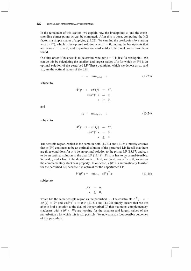
332 LEARNING IN MATHEMATICAL PROGRAMMING
In the remainder of this section, we explain how the breakpoints zi and the corre-sponding corner points xi can be computed. After this is done, computing the KGfactor is a simple matter of applying (13.22). We can find the breakpoints by startingwith x (θn), which is the optimal solution when z = 0, finding the breakpoints thatare nearest to z = 0, and expanding outward until all the breakpoints have beenfound.
Our first order of business is to determine whether z = 0 is itself a breakpoint. Wecan do this by calculating the smallest and largest values of z for which x (θn) is anoptimal solution of the perturbed LP. These quantities, which we denote as z− andz+, are the optimal values of the LPs
z− = miny,s,z z (13.23)
subject to
AT y − s− zσ (j) = θn,
x (θn)Ts = 0,
s ≥ 0,
and
z+ = maxy,s,z z (13.24)
subject to
AT y − s− zσ (j) = θn,
x (θn)Ts = 0,
s ≥ 0.
The feasible region, which is the same in both (13.23) and (13.24), merely ensuresthat x (θn) continues to be an optimal solution of the perturbed LP. Recall that thereare three conditions for x to be an optimal solution to the primal LP (13.17) and y, sto be an optimal solution to the dual LP (13.18). First, x has to be primal-feasible.Second, y and s have to be dual-feasible. Third, we must have xT s = 0, known asthe complementary slackness property. In our case, x (θn) is automatically feasiblefor the perturbed LP, because it is optimal for the unperturbed LP
V (θn) = maxx (θn)Tx (13.25)
subject to
Ax = b,
x ≥ 0,
which has the same feasible region as the perturbed LP. The constraints AT y − s−zσ (j) = θn and x (θn)
Ts = 0 in (13.23) and (13.24) simply ensure that we are
able to find a solution to the dual of the perturbed LP that maintains complementaryslackness with x (θn). We are looking for the smallest and largest values of theperturbation z for which this is still possible. We now analyze four possible outcomesof this procedure.
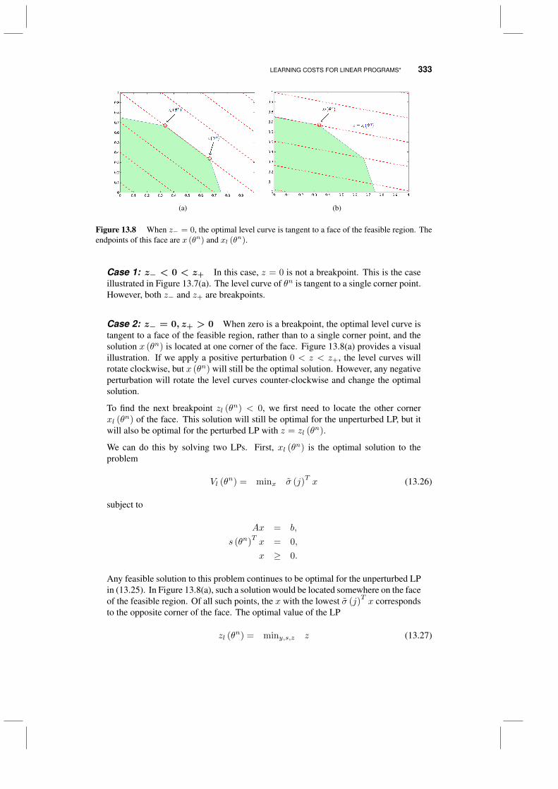
LEARNING COSTS FOR LINEAR PROGRAMS* 333
(a) (b)
Figure 13.8 When z− = 0, the optimal level curve is tangent to a face of the feasible region. Theendpoints of this face are x (θn) and xl (θn).
Case 1: z− < 0 < z+ In this case, z = 0 is not a breakpoint. This is the caseillustrated in Figure 13.7(a). The level curve of θn is tangent to a single corner point.However, both z− and z+ are breakpoints.
Case 2: z− = 0, z+ > 0 When zero is a breakpoint, the optimal level curve istangent to a face of the feasible region, rather than to a single corner point, and thesolution x (θn) is located at one corner of the face. Figure 13.8(a) provides a visualillustration. If we apply a positive perturbation 0 < z < z+, the level curves willrotate clockwise, but x (θn) will still be the optimal solution. However, any negativeperturbation will rotate the level curves counter-clockwise and change the optimalsolution.
To find the next breakpoint zl (θn) < 0, we first need to locate the other cornerxl (θ
n) of the face. This solution will still be optimal for the unperturbed LP, but itwill also be optimal for the perturbed LP with z = zl (θ
n).
We can do this by solving two LPs. First, xl (θn) is the optimal solution to theproblem
Vl (θn) = minx σ (j)
Tx (13.26)
subject to
Ax = b,
s (θn)Tx = 0,
x ≥ 0.
Any feasible solution to this problem continues to be optimal for the unperturbed LPin (13.25). In Figure 13.8(a), such a solution would be located somewhere on the faceof the feasible region. Of all such points, the x with the lowest σ (j)
Tx corresponds
to the opposite corner of the face. The optimal value of the LP
zl (θn) = miny,s,z z (13.27)
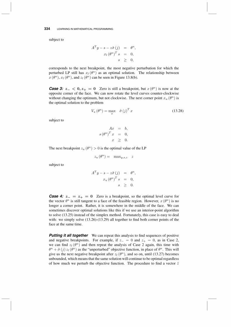
334 LEARNING IN MATHEMATICAL PROGRAMMING
subject to
AT y − s− zσ (j) = θn,
xl (θn)Ts = 0,
s ≥ 0,
corresponds to the next breakpoint, the most negative perturbation for which theperturbed LP still has xl (θn) as an optimal solution. The relationship betweenx (θn), xl (θn), and zl (θn) can be seen in Figure 13.8(b).
Case 3: z− < 0, z+ = 0 Zero is still a breakpoint, but x (θn) is now at theopposite corner of the face. We can now rotate the level curves counter-clockwisewithout changing the optimum, but not clockwise. The next corner point xu (θn) isthe optimal solution to the problem
Vu (θn) = maxx
σ (j)Tx (13.28)
subject to
Ax = b,
s (θn)Tx = 0,
x ≥ 0.
The next breakpoint zu (θn) > 0 is the optimal value of the LP
zu (θn) = maxy,s,z z
subject to
AT y − s− zσ (j) = θn,
xu (θn)Ts = 0,
s ≥ 0.
Case 4: z− = z+ = 0 Zero is a breakpoint, so the optimal level curve forthe vector θn is still tangent to a face of the feasible region. However, x (θn) is nolonger a corner point. Rather, it is somewhere in the middle of the face. We cansometimes discover optimal solutions like this if we use an interior-point algorithmto solve (13.25) instead of the simplex method. Fortunately, this case is easy to dealwith: we simply solve (13.26)-(13.29) all together to find both corner points of theface at the same time.
Putting it all together We can repeat this analysis to find sequences of positiveand negative breakpoints. For example, if z− = 0 and z+ = 0, as in Case 2,we can find zl (θ
n) and then repeat the analysis of Case 2 again, this time withθn + σ (j) zl (θ
n) as the “unperturbed” objective function, in place of θn. This willgive us the next negative breakpoint after zl (θn), and so on, until (13.27) becomesunbounded, which means that the same solution will continue to be optimal regardlessof how much we perturb the objective function. The procedure to find a vector z
BIBLIOGRAPHIC NOTES 335
of breakpoints and a vector x of corresponding corner points can be summarized asfollows.
1) Solve (13.25) to obtain x (θn), y (θn) and s (θn).
2) Solve (13.23) and (13.24) to obtain z−, z+.
2a) If z− < 0 < z+, let z = (z−, z+) and x = (x (θn)).
2b) Otherwise, let z = (0) and let x be an empty vector.
3) While min z > −∞, do the following:
3a) Let θ′ = θn + σ (j) min z.
3b) Find xl (θ′) and zl (θ′) using (13.26) and (13.27).
3c) Update z ← (min z + zl (θ′) , z) and x← (xl (θ
′) , x).
4) While max z <∞, do the following:
4a) Let θ′ = θn + σ (j) max z.
4b) Find xu (θ′) and zu (θ′) using (13.28) and (13.29).
4c) Update z ← (z,max z + zu (θ′)) and x← (x, xu (θ′)).
13.5 BIBLIOGRAPHIC NOTES
Section 13.1 - For other important mathematical programming applications (with a focuson the network and LP models considered in this chapter), see e.g. Vanderbei (2008).
Sections 13.2 - 13.3 - These sections are based on Ryzhov & Powell (2011b). Priorto this paper, several authors in the computer science community addressed the“bandit shortest path” problem, which would be the online version of the shortestpath problem that we consider. For example, Abernethy et al. (2008) describes analgorithm that requires enumerating all the paths, ignoring the structure that arisesfrom overlapping paths. Takimoto & Warmuth (2003) describes the use of a hedgingalgorithm for the online shortest path problems. Stochastic shortest path problemshave been studied even earlier (Kulkarni 1986, Snyder & Steele 1995, Peer & Sharma2007), but usually with the assumption of a known distribution for the rewards.
Section 13.4 - This material is due to Ryzhov & Powell (2011a). The procedure forfinding breakpoints comes from Hadigheh & Terlaky (2006).


CHAPTER 14
OPTIMIZING OVER CONTINUOUSALTERNATIVES*
There are many applications where we have to choose the best value of a continuous,multidimensional vectorx. One example arises in the electricity sector, where utilitieshave to deal with the high variability of electricity spot prices. One strategy is to use abattery to store energy when prices are low, and release energy when prices are high.The idea is illustrated in Figure 14.2, where we store energy when the price goesbelow xstore, and we release energy when the price goes above xwithdraw. We nowface the problem of deciding how to choose x = (xstore, xwithdraw). Let µ(x) bethe expected profits per day that we obtain from using a policy fixed by x, where weassume we can only obtain noisy estimates of µ(x). Our challenge, as with elsewherein this volume, is finding the best value of x as quickly as possible.
While we do not know the true function µ(x), we imagine it might look like thesurface shown in Figure 14.2. We are going to assume it is smooth, but not necessarilyconcave (or convex, if we were solving a minimization problem). If x had only oneor two dimensions, we could discretize it and use the techniques presented in theearlier chapters, although even two dimensions starts to become problematic if, forexample, we would like to discretize each dimension into 100 intervals. If we havethree or more dimensions, discretization quickly becomes cumbersome.
There are a number of problems which require tuning continuous but relatively low-dimensional parameter vectors. Some examples include:
Optimal Learning. By Warren B. Powell and Ilya O. RyzhovCopyright c© 2018 John Wiley & Sons, Inc.
337
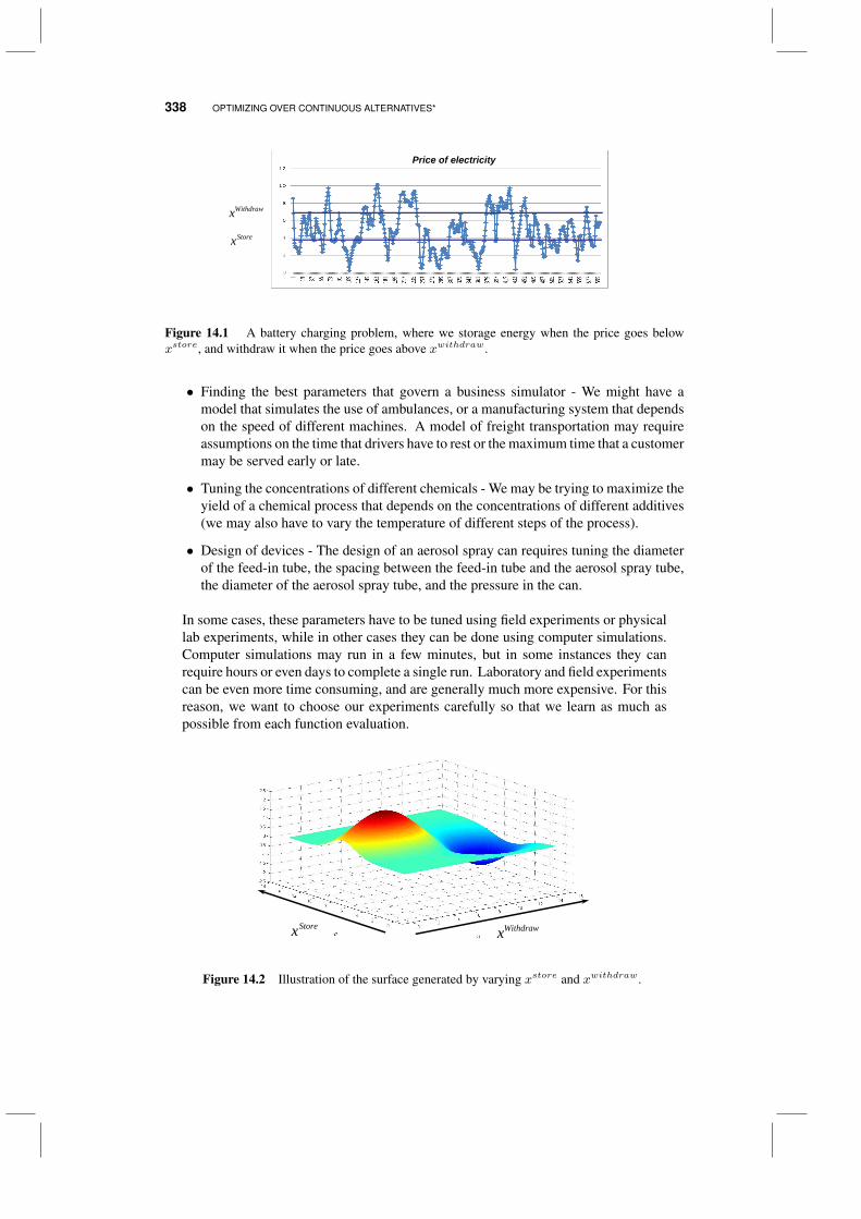
338 OPTIMIZING OVER CONTINUOUS ALTERNATIVES*
Withdrawx
Storex
Price of electricity
Figure 14.1 A battery charging problem, where we storage energy when the price goes belowxstore, and withdraw it when the price goes above xwithdraw.
• Finding the best parameters that govern a business simulator - We might have amodel that simulates the use of ambulances, or a manufacturing system that dependson the speed of different machines. A model of freight transportation may requireassumptions on the time that drivers have to rest or the maximum time that a customermay be served early or late.
• Tuning the concentrations of different chemicals - We may be trying to maximize theyield of a chemical process that depends on the concentrations of different additives(we may also have to vary the temperature of different steps of the process).
• Design of devices - The design of an aerosol spray can requires tuning the diameterof the feed-in tube, the spacing between the feed-in tube and the aerosol spray tube,the diameter of the aerosol spray tube, and the pressure in the can.
In some cases, these parameters have to be tuned using field experiments or physicallab experiments, while in other cases they can be done using computer simulations.Computer simulations may run in a few minutes, but in some instances they canrequire hours or even days to complete a single run. Laboratory and field experimentscan be even more time consuming, and are generally much more expensive. For thisreason, we want to choose our experiments carefully so that we learn as much aspossible from each function evaluation.
53
WithdrawxStorex
Figure 14.2 Illustration of the surface generated by varying xstore and xwithdraw.
THE BELIEF MODEL 339
We are going to continue to use our notation that µ(x) is the true value of the functionat x. The only difference is that x is now a continuous vector. We are going to makea series of experiments x0, x1, . . . , xn, from which we make noisy observations ofour function of the form
yn+1 = µ(xn) + εn+1.
We assume that ε is a random variable that is normally distributed with mean 0 andvariance λ. We wish to design a sequential search policy π that guides the selectionof xi, giving us an estimate of the value of our function which we represent as
Fπ = µ(xN ),
where xN = arg maxx∈X µN (x), and µN (x) is our estimate of µ(x) after N exper-
iments obtained by following policy π. Our challenge is to find the policy π∗ thatsolves
F ∗ = maxπ
Fπ.
This chapter addresses the problem of tuning these multidimensional parametervectors for problems where we do not have access to derivatives. As always, weassume that observing µ(x) is time consuming and/or expensive, and noisy. Also,while we focus on multidimensional parameter vectors, our experimental work as ofthis writing is for vectors where the number of dimensions is less than 10.
14.1 THE BELIEF MODEL
In previous chapters, we have considered different ways of representing our belief inthe function. We started with a lookup table, where we assumed that x was discrete,and there was an estimate θnx for each x (see, for example, Chapters 3, 4 and 5). Wehave also considered models where we used linear regression to approximate µ(x) (asin Chapter 7). In this chapter, we need a different belief model since we have almostno idea about the structure of our function, but we do know it is continuous. Forthis reason, we are going to use an approach known as Gaussian process regressionwhich is a class of nonparametric models which creates an approximation based onall prior observations.
We begin with a prior θ0(x), which is now in the form of a continuous function.We are going to use our policy to generate a sequence of experiments x0, . . . , xn−1,and we are going to use these points to approximate our function. Thus, after thesen experiments y1, . . . , yn, we will have a belief θn(x) at each of these points. Wealso need to capture the covariance in our beliefs about the function at each of thesepoints. We define the n × n matrix Σn, where Σnij = Covn(µ(xi), µ(xj)) is thecovariance in our belief about µ at xi and xj after n iterations. Note that each timewe run a new experiment, θn grows by one element, while the matrix Σn adds a rowand a column.
We are going to take advantage of the continuous structure of the problem andassume that we can write the covariance in our belief between any two points using
340 OPTIMIZING OVER CONTINUOUS ALTERNATIVES*
the function
Cov0(µ(xi), µ(xj)) = β exp(−p∑
m=1
αi(xim − xjm)2), α > 0, β > 0. (14.1)
It is common to refer to the p-dimensional vectorα as the activity ofµ, while the scalarparameter β captures the uncertainty of our belief about µ. The activity parameterα controls the degree of smoothness, where the function becomes smoother as αbecomes smaller. For larger values of α, the covariance between two points shrinkswith α, which means that we learn less about µ(xi) and µ(xj) as xi and xj becomefarther apart.
14.1.1 Updating equations
We have to learn how to update our beliefs about µ(xi), i = 1, . . . , n as we makemore observations. We are going to use the property that the vector θn follows amultivariate normal distribution, where Enµ(xi) = θn(xi) and the covariance matrixis given by Σn. Throughout this chapter En refers to the conditional informationgiven the history of observations y1, . . . , yn.
We start by calculating a vector yn which we call experimental residuals using
yn =
y1
...yn
− θ0(x0)
...θ0(xn−1)
. (14.2)
This is the difference between our observations yi, i = 1, . . . , n, and our originalbelief θ0(xi), i = 1, . . . , n. We also define the residual covariance Sn which isupdated using
Sn = Σ0 +Diagonal([λ(x0), ..., λ(xn−1)]). (14.3)
Expanded into matrices, this is the same as
Sn11 · · · Sn1i · · · Sn1n...
......
......
Sni1 · · · Snii · · · Snin...
......
......
Snn1 · · · Snni · · · Snnn
=
Σ011 · · · Σ0
1i · · · Σ01n
......
......
...Σ0i1 · · · Σ0
ii · · · Σ0in
......
......
...Σ0n1 · · · Σ0
ni · · · Σ0nn
+
λ(x0) 0 · · · · · · 0
0. . . 0 · · ·
...... 0 λ(xi) 0
......
... 0. . . 0
0 · · · · · · 0 λ(xn−1)
Finally, we are going to compute the gain matrix, denoted Gn using
Gn = Σ0[Sn]−1. (14.4)
THE BELIEF MODEL 341
As we see shortly below, the gain matrix is used to weigh new information, whichplays the same role as a stepsize.
The updating equations for the mean vector θn and the covariance matrix Sn are nowgiven by θn(x0)
...θn(xn−1)
=
θ0(x0)...
θ0(xn−1)
+Gnyn, (14.5)
Σn = (In −Gn)Σ0. (14.6)
where In is the n× n identity matrix.
Equations (14.5) and (14.6) update our beliefs around the points x0, . . . , xn that wehave already measured, but we also need a belief for an arbitrary point x, since weneed to search over all possible points to determine the next point that we might wishto evaluate. We begin by defining
Σ0 = Σ0([x0, ..., xn−1, x]),
Σn = Σn([x0, ..., xn−1, x]).
Let ~0 be a column vector of zeroes. Our new gain matrix is given by
Kn = Σ0
In−~0T
[Sn]−1. (14.7)
We can now find θ0 and Σ0 for an arbitrary (n+ 1)st point x usingθn(x0)
...θn(xn−1)θn(x)
=
θ0(x0)
...θ0(xn−1)θ0(x)
+ Knyn, (14.8)
Σn = (In+1 − Kn[In | ~0
])Σ0. (14.9)
If we want the distribution ofµ(x) given ourn observations at some arbitrary decisionx, we can use (14.8) and (14.9) to obtain
θn(x) = θ0(x) +[Σ0(x0, x) , · · · , Σ0(xn−1, x)
][Sn]−1yn, (14.10)
Σn(x, x) = Σ0(x, x)−[Σ0(x0, x) , · · · , Σ0(xn−1, x)
][Sn]−1
Σ0(x0, x)...
Σ0(xn−1, x)
.(14.11)
Equation (14.10) is known as Gaussian process regression (GPR) in some commu-nities, and regression kriging in others.
We have to choose the point xn to measure before we have observed the outcomeyn+1. The updated regression function, given the observations y1, . . . , yn, is nor-
342 OPTIMIZING OVER CONTINUOUS ALTERNATIVES*
mally distributed with distributionθn+1(x0)
...θn+1(xn−1)θn+1(xn)
=
θn(x0)
...θn(xn−1)θn(xn)
+ σ(Σn, xn)Zn+1, (14.12)
where Zn+1 =(yn+1 − θn(xn)
)/√λ(xn) + Σn(xn, xn), with
σ(Σ, x) =Σex√
λ(x) + eTxΣex. (14.13)
Here ex is a column vector of zeroes with a 1 at the row corresponding to decision x.It can be shown that Zn+1 is a standard normal random variate (mean 0, variance 1)because Var(yn+1 − θn(xn)|Fn) = λ(xn) + Σn(xn, xn).
14.1.2 Parameter estimation
Our model is characterized by the p-dimensional vector α, the scalar β and the noiseλ, as well as our prior θ0(x). There may be problems where we feel we can assumethese are known, but in practice we are going to have to estimate them from data. Asis so often the case with statistical estimation, there is more than one way to solvethis problem, but a popular method that we have found works quite well is maximumlikelihood estimation (MLE).
MLE starts by creating a likelihood function which is the product of the density (usingthe normal distribution) of all the prior observations given the unknown parameters.We take the log of this product (giving us the log-likelihood), and then find the valuesof the parameters to maximize the resulting sum.
We form the likelihood function using
Ly(α, β, λ(x0), ..., λ(xn−1), θ0(x0), ..., θ0(xn−1)
)= (2π)−n/2 |Sn|−1/2 exp
−1
2
y1 − θ0(x0)...
yn − θ0(xn−1)
T
(Sn)−1
y1 − θ0(x0)...
yn − θ0(xn−1)
.
Now, if we assume that the variance of the observation noise, λ(·), is a constant λand θ0(·) is a constant θ0, we can write the likelihood function as
Ly(α, β, λ, θ0) = (2π)−n/2|Σ0 + λIn|−1/2exp(−1
2(y − θ01)T (Σ0 + λIn)−1(y − θ01)
),
where 1 is a n × 1 column vector of ones and y =[y1 · · · yn
]T. Note that in
this case we are estimating p+ 3 parameters using n observations. We can write thelog-likelihood function as:
`y(α, β, λ, θ0) = −n2
ln(2π)− 1
2ln(|Σ0 +λIn|)−
1
2(y− θ01)T (Σ0 +λIn)−1(y− θ01).
(14.14)
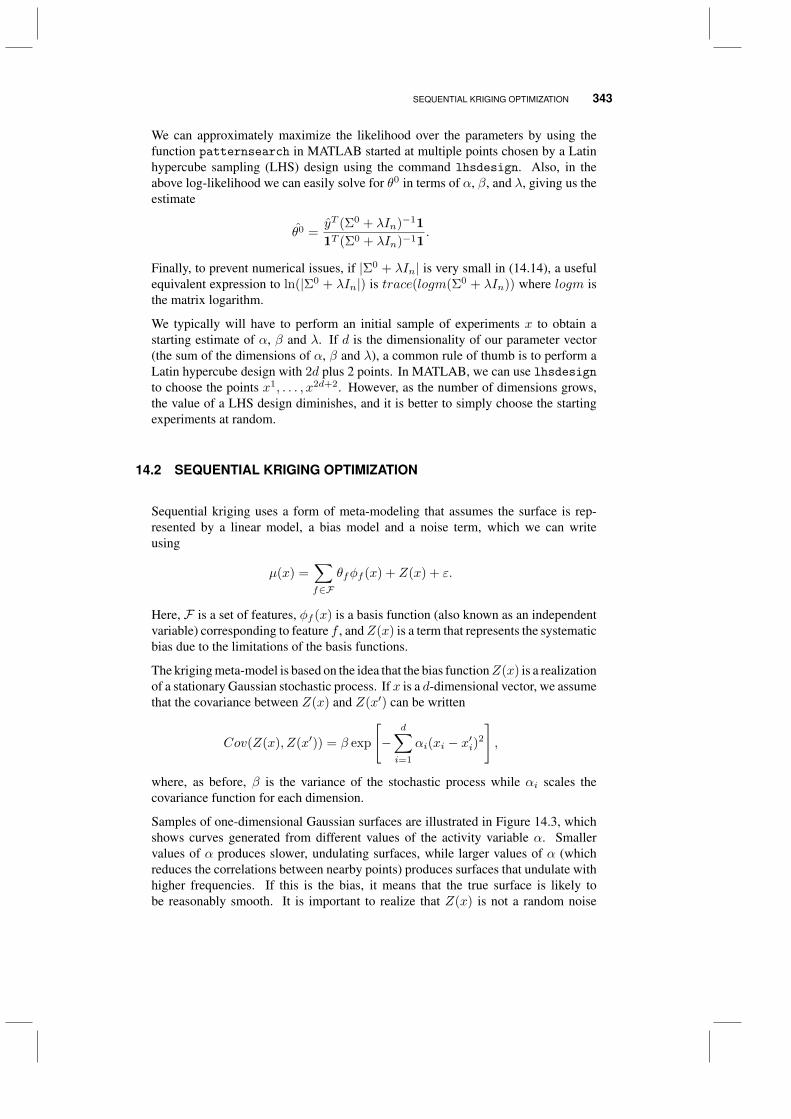
SEQUENTIAL KRIGING OPTIMIZATION 343
We can approximately maximize the likelihood over the parameters by using thefunction patternsearch in MATLAB started at multiple points chosen by a Latinhypercube sampling (LHS) design using the command lhsdesign. Also, in theabove log-likelihood we can easily solve for θ0 in terms of α, β, and λ, giving us theestimate
θ0 =yT (Σ0 + λIn)−11
1T (Σ0 + λIn)−11.
Finally, to prevent numerical issues, if |Σ0 + λIn| is very small in (14.14), a usefulequivalent expression to ln(|Σ0 + λIn|) is trace(logm(Σ0 + λIn)) where logm isthe matrix logarithm.
We typically will have to perform an initial sample of experiments x to obtain astarting estimate of α, β and λ. If d is the dimensionality of our parameter vector(the sum of the dimensions of α, β and λ), a common rule of thumb is to perform aLatin hypercube design with 2d plus 2 points. In MATLAB, we can use lhsdesignto choose the points x1, . . . , x2d+2. However, as the number of dimensions grows,the value of a LHS design diminishes, and it is better to simply choose the startingexperiments at random.
14.2 SEQUENTIAL KRIGING OPTIMIZATION
Sequential kriging uses a form of meta-modeling that assumes the surface is rep-resented by a linear model, a bias model and a noise term, which we can writeusing
µ(x) =∑f∈F
θfφf (x) + Z(x) + ε.
Here, F is a set of features, φf (x) is a basis function (also known as an independentvariable) corresponding to feature f , andZ(x) is a term that represents the systematicbias due to the limitations of the basis functions.
The kriging meta-model is based on the idea that the bias functionZ(x) is a realizationof a stationary Gaussian stochastic process. If x is a d-dimensional vector, we assumethat the covariance between Z(x) and Z(x′) can be written
Cov(Z(x), Z(x′)) = β exp
[−
d∑i=1
αi(xi − x′i)2
],
where, as before, β is the variance of the stochastic process while αi scales thecovariance function for each dimension.
Samples of one-dimensional Gaussian surfaces are illustrated in Figure 14.3, whichshows curves generated from different values of the activity variable α. Smallervalues of α produces slower, undulating surfaces, while larger values of α (whichreduces the correlations between nearby points) produces surfaces that undulate withhigher frequencies. If this is the bias, it means that the true surface is likely tobe reasonably smooth. It is important to realize that Z(x) is not a random noise
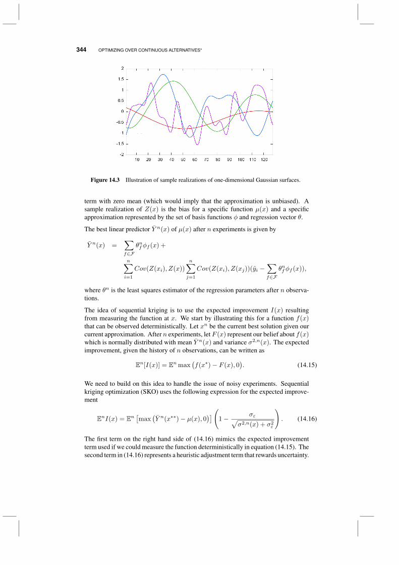
344 OPTIMIZING OVER CONTINUOUS ALTERNATIVES*
Figure 14.3 Illustration of sample realizations of one-dimensional Gaussian surfaces.
term with zero mean (which would imply that the approximation is unbiased). Asample realization of Z(x) is the bias for a specific function µ(x) and a specificapproximation represented by the set of basis functions φ and regression vector θ.
The best linear predictor Y n(x) of µ(x) after n experiments is given by
Y n(x) =∑f∈F
θnf φf (x) +
n∑i=1
Cov(Z(xi), Z(x))
n∑j=1
Cov(Z(xi), Z(xj))(yi −∑f∈F
θnf φf (x)),
where θn is the least squares estimator of the regression parameters after n observa-tions.
The idea of sequential kriging is to use the expected improvement I(x) resultingfrom measuring the function at x. We start by illustrating this for a function f(x)that can be observed deterministically. Let xn be the current best solution given ourcurrent approximation. After n experiments, letF (x) represent our belief about f(x)which is normally distributed with mean Y n(x) and variance σ2,n(x). The expectedimprovement, given the history of n observations, can be written as
En[I(x)] = En max(f(x∗)− F (x), 0
). (14.15)
We need to build on this idea to handle the issue of noisy experiments. Sequentialkriging optimization (SKO) uses the following expression for the expected improve-ment
EnI(x) = En[max
(Y n(x∗∗)− µ(x), 0
)](1− σε√
σ2,n(x) + σ2ε
). (14.16)
The first term on the right hand side of (14.16) mimics the expected improvementterm used if we could measure the function deterministically in equation (14.15). Thesecond term in (14.16) represents a heuristic adjustment term that rewards uncertainty.
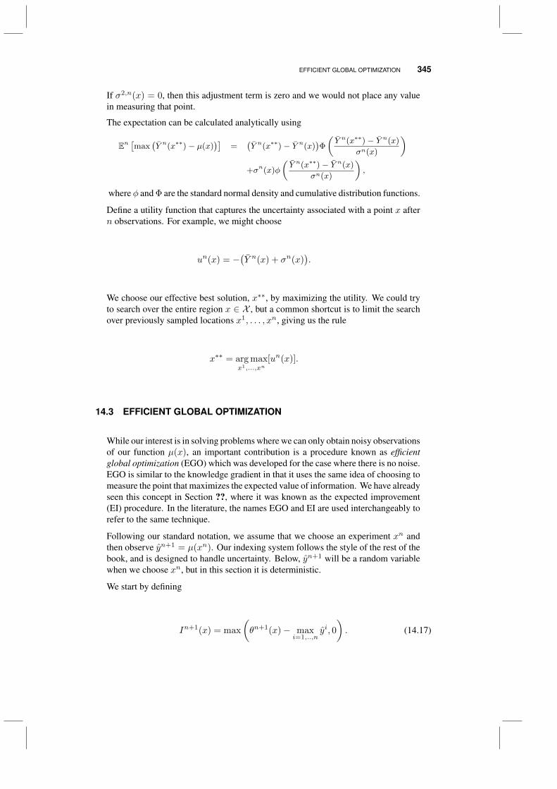
EFFICIENT GLOBAL OPTIMIZATION 345
If σ2,n(x) = 0, then this adjustment term is zero and we would not place any valuein measuring that point.
The expectation can be calculated analytically using
En[max
(Y n(x∗∗)− µ(x)
)]=
(Y n(x∗∗)− Y n(x)
)Φ
(Y n(x∗∗)− Y n(x)
σn(x)
)+σn(x)φ
(Y n(x∗∗)− Y n(x)
σn(x)
),
where φ and Φ are the standard normal density and cumulative distribution functions.
Define a utility function that captures the uncertainty associated with a point x aftern observations. For example, we might choose
un(x) = −(Y n(x) + σn(x)
).
We choose our effective best solution, x∗∗, by maximizing the utility. We could tryto search over the entire region x ∈ X , but a common shortcut is to limit the searchover previously sampled locations x1, . . . , xn, giving us the rule
x∗∗ = arg maxx1,...,xn
[un(x)].
14.3 EFFICIENT GLOBAL OPTIMIZATION
While our interest is in solving problems where we can only obtain noisy observationsof our function µ(x), an important contribution is a procedure known as efficientglobal optimization (EGO) which was developed for the case where there is no noise.EGO is similar to the knowledge gradient in that it uses the same idea of choosing tomeasure the point that maximizes the expected value of information. We have alreadyseen this concept in Section ??, where it was known as the expected improvement(EI) procedure. In the literature, the names EGO and EI are used interchangeably torefer to the same technique.
Following our standard notation, we assume that we choose an experiment xn andthen observe yn+1 = µ(xn). Our indexing system follows the style of the rest of thebook, and is designed to handle uncertainty. Below, yn+1 will be a random variablewhen we choose xn, but in this section it is deterministic.
We start by defining
In+1(x) = max
(θn+1(x)− max
i=1,..,nyi, 0
). (14.17)
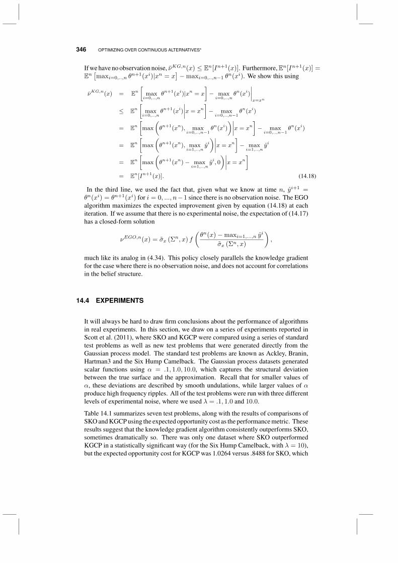
346 OPTIMIZING OVER CONTINUOUS ALTERNATIVES*
If we have no observation noise, νKG,n(x) ≤ En[In+1(x)]. Furthermore,En[In+1(x)] =En[maxi=0,..,n θ
n+1(xi)|xn = x]−maxi=0,..,n−1 θ
n(xi). We show this using
νKG,n(x) = En[
maxi=0,..,n
θn+1(xi)|xn = x
]− maxi=0,..,n
θn(xi)
∣∣∣∣x=xn
≤ En[
maxi=0,..,n
θn+1(xi)
∣∣∣∣x = xn]− maxi=0,..,n−1
θn(xi)
= En[max
(θn+1(xn), max
i=0,..,n−1θn(xi)
)∣∣∣∣x = xn]− maxi=0,..,n−1
θn(xi)
= En[max
(θn+1(xn), max
i=1,..,nyi)∣∣∣∣x = xn
]− maxi=1,..,n
yi
= En[max
(θn+1(xn)− max
i=1,..,nyi, 0
)∣∣∣∣x = xn]
= En[In+1(x)]. (14.18)
In the third line, we used the fact that, given what we know at time n, yi+1 =θn(xi) = θn+1(xi) for i = 0, ..., n−1 since there is no observation noise. The EGOalgorithm maximizes the expected improvement given by equation (14.18) at eachiteration. If we assume that there is no experimental noise, the expectation of (14.17)has a closed-form solution
νEGO,n(x) = σx (Σn, x) f
(θn(x)−maxi=1,...,n y
i
σx (Σn, x)
),
much like its analog in (4.34). This policy closely parallels the knowledge gradientfor the case where there is no observation noise, and does not account for correlationsin the belief structure.
14.4 EXPERIMENTS
It will always be hard to draw firm conclusions about the performance of algorithmsin real experiments. In this section, we draw on a series of experiments reported inScott et al. (2011), where SKO and KGCP were compared using a series of standardtest problems as well as new test problems that were generated directly from theGaussian process model. The standard test problems are known as Ackley, Branin,Hartman3 and the Six Hump Camelback. The Gaussian process datasets generatedscalar functions using α = .1, 1.0, 10.0, which captures the structural deviationbetween the true surface and the approximation. Recall that for smaller values ofα, these deviations are described by smooth undulations, while larger values of αproduce high frequency ripples. All of the test problems were run with three differentlevels of experimental noise, where we used λ = .1, 1.0 and 10.0.
Table 14.1 summarizes seven test problems, along with the results of comparisons ofSKO and KGCP using the expected opportunity cost as the performance metric. Theseresults suggest that the knowledge gradient algorithm consistently outperforms SKO,sometimes dramatically so. There was only one dataset where SKO outperformedKGCP in a statistically significant way (for the Six Hump Camelback, with λ = 10),but the expected opportunity cost for KGCP was 1.0264 versus .8488 for SKO, which
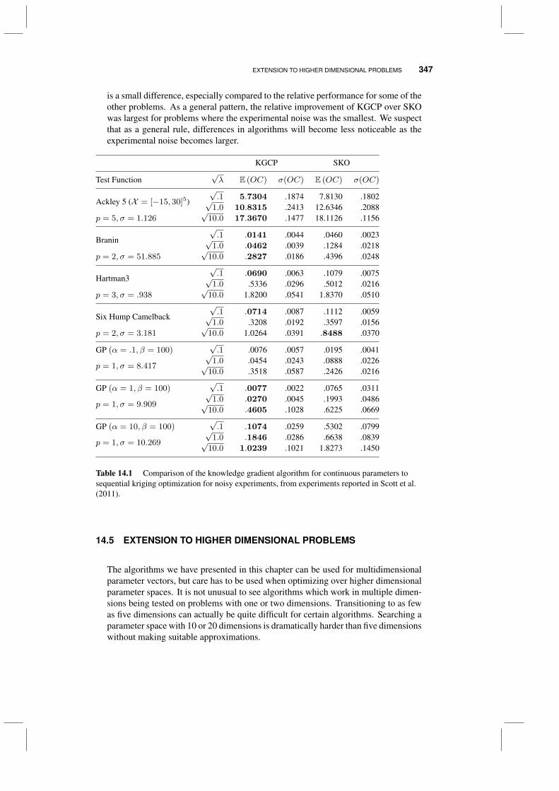
EXTENSION TO HIGHER DIMENSIONAL PROBLEMS 347
is a small difference, especially compared to the relative performance for some of theother problems. As a general pattern, the relative improvement of KGCP over SKOwas largest for problems where the experimental noise was the smallest. We suspectthat as a general rule, differences in algorithms will become less noticeable as theexperimental noise becomes larger.
KGCP SKO
Test Function√λ E (OC) σ(OC) E (OC) σ(OC)
Ackley 5 (X = [−15, 30]5)√.1 5.7304 .1874 7.8130 .1802√
1.0 10.8315 .2413 12.6346 .2088p = 5, σ = 1.126
√10.0 17.3670 .1477 18.1126 .1156
Branin√.1 .0141 .0044 .0460 .0023√
1.0 .0462 .0039 .1284 .0218p = 2, σ = 51.885
√10.0 .2827 .0186 .4396 .0248
Hartman3√.1 .0690 .0063 .1079 .0075√
1.0 .5336 .0296 .5012 .0216p = 3, σ = .938
√10.0 1.8200 .0541 1.8370 .0510
Six Hump Camelback√.1 .0714 .0087 .1112 .0059√
1.0 .3208 .0192 .3597 .0156p = 2, σ = 3.181
√10.0 1.0264 .0391 .8488 .0370
GP (α = .1, β = 100)√.1 .0076 .0057 .0195 .0041
p = 1, σ = 8.417
√1.0 .0454 .0243 .0888 .0226√
10.0 .3518 .0587 .2426 .0216
GP (α = 1, β = 100)√.1 .0077 .0022 .0765 .0311
p = 1, σ = 9.909
√1.0 .0270 .0045 .1993 .0486√
10.0 .4605 .1028 .6225 .0669
GP (α = 10, β = 100)√.1 .1074 .0259 .5302 .0799
p = 1, σ = 10.269
√1.0 .1846 .0286 .6638 .0839√
10.0 1.0239 .1021 1.8273 .1450
Table 14.1 Comparison of the knowledge gradient algorithm for continuous parameters tosequential kriging optimization for noisy experiments, from experiments reported in Scott et al.(2011).
14.5 EXTENSION TO HIGHER DIMENSIONAL PROBLEMS
The algorithms we have presented in this chapter can be used for multidimensionalparameter vectors, but care has to be used when optimizing over higher dimensionalparameter spaces. It is not unusual to see algorithms which work in multiple dimen-sions being tested on problems with one or two dimensions. Transitioning to as fewas five dimensions can actually be quite difficult for certain algorithms. Searching aparameter space with 10 or 20 dimensions is dramatically harder than five dimensionswithout making suitable approximations.
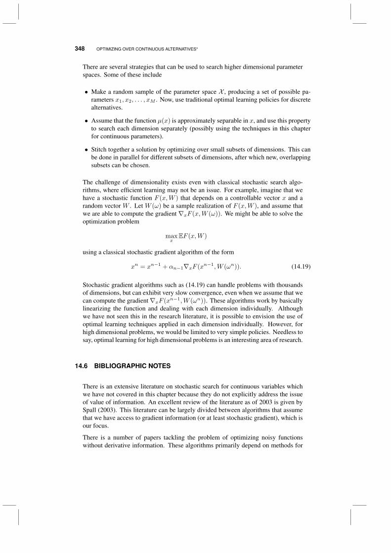
348 OPTIMIZING OVER CONTINUOUS ALTERNATIVES*
There are several strategies that can be used to search higher dimensional parameterspaces. Some of these include
• Make a random sample of the parameter space X , producing a set of possible pa-rameters x1, x2, . . . , xM . Now, use traditional optimal learning policies for discretealternatives.
• Assume that the function µ(x) is approximately separable in x, and use this propertyto search each dimension separately (possibly using the techniques in this chapterfor continuous parameters).
• Stitch together a solution by optimizing over small subsets of dimensions. This canbe done in parallel for different subsets of dimensions, after which new, overlappingsubsets can be chosen.
The challenge of dimensionality exists even with classical stochastic search algo-rithms, where efficient learning may not be an issue. For example, imagine that wehave a stochastic function F (x,W ) that depends on a controllable vector x and arandom vector W . Let W (ω) be a sample realization of F (x,W ), and assume thatwe are able to compute the gradient ∇xF (x,W (ω)). We might be able to solve theoptimization problem
maxx
EF (x,W )
using a classical stochastic gradient algorithm of the form
xn = xn−1 + αn−1∇xF (xn−1,W (ωn)). (14.19)
Stochastic gradient algorithms such as (14.19) can handle problems with thousandsof dimensions, but can exhibit very slow convergence, even when we assume that wecan compute the gradient∇xF (xn−1,W (ωn)). These algorithms work by basicallylinearizing the function and dealing with each dimension individually. Althoughwe have not seen this in the research literature, it is possible to envision the use ofoptimal learning techniques applied in each dimension individually. However, forhigh dimensional problems, we would be limited to very simple policies. Needless tosay, optimal learning for high dimensional problems is an interesting area of research.
14.6 BIBLIOGRAPHIC NOTES
There is an extensive literature on stochastic search for continuous variables whichwe have not covered in this chapter because they do not explicitly address the issueof value of information. An excellent review of the literature as of 2003 is given bySpall (2003). This literature can be largely divided between algorithms that assumethat we have access to gradient information (or at least stochastic gradient), which isour focus.
There is a number of papers tackling the problem of optimizing noisy functionswithout derivative information. These algorithms primarily depend on methods for

BIBLIOGRAPHIC NOTES 349
Monte Carlo sampling of the search region X , and while everyone is looking foralgorithms with fast convergence, most of the theory focuses on asymptotic conver-gence analysis (assuming an off-line application) while convergence rates are studiedempirically. Benveniste et al. (1990), Kushner & Yin (1997) and Kushner & Yin(2003) are important references for the theory behind stochastic search algorithms.Some recent contributions include adaptive search with resampling (Andradottir &Prudius (2010)) and model reference adaptive search (Hu et al. (2007)).
Sections 14.1 - Our belief model is based on material presented in Sacks et al. (1989) andFrazier et al. (2009). Our presentation of Gaussian process regression is based onRasmussen & Williams (2006); the material on regression kriging in Forrester et al.(2008). The recursive updating equations for the means and variances are based onFrazier et al. (2009). The maximum likelihood estimation method for the Gaussianprocess regression model is based on Rasmussen & Williams (2006).
Sections 14.2 - Sequential kriging optimization was proposed by Huang et al. (2006).Stein (1999) provides a thorough introduction to the field of kriging, which evolvedfrom the field of spatial statistics.
Sections ?? - The adaptation of the knowledge gradient for continuous alternatives wasdeveloped by Scott et al. (2011).
Sections 14.3 - Efficient global optimization was proposed by Jones et al. (1998b).
Sections 14.4 - We draw on a series of experiments reported in Scott et al. (2011). Ourtest functions are culled from Frazier et al. (2009), Huang et al. (2006) and Jones etal. (1998b). See also Scott et al. (2010) for additional empirical work on calibrationof an airline business simulator.


CHAPTER 15
LEARNING WITH A PHYSICAL STATE
All of the problems that we have considered in earlier chapters have one characteristicin common. In each of these problems, the decision we make depends only on ourbelief state about the problem. The decision itself can be discrete (as in Chapter3), a subset (Chapter ??), a scalar (Chapter 10), or continuous (Chapter 14), and wehave considered many different types of objective functions (online, offline, or linkedto a complex implementation decision) and different belief structures (lookup table,parametric and nonparametric). However, within each specific problem class, the setof possible decisions has always stayed the same over time, and every policy we havelooked at has made decisions based purely on the available information.
There are many problems where this is not the case, and our decision also dependson a physical state as well as a belief state. A simple example arises when we aretrying to learn the travel times on links in a transportation network. We can traversefrom node i to node j to learn more about the time τij to get from i to j, but doingso puts us at node j, which changes the decisions we can consider next. If we decideto go from i to j, we have to balance the information we gain about τij against theimpact of now being at location j.
Another application arises in medical treatments. Consider the problem of treatinga diabetes patient. The doctor has certain beliefs about the effectiveness of differenttreatments. At the same time, the doctor also observes the results of blood sugartests that are regularly undergone by the patient. The decision to recommend a
Optimal Learning. By Warren B. Powell and Ilya O. RyzhovCopyright c© 2018 John Wiley & Sons, Inc.
351
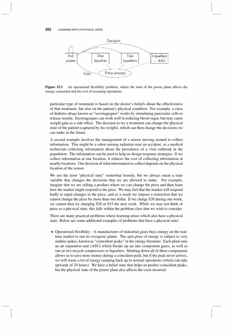
352 LEARNING WITH A PHYSICAL STATE
Figure 15.1 An operational flexibility problem, where the state of the power plant affects theenergy consumed and the cost of resuming operations.
particular type of treatment is based on the doctor’s beliefs about the effectivenessof that treatment, but also on the patient’s physical condition. For example, a classof diabetes drugs known as “secretagogues” works by stimulating pancreatic cells torelease insulin. Secretagogues can work well in reducing blood sugar, but may causeweight gain as a side effect. The decision to try a treatment can change the physicalstate of the patient (captured by his weight), which can then change the decisions wecan make in the future.
A second example involves the management of a sensor moving around to collectinformation. This might be a robot sensing radiation near an accident, or a medicaltechnician collecting information about the prevalence of a viral outbreak in thepopulation. The information can be used to help us design response strategies. If wecollect information at one location, it reduces the cost of collecting information atnearby locations. Our decision of what information to collect depends on the physicallocation of the sensor.
We use the term “physical state” somewhat loosely, but we always mean a statevariable that changes the decisions that we are allowed to make. For example,imagine that we are selling a product where we can change the price and then learnhow the market might respond to the price. We may feel that the market will respondbadly to rapid changes in the price, and as a result we impose a restriction that wecannot change the price by more than one dollar. If we charge $20 during one week,we cannot then try charging $28 or $15 the next week. While we may not think ofprice as a physical state, this falls within the problem class that we wish to consider.
There are many practical problems where learning arises which also have a physicalstate. Below are some additional examples of problems that have a physical state:
• Operational flexibility - A manufacturer of industrial gases buys energy on the real-time market to run its cryogenic plants. The spot price of energy is subject to verysudden spikes, known as “coincident peaks” in the energy literature. Each plant runsan air separation unit (ASU) which breaks up air into component gases, as well asone or two recycle compressors or liquefiers. Shutting down all of these componentsallows us to save more money during a coincident peak, but if the peak never arrives,we will waste a lot of energy ramping back up to normal operations (which can takeupwards of 24 hours). We have a belief state that helps us predict coincident peaks,but the physical state of the power plant also affects the costs incurred.
INTRODUCTION TO DYNAMIC PROGRAMMING 353
• Competitive games - Imagine a game of chess. Each player has a certain belief aboutthe opponent’s strategy, and uses this belief to decide on the next move. However,the decisions a player can make depends on the state of the board.
• Pricing with finite inventory - A store sets a price for a product with the goal ofmaximizing revenue. As in Chapters 7 and ??, we may wish to experiment withdifferent prices and observe the effect on revenues. However, if we have finiteinventory, our decision will depend on the amount we have in stock as well as on ourbeliefs about the revenue curve. Experimentation is less useful when there is lessinventory remaining.
• Mutual fund cash balance - A mutual fund needs cash to meet shareholder redemp-tions. At the same time, keeping more cash on hand means having less money toinvest, leading to lower profits. Over time, we gradually learn about shareholderbehavior and the rate at which redemptions arise. Our ability to meet redemptions atany given time, however, is constrained by the amount of cash on hand.
The physical state introduces a whole new level of challenge. The question of howto make decisions based on both physical and belief states is at the very frontier ofoptimal learning. In this chapter, we give a framework for where to begin thinkingabout this problem. We also suggest a few approaches that integrate the optimallearning concepts we have developed throughout this book into the world of physicalstates, and close with a discussion of how some of these concepts might be takenfurther.
15.1 INTRODUCTION TO DYNAMIC PROGRAMMING
Sequential, stochastic decision problems have long been approached using dynamicprogramming. Assume that we have a process that may be in a physical state St = sat time t. (Throughout this book, we have denoted time by n; the reason whywe switch to t here will become clear shortly.) If we choose a (discrete) actionx, we may land in a state St+1 = s′ with probability p(s′|s, x). Assume that weearn a contribution C(St, x) from taking action x when we are in state St, and thatcontributions are discounted by 0 < γ < 1 with each passing time period. If Vt(St)is the value of being in state St at time t, then we would like to choose our action xtby solving
xt = arg maxx
(C(St, x) + γ
∑s′
p(s′|St, x)Vt+1(s′)
). (15.1)
The problem is that we do not knowVt+1(s′). If we have a finite horizon problem withT as the last time period, we might assume VT (s) = 0 then compute the remainingvalue functions using
Vt(St) = maxx
(C(St, x) + γ
∑s′
p(s′|St, x)Vt+1(s′)
). (15.2)
Equation (15.2) needs to be computed by looping over all states St. If St is discreteand very low dimensional (as in, three or less), this approach can work quite well.
354 LEARNING WITH A PHYSICAL STATE
But there are many problems where the state St has more than three dimensions, orit may be continuous. For these problems (which are quite common), we encounterwhat is widely known as the “curse of dimensionality.”
15.1.1 Approximate dynamic programming
The dynamic programming community has developed an algorithmic strategy knownbroadly as approximate dynamic programming (ADP) that is designed to circumventthe curse of dimensionality. ADP is actually an umbrella for a variety of algorithms,but its most popular form works as follows. Let’s begin by assuming that the state Stis discrete. Further assume that we are given an approximation V
0
t (s) for all states sand times t = 1, . . . , T (for example, we might start with V
0
t (s) = 0).
If we use equation (15.2), we are solving the problem by proceeding backward intime. It is this process that requires that we loop over all possible states, because wedo not know in advance which states that we might actually visit. With approximatedynamic programming, we are going to progress forward in time, starting with agiven initial state S0. If we are in state St at time t and choose action xt (according tosome rule that we discuss below), we are then going to observe a sample realizationof a random variable Wt+1 (which was unknown at time t). Finally, we are going touse a transition function (also known as the state transition model), which gives usthe next state using
St+1 = SM (St, xt,Wt+1).
We are going to simulate our way from time 0 to time T iteratively. To firm up ournotation, let n the iteration index. In iteration n, let Snt be the state that we visit attime t. Also let ωn index the sample path of observations of Wt, which means thatWt+1(ωn) is the sample realization of what we observe between t and t + 1 whilefollowing sample path ωn.
We have to figure out how we are going to make decisions. The most natural policyis to mimic equation (15.1) and solve
xnt = arg maxx
(C(Snt , x) + γ
∑s′
p(s′|Snt , x)Vn−1
t+1 (s′)
). (15.3)
Not surprisingly, we are going to refer to this as a pure exploitation policy, becauseit means to choose the best action based on our current belief about the downstreamvalues captured by V
n−1
t+1 (s′). Before we start criticizing this policy (as we will),we need to close the loop by mentioning how we are coming up with these valuefunction approximations. First compute
vnt = C(Snt , xnt ) + γ
∑s′
p(s′|Snt , xnt )Vn−1
t+1 (s′). (15.4)
We can think of vnt as a sample estimate of the value of being in state Snt . This isthe value that we experienced while we were following our sample path through thestates Sn0 , S
n1 , . . . , S
nT . It would be nice to mimic (15.2) and just set Vt(Snt ) = vnt ,
INTRODUCTION TO DYNAMIC PROGRAMMING 355
but vnt is a noisy sample estimate. For this reason, we have to do smoothing, whichwe can do using
Vn
t (Snt ) = (1− αn−1)Vn−1
t (Snt ) + αn−1vnt .
Here, αn−1 is known as a stepsize, which is a parameter between 0 and 1. It might bea constant (such as αn−1 = .001), but more often it is assigned a declining sequencesuch as αn = a/(a+ n− 1), where a is a tunable parameter.
Notice that, in the above presentation, we have two time indices, n and t. Thisis because we considered a finite-horizon problem ending at time T . The index tdenotes a stage of the problem, whereas the index n denotes the number of times wehave updated our approximation V of the value function. The algorithm works bymaking multiple passes through the problem, so that we solve (15.3) backward fort = T − 1, ..., 1 for each fixed value of n.
We can also accommodate infinite-horizon problems (T → ∞), for which the opti-mality equation (15.2) becomes
V (S) = maxx
(C(S, x) + γ
∑s′
p(s′|S, x)V (s′)). (15.5)
for all states S. In this case, the ADP algorithm merges the two time indices intoone, such that (15.3) becomes
xn = arg maxx
(C(Sn, x) + γ
∑s′
p(s′|Sn, x)Vn−1
(s′)
). (15.6)
and (15.4) becomes
vn = C(Sn, xn) + γ∑s′
p(s′|Sn, xn)Vn−1
(s′). (15.7)
The approximation is updated using
Vn(Sn) = (1− αn−1)V
n−1(Sn) + αn−1v
n. (15.8)
We still run the algorithm by progressing forward in time starting from S0. Now, asingle iteration consists of a visit to a single state Sn, and n is our only time index,as in the rest of the book. We hope that, after a large number of iterations, V
nwill
be close to the true solution of (15.5). To simplify our presentation, we will focus oninfinite-horizon problems when developing our algorithms in this chapter, though itis important to keep in mind the wealth of finite-horizon applications.
We now have the beginnings of an algorithm that seems to have considerable appeal.We can handle arbitrarily complex state variablesSt, and even the random informationWt can be quite complex (problems have been solved with thousands of dimensions),because at any point in time we are working with a single state and a single samplerealization of Wt. It almost seems like magic, so you know that there has to besomething wrong. Indeed, the problem is known as the exploration vs. exploitationproblem, something that should be now be quite familiar to readers of this book.
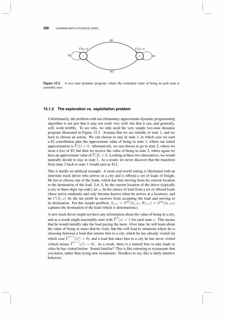
356 LEARNING WITH A PHYSICAL STATE
(1) 0V (2) 0V
$2
-$5
$12
$31 2
Figure 15.2 A two state dynamic program, where the estimated value of being in each state iscurrently zero.
15.1.2 The exploration vs. exploitation problem
Unfortunately, the problem with our elementary approximate dynamic programmingalgorithm is not just that it may not work very well, but that it can, and generally,will, work terribly. To see why, we only need the very simple two-state dynamicprogram illustrated in Figure 15.2. Assume that we are initially in state 1, and wehave to choose an action. We can choose to stay in state 1, in which case we earna $2 contribution plus the approximate value of being in state 1, where our initialapproximation is V (1) = 0. Alternatively, we can choose to go to state 2, where weincur a loss of $5, but then we receive the value of being in state 2, where again wehave an approximate value of V (2) = 0. Looking at these two alternatives, we wouldnaturally decide to stay in state 1. As a result, we never discover that the transitionfrom state 2 back to state 1 would earn us $12.
This is hardly an artificial example. A more real-world setting is illustrated with aninterstate truck driver who arrives in a city and is offered a set of loads of freight.He has to choose one of the loads, which has him moving from his current locationto the destination of the load. Let St be the current location of the driver (typicallya city or three-digit zip code), let xt be his choice of load from a set of offered loads(these arrive randomly and only become known when he arrives at a location), andlet C(St, x) be the net profit he receives from accepting the load and moving toits destination. For this simple problem, St+1 = SM (St, xt,Wt+1) = SM (St, xt)captures the destination of the load (which is deterministic).
A new truck driver might not have any information about the value of being in a city,and as a result might reasonably start with V
0(s) = 1 for each state s. This means
that he would initially take the load paying the most. Over time, he will learn aboutthe value of being in states that he visits, but this will lead to situations where he ischoosing between a load that returns him to a city which he has already visited (inwhich case V
n−1(s′) > 0), and a load that takes him to a city he has never visited
(which means Vn−1
(s′) = 0). As a result, there is a natural bias to take loads tocities he has visited before. Sound familiar? This is like returning to restaurants thatyou know, rather than trying new restaurants. Needless to say, this is fairly intuitivebehavior.
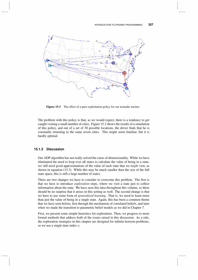
INTRODUCTION TO DYNAMIC PROGRAMMING 357
Figure 15.3 The effect of a pure exploitation policy for our nomadic trucker.
The problem with this policy is that, as we would expect, there is a tendency to getcaught visiting a small number of cities. Figure 15.3 shows the results of a simulationof this policy, and out of a set of 30 possible locations, the driver finds that he isconstantly returning to the same seven cities. This might seem familiar, but it ishardly optimal.
15.1.3 Discussion
Our ADP algorithm has not really solved the curse of dimensionality. While we haveeliminated the need to loop over all states to calculate the value of being in a state,we still need good approximations of the value of each state that we might visit, asshown in equation (15.3). While this may be much smaller than the size of the fullstate space, this is still a large number of states.
There are two changes we have to consider to overcome this problem. The first isthat we have to introduce exploration steps, where we visit a state just to collectinformation about the state. We have seen this idea throughout this volume, so thereshould be no surprise that it arises in this setting as well. The second change is thatwe have to use some form of generalized learning. That is, we need to learn morethan just the value of being in a single state. Again, this has been a common themethat we have seen before, first through the mechanism of correlated beliefs, and laterwhen we made the transition to parametric belief models as we did in Chapter 7.
First, we present some simple heuristics for exploration. Then, we progress to moreformal methods that address both of the issues raised in this discussion. As a rule,the exploration strategies in this chapter are designed for infinite-horizon problems,so we use a single time index n.
358 LEARNING WITH A PHYSICAL STATE
15.2 SOME HEURISTIC LEARNING POLICIES
One very simple policy that is frequently used in practice is our old acquaintanceepsilon-greedy: at time n, we make a random decision with probability ε, or followthe pure exploitation policy (15.6) with probability 1− ε. We face the usual problemof tuning ε, but otherwise, it will be possible to achieve good performance as long asX is fairly small.
Two more sophisticated exploration strategies developed within the computer sciencecommunity are known as R-max andE3. Both of these policies are based on the ideaof categorizing the states according to whether we have “enough” or “not enough”information about them.
The R-max policy makes decisions according to the rule
XRmax,n (Sn;αn) = arg maxx
(C (Sn, x) + γ
∑s
ρns (Sn, x)F (s))
where
F (s) =
Rmax if s has been visited fewer than m times,V n (s) if s has been visited at least m times.
The integer m is a tunable parameter representing the number of times we need tovisit a state in order to obtain “enough” information. The value Rmax is deliberatelychosen to be very large, such that we are more likely to choose an action x if it ismore likely to lead us to states for which we have little information. Eventually, oncewe visit every state enough times, Rmax reduces to the pure exploitation policy . Weare still, however, left with the issue of tuning m and Rmax.
The E3 policy (“Explicit Explore or Exploit”) can be viewed as a modification ofepsilon-greedy. As in R-max, we have a parameter m representing the amount ofinformation that is “sufficient” for us to know the value of being in a state. Uponreaching state Sn, our decision is made as follows. If Sn is a state that we havenever visited before, we make a random decision. If we have visited Sn before,but fewer than m times, we make the decision that we have tried the fewest numberof times among all our previous visits to the state. Finally, if we have visited Sn
more than m times, we follow the pure exploitation policy and make our decisionaccording to (15.6). Once again, the policy reduces to pure exploitation once wehave sufficiently explored the state space. In the early stages, the policy encouragesus to make decisions with which we are unfamiliar, in order to learn about them.
15.3 THE LOCAL BANDIT APPROXIMATION
Our first formal technique, known as the local bandit approximation or LBA, attemptsto convert the dynamic program into a multi-armed bandit problem at each time step,and then uses a Gittins-like calculation to make the next decision. The multi-armedbandit problem, which we covered in Chapter 5, has no physical state. We makeour decision based purely on our knowledge about the rewards obtainable from M
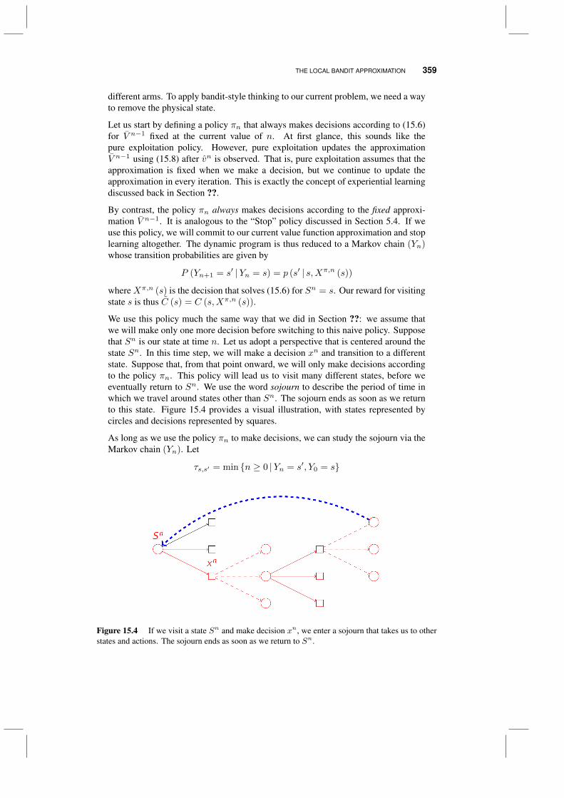
THE LOCAL BANDIT APPROXIMATION 359
different arms. To apply bandit-style thinking to our current problem, we need a wayto remove the physical state.
Let us start by defining a policy πn that always makes decisions according to (15.6)for V n−1 fixed at the current value of n. At first glance, this sounds like thepure exploitation policy. However, pure exploitation updates the approximationV n−1 using (15.8) after vn is observed. That is, pure exploitation assumes that theapproximation is fixed when we make a decision, but we continue to update theapproximation in every iteration. This is exactly the concept of experiential learningdiscussed back in Section ??.
By contrast, the policy πn always makes decisions according to the fixed approxi-mation V n−1. It is analogous to the “Stop” policy discussed in Section 5.4. If weuse this policy, we will commit to our current value function approximation and stoplearning altogether. The dynamic program is thus reduced to a Markov chain (Yn)whose transition probabilities are given by
P (Yn+1 = s′ |Yn = s) = p (s′ | s,Xπ,n (s))
whereXπ,n (s) is the decision that solves (15.6) for Sn = s. Our reward for visitingstate s is thus C (s) = C (s,Xπ,n (s)).
We use this policy much the same way that we did in Section ??: we assume thatwe will make only one more decision before switching to this naive policy. Supposethat Sn is our state at time n. Let us adopt a perspective that is centered around thestate Sn. In this time step, we will make a decision xn and transition to a differentstate. Suppose that, from that point onward, we will only make decisions accordingto the policy πn. This policy will lead us to visit many different states, before weeventually return to Sn. We use the word sojourn to describe the period of time inwhich we travel around states other than Sn. The sojourn ends as soon as we returnto this state. Figure 15.4 provides a visual illustration, with states represented bycircles and decisions represented by squares.
As long as we use the policy πn to make decisions, we can study the sojourn via theMarkov chain (Yn). Let
τs,s′ = min n ≥ 0 |Yn = s′, Y0 = s
Figure 15.4 If we visit a state Sn and make decision xn, we enter a sojourn that takes us to otherstates and actions. The sojourn ends as soon as we return to Sn.
360 LEARNING WITH A PHYSICAL STATE
be the number of transitions needed for the Markov chain (Yn) to reach state s′ forthe first time, provided that it started in state s. The quantities
R (s, s′) = E
τs,s′−1∑n=0
γnf (Yn) |Y0 = s
T (s, s′) = E
τs,s′−1∑n=0
γn |Y0 = s
represent the average discount reward collected and the average discounted timeelapsed, respectively, before our first visit to state s′. We can compute these quantitiesusing first-transition analysis on Yn. First,
R (s, s′) =
f (s) + γ
∑s′′∈S P (Yn+1 = s′′ |Yn = s)R (s′′, s′) if s 6= s′
0 if s = s′.
Similarly,
T (s, s′) =
1 + γ
∑s′′∈S P (Yn+1 = s′′ |Yn = s)T (s′′, s′) if s 6= s′
0 if s = s′.
It follows that, if we visit state Sn and choose action x, the expected reward collectedduring the ensuing sojourn, and the expected length of the sojourn, are given by
Rsojourn (Sn, x) = C (Sn, x) + γ∑s′∈S
p(s′ |Sn, x)R (s′, Sn) ,
T sojourn (Sn, x) = 1 + γ∑s′∈S
p(s′|Sn, x)T (s′, Sn) .
The quantity
νLBA,n (Sn, x) =Rsojourn (Sn, x)
T sojourn (Sn, x)(15.9)
represents the expected reward per expected unit time that we receive during thesojourn.
It turns out that the ratio in (15.9) resembles a Gittins index. In Chapter 5, we definedthe Gittins index of a bandit arm as a risk-free reward that would make us indifferentbetween playing the arm repeatedly or just collecting the reward. An equivalentdefinition describes the Gittins index as the long-term expected reward per play thatwe can obtain from playing the arm over and over.
Thus, in a sense, this analysis is converting the dynamic program into a banditproblem. When we visit state Sn, we behave as if Sn were the only state in thedynamic program. All other states are grouped together into the sojourn. Thedifferent decisions available in state Sn are viewed as “arms” of a bandit, and theexpected reward that we collect during the sojourn after pulling the “arm” x is treatedas the “reward” of that arm. Thus, (15.9) is viewed as the Gittins index of decisionx. We then make decisions according to the simple rule
XLBA,n(Sn) = arg maxx
νLBA,nx ,
THE KNOWLEDGE GRADIENT IN DYNAMIC PROGRAMMING 361
analogous to the Gittins index policy for multi-armed bandits.
Unlike the original Gittins index policy, LBA is not optimal, because we are usingthe policy πn instead of the optimal policy in the analysis of the sojourn. However,when this approach was first introduced, it was a pioneering example of an attempt tobring optimal learning ideas over to learning with a physical state. It also illustratessome of the difficulties inherent in carrying optimal learning concepts over to thephysical state setting.
15.4 THE KNOWLEDGE GRADIENT IN DYNAMIC PROGRAMMING
We are going to develop the concept of the knowledge gradient in the context ofdynamic programs with a physical state. We do this in two steps. First, we are goingto introduce the idea of approximating a value function using a linear regressionmodel. This makes it possible to generalize what we learn from a visit to a singlestate to what we know about all states. Then, we show how to compute the knowledgegradient in this setting.
15.4.1 Generalized learning using basis functions
A limitation of all the policies we have reviewed up to now is that they are limited bythe use of a lookup table belief model for value functions. A much more powerfulway of learning uses some form of generalization. While there are several ways ofdoing this, by far the most popular involves using linear regression to approximatethe value of being in a state.
Before we do this, we have to solve a small technical difficulty. Our pure exploitationpolicy would have chosen an action using
xnt = arg maxx
(C(Snt , x) + γ
∑s′
p(s′|Snt , x)Vn−1
t+1 (s′)
).
If we have a large state space (which is the only time where learning is an issue),then we would never be able to compute the one-step transition matrix p(s′|Snt , xnt ).A more natural way to write this equation is using its expectation form, where wewould write
xnt = arg maxx
(C(Snt , x) + γEV n−1
t+1 (S′|Snt , x)
with S′ denoting the randomly determined next state. We have not solved anythingyet, because we can only compute the expectation for special cases. We can get aroundthis by using the concept of the post-decision state variable which we designate Sxt .The post-decision state is the state immediately after we have made a decision,but before we have learned any new information. For example, imagine we havea simple inventory problem where at time t we need to serve a random demandDt with some resource, where Rt is the amount of resource (medicine, money,vaccines, water, power plants...) currently available. The (pre-decision) state is
362 LEARNING WITH A PHYSICAL STATE
given by St = (Rt, Dt). Unsatisfied demands are lost. The resource variableevolves according to
Rt+1 = Rt − xt + Rt+1,
where 0 ≤ xt ≤ Rt is our decision of how much to withdraw to satisfy demands, andRt+1 represents random additions (blood donation, cash deposits). The post decisionstate Sxt = Rxt , where
Rxt = Rt − xt.
The key idea with the post-decision state is that it is a deterministic function ofthe state St and the action xt. More generally, we assume we have a functionSM,x(St, xt) that returns the post-decision state Sxt .
Using this concept, our exploitation policy would be computed using
xnt = arg maxx
(C(Snt , x) + γV
x,n−1
t (SM,x(Snt , x))), (15.10)
where Vx,n−1
t (Sxt ) is our value function approximation around the post-decisionstate Sxt . Note that this is a deterministic optimization problem, which is much easierto solve. Below, we will again focus on the infinite-horizon formulation, in which(15.10) becomes
xn = arg maxx
(C(Sn, x) + γV
x,n−1(SM,x(Sn, x))
), (15.11)
We now just have to resolve the problem of approximating the value function. Forthis purpose, we propose using a simple linear model of the form
V (Sx,n) =∑f∈F
θfφf (Sx,n) = (φ(Sx,n))T θ.
Here, φf (S) is known as a feature or basis function. These are functions that capturewhat an expert feels are the important characteristics of the state variable. Instead ofhaving to estimate the value of being in each state, we now have to find the regressionvector θ.
In Chapter 7, we showed how we could use the knowledge gradient to estimate theparameters of a linear regression model. We are going to do the same here, but nowwe have to deal with the issue of a physical state. We are also going to adopt anotherconvention that we have used widely in our presentation which is the idea that wehave a prior for our regression model. That is, we are going to assume that we havean initial estimate θ0 as a starting point that is an unbiased estimate of the true value.This is like saying that we have a rough idea of what the value function looks like.This assumption allows us to claim that vn is an unbiased observation of the truevalue V (Sx,n−1) of being in the post-decision state Sx,n−1. We are going to furtherassume that the error ε = vn − V (Sx,n−1), in addition to having mean zero (sincewe assume that our prior is unbiased) also has a known error with variance σ2
ε .
THE KNOWLEDGE GRADIENT IN DYNAMIC PROGRAMMING 363
With this foundation, we can quickly describe the equations needed to update ourregression vector θ. We start by defining the matrix
Xn =
φ1
(Sx,0
)· · · φF
(Sx,0
)...
. . ....
φ1
(Sx,n−1
)· · · φF
(Sx,n−1
) .
This matrix consists of the value of each basis function evaluated at every state thatwe have visited. Also define the vector of observations
yn =
v1
...vn
.If we were using traditional linear regression, we could compute the best regressionvector θn using
θn =[(Xn)
TXn]−1
(Xn)Tyn.
We can compute θn recursively without having to perform matrix inversion. First let
Bn =[(Xn)
TXn]−1
. The updating equation for θn is given by
θn = θn−1 +vn − φ
(Sx,n−1
)Tθn−1
1 + φ (Sx,n−1)TBn−1φ (Sx,n−1)
Bn−1φ(Sx,n−1
). (15.12)
We can also compute the matrix Bn recursively using
Bn = Bn−1 −Bn−1φ
(Sx,n−1
)φ(Sx,n−1
)TBn−1
1 + φ (Sx,n−1)TBn−1φ (Sx,n−1)
. (15.13)
We are going to make the somewhat heroic assumption that the observations vn
are independent and identically distributed with variance σ2ε . This means that the
covariance matrix for the observation vector Y n is Iσ2ε , where I is the identity matrix.
Our estimate of the regression vector is given by
θn = Bn(Xn)TY n.
That is, our approximation of the value of state Sx,n at time n is V n (Sn) =
φ (Sx,n)Tθn. It is also possible to show (as we did in Chapter 7) that the covariance
matrix for θ is given by
Σθ,n = σ2εB
n.
We can now rewrite equation (15.12) as
θn = θn−1 −vn − φ
(Sx,n−1
)Tθn−1
σ2ε + φ (Sx,n−1)
TΣθ,n−1φ (Sx,n−1)
Σθ,n−1φ(Sx,n−1
)(15.14)
and
Σθ,n = Σθ,n−1 −Σθ,n−1φ
(Sx,n−1
)φ(Sx,n−1
)TΣθ,n−1
σ2ε + φ (Sx,n−1)
TΣθ,n−1φ (Sx,n−1)
. (15.15)
364 LEARNING WITH A PHYSICAL STATE
15.4.2 The knowledge gradient
We are now ready to compute a knowledge gradient for each potential action in adynamic program. We are going to build on the principles we have developed earlierin this volume, but care has to be used in the presence of a physical state.
We start by writing our exploitation policy (doing the best given what we know now)in the form
XExp,n (Sn) = arg maxx
Qn(Sn, x) (15.16)
where
Qn(Sn, x) = C(Sn, x) + γφ (Sx,n)Tθn.
When we use the knowledge gradient, we capture the fact that our decision willgenerate information (presumably from an exogenous distribution) that would allowus to update our regression vector, giving us an updated estimate θn+1 (which israndom at time n, when we choose our action). We can write the knowledge gradientpolicy as
XKG,n (Sn) = arg maxx
QKG,n (Sn, x) (15.17)
whereQKG,n(Sn, x) = C(Sn, x) + γEnxV
n+1(Sx,n). (15.18)
To understand this, it is useful to talk through the steps. If we are in state Sn
and choose action x, we would then observe a random quantity Wn+1 that woulddetermine the next pre-decision state Sn+1. Once in state Sn+1, we would observevn+1, which would then be used to update our parameter vector θn to give us anupdated estimate θn+1. However, we are still in state Sn and Wn+1 (and thereforeSn+1 and vn+1) is a random variable. For this reason, we have to take the expectationEnx of V
n+1given what we know now (given by Sn, which captures both our physical
state as well as our belief state), and the action x that we are considering.
Note that while we are in state Sn, the information we gain from a transition fromSn to Sn+1 from taking action x updates our belief about the value function thatmay benefit us even though our next decision is from state Sn+1 (which is randomwhen we are still in state Sn). We did not enjoy this property when we used a lookuptable representation. If we learned something about state s′ from a decision to movefrom s to s′, this new information was of little or no value while we were in states′. The information did not add value until we were in some other state where wemight consider a transition back to state s. We could apply the same principle usinga lookup table representation if we exploited the idea of correlated beliefs.
We start by expanding equation (15.18) using
QKG,n(Sn, x) = C(Sn, x)
+γ∑Sn+1
p(Sn+1|Sn, x)Enx maxx′
Qn+1(Sn+1, x′) (15.19)
To compute the expectation in (15.19) we build on ideas we first presented in Chapter4 and write θn+1 using
θn+1 ∼ θn +Σθ,n+1φ(Sx,n)√
σ2ε + φ(Sx,n)TΣθ,nφ(Sx,n)
Z, (15.20)
THE KNOWLEDGE GRADIENT IN DYNAMIC PROGRAMMING 365
where Z is a standard normal random variable with mean 0 and variance 1. Multi-plying both sides in (15.20) by φ(Sy), for some decision y not necessarily equal tox, gives us the relationship between V n and V n+1 which we can write as
V n+1(Sy) ∼ V n(Sy) +φ(Sy)TΣθ,n−1φ(Sx,n)√σ2ε + φ(Sx,n)TΣθ,nφ(Sx,n)
Z. (15.21)
The quantity φ(Sy)TΣθ,n−1φ(Sx,n) is precisely Covn(Sy, Sx,n).
Using equation (15.21), the last term in (15.19) can be written as
Enx maxx′
Qn+1(Sn+1, x′) = Emaxx′
(anx′ + bnx′Z) (15.22)
where
anx′ = C(Sn+1, x′) + γV n(SM,x(Sn+1, x′)),
bnx′ = γφ(SM,x(Sn+1, x′))TΣθ,n−1φ(Sx,n)√
σ2ε + φ(Sx,n)TΣθ,nφ(Sx,n)
.
Now we have to use the methods for computing the knowledge gradient with corre-lated beliefs (see Section 4.5) to compute (15.22) using
Emaxx′
(anx′ + bnx′Z) =(
maxx′
anx′)
+∑x′
(bnx′+1 − bnx′)f(−|cx′ |),
where f is defined as f(z) = zΦ(z) + φ(z), where φ and Φ denote the standardGaussian pdf and cdf. Readers familiar with Section 4.5 will remember that it isimportant that the actions be sorted so that the slopes bny are sorted in increasingorder, and that dominated lines have been eliminated.
We can now compute the knowledge gradient using
νKG,n(Sx,n, Sn+1) = Emaxx′
(anx′ + bnx′Z)−maxx′
anx′
=∑x′
(bnx′+1 − bnx′
)f(−|cx′ |).
Since anx′ = Qn(Sn+1, x′), the quantity νKG,n(Sx,n, Sn+1) can be viewed as theexpected improvement in our estimate of the value of being in state Sn+1, obtainedas a result of making the random transition from Sx,n (which depends on our action)to Sn+1. We can substitute the definition of the knowledge gradient back into (15.19)to obtain ∑
Sn+1
p(Sn+1|Sn, x
)Enx max
x′Qn+1
(Sn+1, x′
)=
∑Sn+1
p(Sn+1|Sn, x
)maxx′
Qn(Sn+1, x′
)+∑Sn+1
p(Sn+1|Sn, x
)νKG,n
(Sx,n, Sn+1
).
The value of being in the post-decision state is the expected value of being in the nextpre-decision state. We can write this expectation using∑
Sn+1
p(Sn+1|Sn, x) maxx′
Qn(Sn+1, x′
)≈ V n (Sx,n)
366 LEARNING WITH A PHYSICAL STATE
and (15.17) reduces to
XKG,n(Sn) = maxx
C(Sn, x) + γV n(Sx,n)
+∑Sn+1
p(Sn+1|Sn, x)νKG,n(Sx,n, Sn+1). (15.23)
We see that our knowledge gradient policy looks very similar to the pure exploitationpolicy in equation (15.16), with the exception that we now have one more term thatcaptures the value of information.
One potential problem with equation (15.23) is that we may not be able to computethe conditional probability p(Sn+1|Sn, x), especially if the random variables arecontinuous. In this case, a quick work-around is to to approximate the expectation inthe value of information term using Monte Carlo simulation. In this case, we woulduse∑
Sn+1
p(Sn+1|Sn, x
)νKG,n
(Sx,n, Sn+1
)≈ 1
K
K∑k=1
νKG,n(Sx,n, Sn+1
k
),
where Sn+1k = SM,W
(Sx,n,Wn+1(ωk)
)for the kth sample path generated. This
technique works well for relatively low values of K, e.g. K ≈ 20, as long as wehave some sort of simulation model from which we can generate transitions.
The structure of the policy in (15.23) is suited for online learning, as we saw inSection 5.4. If we are trying to learn the value functions as quickly as possible in anoffline setting, we would focus purely on the value of information, giving us a policyof the form
XOff,n(Sn) = arg maxx
∑Sn+1
p(Sn+1|Sn, x
)νKG,n
(Sx,n, Sn+1
). (15.24)
This policy will look odd to readers familiar with approximate dynamic program-ming, since it appears to ignore the contribution from an action and the downstreamvalue. However, in an offline setting, our goal is to just learn the value functionapproximation, with the hope that if we can learn this function quickly, then a pureexploitation policy (holding the value function fixed) will return good results.
15.4.3 Experiments
Experience with this use of the knowledge gradient is quite limited, but we report onexperimental work that is available as this book went to press. We are going to usethese ideas to optimize the performance of an energy storage device such as a battery.LetRn be the amount of energy in the battery as a percentage of total capacity, whichis taken to be 35 megawatt-hours. We allow Rn to take integer values between 0 and100. We can buy energy on the spot market at a price Pn which evolves accordingto the model
logPn+1
Pn= −α log
Pn
P 0+ σZn+1 (15.25)
where Z, as before, is a standard normal random variable with mean 0 and variance1. We use the values α = 0.0633 and σ = 0.2, along with an initial price P 0 = 30.
THE KNOWLEDGE GRADIENT IN DYNAMIC PROGRAMMING 367
The decision xn is an integer from −50 to 50 representing how much to charge(xn ≥ 0) or discharge (xn < 0) the storage device. The decisions xn are constrainedso that Rn does not go negative or above the maximum capacity of the battery. Thepost-decision state is given by
Rx,n = Rn + xn,
P x,n = Pn.
The next pre-decision state is obtained by letting Rn+1 = Rx,n (we assume noexogenous changes to the amount stored in the battery) and generating Pn+1 usingequation (15.25). The single-period reward is given by C(Sn, xn) = −Pnxn, thecost incurred or revenue obtained as a result of our decision. Our goal is to determinea storage and withdrawal policy that maximizes total discounted profits over time,using a discount factor of γ = .99.
The spot price Pn is continuous, and thus we cannot solve the problem exactly. Weuse a parametric value function approximation with six polynomial basis functionsgiven by φ (Sx,n) =
(1, Rx.n, (Rx,n)
2, P x,n, (P x,n)
2, Rx,nP x,n
). We run the KG
policy with the Monte Carlo approximation from equation (15.24), with K = 20.
For each sample path, the algorithm started with a prior θ01 = 15000, θ0
2, ..., θ06 = 0
and a diagonal covariance matrix Σθ,0 with all diagonal elements equal to 5002.An optimistic value for θ0 was chosen heuristically to reduce the likelihood ofgetting stuck in a subset of the state space. The observation noise was chosen to beσ2ε = 20002.
Most experiments with approximate dynamic programming use a series of trainingiterations to estimate the value function approximation, after which θ is fixed and aseries of simulations are run to determine how well the policy works. This is classicaloff-line learning, and yet it is most common to use the exploitation policy given inequation (15.10) which has more of an online structure. For this reason, we reportthe results of four comparisons: we are going to use the online policy XKG,n(Sn)in equation (15.23) and the offline policy XOff,n(Sn) in equation (15.24), tested intwo different objective functions. The first is an online objective function, where weassume that we are accumulating contributions in a real setting as we are learningthe value function. The second is a more traditional offline setting, where we use abudget to fit the value function approximation and then evaluate the policy using aseries of testing iterations. Naturally, we expect the online policy XKG,n(Sn) to dobetter on the online objective function, and we expect the offline policyXOff,n(Sn)to do better on the offline objective function.
Table 15.1 compares our two learning policies using basis functions against an algo-rithm that uses a lookup table representation, and an epsilon-greedy learning policythat we introduced in Section 3.2.3. The average performance of each algorithm,averaged over several hundred problems, shows that as we hoped, the offline KGpolicy (using either basis functions or a lookup table representation) does better onthe offline objective function, and the online KG policy does better on the onlineobjective function. Interestingly, the basis functions worked best for the offline ob-jective function while the lookup table worked best for the online objective function.The epsilon-greedy policy performed poorly on both objective functions.

368 LEARNING WITH A PHYSICAL STATE
Table 15.1 Means and standard errors for the storage problem.
Offline objective Online objectiveMean Avg. SE Mean Avg. SE
Offline KG (basis functions) 1136.20 3.54 -342.23 19.96Online KG (basis functions) 871.13 3.15 44.58 27.71
Offline KG (lookup) 210.43 0.33 -277.38 15.90Online KG (lookup) 79.36 0.23 160.28 5.43Epsilon-greedy (param.) -475.54 2.30 -329.03 25.31
A separate but important issue involves the computational effort to support a policy.For this problem, we can safely say that the epsilon-greedy policy requires virtually nocomputational effort, and for this reason could perhaps be run for more iterations. Theknowledge gradient policy when using a lookup table representation required 0.025seconds for each calculation. The KG policy when using basis functions required.205 seconds to determine the best action which is small, but not negligible. In a trueonline problem, these execution times are probably negligible (perhaps we are makingdecisions once a day or once an hour). However, in many approximate dynamicprogramming applications, this may be considered a fairly significant amount ofoverhead. The value of the policy would have to be judged based on the degree towhich it accelerated convergence.
One final note of caution has to do with the basis function model itself. If the vectorφ of basis functions is poorly chosen – for instance, if the features do not adequatelydescribe the value function, or if V is nonlinear in the features – then ADP canperform very poorly. The literature has found cases in which the parameters θn
will never converge, regardless of how long we run the algorithm. This issue hasnothing to do with our particular choice of exploration strategy, but rather is intrinsicto the linear model. Notwithstanding, basis functions continue to be a very popularalgorithmic strategy in ADP, due to their remarkable ease of use. In the above model,performance can often be vastly improved by tuning σ2
ε or the starting covariancematrix Σθ,0. Unfortunately, we are not able to avoid tunable parameters altogetherin our ADP algorithm, the way we did in Chapter 4. It is important to bear in mind,however, that other policies such as epsilon-greedy would add even more tunableparameters if we were to use them together with basis functions.
15.5 AN EXPECTED IMPROVEMENT POLICY
As in Sections ?? and 14.3, our version of KG for learning with a physical statealso has a close relative in the form of an expected improvement policy. This time,EI appears under the name “value of perfect information” or VPI. The difference inname is due to the fact that this method was developed independently in the computerscience community. Recalling that
Qn(Sn, x) = C(Sn, x) + γφ (Sx,n)Tθn,
BIBLIOGRAPHIC NOTES 369
and definingσ2,nx = φ (Sx,n)
TΣθ,nφ (Sx,n) ,
we calculate
νV PI,n (Sx,n) = σ2,nx f
−∣∣∣∣φ (Sx,n)
Tθn −maxx′ 6=x φ
(Sx′,n)T
θn∣∣∣∣
σ2,nx
.
We then make our decision according to the formula
XV PI,n (Sn) = arg maxx
C(Sn, x) + γV n(Sx,n) + νV PI,n(Sx,n).
Just as the other variants of EI, this policy implicitly assumes that we will learn thetrue value of Sx,n immediately after choosing the decision x. Furthermore, just likethe KG policy, VPI makes a decision by solving Bellman’s equation, plus a value ofinformation term.
15.6 BIBLIOGRAPHIC NOTES
In addition to the models discussed in this chapter, there is a separate stream ofliterature within the computer science community on learning unknown transitionprobabilities in a Markov decision process. This particular learning problem uses theDirichlet distribution that we briefly touched on in Section 2.6 to model the unknownprobabilities; the resulting algorithms tend to have a high degree of computationalcomplexity. The LBA method of Duff & Barto (1996) also grew out of this literature.An example of an early approach is Silver (1963). See e.g. Dearden et al. (1999),Steele (2000) and Duff (2003) for additional work on this topic.
Section 15.1 - We give a very streamlined introduction to ADP based on Chapters 3-4of Powell (2011). Other good references include Puterman (1994), Bertsekas &Tsitsiklis (1996), and Si et al. (2005).
Section 3.2.3 - The R-max method was developed by Brafman & Tennenholtz (2003),whereasE3 is due to Kearns & Singh (2002). Our heuristics from Chapter 3 can alsobe used in this setting; implementation is described e.g. in Sutton & Barto (1998)and Kaelbling (1993).
Section 15.3 - The LBA policy was originally proposed by Duff & Barto (1996) as aconceptual algorithm. The full implementation was worked out by Ryzhov et al.(2010), where some experimental results are given. The expression of the Gittinsindex as expected reward per expected unit time is due to Katehakis & Veinott (1987);see also Dupacova (1995).
Section 15.4 - Basis functions are a standard model for generalized learning; see e.g.Tesauro (1992) for an early treatment. The model continues to see widespread use;see Sutton et al. (2009) for some recent advances. The development of the knowledgegradient for dynamic programming is based on Ryzhov & Powell (2011b). The first

derivation of the knowledge gradient in a dynamic programming setting (that is, inthe presence of a physical state) was given in Ryzhov & Powell (2011b).
Section 15.5 - The VPI policy was proposed by Dearden et al. (1998).
Bibliography
Abernethy, J., Hazan, E. & Rakhlin, A. (2008), Competing in the dark: An efficientalgorithm for bandit linear optimization, in ‘Proceedings of the 21st Annual Conferenceon Learning Theory’, pp. 263–274.
Agrawal, R. (1995), ‘Sample mean based index policies with O (log n) regret for themulti-armed bandit problem’, Advances in Applied Probability 27(4), 1054–1078.
Andradottir, S. & Prudius, A. A. (2010), ‘Adaptive random search for continuous simulationoptimization’, Naval Research Logistics.
Audibert, J. & Bubeck, S. (2010), Best arm identification in multi-armed bandits, in‘Proceedings of the 23rd Annual Conference on Learning Theory (COLT)’, pp. 1–14.
Auer, P., Cesa-bianchi, N. & Fischer, P. (2002), ‘Finite-time analysis of the multiarmedbandit problem’, Machine Learning 47(2), 235–256.
Auer, P., Jaksch, T. & Ortner, R. (2008), Near-optimal regret bounds for reinforcementlearning, in D. Koller, Y. Bengio, D. Schuurmans, L. Bottou & A. Culotta, eds, ‘Advancesin Neural Information Processing Systems’, Vol. 21, pp. 89–96.
Avriel, M. & Wilde, D. (1966), ‘Optimality proof for the symmetric Fibonacci searchtechnique’, Fibonacci Q. 4, 265–269.
370

BIBLIOGRAPHY 371
Banks, J., Nelson, B. L. & J. S. Carson, I. I. (1996), Discrete-Event System Simulation,Prentice-Hall, Inc., Englewood Cliffs, N.J.
Bartlett, P., Dani, V., Hayes, T., Kakade, S., Rakhlin, A. & Tewari, A. (2008), High-probability regret bounds for bandit online linear optimization, in ‘Proceedings of the21st Annual Conference on Learning Theory’, pp. 335–342.
Bechhofer, R. E., Kiefer, J. & Sobel, M. (1968), Sequential Identification and RankingProcedures, University of Chicago Press, Chicago.
Bechhofer, R., Santner, T. & Goldsman, D. (1995), Design and Analysis of Experiments forStatistical Selection, Screening and Multiple Comparisons, J.Wiley & Sons, New York.
Bellman, R. & Kalaba, R. (1959), ‘On adaptive control processes’, OIRE Trans. 4, 1–9.
Benveniste, A., Metivier, M. & Priouret, P. (1990), Adaptive Algorithms and StochasticApproximations, Springer-Verlag, New York.
Berry, D. A. & Fristedt, B. (1985), Bandit Problems, Chapman and Hall, London.
Bertsekas, D. P. & Tsitsiklis, J. N. (1996), Neuro-dynamic programming, Athena Scientific,Belmont, MA.
Bertsimas, D. J. & Nino-Mora, J. (2000), ‘Restless bandits, linear programming relaxations,and a primal-dual index heuristic’, Operations Research 48(1), 80–90.
Brafman, R. I. & Tennenholtz, M. (2003), ‘R-max – a general polynomial time algorithmfor near-optimal reinforcement learning’, Journal of Machine Learning Research 3, 213–231.
Branke, J., Chick, S. E. & Schmidt, C. (2005), New developments in ranking and selec-tion: an empirical comparison of the three main approaches, in M. Kuhl, N. Steiger,F. Argstrong & J. Joines, eds, ‘Proc. 2005 Winter Simulation Conference’, IEEE, Inc.,Piscataway, NJ, pp. 708–717.
Brezzi, M. & Lai, T. (2002), ‘Optimal learning and experimentation in bandit problems’,Journal of Economic Dynamics and Control 27(1), 87—-108.
Bruss, F. (1984), ‘A unified approach to a class of best choice problems with an unknownnumber of options’, The Annals of Probability 12(3), 882–889.
Bull, A. D. (2011), ‘Convergence rates of efficient global optimization algorithms’, Sub-mitted for publication.
Cayley, A. (1875), ‘Mathematical questions with their solutions, No. 4528’, EducationalTimes.
Chhabra, M. & Das, S. (2011), Learning the Demand Curve in Posted-Price Digital GoodsAuctions, in ‘Proceedings of the 10th International Conference on Autonomous Agentsand Multi-Agent Systems’, pp. 63–70.
Chick, S. E. (2003), Expected opportunity cost guarantees and indifference zone selectionprocedures, in S. E. Chick, P. J. Sanchez, D. Ferrin & D. J. Morrice, eds, ‘Proceedingsof the 2003 Winter Simulation Conference’, pp. 465–473.

372 BIBLIOGRAPHY
Chick, S. E. (2006), Subjective Probability and Bayesian Methodology, in S. Henderson &B. Nelson, eds, ‘Handbooks of Operations Research and Management Science, vol. 13:Simulation’, North-Holland Publishing, Amsterdam, pp. 225–258.
Chick, S. E. & Gans, N. (2009), ‘Economic analysis of simulation selection problems’,Management Science 55(3), 421–437.
Chick, S. E. & Inoue, K. (2001), ‘New two-stage and sequential procedures for selectingthe best simulated system’, Operations Research 49(5), 732—-743.
Chick, S. E. & Wu, Y. (2005), ‘Selection procedures with frequentist expected opportunitycost bounds’, Operations Research 53(5), 867–878.
Chick, S. E., Branke, J. & Schmidt, C. (2010), ‘Sequential Sampling to Myopically Maxi-mize the Expected Value of Information’, INFORMS Journal on Computing 22(1), 71–80.
Chvatal, V. (1983), Linear programming, WH Freeman.
Cinlar, E. (2011), Probability and Stochastics, Springer.
Cohn, D., Atlas, L. & Ladner, R. (1994), ‘Improving generalization with active learning’,Machine Learning 5(2201), 221.
Cohn, D., Ghahramani, Z. & Jordan, M. (1996), ‘Active learning with statistical models’,Journal of Artificial Intelligence Research 4, 129–145.
Cozzolino, J., Gonzalez-Zubieta, R. & Miller, R. (1965), Markov decision processes withuncertain transition probabilities, Technical Report 11, Operations Research Center,MIT.
D. R. Barr, M. H. R. (1966), ‘An introduction to ranking and selection procedures’, J. Amer.Statist. Assoc. 61(315), 640– 646.
Dearden, R., Friedman, N. & Andre, D. (1999), Model-based bayesian exploration, in‘Proceedings of the 15th Conference on Uncertainty in Artificial Intelligence’, pp. 150–159.
Dearden, R., Friedman, N. & Russell, S. (1998), Bayesian Q-learning, in ‘Proceedings ofthe 15th National Conference on Artificial Intelligence’, pp. 761–768.
DeGroot, M. H. (1970), Optimal Statistical Decisions, John Wiley and Sons.
Duff, M. (2003), Design for an optimal probe, in ‘Proceedings of the 20th InternationalConference on Machine Learning’, pp. 131–138.
Duff, M. & Barto, A. (1996), Local bandit approximation for optimal learning problems,in M. Mozer, M. Jordan & T. Pesche, eds, ‘Advances in Neural Information ProcessingSystems’, Vol. 9, Cambridge, MA: MIT Press, pp. 1019–1025.
Dupacova, J. (1995), ‘Multistage Stochastic Programs - The State of the Art and SelectedBibliography’, Kybernetica 31, 151–174.
Forrester, A. I. J., Sobester, A. & Keane, A. J. (2008), Engineering design via surrogatemodelling: a practical guide, John Wiley and Sons.

BIBLIOGRAPHY 373
Frazier, P. I. & Powell, W. B. (2010), ‘Paradoxes in Learning and the Marginal Value ofInformation’, Decision Analysis 7(4), 378–403.
Frazier, P. I., Powell, W. B. & Dayanik, S. (2008), ‘A Knowledge Gradient Policyfor Sequential Information Collection’, SIAM Journal on Control and Optimization47(5), 2410—-2439.
Frazier, P. I., Powell, W. B. & Dayanik, S. (2009), ‘The Knowledge-Gradient Policy forCorrelated Normal Beliefs’, INFORMS Journal on Computing 21(4), 599–613.
Fu, M. C. (2002), ‘Optimization for simulation: Theory vs. practice’, INFORMS Journalon Computing 14(3), 192–215.
Gelman, A., Carlin, J. B., Stern, H. S. & Rubin, D. B. (2004), ‘Bayesian Data Analysis,2nd ed’, Chapman & Hall, New York p. 63.
Geman, S., Bienenstock, E. & Doursat, R. (1992), ‘Neural networks and the bias/variancedilemma’, Neural computation 4(1), 1–58.
Gittins, J. (1979), ‘Bandit processes and dynamic allocation indices’, Journal of the RoyalStatistical Society. Series B (Methodological) 41(2), 148–177.
Gittins, J. (1989), ‘Multi-armed Bandit Allocation Indices’, Wiley and Sons: New York.
Gittins, J. & Jones, D. (1974), A dynamic allocation index for the sequential designof experiments, in J. Gani, ed., ‘Progress in statistics’, North Holland, Amsterdam,pp. 241—-266.
Gittins, J., Glazebrook, K. & Weber, R. R. (2011), Multi-Armed Bandit Allocation Indices,John Wiley & Sons, New York.
Glasserman, P. (2004), Monte Carlo Methods in Financial Engineering, Springer-Verlag,New York.
Glazebrook, K. (1982), ‘On the evaluation of suboptimal strategies for families of alternativebandit processes’, Journal of Applied Probability 19(3), 716–722.
Glazebrook, K. & Minty, R. (2009), ‘A Generalized Gittins Index for a Class of MultiarmedBandits with General Resource Requirements’, Mathematics of Operations Research.
Gramacy, R. B. & Lee, H. K. H. (2011), ‘Optimization under unknown constraints’,Valencia discussion paper (to appear). Arxiv preprint arXiv:1004.4027.
Gupta, S. S. & Miescke, K. J. (1994), ‘Bayesian look ahead one stage sampling allocationsfor selecting the largest normal mean’, Statistical Papers 35, 169–177.
Gupta, S. S. & Miescke, K. J. (1996), ‘Bayesian look ahead one-stage sampling allocationsfor selection of the best population’, Journal of statistical planning and inference 54, 229–244.
Hadigheh, A. & Terlaky, T. (2006), ‘Sensitivity analysis in linear optimization: Invariantsupport set intervals’, European Journal of Operational Research 169(3), 1158–1175.
Hastie, T., Tibshirani, R. & Friedman, J. (2009), The elements of statistical learning: datamining, inference and prediction, Springer, New York.

374 BIBLIOGRAPHY
Hastie, T., Tibshirani, R., Friedman, J. & Franklin, J. (2005), The elements of statisticallearning: data mining, inference and prediction, Vol. 27, Springer, New York.
Horrace, W., Marchand, J. & Smeeding, T. (2008), ‘Ranking inequality: Applications ofmultivariate subset selection’, Journal of Economic Inequality 6(1), 5–32.
Hu, J., Fu, M. & Marcus, S. (2007), ‘A model reference adaptive search method for globaloptimization’, Operations Research 55(3), 549–568.
Huang, D., Allen, T. T., Notz, W. I. & Zeng, N. (2006), ‘Global Optimization of StochasticBlack-Box Systems via Sequential Kriging Meta-Models’, Journal of Global Optimiza-tion 34(3), 441–466.
Inoue, K., Chick, S. E. & Chen, C. (1999), ‘An empirical evaluation of several methodsto select the best system’, ACM Transactions on Modeling and Computer Simulation(TOMACS) 9, 381–407.
Jedynak, B., Frazier, P. I. & Sznitman, R. (2011), ‘Questions with noise: Bayes optimalpolicies for entropy loss’, Journal of Applied Probability (to appear).
Jones, D., Schonlau, M. & Welch, W. (1998a), ‘Efficient global optimization of expensiveblack-box functions’, Journal of Global Optimization 13(4), 455—-492.
Jones, D., Schonlau, M. & Welch, W. (1998b), ‘Efficient global optimization of expensiveblack-box functions’, Journal of Global Optimization 13(4), 455–492.
Kaelbling, L. P. (1993), Learning in embedded systems, MIT Press, Cambridge, MA.
Kaminski, P., Bryson Jr, A. & Schmidt, S. (1971), ‘Discrete square root filtering: A surveyof current techniques’, IEEE Transactions on Automatic Control 16(6), 727–736.
Katehakis, M. & Veinott, A. (1987), ‘The Multi-Armed Bandit Problem: Decompositionand Computation’, Mathematics of Operations Research 12(2), 262–268.
Katz, R. & Ionescu, F. (1977), ‘Application of the Free-Wilson Technique to StructurallyRelated Series of Homologues. Quantitative S truct ure-Activity Relations hip Studiesof Narcotic Analgetics’, 20(11), 1413–1419.
Kearns, M. & Singh, S. (2002), ‘Near-optimal reinforcement learning in polynomial time.’,Machine Learning 49, 209–232.
Kleinberg, R., Niculescu-Mizil, A. & Sharma, Y. (2010), ‘Regret bounds for sleepingexperts and bandits’, Machine Learning 80(2), 245–272.
Kulkarni, V. (1986), ‘Shortest paths in networks with exponentially distributed arc lengths’,Networks 16, 255–274.
Kushner, H. J. & Yin, G. G. (1997), Stochastic Approximation Algorithms and Applications,Springer-Verlag, New York.
Kushner, H. J. & Yin, G. G. (2003), Stochastic Approximation and Recursive Algorithmsand Applications, Springer.
Lai, T. (1987), ‘Adaptive treatment allocation and the multi-armed bandit problem’, TheAnnals of Statistics 15(3), 1091–1114.

BIBLIOGRAPHY 375
Lai, T. L. & Robbins, H. (1985), ‘Asymptotically Efficient Adaptive Allocation Rules’,Advances in Applied Mathematics 6, 4–22.
Martin, J. (1967), Bayesian Decision Problems and Markov Chains, John Wiley and Sons.
Miller, A. (2002), Subset selection in regression, CRC Press.
Montgomery, D. C. (2008), Design and analysis of experiments (7th ed.), John Wiley andSons.
Negoescu, D. M., Frazier, P. I. & Powell, W. B. (2010), ‘The Knowledge-Gradient Algo-rithm for Sequencing Experiments in Drug Discovery’, Informs Journal on Computingpp. 1–29.
Negoescu, D. M., Frazier, P. I. & Powell, W. B. (2011), ‘The Knowledge-Gradient Algo-rithm for Sequencing Experiments in Drug Discovery’, INFORMS Journal on Computing23(3), 346–363.
Peer, S. & Sharma, D. (2007), ‘Finding the shortest path in stochastic networks’, Computersand Mathematics with Applications 53, 729–740.
Powell, W. B. (2011), Approximate Dynamic Programming: Solving the curses of dimen-sionality, 2nd. edn, John Wiley & Sons, Hoboken, NJ.
Puterman, M. L. (1994), Markov Decision Processes, 1st edn, Johnn Wiley and Sons,Hoboken.
Rasmussen, C. E. & Williams, C. K. I. (2006), ‘Gaussian Processes for Machine Learning’,The MIT Press.
Robbins, H. & Monro, S. (1951), ‘A stochastic approximation method’, The Annals ofMathematical Statistics 22(3), 400–407.
Roberts, C. P. & Casella, G. (2004), Monte Carlo Statistical Methods, Springer-Verlag,New York.
Rubinstein, R. Y. & Kroese, D. P. (2008), Simulation and the Monte Carlo Method, Wiley-Interscience, New York.
Ryzhov, I. O. & Powell, W. B. (2009a), A Monte Carlo Knowledge Gradient Method forLearning Abatement Potential of Emissions Reduction Technologies, in M. Rossetti,R. R. Hill, A. Dunkin & R. G. Ingals, eds, ‘Proceedings of the 2009 Winter SimulationConference’, pp. 1492–1502.
Ryzhov, I. O. & Powell, W. B. (2009b), A Monte-Carlo Knowledge Gradient Method ForLearning Abatement Potential Of Emissions Reduction Technologies, in M. D. Rossetti,R. R. Hill, B. Johansson, A. Dunkin & R. G. Ingalls, eds, ‘Proceedings of the 2009Winter Simulation Conference’.
Ryzhov, I. O. & Powell, W. B. (2009c), The knowledge gradient algorithm for onlinesubset selection, in ‘Proceedings of the 2009 IEEE Symposium on Adaptive DynamicProgramming and Reinforcement Learning’, pp. 137–144.
Ryzhov, I. O. & Powell, W. B. (2011a), ‘Information collection for linear programs withunknown objective coefficients’, Submitted for publication.

376 BIBLIOGRAPHY
Ryzhov, I. O. & Powell, W. B. (2011b), ‘Information Collection on a Graph’, OperationsResearch 59(1), 188–201.
Ryzhov, I. O. & Powell, W. B. (2011c), The value of information in multi-armed bandits withexponentially distributed rewards, in ‘Proceedings of the 2011 International Conferenceon Computational Science’, pp. 1363–1372.
Ryzhov, I. O., Powell, W. B. & Frazier, P. I. (2011), ‘The knowledge gradient algorithm fora general class of online learning problems’, Operations Research (to appear).
Ryzhov, I. O., Valdez-Vivas, M. R. & Powell, W. B. (2010), Optimal Learning of Tran-sition Probabilities in the Two-Agent Newsvendor Problem, in B. Johansson, S. Jain,J. Montoya-Torres, J. Hugan & E. Yucesan, eds, ‘Proceedings of the 2010 Winter Sim-ulation Conference’, pp. 1088–1098.
Sacks, J., Welch, W., Mitchell, T. J. & Wynn, H. P. (1989), ‘Design and analysis of computerexperiments’, Statistical Science 4(4), 409–423.
Satia, J. & Lave, R. (1973), ‘Markov decision processes with imprecise transition proba-bilities’, Operations Research 21(3), 755–763.
Scott, W., Frazier, P. I. & Powell, W. B. (2011), ‘The Correlated Knowledge Gradient forSimulation Optimization of Continuous Parameters using Gaussian Process Regression’,SIAM J. Control Optim.
Scott, W. R., Powell, W. B. & Simao, H. P. (2010), Calibrating simulation models using theknowledge gradient with continuous parameters, in B. Johansson, S. Jain, J. Montoya-Torres, J. Hugan & E. Yucesan, eds, ‘Proceedings of the 2010 Winter Simulation Con-ference’, pp. 1099–1109.
Settles, B. (2009), Active learning literature survey, Computer Sciences Technical Report1648, University of Wisconsin–Madison.
Si, J., Barto, A. G., Powell, W. B. & Wunsch, D. (2005), Learning and ApproximateDynamic Programming.
Silver, E. (1963), Markovian decision processes with uncertain transition probabilities orrewards, Technical Report 1, Operations Research Center, MIT.
Singh, S. P., Jaakkola, T., Szepesvari, C. & Littman, M. (2000), ‘Convergence re-sults for single-step on-policy reinforcement-learning algorithms’, Machine Learning38(3), 287—-308.
Snyder, T. & Steele, J. (1995), Probabilistic networks and network algorithms, in M. Ball,T. Magnanti & C. Monma, eds, ‘Handbooks of Operations Research and ManagementScience, vol. 7: Networks’, North-Holland Publishing, Amsterdam, pp. 401–424.
Spall, J. C. (2003), Introduction to Stochastic Search and Optimization: Estimation, Simu-lation and Control, John Wiley & Sons, Hoboken, NJ.
Srinivas, N., Krause, A., Kakade, S. M. & Seeger, M. (2010), Gaussian process optimizationin the bandit setting: No regret and experimental design, in ‘Proceedings of the 27thInternational Conference on Machine Learning’, pp. 1015–1022.

BIBLIOGRAPHY 377
Steele, J. M. (2000), Stochastic Calculus and Financial Applications, Springer, New York.
Stein, M. (1999), Interpolation of Spatial Data: Some theory for kriging, Springer Verlag.
Streeter, M. & Smith, S. (2006), A simple distribution-free approach to the max k-armedbandit problem, in ‘Principles and Practice of Constraint Programming’, Vol. 4204 ofLecture Notes in Computer Science, pp. 560–574.
Sutton, R., Maei, H., Precup, D., Bhatnagar, S., Silver, D., Szepesvari, C. & Wiewiora,E. (2009), Fast gradient-descent methods for temporal-difference learning with linearfunction approximation, in ‘Proceedings of the 26th International Conference on MachineLearning’, pp. 993–1000.
Sutton, R. S. & Barto, A. G. (1998), Reinforcement Learning, Vol. 35, MIT Press, Cam-bridge, MA.
Takimoto, E. & Warmuth, M. K. (2003), ‘Path kernels and multiplicative updates’, Journalof Machine Learning Research 4, 773–818.
Tesauro, G. (1992), ‘Practical Issues in Temporal Difference Learning’, Machine Learning8(3-4), 257–277.
Vanderbei, R. (1980), ‘The optimal choice of a subset of a population’, Mathematics ofOperations Research 5(4), 481–486.
Vanderbei, R. J. (2008), Linear programming: foundations and extensions (3rd ed.),Springer.
Vermorel, J. & Mohri, M. (2005), ‘Multi-armed bandit algorithms and empirical evaluation’,Proceedings of the 16th European Conference on Machine Learning pp. 437–448.
Wald, A. & Wolfowitz, J. (1948), ‘Optimum Character of the Sequential Probability RatioTest’, The Annals of Mathematical Statistics 19, 326–339.
Weibull, J. W., Mattsson, L.-G. & Voorneveld, M. (2007), ‘Better May be Worse: SomeMonotonicity Results and Paradoxes in Discrete Choice Under Uncertainty’, Theory andDecision 63(2), 121–151.
Wetherill, G. B. & Glazebrook, K. D. (1986), Sequential methods in statistics, Chapman &Hall.
