TMD DISCUSSION PAPER NO. 107

OPPORTUNITIES AND CHALLENGES IN AGRICULTURE

AND GARMENTS: A GENERAL EQUILIBRIUM ANALYSIS OF THE BANGLADESH ECONOMY

Channing Arndt*

Paul Dorosh Marzia Fontana Sajjad Zohir**

with

Moataz El-Said and Christen Lungren

International Food Policy Research Institute *Department of Agricultural Economics, Purdue University

**Bangladesh Institute of Development Studies (BIDS)

Trade and Macroeconomics Division International Food Policy Research Institute

2033 K Street, N.W. Washington, D.C. 20006, U.S.A.

November 2002

TMD Discussion Papers contain preliminary material and research results, and are circulated prior to a full peer review in order to stimulate discussion and critical comment. It is expected that most Discussion Papers will eventually be published in some other form, and that their content may also be revised. This paper is available at http://www.cgiar.org/ifpri/divs/tmd/dp.htm

Opportunities and Challenges in Agriculture and Garments:

A General Equilibrium Analysis

of the Bangladesh Economy

Channing Arndt***, Paul Dorosh*, Marzia Fontana* and Sajjad Zohir**

with

Moataz El-Said* and Christen Lungren*

Bangladesh and the WTO Project

International Food Policy Research Institute 2033 K Street, N.W.

Washington, D.C. 20006, U.S.A.

November 2002

* International Food Policy Research Institute (IFPRI) ** Bangladesh Institute of Development Studies (BIDS) *** Purdue University

Acknowledgements: This paper is an output of the Bangladesh and the WTO project implemented by researchers from IFPRI and the Bangladesh Institute of Development Studies (BIDS). Funding for this work from the Government of the Netherlands Ministry of Foreign Affairs and the United Kingdom Department for International Development (DFID) is gratefully acknowledged. The authors also wish to thank Hans Lofgren, Sherman Robinson, James Thurlow and participants of a seminar held at BIDS in September 2002 for helpful comments and suggestions. The usual disclaimers apply.

Abstract

For the past two decades, Bangladesh has enjoyed steady growth in per capita

incomes enabling a significant reduction in poverty. An increase in rice productivity,

achieved through a combination of improved seeds, increased fertilizer use, and public

and private investments in irrigation, played a major role in the increase in incomes.

Among the other major factors were a large expansion in textile exports, made possible

by changes in world demand, Bangladesh trade liberalization, and macro-economic

stability; and increases in workers� remittances. In order to accelerate or even maintain

income growth rates and poverty reduction, future policies must be carefully designed to

capture the benefits and minimize the risks of international trade and a constantly

changing international environment.

A proper assessment of the impact of such policies and economic developments

on the poor requires a comprehensive framework to analyze interactions between

different sectors as well as linkages between macro and micro levels. In this paper we

construct a social accounting matrix for 1999/2000 and develop a computable general

equilibrium model (CGE) with special treatment of the rice and wheat sectors. We then

present simulations of the effects of (i) rice productivity shocks, (ii) a decline in the world

rice price, and (iii) a reduction in RMG exports, reflecting an end to preferential access to

RMG markets for Bangladesh goods.

The simulation results suggest that increases in productivity of rice, a key to the

gains in rice production and fall in real rice prices that helped Bangladesh to reduce rural

poverty in the last two decades, still have the potential to benefit most households.

However, in the absence of intervention in domestic markets, the resulting decline in real

rice prices reduces real incomes of larger farmers. If trading links can be established and

exports prevent a price fall, however, both producers and consumers enjoy real income

gains. Reduced Bangladesh textile (RMG) exports affect all households through the

depreciation of the real exchange rate required to offset the decline in export earnings as

well as through the overall reduction in labor demand. According to the simulations, a 25

percent decline in RMG export (excluding knitwear) volume would lead to a 6.0 percent

decrease in wage payments to unskilled female labor in non-agricultural sectors

and a 0.5 to 1.0 percent decline in the real incomes of urban poor households.

Overall, these simulations illustrate the importance of trade policy and links

between Bangladesh and the world economy. International trade offers the potential to

prevent a decline in real prices of rice if productivity of paddy production increases and

to benefit from increased export earnings. It has also permitted a large increase in RMG

export earnings. However, changes in international markets could threaten welfare of

some Bangladesh households, as well, as illustrated by the simulations of lower import

prices of rice that could sharply reduce farmer incomes, and of a decline in textile export

earnings that could sharply reduce female urban employment and urban household

incomes. Moreover, the simulations illustrate important general equilibrium

considerations that need to be taken into account in policy analysis, including large

changes in the real exchange rate needed to avoid an a substantial increase in the current

account deficit in the case of a decline in RMG exports.

Further analysis is needed to better quantify the magnitude of the key linkages

with alternative model specifications and parameters, and in different policy scenarios. In

addition, work is needed on policy alternatives to offset the potential adverse impacts of

declines in terms of trade and export opportunities. Nonetheless, these simulations show

that the Bangladesh economy and household incomes are clearly linked with the global

economy, particularly through foodgrain trade and the RMG sector. Efforts to alleviate

poverty and raise the incomes of the poor should not neglect these linkages, particularly

in cases where these poverty alleviation interventions are large enough to have major

effects on the real exchange rate and female labor earnings.

Table of Contents 1. Introduction ............................................................................................................... 1

2. A Social Accounting Matrix for Bangladesh, 1999-2000 ............................................. 3 2.1. Structure of the SAM................................................................................................4 2.2. Balancing the SAM: the Cross Entropy (CE) Method..............................................8

3. Overview of the Bangladesh CGE Model .................................................................... 10

3.1. Activities, Production, and Factor Markets ............................................................11 3.2. Institutions...............................................................................................................13 3.3. Commodity Markets ...............................................................................................14 3.4. Macroeconomic Balances .......................................................................................18 3.5. Model Parameters ...................................................................................................20

4. Rice simulation results.................................................................................................. 21

4.1 Technical change in paddy production ....................................................................21 4.2 Impacts of increased productivity with exports of rice...........................................25 4.3 Implications of a fall in the import price of rice .....................................................27

5. Impacts of a decline in Textile Exports ........................................................................ 29

5.1 Impacts of a decline in demand for Bangladesh textile exports ..............................31 5.2 Increased foreign exchange inflow .........................................................................34

6. Conclusions ............................................................................................................. 37

References ............................................................................................................. 40

List of Discussion Papers.................................................................................................. 82

List of Figures and Tables Figure 2.1 Expenditure per capita by household type....................................................... 42

Figure 3.1. Production technology.................................................................................... 43

Figure 3.2. Flows of marketed commodities .................................................................... 44

Figure 4.1 The Food Gap in Bangladesh: 1980/81 - 2000/01........................................... 45

Figure 5.1 Sources of Foreign Exchange, Bangladesh 1991-2000 (million US$)............ 47

Table 2.1. Accounts in the Bangladesh SAM 1999-2000 SAM....................................... 48

Table 2.2 � Household types and their definition ............................................................. 49

Table 2.3 - Household groups and their expenditure, Bangladesh 1999-2000................. 50

Table 2.4: Sources of household income (as share of total income), Bangladesh 1999-

2000 ............................................................................................................. 51

Table 2.5 - Macro SAM for Bangladesh, 1999-2000 (million Taka) ............................... 52

Table 2.6a � Structure of agricultural production, Bangladesh 1999-2000...................... 53

Table 2.6b� Structure of non-agricultural production, Bangladesh 1999-2000 ............... 54

Table 2.7: Factor Income Sources for Household Groups, Bangladesh 1999/2000 SAM

(million Taka) ............................................................................................................. 55

Table 4.1: Macroeconomic Indicators and Sectoral Output: Simulations 1-3.................. 56

Table 4.2: Agricultural Sector Prices and Output: Simulations 1-3 ................................. 57

Table 4.3: Macroeconomic Indicators and Sectoral Output: Simulations 4-7.................. 58

Table 4.4: Agricultural Sector Prices and Output: Simulations 4-7 ................................. 59

Table 4.1a: Macroeconomic Indicators and Sectoral Output: Simulations 1a-3a ............ 60

Table 4.2a: Agricultural Sector Prices and Output: Simulations 1a-3a ............................ 61

Table 4.3a: Macroeconomic Indicators and Sectoral Output: Simulations 4a-7a ............ 62

Table 4.4a: Agricultural Sector Prices and Output: Simulations 4a-7a ............................ 63

Table 4.5 Percentage Change in Household Income and Consumption: Simulations 1-7 64

Table 4.5a Percentage Change in Household Income and Consumption: Simulations 1a-

7a ............................................................................................................. 65

Table 4.6: Decomposition of Changes in Household Incomes, Simulation 1* ................ 66

Table 4.7: Decomposition of Changes in Household Incomes, Simulation 3* ................ 67

Table 4.8: Decomposition of Changes in Household Incomes, Simulation 6* ................ 68

Table 4.9 Decomposition of Changes in Household Incomes, Simulation 7* ................. 69

Table 5.1: Structure of final textiles (value in ten billion Taka)....................................... 70

Table 5.2: Intermediate textile supply (values in ten billion Taka) .................................. 70

Table 5.3: Macroeconomic Indicators and Sectoral Output: Simulations 8-12................ 71

Table 5.4: Textile Prices and Output: Simulations 8-12................................................... 72

Table 5.3a: Macroeconomic Indicators and Sectoral Output: Simulations 8a-12a .......... 73

Table 5.4a: Textile Prices and Output: Simulations 8a-12a ............................................. 74

Table 5.5 Percentage Change in Household Income and Consumption: Simulations 8-12 .

............................................................................................................. 75

Table 5.5a Percentage Change in Household Income and Consumption: Simulations 8a-

12a ............................................................................................................. 76

Table 5.6: Decomposition of Changes in Household Incomes, Simulation 8* ................ 77

Table 5.7: Decomposition of Changes in Household Incomes, Simulation 9* ................ 78

Table 5.8: Decomposition of Changes in Household Incomes, Simulation 11* .............. 79

Table 5.9: Decomposition of Changes in Household Incomes, Simulation 12* .............. 80

Appendix Table 1: Aggregation of Original 79 Sectors ................................................... 81

1

1. Introduction

For the past two decades, Bangladesh has enjoyed steady growth in per capita

incomes enabling a significant reduction in poverty. An increase in rice productivity,

achieved through a combination of improved seeds, increased fertilizer use, and public

and private investments in irrigation, played a major role in the increase in incomes.

Among the other major factors were a large expansion in textile exports made possible by

changes in world demand, Bangladesh trade liberalization, and macro-economic stability;

and increases in workers� remittances. In order to accelerate or even maintain income

growth rates and poverty reduction, future policies must be carefully designed to capture

the benefits and minimize the risks of international trade and a constantly changing

international environment.

Rice productivity increases, particularly since the mid-1980s, have spurred real

income growth, reduced real rice prices, and contributed to the decline in rural poverty.

A major objective of agricultural policy was to reduce or eliminate the reliance on

foodgrain imports. Nonetheless, private sector imports, made possible by trade

liberalization in the early 1990s, have increased food security through market-stabilizing

inflows of rice and wheat following major production shortfalls. In the future, if

productivity increases in rice can be sustained, private sector exports of rice could help

prevent a further decline in real prices to the benefit of farmers. Sharp falls in the import

price of rice, perhaps due to dumping of surpluses by exporters, could also threaten

farmer incomes. Thus, trade issues remain vitally important for rice and the agricultural

sector.

At the same time, easing of restrictions on foreign investment, combined with

substantial depreciation of the Taka, have enabled exports of the labor-intensive ready-

made garment industry to expand significantly and greatly increase formal sector female

employment and earnings. Yet, as the scheduled expiration of the Multi-Fiber

Agreement (MFA) draws near, there is much apprehension about the potential effects of

2

trade liberalization in the European Union (EU) and the United States leading to a

reduction in the market share of Bangladesh and sharp reductions in textile earnings and

employment.

A proper assessment of the impact of these policies and external shocks on the

poor requires a comprehensive framework to analyze interactions between different

sectors as well as linkages between macro and micro levels. Significant changes in

productivity of rice, world prices, or export prospects for textiles have profound

implications for real incomes through various channels including the trade balance and

the real exchange rate, the profitability of tradable goods sectors (in particular, major

agricultural commodities and ready-made garments), and returns to labor and capital.

The objective of this paper is to analyze these complex inter-sectoral economic

flows and assess the major implications of trade policies on the welfare of the poor. The

analysis is based on simulations using a computable general equilibrium (CGE) model of

the Bangladesh economy based on a 1999-2000 social accounting matrix (SAM).

Because agriculture accounts for a major share of employment, income and consumption

in Bangladesh, we highlight the effects of policy changes and external shocks on

agricultural prices, output and incomes. The model and the underlying SAM distinguish

two different kinds of rice technology and have disaggregated labor markets and socio-

economic groups, permitting detailed analysis of household welfare and poverty.

The paper is organized as follows. Section 2 discusses the structure of the

Bangladesh economy as reflected in the SAM and discusses the specific features of the

applied model of Bangladesh. Section 3 describes the equations and parameters of the

CGE model. Section 4 reports the results of a series of model simulations covering the

effects of rice productivity shocks, as well as of a decline in the world rice price.

Simulations of a reduction in RMG exports, reflecting an end to preferential access to

RMG markets for Bangladesh goods, are discussed in section 5. Conclusions and policy

implications are presented in section 6.

3

2. A Social Accounting Matrix for Bangladesh, 1999-2000

A SAM is a consistent set of accounts that quantifies the economic flows

involving production, incomes and expenditures at one point in time. Five major types of

accounts are described in the 1999-2000 Bangladesh SAM: activities, commodities,

factors of production, institutions (including rest of the world) and capital (savings and

investment).

The production accounts describe the values of commodity inputs (goods and

services) into each production activity, together with payments to factors of production

(land, labor and capital) and indirect taxes. Commodity accounts record the value of total

supply (the sum of the values of domestic production, imports, indirect taxes and

marketing margins) and total demand (including input use, final consumption, investment

demand, government consumption and exports). Factor accounts describe the sources of

factor income (value added in each production activity) and how these factor payments

are distributed to the various institutions in the economy (different types of households,

enterprises, government and rest of the world). Accounts for institutions comprise all

income and expenditures of institutions, including transfers between institutions. Finally,

the savings-investment account records institutions� savings and how they are spent on

investment commodities.

The year 1999-2000 was chosen as the base for the Bangladesh SAM, as this is

the most recent year for which national accounts data are available. Construction of the

SAM was based on information from various sources including: a 1993-94 input-output

table (BIDS 1998), 1999-2000 national accounts data, the 1995-96 Bangladesh Labor

Force Survey, the 2000 Household Income and Expenditure Survey and several other

reports. The procedure involved two steps. First, a �proto-SAM� was built using the

above-mentioned data. Given that data come from different years and different sources,

the resulting �proto-SAM� was not balanced. Hence, in the second step, the SAM was

balanced using a �maximum-entropy� estimation procedure. Section 2.1 describes the

4

structure of the SAM and how it was constructed. Section 2.2 outlines the estimation

procedure that was used for balancing the SAM.

2.1. Structure of the SAM

Table 2.1 lists the accounts of the 1999-2000 Bangladesh SAM. A total of 53

production activities are specified.1 Of these activities, 12 are agricultural activities, 24

are manufacturing activities, and 17 are services. However, the SAM has only 52

commodities. In all cases but one, each activity produces only one commodity. The

exception is the commodity �rice milling�, which is produced by two activities

(associated with different production technologies representing aman and boro cropping).

The activity/commodity paddy is also split into the �aman� variety and the �boro� variety.

Aman constitutes about 44 percent of total rice production, is rain-fed and slightly more

labor intensive than boro, which is an irrigated crop with higher fertilizer inputs and

higher yields.2 The SAM distinguishes several textile sectors and separates out the ready-

made garment industry and the knitwear industry, for their strategic importance in

exports. The ready-made garment sector is the most female-intensive sector in the market

economy. Conversely, the knitwear industry employs only male labor and is more capital

intensive than garments. The distribution of female employment in Bangladesh is highly

skewed. Women are concentrated in the garment industry (while most other textiles are

male-intensive), in domestic services, and in agriculture, where they mostly work as

unpaid family labor in homestead vegetable production and poultry raising.

The SAM includes 21 factors of production: land, ponds, non-agricultural capital,

agricultural capital (further disaggregated into cattle and poultry) and 16 labor categories,

1 This is an aggregation from the 79 activities described in the 1993-94 BIDS IO table. More precisely, the 79 IO sectors were aggregated into 50 SAM sectors, and later two sectors, paddy and rice milling, were split into two, aman and boro, respectively. Also, an additional sector was added to enable the modeling of domestic production of natural gas for export. Initial value-added for this sector is negligible. Appendix Table 1 documents how the 79 IO sectors were aggregated into the 50 SAM sectors. 2 The relatively small non-irrigated aus season rice crop is also included in boro.

5

disaggregated by gender, four levels of education and type of activity (agricultural and

non-agricultural).3

Households are disaggregated into twelve types, classified according to land

holding size, occupation, and gender of the household�s head, in rural areas, and to level

of education of the household�s head, in urban areas. The main source for the

disaggregation was the 1995-96 LFS (BBS, 1998). Details can be found in Table 2.2.

Income distribution is quite unequal: urban educated households receive 23

percent of total income but constitute only 9 percent of the total population, while

landless and marginal farmers together receive only 10 percent of total income despite

comprising 19 percent of the population (see Figure 2.1). These latter households derive

their income mostly from unskilled labor (about 40 percent) and transfers (about 40

percent). Conversely, about 60 percent of the urban educated households� income comes

from capital. Poor households, especially female-headed ones, must rely on female

employment as an important source of income while female contribution to other

households� income is slight. Large farmers receive about half of their income from land

and agricultural capital. Details are provided in Table 2.3 and Table 2.4.

Macro-economic data

Table 2.5 shows an aggregate version of the 1999-2000 Bangladesh SAM,

derived from national accounts, balance of payments, and government expenditure

accounts.

Production Activities

The starting point for construction of the production activities accounts was data

on value added by activity from 1999-2000 national accounts. Intermediate

3 In the model simulations presented in this paper, labor is aggregated across agriculture and non-agriculture, resulting in the use of 8 labor categories, disaggregated by gender and education level.

6

consumption was calculated using the input-output coefficients from the 1993-94 BIDS

I/O table. Shares of each activity�s gross output and value added in national production

are reported in Table 2.6a and 2.6b.4 As noted earlier, each activity produces a unique

commodity, except for rice milling, in which two activities produce one commodity.

Commodity Accounts

Data on major imports are from Economic Trends.5 Other imports are estimated

using the 1993-94 I/O shares by commodity and the 2000 estimates of total imports

derived from Economic Trends (Bangladesh Bank 2001). Further adjustments were

made to account for illegal trade of cattle and manufactures between India and

Bangladesh. As for cattle, Z. Bakht (1996, p. 13) estimates illegal imports of cows,

bullocks and buffaloes in 1994 as 8654 million Taka. Illegal imports for 1999/2000 are

estimated as the 1994 figure adjusted for population growth between 1993/94 and

1999/2000 (129/117) and increase in prices (6620/5362)^6/5, using the percentage

change in Dhaka wholesale prices of superior quality beef from 1993/94 to 1998/99,

extrapolated to 1999/2000 (12,287 mn Taka). As for manufactured goods, in 1997/98, the

discrepancy between India�s exports of manufactured goods (HS 16) and other

manufactured goods (HS 20) to Bangladesh and figures for Bangladesh imports from

India for these goods were each 155 percent greater than total recorded Bangladesh

imports of these goods.6 This factor was used to estimate illegal imports across all

manufactured goods categories.

4 In the 1993-4 BIDS I/O, the value-added share of capital for rural building is 0.98, compared with 0.69 for urban building. In order to reduce this extremely high share of capital while maintaining a balanced SAM, payments to labor were increased (and payments to capital decreased) in the rural building sector and correspondingly, payments to labor were decreased (and payments to capital increased) in the trade and transportation services sectors. The final value-added share of capital in rural building is 0.55; the shares of capital in trade and transport have increased from 0.21 and 0.22 respectively to 0.32 and 0.36. 5 Bangladesh Bank 2001. Page 20-23, Table-IV. 6 Dorosh, 1999. FMRSP working paper No. 16, Table 3.2.

7

Tariffs are estimated from several sources. Total government revenue was

calculated from Bangladesh Arthonoithic Samishaka, 2001.7 This was then

disaggregated into tax categories based on shares from IMF Table 14 IMF Staff Country

report 98/131. Finally, total tariff revenue was allocated to commodities applying same

average tariff rates as in 1993-94 BIDS I/O.8 Export demand for major export

commodities is also derived from Economic Trends.9 Other exports are estimated by

applying shares from the 1993-94 BIDS I/O to 2000 estimates of total exports from

Economic Trends.

Investment demand by commodity was calculated using the commodity shares

from the 1993-4 Bangladesh I-O table. Government consumption is taken from Ministry

of Finance data and is broken down into pay and allowances (57,150 million Taka) and

purchases of goods and services (24,560 million Taka).10 Government consumption of

good and services was allocated across commodities following 1993-94 SAM shares.

Household Income

No complete data on sources of household income by factor of production is

available. Estimates of labor factor payments to households were made on the basis of

data from the 1995-1996 Labor Force Survey (BBS 1998) while estimates of non-labor

factor payments to households, as well as information on inter-household transfers, were

derived from the 2000 Household Income and Expenditure Survey (HIES). Returns to

land and capital (both agricultural and non-agricultural) were allocated to households

based on HIES data on agricultural production by households, with household earnings

7 Page: 141, Table-13.1 8 To take into account rebates on tariffs on intermediate imports into the RMG and knitwear sectors (milled cloth and yarn), we treated these rebates as export subsidies, adding the value of these tariffs to returns to capital in RMG and knitwear. As a result, capital income to enterprises increased, which we offset by a corresponding decrease in government transfers to enterprises. In the base SAM, the value of export subsidies to RMG is 7389 million Taka (4.3 percent of the value of production), and 2457 million Taka for knitwear (4.9 percent of the value of production). 9 Bangladesh Bank 2001. Page 20-23, Table-IV. 10 Bangladesher Arthnonoitik Samiksha, 2001. pp. 146-147, Table 15.1.

8

from non-agricultural capital assigned to households so as to bring their incomes

approximately in line with reported expenditures. Remittances are also an important

source of revenue for most households. Total current private transfers were derived from

Balance of Payments data, Bangladesh Ministry of Finance, and then distributed to

households according to HIES data on transfers received. The matrix of factor payments

to household groups is given in Table 2.7.

Household Consumption

Data from the 2000 HIES were used to estimate household expenditure by

household and by commodity. It was noted that private consumption calculated from

HIES was lower than total private consumption from national accounts. Hence

consumption in each cell of the household consumption block was augmented by the

ratio of total private consumption from national accounts to total private consumption

from HIES (approximately 1.1). Further adjustments were made to solve discrepancies

resulting from a possible mismatch between I/O categories and HIES classification of

commodities (for example between what is classified as �other textiles� and what is

classified as �clothing�). Expenditure on transport, financial services and other services

was also adjusted upwards because the figures were far below those in the national

accounts (hence consumption in these sectors was increased in each household in

proportion to households� shares in total expenditure).

Savings were allocated to households by assuming saving rates inversely

correlated to their average income (hence, as a result, poor households save the least

while urban educated households save the most).

2.2. Balancing the SAM: the Cross Entropy (CE) Method

The structure of a SAM, with row totals equal to column totals for each account,

requires that inconsistencies in data from various sources be removed. In constructing the

9

SAM, various adjustments to the data were made to produce a �proto-SAM� which was

not fully balanced. Final balancing of the SAM was achieved using the cross entropy

(CE) method.11

The CE technique is a method of solving underdetermined estimation problems.

The problem is underdetermined because, for an n x n matrix, we are seeking

to identify n2 unknown, non-negative parameters, i.e. the cells of the SAM. However,

there are only 2n-1 independent row and column adding-up restrictions. In other words,

restrictions must be imposed on the estimation problem so that we have enough

information to obtain a unique solution and to provide enough degrees of freedom. The

underlying philosophy of CE estimation is to use all and only the information available

for the problem at hand: the estimation procedure should not ignore any available

information nor should it add any false information. 12

In the case of SAM estimation, �information� may be the knowledge that there is

measurement error concerning the variables, and that some parts of the SAM are known

with more certainty than others. There may be a prior in the form a SAM from a previous

year, whereby the entropy problem is to estimate a new set of coefficients �close� to the

prior using new information to update it. Furthermore, �information� could consist of

moment constraints on row and column sums, e.g. the average of the column sums. In

addition to the row and column sums, �information� may also consist of certain economic

aggregates such as total value-added, aggregate consumption, investment, government

consumption, exports and imports. Such information may be incorporated as linear

adding-up restrictions on the relevant elements of the SAM. In addition to equality

constraints such as these, information may also be incorporated in the form of inequality

constraints placing bounds the mentioned macro aggregates. Finally, one may want to

restrict cells that are zero in the prior to remain so also after the CE balancing procedure. 11 The CE method is an approach which originates from information theory (see e.g. Kapur and Kesavan 1992, and Golan et al. 1996) and has been applied to social accounting matrix estimation in e.g. Robinson et al. (2001), and Robinson and El-Said (2000). Only a concise presentation of the technique will be given here, and the reader is referred to the afore-mentioned references for further detail. 12 See Shannon (1948) and Theil (1967) for a discussion of the concept of �information�.

10

In constructing the Bangladesh SAM, a standard error of 5 percent was specified

for column control totals for the activity accounts, with the exception of agriculture

activities, where each cell was fixed with no measurement error. For the commodity and

institution accounts, a standard error of 15 percent was used for each column control

total. For the commodity accounts, column control totals were set at initial column total

in the SAM. For all other accounts, the control totals were set at the average of the

corresponding raw and column totals in the initial SAM. In addition, the major economic

aggregates constraints were imposed with no measurement error. Finally, a few fixed cell

constraints were imposed with no measurement error. These included, in addition to

agriculture activities, government and rest of the world transfers, and the rest of the world

payment to the capital account.

3. Overview of the Bangladesh CGE Model The Bangladesh CGE model used in this study is based on IFPRI�s Standard CGE

Model (Lofgren, et al 2001).13 A CGE model consists of a set of simultaneous equations

that describe the functioning of an economy. These equations specify how all the

payments (economic flows) that are recorded in a SAM change as a consequence of a

change in an exogenous variable or parameter. As a consequence, the model follows the

SAM disaggregation of factors, activities, commodities, and institutions. It is written as a

set of simultaneous equations, many of which are non-linear. The equations define the

behavior of the different actors. In part, this behavior follows simple rules captured by

fixed coefficients (for example, ad valorem tax rates). For production and consumption

decisions, behavior is captured by non-linear, first-order optimality conditions. The

equations also include a set of constraints that have to be satisfied by the system as a

whole but which are not necessarily considered by any individual actor. These

constraints cover markets (for factors and commodities) and macroeconomic aggregates

(balances for savings-investment, the government, and the current-account of the rest of

13 This section draws heavily from Lofgren et. al. (2001), which includes a mathematical statement of the model equations.

11

the world). The basic CGE model is described in Sections 3.1 � 3.4. Section 3.5

discusses model parameters.

3.1. Activities, Production, and Factor Markets

Each producer (represented by an activity) is assumed to maximize profits,

defined as the difference between revenue earned and the cost of factors and intermediate

inputs. Profits are maximized subject to a production technology, the structure of which

is shown in Figure 3.1. At the top level, the technology is specified by a Leontief function

of the quantities of value-added and aggregate intermediate input. Value-added is itself a

CES function of primary factors whereas the aggregate intermediate input is a Leontief

function of disaggregated intermediate inputs.

Each activity produces one or more commodities according to fixed yield

coefficients. (As noted, any commodity may be produced by more than one activity.) The

revenue of the activity is defined by the level of the activity, yields, and commodity

prices at the producer level.

As part of its profit-maximizing decision, each activity uses a set of factors up to

the point where the marginal revenue product of each factor is equal to its wage (also

called factor price or rent). Factor wages may differ across activities, not only when the

market is segmented but also for mobile factors. In the Bangladesh model, wage rates of

each labor type vary across sectors, according to estimated differences in average labor

productivity calculated from national accounts data on factor payments by activity and

labor force survey data on employment. (See the discussion of model parameters in

section 3.5.)

Various factor market closures (mechanisms for equilibrating supplies and

demands in factor markets) can be specified with the model. One standard closure is to

fix the quantity supplied of each factor (e.g. land, labor, capital) at its initial level. An

12

economy-wide wage variable (e.g. land rental rate, wage rate, rate of return to capital) is

free to vary to assure that the sum of demands from all activities equal the quantity

supplied. Each activity pays an activity-specific wage that is the product of the

endogenous economy-wide wage and an exogenous activity-specific wage (distortion)

term that is fixed in this closure.

An alternative closure is to assume that a factor is unemployed and the real wage

is fixed. This assumption is used to model underemployment for a given labor category.

Compared to the default closure, the only change is that the economy-wide wage variable

is fixed (or exogenized) while the supply variable is �flexed� (or endogenized). Each

activity is free to hire any desired quantity at its fixed, activity-specific wage (which,

implicitly, is indexed to the model numéraire). In this setting, the supply variable merely

records the total quantity demanded.

In all scenarios in this paper, except where explicitly noted, capital is sector-

specific. For labor, the simulations adopt two different closures. In the neo-classical

closure, labor is considered fully employed and mobile, and real wages adjust to equate

supply and demand. In the alternative labor market closure, agricultural labor is mobile

across agricultural activities and fully employed, but fixed in the agricultural sector (e.g.,

agricultural labor cannot engage in non-agricultural activities). For non-agricultural labor,

unemployment is assumed to exist for lower skilled labor (classes 0 and 1). A fixed wage

is posited for these labor classes.

13

3.2. Institutions

In the model, households, enterprises, the government, and the rest of the world

represent institutions. The households (disaggregated as in the SAM) receive income

from the factors of production (directly or indirectly, via the enterprises), and transfers

from other institutions. Transfers from the rest of the world to households are fixed in

foreign currency. (All transfers between the rest of the world and domestic institutions

and factors are fixed in foreign currency.) The households use their income to pay direct

taxes, save, consume, and make transfers to other institutions. In the basic model version,

direct taxes and transfers to other domestic institutions are defined as fixed shares of

household income whereas the savings share is flexible for selected households. The

treatment of direct tax and savings shares is related to the choice of closure rule for the

government and savings-investment balances. (This topic is discussed in Section 3.4).

The income that remains (after taxes, savings, and transfers to other institutions) is spent

on consumption.

Household consumption covers marketed commodities, purchased at market

prices that include commodity taxes and transactions costs.14 Household consumption is

allocated across different commodities (both market and home commodities) according to

Linear Expenditure System (LES) demand functions.

Instead of being paid directly to the households, factor incomes may be paid to

one or more enterprises. For example, in our Bangladesh model, non-agricultural capital

is paid to enterprises. Enterprises may also receive transfers from other institutions.

Enterprise incomes are allocated to direct taxes, savings, and transfers to other

institutions. Enterprises do not consume. Apart from this, the payments to and from

enterprises are modeled in the same way as the same payments to and from households.

14 Transactions costs in this SAM (and model) are included as intermediate service inputs in domestic production activities.

14

The government collects taxes and receives transfers from other institutions. In

the basic model version, all taxes are at fixed ad valorem rates. The government uses this

income to purchase commodities for its consumption and for CPI-indexed transfers to

other institutions. In the basic model version, government consumption is fixed in real

(quantity) terms whereas government transfers to domestic institutions (households and

enterprises) are CPI-indexed. Government savings (the difference between government

income and spending) is a flexible residual.

The rest of the world is also treated as an institution. As noted, transfer payments

from the rest of the world and domestic institutions and factors are all fixed in foreign

currency. Commodity trade with the rest of the world is discussed in section 3.3. Foreign

savings (or the current account deficit) is the difference between foreign currency

spending and receipts.

Section 3.4 discusses the rules for clearing the macroeconomic balances (the

macro closures), i.e., how equilibrium is achieved in the balances for the government, the

rest of the world, and the savings-investment account (where institutional savings are

aggregated and allocated to domestic investment).

3.3. Commodity Markets

With the exception of home-consumed output, all commodities (domestic output

and imports) enter markets. Figure 3.2 shows the physical flows for marketed

commodities and associated quantity and price variables as defined in the model

equations discussed in Lofgren, et al. (2001).

Domestic output may be sold in the market or consumed at home. For marketed

output, the first stage in the chain consists of generating aggregated domestic output from

15

the output of different activities of a given commodity. These outputs are imperfectly

substitutable, for example as a result of differences in timing, quality, and location

between different activities. A Constant-Elasticity-of-Substitution (CES) function is used

as aggregation function. The demand for the output of each activity is derived from the

problem of minimizing the cost of supplying a given quantity of aggregated output

subject to this CES function. Activity-specific commodity prices serve the role of

clearing the implicit market for each disaggregated commodity.

At the next stage, aggregated domestic output is allocated between exports and

domestic sales on the assumption that suppliers maximize sales revenue for any given

aggregate output level, subject to imperfect transformability between exports and

domestic sales, expressed by a Constant-Elasticity-of-Transformation (CET) function. In

the international markets, export demands are infinitely elastic at given world prices. The

price received by domestic suppliers for exports is expressed in domestic currency and

adjusted export taxes (subsidies).15 The supply price for domestic sales is equal to the

price paid by domestic demanders. If the commodity is not exported, total output is

passed to the domestic market.

Domestic demand is made up of the sum of demands for household consumption,

government consumption, investment (the determination of which is discussed below),

intermediate inputs, and transactions (trade and transportation) inputs.

15 To model rebates on taxes on intermediate inputs into RMG and knitwear, we make export subsidies endogenous, setting them equal to the estimated value of tariffs paid on yarn and milled cloth by these industries.

16

To the extent that a commodity is imported, all domestic market demands are for

a composite commodity made up of imports and domestic output, the demands for which

are derived on the assumption that domestic demanders minimize cost subject to

imperfect substitutability. This is also captured by a CES aggregation function.16 Total

market demand is directed to imports for commodities that lack domestic production and

to domestic output for non-imported commodities.

The derived demands for imported commodities are met by international supplies

that are infinitely elastic at given world prices. The import prices paid by domestic

demanders also include import tariffs (at fixed ad valorem rates). Similarly, the derived

demand for domestic output is met by domestic suppliers. Flexible prices equilibrate

demands and supplies of domestically marketed domestic output.

The assumptions of imperfect transformability (between exports and domestic

sales of domestic output) and imperfect substitutability (between imports and

domestically sold domestic output) apply to most of the commodity markets in the

Bangladesh model. The exception is for two commodities, rice and wheat, where the

imperfect substitutability assumption is relaxed.17 For these two commodities the

Armington specification would not be appropriate for several reasons. First, if a

commodity is not traded in the base data (as it is the case for rice) it will always remain a

non-tradable in the standard CGE model18, and there would be no way of inducing

imports. Second, if a commodity is traded, its composition is directly determined through

the relative price of its domestic demand component over the domestic price of its import

component. Moreover, an Armington specification does not allow for any market

16 This function is also referred to as an Armington function, named after Paul Armington who introduced imperfect substitutability between imports and domestic commodities in economic models (Armington 1969). 17 See Fontana et. al., (2001) for a more detailed discussion of this approach to modeling rice and wheat trade in Bangladesh. 18 In addition, if the share of imports in the composite commodity is small, the absolute value of change will be small compared to the total demand value of the composite good, even when the substitution elasticity is very high.

17

imperfections or government interventions�like government imports of food aid, which

are observed in the Bangladesh wheat market.

To allow a regime switch between non-tradability and tradability we have

incorporated a treatment of perfect substitutability into our Bangladesh model. Following

this approach, the Armington function for these two commodities is replaced by a

quantity equation defining total supply as the sum of imports and domestic output. In

addition, a price inequality is added which assures that the demand price of domestic

supply is less than or equal to the domestic import price. This price inequality is

associated with the quantity of imports in the following way. As long as the demand price

of domestic supply is less than the domestic import price, the quantity of imports remains

zero. When the demand price of domestic supply equals the domestic import price,

imports becomes perfect substitutes with domestic supply.

Though the government may seek to protect the domestic rice and grain markets

during a regular year from foreign food influx, it may well encourage foreign imports

during deficit years when self-sufficiency in food supply is not given�as in the case of a

flood.19

The export side for the same two commodities is treated in an analogous fashion.

The constant elasticity of transformation (CET) function that usually determines the split

of total sectoral output into exports and domestic supply as imperfect substitutes is

replaced by a quantity equation defining total supply as the sum of exports and domestic

output, and a price inequality between the domestic export price and the demand price of

domestic supply. As long as the domestic supply price exceeds the domestic export price,

no commercial exports occur. As soon as the two prices are equal, domestic supply and

exports will behave as perfect substitutes.

To eliminate the second undesired effect of the Armington specification�the

continuous substitution of domestic supply and imports with respect to their relative

19 Robinson et al. (1998) analyze rice trade by the Indonesian parastatl BULOG using a similar approach.

18

prices described above�the model distinguishes between government imports and

commercial imports, where the sum defines total imports. To account for food aid

operations controlled by the government, the government imports can be fixed at any

desired level while the commercial imports adjusts to satisfy total imports.

Furthermore, the Bangladesh model allows for a combination of the two features,

i.e., fixed government imports in the grain sector, while the sector is modeled with

perfect substitutability for commercial imports. In this market environment, if the

domestic price is strictly below import parity, a sufficiently small marginal reduction of

government imports would not lead to an increase in commercial imports to substitute for

the decrease of imports in this sector since the domestic rice price would not rise to

import parity. However, as reductions in government imports become larger, they will

eventually cause the domestic demand price to increase and to converge towards the

domestic import (parity) price. If the quantity reduction is large enough, the import parity

price will be reached and the commercial imports will be treated as a perfect substitute

with domestic supply of grains.

3.4. Macroeconomic Balances

The model includes three macroeconomic balances: the (current) government

balance, the external balance (the current account of the balance of payments, which

includes the trade balance), and the savings-investment balance. Alternative macro-

closures rules for these balances can be specified.20

In the simulations for this paper, the closure rule for the government balance fixes

all tax rates (and total government consumption in real terms), leaving government

savings (the difference between current government revenues and current government

expenditures) as the (endogenous) residual.

20 Macro closures of CGE models is a contentious topic with a large literature. For summaries, see Robinson (1989), Rattsø (1982), and Taylor (1990).

19

For the external balance (which is expressed in foreign currency), in most

simulations, we model a flexible real exchange rate with fixed foreign savings (the

current account deficit). Given that all other items in the external balance (transfers

between the rest of the world and domestic institutions) are fixed, the trade balance is

also fixed. The consumer price index is the numeraire, fixed at its base level.

If, ceteris paribus, foreign savings are below the exogenous level, a depreciation

of the real exchange rate would correct this situation by simultaneously (i) reducing

spending on imports (a fall in import quantities at fixed world prices); and (ii) increasing

earnings from exports (an increase in export quantities at fixed world prices). In some

simulations (specified below), an alternative closure is used, in which the real exchange

rate (indexed to the model numéraire) is fixed while foreign savings (and the trade

balance) are flexible.21

For the savings-investment balance, we specify a savings-driven closure in which

the value of investment adjusts and marginal savings rates of households are fixed.

Several alternatives to this closure are also possible, including investment-driven

closures, in which the value of savings adjusts according to various specified rules.

The appropriate choice between the different macro closures depends on the

context of the analysis. Given that this is a single-period model, a closure combining

fixed foreign savings, fixed real investment, and fixed real government consumption may

be preferable for simulations that explore the equilibrium welfare changes of alternative

policies. Such a closure avoids the misleading welfare effects that appear when foreign

savings and real investment change in simulations with a single-period model � ceteris

paribus, for the simulated period, increases in foreign savings and decreases in

investment raise household welfare (and vice versa for decreases in foreign savings and

increases in investment). This result is misleading since the analysis does not capture

21 For a discussion of the real exchange rate in neoclassical, trade-focused CGE models, see Devarajan, Lewis, and Robinson (1993).

20

welfare losses in later periods that arise from a larger foreign debt and a smaller capital

stock.

In addition, it is often informative to explore the impact of any experiment under

a set of alternative macro closures. The results often provide important insights into the

real-world trade-offs that are associated with alternative macroeconomic adjustment

patterns.

3.5. Model Parameters

Production and consumption parameters in the Bangladesh model are calibrated

so that both supply and demand are inelastic with respect to price, i.e. so that domestic

supply (demand) of each product would increase (decrease) by less than 1 percent when

its price increases by one percent, holding other factors constant.22 For the agricultural

sectors, the elasticity of substitution between land and labor is set so that the own-price

elasticity of supply for each sector is approximately equal to 0.5.

Household consumption demand is modeled using the linear expenditure system

equations described above. The Frisch parameter is set equal to �1.6 for the urban non-

poor households, and - 4.0 for all other households (Dervis, de Melo and Robinson, 1982;

Lluch, Powell and Williams, 1977). Income elasticities of demand are set equal to one.

Given these parameters, the resulting own-price elasticities for the urban non-poor

households are approximately equal to - 0.6. For all other household groups, the own-

price elasticities of demand are approximately equal to - 0.3.

Differentials in labor productivity (and wage rates) across sectors were calibrated

using average wage rates calculated from labor force survey data, adjusted for estimates

of labor used in secondary activities. Employment data in the labor force survey based

on primary occupation suggests that labor productivity in non-agriculture is more than 5

22 Note that in the general equilibrium model simulations, other factors are not held constant, so that quantity changes are in general not equal to those implied by the change in price of the product and its own-price elasticities of demand.

21

times higher than labor productivity in agriculture. To take into account labor time spent

in secondary non-agricultural activities, we increased the labor force in non-agriculture

by a factor of 1.8. This resulted in a 40-60 split of labor employment between agriculture

and non-agriculture, with secondary non-agriculture employment accounting for 27

percent of total employment. With these adjustments, productivity of labor in non-

agriculture is 1.4 to 2.0 times higher than productivity of labor in agriculture, with the

exception of highly skilled female labor, which is approximately three times as

productive in non-agriculture.

4. Rice simulation results

In this section we analyze the effects of productivity shocks in the paddy sector

and of changes in the level of world rice prices on sectoral output and real consumption

of different socio-economic groups.

4.1 Technical change in paddy production

Technical change in rice (and wheat) production through green revolution

technology (irrigation, improved seeds, and fertilizer) has enabled Bangladesh to more

than double foodgrain production since Independence in 1971. For the last three decades,

a major objective of agricultural and food policy was producing enough foodgrain to

provide adequate domestic consumption without reliance on imports. In each of the last

three years (1999/2000 � 2001/02), Bangladesh has succeeded in meeting this objective

of foodgrain availability, eliminating its national �food gap�, the difference between

target availability of foodgrains (454 grams/person/day) and net domestic production

(gross production less a ten percent allowance for seed, feed and wastage) (Figure 4.1).

Large increases in domestic production of rice and wheat have also led to a long-

term decline in real prices of these foodgrains (Figure 4.2). Since, the early 1990s,

domestic rice prices have been below import parity levels in years of good harvests.

22

Only in years of poor harvests, generally caused by floods or droughts, have prices risen

to import parity levels, making private sector imports profitable (Dorosh, 2001).

Further increases in rice productivity may be possible in the future through

introduction of newly developed rice varieties (e.g. �super-rice� being developed at the

International Rice Research Institute). The simulations in this section model the effects

of an increase in rice productivity.23

To simulate the effects of a rice productivity increase, we model a 10 percent

increase in total factor productivity of aman paddy (simulation 1), boro paddy (simulation

2) and both aman and boro paddy (simulation 3). In each simulation, land and labor

inputs in aman production are fixed at the base levels, making aman production

exogenous. These assumptions on factor inputs reflect a lack of viable alternatives to

land use and the general paucity of other opportunities for labor in rural markets in the

monsoon season.24 Thus, aman production is exogenously determined, set at either the

base level (simulation 2) or 10 percent above the base level (simulations 1 and 3). These

simulations assume a unified market for unskilled labor, with no unemployment.

(Sensitivity analysis with an alternative labor market closure is presented later in this

chapter.)

The productivity increase in aman paddy production in simulation 1 results in a

10 percent increase in aman production (Table 4.2). Given price-inelastic demand for

rice, the market price of aman paddy falls by 4.0 percent and the price of milled rice falls

by 1.5 percent. Rice consumption increases by 0.8 percent, because of the rice price

decline and positive income effects for most households.25

23 These simulations, using a static framework, can also be interpreted as an approximation of a dynamic simulation where per capita domestic supply increases faster than per capita domestic demand. 24 One (somewhat more complex) alternative would be to allow some aman land to shift into jute (which competes with aman for land in the monsoon season) as the result of the decline in the aman paddy price. 25 Note that there is a slight difference between the percentage increases in milled rice production and milled rice consumption because of variations in own-consumption of paddy (rice).

23

Given the increase in aman paddy productivity and the decline in market prices of

rice, boro production becomes less profitable, and land and agricultural labor shift toward

other crops. Boro production declines by 6.5 percent; other crop production rises by 1.6

percent (Table 4.1).26 At a macro-economic level, real GDP increases by 0.5 percent.

This increase stems primarily from the increase in productivity in aman. The productivity

increase also frees labor for use in more productive non-agricultural sectors enabling a

further increase in real GDP.

All household groups except small and large farmers enjoy gains in real incomes

and consumption in this simulation, as returns to labor and capital rise with the increase

in non-agricultural output (Table 4.5, 4.6). However, the decline in paddy prices leads to

a decline in returns to land. Thus, rural households without land benefit less than do

urban households, whose incomes rise by between 0.5 to 1.1 percent. The incomes of

both small and large farmers actually decline by 0.1 and 0.6 percent respectively as

increased incomes from ponds, poultry, cattle and labor are insufficient to offset declines

in returns to their land equal to 1.2 percent of their base real incomes, in the case of large

farmers, and 0.7 for small farmers.

An increase in boro productivity by 10 percent (simulation 2) leads to only a 2.5

percent increase in boro paddy production, instead of a 10 percent gain in output, because

a decline in the price of boro paddy reduces incentives for boro production. Because land

and labor in aman production are fixed, there is no change in aman production in

simulation 2. The gain in total paddy production (1.4 percent) is still slightly larger with

a 10 percent increase in aman productivity (0.9 percent in simulation 1), in part because

value added in the boro paddy sector is 24 percent greater than value added in the aman

paddy sector in the base SAM. As in simulation 1, productivity increases in boro (and a

6.4 percent decline in the boro paddy price) lead to a shift in labor and land to other

agricultural sectors. Value added of other crops increases by 1.6 percent. Overall gains

in real GDP are similar in both simulations, as resources freed up from boro production in

26 Note that in the model, the two rice-milling activities (aman and boro) produce a single undifferentiated product (milled rice). The two types of paddy are not perfect substitutes, however, and there is no restriction explicitly linking the two prices through the cost of storage or other mechanism.

24

simulation 2 are used elsewhere in the economy. The pattern of the income changes

across households are nearly the same as those in simulation 1, given that the distribution

of boro area by farm size is approximately the same as that of aman area. Thus, small

and large farmers� incomes decline by 0.3 and 1.1 percent, respectively, in simulation 2,

compared to declines of 0.1 and 0.6, respectively, in simulation 1.

In simulation 3, the effects of a 10 percent increase in both aman and boro

production are approximately equal to the sum of the effects of separate productivity

shocks. Thus, paddy output rises by 2.2 percent in simulation 3, compared with 0.9 and

1.4 percent in simulations 1 and 2, respectively. Likewise GDP rises by 1.0, 0.5, and 0.5

percent in simulation in simulations 3, 1 and 2, respectively. Changes in household

incomes also approximate the sum of the changes induced by the two separate shocks,

with income to large farmers falling by 1.6 percent in this simulation (Table 4.7).

Simulation results with an alternate labor market closure

Simulations 1 through 3 assume a single labor market for each type of labor and

full employment � assumptions that may reflect medium-term labor market conditions,

but may overstate the wage adjustment in non-agricultural markets and the mobility of

labor between agriculture and non-agriculture in the short-run. To test the sensitivity of

the results to changes in the labor market closure, simulations 1a, 2a, and 3a model

separate labor markets in agriculture and non-agriculture, with open unemployment and a

fixed real wage for unskilled non-agricultural labor (labor classes 0 and 1 for both males

and females).

Under these assumptions, the paddy productivity shocks lead to slightly larger

increases in paddy production than in simulations 1, 2 and 3 as agricultural labor is freed

up from paddy production remains in the agricultural sector (Table 4.1a). As a result,

prices of paddy and rice fall more than with labor mobility between agricultural and non-

agricultural sectors (Table 4.2a). For example, the consumer rice price falls by 3.6

percent in simulation 2a, but falls by only 3.4 percent in simulation 2.

25

Output of other agricultural sectors (other crops, livestock, fishing and forestry)

increase by more with the segmented agricultural and non-agricultural labor markets

because labor released from paddy production is constrained to remain in the agricultural

sector. For the non-agricultural sectors as a whole, there is no gain in available labor

(and capital is fixed). Nonetheless, output of most non-agricultural sectors still increases

because increases in incomes derived from agricultural sectors lead to increased

consumer demand and prices for these goods. Overall, real GDP increases by more in the

unemployment simulations. However, because there is little domestic demand for the

output of the RMG and knitwear sectors, increases in domestic household incomes do not

lead to increased demand and prices for these goods. Thus prices and profitability of

most non-agricultural sectors rise relative to the prices and profitability of the RMG and

knitwear sectors. Labor demand and output increase for activities oriented to the

domestic market; they decrease for the export-oriented RMG and knitwear sectors. For

example, RMG and knitwear decline by 0.4 to 0.7 percent in simulations 1a � 3a, but

increase by 0.4 to 0.6 percent in simulations 1 � 3.

Distributional effects are similar to the full employment case. The larger decline

in rice prices is reflected in a greater decrease in returns to land under the unemployment

closure (Table 4.5a). Additionally, returns to both skilled male labor and capital increase

by relatively more in simulations 1a - 3a due to the availability of unskilled labor in these

sectors at a fixed wage.

4.2 Impacts of increased productivity with exports of rice

In simulations 1-3, productivity shocks in paddy production result in significant

declines in rice prices and reductions in real incomes of medium and large farmers.

Simulations 4 - 7 shown in Table 4.3 and 4.4 model the same productivity shocks, but

allow exports of rice. In the model, the export parity price of rice is equal to the domestic

price, reflecting actual prices in 1999/2000. In this case, any increase in rice production

would lead to exports, with no domestic price decline -- the domestic price remains equal

26

to the export parity price. It is important to emphasize that a low domestic price is not, in

itself, sufficient to generate substantial exports of rice. In addition, Bangladesh traders

would need to develop trading contacts in importing countries, meet importers�

requirements in terms of grades and standards for rice, and establish a reputation as a

reliable supplier of rice. The strong assumption of an effective export parity price floor

for domestic rice prices (in foreign currency terms) is meant to counterbalance the strong

assumption of no possibilities for rice exports made in the simulations described in

Section 4.1. These two simulations thus bracket the range of possible outcomes.

In these simulations, there is a small decline in the price of rice in local currency

terms because rice export earnings lead to an appreciation of the real exchange rate and a

decrease in the export parity price (in Taka) by the same percentage. For example, in

simulation 4, the 10 percent increase in aman paddy productivity leads to exports equal to

2.3 percent of base rice production, a real exchange appreciation of 1.0 percent and a

decrease in the consumer price of rice of 1.0 percent. Due to the perfect link with world

markets, the export price of rice in Taka falls by exactly 1.0 percent as does the price of

domestic rice production. When productivity of both aman and boro rice is shocked,

exports as a share of base rice production increase from zero (the value observed in the

base SAM) to 7.4 percent.

Since exports mitigate the decline in the price of rice, the gains in rice production

are larger in simulations 4 � 6 than in the corresponding simulations with no export parity

price floor (simulations 1 � 3). Thus, paddy production increases by 8.2 percent in

simulation 6 (aman and boro productivity shocks with an export parity price floor) versus

only 2.2 percent in simulation 3 where the rice price declines by 4.7 percent. The

maintenance of resources in agriculture implies fewer factors of production available to

non-agricultural sectors. In addition, the foreign currency earned through exports of rice

reduces the need to export knitwear and ready-made garments (RMG). For these reasons,

production of knitwear and RMG exhibit declines rather than the increases in simulations

1-3

27

Other crops decrease in simulations 4 - 6 rather than increase as they did in

simulations 1 - 3, because more labor and land remain in the paddy sectors when the

paddy price declines less. Similarly, because fewer resources are released from the

paddy sectors, absolute gains in non-agricultural sectors are smaller, as well.

With an export parity price floor for rice, real incomes of medium and large

farmers rise slightly, (e.g. by 0.1 percent for large farmers in simulation 6, as compared

with a decline of 0.1 percent for small farmers and 1.6 percent for large farmers in

simulation 3; Table 4.8). The absence of a decline in the consumer price of rice,

however, results in a lower gain in the value of total consumption of goods and services

for poor households, for whom rice accounts for a large share of total expenditures.

Thus, for urban households with illiterate household heads, total consumption increases

by 0.7 percent in simulation 6, compared with 1.0 percent in simulation 3.

Simulation results with an alternate labor market closure

Results are qualitatively similar across the two closures (Tables 4.3a and 4.4a).

Because labor is fixed in agriculture in the alternative labor market closure, production of

paddy is higher than in the full employment case. Rice exports therefore rise slightly

more in simulations 4a-6a as compared with 4 - 6, resulting in a larger exchange rate

appreciation (1.3 percent in simulation 4a, for example, as compared with 1.0 in

simulation 4) and a larger decline in the consumer rice price, which is directly determined

by the export parity price. As a result, large farmer incomes in simulation 4a decline by

0.2 percent rather than remaining essentially unchanged in simulation 4.

4.3 Implications of a fall in the import price of rice

Simulation 7 models a 35% decline in the world price of rice. This substantial

decline is sufficient to transfer Bangladesh from a position of being at or near export

parity prices to a position of importing rice at rice import price parity. International rice

28

markets do exhibit price volatility in this range. In addition, there is the possibility of

large-scale sales of rice by India at low prices.

Transport costs to and from Bangladesh create a sizeable wedge between import

and export parity prices. Based on 1999/2000 data for import parity prices from India and

Dhaka wholesale prices for coarse rice, the wedge in the model sets the import parity

price in the base simulation at 30 percent more than the export parity price, which, as in

the immediately preceding section, is also equal to the domestic price (world price times

the exchange rate).27 With a 35 percent decline in world prices, import parity prices are

attained. The domestic rice price declines by 6.0 percent and rice imports increase

dramatically (from a small base)28 to a level equal to about 21.5 percent of the base level

rice production. This level of imports compensates for a 30.0 percent decline in boro rice

production. Again, due to a lack of viable alternatives, aman production remains constant

(by assumption) so the entire adjustment in production must be undertaken by boro

production.

The decline in prices for milled rice causes resources to flow away from rice

production and towards other sectors. Production of paddy declines by 16.6 percent while

production of other crops increases by 10.1%. Labor also moves out of agriculture

entirely with knitwear and RMG production expanding particularly sharply. Growth in

this dominant exporting sector is required to generate the foreign exchange to cover the

rapid growth in rice imports.

As expected, medium and large farmers suffer large income declines (1.9 and 4.8

percent, respectively; Table 4.9). Urban consumers, however, enjoy large gains in real

income, which enable them to increase real consumption by 1.1 to 1.6 percent.

27 Dhaka wholesale prices for coarse rice averaged 11.7 Tk/kg in 1999/2000; import parity was estimated as 15.2 Tk/kg. A 35 percent fall in import parity prices implies a wholesale price of 9.9 Tk/kg, 15.6 percent below the base value. 28 A small value for rice imports is observed in the base data even though empirical analysis indicates that Bangladesh rice prices were essentially equivalent to export prices in 1999/2000. These imports are assumed to be high quality or specialty rice. These imports are fixed exogenously. Standard rice imports begin from a zero import level.

29

Simulation results with an alternate labor market closure

With labor fixed in agriculture in the alternative closure, production of boro falls

by 28.1 percent, which is less than the 30.0 percent decrease in production observed in

the fully mobile case. Rice imports therefore increase by less than in simulation 7, and

the real exchange rate depreciation is of a smaller magnitude. Due to this lower

magnitude of depreciation, and the greater fall in domestic rice prices which follows,

returns to land decrease by more in simulation 7a, and so both small and large farmers are

hurt relatively more.

Although production of RMG and knitwear increases by less than in the full

employment simulation due to the smaller depreciation, returns to capital increase by

more in 7a than in 7. This is because, in simulation 7a, total returns to capital are higher

due to the relatively smaller contraction of the rice milling and service sectors. Urban

households therefore experience higher income gains (between 1.8 and 2.3 percent, as

compared with between 1.1 and 1.6 percent in simulation 7).

5. Impacts of a decline in Textile Exports

Textile exports (ready-made garments and knitwear) and remittances have been

Bangladesh�s dominant sources of foreign exchange earnings in the last two decades

(Figure 5.1). From a small base of only 1183 million dollars in 1991, textile exports have

grown to 4353 million dollars in 2000, accounting for 76 percent of export earnings and

46 percent of total foreign exchange earnings in 1999/2000. Workers� remittances have

been more stable, averaging 1.328 billion dollars a year between 1991 and 2000.

30

With the end of the Multi-Fiber Agreement (MFA) on January 1, 2005,

Bangladesh is projected to lose the export advantage it has enjoyed over other

competitors. Bangladesh currently has unconstrained access to EU markets, where many

other competitors are constrained by quotas. In the U.S. market, Bangladesh enjoys a

sizeable quota, while competitors� exports are limited by relatively small quotas. For

example, Spinanger and Francois (2002) estimate the value of the quota on exports of

clothing in 1999 from the People�s Republic of China (PRC) to the European Union to be

15% of the total value of exports. Greater China�s exports of clothing are strongly

constrained by quotas while Bangladesh�s exports are not. Thus, if trade reform occurs,

prices received by Bangladeshi exporters of ready-made garments (RMG) and knitwear

are likely to decline and Bangladesh may lose market share to greater China and other

countries, as these countries gain more access to E.U. and U.S. markets.

Because of differences in the structures of production, input use and trade, (Table

5.1), the RMG and knitwear sectors are likely to be respond differently to changes in

world markets and price incentives. In both sectors, value added accounts for a

relatively small share of the value of production (34.1 percent in RMG and 21.8 percent

in knitwear). Female labor, typically operating small sewing machines, accounts for 12.2

percent of value added in RMG production, almost three times the value added of male

labor. In contrast, essentially no female labor is used in production of knitwear, where

production using knitting machines is more capital intensive (capital accounts for 23.2

percent of value added in knitwear, but only 17.1 percent of value added in the RMG

sector). Much of the inputs are imported. 80.5 percent of milled cloth in Bangladesh, a

major input into RMG production, is imported. Likewise, 66.0 percent of the yarn (the

major input into knitwear) is imported (Table 5.2).

Moreover, policies and external shocks that affect the RMG sector may have

major implications for female wage labor and the situation of women in Bangladesh.

Traditionally, women�s participation in market activities in Bangladesh has been very

low and confined to a narrow range of casual jobs on the margins of the labor market.

However, since the establishment of the garment factories, significant increases in female

31

labor force participation have taken place, with important consequences for gender

equity.29

5.1 Impacts of a decline in demand for Bangladesh textile exports

In the first three simulations in this chapter (simulations 8, 9 and 10), we simulate

a reduction in Bangladesh garment export volume, using a full employment labor market

closure. The simulations are conducted under fairly pessimistic assumptions about the

ability of these exporting sectors to respond to reduced market access. In particular, the

simulations assume that some factories in these sectors would be forced to shut down,

rather than continuing to produce at a lower rental rate on their installed capital. This

would correspond to a scenario where some exporters enter bankruptcy and fail to start

new companies, at least within the simulation period.

In simulation 8, a 25 percent decrease in the quantity (and value, in foreign

currency terms) of RMG Bangladesh exports leads to a 6.8 percent depreciation of the

exchange rate (CPI deflated, Tables 5.3-5.4). This exchange rate depreciation increases

incentives for other exports. Indeed, non-RMG exports, which comprise about 44% of the

value of total exports, increase by 8.6%. The depreciation also decreases incentives to

purchase imports, which decline by 4.6%. The volume of imported intermediates into

RMG production, such as milled cloth, drop particularly steeply. The decline in the

import of cloth accounts for almost one half of the decline in total import volume.

In addition, in any situation requiring an adjustment to a sudden imbalance in the

supply of, and demand for, foreign exchange, the relative sizes of the import and export

accounts must be kept in mind. Since the value of imports in the base exceeds the value

of exports by a factor or more than two, a relatively small level of import volume

adjustment can compensate for a relatively large decline in export receipts. Consequently,

outside of cloth, a relatively small level of import compression for imports excluding

29 See Sobhan and Khundker (2001) and Kabeer (1991).

32

cloth (about 3.0 percent) combined with the export response and the reduction in cloth

imports is sufficient to re-establish external balance.

In simulation 8, all households experience decreases in income as well as real

consumption (Table 5.5, 5.6). Returns to capital fall as RMG contracts, as do the trade,

transportation, and housing services sectors, which decline as household demand falls.

Total wages paid to both unskilled and skilled female labor fall as a direct result of the

decline in RMG production, and returns to both unskilled and skilled male labor also

decline due to the lower demand for services. Though the exchange rate depreciation

increases the value of foreign remittances in local currency terms, this effect is not

enough to counteract the other negative effects on income. The end effect on household

income is greater for urban households (0.5 to 1.6 percent decrease) and nonagricultural

rural households (0.7 to 1.2 percent decrease), which rely heavily on capital, than for

agricultural rural households (0.3 to 0.6 percent decrease).

Simulation 9 models a 25 percent decrease in the export volume of knitwear.

Given that knitwear exports are only about 1/3 the size of RMG exports, the exchange

rate depreciation that results is only 1.3 percent. This exchange rate depreciation induces

a 1.6 percent increase in RMG exports, but the effects in knitwear dominate, causing total

exports to fall by 3.0 percent.

As in Simulation 8, all households lose when the knitwear sector faces reduced

market access (Table 5.7). The decline in returns to capital is smaller when only

knitwear contracts, however, despite the fact that knitwear is more capital-intensive than

RMG. This is because the fall in household incomes and demand for services is smaller

in simulation 9 than in simulation 8. For the same reason, the fall in returns to male labor

is lower. In contrast to simulation 8, female labor gains slightly in the knitwear

simulation as the RMG sector expands due to the depreciation. The end result is that

household incomes decrease by less than in simulation 8, particularly those of urban

households whose incomes fall by between 0.1 and 0.4 percent in simulation 9 as

33

compared with 0.5 to 1.6 percent as well as non-agricultural rural households (0.1 to 0.2

percent decrease in simulation 9 rather than 0.7 to 1.2 percent).

Reduced market access for both major textile export sectors is modeled in

simulation 10 by a reduction in export volume for both RMG and knitwear by 25 percent.

The resulting depreciation in the exchange rate is 8.9 percent, which is approximately

equal to the sum of the changes for the individual shocks. This larger depreciation results

in a 14.6 percent increase in non-RMG, non-knitwear exports, and a 6.3 percent decline

in total imports.

The distributional effect of simulation 10 is approximately equal to the sum the

impacts of the individual textile shocks. Returns to capital as well as male and female

labor fall, as both RMG and knitwear as well as the service sectors contract. As in

simulation 8 and 9, urban and rural non-agricultural households are hurt more than

agricultural households.

In these simulations, we assume that rice export parity is not encountered (as in

the first set of paddy productivity increase simulations) despite the steep decline in the

real exchange rate. As a consequence, real value added in agriculture is largely

unchanged. Paddy rice production declines very marginally in order to release resources

to traded agricultural products. The impacts of a decline in world prices for RMG and

knitwear on the agricultural sector would differ dramatically if large scale exports of rice

at a price close to base domestic prices were possible. In this case, rice production and

exports would increase dramatically (results from this simulation not presented).

Simulation results with an alternate labor market closure

The alternative labor market closure, in which the wage for unskilled labor is

fixed, may more accurately capture the behavior of labor markets in the short-run,

especially for women.. With few formal employment opportunities outside the garment

industry, more female labor time is likely to be devoted to within home activities in the

34

event of a decline in the garment industry, even with relatively little change in the wage

rates paid by remaining garment factories.30

With wage rates for unskilled labor are fixed, and unemployment is allowed in

non-agricultural sectors, the impacts of reduced textile exports on output and incomes is

slightly greater than the impacts under full-employment (Tables 5.3a-5.4a). Real GDP

falls more as fewer factors are utilized in production (1.5 percent in simulation 10a, for

example, as compared with 1.0 percent in simulation 10). Therefore household incomes

are generally lower as well. The subsequent fall in import demand necessitates a smaller

depreciation and so exports fall by more.

As in the full employment case, all households face lower incomes in all three

simulations. The magnitudes of these declines are very similar for farm households, and

higher for non-farm households. This is mostly because returns to capital fall by more in

simulations 8a-10a due to the more pronounced negative impact of the shocks.

The assumption of rigid wages (relative to the CPI) for unskilled labor (classes

zero and one) implies that employment effects are large. Since employment of women is

concentrated in the RMG activity where the impacts of lower world demand for

Bangladesh RMG exports are most directly felt, total demand for female unskilled labor

suffers the most. When demand for both knitwear and RMG decline simultaneously,

unskilled female employment in the non-agricultural sectors declines by 5.6 percent.

Male unskilled employment in non-agriculture, on the other hand, declines by only about

3.2 percent.

5.2 Increased foreign exchange inflow

In simulations 8-10, real exchange rate adjustments had major effects on sectoral

output and income distribution. In order to highlight the importance of real exchange rate

adjustment to a reduction in textile export demand, simulation 11 allows foreign savings 30 Elson (1995) discusses women�s trade-offs between work within the home and work outside the home. See also Fontana and Wood (2000) for an example of this trade-off can be incorporated in a CGE model.

35

(foreign capital inflows) to increase so as to keep the real exchange rate unchanged.

Without the benefit of the real depreciation of simulations 8 � 10, exports decline by 18.3

percent, compared to 14.0 percent in simulation 10 and value added of RMG and

knitwear falls by 22.2 percent.

The increased inflow of foreign capital adds to the pool of savings leading to a 3.6

percent increase in investment particularly in building and construction. Value added and

returns to capital in these sectors increase as do total returns to capital, offsetting the

adverse effects of a fixed exchange rate on export prices in local currency and the

resulting lower returns to capital in RMG and knitwear. For the same reason, returns to

unskilled male labor, which is used intensively in the investment sectors, increases.

Female labor, which is not generally employed by building or construction, loses due to

the contraction of RMG. Additionally, without the real exchange rate depreciation, the

value of foreign remittances remains constant rather than increasing as in simulation 10.

The end effect is that most households still lose, but the magnitude of this loss is

generally very small (Table 5.8). Rural, non-agricultural households with female heads

suffer the most, with their income decreasing by 0.3 percent for the non-poor and by 0.7

percent for the poor.

Simulation 12 then isolates the impact of the foreign savings inflows by modeling

an increase in foreign savings of a magnitude identical to that of simulation 11, (equal to

0.1% percent of base imports), but with no exogenous change in world demand for RMG

and knitwear exports. This increase in capital inflows increases available savings as in

simulation 11, in this case enabling an increase in total investment by 3.2 percent.

Investment spending on construction contributes to an increase of 2.7 percent in output in

this sector. Output of other non-traded sectors, notably private services, also rises.

Increase in demand for traded goods leads to an increase in net imports, but has little

effect on their domestic prices. As a result, the relative price of tradable to non-tradable

goods (the real exchange rate) decreases (appreciates) by 6.0 percent. Export oriented

sectors, such as RMG and knitwear, suffer declines, as evidenced by the 4.6 percent fall

in value added for these two sectors combined.

36

In contrast to simulations 8-11, household incomes all increase in simulation 12

due to the inflow of foreign savings (Table 5.9). Returns to capital as well as to unskilled

and skilled male labor rise but returns to female labor fall, as RMG contracts. Urban

households gain by between 0.4 and 1.4 percent, while agricultural households

experience income gains of between 0.2 and 0.6 percent.

Simulation results with an alternate labor market closure

The effect of the foreign savings shock under the unemployment closure,

simulated in 12a, is greater than under the full-employment closure. Given the

availability of unemployed factors (unskilled male and female labor), output in the

investment sectors is able to expand by more than in simulation 12. Output in

construction increases by 3.2 percent in simulation 12a as compared with 2.7 percent in

simulation 12. Larger increases in incomes and demand results in higher output in other

non-traded sectors and so real GDP increases by 0.5 percent as compared with 0.2

percent under full-employment. The increase in import demand is therefore also higher,

while exports remain initially unchanged, resulting in a lower level of appreciation.

Effects on household income are likewise generally greater, with most urban and rural

non-agricultural households gaining significantly due to increased returns to capital.

The effects of simulation 11a are very similar to the effects of simulation 11. As

observed when comparing simulations 10 and 10a, the negative impact of a garment

export volume shock is of a greater magnitude under unemployment than under full-

employment. Similarly, as seen in simulations 12 and 12a, the positive impact of a

foreign savings shock is greater in the unemployment simulation. Therefore, when we

combine these two shocks in simulations 11 and 11a, the effect of allowing

unemployment acts in the negative direction in terms of the garment shock and in the

positive direction in terms of the foreign savings shock. For example, GDP declines by

slightly more in simulation 11a than in 11, indicating that the larger negative effect of the

export shock overpowers the larger positive effect of the foreign savings shock. Income

37

effects are also very similar in 11 and 11a, though generally slightly lower, as GDP is

lower.

6. Conclusions

In this paper, we have analyzed the impact of different external shocks and policy

changes on sectoral output and household welfare in Bangladesh. using a computable

general equilibrium (CGE) model. In particular, this paper presents simulations of the

impact of (i) an increase in rice productivity and production with and without exports of

rice, (ii) a sharply lower import price for rice, and (iii) a decline in the price received for

Bangladesh textile exports as preferential trade arrangements come to an end.

The results suggest that increases in productivity of rice, a key to the gains in rice

production and fall in real rice prices that helped Bangladesh to reduce rural poverty in

the last two decades, still have the potential to benefit most households. However, in the

absence of intervention in domestic markets, the resulting decline in real rice prices

reduces real incomes of larger farmers. If trading links can be established and exports

prevent a price fall, however, both producers and consumers enjoy real income gains. On

the other hand, sharply lower import prices of rice would have adverse effects on

producers, though the simulations suggest that most household groups benefit.

Reduced revenues from Bangladesh textile (RMG) exports affect all households

through a reduction in labor demand in textile industries, the resulting fall in consumer

demand and output for other sectors, and a depreciation of the real exchange rate that

raises the costs of imported goods. Households for which female labor is an important

source of income suffer relatively greater declines in real incomes. According to the

simulations, a 25 percent decline in RMG exports (excluding knitwear) would lead to a 6

percent decrease in total real wages of unskilled female labor in non-agricultural sectors

and a 0.5 to 1.0 percent decline in the real incomes of urban poor households. The rural

sector benefits little from the 6.8 percent depreciation of the real exchange rate, however,

unless rice exports are feasible, since much of agricultural output is non-traded.

38

Given the massive dislocations of workers and negative effects on household incomes

and consumption implied by a shard decline in RMG exports, policy-makers may wish to

consider steps to ease a transition to lower export earnings (an event largely beyond the

direct control of Bangladesh). Increased investments in transport and

telecommunications infrastructure, improved port management, and avoidance of public

work disruptions could help reduce turnaround time for RMG exports, helping

Bangladesh to minimize loss of market share (Spinanger, 2000). Development of grades

and standards for agricultural exports, establishment of trading contacts, investments in

mechanical graders and sorters for rice and in cold storage facilities and warehouses for

perishable fruits and vegetables could help agricultural exports be more responsive to a

real exchange rate depreciation. Careful macro-economic management, including

avoidance of fiscal deficits and balance of payment deficits, even accumulation of foreign

exchange reserves, may make for an easier adjustment to a loss of RMG export revenues,

if it occurs. Finally, investment in human capital through basic education for garment

sector workers and others, offers the prospect for increased labor productivity and

incomes.

Overall, these simulations illustrate the importance of trade policy and links

between Bangladesh and the world economy. International trade offers the potential to

prevent a decline in real prices of rice if productivity of paddy production increases. It

has also permitted a large increase in RMG export earnings. However, changes in

international markets could threaten welfare of some Bangladesh households, as well, as

illustrated by the simulations of lower import prices of rice that could sharply reduce

farmer incomes, and of a decline in textile export earnings that could sharply reduce

female urban employment and urban household incomes. Moreover, the simulations

illustrate important general equilibrium considerations that need to be taken into account

in policy analysis, including large changes in the real exchange rate needed to avoid an a

substantial increase in the current account deficit in the case of a decline in RMG exports.

39

Further analysis is needed to better quantify the magnitude of the key linkages

with alternative model specifications and parameters, and in different policy scenarios. In

addition, work is needed on policy alternatives to offset the potential adverse impacts of

declines in terms of trade and export opportunities. Nonetheless, these simulations show

that the Bangladesh economy and household incomes are clearly linked with the global

economy, particularly through foodgrain trade and the RMG sector. Efforts to alleviate

poverty and raise the incomes of the poor should not neglect these linkages, particularly

in cases where these poverty alleviation interventions are large enough to have major

effects on the real exchange rate and female labor earnings.

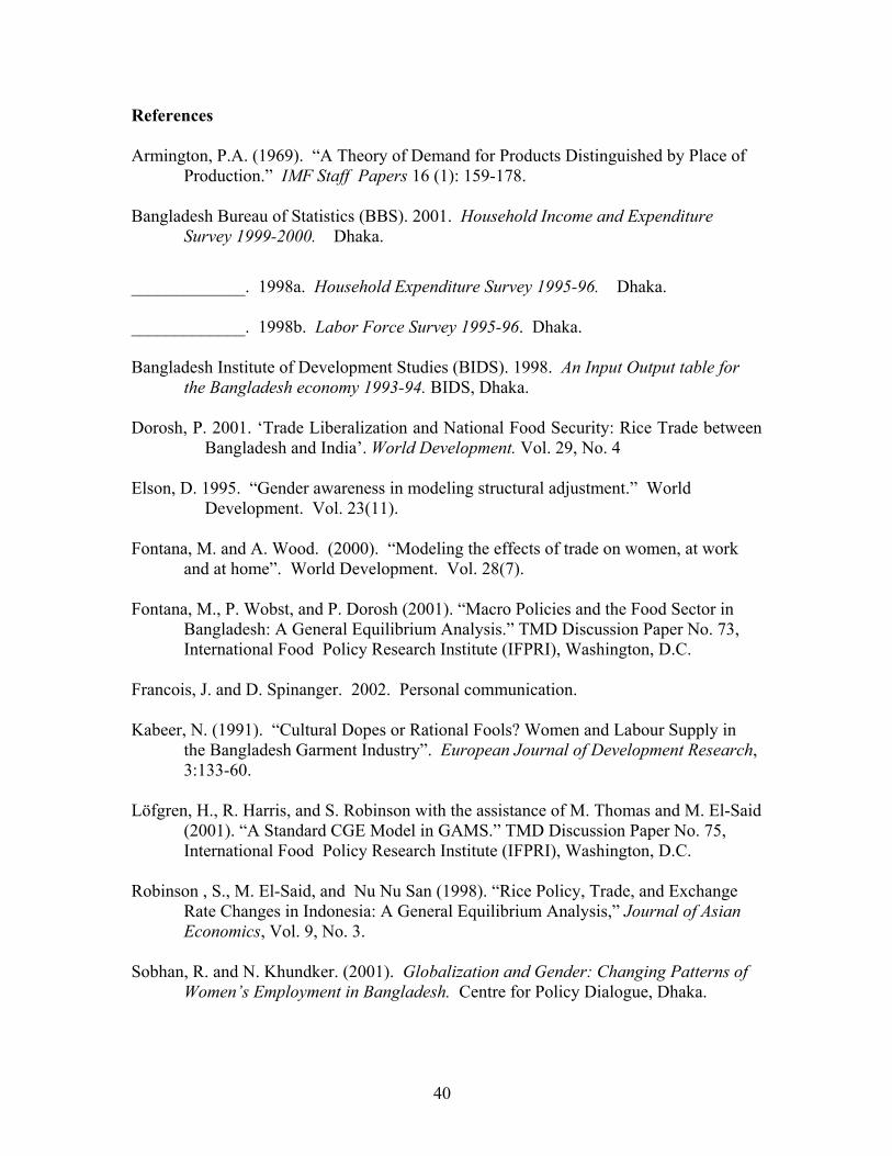
40

References Armington, P.A. (1969). �A Theory of Demand for Products Distinguished by Place of

Production.� IMF Staff Papers 16 (1): 159-178. Bangladesh Bureau of Statistics (BBS). 2001. Household Income and Expenditure

Survey 1999-2000. Dhaka.

_____________. 1998a. Household Expenditure Survey 1995-96. Dhaka. _____________. 1998b. Labor Force Survey 1995-96. Dhaka. Bangladesh Institute of Development Studies (BIDS). 1998. An Input Output table for

the Bangladesh economy 1993-94. BIDS, Dhaka. Dorosh, P. 2001. �Trade Liberalization and National Food Security: Rice Trade between

Bangladesh and India�. World Development. Vol. 29, No. 4 Elson, D. 1995. �Gender awareness in modeling structural adjustment.� World

Development. Vol. 23(11). Fontana, M. and A. Wood. (2000). �Modeling the effects of trade on women, at work

and at home�. World Development. Vol. 28(7). Fontana, M., P. Wobst, and P. Dorosh (2001). �Macro Policies and the Food Sector in

Bangladesh: A General Equilibrium Analysis.� TMD Discussion Paper No. 73, International Food Policy Research Institute (IFPRI), Washington, D.C.

Francois, J. and D. Spinanger. 2002. Personal communication. Kabeer, N. (1991). �Cultural Dopes or Rational Fools? Women and Labour Supply in

the Bangladesh Garment Industry�. European Journal of Development Research, 3:133-60.

Löfgren, H., R. Harris, and S. Robinson with the assistance of M. Thomas and M. El-Said

(2001). �A Standard CGE Model in GAMS.� TMD Discussion Paper No. 75, International Food Policy Research Institute (IFPRI), Washington, D.C.

Robinson , S., M. El-Said, and Nu Nu San (1998). �Rice Policy, Trade, and Exchange

Rate Changes in Indonesia: A General Equilibrium Analysis,� Journal of Asian Economics, Vol. 9, No. 3.

Sobhan, R. and N. Khundker. (2001). Globalization and Gender: Changing Patterns of

Women�s Employment in Bangladesh. Centre for Policy Dialogue, Dhaka.

41

Spinanger, D. 2000. �The WTO, ATC and Textiles and Clothing in a Global Perspective: What�s in it for Bangladesh?,� CPD Occasional Paper No. 8. Dhaka: Centre for Policy Dialogue.

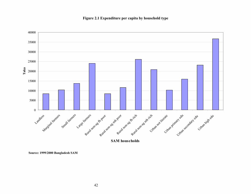
42

Figure 2.1 Expenditure per capita by household type

0

5000

10000

15000

20000

25000

30000

35000

40000

Landle

ssMarg

inal fa

rmers

Small fa

rmers

Large f

armers

Rural n

on-ag

fh po

orRura

l non

-ag m

h poo

rRura

l non

-ag fh

rich

Rural n

on-ag

mh r

ichUrba

n not

literat

eUrba

n prim

ary ed

uUrba

n seco

ndary

edu

Urban h

igh ed

u

SAM households

Tak

a

Source: 1999/2000 Bangladesh SAM

43

Figure 3.1. Production technology

Intermediate (Leontief)

Activity level (CES/Leontief)

Composite commodities

Value added (CES)

Primary factors

Commodity outputs (fixed yield coefficients)

Imported Domestic

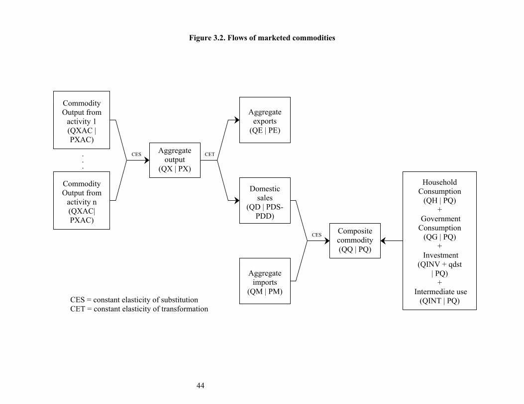
44

Figure 3.2. Flows of marketed commodities

CES

Commodity Output from

activity 1 (QXAC | PXAC)

Commodity Output from

activity n (QXAC| PXAC)

Aggregate output

(QX | PX)

CET

Domestic sales

(QD | PDS-PDD)

Aggregate imports

(QM | PM)

Aggregate exports

(QE | PE)

CES Composite commodity (QQ | PQ)

Household Consumption

(QH | PQ) +

Government Consumption

(QG | PQ) +

Investment (QINV + qdst

| PQ) +

Intermediate use (QINT | PQ)

CES = constant elasticity of substitution CET = constant elasticity of transformation

.

.

.

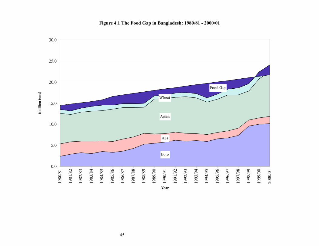
45

Figure 4.1 The Food Gap in Bangladesh: 1980/81 - 2000/01

Boro

Aus

Aman

Wheat

Food Gap

0.0

5.0

10.0

15.0

20.0

25.0

30.0

1980

/81

1981

/82

1982

/83

1983

/84

1984

/85

1985

/86

1986

/87

1987

/88

1988

/89

1989

/90

1990

/91

1991

/92

1992

/93

1993

/94

1994

/95

1995

/96

1996

/97

1997

/98

1998

/99

1999

/00

2000

/01

Year

(mill

ion

tons

)

46

Figure 4.2 National Average Real Wholesale Price of Rice and Wheat in Bangladesh, 1980-2001

0

2

4

6

8

10

12

14

16

18

20

22

24

26

28

Jul.8

0

Jul .8

1

Jul. 8

2

Jul. 8

3

Jul .8

4

Jul .8

5

Jul. 8

6

Jul. 8

7

Jul .8

8

Jul .8

9

Jul. 9

0

Jul. 9

1

Jul .9

2

Jul .9

3

Jul. 9

4

Jul. 9

5

Jul .9

6

Jul .9

7

Jul. 9

8

Jul .9

9

Jul .0

0

(200

0 T

aka/

kg)

Real Wheat Price

Real Rice Price

Note: Prices are deflated using the non-food Dhaka middle-income Cost of Living Index (and the national CPI after June 1998).Source : Dorosh (2001); FPMU data.

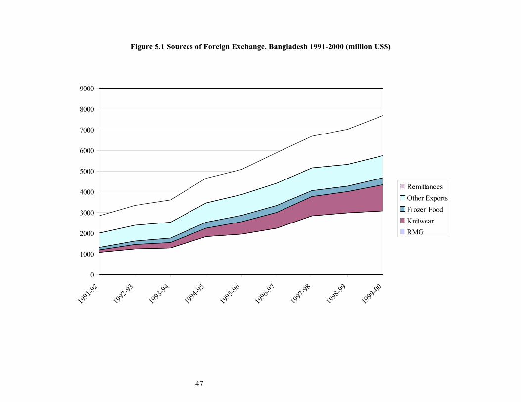
47

Figure 5.1 Sources of Foreign Exchange, Bangladesh 1991-2000 (million US$)

0

1000

2000

3000

4000

5000

6000

7000

8000

9000

1991

-92

1992

-93

1993

-94

1994

-95

1995

-96

1996

-97

1997

-98

1998

-99

1999

-00

RemittancesOther ExportsFrozen FoodKnitwearRMG

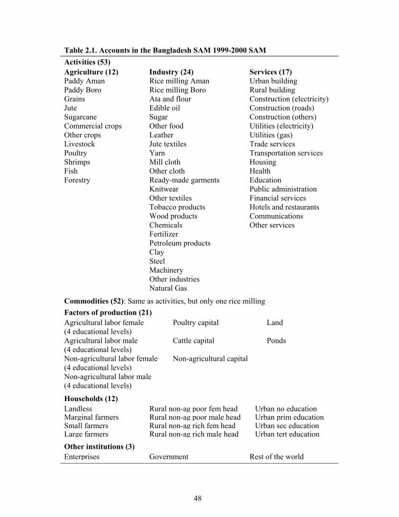
48

Table 2.1. Accounts in the Bangladesh SAM 1999-2000 SAM Activities (53) Agriculture (12) Industry (24) Services (17) Paddy Aman Rice milling Aman Urban building Paddy Boro Rice milling Boro Rural building Grains Ata and flour Construction (electricity) Jute Edible oil Construction (roads) Sugarcane Sugar Construction (others) Commercial crops Other food Utilities (electricity) Other crops Leather Utilities (gas) Livestock Jute textiles Trade services Poultry Yarn Transportation services Shrimps Mill cloth Housing Fish Other cloth Health Forestry Ready-made garments Education Knitwear Public administration Other textiles Financial services Tobacco products Hotels and restaurants Wood products Communications Chemicals Other services Fertilizer Petroleum products Clay Steel Machinery Other industries Natural Gas

Commodities (52): Same as activities, but only one rice milling Factors of production (21) Agricultural labor female (4 educational levels)

Poultry capital Land

Agricultural labor male (4 educational levels)

Cattle capital Ponds

Non-agricultural labor female (4 educational levels)

Non-agricultural capital

Non-agricultural labor male (4 educational levels)

Households (12) Landless Rural non-ag poor fem head Urban no education Marginal farmers Rural non-ag poor male head Urban prim educationSmall farmers Rural non-ag rich fem head Urban sec education Large farmers Rural non-ag rich male head Urban tert education Other institutions (3) Enterprises Government Rest of the world

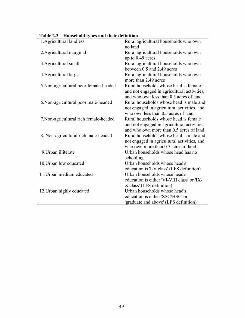
49

Table 2.2 � Household types and their definition 1.Agricultural landless

Rural agricultural households who own no land

2.Agricultural marginal Rural agricultural households who own up to 0.49 acres

3.Agricultural small Rural agricultural households who own between 0.5 and 2.49 acres

4.Agricultural large Rural agricultural households who own more than 2.49 acres

5.Non-agricultural poor female-headed Rural households whose head is female and not engaged in agricultural activities, and who own less than 0.5 acres of land

6.Non-agricultural poor male-headed Rural households whose head is male and not engaged in agricultural activities, and who own less than 0.5 acres of land

7.Non-agricultural rich female-headed Rural households whose head is female and not engaged in agricultural activities, and who own more than 0.5 acres of land

8. Non-agricultural rich male-headed Rural households whose head is male and not engaged in agricultural activities, and who own more than 0.5 acres of land

9.Urban illiterate

Urban households whose head has no schooling

10.Urban low educated Urban households whose head's education is 'I-V class' (LFS definition)

11.Urban medium educated Urban households whose head's education is either 'VI-VIII class' or 'IX-X class' (LFS definition)

12.Urban highly educated Urban households whose head's education is either 'SSC/HSC' or 'graduate and above' (LFS definition)

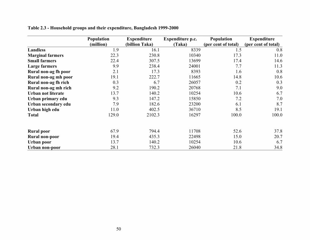
50

Table 2.3 - Household groups and their expenditure, Bangladesh 1999-2000 Population Expenditure Expenditure p.c. Population Expenditure (million) (billion Taka) (Taka) (per cent of total) (per cent of total) Landless 1.9 16.1 8339 1.5 0.8Marginal farmers 22.3 230.8 10340 17.3 11.0Small farmers 22.4 307.5 13699 17.4 14.6Large farmers 9.9 238.4 24001 7.7 11.3Rural non-ag fh poor 2.1 17.3 8393 1.6 0.8Rural non-ag mh poor 19.1 222.7 11665 14.8 10.6Rural non-ag fh rich 0.3 6.7 26057 0.2 0.3Rural non-ag mh rich 9.2 190.2 20768 7.1 9.0Urban not literate 13.7 140.2 10254 10.6 6.7Urban primary edu 9.3 147.2 15850 7.2 7.0Urban secondary edu 7.9 182.6 23200 6.1 8.7Urban high edu 11.0 402.5 36710 8.5 19.1Total 129.0 2102.3 16297 100.0 100.0 Rural poor 67.9 794.4 11708 52.6 37.8Rural non-poor 19.4 435.3 22498 15.0 20.7Urban poor 13.7 140.2 10254 10.6 6.7Urban non-poor 28.1 732.3 26040 21.8 34.8

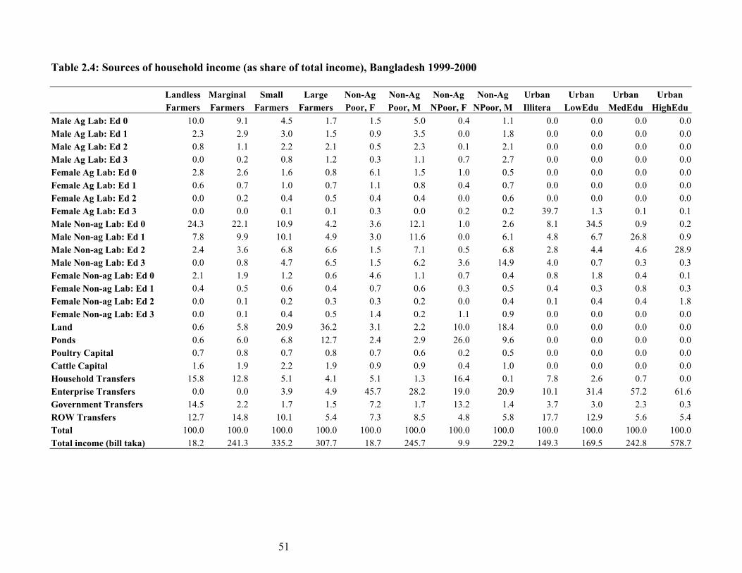
51

Table 2.4: Sources of household income (as share of total income), Bangladesh 1999-2000 Landless Marginal Small Large Non-Ag Non-Ag Non-Ag Non-Ag Urban Urban Urban Urban Farmers Farmers Farmers Farmers Poor, F Poor, M NPoor, F NPoor, M Illitera LowEdu MedEdu HighEduMale Ag Lab: Ed 0 10.0 9.1 4.5 1.7 1.5 5.0 0.4 1.1 0.0 0.0 0.0 0.0 Male Ag Lab: Ed 1 2.3 2.9 3.0 1.5 0.9 3.5 0.0 1.8 0.0 0.0 0.0 0.0 Male Ag Lab: Ed 2 0.8 1.1 2.2 2.1 0.5 2.3 0.1 2.1 0.0 0.0 0.0 0.0 Male Ag Lab: Ed 3 0.0 0.2 0.8 1.2 0.3 1.1 0.7 2.7 0.0 0.0 0.0 0.0 Female Ag Lab: Ed 0 2.8 2.6 1.6 0.8 6.1 1.5 1.0 0.5 0.0 0.0 0.0 0.0 Female Ag Lab: Ed 1 0.6 0.7 1.0 0.7 1.1 0.8 0.4 0.7 0.0 0.0 0.0 0.0 Female Ag Lab: Ed 2 0.0 0.2 0.4 0.5 0.4 0.4 0.0 0.6 0.0 0.0 0.0 0.0 Female Ag Lab: Ed 3 0.0 0.0 0.1 0.1 0.3 0.0 0.2 0.2 39.7 1.3 0.1 0.1 Male Non-ag Lab: Ed 0 24.3 22.1 10.9 4.2 3.6 12.1 1.0 2.6 8.1 34.5 0.9 0.2 Male Non-ag Lab: Ed 1 7.8 9.9 10.1 4.9 3.0 11.6 0.0 6.1 4.8 6.7 26.8 0.9 Male Non-ag Lab: Ed 2 2.4 3.6 6.8 6.6 1.5 7.1 0.5 6.8 2.8 4.4 4.6 28.9 Male Non-ag Lab: Ed 3 0.0 0.8 4.7 6.5 1.5 6.2 3.6 14.9 4.0 0.7 0.3 0.3 Female Non-ag Lab: Ed 0 2.1 1.9 1.2 0.6 4.6 1.1 0.7 0.4 0.8 1.8 0.4 0.1 Female Non-ag Lab: Ed 1 0.4 0.5 0.6 0.4 0.7 0.6 0.3 0.5 0.4 0.3 0.8 0.3 Female Non-ag Lab: Ed 2 0.0 0.1 0.2 0.3 0.3 0.2 0.0 0.4 0.1 0.4 0.4 1.8 Female Non-ag Lab: Ed 3 0.0 0.1 0.4 0.5 1.4 0.2 1.1 0.9 0.0 0.0 0.0 0.0 Land 0.6 5.8 20.9 36.2 3.1 2.2 10.0 18.4 0.0 0.0 0.0 0.0 Ponds 0.6 6.0 6.8 12.7 2.4 2.9 26.0 9.6 0.0 0.0 0.0 0.0 Poultry Capital 0.7 0.8 0.7 0.8 0.7 0.6 0.2 0.5 0.0 0.0 0.0 0.0 Cattle Capital 1.6 1.9 2.2 1.9 0.9 0.9 0.4 1.0 0.0 0.0 0.0 0.0 Household Transfers 15.8 12.8 5.1 4.1 5.1 1.3 16.4 0.1 7.8 2.6 0.7 0.0 Enterprise Transfers 0.0 0.0 3.9 4.9 45.7 28.2 19.0 20.9 10.1 31.4 57.2 61.6 Government Transfers 14.5 2.2 1.7 1.5 7.2 1.7 13.2 1.4 3.7 3.0 2.3 0.3 ROW Transfers 12.7 14.8 10.1 5.4 7.3 8.5 4.8 5.8 17.7 12.9 5.6 5.4 Total 100.0 100.0 100.0 100.0 100.0 100.0 100.0 100.0 100.0 100.0 100.0 100.0 Total income (bill taka) 18.2 241.3 335.2 307.7 18.7 245.7 9.9 229.2 149.3 169.5 242.8 578.7

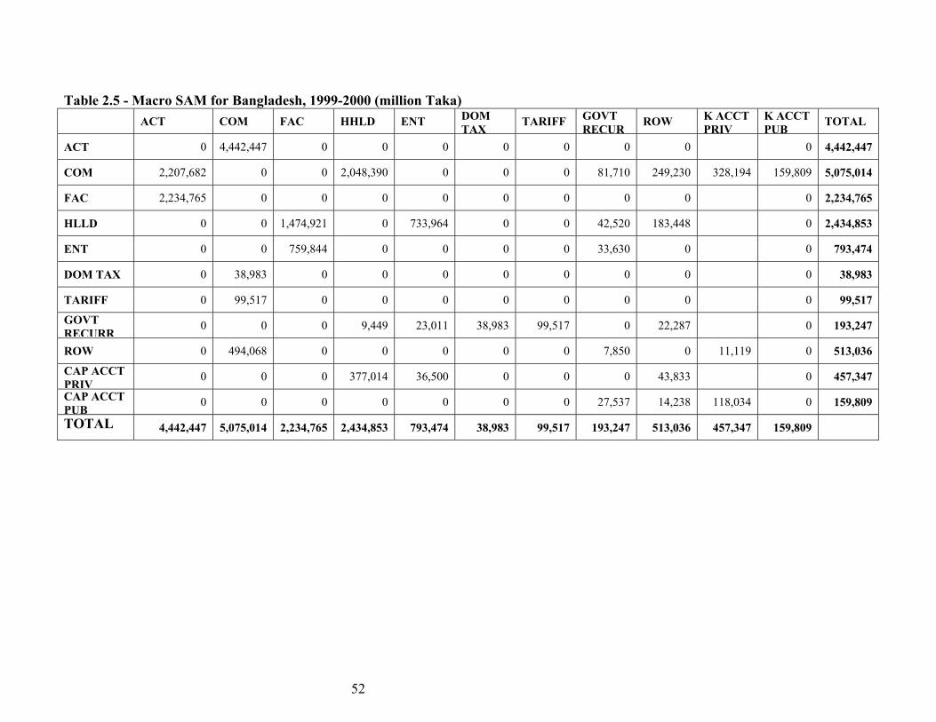
52

Table 2.5 - Macro SAM for Bangladesh, 1999-2000 (million Taka) ACT COM FAC HHLD ENT DOM

TAXTARIFF GOVT

RECURROW K ACCT

PRIVK ACCT PUB

TOTAL

ACT 0 4,442,447 0 0 0 0 0 0 0 0 4,442,447

COM 2,207,682 0 0 2,048,390 0 0 0 81,710 249,230 328,194 159,809 5,075,014

FAC 2,234,765 0 0 0 0 0 0 0 0 0 2,234,765

HLLD 0 0 1,474,921 0 733,964 0 0 42,520 183,448 0 2,434,853

ENT 0 0 759,844 0 0 0 0 33,630 0 0 793,474

DOM TAX 0 38,983 0 0 0 0 0 0 0 0 38,983

TARIFF 0 99,517 0 0 0 0 0 0 0 0 99,517

GOVT RECURR

0 0 0 9,449 23,011 38,983 99,517 0 22,287 0 193,247

ROW 0 494,068 0 0 0 0 0 7,850 0 11,119 0 513,036

CAP ACCT PRIV

0 0 0 377,014 36,500 0 0 0 43,833 0 457,347

CAP ACCT PUB

0 0 0 0 0 0 0 27,537 14,238 118,034 0 159,809

TOTAL 4,442,447 5,075,014 2,234,765 2,434,853 793,474 38,983 99,517 193,247 513,036 457,347 159,809

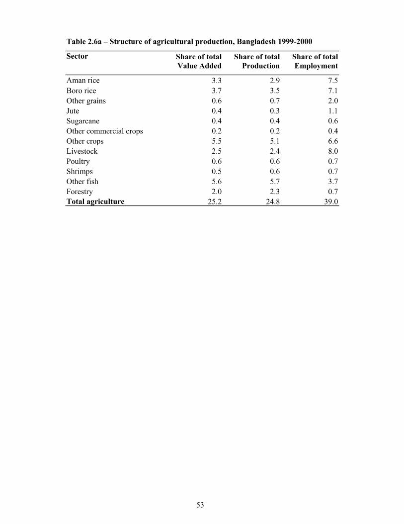
53

Table 2.6a � Structure of agricultural production, Bangladesh 1999-2000

Sector Share of total Value Added

Share of total Production

Share of total Employment

Aman rice 3.3 2.9 7.5Boro rice 3.7 3.5 7.1Other grains 0.6 0.7 2.0Jute 0.4 0.3 1.1Sugarcane 0.4 0.4 0.6Other commercial crops 0.2 0.2 0.4Other crops 5.5 5.1 6.6Livestock 2.5 2.4 8.0Poultry 0.6 0.6 0.7Shrimps 0.5 0.6 0.7Other fish 5.6 5.7 3.7Forestry 2.0 2.3 0.7Total agriculture 25.2 24.8 39.0

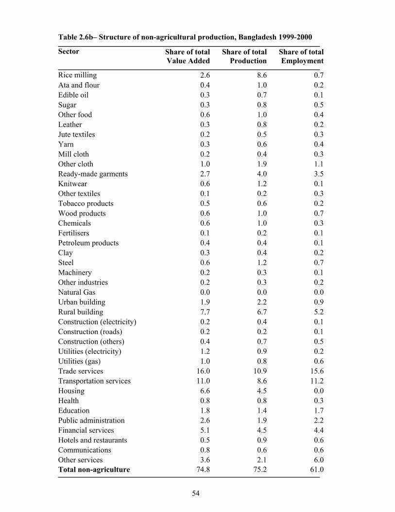
54

Table 2.6b� Structure of non-agricultural production, Bangladesh 1999-2000

Sector Share of total Value Added

Share of total Production

Share of total Employment

Rice milling 2.6 8.6 0.7Ata and flour 0.4 1.0 0.2Edible oil 0.3 0.7 0.1Sugar 0.3 0.8 0.5Other food 0.6 1.0 0.4Leather 0.3 0.8 0.2Jute textiles 0.2 0.5 0.3Yarn 0.3 0.6 0.4Mill cloth 0.2 0.4 0.3Other cloth 1.0 1.9 1.1Ready-made garments 2.7 4.0 3.5Knitwear 0.6 1.2 0.1Other textiles 0.1 0.2 0.3Tobacco products 0.5 0.6 0.2Wood products 0.6 1.0 0.7Chemicals 0.6 1.0 0.3Fertilisers 0.1 0.2 0.1Petroleum products 0.4 0.4 0.1Clay 0.3 0.4 0.2Steel 0.6 1.2 0.7Machinery 0.2 0.3 0.1Other industries 0.2 0.3 0.2Natural Gas 0.0 0.0 0.0Urban building 1.9 2.2 0.9Rural building 7.7 6.7 5.2Construction (electricity) 0.2 0.4 0.1Construction (roads) 0.2 0.2 0.1Construction (others) 0.4 0.7 0.5Utilities (electricity) 1.2 0.9 0.2Utilities (gas) 1.0 0.8 0.6Trade services 16.0 10.9 15.6Transportation services 11.0 8.6 11.2Housing 6.6 4.5 0.0Health 0.8 0.8 0.3Education 1.8 1.4 1.7Public administration 2.6 1.9 2.2Financial services 5.1 4.5 4.4Hotels and restaurants 0.5 0.9 0.6Communications 0.8 0.6 0.6Other services 3.6 2.1 6.0Total non-agriculture 74.8 75.2 61.0

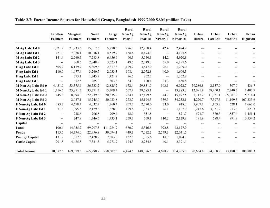
55

Table 2.7: Factor Income Sources for Household Groups, Bangladesh 1999/2000 SAM (million Taka) Rural Rural Rural Rural Landless Marginal Small Large Non-Ag Non-Ag Non-Ag Non-Ag Urban Urban Urban Urban Farmers Farmers Farmers Farmers Poor, F Poor, M NPoor, F NPoor, M Illitera LowEdu MedEdu HighEdu M Ag Lab: Ed 0 1,821.2 21,933.6 15,012.6 5,270.3 276.3 12,258.4 42.4 2,474.9 -- -- -- -- M Ag Lab: Ed 1 421.0 7,088.1 10,036.1 4,519.9 168.6 8,494.3 -- 4,125.8 -- -- -- -- M Ag Lab: Ed 2 141.4 2,760.5 7,283.8 6,456.9 90.3 5,550.1 14.2 4,920.8 -- -- -- -- M Ag Lab: Ed 3 -- 368.6 2,848.9 3,623.1 49.5 2,749.3 65.0 6,197.6 -- -- -- -- F Ag Lab: Ed 0 505.2 6,159.7 5,309.6 2,317.8 1,129.2 3,647.0 96.1 1,209.0 -- -- -- -- F Ag Lab: Ed 1 110.0 1,677.4 3,260.7 2,033.3 198.4 2,072.8 40.0 1,696.3 -- -- -- -- F Ag Lab: Ed 2 -- 373.1 1,245.7 1,421.7 76.5 862.7 -- 1,362.8 -- -- -- -- F Ag Lab: Ed 3 -- 52.5 285.0 303.3 54.9 120.4 23.3 450.8 -- -- -- -- M Non-Ag Lab: Ed 0 4,431.9 53,375.6 36,533.2 12,825.2 672.4 29,831.0 103.1 6,022.7 59,286.8 2,137.0 307.0 436.7 M Non-Ag Lab: Ed 1 1,416.5 23,851.3 33,771.3 15,209.4 567.4 28,583.1 -- 13,883.3 12,091.8 58,450.1 2,240.3 1,407.7 M Non-Ag Lab: Ed 2 445.3 8,694.0 22,939.6 20,335.2 284.4 17,479.5 44.7 15,497.5 7,117.2 11,331.1 65,081.9 5,214.4 M Non-Ag Lab: Ed 3 -- 2,037.1 15,745.0 20,023.8 273.7 15,194.3 359.3 34,252.1 4,220.7 7,397.5 11,199.5 167,333.6 F Non-Ag Lab: Ed 0 383.7 4,678.4 4,032.7 1,760.4 857.7 2,770.0 73.0 918.2 5,907.1 1,163.2 628.1 1,667.0 F Non-Ag Lab: Ed 1 71.8 1,095.5 2,129.6 1,328.0 129.6 1,353.8 26.1 1,107.9 1,247.6 3,031.2 973.8 823.3 F Non-Ag Lab: Ed 2 -- 238.6 796.8 909.4 48.9 551.8 -- 871.7 571.7 570.3 1,857.4 1,451.4 F Non-Ag Lab: Ed 3 -- 247.8 1,346.6 1,433.1 259.3 569.1 110.2 2,129.8 191.9 688.4 891.9 10,554.2 Capital -- -- -- -- -- -- -- -- -- -- -- -- Land 100.4 14,055.2 69,997.3 111,284.9 580.9 5,346.5 992.8 42,127.9 -- -- -- -- Ponds 115.6 14,394.0 22,956.8 39,094.1 449.3 7,012.2 2,579.3 22,031.5 -- -- -- -- Poultry Capital 131.7 1,812.6 2,428.2 2,583.8 132.8 1,385.6 18.7 1,094.1 -- -- -- -- Cattle Capital 291.8 4,485.8 7,331.3 5,773.9 174.3 2,254.5 40.1 2,391.1 -- -- -- -- Total Income 10,387.5 169,379.3 265,290.7 258,507.6 6,474.6 148,086.5 4,628.2 164,765.8 90,634.8 84,768.9 83,180.0 188,888.3

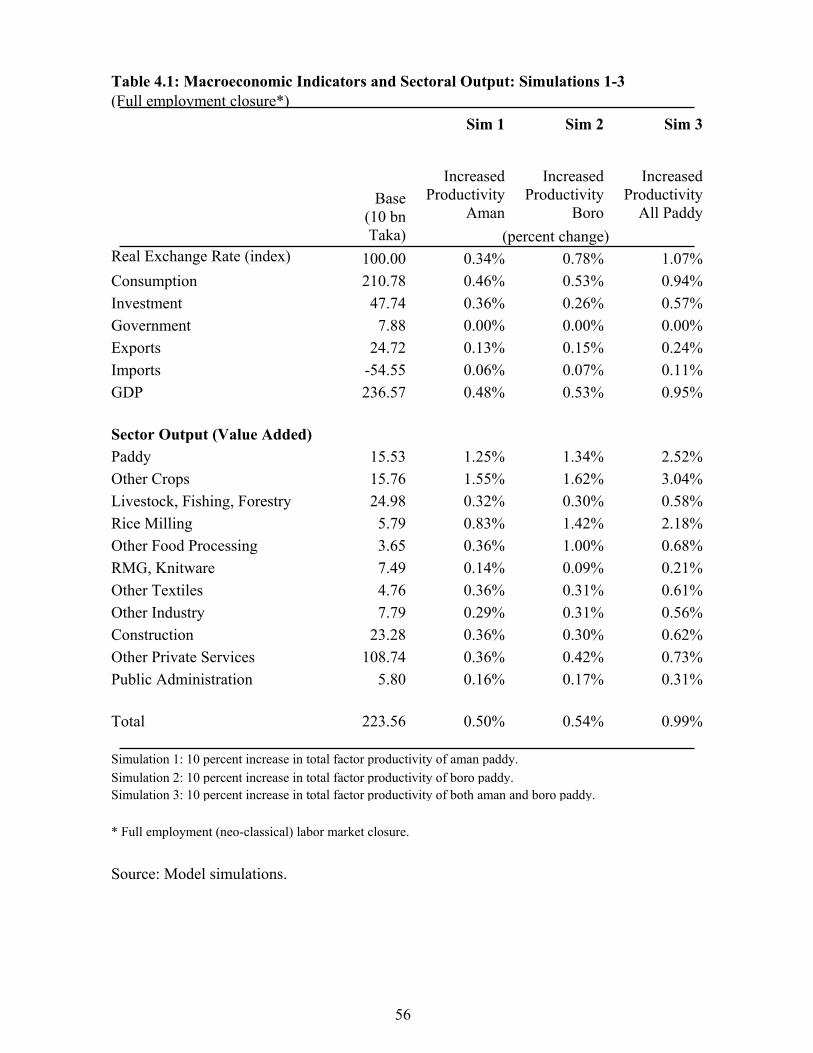
56

Table 4.1: Macroeconomic Indicators and Sectoral Output: Simulations 1-3 (Full employment closure*) Sim 1 Sim 2 Sim 3

Increased Productivity

Aman

Increased Productivity

Boro

Increased Productivity

All Paddy

Base (10 bn Taka) (percent change)

Real Exchange Rate (index) 100.00 0.34% 0.78% 1.07%Consumption 210.78 0.46% 0.53% 0.94%Investment 47.74 0.36% 0.26% 0.57%Government 7.88 0.00% 0.00% 0.00%Exports 24.72 0.13% 0.15% 0.24%Imports -54.55 0.06% 0.07% 0.11%GDP 236.57 0.48% 0.53% 0.95% Sector Output (Value Added) Paddy 15.53 1.25% 1.34% 2.52%Other Crops 15.76 1.55% 1.62% 3.04%Livestock, Fishing, Forestry 24.98 0.32% 0.30% 0.58%Rice Milling 5.79 0.83% 1.42% 2.18%Other Food Processing 3.65 0.36% 1.00% 0.68%RMG, Knitware 7.49 0.14% 0.09% 0.21%Other Textiles 4.76 0.36% 0.31% 0.61%Other Industry 7.79 0.29% 0.31% 0.56%Construction 23.28 0.36% 0.30% 0.62%Other Private Services 108.74 0.36% 0.42% 0.73%Public Administration 5.80 0.16% 0.17% 0.31% Total 223.56 0.50% 0.54% 0.99% Simulation 1: 10 percent increase in total factor productivity of aman paddy. Simulation 2: 10 percent increase in total factor productivity of boro paddy.Simulation 3: 10 percent increase in total factor productivity of both aman and boro paddy. * Full employment (neo-classical) labor market closure.

Source: Model simulations.

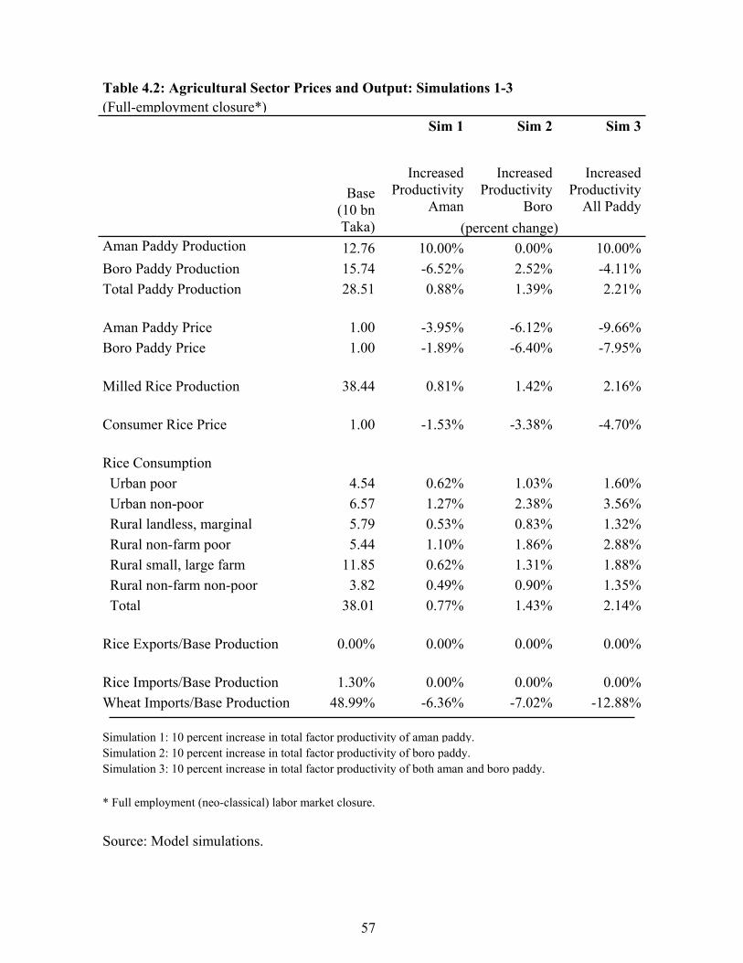
57

Table 4.2: Agricultural Sector Prices and Output: Simulations 1-3 (Full-employment closure*) Sim 1 Sim 2 Sim 3

Increased Productivity

Aman

Increased Productivity

Boro

Increased Productivity

All Paddy

Base (10 bn Taka) (percent change)

Aman Paddy Production 12.76 10.00% 0.00% 10.00%Boro Paddy Production 15.74 -6.52% 2.52% -4.11%Total Paddy Production 28.51 0.88% 1.39% 2.21% Aman Paddy Price 1.00 -3.95% -6.12% -9.66%Boro Paddy Price 1.00 -1.89% -6.40% -7.95% Milled Rice Production 38.44 0.81% 1.42% 2.16% Consumer Rice Price 1.00 -1.53% -3.38% -4.70% Rice Consumption Urban poor 4.54 0.62% 1.03% 1.60% Urban non-poor 6.57 1.27% 2.38% 3.56% Rural landless, marginal 5.79 0.53% 0.83% 1.32% Rural non-farm poor 5.44 1.10% 1.86% 2.88% Rural small, large farm 11.85 0.62% 1.31% 1.88% Rural non-farm non-poor 3.82 0.49% 0.90% 1.35% Total 38.01 0.77% 1.43% 2.14% Rice Exports/Base Production 0.00% 0.00% 0.00% 0.00% Rice Imports/Base Production 1.30% 0.00% 0.00% 0.00%Wheat Imports/Base Production 48.99% -6.36% -7.02% -12.88% Simulation 1: 10 percent increase in total factor productivity of aman paddy.Simulation 2: 10 percent increase in total factor productivity of boro paddy.Simulation 3: 10 percent increase in total factor productivity of both aman and boro paddy. * Full employment (neo-classical) labor market closure.

Source: Model simulations.

58

Table 4.3: Macroeconomic Indicators and Sectoral Output: Simulations 4-7 (Full-employment closure*)

Sim 4 Sim 5 Sim 6 Sim 7

Increased Productivity

Aman

Increased Productivity

Boro

Increased Productivity

All Paddy Lower World

Price

Base (10 bn Taka) (percent change)

Real Exchange Rate (index) 100.00 -0.98% -2.30% -3.20% 11.67%Consumption 210.78 0.57% 0.81% 1.35% 0.02%Investment 47.74 0.40% 0.33% 0.69% 2.11%Government 7.88 0.00% 0.00% 0.00% 0.00%Exports 24.72 2.11% 4.59% 6.43% 16.38%Imports -54.55 0.96% 2.08% 2.92% 7.42%GDP 236.57 0.59% 0.79% 1.34% 0.44% Sector Output (Value Added) Paddy 15.53 3.04% 5.53% 8.29% -15.90%Other Crops 15.76 -0.12% -2.01% -1.95% 10.13%Livestock, Fishing, Forestry 24.98 0.25% 0.15% 0.39% 0.92%Rice Milling 5.79 3.01% 6.51% 9.20% -19.37%Other Food Processing 3.65 0.25% 0.11% 0.35% 1.76%RMG, Knitware 7.49 -0.73% -2.00% -2.69% 7.58%Other Textiles 4.76 -0.16% -0.88% -0.97% 8.31%Other Industry 7.79 0.04% -0.27% -0.24% 2.81%Construction 23.28 0.48% 0.57% 1.00% 1.11%Other Private Services 108.74 0.48% 0.70% 1.14% -0.34%Public Administration 5.80 0.15% 0.16% 0.31% 0.25% Total 223.56 0.58% 0.74% 1.27% -0.27% Simulation 4: 10 percent increase in total factor productivity of aman paddy, with rice exports. Simulation 5: 10 percent increase in total factor productivity of boro paddy, with rice exports.Simulation 6: 10 percent increase in total factor productivity of both aman and boro paddy, with rice exports. Simulation 7: 35 percent reduction in world price of rice. * Full employment (neo-classical) labor market closure.

Source: Model simulations.

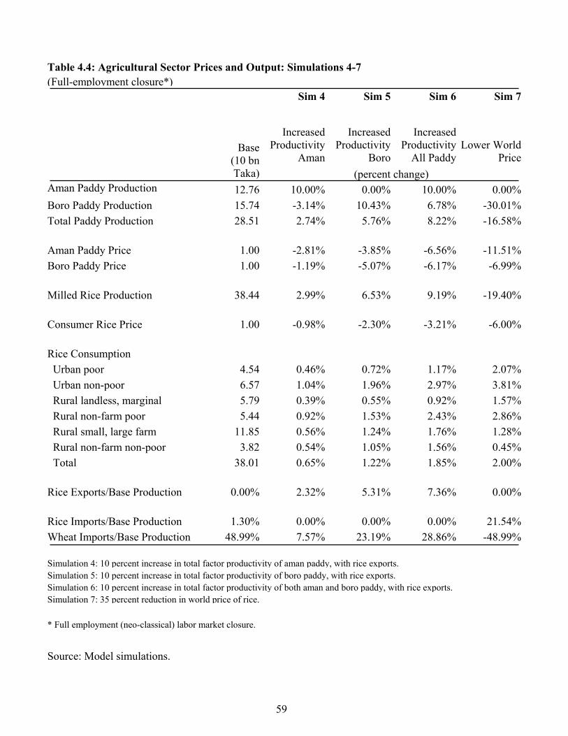
59

Table 4.4: Agricultural Sector Prices and Output: Simulations 4-7 (Full-employment closure*)

Sim 4 Sim 5 Sim 6 Sim 7

Increased Productivity

Aman

Increased Productivity

Boro

Increased Productivity

All Paddy Lower World

Price

Base (10 bn Taka) (percent change)

Aman Paddy Production 12.76 10.00% 0.00% 10.00% 0.00%Boro Paddy Production 15.74 -3.14% 10.43% 6.78% -30.01%Total Paddy Production 28.51 2.74% 5.76% 8.22% -16.58% Aman Paddy Price 1.00 -2.81% -3.85% -6.56% -11.51%Boro Paddy Price 1.00 -1.19% -5.07% -6.17% -6.99% Milled Rice Production 38.44 2.99% 6.53% 9.19% -19.40% Consumer Rice Price 1.00 -0.98% -2.30% -3.21% -6.00% Rice Consumption Urban poor 4.54 0.46% 0.72% 1.17% 2.07% Urban non-poor 6.57 1.04% 1.96% 2.97% 3.81% Rural landless, marginal 5.79 0.39% 0.55% 0.92% 1.57% Rural non-farm poor 5.44 0.92% 1.53% 2.43% 2.86% Rural small, large farm 11.85 0.56% 1.24% 1.76% 1.28% Rural non-farm non-poor 3.82 0.54% 1.05% 1.56% 0.45% Total 38.01 0.65% 1.22% 1.85% 2.00% Rice Exports/Base Production 0.00% 2.32% 5.31% 7.36% 0.00% Rice Imports/Base Production 1.30% 0.00% 0.00% 0.00% 21.54%Wheat Imports/Base Production 48.99% 7.57% 23.19% 28.86% -48.99% Simulation 4: 10 percent increase in total factor productivity of aman paddy, with rice exports. Simulation 5: 10 percent increase in total factor productivity of boro paddy, with rice exports.Simulation 6: 10 percent increase in total factor productivity of both aman and boro paddy, with rice exports. Simulation 7: 35 percent reduction in world price of rice. * Full employment (neo-classical) labor market closure.

Source: Model simulations.

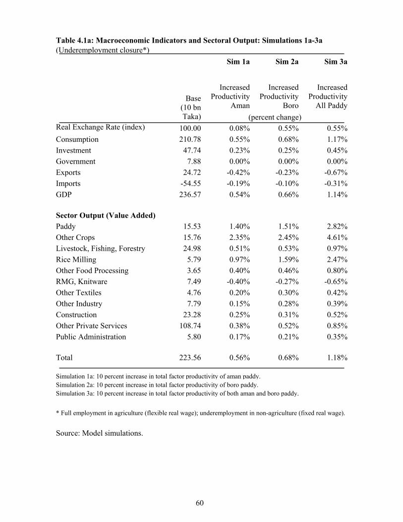
60

Table 4.1a: Macroeconomic Indicators and Sectoral Output: Simulations 1a-3a (Underemployment closure*) Sim 1a Sim 2a Sim 3a

Increased Productivity

Aman

Increased Productivity

Boro

Increased Productivity

All Paddy

Base (10 bn Taka) (percent change)

Real Exchange Rate (index) 100.00 0.08% 0.55% 0.55%Consumption 210.78 0.55% 0.68% 1.17%Investment 47.74 0.23% 0.25% 0.45%Government 7.88 0.00% 0.00% 0.00%Exports 24.72 -0.42% -0.23% -0.67%Imports -54.55 -0.19% -0.10% -0.31%GDP 236.57 0.54% 0.66% 1.14% Sector Output (Value Added) Paddy 15.53 1.40% 1.51% 2.82%Other Crops 15.76 2.35% 2.45% 4.61%Livestock, Fishing, Forestry 24.98 0.51% 0.53% 0.97%Rice Milling 5.79 0.97% 1.59% 2.47%Other Food Processing 3.65 0.40% 0.46% 0.80%RMG, Knitware 7.49 -0.40% -0.27% -0.65%Other Textiles 4.76 0.20% 0.30% 0.42%Other Industry 7.79 0.15% 0.28% 0.39%Construction 23.28 0.25% 0.31% 0.52%Other Private Services 108.74 0.38% 0.52% 0.85%Public Administration 5.80 0.17% 0.21% 0.35% Total 223.56 0.56% 0.68% 1.18% Simulation 1a: 10 percent increase in total factor productivity of aman paddy.Simulation 2a: 10 percent increase in total factor productivity of boro paddy.Simulation 3a: 10 percent increase in total factor productivity of both aman and boro paddy. * Full employment in agriculture (flexible real wage); underemployment in non-agriculture (fixed real wage). Source: Model simulations.

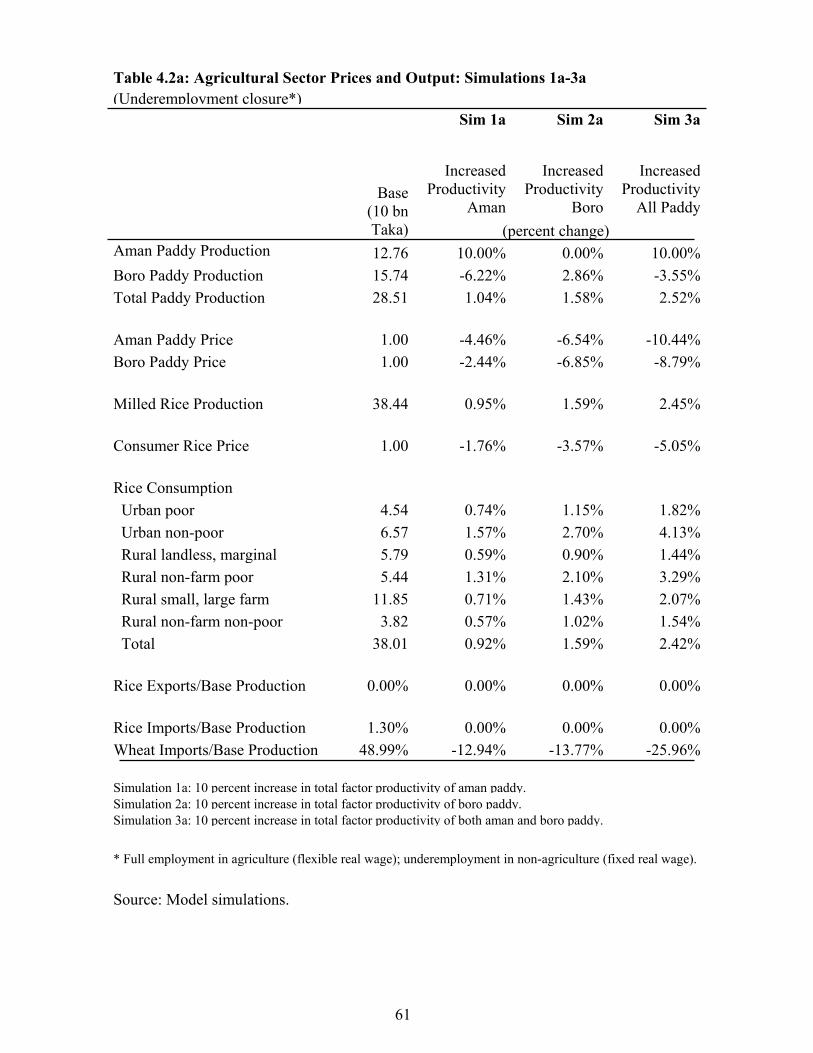
61

Table 4.2a: Agricultural Sector Prices and Output: Simulations 1a-3a (Underemployment closure*) Sim 1a Sim 2a Sim 3a

Increased Productivity

Aman

Increased Productivity

Boro

Increased Productivity

All Paddy

Base (10 bn Taka) (percent change)

Aman Paddy Production 12.76 10.00% 0.00% 10.00%Boro Paddy Production 15.74 -6.22% 2.86% -3.55%Total Paddy Production 28.51 1.04% 1.58% 2.52% Aman Paddy Price 1.00 -4.46% -6.54% -10.44%Boro Paddy Price 1.00 -2.44% -6.85% -8.79% Milled Rice Production 38.44 0.95% 1.59% 2.45% Consumer Rice Price 1.00 -1.76% -3.57% -5.05% Rice Consumption Urban poor 4.54 0.74% 1.15% 1.82% Urban non-poor 6.57 1.57% 2.70% 4.13% Rural landless, marginal 5.79 0.59% 0.90% 1.44% Rural non-farm poor 5.44 1.31% 2.10% 3.29% Rural small, large farm 11.85 0.71% 1.43% 2.07% Rural non-farm non-poor 3.82 0.57% 1.02% 1.54% Total 38.01 0.92% 1.59% 2.42% Rice Exports/Base Production 0.00% 0.00% 0.00% 0.00% Rice Imports/Base Production 1.30% 0.00% 0.00% 0.00%Wheat Imports/Base Production 48.99% -12.94% -13.77% -25.96% Simulation 1a: 10 percent increase in total factor productivity of aman paddy.Simulation 2a: 10 percent increase in total factor productivity of boro paddy.Simulation 3a: 10 percent increase in total factor productivity of both aman and boro paddy. * Full employment in agriculture (flexible real wage); underemployment in non-agriculture (fixed real wage). Source: Model simulations.

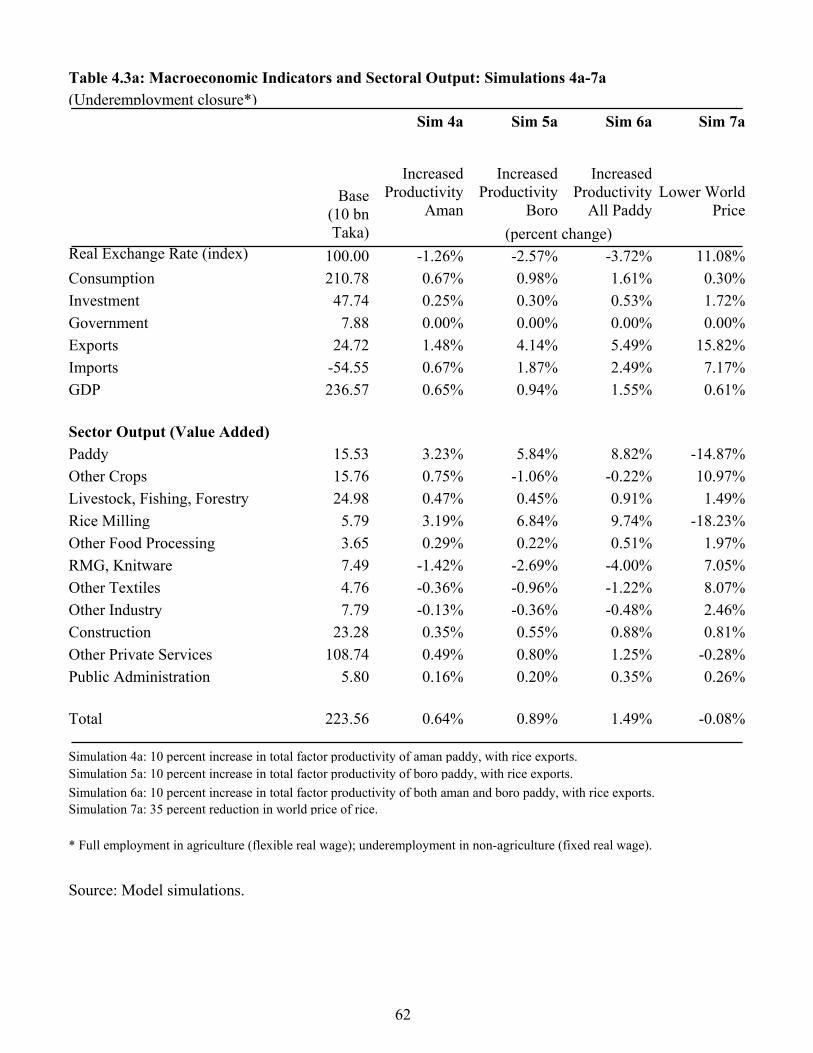
62

Table 4.3a: Macroeconomic Indicators and Sectoral Output: Simulations 4a-7a (Underemployment closure*)

Sim 4a Sim 5a Sim 6a Sim 7a

Increased Productivity

Aman

Increased Productivity

Boro

Increased Productivity

All Paddy Lower World

Price

Base (10 bn Taka) (percent change)

Real Exchange Rate (index) 100.00 -1.26% -2.57% -3.72% 11.08%Consumption 210.78 0.67% 0.98% 1.61% 0.30%Investment 47.74 0.25% 0.30% 0.53% 1.72%Government 7.88 0.00% 0.00% 0.00% 0.00%Exports 24.72 1.48% 4.14% 5.49% 15.82%Imports -54.55 0.67% 1.87% 2.49% 7.17%GDP 236.57 0.65% 0.94% 1.55% 0.61% Sector Output (Value Added) Paddy 15.53 3.23% 5.84% 8.82% -14.87%Other Crops 15.76 0.75% -1.06% -0.22% 10.97%Livestock, Fishing, Forestry 24.98 0.47% 0.45% 0.91% 1.49%Rice Milling 5.79 3.19% 6.84% 9.74% -18.23%Other Food Processing 3.65 0.29% 0.22% 0.51% 1.97%RMG, Knitware 7.49 -1.42% -2.69% -4.00% 7.05%Other Textiles 4.76 -0.36% -0.96% -1.22% 8.07%Other Industry 7.79 -0.13% -0.36% -0.48% 2.46%Construction 23.28 0.35% 0.55% 0.88% 0.81%Other Private Services 108.74 0.49% 0.80% 1.25% -0.28%Public Administration 5.80 0.16% 0.20% 0.35% 0.26% Total 223.56 0.64% 0.89% 1.49% -0.08% Simulation 4a: 10 percent increase in total factor productivity of aman paddy, with rice exports. Simulation 5a: 10 percent increase in total factor productivity of boro paddy, with rice exports. Simulation 6a: 10 percent increase in total factor productivity of both aman and boro paddy, with rice exports. Simulation 7a: 35 percent reduction in world price of rice. * Full employment in agriculture (flexible real wage); underemployment in non-agriculture (fixed real wage).

Source: Model simulations.

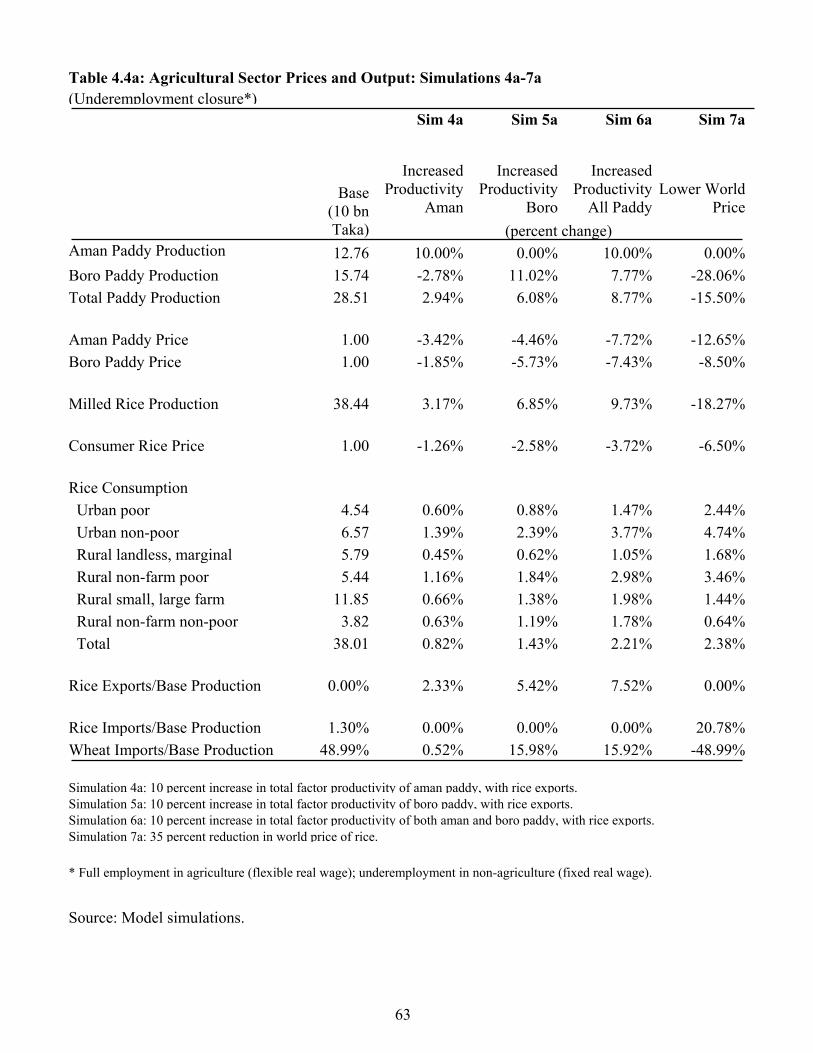
63

Table 4.4a: Agricultural Sector Prices and Output: Simulations 4a-7a (Underemployment closure*) Sim 4a Sim 5a Sim 6a Sim 7a

Increased Productivity

Aman

Increased Productivity

Boro

Increased Productivity

All Paddy Lower World

Price

Base (10 bn Taka) (percent change)

Aman Paddy Production 12.76 10.00% 0.00% 10.00% 0.00%Boro Paddy Production 15.74 -2.78% 11.02% 7.77% -28.06%Total Paddy Production 28.51 2.94% 6.08% 8.77% -15.50% Aman Paddy Price 1.00 -3.42% -4.46% -7.72% -12.65%Boro Paddy Price 1.00 -1.85% -5.73% -7.43% -8.50% Milled Rice Production 38.44 3.17% 6.85% 9.73% -18.27% Consumer Rice Price 1.00 -1.26% -2.58% -3.72% -6.50% Rice Consumption Urban poor 4.54 0.60% 0.88% 1.47% 2.44% Urban non-poor 6.57 1.39% 2.39% 3.77% 4.74% Rural landless, marginal 5.79 0.45% 0.62% 1.05% 1.68% Rural non-farm poor 5.44 1.16% 1.84% 2.98% 3.46% Rural small, large farm 11.85 0.66% 1.38% 1.98% 1.44% Rural non-farm non-poor 3.82 0.63% 1.19% 1.78% 0.64% Total 38.01 0.82% 1.43% 2.21% 2.38% Rice Exports/Base Production 0.00% 2.33% 5.42% 7.52% 0.00% Rice Imports/Base Production 1.30% 0.00% 0.00% 0.00% 20.78%Wheat Imports/Base Production 48.99% 0.52% 15.98% 15.92% -48.99% Simulation 4a: 10 percent increase in total factor productivity of aman paddy, with rice exports. Simulation 5a: 10 percent increase in total factor productivity of boro paddy, with rice exports. Simulation 6a: 10 percent increase in total factor productivity of both aman and boro paddy, with rice exports.Simulation 7a: 35 percent reduction in world price of rice. * Full employment in agriculture (flexible real wage); underemployment in non-agriculture (fixed real wage).

Source: Model simulations.

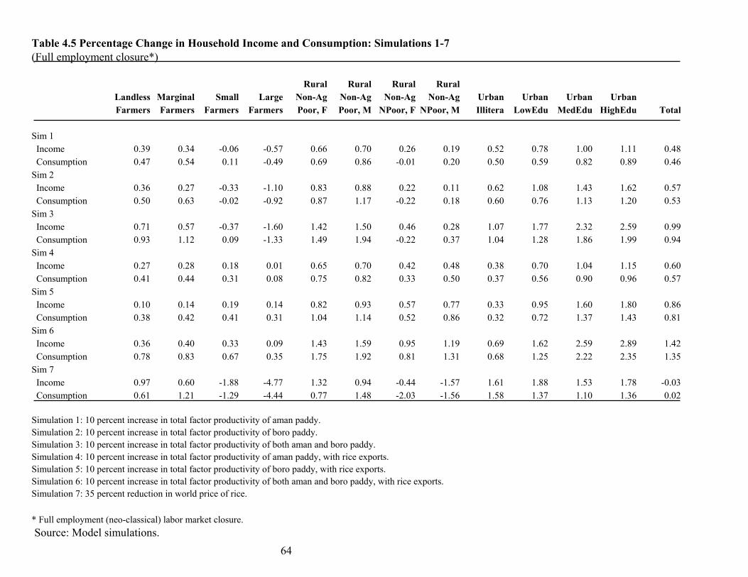
64

Table 4.5 Percentage Change in Household Income and Consumption: Simulations 1-7 (Full employment closure*) Rural Rural Rural Rural Landless Marginal Small Large Non-Ag Non-Ag Non-Ag Non-Ag Urban Urban Urban Urban Farmers Farmers Farmers Farmers Poor, F Poor, M NPoor, F NPoor, M Illitera LowEdu MedEdu HighEdu Total Sim 1 Income 0.39 0.34 -0.06 -0.57 0.66 0.70 0.26 0.19 0.52 0.78 1.00 1.11 0.48 Consumption 0.47 0.54 0.11 -0.49 0.69 0.86 -0.01 0.20 0.50 0.59 0.82 0.89 0.46Sim 2 Income 0.36 0.27 -0.33 -1.10 0.83 0.88 0.22 0.11 0.62 1.08 1.43 1.62 0.57 Consumption 0.50 0.63 -0.02 -0.92 0.87 1.17 -0.22 0.18 0.60 0.76 1.13 1.20 0.53Sim 3 Income 0.71 0.57 -0.37 -1.60 1.42 1.50 0.46 0.28 1.07 1.77 2.32 2.59 0.99 Consumption 0.93 1.12 0.09 -1.33 1.49 1.94 -0.22 0.37 1.04 1.28 1.86 1.99 0.94Sim 4 Income 0.27 0.28 0.18 0.01 0.65 0.70 0.42 0.48 0.38 0.70 1.04 1.15 0.60 Consumption 0.41 0.44 0.31 0.08 0.75 0.82 0.33 0.50 0.37 0.56 0.90 0.96 0.57Sim 5 Income 0.10 0.14 0.19 0.14 0.82 0.93 0.57 0.77 0.33 0.95 1.60 1.80 0.86 Consumption 0.38 0.42 0.41 0.31 1.04 1.14 0.52 0.86 0.32 0.72 1.37 1.43 0.81Sim 6 Income 0.36 0.40 0.33 0.09 1.43 1.59 0.95 1.19 0.69 1.62 2.59 2.89 1.42 Consumption 0.78 0.83 0.67 0.35 1.75 1.92 0.81 1.31 0.68 1.25 2.22 2.35 1.35Sim 7 Income 0.97 0.60 -1.88 -4.77 1.32 0.94 -0.44 -1.57 1.61 1.88 1.53 1.78 -0.03 Consumption 0.61 1.21 -1.29 -4.44 0.77 1.48 -2.03 -1.56 1.58 1.37 1.10 1.36 0.02 Simulation 1: 10 percent increase in total factor productivity of aman paddy. Simulation 2: 10 percent increase in total factor productivity of boro paddy. Simulation 3: 10 percent increase in total factor productivity of both aman and boro paddy. Simulation 4: 10 percent increase in total factor productivity of aman paddy, with rice exports. Simulation 5: 10 percent increase in total factor productivity of boro paddy, with rice exports. Simulation 6: 10 percent increase in total factor productivity of both aman and boro paddy, with rice exports. Simulation 7: 35 percent reduction in world price of rice. * Full employment (neo-classical) labor market closure. Source: Model simulations.

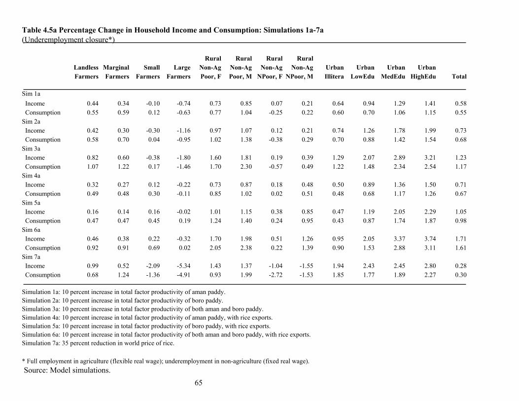
65

Table 4.5a Percentage Change in Household Income and Consumption: Simulations 1a-7a (Underemployment closure*) Rural Rural Rural Rural Landless Marginal Small Large Non-Ag Non-Ag Non-Ag Non-Ag Urban Urban Urban Urban Farmers Farmers Farmers Farmers Poor, F Poor, M NPoor, F NPoor, M Illitera LowEdu MedEdu HighEdu Total Sim 1a Income 0.44 0.34 -0.10 -0.74 0.73 0.85 0.07 0.21 0.64 0.94 1.29 1.41 0.58 Consumption 0.55 0.59 0.12 -0.63 0.77 1.04 -0.25 0.22 0.60 0.70 1.06 1.15 0.55Sim 2a Income 0.42 0.30 -0.30 -1.16 0.97 1.07 0.12 0.21 0.74 1.26 1.78 1.99 0.73 Consumption 0.58 0.70 0.04 -0.95 1.02 1.38 -0.38 0.29 0.70 0.88 1.42 1.54 0.68Sim 3a Income 0.82 0.60 -0.38 -1.80 1.60 1.81 0.19 0.39 1.29 2.07 2.89 3.21 1.23 Consumption 1.07 1.22 0.17 -1.46 1.70 2.30 -0.57 0.49 1.22 1.48 2.34 2.54 1.17Sim 4a Income 0.32 0.27 0.12 -0.22 0.73 0.87 0.18 0.48 0.50 0.89 1.36 1.50 0.71 Consumption 0.49 0.48 0.30 -0.11 0.85 1.02 0.02 0.51 0.48 0.68 1.17 1.26 0.67Sim 5a Income 0.16 0.14 0.16 -0.02 1.01 1.15 0.38 0.85 0.47 1.19 2.05 2.29 1.05 Consumption 0.47 0.47 0.45 0.19 1.24 1.40 0.24 0.95 0.43 0.87 1.74 1.87 0.98Sim 6a Income 0.46 0.38 0.22 -0.32 1.70 1.98 0.51 1.26 0.95 2.05 3.37 3.74 1.71 Consumption 0.92 0.91 0.69 0.02 2.05 2.38 0.22 1.39 0.90 1.53 2.88 3.11 1.61Sim 7a Income 0.99 0.52 -2.09 -5.34 1.43 1.37 -1.04 -1.55 1.94 2.43 2.45 2.80 0.28 Consumption 0.68 1.24 -1.36 -4.91 0.93 1.99 -2.72 -1.53 1.85 1.77 1.89 2.27 0.30 Simulation 1a: 10 percent increase in total factor productivity of aman paddy. Simulation 2a: 10 percent increase in total factor productivity of boro paddy. Simulation 3a: 10 percent increase in total factor productivity of both aman and boro paddy. Simulation 4a: 10 percent increase in total factor productivity of aman paddy, with rice exports. Simulation 5a: 10 percent increase in total factor productivity of boro paddy, with rice exports. Simulation 6a: 10 percent increase in total factor productivity of both aman and boro paddy, with rice exports. Simulation 7a: 35 percent reduction in world price of rice. * Full employment in agriculture (flexible real wage); underemployment in non-agriculture (fixed real wage). Source: Model simulations.

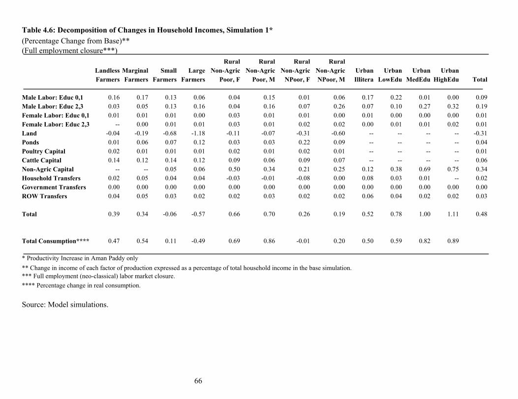
66

Table 4.6: Decomposition of Changes in Household Incomes, Simulation 1* (Percentage Change from Base)** (Full employment closure***) Rural Rural Rural Rural Landless Marginal Small Large Non-Agric Non-Agric Non-Agric Non-Agric Urban Urban Urban Urban Farmers Farmers Farmers Farmers Poor, F Poor, M NPoor, F NPoor, M Illitera LowEdu MedEdu HighEdu Total Male Labor: Educ 0,1 0.16 0.17 0.13 0.06 0.04 0.15 0.01 0.06 0.17 0.22 0.01 0.00 0.09 Male Labor: Educ 2,3 0.03 0.05 0.13 0.16 0.04 0.16 0.07 0.26 0.07 0.10 0.27 0.32 0.19 Female Labor: Educ 0,1 0.01 0.01 0.01 0.00 0.03 0.01 0.01 0.00 0.01 0.00 0.00 0.00 0.01 Female Labor: Educ 2,3 -- 0.00 0.01 0.01 0.03 0.01 0.02 0.02 0.00 0.01 0.01 0.02 0.01 Land -0.04 -0.19 -0.68 -1.18 -0.11 -0.07 -0.31 -0.60 -- -- -- -- -0.31 Ponds 0.01 0.06 0.07 0.12 0.03 0.03 0.22 0.09 -- -- -- -- 0.04 Poultry Capital 0.02 0.01 0.01 0.01 0.02 0.01 0.02 0.01 -- -- -- -- 0.01 Cattle Capital 0.14 0.12 0.14 0.12 0.09 0.06 0.09 0.07 -- -- -- -- 0.06 Non-Agric Capital -- -- 0.05 0.06 0.50 0.34 0.21 0.25 0.12 0.38 0.69 0.75 0.34 Household Transfers 0.02 0.05 0.04 0.04 -0.03 -0.01 -0.08 0.00 0.08 0.03 0.01 -- 0.02 Government Transfers 0.00 0.00 0.00 0.00 0.00 0.00 0.00 0.00 0.00 0.00 0.00 0.00 0.00 ROW Transfers 0.04 0.05 0.03 0.02 0.02 0.03 0.02 0.02 0.06 0.04 0.02 0.02 0.03 Total 0.39 0.34 -0.06 -0.57 0.66 0.70 0.26 0.19 0.52 0.78 1.00 1.11 0.48 Total Consumption**** 0.47 0.54 0.11 -0.49 0.69 0.86 -0.01 0.20 0.50 0.59 0.82 0.89 * Productivity Increase in Aman Paddy only ** Change in income of each factor of production expressed as a percentage of total household income in the base simulation. *** Full employment (neo-classical) labor market closure.**** Percentage change in real consumption. Source: Model simulations.

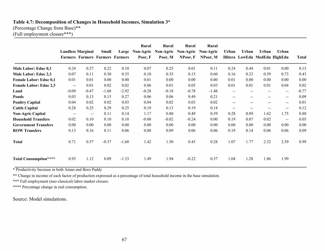
67

Table 4.7: Decomposition of Changes in Household Incomes, Simulation 3* (Percentage Change from Base)** (Full employment closure***) Rural Rural Rural Rural Landless Marginal Small Large Non-Agric Non-Agric Non-Agric Non-Agric Urban Urban Urban Urban Farmers Farmers Farmers Farmers Poor, F Poor, M NPoor, F NPoor, M Illitera LowEdu MedEdu HighEdu Total Male Labor: Educ 0,1 0.24 0.27 0.22 0.10 0.07 0.25 0.01 0.11 0.24 0.44 0.01 0.00 0.15 Male Labor: Educ 2,3 0.07 0.11 0.30 0.35 0.10 0.35 0.15 0.60 0.16 0.23 0.59 0.73 0.43 Female Labor: Educ 0,1 0.01 0.01 0.00 0.00 0.01 0.00 0.00 0.00 0.01 0.00 0.00 0.00 0.00 Female Labor: Educ 2,3 -- 0.01 0.02 0.02 0.06 0.01 0.05 0.03 0.01 0.01 0.01 0.04 0.02 Land -0.09 -0.47 -1.68 -2.92 -0.28 -0.18 -0.78 -1.48 -- -- -- -- -0.77 Ponds 0.03 0.13 0.15 0.27 0.06 0.06 0.49 0.21 -- -- -- -- 0.09 Poultry Capital 0.04 0.02 0.02 0.03 0.04 0.02 0.03 0.02 -- -- -- -- 0.01 Cattle Capital 0.28 0.25 0.29 0.25 0.19 0.13 0.19 0.14 -- -- -- -- 0.12 Non-Agric Capital -- -- 0.11 0.14 1.17 0.80 0.49 0.59 0.28 0.89 1.62 1.75 0.80 Household Transfers 0.02 0.10 0.10 0.10 -0.08 -0.02 -0.24 0.00 0.19 0.07 0.02 -- 0.05 Government Transfers 0.00 0.00 0.00 0.00 0.00 0.00 0.00 0.00 0.00 0.00 0.00 0.00 0.00 ROW Transfers 0.13 0.16 0.11 0.06 0.08 0.09 0.06 0.06 0.19 0.14 0.06 0.06 0.09 Total 0.71 0.57 -0.37 -1.60 1.42 1.50 0.45 0.28 1.07 1.77 2.32 2.59 0.99 Total Consumption**** 0.93 1.12 0.09 -1.33 1.49 1.94 -0.22 0.37 1.04 1.28 1.86 1.99 * Productivity Increase in both Aman and Boro Paddy ** Change in income of each factor of production expressed as a percentage of total household income in the base simulation. *** Full employment (neo-classical) labor market closure. **** Percentage change in real consumption. Source: Model simulations.

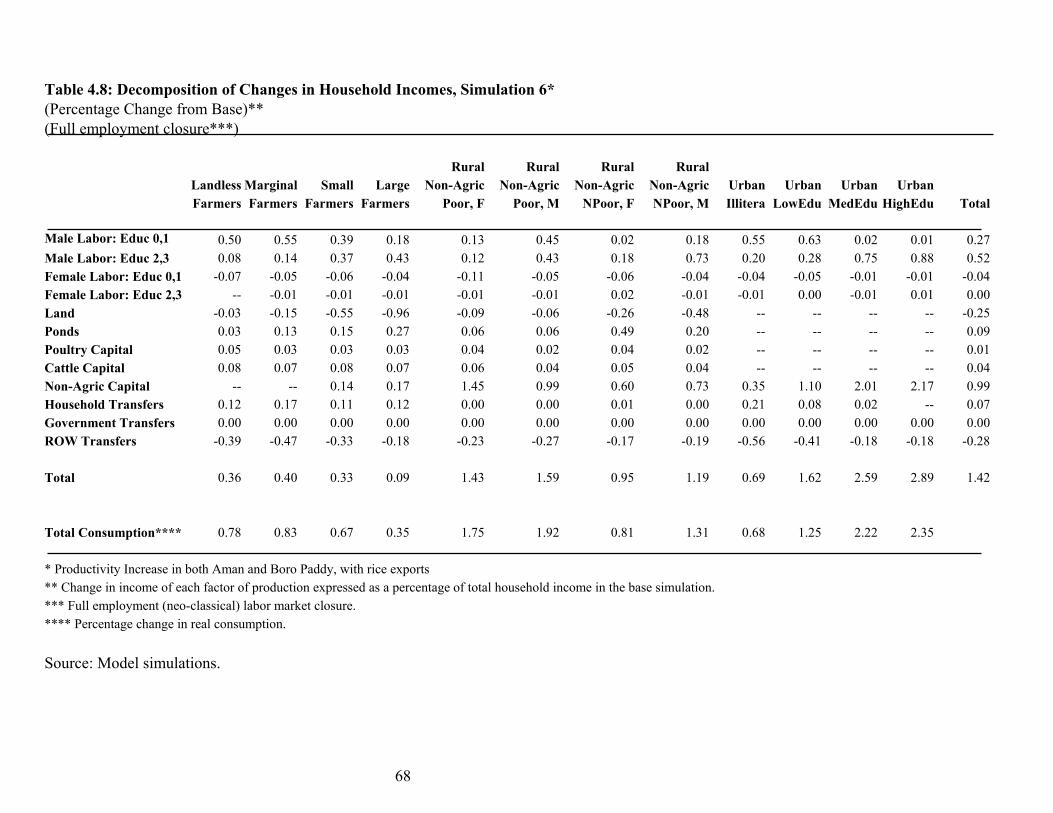
68

Table 4.8: Decomposition of Changes in Household Incomes, Simulation 6* (Percentage Change from Base)** (Full employment closure***) Rural Rural Rural Rural Landless Marginal Small Large Non-Agric Non-Agric Non-Agric Non-Agric Urban Urban Urban Urban Farmers Farmers Farmers Farmers Poor, F Poor, M NPoor, F NPoor, M Illitera LowEdu MedEdu HighEdu Total Male Labor: Educ 0,1 0.50 0.55 0.39 0.18 0.13 0.45 0.02 0.18 0.55 0.63 0.02 0.01 0.27 Male Labor: Educ 2,3 0.08 0.14 0.37 0.43 0.12 0.43 0.18 0.73 0.20 0.28 0.75 0.88 0.52 Female Labor: Educ 0,1 -0.07 -0.05 -0.06 -0.04 -0.11 -0.05 -0.06 -0.04 -0.04 -0.05 -0.01 -0.01 -0.04 Female Labor: Educ 2,3 -- -0.01 -0.01 -0.01 -0.01 -0.01 0.02 -0.01 -0.01 0.00 -0.01 0.01 0.00 Land -0.03 -0.15 -0.55 -0.96 -0.09 -0.06 -0.26 -0.48 -- -- -- -- -0.25 Ponds 0.03 0.13 0.15 0.27 0.06 0.06 0.49 0.20 -- -- -- -- 0.09 Poultry Capital 0.05 0.03 0.03 0.03 0.04 0.02 0.04 0.02 -- -- -- -- 0.01 Cattle Capital 0.08 0.07 0.08 0.07 0.06 0.04 0.05 0.04 -- -- -- -- 0.04 Non-Agric Capital -- -- 0.14 0.17 1.45 0.99 0.60 0.73 0.35 1.10 2.01 2.17 0.99 Household Transfers 0.12 0.17 0.11 0.12 0.00 0.00 0.01 0.00 0.21 0.08 0.02 -- 0.07 Government Transfers 0.00 0.00 0.00 0.00 0.00 0.00 0.00 0.00 0.00 0.00 0.00 0.00 0.00 ROW Transfers -0.39 -0.47 -0.33 -0.18 -0.23 -0.27 -0.17 -0.19 -0.56 -0.41 -0.18 -0.18 -0.28 Total 0.36 0.40 0.33 0.09 1.43 1.59 0.95 1.19 0.69 1.62 2.59 2.89 1.42 Total Consumption**** 0.78 0.83 0.67 0.35 1.75 1.92 0.81 1.31 0.68 1.25 2.22 2.35 * Productivity Increase in both Aman and Boro Paddy, with rice exports ** Change in income of each factor of production expressed as a percentage of total household income in the base simulation. *** Full employment (neo-classical) labor market closure. **** Percentage change in real consumption. Source: Model simulations.

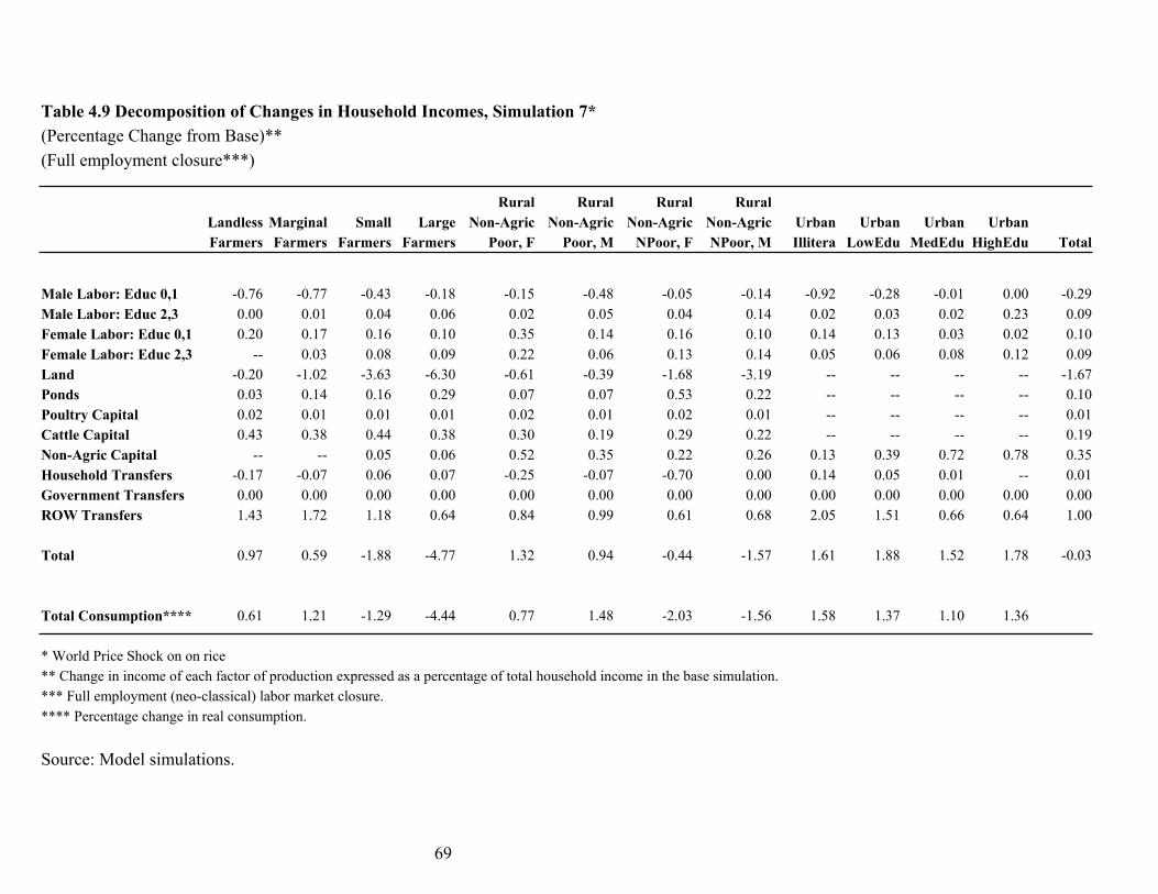
69

Table 4.9 Decomposition of Changes in Household Incomes, Simulation 7* (Percentage Change from Base)** (Full employment closure***) Rural Rural Rural Rural Landless Marginal Small Large Non-Agric Non-Agric Non-Agric Non-Agric Urban Urban Urban Urban Farmers Farmers Farmers Farmers Poor, F Poor, M NPoor, F NPoor, M Illitera LowEdu MedEdu HighEdu Total

Male Labor: Educ 0,1 -0.76 -0.77 -0.43 -0.18 -0.15 -0.48 -0.05 -0.14 -0.92 -0.28 -0.01 0.00 -0.29 Male Labor: Educ 2,3 0.00 0.01 0.04 0.06 0.02 0.05 0.04 0.14 0.02 0.03 0.02 0.23 0.09 Female Labor: Educ 0,1 0.20 0.17 0.16 0.10 0.35 0.14 0.16 0.10 0.14 0.13 0.03 0.02 0.10 Female Labor: Educ 2,3 -- 0.03 0.08 0.09 0.22 0.06 0.13 0.14 0.05 0.06 0.08 0.12 0.09 Land -0.20 -1.02 -3.63 -6.30 -0.61 -0.39 -1.68 -3.19 -- -- -- -- -1.67 Ponds 0.03 0.14 0.16 0.29 0.07 0.07 0.53 0.22 -- -- -- -- 0.10 Poultry Capital 0.02 0.01 0.01 0.01 0.02 0.01 0.02 0.01 -- -- -- -- 0.01 Cattle Capital 0.43 0.38 0.44 0.38 0.30 0.19 0.29 0.22 -- -- -- -- 0.19 Non-Agric Capital -- -- 0.05 0.06 0.52 0.35 0.22 0.26 0.13 0.39 0.72 0.78 0.35 Household Transfers -0.17 -0.07 0.06 0.07 -0.25 -0.07 -0.70 0.00 0.14 0.05 0.01 -- 0.01 Government Transfers 0.00 0.00 0.00 0.00 0.00 0.00 0.00 0.00 0.00 0.00 0.00 0.00 0.00 ROW Transfers 1.43 1.72 1.18 0.64 0.84 0.99 0.61 0.68 2.05 1.51 0.66 0.64 1.00 Total 0.97 0.59 -1.88 -4.77 1.32 0.94 -0.44 -1.57 1.61 1.88 1.52 1.78 -0.03 Total Consumption**** 0.61 1.21 -1.29 -4.44 0.77 1.48 -2.03 -1.56 1.58 1.37 1.10 1.36 * World Price Shock on on rice ** Change in income of each factor of production expressed as a percentage of total household income in the base simulation. *** Full employment (neo-classical) labor market closure. **** Percentage change in real consumption. Source: Model simulations.

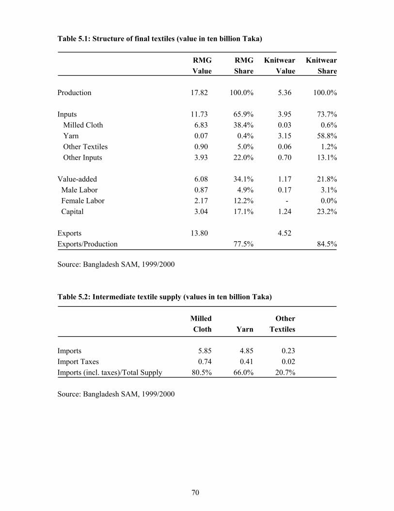
70

Table 5.1: Structure of final textiles (value in ten billion Taka) RMG RMG Knitwear Knitwear Value Share Value Share Production 17.82 100.0% 5.36 100.0% Inputs 11.73 65.9% 3.95 73.7% Milled Cloth 6.83 38.4% 0.03 0.6% Yarn 0.07 0.4% 3.15 58.8% Other Textiles 0.90 5.0% 0.06 1.2% Other Inputs 3.93 22.0% 0.70 13.1% Value-added 6.08 34.1% 1.17 21.8% Male Labor 0.87 4.9% 0.17 3.1% Female Labor 2.17 12.2% - 0.0% Capital 3.04 17.1% 1.24 23.2% Exports 13.80 4.52 Exports/Production 77.5% 84.5% Source: Bangladesh SAM, 1999/2000 Table 5.2: Intermediate textile supply (values in ten billion Taka) Milled Other Cloth Yarn Textiles Imports 5.85 4.85 0.23 Import Taxes 0.74 0.41 0.02 Imports (incl. taxes)/Total Supply 80.5% 66.0% 20.7% Source: Bangladesh SAM, 1999/2000

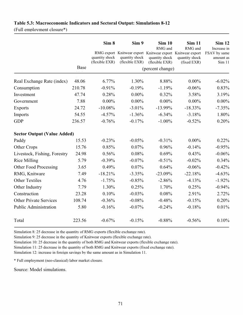
71

Table 5.3: Macroeconomic Indicators and Sectoral Output: Simulations 8-12 (Full employment closure*) Sim 8 Sim 9 Sim 10 Sim 11 Sim 12

RMG export quantity shock (flexible EXR)

Knitwear export quantity shock (flexible EXR)

RMG and Knitwear export

quantity shock (flexible EXR)

RMG and Knitwear export

quantity shock (fixed EXR)

Increase in FSAV by same

amount as Sim 11

Base (10 bn Taka)

(percent change) Real Exchange Rate (index) 48.06 6.77% 1.30% 8.88% 0.00% -6.02%Consumption 210.78 -0.91% -0.19% -1.19% -0.06% 0.83%Investment 47.74 0.28% 0.00% 0.32% 3.58% 3.19%Government 7.88 0.00% 0.00% 0.00% 0.00% 0.00%Exports 24.72 -10.08% -3.01% -13.99% -18.33% -7.35%Imports 54.55 -4.57% -1.36% -6.34% -3.18% 1.80%GDP 236.57 -0.76% -0.17% -1.00% -0.52% 0.20% Sector Output (Value Added) Paddy 15.53 -0.23% -0.05% -0.31% 0.00% 0.22%Other Crops 15.76 0.85% 0.07% 0.96% -0.14% -0.95%Livestock, Fishing, Forestry 24.98 0.56% 0.08% 0.69% 0.43% -0.06%Rice Milling 5.79 -0.39% -0.07% -0.51% -0.02% 0.34%Other Food Processing 3.65 0.49% 0.07% 0.64% -0.06% -0.42%RMG, Knitware 7.49 -18.21% -3.35% -23.09% -22.18% -4.63%Other Textiles 4.76 -1.75% -0.85% -2.86% -4.13% -1.92%Other Industry 7.79 1.30% 0.25% 1.70% 0.25% -0.94%Construction 23.28 0.10% -0.03% 0.08% 2.91% 2.72%Other Private Services 108.74 -0.36% -0.08% -0.48% -0.15% 0.20%Public Administration 5.80 -0.16% -0.07% -0.24% -0.18% 0.01% Total 223.56 -0.67% -0.15% -0.88% -0.56% 0.10% Simulation 8: 25 decrease in the quantity of RMG exports (flexible exchange rate).Simulation 9: 25 decrease in the quantity of Knitwear exports (flexible exchange rate).Simulation 10: 25 decrease in the quantity of both RMG and Knitwear exports (flexible exchange rate). Simulation 11: 25 decrease in the quantity of both RMG and Knitwear exports (fixed exchange rate). Simulation 12: increase in foreign savings by the same amount as in Simulation 11.

* Full employment (neo-classical) labor market closure.

Source: Model simulations.

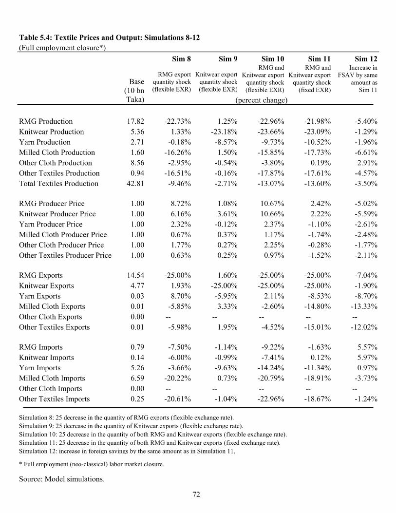
72

Table 5.4: Textile Prices and Output: Simulations 8-12 (Full employment closure*) Sim 8 Sim 9 Sim 10 Sim 11 Sim 12

RMG export quantity shock (flexible EXR)

Knitwear export quantity shock (flexible EXR)

RMG and Knitwear export

quantity shock (flexible EXR)

RMG and Knitwear export

quantity shock (fixed EXR)

Increase in FSAV by same

amount as Sim 11

Base (10 bn Taka) (percent change)

RMG Production 17.82 -22.73% 1.25% -22.96% -21.98% -5.40%Knitwear Production 5.36 1.33% -23.18% -23.66% -23.09% -1.29%Yarn Production 2.71 -0.18% -8.57% -9.73% -10.52% -1.96%Milled Cloth Production 1.60 -16.26% 1.50% -15.85% -17.73% -6.61%Other Cloth Production 8.56 -2.95% -0.54% -3.80% 0.19% 2.91%Other Textiles Production 0.94 -16.51% -0.16% -17.87% -17.61% -4.57%Total Textiles Production 42.81 -9.46% -2.71% -13.07% -13.60% -3.50% RMG Producer Price 1.00 8.72% 1.08% 10.67% 2.42% -5.02%Knitwear Producer Price 1.00 6.16% 3.61% 10.66% 2.22% -5.59%Yarn Producer Price 1.00 2.32% -0.12% 2.37% -1.10% -2.61%Milled Cloth Producer Price 1.00 0.67% 0.37% 1.17% -1.74% -2.48%Other Cloth Producer Price 1.00 1.77% 0.27% 2.25% -0.28% -1.77%Other Textiles Producer Price 1.00 0.63% 0.25% 0.97% -1.52% -2.11% RMG Exports 14.54 -25.00% 1.60% -25.00% -25.00% -7.04%Knitwear Exports 4.77 1.93% -25.00% -25.00% -25.00% -1.90%Yarn Exports 0.03 8.70% -5.95% 2.11% -8.53% -8.70%Milled Cloth Exports 0.01 -5.85% 3.33% -2.60% -14.80% -13.33%Other Cloth Exports 0.00 -- -- -- -- -- Other Textiles Exports 0.01 -5.98% 1.95% -4.52% -15.01% -12.02% RMG Imports 0.79 -7.50% -1.14% -9.22% -1.63% 5.57%Knitwear Imports 0.14 -6.00% -0.99% -7.41% 0.12% 5.97%Yarn Imports 5.26 -3.66% -9.63% -14.24% -11.34% 0.97%Milled Cloth Imports 6.59 -20.22% 0.73% -20.79% -18.91% -3.73%Other Cloth Imports 0.00 -- -- -- -- -- Other Textiles Imports 0.25 -20.61% -1.04% -22.96% -18.67% -1.24% Simulation 8: 25 decrease in the quantity of RMG exports (flexible exchange rate).Simulation 9: 25 decrease in the quantity of Knitwear exports (flexible exchange rate).Simulation 10: 25 decrease in the quantity of both RMG and Knitwear exports (flexible exchange rate). Simulation 11: 25 decrease in the quantity of both RMG and Knitwear exports (fixed exchange rate). Simulation 12: increase in foreign savings by the same amount as in Simulation 11.

* Full employment (neo-classical) labor market closure.

Source: Model simulations.

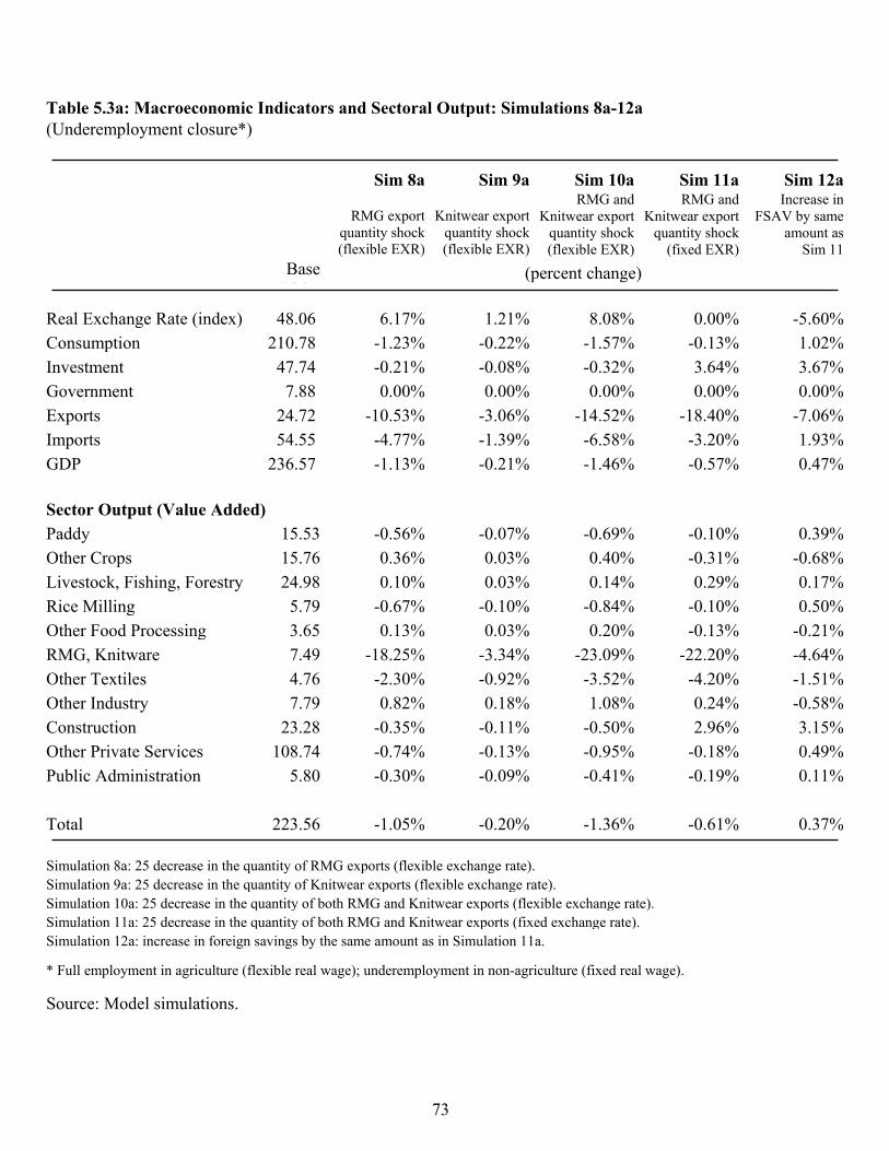
73

Table 5.3a: Macroeconomic Indicators and Sectoral Output: Simulations 8a-12a (Underemployment closure*) Sim 8a Sim 9a Sim 10a Sim 11a Sim 12a

RMG export quantity shock (flexible EXR)

Knitwear export quantity shock (flexible EXR)

RMG and Knitwear export

quantity shock (flexible EXR)

RMG and Knitwear export

quantity shock (fixed EXR)

Increase inFSAV by same

amount as Sim 11

Base (10 bn Taka)

(percent change) Real Exchange Rate (index) 48.06 6.17% 1.21% 8.08% 0.00% -5.60%Consumption 210.78 -1.23% -0.22% -1.57% -0.13% 1.02%Investment 47.74 -0.21% -0.08% -0.32% 3.64% 3.67%Government 7.88 0.00% 0.00% 0.00% 0.00% 0.00%Exports 24.72 -10.53% -3.06% -14.52% -18.40% -7.06%Imports 54.55 -4.77% -1.39% -6.58% -3.20% 1.93%GDP 236.57 -1.13% -0.21% -1.46% -0.57% 0.47% Sector Output (Value Added) Paddy 15.53 -0.56% -0.07% -0.69% -0.10% 0.39%Other Crops 15.76 0.36% 0.03% 0.40% -0.31% -0.68%Livestock, Fishing, Forestry 24.98 0.10% 0.03% 0.14% 0.29% 0.17%Rice Milling 5.79 -0.67% -0.10% -0.84% -0.10% 0.50%Other Food Processing 3.65 0.13% 0.03% 0.20% -0.13% -0.21%RMG, Knitware 7.49 -18.25% -3.34% -23.09% -22.20% -4.64%Other Textiles 4.76 -2.30% -0.92% -3.52% -4.20% -1.51%Other Industry 7.79 0.82% 0.18% 1.08% 0.24% -0.58%Construction 23.28 -0.35% -0.11% -0.50% 2.96% 3.15%Other Private Services 108.74 -0.74% -0.13% -0.95% -0.18% 0.49%Public Administration 5.80 -0.30% -0.09% -0.41% -0.19% 0.11% Total 223.56 -1.05% -0.20% -1.36% -0.61% 0.37% Simulation 8a: 25 decrease in the quantity of RMG exports (flexible exchange rate).Simulation 9a: 25 decrease in the quantity of Knitwear exports (flexible exchange rate).Simulation 10a: 25 decrease in the quantity of both RMG and Knitwear exports (flexible exchange rate). Simulation 11a: 25 decrease in the quantity of both RMG and Knitwear exports (fixed exchange rate). Simulation 12a: increase in foreign savings by the same amount as in Simulation 11a.

* Full employment in agriculture (flexible real wage); underemployment in non-agriculture (fixed real wage).

Source: Model simulations.

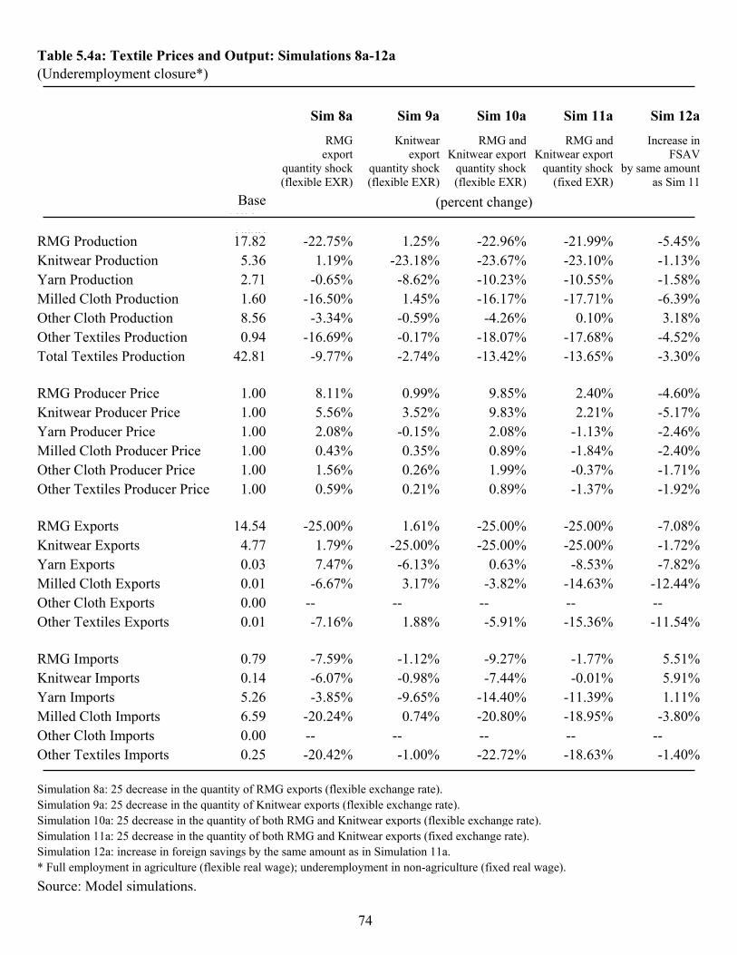
74

Table 5.4a: Textile Prices and Output: Simulations 8a-12a (Underemployment closure*) Sim 8a Sim 9a Sim 10a Sim 11a Sim 12a

RMG export

quantity shock (flexible EXR)

Knitwear export

quantity shock (flexible EXR)

RMG and Knitwear export

quantity shock (flexible EXR)

RMG and Knitwear export

quantity shock (fixed EXR)

Increase in FSAV

by same amount as Sim 11

Base (10 bn Taka)

(percent change) RMG Production 17.82 -22.75% 1.25% -22.96% -21.99% -5.45%Knitwear Production 5.36 1.19% -23.18% -23.67% -23.10% -1.13%Yarn Production 2.71 -0.65% -8.62% -10.23% -10.55% -1.58%Milled Cloth Production 1.60 -16.50% 1.45% -16.17% -17.71% -6.39%Other Cloth Production 8.56 -3.34% -0.59% -4.26% 0.10% 3.18%Other Textiles Production 0.94 -16.69% -0.17% -18.07% -17.68% -4.52%Total Textiles Production 42.81 -9.77% -2.74% -13.42% -13.65% -3.30% RMG Producer Price 1.00 8.11% 0.99% 9.85% 2.40% -4.60%Knitwear Producer Price 1.00 5.56% 3.52% 9.83% 2.21% -5.17%Yarn Producer Price 1.00 2.08% -0.15% 2.08% -1.13% -2.46%Milled Cloth Producer Price 1.00 0.43% 0.35% 0.89% -1.84% -2.40%Other Cloth Producer Price 1.00 1.56% 0.26% 1.99% -0.37% -1.71%Other Textiles Producer Price 1.00 0.59% 0.21% 0.89% -1.37% -1.92% RMG Exports 14.54 -25.00% 1.61% -25.00% -25.00% -7.08%Knitwear Exports 4.77 1.79% -25.00% -25.00% -25.00% -1.72%Yarn Exports 0.03 7.47% -6.13% 0.63% -8.53% -7.82%Milled Cloth Exports 0.01 -6.67% 3.17% -3.82% -14.63% -12.44%Other Cloth Exports 0.00 -- -- -- -- -- Other Textiles Exports 0.01 -7.16% 1.88% -5.91% -15.36% -11.54% RMG Imports 0.79 -7.59% -1.12% -9.27% -1.77% 5.51%Knitwear Imports 0.14 -6.07% -0.98% -7.44% -0.01% 5.91%Yarn Imports 5.26 -3.85% -9.65% -14.40% -11.39% 1.11%Milled Cloth Imports 6.59 -20.24% 0.74% -20.80% -18.95% -3.80%Other Cloth Imports 0.00 -- -- -- -- -- Other Textiles Imports 0.25 -20.42% -1.00% -22.72% -18.63% -1.40% Simulation 8a: 25 decrease in the quantity of RMG exports (flexible exchange rate).Simulation 9a: 25 decrease in the quantity of Knitwear exports (flexible exchange rate).Simulation 10a: 25 decrease in the quantity of both RMG and Knitwear exports (flexible exchange rate). Simulation 11a: 25 decrease in the quantity of both RMG and Knitwear exports (fixed exchange rate). Simulation 12a: increase in foreign savings by the same amount as in Simulation 11a.* Full employment in agriculture (flexible real wage); underemployment in non-agriculture (fixed real wage). Source: Model simulations.

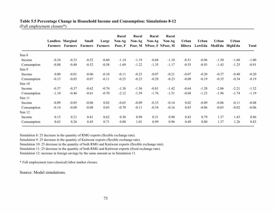
75

Table 5.5 Percentage Change in Household Income and Consumption: Simulations 8-12 (Full employment closure*) Rural Rural Rural Rural Landless Marginal Small Large Non-Ag Non-Ag Non-Ag Non-Ag Urban Urban Urban Urban Farmers Farmers Farmers Farmers Poor, F Poor, M NPoor, F NPoor, M Illitera LowEdu MedEdu HighEdu Total Sim 8 Income -0.34 -0.33 -0.52 -0.60 -1.14 -1.19 -0.68 -1.10 -0.51 -0.96 -1.50 -1.60 -1.00 Consumption -0.88 -0.40 -0.52 -0.58 -1.69 -1.22 -1.35 -1.17 -0.55 -0.93 -1.43 -1.25 -0.91Sim 9 Income 0.00 -0.01 -0.06 -0.10 -0.11 -0.23 -0.07 -0.21 -0.07 -0.20 -0.37 -0.40 -0.20 Consumption -0.13 -0.03 -0.07 -0.11 -0.25 -0.23 -0.28 -0.23 -0.08 -0.19 -0.35 -0.34 -0.19Sim 10 Income -0.37 -0.37 -0.62 -0.74 -1.38 -1.56 -0.81 -1.42 -0.64 -1.28 -2.06 -2.21 -1.32 Consumption -1.10 -0.46 -0.61 -0.70 -2.12 -1.59 -1.76 -1.51 -0.68 -1.23 -1.96 -1.74 -1.19Sim 11 Income -0.09 -0.05 -0.06 0.02 -0.65 -0.09 -0.33 -0.14 0.02 -0.09 -0.06 -0.11 -0.08 Consumption -0.14 -0.08 -0.08 0.03 -0.70 -0.11 -0.34 -0.16 0.03 -0.06 -0.03 -0.02 -0.06Sim 12 Income 0.15 0.21 0.41 0.62 0.30 0.98 0.31 0.90 0.43 0.79 1.37 1.43 0.86 Consumption 0.63 0.26 0.45 0.71 0.80 1.01 0.99 0.96 0.49 0.80 1.37 1.26 0.83 Simulation 8: 25 decrease in the quantity of RMG exports (flexible exchange rate). Simulation 9: 25 decrease in the quantity of Knitwear exports (flexible exchange rate). Simulation 10: 25 decrease in the quantity of both RMG and Knitwear exports (flexible exchange rate). Simulation 11: 25 decrease in the quantity of both RMG and Knitwear exports (fixed exchange rate). Simulation 12: increase in foreign savings by the same amount as in Simulation 11. * Full employment (neo-classical) labor market closure. Source: Model simulations.

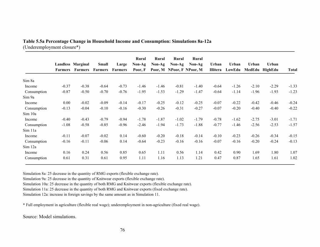
76

Table 5.5a Percentage Change in Household Income and Consumption: Simulations 8a-12a (Underemployment closure*) Rural Rural Rural Rural Landless Marginal Small Large Non-Ag Non-Ag Non-Ag Non-Ag Urban Urban Urban Urban Farmers Farmers Farmers Farmers Poor, F Poor, M NPoor, F NPoor, M Illitera LowEdu MedEdu HighEdu Total Sim 8a Income -0.37 -0.38 -0.64 -0.73 -1.46 -1.46 -0.81 -1.40 -0.64 -1.26 -2.10 -2.29 -1.33 Consumption -0.87 -0.50 -0.70 -0.76 -1.95 -1.53 -1.29 -1.47 -0.64 -1.14 -1.96 -1.93 -1.23Sim 9a Income 0.00 -0.02 -0.09 -0.14 -0.17 -0.25 -0.12 -0.25 -0.07 -0.22 -0.42 -0.46 -0.24 Consumption -0.13 -0.04 -0.10 -0.16 -0.30 -0.26 -0.31 -0.27 -0.07 -0.20 -0.40 -0.40 -0.22Sim 10a Income -0.40 -0.43 -0.79 -0.94 -1.78 -1.87 -1.02 -1.79 -0.78 -1.62 -2.75 -3.01 -1.71 Consumption -1.08 -0.58 -0.85 -0.96 -2.46 -1.94 -1.73 -1.88 -0.77 -1.46 -2.56 -2.53 -1.57Sim 11a Income -0.11 -0.07 -0.02 0.14 -0.60 -0.20 -0.18 -0.14 -0.10 -0.23 -0.26 -0.34 -0.15 Consumption -0.16 -0.11 -0.06 0.14 -0.64 -0.23 -0.16 -0.16 -0.07 -0.16 -0.20 -0.24 -0.13Sim 12a Income 0.16 0.24 0.56 0.85 0.65 1.11 0.56 1.14 0.42 0.90 1.69 1.80 1.07 Consumption 0.61 0.31 0.61 0.95 1.11 1.16 1.13 1.21 0.47 0.87 1.65 1.61 1.02 Simulation 8a: 25 decrease in the quantity of RMG exports (flexible exchange rate). Simulation 9a: 25 decrease in the quantity of Knitwear exports (flexible exchange rate). Simulation 10a: 25 decrease in the quantity of both RMG and Knitwear exports (flexible exchange rate). Simulation 11a: 25 decrease in the quantity of both RMG and Knitwear exports (fixed exchange rate). Simulation 12a: increase in foreign savings by the same amount as in Simulation 11. * Full employment in agriculture (flexible real wage); underemployment in non-agriculture (fixed real wage). Source: Model simulations.

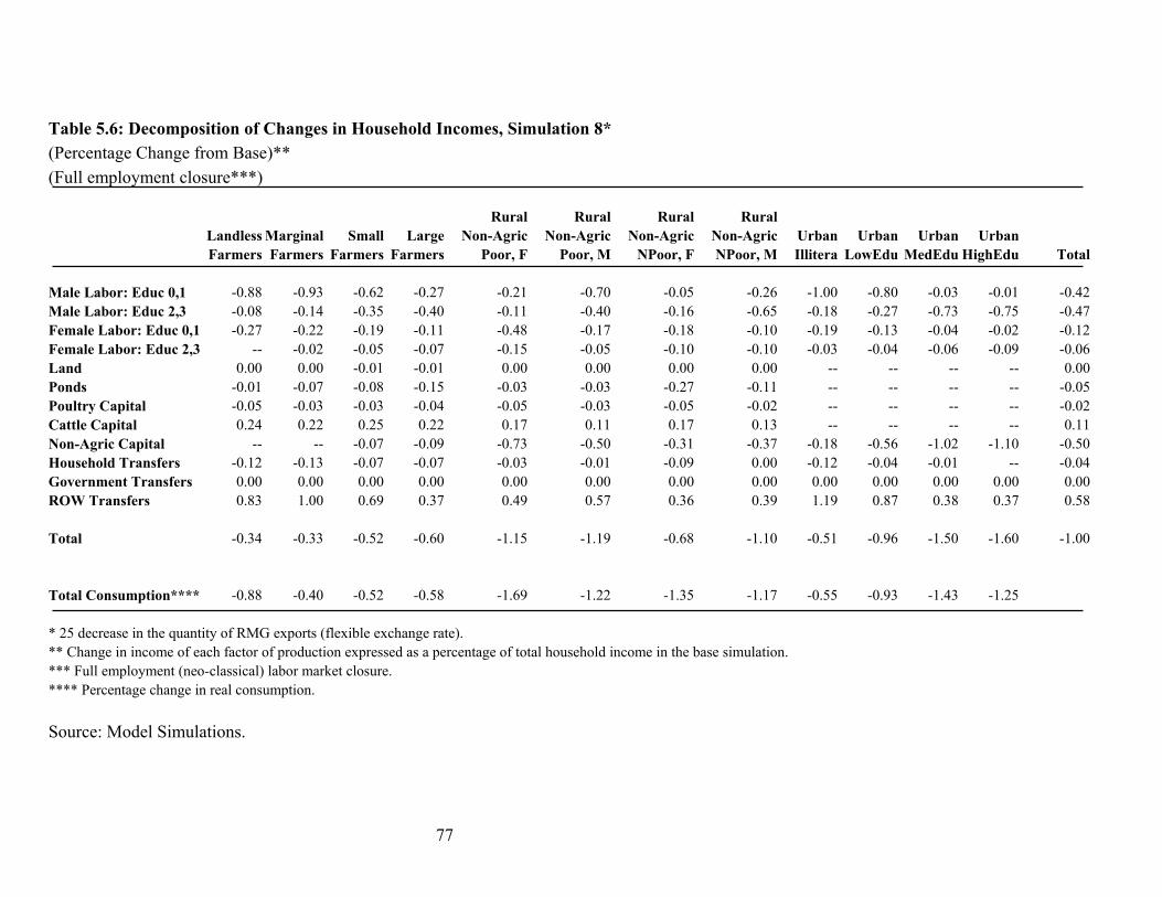
77

Table 5.6: Decomposition of Changes in Household Incomes, Simulation 8*

(Percentage Change from Base)**

(Full employment closure***) Rural Rural Rural Rural Landless Marginal Small Large Non-Agric Non-Agric Non-Agric Non-Agric Urban Urban Urban Urban Farmers Farmers Farmers Farmers Poor, F Poor, M NPoor, F NPoor, M Illitera LowEdu MedEdu HighEdu Total Male Labor: Educ 0,1 -0.88 -0.93 -0.62 -0.27 -0.21 -0.70 -0.05 -0.26 -1.00 -0.80 -0.03 -0.01 -0.42 Male Labor: Educ 2,3 -0.08 -0.14 -0.35 -0.40 -0.11 -0.40 -0.16 -0.65 -0.18 -0.27 -0.73 -0.75 -0.47 Female Labor: Educ 0,1 -0.27 -0.22 -0.19 -0.11 -0.48 -0.17 -0.18 -0.10 -0.19 -0.13 -0.04 -0.02 -0.12 Female Labor: Educ 2,3 -- -0.02 -0.05 -0.07 -0.15 -0.05 -0.10 -0.10 -0.03 -0.04 -0.06 -0.09 -0.06 Land 0.00 0.00 -0.01 -0.01 0.00 0.00 0.00 0.00 -- -- -- -- 0.00 Ponds -0.01 -0.07 -0.08 -0.15 -0.03 -0.03 -0.27 -0.11 -- -- -- -- -0.05 Poultry Capital -0.05 -0.03 -0.03 -0.04 -0.05 -0.03 -0.05 -0.02 -- -- -- -- -0.02 Cattle Capital 0.24 0.22 0.25 0.22 0.17 0.11 0.17 0.13 -- -- -- -- 0.11 Non-Agric Capital -- -- -0.07 -0.09 -0.73 -0.50 -0.31 -0.37 -0.18 -0.56 -1.02 -1.10 -0.50 Household Transfers -0.12 -0.13 -0.07 -0.07 -0.03 -0.01 -0.09 0.00 -0.12 -0.04 -0.01 -- -0.04 Government Transfers 0.00 0.00 0.00 0.00 0.00 0.00 0.00 0.00 0.00 0.00 0.00 0.00 0.00 ROW Transfers 0.83 1.00 0.69 0.37 0.49 0.57 0.36 0.39 1.19 0.87 0.38 0.37 0.58 Total -0.34 -0.33 -0.52 -0.60 -1.15 -1.19 -0.68 -1.10 -0.51 -0.96 -1.50 -1.60 -1.00 Total Consumption**** -0.88 -0.40 -0.52 -0.58 -1.69 -1.22 -1.35 -1.17 -0.55 -0.93 -1.43 -1.25 * 25 decrease in the quantity of RMG exports (flexible exchange rate). ** Change in income of each factor of production expressed as a percentage of total household income in the base simulation. *** Full employment (neo-classical) labor market closure. **** Percentage change in real consumption. Source: Model Simulations.

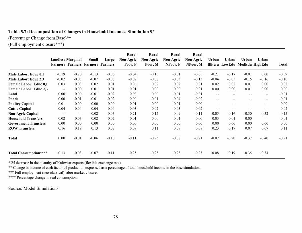
78

Table 5.7: Decomposition of Changes in Household Incomes, Simulation 9*

(Percentage Change from Base)**

(Full employment closure***) Rural Rural Rural Rural Landless Marginal Small Large Non-Agric Non-Agric Non-Agric Non-Agric Urban Urban Urban Urban Farmers Farmers Farmers Farmers Poor, F Poor, M NPoor, F NPoor, M Illitera LowEdu MedEdu HighEdu Total Male Labor: Educ 0,1 -0.19 -0.20 -0.13 -0.06 -0.04 -0.15 -0.01 -0.05 -0.21 -0.17 -0.01 0.00 -0.09 Male Labor: Educ 2,3 -0.02 -0.03 -0.07 -0.08 -0.02 -0.08 -0.03 -0.13 -0.04 -0.05 -0.15 -0.16 -0.10 Female Labor: Educ 0,1 0.03 0.03 0.02 0.01 0.06 0.02 0.02 0.01 0.02 0.02 0.01 0.00 0.02 Female Labor: Educ 2,3 -- 0.00 0.01 0.01 0.01 0.00 0.00 0.01 0.00 0.00 0.01 0.00 0.00 Land 0.00 0.00 -0.01 -0.02 0.00 0.00 -0.01 -0.01 -- -- -- -- -0.01 Ponds 0.00 -0.01 -0.01 -0.02 0.00 -0.01 -0.04 -0.02 -- -- -- -- -0.01 Poultry Capital -0.01 0.00 0.00 0.00 -0.01 0.00 -0.01 0.00 -- -- -- -- 0.00 Cattle Capital 0.04 0.04 0.04 0.04 0.03 0.02 0.03 0.02 -- -- -- -- 0.02 Non-Agric Capital -- -- -0.02 -0.03 -0.21 -0.15 -0.09 -0.11 -0.05 -0.16 -0.30 -0.32 -0.15 Household Transfers -0.02 -0.03 -0.02 -0.02 -0.01 0.00 -0.01 0.00 -0.03 -0.01 0.00 -- -0.01 Government Transfers 0.00 0.00 0.00 0.00 0.00 0.00 0.00 0.00 0.00 0.00 0.00 0.00 0.00 ROW Transfers 0.16 0.19 0.13 0.07 0.09 0.11 0.07 0.08 0.23 0.17 0.07 0.07 0.11 Total 0.00 -0.01 -0.06 -0.10 -0.11 -0.23 -0.08 -0.21 -0.07 -0.20 -0.37 -0.40 -0.21 Total Consumption**** -0.13 -0.03 -0.07 -0.11 -0.25 -0.23 -0.28 -0.23 -0.08 -0.19 -0.35 -0.34 * 25 decrease in the quantity of Knitwear exports (flexible exchange rate). ** Change in income of each factor of production expressed as a percentage of total household income in the base simulation. *** Full employment (neo-classical) labor market closure. **** Percentage change in real consumption. Source: Model Simulations.

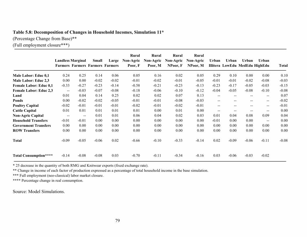
79

Table 5.8: Decomposition of Changes in Household Incomes, Simulation 11*

(Percentage Change from Base)**

(Full employment closure***) Rural Rural Rural Rural Landless Marginal Small Large Non-Agric Non-Agric Non-Agric Non-Agric Urban Urban Urban Urban Farmers Farmers Farmers Farmers Poor, F Poor, M NPoor, F NPoor, M Illitera LowEdu MedEdu HighEdu Total Male Labor: Educ 0,1 0.24 0.25 0.14 0.06 0.05 0.16 0.02 0.05 0.29 0.10 0.00 0.00 0.10 Male Labor: Educ 2,3 0.00 0.00 -0.02 -0.02 -0.01 -0.02 -0.01 -0.05 -0.01 -0.01 -0.02 -0.08 -0.03 Female Labor: Educ 0,1 -0.33 -0.27 -0.23 -0.14 -0.58 -0.21 -0.23 -0.13 -0.23 -0.17 -0.05 -0.03 -0.15 Female Labor: Educ 2,3 -- -0.03 -0.07 -0.08 -0.18 -0.06 -0.10 -0.12 -0.04 -0.05 -0.08 -0.10 -0.08 Land 0.01 0.04 0.14 0.25 0.02 0.02 0.07 0.13 -- -- -- -- 0.07 Ponds 0.00 -0.02 -0.02 -0.05 -0.01 -0.01 -0.08 -0.03 -- -- -- -- -0.02 Poultry Capital -0.02 -0.01 -0.01 -0.01 -0.02 -0.01 -0.02 -0.01 -- -- -- -- -0.01 Cattle Capital 0.01 0.01 0.01 0.01 0.01 0.00 0.01 0.00 -- -- -- -- 0.00 Non-Agric Capital -- -- 0.01 0.01 0.06 0.04 0.02 0.03 0.01 0.04 0.08 0.09 0.04 Household Transfers -0.01 -0.01 0.00 0.00 0.00 0.00 0.00 0.00 -0.01 0.00 0.00 -- 0.00 Government Transfers 0.00 0.00 0.00 0.00 0.00 0.00 0.00 0.00 0.00 0.00 0.00 0.00 0.00 ROW Transfers 0.00 0.00 0.00 0.00 0.00 0.00 0.00 0.00 0.00 0.00 0.00 0.00 0.00 Total -0.09 -0.05 -0.06 0.02 -0.66 -0.10 -0.33 -0.14 0.02 -0.09 -0.06 -0.11 -0.08 Total Consumption**** -0.14 -0.08 -0.08 0.03 -0.70 -0.11 -0.34 -0.16 0.03 -0.06 -0.03 -0.02 * 25 decrease in the quantity of both RMG and Knitwear exports (fixed exchange rate). ** Change in income of each factor of production expressed as a percentage of total household income in the base simulation. *** Full employment (neo-classical) labor market closure. **** Percentage change in real consumption. Source: Model Simulations.

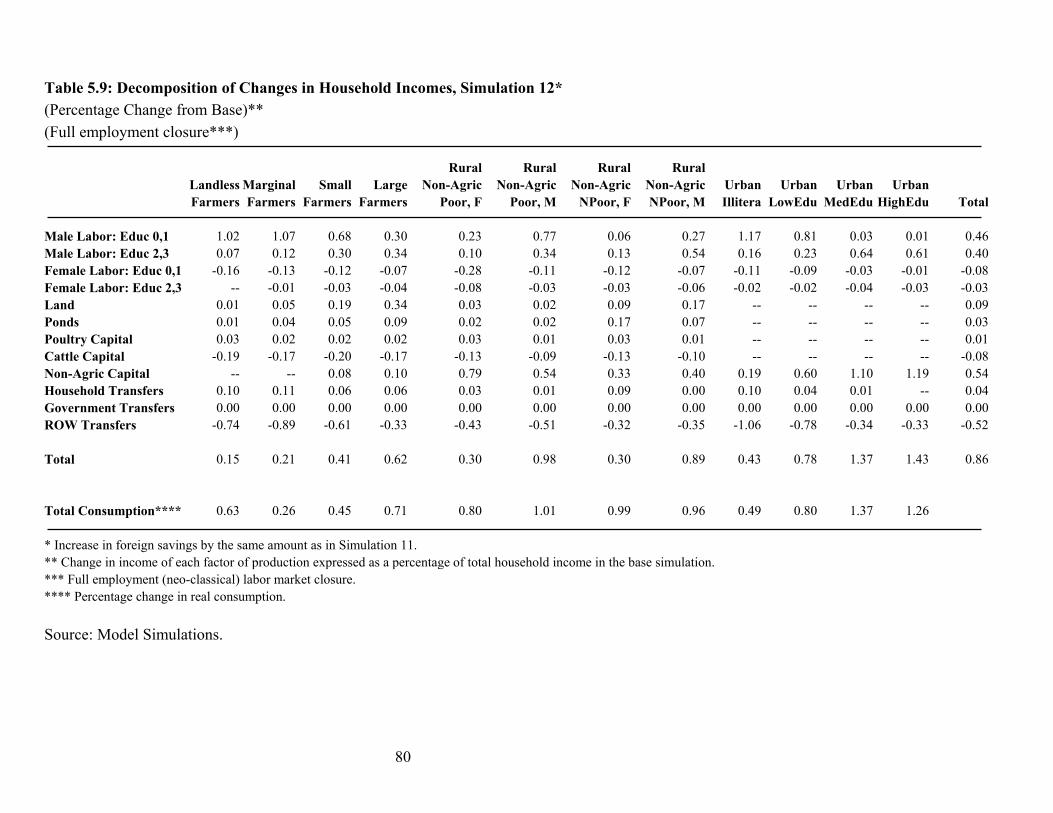
80

Table 5.9: Decomposition of Changes in Household Incomes, Simulation 12*

(Percentage Change from Base)**

(Full employment closure***) Rural Rural Rural Rural Landless Marginal Small Large Non-Agric Non-Agric Non-Agric Non-Agric Urban Urban Urban Urban Farmers Farmers Farmers Farmers Poor, F Poor, M NPoor, F NPoor, M Illitera LowEdu MedEdu HighEdu Total Male Labor: Educ 0,1 1.02 1.07 0.68 0.30 0.23 0.77 0.06 0.27 1.17 0.81 0.03 0.01 0.46 Male Labor: Educ 2,3 0.07 0.12 0.30 0.34 0.10 0.34 0.13 0.54 0.16 0.23 0.64 0.61 0.40 Female Labor: Educ 0,1 -0.16 -0.13 -0.12 -0.07 -0.28 -0.11 -0.12 -0.07 -0.11 -0.09 -0.03 -0.01 -0.08 Female Labor: Educ 2,3 -- -0.01 -0.03 -0.04 -0.08 -0.03 -0.03 -0.06 -0.02 -0.02 -0.04 -0.03 -0.03 Land 0.01 0.05 0.19 0.34 0.03 0.02 0.09 0.17 -- -- -- -- 0.09 Ponds 0.01 0.04 0.05 0.09 0.02 0.02 0.17 0.07 -- -- -- -- 0.03 Poultry Capital 0.03 0.02 0.02 0.02 0.03 0.01 0.03 0.01 -- -- -- -- 0.01 Cattle Capital -0.19 -0.17 -0.20 -0.17 -0.13 -0.09 -0.13 -0.10 -- -- -- -- -0.08 Non-Agric Capital -- -- 0.08 0.10 0.79 0.54 0.33 0.40 0.19 0.60 1.10 1.19 0.54 Household Transfers 0.10 0.11 0.06 0.06 0.03 0.01 0.09 0.00 0.10 0.04 0.01 -- 0.04 Government Transfers 0.00 0.00 0.00 0.00 0.00 0.00 0.00 0.00 0.00 0.00 0.00 0.00 0.00 ROW Transfers -0.74 -0.89 -0.61 -0.33 -0.43 -0.51 -0.32 -0.35 -1.06 -0.78 -0.34 -0.33 -0.52 Total 0.15 0.21 0.41 0.62 0.30 0.98 0.30 0.89 0.43 0.78 1.37 1.43 0.86 Total Consumption**** 0.63 0.26 0.45 0.71 0.80 1.01 0.99 0.96 0.49 0.80 1.37 1.26 * Increase in foreign savings by the same amount as in Simulation 11. ** Change in income of each factor of production expressed as a percentage of total household income in the base simulation. *** Full employment (neo-classical) labor market closure. **** Percentage change in real consumption. Source: Model Simulations.

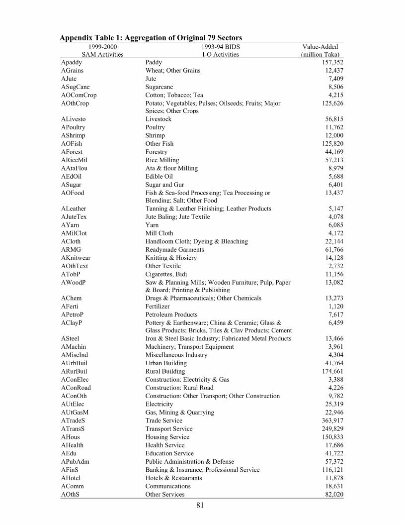
81

Appendix Table 1: Aggregation of Original 79 Sectors 1999-2000

SAM Activities 1993-94 BIDS I-O Activities

Value-Added (million Taka)

Apaddy Paddy 157,352 AGrains Wheat; Other Grains 12,437 AJute Jute 7,409 ASugCane Sugarcane 8,506 AOComCrop Cotton; Tobacco; Tea 4,215 AOthCrop Potato; Vegetables; Pulses; Oilseeds; Fruits; Major

Spices; Other Crops 125,626

ALivesto Livestock 56,815 APoultry Poultry 11,762 AShrimp Shrimp 12,000 AOFish Other Fish 125,820 AForest Forestry 44,169 ARiceMil Rice Milling 57,213 AAtaFlou Ata & flour Milling 8,979 AEdOil Edible Oil 5,688 ASugar Sugar and Gur 6,401 AOFood Fish & Sea-food Processing; Tea Processing or

Blending; Salt; Other Food 13,437

ALeather Tanning & Leather Finishing; Leather Products 5,147 AJuteTex Jute Baling; Jute Textile 4,078 AYarn Yarn 6,085 AMilClot Mill Cloth 4,172 ACloth Handloom Cloth; Dyeing & Bleaching 22,144 ARMG Readymade Garments 61,766 AKnitwear Knitting & Hosiery 14,128 AOthText Other Textile 2,732 ATobP Cigarettes, Bidi 11,156 AWoodP Saw & Planning Mills; Wooden Furniture; Pulp, Paper

& Board; Printing & Publishing 13,082

AChem Drugs & Pharmaceuticals; Other Chemicals 13,273 AFerti Fertilizer 1,120 APetroP Petroleum Products 7,617 AClayP Pottery & Earthenware; China & Ceramic; Glass &

Glass Products; Bricks, Tiles & Clay Products; Cement 6,459

ASteel Iron & Steel Basic Industry; Fabricated Metal Products 13,466 AMachin Machinery; Transport Equipment 3,961 AMiscInd Miscellaneous Industry 4,304 AUrbBuil Urban Building 41,764 ARurBuil Rural Building 174,661 AConElec Construction: Electricity & Gas 3,388 AConRoad Construction: Rural Road 4,226 AConOth Construction: Other Transport; Other Construction 9,782 AUtElec Electricity 25,319 AUtGasM Gas, Mining & Quarrying 22,946 ATradeS Trade Service 363,917 ATransS Transport Service 249,829 AHous Housing Service 150,833 AHealth Health Service 17,686 AEdu Education Service 41,722 APubAdm Public Administration & Defense 57,372 AFinS Banking & Insurance; Professional Service 116,121 AHotel Hotels & Restaurants 11,878 AComm Communications 18,631 AOthS Other Services 82,020

82

List of Discussion Papers No. 51 - �Agriculture-Based Development: A SAM Perspective on Central Viet

Nam� by Romeo M. Bautista (January 2000) No. 52 - �Structural Adjustment, Agriculture, and Deforestation in the Sumatera Regional Economy� by Nu Nu San, Hans Lofgren and Sherman Robinson (March 2000) No. 53 - �Empirical Models, Rules, and Optimization: Turning Positive Economics

on its Head� by Andrea Cattaneo and Sherman Robinson (April 2000) No. 54 - �Small Countries and the Case for Regionalism vs. Multilateralism� by

Mary E. Burfisher, Sherman Robinson and Karen Thierfelder (May 2000) No. 55 - �Genetic Engineering and Trade: Panacea or Dilemma for Developing Countries� by Chantal Pohl Nielsen, Sherman Robinson and Karen Thierfelder (May 2000) No. 56 - �An International, Multi-Region General Equilibrium Model of

Agricultural Trade Liberalization in the South Mediterranean NICs, Turkey, and the European Union� by Ali Bayar, Xinshen Diao and A. Erinc Yeldan (May 2000)

No. 57 - �Macroeconomic and Agricultural Reforms in Zimbabwe: Policy Complementarities Toward Equitable Growth� by Romeo M. Bautista and

Marcelle Thomas (June 2000) No. 58 - �Updating and Estimating a Social Accounting Matrix Using Cross

Entropy Methods� by Sherman Robinson, Andrea Cattaneo and Moataz El-Said (August 2000)

No. 59 - �Food Security and Trade Negotiations in the World Trade Organization:

A Cluster Analysis of Country Groups� by Eugenio Diaz-Bonilla, Marcelle Thomas, Andrea Cattaneo and Sherman Robinson (November 2000)

No. 60 - �Why the Poor Care About Partial Versus General Equilibrium Effects

Part 1: Methodology and Country Case� by Peter Wobst (November 2000) No. 61 - �Growth, Distribution and Poverty in Madagascar: Learning from a Microsimulation Model in a General Equilibrium Framework� by Denis

Cogneau and Anne-Sophie Robilliard (November 2000) No. 62- �Farmland Holdings, Crop Planting Structure and Input Usage: An

Analysis of China's Agricultural Census� by Xinshen Diao, Yi Zhang and Agapi Somwaru (November 2000)

83

No. 63- �Rural Labor Migration, Characteristics, and Employment Patterns: A

Study Based on China's Agricultural Census� by Francis Tuan, Agapi Somwaru and Xinshen Diao (November 2000)

No. 64- �GAMS Code for Estimating a Social Accounting Matrix (SAM) Using

Cross Entropy (CE) Methods� by Sherman Robinson and Moataz El-Said (December 2000)

No. 65- �A Computable General Equilibrium Analysis of Mexicos Agricultural

Policy Reforms� by Rebecca Lee Harris (January 2001) No. 66- �Distribution and Growth in Latin America in an Era of Structural

Reform� by Samuel A. Morley (January 2001) No. 67- �What Has Happened to Growth in Latin America� by Samuel A. Morley (January 2001) No. 68- �Chinas WTO Accession: Conflicts with Domestic Agricultural Policies

and Institutions� by Hunter Colby, Xinshen Diao and Francis Tuan (January 2001)

No. 69- �A 1998 Social Accounting Matrix for Malawi� by Osten Chulu and Peter Wobst (February 2001) No. 70- �A CGE Model for Malawi: Technical Documentation� by Hans Lofgren (February 2001) No. 71- �External Shocks and Domestic Poverty Alleviation: Simulations With a

CGE Model of Malawi� by Hans Lofgren with Osten Chulu, Osky Sichinga, Franklin Simtowe, Hardwick Tchale, Ralph Tseka and Peter Wobst (February 2001)

No. 72 - �Less Poverty in Egypt? Explorations of Alternative Pasts with Lessons

for the Future� by Hans Lofgren (February 2001) No. 73- �Macro Policies and the Food Sector in Bangladesh: A General

Equilibrium Analysis� by Marzia Fontana, Peter Wobst and Paul Dorosh (February 2001)

No. 74- �A 1993-94 Social Accounting Matrix with Gender Features for

Bangladesh� by Marzia Fontana and Peter Wobst (April 2001) No. 75- �A Standard Computable General Equilibrium (CGE) Model� by Hans

Lofgren, Rebecca Lee Harris and Sherman Robinson (April 2001)

84

No. 76- �A Regional General Equilibrium Analysis of the Welfare Impact of Cash Transfers: An Analysis of Progresa in Mexico� by David P. Coady and Rebecca Lee Harris (June 2001)

No. 77- �Genetically Modified Foods, Trade, and Developing Countries� by Chantal Pohl Nielsen, Karen Thierfelder and Sherman Robinson (August 2001) No. 78- �The Impact of Alternative Development Strategies on Growth and Distribution: Simulations with a Dynamic Model for Egypt� by Moataz El-Said, Hans Lofgren and Sherman Robinson (September 2001) No. 79- �Impact of MFA Phase-Out on the World Economy an Intertemporal,

Global General Equilibrium Analysis� by Xinshen Diao and Agapi Somwaru (October 2001)

No. 80- �Free Trade Agreements and the SADC Economies� by Jeffrey D. Lewis, Sherman Robinson and Karen Thierfelder (November 2001) No. 81- �WTO, Agriculture, and Developing Countries: A Survey of Issues� by

Eugenio Diaz-Bonilla, Sherman Robinson, Marcelle Thomas and Yukitsugu Yanoma (January 2002)

No. 82- �On boxes, Contents, and Users: Food Security and the WTO

Negotiations� by Eugenio Diaz-Bonilla, Marcelle Thomas and Sherman Robinson (November 2001: Revised July 2002)

No. 83- �Economy-Wide Effects of El Niño/Southern Oscillation ENSO in

Mexico and the Role of Improved Forecasting and Technological change� by Rebecca Lee Harris and Sherman Robinson (November 2001)

No. 84- �Land Reform in Zimbabwe: Farm-Level Effects and Cost-Benefit Analysis� by Anne-Sophie Robilliard, Crispen Sukume, Yuki Yanoma and

Hans Lofgren (December 2001: Revised May 2002) No. 85- �Developing Country Interest in Agricultural Reforms Under the World

Trade Organization� by Xinshen Diao, Terry Roe and Agapi Somwaru (January 2002)

No. 86- �Social Accounting Matrices for Vietnam 1996 and 1997� by Chantal

Pohl Nielsen (January 2002) No. 87- �How Chinas WTO Accession Affects Rural Economy in the Less Developed Regions: A Multi-Region, General Equilibrium Analysis� by

Xinshen Diao, Shenggen Fan and Xiaobo Zhang (January 2002) No. 88- �HIV/AIDS and Macroeconomic Prospects for Mozambique: An Initial

Assessment� by Charming Arndt (January 2002)

85

No. 89- �International Spillovers, Productivity Growth and Openness in Thailand:

An Intertemporal General Equilibrium Analysis� by Xinshen Diao, Jorn Rattso and Hildegunn Ekroll Stokke (February 2002) No. 90- �Scenarios for Trade Integration in the Americas� by Xinshen Diao,

Eugenio Diaz-Bonilla and Sherman Robinson (February 2002) No. 91- �Assessing Impacts of Declines in the World Price of Tobacco on China,

Malawi, Turkey, and Zimbabwe� by Xinshen Diao, Sherman Robinson, Marcelle Thomas and Peter Wobst (March 2002) No. 92- �The Impact of Domestic and Global Trade Liberalization on Five

Southern African Countries� by Peter Wobst (March 2002) No. 93- �An Analysis of the Skilled-Unskilled Wage Gap Using a General

Equilibrium Trade Model� by Karen Thierfelder and Sherman Robinson (May 2002)

No. 94- �That Was Then But This is Now: Multifunctionality in Industry and

Agriculture� by Eugenio Diaz-Bonilla and Jonathan Tin (May 2002) No. 95- �A 1998 Social Accounting Matrix (SAM) for Thailand� by Jennifer

Chung-I Li (July 2002) No. 96- �Trade and the Skilled-Unskilled Wage Gap in a Model With

Differentiated Goods� by Karen Thierfelder and Sherman Robinson (August 2002)

No. 97- �Estimation of a Regionalized Mexican Social Accounting Matrix: Using

Entropy Techniques to Reconcile Disparate Data Sources� by Rebecca Lee Harris (August 2002)

No. 98- �The Influence of Computable General Equilibrium Models on Policy� by

Shantayanan Devarajan and Sherman Robinson (August 2002) No. 99- �Macro and Macro Effects of Recent and Potential Shocks to Copper

Mining in Zambia� by Hans Lofgren, Sherman Robinson and James Thurlow (August 2002)

No. 100- �A Standard Computable General Equilibrium Model for South Africa�

by James Thurlow and Dirk Ernst van Seventer (September 2002) No. 101- �Can South Africa Afford to Become Africa's First Welfare State� by

James Thurlow (September 2002) No. 102- �HIV/AIDS and Labor Markets in Tanzania� by Channing Arndt and

Peter Wobst (October 2002)

86

No. 103- �Economy-Wide Benefits from Establishing Water User-Right Markets in

a Spatially Heterogeneous Agricultural Economy� by Xinshen Diao, Terry Roe and Rachid Doukkali (October 2002)

No. 104- �Do Direct Payments Have Intertemporal Effects on U.S. Agriculture?�

by Terry Roe, Agapi Somwaru and Xinshen Diao (October 2002) No. 105- �General Equilibrium Measures of Agricultural Policy Bias in Fifteen

Developing Countries� by Henning Tarp Jensen, Sherman Robinson and Finn Tarp (October 2002)

No. 106- �Trade in Genetically Modified Food: A Survey of Empirical Studies� by

Chantal Pohl Nielsen, Sherman Robinson and Karen Thierfelder (November 2002)

No. 107- �Opportunities and Challenges in Agriculture and Garments: A General

Equilibrium Analysis of the Bangladesh Economy� by Channing Arndt, Paul Dorosh, Marzia Fontana and Sajjad Zohir with Moataz El-Said and Christen Lungren (November 2002)

Copies can be obtained by calling Maria Cohan at 202-862-5627 or e-mail: m.cohan@cgiar.org