operational planning–policies and procedures for adf&g
TRANSCRIPT
Special Publication No. 12-13
Operational Planning–Policies and Procedures for ADF&G Fisheries Research and Data Collection Projects
by
Jeff Regnart
and
Charles O. Swanton
August 2012
Alaska Department of Fish and Game Divisions of Sport Fish and Commercial Fisheries
Symbols and Abbreviations The following symbols and abbreviations, and others approved for the Système International d'Unités (SI), are used without definition in the following reports by the Divisions of Sport Fish and of Commercial Fisheries: Fishery Manuscripts, Fishery Data Series Reports, Fishery Management Reports, and Special Publications. All others, including deviations from definitions listed below, are noted in the text at first mention, as well as in the titles or footnotes of tables, and in figure or figure captions. Weights and measures (metric) centimeter cm deciliter dL gram g hectare ha kilogram kg kilometer km liter L meter m milliliter mL millimeter mm Weights and measures (English) cubic feet per second ft3/s foot ft gallon gal inch in mile mi nautical mile nmi ounce oz pound lb quart qt yard yd Time and temperature day d degrees Celsius °C degrees Fahrenheit °F degrees kelvin K hour h minute min second s Physics and chemistry all atomic symbols alternating current AC ampere A calorie cal direct current DC hertz Hz horsepower hp hydrogen ion activity pH (negative log of) parts per million ppm parts per thousand ppt, ‰ volts V watts W
General Alaska Administrative Code AAC all commonly accepted abbreviations e.g., Mr., Mrs.,
AM, PM, etc. all commonly accepted professional titles e.g., Dr., Ph.D., R.N., etc. at @ compass directions:
east E north N south S west W
copyright corporate suffixes:
Company Co. Corporation Corp. Incorporated Inc. Limited Ltd.
District of Columbia D.C. et alii (and others) et al. et cetera (and so forth) etc. exempli gratia (for example) e.g. Federal Information Code FIC id est (that is) i.e. latitude or longitude lat. or long. monetary symbols (U.S.) $, ¢ months (tables and figures): first three letters Jan,...,Dec registered trademark trademark United States (adjective) U.S. United States of America (noun) USA U.S.C. United States
Code U.S. state use two-letter
abbreviations (e.g., AK, WA)
Mathematics, statistics all standard mathematical signs, symbols and abbreviations alternate hypothesis HA base of natural logarithm e catch per unit effort CPUE coefficient of variation CV common test statistics (F, t, χ2, etc.) confidence interval CI correlation coefficient (multiple) R correlation coefficient (simple) r covariance cov degree (angular ) ° degrees of freedom df expected value E greater than > greater than or equal to ≥ harvest per unit effort HPUE less than < less than or equal to ≤ logarithm (natural) ln logarithm (base 10) log logarithm (specify base) log2, etc. minute (angular) ' not significant NS null hypothesis HO percent % probability P probability of a type I error (rejection of the null hypothesis when true) α probability of a type II error (acceptance of the null hypothesis when false) β second (angular) " standard deviation SD standard error SE variance population Var sample var
SPECIAL PUBLICATION NO. 12-13
POLICIES AND PROCEDURES FOR ADF&G FISHERIES RESEARCH AND DATA COLLECTION PROJECTS
by
Jeff Regnart Division of Commercial Fisheries, Anchorage
and
Charles O. Swanton Division of Sport Fish, Juneau
Alaska Department of Fish and Game Division of Sport Fish, Research and Technical Services 333 Raspberry Road, Anchorage, Alaska, 99518-1565
August 2012
The Special Publication series was established by the Division of Sport Fish in 1991 for the publication of techniques and procedures manuals, informational pamphlets, special subject reports to decision-making bodies, symposia and workshop proceedings, application software documentation, in-house lectures, and became a joint divisional series in 2004 with the Division of Commercial Fisheries. Special Publications are intended for fishery and other technical professionals. Special Publications are available through the Alaska State Library, Alaska Resources Library and Information Services (ARLIS) and on the Internet: http://www.adfg.alaska.gov/sf/publications/. This publication has undergone editorial and peer review.
Jeff Regnart, Alaska Department of Fish and Game, Division of Commercial Fisheries
333 Raspberry Road Anchorage, AK 99518-1565, USA
and
Charles O. Swanton Alaska Department of Fish and Game, Division of Sport Fish,
PO Box 115526 Juneau, AK 99811-5526, USA
This document should be cited as: Regnart, J. and C. O. Swanton. 2012. Operational planning–policies and procedures for ADF&G fisheries research
and data collection projects. Alaska Department of Fish and Game, Special Publication No. 12-13, Anchorage.
The Alaska Department of Fish and Game (ADF&G) administers all programs and activities free from discrimination based on race, color, national origin, age, sex, religion, marital status, pregnancy, parenthood, or disability. The department administers all programs and activities in compliance with Title VI of the Civil Rights Act of 1964, Section 504 of the Rehabilitation Act of 1973, Title II of the Americans with Disabilities Act (ADA) of 1990, the Age Discrimination Act of 1975, and Title IX of the Education Amendments of 1972.
If you believe you have been discriminated against in any program, activity, or facility please write: ADF&G ADA Coordinator, P.O. Box 115526, Juneau, AK 99811-5526
U.S. Fish and Wildlife Service, 4401 N. Fairfax Drive, MS 2042, Arlington, VA 22203 Office of Equal Opportunity, U.S. Department of the Interior, 1849 C Street NW MS 5230, Washington DC 20240
The department’s ADA Coordinator can be reached via phone at the following numbers: (VOICE) 907-465-6077, (Statewide Telecommunication Device for the Deaf) 1-800-478-3648,
(Juneau TDD) 907-465-3646, or (FAX) 907-465-6078 For information on alternative formats and questions on this publication, please contact:
ADF&G Division of Sport Fish, Research and Technical Services, 333 Raspberry Road, Anchorage AK 99518 (907) 267-2375
i
TABLE OF CONTENTS Page
LIST OF APPENDICES ............................................................................................................................................... ii
FOREWORD ................................................................................................................................................................iii
POLICY OVERVIEW .................................................................................................................................................. 1
Categorization of Operational Plans .............................................................................................................................. 2 Category I ................................................................................................................................................................. 2 Category II ................................................................................................................................................................ 2 Category III ............................................................................................................................................................... 3
Operational Plan Review and Development .................................................................................................................. 3 New projects .................................................................................................................................................... 4 Existing projects .............................................................................................................................................. 4 Amendment process ........................................................................................................................................ 4 Recurrent, multi-year, and bundled operational plans ..................................................................................... 4 Signature and editorial process ........................................................................................................................ 5 Regional coordination ..................................................................................................................................... 5 Program coordination ...................................................................................................................................... 5
OPERATIONAL PLAN ELEMENTS–DOCUMENT REQUIREMENTS AND GUIDELINES ................................ 5
Element Descriptions ..................................................................................................................................................... 6 Signature page .......................................................................................................................................................... 6 Purpose ..................................................................................................................................................................... 6
Background ..................................................................................................................................................... 6 Objectives ................................................................................................................................................................. 7 Methods .................................................................................................................................................................... 8
Experimental or study design .......................................................................................................................... 8 Sample sizes .................................................................................................................................................... 8 Sampling methods or data collection .............................................................................................................. 8 Data analysis ................................................................................................................................................... 8
Schedule and Deliverables ........................................................................................................................................ 8 Responsibilities ......................................................................................................................................................... 9 References Cited ....................................................................................................................................................... 9
Appendices ...................................................................................................................................................... 9 MISCELLANEOUS ITEMS AND RECOMMENDATIONS ...................................................................................... 9
Best practices manuals .............................................................................................................................................. 9 Grant proposals ......................................................................................................................................................... 9 Policy Review ........................................................................................................................................................... 9 Archiving of operational plans ................................................................................................................................. 9
APPENDIX A EXAMPLE SIGNATURE PAGES ..................................................................................................... 11
APPENDIX B EXAMPLE CATEGORY I OPERATIONAL PLAN ......................................................................... 17
APPENDIX C EXAMPLE CATEGORY II OPERATIONAL PLAN ....................................................................... 31
APPENDIX D EXAMPLE CATEGORY III OPERATIONAL PLAN ...................................................................... 57 APPENDIX E EXAMPLE OPERATIONAL PLAN AMENDMENT ..................................................................... 125
APPENDIX F OPERATIONAL PLANNING MEETING NOTES ......................................................................... 135
ii
LIST OF APPENDICES Appendix Page A1. Example signature page for category I operational plan. .............................................................................. 12 A2. Example signature page category II operational plan. ................................................................................... 13 A3. Example signature page category III operational plan. ................................................................................. 14 A4. Example signature page operational plan amendment. ................................................................................. 15 B1. Example of a category I operational plan with ROP format.......................................................................... 18 C1. Example of a category II operational plan with ROP format. ....................................................................... 32 D1. Example of a category III operational plan with ROP format. ...................................................................... 58 E1. Requirements for Operational Plan Amendment ......................................................................................... 126 E2. Example Operational Plan Amendment. ..................................................................................................... 127 F1. Regional operational planning meeting notes, Juneau 11/22/11. ................................................................ 136 F2. Regional operational planning meeting notes, Fairbanks 11/9/2011. .......................................................... 143 F3. Regional Operational Planning Notes, Anchorage 11/8/2011. .................................................................... 160
iii
FOREWORD Management of Alaska’s fisheries is based on sound scientific practices and objective-based research. Commitment to scientific principles and proper planning for fisheries projects ensure that data and information collected will address management needs and are scientifically defensible.
In 2011, an initiative was undertaken to develop a unified policy for the divisions of Sport Fish and Commercial Fisheries regarding operational planning for fisheries projects. During the fall of 2011, the directors and chief fisheries scientists from both divisions met to formulate general guidelines and explore options for how to design and implement this policy. A list of guidelines and talking points were then presented at 3 regional meetings (Fairbanks, Anchorage, and Juneau) where staff critiqued the materials and offered new ideas (Appendix F). At each meeting, regional and area offices from both divisions were represented and staff included biometricians, project and area biologists, research and management coordinators, fisheries scientists, and regional supervisors. This document is the product of these meetings and what has been learned over the years by both divisions.
The overall goal of this policy is to ensure that the many benefits of good planning are realized. Some of the benefits include a clearly articulated purpose statement for all fisheries projects that can be understood by all stakeholders, regulators, and funding sources, and that expectations and responsibilities are understood and agreed upon. Proper planning ensures that data are statistically sound and appropriate for good fisheries management. It also facilitates staff development, improves budgeting decisions, promotes timeliness of reporting, and provides a record of the research objectives, experimental designs, and data collection protocols. It is stressed, however, that efficiency is of paramount importance to project planning efforts and undue attention to minor aspects of the planning document will marginalize these benefits. To ensure that this policy remains effective and meets the needs of the two divisions, periodic reviews and revisions are critical.
Jeff Regnart, Director, Division of Commercial Fisheries
Charles O. Swanton, Director, Division of Sport Fish

iv

1
POLICY OVERVIEW This policy establishes guidelines and outlines procedures for the development of operational plans for fisheries projects conducted by divisions of Commercial Fisheries and Sport Fish of the Alaska Department of Fish and Game. For the purposes of this document, a fisheries project is defined as any funded activity directed at the collection of data or information used in fisheries management. The spectrum of possible projects is broad and could include a multi-faceted approach for modeling groundfish biomass, the development of new acoustic tools, or a simple foot survey to count salmon. If a particular activity is not obviously a fisheries project, the regional research coordinator (RRC–Fishery Biologist IV)1 or chief fishery scientist will need to determine if the activity warrants an operational plan.
Although there are many facets to planning a fisheries project, this policy specifically provides guidance for a written operational planning document and assumes that other planning components (such as identifying and prioritizing information needs and budgeting for fisheries projects) have already been completed and plans are ready to be developed and written. For this policy to be successful, flexibility is needed to accommodate the varying needs and organizational structures among the divisions and regions. This policy directs that:
1) A written operational plan, which may cover multiple years, will exist for all fisheries projects.
2) Operational plans will require the appropriate signatory approval.
3) For each plan, the level of detail and level of signatory approval is established by the RRC.
4) Operational plans should be completed and signed prior to data collection activities and no fisheries projects may be fielded without prior approval of the RRC.
5) All operational plans will follow, to a reasonable extent, a standardized template or format.
6) All operational plans will be electronically archived as “Regional Operational Plans (ROPs).
7) Grant proposals must receive authority approval by the appropriate regional supervisor and fisheries scientist prior to submission.
8) All fisheries projects will be reviewed annually to ensure compliance with this policy.
9) For each division, the policy and procedures for operational planning will be administered by their respective chief fisheries scientist(s).
The operational planning process is a cooperative venture among research biologists, fisheries managers, research coordinators, biometricians, regional supervisors, and others, and the written plan is the vehicle with which the cooperation is organized. Development of the plan by the project leader forces all participants to think about what they propose to do and the signed document is the tangible evidence that planning has taken place.
1 The abbreviation RRC will be used in this document to mean the regional research coordinator, chief fisheries scientist, or staff member in
charge of the operational planning process for their region or administrative unit.

2
CATEGORIZATION OF OPERATIONAL PLANS Central to this policy is a classification system for operational plans and the associated responsibilities of the RRC. The level of detail required for a successful plan can vary greatly and three categories (I–III) of operational plans have been established. Each category of operational plan has a different level of signatory approval and detail-category I has the lowest, and category III the highest.
The RRC is responsible and has discretion for assigning operational plan categories for all fisheries projects. During the initial project assessment, consultation with the project leader and biometrician (or fisheries scientist depending on their roles) is advised to ensure that the appropriate level of review occurs and that the RRC’s expectations for plan detail are made clear to the authors. The signature requirements and the general characteristics of each category level are presented.
Category I This category requires signatory approval of the project leader and RRC. Additional signatures from regional staff may be included as determined by the regional supervisor, but are optional. The characteristics of this fisheries project must include characteristic 1 and one or more characteristics 2-5:
1) If no current operational plan exists and only basic2 or no statistical analysis needed; and,
2) High proficiency and project-specific job knowledge by the project leader;
3) Sampling procedures are routine and well-established;
4) Existence of previously approved operational plan or peer-reviewed citable report or journal article with operational details; or,
5) Standardized methods have been previously developed and are citable in a peer-reviewed report or journal article.
Category II This category requires all Category I signatures plus the signature of at least one consulting biometrician and characteristics must include one or more of the following:
1) Incomplete project-specific job knowledge or experience of project leader (e.g., new hire);
2) No existing operational plan;
3) Ongoing or multiyear project with significant changes to methods;
4) Application of new methods or technologies;
5) Parameter estimation, advanced hypothesis testing, or statistical analysis required;
6) Assistance by a consulting biometrician required for data analysis; and,
7) Potential for significant bias resulting in erroneous interpretation of results. 2 Basic statistics are the mean and variance of a normally distributed variate and any basic hypothesis tests such as the z-test, t-test, or one-way
ANOVA.
3
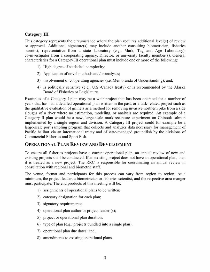
Category III This category represents the circumstance where the plan requires additional level(s) of review or approval. Additional signature(s) may include another consulting biometrician, fisheries scientist, representative from a state laboratory (e.g., Mark, Tag and Age Laboratory), co-investigator from a cooperating agency, Director, or university faculty member(s). General characteristics for a Category III operational plan must include one or more of the following:
1) High degree of statistical complexity;
2) Application of novel methods and/or analyses; 3) Involvement of cooperating agencies (i.e. Memoranda of Understanding); and,
4) Is politically sensitive (e.g., U.S.-Canada treaty) or is recommended by the Alaska Board of Fisheries or Legislature.
Examples of a Category I plan may be a weir project that has been operated for a number of years that has had a detailed operational plan written in the past, or a task-related project such as the qualitative evaluation of gillnets as a method for removing invasive northern pike from a side sloughs of a river where no estimation, modeling, or analysis are required. An example of a Category II plan would be a new, large-scale mark-recapture experiment on Chinook salmon implemented by a single region and division. A Category III project could for example be a large-scale port sampling program that collects and analyzes data necessary for management of Pacific halibut via an international treaty and of state-managed groundfish by the divisions of Commercial Fisheries and Sport Fish.
OPERATIONAL PLAN REVIEW AND DEVELOPMENT To ensure all fisheries projects have a current operational plan, an annual review of new and existing projects shall be conducted. If an existing project does not have an operational plan, then it is treated as a new project. The RRC is responsible for coordinating an annual review in consultation with regional and biometric staff.
The venue, format and participants for this process can vary from region to region. At a minimum, the project leader, a biometrician or fisheries scientist, and the respective area manger must participate. The end products of this meeting will be:
1) assignments of operational plans to be written;
2) category designation for each plan;
3) signatory requirements;
4) operational plan author or project leader (s);
5) project or operational plan duration;
6) type of plan (e.g., projects bundled into a single plan);
7) operational plan due dates; and,
8) amendments to existing operational plans.
4
Further refinement of assigned operational plans or amendments will be required. This could apply to objective language, methods, sample sizes, or crew assignments. This refinement may occur during a small focus group consisting of the project leader, RRC and assigned biometrician or fisheries scientist, or may occur during a dedicated “operational planning meeting” at a regional level with all research staff, managers, and biometricians invited.
New projects For new projects, an operational plan will need to be developed, written and archived. In consultation with a biometrician and project leader, the RRC will categorize the plan, determine the appropriate signatory requirements, and assign the writing of the operational plan to the project leader. A due date will be assigned for submission of the draft plan to the RRC.
Existing projects These are defined as projects with an approved, existing operational plan; either for a single project requiring multiple years to complete (e.g., a coded-wire-tagging project) or a recurring project (e.g., salmon weir). The intent of the review by the RRC is to ensure that the operational plan is current, meaning that no significant or meaningful changes to the project have occurred, or if simply too much time has elapsed since the original plan was written. Determination of what is significant or meaningful will be left to the discretion of the RRC. Consultation with the project leader and biometric staff should be considered. If no significant or meaningful changes have occurred to the project, then no new plan is needed. If significant or meaningful changes to the fisheries project have or need to occur, the existing plan may be amended, or rewritten based on the magnitude of the changes. This may only require an updated signature page if there are no changes to the operational plan. All operational plans should be revised or re-written every 5–6 years even if no significant or meaningful changes have occurred.
Amendment process In many circumstances, only one or two components of the operational plan change annually and rewriting a completely new plan is not warranted. For example, where minor modifications to sample size, sampling area, or gear type are necessary, but objectives, experimental design, and data analysis are functionally unchanged, a short amendment may be written detailing the change. The amendment will consist of a signature page and a page or two of text describing the minor changes in protocol (Appendix E). The new signature page (Appendix A) and amended text will then be attached to a copy of the old plan and then archived as a package just as any other plan would be. Eventually, a new plan will have to be written if amendments begin to compound annually or if too much time has lapsed (i.e., 5–6 years).
Recurrent, multi-year, and bundled operational plans To promote efficiency, recurrent, multi-year and bundled plans are encouraged. Recurrent projects are the same projects fielded annually, such as a counting tower. A multi-year project may be a 3-year radiotelemetry investigation, or a 5-year Jolly-Seber experiment. A bundled plan is used for grouping similar projects, such as all weirs within a major drainage, all having the same basic experimental design and analytical procedures, with only minor differences, for example, in crew size, counting schedule, or equipment. Recurrent, multi-year, and bundled plans must still be reviewed every year.
5
Signature and editorial process Reviews of the operational plan should be provided by all signatories on the Signature page. During the review process, a collaborative approach is encouraged to ensure any proposed modifications to the original project design are well founded and agreed upon by the previous reviewers. Reviews should follow the hierarchical progression as listed on the signatory page, and for Category II and III plans, biometric assistance and review should be completed first. Upon completion of all reviews, the RRC will incorporate all remaining editorial comments and route the Signature page for signatures. Only the final version of the operational plan will be signed.
Regional coordination An annual meeting between RRCs and Chief Fisheries Scientists of the Divisions of Commercial Fisheries and Sport Fish will occur to discuss all existing and potential research projects. The purpose of this meeting is to identify areas of common interest and potential cooperation, promote data sharing, eliminate duplication of effort, and avoid competing grant proposals. This meeting should be held prior to any regional operational planning efforts. For those projects where potential coordination is identified, a representative (e.g., project leader or consulting biometrician) from the other division will be a participant during the all planning phases commensurate with the level of involvement. This involvement could range from being co-project leader and co-signatory for a large-scaled Chinook salmon radiotelemetry project to simply taking genetic samples for the other division.
Program coordination An annual review of the operational planning program will be conducted to ensure adherence to the policy and identify areas for improvement. The participants of this meeting will include all Chief Fisheries Scientists and invited participants.
OPERATIONAL PLAN ELEMENTS–DOCUMENT REQUIREMENTS AND GUIDELINES
All operational plans, Categories I−III, will follow the same minimum guidelines to ensure consistency. These guidelines are not intended to be overly prescriptive and the amount of detail and organization within a primary element of the plan (e.g., the methods section) will vary. Ultimately, it is incumbent upon the RRC to provide direction when needed. The use of, for example, secondary headers and tables is encouraged to improve readability and organization. The most recent versions of the ADF&G Writer’s Guide should be used to help ensure consistent writing standards, and plans should be formatted for publication in the ROP series.
The use of references in lieu of detailed written descriptions of methods is strongly encouraged to improve efficiency. Examples of materials that can be referenced include management plans, management reports, best practices manuals, prior operational plans, prior ADF&G reports, or published literature. For example, if the history of a fishery is well documented in an area management report, then this material can simply be referenced instead of reiterating the same message in the operational plan. Similarly, for the data analysis description, if the analytical techniques are well documented in a prior year’s report and did not change, that report can be cited.
6
All operational plans will be archived as Regional Operational Plans to ensure that plans are accessible to the public and departmental staff for future use, including excerpting of text, tables, and figures. ROPs are not blind peer reviewed across regions, and the public view will contain a waiver that tags the file as a planning document.
ELEMENT DESCRIPTIONS At a minimum, each operational plan will include the following primary headers, except for the Background and Appendix sections, which are optional:
SIGNATURE PAGE SCHEDULE AND DELIVERABLES PURPOSE RESPONSIBILITES BACKGROUND (optional) REFERENCES CITED OBJECTIVES APPENDIX (optional) METHODS
Examples of approved operational plans (Categories I–III) are provided (Appendix B-D). Other examples are located within the Division of Sport Fish Intranet web site http://docushare.sf.adfg.state.ak.us/dsweb/homepage; accessed 06/2012), although structure and headers will be slightly different than what is defined in this policy.
Signature page The title or signatory page must include the project title, project leader(s), Division, Region and Area, project nomenclature (e.g., funding source and/or grant numbers), field dates, plan type, and signatures. The appropriate signatory lines are listed hierarchically and include the names and title of the signatories (Appendix A).
Purpose The Purpose section should provide a specific and accurate synopsis of the study goal(s). This section should clearly articulate what the specific management information needs are, how and the extent to which the project will address them, and how the data will be used to facilitate management of the fishery. For Category I plans with a very simple and well defined purpose and established history, this section need not include anything more than that. If the plan requires additional language to provide context for the study, and if a detailed Background section is not being written (see description below), this section may also include a brief review of the previous work that has been conducted that is relevant to the project being proposed, a synopsis of the fishery characteristics (e.g., harvest and participation), or any other pertinent background information that is germane to the goal and objectives of the study. If a substantial amount (i.e., three or more paragraphs) of supporting information is required to provide context for the project goals and objectives, then a Background section should be written.
Background This section provides additional context for the project and is optional. It can provide further rationale for the study, hypothesis tests, or choice of methods. The subject matter may provide for geographical context, detail the history related to the project, explain the evolution of the current study design, or consist of literature review to support the approach or utility of the project. A good Background section need not be an exhaustive case study and the level of detail included is left to the discretion of the project leader and RRC.
7
Objectives This is the most important section of the operational plan because it establishes the criteria for success and dictates the experimental design, sample sizes and sampling protocols. Objectives are statements that relate to the purpose or goals of the study. Objectives should be understandable and unambiguous and written in such a way that sample sizes or sampling effort can readily be determined and there is a clear way to measure success.
If sampling is involved the objective statements should begin with infinitives such as to test or to estimate and have associated statistical criteria providing a way to gauge the project’s success. For example:
- To estimate the abundance of mature burbot in Lake Louise such that the estimate is within 10% of the actual abundance 95% percent of the time.
- To test the hypothesis that survival rates of coho salmon hooked and released in the estuary of the Little Susitna River are the same as those coho salmon hooked and released farther upstream in order to detect at least a difference of 0.10 between survival rates with α = 0.05 and β = 0.10 (or Power = 1-β).
Not all objective statements need to have statistical criteria associated with them. For example, an area management biologist who is testing the efficacy of manual removal methods (i.e., gillnetting) for reducing numbers of invasive northern pike may construct a project objective statement as follows:
- Reduce the number of northern pike in 20 side channel sloughs between May 10 and May 30 of upper Alexander Creek such that the final catch in each slough is equal to or less than 15% of the peak catch.
A biologist, without insufficient funding to mount a long-term stock assessment program may be interested in assessing the potential effect of a fishing regulation. Here the objective may be written as:
- Calculate the relative stock density (RSD) of northern pike ≥560 mm FL captured in Alexander Lake from May 6 to May 25 with hoop nets and hook-and-line gear, such that a RSD of 38% would indicate a potential slot limit effect on size structure.
In some cases a count or census of a population may be conducted and there is no sampling or estimation involved. An example of an objective statement for such a scenario is:
- Count coho salmon in the Delta Clearwater River from a drifting river boat during peak spawning to document minimum escapement, such that achievement of the escapement goal can be ascertained.
Lastly, some fisheries projects will be less quantitative in nature because, for example, generalized life-history information is of interest. For example;
- Describe the seasonal distributions of burbot radio-tagged during the fall of 2011 within two geographic sections, the Lower and Upper Kuskokwim River (excluding the George River) during aerial surveys conducted during winter2011/2012 and spring 2012.
For many projects, data indirectly related to the study goals are often collected for various reasons and do not drive the study design or sampling; for example, the collection of genetic tissue samples for another agency or measuring water levels at a weir. These activities should be listed under a subheading of “Secondary Objectives”.
8
Methods This section is written as a process description, where details should be precise, complete, and concise-including only relevant information. In many cases, the Methods section will benefit by including four broad subsections 1) Experimental or study design; 2) Sampling methods or Data Collection; 3) Sample size; and, 4) Data analysis, described in greater detail below. However, in some cases these subsections may not be easily used or separated without a lot of redundancy or affecting flow. In these circumstances combining some, using substitute subheaders, or eliminating them all may result in a more concise and fluid report. Use of additional subsections may improve clarity and organization. For example, these could include Overview of study design, Study area, Capture techniques, Weir construction, Sonar operation, Tissue sampling procedures, etc. Design of methods section structure will be left to the discretion of the RRC and project leader.
Experimental or study design In this section the sampling design, equipment, and analytical techniques are outlined, and if needed, supported with references to literature or previous work. Limitations or anticipated outcomes of the study design may be discussed and potential biases can be addressed. Units of measure are introduced, as well as, for example, controls, treatments, replications, or sampling strata. The use of tables or appendices that link the units (e.g., dates or geographic strata) with sample size(s) is effective.
Sample sizes Sample sizes needed to meet the objectives are stated. Determination and rationale of sample sizes are explained. These may be based on the literature, previous studies, or informed professional experience and should be referenced.
Sampling methods or data collection Sampling methods describe how and what data are collected and how sample sizes are to be achieved, given the planned intensity of sampling. It provides, for example, descriptions of sampling gear or equipment, crew sizes, distribution of sampling effort, itemized list of data (e.g., tag number, length, gear type, etc.), and measurement techniques and units of measure.
Data analysis Conditions necessary for obtaining unbiased results and diagnostic tests that will be used to detect whether conditions for accurate estimation have been met are listed and cited. Procedures used to correct estimates for bias are also listed and cited. If no formal diagnostic tests are possible, rationales as to why conditions will be met or why bias in estimates will be insignificant are given. In some cases, it may be easier to address the conditions or potential biases within the Experimental or Study design sections.
All but the most basic equations behind the calculations in the analysis will be in this section. Complex equations will be cited as to their source in literature (e.g., equations describing stratified, multistage sampling designs). All notations will be defined.
Schedule and Deliverables A concise description of project deliverables should be included. A timetable for the major activities of the project such as completion of the operational plan, sampling dates, completion of
9
the data analysis and report(s) should also be stated. Lastly, this section should identify where and how the data will be formatted and stored.
Responsibilities This is a bulleted list of departmental project personnel including their names, positions, and primary responsibly (e.g. assist with fish capture or project leader). The list should encompass only those directly involved in with the data collection and analysis, such as the biometrician, project leader(s), field crew leader(s), and technicians.
References Cited References to all citations are listed here and follow guidelines described in Alaska Department of Fish and Game Writer’s Guide.
Appendices Materials for appendices may include data forms, maps, standard operating procedures, analytical techniques, field instructions for technicians, technical illustrations, or survey questions.
MISCELLANEOUS ITEMS AND RECOMMENDATIONS During the regional staff meetings used to help formulate this plan, several items of significance were identified.
Best practices manuals: The divisions should work towards the development of “Best Practices Manuals” that can be referenced in an operational plan. Topics could, for example, cover standard practices for sonar operations or mark-recapture studies.
Grant proposals: Approval of grant proposals prior to submission to the funding source by the appropriate Chief Fisheries Scientist and regional supervisor is required to ensure that proposals are consistent with this policy and make certain that adequate coordination and communication occurs. Authority requests must include the title, funding source, project purpose, and a listing of project objectives. These may be submitted and approved by email.
Grant proposals may not be used in lieu of an operational plan. For all funded project(s), an operational plan must be written. Depending on the level of detail in the proposal, this may simply require reformatting of the grant proposal and adding a signature cover page.
Policy Review: This policy should be revised every 4–5 years. Undoubtedly there will be ways to improve the policy to ensure that the process is still efficient and that good planning is consistently occurring.
Archiving of operational plans: All final documents will be submitted to Division of Sport Fish Research and Technical Services (RTS) statewide editor through the RRC, or designee. All signed operational plans will be electronically archived as Regional Operational Reports. The ROP series will be assigned a number regionally composed of the following elements: (1) ROP, (2) two-letter Division designation [e. g., CF or SF]; (3) number of the region followed by the regional office (4) two-digit designating the current year [e. g., 12] (5) 2-digit sequence number. Regional publications staff will assign a number, generate a tagged pdf file with metadata filled in, and establish pagination, links and bookmarks. Metadata necessary to enable the Internet search capability for archival (full citation, abstract and keywords) will be compiled and submitted to RTS along with the request for archival memo.

10

11
APPENDIX A
EXAMPLE SIGNATURE PAGES
12
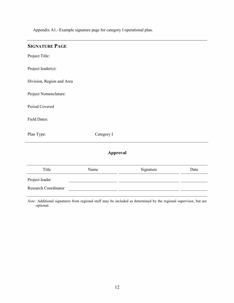
Appendix A1.–Example signature page for category I operational plan.
SIGNATURE PAGE
Project Title:
Project leader(s):
Division, Region and Area
Project Nomenclature:
Period Covered
Field Dates:
Plan Type: Category I
Approval
Title Name Signature Date
Project leader
Research Coordinator Note: Additional signatures from regional staff may be included as determined by the regional supervisor, but are
optional.
13
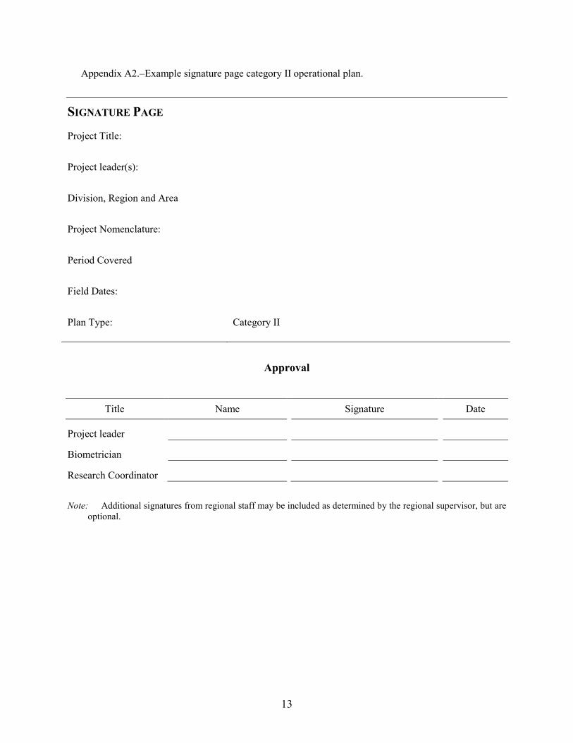
Appendix A2.–Example signature page category II operational plan.
SIGNATURE PAGE
Project Title:
Project leader(s):
Division, Region and Area
Project Nomenclature:
Period Covered
Field Dates:
Plan Type: Category II
Approval
Title Name Signature Date
Project leader
Biometrician
Research Coordinator Note: Additional signatures from regional staff may be included as determined by the regional supervisor, but are
optional.
14
Appendix A3.–Example signature page category III operational plan.
SIGNATURE PAGE
Project Title:
Project leader(s):
Division, Region and Area
Project Nomenclature:
Period Covered
Field Dates:
Plan Type: Category III
Approval
Title Name Signature Date
Project leader
Biometrician
Research Coordinator
Regional Supervisor Note: Additional signatures from regional staff may include another consulting biometrician, fisheries scientist,
representative from a state laboratory, co-investigator from a cooperating agency, director, or university faculty member.
15
Appendix A4.–Example signature page operational plan amendment.
SIGNATURE PAGE
Project Title:
Project leader(s):
Division, Region and Area
Project Nomenclature:
Period Covered
Field Dates:
Plan Type: Amendment
Approval
Title Name Signature Date
Project leader
Research Coordinator
Note: Additional signatures may be required at the discretion of the RCC.

16

17
APPENDIX B
EXAMPLE CATEGORY I OPERATIONAL PLAN
APPENDIX B. EXAMPLE CATEGORY I OPERATIONAL PLAN
18
Appendix B1.–Example of a category I operational plan with ROP format.
Regional Operational Plan SF.3F.12-01
Operational Plan: Contribution of Gulkana Hatchery Sockeye Salmon Returns in the Chitina Subdistrict Personal Use Fishery
by
Author Name
May 20XX
Alaska Department of Fish and Game Divisions of Sport Fish and Commercial Fisheries

APPENDIX B. EXAMPLE CATEGORY I OPERATIONAL PLAN
Symbols and Abbreviations The following symbols and abbreviations, and others approved for the Système International d'Unités (SI), are used without definition in the following reports by the Divisions of Sport Fish and of Commercial Fisheries: Fishery Manuscripts, Fishery Data Series Reports, Fishery Management Reports, and Special Publications. All others, including deviations from definitions listed below, are noted in the text at first mention, as well as in the titles or footnotes of tables, and in figure or figure captions. Weights and measures (metric) centimeter cm deciliter dL gram g hectare ha kilogram kg kilometer km liter L meter m milliliter mL millimeter mm Weights and measures (English) cubic feet per second ft3/s foot ft gallon gal inch in mile mi nautical mile nmi ounce oz pound lb quart qt yard yd Time and temperature day d degrees Celsius °C degrees Fahrenheit °F degrees kelvin K hour h minute min second s Physics and chemistry all atomic symbols alternating current AC ampere A calorie cal direct current DC hertz Hz horsepower hp hydrogen ion activity pH (negative log of) parts per million ppm parts per thousand ppt, ‰ volts V watts W
General Alaska Administrative Code AAC all commonly accepted abbreviations e.g., Mr., Mrs.,
AM, PM, etc. all commonly accepted professional titles e.g., Dr., Ph.D., R.N., etc. at @ compass directions:
east E north N south S west W
copyright corporate suffixes:
Company Co. Corporation Corp. Incorporated Inc. Limited Ltd.
District of Columbia D.C. et alii (and others) et al. et cetera (and so forth) etc. exempli gratia (for example) e.g. Federal Information Code FIC id est (that is) i.e. latitude or longitude lat. or long. monetary symbols (U.S.) $, ¢ months (tables and figures): first three letters Jan,...,Dec registered trademark trademark United States (adjective) U.S. United States of America (noun) USA U.S.C. United States
Code U.S. state use two-letter
abbreviations (e.g., AK, WA)
Mathematics, statistics all standard mathematical signs, symbols and abbreviations alternate hypothesis HA base of natural logarithm e catch per unit effort CPUE coefficient of variation CV common test statistics (F, t, χ2, etc.) confidence interval CI correlation coefficient (multiple) R correlation coefficient (simple) r covariance cov degree (angular ) ° degrees of freedom df expected value E greater than > greater than or equal to ≥ harvest per unit effort HPUE less than < less than or equal to ≤ logarithm (natural) ln logarithm (base 10) log logarithm (specify base) log2, etc. minute (angular) ' not significant NS null hypothesis HO percent % probability P probability of a type I error (rejection of the null hypothesis when true) α probability of a type II error (acceptance of the null hypothesis when false) β second (angular) " standard deviation SD standard error SE variance population Var sample var
APPENDIX B. EXAMPLE CATEGORY I OPERATIONAL PLAN
REGIONAL OPERATIONAL PLAN SF.3F.12-01
CONTRIBUTION OF GULKANA HATCHERY SOCKEYE SALMON RETURNS IN THE CHITINA SUBDISTRICT PERSONAL USE FISHERY
by
Author Name
Alaska Department of Fish and Game, Division of Sport Fish, Fairbanks
Alaska Department of Fish and Game Division of Sport Fish, Research and Technical Services
1300 College Road, Fairbanks Alaska 99701
Month Year
APPENDIX B. EXAMPLE CATEGORY I OPERATIONAL PLAN
25
The Regional Operational Plan Series was established in 2012 to archive and provide public access to operational plans for fisheries projects of the Divisions of Commercial Fisheries and Sport Fish, as per joint-divisional Operational Planning Policy. Documents in this series are planning documents that may contain raw data, preliminary data analyses and results, and describe operational aspects of fisheries projects that may not actually be implemented. All documents in this series are subject to a technical review process and receive varying degrees of regional, divisional, and biometric approval, but do not generally receive editorial review. Results from the implementation of the operational plan described in this series may be subsequently finalized and published in a different department reporting series or in the formal literature. Please contact the author if you have any questions regarding the information provided in this plan. Regional Operational Plans are available on the Internet at: http://www.adfg.alaska.gov/sf/publications/
Author name, Alaska Department of Fish and Game, Division of Sport Fish,
1300 College Road, Fairbanks, AK 99701-1599 USA
This document should be cited as: Author Name. Year. Contribution of Gulkana hatchery sockeye salmon returns in the Chitina Subdistrict personal
use fishery. Alaska Department of Fish and Game, Regional Operational Plan ROP.SF.3F.12-01, Fairbanks.
The Alaska Department of Fish and Game (ADF&G) administers all programs and activities free from discrimination based on race, color, national origin, age, sex, religion, marital status, pregnancy, parenthood, or disability. The department administers all programs and activities in compliance with Title VI of the Civil Rights Act of 1964, Section 504 of the Rehabilitation Act of 1973, Title II of the Americans with Disabilities Act (ADA) of 1990, the Age Discrimination Act of 1975, and Title IX of the Education Amendments of 1972.
If you believe you have been discriminated against in any program, activity, or facility please write: ADF&G ADA Coordinator, P.O. Box 115526, Juneau, AK 99811-5526
U.S. Fish and Wildlife Service, 4401 N. Fairfax Drive, MS 2042, Arlington, VA 22203 Office of Equal Opportunity, U.S. Department of the Interior, 1849 C Street NW MS 5230, Washington DC 20240
The department’s ADA Coordinator can be reached via phone at the following numbers: (VOICE) 907-465-6077, (Statewide Telecommunication Device for the Deaf) 1-800-478-3648,
(Juneau TDD) 907-465-3646, or (FAX) 907-465-6078 For information on alternative formats and questions on this publication, please contact:
ADF&G, Division of Sport Fish, Research and Technical Services, 333 Raspberry Rd, Anchorage AK 99518 (907) 267-2375
APPENDIX B. EXAMPLE CATEGORY I OPERATIONAL PLAN
22
SIGNATURE PAGE
Project Title: Contribution of Gulkana Hatchery Sockeye Salmon Returns in the Chitina Subdistrict Personal Use Fishery
Project leader(s): Name, Title e. g., Fishery Biologist II Name, Title
Division, Region and Area Sport Fish, Region III, Fairbanks
Project Nomenclature: FIS-104
Period Covered
Field Dates:
Plan Type: Category I
Approval
Title Name Signature Date
Project leader
Research Coordinator
APPENDIX B. EXAMPLE CATEGORY I OPERATIONAL PLAN
23
TABLE OF CONTENTS
Page LIST OF FIGURES ..................................................................................................................................................... 23 LIST OF APPENDICES ............................................................................................................................................. 23
PURPOSE.................................................................................................................................................................... 24
OBJECTIVES .............................................................................................................................................................. 24
METHODS .................................................................................................................................................................. 24
SCHEDULE AND DELIVERABLES ........................................................................................................................ 26
RESPONSIBILITIES .................................................................................................................................................. 26 REFERENCE CITED .................................................................................................................................................. 26
APPENDIX A:SAMPLING FORMS .......................................................................................................................... 27
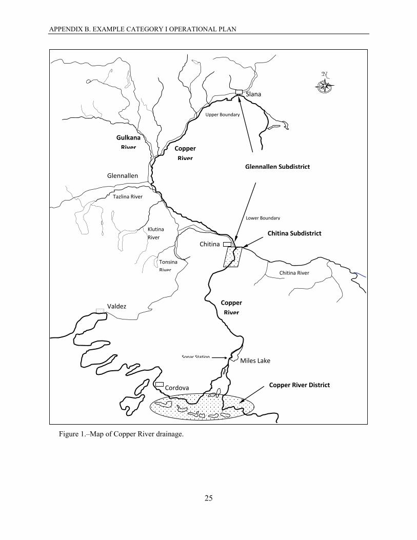
LIST OF FIGURES Figure Page 1 Map of Copper River drainage. .................................................................................................................... 25
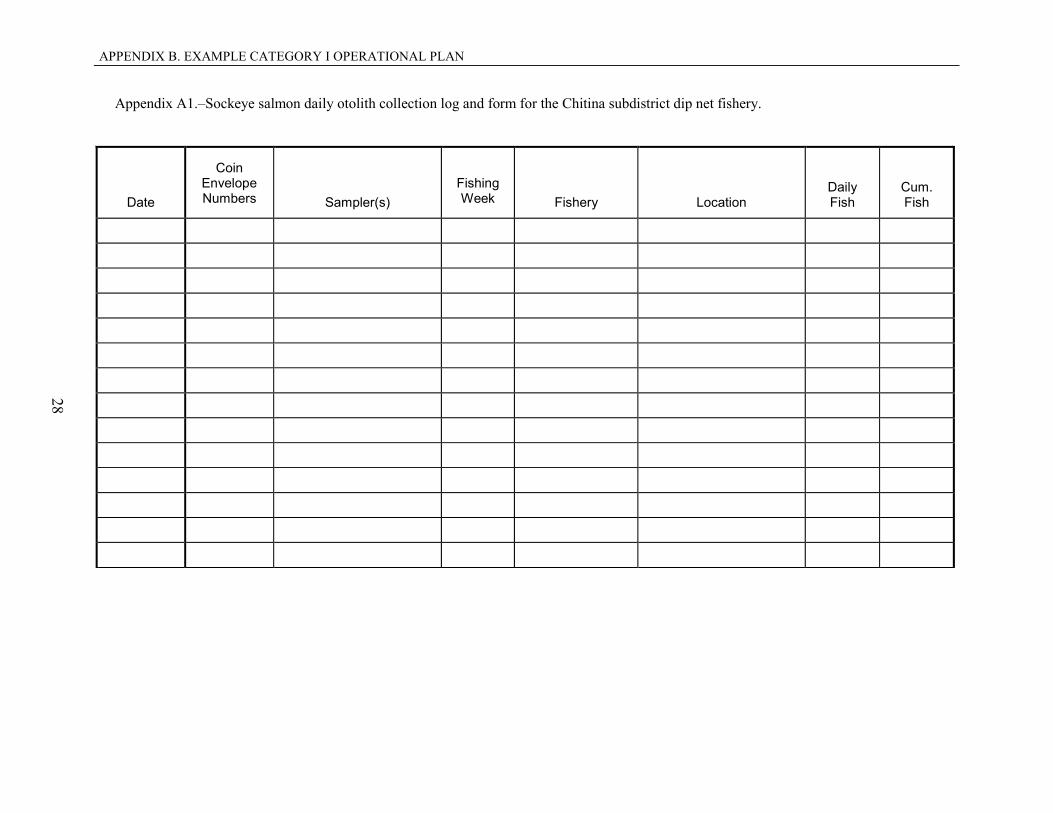
LIST OF APPENDICES Appendix Page A1. Sockeye salmon daily otolith collection log and form for the Chitina subdistrict dip net fishery. ................ 28
APPENDIX B. EXAMPLE CATEGORY I OPERATIONAL PLAN
24
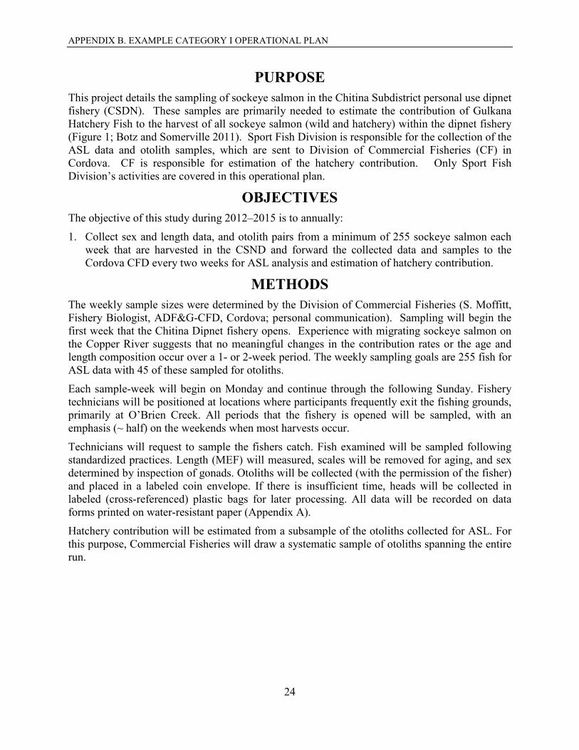
PURPOSE This project details the sampling of sockeye salmon in the Chitina Subdistrict personal use dipnet fishery (CSDN). These samples are primarily needed to estimate the contribution of Gulkana Hatchery Fish to the harvest of all sockeye salmon (wild and hatchery) within the dipnet fishery (Figure 1; Botz and Somerville 2011). Sport Fish Division is responsible for the collection of the ASL data and otolith samples, which are sent to Division of Commercial Fisheries (CF) in Cordova. CF is responsible for estimation of the hatchery contribution. Only Sport Fish Division’s activities are covered in this operational plan.
OBJECTIVES The objective of this study during 2012–2015 is to annually:
1. Collect sex and length data, and otolith pairs from a minimum of 255 sockeye salmon each week that are harvested in the CSND and forward the collected data and samples to the Cordova CFD every two weeks for ASL analysis and estimation of hatchery contribution.
METHODS The weekly sample sizes were determined by the Division of Commercial Fisheries (S. Moffitt, Fishery Biologist, ADF&G-CFD, Cordova; personal communication). Sampling will begin the first week that the Chitina Dipnet fishery opens. Experience with migrating sockeye salmon on the Copper River suggests that no meaningful changes in the contribution rates or the age and length composition occur over a 1- or 2-week period. The weekly sampling goals are 255 fish for ASL data with 45 of these sampled for otoliths.
Each sample-week will begin on Monday and continue through the following Sunday. Fishery technicians will be positioned at locations where participants frequently exit the fishing grounds, primarily at O’Brien Creek. All periods that the fishery is opened will be sampled, with an emphasis (~ half) on the weekends when most harvests occur.
Technicians will request to sample the fishers catch. Fish examined will be sampled following standardized practices. Length (MEF) will measured, scales will be removed for aging, and sex determined by inspection of gonads. Otoliths will be collected (with the permission of the fisher) and placed in a labeled coin envelope. If there is insufficient time, heads will be collected in labeled (cross-referenced) plastic bags for later processing. All data will be recorded on data forms printed on water-resistant paper (Appendix A).
Hatchery contribution will be estimated from a subsample of the otoliths collected for ASL. For this purpose, Commercial Fisheries will draw a systematic sample of otoliths spanning the entire run.
APPENDIX B. EXAMPLE CATEGORY I OPERATIONAL PLAN
25
Figure 1.–Map of Copper River drainage.
Slana
Tonsina River
Klutina River
Tazlina River
Glennallen
Valdez
Chitina
Copper River
Chitina River
Sonar Station
Cordova
Miles Lake
Gulkana River
Copper River District
Chitina Subdistrict
Glennallen Subdistrict
Lower Boundary
Upper Boundary
Copper River
APPENDIX B. EXAMPLE CATEGORY I OPERATIONAL PLAN
26
The number on the coin envelope containing otoliths will be entered on the daily otolith collection log (Appendix A) adjacent to the date, sampler, and fishery information. At the end of each day, the otoliths will be transferred to a master tray and data from the otolith collection log will be transferred to the otolith sampling form. A tray holds 96 paired sets of otoliths and must be completely filled before using a second tray (i.e. only if there are not enough wells in a tray for the entire day’s otoliths, a new tray will be used). Trays need not be separated by week, as tray numbering and sampling forms will identify the collection date. Both right and left otoliths will be removed from the fish and placed in the same well of the tray; if both are not removed from the salmon a bead will be placed in the tray with the single otolith so that the lab knows that one otolith was missing. Identifying labels will be placed on master trays, and sampling forms and trays will be shipped to the processing contractor and examined for strontium marks. Duplicate copies of the sampling forms will be made prior to shipping.
SCHEDULE AND DELIVERABLES The annual schedule of activities for the 2013–2016 fishing season is as follows:
Date Activity
June–August 31 Sampling occurs
Every two weeks Ship sockeye salmon scales, otoliths and corresponding data to CFD-Cordova
September 30 Final data sent to CFD-Cordova for analysis
December 1 Final data results and hatchery contribution determined and distributed by CF to SF-Glennallen
RESPONSIBILITIES Project Fisheries Biologist II Supervise project, assist in field sampling as needed
Project Fisheries Biologist I Crew leader, supervise daily activities and training of new personnel in sampling procedures and assist in field sampling as needed. Summarize the weekly sampling results. Send sampling summary and otoliths to Cordova bi-weekly.
REFERENCE CITED Botz, J. and M. A. Somerville. 2011. Management of salmon stocks in the Copper River, report to the Alaska Board
of Fisheries: December 2-7, 2011, Valdez, Alaska. Alaska Department of Fish and Game, Special Publication No. 11-13, Anchorage.
APPENDIX B. EXAMPLE CATEGORY I OPERATIONAL PLAN
27
APPENDIX A: SAMPLING FORMS
APPENDIX B. EXAMPLE CATEGORY I OPERATIONAL PLAN
28
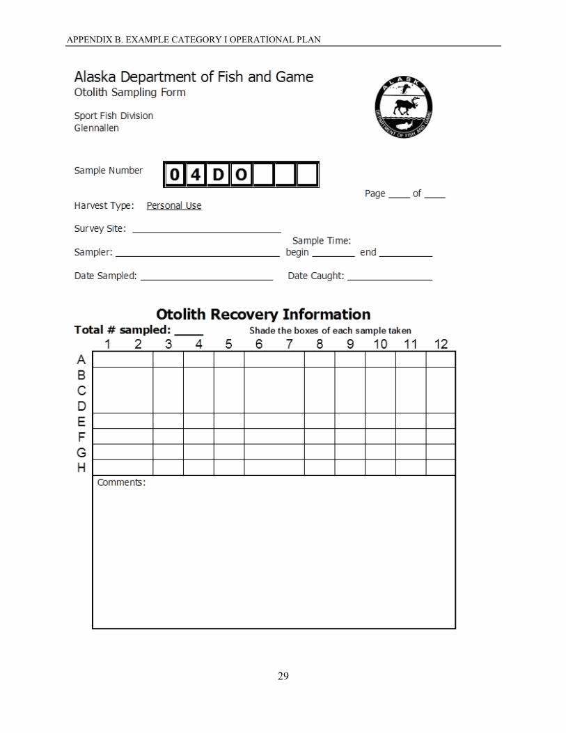
Appendix A1.–Sockeye salmon daily otolith collection log and form for the Chitina subdistrict dip net fishery.
Date
Coin Envelope Numbers
Sampler(s)
Fishing Week
Fishery
Location
Daily Fish
Cum. Fish
APPENDIX B. EXAMPLE CATEGORY I OPERATIONAL PLAN
29

30

31
APPENDIX C
EXAMPLE CATEGORY II OPERATIONAL PLAN
APPENDIX C. EXAMPLE CATEGORY II OPERATIONAL PLAN
32
Appendix C1.–Example of a category II operational plan with ROP format.
Regional Operational Plan SF.3F.12-02
Stock Assessment of Northern Pike in Volkmar Lake, 2013
by
Author Name
Month 20XX
Alaska Department of Fish and Game Divisions of Sport Fish and Commercial Fisheries

APPENDIX C. EXAMPLE CATEGORY II OPERATIONAL PLAN
Symbols and Abbreviations The following symbols and abbreviations, and others approved for the Système International d'Unités (SI), are used without definition in the following reports by the Divisions of Sport Fish and of Commercial Fisheries: Fishery Manuscripts, Fishery Data Series Reports, Fishery Management Reports, and Special Publications. All others, including deviations from definitions listed below, are noted in the text at first mention, as well as in the titles or footnotes of tables, and in figure or figure captions. Weights and measures (metric) centimeter cm deciliter dL gram g hectare ha kilogram kg kilometer km liter L meter m milliliter mL millimeter mm Weights and measures (English) cubic feet per second ft3/s foot ft gallon gal inch in mile mi nautical mile nmi ounce oz pound lb quart qt yard yd Time and temperature day d degrees Celsius °C degrees Fahrenheit °F degrees kelvin K hour h minute min second s Physics and chemistry all atomic symbols alternating current AC ampere A calorie cal direct current DC hertz Hz horsepower hp hydrogen ion activity pH (negative log of) parts per million ppm parts per thousand ppt, ‰ volts V watts W
General Alaska Administrative Code AAC all commonly accepted abbreviations e.g., Mr., Mrs.,
AM, PM, etc. all commonly accepted professional titles e.g., Dr., Ph.D., R.N., etc. at @ compass directions:
east E north N south S west W
copyright corporate suffixes:
Company Co. Corporation Corp. Incorporated Inc. Limited Ltd.
District of Columbia D.C. et alii (and others) et al. et cetera (and so forth) etc. exempli gratia (for example) e.g. Federal Information Code FIC id est (that is) i.e. latitude or longitude lat. or long. monetary symbols (U.S.) $, ¢ months (tables and figures): first three letters Jan,...,Dec registered trademark trademark United States (adjective) U.S. United States of America (noun) USA U.S.C. United States
Code U.S. state use two-letter
abbreviations (e.g., AK, WA)
Mathematics, statistics all standard mathematical signs, symbols and abbreviations alternate hypothesis HA base of natural logarithm e catch per unit effort CPUE coefficient of variation CV common test statistics (F, t, χ2, etc.) confidence interval CI correlation coefficient (multiple) R correlation coefficient (simple) r covariance cov degree (angular ) ° degrees of freedom df expected value E greater than > greater than or equal to ≥ harvest per unit effort HPUE less than < less than or equal to ≤ logarithm (natural) ln logarithm (base 10) log logarithm (specify base) log2, etc. minute (angular) ' not significant NS null hypothesis HO percent % probability P probability of a type I error (rejection of the null hypothesis when true) α probability of a type II error (acceptance of the null hypothesis when false) β second (angular) " standard deviation SD standard error SE variance population Var sample var
APPENDIX C. EXAMPLE CATEGORY II OPERATIONAL PLAN
REGIONAL OPERATIONAL PLAN SF.3F.12-02
STOCK ASSESSMENT OF NORTHERN PIKE IN VOLKMAR LAKE, 2013
by
Author Name
Alaska Department of Fish and Game, Division of Sport Fish, Fairbanks
Alaska Department of Fish and Game Division of Sport Fish, Research and Technical Services
1300 College Road, Fairbanks Alaska 99701
Month Year
APPENDIX C. EXAMPLE CATEGORY II OPERATIONAL PLAN
The Regional Operational Plan Series was established in 2012 to archive and provide public access to operational plans for fisheries projects of the Divisions of Commercial Fisheries and Sport Fish, as per joint-divisional Operational Planning Policy. Documents in this series are planning documents that may contain raw data, preliminary data analyses and results, and describe operational aspects of fisheries projects that may not actually be implemented. All documents in this series are subject to a technical review process and receive varying degrees of regional, divisional, and biometric approval, but do not generally receive editorial review. Results from the implementation of the operational plan described in this series may be subsequently finalized and published in a different department reporting series or in the formal literature. Please contact the author if you have any questions regarding the information provided in this plan. Regional Operational Plans are available on the Internet at: http://www.adfg.alaska.gov/sf/publications/
Author name, Alaska Department of Fish and Game, Division of Sport Fish,
1300 College Road, Fairbanks, AK 99701-1599 USA
This document should be cited as: Author Name. Year. Stock assessment of northern pike in Volkmar Lake, 2013. Alaska Department of Fish and
Game, Regional Operational Plan ROP.SF.3F.12-02, Fairbanks.
The Alaska Department of Fish and Game (ADF&G) administers all programs and activities free from discrimination based on race, color, national origin, age, sex, religion, marital status, pregnancy, parenthood, or disability. The department administers all programs and activities in compliance with Title VI of the Civil Rights Act of 1964, Section 504 of the Rehabilitation Act of 1973, Title II of the Americans with Disabilities Act (ADA) of 1990, the Age Discrimination Act of 1975, and Title IX of the Education Amendments of 1972.
If you believe you have been discriminated against in any program, activity, or facility please write: ADF&G ADA Coordinator, P.O. Box 115526, Juneau, AK 99811-5526
U.S. Fish and Wildlife Service, 4401 N. Fairfax Drive, MS 2042, Arlington, VA 22203 Office of Equal Opportunity, U.S. Department of the Interior, 1849 C Street NW MS 5230, Washington DC 20240
The department’s ADA Coordinator can be reached via phone at the following numbers: (VOICE) 907-465-6077, (Statewide Telecommunication Device for the Deaf) 1-800-478-3648,
(Juneau TDD) 907-465-3646, or (FAX) 907-465-6078 For information on alternative formats and questions on this publication, please contact:
ADF&G, Division of Sport Fish, Research and Technical Services, 333 Raspberry Rd, Anchorage AK 99518 (907) 267-2375
APPENDIX C. EXAMPLE CATEGORY II OPERATIONAL PLAN
36
SIGNATURE PAGE
Project Title: Stock Assessment of Northern Pike in Volkmar Lake, 2013
Project leader(s): Name, Title; e. g., Fishery Biologist III
Division, Region, and Area Sport Fish, Region III, Fairbanks
Project Nomenclature: FIS-104
Period Covered
Field Dates: June 4, 2013–June 25, 2013
Plan Type: Category II
Approval
Title Name Signature Date
Project leader
Biometrician
Research Coordinator
APPENDIX C. EXAMPLE CATEGORY II OPERATIONAL PLAN
37
TABLE OF CONTENTS Page
LIST OF TABLES....................................................................................................................................................... 37
LIST OF FIGURES ..................................................................................................................................................... 37
PURPOSE.................................................................................................................................................................... 38
BACKGROUND ......................................................................................................................................................... 38
OBJECTIVES .............................................................................................................................................................. 42 METHODS .................................................................................................................................................................. 42
SCHEDULE AND DELIVERABLES ........................................................................................................................ 49
RESPONSIBILITIES .................................................................................................................................................. 49
REFERENCES CITED ............................................................................................................................................... 50
LIST OF TABLES Table Page 1. Numbers of northern pike ≥450 mm FL marked and recaptured (≥2 days after being marked) by
sampling area for the mulit-event (8 days) experiment in Volkmar Lake during 2005. ................................ 44 2. Distribution of sampling effort for beach seining (S), gillnetting (G), and hook-and-line (H&L) during
both events of the mark-recapture experiment in Volkmar Lake. ................................................................... 45
LIST OF FIGURES
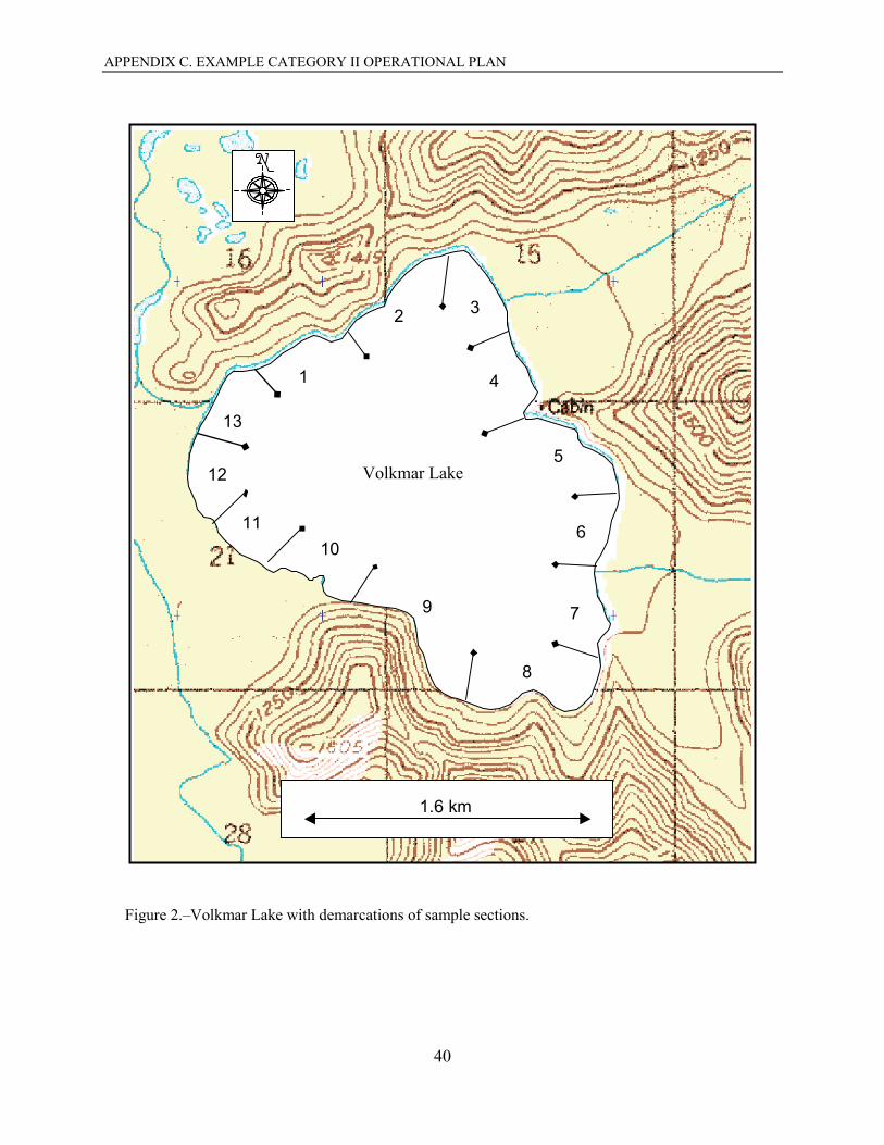
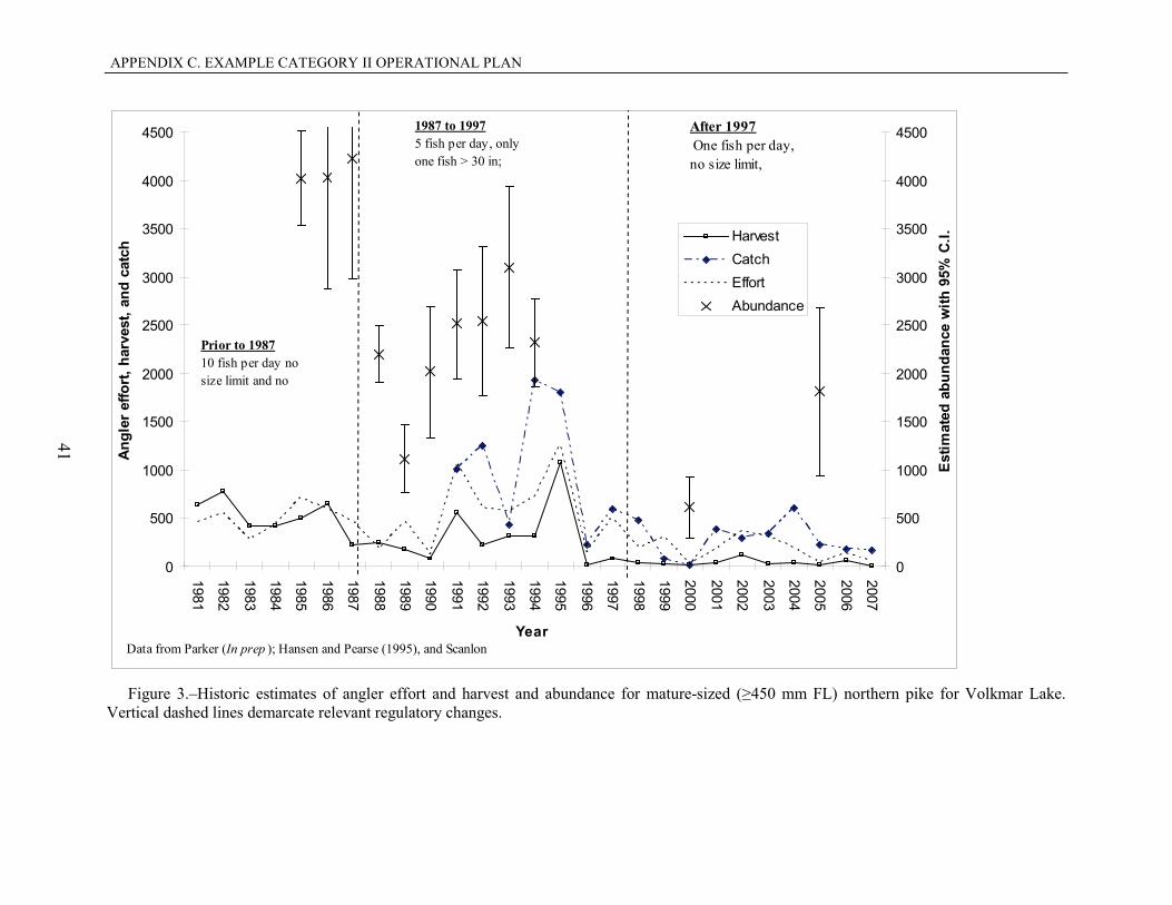
Figure Page 1. Location of Volkmar Lake. .............................................................................................................................. 39 2. Volkmar Lake with demarcations of sample sections. .................................................................................... 40 3. Historic estimates of angler effort and harvest and abundance for mature-sized (≥450 mm FL) northern
pike for Volkmar Lake. Vertical dashed lines demarcate relevant regulatory changes. ................................. 41
APPENDIX C. EXAMPLE CATEGORY II OPERATIONAL PLAN
38
PURPOSE A determination if the population of northen pike Esox lucius ≥450 mm FL in Volkmar Lake has reached a level above 2,000 fish is needed in order to address a regulatory proposal submitted but the department relative to the 2010 Alaska Board of Fisheries meeting. The proposed regulation would raise the bag limit from 1 to 3 fish to provide additional harvest opportunity. Based on recent catch, harvest and effort trends, a 3-fish bag limit should be sustainable provided the population size exceeds 2,000 northern pike (≥450mm). It was judged that annual harvests should not exceed 15% exploitation.
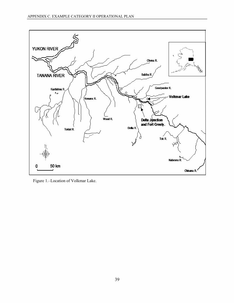
BACKGROUND Volkmar Lake is a semi-remote 373-ha lake located approximately 25 km northeast of Delta Junction (Figures 1 and 2). It is at an elevation of 326 m, has a maximum depth of 12.8 m, and a shoreline circumference of 8.2 km. The lake has two small inlets and an ill-defined outlet that drains westerly through wetlands towards the Goodpaster River. Nearshore waters are shallow, with beds of aquatic vegetation providing spawning and rearing substrate for northern pike. Volkmar Lake is typically ice-free from mid-May to early October and spawning of northern pike generally coincides with the beginning of the ice-free period and continues for up to two weeks into late May. Other fish species present in the lake include humpback whitefish Coregonus pidschian, least cisco C. sardinella, and slimy sculpin Cottus cognatus.
Volkmar Lake supports the second largest northern pike lake fishery in the Upper Tanana Management Area. The popularity of Volkmar Lake is attributed to: 1) its picturesque setting; 2) close proximity to Delta Junction and Fort Greely; 3) private lands and cabins around its shoreline; 4) the numerous recreational cabins and private lands along the neighboring Goodpaster River; and, 5) its relatively easy access. During the summer, access is restricted to float-equipped aircraft; therefore, fishing occurs almost exclusively during the winter and spring when most anglers access Volkmar Lake by snowmachining in from Quartz Lake and traveling along portions of the Goodpaster River or by crossing the Tanana River from Sawmill Creek Road, which extends out of Delta Junction.
Almost all of the sport fishing effort in Volkmar Lake is directed at northern pike because of the absence of other sport fishes. After a period of relatively stable effort and harvests during the 1980s, the popularity of Volkmar Lake peaked during the early to mid-1990s (Figure 3), after which effort, catch and harvest dropped off considerably. The drop in effort, harvest, and catch is attributed to an apparent sharp decline in the population size and a concomitant change in the fishing regulation. The decision to reduce the bag limit from five fish to one was based on the harvest of fish in 1995 (1,084 fish harvested) and an apparent decline in the population based on several reports in 1996 and 1997 from long-time users of the lake–no current stock status information was available. In 2000, a stock assessment was conducted and the estimated abundance of northern pike ≥450 mm FL was 615 (SE = 161), which confirmed suspicions of a reduced population size (Scanlon 2001).
APPENDIX C. EXAMPLE CATEGORY II OPERATIONAL PLAN
39
Figure 1.–Location of Volkmar Lake.
APPENDIX C. EXAMPLE CATEGORY II OPERATIONAL PLAN
40
Figure 2.–Volkmar Lake with demarcations of sample sections.
1.6 km
Volkmar Lake
1
2 3
4
6
5
9
10 11
12
13
7
8
Volkmar Lake
APPENDIX C. EXAMPLE CATEGORY II OPERATIONAL PLAN
41
Figure 3.–Historic estimates of angler effort and harvest and abundance for mature-sized (≥450 mm FL) northern pike for Volkmar Lake.
Vertical dashed lines demarcate relevant regulatory changes.
0
500
1000
1500
2000
2500
3000
3500
4000
4500
1981
1982
1983
1984
1985
1986
1987
1988
1989
1990
1991
1992
1993
1994
1995
1996
1997
1998
1999
2000
2001
2002
2003
2004
2005
2006
2007
Year
Angl
er e
ffort,
har
vest
, and
cat
ch
0
500
1000
1500
2000
2500
3000
3500
4000
4500
Estim
ated
abu
ndan
ce w
ith 9
5% C
.I.HarvestCatchEffortAbundance
1987 to 19975 fish per day, only one fish > 30 in;
After 1997 One fish per day, no size limit,
i i
Prior to 198710 fish per day no size limit and no
Data from Parker (In prep ); Hansen and Pearse (1995), and Scanlon
APPENDIX C. EXAMPLE CATEGORY II OPERATIONAL PLAN
42
In 2005, another stock assessment was conducted to address potential regulatory proposals by the public that sought to raise bag limits for the 2007 Board of Fisheries meeting. At this time catch reports from anglers, especially for mature-sized fish, indicated that the population may have rebounded from the low levels experienced in 2000. An estimated abundance of 2,000 fish ≥450 mm FL was selected by the area manager as the minimum threshold at which any regulatory changes that might increase harvest would be supported by the department. The threshold related directly to the desired spawning population size recommended by Hansen and Pearse (1995) that identified a sustainable harvest level of up to 300 fish. In 2005, the estimated abundance was 1,814 (SE = 864) fish ≥450 mm FL indicating an increase in population size, but the increase was insufficient to allow more liberal fishing regulations.
OBJECTIVES The research objectives for Volkmar Lake in 2009 will be to:
1. test the null hypothesis that the abundance of northern pike ≥450mm in Volkmar Lake is ≤2,000 with 50% power of rejecting the null hypothesis if the true abundance is ≥2,518 using alpha = 0.05;
2. estimate the abundance of the northern pike population ≥450 mm FL in Volkmar Lake during 2009 such that the estimate is within 25 percentage points of the actual value 95% of the time; and,
3. estimate the length composition of the northern pike population ≥450 mm FL in Volkmar Lake such that the estimates of proportions are within 5 percentage points of the actual value 95% of the time.
Objective 1 relates directly to the sustainable population size and the desired level of certainty needed to evaluate proposals to liberalize fishing regulations. Objective 2 is included because this level of precision is desired regardless of population size.
METHODS EXPERIMENTAL AND SAMPLING DESIGN The more recent studies at Volkmar Lake (1992–1994, 2000) have used multiple-event mark-recapture techniques for a closed population and the program CAPTURE (Rexstad and Burnham 1992) to estimate abundance. A sampling event consisted of systematically beach seining around the lake perimeter over a course of a day and approximately eight days of sampling were typically conducted. In 2005, this same approach was designed and employed, but during analysis the data had to be formatted as a Peterson two-sample mark-recapture experiment to estimate abundance (Wuttig and Reed In prep). The assumption that all northern pike will have a similar probability of capture during each sampling event (i.e. each day), or marked and unmarked northern pike will mix completely between events was unrealistic and could never be adequately satisfied. The effectiveness of a beach seine is highly dependent on the structure (i.e. shape and woody debris) of the shoreline, which is not uniform in Volkmar Lake. Based on the recommendations of Wuttig and Reed (In prep) the multi-event approach has been abandoned.
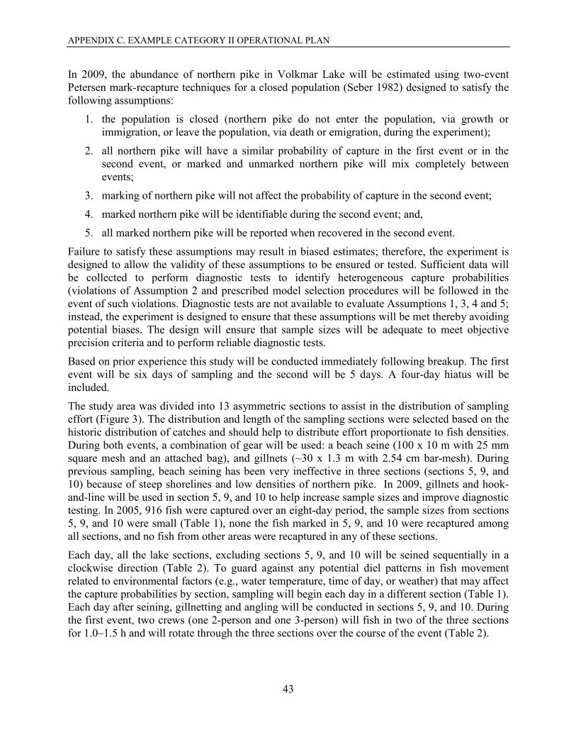
APPENDIX C. EXAMPLE CATEGORY II OPERATIONAL PLAN
43
In 2009, the abundance of northern pike in Volkmar Lake will be estimated using two-event Petersen mark-recapture techniques for a closed population (Seber 1982) designed to satisfy the following assumptions:
1. the population is closed (northern pike do not enter the population, via growth or immigration, or leave the population, via death or emigration, during the experiment);
2. all northern pike will have a similar probability of capture in the first event or in the second event, or marked and unmarked northern pike will mix completely between events;
3. marking of northern pike will not affect the probability of capture in the second event;
4. marked northern pike will be identifiable during the second event; and,
5. all marked northern pike will be reported when recovered in the second event.
Failure to satisfy these assumptions may result in biased estimates; therefore, the experiment is designed to allow the validity of these assumptions to be ensured or tested. Sufficient data will be collected to perform diagnostic tests to identify heterogeneous capture probabilities (violations of Assumption 2 and prescribed model selection procedures will be followed in the event of such violations. Diagnostic tests are not available to evaluate Assumptions 1, 3, 4 and 5; instead, the experiment is designed to ensure that these assumptions will be met thereby avoiding potential biases. The design will ensure that sample sizes will be adequate to meet objective precision criteria and to perform reliable diagnostic tests.
Based on prior experience this study will be conducted immediately following breakup. The first event will be six days of sampling and the second will be 5 days. A four-day hiatus will be included.
The study area was divided into 13 asymmetric sections to assist in the distribution of sampling effort (Figure 3). The distribution and length of the sampling sections were selected based on the historic distribution of catches and should help to distribute effort proportionate to fish densities. During both events, a combination of gear will be used: a beach seine (100 x 10 m with 25 mm square mesh and an attached bag), and gillnets (~30 x 1.3 m with 2.54 cm bar-mesh). During previous sampling, beach seining has been very ineffective in three sections (sections 5, 9, and 10) because of steep shorelines and low densities of northern pike. In 2009, gillnets and hook-and-line will be used in section 5, 9, and 10 to help increase sample sizes and improve diagnostic testing. In 2005, 916 fish were captured over an eight-day period, the sample sizes from sections 5, 9, and 10 were small (Table 1), none the fish marked in 5, 9, and 10 were recaptured among all sections, and no fish from other areas were recaptured in any of these sections.
Each day, all the lake sections, excluding sections 5, 9, and 10 will be seined sequentially in a clockwise direction (Table 2). To guard against any potential diel patterns in fish movement related to environmental factors (e.g., water temperature, time of day, or weather) that may affect the capture probabilities by section, sampling will begin each day in a different section (Table 1). Each day after seining, gillnetting and angling will be conducted in sections 5, 9, and 10. During the first event, two crews (one 2-person and one 3-person) will fish in two of the three sections for 1.0–1.5 h and will rotate through the three sections over the course of the event (Table 2).
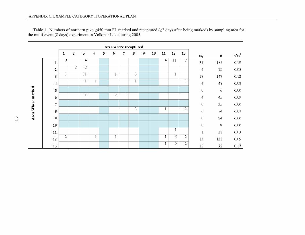
APPENDIX C. EXAMPLE CATEGORY II OPERATIONAL PLAN
44
Table 1.–Numbers of northern pike ≥450 mm FL marked and recaptured (≥2 days after being marked) by sampling area for the multi-event (8 days) experiment in Volkmar Lake during 2005.
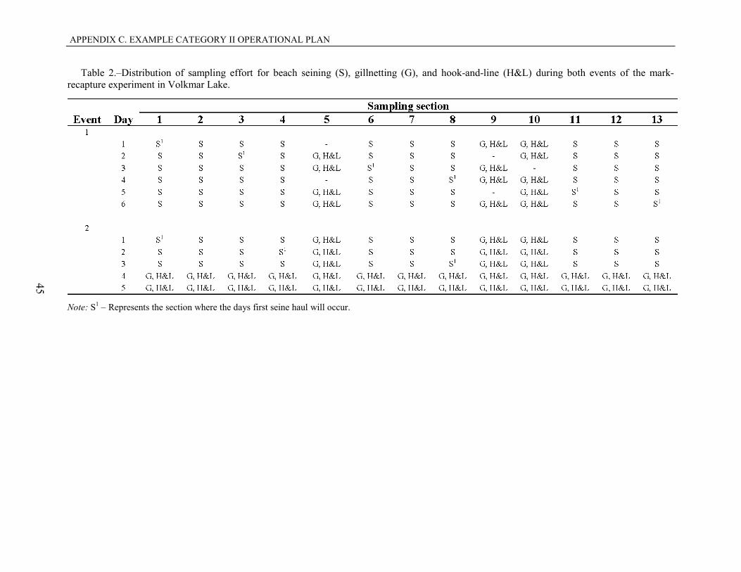
APPENDIX C. EXAMPLE CATEGORY II OPERATIONAL PLAN
45
Table 2.–Distribution of sampling effort for beach seining (S), gillnetting (G), and hook-and-line (H&L) during both events of the mark-recapture experiment in Volkmar Lake.
Note: S1 – Represents the section where the days first seine haul will occur.
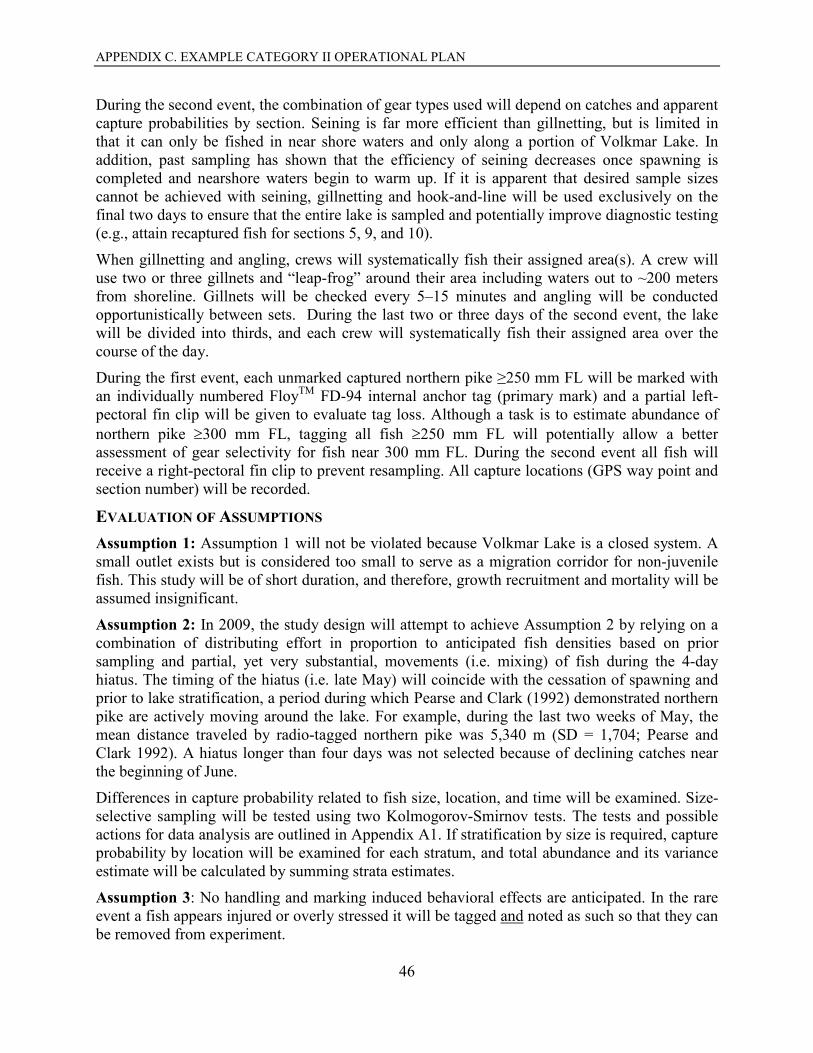
APPENDIX C. EXAMPLE CATEGORY II OPERATIONAL PLAN
46
During the second event, the combination of gear types used will depend on catches and apparent capture probabilities by section. Seining is far more efficient than gillnetting, but is limited in that it can only be fished in near shore waters and only along a portion of Volkmar Lake. In addition, past sampling has shown that the efficiency of seining decreases once spawning is completed and nearshore waters begin to warm up. If it is apparent that desired sample sizes cannot be achieved with seining, gillnetting and hook-and-line will be used exclusively on the final two days to ensure that the entire lake is sampled and potentially improve diagnostic testing (e.g., attain recaptured fish for sections 5, 9, and 10).
When gillnetting and angling, crews will systematically fish their assigned area(s). A crew will use two or three gillnets and “leap-frog” around their area including waters out to ~200 meters from shoreline. Gillnets will be checked every 5–15 minutes and angling will be conducted opportunistically between sets. During the last two or three days of the second event, the lake will be divided into thirds, and each crew will systematically fish their assigned area over the course of the day.
During the first event, each unmarked captured northern pike ≥250 mm FL will be marked with an individually numbered FloyTM FD-94 internal anchor tag (primary mark) and a partial left-pectoral fin clip will be given to evaluate tag loss. Although a task is to estimate abundance of northern pike ≥300 mm FL, tagging all fish ≥250 mm FL will potentially allow a better assessment of gear selectivity for fish near 300 mm FL. During the second event all fish will receive a right-pectoral fin clip to prevent resampling. All capture locations (GPS way point and section number) will be recorded.
EVALUATION OF ASSUMPTIONS Assumption 1: Assumption 1 will not be violated because Volkmar Lake is a closed system. A small outlet exists but is considered too small to serve as a migration corridor for non-juvenile fish. This study will be of short duration, and therefore, growth recruitment and mortality will be assumed insignificant.
Assumption 2: In 2009, the study design will attempt to achieve Assumption 2 by relying on a combination of distributing effort in proportion to anticipated fish densities based on prior sampling and partial, yet very substantial, movements (i.e. mixing) of fish during the 4-day hiatus. The timing of the hiatus (i.e. late May) will coincide with the cessation of spawning and prior to lake stratification, a period during which Pearse and Clark (1992) demonstrated northern pike are actively moving around the lake. For example, during the last two weeks of May, the mean distance traveled by radio-tagged northern pike was 5,340 m (SD = 1,704; Pearse and Clark 1992). A hiatus longer than four days was not selected because of declining catches near the beginning of June.
Differences in capture probability related to fish size, location, and time will be examined. Size-selective sampling will be tested using two Kolmogorov-Smirnov tests. The tests and possible actions for data analysis are outlined in Appendix A1. If stratification by size is required, capture probability by location will be examined for each stratum, and total abundance and its variance estimate will be calculated by summing strata estimates.
Assumption 3: No handling and marking induced behavioral effects are anticipated. In the rare event a fish appears injured or overly stressed it will be tagged and noted as such so that they can be removed from experiment.
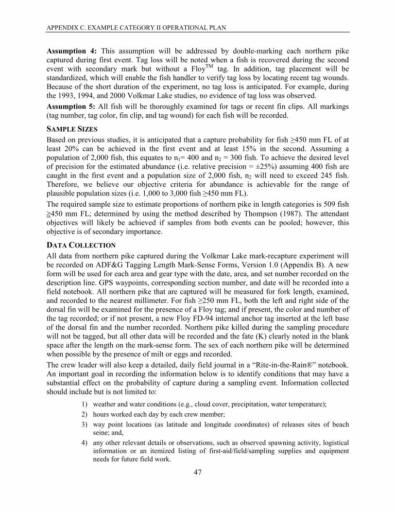
APPENDIX C. EXAMPLE CATEGORY II OPERATIONAL PLAN
47
Assumption 4: This assumption will be addressed by double-marking each northern pike captured during first event. Tag loss will be noted when a fish is recovered during the second event with secondary mark but without a FloyTM tag. In addition, tag placement will be standardized, which will enable the fish handler to verify tag loss by locating recent tag wounds. Because of the short duration of the experiment, no tag loss is anticipated. For example, during the 1993, 1994, and 2000 Volkmar Lake studies, no evidence of tag loss was observed. Assumption 5: All fish will be thoroughly examined for tags or recent fin clips. All markings (tag number, tag color, fin clip, and tag wound) for each fish will be recorded.
SAMPLE SIZES Based on previous studies, it is anticipated that a capture probability for fish ≥450 mm FL of at least 20% can be achieved in the first event and at least 15% in the second. Assuming a population of 2,000 fish, this equates to n1= 400 and n2 = 300 fish. To achieve the desired level of precision for the estimated abundance (i.e. relative precision = ±25%) assuming 400 fish are caught in the first event and a population size of 2,000 fish, n2 will need to exceed 245 fish. Therefore, we believe our objective criteria for abundance is achievable for the range of plausible population sizes (i.e. 1,000 to 3,000 fish ≥450 mm FL). The required sample size to estimate proportions of northern pike in length categories is 509 fish ≥450 mm FL; determined by using the method described by Thompson (1987). The attendant objectives will likely be achieved if samples from both events can be pooled; however, this objective is of secondary importance.
DATA COLLECTION All data from northern pike captured during the Volkmar Lake mark-recapture experiment will be recorded on ADF&G Tagging Length Mark-Sense Forms, Version 1.0 (Appendix B). A new form will be used for each area and gear type with the date, area, and set number recorded on the description line. GPS waypoints, corresponding section number, and date will be recorded into a field notebook. All northern pike that are captured will be measured for fork length, examined, and recorded to the nearest millimeter. For fish ≥250 mm FL, both the left and right side of the dorsal fin will be examined for the presence of a Floy tag; and if present, the color and number of the tag recorded; or if not present, a new Floy FD-94 internal anchor tag inserted at the left base of the dorsal fin and the number recorded. Northern pike killed during the sampling procedure will not be tagged, but all other data will be recorded and the fate (K) clearly noted in the blank space after the length on the mark-sense form. The sex of each northern pike will be determined when possible by the presence of milt or eggs and recorded. The crew leader will also keep a detailed, daily field journal in a “Rite-in-the-Rain®” notebook. An important goal in recording the information below is to identify conditions that may have a substantial effect on the probability of capture during a sampling event. Information collected should include but is not limited to:
1) weather and water conditions (e.g., cloud cover, precipitation, water temperature); 2) hours worked each day by each crew member; 3) way point locations (as latitude and longitude coordinates) of releases sites of beach
seine; and, 4) any other relevant details or observations, such as observed spawning activity, logistical
information or an itemized listing of first-aid/field/sampling supplies and equipment needs for future field work.
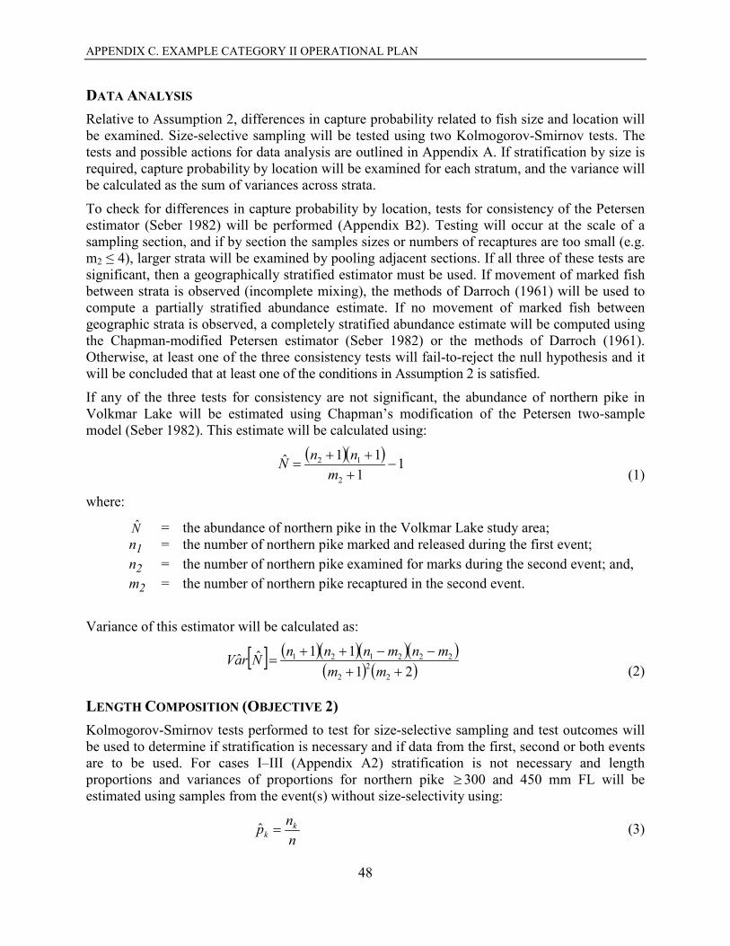
APPENDIX C. EXAMPLE CATEGORY II OPERATIONAL PLAN
48
DATA ANALYSIS Relative to Assumption 2, differences in capture probability related to fish size and location will be examined. Size-selective sampling will be tested using two Kolmogorov-Smirnov tests. The tests and possible actions for data analysis are outlined in Appendix A. If stratification by size is required, capture probability by location will be examined for each stratum, and the variance will be calculated as the sum of variances across strata.
To check for differences in capture probability by location, tests for consistency of the Petersen estimator (Seber 1982) will be performed (Appendix B2). Testing will occur at the scale of a sampling section, and if by section the samples sizes or numbers of recaptures are too small (e.g. m2 ≤ 4), larger strata will be examined by pooling adjacent sections. If all three of these tests are significant, then a geographically stratified estimator must be used. If movement of marked fish between strata is observed (incomplete mixing), the methods of Darroch (1961) will be used to compute a partially stratified abundance estimate. If no movement of marked fish between geographic strata is observed, a completely stratified abundance estimate will be computed using the Chapman-modified Petersen estimator (Seber 1982) or the methods of Darroch (1961). Otherwise, at least one of the three consistency tests will fail-to-reject the null hypothesis and it will be concluded that at least one of the conditions in Assumption 2 is satisfied.
If any of the three tests for consistency are not significant, the abundance of northern pike in Volkmar Lake will be estimated using Chapman’s modification of the Petersen two-sample model (Seber 1982). This estimate will be calculated using:
( )( ) 11
11ˆ2
12 −+
++=
mnnN
(1)
where:
N = the abundance of northern pike in the Volkmar Lake study area; n1 = the number of northern pike marked and released during the first event; n2 = the number of northern pike examined for marks during the second event; and, m2 = the number of northern pike recaptured in the second event.
Variance of this estimator will be calculated as:
[ ] ( )( )( )( )( ) ( )21
11ˆˆ2
22
222121
++−−++
=mm
mnmnnnNraV
(2)
LENGTH COMPOSITION (OBJECTIVE 2) Kolmogorov-Smirnov tests performed to test for size-selective sampling and test outcomes will be used to determine if stratification is necessary and if data from the first, second or both events are to be used. For cases I–III (Appendix A2) stratification is not necessary and length proportions and variances of proportions for northern pike ≥ 300 and 450 mm FL will be estimated using samples from the event(s) without size-selectivity using:
nnp k
k =ˆ (3)
APPENDIX C. EXAMPLE CATEGORY II OPERATIONAL PLAN
49
where:
=kp the proportion of northern pike that are within length category k;
nk = the number of northern pike sampled that are within length category k; and,
n = the total number of northern pike sampled. The unbiased variance of this proportion is estimated as (Cochran 1977):
[ ] ( )1ˆ1ˆˆˆ
−−
=n
pppV kkk (4)
If diagnostic tests indicate case IV, there is size-selectivity during both events and data must be stratified to eliminate variability in capture probabilities within strata for at least one or both sampling events. Formulae to adjust length composition estimates are presented in Appendix A1.
SCHEDULE AND DELIVERABLES Dates of sampling events in 2009 and other field and office activities are summarized below. All research results will be compiled in a State of Alaska Fisheries Data Series Report.
Date(s) Activity May 1 to May 13, 2009 Field preparations ~May 15, 2009 Start of first event. ~May 25, 2009 Start of second event October 1, 2009 Data entered into spreadsheet Dec 31, 2009 Data analysis complete February 1, 2010 Draft report submitted to project biometrician March 1, 2010 Draft report to research supervisor
RESPONSIBILITIES List of Personnel and Duties:
Fishery Biologist III Data analysis and report writing. Prepare sampling kits, sampling gear and arrange logistics. Oversee field activities and assist in sampling.
Biometrician II Duties: Assist in preparation of statistical design of field investigation for operational plan, and review data analysis and final report. Assist with capture, sampling, and data collection.
Fisheries Biologist I Assist with field preparations, supervision of field crews, and assist sampling.
Fish and Wildlife Technician III Duties: Assist with capture, sampling, and data collection.
Fish and Wildlife Technician IV Duties: Assist with capture, sampling, and data collection.
APPENDIX C. EXAMPLE CATEGORY II OPERATIONAL PLAN
50
REFERENCES CITED Bailey, N. T. J. 1951. On estimating the size of mobile populations from capture-recapture data. Biometrika
38:293-306.
Bailey, N. T. J. 1952. Improvements in the interpretation of recapture data. Journal of Animal Ecology 21:120-127.
Chapman, D. G. 1951. Some properties of the hypergeometric distribution with applications to zoological censuses. University of California Publications in Statistics 1:131-160.
Cochran, W. G. 1977. Sampling techniques. John Wiley and Sons, New York.
Conover, W. J. 1980. Practical nonparametric statistics 2nd ed. John Wiley & Sons, New York. 493pp.
Darroch, J. N. 1961. The two-sample capture-recapture census when tagging and sampling are stratified. Biometrika 48:241-260.
Hansen, P. A., and G. A. Pearse. 1995. Abundance and composition of northern pike in Volkmar and Deadman Lakes, 1994. Alaska Department of Fish and Game, Fishery Data Series No. 95-07, Anchorage.
Pearse, G. A., and J. H. Clark. 1992. Movements and distributions of radio tagged northern pike in Volkmar Lake. Alaska Department of Fish and Game, Fishery Data Series No. 92-28, Anchorage.
Rexstad, E., and K. Burnham. 1992. User's guide for the interactive program CAPTURE. Colorado Cooperative Fish and Wildlife Unit, Fort Collins, CO 80523. 29 pp. (includes Program CAPTURE).
Seber, G. A. F. 1982. The estimation of animal abundance and related parameters. Charles Griffin and Co., Ltd. London, U.K.
Scanlon, B. P. 2001. Abundance and composition of the northern pike populations in Volkmar Lake and Minto Flats, 2000. Alaska Department of Fish and Game, Fishery Data Series No. 01-29, Anchorage.
Thompson, S. K. 1987. Sample size for estimating multinomial proportions. American Statistician 41(1):122-132.
Wuttig, K. W. and D Reed. In prep. Abundance and composition of the northern pike in Volkmar Lake, 2005, and George Lake, 2006. Alaska Department of Fish and Game, Fishery Data Series, Anchorage.

APPENDIX C. EXAMPLE CATEGORY II OPERATIONAL PLAN
51
APPENDIX A
APPENDIX C. EXAMPLE CATEGORY II OPERATIONAL PLAN
52
Appendix A1.–Procedures for detecting and adjusting for size or sex selective sampling during a 2-sample mark recapture experiment.
Overview Size and sex selective sampling may result in the need to stratify by size and/or sex in order to obtain unbiased estimates of abundance and composition. In addition, the nature of the selectivity determines whether the first, second or both event samples are used for estimating composition. The Kolmogorov-Smirnov two sample (K-S) test (Conover 1980) is used to detect significant evidence that size selective sampling occurred during the first or second sampling events and contingency table analysis (Chi-square test) is generally used to detect significant evidence that sex selective sampling occurred during the first or second sampling events.
K-S tests are used to evaluate the second sampling event by comparing the length frequency distribution of all fish marked during the first event (M) with that of marked fish recaptured during the second event (R), using the null test hypothesis (Ho) of no difference. The first sampling event is evaluated by comparing the length frequency distribution of all fish inspected for marks during the second event (C) with that of R. Chi-square tests are used to compare the counts of observed males to females between M&R and C&R according to the null hypothesis that the probability that a sampled fish is male or female is independent of the sample. When the proportions by gender are estimated for a subsample (usually from C), rather than observed for all fish in the sample, contingency table analysis is not appropriate and the proportions of females (or males) are compared using a two sample test (e.g. Student’s t-test).
Mark-recapture experiments are designed to obtain sample sizes sufficient to 1) achieve precision objectives for abundance and composition estimates; and, 2) ensure that the diagnostic tests (i.e., tests for selectivity) have power adequate for identifying selectivity that could result in significantly biased estimates. Despite careful design, experiments may result in inadequate sample sizes leading to unreliable diagnostic test results due to low power. As a result, detection and adjusting for size and sex selectivity involves evaluating the power of the diagnostic tests.
The protocols that follow are used to classify the experiment into one of four cases. For each case the following are specified: 1) whether stratification is necessary; 2) which sample event’s data should be used when estimating composition; and, 3) the estimators to be used for composition estimates when stratifying. The first protocols assume adequate power. These are followed by supplemental protocols to be used when power is suspect and guidelines for evaluating power.
Protocols given Adequate Power Case I:
M vs. R C vs. R
Fail to reject Ho Fail to reject Ho
There is no size/sex selectivity detected during either sampling event. Abundance is calculated using a Petersen-type model from the entire data set without stratification. Composition parameters may be estimated after pooling length, sex, and age data from both sampling events.
Case II:
M vs. R C vs. R
Reject Ho Fail to reject Ho
There is no size/sex selectivity detected during the first event but there is during the second event sampling. Abundance is calculated using a Petersen-type model from the entire data set without stratification. Composition parameters may be estimated using length, sex, and age data from the first sampling event without stratification. If composition is estimated from second event data or after pooling both sampling events, data must first be stratified to eliminate variability in capture probability (detected by the M vs. R test) within strata. Composition parameters are estimated within strata, and abundance for each stratum needs to be estimated using a Petersen-type formula.
-continued-
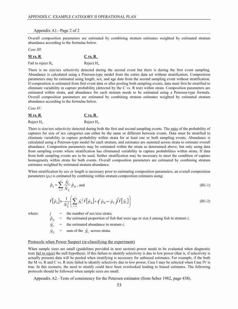
APPENDIX C. EXAMPLE CATEGORY II OPERATIONAL PLAN
53
Appendix A1.–Page 2 of 2
Overall composition parameters are estimated by combining stratum estimates weighted by estimated stratum abundance according to the formulae below.
Case III:
M vs. R C vs. R
Fail to reject Ho Reject Ho
There is no size/sex selectivity detected during the second event but there is during the first event sampling. Abundance is calculated using a Petersen-type model from the entire data set without stratification. Composition parameters may be estimated using length, sex, and age data from the second sampling event without stratification. If composition is estimated from first event data or after pooling both sampling events, data must first be stratified to eliminate variability in capture probability (detected by the C vs. R test) within strata. Composition parameters are estimated within strata, and abundance for each stratum needs to be estimated using a Petersen-type formula. Overall composition parameters are estimated by combining stratum estimates weighted by estimated stratum abundance according to the formulae below.
Case IV:
M vs. R C vs. R
Reject Ho Reject Ho
There is size/sex selectivity detected during both the first and second sampling events. The ratio of the probability of captures for size of sex categories can either be the same or different between events. Data must be stratified to eliminate variability in capture probability within strata for at least one or both sampling events. Abundance is calculated using a Petersen-type model for each stratum, and estimates are summed across strata to estimate overall abundance. Composition parameters may be estimated within the strata as determined above, but only using data from sampling events where stratification has eliminated variability in capture probabilities within strata. If data from both sampling events are to be used, further stratification may be necessary to meet the condition of capture homogeneity within strata for both events. Overall composition parameters are estimated by combining stratum estimates weighted by estimated stratum abundance.
When stratification by sex or length is necessary prior to estimating composition parameters, an overall composition parameters (pk) is estimated by combining within stratum composition estimates using:
∑= Σ
=j
iik
ik p
NNp
1, and (B1-1)
[ ] [ ] [ ]
+≈ ∑ −
=ΣNVpppVNN
pV i
j
ikikikik )(
1
222
1 (B1-2)
where: j = the number of sex/size strata; pikˆ = the estimated proportion of fish that were age or size k among fish in stratum i; N iˆ = the estimated abundance in stratum i; N Σ = sum of the N iˆ across strata.
Protocols when Power Suspect (re-classifying the experiment) When sample sizes are small (guidelines provided in next section) power needs to be evaluated when diagnostic tests fail to reject the null hypothesis. If this failure to identify selectivity is due to low power (that is, if selectivity is actually present) data will be pooled when stratifying is necessary for unbiased estimates. For example, if the both the M vs. R and C vs. R tests failed to identify selectivity due to low power, Case I may be selected when Case IV is true. In this scenario, the need to stratify could have been overlooked leading to biased estimates. The following protocols should be followed when sample sizes are small.
Appendix A2.–Tests of consistency for the Petersen estimator (from Seber 1982, page 438).
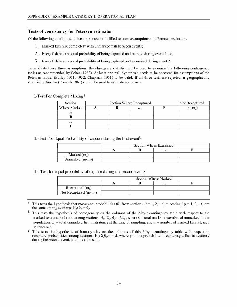
APPENDIX C. EXAMPLE CATEGORY II OPERATIONAL PLAN
54
Tests of consistency for Petersen estimator Of the following conditions, at least one must be fulfilled to meet assumptions of a Petersen estimator:
1. Marked fish mix completely with unmarked fish between events;
2. Every fish has an equal probability of being captured and marked during event 1; or,
3. Every fish has an equal probability of being captured and examined during event 2.
To evaluate these three assumptions, the chi-square statistic will be used to examine the following contingency tables as recommended by Seber (1982). At least one null hypothesis needs to be accepted for assumptions of the Petersen model (Bailey 1951, 1952; Chapman 1951) to be valid. If all three tests are rejected, a geographically stratified estimator (Darroch 1961) should be used to estimate abundance.
I.-Test For Complete Mixing a Section Section Where Recaptured Not Recaptured Where Marked A B … F (n1-m2) A B ... F
II.-Test For Equal Probability of capture during the first eventb Section Where Examined A B … F Marked (m2) Unmarked (n2-m2)
III.-Test for equal probability of capture during the second eventc
Section Where Marked A B … F Recaptured (m2) Not Recaptured (n1-m2)
a This tests the hypothesis that movement probabilities (θ) from section i (i = 1, 2, ...s) to section j (j = 1, 2, ...t) are
the same among sections: H0: θij = θj. b This tests the hypothesis of homogeneity on the columns of the 2-by-t contingency table with respect to the
marked to unmarked ratio among sections: H0: Σiaiθij = kUj , where k = total marks released/total unmarked in the population, Uj = total unmarked fish in stratum j at the time of sampling, and ai = number of marked fish released in stratum i.
c This tests the hypothesis of homogeneity on the columns of this 2-by-s contingency table with respect to recapture probabilities among sections: H0: Σjθijpj = d, where pj is the probability of capturing a fish in section j during the second event, and d is a constant.

APPENDIX C. EXAMPLE CATEGORY II OPERATIONAL PLAN
55
APPENDIX B
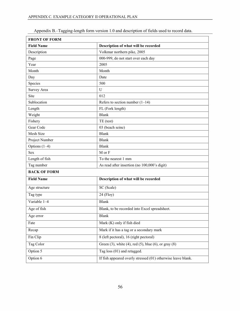
APPENDIX C. EXAMPLE CATEGORY II OPERATIONAL PLAN
56
Appendix B.–Tagging-length form version 1.0 and description of fields used to record data.
FRONT OF FORM Field Name Description of what will be recorded Description Volkmar northern pike, 2005 Page 000-999, do not start over each day Year 2005 Month Month Day Date Species 500 Survey Area U Site 012 Sublocation Refers to section number (1–14) Length FL (Fork length) Weight Blank Fishery TE (test) Gear Code 03 (beach seine) Mesh Size Blank Project Number Blank Options (1–4) Blank Sex M or F Length of fish To the nearest 1 mm Tag number As read after insertion (no 100,000’s digit)
BACK OF FORM
Field Name Description of what will be recorded
Age structure SC (Scale)
Tag type 24 (Floy)
Variable 1–4 Blank
Age of fish Blank, to be recorded into Excel spreadsheet.
Age error Blank
Fate Mark (K) only if fish died
Recap Mark if it has a tag or a secondary mark
Fin Clip 8 (left pectoral), 16 (right pectoral)
Tag Color Green (3), white (4), red (5), blue (6), or gray (8)
Option 5 Tag loss (01) and retagged.
Option 6 If fish appeared overly stressed (01) otherwise leave blank.
57
APPENDIX D
EXAMPLE CATEGORY III OPERATIONAL PLAN
APPENDIX D. EXAMPLE CATEGORY III OPERATIONAL PLAN
58
Appendix D1.–Example of a category III operational plan with ROP format.
Regional Operational Plan SF.1J.11-01
2011 Southeast Alaska Marine Boat Sport Fishery Harvest Studies
by
Mike Jaenicke
and
Allen E. Bingham
April 2011
Alaska Department of Fish and Game Divisions of Sport Fish and Commercial Fisheries
APPENDIX D. EXAMPLE CATEGORY III OPERATIONAL PLAN
Symbols and Abbreviations The following symbols and abbreviations, and others approved for the Système International d'Unités (SI), are used without definition in the following reports by the Divisions of Sport Fish and of Commercial Fisheries: Fishery Manuscripts, Fishery Data Series Reports, Fishery Management Reports, and Special Publications. All others, including deviations from definitions listed below, are noted in the text at first mention, as well as in the titles or footnotes of tables, and in figure or figure captions. Weights and measures (metric) centimeter cm deciliter dL gram g hectare ha kilogram kg kilometer km liter L meter m milliliter mL millimeter mm Weights and measures (English) cubic feet per second ft3/s foot ft gallon gal inch in mile mi nautical mile nmi ounce oz pound lb quart qt yard yd Time and temperature day d degrees Celsius °C degrees Fahrenheit °F degrees kelvin K hour h minute min second s Physics and chemistry all atomic symbols alternating current AC ampere A calorie cal direct current DC hertz Hz horsepower hp hydrogen ion activity pH (negative log of) parts per million ppm parts per thousand ppt, ‰ volts V watts W
General Alaska Administrative Code AAC all commonly accepted abbreviations e.g., Mr., Mrs.,
AM, PM, etc. all commonly accepted professional titles e.g., Dr., Ph.D., R.N., etc. at @ compass directions:
east E north N south S west W
copyright corporate suffixes:
Company Co. Corporation Corp. Incorporated Inc. Limited Ltd.
District of Columbia D.C. et alii (and others) et al. et cetera (and so forth) etc. exempli gratia (for example) e.g. Federal Information Code FIC id est (that is) i.e. latitude or longitude lat. or long. monetary symbols (U.S.) $, ¢ months (tables and figures): first three letters Jan,...,Dec registered trademark trademark United States (adjective) U.S. United States of America (noun) USA U.S.C. United States
Code U.S. state use two-letter
abbreviations (e.g., AK, WA)
Mathematics, statistics all standard mathematical signs, symbols and abbreviations alternate hypothesis HA base of natural logarithm e catch per unit effort CPUE coefficient of variation CV common test statistics (F, t, χ2, etc.) confidence interval CI correlation coefficient (multiple) R correlation coefficient (simple) r covariance cov degree (angular ) ° degrees of freedom df expected value E greater than > greater than or equal to ≥ harvest per unit effort HPUE less than < less than or equal to ≤ logarithm (natural) ln logarithm (base 10) log logarithm (specify base) log2, etc. minute (angular) ' not significant NS null hypothesis HO percent % probability P probability of a type I error (rejection of the null hypothesis when true) α probability of a type II error (acceptance of the null hypothesis when false) β second (angular) " standard deviation SD standard error SE variance population Var sample var
APPENDIX D. EXAMPLE CATEGORY III OPERATIONAL PLAN
REGIONAL OPERATIONAL PLAN SF.1J.11-01
2011 SOUTHEAST ALASKA MARINE BOAT SPORT FISHERY HARVEST STUDIES
by
Mike Jaenicke Alaska Department of Fish and Game, Division of Sport Fish, Juneau
and
Allen E. Bingham Alaska Department of Fish and Game, Division of Sport Fish, Anchorage.
Alaska Department of Fish and Game Division of Sport Fish,
802 3rd Street, Douglas, AK 99824
April 2011
APPENDIX D. EXAMPLE CATEGORY III OPERATIONAL PLAN
25
The Regional Operational Plan Series was established in 2012 to archive and provide public access to operational plans for fisheries projects of the Divisions of Commercial Fisheries and Sport Fish, as per joint-divisional Operational Planning Policy. Documents in this series are planning documents that may contain raw data, preliminary data analyses and results, and describe operational aspects of fisheries projects that may not actually be implemented. All documents in this series are subject to a technical review process and receive varying degrees of regional, divisional, and biometric approval, but do not generally receive editorial review. Results from the implementation of the operational plan described in this series may be subsequently finalized and published in a different department reporting series or in the formal literature. Please contact the author if you have any questions regarding the information provided in this plan. Regional Operational Plans are available on the Internet at: http://www.adfg.alaska.gov/sf/publications/
Mike Jaenicke, Alaska Department of Fish and Game, Division of Sport Fish,
802 3rd Street, Douglas, AK 99824 and
Allen E. Bingham Alaska Department of Fish and Game, Division of Sport Fish
333 Raspberry Road Anchorage, Alaska 99518
This document should be cited as: M. Jaenicke and Bingham, A. E. 2011. 2011 Southeast Alaska marine boat sport fishery harvest studies, 2011.
Alaska Department of Fish and Game, Regional Operational Plan ROP.SF.IJ.11-01, Juneau.
The Alaska Department of Fish and Game (ADF&G) administers all programs and activities free from discrimination based on race, color, national origin, age, sex, religion, marital status, pregnancy, parenthood, or disability. The department administers all programs and activities in compliance with Title VI of the Civil Rights Act of 1964, Section 504 of the Rehabilitation Act of 1973, Title II of the Americans with Disabilities Act (ADA) of 1990, the Age Discrimination Act of 1975, and Title IX of the Education Amendments of 1972.
If you believe you have been discriminated against in any program, activity, or facility please write: ADF&G ADA Coordinator, P.O. Box 115526, Juneau, AK 99811-5526
U.S. Fish and Wildlife Service, 4401 N. Fairfax Drive, MS 2042, Arlington, VA 22203 Office of Equal Opportunity, U.S. Department of the Interior, 1849 C Street NW MS 5230, Washington DC 20240
The department’s ADA Coordinator can be reached via phone at the following numbers: (VOICE) 907-465-6077, (Statewide Telecommunication Device for the Deaf) 1-800-478-3648,
(Juneau TDD) 907-465-3646, or (FAX) 907-465-6078 For information on alternative formats and questions on this publication, please contact:
ADF&G, Division of Sport Fish, Research and Technical Services, 333 Raspberry Rd, Anchorage AK 99518 (907) 267-2375
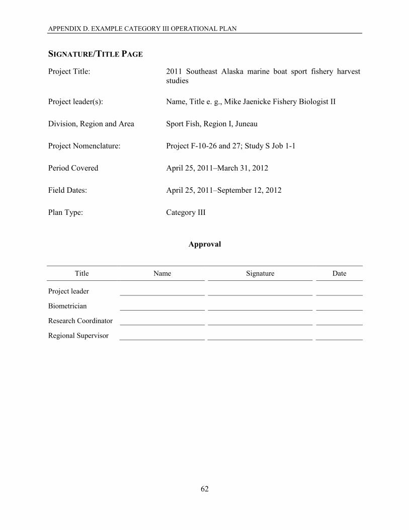
APPENDIX D. EXAMPLE CATEGORY III OPERATIONAL PLAN
62
SIGNATURE/TITLE PAGE
Project Title: 2011 Southeast Alaska marine boat sport fishery harvest studies
Project leader(s): Name, Title e. g., Mike Jaenicke Fishery Biologist II
Division, Region and Area Sport Fish, Region I, Juneau
Project Nomenclature: Project F-10-26 and 27; Study S Job 1-1
Period Covered April 25, 2011–March 31, 2012
Field Dates: April 25, 2011–September 12, 2012
Plan Type: Category III
Approval
Title Name Signature Date
Project leader
Biometrician
Research Coordinator
Regional Supervisor
APPENDIX D. EXAMPLE CATEGORY III OPERATIONAL PLAN
63
TABLE OF CONTENTS Page
PURPOSE.................................................................................................................................................................... 65
BACKGROUND ......................................................................................................................................................... 65
Chinook Salmon .......................................................................................................................................................... 66 Coho Salmon ............................................................................................................................................................... 69 Other Species ............................................................................................................................................................... 69 OBJECTIVES .............................................................................................................................................................. 71
Primary objectives ....................................................................................................................................................... 71 Secondary objectives ................................................................................................................................................... 72 METHODS .................................................................................................................................................................. 73
Generalized Procedures ............................................................................................................................................... 73 Study Design ............................................................................................................................................................... 74
Preliminary 2011 Total Sport Harvest of Chinook and Coho Salmon (Objectives 1a, 3a) .................................... 77 Hatchery and Non-Hatchery Contributions-Chinook and Coho Salmon (Objectives 1b and 3b) .......................... 77 Pacific Salmon Treaty Harvest (Objectives 1c and 2) ............................................................................................ 77 Average Weight Estimates (Objective 4), and Length Composition (Secondary Objective 1) of Pacific Halibut .................................................................................................................................................................... 79 Proportion of Pacific Halibut Harvested by Unguided Anglers Prior to Mean IPHC Survey Date (Objective 5) ............................................................................................................................................................................. 81 Average Weight and Preliminary Biomass Estimates of Lingcod (Objective 6) .................................................... 81 Rockfish Species Composition; and Average Weight Estimates and Preliminary Biomass of Demersal Shelf
Rockfish (Objective 7) ...................................................................................................................................... 82 Release Estimates for Chinook Salmon, Rockfish, Pacific Halibut, and Lingcod (Objective 8) ............................ 82 Weekly Harvest per Unit Effort of Chinook and Coho Salmon and Pacific Halibut (Secondary Objectives 2 and 3) ...................................................................................................................................................................... 82 Mid-season Projected Preliminary 2011 Harvest of Lingcod and Yelloweye Rockfish (Secondary Objectives 4 and 5)....................................................................................................................................................................... 83 Estimates of Genetic Composition of Chinook Salmon Harvest (Secondary Objective 6) .................................... 83
Data Collection ............................................................................................................................................................ 84 Creel Samplers ........................................................................................................................................................ 84 Catch Samplers ....................................................................................................................................................... 86
Data Reduction ............................................................................................................................................................ 86 Data Analysis ............................................................................................................................................................... 87
General Estimation Approach ................................................................................................................................. 87 Intrinsic Parameter Estimates ........................................................................................................................ 87 2011 Preliminary Estimates ........................................................................................................................... 98 Mid-season Projections ............................................................................................................................... 100
Preliminary 2011 Total Sport Harvest of Chinook and Coho Salmon (Objectives 1a and 3a) ............................. 101 Hatchery and Non-Hatchery Contributions-Chinook and Coho Salmon (Objectives 1b and 3b) ......................... 102 Pacific Salmon Treaty Harvest (Objectives 1c and 2) .......................................................................................... 103 Average Weight Estimates (Objective 4), and Length Composition (Secondary Objective 1) of Pacific Halibut .................................................................................................................................................................. 104 Proportion of Pacific Halibut Harvested by Unguided Anglers Prior to Mean IPHC Survey Date (Objective 5) ........................................................................................................................................................................... 105 Average Weight and Preliminary Biomass Estimates of Lingcod (Objective 6) .................................................. 105 Rockfish Species Composition; and Average Weight Estimates and Preliminary Biomass Removals of
Demersal Shelf Rockfish (Objective 7) .......................................................................................................... 106 Estimates of the Proportion Released for Chinook Salmon, Rockfish, Pacific Halibut, and Lingcod (Objective 8) ......................................................................................................................................................... 108
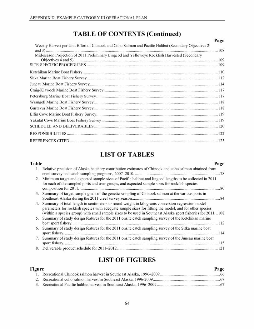
APPENDIX D. EXAMPLE CATEGORY III OPERATIONAL PLAN
64
TABLE OF CONTENTS (Continued) Page
Weekly Harvest per Unit Effort of Chinook and Coho Salmon and Pacific Halibut (Secondary Objectives 2 and 3) .................................................................................................................................................................... 108 Mid-season Projection of 2011 Preliminary Lingcod and Yelloweye Rockfish Harvested (Secondary
Objectives 4 and 5) ......................................................................................................................................... 109 SITE-SPECIFIC PROCEDURES ............................................................................................................................. 109 Ketchikan Marine Boat Fishery ................................................................................................................................. 110 Sitka Marine Boat Fishery Survey ............................................................................................................................. 112 Juneau Marine Boat Fishery Survey .......................................................................................................................... 114 Craig/Klawock Marine Boat Fishery Survey ............................................................................................................. 117 Petersburg Marine Boat Fishery Survey .................................................................................................................... 117 Wrangell Marine Boat Fishery Survey ...................................................................................................................... 118 Gustavus Marine Boat Fishery Survey ...................................................................................................................... 118 Elfin Cove Marine Boat Fishery Survey .................................................................................................................... 119 Yakutat Cove Marine Boat Fishery Survey ............................................................................................................... 119 SCHEDULE AND DELIVERABLES ...................................................................................................................... 120
RESPONSIBILITIES ................................................................................................................................................ 122
REFERENCES CITED ............................................................................................................................................. 123
LIST OF TABLES Table Page 1. Relative precision of Alaska hatchery contribution estimates of Chinook and coho salmon obtained from
creel survey and catch sampling programs, 2007–2010. ................................................................................. 78 2. Minimum target and expected sample sizes of Pacific halibut and lingcod lengths to be collected in 2011
for each of the sampled ports and user groups, and expected sample sizes for rockfish species composition for 2011. ...................................................................................................................................... 80
3. Summary of target sample goals of the genetic sampling of Chinook salmon at the various ports in Southeast Alaska during the 2011 creel survey season. ................................................................................... 84
4. Summary of total length in centimeters to round weight in kilograms conversion-regression model parameters for rockfish species with adequate sample sizes for fitting the model, and for other species (within a species group) with small sample sizes to be used in Southeast Alaska sport fisheries for 2011. .. 108
5. Summary of study design features for the 2011 onsite catch sampling survey of the Ketchikan marine boat sport fishery. .......................................................................................................................................... 112
6. Summary of study design features for the 2011 onsite catch sampling survey of the Sitka marine boat sport fishery. .................................................................................................................................................. 114
7. Summary of study design features for the 2011 onsite catch sampling survey of the Juneau marine boat sport fishery. .................................................................................................................................................. 115
8. Deliverable product schedule for 2011–2012. ............................................................................................... 121
LIST OF FIGURES Figure Page 1. Recreational Chinook salmon harvest in Southeast Alaska, 1996–2009 ......................................................... 66 2. Recreational coho salmon harvest in Southeast Alaska, 1996-2009 ................................................................ 67 3. Recreational Pacific halibut harvest in Southeast Alaska, 1996–2009 ............................................................ 67
APPENDIX D. EXAMPLE CATEGORY III OPERATIONAL PLAN
65
PURPOSE The primarily purpose of this project is to estimate the harvest of Chinook salmon Oncorhynchus tshawytscha, coho salmon O. kisutch, and Pacific halibut Hippoglossus stenolepis for the marine boat sport fisheries in Southeast Alaska, and secondarily for rockfish Sebastes spp. and lingcod Ophiodon elongates (Figures 1–3). These fisheries are diverse and effort is mostly concentrated around the major communities of Juneau, Ketchikan, Sitka, Wrangell, and Petersburg. Substantial effort is also expended near remote fishing lodges and smaller communities throughout the region such as Craig/Klawock, Gustavus, Elfin Cove, and Yakutat. The data needs and impetus for management of all these species varies.
The generalized approach is to survey sport anglers and sample their catches at primary access points such as harbors and boat launches and use this data together with the Statewide Harvest Survey (SWHS)3 to estimate desired parameters. For example, relative to Chinook salmon the state has an obligation to estimate the contribution of Canadian stocks under the US/Canada Pacific Salmon Treaty (Public Law 99-5) and identification of coded wired tags (CWT) is critical. The sport charter harvest of Pacific halibut is managed under a guideline harvest level (GHL) adopted by the North Pacific Fisheries Management Council (NPFMC) and port sampling provides essential data on lengths and average weights needed for estimating harvested biomass by guided and unguided fishers. Harvest per unit effort (HPUE) for coho salmon in the Juneau and Ketchikan marine sport fisheries is used to monitor the relative abundance and movement of coho salmon to inside waters from early June to September depending on the strength of the run, and the Juneau HPUE is specifically cited in 5 AAC 29.110 (Management of Coho Salmon Troll Fishery).
BACKGROUND The 2011 project has undergone a relatively major redesign of survey procedures from previous years for the major ports of Juneau, Ketchikan, and Sitka, along with some adaptations to survey procedures in the minor ports. The redesign was prompted both not only to fit the project within current budgetary constraints, but also to address the changing nature of the types of information needed for managing the marine boat sport fisheries in Southeast Alaska. Correspondingly, the Statewide Harvest Survey (SWHS)4 is also undergoing a redesign for 2011. Due to the nature of the underlying procedure for obtaining the preliminary values for the final estimates associated with the primary objectives for this project (see the Objectives section below), the values obtained by the project for 2011 are expected to be subject to unknown error that will not be evident until completion of paired SWHS and on-site harvest sampling data with the two new designs (see additional details regarding these constraints in the Study Design section).
This operational plan represents the planning conducted to-date to implement the redesign of the project for 2011. The plan documents the study design, sample size goals, sampling schedules, data collection and recording protocols to be implemented for the 2011 survey. The data reduction and data analysis procedures presented herein are likely to be revised as further planning and analysis (e.g., simulation of the sampling design with past-year data) is completed following the initiation of field activities in late April.
Marine boat sport fisheries primarily targeted on Chinook salmon Oncorhynchus tshawytscha, coho salmon O. kisutch, and Pacific halibut Hippoglossus stenolepis are the largest sport
3 The annual mail survey of licensed sport anglers in Alaska conducted by ADF&G, Division of Sport Fish. 4 The annual mail survey of licensed sport anglers in Alaska conducted by ADF&G, Division of Sport Fish.
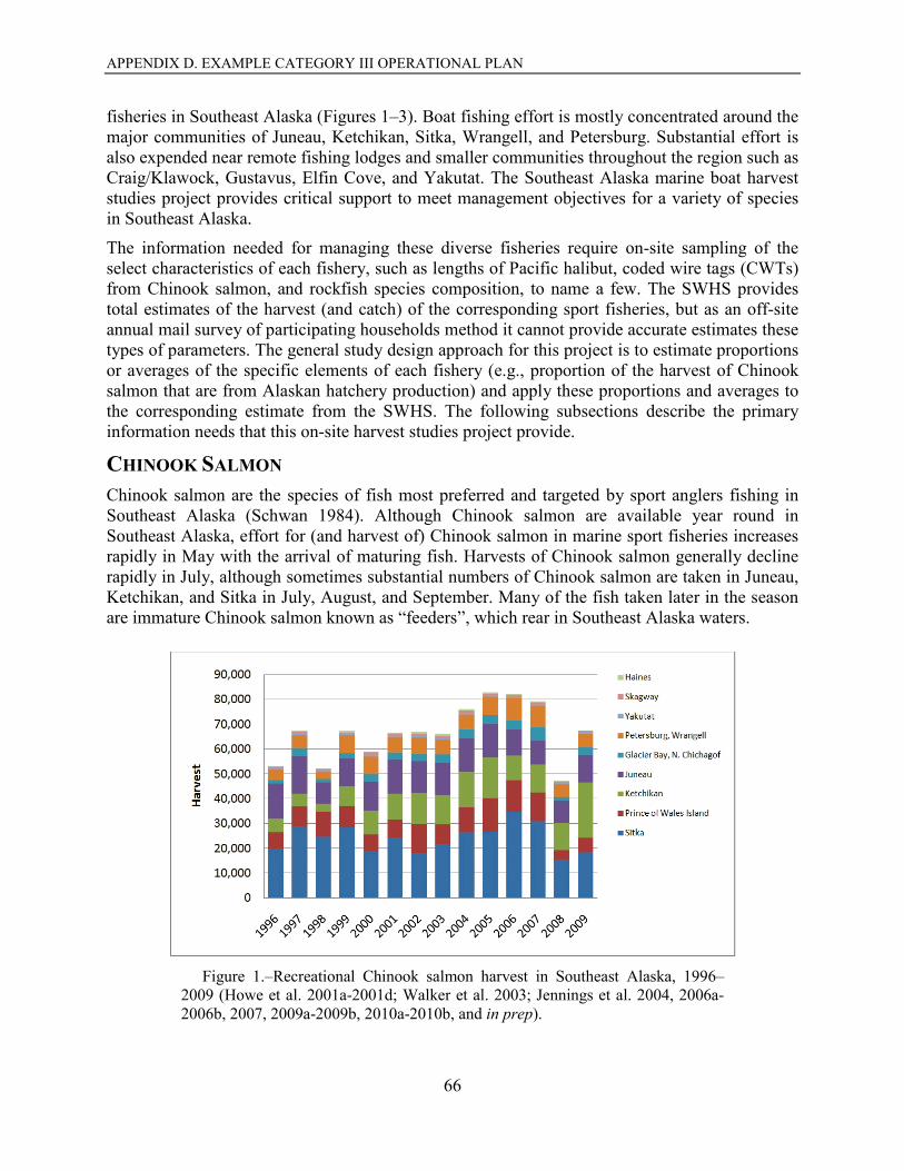
APPENDIX D. EXAMPLE CATEGORY III OPERATIONAL PLAN
66
fisheries in Southeast Alaska (Figures 1–3). Boat fishing effort is mostly concentrated around the major communities of Juneau, Ketchikan, Sitka, Wrangell, and Petersburg. Substantial effort is also expended near remote fishing lodges and smaller communities throughout the region such as Craig/Klawock, Gustavus, Elfin Cove, and Yakutat. The Southeast Alaska marine boat harvest studies project provides critical support to meet management objectives for a variety of species in Southeast Alaska.
The information needed for managing these diverse fisheries require on-site sampling of the select characteristics of each fishery, such as lengths of Pacific halibut, coded wire tags (CWTs) from Chinook salmon, and rockfish species composition, to name a few. The SWHS provides total estimates of the harvest (and catch) of the corresponding sport fisheries, but as an off-site annual mail survey of participating households method it cannot provide accurate estimates these types of parameters. The general study design approach for this project is to estimate proportions or averages of the specific elements of each fishery (e.g., proportion of the harvest of Chinook salmon that are from Alaskan hatchery production) and apply these proportions and averages to the corresponding estimate from the SWHS. The following subsections describe the primary information needs that this on-site harvest studies project provide.
CHINOOK SALMON Chinook salmon are the species of fish most preferred and targeted by sport anglers fishing in Southeast Alaska (Schwan 1984). Although Chinook salmon are available year round in Southeast Alaska, effort for (and harvest of) Chinook salmon in marine sport fisheries increases rapidly in May with the arrival of maturing fish. Harvests of Chinook salmon generally decline rapidly in July, although sometimes substantial numbers of Chinook salmon are taken in Juneau, Ketchikan, and Sitka in July, August, and September. Many of the fish taken later in the season are immature Chinook salmon known as “feeders”, which rear in Southeast Alaska waters.
Figure 1.–Recreational Chinook salmon harvest in Southeast Alaska, 1996–
2009 (Howe et al. 2001a-2001d; Walker et al. 2003; Jennings et al. 2004, 2006a-2006b, 2007, 2009a-2009b, 2010a-2010b, and in prep).
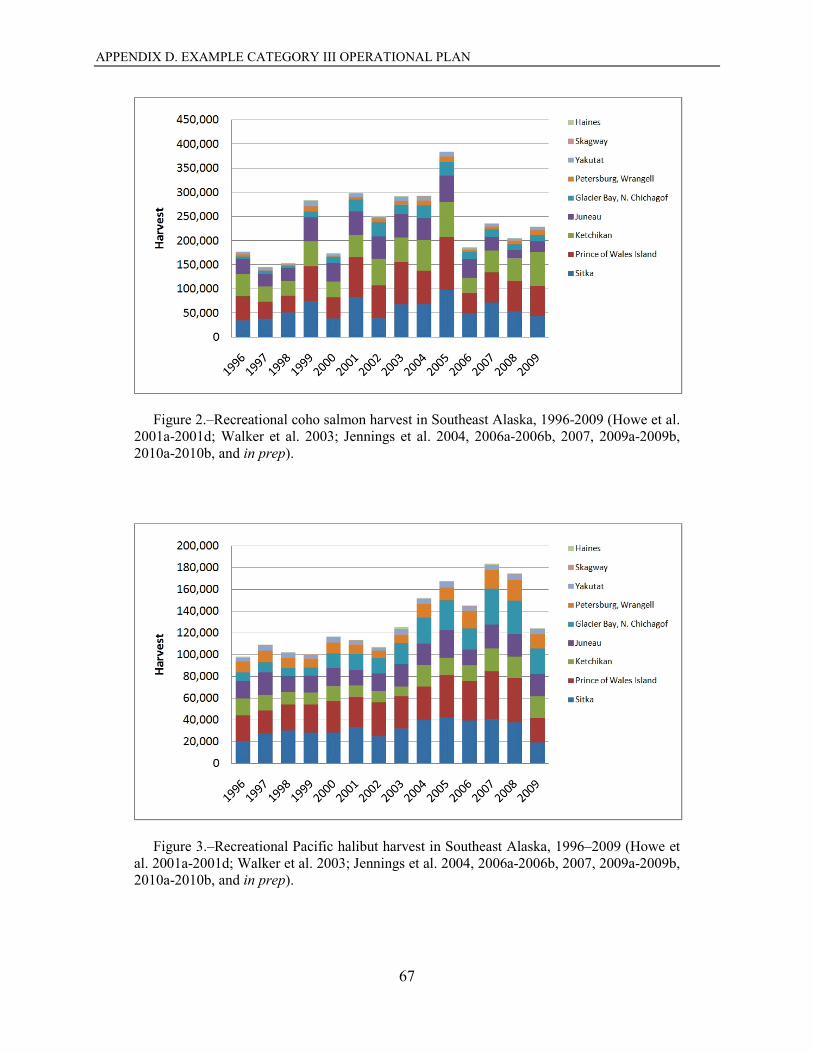
APPENDIX D. EXAMPLE CATEGORY III OPERATIONAL PLAN
67
Figure 2.–Recreational coho salmon harvest in Southeast Alaska, 1996-2009 (Howe et al. 2001a-2001d; Walker et al. 2003; Jennings et al. 2004, 2006a-2006b, 2007, 2009a-2009b, 2010a-2010b, and in prep).
Figure 3.–Recreational Pacific halibut harvest in Southeast Alaska, 1996–2009 (Howe et al. 2001a-2001d; Walker et al. 2003; Jennings et al. 2004, 2006a-2006b, 2007, 2009a-2009b, 2010a-2010b, and in prep).
APPENDIX D. EXAMPLE CATEGORY III OPERATIONAL PLAN
68
For 2011, the Alaska Board of Fisheries (BOF) has allocated 20% of the combined commercial troll and sport US/Canada Pacific Salmon Treaty (Public Law 99-5) catch quota for Chinook salmon to the Southeast Alaska sport fishery. (see Appendix A5 for history of Chinook salmon management in Southeast Alaska).
In February 2009, the BOF met and reaffirmed a 20% allocation of Chinook salmon to the sport fishery. A revised set of “tools” at the mid- to lower-levels of abundance index (AI) were added to the “tools” established in February 2003, in order to provide the sport fishery a means of managing the sport fishery at low abundance indices. These new tools include allowing resident anglers the use of 2 rods from October through the following March during years when the AI is less than or equal to 1.5. In years when the AI is less than or equal to 1.1, the annual harvest for nonresident anglers will be 3 king salmon 28 inches or greater in length during May 1 to June 30, and from July 1 to December 31 the nonresident annual limit will be 1 king salmon 28 inches or greater in length. The fishery will continue to be managed according to the preseason abundance index.
The harvest estimates from the annual mail survey of licensed sport anglers in Alaska (SWHS) produces harvest estimates for any particular year after June the following year. This project will provide preliminary projections of the final estimates that will be derived following the publication of the annual SWHS mail survey harvest estimates. The projections are calculated by multiplying observed catch and harvest in each sampled port by an expansion factor for each SWHS area (expansion factors are derived from the ratios of past final SWHS estimates and observed on-site statistics).
A preliminary estimate of the annual Southeast Alaska “treaty” Chinook sport harvest from onsite survey data is also provide to the Pacific Salmon Commission in October of the year of the estimate as a preliminary number for accounting purposes (hereafter referenced as ‘Pacific Salmon Treaty harvest’). In 2010, the preliminary sport harvest calculated by this project is 41,183 treaty fish (217 fish over the 20% allocation) from a total harvest of 51,350 fish. Alaska hatchery stocks accounted for about 20% of the total Chinook harvest in 2010 in Southeast Alaska. These preliminary estimates are derived from combining the preliminary harvest estimates with information from sampling of the Chinook harvest for the absence of an adipose fin, indicating the presence of a CWT. The proportion of Alaska hatchery stocks as estimated from the CWT information is multiplied by the preliminary total harvest to obtain the preliminary Pacific Salmon Treaty harvest. Additionally, estimates of preliminary contributions by CWT lot for non-Alaska hatcheries as well as a few tagged wild stocks are also obtained by this project.
Data useful for management of Chinook stocks in specific areas are also collected. For example, managers for the Taku River and Stikine River fisheries use inseason harvest information to monitor the return used for inseason management as a transboundary river. Accordingly, weekly estimates of the Pacific Salmon Treaty harvest will be estimated by this project for District 86 in the Petersburg/Wrangell area associated with the Stikine River and District 11 in the Juneau area associated with the Taku River.
5 Appendices are available in the original 2011 southeast marine operational plan; for availability contact Division of Sport Fish, RTS.
6 Districts reference the Commercial Fish Salmon districts.
APPENDIX D. EXAMPLE CATEGORY III OPERATIONAL PLAN
69
In addition, data on age composition of Chinook salmon taken in the spring in Juneau, Ketchikan, Petersburg, and Wrangell will be gathered for sibling models used in projections for Pacific Salmon Treaty and other stocks.
The genetic stock identification of Chinook salmon being harvested by the various fisheries in Southeast Alaska is a management tool being evaluated by the Pacific Salmon Commission. Accordingly, genetic structures will be collected in a number of fisheries to address this evaluation. Additionally, this year in the Sitka area heads will be collected from harvested Chinook salmon for otoliths related to this stock identification effort.
An important shoreline fishery for Chinook salmon in the spring occurs at False Outer Point near Juneau. Gathering CWTs from this fishery will provide additional baseline data for stock composition of this fishery as well as provide additional recoveries of tagged wild Taku River stocks. Accordingly, this one shoreline fishery will be surveyed in a similar manner as sampling of the various boat access locations at the various ports, for estimation of parameters related to the Chinook salmon fishery only.
COHO SALMON Estimates of Alaska hatchery contributions for coho salmon harvested in the sport fisheries in Juneau, Ketchikan, Sitka, Craig/Klawock, Petersburg, Wrangell, Gustavus, Elfin Cove, and Yakutat are also calculated for evaluation of enhancement projects. Additionally, recovery of tagged indicator stocks of wild coho salmon may be expected, especially in the Juneau fishery from wild stock tagging programs at Auke Creek and in the Taku and Berners river drainages, and in the Ketchikan and Sitka fisheries from tagging projects in the Unuk, Hugh Smith, and Nakwasina drainages as well as others in the region.
Coho salmon harvest rates by the marine sport fisheries are an important tool for management of this fishery and for information provided to the public. Harvest per unit effort (HPUE) for coho salmon in the Juneau and Ketchikan marine sport fisheries is used to monitor the relative abundance and movement of coho salmon to inside waters from early June to September depending on the strength of the run, and the Juneau HPUE is specifically cited in 5 AAC 29.110 (Management of Coho Salmon Troll Fishery). Coho HPUE statistics are used along with fishery performance information from the commercial fisheries and early season escapement estimates to assist managers with inseason management. Coho salmon harvest rates, as determined from the creel survey programs, are also sought by recreational anglers and used to help plan their fishing activities. Measures of sport HPUE may be somewhat biased because of the way data are reported during an interview and should be used with caution to implement management measures in a fishery. Nonetheless, HPUE can still be quite useful to both managers and to members of the public.
OTHER SPECIES Harvests of other fish species occur within most of the surveyed fisheries and estimates of these harvests are also important for management and informational purposes. Some of the management needs for these other species are as follows.
Sport charter harvest of Pacific halibut is managed under a guideline harvest level (GHL) adopted by the North Pacific Fisheries Management Council (NPFMC). Average weights in the sport harvest are needed to estimate removals in weight units for purposes of stock assessment
APPENDIX D. EXAMPLE CATEGORY III OPERATIONAL PLAN
70
and management. Estimates of fishery parameters obtained by this project will be forwarded to the project staff for the operational plan entitled “Statewide Pacific halibut harvest estimation”. That project will combine the average weights for both components of the fishery (guided and unguided) from this on-site sampling project with estimates from the SWHS and logbooks to obtain estimates and projections of sport halibut removals in biomass units for both the NPFMC and the International Pacific Halibut Commission (IPHC). Additionally, release information for halibut is provided to the statewide Pacific halibut project for use in estimating total mortalities. Finally, a proportion of the unguided halibut harvest that occurs prior to the mean IPHC survey date is also provided as requested by the statewide halibut project.
For demersal shelf rockfish (DSR), this program will calculate average weights of the sport fishery harvest for the NPFMC using a length-weight relationship developed from previous length and weight data of the sport harvested DSR species in Southeast Alaska. The seven DSR species are yelloweye (Sebastes ruberrimus), quillback (S. maliger) copper (S. caurinus), canary (S. pinniger), tiger (S. nigrocinctus), china (S. nebulosus), and rosethorn (S. helvomaculatus). Of the seven DSR species, yelloweye rockfish grow the largest in size in terms of length and weight, are relatively abundant on the outer coast, are mistakenly identified as “red snapper”, and are the most desired rockfish species to harvest. Numbers of DSR released will be also recorded by species. The average weight estimates will be combined with projections of the total catch from the SWHS (in a similar manner as noted above for Chinook salmon), to obtain preliminary estimates of the biomass of removals of DSR for the fisheries of concern.
Additionally, species composition of the rockfish harvest in all ports will be estimated; and an estimate of the percent of change of yelloweye rockfish harvested (from previous years) by August 4 in the ports of Sitka, Ketchikan, Craig/Klawock, Gustavus, Elfin Cove, and Yakutat will be obtained for inseason management purposes.
For lingcod, this program will calculate average weights of the sport fishery and report them to the Board of Fish (BOF) and Division of Commercial Fisheries. Sport harvests (in numbers) of lingcod will continue to be monitored by the SWHS, but stocks will be managed by the estimated weight of the sport harvest in relation to lingcod management area quotas. Therefore, methods to estimate the average round weight of lingcod harvested in outer coast sport fisheries (Craig/Klawock, Sitka, Gustavus, Elfin Cove, and Yakutat) will be conducted in 2011. The average weight estimates will be combined with projections of the total harvest from the SWHS to obtain preliminary estimates of the biomass of removals of lingcod for the fisheries of concern. In 2011 numbers of released lingcod will be recorded to calculate CPUE that may be used to determine population trends.
The sablefish sport harvest is relatively small; however, some stocks of sablefish exploited by multiple Southeast Alaska fisheries may need to be managed conservatively. Accordingly, when sablefish are observed at the various ports surveyed by this project they will be measured for length and their numbers recorded as a baseline information tool.
Documenting fish released during an interview can sometimes produce statistics that are likely biased due to poor recall from a recently completed trip in comparison with data collected on the number of fish harvested, which a sampler can usually confirm during the interview. However, if the number of fish released is low, then the number is more likely to be reliable. When the number of released fish is added to the number harvested, estimates of total catch can be computed that may give managers an idea of the abundance for a species—especially those that
APPENDIX D. EXAMPLE CATEGORY III OPERATIONAL PLAN
71
have low catch rates and low daily bag limits (e.g., Chinook salmon). Additionally, an estimate of total catch can sometimes give managers a better idea of fish abundance than can the harvest, especially when fish are released because they are small, under the minimum size required, or simply a species not desired by an angler. In 2011, numbers of released large and small Chinook, halibut, lingcod, and rockfish by species (or by species grouping) will be recorded to determine mortality that can be used to determine total removals by sport fisheries.
OBJECTIVES PRIMARY OBJECTIVES Unless otherwise stated, objectives and tasks are for all ports surveyed for the duration that the survey is in the port. Ports, dates, and associated objectives are as follows:
Port Start Date End Date Objectives addressed by Port Juneau April 25, 2011 September 11, 2011 1–5, 7, and 8 Sitka, Ketchikan April 25, 2011 September 11, 2011 1 and 3–8 Petersburg, Wrangell April 25, 2011 August 28, 2011 1–5, 7, and 8 Craig/Klawock, Yakutat April 25, 2011 August 28, 2011 1 and 3–8 Elfin Cove, Gustavus May 2, 2011 August 28, 2011 1 and 3–8 Juneau-False Outerpoint Shoreline April 11, 2011 May 31, 2011 1, 8
The objectives for the 2011 project include the following:
1. Estimate the preliminary 2011 values7 of the following characteristics of the Chinook salmon harvest in Southeast Alaska:
a. total sport harvest; b. relative and total Alaska hatchery and non-Alaska hatchery contributions; and, c. Pacific Salmon Treaty harvest
with a precision of ±20 percentage points under 90% confidence for the estimate of relative Alaska hatchery contribution for each port.8
2. Estimate the early season (late April to mid-July) Chinook Pacific salmon treaty harvest for Commercial Salmon Districts 8 (Petersburg/Wrangell) and 11 (Juneau)9.
3. Estimate the preliminary 2011 values of the following characteristics of the coho salmon harvest in Southeast Alaska:
a. Total sport harvest; and, b. relative and total Alaska hatchery and non-Alaska hatchery contribution
with precisions of ±20 percentage points under 90% confidence for the relative contribution estimates by coded wire tag lot for each port10.
7 The ‘preliminary values’ references that the estimates desired are projections of the final estimates that will be derived following the
publication of the annual SWHS mail survey harvest estimates. 8 The 2011 project involves a relatively major redesign of survey procedures from previous years for the major ports of Juneau, Ketchikan,
and Sitka. It is anticipated that following the completion of the 2011–2013 surveys, and the publication of the corresponding 2011–2013 SWHS harvest estimates, that objective criteria for the (a) total harvest, (b) total Alaska hatchery contributions, and (c) Pacific Salmon Treaty harvest will be determined. Only the relative Alaska hatchery contribution estimates are fully set by the sampling rates in the current project, and hence the reason for only listing that objective criteria for this year’s plan.
9 The precision realized from achieving Objective 1 will suffice for the goal precision for this objective. 10 Similar to the objective criterion associated with Chinook salmon harvest characteristics, for 2011 only the relative contribution estimates
are fully set by the sampling rates in the current project.
APPENDIX D. EXAMPLE CATEGORY III OPERATIONAL PLAN
72
4. Estimate the average net weight of the harvest of Pacific halibut by guided and unguided anglers at each port, with relative precision of ±20% under 90% confidence for each user group at each port.
5. Estimate the proportion of the Pacific halibut harvested by unguided anglers prior to the mean IPHC survey date11, with a precision of ±20 percentage points under 90% confidence.
6. Estimate the average weight and preliminary biomass of the sport harvest of lingcod by guided and unguided anglers in Sitka, Ketchikan, Craig/Klawock, Gustavus, Elfin Cove, and Yakutat, such that the relative precision for the estimated average weight of the harvest at each port is:
a. ±20% under 80% confidence for the harvest by unguided anglers;
b. ±10% under 90% confidence for the harvest by guided anglers; and,
c. ±10% under 90% confidence for the harvest by all anglers.
7. Estimate the preliminary 2011 values of the following characteristics of the rockfish harvest:
a. biomass of total sport removals (harvest and release mortality) for demersal rockfish (DSR) from the Southeast Outside District (Craig/Klawock, Sitka, Gustavus, Elfin Cove, and Yakutat combined) for each user group (guided and unguided);
b. species composition for all rockfish harvested by guided and unguided anglers at each port; and,
c. average weight by species for rockfish harvested by guided and unguided anglers at each port
with a relative precision of ±20% under 90% confidence for the estimate of average weight by species for each port.
8. Estimate the proportion of catch of Chinook salmon (both <28 inches and ≥28 inches), rockfish (yelloweye, other DSR, slope, and pelagic), halibut, and lingcod released by species or species grouping.12
SECONDARY OBJECTIVES In addition to meeting the objectives listed above, this project will address secondary management needs. For example, a terminal exclusion area near Wrangell and Petersburg has been established for harvests of Chinook salmon returning to the Stikine River, and a similar terminal exclusion area near Juneau has been established for Taku River Chinook salmon. Documentation of those fish in the area during the spring is necessary in order for a terminal exclusion to be issued under Pacific Salmon Treaty agreements.
To fulfill these management needs, additional tasks include:
1. Estimate the length composition of Pacific halibut harvested by guided and nonguided anglers at all sampled ports every two to three years.
11 Each year the IPHC conducts a longline survey of the Pacific halibut stock. The survey utilizes numerous stations in IPHC Area 2C and
takes many days to complete. Harvest that occurs prior to the survey has the potential to affect the survey catch. Therefore, the IPHC annually requests estimates of the proportions of charter and non-charter harvest that occurred prior to the average survey date. These estimates, along with similar estimates from the commercial fishery, are used to standardize the longline survey abundance index to account for variation in the amount of harvest prior to the mean date of the survey.
12 The precision realized from achieving the objective criterion for estimates of the preliminary harvest (previous objectives) will suffice for the goal precision for the estimated proportion of the catch released by the various species or species groupings for this objective.
APPENDIX D. EXAMPLE CATEGORY III OPERATIONAL PLAN
73
2. Report the observed harvest per unit of effort (HPUE) of Chinook and coho salmon, and Pacific halibut to the public at all ports on a weekly basis.
3. Report the coho salmon weekly HPUE, cumulative HPUE, and a seasonal summary of trends in Juneau to Division of Commercial Fisheries troll biologists June 15 through end of July.
4. Project the 2011 preliminary harvest of lingcod by August 4 in the ports of Sitka, Ketchikan, Craig/Klawock, Gustavus, Elfin Cove, and Yakutat.13
5. Project the 2011 preliminary harvest of yelloweye rockfish by August 4 in the ports of Sitka, Ketchikan, Craig/Klawock, Gustavus, Elfin Cove, and Yakutat.
6. Collect genetic tissue samples (axillary spine clips) and corresponding age structures (scales) from Chinook salmon harvested at all sampled ports (with a targeted sampling rate that is proportional to the observed harvest), and provide the proportion of the observed harvest sampled each week to the ADF&G Genetics Laboratory. In addition, the corresponding heads from the sampled Chinook salmon will be collected in Sitka for stock identification purposes (via otoliths).
7. Measure lengths from all sablefish observed during interviews conducted at all surveyed ports.
8. Collecting species composition of the harvest information from all fisheries sampled.
METHODS GENERALIZED PROCEDURES As noted, the 2011 rendition of this project has undergone a major redesign of survey procedures from previous years for the major ports of Juneau, Ketchikan, and Sitka, along with some adaptations to survey procedures in the minor ports. Additionally, the SWHS is also undergoing a redesign for 2011. Due to the nature of the underlying procedure for obtaining the preliminary values for the final estimates associated with the primary objectives for this project, the values obtained by the project for 2011 are expected to be subject to unknown error that will not be evident until completion of at least 3 years of paired SWHS and on-site harvest sampling data with the two new designs. It is anticipated that following the completion of at least 3 years of on-site surveys with the new design (the 2011–2013 surveys), and the publication of the corresponding SWHS harvest estimates, that the expansion factors used to obtain the preliminary values of desired parameter estimates will be directly obtained from the pairing of final SWHS estimates and observed on-site data for the previous years14.
The primary objectives for this project are generally aimed at obtaining the preliminary values of estimates of desired parameters (e.g., Pacific Salmon Treaty harvest). However, the estimates of these parameters that will eventually be calculated using the information from the published harvest estimate from the SWHS for each year in question will serve as the final ‘official’ estimate for each parameter. Accordingly, the estimates of such parameters as relative Alaska hatchery contribution for Chinook salmon by port, average weight of lingcod harvested by port, etc. are directly impacted by the sampling rates outlined below. The sampling error for these intrinsic (to this project) parameter estimates will directly impact the overall error of the preliminary estimates as well as the final ‘official’ estimates. Within this operational plan for
13 Estimates of the percent change of lingcod and yelloweye rockfish in the noted ports (Tasks 4 and 5), will be calculated by combining separate estimates for the guided and unguided components of the fishery.
14 It is likely that a total of 5 years of the most recent paired values of SWHS and on-site observed harvest will be used in the long-run for calculation of expansion factors, with the proviso that the on-site sampling program at each port remains at relatively similar intensity and coverage over all years used for expansion factor calculation.
APPENDIX D. EXAMPLE CATEGORY III OPERATIONAL PLAN
74
2011 only the sampling error associated with the intrinsic parameter estimates were used to state the goals for precision (as outlined in the Objectives section, above). Additionally, the revisions in the design were not completely factored into the setting of sample sizes or allocations of sampling effort due to time constraints as well as the uncertainty as to the change in the relationship between the revised SWHS and the revised on-site survey. Sample size goals were accordingly set primarily to mirror the goals set in 2010. It is anticipated that once 3 or more years of paired values of final SWHS and on-site sampling data are obtained, that goals for precision will be more directly aimed at the real parameters of interest (e.g., the Pacific Salmon Treaty harvest in total).
Procedures for obtaining estimates associated with each of the study objectives will be similar for each of the surveyed locations. The following sections detail the procedures that are common to multiple surveys. Site-specific differences in procedures are outlined in later sections of this operational plan.
STUDY DESIGN The general approach for collecting the information necessary to achieve the objectives and s for this project involves sampling exiting boat parties at major harbors and boat ramps at each of the ports selected for surveying. The specific harbors and boat ramps to be surveyed at each port were selected to be representative of the majority of exiting sport fish boats accessing the fisheries. Locations with little sport fishing activity, as evidenced from historic creel surveys within a port location, were removed from consideration for sampling in 2011, with the understanding that the parameters of interest would not be expected to vary substantially from one harbor to the next. Because the less frequently used access locations represent so little of the fishery, departures from the assumption of no difference in the parameters of interest would be minimized in regards to the inference to the total fishery. In some instances some locations of relatively minor use by the fishery were included for sampling in some ports, as these lower-use locations may be representative of locations of fishing or components of the fishing public that may be otherwise unrepresented with sampling only the heavier-use locations (for example Starrigavan boat launch in Sitka; although it is a low-use access location, it is primarily used by unguided anglers and may be periodically sampled to achieve adequate samples from that component of the fishery).
The days of the week and the time periods to sample were similarly restricted to those days and time periods wherein the majority of sport boats exit the fishery (as evidenced from historic creel or catch sampling surveys). Because there are patterns of differing relative use by guided versus unguided segments of each fishery in regards to the day of the week (e.g., more weekend use by unguided anglers), and within the fishing day (e.g., some guides time their fishing trips related to cruise boat schedules), then it will be necessary to estimate all parameters of interest separately by each of these components of the fishery. For example, the proportion of Alaska hatchery composition of the Chinook harvest of guided anglers in the Ketchikan area would be combined with the SWHS estimate of guided Chinook harvest for SWHS survey Area A to obtain that parameter component of the overall Alaska hatchery harvest estimate (obtained by combining with the corresponding unguided component estimated in the same manner).
As noted above, the general study design approach for this project is to estimate proportions or averages of the specific elements of each fishery (e.g., proportion of the harvest of Chinook salmon that are from Alaskan hatchery production) and apply these proportions and averages to
APPENDIX D. EXAMPLE CATEGORY III OPERATIONAL PLAN
75
the corresponding estimate from the SWHS. The information necessary for estimating these proportions will be gathered by measuring characteristics of the catch of intercepted boat parties at the sampled harbors and boat launches. At all ports, most or all of the survey technicians conduct complete “interviews”, which include gathering information from each intercepted boat party on: effort, harvest and catch, logbook information, and biological sampling of the catch. During all scheduled “interview” samples the interviewers gather and record additional information on the number of exiting boat parties that is used in the estimation process described below. These interview samples and the survey technicians who conduct them are generally referenced as “creel samples” and “creel technicians” throughout this operational plan. In some instances the parameter of interest is the magnitude of the harvest or the numbers of fish released by species or species group itself (e.g., Objective 1a: total sport harvest of Chinook salmon). The necessary information to address those needs is also incorporated into the design (see Data Analysis section for further details).
Additionally, in Ketchikan, Juneau, Sitka, and Craig/Klawock one or more survey technicians will concentrate on conducting “catch sampling,” which includes the gathering of information on CWT sampling of Chinook and coho salmon, and collection of biological samples on groundfish species. The catch sampling is performed at the busiest docks at the busiest times to maximize the number of available samples. This additional sampling is needed to meet the sampling goals in the high harvest ports where it is difficult for the interviewers to obtain the biological sampling goals while interviewing. The catch sampling samples and survey technicians who collect them are generally referenced as “catch sampling” and “catch samplers” (or “catch sampling technicians”).
The design for sampling the catch is a stratified 4-stage sample survey with days to sample across the season representing the first-stage sampling units, the harbors and boat launches sampled within a selected day representing the second-stage sampling units, the boat parties exiting the fishery during each day at each exit location representing the third-stage sampling units, and then finally each fish (by species) representing the fourth-stage or “terminal” sampling unit. To avoid potential for sub-sampling bias, whenever a boat party is contacted for sampling, the entire catch of either all species of interest or subsets of species will be censused. The strata are composed of the combination of general port location (e.g., Ketchikan) and components of the fishery (guided and unguided). The sampling unit selection procedures for this survey are not, however, done as a random probability-based sample survey in the standard sense, but were designed to obtain relative proportional sampling of the angling effort and harvest. Information on the number of exiting boat parties will be recorded at each sampled exit location during each sampled day for all ‘creel samples’, and when combined with the numbers of fish by species observed on each sampled boat will provide weighting factors for each sampling stage to address the likelihood that the sampling will not be exactly proportional to the harvest of all species at all times. The resulting estimation approach is comprised of a 4-stage weighted-average (see the Data Analysis section below for further details).
The majority of sampling effort directed at gathering the information necessary to address the objectives and tasks for this project will be obtained as described above, that is a stratified 4-stage sample survey with corresponding counts of boat parties for each harbor or launch sampled within each day sampled. These corresponding counts of boat parties are used in the weighted average estimation process. As noted above, some of the technicians and samples at the ports of Ketchikan, Juneau, Sitka, and Craig/Klawock will be conducting ‘catch sampling’ only and will
APPENDIX D. EXAMPLE CATEGORY III OPERATIONAL PLAN
76
not be gathering or recording information on the numbers of exiting boat parties. The data collected during these catch sampling-only samples will be treated somewhat differently than described above for the creel samples in that the sample weights will be estimated via a ratio estimation approach derived from the ratio of observed harvest numbers by species in boat parties intercepted by the catch samplers within a sampled day to the estimated number of fish harvested within that same day covered by the creel samplers. On days without corresponding creel samples, the catch sample data sample weights will be calculated in a similar manner, but using across-day ratio estimation (see the Data Analysis section below for further details).
In order to obtain the “preliminary 2011 values” associated with the primary objectives, a prediction of the corresponding harvest estimate from the SWHS will need to be made for each species by location. The general approach to be used in 2011 to make this prediction has been used successfully in the past and involves using past ratios of either observed or estimated harvest by major species from this on-site survey compared to the final SWHS estimates for the corresponding year. The estimated harvest from the on-site creel surveys conducted in Ketchikan, Juneau, and Sitka formed the denominator of the expansion factor ratio for those locations in the past; whereas the observed harvest for the catch-sampling-only locations of Crag/Klawock; Petersburg, Wrangell; Elfin Cove, Gustavus; and Yakutat served as the components of denominator of the ratio for those locations. An average of the ratios obtained from 5 years of the most recently available SWHS estimates combined with the corresponding year’s on-site values will be used in 2011 for these catch-sampling-only locations. Because the 2011 redesign of the sampling program in Ketchikan, Sitka, and Juneau will change those locations to catch-sampling-only, the ratio to be used for this prediction for 2011 will be derived by simulating the 2011 on-site sampling design using past creel survey data15. The expansion factor ratio would then be applied to the observed 2011 estimated averages or proportions for each corresponding parameter of interest (e.g., relative Alaska hatchery contribution) to obtain the preliminary 2011 values. Note that the expansion factors are developed separately for each SWHS Survey Area, as follows: Ketchikan represents SWHS Area A; Craig/Klawock = Area B; Petersburg and Wrangell = Area C; Sitka = Area D, Juneau = Area E; Gustavus and Elfin Cove = Area G, and Yakutat = Area H. In order to get a regionwide total estimate (expanding up for SWHS Area F (Haines/Skagway) a similarly derived 5-year average ratio of the total Southeast Alaska estimate from the SWHS to the sum of SWHS estimates for the Survey Areas represented in our on-site sampling (i.e., Areas A–E, G & H) will be used to expand to the total for the region.
Anticipated precision estimates for the various intrinsic (to this on-site project) parameter estimates for the objectives with precision goals (aka ‘objective criteria’) are currently projected to be approximately at the same levels as obtained in past year surveys for 2 basic reasons: (1) sampling sizes (technician hours) will be the same as in past years for the ports of Craig/Klawock, Petersburg, Wrangell, Elfin Cove, Gustavus, and Yakutat, or (2) although technician hours will be reduced in Ketchikan, Sitka, and Juneau, the hours within the day and specific harbors/locations to be surveyed have historically provided the majority of sampled fish by species in the past16. As noted above, due to the nature of the tandem re-design of this project
15 These simulations have not been completed at the time of finalizing this operational plan prior to fielding the project. Current plans call for completing the simulations during the May to mid-July time period, in anticipation of making mid-season projections for the Chinook salmon, and rockfish harvests.
16 In previous years, the surveys at these three major ports were probability based multi-stage sample surveys that in general sampled with equal probability (within all days, all periods within a day, all locations within a day, and all exiting boat parties within a sampled location), and as such technician hours were often ‘spent’ surveying at locations with few if any observed harvest.
APPENDIX D. EXAMPLE CATEGORY III OPERATIONAL PLAN
77
as well as the SWHS, the final precision estimates will very likely be quite different than the anticipated precision values from past years. That said, the allocation of technician-hours by day and location was designed to maximize the proportion of the harvest sampled at a relatively stable and consistent level throughout the surveyed periods. The following subsections include descriptions of the general estimation approach, and outline past levels of precision obtained for the primary objectives.
Preliminary 2011 Total Sport Harvest of Chinook and Coho Salmon (Objectives 1a, 3a) The total predicted harvest estimate for each port corresponding to each SWHS survey area as obtained by the ratio expansion factor approach described above will comprise the estimates of the preliminary 2011 total harvest of Chinook and coho salmon for each of those areas. The sum of the predicted harvest for the surveyed SWHS areas will then be expanded up to the regional total by the corresponding expansion factor (also as described above).
Hatchery and Non-Hatchery Contributions-Chinook and Coho Salmon (Objectives 1b and 3b) During each of the surveys of the marine boat sport fisheries at each port (Ketchikan, Craig/Klawock, Petersburg, etc.) the technicians will attempt to inspect each harvested Chinook salmon for a missing adipose fin (indicating the probable presence of a CWT). The number of Chinook salmon inspected for adipose fin clips will be recorded, and heads from Chinook salmon with adipose fin clips will be collected and identified with a uniquely numbered cinch strap. Cinch strapped heads from Chinook salmon will be forwarded to the ADF&G Mark, Age, and Tag Laboratory (Tag Lab) for eventual dissection, tag removal, and decoding.
Information from the sampling program as well as the coastwide CWT database will be used to estimate the contributions of Alaska hatchery Chinook salmon using an adaptation of Bernard and Clark’s (1996) procedures, as outlined in the Data Analysis section of this plan. Similar procedures will be used to estimate the contribution of non-Alaskan hatchery and tagged wild coho stocks to the marine boat sport fisheries.
The precision of Alaska hatchery contribution estimates of Chinook and coho salmon have generally been consistently met in the past (Table 1), thus the approximate allocation of sampling effort will be repeated, and with the expectations that the samples sizes (fish scanned for hatchery origin) will be similar in 2011 as observed in past years. Accordingly, similar levels of precision are expected in 2011.
The relative contribution estimates for each species by each CWT lot will be expanded by the corresponding predicted harvest estimate for the SWHS to obtain the 2011 preliminary values for the corresponding total estimates contributions by CWT lot.
Pacific Salmon Treaty Harvest (Objectives 1c and 2) Estimates of the treaty harvest are then obtained by subtracting out from the total Chinook salmon preliminary harvest estimate the components of the harvest that do not count against the treaty (e.g., Alaskan hatchery harvest). The early season estimate of treaty harvest for Commercial Fishing Districts 8 (Petersburg/Wrangell) and 11 (Juneau), will be obtained in similar manner using the corresponding components of the 2011 preliminary harvest estimates combined with the past 5 years of recreational harvest timing data in these districts.
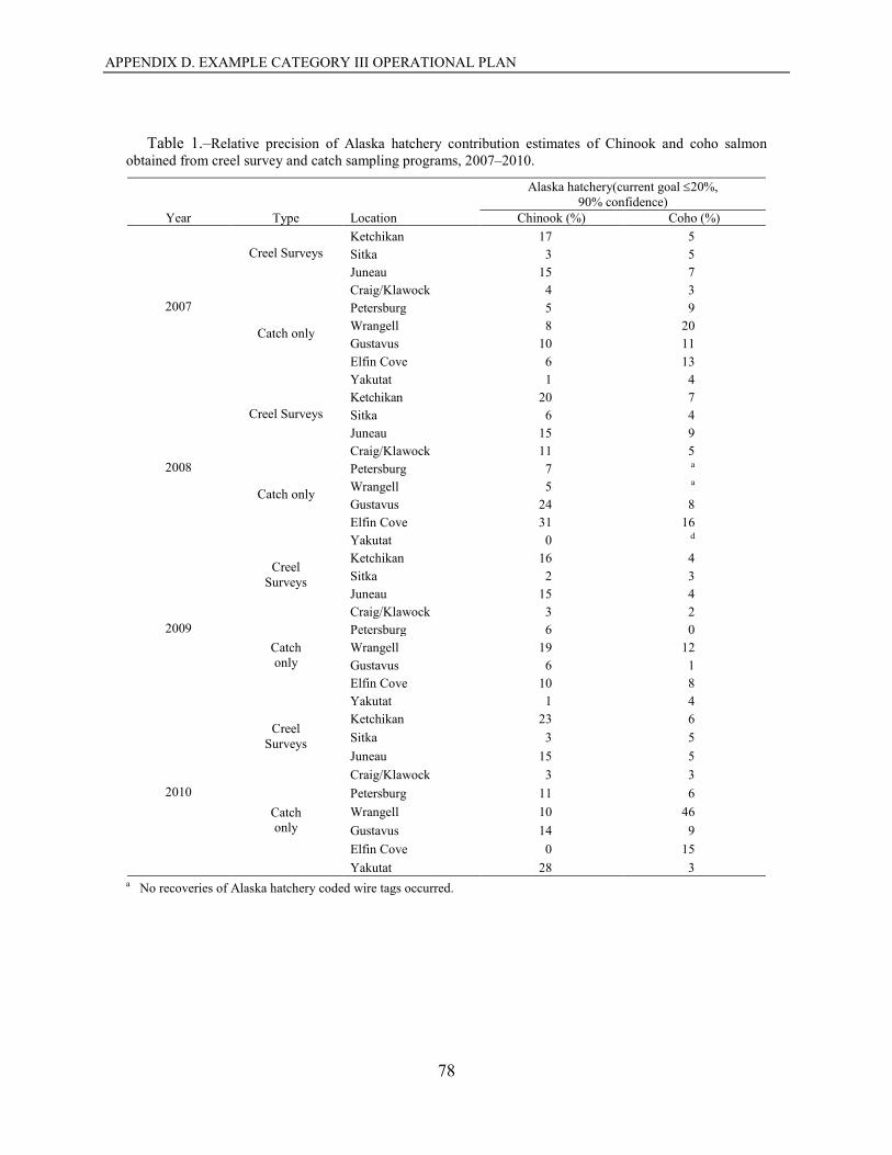
APPENDIX D. EXAMPLE CATEGORY III OPERATIONAL PLAN
78
Table 1.–Relative precision of Alaska hatchery contribution estimates of Chinook and coho salmon
obtained from creel survey and catch sampling programs, 2007–2010.
Year Type Location
Alaska hatchery(current goal ≤20%, 90% confidence)
Chinook (%) Coho (%)
2007
Creel Surveys Ketchikan 17 5 Sitka 3 5 Juneau 15 7
Catch only
Craig/Klawock 4 3 Petersburg 5 9 Wrangell 8 20 Gustavus 10 11 Elfin Cove 6 13
Yakutat 1 4
2008
Creel Surveys Ketchikan 20 7 Sitka 6 4 Juneau 15 9
Catch only
Craig/Klawock 11 5 Petersburg 7 a
Wrangell 5 a Gustavus 24 8 Elfin Cove 31 16 Yakutat 0 d
2009
Creel Surveys
Ketchikan 16 4 Sitka 2 3 Juneau 15 4
Catch only
Craig/Klawock 3 2 Petersburg 6 0 Wrangell 19 12 Gustavus 6 1 Elfin Cove 10 8 Yakutat 1 4
2010
Creel Surveys
Ketchikan 23 6 Sitka 3 5 Juneau 15 5
Catch only
Craig/Klawock 3 3 Petersburg 11 6 Wrangell 10 46 Gustavus 14 9 Elfin Cove 0 15 Yakutat 28 3
a No recoveries of Alaska hatchery coded wire tags occurred.
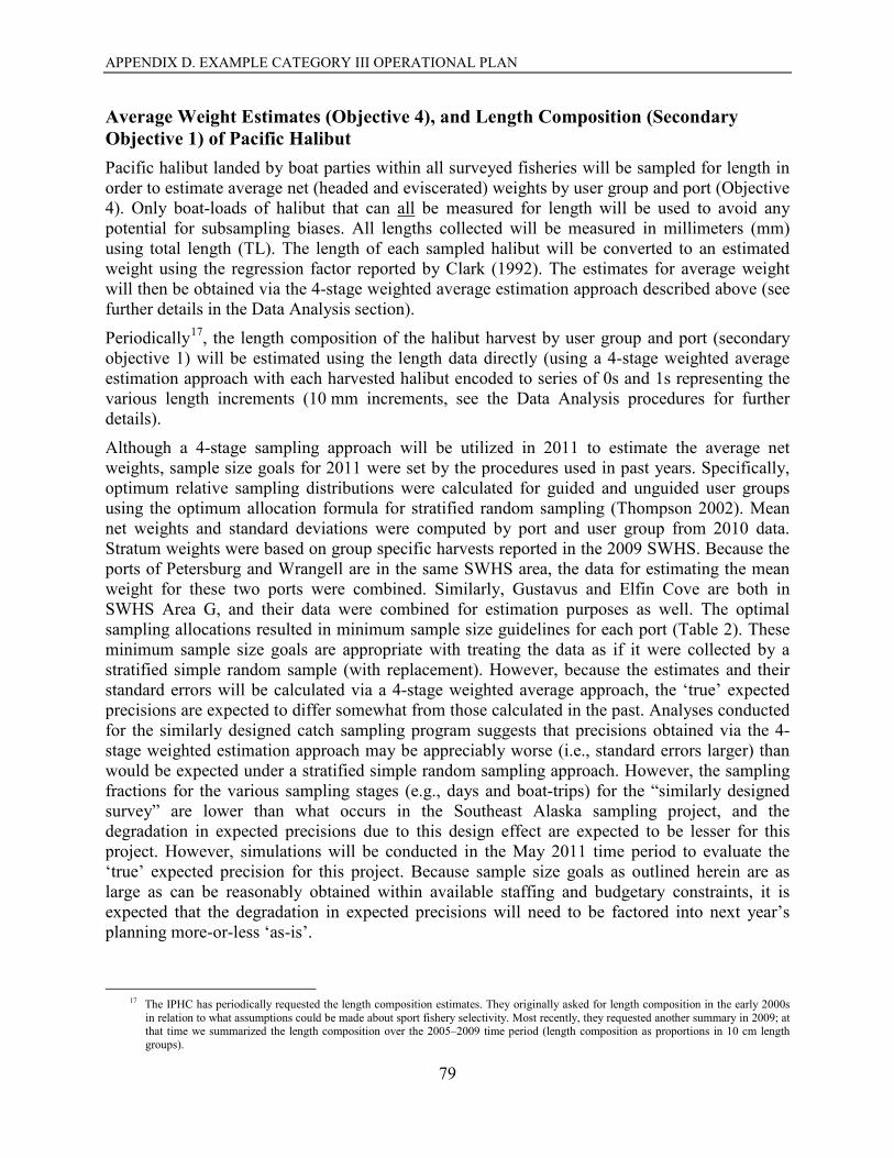
APPENDIX D. EXAMPLE CATEGORY III OPERATIONAL PLAN
79
Average Weight Estimates (Objective 4), and Length Composition (Secondary Objective 1) of Pacific Halibut Pacific halibut landed by boat parties within all surveyed fisheries will be sampled for length in order to estimate average net (headed and eviscerated) weights by user group and port (Objective 4). Only boat-loads of halibut that can all be measured for length will be used to avoid any potential for subsampling biases. All lengths collected will be measured in millimeters (mm) using total length (TL). The length of each sampled halibut will be converted to an estimated weight using the regression factor reported by Clark (1992). The estimates for average weight will then be obtained via the 4-stage weighted average estimation approach described above (see further details in the Data Analysis section).
Periodically17, the length composition of the halibut harvest by user group and port (secondary objective 1) will be estimated using the length data directly (using a 4-stage weighted average estimation approach with each harvested halibut encoded to series of 0s and 1s representing the various length increments (10 mm increments, see the Data Analysis procedures for further details).
Although a 4-stage sampling approach will be utilized in 2011 to estimate the average net weights, sample size goals for 2011 were set by the procedures used in past years. Specifically, optimum relative sampling distributions were calculated for guided and unguided user groups using the optimum allocation formula for stratified random sampling (Thompson 2002). Mean net weights and standard deviations were computed by port and user group from 2010 data. Stratum weights were based on group specific harvests reported in the 2009 SWHS. Because the ports of Petersburg and Wrangell are in the same SWHS area, the data for estimating the mean weight for these two ports were combined. Similarly, Gustavus and Elfin Cove are both in SWHS Area G, and their data were combined for estimation purposes as well. The optimal sampling allocations resulted in minimum sample size guidelines for each port (Table 2). These minimum sample size goals are appropriate with treating the data as if it were collected by a stratified simple random sample (with replacement). However, because the estimates and their standard errors will be calculated via a 4-stage weighted average approach, the ‘true’ expected precisions are expected to differ somewhat from those calculated in the past. Analyses conducted for the similarly designed catch sampling program suggests that precisions obtained via the 4-stage weighted estimation approach may be appreciably worse (i.e., standard errors larger) than would be expected under a stratified simple random sampling approach. However, the sampling fractions for the various sampling stages (e.g., days and boat-trips) for the “similarly designed survey” are lower than what occurs in the Southeast Alaska sampling project, and the degradation in expected precisions due to this design effect are expected to be lesser for this project. However, simulations will be conducted in the May 2011 time period to evaluate the ‘true’ expected precision for this project. Because sample size goals as outlined herein are as large as can be reasonably obtained within available staffing and budgetary constraints, it is expected that the degradation in expected precisions will need to be factored into next year’s planning more-or-less ‘as-is’.
17 The IPHC has periodically requested the length composition estimates. They originally asked for length composition in the early 2000s
in relation to what assumptions could be made about sport fishery selectivity. Most recently, they requested another summary in 2009; at that time we summarized the length composition over the 2005–2009 time period (length composition as proportions in 10 cm length groups).
APPENDIX D. EXAMPLE CATEGORY III OPERATIONAL PLAN
80
Table 2.–Minimum target and expected sample sizes of Pacific halibut and lingcod lengths to be collected in 2011 for each of the sampled ports and user groups (NA = Not Applicable), and expected sample sizes for rockfish species composition for 2011.
Spec
ies
User group
Ketchikan Craig/Klawock Gustavus/ Elfin
Cove Petersburg/Wrangell Sitka Juneau Yakutat
Target Expecteda Target Expecteda Target Expecteda Target Expecteda Target Expecteda Target Expecteda Target Expecteda
Hal
ibut
Noncharter 152 568 119 157 104 232 98 744 100 57 230 934 95 47
Charter 235 280 538 438 270 785 106 262 280 609 257 282 427 427
Total 387 848 657 595 374 1,017 204 1,006 380 666 487 1,216 522 474
Ling
cod Noncharter 41 71 27 129 25 25 NA NA 10 45 NA NA 8 29
Charter 188 24 45 321 8 101 NA NA 27 186 NA NA 27 233
Total 229 95 72 450 33 126 NA NA 37 231 NA NA 35 262
Roc
kfis
h Noncharter
456
407
121
145
212
227
25
Charter 170 1,038 757 6 1,256 64 274
Total 626 1,445 878 151 1,468 291 299 a Expected sample sizes = 2010 actual sample size.
Appendix D.–Example Category III Operational Plan
81
Halibut measurements will have a priority on a fraction of the sampled days, during which groundfish (i.e., halibut, lingcod, and rockfish) measurements will take priority over Chinook salmon genetics sampling. A systematic sampling protocol will be employed, in which one of k days are sampled. Subsampling will occur every 3rd day in Juneau, Ketchikan, Sitka, Craig/Klawock, Petersburg/Wrangell, Gustavus, Elfin Cove, and Yakutat. The starting day in which to start sampling was randomly selected (e.g., number between 1 and 3) for the first week, and continued according to the systematic schedule for each port noted above. If the next selected sample day happened to fall on: 1) a non-work day; 2) a day that was only being catch sampled (Ketchikan, Sitka, or Juneau); or, 3) a designated derby sampling day18, the closest “standard day” worked was selected for sampling (with a “coin flip” used to resolve ties). In those instances noted above, only the day to conduct sampling was adjusted forward - counts to the next subsample day were not. In ports of Ketchikan, Sitka, or Juneau, where there are both creel and catch sampling programs, only creel samplers will reprioritize their sampling goals on the designated days. Catch samplers will maintain their assigned priorities for salmon (see Appendix B1 for priorities). Data collected on designated groundfish sampling priority days will be denoted on the AWL mark-sense form differently than regular creel days, although all AWL, regardless of sampling priority day, will be included in the analysis of the length data to calculate estimates of mean net weight of halibut.
Differences in weight distributions between the “halibut sampling days” and the other sampling days will be analyzed postseason to determine if they are significant for purposes of pooling data. Inseason monitoring of port- and class-specific halibut samples will be maintained in order to ensure minimum sample size goals are met.
Proportion of Pacific Halibut Harvested by Unguided Anglers Prior to Mean IPHC Survey Date (Objective 5) The sampling weights used in the 4-stage weighted average estimator used to calculate the average net weights by component of the fishery (guided versus unguided) (Objective 4) are approximations of the number of halibut harvested (i.e., approximately equivalent to a ‘direct expansion’ creel survey). Postseason the mean IPHC survey date will be identified and then used to post-stratify the estimates of harvest before and after that date, then the proportion of the harvest before the date will be calculated from these estimates (see the Data Analysis section for further details).
Average Weight and Preliminary Biomass Estimates of Lingcod (Objective 6) Lingcod landed by boat parties in Craig/Klawock, Sitka, Ketchikan, Gustavus, Elfin Cove, and Yakutat will be sampled for length in order to estimate the average round weight. The average round weight estimates for each user group will then be multiplied by the 2011 preliminary estimate of the harvest of lingcod (in numbers) for each user group19 to obtain estimates of the preliminary biomass estimate of the harvest of lingcod at each port.
18 The derbies conducted at each location are directed at salmon and during these days the vast majority of harvest is of salmon with few
other species observed. The primary survey/sampling duties of the technicians on derby days relate to collection of information related to the salmon harvest. It is expected that the resultant sampling rate will not be truly proportional because we've purposely avoided these derby day samples. However, because the 4-stage weighted estimation procedure factors in departures from non-proportional sampling this should not be an issue. We will however evaluate the degree of departure from proportional sampling postseason, and will post-stratify estimates of average net weight of Pacific halibut if necessary.
19 The 2011 preliminary estimate of lingcod harvest at each port by user group will be calculated in the same manner as that described for estimates of the preliminary harvest of Chinook and coho salmon (Objectives 1a, and 3a).
Appendix D.–Example Category III Operational Plan
82
Sample size goals for 2011 for lingcod average round weight were set in the same manner as described above for the Pacific halibut net weight estimates (Objective 4). The means and standard deviations of lingcod weights were computed by port and user group from 2010 data. Stratum weights were based on group-specific harvests reported in the 2009 SWHS. The optimal sampling allocations resulted in minimum sample size guidelines for each port (Table 2). As with the halibut weight estimates, these minimum sample size goals are appropriate with treating the data as if it were collected by a stratified simple random sample (with replacement). However, because the estimates and their standard errors will be calculated via a 4-stage weighted average approach, the ‘true’ expected precisions are expected to differ somewhat from those calculated in the past.
Rockfish Species Composition; and Average Weight Estimates and Preliminary Biomass of Demersal Shelf Rockfish (Objective 7) Rockfish landed by boat parties in Craig/Klawock, Sitka, Ketchikan, Petersburg, Wrangell, Elfin Cove, Gustavus, Juneau and Yakutat will be identified to species (Objective 7b) and sampled for length. At the Southeast Outside District sampled ports (Craig/Klawock, Sitka, Gustavus, Elfin Cove, and Yakutat combined) the measured lengths will be converted to a round weight by species by user group using a length-weight relationship to estimate the average weight for each DSR species (Objective 7c). Then the weights will be used to obtain the 2011 preliminary biomass for the DSR rockfish species using the same approach outlined above for Pacific halibut average net weight estimates (Objective 7a). If harvest by anglers is similar as occurred in 2010, then sample sizes for this objective for 2011 are expected to meet or exceed those experienced in 2010 (Table 2).
Release Estimates for Chinook Salmon, Rockfish, Pacific Halibut, and Lingcod (Objective 8) During all interview samples the boat parties will be asked to report the numbers of Chinook salmon (both <28 inches and ≥28 inches), rockfish (yelloweye, other DSR, slope, and pelagic), halibut, and lingcod released by species (or species grouping for DSR, slope, and pelagic). These reported values will be combined with the observed/reported numbers of fish harvested to estimate the total catch by species, then used to calculate the proportion of the catch that was released. A coding of the numbers of fish caught that were released will be used in the actual calculation for the proportion released (i.e., 0 if caught fish harvested, 1 if released), so that the 4-stage weighted average approach can be implemented on the coded values to estimate these proportions (see the Data Analysis section for details).
Weekly Harvest per Unit Effort of Chinook and Coho Salmon and Pacific Halibut (Secondary Objectives 2 and 3) All boat parties intercepted for sampling by interview technicians will be asked to report the number of targeted rod-hours directed at fishing for salmon versus groundfish at each port. This information will be paired with the corresponding numbers of Chinook and coho salmon or Pacific halibut harvested on a weekly basis to calculate a weekly HPUE for each species (Task 2). These HPUE estimates are only intended as a guideline for use by the public for their information as to the level of effort expended to harvest 1 fish by species on a weekly basis. The HPUE for coho salmon for the Juneau area will be cumulated for the period of June 15 through July 31, and summarized for used by Division of Commercial Fisheries for their information and
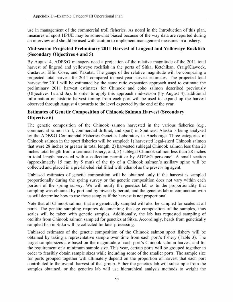
Appendix D.–Example Category III Operational Plan
83
use in management of the commercial troll fisheries. As noted in the Introduction of this plan, measures of sport HPUE may be somewhat biased because of the way data are reported during an interview and should be used with caution to implement management measures in a fishery.
Mid-season Projected Preliminary 2011 Harvest of Lingcod and Yelloweye Rockfish (Secondary Objectives 4 and 5) By August 4, ADF&G managers need a projection of the relative magnitude of the 2011 total harvest of lingcod and yelloweye rockfish in the ports of Sitka, Ketchikan, Craig/Klawock, Gustavus, Elfin Cove, and Yakutat. The gauge of the relative magnitude will be comparing a projected total harvest for 2011 compared to past-year harvest estimates. The projected total harvest for 2011 will be estimated by the same ratio expansion approach used to estimate the preliminary 2011 harvest estimates for Chinook and coho salmon described previously (Objectives 1a and 3a). In order to apply this approach mid-season (by August 4), additional information on historic harvest timing from each port will be used to expand up the harvest observed through August 4 upwards to the level expected by the end of the year.
Estimates of Genetic Composition of Chinook Salmon Harvest (Secondary Objective 6) The genetic composition of the Chinook salmon harvested in the various fisheries (e.g., commercial salmon troll, commercial driftnet, and sport) in Southeast Alaska is being analyzed by the ADF&G Commercial Fisheries Genetics Laboratory in Anchorage. Three categories of Chinook salmon in the sport fisheries will be sampled: 1) harvested legal-sized Chinook salmon that were 28 inches or greater in total length; 2) harvested sublegal Chinook salmon less than 28 inches total length from a terminal fishery; and, 3) sublegal Chinook salmon less than 28 inches in total length harvested with a collection permit or by ADF&G personnel. A small section (approximately 15 mm by 5 mm) of the tip of a Chinook salmon’s axillary spine will be collected and placed in a pre-labeled vial filled with ethanol as the preserving agent.
Unbiased estimates of genetic composition will be obtained only if the harvest is sampled proportionally during the spring survey or the genetic composition does not vary within each portion of the spring survey. We will notify the genetics lab as to the proportionality that sampling was obtained by port and by biweekly period, and the genetics lab in conjunction with us will determine how to use these samples if the harvest is not proportional.
Note that all Chinook salmon that are genetically sampled will also be sampled for scales at all ports. The genetic sampling requires documenting the age composition of the samples, thus scales will be taken with genetic samples. Additionally, the lab has requested sampling of otoliths from Chinook salmon sampled for genetics at Sitka. Accordingly, heads from genetically sampled fish in Sitka will be collected for later processing.
Unbiased estimates of the genetic composition of the Chinook salmon sport fishery will be obtained by taking a representative sample over time from each port’s fishery (Table 3). The target sample sizes are based on the magnitude of each port’s Chinook salmon harvest and for the requirement of a minimum sample size. This year, certain ports will be grouped together in order to feasibly obtain sample sizes while including some of the smaller ports. The sample size for ports grouped together will ultimately depend on the proportion of harvest that each port contributed to the overall harvest of that group. Either the genetics lab will subsample from the samples obtained, or the genetics lab will use hierarchical analysis methods to weight the
Appendix D.–Example Category III Operational Plan
84
samples obtained (Sara Gilk, ADF&G genetics lab, and S. McPherson, ADF&G Sport Fish December 9, 2010 meeting in Douglas). Legal and sublegal Chinook salmon (harvested in local Terminal Harvest Areas, THA, with returning hatchery Chinook salmon) will be sampled from fish being brought back to the docks/boat ramps at the sampled ports in Southeast Alaska during the 2011 season. In order to obtain the axillary spine clips from sublegal Chinook salmon not in the terminal area, ADF&G personnel and charter operators will be recruited to conduct the sampling in Ketchikan, Sitka, Juneau, Wrangell, and Craig. The charter operators will be paid a $100.00 base plus $5.00 per fish harvested and turned in to ADF&G for sampling. Confiscated sublegal fish from illegal harvest will also be sampled when feasible at the ports where sublegal sampling is indicated in the chart below. The fish will be donated to charity if possible, and otherwise sacrificed and disposed of properly.
Table 3.–Summary of target sample goals of the genetic sampling of Chinook salmon at the various
ports in Southeast Alaska during the 2011 creel survey season. Terminal Harvest Area = THA.
Legal (≥28 inchesTL) Chinook salmon harvested
Port Through biweek 13 After biweek 13 All season Outside:
775 775
1,550
Yakatat, Gustavus, Elfin Cove, Sitka, and Craig/Klawock min.requirement for entire season
Juneau, Haines, and Skagway NA NA 635 Petersburg and Wrangell NA NA 550 Ketchikan NA NA 600 3,335
Sublegal (<28 inches TL) Chinook salmon
Port Harvested in THAs Harvested in non-THAs Ketchikan 75 175 Sitka 0 150 Juneau 50 75 Petersburg 50 0 Craig/Klawock 0 50 Wrangell 0 50 Gustavus 0 0 Elfin Cove 0 0 Yakutat 0 0 Skagway 0 20 Haines 0 0 Totals 175 520
DATA COLLECTION Creel Samplers Data will be collected from each boat party interviewed during scheduled ‘creel samples’ (a.k.a interview samples) at Ketchikan, Sitka, Juneau, Petersburg, Craig/Klawock, Wrangell, Gustavus, Elfin Cove, and Yakutat. All ports have technicians completing interviews during each scheduled sampling period that include number of rods fished, number of anglers fishing, hours fished, trip
Appendix D.–Example Category III Operational Plan
85
type (guided or unguided), number of days in trip, location fished, target (e.g., salmon or groundfish), and number of fish kept and/or released by species. In 2011, the creel technician will record the number of boats returning to the harbor and recorded as follows: 1) counted but not contacted; 2) contacted but not fishing; 3) fishing but not interviewed; and, 4) interviewed. The technicians will record the logbook number of the charter operator, and whether or not the number of anglers (clients plus crew) or the number of fish harvested by species have been physically verified. All onsite interview data will be recorded on “Port Sampling Interview” mark-sense forms (version 1.0 or 1.1).
In addition, to interviewing boat parties, creel technicians will also sample harvested fish as scheduled. Harvests of Chinook salmon and coho salmon checked for adipose fin clips will be recorded as “sampled”, while harvests not checked will be recorded as “not sampled”. Heads from adipose-finclipped fish will be collected and identified with a uniquely numbered cinch strap (assigned by the Tag Lab).
Chinook salmon selected for genetic sampling will be sampled for scales and will have their axillary appendage, located above the pelvic fin, excised. Also these fish will have their scales sampled. This sampling will only occur if all of the Chinook salmon harvested by a given boat party can be examined and none of the harvest has been cleaned on the fishing grounds or en route back to the port. Five scales will be sampled near the preferred area on each Chinook salmon, at a point on a diagonal line from the posterior insertion of the dorsal fin to the anterior insertion of the anal fin, 2 rows above the lateral line (Welander 1940). If the scales in the preferred location cannot be obtained, another set of scales will be taken from as close to the preferred scale area as possible. However, scales will only be taken from the area bounded dorsally by the fourth row of scales above the lateral line, ventrally by the lateral line, and between lines drawn vertically from the posterior insertion of the dorsal fin and the anterior insertion of the anal fin. If no scales are available in the preferred area on the left side of the fish, scales will be collected from the preferred area on the right side of the fish. Scales will then be mounted on gum cards, and impressions will be made in cellulose acetates (Clutter and Whitesel 1956). The scales will then be aged using ADF&G procedures (S. McPherson, ADF&G Sport Fish, Douglas, personnel communication). Lengths to the nearest 5 mm (MEF)20 of these Chinook salmon will also be recorded on Alternate Age Weight Length (AWL) mark-sense forms to which the gum cards are then taped.
Total length to the nearest 5 mm of Pacific halibut, rockfish, lingcod and sablefish sampled will also be recorded on Alternate AWL forms. Halibut, rockfish, and lingcod will be measured only if all of the fish harvested by a given boat party can be examined and none of the catch has been butchered on the grounds or en route back to port. All data recording procedures are outlined in detail in the Southeast Marine Harvest Surveys Creel Technician Manual.
Data collected from each boat party interviewed at all sampled ports’ marine boat sport fisheries will include the number of Chinook and coho salmon checked for adipose fin clips. Heads from adipose-finclipped fish will be collected and identified with a uniquely numbered cinch strap (assigned by the Tag Lab). Detailed information concerning the adipose-finclipped fish will be
20 The measurement of MEF length, instead of snout to fork (SNF) length, will be collected for Chinook and coho salmon by the creel
survey technicians for AWL, genetic and CWT sampling. The SNF length had been collected by the sport fish creel survey for the last 20 years or so, while the commercial fishery port sampling, and escapement projects have been collecting MEF. The Tag Lab requested that the creel survey CWT sampled Chinook and coho have MEF lengths rather than SNF lengths in the fall of 2005, so beginning in 2006 MEF has been collected.
Appendix D.–Example Category III Operational Plan
86
recorded on Coded Wire Tag Recovery Sampling Forms. Chinook salmon scales and genetic samples (axillary appendage clip) will be collected at all these ports.
Catch Samplers Ketchikan, Sitka, Craig/Klawock, and Juneau will each have one or more additional technician(s) who concentrate on CWT sampling of Chinook and coho salmon and collection of biological samples. They do not emphasize groundfish sampling on the aforementioned groundfish sampling days; however, as time allows they will record total length to the nearest 5 mm of Pacific halibut, rockfish, lingcod and sablefish. The catch samplers at these ports will record length, take scale samples and genetic samples from Chinook brought into the docks during their shifts according to the percent of sampling set for each port, while checking Chinook and coho salmon for the CWTd fish.
The catch samplers will complete AWL forms for each species in the same format as the interview technicians. The catch sampler technicians will record the boat number to show how many boats were sampled in that period in the card position column. If they sample both salmon and groundfish from the same boat, the boat number will be the same. Boat numbers will be recorded for all species. The catch samplers will also record the number of boats they were unable to sample due to time constraints, uncooperative anglers, etc.
The Catch Sampling CWT Daily Summary form will be used to count the Chinook and coho salmon in the respective areas where they were harvested.
DATA REDUCTION All technicians will first check their data forms and then turn them in to the appropriate area office on a weekly basis: Ketchikan for the Ketchikan, Craig/Klawock, Petersburg, and Wrangell surveys; and Douglas for the Sitka, Juneau, Gustavus, Elfin Cove, and Yakutat surveys. The mark-sense data forms will be checked again, grouped into batches, and sent to Research and Technical Services (RTS) in Anchorage for op-scan reading. After op-scan reading is completed, the data will then be returned to the appropriate area office for final editing and analysis (as per suggested procedures outlined in Appendix B3). Data will initially be edited in a word processing package on a microcomputer and then the data will be read into a statistical analysis system dataset using SAS for Windows. After final checking of the SAS dataset, the data will be analyzed according to the procedures outlined below. Once data are finalized, the data files will be archived at Research and Technical Services (RTS) in Anchorage and in the Douglas office.
Cinch-strapped heads collected from adipose-finclipped Chinook and coho salmon along with CWT Recovery Sampling forms will be taken or mailed to the Tag Lab in Juneau where any tags present will be removed and decoded. All shipments of cinch-strapped heads will include the following information: the date and number of heads, as well as the number of CWT Recovery Sampling forms in each shipment. The tag recovery information from each head will then be entered into the Tag Lab database. In conjunction with Tag Lab personnel, the number of fish sampled for adipose fin clips and estimated harvest (for the onsite creel survey locations) will also be entered into a related database so that hatchery contribution estimates can be generated directly. Chinook salmon scales will be pressed onto acetates and then read by Division of Sport Fish personnel. Ages will be recorded onto the matching Alternate AWL mark-sense forms and then the forms will be submitted to RTS for op-scan reading and then returned for editing and
Appendix D.–Example Category III Operational Plan
87
data analysis. Pacific halibut, rockfish and lingcod lengths will also be recorded on alternate AWL forms and then scanned similarly to the Chinook salmon AWL forms.
DATA ANALYSIS The data analysis procedures necessary to achieve the objectives and tasks for the 2011 project generally involve a 2-step estimation approach. The first step involves estimation of parameters that are intrinsic to the information gathered during the fielding of the project (i.e., data gathered regarding the characteristics of intercepted boat parties and their harvest during creel or catch sampling) or derived after laboratory follow-up activities (e.g., CWT analyses). The second step involves expanding these intrinsic estimates to the preliminary 2011 value that corresponds to a projection of the parameter estimates that can be calculated following the publication of the final SWHS estimates of harvest for the corresponding species or species group. Application of the 2-step estimation approach takes place for most of the objectives or tasks following the completion of all data collection by this project for the season, although for some objectives or tasks, the process occurs at “mid-season” milestone dates (e.g., secondary objective 5: August 4 projections related to lingcod harvest).
In the following subsections the general 2-step estimation approach is outlined for both the mid-season and end-of-season projections of the 2011 preliminary parameter estimates. These subsections are then followed by specific details regarding application of the estimation approach for each of the objectives and tasks.
General Estimation Approach Intrinsic Parameter Estimates As noted previously, the general study design for this project involves estimation of proportions or averages of the specific elements of each fishery from the on-site survey, and then applying these proportions and averages to the corresponding estimate from the SWHS. The on-site sample survey design is a stratified 4-stage sample survey with days to sample across the season representing the first-stage sampling units, the harbors and boat launches sampled within a selected day representing the second-stage sampling units, and the boat parties exiting the fishery during each day at each exit location representing the third-stage sampling units, and then finally each fish (by species) representing the fourth-stage or “terminal” sampling unit. To avoid potential for subsampling bias, whenever a boat party is contacted for sampling the entire harvest of either all species of interest or subsets of species will be censused. The strata are composed of the combination of general port location (e.g., Ketchikan) and components of the fishery (guided and unguided). The sampling unit selection procedures for this survey was not done as a random probability-based sample survey in the standard sense, but were designed to obtain relative proportional sampling of the angling effort and harvest. Information on the number of exiting boat parties will be recorded at each sampled access location during each sampled day for all samples, and when combined with the numbers of fish by species observed on each sampled boat will provide weighting factors for each sampling stage to address the likelihood that the sampling will not be exactly proportional to the harvest of all species at all times. The resulting estimation approach is comprised of a 4-stage weighted-average calculation.
At all ports, most or all of the survey technicians conduct complete interviews, which include gathering information from each intercepted boat party on: effort, harvest and catch, logbook information, and biological sampling of the catch. During these scheduled “creel” samples the
Appendix D.–Example Category III Operational Plan
88
interviewers additionally gather and record information on the number of exiting boat parties that is used in the weighting estimation process described below. As noted previously one technician at the ports of Ketchikan, Craig/Klawock, Sitka, and Juneau conduct catch sampling only inshifts. These catch samplers will collect and record a corresponding count of the number of exiting boat parties21.
Standard estimation equations will be used to calculate estimates of the intrinsic averages or proportions associated with the objectives and tasks for this project for a stratified 4-stage sample survey with days, exit locations, boat parties, and harvested fish by species representing the sampling stages. Additionally the standard estimation equations for the corresponding variance estimates will be used as approximations of the sampling variance and standard errors (SEs). The equations were adapted from estimating equations from Sukhatme, et al. (1984: section 8.10 pages 346-351) for estimating averages for a 3-stage sample survey. The coded-variable approach for obtaining estimates associated with proportions is also per Sukatme, et al. (1984: section 2.10, pages 42-45). Because the sampling unit selection procedures for this survey are not, however, done as a random probability-based sample survey in the standard sense, the corresponding variance and SE estimates are, as noted above, considered approximations22.
As noted above the parameters of interest associated with the objectives and tasks for this project mostly represent averages or proportions of the corresponding harvest (or in some cases numbers of fish released) by species. In some instances the parameter of interest is the magnitude of the harvest or the numbers of fish released by species or species group itself (e.g. Objective 1a: total sport harvest of Chinook salmon). The weighting factors associated with the weighting estimation approach provide estimates of the magnitude of the harvest itself. The averages associated with the “y” terms in the equations below represent the former parameter estimates (averages or proportions), whereas the “N” terms represent the latter parameter estimates (total harvest). Because sampling at all ports are directed at only a portion of the access locations from which anglers access the various fisheries, and sampling shifts are by design directed at the busier portions of the day and days of the week, then the estimated harvest is not an unbiased estimate of the harvest by user group at each port for the season in total23. The use of the corresponding estimate of harvest is for use in expanding up to the preliminary 2011 values for the associated parameters corresponding to the values from the final SWHS harvest estimates, via the ratio estimation approach outlined later in this plan. Accordingly, these estimates of harvest are referenced herein as harvest indices.
21 The level of detail of the count of boats associated with catch sampling will not be at the same degree in comparison to the counts
conducted by creel samplers. The catch sampling activities often involves the catch samplers roaming from access location to access location within a scheduled shift to maximize the number of fish (of one or more species or group of species) sampled for biological characteristics. Similarly, the catch samplers will be periodically focus on a portion of an access location and will not necessarily be able to ascertain the numbers of returning boat parties for the remainder of the access location not covered. Accordingly, the boat counts for these catch samplers will reference the number of ‘missed’ boats for the shift (regardless of location) and the general area sampled at each location, and will only be a gross measure of the general fishing activity for weighting purposes only. The counts will not be used for estimation of total harvest indices.
22 The degree of approximation is expected to be slight in that the sample selection process in some instances closely approximates a random sampling process, or represents a census or a near census at some of the sampling stages in the 4-stage sampling process. Also, the use of the 4-stage variance estimating equations is expected to represent a better description of the sampling error than the ‘naïve’ estimators used in past years, wherein the multi-stage design was ignored and the data on such parameters as species composition for rockfish were treated as if it was obtained by a simple random sampling design with replacement, even though the data were obtained by a multi-stage sample survey without replacement.
23 Additionally, because the counts of boat parties that are not sampled for creel or catch samples are only approximately accurate, then the expansion associated with the number of boat parties within a sampled shift (access location within a day for creel samples) only provides an approximate estimate of the harvest during the shift.
Appendix D.–Example Category III Operational Plan
89
Calculation of the proportional estimates associated with objectives that relate CWT contributions to Chinook and coho salmon (Objectives 1b, 1c, and 2b) will not involve direct use of the 4-stage estimating equations. However, the estimates of the magnitude of harvest for biweekly periods from 4-stage sampling equations will be used for weighting purposes for the CWT contribution estimation equations. The specific equations for the CWT estimation approach that are adapted from Bernard and Clark (1996) are outlined after the 4-stage estimating equations below.
Four-stage Estimating Equations The first step in the 4-stage estimating equation calculation involves estimating an average across all fish by species or species group within a sampled boat party:
n
y = y
mhijk
hijko
n
o=1hijk
Σmhijk
(1)
where: nmhijk is the number of fish sampled (e.g., measured) for the average or proportion from the total number harvested by sampled boat party k, at sampled access location j (i.e., the sampled harbor or boat launch) during sampled day i within stratum h24; and yhijko equals the
measurement (or converted measurement) for parameters of interest representing averages (e.g., weight of each fish) for the oth fish sampled from each sampled boat party. In the case of parameters that represent proportions (for example, species composition), then the yhijko equals
the coding for proportional estimates as follows:
=ywhijko 1, if the fish belongs to the category w associated with each proportion; (2)
0, otherwise.
Note that there would be W separate values of these coded values associated with each category in the proportion. For example, if the proportions of interest had 4 categories (W = 4), there would be separate calculations for each of the 4 categories (denoted by the subscript w), and each would then be substituted into equation 1.
Note that the strata within each port are defined whether or not the sampled boat party is a charter or guided boat, versus an unguided or private boat party. Accordingly, all characteristics of the information gathered at the terminal (4th stage) in this stratified multi-stage design belong to 1 of the 2 strata.
The estimate (from equation ) will then be weighted by the relative ‘size’ of each boat party compared to other boat parties sampled (for the average or proportion) within the same access location sampled within the sampled day, with the weight calculated as follows (wherein ‘size’ relates to the number of fish by species or species group):
mhij
mhijkhijk N
Nw =4 (3)
24 Although strata are defined as the combination of major port and user group: guided or chartered, versus unguided or private, the
referencing of strata (or stratum) in these equations is restricted to the distinction between the user groups (guided/unguided or chartered/private).
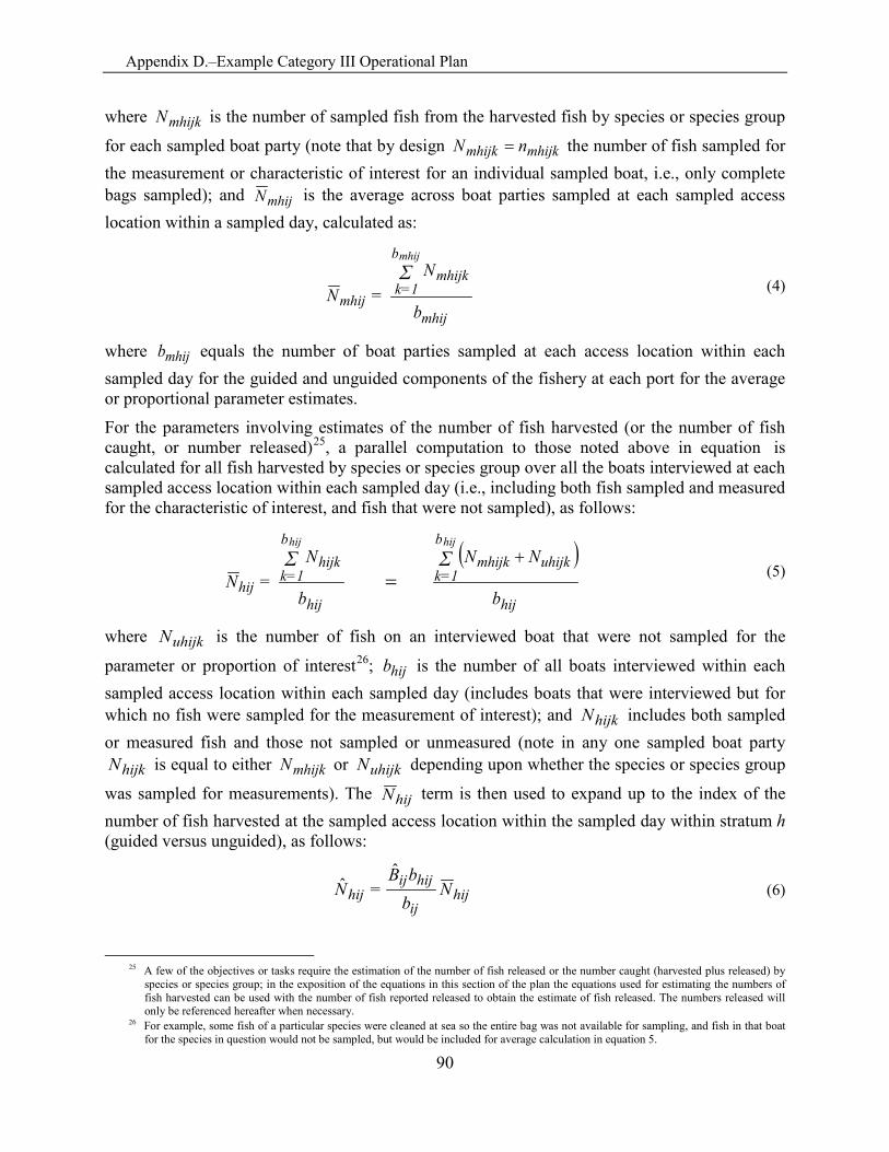
Appendix D.–Example Category III Operational Plan
90
where mhijkN is the number of sampled fish from the harvested fish by species or species group
for each sampled boat party (note that by design mhijkmhijk nN = the number of fish sampled for the measurement or characteristic of interest for an individual sampled boat, i.e., only complete bags sampled); and mhijN is the average across boat parties sampled at each sampled access location within a sampled day, calculated as:
mhij
mhijkb
k=1mhij
b
N = N
Σmhij
(4)
where mhijb equals the number of boat parties sampled at each access location within each sampled day for the guided and unguided components of the fishery at each port for the average or proportional parameter estimates.
For the parameters involving estimates of the number of fish harvested (or the number of fish caught, or number released)25, a parallel computation to those noted above in equation is calculated for all fish harvested by species or species group over all the boats interviewed at each sampled access location within each sampled day (i.e., including both fish sampled and measured for the characteristic of interest, and fish that were not sampled), as follows:
( )
hij
uhijkmhijkb
k=1
hij
hijkb
k=1hij
b
NN
b
N = N
ΣΣhijhij
+=
(5)
where uhijkN is the number of fish on an interviewed boat that were not sampled for the
parameter or proportion of interest26; hijb is the number of all boats interviewed within each sampled access location within each sampled day (includes boats that were interviewed but for which no fish were sampled for the measurement of interest); and hijkN includes both sampled or measured fish and those not sampled or unmeasured (note in any one sampled boat party
hijkN is equal to either mhijkN or uhijkN depending upon whether the species or species group
was sampled for measurements). The hijN term is then used to expand up to the index of the number of fish harvested at the sampled access location within the sampled day within stratum h (guided versus unguided), as follows:
hijij
hijijhij N
bbB
=Nˆ
ˆ (6)
25 A few of the objectives or tasks require the estimation of the number of fish released or the number caught (harvested plus released) by
species or species group; in the exposition of the equations in this section of the plan the equations used for estimating the numbers of fish harvested can be used with the number of fish reported released to obtain the estimate of fish released. The numbers released will only be referenced hereafter when necessary.
26 For example, some fish of a particular species were cleaned at sea so the entire bag was not available for sampling, and fish in that boat for the species in question would not be sampled, but would be included for average calculation in equation 5.
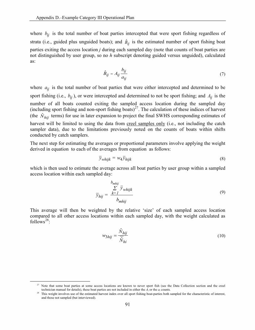
Appendix D.–Example Category III Operational Plan
91
where ijb is the total number of boat parties intercepted that were sport fishing regardless of
strata (i.e., guided plus unguided boats); and ijB is the estimated number of sport fishing boat parties exiting the access location j during each sampled day (note that counts of boat parties are not distinguished by user group, so no h subscript denoting guided versus unguided), calculated as:
ij
ijijij a
bAB =ˆ (7)
where ija is the total number of boat parties that were either intercepted and determined to be
sport fishing (i.e., ijb ), or were intercepted and determined to not be sport fishing; and ijA is the number of all boats counted exiting the sampled access location during the sampled day (including sport fishing and non-sport fishing boats)27. The calculation of these indices of harvest (the hijN terms) for use in later expansion to project the final SWHS corresponding estimates of harvest will be limited to using the data from creel samples only (i.e., not including the catch sampler data), due to the limitations previously noted on the counts of boats within shifts conducted by catch samplers.
The next step for estimating the averages or proportional parameters involve applying the weight derived in equation to each of the averages from equation as follows:
hijkwhijk y = wy 4 (8)
which is then used to estimate the average across all boat parties by user group within a sampled access location within each sampled day:
mhij
whijk
b
k=1hij
b
y = y
Σmhij
(9)
This average will then be weighted by the relative ‘size’ of each sampled access location compared to all other access locations within each sampled day, with the weight calculated as follows28:
hi
hijhij
N
Nw
ˆ
ˆ3 = (10)
27 Note that some boat parties at some access locations are known to never sport fish (see the Data Collection section and the creel
technician manual for details), these boat parties are not included in either the Ai or the ai counts. 28 This weight involves use of the estimated harvest index over all sport fishing boat-parties both sampled for the characteristic of interest,
and those not sampled (but interviewed).

Appendix D.–Example Category III Operational Plan
92
where hijN is the index of the number of fish harvested by each species or species group for
each sampled access location as calculated above in equation ; and hiN is the average number harvested across access locations sampled within each sampled day calculated as:
ˆ
ˆi
hijq
j=1hi
q
N = N
Σi
(11)
where iq is the number of access locations sampled within each sampled day (at this stage of the sampling there is no distinction between the guided and unguided components, and hence the dropping of the stratum subscript h).
For the parameters involving estimates of the number of fish harvested, the hiN term is used to expand up to the index of the number of fish harvested during the sampled day by user group (guided versus unguided), as follows:
hiihi NQ =N ˆˆ (12)
where iQ is the number of access locations that could have been sampled within each day.
The next step for estimating the averages or proportional parameters involve applying the weight derived in equation to each of the averages from equation as follows:
hijhijwhij y = wy 3 (13)
which is then used to estimate the average across all sampled access locations by user group within each sampled day:
i
whijq
j=1hi
q
y = y
Σi
(14)
This average will then be weighted by the relative ‘size’ of each sampled day compared to all other days sampled, with the weight calculated as follows:
h
hihi
NNwˆˆ
2 = (15)
where hiN is the index of the number of fish harvested by each species or species group for each
sampled day as calculated above in equation ; and hN is the average number harvested across sampled days calculated as:
ˆ
ˆd
N = N
hid
i=1h
Σ
(16)
where d is the number of days sampled for each major port (across all sampled locations).
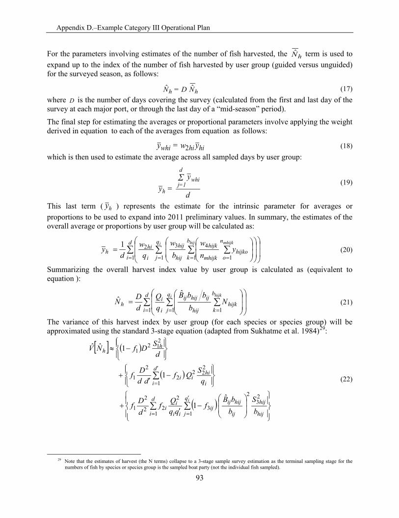
Appendix D.–Example Category III Operational Plan
93
For the parameters involving estimates of the number of fish harvested, the hN term is used to expand up to the index of the number of fish harvested by user group (guided versus unguided) for the surveyed season, as follows:
hh ND =N ˆˆ (17) where D is the number of days covering the survey (calculated from the first and last day of the survey at each major port, or through the last day of a “mid-season” period).
The final step for estimating the averages or proportional parameters involve applying the weight derived in equation to each of the averages from equation as follows:
hihiwhi y = wy 2 (18) which is then used to estimate the average across all sampled days by user group:
d
y = y
whid
j=1h
Σ
(19)
This last term ( yh ) represents the estimate for the intrinsic parameter for averages or proportions to be used to expand into 2011 preliminary values. In summary, the estimates of the overall average or proportions by user group will be calculated as:
∑ ∑ ∑ ∑= = = =
=
d
i
q
j
b
k
n
ohijko
mhijk
hijk
hij
hij
i
hih
i hij mhijky
nw
bw
qw
d y
1 1 1 1
4321 (20)
Summarizing the overall harvest index value by user group is calculated as (equivalent to equation ):
∑ ∑ ∑= = =
=
d
i
q
j
b
khijk
hij
ijhijij
i
ih
i hijkN
bbbB
dD N
1 1 1
ˆˆ (21)
The variance of this harvest index by user group (for each species or species group) will be approximated using the standard 3-stage equation (adapted from Sukhatme et al. 1984)29:
[ ] ( )
( )
( )
−
′+
−′
+
−≈
∑ ∑
∑
=
′
=
′
=
d
i hij
hijq
j ij
hijijij
ii
ii
d
i i
hiii
hh
bS
bbB
fqq
QfdDf
qSQf
ddDf
dSDfNV
i
1
23
2
13
2
22
2
1
1
222
2
2
1
212
1
ˆ1
1
1ˆˆ
(22)
29 Note that the estimates of harvest (the N terms) collapse to a 3-stage sample survey estimation as the terminal sampling stage for the
numbers of fish by species or species group is the sampled boat party (not the individual fish sampled).
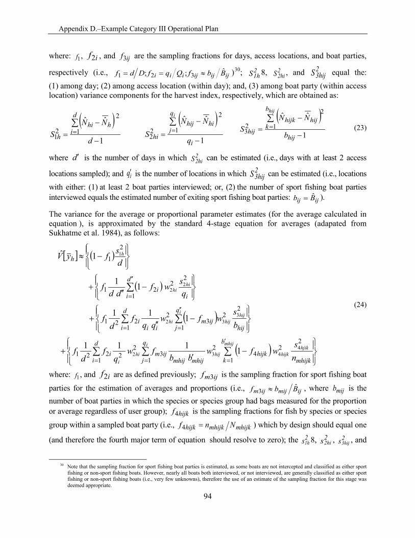
Appendix D.–Example Category III Operational Plan
94
where: 1f , if2 , and ijf3 are the sampling fractions for days, access locations, and boat parties,
respectively (i.e., ijijijiii BbfQqfDdf ˆ;; 321 ≈== )30; S21h 8, S2
2hi , and S 23hij equal the:
(1) among day; (2) among access location (within day); and, (3) among boat party (within access location) variance components for the harvest index, respectively, which are obtained as:
( )1
ˆˆ1
2
21 −
−=∑=
d
NNS
d
ihhi
h
( )1
ˆˆ1
2
22 −
−
=∑=
i
q
jhihij
hi q
NNS
i
( )1
ˆˆ1
2
23 −
−=∑=
hij
b
khijhijk
hij b
NNS
hij
(23)
where d ′ is the number of days in which S22hi can be estimated (i.e., days with at least 2 access
locations sampled); and iq′ is the number of locations in which S 23hij can be estimated (i.e., locations
with either: (1) at least 2 boat parties interviewed; or, (2) the number of sport fishing boat parties interviewed equals the estimated number of exiting sport fishing boat parties: ijij Bb ˆ= ).
The variance for the average or proportional parameter estimates (for the average calculated in equation ), is approximated by the standard 4-stage equation for averages (adapated from Sukhatme et al. 1984), as follows:
[ ] ( )
( )
( )
( )
−′
+
−′′
+
−′′
+
−≈
∑ ∑∑
∑∑
∑
=
′
==
′′
==
′′
=
i mhijhjik
hijkhijhii
i hijhijhi
hihi
h
q
j
b
k mhijkhijk
mhijmhijijm
d
ii
q
j hijijm
ii
d
ii
i
d
ii
h
ns
wfwbb
fwq
fd
f
bs
wfwqq
fd
f
qswf
ddf
dsfyV
1 1
22
42
32
21
221
1
22
32
1221
2
1
221
2
1
4432
332
22
1
1111
111
11
1ˆ
(24)
where: 1f , and if2 are as defined previously; ijmf 3 is the sampling fraction for sport fishing boat
parties for the estimation of averages and proportions (i.e., ijmijijm Bbf ˆ3 ≈ , where mijb is the number of boat parties in which the species or species group had bags measured for the proportion or average regardless of user group); hijkf4 is the sampling fractions for fish by species or species
group within a sampled boat party (i.e., mhijkmhijkhijk Nnf =4 ) which by design should equal one
(and therefore the fourth major term of equation should resolve to zero); the s21h 8, s2
2hi , s23hij , and
30 Note that the sampling fraction for sport fishing boat parties is estimated, as some boats are not intercepted and classified as either sport
fishing or non-sport fishing boats. However, nearly all boats both interviewed, or not interviewed, are generally classified as either sport fishing or non-sport fishing boats (i.e., very few unknowns), therefore the use of an estimate of the sampling fraction for this stage was deemed appropriate.
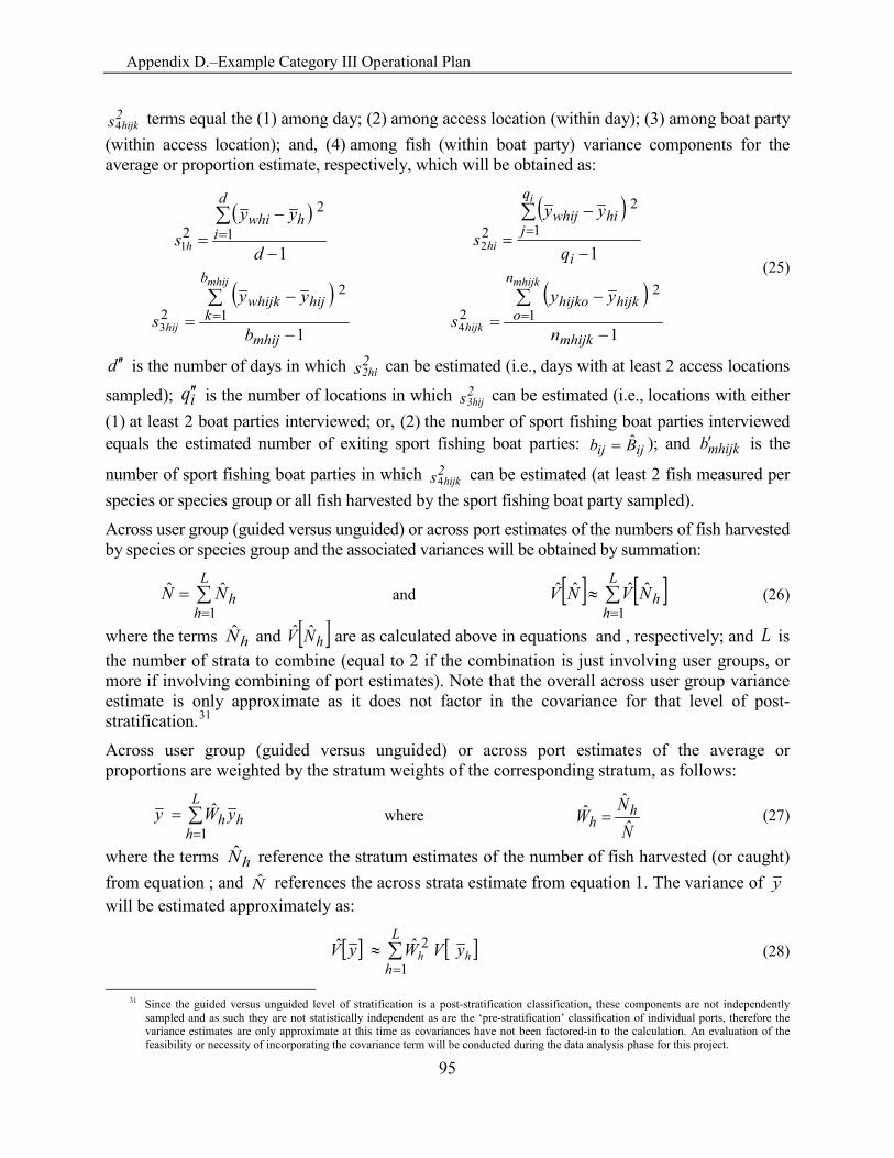
Appendix D.–Example Category III Operational Plan
95
s2hijk4 terms equal the (1) among day; (2) among access location (within day); (3) among boat party
(within access location); and, (4) among fish (within boat party) variance components for the average or proportion estimate, respectively, which will be obtained as:
( )
11
2
21 −
−=∑=
d
yys
d
ihwhi
h
( )1
1
2
22 −
−
=∑=
i
q
jhiwhij
q
yys
i
hi
(25)
( )1
1
2
23 −
−=
∑=
mhij
b
khijwhijk
b
yys
mhij
hij
( )1
1
2
24 −
−=
∑=
mhijk
n
ohijkhijko
n
yys
mhijk
hijk
d ′′ is the number of days in which s22hi can be estimated (i.e., days with at least 2 access locations
sampled); iq ′′ is the number of locations in which s23hij can be estimated (i.e., locations with either
(1) at least 2 boat parties interviewed; or, (2) the number of sport fishing boat parties interviewed equals the estimated number of exiting sport fishing boat parties: ijij Bb ˆ= ); and mhijkb′ is the
number of sport fishing boat parties in which s2hijk4 can be estimated (at least 2 fish measured per
species or species group or all fish harvested by the sport fishing boat party sampled).
Across user group (guided versus unguided) or across port estimates of the numbers of fish harvested by species or species group and the associated variances will be obtained by summation:
∑=
=L
hhNN
1ˆˆ and [ ] [ ]∑
=≈
L
hhNVNV
1ˆˆˆˆ (26)
where the terms hN and [ ]hNV ˆˆ are as calculated above in equations and , respectively; and L is the number of strata to combine (equal to 2 if the combination is just involving user groups, or more if involving combining of port estimates). Note that the overall across user group variance estimate is only approximate as it does not factor in the covariance for that level of post-stratification.31
Across user group (guided versus unguided) or across port estimates of the average or proportions are weighted by the stratum weights of the corresponding stratum, as follows:
∑=
=L
hhh yW y
1ˆ where
NNW h
h ˆˆ
ˆ = (27)
where the terms hN reference the stratum estimates of the number of fish harvested (or caught) from equation ; and N references the across strata estimate from equation 1. The variance of y will be estimated approximately as:
[ ] [ ]∑=
≈L
hhh yVW yV
1
2ˆˆ (28)
31 Since the guided versus unguided level of stratification is a post-stratification classification, these components are not independently
sampled and as such they are not statistically independent as are the ‘pre-stratification’ classification of individual ports, therefore the variance estimates are only approximate at this time as covariances have not been factored-in to the calculation. An evaluation of the feasibility or necessity of incorporating the covariance term will be conducted during the data analysis phase for this project.
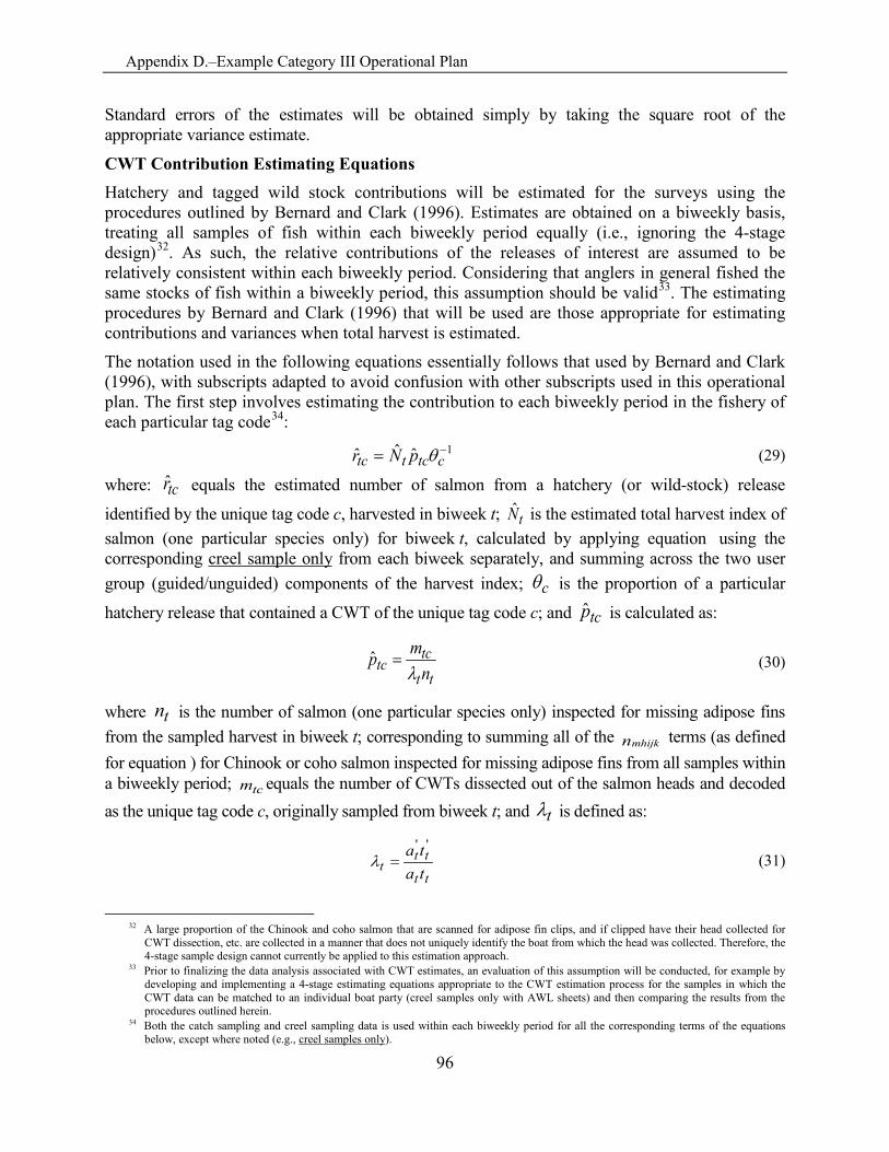
Appendix D.–Example Category III Operational Plan
96
Standard errors of the estimates will be obtained simply by taking the square root of the appropriate variance estimate.
CWT Contribution Estimating Equations Hatchery and tagged wild stock contributions will be estimated for the surveys using the procedures outlined by Bernard and Clark (1996). Estimates are obtained on a biweekly basis, treating all samples of fish within each biweekly period equally (i.e., ignoring the 4-stage design)32. As such, the relative contributions of the releases of interest are assumed to be relatively consistent within each biweekly period. Considering that anglers in general fished the same stocks of fish within a biweekly period, this assumption should be valid33. The estimating procedures by Bernard and Clark (1996) that will be used are those appropriate for estimating contributions and variances when total harvest is estimated.
The notation used in the following equations essentially follows that used by Bernard and Clark (1996), with subscripts adapted to avoid confusion with other subscripts used in this operational plan. The first step involves estimating the contribution to each biweekly period in the fishery of each particular tag code34:
1ˆˆˆ −= ctcttc pNr θ (29)
where: tcr equals the estimated number of salmon from a hatchery (or wild-stock) release
identified by the unique tag code c, harvested in biweek t; tN is the estimated total harvest index of salmon (one particular species only) for biweek t, calculated by applying equation using the corresponding creel sample only from each biweek separately, and summing across the two user group (guided/unguided) components of the harvest index; cθ is the proportion of a particular
hatchery release that contained a CWT of the unique tag code c; and tcp is calculated as:
tt
tctc n
mpλ
=ˆ (30)
where tn is the number of salmon (one particular species only) inspected for missing adipose fins from the sampled harvest in biweek t; corresponding to summing all of the nmhijk terms (as defined for equation ) for Chinook or coho salmon inspected for missing adipose fins from all samples within a biweekly period; tcm equals the number of CWTs dissected out of the salmon heads and decoded as the unique tag code c, originally sampled from biweek t; and tλ is defined as:
tt
ttt ta
ta ''=λ (31)
32 A large proportion of the Chinook and coho salmon that are scanned for adipose fin clips, and if clipped have their head collected for
CWT dissection, etc. are collected in a manner that does not uniquely identify the boat from which the head was collected. Therefore, the 4-stage sample design cannot currently be applied to this estimation approach.
33 Prior to finalizing the data analysis associated with CWT estimates, an evaluation of this assumption will be conducted, for example by developing and implementing a 4-stage estimating equations appropriate to the CWT estimation process for the samples in which the CWT data can be matched to an individual boat party (creel samples only with AWL sheets) and then comparing the results from the procedures outlined herein.
34 Both the catch sampling and creel sampling data is used within each biweekly period for all the corresponding terms of the equations below, except where noted (e.g., creel samples only).
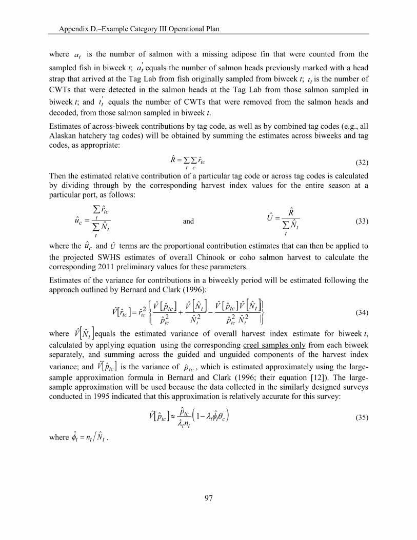
Appendix D.–Example Category III Operational Plan
97
where ta is the number of salmon with a missing adipose fin that were counted from the
sampled fish in biweek t; 'ta equals the number of salmon heads previously marked with a head
strap that arrived at the Tag Lab from fish originally sampled from biweek t; tt is the number of CWTs that were detected in the salmon heads at the Tag Lab from those salmon sampled in biweek t; and '
tt equals the number of CWTs that were removed from the salmon heads and decoded, from those salmon sampled in biweek t. Estimates of across-biweek contributions by tag code, as well as by combined tag codes (e.g., all Alaskan hatchery tag codes) will be obtained by summing the estimates across biweeks and tag codes, as appropriate:
∑∑=t c
tcrR ˆˆ (32)
Then the estimated relative contribution of a particular tag code or across tag codes is calculated by dividing through by the corresponding harvest index values for the entire season at a particular port, as follows:
∑
∑=
tt
ttc
c N
ru ˆ
ˆˆ and ∑
=
ttN
RU ˆˆˆ (33)
where the cu and U terms are the proportional contribution estimates that can then be applied to the projected SWHS estimates of overall Chinook or coho salmon harvest to calculate the corresponding 2011 preliminary values for these parameters. Estimates of the variance for contributions in a biweekly period will be estimated following the approach outlined by Bernard and Clark (1996):
[ ] [ ] [ ] [ ] [ ]
−+= 22222
ˆˆ
ˆˆˆˆ
ˆ
ˆˆ
ˆ
ˆˆˆˆˆ
ttcttctc
Np
NVpV
N
NV
p
pVrrV ttcttc
tc (34)
where [ ]tNV ˆˆ equals the estimated variance of overall harvest index estimate for biweek t, calculated by applying equation using the corresponding creel samples only from each biweek separately, and summing across the guided and unguided components of the harvest index variance; and [ ]tcpV ˆˆ is the variance of tcp , which is estimated approximately using the large-sample approximation formula in Bernard and Clark (1996; their equation [12]). The large-sample approximation will be used because the data collected in the similarly designed surveys conducted in 1995 indicated that this approximation is relatively accurate for this survey:
[ ] ( )ctttt
tctc n
ppV θφλλ
ˆ1ˆˆˆ −≈ (35)
where ttt Nn ˆˆ =φ .
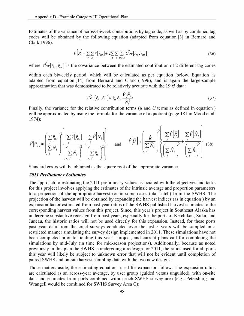
Appendix D.–Example Category III Operational Plan
98
Estimates of the variance of across-biweek contributions by tag code, as well as by combined tag codes will be obtained by the following equation (adapted from equation [3] in Bernard and Clark 1996):
[ ] [ ] [ ]∑∑ ∑∑∑>
∧+=
t c cututc
t ctc rrCovrVRV ˆ,ˆ2ˆˆˆˆ (36)
where [ ]tutc rrCov ˆ,ˆ∧ is the covariance between the estimated contribution of 2 different tag codes
within each biweekly period, which will be calculated as per equation below. Equation is adapted from equation [14] from Bernard and Clark (1996), and is again the large-sample approximation that was demonstrated to be relatively accurate with the 1995 data:
[ ] [ ]2ˆ
ˆˆˆˆˆ,ˆ
t
ttutctutc
N
NVrrrrCov ≈
∧ (37)
Finally, the variance for the relative contribution terms (u and U terms as defined in equation ) will be approximated by using the formula for the variance of a quotient (page 181 in Mood et al. 1974):
[ ][ ] [ ]
+
≈
∑
∑
∑
∑
∑
∑
22
2
ˆ
ˆˆ
ˆ
ˆˆ
ˆ
ˆˆˆ
ttc
tt
tt
ttc
tt
ttc
c
r
NV
N
rV
N
ruV and [ ]
[ ] [ ]
+
≈
∑
∑
∑
∑
∑ 22
2
ˆ
ˆˆ
ˆ
ˆˆ
ˆˆˆˆ
t
tt
tt
t
tt
R
NV
N
RV
NRUV
(38)
Standard errors will be obtained as the square root of the appropriate variance.
2011 Preliminary Estimates The approach to estimating the 2011 preliminary values associated with the objectives and tasks for this project involves applying the estimates of the intrinsic average and proportion parameters to a projection of the appropriate harvest (or in some cases total catch) from the SWHS. The projection of the harvest will be obtained by expanding the harvest indices (as in equation ) by an expansion factor estimated from past year ratios of the SWHS published harvest estimates to the corresponding harvest values from this project. Since, this year’s project in Southeast Alaska has undergone substantive redesign from past years, especially for the ports of Ketchikan, Sitka, and Juneau, the historic ratios will not be used directly for this expansion. Instead, for these ports past year data from the creel surveys conducted over the last 5 years will be sampled in a restricted manner simulating the survey design implemented in 2011. These simulations have not been completed prior to fielding this year’s project, and current plans call for completing the simulations by mid-July (in time for mid-season projections). Additionally, because as noted previously in this plan the SWHS is undergoing a redesign for 2011, the ratios used for all ports this year will likely be subject to unknown error that will not be evident until completion of paired SWHS and on-site harvest sampling data with the two new designs.
Those matters aside, the estimating equations used for expansion follow. The expansion ratios are calculated as an across-year average, by user group (guided versus unguided), with on-site data and estimates from ports combined within each SWHS survey area (e.g., Petersburg and Wrangell would be combined for SWHS Survey Area C):
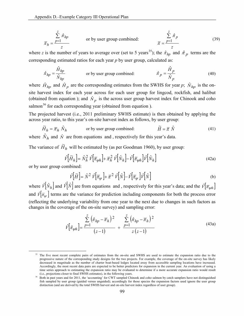
Appendix D.–Example Category III Operational Plan
99
z
z
php
h
∑== 1π
π or by user group combined:
z
z
pp∑
== 1π
π (39)
where z is the number of years to average over (set to 5 years35); the hpπ and pπ terms are the corresponding estimated ratios for each year p by user group, calculated as:
hp
hphp N
Hˆ
ˆˆ =π or by user group combined:
p
pp N
Hˆ
ˆˆ =π (40)
where hpH and pH are the corresponding estimates from the SWHS for year p; hpN is the on-site harvest index for each year across for each user group for lingcod, rockfish, and halibut (obtained from equation ); and pN is the across user group harvest index for Chinook and coho salmon36 for each corresponding year (obtained from equation ).
The projected harvest (i.e., 2011 preliminary SWHS estimate) is then obtained by applying the across year ratio, to this year’s on-site harvest index as follows, by user group:
hhh NH ˆ~ π= or by user group combined: NH ˆ~ π= (41)
where hN and N are from equations and , respectively for this year’s data.
The variance of hH~ will be estimated by (as per Goodman 1960), by user group:
[ ] [ ] [ ] [ ] [ ]hhhhhhh NVVNVVNHV ˆˆˆˆˆˆˆ~ˆ 22ψψ πππ −+= (42a)
or by user group combined:
[ ] [ ] [ ] [ ] [ ]NVVNVVNHV ˆˆˆˆˆˆˆ~ˆ 22ψψ πππ −+= (b)
where [ ]hNV ˆˆ and [ ]NV ˆˆ are from equations and , respectively for this year’s data; and the [ ]hV ψπˆ
and [ ]ψπV terms are the variance for prediction including components for both the process error (reflecting the underlying variability from one year to the next due to changes in such factors as changes in the coverage of the on-site survey) and sampling error:
[ ]( )( )
( )( )1
ˆ
1
ˆ
ˆˆ 1
2
1
2
−
−
+−
−
=∑∑==
zzzV
z
phhp
z
phhp
h
ππππ
πψ (43a)
35 The five most recent complete pairs of estimates from the on-site and SWHS are used to estimate the expansion ratio due to the
progressive nature of the corresponding study designs for the two projects. For example, the coverage of the on-site survey has likely decreased in magnitude as the number of charter boat-based lodges located away from accessible sampling locations have increased. Accordingly, the most recent data pairs are expected to be better predictors for expansion in the current year. An evaluation of using a time series approach to estimating the expansion ratio may be evaluated to determine if a more accurate expansion ratio would result (i.e., projections closer to final SWHS estimates), in the following years.
36 Both in past years and for 2011, the ‘accounting’ for CWT sampled Chinook and coho salmon by catch samplers have not distinguished fish sampled by user group (guided versus unguided); accordingly for those species the expansion factors used ignore the user group distinction (and are derived by the total SWHS harvest and on-site harvest index regardless of user group).
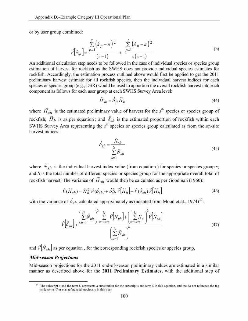
Appendix D.–Example Category III Operational Plan
100
or by user group combined:
[ ]( )( )
( )( )1
ˆ
1
ˆ
ˆˆ 1
2
1
2
−
−
+−
−
=∑∑==
zzzV
z
pp
z
pp ππππ
πψ (b)
An additional calculation step needs to be followed in the case of individual species or species group estimation of harvest for rockfish as the SWHS does not provide individual species estimates for rockfish. Accordingly, the estimation process outlined above would first be applied to get the 2011 preliminary harvest estimate for all rockfish species, then the individual harvest indices for each species or species group (e.g., DSR) would be used to apportion the overall rockfish harvest into each component as follows for each user group at each SWHS Survey Area level:
hshsh HH ~ˆ~ δ= (44)
where shH~ is the estimated preliminary value of harvest for the sth species or species group of
rockfish; hH~ is as per equation ; and shδ is the estimated proportion of rockfish within each SWHS Survey Area representing the sth species or species group calculated as from the on-site harvest indices:
∑=
= S
ssh
shsh
N
N
1ˆ
ˆδ
(45)
where shN is the individual harvest index value (from equation ) for species or species group s; and S is the total number of different species or species group for the appropriate overall total of rockfish harvest. The variance of shH~ would then be calculated as per Goodman (1960):
[ ] [ ]hshhshshhsh HVVHVVHHV ~ˆ)ˆ(ˆ~ˆˆ)ˆ(ˆ~)~(ˆ 22 δδδ −+= (46)
with the variance of shδ calculated approximately as (adapted from Mood et al., 1974)37:
[ ][ ] [ ]
4
1
22
1
ˆ
ˆˆˆˆˆˆˆˆ ,1 ,1
+
≈
∑
∑ ∑∑
=
= ≠= ≠=
U
ush
shU U
uuhU
uuh
sh
N
NVNNVNV suu suuδ
(47)
and [ ]shNV ˆˆ as per equation , for the corresponding rockfish species or species group.
Mid-season Projections Mid-season projections for the 2011 end-of-season preliminary values are estimated in a similar manner as described above for the 2011 Preliminary Estimates, with the additional step of
37 The subscript u and the term U represents a substitution for the subscript s and term S in this equation, and the do not reference the tag
code terms U or u as referenced previously in this plan.
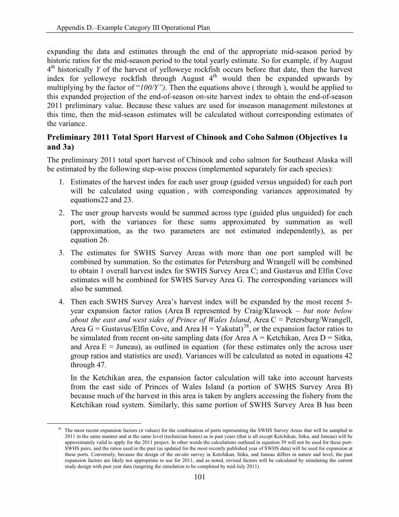
Appendix D.–Example Category III Operational Plan
101
expanding the data and estimates through the end of the appropriate mid-season period by historic ratios for the mid-season period to the total yearly estimate. So for example, if by August 4th historically Y of the harvest of yelloweye rockfish occurs before that date, then the harvest index for yelloweye rockfish through August 4th would then be expanded upwards by multiplying by the factor of “100/Y”). Then the equations above ( through ), would be applied to this expanded projection of the end-of-season on-site harvest index to obtain the end-of-season 2011 preliminary value. Because these values are used for inseason management milestones at this time, then the mid-season estimates will be calculated without corresponding estimates of the variance.
Preliminary 2011 Total Sport Harvest of Chinook and Coho Salmon (Objectives 1a and 3a) The preliminary 2011 total sport harvest of Chinook and coho salmon for Southeast Alaska will be estimated by the following step-wise process (implemented separately for each species):
1. Estimates of the harvest index for each user group (guided versus unguided) for each port will be calculated using equation , with corresponding variances approximated by equations22 and 23.
2. The user group harvests would be summed across type (guided plus unguided) for each port, with the variances for these sums approximated by summation as well (approximation, as the two parameters are not estimated independently), as per equation 26.
3. The estimates for SWHS Survey Areas with more than one port sampled will be combined by summation. So the estimates for Petersburg and Wrangell will be combined to obtain 1 overall harvest index for SWHS Survey Area C; and Gustavus and Elfin Cove estimates will be combined for SWHS Survey Area G. The corresponding variances will also be summed.
4. Then each SWHS Survey Area’s harvest index will be expanded by the most recent 5-year expansion factor ratios (Area B represented by Craig/Klawock – but note below about the east and west sides of Prince of Wales Island, Area C = Petersburg/Wrangell, Area G = Gustavus/Elfin Cove, and Area H = Yakutat)38, or the expansion factor ratios to be simulated from recent on-site sampling data (for Area A = Ketchikan, Area D = Sitka, and Area E = Juneau), as outlined in equation (for these estimates only the across user group ratios and statistics are used). Variances will be calculated as noted in equations 42 through 47.
In the Ketchikan area, the expansion factor calculation will take into account harvests from the east side of Princes of Wales Island (a portion of SWHS Survey Area B) because much of the harvest in this area is taken by anglers accessing the fishery from the Ketchikan road system. Similarly, this same portion of SWHS Survey Area B has been
38 The most recent expansion factors (π values) for the combination of ports representing the SWHS Survey Areas that will be sampled in
2011 in the same manner and at the same level (technician hours) as in past years (that is all except Ketchikan, Sitka, and Juneau) will be approximately valid to apply for the 2011 project. In other words the calculations outlined in equation 39 will not be used for these port-SWHS pairs, and the ratios used in the past (as updated for the most recently published year of SWHS data) will be used for expansion at these ports. Conversely, because the design of the on-site survey in Ketchikan, Sitka, and Juneau differs in nature and level, the past expansion factors are likely not appropriate to use for 2011, and as noted, revised factors will be calculated by simulating the current study design with past year data (targeting the simulation to be completed by mid-July 2011).
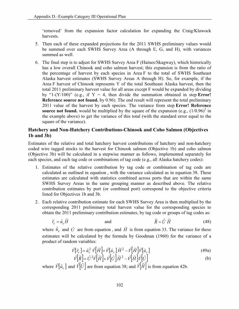
Appendix D.–Example Category III Operational Plan
102
‘removed’ from the expansion factor calculation for expanding the Craig/Klawock harvests.
5. Then each of these expanded projections for the 2011 SWHS preliminary values would be summed over each SWHS Survey Area (A through E, G, and H), with variances summed as well.
6. The final step is to adjust for SWHS Survey Area F (Haines/Skagway), which historically has a low overall Chinook and coho salmon harvest; this expansion is from the ratio of the percentage of harvest by each species in Area F to the total of SWHS Southeast Alaska harvest estimates (SWHS Survey Areas A through H). So, for example, if the Area F harvest of Chinook represents Y of the total Southeast Alaska harvest, then the total 2011 preliminary harvest value for all areas except F would be expanded by dividing by “1-(Y/100)” (e.g., if Y = 4, then divide the summation obtained in step Error! Reference source not found. by 0.96). The end result will represent the total preliminary 2011 value of the harvest by each species. The variance from step Error! Reference source not found. would be multiplied by the square of the expansion (e.g., (1/0.96)2 in the example above) to get the variance of this total (with the standard error equal to the square of the variance).
Hatchery and Non-Hatchery Contributions-Chinook and Coho Salmon (Objectives 1b and 3b) Estimates of the relative and total hatchery harvest contributions of hatchery and non-hatchery coded wire tagged stocks to the harvest for Chinook salmon (Objective 1b) and coho salmon (Objective 3b) will be calculated in a stepwise manner as follows, implemented separately for each species, and each tag code or combinations of tag code (e.g., all Alaska hatchery codes):
1. Estimates of the relative contribution by tag code or combination of tag code are calculated as outlined in equation , with the variance calculated as in equation 38. These estimates are calculated with statistics combined across ports that are within the same SWHS Survey Areas in the same grouping manner as described above. The relative contribution estimates by port (or combined port) correspond to the objective criteria listed for Objectives 1b and 3b.
2. Each relative contribution estimate for each SWHS Survey Area is then multiplied by the corresponding 2011 preliminary total harvest value for the corresponding species to obtain the 2011 preliminary contribution estimates, by tag code or groups of tag codes as:
Hur cc~ˆ~ = and HUR ~ˆ~ = (48)
where cu and U are from equation , and H~ is from equation 33. The variance for these estimates will be calculated by the formula by Goodman (1960) for the variance of a product of random variables:
[ ] [ ] [ ] [ ] [ ]cccc uVHVHuVHVurV ˆˆ~ˆ~ˆˆ~ˆˆ~ˆ 22 −+= (49a)
[ ] [ ] [ ] [ ] [ ]UVHVHUVHVURV ˆˆ~ˆ~ˆˆ~ˆˆ~ˆ 22 −+=
(b)
where [ ]cuV ˆˆ and [ ]UV ˆˆ are from equation 38; and [ ]HV ~ˆ is from equation 42b.
Appendix D.–Example Category III Operational Plan
103
3. The total contribution estimates by tag code or combined tag code for each species over all survey areas is obtained by summation across SWHS Survey Areas in a similar manner as described above for the Preliminary 2011 Total Sport Harvest, with variances obtained by summation.
Pacific Salmon Treaty Harvest (Objectives 1c and 2) The Pacific Salmon Treaty Harvest (Chinook salmon) will be estimated for Southeast Alaska in total (Objective 1c) by first calculating the total Alaska hatchery contributions for each SWHS Survey Area as described above (Hatchery and Non-Hatchery Contributions-Chinook and Coho Salmon). Then the following steps will be followed to estimate the preliminary treaty harvest for Southeast Alaska for 201139:
1. The total contribution estimate of Alaska hatchery to the Chinook salmon harvest by SWHS Survey Area is then subtracted from the 2011 Preliminary Total Harvest of Chinook salmon for each Survey area, the resulting estimate of the preliminary total harvest of Chinook salmon without Alaskan hatchery fish (as Alaskan Hatchery fish do not count towards the treaty). These reduced total harvests would then be summed across all surveyed SWHS Survey Areas.
Because Wrangell Narrows is specifically denoted in the SWHS, and because we are able to identify those Chinook salmon harvested and sampled from Wrangell Narrows in the data, we omit these fish from the inseason harvest projection. The Wrangell Narrows-Blind Slough Terminal Harvest Area Salmon Management Plan (5 AAC 33.381) specifically notes Chinook harvested in that area as being 100 Alaska hatchery, and therefore would not count toward the quota.
2. The next step is to adjust for SWHS Survey Areas with low Chinook salmon harvest, which includes the Haines/Skagway and Yakutat areas. The expansion factor to be used was approximately 1.04 (derived from past SWHS estimates), which indicated that these combined SWHS Survey Area’s harvests only represented a minor percentage (4) of the Southeast Alaska regional harvest.
3. The final step will be to adjust the treaty harvest upward to reflect the subtraction of the base catch and “risk adjustment factor” from the total Alaskan hatchery contribution estimate40. The risk adjustment factor is calculated by multiplying the standard error of the Alaska hatchery contribution estimate by 1.272. This subtraction ensures that the calculated contribution does not exceed the actual contribution. The preseason estimate of the base catch and “risk adjustment factor” is 15 of the Alaska hatchery contribution.
The need for, as well as the process for calculating the early season (late April through mid-July) treaty harvest for Commercial Salmon Districts 8 (Petersburg/Wrangell) and 11 (Juneau), follows:
District 8: The Pacific Salmon Treaty requires the U.S. delegation (and Alaska in particular in this case) to provide weekly estimates of wild Stikine River large (≥28”) Chinook salmon being harvested in District 8 by both sport and commercial fishermen
39 Variances (and standard errors) are not currently estimated for the Pacific Salmon Treaty estimates as the point estimates are used ‘as-is’
for treaty purposes. 40 The adjustment of the total Alaskan hatchery contribution estimate by the “risk adjustment factor” is determined by procedures
associated with the U.S./Canada treaty. The end result of the subtraction of the adjustment factor from the contribution estimate is to increase the size of the treaty harvest estimate. The final estimate of the “risk adjustment factor” for the sport treaty harvest is calculated by John Carlile, Fishery Scientist, Division of Commercial Fisheries at ADF&G Headquarters.
Appendix D.–Example Category III Operational Plan
104
during late April to mid-July. Large Chinook salmon sport harvest in District 8 is sampled onsite at the ports of Petersburg (north end of District 8) and Wrangell (south end of District 8), and the onsite samplers summarize the District 8-specific information as part of their weekly paperwork. Recoveries of CWTs from large Chinook salmon in District 8 areas from the weekly sport fisheries are used to estimate the relative contribution of Alaska and non-Alaska hatchery fish, and non-Alaska wild fish. The total wild large Chinook salmon harvest is estimated by subtracting the estimated number of Alaska and non-Alaska hatchery fish, and non-Alaska wild fish from the estimated total harvest. The recent 5-year average of the expansion factor for each port (Petersburg has an expansion factor of 5 and Wrangell’s is 4) is applied to the above relative estimates to project the total harvest of District 8 large Chinook salmon.
District 11: The Pacific Salmon Treaty requires the U.S. delegation (and Alaska in particular in this case) to provide weekly estimates of wild Taku River large (≥28”) Chinook salmon being harvested in District 11 by both sport and commercial fishermen during late April to early July. Large Chinook salmon harvest in District 11, which includes the majority of the Juneau-area marine waters, are sampled onsite at the port of Juneau. In addition to the sampled docks and boat launches, during mid-April to the end of May the unique shoreline Chinook fishery at Picnic Cove on the north end of Douglas Island is sampled, as it occurs in District 11. The District 11 harvest information is the majority of the entire harvest encountered by onsite personnel in Juneau, so the data are examined and any Chinook salmon information from outside of District 11 is excluded. Recoveries of CWTs from large Chinook salmon from District 11 areas from the weekly sport fisheries are used to estimate the relative contribution of Alaska and non-Alaska hatchery fish, and non-Alaska wild fish. The total wild large Chinook salmon harvest is estimated by subtracting the estimated number of Alaska and non-Alaska hatchery fish, and non-Alaska wild fish from the estimated total harvest. An expansion factor for Juneau will be developed to expand to projected total harvest estimates for District 11.
Note that in both cases, due to the nature of this information need for addressing Pacific Salmon Treaty requirements inseason, no estimates of variance are required at this time.
Average Weight Estimates (Objective 4), and Length Composition (Secondary Objective 1) of Pacific Halibut Estimates of the mean net weights of halibut harvested at all sampled ports will be made in 2011 by first converting each measured length using the IPHC length-weight relationship to obtain an individual weight for each fish measured, as:
βα hijkohijko L = W (50)
where hijkoW is the converted weight for each fish o in the kth sampled boat party’s bag, at access
location j, on the sampled day i for each user group h (guided versus unguided), the hijkoL is the length for each halibut measured, and α and β are the estimated regression parameters for the length-to-weight conversion model endorsed by the IPHC (Clark 1992), with α = 6.921 x 10⁻⁶ and β = 3.24 for net weight in pounds converted from total length in centimeters. The individual lengths for each fish are converted to weights in this approach rather than applying the conversion to a mean length as per the recommendations by Nielsen and Schoch (1980). No
Appendix D.–Example Category III Operational Plan
105
correction will be made for transformation bias because the length-weight relationship was based on a large sample and the residual variance is extremely small (William Clark, IPHC, personal communication). Mean weight estimates are presented in pounds rather than kilograms because that is the standard unit used by halibut management agencies. The mean weight estimates by user group for each port or combined ports within each SWHS Survey Area are then calculated by substituting the converted weight values ( hijkoW ) for the yhijko term in equation resulting in the average net weight by user group at each port or combined port (the combined port estimates are produced by treating each access location at each port as if they were separate access locations in the combined port in the multi-stage calculations). The estimated variances for these averages will be approximated by similar substitution into equation , with standard errors calculated as the square root of the variances.
Proportion of Pacific Halibut Harvested by Unguided Anglers Prior to Mean IPHC Survey Date (Objective 5) The proportion of the Pacific halibut harvested by unguided anglers prior to the mean IPHC survey date will be as follows for each port (or combined port):
+
=≥<
<
<
)()(
)(
)( ˆˆ
ˆˆ
IDduIDdu
IDdu
IDduNN
Np (51)
where )(ˆ Ddup < is the proportion of the halibut harvest index for the unguided component41 of the
fishery for the date d less than the mean IPHC survey date ( ID ), )(ˆ
IDduN < is the harvest index using creel samples only for the unguided component prior to the mean IPHC survey date (as previously noted the mean date will be provided by IPHC) at each port by using equation on this restricted data set, and )(
ˆIDduN ≥ is the unguided harvest index for dates greater than or equal to
the mean IPHC survey date (again from equation on those restricted dates). The variance of )(ˆ Ddup < will be calculated approximately as (adapted from Mood et al. 1974):
[ ]( ) [ ] [ ]
( )422
)()(
)()()()()(
)( ˆˆ
ˆˆˆˆˆˆˆˆˆ
IDduDdu
DduIDduIDduIDduDdu
DduNN
NVNNVNNpV
≥<
<≥≥≥<
<+
++≈ (52)
where the corresponding variance terms are calculated from equation on the two sets of data restricted by date.
The span of dates of the surveys at each port is expected to cover the vast majority of the halibut sport fishery for the unguided component; however, an unknown portion of the total yearly harvest likely occurs both before and after the dates covered. Accordingly, the proportions estimated by equation may be biased by some unknown degree (but the bias is assumed to be minimal in magnitude).
Average Weight and Preliminary Biomass Estimates of Lingcod (Objective 6) The average round weight estimates for lingcod by user group (guided versus unguided) and user group combined for the ports of Sitka, Ketchikan, Craig/Klawock, Gustavus, Elfin Cove, and
41 The subscript u represents unguided, and does not reference the tag code terms U or u as referenced previously in this plan.
Appendix D.–Example Category III Operational Plan
106
Yakutat will be calculated in the same manner as described above for the average weight of halibut. The corresponding estimated for the regression parameters are α = 7.9 x 10⁻⁶ and β = 3.07 for round weight in kilograms, with total length measured in centimeters for use in equation 50. The values for α and β are those used by the Division of Commercial Fisheries (Dave Carlile, ADF&G Juneau, personnel communication). The mean weight estimates by user group and in total for each port or combined ports within each SWHS Survey Area are then calculated by substituting the converted weight values for the yhijko term in equation , resulting in the average round weight by user group at each port or combined port (the combined port estimates are produced by treating each access location at each port as if they were separate access locations in the combined port in the multi-stage calculations). The estimated variances for these averages will be approximated by similar substitution into equation , with standard errors calculated as the square root of the variances.
The preliminary biomass estimate for each SWHS Survey Area will then be estimated by multiplying the resultant average weights for each port (or combined ports within each SWHS Survey Area) by the corresponding preliminary harvest estimate (by user group and user group combined), as follows:
hh Hw = Wh~~
and Hw = W ~~ (53)
where hw and w are the average weight estimates by user group and by user group combined as
calculated by equation (with weight substituted for “y”); and hH~ and H~ equal to the preliminary harvest of lingcod in numbers of fish for each user group and user group combined as obtained by equation 20. The variance of the estimated biomass will be calculated by the equation of Goodman (1960) as:
[ ] [ ] [ ] [ ] [ ]hhhhhhh wVHVHwVHVwWV ˆ~ˆ~ˆ~ˆ~ˆ 22 −+= and (54a)
[ ] [ ] [ ] [ ] [ ]wVHVHwVHVwWV ˆ~ˆ~ˆ~ˆ~ˆ 22 −+=
(b)
where [ ]hwV and [ ]wV are from equation 24; and [ ]hHV ~ˆ and [ ]HV ~ˆ are from equations 42a and 42b, respectively.
Rockfish Species Composition; and Average Weight Estimates and Preliminary Biomass Removals of Demersal Shelf Rockfish (Objective 7) The species composition of rockfish will be estimated as proportions of the harvest at each port (or combined ports within a SWHS Survey Area) and calculated as outlined in equation , with corresponding variances from equation 47.
The average weight by rockfish species for each species and species grouping will be estimated in the similar manner as described above for the halibut and lingcod. The regression parameters for converting lengths to weight were developed from paired length and weight data collected by this project during 2006 and 2007, or from other sources for species with low sample sizes (see Table 4).
As was done for the halibut and lingcod average weight calculation, each rockfish by species with a measured length will have the length converted to a weight (using equation with the regression parameters in Table 4), and the resultant weights will be substituted into equation , resulting in the average round weight by user group at each port or combined port. The estimated variances for these averages will be approximated by similar substitution into equation , with
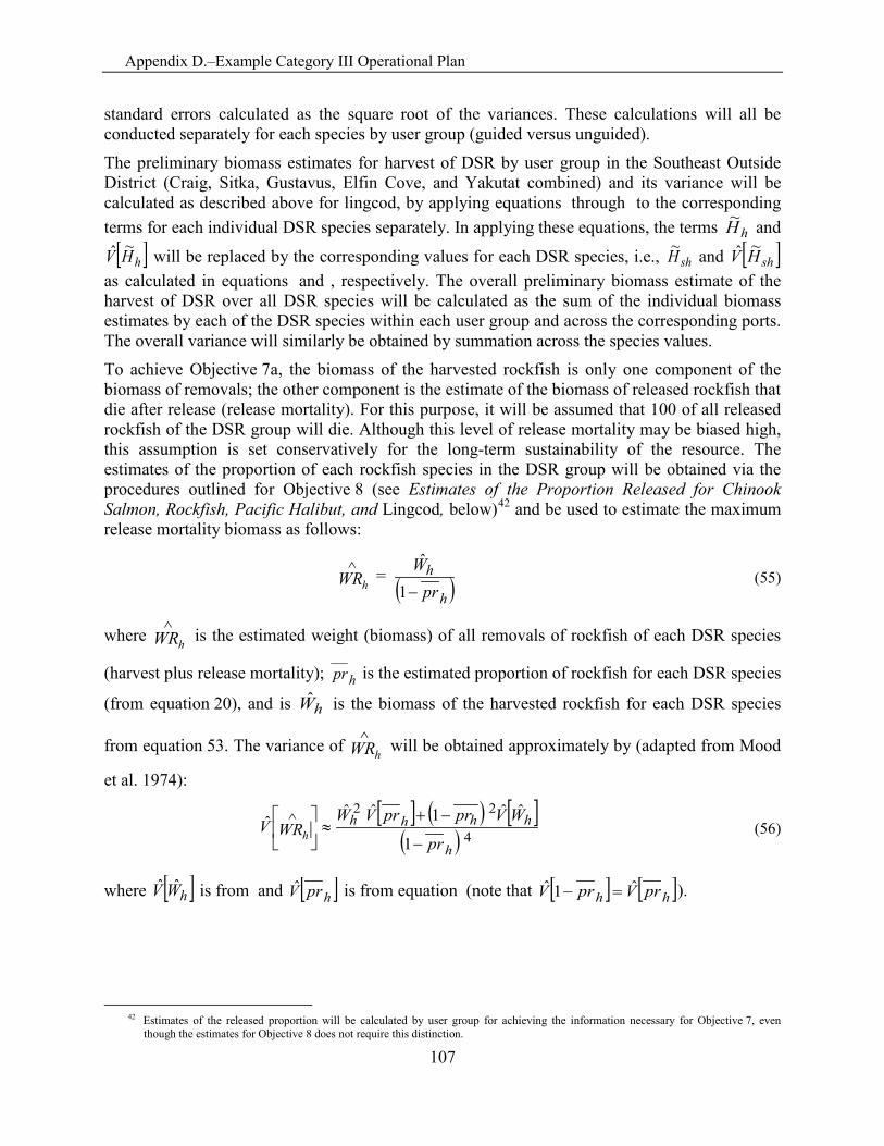
Appendix D.–Example Category III Operational Plan
107
standard errors calculated as the square root of the variances. These calculations will all be conducted separately for each species by user group (guided versus unguided).
The preliminary biomass estimates for harvest of DSR by user group in the Southeast Outside District (Craig, Sitka, Gustavus, Elfin Cove, and Yakutat combined) and its variance will be calculated as described above for lingcod, by applying equations through to the corresponding terms for each individual DSR species separately. In applying these equations, the terms hH~ and
[ ]hHV ~ˆ will be replaced by the corresponding values for each DSR species, i.e., shH~ and [ ]shHV ~ˆ as calculated in equations and , respectively. The overall preliminary biomass estimate of the harvest of DSR over all DSR species will be calculated as the sum of the individual biomass estimates by each of the DSR species within each user group and across the corresponding ports. The overall variance will similarly be obtained by summation across the species values. To achieve Objective 7a, the biomass of the harvested rockfish is only one component of the biomass of removals; the other component is the estimate of the biomass of released rockfish that die after release (release mortality). For this purpose, it will be assumed that 100 of all released rockfish of the DSR group will die. Although this level of release mortality may be biased high, this assumption is set conservatively for the long-term sustainability of the resource. The estimates of the proportion of each rockfish species in the DSR group will be obtained via the procedures outlined for Objective 8 (see Estimates of the Proportion Released for Chinook Salmon, Rockfish, Pacific Halibut, and Lingcod, below)42 and be used to estimate the maximum release mortality biomass as follows:
( )h
hpr
W= WRh −1
ˆ^ (55)
where hWR is the estimated weight (biomass) of all removals of rockfish of each DSR species
(harvest plus release mortality); hpr is the estimated proportion of rockfish for each DSR species
(from equation 20), and is hW is the biomass of the harvested rockfish for each DSR species
from equation 53. The variance of hWR will be obtained approximately by (adapted from Mood
et al. 1974):
[ ] ( ) [ ]( ) 4
22
1
ˆˆ1ˆˆ^ˆh
hhhh
pr
WVprprVWWRV h −
−+≈
(56)
where [ ]hWV ˆˆ is from and [ ]hprV is from equation (note that [ ] [ ]hh prVprV ˆ1ˆ =− ).
42 Estimates of the released proportion will be calculated by user group for achieving the information necessary for Objective 7, even
though the estimates for Objective 8 does not require this distinction.
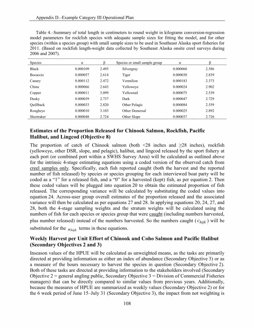
Appendix D.–Example Category III Operational Plan
108
Table 4.–Summary of total length in centimeters to round weight in kilograms conversion-regression model parameters for rockfish species with adequate sample sizes for fitting the model, and for other species (within a species group) with small sample sizes to be used in Southeast Alaska sport fisheries for 2011. (Based on rockfish length-weight data collected by Southeast Alaska onsite creel surveys during 2006 and 2007).
Species α β Species or small sample group α β
Black 0.000109 2.495 Silvergray 0.000060 2.586 Bocaccio 0.000057 2.614 Tiger 0.000030 2.839 Canary 0.000112 2.472 Vermilion 0.000183 2.373 China 0.000066 2.643 Yelloweye 0.000024 2.902 Copper 0.000011 3.099 Yellowtail 0.000075 2.539 Dusky 0.000039 2.737 Dark 0.000047 2.729 Quillback 0.000033 2.820 Other Pelagic 0.000084 2.559 Rougheye 0.000010 3.103 Other Demersal 0.000025 2.892 Shortraker 0.000048 2.724 Other Slope 0.000037 2.726
Estimates of the Proportion Released for Chinook Salmon, Rockfish, Pacific Halibut, and Lingcod (Objective 8) The proportion of catch of Chinook salmon (both <28 inches and ≥28 inches), rockfish (yelloweye, other DSR, slope, and pelagic), halibut, and lingcod released by the sport fishery at each port (or combined port within a SWHS Survey Area) will be calculated as outlined above for the intrinsic 4-stage estimating equations using a coded version of the observed catch from creel samples only. Specifically, each fish reported caught (both the harvest and the reported number of fish released) by species or species grouping for each interviewed boat party will be coded as a “1” for a released fish, and a “0” for a harvested (kept) fish, as per equation 2. Then these coded values will be plugged into equation 20 to obtain the estimated proportion of fish released. The corresponding variance will be calculated by substituting the coded values into equation 24. Across-user group overall estimates of the proportion released and the associated variance will then be calculated as per equations 27 and 28. In applying equations 20, 24, 27, and 28, both the 4-stage sampling weights and the stratum weights will be calculated using the numbers of fish for each species or species group that were caught (including numbers harvested, plus number released) instead of the numbers harvested. So the numbers caught ( hijkc ) will be substituted for the nhijk terms in these equations.
Weekly Harvest per Unit Effort of Chinook and Coho Salmon and Pacific Halibut (Secondary Objectives 2 and 3) Inseason values of the HPUE will be calculated as unweighted means, as the tasks are primarily directed at providing information as either an index of abundance (Secondary Objective 3) or as a measure of the hours necessary to harvest the species in question (Secondary Objective 2). Both of these tasks are directed at providing information to the stakeholders involved (Secondary Objective 2 = general angling public, Secondary Objective 3 = Division of Commercial Fisheries managers) that can be directly compared to similar values from previous years. Additionally, because the measures of HPUE are summarized as weekly values (Secondary Objective 2) or for the 6 week period of June 15–July 31 (Secondary Objective 3), the impact from not weighting is
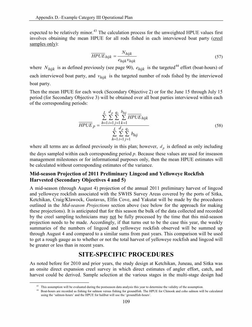
Appendix D.–Example Category III Operational Plan
109
expected to be relatively minor.43 The calculation process for the unweighted HPUE values first involves obtaining the mean HPUE for all rods fished in each interviewed boat party (creel samples only):
hijkhijk
hijkhijk ve
NHPUE = (57)
where hijkN is as defined previously (see page 90), hijke is the targeted44 effort (boat-hours) of
each interviewed boat party, and hijkv is the targeted number of rods fished by the interviewed boat party.
Then the mean HPUE for each week (Secondary Objective 2) or for the June 15 through July 15 period (for Secondary Objective 3) will be obtained over all boat parties interviewed within each of the corresponding periods:
∑ ∑ ∑
∑ ∑ ∑ ∑
= = =
= = = ==L
h
d
i
q
jhij
L
h
d
i
q
j
b
khijk
pp i
p i hij
b
HPUEHPUE
1 1 1
1 1 1 1 (58)
where all terms are as defined previously in this plan; however, pd is defined as only including the days sampled within each corresponding period p. Because these values are used for inseason management milestones or for informational purposes only, then the mean HPUE estimates will be calculated without corresponding estimates of the variance.
Mid-season Projection of 2011 Preliminary Lingcod and Yelloweye Rockfish Harvested (Secondary Objectives 4 and 5) A mid-season (through August 4) projection of the annual 2011 preliminary harvest of lingcod and yelloweye rockfish associated with the SWHS Survey Areas covered by the ports of Sitka, Ketchikan, Craig/Klawock, Gustavus, Elfin Cove, and Yakutat will be made by the procedures outlined in the Mid-season Projections section above (see below for the approach for making these projections). It is anticipated that for this season the bulk of the data collected and recorded by the creel sampling technicians may not be fully processed by the time that this mid-season projection needs to be made. Accordingly, if that turns out to be the case this year, the weekly summaries of the numbers of lingcod and yelloweye rockfish observed will be summed up through August 4 and compared to a similar sums from past years. This comparison will be used to get a rough gauge as to whether or not the total harvest of yelloweye rockfish and lingcod will be greater or less than in recent years.
SITE-SPECIFIC PROCEDURES As noted before for 2010 and prior years, the study design at Ketchikan, Juneau, and Sitka was an onsite direct expansion creel survey in which direct estimates of angler effort, catch, and harvest could be derived. Sample selection at the various stages in the multi-stage design had
43 This assumption will be evaluated during the postseason data analysis this year to determine the validity of the assumption. 44 Boat-hours are recorded as fishing for salmon versus fishing for groundfish. The HPUE for Chinook and coho salmon will be calculated
using the ‘salmon-hours’ and the HPUE for halibut will use the ‘groundfish-hours’.
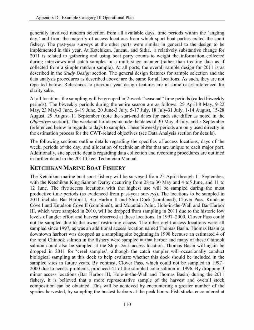
Appendix D.–Example Category III Operational Plan
110
generally involved random selection from all available days, time periods within the ‘angling day,’ and from the majority of access locations from which sport boat parties exited the sport fishery. The past-year surveys at the other ports were similar in general to the design to be implemented in this year. At Ketchikan, Juneau, and Sitka, a relatively substantive change for 2011 is related to gathering and using boat party counts to weight the information collected during interviews and catch samples in a multi-stage manner (rather than treating data as if collected from a simple random sample). At all ports, the overall sample design for 2011 is as described in the Study Design section. The general design features for sample selection and the data analysis procedures as described above, are the same for all locations. As such, they are not repeated below. References to previous year design features are in some cases referenced for clarity sake.
At all locations the sampling will be grouped in 2-week “seasonal” time periods (called biweekly periods). The biweekly periods during the entire season are as follows: 25 April-8 May, 9-22 May, 23 May-3 June, 6–19 June, 20 June-3 July, 5-17 July, 18 July-31 July, 1-14 August, 15-28 August, 29 August–11 September (note the start-end dates for each site differ as noted in the Objectives section). The weekend-holidays include the dates of 30 May, 4 July, and 5 September (referenced below in regards to days to sample). These biweekly periods are only used directly in the estimation process for the CWT-related objectives (see Data Analysis section for details).
The following sections outline details regarding the specifics of access locations, days of the week, periods of the day, and allocation of technician shifts that are unique to each major port. Additionally, site specific details regarding data collection and recording procedures are outlined in further detail in the 2011 Creel Technician Manual.
KETCHIKAN MARINE BOAT FISHERY The Ketchikan marine boat sport fishery will be surveyed from 25 April through 11 September, with the Ketchikan King Salmon Derby occurring from 28 to 30 May and 4 to5 June, and 11 to 12 June. The five access locations with the highest use will be sampled during the most productive time periods (as evidenced from past-year surveys). The locations to be sampled in 2011 include: Bar Harbor I, Bar Harbor II and Ship Dock (combined), Clover Pass, Knudson Cove I and Knudson Cove II (combined), and Mountain Point. Hole-in-the-Wall and Bar Harbor III, which were sampled in 2010, will be dropped from sampling in 2011 due to the historic low levels of angler effort and harvest observed at these locations. In 1997–2000, Clover Pass could not be sampled due to the owner restricting access. The other eight access locations were all sampled since 1997, as was an additional access location named Thomas Basin. Thomas Basin (a downtown harbor) was dropped as a sampling site beginning in 1998 because an estimated 4 of the total Chinook salmon in the fishery were sampled at that harbor and many of these Chinook salmon could also be sampled at the Ship Dock access location. Thomas Basin will again be dropped in 2011 for ‘creel samples’, although the catch sampler will occasionally conduct biological sampling at this dock to help evaluate whether this dock should be included in the sampled sites in future years. By contrast, Clover Pass, which could not be sampled in 1997–2000 due to access problems, produced 41 of the sampled coho salmon in 1996. By dropping 3 minor access locations (Bar Harbor III, Hole-in-the-Wall and Thomas Basin) during the 2011 fishery, it is believed that a more representative sample of the harvest and overall stock composition can be obtained. This will be achieved by encountering a greater number of the species harvested, by sampling the busiest harbors at the peak hours. Fish stocks encountered at
Appendix D.–Example Category III Operational Plan
111
the three dropped locations are unlikely to be different stocks than those sampled at the remaining locations. Salmon Falls (a lodge on the north end of the Ketchikan road system) was dropped as of 2003 due to lack of cooperation from the lodge owner and remains inaccessible.
A total of 2 to 4 staff 45 are assigned to the project, working 6.5 hours each scheduled day. All weekends and holidays will be worked, and in general the days off for creel samplers will be Tuesday and Wednesday. The catch samplers will generally have Thursday and Friday off. Allocation of sampling effort was determined by a combination of periods of greatest levels of angling effort and harvest, by dock and by hour as evidenced from past-year surveys. The scheduling of days and periods to sample within the entire survey were structurally different for derby versus non-derby periods as described below.
Within any of the non-derby biweekly periods (i.e., biweeks 9, 10, 13–18), 2 to 4 technicians (2–3 interview technicians and 1 catch sampler) will be deployed to conduct the creel and catch sampling. Days off were designated as Tuesdays and Wednesdays with all holidays worked, and harbors were selected at random without replacement (WOR) for each day sampled.
The specific time periods for sampling within each day were set to maximize the expected number of interviews and observed harvest as evidenced from past surveys. The specific time periods to cover shift within the season as noted in Table 5. An additional 30 minutes was given to the Ship Dock/Bar Harbor II selection to accommodate the travel between harbor, therefore giving 6.5 hours of actual sample time. The sampling time for this location was adjusted according to when the cruise ship charters would be returning to the docks. This information was provided by the cruise ship schedule and the business booking the guided charter trips.
Within the two derby biweekly periods (i.e., biweeks 11 and 12), 4 technicians (3 interview technicians and 1 catch sampler) will conduct harvest sampling for 6.5 hours Wednesday through Sunday, with the non-derby day sampling periods determined as stated above. Each sampling day was selected at random WOR from all available harbors (Table 5).
The sampling time during the seven days of the derby will be from 14:30–21:00. This was based on the maximum number of entered fish by hour in 2009 and 2010, and 2 of the 4 weigh-in stations will be covered with a catch sampler. The weigh-in stations chosen are those most likely to provide the best chance of sampling the most entries. Reviewing the past seven years (2004–2010) showed Mountain Point, Bar Harbor, and Knudson Cove had productive years for the King Salmon Derby. To ensure the samples are representative of the stock composition, a south-of-town or in-town harbor and a north-of-town harbor will be scheduled. The sampling time for the derby days changed in 2011 to sample consistently throughout the season and proportional to the harvest (Table 5). In the past, all derby weigh-in stations (3 or 4) were sampled from 12:00 to 21:00; each day was primarily covered by volunteers conducting CWT sampling on all entered fish.
Additional CWT harvest inspection samples were scheduled during the spring Chinook fishery (17 May through 27 June) and the main coho season (starting on 1 July). These additional samples were directed at increasing the proportion of harvested Chinook and coho salmon inspected for adipose fin clips (denoting the possible presence of a CWT). The scheduling of these "CWT samples" was structured to consistently sample at locations with a substantial harvest of Chinook and coho salmon that "represented the fishery". Data from previous creel
45 Dependent upon the period of the survey, see preseason planning calendar.
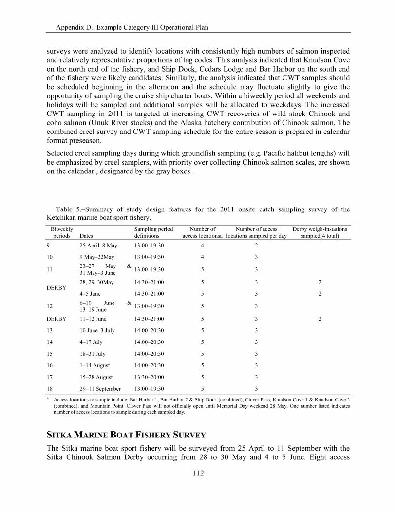
Appendix D.–Example Category III Operational Plan
112
surveys were analyzed to identify locations with consistently high numbers of salmon inspected and relatively representative proportions of tag codes. This analysis indicated that Knudson Cove on the north end of the fishery, and Ship Dock, Cedars Lodge and Bar Harbor on the south end of the fishery were likely candidates. Similarly, the analysis indicated that CWT samples should be scheduled beginning in the afternoon and the schedule may fluctuate slightly to give the opportunity of sampling the cruise ship charter boats. Within a biweekly period all weekends and holidays will be sampled and additional samples will be allocated to weekdays. The increased CWT sampling in 2011 is targeted at increasing CWT recoveries of wild stock Chinook and coho salmon (Unuk River stocks) and the Alaska hatchery contribution of Chinook salmon. The combined creel survey and CWT sampling schedule for the entire season is prepared in calendar format preseason.
Selected creel sampling days during which groundfish sampling (e.g. Pacific halibut lengths) will be emphasized by creel samplers, with priority over collecting Chinook salmon scales, are shown on the calendar , designated by the gray boxes.
Table 5.–Summary of study design features for the 2011 onsite catch sampling survey of the
Ketchikan marine boat sport fishery. Biweekly periods Dates
Sampling period definitions
Number of access locationsa
Number of access locations sampled per day
Derby weigh-instations sampled(4 total)
9 25 April–8 May 13:00–19:30 4 2
10 9 May–22May 13:00–19:30 4 3
11 23–27 May & 31 May–3 June 13:00–19:30 5 3
DERBY 28, 29, 30May 14:30–21:00 5 3 2
4–5 June 14:30–21:00 5 3 2
12 6–10 June & 13–19 June 13:00–19:30 5 3
DERBY 11–12 June 14:30–21:00 5 3 2
13 10 June–3 July 14:00–20:30 5 3
14 4–17 July 14:00–20:30 5 3
15 18–31 July 14:00–20:30 5 3
16 1–14 August 14:00–20:30 5 3
17 15–28 August 13:30–20:00 5 3
18 29–11 September 13:00–19:30 5 3 a Access locations to sample include: Bar Harbor 1, Bar Harbor 2 & Ship Dock (combined), Clover Pass, Knudson Cove 1 & Knudson Cove 2
(combined), and Mountain Point. Clover Pass will not officially open until Memorial Day weekend 28 May. One number listed indicates number of access locations to sample during each sampled day.
SITKA MARINE BOAT FISHERY SURVEY The Sitka marine boat sport fishery will be surveyed from 25 April to 11 September with the Sitka Chinook Salmon Derby occurring from 28 to 30 May and 4 to 5 June. Eight access
Appendix D.–Example Category III Operational Plan
113
locations in the Sitka marine boat fishery will be sampled: Crescent Harbor 1, Crescent Harbor 2, Sealing Cove 1, Sealing Cove 2, Thomsen Harbor 1, Thomsen Harbor 2, Starrigavin Boat Launch, and The Cove. These are the same locations sampled since 2005 (i.e., no docks were dropped for sampling from the Sitka area).
The creel technicians will generally have Monday and Tuesday off each week. Days off will be shifted in a week if a standard day off falls on a holiday or a derby day. All technicians will work the same schedule on the dock. Examination of data from 2006 to 2010 indicated that the majority of anglers returned to port during this sampling period. A total of 2 to 4 staff are assigned to the project and each of these staff can sample 10 days within each biweekly period. During the non-derby biweekly periods, the schedule was generated as follows: 1) two consecutive days off were set as described above; and, 2) locations to sample from the access locations were selected at random WOR. A similar procedure was used for scheduling sampling during the derby biweekly period. The specific time periods for sampling within each day was set to maximize the expected number of interviews and observed harvest as evidenced from past surveys. The specific time periods to cover shift within the season are noted in Table 6. The number of sampling units scheduled for the entire season is also summarized in Table 6, and the resultant schedule for the entire season is presented in calendar format preseason.
Additional CWT harvest inspection samples were scheduled for 1–2 additional biological samplers to increase the proportion of harvested Chinook and coho salmon inspected for adipose fin clips. CWT sampling was scheduled to consistently sample at locations with a substantial harvest of Chinook and coho salmon that “represent the fishery” based on prior-year data and the current Sitka cruise ship schedule (for chartered vessels). The additional sampler will also able to inspect fish landed at the busier charter vessel harbors catering to cruise ship passengers that may be missed during normal creel survey interviews because of time constraints. CWT samples were scheduled from Monday through Sunday with 2 consecutive days off. During the derby days, the CWT sampler will be deployed at the derby entry station to increase the inspection of harvested fish for adipose fin clips, and to collect genetic samples from Chinook salmon. The derby entry station at Crescent Harbor is open from 0700 to 1900.
Selected creel sampling days during which groundfish sampling (e.g. Pacific halibut lengths) will be emphasized by creel samplers with priority are shown by the gray boxes in the season calendar.
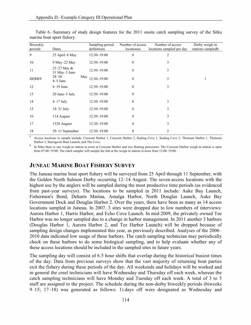
Appendix D.–Example Category III Operational Plan
114
Table 6.–Summary of study design features for the 2011 onsite catch sampling survey of the Sitka marine boat sport fishery. Biweekly periods Dates
Sampling period definitions
Number of access locationsa
Number of access locations sampled per day
Derby weigh-in stations sampledb
9 25 April–8 May 12:30–19:00 8 2
10 9 May–22 May 12:30–19:00 8 3
11 23–27 May & 31 May–3 June 12:30–19:00 8 3
DERBY 28–30 May 4–5 June 12:30–19:00 8 3 1
12 6–19 June 12:30–19:00 8 3
13 20 June–3 July 12:30–19:00 8
14 4–17 July 12:30–19:00 8 3
15 18–31 July 12:30–19:00 8 3
16 114 August 12:30–19:00 8 3
17 1528 August 12:30–19:00 8 3
18 29–11 September 12:30–19:00 8 2 a Access locations to sample include: Crescent Harbor 1, Crescent Harbor 2, Sealing Cove 1, Sealing Cove 2, Thomsen Harbor 1, Thomsen
Harbor 2, Starrigavin Boat Launch, and The Cove. b In Sitka there is one weigh-in station in town at Crescent Harbor and two floating processors. The Crescent Harbor weigh-in station is open
from 07:00–19:00. The catch sampler will sample the fish at the weigh-in station in town from 12:00–19:00.
JUNEAU MARINE BOAT FISHERY SURVEY The Juneau marine boat sport fishery will be surveyed from 25 April through 11 September, with the Golden North Salmon Derby occurring 12–14 August. The seven access locations with the highest use by the anglers will be sampled during the most productive time periods (as evidenced from past-year surveys). The locations to be sampled in 2011 include: Auke Bay Launch, Fishermen's Bend, Deharts Marina, Amalga Harbor, North Douglas Launch, Auke Bay Government Dock and Douglas Harbor 2. Over the years, there have been as many as 14 access locations sampled in Juneau. In 2007, 3 sites were dropped due to low numbers of interviews: Aurora Harbor 1, Harris Harbor, and Echo Cove Launch. In mid-2009, the privately owned Tee Harbor was no longer sampled due to a change in harbor management. In 2011 another 3 harbors (Douglas Harbor 1, Aurora Harbor 2, and Tee Harbor Launch) will be dropped because of sampling design changes implemented this year, as previously described. Analyses of the 2006–2010 data indicated low usage of these harbors. The catch sampling technician may periodically check on these harbors to do some biological sampling, and to help evaluate whether any of these access locations should be included in the sampled sites in future years.
The sampling day will consist of 6.5 hour shifts that overlap during the historical busiest times of the day. Data from previous surveys show that the vast majority of returning boat parties exit the fishery during these periods of the day. All weekends and holidays will be worked and in general the creel technicians will have Wednesday and Thursday off each week, whereas the catch sampling technicians will have Monday and Tuesday off each week. A total of 3 to 5 staff are assigned to the project. The schedule during the non-derby biweekly periods (biweeks 9–15; 17–18) was generated as follows: 1) days off were designated as Wednesday and
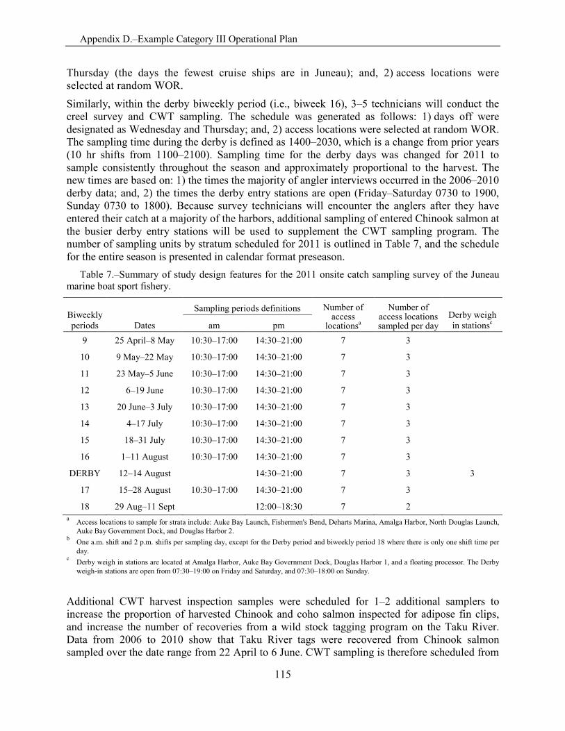
Appendix D.–Example Category III Operational Plan
115
Thursday (the days the fewest cruise ships are in Juneau); and, 2) access locations were selected at random WOR.
Similarly, within the derby biweekly period (i.e., biweek 16), 3–5 technicians will conduct the creel survey and CWT sampling. The schedule was generated as follows: 1) days off were designated as Wednesday and Thursday; and, 2) access locations were selected at random WOR. The sampling time during the derby is defined as 1400–2030, which is a change from prior years (10 hr shifts from 1100–2100). Sampling time for the derby days was changed for 2011 to sample consistently throughout the season and approximately proportional to the harvest. The new times are based on: 1) the times the majority of angler interviews occurred in the 2006–2010 derby data; and, 2) the times the derby entry stations are open (Friday–Saturday 0730 to 1900, Sunday 0730 to 1800). Because survey technicians will encounter the anglers after they have entered their catch at a majority of the harbors, additional sampling of entered Chinook salmon at the busier derby entry stations will be used to supplement the CWT sampling program. The number of sampling units by stratum scheduled for 2011 is outlined in Table 7, and the schedule for the entire season is presented in calendar format preseason.
Table 7.–Summary of study design features for the 2011 onsite catch sampling survey of the Juneau marine boat sport fishery.
Biweekly periods Dates
Sampling periods definitions Number of access
locationsa
Number of access locations sampled per day
Derby weigh in stationsc am pm
9 25 April–8 May 10:30–17:00 14:30–21:00 7 3
10 9 May–22 May 10:30–17:00 14:30–21:00 7 3
11 23 May–5 June 10:30–17:00 14:30–21:00 7 3
12 6–19 June 10:30–17:00 14:30–21:00 7 3
13 20 June–3 July 10:30–17:00 14:30–21:00 7 3
14 4–17 July 10:30–17:00 14:30–21:00 7 3
15 18–31 July 10:30–17:00 14:30–21:00 7 3
16 1–11 August 10:30–17:00 14:30–21:00 7 3
DERBY 12–14 August 14:30–21:00 7 3 3
17 15–28 August 10:30–17:00 14:30–21:00 7 3
18 29 Aug–11 Sept 12:00–18:30 7 2 a Access locations to sample for strata include: Auke Bay Launch, Fishermen's Bend, Deharts Marina, Amalga Harbor, North Douglas Launch,
Auke Bay Government Dock, and Douglas Harbor 2. b One a.m. shift and 2 p.m. shifts per sampling day, except for the Derby period and biweekly period 18 where there is only one shift time per
day. c Derby weigh in stations are located at Amalga Harbor, Auke Bay Government Dock, Douglas Harbor 1, and a floating processor. The Derby
weigh-in stations are open from 07:30–19:00 on Friday and Saturday, and 07:30–18:00 on Sunday.
Additional CWT harvest inspection samples were scheduled for 1–2 additional samplers to increase the proportion of harvested Chinook and coho salmon inspected for adipose fin clips, and increase the number of recoveries from a wild stock tagging program on the Taku River. Data from 2006 to 2010 show that Taku River tags were recovered from Chinook salmon sampled over the date range from 22 April to 6 June. CWT sampling is therefore scheduled from
Appendix D.–Example Category III Operational Plan
116
25 April through 12 June 2011 to maximize the number of Chinook salmon examined, while attempting to collect a representative stock composition sample for the entire fishery. Data from 2007 to 2010 indicate that 22 of the total Chinook harvest was landed at south-end harbors (Douglas 1 & 2 and Aurora 2) during biweeks 9–13, with 16 landed at Douglas 2. Anglers landing fish at these south-end harbors generally fish different areas than those using north-end harbors. The largest number of Chinook salmon could be sampled at either Douglas (representative of the south-end fishery) or Auke Bay (representative of the north-end fishery). The sampler at “Auke Bay” would primarily cover Auke Bay Government Dock, but could sometimes move to Dehart’s and/or Auke Bay Launch. For 2011, the catch sampler will also sample the spring fishery at Tee Harbor Launch because it is no longer one of the randomly chosen docks, but represents a unique spring Chinook fishery. Within a biweekly period, all Fridays, Saturdays and Sundays (and Memorial Day) will be sampled, with Monday and Tuesday generally set as days off. CWT samples were scheduled to consistently sample at locations with a substantial harvest of Chinook and coho salmon that “represent the fishery” based on prior-year data and the current Juneau cruise ship schedule (for chartered vessels). However, when low tides occurred in the mornings during the False Outer Point fishery (see next paragraph), the schedule was set for earlier in the day to try to intercept the early morning anglers. If only one catch sampler is funded, Douglas will be scheduled for sampling 1 day per week in biweeks 9, 10, and 13, and for 3 days per biweek in biweeks 11 and 12. As previously noted, it is not critical that sampling be exactly proportional to harvest as the weighting procedure to be implemented this year (described in the Study Design and Data Analysis sections) corrects for departures from proportional sampling. Regardless, this sampling schedule is thought to be representative of the entire spring fishery. If funding allows for 2 spring catch samplers, then one will sample the False Outer Point fishery and Douglas, while the other will sample Auke Bay and Tee Harbor Launch.
A shoreline fishery for Chinook salmon at False Outer Point (Picnic Cove) on the north end of Douglas Island will also be sampled in conjunction with late-April through May marine boat CWT sampling effort. This fishery is believed to target almost entirely wild stocks headed for the Taku River (based on limited prior CWT sampling). A harvest estimate for this shoreline fishery will be obtained from the SWHS. This fishery is tide dependent; at high tides, anglers are displaced to areas where they generally harvest few fish. This fishery will be proportionally sampled 5 days per week from 11 April to 31 May, either at the beginning or end of the shifts outlined above - dependent upon the tidal stage. It takes about 1.5 hours to travel to/from the site and check all harvested fish for CWTs. In 2009 and 2010, over 75 of the samples taken by the catch sampler in biweeks 8–11 were from Chinook salmon harvested at Picnic Cove versus Douglas or Auke Bay during the rest of the shift. This fishery is essentially over by 1 June and therefore need not be sampled after that. The additional sampler will also sample coho salmon for missing adipose fins from 13 June through 28 August to increase recoveries of Taku River wild stocks. Data from 2007 to 2010 indicated that only 5 of the total coho harvest was landed at south-end harbors, therefore all additional CWT sampling was scheduled at Auke Bay. Within a biweekly period, all weekends and holidays will be sampled and 2 or 3 additional samples per week were allocated to weekdays. CWT sampling was scheduled to consistently sample at locations with a substantial harvest of Chinook and coho salmon that “represent the fishery.” However, when low tides occurred in the mornings, the schedule was set for earlier in the day to try to intercept the early
Appendix D.–Example Category III Operational Plan
117
morning fishermen. All the additional CWT samples for both Chinook and coho salmon are listed in conjunction with the regular creel survey schedule in the preseason calendar.
Selected creel sampling days in which Pacific halibut harvest will be sampled for length information with priority over collecting Chinook salmon scales is shown by the gray boxes in the preseason planning calendar.
CRAIG/KLAWOCK MARINE BOAT FISHERY SURVEY During the period from 2 May to 28 August 2011, 3 technicians will sample the fishery. The two primary ports being sampled are the six access locations in Craig: 1) North Cove Harbor and ramp; 2) South Cove Harbor; 3) Shelter Cove; 4) Catch A King; 5) Haida/Sunnahae Lodges; and, 6) Ruth Ann’s; and 5 access locations in the Klawock area: 1) Klawock Boat Ramp; 2) Klawock Boat Harbor; 3) Fireweed Inn Dock; 4) Log Cabin Dock; and, 5) old Prince of Wales Lodge Dock.
Two creel technicians will conduct both creel survey (e.g., effort, catch and release, etc.) and biological data sampling, while the third technician will be dedicated to collecting biological data only. On Saturday and Sunday, Craig and Klawock will each have 1 creel technician conducting catch and effort interviews, as well as collecting biological data. One creel technician will be scheduled to sample MondayWednesday and Saturday–Sunday from 1200 to 1830, while the second creel technician will sample on Thursday–Sunday from 1200 to 1830. The catch sampler (i.e., person who only does biological sampling) will work Monday through Friday (sampling period: 1200–1830) at whatever location the creel interviewer is not scheduled to sample.
In 1997, a substantial number of charter vessels moved from the public harbor to their own private moorage facilities and the number of Chinook salmon sampled dropped substantially from previous years. In 1998, the sampler surveyed additional private moorage facilities where charter vessels dock during all of the sampling days. Because all the vessels return at the same time, it will take only 1–2 hours (of the scheduled 6.5 hour shift) to sample these additional moorages. Both samplers will continue this additional sampling in 2011 when scheduled at the Craig/Klawock harbors. This design should provide a consistent proportion of sampling effort throughout the season, and maximize the number of Chinook and coho salmon sampled.
PETERSBURG MARINE BOAT FISHERY SURVEY During 25 April to 28 August 2010, 1 technician will sample the harvest of boat-anglers returning to access locations (harbors) in the Petersburg area. The technician will sample 5 days per week (all weekend/holidays plus 2 or 3 randomly selected weekdays). During each sample period, the sampler is scheduled to inspect harvests at both the North/Middle Harbor aggregate and at the South Harbor from 1230 to 1900.
During the Petersburg Salmon Derby (27 May–30 May), additional staff will be stationed at the North Harbor weigh-in station for CWT and genetic sampling of Chinook salmon. The derby schedule will be from 1430–2100 each of the four days. Derby entries by half hour were reviewed for 3 previous years to determine the time when the maximum number of fish were entered. In the past, all entries were sampled, but in 2011 the sampling period was shortened to be consistent throughout the season, and to provide representative sampling proportional to the harvest.
The sampling schedule was generated with 2 consecutive days off and chosen weekly at random. Days in which Pacific halibut harvest will be sampled for length information with priority over collecting Chinook salmon scales is shown by the gray boxes in the preseason calendar.
Appendix D.–Example Category III Operational Plan
118
WRANGELL MARINE BOAT FISHERY SURVEY During the period from 25 April to 28 August 2011, 1 technician will sample the harvest of boat-anglers returning to access locations (harbors) in the Wrangell area. Three access locations in the Wrangell marine boat fishery are located downtown within sight of each other: 1) Inner Town Harbor; 2) Outer Town Harbor; and, 3) Government Dock. Shoemaker Harbor is located about 3 miles out the road from the other access locations. In 2008, Heritage Harbor, located approximately 2 miles south from downtown Wrangell, was made available for moorage and boat launching. It was found during the 2008 season that Heritage Harbor had little or no sport fishing activity; however, use increased in 2009 and interviews were conducted. In 2011, Heritage Harbor will be sampled equal to the Town Harbors and Shoemaker. Roughly 30 of the Chinook salmon harvest is brought into Shoemaker Harbor.
Examination of 1996 catch sample data indicated that the largest number of Chinook salmon could be examined by concentrating sampling effort on weekends and in the middle of the sampling day. The sampling schedule was generated as follows by allocating 5 sampling days per week: all weekend/holidays (Saturdays, Sundays, 30 May and 4 July) were selected for sampling from 1200 to 2030 (8.5 hours), and 2 or 3 remaining sampling days (of the 5 per week) were randomly selected from weekday days for sampling from 1400 to 2000 (6 hours). Days off were selected as either Monday/Tuesday, Tuesday/Wednesday, Wednesday/Thursday, Thursday/Friday, with Monday/Tuesday and Thursday/Friday being weighted heavier than the others. Harbors were selected at random WOR and sampled during 4 hour shifts on the weekend/holidays and approximately 3 hours on the weekdays depending on the time for travel. All harbors were treated equal to ensure the sample was representative of the entire fishery.
Selected creel sampling days during which Pacific halibut harvest will be sampled for length information with priority over collecting Chinook salmon scales are shown by the gray boxes in the preseason planning calendar.
GUSTAVUS MARINE BOAT FISHERY SURVEY During the period from 2 May to 28 August 2011, 1 technician will sample the harvest of boat-anglers returning to access locations (harbors) in the Gustavus area. The main access location is the dock/pier located immediately south of the main residential area of Gustavus. The sampling schedule was generated with 2 consecutive days off between Monday and Friday and chosen weekly at random, with the timing of the daily sampling dependent upon when marine boat fishers are returning from trips. Based on the interviews collected in 2002 in Gustavus, the time period of 12:00–19:00 was determined to represent over 90 of the collected interviews. Therefore, all sampling in Gustavus in 2011 will occur during 12:00–19:00.
The technician will collect Chinook salmon scale samples during the months of May and June (i.e., the spring fishery), as well as from Chinook salmon sampled for axillary appendage clips for the genetic sampling for the rest of the season. Selected creel sampling days in Gustavus in which sampling Pacific halibut, rockfish and lingcod harvest for length information will have priority over collecting Chinook salmon scale samples are shown by the gray boxes (designated groundfish priority sampling days) in the preseason planning calendar.
Appendix D.–Example Category III Operational Plan
119
ELFIN COVE MARINE BOAT FISHERY SURVEY During the period from 9 May to 28 August 2011, 1 technician will sample the harvest of boat-anglers returning to access locations (docks) in the Elfin Cove area. There is an inner and outer harbor separated by a narrow channel at Elfin Cove, and each harbor has 3 private/lodge docks and 1 public dock. Previous sport fish catch sampling at Elfin Cove in 2002 and 2003 (conducted by a University of Washington Fisheries graduate student in cooperation with our Marine Harvest Program) indicated a difficulty in trying to sample more than 1 or 2 of these exit points each day due to all lodge boats returning at the same general time in the late afternoon, and that very little nonguided/private angler fishing occurs in Elfin Cove. The catch sampler at Elfin Cove in 2002 and 2003 ended up contacting lodges to determine when their charter boats would be returning, and then the sampler would randomly select one of the docks to conduct the catch sampling for several hours.
For 2011, the schedule was set up as follows: 2 consecutive days off were chosen randomly between Monday and Friday of each week, then the inner or outer harbor was randomly selected for each day. In prior years, a dock was also chosen for each day to assist the sampler in deciding which dock to sample in the designated harbor in the event of several boats returning at once. However due to low bookings for 2011, fewer boats will be operating with some lodges not opening for business at all. Because each dock is tied to a lodge, the additional designation is not needed for the sampler this season. The timing of the daily sampling is dependent upon when marine boat fishers are returning from trips. Based on the catch sampling interviews collected in 2002 and 2003 in Elfin Cove, most lodge boats returned to their docks during the afternoon between 1600 and 1830, therefore, the period of 1300–1900 was selected as the tentative sampling period each day, with the idea that during the early afternoon the catch sampler will attempt to interview the few private boats that are returning to the various docks in Elfin Cove. An ADF&G employee conducted the catch sampling in 2004 through 2010 in Elfin Cove, and followed the above schedule with good success in obtaining interviews and collecting biological data throughout the season.
The technician will collect Chinook salmon axillary appendage clips for the genetic sampling and scale samples over the whole of the season.
Selected creel sampling days in Elfin Cove in which sampling Pacific halibut, rockfish, and lingcod harvest for length information will have priority over collecting Chinook salmon scale samples are shown by the gray boxes (designated groundfish sampling days) in the preseason planning caldendar.
YAKUTAT COVE MARINE BOAT FISHERY SURVEY During the period from 25 April to 28 August 2011, 1 technician will sample the harvest of boat-anglers returning to Small Boat Harbor and Yakutat Lodge dock in Yakutat. Because of the small fleet and 2 sampling sites, a sampling schedule was established that would effectively cover weekends/holidays and the busier weekdays. Days worked will be Saturday, Sunday, holidays that fall on a weekday, with 2 consecutive days off randomly chosen between Monday and Friday. The vast majority of the sport catch and harvest in Yakutat is by guided anglers. It is possible to monitor charter trip arrivals back to port by VHF radio/scheduled arrival time so that most daily landings can be sampled. Because charter vessel landings may be staggered across the day, the 7 hours worked in a day by the technician will be adjusted accordingly. The schedule for
Appendix D.–Example Category III Operational Plan
120
the entire season is presented in calendar format preseason. There is some uncertainty as to when the Yakutat Lodge dock will be operational during the 2011 season; therefore, the technician will randomly chose 2 days per week to sample at the Yakutat Lodge dock when the dock is operational.
Selected creel sampling days in which Pacific halibut, rockfish, and lingcod harvest will be sampled for length information are indicated on the schedule by gray shading outlined in the preseason planning calendar.
SCHEDULE AND DELIVERABLES Field activities associated with surveying the marine boat sport fisheries will be initiated in 2011 on 25 April and conclude on 11 September in accordance with the attached sampling schedules. The survey of the Juneau-False Outerpoint Shoreline marine fishery will be initiated on 11 April and conclude on 31 May. Weekly summaries of catch rates and harvests will be produced to generate weekly sport fishing reports for distribution by recorded phone reports, radio reports, and newspaper articles.
Data editing and analysis activities will be initiated in early May 2011. Mark-sense marine interview forms will be processed on a weekly basis starting on 1 May. Projections of treaty Chinook salmon harvests will be made 2 times. The first estimate of the treaty Chinook salmon harvest will be an inseason projection produced by late June (covering the 25 April to 26 June 2011 time period) for use in helping manage the commercial fisheries to obtain the overall Pacific Salmon Treaty quota for Southeast Alaska. The second estimate will be a postseason projection. Computations of HPUE in the marine coho salmon fishery will be provided to the Division of Commercial Fisheries on a biweekly basis beginning on 6 June 2011 to assist managers with the requirements of 5 AAC 29.110.
During May–June 2011, staff will conduct the simulations for the ports of Ketchikan, Sitka, and Juneau as necessary to calculate the expansion factor values to be used for 2011 estimates of preliminary values as outlined above in the Data Analysis section (expansion factors from previous years will be used for the other ports). Starting in May and extending into July 2011, staff will also be rewriting or developing new SAS programming code to implement the changes in the data analysis procedures as outlined in this plan.
Final error correction, reduction, and analysis of the 2011 survey data will be completed by 22 October 2011. Final ‘preliminary’ estimates of the Southeast Alaska harvest of Chinook and coho salmon for the 2011 season will be produced by 29 October 2011.
All cinch-strapped salmon heads will be submitted to the Tag Lab by 23 September 2011. Final decoding of the tag lots for coded wire tagged salmon will be completed by 17 October 2011. Estimates of the contributions to the fishery by the various CWT lots will be completed by 7 November 2011.
All Pacific halibut length data will be corrected by 1 October 2011. Mean weight estimates and estimated weight of the Pacific halibut harvest will be produced by 15 October 2011. Scales from Chinook salmon will be read by 14 January 2011. Age composition and length-at-age estimates for Chinook salmon will be produced by 15 February 2011.
All the Chinook salmon genetic samples collected during the 2011 creel survey season will be sent to the ADF&G Commercial Fisheries Genetics Laboratory by 6 October 2011. Information
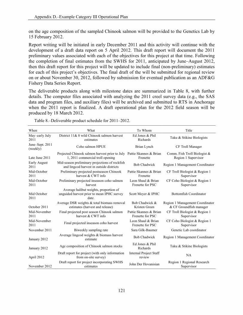
Appendix D.–Example Category III Operational Plan
121
on the age composition of the sampled Chinook salmon will be provided to the Genetics Lab by 15 February 2012.
Report writing will be initiated in early December 2011 and this activity will continue with the development of a draft data report on 5 April 2012. This draft report will document the 2011 preliminary values associated with each of the objectives for this project at that time. Following the completion of final estimates from the SWHS for 2011, anticipated by June–August 2012, then this draft report for this project will be updated to include final (non-preliminary) estimates for each of this project’s objectives. The final draft of the will be submitted for regional review on or about November 30, 2012, followed by submission for eventual publication as an ADF&G Fishery Data Series Report.
The deliverable products along with milestone dates are summarized in Table 8, with further details. The computer files associated with analyzing the 2011 creel survey data (e.g., the SAS data and program files, and auxiliary files) will be archived and submitted to RTS in Anchorage when the 2011 report is finalized. A draft operational plan for the 2012 field season will be produced by 18 March 2012.
Table 8.–Deliverable product schedule for 2011–2012.
When What To Whom Title May–early July 2011
District 11& 8 wild Chinook salmon harvest estimates
Ed Jones & Phil Richards Taku & Stikine Biologists
June–Sept. 2011 (weekly) Coho salmon HPUE Brian Lynch CF Troll Manager
Late June 2011 Projected Chinook salmon harvest prior to July
1, 2011 commercial troll opening Pattie Skannes & Brian
Frenette Comm. Fish Troll Biologist &
Region 1 Supervisor Early August 2011
Mid-season preliminary projections of rockfish and lingcod harvest in outside districts Bob Chadwick Region 1 Management Coordinator
Mid-October 2011
Preliminary projected postseason Chinook harvest & CWT info
Pattie Skannes & Brian Frenette
CF Troll Biologist & Region 1 Supervisor
Mid-October 2011
Preliminary projected inseason coho salmon harvest
Leon Shaul & Brian Frenette for PSC
CF Coho Biologist & Region 1 Supervisor
Mid October 2011
Average halibut weights, proportion of unguided harvest prior to mean IPHC survey
date. Scott Meyer & IPHC Bottomfish Coordinator
October 2011 Average DSR weights & total biomass removal
estimates (harvest and release) Bob Chadwick &
Kristen Green Region 1 Management Coordinator
& CF Groundfish manager Mid-November 2011
Final projected post season Chinook salmon harvest & CWT info
Pattie Skannes & Brian Frenette for PSC
CF Troll Biologist & Region 1 Supervisor
Mid-November 2011 Final projected inseason coho harvest Leon Shaul & Brian
Frenette for PSC CF Coho Biologist & Region 1
Supervisor November 2011 Biweekly sampling rate Sara Gilk-Baumer Genetic Lab coordinator
January 2012 Average lingcod weights & biomass harvest
estimate Bob Chadwick Region 1 Management Coordinator
January 2012 Age composition of Chinook salmon stocks Ed Jones & Phil Richards Taku & Stikine Biologists
April 2012 Draft report for project (with only information
from on-site survey) Internal Project Staff
review NA
November 2012 Draft report for project incorporating SWHS
estimates John Der Hovanisian Region 1 Regional Research Supervisor
Appendix D.–Example Category III Operational Plan
122
RESPONSIBILITIES Michael Jaenicke, Fishery Biologist III
Duties: Coordinates all aspects of the project. Assists biometrician with study design and schedule generation. Performs and coordinates data analyses in conjunction with biometrician. Co-authors final report and provides inseason data to appropriate personnel. Supervises project personnel.
Kathleen Wendt, Fishery Biologist II Duties: Assists biometrician with study design and schedule generation. Performs and
coordinates data analyses in conjunction with project leader and biometrician. Lead author for final report and provides inseason data to project leader. Supervises project personnel in Ketchikan, Petersburg, Wrangell, and Craig/Klawock.
Vacant, Fishery Biologist I/II Duties: Performs data analyses in conjunction with project leader and biometrician. Assists in
schedule generation. Provides inseason data to project leader. Supervises project personnel in Juneau, Sitka, Gustavus, and Elfin Cove.
Diana Tersteeg, Research Analyst II Duties: Performs data analyses in conjunction with project leader and biometrician. Responsible
for researching and implementing future conversion of data collecting from paper recording to handheld devices. Design and write programs or queries using various statistical software packages such as SAS or database programs. Create statistically valid reports and technically detailed tables and figures necessary to meet the annual reporting requirements of the program.
Brian Marston, Fishery Biologist III Duties: Performs data analyses in conjunction with project leader and biometrician. Assists in
schedule generation. Supervises project personnel in Yakutat. Sue Millard, Fisheries Technician IV
Duties: Helps supervise Fisheries Technician IIIs and IIs. Coordinates samplers in other locations. Also checks and edits data and assists with other office activities.
James Hahl and Judy Slattery, Fisheries Technician III, Duties: As crew leaders in Sitka and Ketchikan they help supervise creel survey personnel in
Sitka and Ketchikan in addition to checking and editing data. Assist in schedule generation, sublegal Chinook sampling and other office activities.
Allen Bingham, Biometrician IV, and Sarah Power, Biometrician II Duties: Provides input in sampling design and allocation, and designs scheduling procedures and
incorporates into operational plan. Provides procedures for calculation of estimates and standard errors. Assist in report writing. Also reviews operational plan and final report.
Bruce Kruger, Mary Jo Lord-Wild, and Allen Hoffman, Fisheries Technician III Duties: Conduct catch sampling in remote locations as schedule dictates and provide summaries
of data on a weekly basis. In addition notes potential sampling problems and advise possible solutions.
Fisheries Technician IIs and IIIs Duties: Conduct creel or catch sample surveys as schedule dictates and provide summaries of
data on a weekly basis. RTS staff Process mark-sense forms.
Appendix D.–Example Category III Operational Plan
123
REFERENCES CITED Bernard, D. R., and J. E. Clark. 1996. Estimating salmon harvest with coded-wire tags. Canadian Journal of
Fisheries and Aquatic Sciences 53:2323-2332.
Clark, W. G. 1992. Validation of the IPHC length-weight relationship for halibut. Pages 113-116 in Report and assessment of research activities, 1991. International Pacific Halibut Commission, Seattle, WA.
Clutter, R. and L. Whitesel. 1956. Collection and interpretation of sockeye salmon scales. Bulletin of the International Pacific Salmon Fisheries Commission, No. 9.
Goodman, L.A. 1960. On the exact variance of a product. Journal of the American Statistical Association 66:608-713.
Howe, A. L., R. J. Walker, C. Olnes, K. Sundet, and A. E. Bingham. 2001a. Revised Edition: Harvest, catch, and participation in Alaska sport fisheries during 1996. Alaska Department of Fish and Game, Fishery Data Series No. 97-29 (revised), Anchorage.
Howe, A. L., R. J. Walker, C. Olnes, K. Sundet, and A. E. Bingham. 2001b. Revised Edition: Harvest, catch, and participation in Alaska sport fisheries during 1997. Alaska Department of Fish and Game, Fishery Data Series No. 98-25 (revised), Anchorage.
Howe, A. L., R. J. Walker, C. Olnes, K. Sundet, and A. E. Bingham. 2001c. Revised Edition: Participation, catch, and harvest in Alaska sport fisheries during 1998. Alaska Department of Fish and Game, Fishery Data Series No. 99-41 (revised), Anchorage.
Howe, A. L., R. J. Walker, C. Olnes, K. Sundet, and A. E. Bingham. 2001d. Participation, catch, and harvest in Alaska sport fisheries during 1999. Alaska Department of Fish and Game, Fishery Data Series No. 01-8, Anchorage.
Jennings, G. B., K. Sundet, A. E. Bingham, and D. Sigurdsson. 2004. Participation, catch, and harvest in Alaska sport fisheries during 2001. Alaska Department of Fish and Game, Fishery Data Series No. 04-11, Anchorage.
Jennings, G. B., K. Sundet, A. E. Bingham, and D. Sigurdsson. 2006a. Participation, catch, and harvest in Alaska sport fisheries during 2002. Alaska Department of Fish and Game, Fishery Data Series No. 06-34, Anchorage.
Jennings, G. B., K. Sundet, A. E. Bingham, and D. Sigurdsson. 2006b. Participation, catch, and harvest in Alaska sport fisheries during 2003. Alaska Department of Fish and Game, Fishery Data Series No. 06-44, Anchorage.
Jennings, G. B., K. Sundet, and A. E. Bingham. 2007. Participation, catch, and harvest in Alaska sport fisheries during 2004. Alaska Department of Fish and Game, Fishery Data Series No. 07-40, Anchorage.
Jennings, G. B., K. Sundet, and A. E. Bingham. 2009a. Participation, catch, and harvest in Alaska sport fisheries during 2005. Alaska Department of Fish and Game, Fishery Data Series No. 09-47, Anchorage.
Jennings, G. B., K. Sundet, and A. E. Bingham. 2009b. Participation, catch, and harvest in Alaska sport fisheries during 2006. Alaska Department of Fish and Game, Fishery Data Series No. 09-54, Anchorage.
Jennings, G. B., K. Sundet, and A. E. Bingham. 2010a. Participation, catch, and harvest in Alaska sport fisheries during 2007. Alaska Department of Fish and Game, Fishery Data Series No. 10-02, Anchorage.
Jennings, G. B., K. Sundet, and A. E. Bingham. 2010b. Participation, catch, and harvest in Alaska sport fisheries during 2008. Alaska Department of Fish and Game, Fishery Data Series No. 10-22, Anchorage.
Jennings, G. B., K. Sundet, and A. E. Bingham. In prep. Participation, catch, and harvest in Alaska sport fisheries during 2009. Alaska Department of Fish and Game, Fishery Data Series, Anchorage.
Mood, A.M, F.A. Graybill, and D.C. Boes. 1974. Introduction to the Theory of Statistics, third edition. McGraw-Hill, New York.
Nielsen, L. A. and W. F. Schoch. 1980. Errors in estimating mean weight and other statistics from mean length. Transactions of the American Fisheries Society 109:319-322.
Appendix D.–Example Category III Operational Plan
124
REFERENCES CITED (Continued) Schwan, M. 1984. Recreational fisheries of Southeast Alaska, including Yakutat: an assessment. Alaska Department
of Fish and Game, Juneau.
Suchanek, P. M., S. H. Hoffman, R. E. Chadwick, D. E. Beers, T. E. Brookover, M. W. Schwan, R. P. Ericksen, R. E. Johnson, B. J. Glynn, and B. J. Frenette. 2002. Area management report for the sport fisheries of Southeast Alaska, 2000. Alaska Department of Fish and Game, Fishery Management Report No. 02-04, Anchorage.
Sukhatme, P.V., B. V. Sukhatme, S. Sukhatme, and C. Asok. 1984. Sampling theory of surveys with applications, third edition. Iowa State University Press and Indian Society of Agricultural Statistics, Ames, Iowa.
Thompson, S. K. 2002. Sampling, second edition. John Wiley and Sons, New York.
Walker R. J., C. Olnes, K. Sundet, A. L. Howe, and A. E. Bingham. 2003. Participation, catch, and harvest in Alaska sport fisheries during 2000. Alaska Department of Fish and Game, Fishery Data Series No. 03-05, Anchorage.
Welander, A. D. 1940. A study of the development of the scale of the chinook salmon (Oncorhynchus tshawytscha). Master's thesis, University of Washington, Seattle.
Appendix E2 – Example Operational Plan Amendment
125
APPENDIX E
EXAMPLE OPERATIONAL PLAN AMENDMENT
Appendix E2 – Example Operational Plan Amendment
126
Appendix E1.–Requirements for Operational Plan Amendment
The amendment will be formatted as a Regional Operational Plan, and consists of five sections; 1) Signature Page, 2) Purpose, 3) Reason for Change, 4) Description of Change and 5) Appendix containing the original operational plan. The Purpose section is the same as the original – copied and pasted. “Reason for Change” describes the circumstances that required a modification to the plan. “Description of the Change” identifies the specific sections or sub sections of the operational plan that were affected (e.g. Sample size) and explains what modifications will be made to the project design. The body of the amendment should be kept short (e.g., 1-2 pages).
.
Appendix E2 – Example Operational Plan Amendment
127
Appendix E2.–Example Operational Plan Amendment.
Regional Operational Plan
Operational Plan Amendment: Enumeration of Chena River Chinook Salmon 2012–2017
by
Author(s)
Month YYYY
Alaska Department of Fish and Game Divisions of Sport and Commercial Fisheries

Appendix E2 – Example Operational Plan Amendment
Symbols and Abbreviations The following symbols and abbreviations, and others approved for the Système International d'Unités (SI), are used without definition in the following reports by the Divisions of Sport Fish and of Commercial Fisheries: Fishery Manuscripts, Fishery Data Series Reports, Fishery Management Reports, Special Publications and the Division of Commercial Fisheries Regional Reports. All others, including deviations from definitions listed below, are noted in the text at first mention, as well as in the titles or footnotes of tables, and in figure or figure captions. Weights and measures (metric) centimeter cm deciliter dL gram g hectare ha kilogram kg kilometer km liter L meter m milliliter mL millimeter mm Weights and measures (English) cubic feet per second ft3/s foot ft gallon gal inch in mile mi nautical mile nmi ounce oz pound lb quart qt yard yd Time and temperature day d degrees Celsius °C degrees Fahrenheit °F degrees kelvin K hour h minute min second s Physics and chemistry all atomic symbols alternating current AC ampere A calorie cal direct current DC hertz Hz horsepower hp hydrogen ion activity pH (negative log of) parts per million ppm parts per thousand ppt, ‰ volts V watts W
General Alaska Administrative Code AAC all commonly accepted abbreviations e.g., Mr., Mrs.,
AM, PM, etc. all commonly accepted professional titles e.g., Dr., Ph.D., R.N., etc. at @ compass directions:
east E north N south S west W
copyright corporate suffixes:
Company Co. Corporation Corp. Incorporated Inc. Limited Ltd.
District of Columbia D.C. et alii (and others) et al. et cetera (and so forth) etc. exempli gratia (for example) e.g. Federal Information Code FIC id est (that is) i.e. latitude or longitude lat. or long. monetary symbols (U.S.) $, ¢ months (tables and figures): first three letters Jan,...,Dec registered trademark trademark United States (adjective) U.S. United States of America (noun) USA U.S.C. United States
Code U.S. state use two-letter
abbreviations (e.g., AK, WA)
Mathematics, statistics all standard mathematical signs, symbols and abbreviations alternate hypothesis HA base of natural logarithm e catch per unit effort CPUE coefficient of variation CV common test statistics (F, t, χ2, etc.) confidence interval CI correlation coefficient (multiple) R correlation coefficient (simple) r covariance cov degree (angular ) ° degrees of freedom df expected value E greater than > greater than or equal to ≥ harvest per unit effort HPUE less than < less than or equal to ≤ logarithm (natural) ln logarithm (base 10) log logarithm (specify base) log2, etc. minute (angular) ' not significant NS null hypothesis HO percent probability P probability of a type I error (rejection of the null hypothesis when true) α probability of a type II error (acceptance of the null hypothesis when false) β second (angular) " standard deviation SD standard error SE variance population Var sample var
Appendix E2 – Example Operational Plan Amendment
REGIONAL OPERATIONAL PLAN NO. RRYY-XX
ENUMERATION OF CHENA RIVER CHINOOK SALMON 2012-2017
by
Author(s)
Division, Address
Alaska Department of Fish and Game Division of Commercial Fisheries
333 Raspberry Road, Anchorage, AK 99518
Month YYYY
Appendix E2 – Example Operational Plan Amendment
The Regional Operational Plan Series was established in 2012 to archive and provide public access to operational plans for fisheries projects of the Divisions of Commercial Fisheries and Sport Fish, as per joint-divisional Operational Planning Policy. Documents in this series are planning documents that may contain raw data, preliminary data analyses and results, and describe operational aspects of fisheries projects that may not actually be implemented. All documents in this series are subject to a technical review process and receive varying degrees of regional, divisional, and biometric approval, but do not generally receive editorial review. Results from the implementation of the operational plan described in this series may be subsequently finalized and published in a different department reporting series or in the formal literature. Please contact the author if you have any questions regarding the information provided in this plan. Regional Operational Plans are available on the Internet at: http://www.adfg.alaska.gov/sf/publications/
Author(s), Alaska Department of Fish and Game, Division,
Address, USA This document should be cited as: Author(s). YYYY. Title. Alaska Department of Fish and Game, Division, Regional Operational Plan RRYY-XX,
Anchorage.
The Alaska Department of Fish and Game (ADF&G) administers all programs and activities free from discrimination based on race, color, national origin, age, sex, religion, marital status, pregnancy, parenthood, or disability. The department administers all programs and activities in compliance with Title VI of the Civil Rights Act of 1964, Section 504 of the Rehabilitation Act of 1973, Title II of the Americans with Disabilities Act (ADA) of 1990, the Age Discrimination Act of 1975, and Title IX of the Education Amendments of 1972.
If you believe you have been discriminated against in any program, activity, or facility please write: ADF&G ADA Coordinator, P.O. Box 115526, Juneau, AK 99811-5526
U.S. Fish and Wildlife Service, 4401 N. Fairfax Drive, MS 2042, Arlington, VA 22203 Office of Equal Opportunity, U.S. Department of the Interior, 1849 C Street NW MS 5230, Washington DC 20240
The department’s ADA Coordinator can be reached via phone at the following numbers: (VOICE) 907-465-6077, (Statewide Telecommunication Device for the Deaf) 1-800-478-3648, (Juneau TDD) 907-
465-3646, or (FAX) 907-465-6078 For information on alternative formats and questions on this publication, please contact:
ADF&G, Division of Sport Fish, Research and Technical Services, 333 Raspberry Road, Anchorage AK 99518 (907)267-2375.
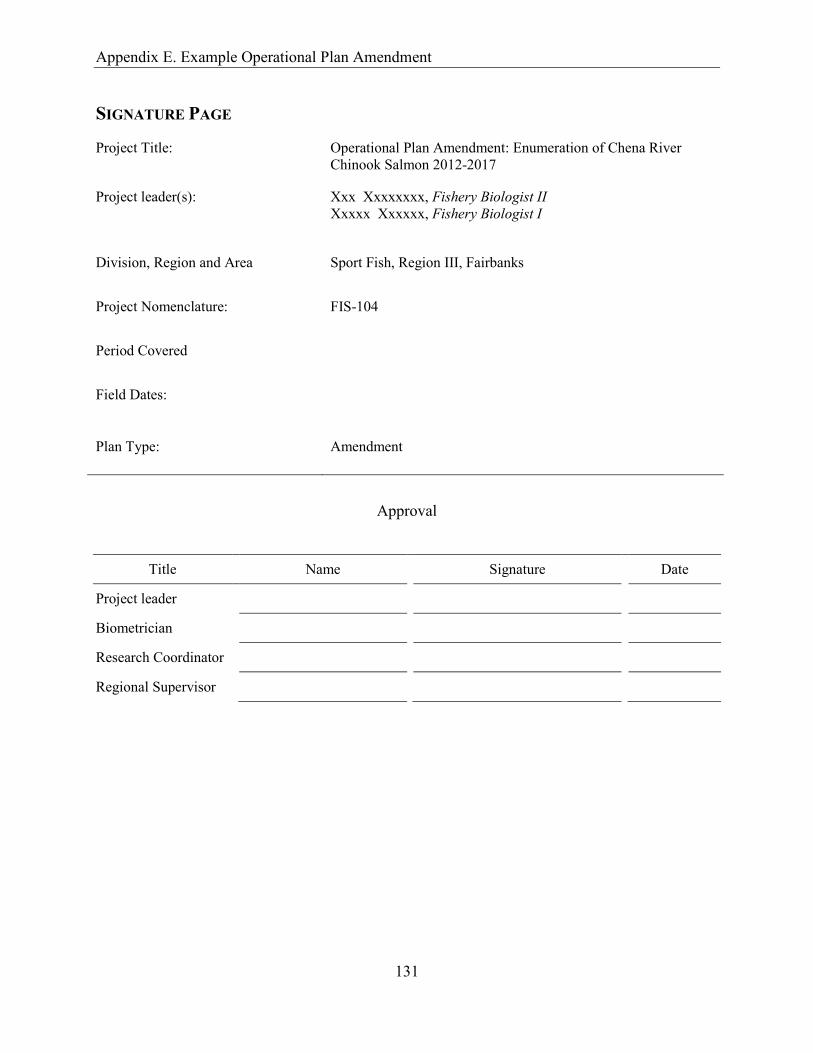
Appendix E. Example Operational Plan Amendment
131
SIGNATURE PAGE
Project Title: Operational Plan Amendment: Enumeration of Chena River Chinook Salmon 2012-2017
Project leader(s): Xxx Xxxxxxxx, Fishery Biologist II Xxxxx Xxxxxx, Fishery Biologist I
Division, Region and Area Sport Fish, Region III, Fairbanks
Project Nomenclature: FIS-104
Period Covered
Field Dates:
Plan Type: Amendment
Approval
Title Name Signature Date
Project leader
Biometrician
Research Coordinator
Regional Supervisor

Appendix E. Example Operational Plan Amendment
132
TABLE OF CONTENTS Page
PURPOSE.................................................................................................................................................................. 133
REASON FOR CHANGE ......................................................................................................................................... 133 DESCRIPTION OF CHANGE .................................................................................................................................. 133
Appendix E. Example Operational Plan Amendment
133
PURPOSE Counting tower techniques are used to estimate Chinook Onchorhynchus tshawytscha salmon escapement in the Chena River. The daily escapement estimates provide information on run magnitude and timing, which allows managers to modify fishing regulations to achieve the established escapement goal. The annual escapement estimates are periodically used to refine the biological escapement goal currently established by ADF&G at 2,800–5,700 Chinook salmon. In 2001, the Alaska Board of Fisheries directed ADF&G to manage Chinook salmon harvests so that the escapements falls within this BEG.
REASON FOR CHANGE A change in the sample size was needed to achieve precision criteria relative to Objective 3. In the previous year, scales from 350 Chinook salmon were collected for aging and it was believed that this sample size would provide adequate precision for estimates of age composition. However, poor precision in the estimate of the age composition was attained because of a abnormally high reabsorption rate of scales;
DESCRIPTION OF CHANGE During carcass on the Chena River, scales from an additional 100 Chinook salmon will be collected for a total sample size 450 fish. This should ensure that the minimum sample size of 300 “readable” scales is achieved.

134

135
APPENDIX F OPERATIONAL PLANNING MEETING
NOTES

136
Appendix F1.–Regional operational planning meeting notes, Juneau 11/22/11.
Divisions of Sport and Commercial Fisheries Operational Planning Policy Revision and Development Meeting November 22, 2011
Introduction: Benefits: • Add to the benefits section “to prevent the loss of institutional knowledge due to the large
number of staff retiring in the near future”. • Discussion: The primary purpose is to provide evidence that good planning has occurred. The
use of the terminology “provide evidence” originated from Bob Clarke and prompted a lot of discussion. It was agreed that good planning has been done in the past, but there were concerns about being requested to “provide evidence”. In general, it was agreed we need to communicate why we are doing a project, what the data is being used for, and what questions we are trying to ask. B. Frenette – Suggested wording change to bullet one (ii): The research/management ـ
questions (objectives) are clearly articulated. D. Woodby – Discussion on the biometric shop from the Dept. leadership. CFD has done ـ
a lot of project op planning, but not on an annual cycle. C. Swanton (SF) wanted a review of the system; J. Regnart (CF) wanted to do more. Consistency between divisions was important. With regard to some of the initial op planning, some died the death of “too many signatures”. The process needs to be made more efficient.
”.S. Dressel – Suggested wording change to “ensure good planning has occurred ـ• Other Benefits/uses:
S. Powers – operational plans communicate to others what has been done so there is a ـplace to start; improvements can’t be made without it.
E. Jones – field guide for crews ـ C. Siddon – field guide and op plan are two different entities; important to define ـ
audience. .S. Heinel – Op plan serves as template for reports/deliverables ـ .A. Bingham – the op plan can be what you want or need it to be ـ .D. Woodby – “develop staff” by having to do a lot of research to develop the project (e.g ـ
look at primary literature and looking at what others have done. B. Taras – the important part of the planning process is bringing people together to ـ
discuss. Discussion on op plan process:
C. Siddon – There is no argument that it has to be done; the issue is about the “nuts and ـbolts” of how to do it. How much more time needs to be spent? How much more detail?
?S. Dressel – Do we have to cut projects if we need to spend more time with this ـ .B. Frenette – the answer to these types of questions are with designing the categories ـ
-continued-
137
Appendix F1.–Page 2 of 7.
J. Timothy (Habitat) – Habitat implements what sampling is required in the permits that ـ
are looked at by a lot of different agencies. Our projects look at long term changes that are somewhat “squishy” in nature and do not cover annual statistical sampling. The money to do the sampling is from companies requesting the permits. Sampling is a compromise that the companies can buy into. The science is not for management; it is to look into impacts caused by activities. Habitat doesn’t really have an op plan. We use the methodology by other contractors. K. Wuttig – commented on the possible litigation issues.
A. Bingham – SFD projects have standards but some are very different in nature than ـyour standard fish projects such as permitting pike removal. SFD has not formally categorized these types of projects. Once the process gets more efficient; then should be less cost.
Discussion on the definition of the categories and how they determine the costs of ـimplementing the Op Plan Policy. There are a lot of advantages to reviewing the procedures and being more efficient, concise, and editing down the size…i.e. eliminating “op plan creep”.
J. Timothy – Habitat permits are circulated to other biologists and other Depts. and is in ـessence their op planning.
Process overview: reviewed Prescreening and potential criteria for determining operational plan categories: reviewed • RRC, project biologist, and possibly Reg. Supv. makes a Yes/No decision for each project on
whether a new or revised op plan is required. • Greater than three years since the last op plan is related to the BOF cycle. • S. Powers – 1st year consider new projects. Data is collected and therefore a review may be
needed in the 2nd year to adjust (e.g. crew size change could affect sampling and would require a review).
• D. Woodby – Memo for new or simple changes that do not require design changes. • A. Bingham – What this is trying to capture is that there is an “annual review” by someone;
do we need to do another plan or do we need to just do a memo. SFD has a chief biometrician that keeps things going. Someone would be needed to keep the process moving.
Policy Guidelines: reviewed • E. Jones – op plan should be reviewed annually by RRC not the biometrician. • A. Bingham – op plan should be reviewed annually even if it is a multi-year plan. • Discussion on what constitutes a “fisheries project”:
- E. Jones – Op plan policy should cover all divisions and all research projects. Should not include management projects; don’t think that managers should write op plans. If you spend money, you should have an op plan.
-continued-
138
Appendix F1.–Page 3 of 7.
- K. Wuttig – a question needs to be articulated in the op plan; the plan does not have to be more than 2 pages
- S. Heinl – Researchers could write the op plan for a management project, and it would not have to change annually.
- J. Timothy – Habitat gets money and needs to use money quickly. E. Jones – still need to write down how you are using the money. Documentation is needed and this can suffice as an op.
- B. Taras – Definition of the categories can be tailored to the need of the individual division. There is flexibility in the process.
- A. Bingham – SFD written policy is that every project budgeted that requires an estimate and hypothesis needs a plan. The process of defining an objective, task, 1° and 2° objectives were used as a means of getting out of defining sample sizes. We could get to the same place with op plans by defining whether a project is management/research related so that we can get out of writing an op.
- B. Taras – it was also important to document expenditures. This was brought into the op planning process so things were put into the estimate or hypothesis testing. There was also some documentation for costs of the resources and putting people at “risk”.
- Documentation of the duties/responsibilities of the people involved. - J. Timothy – a lot of times we record presence or absence in our projects. We also do
tracking for the AWC. We have the authority to write permits. Due to our funding, we can’t contract out for biometric support. We would have to bite out support out of the other Divisions.
- K. Wuttig – should establish a protocol for looking for the “presence and absence”. Do proposals for grants suffice as ops? RRC would have to look at it.
- B. Frenette – planning for these types of projects have already occurred in other Divisions.
- A. Bingham – In the past, we have included op plan with the grant proposal. If it is something we haven’t done, I would feel more comfortable with a plan. Sometimes grant agencies don’t want to see the details either, so that is a consideration.
Categories criteria: • There really isn’t any scoring behind the categories. • Signatures drive the categories. • Is 4 categories too many? • Discussion on definition of categories specifically with respect to multi-year plans and the
requirement of the annual op plan. - Questions regarding complexity of the analysis or review defining the category of the
plan. Asked whether there would be any situation where a plan would not have to be written. Suggestions: Add a signature or date on top of an old plan; develop another vehicle such as a memo for a “repeat” plan; or add an amendment to a plan that only needs to be signed off by the Reg. Supv.
-continued-
139
Appendix F1.–Page 4 of 7.
- D. Woodby – there are two different models that we are working from. SFD model where
there is a biometrician shop and the SE CF model where they work as a “team” on a project.
- A. Bingham – pointed out that there is a biometrician assigned to a project or set of projects. If there are no statistics involved then there generally is no biometrician assigned.
- K. Wuttig – Signature means that op plan has been critically reviewed. In some cases the RRC can do this.
- S. Powers – Stressed that she would want to have input into the plan because biologist may not know what a significant change is and how it will affect the project.
- A. Bingham – Don’t feel that there will be too many Category I projects, which may not get biometric approval. Doesn’t personally or professionally agree with this. You have to have someone to say that it goes.
- S. Fleischman – Flexibility. What you need to decide is a list of parameters that need to be decided on each year (completed with Reg. Supv., RRC, Biologist, and Biometrician). You can specify what decisions have to be made for each plan. Flowchart/decision sheet or tree that determines what is in a plan and what signatures are required.
• Discussion on “who” will be involved in deciding what project should have an op plan. Is this dependent on type of analysis, publication requirements, etc. Need consistency between the Divisions with maybe some differences between the regions. Could be done on a case by case basis. - B. Taras – suggest a two stage process: 1) do we need a plan? 2) If so then who’s
involved? - C. Siddon – Does not have to be either or. There are overlapping concepts to cover all.
• Discussion on who signs: Critical review and signatures need to be defined by policy and consistent between regions and Divisions. With regard to the question as to whether a Reg. Supv. needs to sign, S. Kelley indicated that he didn’t need to see Category I and II projects. B. Frenette wanted to see projects from all categories because of possible last minute funding changes. Question was posed as to what the signature meant and whether the Reg. Supv. signature is “optional”.
• D. Woodby – signature implies responsibility. • A. Bingham – SFD has a current written policy that a project will not be fielded without an
approved plan. Possibility that Reg. Supv. could sign to indicate that the “policy” has been met even though a plan may not get written. Reg. Supv. signature could then trump the policy.
• Discussion on requesting a second biometric review. This could be done for numerous reasons and requested by the people responsible for signing determined through the initial decision tree. There was a distinction made between a 2nd “review” vs. a “consultation” by a 2nd biometrician. One would review the entire project after the planning process and the other would take part in the designing process. All agreed that the decision would have to be up front.
-continued-
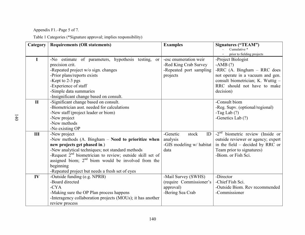
140
140
Appendix F1.–Page 5 of 7.
Table 1 Categories (*Signature approval; implies responsibility)
Category Requirements (OR statements) Examples Signatures (“TEAM”) - Cumulative * - prior to fielding projects
I -No estimate of parameters, hypothesis testing, or precision crit. -Repeated project w/o sign. changes -Prior plans/reports exists -Kept to 2-3 pgs -Experience of staff -Simple data summaries -Insignificant change based on consult.
-esc enumeration weir -Red King Crab Survey -Repeated port sampling projects
-Project Biologist -AMB (?) -RRC (A. Bingham – RRC does not operate in a vacuum and gen. consult biometrician; K. Wuttig – RRC should not have to make decision)
II -Significant change based on consult. -Biometrician asst. needed for calculations -New staff (project leader or biom) -New project -New methods -No existing OP
-Consult biom -Reg. Supv. (optional/regional) -Tag Lab (?) -Genetics Lab (?)
III -New project -New methods (A. Bingham – Need to prioritize when new projects get phased in.) -New analytical techniques; not standard methods -Request 2nd biometrician to review; outside skill set of assigned biom; 2nd biom would be involved from the beginning -Repeated project but needs a fresh set of eyes
-Genetic stock ID analysis -GIS modeling w/ habitat data
-2nd biometric review (Inside or outside reviewer or agency; expert in the field – decided by RRC or Team prior to signatures) -Biom. or Fish Sci.
IV -Outside funding (e.g. NPRB) -Board directed -CYA -Making sure the OP Plan process happens -Interagency collaboration projects (MOUs); it has another review process
-Mail Survey (SWHS) (require Commissioner’s approval) -Bering Sea Crab
-Director -Chief Fish Sci. -Outside Biom. Rev recommended -Commissioner
141
Appendix F1.–Page 6 of 7. • A. Bingham – The additional required signature may help make sure the process happened. • Category IV option: Should be considered by a case by case basis. There are a lot of
situations where plans are requested for specific external funding for the purpose informing and not necessarily for approval purposes. MOUs associated with these have their own review process. Suggestion to add other cooperators on as signatories e.g. CWT Tag Lab or the Genetics Lab. This was thought to help the communication process.
OP Plan Elements – Table 1 (See page 10 of handout) • Discussion on what else is needed it the template for each category. Some suggestions were
appendices, budgets, duties or responsibilities, deliverables, grant no., and schedule. In Category I since there are no formulas, one could just reference other op plans or best practices manuals.
• SFD template: - Intro - Objective - Study Design
• Data Collection • Data reduction • Data analysis
- Schedules - Responsibilities - Reports - Budget - Literature Cited - Appendices
• Discussion on op plan template: Should have the same structure/template for each category of op plan, but with different levels of detail. Suggest that formats are similar to what is requested for grants. Field guides should be separate. Question was brought up regarding non-standard projects such as “removal” projects. It was suggested that removal projects should require some type of evaluation and the evaluation methods could be formalized in an op plan.
• Discussion on the CFD model where there is a larger umbrella project with an overall objective with smaller projects under it with their own objectives. This brought the group back to the discussion of how to define a project. Stock assessment models were used as an example. The modeling is an iterative process and could go on for years. This should not go through an op plan process. The smaller components however would require an op plan. It was noted that stock assessment was defined differently by SFD and CFD. It was suggested that a methods paper could be written that describes everything that goes into the model.
• A. Bingham – “why are we doing these projects?” – we are doing it for the Bigger projects that do not have op plans. Without the background of why we are out there we can’t go back and revise the objectives. There needs to be some understanding of the whole picture. This would be beneficial in such things as the budget cutting exercises. B. Frenette – provided the web redesign example where it was never communicated how all the research fed into the whole process; an example was the interdivisional management of salmon.
-continued-
142
Appendix F1.–Page 7 of 7. • D. Woodby – provided the example of the Stock Assessment and Fishery Evaluation (SAFE)
report would be not as detailed as per say a strategic plan, but is provided on an annual basis. It would summarize the best available scientific information concerning the conditions of the stocks, marine ecosystems, and fisheries being managed under Federal regulation. This document would not be in place before the first op plan.
Additional Discussion points/thoughts (See page 11): • D. Woodby – wanted to make the distinction that in CF biometricians are asked to design a
project and sometimes are the project leaders. They do more than review op plans. A. Bingham – SFD has a senior biometrician and in some situations the biometricians participate in projects and surveys.
• Discussion on definition of an objective: key is flexibility. - K. Wuttig – anything that leads operations or sampling is an ‘objective’. - A. Bingham – objectives are defined as having objective criteria e.g. evaluation testing
and estimating precision. “Tasks” referred to data collection alongside data that is collected under the objectives. Primary objectives were those that drive the sampling while secondary objectives were information collected that you could use later. This information had meaning but could not be used with statistical rigor.
- S. Dressel – CF projects have objectives but don’t have statistical measure or criteria with them in the plan. There would be secondary objectives in the text. They have more methodological objectives; more like a field guide e.g. objectives is more about the “timing” of the data collection. Biggest concern is about the differences in the audience and what that means to work load in developing a new document.
• Op plan and field manual could be separate. There is a lot of redundancy that could be removed.
• There is a lot of expertise in both divisions. • Drafting an op plan policy will not be the same as administering the policy. Someone will
have to take the lead to make sure the policy is followed. SFD has centralized biometricians in RTS.
Centralized vs. Regional: • Accountability – essentially the Reg. Supv. • Discussed the phase in approach that A. Bingham brought up earlier and possibility using a
priority system to determine which plans are done first. • Need to try to minimize administrative costs. Some POPs are already done but may need
rewriting. • K. Wuttig – a small committee will be formed to draft the policy and then evaluate. • E. Jones – who is going to be the CFD Allen Bingham? Suggest that we give the RRCs some
free reign to make some decisions. • A. Bingham – there are reporting policies for both SFD and CFD. SFD reporting is
contractual and tied with funding process. We have a ‘contract’ to the public. Someone will need to bird dog this so that we can succeed in the policy and be consistent in its use.
• Expect to have a draft of the policy next spring.
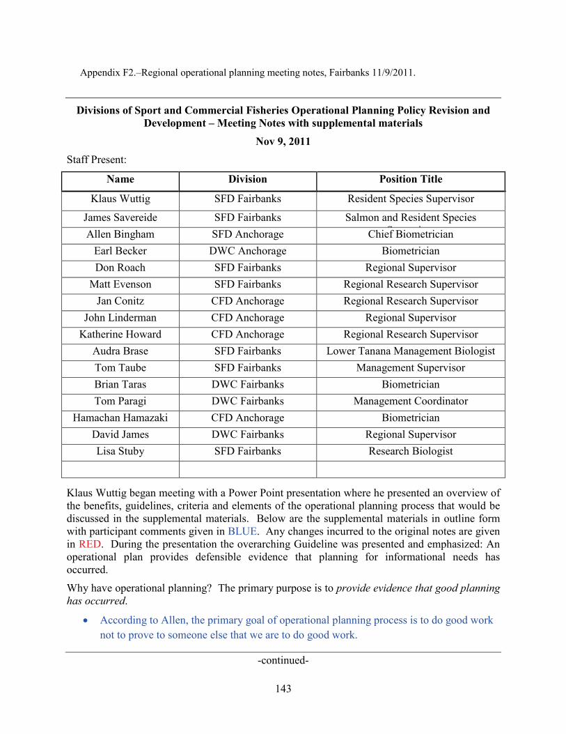
143
Appendix F2.–Regional operational planning meeting notes, Fairbanks 11/9/2011.
Divisions of Sport and Commercial Fisheries Operational Planning Policy Revision and Development – Meeting Notes with supplemental materials
Nov 9, 2011 Staff Present:
Name Division Position Title
Klaus Wuttig SFD Fairbanks Resident Species Supervisor
James Savereide SFD Fairbanks Salmon and Resident Species S i Allen Bingham SFD Anchorage Chief Biometrician
Earl Becker DWC Anchorage Biometrician Don Roach SFD Fairbanks Regional Supervisor
Matt Evenson SFD Fairbanks Regional Research Supervisor Jan Conitz CFD Anchorage Regional Research Supervisor
John Linderman CFD Anchorage Regional Supervisor Katherine Howard CFD Anchorage Regional Research Supervisor
Audra Brase SFD Fairbanks Lower Tanana Management Biologist Tom Taube SFD Fairbanks Management Supervisor Brian Taras DWC Fairbanks Biometrician Tom Paragi DWC Fairbanks Management Coordinator
Hamachan Hamazaki CFD Anchorage Biometrician David James DWC Fairbanks Regional Supervisor Lisa Stuby SFD Fairbanks Research Biologist
Klaus Wuttig began meeting with a Power Point presentation where he presented an overview of the benefits, guidelines, criteria and elements of the operational planning process that would be discussed in the supplemental materials. Below are the supplemental materials in outline form with participant comments given in BLUE. Any changes incurred to the original notes are given in RED. During the presentation the overarching Guideline was presented and emphasized: An operational plan provides defensible evidence that planning for informational needs has occurred.
Why have operational planning? The primary purpose is to provide evidence that good planning has occurred.
• According to Allen, the primary goal of operational planning process is to do good work not to prove to someone else that we are to do good work.
-continued-
144
Appendix F2.–Page 2 of 17.
• Even though overarching goal, the process itself has a lot of side benefits: ideas of
improving communication, collaborative process with the biometrician, research biologists, regional research biologists (“team effort”).
• Management need drives research and this need to also be laid out in the operational plan and made explicit in document
• Comment expressed that link between management needs and research objectives needs to be stated.
• A well-constructed operational plan can serve another purpose by helping with post-project report writing since the introduction, methods, etc. will mostly be worked out. Interrelated benefits include:
Defining purpose of project data i. Purpose (goal) of each research project is clearly articulated.
ii. The research and management question (objectives) are clearly articulated.
• Sometimes a management need will not be readily definable if the research need is something like understanding life history of a species that may not have any immediate management need. However, this information will be necessary for long-term management of a species/stock. Can’t manage what we don’t understand.
• Intent of this policy is to keep it specific for a particular work and objectives.
• Need to understand how projects fit into the big picture and how specific are we in addressing management needs.
• Where draw line between management projects vs. research projects. Need to incorporate management needs.
• If spending money, even if project is a feasibility or one is answering a public information need (ex. How many people are sport fishing on a drainage on July 4th) still need to explain why the project is being done. This is the request from the Division Leadership Team (DLT).
• There are situations where for example in ocean fisheries the project biologist and field crew will have to fish in different locations from that stated in the operational plan, so spend money and can deviate from plan.
• Concern was expressed about the lack of flexibility in plans for unanticipated things. Provisions can be put in the operational plans for these. The BIG reason for having an operational plan is to show basically defending the need for a project and the money to be spent conducting the research.
-continued-
145
Appendix F2.–Page 3 of 17. • A big benefit of the operational plan and the operational planning process
is the collaborative process of incorporating idea of incorporating input from a lot of different people.
• Operational plans provide a justification for all of the field activities and may justify risk to staff: ex. aerial surveys which may not be safe, but the data is important enough to justify the hazard.
Helps to define and apply the best methods (do good science) Develop staff
iii. Researching methods, prior studies, and management practices improves education
Communication iv. Everyone responsible or interested is informed.
Collecting defensible data (statistically sound) v. Mandates time be set aside to think about what needs to be done and
how to do it correctly. vi. Ensure best methods are applied.
vii. Biometric input to ensure data is statistically sound. viii. Consistency of methods and data.
Budgeting ix. Better budgeting x. Accountability to funding sources (e.g. Fed aid, SOA,OSM, SSF).
Deliverables xi. Operational plan
xii. Timeline for data analysis and reporting. xiii. Protocol for archiving data.
Archiving (electronically) what has been done. xiv. Methods xv. Consistent data
-continued-

146
Appendix F2.–Page 4 of 17.
Generalized process of how operational planning process will work: 1) A regional list of prioritized fisheries projects is assimilated annually.
a. Process tailored to best fit regional needs. b. Parties involved may include project leaders, research coordinator, management
coordinator, biometrician and regional supervisor.
2) For each plan, goals and objectives of fisheries projects are clearly articulated and linked to management need.
3) Research coordinator reviews project list to determine if respective operational plans (new or revised) are required.
4) This results in two actions (see prescreening criteria below): a. No, new or updated project operation plan not needed.
b. Yes, new or updated operational plan needed for upcoming field season.
5) If yes, assigned operational plans will be graded into categories.
6) Operational plan written by project leader in consolation with assigned biometrician if
needed.
7) Plan reviewed and signed
8) Archived into intranet. • Need mechanism for a memorandum. For a multi-year project need to provide good
evidence for minor changes that will improve the project. Since all will be archived, the multi-year operational plan and updated memo will be archived.
• Where operational plans will be archived for CFD is still being discussed. • Sometimes there will be a need to make significant changes inseason. For these but do
we go into an amendment? It should be up to the research coordinator to see if a memo update is needed—just state in annual report.
• Efficiency in the operational planning process and final product is important! • Operational plans can be utilized as field documents that someone can follow out in the
field. There can be an advantage of melding functional field operations with operational plan. However, the details contained in an operational plan may be too confusing. Perhaps good to have field methods contained in an appendix within an operational plan.
-continued-
147
Appendix F2.–Page 5 of 17.
• Concern expressed about a project plan becoming unwieldy with too much information. Impetus to simplify the process, make the same statement with less work, more efficiency.
• However a citable document of field methods can be referred to in the operational plan. Every little detail does not have to be contained within an operational plan.
• Don Roach mentioned that when he signs off on an operational plan, he looks at number of people involved, budgetary needs, planning relevancy to objectives, etc. He will ask of the importance of the objectives to research and management needs, etc.
• We don’t need to be a “slave” to the details of an operational plan.
Prescreening criteria (new or revised operational plan required?):
- Yes: o New project o Significant changes to existing project.
Question, what constitute a significant change • Added signature • Change in category.
o More than three years (?) since last operational plan o Pending ramification, board cycle
- No: o No significant changes
Simple changes in dates, crew size, or field logistics (moving camp). o Operational plan still current o No significant changes
Policy guidelines (these are generally non-negotiable) Overarching Guideline: Providing defensible evidence that planning for informational
needs has occurred.
1. An operational plan for all fisheries projects will be written. • Anytime some of our resources are being used, need a plan. • Do OSM proposals constitute an operational plan?? Here it will be an individual call. • If have a cooperative projects between divisions or outside with federal agencies, NGO’s,
etc. do we also need for them to sign off on as well? In past years, they haven’t signed off. In some instances NGOs have gone outside parameters listed so there can be a need to have this agreement and understanding. So, may be important to involve NGOs, and other agency types in.
-continued-
148
Appendix F2.-Page 6 of 17. • We currently do cooperative agreements with NGOs, etc. and Memorandums of
Understanding with USFWS. Worry about any controversy at board meetings with data collected without some agreement all around with the ADFG project operational plans and agencies, NGOs, etc. who were not directly involved with the operational planning process.
• Question of should grant funding agencies (ex. OSM) sign off on it? A policy established along these lines could have implications. How far could one stray from an Investigation Plan in an Operational Plan? Through our operational planning process we often add more detail and additional information. Investigation plans need to be kept to a certain content. Many times operational plans can be redundant and sometimes contradictory.
• For Sport Fish Division Federal Aid projects operational plan details are added to contracts.
• AYK-SSI funds ADFG and NGOs and there can be lots of overlapping in cooperative efforts. See potential for some conflicts in having a separate process in addition to the investigation plan with SSI since the operational planning process will be primarily a departmental effort.
2. Policy will be applicable to SF and CF.
3. A Special Publication will be drafted: ADF&G policy and procedures for planning fisheries projects.
4. Efficiency is important – should not require any more effort and paperwork than are
necessary. Plan to have plans on file so don’t have to “reinvent the wheel” and they will be available for others to utilize. They should also be accessible to the public. Point brought up that we should be able to hand out our operational plans but might not be good for the general public to peruse the internet site where they will be archived. Right now operational plans are provide upon request. This detail is currently being worked out.
5. Categories of operational plans will be explored and/or developed, each with their own
requirements relative to rigor, biometric review, and signatures.
6. Consolidated or bundled plans will be permitted (e.g. all weirs on the Kuskokwim River).
7. Operational plans can cover multiple years (e.g. written for up to three years) in the
absence of significant changes to the study design. Although greater frequency is encouraged if it can improve study design.
-continued-

149
Appendix F2.–Page 7 of 17.
• Some projects have occurred on a yearly basis for many years. Given that on a yearly basis the research coordinator, etc. signs off that this plan is still valid barring any changes, no need to create a new plan for each field season. However, in the original plan, something needs to be added that changes could be made after a year or more at the discretion of the research coordinator.
• Every year research coordinator needs to look at all projects and consider what the needs are.
8. Plans will be reviewed annually to identify if significant changes to project design warrant a new plan.
• Can break down into: 1. No change, 2. Need amendment(s), 3. Need new operational plan
9. Efforts will be made to develop “best practices” manuals that can be referenced (e.g.
sonar operation). • DLT would like to see for applications where sampling is standardized (ex. genetics)
user manuals. 10. All operational plans will be electronically archived.
11. Responsibilities of those involved in the process should be clearly identified and
articulated in the policy. a. Project leader, Biometricians, Research coordinator, Etc. • Drawing up a timeline was suggested were project management and research
meet together determine the questions, select the project biologist(s), and present a clear line of what has and will happened in the project planning process in a table.
12. The scope of this effort will not go beyond the actually drafting a Policy. Within the
policy, formalized longer-termed planning efforts are likely not needed and will be based on regional needs/efforts.
• Up to the individual division and region.
-continued-

150
Appendix F2.–Page 8 of 17.
Potential criteria for determining operational plan categories.
1) Standardization of methods a. Frequency/repetitiveness of project b. Is there a citable report where methods worked in similar circumstances c. Availability of “best practices” manuals.
2) Analytical complexity
a. Risk of bias b. biometric support needed for study design and data analysis c. Knowledge of project biologist
3) Logistical complexity
a. Cost • Project costs will almost always increase (ex. gas and aviation gas costs in rural
Alaska). Cost can determine category in operational plan and project complexity. Ask if it is adequate to achieve the objectives with long-term cost projections.
b. Project scale / number of personnel c. geography
4) Administrative complexity
a. Multiple jurisdictions/agencies
5) Managerial risk a. Sustainability of stocks/populations b. Political / legislative interest c. Number of stake holders/NGOs d. Funding agency e. Economic risk (need to consider the user groups)
-continued-
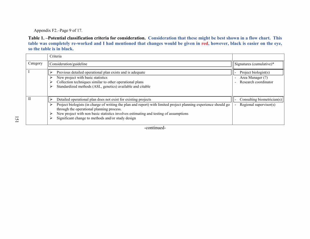
151
Appendix F2.–Page 9 of 17.
Table 1. –Potential classification criteria for consideration. Consideration that these might be best shown in a flow chart. This table was completely re-worked and I had mentioned that changes would be given in red, however, black is easier on the eye, so the table is in black. Criteria
Category Consideration/guideline Signatures (cumulative)*
I
Previous detailed operational plan exists and is adequate New project with basic statistics Collection techniques similar to other operational plans Standardized methods (ASL, genetics) available and citable
- Project biologist(s) - Area Manager (?) - Research coordinator
II
Detailed operational plan does not exist for existing projects Project biologists (in charge of writing the plan and report) with limited project planning experience should go
through the operational planning process. New project with non basic statistics involves estimating and testing of assumptions Significant change to methods and/or study design
- Consulting biometrician(s) - Regional supervisor(s)
-continued-
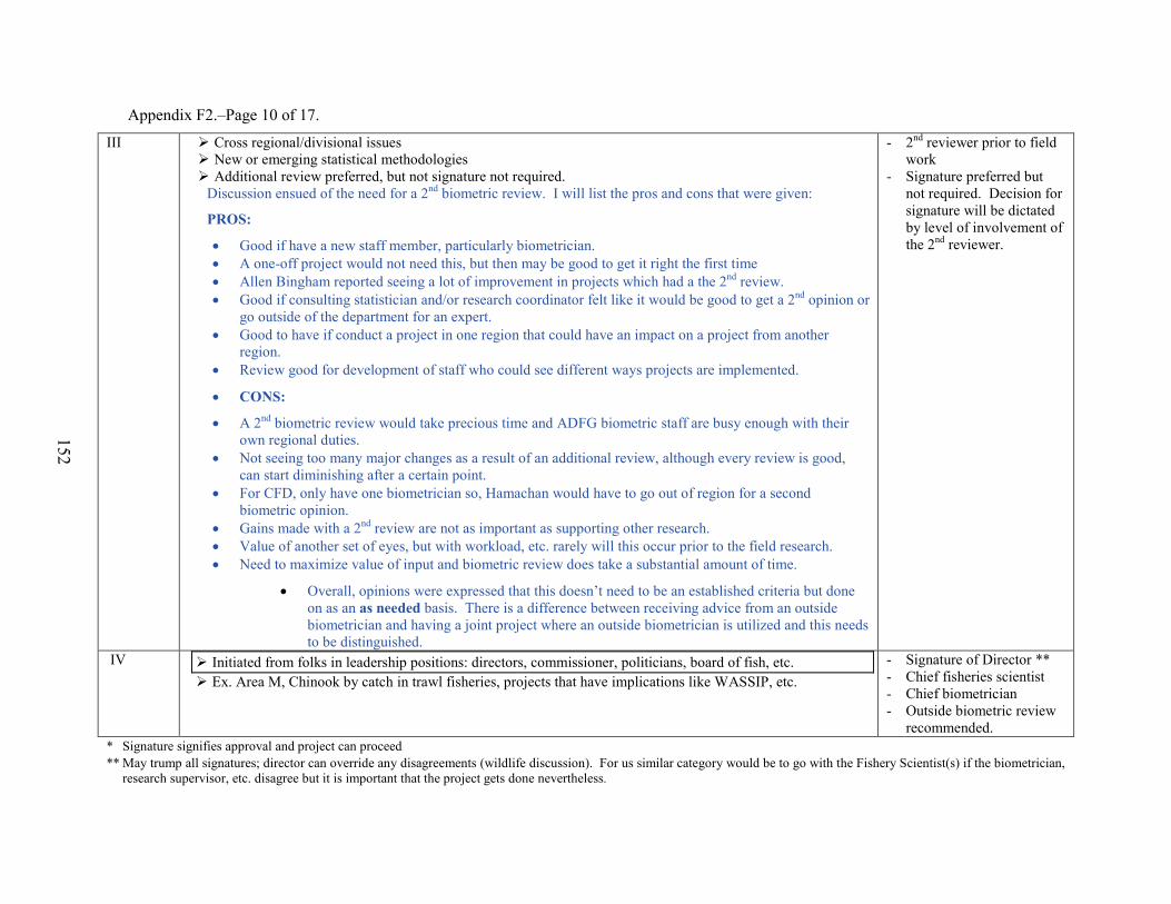
152
Appendix F2.–Page 10 of 17.
III
Cross regional/divisional issues New or emerging statistical methodologies Additional review preferred, but not signature not required.
Discussion ensued of the need for a 2nd biometric review. I will list the pros and cons that were given:
PROS:
• Good if have a new staff member, particularly biometrician. • A one-off project would not need this, but then may be good to get it right the first time • Allen Bingham reported seeing a lot of improvement in projects which had a the 2nd review. • Good if consulting statistician and/or research coordinator felt like it would be good to get a 2nd opinion or
go outside of the department for an expert. • Good to have if conduct a project in one region that could have an impact on a project from another
region. • Review good for development of staff who could see different ways projects are implemented.
• CONS:
• A 2nd biometric review would take precious time and ADFG biometric staff are busy enough with their own regional duties.
• Not seeing too many major changes as a result of an additional review, although every review is good, can start diminishing after a certain point.
• For CFD, only have one biometrician so, Hamachan would have to go out of region for a second biometric opinion.
• Gains made with a 2nd review are not as important as supporting other research. • Value of another set of eyes, but with workload, etc. rarely will this occur prior to the field research. • Need to maximize value of input and biometric review does take a substantial amount of time.
• Overall, opinions were expressed that this doesn’t need to be an established criteria but done on as an as needed basis. There is a difference between receiving advice from an outside biometrician and having a joint project where an outside biometrician is utilized and this needs to be distinguished.
- 2nd reviewer prior to field work
- Signature preferred but not required. Decision for signature will be dictated by level of involvement of the 2nd reviewer.
IV Initiated from folks in leadership positions: directors, commissioner, politicians, board of fish, etc. Ex. Area M, Chinook by catch in trawl fisheries, projects that have implications like WASSIP, etc.
- Signature of Director ** - Chief fisheries scientist - Chief biometrician - Outside biometric review
recommended. * Signature signifies approval and project can proceed ** May trump all signatures; director can override any disagreements (wildlife discussion). For us similar category would be to go with the Fishery Scientist(s) if the biometrician,
research supervisor, etc. disagree but it is important that the project gets done nevertheless.
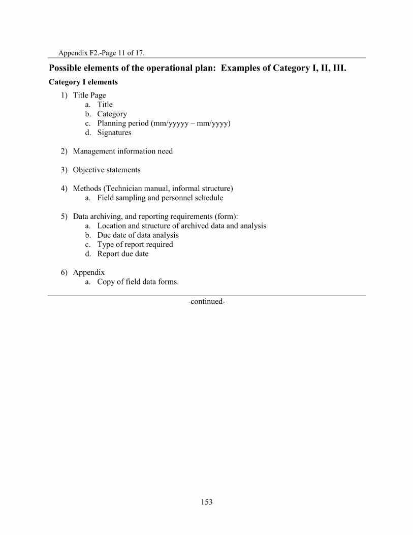
153
Appendix F2.-Page 11 of 17.
Possible elements of the operational plan: Examples of Category I, II, III. Category I elements
1) Title Page a. Title b. Category c. Planning period (mm/yyyyy – mm/yyyy) d. Signatures
2) Management information need
3) Objective statements
4) Methods (Technician manual, informal structure)
a. Field sampling and personnel schedule
5) Data archiving, and reporting requirements (form): a. Location and structure of archived data and analysis b. Due date of data analysis c. Type of report required d. Report due date
6) Appendix
a. Copy of field data forms.
-continued-
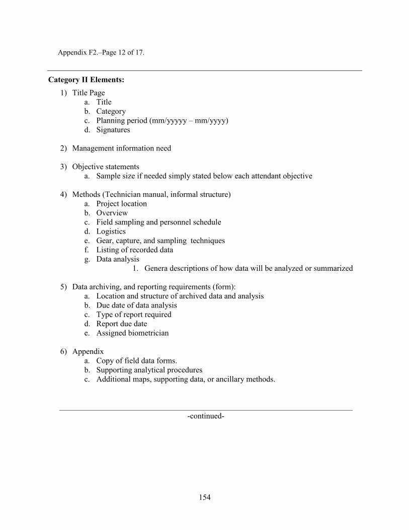
154
Appendix F2.–Page 12 of 17.
Category II Elements: 1) Title Page
a. Title b. Category c. Planning period (mm/yyyyy – mm/yyyy) d. Signatures
2) Management information need
3) Objective statements
a. Sample size if needed simply stated below each attendant objective
4) Methods (Technician manual, informal structure) a. Project location b. Overview c. Field sampling and personnel schedule d. Logistics e. Gear, capture, and sampling techniques f. Listing of recorded data g. Data analysis
1. Genera descriptions of how data will be analyzed or summarized
5) Data archiving, and reporting requirements (form): a. Location and structure of archived data and analysis b. Due date of data analysis c. Type of report required d. Report due date e. Assigned biometrician
6) Appendix
a. Copy of field data forms. b. Supporting analytical procedures c. Additional maps, supporting data, or ancillary methods.
-continued-
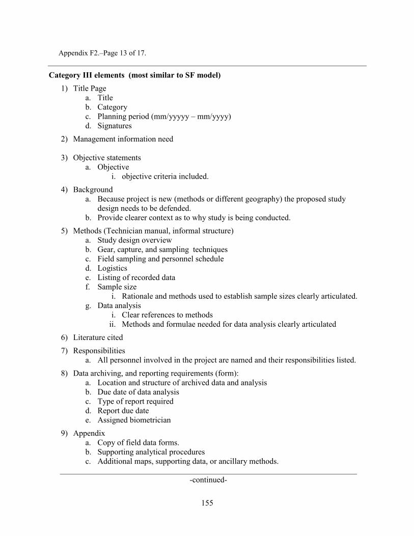
155
Appendix F2.–Page 13 of 17.
Category III elements (most similar to SF model) 1) Title Page
a. Title b. Category c. Planning period (mm/yyyyy – mm/yyyy) d. Signatures
2) Management information need
3) Objective statements a. Objective
i. objective criteria included.
4) Background a. Because project is new (methods or different geography) the proposed study
design needs to be defended. b. Provide clearer context as to why study is being conducted.
5) Methods (Technician manual, informal structure) a. Study design overview b. Gear, capture, and sampling techniques c. Field sampling and personnel schedule d. Logistics e. Listing of recorded data f. Sample size
i. Rationale and methods used to establish sample sizes clearly articulated. g. Data analysis
i. Clear references to methods ii. Methods and formulae needed for data analysis clearly articulated
6) Literature cited
7) Responsibilities a. All personnel involved in the project are named and their responsibilities listed.
8) Data archiving, and reporting requirements (form): a. Location and structure of archived data and analysis b. Due date of data analysis c. Type of report required d. Report due date e. Assigned biometrician
9) Appendix a. Copy of field data forms. b. Supporting analytical procedures c. Additional maps, supporting data, or ancillary methods.
-continued-
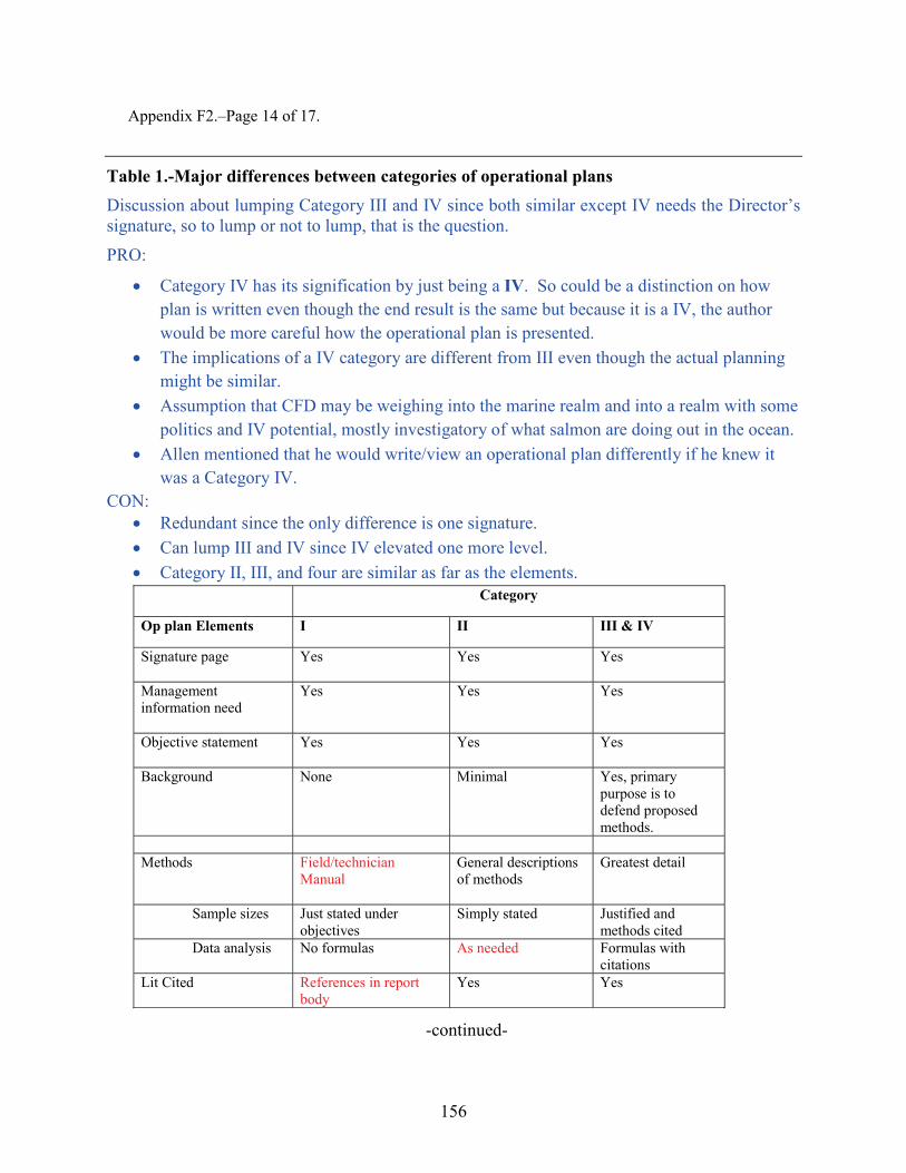
156
Appendix F2.–Page 14 of 17.
Table 1.-Major differences between categories of operational plans Discussion about lumping Category III and IV since both similar except IV needs the Director’s signature, so to lump or not to lump, that is the question.
PRO:
• Category IV has its signification by just being a IV. So could be a distinction on how plan is written even though the end result is the same but because it is a IV, the author would be more careful how the operational plan is presented.
• The implications of a IV category are different from III even though the actual planning might be similar.
• Assumption that CFD may be weighing into the marine realm and into a realm with some politics and IV potential, mostly investigatory of what salmon are doing out in the ocean.
• Allen mentioned that he would write/view an operational plan differently if he knew it was a Category IV.
CON: • Redundant since the only difference is one signature. • Can lump III and IV since IV elevated one more level. • Category II, III, and four are similar as far as the elements.
-continued-
Category
Op plan Elements I II III & IV
Signature page
Yes Yes Yes
Management information need
Yes Yes Yes
Objective statement
Yes Yes Yes
Background None Minimal Yes, primary purpose is to defend proposed methods.
Methods
Field/technician Manual
General descriptions of methods
Greatest detail
Sample sizes
Just stated under objectives
Simply stated Justified and methods cited
Data analysis
No formulas As needed Formulas with citations
Lit Cited
References in report body
Yes Yes
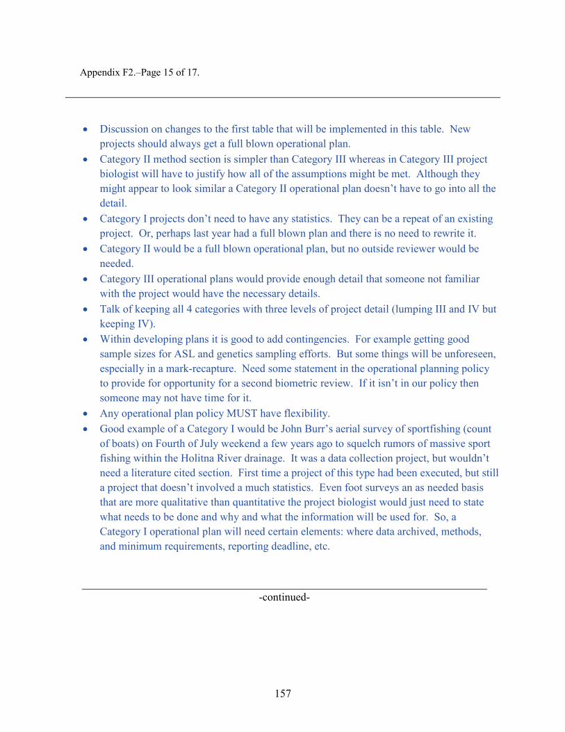
157
Appendix F2.–Page 15 of 17.
• Discussion on changes to the first table that will be implemented in this table. New projects should always get a full blown operational plan.
• Category II method section is simpler than Category III whereas in Category III project biologist will have to justify how all of the assumptions might be met. Although they might appear to look similar a Category II operational plan doesn’t have to go into all the detail.
• Category I projects don’t need to have any statistics. They can be a repeat of an existing project. Or, perhaps last year had a full blown plan and there is no need to rewrite it.
• Category II would be a full blown operational plan, but no outside reviewer would be needed.
• Category III operational plans would provide enough detail that someone not familiar with the project would have the necessary details.
• Talk of keeping all 4 categories with three levels of project detail (lumping III and IV but keeping IV).
• Within developing plans it is good to add contingencies. For example getting good sample sizes for ASL and genetics sampling efforts. But some things will be unforeseen, especially in a mark-recapture. Need some statement in the operational planning policy to provide for opportunity for a second biometric review. If it isn’t in our policy then someone may not have time for it.
• Any operational plan policy MUST have flexibility. • Good example of a Category I would be John Burr’s aerial survey of sportfishing (count
of boats) on Fourth of July weekend a few years ago to squelch rumors of massive sport fishing within the Holitna River drainage. It was a data collection project, but wouldn’t need a literature cited section. First time a project of this type had been executed, but still a project that doesn’t involved a much statistics. Even foot surveys an as needed basis that are more qualitative than quantitative the project biologist would just need to state what needs to be done and why and what the information will be used for. So, a Category I operational plan will need certain elements: where data archived, methods, and minimum requirements, reporting deadline, etc.
-continued-
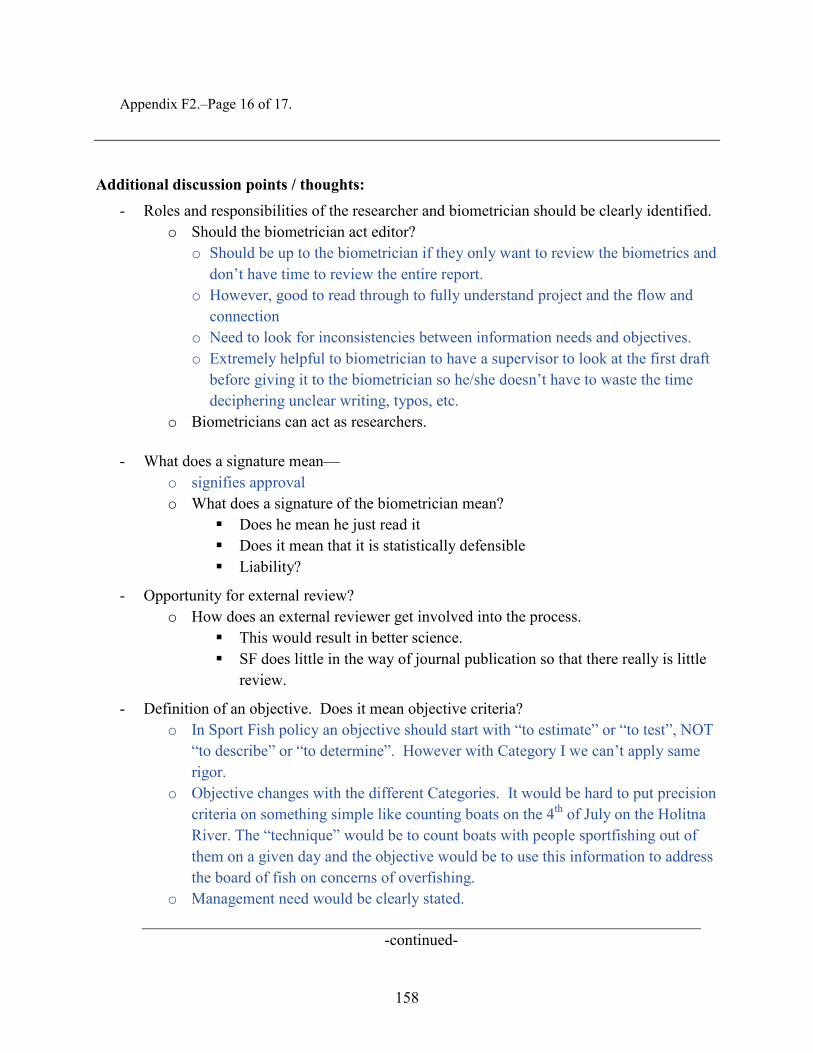
158
Appendix F2.–Page 16 of 17.
Additional discussion points / thoughts:
- Roles and responsibilities of the researcher and biometrician should be clearly identified. o Should the biometrician act editor?
o Should be up to the biometrician if they only want to review the biometrics and don’t have time to review the entire report.
o However, good to read through to fully understand project and the flow and connection
o Need to look for inconsistencies between information needs and objectives. o Extremely helpful to biometrician to have a supervisor to look at the first draft
before giving it to the biometrician so he/she doesn’t have to waste the time deciphering unclear writing, typos, etc.
o Biometricians can act as researchers.
- What does a signature mean— o signifies approval o What does a signature of the biometrician mean?
Does he mean he just read it Does it mean that it is statistically defensible Liability?
- Opportunity for external review? o How does an external reviewer get involved into the process.
This would result in better science. SF does little in the way of journal publication so that there really is little
review.
- Definition of an objective. Does it mean objective criteria? o In Sport Fish policy an objective should start with “to estimate” or “to test”, NOT
“to describe” or “to determine”. However with Category I we can’t apply same rigor.
o Objective changes with the different Categories. It would be hard to put precision criteria on something simple like counting boats on the 4th of July on the Holitna River. The “technique” would be to count boats with people sportfishing out of them on a given day and the objective would be to use this information to address the board of fish on concerns of overfishing.
o Management need would be clearly stated.
-continued-
159
Appendix F2.–Page 17 of 17.
o Objectives and tasks—Matt’s pet peeve. There have been project situations where data is collected in addition to primary purpose of study. Need to change/delete the term “task”. If we are spending money then we should have primary and secondary “objectives”. A secondary objective is an objective without criteria. So this is something that needs to be clarified. A task is what you do to accomplish an objective.
- Operational plan may serve as a manual for Field technicians. o Recognize the primary purpose is to not be constructed as a field manual.
- Recognition that a “one-size fits all” approach is too inflexible.
- We need a single citation for the SWHS data base.
- A benefit of the new policy should be that the expertise between divisions and among all regions is communicated / shared. Thoughts on how to achieve this.
- Policy administration discussion.
o Centralized vs. regional approach-make sure they are done on the due date, etc who will oversee that will make sure all this happens that all tasks are accomplished. SFD has the infrastructure with a biometrician coordinator and regional
biometricians. If headquarters is involved then all of the regions will have to be involved
with compliance. In CFD no central server to house operational plans which needs to be dealt with at headquarters. Also need a project archival system so know which projects are being conducted in a given year.
Definitely some statewide implications to implementing the operational planning process for both CFD and SFD. For the individual project biologist the responsibility of getting operational plan(s) done will be at the regional level.
CFD has one biometrician. A 2nd biometric review would have to come from a different division.
If implement this process, then need fixed timelines for individual projects. If start projects in May it means project operational plans need to be reviewed by March in order to insure that the operational plan is finalized prior to field efforts. There could be issues with time.
If CFD gets lots of Category IIIs, then they may need headquarters involvement if wish secondary reviews since Hamachan is the sole biometrician.
BIG question of the afternoon is how to implement this process.
160
Appendix F3.Regional Operational Planning Notes, Anchorage 11/8/2011.
11/8/11 – Operational Planning Meeting – Rabbit Creek Rifle Range -Anchorage
How well is operational planning working for Sport Fish?
• Simple management projects shouldn’t require extensive review. o Criteria would help with consistency (Miller).
• Reporting (Deliverables) is sometimes inconsistent (i.e. memo vs. report) • Permitting projects between sport fish and commercial fisheries are currently
difficult because processes are not standardized. • Works well with some confusion regarding level of review for different project
types. • The Sport Fish strategic plan drives the op planning process and budgeting,
which works well (Vania). • Annual area review meetings are held to discuss which management issues are
on the horizon and what management questions there are (Hasbrouck). • Process works well for defensibility of complicated projects (example, sonar).
It also aids the development of the project report (Burwen). • Often, plan language can be used as templates for new plans (Bingham). • The current planning process is difficult for entities such as KBRR when they
are doing purely “research” projects (Bingham). What is the burden for Sport Fish?
• Most plans are currently written annually, with all levels of review. For some projects, this isn’t necessary (Miller).
o A clear policy on different plan options would streamline the process.
• This shouldn’t be looked as a burden (Vania). Op planning is a necessary component of the fisheries
projects. Not a burden to entities that supply project funds (Clark). Huge external benefit to streamlining these processes for the
Department (Clark). Plans provide transparency (Clark).
• Need flexibility so that in-season projects can take place quickly if necessary ( Vania).
Categorization will really help. Sometimes, review occurs after the field season, but the
project leader and consulting biometrician almost always have reviews completed beforehand (Bingham).
-continued-

161
Appendix F3.–Page 2 of 11.
Commercial Fisheries Westward Regional Process
• All projects have a plan • New plans have multiple reviews • Recurring projects have a single review • Plans are published and archived after review, but are still internal documents. • Question: are all surveys projects? • Plans have references, appendices, etc. They are thorough documents because the public can view these.
History of Sport Fish Operational Planning (Bingham)
• 1989, informal planning procedures • 2000, Director formalized the process verbally • 200?, Written policy regarding planning and biometric review • Currently, looking at multi-year planning
For Commercial Fisheries to Consider…
o Do we need both planning documents and reports to be published? o Sport Fish houses Op plans on the intranet. If the public requests a copy, we can
provide it, but there is a disclaimer statement that the plan is not formally published (Bingham).
o Need flexibility regarding if and where plans should be made public (Baker). o Projects that are soft funded already go through significant review in the grant
proposal process. Is more planning required on top of this (Baker)? Proposals and Op Plans are similar documents.
o Policy needs to address this. o How does the process work for 3-year projects such as AKSSF (Baker)? o When does biometric review occur on grant proposals? o Sport Fish considers grant proposals as preliminary. Project details are usually
worked out during the Operational planning process. This is because it is unknown if the project will get funded. Detailed planning occurs once this has been answered (Erickson).
o Sport Fish requires an operational plan for “funded projects” (Bingham). o It would be useful to have a process to decide if a project is worth pursuing funding
for.
Operational Plan Issues
o Background sections in plans sometimes contain “opinion” of the project biologist. Should plans be made public, this could be problematic (Erickson).
o Reporting is often behind, so the “background” section has become a“mini-report” with data from previous reports (Bingham).
-continued-
162
Appendix F3.–Page 3 of 11.
Generalized process of how operational planning process will work: 1. A regional list of prioritized fisheries projects is assimilated annually. This policy assumes a list of prioritized projects already exists ().
Statement in policy that clarifies the planning process meets the needs of the region or division, etc. (Baker).
2. For each plan, goals and objectives of fisheries projects are clearly articulated and linked to management need. Oversight, handled by biometrics in sport fish and by research coordinator, in commercial fisheries needs to occur (Clark).
Is it a regional decision on how to administer op plans? (Klaus)
3. Research coordinator reviews project list to determine if respective operational plans are required Who is responsible to for administering the planning policy (i.e. Research coordinator, chief biometrician?) (Bingham)
Section heads and regional supervisors should delegate (Volk).
This gives the region flexibility (Miller).
4. This results in two actions 5. If yes, assigned operational plans will be graded into categories. 6. Operational plan written by project leader in consultation with assigned biometrician if needed. 7. Plan reviewed and signed
8. Archived into intranet
Prescreening Criteria (new or revised operational plan required)? SKIP
Policy Guidelines 1. An operational plan for all fisheries projects will be written. What is the definition of a project (Miller)? (Unanswered during discussion)
Commercial Fisheries managers fly aerial surveys routinely; there is no plan for these activities. There are 30-40 year data sets for some of these efforts that have never had a plan (T. Baker).
Regional supervisor will make the call (Klaus).
-continued-

163
Appendix F3.–Page 4 of 11.
Any project that tests a parameter or a hypothesis requires an operational plan (Bingham)
Could a survey protocol substitute for an operational plan?
Policy should clarify which activities require a plan (T. Baker)
This is where the categorization concept comes into play (Klaus)
The Regional Supervisor ultimately should decide whether a plan is needed for an in-season activity (Miller). However, these activities should be considered in the spring and included in a plan (Klaus).
Include a category that accounts for potential activities that may or may not arise during the season (Bingham)?
2. Policy will be applicable to SF and CF. A “How to manual” will be drafted on how to create plans (Klaus).
3. A special publication will be drafted 4. Efficiency is important – should not require any more effort and paperwork than necessary. 5. Categories of operational plans will be explored and/ or developed, each with their own requirements relative to rigor, biometric review, and signatures. 6. Consolidated or bundles plans will be permitted. 7. Operational plans can cover multiple years in the absence of significant changes to the study design. Although greater frequency is encouraged if it can improve study design. S Significant changes will be defined by the regional supervisor. (Wuttig)
8. Plans will be reviewed annually to identify if significant changes to project design warrant a new plan.
The need for a plan will be reviewed annually (Bingham). Post-season, projects may need tweaking (Tracy)
Need the ability to modify a plan between years without redoing an entire plan (Fleishman)
Currently, we do a full review of a plan amendment, and that isn’t always necessary (Craig).
This is because of a need for accounting and ensuring that planning is still taking place (Bingham)
How do we do amendments for multi-year projects? This needs its own category (Fleishman and Wuttig)
How do we do amendments in-season (Burwen)?
Things need to change mid-season sometimes (Wuttig)
-continued-
164
Appendix F3.–Page 5 of 11.
People want the ability to be flexible if changes arise (Baker)
Amendments that often occur in RII are handled by memos to document what we are doing (Erickson)
The amendments pertain more to multi-year projects (Wuttig)
If $ becomes available, there is a need to have flexibility to add an activity without an operational plan (Lignau/ Craig). This is a management call, not a research project.
Is this sort of activity defensible (BIngham)?
The process may need to be fluid (i.e. after a few years, if the same in-season activity continuously comes up, a decision eventually gets made to write a plan pre-season (Wuttig).
Again, this should be up to the regional supervisor (Miller)
This comes back to what is a fisheries project? (BIngham) or a management activity (Vania and Miller)
There are some activities that are not a “project”. It is just an information gathering activity, and it is up to the discretion of the regional supervisor as to whether a plan is needed or not (Baker, Wuttig)
9. Efforts will be made to develop “best practices” manuals that can be referenced It is most efficient to write the manuals before the operational plans (Clark).
10. All operational plans will be electronically archived. 11. Responsibilities of those involved in the process should be clearly identified and articulated in the policy. The process is a team effort. Sometimes the plan author is not the project leader (Bingham)
The plans are often collaborative.
A biometrician should be involved for all plans until a best practices manual is created (Bingham).
Sometimes projects that seem simple are often more complicated than thought, and a biometrician can help clarify unforeseen difficulties with projects.
Biometricians should be involved in all levels of the plan (i.e. formulating objectives through the final document). However, signatures may not be required for category 1 projects.
What is a category 1 project (Bingham)?
-continued-
165
Appendix F3.–Page 6 of 11.
Will there be a statement in the policy that states the op planning process is only one component of larger planning efforts in the Department? (Hasbrouck)
12. The scope of this effort will not go beyond actually drafting policy. Within the policy, formalized longer-termed planning efforts are likely not needed and will be based on regional needs/ efforts.
Potential criteria for determining operational plan categories? Not every project is as simple as it sounds (Volk)
For every category, we need to have sufficient detail. For the first year of the plan of an on-going project like a weir, the plan needs to be a thorough document. However, afterwards, the plan doesn’t need extensive review. (Baker)
When an op plan is developed, it is for the foreseen project. If complications arise in the field, that just needs to be dealt with (Vania).
We don’t have to have every possible source of bias addressed in the op plans. It isn’t necessary to make a plan defensible (Wuttig)
Categories should be based on who reviews the plan rather than the complexity of the planning document itself (Baker)
A non-complex project still needs a plan so it can be referenced (Bingham).
Idea: Three categories acknowledge the different levels of complexity that determine the type of plan
Table, p. 5
Requirements column doesn’t line up with signature requirements (Miller)
Criteria Signatures
Example. Pike netting may not need biometric review. A rotenone treatment, for example, needs review, but perhaps not by a biometrician (Miller, Bingham)
Do we need categories? Can we just have plans with different requirements that lay out projects (Fleishman)
What are the elements of the operational plan? Do we need one at all? What is in it? Who signs it? (Fleischman)
The process needs consistency. What are the criteria? (Clark)
Elements of an Operational Plan
Type 1 – What type of plan is this, a full-blown plan or a memo? (Baker)
Pigeon-holing into categories is grey, but it is a good place to start organization (Baker).
-continued-
166
Appendix F3.–Page 7 of 11.
Table p. 10
Lengthy background sections are unnecessary (Wuttig)
Management information need is what should be in background (Bingham)
Category 1 - introduction includes purpose and need; Category 3 – Needs more extensive background/ introduction sections (Baker).
Use a flow chart to make decisions that get to this table (Miller) and the suite of signatures needed/ document requirements (Munrow)
Could a category 1 plan just be a template that needs to be filled out by the project biologist (Burwen).
All plans categories could have a template (Dunker).
Clarification – categories are for plans, nor for projects (Hasbrouck)
Category 1 – For example, project may or may not be simple, but the plan is category 1 because the methods have been worked out well with previous projects (Clark).
A category 1 project that is new could require a category 3 plan and vice versa (Miller)
Should this table be included in this policy? (Miller)
Need to keep in mind why we are doing this:
- To provide evidence of planning - This can be done with or without extensive literature
reviews for simple plans. We already have a precursor to the category system. We should keep the plan elements, and change the signature requirements (Bingham)
We would never be able to have a category 1 plan for a new project (Bingham)
Again, the flow chart could lead to the plan type.
- This gives guidance, but does not need to be perfect (Baker)
How are category 2 and 3 plans different?
- Levels of review - Category II does not need background (Wuttig)
What about the length of the project? How does this fit within categories (Miller)?
- Projects are generally multi-year (Woodby) - Need a policy on how long plans can last for
(Wuttig)
-continued-
167
Appendix F3.–Page 8 of 11.
Need to remember that signatures are a function of the category (Volk).
We need to have simple, flexible way to amend a multi-year plan.
- If a long-term project, after x years, a project can be written in a category 1 plan and reference an earlier version.
Plans should be updated every three years (non-BOF years) (Baker).
Also, if best practices/ field manuals are formalized, these documents can be referenced instead of writing lengthy descriptions in the op plans (Baker).
As is, methods sections in op plan have a lot of redundancy (Wuttig)
- Study design/ data collection sections are duplicated in most plans (Bingham)
Category III plans should include a budget (Baker), but this will require annual updates (Volk).
Need to include a description of the expected deliverable and when it will be available.
As is, op plans continuously grow because of annual review (plan creep), so they get longer from year to year. This makes the whole process daunting to biologist when the expectation is 100-page op plans (Erickson).
Discussion while creating the Table, p.5
Without requirement of biometic review, biologists can’t have their assistance (Bingham).
In the policy, include examples of plans or scenarios for each category (Fleishman)
As this gets worked through further, should categories 3&4 or 2&3 be collapsed down into a single category? Do we need for levels? Each level creates more grey area.
Examples of projects/ categories”
Nushagak Kings – Category 3
Nome stream surveys for grayling – Category 2
Aerial surveys – Category 1
Personal Use – Category 1
Rotenone Treatment – Category 1
The decision of category ultimately resides with the research coordinator. This should be included as a policy statement.
-continued-
168
Appendix F3.–Page 9 of 11.
Additional discussion points/ thoughts:
Roles and responsibilities of the researcher and biometrician should be clearly identified. Should biometricians edit operational plans? Should we outline the exact role of the biometrician in the in the policy?
Responsibilities may be described as “at a minimum” biometrics will review for statistical rigor.
Each area can have their own guidelines on editing responsibilities. Generally, it is the job of the publications tech to edit grammar, etc. (Baker).
Without it being a requirement, biometricians can/ should edit op plans if it improvements the document (Hansen).
Does the editing take too much time?
If plans are poorly written, biometricians have had to take the role of “re-writing” parts of the plan (Bingham). One way or another, improvements have to be made to documents like this.
Timing is an important side board. The plan should be complete before the project is initiated in the field, and the biometrician may not have the time to edit an op plan for grammar (Bingham).
What does a signature mean? Sometimes there are disagreements on projects, and the biometrician will not sign it. The policy will have to address what happens in this situation? (Craig)
Could there be a petition process to resolve this? Who would be involved in the resolution?
One challenge is that there are organizational differences between sport fish and commercial fish (Hasbrouck), so the resolution may differ within the divisions.
There may be different levels on how to resolve cases where projects are not signed off on. The regional supervisor may make the final decision, or the project would have to be resolved by the next field season, for example.
This would be important to clarify in the policy (Baker)
In the past, there have been plans where the objective statement did not match the planned procedures (Bingham).
Opportunity for external review Don’t lose sight that external review may not be required outside the Department (cross-division, etc.)
Definition of an objective. Does it mean objective criteria? Objectives vs. Tasks –should this be addressed in the policy?
This is an example of why some plans in the past have not been signed (Erickson)
-continued-
169
Appendix F3.–Page 10 of 11.
An objective statement refers to directed sampling and requires precision criteria (Hansen/ Bingham).
An objective should be measureable (Bingham)
If you are collecting data, it has value, and should be stated as an objective (Wuttig).
Sometimes collecting data for another entity is considered as a task, but is still costing money (Bingham).
Tasks don’t drive sampling. They are byproducts (Hansen). For example, water quality data are considered tasks rather than objectives (Baker).
Do objectives require precision criteria?
This is already outlined in an exisitng Department document.
Often, we collect information opportunistically, but this does not require an objective (Baker).
For unanticipated activities that come up in-season, the current objective criteria will not work in all cases. This scenario should be addressed in policy (Craig).
Operational plan should serve as a manual for field technicians. If a plan is complicated (Category II or III), a smaller appendix stating just the field procedures would be useful to serve as a field manual for technicians (Wuttig).
Recognition that a “one-size fits all” approach is too inflexible. We need a single citation for the SWHS data base. A benefit of the new policy should be that the expertise between divisions and among all regions is communicated/shared. Documents outlining best practices and fisheries techniques for the division(s) would streamline field techniques, samples sizes, etc.
Centralized vs. regional approach Sport fish has RTS/ commercial fisheries has another structure that works well.
The policy will not dictate administration.
Separate supervision of biometrics and research biologists is necessary for collaborative and sometimes contentious interactions to improve projects (Bingham).
A centralized approach is beneficial when vacancies occur. The chief biometrician can ensure that biometric support is available statewide where and when it is needed (Bingham).
In sport fish, there is not a regional vs. centralized approach. There are regional management needs, and it is a collaborative effort between biometricians and the regions to make sure management needs are met. It is not really a “versus” situation (Hasbrouck).
-continued-
170
Appendix F3.–Page 11 of 11.
Centralized in sport fish vs. regional in commercial fish – each system currently works well within each division.
In commercial fisheries, operational plans were written, but there was not a formal process.
The question is how best to administer the new policy across the two divisions, given that there are different structures.
Future discussion: how does this fit into strategic planning and long-term planning for the divisions (Baker).
The centralized approach for administration is the most efficient, but the regions have to decide how best to implement their biometric resources (Earl).