JOURNAL OFSOUND ANDVIBRATION

www.elsevier.com/locate/jsvi

Journal of Sound and Vibration 262 (2003) 201–217

One to one resonant double Hopf bifurcation in aeroelasticoscillators with tuned mass dampers

V. Gattulli*, F. Di Fabio, A. Luongo

Dipartimento di Ingegneria delle Strutture, delle Acque e del Terreno, Universit "a di L’Aquila, Piazzale E. Pontieri 2,

67040 Monteluco di Roio (L’Aquila), Italy

Received 9 November 2001; accepted 1 May 2002

Abstract

The effects of a tuned added mass on the aeroelastic stability of a single degree of freedom bluff bodyexposed to a steady flow are investigated. The model captures the essential aspects of the behaviour offlexible structures equipped with Tuned Mass Dampers undergoing galloping oscillations. The systemexhibits simple as well double Hopf bifurcations, of non-resonant and 1:1 resonant type. Postcriticalbehaviour of the system in the neighbourhood of the 1:1 resonant type bifurcation is investigated.Employing the Multiple Scale Method, a second order bifurcation equation in the complex amplitude ofmotion is obtained. Analytical solutions are used to describe the bifurcation scenario in the cases of bothundercritical and supercritical aerodynamic behaviour of the bluff body. The effectiveness of the TunedMass Damper even in the postcritical range is proved.r 2002 Elsevier Science Ltd. All rights reserved.

1. Introduction

The stability of aerodynamic oscillators plays an important role for many structures subjectedto wind and/or ocean waves [1–3]. Therefore, mechanical devices added to the structural system toprevent or reduce the magnitude of aeroelastic phenomena are of current research interest [4–7].The concept of damping a structural system by adding a small mass to it dates back to the

beginning of the century. Previous studies on tunable mass dampers have set out to optimizemechanical design characteristics in order to increase the critical value at which the dynamicinstability phenomenon is triggered [8,9]. However, in order to investigate system performancewhen the flow velocity exceeds the critical value, an analysis of the postcritical behaviour isneeded.

*Corresponding author. Fax: +39-862-434548.

E-mail address: gattulli@ing.univaq.it (V. Gattulli).

0022-460X/03/$ - see front matter r 2002 Elsevier Science Ltd. All rights reserved.

PII: S 0 0 2 2 - 4 6 0 X ( 0 2 ) 0 1 1 3 5 - 5

Investigations on the system postcritical behaviour have been performed by means ofnumerical, analytical and experimental methods [10,11]. Nevertheless, in the numerical andexperimental tests presented, the dynamical behaviour has been described only for some specificvalues of the system parameters. Most importantly, the analysis relies on the assumption that thepostcritical behaviour of the system can be described referring to an equivalent single degree offreedom (s.d.o.f.) system whose approximate solution has been pursued by the multiple scalemethod [10] or by the averaging method in [11].A first study of the system postcritical behaviour as a 2d.o.f. system has been presented by the

authors in Ref. [12], with the aim to describe the entire postcritical scenario in the completeparameter-space. In this study, the primary system (PS) and the added mass (TMD) are assumedto posses a s.d.o.f. and to be linear, with the only source of non-linearities arising from the flow-structure interaction. Using a perturbation method, simple and double Hopf bifurcations,occurring at different values of the parameters, have been analyzed. The effectiveness of TMDshas been shown to persist even in the postcritical range, since TMDs generally reduce theamplitude of oscillations in the supercritical case. However, the analysis developed in Ref. [12]was only partial, since it was assumed that (a) a pair of conjugate eigenvalues of the Jacobianmatrix is stable (simple Hopf) or (b) the two pairs are both critical but distinct (non-resonant

double Hopf). Indeed, due to the tuning between the PS and the TMD, the two eigenvalue pairsare very close to each other, so it is suspected that (a) the stable pair may play some role in thedescription of the system behaviour and (b) some interaction between the nearly resonantfrequencies may occur. This last problem was tentatively addressed by building up a so-calledquasi-resonant solution based on the assumption that the Jacobian matrix admits two well-separated eigenvectors when the frequencies are still very close to each other; however, thishypothesis breaks down when the two frequencies exactly coalesce, since the matrix becomesdefective (nilpotent). The quasi-resonant solution revealed qualitative aspects of the motion whichcannot be described by the non-resonant solution. It was therefore concluded that a more refinedanalysis is necessary, in order to describe the neighbourhood of the coalescence point in theparameter space at which a 1:1 resonant double Hopf bifurcation takes place. However, such ananalysis is not trivial, since standard perturbation methods do not work when the Jacobian isdefective; therefore an adapted procedure must be employed.In this paper the model presented in Ref. [13] is considered and the postcritical behaviour of the

system is analyzed for a Hopf bifurcation in the region of 1:1 resonance. The multiple scalemethod (MSM) is employed to analyze the defective bifurcation according to the algorithmdeveloped in Ref. [14]. This analysis is believed to be new, both from a mathematical and aphysical point of view. A second order complex bifurcation equation in the amplitude of theunique critical mode is derived and the postcritical scenario is analyzed in the bifurcationparameter space. Then, the limits of validity of the concept of equivalent s.d.o.f. introduced inRefs. [10,11] are critically discussed, in the light of the more accurate analysis performed here.

2. Problem formulation

An elastically supported bluff body connected with a small added mass and subject to a steadyflow is considered (Fig. 1). Both the bluff body primary system (PS) and the added mass (TMD)

V. Gattulli et al. / Journal of Sound and Vibration 262 (2003) 201–217202

are assumed to possess a s.d.o.f. and to be linear. The aerodynamic forces acting on the TMD areassumed to be negligible in comparison with those acting on the PS. These forces are obtainedusing the quasi-static theory [15] taking into account both drag and lift components and retainingthe linear and cubic terms of their Taylor expansion. The equation of motion has been derived inRef. [12]. By using non-dimensional quantities and adopting a state-space representation theyread:

’x ¼ Lxþ fðx;mÞ: ð1Þ

In Eq. (1)

L ¼0 I

�K �C

" #ð2Þ

is the system matrix with

C ¼2xsð1� nÞ þ 2mgxt �2mgxt

�2gxt 2gxt

" #; K ¼

1þ mg2 �mg2

�g2 g2

" #ð3Þ

being the damping and stiffness matrices, respectively; x ¼ fq1; q2; ’q1; ’q2gT is the state-space

vector, with q1 and q2 the non-dimensional cross-flow displacements of PS and TMD,respectively; m ¼ fm; g; xt; ng is the vector of control parameters; f ¼ ffig collects the non-linearpart of the vector field, whose components are

f1 ¼ 0; f2 ¼ 0; f3 ¼1

2

d2A1A3xsn

x33; f4 ¼ 0: ð4Þ

.

ms

mt

msωs2 2msωsξ s

q1

q2

U

q1 α

2mtωtξ tmtωt2

TMD

PS

Fig. 1. Aeroelastic oscillator with tuned mass damper.

V. Gattulli et al. / Journal of Sound and Vibration 262 (2003) 201–217 203

In Eqs. (1)–(4) the following non-dimensional variables have been introduced:

q1 ¼#q1

D; q2 ¼

#q2

D; m ¼

mt

ms

; g ¼ot

os

; n ¼U

Uunc

;

U ¼#U

osD; Uunc ¼

2xs

dA1; d ¼

1

2

raD2

ms

; t ¼ #tos; ð5Þ

where D is a typical dimension of the body, ms;mt; xs; xt are masses and damping coefficients, os

and ot are the undamped frequencies of the two isolated bodies, U is the uniform flow velocity,Uunc its critical value for the uncontrolled structure; Ai are the aerodynamic coefficients, ra the airdensity and t the time, the hat denoting dimensional quantities.

3. Bifurcation analysis

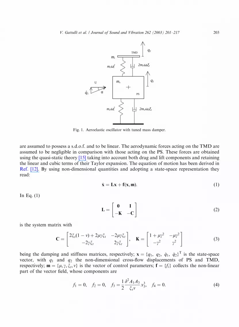
The equations of motion (1) admit the equilibrium position x ¼ 0: The position is stable orunstable depending on the values of the parameters m; especially on the parameter n whichaccounts for the flow velocity. The problem has been analyzed in Refs. [8–11] and completelydescribed in Ref. [12] where analytical expressions of non-resonant and resonant double Hopfmanifolds are given. A 3-D representation of the critical manifolds is depicted in Fig. 2a fora fixed value of m in the ðn; xt; gÞ-space, while the manifolds in the ðn; xt; mÞ-space can be found in

ν

ξ tγ

ν

ξ tγ

0

20

40

60

80

ν

ξ t

P0

0 0.02 0.04 0.060

20

40

60

80

P0ν

ξ t

0 0.02 0.04 0.06

(a) (b)

(c) (d)

Fig. 2. Critical manifolds in the ðn; xt; gÞ-space for m ¼ 0:005; exact (a,c) versus perturbative solution (b,d): (a) and(b) 3-D view; (c) and (d) sections for different g (heavy line g ¼ g0 ¼ 0:9975; light line g ¼ 0:9925).

V. Gattulli et al. / Journal of Sound and Vibration 262 (2003) 201–217204

Ref. [13]. Highlighted, in particular, is the existence of a peculiar point P0 � ðn0; xt0; g0Þ at whichthe critical flow velocity is maximized (optimum TMD that realizes a strong enhancement of thecritical flow velocity). In Fig. 2c sections at g ¼ g0 and gag0 of the critical manifold are shown.For a high level of damping xt in the TMD, a simple Hopf occurs; at a low level of damping anon-resonant double Hopf bifurcation or two successive closely-spaced bifurcations manifestthemselves. At P0 a 1:1 resonant double Hopf bifurcation occurs.The interest is here focused on the system postcritical behaviour around the point P0: At this

point, the system is defective (or nilpotent) since the critical eigenvalues l1;2 ¼ þio; l3;4 ¼�io ði ¼

ffiffiffiffiffiffiffi�1

pÞ coalesce into one pair. Only one right eigenvector u1 and one left eigenvector v2 is

associated with l1;2 ¼ þio; namely:

ðL0 � ioIÞu1 ¼ 0; ðL0 � ioIÞHv2 ¼ 0; ð6Þ

where L0 is the state-space matrix evaluated at P0 and H denotes the transpose conjugate. Thedefective bases are completed by the generalized u2 and v1 eigenvectors, which are (not unique)solutions of

ðL0 � ioIÞu2 ¼ u1; ðL0 � ioIÞHv1 ¼ v2; ð7Þ

respectively. Right and left eigenvectors are made bi-orthonormal, i.e., vHj uj ¼ dij ði; j ¼ 1; 2Þ:Since the bifurcation has codimension-3 (i.e., three conditions of the eigenvalues hold, namely

Reðl1Þ ¼ Reðl2Þ ¼ 0; Imðl1Þ ¼ Imðl2ÞÞ; three bifurcation parameters transverse to the criticalmanifold must be taken. By fixing m; the remaining ðn; xt; gÞ-parameters are selected as bifurcationparameters and the neighbourhood of P0 in Fig. 2 is spanned. The multiple scale method (MSM)is applied to perform the non-linear analysis, according to the procedure illustrated in Ref. [14].The deviations of the parameters from the bifurcation values ðn0; xt0; gt0Þ are assumed to be

small, of order e2; with e a perturbation parameter, namely:

n ¼ n0 þ e2n2; g ¼ g0 þ e2g2; xt ¼ xt0 þ e2xt2: ð8Þ

The incremental parameter n2 represents a distinguished parameter (positive for overcritical flowvelocities) and the incremental parameters xt2 and g2 represent splitting parameters. Moreover, thestate-space variables are expanded in series of integer powers of e as

xðt; eÞ ¼ ex1 þ e2x2 þ e3x3 þ e4x4 þ Oðe5Þ ð9Þ

and several independent temporal scales tk ¼ ekt ðk ¼ 0; 1;yÞ are introduced, so that d=dt ¼d0 þ ed1 þ?; with dk :¼ @=@tk: By substituting the previous equations in the Eq. (1) andcollecting terms with the same powers of e; the following perturbation equations are drawn up tothe e4-order:

ðL0 � d0Þx1 ¼ 0;

ðL0 � d0Þx2 ¼ d1x1;

ðL0 � d0Þx3 ¼ d1x2 þ ðd2 � L2Þx1 � 16f0xxxx

31;

ðL0 � d0Þx4 ¼ d1x3 þ ðd2 � L2Þx2 � 12f0xxxx

21x2: ð10Þ

V. Gattulli et al. / Journal of Sound and Vibration 262 (2003) 201–217 205

In Eqs. (10) L2 is the second order part of the e-expansion of L around P0 (i.e., L ¼ L0 þ e2L2),whose submatrices, according to Eqs. (2) and (3), are

C2 ¼ 2�xsn2 þ mðg0xt2 þ g2xt0Þ �mðg0xt2 þ g2xt0Þ

�ðg0xt2 þ g2xt0Þ ðg0xt2 þ g2xt0Þ

" #;

K2 ¼ 2mg0g2 �mg0g2�g0g2 g0g2

" #: ð11Þ

Finally, f0xxx is the third derivative of the non-linear part of the vector field at P0; namely

f0xxxxyz ¼ 6dA3

Ux3y3z3: ð12Þ

It should be noted that, in Eq. (12), the actual value U of the flow velocity is used, instead of thebifurcation value U0 [2]. Although this procedure is inconsistent, numerical results have shownthat it improves the accuracy of the solution for UbU0 [12].According to the spectral properties (6) of the defective matrix L0; the non-diverging generating

solution of Eq. (10) reads

x1 ¼ Au1eiot0 þ c:c:; ð13Þ

where A is the complex amplitude depending on slower time scales and c:c: stands for the complexconjugate terms. By substituting Eq. (13) in Eq. (10) and accounting for Eq. (7), it follows that

x2 ¼ d1Au2eiot0 þ c:c: ð14Þ

It should be noted that, although L0 is singular, no solvability conditions must be enforced onEq. ð102Þ; since the known term belongs to the range of the operator. In contrast, starting on e3-order perturbation equations, solvability requires that the known term be orthogonal to theunique left eigenvector v2: By accounting for Eq. (13), the solvability of Eq. ð103Þ reads

vH2 ðd21Au2 � AL2u1 � 1

2A2 %Af0xxxu

21 %u1Þ ¼ 0; ð15Þ

where an overbar denotes the complex conjugate. From Eq. (15) an ordinary differential equationin the complex amplitude Aðt1; t2;yÞ follows:

d21A ¼ s31A þ s32A2 %A ð16Þ

whose coefficients (and those introduced from now on) are given in Appendix A. By solvingEq. (10), and omitting the complementary function, it is found that

x3 ¼ ðd2Au2 � p31Au2 � p32A2 %Au2Þeiot0 þ z111A

3e3iot0 : ð17Þ

By using Eqs. (14) and (17) in ð104Þ the relevant solvability conditions read

2d1d2A ¼ s41d1A þ s42A %Ad1A þ s43A2d1 %A: ð18Þ

The solvability conditions in Eqs. (16) and (18) are combined in a unique equation by comingback to the true time t through a consistent reconstitution procedure [16]. By using the chain rule

d2A

dt2¼ ðe2d21 þ 2e

3d1d2ÞA þ Oðe4Þ ð19Þ

V. Gattulli et al. / Journal of Sound and Vibration 262 (2003) 201–217206

the evolutive equation for the postcritical complex amplitude A follows:

d2A

dt2¼ C1A þ C2

dA

dtþ C3A

2 %A þ C4A %AdA

dtþ C5A

2 d %A

dt: ð20Þ

In Eq. (20) the parameter e has been absorbed in accordance with eA-A; e d=dt-d=dt; and thecoefficients Ci are reported in Appendix A. Expressing the amplitudes in polar form A ¼ 1

2aðtÞeiyðtÞ

and separating the real and imaginary parts of Eqs. (20), four differential equations of the firstorder in the real variables ða; y; r; sÞ follow:

’a ¼ r;

’r ¼ R1a þ as2 þ 14

R3a3 þ R2r � I2as þ 1

4ðR4 þ R5Þa2r þ 1

4ðI5 � I4Þa3s;

a’s ¼ I1a � 2rs þ 14

I3a3 þ R2as þ I2r þ 1

4ðI4 þ I5Þa2r þ 1

4ðR4 � R5Þa3s;

’y ¼ s; ð21Þ

where Ri ¼ ReðCiÞ and Ii ¼ ImðCiÞ: In Eqs. ð211Þ–ð213Þ; the unknown variables ða; r; sÞ; are innumber equal to the codimension of the problem; the variables describe the postcritical behaviourof the system of Eq. (1) in the region of a 1:1 resonant double Hopf bifurcation. Eq. ð214Þ;decoupled from the previous equations, describes the evolution of the phase y: The steady statesolutions of (21) are obtained by zeroing the right-hand side terms of ð211Þ–ð213Þ: Since a cubicequation in a2 can be drawn, up to three real non-trivial solutions ða; sÞ are sought, depending onthe control parameter values. The solutions represent periodic motion (limit cycles) of system (1)with constant amplitude a and frequency O ¼ oþ s:

4. Bifurcation scenario

Numerical investigations have been carried out to analyze the system postcritical behaviourusing the illustrated analytical solutions as well as direct time-integration of the equations ofmotion. Use is made of either Eq. (20) in the complex amplitude A or its equivalent realrepresentation given by Eqs. (21).Eqs. (20) and (21) admit the trivial solution A ¼ 0 8t: In order to evaluate the region of the

parameters where a non-trivial solution exists, a bifurcation analysis is performed. Since Eq. (21)is in non-standard normal form (in particular Eq. ð213Þ contains the product a’s) the standardJacobian eigenvalue analysis fails. Therefore, the complex amplitude equation must be directlydiscussed.Considering only the linear part of Eq. (20), it can be re-written in a state-space form as

’A

.A

" #¼

0 1

C1 C2

" #A

’A

" #; ð22Þ

where both A and Ci are complex quantities. In particular, ReðCiÞ and ImðCiÞ are linearcombinations of the ðn2; xt2; g2Þ-parameters through the matrix L2 (see Appendix A). The stability

V. Gattulli et al. / Journal of Sound and Vibration 262 (2003) 201–217 207

of the trivial solution A ¼ 0 of Eq. (20) is governed by the spectrum of the complex state matrix inEq. (22). Its eigenvalues are given by

li ¼ 12 C27

ffiffiffiffiffiffiffiffiffiffiffiffiffiffiffiffiffiffiffiffiC22 þ 4C1

q� �; i ¼ 1; 2 ð23Þ

and the critical condition at which a static bifurcation takes place is ReðliÞ ¼ 0: By expressing thecoefficients Ci in terms of the ðn2; xt2; g2Þ-parameters, and using Eqs. (8) the critical conditionsfurnish two manifolds, represented in Fig. 2b. They are tangent at P0 to the exact manifolds ofFig. 2a, evaluated through the spectral analysis of the linear part of Eq. (1) (see also Ref. [12]),and therefore represent a local approximation of these manifolds. The section at g ¼ g0 and gag0illustrated in Fig. 2d, and compared with Fig. 2c, shows the degree of approximation achieved bythe e4-order expansion.The postcritical behaviour is described by analyzing the dependence of the limit-cycle

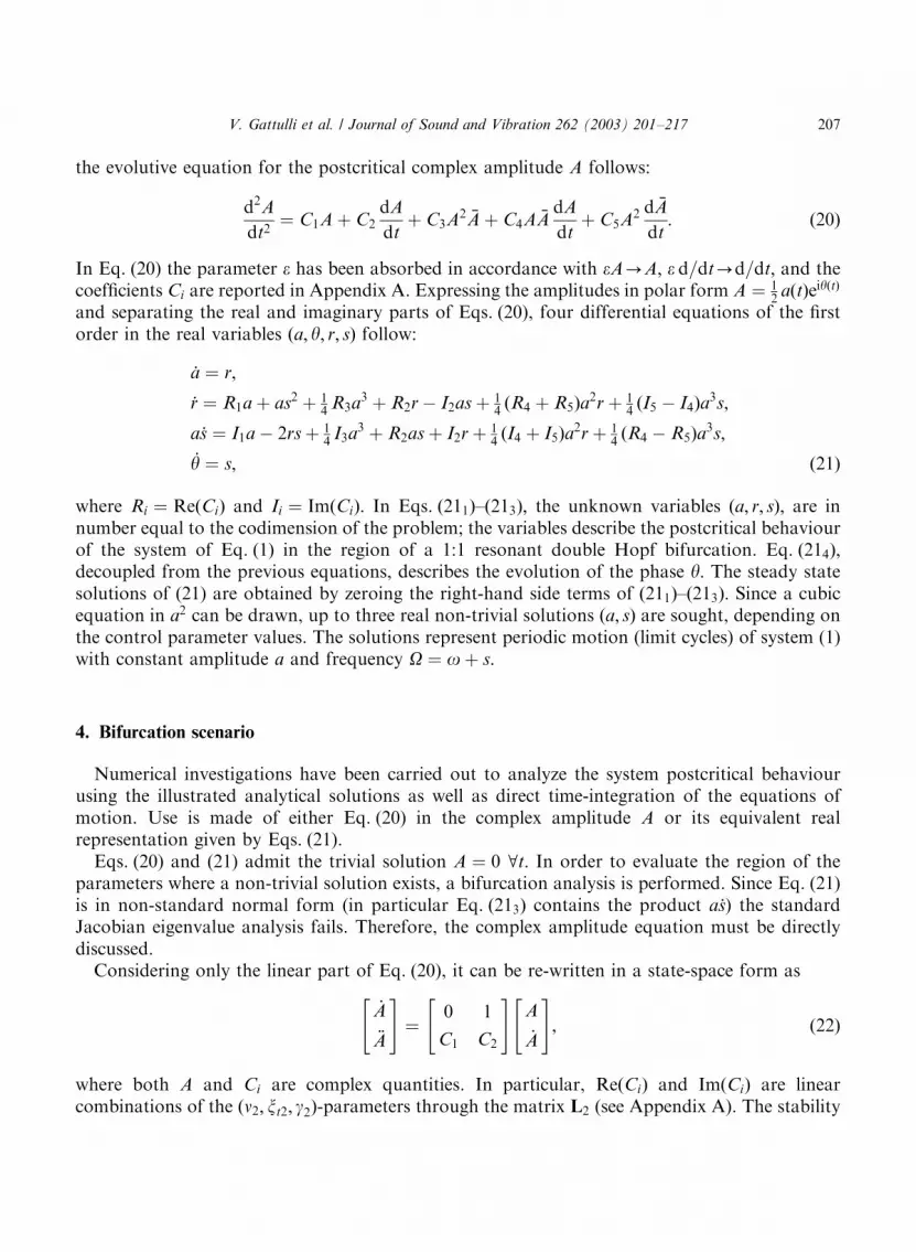
amplitudes on the control parameters. Fig. 3 shows the amplitude a versus the flow velocity n andthe damping xt for the perfect tuned system ðg ¼ g0Þ and supercritical aerodynamic behaviour(A3o0 in Eq. (4)). The regions of existence of the limit cycles are depicted in Fig. 3a, namely: inthe region R0 no limit cycles exist, but only the stable trivial solution is admitted; in R1 and R2andR3 one, two, and three limit cycles exist, respectively, according to the discussion of Eqs. (21).Such solutions are represented in a 3-D-view in Fig. 3b. The two stable solutions of region R2emerge from the double Hopf boundary S2; they coalesce in the amplitude a but differ in thefrequency correction s: A unique solution rises from the simple Hopf boundaries, being stable atSþ1 (positive velocity of the eigenvalues at the criticality) and unstable at S�

1 (negative velocity).The three solutions existing in the region R3 coalesce along the line C:In Fig. 3b four sections are selected, three (I, II, III) parallel to the ðn; aÞ-plane, the fourth (VI)

parallel to the ðxt; aÞ-plane. Path I crosses the region R0; R2 and R3 showing the occurrence of asuccessive bifurcation at S�

1 : Path II contains the peculiar point P0 and it shows the transitionfrom the region R0 to the line C; where the three solutions coalesce in one. Path III illustrates thepassage from R0 to R1 through a simple Hopf bifurcation. Path IV explains the coalescencemechanism: the two stable solutions ofR2 are associated to almost opposite frequency corrections(see s in Fig. 3e) while the unstable solution has no frequency correction. At the crossing betweenpath IV and the line C; the three solutions coalesce to one with zero frequency correction (Figs. 3dand e). It is worth noticing that the coalescence occurs at the smallest amplitude existing for anygiven n > n0:The analytical results of Fig. 3 have been compared with the direct numerical integration of

the equations of motion (1) and an excellent accordance between them has been found (seeFigs. 3c and d). Moreover, the curves have been compared with that of the uncontrolled system,which only depends on n: It is seen that the limit-cycle amplitudes of the controlled system arealways below the uncontrolled ones. Therefore, the TMD has a beneficial effect even in thepostcritical range, the maximum benefit occurring at n ¼ n0; i.e., at the optimum value of theTMD.To better illustrate the role of the frequency correction s; the two limit cycles existing at the

point QAR2; with the same amplitudes and opposite corrections, have been depicted on theðq1; q2Þ-configuration plane (Fig. 4). Here, the perturbative solution at the first order (x ¼ ex1;I-curves) and that at the second order (x ¼ ex1 þ e2x2; II-curves) have been compared with direct

V. Gattulli et al. / Journal of Sound and Vibration 262 (2003) 201–217208

numerical integration (EX-curves). The first order solution appears quite rough in comparisonwith the second order solution, which is very close to the exact one. The differences are ascribed tothe fact that the first order solution x1 (Eq. (13)), predicts steady state oscillations along theproper eigenvector u1 at P0; therefore, it is not able to capture the dependence of the q1=q2 ratioon the control parameters. The second order term x2 (Eq. (14)) instead accounts for suchmodification, since its factor d1A ¼ isA is parameter-dependent through the frequency corrections: Therefore the second order solution xCex1 þ e2x2 ¼ Aðu1 þ isu2Þeiot þ c:c: is an harmonicmotion along a vector that is just the lower order approximation of the proper eigenvectors at a

0 0.02 0.04 0.060

20

40

60

80

ν

ξ t

P0

I II III

IV

R0

R2

R1

R3 C

S2

Q

(a)

S1-

S1+

a

ξ t

νI

IIIII

IV

(b)

0 10 20 30 40 50 60 70 800

1

2

3

4

5

a

ν

unc

I III

II

I

(c)

0 0.02 0.04 0.060

2

4

6

8

ξ t

a

unc

IV

(d) (e)

0 0.02 0.04 0.06-0.08

-0.04

0

0.04

0.08

ξ t

s

IV

Fig. 3. Supercritical scenario in the ðn; xtÞ-space for g ¼ g0 ¼ 0:9975 and A3 ¼ �421: (a) existence regions of non-trivialsolutions, (b) 3-D view in the ðn; xt; aÞ-space, (c) I, II, III ðn; aÞ-sections, (d) IV ðxt; aÞ-section, (e) IV ðxt; sÞ-section.Continuous lines: stable solutions; dashed lines: unstable solutions; dots: numerical results; unc: uncontrolled system.

V. Gattulli et al. / Journal of Sound and Vibration 262 (2003) 201–217 209

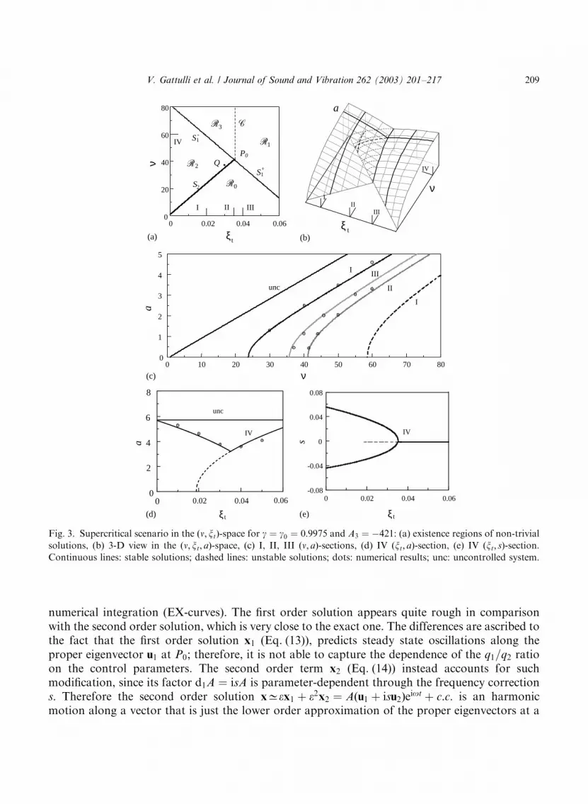
Qi-point [17], if non-linearities are neglected in s:However, since the sensitivity of the eigenvectorsof a defective matrix is high, it is expected that the region of validity of the resonant solution isquite limited.The effect on the postcritical behaviour of imperfect tuning ðgag0Þ between the PS and the

TMD is analyzed in Fig. 5. The regions in which the limit cycles exist are illustrated in Fig. 5a.The simultaneous passage of two eigenvalues across the imaginary axis is broken by the detuning(it should be remembered that the locus of double Hopf belongs to the plane g ¼ g0); as aconsequence, a simple Hopf occurs for increasing n for any value of xt along the lower boundarySþ1l : From it a regular surface arises, as illustrated in Fig. 5b. Along the higher boundaries Sþ

1h andS�1 ; two successive simple Hopfs occur, with positive and negative velocities of the eigenvaluesrespectively. There, new surfaces arise, which coalesce along the line C; where a locus of limitpoints with respect to xt occurs. In summary, with respect to the perfectly tuned case (Fig. 3b) thetwo surfaces in R2 split: the upper one smoothly matches the surface in R1; while the lower onematches the surface in R3: Two typical sections (I, II in Fig. 5b) are sufficient to describe thescenario for increasing n (see Fig. 5c). Path I crosses all the regions Ri ði ¼ 0;y; 3Þ: Along it astable limit cycle first bifurcates from the trivial solution at Sþ

1l ; then an initially unstable limitcycle bifurcates at Sþ

1h; finally, at S�1 ; a third unstable limit cycle bifurcates while the second one

regains stability through a Neimark bifurcation, from which modulated solutions arise (notstudied here). Path II corresponds to a simple Hopf bifurcation with a stable limit cycle. Path IIIshows the dependence of the amplitude (Fig. 5a) and of the frequency correction (Fig. 5e) on xt:The curves can be usefully interpreted as perturbations of those in Figs. 3d and e, due to thedetuning. The separation of the coincident solutions appears clearly. Along the lower branch inFig. 5d first a Neimark bifurcation at S�

1 and then a limit point at C occur. Finally, the s-path ofFig. 5d shows that the detuning gives rise to the lack of symmetry of the two solutions in R2:Consequently, these solutions are represented by two orbits in the ðq1; q2Þ-configuration planewith different amplitudes and orientations. Direct numerical integration of Eq. (1) shows acomplete qualitative agreement (see Figs. 5c and d), while quantitative differences increase whenmoving away from the point P0: Moreover, the amplitudes are found to be always below that of

-2 -1 0 1 2

-20

-10

0

10

20

q1

q 2

I I

II

II

EX

EX

-2 -1 0 1 2

-20

-10

0

10

20

q1

q 2

(a) (b)

Fig. 4. Limit cycle at point Q � ð37:8; 0:033; 0:9975Þ in the ðq1; q2Þ-configuration plane; direct integration (EX) versus I-order and II-order perturbative solutions: (a) s > 0; (b) so0:

V. Gattulli et al. / Journal of Sound and Vibration 262 (2003) 201–217210

the uncontrolled system, except for a very small xt not shown in Fig. 5d. This erroneous result ishowever a consequence of the rough approximation of the bifurcation locus Sþ

1l far from P0 givenby the perturbation solution, as is apparent from Figs. 2c and d.The influence of the sign of the non-linear aerodynamical force on system postcritical behaviour

is then investigated. A positive aerodynamic coefficient A3 is considered (i.e., a section with asubcritical aerodynamic behaviour) and the previous analysis is repeated. In the perfectly tunedcase (g ¼ g0) the scenario changes as seen in Fig. 6. In Fig. 6a the regions of limit cycle existenceare illustrated; they are of course bounded by the same manifolds Sþ

1 ;S�1 ;S2 of the supercritical

0 0.02 0.04 0.060

20

40

60

80

ν

ξ t

0

I II

III1

2

3 C

S1-

S1h+ S1l

+

a

ξ t

νIII

III

(b)

0 10 20 30 40 50 60 70 800

1

2

3

4

5

III

a

ν

IIunc

N

0 0.02 0.04 0.060

2

4

6

III

ξ t

a III

unc

N

L

0 0.02 0.04 0.06-0.08

-0.04

0

0.04

0.08

III

ξ t

s

III

(a)

(c)

(d) (e)

R

R

R

R

Fig. 5. Supercritical scenario in the ðn; xtÞ-plane for g ¼ 0:9925 and A3 ¼ �421: (a) existence regions of non-trivialsolutions, (b) 3-D view in the ðn; xt; aÞ-space; (c) I, II ðn; aÞ-sections; (d) III ðxt; aÞ-section, (e) III ðxt; sÞ-section.Continuous lines: stable solutions; dashed lines: unstable solutions; dots: numerical results; unc: uncontrolled system.

V. Gattulli et al. / Journal of Sound and Vibration 262 (2003) 201–217 211

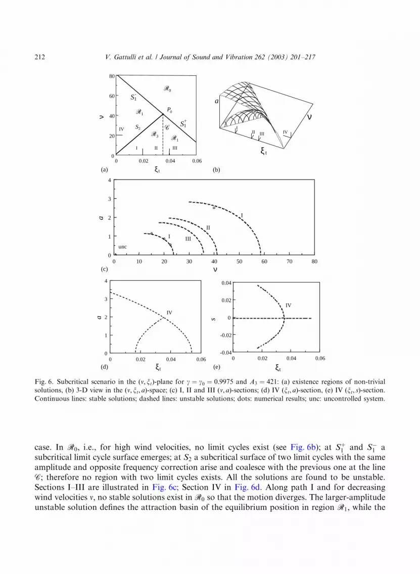
case. In R0; i.e., for high wind velocities, no limit cycles exist (see Fig. 6b); at Sþ1 and S�

1 asubcritical limit cycle surface emerges; at S2 a subcritical surface of two limit cycles with the sameamplitude and opposite frequency correction arise and coalesce with the previous one at the lineC; therefore no region with two limit cycles exists. All the solutions are found to be unstable.Sections I–III are illustrated in Fig. 6c; Section IV in Fig. 6d. Along path I and for decreasingwind velocities n; no stable solutions exist in R0 so that the motion diverges. The larger-amplitudeunstable solution defines the attraction basin of the equilibrium position in region R1; while the

P0

0 0.02 0.04 0.060

20

40

60

80

ν

ξ t

R0

R1

I II III

IVR3 R1

S2

(a)

(c)

(d) (e)

C

S1-

S1+

a

ξ t

νI

II III IV

(b)

0 10 20 30 40 50 60 70 800

1

2

3

4

I

II

III

I

unc

a

ν

0 0.02 0.04 0.060

1

2

3

4

ξt

a

IV

0 0.02 0.04 0.06-0.04

-0.02

0

0.02

0.04

ξt

s

IV

Fig. 6. Subcritical scenario in the ðn; xtÞ-plane for g ¼ g0 ¼ 0:9975 and A3 ¼ 421: (a) existence regions of non-trivialsolutions, (b) 3-D view in the ðn; xt; aÞ-space; (c) I, II and III ðn; aÞ-sections; (d) IV ðxt; aÞ-section, (e) IV ðxt; sÞ-section.Continuous lines: stable solutions; dashed lines: unstable solutions; dots: numerical results; unc: uncontrolled system.

V. Gattulli et al. / Journal of Sound and Vibration 262 (2003) 201–217212

smaller solution bounds that in R3: Path II follows the locus C of the amplitude-coalescingsolutions (with no frequency corrections). Path III illustrates the Hopf subcritical bifurcationwhile path IV shows the coalescence mechanism (Figs. 6a and e). Numerical results have againconfirmed the perturbation analysis (Fig. 6c). Finally, the amplitude curves, compared with thoseof the uncontrolled system (where they are almost unnoticeable in the scale of the plot) turn out tobe all higher: therefore the TMD has a beneficial effect also on sections with subcritical behaviour,since it enlarges the attraction basin.

0 0.02 0.04 0.060

20

40

60

80

ν

ξt

R0

I II

III

R1

R2

R3

C

(a)

(c)

(d) (e)

R1

S1

S1l+

S1h+

-

a

ν

(b)

I II

III

ξ t

0 10 20 30 40 50 60 70 800

1

2

3

4

a

ν

I

I

I IIunc

0 0.02 0.04 0.060

1

2

3

4

ξ t

a

III

III

0 0.02 0.04 0.06-0.04

-0.02

0

0.02

0.04

ξ t

s

III

III

Fig. 7. Subcritical scenario in the ðn; xtÞ-plane for g ¼ 0:9925 and A3 ¼ 421: (a) existence regions of non-trivialsolutions, (b) 3-D view in the ðn; xt; aÞ-space; (c) I, II ðn; aÞ-sections; (d) III ðxt; aÞ-section, (e) III ðxt; sÞ-section.Continuous lines: stable solutions; dashed lines: unstable solutions; dots: numerical results; unc: uncontrolled system.

V. Gattulli et al. / Journal of Sound and Vibration 262 (2003) 201–217 213

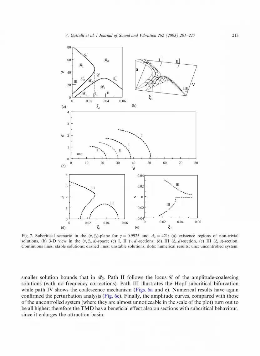
In Fig. 7 analysis is completed with subcritical aerodynamic behaviour in the imperfectly tunedcase. The results should be read as a perturbation of the tuned case.

5. Discussion

Some results have been presented in literature [10,11] to demonstrate the effectiveness of theTMD also in the postcritical range. They are based on the assumption that the steady dynamics ofa PS equipped with a TMD can be described by an equivalent s.d.o.f. system. Two differentapproaches have been followed in those papers. An equivalent structural damping was defined inRef. [11] by equating the critical velocities of the controlled and uncontrolled systems. Accordingto this criterion, the TMD would only modify the linear properties of the PS, by increasing thestructural damping, without affecting the non-linear forces acting on it. A more refined analysiswas performed in Ref. [10], by assuming that the ratio between the PS and TMD amplitudes ofmotion remains constant in time. The procedure leads to an equivalent s.d.o.f. system, in which,again, only the linear terms (damping as well stiffness) are modified by the TMD. In addition, anon-linear algebraic equation must be solved to get the unknown frequency as function of thelinear parameters only (mass ratio, frequency ratio and damping). Both equivalent oscillatorsfurnish limit cycle amplitudes smaller than the uncontrolled ones.The analysis developed in the present paper permits the results of Refs. [10,11] to be discussed.

It should initially be observed that the reduction of the system to a s.d.o.f. system is generallyincorrect. Indeed, while the non-linear dynamics of the simple aeroelastic oscillator is essentiallygoverned by a one-dimensional equation of the type ’a ¼ f ðaÞ; where a is the oscillation amplitude,the dynamics of the coupled system is governed by a three-dimensional equation ’a ¼ fðaÞ; where’a ¼ ð ’a; a; sÞ and s is the time-dependent frequency correction (see Eq. (21)). This dynamic richnessis a direct consequence of the fact that, around the optimum point P0; both the pairs ofeigenvalues play an active role in the postcritical behaviour, either in the region R2 (where bothare unstable) and in region R1 and R3 (where only one is unstable but, the other is close to it).Therefore, no equivalence can exist among systems whose essential dynamics develop in spaces ofdifferent dimensions. For example, steady quasi-periodic solutions are admitted by the three-dimensional system (although they have been found here to be of unstable type), but areforbidden in the one-dimensional one. The main difference between the two systems is that, whilethe frequency correction does not substantially affect the dynamics of the simple aeroelasticoscillator (since it does not modify the amplitude of the motion), in contrast it actively contributesto the dynamics of the coupled oscillator (being strongly connected with the amplitude).From Eq. ð213Þ it is seen that, even in the steady motion in which ’a ¼ 0; the frequency

correction s depends on both linear and non-linear terms in the amplitude a: The linear termsaccount for the modification occurring in the frequency when the parameters are varied from theiroptimum value (i.e., they describe the sensitivity of the eigenvalues of the system at the doubleHopf bifurcation point P0); the non-linear terms account for the effects of the aerodynamic forces.The perturbation analysis developed in Section 3 shows that these effects all appear at the same e4-order (see Eq. (18)) so that it is not allowed to neglect the latter in comparison with the former. Ifnon-linear effects have to be ignored, then, consistently, linear terms must be ignored too, ands ¼ 0 must be taken, as predicted by the e3-order perturbation equation (16).

V. Gattulli et al. / Journal of Sound and Vibration 262 (2003) 201–217214

However, the role played by non-linearities in the frequency correction equation ð213Þ isfundamental to a correct description of the system behaviour. Indeed, if they are consistentlyaccounted for, the algebraic problem associated with Eqs. ð211;2;3Þ leads to a degree-three equationin the squared amplitude a; responsible for the multiple branch solution displayed in regions R2and R3 (see Figs. 3 and 5). In contrast, if s is taken as independent of the amplitude (e.g., equal tozero), then a linear equation in the squared amplitude is found, structurally indentical to that ofthe aeroelastic oscillator. Thus, the existence of a region of multiple branch solution is obscured.As an example, if region R1 (with g ¼ g0) in Fig. 3 is considered (simple Hopf bifurcation for theperfectly tuned system), s ¼ 0 is found, i.e., linear and non-linear effects on frequency balanceeach other. The following approximate expression for the limit cycle can be derived:

a2 ¼ �4

3

½ðxsn2 þ xt2Þ=m�UdA3

¼4

3

xeU

dA3ð24Þ

from which an equivalent damping xe is drawn. Both the analyses developed in Refs. [10,11] donot account for non-linear frequency correction and, in fact, do not highlight the existence ofmultiple branch solutions. However, these analyses were applied to systems some way from thedouble Hopf bifurcation point and only in the region R1; where it is reasonable to suppose thatthe interaction between the two couples of eigenvalues is weak (since the stable couple has apassive role). Therefore, the conclusions of Refs. [10,11] about the effectiveness of the TMD arecorrect, but cannot be considered of general validity; however, they have been confirmed andgeneralized by the wider analysis performed here.

6. Conclusions

The postcritical behaviour of a s.d.o.f. system equipped with a Tuned Mass Damper has beenanalyzed for double Hopf bifurcation in the neighbourhood of 1:1 resonance. Due to thecoalescence of its eigenvalues, the system is defective at the criticality, and therefore admits anincomplete set of eigenvectors. By using the Multiple Scale Method, a second order bifurcationequation governing the time-evolution of the complex amplitude of the critical mode has beenderived. When a real-variables representation is adopted, three first order differential equations,uncoupled from the fourth and describing the asymptotic dynamic of the system, have beenfound. By solving the associate algebraic equations, steady solutions have been found representinglimit cycles for the original mechanical system. The regions of existence of such limit cycles havebeen studied in the space of the control parameters. Up to three limit cycles have been found tocoexist, both for aerodynamically stable and for aerodynamically unstable section shapes.Perturbation results have been found to be in excellent agreement with results obtained by directlyintegrating the equations of motion. In all cases considered it has been found that the TMD has abeneficial effect on the postcritical behaviour of the system, since it reduces the limit cycleamplitudes in the supercritical case and increases them in the subcritical case. These results, whilethey confirm the findings of Refs. [10,11], extend them to the whole parameter region of technicalinterest, where previous methods of analysis cannot be employed.

V. Gattulli et al. / Journal of Sound and Vibration 262 (2003) 201–217 215

Appendix A

The expressions of the coefficients in Eqs. (16)–(20) are

s31 ¼C1 ¼ vH2 L2u1;

p31 ¼ vH1 L2u1;

p32 ¼ 12vH1 f

0xxxu

21 %u1;

s41 ¼C2 ¼ p31 þ vH2 L2u2;

s32 ¼C3 ¼ 12vH2 f

0xxxu

21 %u1;

s42 ¼C4 ¼ 2p32vH2 u2 þ vH2 f0xxxu1 %u1 %u2;

s43 ¼C5 ¼ p32vH2 u2 þ

12vH2 f

0xxxu

21 %u2: ðA:1Þ

In Eqs. (A.1), uk and vk ðk ¼ 1; 2Þ are the right and the left eigenvectors defined by Eqs. (6) and(7); an overbar denotes the complex conjugate and ð ÞH the transpose conjugate. Moreover, z111 isthe solution to the following algebraic problem:

ðL0 � 3io0Þz111 ¼ 16f0xxxu

31: ðA:2Þ

References

[1] G.V. Parkinson, N.P.H. Brooks, On the aeroelastic instability of bluff cylinders, Journal of Applied Mechanics 28

(1961) 252–258.

[2] M. Novak, Aeroelastic galloping of prismatic bodies, Engineering of Mechanics Division 96 (1969) 115–142.

[3] R.M. Corless, G.V. Parkinson, A model of the combined effects of vortex-induced oscillation and galloping,

Journal of Fluids and Structures 2 (1988) 203–220.

[4] T.T. Soong, G.F. Dargush, Passive Energy Dissipation Systems in Structural Engineering, Wiley, New York, 1997.

[5] A. Larsen, Vortex-induced response of bridges and control by tuned mass dampers, in: Moan et al. (Eds.),

Structural Dynamics—EURODYN’93, A.A. Balkema, Rotterdam, 1993, pp. 1003–1010.

[6] A. Larsen, E. Svensson, H. Andersen, Design aspects of tuned mass dampers for the Great Belt East Bridge

approach span, Journal of Wind Engineering and Industrial Aerodynamics 54–55 (1993) 413–426.

[7] V. Gattulli, R. Ghanem, Adaptive control of flow-induced oscillations including vortex effects, International

Journal of Non-Linear Mechanics 34 (1999) 853–868.

[8] M.D. Rowbottom, The optimization of mechanical dampers to control self-excited galloping oscillations, Journal

of Sound and Vibration 75 (1981) 559–576.

[9] Y. Fujino, M. Ab!e, Design formulas for tuned mass dampers based on a perturbation technique, Earthquake

Engineering and Structural Dynamics 22 (1993) 833–854.

[10] Y. Fujino, P. Warnitchai, M. Ito, Suppression of galloping of bridge tower using tuned mass damper, Journal of

the Faculty of Engineering, The University of Tokyo 38 (1985) 49–73.

[11] M. Abdel-Rohman, Design of tuned mass dampers for suppression of galloping in tall prismatic structures,

Journal of Sound and Vibration 171 (1994) 289–299.

[12] V. Gattulli, F. Di Fabio, A. Luongo, Simple and double Hopf bifurcations in aeroelastic oscillators with tuned

mass dampers, Journal of Franklin Institute 338 (2001) 187–201.

V. Gattulli et al. / Journal of Sound and Vibration 262 (2003) 201–217216

[13] A. Luongo, V. Gattulli, F. Di Fabio, 1:1 Resonant Hopf bifurcations in slender space structures with tuned mass

dampers, 42nd AIAA/ASME/ASCE/AHS/ASC Structures, Structural Dynamics and Materials Conference,

AIAA 2001-1308, 2001.

[14] A. Di Egidio, A. Paolone, A. Luongo, Analisi postcritica di strutture autoeccitate in risonanza 1:1, Proceedings of

14th Italian Conference on Theoretical and Applied Mechanics, AIMETA’99, Como, Italy, 1999.

[15] R.D. Blevins, Flow-Induced Vibration, 2nd Edition, Van Nostrand Reinhold, New York, 1990.

[16] A. Luongo, A. Paolone, On the reconstitution problem in the multiple time-scale method, Nonlinear Dynamics 19

(1999) 133–156.

[17] A. Luongo, Eigensolutions sensitivity for nonsymmetric matrices with repeated eigenvalues, American Institute of

Aeronautics and Astronautics Journal 31 (1993) 1321–1328.

V. Gattulli et al. / Journal of Sound and Vibration 262 (2003) 201–217 217