This article was downloaded by: [The University of British Columbia]On: 03 April 2012, At: 09:58Publisher: Taylor & FrancisInforma Ltd Registered in England and Wales Registered Number: 1072954 Registeredoffice: Mortimer House, 37-41 Mortimer Street, London W1T 3JH, UK

Engineering OptimizationPublication details, including instructions for authors andsubscription information:http://www.tandfonline.com/loi/geno20

Configuration optimization of dampersfor adjacent buildings under seismicexcitationsKasra Bigdeli a , Warren Hare b & Solomon Tesfamariam aa School of Engineeringb Mathematics, University of British Columbia, Kelowna, BC,Canada

Available online: 02 Apr 2012

To cite this article: Kasra Bigdeli, Warren Hare & Solomon Tesfamariam (2012): Configurationoptimization of dampers for adjacent buildings under seismic excitations, EngineeringOptimization, DOI:10.1080/0305215X.2012.654788

To link to this article: http://dx.doi.org/10.1080/0305215X.2012.654788

PLEASE SCROLL DOWN FOR ARTICLE

Full terms and conditions of use: http://www.tandfonline.com/page/terms-and-conditions

This article may be used for research, teaching, and private study purposes. Anysubstantial or systematic reproduction, redistribution, reselling, loan, sub-licensing,systematic supply, or distribution in any form to anyone is expressly forbidden.

The publisher does not give any warranty express or implied or make any representationthat the contents will be complete or accurate or up to date. The accuracy of anyinstructions, formulae, and drug doses should be independently verified with primarysources. The publisher shall not be liable for any loss, actions, claims, proceedings,demand, or costs or damages whatsoever or howsoever caused arising directly orindirectly in connection with or arising out of the use of this material.

Engineering OptimizationiFirst, 2012, 1–19

Configuration optimization of dampers for adjacent buildingsunder seismic excitations

Kasra Bigdelia, Warren Hareb* and Solomon Tesfamariama

aSchool of Engineering and bMathematics, University of British Columbia, Kelowna, BC, Canada

(Received 17 June 2011; final version received 8 December 2011)

Passive coupling of adjacent structures is known to be an effective method to reduce undesirable vibrationsand structural pounding effects. Past results have shown that reducing the number of dampers can consid-erably decrease the cost of implementation and does not significantly decrease the efficiency of the system.The main objective of this study was to find the optimal arrangement of a limited number of dampersto minimize interstorey drift. Five approaches to solving the resulting bi-level optimization problem areintroduced and examined (exhaustive search, inserting dampers, inserting floors, locations of maximumrelative velocity and a genetic algorithm) and the numerical efficiency of each method is examined. Theresults reveal that the inserting damper method is the most efficient and reliable method, particularly fortall structures. It was also found that increasing the number of dampers does not necessarily increase theefficiency of the system. In fact, increasing the number of dampers can exacerbate the dynamic responseof the system.

Keywords: earthquake damage control; bi-level optimization; coupled structures; viscous dampers;discrete optimization

1. Introduction

In most metropolitan areas, limited land availability and high demand for residency and officebuildings lead to high-rise buildings being constructed in close proximity. During an earthquakesuch adjacent buildings are prone to pounding. The damage due to pounding during earthquakes ishighly destructive and particularly frequent in dense urban centres (Tesfamariam and Saatcioglu2010). For example, severe damage was observed in the Mexico City earthquake (1985), the LomaPrieta earthquake (1989), the Kobe earthquake (1994) and the recent New Zealand earthquake(2011). Many studies have investigated the use of dampers (connectors) to reduce pounding-induced damage and to increase the seismic resistance of a structure (Xu et al. 1999a, Azuma et al.2006, Bharti et al. 2010). Types of damper can be grouped into active devices (Xu and Zhang 2002,Ying et al. 2003), semi-active magnetorheological (MR) dampers (Qu and Xu 2001, Bharti andShrimali 2007), friction dampers (Bhaskararao and Jangid 2006a, Ng and Xu 2006), viscoelasticdampers (Zhang and Xu 1999, Zhu et al. 2010) and fluid dampers (Zhang and Xu 2000,Yang and

*Corresponding author. Email: Warren.Hare@ubc.ca

ISSN 0305-215X print/ISSN 1029-0273 online© 2012 Taylor & Francishttp://dx.doi.org/10.1080/0305215X.2012.654788http://www.tandfonline.com

Dow

nloa

ded

by [

The

Uni

vers

ity o

f B

ritis

h C

olum

bia]

at 0

9:58

03

Apr

il 20

12

2 K. Bigdeli et al.

Lu 2003). Experimental studies have also confirmed the efficiency of the damper connectors tomitigate vibrations of structures (Xu et al. 1999b, Ng and Xu 2006, Yang and Lu 2003).

Many modern applications in structural vibration control have been enhanced through theapplication of optimization (see e.g.Viswamurthy and Ganguli 2007, Mezyk 2002 and referencestherein). However, very little has been done with regard to optimizing the use of dampers todecrease seismic damage. Current optimization studies involving damper connectors for adjacentbuildings can be categorized into two groups: single degree-of-freedom (SDOF) and multi-degree-of-freedom (MDOF) systems. The former is more likely to result in an analytical solution, butis too inaccurate for practical purposes; the latter is more accurate, but too complicated to besolved analytically. For example, Basili and De Angelis (2007b) studied the optimal mechani-cal properties of nonlinear hysteric dampers connecting two SDOF structures. They presentedexplicit equations relating dissipation energy, relative displacement and relative acceleration tothe mechanical properties of the dampers. In another study, Basili and De Angelis (2007a) stud-ied the same problem for two MDOF structures. However, in the latter study, when consideringoptimization aspects they estimated the MDOF structures using a pair of SDOF systems andfollowed the same procedure as they did in their earlier work. Zhu and Xu (2005) presented ananalytical closed form solution for mechanical properties of a fluid damper connecting two SDOFstructures. In Xu et al. (1999a), multiple uniform dampers throughout the buildings connect everyadjacent floor of MDOF structures. The optimal damping coefficient is simply found by plottingthe objective function versus damping coefficient for different stiffnesses of connectors. Ok et al.(2008) examined a multi-objective optimization based on a genetic algorithm for a set of cou-pled MDOF structures connected to each other by MR dampers. They assumed the number ofdampers and the voltage for MR dampers installed at each floor as design parameters. Since abounded domain for voltage is assumed, they allowed each floor to have more than one damper ifthat was more effective. Still, no optimal arrangement is provided when the number of dampersis limited.

In general, analytical and experimental studies have examined the dynamic characteristics andresponses of the structures before and after implementing a damping device in order to showtheir effectiveness. However, a few studies have examined the effect of non-uniform distributionof the dampers (Yang and Lu 2003, Bhaskararao and Jangid 2006a, b, Ok et al. 2008, Bhartiet al. 2010). None of these studies provides a clear comparison to show the quality of their ownproposed arrangement/solution. For example, in Yang and Lu (2003) it is experimentally shownthat placing viscous dampers on every floor is unnecessary, and that the number of dampers canbe reduced with minimal loss in performance. But no solution, other than trial and error, forthe optimal arrangement is provided. A similar study, but for MR dampers, was conducted byBharti et al. (2010), which confirmed that it is not necessity to equip every single floor with adamper. A genetic algorithm performed by Ok et al. (2008) for structures equipped with MRdampers confirmed the results presented in Bharti et al. (2010). As an attempt to deliver a clearmethod to find the optimal arrangement, Patel and Jangid (2010) proposed that viscous dampersshould be installed in floors with maximum relative velocity, since the force generated in viscousdampers depends on relative velocity. In a similar study (Bhaskararao and Jangid 2006a), the bestplaces for friction dampers are suggested to be the floors with maximum relative displacementdue to an analogous intuition. However, to the authors’ knowledge, there is no deterministicoptimization method available to find the best arrangement of dampers when the number ofdampers is limited.

In this article, a couple of deterministic combinatorial optimization techniques are presentedto determine the optimal location for a limited number of viscous dampers. Combinatorialoptimization methods have been shown to be effective in finding the optimal arrangement ofviscous dampers for a single building (Agrawal and Yang 1999). Unlike random/evolutionarysearch methods, deterministic methods as presented in this article lead to a certain solution.

Dow

nloa

ded

by [

The

Uni

vers

ity o

f B

ritis

h C

olum

bia]

at 0

9:58

03

Apr

il 20

12

Engineering Optimization 3

A comparison study is presented to verify the effectiveness of the presented methods. As inXu et al. (1999a), each floor can have one damper at most and all dampers are assumed tobe similar. The final result is a bi-level optimization problem, where the objective functiondepends on the damping coefficient and damper location. In order to compute the ‘best’ numberof dampers to use, one can compute the optimal damping coefficient and damper location foreach possible number of dampers, and then select the desired balance between cost and damagemitigation.

This article introduces two optimization algorithms to determine the optimal configuration fora given number of dampers: a damper insertion heuristic and a floor insertion heuristic. For thepurposes of comparison, this article includes a non-heuristic approach, an exhaustive search, aswell as a genetic algorithm, and a fifth method, the highest relative velocity heuristic, based on thework of Patel and Jangid (2010). The exhaustive search is guaranteed to be globally optimal, but isextremely time consuming. Indeed, in the most difficult cases an exhaustive search is completelyintractable. The damper insertion and floor insertion heuristics are considerably faster, but notguaranteed to return the globally optimal solution. However, numerical tests suggest that theyare both highly effective. Results also show that the genetic approach can be considered as areasonable option if the convergence rate is more important than the accuracy of the results.For more accurate results, the damper insertion method is the best method among the presentedmethods. The final technique (highest relative velocity heuristic) assumes that the best locationsfor viscous dampers are the floors that have the maximum relative velocity. This makes intuitivesense because the force generated in viscous dampers is a function of relative velocity. However,the results presented in this study show that this arrangement does not generally result in optimalperformance. Details of each method are discussed in Section 3.

To examine the efficiency of these techniques, various numerical examples are presented(Section 4). For each method, the total computational effort is examined, through both the cal-culation of the number of simulations required and the central processing unit (CPU) time usedfor the numerical tests. Furthermore, a comparison between the resulting qualities of the finalsolution using each technique is presented.

Optimization is performed on a simulation model, discussed in Section 2. Some discussionon the formulation of the optimization problem can be found in Section 2.5. Conclusions anddiscussion of future research can be found in Section 5.

2. Physical model

2.1. Assumptions and limitations

The ground motion and dynamic response of the buildings are assumed to be unidirectional.To prevent the effect of torsional vibrations of the buildings, both buildings are assumed to besymmetrical and their centres of mass are located in the same plane. Figure 1 shows that eachbuilding is modelled as an MDOF system consisting of lumped masses, representing mass foreach floor; a linear spring, representing stiffness of columns; and a linear viscous damper.

In order to connect adjacent buildings, both buildings are assumed to have the same floorelevations. However, the heights of the buildings do not need to match. Damper connectors aremodelled as viscous dampers with a damping coefficient variable (the damping coefficient isuniform across all dampers). Many mechanical models are available to represent the dynamicbehaviour of the fluid dampers. In this study, fluid dampers are modelled as a set of parallel linearsprings and dampers. Based on results presented in Xu et al. (1999a) and Zhang and Xu (1999), itis further assumed that the stiffness of the fluid damper can be neglected without any significanteffects on the model and performance.

Dow

nloa

ded

by [

The

Uni

vers

ity o

f B

ritis

h C

olum

bia]

at 0

9:58

03

Apr

il 20

12

4 K. Bigdeli et al.

Building1

Building 2

cd,n-1

cd,n-3

cd2

Base Excitation

c11

c22c21

c31

cn-2,1

cn-1,1

cn1

cn+1,1

cn+m,1

cn2

cn-1,2

c12

cn-2,2

c32

k12

k22

k32

kn-2,2

kn-1,2

kn2

k11

k21

k31

kn-2,1

kn-1,1

kn1

kn+1

kn+m,1

m11

m21

mn-2,1

mn-3,1

mn-1,1

mn1

mn+m-1,1

mn+m,1

m12

m22

mn-2,2

mn-3,2

mn-1,2

mn2

Figure 1. Schematic model of buildings.

2.2. Modelling and analysis

As shown in Figure 1, buildings 1 and 2 have n + m and n storeys, respectively. The mass, shearstiffness and damping coefficients for the ith storey are mi1, ki1 and ci1 for building 1 and mi2,ki2 and ci2 for building 2, respectively. The damping coefficient and stiffness coefficient of thedamper at the ith floor are cdi and kdi, respectively. The dynamic model for both structures is takento be a 2n + m degree of freedom system.

Let xi1(t) and xi2(t) be the displacement of the ith floor of buildings 1 and 2 in time domain,respectively. Consequently, xi1(t) and xi2(t) represent the velocity, and xi1(t) and xi2(t) representthe acceleration of the ith floor of buildings 1 and 2, respectively.

Dow

nloa

ded

by [

The

Uni

vers

ity o

f B

ritis

h C

olum

bia]

at 0

9:58

03

Apr

il 20

12

Engineering Optimization 5

To find a general and reliable objective function, the model is analysed in the pseudo-excitationfrequency domain rather than the time domain, which is usually associated with a specific realearthquake record. Therefore, displacement, velocity and acceleration values are transformedfrom functions of time into functions of frequency ω, as xi1(ω), xi2(ω), xi1(ω), xi2(ω), xi1(ω) andxi2(ω).As before, the first index corresponds to the floor number and the second index correspondsto the building number. Since calculated parameters in the frequency domain are complex values,the squared magnitude, also known as the auto-spectral density, is used for optimization. Forexample, the auto-spectral density of displacement for the ith floor of building b is written as:

Sxib(ω) = xib(ω) • conj(xib(ω)) (1)

Subsequently, applying integration over the frequency domain will result in statistical parame-ters, which represent standard deviations of displacement, velocity and acceleration of each floor.For instance, for the ith floor of building b, its standard deviation of displacement response is:

σxib =[∫ +∞

−inftySxib(ω)dω

]1/2

(2)

2.3. Simulation

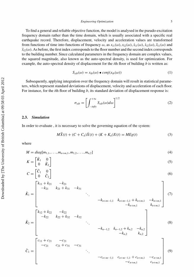
In order to evaluate , it is necessary to solve the governing equation of the system:

MX(t) + (C + Cd)X(t) + (K + Kd)X(t) = MEg(t) (3)

where

M = diag[m1,1, . . . , mn+m,1, m1,2, . . . , mn,2] (4)

K =[

K1 00 K2

](5)

C =[

C1 00 C2

](6)

K1 =

⎡⎢⎢⎢⎢⎢⎣

k11 + k21 −k21

−k21 k21 + k31 −k31

. . .−kn+m−1,1 kn+m−1,1 + kn+m,1 −kn+m,1

−kn+m,1 kn+m,1

⎤⎥⎥⎥⎥⎥⎦

(7)

K2 =

⎡⎢⎢⎢⎢⎢⎣

k12 + k22 −k22

−k22 k22 + k32 −k32

. . .−kn−1,2 kn−1,2 + kn,2 −kn,2

−kn,2 kn,2

⎤⎥⎥⎥⎥⎥⎦

(8)

C1 =

⎡⎢⎢⎢⎢⎢⎣

c11 + c21 −c21

−c21 c21 + c31 −c31

. . .−cn+m−1,1 cn+m−1,1 + cn+m,1 −cn+m,1

−cn+m,1 cn+m,1

⎤⎥⎥⎥⎥⎥⎦

(9)

Dow

nloa

ded

by [

The

Uni

vers

ity o

f B

ritis

h C

olum

bia]

at 0

9:58

03

Apr

il 20

12

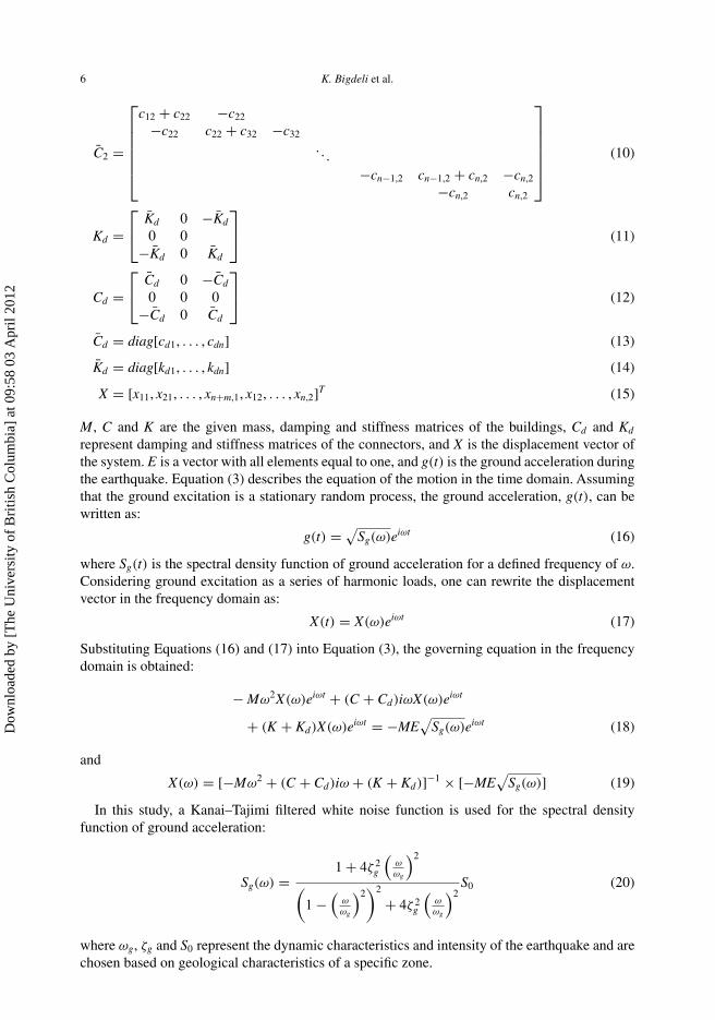
6 K. Bigdeli et al.

C2 =

⎡⎢⎢⎢⎢⎢⎣

c12 + c22 −c22

−c22 c22 + c32 −c32

. . .−cn−1,2 cn−1,2 + cn,2 −cn,2

−cn,2 cn,2

⎤⎥⎥⎥⎥⎥⎦

(10)

Kd =⎡⎣ Kd 0 −Kd

0 0−Kd 0 Kd

⎤⎦ (11)

Cd =⎡⎣ Cd 0 −Cd

0 0 0−Cd 0 Cd

⎤⎦ (12)

Cd = diag[cd1, . . . , cdn] (13)

Kd = diag[kd1, . . . , kdn] (14)

X = [x11, x21, . . . , xn+m,1, x12, . . . , xn,2]T (15)

M, C and K are the given mass, damping and stiffness matrices of the buildings, Cd and Kd

represent damping and stiffness matrices of the connectors, and X is the displacement vector ofthe system. E is a vector with all elements equal to one, and g(t) is the ground acceleration duringthe earthquake. Equation (3) describes the equation of the motion in the time domain. Assumingthat the ground excitation is a stationary random process, the ground acceleration, g(t), can bewritten as:

g(t) = √Sg(ω)eiωt (16)

where Sg(t) is the spectral density function of ground acceleration for a defined frequency of ω.Considering ground excitation as a series of harmonic loads, one can rewrite the displacementvector in the frequency domain as:

X(t) = X(ω)eiωt (17)

Substituting Equations (16) and (17) into Equation (3), the governing equation in the frequencydomain is obtained:

− Mω2X(ω)eiωt + (C + Cd)iωX(ω)eiωt

+ (K + Kd)X(ω)eiωt = −ME√

Sg(ω)eiωt (18)

and

X(ω) = [−Mω2 + (C + Cd)iω + (K + Kd)]−1 × [−ME√

Sg(ω)] (19)

In this study, a Kanai–Tajimi filtered white noise function is used for the spectral densityfunction of ground acceleration:

Sg(ω) =1 + 4ζ 2

g

(ωωg

)2

(1 −

(ωωg

)2)2

+ 4ζ 2g

(ωωg

)2S0 (20)

where ωg, ζg and S0 represent the dynamic characteristics and intensity of the earthquake and arechosen based on geological characteristics of a specific zone.

Dow

nloa

ded

by [

The

Uni

vers

ity o

f B

ritis

h C

olum

bia]

at 0

9:58

03

Apr

il 20

12

Engineering Optimization 7

Having developed a formula for Sg, it is now possible to numerically approximate σxib. To dothis, upper and lower limits of ±20 rad/s are imposed. Using a trapezoid rule approximation witha step size of 0.02 to the integral in Equation (2), one can easily calculate the standard deviationof the response. It is worth noting that previous studies show that the effect of the frequenciesgreater than 20 rad/s on the response of the structure is negligible (Xu et al. 1999a, Xu andZhang 2002).

2.4. Mechanical properties of dampers

It is clear that the standard deviation of displacement (σxib) for a set of dampers is highly dependenton the mechanical properties of the damper connectors, since the damping and stiffness matricesof the connectors in Equation (3), Cd and Kd , are dependent on cdi and kdi (Equations 3 and11–14). Therefore, to determine the optimal effect of a given damper arrangement, it is necessaryto determine the optimal damping and stiffness coefficients. Moreover, the optimal damping andstiffness coefficients for a set of dampers are dependent on both the number of dampers used andthe damper placement. Therefore, for each damper arrangement considered, the algorithm mustoptimize the damping and stiffness coefficients.

Results from Xu et al. (1999a) and Zhang and Xu (1999) show that the stiffness of the connectorsdoes not change the objective function significantly as long as values of cdi are optimal and kdi aresmall. Moreover, the value of σxib will increase if kdi has a very large value, i.e. rigid connectors.Thus, it is assumed that kdi = 0 for all d and i. This simplifies the problem, but the final resultwill remain accurate.

Furthermore, results from Xu et al. (1999a), Zhang and Xu (1999, 2000), Zhu et al. (2010),Yang and Lu (2003) and Luco and De Barros (1998) argue that it is reasonable to assume that alldamping coefficients are equal. Therefore, it is assumed that

cd1 = cd2 = . . . = cdn. (21)

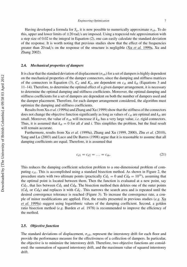
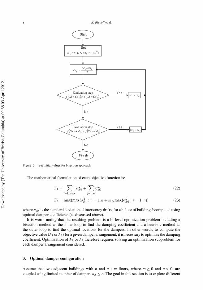
This reduces the damping coefficient selection problem to a one-dimensional problem of com-puting cd1. This is accomplished using a standard bisection method. As shown in Figure 2, theprocedure starts with two ultimate points (practically CdL = 0 and CdR = 1016), assuming thatthe optimal point is located between them. Then the function is evaluated at a new point, sayCdC , that lies between CdL and CdR. The bisection method then deletes one of the outer points(CdL or CdR) and replaces it with CdC . This narrows the search area and is repeated until thedesired convergence tolerance is reached (Figure 3). To increase the convergence rate, a cou-ple of minor modifications are applied. First, the results presented in previous studies (e.g. Xuet al. 1999a) suggest using logarithmic values of the damping coefficient. Second, a goldenratio bisection method (e.g. Burden et al. 1978) is recommended to improve the efficiency ofthe method.

2.5. Objective function

The standard deviations of displacement, σxib, represent the interstorey drift for each floor andprovide the performance measure for the effectiveness of a collection of dampers. In particular,the objective is to minimize the interstorey drift. Therefore, two objective functions are consid-ered: the summation of squared interstorey drift, and the maximum value of squared interstoreydrift.

Dow

nloa

ded

by [

The

Uni

vers

ity o

f B

ritis

h C

olum

bia]

at 0

9:58

03

Apr

il 20

12

8 K. Bigdeli et al.

Set

and 0=L

Cd )10(16

∞=R

Cd

2RL

C

CdCdCd

+=

Evaluation step( ) ( )RC CdCdfCdCdf =>= CL

CdCd =

No

No

Yes

Yes

Start

Finish

Evaluation step( ) ( )LC CdCdfCdCdf =>= CR

CdCd =

Figure 2. Set initial values for bisection approach.

The mathematical formulation of each objective function is:

F1 =∑

i=1..n+m

σ 2di1 +

∑j=1..n

σ 2dj2 (22)

F2 = max{max{σ 2di1 : i = 1..n + m}, max{σ 2

di2 : i = 1..n}} (23)

where σdib is the standard deviation of interstorey drifts, for ith floor of building b computed usingoptimal damper coefficients (as discussed above).

It is worth noting that the resulting problem is a bi-level optimization problem including abisection method as the inner loop to find the damping coefficient and a heuristic method asthe outer loop to find the optimal locations for the dampers. In other words, to compute theobjective value (F1 or F2) for a given damper arrangement, it is necessary to optimize the dampingcoefficient. Optimization of F1 or F2 therefore requires solving an optimization subproblem foreach damper arrangement considered.

3. Optimal damper configuration

Assume that two adjacent buildings with n and n + m floors, where m ≥ 0 and n > 0, arecoupled using limited number of dampers nd ≤ n. The goal in this section is to explore different

Dow

nloa

ded

by [

The

Uni

vers

ity o

f B

ritis

h C

olum

bia]

at 0

9:58

03

Apr

il 20

12

Engineering Optimization 9

Set k=0

Evaluation step

( ) ( )kC

kL CdCdfCdCdf =<= +1

k

C

k

R

k

L

k

L

k

L

k

C

CdCd

CdCd

CdCd

=

=

=

+

+

++

1

1

11

21

kC

kRk

R

CdCdCd

+=

+

Evaluation step

k

C

k

L

k

R

k

R

k

R

k

C

CdCd

CdCd

CdCd

=

=

=

+

+

++

1

1

11

k

C

k

CCdCd =

+1

No

No

Yes

Yes

tolCdCdk

R

k

Le<−

Yes

Start

1+= kk

Finish

No

⎟⎠⎞⎜⎝

⎛ ==

=

kcCdCdff

kcCdCdOptimumalSet initial values

(Figure2)

( ) ( )kC

kR CdCdfCdCdf =<= +1

21

kC

kRk

R

CdCdCd

+=

+

Figure 3. Optimal damping coefficient of dampers for a specific arrangement of dampers using bisection method.

methods of locating the optimal placement for these dampers. Five different optimal damperplacement techniques are considered: exhaustive search approach, inserting dampers, insertingfloors, maximum velocity locations, and a genetic algorithm. Each damper placement techniqueis explained below.

3.1. Exhaustive search approach

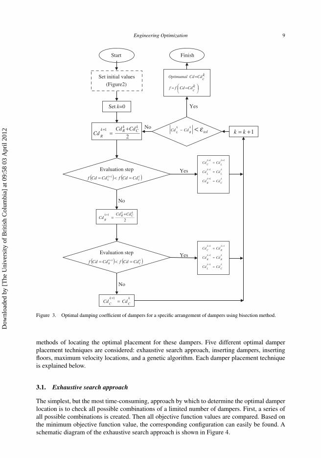
The simplest, but the most time-consuming, approach by which to determine the optimal damperlocation is to check all possible combinations of a limited number of dampers. First, a series ofall possible combinations is created. Then all objective function values are compared. Based onthe minimum objective function value, the corresponding configuration can easily be found. Aschematic diagram of the exhaustive search approach is shown in Figure 4.

Dow

nloa

ded

by [

The

Uni

vers

ity o

f B

ritis

h C

olum

bia]

at 0

9:58

03

Apr

il 20

12

10 K. Bigdeli et al.

Start

Get: Mechanical properties of two buildings, m, n and nd

i=1

Analyse based on optimal damping coefficient, and put

Obj(i)=Objective function value(Figure 3)

Preprocessing: determine all N

possible combinations, where N = ⎟⎟⎠

⎞⎜⎜⎝

⎛

dn

n

Ni <

i = i+1

End

Set configuration of dampers as ith

possible case

ii = , where

},...,2,1{

)()(

nj

jObjiObj

∈≤

Yes

Set configuration as ithpossible case

No

Figure 4. Flowchart for exhaustive search optimization approach.

Clearly, such an exhaustive search must return the global optimum. However, in this approach,the number of required simulations N1 is equal to the number of all combinations:

N1 =(

nnd

)= n!

(n − nd)!nd ! (24)

where n is the number of adjacent floors and nd is the number of available dampers.

3.2. Inserting dampers

Although the first method always results in the best possible solution to the problem, it can betime consuming when the number of possible combinations is large. For example, for the caseof two 40-storey buildings that are coupled using 10 dampers, the exhaustive search method willrequire about 8.5 × 108 simulations (approximately 250 years at 10 seconds per simulation).

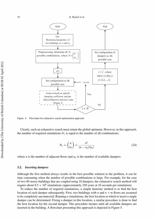
To reduce the number of required simulations, a simple heuristic method is to find the bestlocation of each damper subsequently. First, two buildings with n and n + m floors are assumedto be completely unconnected. Running n simulations, the best location at which to insert a singledamper can be determined. Fixing a damper in this location, a similar procedure is done to findthe best location for the second damper. This procedure iterates until all available dampers areinserted in the building. A flowchart presenting this approach is depicted in Figure 5.

Dow

nloa

ded

by [

The

Uni

vers

ity o

f B

ritis

h C

olum

bia]

at 0

9:58

03

Apr

il 20

12

Engineering Optimization 11

Start

Get:

Mechanical properties of two buildings, m, n and nd

i=1

Analyse based on optimal damping coefficient, and put

Obj(i)=Objective function value(Figure 3)

Remove recently added damper in ith floor

Initialize with 0=dn

(unconnected buildings)

ni <

i = i+1

End

Add a damper in ithfloor, and set

1+= dd nn

ii = , where

},...,2,1{

)()(

nj

jObjiObj

∈≤

Yes

Yes

No

Any damper already in ith floor?

Add a damper in ith floor

nnd <

NoObj(i) =∞

No

Yes

Figure 5. Flowchart for inserting dampers optimization approach.

The number of required simulations N2 can be calculated as:

N2 = n + (n − 1) + . . . + (n − (nd − 1))

= n nd + nd −(

n2d + nd

2

)(25)

where, as before, n is the number of adjacent floors and nd is the number of available dampers.

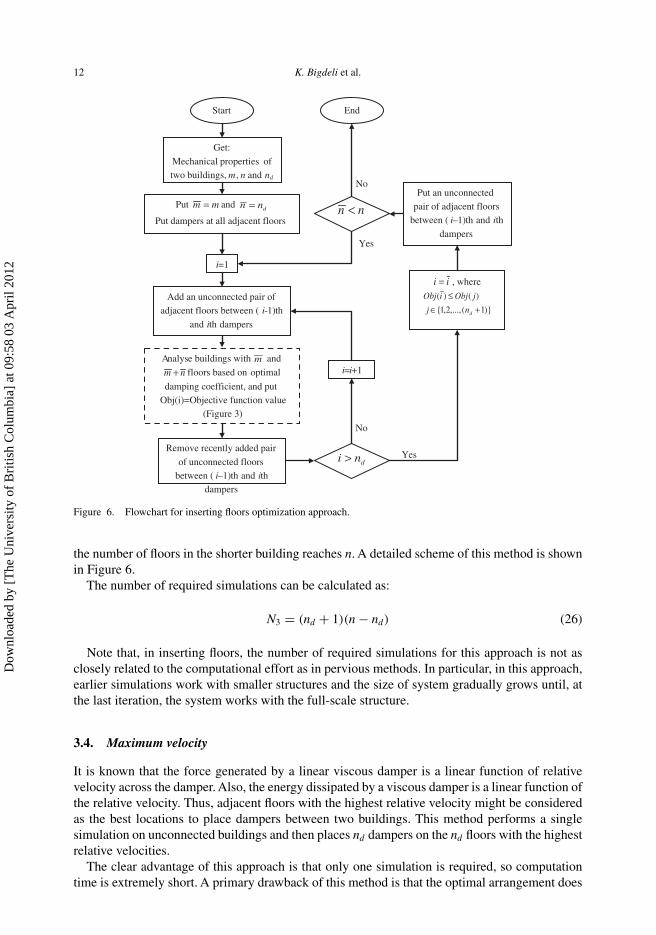
3.3. Inserting floors

This approach begins by reducing the number of adjacent floors (n) to the number of availabledampers (nd). Consequently, two buildings with nd and nd + m floors, which are connected onall adjacent floors, are constructed. Next, the algorithm locates the best place to insert a pair ofadjacent floors without dampers and keep the objective function as low as possible. After insertingthe first pair, two adjacent buildings with nd + 1 and nd + 1 + m floors, which are connected inonly nd floors, have been constructed. An analogous procedure is carried out to find the bestlocation for a second pair of unconnected adjacent floors. This iterative procedure continues until

Dow

nloa

ded

by [

The

Uni

vers

ity o

f B

ritis

h C

olum

bia]

at 0

9:58

03

Apr

il 20

12

12 K. Bigdeli et al.

Start

Get:

Mechanical properties of two buildings, m, n and nd

i=1

Add an unconnected pair of adjacent floors between ( i-1)th

and ith dampers

Analyse buildings with m and

nm + floors based on optimal

damping coefficient, and put Obj(i)=Objective function value

(Figure 3)

Remove recently added pair

of unconnected floors between ( i–1)th and ith

dampers

Put mm = and dnn =Put dampers at all adjacent floors

dni >

i=i+1

End

nn <Put an unconnected

pair of adjacent floors between ( i–1)th and ith

dampers

ii = , where

)}1(,...,2,1{

)()(

+∈≤

dnj

jObjiObj

Yes

Yes

No

No

Figure 6. Flowchart for inserting floors optimization approach.

the number of floors in the shorter building reaches n. A detailed scheme of this method is shownin Figure 6.

The number of required simulations can be calculated as:

N3 = (nd + 1)(n − nd) (26)

Note that, in inserting floors, the number of required simulations for this approach is not asclosely related to the computational effort as in pervious methods. In particular, in this approach,earlier simulations work with smaller structures and the size of system gradually grows until, atthe last iteration, the system works with the full-scale structure.

3.4. Maximum velocity

It is known that the force generated by a linear viscous damper is a linear function of relativevelocity across the damper. Also, the energy dissipated by a viscous damper is a linear function ofthe relative velocity. Thus, adjacent floors with the highest relative velocity might be consideredas the best locations to place dampers between two buildings. This method performs a singlesimulation on unconnected buildings and then places nd dampers on the nd floors with the highestrelative velocities.

The clear advantage of this approach is that only one simulation is required, so computationtime is extremely short. A primary drawback of this method is that the optimal arrangement does

Dow

nloa

ded

by [

The

Uni

vers

ity o

f B

ritis

h C

olum

bia]

at 0

9:58

03

Apr

il 20

12

Engineering Optimization 13

not depend on the objective function. In Section 4, it is shown that this method generally does notlead to a good arrangement.

3.5. Genetic algorithm

Genetic algorithms are known to be an effective approach to solve many engineering optimizationproblems (see Hadi andArfiadi 1998, Singh and Moreschi 2002,Alkhatib et al. 2004, Ok et al. 2008and references therein). Genetic algorithms are considered particularly useful when derivativeinformation is not available. In this study, an optimization approach based on a genetic algorithmis considered to find the best configuration of a limited number of dampers.

The implementation follows a standard ‘selection, competition, reproduction’ technique (Vose1999). The first step is to generate the initial population of points. This is done using a procedurethat picks random combinations of dampers, and it continues until the desired population, i.e. num-ber of points, is achieved. In accordance with a genetic algorithm, the next step is to evaluate theobjective function at all points of the current population. Then, using a competition, some pointssurvive and go to the next generation, while the others die. To make up for the dead points, areproduction procedure will generate enough new points. The algorithm uses the survivors asthe parents to reproduce children. Within the reproduction procedure, a mutation step randomlyalters some point from one generation to the next. Finally, the objective function is evaluated atall points of the new generation. The procedure repeats until the stopping condition is satisfied.

4. Numerical results

To illustrate the efficiency and accuracy of each method, various examples are studied. At the firststage, the time required for each presented method is examined. At the second stage, the qualityof the solutions obtained by each method is examined. Before discussing the results, the test setsused in this article are discussed.

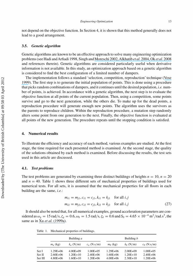
4.1. Test problems

The test problems are generated by examining three distinct buildings of heights n = 10, n = 20and n = 40. Table 1 shows three different sets of mechanical properties of buildings used fornumerical tests. For all sets, it is assumed that the mechanical properties for all floors in eachbuilding are the same, i.e.:

mi1 = mj1, ci1 = cj1, ki1 = kj1 for all i, j

mi2 = mj2, ci2 = cj2, ki2 = kj2 for all i, j (27)

It should also be noted that, for all numerical examples, ground acceleration parameters are con-sidered asωg = 15 rad/s, ζg = 0.6,ωk = 1.5 rad/s, ζk = 0.6 and S0 = 4.65 × 10−4 m2/rad.s3, thesame as in Xu et al. (1999a).

Table 1. Mechanical properties of buildings.

Building a Building b

ma (kg) ka (N/m) ca (N.s/m) mb (kg) kb (N/m) cb (N.s/m)

Set I 1.29E+06 4.00E+09 1.00E+05 1.29E+06 2.00E+09 1.00E+05Set II 2.60E+06 1.20E+10 2.40E+06 1.60E+06 1.20E+10 2.40E+06Set III 4.80E+06 1.60E+10 1.20E+06 4.00E+06 2.30E+10 1.20E+06

Dow

nloa

ded

by [

The

Uni

vers

ity o

f B

ritis

h C

olum

bia]

at 0

9:58

03

Apr

il 20

12

14 K. Bigdeli et al.

Table 2. Different sets for numerical tests.

fa fb Case

10 10 110 20 220 10 310 40 440 10 520 20 620 40 740 20 8

Table 2 tabulates the eight different building height relations considered in this research. Foreach case, the different building height are given in fa and fb (denoting the number of floors forbuildings a and b).

Considering the three sets of mechanical properties given in Table 1, this creates 24 adjacentbuilding scenarios. For each building scenario, four possible numbers of dampers are considered:one damper, 25% of floors having dampers, 50% of floors having dampers and 75% of floorshaving dampers (rounding up). More precisely,

• If the shorter building has 10 floors, then nd = 1, 3, 5 and 8.• If the shorter building has 20 floors, then nd = 1, 5, 10 and 15.

This yields 96 test problems. Solving each problem for objective function 1 and objective function2 gives a grand total of 192 numerical tests.

For each problem, an optimal damper placement is determined using the four techniques out-lined in Section 3. However, it should be noted that, owing to the problem size, the exhaustivesearch was only used on problems where the shorter building was 10 floors.

4.2. Solution time

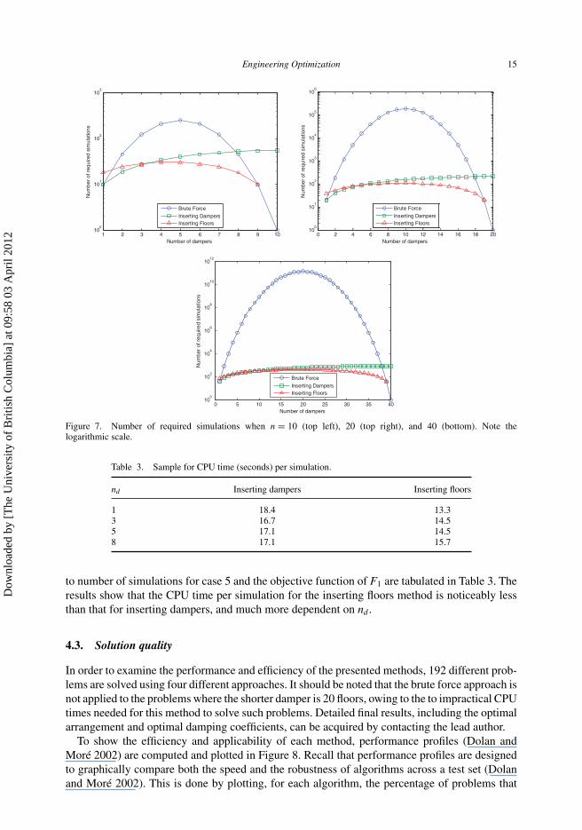
Clearly, the time taken to apply each method is highly dependent on the number of simula-tions required to complete the method. Applying Equations (24)–(26), the number of simulationsrequired for each method is computed. Figure 7 shows the number of required simulations versusthe number of available dampers. (Figure 7 does not plot the number of simulations required inthe maximum velocity method, as this number is always 1.)

The number of simulations required for the exhaustive search method is generally much higherthan for the other two methods. In many cases, it may be intractable to employ an exhaustivesearch to find the optimal configuration. For example, it is estimated that the time required for anexhaustive search to solve the problem of placing 20 dampers over 40 floors is about 40,000 years,while the inserting floors method can solve the same problem in less than 2 hours. Even with asupercomputer, say 100 times faster than common machines, the solution time of the exhaustivesearch method will be 400 years, which confirms the impracticability of this method. Note thatthe number of required simulations for a genetic algorithm is not a fixed value for each case, sincethis method is an evolutionary method that uses some random numbers to generate the final result.

However, it should be noted that the required CPU time associated with a method is not anexact formula of the number of simulations required. Since each simulation solves an optimizationsubproblem (computing damping coefficient), the convergence rate of this subproblem plays arole in the total CPU time. This is even more pronounced in the inserting floors method, as thismethod starts with a small model, which needs a shorter time to complete, and concludes with afull-sized model, which needs a longer time to complete. As an example, the ratios of CPU time

Dow

nloa

ded

by [

The

Uni

vers

ity o

f B

ritis

h C

olum

bia]

at 0

9:58

03

Apr

il 20

12

Engineering Optimization 15

1 2 3 4 5 6 7 8 9 1010

0

101

102

103

Number of dampers

Num

ber

of r

equi

red

sim

ulat

ions

Brute Force

Inserting DampersInserting Floors

0 2 4 6 8 10 12 14 16 18 2010

0

101

102

103

104

105

106

Number of dampers

Num

ber

of r

equi

red

sim

ulat

ions

Brute Force

Inserting DampersInserting Floors

0 5 10 15 20 25 30 35 4010

0

102

104

106

108

1010

1012

Number of dampers

Num

ber

of r

equi

red

sim

ulat

ions

Brute Force

Inserting DampersInserting Floors

Figure 7. Number of required simulations when n = 10 (top left), 20 (top right), and 40 (bottom). Note thelogarithmic scale.

Table 3. Sample for CPU time (seconds) per simulation.

nd Inserting dampers Inserting floors

1 18.4 13.33 16.7 14.55 17.1 14.58 17.1 15.7

to number of simulations for case 5 and the objective function of F1 are tabulated in Table 3. Theresults show that the CPU time per simulation for the inserting floors method is noticeably lessthan that for inserting dampers, and much more dependent on nd .

4.3. Solution quality

In order to examine the performance and efficiency of the presented methods, 192 different prob-lems are solved using four different approaches. It should be noted that the brute force approach isnot applied to the problems where the shorter damper is 20 floors, owing to the to impractical CPUtimes needed for this method to solve such problems. Detailed final results, including the optimalarrangement and optimal damping coefficients, can be acquired by contacting the lead author.

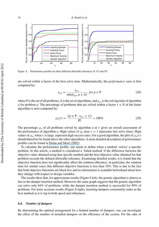
To show the efficiency and applicability of each method, performance profiles (Dolan andMoré 2002) are computed and plotted in Figure 8. Recall that performance profiles are designedto graphically compare both the speed and the robustness of algorithms across a test set (Dolanand Moré 2002). This is done by plotting, for each algorithm, the percentage of problems that

Dow

nloa

ded

by [

The

Uni

vers

ity o

f B

ritis

h C

olum

bia]

at 0

9:58

03

Apr

il 20

12

16 K. Bigdeli et al.

20 40 60 800

0.2

0.4

0.6

0.8

1P

()

for

max

imum

allo

wab

le to

lera

nce

of 5

%

Inserting Damper

Inserting Floors

Brute ForceMaximum Velocity

Genetic Algorithm

10 20 30 40 50 600

0.2

0.4

0.6

0.8

1

P(

) fo

r m

axim

um a

llow

able

tol

eran

ce o

f 1%

Inserting Damper

Inserting Floors

Brute ForceMaximum Velocity

Genetic Algorithm

τ

τ τ

τ

Figure 8. Performance profiles for three different allowable tolerances of 1% and 5%

are solved within a factor of the best solve time. Mathematically, the performance ratio is firstcomputed by:

rp,a = tp,a

min{tp,a, a ∈ A} , for p ∈ P (28)

where P is the set of all problems,A is the set of algorithms, and tp,a is the solving time of algorithma for problem p. The percentage of problems that are solved within a factor τ ∈ � of the fasteralgorithm is next computed by:

ρa(τ ) = |{p ∈ P : rp,a ≤ τ }||P| × 100% (29)

The percentage ρa of all problems solved by algorithm a at τ gives an overall assessment ofthe performance of algorithm a. High values of ρa near τ = 1 represents fast solve times. Highvalues of ρa, when τ is large, represent high success rates. For a good algorithm, the plot of ρa(τ )

should therefore be found above the other algorithms. A more detailed description of performanceprofiles can be found in Dolan and Moré (2002).

To calculate the performance profile, one needs to define when a method ‘solves’ a specificproblem. In this article, a method is considered a ‘failed method’ if the difference between theobjective value obtained using that specific method and the best objective value obtained for thatproblem exceeds the defined allowable tolerance. Examining detailed results, it is found that theobjective function does not significantly affect the solution efficiency; in particular, the solutiontime for similar cases (but different objective function) is less than 10%. This is due to the factthat both objective functions are black box and no information is available beforehand about howthey change with respect to design variables.

The results show that, for approximate results (Figure 8 left), the genetic algorithm is almost asfast as the damper insertion method. However, the same graph suggests that the genetic algorithmcan solve only 84% of problems, while the damper insertion method is successful for 99% ofproblems. For more accurate results (Figure 8 right), inserting dampers consistently ranks as thebest method as it is top in both speed and robustness.

4.4. Number of dampers

By determining the optimal arrangement for a limited number of dampers, one can investigatethe effect of the number of installed dampers on the efficiency of the system. For the sake of

Dow

nloa

ded

by [

The

Uni

vers

ity o

f B

ritis

h C

olum

bia]

at 0

9:58

03

Apr

il 20

12

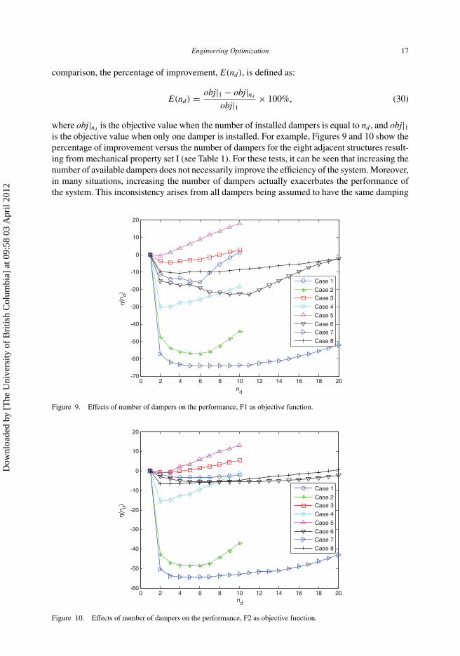
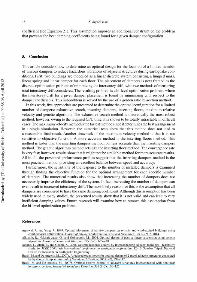
Engineering Optimization 17

comparison, the percentage of improvement, E(nd), is defined as:

E(nd) = obj|1 − obj|nd

obj|1 × 100%, (30)

where obj|nd is the objective value when the number of installed dampers is equal to nd , and obj|1is the objective value when only one damper is installed. For example, Figures 9 and 10 show thepercentage of improvement versus the number of dampers for the eight adjacent structures result-ing from mechanical property set I (see Table 1). For these tests, it can be seen that increasing thenumber of available dampers does not necessarily improve the efficiency of the system. Moreover,in many situations, increasing the number of dampers actually exacerbates the performance ofthe system. This inconsistency arises from all dampers being assumed to have the same damping

0 2 4 6 8 10 12 14 16 18 20-70

-60

-50

-40

-30

-20

-10

0

10

20

nd

(nd)

Case 1

Case 2Case 3

Case 4

Case 5

Case 6Case 7

Case 8

η

Figure 9. Effects of number of dampers on the performance, F1 as objective function.

0 2 4 6 8 10 12 14 16 18 20-60

-50

-40

-30

-20

-10

0

10

20

nd

(nd)

Case 1

Case 2Case 3

Case 4

Case 5

Case 6Case 7

Case 8

η

Figure 10. Effects of number of dampers on the performance, F2 as objective function.

Dow

nloa

ded

by [

The

Uni

vers

ity o

f B

ritis

h C

olum

bia]

at 0

9:58

03

Apr

il 20

12

18 K. Bigdeli et al.

coefficient (see Equation 21). This assumption imposes an additional constraint on the problemthat prevents the best damping coefficients being found for a given damper configuration.

5. Conclusion

This article considers how to determine an optimal design for the location of a limited numberof viscous dampers to reduce hazardous vibrations of adjacent structures during earthquake con-ditions. First, two buildings are modelled as a linear discrete system consisting a lumped mass,linear spring and linear damper for each floor. The placement of dampers is next framed as thediscrete optimization problem of minimizing the interstorey drift, with two methods of measuringtotal interstorey drift considered. The resulting problem is a bi-level optimization problem, wherethe interstorey drift for a given damper placement is found by minimizing with respect to thedamper coefficients. This subproblem is solved by the use of a golden ratio bi-section method.

In this work, five approaches are presented to determine the optimal configuration for a limitednumber of dampers: exhaustive search, inserting dampers, inserting floors, maximum relativevelocity and genetic algorithm. The exhaustive search method is theoretically the most robustmethod; however, owing to the required CPU time, it is shown to be totally intractable in difficultcases.The maximum velocity method is the fastest method since it determines the best arrangementin a single simulation. However, the numerical tests show that this method does not lead toa reasonable final result. Another drawback of the maximum velocity method is that it is notsensitive to objective function. A more accurate method is the inserting floors method. Thismethod is faster than the inserting dampers method, but less accurate than the inserting dampersmethod. The genetic algorithm method acts like the inserting floor method. The convergence rateis very fast; however, results show that it might not be a reliable method for more accurate results.All in all, the presented performance profiles suggest that the inserting dampers method is themost practical method, providing an excellent balance between speed and accuracy.

Furthermore, the sensitivity of the response to the number of installed dampers is examinedthrough finding the objective function for the optimal arrangement for each specific numberof dampers. The numerical results also show that increasing the number of dampers does notnecessarily improve the efficiency of the system. In fact, increasing the number of dampers caneven result in increased interstorey drift. The most likely reason for this is the assumption that alldampers are considered to have the same damping coefficient. Although this assumption has beenwidely used in many studies, the presented results show that it is not valid and can lead to veryinefficient damping values. Future research will examine how to remove this assumption fromthe bi-level optimization problem.

References

Agrawal, A. and Yang, J., 1999. Optimal placement of passive dampers on seismic and wind-excited buildings usingcombinatorial optimization. Journal of Intelligent Material Systems and Structures, 10 (12), 997–1014.

Alkhatib, R., Nakhaie Jazar, G., and Golnaraghi, M., 2004. Optimal design of passive linear suspension using geneticalgorithm. Journal of Sound and Vibration, 275 (3–5), 665–691.

Azuma, Y., Otani, S., and Ohami, K., 2006. Seismic response control by interconnecting adjacent buildings—feasibilitystudy. In: ICEE 2006: 4th international conference on earthquake engineering, 12–13 October Taipei. NationalCenter for Research on Earthquake Engineering.

Basili, M. and De Angelis, M., 2007a. A reduced order model for optimal design of 2-mdof adjacent structures connectedby hysteretic dampers. Journal of Sound and Vibration, 306 (1–2), 297–317.

Basili, M. and De Angelis, M., 2007b. Optimal passive control of adjacent structures interconnected with nonlinearhysteretic devices. Journal of Sound and Vibration, 301 (1–2), 106–125.

Dow

nloa

ded

by [

The

Uni

vers

ity o

f B

ritis

h C

olum

bia]

at 0

9:58

03

Apr

il 20

12

Engineering Optimization 19

Bharti, S. and Shrimali, M., 2007. Seismic performance of connected building with MR dampers. In: Proceedings of the8th Pacific conference on earthquake engineering, 3–5 December Singapore: Nangyang Technological University,1–12.

Bharti, S., Dumne, S., and Shrimali, M., 2010. Seismic response analysis of adjacent buildings connected with MRdampers. Engineering Structures, 32 (8), 2122–2133.

Bhaskararao, A. and Jangid, R., 2006a. Seismic analysis of structures connected with friction dampers. EngineeringStructures, 28 (5), 690–703.

Bhaskararao, A. and Jangid, R., 2006b. Seismic response of adjacent buildings connected with friction dampers. Bulletinof Earthquake Engineering, 4 (1), 43–64.

Burden, R.L., Faires, J.D., and Reynolds, A.C., 1978. Numerical analysis. Boston, MA: Prindle, Weber and Schmidt.Dolan, E.D. and Moré, J.J., 2002. Benchmarking optimization software with performance profiles. Mathematical

Programming, 91 (2), 201–213.Hadi, M. and Arfiadi, Y., 1998. Optimum design of absorber for MDOF structures. Journal of Structural Engineering,

124 (11), 1272–1280.Luco, J. and De Barros, F., 1998. Optimal damping between two adjacent elastic structures. Earthquake Engineering and

Structural Dynamics, 27 (7), 649–659.Mezyk, A., 2002. The use of optimization procedures in tuning vibration dampers. Engineering Optimization, 34 (5),

503–521.Ng, C. and Xu, Y., 2006. Seismic response control of a building complex utilizing passive friction damper: experimental

investigation. Earthquake Engineering and Structural Dynamics, 35 (6), 657–677.Ok, S., Song, J., and Park, K., 2008. Optimal design of hysteretic dampers connecting adjacent structures using multi-

objective genetic algorithm and stochastic linearization method. Engineering Structures, 30 (5), 1240–1249.Patel, C. and Jangid, R., 2010. Seismic response of dynamically similar adjacent structures connected with viscous

dampers. IES Journal Part A: Civil and Structural Engineering, 3 (1), 1–13.Qu, W. and Xu, Y., 2001. Semi-active control of seismic response of tall buildings with podium structure using ER/MR

dampers. Structural Design of Tall Buildings, 10 (3), 179–192.Singh, M.P. and Moreschi, L.M., 2002. Optimal placement of dampers for passive response control. Earthquake

Engineering and Structural Dynamics, 31 (4), 955–976.Tesfamariam, S. and Saatcioglu, M., 2010. Seismic vulnerability assessment of reinforced concrete buildings using

hierarchical fuzzy rule base modeling. Earthquake Spectra, 26 (1), 235–256.Viswamurthy, S.R. and Ganguli, R., 2007. Optimal placement of trailing-edge flaps for helicopter vibration reduction

using response surface methods. Engineering Optimization, 39 (2), 185–202.Vose, M.D., 1999. The simple genetic algorithm: foundations and theory (complex adaptive systems). Cambridge, MA:

MIT Press.Xu,Y. and Zhang, W., 2002. Closed-form solution for seismic response of adjacent buildings with linear quadratic Gaussian

controllers. Earthquake Engineering and Structural Dynamics, 31 (2), 235–259.Xu,Y., He, Q., and Ko, J., 1999a. Dynamic response of damper-connected adjacent buildings under earthquake excitation.

Engineering Structures, 21 (2), 135–148.Xu,Y., et al., 1999b. Experimental investigation of adjacent buildings connected by fluid damper. Earthquake Engineering

and Structural Dynamics, 28 (6), 609–631.Yang, Z. and Lu, X., 2003. Experimental seismic study of adjacent buildings with fluid dampers. Journal of Structural

Engineering, 129 (2), 197.Ying, Z., Ni, Y., and Ko, J., 2003. Stochastic optimal coupling-control of adjacent building structures. Computers and

Structures, 81 (30–31), 2775–2787.Zhang, W. and Xu, Y., 1999. Dynamic characteristics and seismic response of adjacent buildings linked by discrete

dampers. Earthquake Engineering and Structural Dynamics, 28 (10), 1163–1185.Zhang, W. and Xu,Y., 2000. Vibration analysis of two buildings linked by Maxwell model-defined fluid dampers. Journal

of Sound and Vibration, 233 (5), 775–796.Zhu, H. and Xu, Y., 2005. Optimum parameters of Maxwell model-defined dampers used to link adjacent structures.

Journal of Sound and Vibration, 279 (1–2), 253–274.Zhu, H., Ge, D., and Huang, X., 2010. Optimum connecting dampers to reduce the seismic responses of parallel structures.

Journal of Sound and Vibration, 330 (9), 1931–1949.

Dow

nloa

ded

by [

The

Uni

vers

ity o

f B

ritis

h C

olum

bia]

at 0

9:58

03

Apr

il 20

12