on the systemic nature of weather risk

On the Systemic Nature of Weather Risk

Guenther Filler* Martin Odening* Ostap Okhrin*

Wei Xu*

SFB 649 Discussion Paper 2009-002

SFB

6

4 9

E

C O

N O

M I

C

R

I S

K

B

E R

L I

N

*Humboldt-Universität zu Berlin, Germany

This research was supported by the Deutsche Forschungsgemeinschaft through the SFB 649 "Economic Risk".

http://sfb649.wiwi.hu-berlin.de

ISSN 1860-5664

SFB 649, Humboldt-Universität zu Berlin Spandauer Straße 1, D-10178 Berlin

On the Systemic Nature of Weather Risk

Wei Xu, Guenther Filler, Martin Odening1

Department of Agricultural Economics and Social Sciences,Humboldt-Universitat zu Berlin, D-10099 Berlin, Germany

Ostap Okhrin

Institute for Statistics and Econometrics, CASE - Center for Applied Statistics and Economics,Humboldt-Universitat zu Berlin, D-10099 Berlin, Germany

Abstract: Systemic weather risk is a major obstacle for the formation of private (non-subsidized) crop insurance. This paper explores the possibility of spatial diversification ofinsurance by estimating the joint occurrence of unfavorable weather conditions in differentlocations. For that purpose copula methods are employed that allow an adequate descrip-tion of stochastic dependencies between multivariate random variables. The estimationprocedure is applied to weather data in Germany. Our results indicate that indemnitypayments based on temperature as well as on cumulative rainfall show strong stochasticdependence even at a national scale. Thus the possibility to reduce risk exposure byincreasing the trading area of the insurance is limited. Irrespective of their economicimplications our results pinpoint the necessity of a proper statistical modeling of the de-pendence structure of multivariate random variables. The usual approach of measuringstochastic dependence with linear correlation coefficients turned out to be questionable inthe context of weather insurance as it may overestimate diversification effects considerably.

Keywords: weather risk, crop insurance, copulaJEL Classification: C14, Q19

1Address of correspondence to Martin Odening: Department of Agricultural Economics and SocialSciences, Philippstraße 13, D-10115 Berlin, Phone: +49(0)30 2093 6487, Fax: +49(0)30 2093 6465,Email: [email protected] This work was supported by Deutsche Forschungsgemeinschaftthrough the SFB 649 ”Economic Risk”. We wish to thank members of the SFB for helpful comments onan earlier version of this paper.

1 Introduction

Insurance of weather related production risks is a challenge for agricultural insurers. Awell known precondition of insurability is that individual risks are independent or if thecovariance among risks is small. This requirement rules out covariate or systemic risk.While such an assumption holds for some types of weather hazards, as for example haildamages, it does not for other types, at least at a regional level. Drought risk is a strikingexample for a peril that affects most if not all farmers in a whole region. Miranda andGlauber (1997) argue that the existence of systemic weather risk constitutes the mainreason for the failure of private crop insurance markets unless efficient and affordableinstruments for transferring this risk are available. This conjecture is based on the obser-vation that existing crop insurance programs including drought risk are either subsidized(e.g. United States or Canada) or have negligible participation rates (as in Germany).However, there several possible instruments that allow handling of systemic risks, amongthem reinsurance or weather derivatives (Xu, Odening and Musshoff 2008). Alternatively,an insurance company may try to spatially diversify systemic weather risk by increasing itstrading area. In order to identify appropriate measures for coping with systemic weatherrisk, it is necessary to quantify these risks. Clearly, the systemic nature of weather riskdepends on the scale that one considers. At locations within a country or a state weatherevents like drought are highly correlated whereas these dependencies vanish at a nationalor global level. Thus the question arises how the dependence structure of weather eventschanges as a function of space and distance. The relationship between weather events atdifferent locations is not only relevant when calculating joint losses from the viewpointof the insurer. It is also crucial for the hedging effectiveness of weather derivatives thatinsurance companies may wish to sell to farmers. It has been frequently stressed in theliterature that the hedging effectiveness of weather derivatives is eroded by geographicalbasis risk (e.g. Woodard and Garcia 2008).

In view of the relevance of spatial dependence of weather events for insurance issues itis not surprising that many attempts for a quantification have been made. The usualapproach is based on simple correlation coefficients between weather variables or indiceswhich are measured at different locations (weather stations). With these correlationcoefficients at hand de-correlation functions can be easily estimated, depicting correlationof weather variables as a function of the distance between weather stations. Examples ofthis kind of approach can be found in Woodard and Garcia (2008) or in Odening, Musshoffand Xu (2007). Goodwin (2001) applies the same technique to US yield data. Wang andZhang (2003) also address the spatial characteristics of crop insurance. Using the conceptof finite range positive dependence of spatial variables they calculate the effectiveness ofrisk pooling for cropping areas in the US. Their results are likewise based on correlationsdepending on lag distances.

The use of linear correlation of risks is computationally appealing but has some well-known pitfalls (cf. McNeil, Frey and Embrechts 2005). First of all, linear correlationcannot capture nonlinear dependence. Moreover, linear correlation in general does notcontain all relevant information on the dependency structure of risks. That means, jointdistributions with the same correlation coefficient may show a different behavior, partic-ularly in their tails. This in turn may lead to an underestimation or overestimation of thelikelihood of extreme insurance losses. An exception is the multivariate normal distribu-tion where knowledge of the marginal distributions and the correlation matrix uniquelydetermines the joint distribution. However, there is much empirical evidence that weather

1

indices as well as yield distributions are not normally distributed (e.g., Odening, Musshoffand Xu 2007, Goodwin and Ker 2002). The direct modeling and estimation of joint dis-tributions of weather variables is in theory a response to the aforementioned problems,but it is practically affected by the shortness of available data series. Empirical datahave to provide information on both the marginal distribution of weather indices and thedependence structure between them. A compromise between the restrictive applicationof linear correlations and the estimation of multivariate distributions is the use of copulas(Joe 1997, Nelsen 2006). Copulas avoid the direct estimation of multivariate distributionsbut allow for much greater flexibility in modeling the dependence structure compared tosimple correlation coefficients. The basic idea of a copula function is to link marginaldistributions together to a joint distribution (Sklar 1959). An advantage of copulas isthat they can be determined independently from the marginal distributions of the riskvariables using either parametric or nonparametric estimation procedures. Copulas be-came increasingly popular in the last years and have been applied to various problems infinance (c.f. Embrechts, McNeil and Straumann 1999, Cherubini, Luciano and Vecchiato2004). Applications in agricultural economics, however, are rare. Vedenov (2008) ana-lyzes the relationship between individual farm yields and area yields and Zhu, Ghosh andGoodwin (2008) investigate the dependence of prices and yields in the context of revenueinsurance. To the knowledge of the authors copulas have not been used for the estimationof spatial dependence of weather events so far.

The objective of this paper is to model and to estimate the losses of a weather relatedinsurance at different regional levels and different aggregation levels. We assume thatindemnity payments directly or indirectly depend on weather indices measured at severallocations. The underlying question is to what extent weather risks exposures at differentplaces can be diversified by increasing the selling area of the contracts. We are particularlyinterested in the tail behavior of the joint loss distribution as the probability of largelosses is crucial for the required buffer fund of the insurer and the premium loading abovethe expected payoff and thus for the viability of an index-based crop insurance. Forthat purpose the probability distribution of the joint losses is estimated using copulas.Once the copula function and the marginal distributions of the weather indices havebeen determined the value-at-risk (VaR) of the insurers total losses can be calculated bymeans of stochastic simulation. By comparing results of different copula types with thosefrom simple correlations we contribute to the discussion of an appropriate modeling ofstatistical dependencies in the context of weather insurance.

The remainder of the paper is organized as follows. Section 2 briefly reviews some basicproperties of copula functions and explains their specification and estimation. Next, wedescribe the use of copulas in the particular context of simulating weather-dependentinsurance losses. In section 3 this procedure is then applied to weather data in Germany.The results are presented in section 4. The paper ends with a discussion of the viabilityof crop insurance in Germany and some conclusions on the usefulness of the copula-basedmeasurement of dependent risks.

2

2 Measuring spatial weather dependence

with copulae

2.1 Identification and estimation of copulae

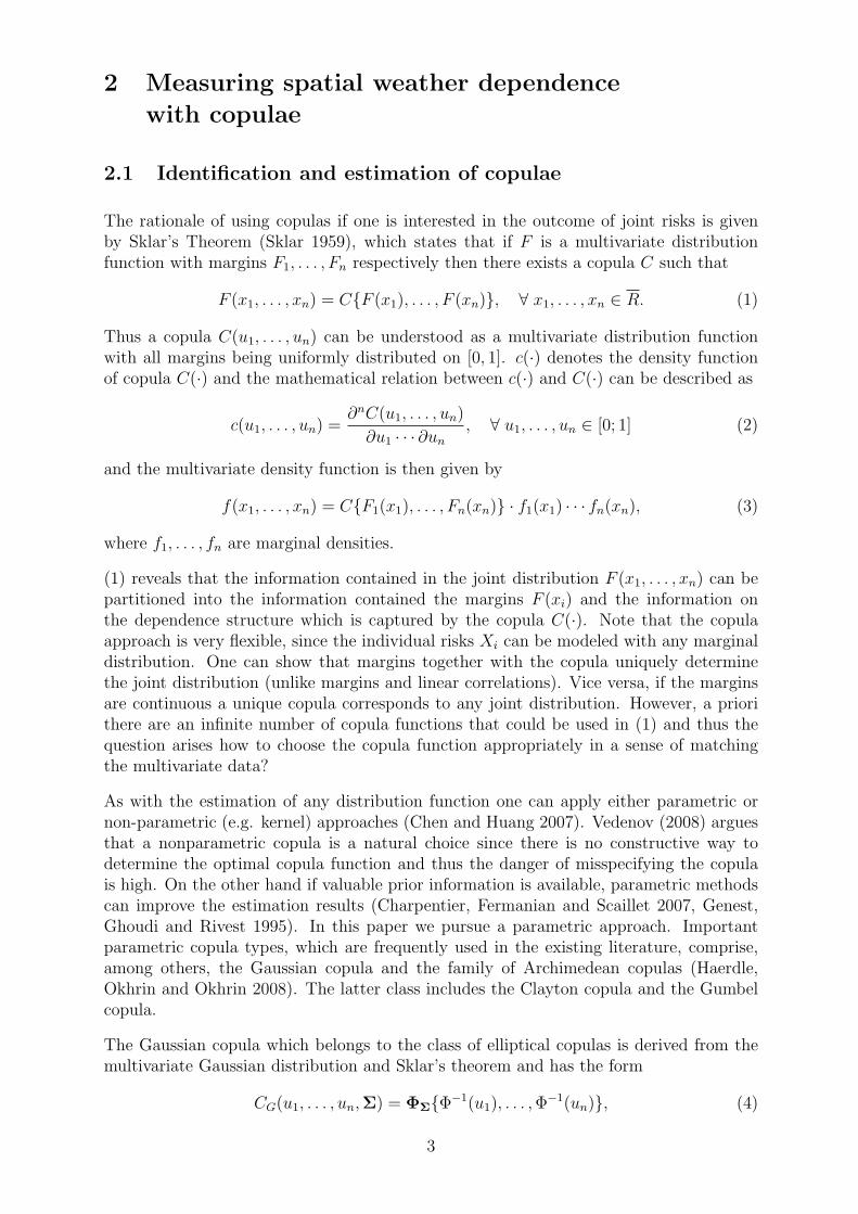
The rationale of using copulas if one is interested in the outcome of joint risks is givenby Sklar’s Theorem (Sklar 1959), which states that if F is a multivariate distributionfunction with margins F1, . . . , Fn respectively then there exists a copula C such that

F (x1, . . . , xn) = C{F (x1), . . . , F (xn)}, ∀ x1, . . . , xn ∈ R. (1)

Thus a copula C(u1, . . . , un) can be understood as a multivariate distribution functionwith all margins being uniformly distributed on [0, 1]. c(·) denotes the density functionof copula C(·) and the mathematical relation between c(·) and C(·) can be described as

c(u1, . . . , un) =∂nC(u1, . . . , un)

∂u1 · · · ∂un, ∀ u1, . . . , un ∈ [0; 1] (2)

and the multivariate density function is then given by

f(x1, . . . , xn) = C{F1(x1), . . . , Fn(xn)} · f1(x1) · · · fn(xn), (3)

where f1, . . . , fn are marginal densities.

(1) reveals that the information contained in the joint distribution F (x1, . . . , xn) can bepartitioned into the information contained the margins F (xi) and the information onthe dependence structure which is captured by the copula C(·). Note that the copulaapproach is very flexible, since the individual risks Xi can be modeled with any marginaldistribution. One can show that margins together with the copula uniquely determinethe joint distribution (unlike margins and linear correlations). Vice versa, if the marginsare continuous a unique copula corresponds to any joint distribution. However, a priorithere are an infinite number of copula functions that could be used in (1) and thus thequestion arises how to choose the copula function appropriately in a sense of matchingthe multivariate data?

As with the estimation of any distribution function one can apply either parametric ornon-parametric (e.g. kernel) approaches (Chen and Huang 2007). Vedenov (2008) arguesthat a nonparametric copula is a natural choice since there is no constructive way todetermine the optimal copula function and thus the danger of misspecifying the copulais high. On the other hand if valuable prior information is available, parametric methodscan improve the estimation results (Charpentier, Fermanian and Scaillet 2007, Genest,Ghoudi and Rivest 1995). In this paper we pursue a parametric approach. Importantparametric copula types, which are frequently used in the existing literature, comprise,among others, the Gaussian copula and the family of Archimedean copulas (Haerdle,Okhrin and Okhrin 2008). The latter class includes the Clayton copula and the Gumbelcopula.

The Gaussian copula which belongs to the class of elliptical copulas is derived from themultivariate Gaussian distribution and Sklar’s theorem and has the form

CG(u1, . . . , un,Σ) = ΦΣ{Φ−1(u1), . . . ,Φ−1(un)}, (4)

3

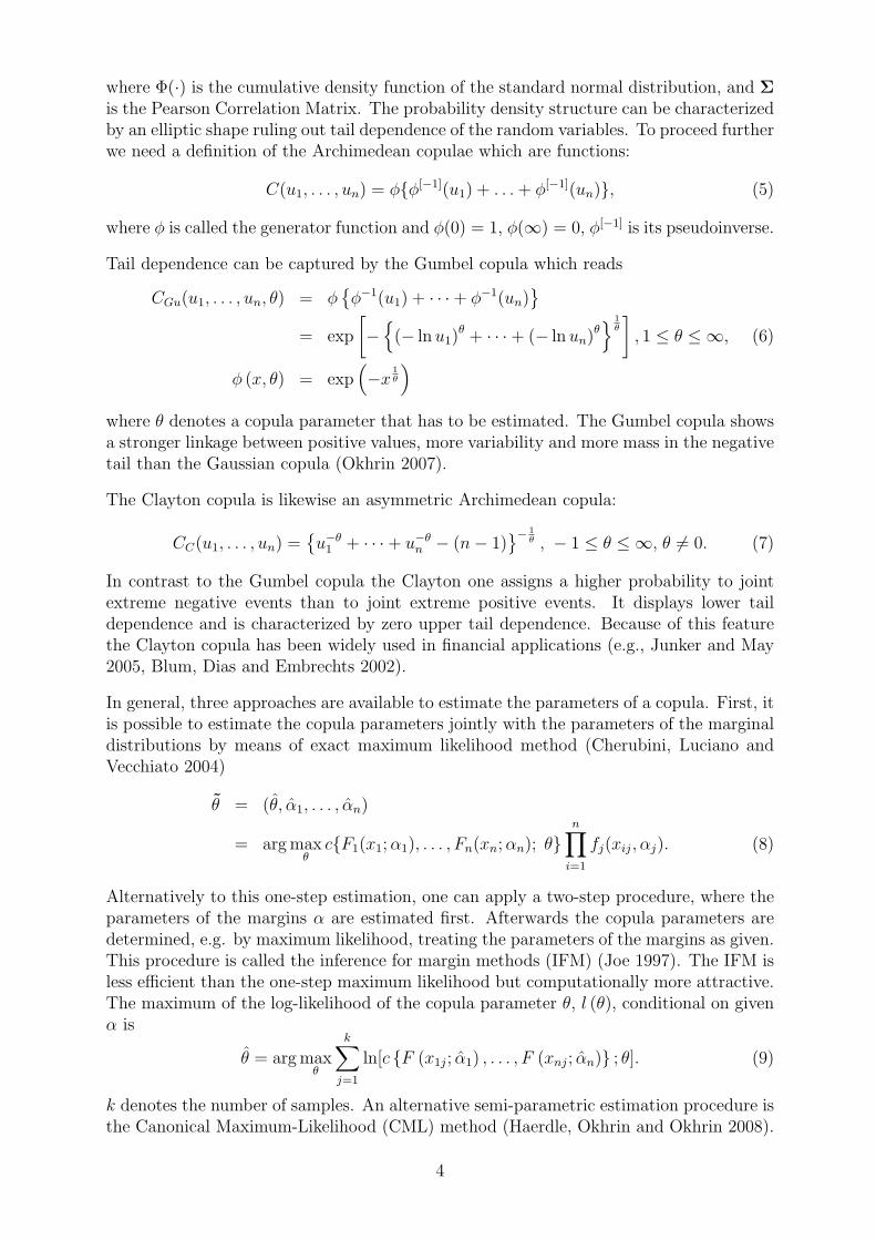
where Φ(·) is the cumulative density function of the standard normal distribution, and Σis the Pearson Correlation Matrix. The probability density structure can be characterizedby an elliptic shape ruling out tail dependence of the random variables. To proceed furtherwe need a definition of the Archimedean copulae which are functions:

C(u1, . . . , un) = φ{φ[−1](u1) + . . .+ φ[−1](un)}, (5)

where φ is called the generator function and φ(0) = 1, φ(∞) = 0, φ[−1] is its pseudoinverse.

Tail dependence can be captured by the Gumbel copula which reads

CGu(u1, . . . , un, θ) = φ{φ−1(u1) + · · ·+ φ−1(un)

}= exp

[−{

(− lnu1)θ + · · ·+ (− lnun)θ

} 1θ

], 1 ≤ θ ≤ ∞, (6)

φ (x, θ) = exp(−x

1θ

)where θ denotes a copula parameter that has to be estimated. The Gumbel copula showsa stronger linkage between positive values, more variability and more mass in the negativetail than the Gaussian copula (Okhrin 2007).

The Clayton copula is likewise an asymmetric Archimedean copula:

CC(u1, . . . , un) ={u−θ1 + · · ·+ u−θn − (n− 1)

}− 1θ , − 1 ≤ θ ≤ ∞, θ 6= 0. (7)

In contrast to the Gumbel copula the Clayton one assigns a higher probability to jointextreme negative events than to joint extreme positive events. It displays lower taildependence and is characterized by zero upper tail dependence. Because of this featurethe Clayton copula has been widely used in financial applications (e.g., Junker and May2005, Blum, Dias and Embrechts 2002).

In general, three approaches are available to estimate the parameters of a copula. First, itis possible to estimate the copula parameters jointly with the parameters of the marginaldistributions by means of exact maximum likelihood method (Cherubini, Luciano andVecchiato 2004)

θ = (θ, α1, . . . , αn)

= arg maxθc{F1(x1;α1), . . . , Fn(xn;αn); θ}

n∏i=1

fj(xij, αj). (8)

Alternatively to this one-step estimation, one can apply a two-step procedure, where theparameters of the margins α are estimated first. Afterwards the copula parameters aredetermined, e.g. by maximum likelihood, treating the parameters of the margins as given.This procedure is called the inference for margin methods (IFM) (Joe 1997). The IFM isless efficient than the one-step maximum likelihood but computationally more attractive.The maximum of the log-likelihood of the copula parameter θ, l (θ), conditional on givenα is

θ = arg maxθ

k∑j=1

ln[c {F (x1j; α1) , . . . , F (xnj; αn)} ; θ]. (9)

k denotes the number of samples. An alternative semi-parametric estimation procedure isthe Canonical Maximum-Likelihood (CML) method (Haerdle, Okhrin and Okhrin 2008).

4

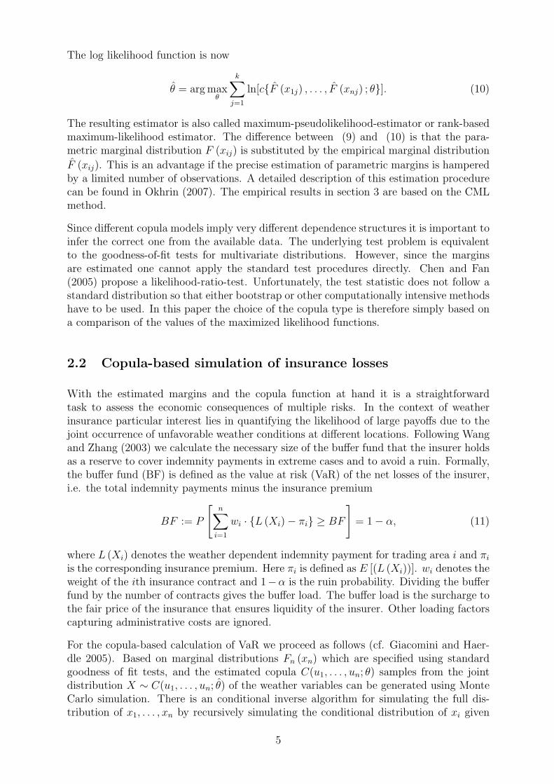
The log likelihood function is now

θ = arg maxθ

k∑j=1

ln[c{F (x1j) , . . . , F (xnj) ; θ}]. (10)

The resulting estimator is also called maximum-pseudolikelihood-estimator or rank-basedmaximum-likelihood estimator. The difference between (9) and (10) is that the para-metric marginal distribution F (xij) is substituted by the empirical marginal distribution

F (xij). This is an advantage if the precise estimation of parametric margins is hamperedby a limited number of observations. A detailed description of this estimation procedurecan be found in Okhrin (2007). The empirical results in section 3 are based on the CMLmethod.

Since different copula models imply very different dependence structures it is important toinfer the correct one from the available data. The underlying test problem is equivalentto the goodness-of-fit tests for multivariate distributions. However, since the marginsare estimated one cannot apply the standard test procedures directly. Chen and Fan(2005) propose a likelihood-ratio-test. Unfortunately, the test statistic does not follow astandard distribution so that either bootstrap or other computationally intensive methodshave to be used. In this paper the choice of the copula type is therefore simply based ona comparison of the values of the maximized likelihood functions.

2.2 Copula-based simulation of insurance losses

With the estimated margins and the copula function at hand it is a straightforwardtask to assess the economic consequences of multiple risks. In the context of weatherinsurance particular interest lies in quantifying the likelihood of large payoffs due to thejoint occurrence of unfavorable weather conditions at different locations. Following Wangand Zhang (2003) we calculate the necessary size of the buffer fund that the insurer holdsas a reserve to cover indemnity payments in extreme cases and to avoid a ruin. Formally,the buffer fund (BF) is defined as the value at risk (VaR) of the net losses of the insurer,i.e. the total indemnity payments minus the insurance premium

BF := P

[n∑i=1

wi · {L (Xi)− πi} ≥ BF

]= 1− α, (11)

where L (Xi) denotes the weather dependent indemnity payment for trading area i and πiis the corresponding insurance premium. Here πi is defined as E [(L (Xi))]. wi denotes theweight of the ith insurance contract and 1−α is the ruin probability. Dividing the bufferfund by the number of contracts gives the buffer load. The buffer load is the surcharge tothe fair price of the insurance that ensures liquidity of the insurer. Other loading factorscapturing administrative costs are ignored.

For the copula-based calculation of VaR we proceed as follows (cf. Giacomini and Haer-dle 2005). Based on marginal distributions Fn (xn) which are specified using standardgoodness of fit tests, and the estimated copula C(u1, . . . , un; θ) samples from the jointdistribution X ∼ C(u1, . . . , un; θ) of the weather variables can be generated using MonteCarlo simulation. There is an conditional inverse algorithm for simulating the full dis-tribution of x1, . . . , xn by recursively simulating the conditional distribution of xi given

5

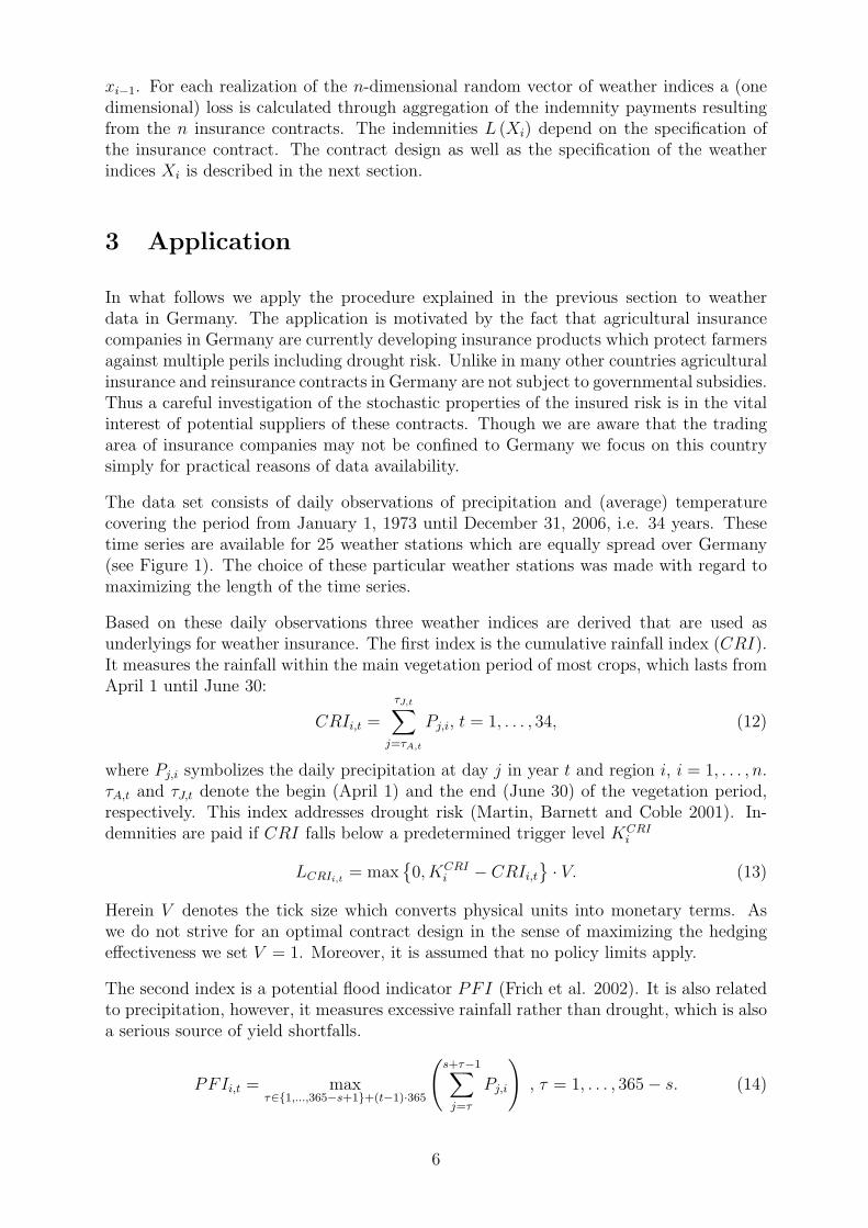
xi−1. For each realization of the n-dimensional random vector of weather indices a (onedimensional) loss is calculated through aggregation of the indemnity payments resultingfrom the n insurance contracts. The indemnities L (Xi) depend on the specification ofthe insurance contract. The contract design as well as the specification of the weatherindices Xi is described in the next section.

3 Application

In what follows we apply the procedure explained in the previous section to weatherdata in Germany. The application is motivated by the fact that agricultural insurancecompanies in Germany are currently developing insurance products which protect farmersagainst multiple perils including drought risk. Unlike in many other countries agriculturalinsurance and reinsurance contracts in Germany are not subject to governmental subsidies.Thus a careful investigation of the stochastic properties of the insured risk is in the vitalinterest of potential suppliers of these contracts. Though we are aware that the tradingarea of insurance companies may not be confined to Germany we focus on this countrysimply for practical reasons of data availability.

The data set consists of daily observations of precipitation and (average) temperaturecovering the period from January 1, 1973 until December 31, 2006, i.e. 34 years. Thesetime series are available for 25 weather stations which are equally spread over Germany(see Figure 1). The choice of these particular weather stations was made with regard tomaximizing the length of the time series.

Based on these daily observations three weather indices are derived that are used asunderlyings for weather insurance. The first index is the cumulative rainfall index (CRI).It measures the rainfall within the main vegetation period of most crops, which lasts fromApril 1 until June 30:

CRIi,t =

τJ,t∑j=τA,t

Pj,i, t = 1, . . . , 34, (12)

where Pj,i symbolizes the daily precipitation at day j in year t and region i, i = 1, . . . , n.τA,t and τJ,t denote the begin (April 1) and the end (June 30) of the vegetation period,respectively. This index addresses drought risk (Martin, Barnett and Coble 2001). In-demnities are paid if CRI falls below a predetermined trigger level KCRI

i

LCRIi,t = max{

0, KCRIi − CRIi,t

}· V. (13)

Herein V denotes the tick size which converts physical units into monetary terms. Aswe do not strive for an optimal contract design in the sense of maximizing the hedgingeffectiveness we set V = 1. Moreover, it is assumed that no policy limits apply.

The second index is a potential flood indicator PFI (Frich et al. 2002). It is also relatedto precipitation, however, it measures excessive rainfall rather than drought, which is alsoa serious source of yield shortfalls.

PFIi,t = maxτ∈{1,...,365−s+1}+(t−1)·365

(s+τ−1∑j=τ

Pj,i

), τ = 1, . . . , 365− s. (14)

6

The PFI equals the rainfall sum of the wettest s-day-period within a year. Here wechoose s = 5. The insurance payoff for the PFI has the structure of a call option, i.e.

LPFIi,t = max{

0, PFIi,t −KPFIi

}· V (15)

The third index that we suggest is the “Growing Degree Days” (GDDs). The GDD indexis intended to measure impact of temperature on the growth and the development ofplants during a growing season (World Bank 2005)

GDDi,t =

τO,t∑j=τM,t

max(

0, Tj,i − T), (16)

where Tj,i denotes daily temperature in degrees Celsius. τM,t and τO,t stand for thebegin (March 1) and the end (October 31) of the growing season, respectively. The basetemperature T is the minimum temperature that has to be exceeded before plant growthis stimulated. Though this threshold is plant specific we assume a constant value of 5◦C.Indemnities are calculated according to

LGDDi,t = max{

0, KGDDi −GDDi,t

}· V (17)

For all three indices we assume two alternative trigger levels, namely the 50% quantileand the 15% quantile of the respective index distribution.

The analysis of the spatial dependence of the aforementioned weather indices is carried outwithin three scenarios. The first scenario refers to only one state, Brandenburg (includingBerlin). Brandenburg is located in North East Germany and thus affected by a drycontinental climate. Four weather stations of our sample are located in this state (Berlin-Tempelhof, Neuruppin, Potsdam, and Lindenberg) and we expect significant dependenceof the respective indices at this regional level. In the second and third scenario we considerthe entire German state. In order to limit the dimension of the estimation problem thecountry is divided into four regions (A-D) of comparable size. These regions representthe Eastern (A), the North-Western (B), the Western (C) and the Southern (D) partof Germany. The number of weather stations varies between 5 (regions C and D) and 9(region A). Figure 1 depicts the number and the location of the available weather stations.Scenario 2 and 3 differ in the aggregation level of the weather indices. While in scenario 2each region is represented by only one weather station (Potsdam, Hamburg, Duesseldorf,and Stuttgart, respectively) an average of all weather stations situated in the respectiveregion underlies scenario 3.

Figure 1 about here

4 Results and Discussion

Marginal distributions and copulas have been estimated for the CRI, the PFI and theGDD index using the statistical procedures described in section 2. First of all, 36 marginaldistributions (3 indices, 4 locations, 3 regional levels) have been selected in accordancewith standard goodness of fit tests, i.e., Kolmogorov-Smirnoff test, χ2 and Anderson-Darling test. The Lognormal, the Gamma and Beta distribution show the best fit for therainfall-based indices (CRI and PFI), whereas the Weibull distribution fits the obser-vations of the temperature-based index (GDD). Next, two different parametric copulas

7

have been estimated, namely the Clayton copula and the Gumbel copula. The results arepresented in table 1. The values of the maximized likelihood functions support the choiceof the Clayton copula. In what follows we only discuss the results for this copula type.

Table 1 and table 2 about here

The main results of the simulations are summarized in table 2 and table 3. Table 2displays the expected insurance payoffs for the regions under consideration. Obviouslyconsiderable differences exist between locations. This finding should be kept in mindwhen interpreting the effects of aggregating trading areas for weather insurance whichare presented in table 3. As explained above the buffer load is derived from the bufferfund which is defined as the 99% quantile of loss distribution for the insurer minus thefair premium. The loss distribution is the outcome of 10.000 random draws from theestimated margins and the estimated copula. Dividing the buffer fund by the number oftrading areas (n = 1, 2, 3, or 4, respectively) yields the buffer load. The buffer load isdepicted for trading areas of growing size (A, A+B, A+B+C, and A+B+C+D) and forinsurance contracts with two different trigger levels (15% and 50% quantile). Moreover,table 3 allows a comparison of the copula based approach that we propagate here andthe traditional method of using Pearsons linear correlation coefficients2. Both methodsuse the same marginal distributions and differ only in the estimation of the dependencestructure of the weather indices at different locations.

Table 3 about here

First of all, the size of the buffer load may appear surprisingly high in relation to the ex-pected insurance payoff. Loosely speaking this finding indicates that the loss distributionis wide and shows fat tails. Of course the buffer load depends on the trigger level. Thevalues increase by a factor between 1,3 and 2,3 if the insurance contracts refer to the 50%quantile instead of the 15% quantile of the index distributions.

From a methodological viewpoint it is interesting to realize that the two methods ofconsidering stochastic dependence between trading areas show considerable differences.In case of the drought insurance (CRI) the assumption of linear correlations tends tounderestimate the risk of large joint indemnity payments for all three scenarios comparedwith the copula method. For the largest trading area (A+B+C+D) this underestimationvaries between 11% and 21% in case of the 50% trigger value and lies between 18% and31% in case of the 15% trigger. For the other two insurance contracts the differences ofthe buffer load are less pronounced. There are also cases in which the Clayton copularesults in a lower buffer load than the linear correlation.

Table 3 also depicts spatial diversification effects of weather insurance. It can be seenthat the decline of the buffer load is rather small if the trading area becomes larger. Insome cases the buffer load even increases. This finding, which contradicts the intuitiveexpectation of diversification effects, can be explained by the heterogeneity of the weatherindices in the trading areas that are pooled. As mentioned before, the index distributionsare neither independent nor identically distributed. In order to assess the diversificationeffect more accurately we calculate the relative difference of the buffer load of a jointinsurance of all four regions A-D compared to the sum of buffer loads associated withseparate insurance for each region (last column in table 3). Recall that the buffer load

2The generation of multivariate random variables with arbitrary marginals following a given linearcorrelation matrix is carried out with the method of Iman and Conover (1982).

8

in the i.i.d. case declines with 1/√n , which means that we could expect a reduction by

50% for n = 4 in that case. Apparently, the possibility of spatial diversification heavilydepends on the insured weather event. For example, the buffer load for the contract basedon the potential flood indicator (PFI) decreases considerably, particularly for scenario2, irrespective of the trigger level and how the joint distribution has been computed.Opposed to that the decline of the buffer load is negligible for the insurance against lowtemperature. This result reflects the high stochastic dependence of the GDD at differentlocations. This holds for the state level as well as for the national level. Diversification isalso modest for the drought insurance based on the CRI index. It is worth mentioning thatthe spatial diversification potential is not much higher in the whole country (Germany)than in a single state (Brandenburg). This is particularly true if the weather indices arecalculated as an average value out of several weather stations (scenario S3). Finally, weemphasize again the difference between copulas and linear correlations: On the one handthe use of linear correlations underestimates the effect of spatial diversification for theinsurance against excessive rain, on the other hand this effect is overestimated in case ofthe drought insurance and the GDD based insurance.

5 Conclusions

In this paper we have explored the risk that insurer will face when selling contracts withweather-based payoffs in Germany. Our results indicate that indemnity payments basedon temperature as well as on cumulative rainfall show strong stochastic dependence atdifferent regions in Germany. Thus the possibility to reduce risk exposure by increasingthe trading area of the insurance is limited. Though the results are specific to Germany weconjecture that the situation in other EU countries of similar size and climate conditionsdoes not differ in principle. At the first glance our results contradict those of Wang andZhang (2003) who found that the distance for the positive dependence of crop yields in theUS is at most 570 miles and hence the required buffer load for national crop insurance israther small. However, our results are not directly comparable. We analyze weather datawhereas Wang and Zhang (2003) investigate regional crop yields. Regional differencesin soil quality, for example, may lead to differences in yields even if weather conditionsare similar. Moreover, our results rely on several assumptions that have an influenceon the buffer load. Firstly, we did not take into account product diversification of theinsurer. Secondly, only a single period has been considered and equity reserves thatare built in years with premium surpluses have been ignored. Thirdly, the buffer loadcan be controlled by choice of the trigger value for the indemnity payments. It can beexpected that the dependence of insurance payoffs at different locations becomes smallerif the trigger level is reduced. Defining absolute trigger values instead of relative ones(i.e. quantiles of the regional distributions) will effect the dependence structure of thepayments, too. Fourthly, in our application the definition of trading areas took place onan ad-hoc basis. This procedure leaves room for a thorough identification of smaller andmore homogenous climatic zones showing less dependence. Considering all these pointsour results must be interpreted with care. We do not state that private (unsubsidized) cropinsurance is impossible in view of systemic weather risk at all. Anyhow, we believe that ourfinding may explain the reluctance of insurance companies to enter this market segmentin Germany. Global reinsurance or transferring weather risk to the capital markets bymeans of weather bonds could of course alleviate this problem.

9

Irrespective of their economic implications our results pinpoint the necessity of a properstatistical modeling of the dependence structure of multivariate random variables. Theusual approach of measuring stochastic dependence with linear correlation coefficientsturned out to be questionable in the context of weather insurance. Considerable differenceswith regard to the weather risk assessment occurred in comparison with the more generalcopula method. Unfortunately, our empirical results are weakened by a rather small database. The estimation of 4-dimensional distributions with only 34 observations is inevitablyaccompanied by large estimation errors. A solution to this problem could be the use ofdaily weather data. We suggest this as a direction for further research.

References

Blum, P., Dias, A. and Embrechts, P. (2002). The art of dependence modelling: The latestadvances in correlation analysis, in M. Lane (ed.), Alternative Risk Strategies, Risk Books,London, pp. 339–356.

Charpentier, A., Fermanian, J.-D. and Scaillet, O. (2007). The estimation of copulas: the-ory and practice, in J. Rank (ed.), Copulas: From theory to application in finance, RiskPublications, London, chapter Section 2.

Chen, S. X. and Fan, Y. (2005). Pseudo-likelihood ratio tests for model selection in semipara-metric multivariate copula models, The Canadian Journal of Statistics 33: 389–414.

Chen, S. X. and Huang, T. (2007). Nonparametric estimation of copula functions for dependencemodeling, The Canadian Journal of Statistics 35: 265–282.

Cherubini, U., Luciano, E. and Vecchiato, W. (2004). Copula Methods in Finance, Wiley,Chichester.

Embrechts, P., McNeil, A. J. and Straumann, D. (1999). Correlation and dependence in riskmanagement: Properties and pitfalls, RISK pp. 69–71.

Frich, P., Alexander, L. V., Della-Marta, P., Gleason, B., Haylock, M., Klein Tank, A. M. G.and Peterson, T. (2002). Observed coherent changes in climatic extremes during the secondhalf of the twentieth century, Climate Research 19: 193–212.

Genest, C., Ghoudi, K. and Rivest, L. (1995). A semiparametric estimation procedure of de-pendence parameters in multivariate families of distributions, Biometrika 82: 543–552.

Giacomini, E. and Haerdle, W. (2005). Value-at-risk calculation with time varying copulae, SFB649 Discussion Paper 2005-004: 543–552.

Goodwin, B. (2001). Problems with market insurance in agriculture, American Journal ofAgricultural Economics 83: 643–649.

Goodwin, B. and Ker, A. (2002). Modeling price and yield risk, in R. Just and R. Pope (eds),A Comprehensive Assessment of the Role of Risk in U.S. Agriculture, Kluwer, Boston,pp. 289–323.

Haerdle, W., Okhrin, O. and Okhrin, Y. (2008). Modeling dependencies in finance using copulae,in W. Haerdle, N. Hautsch and L. Overbeck (eds), Applied Quantitative Finance, 2 edn,Springer Verlag. in press.

Iman, R. and Conover, W. (1982). A distribution-free approach to inducing rank correla-tion among input variables, Communications in Statistics - Simulation and Computation11: 311–334.

10

Joe, H. (1997). Multivariate Models and Dependence Concepts, Chapman & Hall, London.

Junker, M. and May, A. (2005). Measurement of aggregate risk with copulas, EconometricsJournal 8: 428–454.

Martin, S. W., Barnett, B. J. and Coble, K. H. (2001). Developing and pricing precipitationinsurance, Journal of Agricultural and Resource Economics 26: 261–274.

McNeil, A., Frey, R. and Embrechts, P. (2005). Quantitative Risk Management, PrincetonUniversity Press, Princeton.

Miranda, M. and Glauber, J. (1997). Systemic risk, reinsurance, and the failure of crop insurancemarkets, American Journal of Agricultural Economics 79: 206–215.

Nelsen, R. B. (2006). An Introduction to Copulas, Springer Verlag, New York.

Odening, M., Muhoff, O. and Xu, W. (2007). Analysis of rainfall derivatives using daily precip-itation models: Opportunities and pitfalls, Agricultural Finance Review 67: 135–156.

Okhrin, O. (2007). Hierarchical Archimedean Copulas: Structure Determination, Properties,Applications, PhD thesis, Faculty of Economics, European University Viadrina, Frankfurt(Oder), Germany.

Sklar, A. (1959). Fonctions de repartition a n dimension et leurs marges, Publ. Inst. Stat.Univ.Paris 8: 299–231.

Vedenov, D. (2008). Application of copulas to estimation of joint crop yield distributions, Selectedpaper at the Annual Meeting of the AAEA 2008 . Available at http://ageconsearch.umn.edu/handle/6264.

Wang, H. and Zhang, H. (2003). On the possibility of a private crop insurance market: A spatialstatistics approach, The Journal of Risk and Insurance 70: 111–124.

Woodard, J. and Garcia, P. (2008). Basis risk and weather hedging effectiveness, Special Issueof the Agricultural Finance Review 68: 111–124.

WorldBank (2005). Managing agricultural production risk. Available at http://www.globalagrisk.com/pubs/2005_ESW_Managing_Ag_Risk.pdf.

Xu, W., Odening, M. and Musshoff, O. (2008). Optimal design of weather bonds, Selected paperat the Annual Meeting of the AAEA 2008 . Available at http://ageconsearch.umn.edu/handle/6781.

Zhu, Y., Ghosh, S. and Goodwin, B. (2008). Modeling dependence in the design of whole farminsurance contract a copula-based approach, Selected paper at the Annual Meeting of theAAEA 2008 . Available at http://ageconsearch.umn.edu/handle/6282.

11

http://ageconsearch.umn.edu/handle/6264


http://www.globalagrisk.com/pubs/2005_ESW_Managing_Ag_Risk.pdf

http://www.globalagrisk.com/pubs/2005_ESW_Managing_Ag_Risk.pdf




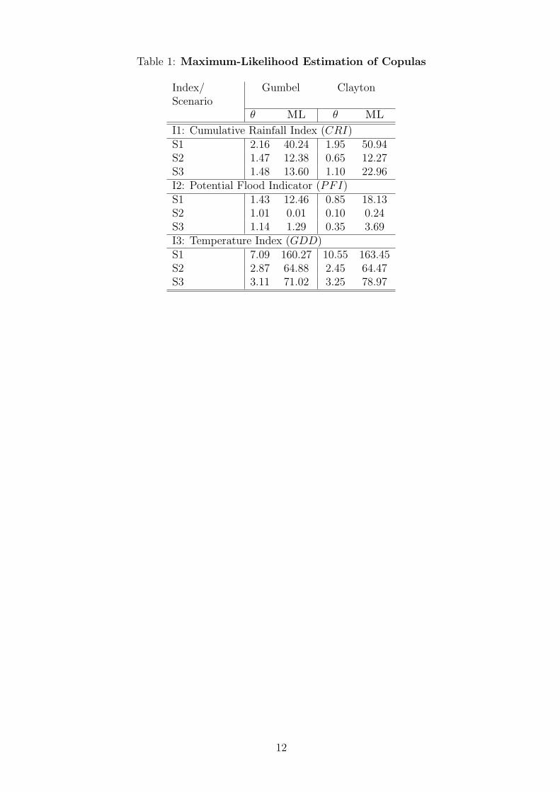
Table 1: Maximum-Likelihood Estimation of Copulas

Index/Scenario

Gumbel Clayton

θ ML θ ML

I1: Cumulative Rainfall Index (CRI)S1 2.16 40.24 1.95 50.94S2 1.47 12.38 0.65 12.27S3 1.48 13.60 1.10 22.96I2: Potential Flood Indicator (PFI)S1 1.43 12.46 0.85 18.13S2 1.01 0.01 0.10 0.24S3 1.14 1.29 0.35 3.69I3: Temperature Index (GDD)S1 7.09 160.27 10.55 163.45S2 2.87 64.88 2.45 64.47S3 3.11 71.02 3.25 78.97

12

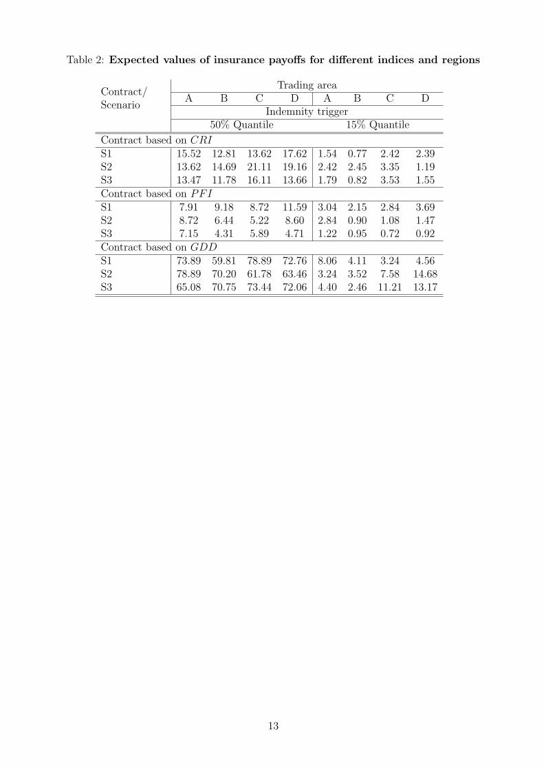
Table 2: Expected values of insurance payoffs for different indices and regions

Contract/Scenario

Trading areaA B C D A B C D

Indemnity trigger50% Quantile 15% Quantile

Contract based on CRIS1 15.52 12.81 13.62 17.62 1.54 0.77 2.42 2.39S2 13.62 14.69 21.11 19.16 2.42 2.45 3.35 1.19S3 13.47 11.78 16.11 13.66 1.79 0.82 3.53 1.55Contract based on PFIS1 7.91 9.18 8.72 11.59 3.04 2.15 2.84 3.69S2 8.72 6.44 5.22 8.60 2.84 0.90 1.08 1.47S3 7.15 4.31 5.89 4.71 1.22 0.95 0.72 0.92Contract based on GDDS1 73.89 59.81 78.89 72.76 8.06 4.11 3.24 4.56S2 78.89 70.20 61.78 63.46 3.24 3.52 7.58 14.68S3 65.08 70.75 73.44 72.06 4.40 2.46 11.21 13.17

13

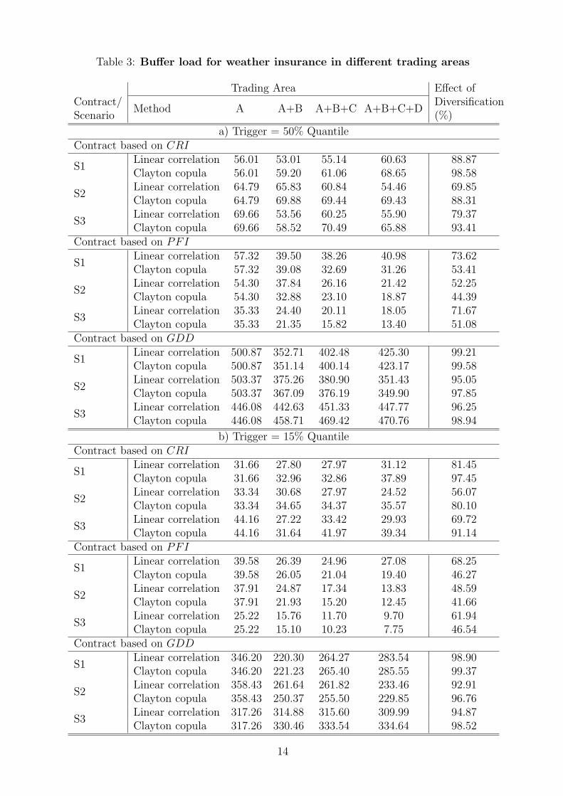
Table 3: Buffer load for weather insurance in different trading areas

Trading Area Effect ofDiversification(%)

Contract/Scenario

Method A A+B A+B+C A+B+C+D

a) Trigger = 50% QuantileContract based on CRI

S1Linear correlation 56.01 53.01 55.14 60.63 88.87Clayton copula 56.01 59.20 61.06 68.65 98.58



Contract based on PFI




Contract based on GDD




b) Trigger = 15% QuantileContract based on CRI




Contract based on PFI




Contract based on GDD




14

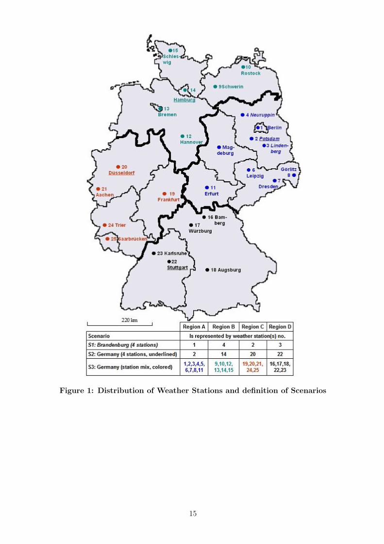
Figure 1: Distribution of Weather Stations and definition of Scenarios

15

SFB 649 Discussion Paper Series 2009

For a complete list of Discussion Papers published by the SFB 649, please visit http://sfb649.wiwi.hu-berlin.de.

001 "Implied Market Price of Weather Risk" by Wolfgang Härdle and Brenda López Cabrera, January 2009.

002 "On the Systemic Nature of Weather Risk" by Guenther Filler, Martin Odening, Ostap Okhrin and Wei Xu, January 2009.

SFB 649, Spandauer Straße 1, D-10178 Berlin

http://sfb649.wiwi.hu-berlin.de

This research was supported by the Deutsche Forschungsgemeinschaft through the SFB 649 "Economic Risk".

on the systemic nature of weather risk

Documents