on the reduction of stochastic kinetic theory models of complex fluids
TRANSCRIPT
IOP PUBLISHING MODELLING AND SIMULATION IN MATERIALS SCIENCE AND ENGINEERING
Modelling Simul. Mater. Sci. Eng. 15 (2007) 639–652 doi:10.1088/0965-0393/15/6/004
On the reduction of stochastic kinetic theory models ofcomplex fluids
F Chinesta1, A Ammar2, A Falco3 and M Laso4
1 Laboratoire de Mecanique des Systemes et des Procedes, UMR 8106 CNRS-ENSAM-ESEM,151 Boulevard de l’Hopital, F-75013 Paris, France2 Laboratoire de Rhéeologie UMR 5520 CNRS-INPG-UJF, 1301 rue de la piscine, BP 53Domaine Universitaire, F-38041 Grenoble Cedex 9, France3 Universidad CEU Cardenal Herrera, San Bartolome 55, E-46115 Alfara del Patriarca, Spain4 Laboratory of Non-Metallic Materials, ETSII-UPM, Jose Gutierrez Abascal 2, E-28006 Madrid,Spain
E-mail: [email protected], [email protected], [email protected] [email protected]
Received 13 December 2006, in final form 2 July 2007Published 21 August 2007Online at stacks.iop.org/MSMSE/15/639
AbstractKinetic theory models involving the Fokker–Planck equation are usually solvedin the framework of stochastic approaches, which allows us to circumvent thedifficulties related to the multidimensional character of that equation. In fact,the Fokker–Planck equation governs the evolution of the distribution functionthat defines the molecular configuration at each point of the physical spaceand at each time. As the molecular conformation is usually defined by severalcoordinates, the resulting distribution function will depend on the physicaland configuration coordinates and the time. Although different numericalstrategies have recently been proposed for solving that equation with efficiencyand accuracy (Ammar et al 2006 J. Non-Newtonian Fluid Mech. 134 136–47, Ammar et al 2006 J. Non-Newtonian Fluid Mech. 139 153–76) thestochastic approach is today the most common for solving general kinetictheory models. This paper presents some preliminary results that provideevidence for the potential applicability of model reduction techniques basedon the Karhunen–Loeve decomposition or on separated representations forreducing the computational efforts related to the solution of such models inthe Brownian configuration fields framework.
(Some figures in this article are in colour only in the electronic version)
1. Introduction
Many natural and synthetic fluids are viscoelastic materials, in the sense that the stress enduredby a macroscopic fluid element depends upon the history of the deformation experienced bythat element.
0965-0393/07/060639+14$30.00 © 2007 IOP Publishing Ltd Printed in the UK 639
640 F Chinesta et al
Atomistic modeling is the most detailed level of description that can be applied today inrheological studies, but its simulation requires enormous computer resources, and so they arecurrently limited to flow geometries of molecular dimensions.
Kinetic theory models provide a coarse-grained description of molecular configurations.They are meant to display in a more or less accurate fashion the important features that governthe flow-induced evolution of configurations.
Micro–macro methods couple the coarse-grained molecular scale of kinetic theory to themacroscopic scale of continuum mechanics (the reader can refer to the review paper [9] andthe references therein). This approach is much more demanding in computer resources thanmore conventional continuum simulations that integrate a constitutive equation to evaluate theviscoelastic contribution of the stress tensor.
Since the early 1990s the field has developed considerably following the introduction ofthe CONNFFESSIT method by Ottinger and Laso [10].
Kinetic theory provides two basic building blocks: the diffusion or Fokker–Planck equationthat governs the evolution of the distribution function (giving the probability distribution ofconfigurations) and an expression relating the viscoelastic stress to the distribution function.The Fokker–Planck equation has the general form
dψ
dt+
∂
∂X(Aψ) = 1
2
∂
∂X
∂
∂X: (Dψ), (1)
where vectors are affected by an underline and matrices by a double underline, dψ/dt is thematerial derivative, vector X defines the coarse-grained configuration and has dimensions N .Factor A is an N -dimensional vector that defines the drift or deterministic component of themolecular model. Finally D is a symmetric, positive definite N × N matrix that embodiesthe diffusive or stochastic component of the molecular model. In general both A and D (andin consequence the distribution function ψ) depend on the physical coordinates x, on theconfiguration coordinates X and on the time t .
The second building block of a kinetic theory model is an expression relating thedistribution function and the stress. It takes the form
τp
=∫
C
g(X)ψ dX, (2)
where C represents the configuration space and g is a model-dependent tensorial function
of configuration. In a complex flow, the velocity field is a priori unknown and the stressfield are coupled through the conservation laws. In the isothermal and incompressible casethe conservation of mass and momentum balance are then expressed (neglecting the bodyforces) by
Divv = 0,
ρdv
dt= Div(−pI + τ
p+ 2ηsd),
(3)
where ρ is the fluid density, p the pressure and 2ηsd a purely viscous component (d being thestrain rate tensor). The set of coupled equations (1)–(3), supplemented with suitable initialand boundary conditions in both physical and configuration spaces, is the generic multiscaleformulation.
Three basic approaches have been adopted for exploiting the generic multiscale model:the continuum approach; the Fokker–Planck approach and the stochastic approach. This paperfocuses on the last approach.
The stochastic approach is based on the mathematical equivalence between the Fokker–Planck equation (1) and the following Ito stochastic differential equation:
dX = A dt + B dW, (4)

On the reduction of stochastic kinetic theory models of complex fluids 641
where D = B BT and W is a Wiener stochastic process of dimension N . In a complexflow, the stochastic differential equation (4) applies along individual flow trajectories, the timederivative is thus a material derivation. Instead of solving the deterministic Fokker–Planckequation (1), one solves the associated stochastic differential equation (4) for a large ensembleof realizations of the stochastic process X by means of a suitable numerical technique.
The control of the statistical noise is a major issue in stochastic micro–macro simulationsbased on the stochastic approach. Moreover, to reconstruct the distribution one needs to operatewith an extremely large number of particles; however, in general, only the moments of such adistribution are required, which can be computed as an ensemble average using a much morereduced population of particles.
The Brownian configuration fields (BCFs) is a technique proposed in [8] allowing usto reduce the variance as well as to accelerate the numerical simulations. In this paper wepresent some preliminary results that seem to reveal that BCF models can be reduced by usinga Karhunen–Loeve decomposition which does not run in the context of the original stochasticapproach.
The proposed technique will be illustrated on the kinetic theory model related to a shortfiber suspension in a Newtonian fluid. For this reason, we start by introducing such a modelin the next section.
1.1. Governing equations for a short fiber suspension
In the case of a dilute short fiber suspension, the configuration distribution function (alsoknown as orientation distribution function) gives the probability of finding the fiber in a givendirection. Obviously, this function depends on the physical coordinates (space and time) aswell as on the configuration coordinates, which taking into account the rigid character of thefibers, are defined on the surface of the unit sphere. Thus, we can write ψ(x, t, p), wherex defines the position of the fiber center of mass, t the time and p the unit vector definingthe fiber orientation. The evolution of the distribution function is given by the Fokker–Planckequation:
dψ
dt= − ∂
∂p(ψp) +
∂
∂p
(Dr
∂ψ
∂p
), (5)
where d/dt represents the material derivative, Dr is a diffusion coefficient and p is the fiberrotation velocity. The orientation distribution function must verify the normality condition:∮
ψ(p) dp = 1. (6)
When the fibers are assumed ellipsoidal and when the suspension is dilute enough, the rotationvelocity can be obtained from the Jeffery’s equation
p = � p + kD p − k(pTD p)p, (7)
where � and D are the vorticity and the strain rate tensors, respectively, associated with thefluid flow undisturbed by the presence of the fibers, and k is a scalar which depends on thefiber aspect ratio λ (ratio between the fiber length and the fiber diameter)
k = λ2 − 1
λ2 + 1. (8)
In a former work [4] the discretization of the steady-state Fokker–Planck equation was carriedout in steady recirculating flows using a particle technique, where the diffusion term wasmodeled from random motions. It was pointed out that the number of fibers required in thisstochastic simulation to describe the fiber distribution increases significantly with the diffusioncoefficient Dr .
642 F Chinesta et al
2. Reduced order modeling
The model reduction technique that we propose in this work is based on the use of the Karhunen–Loeve decomposition, which we summarize in the next section.
2.1. The Karhunen–Loeve decomposition
We assume that the evolution of a certain field u(x, t) is known (being its evolution governedby a PDE). In practical applications, this field is expressed in a discrete form, that is, it isknown at the Nn nodes of a spatial mesh and at some times u(x i, t
n) ≡ uni , ∀n ∈ [1, . . . , P ]
and ∀i ∈ [1, . . . , Nn]. The main idea of the Karhunen–Loeve (KL) decomposition is howto obtain the most typical or characteristic structure φ(x) among these un(x), ∀n. This isequivalent to obtaining a function φ(x) that maximizes λ defined by
λ =∑n=P
n=1
[∑i=Nn
i=1 φ(x i)un(x i)
]2
∑i=Ni=1 (φ(x i))
2. (9)
By applying standard variational calculus, the maximization of equation (9) leads to
n=P∑n=1
(i=Nn∑
i=1
φ(x i)un(x i)
)j=Nn∑j=1
φ(x j )un(x j )
= λ
i=Nn∑i=1
φ(x i)φ(x i); ∀φ (10)
which can be rewritten in the form
i=Nn∑i=1
j=Nn∑j=1
[n=P∑n=1
un(x i)un(x j )φ(x j )
]φ(x i)
= λ
i=Nn∑i=1
φ(x i)φ(x i); ∀φ (11)
Defining the vector φ such that its i-component is φ(x i), equation (11) takes the followingmatrix form
φTC φ = λφ
Tφ; ∀φ ⇒ C φ = λφ, (12)
where the two points correlation matrix is given by
Cij =n=P∑n=1
un(x i)un(x j ) ⇔ C =
n=P∑n=1
un(un)T, (13)
which is symmetric and positive definite. If we define the matrix Q containing the discrete
field history:
Q =
u11 u2
1 · · · uP1
u12 u2
2 · · · uP2
......
. . ....
u1Nn
u2Nn
· · · uPNn
(14)
then, matrix C in equation (12) gives
C = Q QT. (15)
Thus, the functions defining the most characteristic structure of un(x) are theeigenfunctions φk(x), whose discrete expression is φ
k, associated with the highest eigenvalues.

On the reduction of stochastic kinetic theory models of complex fluids 643
2.2. A posteriori reduced modeling
If some direct simulations have been carried out, we can determine u(x i, tn) ≡ un
i , ∀i ∈[1, . . . , Nn], ∀n ∈ [1, . . . , P ], and from that information the r eigenvectors φT
k=
[φk(x1), . . . , φk(x Nn)], ∀k ∈ [1, . . . , r] (with r � Nn) related to the r-highest eigenvalues
λ1, . . . , λr (that are assumed ordered, being λ1 the highest eigenvalue). These eigenvaluesverify λk > ελ1, ∀k ∈ [1, . . . , r] (with ε a small enough value that in our simulations is setto 10−8) and λk < ελ1 ∀k ∈ [r + 1, . . . , Nn].
Now, we can try to use these r eigenfunctions for approximating the solution of a problemslightly different from the one that has served to define u(x i, t
n). For this purpose we need todefine the matrix
B =
φ1(x1) φ2(x1) · · · φr(x1)
φ1(x 2) φ2(x 2) · · · φr(x 2)
......
. . ....
φ1(x Nn) φ2(x Nn
) · · · φr(x Nn)
. (16)
Now, we consider the linear system of equations resulting from the discretization of apartial differential equation (PDE) in the form
K Un = Fn−1. (17)
In the case of transient problems Fn−1 contains the contribution of the solution at the previoustime step.
Then, the unknown vector containing the nodal degrees of freedom can be expressed as
Un =i=r∑i=1
φiξni = B ξn, (18)
which implies
K Un = Fn−1 ⇒ K B ξn = Fn−1 (19)
and multiplying both terms by BT it gives
BTK B ξn = BTFn−1, (20)
which proves that the resulting linear system has a small size, i.e. the dimensions of BTK B
are r × r , with r � Nn, and the dimensions of both xi and BTF are r × 1.
Remark 2.1. Equation (20) can also be derived introducing the approximation (18) into thePDE Galerkin form.
See [1] or [11] for more details on the application on model reduction for simulatingkinetic theory models based on the use of the Fokker–Planck formalism.
3. Reduced Brownian configuration fields (R-BCF)
The BCF technique is based on substituting the solution of equation (4) along individualtrajectories by the solution of the evolution of several fields (the so-called Brownianconfiguration fields). From now on we consider the kinetic theory model related to the flow ofa short fiber suspension, with both the flow and the fiber orientation assumed in a 2D physicalspace (the extension to 3D is straightforward). As we are interested in the orientation solution,
644 F Chinesta et al
we consider that the flow kinematics and the fiber orientation are uncoupled, and therefore weare computing the orientation solution for a given velocity field.
We assume a simple shear flow characterized by the following kinematics
v =(
u
v
)=(
γ y
0
). (21)
The fiber orientation can be described from the angle ϕ:
p =(
px
py
)=(
cos ϕ
sin ϕ
). (22)
Thus, the Fokker–Planck equation (equation (5)) reduces to
∂ψ
dt+ u
∂ψ
∂x= − ∂
∂ϕ(ψϕ) + Dr
∂2ψ
∂ϕ2, (23)
where the diffusion coefficient Dr is assumed scalar and constant.The fibers are assumed with an infinite aspect ratio (k = 1 in equation (7)), leading to
ϕ = dϕ
dt= − sin2 ϕ, (24)
which implies that the flow tends to align the fiber in the flow direction.The domain in which the Fokker–Planck (FP) equation is defined is defined by � =
]0, L] × [−H, H ], and the time interval ]0, T ]. Due to the advective character of the FPequation in the physical space only a boundary condition is required on the inflow boundaryx = 0, which we represent by ψinf(y, t). The initial distribution is given by ψ(x, t = 0) = ψ0.
Again, due to the advective character of the FP equation in the physical space, the solutionon a flow trajectory y = cte does not depend on the solution on the neighbor trajectories.Thus, we will restrict our analysis to the one-dimensional trajectory defined by y = 1.
The simplest (explicit and first order) stochastic simulation consists of the following.
1. Define a number of fibers ϕi initially distributed in the physical domain ]0, L] representingthe initial fiber distribution ψ0.
2. Update the position of each fiber according to the flow kinematics (in our case defined ony = 1 with γ = 1):{
xn+1i = xn
i + u(xni , yn
i , tn) t = xni + t,
yn+1i = 1
∀i, ∀n � 1 (25)
3. Update the orientation of each fiber according to
ϕn+1i = ϕn
i + ϕ(ϕni , tn) t + W
n,n+1i , ∀i, (26)
where ϕ(ϕni , tn) = − sin2(ϕn
i ) and W is a random number with zero mean and a varianceof 2Dr t .
4. To avoid the loss of fibers we introduce new fibers in the domain through the inflowboundary x = 0 whose orientation represents the boundary condition ψinf , in order tokeep constant the number of particles into the domain.
Despite the consideration of a first order explicit scheme for the stochastic equationintegration, higher order integration schemes are available.
We prove later that the extraction of representative modes from this kind of analysis is notevident, a fact that motivates the consideration of the BCF framework.
Because the random term in the stochastic equation is uncorrelated in space, it is possibleto define stochastic fields whose evolutions can be solved by using standard techniques forPDEs, making use of fixed or moving meshes. In what follows we consider a fixed mesh on
On the reduction of stochastic kinetic theory models of complex fluids 645
the physical domain on which the evolution of different fields ϕi(x, t) is computed. For thispurpose we simply substitute the resolution of equations (25) and (26) by the solution of
ϕn+1i (x) = ϕn
i (x) − u(x)∂ϕn+θ
i
∂x t + ϕ(ϕn+θ
i (x)) t + Wn,n+1i , ∀i, (27)
where ∂u/∂x = 0.Different techniques have been used in the literature for solving this equation, all of
them stabilizing its advection character: SUPG, discontinuous-Galerkin, etc. In the case ofconsidering an explicit strategy (θ = 0 in equation (27)) no linear system must be solved butextremely small time steps are needed. In the other case, if one considers implicit (θ = 1) orsemi-implicit (0 < θ < 1) schemes, the solution of a linear system (whose size correspondsto the number of nodes used in the space discretization, Nn) is required at each time step.
In the semi-implicit case, where the flow-induced orientation term is considered at theprevious time step, we obtain
K ϕn+1i
= Fn( Wn,n+1i ). (28)
Obviously, the fully implicit case results in a non-linear system that must be solved using anappropriate linearization schema.
One possibility for reducing the computing time consists of solving the previous modelfor one field, and then extracting from its time evolution the r characteristic modes via theapplication of the Karhunen–Loeve decomposition, defining the reduced approximation basis.Now, the remaining fields could be computed after projection on the reduced approximationbasis. Thus, even if one is using an implicit (or semi-implicit) strategy the size of the linearsystems involved is r × r instead of Nn × Nn.
3.1. Numerical results
3.1.1. Evaluating the applicability of reduction techniques in the standard stochastic approach.First, we consider a population consisting of N fibers located on the streamline y = 0,isotropically distributed. These fibers are subjected to a unit shear flow (γ = 1) but theydo not move along the streamline because the velocity field vanishes on this streamline.
The initial fibers orientation is defined by
ϕ0i = 0. (29)
The orientation updating is defined at each time step according to
ϕn+1i = ϕn
i + ϕ(ϕni ) t + W
n,n+1i , ∀i. (30)
Now, we define the matrix Q
Q =
ϕ11 ϕ2
1 · · · ϕP1
ϕ12 ϕ2
2 · · · ϕP2
......
. . ....
ϕ1N ϕ2
N · · · ϕPN
, (31)
which defines the eigenvalue problem
Q QT φ = λφ. (32)
The main difficulty related to the use of the these computed modes is that they areassociated with a specific particles position, the one that served to define Q. As soon as the
particle trajectories differ from the ones that served to compute the characteristic functions,
646 F Chinesta et al
the reduced approximation is no more valid. To illustrate this fact, we consider the reducedapproximation basis composed of the r eigenvectors related to the highest eigenvalues (the r
verifying λk > 10−8λ1, being λ1 the highest one). These eigenvectors define the matrix B
according to equation (16).Now, equation (30) is written in the matrix form
ϕn+1 = ϕn + ϕ(ϕn) t + Wn,n+1 (33)
that after projection onto the reduced approximation basis results
BTB ξn+1 = BTB ξn + BTϕ(B ξn) t + BT Wn,n+1. (34)
In general the initial condition is added to the reduced approximation basis:
B ← [ϕ0 B], (35)
which allows us to properly define the initial condition associated with the reduced unknownvector ξ 0: (
ξ 0)T
= (1, 0, · · · , 0). (36)
The integration of equation (34) from the initial condition (36) allows us to compute theparticles orientation at any time:
ϕn = B ξn (37)
and the associated moments of the orientation distribution. In particular the second ordermoment results
an =∫ 2π
0p ⊗ p ψn(ϕ) dϕ, (38)
where p is defined in equation (22). When one uses the stochastic approach the distributionfunction is defined from the Dirac masses according to
ψn(ϕ) =i=N∑i=1
1
Nδ(ϕ − ϕn
i ), (39)
which implies
an = 1
N
i=N∑i=1
(cos2(ϕn
i ) sin(ϕni ) · cos(ϕn
i )
sin(ϕni ) · cos(ϕn
i ) sin2(ϕni )
). (40)
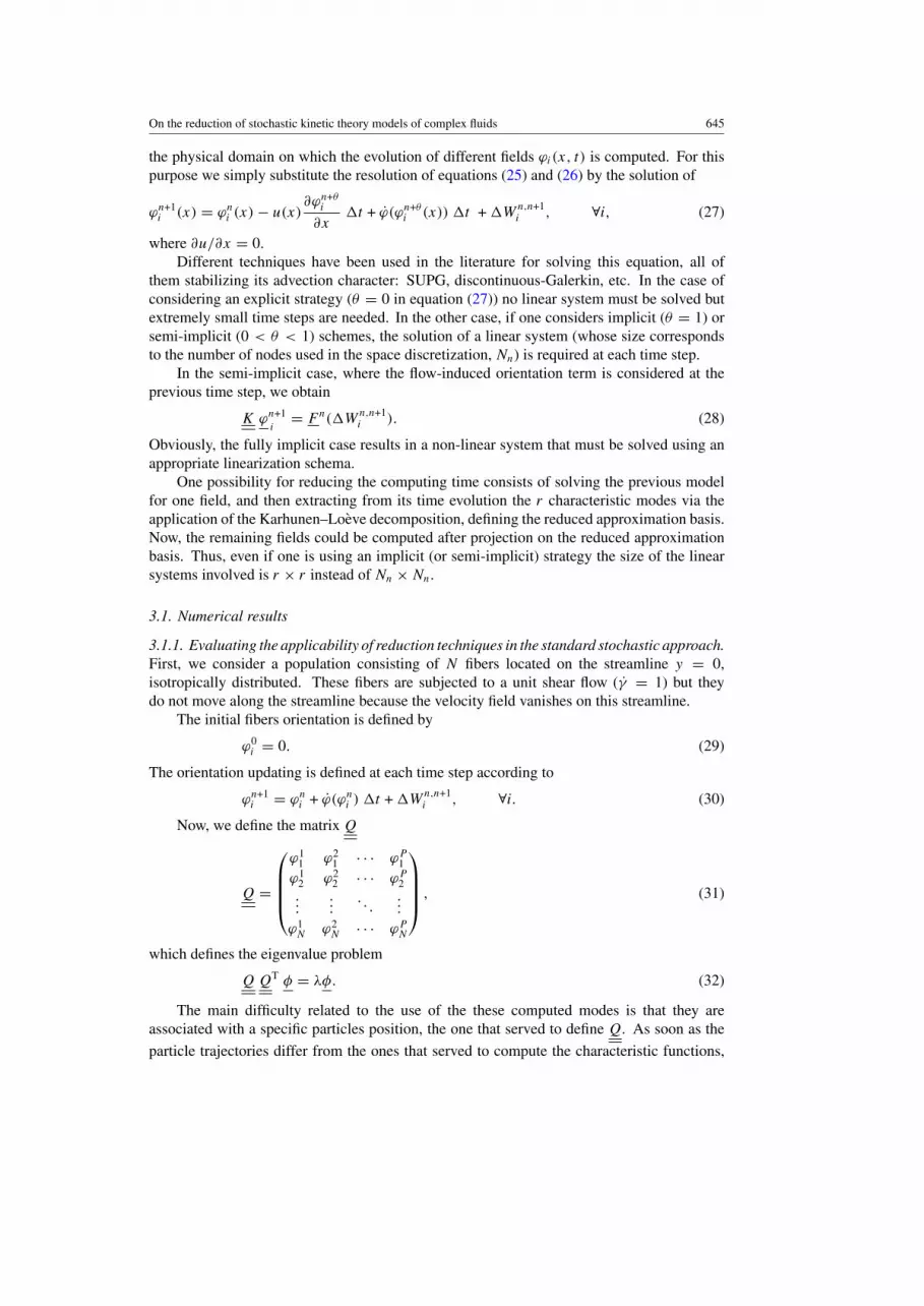
Now, we can compare the evolution of the first component of the second order orientationtensor a11, computed from the particles position determined by using both a standard stochasticprocedure (equation (30)) and the reduced modeling defined in equation (34). Figure 1depicts both solutions from which we can conclude the lack of accuracy related to the reducedmodeling. In this simulation we consider Dr = 0.05, N = 300, k = 1, γ = 1, t = 0.1and T = 30. All the fibers were assumed initially aligned in the x-direction according toequation (29). The stochastic solution, even if there is a significant noise (which can be reducedby increasing the number of particles), approaches the steady-state exact solution, whereas thecomputed in the reduced approximation basis (in this case composed of 14 eigenfunctions)evolves towards an isotropic distribution.
In conclusion, the direct reduction of stochastic simulations by applying the Karhunen–Loeve decomposition does not run despite the simplicity of the flows considered in the previousanalysis. In our opinion the reason for this behavior is that the reduced basis is associated withthe particles trajectories involved in the Karhunen–Loeve decomposition. Thus, when thisreduced basis is applied for describing other particles trajectories significant deviations areexpected and, in fact, found.

On the reduction of stochastic kinetic theory models of complex fluids 647
0 50 100 150 200 250 3000.4
0.5
0.6
0.7
0.8
0.9
1
time step
a11
Figure 1. Comparison between reduced order solution (blue stars) and the standard stochastic one(red stars).
3.1.2. Numerical results on the reduced BCF. Now, we solve the same problem on thestreamline related to y = 1 using the reduced BCF strategy previously described. On thisstreamline the kinematics is defined by u = 1 and v = 0. At present we assume thatall the fibers located on the inflow boundary x = 0 are aligned in the y-direction, i.e.ϕ(x = 0, t) = π/2. The same fiber orientation was assumed in the flow domain at theinitial time ϕ(x, t = 0) = π/2.
We compute the evolution of a BCF ϕ1(x, t) from its initial value ϕ1(x, t = 0) = π/2until the maximum simulation time T = π/2, being the physical domain length L = 3. Thediffusion coefficient was set to Dr = 0.05 and an infinite fiber aspect ratio.
The number of Brownian configurations fields was set to 200 and 50 nodes were uniformlydsitributed on the physical domain (Nn = 50). A semi-implicit backward finite differencescheme was employed to discretize the transport equation related to the first BCF ϕ1(x, t),being the time step t = T/300. From this evolution, matrix Q was computed, allowing us to
extract the characteristic solution information, which in this case consists of five eigenfunctions.Now, the evolution of the remaining BCF (ϕ2(x, t) · · · ϕ200(x, t)) was computed using thereduced approximation basis consisting of the five eigenfunctions extracted from the completeevolution analysis of the first BCF ϕ1(x, t). Thus, the size of the linear systems solved at eachtime step, for all the BCF (except the first one) was 5 × 5, allowing a significant CPU timereduction.
Figure 2 depicts the different components of the second order orientation tensor (a22 inred, a11 in blue and a12 in green). The continuous line represents the solution when all theBCFs are computed using the global approximation basis (non-reduced model):
K ϕn+1i
= Fn( Wn,n+1i ), ∀i. (41)
The evolution of the first BCF served to define the reduced approximation basis (B) viathe Karhunen–Loeve decomposition. When this basis is used to span the remaining BCFevolutions
BTK B ξn+1i
= BTFn( Wn,n+1i ), ∀i > 1, (42)

648 F Chinesta et al
0 0.5 1 1.5 2 2.5 30
0.2
0.4
0.6
0.8
1
1.2
1.4
x
a11,
a12
, a22
Figure 2. Comparison between reduced and non-reduced BCF solutions.
the resulting orientation tensor components are illustrated using the star symbols in figure 2.We notice a slight deviation between both solutions, the non-reduced one and the one justcomputed using the reduced approximation basis.
The aforementioned deviation was expected because (i) the reduced simulation definesthe solution on the approximation basis spanned by the five eigenfunctions extracted fromthe solution of the first BCF and (ii) the Brownian terms W
n,n+1i in equations (41) and
(42) are different. One could expect that the random effects being the same, i.e. Wn,n+1i
in equations (41) and (42) being the same, the accuracy should increase, because in thiscase the accuracy only depends on the number of significant eigenfunctions retained fromthe Karhunen–Loeve decomposition of ϕ1(x, t). In order to prove this, we compute againthe evolution of the different orientation tensor components using the non-reduced approach(equation (41)) but considering the random term W
n,n+1i used to integrate equation (42). It can
be noticed in figure 2 (discontinuous curves) that in this case both results are very close, provingthat a very reduced number of approximation functions are enough to accurately represent thefield evolution.
The accuracy can be improved by increasing the number of nodes used in the spacediscretization, the number of BCF or by reducing the time step. In any case the results arevery stable, and similar results were obtained by running the simulation code several times,with deviations that rarely exceed some per cent. As the computed solutions are very accuratethere is no necessity of enrichment of the reduced approximation basis. In any case such anadaptation could be carried out using some Krylov subspaces as described in [11] or [1].
4. Separated representation of the reduced Brownian configurations fields
In this section we explore the application of a separated representation and the associatedtensor product approximation basis for solving the transport equation governing the evolutionof the BCFs. Thus, coming back to that equation:
ϕn+1i (x) = ϕn
i (x) − u(x)∂ϕn+θ
i
∂x t + ϕ(ϕn+θ
i (x)) t + Wn,n+1i , ∀i, (43)

On the reduction of stochastic kinetic theory models of complex fluids 649
we can write∂ϕi(x, t)
∂t= −u(x)
∂ϕi(x, t)
∂x+ (ϕ(ϕi(x)) + Hi(t)), ∀i, (44)
where Hi(t) is a piecewise constant function defined as
Hi(t) =
W0,1i
t0 < t < t
......
Wn,n+1i
tn t < t < (n + 1) t
......
WP−1,Pi
tT − t < t < T,
(45)
where Wn,n+1i is a random number with zero mean and variance 2Dr t , t being the time
step that will be considered for the time discretization of equation (44). In any case, withHi(t) computed according to the previous expression, it becomes a deterministic time functionwhich affects the evolution of the configuration field under consideration.
Now, the separated representation and the associated tensor product approximation basiscould be applied to perform a space–time simultaneous resolution, according to the proceduresproposed in [2, 3] which are based on the following functional approximation:
ϕi(x, t) =∑
j
αij × F i
j (x) × Gij (t). (46)
The construction of this solution requires an iteration scheme involving a projection andan enrichment step at each iteration. The simplest reduction strategy lies in the construction ofthe tensor product approximation basis, defined by functions F 1
j (x) and G1j (t) by solving the
evolution problem related to the first configuration field, and then looking for the solution ofthe remaining configuration fields by a simple projection onto the basis F 1
j (x) and G1j (t) which
allows us to compute the coefficients αij , ∀i > 1. Note that due to the non-linear character of
equation (44) this projection stage requires an appropriate iteration scheme.Figure 3 illustrates the results computed by using the reduced approximation basis obtained
from the separated representation of the first BCF. In this figure we depict the functions F 1j ,
G1j , the components of the second order orientation tensor at the final time t = T = π/2 and
finally the orientation ellipsoids (the axes length represents the intensity of the fiber orientationalong the axes direction) in the space–time domain.
Figure 4 compares the just computed components of the second order orientation tensorand the ones computed by solving the separated representation of the 200 BCF.
The computed solution when one solves the reduced representation of all the BCF isvery close to the one obtained from the reduced modeling based on the use of the Karhunen–Loeve decomposition. For comparison purposes we represent in figure 5 the just computedsolution and the one computed using the Karhunen–Loeve reduction technique (also depictedin figure 2).
From these preliminary results we notice that the separated representation simulationsusing the reduced approximation basis computed from a single BCF exhibit lower accuracythan the ones based on the use of the Karhunen–Loeve decomposition previously analyzed.A more in-depth analysis on the construction of optimal reduced basis constitutes work inprogress.

650 F Chinesta et al
0 0.5 1 1.5 2 2.5 3–3
–2
–1
0
1
2
3
4
x
F
0 0.2 0.4 0.6 0.8 1 1.2 1.4 1.6–3
–2
–1
0
1
2
3
t
G
0 0.5 1 1.5 2 2.5 30
0.2
0.4
0.6
0.8
1
1.2
1.4
a11,
a12
, a22
x0 0.5 1 1.5 2 2.5 3
0
0.5
1
1.5
t
x
Figure 3. Reduced BCF using a separated representation: (top-left) functions F 1j (x); (top-right)
functions G1j (t), (bottom-left) components of the second order orientation tensor at t = T = π/2
and (bottom-right) space–time representation of the orientation ellipsoids.
0 0.5 1 1.5 2 2.5 30
0.2
0.4
0.6
0.8
1
1.2
1.4
a11,
a12
, a22
x0 0.5 1 1.5 2 2.5 3
0
0.2
0.4
0.6
0.8
1
1.2
1.4
a11,
a12
, a22
x
Figure 4. Separated representation of BCF: (left) components of the second order orientationtensor at t = T = π/2 computed using the reduced approximation basis related to the first BCFand (right) results obtained from a separated representation of the 200 BCF.

On the reduction of stochastic kinetic theory models of complex fluids 651
0 0.5 1 1.5 2 2.5 30
0.2
0.4
0.6
0.8
1
1.2
1.4
x
a11,
a12
, a22
0 0.5 1 1.5 2 2.5 30
0.2
0.4
0.6
0.8
1
1.2
1.4
a11,
a12
, a22
x
Figure 5. Reduced BCF using: (left) a Karhunen–Loeve reduction technique and (right) a separatedrepresentation of all the 200 BCF.
5. Conclusions
In this work we have presented some preliminary results revealing the viability of a modelreduction in the context of stochastic simulations. The proposed model reduction is basedon a direct numerical simulation of a BCF (or a reduced number of them), from which themore relevant information on the solution can be extracted by applying the Karhunen–Loevedecomposition. After that, the evolution of the other BCFs could be computed using thereduced approximation basis just computed, with the associated benefits in the CPU timereduction.
This work opens numerous perspectives. One of them consists of the application of aseparated representation and the associated tensor product approximation basis for solving thetransport equation governing the evolution of the BCFs, as illustrated in the last section.
At present, due to the low dimensional configuration space as well as to the very simplephysical domain considered, no conclusions can be extracted concerning the computing costand the convergence rate. This work constitutes a first attempt on the reduction of stochasticapproaches, and it only proves that a certain reduction can be carried out (in the framework ofboth the Karhunen–Loeve decomposition and the tensor product approximation basis).
References
[1] Ammar A, Ryckelynck D, Chinesta F and Keunings R 2006 On the reduction of kinetic theory models relatedto finitely extensible dumbbells J. Non-Newtonian Fluid Mech. 134 136–47
[2] Ammar A, Mokdad B, Chinesta F and Keunings R 2006 A new family of solvers for some classes ofmultidimensional partial differential equations encountered in kinetic theory modelling of complex fluidsJ. Non-Newtonian Fluid Mech. 139 153–76
[3] Ammar A, Mokdad B and Chinesta F 2007 A new family of solvers for some classes of multidimensional partialdifferential equations encountered in kinetic theory modelling of complex fluids: II. Transient simulationusing space-time separated representations J. Non-Newtonian Fluid Mech. 144 98–121
[4] Chinesta F, Chaidron G and Poitou A 2003 On the solution of the Fokker–Planck equations in steady recirculatingflows involving short fiber suspensions J. Non-Newtonian Fluid Mech. 113 97–125
[5] De Gennes P G 1971 Reptation of a polymer chain in the presence of fixed obstacles J. Chem. Phys. 55 572–9[6] Doi M and Edwards S F 1978 The Theory of Polymer Dynamics (Oxford: Clarendon)[7] Fang J, Kroger M and Ottinger H C 2000 A thermodynamically admissible reptation model for fast flows of
entangled polymers. II. Model predictions for shear and extensional flows J. Rheol. 40 1293–318

652 F Chinesta et al
[8] Hulsen M A, van Heel A P G and van der Brule B H A A 1997 Simulation of viscoelastic flows using brownianconfiguration fields J. Non–Newtonian Fluid Mech. 70 79–101
[9] Keunings R 2004 Micro–macro methods for the multiscale simulation viscoelastic flow using molecular modelsof kinetic theory Rheology Reviews ed D M Binding and K Walters (British Society of Rheology) pp 67–98
[10] Ottinger H C and Laso M 1992 Smart polymers in finite element calculation Int Congr. on Rheology (Brussels,Belguim)
[11] Ryckelynck D, Chinesta F, Cueto E and Ammar A 2006 On the a priori model reduction: overview and recentdevelopments Arch. Comput. Methods Eng. 13/1 91–128