on the kinetic arrest of hydrate slurries - mountain scholar

ON THE KINETIC ARREST OF HYDRATE SLURRIES

by

J. Alejandro Dapena

A thesis submitted to the Faculty and the Board of Trustees of the Colorado School

of Mines in partial fulfillment of the requirements for the degree of Doctor of Philosophy

(Chemical Engineering).

Golden, Colorado

Date

Signed:J. Alejandro Dapena

Signed:Dr. David T. Wu

Thesis Advisor

Signed:Dr. Carolyn A.Koh

Thesis Advisor

Golden, Colorado

Date

Signed:Dr. Anuj ChauhanProfessor and Head

Department of Chemical & Biological Engineering

ii

ABSTRACT

Natural gas hydrates are clathrate compounds consisting of a network of hydrogen-bonded

water molecules that host small hydrocarbons within the resulting structure. Subsea oil &

gas production pipelines can provide the required thermodynamic conditions for hydrate

formation; consequently, natural gas hydrate crystals can be present in a wide variety of

shapes and sizes ranging from colloidal hydrate suspensions to macroscopic hydrate particles

resulting from phenomena such as hydrate deposit sloughing and hydrate particle agglomer-

ation. Such variability in the properties of the hydrate particles in the pipeline turns several

phenomena into potential mechanisms for hydrate plug formation. These phenomena can

involve, for example, the emergence of a sample-spanning skeleton of particles resistant to

applied stresses (i.e. yield stress materials), or the accumulation and eventual clogging of

discrete macroscopic hydrate particles due to the formation of stabilizing mechanical struc-

tures at flow path constrictions. Accordingly, a sound assessment of the hydrate plugging

risk in a given scenario needs to consider all the possible mechanisms that could result in

the kinetic arrest of hydrate particles in the system.

A series of investigations looking at the aforementioned phenomena were carried out

aimed to advance the understanding of hydrate plugging risk in subsea oil & gas pro-

duction. These studies included laboratory experiments involving a variety of multiple

length-scale equipment, as well as numerical simulations implementing the discrete element

method (DEM). The experimental investigations encompassed low-volume apparatuses (e.g.

high-pressure rheometer (HP-rheometer)), or even surface chemistry level tools (e.g. micro-

mechanical forces apparatus (HP-MMF) and water/hydrate surface contact angle measure-

ments), all the way up to pilot-scale equipment, such as Tulsa University and ExxonMobil

flowloop facilities. The combined information and understanding resulting from these in-

vestigations derived in several outcomes, which can ultimately turn into useful tools in the

iii

daily life of flow assurance engineers. On the one hand, the HP-rheometer studies looking at

the performance of hydrate dispersants both under flowing and static conditions lead to the

development of an experimental protocol for the quantitative assessment of the performance

these chemicals in continuous and transient operations. The multiple length scale investi-

gations using similar fluid compositions to those previously utilized in the HP-rheometer

tests provided further validation for the proposed protocols to assess hydrate dispersant

performance. A qualitative agreement was observed between HP-MMF, HP-rheometer, and

high-pressure autoclave (HP-autoclave) regarding the range of hydrate dispersant concen-

tration leading to a transition from fully- to under-inhibited hydrate particle agglomeration.

Furthermore, a quantitative comparison of the hydrate cohesive forces obtained from HP-

MMF experiments and those derived from HP-rheometer yield stress measurements resulted

in an order of magnitude agreement between these equipment. On the other hand, the bench-

scale flowloop tests and DEM simulations looking at particle accumulation and clogging at

flow path constrictions lead to an advanced understanding of the interconnection between

the behavior of intrinsic properties of the system (e.g. pressure drop and kinetic energy fluc-

tuations) and the macroscopic phenomena visually observed during the experiments (e.g.

intermittent particle flow and arch breakage). Using signal processing techniques to analyze

the continuous output data generated during the experiments showed that the clogging risk

in the system could be monitored in real-time through easily accessible information, such as

pressure drop evolution. Finally, using survival analysis tools, such as Weibull analysis, to

interpret the results obtained from numerical simulations provided further insights into the

failure of avalanches and clogs during the intermittent flow of particles across a flow path

constriction.

Ultimately, the experimental results, data processing methods, and analysis techniques

derived from these investigations might provide the foundation for a new generation of

probability-based risk analysis tools that can be used by flow assurance engineers in the

field. These tools could help to effectively assess the potential consequences of deploying

iv

novel hydrate management strategies in a given scenario having a significant impact on the

economics of both future field developments, as well as in current brown fields utilizing

over-conservative hydrate plug mitigation methods.

v

TABLE OF CONTENTS

ABSTRACT . . . . . . . . . . . . . . . . . . . . . . . . . . . . . . . . . . . . . . . . . iii

LIST OF FIGURES . . . . . . . . . . . . . . . . . . . . . . . . . . . . . . . . . . . . . xi

LIST OF TABLES . . . . . . . . . . . . . . . . . . . . . . . . . . . . . . . . . . . . . xviii

LIST OF SYMBOLS . . . . . . . . . . . . . . . . . . . . . . . . . . . . . . . . . . . . . xix

LIST OF ABBREVIATIONS . . . . . . . . . . . . . . . . . . . . . . . . . . . . . . . . xxi

ACKNOWLEDGMENTS . . . . . . . . . . . . . . . . . . . . . . . . . . . . . . . . . xxiii

DEDICATION . . . . . . . . . . . . . . . . . . . . . . . . . . . . . . . . . . . . . . . xxvi

CHAPTER 1 INTRODUCTION . . . . . . . . . . . . . . . . . . . . . . . . . . . . . . . 1

1.1 Thesis organization . . . . . . . . . . . . . . . . . . . . . . . . . . . . . . . . . . 5

CHAPTER 2 EXPERIMENTAL INVESTIGATION USING A HP-RHEOMETERTO QUANTIFY HYDRATE DISPERSANT PERFORMANCE FORENERGY TRANSPORT & STORAGE APPLICATIONS . . . . . . . . . 8

2.1 Introduction . . . . . . . . . . . . . . . . . . . . . . . . . . . . . . . . . . . . . . 9

2.1.1 Flow and jamming in solid suspensions . . . . . . . . . . . . . . . . . . 13

2.1.2 Hydrate dispersant performance characterization . . . . . . . . . . . . . 15

2.1.3 Rheology of concentrated solid suspensions and hydrate slurries . . . . 16

2.1.4 Rheological characterization of yield stress materials . . . . . . . . . . . 23

2.2 Experimental methods . . . . . . . . . . . . . . . . . . . . . . . . . . . . . . . 24

2.2.1 Materials . . . . . . . . . . . . . . . . . . . . . . . . . . . . . . . . . . 25

2.2.2 High-pressure rheological tests . . . . . . . . . . . . . . . . . . . . . . . 25

2.2.2.1 Constant shear rate rheological studies . . . . . . . . . . . . . 28

vi

2.2.2.2 Transient rheological studies . . . . . . . . . . . . . . . . . . . 29

2.3 Results and discussion . . . . . . . . . . . . . . . . . . . . . . . . . . . . . . . 31

2.3.1 Constant shear rate rheological studies . . . . . . . . . . . . . . . . . . 33

2.3.2 Transient rheological studies . . . . . . . . . . . . . . . . . . . . . . . . 41

2.3.2.1 Influence of hydrate dispersant concentration and shut-intime on hydrate slurry yield stress: quantifying hydratedispersant under-dosing . . . . . . . . . . . . . . . . . . . . . 41

2.3.2.2 Comparison of multiple transient experimental methods toassess hydrate dispersant performance in shut-in/restartscenarios . . . . . . . . . . . . . . . . . . . . . . . . . . . . . 47

2.4 Conclusions . . . . . . . . . . . . . . . . . . . . . . . . . . . . . . . . . . . . . 51

CHAPTER 3 DEVELOPMENT OF A MULTI-SCALE EXPERIMENTALWORKFLOW TO QUANTIFY HYDRATE DISPERSANTPERFORMANCE FOR EFFECTIVE PRODUCTION CHEMISTRYDECISION-MAKING . . . . . . . . . . . . . . . . . . . . . . . . . . . . 54

3.1 Introduction . . . . . . . . . . . . . . . . . . . . . . . . . . . . . . . . . . . . . 55



3.4 Conclusions . . . . . . . . . . . . . . . . . . . . . . . . . . . . . . . . . . . . . 75

CHAPTER 4 ON THE CHARACTERIZATION OF FLUID-DRIVEN PARTICLEJAMMING IN THE INTERMITTENT PARTICLE FLOW REGIME . 77

4.1 Introduction . . . . . . . . . . . . . . . . . . . . . . . . . . . . . . . . . . . . . 78


4.2.1 Bench-scale experiments on fluid-driven intermittent particle flowand jamming . . . . . . . . . . . . . . . . . . . . . . . . . . . . . . . . 85

vii

4.2.2 DEM simulations of particle flow across a flow path constriction:intermittent particle flow and jamming phenomena . . . . . . . . . . . 89


4.3.1 Characterizing pressure drop and kinetic energy fluctuating behaviorin the intermittent particle flow regime . . . . . . . . . . . . . . . . . . 92

4.3.1.1 Pressure drop modeling during the intermittent fluid-drivenparticle flow across flow path restrictions or bottlenecks . . . 94

4.3.1.2 The pressure drop fluctuations and intermittent particleflow: an early jamming indicator . . . . . . . . . . . . . . . 101

4.3.1.3 Jamming risk assessment based on the kinetic energyfluctuating behavior during the intermittent flow ofparticles across a flow path restriction: A DEM approach . . 111

4.3.2 Particle avalanche/clog time-lapse distributions in the intermittentparticle flow regime . . . . . . . . . . . . . . . . . . . . . . . . . . . . 120

4.3.3 Stick/slip detection in bench-scale flowloop tests . . . . . . . . . . . . 131

4.3.4 Characterizing flow of asymmetric particles across a flow pathconstriction . . . . . . . . . . . . . . . . . . . . . . . . . . . . . . . . 133

4.4 Conclusions . . . . . . . . . . . . . . . . . . . . . . . . . . . . . . . . . . . . 137

CHAPTER 5 GAS HYDRATE MANAGEMENT STRATEGIES USINGANTI-AGGLOMERANTS: CONTINUOUS & TRANSIENTPILOT-SCALE FLOWLOOP STUDIES . . . . . . . . . . . . . . . . . 140

5.1 Introduction . . . . . . . . . . . . . . . . . . . . . . . . . . . . . . . . . . . . 141

5.2 Experimental procedure . . . . . . . . . . . . . . . . . . . . . . . . . . . . . 143

5.2.1 High-pressure industrial-scale flowloop tests . . . . . . . . . . . . . . 143

5.2.2 Water/oil dispersion tests . . . . . . . . . . . . . . . . . . . . . . . . 146

5.3 Results and discussion . . . . . . . . . . . . . . . . . . . . . . . . . . . . . . 147

5.3.1 Mixture velocity effects on hydrate particle transportability usingAAs . . . . . . . . . . . . . . . . . . . . . . . . . . . . . . . . . . . . 148

viii

5.3.2 AA performance during shut-in and restart operations . . . . . . . . 157

5.4 Conclusions . . . . . . . . . . . . . . . . . . . . . . . . . . . . . . . . . . . . 164

5.5 Acknowledgements . . . . . . . . . . . . . . . . . . . . . . . . . . . . . . . . 165

CHAPTER 6 HP-RHEOMETER & PILOT-SCALE FLOWLOOP STUDIES ONHYDRATE SLURRY TRANSPORTABILITY USING AAS . . . . . . 166

6.1 Introduction . . . . . . . . . . . . . . . . . . . . . . . . . . . . . . . . . . . . 166

6.2 Experimental methods . . . . . . . . . . . . . . . . . . . . . . . . . . . . . . 167

6.3 Results and discussion . . . . . . . . . . . . . . . . . . . . . . . . . . . . . . 170

6.3.1 Treating partially dispersed systems with AAs to prevent hydrateplug formation: high-pressure pilot-scale flowloop and rheologicalstudies at different water contents . . . . . . . . . . . . . . . . . . . . 171

6.3.1.1 Hydrate plugging mitigation using AAs inpartially-dispersed systems at intermediate water contents . 172

6.3.1.2 Hydrate plugging mitigation using AAs inpartially-dispersed systems at high water contents . . . . . . 180

6.3.1.3 The influence of the water content on the hydrate slurryviscosity and the hydrate particle transportability usingAAs . . . . . . . . . . . . . . . . . . . . . . . . . . . . . . . 184

6.3.1.4 The hysteresis in the phase-inversion point of the water/oildispersions in the presence of AAs . . . . . . . . . . . . . . 187

6.3.1.5 The hydrate slurry yield stress in systems with differentwater content dosed with AAs . . . . . . . . . . . . . . . . . 189

6.3.2 Influence of pilot-scale flowloop design on the plugging riskassessment resulting from hydrate transportability studies conductedat different facilities . . . . . . . . . . . . . . . . . . . . . . . . . . . . 189

6.3.2.1 The hydrate formation kinetics in both ExxonMobil andThe University of Tulsa flowloop facilities . . . . . . . . . . 193

6.3.2.2 The hydrate particle contribution to the frictional pressuredrop in both ExxonMobil and The University of Tulsaflowloop facilities . . . . . . . . . . . . . . . . . . . . . . . . 196

ix

6.4 Conclusions . . . . . . . . . . . . . . . . . . . . . . . . . . . . . . . . . . . . 202

CHAPTER 7 CONCLUSIONS . . . . . . . . . . . . . . . . . . . . . . . . . . . . . . 203

CHAPTER 8 WAY FORWARD . . . . . . . . . . . . . . . . . . . . . . . . . . . . . 207

REFERENCES CITED . . . . . . . . . . . . . . . . . . . . . . . . . . . . . . . . . . 211

APPENDIX A MODEL LIQUID HYDROCARBON COMPOSITION . . . . . . . . 238

APPENDIX B FLUID-PARTICLE MOMENTUM BALANCE . . . . . . . . . . . . 239

x

LIST OF FIGURES

Figure 1.1 Schematic of the different phenomena considered in this research studyfocused on the kinetic arrest of hydrate slurries . . . . . . . . . . . . . . . . 5

Figure 2.1 Natural gas hydrate structures formed in the presence of differenthydrate formers . . . . . . . . . . . . . . . . . . . . . . . . . . . . . . . . 10

Figure 2.2 Universal phase diagram for attractive colloidal particles . . . . . . . . . . 14

Figure 2.3 Relative viscosity behavior as a function of Peclet number (Pe)resulting from Krieger & Dougherty dimensional analysis . . . . . . . . . 20

Figure 2.4 Shear-dependent structures and shear-thinning behavior ofconcentrated suspensions of interacting solid particles . . . . . . . . . . . 22

Figure 2.5 Schematic of the high-pressure rheometer setup . . . . . . . . . . . . . . . 27

Figure 2.6 Schematic of the experimental procedure for the high-pressurerheological tests conducted within these studies . . . . . . . . . . . . . . . 29

Figure 2.7 Typical experimental results from the different transient rheologicalmethods utilized . . . . . . . . . . . . . . . . . . . . . . . . . . . . . . . . 32

Figure 2.8 Typical viscosity profile obtained from constant shear rate rheologicaltests . . . . . . . . . . . . . . . . . . . . . . . . . . . . . . . . . . . . . . 34

Figure 2.9 Apparent viscosity and hydrate volume fraction profiles from constantshear rate high-pressure rheometer tests . . . . . . . . . . . . . . . . . . . 36

Figure 2.10 The ratio of effective to actual hydrate volume fraction (HV FRatio) atthe critical stages during hydrate formation . . . . . . . . . . . . . . . . . 40

Figure 2.11 Yield stress values obtained from shear stress-controlled ramps insystems dosed with different concentrations of hydrate dispersant . . . . . 43

Figure 2.12 Flow curves resulting from shear stress-controlled transient tests insystems dosed with different hydrate dispersant concentrations . . . . . . 45

Figure 2.13 Comparison of yield stress values obtained using either the shear ratespike method or traditional non-Newtonian rheological models . . . . . . 46

xi

Figure 2.14 Experimental yield stress values obtained using different measuringtechniques to characterize non-Newtonian materials . . . . . . . . . . . . 49

Figure 2.15 Shear rate-controlled ramps showing both increasing/decreasing shearrate pathways looking at hysteresis behavior in the stress profiles . . . . . 52

Figure 3.1 Conceptual picture sketching the multiple mechanisms related tohydrate plugging in subsea oil & gas flowlines . . . . . . . . . . . . . . . 56

Figure 3.2 Conceptual picture of hydrate plug mitigation using AAs . . . . . . . . . 58

Figure 3.3 Flow diagram showing the multiple length scales experimentalequipment used in these studies . . . . . . . . . . . . . . . . . . . . . . . 61

Figure 3.4 Results from pilot-scale flowloop, HP-autoclave, and HP-rheometerstudies on hydrate transportability in surfactant-free liquidhydrocarbon systems . . . . . . . . . . . . . . . . . . . . . . . . . . . . . 63

Figure 3.5 Flow diagram describing the interconnection between the multiplelength scale equipment utilized to investigate hydrate pluggingmechanisms . . . . . . . . . . . . . . . . . . . . . . . . . . . . . . . . . . 64

Figure 3.6 HP-rheometer and HP-autoclave results from tests conducted usingdifferent HD A dosages . . . . . . . . . . . . . . . . . . . . . . . . . . . . 65

Figure 3.7 Interconnection between the multiple length scale equipment utilized toquantify LDHI-AA performance in transient and continuous scenarios . . 66

Figure 3.8 Multiple length scale equipment (HP-MMF, HP-rheometer,HP-autoclave) showing the transition from fully- to under-inhibitedhydrate agglomeration . . . . . . . . . . . . . . . . . . . . . . . . . . . . 68

Figure 3.9 Yield stress model for suspensions of weakly attractive colloidal particles . 69

Figure 3.10 Contact angle tests images and HP-rheometer flow curves from systemsdosed with HD A . . . . . . . . . . . . . . . . . . . . . . . . . . . . . . . 73

Figure 3.11 Comparison of AA performance assessment using low-sample volumeexperimental methods . . . . . . . . . . . . . . . . . . . . . . . . . . . . . 74

Figure 4.1 Examples of systems of a distinct nature that could potentially clog . . . 80

Figure 4.2 Universal clogging phase diagram for particle flow in pipelines . . . . . . 82

xii

Figure 4.3 Bench-scale flowloop used to investigate fluid-driven intermittentparticle flow across flow path restrictions and jamming . . . . . . . . . . . 85

Figure 4.4 Characteristic pressure drop profile obtained from bench-scalefluid-drive particle jamming experiments . . . . . . . . . . . . . . . . . . 88

Figure 4.5 Characteristic particle concentration profiles obtained from bench-scalefluid-drive particle jamming experiments . . . . . . . . . . . . . . . . . . 90

Figure 4.6 Snapshot corresponding to the initialization stage of a typical DEMsimulation looking at particle flow across a centered flow path restriction . 92

Figure 4.7 Snapshot showing standard particle flow in a typical DEM simulationlooking at particle flow across a centered flow path restriction . . . . . . . 93

Figure 4.8 Characteristic DP behavior during the different stages of a singleindependent experimental run in the bench-scale jamming flowloop . . . . 95

Figure 4.9 Conceptual picture showing the characteristic stages normally found ina bench-scale flowloop test looking at particle flow across a flow pathconstriction and the particle velocity behavior at each stage . . . . . . . . 97

Figure 4.10 Bench-scale flowloop upgrades allowing video recordingssynchronization with the pressure drop profiles . . . . . . . . . . . . . . . 99

Figure 4.11 Calculated pressure drop using Ergun equation and based on thebacklog length measurements obtained from the video recordings duringbench-scale flowloop tests . . . . . . . . . . . . . . . . . . . . . . . . . . 102

Figure 4.12 Characteristic pressure drop behavior showing the different stagesutilized for early jam detection in bench-scale flowloop experimentalstudies . . . . . . . . . . . . . . . . . . . . . . . . . . . . . . . . . . . . 104

Figure 4.13 Discretization of the pressure drop data from a single independentbench-scale flowloop experimental run into identical time bins forpressure drop fluctuations quantification . . . . . . . . . . . . . . . . . . 105

Figure 4.14 Normalized DP fluctuations parameter behavior as a function of timecorresponding to the pressure drop profile from a single independentbench-scale flowloop experimental run . . . . . . . . . . . . . . . . . . . 106

Figure 4.15 ”Time-to-Jam” survival probability for systems with different particlevolume fractions suspended in the carrier fluid flowing towards therestriction . . . . . . . . . . . . . . . . . . . . . . . . . . . . . . . . . . 108

xiii

Figure 4.16 Mean flow survival time as a function of the particle concentrationapproaching the flow path restriction . . . . . . . . . . . . . . . . . . . 109

Figure 4.17 Hypothetical particle jamming risk assessment tool based on thepressure drop fluctuations . . . . . . . . . . . . . . . . . . . . . . . . . . 110

Figure 4.18 Total kinetic energy of the 2D system as a function of time from anindependent simulation run using the first generation Cluster2D version 112

Figure 4.19 Mean elapsed time (τ) between KE minima falling below KEF lowArrest . 113

Figure 4.20 Sensitivity analysis on the influence of friction coefficient on thenumerical instabilities during DEM initialization stages . . . . . . . . . 116

Figure 4.21 Sensitivity analysis on the initialization time required for systemstabilization before initiating particle flow . . . . . . . . . . . . . . . . . 116

Figure 4.22 KE/particle in different user-defined regions created in the simulationchannel . . . . . . . . . . . . . . . . . . . . . . . . . . . . . . . . . . . . 117

Figure 4.23 Kinetic energy profiles from regions both far away and immediatelynext to the restriction . . . . . . . . . . . . . . . . . . . . . . . . . . . . 118

Figure 4.24 Example of arch detection using kinetic energy profiles from region 5 . . 119

Figure 4.25 Kinetic energy dispersion index as a function of R for both centeredand bottom restriction locations . . . . . . . . . . . . . . . . . . . . . . 121

Figure 4.26 Influence of fluid velocity and particle size dispersion on clog lag timesurvival function . . . . . . . . . . . . . . . . . . . . . . . . . . . . . . . 124

Figure 4.27 Avalanche/clog survival functions obtained using both Kaplan-Meierand Weibull fitters . . . . . . . . . . . . . . . . . . . . . . . . . . . . . . 125

Figure 4.28 Mean particle avalanche/clog duration as a function ofrestriction-to-particle diameter ratio . . . . . . . . . . . . . . . . . . . . 125

Figure 4.29 Avalanche/clog survival functions obtained using both Kaplan-Meierand Weibull fitters . . . . . . . . . . . . . . . . . . . . . . . . . . . . . . 128

Figure 4.30 Flow index as a function of KE dispersion index for both centered andbottom restriction locations . . . . . . . . . . . . . . . . . . . . . . . . . 129

xiv

Figure 4.31 Sensitivity analysis on the influence of particle size dispersion,wall-to-restriction distance, and particle-wall friction coefficient on theKE dispersion index . . . . . . . . . . . . . . . . . . . . . . . . . . . . . 130

Figure 4.32 Sensitivity analysis on the influence of particle size dispersion andwall-to-restriction distance on the Weibull shape factor of particledetection-based avalanche and clog lapses . . . . . . . . . . . . . . . . . 131

Figure 4.33 Pressure drop signals and bench-scale flowloop tests snapshotscorresponding to slip/stick phenomena occurrence . . . . . . . . . . . . 132

Figure 4.34 Flow index as a function of kinetic energy dispersion index R for bothcentered and bottom restriction locations . . . . . . . . . . . . . . . . . 134

Figure 4.35 Non-symmetrical particle aggregates (dimers) used in bench-scaleflowloop tests . . . . . . . . . . . . . . . . . . . . . . . . . . . . . . . . 135

Figure 4.36 Jamming rate for non-symmetrical particles (dimers) . . . . . . . . . . . 137

Figure 5.1 Schematic of the ExxonMobil high-pressure pilot-scale flowloop . . . . . 144

Figure 5.2 Schematic of the experimental procedure used during the testsconducted at the ExxonMobil flowloop facilities . . . . . . . . . . . . . 146

Figure 5.3 Relative pressure drop flowloop tests conducted at XoM facilitieswith/without AA injection and at different mixture velocities . . . . . . 149

Figure 5.4 Time evolution of relative pressure drop, particle/droplet size, and massflow rate in XoM Flowloop tests . . . . . . . . . . . . . . . . . . . . . . 151

Figure 5.5 Water/oil dispersion tests for liquid hydrocarbon systems with/withoutanti-agglomerant HD C injection . . . . . . . . . . . . . . . . . . . . . . 154

Figure 5.6 Hydrate growth & Mean droplet/particle size during hydrate formationat different mixture velocities . . . . . . . . . . . . . . . . . . . . . . . . 155

Figure 5.7 Relative pressure drop and mass flowrate before shut-in and afterrestart in flowloop tests conducted at XoM facilities . . . . . . . . . . . 159

Figure 5.8 Mean droplet/particle size before shut-in and after restart in flowlooptests conducted at XoM facilities . . . . . . . . . . . . . . . . . . . . . . 161

Figure 5.9 Droplet/particle size evolution throughout hydrate formation in XoMflowloop tests with and without AA injection . . . . . . . . . . . . . . . 162

xv

Figure 6.1 Schematic of the high-pressure pilot-scale flowloop at The University ofTulsa . . . . . . . . . . . . . . . . . . . . . . . . . . . . . . . . . . . . . 169

Figure 6.2 DP and viscosity profiles as a function of hydrate volume fraction forthe intermediate water content systems studied in TU pilot-scaleflowloop . . . . . . . . . . . . . . . . . . . . . . . . . . . . . . . . . . . 173

Figure 6.3 A snapshot from the TU pilot-scale flowloop viewports showing largehydrate particles accumulating at the bottom of the pipeline . . . . . . 175

Figure 6.4 Hydrate formation kinetics in TU pilot-scale flowloop tests . . . . . . . 179

Figure 6.5 Repeatability of the HP-rheometer tests in the presence of AAs . . . . . 181

Figure 6.6 DP and viscosity profiles as a function of hydrate volume fraction forthe high water content systems studied in TU pilot-scale flowloop . . . 183

Figure 6.7 [DP and viscosity profiles as a function of hydrate volume fraction forthe different content systems dosed with AA HD A studied in TUpilot-scale flowloop . . . . . . . . . . . . . . . . . . . . . . . . . . . . . 185

Figure 6.8 Conceptual picture for hydrate particle dispersion in oil- andwater-continuous systems with a model non-dispersing oil dosed withAAs . . . . . . . . . . . . . . . . . . . . . . . . . . . . . . . . . . . . . . 188

Figure 6.9 Effect of different AA HD A concentrations on water/oil dispersionphase-inversion point . . . . . . . . . . . . . . . . . . . . . . . . . . . . 190

Figure 6.10 Measured yield stress as a function of shut-in time using model liquidhydrocarbon mixture at different water contents . . . . . . . . . . . . . 191

Figure 6.11 Hydrate volume fraction as a function of time from XoM and TUpilot-scale flowloop tests . . . . . . . . . . . . . . . . . . . . . . . . . . 194

Figure 6.12 Friction factor as a function of hydrate volume fraction from XoM andTU pilot-scale flowloop tests . . . . . . . . . . . . . . . . . . . . . . . . 198

Figure 6.13 Temperature profiles from the XoM and the TU pilot-scale flowlooptests . . . . . . . . . . . . . . . . . . . . . . . . . . . . . . . . . . . . . 200

Figure 6.14 Temperature profiles from the XoM and the TU pilot-scale flowlooptests . . . . . . . . . . . . . . . . . . . . . . . . . . . . . . . . . . . . . 201

xvi

Figure 8.1 Pressure drop fluctuations related to the intermittent flow ofmacroscopic hydrate particles recorded at the TU pilot-scale flowloopviewports . . . . . . . . . . . . . . . . . . . . . . . . . . . . . . . . . . . 209

xvii

LIST OF TABLES

Table 2.1 Physical properties of the liquid hydrocarbon mixture used in thesestudies . . . . . . . . . . . . . . . . . . . . . . . . . . . . . . . . . . . . . 25

Table 2.2 Experimental matrix of the high-pressure rheological for the developmentof hydrate dispersant performance quantification protocols . . . . . . . . . 26

Table 3.1 Summary of the data acquisition capabilities and the required samplevolume for the multiple scale equipment . . . . . . . . . . . . . . . . . . . . 60

Table 3.2 Comparison between hydrate cohesive forces obtained from HP-MMFtests and calculated from HP-rheometer yield stress measurements . . . . . 71

Table 4.1 The diameter of the dimer particle equivalent sphere according to thedifferent definitions for the particle size. . . . . . . . . . . . . . . . . . . . 136

Table A.1 Model liquid hydrocarbon composition in wt.% . . . . . . . . . . . . . . 238

xviii

LIST OF SYMBOLS

Actual volume fraction . . . . . . . . . . . . . . . . . . . . . . . . . . . . . . . . . . φActual

Aggregate diameter . . . . . . . . . . . . . . . . . . . . . . . . . . . . . . . . . . . . . . dA

Boltzmann constant . . . . . . . . . . . . . . . . . . . . . . . . . . . . . . . . . . . . . kB

Brownian diffusion time . . . . . . . . . . . . . . . . . . . . . . . . . . . . . . . . . . . tBr

Consistency index . . . . . . . . . . . . . . . . . . . . . . . . . . . . . . . . . . . . . . . k

Critical restriction-to-particle ratio . . . . . . . . . . . . . . . . . . . . . . . . . . . . . Rc

Dispersion index . . . . . . . . . . . . . . . . . . . . . . . . . . . . . . . . . . . . (Dindex)

Effective volume fraction . . . . . . . . . . . . . . . . . . . . . . . . . . . . . . . . φeffective

Einstein coefficient . . . . . . . . . . . . . . . . . . . . . . . . . . . . . . . . . . . . . . B

Fluid velocity . . . . . . . . . . . . . . . . . . . . . . . . . . . . . . . . . . . . . . . . . vf

Hydrate cohesive forces . . . . . . . . . . . . . . . . . . . . . . . . . . . . . . . . . . . FA

Interparticle attractive forces . . . . . . . . . . . . . . . . . . . . . . . . . . . . . . . Fmax

Interstitial fluid velocity . . . . . . . . . . . . . . . . . . . . . . . . . . . . . . . . . . . ui

Kinetic energy . . . . . . . . . . . . . . . . . . . . . . . . . . . . . . . . . . . . . . . KE

Maximum particle velocity . . . . . . . . . . . . . . . . . . . . . . . . . . . . . . . . vp max

Maximum kinetic energy . . . . . . . . . . . . . . . . . . . . . . . . . . . . . . . . KEmax

Maximum packing or volume fraction . . . . . . . . . . . . . . . . . . . . . . . . . . . φmax

Mean elapsed time between consecutive arch formation . . . . . . . . . . . . . . . . . . (τ)

Mean value of data set X . . . . . . . . . . . . . . . . . . . . . . . . . . . . . . . . . . X

Particle diameter . . . . . . . . . . . . . . . . . . . . . . . . . . . . . . . . . . . . . . . dp

xix

Particle velocity . . . . . . . . . . . . . . . . . . . . . . . . . . . . . . . . . . . . . . . . vp

Particle volume fraction . . . . . . . . . . . . . . . . . . . . . . . . . . . . . . . . . . . φ

Particle-particle friction coefficient . . . . . . . . . . . . . . . . . . . . . . µparticle−particle

Peclet number . . . . . . . . . . . . . . . . . . . . . . . . . . . . . . . . . . . . . . . . . Pe

Percolation threshold . . . . . . . . . . . . . . . . . . . . . . . . . . . . . . . . . . . . . φc

Phi transition for hydrate transport . . . . . . . . . . . . . . . . . . . . . . . . . φtransition

Power law or flow index . . . . . . . . . . . . . . . . . . . . . . . . . . . . . . . . . . . . n

Ratio of effective to actual hydrate volume fraction . . . . . . . . . . . . . . . . HV FRatio

Relative viscosity of the suspension . . . . . . . . . . . . . . . . . . . . . . . . . . . . . ηr

Shear rate . . . . . . . . . . . . . . . . . . . . . . . . . . . . . . . . . . . . . . . . . . . γ

Shear stress . . . . . . . . . . . . . . . . . . . . . . . . . . . . . . . . . . . . . . . . . . σ

Superficial fluid velocity . . . . . . . . . . . . . . . . . . . . . . . . . . . . . . . . . . . us

Survival function . . . . . . . . . . . . . . . . . . . . . . . . . . . . . . . . . . . . . . S(t)

Temperature . . . . . . . . . . . . . . . . . . . . . . . . . . . . . . . . . . . . . . . . . T

Transient flow arrest kinetic energy . . . . . . . . . . . . . . . . . . . . . . . KEF lowArrest

Variance of date set X . . . . . . . . . . . . . . . . . . . . . . . . . . . . . . . . (V ar(X))

Viscosity of the carrier fluid . . . . . . . . . . . . . . . . . . . . . . . . . . . . . . . ηfluid

Wall-particle friction coefficient . . . . . . . . . . . . . . . . . . . . . . . . . . µwall−particle

Weibull hazard function . . . . . . . . . . . . . . . . . . . . . . . . . . . . . . . . . . H(t)

Weibull scale parameter . . . . . . . . . . . . . . . . . . . . . . . . . . . . . . . . λWeibull

Weibull shape factor . . . . . . . . . . . . . . . . . . . . . . . . . . . . . . . . . . ρWeibull

Yield stress . . . . . . . . . . . . . . . . . . . . . . . . . . . . . . . . . . . . . . . . . . σy

xx

LIST OF ABBREVIATIONS

Average absolute deviation . . . . . . . . . . . . . . . . . . . . . . . . . . . . . . . AAD

Break-even point . . . . . . . . . . . . . . . . . . . . . . . . . . . . . . . . . . . . . . BEP

Capital expenditure . . . . . . . . . . . . . . . . . . . . . . . . . . . . . . . . . . CAPEX

Center for Hydrate Research . . . . . . . . . . . . . . . . . . . . . . . . . . . . . . . CHR

Combined motor and transducer . . . . . . . . . . . . . . . . . . . . . . . . . . . . CMT

Complementary cumulative distribution function . . . . . . . . . . . . . . . . . . . CCDF

Condensate-to-gas ratio . . . . . . . . . . . . . . . . . . . . . . . . . . . . . . . . . CGR

Department of Energy . . . . . . . . . . . . . . . . . . . . . . . . . . . . . . . . . . DOE

Discrete element method . . . . . . . . . . . . . . . . . . . . . . . . . . . . . . . . . DEM

Final investment decision . . . . . . . . . . . . . . . . . . . . . . . . . . . . . . . . . FID

Focused beam reflectance measurement . . . . . . . . . . . . . . . . . . . . . . . . FBRM

Gas-to-oil ratio . . . . . . . . . . . . . . . . . . . . . . . . . . . . . . . . . . . . . . GOR

High-density polyethylene . . . . . . . . . . . . . . . . . . . . . . . . . . . . . . . . HDPE

High-pressure autoclave . . . . . . . . . . . . . . . . . . . . . . . . . . . . . HP-autoclave

High-pressure differential scanning calorimetry . . . . . . . . . . . . . . . . . . . HP-DSC

High-pressure micro-mechanical forces apparatus . . . . . . . . . . . . . . . . . HP-MMF

High-pressure rheometer . . . . . . . . . . . . . . . . . . . . . . . . . . . . HP-rheometer

Hydrate anti-agglomerant . . . . . . . . . . . . . . . . . . . . . . . . . . . . . . . . . AA

Hydrate dispersant . . . . . . . . . . . . . . . . . . . . . . . . . . . . . . . . . . . . . HD

International system of units . . . . . . . . . . . . . . . . . . . . . . . . . . . . . . . . SI

xxi

Kinetic energy . . . . . . . . . . . . . . . . . . . . . . . . . . . . . . . . . . . . . . . KE

Kinetic hydrate inhibitor . . . . . . . . . . . . . . . . . . . . . . . . . . . . . . . . . . KHI

Line of sight . . . . . . . . . . . . . . . . . . . . . . . . . . . . . . . . . . . . . . . . . . los

Low-dosage hydrate inhibitors . . . . . . . . . . . . . . . . . . . . . . . . . . . . . . LDHI

Micro-encapsulated phase change material . . . . . . . . . . . . . . . . . . . . . . MPCM

National Energy Technology Laboratory . . . . . . . . . . . . . . . . . . . . . . . . NETL

Natural gas and natural gas plant liquids . . . . . . . . . . . . . . . . . . . . . . . . NGPL

Operational expenditure . . . . . . . . . . . . . . . . . . . . . . . . . . . . . . . . . OPEX

Organisation for Economic Cooperation and Development . . . . . . . . . . . . . OECD

Particle vision and measurement . . . . . . . . . . . . . . . . . . . . . . . . . . . . PVM

Point of sale . . . . . . . . . . . . . . . . . . . . . . . . . . . . . . . . . . . . . . . . . POS

Pressure and temperature . . . . . . . . . . . . . . . . . . . . . . . . . . . . . . . . . PT

Pressure drop . . . . . . . . . . . . . . . . . . . . . . . . . . . . . . . . . . . . . . . . DP

Research Partnership to Secure Energy for America . . . . . . . . . . . . . . . . . RPSEA

Solidified natural gas . . . . . . . . . . . . . . . . . . . . . . . . . . . . . . . . . . . . SNG

Standard temperature and pressure conditions . . . . . . . . . . . . . . . . . . . . . . STP

Structure H hydrate . . . . . . . . . . . . . . . . . . . . . . . . . . . . . . . . . . . . . sH

Structure I hydrate . . . . . . . . . . . . . . . . . . . . . . . . . . . . . . . . . . . . . . sI

Structure II hydrate . . . . . . . . . . . . . . . . . . . . . . . . . . . . . . . . . . . . . sII

Thermodynamic hydrate inhibitor . . . . . . . . . . . . . . . . . . . . . . . . . . . . . THI

Trillion cubic meters . . . . . . . . . . . . . . . . . . . . . . . . . . . . . . . . . . . TCM

Two-dimensional . . . . . . . . . . . . . . . . . . . . . . . . . . . . . . . . . . . . . . . 2D

xxii

ACKNOWLEDGMENTS

I would like to thank the Colorado School of Mines for offering me the opportunity to

be part of the Chemical and Biological Engineering department doctoral program in this

distinguished institution.

Also, I would like to thank the Center for Hydrate Research (CHR) at the Colorado

School of Mines. This world-class research center provided the perfect environment for

continued growth as an independent investigator, both from a technical and a community

perspective. The outstanding past and current researchers (a.k.a. hydrate busters) that

have built this institution have created an admirable place to work that impresses anyone

who has the opportunity to become part of it. Particular mention deserves Dr. E. Dendy

Sloan, an inspiring figure that represents the cornerstone of the center, who shared valuable

time and advice with me over these years.

In special I would like to thank my advisors, Dr. David T. Wu, and Dr. Carolyn A.

Koh. On the one hand, Dr. Wu provided me with some of the most exciting technical

and conceptual discussions in my life, as well as some of the kindest words I have received

whenever I needed it. The challenge of making my analysis sound to him before every

meeting represents one of the strongest driving forces I found to advance the work contained

in this manuscript. On the other hand, I will never have enough words to thank Dr. Koh

for everything she has done for me over these years, which have made this PhD program a

memorable experience. Dr. Koh always offered both the wise advice I needed, as well as

the freedom I could have never wished to explore the research paths I felt passionate about,

ultimately resulting in the success of this project. I will be forever thankful to both, and

also always available for anything I can contribute to the future success of the group.

My PhD committee members, Dr. Graham Mustoe, Dr. Masami Nakagawa, Dr. Ning

Wu, and Dr. Doug Turner. They actively contributed to enrich this project with their

xxiii

comments, suggestions, and even their direct involvement in the experiments. I would like

to particularly thank Dr. Graham Mustoe, who took time apart from his retirement to

update and advance the computational simulation tools used in these investigations in order

to obtain the best possible outcomes from this work.

Everyone in the Chemical and Biological Engineering department, professors, program

assistants, lab support, janitors, students, police, etc., whoever shared space, conversations,

and smiles, making every day better. I wish the best to all of you.

I would like to thank the sponsors and partners that made this work possible both for

their economic and technical contribution. The Department of Energy - National Energy

Technology Laboratory (DOE-NETL) Research Partnership to Secure Energy for America

(RPSEA) that supported the Tulsa University pilot-scale flowloop studies, as well as the com-

plementary high-pressure rheological and liquid/liquid dispersion tests contained in Chapter

6. As well as the CHR consortium members, who supported all the other pieces of work

contained in this manuscript. Their industrial perspective was critical to increase the value

resulting from this research project.

Of course, my family. They would have the first line if this was an autobiography and not

a technical report. They mean everything to me, and I would not have done anything like

this without them. They might have not been physically present for most of this journey;

nevertheless, their absence encouraged me much more than any other thing I know. I could

not fail them. I did not. There is no big step that requires no sacrifice, and the distance

sometimes felt infinite in my case. All of them are mirrors that I looked at whenever I needed

to take the right decision in a hard situation. I am looking forward to a new stage that can

bring you closer to me.

My friends. Everywhere. A life path such as mine leaves you with roots in many places,

and I always do my best to keep those connections alive. At the same time, every new place

offers a new land, a new opportunity, to grow fresh and strong roots that will keep you

standing during the current moments. In parallel to the results showed here, a large number

xxiv

of friendships came up, both within and outside the school. Many of them have already left

this magic place, as I will do soon. We’ll carry our memories with us, as well as many more

future experiences to come.

Finally, I want to thank Colorado, and especially Golden. I could not have found a better

place to call home. The astonishing scenic views are just as good as the people here. I will

leave, but I will never forget. And I hope I have the opportunity to call this land my home

again.

Thank you all.

xxv

In dedication to the Doctors of Philosophy in my family who inspired me

to always keep going no matter what

xxvi

CHAPTER 1

INTRODUCTION

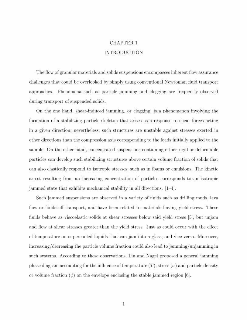
The flow of granular materials and solids suspensions encompasses inherent flow assurance

challenges that could be overlooked by simply using conventional Newtonian fluid transport

approaches. Phenomena such as particle jamming and clogging are frequently observed

during transport of suspended solids.

On the one hand, shear-induced jamming, or clogging, is a phenomenon involving the

formation of a stabilizing particle skeleton that arises as a response to shear forces acting

in a given direction; nevertheless, such structures are unstable against stresses exerted in

other directions than the compression axis corresponding to the loads initially applied to the

sample. On the other hand, concentrated suspensions containing either rigid or deformable

particles can develop such stabilizing structures above certain volume fraction of solids that

can also elastically respond to isotropic stresses, such as in foams or emulsions. The kinetic

arrest resulting from an increasing concentration of particles corresponds to an isotropic

jammed state that exhibits mechanical stability in all directions. [1–4].

Such jammed suspensions are observed in a variety of fluids such as drilling muds, lava

flow or foodstuff transport, and have been related to materials having yield stress. These

fluids behave as viscoelastic solids at shear stresses below said yield stress [5], but unjam

and flow at shear stresses greater than the yield stress. Just as could occur with the effect

of temperature on supercooled liquids that can jam into a glass, and vice-versa. Moreover,

increasing/decreasing the particle volume fraction could also lead to jamming/unjamming in

such systems. According to these observations, Liu and Nagel proposed a general jamming

phase diagram accounting for the influence of temperature (T ), stress (σ) and particle density

or volume fraction (φ) on the envelope enclosing the stable jammed region [6].

1

Both clogging and jamming phenomena represent potential plugging risks in subsea oil

& gas flowlines where solids, such as gas hydrate, can be present. Therefore, a sound risk

assessment of these phenomena in systems containing suspended solid particles could result

in optimized risk management strategies for offshore oil & gas production. Effective gas

hydrate management strategies could have a significant influence on the final investment

decision (FID) during the sanctioning process of new deepwater developments. Costs reduc-

tions in both capital (CAPEX) and operational (OPEX) expenditures could make a field

development economically viable by lowering the crude oil price associated with the break-

even point (BEP) of the project. Moreover, risk-based modifications of over-conservative

hydrate management strategies utilized in brown fields could result in an increased revenue

obtained from the operative assets.

Potential CAPEX reductions have been associated with a risk-based optimization of the

conventional hydrate management strategies utilized in offshore oil & gas production, for

example:

• Umbilicals size reduction after removing unnecessary injection lines for hydrate in-

hibitors

• Decreasing required space for chemical storage on the platform topsides

• Minimization of the pipeline thermal insulation

Similarly, a few critical areas offer attractive OPEX reduction opportunities, which are

related to a transition into risk-based hydrate management strategies, such as:

• Optimization of hydrate dispersant dosing schedule

• Suppression of unnecessary thermodynamic hydrate inhibitor injection in brown fields

with over-conservative design

• Simplification of planned shut-in/restart protocols wherever the intrinsic characteristics

of the systems help to prevent hydrate plugs

2

Both pilot- and bench-scale tests, in addition to computer-based experiments, have been

conducted to advance the understanding of the different mechanisms leading to the kinetic

arrest of suspended hydrate particles. These studies focused on two major plugging mecha-

nisms that can be observed during the transport of suspended solids, namely particle jam-

ming and particle clogging.

The equipment used to investigate the particle jamming phenomena resulting in materials

with a finite yield stress value included contact angle measurements, a high-pressure micro-

mechanical forces apparatus (HP-MMF), a high-pressure rheometer (HP-rheometer), a high-

pressure autoclave (HP-autoclave), and pilot-scale flowloop facilities located at both Tulsa

University and ExxonMobil. These equipment introduces a variety of experimental condi-

tions and data acquisition tools that combined can provide a comprehensive understanding

of hydrate plugging phenomena. The key objectives from these multiple length scale studies

included developing an experimental framework to quantitatively assess hydrate dispersant

performance and the subsequent comparison and and scaling of these results. However,

the aforementioned set of equipment also presents a series of limitations intrinsic to each

experimental technique. For example, MMF studies lacked shear forces and a fixed water

content of 10 vol.% was used. In contrast, the shear rate in the HP-rheometer tests was up

to an order of magnitude greater than those normally found in the field. Similarly, the shear

field in HP-autoclave cannot be properly defined, and pilot-scale flowloop facilities, despite

providing the closest scenario to field conditions, also introduce significant uncertainties that

can affect interpretation. These limitations hindered several potential quantitative compar-

isons across experimental scales, and should be considered during future experimental design

looking at multi-scale experimental results scaling regarding hydrate transportability.

These multi-scale experimental studies were meant to provide the industry with reliable

experimental workflows to assess hydrate plugging risk, whilst minimizing the required crude

oil sample. The outcomes presented in this manuscript showed that hydrate dispersant

performance from low-volume experimental methods, such as HP-MMF and water/hydrate

3

contact angle measurements, correlated with the observations from large-scale equipment

(e.g. pilot-scale flowloops).

On the other hand, particle clogging phenomenon at flow path constrictions was investi-

gated using a combination of bench-scale laboratory flowloop tests and numerical simulations

implementing the discrete element method (DEM). These studies intended to utilize the re-

sults from DEM simulations in a two-dimensional channel to provide a proof-of-concept for

the features observed during the bench-scale flowloop tests. Such features include the pres-

sure drop fluctuations observed during the intermittent flow of particles across a flow path

constriction. These fluctuations, which were related to the sudden changes in the particle

velocity near the restriction caused by the transient formation of stabilizing structures. Ki-

netic energy fluctuations from DEM simulations are hypothesized to be of the same nature

as the pressure drop fluctuations in the bench-scale flowloop studies; hence, providing a

feature that correlates with the formation of transient stabilizing structures, which can be

continuously monitored throughout the experiments. There are clear disconnects between

the experimental techniques used to investigate the clogging phenomena such as the system

dimension (i.e. two-dimensional and three-dimensional systems), the absence of the fluid

forces in the DEM simulations and the wall-to-restriction distance in each setup, many of

which were related to the limitations found in the respective systems. For that reason, no

direct comparison has been conducted between these equipment beyond the proof-of-concept

used to correlate the nature of the experimental observations.

These investigations intended to provide the foundation for a new generation of hydrate

plugging risk assessment tools based on continuous data monitoring and probabilistic models,

which can be ultimately more useful for the daily flow assurance activities. For instance, the

evolution with time of the pressure drop fluctuations in a specific region within a pipeline,

which is considered to be a potential clogging area, could function as an indicator of an

increasing clogging risk. Accordingly, continuous monitoring of the pressure drop in this

particular region utilizing the methods described in this thesis dissertation could be consid-

4

ered as a viable real-time tool to assess clogging risk. Potential limitations for the deployment

of these plugging risk analysis methods are related to multiple phenomena that can result in

pressure drop fluctuations, such as multiphase slugging and particle clogging. Appropriate

interpretation of the periodic pressure signals caused by these different phenomena becomes

fundamental for sound flow assurance risk monitoring based on such information.

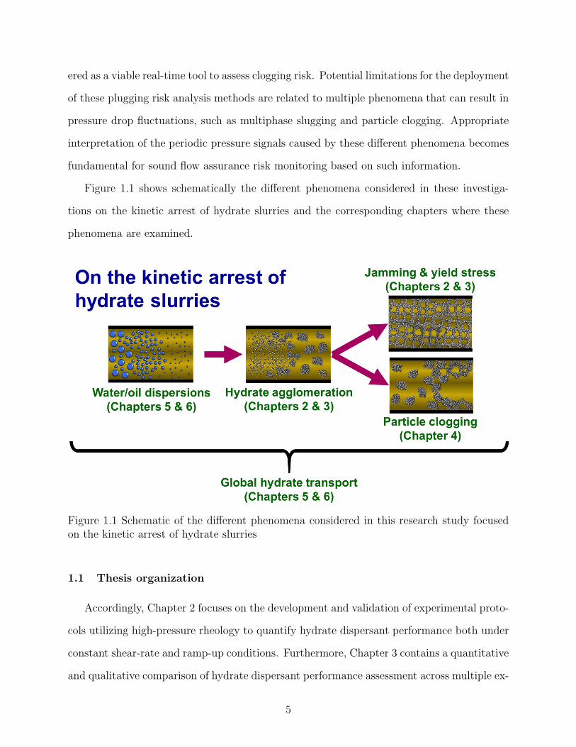
Figure 1.1 shows schematically the different phenomena considered in these investiga-

tions on the kinetic arrest of hydrate slurries and the corresponding chapters where these

phenomena are examined.

Figure 1.1 Schematic of the different phenomena considered in this research study focusedon the kinetic arrest of hydrate slurries

1.1 Thesis organization

Accordingly, Chapter 2 focuses on the development and validation of experimental proto-

cols utilizing high-pressure rheology to quantify hydrate dispersant performance both under

constant shear-rate and ramp-up conditions. Furthermore, Chapter 3 contains a quantitative

and qualitative comparison of hydrate dispersant performance assessment across multiple ex-

5

perimental scales from surface chemistry-based techniques, such as water/hydrate contact

angles or hydrate cohesive force measurements to pilot-scale studies in industrial flowloop

facilities. This collaborative multi-scale investigations also resulted in the scaling-up of the

hydrate cohesive forces obtained from HP-MMF tests by using particle network-based yield

stress models. Ultimately, the hydrate cohesive forces calculated from experimental HP-

rheometer yield stress measurements were compared with those from HP-MMF studies in

systems with similar fluid composition.

Chapter 4 presents a comprehensive characterization of the fluid-driven intermittent par-

ticle flow regime that precedes jamming onset. These studies provided insights into the

influence of multiple experimental parameters (e.g. fluid velocity or particle concentration

and size dispersion) on the jamming phenomena through the application of statistical tools

such as survival analysis. The results in this section correspond to both bench-scale flowloop

tests and DEM simulations intended to elucidate the key properties related to jamming oc-

currence during the intermittent flow of discrete bodies through a constriction, particularly

in the presence of fluid-related shear forces in the system.

Finally, Chapters 5 & 6 introduces a validation for the low-volume experimental tech-

niques proposed to assess hydrate dispersant performance by introducing results and analysis

from hydrate transportability studies in pilot-scale equipment, which provide a closer sce-

nario to actual oil & gas production flowlines. These studies allowed evaluating the influence

of parameters, such as mixture velocity, on the performance of hydrate dispersants using a

surfactant-free liquid hydrocarbon phase, both under flowing and static conditions. These

results include an evaluation of hydrate dispersant ability to prevent hydrate accumulation

and plugging in systems showing partial liquid/liquid dispersion before chemical injection. In

addition, hydrate transportability tests conducted using matching fluid composition and flow

conditions in different pilot-scale flowloop facilities provided novel insights into the influence

of the design parameters on the experimental outcome from hydrate transportability studies

conducted in different pilot-scale facilities. The content in Chapter 5 has been reprinted with

6

authorization from the Offshore Technology Conference and corresponds to 2017 Offshore

Technology Conference oral presentation with title ”Gas Hydrate Management Strategies

Using Anti-Agglomerants: Continuous & Transient Pilot-Scale Flowloop Studies”, and the

respective extended abstract (OTC-27621-MS) [131]. J. A. Dapena participated in the pilot-

scale flowloop data collection at ExxonMobil flowloop facilities, and carried-out both the

data analysis and the manuscript writing. V. Srivastava, and T. B. Charlton also took part

in the data collection at ExxonMobil and provided further suggestions and comments on the

results analysis and paper writing. Y. Wang provided the heat transfer coefficients for the

flowloop tests calculated from multiphase flow computational simulations. A. A. Gardner

carried out the water/oil dispersion tests. E. D. Sloan, L. E. Zerpa, D. T. Wu, C. A. Koh,

and A. A. Majid provided valuable guidance and input to this work. The corresponding

author of the paper is C. A. Koh.

7

CHAPTER 2

EXPERIMENTAL INVESTIGATION USING A HP-RHEOMETER TO QUANTIFY

HYDRATE DISPERSANT PERFORMANCE FOR ENERGY TRANSPORT &

STORAGE APPLICATIONS

Natural gas hydrates, which can encapsulate small hydrocarbon molecules in a volume

ratio up to 1:180 with respect to the standard temperature and pressure (STP) conditions,

represent an attractive alternative for safe cost-effective energy transport & storage. Ac-

cordingly, emerging technologies such as the solidified natural gas (SNG), which is based

on gas hydrate clathrates, represent a fitting solution to meet the increasing global en-

ergy demand whilst minimizing carbon dioxide emissions. However, successfully deploy-

ing such technologies requires developing a reliable energy transport method. Quaternary

ammonium-based surfactants, for example, can prevent naturally occurring hydrate particle

agglomeration; hence, leading to the formation of stable colloidal suspensions that constitute

flowable hydrate slurries. Current screening methods for hydrate dispersants, such as quater-

nary ammonium-based surfactants, are merely qualitative, which only provide a pass/failure

verdict. This work focused on developing an experimental framework and establishing suit-

able indicators to quantitatively evaluate the performance of methane hydrate dispersants

in both transient and steady-state conditions using high-pressure rheology. These exper-

imental studies involved a liquid hydrocarbon/water mixture as the carrier media dosed

at multiple concentrations with a variety of quaternary ammonium-based hydrate disper-

sants. The proposed performance indicator under constant shear rate conditions was able

to capture the influence of hydrate dispersant concentration, showing an increasing ratio of

effective-to-actual volume fraction of hydrates corresponding to a decreasing hydrate dis-

persant concentration. Moreover, yield stress values obtained from transient tests provided

further insights into the performance of these chemicals by considering the influence of shut-

8

in time. These transient tests allowed the comparison of experimentally obtained flow curves

with traditional rheological models for non-Newtonian fluids with a yield stress. Both the

Casson model (2 tunable parameters) and the Herschel-Bulkley model (3 tunable parameters)

showed similar agreement with experimentally obtained yield stress values. On the other

hand, the Bingham model (2 tunable parameters) resulted in much greater discrepancies.

Therefore, the Casson model, having one less tunable parameter than the Herschel-Bulkley

model, might provide a more fundamental description of the rheological behavior of hydrate

slurries. Finally, the tests involving shear stress-controlled ramps led to the highest yield

stress values among the transient experimental methods evaluated. These measurements

showing higher static than dynamic yield stress values suggest hydrate slurries behave as

thixotropic yield stress materials rather than ideal yield stress fluids. The experimental re-

sults and observations from these studies provide evidence to support high-pressure rheology

as a suitable screening technique to rank hydrate dispersant formulations. This technique

could advance chemical selection processes leading to optimal dosages for safe energy trans-

port using hydrate slurries. Ultimately, the quantitative assessment of hydrate dispersant

performance introduced in this paper could improve the cost-effectiveness of hydrate slurries

as a prospective media for energy transport & storage.

2.1 Introduction

Natural gas hydrates are solid inclusion compounds containing small hydrocarbon molecules

(i.e. “guest molecules”) within a crystalline network of water molecules. At given thermo-

dynamic conditions, the clathrate hydrate state becomes the most energetically favorable

configuration of a system. Depending upon the composition of the gas mixture containing

the hydrate formers or “guest molecules”, different hydrate structures can emerge (See Fig-

ure 2.1). Small hydrocarbons (e.g. methane and ethane) and carbon dioxide lead to the

formation of Structure I (sI) hydrates. On the other hand, longer hydrocarbons as propane

and iso-butane favor the formation of Structure II (sII) hydrates. Finally, certain gas mix-

tures, such as methane + neohexane or methane + cycloheptane, could result in the rather

9

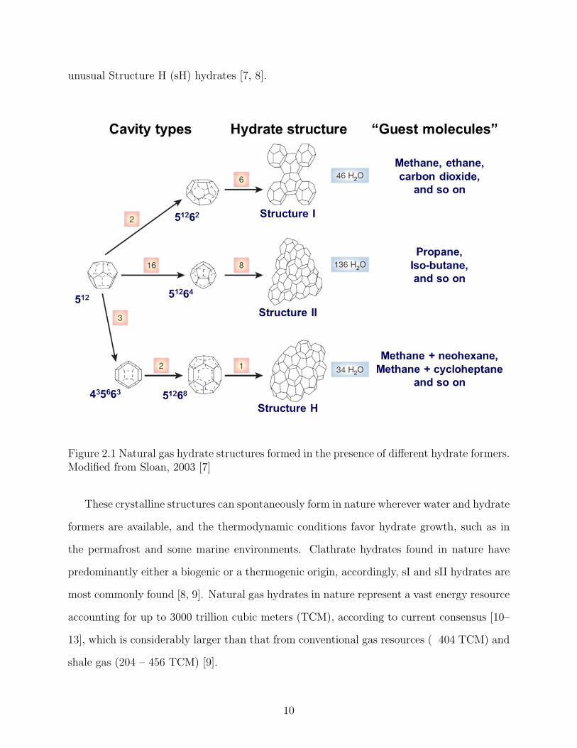
unusual Structure H (sH) hydrates [7, 8].

Figure 2.1 Natural gas hydrate structures formed in the presence of different hydrate formers.Modified from Sloan, 2003 [7]

These crystalline structures can spontaneously form in nature wherever water and hydrate

formers are available, and the thermodynamic conditions favor hydrate growth, such as in

the permafrost and some marine environments. Clathrate hydrates found in nature have

predominantly either a biogenic or a thermogenic origin, accordingly, sI and sII hydrates are

most commonly found [8, 9]. Natural gas hydrates in nature represent a vast energy resource

accounting for up to 3000 trillion cubic meters (TCM), according to current consensus [10–

13], which is considerably larger than that from conventional gas resources ( 404 TCM) and

shale gas (204 – 456 TCM) [9].

10

Remarkably, clathrate structures can efficiently store small hydrocarbon molecules (i.e.

methane, ethane, propane, etc.) at relatively mild conditions up to concentrations only ob-

served in highly compressed gases. Depending on the cage occupancy, hydrates can compress

natural gas volume up to 180 times relative to standard temperature and pressure (STP)

conditions, which roughly compares to the methane molecules concentration observed at 273

K and 180 bar [7]. These properties turn hydrates into a prospective media providing safe

and environmentally friendly transport and storage of energy, which could help to meet the

increasing global energetic demand. The energy demand growth will be particularly signif-

icant among emerging economies that are not members of the Organisation for Economic

Cooperation and Development (OECD), such as India and China, whose combined energy

demand is expected to increase by 112% between 2010 and 2040 [9].

Natural gas and natural gas plant liquids (NGPL) are expected to be the fossil fuels with

the highest production growth by 2050 according to the current projections from U.S. Energy

Administration, in part due to an increase in the natural gas-fired electricity generation [14].

In addition, natural gas represents the cleanest burning fossil fuel. Hence, developing safe and

effective natural gas storage and transportation technologies becomes crucial to maximize

energy efficiency in the coming years. The solidified natural gas (SNG) technology [15],

based on natural gas clathrates, provides a pathway for the development of an application

that takes advantage of the unique capabilities of gas hydrates for energy transport and

storage. Although significant advances have been accomplished, commercialization of the

SNG technology still requires finding answers to the remaining technical challenges related

to the hydrate formation, transport and storage processes.

The suspension of hydrate particles in a carrier fluid, leading to the formation of a

hydrate slurry, represents a viable alternative for energy transport using gas hydrates. In

addition, the latent heat associated with the hydrate formation/dissociation processes turns

hydrate slurries into a prospective option for efficient cold thermal energy storage using

micro-encapsulated phase change materials (MPCMs) [16–19]. However, the aggregative

11

nature of hydrate particles triggers multiple phenomena, such as viscosification, deposition,

and jamming, causing major transportability issues [20–22].

Deeper and longer subsea developments in the oil & gas industry stimulated the maturing

of novel hydrate management methods, such as the low-dosage hydrate inhibitors (LDHIs),

which include both kinetic hydrate inhibitors (KHIs) and hydrate dispersants [23–34]. In

general, dispersants or anti-agglomerants are chemical additives that prevent particle aggre-

gation by creating steric or electrostatic barriers that modify the inter-particle potential.

Preventing particle aggregation ultimately leads to increased suspension stability [35, 36].

Hydrate dispersants promote the formation of stable and transportable suspensions of hy-

drate particles; hence, preventing accumulation mechanisms such as bedding and deposition.

Several surface-active compounds, such as quaternary ammonium-based surfactants, have

shown affinity for the hydrate surface [37–39]. These chemicals, which can promote hydrate

particle dispersion, could enable the safe and cost-effective transport and storage of energy

using clathrate hydrates to encapsulate natural gas. However, reliable experimental work-

flows to characterize and compare the performance of these chemicals are required in order

to successfully deploy such technologies in the field. Solids suspensions, such as colloidal

systems, could present either flowing or arrested states upon the combined contribution

from multiple parameters including shear forces, solids volume fraction and particle-particle

interactions. High-pressure rheological studies provide suitable conditions to quantify the

crossed-effect of the aforementioned parameters on the hydrate dispersing performance of a

given chemical.

The main objectives of this experimental work were to: (i) establish a protocol to eval-

uate hydrate dispersant performance in constant shear rate conditions; (ii) compare the

different experimental methods to measure yield stress of hydrate slurries; (iii) evaluate the

flow behavior of hydrate slurries and compare against with established rheological models for

non-Newtonian fluids with a yield stress; and (iv) evaluate the influence of variables, such

as hydrate dispersant concentration, on the rheological properties of hydrate slurries. Both

12

the experimental results and the analysis presented in this paper intend to lead ultimately

to a more reliable assessment of the performance of hydrate dispersants in aqueous/liquid

hydrocarbon/gas hydrate systems. This manuscript contains a comprehensive review of

the phenomena involved in the transport of suspended solid particles, including rheolog-

ical modeling of solid suspensions and current methodologies used for hydrate dispersant

screening and selection; an experimental methodology section describing the high-pressure

rig and the procedures utilized in these studies; finally, a compendium of the key outcomes

obtained from this work, covering both constant shear rate and transient studies, as well as

the corresponding conclusions, are provided.

2.1.1 Flow and jamming in solid suspensions

In general, the transport of suspended solids poses greater challenges than traditional

fluids. The suspensions of interacting colloidal particles might undergo transitions from

“fluid-like” to “solid-like” states and become jammed materials with isotropic mechanical

stability. Jammed systems are considered “fragile matter” [1]; therefore, the self-stabilizing

structures can subsequently collapse by different means inherent to each particular system,

which introduce some kind of perturbation. For example, either the vibrations caused by

fluid flow or the defects in the stabilizing structures related to particle size dispersion can

lead to unjamming events that resume solid particle flow.

According to the universal jamming phase diagram shown in Figure 2.2, increasing stress

applied on the jammed material might bring the system outside the envelope enclosing

the jammed region, consequently, the colloidal suspension would unjam and resume flow.

Similarly, the likelihood of a colloidal suspension to be in a jammed state increases both

with increasing attractive forces between particles and with an increasing volume fraction of

solids in the system. Accordingly, the line separating the jammed and not-jammed regions

in the kbT/Fmax - σ/σ0 and 1/φ - σ/σ0 planes corresponds to the yield stress of the material

for a given temperature, interparticle attractive force, and solid volume fraction. In this

jamming phase diagram for weakly attractive colloidal suspensions the stress is normalized

13

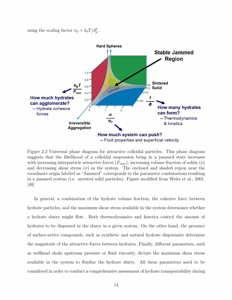
using the scaling factor σ0 = kbT/d3p .

Figure 2.2 Universal phase diagram for attractive colloidal particles. This phase diagramsuggests that the likelihood of a colloidal suspension being in a jammed state increaseswith increasing interparticle attractive forces (Fmax), increasing volume fraction of solids (φ)and decreasing shear stress (σ) in the system. The enclosed and shaded region near thecoordinate origin labeled as “Jammed” corresponds to the parameter combinations resultingin a jammed system (i.e. arrested solid particles). Figure modified from Weitz et al., 2001.[40]

In general, a combination of the hydrate volume fraction, the cohesive force between

hydrate particles, and the maximum shear stress available in the system determines whether

a hydrate slurry might flow. Both thermodynamics and kinetics control the amount of

hydrates to be dispersed in the slurry in a given system. On the other hand, the presence

of surface-active compounds, such as synthetic and natural hydrate dispersants determine

the magnitude of the attractive forces between hydrates. Finally, different parameters, such

as wellhead choke upstream pressure or fluid viscosity, dictate the maximum shear stress

available in the system to fluidize the hydrate slurry. All these parameters need to be

considered in order to conduct a comprehensive assessment of hydrate transportability during

14

both steady-state and transient operations.

2.1.2 Hydrate dispersant performance characterization

A comprehensive understanding of the mechanisms leading to efficient hydrate particle

transport would allow the successful deployment of innovative hydrate management strate-

gies, such as hydrate dispersants. Such understanding includes assessing the influence of

diverse operational parameters on the performance of these additives. These parameters

could include the gas-to-liquid ratio, hydrate sub-cooling, the composition of the aqueous

phase, and the hydrate dispersant formulation and dosing, for example. A better understand-

ing of the hydrate slurry rheological properties in systems dosed with hydrate dispersants

could help to extend the current operational envelope defining the safe limits for the use of

these chemicals.

Characterization tools are required to quantitatively assess the performance of hydrate

dispersant formulations. Multiple types of experimental equipment are available to investi-

gate hydrate slurry properties and transportability in a wide range of experimental condi-

tions. These experimental setups comprise several length scales, from the surface chemistry

level to pilot-scale facilities. These setups include equipment such as the micromechanical

force apparatus or MMF [41–46]; rocking cells [25, 38, 47–51]; rheometers [52–61]; auto-

claves [62–66]; and multiple scale flowloops [67–74]. Each experimental equipment type

introduces advantages and disadvantages with respect to other techniques. In addition,

molecular dynamics computational simulations have been used to investigate and predict

hydrate dispersant performance, including comparison with rocking cell results [37, 75–79].

The pilot-scale flowloops provide the closest scenario to pipelines; thus, they are con-

sidered the most suitable equipment to study hydrate transportability [68, 69, 80, 81]. In

addition to the similarities with respect to actual field conditions, pilot scale flowloops of-

fer several data acquisition tools yielding useful information for results analysis. However,

prohibitive maintenance and operation costs pose a limitation to conduct flowloop tests on

a regular basis as a chemical additive ranking and characterization tool. Moreover, large

15

flowloop sizes may cause uncertainties on the precise phenomena occurring throughout the

experiments, making the analysis of the results highly complex.

In contrast, high-pressure rheometers require relatively low maintenance, small sam-

ple volumes, and provide a high sensitivity to measure viscosity changes. These features

turn high-pressure rheometers into a cost-effective apparatus suitable to investigate hydrate

slurry properties and to quantitatively assess hydrate dispersant performance. Moreover,

high-pressure rheometers can provide insights into the slurry mechanical properties during

shut-in/restart operations. Previous studies have measured the yield stress of both ice and

hydrate slurries [58, 59, 61, 82–85]; however, such yield stress values have not been used to

quantitatively assess hydrate dispersant performance before. Nevertheless, rheological stud-

ies might raise concerns regarding flow pattern discrepancies with respect to pipeline scenar-

ios. Furthermore, high-pressure rheometers could present limitations to study low-stability

emulsions or systems where particle accumulation and deposition could cause heterogeneities

in the sample.

2.1.3 Rheology of concentrated solid suspensions and hydrate slurries

The rheological properties could be critical to assess the transportability of a hydrate

slurry in subsea pipelines. The rheological properties could be critical to assess the trans-

portability of a hydrate slurry in subsea pipelines. Newton’s constitutive law relates the

shear stress (σyx) to the velocity gradient or shear rate (γ) through a proportionality con-

stant (k), known as the consistency index or viscosity coefficient, according to Equation 2.1

[86]:

σyx = kdvxdy

= kγ (2.1)

Equation 2.1 applies to fluids of low molar mass, known as Newtonian fluids; however,

several fluids exhibit a non-linear shear stress response to the shear rate. This behavior

is commonly observed in fluids containing a structured network that could be gradually

destroyed by increasing shear forces. A power-law constitutive equation has been proposed

16

to describe the shear stress response to shear rate in non-Newtonian fluids according to

Equation 2.2,

σ = kγn (2.2)

where n is the power law index or flow index. A flow index n < 1 corresponds to a

shear-thinning fluid (i.e. fluids with a decreasing apparent viscosity at high shear rates, such

as gels or concentrated emulsions). On the other hand, a flow index n > 1 corresponds to

shear-thickening fluids (i.e. correspond to fluids that become more viscous at high shear

rates, such as cornstarch solutions).

Furthermore, as the imposed shear rate tends to zero, some fluids show finite non-zero

shear stress denoted as the yield stress of the sample. The Bingham model describes a

fluid that behaves as a solid at shear stresses lower than the yield stress (σy); yet, shows

a Newtonian behavior at shear stress values greater than the yield stress (i.e. Bingham

fluids). The Bingham model can be considered as a specific case within the more general

Hershel-Bulkley model, which extends the scope to include non-Newtonian fluids with yield

stress. Equation 2.3 shows the Hershel-Bulkley model.

σ = σy + kγn (2.3)

Equation 2.3 with an n value equal to 1 reduces to the simple Bingham model. There

are additional constitutive equations commonly used to describe non-Newtonian fluids with

a yield stress, such as Equation 2.4.

σn = σny + kγn (2.4)

Equation 2.4 with a flow index equal to 1/2 (i.e. n = 1/2) becomes the Casson model,

which successfully describes fluids that are shear thinning at low shear rates, such as blood

[87].

The suspensions of solid particles introduce further rheological complexities. Most studies

focused on the relative viscosity of the suspension (ηr) with respect to the pure carrier fluid

viscosity (ηfluid), as a function of the solid volume fraction in the suspension (φ), leading to

17

an expression with a general form like Equation 2.5 [88]:

ηr =ηsuspensionηfluid

= f(φ) (2.5)

Rather than a universal expression for f(φ), several theoretical and empirical models are

available depending on the range of particle volume fractions relevant for each specific case.

Three different regimes are observed for f(φ) [89, 90]:

• A dilute regime φ ≤ 0.01 − 0.02 showing both a Newtonian behavior and a linear

dependence on φ

• A semi-dilute regime 0.02 ≤ φ ≤ 0.25 where the relative viscosity dependence on φ

becomes non-linear, yet the aforementioned Newtonian behavior remains

• Finally, a concentrated regime arises at φ ≥ 0.25 leading to abrupt relative viscosity

increments with increasing solids volume fraction, as well as the emergence of non-

Newtonian features, such as yield stress or shear-thinning behavior

Based on the hydrodynamics involved in fluid flow around individual particles, Einstein

obtained an analytical solution for the bulk viscosity of dilute suspensions of neutrally buoy-

ant hard spheres in a viscous liquid according to Equation 2.6. The first order term account-

ing for the particle concentration effects O(φ), also known as the “Einstein coefficient” (B),

reduces to a value of 5/2 [89, 91–96]. The second order term related to the particle volume

fraction O(φ2) was calculated much later by Batchelor and Green [97, 98], and depends upon

the flow field and the particle-particle hydrodynamic interactions.

ηr = 1 +Bφ+O(φ2) (2.6)

Nevertheless, concentrated suspensions of solid particles can exhibit non-Newtonian rhe-

ological properties; hence, the viscosity concept established for homogeneous fluids may not

apply to systems containing dispersed solids [99–101]. The initial dimensional analysis con-

ducted by Krieger & Dougherty for a suspension of small rigid monodisperse spheres in a

Newtonian fluid considers that, at any given moment, there would be pairs of spheres with

18

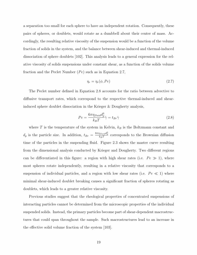
a separation too small for each sphere to have an independent rotation. Consequently, these

pairs of spheres, or doublets, would rotate as a dumbbell about their center of mass. Ac-

cordingly, the resulting relative viscosity of the suspension would be a function of the volume

fraction of solids in the system, and the balance between shear-induced and thermal-induced

dissociation of sphere doublets [102]. This analysis leads to a general expression for the rel-

ative viscosity of solids suspensions under constant shear, as a function of the solids volume

fraction and the Peclet Number (Pe) such as in Equation 2.7,

ηr = ηr(φ, Pe) (2.7)

The Peclet number defined in Equation 2.8 accounts for the ratio between advective to

diffusive transport rates, which correspond to the respective thermal-induced and shear-

induced sphere doublet dissociation in the Krieger & Dougherty analysis,

Pe =6πηfluidd

3p

kBTγ = tBrγ (2.8)

where T is the temperature of the system in Kelvin, kB is the Boltzmann constant and

dp is the particle size. In addition, tBr =6πηfluidd

3p

kBTcorresponds to the Brownian diffusion

time of the particles in the suspending fluid. Figure 2.3 shows the master curve resulting

from the dimensional analysis conducted by Krieger and Dougherty. Two different regions

can be differentiated in this figure: a region with high shear rates (i.e. Pe ≫ 1), where

most spheres rotate independently, resulting in a relative viscosity that corresponds to a

suspension of individual particles, and a region with low shear rates (i.e. Pe ≪ 1) where

minimal shear-induced doublet breaking causes a significant fraction of spheres rotating as

doublets, which leads to a greater relative viscosity.

Previous studies suggest that the rheological properties of concentrated suspensions of

interacting particles cannot be determined from the microscopic properties of the individual

suspended solids. Instead, the primary particles become part of shear-dependent macrostruc-

tures that could span throughout the sample. Such macrostructures lead to an increase in

the effective solid volume fraction of the system [103].

19

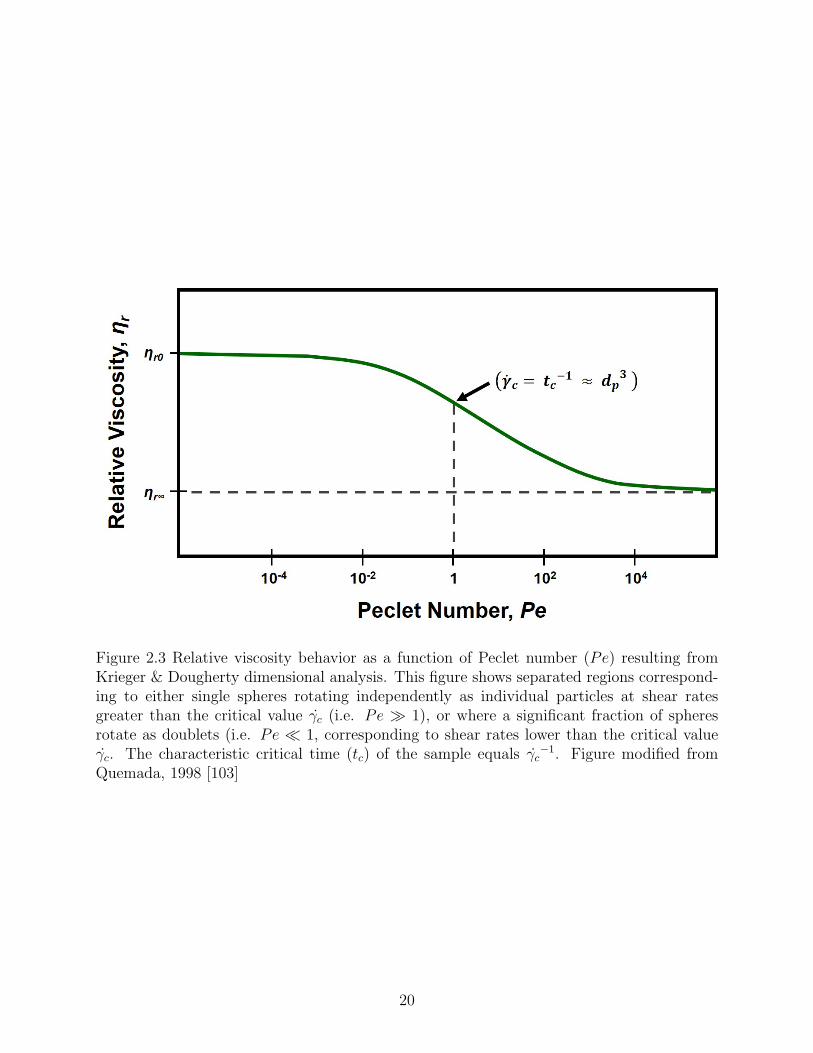
Figure 2.3 Relative viscosity behavior as a function of Peclet number (Pe) resulting fromKrieger & Dougherty dimensional analysis. This figure shows separated regions correspond-ing to either single spheres rotating independently as individual particles at shear ratesgreater than the critical value γc (i.e. Pe ≫ 1), or where a significant fraction of spheresrotate as doublets (i.e. Pe ≪ 1, corresponding to shear rates lower than the critical valueγc. The characteristic critical time (tc) of the sample equals γc

−1. Figure modified fromQuemada, 1998 [103]

20

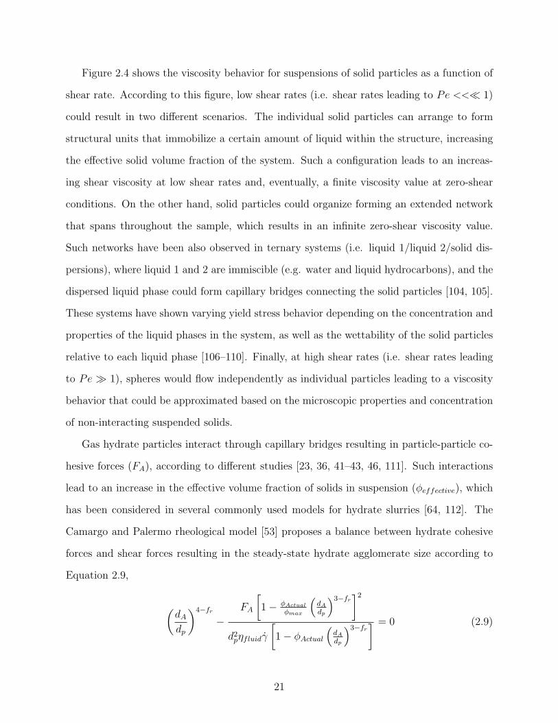
Figure 2.4 shows the viscosity behavior for suspensions of solid particles as a function of

shear rate. According to this figure, low shear rates (i.e. shear rates leading to Pe <<≪ 1)

could result in two different scenarios. The individual solid particles can arrange to form

structural units that immobilize a certain amount of liquid within the structure, increasing

the effective solid volume fraction of the system. Such a configuration leads to an increas-

ing shear viscosity at low shear rates and, eventually, a finite viscosity value at zero-shear

conditions. On the other hand, solid particles could organize forming an extended network

that spans throughout the sample, which results in an infinite zero-shear viscosity value.

Such networks have been also observed in ternary systems (i.e. liquid 1/liquid 2/solid dis-

persions), where liquid 1 and 2 are immiscible (e.g. water and liquid hydrocarbons), and the

dispersed liquid phase could form capillary bridges connecting the solid particles [104, 105].

These systems have shown varying yield stress behavior depending on the concentration and

properties of the liquid phases in the system, as well as the wettability of the solid particles

relative to each liquid phase [106–110]. Finally, at high shear rates (i.e. shear rates leading

to Pe ≫ 1), spheres would flow independently as individual particles leading to a viscosity

behavior that could be approximated based on the microscopic properties and concentration

of non-interacting suspended solids.

Gas hydrate particles interact through capillary bridges resulting in particle-particle co-

hesive forces (FA), according to different studies [23, 36, 41–43, 46, 111]. Such interactions

lead to an increase in the effective volume fraction of solids in suspension (φeffective), which

has been considered in several commonly used models for hydrate slurries [64, 112]. The

Camargo and Palermo rheological model [53] proposes a balance between hydrate cohesive

forces and shear forces resulting in the steady-state hydrate agglomerate size according to

Equation 2.9,

(

dAdp

)4−fr

−

FA

[

1− φActual

φmax

(

dAdp

)3−fr]2

d2pηfluidγ

[

1− φActual

(

dAdp

)3−fr] = 0 (2.9)

21

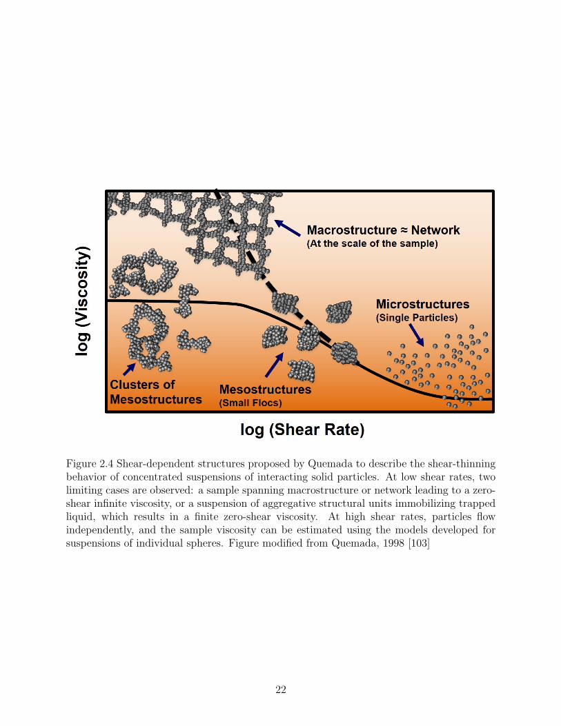
Figure 2.4 Shear-dependent structures proposed by Quemada to describe the shear-thinningbehavior of concentrated suspensions of interacting solid particles. At low shear rates, twolimiting cases are observed: a sample spanning macrostructure or network leading to a zero-shear infinite viscosity, or a suspension of aggregative structural units immobilizing trappedliquid, which results in a finite zero-shear viscosity. At high shear rates, particles flowindependently, and the sample viscosity can be estimated using the models developed forsuspensions of individual spheres. Figure modified from Quemada, 1998 [103]

22

where dp and dA are the hydrate primary particle and aggregate size respectively, fr is

the fractal dimension of the hydrate aggregates, φActual is the hydrate volume fraction, and

φmax = 4/7 is the maximum volume fraction of solids, which corresponds to the loose random

packing of monodisperse spheres.

Finally, the resulting size ratio of aggregates to primary hydrate particles, combined with

the fractal nature of the hydrate aggregates, leads to the effective volume fraction of solids

in suspension as shown in Equation 2.10:

φeffectiveφActual

=

(

dAdp

)3−fr

(2.10)

2.1.4 Rheological characterization of yield stress materials

In general, yield stress materials could be divided into different categories. Some ma-

terials, such as colloidal gels or suspensions of fractal aggregates, require to break down of

an internal percolated structure in order to flow. These structures progressively degrade

under the high shear stresses leading to lower viscosity over time; however, at low shear

stresses, such percolating structures might rebuild and lead to an increase in both viscos-

ity and yield stress. These phenomena, known as shear rejuvenation and aging, result in

“thixotropic” yield stress materials, which might require higher shear stress to initiate flow

than to maintain it. Accordingly, different yield stress values can be obtained depending

upon the experimental methodology used, which corresponds to either the “static” yield

stress (i.e. required shear stress to initiate flow) or the “dynamic” yield stress (i.e. shear

stress at which flow stops) [113].

On the other hand, materials with dense packing of soft particles, such as foams or

concentrated emulsions, do not show rejuvenation, nor aging. These systems, considered as

ideal yield stress materials, do not flow at all if the applied shear stress is below the yield

stress [5, 114]. In general, according to the percolation theory, the sample yield strength

arises at solid volume fractions greater than the percolation threshold (φc) [115, 116]. Such

a percolation threshold could be material and history dependent.

23

Multiple experimental methods allow measuring static and dynamic yield stress values.

These rheological methods consist of both direct and indirect measurements. Direct yield

stress measurement techniques include the vane method developed by Nguyen and Boger

to measure flow properties of non-Newtonian fluids, such as concentrated suspensions and

“structured liquids” [5, 117]. Oscillatory amplitude sweeps could also provide a direct mea-

surement of the yield stress based on the elastic and viscous moduli crossover (i.e. maximum

elastic stress) [118, 119]. Shear stress ramps have also been used to measure the static yield

stress of a sample by examining the intersection of the two linear regions in a shear rate

versus shear stress log-log plot [87, 119]. Indirect methods are also available to determine

either the dynamic or the static yield stress of a sample. These indirect methods use different

rheological models fitted to experimental data from increasing/decreasing shear rate/stress

ramps to extrapolate the shear stress data to near zero shear rate values (i.e. intercept with

the ordinate) [120–123]. Several of these methods provide insights into phenomena such as

thixotropy and fluidization profiles, in addition to the measurement of the yield stress of a

sample [87].

2.2 Experimental methods

The performance of a variety of hydrate dispersant formulations dosed at multiple con-

centrations was quantitatively evaluated using both continuous and transient high-pressure

rheological measurements. Previous studies showed hydrate particles could be successfully

dispersed and transported in a liquid hydrocarbon phase using low-dosage hydrate inhibitors

[26, 29, 124]. In addition, increasing salinity was shown to enhance ionic hydrate dispersant

performance [77, 125]. Accordingly, the fluid composition for these high-pressure rheological

studies consists of a liquid phase constituted by 50 vol.% of a liquid hydrocarbon mixture,

and 50 vol.% of an aqueous solution containing 3.5 wt.% sodium chloride (NaCl). The liquid

phase was pressurized using methane (CH4) gas, which leads to the formation of structure

I hydrates. Finally, the hydrate dispersants were dosed with respect to the total volume of

the aqueous phase in the system.

24

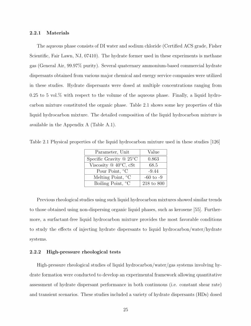
2.2.1 Materials

The aqueous phase consists of DI water and sodium chloride (Certified ACS grade, Fisher

Scientific, Fair Lawn, NJ, 07410). The hydrate former used in these experiments is methane

gas (General Air, 99.97% purity). Several quaternary ammonium-based commercial hydrate

dispersants obtained from various major chemical and energy service companies were utilized

in these studies. Hydrate dispersants were dosed at multiple concentrations ranging from

0.25 to 5 vol.% with respect to the volume of the aqueous phase. Finally, a liquid hydro-

carbon mixture constituted the organic phase. Table 2.1 shows some key properties of this

liquid hydrocarbon mixture. The detailed composition of the liquid hydrocarbon mixture is

available in the Appendix A (Table A.1).

Table 2.1 Physical properties of the liquid hydrocarbon mixture used in these studies [126]

Parameter, Unit Value

Specific Gravity @ 25◦C 0.863Viscosity @ 40◦C, cSt 68.5

Pour Point, ◦C -9.44Melting Point, ◦C -60 to -9Boiling Point, ◦C 218 to 800

Previous rheological studies using such liquid hydrocarbon mixtures showed similar trends

to those obtained using non-dispersing organic liquid phases, such as kerosene [55]. Further-

more, a surfactant-free liquid hydrocarbon mixture provides the most favorable conditions

to study the effects of injecting hydrate dispersants to liquid hydrocarbon/water/hydrate

systems.

2.2.2 High-pressure rheological tests

High-pressure rheological studies of liquid hydrocarbon/water/gas systems involving hy-

drate formation were conducted to develop an experimental framework allowing quantitative

assessment of hydrate dispersant performance in both continuous (i.e. constant shear rate)

and transient scenarios. These studies included a variety of hydrate dispersants (HDs) dosed

25

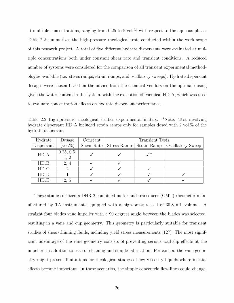
at multiple concentrations, ranging from 0.25 to 5 vol.% with respect to the aqueous phase.

Table 2.2 summarizes the high-pressure rheological tests conducted within the work scope

of this research project. A total of five different hydrate dispersants were evaluated at mul-

tiple concentrations both under constant shear rate and transient conditions. A reduced

number of systems were considered for the comparison of all transient experimental method-

ologies available (i.e. stress ramps, strain ramps, and oscillatory sweeps). Hydrate dispersant

dosages were chosen based on the advice from the chemical vendors on the optimal dosing

given the water content in the system, with the exception of chemical HD A, which was used

to evaluate concentration effects on hydrate dispersant performance.

Table 2.2 High-pressure rheological studies experimental matrix. *Note: Test involvinghydrate dispersant HD A included strain ramps only for samples dosed with 2 vol.% of thehydrate dispersant

Hydrate Dosage Constant Transient TestsDispersant (vol.%) Shear Rate Stress Ramp Strain Ramp Oscillatory Sweep

HD A0.25, 0.5,

X X X*1, 2

HD B 2, 4 X X

HD C 2 X X X

HD D 1 X X X X

HD E 2, 5 X X X X

These studies utilized a DHR-2 combined motor and transducer (CMT) rheometer man-

ufactured by TA instruments equipped with a high-pressure cell of 30.8 mL volume. A

straight four blades vane impeller with a 90 degrees angle between the blades was selected,

resulting in a vane and cup geometry. This geometry is particularly suitable for transient

studies of shear-thinning fluids, including yield stress measurements [127]. The most signif-

icant advantage of the vane geometry consists of preventing serious wall-slip effects at the

impeller, in addition to ease of cleaning and simple fabrication. Per contra, the vane geom-

etry might present limitations for rheological studies of low viscosity liquids where inertial

effects become important. In these scenarios, the simple concentric flow-lines could change,

26

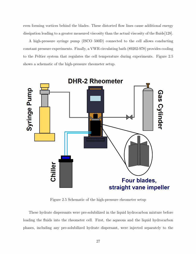
even forming vortices behind the blades. These distorted flow lines cause additional energy

dissipation leading to a greater measured viscosity than the actual viscosity of the fluids[128].

A high-pressure syringe pump (ISCO 500D) connected to the cell allows conducting

constant pressure experiments. Finally, a VWR circulating bath (89202-978) provides cooling

to the Peltier system that regulates the cell temperature during experiments. Figure 2.5

shows a schematic of the high-pressure rheometer setup.

Figure 2.5 Schematic of the high-pressure rheometer setup

These hydrate dispersants were pre-solubilized in the liquid hydrocarbon mixture before

loading the fluids into the rheometer cell. First, the aqueous and the liquid hydrocarbon

phases, including any pre-solubilized hydrate dispersant, were injected separately to the

27

high-pressure rheometer cell. Next, a 30-minute homogenization stage at 20◦C, atmospheric

pressure, and constant shear rate was conducted before pressurizing the system. Bottle tests

carried out at room temperature and pressure, and low shear rate conditions showed that the

samples dosed with the different hydrate dispersant formulations, which are surface-active

compounds, resulted in homogeneous dispersions.

2.2.2.1 Constant shear rate rheological studies

High-pressure rheological studies can be divided into two sections: constant shear rate

and transient tests. Constant shear rate tests constitute the initial stages, which include

a dynamic cool down leading to hydrate formation. These tests allow assessment of the

hydrate slurry rheological properties, such as viscosity, under flowing conditions. In addition,

constant shear rate tests provide insights into dynamic changes in such rheological properties

over time due to the influence of shear stresses.

Once the liquid sample was loaded into the high-pressure cell, the system was pressurized

up to 103.42 bar. This pressure was maintained constant throughout the experiments using

an automated syringe pump. A 4.5-hour step at a constant shear rate and 20◦C followed,

which allows gas saturation of the liquid sample. After saturation, a dynamic cooldown

from 20◦C to 1◦C with a 0.5◦C/min cooling rate was conducted and followed by a constant

temperature stage, which encompassed the hydrate formation period. The constant tem-

perature stage continued until both the gas consumption due to hydrate formation ceased

and the sample viscosity stabilized. Combined temperature and pressure experimental con-

ditions (i.e. 1◦C and 103.42 bar) resulted in 10.8◦C subcooling before the hydrate onset,

which constitutes the initial driving force for hydrate formation in the system. Such sub-

cooling gradually decreases as water converts into hydrate and the concentration of salt in

the aqueous phase increases. Note: the hydrate equilibrium conditions were determined

using Multiflash®. A series of transient experiments, which are described in detail in Sec-

tion 2.2.2.2, was conducted after the system reached equilibrium under constant shear rate

conditions. Finally, a heating stage from 1◦C to 20◦C with a heating rate of 0.5◦C/min, and

28

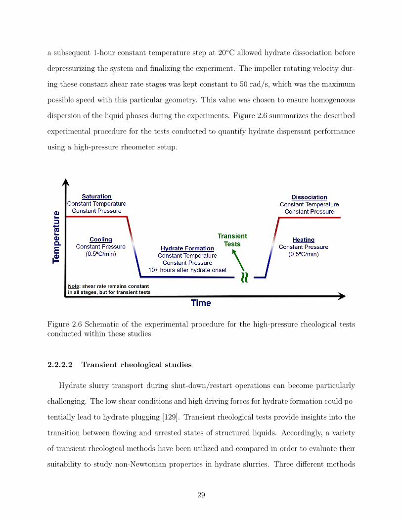
a subsequent 1-hour constant temperature step at 20◦C allowed hydrate dissociation before

depressurizing the system and finalizing the experiment. The impeller rotating velocity dur-

ing these constant shear rate stages was kept constant to 50 rad/s, which was the maximum

possible speed with this particular geometry. This value was chosen to ensure homogeneous

dispersion of the liquid phases during the experiments. Figure 2.6 summarizes the described

experimental procedure for the tests conducted to quantify hydrate dispersant performance

using a high-pressure rheometer setup.

Figure 2.6 Schematic of the experimental procedure for the high-pressure rheological testsconducted within these studies

2.2.2.2 Transient rheological studies

Hydrate slurry transport during shut-down/restart operations can become particularly

challenging. The low shear conditions and high driving forces for hydrate formation could po-

tentially lead to hydrate plugging [129]. Transient rheological tests provide insights into the

transition between flowing and arrested states of structured liquids. Accordingly, a variety

of transient rheological methods have been utilized and compared in order to evaluate their

suitability to study non-Newtonian properties in hydrate slurries. Three different methods

29

were considered in these studies: Shear stress ramps, shear rate-controlled flow curves, and

oscillatory tests (amplitude or stress sweeps). These different methods provide a measure-

ment of either dynamic or static yield stress values, as discussed in Section 2.1.4. In addition,

an in-house Python code (See Supplementary Information) was developed to automatically

analyze transient test results and to compare such results with traditional non-Newtonian

rheological models using error minimization tools.

Shear stress-controlled ramps Logarithmic shear stress ramps from 0.01 to 2500 Pa

(maximum stress allowed by the equipment) were conducted over a 1.5 h period, with a data

collection of 20 points per every tenfold increase. These tests provide a static yield stress

value measurement corresponding to a transition from rest to a flowing state. A sudden

increase in the measured shear rate (see Figure 2.7, left) indicates the fluidization of the

sample at a given shear stress value (i.e. the yield stress) [85, 119]. This experimental

technique allows evaluating the influence of the shut-in time on the sample yield stress

by conducting the shear stress ramps after a zero-shear stress period of a given duration.

Figure 2.7 (left) also highlights reproducibility in the yield stress measurements using this

experimental technique.

Shear rate-controlled flow curves Both increasing and decreasing logarithmic shear

rate ramps were conducted from 0.01 to 450 s-1 and vice versa, with 20 data points being

collected per every tenfold increase. Each data point allowed for a 30 seconds equilibration

stage before starting the measure and 60 seconds averaging time to collect the data. These

tests allowed detecting hysteresis in the sample depending upon the experimental path and

provided insights into shear-banding and wall slip phenomena during data collection. In

addition, non-Newtonian rheological models, such as Hershel-Bulkley or Casson, can be

compared the experimental results obtained from these measurements [84, 130]. Dynamic

yield stress values, corresponding to the ordinate intercept (i.e. zero shear viscosity) in

Figure 2.7 (center), are calculated using the rheological models discussed in Section 2.1.3.

30

Shear rate-controlled flow curves Logarithmic oscillation amplitude sweeps from

0.01 to 2500 Pa were conducted with 20 data points being collected per every tenfold in-

crease. Two oscillation frequencies, 0.1 and 1 Hz, were utilized for these measurements. The

interception between the storage modulus (G’) and loss modulus (G”) indicates fluidization

and correspons to the sample yield stress, providing the storage modulus was greater than

the loss modulus at low oscillation stresses (see Figure 2.7, right). This method provides

insights into the structural properties of the hydrate slurry sample in the absence of shear

stresses.

These transient studies were conducted at the same pressure and temperature conditions

set for hydrate formation in the constant shear rate tests described in Section 2.2.2.1. In

addition, every independent transient test included a 1-hour homogenization stage at 50

rad/s between consecutive measurements. This stage allowed the sample to recover the

steady-state rheological properties reached during the constant shear rate studies that pre-

ceded. In tests involving a shut-in stage, the shear stress was set to 0 Pa, while the pressure

and temperature remained constant. Multiple shut-in times ranging from 0 to 8 hours were

evaluated.

2.3 Results and discussion

The performance of hydrate dispersants was investigated using a high-pressure rheometer

setup. These studies allowed establishing performance indicators under different conditions,

which can quantify the influence of variables such as hydrate dispersant concentration and

formulation on hydrate transportability. The high-pressure rheological experiments were di-

vided into two sections, namely constant shear rate and transient tests, providing insights

into the performance of hydrate dispersants in both steady-state and transient flowing con-

ditions.

31

Figure 2.7 Typical experimental results and the corresponding yield stress indicator fromthe different transient rheological tests conducted in these studies. Left: shear rate versusshear stress profile from shear stress-controlled ramps. The sudden increase in the shear rateindicates fluidization. Results correspond to a system dosed with 1 vol.% hydrate dispersantHD A and with a shear stress ramp conducted immediately after the homogenization stage(i.e. 0-hour shut-in). Center: shear stress versus shear rate flow curves from shear rate-controlled tests, including both increasing and decreasing shear-rate ramps. Yield stresscorresponds to the intercept with the ordinate (i.e. zero shear viscosity). These resultscorrespond to a system dosed with 1 vol.% hydrate dispersant HD A. Right: Storage modulus(solid markers) and loss modulus (hollow markers) versus oscillation stress from oscillatorystress sweeps. The yield stress corresponds to the oscillation stress at the intercept betweenthe storage and loss modulus. These results correspond to systems dosed with 2 vol.%hydrate dispersant HD D

32

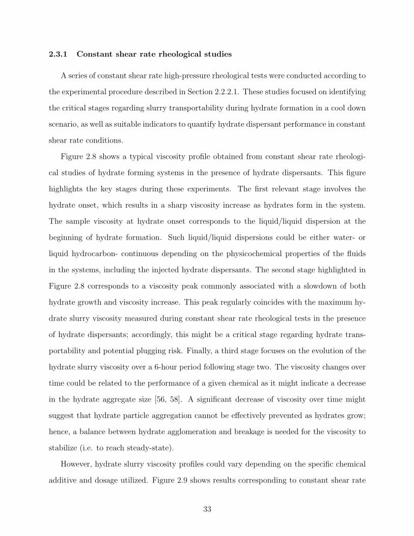
2.3.1 Constant shear rate rheological studies

A series of constant shear rate high-pressure rheological tests were conducted according to

the experimental procedure described in Section 2.2.2.1. These studies focused on identifying

the critical stages regarding slurry transportability during hydrate formation in a cool down

scenario, as well as suitable indicators to quantify hydrate dispersant performance in constant

shear rate conditions.

Figure 2.8 shows a typical viscosity profile obtained from constant shear rate rheologi-

cal studies of hydrate forming systems in the presence of hydrate dispersants. This figure

highlights the key stages during these experiments. The first relevant stage involves the

hydrate onset, which results in a sharp viscosity increase as hydrates form in the system.

The sample viscosity at hydrate onset corresponds to the liquid/liquid dispersion at the

beginning of hydrate formation. Such liquid/liquid dispersions could be either water- or

liquid hydrocarbon- continuous depending on the physicochemical properties of the fluids

in the systems, including the injected hydrate dispersants. The second stage highlighted in

Figure 2.8 corresponds to a viscosity peak commonly associated with a slowdown of both

hydrate growth and viscosity increase. This peak regularly coincides with the maximum hy-

drate slurry viscosity measured during constant shear rate rheological tests in the presence

of hydrate dispersants; accordingly, this might be a critical stage regarding hydrate trans-

portability and potential plugging risk. Finally, a third stage focuses on the evolution of the

hydrate slurry viscosity over a 6-hour period following stage two. The viscosity changes over

time could be related to the performance of a given chemical as it might indicate a decrease

in the hydrate aggregate size [56, 58]. A significant decrease of viscosity over time might

suggest that hydrate particle aggregation cannot be effectively prevented as hydrates grow;

hence, a balance between hydrate agglomeration and breakage is needed for the viscosity to

stabilize (i.e. to reach steady-state).

However, hydrate slurry viscosity profiles could vary depending on the specific chemical

additive and dosage utilized. Figure 2.9 shows results corresponding to constant shear rate

33

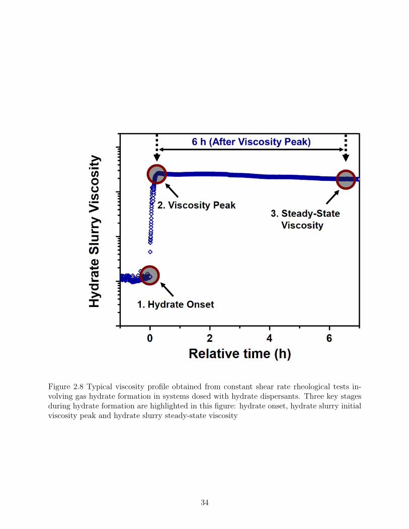
Figure 2.8 Typical viscosity profile obtained from constant shear rate rheological tests in-volving gas hydrate formation in systems dosed with hydrate dispersants. Three key stagesduring hydrate formation are highlighted in this figure: hydrate onset, hydrate slurry initialviscosity peak and hydrate slurry steady-state viscosity

34

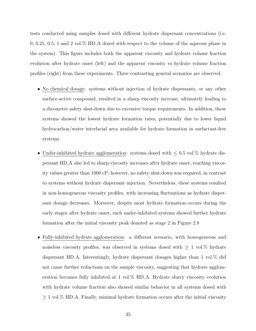
tests conducted using samples dosed with different hydrate dispersant concentrations (i.e.

0, 0.25, 0.5, 1 and 2 vol.% HD A dosed with respect to the volume of the aqueous phase in

the system). This figure includes both the apparent viscosity and hydrate volume fraction

evolution after hydrate onset (left) and the apparent viscosity vs hydrate volume fraction

profiles (right) from these experiments. Three contrasting general scenarios are observed:

• No chemical dosage: systems without injection of hydrate dispersants, or any other

surface-active compound, resulted in a sharp viscosity increase, ultimately leading to

a rheometer safety shut-down due to excessive torque requirements. In addition, these

systems showed the lowest hydrate formation rates, potentially due to lower liquid

hydrocarbon/water interfacial area available for hydrate formation in surfactant-free

systems

• Under-inhibited hydrate agglomeration: systems dosed with ≤ 0.5 vol.% hydrate dis-

persant HD A also led to sharp viscosity increases after hydrate onset, reaching viscos-

ity values greater than 1000 cP; however, no safety shut-down was required, in contrast

to systems without hydrate dispersant injection. Nevertheless, these systems resulted

in non-homogeneous viscosity profiles, with increasing fluctuations as hydrate disper-

sant dosage decreases. Moreover, despite most hydrate formation occurs during the

early stages after hydrate onset, such under-inhibited systems showed further hydrate

formation after the initial viscosity peak denoted as stage 2 in Figure 2.8

• Fully-inhibited hydrate agglomeration: a different scenario, with homogeneous and

noiseless viscosity profiles, was observed in systems dosed with ≥ 1 vol.% hydrate

dispersant HD A. Interestingly, hydrate dispersant dosages higher than 1 vol.% did

not cause further reductions on the sample viscosity, suggesting that hydrate agglom-

eration becomes fully inhibited at 1 vol.% HD A. Hydrate slurry viscosity evolution

with hydrate volume fraction also showed similar behavior in all systems dosed with

≥ 1 vol.% HD A. Finally, minimal hydrate formation occurs after the initial viscosity

35

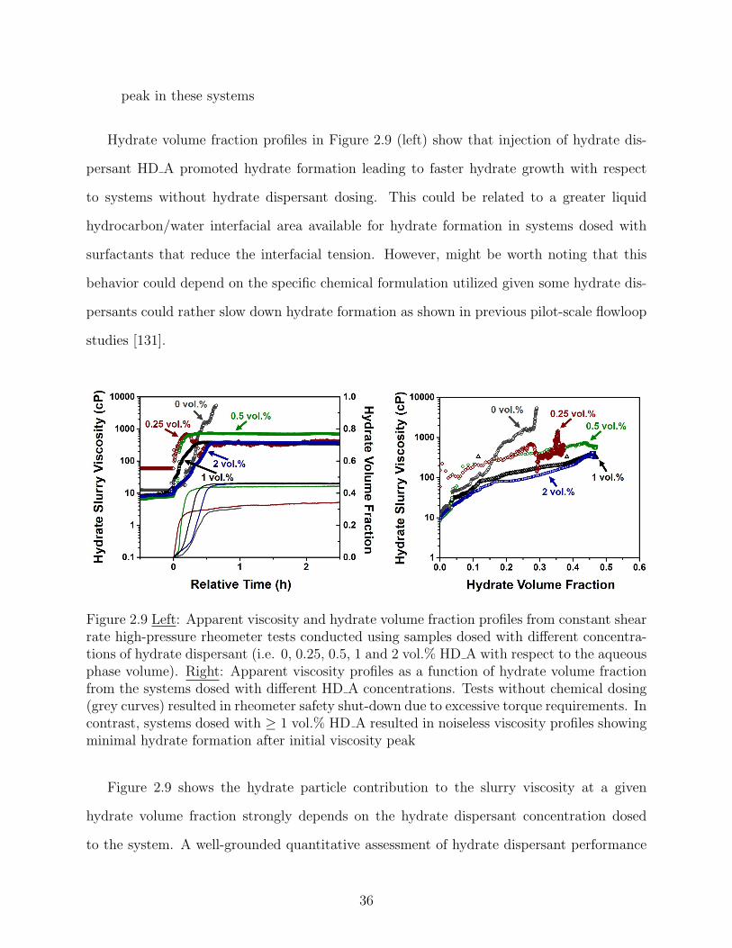
peak in these systems

Hydrate volume fraction profiles in Figure 2.9 (left) show that injection of hydrate dis-

persant HD A promoted hydrate formation leading to faster hydrate growth with respect

to systems without hydrate dispersant dosing. This could be related to a greater liquid

hydrocarbon/water interfacial area available for hydrate formation in systems dosed with

surfactants that reduce the interfacial tension. However, might be worth noting that this

behavior could depend on the specific chemical formulation utilized given some hydrate dis-

persants could rather slow down hydrate formation as shown in previous pilot-scale flowloop

studies [131].

Figure 2.9 Left: Apparent viscosity and hydrate volume fraction profiles from constant shearrate high-pressure rheometer tests conducted using samples dosed with different concentra-tions of hydrate dispersant (i.e. 0, 0.25, 0.5, 1 and 2 vol.% HD A with respect to the aqueousphase volume). Right: Apparent viscosity profiles as a function of hydrate volume fractionfrom the systems dosed with different HD A concentrations. Tests without chemical dosing(grey curves) resulted in rheometer safety shut-down due to excessive torque requirements. Incontrast, systems dosed with ≥ 1 vol.% HD A resulted in noiseless viscosity profiles showingminimal hydrate formation after initial viscosity peak

Figure 2.9 shows the hydrate particle contribution to the slurry viscosity at a given

hydrate volume fraction strongly depends on the hydrate dispersant concentration dosed

to the system. A well-grounded quantitative assessment of hydrate dispersant performance

36

at the critical stages highlighted in Figure 2.8 requires indicators accounting for the actual

contribution of hydrate particles suspended in the fluid to the viscosity of the sample. The

suspension of fractal aggregates, such as hydrate particles, involves the formation of multi-

particle structures, which increases the effective volume fraction of the suspended solids

[132]. Accordingly, the ratio of the effective to the actual volume fraction of hydrates, which

accounts for the degree of agglomeration of hydrate particles, could be a suitable indicator

of hydrate dispersant performance.

As discussed in Section 2.1.3, most rheological studies of solids suspensions focus on the

relative increase in sample viscosity as the volume fraction of suspended solids increases in the

system. The hydrate slurry viscosity was normalized utilizing the pure liquid hydrocarbon

mixture viscosity at the same pressure and temperature conditions used during constant

shear rate rheological studies involving hydrate formation. Accordingly, the hydrate slurry

relative viscosity (ηr) follows Equation 2.11:

ηr =Hydrate Slurry Viscosity

Pure Oil Viscosity@ 103.42 bar and 1◦C

(2.11)

Such normalization assumes most of the water converts into hydrate; consequently, the

hydrate particles are suspended in a liquid hydrocarbon-continuous medium, and the con-

tribution to viscosity from the remaining dispersed liquid phase could be neglected. These

assumptions are in agreement with the experimental observations in Figure 2.9, showing

hydrate volume fractions near 0.45 in tests with 50 vol.% water content sufficiently dosed

with an effective hydrate dispersant formulation.

Finally, the effective volume of hydrate particles (φeffective) in suspension at the two last

critical stages highlighted in Figure 2.8 was determined using Mill’s viscosity model (Equa-

tion 2.12). This model, which was originally developed for suspensions of non-interacting

monodispersed hard spheres [94], has been utilized in multiple previous studies focused on

the rheological characterization of hydrate slurries [64, 112].

37

ηr =1− φeffective

(

1−φeffectiveφmax

)2 (2.12)

Where φmax = 4/7 corresponds to the random loose packing of monodisperse spheres.

On the other hand, pressure, temperature and volume data recorded in parallel to the

rheological tests allow calculating the amount of gas consumed due to hydrate formation

and, therefore, the actual volume of hydrates in the system. Furthermore, the actual hydrate

volume fraction with respect to the slurry (φActual) follows Equation 2.13:

φActual =Hydrate Volume

Hydrate Volume + Unconverted Water + Oil Volume(2.13)

Figure 2.10 shows the ratio of effective to actual hydrate volume fraction (HV FRatio)

calculated from the data at the two last critical stages indicated in Figure 2.8 (i.e. viscosity

peak and steady-state viscosity). These results correspond to a series of experiments using

multiple hydrate dispersant formulations at different concentrations in systems containing a

liquid hydrocarbon mixture at 50 vol.% water content, with 3.5 wt.% NaCl in the aqueous

phase.

These experiments showed that sufficient dosing of an effective hydrate dispersant for-

mulation (i.e. 1 and 2 vol.% HD A, and 2 vol.% HD C) leads to an HV FRatio at the ini-

tial viscosity peak close to unity. Such an outcome suggests that fully inhibiting hydrate

agglomeration results in particles that resemble non-interacting monodispersed spheres in

suspension. In contrast, both a low-performance hydrate dispersant (HD B) and a low con-

centration of an effective hydrate dispersant (i.e. 0.25 vol.% HD A) resulted in a significantly

higher HV FRatio (i.e. HV FRatio ≥ 1.5). The effectiveness of these hydrate dispersant formu-

lations is based on their performance in pilot-scale flowloop tests [131] and micromechanical

forces apparatus (MMF) studies [133].

Furthermore, in Figure 2.10 (right), those systems with anHV FRatio greater than unity at

the initial viscosity peak also exhibit an important decrease in the ratio of effective to actual

hydrate volume fraction over time. On the other hand, those systems with an HV FRatio close

38

to unity at the initial viscosity peak showed little viscosity changes over time, as observed

in Figure 2.9.

Previous studies have proposed multiple mechanisms that could take place at the same

time causing the gradual hydrate slurry viscosity decrease observed after the initial viscos-

ity peak (i.e. stage 2 in Figure 2.8). These mechanisms include the re-dissolution of small

hydrocarbon molecules after hydrate formation, the gradual breakage of hydrate aggregates

due to both the continuous shear forces acting on the hydrate aggregates following the ini-

tial catastrophic aggregation stage, and the reduction in the hydrate particle cohesive forces

due to decreasing free-water for capillary bridging in the system as hydrates form [56, 58].

The experiments in this work showed that systems sufficiently dosed with hydrate disper-

sant (i.e. HV FRatio values ∼ 1 at the initial viscosity peak) resulted in minimal viscosity

changes over time contrary to systems with insufficient hydrate dispersant dosing, yet gas

re-dissolution should still occur in both cases. According to these results, the re-dissolution

of small hydrocarbon molecules in the liquid phases might have a minor influence on the

viscosity evolution of hydrate slurries in comparison to the breakage of hydrate aggregates.

Such outcome helps to discern between the different hypotheses previously used to give an

explanation to the hydrate slurry viscosity decrease observed after the initial viscosity peak.

Additional hydrate dispersant formulations (i.e. HD D and HD E) were tested using

the approach described in this section showing distinct performance based on the HV FRatio

values obtained at the critical stages highlighted in Figure 2.8. Hydrate dispersant HD E

led to HV FRatio values ∼ 1 at the initial viscosity peak, as well as six hours later, regardless

of the concentration utilized (i.e. 2 and 5 vol.% hydrate dispersant HD E), indicating full

inhibition of hydrate particle agglomeration. In contrast, hydrate dispersant HD D dosed

at 1 vol.% resulted in HV FRatio values ∼ 1.2 at the initial viscosity peak that decreased to

∼ 1 overtime under shear forces, suggesting hydrate agglomeration under inhibition. Ac-

cordingly, 2 vol.% represents sufficient dosage to fully inhibit hydrate agglomeration using

either hydrate dispersant HD A or HD E. Moreover, as observed for hydrate dispersant

39

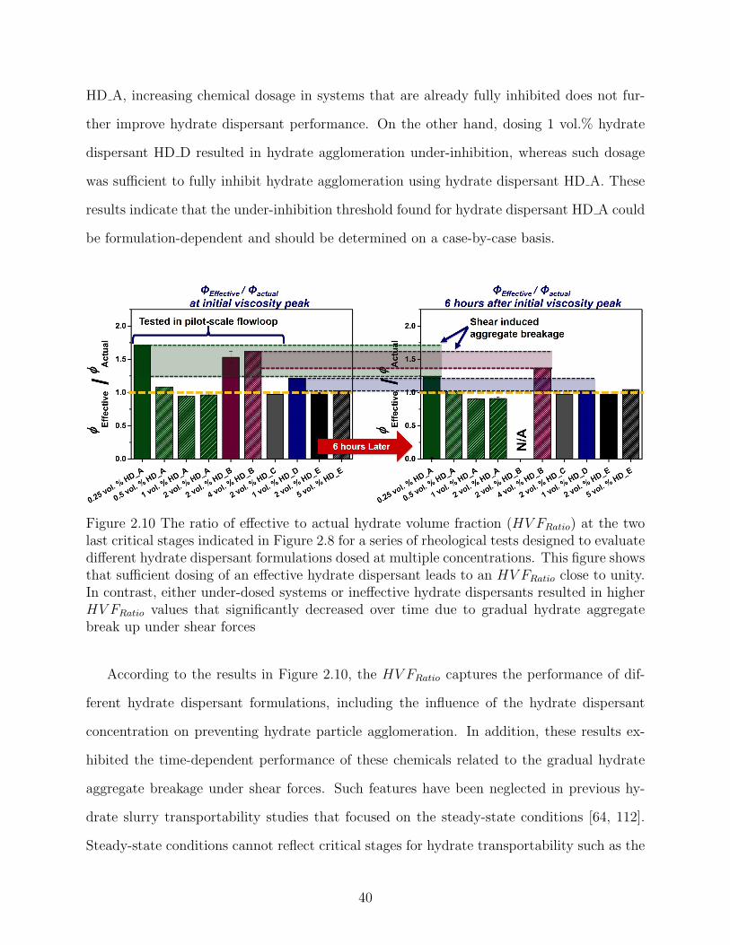
HD A, increasing chemical dosage in systems that are already fully inhibited does not fur-

ther improve hydrate dispersant performance. On the other hand, dosing 1 vol.% hydrate

dispersant HD D resulted in hydrate agglomeration under-inhibition, whereas such dosage

was sufficient to fully inhibit hydrate agglomeration using hydrate dispersant HD A. These

results indicate that the under-inhibition threshold found for hydrate dispersant HD A could

be formulation-dependent and should be determined on a case-by-case basis.

Figure 2.10 The ratio of effective to actual hydrate volume fraction (HV FRatio) at the twolast critical stages indicated in Figure 2.8 for a series of rheological tests designed to evaluatedifferent hydrate dispersant formulations dosed at multiple concentrations. This figure showsthat sufficient dosing of an effective hydrate dispersant leads to an HV FRatio close to unity.In contrast, either under-dosed systems or ineffective hydrate dispersants resulted in higherHV FRatio values that significantly decreased over time due to gradual hydrate aggregatebreak up under shear forces

According to the results in Figure 2.10, the HV FRatio captures the performance of dif-

ferent hydrate dispersant formulations, including the influence of the hydrate dispersant

concentration on preventing hydrate particle agglomeration. In addition, these results ex-

hibited the time-dependent performance of these chemicals related to the gradual hydrate

aggregate breakage under shear forces. Such features have been neglected in previous hy-

drate slurry transportability studies that focused on the steady-state conditions [64, 112].

Steady-state conditions cannot reflect critical stages for hydrate transportability such as the

40

initial viscosity peak. As shown in Figure 2.10, the steady-state rheological properties of a

hydrate particle suspension could lead to an over-optimistic assessment of the plugging risk

(i.e. HV FRatio ∼ 1) given such an assessment might encompass the gradual breakage of hy-

drate aggregates under shear forces. For this reason, hydrate plugging risk assessments based

on steady-state results only could be misleading, particularly for under-inhibited systems.

Finally, is worth noting that HV FRatio values below unity might be consequence of errors

measuring the relatively low viscosity of the liquid hydrocarbon mixture using the vane

impeller geometry as discussed in Section 2.2.2, as well as an increased maximum packing

fraction (φmax) caused by polydispersity of hydrate particles [134].

2.3.2 Transient rheological studies

A series of transient tests were conducted following the aforementioned constant shear-

rate high-pressure rheological studies. Low shear conditions favor hydrate particle aggrega-

tion by minimizing shear-induced aggregate breakage according to the force balance in 2.9.

These studies included multiple experimental methods, such as shear rate-controlled and

shear-stress controlled ramps, and oscillatory tests, which allow yield stress measurement in

structured fluids. The influence of hydrate dispersant concentration was studied using both

shear stress-controlled and shear rate-controlled ramps following the procedure described in

Section 2.2.2.2. Shear stress-controlled tests provided additional insights into the influence

of shut-in time on yield stress values. Finally, oscillatory tests offered further validation of

the transient experiments and allowed comparison of different experimental techniques used

to measure either the static or the dynamic yield stress of a sample.

2.3.2.1 Influence of hydrate dispersant concentration and shut-in time on hy-drate slurry yield stress: quantifying hydrate dispersant under-dosing

Shear stress-controlled ramps were conducted in order to quantify the yield stress of

hydrate slurries dosed with different hydrate dispersants HD A concentrations ranging from

0.25 to 2 vol.% with respect to the water content of the system. These systems involved

41

a liquid hydrocarbon phase, and an aqueous phase containing 3.5 wt.% NaCl, as described

previously. Multiple shut-in periods were evaluated in the shear stress-controlled ramps (i.e.

0, 4 and 8-hour shut-in periods). These shut-in stages involve a zero-shear stress period

of a given length of time at constant pressure and temperature conditions. Such conditions

intended to mimic a shut-in/restart scenario in subsea pipelines transporting hydrate slurries.

Figure 2.11 shows experimental results from stress-controlled ramps in tests with varying

hydrate dispersant dosage and with multiple shut-in periods. A steep increase in the mea-

sured yield stress was observed at hydrate dispersant dosages below 1 vol.%. Systems dosed

with 0.25 and 0.5 vol.% HD A not only showed higher yield stress in tests without shut-

in but also exhibited increasing yield stress values with increasing shut-in periods. Longer

shut-in periods allow for longer contact time between hydrate particles, which results in in-

creasing hydrate cohesive forces [43]. Greater cohesive forces could lead to more consolidated

particle networks with a higher yield stress, according to previous studies on suspensions of

weakly attractive colloidal particles [116]. The concentration and shut-in period dependence

of the hydrate dispersant performance observed in samples dosed with less than 1 vol.%

of the chemical additive indicates such dosage as the threshold separating fully-dosed from

under-dosed systems.

On the other hand, systems dosed with 1 vol.% or more hydrate dispersant HD A showed

similar yield stress values (i.e. ∼ 10 Pa), which remained constant regardless of the length of

the shut-in stage. These results suggest that 1 vol.% might result in full hydrate agglomer-

ation inhibition, and further dosage increase does not significantly improve the performance

of this chemical. These results are in further agreement with the observations from con-

stant shear rate tests described in Section 2.3.1. Yield stress values from a variety of daily

life materials are also shown in Figure 2.11 to provide a tangible indicator of the hydrate

slurry consistency resulting from tests dosed with different hydrate dispersant concentration

[135–139]. Dosing 0.25 vol.% hydrate dispersant HD A led to a hydrate slurry with flow

properties that resembles peanut butter; in contrast, dosing 1 or 2 vol.% hydrate dispersant

42

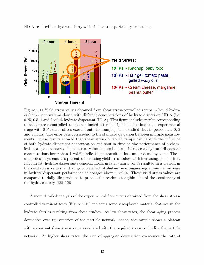
HD A resulted in a hydrate slurry with similar transportability to ketchup.

Figure 2.11 Yield stress values obtained from shear stress-controlled ramps in liquid hydro-carbon/water systems dosed with different concentrations of hydrate dispersant HD A (i.e.0.25, 0.5, 1 and 2 vol.% hydrate dispersant HD A). This figure includes results correspondingto shear stress-controlled ramps conducted after multiple shut-in times (i.e. experimentalstage with 0 Pa shear stress exerted onto the sample). The studied shut-in periods are 0, 3and 8 hours. The error bars correspond to the standard deviation between multiple measure-ments. These results showed that shear stress-controlled ramps can capture the influenceof both hydrate dispersant concentration and shut-in time on the performance of a chem-ical in a given scenario. Yield stress values showed a steep increase at hydrate dispersantconcentrations lower than 1 vol.%, indicating a transition into under-dosed systems. Theseunder-dosed systems also presented increasing yield stress values with increasing shut-in time.In contrast, hydrate dispersants concentrations greater than 1 vol.% resulted in a plateau inthe yield stress values, and a negligible effect of shut-in time, suggesting a minimal increasein hydrate dispersant performance at dosages above 1 vol.%. These yield stress values arecompared to daily life products to provide the reader a tangible idea of the consistency ofthe hydrate slurry [135–139]

A more detailed analysis of the experimental flow curves obtained from the shear stress-

controlled transient tests (Figure 2.12) indicates some viscoplastic material features in the

hydrate slurries resulting from these studies. At low shear rates, the shear aging process

dominates over rejuvenation of the particle network; hence, the sample shows a plateau

with a constant shear stress value associated with the required stress to fluidize the particle

network. At higher shear rates, the rate of aggregate destruction overcomes the rate of

43

formation, and the flow curve behavior becomes that of a viscous (or Newtonian) fluid. The

yield point marks the transition between the two regimes [114, 140]. Accordingly, traditional

rheological models for yield stress fluids, such as the Hershel-Bulkley (See Equation 2.3) or

the Casson (See Equation 2.4) models might successfully describe such materials and provide

analytical values for the yield stress.

Three different rheological models for non-Newtonian fluids with yield stress (i.e. Bing-

ham, Herschel-Bulkley and Casson models) were fitted to the experimental data from the

stress-controlled transient tests. Predicted yield stress values were compared with the ex-

perimental results from tests with both varying hydrate dispersant HD A dosing and after

different shut-in periods. A squared error minimization method was utilized to determine

the optimum parameters for each model.

Figure 2.12 shows that all these three models have good agreement with the experimental

data at high shear rates (i.e. γ ≥ 10 s-1). However, the Bingham model fails to predict the

experimental shear stress at low shear rates (i.e. γ ≤ 10 s-1). On the other hand, both the

Herschel- Bulkley and the Casson model showed better agreement with the experimental

data at low shear rates. Figure 2.13 comprises the mean yield stress values determined using

the different rheological models, and compares such yield stress values with the experimental

results obtained using the shear rate spike method [119]. This figure shows that the Bingham

model, which failed to predict shear stress at low shear rates, resulted in over-predicted yield

stress values with respect to the experimental observation. Over-predicted yield stress values

using the Bingham model were particularly noticeable in systems sufficiently dosed with

hydrate dispersant, which showed relatively low yield stresses. In contrast, both the Casson

and the Herschel-Bulkley models, which showed better agreement predicting shear stress at

low shear rates conditions, led to yield stress values closer to the experimental results. Error

bars correspond to the standard deviation between multiple yield stress measurements.

These results suggest that the hydrate slurry could show shear thinning behavior at low

shear rates that favor hydrate particle aggregation [103]. Nevertheless, despite increasing hy-

44

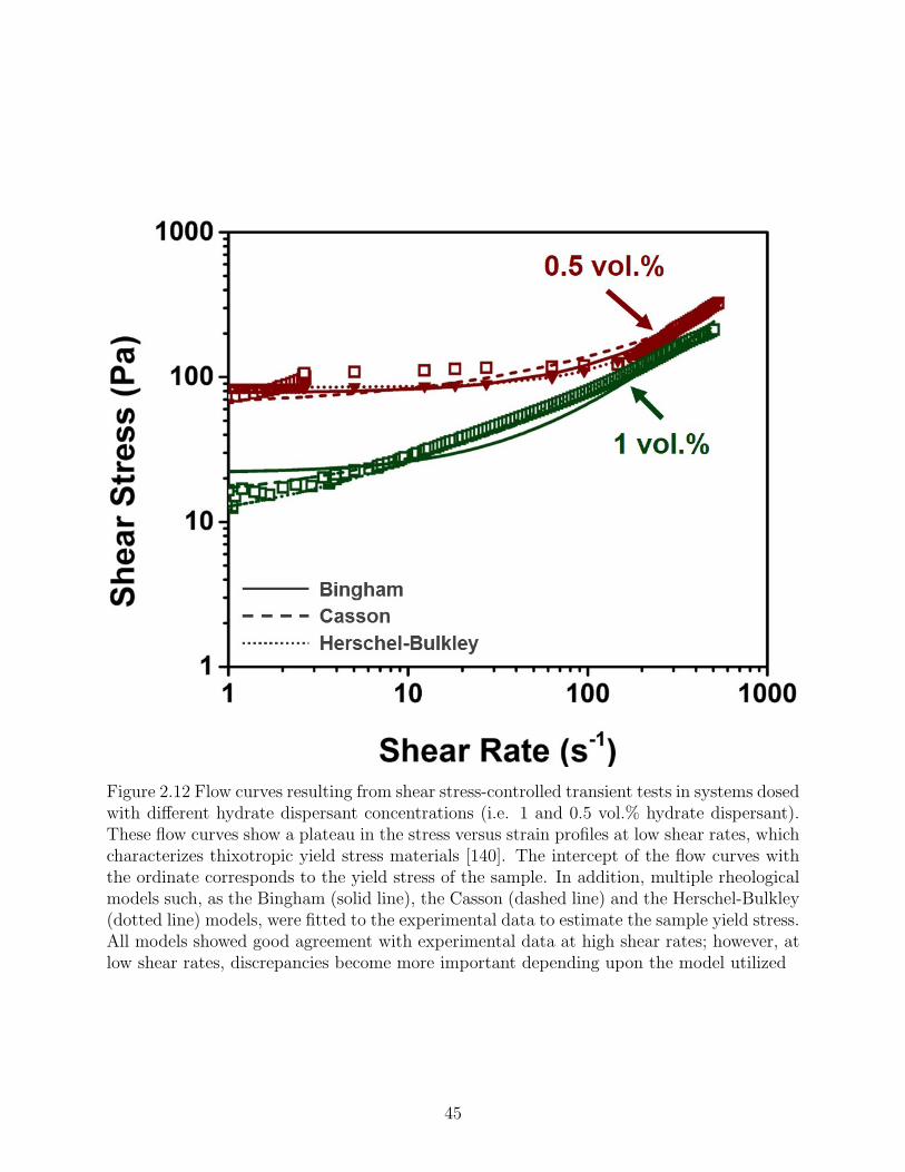
Figure 2.12 Flow curves resulting from shear stress-controlled transient tests in systems dosedwith different hydrate dispersant concentrations (i.e. 1 and 0.5 vol.% hydrate dispersant).These flow curves show a plateau in the stress versus strain profiles at low shear rates, whichcharacterizes thixotropic yield stress materials [140]. The intercept of the flow curves withthe ordinate corresponds to the yield stress of the sample. In addition, multiple rheologicalmodels such, as the Bingham (solid line), the Casson (dashed line) and the Herschel-Bulkley(dotted line) models, were fitted to the experimental data to estimate the sample yield stress.All models showed good agreement with experimental data at high shear rates; however, atlow shear rates, discrepancies become more important depending upon the model utilized

45

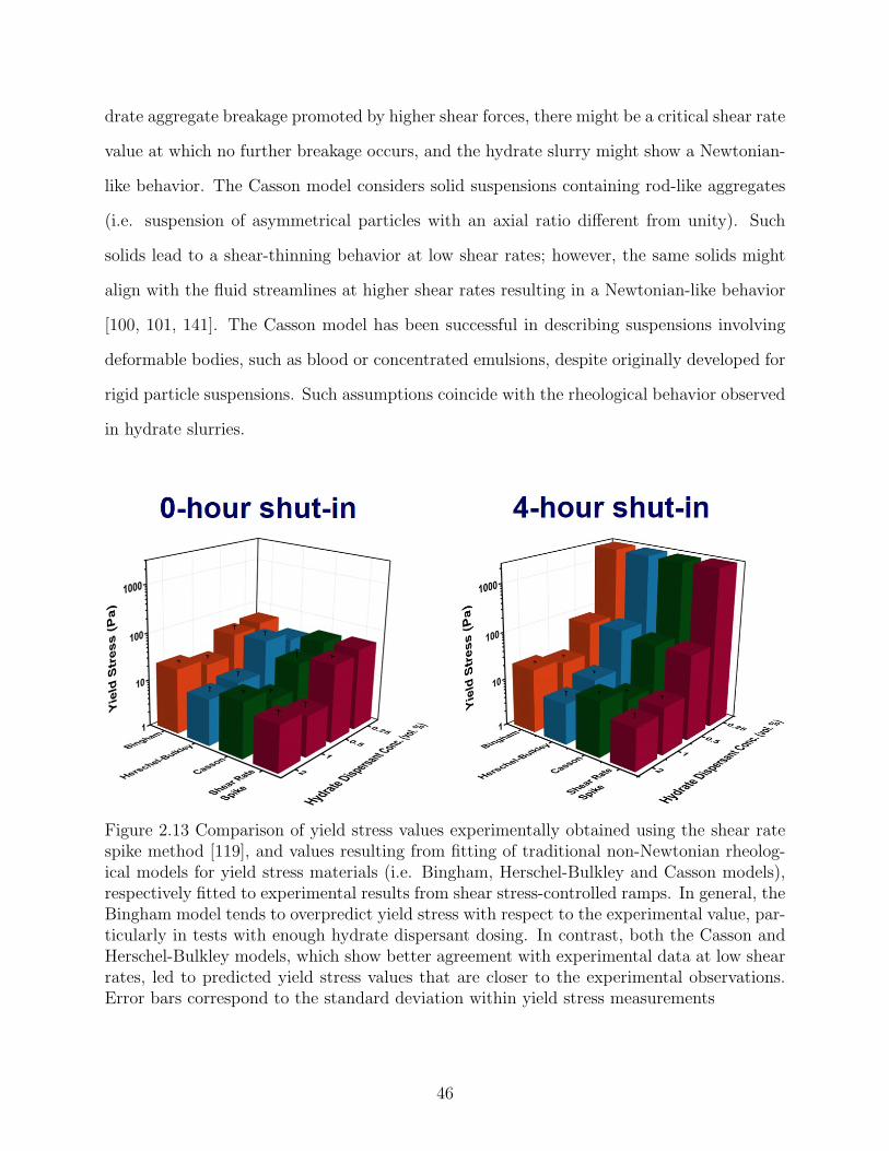
drate aggregate breakage promoted by higher shear forces, there might be a critical shear rate

value at which no further breakage occurs, and the hydrate slurry might show a Newtonian-

like behavior. The Casson model considers solid suspensions containing rod-like aggregates

(i.e. suspension of asymmetrical particles with an axial ratio different from unity). Such

solids lead to a shear-thinning behavior at low shear rates; however, the same solids might

align with the fluid streamlines at higher shear rates resulting in a Newtonian-like behavior

[100, 101, 141]. The Casson model has been successful in describing suspensions involving

deformable bodies, such as blood or concentrated emulsions, despite originally developed for

rigid particle suspensions. Such assumptions coincide with the rheological behavior observed

in hydrate slurries.

Figure 2.13 Comparison of yield stress values experimentally obtained using the shear ratespike method [119], and values resulting from fitting of traditional non-Newtonian rheolog-ical models for yield stress materials (i.e. Bingham, Herschel-Bulkley and Casson models),respectively fitted to experimental results from shear stress-controlled ramps. In general, theBingham model tends to overpredict yield stress with respect to the experimental value, par-ticularly in tests with enough hydrate dispersant dosing. In contrast, both the Casson andHerschel-Bulkley models, which show better agreement with experimental data at low shearrates, led to predicted yield stress values that are closer to the experimental observations.Error bars correspond to the standard deviation within yield stress measurements

46

A quantitative comparison of the yield stress values obtained using the aforementioned

rheological models reveals that both Herschel-Bulkley and Casson models led to a comparable

agreement with respect to the manually determined yield stress values, which correspond

to the shear rate spike observed during shear stress ramps [119]. The average absolute

deviation (AAD) for the Herschel-Bulkley and Casson models were 36.5 % and 41.93 %

respectively. In contrast, the Bingham model led to yield stress values with a 119.3 %

AAD considering all yield stress measurements from samples dosed with hydrate dispersant

HD A at concentrations ranging from 0.25 to 2 vol.%, and including measurements taken

after shut-in periods of different length. The Casson model resulted in an AAD only 5 %

larger than the Herschel-Bulkley model. These results suggest that the Casson model, which

describes materials with significant shear thinning at low shear-rate values and a Newtonian-

like response at high shear rates, could provide an adequate representation of the hydrate

slurry rheological behavior while using less fitting parameters than the Herschel-Bulkley

model.

2.3.2.2 Comparison of multiple transient experimental methods to assess hy-drate dispersant performance in shut-in/restart scenarios

Parameters such as the sample history and the experimental methods utilized could

have a significant effect on yield stress measurements. This is particularly important for

some thixotropic fluids, such as solid suspensions [114]. Different experimental techniques

measure either the “static” yield stress (i.e. required shear stress to initiate flow) or the

“dynamic” yield stress (i.e. shear stress at which flow stops). A combination of shear stress

ramps, shear rate ramps, and oscillatory tests were conducted to characterize the fluidization

process of the hydrate slurry according to the procedures described in Section 2.2.2.2.

Figure 2.14 shows the yield stress values obtained using these different experimental

methodologies in systems dosed with a variety of hydrate dispersant formulations and dosages.

Yield stress values obtained from the different experimental techniques are relatively close,

indicating the validity of these yield stress measurements. In addition, the performance of

47

the evaluated chemicals during the transient tests is in good agreement in most cases with

the constant shear rate results showed in Figure 2.10.

The shear stress-controlled ramps, which measure the static yield stress of a sample,

resulted in slightly higher yield stress values than the dynamic yield stress measurements (i.e.

shear rate-controlled ramps and oscillatory tests). Accordingly, this experimental technique

involving shear stress-controlled ramps might represent a more conservative approach to

characterize hydrate dispersant performance in hydrate slurry samples. Furthermore, the

higher static than dynamic yield stress values characterizes thixotropic materials, which

might require greater shear stress to initiate flow than to maintain a flowing state. Such

behavior contrasts with ideal yield stress materials, which would not flow at all at any shear

stress value below the yield stress [114].

According to previous investigations looking at the fluidization mechanisms in transient

rheological studies in different non-Newtonian samples, such as laponite (clay) suspensions

and Carbopol microgels, the hysteresis from strain-controlled flow curves might provide

better insights into such fluidization mechanisms [142–144]. These previous investigations

looking at various structured fluids incorporate ultrasonic velocimetry measurements that

provide the velocity profile of the sample within the rheometer cell, in parallel to the flow

curve rheological measurements.

Shear rate-controlled ramps were conducted following two different experimental path-

ways, (i.e. either up/down or down/up shear rate ramps), according to the experimental

procedure described in Section 2.2.2.2. Figure 2.15 shows shear stress profiles from shear

rate-controlled ramps conducted following opposite experimental pathways.

The stress profile from increasing shear rate ramps in tests that started with such ramps as

the initial experimental stage showed a characteristic behavior (i.e. blue curve in Figure 2.15,

left). Initially, gradual growth in shear stress occurs as the shear rate increases. A stress

peak arises at a given shear rate value (i.e. γ ∼ 1 s-1 in this particular case), followed by a

period with no further growth in the shear stress as the shear rate keeps increasing. Finally,

48

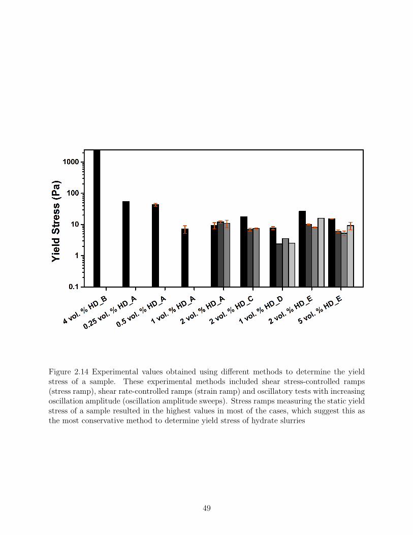
Figure 2.14 Experimental values obtained using different methods to determine the yieldstress of a sample. These experimental methods included shear stress-controlled ramps(stress ramp), shear rate-controlled ramps (strain ramp) and oscillatory tests with increasingoscillation amplitude (oscillation amplitude sweeps). Stress ramps measuring the static yieldstress of a sample resulted in the highest values in most of the cases, which suggest this asthe most conservative method to determine yield stress of hydrate slurries

49

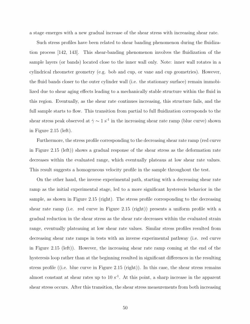
a stage emerges with a new gradual increase of the shear stress with increasing shear rate.

Such stress profiles have been related to shear banding phenomenon during the fluidiza-

tion process [142, 143]. This shear-banding phenomenon involves the fluidization of the

sample layers (or bands) located close to the inner wall only. Note: inner wall rotates in a

cylindrical rheometer geometry (e.g. bob and cup, or vane and cup geometries). However,

the fluid bands closer to the outer cylinder wall (i.e. the stationary surface) remain immobi-

lized due to shear aging effects leading to a mechanically stable structure within the fluid in

this region. Eventually, as the shear rate continues increasing, this structure fails, and the

full sample starts to flow. This transition from partial to full fluidization corresponds to the

shear stress peak observed at γ ∼ 1 s-1 in the increasing shear rate ramp (blue curve) shown

in Figure 2.15 (left).

Furthermore, the stress profile corresponding to the decreasing shear rate ramp (red curve

in Figure 2.15 (left)) shows a gradual response of the shear stress as the deformation rate

decreases within the evaluated range, which eventually plateaus at low shear rate values.

This result suggests a homogeneous velocity profile in the sample throughout the test.

On the other hand, the inverse experimental path, starting with a decreasing shear rate

ramp as the initial experimental stage, led to a more significant hysteresis behavior in the

sample, as shown in Figure 2.15 (right). The stress profile corresponding to the decreasing

shear rate ramp (i.e. red curve in Figure 2.15 (right)) presents a uniform profile with a

gradual reduction in the shear stress as the shear rate decreases within the evaluated strain

range, eventually plateauing at low shear rate values. Similar stress profiles resulted from

decreasing shear rate ramps in tests with an inverse experimental pathway (i.e. red curve

in Figure 2.15 (left)). However, the increasing shear rate ramp coming at the end of the

hysteresis loop rather than at the beginning resulted in significant differences in the resulting

stress profile ((i.e. blue curve in Figure 2.15 (right)). In this case, the shear stress remains

almost constant at shear rates up to 10 s-1. At this point, a sharp increase in the apparent

shear stress occurs. After this transition, the shear stress measurements from both increasing

50

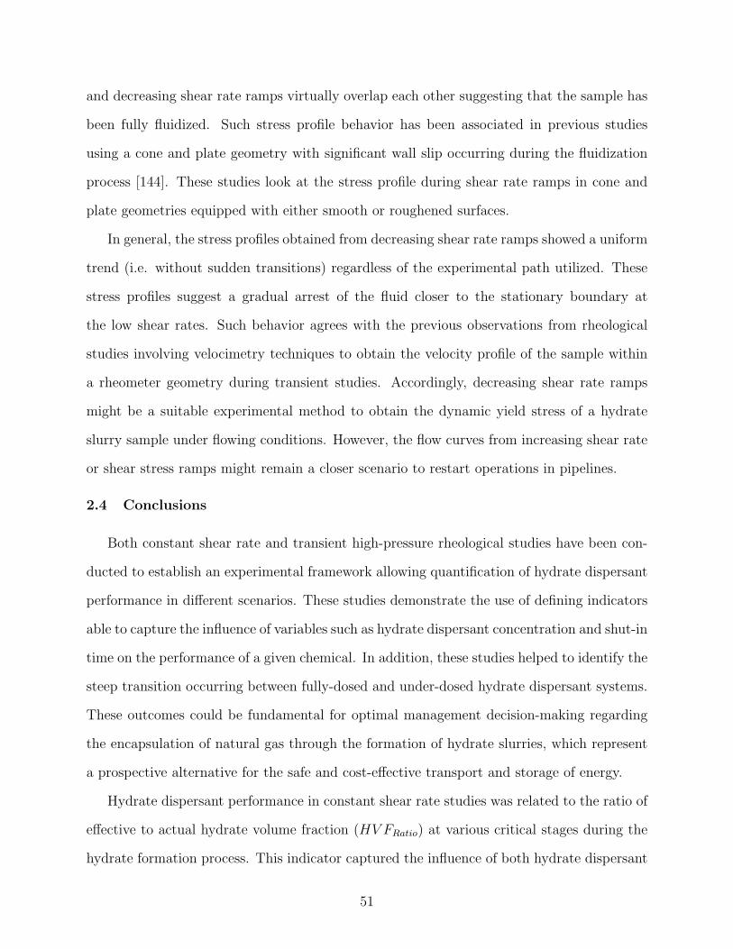
and decreasing shear rate ramps virtually overlap each other suggesting that the sample has

been fully fluidized. Such stress profile behavior has been associated in previous studies

using a cone and plate geometry with significant wall slip occurring during the fluidization

process [144]. These studies look at the stress profile during shear rate ramps in cone and

plate geometries equipped with either smooth or roughened surfaces.

In general, the stress profiles obtained from decreasing shear rate ramps showed a uniform

trend (i.e. without sudden transitions) regardless of the experimental path utilized. These

stress profiles suggest a gradual arrest of the fluid closer to the stationary boundary at

the low shear rates. Such behavior agrees with the previous observations from rheological

studies involving velocimetry techniques to obtain the velocity profile of the sample within

a rheometer geometry during transient studies. Accordingly, decreasing shear rate ramps

might be a suitable experimental method to obtain the dynamic yield stress of a hydrate

slurry sample under flowing conditions. However, the flow curves from increasing shear rate

or shear stress ramps might remain a closer scenario to restart operations in pipelines.

2.4 Conclusions

Both constant shear rate and transient high-pressure rheological studies have been con-

ducted to establish an experimental framework allowing quantification of hydrate dispersant

performance in different scenarios. These studies demonstrate the use of defining indicators

able to capture the influence of variables such as hydrate dispersant concentration and shut-in

time on the performance of a given chemical. In addition, these studies helped to identify the

steep transition occurring between fully-dosed and under-dosed hydrate dispersant systems.

These outcomes could be fundamental for optimal management decision-making regarding

the encapsulation of natural gas through the formation of hydrate slurries, which represent

a prospective alternative for the safe and cost-effective transport and storage of energy.

Hydrate dispersant performance in constant shear rate studies was related to the ratio of

effective to actual hydrate volume fraction (HV FRatio) at various critical stages during the

hydrate formation process. This indicator captured the influence of both hydrate dispersant

51

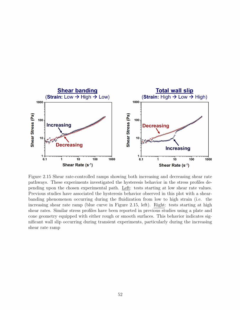
Figure 2.15 Shear rate-controlled ramps showing both increasing and decreasing shear ratepathways. These experiments investigated the hysteresis behavior in the stress profiles de-pending upon the chosen experimental path. Left: tests starting at low shear rate values.Previous studies have associated the hysteresis behavior observed in this plot with a shear-banding phenomenon occurring during the fluidization from low to high strain (i.e. theincreasing shear rate ramp (blue curve in Figure 2.15, left). Right: tests starting at highshear rates. Similar stress profiles have been reported in previous studies using a plate andcone geometry equipped with either rough or smooth surfaces. This behavior indicates sig-nificant wall slip occurring during transient experiments, particularly during the increasingshear rate ramp

52

formulation and dosage on hydrate particle agglomeration.

On the other hand, transient tests provided insights into hydrate dispersant performance

in shut-in/restart scenarios. Shear stress-controlled ramps successfully assessed the influ-

ence of hydrate dispersant concentration and shut-in time on the hydrate slurry yield stress,

while showing good experimental reproducibility. The experimental flow curves resulting

from shear stress-controlled ramps were compared with traditional rheological models for

non-Newtonian fluids with yield stress. These models included Bingham, Herschel-Bulkley

and Casson models. According to these results, the Casson model, which showed good

agreement with the experimental flow curves while using less tunable parameters than tra-

ditional Herschel-Bulkley model, could be a more suitable model to describe hydrate slurry

rheological behavior.

Moreover, multiple rheological techniques were used to measure the yield stress of hy-

drate slurry samples allowing comparison of these methods. The yield stress values resulting

from shear stress-controlled ramps were higher in most cases than those values obtained

from either shear rate-controlled ramps or oscillatory amplitude sweeps. Accordingly, this

experimental technique, which implies a static yield stress measurement, might be a more

conservative method to characterize hydrate dispersant performance in hydrate slurry sam-

ples. In addition, higher yield stress values obtained from static measurement suggest that

hydrate slurries in the presence of hydrate dispersants behave as thixotropic fluids rather

than ideal yield stress materials. Such fluids might require greater shear stress to initiate flow

than to maintain a flowing state due to competing shear aging and rejuvenation processes in

the sample. In addition, strain-controlled flow curves provided insights into the fluidization

mechanisms in transient rheological studies of hydrate slurries. These results helped to iden-

tify both shear-banding and wall slip phenomena occurring during the transient rheological

tests. The observed phenomena might depend on the chosen experimental pathway in shear

rate-controlled experiments.

53

CHAPTER 3

DEVELOPMENT OF A MULTI-SCALE EXPERIMENTAL WORKFLOW TO

QUANTIFY HYDRATE DISPERSANT PERFORMANCE FOR EFFECTIVE

PRODUCTION CHEMISTRY DECISION-MAKING

Offshore deepwater oil and gas production encompasses several flow assurance issues that

are highly challenging from a technical perspective; however, such challenges present poten-

tial opportunities to reduce capital and operational expenditures in new field developments.

Among the different flow assurance phenomena involved in subsea operations, natural gas

hydrate plugs are the main cause of downtimes, which have major economic consequences

for the industry. In addition, traditional hydrate management strategies using thermody-

namic hydrate inhibitors (e.g. MeOH and glycols) become cost prohibitive as the water

content increases in mature fields or as new field developments move into deeper waters.

Accordingly, the mitigation of gas hydrate plugging risk using cost-effective hydrate man-

agement strategies could cause important reductions in the break-even point (BEP) of a

project boosting its economic feasibility. The experimental techniques commonly used to

assess hydrate plugging risk in crude oil systems, such as rocking cells or autoclaves, require

large sample volumes. Such sample volumes are not readily available using bottomhole sam-

pling techniques before developing a new field. Therefore, generating and benchmarking an

experimental framework using apparatuses that require low oil sample volumes could make

testing feasible in cases with limited sample availability. Allowing such testing could be

crucial to optimize future project developments, while also reducing both costs and time

required to obtain the right selection of chemical additives for a specific field. Multi-scale

experimental studies ranging from pilot-scale flowloops to surface chemistry level techniques,

such as a high-pressure micromechanical force (HP-MMF) apparatus, have been conducted

to both validate the different experimental techniques and to find their limitations. These

54

studies included pilot-scale flowloop, HP-autoclave, HP-rheometer, contact angle measure-

ments, and HP-MMF experiments using both model and crude oil systems with/without

dosing of hydrate anti-agglomerants (AAs). Preliminary results showed that all these tech-

niques can capture differences in the plugging tendency between a surfactant-free model oil

and a crude oil sample. In addition, HP-autoclave, HP-rheometer, and HP-MMF results

showed a consistent AA dosage cutoff to separate an under-inhibited from a fully-inhibited

system. Moreover, the hydrate cohesive forces calculated from transient yield stress measure-

ments showed order of magnitude agreement with the values obtained from HP-MMF tests

in systems using different AA formulations dosed at multiple concentrations. Results from

these investigations could significantly change the experimental approach currently used to

evaluate crude oil plugging tendency before developing new fields and result in major cost/-

time reductions during production chemistry selection. Ultimately this approach could lead

to an optimized development of new production assets with lower CAPEX and OPEX. Fur-

thermore, the consistency observed between the different experimental techniques could help

to develop and validate more robust models for relevant phenomena such as hydrate particle

agglomeration.

3.1 Introduction

Multiple phenomena, particularly those related to the precipitation and transport of hy-

drocarbon solids, can give rise to challenging obstacles for offshore deepwater oil & gas pro-

duction. A traditional subsea production system could present simultaneously phenomena

such as wax deposition, gas hydrate formation, asphaltene precipitation, scaling, slugging,

and corrosion/erosion failures. Accordingly, flow assurance encompasses a variety of disci-

plines (e.g. thermodynamics, multi-phase flow, and surface chemistry), which are combined

to provide the required design and management strategies to reliably transport fluids from

the reservoir to the point of sale (POS) [145–147]. Currently, gas hydrate plugs remain a ma-

jor flow assurance concern in subsea oil & gas production, causing both significant downtime

periods and over-conservative hydrate management strategies, which result in a decreased

55

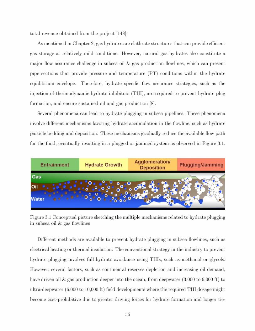
total revenue obtained from the project [148].

As mentioned in Chapter 2, gas hydrates are clathrate structures that can provide efficient

gas storage at relatively mild conditions. However, natural gas hydrates also constitute a

major flow assurance challenge in subsea oil & gas production flowlines, which can present

pipe sections that provide pressure and temperature (PT) conditions within the hydrate

equilibrium envelope. Therefore, hydrate specific flow assurance strategies, such as the

injection of thermodynamic hydrate inhibitors (THI), are required to prevent hydrate plug

formation, and ensure sustained oil and gas production [8].

Several phenomena can lead to hydrate plugging in subsea pipelines. These phenomena

involve different mechanisms favoring hydrate accumulation in the flowline, such as hydrate

particle bedding and deposition. These mechanisms gradually reduce the available flow path

for the fluid, eventually resulting in a plugged or jammed system as observed in Figure 3.1.

Figure 3.1 Conceptual picture sketching the multiple mechanisms related to hydrate pluggingin subsea oil & gas flowlines

Different methods are available to prevent hydrate plugging in subsea flowlines, such as

electrical heating or thermal insulation. The conventional strategy in the industry to prevent

hydrate plugging involves full hydrate avoidance using THIs, such as methanol or glycols.

However, several factors, such as continental reserves depletion and increasing oil demand,

have driven oil & gas production deeper into the ocean, from deepwater (3,000 to 6,000 ft) to

ultra-deepwater (6,000 to 10,000 ft) field developments where the required THI dosage might

become cost-prohibitive due to greater driving forces for hydrate formation and longer tie-

56

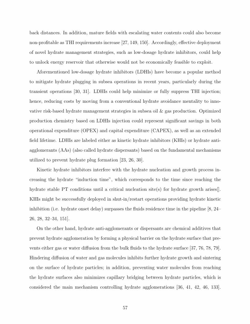
back distances. In addition, mature fields with escalating water contents could also become

non-profitable as THI requirements increase [27, 149, 150]. Accordingly, effective deployment

of novel hydrate management strategies, such as low-dosage hydrate inhibitors, could help

to unlock energy reservoir that otherwise would not be economically feasible to exploit.

Aforementioned low-dosage hydrate inhibitors (LDHIs) have become a popular method

to mitigate hydrate plugging in subsea operations in recent years, particularly during the

transient operations [30, 31]. LDHIs could help minimize or fully suppress THI injection;

hence, reducing costs by moving from a conventional hydrate avoidance mentality to inno-

vative risk-based hydrate management strategies in subsea oil & gas production. Optimized

production chemistry based on LDHIs injection could represent significant savings in both

operational expenditure (OPEX) and capital expenditure (CAPEX), as well as an extended

field lifetime. LDHIs are labeled either as kinetic hydrate inhibitors (KHIs) or hydrate anti-

agglomerants (AAs) (also called hydrate dispersants) based on the fundamental mechanisms

utilized to prevent hydrate plug formation [23, 26, 30].

Kinetic hydrate inhibitors interfere with the hydrate nucleation and growth process in-

creasing the hydrate “induction time”, which corresponds to the time since reaching the

hydrate stable PT conditions until a critical nucleation site(s) for hydrate growth arises[].

KHIs might be successfully deployed in shut-in/restart operations providing hydrate kinetic

inhibition (i.e. hydrate onset delay) surpasses the fluids residence time in the pipeline [8, 24–

26, 28, 32–34, 151].

On the other hand, hydrate anti-agglomerants or dispersants are chemical additives that

prevent hydrate agglomeration by forming a physical barrier on the hydrate surface that pre-

vents either gas or water diffusion from the bulk fluids to the hydrate surface [37, 76, 78, 79].

Hindering diffusion of water and gas molecules inhibits further hydrate growth and sintering

on the surface of hydrate particles; in addition, preventing water molecules from reaching

the hydrate surfaces also minimizes capillary bridging between hydrate particles, which is

considered the main mechanism controlling hydrate agglomerations [36, 41, 42, 46, 133].

57

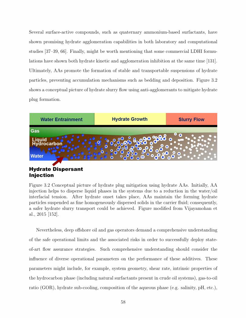
Several surface-active compounds, such as quaternary ammonium-based surfactants, have

shown promising hydrate agglomeration capabilities in both laboratory and computational

studies [37–39, 66]. Finally, might be worth mentioning that some commercial LDHI formu-

lations have shown both hydrate kinetic and agglomeration inhibition at the same time [131].

Ultimately, AAs promote the formation of stable and transportable suspensions of hydrate

particles, preventing accumulation mechanisms such as bedding and deposition. Figure 3.2

shows a conceptual picture of hydrate slurry flow using anti-agglomerants to mitigate hydrate

plug formation.

Figure 3.2 Conceptual picture of hydrate plug mitigation using hydrate AAs. Initially, AAinjection helps to disperse liquid phases in the systems due to a reduction in the water/oilinterfacial tension. After hydrate onset takes place, AAs maintain the forming hydrateparticles suspended as fine homogeneously dispersed solids in the carrier fluid; consequently,a safer hydrate slurry transport could be achieved. Figure modified from Vijayamohan etal., 2015 [152].

Nevertheless, deep offshore oil and gas operators demand a comprehensive understanding

of the safe operational limits and the associated risks in order to successfully deploy state-

of-art flow assurance strategies. Such comprehensive understanding should consider the

influence of diverse operational parameters on the performance of these additives. These

parameters might include, for example, system geometry, shear rate, intrinsic properties of

the hydrocarbon phase (including natural surfactants present in crude oil systems), gas-to-oil

ratio (GOR), hydrate sub-cooling, composition of the aqueous phase (e.g. salinity, pH, etc.),

58

anti-agglomerant cocktail formulation and dosing, or synergistic/antagonistic interactions

with other production chemistry additives.

Accordingly, as mentioned in Chapter 2, characterization tools capable of providing reli-

able hydrate transportability assessments in systems dosed with either natural or synthetic

hydrate dispersing molecules become crucial. Section 2.1.2 summarizes the different equip-

ment available to investigate hydrate slurry properties and transportability, such as MMF

[41–46], rocking cells [25, 38, 47–51], rheometers [52–61], autoclaves [62–66], and multiple

scale flowloops [67–74].

Innovative production strategies, such as cold flow [81, 153–155] and AA injection, could

help to mitigate some of the hydrate accumulation and plugging mechanisms in Figure 3.1.

However, inhibiting hydrate agglomeration cannot prevent transitions into the stable jam-

ming region due to high hydrate volume fractions or low shear areas in the flowline, as well as

clogging of sloughed-off macroscopic hydrate particles at pipeline constrictions. Therefore,

an advanced understanding of the risks related to the transport of hydrate slurries in the

presence of either natural or synthetic hydrate dispersants, or to the intermittent flow of

macroscopic hydrate particles in the pipe, becomes of great importance. Results and analy-

sis in this chapter intend to close the gap between multiple scales of experimental equipment

regarding hydrate transportability and plugging tendency studies in gas/water/liquid hy-

drocarbon systems. Both quantitative and qualitative comparisons have been conducted

in order to connect hydrate dispersant performance rankings resulting from multiple-scale

experimental equipment.


The experimental equipment available at The Center for Hydrate Research (CHR) cover

several length scales and provide a large variety of data going from optical techniques to

measure particle size distributions to torque measurements and pressure drop recordings,

which directly correlate with the resistance to flow in the system.

59

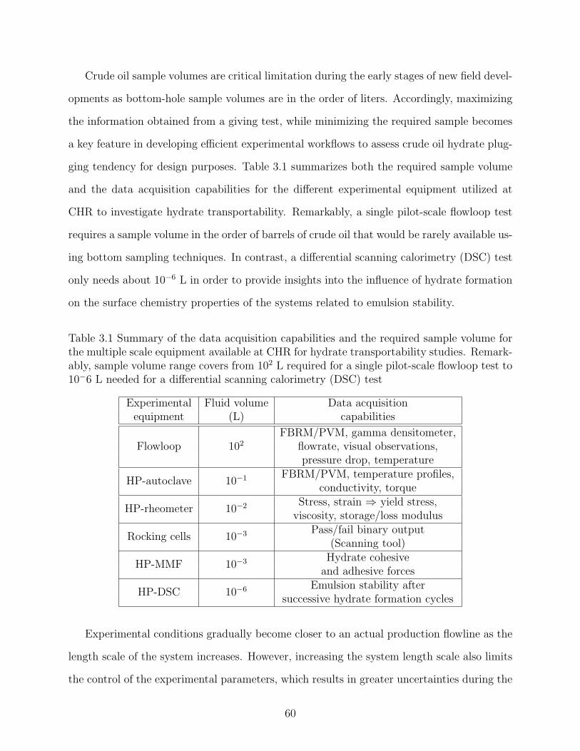
Crude oil sample volumes are critical limitation during the early stages of new field devel-

opments as bottom-hole sample volumes are in the order of liters. Accordingly, maximizing

the information obtained from a giving test, while minimizing the required sample becomes

a key feature in developing efficient experimental workflows to assess crude oil hydrate plug-

ging tendency for design purposes. Table 3.1 summarizes both the required sample volume

and the data acquisition capabilities for the different experimental equipment utilized at

CHR to investigate hydrate transportability. Remarkably, a single pilot-scale flowloop test

requires a sample volume in the order of barrels of crude oil that would be rarely available us-

ing bottom sampling techniques. In contrast, a differential scanning calorimetry (DSC) test

only needs about 10−6 L in order to provide insights into the influence of hydrate formation

on the surface chemistry properties of the systems related to emulsion stability.

Table 3.1 Summary of the data acquisition capabilities and the required sample volume forthe multiple scale equipment available at CHR for hydrate transportability studies. Remark-ably, sample volume range covers from 102 L required for a single pilot-scale flowloop test to10−6 L needed for a differential scanning calorimetry (DSC) test

Experimental Fluid volume Data acquisitionequipment (L) capabilities

FlowloopFBRM/PVM, gamma densitometer,

102 flowrate, visual observations,pressure drop, temperature

HP-autoclave 10−1 FBRM/PVM, temperature profiles,conductivity, torque

HP-rheometer 10−2 Stress, strain ⇒ yield stress,viscosity, storage/loss modulus

Rocking cells 10−3 Pass/fail binary output(Scanning tool)

HP-MMF 10−3 Hydrate cohesiveand adhesive forces

HP-DSC 10−6 Emulsion stability aftersuccessive hydrate formation cycles

Experimental conditions gradually become closer to an actual production flowline as the

length scale of the system increases. However, increasing the system length scale also limits

the control of the experimental parameters, which results in greater uncertainties during the

60

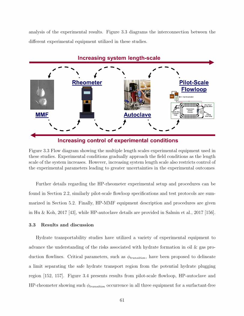
analysis of the experimental results. Figure 3.3 diagrams the interconnection between the

different experimental equipment utilized in these studies.

Figure 3.3 Flow diagram showing the multiple length scales experimental equipment used inthese studies. Experimental conditions gradually approach the field conditions as the lengthscale of the system increases. However, increasing system length scale also restricts control ofthe experimental parameters leading to greater uncertainties in the experimental outcomes

Further details regarding the HP-rheometer experimental setup and procedures can be

found in Section 2.2, similarly pilot-scale flowloop specifications and test protocols are sum-

marized in Section 5.2. Finally, HP-MMF equipment description and procedures are given

in Hu & Koh, 2017 [43], while HP-autoclave details are provided in Salmin et al., 2017 [156].


Hydrate transportability studies have utilized a variety of experimental equipment to

advance the understanding of the risks associated with hydrate formation in oil & gas pro-

duction flowlines. Critical parameters, such as φtransition, have been proposed to delineate

a limit separating the safe hydrate transport region from the potential hydrate plugging

region [152, 157]. Figure 3.4 presents results from pilot-scale flowloop, HP-autoclave and

HP-rheometer showing such φtransition occurrence in all three equipment for a surfactant-free

61

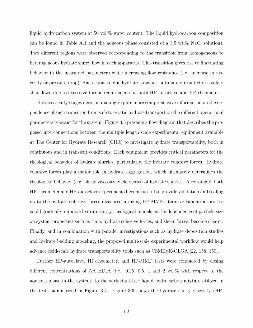
liquid hydrocarbon system at 50 vol.% water content. The liquid hydrocarbon composition

can be found in Table A.1 and the aqueous phase consisted of a 3.5 wt.% NaCl solution).

Two different regions were observed corresponding to the transition from homogeneous to

heterogeneous hydrate slurry flow in each apparatus. This transition gives rise to fluctuating

behavior in the measured parameters while increasing flow resistance (i.e. increase in vis-

cosity or pressure drop). Such catastrophic hydrate transport ultimately resulted in a safety

shut-down due to excessive torque requirements in both HP-autoclave and HP-rheometer.

However, early stages decision making require more comprehensive information on the de-

pendence of such transition from safe to erratic hydrate transport on the different operational

parameters relevant for the system. Figure 3.5 presents a flow diagram that describes the pro-

posed interconnections between the multiple length scale experimental equipment available

at The Center for Hydrate Research (CHR) to investigate hydrate transportability, both in

continuous and in transient conditions. Each equipment provides critical parameters for the

rheological behavior of hydrate slurries, particularly, the hydrate cohesive forces. Hydrate

cohesive forces play a major role in hydrate aggregation, which ultimately determines the

rheological behavior (e.g. shear viscosity, yield stress) of hydrate slurries. Accordingly, both

HP-rheometer and HP-autoclave experiments become useful to provide validation and scaling

up to the hydrate cohesive forces measured utilizing HP-MMF. Iterative validation process

could gradually improve hydrate slurry rheological models as the dependence of particle size

on system properties such as time, hydrate cohesive forces, and shear forces, become clearer.

Finally, and in combination with parallel investigations such as hydrate deposition studies

and hydrate bedding modeling, the proposed multi-scale experimental workflow would help

advance field-scale hydrate transportability tools such as CSMHyK-OLGA [22, 158, 159].

Further HP-autoclave, HP-rheometer, and HP-MMF tests were conducted by dosing

different concentrations of AA HD A (i.e. 0.25, 0.5, 1 and 2 vol.% with respect to the

aqueous phase in the system) to the surfactant-free liquid hydrocarbon mixture utilized in

the tests summarized in Figure 3.4. Figure 3.6 shows the hydrate slurry viscosity (HP-

62

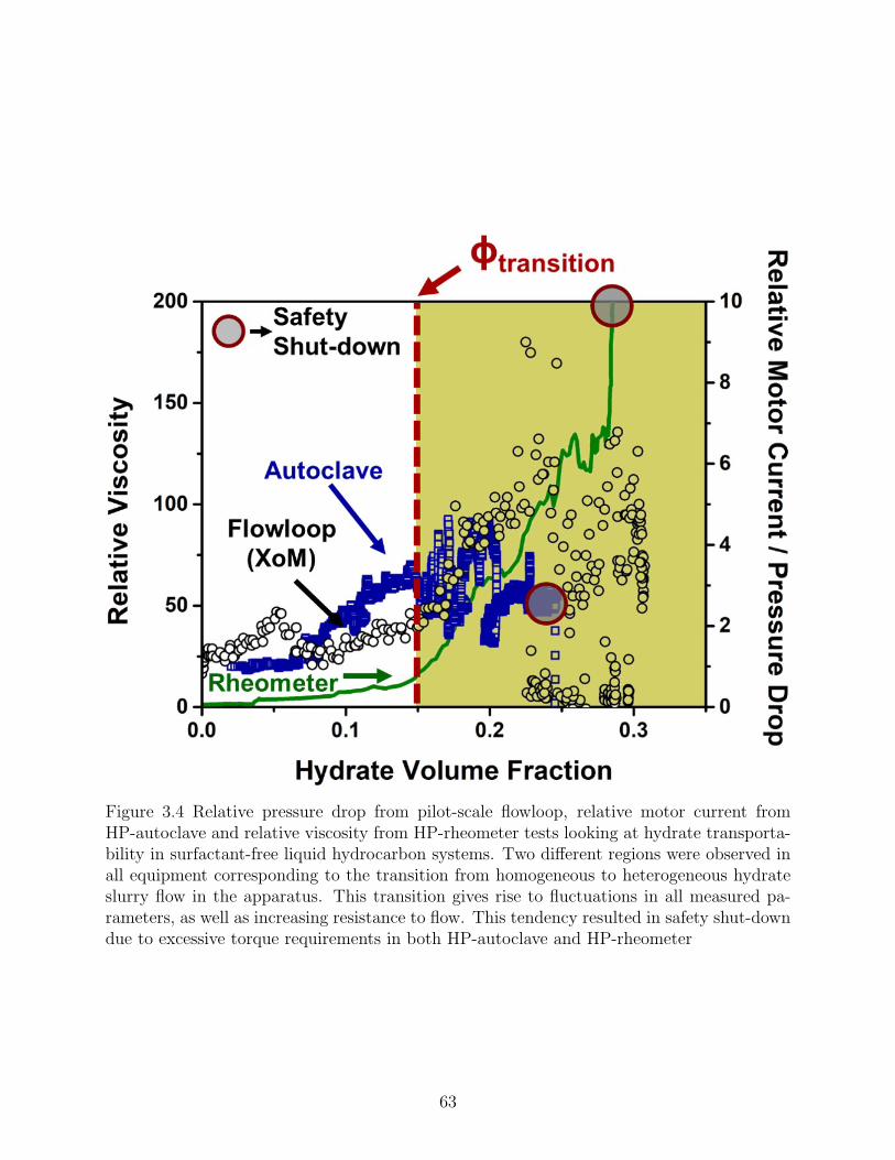
Figure 3.4 Relative pressure drop from pilot-scale flowloop, relative motor current fromHP-autoclave and relative viscosity from HP-rheometer tests looking at hydrate transporta-bility in surfactant-free liquid hydrocarbon systems. Two different regions were observed inall equipment corresponding to the transition from homogeneous to heterogeneous hydrateslurry flow in the apparatus. This transition gives rise to fluctuations in all measured pa-rameters, as well as increasing resistance to flow. This tendency resulted in safety shut-downdue to excessive torque requirements in both HP-autoclave and HP-rheometer

63

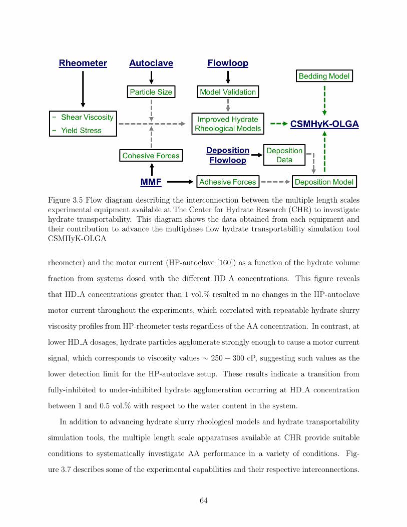
Figure 3.5 Flow diagram describing the interconnection between the multiple length scalesexperimental equipment available at The Center for Hydrate Research (CHR) to investigatehydrate transportability. This diagram shows the data obtained from each equipment andtheir contribution to advance the multiphase flow hydrate transportability simulation toolCSMHyK-OLGA

rheometer) and the motor current (HP-autoclave [160]) as a function of the hydrate volume

fraction from systems dosed with the different HD A concentrations. This figure reveals

that HD A concentrations greater than 1 vol.% resulted in no changes in the HP-autoclave

motor current throughout the experiments, which correlated with repeatable hydrate slurry

viscosity profiles from HP-rheometer tests regardless of the AA concentration. In contrast, at

lower HD A dosages, hydrate particles agglomerate strongly enough to cause a motor current

signal, which corresponds to viscosity values ∼ 250 − 300 cP, suggesting such values as the

lower detection limit for the HP-autoclave setup. These results indicate a transition from

fully-inhibited to under-inhibited hydrate agglomeration occurring at HD A concentration

between 1 and 0.5 vol.% with respect to the water content in the system.

In addition to advancing hydrate slurry rheological models and hydrate transportability

simulation tools, the multiple length scale apparatuses available at CHR provide suitable

conditions to systematically investigate AA performance in a variety of conditions. Fig-

ure 3.7 describes some of the experimental capabilities and their respective interconnections.

64

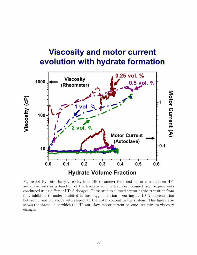
Figure 3.6 Hydrate slurry viscosity from HP-rheometer tests and motor current from HP-autoclave tests as a function of the hydrate volume fraction obtained from experimentsconducted using different HD A dosages. These studies allowed capturing the transition fromfully-inhibited to under-inhibited hydrate agglomeration occurring at HD A concentrationbetween 1 and 0.5 vol.% with respect to the water content in the system. This figure alsoshows the threshold at which the HP-autoclave motor current becomes sensitive to viscositychanges

65

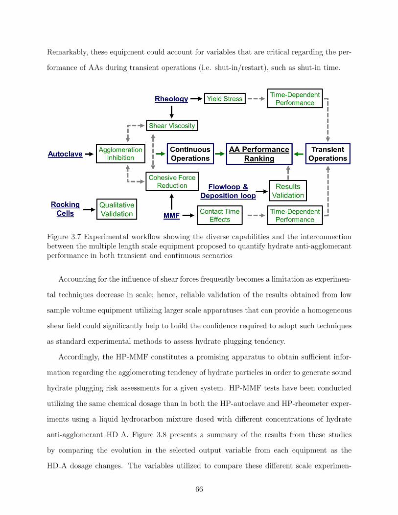
Remarkably, these equipment could account for variables that are critical regarding the per-

formance of AAs during transient operations (i.e. shut-in/restart), such as shut-in time.

Figure 3.7 Experimental workflow showing the diverse capabilities and the interconnectionbetween the multiple length scale equipment proposed to quantify hydrate anti-agglomerantperformance in both transient and continuous scenarios

Accounting for the influence of shear forces frequently becomes a limitation as experimen-

tal techniques decrease in scale; hence, reliable validation of the results obtained from low

sample volume equipment utilizing larger scale apparatuses that can provide a homogeneous

shear field could significantly help to build the confidence required to adopt such techniques

as standard experimental methods to assess hydrate plugging tendency.

Accordingly, the HP-MMF constitutes a promising apparatus to obtain sufficient infor-

mation regarding the agglomerating tendency of hydrate particles in order to generate sound

hydrate plugging risk assessments for a given system. HP-MMF tests have been conducted

utilizing the same chemical dosage than in both the HP-autoclave and HP-rheometer exper-

iments using a liquid hydrocarbon mixture dosed with different concentrations of hydrate

anti-agglomerant HD A. Figure 3.8 presents a summary of the results from these studies

by comparing the evolution in the selected output variable from each equipment as the

HD A dosage changes. The variables utilized to compare these different scale experimen-

66

tal equipment include both static measurements (i.e. yield stress from HP-rheometer and

hydrate cohesive forces from HP-MMF [161]) and parameters evaluated under shear forces

(i.e. mean particle/droplet size from HP-autoclave [160]). Remarkably, all three equipment

showed qualitative agreement on their response to AA concentration changes. At AA HD A

dosages geq1 vol.% no changes are observed in any of the aforementioned experimental vari-

ables, with roughly constant yield stress, particle size and hydrate cohesive force values

regardless of further increasing AA dosage (i.e. a plateau was observed in all three variables

at HD A concentrations ≥ 1 vol.%). In contrast, at HD A concentrations ≤ 1 vol.%, a sharp

transition with increasing values coming from all three variables was detected. The sudden

transition taking place between 1 and 0.5 vol.% HD A suggest a shift from full-inhibition

to under-inhibition of hydrate agglomeration that was captured by each of the experimental

equipment utilized in these studies.

Moreover, the absence of shear forces in both HP-MMF and transient HP-rheometer tests

provides suitable conditions to conduct a quantitative comparison of the experimental output

obtained from these two pieces of equipment. Previous rheological studies have suggested

that the response of a particle suspension to applied stress depends upon a combination of

multiple variables [40]. A suspension particles could either be in a flowing or in a jammed

(arrested) state depending on the given combination of particle-particle attractive forces

(Fmax), temperature (T ), applied shear stress σ, and particle volume fraction φ in the system

as shown in Figure 2.2 in Section 2.1.1.

Several rheological studies looking at the mechanical properties of concentrated particle

suspensions suggested a series of relations between the yield stress of the sample and the

intrinsic particle properties [116, 162–165]. The general relation resulting from these studies

follows Equation 3.1.

σy ∝F αAφ

ψ

dβp(3.1)

Where α, ψ and β are system dependent parameters.

67

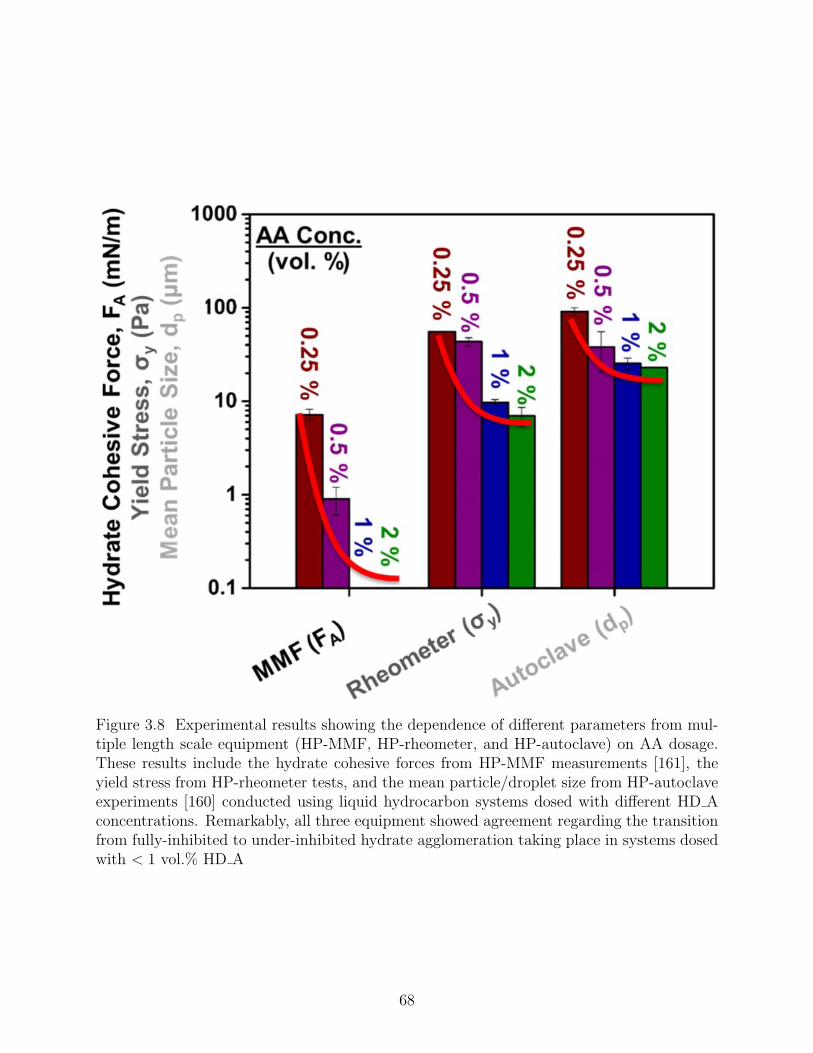
Figure 3.8 Experimental results showing the dependence of different parameters from mul-tiple length scale equipment (HP-MMF, HP-rheometer, and HP-autoclave) on AA dosage.These results include the hydrate cohesive forces from HP-MMF measurements [161], theyield stress from HP-rheometer tests, and the mean particle/droplet size from HP-autoclaveexperiments [160] conducted using liquid hydrocarbon systems dosed with different HD Aconcentrations. Remarkably, all three equipment showed agreement regarding the transitionfrom fully-inhibited to under-inhibited hydrate agglomeration taking place in systems dosedwith < 1 vol.% HD A

68

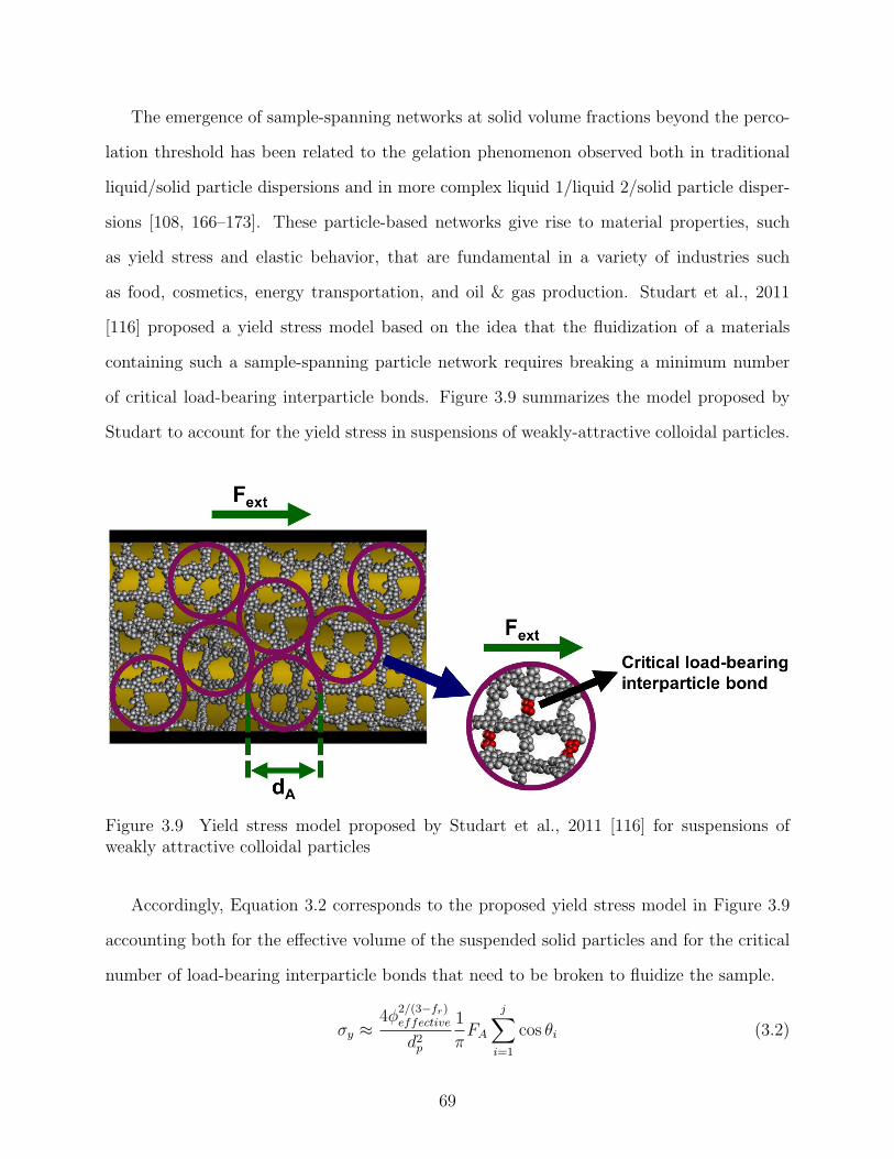
The emergence of sample-spanning networks at solid volume fractions beyond the perco-

lation threshold has been related to the gelation phenomenon observed both in traditional

liquid/solid particle dispersions and in more complex liquid 1/liquid 2/solid particle disper-

sions [108, 166–173]. These particle-based networks give rise to material properties, such

as yield stress and elastic behavior, that are fundamental in a variety of industries such

as food, cosmetics, energy transportation, and oil & gas production. Studart et al., 2011

[116] proposed a yield stress model based on the idea that the fluidization of a materials

containing such a sample-spanning particle network requires breaking a minimum number

of critical load-bearing interparticle bonds. Figure 3.9 summarizes the model proposed by

Studart to account for the yield stress in suspensions of weakly-attractive colloidal particles.

Figure 3.9 Yield stress model proposed by Studart et al., 2011 [116] for suspensions ofweakly attractive colloidal particles

Accordingly, Equation 3.2 corresponds to the proposed yield stress model in Figure 3.9

accounting both for the effective volume of the suspended solid particles and for the critical

number of load-bearing interparticle bonds that need to be broken to fluidize the sample.

σy ≈4φ

2/(3−fr)effective

d2p

1

πFA

j∑

i=1

cos θi (3.2)

69

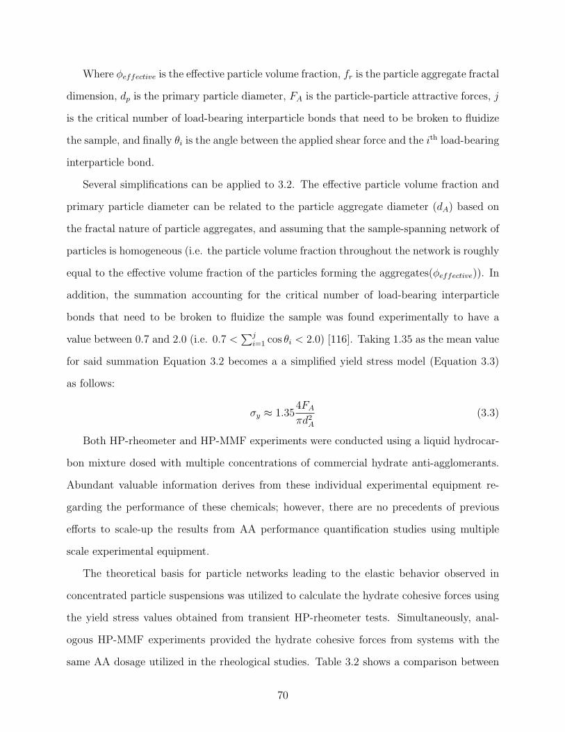
Where φeffective is the effective particle volume fraction, fr is the particle aggregate fractal

dimension, dp is the primary particle diameter, FA is the particle-particle attractive forces, j

is the critical number of load-bearing interparticle bonds that need to be broken to fluidize

the sample, and finally θi is the angle between the applied shear force and the ith load-bearing

interparticle bond.

Several simplifications can be applied to 3.2. The effective particle volume fraction and

primary particle diameter can be related to the particle aggregate diameter (dA) based on

the fractal nature of particle aggregates, and assuming that the sample-spanning network of

particles is homogeneous (i.e. the particle volume fraction throughout the network is roughly

equal to the effective volume fraction of the particles forming the aggregates(φeffective)). In

addition, the summation accounting for the critical number of load-bearing interparticle

bonds that need to be broken to fluidize the sample was found experimentally to have a

value between 0.7 and 2.0 (i.e. 0.7 <∑j

i=1 cos θi < 2.0) [116]. Taking 1.35 as the mean value

for said summation Equation 3.2 becomes a a simplified yield stress model (Equation 3.3)

as follows:

σy ≈ 1.354FAπd2A

(3.3)

Both HP-rheometer and HP-MMF experiments were conducted using a liquid hydrocar-

bon mixture dosed with multiple concentrations of commercial hydrate anti-agglomerants.

Abundant valuable information derives from these individual experimental equipment re-

garding the performance of these chemicals; however, there are no precedents of previous

efforts to scale-up the results from AA performance quantification studies using multiple

scale experimental equipment.

The theoretical basis for particle networks leading to the elastic behavior observed in

concentrated particle suspensions was utilized to calculate the hydrate cohesive forces using

the yield stress values obtained from transient HP-rheometer tests. Simultaneously, anal-

ogous HP-MMF experiments provided the hydrate cohesive forces from systems with the

same AA dosage utilized in the rheological studies. Table 3.2 shows a comparison between

70

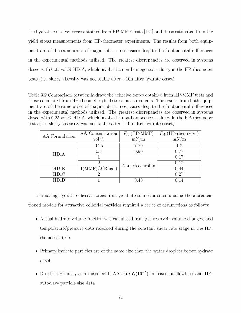
the hydrate cohesive forces obtained from HP-MMF tests [161] and those estimated from the

yield stress measurements from HP-rheometer experiments. The results from both equip-

ment are of the same order of magnitude in most cases despite the fundamental differences

in the experimental methods utilized. The greatest discrepancies are observed in systems

dosed with 0.25 vol.% HD A, which involved a non-homogeneous slurry in the HP-rheometer

tests (i.e. slurry viscosity was not stable after +10h after hydrate onset).

Table 3.2 Comparison between hydrate the cohesive forces obtained from HP-MMF tests andthose calculated from HP-rheometer yield stress measurements. The results from both equip-ment are of the same order of magnitude in most cases despite the fundamental differencesin the experimental methods utilized. The greatest discrepancies are observed in systemsdosed with 0.25 vol.% HD A, which involved a non-homogeneous slurry in the HP-rheometertests (i.e. slurry viscosity was not stable after +10h after hydrate onset)

AA FormulationAA Concentration FA (HP-MMF) FA (HP-rheometer)

vol.% mN/m mN/m

HD A

0.25 7.20 1.80.5 0.90 0.771

Non-Measurable

0.172 0.12

HD E 1(MMF)/2(Rheo.) 0.44HD C 2 0.27HD D 1 0.40 0.14

Estimating hydrate cohesive forces from yield stress measurements using the aforemen-

tioned models for attractive colloidal particles required a series of assumptions as follows:

• Actual hydrate volume fraction was calculated from gas reservoir volume changes, and

temperature/pressure data recorded during the constant shear rate stage in the HP-

rheometer tests

• Primary hydrate particles are of the same size than the water droplets before hydrate

onset

• Droplet size in system dosed with AAs are O(10−5) m based on flowloop and HP-

autoclave particle size data

71

• Hydrate aggregate size was calculated from experimental relative viscosity results using

Camargo & Palermo hydrate slurry viscosity model [53, 112]

Another experimental technique that requires minimum sample volume corresponds to

the measurement of the contact angle of a water droplet on the surface of a cyclopentane

hydrate particle. High contact angles indicate hydrophobic hydrate surfaces due to the

adsorption of surface-active compounds. Such hydrate particles would experience minimal

aggregation according to the capillary bridge theory; in contrast to surfactant-free hydrate

surfaces that are rather water wet. Contact angle measurements were conducted as described

in [133] utilizing HD A. Figure 3.10 includes both HP-rheometer flow curves, as well as

snapshots taken during the contact angle measurements with/without AA HD A [133, 174].

The increasing concentration of AA HD A in the system leads to lower yield stress values

(i.e. intercept with the ordinate); notwithstanding this trend, dosing 1 vol.% AA HD A

to the system still resulted in a finite yield stress value despite the water/hydrate surface

contact angle was ∼ 180◦. Several previous studies on the rheological properties showed that

liquid 1/liquid 2/ solid particle dispersions can show finite yield stress even if the particles

are not wet by the fluid in the smallest proportion in the system. Such behavior has been

related to the emergence of pendular and capillary states characterized by the presence of

macroscopic particle networks [104–110]. Furthermore, no rheological flow curves could be

conducted without any AA dosage to the surfactant-free liquid hydrocarbon mixture given

the HP-rheometer resulted in a shut-down during hydrate formation stages.

Finally, incorporating water/hydrate surface contact angle measurements in an experi-

mental workflow to assess hydrate plugging tendencies in gas/water hydrocarbon systems

introduces a quick and relatively simple scanning tool that requires minimal sample volume

to provide a first-pass assessment of aggregation nature of hydrate particles in a given sys-

tem. Figure 3.11 provides a multi-scale comparison showing the correlation between the

measured contact angles [133, 174], yield stress, and hydrate cohesive forces for high and

low-performance AAs. On one side, hydrate surfaces with an intermediate wettability, such

72

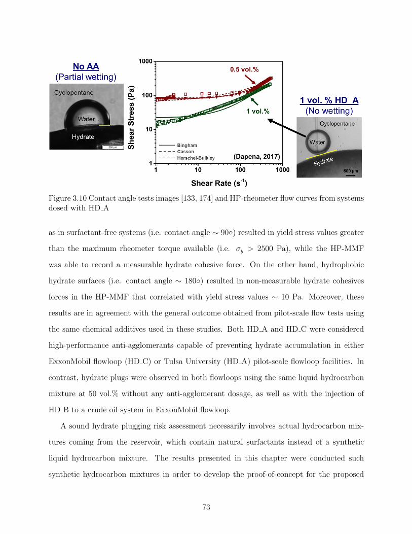
Figure 3.10 Contact angle tests images [133, 174] and HP-rheometer flow curves from systemsdosed with HD A

as in surfactant-free systems (i.e. contact angle ∼ 90◦) resulted in yield stress values greater

than the maximum rheometer torque available (i.e. σy > 2500 Pa), while the HP-MMF

was able to record a measurable hydrate cohesive force. On the other hand, hydrophobic

hydrate surfaces (i.e. contact angle ∼ 180◦) resulted in non-measurable hydrate cohesives

forces in the HP-MMF that correlated with yield stress values ∼ 10 Pa. Moreover, these

results are in agreement with the general outcome obtained from pilot-scale flow tests using

the same chemical additives used in these studies. Both HD A and HD C were considered

high-performance anti-agglomerants capable of preventing hydrate accumulation in either

ExxonMobil flowloop (HD C) or Tulsa University (HD A) pilot-scale flowloop facilities. In

contrast, hydrate plugs were observed in both flowloops using the same liquid hydrocarbon

mixture at 50 vol.% without any anti-agglomerant dosage, as well as with the injection of

HD B to a crude oil system in ExxonMobil flowloop.

A sound hydrate plugging risk assessment necessarily involves actual hydrocarbon mix-

tures coming from the reservoir, which contain natural surfactants instead of a synthetic

liquid hydrocarbon mixture. The results presented in this chapter were conducted such

synthetic hydrocarbon mixtures in order to develop the proof-of-concept for the proposed

73

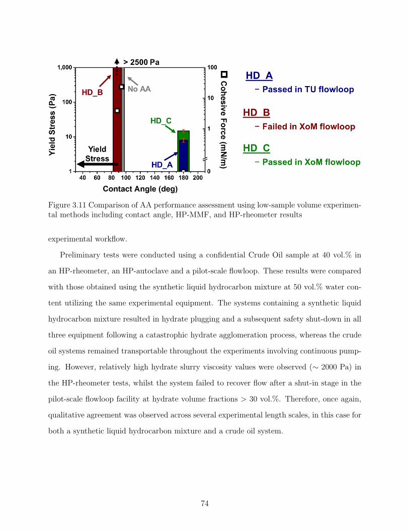
Figure 3.11 Comparison of AA performance assessment using low-sample volume experimen-tal methods including contact angle, HP-MMF, and HP-rheometer results

experimental workflow.

Preliminary tests were conducted using a confidential Crude Oil sample at 40 vol.% in

an HP-rheometer, an HP-autoclave and a pilot-scale flowloop. These results were compared

with those obtained using the synthetic liquid hydrocarbon mixture at 50 vol.% water con-

tent utilizing the same experimental equipment. The systems containing a synthetic liquid

hydrocarbon mixture resulted in hydrate plugging and a subsequent safety shut-down in all

three equipment following a catastrophic hydrate agglomeration process, whereas the crude

oil systems remained transportable throughout the experiments involving continuous pump-

ing. However, relatively high hydrate slurry viscosity values were observed (∼ 2000 Pa) in

the HP-rheometer tests, whilst the system failed to recover flow after a shut-in stage in the

pilot-scale flowloop facility at hydrate volume fractions > 30 vol.%. Therefore, once again,

qualitative agreement was observed across several experimental length scales, in this case for

both a synthetic liquid hydrocarbon mixture and a crude oil system.

74

3.4 Conclusions

In the past, most gas hydrate transportability studies have utilized isolated pieces of

equipment; however, limited efforts have been directed towards the quantitative comparison

and scaling-up of the results across the different equipment. This work proposes a novel

workflow comprising several experimental length scales intended to provide a reliable as-

sessment of anti-agglomerant performance whilst minimizing the required AA and crude oil

sample volumes.

This workflow included a qualitative comparison of the performance assessment obtained

from multiple length scale equipment corresponding to systems dosed with different AA

concentrations. The compared output variables (i.e. hydrate cohesive force, yield stress,

and particle size) showed good agreement regarding the threshold separating fully-inhibited

from under-inhibited hydrate agglomeration. In all cases, a sharp increase in the measured

parameter was observed at AA dosages below the under-inhibition limit.

On the other hand, the hydrate cohesive forces from HP-MMF tests and the yield stress

from HP-rheometer measurements were quantitatively compared utilizing conventional yield

stress models for suspensions of attractive colloidal particles. The calculated cohesive forces

from the measured yield stress values were of the same order of magnitude than those

obtained from HP-MMF test in systems with the same AA dosage. Furthermore, rheological

flow curves suggested finite yield stress values in systems that showed highly hydrophobic

hydrate surfaces (i.e. contact angle ∼ 180◦). These results indicate that simple capillary

bridging theory might be insufficient to fully describe hydrate particle-particle interactions

in water/hydrate/liquid hydrocarbon systems.

Finally, water/hydrate surface contact angle below 100◦ resulted in hydrate plugging in

pilot-scale flowloop, as wells as yield stress values beyond the HP-rheometer torque limits,

which corresponded to measurable hydrate cohesive forces in HP-MMF tests. In contrast,

contact angles ∼ 180◦ provided safe slurry transport in flowloop tests, as well as yield stress

values ∼ 10 Pa, while the hydrate cohesive forces were not measurable using HP-MMF

75

techniques.

In summary, both qualitative and quantitative (i.e. order of magnitude) agreement was

observed across the multiple length scales utilized in the Center for Hydrate Research to

investigate AA and crude oil hydrate dispersing properties. Further validation of hydrate

plugging risk assessment based on experimental methods that require low sample volumes

could ultimately provide the oil & gas industry with reliable and cost-effective tools to

minimize costs at the early design stages of new field developments.

76

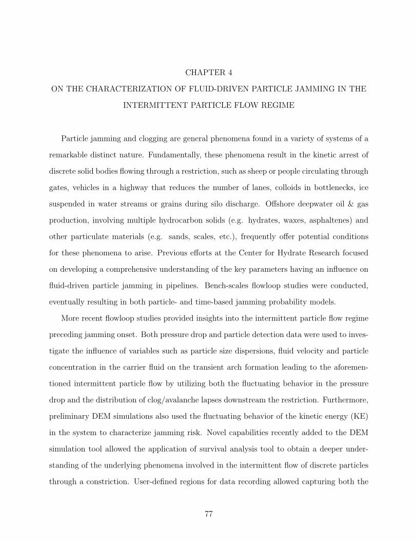
CHAPTER 4

ON THE CHARACTERIZATION OF FLUID-DRIVEN PARTICLE JAMMING IN THE

INTERMITTENT PARTICLE FLOW REGIME

Particle jamming and clogging are general phenomena found in a variety of systems of a

remarkable distinct nature. Fundamentally, these phenomena result in the kinetic arrest of

discrete solid bodies flowing through a restriction, such as sheep or people circulating through

gates, vehicles in a highway that reduces the number of lanes, colloids in bottlenecks, ice

suspended in water streams or grains during silo discharge. Offshore deepwater oil & gas

production, involving multiple hydrocarbon solids (e.g. hydrates, waxes, asphaltenes) and

other particulate materials (e.g. sands, scales, etc.), frequently offer potential conditions

for these phenomena to arise. Previous efforts at the Center for Hydrate Research focused

on developing a comprehensive understanding of the key parameters having an influence on

fluid-driven particle jamming in pipelines. Bench-scales flowloop studies were conducted,

eventually resulting in both particle- and time-based jamming probability models.

More recent flowloop studies provided insights into the intermittent particle flow regime

preceding jamming onset. Both pressure drop and particle detection data were used to inves-

tigate the influence of variables such as particle size dispersions, fluid velocity and particle

concentration in the carrier fluid on the transient arch formation leading to the aforemen-

tioned intermittent particle flow by utilizing both the fluctuating behavior in the pressure

drop and the distribution of clog/avalanche lapses downstream the restriction. Furthermore,

preliminary DEM simulations also used the fluctuating behavior of the kinetic energy (KE)

in the system to characterize jamming risk. Novel capabilities recently added to the DEM

simulation tool allowed the application of survival analysis tool to obtain a deeper under-

standing of the underlying phenomena involved in the intermittent flow of discrete particles

through a constriction. User-defined regions for data recording allowed capturing both the

77

avalanche/clog lapse distribution downstream the flow path restriction and the KE behavior

right upstream said constriction. The application of statistical analysis tools such as the KE

dispersion index (i.e. variance-to-mean ratio) and the downstream particle-detection flow

index (i.e. ratio of particle avalanche lapses to particle (avalanche + clog) lapses), which ul-

timately showed correlation. These results provide additional evidence suggesting that both

kinetic energy and the pressure drop fluctuations during the intermittent particle flow regime

are related to the transient arch formation/breakage occurring at the flow path constriction.

Finally, various probabilistic models (i.e. Kaplan-Meier and Weibull probability distribu-

tions) were utilized to further examine the intermittent particle flow regime. Weibull shape

factor suggested that both the particle avalanche and clog distributions present a wear-out

kind of failure behavior, indicating, for example, that the particle avalanche interruption

rate increases with time.

The methods included in this research update provide an analytical framework to effi-

ciently analyze future DEM simulations looking into more realistic pipeline-like conditions.

For example, utilizing the KE dispersion index to asses jamming risk instead of traditional

and more computationally intensive methods, such as individual particle avalanche/clog de-

tection or exclusively looking at the final outcome of a jamming simulation rather than

making use of the whole experimental data output.

4.1 Introduction

Granular materials and solids suspensions flowing along pipelines can result in parti-

cle accumulation at flow path constrictions. The increasing particle concentration at the

accumulation points can promote self-stabilizing mechanical structures capable of kineti-

cally arresting the suspended solids. Such transitions from a fluid-like to a solid-like state

are known as particle jamming or clogging. As discussed in Section 3.1, particle jamming

could be a potential plugging mechanism for large solids flowing in subsea pipelines, such as

sloughed hydrate deposits or hydrate agglomerates. Jammed systems are considered ”fragile

matter” [1], meaning that the self-stabilizing structures can collapse due to different causes

78

inherent to the system. The alternating formation and destruction of such structures result

in the intermittent flow of solid particles.

Jamming is a general phenomenon occurring in systems of a remarkably distinct nature

whenever multiple discrete bodies compete for limited space under a given driving force.

Things get jammed in all kinds of scenarios. From everyday situations, such as driving in

traffic or going to the supermarket, to more unconventional environments, such in factories,

where powdered raw materials might clog the transfer conduits, or in offshore oil & gas

production, where hydrate agglomerates might block the pipeline due to jamming [6, 175,

176]. Clogging, which is a specific case within the jamming phenomena, can be defined

as the transition of a flowing system into a solid caused by the emergence of an adaptive

skeleton that forms in response to an applied load [177–179]. These transitions are frequently

observed in systems containing discrete macroscopic bodies that could exhibit structural

arrest [180]. Such systems containing discrete bodies can form a contact network of force

chains responsible for propagating stress[177].

Discrete bodies flowing through a constriction or bottleneck can lead to the formation of

the aforementioned self-stabilizing structures ultimately clogging the system [180–186]. The

force chains can support big loads in the same direction that the forces giving rise to the

clogged state. However, minimal forces acting in any other direction could collapse the force

chain network, resuming particle flow. [177, 179, 187, 188].Such structural fragility causes

the system to alternate between clogged and unclogged states leading to an intermittent flow

of particles [189–191]. Figure 4.1 shows a few examples of situations where discrete bodies

flow through a bottleneck and could potentially clog the system.

Previous studies suggested that the different variables having an influence on the clogging

transitions can be grouped into three generic parameters [181]:

• The length scale of the system that, in a particle suspension flow in a pipeline scenario,

depends upon the particle/restriction shape and size

79

Figure 4.1 Examples of systems of a distinct nature that could potentially clog. Figure A:Confocal images of dense suspensions of fluorescent PMMA particles flowing from left toright through constricted microchannels with varying constriction angles. Figure modifiedfrom Genovese & Sprakel, 2011 [192]. Figure B: Effect of the obstacle position in the flowof sheep through a narrow door. Left: The typical clog observed without an obstacle.Right: The typical clog observed with an obstacle located 0.60 meters away from the door.Figure modified from Garcimartin et al., 2016 [193]. Figure C: Microfluidic colloid filtration.Left: Build-up of the filter cake during filtration of microgel suspension. Right: Increasingcrystallinity under growing pressure drop during the filtration process. Figure modified fromLinkhorst et al., 2016 [194]

80

• The compatible loads relate to the driving forces giving rise to the clogged state (i.e.

forces acting in the direction of the major compression axis). In fluid-driven particle

jamming, the fluid provides such forces and the major compression axis corresponds

to the fluid flow direction

• The incompatible loads responsible for the collapse of the clogging structures. These are

normally related to noise and vibrations acting on the stabilizing force chains. Fluid

flow through the clogged particles can cause such vibrations leading to unclogging

events

Defining these parameters for the specific case of fluid-driven particle jamming makes ev-

ident a unique feature in these systems where the fluid flow is responsible both for giving rise

to clogging events and for providing the vibrations leading to unclogging transitions. Fig-

ure 4.2 shows an adaptation of the universal clogging phase diagram proposed by Zuriguel,

2014 [181] tailored for a scenario comprising fluid-driven flow of suspended particles through

a flow path constriction. This phase diagram considers the contribution of the three generic

parameters that are relevant during clogging transitions (i.e.the compatible loads, the in-

compatible loads and the length scale of the system).

Fluid-driven particle jamming studies previously conducted at the Center for Hydrate

Research (CHR) at the Colorado School of Mines investigated the influence of key parameters

such as the fluid velocity, the restriction shape, and the particle-to-restriction diameter ratio

(R = dp/dR). These studies lead to the development of both particle number-based and

time-based probability models for fluid-driven particle jamming [175, 186]. Both of these

models consider the probability of observing a jamming event following a finite number of

not jammed events, which can either correspond to a particle flowing across the restriction

or a time step being elapsed without the occurrence of a jam.

The particle-based jamming model describes the probability of observing a jamming event

as the nth particle approaches the restriction providing n − 1 particles have been through

the restriction already providing n − 1 particles have been through the restriction already

81

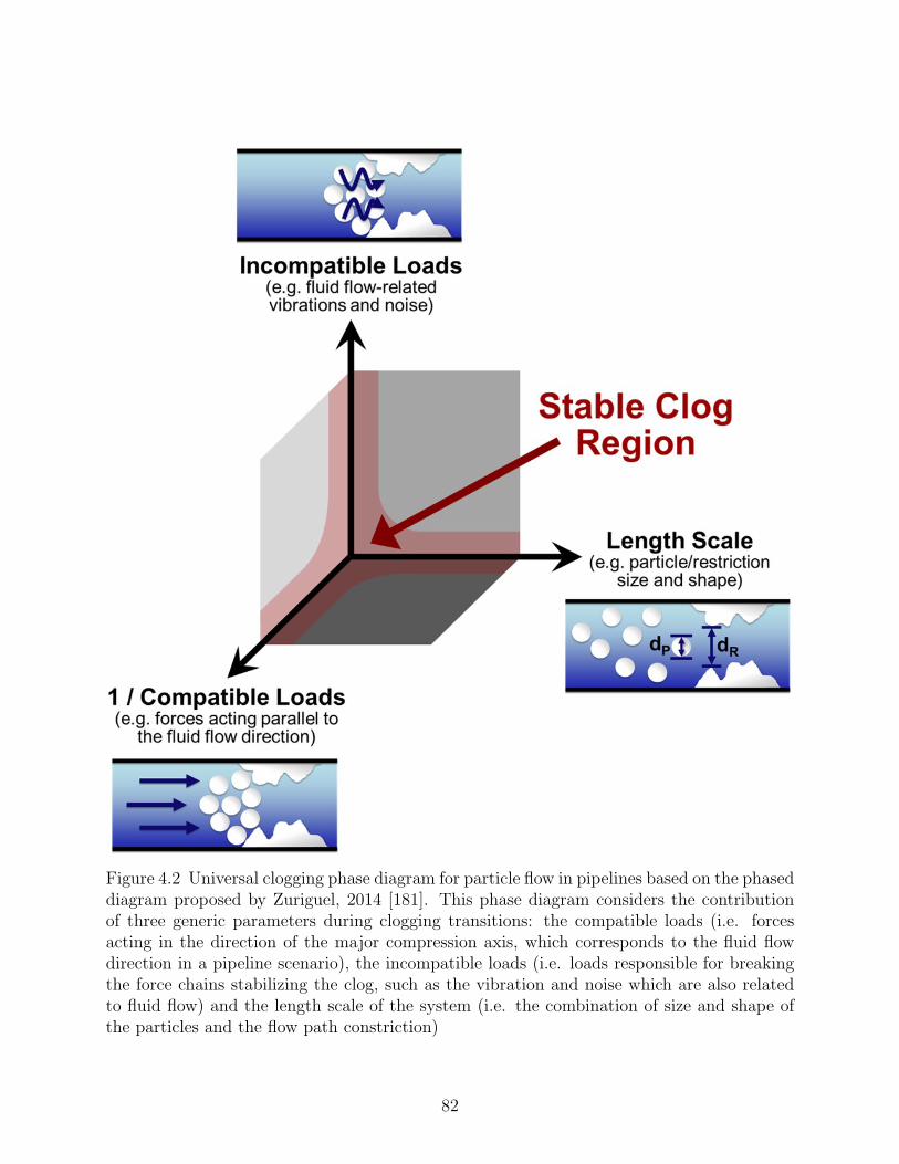
Figure 4.2 Universal clogging phase diagram for particle flow in pipelines based on the phaseddiagram proposed by Zuriguel, 2014 [181]. This phase diagram considers the contributionof three generic parameters during clogging transitions: the compatible loads (i.e. forcesacting in the direction of the major compression axis, which corresponds to the fluid flowdirection in a pipeline scenario), the incompatible loads (i.e. loads responsible for breakingthe force chains stabilizing the clog, such as the vibration and noise which are also relatedto fluid flow) and the length scale of the system (i.e. the combination of size and shape ofthe particles and the flow path constriction)

82

without jamming (pjam (n)). Each particle (k) might either flow through the restriction

with probability (pk) or jam at the restriction with probability (1− pk). Accordingly, the

probability of observing a jamming event as the nth particle flows across the restriction

implies that n − 1 particles previously flowed through the bottleneck with probability pk

each, while the n-particle gets jammed with probability 1− pn following Equation 4.1 [186]:

pjam (n) = (1− pn)n−1∏

k=0

pk (4.1)

Further model development considered an analogous time-based approach in order to

optimize the analysis of the experimental results obtained from the automated bench-scale

flowloop designed and constructed at the CHR specifically to study fluid-driven particle

jamming phenomena. The model suggests that the jamming probability (pjam) at time t

depends upon a series of time steps elapsing with non-jamming events followed by a jamming

event taking place at the subsequent time step. A continuous function (r (t)) represents the

jamming rate at a given time (i.e. average number of jamming events occurring per time

step). Accordingly, Equation 4.2 computes the probability of observing a jamming event at

time t (i.e. pjam (t)) providing no jamming event has occurred yet [175]:

pjam (t) = r (t) exp

{

−

∫ 0

t

r (t) dt

}

(4.2)

In addition, the probability of an individual particle going through the restriction (pk),

has been shown to saturate to a constant value after a critical number of particles have

flowed across the orifice, both in gravity-driven and fluid-driven particle jamming scenarios

[185, 186]. Likewise, the time-based jamming rate saturates to a constant value corresponding

to the steady-state jamming regime taking place after full backlog development (λ) [175].

The bench-scale automated flowloop specifically designed at CHR [175] to investigate

fluid-driven particle jamming is a unique piece of experimental equipment that introduces

fluid shear forces into the jamming/clogging phenomena. Previous studies focused on the

characterization and modeling of fluid-driven particle jamming in the backlogged (or steady-

state) regime, using experimental flowloops with both 2D and 3D restrictions in the flow

83

path [175, 186, 195, 196].

In addition to laboratory investigations, computational tools have been previously used

to break into pieces the underlying phenomena involved in the transport of solid particles

suspended in a carrier fluid. Several studies have been conducted utilizing two-way couplings

of computational fluid dynamics (CFD) and discrete element methods (DEM) [197–200],

which are available both as open-source projects, such as YADE (python DEM package) or

CFDEMrproject, which utilizes LAMMPS-based DEM code (LIGGGHTS), both of them

coupled with the open-source CFD toolbox OpenFOAMr, as well as commercial software

(e.g. EDEM (coupled with CFD software ANSYS Fluent) or Particle Flow Code (PFC™)).

DEM simulations have been used also to look into the jamming and clogging phenomena

both in the absence [201–204] or presence [182, 183, 205, 206] of fluid forces. Recent studies

have implemented a lattice Boltzmann method (LBM) to simulate the fluid field part of the

coupling with a DEM engine in the development of novel multiphase fluid models [207, 208].

The studies discussed in this report focused on characterizing the intermittent particle

flow regime preceding jamming transitions, particularly looking at the particle concentration

and size dispersion effects on the jamming probability distribution. These laboratory results

are coupled with 2D DEM simulations of granular flow across restrictions. These simula-

tions allowed relating the intermittent flow of particles across the restriction to fluctuations

arising in the kinetic energy of the system. The influence of some additional parameters was

included in these studies on fluid-driven jamming transitions, such as particle shape and size

dispersion.


Both a bench-scale flowloop and DEM simulations were used to study the intermittent

particle flow preceding jamming onset in fluid-driven particle flow across restrictions.

84

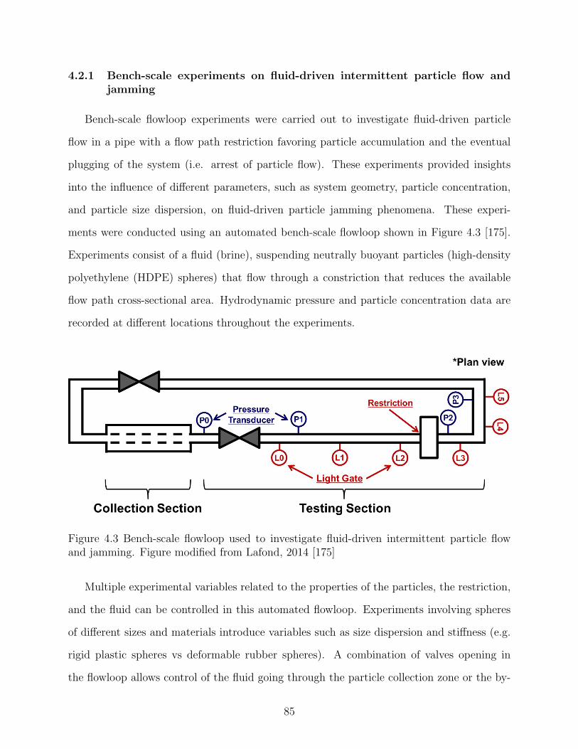
4.2.1 Bench-scale experiments on fluid-driven intermittent particle flow andjamming

Bench-scale flowloop experiments were carried out to investigate fluid-driven particle

flow in a pipe with a flow path restriction favoring particle accumulation and the eventual

plugging of the system (i.e. arrest of particle flow). These experiments provided insights

into the influence of different parameters, such as system geometry, particle concentration,

and particle size dispersion, on fluid-driven particle jamming phenomena. These experi-

ments were conducted using an automated bench-scale flowloop shown in Figure 4.3 [175].

Experiments consist of a fluid (brine), suspending neutrally buoyant particles (high-density

polyethylene (HDPE) spheres) that flow through a constriction that reduces the available

flow path cross-sectional area. Hydrodynamic pressure and particle concentration data are

recorded at different locations throughout the experiments.

Figure 4.3 Bench-scale flowloop used to investigate fluid-driven intermittent particle flowand jamming. Figure modified from Lafond, 2014 [175]

Multiple experimental variables related to the properties of the particles, the restriction,

and the fluid can be controlled in this automated flowloop. Experiments involving spheres

of different sizes and materials introduce variables such as size dispersion and stiffness (e.g.

rigid plastic spheres vs deformable rubber spheres). A combination of valves opening in

the flowloop allows control of the fluid going through the particle collection zone or the by-

85

pass section. This flowloop feature provides control on the particle volume fraction flowing

towards the restriction. Moreover, the flow path restrictions can be of different shape and

size.

The collection section consists of concentric pipes with the annulus connected to the

pump suction, promoting the accumulation of the particles in this section. The inner pipe

is perforated with holes that are smaller than the experimental particles. This configuration

allows separation of the particles from the carrier fluid between independent experimental

runs.

The flowloop testing section, embodied in a 4” diameter (schedule 40) acrylic pipe, accom-

modates multiple data acquisition tools. Four pressure transducers located both upstream

(2) and downstream (2) the restriction provide pressure drop recordings during the experi-

ments. Additionally, six photoelectric sensors distributed across the testing section check for

the presence of particles flowing at these specific locations throughout the tests, eventually

providing an estimate of the particle volume fraction flowing in the pipeline. Finally, video

recordings at the flow path restriction, which are time-marked using a LED indicator, allowed

connecting the pressure drop data with the events taking place as the particles flowed across

the restriction. Such events included particle accumulation (i.e. backlogging), intermittent

particle flow, and, ultimately, particle jamming. The apparatus automated operational pro-

tocol resets to the same starting point after each independent run in order to conduct a new

experiment. Such design allows as many as 500-1000 runs per day, depending on the total

experimental time of a single independent run. This equipment yields statistically signifi-

cant data that, after appropriate processing and analysis, could help to develop stochastic

models describing the plugging risk related to the transportation of solids in a pipe with a

constriction.

Tests conducted using the bench-scale jamming flowloop provide multiple useful output

data. Two major pieces of information obtained from the automated bench-scale flowloop

for fluid-driven jamming studies are the pressure drop across the restriction (Figure 4.4) and

86

the particle concentration (Figure 4.5) profiles:

1. Pressure drop profiles: Four pressure transducers (P0 − P3) installed along the testing

section continuously record the hydrodynamic pressure of the system. Two pressure

transducers are located both upstream (P0, P1) and downstream (P2, P3) the restric-

tion (See Figure 4.3). The pressure drop across the restriction provides insights into

the events taking place during the jamming transitions. After running a statistically

significant number of experiments, a well-defined characteristic pressure drop profile

for each specific experimental configuration (i.e. combination of restriction/particle

shape and size). Figure 4.4 shows the characteristic pressure drop profile as a function

of time obtained after 1,500 independent runs in the bench-scale jamming flowloop

using a neutrally buoyant bi-disperse system containing 1/2” and 3/4” HDPE spheres

in a 1:1 ratio, resulting in an 5/8” average sphere diameter (dp) and the restriction

diameter (dR) of 5/4” yielding a particle diameter to restriction diameter ratio equal

to 2 (R = dR/dp = 2). The fluid velocity was 0.114 m/s

2. Particle concentration profiles: Six light gates (L0 − L5) with their respective light

reflectors installed along the testing section (see Figure 4.3) check for the presence

particles at a given position and time. These light gates give a binary signal indicating

whether an object blocks the light path (i.e. the laser is not returning to the source)

or not. Given the independent bench-scale flowloop runs are performed following an

identical procedure, the averaged light gate signal from a full experimental data set

provides a profile that correlates with the particle concentration at the different pipe

locations as a function of time. The actual particle concentration could be estimated

from these data by means of geometric assumptions related to the particle shape and

size [175] that are valid within a certain particle concentration range. Figure 4.5 shows

the concentration profile as a function of time resulting from the same bench-scale

jamming flowloop data set that yielded the pressure drop profile in Figure 4.4. In this

figure, Plos is the probability of having a line of sight (los) between the nth laser source

87

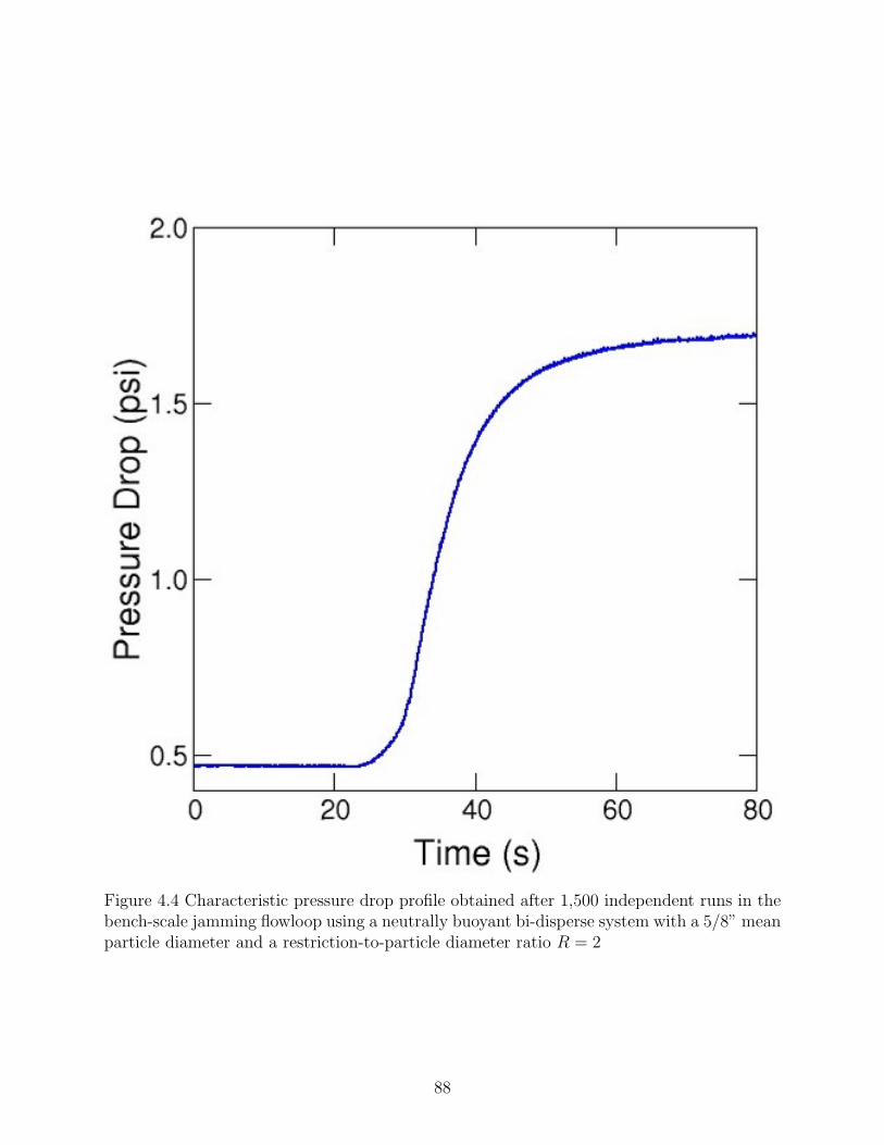
Figure 4.4 Characteristic pressure drop profile obtained after 1,500 independent runs in thebench-scale jamming flowloop using a neutrally buoyant bi-disperse system with a 5/8” meanparticle diameter and a restriction-to-particle diameter ratio R = 2

88

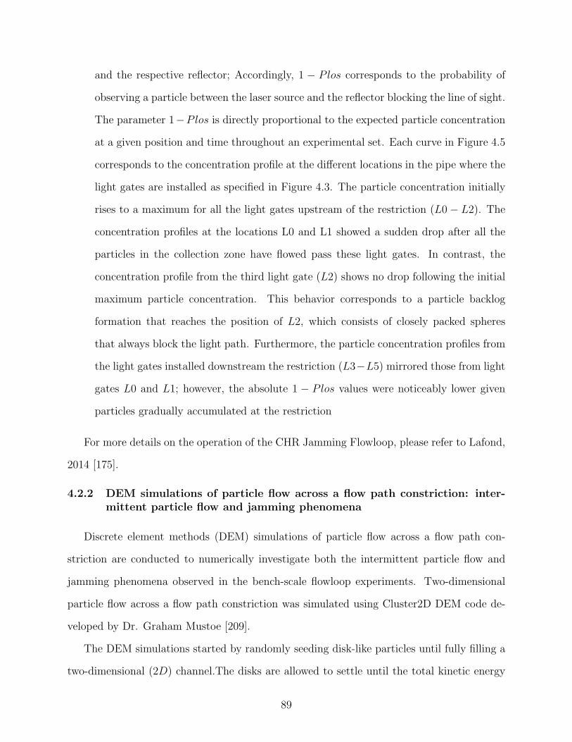
and the respective reflector; Accordingly, 1 − Plos corresponds to the probability of

observing a particle between the laser source and the reflector blocking the line of sight.

The parameter 1−Plos is directly proportional to the expected particle concentration

at a given position and time throughout an experimental set. Each curve in Figure 4.5

corresponds to the concentration profile at the different locations in the pipe where the

light gates are installed as specified in Figure 4.3. The particle concentration initially

rises to a maximum for all the light gates upstream of the restriction (L0− L2). The

concentration profiles at the locations L0 and L1 showed a sudden drop after all the

particles in the collection zone have flowed pass these light gates. In contrast, the

concentration profile from the third light gate (L2) shows no drop following the initial

maximum particle concentration. This behavior corresponds to a particle backlog

formation that reaches the position of L2, which consists of closely packed spheres

that always block the light path. Furthermore, the particle concentration profiles from

the light gates installed downstream the restriction (L3−L5) mirrored those from light

gates L0 and L1; however, the absolute 1 − Plos values were noticeably lower given

particles gradually accumulated at the restriction

For more details on the operation of the CHR Jamming Flowloop, please refer to Lafond,

2014 [175].

4.2.2 DEM simulations of particle flow across a flow path constriction: inter-mittent particle flow and jamming phenomena

Discrete element methods (DEM) simulations of particle flow across a flow path con-

striction are conducted to numerically investigate both the intermittent particle flow and

jamming phenomena observed in the bench-scale flowloop experiments. Two-dimensional

particle flow across a flow path constriction was simulated using Cluster2D DEM code de-

veloped by Dr. Graham Mustoe [209].

The DEM simulations started by randomly seeding disk-like particles until fully filling a

two-dimensional (2D) channel.The disks are allowed to settle until the total kinetic energy

89

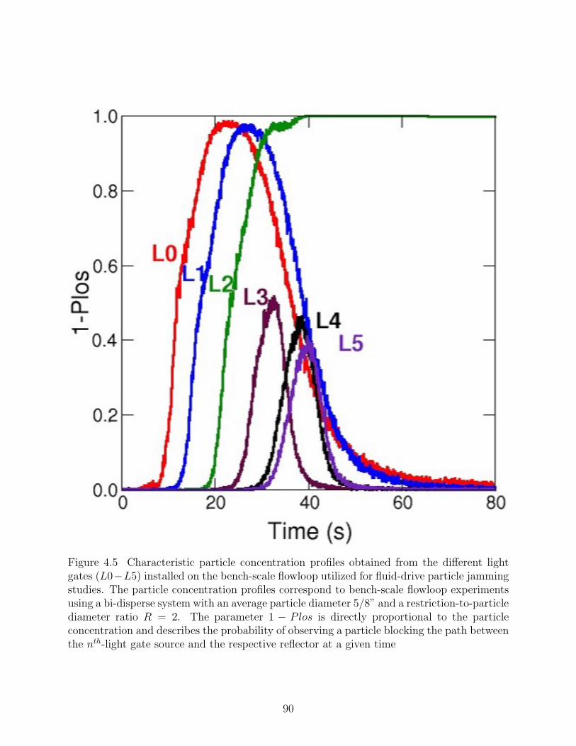
Figure 4.5 Characteristic particle concentration profiles obtained from the different lightgates (L0−L5) installed on the bench-scale flowloop utilized for fluid-drive particle jammingstudies. The particle concentration profiles correspond to bench-scale flowloop experimentsusing a bi-disperse system with an average particle diameter 5/8” and a restriction-to-particlediameter ratio R = 2. The parameter 1 − Plos is directly proportional to the particleconcentration and describes the probability of observing a particle blocking the path betweenthe nth-light gate source and the respective reflector at a given time

90

of the system stabilizes. Once particles have settled, a restriction-like gate with a given

size and y-axis position opens at the right end of the channel. Particles are allowed to

flow across the restriction under the effect of a constant force field acting on the axial

direction of the channel. (i.e. x-axis). The 2nd-generation of DEM simulations utilized an

updated version of Cluster2D DEM code specifically tailored to analyze the data coming

from simulations looking at the flow of particles across a flow path constriction in a 2D

channel. This updated version included an improved seeding algorithm allowing to conduct

independent simulations with different random arrangements of particles in a time-efficient

manner. In addition, user-defined data recording regions can now be defined. Such user-

defined regions provide output data containing the particle count and total kinetic energy

within a given region. This feature becomes particularly useful regarding the jamming

phenomena, where the events controlling the dynamics of the system are concentrated near

the flow path constriction. Figure 4.6 presents a snapshot taken during the initialization

stage of an individual simulation of particle flow across a flow path constriction conducted

using Cluster2D DEM simulation tool. This image sketches the location of the different

user-defined regions considered in these simulations. Particularly important are the regions

located immediately upstream and downstream the flow path restrictions, namely regions

R5 & R6-R8 respectively.

Finally, periodic boundary conditions are applied in the x-direction. Setting such bound-

ary conditions allows reinserting in the left end of the channel each particle that exits the

system at the right end of the simulation box. This feature recycles the particles present in

the system, which permits conducting simulations with a long run time without adding new

particles that would increase the computational requirements of the experiment. Figure 4.7

shows a snapshot taken after particle flow across the flow path restriction starts. This image

captures the particles leaving at the right end of the simulation box, and being reinserted at

the left end of the same box. Color-coded particle velocity shows particles moving fast near

and downstream the restriction, whilst the bulk particles remain almost immobilized. This

91

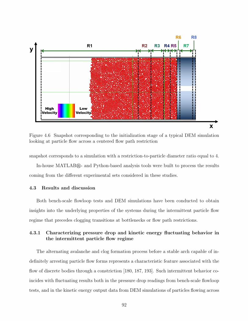
Figure 4.6 Snapshot corresponding to the initialization stage of a typical DEM simulationlooking at particle flow across a centered flow path restriction

snapshot corresponds to a simulation with a restriction-to-particle diameter ratio equal to 4.

In-house MATLABr- and Python-based analysis tools were built to process the results

coming from the different experimental sets considered in these studies.


Both bench-scale flowloop tests and DEM simulations have been conducted to obtain

insights into the underlying properties of the systems during the intermittent particle flow

regime that precedes clogging transitions at bottlenecks or flow path restrictions.

4.3.1 Characterizing pressure drop and kinetic energy fluctuating behavior inthe intermittent particle flow regime

The alternating avalanche and clog formation process before a stable arch capable of in-

definitely arresting particle flow forms represents a characteristic feature associated with the

flow of discrete bodies through a constriction [180, 187, 193]. Such intermittent behavior co-

incides with fluctuating results both in the pressure drop readings from bench-scale flowloop

tests, and in the kinetic energy output data from DEM simulations of particles flowing across

92

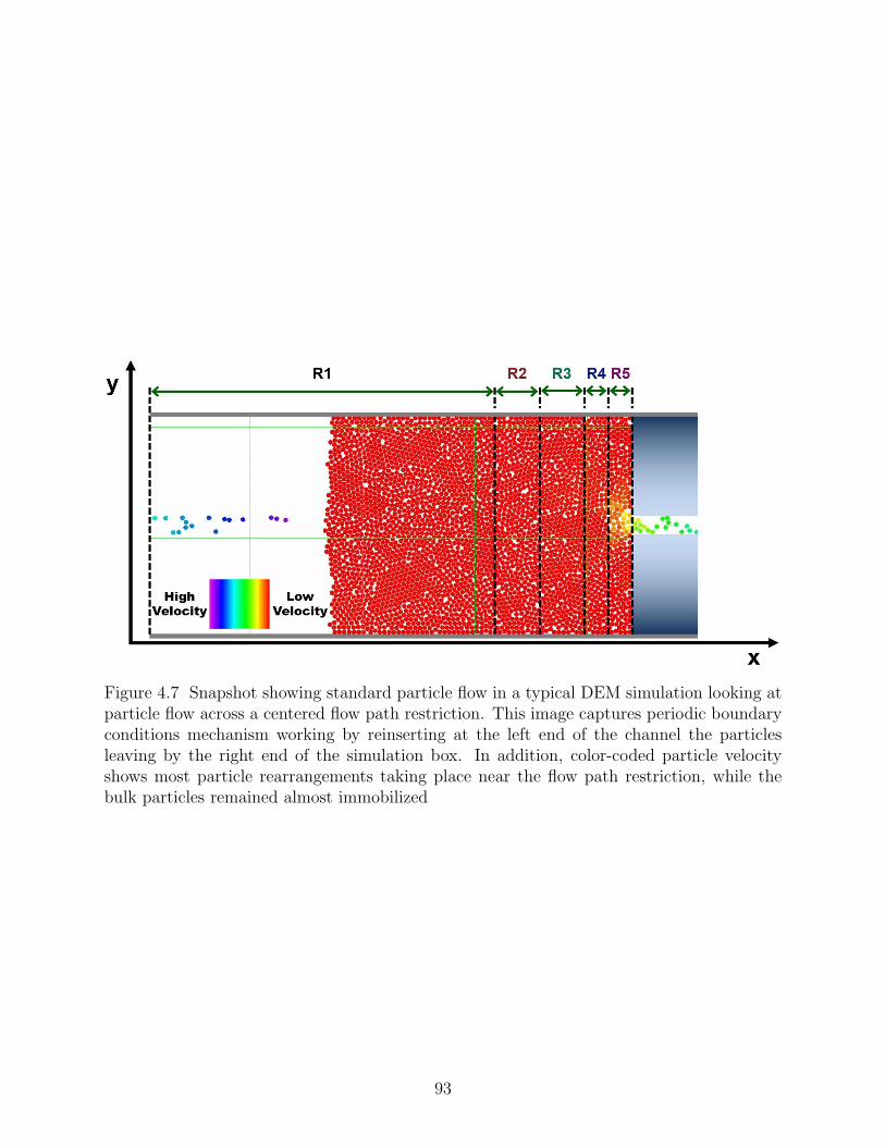
Figure 4.7 Snapshot showing standard particle flow in a typical DEM simulation looking atparticle flow across a centered flow path restriction. This image captures periodic boundaryconditions mechanism working by reinserting at the left end of the channel the particlesleaving by the right end of the simulation box. In addition, color-coded particle velocityshows most particle rearrangements taking place near the flow path restriction, while thebulk particles remained almost immobilized

93

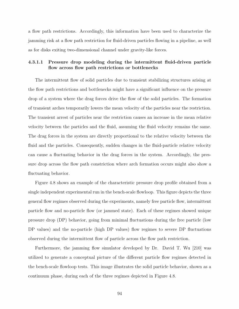
a flow path restrictions. Accordingly, this information have been used to characterize the

jamming risk at a flow path restriction for fluid-driven particles flowing in a pipeline, as well

as for disks exiting two-dimensional channel under gravity-like forces.

4.3.1.1 Pressure drop modeling during the intermittent fluid-driven particleflow across flow path restrictions or bottlenecks

The intermittent flow of solid particles due to transient stabilizing structures arising at

the flow path restrictions and bottlenecks might have a significant influence on the pressure

drop of a system where the drag forces drive the flow of the solid particles. The formation

of transient arches temporarily lowers the mean velocity of the particles near the restriction.

The transient arrest of particles near the restriction causes an increase in the mean relative

velocity between the particles and the fluid, assuming the fluid velocity remains the same.

The drag forces in the system are directly proportional to the relative velocity between the

fluid and the particles. Consequently, sudden changes in the fluid-particle relative velocity

can cause a fluctuating behavior in the drag forces in the system. Accordingly, the pres-

sure drop across the flow path constriction where arch formation occurs might also show a

fluctuating behavior.

Figure 4.8 shows an example of the characteristic pressure drop profile obtained from a

single independent experimental run in the bench-scale flowloop. This figure depicts the three

general flow regimes observed during the experiments, namely free particle flow, intermittent

particle flow and no-particle flow (or jammed state). Each of these regimes showed unique

pressure drop (DP) behavior, going from minimal fluctuations during the free particle (low

DP values) and the no-particle (high DP values) flow regimes to severe DP fluctuations

observed during the intermittent flow of particle across the flow path restriction.

Furthermore, the jamming flow simulator developed by Dr. David T. Wu [210] was

utilized to generate a conceptual picture of the different particle flow regimes detected in

the bench-scale flowloop tests. This image illustrates the solid particle behavior, shown as a

continuum phase, during each of the three regimes depicted in Figure 4.8.

94

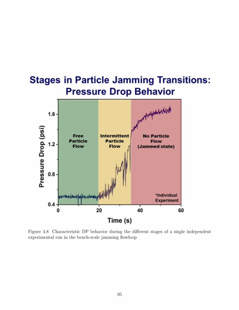
Figure 4.8 Characteristic DP behavior during the different stages of a single independentexperimental run in the bench-scale jamming flowloop

95

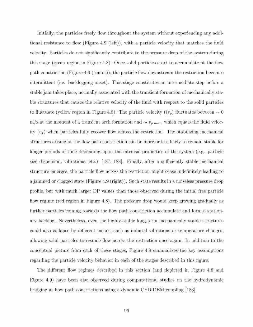
Initially, the particles freely flow throughout the system without experiencing any addi-

tional resistance to flow (Figure 4.9 (left)), with a particle velocity that matches the fluid

velocity. Particles do not significantly contribute to the pressure drop of the system during

this stage (green region in Figure 4.8). Once solid particles start to accumulate at the flow

path constriction (Figure 4.9 (center)), the particle flow downstream the restriction becomes

intermittent (i.e. backlogging onset). This stage constitutes an intermediate step before a

stable jam takes place, normally associated with the transient formation of mechanically sta-

ble structures that causes the relative velocity of the fluid with respect to the solid particles

to fluctuate (yellow region in Figure 4.8). The particle velocity ((vp) fluctuates between ∼ 0

m/s at the moment of a transient arch formation and ∼ vp max, which equals the fluid veloc-

ity (vf ) when particles fully recover flow across the restriction. The stabilizing mechanical

structures arising at the flow path constriction can be more or less likely to remain stable for

longer periods of time depending upon the intrinsic properties of the system (e.g. particle

size dispersion, vibrations, etc.) [187, 188]. Finally, after a sufficiently stable mechanical

structure emerges, the particle flow across the restriction might cease indefinitely leading to

a jammed or clogged state (Figure 4.9 (right)). Such state results in a noiseless pressure drop

profile, but with much larger DP values than those observed during the initial free particle

flow regime (red region in Figure 4.8). The pressure drop would keep growing gradually as

further particles coming towards the flow path constriction accumulate and form a station-

ary backlog. Nevertheless, even the highly-stable long-term mechanically stable structures

could also collapse by different means, such as induced vibrations or temperature changes,

allowing solid particles to resume flow across the restriction once again. In addition to the

conceptual picture from each of these stages, Figure 4.9 summarizes the key assumptions

regarding the particle velocity behavior in each of the stages described in this figure.

The different flow regimes described in this section (and depicted in Figure 4.8 and

Figure 4.9) have been also observed during computational studies on the hydrodynamic

bridging at flow path constrictions using a dynamic CFD-DEM coupling [183].

96

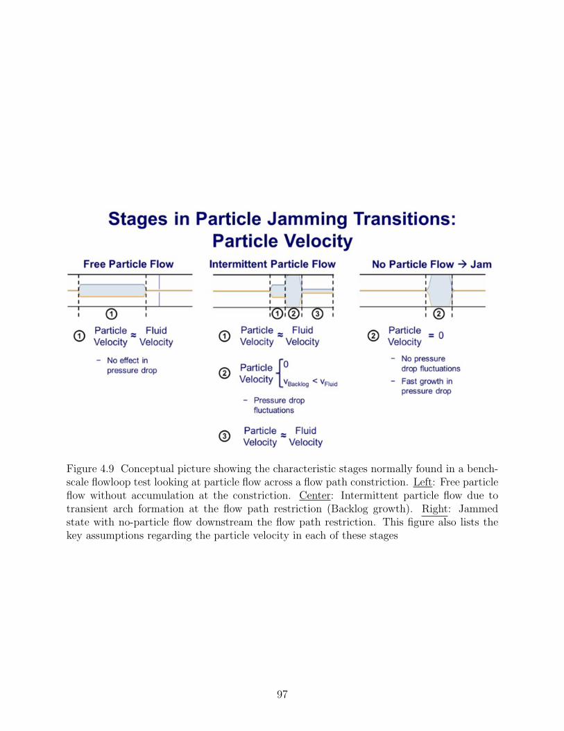
Figure 4.9 Conceptual picture showing the characteristic stages normally found in a bench-scale flowloop test looking at particle flow across a flow path constriction. Left: Free particleflow without accumulation at the constriction. Center: Intermittent particle flow due totransient arch formation at the flow path restriction (Backlog growth). Right: Jammedstate with no-particle flow downstream the flow path restriction. This figure also lists thekey assumptions regarding the particle velocity in each of these stages

97

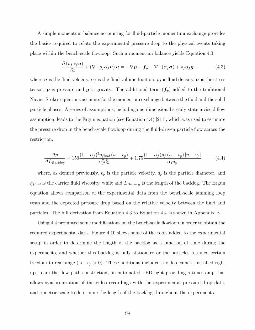
A simple momentum balance accounting for fluid-particle momentum exchange provides

the basics required to relate the experimental pressure drop to the physical events taking

place within the bench-scale flowloop. Such a momentum balance yields Equation 4.3,

∂ (ρfαfu)

∂t+ (∇ · ρfαfu)u = −∇p− fp +∇ · (αfσ) + ρfαfg (4.3)

where u is the fluid velocity, αf is the fluid volume fraction, ρf is fluid density, σ is the stress

tensor, p is pressure and g is gravity. The additional term (fp) added to the traditional

Navier-Stokes equations accounts for the momentum exchange between the fluid and the solid

particle phases. A series of assumptions, including one-dimensional steady-state inviscid flow

assumption, leads to the Ergun equation (see Equation 4.4) [211], which was used to estimate

the pressure drop in the bench-scale flowloop during the fluid-driven particle flow across the

restriction.

∆p

∆LBacklog= 150

(1− αf )2ηfluid (u− vp)

α2fd

2p

+ 1.75(1− αf )ρf (u− vp) |u− vp|

αfdp(4.4)

where, as defined previously, vp is the particle velocity, dp is the particle diameter, and

ηfluid is the carrier fluid viscosity, while and LBacklog is the length of the backlog. The Ergun

equation allows comparison of the experimental data from the bench-scale jamming loop

tests and the expected pressure drop based on the relative velocity between the fluid and

particles. The full derivation from Equation 4.3 to Equation 4.4 is shown in Appendix B.

Using 4.4 prompted some modifications on the bench-scale flowloop in order to obtain the

required experimental data. Figure 4.10 shows some of the tools added to the experimental

setup in order to determine the length of the backlog as a function of time during the

experiments, and whether this backlog is fully stationary or the particles retained certain

freedom to rearrange (i.e. vp > 0). These additions included a video camera installed right

upstream the flow path constriction, an automated LED light providing a timestamp that

allows synchronization of the video recordings with the experimental pressure drop data,

and a metric scale to determine the length of the backlog throughout the experiments.

98

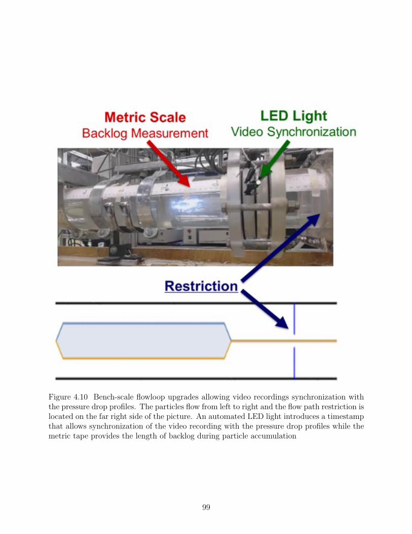
Figure 4.10 Bench-scale flowloop upgrades allowing video recordings synchronization withthe pressure drop profiles. The particles flow from left to right and the flow path restriction islocated on the far right side of the picture. An automated LED light introduces a timestampthat allows synchronization of the video recording with the pressure drop profiles while themetric tape provides the length of backlog during particle accumulation

99

Combining the Ergun equation with the available experimental data from the bench-

scale flowloop makes possible to estimate the pressure drop change in the system as particles

accumulate and intermittently flow across the restriction. The expected increase in the

pressure drop is calculated as a function of the backlog length once the system has jammed

(i.e. when the particle velocity can be assumed to be equal to 0 m/s.

Figure 4.11 shows such estimated pressure drop for an individual experiment using

58” HDPE spherical particles and a restriction diameter equal to 5

4”, yielding a ratio of

restriction-to-particle diameter equal to 2 (i.e. R = 2). The superficial fluid velocity (us)

in these experiments was 0.11 m/s. The fluid volume fraction in the backlog after jamming

onset occurs was assumed ∼ 0.4; therefore, the solid volume fraction or packing (1− αf ) in

the backlog was ∼ 0.6, corresponding to the loose random packing volume fraction of ideal

spheres.

In Figure 4.11, the red markers indicate to the length of the backlog measured after

jamming onset, and the black markers represent the recorded pressure drop in the system.

The blue curve corresponds to the calculated pressure drop using the length of the back-

log determined from video recordings (red markers) and the aforementioned assumptions.

Additionally, considering that the backlog might grow linearly w.r.t. time before jamming

onset takes place, Equation 4.4 can also provide an estimate of the particle velocity limits

during the intermittent particle flow regime. Accordingly, the pressure drop was calculated

assuming different mean velocities for the particle phase and linear growth of the backlog

from the beginning of the particle accumulation until the jamming onset. The green curves

(dotted lines in Figure 4.11) show the calculated pressure drop for each of the assumed mean

velocities for the particles.

Assuming the particle velocity equal to zero (i.e. the particle flow is arrested and the

relative velocity is maximum), the calculated pressure drop in Figure 4.11 matches most of

the peaks in the recorded experimental pressure drop; which are related to the transient arch

formation and breakage. On the other hand, the estimated pressure drop assuming higher

100

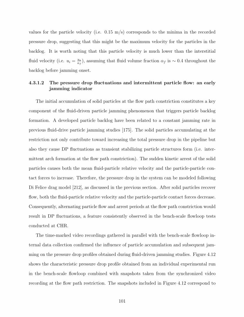
values for the particle velocity (i.e. 0.15 m/s) corresponds to the minima in the recorded

pressure drop, suggesting that this might be the maximum velocity for the particles in the

backlog. It is worth noting that this particle velocity is much lower than the interstitial

fluid velocity (i.e. ui =usαf), assuming that fluid volume fraction αf is ∼ 0.4 throughout the

backlog before jamming onset.

4.3.1.2 The pressure drop fluctuations and intermittent particle flow: an earlyjamming indicator

The initial accumulation of solid particles at the flow path constriction constitutes a key

component of the fluid-driven particle jamming phenomenon that triggers particle backlog

formation. A developed particle backlog have been related to a constant jamming rate in

previous fluid-drive particle jamming studies [175]. The solid particles accumulating at the

restriction not only contribute toward increasing the total pressure drop in the pipeline but

also they cause DP fluctuations as transient stabilizing particle structures form (i.e. inter-

mittent arch formation at the flow path constriction). The sudden kinetic arrest of the solid

particles causes both the mean fluid-particle relative velocity and the particle-particle con-

tact forces to increase. Therefore, the pressure drop in the system can be modeled following

Di Felice drag model [212], as discussed in the previous section. After solid particles recover

flow, both the fluid-particle relative velocity and the particle-particle contact forces decrease.

Consequently, alternating particle flow and arrest periods at the flow path constriction would

result in DP fluctuations, a feature consistently observed in the bench-scale flowloop tests

conducted at CHR.

The time-marked video recordings gathered in parallel with the bench-scale flowloop in-

ternal data collection confirmed the influence of particle accumulation and subsequent jam-

ming on the pressure drop profiles obtained during fluid-driven jamming studies. Figure 4.12

shows the characteristic pressure drop profile obtained from an individual experimental run

in the bench-scale flowloop combined with snapshots taken from the synchronized video

recording at the flow path restriction. The snapshots included in Figure 4.12 correspond to

101

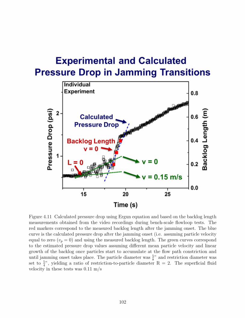
Figure 4.11 Calculated pressure drop using Ergun equation and based on the backlog lengthmeasurements obtained from the video recordings during bench-scale flowloop tests. Thered markers correspond to the measured backlog length after the jamming onset. The bluecurve is the calculated pressure drop after the jamming onset (i.e. assuming particle velocityequal to zero (vp = 0) and using the measured backlog length. The green curves correspondto the estimated pressure drop values assuming different mean particle velocity and lineargrowth of the backlog once particles start to accumulate at the flow path constriction anduntil jamming onset takes place. The particle diameter was 5

8” and restriction diameter was

set to 54”, yielding a ratio of restriction-to-particle diameter R = 2. The superficial fluid

velocity in these tests was 0.11 m/s

102

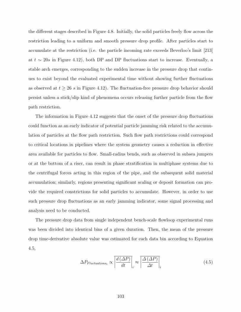
the different stages described in Figure 4.8. Initially, the solid particles freely flow across the

restriction leading to a uniform and smooth pressure drop profile. After particles start to

accumulate at the restriction (i.e. the particle incoming rate exceeds Beverloo’s limit [213]

at t ∼ 20s in Figure 4.12), both DP and DP fluctuations start to increase. Eventually, a

stable arch emerges, corresponding to the sudden increase in the pressure drop that contin-

ues to exist beyond the evaluated experimental time without showing further fluctuations

as observed at t ≥ 26 s in Figure 4.12). The fluctuation-free pressure drop behavior should

persist unless a stick/slip kind of phenomena occurs releasing further particle from the flow

path restriction.

The information in Figure 4.12 suggests that the onset of the pressure drop fluctuations

could function as an early indicator of potential particle jamming risk related to the accumu-

lation of particles at the flow path restriction. Such flow path restrictions could correspond

to critical locations in pipelines where the system geometry causes a reduction in effective

area available for particles to flow. Small-radius bends, such as observed in subsea jumpers

or at the bottom of a riser, can result in phase stratification in multiphase systems due to

the centrifugal forces acting in this region of the pipe, and the subsequent solid material

accumulation; similarly, regions presenting significant scaling or deposit formation can pro-

vide the required constrictions for solid particles to accumulate. However, in order to use

such pressure drop fluctuations as an early jamming indicator, some signal processing and

analysis need to be conducted.

The pressure drop data from single independent bench-scale flowloop experimental runs

was been divided into identical bins of a given duration. Then, the mean of the pressure

drop time-derivative absolute value was estimated for each data bin according to Equation

4.5,

∆PF luctuationsi ∝

∣

∣

∣

∣

d (∆P )

dt

∣

∣

∣

∣

i

≈

∣

∣

∣

∣

∆ (∆P )

∆t

∣

∣

∣

∣

i

(4.5)

103

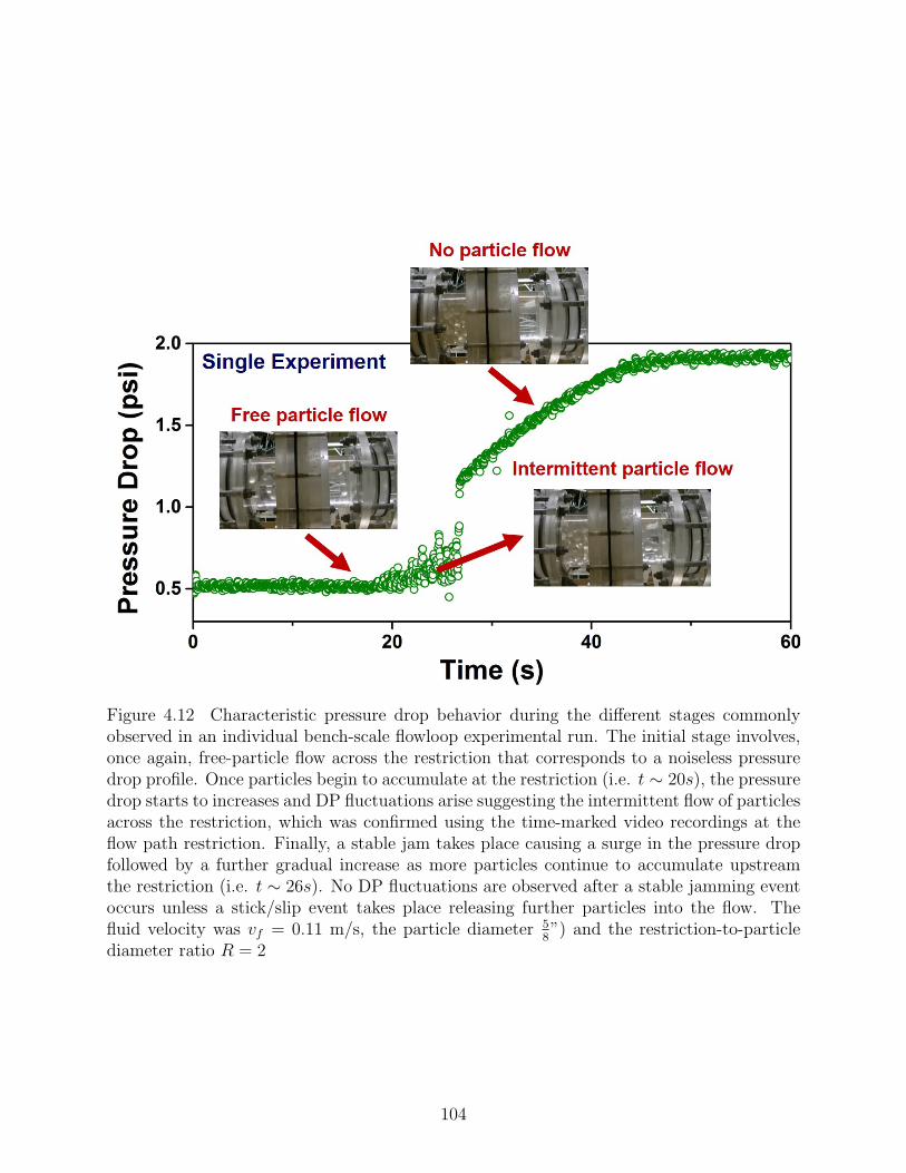
Figure 4.12 Characteristic pressure drop behavior during the different stages commonlyobserved in an individual bench-scale flowloop experimental run. The initial stage involves,once again, free-particle flow across the restriction that corresponds to a noiseless pressuredrop profile. Once particles begin to accumulate at the restriction (i.e. t ∼ 20s), the pressuredrop starts to increases and DP fluctuations arise suggesting the intermittent flow of particlesacross the restriction, which was confirmed using the time-marked video recordings at theflow path restriction. Finally, a stable jam takes place causing a surge in the pressure dropfollowed by a further gradual increase as more particles continue to accumulate upstreamthe restriction (i.e. t ∼ 26s). No DP fluctuations are observed after a stable jamming eventoccurs unless a stick/slip event takes place releasing further particles into the flow. Thefluid velocity was vf = 0.11 m/s, the particle diameter 5

8”) and the restriction-to-particle

diameter ratio R = 2

104

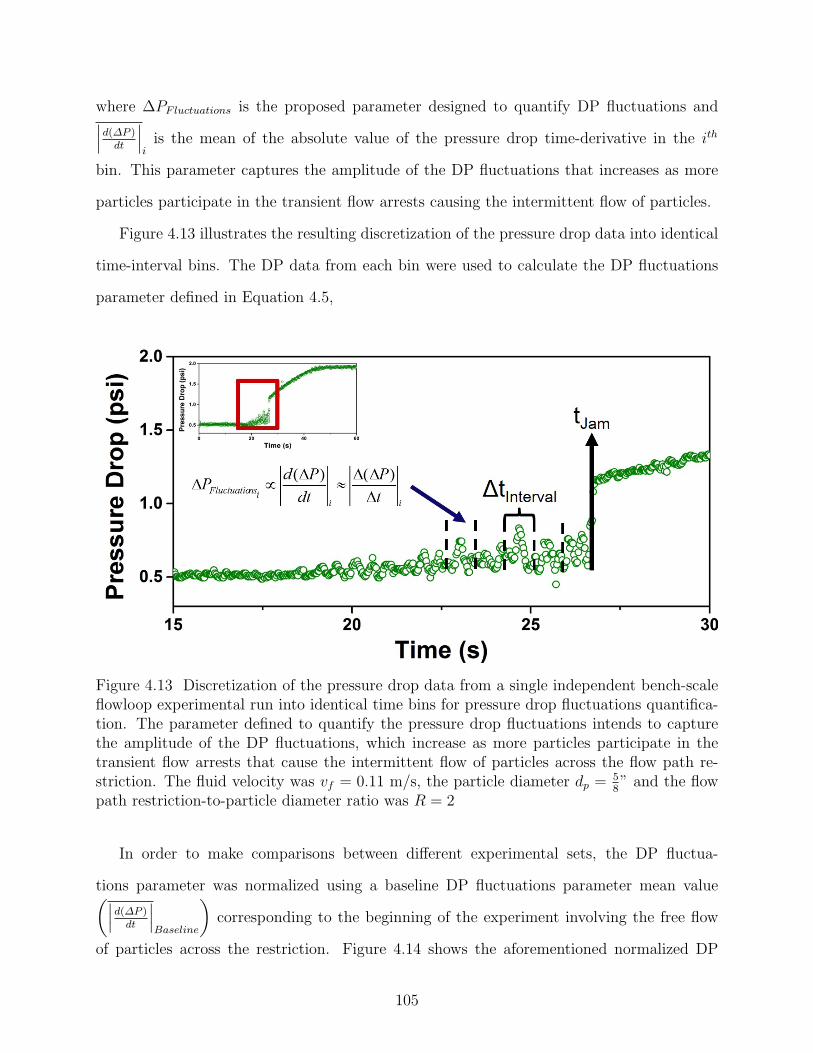
where ∆PF luctuations is the proposed parameter designed to quantify DP fluctuations and∣

∣

∣

d(∆P )dt

∣

∣

∣

iis the mean of the absolute value of the pressure drop time-derivative in the ith

bin. This parameter captures the amplitude of the DP fluctuations that increases as more

particles participate in the transient flow arrests causing the intermittent flow of particles.

Figure 4.13 illustrates the resulting discretization of the pressure drop data into identical

time-interval bins. The DP data from each bin were used to calculate the DP fluctuations

parameter defined in Equation 4.5,

Figure 4.13 Discretization of the pressure drop data from a single independent bench-scaleflowloop experimental run into identical time bins for pressure drop fluctuations quantifica-tion. The parameter defined to quantify the pressure drop fluctuations intends to capturethe amplitude of the DP fluctuations, which increase as more particles participate in thetransient flow arrests that cause the intermittent flow of particles across the flow path re-striction. The fluid velocity was vf = 0.11 m/s, the particle diameter dp =

58” and the flow

path restriction-to-particle diameter ratio was R = 2

In order to make comparisons between different experimental sets, the DP fluctua-

tions parameter was normalized using a baseline DP fluctuations parameter mean value(

∣

∣

∣

d(∆P )dt

∣

∣

∣

Baseline

)

corresponding to the beginning of the experiment involving the free flow

of particles across the restriction. Figure 4.14 shows the aforementioned normalized DP

105

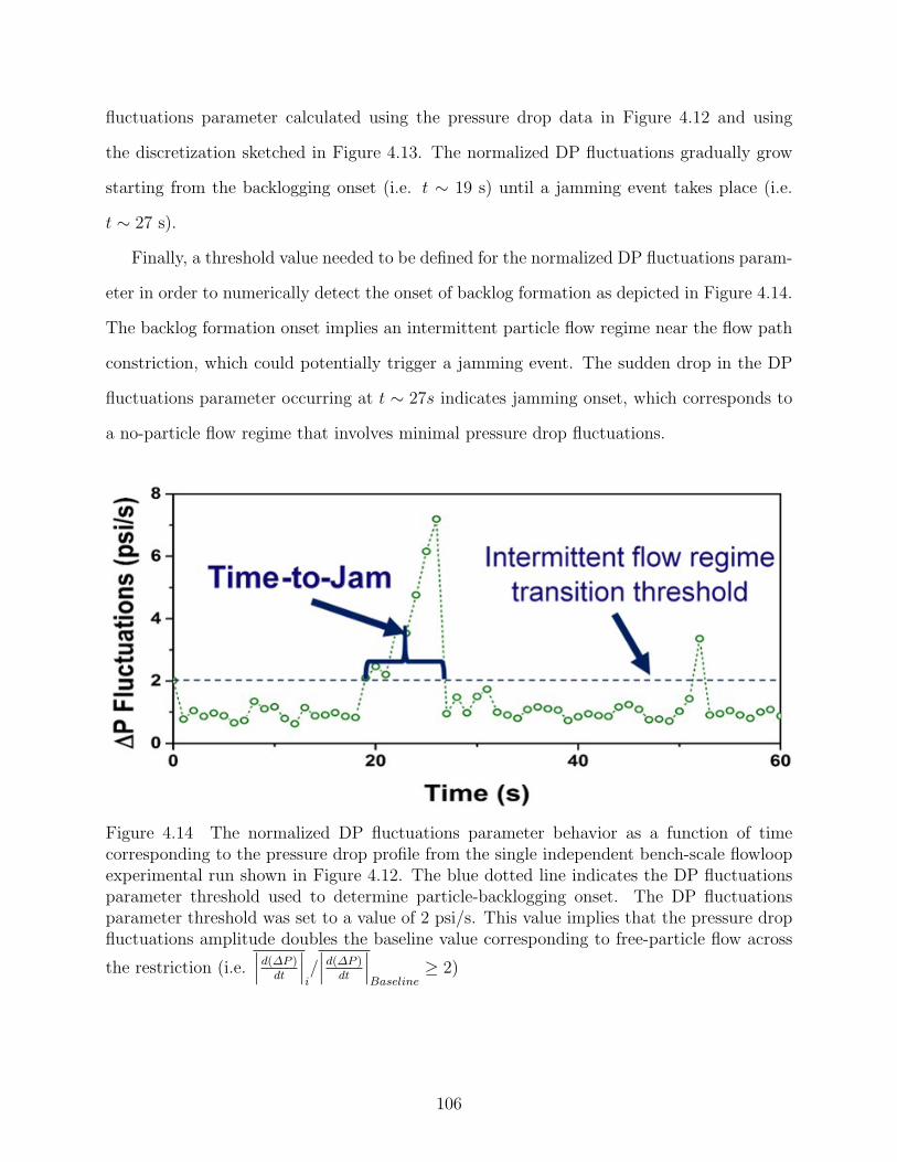
fluctuations parameter calculated using the pressure drop data in Figure 4.12 and using

the discretization sketched in Figure 4.13. The normalized DP fluctuations gradually grow

starting from the backlogging onset (i.e. t ∼ 19 s) until a jamming event takes place (i.e.

t ∼ 27 s).

Finally, a threshold value needed to be defined for the normalized DP fluctuations param-

eter in order to numerically detect the onset of backlog formation as depicted in Figure 4.14.

The backlog formation onset implies an intermittent particle flow regime near the flow path

constriction, which could potentially trigger a jamming event. The sudden drop in the DP

fluctuations parameter occurring at t ∼ 27s indicates jamming onset, which corresponds to

a no-particle flow regime that involves minimal pressure drop fluctuations.

Figure 4.14 The normalized DP fluctuations parameter behavior as a function of timecorresponding to the pressure drop profile from the single independent bench-scale flowloopexperimental run shown in Figure 4.12. The blue dotted line indicates the DP fluctuationsparameter threshold used to determine particle-backlogging onset. The DP fluctuationsparameter threshold was set to a value of 2 psi/s. This value implies that the pressure dropfluctuations amplitude doubles the baseline value corresponding to free-particle flow across

the restriction (i.e.∣

∣

∣

d(∆P )dt

∣

∣

∣

i/∣

∣

∣

d(∆P )dt

∣

∣

∣

Baseline≥ 2)

106

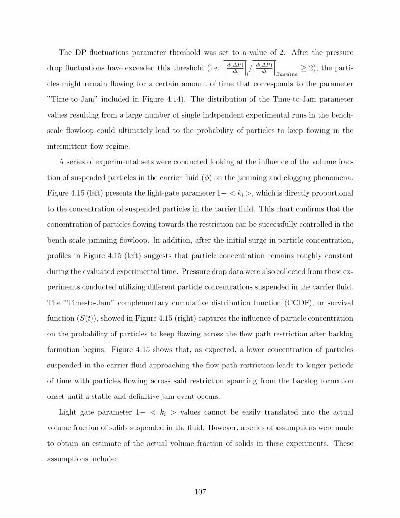
The DP fluctuations parameter threshold was set to a value of 2. After the pressure

drop fluctuations have exceeded this threshold (i.e.∣

∣

∣

d(∆P )dt

∣

∣

∣

i/∣

∣

∣

d(∆P )dt

∣

∣

∣

Baseline≥ 2), the parti-

cles might remain flowing for a certain amount of time that corresponds to the parameter

”Time-to-Jam” included in Figure 4.14). The distribution of the Time-to-Jam parameter

values resulting from a large number of single independent experimental runs in the bench-

scale flowloop could ultimately lead to the probability of particles to keep flowing in the

intermittent flow regime.

A series of experimental sets were conducted looking at the influence of the volume frac-

tion of suspended particles in the carrier fluid (φ) on the jamming and clogging phenomena.

Figure 4.15 (left) presents the light-gate parameter 1− < ki >, which is directly proportional

to the concentration of suspended particles in the carrier fluid. This chart confirms that the

concentration of particles flowing towards the restriction can be successfully controlled in the

bench-scale jamming flowloop. In addition, after the initial surge in particle concentration,

profiles in Figure 4.15 (left) suggests that particle concentration remains roughly constant

during the evaluated experimental time. Pressure drop data were also collected from these ex-

periments conducted utilizing different particle concentrations suspended in the carrier fluid.

The ”Time-to-Jam” complementary cumulative distribution function (CCDF), or survival

function (S(t)), showed in Figure 4.15 (right) captures the influence of particle concentration

on the probability of particles to keep flowing across the flow path restriction after backlog

formation begins. Figure 4.15 shows that, as expected, a lower concentration of particles

suspended in the carrier fluid approaching the flow path restriction leads to longer periods

of time with particles flowing across said restriction spanning from the backlog formation

onset until a stable and definitive jam event occurs.

Light gate parameter 1− < ki > values cannot be easily translated into the actual

volume fraction of solids suspended in the fluid. However, a series of assumptions were made

to obtain an estimate of the actual volume fraction of solids in these experiments. These

assumptions include:

107

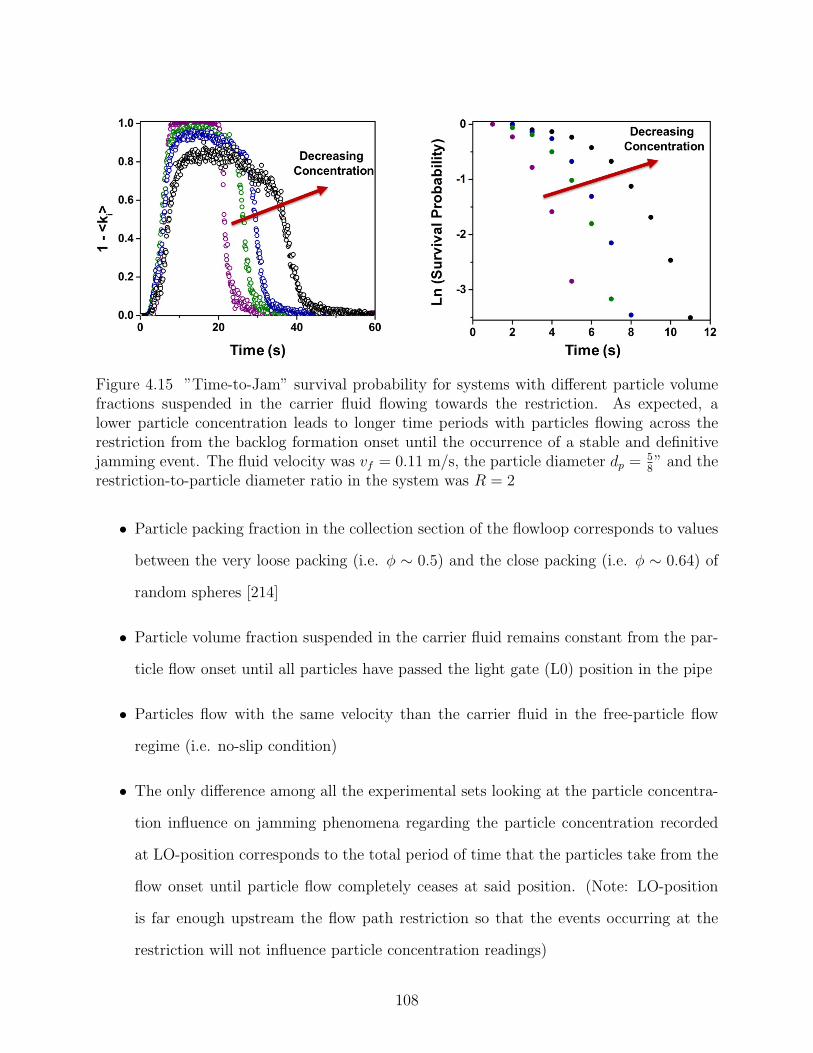
Figure 4.15 ”Time-to-Jam” survival probability for systems with different particle volumefractions suspended in the carrier fluid flowing towards the restriction. As expected, alower particle concentration leads to longer time periods with particles flowing across therestriction from the backlog formation onset until the occurrence of a stable and definitivejamming event. The fluid velocity was vf = 0.11 m/s, the particle diameter dp =

58” and the

restriction-to-particle diameter ratio in the system was R = 2

• Particle packing fraction in the collection section of the flowloop corresponds to values

between the very loose packing (i.e. φ ∼ 0.5) and the close packing (i.e. φ ∼ 0.64) of

random spheres [214]

• Particle volume fraction suspended in the carrier fluid remains constant from the par-

ticle flow onset until all particles have passed the light gate (L0) position in the pipe

• Particles flow with the same velocity than the carrier fluid in the free-particle flow

regime (i.e. no-slip condition)

• The only difference among all the experimental sets looking at the particle concentra-

tion influence on jamming phenomena regarding the particle concentration recorded

at LO-position corresponds to the total period of time that the particles take from the

flow onset until particle flow completely ceases at said position. (Note: LO-position

is far enough upstream the flow path restriction so that the events occurring at the

restriction will not influence particle concentration readings)

108

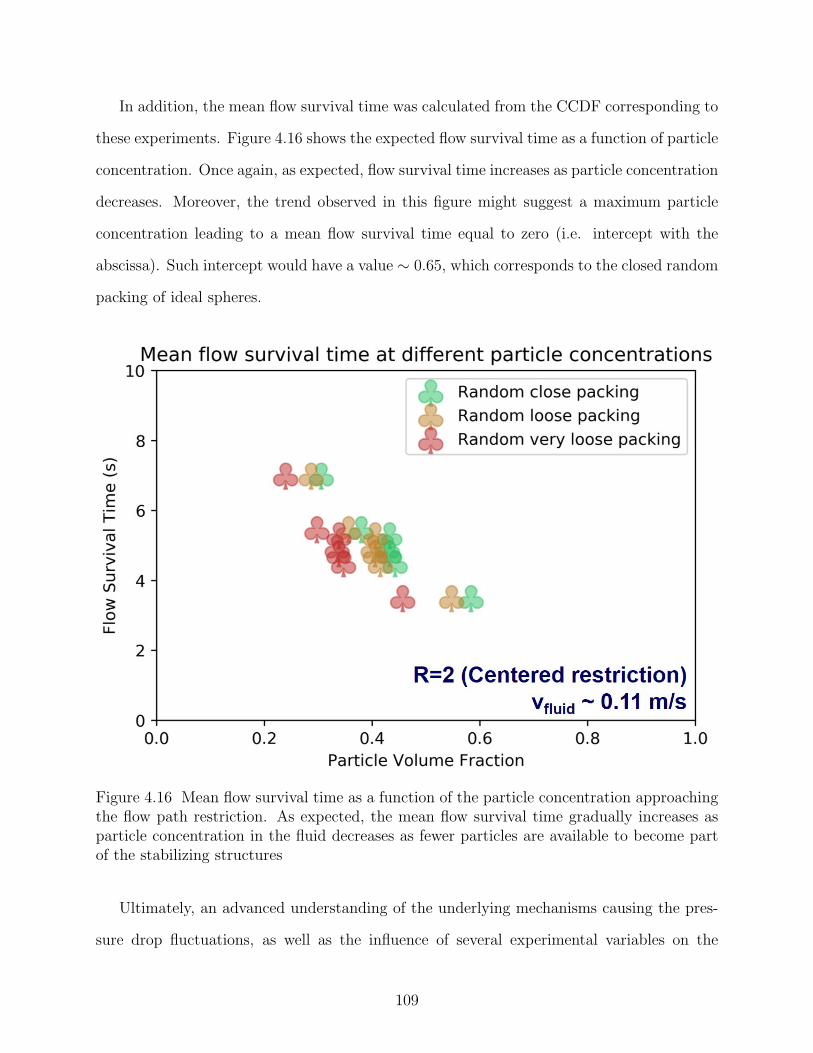
In addition, the mean flow survival time was calculated from the CCDF corresponding to

these experiments. Figure 4.16 shows the expected flow survival time as a function of particle

concentration. Once again, as expected, flow survival time increases as particle concentration

decreases. Moreover, the trend observed in this figure might suggest a maximum particle

concentration leading to a mean flow survival time equal to zero (i.e. intercept with the

abscissa). Such intercept would have a value ∼ 0.65, which corresponds to the closed random

packing of ideal spheres.

Figure 4.16 Mean flow survival time as a function of the particle concentration approachingthe flow path restriction. As expected, the mean flow survival time gradually increases asparticle concentration in the fluid decreases as fewer particles are available to become partof the stabilizing structures

Ultimately, an advanced understanding of the underlying mechanisms causing the pres-

sure drop fluctuations, as well as the influence of several experimental variables on the

109

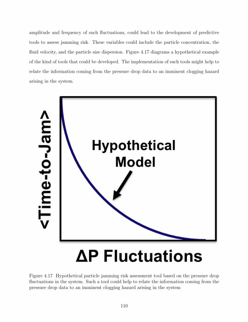
amplitude and frequency of such fluctuations, could lead to the development of predictive

tools to assess jamming risk. These variables could include the particle concentration, the

fluid velocity, and the particle size dispersion. Figure 4.17 diagrams a hypothetical example

of the kind of tools that could be developed. The implementation of such tools might help to

relate the information coming from the pressure drop data to an imminent clogging hazard

arising in the system.

Figure 4.17 Hypothetical particle jamming risk assessment tool based on the pressure dropfluctuations in the system. Such a tool could help to relate the information coming from thepressure drop data to an imminent clogging hazard arising in the system

110

4.3.1.3 Jamming risk assessment based on the kinetic energy fluctuating be-havior during the intermittent flow of particles across a flow path re-striction: A DEM approach

Computational simulations implementing the discrete element method to investigate par-

ticle flow across a flow path restriction were conducted in order to advance the understanding

of the underlying mechanisms leading to either the transient or the definitive kinetic arrest

of the particles. The simulations were conducted according to the procedure described in

Section 4.2.2.

In order to analyze the simulation results, In-house MATLABr- and Python-based anal-

ysis tools were developed. The algorithms track the kinetic energy of the system (KE) and

determine whether the KE drops below a user-defined threshold (KEFLowArrest) that cor-

responds to the formation of a stabilizing arch structure at the restriction. Initially, this

threshold was defined as a fraction of the maximum total kinetic energy of the system

(KEmax), which coincides with the start of particle flow at the beginning of the experi-

ment for the original simulation case conducted using the first-generation Cluster2D version

available for these studies.

Figure 4.18 shows a total KE plot as a function of time from an individual simulation run

using the first-generation Cluster2D version used in these studies. The system restriction-to-

particle diameter ratio was R = 4. A stable and definitive jam occurs at time ∼ 70s. Before

the jamming onset, the total kinetic energy periodically reaches a minimum associated with

the onset of a transient arrest. Furthermore, the total kinetic energy reaches a KEmax right

after the particles start to flow across the restriction (i.e. time ∼ 10 s).

The frequency of the total kinetic energy minima might provide insights into the plugging

tendency of a given system. The two KE plots in Figure 4.18 corresponds to the same

experimental data; however, different features are highlighted in each figure. The left figure

labels the key stages during the simulation of particle flow across a flow path constriction (i.e.

particle flow onset, KEmax, transient flow arrest, and jamming onset). On the other hand,

the figure on the right includes two reference lines corresponding to different definitions of

111

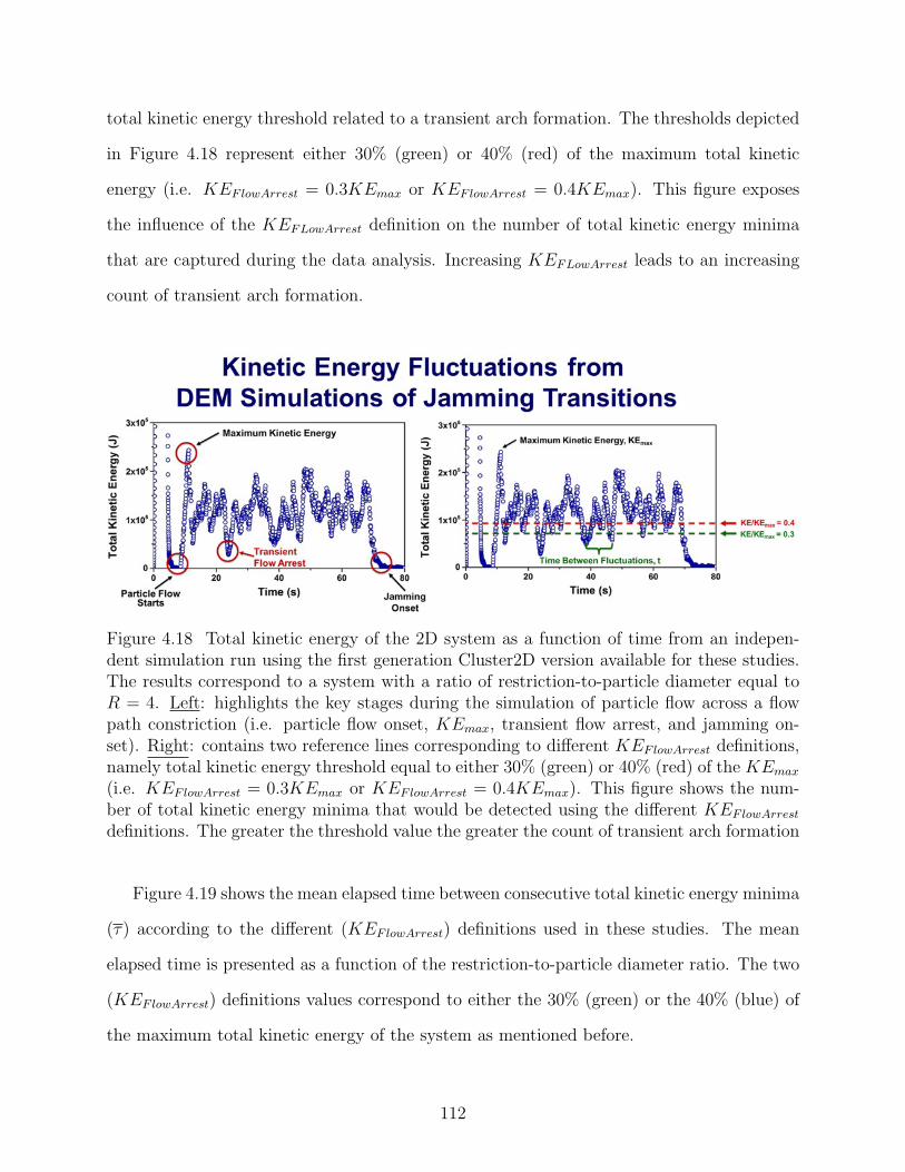
total kinetic energy threshold related to a transient arch formation. The thresholds depicted

in Figure 4.18 represent either 30% (green) or 40% (red) of the maximum total kinetic

energy (i.e. KEF lowArrest = 0.3KEmax or KEF lowArrest = 0.4KEmax). This figure exposes

the influence of the KEFLowArrest definition on the number of total kinetic energy minima

that are captured during the data analysis. Increasing KEFLowArrest leads to an increasing

count of transient arch formation.

Figure 4.18 Total kinetic energy of the 2D system as a function of time from an indepen-dent simulation run using the first generation Cluster2D version available for these studies.The results correspond to a system with a ratio of restriction-to-particle diameter equal toR = 4. Left: highlights the key stages during the simulation of particle flow across a flowpath constriction (i.e. particle flow onset, KEmax, transient flow arrest, and jamming on-set). Right: contains two reference lines corresponding to different KEF lowArrest definitions,namely total kinetic energy threshold equal to either 30% (green) or 40% (red) of the KEmax(i.e. KEF lowArrest = 0.3KEmax or KEF lowArrest = 0.4KEmax). This figure shows the num-ber of total kinetic energy minima that would be detected using the different KEF lowArrestdefinitions. The greater the threshold value the greater the count of transient arch formation

Figure 4.19 shows the mean elapsed time between consecutive total kinetic energy minima

(τ) according to the different (KEF lowArrest) definitions used in these studies. The mean

elapsed time is presented as a function of the restriction-to-particle diameter ratio. The two

(KEF lowArrest) definitions values correspond to either the 30% (green) or the 40% (blue) of

the maximum total kinetic energy of the system as mentioned before.

112

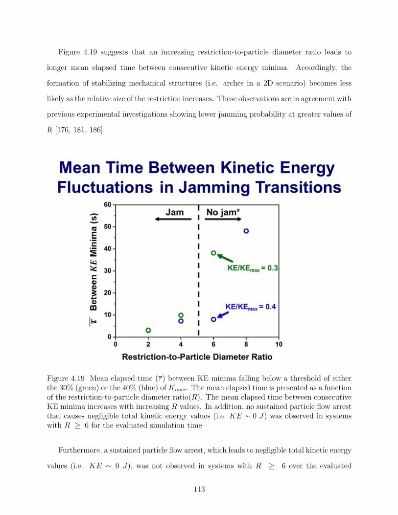
Figure 4.19 suggests that an increasing restriction-to-particle diameter ratio leads to

longer mean elapsed time between consecutive kinetic energy minima. Accordingly, the

formation of stabilizing mechanical structures (i.e. arches in a 2D scenario) becomes less

likely as the relative size of the restriction increases. These observations are in agreement with

previous experimental investigations showing lower jamming probability at greater values of

R [176, 181, 186].

Figure 4.19 Mean elapsed time (τ) between KE minima falling below a threshold of eitherthe 30% (green) or the 40% (blue) of Kmax. The mean elapsed time is presented as a functionof the restriction-to-particle diameter ratio(R). The mean elapsed time between consecutiveKE minima increases with increasing R values. In addition, no sustained particle flow arrestthat causes negligible total kinetic energy values (i.e. KE ∼ 0 J) was observed in systemswith R ≥ 6 for the evaluated simulation time

Furthermore, a sustained particle flow arrest, which leads to negligible total kinetic energy

values (i.e. KE ∼ 0 J), was not observed in systems with R ≥ 6 over the evaluated

113

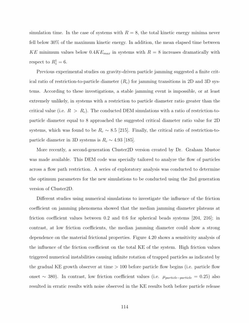
simulation time. In the case of systems with R = 8, the total kinetic energy minima never

fell below 30% of the maximum kinetic energy. In addition, the mean elapsed time between

KE minimum values below 0.4KEmax in systems with R = 8 increases dramatically with

respect to R11 = 6.

Previous experimental studies on gravity-driven particle jamming suggested a finite crit-

ical ratio of restriction-to-particle diameter (Rc) for jamming transitions in 2D and 3D sys-

tems. According to these investigations, a stable jamming event is impossible, or at least

extremely unlikely, in systems with a restriction to particle diameter ratio greater than the

critical value (i.e. R > Rc). The conducted DEM simulations with a ratio of restriction-to-

particle diameter equal to 8 approached the suggested critical diameter ratio value for 2D

systems, which was found to be Rc ∼ 8.5 [215]. Finally, the critical ratio of restriction-to-

particle diameter in 3D systems is Rc ∼ 4.93 [185].

More recently, a second-generation Cluster2D version created by Dr. Graham Mustoe

was made available. This DEM code was specially tailored to analyze the flow of particles

across a flow path restriction. A series of exploratory analysis was conducted to determine

the optimum parameters for the new simulations to be conducted using the 2nd generation

version of Cluster2D.

Different studies using numerical simulations to investigate the influence of the friction

coefficient on jamming phenomena showed that the median jamming diameter plateaus at

friction coefficient values between 0.2 and 0.6 for spherical beads systems [204, 216]; in

contrast, at low friction coefficients, the median jamming diameter could show a strong

dependence on the material frictional properties. Figure 4.20 shows a sensitivity analysis of

the influence of the friction coefficient on the total KE of the system. High friction values

triggered numerical instabilities causing infinite rotation of trapped particles as indicated by

the gradual KE growth observer at time > 100 before particle flow begins (i.e. particle flow

onset ∼ 380). In contrast, low friction coefficient values (i.e. µparticle−particle = 0.25) also

resulted in erratic results with noise observed in the KE results both before particle release

114

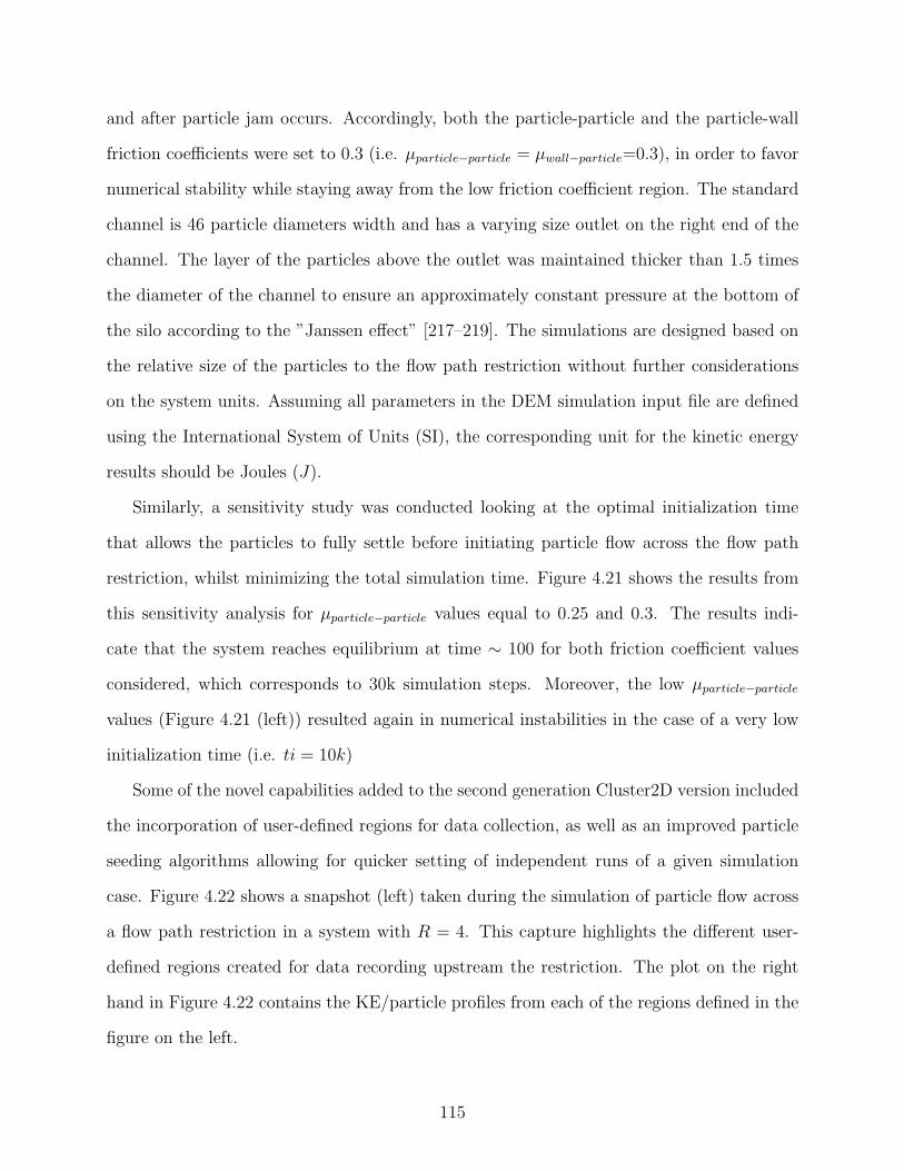
and after particle jam occurs. Accordingly, both the particle-particle and the particle-wall

friction coefficients were set to 0.3 (i.e. µparticle−particle = µwall−particle=0.3), in order to favor

numerical stability while staying away from the low friction coefficient region. The standard

channel is 46 particle diameters width and has a varying size outlet on the right end of the

channel. The layer of the particles above the outlet was maintained thicker than 1.5 times

the diameter of the channel to ensure an approximately constant pressure at the bottom of

the silo according to the ”Janssen effect” [217–219]. The simulations are designed based on

the relative size of the particles to the flow path restriction without further considerations

on the system units. Assuming all parameters in the DEM simulation input file are defined

using the International System of Units (SI), the corresponding unit for the kinetic energy

results should be Joules (J).

Similarly, a sensitivity study was conducted looking at the optimal initialization time

that allows the particles to fully settle before initiating particle flow across the flow path

restriction, whilst minimizing the total simulation time. Figure 4.21 shows the results from

this sensitivity analysis for µparticle−particle values equal to 0.25 and 0.3. The results indi-

cate that the system reaches equilibrium at time ∼ 100 for both friction coefficient values

considered, which corresponds to 30k simulation steps. Moreover, the low µparticle−particle

values (Figure 4.21 (left)) resulted again in numerical instabilities in the case of a very low

initialization time (i.e. ti = 10k)

Some of the novel capabilities added to the second generation Cluster2D version included

the incorporation of user-defined regions for data collection, as well as an improved particle

seeding algorithms allowing for quicker setting of independent runs of a given simulation

case. Figure 4.22 shows a snapshot (left) taken during the simulation of particle flow across

a flow path restriction in a system with R = 4. This capture highlights the different user-

defined regions created for data recording upstream the restriction. The plot on the right

hand in Figure 4.22 contains the KE/particle profiles from each of the regions defined in the

figure on the left.

115

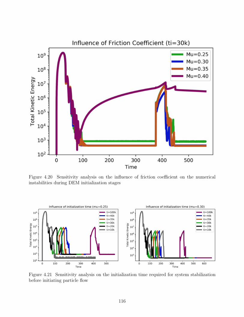
Figure 4.20 Sensitivity analysis on the influence of friction coefficient on the numericalinstabilities during DEM initialization stages

Figure 4.21 Sensitivity analysis on the initialization time required for system stabilizationbefore initiating particle flow

116

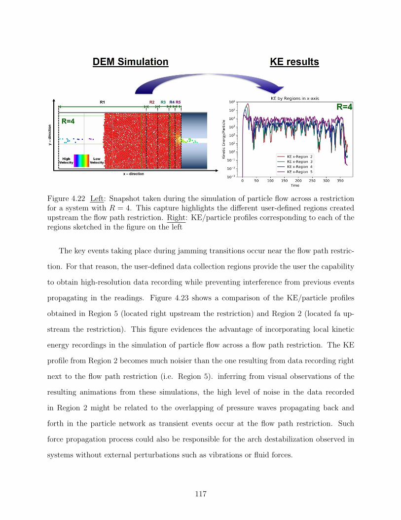
Figure 4.22 Left: Snapshot taken during the simulation of particle flow across a restrictionfor a system with R = 4. This capture highlights the different user-defined regions createdupstream the flow path restriction. Right: KE/particle profiles corresponding to each of theregions sketched in the figure on the left

The key events taking place during jamming transitions occur near the flow path restric-

tion. For that reason, the user-defined data collection regions provide the user the capability

to obtain high-resolution data recording while preventing interference from previous events

propagating in the readings. Figure 4.23 shows a comparison of the KE/particle profiles

obtained in Region 5 (located right upstream the restriction) and Region 2 (located fa up-

stream the restriction). This figure evidences the advantage of incorporating local kinetic

energy recordings in the simulation of particle flow across a flow path restriction. The KE

profile from Region 2 becomes much noisier than the one resulting from data recording right

next to the flow path restriction (i.e. Region 5). inferring from visual observations of the

resulting animations from these simulations, the high level of noise in the data recorded

in Region 2 might be related to the overlapping of pressure waves propagating back and

forth in the particle network as transient events occur at the flow path restriction. Such

force propagation process could also be responsible for the arch destabilization observed in

systems without external perturbations such as vibrations or fluid forces.

117

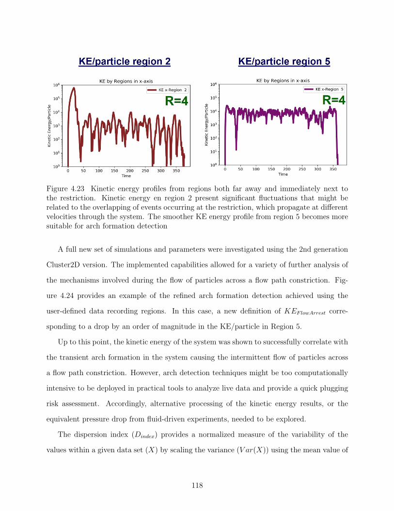
Figure 4.23 Kinetic energy profiles from regions both far away and immediately next tothe restriction. Kinetic energy en region 2 present significant fluctuations that might berelated to the overlapping of events occurring at the restriction, which propagate at differentvelocities through the system. The smoother KE energy profile from region 5 becomes moresuitable for arch formation detection

A full new set of simulations and parameters were investigated using the 2nd generation

Cluster2D version. The implemented capabilities allowed for a variety of further analysis of

the mechanisms involved during the flow of particles across a flow path constriction. Fig-

ure 4.24 provides an example of the refined arch formation detection achieved using the

user-defined data recording regions. In this case, a new definition of KEF lowArrest corre-

sponding to a drop by an order of magnitude in the KE/particle in Region 5.

Up to this point, the kinetic energy of the system was shown to successfully correlate with

the transient arch formation in the system causing the intermittent flow of particles across

a flow path constriction. However, arch detection techniques might be too computationally

intensive to be deployed in practical tools to analyze live data and provide a quick plugging

risk assessment. Accordingly, alternative processing of the kinetic energy results, or the

equivalent pressure drop from fluid-driven experiments, needed to be explored.

The dispersion index (Dindex) provides a normalized measure of the variability of the

values within a given data set (X) by scaling the variance (V ar(X)) using the mean value of

118

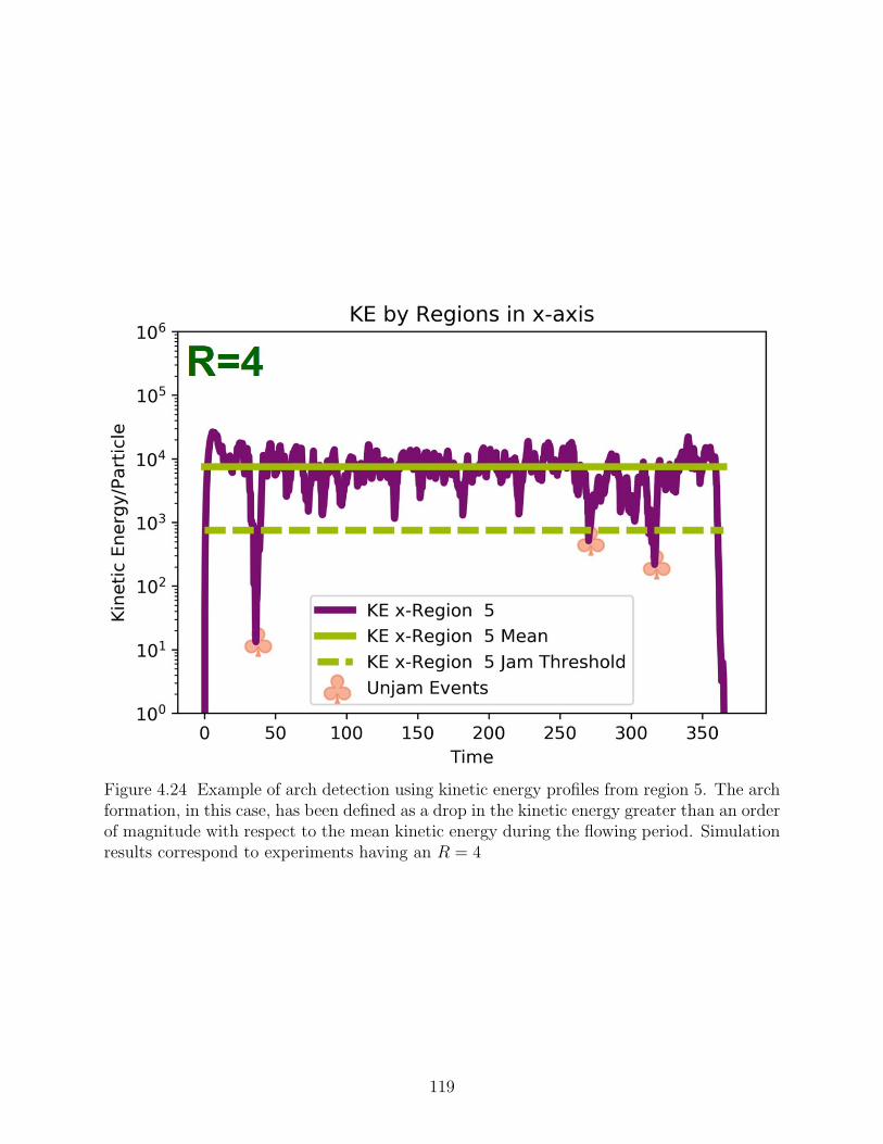
Figure 4.24 Example of arch detection using kinetic energy profiles from region 5. The archformation, in this case, has been defined as a drop in the kinetic energy greater than an orderof magnitude with respect to the mean kinetic energy during the flowing period. Simulationresults correspond to experiments having an R = 4

119

the data set (i.e. Dindex = V ar(X)/X). Such parameter helps quantifying phenomena such

a time between events, as well as processes where the underlying probability distribution is

suspected to be exponential.

Figure 4.25 presents the calculated KE dispersion index for different restriction-to-particle

values evaluated in a system with either a centered or a bottom located (bedding like) flow

path restriction. These results show that the KE dispersion index plateaus at R ≥ 6, which

coincides with the restriction-to-particle diameter ratio threshold after which stable jams

were not observed during the simulated time. Therefore, the KE dispersion index from DEM

simulations seems to correlate with the restriction-to-particle diameter ratio in a similar way

than the frequency between kinetic energy minima; hence, this parameter could provide

an estimation of the plugging phenomena associated with a specific system. Finally, KE

dispersion index showed higher values for a system that represents a greater plugging risk,

such as a centered restriction, than in a bottom located restriction scenario, which does not

provide a surface to support a stabilizing structure on both ends of the flow path restriction.

These results were in agreement with the experimental and numerical observations during

the discharge of particles from two- and three-dimensional silos [220]. These investigations

showed that lower restriction-to-particle diameter ratios resulted in increasing amplitude of

the particle velocity fluctuations, which were also related to greater intermittency in the flow

of particles exiting the silo.

4.3.2 Particle avalanche/clog time-lapse distributions in the intermittent par-ticle flow regime

Previous studies on clogging transitions of many-particle systems flowing through bottle-

necks suggested that the intermittent particle flow regime constitutes a characteristic feature

of granular materials flowing across flow path restrictions. This intrinsic behavior has been

used to analyze the plugging tendency of diverse systems and to evaluate the effect of differ-

ent experimental variables on jamming/clogging transitions [181, 189]. In order to quantify

the intermittency of particle flow, these studies have measured the elapsed time between con-

120

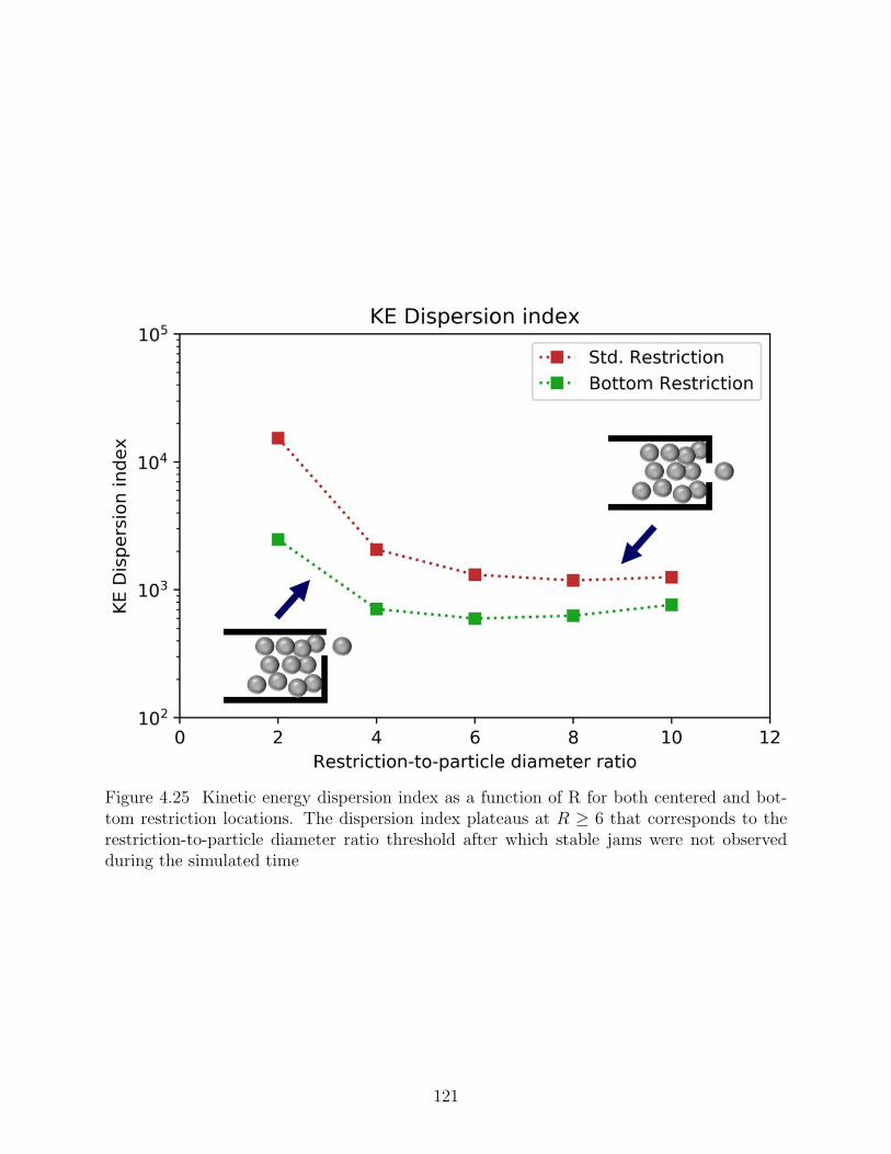
Figure 4.25 Kinetic energy dispersion index as a function of R for both centered and bot-tom restriction locations. The dispersion index plateaus at R ≥ 6 that corresponds to therestriction-to-particle diameter ratio threshold after which stable jams were not observedduring the simulated time

121

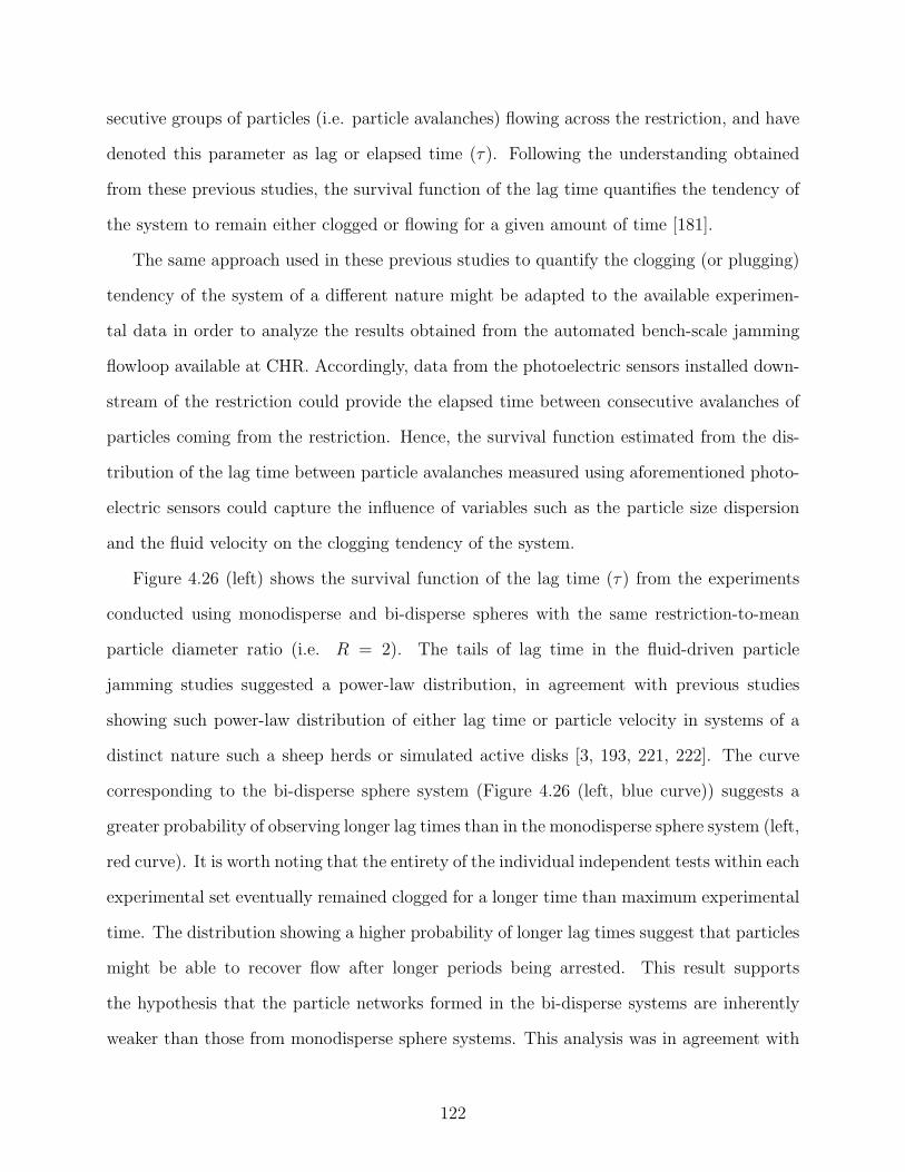
secutive groups of particles (i.e. particle avalanches) flowing across the restriction, and have

denoted this parameter as lag or elapsed time (τ). Following the understanding obtained

from these previous studies, the survival function of the lag time quantifies the tendency of

the system to remain either clogged or flowing for a given amount of time [181].

The same approach used in these previous studies to quantify the clogging (or plugging)

tendency of the system of a different nature might be adapted to the available experimen-

tal data in order to analyze the results obtained from the automated bench-scale jamming

flowloop available at CHR. Accordingly, data from the photoelectric sensors installed down-

stream of the restriction could provide the elapsed time between consecutive avalanches of

particles coming from the restriction. Hence, the survival function estimated from the dis-

tribution of the lag time between particle avalanches measured using aforementioned photo-

electric sensors could capture the influence of variables such as the particle size dispersion

and the fluid velocity on the clogging tendency of the system.

Figure 4.26 (left) shows the survival function of the lag time (τ) from the experiments

conducted using monodisperse and bi-disperse spheres with the same restriction-to-mean

particle diameter ratio (i.e. R = 2). The tails of lag time in the fluid-driven particle

jamming studies suggested a power-law distribution, in agreement with previous studies

showing such power-law distribution of either lag time or particle velocity in systems of a

distinct nature such a sheep herds or simulated active disks [3, 193, 221, 222]. The curve

corresponding to the bi-disperse sphere system (Figure 4.26 (left, blue curve)) suggests a

greater probability of observing longer lag times than in the monodisperse sphere system (left,

red curve). It is worth noting that the entirety of the individual independent tests within each

experimental set eventually remained clogged for a longer time than maximum experimental

time. The distribution showing a higher probability of longer lag times suggest that particles

might be able to recover flow after longer periods being arrested. This result supports

the hypothesis that the particle networks formed in the bi-disperse systems are inherently

weaker than those from monodisperse sphere systems. This analysis was in agreement with

122

the visual observations from tests with bi-disperse spheres. In these experiments, after

the particle flow apparently ceases completely, the particle network stabilizing the system

might collapse allowing the particles to flow again until a new stabilizing structure arises

(i.e. stick/slip phenomena). This contrasts with the visual observations from monodisperse

systems showing a very stable behavior after the jamming or clogging onset. The stabilizing

structures developed in the bi-disperse systems might contain more geometrical defects that

decrease the mechanical resistance of the particle network against external perturbations,

such as the vibrations caused by the fluid flow [188].

The same data treatment and analysis were applied to experiments conducted with dif-

ferent fluid velocities. In Figure 4.26 (right), the survival function of the lag time suggests

a greater probability of observing a stick/slip event after longer periods of particle flow

arrest as the fluid velocity increases. The greater fluid velocity might introduce further vi-

brations or noise acting on the stabilizing structures. Such vibrations are likely to break

the arches stabilizing the jammed particles according to the previous investigations carried

out by Mankoc et al., 20019 focused on the discharge of granular material in vibrated and

non-vibrated silos [187].

Constructing particle avalanche/clog size distributions is also possible now with the up-

dated capabilities available in the second generation Cluster2D version. User-defined data

recording regions 6 and 8 in Figure 4.6 were designed specifically to recreate the data col-

lection performed using the photoelectric light gates installed in the bench-scale flowloop.

The user-defined data collection regions output both the total kinetic energy and the particle

count in the said region over time; hence, particle count data in a given region corresponds to

the particle-detection based data avalanche/clog detection used in the bench-scale flowloop

tests. Figure 4.27 (left) shows the survival function resulting from Kaplan-Meier fitting to

the clog/avalanche size distributions obtained from the DEM simulation tool. This fitting

utilizes a step function connecting the different data bins contained in the input distribution.

From these results, it becomes clear that the output data obtained from these simulations

123

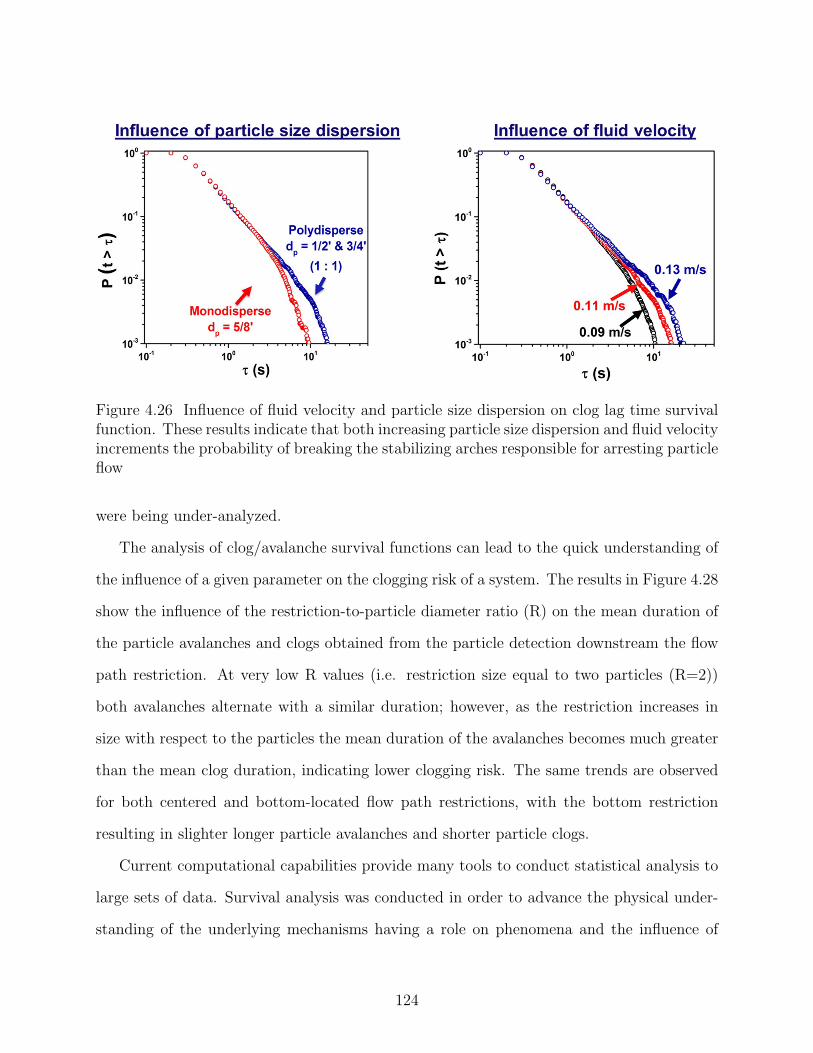
Figure 4.26 Influence of fluid velocity and particle size dispersion on clog lag time survivalfunction. These results indicate that both increasing particle size dispersion and fluid velocityincrements the probability of breaking the stabilizing arches responsible for arresting particleflow

were being under-analyzed.

The analysis of clog/avalanche survival functions can lead to the quick understanding of

the influence of a given parameter on the clogging risk of a system. The results in Figure 4.28

show the influence of the restriction-to-particle diameter ratio (R) on the mean duration of

the particle avalanches and clogs obtained from the particle detection downstream the flow

path restriction. At very low R values (i.e. restriction size equal to two particles (R=2))

both avalanches alternate with a similar duration; however, as the restriction increases in

size with respect to the particles the mean duration of the avalanches becomes much greater

than the mean clog duration, indicating lower clogging risk. The same trends are observed

for both centered and bottom-located flow path restrictions, with the bottom restriction

resulting in slighter longer particle avalanches and shorter particle clogs.

Current computational capabilities provide many tools to conduct statistical analysis to

large sets of data. Survival analysis was conducted in order to advance the physical under-

standing of the underlying mechanisms having a role on phenomena and the influence of

124

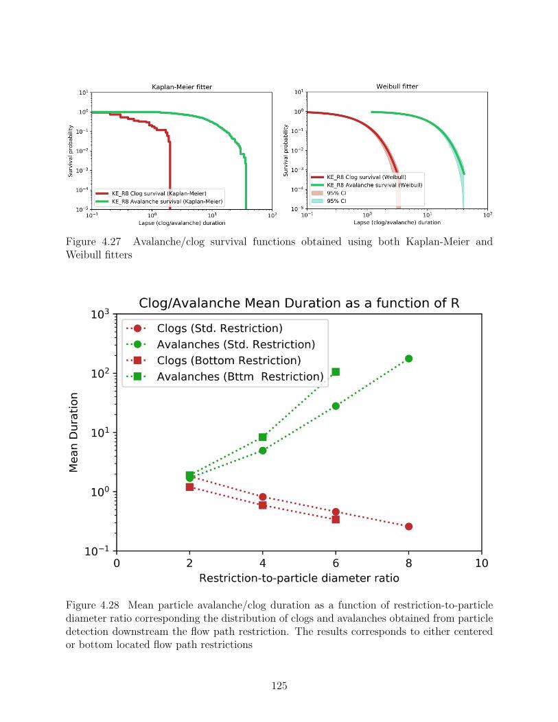
Figure 4.27 Avalanche/clog survival functions obtained using both Kaplan-Meier andWeibull fitters

Figure 4.28 Mean particle avalanche/clog duration as a function of restriction-to-particlediameter ratio corresponding the distribution of clogs and avalanches obtained from particledetection downstream the flow path restriction. The results corresponds to either centeredor bottom located flow path restrictions

125

the different parameters on such kinetic arrest transitions. The Weibull probability distri-

bution was selected based on the frequent use of this model to analyze failure mechanisms.

4.6 shows the complementary cumulative distribution function (CCDF), or survival function

(S(t)), for the Weibull probability distribution.

S(t) = exp((t

λWeibull

)ρWeibull) , λWeibull > 0, ρWeibull > 0 (4.6)

Figure 4.27 (right) displays the resulting survival function obtained from fitting the

Weibull probability distribution to the clog/avalanche distributions obtained from the con-

ducted DEM simulations. Should be noticed that no particle avalanches or clogs were de-

tected in region 6 for any of the analyzed cases. This region, located right downstream the

flow path restriction might not be far enough for allow particles leaving the restriction with

different velocities to separate; hence, causing no periods with no particle flow in region 6

before jamming onset. Such influence of the position of the detector on the obtained results,

which has been ignored in previous experimental studies, need to be considered in further

investigations looking at this phenomenon.

Utilizing survival analysis tools, such as the Weibull probability, offer many more advan-

tages than smoother curves. This distribution has been extensively used in survival analysis

looking at diverse phenomena such as slip failure mechanisms in fiber bundles [223], snow

avalanche runout distances & lethal power [224, 225], coronary heart disease risk predic-

tion [226, 226–228], and wind speed distribution for potential energy prospects [229]. This

parametric model, originally developed using three parameters but normally simplified to a

two-parameter model, offer insights into the failure behavior in a given process. The Weibull

shape factor (ρWeibull) determines whether the failure rate (i.e. events per unit time) in-

creases (ρWeibull > 1), decreases (ρWeibull < 1) or remains constant (ρWeibull = 1) over time.

Increasing failure rates over time are related to wear-out failure behavior, whereas decreasing

failure rates indicate early-life failures. In addition, the Weibull scale parameter (λWeibull),

which has the same unit as the phenomenological events being observed (i.e. time or par-

ticle number units in the case of particle avalanches being studied), determines the stretch

126

of the distribution in the abscissa and relates to the characteristic life of the events being

measured (i.e. characteristic particle avalanche time-lapse). Finally, the Weibull hazard

function (H(t)) (See 4.7) yields the failure rate of the process, which in the case of jamming

phenomena corresponds to the jamming rate in the system.

H(t) = (t

λWeibull

)ρWeibull (4.7)

At (ρWeibull)=1 the Weibull distribution reduces to an exponential distribution; hence,

as (ρWeibull) deviates from unity, it captures history-dependent features in the data such as

high levels of infant mortality, as well as the aforementioned early-life and wear-out failure

tendencies. Finally, alternative methods could be also utilized to study history-dependent

processes, such as statistical tools (e.g. Nelson-Aalen estimator) and other parametric models

(e.g. exponential, log-logistic, and log-normal probability distributions) that are commonly

used in survival analysis, in addition to the power-law probability distribution whose survival

functions shows an apparent linear behavior in a log-log chart.

Figure 4.29 contains the Weibull shape factor resulting from fitting the Weibull proba-

bility distribution to the clog/avalanche distributions from region 8, both for systems with

a centered and a bottom located restrictions. In all cases, the shape factor corresponding to

both clogs and avalanche in each system showed values greater than 1, suggesting a wear-out

failure behavior for both features. Interestingly, all shape factors showed a minimum at R

values between 4 and 6, which corresponds to the regions separating jamming occurrence

from no jamming occurrence based on the previous simulation results. Such minima suggest

a transition in the characteristics of clogging/unclogging process at R values around this

region.

Finally, generating avalanche/clog distributions from the DEM simulations of particle

flow across a flow path constriction permit implementing analysis concepts such as the flow

index or flowing parameter (Φ) [180, 181, 205], which accounts for the ratio of total avalanche

periods to the total flow time evaluated (i.e. Φ = tavalanche

tavalanche+tclog). Figure 4.30 presents the

flow index calculated both for the centered- and the bottom-located restrictions as a function

127

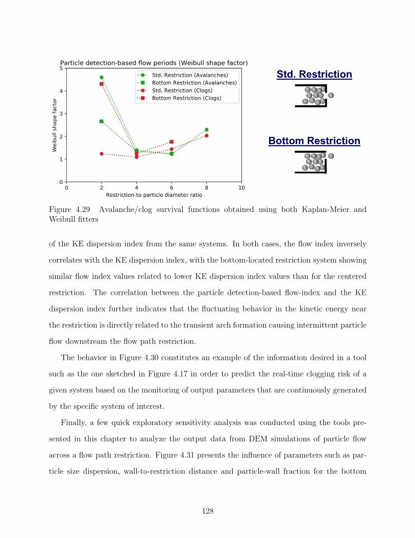
Figure 4.29 Avalanche/clog survival functions obtained using both Kaplan-Meier andWeibull fitters

of the KE dispersion index from the same systems. In both cases, the flow index inversely

correlates with the KE dispersion index, with the bottom-located restriction system showing

similar flow index values related to lower KE dispersion index values than for the centered

restriction. The correlation between the particle detection-based flow-index and the KE

dispersion index further indicates that the fluctuating behavior in the kinetic energy near

the restriction is directly related to the transient arch formation causing intermittent particle

flow downstream the flow path restriction.

The behavior in Figure 4.30 constitutes an example of the information desired in a tool

such as the one sketched in Figure 4.17 in order to predict the real-time clogging risk of a

given system based on the monitoring of output parameters that are continuously generated

by the specific system of interest.

Finally, a few quick exploratory sensitivity analysis was conducted using the tools pre-

sented in this chapter to analyze the output data from DEM simulations of particle flow

across a flow path restriction. Figure 4.31 presents the influence of parameters such as par-

ticle size dispersion, wall-to-restriction distance and particle-wall fraction for the bottom

128

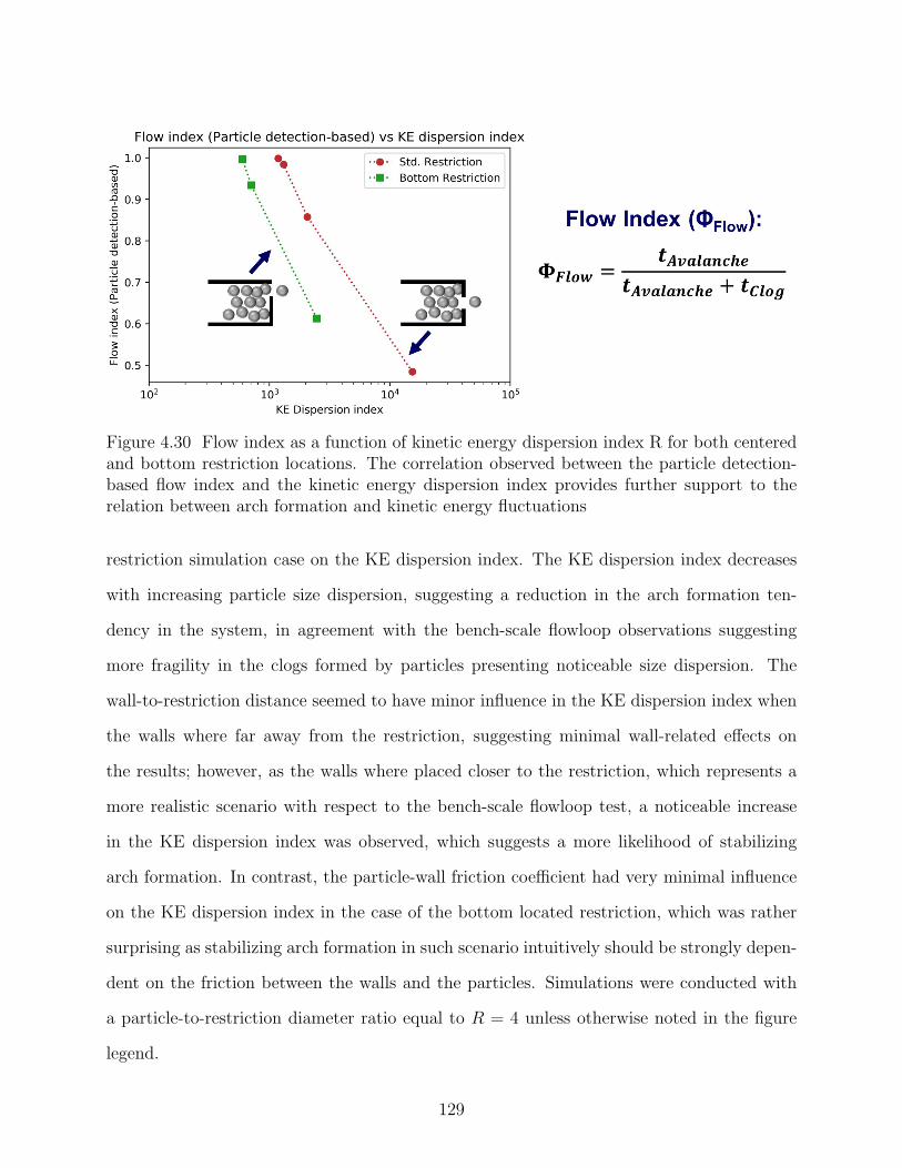
Figure 4.30 Flow index as a function of kinetic energy dispersion index R for both centeredand bottom restriction locations. The correlation observed between the particle detection-based flow index and the kinetic energy dispersion index provides further support to therelation between arch formation and kinetic energy fluctuations

restriction simulation case on the KE dispersion index. The KE dispersion index decreases

with increasing particle size dispersion, suggesting a reduction in the arch formation ten-

dency in the system, in agreement with the bench-scale flowloop observations suggesting

more fragility in the clogs formed by particles presenting noticeable size dispersion. The

wall-to-restriction distance seemed to have minor influence in the KE dispersion index when

the walls where far away from the restriction, suggesting minimal wall-related effects on

the results; however, as the walls where placed closer to the restriction, which represents a

more realistic scenario with respect to the bench-scale flowloop test, a noticeable increase

in the KE dispersion index was observed, which suggests a more likelihood of stabilizing

arch formation. In contrast, the particle-wall friction coefficient had very minimal influence

on the KE dispersion index in the case of the bottom located restriction, which was rather

surprising as stabilizing arch formation in such scenario intuitively should be strongly depen-

dent on the friction between the walls and the particles. Simulations were conducted with

a particle-to-restriction diameter ratio equal to R = 4 unless otherwise noted in the figure

legend.

129

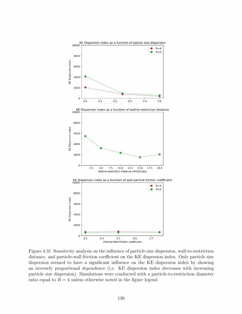
Figure 4.31 Sensitivity analysis on the influence of particle size dispersion, wall-to-restrictiondistance, and particle-wall friction coefficient on the KE dispersion index. Only particle sizedispersion seemed to have a significant influence on the KE dispersion index by showingan inversely proportional dependence (i.e. KE dispersion index decreases with increasingparticle size dispersion). Simulations were conducted with a particle-to-restriction diameterratio equal to R = 4 unless otherwise noted in the figure legend

130

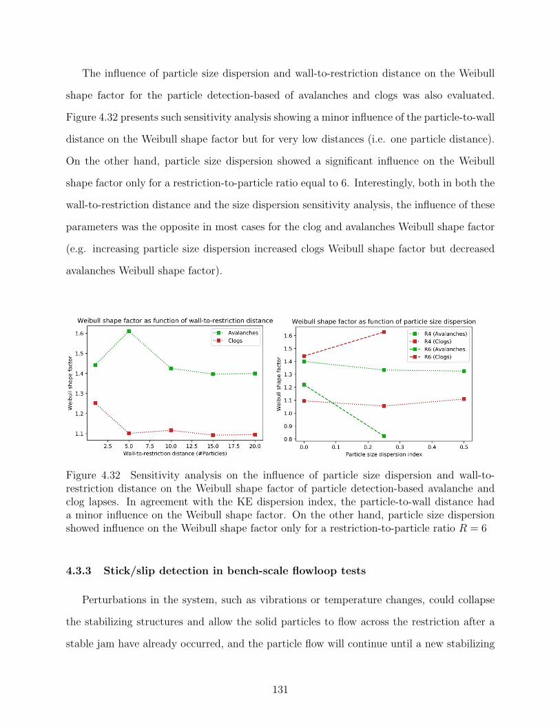
The influence of particle size dispersion and wall-to-restriction distance on the Weibull

shape factor for the particle detection-based of avalanches and clogs was also evaluated.

Figure 4.32 presents such sensitivity analysis showing a minor influence of the particle-to-wall

distance on the Weibull shape factor but for very low distances (i.e. one particle distance).

On the other hand, particle size dispersion showed a significant influence on the Weibull

shape factor only for a restriction-to-particle ratio equal to 6. Interestingly, both in both the

wall-to-restriction distance and the size dispersion sensitivity analysis, the influence of these

parameters was the opposite in most cases for the clog and avalanches Weibull shape factor

(e.g. increasing particle size dispersion increased clogs Weibull shape factor but decreased

avalanches Weibull shape factor).

Figure 4.32 Sensitivity analysis on the influence of particle size dispersion and wall-to-restriction distance on the Weibull shape factor of particle detection-based avalanche andclog lapses. In agreement with the KE dispersion index, the particle-to-wall distance hada minor influence on the Weibull shape factor. On the other hand, particle size dispersionshowed influence on the Weibull shape factor only for a restriction-to-particle ratio R = 6

4.3.3 Stick/slip detection in bench-scale flowloop tests

Perturbations in the system, such as vibrations or temperature changes, could collapse

the stabilizing structures and allow the solid particles to flow across the restriction after a

stable jam have already occurred, and the particle flow will continue until a new stabilizing

131

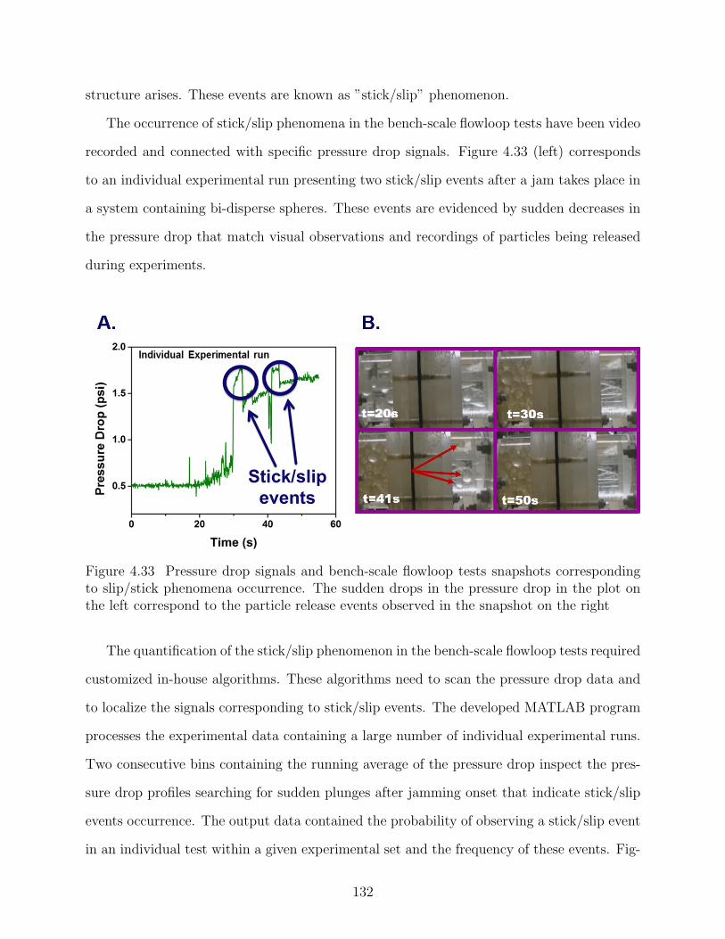
structure arises. These events are known as ”stick/slip” phenomenon.

The occurrence of stick/slip phenomena in the bench-scale flowloop tests have been video

recorded and connected with specific pressure drop signals. Figure 4.33 (left) corresponds

to an individual experimental run presenting two stick/slip events after a jam takes place in

a system containing bi-disperse spheres. These events are evidenced by sudden decreases in

the pressure drop that match visual observations and recordings of particles being released

during experiments.

Figure 4.33 Pressure drop signals and bench-scale flowloop tests snapshots correspondingto slip/stick phenomena occurrence. The sudden drops in the pressure drop in the plot onthe left correspond to the particle release events observed in the snapshot on the right

The quantification of the stick/slip phenomenon in the bench-scale flowloop tests required

customized in-house algorithms. These algorithms need to scan the pressure drop data and

to localize the signals corresponding to stick/slip events. The developed MATLAB program

processes the experimental data containing a large number of individual experimental runs.

Two consecutive bins containing the running average of the pressure drop inspect the pres-

sure drop profiles searching for sudden plunges after jamming onset that indicate stick/slip

events occurrence. The output data contained the probability of observing a stick/slip event

in an individual test within a given experimental set and the frequency of these events. Fig-

132

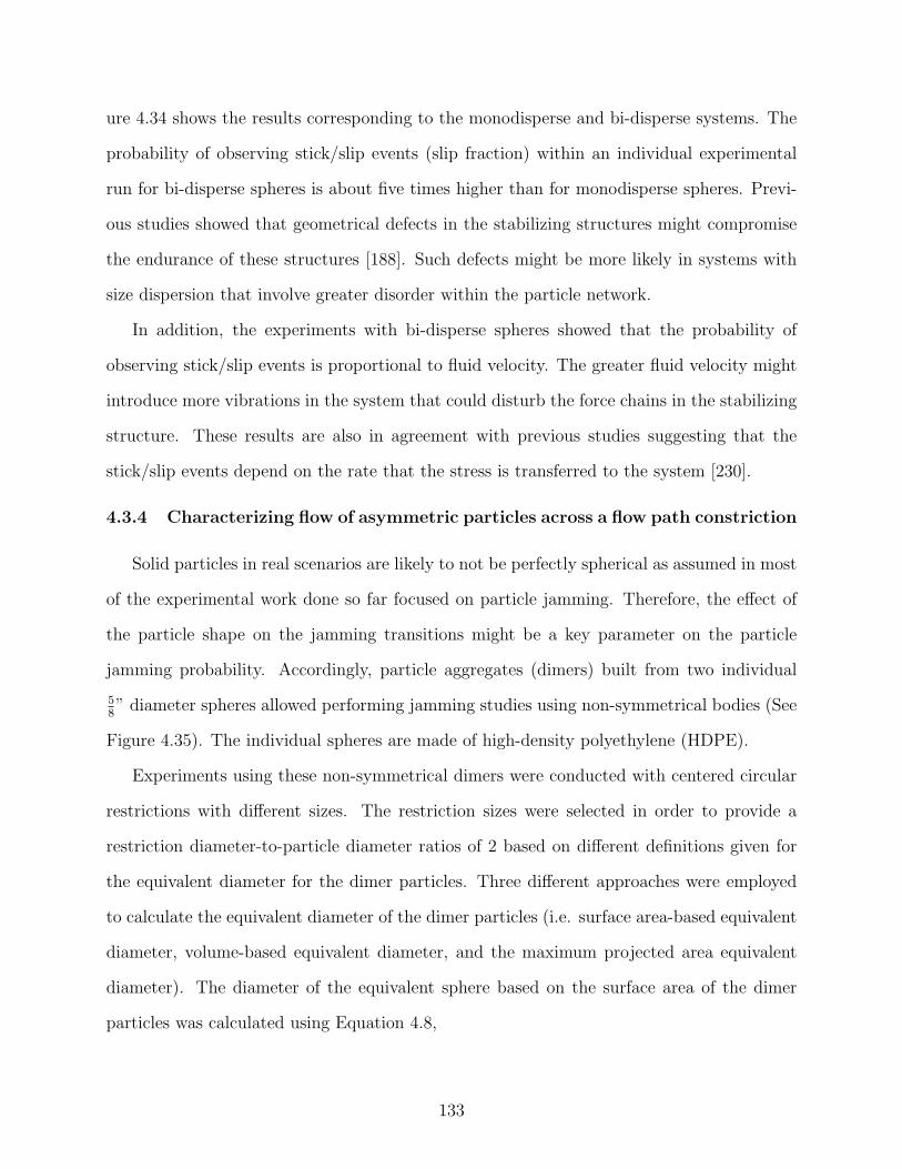
ure 4.34 shows the results corresponding to the monodisperse and bi-disperse systems. The

probability of observing stick/slip events (slip fraction) within an individual experimental

run for bi-disperse spheres is about five times higher than for monodisperse spheres. Previ-

ous studies showed that geometrical defects in the stabilizing structures might compromise

the endurance of these structures [188]. Such defects might be more likely in systems with

size dispersion that involve greater disorder within the particle network.

In addition, the experiments with bi-disperse spheres showed that the probability of

observing stick/slip events is proportional to fluid velocity. The greater fluid velocity might

introduce more vibrations in the system that could disturb the force chains in the stabilizing

structure. These results are also in agreement with previous studies suggesting that the

stick/slip events depend on the rate that the stress is transferred to the system [230].

4.3.4 Characterizing flow of asymmetric particles across a flow path constriction

Solid particles in real scenarios are likely to not be perfectly spherical as assumed in most

of the experimental work done so far focused on particle jamming. Therefore, the effect of

the particle shape on the jamming transitions might be a key parameter on the particle

jamming probability. Accordingly, particle aggregates (dimers) built from two individual

58” diameter spheres allowed performing jamming studies using non-symmetrical bodies (See

Figure 4.35). The individual spheres are made of high-density polyethylene (HDPE).

Experiments using these non-symmetrical dimers were conducted with centered circular

restrictions with different sizes. The restriction sizes were selected in order to provide a

restriction diameter-to-particle diameter ratios of 2 based on different definitions given for

the equivalent diameter for the dimer particles. Three different approaches were employed

to calculate the equivalent diameter of the dimer particles (i.e. surface area-based equivalent

diameter, volume-based equivalent diameter, and the maximum projected area equivalent

diameter). The diameter of the equivalent sphere based on the surface area of the dimer

particles was calculated using Equation 4.8,

133

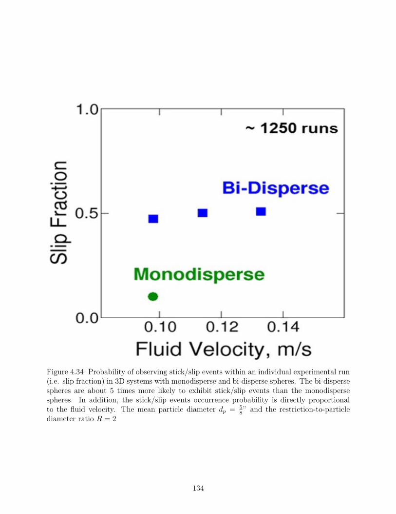
Figure 4.34 Probability of observing stick/slip events within an individual experimental run(i.e. slip fraction) in 3D systems with monodisperse and bi-disperse spheres. The bi-dispersespheres are about 5 times more likely to exhibit stick/slip events than the monodispersespheres. In addition, the stick/slip events occurrence probability is directly proportionalto the fluid velocity. The mean particle diameter dp = 5

8” and the restriction-to-particle

diameter ratio R = 2

134

Figure 4.35 Non-symmetrical particle aggregates (dimers) used in bench-scale flowloop tests.The dimers are formed from two 5

8” individual high-density polyethylene (HDPE) spheres

dpEquivalent=

√

ADimerπ

(4.8)

where dpEquivalentis the diameter of the equivalent sphere and ADimer is the actual surface

area of the dimer particles. On the other hand, the diameter of the equivalent sphere based

on the volume of the dimer particles follows Equation 4.9,

dpEquivalent= 2

3

√

3VDimer4π

(4.9)

where VDimer is the total volume of the dimer particles. Finally, Equation 4.10 yields

the diameter of the equivalent sphere considering the maximum projected area of the dimer

particles,

dpEquivalent= 2dpprimary

(4.10)

where dpprimaryis the diameter of the primary particles forming the dimer aggregates.

Table 4.1 summarizes the diameter of the equivalent spheres to the dimer particles, which

135

are calculated using Equation 4.8, Equation 4.9 and Equation 4.10. This table also includes

the diameter of the restriction used for these studies according to the different dimer particle

equivalent diameter definitions in order to provide a constant restriction-to-particle diameter

ratio R ∼ 2.

Table 4.1: The diameter of the dimer particle equivalent sphere according to the differentdefinitions for the particle size. The diameter of the equivalent sphere were calculated usingEquation 4.8, Equation 4.9 and Equation 4.10

Equivalent Sphere Definition Equivalent Sphere Diameter (in) Restriction Diameter (in)

Area Based 0.88 1.75Volume Based 0.78 1.50

Max. Projected Area Based 1.25 2.50

Moreover, Equation 4.11 allows calculating the sphericity of the dimer particles (Ψ),

Ψ =AEquivalentSphereV olume

ADimer(4.11)

where AEquivalentSphereV olumeis the surface area of the equivalent sphere, which was cal-

culated based on the actual volume of the dimer particles according to Equation 4.9 and

ADimer is the actual surface area of the dimer particles. The sphericity of dimer particles

formed from two identical spheres was Ψ = 0.7937.

Figure 4.36 shows the steady-state jamming rate obtained using the jamming model pro-

posed by Lafond, 2014 [175] according to Equation 4.2 for these three different experimental

sets. The jamming rate shows a constant value for the dimer system after particle backlog-

ging, similarly to the results from single spheres crossing a circular restriction. The dimer

volume-based equivalent diameter system yields the closest steady-state jamming rate value

with respect to those obtained from the individual spheres having the same ratio of restric-

tion to particle diameters (R). The jamming rate from tests assuming a surface area-based

equivalent diameter of the dimers is close as well to the individual spheres as well.

On the other hand, the maximum projected area-based equivalent diameter restriction

clearly result in lower the steady-state jamming rates as this restriction is much larger. These

136

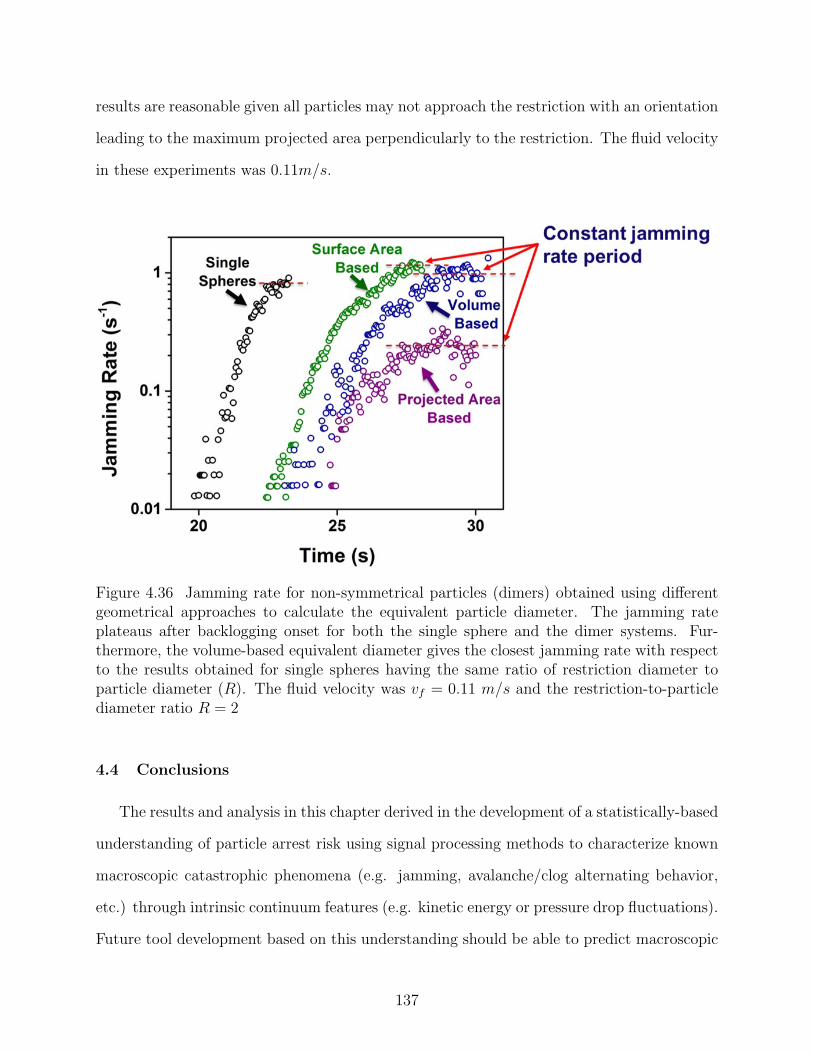
results are reasonable given all particles may not approach the restriction with an orientation

leading to the maximum projected area perpendicularly to the restriction. The fluid velocity

in these experiments was 0.11m/s.

Figure 4.36 Jamming rate for non-symmetrical particles (dimers) obtained using differentgeometrical approaches to calculate the equivalent particle diameter. The jamming rateplateaus after backlogging onset for both the single sphere and the dimer systems. Fur-thermore, the volume-based equivalent diameter gives the closest jamming rate with respectto the results obtained for single spheres having the same ratio of restriction diameter toparticle diameter (R). The fluid velocity was vf = 0.11 m/s and the restriction-to-particlediameter ratio R = 2

4.4 Conclusions

The results and analysis in this chapter derived in the development of a statistically-based

understanding of particle arrest risk using signal processing methods to characterize known

macroscopic catastrophic phenomena (e.g. jamming, avalanche/clog alternating behavior,

etc.) through intrinsic continuum features (e.g. kinetic energy or pressure drop fluctuations).

Future tool development based on this understanding should be able to predict macroscopic

137

phenomena based on continuous monitoring of the output parameters obtained from the

system that are relevant for the particular phenomena of interest to be detected.

Moreover, this chapter contains the implementation of survival analysis tools, such as

model fitting using the Weibull probability distribution, to evaluate history-dependent fea-

tures using output data (e.g. particle avalanche/clog or KE-based arch formation distribu-

tions), and to obtain further understanding into the system intrinsic properties such as the

failure behavior.

These analysis methods helped to maximize the information obtained both from bench-

scale flowloop and DEM tests by looking at parameters from the system that are continuously

generated, such as kinetic energy, pressure drop, avalanche/clog distribution, instead of tra-

ditional analysis conducted looking exclusively at the final outcome from a jamming/clogging

test.

Some additional key outcomes resulting from these investigations include:

• DEM simulations of particle flow across a flow path constriction showed that the fre-

quency of the fluctuations of the total kinetic energy of the system decreases with

increasing ratio of the restriction to the particle diameter, which might suggest a lower

plugging tendency of the system as well.

• Bench-scale flowloop pressure drop during jamming transitions was modeled consider-

ing the momentum exchange between the particles and the fluid phases

• Increasing particle size dispersion seemed to lower mechanical resistance in the sys-

tems against external perturbations caused by the fluid flow (i.e. vibrations). The

probability of observing ”stick-slip” phenomena is about five times greater in a bi-

disperse particle system than in a monodisperse system. Moreover, the probability of

”stick-slip” events increases with increasing fluid velocity

• Similarly, particle detection-based analysis of the bench-scale flowloop tests looking at

the effect of particle size dispersion and fluid velocity on the clog lag times distribution

138

showed that the probability of recovering flow after a given amount of time under a

transient jam increases with both increasing particle size dispersion and fluid velocity

• Bench-scale flowloop studies were conducted using non-symmetrical particle aggregates

(dimers). These studies showed that the steady-state jamming rate of the particle

dimers correlates with that from individual spheres with an equivalent volume-based or

surface area-based diameter. In contrast, jamming studies assuming a dimer equivalent

diameter based on the maximum projected area of the aggregates resulted in a much

lower steady-state jamming rate than that from the corresponding single sphere system

with the same restriction-to-particle diameter ratio

• Pressure drop-based early jamming detection captured the increasing probability of a

system to remain flowing as the volume fraction of suspended solids in the carrier fluid

approaching the restriction decreases

139

CHAPTER 5

GAS HYDRATE MANAGEMENT STRATEGIES USING ANTI-AGGLOMERANTS:

CONTINUOUS & TRANSIENT PILOT-SCALE FLOWLOOP STUDIES

Paper presented and published in the 2017 Offshore Technology Conference[131].

J. A. Dapena, A. A. Majid, V. Srivastava, Y. Wang, T. B. Charlton, A. A. Gardner, E. D.

Sloan, L. E. Zerpa, D. T. Wu, C. A. Koh

Subsea oil and gas flowlines can provide favorable conditions for gas hydrate formation,

which can lead to flow assurance issues as hydrate particles agglomerate and accumulate in

the flowline. Shut-in and restart operations are particularly critical for hydrate plug forma-

tion. Traditional strategies to mitigate hydrate plugging use total hydrate avoidance with

thermodynamic inhibitors; however, thermodynamic inhibition can become cost-prohibitive

as oil production moves towards harsher environments associated with deeper drilling. Hy-

drate management strategies using low dosage hydrate inhibitors (LDHI), such as anti-

agglomerants (AAs), are an attractive alternative to reduce operational and capital expen-

ditures in offshore oil and gas production. In order to successfully deploy anti-agglomerants

to mitigate hydrate plugging, a comprehensive understanding of the variables affecting the

performance of these additives, such as oil composition and mixture velocity, is needed.

Industrial-scale flowloop studies are valuable to investigate the influence of these variables

on hydrate particle transportability when using AAs. These experimental setups could be

also useful to assess AA performance during transient operations (i.e. shut-in and restart);

however, large-scale flowloop data at these conditions is limited.

High-pressure industrial-scale flowloop tests were conducted using a non-dispersing oil at

50 vol.% water content and 70 vol.% liquid loading. The aqueous phase is a 3.5 wt.% NaCl

solution and the gas phase comprises a natural gas favoring the formation of sII gas hydrates.

140

The AA used in these tests is a quaternary ammonium salt. Both baseline (without AA

injection) and AA dosed (2 vol.% AA) tests were conducted in order to compare the influence

of mixture velocity on hydrate transportability using AAs with respect to systems without

AA injection. Three different mixture velocities (2.3, 3.7 and 5.8 ft s-1) were employed. The

experimental procedure included shut-in and restart operations. A combination of different

data, such as temperature and pressure drop profiles, mass flow rate and droplet/particle size

evolution was used to analyze the effects of AA injection at the different studied velocities.

Additionally, water/oil dispersion tests were carried out in order to investigate the influence

of the AA on the properties of the dispersion.

Both hydrate growth rate and droplet/particle size were influenced by mixture velocity

in baseline tests; however, experiments with 2 vol.% AA showed similar hydrate growth

rates and droplet/particle sizes regardless of the mixture velocity. In addition, despite AAs

reducing hydrate bedding at all mixture velocities with respect to baseline experiments, a

certain velocity was needed to completely suppress any indication of hydrate bedding in

these systems. Moreover, AA injection successfully inhibited hydrate particle size increase

(agglomeration) under static conditions (shut-in), allowing solid material flow after restarting

the system. Finally, dispersion tests showed that this particular AA formulation modifies

the surface chemistry properties of the system and favors water-continuous dispersions at

room conditions with respect to systems without addition of AA.

5.1 Introduction

Natural gas hydrates are solid inclusion compounds comprised of small hydrocarbon

molecules within a crystalline network of water molecules, which form at high-pressure and

low temperature. Subsea oil and gas flowlines operating under hydrate formation conditions

require additional measures, such as thermodynamic hydrate inhibitor injection, in order to

assure oil and gas fluid flow [8].

Traditional oil and gas production strategies relied on full hydrate avoidance using ther-

modynamic hydrate inhibitors (THIs) (e.g. methanol, mono-ethylene glycol) to shift the

141

hydrate equilibrium conditions of the system to higher pressure and lower temperatures.

However, as oil and gas production moves to deeper water developments with environments

of higher pressures and lower temperatures, in addition to longer tiebacks and higher water

content as the field matures, the required THI dosage increases considerably given THI in-

jection is based upon the water content and this can become cost-prohibitive. Low dosage

hydrate inhibitors (LDHIs), such as anti-agglomerants (AAs), constitute an attractive al-

ternative to minimize injection of THIs and to reduce costs by moving from traditional

avoidance to management strategies. Using AAs could represent significant savings both in

operational expenditure (OPEX) and in capital expenditure (CAPEX), as well as extend

the field lifetime [26].

Shut-in and cold restart operations are major flow assurance concerns in subsea oil and

gas production. Restart operations are critical for hydrate formation due to decreasing

temperature in the system during the shut-in period [129]. AAs can be considered to prevent

hydrate plugging in restart operations while minimizing injection of THIs [29]. In order to

deploy hydrate management strategies, such as AAs, comprehensive understanding of the

mechanisms leading to successful hydrate particle transport is needed, as well as recognizing

the influence that different operational parameters can have on the performance of these

additives. These parameters include the properties of the organic phase, fluid velocity, or

the type of chemical used.

Flowloop facilities offer the closest laboratory conditions to subsea flowlines in order to

study hydrate particle transportability before deploying new technologies in oil production

fields. Data such as particle size evolution can be utilized to determine whether AAs can

prevent hydrate particle agglomeration under static conditions (i.e. shut-in period). Various

properties can be used to evaluate hydrate transportability in flowloop studies: pressure

drop and temperature profiles, mass flowrate, and visual video observations. Droplet/particle

chord length distribution (CLD) analysis and particle video imaging methods are particularly

useful to evaluate hydrate growth and hydrate particle agglomeration, both with and without

142

AA injection [231]. These two latter methods can provide insights into the mechanisms

leading to hydrate particle accumulation and plugging in different systems. In addition,

these tools allow exploring the effects of shut-in conditions on hydrate particle morphology

and size distribution. This information, coupled with pressure drop and temperature profiles,

is valuable to assess AA performance during transient operations.

The analysis of results obtained from high-pressure industrial-scale flowloop tests is pre-

sented in this work. A non-dispersing oil was used to evaluate the effect of mixture velocity

on hydrate formation kinetics and hydrate particle size evolution in a system dosed with

an AA. These tests allow quantification and comparison of the influence of mixture velocity

with respect to baseline experiments without AA injection.

5.2 Experimental procedure

A combination of high-pressure pilot-scale flowloop tests and water/oil dispersion tests

were utilized to understand the influence of anti-agglomerant injection on hydrate trans-

portability and liquid/liquid dispersion properties in systems containing a non-dispersing

liquid hydrocarbon phase and 3.5 wt.% NaCl aqueous solution.

5.2.1 High-pressure industrial-scale flowloop tests

Hydrate transportability studies under continuous pumping (CP) and transient condi-

tions were conducted using a high-pressure pilot-scale flowloop. The experimental setup con-

sists of a 295 ft. (∼ 90 m) long and 3.8 inches (∼ 9.7 cm) internal diameter pipe connected

to a custom-made multiphase sliding vane pump (positive displacement pump). The system

is located in a temperature-controlled room with a temperature range from 20◦F (∼ −7◦C)

to 90◦F (∼ 32◦C). A gas-filled piston accumulator is connected to a hydraulic pressure unit

(HPU) to control the pressure in the flowloop [81]. Figure 5.1 presents a diagram of the

high-pressure pilot-scale flowloop facility at ExxonMobil (Houston, TX 77034)

Multiple data acquisition tools are available in this flowloop facility, such as: pressure

and temperature recordings at several locations in the loop of both the fluids inside the loop

143

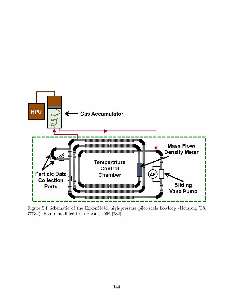
Figure 5.1 Schematic of the ExxonMobil high-pressure pilot-scale flowloop (Houston, TX77034). Figure modified from Boxall, 2009 [232]

144

and the pipe surface, mass flowrate measurements using a multiphase flow meter (Corio-

lis type), video imaging and chord length distribution data collection that allows tracking

of the droplet/particle size distribution throughout the experiments, and traditional video

recording of the fluids inside the loop from the viewing ports installed on the pipe.

Flowloop tests were conducted at 70 vol.% liquid loading and 50 vol.% water content.

The oil phase is a liquid hydrocarbon mixture with a specific gravity of 865 kg m-3 and

a viscosity of 59.1 cP (at 104◦F (40◦C)). The aqueous phase is a brine solution (3.5 wt.%

NaCl) with a density of 1023 kg m-3. The gas phase was a natural gas composition, which

forms structure II (sII) hydrates. The experimental matrix included both baseline tests and

experiments with 2 vol.% AA injection. The AA, a quaternary ammonium-based surfactant,

was dosed with respect to the volume of the aqueous phase in the system. Three different

mixture velocities were studied (2.3, 3.7 and 5.8 ft s-1) for both baseline and AA tests.

The flowloop experimental procedure starts by charging the system with fluids, followed

by pressurization to 1000 psig at a room temperature of 85◦F. The fluids were mixed for

about an hour at the experimental mixture velocity for a given test. After mixing, the

room temperature set point was changed to 38◦F (∼3.3◦C), initiating a cooling stage at a

rate of ∼25◦F hr-1 (∼14◦C hr-1), and eventually leading to hydrate onset. The experiment

continues until either hydrate formation ceases and pressure drop stabilizes, or the system

was considered to be plugged (i.e. the safety threshold for the pump power output was

reached). Flowloop temperature and pressure, together with the gas accumulator volume,

were used to calculate the amount of hydrates formed throughout the experiment. In the case

that the system had not plugged, a shut-in period was allowed for a given amount of time

(i.e. mixture velocity was set to zero), while keeping the temperature and pressure set points

constant. The shut-in periods for the experiments with AA injection was set to six hours in

order to maximize the length of the shut-in stages within the available experimental time at

the flowloop facilities. After each shut-in stage, the pump was restarted (i.e. a cold restart

test) to verify whether hydrate particle agglomeration under static conditions was prevented

145

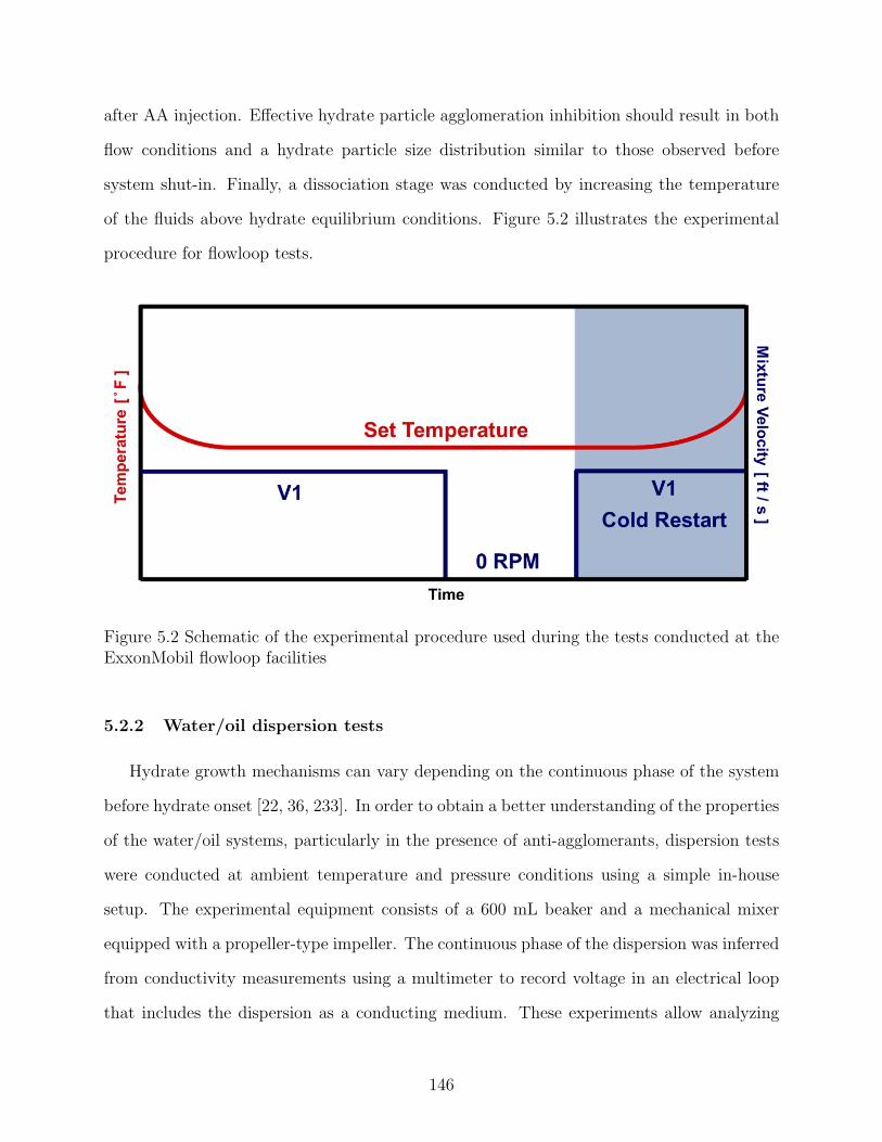
after AA injection. Effective hydrate particle agglomeration inhibition should result in both

flow conditions and a hydrate particle size distribution similar to those observed before

system shut-in. Finally, a dissociation stage was conducted by increasing the temperature

of the fluids above hydrate equilibrium conditions. Figure 5.2 illustrates the experimental

procedure for flowloop tests.

Figure 5.2 Schematic of the experimental procedure used during the tests conducted at theExxonMobil flowloop facilities

5.2.2 Water/oil dispersion tests

Hydrate growth mechanisms can vary depending on the continuous phase of the system

before hydrate onset [22, 36, 233]. In order to obtain a better understanding of the properties

of the water/oil systems, particularly in the presence of anti-agglomerants, dispersion tests

were conducted at ambient temperature and pressure conditions using a simple in-house

setup. The experimental equipment consists of a 600 mL beaker and a mechanical mixer

equipped with a propeller-type impeller. The continuous phase of the dispersion was inferred

from conductivity measurements using a multimeter to record voltage in an electrical loop

that includes the dispersion as a conducting medium. These experiments allow analyzing

146

the influence of the AAs on the water/oil dispersions.

The experimental procedure consisted of initially loading the system with a pure liquid

phase, either an aqueous or an organic phase. Mixing was started at a given constant

velocity (e.g. 500 RPM) and at ambient temperature and pressure. The water content in

the system was systematically increased or decreased by 5 vol.% with the addition of a given

volume of the dispersed phase (i.e. an aqueous phase was added to increase water content

and an organic phase was added to decrease water content). After each addition of the

dispersed phase, the system was allowed to stabilize for 30 min before measuring voltage.

In the case of using an AA, this was dosed based on the water content in the system (i.e.

if water content was increased, more AA was directly dosed to the dispersion), yielding a

constant concentration of AA with respect to the aqueous phase throughout the experiment.

Independent tests were run either by increasing or decreasing water content in the system

in order to determine the dispersion phase inversion point from water-in-oil to oil-in-water

and vice versa.


Experiments were designed and conducted using a non-dispersing liquid hydrocarbon

mixture as the organic phase at 50 vol.% water content (3.5 wt.% NaCl) with 70 vol.%

liquid loading, and natural gas. Such an organic phase was selected for several reasons.

The transparent color allows good visualization of both droplets and hydrate particles for

video recording from the visual ports. Moreover, previous rheological studies using liquid

hydrocarbon mixtures have shown similar trends to those with non-dispersing oils, such as

kerosene [55]. Finally, the liquid hydrocarbon mixture utilized in these studies provides a

surfactant-free organic phase suitable to better understand the effects of AAs on water/oil

and water/oil/hydrate dispersions.

Temperature, pressure, and gas reservoir volume data were used to calculate gas con-

sumption during hydrate formation. The hydrate volume fraction (HV F ) is defined as the

volume of hydrate particles with respect to the total volume of liquids and solids in the slurry

147

according to Equation 5.1,

Hydrate V olumeFraction =Hydrate V olume

Hydrate V olume + UnconvertedWater V olume + Oil V olume(5.1)

where the Unconverted Water V olume is the remaining water in the system that has not

been converted into hydrates.

The pressure drop evolution after hydrate formation is analyzed in terms of the relative

pressure drop at a given time with respect to the pressure drop measured at hydrate onset

according to Equation 5.2,

Relative Pressure Drop (t) =Pressure Drop (t)

Pressure Drop@Hydrate Onset

(5.2)

where Pressure DropHydrate Onset is the pressure drop of the system at the hydrate onset

(i.e. relative time= 0).

5.3.1 Mixture velocity effects on hydrate particle transportability using AAs

Experiments at three different mixture velocities (2.3, 3.7 and 5.8 ft s-1) were conducted

both with and without injection of 2 vol.% AA. Dispersion tests suggest that the liquid

hydrocarbon system selected for these experiments at 50 vol.% water content and 3.5 wt.%

NaCl is within the transition region making it difficult to determine the continuous phase

of the dispersion before hydrate onset (i.e. relative time < 0). Measured data, such as

pressure drop and droplet/particle CLDs were used to infer the type of dispersion present in

the system before hydrate onset.

Relative pressure drop profiles as a function of hydrate volume fraction at the three

studied velocities with and without AA injection (Figure 5.3) showed that this particular

AA does not help reduce the relative pressure drop of the system with respect to baseline

tests. However, as discussed in the next section, hydrate bedding was observed in baseline

experiments, which reduces the amount of hydrate particles transported in the flowing slurry.

Lower solids concentration in the flowing liquids could reduce the overall slurry viscosity

148

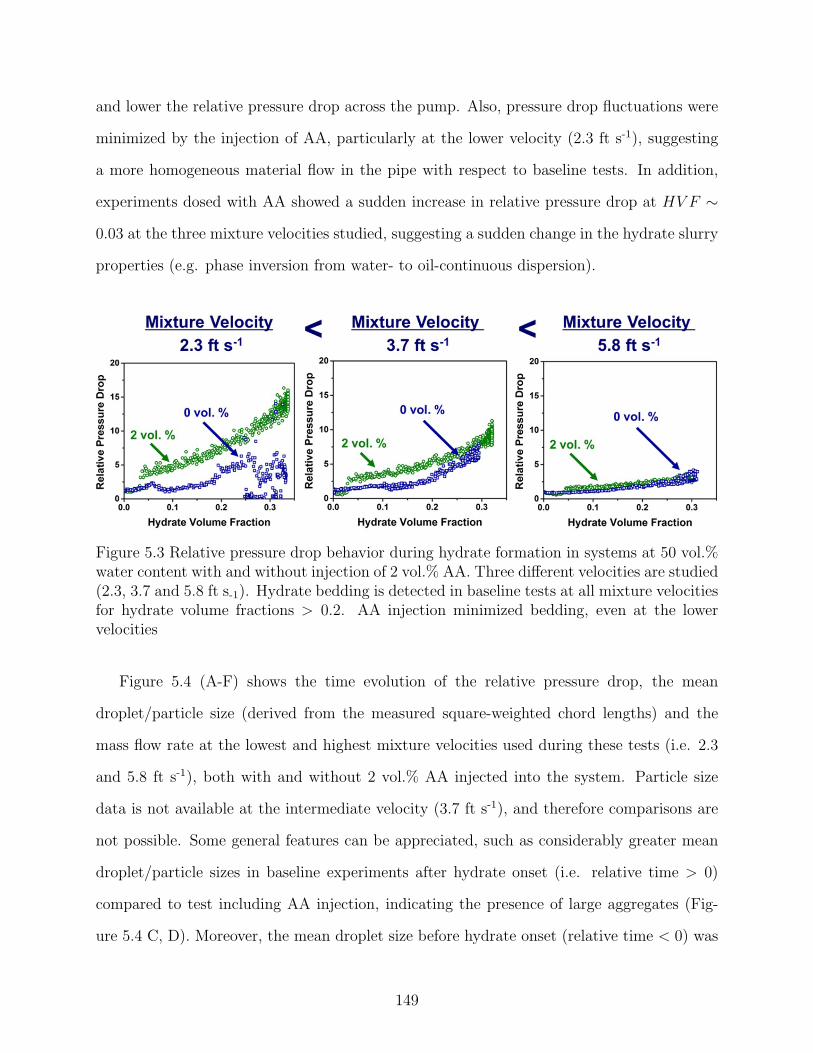
and lower the relative pressure drop across the pump. Also, pressure drop fluctuations were

minimized by the injection of AA, particularly at the lower velocity (2.3 ft s-1), suggesting

a more homogeneous material flow in the pipe with respect to baseline tests. In addition,

experiments dosed with AA showed a sudden increase in relative pressure drop at HV F ∼

0.03 at the three mixture velocities studied, suggesting a sudden change in the hydrate slurry

properties (e.g. phase inversion from water- to oil-continuous dispersion).

Figure 5.3 Relative pressure drop behavior during hydrate formation in systems at 50 vol.%water content with and without injection of 2 vol.% AA. Three different velocities are studied(2.3, 3.7 and 5.8 ft s-1). Hydrate bedding is detected in baseline tests at all mixture velocitiesfor hydrate volume fractions > 0.2. AA injection minimized bedding, even at the lowervelocities

Figure 5.4 (A-F) shows the time evolution of the relative pressure drop, the mean

droplet/particle size (derived from the measured square-weighted chord lengths) and the

mass flow rate at the lowest and highest mixture velocities used during these tests (i.e. 2.3

and 5.8 ft s-1), both with and without 2 vol.% AA injected into the system. Particle size

data is not available at the intermediate velocity (3.7 ft s-1), and therefore comparisons are

not possible. Some general features can be appreciated, such as considerably greater mean

droplet/particle sizes in baseline experiments after hydrate onset (i.e. relative time > 0)

compared to test including AA injection, indicating the presence of large aggregates (Fig-

ure 5.4 C, D). Moreover, the mean droplet size before hydrate onset (relative time < 0) was

149

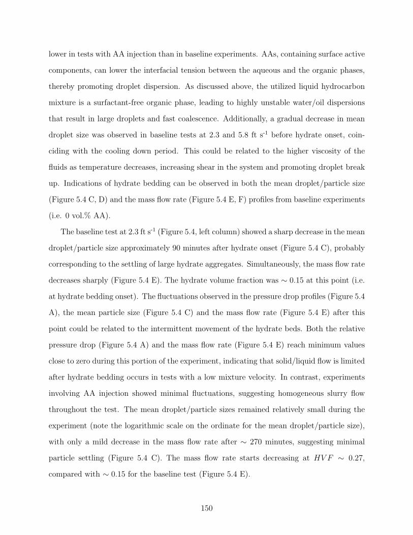
lower in tests with AA injection than in baseline experiments. AAs, containing surface active

components, can lower the interfacial tension between the aqueous and the organic phases,

thereby promoting droplet dispersion. As discussed above, the utilized liquid hydrocarbon

mixture is a surfactant-free organic phase, leading to highly unstable water/oil dispersions

that result in large droplets and fast coalescence. Additionally, a gradual decrease in mean

droplet size was observed in baseline tests at 2.3 and 5.8 ft s-1 before hydrate onset, coin-

ciding with the cooling down period. This could be related to the higher viscosity of the

fluids as temperature decreases, increasing shear in the system and promoting droplet break

up. Indications of hydrate bedding can be observed in both the mean droplet/particle size

(Figure 5.4 C, D) and the mass flow rate (Figure 5.4 E, F) profiles from baseline experiments

(i.e. 0 vol.% AA).

The baseline test at 2.3 ft s-1 (Figure 5.4, left column) showed a sharp decrease in the mean

droplet/particle size approximately 90 minutes after hydrate onset (Figure 5.4 C), probably

corresponding to the settling of large hydrate aggregates. Simultaneously, the mass flow rate

decreases sharply (Figure 5.4 E). The hydrate volume fraction was ∼ 0.15 at this point (i.e.

at hydrate bedding onset). The fluctuations observed in the pressure drop profiles (Figure 5.4

A), the mean particle size (Figure 5.4 C) and the mass flow rate (Figure 5.4 E) after this

point could be related to the intermittent movement of the hydrate beds. Both the relative

pressure drop (Figure 5.4 A) and the mass flow rate (Figure 5.4 E) reach minimum values

close to zero during this portion of the experiment, indicating that solid/liquid flow is limited

after hydrate bedding occurs in tests with a low mixture velocity. In contrast, experiments

involving AA injection showed minimal fluctuations, suggesting homogeneous slurry flow

throughout the test. The mean droplet/particle sizes remained relatively small during the

experiment (note the logarithmic scale on the ordinate for the mean droplet/particle size),

with only a mild decrease in the mass flow rate after ∼ 270 minutes, suggesting minimal

particle settling (Figure 5.4 C). The mass flow rate starts decreasing at HV F ∼ 0.27,

compared with ∼ 0.15 for the baseline test (Figure 5.4 E).

150

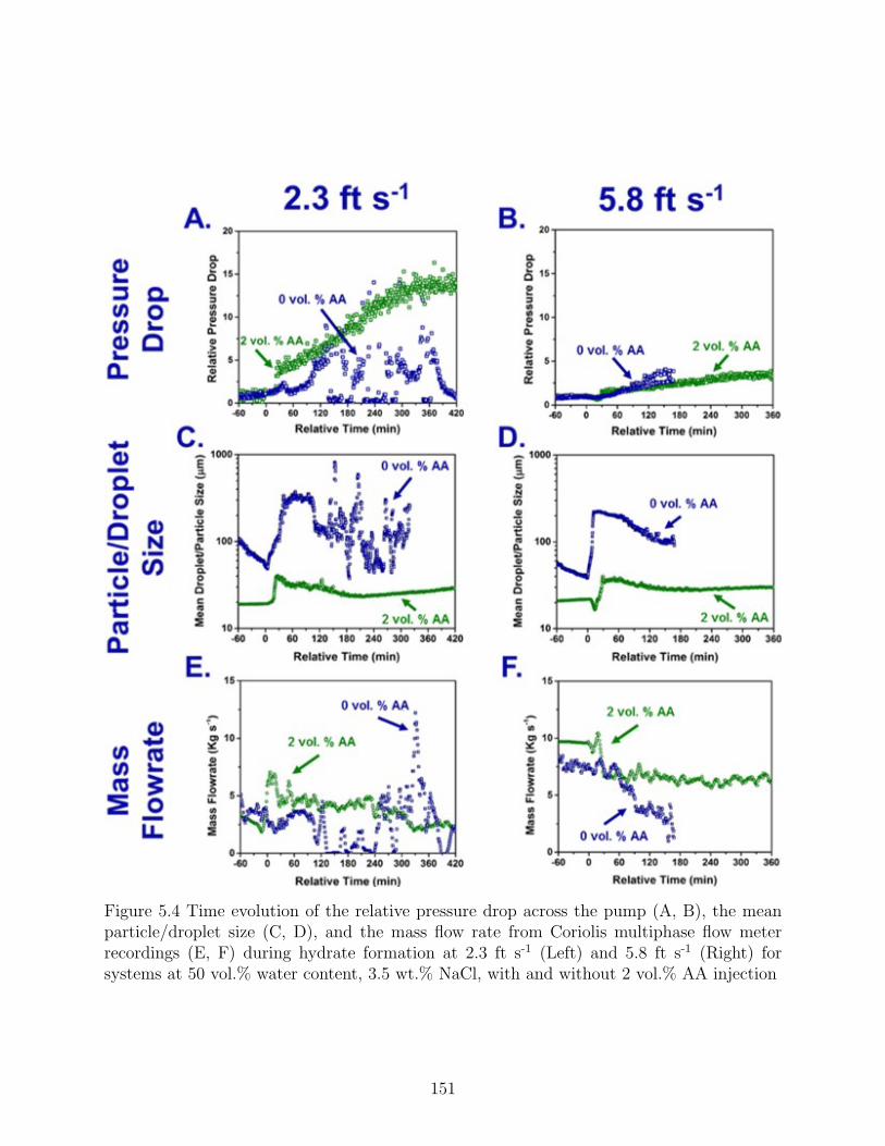
Figure 5.4 Time evolution of the relative pressure drop across the pump (A, B), the meanparticle/droplet size (C, D), and the mass flow rate from Coriolis multiphase flow meterrecordings (E, F) during hydrate formation at 2.3 ft s-1 (Left) and 5.8 ft s-1 (Right) forsystems at 50 vol.% water content, 3.5 wt.% NaCl, with and without 2 vol.% AA injection

151

The baseline test at a higher velocity (5.8 ft s-1) also showed signals of hydrate bedding

occurring in the system (Figure 5.4, right column). Both the mean droplet/particle size

(Figure 5.4 D) and the mass flow rate (FFigure 5.4 F) decreased about 70 min after hydrate

onset, coinciding again with fluctuations in the pressure drop (Figure 5.4 B). This behavior

indicates settling of larger hydrate aggregates, reducing the mean droplet/particle size in

the flowing slurry. The mean droplet/particle size starts decreasing before hydrate bedding

onset, but at a much lower rate than in the test at 2.3 ft s-1 (Figure 5.4 D). However, the

decreasing trend in the mean droplet/particle size intensifies 70 minutes after hydrate onset,

coinciding with an HV F ∼ 0.16. In contrast, with an injection of 2 vol.% AA, both the mean

droplet/particle size (Figure 5.4 D) and the mass flow rate (Figure 5.4 F) remained fairly

constant throughout the test, indicating efficient hydrate transport without accumulation

during the entire experiment.

Although the mean droplet/particle size remained fairly constant in tests dosed with

anti-agglomerants, a sudden increase was observed about 30 minutes after the hydrate on-

set (Figure 5.4 C, D), coinciding with the sharp increase in relative pressure drop taking

place at HV F ∼ 0.03 (Figure 5.3, left and right plots). Simultaneously, the mass flow

rate sharply decreases at this point (Figure 5.4 E, F). The oil phase, having a higher vis-

cosity than the aqueous phase, could cause a sudden increase in the relative pressure drop

if a dispersion phase inversion takes place (i.e. transition from a water-continuous to an

oil-continuous slurry). Moreover, this particular AA was found to favor water-continuous

dispersions according to the dispersion tests conducted at 2 vol.% AA and with the same

liquid hydrocarbon mixture used in the flowloop tests. Figure 5.5 shows the transition from

an oil-continuous dispersion to a water-continuous dispersion occurring at ∼ 55 vol.% wa-

ter content in systems both with and without injection of AA (Figure 5.5 A, B). Similarly,

the transition from a water-continuous to an oil-continuous dispersion takes place at ∼ 25

vol.% water content in baseline experiments (i.e. without injection of AA) (Figure 5.5 A).

However, dosing 2 vol.% AA is sufficient to prevent a transition from a water-continuous to

152

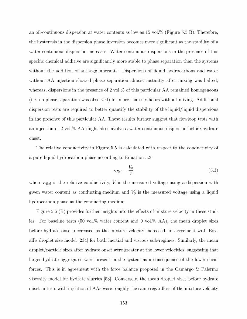
an oil-continuous dispersion at water contents as low as 15 vol.% (Figure 5.5 B). Therefore,

the hysteresis in the dispersion phase inversion becomes more significant as the stability of a

water-continuous dispersion increases. Water-continuous dispersions in the presence of this

specific chemical additive are significantly more stable to phase separation than the systems

without the addition of anti-agglomerants. Dispersions of liquid hydrocarbons and water

without AA injection showed phase separation almost instantly after mixing was halted;

whereas, dispersions in the presence of 2 vol.% of this particular AA remained homogeneous

(i.e. no phase separation was observed) for more than six hours without mixing. Additional

dispersion tests are required to better quantify the stability of the liquid/liquid dispersions

in the presence of this particular AA. These results further suggest that flowloop tests with

an injection of 2 vol.% AA might also involve a water-continuous dispersion before hydrate

onset.

The relative conductivity in Figure 5.5 is calculated with respect to the conductivity of

a pure liquid hydrocarbon phase according to Equation 5.3:

κRel =V0V

(5.3)

where κRel is the relative conductivity, V is the measured voltage using a dispersion with

given water content as conducting medium and V0 is the measured voltage using a liquid

hydrocarbon phase as the conducting medium.

Figure 5.6 (B) provides further insights into the effects of mixture velocity in these stud-

ies. For baseline tests (50 vol.% water content and 0 vol.% AA), the mean droplet sizes

before hydrate onset decreased as the mixture velocity increased, in agreement with Box-

all’s droplet size model [234] for both inertial and viscous sub-regimes. Similarly, the mean

droplet/particle sizes after hydrate onset were greater at the lower velocities, suggesting that

larger hydrate aggregates were present in the system as a consequence of the lower shear

forces. This is in agreement with the force balance proposed in the Camargo & Palermo

viscosity model for hydrate slurries [53]. Conversely, the mean droplet sizes before hydrate

onset in tests with injection of AAs were roughly the same regardless of the mixture velocity

153

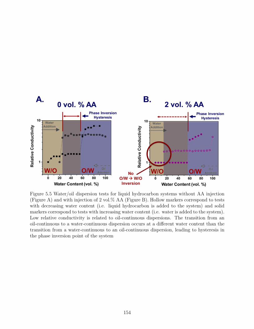
Figure 5.5 Water/oil dispersion tests for liquid hydrocarbon systems without AA injection(Figure A) and with injection of 2 vol.% AA (Figure B). Hollow markers correspond to testswith decreasing water content (i.e. liquid hydrocarbon is added to the system) and solidmarkers correspond to tests with increasing water content (i.e. water is added to the system).Low relative conductivity is related to oil-continuous dispersions. The transition from anoil-continuous to a water-continuous dispersion occurs at a different water content than thetransition from a water-continuous to an oil-continuous dispersion, leading to hysteresis inthe phase inversion point of the system

154

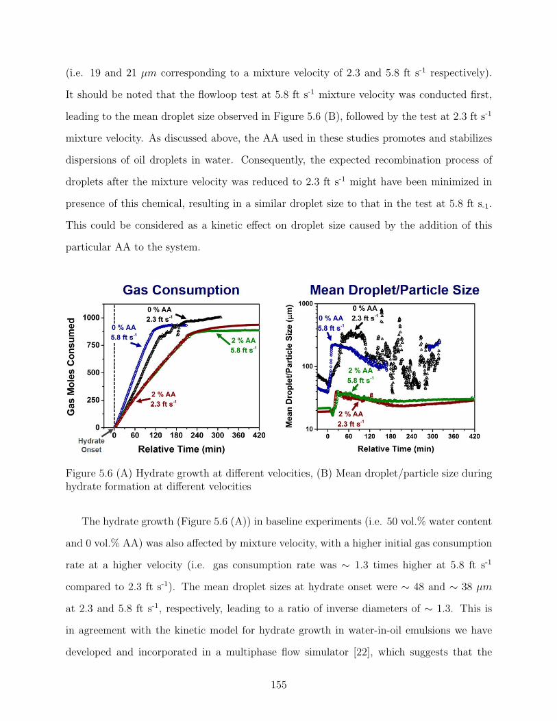
(i.e. 19 and 21 µm corresponding to a mixture velocity of 2.3 and 5.8 ft s-1 respectively).

It should be noted that the flowloop test at 5.8 ft s-1 mixture velocity was conducted first,

leading to the mean droplet size observed in Figure 5.6 (B), followed by the test at 2.3 ft s-1

mixture velocity. As discussed above, the AA used in these studies promotes and stabilizes

dispersions of oil droplets in water. Consequently, the expected recombination process of

droplets after the mixture velocity was reduced to 2.3 ft s-1 might have been minimized in

presence of this chemical, resulting in a similar droplet size to that in the test at 5.8 ft s-1.

This could be considered as a kinetic effect on droplet size caused by the addition of this

particular AA to the system.

Figure 5.6 (A) Hydrate growth at different velocities, (B) Mean droplet/particle size duringhydrate formation at different velocities

The hydrate growth (Figure 5.6 (A)) in baseline experiments (i.e. 50 vol.% water content

and 0 vol.% AA) was also affected by mixture velocity, with a higher initial gas consumption

rate at a higher velocity (i.e. gas consumption rate was ∼ 1.3 times higher at 5.8 ft s-1

compared to 2.3 ft s-1). The mean droplet sizes at hydrate onset were ∼ 48 and ∼ 38 µm

at 2.3 and 5.8 ft s-1, respectively, leading to a ratio of inverse diameters of ∼ 1.3. This is

in agreement with the kinetic model for hydrate growth in water-in-oil emulsions we have

developed and incorporated in a multiphase flow simulator [22], which suggests that the

155

initial rate of gas consumption for hydrate growth is linearly dependent on the surface area

of water droplets, as given in Equation 5.4:

−dngasdt

= uk1 exp

(

k2Tsys

)

AS∆Tsub1

Wg

(5.4)

where ngas is moles of gas consumed for hydrate formation, k1 and k2 are the intrin-

sic rate constants, AS is the surface area between the water and the hydrocarbon phases,

Wg is the average molecular weight of the hydrate-forming components, Tsys is the sys-

tem temperature, ∆Tsub is the subcooling or thermal driving force for hydrate formation

(∆Tsub = Thyd eq − Tsys). Thyd eq is the hydrate equilibrium temperature at a given system

pressure and composition. Finally, u is a scaling factor accounting for mass and heat trans-

fer resistances that are not present in the original intrinsic hydrate growth kinetic models

[235–237]. Theoretical gas consumption rates for the baseline tests were calculated using the

droplet size data from Figure 5.6 (B), the temperature of the system and the experimental

subcooling at the hydrate onset. The theoretical gas consumption rate at the onset of hy-

drate formation was approximately three orders of magnitude higher than the experimental

gas consumption rate. It is worth noting that the droplet size used in these calculations cor-

responds to the mean square-weighted chord length that may not correspond to the actual

droplet size in the system [234]. This analysis also assumes that all the free-water in the

system was fully dispersed in the oil phase as droplets. However, previous studies showed

that the free-water phase could be only partially dispersed in the oil phase at low mixture

velocities, with the remaining water as a separated aqueous phase reducing the water/oil

interfacial area [152]. The extent of water dispersion cannot be verified in these studies.

Additionally, both surface area and subcooling are considered constant throughout hydrate

formation. However, the salt concentration in the aqueous phase should increase as water

was consumed to form hydrates, lowering the hydrate equilibrium temperature and, there-

fore, decreasing subcooling. The available surface area for hydrate formation could also vary

due to water consumption following hydrate formation and subsequent changes in the flow

156

regime.

The effect of mixture velocity on the mean droplet size at hydrate onset in experiments

with 2 vol.% AA was masked by the increased stability of the dispersion with these surfac-

tants, which helped maintain the low mean droplet size obtained in the initial tests at the

higher mixture velocity. Hence, the surface area available for hydrate growth at the different

mixture velocities was comparable resulting in similar initial gas consumption rates in ex-

periments at 2.3 and 5.8 ft s-1 mixture velocity dosed with anti-agglomerants. Moreover, the

initial gas consumption rate in experiments dosed with this particular AA was lower when

compared with baseline tests, despite offering more surface area for hydrate formation. This

result suggests potential hydrate kinetic inhibition effects associated with this AA formu-

lation. Gas consumption rates in baseline tests at 2.3 and 5.8 ft s-1 mixture velocity were

∼ 1.6 and ∼ 2 times higher, respectively, when compared with gas consumption rates from

corresponding tests at the same mixture velocity dosed with 2 vol.% AA.

5.3.2 AA performance during shut-in and restart operations

Stagnant conditions during shut-in can lead to hydrate particle agglomeration due to

negligible shear forces in the system, therefore, increasing overall hydrate particle size and

making solid material transport throughout the system difficult. Injection of AAs could

reduce hydrate cohesive forces, favoring re-dispersion of hydrate particles once fluid flow

restarts.

Simulating a shut-in period after hydrates stop forming in flowloop tests allows assessment

of the capability of AAs to prevent hydrate particle agglomeration in stagnant conditions,

and to recover hydrate transportability after restart. Flowloop experiments with an injection

of 2 vol.% AA were shut in for six hours and restarted. Tests initially conducted at 2.3 and

3.7 ft s-1 were restarted at the same velocity used for hydrate formation under continuous

pumping. The test with hydrate formation at higher velocity (5.8 ft s-1) was restarted at a

low velocity (2.3 ft s-1) in order to evaluate the consequences of restarting the system at a

lower velocity than that at which hydrates were formed. Moreover, the baseline experiment

157

with hydrate formation at 5.8 ft s-1 was also shut-in for a period of two hours and restarted

at 5.8 ft s-1 again. Baseline tests at lower velocities were not shut-in due to time limitations.

The relative pressure drop and the mass flow rate data were used to determine whether

flowing conditions observed before shut-in can be recovered after restarting the system.

Particle/droplet size measurements provided information about the evolution of the hydrate

particle size during shut-in.

Figure 5.7 shows the relative pressure drop (A) and the mass flowrate (B) from experi-

ments with 2 vol.% AA injection, two hours both before shut-in and after restart. Results

from experiments at two different mixture velocities (2.3 and 3.7 ft s-1) are shown. The

relative pressure drop and the mass flowrate were almost identical both before shut-in and

after restart at 3.7 ft s-1, suggesting that the properties of the flowing slurry were unaffected

during the shut-in period. Similar results were observed at a lower velocity (2.3 ft s-1);

however, the relative pressure drop was slightly lower after the restart with respect to the

relative pressure drop values before shut-in. This reduction in the relative pressure drop

could be attributed to some hydrate particles deposited at the bottom of the pipe, which

cannot be lifted at this low velocity. Deposited hydrate particles might reduce the slurry

viscosity due to lower solids concentration, causing a slight decrease in the relative pressure

drop observed in Figure 5.7 (A). In this figure, the relative time was defined with respect to

the time at which the system was shut-in.

Another interesting aspect of shut-in operations is the evolution of the hydrate particle

size. Figure 5.8 shows mean particle/droplet sizes before shut-in and after restart from liquid

hydrocarbon systems dosed with 2 vol.% AA. Mean droplet/particle sizes from tests at 2.3

and 5.8 ft s-1 mixture velocity are included. As discussed in Figure 5.4, the mixture velocity

had a minor influence on hydrate particle size when sufficient AA was dosed to the system.

This suggests that once hydrate particles are broken by shear forces, the recombination

process of such particles can be slowed down by the AA. This could lead to a stable dispersion

of fine hydrate particles, similar to the droplet behavior in a surfactant-stabilized emulsion.

158

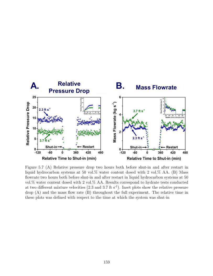
Figure 5.7 (A) Relative pressure drop two hours both before shut-in and after restart inliquid hydrocarbon systems at 50 vol.% water content dosed with 2 vol.% AA. (B) Massflowrate two hours both before shut-in and after restart in liquid hydrocarbon systems at 50vol.% water content dosed with 2 vol.% AA. Results correspond to hydrate tests conductedat two different mixture velocities (2.3 and 3.7 ft s-1). Inset plots show the relative pressuredrop (A) and the mass flow rate (B) throughout the full experiment. The relative time inthese plots was defined with respect to the time at which the system was shut-in

159

After restarting the system at t 2.3 ft s-1, a sudden increase in mean droplet/particle size was

observed. Such an increase could be related to hydrate particles that have come together

during shut-in forming weakly bonded agglomerates and that are initially detected after

restarting flow in the system. However, given the relatively low hydrate cohesive forces in

the presence of this AA, such hydrate clumps could easily break, eventually leading to a

mean droplet/particle size similar to those obtained before the shut-in stage, regardless of

the velocity at which hydrate particles were formed.

Finally, a comparison of the particle sizes both before and after the shut-in stage in

systems with and without AA injection provides further insights into the performance of

these chemicals in stagnant conditions. Figure 5.9 shows the droplet/particle size resulting

from tests conducted at 5.8 ft s-1 mixture velocity with and without 2 vol.% AA dosed to

the system. These results consist of the mean droplet/particle sizes before and after the

hydrate onset, including the shut-in stage, as well as the chord length count from different

size ranges of droplet/particles. The chord length counts were divided in three subgroups:

small droplets/particles (d < 50 µm), medium droplets/particles (50 < d < 150 µm) and

large droplets/particles (150 < d < 300 µm).

Useful information regarding AA performance can be inferred based on the hydrate par-

ticle size distribution at different stages of the experiment. First, at the hydrate onset (i.e.

relative time ∼ 0), a sudden increase in the mean droplet particle size was observed in tests

both with and without AA injection (Figure 5.9 (A) and (E)); however, such increase was

more pronounced in the experiments without AA. The sharp increase in the droplet/particle

size around the hydrate onset could be related to a decrease in the counts of small particles in

both systems (Figure 5.9 (B) and (F)). Previous studies using chord length counts to analyze

hydrate growth and agglomeration have related the decrease in the small chord length counts

coinciding with the hydrate onset to systems that were water-continuous before the hydrate

onset [238]. Furthermore, counts of both medium and large droplets/particles (Figure 5.9

(C) and (D)) increased by one and two orders of magnitude respectively at the hydrate onset

160

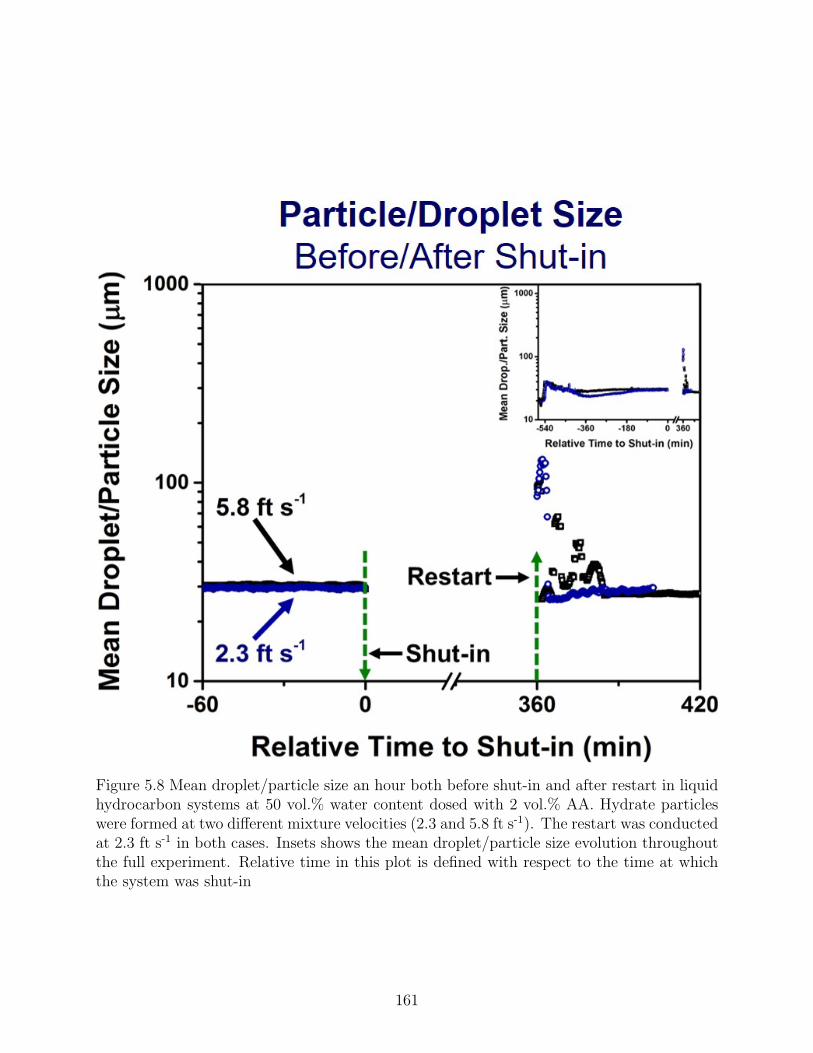
Figure 5.8 Mean droplet/particle size an hour both before shut-in and after restart in liquidhydrocarbon systems at 50 vol.% water content dosed with 2 vol.% AA. Hydrate particleswere formed at two different mixture velocities (2.3 and 5.8 ft s-1). The restart was conductedat 2.3 ft s-1 in both cases. Insets shows the mean droplet/particle size evolution throughoutthe full experiment. Relative time in this plot is defined with respect to the time at whichthe system was shut-in

161

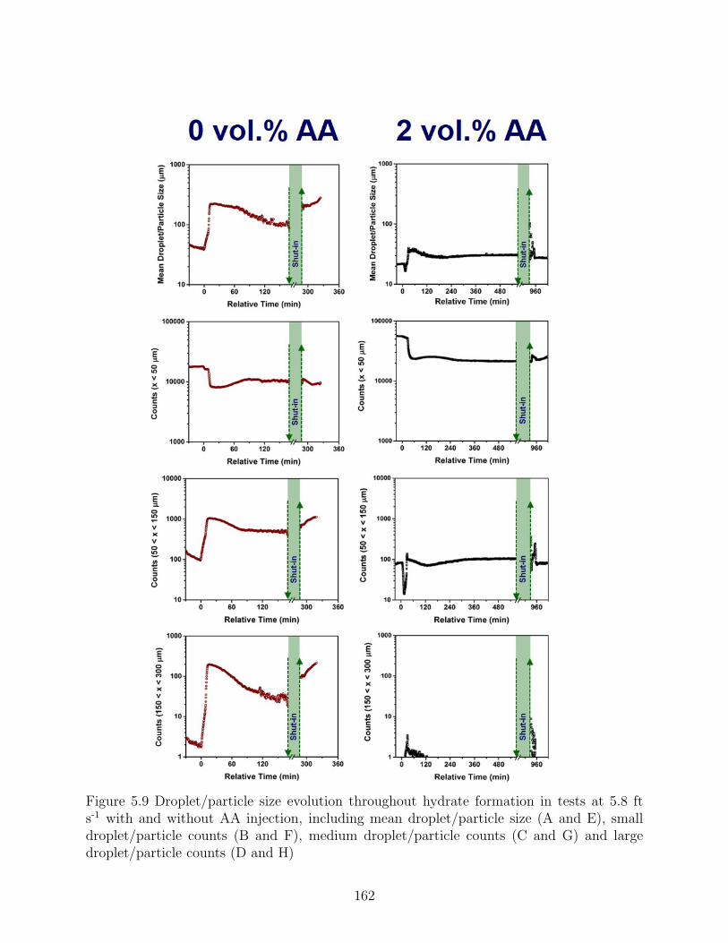
Figure 5.9 Droplet/particle size evolution throughout hydrate formation in tests at 5.8 fts-1 with and without AA injection, including mean droplet/particle size (A and E), smalldroplet/particle counts (B and F), medium droplet/particle counts (C and G) and largedroplet/particle counts (D and H)

162

in systems without AA injection. On the other hand, medium and large droplet/particle

counts (Figure 5.9 (G) and (H)) remained roughly constant throughout the experiment in

systems dosed with AAs, despite a sudden dip in medium particle counts and slight appear-

ance of large particles around the hydrate onset. The large particle counts are close to zero

for most of the test apart from the hydrate onset in tests with AA injection. According

to these results, the increase in the mean droplet/particle size (Figure 5.9 (A)) observed

around the hydrate onset in systems without AA injection should be related mainly to the

appearance of medium and large hydrate agglomerates (Figure 5.9 (C) and (D)). Conversely,

the increasing droplet/particle size in systems with AA injection (Figure 5.9 (E)) could be

related to decreasing counts of small particles instead (Figure 5.9 (F)). Such a decrease in

the small particle counts could have been associated in previous studies with changes in the

reflective properties of water/oil droplets that turn into hydrate particles [237]. The medium

and large droplet/particle counts gradually decrease over the experiments, particularly in the

tests without AA injection, suggesting that bedding of larger hydrate particles in the system

causes an additional decrease in mean droplet/particle sizes.

Høiland [239] showed that hydrate formation could have contrasting effects on the surface

chemistry of a system depending on the composition of the oil phase. Crude oils with low

plugging tendency tend to form oil-wet hydrate particles, favoring oil-continuous dispersions

after hydrates start to form. Accordingly, effective hydrate anti-agglomeration has been

associated with the formation of oil-wet hydrate particles [26]. These observations provide

further support to a possible transition from a water-continuous to an oil-continuous dis-

persion occurring in flowloop tests after hydrate onset in the systems dosed with 2 vol.%

AA.

Finally, after a shut-in period of six hours and a restart at 2.3 ft s-1 was conducted,

all droplet/particle counts (small, medium and large) recover to similar values to those

observed before shut-in (Figure 5.9 (F), (G) and (H)) in systems dosed with AAs. Higher

counts of medium and large droplets/particles are noticed right after the restart; however,

163

such increasing counts vanished within 30 minutes after fluid flow restarted. These medium

and large droplet/particle counts could be related to clumps of hydrate particles moving

together, which are weakly interacting due to the reduced cohesive forces between hydrate

particles in the presence of AAs. Such hydrate clumps might be easily re-dispersed into

fine hydrate particles under the influence of shear forces resulting in the same particle size

distribution observed before shut-in. On the other hand, a noticeable increase in the mean

droplet/particle size occurred during shut-in (Figure 5.9 (A)) in tests without AA injection.

The medium and large droplet/particle counts increased during the shut-in resulting in a

greater mean droplet/particle size (Figure 5.9 (C) and (D)). Large hydrate aggregates could

have formed under static conditions during shut-in in absence of anti-agglomerants. Medium

and large droplet/particle counts further increased as time progresses after the fluid flow

restarted, suggesting that large aggregates, which cannot be broken up by the shear forces,

might have been re-dispersed in the flowing slurry. These results indicate that hydrate

particle agglomeration during shut-in could be prevented using an effective AA in systems

with a non-dispersing oil phase.

5.4 Conclusions

High-pressure industrial-scale flowloop tests using a non-dispersing oil were conducted

in order to compare the influence of mixture velocity on hydrate particle transportability

in systems both with and without dosing hydrate dispersants or anti-agglomerants (AAs).

These experiments included dynamic cool-down tests, as well as shut-in and restart scenarios,

which can be critical for flow assurance in subsea oil & gas production. The influence of

mixture velocity was observed in baseline tests both in the hydrate growth rates (directly

proportional) and the mean droplet/particle size (inversely proportional). However, such

dependence on mixture velocity vanished after the injection of the AA formulation used in

these flowloop studies. Dosing anti-agglomerants to the system resulted in similar hydrate

growth and particle size evolution regardless of the mixture velocity utilized. Moreover,

complementary water/oil dispersion tests showed that this AA formulation also modifies the

164

surface chemistry of the liquid/liquid dispersion by favoring water-continuous systems with

respect to surfactant-free samples.

The injection of AAs helped to minimize hydrate particle bedding at all studied velocities;

however, a certain minimum velocity was required to fully prevent hydrate particle bedding.

Moreover, this particular AA formulation successfully inhibited hydrate particle size increase

(agglomeration) under static conditions (shut-in), allowing the full recovery of solid material

flow after restarting the system. In this sense, the droplet/particle CLD measurements

provided useful information to assess AA performance with respect to the equivalent baseline

tests without chemical injection.

5.5 Acknowledgements

The authors acknowledge the significant contributions to this work by Brendon Keinath,

Doug Turner, Geetha Mahadevan, Todd Lagus, Giovanny Grasso, Tabish Maqbool, Glenn

Cobb, Roy Livingston and all staffs from ExxonMobil Upstream Research Company (Hous-

ton, TX 77098, USA) for access to the flowloop facilities and guidance during the experi-

mental investigation and analyses of this work. The authors would also like to thank the

CSM Hydrate Consortium members for funding and support.

165

CHAPTER 6

HP-RHEOMETER & PILOT-SCALE FLOWLOOP STUDIES ON HYDRATE SLURRY

TRANSPORTABILITY USING AAS

Chapter 6 contains a series of pilot-scale flowloop studies conducted both at Tulsa Univer-

sity and ExxonMobil Flowloop scale facilities. These flowloop tests provided further valida-

tion of the hydrate performance assessment protocols proposed in this work using low-sample

volume experimental apparatuses. In additions, these set of pilot-scale flowloop tests allowed

direct comparison of the results obtained from hydrate transportability studies conducted at

different pilot-scale flowloop facilities is systems with similar experimental conditions. Fi-

nally, complementary HP-rheometer tests provided further insights into the interconnection

between hydrate slurry viscosity and the pressure drop observed during pilot-scale flowloop

experiments involving hydrate formation.

6.1 Introduction

In gas-dominated systems, the major concerns are related to the performance of hydrate

anti-agglomerants at high water contents. Accordingly, the condensate-to-gas ratio (CGR)

and the water content could be the main parameters to assess AAs suitability for such

systems. On the other hand, the relatively low gas-to-oil ratio (GOR) in oil-dominated

systems could limit the water conversion into hydrates. Therefore, the maximum amount of

water that can be thermodynamically converted into hydrates might be the key parameter

to consider for implementing AAs crude oil pipelines. Currently, oil companies (e.g. TOTAL

S.A.) might consider safe to utilize AAs in systems with a maximum hydrate volume fraction

in the liquid phase below 30 vol. % [30].

Deep offshore oil and gas operators require a comprehensive understanding of the mecha-

nisms leading to efficient hydrate particle transport in order to successfully deploy innovative

hydrate management strategies, such as AAs. This understanding should include the relative

166

influence of diverse operational parameters on the performance of these additives. These

parameters could include, for example, shear rate, GOR, CGR, sub-cooling, the natural

surface-active components in the hydrocarbon phase, the composition of the aqueous phase,

and the AA formulation and dosing, for example. A better understanding of the hydrate

growth kinetics and slurry rheological properties in systems dosed with anti-agglomerants

could help to extend the current comfort zone for utilizing AAs in a specific scenario.

This chapter summarizes a series of pilot-scale flowloop tests using a model liquid hydro-

carbon mixture as the organic phase. Complementary high-pressure rheometer tests have

been conducted in order to better understand the pilot-scale flowloop results based on the

rheological behavior of the hydrate slurry in the presence of AAs.

Furthermore, pilot-scale flowloop facilities might represent the closest environment to

operative subsea flowlines traditionally available to study hydrate particle transportability.

However, the scalability of experimental results from the laboratory to field-scale processes

has traditionally been a major engineering challenge, and flowloop studies are not exempt

from these difficulties [153]. Several parameters may vary between flowloop facilities, such as

pipe diameter, total length, geometry, pump design, data acquisition devices, temperature

control, or gas supply systems. Therefore, studies to identify the influence of the experimental

setup on flowloop test results are needed in order to develop system-independent models for

hydrate formation and transport in subsea flowlines. This chapter includes results and

analysis from a set of experiments specifically designed to directly compare two different

pilot-scale flowloop facilities (i.e. ExxonMobil and University of Tulsa flowloops)


Multiple experimental setups, such as HP-rheometer and pilot-scale flowloops, have been

used to study the hydrate slurry transportability in the presence of AAs. These studies

included the evaluation of the influence on the AA performance of several experimental pa-

rameters, such as water content and AA dosing. These investigations involved both dynamic

cool-down and shut-in/restart experimental modes.

167

Flowloop facilities offer the closest laboratory conditions to subsea flowlines in order to

study hydrate particle transportability before deploying new technologies in oil production

fields. Data such as particle size evolution can be utilized to determine whether AAs can

prevent hydrate particle agglomeration under static conditions (i.e. shut-in period). Several

other flowloop output data can be used to evaluate hydrate transportability (e.g pressure

drop and temperature profiles, mass flow rate, and visual video observations). Droplet/-

particle chord length distribution (CLD) analysis and particle video imaging methods are

particularly useful to evaluate hydrate growth and hydrate particle agglomeration, both with

and without AA injection [231, 238]. These two latter methods can provide insights into

the mechanisms leading to hydrate particle accumulation and plugging in different systems.

In addition, these tools allow exploring the effects of shut-in conditions on hydrate parti-

cle morphology and size distribution. This information, coupled with pressure drop and

temperature profiles, is valuable to assess AA performance during transient operations.

Two different pilot-scale flowloop facilities are used in these studies, namely ExxonMobil

flowloop (ExxonMobil Upstream Research Company, Houston, TX 77098, USA) and Uni-

versity of Tulsa flowloop (Petroleum Engineering Department, University of Tulsa, 800 S

Tucker Dr., Tulsa OK 74104, USA).

The ExxonMobil flowloop facility design and experimental procedures are described in

Section 5.2. Some remarkable capabilities of this pilot-scale flowloop are the pressure and

temperature recordings at several locations in the loop, including fluid and surface tem-

peratures, the mass flow rate measurements with a multiphase flow meter (Coriolis type),

the particle Vision and Measurement (PVM) and Focused Beam Reflectance Measurement

(FBRM) devices used to track droplet/particle size evolution during the experiments, and

regular but valuable traditional video recording of the fluids circulating inside the loop was

possible through the viewing ports.

The TU flowloop (Figure 6.1) consists of a 162 ft (∼ 49 m) long and 2.9” (7.4 cm)

internal diameter pipe. A commercial twin-screw Leistritz pump is used to circulate fluids

168

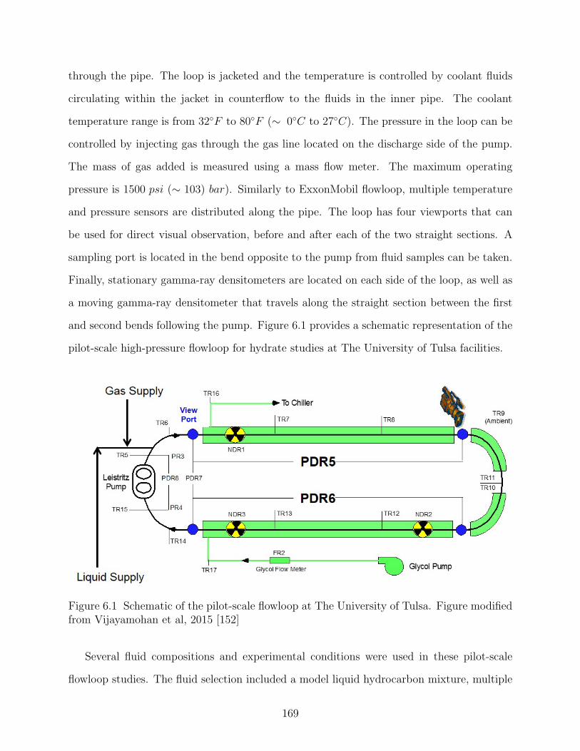
through the pipe. The loop is jacketed and the temperature is controlled by coolant fluids

circulating within the jacket in counterflow to the fluids in the inner pipe. The coolant

temperature range is from 32◦F to 80◦F (∼ 0◦C to 27◦C). The pressure in the loop can be

controlled by injecting gas through the gas line located on the discharge side of the pump.

The mass of gas added is measured using a mass flow meter. The maximum operating

pressure is 1500 psi (∼ 103) bar). Similarly to ExxonMobil flowloop, multiple temperature

and pressure sensors are distributed along the pipe. The loop has four viewports that can

be used for direct visual observation, before and after each of the two straight sections. A

sampling port is located in the bend opposite to the pump from fluid samples can be taken.

Finally, stationary gamma-ray densitometers are located on each side of the loop, as well as

a moving gamma-ray densitometer that travels along the straight section between the first

and second bends following the pump. Figure 6.1 provides a schematic representation of the

pilot-scale high-pressure flowloop for hydrate studies at The University of Tulsa facilities.

Figure 6.1 Schematic of the pilot-scale flowloop at The University of Tulsa. Figure modifiedfrom Vijayamohan et al, 2015 [152]

Several fluid compositions and experimental conditions were used in these pilot-scale

flowloop studies. The fluid selection included a model liquid hydrocarbon mixture, multiple

169

anti-agglomerant formulations and concentrations, different water contents and gas com-

positions leading to the formation of both structure I (sI) and structure II (sII) hydrates.

Moreover, different operation modes, such as continuous pumping and transient tests are in-

corporated in these studies, together with different mixture velocities. Some of the tests were

designed to provide specific data allowing a direct comparison of the two different flowloop

facilities. The general experimental procedure for the pilot-scale flowloop studies is described

in Figure 5.2.

In addition, complementary HP-rheometer tests were performed in order to assess the

use of low dosage hydrate inhibitors (LDHIs) to minimize hydrate particles agglomeration

leading jammed systems associated with an excessively high slurry viscosity in rheological

studies [55]. The HP-rheometer and experimental procedures are described in Section 2.2.

The hydrate growth mechanisms and the transportability of hydrate particles may be

dependent on properties, such as viscosity or gas solubility, of the continuous phase of the

system. Therefore, knowledge of the initial properties of the water/oil dispersion before

hydrate formation might be useful to properly analyze the results from flowloop and rheol-

ogy studies conducted in this project. Anti-agglomerants, being surface-active compounds,

would reduce oil-water interfacial tension promoting homogeneous dispersion of water and

oil phases. Additional dispersion tests were conducted following utilizing the in-house setup

and the procedures described in Section 5.2.2.


A series of pilot-scale flowloop tests were conducted to evaluate the hydrate slurry trans-

portability using AAs in a variety of scenarios. These experiments investigated the influence

on AA performance of different experimental variables such as water content, fluid velocity,

operation mode (i.e. shut-in/restart or dynamic cool-down modes) and AA formulation/dos-

ing. Complementary HP-rheometer tests were conducted using the same liquid compositions

used in the pilot-scale flowloop studies in order to obtain insights into the rheological prop-

erties of the hydrate slurries in the presence of AAs, which might help to understand the

170

pressure drop behavior from the flowloop tests.

The temperature, pressure and injected gas data are used to calculate the gas consump-

tion during the hydrate formation. The hydrate volume fraction (HV F ) is defined as the

volume of hydrate particles with respect to the total volume of liquids and solids in the slurry

according to Equation 5.1.

The pressure drop evolution after hydrate formation is analyzed in terms of the relative

pressure drop at a given time with respect to the pressure drop measured at hydrate onset

according to Equation 5.2.

6.3.1 Treating partially dispersed systems with AAs to prevent hydrate plugformation: high-pressure pilot-scale flowloop and rheological studies atdifferent water contents

Previous studies have shown that partially dispersed systems (i.e. oil-in-water or water-

in-oil dispersions with an additional separated water phase) are particularly prone to result

in hydrate plugs [240]. The partially dispersed systems can be associated with non-dispersing

organic phases with a lack of surface-active compounds favoring phase dispersion, such as

kerosene, mineral oils and gas condensates. Consequently, AAs represent an attractive al-

ternative to reduce hydrate plugging risk in these type of systems both by promoting full

dispersion of the liquid phases due to lower interfacial tensions and by forming stable hydrate

dispersions through inhibiting hydrate particle agglomeration.

A series of pilot-scale flowloop tests were conducted using AAs to prevent hydrate plug

formation in partially dispersed systems at different operational conditions. These opera-

tional conditions include water contents ranging from 30 to 80 vol. %, both transient and

continuous operations, and different AA dosing. Complementary high-pressure rheological

studies were conducted with the same liquid composition from the pilot-scale flowloop tests

in order to obtain insights into the rheological properties of the hydrate slurry in the presence

of AAs and relate such rheological properties to the pressure drop results from the flowloop

tests.

171

6.3.1.1 Hydrate plugging mitigation using AAs in partially-dispersed systemsat intermediate water contents

Tests were conducted using a model liquid hydrocarbon mixture system at 50 vol. %

water content (3.5 wt.% NaCl) and 70 vol.% liquid loading. The hydrate former is the Tulsa

natural gas, which leads to the formation of sII hydrates. These tests were conducted at two

different AA dosages (i.e. 1 and 2 vol.% with respect to the aqueous phase of the system).

The mixture velocity during hydrate formation is 2.3 ft s−1. Such mixture velocity was

low enough to favor the formation of a free-water phase that separates from the water-in-oil

dispersion in the baseline tests (i.e. a partially dispersed system without AA injection). An

additional baseline test at a greater mixture velocity (5.8 ft s−1) allows comparisons with a

fully dispersed system (i.e. one of the liquid phases is totally dispersed into the other).

Figure 6.2 (A) shows the pressure drop profiles as a function of the hydrate volume frac-

tion from flowloop tests using three different AA concentrations (i.e. 0, 1 and 2 vol.%). The

baseline experiments, at both 2.3 and 5.8 ft s−1 mixture velocity, showed a sharp increase

in the pressure drop upon the hydrate onset. The visual observations from the viewports

showed hydrate beds forming on the bottom of the pipe (i.e. hydrate accumulation at the

bottom of the pipe); however, such hydrates are flowing slowly rather than being stationary

deposits (See Figure 6.3). These moving hydrate beds might require significant energy input

in order to flow, leading to the large pressure drop observed at relatively low hydrate volume

fractions. Both baseline experiments were terminated before the hydrate formation ceased

due to the large pressure drop values and energy input requirements. Accordingly, the base-

line tests at intermediate water contents are considered ”non-pumpable” systems leading to

a hydrate plug.

Figure 6.2 (A) also shows the pressure drop profiles from experiments dosed with ei-

ther 1 or 2 vol.% HD A. Unlike the baseline tests that showed large hydrate aggregates at

the flowloop viewports, no large hydrates aggregates were detected from visual observations

after the injection of HD A. The measured pressure drop was similar at the beginning of

172

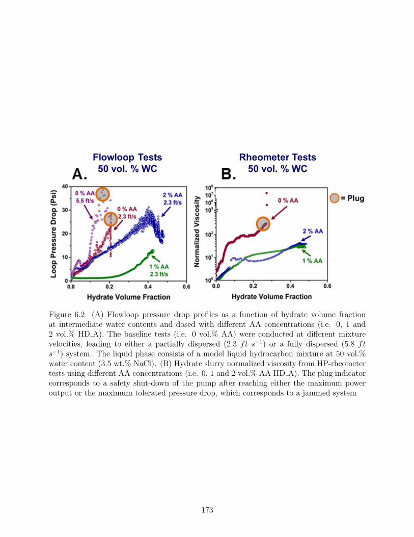
Figure 6.2 (A) Flowloop pressure drop profiles as a function of hydrate volume fractionat intermediate water contents and dosed with different AA concentrations (i.e. 0, 1 and2 vol.% HD A). The baseline tests (i.e. 0 vol.% AA) were conducted at different mixturevelocities, leading to either a partially dispersed (2.3 ft s−1) or a fully dispersed (5.8 fts−1) system. The liquid phase consists of a model liquid hydrocarbon mixture at 50 vol.%water content (3.5 wt.% NaCl). (B) Hydrate slurry normalized viscosity from HP-rheometertests using different AA concentrations (i.e. 0, 1 and 2 vol.% AA HD A). The plug indicatorcorresponds to a safety shut-down of the pump after reaching either the maximum poweroutput or the maximum tolerated pressure drop, which corresponds to a jammed system

173

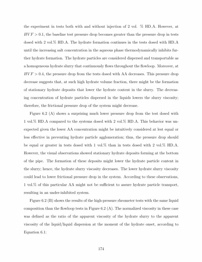
the experiment in tests both with and without injection of 2 vol. % HD A. However, at

HV F > 0.1, the baseline test pressure drop becomes greater than the pressure drop in tests

dosed with 2 vol.% HD A. The hydrate formation continues in the tests dosed with HD A

until the increasing salt concentration in the aqueous phase thermodynamically inhibits fur-

ther hydrate formation. The hydrate particles are considered dispersed and transportable as

a homogeneous hydrate slurry that continuously flows throughout the flowloop. Moreover, at

HV F > 0.4, the pressure drop from the tests dosed with AA decreases. This pressure drop

decrease suggests that, at such high hydrate volume fraction, there might be the formation

of stationary hydrate deposits that lower the hydrate content in the slurry. The decreas-

ing concentration of hydrate particles dispersed in the liquids lowers the slurry viscosity;

therefore, the frictional pressure drop of the system might decrease.

Figure 6.2 (A) shows a surprising much lower pressure drop from the test dosed with

1 vol.% HD A compared to the systems dosed with 2 vol.% HD A. This behavior was un-

expected given the lower AA concentration might be intuitively considered at lest equal or

less effective in preventing hydrate particle agglomeration; thus, the pressure drop should

be equal or greater in tests dosed with 1 vol.% than in tests dosed with 2 vol.% HD A.

However, the visual observations showed stationary hydrate deposits forming at the bottom

of the pipe. The formation of these deposits might lower the hydrate particle content in

the slurry; hence, the hydrate slurry viscosity decreases. The lower hydrate slurry viscosity

could lead to lower frictional pressure drop in the system. According to these observations,

1 vol.% of this particular AA might not be sufficient to assure hydrate particle transport,

resulting in an under-inhibited system.

Figure 6.2 (B) shows the results of the high-pressure rheometer tests with the same liquid

composition than the flowloop tests in Figure 6.2 (A). The normalized viscosity in these case

was defined as the ratio of the apparent viscosity of the hydrate slurry to the apparent

viscosity of the liquid/liquid dispersion at the moment of the hydrate onset, according to

Equation 6.1:

174

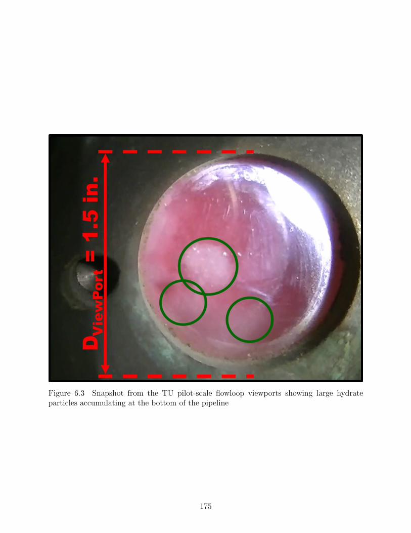
Figure 6.3 Snapshot from the TU pilot-scale flowloop viewports showing large hydrateparticles accumulating at the bottom of the pipeline

175

ηNormalized =ηApparentHydrateSlurry

(t)

ηApparent@HydrateOnset

(6.1)

The normalized viscosity profiles from the high-pressure rheometer tests in Figure 6.2

(B) shows qualitative agreement with the pressure drop profiles from flowloop tests in Fig-

ure 6.2 (A) corresponding to the baseline tests (i.e. 50 vol.% water content and 0 vol.%

AA). The baseline tests in both experimental setups resulted in safety shut-downs due to

excessive energy input requirements to maintain flow (i.e. very high viscosity); hence, water

conversion was not complete. On the other hand, the experiments with AA injection allows

the maximum possible conversion of water into hydrates without showing such a high in-

crease neither in the normalized viscosity nor in the pressure drop of the system. However,

HP-rheometer experiments dosed with either 1 or 2 vol.% HD A resulted in similar normal-

ized slurry viscosity profiles as a function of the hydrate volume fraction. This rheological

behavior contradicts the pressure drop results from pilot-scale flowloop tests showing a much

lower pressure drop in systems dosed with 1 vol.% HD A when compared to system dosed

with 2 vol.% HD A. The HP-rheometer tests are conducted at a high mixing velocity (477

RPM) leading to an apparent shear rate ∼ 675 s−1, according to the experimental procedure

from previous hydrate slurry rheological studies conducted at CHR [241]. The differences

in the flow patterns and the shear rate between the flowloop and the rheometer geometries,

in addition to the small gap in the HP-rheometer cell, might prevent phenomena such a

hydrate deposition on the walls during the HP-rheometer tests and mask the influence of

AA concentration on the hydrate slurry transportability. Nevertheless, these observations

are in contrast with all results obtained from every other experimental equipment discussed

in Chapters 2 & 3 and could represent an artifact. The high cost associated with pilot-scale

flowloop tests prevents the possibility of conducting an experimental repeat to confirm the

observations from this single test.

Finally, it is worth noting that the viscosity before the hydrate onset from the rheological

studies at 50 vol.% water content dosed with either 1 or 2 vol.% AA HD A was similar to those

176

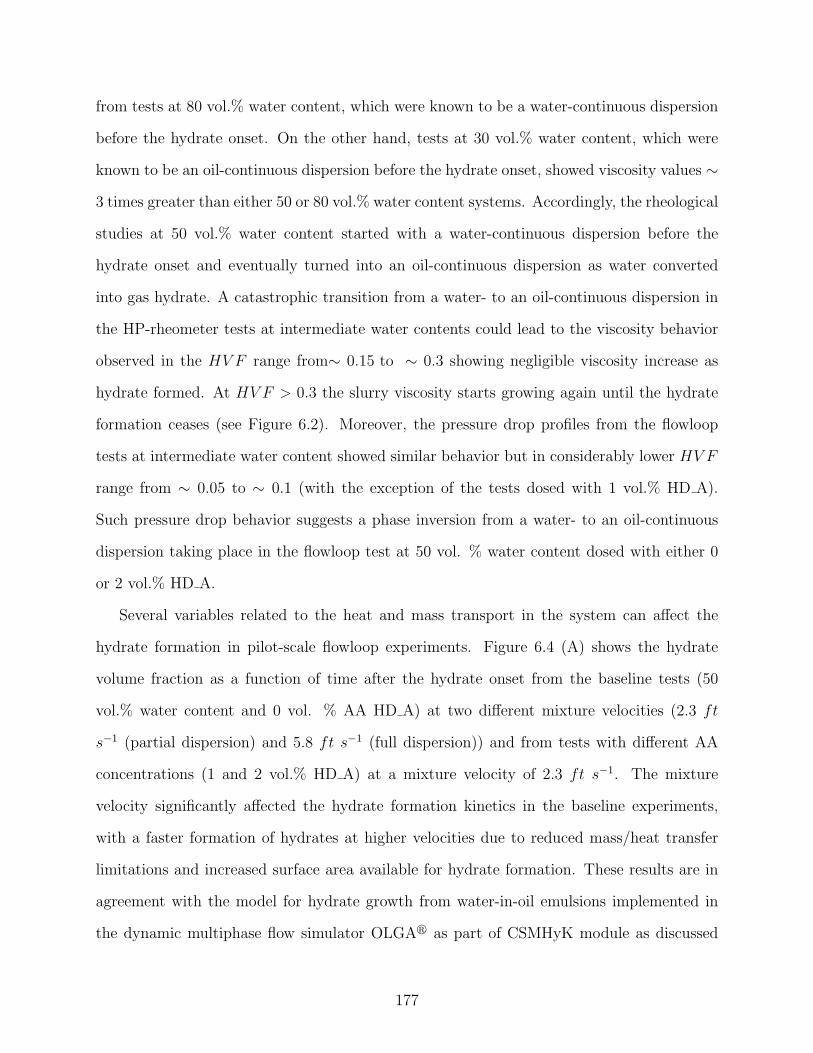
from tests at 80 vol.% water content, which were known to be a water-continuous dispersion

before the hydrate onset. On the other hand, tests at 30 vol.% water content, which were

known to be an oil-continuous dispersion before the hydrate onset, showed viscosity values ∼

3 times greater than either 50 or 80 vol.% water content systems. Accordingly, the rheological

studies at 50 vol.% water content started with a water-continuous dispersion before the

hydrate onset and eventually turned into an oil-continuous dispersion as water converted

into gas hydrate. A catastrophic transition from a water- to an oil-continuous dispersion in

the HP-rheometer tests at intermediate water contents could lead to the viscosity behavior

observed in the HV F range from∼ 0.15 to ∼ 0.3 showing negligible viscosity increase as

hydrate formed. At HV F > 0.3 the slurry viscosity starts growing again until the hydrate

formation ceases (see Figure 6.2). Moreover, the pressure drop profiles from the flowloop

tests at intermediate water content showed similar behavior but in considerably lower HV F

range from ∼ 0.05 to ∼ 0.1 (with the exception of the tests dosed with 1 vol.% HD A).

Such pressure drop behavior suggests a phase inversion from a water- to an oil-continuous

dispersion taking place in the flowloop test at 50 vol. % water content dosed with either 0

or 2 vol.% HD A.

Several variables related to the heat and mass transport in the system can affect the

hydrate formation in pilot-scale flowloop experiments. Figure 6.4 (A) shows the hydrate

volume fraction as a function of time after the hydrate onset from the baseline tests (50

vol.% water content and 0 vol. % AA HD A) at two different mixture velocities (2.3 ft

s−1 (partial dispersion) and 5.8 ft s−1 (full dispersion)) and from tests with different AA

concentrations (1 and 2 vol.% HD A) at a mixture velocity of 2.3 ft s−1. The mixture

velocity significantly affected the hydrate formation kinetics in the baseline experiments,

with a faster formation of hydrates at higher velocities due to reduced mass/heat transfer

limitations and increased surface area available for hydrate formation. These results are in

agreement with the model for hydrate growth from water-in-oil emulsions implemented in

the dynamic multiphase flow simulator OLGAr as part of CSMHyK module as discussed

177

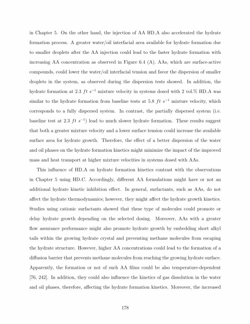
in Chapter 5. On the other hand, the injection of AA HD A also accelerated the hydrate

formation process. A greater water/oil interfacial area available for hydrate formation due

to smaller droplets after the AA injection could lead to the faster hydrate formation with

increasing AA concentration as observed in Figure 6.4 (A). AAs, which are surface-active

compounds, could lower the water/oil interfacial tension and favor the dispersion of smaller

droplets in the system, as observed during the dispersion tests showed. In addition, the

hydrate formation at 2.3 ft s−1 mixture velocity in systems dosed with 2 vol.% HD A was

similar to the hydrate formation from baseline tests at 5.8 ft s−1 mixture velocity, which

corresponds to a fully dispersed system. In contrast, the partially dispersed system (i.e.

baseline test at 2.3 ft s−1) lead to much slower hydrate formation. These results suggest

that both a greater mixture velocity and a lower surface tension could increase the available

surface area for hydrate growth. Therefore, the effect of a better dispersion of the water

and oil phases on the hydrate formation kinetics might minimize the impact of the improved

mass and heat transport at higher mixture velocities in systems dosed with AAs.

This influence of HD A on hydrate formation kinetics contrast with the observations

in Chapter 5 using HD C. Accordingly, different AA formulations might have or not an

additional hydrate kinetic inhibition effect. In general, surfactants, such as AAs, do not

affect the hydrate thermodynamics; however, they might affect the hydrate growth kinetics.

Studies using cationic surfactants showed that these type of molecules could promote or

delay hydrate growth depending on the selected dosing. Moreover, AAs with a greater

flow assurance performance might also promote hydrate growth by embedding short alkyl

tails within the growing hydrate crystal and preventing methane molecules from escaping

the hydrate structure. However, higher AA concentrations could lead to the formation of a

diffusion barrier that prevents methane molecules from reaching the growing hydrate surface.

Apparently, the formation or not of such AA films could be also temperature-dependent

[76, 242]. In addition, they could also influence the kinetics of gas dissolution in the water

and oil phases, therefore, affecting the hydrate formation kinetics. Moreover, the increased

178

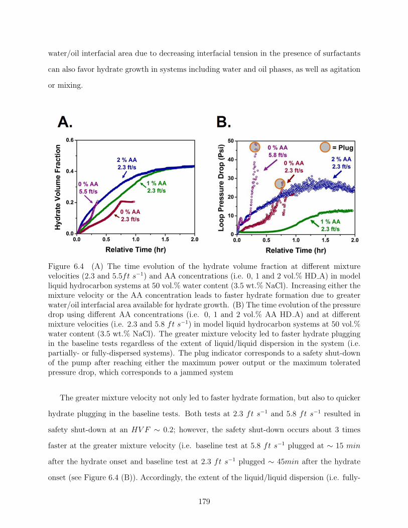
water/oil interfacial area due to decreasing interfacial tension in the presence of surfactants

can also favor hydrate growth in systems including water and oil phases, as well as agitation

or mixing.

Figure 6.4 (A) The time evolution of the hydrate volume fraction at different mixturevelocities (2.3 and 5.5ft s−1) and AA concentrations (i.e. 0, 1 and 2 vol.% HD A) in modelliquid hydrocarbon systems at 50 vol.% water content (3.5 wt.% NaCl). Increasing either themixture velocity or the AA concentration leads to faster hydrate formation due to greaterwater/oil interfacial area available for hydrate growth. (B) The time evolution of the pressuredrop using different AA concentrations (i.e. 0, 1 and 2 vol.% AA HD A) and at differentmixture velocities (i.e. 2.3 and 5.8 ft s−1) in model liquid hydrocarbon systems at 50 vol.%water content (3.5 wt.% NaCl). The greater mixture velocity led to faster hydrate pluggingin the baseline tests regardless of the extent of liquid/liquid dispersion in the system (i.e.partially- or fully-dispersed systems). The plug indicator corresponds to a safety shut-downof the pump after reaching either the maximum power output or the maximum toleratedpressure drop, which corresponds to a jammed system

The greater mixture velocity not only led to faster hydrate formation, but also to quicker

hydrate plugging in the baseline tests. Both tests at 2.3 ft s−1 and 5.8 ft s−1 resulted in

safety shut-down at an HV F ∼ 0.2; however, the safety shut-down occurs about 3 times

faster at the greater mixture velocity (i.e. baseline test at 5.8 ft s−1 plugged at ∼ 15 min

after the hydrate onset and baseline test at 2.3 ft s−1 plugged ∼ 45min after the hydrate

onset (see Figure 6.4 (B)). Accordingly, the extent of the liquid/liquid dispersion (i.e. fully-

179

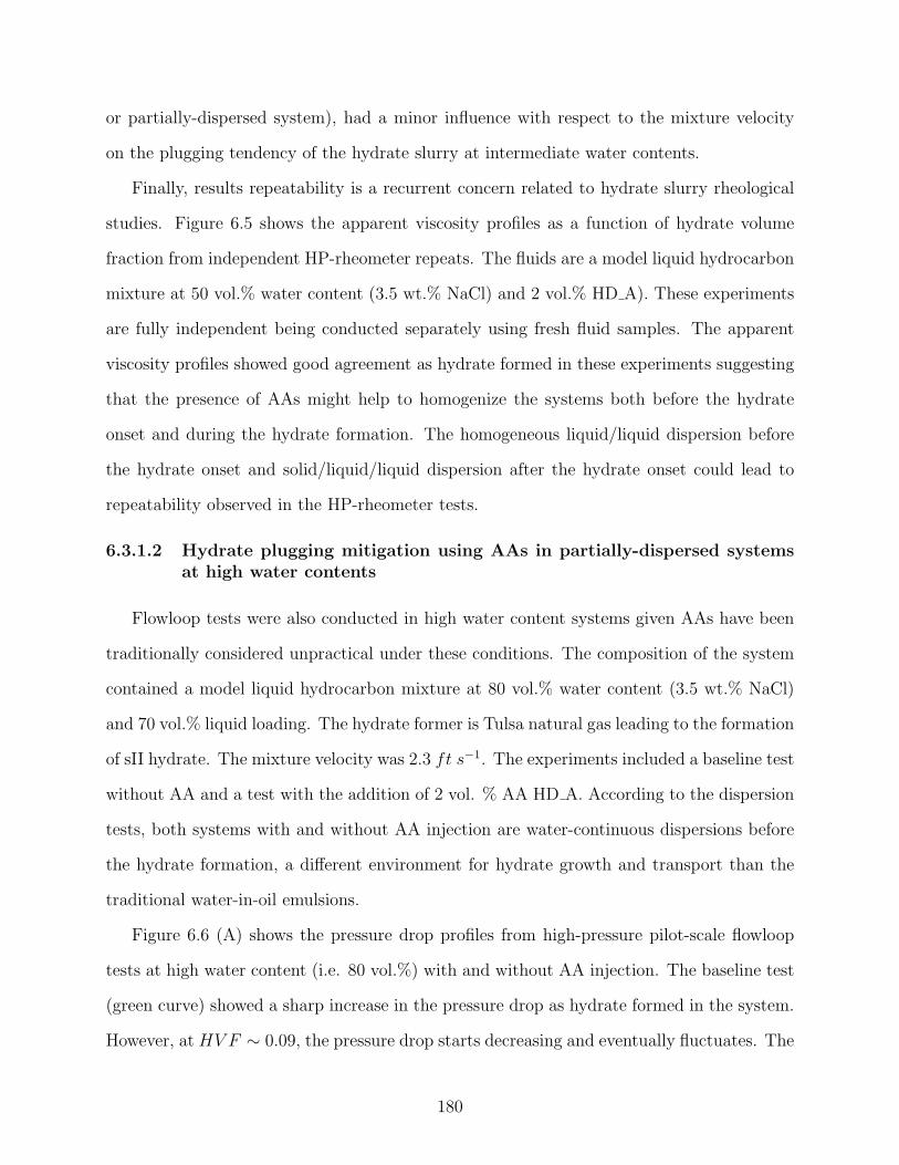
or partially-dispersed system), had a minor influence with respect to the mixture velocity

on the plugging tendency of the hydrate slurry at intermediate water contents.

Finally, results repeatability is a recurrent concern related to hydrate slurry rheological

studies. Figure 6.5 shows the apparent viscosity profiles as a function of hydrate volume

fraction from independent HP-rheometer repeats. The fluids are a model liquid hydrocarbon

mixture at 50 vol.% water content (3.5 wt.% NaCl) and 2 vol.% HD A). These experiments

are fully independent being conducted separately using fresh fluid samples. The apparent

viscosity profiles showed good agreement as hydrate formed in these experiments suggesting

that the presence of AAs might help to homogenize the systems both before the hydrate

onset and during the hydrate formation. The homogeneous liquid/liquid dispersion before

the hydrate onset and solid/liquid/liquid dispersion after the hydrate onset could lead to

repeatability observed in the HP-rheometer tests.

6.3.1.2 Hydrate plugging mitigation using AAs in partially-dispersed systemsat high water contents

Flowloop tests were also conducted in high water content systems given AAs have been

traditionally considered unpractical under these conditions. The composition of the system

contained a model liquid hydrocarbon mixture at 80 vol.% water content (3.5 wt.% NaCl)

and 70 vol.% liquid loading. The hydrate former is Tulsa natural gas leading to the formation

of sII hydrate. The mixture velocity was 2.3 ft s−1. The experiments included a baseline test

without AA and a test with the addition of 2 vol. % AA HD A. According to the dispersion

tests, both systems with and without AA injection are water-continuous dispersions before

the hydrate formation, a different environment for hydrate growth and transport than the

traditional water-in-oil emulsions.

Figure 6.6 (A) shows the pressure drop profiles from high-pressure pilot-scale flowloop

tests at high water content (i.e. 80 vol.%) with and without AA injection. The baseline test

(green curve) showed a sharp increase in the pressure drop as hydrate formed in the system.

However, at HV F ∼ 0.09, the pressure drop starts decreasing and eventually fluctuates. The

180

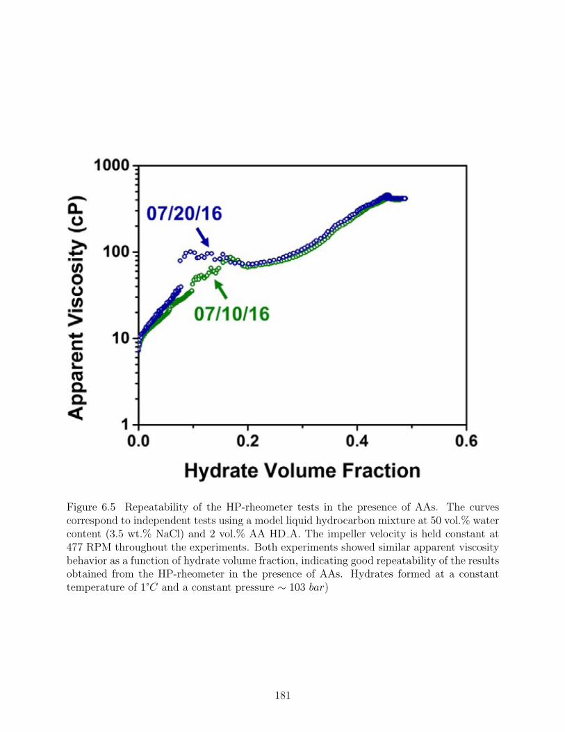
Figure 6.5 Repeatability of the HP-rheometer tests in the presence of AAs. The curvescorrespond to independent tests using a model liquid hydrocarbon mixture at 50 vol.% watercontent (3.5 wt.% NaCl) and 2 vol.% AA HD A. The impeller velocity is held constant at477 RPM throughout the experiments. Both experiments showed similar apparent viscositybehavior as a function of hydrate volume fraction, indicating good repeatability of the resultsobtained from the HP-rheometer in the presence of AAs. Hydrates formed at a constanttemperature of 1°C and a constant pressure ∼ 103 bar)

181

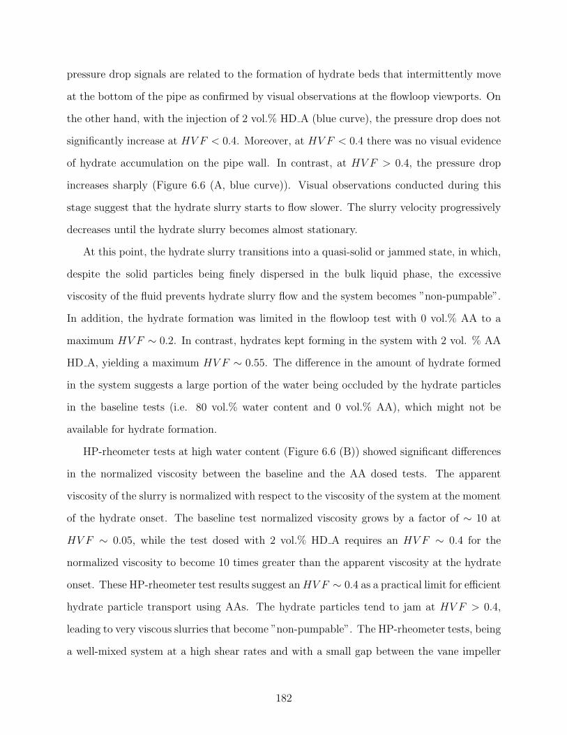
pressure drop signals are related to the formation of hydrate beds that intermittently move

at the bottom of the pipe as confirmed by visual observations at the flowloop viewports. On

the other hand, with the injection of 2 vol.% HD A (blue curve), the pressure drop does not

significantly increase at HV F < 0.4. Moreover, at HV F < 0.4 there was no visual evidence

of hydrate accumulation on the pipe wall. In contrast, at HV F > 0.4, the pressure drop

increases sharply (Figure 6.6 (A, blue curve)). Visual observations conducted during this

stage suggest that the hydrate slurry starts to flow slower. The slurry velocity progressively

decreases until the hydrate slurry becomes almost stationary.

At this point, the hydrate slurry transitions into a quasi-solid or jammed state, in which,

despite the solid particles being finely dispersed in the bulk liquid phase, the excessive

viscosity of the fluid prevents hydrate slurry flow and the system becomes ”non-pumpable”.

In addition, the hydrate formation was limited in the flowloop test with 0 vol.% AA to a

maximum HV F ∼ 0.2. In contrast, hydrates kept forming in the system with 2 vol. % AA

HD A, yielding a maximum HV F ∼ 0.55. The difference in the amount of hydrate formed

in the system suggests a large portion of the water being occluded by the hydrate particles

in the baseline tests (i.e. 80 vol.% water content and 0 vol.% AA), which might not be

available for hydrate formation.

HP-rheometer tests at high water content (Figure 6.6 (B)) showed significant differences

in the normalized viscosity between the baseline and the AA dosed tests. The apparent

viscosity of the slurry is normalized with respect to the viscosity of the system at the moment

of the hydrate onset. The baseline test normalized viscosity grows by a factor of ∼ 10 at

HV F ∼ 0.05, while the test dosed with 2 vol.% HD A requires an HV F ∼ 0.4 for the

normalized viscosity to become 10 times greater than the apparent viscosity at the hydrate

onset. These HP-rheometer test results suggest anHV F ∼ 0.4 as a practical limit for efficient

hydrate particle transport using AAs. The hydrate particles tend to jam at HV F > 0.4,

leading to very viscous slurries that become ”non-pumpable”. The HP-rheometer tests, being

a well-mixed system at a high shear rates and with a small gap between the vane impeller

182

Figure 6.6 (A) Pressure drop profile from pilot-scale flowloop tests using a model liquidhydrocarbon mixture systems at high water content (i.e. 80 vol.%), with 0 and 2 vol.%AA HD A. (B) Normalized viscosity profile from HP-rheometer tests using a model liquidhydrocarbon mixture systems at high water content (80 vol.%), with 0 and 2 vol.% AAHD A. These plots depict two different types of hydrate plugs. The flowloop baseline test(green curve in (A)) plugged as the hydrate particles settled at the bottom of the pipe andstopped flowing. On the other hand, the tests with AA injection (blue curve in (A)) pluggedgiven a safety shut-down occurred after the flowloop pressure drop threshold was exceeded.The HP-rheometer baseline test (green curve in (B)) plugged as the maximum allowed torquewas reached

183

and the cup walls, could mask hydrate accumulation phenomena, such as wall deposition,

which might cause the pressure drop behavior observed in the flowloop tests without AA

injection (green curve in Figure 6.6 (A)).

6.3.1.3 The influence of the water content on the hydrate slurry viscosity andthe hydrate particle transportability using AAs

The pilot-scale flowloop tests in this section covered a range of water content from 30 to

80 vol.%. This range of water content provides relevant rheological data related to the con-

tribution of the hydrate particles to the slurry rheological properties in systems that can be

either oil-continuous, water-continuous, or near the dispersion phase-inversion region. Fig-

ure 6.7 combines results from pilot-scale flowloop tests (A) and HP-rheometer experiments

(B) from systems at 30, 50 and 80 vol.% water content and 2 vol.% HD A. Figure 6.7 (A)

shows greater relative pressure drop values in the pilot-scale flowloop tests at the intermedi-

ate water content (i.e. 50 vol.%) than in both the extreme cases (i.e. 30 vol.% (oil-continuous

dispersion) and 80 vol.% (water-continuous dispersion)), at any given hydrate volume frac-

tion < 0.4. Similarly, the HP-rheometer test results (Figure 6.7 (B)) showed a greater initial

increase in the normalized viscosity for the system at intermediate water content. The nor-

malized hydrate slurry viscosity at HV F ∼ 0.1 is about 5 times greater at the intermediate

water content than in either the high or the low water content systems.

Moreover, the rheometer results (Figure 6.7 (B)) showed that the evolution of the hydrate

slurry normalized viscosity during the hydrate formation was different for the oil-continuous

(i.e. 30 vol.% water content) and the water-continuous systems (i.e. 80 vol.% water con-

tent) dosed with AAs. The oil-continuous system showed a sharp increase in the normalized

viscosity right after the hydrate onset and a mild gradual growth afterward. The gas re-

saturation after the initial gas depletion at the hydrate onset might have significant effects

in oil-continuous systems with a high gas solubility in the continuous phase of the disper-

sion. On the other hand, the water-continuous system showed a different behavior with the

hydrate slurry normalized viscosity gradually increasing as hydrate formed in the system,

184

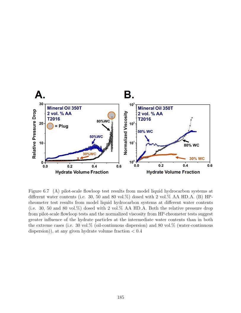
Figure 6.7 (A) pilot-scale flowloop test results from model liquid hydrocarbon systems atdifferent water contents (i.e. 30, 50 and 80 vol.%) dosed with 2 vol.% AA HD A. (B) HP-rheometer test results from model liquid hydrocarbon systems at different water contents(i.e. 30, 50 and 80 vol.%) dosed with 2 vol.% AA HD A. Both the relative pressure dropfrom pilot-scale flowloop tests and the normalized viscosity from HP-rheometer tests suggestgreater influence of the hydrate particles at the intermediate water contents than in boththe extreme cases (i.e. 30 vol.% (oil-continuous dispersion) and 80 vol.% (water-continuousdispersion)), at any given hydrate volume fraction < 0.4

185

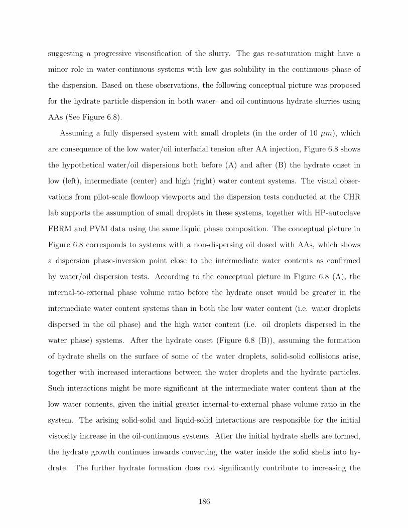
suggesting a progressive viscosification of the slurry. The gas re-saturation might have a

minor role in water-continuous systems with low gas solubility in the continuous phase of

the dispersion. Based on these observations, the following conceptual picture was proposed

for the hydrate particle dispersion in both water- and oil-continuous hydrate slurries using

AAs (See Figure 6.8).

Assuming a fully dispersed system with small droplets (in the order of 10 µm), which

are consequence of the low water/oil interfacial tension after AA injection, Figure 6.8 shows

the hypothetical water/oil dispersions both before (A) and after (B) the hydrate onset in

low (left), intermediate (center) and high (right) water content systems. The visual obser-

vations from pilot-scale flowloop viewports and the dispersion tests conducted at the CHR

lab supports the assumption of small droplets in these systems, together with HP-autoclave

FBRM and PVM data using the same liquid phase composition. The conceptual picture in

Figure 6.8 corresponds to systems with a non-dispersing oil dosed with AAs, which shows

a dispersion phase-inversion point close to the intermediate water contents as confirmed

by water/oil dispersion tests. According to the conceptual picture in Figure 6.8 (A), the

internal-to-external phase volume ratio before the hydrate onset would be greater in the

intermediate water content systems than in both the low water content (i.e. water droplets

dispersed in the oil phase) and the high water content (i.e. oil droplets dispersed in the

water phase) systems. After the hydrate onset (Figure 6.8 (B)), assuming the formation

of hydrate shells on the surface of some of the water droplets, solid-solid collisions arise,

together with increased interactions between the water droplets and the hydrate particles.

Such interactions might be more significant at the intermediate water content than at the

low water contents, given the initial greater internal-to-external phase volume ratio in the

system. The arising solid-solid and liquid-solid interactions are responsible for the initial

viscosity increase in the oil-continuous systems. After the initial hydrate shells are formed,

the hydrate growth continues inwards converting the water inside the solid shells into hy-

drate. The further hydrate formation does not significantly contribute to increasing the

186

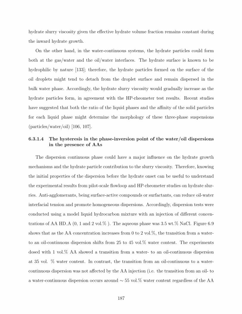
hydrate slurry viscosity given the effective hydrate volume fraction remains constant during

the inward hydrate growth.

On the other hand, in the water-continuous systems, the hydrate particles could form

both at the gas/water and the oil/water interfaces. The hydrate surface is known to be

hydrophilic by nature [133]; therefore, the hydrate particles formed on the surface of the

oil droplets might tend to detach from the droplet surface and remain dispersed in the

bulk water phase. Accordingly, the hydrate slurry viscosity would gradually increase as the

hydrate particles form, in agreement with the HP-rheometer test results. Recent studies

have suggested that both the ratio of the liquid phases and the affinity of the solid particles

for each liquid phase might determine the morphology of these three-phase suspensions

(particles/water/oil) [106, 107].

6.3.1.4 The hysteresis in the phase-inversion point of the water/oil dispersionsin the presence of AAs

The dispersion continuous phase could have a major influence on the hydrate growth

mechanisms and the hydrate particle contribution to the slurry viscosity. Therefore, knowing

the initial properties of the dispersion before the hydrate onset can be useful to understand

the experimental results from pilot-scale flowloop and HP-rheometer studies on hydrate slur-

ries. Anti-agglomerants, being surface-active compounds or surfactants, can reduce oil-water

interfacial tension and promote homogeneous dispersions. Accordingly, dispersion tests were

conducted using a model liquid hydrocarbon mixture with an injection of different concen-

trations of AA HD A (0, 1 and 2 vol.% ). The aqueous phase was 3.5 wt.% NaCl. Figure 6.9

shows that as the AA concentration increases from 0 to 2 vol.%, the transition from a water-

to an oil-continuous dispersion shifts from 25 to 45 vol.% water content. The experiments

dosed with 1 vol.% AA showed a transition from a water- to an oil-continuous dispersion

at 35 vol. % water content. In contrast, the transition from an oil-continuous to a water-

continuous dispersion was not affected by the AA injection (i.e. the transition from an oil- to

a water-continuous dispersion occurs around ∼ 55 vol.% water content regardless of the AA

187

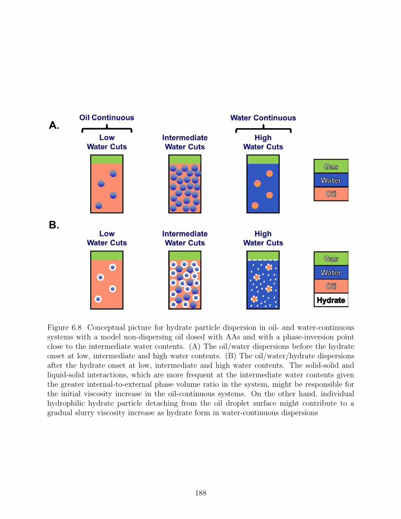
Figure 6.8 Conceptual picture for hydrate particle dispersion in oil- and water-continuoussystems with a model non-dispersing oil dosed with AAs and with a phase-inversion pointclose to the intermediate water contents. (A) The oil/water dispersions before the hydrateonset at low, intermediate and high water contents. (B) The oil/water/hydrate dispersionsafter the hydrate onset at low, intermediate and high water contents. The solid-solid andliquid-solid interactions, which are more frequent at the intermediate water contents giventhe greater internal-to-external phase volume ratio in the system, might be responsible forthe initial viscosity increase in the oil-continuous systems. On the other hand, individualhydrophilic hydrate particle detaching from the oil droplet surface might contribute to agradual slurry viscosity increase as hydrate form in water-continuous dispersions

188

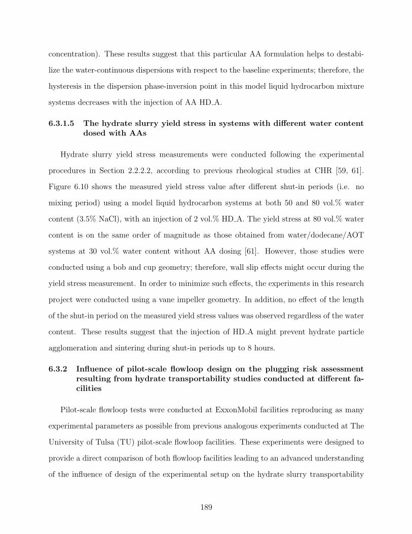
concentration). These results suggest that this particular AA formulation helps to destabi-

lize the water-continuous dispersions with respect to the baseline experiments; therefore, the

hysteresis in the dispersion phase-inversion point in this model liquid hydrocarbon mixture

systems decreases with the injection of AA HD A.

6.3.1.5 The hydrate slurry yield stress in systems with different water contentdosed with AAs

Hydrate slurry yield stress measurements were conducted following the experimental

procedures in Section 2.2.2.2, according to previous rheological studies at CHR [59, 61].

Figure 6.10 shows the measured yield stress value after different shut-in periods (i.e. no

mixing period) using a model liquid hydrocarbon systems at both 50 and 80 vol.% water

content (3.5% NaCl), with an injection of 2 vol.% HD A. The yield stress at 80 vol.% water

content is on the same order of magnitude as those obtained from water/dodecane/AOT

systems at 30 vol.% water content without AA dosing [61]. However, those studies were

conducted using a bob and cup geometry; therefore, wall slip effects might occur during the

yield stress measurement. In order to minimize such effects, the experiments in this research

project were conducted using a vane impeller geometry. In addition, no effect of the length

of the shut-in period on the measured yield stress values was observed regardless of the water

content. These results suggest that the injection of HD A might prevent hydrate particle

agglomeration and sintering during shut-in periods up to 8 hours.

6.3.2 Influence of pilot-scale flowloop design on the plugging risk assessmentresulting from hydrate transportability studies conducted at different fa-cilities

Pilot-scale flowloop tests were conducted at ExxonMobil facilities reproducing as many

experimental parameters as possible from previous analogous experiments conducted at The

University of Tulsa (TU) pilot-scale flowloop facilities. These experiments were designed to

provide a direct comparison of both flowloop facilities leading to an advanced understanding

of the influence of design of the experimental setup on the hydrate slurry transportability

189

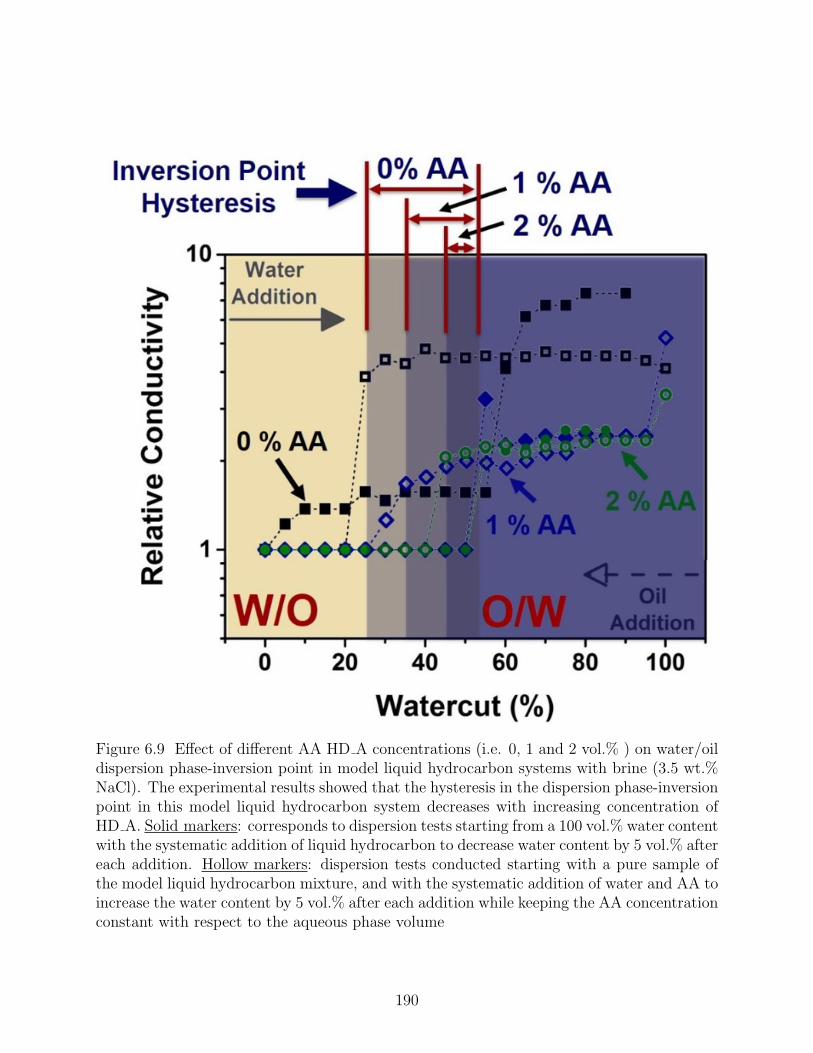
Figure 6.9 Effect of different AA HD A concentrations (i.e. 0, 1 and 2 vol.% ) on water/oildispersion phase-inversion point in model liquid hydrocarbon systems with brine (3.5 wt.%NaCl). The experimental results showed that the hysteresis in the dispersion phase-inversionpoint in this model liquid hydrocarbon system decreases with increasing concentration ofHD A. Solid markers: corresponds to dispersion tests starting from a 100 vol.% water contentwith the systematic addition of liquid hydrocarbon to decrease water content by 5 vol.% aftereach addition. Hollow markers: dispersion tests conducted starting with a pure sample ofthe model liquid hydrocarbon mixture, and with the systematic addition of water and AA toincrease the water content by 5 vol.% after each addition while keeping the AA concentrationconstant with respect to the aqueous phase volume

190

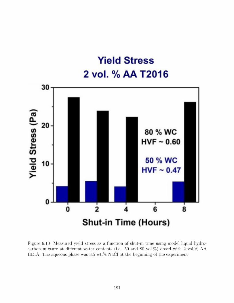
Figure 6.10 Measured yield stress as a function of shut-in time using model liquid hydro-carbon mixture at different water contents (i.e. 50 and 80 vol.%) dosed with 2 vol.% AAHD A. The aqueous phase was 3.5 wt.% NaCl at the beginning of the experiment

191

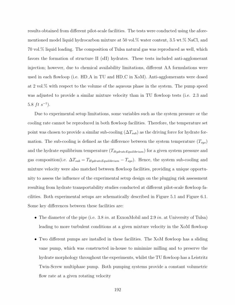
results obtained from different pilot-scale facilities. The tests were conducted using the afore-

mentioned model liquid hydrocarbon mixture at 50 vol.% water content, 3.5 wt.% NaCl, and

70 vol.% liquid loading. The composition of Tulsa natural gas was reproduced as well, which

favors the formation of structure II (sII) hydrates. These tests included anti-agglomerant

injection; however, due to chemical availability limitations, different AA formulations were

used in each flowloop (i.e. HD A in TU and HD C in XoM). Anti-agglomerants were dosed

at 2 vol.% with respect to the volume of the aqueous phase in the system. The pump speed

was adjusted to provide a similar mixture velocity than in TU flowloop tests (i.e. 2.3 and

5.8 ft s−1).

Due to experimental setup limitations, some variables such as the system pressure or the

cooling rate cannot be reproduced in both flowloop facilities. Therefore, the temperature set

point was chosen to provide a similar sub-cooling (∆Tsub) as the driving force for hydrate for-

mation. The sub-cooling is defined as the difference between the system temperature (Tsys)

and the hydrate equilibrium temperature (THydrateEquilibrium) for a given system pressure and

gas composition(i.e. ∆Tsub = THydrateEquilibrium − Tsys). Hence, the system sub-cooling and

mixture velocity were also matched between flowloop facilities, providing a unique opportu-

nity to assess the influence of the experimental setup design on the plugging risk assessment

resulting from hydrate transportability studies conducted at different pilot-scale flowloop fa-

cilities. Both experimental setups are schematically described in Figure 5.1 and Figure 6.1.

Some key differences between these facilities are:

• The diameter of the pipe (i.e. 3.8 in. at ExxonMobil and 2.9 in. at University of Tulsa)

leading to more turbulent conditions at a given mixture velocity in the XoM flowloop

• Two different pumps are installed in these facilities. The XoM flowloop has a sliding

vane pump, which was constructed in-house to minimize milling and to preserve the

hydrate morphology throughout the experiments, whilst the TU flowloop has a Leistritz

Twin-Screw multiphase pump. Both pumping systems provide a constant volumetric

flow rate at a given rotating velocity

192

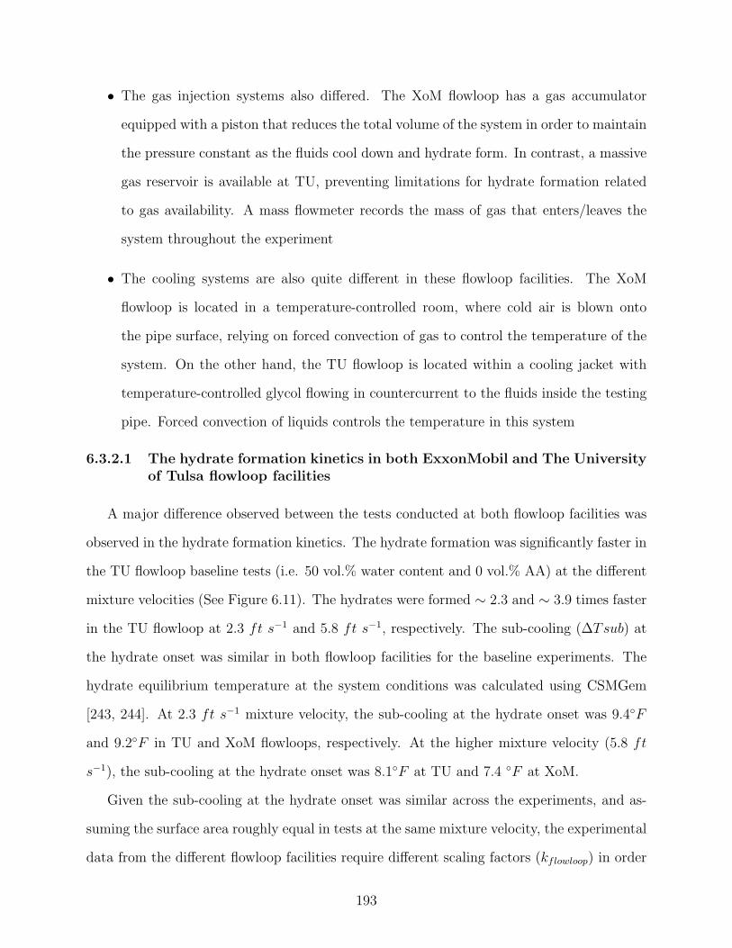
• The gas injection systems also differed. The XoM flowloop has a gas accumulator

equipped with a piston that reduces the total volume of the system in order to maintain

the pressure constant as the fluids cool down and hydrate form. In contrast, a massive

gas reservoir is available at TU, preventing limitations for hydrate formation related

to gas availability. A mass flowmeter records the mass of gas that enters/leaves the

system throughout the experiment

• The cooling systems are also quite different in these flowloop facilities. The XoM

flowloop is located in a temperature-controlled room, where cold air is blown onto

the pipe surface, relying on forced convection of gas to control the temperature of the

system. On the other hand, the TU flowloop is located within a cooling jacket with

temperature-controlled glycol flowing in countercurrent to the fluids inside the testing

pipe. Forced convection of liquids controls the temperature in this system

6.3.2.1 The hydrate formation kinetics in both ExxonMobil and The Universityof Tulsa flowloop facilities

A major difference observed between the tests conducted at both flowloop facilities was

observed in the hydrate formation kinetics. The hydrate formation was significantly faster in

the TU flowloop baseline tests (i.e. 50 vol.% water content and 0 vol.% AA) at the different

mixture velocities (See Figure 6.11). The hydrates were formed ∼ 2.3 and ∼ 3.9 times faster

in the TU flowloop at 2.3 ft s−1 and 5.8 ft s−1, respectively. The sub-cooling (∆Tsub) at

the hydrate onset was similar in both flowloop facilities for the baseline experiments. The

hydrate equilibrium temperature at the system conditions was calculated using CSMGem

[243, 244]. At 2.3 ft s−1 mixture velocity, the sub-cooling at the hydrate onset was 9.4◦F

and 9.2◦F in TU and XoM flowloops, respectively. At the higher mixture velocity (5.8 ft

s−1), the sub-cooling at the hydrate onset was 8.1◦F at TU and 7.4 ◦F at XoM.

Given the sub-cooling at the hydrate onset was similar across the experiments, and as-

suming the surface area roughly equal in tests at the same mixture velocity, the experimental

data from the different flowloop facilities require different scaling factors (kflowloop) in order

193

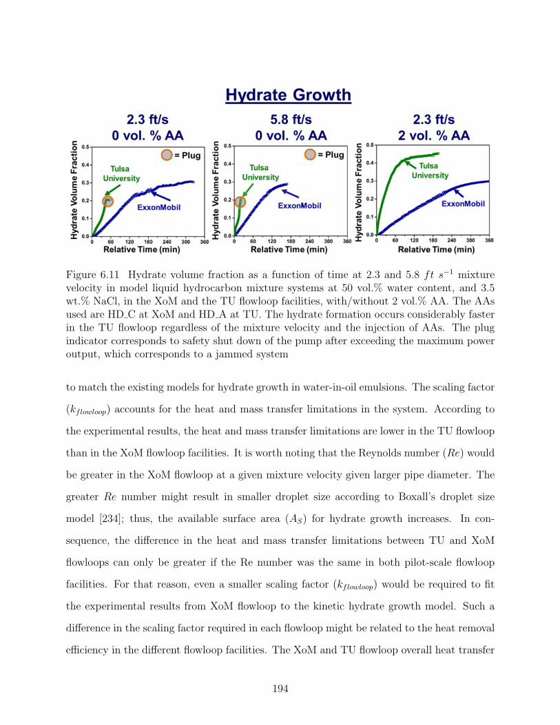
Figure 6.11 Hydrate volume fraction as a function of time at 2.3 and 5.8 ft s−1 mixturevelocity in model liquid hydrocarbon mixture systems at 50 vol.% water content, and 3.5wt.% NaCl, in the XoM and the TU flowloop facilities, with/without 2 vol.% AA. The AAsused are HD C at XoM and HD A at TU. The hydrate formation occurs considerably fasterin the TU flowloop regardless of the mixture velocity and the injection of AAs. The plugindicator corresponds to safety shut down of the pump after exceeding the maximum poweroutput, which corresponds to a jammed system

to match the existing models for hydrate growth in water-in-oil emulsions. The scaling factor

(kflowloop) accounts for the heat and mass transfer limitations in the system. According to

the experimental results, the heat and mass transfer limitations are lower in the TU flowloop

than in the XoM flowloop facilities. It is worth noting that the Reynolds number (Re) would

be greater in the XoM flowloop at a given mixture velocity given larger pipe diameter. The

greater Re number might result in smaller droplet size according to Boxall’s droplet size

model [234]; thus, the available surface area (AS) for hydrate growth increases. In con-

sequence, the difference in the heat and mass transfer limitations between TU and XoM

flowloops can only be greater if the Re number was the same in both pilot-scale flowloop

facilities. For that reason, even a smaller scaling factor (kflowloop) would be required to fit

the experimental results from XoM flowloop to the kinetic hydrate growth model. Such a

difference in the scaling factor required in each flowloop might be related to the heat removal

efficiency in the different flowloop facilities. The XoM and TU flowloop overall heat transfer

194

coefficients (Uoverall) were calculated using the dynamic multiphase flow simulator OLGA®

to match the fluid temperature during the cool-down stage. These coefficients differ by al-

most an order of magnitude between the XoM flowloop (i.e. UoverallXoM= 50 W m−2 K−1)

and TU (i.e. UoverallXoM= 400 W m−2 K−1) flowloop. The contrast in the heat removal ca-

pabilities between the two pilot-scale flowloop setups utilized in these studies might lead to

the disparity in the hydrate growth kinetics at each facility.

Nevertheless, another major difference between these two experimental sets was the sys-

tem pressure at the beginning of hydrate formation. The equilibrium gas concentration in

MO 350T at the different experimental pressures was calculated using the PVT and physical

properties package Multiflashr. The concentration (mol L−1) of methane (CH4), the main

component in the experimental gas mixture, is∼ 34 % lower at 1000 psig than at 1500 psig

in the temperature range from 52°F to 38°F . The lower equilibrium concentration of gas in

the oil phase in the XoM flowloop might cause slower solubilization of gas from the vapor

to the oil phase after the gas is depleted due to the hydrate formation. The driving force

controlling the solubilization of gas from the vapor to the oil phase is the gas concentration

gradient between the bulk oil phase and the gas/oil interface, which is assumed to be at the

equilibrium concentration of gas in the oil phase [245].

The hydrate formation in the baseline tests (50 vol.% water content and 0 vol.% AA)

in Figure 6.11 (Left and Center) leads to plugging in the TU flowloop; hence, the pumping

system shuts down before hydrate formation ceases. The early termination of the experiments

at the TU flowloop leads to the greater final hydrate volume fraction in the baseline tests at

the XoM flowloop facility. On the other hand, the AA injection prevented plugging in both

flowloops (Figure 6.11 (Right)). The lower final hydrate volume fraction in XoM flowloop

corresponds to gas availability limitations. After the volume of the gas accumulator in

XoM flowloop vanishes, hydrates might keep forming until the system pressure reaches the

thermodynamic hydrate equilibrium boundary. In contrast, the larger gas reservoir at TU

flowloop allows the maximum possible conversion of water into hydrate, which stops after

195

the system reaches the thermodynamic hydrate equilibrium boundary due to the increasing

salinity during hydrate formation. The hydrate formation consumes water; therefore, the

salt concentration in the remaining unconverted liquid water increases and shifts the hydrate

thermodynamic equilibrium boundary to greater pressures and lower temperatures.

6.3.2.2 The hydrate particle contribution to the frictional pressure drop in bothExxonMobil and The University of Tulsa flowloop facilities

The hydrate particles not only formed faster in the TU flowloop, but the pressure drop

behavior as hydrate formed in the pipe was also dissimilar between the two flowloop facilities

investigated. In order to make a fair comparison between the flowloop facilities, the fric-

tion factor required to yield the measured experimental pressure drop during the tests was

calculated. The friction factor has been used as a normalization parameter to evaluate the

hydrate transportability in previous flowloop studies [112]. The friction factor for the two

different experimental setups can be extracted using the Darcy-Weisbach equation (Equation

6.2) for pipe flow resistance [246–248],

FrictionFactor =2 ·∆PExperimental · PipeDiameter

P ipeLength · ρm · u2m(6.2)

where ρm and um are the density and the velocity of the mixture respectively, and ∆PExperimental

is the measured experimental pressure drop. Figure 6.12 shows the calculated friction factor

as hydrates form in the pipe in both XoM and TU flowloops. Using 6.2 to calculate the

friction factor in a multiphase system and to compare the two flowloop facilities requires

assuming that the pressure drop corresponding to the gas phase remains roughly constant

throughout the tests (i.e. hydrate formation does not influence the pressure drop of the

gas phase). Therefore, the increase in the frictional pressure drop corresponds only to an

increasing flow resistance due to hydrate formation in the liquid phase.

The baseline experiments (i.e. 50 vol.% water content and 0 vol.% AA) showed similar

friction factors at the low hydrate volume fractions suggesting that hydrate particles are

behaving in a similar way in both flowloop facilities. However, after an HV F ∼ 0.05 for

196

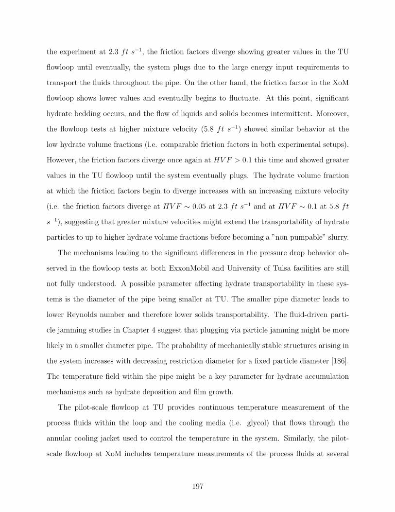
the experiment at 2.3 ft s−1, the friction factors diverge showing greater values in the TU

flowloop until eventually, the system plugs due to the large energy input requirements to

transport the fluids throughout the pipe. On the other hand, the friction factor in the XoM

flowloop shows lower values and eventually begins to fluctuate. At this point, significant

hydrate bedding occurs, and the flow of liquids and solids becomes intermittent. Moreover,

the flowloop tests at higher mixture velocity (5.8 ft s−1) showed similar behavior at the

low hydrate volume fractions (i.e. comparable friction factors in both experimental setups).

However, the friction factors diverge once again at HV F > 0.1 this time and showed greater

values in the TU flowloop until the system eventually plugs. The hydrate volume fraction

at which the friction factors begin to diverge increases with an increasing mixture velocity

(i.e. the friction factors diverge at HV F ∼ 0.05 at 2.3 ft s−1 and at HV F ∼ 0.1 at 5.8 ft

s−1), suggesting that greater mixture velocities might extend the transportability of hydrate

particles to up to higher hydrate volume fractions before becoming a ”non-pumpable” slurry.

The mechanisms leading to the significant differences in the pressure drop behavior ob-

served in the flowloop tests at both ExxonMobil and University of Tulsa facilities are still

not fully understood. A possible parameter affecting hydrate transportability in these sys-

tems is the diameter of the pipe being smaller at TU. The smaller pipe diameter leads to

lower Reynolds number and therefore lower solids transportability. The fluid-driven parti-

cle jamming studies in Chapter 4 suggest that plugging via particle jamming might be more

likely in a smaller diameter pipe. The probability of mechanically stable structures arising in

the system increases with decreasing restriction diameter for a fixed particle diameter [186].

The temperature field within the pipe might be a key parameter for hydrate accumulation

mechanisms such as hydrate deposition and film growth.

The pilot-scale flowloop at TU provides continuous temperature measurement of the

process fluids within the loop and the cooling media (i.e. glycol) that flows through the

annular cooling jacket used to control the temperature in the system. Similarly, the pilot-

scale flowloop at XoM includes temperature measurements of the process fluids at several

197

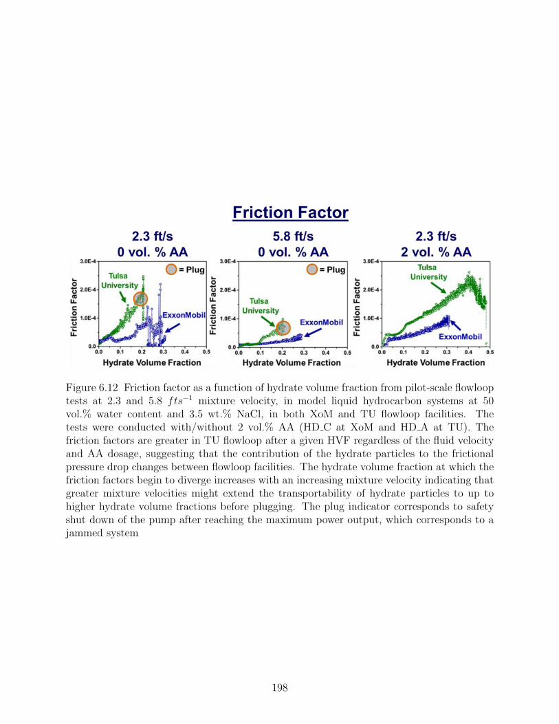
Figure 6.12 Friction factor as a function of hydrate volume fraction from pilot-scale flowlooptests at 2.3 and 5.8 fts−1 mixture velocity, in model liquid hydrocarbon systems at 50vol.% water content and 3.5 wt.% NaCl, in both XoM and TU flowloop facilities. Thetests were conducted with/without 2 vol.% AA (HD C at XoM and HD A at TU). Thefriction factors are greater in TU flowloop after a given HVF regardless of the fluid velocityand AA dosage, suggesting that the contribution of the hydrate particles to the frictionalpressure drop changes between flowloop facilities. The hydrate volume fraction at which thefriction factors begin to diverge increases with an increasing mixture velocity indicating thatgreater mixture velocities might extend the transportability of hydrate particles to up tohigher hydrate volume fractions before plugging. The plug indicator corresponds to safetyshut down of the pump after reaching the maximum power output, which corresponds to ajammed system

198

locations in the pipe throughout the experiments. In addition, the XoM flowloop incor-

porates direct measurement of the pipe outer surface temperature. Figure 6.13 shows the

temperature profiles from both flowloops corresponding to the baseline tests in Figure 6.12.

Figure 6.13 presents in the left ordinate the process fluid temperature and either the cooling

media (TU) or the pipe surface (XoM), while the right ordinate corresponds to the temper-

ature difference between the process fluids and either the cooling media (TU) or the pipe

surface (XoM).

Figure 6.13(left) shows the process fluid temperature closely following the coolant tem-

perature until the hydrate onset in the flowloop tests at TU. The greater fluid velocity, which

favors the heat transfer in the system, leads to the smaller temperature difference between

the process fluids and the coolant. On the other hand, the temperature profiles from XoM

in Figure 6.13 (right) show a lag between the room temperature and the temperature of the

fluids in the loop. The lower overall heat transfer coefficient in the XoM flowloop might

cause a delay in the fluid temperature response to the room temperature. At the hydrate

onset, a temperature peak is noticeable in both systems; however, the temperature increase

due to the exothermic hydrate formation is more significant in the TU flowloop. This is

somehow unexpected given the greater heat removal efficiency in the TU flowloop; yet, the

amount of hydrate formed during this initial stage is considerably greater in the TU flowloop

tests as well (See Figure 6.11), which might lead to the higher temperature rise observed in

Figure 6.13.

Finally, Figure 6.13 shows that the pipe surface temperature at XoM closely follows the

process fluid temperature, suggesting a negligible temperature gradient between the fluid

bulk phase and the walls of the pipe. Such a minimal temperature gradient remains during

and after the hydrate formation. On the other hand, the pipe walls in the TU flowloop,

which are in direct contact with the coolant flowing in the jacket, might be assumed at

the same temperature than the coolant. Accordingly, a temperature gradient within the

pipe might arise, which could drive the hydrate particle accumulation closer to the wall in a

199

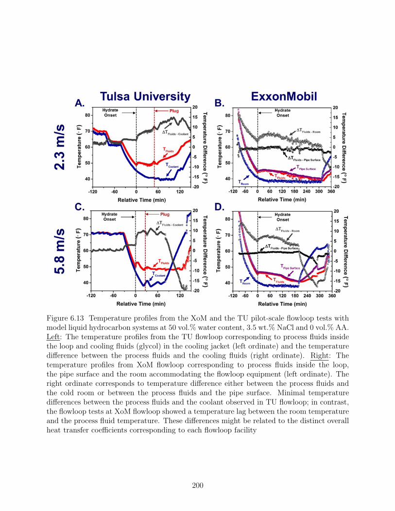
Figure 6.13 Temperature profiles from the XoM and the TU pilot-scale flowloop tests withmodel liquid hydrocarbon systems at 50 vol.% water content, 3.5 wt.% NaCl and 0 vol.% AA.Left: The temperature profiles from the TU flowloop corresponding to process fluids insidethe loop and cooling fluids (glycol) in the cooling jacket (left ordinate) and the temperaturedifference between the process fluids and the cooling fluids (right ordinate). Right: Thetemperature profiles from XoM flowloop corresponding to process fluids inside the loop,the pipe surface and the room accommodating the flowloop equipment (left ordinate). Theright ordinate corresponds to temperature difference either between the process fluids andthe cold room or between the process fluids and the pipe surface. Minimal temperaturedifferences between the process fluids and the coolant observed in TU flowloop; in contrast,the flowloop tests at XoM flowloop showed a temperature lag between the room temperatureand the process fluid temperature. These differences might be related to the distinct overallheat transfer coefficients corresponding to each flowloop facility

200

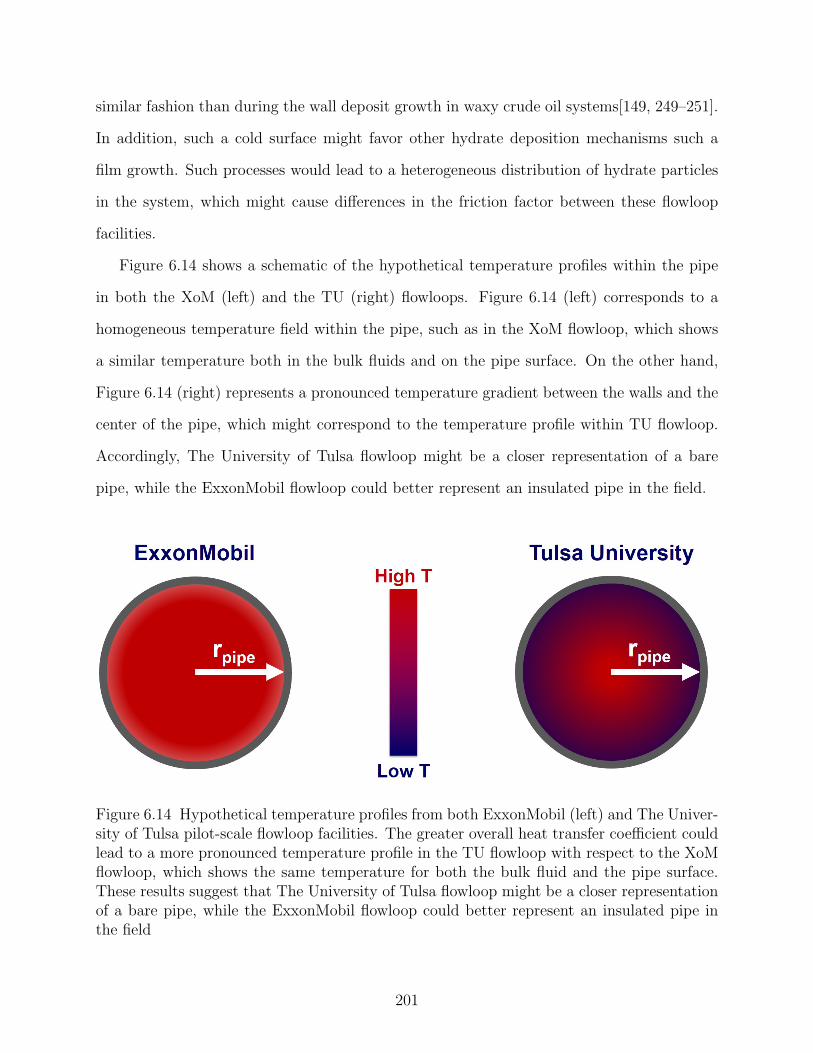
similar fashion than during the wall deposit growth in waxy crude oil systems[149, 249–251].

In addition, such a cold surface might favor other hydrate deposition mechanisms such a

film growth. Such processes would lead to a heterogeneous distribution of hydrate particles

in the system, which might cause differences in the friction factor between these flowloop

facilities.

Figure 6.14 shows a schematic of the hypothetical temperature profiles within the pipe

in both the XoM (left) and the TU (right) flowloops. Figure 6.14 (left) corresponds to a

homogeneous temperature field within the pipe, such as in the XoM flowloop, which shows

a similar temperature both in the bulk fluids and on the pipe surface. On the other hand,

Figure 6.14 (right) represents a pronounced temperature gradient between the walls and the

center of the pipe, which might correspond to the temperature profile within TU flowloop.

Accordingly, The University of Tulsa flowloop might be a closer representation of a bare

pipe, while the ExxonMobil flowloop could better represent an insulated pipe in the field.

Figure 6.14 Hypothetical temperature profiles from both ExxonMobil (left) and The Univer-sity of Tulsa pilot-scale flowloop facilities. The greater overall heat transfer coefficient couldlead to a more pronounced temperature profile in the TU flowloop with respect to the XoMflowloop, which shows the same temperature for both the bulk fluid and the pipe surface.These results suggest that The University of Tulsa flowloop might be a closer representationof a bare pipe, while the ExxonMobil flowloop could better represent an insulated pipe inthe field

201

6.4 Conclusions

The pilot-scale flowloop and HP-rheometer studies analyzed in this section provided

understanding of the influence of different variables on the performance of anti-agglomerants

as a hydrate management strategy to prevent plugging in flowlines.

The results from pilot-scale flowloop tests using a non-dispersing model oil and presented

in this section suggest that AAs might be successful mitigating hydrate plugging in partially

dispersed systems at different water contents. Moreover, the normalized viscosity from HP-

rheometer studies showed qualitative agreement with the relative pressure drop from pilot-

scale flowloop tests at the different water contents. In addition, greater both relative pressure

drop and normalized viscosity were observed at intermediate water contents, which might

be related to more significant solid-solid and solid-liquid interactions due to a greater ratio

of internal-to-external phase volume at said water contents

Furthermore, pilot-scale flowloop tests at different flowloop facilities showed that the spe-

cific characteristics of the experimental setup need to be taken into account when analyzing

the results. A greater heat transfer coefficient could accelerate the hydrate formation and

increase the hydrate particle contribution to the frictional pressure drop.

202

CHAPTER 7

CONCLUSIONS

A series of investigations were conducted looking at the different mechanisms resulting

in the kinetic arrest of suspended hydrate particles flowing in subsea oil & gas production

lines. These research efforts included the collection and analysis of experimental data from

a variety of sources such as liquid/liquid dispersion tests, HP-rheometer, various pilot-scale

flowloop facilities, as well as computer-based experiments using the discrete element method

(DEM) to study the flow of discrete solid particles through a flow path constriction. In

addition, a collaborative effort to develop a functional multi-scale experimental workflow

capable of assessing hydrate dispersant performance incorporated results generated using

further experimental techniques into these investigations such as contact angle measure-

ments, HP-MMF hydrate cohesive forces, and HP-autoclave particle size and motor current

measurements. The combination of the results obtained from this collection of equipment

and in-depth analysis comprising modeling efforts and the implementation of statistical and

survival analysis tools derived in a variety of outcomes that helped advancing the under-

standing of hydrate plugging phenomena in offshore oil & gas production pipelines.

Experimental protocols specifically developed to quantitatively assess hydrate dispersant

performance using an HP-rheometer were validated using a variety of commercial dispersants

dosed at multiple concentrations. These protocols provide quantitative performance indica-

tors in both constant shear rate and ramp-up scenarios. The application of the proposed

experimental protocols successfully captured the influence of experimental variables such as

shut-in time, and hydrate dispersant formulation and dosage. Furthermore, the information

obtained from the rheological characterizations conducted within these studies provided fur-

ther insights into the mechanical properties of hydrate slurries under static conditions. Both

the hysteresis behavior and the divergent results obtained from either static or dynamic yield

203

stress measurements indicated that the suspensions of hydrate particles in the presence of

hydrate dispersants behave as thixotropic yield stress materials rather than ideal yield stress

fluids. Finally, a parametric fitting of the experimental data using traditional rheological

models (e.g. Bingham, Herschel-Bulkley, Casson) showed that the Casson model, which

resulted in similar predictions than the Herschel-Bulkley model whilst using two instead of

three fitting parameters, might be the most suitable rheological model to describe hydrate

slurry rheological behavior.

Furthermore, the quantification of hydrate dispersant performance was extended over

multiple scales of experimental equipment in order to close the gap existing between these

techniques. The qualitative comparison of HP-MMF, HP-rheometer and HP-autoclave as-

sessment of hydrate dispersant performance showed agreement regarding the influence of

hydrate dispersant dosage on the effectiveness of a given chemical in preventing hydrate

particle agglomeration. All three equipment registered a surge in their respective output pa-

rameters taking place at chemical dosages below 1 vol.% with respect to the aqueous phase

volume in the system; such sudden change in the system behavior indicates a transition

from full- to under-inhibited hydrate particle agglomeration occurring at hydrate dispersant

concentrations ≤ 1 vol.% for the specific chemical formulation utilized in this assessment.

Moreover, a quantitative comparison between the hydrate cohesive forces obtained from HP-

MMF experiments and the hydrate cohesive forces calculated from HP-rheometer transient

test results using conventional yield stress models for attractive particles showed that the

cohesive forces resulting from these two pieces of equipment were of the same order of mag-

nitude for a variety of hydrate dispersant formulations and dosages despite the fundamental

differences between these experimental techniques.

Simultaneous investigations were conducted looking at different kinetic arrest mecha-

nisms pertinent to macroscopic particles flowing in pipelines rather than to colloidal-like

suspensions with yield stress. These studies encompassed both bench-scale flowloop tests

and DEM simulations of discrete solid particles flowing across a flow path constriction. The

204

bench-scale flowloop provides the unique feature of introducing fluid forces in the labora-

tory investigations on particle jamming. These studies included a comprehensive analysis

of the intermittent particle flow regime preceding jamming onset. Several intrinsic features

of the system regarding the intermittent flow of particles across a flow path restriction were

characterized during this analysis, such as the pressure drop (DP) and kinetic energy (KE)

fluctuations from bench-scale flowloop and DEM experiments respectively, as well as the al-

ternating avalanche/clog formation leading to a frequency distribution of these events. The

large amount of data generated by these investigations was analyzed using statistical and

survival analysis tools.

These studies showed that the clogging risk of a system could be monitored using statis-

tical definitions based on output data continuously generated by the system such as the KE

dispersion index, which might correlate for example, with the DP dispersion index in systems

involving fluid flow in addition to the solid material transport. Moreover, the correlation ob-

served between the KE dispersion index and the particle detection-based flow index further

indicates that the KE energy fluctuations near the flow path restriction are directly related

to the intermittent arch formation. Application of survival analysis tools provided further

insights into the mechanisms involved in the jamming/clogging phenomena by showing a

wear-out failure behavior in both the clogs and avalanches distributions obtained from DEM

simulations. These studies also allowed exploration of the influence of variables such as par-

ticle size dispersion, fluid velocity, and particle shape on the occurrence of jamming/clogging

transitions. These results could provide the foundation for the analysis of the results from

future numerical studies looking at clogging/jamming phenomena in more realistic subsea

flowline scenario. Ultimately, the understanding regarding the distinct features related to the

intermittent flow of particles across a restriction resulting from these studies might pave the

way for the development of probabilistic models to assess hydrate plugging risk in subsea oil

& gas production, which could be more useful from a flow assurance engineering perspective.

205

Finally, pilot-scale flowloop experiments provided industrial-scale validation of the lab-

oratory results obtained as part of these investigations. In addition, flowloop tests allowed

introducing experimental parameters relevant in the field, such as fluid velocity and shut-in

conditions, on the performance of hydrate dispersants. The hydrate dispersant performance

assessment resulting from flowloop tests was in agreement in all cases with the laboratory-

scale performance assessment, providing further support to the results coming from the

proposed multi-scale experimental workflow developed to assess hydrate dispersant perfor-

mance. On top of that, the pilot-scale flowloop tests conducted within this research projected

provided a unique opportunity to cross-compare the influence of several design parameters

on the experimental results obtained from hydrate transportability studies utilizing different

pilot-scale flowloop facilities.

206

CHAPTER 8

WAY FORWARD

The continuation of the systematic investigations looking at the risk associated with

macroscopic discrete bodies flowing in pipelines should focus on isolating the specific phe-

nomena with potential flow assurance consequences (e.g. sloughing, clogging, deposition) for

a parametric examination considering the experimental variables playing a key role for each

phenomenon.

These studies need to incorporate experimental conditions that are representative of sub-

sea oil & gas production pipelines. Approaching such conditions using laboratory equipment

present major technical challenges that become both time- and cost-prohibitive. In contrast,

the current and ever-growing computational power for tools such as coupled CFD-DEM sim-

ulations makes possible to continuously increase the number of particles in the system, to

introduce fluid forces in the system and to unlock a series of variables such as particle-particle

interaction forces, particle shape, particle-particle and particle-wall friction coefficients, and

a wider range of fluid velocities, for example. Accordingly, now onwards bench-scale exper-

iments should only provide the first-pass validation for the newly developed computational

models before conducting reliable further numerical exploration of experimental parameters

beyond the laboratory equipment limitations.

Potential areas of interest for computational investigations include the kinetic arrest of

macroscopic solids at sharp flowline turns where the effective area available for particle

flow decreases. Visual observations while conducting bench-scale flowloop tests suggested

that these regions can provide potential support for the formation of stabilizing structures,

particularly in the presence of non-spherical particles such as could be the case with sloughed

hydrate deposits. Such scenarios can found in subsea flowlines in both jumper and riser

geometries, which could become potential plugging locations. The implementation of the

207

result analysis and methods described in this manuscript can provide the foundation to

interpret the data obtained from these computational investigations. Incorporating time-

dependent models for both particle-particle and particle-wall interaction forces constitutes

another attractive field of study to implement the proposed analysis techniques based on the

intermittency intrinsically related to the jamming and clogging phenomena. These models

could become relevant both in erosion-like sloughing studies, as well as particle clogging

investigations such as those described in this manuscript, which could help to advance the

understanding of the risk associated with the transport of solid particles in subsea flowlines.

Similarly, the fluctuating behavior observed in the pressure drop in fluid-driven particle

flow across constrictions, which has been related to the intermittent flow of solid parti-

cles downstream the restriction in bench-scale flowloop investigations, constitutes an impor-

tant feature traditionally overlooked during the analysis of pilot-scale flowloop test results.

Partially-dispersed systems, such as those investigated in TU pilot-scale flowloop facilities

[240, 252], provides a suitable data set for the analysis of the fluctuating behavior of the

pressure drop during hydrate plugging in different water content systems. Figure 8.1 shows

both the pressure drop profiles and the viewport snapshots corresponding to the intermit-

tent flow on macroscopic hydrate particles observed in the TU pilot-scale flowloop during

the investigations on hydrate plugging mechanisms in partially-dispersed systems. Similarly,

field cases, such as the Werner-Bolley field test [8, 253], have shown fluctuating pressure drop

behavior, which can be revisited using the analysis methods described in this manuscript.

On the other hand, different investigations could be conducted in parallel regarding

the development of cost-effective tools and protocols to asses hydrate plugging tendency,

including hydrate dispersant performance, in crude oil systems. These investigations should

ultimately focus on the development of risk-based models for optimized hydrate management

strategies.

First, developing a more comprehensive understanding of the physicochemical interac-

tions between hydrate particles, and the liquid hydrocarbon and aqueous phases in the

208

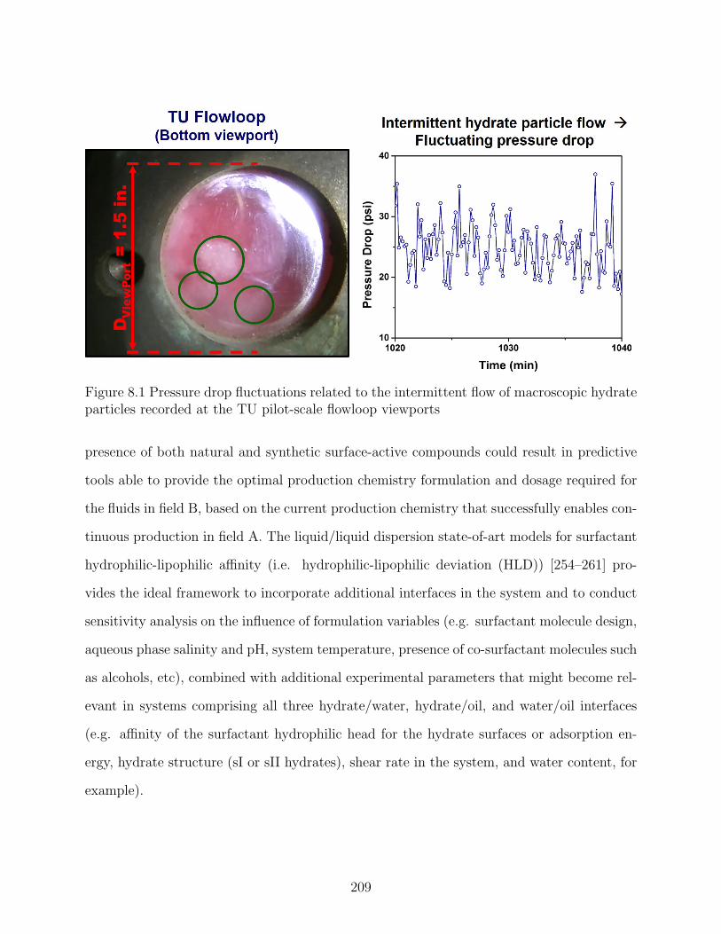
Figure 8.1 Pressure drop fluctuations related to the intermittent flow of macroscopic hydrateparticles recorded at the TU pilot-scale flowloop viewports

presence of both natural and synthetic surface-active compounds could result in predictive

tools able to provide the optimal production chemistry formulation and dosage required for

the fluids in field B, based on the current production chemistry that successfully enables con-

tinuous production in field A. The liquid/liquid dispersion state-of-art models for surfactant

hydrophilic-lipophilic affinity (i.e. hydrophilic-lipophilic deviation (HLD)) [254–261] pro-

vides the ideal framework to incorporate additional interfaces in the system and to conduct

sensitivity analysis on the influence of formulation variables (e.g. surfactant molecule design,

aqueous phase salinity and pH, system temperature, presence of co-surfactant molecules such

as alcohols, etc), combined with additional experimental parameters that might become rel-

evant in systems comprising all three hydrate/water, hydrate/oil, and water/oil interfaces

(e.g. affinity of the surfactant hydrophilic head for the hydrate surfaces or adsorption en-

ergy, hydrate structure (sI or sII hydrates), shear rate in the system, and water content, for

example).

209

At the same time, minimizing the required crude oil sample to both reliably assess the

hydrate plugging tendency of a system and to reach the optimal production chemistry for-

mulation and dosage for a specific field could have a significant economic impact during the

early design stages of new field developments. Sound plugging risk assessments might enable

well-grounded decision-making to prescind over-conservative hydrate management/preven-

tion strategies wherever they are not needed. Quantitative scaling of the output variables

from multiple scales experimental equipment becomes essential to reduce uncertainties in

the hydrate plugging risk assessments while minimizing the required crude oil sample. Ef-

forts should be directed towards validating the interconnection between hydrate cohesive

forces, hydrate particle size, shear viscosity, yield stress, pressure drop, for example, as it

was done using classic yield stress models to connect HP-MMF hydrate cohesive forces with

the HP-rheometer yield stress measurements.

Ultimately, the scaling rules resulting from such multiple scales experimental investi-

gations need to be incorporated into dynamic hydrate transportability simulations tools

generated at CHR, such as CSMHyK-OLGAr. First steps might involve the implementa-

tion of the yield stress models presented in 3 in order to estimate the pressure differential

requirements for the successful restart of a pipeline in the presence of a hydrate slurry, in a

similar way previous studies have approach restart operations of waxy crude oils [262]. Such

a tool would provide engineers with an idea of the likelihood of the system to restart without

further external intervention, and whether some kind of remediation method might need to

be deployed.

210

REFERENCES CITED

[1] Andrea J Liu and Sidney R Nagel. Nonlinear dynamics: Jamming is not just coolany more. Nature, 396(6706):21–22, 1998. ISSN 0028-0836. doi: 10.1038/23819.URL http://www.nature.com/nature/journal/v396/n6706/full/396021a0.

html{%}5Cnfiles/790/Liu{_}Nagel{_}1998{_}Nonlineardynamics.pdfhttp://

www.nature.com/nature/journal/v396/n6706/full/396021a0.html{%}5Cnfiles/

790/Liu{_}Nagel{_}1998{_}Nonlineardynamics.pdf.

[2] H T Nguyen, C Reichhardt, and C J O Reichhardt. Clogging and jamming transitionsin periodic obstacle arrays. Physical Review E, 95(3):1–5, 2017. ISSN 24700053. doi:10.1103/PhysRevE.95.030902.

[3] C J O Reichhardt. Jamming and Clogging of Passive and Active Particles in DisorderedMedia, 2017.

[4] Ryohei Seto, Abhinendra Singh, Bulbul Chakraborty, Morton M. Denn, and Jeffrey F.Morris. Shear jamming and fragility in dense suspensions. Granular Matter, 21(3):1–8,2019. ISSN 1434-5021. doi: 10.1007/s10035-019-0931-5. URL https://doi.org/10.

1007/s10035-019-0931-5.

[5] Fabien Mahaut, Xavier Chateau, Philippe Coussot, and Guillaume Ovarlez. Yieldstress and elastic modulus of suspensions of noncolloidal particles in yield stress fluids.Journal of Rheology, 52(1):287, 2008. doi: 10.1122/1.2798234.

[6] Andrea J Liu and Sidney R Nagel. Jamming and Rheology: An Introduction. In Jam-ming and Rheology: Constrained Dynamics on Microscopic and Macroscopic Scales,pages 1–5. CRC Press, London, first edit edition, 2001. ISBN 9780748408795.

[7] E Dendy Sloan Jr. Fundamental principles and applications of natural gas hydrates.Nature, 426:353–359, 2003.

[8] E Dendy Sloan and Carolyn A Koh. Clathrate hydrates of natural gases. CRC Press,Boca Raton, FL, 3rd edition, 2008. ISBN 9780849390784.

[9] Zheng Rong Chong, She Hern Bryan Yang, Ponnivalavan Babu, Praveen Linga, andXiao Sen Li. Review of natural gas hydrates as an energy resource: Prospects and chal-lenges. Applied Energy, 162:1633–1652, 2016. ISSN 03062619. doi: 10.1016/j.apenergy.2014.12.061. URL http://dx.doi.org/10.1016/j.apenergy.2014.12.061.

211

[10] David Archer, Bruce Buffett, and Victor Brovkin. Ocean methane hydrates as a slowtipping point in the global carbon cycle. Proceedings of the National Academy ofSciences of the United States of America (PNAS), 106(49):20596–20601, 2009. ISSN0027-8424. doi: 10.1073/pnas.0800885105.

[11] Ray Boswell and Timothy S Collett. Current perspectives on gas hydrate resources.Energy and Environmental Science, 4(4):1206–1215, 2011. ISSN 17545692. doi: 10.1039/c0ee00203h.

[12] Alexei V Milkov. Global estimates of hydrate-bound gas in marine sediments: Howmuch is really out there? Earth-Science Reviews, 66(3-4):183–197, 2004. ISSN00128252. doi: 10.1016/j.earscirev.2003.11.002.

[13] Carolyn D. Ruppel. Methane Hydrates and Contemporary Climate Change,2011. URL https://www.nature.com/scitable/knowledge/library/

methane-hydrates-and-contemporary-climate-change-24314790.

[14] U.S. Energy Information Administration. Annual Energy Outlook 2019 with pro-jections to 2050. Technical report, U.S. Energy Information Administration, Wash-ington, DC, 2019. URL https://www.eia.gov/outlooks/aeo/pdf/0383(2017)

.pdf{%}5Cnhttp://www.eia.gov/outlooks/aeo/pdf/0383(2017).pdf.

[15] Hari Prakash Veluswamy, Asheesh Kumar, Yutaek Seo, Ju Dong Lee, and PraveenLinga. A review of solidified natural gas (SNG) technology for gas storage via clathratehydrates. Applied Energy, 216:262–285, 2018. ISSN 03062619. doi: 10.1016/j.apenergy.2018.02.059. URL https://doi.org/10.1016/j.apenergy.2018.02.059.

[16] F. Ma, P. Zhang, and X. J. Shi. Investigation of thermo-fluidic performance of phasechange material slurry and energy transport characteristics. Applied Energy, 227:643–654, 2018. ISSN 03062619. doi: 10.1016/j.apenergy.2017.08.146.

[17] E. Oro, A. de Gracia, A. Castell, M. M. Farid, and L. F. Cabeza. Review on phasechange materials (PCMs) for cold thermal energy storage applications. Applied Energy,99:513–533, 2012. ISSN 03062619. doi: 10.1016/j.apenergy.2012.03.058.

[18] Ziad Youssef, Anthony Delahaye, Li Huang, Francois Trinquet, Laurence Fournaison,Clemens Pollerberg, and Christian Doetsch. State of the art on phase change materialslurries. Energy Conversion and Management, 65:120–132, 2013. ISSN 01968904. doi:10.1016/j.enconman.2012.07.004. URL http://dx.doi.org/10.1016/j.enconman.

2012.07.004.

[19] P. Zhang, Z. W. Ma, and R. Z. Wang. An overview of phase change material slurries:MPCS and CHS. Renewable and Sustainable Energy Reviews, 14(2):598–614, 2010.ISSN 13640321. doi: 10.1016/j.rser.2009.08.015.

212

[20] E. Dendy Sloan, Jefferson L. Creek, and Amadeu K. Sum. Where and How AreHydrate Plugs Formed? In Natural Gas Hydrates in Flow Assurance, chapter Two,pages 13–36. Elsevier Inc., Boston, MA, 2011. ISBN 9781856179454. doi: 10.1016/B978-1-85617-945-4.00002-9.

[21] Amadeu K. Sum, Carolyn A. Koh, and E. Dendy Sloan. Developing a comprehensiveunderstanding and model of hydrate in multiphase flow: From laboratory measure-ments to field applications. Energy and Fuels, 26(7):4046–4052, 2012. ISSN 08870624.doi: 10.1021/ef300191e.

[22] Luis E. Zerpa, E. Dendy Sloan, Amadeu K. Sum, and Carolyn A. Koh. Overview ofCSMHyK: A transient hydrate formation model. Journal of Petroleum Science andEngineering, 98-99:122–129, 2012. ISSN 09204105. doi: 10.1016/j.petrol.2012.08.017.URL http://dx.doi.org/10.1016/j.petrol.2012.08.017.

[23] Zachary M. Aman and Carolyn A. Koh. Interfacial phenomena in gas hydrate sys-tems. Chem. Soc. Rev., 45(6):1678–1690, 2016. ISSN 0306-0012. doi: 10.1039/C5CS00791G. URL http://dx.doi.org/10.1039/C5CS00791Ghttp://xlink.rsc.

org/?DOI=C5CS00791G.

[24] Mike Eaton, Jason Lachance, and Larry Talley. Kinetic Hydrate Inhibitors Perfor-mance. In Natural Gas Hydrates in Flow Assurance, chapter Six, pages 105–143.Elsevier Inc., 2011. ISBN 9781856179454. doi: 10.1016/B978-1-85617-945-4.00006-6.

[25] Wei Ke and Malcolm A. Kelland. Kinetic Hydrate Inhibitor Studies for Gas HydrateSystems: A Review of Experimental Equipment and Test Methods. Energy & Fuels, 30(12):10015–10028, 2016. ISSN 15205029. doi: 10.1021/acs.energyfuels.6b02739. URLhttp://pubs.acs.org/doi/abs/10.1021/acs.energyfuels.6b02739.

[26] Malcolm A Kelland. History of the Development of Low Dosage Hydrate Inhibitors.Energy Fuels, 20(3):825–847, 2006. ISSN 0887-0624. doi: 10.1021/ef050427x.

[27] Richard Kopps, Rama Venkatesan, Jeff Creek, and Alberto Montesi. FlowAssurance Challenges in Deepwater Gas Developments. In SPE Asia PacificOil & Gas Conference and Exhibition, number SPE 109670, page SPE 109670,Jakarta, Indonesia, 2007. ISBN 9781613990407. doi: 10.2118/109670-MS.URL http://scholar.google.com/scholar?hl=en{&}btnG=Search{&}q=intitle:

Flow+Assurance+Challenges+in+Deepwater+Gas+Developments{#}4.

[28] J P Lederhos, J P Long, A K Sum, R L Christiansen, and E Dendy Sloan. Effectivekinetic inhibitors for natural gas hydrates. Chemical Engineering Science, 51(8):1221–1229, 1996. ISSN 00092509. doi: 10.1016/0009-2509(95)00370-3.

213

[29] A P Mehta, P B Hebert, E R Cadena, and J P Weatherman. Fulfilling the Promise ofLow-Dosage Hydrate Inhibitors: Journey From Academic Curiosity to Successful FieldImplementation. SPE Production & Facilities, 18(1):73–79, 2003. ISSN 01603663. doi:10.2118/81927-PA.

[30] Thierry Palermo, Luc Riviere, and Clement Boireau. Capex savings might raise flowassurance challenges. In 9th International Conference on Gas Hydrates (ICGH9),Denver, CO, 2017.

[31] Z Patel, M Dibello, K Fontentot, A Guillory, and R M Hesketh-Prichard. ContinuousApplication of Anti-Agglomerant LDHI for Gas-Condensate Subsea Tieback Wells inDeepwater Gulf of Mexico. In Offshore Technology Conference, number OTC-21836-MS, Houston, TX, 2011. ISBN 9781613991176. doi: 10.4043/21836-MS.

[32] Bahman Tohidi, Ross Anderson, Houra Mozaffar, and Foroogh Tohidi. The Return ofKinetic Hydrate Inhibitors. Energy and Fuels, 29(12):8254–8260, 2015. ISSN 15205029.doi: 10.1021/acs.energyfuels.5b01794.

[33] S. B. Fu, L. M. Cenegy, and C. S. Neff. A Summary of Successful Field Applications ofA Kinetic Hydrate Inhibitor. In SPE International Symposium on Oilfield Chemistry,pages 1–8, Houston, TX, 2001. doi: 10.2118/65022-ms.

[34] L D Talley and G F Mitchell. Application of Proprietary Kinetic Hydrate Inhibitorsin Gas Flowlines. In Offshore Technology Conference, page OTC 11036, Houston, TX,1999.

[35] Fatemeh Khalkhal, Ajay Singh Negi, James Harrison, Casey D Stokes, David L Mor-gan, and Chinedum O Osuji. Evaluating the Dispersant Stabilization of ColloidalSuspensions from the Scaling Behavior of Gel Rheology and Adsorption Measure-ments. Langmuir, 34(3):1092–1099, 2018. ISSN 0743-7463. doi: 10.1021/acs.langmuir.7b03343. URL http://pubs.acs.org/doi/abs/10.1021/acs.langmuir.7b03343.

[36] L E Zerpa, J L Salager, C A Koh, E D Sloan, and A K Sum. Surface Chemistry andGas Hydrates in Flow Assurance. Industrial & Engineering Chemistry Research, 50(1):188–197, 2011. ISSN 0888-5885. doi: 10.1021/ie100873k. URL http://pubs.acs.

org/doi/abs/10.1021/ie100873k.

[37] Tai Bui, Anh Phan, Deepak Monteiro, Qiang Lan, Mark Ceglio, Erick Acosta, PushkalaKrishnamurthy, and Alberto Striolo. Evidence of Structure-Performance Relation forSurfactants Used as Antiagglomerants for Hydrate Management. Langmuir, 33(9):acs.langmuir.6b04334, 2017. ISSN 15205827. doi: 10.1021/acs.langmuir.6b04334. URLhttp://pubs.acs.org/doi/abs/10.1021/acs.langmuir.6b04334.

214

[38] Pei Cheng Chua and Malcolm A Kelland. Study of the Gas Hydrate Anti-agglomerantPerformance of a Series of n-Alkyl-tri(n-butyl)ammonium Bromides. Energy & Fuels,27(3):1285–1292, 2013. ISSN 0887-0624. doi: 10.1021/ef3018546. URL http://pubs.

acs.org/doi/abs/10.1021/ef3018546.

[39] Hadi Mehrabian, Matthew R. Walsh, and Bernhardt L Trout. In Silico Analysis of theEffect of Alkyl Tail Length on Anti-Agglomerant Adsorption to Natural Gas Hydratesin Brine. The Journal of Physical Chemistry C, 123(28):17239–17248, 2019. ISSN1932-7447. doi: 10.1021/acs.jpcc.9b01952.

[40] V. Trappe, V. Prasad, Luca Cipelletti, P. N. Segre, and D. A. Weitz. Jamming phasediagram for attractive particles. Nature, 411:772–775, 2001. ISSN 00280836. doi:10.1038/35081021. URL http://www.nature.com/doifinder/10.1038/35081021.

[41] Zachary M Aman, Erika P Brown, E Dendy Sloan, Amadeu K Sum, and Carolyn AKoh. Interfacial mechanisms governing cyclopentane clathrate hydrate adhesion /cohesion. Phys. Chem. Chem. Phys., 13:19796–19806, 2011. doi: 10.1039/c1cp21907c.

[42] Laura E. Dieker, Zachary M. Aman, Nathan C. George, Amadeu K. Sum, E. DendySloan, and Carolyn A. Koh. Micromechanical adhesion force measurements betweenhydrate particles in hydrocarbon oils and their modifications. Energy and Fuels, 23(12):5966–5971, 2009. ISSN 08870624. doi: 10.1021/ef9006615.

[43] Sijia Hu and Carolyn A. Koh. Interfacial Properties and Mechanisms Dominating GasHydrate Cohesion and Adhesion in Liquid and Vapor Hydrocarbon Phases. Langmuir,33(42):11299–11309, 2017. ISSN 15205827. doi: 10.1021/acs.langmuir.7b02676.

[44] Shane A. Morrissy, Temiloluwa O. Kuteyi, Mike L. Johns, Eric F. May, Zachary M.Aman, and Stuart. F. McKay. Quantitative Ranking and Development of Hy-drate Anti-Agglomerants. In Offshore Technology Conference Asia, Kuala Lumpur,Malaysia, 2018. doi: 10.4043/28578-ms.

[45] Shane A. Morrissy, Vincent W. Lim, Eric F. May, Michael L. Johns, Zachary M. Aman,and Brendan F. Graham. Micromechanical Cohesive Force Measurements betweenPrecipitated Asphaltene Solids and Cyclopentane Hydrates. Energy and Fuels, 29(10):6277–6285, 2015. ISSN 15205029. doi: 10.1021/acs.energyfuels.5b01427.

[46] Craig J. Taylor, Laura E. Dieker, Kelly T. Miller, Carolyn A. Koh, and E. DendySloan. Micromechanical adhesion force measurements between tetrahydrofuran hy-drate particles. Journal of Colloid and Interface Science, 306(2):255–261, 2007. ISSN00219797. doi: 10.1016/j.jcis.2006.10.078.

215

[47] Malcolm A. Kelland, Erik G. Dirdal, and Anders Grinrød. Novel Benchtop WheelLoop for Low Dosage Gas Hydrate Inhibitor Screening: Comparison To Rocking Cellsfor a Series of Anti-Agglomerants. Journal of Chemical and Engineering Data, 60(2):252–257, 2014. ISSN 15205134. doi: 10.1021/je5005627.

[48] Minwei Sun and Abbas Firoozabadi. New surfactant for hydrate anti-agglomerationin hydrocarbon flowlines and seabed oil capture. Journal of Colloid and InterfaceScience, 402:312–319, 2013. ISSN 00219797. doi: 10.1016/j.jcis.2013.02.053. URLhttp://dx.doi.org/10.1016/j.jcis.2013.02.053.

[49] Minwei Sun and Abbas Firoozabadi. Gas hydrate powder formation - Ultimate solutionin natural gas flow assurance. Fuel, 146:1–5, 2015. ISSN 00162361. doi: 10.1016/j.fuel.2014.12.078. URL http://dx.doi.org/10.1016/j.fuel.2014.12.078.

[50] J Dalton York and Abbas Firoozabadi. Comparing effectiveness of rhamnolipid biosur-factant with a quaternary ammonium salt surfactant for hydrate anti-agglomeration.Journal of Physical Chemistry B, 112(3):845–851, 2008. ISSN 15206106. doi:10.1021/jp077271h.

[51] J Dalton York and Abbas Firoozabadi. Effect of brine on hydrate antiagglomeration.Energy & Fuels, 23(6):2937–2946, 2009. ISSN 08870624. doi: 10.1021/ef800937p.

[52] Amit Ahuja, Anam Iqbal, Mohsin Iqbal, Jae W. Lee, and Jeffrey F. Morris. Rhe-ology of Hydrate-Forming Emulsions Stabilized by Surfactant and Hydrophobic Sil-ica Nanoparticles. Energy and Fuels, 32(5):5877–5884, 2018. ISSN 15205029. doi:10.1021/acs.energyfuels.8b00795.

[53] Ricardo Camargo and Thierry Palermo. Rheological Properties of Hydrate Suspensionsin an Asphaltenic Crude Oil. In Proceedings of the Fourth International Conferenceon Gas Hydrates, number 1, pages 880–885, Yokohama, Japan, 2002.

[54] Karin Hald and Sven Nuland. Hydrate slurry rheology in the petroleum industry.Annual Transactions of the Nordic Rheology Society, 15, 2007.

[55] Prasad U Karanjkar, Amit Ahuja, Genti Zylyftari, Jae W Lee, and Jeffrey F. Morris.Rheology of cyclopentane hydrate slurry in a model oil-continuous emulsion. RheologicaActa, 55(3):235–243, 2016. ISSN 00354511. doi: 10.1007/s00397-016-0911-1.

[56] Ahmad A.A. Majid, David T. Wu, and Carolyn A. Koh. New in Situ Measurementsof the Viscosity of Gas Clathrate Hydrate Slurries Formed from Model Water-in-OilEmulsions. Langmuir, 33(42):11436–11445, 2017. ISSN 15205827. doi: 10.1021/acs.langmuir.7b02642.

216

[57] Jorge Peixinho, Prasad U. Karanjkar, Jae W. Lee, and Jeffrey F. Morris. Rheology ofhydrate forming emulsions. Langmuir, 26(14):11699–11704, 2010. ISSN 07437463. doi:10.1021/la101141j.

[58] Yahua Qin, Zachary M. Aman, Paul F. Pickering, Michael L. Johns, and Eric F.May. High pressure rheological measurements of gas hydrate-in-oil slurries. Jour-nal of Non-Newtonian Fluid Mechanics, 248:40–49, 2017. ISSN 03770257. doi:10.1016/j.jnnfm.2017.08.006. URL http://dx.doi.org/10.1016/j.jnnfm.2017.08.

006https://doi.org/10.1016/j.jnnfm.2017.08.006.

[59] Patrick Joseph Rensing. Studies on the Rheology of Ice and Clathrate Hydrate SlurriesFormed In Situ from Water-in-Oil Emulsions. Phd, Colorado School of Mines, 2010.

[60] Tony Spratt, Pete Conrad, Colton Asheim, Ryan McCarthy, and Tommy Golczyn-ski. Utilizing the High-Pressure Rheometer for Comparison of LDHI Effectiveness. InOffshore Technology Conference, Houston, TX, 2018. doi: 10.4043/28717-ms.

[61] Eric B. Webb, Carolyn A. Koh, and Matthew W. Liberatore. Rheological Proper-ties of Methane Hydrate Slurries Formed From AOT + Water + Oil Microemulsions.Langmuir, 29(35):10997–11004, 2013. ISSN 07437463. doi: 10.1021/la4022432.

[62] Masoumeh Akhfash, Zachary M. Aman, Sang Yoon Ahn, Michael L. Johns, and Eric F.May. Gas hydrate plug formation in partially-dispersed water-oil systems. ChemicalEngineering Science, 140:337–347, 2016. ISSN 00092509. doi: 10.1016/j.ces.2015.09.032. URL http://dx.doi.org/10.1016/j.ces.2015.09.032.

[63] Zachary M. Aman, William G.T. Syddall, Agnes Haber, Yahua Qin, Brendan Graham,Eric F. May, Michael L. Johns, and Paul F. Pickering. Characterization of Crude OilsThat Naturally Resist Hydrate Plug Formation. Energy and Fuels, 31(6):5806–5816,2017. ISSN 15205029. doi: 10.1021/acs.energyfuels.6b02943.

[64] Hossein Moradpour, Antonin Chapoy, and Bahman Tohidi. Bimodal model for pre-dicting the emulsion-hydrate mixture viscosity in high water cut systems. Fuel,90(11):3343–3351, 2011. ISSN 00162361. doi: 10.1016/j.fuel.2011.06.038. URLhttp://dx.doi.org/10.1016/j.fuel.2011.06.038.

[65] Xiao-Qin Wang, Hui-Bo Qin, Qing-Lan Ma, Zhen-Feng Sun, Ke-Le Yan, Zhi-YuSong, Kai Guo, Da-Meng Liu, Guang-Jin Chen, and Chang-Yu Sun. Hydrate An-tiagglomeration Performance for the Active Components Extracted from a Terres-trial Plant Fruit. Energy & Fuels, 31(1):287–298, 2017. ISSN 0887-0624. doi: 10.1021/acs.energyfuels.6b02305. URL http://pubs.acs.org/doi/abs/10.1021/acs.

energyfuels.6b02305.

217

[66] H. Delroisse, J. P. Torre, and C. Dicharry. Effects of a Quaternary Ammonium Salt onthe Growth, Wettability, and Agglomeration of Structure II Hydrate Crystals. Energyand Fuels, 32(12):12277–12288, 2018. ISSN 15205029. doi: 10.1021/acs.energyfuels.8b02980.

[67] Anthony Delahaye, Laurence Fournaison, Salem Jerbi, and Nadia Mayoufi. Rheologicalproperties of CO2 hydrate slurry flow in the presence of additives. Industrial andEngineering Chemistry Research, 50(13):8344–8353, 2011. ISSN 08885885. doi: 10.1021/ie200185q.

[68] D Estanga, S Subramanian, M Walsh, E Dellecase, M Volk, and E Bbosa. Low DosageHydrate Anti-Agglomerant Failure during Pipe Flow. In 9th International Conferenceon Gas Hydrates, Denver, CO, 2017.

[69] Philippe Glenat, Ludovic Pagezy, Romain Devoisselle, Patrick Bourg, Mathieu Pere,and Aline Melchuna. Rheological study of liquid hydrates slurries in presence of com-mercial hydrates dispersants (AA-LDHIs). In 9th International Conference on GasHydrates2, pages 1–18, Denver, CO, 2017.

[70] Derek M Kleehammer. Rheology of Hydrate Slurries: Transferability Between a Labo-ratory Viscometer and a Pilot Scale Flow Loop. PhD thesis, Colorado School of Mines,2005.

[71] X F Lv, J Gong, W Q Li, B H Shi, D Yu, and H H Wu. Experimental Study onNatural-Gas- Hydrate-Slurry Flow. Society of Petroleum Engineers Journal, 19(2):206–214, 2013. ISSN 1086-055X. doi: 10.2118/158597-PA.

[72] Aline Melchuna, Ana Cameirao, Yamina Ouabbas, Jean-michel Herri, Cours Fauriel,and Philippe Glenat. Transport of Hydrate Slurry At High Water Cut. In The 8thInternational Conference on Gas Hydrates, pages 1–11, Beijing, 2014.

[73] Bao Zi Peng, Jun Chen, Chang Yu Sun, Abhijit Dandekar, Shao Hui Guo, Bei Liu,Liang Mu, Lan Ying Yang, Wen Zhi Li, and Guang Jin Chen. Flow characteristicsand morphology of hydrate slurry formed from (natural gas+diesel oil/condensateoil+water) system containing anti-agglomerant. Chemical Engineering Science, 84:333–344, 2012. ISSN 00092509. doi: 10.1016/j.ces.2012.08.030. URL http://dx.doi.

org/10.1016/j.ces.2012.08.030.

[74] Ke Le Yan, Chang Yu Sun, Jun Chen, Li Tao Chen, De Ji Shen, Bei Liu, Meng LeiJia, Meng Niu, Yi Ning Lv, Nan Li, Zhi Yu Song, Shu Shan Niu, and Guang JinChen. Flow characteristics and rheological properties of natural gas hydrate slurryin the presence of anti-agglomerant in a flow loop apparatus. Chemical EngineeringScience, 106:99–108, 2014. ISSN 00092509. doi: 10.1016/j.ces.2013.11.015. URLhttp://dx.doi.org/10.1016/j.ces.2013.11.015.

218

[75] Michael A Bellucci, Matthew R Walsh, and Bernhardt L Trout. Molecular DynamicsAnalysis of Anti-Agglomerant Surface Adsorption in Natural Gas Hydrates. Journalof Physical Chemistry C, 122(5):2673–2683, 2018. ISSN 19327455. doi: 10.1021/acs.jpcc.7b09573.

[76] Tai Bui, Francois Sicard, Deepak Monteiro, Qiang Lan, Mark Ceglio, Charlotte Bur-ress, and Alberto Striolo. Anti-Agglomerants Affect Gas Hydrate Growth. TheJournal of Physical Chemistry Letters, 9(12):3491–3496, 2018. ISSN 19487185. doi:10.1021/acs.jpclett.8b01180.

[77] Felipe Jimenez-Angeles and Abbas Firoozabadi. Hydrophobic Hydration and the Ef-fect of NaCl Salt in the Adsorption of Hydrocarbons and Surfactants on ClathrateHydrates. ACS Central Science, 4(7):820–831, 2018. ISSN 23747951. doi: 10.1021/acscentsci.8b00076.

[78] Anh Phan, Tai Bui, Erick Acosta, Pushkala Krishnamurthy, and Alberto Striolo.Molecular mechanisms responsible for hydrate anti-agglomerant performance. Phys.Chem. Chem. Phys., 18(36):24859–24871, 2016. ISSN 1463-9076. doi: 10.1039/C6CP03296F. URL http://xlink.rsc.org/?DOI=C6CP03296F.

[79] Francois Sicard, Tai Bui, Deepak Monteiro, Qiang Lan, Mark Ceglio, Charlotte Bur-ress, and Alberto Striolo. Emergent Properties of Antiagglomerant Films ControlMethane Transport: Implications for Hydrate Management. Langmuir, 34(33):9701–9710, 2018. ISSN 15205827. doi: 10.1021/acs.langmuir.8b01366.

[80] Ben Bbosa, Emmanuel DelleCase, Michael Volk, and Evren Ozbayoglu. AvoidingFlowline Plugging: A Deposition Velocity Model and Stability Map. In SPE WesternRegional Meeting, number SPE-180494-MS, pages 23–26, Anchorage, AK, 2016. ISBN9781613994658. doi: 10.2118/180494-MS. URL http://www.onepetro.org/doi/10.

2118/180494-MS.

[81] Doug Turner and Larry Talley. Hydrate Inhibition Via Cold Flow - No Chemicalsor Insulation. In Proceedings of the 6th International Conference on Gas Hydrates,Vancouver, Canada, 2008.

[82] Amit Ahuja, Genti Zylyftari, and Jeffrey F. Morris. Yield stress measurements ofcyclopentane hydrate slurry. Journal of Non-Newtonian Fluid Mechanics, 220:116–125, 2015. ISSN 03770257. doi: 10.1016/j.jnnfm.2014.11.007. URL http://dx.doi.

org/10.1016/j.jnnfm.2014.11.007.

[83] Paulo H. De Lima Silva, Monica F. Naccache, Paulo R. De Souza Mendes, Flavio B.Campos, Adriana Teixeira, and Amadeu K. Sum. Rheology of Tetrahydrofuran Hy-drate Slurries. Energy and Fuels, 31(12):14385–14392, 2017. ISSN 15205029. doi:10.1021/acs.energyfuels.7b02425.

219

[84] Gaurav Pandey, Praveen Linga, and Jitendra S. Sangwai. High pressure rheology of gashydrate formed from multiphase systems using modified Couette rheometer. Reviewof Scientific Instruments, 88(2):1–10, 2017. ISSN 10897623. doi: 10.1063/1.4974750.

[85] Patrick J. Rensing, Matthew W. Liberatore, Amadeu K. Sum, Carolyn A. Koh, andE. Dendy Sloan. Viscosity and yield stresses of ice slurries formed in water-in-oilemulsions. Journal of Non-Newtonian Fluid Mechanics, 166(14-15):859–866, 2011.ISSN 03770257. doi: 10.1016/j.jnnfm.2011.05.003. URL http://dx.doi.org/10.

1016/j.jnnfm.2011.05.003.

[86] William M Deen. Analysis of Transport Phenomena. Oxford University Press, secondedi edition, 2011. ISBN 9780199740284.

[87] Daniel Bonn, Morton M. Denn, Ludovic Berthier, Thibaut Divoux, and Sebastien Man-neville. Yield stress materials in soft condensed matter. Reviews of Modern Physics,89(3):1–40, 2017. ISSN 15390756. doi: 10.1103/RevModPhys.89.035005.

[88] Jan Mewis and Norman J Wagner. Colloidal Suspension Rheology. Cambridge Uni-versity Press, 2012. ISBN 978-0-521-51599-3.

[89] S Mueller, E W Llewellin, and H M Mader. The rheology of suspensions of solid parti-cles. Proceedings of the Royal Society A, 466(2116):1201–1228, 2010. ISSN 0303-402X.doi: 10.1007/BF01432034. URL http://link.springer.com/10.1007/BF01432034.

[90] Ir R Rutgers. Relative viscosity of suspensions of rigid spheres in Newtonian liquids.Rheologica Acta, 2(3):202–210, 1962. ISSN 00354511. doi: 10.1007/BF01983952.

[91] Albert Einstein. Eine neue Bestimmung der Molekuldimensionen. Annals of Physics,324(2):289–306, 1906.

[92] Albert Einstein. Berichtigung zu meiner Arbeit: Eine neue Bestimmung derMolekuldimensionen. Annals of Physics, 339(3):591–592, 1911.

[93] John Happel. Viscosity of Suspensions of Uniform Spheres. Journal of Applied Physics,28(11):1288–1292, 1957. ISSN 00218979. doi: 10.1063/1.1722635.

[94] P Mills. Non-Newtonian behaviour of flocculated suspensions. Journal de PhysiqueLettres, 46(7):301–309, 1985. doi: 10.1051/jphyslet:01985004607030100.

[95] M. Mooney. The viscosity of a concentrated suspension of spherical particles. Journalof Colloid Science, 6(2):162–170, 1951. ISSN 00958522. doi: 10.1016/0095-8522(51)90036-0.

220

[96] Kiyoshi Toda and Hisamoto Furuse. Extension of Einstein’s viscosity equation tothat for concentrated dispersions of solutes and particles. Journal of Bioscience andBioengineering, 102(6):524–528, 2006. ISSN 13891723. doi: 10.1263/jbb.102.524.

[97] G. K. Batchelor and J. T. Green. The determination of the bulk stress in a sus-pension of spherical particles to order c 2. Journal of Fluid Mechanics, 56(3):401–427, dec 1972. ISSN 0022-1120. doi: 10.1017/S0022112072002435. URL http:

//www.journals.cambridge.org/abstract{_}S0022112072002435.

[98] P Snabre and P Mills. Rheology of concentrated suspensions of viscoelastic particles.Colloids and Surfaces A: Physicochemical and Engineering Aspects, 152(1-2):79–88,1999. ISSN 09277757. doi: 10.1016/S0927-7757(98)00619-0.

[99] D. Quemada. Rheology of concentrated disperse systems and minimum energy dissi-pation principle. I. Viscosity-concentration relationship. Rheologica Acta, 16(1):82–94,1977. ISSN 00354511. doi: 10.1007/BF01516932.

[100] D Quemada. Rheology of concentrated disperse systems II. A model for non-Newtonianshear viscosity in steady flows. Rheologica Acta, 17(6):632–642, 1978. ISSN 00354511.doi: 10.1007/BF01522036. URL https://link.springer.com/content/pdf/10.

1007{%}2FBF01522036.pdf.

[101] D Quemada. Rheology of concentrated disperse systems III. General features of theproposed non-newtonian model. Comparison with experimental data. Rheologica Acta,17(6):643–653, 1978.

[102] Irvin M Krieger and Thomas J Dougherty. A Mechanism for Non-Newtonian Flow inSuspensions of Rigid Spheres. Transactions of the Society of Rheology, 3(1):137–152,1959. URL http://sor.scitation.org/doi/abs/10.1122/1.548848.

[103] D Quemada. Rheological modelling of complex fluids. I. The concept of effectivevolume fraction revisited. Eur. Phys. J. AP, 1(1):119–127, 1998. ISSN 1286-0042. doi:10.1051/epjap:1998125. URL http://www.epjap.org/10.1051/epjap:1998125.

[104] Frank Bossler and Erin Koos. Structure of Particle Networks in Capillary Suspen-sions with Wetting and Nonwetting Fluids. Langmuir, 32(6):1489–1501, 2016. ISSN15205827. doi: 10.1021/acs.langmuir.5b04246.

[105] Erin Koos and Norbert Willenbacher. Capillary Forces in Suspension Rheology. Sci-ence, 331(6019):897–900, 2011. doi: 10.1126/science.1199339. URL www.sciencemag.

org/cgi/content/full/331/6019/894/DC1.

221

[106] Krassimir D. Danov, Mihail T. Georgiev, Peter A. Kralchevsky, Gergana M. Radulova,Theodor D. Gurkov, Simeon D. Stoyanov, and Eddie G. Pelan. Hardening of parti-cle/oil/water suspensions due to capillary bridges: Experimental yield stress and the-oretical interpretation. Advances in Colloid and Interface Science, 251:80–96, 2018.ISSN 00018686. doi: 10.1016/j.cis.2017.11.004. URL https://doi.org/10.1016/j.

cis.2017.11.004.

[107] Mihail T Georgiev, Krassimir D Danov, Peter A Kralchevsky, Theodor D Gurkov, Den-itsa P Krusteva, Luben N Arnaudov, Simeon D Stoyanov, and Eddie G Pelan. Rheologyof particle/water/oil three-phase dispersions: Electrostatic vs. capillary bridge forces.Journal of Colloid and Interface Science, 513(1):515–526, 2018. ISSN 10957103. doi:10.1016/j.jcis.2017.11.057. URL https://doi.org/10.1016/j.jcis.2017.11.057.

[108] Erin Koos. Capillary suspensions: Particle networks formed through the capillaryforce. Current Opinion in Colloid and Interface Science, 19(6):575–584, 2014. ISSN18790399. doi: 10.1016/j.cocis.2014.10.004. URL http://dx.doi.org/10.1016/j.

cocis.2014.10.004.

[109] Erin Koos, Julia Johannsmeier, Linda Schwebler, and Norbert Willenbacher. Tuningsuspension rheology using capillary forces. Soft Matter, 8(24):6620–6628, 2012. ISSN1744683X. doi: 10.1039/c2sm25681a.

[110] Junyi Yang, Nicole Heinichen, and Sachin S. Velankar. The effect of particle wettabilityon the of rheology particulate suspensions with capillary force. Colloids and SurfacesA: Physicochemical and Engineering Aspects, 558:164–170, 2018. ISSN 18734359. doi:10.1016/j.colsurfa.2018.08.062. URL https://doi.org/10.1016/j.colsurfa.2018.

08.062.

[111] Wuchang Wang, Yuxing Li, Haihong Liu, and Pengfei Zhao. Study of AgglomerationCharacteristics of Hydrate Particles in Oil/Gas Pipelines. Advances in MechanicalEngineering, 2015. ISSN 16878140. doi: 10.1155/2014/457050.

[112] Anne Sinquin, Thierry Palermo, and Yannick Peysson. Rheological and Flow Prop-erties of Gas Hydrate Suspensions. Oil & Gas Science and Technology, 59(1):41–57,2004. ISSN 1294-4475. doi: 10.2516/ogst:2004005.

[113] Maureen Dinkgreve, Jose Paredes, Morton M. Denn, and Daniel Bonn. On differentways of measuring “the” yield stress. Journal of Non-Newtonian Fluid Mechanics,238:233–241, 2016. ISSN 03770257. doi: 10.1016/j.jnnfm.2016.11.001. URL http:

//dx.doi.org/10.1016/j.jnnfm.2016.11.001.

[114] Daniel Bonn and Morton M. Denn. Yield Stress Fluids Slowly Yield to Analysis.Science, 324(5933):1401–1403, 2009. doi: 10.1126/science.1174217.

222

[115] Robert J Flatt and Paul Bowen. Yodel: A Yield Stress Model for Suspensions. Journalof the American Ceramic Society, 89(4):1244–1256, 2006. doi: 10.1111/j.1551-2916.2005.00888.x.

[116] Andre R Studart, Esther Amstad, and Ludwig J Gauckler. Yielding ofweakly attractive nanoparticle networks. Soft Matter, 7(14):6408–6412,2011. ISSN 1744-6848. doi: 10.1039/c1sm05598d. URL http://pubs.

rsc.org/en/Content/ArticleLanding/2011/SM/c1sm05598d{%}5Cnpapers:

//4bbe7dda-7fed-4d23-8c1c-c2c5fa8cce83/Paper/p4254.

[117] Quoc Dzuy Nguyen and David V. Boger. Direct Yield Stress Measurement with theVane Method. Journal of Rheology, 29(3):335–347, 1985. ISSN 0148-6055. doi: 10.1122/1.549794. URL http://sor.scitation.org/doi/10.1122/1.549794.

[118] Rubens R. Fernandes, Diogo E. V. Andrade, Admilson T. Franco, and Cezar O. R.Negrao. The yielding and the linear-to-nonlinear viscoelastic transition of an elasto-viscoplastic material. Journal of Rheology, 61(5):893–903, 2017. ISSN 0148-6055. doi:10.1122/1.4991803. URL http://sor.scitation.org/doi/10.1122/1.4991803.

[119] Jonathan J Stickel, Jeffrey S Knutsen, Matthew W Liberatore, Wing Luu, Dou-glas W Bousfield, Daniel J Klingenberg, C. Tim Scott, Thatcher W Root, Max REhrhardt, and Thomas O Monz. Rheology measurements of a biomass slurry: Aninter-laboratory study. Rheologica Acta, 48(9):1005–1015, 2009. ISSN 00354511. doi:10.1007/s00397-009-0382-8.

[120] Gnanli Landrou, Coralie Brumaud, Michael L. Plotze, FrankWinnefeld, and GuillaumeHabert. A fresh look at dense clay paste: Deflocculation and thixotropy mechanisms.Colloids and Surfaces A: Physicochemical and Engineering Aspects, 539:252–260, 2018.ISSN 18734359. doi: 10.1016/j.colsurfa.2017.12.029.

[121] Guillaume Ovarlez, Fabien Mahaut, Stephanie Deboeuf, Nicolas Lenoir, Sarah Hor-mozi, and Xavier Chateau. Flows of suspensions of particles in yield stress fluids.Journal of Rheology, 59(6):1449–1486, 2015. ISSN 0148-6055. doi: 10.1122/1.4934363.URL http://sor.scitation.org/doi/10.1122/1.4934363.

[122] Natalia V Pimenova and Thomas R Hanley. Effect of Corn Stover Concentration onRheological Characteristics. Applied Biochemistry and Biotechnology, 114(1-3):347–360, 2004. ISSN 0273-2289. doi: 10.1385/ABAB:114:1-3:347. URL http://link.

springer.com/10.1385/ABAB:114:1-3:347.

[123] H. Zhu, Y. D. Kim, and D. De Kee. Non-Newtonian fluids with a yield stress. Journalof Non-Newtonian Fluid Mechanics, 129(3):177–181, 2005. ISSN 03770257. doi: 10.1016/j.jnnfm.2005.06.001.

223

[124] Thierry Palermo and E Sloan. Artificial and Natural Inhibition of Hydrates. In NaturalGas Hydrates in Flow Assurance, chapter Five, pages 87–104. Elsevier Inc., Boston,MA, 2011. ISBN 9781856179454. doi: 10.1016/B978-1-85617-945-4.00005-4. URLhttp://dx.doi.org/10.1016/B978-1-85617-945-4.00005-4.

[125] Sanbao Dong and Abbas Firoozabadi. Hydrate anti-agglomeration and synergy effectin normal octane at varying water cuts and salt concentrations. Journal of ChemicalThermodynamics, 117:214–222, 2018. ISSN 10963626. doi: 10.1016/j.jct.2017.09.016.URL https://doi.org/10.1016/j.jct.2017.09.016.

[126] STE Oil Company. STE Oil Company Technical Data, 2019. URL https://www.

steoil.com/msds-tech-data{#}CP350t.

[127] Quoc Dzuy Nguyen and David V. Boger. Yield Stress Measurement for ConcentratedSuspensions. Journal of Rheology, 27(4):321–349, 1983. ISSN 01486055. doi: 10.1122/1.549709. URL http://sor.scitation.org/doi/10.1122/1.549709.

[128] Howard Anthony Barnes and Quoc Dzuy Nguyen. Rotating vane rheometry — areview. Journal of Non-Newtonian Fluid Mechanics, 98(1):1–14, 2001. ISSN 03770257.doi: 10.1016/S0377-0257(01)00095-7.

[129] Shing-Ming Chen. Un-planned Shut-in and Deepwater Gas Hydrate Prevention. InOffshore Technology Conference, number OTC 20436, Houston, TX, 2010. ISBN9781617384264.

[130] Junyi Yang and Sachin S. Velankar. Preparation and yielding behavior of pendularnetwork suspensions. Journal of Rheology, 61(2):217–228, 2017. ISSN 0148-6055. doi:10.1122/1.4973962.

[131] J Alejandro Dapena, Ahmad A A Majid, Vishal Srivastava, Yan Wang, Thomas BCharlton, Andres A Gardner, E Dendy Sloan, Luis E Zerpa, David T Wu, and Car-olyn A Koh. Gas Hydrate Management Strategies Using Anti-Agglomerants : Contin-uous & Transient Large-Scale Flowloop Studies. In Offshore Technology Conference,number OTC-27621-MS, pages 1–17, Houston, TX, 2017. ISBN 9781510842083.

[132] Thierry Palermo and Eric Tournis. Viscosity prediction of waxy oils: Suspension ofFractal Aggregates (SoFA) model. Industrial and Engineering Chemistry Research, 54(16):4526–4534, 2015. ISSN 15205045. doi: 10.1021/ie504166n.

[133] Erika P. Brown, Sijia Hu, Jon Wells, Xiaohui Wang, and Carolyn A. Koh. DirectMeasurements of Contact Angles on Cyclopentane Hydrates. Energy and Fuels, 32(6):6619–6626, 2018. ISSN 15205029. doi: 10.1021/acs.energyfuels.8b00803.

224

[134] Jing He, Stephanie S Lee, and Dilhan M Kalyon. Shear viscosity and wall slip behaviorof dense suspensions of polydisperse particles. Journal of Rheology, 63(1):19–32, 2019.doi: 10.1122/1.5053702.

[135] C. R. Daubert, J. A. Tkachuk, and V. D. Truong. Quantitative measurement of foodspreadability using the vane method. Journal of Texture Studies, 29(4):427–435, 1998.ISSN 00224901. doi: 10.1111/j.1745-4603.1998.tb00814.x.

[136] Mehdi Habibi, M. Dinkgreve, J. Paredes, Daniel Bonn, and M. M. Denn. Normal stressmeasurement in foams and emulsions in the presence of slip. Journal of Non-NewtonianFluid Mechanics, 238:33–43, 2016. ISSN 03770257. doi: 10.1016/j.jnnfm.2016.06.008.URL http://dx.doi.org/10.1016/j.jnnfm.2016.06.008.

[137] Kyeongseok Oh, Mark Jemmett, and Milind Deo. Yield behavior of gelled waxy oil:Effect of stress application in creep ranges. Industrial and Engineering ChemistryResearch, 48(19):8950–8953, 2009. ISSN 08885885. doi: 10.1021/ie9000597.

[138] James F Steffe. Rheological Methods in Food Process Engineering. Freeman Press, EastLansing, MI, second edition, 1996. ISBN 0963203614. doi: 10.1016/0260-8774(94)90090-6.

[139] Adriano Sun and Sundaram Gunasekaran. Yield Stress in Foods: Measurements andApplications. International Journal of Food Properties, 12(1):70–101, 2009. ISSN10942912. doi: 10.1080/10942910802308502.

[140] Saoussen Laribi, Jean Marie Fleureau, Jean Louis Grossiord, and Nejia Kbir-Ariguib.Comparative yield stress determination for pure and interstratified smectite clays. Rhe-ologica Acta, 44(3):262–269, 2005. ISSN 00354511. doi: 10.1007/s00397-004-0406-3.

[141] G W Scott Blair. The Success of Casson’s Equation. Rheologica Acta, 3(5):184–187,1966.

[142] Thibaut Divoux, Vincent Grenard, and Sebastien Manneville. Rheological Hysteresis inSoft Glassy Materials. Physical Review Letters, 110(1):1–5, 2013. ISSN 00319007. doi:10.1103/PhysRevLett.110.018304. URL http://dx.doi.org/10.1039/C6SM02581A.

[143] Rangarajan Radhakrishnan, Thibaut Divoux, Sebastien Manneville, and Suzanne MFielding. Understanding rheological hysteresis in soft glassy materials. Soft Matter,13:1834–1852, 2017. ISSN 17446848. doi: 10.1039/c6sm02581a. URL http://dx.doi.

org/10.1039/C6SM02581A.

225

[144] Heather Margaret Shewan, Jason Richard Stokes, and Michel Cloitre. Particle-wall tribology of slippery hydrogel particle suspensions. Soft Matter, 13(10):2099–2106, 2017. ISSN 1744-683X. doi: 10.1039/C6SM01775D. URLhttp://pubs.rsc.org/en/Content/ArticleLanding/2017/SM/C6SM01775Dhttp:

//xlink.rsc.org/?DOI=C6SM01775D.

[145] Lloyd D Brown. Flow assurance: A piˆ3 discipline. In Offshore Technology Conference,number OTC 14010, Houston, TX, 2002. URL http://www.cheric.org/research/

tech/periodicals/view.php?seq=390728.

[146] A KM Jamaluddin, J Nighswander, and N Joshi. A Systematic Approach in DeepwaterFlow Assurance Fluid Characterization. In SPE Annual Technical Conference andExhibition, page SPE 71546, New Orleans, LA, 2001. SPE. doi: 10.2118/71546-MS.

[147] Tarek Ahmed. Flow Assurance. In Equations of State and PVT Analysis, chapterSix, pages 457–533. Gulf Publishing Company, Houston, TX, 2007. doi: 10.1016/B978-1-933762-03-6.50011-3. URL https://linkinghub.elsevier.com/retrieve/

pii/B9781933762036500113.

[148] Dendy Sloan. Introduction. In Natural Gas Hydrates in Flow Assurance, chapter One,pages 1–11. Elsevier Inc., Boston, MA, 2011. ISBN 9781856179454. doi: 10.1016/B978-1-85617-945-4.00001-7.

[149] J.L L Creek, Hans Jacob Lund, James P Brill, and Mike Volk. Wax deposition insingle phase flow. Fluid Phase Equilibria, 158-160:801–811, 1999. ISSN 03783812. doi:10.1016/S0378-3812(99)00106-5.

[150] J M Bell, Y D Chin, and S Hanrahan. State-of-the-art of ultra deepwater produc-tion technologies. In Offshore Technology Conference, number OTC 17615-MS, pages17615–MS, 2005. ISBN 978-1-55563-252-6. doi: 10.4043/17615-MS.

[151] Houra Mozaffar, Ross Anderson, and Bahman Tohidi. Reliable and Repeatable Eval-uation of Kinetic Hydrate Inhibitors Using a Method Based on Crystal Growth In-hibition. Energy & Fuels, 30(12):10055–10063, 2016. ISSN 0887-0624. doi: 10.1021/acs.energyfuels.6b00382. URL http://pubs.acs.org/doi/abs/10.1021/acs.

energyfuels.6b00382.

[152] Prithvi Vijayamohan. Experimental Investigation of Gas Hydrate Formation, Pluggingand Transportability in Partially Dispersed and Water Continuous Systems. Phd thesis,Colorado School of Mines, 2015.

[153] Jason W. Lachance, Larry D. Talley, Don P. Shatto, Douglas J. Turner, and Michael W.Eaton. Formation of hydrate slurries in a once-through operation. Energy & Fuels, 26(7):4059–4066, 2012. ISSN 08870624. doi: 10.1021/ef3002197.

226

[154] E.D. D Sloan, C.a. Koh, a.K. K Sum, a.L. L Ballard, G.J. J Shoup, N. McMullen,J.L. L Creek, and T. Palermo. Hydrates: State of the Art Inside and Outside Flowlines.Journal of Petroleum Technology, 61(12):89–94, 2009. ISSN 01492136. doi: 10.2118/118534-MS.

[155] Larry D Talley, Douglas J Turner, and Douglas K Priedeman. Method of generatinga non-plugging hydrate slurry, 2013.

[156] Davi Costa Salmin, Ahmad A. A. Majid, Jonathan Wells, E. Dendy Sloan, DouglasEstanga, Greg Kusinski, Mayela Rivero, Joseph Gomes, David T. Wu, Luis E. Zerpa,and Carolyn A. Koh. Study of Anti-Agglomerant Low Dosage Hydrate Inhibitor Per-formance. In Offshore Technology Conference, pages OTC–27911–MS, Houston, TX,2017. SPE. doi: 10.4043/27911-ms.

[157] Sanjeev V. Joshi, Giovanny A. Grasso, Patrick G. Lafond, Ishan Rao, Eric Webb,Luis E. Zerpa, E. Dendy Sloan, Carolyn A. Koh, and Amadeu K. Sum. Experimentalflowloop investigations of gas hydrate formation in high water cut systems. ChemicalEngineering Science, 97:198–209, 2013. ISSN 00092509. doi: 10.1016/j.ces.2013.04.019.URL http://dx.doi.org/10.1016/j.ces.2013.04.019.

[158] Yan Wang, Carolyn A. Koh, J. Alejandro Dapena, and Luis E. Zerpa. A transientsimulation model to predict hydrate formation rate in both oil- and water-dominatedsystems in pipelines. Journal of Natural Gas Science and Engineering, 58(July):126–134, 2018. ISSN 18755100. doi: 10.1016/j.jngse.2018.08.010. URL https://doi.org/

10.1016/j.jngse.2018.08.010.

[159] Yan Wang, Lourdes M Rivero, Thierry Palermo, Carolyn A Koh, and Luis E Zerpa.Assessing Hydrate Formation in a Gas Condensate Subsea Tieback Using a TransientHydrate Simulation Tool. In Offshore Technology Conference, pages OTC–29289–MS,2019. doi: 10.4043/29280-ms.

[160] Davi Costa Salmin. The impact of synthetic and natural surface-active components onhydrate agglomeration. Phd thesis, Colorado School of Mines, 2019.

[161] Sijia Hu. Interfacial Properties of CH4/C2H6 Gas Hydrate Particles with ChemicalAdditives. Phd thesis, Colorado School of Mines, 2019.

[162] Thomas Gillespie. An extension of Goodeve’s impulse theory of viscosity topseudoplastic systems. Journal of Colloid Science, 15(15):219–231, 1960. ISSN00958522. doi: 10.1016/0095-8522(60)90024-6. URL http://www.sciencedirect.

com/science/article/pii/0095852260900246.

227

[163] Robert J. Hunter and S. K. Nicol. The dependence of plastic flow behavior of claysuspensions on surface properties. Journal of Colloid And Interface Science, 28(2):250–259, 1968. ISSN 00219797. doi: 10.1016/0021-9797(68)90127-6.

[164] Bruce A Firth and Robert J Hunter. Flow Properties of Coagulated Colloidal Sus-pensions. I. Energy Dissipation in the Flow Units. Journal of Colloid and InterfaceScience, 57(2):248–256, 1976. doi: 10.1016/0021-9797(76)90200-9.

[165] R de Rooij, A. A Potanin, D van den Ende, and J Mellema. Steady shear viscosity ofweakly aggregating polystyrene latex dispersions. The Journal of Chemical Physics,99(11):9213–9223, 1993. doi: 10.1063/1.465537.

[166] Peter J. Lu, Emanuela Zaccarelli, Fabio Ciulla, Andrew B. Schofield, FrancescoSciortino, and David A. Weitz. Gelation of particles with short-range attraction. Na-ture, 453:499–503, 2008. ISSN 14764687. doi: 10.1038/nature06931.

[167] Susanne Hoffmann, Erin Koos, and Norbert Willenbacher. Using capillary bridges totune stability and flow behavior of food suspensions. Food Hydrocolloids, 40:44–52,2014. ISSN 0268005X. doi: 10.1016/j.foodhyd.2014.01.027. URL http://dx.doi.

org/10.1016/j.foodhyd.2014.01.027.

[168] H. Kanai, R. C. Navarrete, C. W. Macosko, and L. E. Scriven. Fragile networks andrheology of concentrated suspensions. Rheologica Acta, 31(4):333–344, 1992. ISSN00354511. doi: 10.1007/BF00418330.

[169] Y. Gao and M. L. Kilfoil. Direct imaging of dynamical heterogeneities near the colloid-gel transition. Physical Review Letters, 99(078301):1–4, 2007. ISSN 00319007. doi:10.1103/PhysRevLett.99.078301.

[170] C. Servais, H. Ranc, and I. D. Roberts. Chocolate viscosity. Journal of Texture Studies,34(5-6):467–497, 2004.

[171] B. Ruzicka, E. Zaccarelli, L. Zulian, R. Angelini, M. Sztucki, A. Moussaıd,T. Narayanan, and F. Sciortino. Observation of empty liquids and equilibriumgels in a colloidal clay. Nature Materials, 10:56–60, 2011. ISSN 0094243X. doi:10.1038/nmat2921. URL http://dx.doi.org/10.1038/nmat2921.

[172] Boris Bitsch, Jens Dittmann, Marcel Schmitt, Philip Scharfer, Wilhelm Schabel, andNorbert Willenbacher. A novel slurry concept for the fabrication of lithium-ion batteryelectrodes with beneficial properties. Journal of Power Sources, 265:81–90, 2014. ISSN03787753. doi: 10.1016/j.jpowsour.2014.04.115. URL http://dx.doi.org/10.1016/

j.jpowsour.2014.04.115.

228

[173] Hans M. Wyss, Elena V. Tervoort, and Ludwig J. Gauckler. Mechanics and microstruc-tures of concentrated particle gels. Journal of the American Ceramic Society, 88(9):2337–2348, 2005. ISSN 00027820. doi: 10.1111/j.1551-2916.2005.00622.x.

[174] Erika P. Brown. Studies of hydrate cohesion, adhesion and interfacial properties usingmicromechanical force measurements. Phd thesis, Colorado School of Mines, 2016.

[175] Patrick G Lafond. Particle jamming during the discharge of fluid-driven granular flow.Phd thesis, Colorado School of Mines, 2014.

[176] Kiwing To, Pik-Yin Lai, and H. K. Pak. Jamming of granular flow in a two-dimensionalhopper. Physical Review Letters, 86(1):71–74, 2001.

[177] M. E. Cates, J. P. Wittmer, J.-P. Bouchaud, and P. Claudin. Jamming and static stresstransmission in granular materials. Chaos: An Interdisciplinary Journal of NonlinearScience, 9(3):511–522, 1999. ISSN 1054-1500. doi: 10.1063/1.166456. URL http:

//aip.scitation.org/doi/10.1063/1.166456.

[178] M Hermes and M Dijkstra. Jamming of polydisperse hard spheres:The effect of kinetic arrest. EPL (Europhysics Letters), 89(3):38005(1–6), 2010. ISSN 0295-5075. doi: 10.1209/0295-5075/89/38005. URLhttp://iopscience.iop.org/0295-5075/89/3/38005/fulltext/{%}5Cnpapers3:

//publication/doi/10.1209/0295-5075/89/38005.

[179] Zenamarkos B. Sendekie and Patrice Bacchin. Colloidal Jamming Dynamics in Mi-crochannel Bottlenecks. Langmuir, 32(6):1478–1488, 2016. ISSN 15205827. doi:10.1021/acs.langmuir.5b04218.

[180] Iker Zuriguel. Invited review : Clogging of granular materials in bottlenecks. Pa-pers in physics, 6(2), 2014. URL http://www.scielo.org.ar/scielo.php?script=

sci{_}arttext{&}pid=S1852-42492014000200008.

[181] Iker Zuriguel, Daniel Ricardo Parisi, Raul Cruz Hidalgo, Celia Lozano, Alvaro Janda,Paula Alejandra Gago, Juan Pablo Peralta, Luis Miguel Ferrer, Luis Ariel Pugnaloni,Eric Clement, Diego Maza, Ignacio Pagonabarraga, Angel Garcimartın, and Eric Cle.Clogging transition of many-particle systems flowing through bottlenecks. ScientificReports, 4:1–8, 2014. ISSN 2045-2322. doi: 10.1038/srep07324. URL http://www.

nature.com/doifinder/10.1038/srep07324.

[182] Ingrid Tomac and Marte Gutierrez. Fluid lubrication effects on particle flow andtransport in a channel. International Journal of Multiphase Flow, 65:143–156, 2014.ISSN 03019322. doi: 10.1016/j.ijmultiphaseflow.2014.04.007. URL http://dx.doi.

org/10.1016/j.ijmultiphaseflow.2014.04.007.

229

[183] Somnath Mondal, Chu Hsiang Wu, and Mukul M. Sharma. Coupled CFD-DEM simu-lation of hydrodynamic bridging at constrictions. International Journal of MultiphaseFlow, 84:245–263, 2016. ISSN 03019322. doi: 10.1016/j.ijmultiphaseflow.2016.05.001.

[184] B. Dersoir, A. B. Schofield, and H. Tabuteau. Clogging transition induced by selffiltration in a slit pore. Soft Matter, 13(10):2054–2066, 2017. ISSN 1744-683X. doi:10.1039/C6SM02605B. URL http://xlink.rsc.org/?DOI=C6SM02605B.

[185] Iker Zuriguel, Angel Garcimartın, Diego Maza, Luis A. Pugnaloni, and J. M. Pastor.Jamming during the discharge of granular matter from a silo. Physical Review E, 71(5):1–9, 2005. ISSN 15393755. doi: 10.1103/PhysRevE.71.051303.

[186] Patrick G. Lafond, Matthew W. Gilmer, Carolyn A. Koh, E. Dendy Sloan, David T.Wu, and Amadeu K. Sum. Orifice jamming of fluid-driven granular flow. PhysicalReview E - Statistical, Nonlinear, and Soft Matter Physics, 87(4):1–8, 2013. ISSN15393755. doi: 10.1103/PhysRevE.87.042204.

[187] Cristian Mankoc, Angel Garcimartın, Iker Zuriguel, Diego Maza, and Luis A. Pug-naloni. Role of vibrations in the jamming and unjamming of grains discharging froma silo. Physical Review E, 80(1):1–7, 2009. ISSN 15393755. doi: 10.1103/PhysRevE.80.011309.

[188] C Lozano, I Zuriguel, and A Garcimart. Stability of clogging arches in a silo submittedto vertical vibrations. Physical Review E, 91(062203), 2015. doi: 10.1103/PhysRevE.91.062203.

[189] C C Thomas and D J Durian. Intermittency and velocity fluctuations in hopper flowsprone to clogging. Physical Review E, 94(2), 2016. ISSN 15502376. doi: 10.1103/PhysRevE.94.022901.

[190] S. S. Manna and H. J. Herrmann. Intermittent granular flow and clogging with internalavalanches. Eur. Phys. J. E, 1(4):341–344, 2000.

[191] Dirk Helbing, Anders Johansson, Joachim Mathiesen, Mogens H Jensen, and AlexHansen. Analytical Approach to Continuous and Intermittent Bottleneck Flows. Phys-ical Review Letters, 97(168001), 2006. doi: 10.1103/PhysRevLett.97.168001.

[192] Damiano Genovese and Joris Sprakel. Crystallization and intermittent dynamics inconstricted microfluidic flows of dense suspensions. Soft Matter, 7(8):3889–3896, 2011.ISSN 1744-683X. doi: 10.1039/c0sm01338b.

230

[193] Iker Zuriguel, Jorge Olivares, Jose M Pastor, Cesar Martın-Gomez, Luis M Ferrer,Juan J Ramos, and Angel Garcimartın. Effect of obstacle position in the flow of sheepthrough a narrow door. Physical Review E, 94(3):1–8, 2016. ISSN 24700053. doi:10.1103/PhysRevE.94.032302.

[194] John Linkhorst, Torsten Beckmann, Dennis Go, Alexander J. C. Kuehne, and MatthiasWessling. Microfluidic colloid filtration. Scientific Reports, 22376, 2016. ISSN 2045-2322. doi: 10.1038/srep22376. URL http://dx.doi.org/10.1038/srep22376http:

//www.nature.com/articles/srep22376.

[195] Alfredo Guariguata. Jamming Mechanisms of Hydrate Particles: Experi-ments and Modeling. Msc thesis, Colorado School of Mines, 2009. URLhttp://scholar.google.com/scholar?hl=en{&}btnG=Search{&}q=intitle:

Jamming+Mechanisms+of+Hydrate+Particles:+Experiments+and+Modeling{#}0.

[196] Alfredo Guariguata, Masika A. Pascall, Matthew W. Gilmer, Amadeu K. Sum,E. Dendy Sloan, Carolyn A. Koh, and David T. Wu. Jamming of particles in a two-dimensional fluid-driven flow. Physical Review E - Statistical, Nonlinear, and SoftMatter Physics, 86(6):1–10, 2012. ISSN 15393755. doi: 10.1103/PhysRevE.86.061311.

[197] Ingrid Tomac and Marte Gutierrez. Discrete element modeling of non-linear submergedparticle collisions. Granular Matter, 15(6):759–769, 2013. ISSN 14345021. doi: 10.1007/s10035-013-0442-8.

[198] Ingrid Tomac and Marte Gutierrez. Micromechanics of proppant agglomeration dur-ing settling in hydraulic fractures. Journal of Petroleum Exploration and ProductionTechnology, 5(4):417–434, 2015. ISSN 21900566. doi: 10.1007/s13202-014-0151-9.

[199] Huaqing Ma and Yongzhi Zhao. CFD-DEM investigation of the fluidization of binarymixtures containing rod-like particles and spherical particles in a fluidized bed. PowderTechnology, 336:533–545, 2018. ISSN 1873328X. doi: 10.1016/j.powtec.2018.06.034.URL https://doi.org/10.1016/j.powtec.2018.06.034.

[200] Bruno Blais, Olivier Bertrand, Louis Fradette, and Francois Bertrand. CFD-DEMsimulations of early turbulent solid–liquid mixing: Prediction of suspension curve andjust-suspended speed. Chemical Engineering Research and Design, 123(1):388–406,2017. ISSN 02638762. doi: 10.1016/j.cherd.2017.05.021.

[201] Julio R Valdes and J Carlos Santamarina. Particle Clogging in Radial Flow : MicroscaleMechanisms. SPE Jo, 11(02):193–198, 2006.

[202] Julio R Valdes and J Carlos Santamarina. Clogging: Bridge formation and vibration-based destabilization. Canadian Geotechnical Journal, 45(2):177–184, 2008. doi: 10.1139/T07-088.

231

[203] Somnath Mondal and Mukul M. Sharma. Role of flying buttresses in the jamming ofgranular matter through multiple rectangular outlets. Granular Matter, 16(1):125–132,2014. ISSN 14345021. doi: 10.1007/s10035-013-0461-5.

[204] Michel Tsukahara, Lionel Pournin, and Thomas M. Liebling. Simple probabilisticmodeling of granular jamming and validation using DEM. AIP Conference Proceedings,1145(1):499–502, 2009. ISSN 0094243X. doi: 10.1063/1.3179973.

[205] Mojtaba P. Shahri, Jian Huang, Clayton S. Smith, and Francisco E. Fragachan. An En-gineered Approach to Design Biodegradables Solid Particulate Diverters: Jamming andPlugging. In SPE Annual Technical Conference and Exhibition, pages SPE–187433–MS, San Antonio, TX, 2017. SPE. doi: 10.2118/187433-ms.

[206] Anna Lyhne Jensen, Henrik Sørensen, and Lasse Rosendahl. Towards Simulation ofClogging Effects in Wastewater Pumps : Modelling of Fluid Forces on a Fiber ofBonded Particles using a Coupled CFD-DEM Approach. In International Symposiumon Transport Phenomena and Dynamics of Rotating Machinery, pages 1–6, Honolulu,HI, 2016.

[207] Wen-tao Ding and Wen-jie Xu. Study on the multiphase fl uid-solid interaction ingranular materials based on an LBM-DEM coupled method. Powder Technology, 335:301–314, 2018. ISSN 0032-5910. doi: 10.1016/j.powtec.2018.05.006. URL https:

//doi.org/10.1016/j.powtec.2018.05.006.

[208] Franck Lomine, Luc Scholtes, Luc Sibille, and Philippe Poullain. Modeling offluid–solid interaction in granular media with coupled lattice Boltzmann/discrete ele-ment methods: application to piping erosion. International Journal for Numerical andAnalytical Methods in Geomechanics, 37(6):577–596, 2013. doi: 10.1002/nag.

[209] Graham Mustoe. Cluster 2D Discrete Element Computer Code – V2010 Documenta-tion, 2014.

[210] David T Wu. Jamming Flow Simulator, 2010.

[211] Clayton T Crowe, Martin Sommerfeld, and Yutaka Tsuji. Multiphase Flows withDroplets and Particles. CRC Press New York, 1998. ISBN 0849394694. doi:10.1201/b11103-4. URL http://books.google.de/books?id=CioXotlGMiYC.

[212] R Di Felice. The voidage function for fluid-particle interaction systems. InternationalJournal of Multiphase Flow, 20(1):153–159, 1994.

232

[213] W.A. Beverloo, H.A. Leniger, and J. van de Velde. The flow of granu-lar solids through orifices. Chemical Engineering Science, 15(3-4):260–269,1961. ISSN 00092509. doi: 10.1016/0009-2509(61)85030-6. URL http:

//www.sciencedirect.com/science/article/pii/0009250961850306{%}5Cnhttp:

//linkinghub.elsevier.com/retrieve/pii/0009250961850306.

[214] Leonardo E. Silbert. Jamming of frictional spheres and random loose packing.pdf. SoftMatter, 6(13):2918–2924, 2010.

[215] A. Janda, I. Zuriguel, A. Garcimartın, L. A. Pugnaloni, and D. Maza. Jammingand critical outlet size in the discharge of a two-dimensional silo. EPL (Euro-physics Letters), 84(4):44002, 2008. ISSN 0295-5075. doi: 10.1209/0295-5075/84/44002. URL http://stacks.iop.org/0295-5075/84/i=4/a=44002?key=crossref.

5d9f2690bc516b108eebf0e7f9b98ad4.

[216] L Pournin, M Ramaioli, P Folly, and Th M Liebling. About the influence of frictionand polydispersity on the jamming behavior of bead assemblies. European PhysicalJournal E, 23:229–235, 2007. ISSN 12928941. doi: 10.1140/epje/i2007-10176-5.

[217] L Vanel, P Claudin, J Bouchaud, Me Cates, E Clement, and Jp Wittmer. Stresses insilos: comparison between theoretical models and new experiments. Physical reviewletters, 84(7):1439–42, 2000. ISSN 1079-7114. doi: 10.1103/PhysRevLett.84.1439. URLhttp://www.ncbi.nlm.nih.gov/pubmed/11017537.

[218] M. A. Aguirre, J. G. Grande, A. Calvo, L. A. Pugnaloni, and J. C. Geminard. Pressureindependence of granular flow through an aperture. Physical Review Letters, 104(23):1–4, 2010. ISSN 00319007. doi: 10.1103/PhysRevLett.104.238002.

[219] C. Mankoc, A. Janda, R. Arevalo, J. M. Pastor, I. Zuriguel, A. Garcimartın, andD. Maza. The flow rate of granular materials through an orifice. Granular Matter, 9(6):407–414, 2007. ISSN 14345021. doi: 10.1007/s10035-007-0062-2.

[220] Iker Zuriguel, Diego Maza, Alvaro Janda, Raul Cruz Hidalgo, and Angel Garcimartın.Velocity fluctuations inside two and three dimensional silos. Granular Matter, 21(3):1–9, 2019. ISSN 14347636. doi: 10.1007/s10035-019-0903-9. URL https://doi.org/

10.1007/s10035-019-0903-9.

[221] J M Pastor, L M Ferrer, J J Ramos, and I Zuriguel. Flow and clogging of a sheepherd passing through a bottleneck. Physical Review E, 91(022808):1–7, 2015. doi:10.1103/PhysRevE.91.022808.

[222] C J O Reichhardt and C Reichhardt. Avalanche dynamics for active matter in het-erogeneous media Avalanche dynamics for active matter in heterogeneous media. NewJournal of Physics, 20(025002):1–9, 2018.

233

[223] Z. Halasz and F. Kun. Slip avalanches in a fiber bundle model. EPL (EurophysicsLetters), 89(2):26008, 2010. ISSN 02955075. doi: 10.1209/0295-5075/89/26008.

[224] C. J. Keylock. An alternative form for the statistical distribution of extreme avalancherunout distances. Cold Regions Science and Technology, 42(3):185–193, 2005. ISSN0165232X. doi: 10.1016/j.coldregions.2005.01.004.

[225] Andrea M. Leiter and Gerald J. Pruckner. Dying in an Avalanche: Current Risksand Valuation. In Game Theory and Information, number November, page 0511009.University Library of Munich, Munich, 2005.

[226] Keaven M Anderson, Patricia M Odell, Peter W F Wilson, and William B Kannel.Cardiovascular disease risk profiles. American Heart Journal, 121(1):293–298, 1991.

[227] Mika Kivimaki, G. David Batty, Mark Hamer, Jane E. Ferrie, Jussi Vahtera, MariannaVirtanen, Michael G. Marmot, Archana Singh-Manoux, and Martin J. Shipley. Usingadditional information on working hours to predict coronary heart disease: a cohortstudy. Annals of Internal Medicine, 154(7):457–463, 2011. ISSN 15378276. doi: 10.1038/jid.2014.371.

[228] Mika Kivimaki, Martin J. Shipley, Jane E. Ferrie, Archana Singh-Manoux, G. DavidBatty, Tarani Chandola, Michael G. Marmot, and George Davey Smith. Best-practiceinterventions to reduce socioeconomic inequalities of coronary heart disease mortalityin UK: a prospective occupational cohort study. The Lancet, 372(9650):1648–1654,2008. ISSN 01406736. doi: 10.1016/S0140-6736(08)61688-8. URL http://dx.doi.

org/10.1016/S0140-6736(08)61688-8.

[229] Seyit A. Akdag and Ali Dinler. A new method to estimate Weibull parameters forwind energy applications. Energy Conversion and Management, 50(7):1761–1766, 2009.ISSN 01968904. doi: 10.1016/j.enconman.2009.03.020.

[230] E Kolb, T Mazozi, E Clement, and J Duran. Force fluctuations in a vertically pushedgranular column. European Physical Journal B, 8(3):483–491, 1999. ISSN 1434-6028.doi: 10.1007/s100510050715.

[231] Hung Leba, Ana Cameirao, Jean Michel Herri, Myriam Darbouret, Jean Louis Peytavy,and Philippe Glenat. Chord length distributions measurements during crystallizationand agglomeration of gas hydrate in a water-in-oil emulsion: Simulation and exper-imentation. Chemical Engineering Science, 65(3):1185–1200, 2010. ISSN 00092509.doi: 10.1016/j.ces.2009.09.074.

[232] John A Boxall. Hydrate Plug Formation from <50% Water Content Water-in-OilEmulsions. Phd, Colorado School of Mines, 2009.

234

[233] Luis E Zerpa. A PRACTICAL MODEL TO PREDICT GAS HYDRATE FORMA-TION, DISSOCIATION AND TRANSPORTABILITY IN OIL AND GAS FLOW-LINES. Phd thesis, Colorado School of Mines, 2013.

[234] John A. Boxall, Carolyn A. Koh, E. Dendy Sloan, Amadeu K. Sum, and David T. Wu.Droplet size scaling of water-in-oil emulsions under turbulent flow. Langmuir, 28(1):104–110, 2012. ISSN 07437463. doi: 10.1021/la202293t. URL http://www.ncbi.nlm.

nih.gov/pubmed/22047095.

[235] P Englezos, N Kalogerakis, P D D Dholabhai, and P R R Bishnoi. Kinetics of formationof methane and ethane gas hydrates. Chemical Engineering Science, 42(11):2647–2658,1987. ISSN 00092509. doi: 10.1016/0009-2509(87)87015-X.

[236] A Vysniauskas and P R R Bishnoi. A kinetic study of methane hydrate forma-tion. Chemical Engineering Science, 38(7):1061–1072, 1983. ISSN 00092509. doi:10.1016/0009-2509(83)80027-X. URL http://www.sciencedirect.com/science/

article/pii/000925098380027X.

[237] Douglas J Turner. Clathrate hydrate formation in water-in-oil dispersions. Phd thesis,Colorado School of Mines, 2005. URL http://elibrary.ru/item.asp?id=9065504.

[238] Aline Melchuna, Ana Cameirao, Jean Michel Herri, and Philippe Glenat. Topologi-cal modeling of methane hydrate crystallization from low to high water cut emulsionsystems. Fluid Phase Equilibria, 413(Special Issue: Gas Hydrates and SemiclathrateHydrates):158–169, 2016. ISSN 03783812. doi: 10.1016/j.fluid.2015.11.023. URLhttp://dx.doi.org/10.1016/j.fluid.2015.11.023.

[239] S Høiland, K M Askvik, P Fotland, E Alagic, T Barth, and F Fadnes. Wettability ofFreon hydrates in crude oil/brine emulsions. Journal of Colloid and Interface Science,287(1):217–225, 2005. ISSN 00219797. doi: 10.1016/j.jcis.2005.01.080.

[240] P Vijayamohan, Ahmad A A Majid, P Chaudhari, Dendy E. Sloan, Amadeu K. Sum,Carolyn a Koh, E Dellacase, and M Volk. Hydrate Modeling & Flow Loop Experi-ments for Water Continuous & Partially Dispersed Systems. In Offshore TechnologyConference, Houston, TX, 2014. ISBN 978-1-61399-308-8. doi: 10.4043/25307-ms.

[241] Ahmad A. A. Majid. An Investigation on the Viscosity and Transportability of MethaneHydrate Slurries Using a High Pressure Rheometer and Flowloop. Phd, ColoradoSchool of Mines, 2015.

[242] Ugur Karaaslan and Mahmut Parlaktuna. Surfactants as hydrate promoters? Energyand Fuels, 14(5):1103–1107, 2000. ISSN 08870624. doi: 10.1021/ef000069s.

235

[243] A L Ballard and Jr D Sloan. The next generation of hydrate prediction: An overview.Journal of Supramolecular Chemistry, 2(4-5):385–392, 2003. ISSN 14727862. doi:10.1016/S1472-7862(03)00063-7.

[244] L Ballard and E D Sloan. The next generation of hydrate prediction IV: A comparisonof available hydrate prediction programs. Fluid Phase Equilibria, 216(2):257–270, 2004.ISSN 03783812. doi: 10.1016/j.fluid.2003.11.004.

[245] Douglas J Turner, Kelly T Miller, and E Dendy Sloan. Methane hydrate formationand an inward growing shell model in water-in-oil dispersions. Chemical EngineeringScience, 64(18):3996–4004, 2009. ISSN 00092509. doi: 10.1016/j.ces.2009.05.051.

[246] Lewis F Moody. Friction factors for pipe flow. Trans ASME, 55(8):671–684, 1944.

[247] Eva Romeo, Carlos Royo, and Antonio Monzon. Improved explicit equations for esti-mation of the friction factor in rough and smooth pipes. Chemical Engineering Journal,86(3):369–374, 2002. ISSN 13858947. doi: 10.1016/S1385-8947(01)00254-6.

[248] R Byron Bird, Warren E Stewart, and Edwin N Lightfoot. Transport phenomena. JohnWiley & Sons, New York, rev. 2nd e edition, 2007. ISBN ISBN 0470115394.

[249] O C Hernandez, H Hensley, C Sarica, M Volk, J P Brill, and E Delle-case. Im-provements in Single-Phase Paraffin Deposition Modeling. In SPE Annual TechnicalConference, number SPE 84502, pages 1–9, Denver, CO, 2003.

[250] Zhenyu Huang, Hyu Su Lee, Michael Senra, and H. Scott Fogler. A FundamentalModel of Wax Deposition in Subsea Oil Pipelines. AlChE Journal, 57(11):2955–2964,2011. ISSN 12350621. doi: 10.1002/aic.

[251] Sheng Zheng, Mohamed Saidoun, Khalid Mateen, Thierry Palermo, Yiyu Ren, andH. Scott Fogler. Wax Deposition Modeling with Considerations of Non-NewtonianFluid. In Offshore Technology Conference, pages OTC–26914–MS, Houston, TX, 2016.

[252] Ahmad A.A. Majid, Giovanny Grasso, Jefferson L. Creek, Hao Qin, Thomas Charlton,Douglas Estanga, Mayela Rivero, Ben Bbosa, Amaka Waturuocha, Mike Volk, andCarolyn A. Koh. A review of hydrate formation for partially dispersed systems inmultiphase flow conditions & the detection of hydrate deposits. In Offshore TechnologyConference, number OTC-27877-MS, pages 1–12, 2017. ISBN 9781510842083.

[253] E. Dendy Sloan, Carolyn A. Koh, and Amadeu K. Sum. Six Industrial Hydrate Block-age Examples and Lessons Learned. In Natural Gas Hydrates in Flow Assurance, chap-ter Appendix, pages 171–191. Elsevier Inc., Boston, MA, 2011. ISBN 9781856179454.doi: 10.1016/B978-1-85617-945-4.00014-5. URL http://linkinghub.elsevier.com/

retrieve/pii/B9781856179454000145.

236

[254] Jl L Salager. Phase Transformation and Emulsion Inversion on the Basis of Catastro-phe Theory. In Paul Becher, editor, Encyclopedia of Emulsion Technology, volume 3,chapter Two, page 57. Marcel Dekker, Inc., Merida, Venezuela, 1988.

[255] Jean Louis Salager and Ana Mar\’\ia Forgiarini. Emulsion stabilization, breaking, andinversion depends upon formulation: Advantage or inconvenience in flow assurance.Energy & Fuels, 26(7):4027–4033, 2012. ISSN 08870624. doi: 10.1021/ef3001604.

[256] M. Bourrel, J. L. Salager, R. S. Schechter, and W. H. Wade. A correlation for phasebehavior of nonionic surfactants. Journal of Colloid And Interface Science, 75(2):451–461, 1980. ISSN 00219797. doi: 10.1016/0021-9797(80)90470-1.

[257] T Gu, B.-Y. Zhu, and H Rupprecht. Surfactant adsorption and surface micellization.Prog. Colloid Polym. Sci., 88:74–85, 1992.

[258] Rui Zhang and P Somasundaran. Advances in adsorption of surfactants and theirmixtures at solid/solution interfaces. Advances in Colloid and Interface Science, 123-126(SPEC. ISS.):213–229, 2006. ISSN 00018686. doi: 10.1016/j.cis.2006.07.004.

[259] Fredrik Tiberg, Johanna Brinck, and Lachlan Grant. Adsorption and surface-induced self-assembly of surfactants at the solid-aqueous interface. Current Opin-ion in Colloid and Interface Science, 4(6):411–419, 1999. ISSN 13590294. doi:10.1016/S1359-0294(00)00016-9.

[260] Santanu Paria and Kartic C Khilar. A review on experimental studies of surfactantadsorption at the hydrophilic solid-water interface. Advances in Colloid and InterfaceScience, 110(3):75–95, 2004. ISSN 00018686. doi: 10.1016/j.cis.2004.03.001.

[261] P Somasundaran and S Krishnakumar. Adsorption of surfactants and polymers atthe solid-liquid interface. Colloids and Surfaces A: Physicochemical and EngineeringAspects, 123-124(96):491–513, 1997. ISSN 09277757. doi: 10.1016/S0927-7757(96)03829-0.

[262] Rafael Mendes, Guillaume Vinay, and Philippe Coussot. Yield stress and minimumpressure for simulating the flow restart of a waxy crude oil pipeline. Energy and Fuels,31(1):395–407, 2017. ISSN 15205029. doi: 10.1021/acs.energyfuels.6b02576.

237

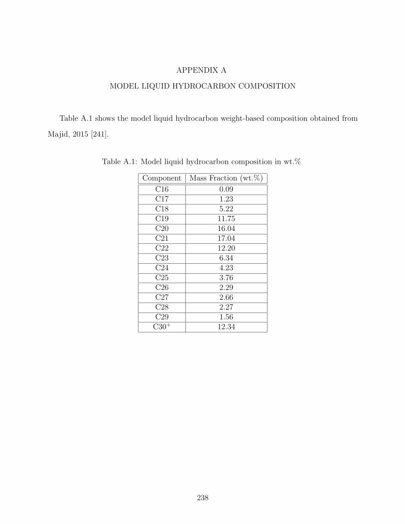
APPENDIX A

MODEL LIQUID HYDROCARBON COMPOSITION

Table A.1 shows the model liquid hydrocarbon weight-based composition obtained from

Majid, 2015 [241].

Table A.1: Model liquid hydrocarbon composition in wt.%

Component Mass Fraction (wt.%)

C16 0.09C17 1.23C18 5.22C19 11.75C20 16.04C21 17.04C22 12.20C23 6.34C24 4.23C25 3.76C26 2.29C27 2.66C28 2.27C29 1.56C30+ 12.34

238

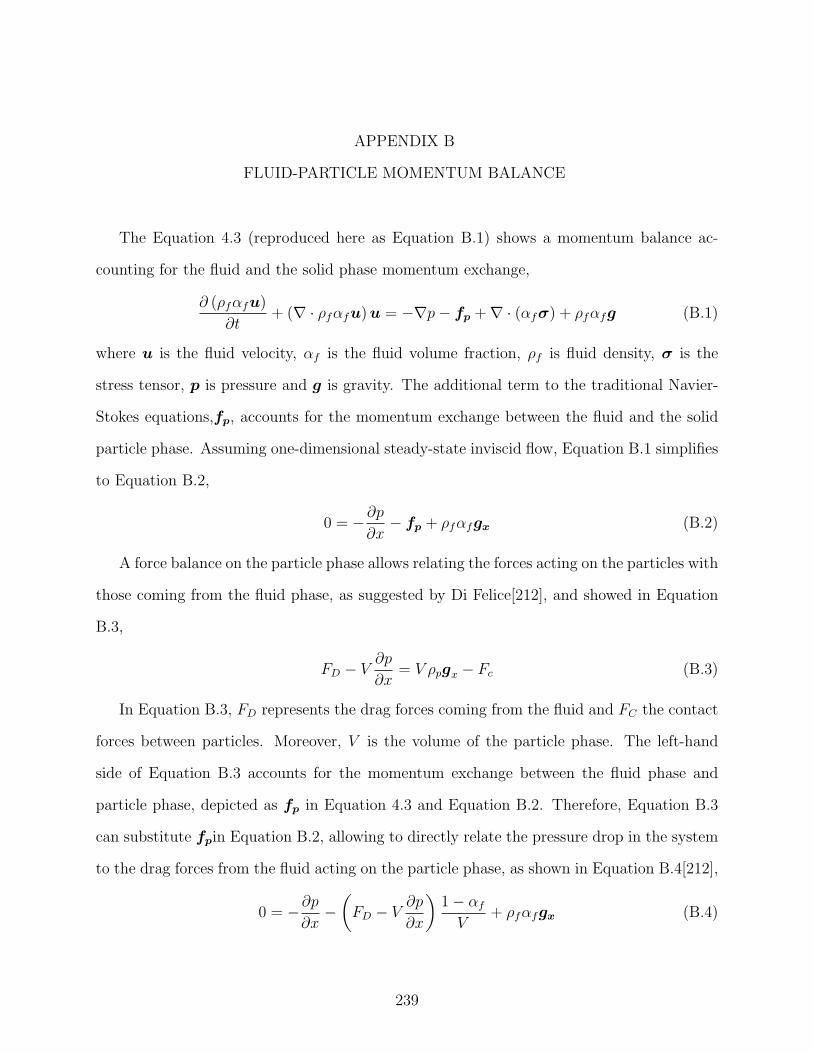
APPENDIX B

FLUID-PARTICLE MOMENTUM BALANCE

The Equation 4.3 (reproduced here as Equation B.1) shows a momentum balance ac-

counting for the fluid and the solid phase momentum exchange,

∂ (ρfαfu)

∂t+ (∇ · ρfαfu)u = −∇p− fp +∇ · (αfσ) + ρfαfg (B.1)

where u is the fluid velocity, αf is the fluid volume fraction, ρf is fluid density, σ is the

stress tensor, p is pressure and g is gravity. The additional term to the traditional Navier-

Stokes equations,fp, accounts for the momentum exchange between the fluid and the solid

particle phase. Assuming one-dimensional steady-state inviscid flow, Equation B.1 simplifies

to Equation B.2,

0 = −∂p

∂x− fp + ρfαfgx (B.2)

A force balance on the particle phase allows relating the forces acting on the particles with

those coming from the fluid phase, as suggested by Di Felice[212], and showed in Equation

B.3,

FD − V∂p

∂x= V ρpgx − Fc (B.3)

In Equation B.3, FD represents the drag forces coming from the fluid and FC the contact

forces between particles. Moreover, V is the volume of the particle phase. The left-hand

side of Equation B.3 accounts for the momentum exchange between the fluid phase and

particle phase, depicted as fp in Equation 4.3 and Equation B.2. Therefore, Equation B.3

can substitute fpin Equation B.2, allowing to directly relate the pressure drop in the system

to the drag forces from the fluid acting on the particle phase, as shown in Equation B.4[212],

0 = −∂p

∂x−

(

FD − V∂p

∂x

)

1− αfV

+ ρfαfgx (B.4)

239

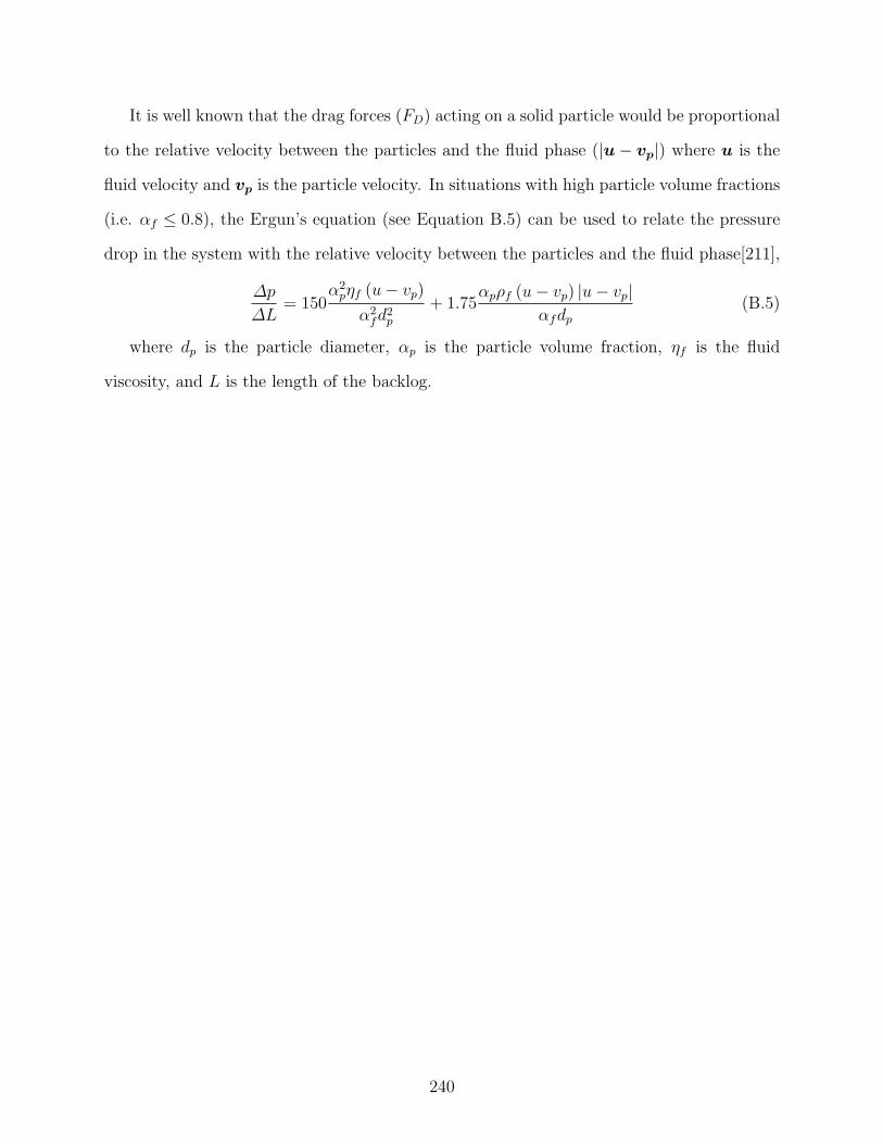
It is well known that the drag forces (FD) acting on a solid particle would be proportional

to the relative velocity between the particles and the fluid phase (|u− vp|) where u is the

fluid velocity and vp is the particle velocity. In situations with high particle volume fractions

(i.e. αf ≤ 0.8), the Ergun’s equation (see Equation B.5) can be used to relate the pressure

drop in the system with the relative velocity between the particles and the fluid phase[211],

∆p

∆L= 150

α2pηf (u− vp)

α2fd

2p

+ 1.75αpρf (u− vp) |u− vp|

αfdp(B.5)

where dp is the particle diameter, αp is the particle volume fraction, ηf is the fluid

viscosity, and L is the length of the backlog.

240

on the kinetic arrest of hydrate slurries - mountain scholar

Documents