on the importance of the deadlock trap property for monotonic liveness
TRANSCRIPT
On the Importance of theDeadlock Trap Property for Monotonic Liveness
Monika Heiner1, Cristian Mahulea2, Manuel Silva2
1 Department of Computer Science, Brandenburg University of TechnologyPostbox 10 13 44, 03013 Cottbus, Germany
[email protected] Instituto de Investigacion en Ingenierıa de Aragon (I3A),
Universidad de Zaragoza, Maria de Luna 1, E-50018 Zaragoza, [email protected], [email protected]
Abstract. In Petri net systems, liveness is an important property cap-turing the idea of no transition (action) becoming non-fireable (unattain-able). Additionally, in some situations it is particularly interesting tocheck if the net system is (marking) monotonically live, i.e., it remainslive for any marking greater than the initial one. In this paper, we dis-cuss structural conditions preserving liveness under arbitrary markingincrease. It is proved that the deadlock trap property (DTP) is a neces-sary condition for liveness monotonicity of ordinary nets, and necessaryand sufficient for some subclasses. We illustrate also how the result canbe used to study liveness monotonicity for non-ordinary nets using a sim-ulation preserving the firing language. Finally, we apply these conditionsto several case studies of biomolecular networks.
1 Motivation
Petri nets are a natural choice to represent biomolecular networks. Various typesof Petri nets may be useful – qualitative, deterministically timed, stochastic, con-tinuous or hybrid ones, depending on the available information and the kind ofproperties to be analysed. Accordingly, the integrative framework demonstratedby several case studies in [GHR+08], [HGD08], [HDG10] applies a family of re-lated Petri net models, sharing structure, but differing in their kind of kineticinformation.
A key notion of the promoted strategy of biomodel engineering is the levelconcept, which has been introduced in the Petri net framework in [GHL07]. Here,a token stands for a specific amount of mass, defined by the total mass dividedby the number of levels. Thus, increasing the token number to represent a certainamount of mass means to increase the resolution of accuracy.
This procedure silently assumes some kind of behaviour preservation whilethe marking is increased (typically multiplied by a factor) to represent a finergranularity of the mass flowing through the network. However, as it is well-knownin Petri net theory, liveness is not monotonic with respect to (w.r.t.) the initialmarking for general Petri nets. Thus, there is no reason to generally assume that
2 M. Heiner, C. Mahulea, and M. Silva
there is no significant change in the possible behaviour by marking increase.Contrary, under liveness monotonicity w.r.t. the initial marking we can expectcontinuization (fluidization) to be reasonable. However, only a particular kindof monotonicity seems to be needed for continuization: homothetic liveness, i.e.,liveness preservation while multiplying the initial marking by k [RTS99], [SR02].
At structural level, (monotonic) liveness can be considered using transforma-tion (reduction) rules [Ber86], [Sil85], [Mur89], [Sta90], the classical analysis forordinary nets based on the Deadlock Trap Property (DTP) [Mur89], [Sta90], orthe results of Rank Theorems, which are directly applicable to non-ordinary nets[TS96], [RTS98]. In this paper, we concentrate on the DTP, which will initiallybe used for ordinary net models, and later extended to non-ordinary ones.
This paper is organized as follows. We start off with recalling relevant notionsand results of Petri net theory. Afterwards we introduce the considered subjectby looking briefly at two examples, before turning to our main result yieldinga necessary condition for monotonic liveness. We demonstrate the usefulness ofour results for the analysis of biomolecular networks by a variety of case studies.We conclude with an outlook on open issues.
2 Preliminaries
We assume basic knowledge of the standard notions of place/transition Petrinets, see e.g. [DHP+93], [HGD08], [DA10]. To be self-contained we recall thefundamental notions relevant for our paper.
Definition 1 (Petri net, syntax).A Petri net is a tuple N = 〈P, T,Pre,Post〉, and a Petri net system is a
tuple Σ = 〈N ,m0〉, where
– P and T are finite, non-empty, and disjoint sets. P is the set of places. Tis the set of transitions.
– Pre,Post ∈ N|P|×|T| are the pre- and post-matrices, where | · | is the car-dinality of a set, i.e., its number of elements. For a place pi ∈ P and atransition tj ∈ T , Pre(pi, tj) is the weight of the arc connecting pi to tj (0if there is no arc), while Post(pi, tj) is the weight of the arc connecting tj topi.
– m0 ∈ N|P |≥0 gives the initial marking.– m(p) yields the number of tokens on place p in the marking m. A placep with m(p) = 0 is called empty (unmarked) in m, otherwise it is calledmarked (non-empty). A set of places is called empty if all its places areempty, otherwise marked.
– The preset and postset of a node x ∈ P ∪ T are denoted by • x and x • .They represent the input and output transitions of a place x, or the inputand output places of a transition x. More specifically, if tj ∈ T , • tj = {pi ∈P |Pre(pi, tj) > 0} and tj • = {pi ∈ P |Post(pi, tj) > 0}. Similarly, if pi ∈ P ,• pi = {tj ∈ T |Post(pi, tj) > 0} and pi • = {tj ∈ T |Pre(pi, tj) > 0}.We extend both notions to a set of nodes X ⊆ P ∪ T and define the set ofall prenodes •X :=
⋃x∈X
• x, and the set of all postnodes X • :=⋃
x∈X x • .
DTP and Monotonic Liveness 3
– A node x ∈ P ∪T is called source node, if • x = ∅, and sink node if x • = ∅.A boundary node is either a sink or a source node (but not both, because weassume a connected net).
Definition 2 (Petri net, behaviour). Let 〈N ,m0〉 be a net system.
– A transition t is enabled at marking m, written as m[t〉, if∀p ∈ •t : m(p) ≥ Pre(p, t), else disabled.
– A transition t, enabled in m, may fire (occur), leading to a new marking m′,written as m[t〉m′, with ∀p ∈ P : m′(p) = m(p)− Pre(p, t) + Post(p, t).
– The set of all markings reachable from a marking m0, written as [m0〉, isthe smallest set such that m0 ∈ [m0〉, m ∈ [m0〉 ∧m[t〉m′ ⇒m′ ∈ [m0〉.
– The reachability graph (RG) is a directed graph with [m0〉 as set of nodes,and the labelled arcs denote the reachability relation m[t〉m′.
Definition 3 (Behavioural properties). Let 〈N ,m0〉 be a net system.
– A place p is k-bounded (bounded for short) if there is a positive integernumber k, serving as an upper bound for the number of tokens on this placein all reachable markings of the Petri net: ∃ k ∈ N0 : ∀m ∈ [m0〉 : m(p) ≤ k .
– A Petri net system is k-bounded (bounded for short) if all its places arek-bounded.
– A transition t is dead at marking m if it is not enabled in any marking m′
reachable from m: 6 ∃ m′ ∈ [m〉 : m′[t〉.– A transition t is live if it is not dead in any marking reachable from m0.– A marking m is dead if there is no transition which is enabled in m.– A Petri net system is deadlock-free (weakly live) if there are no reachable
dead markings.– A Petri net system is live (strongly live) if each transition is live.
Definition 4 (Net structures). Let N = 〈P, T,Pre,Post〉 be a Petri net.N is
– Homogeneous (HOM) if ∀p ∈ P : t, t′ ∈ p• ⇒ Pre(p, t) = Pre(p, t′);– Ordinary (ORD) if ∀p ∈ P and ∀t ∈ T , Pre(p, t) ≤ 1 and Post(p, t) ≤ 1;– Extended Simple (ES) (sometimes also called asymmetric choice) if it is
ORD and ∀ p, q ∈ P : p• ∩ q• = ∅ ∨ p• ⊆ q• ∨ q• ⊆ p•;– Extended Free Choice (EFC) if it is ORD and ∀ p, q ∈ P : p•∩ q• = ∅∨p• =q•.
Definition 5 (DTP). Let N = 〈P, T,Pre,Post〉 be a Petri net.
– A siphon (structural deadlock, co-trap) is a non-empty set of places D ⊆ Pwith •D ⊆ D • .
– A trap is a non-empty set of places Q ⊆ P with Q • ⊆ •Q.– A minimal siphon (trap) is a siphon (trap) not including a siphon (trap) as
a proper subset.– A bad siphon is a siphon, which does not include a trap.

4 M. Heiner, C. Mahulea, and M. Silva
– An empty siphon (trap) is a siphon (trap), not containing a token.– The Deadlock Trap Property (DTP) asks for every siphon to include an
initially marked trap, i.e., marked at m0.
The DTP can be reformulated as: minimal siphons are not bad and themaximal traps included are initially marked.
Definition 6 (Semiflows). Let N = 〈P, T,Pre,Post〉 be a net.
– The token flow matrix (or incidence matrix if the net is pure, i.e., self-loopfree) is a matrix C = Post− Pre.
– A place vector is a vector y ∈ Z|P |; a transition vector is a vector x ∈ Z|T |.– A P-semiflow is a place vector y with y ·C = 0, y ≥ 0, y 6= 0;
a T-semiflow is a transition vector x with C · x = 0, x ≥ 0, x 6= 0.– The support of a semiflow x, written as supp(x), is the set of nodes corre-
sponding to the non-zero entries of x.– A net is conservative if every place belongs to the support of a P-semiflow.– A net is consistent if every transition belongs to the support of a T-semiflow.– In a minimal semiflow x, supp (x) does not contain the support of any other
semiflow z, i.e., 6 ∃ semiflow z : supp (z) ⊂ supp (x), and the greatest com-mon divisor of x is 1.
– A mono-T-semiflow net (MTS net) is a consistent and conservative net thathas exactly one minimal T-semiflow.
For convenience, we give vectors (markings, semiflows) in a short-hand nota-tion by enumerating only the non-zero entries. Finally, we recall some well-knownrelated propositions (see for example [Mur89], [Sta90]), which might be usefulfor the reasoning we pursue in this paper.
Proposition 1 (Basics).
1. An empty siphon remains empty forever. A marked trap remains marked forever.
2. If R and R′ are siphons (traps), then R ∪R′ is also a siphon (trap).3. A minimal siphon (trap) is a P-strongly-connected component, i.e., its places
are strongly connected.4. A deadlocked Petri net system has an empty siphon.5. Each siphon of a live net system is initially marked.6. If there is a bad siphon, the DTP does not hold.7. A source place p establishes a bad siphon D = {p} on its own, and a sink
place q a trap Q = {q}.8. If each transition has a pre-place, then P • = T , and if each transition has
a post-place, then •P = T . Thus, in a net without boundary transitions, thewhole set of places is a siphon as well as a trap (however, not necessarilyminimal ones).
9. For a P-semiflow x it holds • supp(x) = supp(x) • . Thus, the support of aP-semiflow is siphon and trap as well (however, generally not vice versa).
DTP and Monotonic Liveness 5
Proposition 2 (DTP and behavioural properties).
1. An ordinary Petri net without siphons is live.2. If N is ordinary and the DTP holds for m0, then 〈N ,m0〉 is deadlock-free.3. If N is ES and the DTP holds for m0, then 〈N ,m0〉 is live.4. Let N be an EFC net. 〈N ,m0〉 is live iff the DTP holds.
We conclude this section with a proposition from [CCS91], which might beless known.
Proposition 3 (MTS net and behavioural properties). Liveness anddeadlock-freeness coincide in mono-T-semiflow net systems.
3 Monotonic Liveness
If a property holds for a Petri net N with the marking m0, and it also holds inN for any m ≥m0, then it is said to be monotonic in the system 〈N ,m0〉. Inthis paper we are especially interested in monotonic liveness.
Definition 7 (Monotonic liveness).Let 〈N ,m0〉 be a Petri net system. It is called monotonically live, if being
live for m0, it remains live for any m ≥m0.
We are looking for conditions, at best structural conditions, preserving live-ness under arbitrary marking increase. To illustrate the problem, let’s considera classical example [Sta90], [SR02].
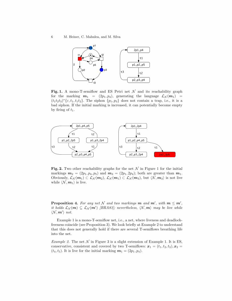
Example 1. The netN in Figure 1 is ES, conservative, consistent, and covered byone T-semiflow. It is live for the given initial marking m1 = (2p1, p4). Addinga token to place p5 yields the initial marking m2 = (2p1, p4, p5) and the netsystem remains live for m2 ≥ m1. However, adding a token to p4 yields theinitial marking m3 = (2p1, 2p4) and the net behaviour now contains finite firingsequences, i.e., it can run into a deadlock (dead state). Thus, the net system isnot live for m3 ≥m1. It is not monotonically live.
How to distinguish both cases? The net has two (minimal) bad siphonsD1 = {p1, p2} and D2 = {p1, p3}. There is no chance to prevent these siphonsfrom getting empty for arbitrary markings. D1 can potentially be emptiedby firing t2 ∈ D1
• \ •D1, and D2 by firing t1 ∈ D2• \ •D2. The latter case
destroyed the liveness for m3 as it will equally occur for all initial markingsallowing transition sequences containing one of the troublemakers, in thisexample t1 and t2, sufficiently often. �
One lesson learnt from the previous example is, a net does not have to makeuse of the additional tokens. Thus, all behaviour (set of transition sequences),which is possible for m is still possible for m′, with m ≤ m′. However, newtokens may allow for additional system behaviour, which is actually well-knownin Petri net theory, see Proposition 4.
6 M. Heiner, C. Mahulea, and M. Silva
p1
p4
p5
p2 p3
t1 t2
t3
2
ORD PUR HOM NBM CSV SCF CON SC FT0 TF0 FP0 PF0 NC N Y Y Y Y N Y Y N N N N ES DTP CPI CTI SCTI SB k-b 1-b DCF DSt DTr LIV REV N Y Y Y Y Y N Y 0 N Y Y
minimal deadlock, not containing a trap:D1={p1, p2}; D2={p1,p3}t1 may clean D2, t2 may clean D1;
2p1,p4
p1,p2,p5
p1,p3,2p4
p2,p3,p4
2p2,2p5
t1
t2t3
p2,p3,p4,p5
p1,p2,2p5
2p1,p4,p5
t3 t2
t1 t2
t1
p2,p3,2p4
p1,p2,p4,p5
2p1,2p4
t3t2
t1
t1
Fig. 1. A mono-T-semiflow and ES Petri net N and its reachability graphfor the marking m1 = (2p1, p4), generating the language LN (m1) =(t1t2t3)∗{ε, t1, t1t2}. The siphon {p1, p3} does not contain a trap, i.e., it is abad siphon. If the initial marking is increased, it can potentially become emptyby firing of t1.
2p1,p4
p1,p2,p5
p1,p3,2p4
p2,p3,p4
2p2,2p5
t1
t2t3
p2,p3,p4,p5
p1,p2,2p5
2p1,p4,p5
t3 t2
t1 t2
t1
p2,p3,2p4
p1,p2,p4,p5
2p1,2p4
t3t2
t1
t1
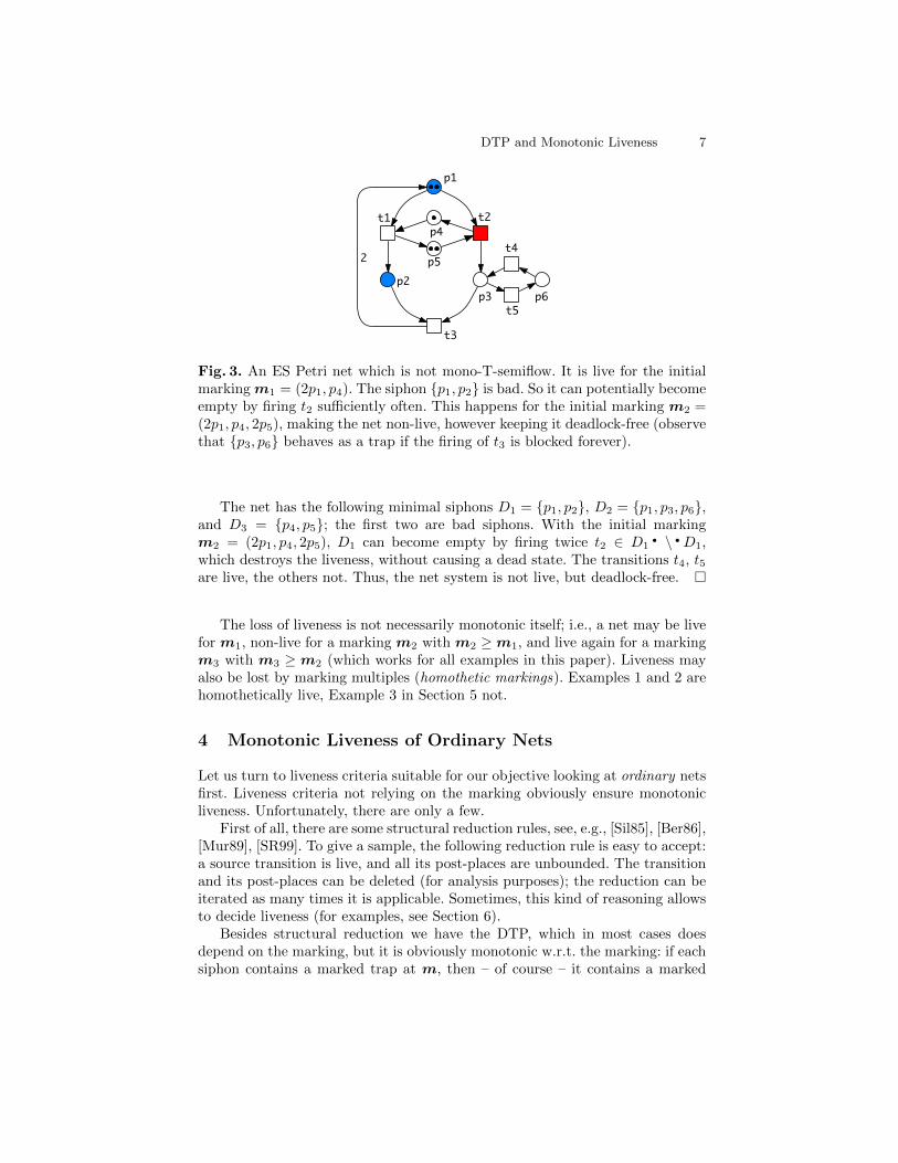
Fig. 2. Two other reachability graphs for the net N in Figure 1 for the initialmarkings m2 = (2p1, p4, p5) and m3 = (2p1, 2p4); both are greater than m1.Obviously, LN (m1) ⊂ LN (m2), LN (m1) ⊂ LN (m3), but 〈N ,m3〉 is not livewhile 〈N ,m1〉 is live.
Proposition 4. For any net N and two markings m and m′, with m ≤ m′,it holds LN (m) ⊆ LN (m′) [BRA83]; nevertheless, 〈N ,m〉 may be live while〈N ,m′〉 not.
Example 1 is a mono-T-semiflow net, i.e., a net, where liveness and deadlock-freeness coincide (see Proposition 3). We look briefly at Example 2 to understandthat this does not generally hold if there are several T-semiflows breathing lifeinto the net.
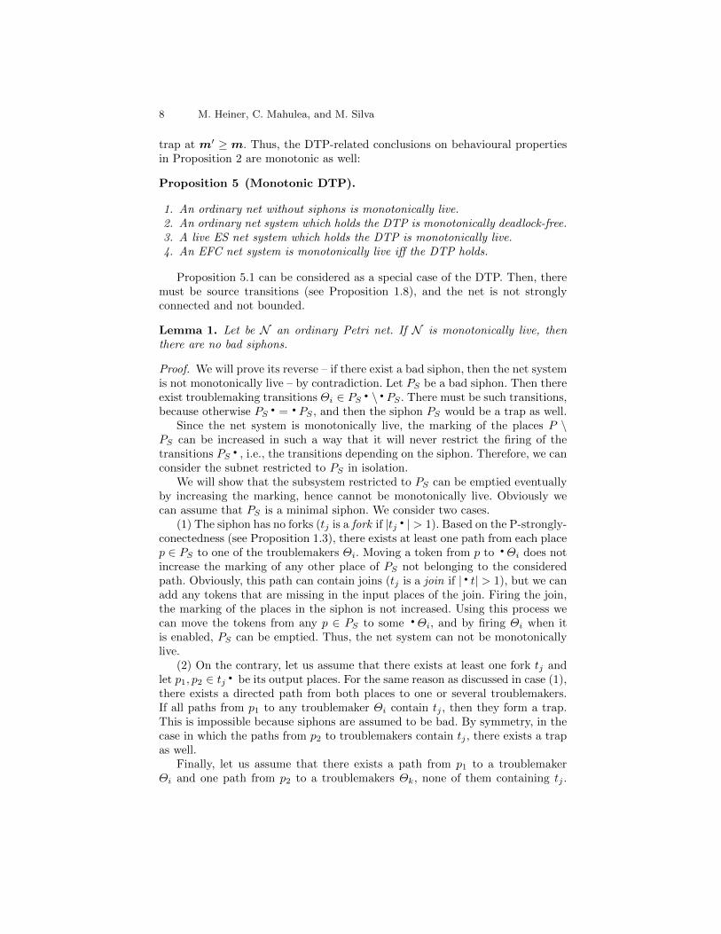
Example 2. The net N in Figure 3 is a slight extension of Example 1. It is ES,conservative, consistent and covered by two T-semiflows: x1 = (t1, t2, t3),x2 =(t4, t5). It is live for the initial marking m1 = (2p1, p4).
DTP and Monotonic Liveness 7
p1
p4
p5
p2
p3
t1 t2
t3
PUR ORD HOM NBM CSV SCF FT0 TF0 FP0 PF0 CON SC NC
Y N Y Y Y N N N N N Y Y ES
DTP CPI CTI SB k-B 1-B DCF DSt DTr LIV REV
N Y Y Y Y N N 0 N N N
minimal deadlock, not containing a trap:
D1={p1, p2}, D2={p1,p3};
t2 may clean D1, t1 may clean D2;
2t4
t5p6
transitions t1, t2, t3 are non-live.
Fig. 3. An ES Petri net which is not mono-T-semiflow. It is live for the initialmarking m1 = (2p1, p4). The siphon {p1, p2} is bad. So it can potentially becomeempty by firing t2 sufficiently often. This happens for the initial marking m2 =(2p1, p4, 2p5), making the net non-live, however keeping it deadlock-free (observethat {p3, p6} behaves as a trap if the firing of t3 is blocked forever).
The net has the following minimal siphons D1 = {p1, p2}, D2 = {p1, p3, p6},and D3 = {p4, p5}; the first two are bad siphons. With the initial markingm2 = (2p1, p4, 2p5), D1 can become empty by firing twice t2 ∈ D1
• \ •D1,which destroys the liveness, without causing a dead state. The transitions t4, t5are live, the others not. Thus, the net system is not live, but deadlock-free. �
The loss of liveness is not necessarily monotonic itself; i.e., a net may be livefor m1, non-live for a marking m2 with m2 ≥m1, and live again for a markingm3 with m3 ≥m2 (which works for all examples in this paper). Liveness mayalso be lost by marking multiples (homothetic markings). Examples 1 and 2 arehomothetically live, Example 3 in Section 5 not.
4 Monotonic Liveness of Ordinary Nets
Let us turn to liveness criteria suitable for our objective looking at ordinary netsfirst. Liveness criteria not relying on the marking obviously ensure monotonicliveness. Unfortunately, there are only a few.
First of all, there are some structural reduction rules, see, e.g., [Sil85], [Ber86],[Mur89], [SR99]. To give a sample, the following reduction rule is easy to accept:a source transition is live, and all its post-places are unbounded. The transitionand its post-places can be deleted (for analysis purposes); the reduction can beiterated as many times it is applicable. Sometimes, this kind of reasoning allowsto decide liveness (for examples, see Section 6).
Besides structural reduction we have the DTP, which in most cases doesdepend on the marking, but it is obviously monotonic w.r.t. the marking: if eachsiphon contains a marked trap at m, then – of course – it contains a marked
8 M. Heiner, C. Mahulea, and M. Silva
trap at m′ ≥ m. Thus, the DTP-related conclusions on behavioural propertiesin Proposition 2 are monotonic as well:
Proposition 5 (Monotonic DTP).
1. An ordinary net without siphons is monotonically live.2. An ordinary net system which holds the DTP is monotonically deadlock-free.3. A live ES net system which holds the DTP is monotonically live.4. An EFC net system is monotonically live iff the DTP holds.
Proposition 5.1 can be considered as a special case of the DTP. Then, theremust be source transitions (see Proposition 1.8), and the net is not stronglyconnected and not bounded.
Lemma 1. Let be N an ordinary Petri net. If N is monotonically live, thenthere are no bad siphons.
Proof. We will prove its reverse – if there exist a bad siphon, then the net systemis not monotonically live – by contradiction. Let PS be a bad siphon. Then thereexist troublemaking transitions Θi ∈ PS
• \ • PS . There must be such transitions,because otherwise PS
• = • PS , and then the siphon PS would be a trap as well.Since the net system is monotonically live, the marking of the places P \
PS can be increased in such a way that it will never restrict the firing of thetransitions PS
• , i.e., the transitions depending on the siphon. Therefore, we canconsider the subnet restricted to PS in isolation.
We will show that the subsystem restricted to PS can be emptied eventuallyby increasing the marking, hence cannot be monotonically live. Obviously wecan assume that PS is a minimal siphon. We consider two cases.
(1) The siphon has no forks (tj is a fork if |tj • | > 1). Based on the P-strongly-conectedness (see Proposition 1.3), there exists at least one path from each placep ∈ PS to one of the troublemakers Θi. Moving a token from p to •Θi does notincrease the marking of any other place of PS not belonging to the consideredpath. Obviously, this path can contain joins (tj is a join if | • t| > 1), but we canadd any tokens that are missing in the input places of the join. Firing the join,the marking of the places in the siphon is not increased. Using this process wecan move the tokens from any p ∈ PS to some •Θi, and by firing Θi when itis enabled, PS can be emptied. Thus, the net system can not be monotonicallylive.
(2) On the contrary, let us assume that there exists at least one fork tj andlet p1, p2 ∈ tj • be its output places. For the same reason as discussed in case (1),there exists a directed path from both places to one or several troublemakers.If all paths from p1 to any troublemaker Θi contain tj , then they form a trap.This is impossible because siphons are assumed to be bad. By symmetry, in thecase in which the paths from p2 to troublemakers contain tj , there exists a trapas well.
Finally, let us assume that there exists a path from p1 to a troublemakerΘi and one path from p2 to a troublemakers Θk, none of them containing tj .
DTP and Monotonic Liveness 9
On both paths the same kind of reasoning can be applied (in an iterative wayif several forks appear). Therefore, the siphon can be emptied even if firing tjincreases the tokens in PS . �
Lemma 1 helps to preclude monotonic liveness for Examples 1 and 2 as wellas for all other non-monotonically live examples we are aware of.
Theorem 1. Let be N an ordinary Petri net. If 〈N ,m0〉 is monotonically live,then the DTP holds.
Proof. The structural check of the DTP can have three possible outcomes.
1. If there are no siphons, then the DTP holds trivially and the net is mono-tonically live (see Proposition 5.1).
2. If there are bad siphons, then the DTP does not hold for any initial markingand the net is not monotonically live (see Lemma 1).
3. If each siphon includes a trap, then the maximal trap PT in every minimalsiphon PS has to be initially marked to fulfill the DTP. Because we assumeliveness of the net system, there has to be at least one token in each minimalsiphon (see Proposition 1.5). Let us assume that a token is not in PT , butin a place p ∈ PS \PT . If there exists at least one path without forks from pto a troublemaking transition Θi ∈ PS
• \ • PS not containing any transitionbelonging to the trap, • PT , then p can be emptied using the same reasoningas used in the proof of in Lemma 1, case (1). Therefore the net can notbe live. If the path from p to a troublemaking transition Θi ∈ PS
• \ • PS
contains a fork, then the output places of the fork will be marked when pis emptied, and the paths from the output places of the forks to the outputshould be considered separately.Finally, if all paths from p to the troublemaking transitions contain at leastone transition • PT , then the trap PT is not maximal since PT together withall places belonging to the above mentioned paths (including all non-minimalones) from p to transitions • PT are also a trap. �
According to Theorem 1, the DTP establishes a necessary condition for mono-tonic liveness, which complements Proposition 5.3.
Corollary 1. A live ES net system is monotonically live iff the DTP holds.
Moreover, for those systems for which deadlock-freeness is equivalent to live-ness, the DTP is a sufficient criteria for liveness monotonicity. This leads, forexample, to the following theorem:
Theorem 2. Let be N an ordinary mono-T-semiflow Petri net which for m0
fulfills the DTP. Then the system 〈N ,m〉 is live for any m ≥m0.
Proof. It follows from Proposition 5.2 (DTP and deadlock-freeness mono-tonicity) and Proposition 3 (equivalence of liveness and deadlock freeness in
10 M. Heiner, C. Mahulea, and M. Silva
mono-T-semiflow net systems). �
Therefore, the DTP is a sufficient criterion for monotonic liveness of ordinarymono-T-semiflow net systems as well. In summary, while the DTP is in generalneither necessary nor sufficient for liveness, it turns out to be the case to keepalive ordinary ES nets or ordinary mono-T-semiflow nets under any markingincrease.
5 Monotonic Liveness of Non-ordinary Nets
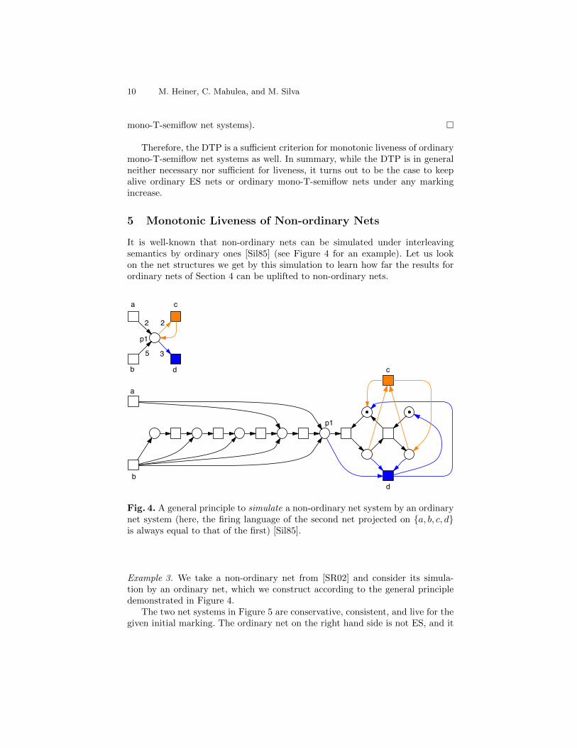
It is well-known that non-ordinary nets can be simulated under interleavingsemantics by ordinary ones [Sil85] (see Figure 4 for an example). Let us lookon the net structures we get by this simulation to learn how far the results forordinary nets of Section 4 can be uplifted to non-ordinary nets.
p1
p1
a
b
c
d
a
b
d
c
2
5
2
3
unfolding of non-ordinary nets to ordinary nets
Fig. 4. A general principle to simulate a non-ordinary net system by an ordinarynet system (here, the firing language of the second net projected on {a, b, c, d}is always equal to that of the first) [Sil85].
Example 3. We take a non-ordinary net from [SR02] and consider its simula-tion by an ordinary net, which we construct according to the general principledemonstrated in Figure 4.
The two net systems in Figure 5 are conservative, consistent, and live for thegiven initial marking. The ordinary net on the right hand side is not ES, and it
DTP and Monotonic Liveness 11
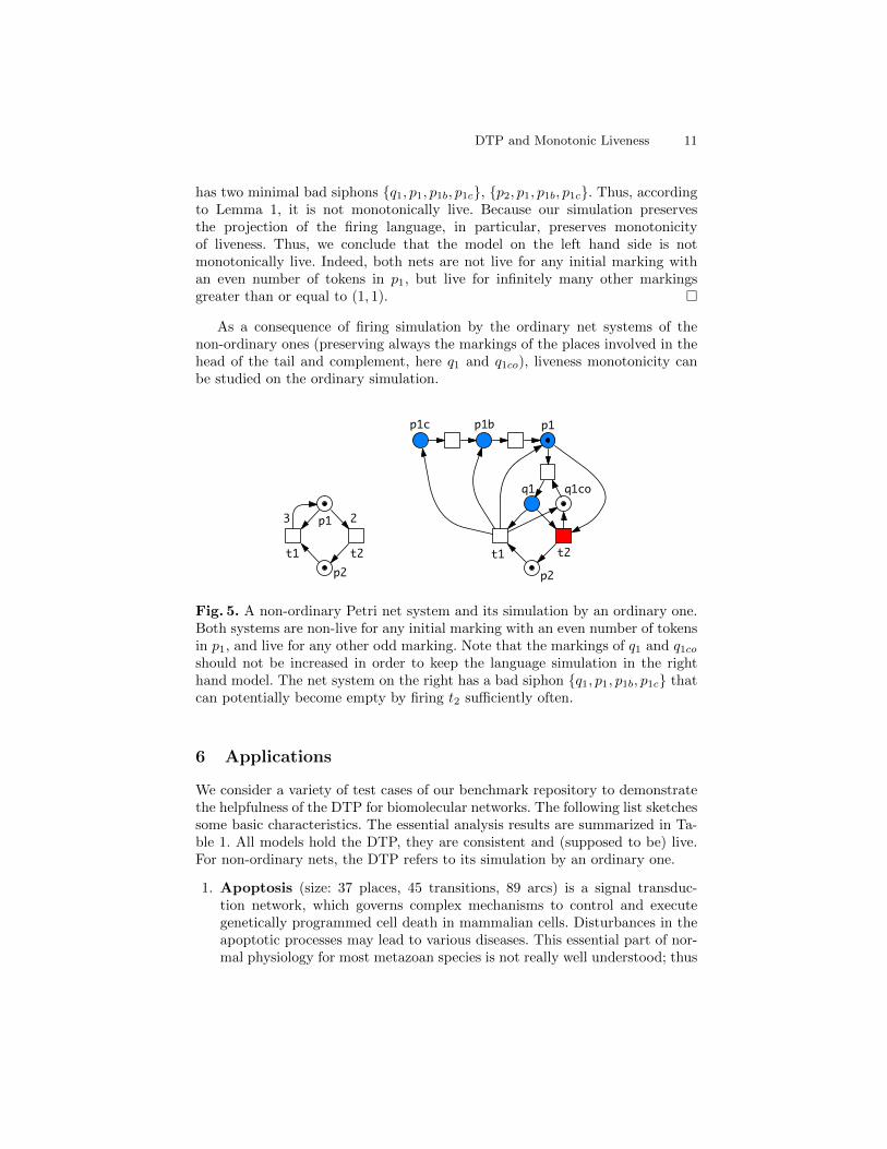
has two minimal bad siphons {q1, p1, p1b, p1c}, {p2, p1, p1b, p1c}. Thus, accordingto Lemma 1, it is not monotonically live. Because our simulation preservesthe projection of the firing language, in particular, preserves monotonicityof liveness. Thus, we conclude that the model on the left hand side is notmonotonically live. Indeed, both nets are not live for any initial marking withan even number of tokens in p1, but live for infinitely many other markingsgreater than or equal to (1, 1). �
As a consequence of firing simulation by the ordinary net systems of thenon-ordinary ones (preserving always the markings of the places involved in thehead of the tail and complement, here q1 and q1co), liveness monotonicity canbe studied on the ordinary simulation.
q1coq1
p1c p1b
p2
p1
t2t1
p1
p2t1 t2
23
Fig. 5. A non-ordinary Petri net system and its simulation by an ordinary one.Both systems are non-live for any initial marking with an even number of tokensin p1, and live for any other odd marking. Note that the markings of q1 and q1coshould not be increased in order to keep the language simulation in the righthand model. The net system on the right has a bad siphon {q1, p1, p1b, p1c} thatcan potentially become empty by firing t2 sufficiently often.
6 Applications
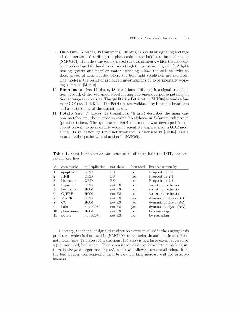
We consider a variety of test cases of our benchmark repository to demonstratethe helpfulness of the DTP for biomolecular networks. The following list sketchessome basic characteristics. The essential analysis results are summarized in Ta-ble 1. All models hold the DTP, they are consistent and (supposed to be) live.For non-ordinary nets, the DTP refers to its simulation by an ordinary one.
1. Apoptosis (size: 37 places, 45 transitions, 89 arcs) is a signal transduc-tion network, which governs complex mechanisms to control and executegenetically programmed cell death in mammalian cells. Disturbances in theapoptotic processes may lead to various diseases. This essential part of nor-mal physiology for most metazoan species is not really well understood; thus

12 M. Heiner, C. Mahulea, and M. Silva
there exist many model versions. The validation by Petri net invariants ofthe model considered here is discussed in [HKW04], [HK04].
2. RKIP (size: 11 places, 11 transitions, 14 arcs) models the core of the in-fluence of the Raf-1 Kinase Inhibitor Protein (RKIP) on the Extracellularsignal Regulated Kinase (ERK) signalling pathway. It is one of the standardexamples used in the systems biology community. It has been introduced in[CSK+03]; the corresponding qualitative, stochastic, continuous Petri netsare scrutinized in [GH06], [HDG10].
3. Biosensor (size: 6 places, 10 transitions, 21 arcs) is a gene expression net-work extended by metabolic activity. The model is a general template of abiosensor, which can be instantiated to be adapted to specic pollutants. It isconsidered as qualitative, stochastic, and continuous Petri net in [GHR+08]to demonstrate a model-driven design of a self-powering electrochemicalbiosensor.
4. Hypoxia (size: 14 places, 19 transitions, 56 arcs) is one of the well-studied molecular pathways activated under hypoxia condition. It mod-els the Hypoxia Induced Factor (HIF) pathway responsible for regulatingoxygen-sensitive gene expression. The version considered here is discussed in[YWS+07]; the corresponding qualitative and continuous Petri nets are usedin [HS10] to determine the core network.
5. Lac operon (size: 11 places, 17 transitions, 41 arcs) is a classical exampleof prokaryotic gene regulation. We re-use the simplified model discussed in[Wil06]. Its corresponding stochastic Petri net is considered in [HLGM09].
6. G/PPP (size: 26 places, 32 transitions, 76 arcs) is a simplified model of thecombined glycolysis (G) and pentose phosphate pathway (PPP) in erythro-cytes (red blood cells). It belongs to the classical examples of biochemistrytextbooks, see e.g. [BTS02], and thus of systems biology as well. The modelwas first discussed using Petri net technologies in [Red94]. Its validation byPetri net invariants is shown in [HK04], and a more exhaustive qualitativeanalysis in [KH08].
7. MAPK (size: 22 places, 30 transitions, 90 arcs) models the signallingpathway of the mitogen-activated protein kinase cascade, published in[LBS00]. It is a three-stage double phosphorylation cascade; each phosphory-lation/dephosphorylation step applies the mass action kinetics pattern. Thecorresponding qualitative, stochastic, and continuous Petri net are scruti-nized in [GHL07], [HGD08].
8. CC – Circadian clock (size: 14 places, 16 transitions, 58 arcs) refers to thecentral time signals of a roughly 24-hour cycle in living entities. Circadianrhythms are used by a wide range of organisms to anticipate daily changesin the environment. The model published in [BL00] demonstrates that cir-cadian network can oscillate reliably in the presence of stochastic biomolec-ular noise and when cellular conditions are altered. It is also available asPRISM model on the PRISM website (http://www.prismmodelchecker.org).Its corresponding stochastic Petri net belongs to the benchmark suite used in[SH09]. We consider here a version with inhibitor arcs modelled by co-places.
DTP and Monotonic Liveness 13
9. Halo (size: 37 places, 38 transitions, 138 arcs) is a cellular signaling and reg-ulation network, describing the phototaxis in the halobacterium salinarum[NMOG03]. It models the sophisticated survival strategy, which the halobac-terium developed for harsh conditions (high temperature, high salt). A lightsensing system and flagellar motor switching allows the cells to swim tothose places of their habitat where the best light conditions are available.The model is the result of prolonged investigations by experimentally work-ing scientists [Mar10].
10. Pheromone (size: 42 places, 48 transitions, 119 arcs) is a signal transduc-tion network of the well understood mating pheromone response pathway inSaccharomyces cerevisiae. The qualitative Petri net in [SHK06] extends a for-mer ODE model [KK04]. The Petri net was validated by Petri net invariantsand a partitioning of the transition set.
11. Potato (size: 17 places, 25 transitions, 78 arcs) describes the main car-bon metabolism, the sucrose-to-starch breakdown in Solanum tuberosum(potato) tubers. The qualitative Petri net model was developed in co-operation with experimentally working scientists, experienced in ODE mod-elling. Its validation by Petri net invariants is discussed in [HK04], and amore detailed pathway exploration in [KJH05].
Table 1. Some biomolecular case studies; all of them hold the DTP, are con-sistent and live.
# case study multiplicities net class bounded liveness shown by
1 apoptosis ORD ES no Proposition 2.12 RKIP ORD ES yes Proposition 2.33 biosensor ORD ES no Proposition 2.3
4 hypoxia ORD not ES no structural reduction5 lac operon HOM not ES no structural reduction6 G/PPP HOM not ES no structural reduction
7 MAPK ORD not ES yes dynamic analysis (RG)8 CC HOM not ES yes dynamic analysis (RG)9 halo not HOM not ES yes dynamic analysis (RG)
10 pheromone HOM not ES no by reasoning11 potato not HOM not ES no by reasoning
Contrary, the model of signal transduction events involved in the angiogenesisprocesses, which is discussed in [NMC+09] as a stochastic and continuous Petrinet model (size: 39 places, 64 transitions, 185 arcs) is to a large extent covered bya (non-minimal) bad siphon. Thus, even if the net is live for a certain marking m,there is always a larger marking m′, which will allow to remove all tokens fromthe bad siphon. Consequently, an arbitrary marking increase will not preserveliveness.
14 M. Heiner, C. Mahulea, and M. Silva
7 Tools
The Petri nets for the case studies have been constructed using Snoopy [RMH10],a tool to design and animate or simulate hierarchical graphs, among them qual-itative, stochastic and continuous Petri nets as used in the case studies in Sec-tion 6. Snoopy provides export to various analysis tools as well as import andexport of the Systems Biology Markup Language (SBML).
The qualitative analyses have been made with the Petri net analysis toolCharlie [Fra09], complemented by the structural reduction rules supported bythe Integrated Net Analyser INA [SR99].
8 Conclusions
We have discussed the problem of monotonic liveness, with one of the motivationsoriginating from bio-model engineering. We have presented a new result showingthe necessity of the DTP for monotonic liveness.
Moreover, we immediately know – thanks to the well-known propositions ofthe DTP – that ordinary ES nets are monotonically iff the DTP holds. Further-more, we know – because the DTP monotonically ensures deadlock freeness –that for any net class, in which liveness and deadlock freeness coincide, mono-tonic liveness is characterized by the DTP. We have shown one instance for thiscase: the mono-T-semiflow nets (MTS).
We have demonstrated the usefulness of our results by applying them to avariety of biomolecular networks.
One of the remaining open issues is: what are sufficient conditions for mono-tonic liveness for more general net structures? While none of our test cases is anMTS net, this line might be worth being explored more carefully, e.g. by lookingat FRT nets (Freely Related T-Semiflows) [CS92] and extensions.
Acknowledgements. This work has been partially supported by CICYT- FEDER grant DPI2006-15390 and by the European Community’s SeventhFramework Programme under project DISC (Grant Agreement n. INFSO-ICT-224498). The work of M. Heiner was supported in part by the grant DPI2006-15390 for a stay with the Group of Discrete Event Systems Engineering (GISED);the main ideas of this paper have been conceived during this period.
References
Ber86. G. Berthelot. Checking properties of nets using transformations. InG. Rozenberg, editor, Advances in Petri Nets 1985, volume 222 of LectureNotes in Computer Science, pages 19–40. Springer, 1986.
BL00. N. Barkai and S. Leibler. Biological rhythms: Circadian clocks limited bynoise. Nature, 403(6767):267–268, 2000.
BRA83. G. W. BRAMS. Reseaux de Petri. Theorie et pratique (2 tomes). Masson,1983.
DTP and Monotonic Liveness 15
BTS02. J.M. Berg, J.L. Tymoczko, and L. Stryer. Biochemistry, 5th ed. WH Free-man and Company, New York, 2002.
CCS91. J. Campos, G. Chiola, and M. Silva. Ergodicity and Throughput Bounds ofPetri Nets with Unique Consistent Firing Count Vector. IEEE Transactionson Software Engineering, 17:117–125, 1991.
CS92. J. Campos and M. Silva. Structural techniques and performance bounds ofstochastic Petri net models. In Advances in Petri Nets 1992, volume 609 ofLecture Notes in Computer Science, pages 352–391. Springer-Verlag, 1992.
CSK+03. K.-H. Cho, S.-Y. Shin, H.-W. Kim, O. Wolkenhauer, B. McFerran, andW. Kolch. Mathematical modeling of the influence of RKIP on the ERKsignaling pathway. In Proc. CMSB, pages 127–141. Springer, LNCS 2602,2003.
DA10. R. David and H. Alla. Discrete, Continuous, and Hybrid Petri Nets.Springer, 2010.
DHP+93. F. DiCesare, G. Harhalakis, J.M. Proth, M. Silva, and F.B. Vernadat. Prac-tice of Petri nets in manufacturing. Chapman & Hall, 1993.
Fra09. A. Franzke. Charlie 2.0 - a multi-threaded Petri net analyzer. DiplomaThesis, Brandenburg University of Technology at Cottbus, CS Dep., 2009.
GH06. D. Gilbert and M. Heiner. From Petri nets to differential equations - anintegrative approach for biochemical network analysis. In Proc. ICATPN2006, pages 181–200. LNCS 4024, Springer, 2006.
GHL07. D. Gilbert, M. Heiner, and S. Lehrack. A unifying framework for modellingand analysing biochemical pathways using Petri nets. In Proc. CMSB,pages 200–216. LNCS/LNBI 4695, Springer, 2007.
GHR+08. D. Gilbert, M. Heiner, S. Rosser, R. Fulton, Xu Gu, and M. Trybi lo. A CaseStudy in Model-driven Synthetic Biology. In Proc. 2nd IFIP Conferenceon Biologically Inspired Collaborative Computing (BICC), IFIP WCC 2008,Milano, pages 163–175, 2008.
HDG10. M. Heiner, R. Donaldson, and D. Gilbert. Petri Nets for Systems Biology,in Iyengar, M.S. (ed.), Symbolic Systems Biology: Theory and Methods.Jones and Bartlett Publishers, Inc., in Press, 2010.
HGD08. M. Heiner, D. Gilbert, and R. Donaldson. Petri nets in systems and syn-thetic biology. In Schools on Formal Methods (SFM), pages 215–264. LNCS5016, Springer, 2008.
HK04. M. Heiner and I. Koch. Petri Net Based Model Validation in SystemsBiology. In Proc. ICATPN, LNCS 3099, pages 216–237. Springer, 2004.
HKW04. M. Heiner, I. Koch, and J. Will. Model Validation of Biological PathwaysUsing Petri Nets - Demonstrated for Apoptosis. BioSystems, 75:15–28,2004.
HLGM09. M. Heiner, S. Lehrack, D. Gilbert, and W. Marwan. Extended StochasticPetri Nets for Model-Based Design of Wetlab Experiments. Transactionson Computational Systems Biology XI, pages 138–163, 2009.
HS10. M. Heiner and K. Sriram. Structural analysis to determine the core ofhypoxia response network. PLoS ONE, 5(1):e8600, 01 2010.
KH08. I. Koch and M. Heiner. Petri Nets, in B.H. Junker and F. Schreiber (eds.),Biological Network Analysis, chapter 7, pages 139–179. Wiley Book Serieson Bioinformatics, 2008.
KJH05. I. Koch, B.H. Junker, and M. Heiner. Application of Petri Net Theory forModeling and Validation of the Sucrose Breakdown Pathway in the PotatoTuber. Bioinformatics, 21(7):1219–1226, 2005.
16 M. Heiner, C. Mahulea, and M. Silva
KK04. B. Kofahl and E. Klipp. Modelling the dynamics of the yeast pheromonepathway. Yeast, 21(10):831–850, 2004.
LBS00. A. Levchenko, J. Bruck, and P.W. Sternberg. Scaffold proteins may bipha-sically affect the levels of mitogen-activated protein kinase signaling andreduce its threshold properties. Proc Natl Acad Sci USA, 97(11):5818–5823,2000.
Mar10. W. Marwan. Phototaxis in halo bacterium as a case study for extendedstochastic Petri nets. Private Communication, 2010.
Mur89. T. Murata. Petri Nets: Properties, Analysis and Applications. Proc.of theIEEE 77, 4:541–580, 1989.
NMC+09. L Napione, D Manini, F Cordero, A Horvath, A Picco, M De Pierro, S Pa-van, M Sereno, A Veglio, F Bussolino, and G Balbo. On the Use of Stochas-tic Petri Nets in the Analysis of Signal Transduction Pathways for Angio-genesis Process. In Proc. CMSB, pages 281–295. Springer, LNCS/LNBI5688, 2009.
NMOG03. T. Nutsch, W. Marwan, D. Oesterhelt, and E.D. Gilles. Signal process-ing and flagellar motor switching during phototaxis of Halobacterium sali-narum. Genome research, 13(11):2406–2412, 2003.
Red94. V. N. Reddy. Modeling Biological Pathways: A Discrete Event SystemsApproch. Master thesis, University of Maryland, 1994.
RMH10. C. Rohr, W. Marwan, and M. Heiner. Snoopy - a unifying Petri net frame-work to investigate biomolecular networks. Bioinformatics, 26(7):974–975,2010.
RTS98. L. Recalde, E. Teruel, and M. Silva. On linear algebraic techniques for live-ness analysis of P/T systems. Journal of Circuits, Systems, and Computers,8(1):223–265, 1998.
RTS99. L. Recalde, E. Teruel, and M. Silva. Autonomous continuous P/T systems.In Proc. ICATPN, pages 107–126. Springer, LNCS 1689, 1999.
SH09. M. Schwarick and M. Heiner. CSL model checking of biochemical networkswith Interval Decision Diagrams. In Proc. CMSB, pages 296–312. Springer,LNCS/LNBI 5688, 2009.
SHK06. A. Sackmann, M. Heiner, and I. Koch. Application of Petri Net BasedAnalysis Techniques to Signal Transduction Pathways. BMC Bioinformat-ics, 7:482, 2006.
Sil85. M. Silva. Las Redes de Petri: en la Automatica y la Informatica. EditorialAC, 1985.
SR99. P.H. Starke and S. Roch. INA - The Intergrated Net Analyzer. HumboldtUniversity Berlin, www.informatik.hu-berlin.de/∼starke/ina.html, 1999.
SR02. M. Silva and L. Recalde. Petri nets and integrality relaxations: A view ofcontinuous Petri net models. IEEE Transactions on Systems, Man, andCybernetics, Part C: Applications and Reviews, 32(4):314–327, 2002.
Sta90. P.H. Starke. Analysis of Petri Net Models (in German). B. G. Teubner,Stuttgart, Stuttgart, 1990.
TS96. E. Teruel and M. Silva. Structure theory of equal conflict systems. Theo-retical Computer Science, 153:271–300, 1996.
Wil06. D.J. Wilkinson. Stochastic Modelling for System Biology. CRC Press, NewYork, 1st Edition, 2006.
YWS+07. Y. Yu, G. Wang, R. Simha, W. Peng, F. Turano, and C. Zeng. Pathwayswitching explains the sharp response characteristic of hypoxia responsenetwork. PLoS Comput Biol, 3(8):e171, 2007.